/


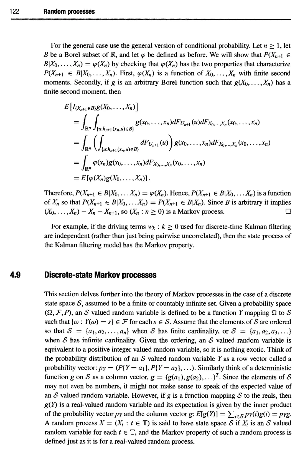


Теги: engineering random processes cambridge university press statistics production process theory of variety
ISBN: 978-1-107-10012-1
Год: 2015


Текст
>
г·
BRUCE HAJEK
Random Processes for Engineers
This engaging introduction to random processes provides students with the critical
tools needed to design and evaluate engineering systems that must operate reliably in
uncertain environments.
A brief review of probability theory and real analysis of deterministic functions sets
the stage for understanding random processes, while the underlying measure theoretic
notions are explained in an intuitive, straightforward style. Students will learn to manage
the complexity of randomness through the use of simple classes of random processes,
statistical means and correlations, asymptotic analysis, sampling, and effective
algorithms. Key topics covered include:
• Calculus of random processes in linear systems
• Kalman and Wiener filtering
• Hidden Markov models for statistical inference
• The estimation maximization (EM) algorithm
• An introduction to martingales and concentration inequalities
Understanding of the key concepts is reinforced through more than 100 worked
examples and 300 thoroughly tested homework problems (half of which are solved in detail
at the end of the book, with the remaining solutions available online for instructors at
www. Cambridge, org/hajek).
Bruce Hajek has been an avid student, instructor, and user of probability theory for his
entire career. He is the Mary Lou and Leonard C. Hoeft Chair of Engineering, Center
for Advanced Study Professor of Electrical and Computer Engineering, and Professor
in the Coordinated Science Laboratory at the University of Illinois. Among his many
awards, he is a member of the US National Academy of Engineering and a recipient of
the IEEE Koji Kobayashi Computers and Communications Award. He is co-author, with
E. Wong, of the more advanced book, Stochastic Processes in Engineering Systems, 2nd
edn, 1985.
"A comprehensive exposition of random processes ... Abstract concepts are nicely
explained through many examples ... The book will be very helpful for beginning
graduate students who want a firm foundational understanding of random processes.
It will also serve as a nice reference for the advanced reader."
Anima Anandkumar, The University of California, Irvine
"This is a fantastic book from one of the eminent experts in the field, and is the standard
text for the graduate class I teach in ECE at UT Austin. The material covered is perfect
for a first-year graduate class in Probability and Stochastic Processes."
Sanjay Shakkottai, The University of Texas at Austin
"This is an excellent introductory book on random processes and basic estimation theory
from the foremost expert and is suitable for advanced undergraduate students and/or
first-year graduate students who are interested in stochastic analysis. It covers an
extensive set of topics that are very much applicable to a wide range of engineering fields."
Richard La, University of Maryland
"Bruce Hajek has created a textbook for engineering students with interest in
control, signal processing, communications, machine learning, amongst other disciplines in
electrical engineering and computer science. Anyone who knows Bruce Hajek knows
that he cares deeply about the foundations of probability and statistics, and he is equally
engaged in applications. Bruce is a dedicated teacher and author in the spirit of Prof.
Joe Doob, formally at the statistics department at the University of Illinois.
I was fortunate to have a mature draft of his book when I introduced a stochastic
processes course to my department in the spring of 2014. The book provides an entirely
accessible introduction to the foundations of stochastic processes. I was surprised to
find that the students in my course enjoyed Hajek's introduction to measure theory, and
(at least by the end of the course) could appreciate the value of the abstract concepts
introduced at the start of the text.
It includes applications of this general theory to many topics that are of tremendous
interest to students and practitioners, such as nonlinear filtering, statistical methods
such as the EM-algorithm, and stability theory for Markov processes. Because the book
establishes strong foundations, in a course it is not difficult to substitute other
applications, such as Monte-Carlo methods or reinforcement learning. Graduate students will
be thrilled to learn these exciting techniques from an accessible source."
Sean Meyn, University of Florida
Random Processes for
Engineers
BRUCE HAJEK
University of Illinois
m
CAMBRIDGE
UNIVERSITY PRESS
Cambridge
UNIVERSITY PRESS
University Printing House, Cambridge CB2 8BS, United Kingdom
Cambridge University Press is part of the University of Cambridge.
It furthers the University's mission by disseminating knowledge in the pursuit of
education, learning and research at the highest international levels of excellence.
www.cambridge.org
Information on this title: www.cambridge.org/9781107100121
© Cambridge University Press 2015
This publication is in copyright. Subject to statutory exception
and to the provisions of relevant collective licensing agreements,
no reproduction of any part may take place without the written
permission of Cambridge University Press.
First published 2015
Printed in the United Kingdom by Clays, St Ives pic
A catalog record for this publication is available from the British Library
Library of Congress Cataloging in Publication Data
Hajek, Bruce.
Random processes for engineers / Bruce Hajek, Illinois.
Includes bibliographical references and index.
ISBN 978-1-107-10012-1 (Hardback)
1. Engineering mathematics-Study and teaching (Graduate) 2. Stochastic processes-Study
and teaching (Graduate) 3. Numbers, Random-Study and teaching (Graduate) I. Title.
TA340.H325 2015
519.2/3-dc23 2014035900
ISBN 978-1-107-10012-1 Hardback
Additional resources for this publication at www.cambridge.org/hajek
Cambridge University Press has no responsibility for the persistence or accuracy of
URLs for external or third-party internet websites referred to in this publication,
and does not guarantee that any content on such websites is, or will remain,
accurate or appropriate.
To Beth, for her loving support.
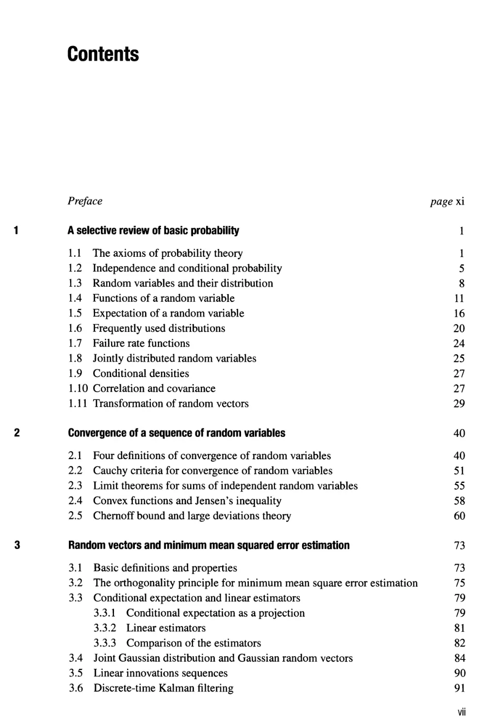
Contents
Preface
1 A selective review of basic probability
1.1 The axioms of probability theory
1.2 Independence and conditional probability
1.3 Random variables and their distribution
1.4 Functions of a random variable
1.5 Expectation of a random variable
1.6 Frequently used distributions
1.7 Failure rate functions
1.8 Jointly distributed random variables
1.9 Conditional densities
1.10 Correlation and covariance
1.11 Transformation of random vectors
2 Convergence of a sequence of random variables
2.1 Four definitions of convergence of random variables
2.2 Cauchy criteria for convergence of random variables
2.3 Limit theorems for sums of independent random variables
2.4 Convex functions and Jensen's inequality
2.5 Chernoff bound and large deviations theory
3 Random vectors and minimum mean squared error estimation
3.1 Basic definitions and properties
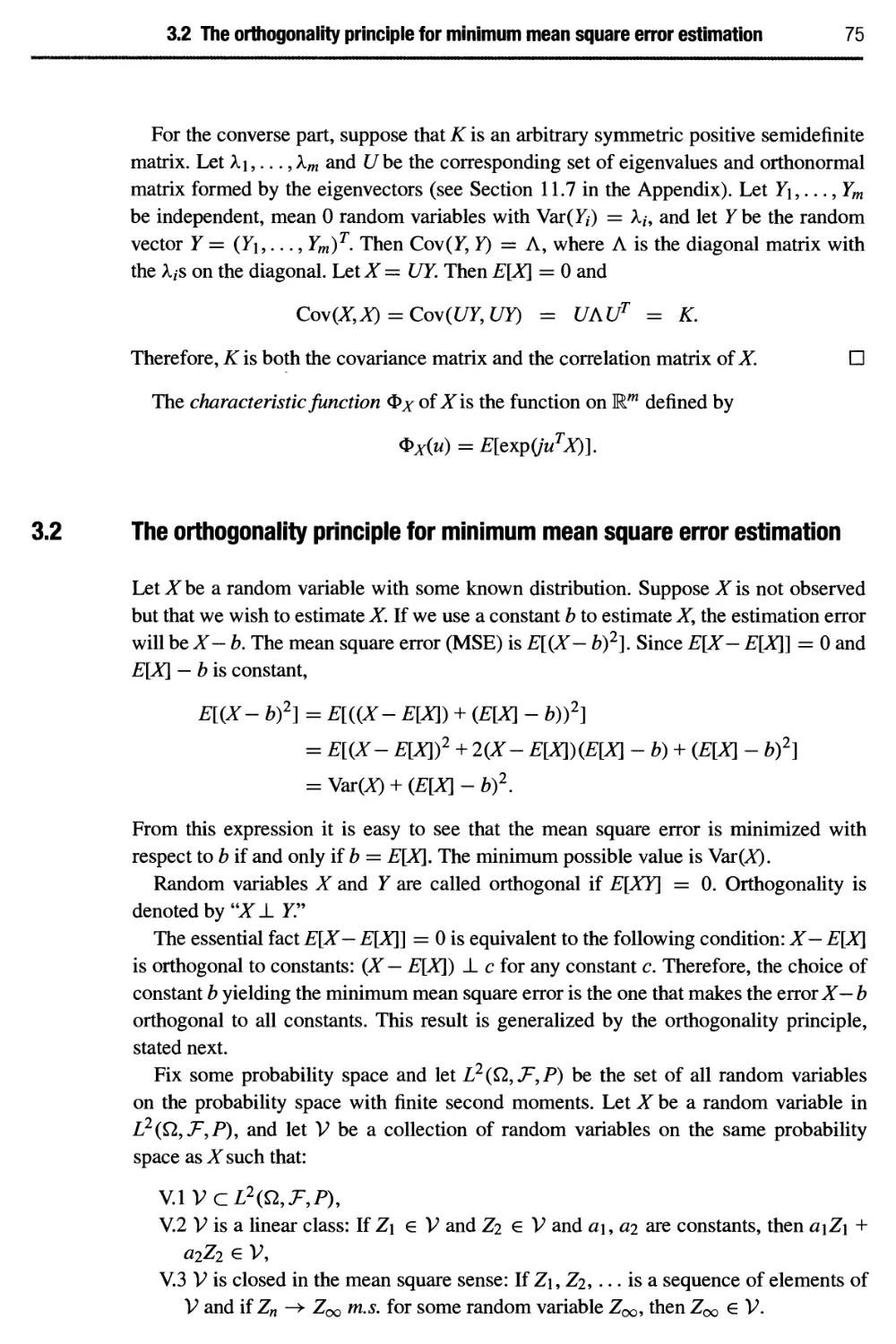
3.2 The orthogonality principle for minimum mean square error estimation
3.3 Conditional expectation and linear estimators
3.3.1 Conditional expectation as a projection
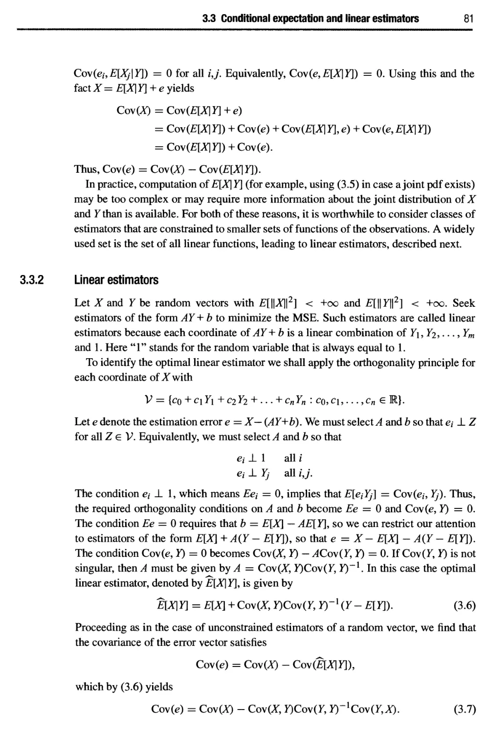
3.3.2 Linear estimators
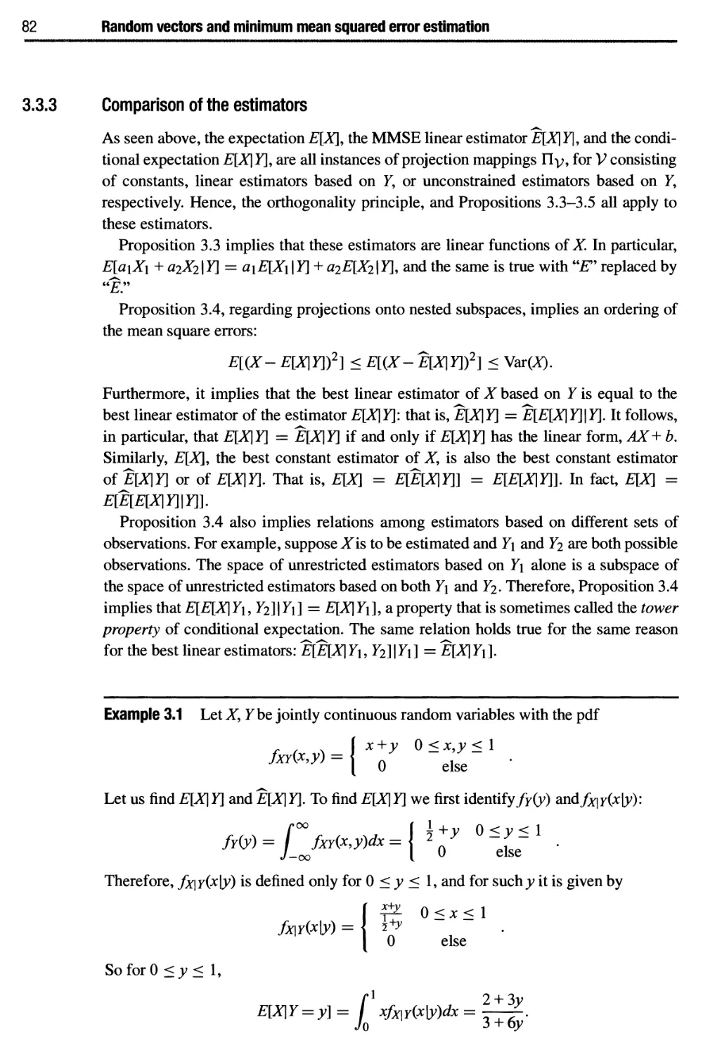
3.3.3 Comparison of the estimators
3.4 Joint Gaussian distribution and Gaussian random vectors
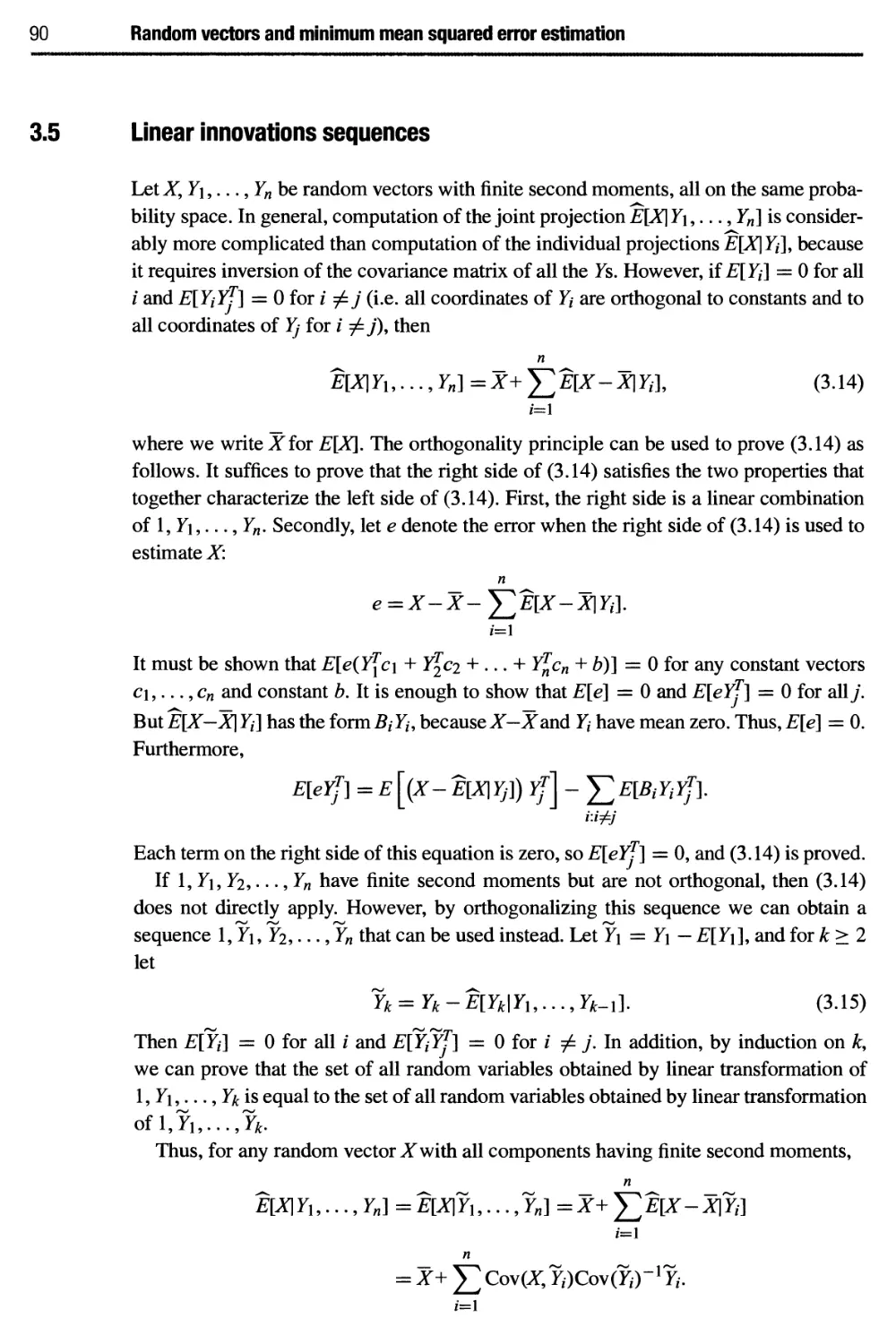
3.5 Linear innovations sequences
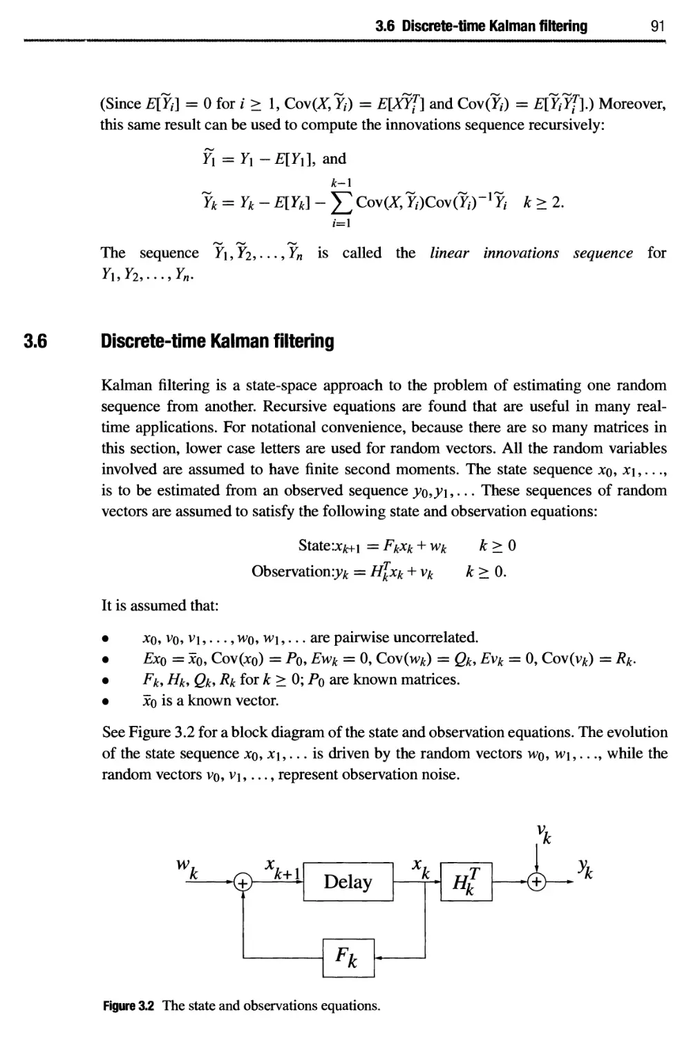
3.6 Discrete-time Kalman filtering
viii Contents
Random processes 103
4.1 Definition of a random process 103
4.2 Random walks and gambler's ruin 106
4.3 Processes with independent increments and martingales 108
4.4 Brownian motion 110
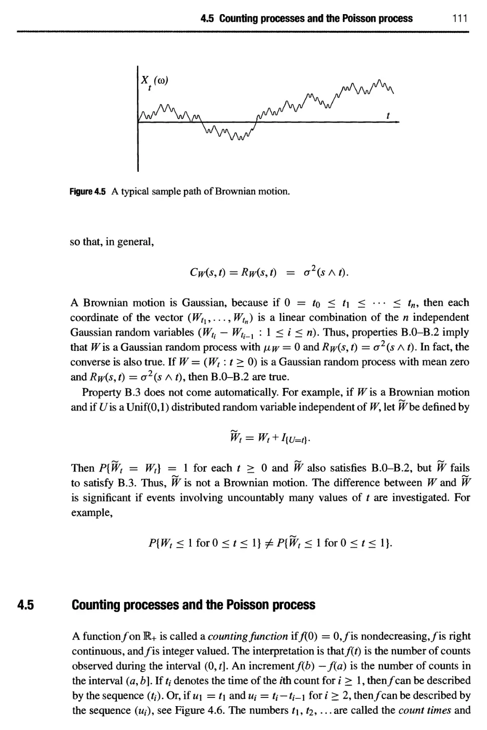
4.5 Counting processes and the Poisson process 111
4.6 Stationarity 115
4.7 Joint properties of random processes 118
4.8 Conditional independence and Markov processes 118
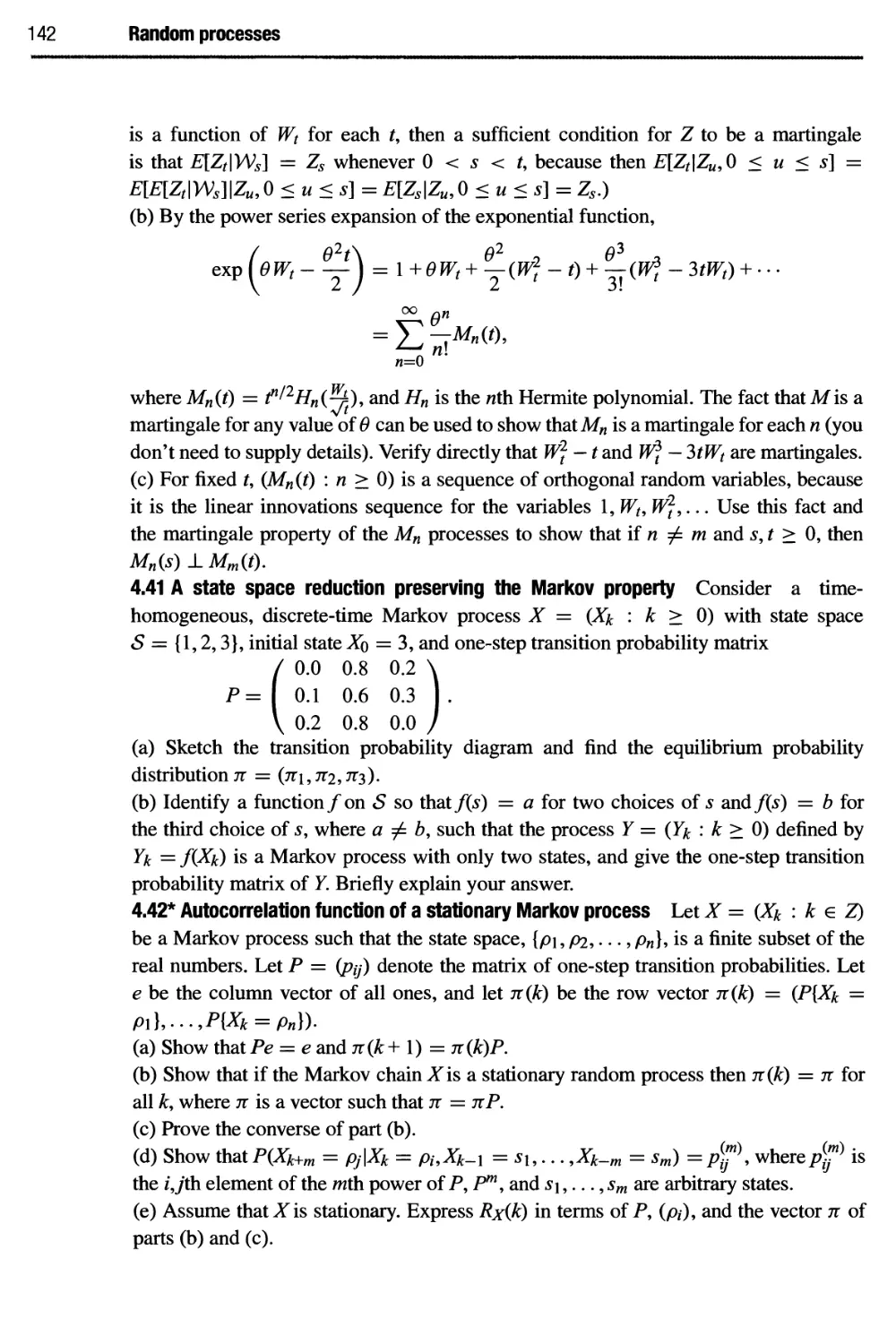
4.9 Discrete-state Markov processes 122
4.10 Space-time structure of discrete-state Markov processes 129
Inference for Markov models 143
5.1 A bit of estimation theory 143
5.2 The expectation-maximization (EM) algorithm 148
5.3 Hidden Markov models 152
5.3.1 Posterior state probabilities and the forward-backward algorithm 153
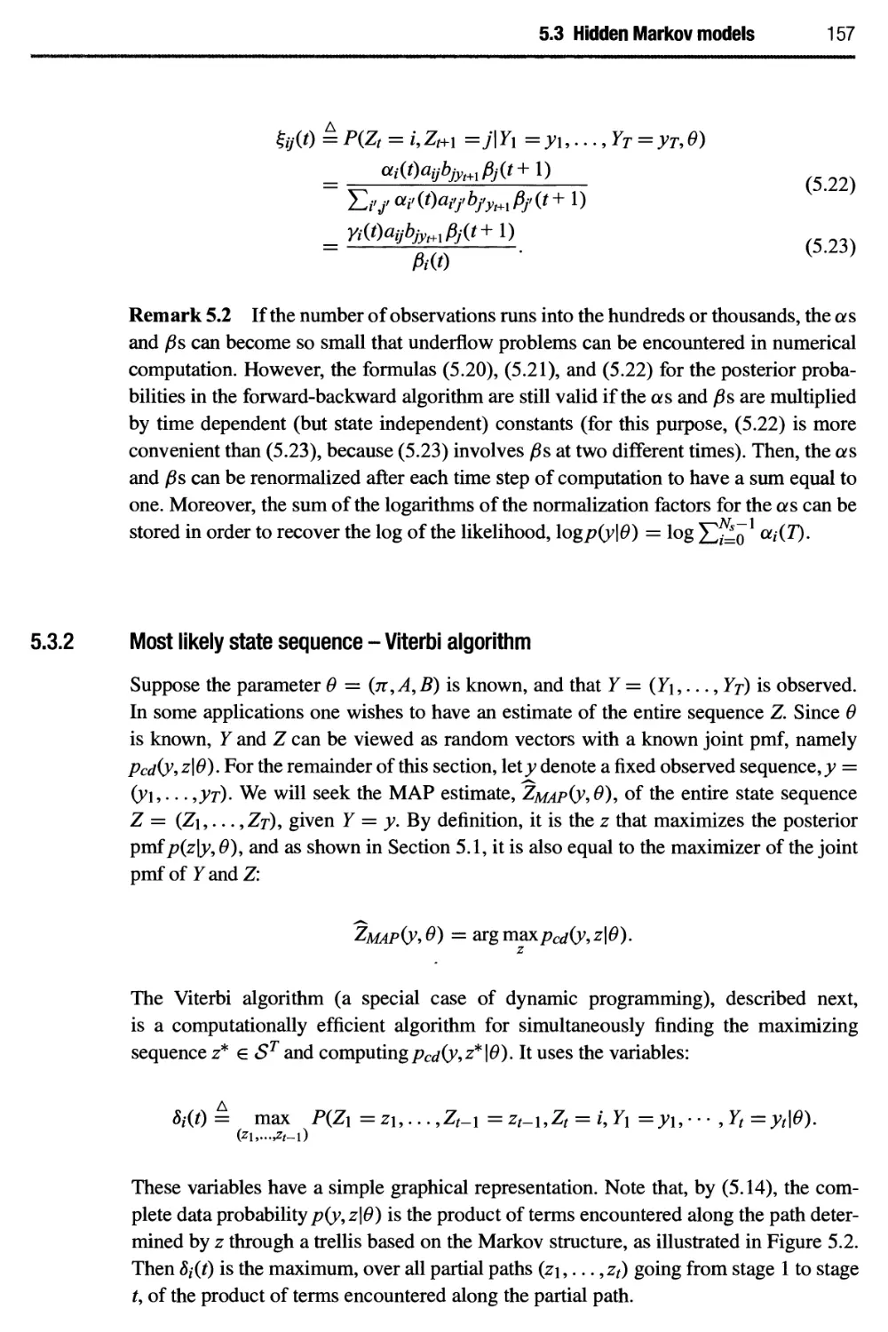
5.3.2 Most likely state sequence - Viterbi algorithm 157
5.3.3 The Baum-Welch algorithm, or EM algorithm for HMM 158
5.4 Notes 160
Dynamics of countable-state Markov models 167
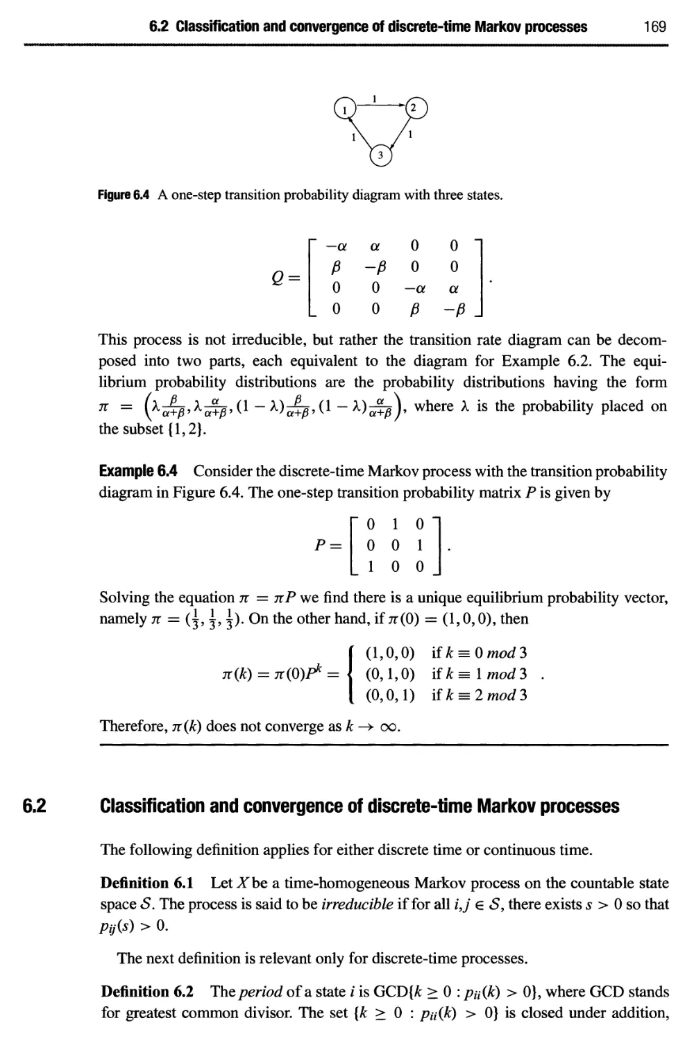
6.1 Examples with finite state space 167
6.2 Classification and convergence of discrete-time Markov processes 169
6.3 Classification and convergence of continuous-time Markov processes 172
6.4 Classification of birth-death processes 175
6.5 Time averages vs. statistical averages 177
6.6 Queueing systems, M/M/l queue and Little's law 178
6.7 Mean arrival rate, distributions seen by arrivals, and PASTA 181
6.8 More examples of queueing systems modeled as Markov birth-death
processes 184
6.9 Foster-Lyapunov stability criterion and moment bounds 186
6.9.1 Stability criteria for discrete-time processes 186
6.9.2 Stability criteria for continuous-time processes 193
Basic calculus of random processes 206
7.1 Continuity of random processes 206
7.2 Mean square differentiation of random processes 212
7.3 Integration of random processes 216
7.4 Ergodicity 223
7.5 Complexification, Part I 229
7.6 The Karhunen-Loeve expansion 231
Contents Ix
7.7 Periodic WSS random processes 238
8 Random processes in linear systems and spectral analysis 248
8.1 Basic definitions 248
8.2 Fourier transforms, transfer functions, and power spectral densities 252
8.3 Discrete-time processes in linear systems 258
8.4 Baseband random processes 260
8.5 Narrowband random processes 263
8.6 Complexification, Part II 269
9 Wiener filtering 280
9.1 Return of the orthogonality principle 280
9.2 The causal Wiener filtering problem 283
9.3 Causal functions and spectral factorization 284
9.4 Solution of the causal Wiener filtering problem for rational power
spectral densities 288
9.5 Discrete-time Wiener filtering 292
10 Martingales 304
10.1 Conditional expectation revisited 304
10.2 Martingales with respect to filtrations 310
10.3 Azuma-Hoeffding inequality 313
10.4 Stopping times and the optional sampling theorem 316
10.5 Notes 321
11 Appendix 325
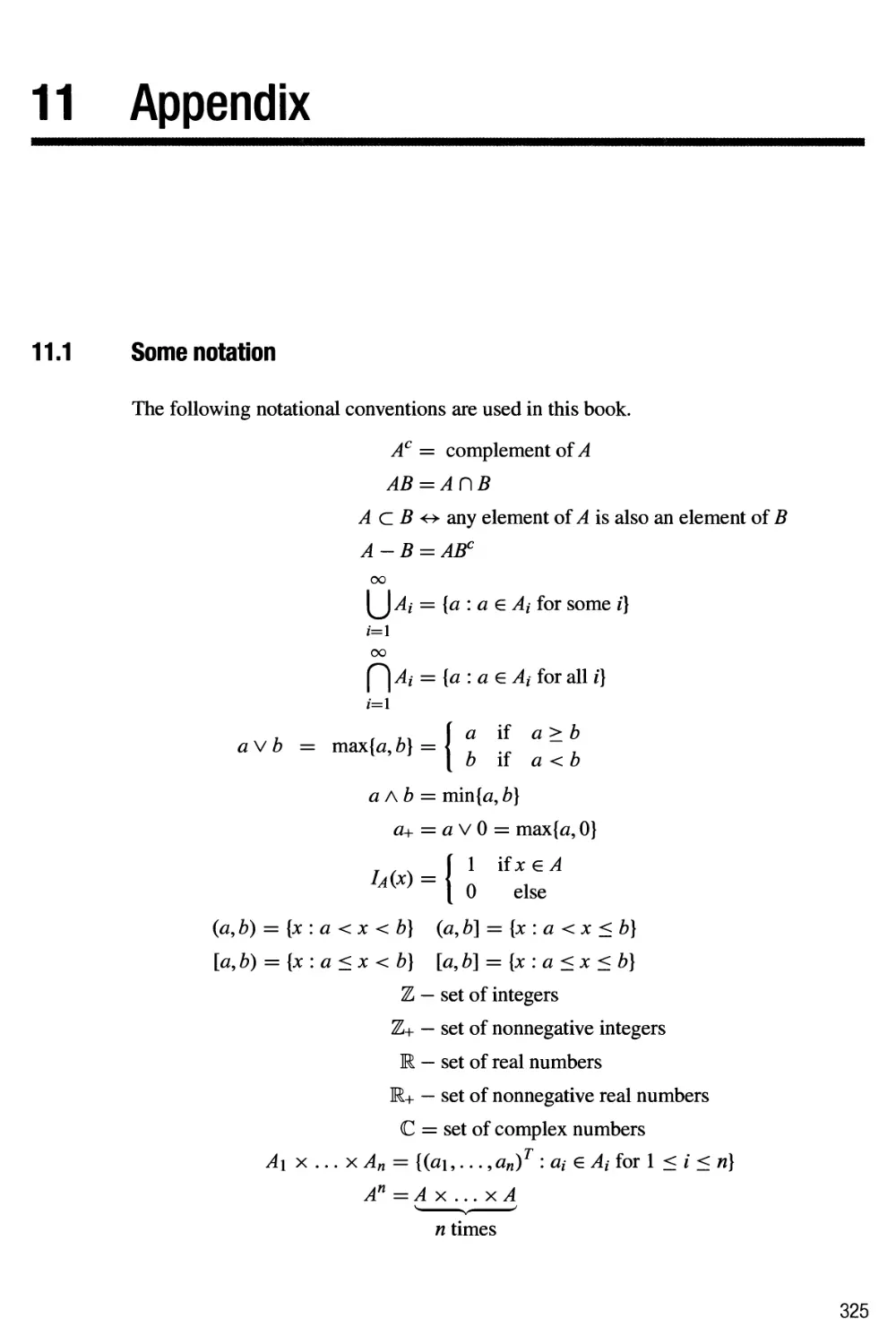
11.1 Some notation 325
11.2 Convergence of sequences of numbers 326
11.3 Continuity of functions 330
11.4 Derivatives of functions 331
11.5 Integration 333
11.5.1 Riemann integration 333
11.5.2 Lebesgue integration 335
11.5.3 Riemann-Stieltjes integration 335
11.5.4 Lebesgue-Stieltjes integration 336
11.6 On convergence of the mean 336
11.7 Matrices 339
12 Solutions to even numbered problems 344
References 411
Index 412
Preface
From an applications viewpoint, the main reason to study the subject of this book is to
help deal with the complexity of describing random, time-varying functions. A random
variable can be interpreted as the result of a single measurement. The distribution of
a single random variable is fairly simple to describe. It is completely specified by
the cumulative distribution function F(x), a function of one variable. It is relatively
easy to approximately represent a cumulative distribution function on a computer. The
joint distribution of several random variables is much more complex, for in general
it is described by a joint cumulative probability distribution function, F(x\,X2,... ,xw),
which is much more complicated than η functions of one variable. A random process, for
example a model of time-varying fading in a communication channel, involves many,
possibly infinitely many (one for each time instant t within an observation interval)
random variables. Woe the complexity!
This book helps prepare the reader to understand and use the following methods for
dealing with the complexity of random processes:
• Work with moments, such as means and covariances.
• Use extensively processes with special properties. Most notably, Gaussian
processes are characterized entirely by means and covariances, Markov processes
are characterized by one-step transition probabilities or transition rates, and initial
distributions. Independent increment processes are characterized by the
distributions of single increments.
• Appeal to models or approximations based on limit theorems for reduced
complexity descriptions, especially in connection with averages of independent,
identically distributed random variables. The law of large numbers tells us, in a certain
sense, that a probability distribution can be characterized by its mean alone.
The central limit theorem similarly tells us that a probability distribution can
be characterized by its mean and variance. These limit theorems are analogous
to, and in fact examples of, perhaps the most powerful tool ever discovered for
dealing with the complexity of functions: Taylor's theorem, in which a function
in a small interval can be approximated using its value and a small number of
derivatives at a single point.
• Diagonalize. A change of coordinates reduces an arbitrary η-dimensional
Gaussian vector into a Gaussian vector with η independent coordinates. In the new
coordinates the joint probability distribution is the product of η one-dimensional
XI
xii Preface
distributions, representing a great reduction of complexity. Similarly, a random
process on an interval of time is diagonalized by the Karhunen-Loeve
representation. A periodic random process is diagonalized by a Fourier series
representation. Stationary random processes are diagonalized by Fourier transforms.
• Sample. A narrowband continuous time random process can be exactly
represented by its samples taken with sampling rate twice the highest frequency of the
random process. The samples offer a reduced complexity representation of the
original process.
• Work with baseband equivalent. The range of frequencies in a typical wireless
transmission is much smaller than the center frequency, or carrier frequency, of
the transmission. The signal could be represented directly by sampling at twice
the largest frequency component. However, the sampling frequency, and hence
the complexity, can be dramatically reduced by sampling a baseband equivalent
random process.
This book was written for the first semester graduate course on random processes
offered by the Department of Electrical and Computer Engineering at the University
of Illinois at Urbana-Champaign. Students in the class are assumed to have had a
previous course in probability, which is briefly reviewed in the first chapter. Students
are also expected to have some familiarity with real analysis and elementary linear
algebra, such as the notions of limits, definitions of derivatives, Riemann integration,
and diagonalization of symmetric matrices. These topics are reviewed in the appendix.
Finally, students are expected to have some familiarity with transform methods and
complex analysis, though the concepts used are reviewed in the relevant chapters.
Each chapter represents roughly two weeks of lectures, and includes homework
problems. Solutions to the even numbered problems without stars can be found at the end
of the book. Students are encouraged to first read a chapter, then try doing the even
numbered problems before looking at the solutions. Problems with stars, for the most
part, investigate additional theoretical issues, and solutions are not provided.
Hopefully some students reading this book will find the problems useful for
understanding the diverse technical literature on systems engineering, ranging from control
systems, signal and image processing, communication theory, and analysis of a variety
of networks and algorithms. Hopefully some students will go on to design systems, and
define and analyze stochastic models. Hopefully others will be motivated to continue
study in probability theory, going on to learn measure theory and its applications to
probability and analysis in general.
A brief comment is in order on the level of rigor and generality at which this book
is written. Engineers and scientists have great intuition and ingenuity, and routinely
use methods that are not typically taught in undergraduate mathematics courses. For
example, engineers generally have good experience and intuition about transforms, such
as Fourier transforms, Fourier series, and z-transforms, and some associated methods of
complex analysis. In addition, they routinely use generalized functions, in particular the
delta function is frequently used. The use of these concepts in this book leverages on
this knowledge, and it is consistent with mathematical definitions, but full mathematical
Preface xiii
justification is not given in every instance. The mathematical background required for
a full mathematically rigorous treatment of the material in this book is roughly at the
level of a second year graduate course in measure theoretic probability, pursued after a
course on measure theory.
The author gratefully acknowledges the many students and faculty members,
including Todd Coleman, Christoforos Hadjicostis, Jonathan Ligo, Andrew Singer,
R. Srikant, and Venu Veeravalli who gave many helpful comments and suggestions.
Organization
The first four chapters of the book are used heavily in the remaining chapters, so most
readers should cover those chapters before moving on.
Chapter 1 is meant primarily as a review of concepts found in a typical first course on
probability theory, with an emphasis on axioms and the definition of expectation.
Readers desiring a more extensive review of basic probability are referred to the
author's notes for ECE 313 at the University of Illinois.
Chapter 2 focuses on various ways in which a sequence of random variables can
converge, and the basic limit theorems of probability: law of large numbers, central
limit theorem, and the asymptotic behavior of large deviations.
Chapter 3 focuses on minimum mean square error estimation and the orthogonality
principle. Kalman filtering is explained from the geometric standpoint based on
innovations sequences.
Chapter 4 introduces the notion of a random process, and briefly covers several key
examples and classes of random processes. Markov processes and martingales are
introduced in this chapter, but are covered in greater depth in later chapters.
After Chapter 4 is covered, the following four topics can be covered independently
of each other.
Chapter 5 describes the use of Markov processes for modeling and statistical
inference. Applications include natural language processing.
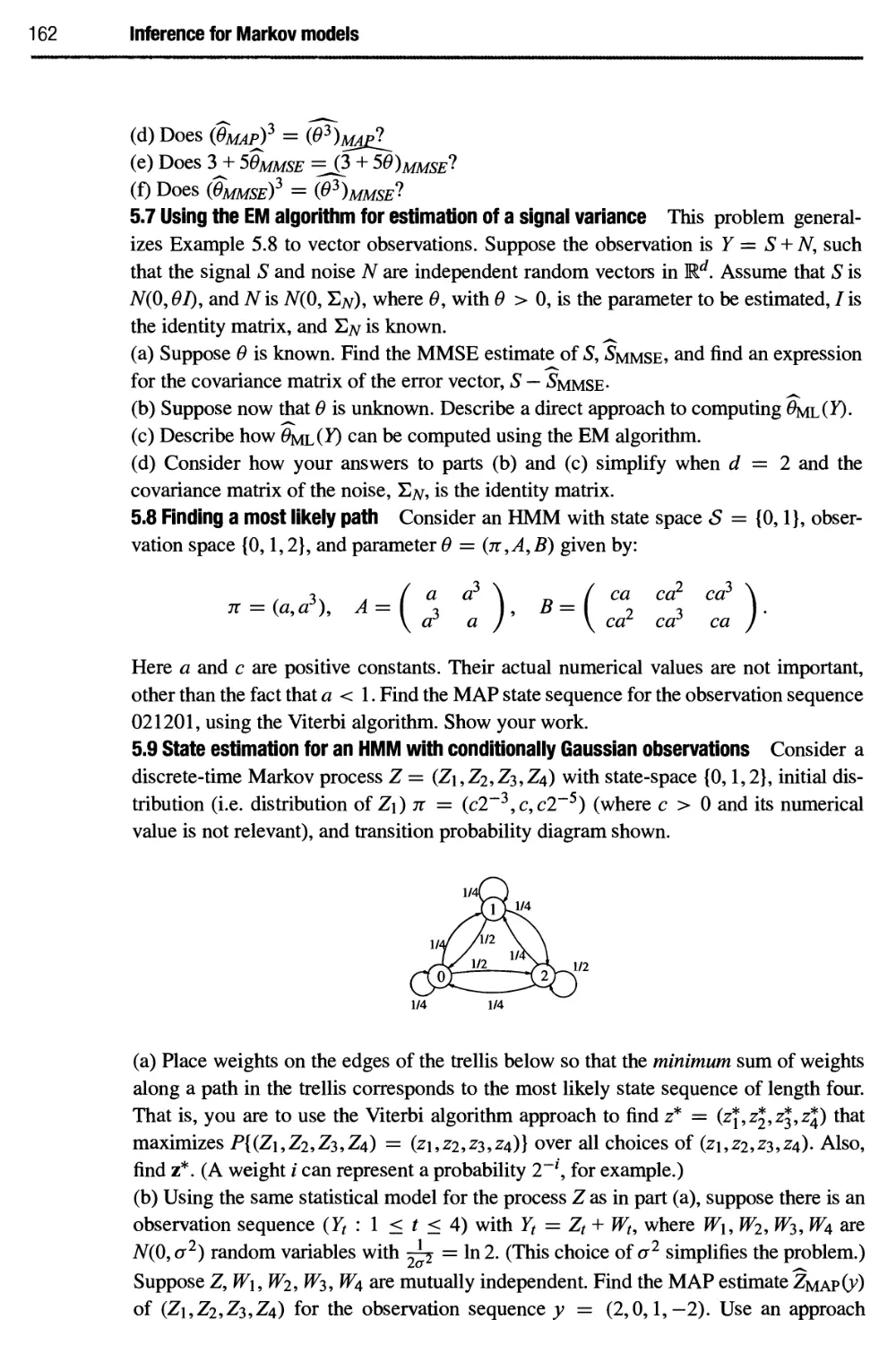
Chapter 6 describes the use o/ Markov processes for modeling and analysis of
dynamical systems. Applications include modeling of queueing systems.
Chapters 7-9 develop calculus for random processes based on mean square
convergence, moving to linear filtering, orthogonal expansions, and ending with causal
and noncausal Wiener filtering.
Chapter 10 explores martingales with respect to filtrations, with emphasis on
elementary concentration inequalities, and on the optional sampling theorem.
In recent one-semester course offerings, the author covered Chapters 1-5, Sections
6.1-6.8, Chapter 7, Sections 8.1-8.4, and Section 9.1. Time did not permit covering
the Foster-Lyapunov stability criteria, noncausal Wiener filtering, and the chapter on
martingales.
A number of background topics are covered in the appendix, including basic notation.
1 A selective review of basic probability
This chapter reviews many of the main concepts in a first level course on probability
theory, with more emphasis on axioms and the definition of expectation than is typical
of a first course.
1.1 The axioms of probability theory
Random processes are widely used to model systems in engineering and scientific
applications. This book adopts the most widely used framework of probability and random
processes, namely the one based on Kolmogorov's axioms of probability. The idea is
to assume a mathematically solid definition of the model. This structure encourages a
modeler to have a consistent, if not accurate, model.
A probability space is a triplet (Ω, J7, V). The first component, Ω, is a nonempty set.
Each element ω of Ω is called an outcome and Ω is called the sample space. The second
component, J7, is a set of subsets of Ω called events. The set of events J7 is assumed
to be a σ-algebra, meaning it satisfies the following axioms (see Appendix 11.1 for set
notation):
A.1 Ω € J",
A.2 If Ле J" thence J",
A.3 If А, В e J7 then AUВ e J7. Also, if A\, Α2,... is a sequence of elements in J7
then U~i Μ e T.
lfA,Be J7, then AB e Τ by A.2, A.3 and the fact AB = (Ac U Bcf. By the same
reasoning, if A\, Α2,... is a sequence of elements in a σ-algebra J7, then Q?f j Ai e J7.
Events Ai, i e /, indexed by a set / are called mutually exclusive if the intersection
AjAj = 0 for all ij e / with i φ]. The final component, P, of the triplet (Ω, F,P) is a
probability measure on Τ satisfying the following axioms:
P.l P(A) > 0 for all A e J7,
P.2 If А, В e Τ and A and В are mutually exclusive, P(A U B) = P(A) + P(B). Also,
if A1, A2,... is a sequence of mutually exclusive events in J7 then Ρ (US 1 Ai) =
Ρ.3Ρ(Ω) = 1.
1
2 A selective review of basic probability
The axioms imply a host of properties including the following. For any subsets A, B,
С οι J·.
• If А с В then P(A) <P(B),
• P(A UB)= P(A) + P(B) - P(AB),
• P(A U В U Q = P(A) + P(B) + P(Q - P(AB) - P(AQ - P(BQ + P(ABQ,
• P(A)+P(AC) = 1,
• P(0) = 0.
Example 1.1 (Toss of a fair coin) Using "/Г for "heads" and "7" for "tails," the toss
of a fair coin is modeled by
Ω = {#,71 T= {{//}, {71, {#, 71,0}
P{//} = Ρ{Γ} = - P{H, T] = 1 P(0) = 0.
Note that, for brevity, we omitted the parentheses and wrote P{H} instead of Р({Щ).
Example 1.2 (Standard unit-interval probability space) Take Ω = {ω : 0 < ω < 1}.
Imagine an experiment in which the outcome ω is drawn from Ω with no preference
towards any subset. In particular, we want the set of events Τ to include intervals, and
the probability of an interval [a, b] with 0 < a < b < 1 to be given by:
P([a,b]) = b-a. (1.1)
Taking a = b, we see that Τ contains singleton sets {a}, and these sets have probability
zero. Since Τ is to be a σ-algebra, it must also contain all the open intervals (a, b) in Ω,
and for such an open interval, P( (a,b)) = b — a. Any open subset of Ω is the union of a
finite or countably infinite set of open intervals, so that Τ should contain all open and all
closed subsets of Ω. Thus, F must contain any set that is the intersection of countably
many open sets, the union of countably many such sets, and so on. The specification of
the probability function Ρ must be extended from intervals to all of J7. It is not a priori
clear how large Τ can be. It is tempting to take Τ to be the set of all subsets of Ω.
However, that idea doesn't work - see Problem 1.37 showing that the length of all subsets of
R can't be defined in a consistent way. The problem is resolved by taking Τ to be the
smallest σ-algebra containing all the subintervals of Ω, or equivalently, containing all
the open subsets of Ω. This σ-algebra is called the Borel σ-algebra for [0,1]» and the sets
in it are called Borel sets. While not every subset of Ω is a Borel subset, any set we are
likely to encounter in applications is a Borel set. The existence of the Borel σ-algebra is
discussed in Problem 1.38. Furthermore, extension theorems of measure theory1 imply
that Ρ can be extended from its definition (1.1) for interval sets to all Borel sets.
See, for example, (Royden 1968) or (Varadhan 2001). The σ -algebra Τ can be extended somewhat further
by requiring the following completeness property: if В с A e Τ with P(A) = 0, then В e Τ (and also
P(B) = 0).
1.1 The axioms of probability theory 3
The smallest σ-algebra, B, containing the open subsets of R is called the Borel
σ-algebra for R, and the sets in it are called Borel subsets ofR. Similarly, the Borel
σ-algebra Bn of subsets of W1 is the smallest σ-algebra containing all sets of the form
[a\,b\] χ [tf2,62] x · · · x [an, bn]. Sets in Bn are called Borel subsets of MP. The class
of Borel sets includes not only rectangle sets and countable unions of rectangle sets, but
all open sets and all closed sets. Virtually any subset of W arising in applications is a
Borel set.
Example 1.3 (Repeated binary trials) Suppose we would like to represent an infinite
sequence of binary observations, where each observation is a zero or one with equal
probability. For example, the experiment could consist of repeatedly flipping a fair coin,
and recording a one each time it shows heads and a zero each time it shows tails. Then
an outcome ω would be an infinite sequence, ω = (ω\,α>2,···), such that for each
i > 1, (Oi € {0,1}. Let Ω be the set of all such &>s. The set of events can be taken to
be large enough so that any set that can be defined in terms of only finitely many of
the observations is an event. In particular, for any binary sequence (b\,- · · , bn) of some
finite length n, the set [ω e Ω : ω,- = bi for 1 < / < n] should be in T, and the
probability of such a set is taken to be 2~n.
There are also events that don't depend on a fixed, finite number of observations. For
example, let F be the event that an even number of observations is needed until a one is
observed. Show that F is an event and then find its probability.
Solution
For к > 1, let Ek be the event that the first one occurs on the Ath observation. So Ek =
{ω : ω\ = a>2 = — - = ω#-ΐ = 0 and a>k = 1}. Then Ek depends on only a finite number
of observations, so it is an event, and P{Ek) = 2~k. Observe that F = E2 UE4 UEe U...,
so F is an event by Axiom A.3. Also, the events £2,^4,... are mutually exclusive, so
by the full version of Axiom P.2:
/>(^=№)+p(£4)+... = l(i + (i) + (I)2+...) = TiT = I.
The following lemma gives a continuity property of probability measures which is
analogous to continuity of functions on Rw, reviewed in Appendix 11.3. If B\,B2,... is
a sequence of events such that B\ С В2 С #з С ..., then we can think that Bj converges
to the set Ugji?,· as 7 -> 00. The lemma states that in this case, P{Bj) converges to the
probability of the limit set as jr —> 00.
Lemma 1.1 (Continuity of probability) Suppose B\,B2,...isa sequence of events.
(a) IfBx CB2C··· then liny-oo P(Bj) = Ρ flj~i Bi) ·
(b) IfBx DB2D··· then lim^ P(Bj) = Ρ (Π£ι Bf) .
4 A selective review of basic probability
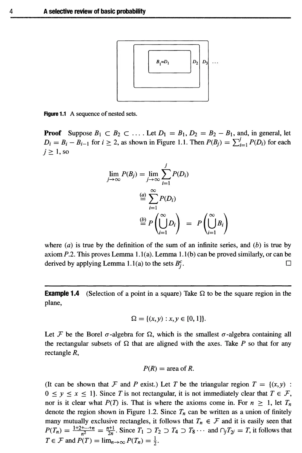
Figure 1.1 A sequence of nested sets.
Proof Suppose 5i eft С .... Let D\ = ft, ft = ft — ft, and, in general, let
A = ft - ft_i for ι > 2, as shown in Figure 1.1. Then P(Bj) = jji=l Р(Д) for each
j > 1, so
J
lim P(Bj) = lim Г?(Д·)
—von ^ /Unn ^—-^
y-»oo
^°°£l
(a)
^ Еад
i=l
■'&*) - -&■)
where (л) is true by the definition of the sum of an infinite series, and (b) is true by
axiomP.2. This proves Lemma 1.1(a). Lemma 1.1(b) can be proved similarly, or can be
derived by applying Lemma 1.1(a) to the sets Bc-. D
Example 1-4 (Selection of a point in a square) Take Ω to be the square region in the
plane,
Ω = {(x,y) : x,y g [0,1]}.
Let Τ be the Borel σ-algebra for Ω, which is the smallest σ-algebra containing all
the rectangular subsets of Ω that are aligned with the axes. Take Ρ so that for any
rectangle ft
P(R) = area of/?.
(It can be shown that Τ and Ρ exist.) Let Τ be the triangular region Τ = {(x,y) :
0 < у < χ < 1}. Since Г is not rectangular, it is not immediately clear that Τ e J7,
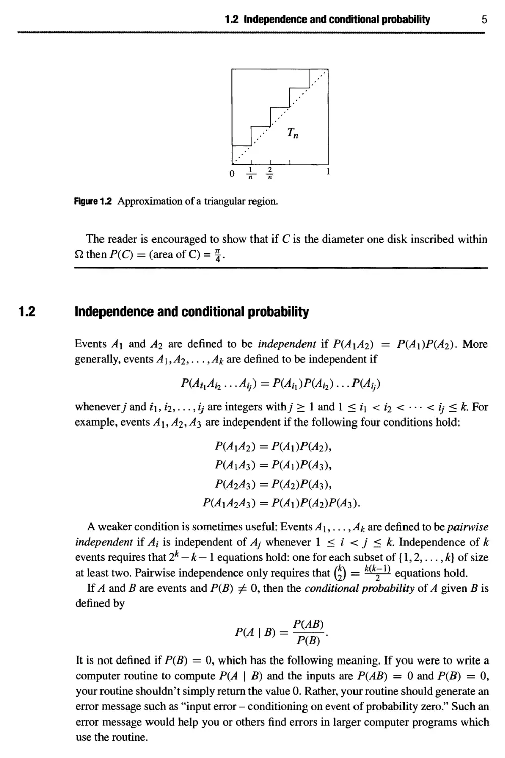
nor is it clear what P(T) is. That is where the axioms come in. For η > 1, let Tn
denote the region shown in Figure 1.2. Since Tn can be written as a union of finitely
many mutually exclusive rectangles, it follows that Tn € Τ and it is easily seen that
P(Tn) = 1+2+-"+w = *gi. Since 7Ϊ э Г2 Э Г4 Э Г8 · · · and Π,Γ^ = Γ, it follows that
Те Τ andP(T) = lim^ooP^) = {.
1.2 Independence and conditional probability 5
l·'
T„
Figure 1.2 Approximation of a triangular region.
The reader is encouraged to show that if С is the diameter one disk inscribed within
Ω then P(Q = (area of C) = f.
1.2
Independence and conditional probability
Events A\ and A2 are defined to be independent if P(A\A2) = P(A\)P(A2). More
generally, events A\ ,A2,... ,Ak are defined to be independent if
P(AhAh ... Atj) = P(Ah)P(Ah).. .Ρ(Αφ
whenever7 and /1, /2,..., ij are integers withy > 1 and 1 < /1 < /2 < · · · < ij < k. For
example, events А\,А2,Аз are independent if the following four conditions hold:
Ρ(4ιΑ2) = Ρ(Αι)Ρ(Α2)9
Ρ(4ιΑ3)=Ρ(Αι)Ρ(Α3)9
P(A2A3)=P(A2)P(A3),
P(AlA2A3)=P(Al)P(A2)P(A3).
A weaker condition is sometimes useful: Events A \,..., Ak are defined to be pairwise
independent if Ai is independent of Aj whenever 1 < / < j < k. Independence of к
events requires that 2k — к — 1 equations hold: one for each subset of {1,2,... ,k) of size
at least two. Pairwise independence only requires that (2) = -Цг-^ equations hold.
If A and В are events and P(B) φ 0, then the conditional probability oiA given В is
defined by
P(A I B) =
P(AB)
P(B) '
It is not defined if P(B) = 0, which has the following meaning. If you were to write a
computer routine to compute P(A \ B) and the inputs are P(AB) = 0 and P(B) = 0,
your routine shouldn't simply return the value 0. Rather, your routine should generate an
error message such as "input error - conditioning on event of probability zero." Such an
error message would help you or others find errors in larger computer programs which
use the routine.
6 A selective review of basic probability
As a function of A for В fixed with P(B) φ 0, the conditional probability of A given
В is itself a probability measure for Ω and J7. More explicitly, fix В with P(B) φ 0. For
each event A define P'{A) = P(A \ B). Then (Ω, F,P') is a probability space, because
P' satisfies the axioms P\ — P3. (Try showing that.)
If A and В are independent then Ac and В are independent. Indeed, if A and В are
independent then
P(ACB) = P(B) - P(AB) = (1 - P(A))P(B) = P(AC)P(B).
Similarly, if A, B, and С are independent events then А В is independent of C. More
generally, suppose E\,E2,... ,En are independent events, suppose η = щ + · · · + nk
with щ > 1 for each /, and suppose F\ is defined by Boolean operations (intersections,
complements, and unions) of the first n\ events E\,...,Eni,F2 is defined by Boolean
operations on the next «2 events, Eni+\,... ,Eni+rl2, and so on. Then F\,.. .,Fk are
independent.
Events E\,..., Ek are said to form a partition of Ω if the events are mutually exclusive
and Ω = E\ U.. .UEk. Of course for a partition, P(E\)+.. ЛР{Ек) = 1. More generally,
for any event A, the law of total probability holds because A is the union of the mutually
exclusive sets AE\,AE2,... ,AEk'.
P(A)=P(AEi) + ...+P(AEk).
If P(Ei) φ 0 for each /, this can be written as
P(A) = P(A | Ει)Ρ(Ει) + ...+P(A\ Ek)P{Ek).
Figure 1.3 illustrates the condition of the law of total probability.
Judicious use of the definition of conditional probability and the law of total
probability leads to Bayes'formula for P(E( | A) (if P(A) φ 0) in simple form
P(AEj) P(A | EdPjEj)
P(Ei A) = = ,
P(A) P(A)
or in expanded form:
P(A | ЕдР{Ед
P(Ei | A) =
P(A | EX)P{EX) + ...+P{A\ Ek)P(Ek)
The remainder of this section gives the Borel-Cantelli lemma. It is a simple result
based on continuity of probability and independence of events, but it is not typically
Figure 1.3 Partitioning a set A using a partition of Ω.
1.2 Independence and conditional probability 7
encountered in a first course on probability. Let (An : η > 0) be a sequence of events
for a probability space (Ω, J7, P).
Definition 1.2 The event [An infinitely often} is the set of ω e Ω such that ω e An for
infinitely many values of n.
Another way to describe {An infinitely often} is that it is the set of ω such that for any
k, there is an η > к such that ω e An. Therefore,
[An infinitely often} = n*>i (Un>kAn) .
For each k, the set Un>kAn is a countable union of events, so it is an event, and {An
infinitely often} is an intersection of countably many such events, so that [An infinitely
often} is also an event.
Lemma 1.3 (Borel-Cantelli lemma) Let (An : η > 1) be a sequence of events and let
pn = P{An).
(a) tfY^i Pn < oo, then P{An infinitely often] = 0.
(b) VY1^L\Pn = oo andA\,A2,... are mutually independent, then
P{An infinitely often] = 1.
Proof (a) Since {An infinitely often} is the intersection of the monotonically non-
increasing sequence of events Un>kAn, it follows from the continuity of
probability for monotone sequences of events (Lemma 1.1) that P{An infinitely often} =
\\тк-*ооР(У)п>кАп)· Lemma 1.1, the fact that the probability of a union of events
is less than or equal to the sum of the probabilities of the events, and the definition of
the sum of a sequence of numbers, yield that for any к > 1,
m oo
P(Un>kAn) = lim P(U™=kAn) < lim Υ\ρη = У>„.
n=k n=k
Therefore, P{An infinitely often} < lim^ooZ!SU/V If Σ^ιΡη < °°> tnen
lim^oo Y^LkPn = 0, which implies part (a) of the lemma.
(b) Suppose that Y^L\Pn = +oo and that the events A\,A2, · · · are mutually
independent. For any к > 1, using the fact 1 — и < exp(—u) for all w,
PQJn>kAn)
m
= lim P{U™=kAn) = lim 1 - Y\(\ -p„)
n=k
> lim 1 - exp
m—>oo
(- Σ,Ρη J = 1 - exp I - Σ?η ) = l~ exP(_0°) = L
n=k / \ n=k I
Therefore, P{An infinitely often} = lim^oo P(^n>k^n) = 1· Π
Example 1.5 Consider independent coin tosses using biased coins, such that P(An) =
pn = 1, where An is the event of getting heads on the nth toss. Since Y^L\ ^ = +oo,
δ Α selective review of basic probability
the part of the Borel-Cantelli lemma for independent events implies that P{An infinitely
often} = 1.
Example 1.6 Let (Ω,Τ,Ρ) be the standard unit-interval probability space defined
in Example 1.2, and let An = [0, ^). Then pn = £ and An+\ С An for η > 1.
The events are not independent, because for m < n, P(AmAn) = P(An) = - φ
P(Am)P(An). Of course 0 e An for all n. But for any ω e (0,1], ω g An for η > ^.
Therefore, {An infinitely often} = {0}. The single point set {0} has probability zero,
so P{An infinitely often} = 0. This conclusion holds even though Σ™=\Ρη = +oo,
illustrating the need for the independence assumption in Lemma 1.3(b).
1.3 Random variables and their distribution
Let a probability space (Ω, J7, P) be given. By definition, a random variable is a function
ΛΓ from Ω to the real line R that is Τ measurable, meaning that for any number c,
{ω:Χ(ω)<ο} e J\ (1.2)
If Ω is finite or countably infinite, then Τ can be the set of all subsets of Ω, in which
case any real-valued function on Ω is a random variable.
If (Ω, Τ,Ρ) is the standard unit-interval probability space described in Example 1.2,
then the random variables on (Ω, Τ,Ρ) are called the Borel measurable functions on Ω.
Since the Borel σ -algebra contains all subsets of [0,1] that come up in applications, for
practical purposes we can think of any function on [0,1] as being a random variable.
For example, any piecewise continuous or piecewise monotone function on [0,1] is a
random variable for the standard unit-interval probability space.
The cumulative distribution function (CDF) of a random variable X'\$ denoted by Fx.
It is the function, with domain the real line R, defined by
Fx(c) = Ρ{ω : Χ{ω) < с]
= P{X < с] (for Short).
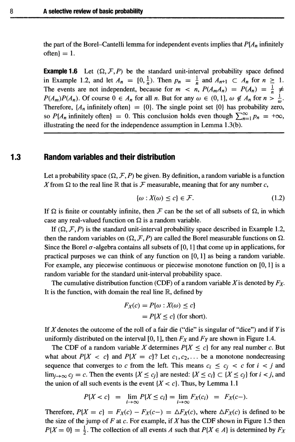
If ^f denotes the outcome of the roll of a fair die ("die" is singular of "dice") and if У is
uniformly distributed on the interval [0,1]» then Fx and Fy are shown in Figure 1.4.
The CDF of a random variable X determines P{X < c] for any real number c. But
what about P{X < c] and P{X = c}? Let c\,C2, · · · be a monotone nondecreasing
sequence that converges to с from the left. This means a < Cj < с for i < j and
limy^oo Cj = c. Then the events [X < Cj] are nested: [X < q} С {X < Cj] for / <j, and
the union of all such events is the event {X < c]. Thus, by Lemma 1.1
P{X<c] = \imP{X<a}= limFxia) = Fx(c-).
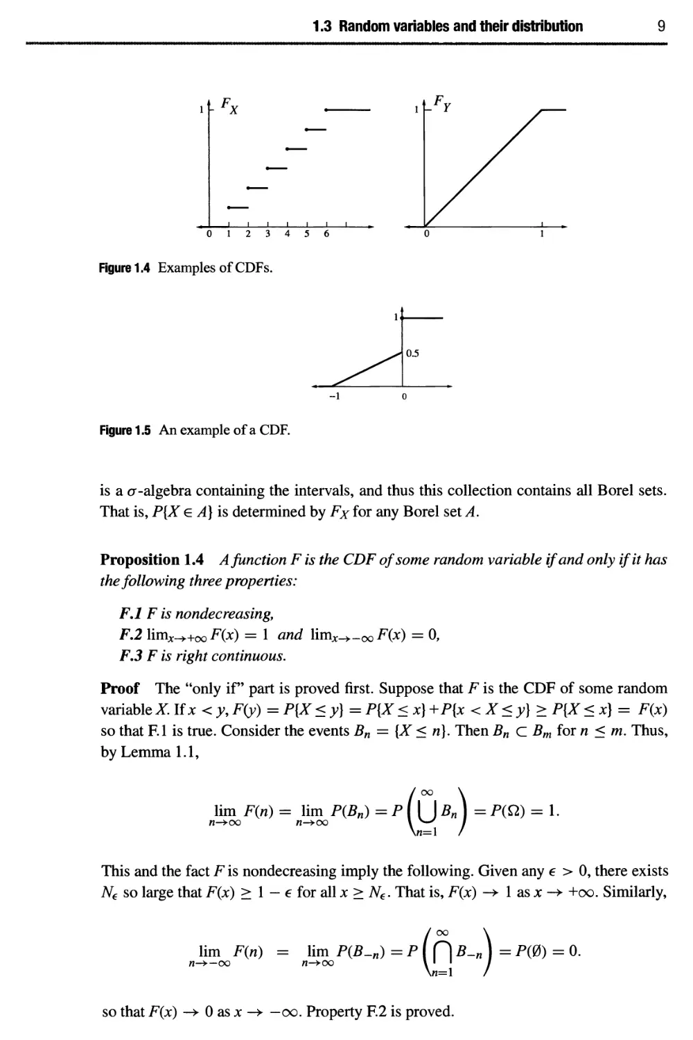
Therefore, P{X = c] = Fx(c) - Fx(c-) = AFx(c), where AFx(c) is defined to be
the size of the jump of F at c. For example, if X has the CDF shown in Figure 1.5 then
P{X = 0} = \. The collection of all events A such that P[X e A] is determined by Fx
1.3 Random variables and their distribution
9
YFx
2 3 4 5 6
Figure 1.4 Examples of CDFs.
Figure 1.5 An example of a CDF.
is a σ-algebra containing the intervals, and thus this collection contains all Borel sets.
That is, P{X e A] is determined by Fx for any Borel set A.
Proposition 1.4 A function F is the CDF of some random variable if and only if it has
the following three properties:
F.l F is nondecreasing,
F.2 \imx-++<X) F(x) = 1 and lim^-oo^C*) = 0,
F.3 F is right continuous.
Proof The "only if" part is proved first. Suppose that F is the CDF of some random
variable^. If χ < у, F(y) = P{X <y} = P{X < x] +P{x < X < y] > P{X < x] = F(x)
so that F.l is true. Consider the events Bn = [X < n]. Then Bn с Bm for η < m. Thus,
by Lemma 1.1,
lim F(n) = lim P(Bt
w-»oo w-»oo
n)=pl[JBn\ =
Ρ(Ω) = 1.
This and the fact F is nondecreasing imply the following. Given any e > 0, there exists
N€ so large that F(x) > 1 - 6 for all χ > N€. That is, F(x) -> 1 as χ -> +oo. Similarly,
lim F(n) = lim P(B
л->—oo л->оо
-n)=p([\B-") =
P№ = o.
so that F(x) -¥■ 0 as χ -> —oo. Property F.2 is proved.
10 A selective review of basic probability
The proof of F.3 is similar. Fix an arbitrary real number x. Define the sequence of
events An for η > 1 by An = [X < χ + ^}. Then An cAmfovn>m so
lim F
w-»oo
(χ+λΛ=\\^Ρ{Αη)=ρΙ^^
Convergence along the sequence χ + ^, together with the fact that F is nondecreasing,
implies that F(x+) = F(x). Property F.3 is thus proved. The proof of the "only if
portion of Proposition 1.4 is complete.
To prove the "if part of Proposition 1.4, let F be a function satisfying properties
F.1-F.3. It must be shown that there exists a random variable with CDF F. Let Ω = R
and let Τ be the set В of Borel subsets of R. Define Ρ on intervals of the form (a, b] by
P((a, b]) = F(b) — F(a). It can be shown by an extension theorem of measure theory
that Ρ can be extended to all of Τ so that the axioms of probability are satisfied. Finally,
let Χ(ω) = ω for all ω e Ω. Then
P(Xe(a,b])=P((a,b]) = F(b) - F(a).
Therefore, ^has CDF F. So F is a CDF, as was to be proved. D
The vast majority of random variables described in applications are one of two types,
to be described next. A random variable X is a discrete random variable if there is a
finite or countably infinite set of values {xj : / e 1} such that P{X e {*,· : ί e 7}} = 1.
The probability mass function (pmf) of a discrete random variable X, denoted px(x), is
defined by px(x) = P[X = x]. Typically the pmf of a discrete random variable is much
more useful than the CDF. However, the pmf and CDF of a discrete random variable are
related by ρχ(χ) = AFx(x) and conversely,
Fx(x)= Σρχψ\ (1.3)
y:y<x
where the sum in (1.3) is taken only over>> such thatpxiy) Φ 0. If ^f is a discrete random
variable with only finitely many mass points in any finite interval, then Fj^is a piecewise
constant function.
A random variable Xis a continuous random variable if the CDF is the integral of a
function:
FX{x) = Γ fxiy)dy.
«/—oo
The function/^ is called the probability density function (pdf). If the pdf/Hs continuous
at a point x, then the value fx{x) has the following nice interpretation:
1 Γχ+ε
fx(x) = lim - / fxiy)dy
ε^ο ε Jx
= lim -P{x < X < χ + ε].
ε^Ο ε
1.4 Functions of a random variable 11
If A is any Borel subset of R, then
P{XeA}= ffx(x)dx. (1.4)
Ja
The integral in (1.4) can be understood as a Riemann integral if A is a finite union of
intervals and/is piecewise continuous or monotone. In general,/^ is required to be
Borel measurable and the integral is defined by Lebesgue integration.2
Any random variable Jonan arbitrary probability space has a CDF Fx. As noted in
the proof of Proposition 1.4 there exists a probability measure Ρχ (called Ρ in the proof)
on the Borel subsets of R such that for any interval (я, b],
Px((a,b])=P{Xe(a,b]}.
We define the probability distribution of Xto be the probability measure Ρχ. The
distribution Ρχ is determined uniquely by the CDF Fx. The distribution is also determined by
the pdf/Hf -^is continuous type, or the pmf ρχϊί Xis discrete type. In common usage,
the response to the question "What is the distribution of ΧΊ" is answered by giving one
or more of Fx, fx, or ρχ, or possibly a transform of one of these, whichever is most
convenient.
1.4 Functions of a random variable
Recall that a random variable X on a probability space (Ω, F,P) is a function mapping
Ω to the real line R, satisfying the condition [ω : Χ(ω) < a] e Τ for all agI. Suppose
g is a function mapping R to R that is not too bizarre. Specifically, suppose for any
constant с that \x : g(x) < c] is a Borel subset of R. Let Υ(ω) = g{X{a))). Then Υ maps
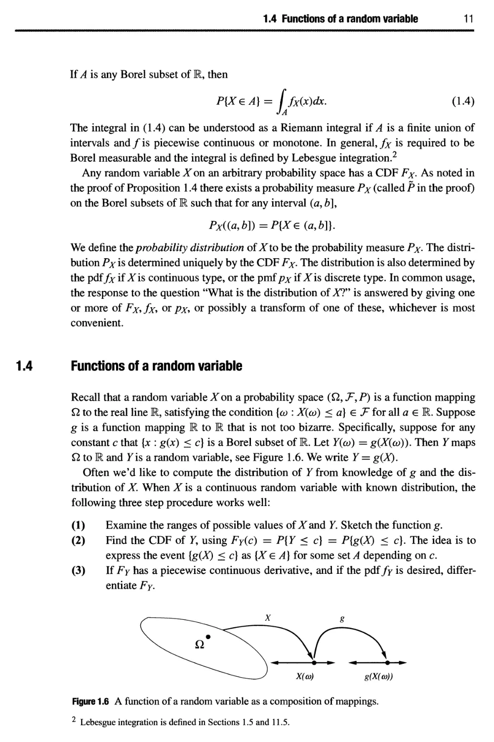
Ω to R and Υ is a random variable, see Figure 1.6. We write Υ = g(X).
Often we'd like to compute the distribution of Υ from knowledge of g and the
distribution of X. When X is a continuous random variable with known distribution, the
following three step procedure works well:
(1) Examine the ranges of possible values of X and Y. Sketch the function g.
(2) Find the CDF of 7, using FY(c) = P{Y < c] = P{g(X) < c]. The idea is to
express the event [g(X) < c] as [X e A] for some set A depending on с
(3) If Fy has a piecewise continuous derivative, and if the puffy is desired,
differentiate Fy.
Figure 1.6 A function of a random variable as a composition of mappings.
2 Lebesgue integration is defined in Sections 1.5 and 11.5.
12 A selective review of basic probability
If instead Xis a discrete random variable then step 1 should be followed. After that
the pmf of Υ can be found from the pmf of fusing
pr(y)
P{g(X)=y}= Σ Ρ**)-
x:g(x)=y
Example 1.7 Suppose Xis an Ν(μ = 2, σ2 = 3) random variable (see Section 1.6 for
the definition) and Υ = X2. Let us describe the density of Y. Note that Υ = g(X) where
g(x) = χ2. The support of the distribution of ΛΓis the whole real line, and the range of g
over this support is R+. Next we find the CDF, FY. Since P{Y > 0} = 1, FY(c) = 0 for
с < 0. For с > 0,
FY(c) = P{X2 <c}=P{-yfi<X<yfi]
= P
-y/c ■
■2 X-2 Jc-2
— < < v
л/3 л/3 л/3
f-j~c-2
}
Differentiate with respect to c, using the chain rule and O'(s) = —=exp(— y), to
)
obtain
fr(c) =
/247ГС
«К-[^П+ехр(-№Г)1 lfci0
0
ifc<0
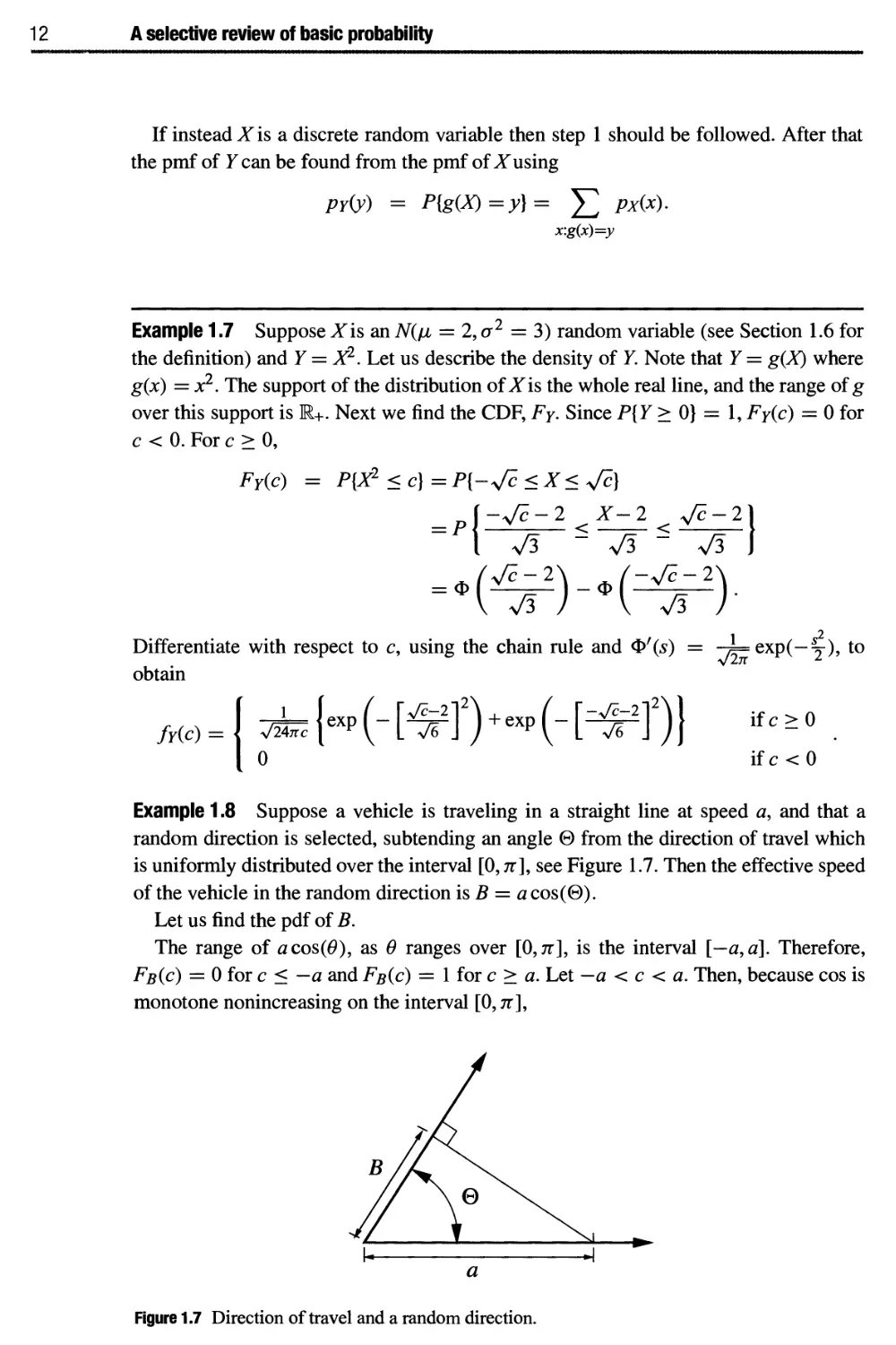
Example 1.8 Suppose a vehicle is traveling in a straight line at speed a, and that a
random direction is selected, subtending an angle Θ from the direction of travel which
is uniformly distributed over the interval [0, π], see Figure 1.7. Then the effective speed
of the vehicle in the random direction is В = a cos(0).
Let us find the pdf of B.
The range of я cos(#), as θ ranges over [Ο,π], is the interval [—a, a]. Therefore,
Fb(c) = 0 for с < —a and Fb(c) = 1 for с > a. Let — a < с < a. Then, because cos is
monotone nonincreasing on the interval [0, π],
Figure 1.7 Direction of travel and a random direction.
1.4 Functions of a random variable 13
FB(c) = P{tfcos(0) < c] =PJcos(0) < -j
= p{0>cos-'Q)
= 1
cos
-1 (c
(h)
π
Therefore, because cos l (y) has derivative, -(1 - y2) 2,
I —/ \ >> \ с \< а
Mc)=\ *JF=?
О \ с \> a
A sketch of the density is given in Figure 1.8.
Example 1-9 Suppose Υ = tan(0), as illustrated in Figure 1.9, where Θ is uniformly
distributed over the interval (-f, f) · Let us find the pdf of Y. The function tan(#)
increases from -00 to 00 as θ ranges over the interval (-f, f )·
For any real c,
FY(c)=P{Y<c]
= P{tan(0) < c]
λ tan-4c) + f
= Ρ{Θ < tan-1 (с)} = ——2..
π
Differentiating the CDF with respect to с yields that Υ has the Cauchy pdf:
1
fY(c)
n(l+c2)
00 < с < oo.
-a 0 a
Figure 1.8 The pdf of the effective speed in a uniformly distributed direction in two dimensions.
Figure 1.9 A horizontal line, a fixed point at unit distance, and a line through the point with
random direction.
14 A selective review of basic probability
Example 1.10 Given an angle θ expressed in radians, let (Θ mod 2π) denote the
equivalent angle in the interval [0,2π]. Thus, (Θ mod 2π) is equal to θ+2πη, where the
integer η is such that 0 < θ + 2πη < 2π.
Let Θ be uniformly distributed over [0,2π], let h be a constant, and let
Θ = (0 + umod27T).
Let us find the distribution of Θ.
Clearly Θ takes values in the interval [0,2π], so fix с with 0 < с < 2π and seek to
findP{0 < cJ.LeM denote the interval [h,h+2n].Thus9 Θ+h is uniformly distributed
over A. Let В = \Jn[2nn, 2πη + с]. Thus Θ < с if and only if Θ + h e B. Therefore,
P{® <c}= f —(ΙΘ.
JApiB 2π
By sketching the set B, it is easy to see that A f] В is either a single interval of length c,
or the union of two intervals with lengths adding to c. Therefore, Ρ{Θ < с] = ^, so
that Θ is itself uniformly distributed over [0,2π].
Example 1.11 Let Xbc an exponentially distributed random variable with parameter λ.
Let Υ = \X\, which is the integer part of X, and let R = X— \X\, which is the remainder.
We shall describe the distributions of Υ and R.
Clearly Υ is a discrete random variable with possible values 0,1,2,..., so it is
sufficient to find the pmf of Y. For integers к > 0,
pY{k) =P{k<X<k+\] = / Xe'^dx = e~xk( 1 - e~x)
and /?Η&) = 0 for other к.
Turn next to the distribution of R. Clearly R takes values in the interval [0,1]. So let
0 < с < 1 and find Fr(c):
ί oo Λ
FR(c)=P{X-[X}<c} = p\xe\J[k,k + c]\
ι k=o \
oo oo 1 _^c
= £>{* <z< fc+cj = £>-ud - <τλ<) = т^г,
fc=0 fc=0
where we used the fact 1 + a + a2 + · · · = y^ for | a | < 1. Differentiating Fr yields
the pmf:
,,, ί ^ 0<c<l
I 0 otherwise
What happens to the density of R as λ -> 0 or as λ -> oo? By l'Hopital's rule,
1 0<c<1
lim fp(c) = . л
λ^ο 0 otherwise
1.4 Functions of a random variable 15
That is, in the limit as λ -> 0, the density of ^becomes more and more evenly spread
out, and R becomes uniformly distributed over the interval [0,1]. If λ is very large
then the factor 1 — e~k is nearly one , and the density of R is nearly the same as the
exponential density with parameter λ.
An important step in many computer simulations of random systems is to generate a
random variable with a specified CDF, by applying a function to a random variable that
is uniformly distributed on the interval [0,1]. Let F be a function satisfying the three
properties required of a CDF, and let C/be uniformly distributed over the interval [0,1].
The problem is to find a function g so that Fis the CDF of g(U). An appropriate function
g is given by the inverse function of F. Although F may not be strictly increasing, a
suitable version of F-1 always exists, defined for 0 < и < 1 by
F"1^) = min{x : F(x) > u]. (1.5)
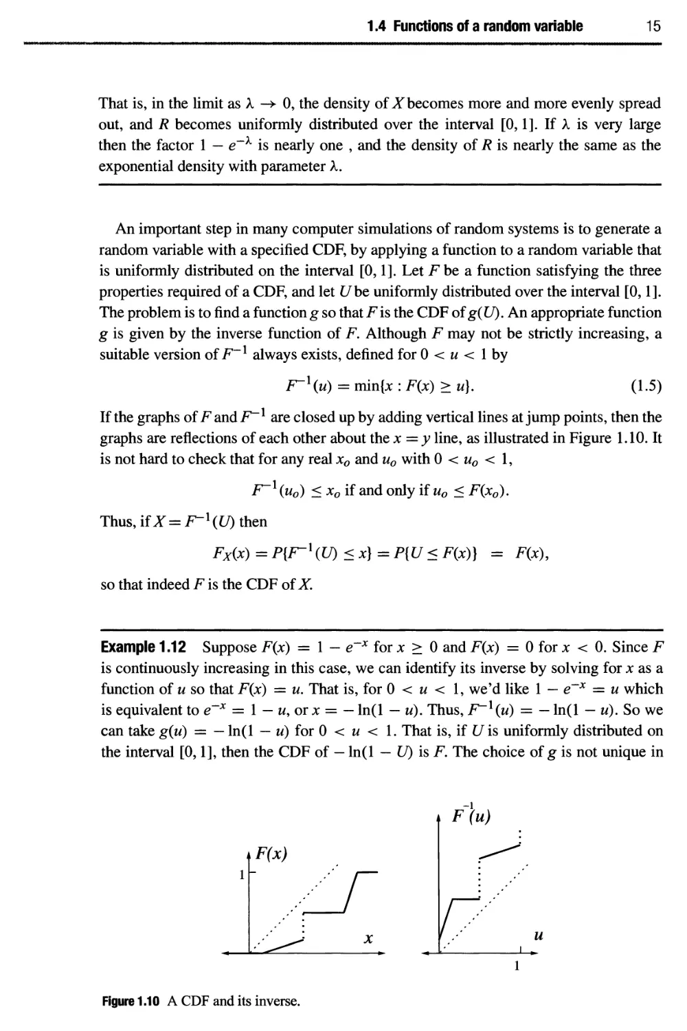
If the graphs of Fandi^1 are closed up by adding vertical lines at jump points, then the
graphs are reflections of each other about the χ = у line, as illustrated in Figure 1.10. It
is not hard to check that for any real x0 and u0 with 0 < u0 < 1,
F~l (u0) < x0 if and only if uQ < F(x0).
Thus, if X=F-\U) then
Fx(x)=P{F-l(U)<x}=P{U<F(x)} = F(x),
so that indeed F is the CDF of X.
Example 1.12 Suppose F(x) = 1 - e~x for χ > 0 and F(x) = 0 for χ < 0. Since F
is continuously increasing in this case, we can identify its inverse by solving for χ as a
function of и so that F(x) = u. That is, for 0 < и < 1, we'd like 1 — e~x = и which
is equivalent to e~x = 1 — w, or χ = — ln(l — u). Thus, F~l(u) = — ln(l — u). So we
can take g(w) = — ln(l — u) for 0 < и < 1. That is, if Uis uniformly distributed on
the interval [0,1], then the CDF of — ln(l — £/) is F. The choice of g is not unique in
F(u)
F(x)
Figure 1.10 A CDF and its inverse.
1
16 A selective review of basic probability
general. For example, 1 — C/has the same distribution as t/, so the CDF of — ln(L0 is
also F. To double check the answer, note that if χ > 0, then
P{- ln(l - U) < x] = P{ln(l -U)> -x]
= P{1 - U> e~x}=P{U< l-e-x}=F(x).
Example 1.13 Suppose F is the CDF for the experiment of rolling a fair die, shown
on the left half of Figure 1.4. One way to generate a random variable with CDF F is to
actually roll a die. To simulate that on a computer, we'd seek a function g so that g(U)
has the same CDF. Using g = F~l and using (1.5) or the graphical method illustrated
in Figure 1.10 to find F-1, we get that for 0 < и < 1, g(w) = / for ^ < и < | for
1 < i < 6. To double check the answer, note that if 1 < / < 6, then
ί ι - 1 ι 1 1
p{g(t/) = ;}=p{—<t/<-J = -
so that g(U) has the correct pmf, and hence the correct CDF.
1.5 Expectation of a random variable
The expectation, alternatively called the mean, of a random variable ΛΓcan be defined in
several different ways. Before giving a general definition, we shall consider a
straightforward case. A random variable X is called simple if there is a finite set {x\,... ,xm]
such that Χ(ω) e {x\,... ,xm] for all ω. The expectation of such a random variable is
defined by
m
E[X\ = Y^XiP{X=Xi}. (1.6)
i=l
The definition (1.6) clearly shows that E[X\ for a simple random variable ^f depends
only on the pmf of X.
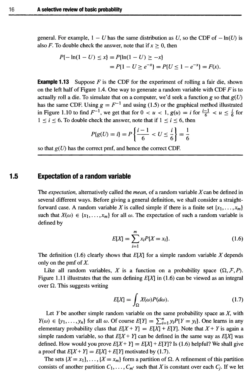
Like all random variables, X is a function on a probability space (Ω,Τ,Ρ).
Figure 1.11 illustrates that the sum defining E[X\ in (1.6) can be viewed as an integral
over Ω. This suggests writing
E[X\ = f Χ(ώ)Ρ(άώ). (1.7)
Let Υ be another simple random variable on the same probability space as X, with
Υ(ω) g {y\,... ,yn] for all ω. Of course E[Y] = Σ"=1 yiP{Y = }>/}· One learns in any
elementary probability class that E[X+ Y] = E[X\ + E[Y]. Note that X+ Υ is again a
simple random variable, so that E[X+ Y] can be defined in the same way as E[X\ was
defined. How would you prove E[X+ Y] = E[X\ + Ε[Υ]Ί Is (1.6) helpful? We shall give
a proof that E[X+ Y] = E[X\ + E[Y] motivated by (1.7).
The sets [X = x\},..., {X = xm] form a partition of Ω. A refinement of this partition
consists of another partition C\,..., Cm> such that Xis constant over each Cj. If we let
1.5 Expectation of a random variable 17
Χ(ω)=Χι
Χ(ω)=χ2
Χ(ω)=χ3
Figure 1.11 A simple random variable with three possible values.
Xj denote the value of ΛΓon Cy, then clearly
E[X\ = Y^xfi(Cj].
J
Now, it is possible to select the partition C\,..., Cm> so that both X and Υ are constant
over each C/. For example, each Cy could have the form {X = χ/} Π {7 = ^} for some
/, &. Let jc|. denote the value of X and j/. denote the value of Υ on Cj. Then У. +>/■ is the
value of X+ Υ on Cy. Therefore,
ДДГ+Ч = Y^ix'j+^PiC^^^jPiC^+Y^y^PiC^^Em+Ein
While the expression (1.7) is rather indicative, it would be overly restrictive to interpret
it as a Riemann integral over Ω. For example, if X is a random variable for the standard
unit-interval probability space denned in Example 1.2, then it is tempting to define E[X\
by Riemann integration (see the Appendix):
E[X]
Jo
Χ(ώ)άω.
(1.8)
However, suppose X is the simple random variable such that X(w) = 1 for rational
values of ω andX(cD) = 0 otherwise. Since the set of rational numbers in Ω is countably
infinite, such X satisfies P{X = 0} = 1. Clearly we'd like E[X\ = 0, but the Riemann
integral (1.8) is not convergent for this choice of X.
The expression (1.7) can be used to define E[X\ in great generality if it is interpreted
as a Lebesgue integral, defined as follows: suppose ΛΓis an arbitrary nonnegative random
variable. Then there exists a sequence of simple random variables Χχ,Χζ,... such that
for every ω e Ω, Χ\(ω) < Xzdco) < ... οηάΧη(ω) -> Χ(ω) as η -> oo. Then E[Xn]
is well defined for each η and is nondecreasing in n, so the limit of E[X„] as η -> oo
1 δ Α selective review of basic probability
exists with values in [0,+oo]. Furthermore it can be shown that the value of the limit
depends only on (Ω,Τ,Ρ) and X, not on the particular choice of the approximating
simple sequence. We thus define E[X\ = limw_>oo£Ki]· Thus, E[X\ is always well
defined in this way, with possible value +00, if X is a nonnegative random variable.
Suppose X is an arbitrary random variable. Define the positive part of X to be the
random variable X+ defined by Χ+(ω) = max{0,^f(u/)} for each value of ω. Similarly
define the negative part of ^f to be the random variable Χ- (ω) = max{0, —Χ(ω)}. Then
Χ(ω) = Χ+(ω) —Χ- (ω) for all ω, andXf. andX_ are both nonnegative random variables.
As long as at least one of E[X+] or E[X-] is finite, define E[X\ = E[X+] - E[X-]. The
expectation E[X\ is undefined if E[X+] = E[X-] = +00. This completes the definition
of E[X\ using (1.7) interpreted as a Lebesgue integral.
We will prove that E[X\ defined by the Lebesgue integral (1.7) depends only on the
CDF of X. It suffices to show this for a nonnegative random variable X. For such a
random variable, and η > 1, define the simple random variable Xn by
v/ ч ί k2~n if k2~n <Χ(ω) <(к+\)2~п, k= 0,1,.. .,22w - 1
ΧΛω) = J 0 else
Then
22n-\
E[Xn\ = Σ k2-n(Fx({k+ \)2-n)-Fx(k2-n)),
so that E[Xn] is determined by the CDF Fx for each n. Furthermore, the ^„s are nonde-
creasing in η and converge to X. Thus, E[X\ = limw_>oo E[Xn], and therefore the limit
E[X] is determined by Fx.
In Section 1.3 we defined the probability distribution Ρ χ of a random variable such
that the canonical random variable Χ(ω) = ω on (R, Β,Ρχ) has the same CDF as X.
Therefore E[X\ = E[X\, or
/00
xPx(dx) (Lebesgue). (1.9)
-00
By definition, the integral (1.9) is the Lebesgue-Stieltjes integral of χ with respect to
Fx, so that
/00
xdFx{x) (Lebesgue-Stieltjes). (1.10)
-00
Expectation has the following properties. Let Χ, Υ be random variables and с be a
constant.
E.l (Linearity) E[cX\ = cE[X\. lfE[X\, E[Y], and E[X\ +E[Y] are well defined, then
E[X+ Y] is well defined and E[X+ Y] = E[X\ + E[Y].
E.2 (Preservation of order) If P{X > Y) = 1 and E[Y] > -00, then E[X\ is well
defined and E[X\ > E[Y].
E.3If^haspdf/*rthen
/00
xfx(x)dx (Lebesgue).
-00
1.5 Expectation of a random variable 19
E.4 If ^fhas pmf/^then
E[X] = ^χρχ(χ) + Σχρχ(χ).
χ>0 χ<0
E.5 (Law of the unconscious statistician (LOTUS)) If g is Borel measurable,
E[g(X)] = [ g(X(aj))P(daj) (Lebesgue)
-Γ
g(x)dFx(x) (Lebesgue-Stieltjes),
and when X is a continuous type random variable
/00
g(x)fxix)dx
-00
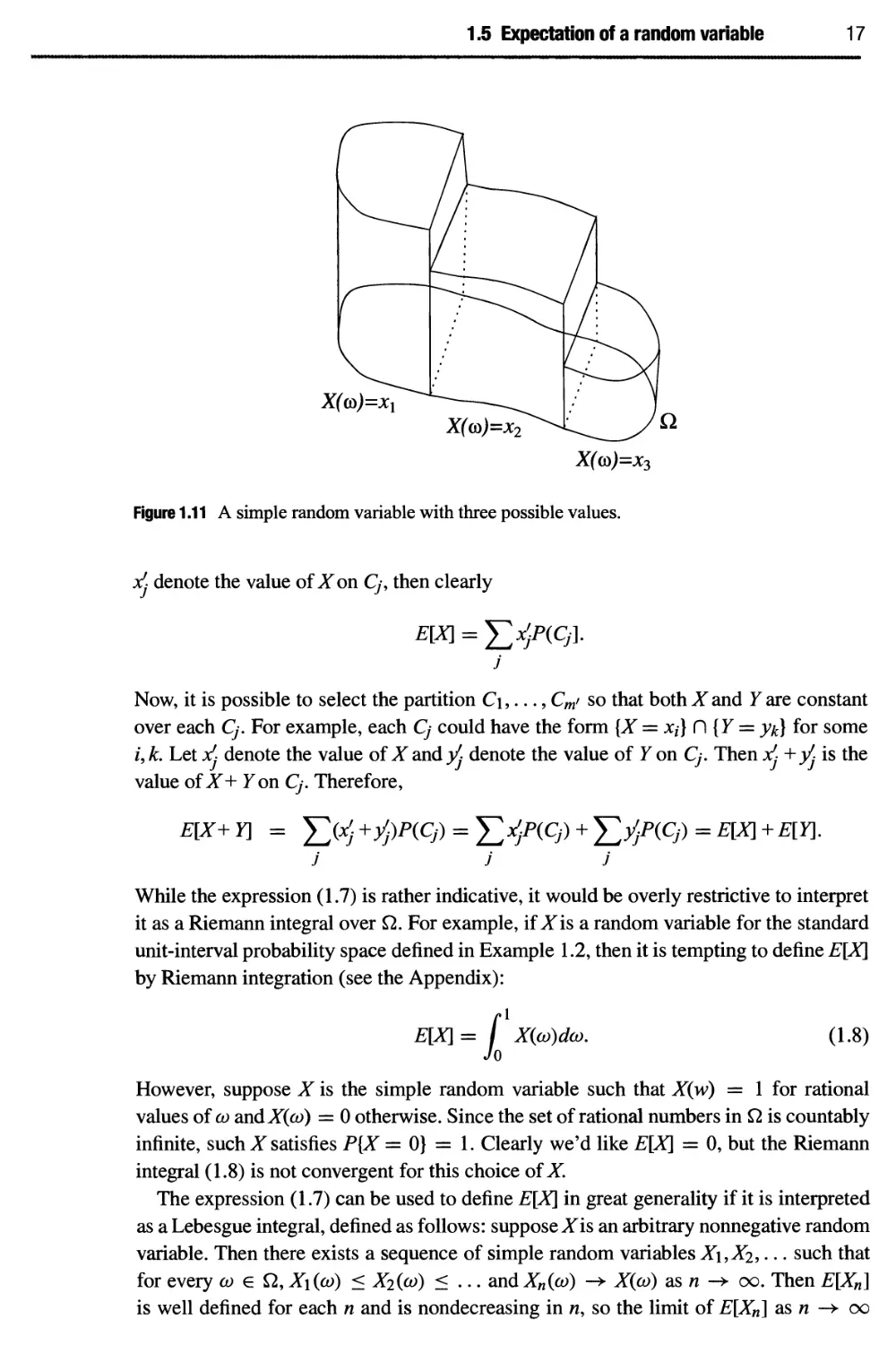
E.6 (Integration by parts formula)
E[X]= [
Jo
(Lebesgue).
oo /»0
(l - Fx(x))dx - Fx(x)dx,
J — OQ
(1.11)
which is well denned whenever at least one of the two integrals in (1.11) is finite.
There is a simple graphical interpretation of (1.11). Namely, E[X\ is equal to the
area of the region between the horizontal line {y = 1} and the graph of Ρχ and
contained in {x > 0}, minus the area of the region bounded by the χ axis and the
graph of Fx and contained in {x < 0}, as long as at least one of these regions has
finite area, see Figure 1.12.
Properties E.l and E.2 are true for simple random variables and they carry over to
general random variables in the limit defining the Lebesgue integral (1.7). Properties
E.3 and E.4 follow from the equivalent definition (1.9) and properties of Lebesgue-
Stieltjes integrals. Property E.5 can be proved by approximating g by piecewise constant
functions. Property E.6 can be proved by integration by parts applied to (1.10).
Alternatively, since F^O^hasthe same distribution as X, if Uis uniformly distributed on the
interval [0,1], the law of the unconscious statistician yields that E[X\ = f0 F^l(u)du,
and this integral can also be interpreted as the difference of the areas of the same two
regions.
Figure 1.12 E[X] is the difference of two areas.
20 A selective review of basic probability
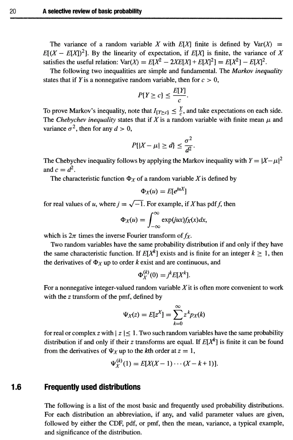
The variance of a random variable X with E[X] finite is defined by Var(X) =
E[(X — E[X\)2]. By the linearity of expectation, if E[X\ is finite, the variance of X
satisfies the useful relation: Мж{Х) = E[X2 - 2XE[X] + E[X\2] = E[X2] - E[X\2.
The following two inequalities are simple and fundamental. The Markov inequality
states that if Υ is a nonnegative random variable, then for с > 0,
E[Y]
P{Y>c}<
с
To prove Markov's inequality, note that I{y>c) < \, and take expectations on each side.
The Chebychev inequality states that if X is a random variable with finite mean μ and
variance σ2, then for any d > 0,
a2
P{\X-^>d}<-^.
The Chebychev inequality follows by applying the Markov inequality with Υ = \Χ—μ\2
and с = d2.
The characteristic function Φχ of a random variable ^f is defined by
Фх(и) = E[e>uX]
for real values of u, where у = \/^T. For example, if ^fhas pdf/i then
/oo
exp(jux)fx(x)dx,
-oo
which is 2π times the inverse Fourier transform of /χ.
Two random variables have the same probability distribution if and only if they have
the same characteristic function. If E[J^] exists and is finite for an integer к > 1, then
the derivatives of Φχ up to order к exist and are continuous, and
Ф^(0) =jkE[Xk].
For a nonnegative integer-valued random variable ЛГ it is often more convenient to work
with the ζ transform of the pmf, defined by
oo
4>χ(ζ)=Ε[ζχ] = Σζ*Ρχ(®
k=0
for real or complex ζ with \ ζ \< 1. Two such random variables have the same probability
distribution if and only if their ζ transforms are equal. If E[J^] is finite it can be found
from the derivatives of Ψχ up to the Ath order at ζ = 1,
Ψ^}(1) = E[X(X- 1) · · · (Х- к+ 1)].
1.6 Frequently used distributions
The following is a list of the most basic and frequently used probability distributions.
For each distribution an abbreviation, if any, and valid parameter values are given,
followed by either the CDF, pdf, or pmf, then the mean, variance, a typical example,
and significance of the distribution.
1.6 Frequently used distributions 21
The constants/?, λ, μ,σ, a, b, and a are real-valued, and η and / are integer-valued,
except η can be noninteger-valued in the case of the gamma distribution.
Bernoulli:
Be(p),0<p< 1
pmf: p(i) =
ρ / = 1
Ι-ρ i = 0
0 else
z-transform: 1 — p+pz
mean:/? variance: p{\ — p)
Example: Number of heads appearing in one flip of a coin. The coin is called fair if
p=\ and biased otherwise.
Binomial:
Bi(n,p),n > 1,0 <p < 1
•wo-(^
pmf:/?(/) = I . \p\\ -p)n~l 0<i<n
z-transform: (1 —p+pz)n
mean: np variance: np(l — p)
Example: Number of heads appearing in η independent flips of a coin.
Poisson:
Х*е~к
pmf: p(i) = —-— / > 0
/!
z-transform: exp(X(z — 1))
mean: λ variance: λ
Example: Number of phone calls placed during a ten second interval in a large city.
Significance: The Poisson pmf is the limit of the binomial pmf as η -> +oo and/? -> 0
in such a way that np -> λ.
Geometric:
Geo(p),0 <p< 1
pmf:/?(/) = (l -ρΫ V ι
pz
z-transform:
1 —z+pz
1 \-p
mean: - variance: —5—
ρ ρ2
22 A selective review of basic probability
Example: Number of independent flips of a coin until heads first appears.
Significant property: If ^fhas the geometric distribution, P{X > /} = (1 — p)1 for integers
i > 1. So Xhas the memoryless property:
P(X> i+j\X> i)=P{X>j}foviJ>l.
Any positive integer-valued random variable with this property has a geometric
distribution.
Gaussian
(also called Normal): Ν(μ, σ2), μ e R, σ > 0
pdf(if^>0):/W = -^=eXp(-^)
Prt(ifol = 0y.P(X) = {l *=£
t?c2s
characteristic function: exp I jup
( ιι2σ2\
yuix - —)
mean: μ variance: σ
Example: Instantaneous voltage difference (due to thermal noise) measured across a
resistor held at a fixed temperature.
Q(c) = 1 - Ф(с) = Г JLe-T«fc.
J с ν2π
Notation: The character Φ is often used to denote the CDF of an N(0,1) random
variable,3 and Q is often used for the complementary CDF:
r-οο л _£
Jc \fbl
Significant property (Central limit theorem): If Χι,Χζ, · · · are independent and
identically distributed with mean μ and nonzero variance σ2, then for any constant c,
lim ΡI — ==? < с \ = Ф(с).
Exponential:
Εχρ(λ), λ > О
pdf: flx) = \е~^ χ > О
characteristic function:
λ-ju
1 1
mean: — variance:
—τα A
3 As noted earlier, Φ is also used to denote characteristic functions. The meaning should be clear from the
context.
1.6 Frequently used distributions 23
Example: Time elapsed between noon sharp and the first telephone call placed in a
large city, on a given day.
Significance: If Xhas the Εχρ(λ) distribution, P{X> t] = e~Xt for t > 0. So X has the
memoryless property:
P{X> s + t | X> s] = P{X> ή s,t> 0.
Any nonnegative random variable with this property is exponentially distributed.
Uniform:
U(a, b) — oo < a < b < oo
{τΛ- α < χ <
V "else"
characteristic function:
b
ejub _ ejua
ju(b - a)
a + b . (b-a)2
mean: variance: ———
2 12
Example: The phase difference between two independent oscillators operating at the
same frequency may be modeled as uniformly distributed over [0,2π].
Significance: Uniform is uniform.
Gamma(n,a):
n, a > 0 (n real valued)
anxn-xe~ax
/•OO
where Г (л) = / sn~xe~sds
Jo
characteristic function
\a -juj
n . n
mean: — variance: -^
a az
Significance: If η is a positive integer then Γ(η) = (n - 1)! and a Gamma(n, a) random
variable has the same distribution as the sum of n independent, Exp(a) distributed
random variables.
24 A selective review of basic probability
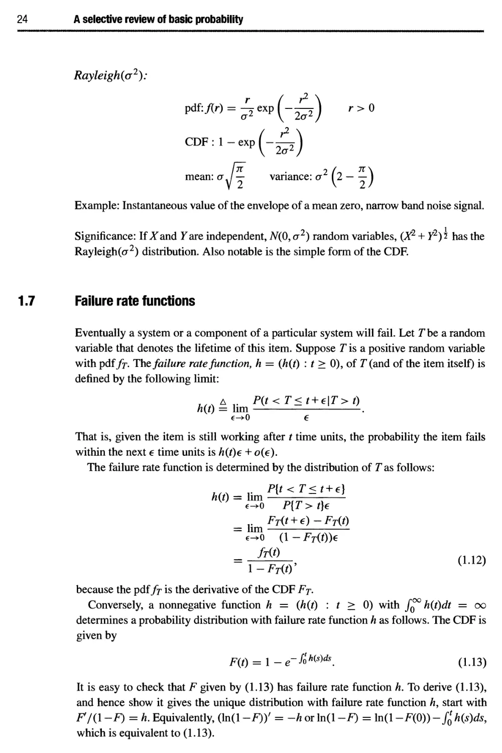
Rayleigh(a2):
r2
CDF:l-exp(-^)
mean: crJ— variance: σ (2 J
Example: Instantaneous value of the envelope of a mean zero, narrow band noise signal.
Significance: If Xand Tare independent, N(0, σ2) random variables, (X2 + У2)з has the
Rayleigh(a2) distribution. Also notable is the simple form of the CDF.
1.7 Failure rate functions
Eventually a system or a component of a particular system will fail. Let Г be a random
variable that denotes the lifetime of this item. Suppose Г is a positive random variable
with pdf/7\ ТЫ failure rate function, h = (h(t) : t > 0), of Г (and of the item itself) is
defined by the following limit:
δ P(t<T<t + e\T>t)
h(t) = lim .
e-»0 6
That is, given the item is still working after t time units, the probability the item fails
within the next e time units is h(f)e + o(e).
The failure rate function is determined by the distribution of Γ as follows:
P{t < T<t + e]
h(t) = lim
e-»0 P{T>t}€
FT(t + €)-FT(i)
= lim
(\-FT(t))e
(1.12)
e^O (1 - FT(t))€
hit)
1-FjitY
because the pdf fy is the derivative of the CDF Fj.
Conversely, a nonnegative function h = (h(t) : t > 0) with /0°° h(t)dt = oo
determines a probability distribution with failure rate function h as follows. The CDF is
given by
F(i) = \-e-&h{s)ds. (1.13)
It is easy to check that F given by (1.13) has failure rate function h. To derive (1.13),
and hence show it gives the unique distribution with failure rate function h, start with
F7(l -F) = h. Equivalent^, (ln(l -F))f = -h or ln(l -F) = ln(l -F(0)) -Ц h(s)ds,
which is equivalent to (1.13).
1.8 Jointly distributed random variables 25
0
t>0
else
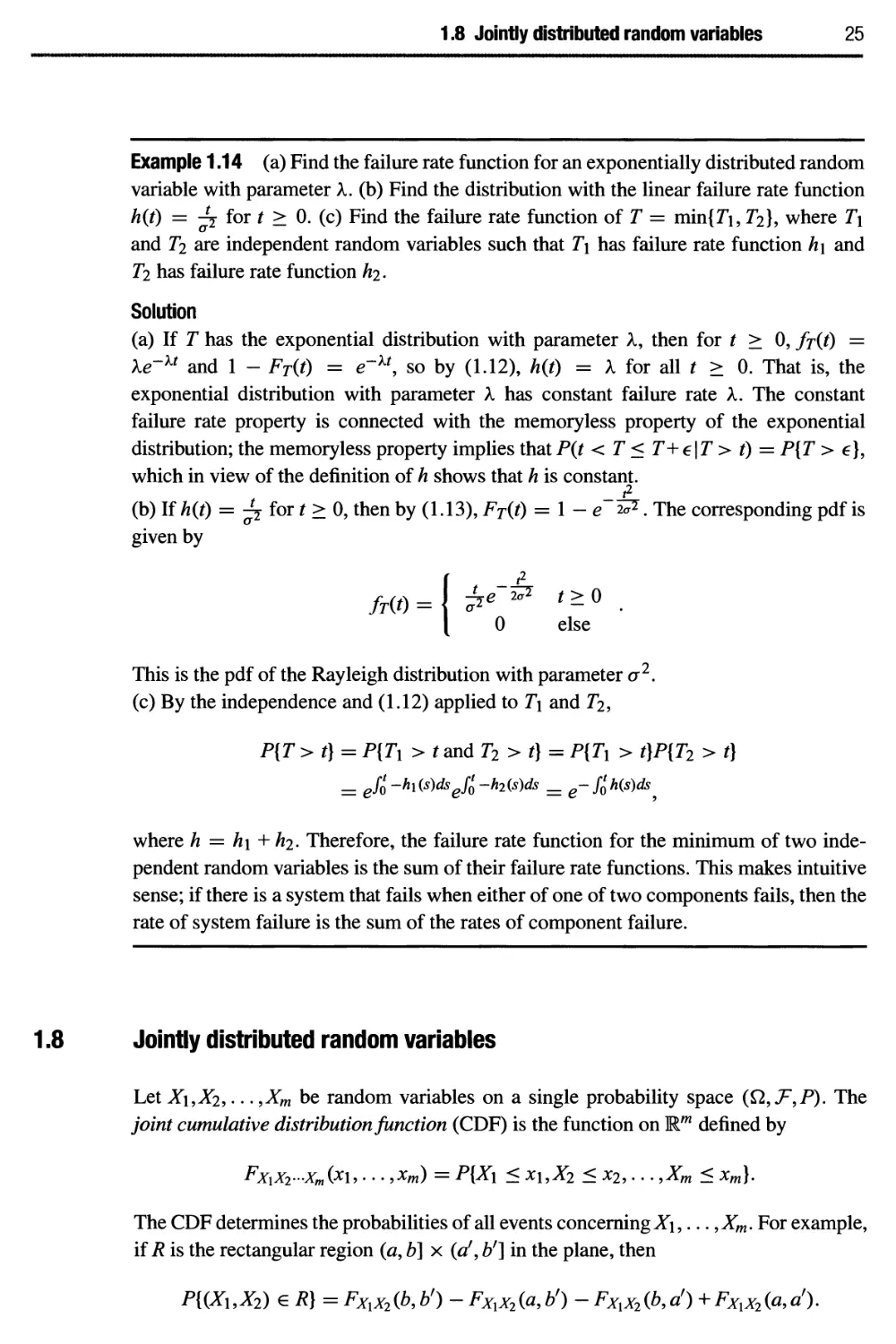
Example 1.14 (a) Find the failure rate function for an exponentially distributed random
variable with parameter λ. (b) Find the distribution with the linear failure rate function
h{f) = jp for t > 0. (c) Find the failure rate function of Τ = тт{Гь T2], where T\
and T2 are independent random variables such that T\ has failure rate function h\ and
T2 has failure rate function h2.
Solution
(a) If Τ has the exponential distribution with parameter λ, then for t > 0, fy(f) =
Xe~kt and 1 - FT(t) = e~kt, so by (1.12), hit) = λ for all t > 0. That is, the
exponential distribution with parameter λ has constant failure rate λ. The constant
failure rate property is connected with the memoryless property of the exponential
distribution; the memoryless property implies that P(t < Τ< T+e\T> t) = P{T > e},
which in view of the definition of h shows that h is constant.
(b) If h(t) = ji for t > 0, then by (1.13), FT(t) = l-e 2^. The corresponding pdf is
given by
fnt) =
This is the pdf of the Rayleigh distribution with parameter σ2.
(с) By the independence and (1.12) applied to T\ and T2,
P{T>t}=P{Ti >iandT2 > ή = Ρ{Τλ > t}P{T2 > ή
= efi-hi(s)dseft>-h2Ws = e-tih(s)ds^
where h = h\ + h2. Therefore, the failure rate function for the minimum of two
independent random variables is the sum of their failure rate functions. This makes intuitive
sense; if there is a system that fails when either of one of two components fails, then the
rate of system failure is the sum of the rates of component failure.
1.8 Jointly distributed random variables
Let X\,X2, · · · ,Xm be random variables on a single probability space (Ω,F,P). The
joint cumulative distribution function (CDF) is the function on Rm defined by
FxiXl-Xmfa'· · · >χ™) = P{X\ < X\,Xl <X2,··· Лт < Xm).
The CDF determines the probabilities of all events concerning X\,... ,Xm. For example,
if R is the rectangular region (a, b] χ (α\ bf] in the plane, then
P{(Xi,X2) eR}= FXlX2(b,b') - FXxXl(a,bf) - FXxXl(b,d) + FXxXl(a,d).
26 A selective review of basic probability
Γ
fxi(V\) = I
J-c
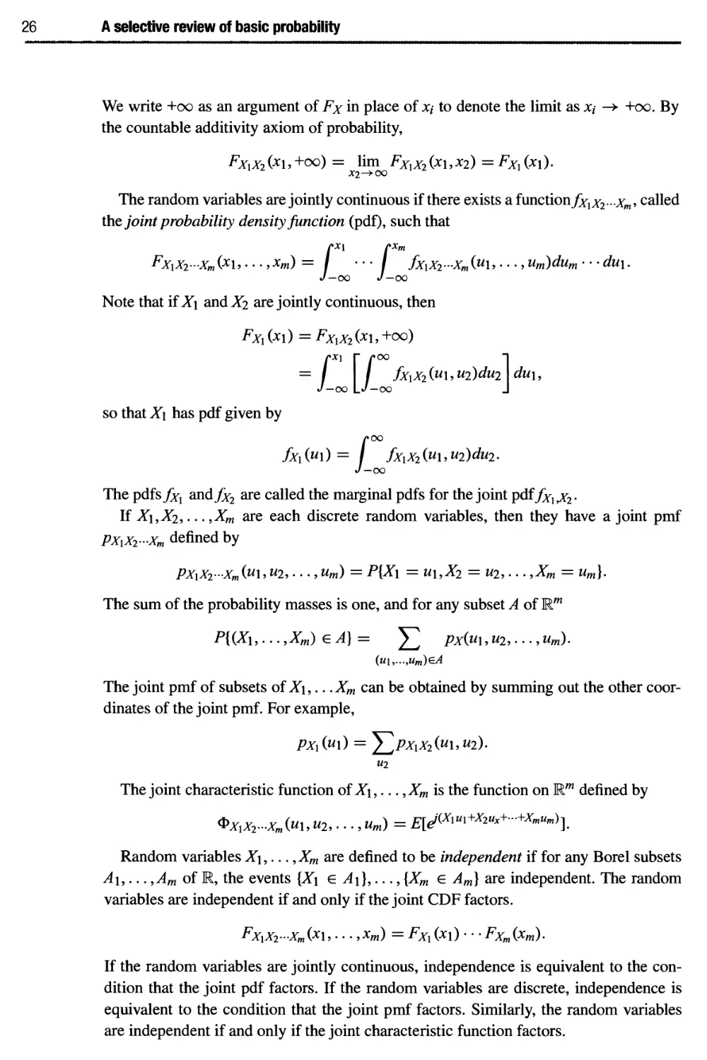
We write +00 as an argument of Fx in place of Xf to denote the limit as Xi -> +00. By
the countable additivity axiom of probability,
FXxx2 (x\, +00) = lim FXlχ2 Cxi, x2) = FXl (χλ).
Jt2->00
The random variables are jointly continuous if there exists a function/*^·-J^, called
the joint probability density function (pdf), such that
/X\ rxm
"· I fxiX2-xm(M\> · · · > um)dum •••du\.
-00 J—00
Note that if X\ and X2 are jointly continuous, then
FXx (x\) = FXxx2 (χι, +00)
= / / fxlx2(ui,u2)du2\dui,
so that X\ has pdf given by
r»oo
fxxx2(u\,U2)du2.
-00
The pdfs^ andfx2 are called the marginal pdfs for the joint pdf/j^ д2.
If Χι,Χζ, · · · ,Xm are each discrete random variables, then they have a joint pmf
PXiXr-Xm defined by
PXlX2-Xm(ul9U2> •••9Um)= P{X\ = Щ,Х2 = U2, . · . ,Xm = Um].
The sum of the probability masses is one, and for any subset A of Rm
P{(X\,...,Xm) eA}= Σ Px(u\,U2,---,um).
{и\,...,ит)еА
The joint pmf of subsets of X\,.. .Xm can be obtained by summing out the other
coordinates of the joint pmf. For example,
РхЛт) = ^2рххх2(щ,и2).
u2
The joint characteristic function of X\,... ,Xm is the function on Rm defined by
Фххх2...хт(т, и2, ...,ит)= E[^Xw+x^+"+x-u^l
Random variables X\,... ,Xm are defined to be independent if for any Borel subsets
A\,... ,Am of R, the events {^1 e A\],..., {Xm e Am] are independent. The random
variables are independent if and only if the joint CDF factors.
Fxxx2..xm(x\,. ..,xm)= FXx(x\) · · ·FXm(xm).
If the random variables are jointly continuous, independence is equivalent to the
condition that the joint pdf factors. If the random variables are discrete, independence is
equivalent to the condition that the joint pmf factors. Similarly, the random variables
are independent if and only if the joint characteristic function factors.
1.10 Correlation and covariance 27
1.9 Conditional densities
Suppose that X and Υ have a joint pdf /χγ. Recall that the pdf fy, the second marginal
density of/χγ, is given by
/00
fxY(x,y)dx.
-00
The conditional pdf of Xgiven 7, denoted by/χ\γ(χ | У), is undefined if fy(y) = 0. It is
defined for у such that fy(y) > 0 by
fx\r(x\y)= r/. -oo<x<+oo.
If у is fixed and fy(y) > 0, then as a function of χ,/χ\γ (χ \ y) is itself a pdf.
The expectation of the conditional pdf is called the conditional expectation (or
conditional mean) of X given Υ = у, written as
/oo
xfx\r(x\y)dx.
-OO
If the deterministic function E[X \ Υ = у] is applied to the random variable Y, the result
is a random variable denoted by E[X \ Y].
Note that conditional pdf and conditional expectation were so far defined in case
X and Υ have a joint pdf. If instead, X and Υ are both discrete random variables, the
conditional pmf ρχ\γ and the conditional expectation E[X \ Υ = у] can be defined in a
similar way. More general notions of conditional expectation are considered later.
1.10 Correlation and covariance
Let X and Υ be random variables on the same probability space with finite second
moments. Three important related quantities are:
the correlation: E[XY],
the covariance: Cov(^, Y) = E[(X- E[X\)(Y- E[Y])l
Cov(X,Y)
the correlation coefficient: ρχγ =
VVarCY)Var(y)
A fundamental inequality is Schwarz's inequality:
| E[XY\ | < у/ЕЦРЩУ2]· (114)
Furthermore, if E[Y2] φ 0, equality holds if and only if P(X = cY) = 1 for some
constant c. Schwarz's inequality (1.14) is equivalent to the L2 triangle inequality for
random variables:
E[(X+Y)2]? <E[X2V- +£[72]5. (1.15)
28 A selective review of basic probability
Schwarz's inequality can be proved as follows. If P{Y = 0} = 1 the inequality is
trivial, so suppose E[Y2] > 0. By the inequality (a + b)2 < 2a2 + 2b2 it follows that
E[(X- XT)2] < oo for any constant λ. Take λ = Ε[ΧΥ]/Ε[Υ2] and note that
0 < E[(X- λΥ)2] = E[X2] - 2λΕ[ΧΥ] + λ2Ε[Υ2]
= E{X\ Ε[ΧΥ]2
E[P] '
which is clearly equivalent to the Schwarz inequality. lfP(X = cY) = 1 for some с then
equality holds in (1.14), and conversely, if equality holds in (1.14) then P(X = cY) = 1
for с = λ.
Application of Schwarz's inequality to^f — E[X] and Υ — E[Y] in place of X and Υ
yields that
| CovtY, Y) | < yVar(^)Var(y).
Furthermore, if Var( Υ) φ 0 then equality holds if and only if X = aY+ b for some
constants a and b. Consequently, if Var(X) and Var(Y) are not zero, so that the correlation
coefficient ρχγ is well defined, then | ρχγ \< 1 with equality if and only if X = aY+ b
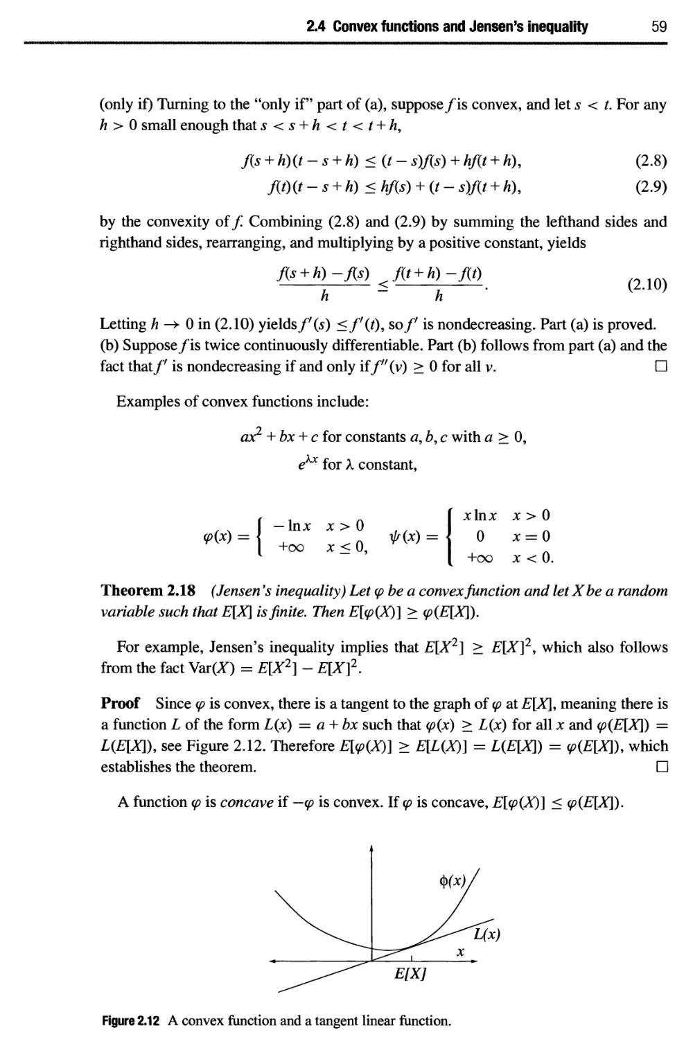
for some constants a, b.
The following alternative expressions for Cov(X, Y) are often useful in calculations:
Co\(X,Y) = E[X(Y-E[Y])]=E[(X-E[X])Y]=E[XY]-E[X]E[Y].
In particular, if either X or Υ has mean zero then E[XY] = Cov(X, Y).
Random variables X and Υ are called orthogonal if E[XY] = 0 and are called
uncorrected if Cov(X, Y) = 0. If X and Υ are independent then they are uncorrected. The
converse is far from true. Independence requires a large number of equations to be true,
namely Fxy(x,y) = F^(x)Fy(y) for every real value of χ and>>. The condition of being
uncorrected involves only a single equation to hold.
Covariance generalizes variance, in that Var(^Q = Co\(X,X). Covariance is linear in
each of its two arguments:
CovtT+ Y,U+V) = CovtY, U) + CovtT, V) + Cov(7, U) + Cov(7, V)
Co\(aX+ b,cY+d)= acCo\(X, Y).
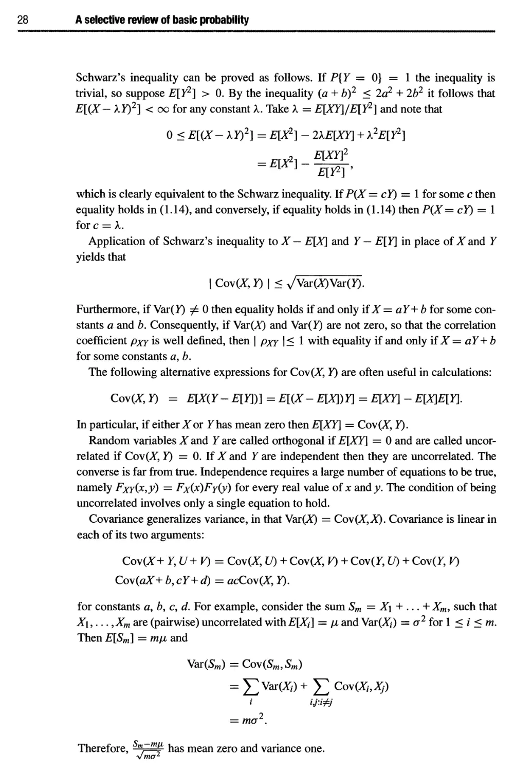
for constants β, b, c, d. For example, consider the sum Sm = X\ + ... + Xmi such that
X\,...,Xm зге (pairwise) uncorrected with E[X{\ = μ and Var(^Q) = σ2 for 1 < i < m.
Then E[Sm] = ιημ and
Var(5m) = Cov(5m
= J2Var(Xi)+J2Cov(Xi,Xf)
2
= та .
Therefore, Sm~m^ has mean zero and variance one.
1.11 Transformation of random vectors 29
1.11
Transformation of random vectors
A random vector Xoi dimension m has the form
X =
ί Ъ \
U )
where X\,... ,Xm are random variables. The joint distribution of X\,... ,Xm can be
considered to be the distribution of the vector X. For example, if X\,... ,Xm are jointly
continuous, the joint pdf fxxxv.xm(x\, · · · ,Xm) can as well be written asfx(x), and be
thought of as the pdf of the random vector X.
Let X be a continuous type random vector on Rm. Let g be a one-to-one mapping
from Rm to Rm. Think of g as mapping x-space (here χ is lower case, representing a
coordinate value) into^-space. As χ varies over Rm, у varies over the range of g. All the
while,у = g(x) or, equivalently, χ = g~l (y).
Suppose that the Jacobian matrix of derivatives ^(x) is continuous in χ and non-
singular for all x. By the inverse function theorem of vector calculus, it follows that
the Jacobian matrix of the inverse mapping (from у to x) exists and satisfies Щ (y) =
(1* W ) · ^se I ^ I for a square matrix К to denote | det(K) |.
Proposition 1.5 Under the above assumptions, Υ is a continuous type random vector
and for у in the range ofg:
ш =
fxix)
=fxix)
дх.
Ту
(У)
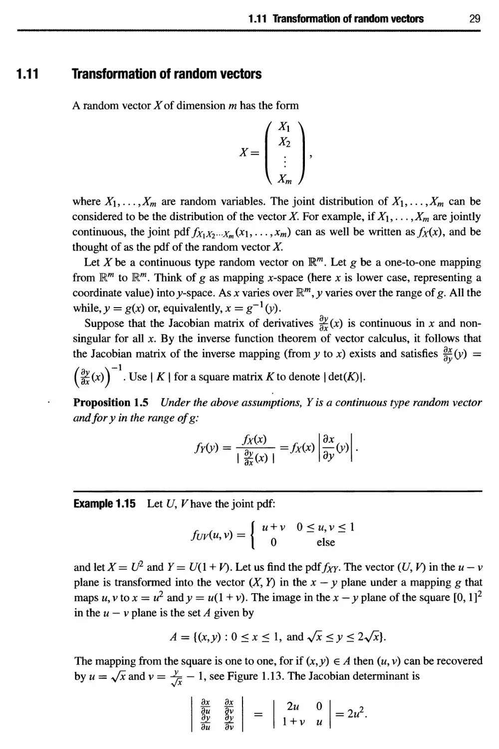
Example 1.15 Let U, V have the joint pdf:
fuvi
(u,v) = l
u + v
0
0 < u, ν < 1
else
and let^T= U2 and Y= (7(1 + V). Let us find the pdf^. The vector (U, V) in the и - ν
plane is transformed into the vector (X, Y) in the χ — у plane under a mapping g that
maps u, ν to χ = и2 ana у = u{\ + ν). The image in the χ —у plane of the square [0, l]2
in the и — ν plane is the set A given by
A = {(x,y) : 0 < χ < 1, and yfx < у < lyfx).
The mapping from the square is one to one, for if (x,y) e A then (w, v) can be recovered
by и = y/x and ν = -y= — 1, see Figure 1.13. The Jacobian determinant is
дх
£
ди
дх
ё
dv
=
2и 0
1 + ν и
= 2и2.
30 A selective review of basic probability
Figure 1.13 Transformation from the и — ν plane to the χ — у plane.
Therefore, using the transformation formula and expressing и and ν in terms of χ and
у yields
fxnx,y) =
1 ξ if (*,>>) еЛ
0
else
Example 1.16 Let U and Vbe independent continuous type random variables. Let X =
U+ Fand Υ = V. Let us find the joint density of Χ, Υ and the marginal density of X. The
mapping
g:(w ν ) -> ( w v) = (w + v v)
is invertible, with inverse given by и = χ — у and ν = у. The absolute value of the
Jacobian determinant is given by
дх дх
ду ду
ди dv
1 1
О 1
1.
Therefore
fxnx,y) =fuv(u,v) =fu(x-y)fv(y)·
The marginal density of ^f is given by
/oo /»oo
fxnx,y)dy= / fu(x - y)fv(y)dy.
-oo J—oo
That is fx=fu*fv.
Example 1.17 Let X\ and X2 be independent N(0, σ2) random variables, and let X =
(X\,X2)T denote the two-dimensional random vector with coordinatesX\ and X2. Any
point of χ g R2 can be represented in polar coordinates by the vector (r,6)T such that
r = \\x\\ = (x\ +;фз and θ = tan-1 (&\ with values r > 0 and 0 < θ < 2π. The
inverse of this mapping is given by
Problems 31
χι = rcos(0)
X2 = rsin(0).
We endeavor to find the pdf of the random vector (R, θ)τ, the polar coordinates of X.
The pdf of Х'\ъ given by
1 _ ^
fx(x) =fxi(xi)fx2(x2) = ^^2e ***·
The range of the mapping is the set r > 0 and 0 < θ < 2π. On the range,
dx
Therefore for (r,6)T in the range of the mapping,
Э*1
дХ2
дг
дХ]
дХ2
дв
cos(0) —rsin(0)
sin(0) rcos(0)
fRMr,0)=fxW
dx
(;)
r __
2πσ2
e 2σ^
Of course fR,@(r,e) = 0 off the range of the mapping. The joint density factors into
a function of r and a function of Θ, so R and Θ are independent. Moreover, R has the
Rayleigh density with parameter σ2, and Θ is uniformly distributed on [0,2π].
Problems
1.1 Simple events A register contains eight random binary digits which are mutually
independent. Each digit is a zero or a one with equal probability.
(a) Describe an appropriate probability space (Ω, Τ,Ρ) corresponding to looking at the
contents of the register.
(b) Express each of the following four events explicitly as subsets of Ω, and find their
probabilities:
E\ = "No two neighboring digits are the same,"
E2 = "Some cyclic shift of the register contents is equal to 01100110,"
£3 = "The register contains exactly four zeros,"
£4 = "There is a run of at least six consecutive ones."
(c) Find P(E\ \ЕЪ) and P(E2\E3).
1.2 A ballot problem Suppose there is an election with two candidates and six ballots
turned in, such that four of the ballots are for the winning candidate and two of the
ballots are for the other candidate. The ballots are opened and counted one at a time,
in random order, with all orders equally likely. Find the probability that from the time
the first ballot is counted until all the ballots are counted, the winning candidate has the
majority of the ballots counted. ("Majority" means there are strictly more votes for the
winning candidate than for the other candidate.)
32 A selective review of basic probability
1.3 Ordering of three random variables Suppose X, Y, and t/are mutually independent,
such that X and Υ are each exponentially distributed with some common parameter
λ > 0, and C/is uniformly distributed on the interval [0,1]· Express P{X < U < Y] in
terms of λ. Simplify your answer.
1.4 Independent vs. mutually exclusive (a) Suppose that an event Ε is independent of
itself. Show that either P(E) = 0 or P(E) = 1.
(b) Events A and В have probabilities P(A) = 0.3 and P(B) = 0.4. What is P(A U B) if
A and В are independent? What is P(A U B) if A and В are mutually exclusive?
(c) Now suppose that P(A) = 0.6 and P(B) = 0.8. In this case, could the events A and В
be independent? Could they be mutually exclusive?
1.5 Congestion at output ports Consider a packet switch with some number of input
ports and eight output ports. Suppose four packets simultaneously arrive on different
input ports, and each is routed toward an output port. Assume the choices of output ports
are mutually independent, and for each packet, each output port has equal probability.
(a) Specify a probability space (Ω, Τ,Ρ) to describe this situation.
(b) Let Xi denote the number of packets routed to output port / for 1 < / < 8. Describe
the joint pmf of X\,... ,X%.
(c)FindCov(^b^2).
(d)FindP{A/< 1 for all/}.
(e)FmdP{JTi <2faralli}.
1.6 Frantic search At the end of each day Professor Plum puts her glasses in her
drawer with probability .90, leaves them on the table with probability .06, leaves
them in her briefcase with probability 0.03, and she actually leaves them at the office
with probability 0.01. The next morning she has no recollection of where she left the
glasses. She looks for them, but each time she looks in a place the glasses are actually
located, she misses finding them with probability 0.1, whether or not she already
looked in the same place. (After all, she doesn't have her glasses on and she is in a
hurry.)
(a) Given that Professor Plum didn't find the glasses in her drawer after looking one
time, what is the conditional probability the glasses are on the table?
(b) Given that she didn't find the glasses after looking for them in the drawer and on the
table once each, what is the conditional probability they are in the briefcase?
(c) Given that she failed to find the glasses after looking in the drawer twice, on the
table twice, and in the briefcase once, what is the conditional probability she left the
glasses at the office?
1.7 Conditional probability of failed device given failed attempts A particular
webserver may be working or not working. If the webserver is not working, any attempt
to access it fails. Even if the webserver is working, an attempt to access it can fail due
to network congestion beyond the control of the webserver. Suppose that the a-priori
probability that the server is working is 0.8. Suppose that if the server is working, then
each access attempt is successful with probability 0.9, independently of other access
attempts. Find the following quantities.
(a) P{ first access attempt fails),
(b) P(server is working | first access attempt fails),
Problems 33
(c) P(second access attempt fails | first access attempt fails),
(d) P(server is working | first and second access attempts fail).
1.8 Conditional probabilities - basic computations of iterative decoding
(a) Suppose B\,.. .,Bn,Y\,.. .,Ynare discrete random variables with joint pmf
Л) = {
nih и л, л, ч ι - ~П FEU qtiyiVt) if bt e {0,1} for 1 < i < η
р(Ьи...,Ьп,Уи...,Уп) = \ 0 dse
where qi(yi\bj) as a function of у χ is a pmf for &,· e {0,1}. Finally, let В = B\ 0 · · · Θ #„
represent the modulo two sum of #i, · · · , Bn. Thus, the ordinary sum of the n+1 random
variables B\,..., Βη, Β is even. Express P(# = 11 Y\ = y\,··· ,Yn=yn) in terms of the
yi and the functions qt. Simplify your answer,
(b) Suppose В and Z\,..., Z# are discrete random variables with joint pmf
p(b,zu...,zk) =
\Yi=lrj(zj\b) if be {0,1}
0 else
where rj(zj\b) as a function of zj is a pmf for b e {0,1} fixed.
Express P(B = \\Z\ = zi,..., Z# = z#) in terms of the zy and the functions η.
1.9 Conditional lifetimes; memoryless property of the geometric distribution (a) Let X
represent the lifetime, rounded up to an integer number of years, of a certain car battery.
Suppose that the pmf of^fis given by px(k) = 0.2 if 3 < к < 7 andpx(k) = 0 otherwise,
(i) Find the probability, P{X > 3}, that a three year old battery is still working,
(ii) Given that the battery is still working after five years, what is the conditional
probability that the battery will still be working three years later? (i.e. what is P(X > %\X >
5)?).
(b) A certain basketball player shoots the ball repeatedly from half court during practice.
Each shot is a success with probability/? and a miss with probability 1 —p, independently
of the outcomes of previous shots. Let У denote the number of shots required for the first
success.
(i) Express the probability that she needs more than three shots for a success, P[Y > 3},
in terms of/?.
(ii) Given that she already missed the first five shots, what is the conditional probability
that she will need more than three additional shots for a success? (i.e. what is P(Y >
8|7>5)?).
(iii) What type of probability distribution does Υ have?
1.10 Blue corners Suppose each corner of a cube is colored blue, independently of the
other corners, with some probability p. Let В denote the event that at least one face of
the cube has all four corners colored blue.
(a) Find the conditional probability of В given that exactly five corners of the cube are
colored blue.
(b) Find P(B), the unconditional probability of B.
1.11 Distribution of the flow capacity of a network A communication network is shown
The link capacities in megabits per second (Mbps) are given by C\ = C3 = 5,
C2 = Cs = 10 and C4 = 8, and are the same in each direction. Information flow from
the source to the destination can be split among multiple paths. For example, if all links
34 A selective review of basic probability
Destination
are working, then the maximum communication rate is 10 Mbps: 5 Mbps can be routed
over links 1 and 2, and 5 Mbps can be routed over links 3 and 5. Let F,- be the event
that link i fails. Suppose that F\,F2,F3,F4, and F$ are independent and P(Fi) = 0.2
for each i. Let X be defined as the maximum rate (in Mbits per second) at which data
can be sent from the source node to the destination node. Find the pmf ρχ.
1.12 Recognizing cumulative distribution functions Which of the following are valid
CDFs? For each that is not valid, state at least one reason why. For each that is valid,
findPfA2 >5}.
Fi(x) =
4 , , F2(x)
i-V *^°
0 x<0
0.5 + e"x 0 < χ < 3
1 x>3
F3(x) = I
0 x<0
0.5 + ^ 0<x<10
1 x> 10
1.13 A CDF Of mixed type Let X have the CDF shown.
1.0
0.5
С
\Fx
/
1 2
(a)FindP{^<0.8}.
(b)Find£[X|.
(c) Find VartY).
1.14 CDF and characteristic function of a mixed type random variable
Let^f = (U— 0.5)+, where C/is uniformly distributed over the interval [0,1]. That is,
X= U- 0.5 if U- 0.5 > 0, and^r= 0 if U- 0.5 < 0.
(a) Find and carefully sketch the CDF Fx. In particular, what is Fy(0)?
(b) Find the characteristic function Φχ{ύ) for real values of u.
1.15 Poisson and geometric random variables with conditioning Let У be a Poisson
random variable with mean μ > 0 and let Ζ be a geometrically distributed random
variable with parameter/? with 0 < ρ < 1. Assume Υ and Ζ are independent.
(a) Find P{Y < Z]. Express your answer as a simple function of μ and p.
Problems 35
(b) Find P(Y < Z\Z = i) for / > 1. (Hint: This is a conditional probability for events.)
(c) Find P(Y = i\Y < Z) for i > 0. Express your answer as a simple function of/?, μ
and /. (Hint: This is a conditional probability for events.)
(d) Find E[Y\Y < Z], which is the expected value computed according to the conditional
distribution found in part (c). Express your answer as a simple function of μ and/?.
1.16 Conditional expectation for uniform density over a triangular region
Let (X, Y) be uniformly distributed over the triangle with coordinates (0,0), (1,0), and
(2,1).
(a) What is the value of the joint pdf inside the triangle?
(b) Find the marginal density of X,fx(x). Be sure to specify your answer for all real
values of x.
(c) Find the conditional density function fy\x(y\x). Be sure to specify which values of χ
the conditional density is well defined for, and for such χ specify the conditional density
for ally. Also, for such χ briefly describe the conditional density of у in words.
(d) Find the conditional expectation £[7]^ = x]. Be sure to specify which values of χ
this conditional expectation is well defined for.
1.17 Transformation of a random variable Let X be exponentially distributed with
mean λ-1. Find and carefully sketch the distribution functions for the random variables
Υ = exp(X) and Ζ = min(^, 3).
1.18 Density Of a function Of a random variable Suppose X is a random variable with
probability density function
. , ч f 2x 0 < χ < 1
MX) = \ 0 else
(a)FwdP(X>0A\X<0.«).
(b) Find the density function of Υ defined by Υ = — log(A^.
1.19 Moments and densities of functions of a random variable Suppose the length L
and width W of a rectangle are independent and each uniformly distributed over the
interval [0, 1]. Let С = 2L + 2W(the length of the perimeter) and A = L^(the area).
Find the means, variances, and probability densities of С and A.
1.20 Functions of independent exponential random variables Let X\ and X2 be
independent random variables, with Xi being exponentially distributed with parameter λ/,
(a) Find the pdf of Ζ = rxun{X\9X2}. (b) Find the pdf of R = f^.
1.21 Using the Gaussian Q function Express each of the given probabilities in terms of
the standard Gaussian complementary CDF Q.
(a) P{X > 16}, where^has the N(10,9) distribution.
(b) P{X2 > 16}, where ^Thas the N(10,9) distribution.
(c) P{\X— 2Y\ > 1}, whereof and У are independent, N(0,1) random variables. (Hint:
Linear combinations of independent Gaussian random variables are Gaussian.)
1.22 Gaussians and the Q function Let X and Υ be independent, N(0,1) random
variables.
(a) Find Cov(3^+ 2Y,X+ 57+ 10).
(b) Express P{X+ 47 > 2} in terms of the Q function.
(c) Express P{(X— Y)2 > 9} in terms of the Q function.
36 A selective review of basic probability
1.23 Correlation Of histogram values Suppose that η fair dice are independently rolled.
Let
_ ί 1 if a 1 shows on the /th roll _ ί 1 if a 2 shows on the /th roll
* ~ { 0 else ' ' ~ J 0 else
Let X denote the sum of the XfS, which is simply the number of 1 s rolled. Let У denote
the sum of the У/s, which is simply the number of 2s rolled. Note that if a histogram is
made recording the number of occurrences of each of the six numbers, then X and Υ are
the heights of the first two entries in the histogram.
(a)Find£[^i]andVar№).
(b) Find E[X\ and Var(X).
(c) Find Cov(^·, Yj) if 1 < ij < η (Hint: Does it make a difference if i =/?)
(d) Find CovCA", Y) and the correlation coefficient p(X, Y).
(e) Find ДУ]^ = x] for any integer χ with 0 < χ < п. Note that your answer should
depend on χ and n, but otherwise your answer is deterministic.
1.24 Working with a joint density Suppose ^ and У have joint density function/^ y(x,y)
c(\ +xy) if 2 < χ < 3 and 1 < у < 2, and fxj{x,y) = 0 otherwise, (a) Find с (b) Find
fxandfy. (c) Findfx]Y.
1.25 A function of jointly distributed random variables Suppose (U, V) is uniformly
distributed over the square with corners (0,0), (1,0), (1,1), and (0,1), and letX = UV.
Find the CDF and pdf of X.
1.26 Density Of a difference Let X and У be independent, exponentially distributed
random variables with parameter λ, such that λ > 0. Find the pdf of Ζ = \X — Y\.
1.27 Working with a two-dimensional density Let the random variables X and Υ be
jointly uniformly distributed over the region shown.
(a) Determine the value offxj on the region shown.
(b) Find/γ, the marginal pdf of X.
(c) Find the mean and variance of X.
(d) Find the conditional pdf of Υ given that X = x, for 0 < χ < 1.
(e) Find the conditional pdf of У given that^f = x, for 1 < jc < 2.
(f) Find and sketch ^[У]^ = χ] as a function of x. Be sure to specify which range of χ
this conditional expectation is well defined for.
1.28 Some Characteristic functions Find the mean and variance of random variables
with the following characteristic functions: (а) Ф(и) = exp(—5u2 + 2/w); (b) Ф(и) =
(ёи - \)/ju\ and (с) Ф(и) = ехр(Я(^м - 1)).
1.29 Uniform density over a union of two square regions Let X and У be jointly
uniformly distributed on the region {0 < и < 1,0 < ν < 1} U {-1 < и < 0, -1 < ν < 0}.
(a) Determine the value of/3ry on the region shown.
Problems 37
(b) Finafx, the marginal pdf of X.
(c) Find the conditional pdf of Υ given that X — я, for 0 < a < 1.
(d) Find the conditional pdf of Υ given that X — я, for -1 < a < 0.
(e) Find E[Y\X = a] for \a\ < 1.
(f) What is the correlation coefficient of X and У?
(g) Are X and Υ independent?
(h) What is the pdf of Ζ = X+ У?
1.30 A transformation of jointly continuous random variables Suppose (U, V) has joint
pdf
^ , ч [ 9mV if 0<m<1&0<v<1
A^<«,v) = j 0 dse
Let^=3C/and7=C/K
(a) Find the joint pdf of X and Y, being sure to specify where the joint pdf is zero.
(b) Using the joint pdf of X and 7, find the conditional pdf, fy\x(y\x), of У givenX (Be
sure to indicate which values of χ the conditional pdf is well defined for, and for each
such χ specify the conditional pdf for all real values of y.)
1.31 Transformation of densities Let U and Fhave the joint pdf:
r , ч [ c(u - v)2 0 < u, ν < 1
Λκ«,ν) = | 0 else
for some constant с
(a) Find the constant с
(b) Suppose X= U2 and Υ = U2V2. Describe the joint pdffxj(x,y) of ^Tand Y. Be sure
to indicate where the joint pdf is zero.
1.32 Opening a bicycle combination lock A certain bicycle combination lock has 104
possible combinations, ranging from 0000 to 9999. Suppose the combination required
to open the lock takes any one of the possible values with equal probability. Suppose
it takes two seconds to try opening the lock with a given combination. Find the mean
and standard deviation of the amount of time, each to within a minute, of how long it
would take to open the lock by cycling through the combinations without repetition.
(Hint: You can approximate the random amount of time required by a continuous type
random variable.)
1.33 Transformation Of joint densities Assume X and Υ are independent, each with the
exponential pdf with parameter λ > 0. Let W = Χ— Υ and Ζ = Χ2 +Χ— Y. Find the
joint pdf of (W, Z). Be sure to specify its support (i.e. where it is not zero).
1.34 Computing some COvariances Suppose X,Y, and Ζ are random variables, each
with mean zero and variance 20, such that Co\(X,Y) = Co\(X,Z) = 10 and
Cov(7,Z) = 5.
(a)FindCov(^+y,^-y).
(b) Find Cov(3X+Z,3X+Y). (c) Find E[(X+ Y)2].
38 A selective review of basic probability
1.35 Conditional densities and expectations Suppose that random variables X and Υ
have the joint pdf:
r , . 4w2, 0 < ν < и < 1
да
<«-ЧоГ
elsewhere
(a) Find E[XY].
(b) Find/y(v). Be sure to specify it for all values of v.
(c) Find fx\Y(u\v). Be sure to specify where it is undefined, and where it is zero.
(d) FindE[X2\Y = v] for0 < ν < 1.
1.36 Jointly distributed variables Let U and V be independent random variables, such
that C/is uniformly distributed over the interval [0, 1], and Fhas the exponential
probability density function.
(a) Calculate Ei^j].
(b) Calculate P{U < V\.
(c) Find the joint probability density function of Υ and Z, where Υ = U2 and Ζ = UV.
1.37* Why not every set has a length Suppose a length (actually, "one-dimensional
volume" would be a better name) of any subset А с R could be defined, so that the
following axioms are satisfied:
L0: 0 < length^) < oo for any А С R,
LI: Length([tf, b]) = b — a for a < b,
L2: Length 04) = length^ +y), for any ^ci and у e R, where A +y represents the
translation of A by >>, defined by A +y = {χ +y : χ e A],
L3: If A = U^Bi such that BUB2,... are disjoint, then length^) = ]Pgi length^·)
The purpose of this problem is to show that the above supposition leads to a
contradiction. Let Q denote the set of rational numbers, Q = {p/q : p, q e Z, q φ 0}.
(a) Show that the set of rational numbers can be expressed as Q = {q\, q2, ·..}, which
means that Q is countably infinite. Say that x,y e R are equivalent, and write χ ~ y, if
(b) Show that ~ is an equivalence relation, meaning it is reflexive (a ~ a for all a e R),
symmetric (a ~ b implies b ~ a), and transitive (a ~ b and Ь ~ с implies a ~ c). For
any χ g R, let β* = Q + jc.
(c) Show that for any x,y e R, either Qx = g^ or QxDQy = 0. Sets of the form β* are
called equivalence classes of the equivalence relation ~.
(d) Show that Qx Π [0,1] φ 0 for all χ e Λ, or in other words, each equivalence class
contains at least one element from the interval [0,1]. Let Vbe a set obtained by choosing
exactly one element in [0,1] from each equivalence class (by accepting that Vis well
defined, you'll be accepting what is called the Axiom of Choice). So V is a subset of
[0,1]. Suppose q\,q'2, · · · is an enumeration of all the rational numbers in the interval
[—1,1], with no number appearing twice in the list. Let V{ = V+ q\ for / > 1.
(e) Verify that the sets V\ are disjoint, and [0,1] с Ugj V\ С [-1,2]. Since the VjS are
translations of V, they should all have the same length as V. If the length of Fis defined
to be zero, then [0,1] would be covered by a countable union of disjoint sets of length
zero, so [0,1] would also have length zero. If the length of V were strictly positive, then
Problems 39
the countable union would have infinite length, and hence the interval [—1,2] would
have infinite length. Either way there is a contradiction.
1.38* On sigma-algebras, random variables, and measurable functions Prove the seven
statements lettered (a)-(g) in what follows.
Definition. Let Ω be an arbitrary set. A nonempty collection Τ of subsets of Ω is
defined to be an algebra if: (i) Ac e Τ whenever A e F and (ii) AU В e Τ whenever
A,BeT.
(a) If Τ is an algebra then 0 e Τ, Ω e T, and the union or intersection of any finite
collection of sets in Τ is in T. Definition. Τ is called a σ-algebra if Τ is an algebra
such that whenever A\ ,A2,... are each in F, so is the union, UAi.
(b) If J7 is a σ-algebra and B\, Β2,... are in F, then so is the intersection, П#г.
(c) Let t/be an arbitrary nonempty set, and suppose that Tu is a σ-algebra of subsets of
Ω for each и е U. Then the intersection C\u^uTu is also a σ-algebra.
(d) The collection of all subsets of Ω is a σ -algebra.
(e) If T0 is any collection of subsets of Ω then there is a smallest σ -algebra containing
T0 (Hint: use (c) and (d).)
Definitions. B(R) is the smallest σ -algebra of subsets of R which contains all sets
of the form (-00,a]. Sets in B(R) are called Borel sets. A real-valued random
variable on a probability space (Ω, T,P) is a real-valued function X on Ω such that
{ω : Χ(ω) < a] e Τ for any a e R.
(f) If Xis a random variable on (Ω, T,P) and A e B(R) then {ω : Χ(ω) e A] e Т.
(Hint: Fix a random variable X. Let V be the collection of all subsets A of B(R) for
which the conclusion is true. It is enough (why?) to show that V contains all sets of the
form (-00, a] and that V is a σ-algebra of subsets of R. You must use the fact that Τ is
a σ -algebra.)
Remark. By (f), Ρ{ω : Χ(ω) e A], or P{X e A] for short, is well defined for A e B(R).
Definition. A function g mapping R to R is called Borel measurable if {x : g(x) e A] e
B(R) whenever Л е B(R).
(g) If X is a real-valued random variable on (Ω,Τ,Ρ) and g is a Borel measurable
function, then Υ defined by Υ = g(X) is also a random variable on (Ω, Τ, Ρ).
2 Convergence of a sequence of
random variables
Convergence to limits is a central concept in the theory of calculus. Limits are used
to define derivatives and integrals. So to study integrals and derivatives of random
functions it is natural to begin by examining what it means for a sequence of random
variables to converge. Convergence of sequences of random variables is also central to
important tools in probability theory, such as the law of large numbers and central limit
theorem. See the Appendix for a review of the definition of convergence for a sequence
of numbers.
2.1 Four definitions of convergence of random variables
Recall that a random variable ^Tis a function on Ω for some probability space (Ω, J7, P).
A sequence of random variables (Χη(ω) : η > 1) is hence a sequence of functions. There
are many possible definitions for convergence of a sequence of random variables. One
idea is to require^(ω) to converge for each fixed ω. However, at least intuitively, what
happens on an event of probability zero is not important. Thus, we use the following
definition.
Definition 2.1 A sequence of random variables (Xn : η > 1) converges almost
surely to a random variable X, if all the random variables are defined on the same
probability space, and P{\imn^ooXn = X] = 1. Almost sure convergence is denoted
by \imn^oQXn = Xa.s. orX„ -»' X.
Conceptually, to check almost sure convergence, one can first find the set {ω :
lim„_^oo^Gi(^) = X{o))} and then see if it has probability one.
We shall construct some examples using the standard unit-interval probability space
defined in Example 1.2. This particular choice of (Ω,Τ,Ρ) is useful for generating
examples, because random variables, being functions on Ω, can be simply specified by
their graphs. For example, consider the random variable X pictured in Figure 2.1. The
probability mass function for such Xis given by P{X = 1} = P{X = 2} = \ and
P{X = 3} = j. Figure 2.1 is a bit ambiguous, in that it is not clear what the values
of X are at the jump points, ω = 1/4 or ω = 1/2. However, each of these points has
probability zero, so the distribution of ^f is the same no matter how Xis defined at those
points.
40
2.1 Four definitions of convergence of random variables 41
Χ(ω)
I I I L
о J- -1 -2- ι
u 4 2 4 *
Figure 2.1 A random variable on (Ω, Τ, P).
X2(o>)
Χχ{ω)
1
0
ω
О
**(<»)
Χ4(ω)
ω
0 1 0 1 0 1
Figure 2.2 Χ«(ω) = ω" on the standard unit-interval probability space.
0 1
Example 2.1 Let (Xn : η > 1) be the sequence of random variables on the standard
unit-interval probability space defined by Χη(ω) = ωη, illustrated in Figure 2.2.
This sequence converges for all ω e Ω, with the limit
lim Χη(ώ)
n-+oo
0 ΐί0<ω<1
1 \ϊω=\
The single point set {1} has probability zero, so it is also true (and simpler to say) that
(Xn '. η > 1) converges a.s. to zero. In other words, if we let X be the zero random
variable, defined by Χ(ω) = 0 for all ω, then^T„ -V X.
Example 2.2 (Moving, shrinking rectangles) Let (Xn : η > 1) be the sequence of
random variables on the standard unit-interval probability space, as shown in Figure 2.3.
The variableX\ is identically one. The variables^ and^3 are one on intervals of length
\. The variables ^4,^5,^6» and Xj are one on intervals of length |. In general, each
η > 1 can be written asn = 2k +j where к = Цп2 nj and 0 < j < 2k. The variable Xn is
one on the length 2~k interval (j2~k, (j + l)2~k].
To investigate a.s. convergence, fix an arbitrary value for ω. Then for each к > 1,
there is one value of η with 2k < η < 2k+l such that Χη(ώ) = 1, and Χη(ω) = 0 for all
other n. Therefore, Ηηι^οο^ίω) does not exist. That is, [ω : lim^oo^Gi exists} = 0,
so of course, Р\\1тп-+ооХп exists} = 0. Thus, Xn does not converge in the a.s. sense.
However, for large n, P[Xn = 0} is close to one. This suggests that Xn converges to
the zero random variable in some weaker sense.
42 Convergence of a sequence of random variables
Μω)
Χ2{ω)
Χ3(ώ)
Шсо)
Χ5(ω)
Ы<»)
ΧΊ{ω)
Figure 2.3 A sequence of random variables on (Ω, T, P).
Example 2.2 motivates us to consider the following weaker notion of convergence of
a sequence of random variables.
Definition 2.2 A sequence of random variables (Xn) converges to a random variable X
in probability if all the random variables are defined on the same probability space, and
for any e > 0, lim„_^oo P{\X—Xn\ > e} = 0. Convergence in probability is denoted by
\imn-+oQXn = Xp., or Xn -4- X.
Convergence in probability requires that \X — Xn\ be small with high probability (to
be precise, less than or equal to e with probability that converges to one as η —> oo),
but on the small probability event that \X—Xn\ is not small, it can be arbitrarily large.
For some applications that is unacceptable. Roughly speaking, the next definition of
convergence requires that \X — Xn\ be small with high probability for large n, and even
if it is not small, the average squared value has to be small enough.
Definition 2.3 A sequence of random variables (Xn) converges to a random variable^
in the mean square sense if all the random variables are defined on the same probability
space, E[X2] < +oo for all n, and lim„_»oo E[(Xn —X)2] = 0. Mean square convergence
is denoted by \imn^oQXn = Xm.s. ovXn -V X.
Although it is not explicitly stated in the definition of m.s. convergence, the limit
random variable must also have a finite second moment:
Proposition 2.4 IfXn ™' Xy then E[X2] < +oo.
Proof Suppose Xn -V X. By definition, E[X2] < oo for all n. Also, there exists some
n0 so E[(X-Xn)2] < 1 for all n>n0. The I? triangle inequality for random variables,
(1.15), yieldsEUXoo)2]? < £[(ЛГ«, -ХПо)2]^ +Ε[Χ2ηβ < +oo. D
2.1 Four definitions of convergence of random variables 43
Example 2.3 (More moving, shrinking rectangles) This example is along the same
lines as Example 2.2, using the standard unit-interval probability space. Each random
variable of the sequence (Xn : η > 1) is defined as indicated in Figure 2.4, where the
value an > 0 is some constant depending on n. The graph of Xn for η > 1 has height an
over some subinterval of Ω of length i. We don't explicitly identify the location of the
interval, but we require that for any fixed ω, Xn(o)) = an for infinitely many values of
n, and Xn(oj) = 0 for infinitely many values of n. Such a choice of the locations of the
intervals is possible because the sum of the lengths of the intervals, 5^11 w' *s i1^11^·
Of course Xn -V 0 if the deterministic sequence (an) converges to zero. However, if
there is a constant e > 0 such that an > e for all η (for example if an = 1 for all ή),
then [ω : Ιίπΐη^^Χ^ω) exists} = 0, just as in Example 2.2. The sequence converges
to zero in probability for any choice of the constants (an), because for any e > 0,
P{\Xn - 0| > 6} < P{Xn φ 0} =
1
0.
9 a1
Finally, to investigate mean square convergence, note that E[\Xn — 0|z] = -£. Hence,
2
Xn -V 0 if and only if the sequence of constants (an) is such that lim„_^oo ^f = 0. For
example, if an = ln(n) for all n, then Xn -У 0, but if an = y/n, then (Xn) does not
converge to zero in the m.s. sense. (Proposition 2.7 below shows that a sequence can
p.
have only one limit in the a.s., p., or m.s. senses, so the fact^f„ -> 0, implies that zero
2
is the only possible limit in the m.s. sense. So if ^ ■/> 0, then (Xn) doesn't converge to
any random variable in the m.s. sense.)
Example 2.4 (Anchored, shrinking rectangles) Let (Xn : η > 1) be a sequence of
random variables defined on the standard unit-interval probability space, as indicated in
Figure 2.5, where the value an > 0 is some constant depending on n. That is, Xn(co) is
equal to an if 0 < ω < 1/n, and to zero otherwise. For any nonzero ω in Ω, Χη(ω) = 0
for all η such that η > Ι/ω. Therefore, Xn -V 0.
Χ„(ω)
0 1/n 1
Figure 2.4 A sequence of random variables corresponding to moving, shrinking rectangles.
44 Convergence of a sequence of random variables
X»
0 1/n
Figure 2.5 A sequence of random variables corresponding to anchored, shrinking rectangles.
Mco)
о
Χ2(ω)
ι ι ω
о
Χ3(ω)
! ■ . ω
о
ω
0 1 0 1 0 1
Figure 2.6 A sequence of random variables obtained by rearrangement of rectangles.
Whether the sequence (Xn) converges in p. or m.s. sense for this example is exactly
the same as in Example 2.3. That is, for convergence in probability or mean square
p.
sense, the locations of the shrinking intervals of support don't matter. So Xn —*> 0. And
Xn ™' 0 if and only if ^ -> 0.
It is shown in Proposition 2.7 below that either a.s. or m.s. convergence implies
convergence in probability. Example 2.4 shows that a.s. convergence, like convergence
in probability, can allow \Xn(oj) — Χ(ω)\ to be extremely large for ω in a small
probability set. So neither convergence in probability, nor a.s. convergence, implies m.s.
convergence, unless an additional assumption is made to control \Xn(o)) — X(aS)\
everywhere on Ω.
Example 2.5 (Rearrangements of rectangles) Let (Xn : η > 1) be a sequence of random
variables defined on the standard unit-interval probability space. The first three random
variables in the sequence are indicated in Figure 2.6. Suppose that the sequence is
periodic, with period three, so that Хп+з = Xn for all η > 1. Intuitively speaking, the
sequence of random variables persistently jumps around. Obviously it does not converge
in the a.s. sense. The sequence does not settle down to converge, even in the sense of
convergence in probability, to any one random variable. This can be proved as follows.
Suppose for the sake of contradiction that Xn -> ^f for some random variable. Then for
any 6 > 0 and 8 > 0, if η is sufficiently large, P{\Xn —X\ > e] < 8. But because the
sequence is periodic, it must be that P{\Xn — X\ > e] < 8 for 1 < η < 3. Since 8 is
arbitrary it must be that P{\Xn — X\ > e] = 0 for 1 < η < 3. Since 6 is arbitrary it
2.1 Four definitions of convergence of random variables 45
must be that P{X = Xn] = 1 for 1 < η < 3. Hence, P{X\ = X2=X3} = \, which is a
contradiction. Thus, the sequence does not converge in probability. A similar argument
shows it does not converge in the m.s. sense, either.
Even though the sequence fails to converge in a.s., m.s., or p. senses, it can be
observed that all of the ^f„s have the same probability distribution. The variables are
only different in that the places they take their possible values are rearranged.
Example 2.5 suggests that it would be useful to have a notion of convergence that
just depends on the distributions of the random variables. One idea for a definition of
convergence in distribution is to require that the sequence of CDFs Fxn (x) converge as
η -> oo for all n. The following example shows such a definition could give unexpected
results in some cases.
Example 2.6 Let U be uniformly distributed on the interval [0,1], and for η > 1, let
Xn = ("^ u. Let X denote the random variable such that X = 0 for all ω. It is easy to
verify that Xn ^> X<ma Xn Д X. Does the CDF of Xn converge to the CDF of ΧΊ The
CDF of Xn is graphed in Figure 2.7. The CDF Fxn (x) converges to 0 for χ < 0 and to one
for χ > 0. However, Fxn(0) alternates between 0 and 1 and hence does not converge to
anything. In particular, it does not converge to Fy(0). Thus, Fxn(x) converges to Fx{x)
for all χ except χ = 0.
Recall that the distribution of a random variable X has probability mass Δ at some
value x0, i.e. P[X = x0] = Δ > 0, if and only if the CDF has a jump of size Δ at x0:
F(x0) — F(x0—) = Δ. Example 2.6 illustrates the fact that if the limit random variable
X has such a point mass, then even if Xn is very close to X9 the value Fxn (x) need
not converge. To overcome this phenomenon, we adopt a definition of convergence in
distribution which requires convergence of the CDFs only at the continuity points of the
limit CDF. Continuity points are defined for general functions in Appendix 11.3. Since
CDFs are right-continuous and nondecreasing, a point χ is a continuity point of a CDF
F if and only if there is no jump of Fat X i.e. if Fx(x) = Fx{x—).
Figure 2.7 CDF of Xn
izl£
Ε* и odd
46 Convergence of a sequence of random variables
Definition 2.5 A sequence (Xn : η > 1) of random variables converges in distribution
to a random variable X if
lim Fx„ (x) = Fx(x) at all continuity points χ ofFx.
n-+oo
Convergence in distribution is denoted by \m\n-+OQXn = X d. от Xn -4- X.
One way to investigate convergence in distribution is through the use of characteristic
functions.
Proposition 2.6 Let (Xn) be a sequence of random variables and let X be a random
variable. Then the following are equivalent:
(i) Xn^X.
(ii) Ε [f(Xn)] —> E\f(X)] for any bounded continuous function f,
(Hi) Фхп(и) —> &x(u)for each kg! (i.e. pointwise convergence of characteristic
functions).
The relationships among the four types of convergence discussed in this section
are given in the following proposition, and are pictured in Figure 2.8. The definitions
use differing amounts of information about the random variables (Xn : η > 1) and
X involved. Convergence in the a.s. sense involves joint properties of all the random
variables. Convergence in the p. or m.s. sense involves only pairwise joint
distributions - namely those of (Xn,X) for all n. Convergence in distribution involves only
the individual distributions of the random variables to have a convergence property.
Convergence in the a.s., m.s., and p. senses requires the variables to all be defined on
the same probability space. For convergence in distribution, the random variables need
not be defined on the same probability space.
Proposition 2.7 (a) IfXn ^> X then Xn Д X.
(b) IfXn ^* X then Xn 4 X.
m.
Figure 2.8 Relationships among four types of convergence of random variables.
=>
2.1 Four definitions of convergence of random variables 47
(c) IfP{\Xn\ < Y] = 1 for all η for some fixed random variable Υ with E[Y2] < oo,
and ifXn -4- Xy then Xn -У X.
(d) IfXn 4 XthenXn Д Jr.
(e) Suppose Xn -^ X in the p.y m.s.y or a.s. sense and Xn —> 7 ш ί/ге /λ, га.£., <?r
a. 5. sense. Then P{X = Y] = \. That is, if differences on sets of probability zero
are ignored, a sequence of random variables can have only one limit (ifp.y m.s.y
and/or a.s. senses are used).
(f) Suppose Xn -4- XandXn -4- Y. Then X and Υ have the same distribution.
Proof (a) Suppose Xn -V Jf and let e > 0. Define a sequence of events An by
Αη = {ω:\Χη(ω)-Χ(ω)\<€].
We only need to show that P(An) -> 1. Define Bn by
Βη = {ω:\ Xk(ft)) - Χ(ω) |< e for all к > η}.
Note that £„ с An and #i С Я2 С ... so lim,,-^ P(Bn) = P(B) where В = \J™=1 Bn.
Clearly
В D {ω : lim Χη(ω) =Χ(ω)},
n-+oo
so 1 = P(B) = ΐΜη-ϊοοΡ(Βη). Since Р(ЛИ) is squeezed between P(5„) and 1,
limn^oo P(An) = l9soXn->X.
(b) SupposeXn -У JTand let 6 > 0. By the Markov inequality applied to \X — Xn\2,
Р{\Х-Хп\>е)<ЩХ~/п12]. (2.1)
The right side of (2.1), and hence the left side of (2.1), converge to zero as η goes to
infinity. Therefore^ —► ^as η —> oo.
(c) Suppose Jl„ -> ^ Then for any 6 > 0,
P{| X\> Y+€] < P{| ^-^w l> 6} -> 0,
so that P{| X |> Y + e} = 0 for every 6 > 0. Thus, P{| JT |< У} = 1, so that
P{| Jf- Jf,, |2< 4У2} = 1. Therefore, with probability one, for any e > 0,
\X-Xn\2<4Y2I{\x-xn\>e}+e2
so
E[\ X- Xn |2] < 4Ε[Υ%χ-Χη1>€}] + 62.
In the special case that P{Y = L} = 1 for a constant L, the term £|T2/{|jr-;r„|>e}] is equal
toL2P{|^r-^| > e}, and by the hypotheses, P{\X-Xn| > 6} -> 0. Even if 7is random,
since £[72] < ooandPflJf-Jf,,! > 6} -* 0, it still follows that ДУ2^^-^!^}] -+ Oas
48 Convergence of a sequence of random variables
Χ-δ X
Figure 2.9 A CDF at a continuity point.
η -> oo, by Corollary 11.13 (see Appendix). So, for η large enough, E[\X—Xn\2] < 2e2.
Since 6 was arbitrary, ^f„ ->" X
(d) Assume ^ —> ^· Select any continuity point χ of F^. It must be proved that
Пт^оо^Д*) = Fx(x). Let 6 > 0. Then there exists 8 > 0 so that FyOO <
Fx(x - 8) + § (see Figure 2.9). Now
{ЛГ<х-<$}=:{ЛГ<*-<$, Xn <x}U{X<x-8, Xn >x]
C{Xn<x}U{\X-Xn\>8]
so
Fx(x -8)< FXn(x) + P{\ Xn-X\> 8].
For all η sufficiently large, P{\ Xn — X |> 8} < |. This and the choice of 8 yield,
for all η sufficiently large, Fx(x) < Fxn(x) + 6. Similarly, for all η sufficiently large,
Fx(x) > FxN(x) — 6. So for all η sufficiently large, |Fyw(x) — Fx(x)\ < 6. Since e was
arbitrary, lim^oo Fy„ (x) = Fx(x).
p. p.
(e) By parts (a) and (b), already proved, we can assume that^ -> Zand^ -> Y- Let
6 > 0and<5 > 0, and selectNso large that P{\Xn-X\ > e} < 8andP{\Xn-Y\ > e] < 8
for all η > N. By the triangle inequality, |^f- У| < \XN - X\ + \XN - Y\. Thus,
{|^- Y\ > 2б} с {|Лаг - Jf| > 6} U {|ϊ# - JT| > 6} so that
P{\X- Y\ > 26} < P{|^v - ^1 > *} + ^{№v - *Ί > e} < 2<5. We have proved that
P{\X- Y\ > 26} < 28. Since 8 was arbitrary, it must be that P{\X- Y\ > 2б} = 0. Since
6 was arbitrary, it must be that P{\X- Y\ = 0} = 1.
(f) Suppose Хи -4- X and Xn -> 7. Then Fjtfx) = Fy(y) whenever χ is a
continuity point of both χ and y. Since Fx and Fy are nondecreasing and bounded,
they can have only finitely many discontinuities of size greater than \/n for any n,
so that the total number of discontinuities is at most countably infinite. Hence, in
any nonempty interval, there is a point of continuity of both functions. So for any
χ e Ш, there is a strictly decreasing sequence of numbers converging to x, such
that xn is a point of continuity of both Fx and Fy. So Fx{xn) = i*Y(x„) for all
n. Taking the limit as η -> oo and using the right-continuity of CDFs, we have
Fx(x)=Fy(x). Π
2.1 Four definitions of convergence of random variables 49
Example 2.7 Suppose P{X0 > 0} = 1 andXn = 6 + y/Xn-\ for η > 1. For example, if
for some ω it happens that A!b(<u) = 12, then
Ari(£u) = 6 + Vl2 = 9.465...
Λ"2(ω) = 6 + V9!46 = 9.076...
Χ3(ω) = 6 + V9.076 = 9.0127...
Examining Figure 2.10, it is clear that for any ω with Χο(ω) > 0, the sequence of
numbers Χη(ω) converges to 9. Therefore, Xn -V 9. The rate of convergence can be
bounded as follows.
Note that for each x>0, |6 + V^~9| < | 6 + | - 9 |. Therefore,
\Χη(ω)-9\ < \6 + Χη~13(ω) -9\ = ^\Χη-ι(ω)-9\
so that by induction on n,
\Χη(ω)-9\<3-η\Χ0(ω)-9\. (2.2)
Since Xn a4: 9 it follows that^ 4 9.
Finally, we investigate m.s. convergence under the assumption that E[X^\ < +oo. By
the inequality (a + b)2 < 2a2 + 2b2, it follows that
E[(X0 - 9)2] < 2(E[X2] + 81). (2.3)
Squaring and taking expectations on each side of (2.2) and using (2.3) thus yields
^[|^-9|2]<2.3-2w{^4] + 81}
Therefore, *„ ™'9.
Example2.8 Let Wo,W\,... be independent, normal random variables with mean 0
and variance 1. LetX_i = 0 and
Xn = {.9)Χη-χ + Wn η > 0.
Figure 2.10 Graph of the functions 6 + <Jx and 6 + |.
50 Convergence of a sequence of random variables
?k # # · ···
· · · ·
L · · к
Figure 2.11 A typical sample sequence of X.
In what sense does Xn converge as η goes to infinity? For fixed ω, the sequence of
numbers Χο(ω),Χ\ (ω),... might appear as in Figure 2.11.
Intuitively speaking, Xn persistently moves. We claim that Xn does not converge
in probability (so also not in the a.s. or m.s. senses). Here is a proof of the claim.
Examination of a table for the normal distribution yields that P{Wn > 2} = P{Wn <
-2} > 0.02. Then
P{\ Xn -Xn-\ l> 2} > P{Xn-i >0,Wn< -2}+Ρ{Χη-χ <0,Wn> 2}
= P{Xn-\ > 0}P{Wn < -2} +P{Xn-i < 0}P{Wn > 2}
= P{Wn> 2} > 0.02.
Therefore, for any random variable X,
P{\Xn-X\>l}+P{\Xn-i-X\>l]
>P{\Xn-X\>lor \Χη-χ-Χ\>\]
>P{\Xn-Xn-i l>2}>0.02,
so P{\ Xn — X |> 1} does not converge to zero as η —> oo. So Xn does not converge in
probability to any random variable X. The claim is proved.
Although Xn does not converge in probability, or in the a.s. or m.s. senses, it
nevertheless seems to asymptotically settle into an equilibrium. To probe this point further,
let us find the distribution of Xn for each n:
X0 = W0isN(0,\),
Xx =(.9)^o + ^i is MO, 1.81),
X2 = (ЭД + W2 isN(0, (.81)0.81 + 1)).
In general, Xn is iV(0, σ^) where the variances satisfy σ^ = (0.81)a^_j +1 so σ^ —> σ^
where σ^ = щд = 5.263. Therefore, the CDF of Xn converges everywhere to the
CDF of any random variable X which has the N(0, σ^) distribution. So Xn -4- ^Tfor any
such X.
The previous example involved convergence in distribution of Gaussian random
variables. The limit random variable was also Gaussian. In fact, we close this section by
showing that limits of Gaussian random variables are always Gaussian. Recall that X
2.2 Cauchy criteria for convergence of random variables 51
is a Gaussian random variable with mean μ and variance σ2 if either σ2 > 0 and
Fx(c) = Φί^1) for all c, where Φ is the CDF of the standard N(0,1) distribution, or
σ2 = 0, in which case Fx(c) = 1{€>μ] and P{X = μ] = 1.
Proposition 2.8 Suppose Xn is a Gaussian random variable for each ny andXn —> .ΛΌο
as η —> oo, ш шгу <?ne of the four senses, #.£., m.s., /λ, <?r J. 77геп .ΛΌο w a/stf α Gaussian
random variable.
Proof Since convergence in the other senses implies convergence in distribution, we
can assume that the sequence converges in distribution. Let μη and σ„ denote the mean
and variance ofXn. The first step is to show that the sequence σ2 is bounded. Intuitively,
if it weren't bounded, the distribution οϊΧη would get too spread out to converge. Since
FjTqo is a valid CDF, there exists a value L so large that Fx^ (-L) < ^ and Fx^ (L) > |.
By increasing L if necessary, we can also assume that L and —L are continuity points
of Fx^. So there exists n0 so that, whenever η > η0, Ρχη (-L) < | and Fy„ (L) >
f. Therefore, for η > n0, P{\Xn\ < L] > FXn{\) - FXn{\) > \. For σ2 fixed, the
probability P{\Xn\ < Ц is maximized by μη = 0, so no matter what the value of μη
is, 2Φ(^-) - 1 > P{\Xn\ < Ц. Therefore, for η > n0, Φ(^) > I, or equivalently,
σ„ < Ь/Ф~1 (|), where Ф-1 is the inverse of Ф. The first n0 — 1 terms of the sequence
(σ2) are finite. Therefore, the whole sequence (σ^) is bounded.
Constant random variables are considered to be Gaussian random variables - namely
degenerate ones with zero variance. So assume without loss of generality that Xqq is
not a constant random variable. Then there exists a value cQ so that Fx^ico) is strictly
between zero and one. Since Fx^ is right-continuous, the function must lie strictly
between zero and one over some interval of positive length, with left endpoint c0. The
function can only have countably many points of discontinuity, so it has infinitely many
points of continuity such that the function value is strictly between zero and one. Let c\
and C2 be two distinct such points, and let/?i and/?2 denote the values of Fx^ at those
two points, and let b{ — Φ~ι(ρί) for / = 1,2. It follows that lim^oo €ί~μη = b{ for
i — 1,2. The limit of the difference of the sequences is the difference of the limits, so
lim^oo £λττλ = b\—b2- Since c\ — C2 φ0 and the sequence (σ„) is bounded, it follows
that (ση) has a finite limit, σοο, and therefore also (μη) has a finite limit, /Xoo· Therefore,
the CDFs Fxn converge pointwise to the CDF for the Νίμ^,σ^) distribution. Thus,
ΑΌο has the Ν(μοο, σ^) distribution. D
2.2 Cauchy criteria for convergence of random variables
It is important to be able to show that a limit exists even if the limit value is not known.
For example, it is useful to determine if the sum of an infinite series of numbers is
convergent without needing to know the value of the sum. One useful result for this
purpose is that if (xn : η > 1) is monotone nondecreasing, i.e. x\ < X2 < · ·., and if
it satisfies xn < L for all η for some finite constant L, then the sequence is convergent.
This result carries over immediately to random variables: if C^ : η > 1) is a sequence
52 Convergence of a sequence of random variables
of random variables such P{Xn < Xn+\} = 1 for all η and if there is a random variable
Υ such that P{Xn < Y] = 1 for all n, then (Xn) converges a.s.
For deterministic sequences that are not monotone, the Cauchy criteria give a simple
yet general condition that implies convergence to a finite limit. A deterministic sequence
(xn '- n> 1) is said to be a Cauchy sequence if lim^-^oo \xm —xn\ = 0. This means that,
for any e > 0, there exists Nsufficiently large, such that \xm — xn\ < e for all m, η > N
If the sequence (xn) has a finite limit Xqq, then the triangle inequality for distances
between numbers, \xm — xn\ < \xm — Xool + \*n — *ool> implies that the sequence is a
Cauchy sequence. More useful is the converse statement, called the Cauchy criteria for
convergence, or the completeness property of R: if (xn) is a Cauchy sequence then (xn)
converges to a finite limit as η —> oo. The following proposition gives similar criteria
for convergence of random variables.
Proposition 2.9 (Cauchy criteria for random variables) Let (Xn) be a sequence of
random variables on a probability space (Ω, Τ,Ρ).
(a) Xn converges a.s. to some random variable if and only if
Ρ{ω : lim \Xm(a>) -Xnip))\ = 0} = 1.
ra,w-»oo
(b) Xn converges m.s. to some random variable if and only if (Xn) is a Cauchy
sequence in the m.s. sense, meaning E[X2] < +oofor all η and
lim E[(Xm-Xn)2] = 0. (2.4)
га,и-»оо
(c) Xn converges p. to some random variable if and only if for every 6 > 0,
lim P{\Xm-Xn\>e} = 0. (2.5)
m,n-»oo
Proof (a) For any ω fixed, (Χη(ω) : η > 1) is a sequence of numbers. So by the
Cauchy criterion for convergence of a sequence of numbers, the following equality of
sets holds:
{ω : lim Χη(ω) exists and is finite} = {ω : lim \Xm{co) — Χη(ω)\ — 0}.
и-»оо т,п-> oo
Thus, the set on the left has probability one (i.e. ^converges a.s. to a random variable)
if and only if the set on the right has probability one. Part (a) is proved.
(b) First the "only if" part is proved. Suppose Xn ^V Xqq . By the L2 triangle inequality
for random variables,
E[{Xn -XmYP < E[(Xm - *оо)2р +ЩХп - *οο)2μ· (2.6)
Since Xn ->' ^Όο> the right side of (2.6) converges to zero asw,n -> oo, so that (2.4)
holds. The "only if" part of (b) is proved.
Moving to the proof of the "if" part, suppose that (2.4) holds. Choose the sequence
k\ < &2 < · · · recursively as follows. Let k\ be so large that E[(Xn — Xkx)2] < 1/2 for
all η > k\. Given k\,.. .,ki-\, let k\ be so large that k\ > &,·_ ι and E[(Xn — X^,)2] < 2~l
for all η > kj. It follows from this choice of the Α,-s that E[(Xki+l — Xkj)2] 5 2~* for
all/> l.Let^ = I**! I + Σ?=/l**m " xh I · Note that \Xh \ < Sn for 1 < i < kby
2.2 Cauchy criteria for convergence of random variables 53
the triangle inequality for differences of real numbers. By the I? triangle inequality for
random variables (1.15),
n-\
E[S$ <E[X2k^+Y^E[{Xki+l -Xki)2V <Д[Л£]* + 1.
i=\
Since Sn is monotonically increasing, it converges a.s. to a limit 5Όο· Note that \X^\ <
Soo for alii > 1. By the monotone convergence theorem, E[S%q] = lim„_>oo E[S2] <
(E[X2kiP+l)2. So, Sqo is in L (Ω,Τ,Ρ). In particular, SOo is finite a.s., and for any
ω such that Soo(co) is finite, the sequence of numbers (Χ^(ω) : / > 1) is a Cauchy
sequence (see Example 11.3 in the Appendix). By completeness of R, for ω in that set,
the limit ^Yoo(cd) exists. LetXooico) = 0 on the zero probability event that (A^(&0 : / >
1) does not converge. Summarizing, we have Цгп^осА,· = ^Όο a.s. and \Χ%\ < SOo
where Sqq € 12(Ω, J7,Ρ). It therefore follows from Proposition 2.7(c) that ^ -V Xqq.
The final step is to prove that the entire sequence (Xn) converges in the m.s. sense to
^loo· For this purpose, let 6 > 0. Select / so large that E[(Xn — X^)2] < 62 for all η > ки
and E[{Xkt — ^Όο)2] < 62. Then, by the I? triangle inequality, for any η > ки
E[(Xn -*оо)2р < E(Xn -Xki)2¥ +E[(Xki -ΧοοΫΥ1 < 26.
Since 6 was arbitrary, Xn ->' Xqq. The proof of (b) is complete.
(c) First the "only if" part is proved. Suppose Xn -4- X^. Then for any 6 > 0,
P{\Xm -Xn\ > 26} <P{\Xm -X^ > e}+P{\Xm-X00\ > 6} -> 0
as m, η -> oo, so that (2.5) holds. The "only if" part is proved.
Moving to the proof of the "if" part, suppose (2.5) holds. Select an increasing
sequence of integers hi so that P{\Xn — Xm\ > 2~*} < 2~l for all m,n > ки
It follows, in particular, that P{\Xki+l - Xkt\ > 2~'} < 2~'. Since the sum of
the probabilities of these events is finite, the probability that infinitely many of the
events is true is zero, by the Borel-Cantelli lemma (specifically, Lemma 1.3(a)). Thus,
P{\Xki+l —Xki\ < 2~* for all large enough /} = 1. Thus, for all ω in a set with probability
one, (Χ^(ω) : / > 1) is a Cauchy sequence of numbers. By completeness of R, for ω
in that set, the limit ^Όο(ω) exists. Let ^οο(ω) = 0 on the zero probability event that
(Xki(co) :i> 1) does not converge. Then, X^ —> .ΛΌο· It follows that^LJ^· —> ^foo as well.
The final step is to prove that the entire sequence (Xn) converges in the p. sense to
Xoo. For this purpose, let 6 > 0. Select / so large that P{11Хи — Х^\\ > е] < 6 for all
η > ku andP{|^ -X*>\ >e}<e- ThenP{|^„ -JTqoI > 2б} < 2б for all η > ки Since
6 was arbitrary, Xn -4- Xqq. The proof of (c) is complete. D
The following is a corollary of Proposition 2.9(c) and its proof.
Corollary 2.10 IfXn —> ^oo> then there is α subsequence (X^ : / > 1) such that
Hmj.+ooXki — Xoo as-
Proof By Proposition 2.9(c), the sequence satisfies (2.9). By the proof of
Proposition 2.9(c) there is a subsequence (A^) that converges a.s. By uniqueness of limits in
54 Convergence of a sequence of random variables
the p. or a.s. senses, the limit of the subsequence is the same random variable, ^Όο (up
to differences on a set of measure zero). D
Proposition 2.9(b), the Cauchy criterion for mean square convergence, is used
extensively in these notes. The remainder of this section concerns a more convenient form of
the Cauchy criteria for m.s. convergence.
Proposition 2.11 (Correlation version of the Cauchy criterion for m.s. convergence)
Let (Xn) be a sequence of random variables with E[X2] < +00 for each n. Then there
exists a random variable X such thatXn ->' X if and only if the limit lim^-^oo E[XnXm]
exists and is finite. Furthermore, ifXn —> Xy then Ιΐπι,κ,η-ίοο
E[XnXm]=E[X2].
Proof The "if" part is proved first. Suppose lim^-^oo E[XnXm] = с for a finite
constant с Then
E[(Xn -Xmf\ = E[X2] - 2E[XnXm] + E[X2J
—> с — 2c + с = 0 as m, η —> oo.
Thus, Xn is Cauchy in the m.s. sense, so Xn ->' Xiox some random variable X.
To prove the "only if" part, suppose Xn -» X. Observe next that
E[XmXn] = E[(X+ (Xm - X))(X+ (Xn ~X))]
= E[X2 + (Xm -X)X+X(Xn -X) + (Xm -X)(Xn ~X)l
By the Cauchy-Schwarz inequality,
E[\ (Xm -X)X\]<E[(Xm -X)2]h[X2]l2 -> 0,
E[\ (Xm -X)(Xn -X) |] < E[(Xm -X)2]l2E[(Xn -X)2]? -> 0,
and similarly E[\ X(Xn -X)\]-+0. Thus E[XmXn] -* E[X2]. This establishes both the
"only if part of the proposition and the last statement of the proposition. The proof of
the proposition is complete. D
Corollary 2.12 SupposeXn ^* Xand Yn ^* Y. Then E[XnYn] -► E[XY\.
Proof By the inequality (a+b)2 < 2a2+2b2, it follows tiaaXXn+Yn ^* X+Yas η -> oo.
Proposition 2.11 therefore implies that E[(Xn + Yn)2] -+ E[(X+ Y)2], E[X2] -* E[X2],
and E[Y2n] -* E[Y2]. SinceXnYn = ((Xn + Yn)2 ~Xl ~ Y^)/2* the corollary follows. D
Corollary 2.13 Suppose Xn ^* X. Then E[Xn] -► E[X\.
Proof Corollary 2.13 follows from Corollary 2.12 by taking Yn = 1 for all n. D
Example 2.9 This example illustrates the use of Proposition 2.11. Let X\,X2,... be
mean zero random variables such that
2.3 Limit theorems for sums of independent random variables 55
Does the series Σ^χ ψ converge in the mean square sense to a random variable with
a finite second moment? Let Yn = Σ/Li ψ· ^ne question is whether Yn converges in
the mean square sense to a random variable with finite second moment. The answer is
yes if and only if lim^-^oo E[YmYn] exists and is finite. Observe that
min(ra,w) 1 oo -.
E[YmYn]= Σ Ή ~^ Χ)τ2 asm,«-^ oo.
k=\ K k=\ K
This sum is smaller than 1 + ff° \dx = 2 < oo.1 Therefore, by Proposition 2.11, the
series Y^Li -γ indeed converges in the m.s. sense.
2.3 Limit theorems for sums of independent random variables
Sums of many independent random variables often have distributions that can be
characterized by a small number of parameters. For engineering applications, this represents
a low complexity method for describing the random variables. An analogous tool is the
Taylor series approximation. A continuously differentiable function/can be
approximated near zero by the first order Taylor's approximation
Д*)^Д0)+*/(0).
A second order approximation, in case/is twice continuously differentiable, is
x2
Д*)^Д0)+х/Ч0) + у/"(0).
Bounds on the approximation error are given by Taylor's theorem, found in Appendix
11.4. In essence, Taylor's approximation lets us represent the function by the numbers
ДО), /40), and/"(0). We shall see that the law of large numbers and central limit
theorem can be viewed not just as analogies of the first and second order Taylor's
approximations, but actually as consequences of them.
Lemma 2.14 Let (zn : η > I) be a sequence of real or complex numbers with limit z.
Then (1 + ^)n -> e2 as η -> oo.
Proof The basic idea is to note that (1 + s)n = exp(nln(l + s)), and apply a power
series expansion of ln(l + s) about the point s = 0. The details are given next. Since
the sequence (z„) converges to a finite limit, | ^ | < \ for all sufficiently large n, so it
suffices to consider ln(l + s) for complex s with \s\ < \. Note that the Ath derivative of
ln(l + s) evaluated at s = 0 is (-l)(k~l)(k - 1)! for к > 1. Since the function ln(l + s)
is analytic in an open region containing |^| < ^, its power series expansion converges
absolutely:
In fact, the sum is equal to ^, but the technique of comparing the sum to an integral to show the sum is
finite is the main point here.
56 Convergence of a sequence of random variables
ln(l+j) = £
k=\
/(_!)(*+!)
Therefore, for \s\ < \9
\\n(\+s)-s\ =
Σ
k=2
/(_1)(W)
00 ?~k kl2
fc=2
So, for И < 5, ln(l +5) = 5 + \s\2h(s), where й is a function such that \h(s)\ < \. Thus,
for η sufficiently large,
('♦?)■-»mi+ι»
/ ^|zw|2fe(zw/n)\
= exp I zn + J ,
and, by continuity of the exponential function, the conclusion of the lemma follows. D
A sequence of random variables (Xn) is said to be independent and identically
distributed (iid) if the ^s are mutually independent and identically distributed.
Proposition 2.15 (Law of large numbers) Suppose that X\,X2,... is a sequence of
random variables such that eachXi has finite mean m. Let Sn = X\ + · -·+Χη. Then
(a)
(b)
(c)
С 171 S С Ρ· С d.
-£ -У m (hence also -£ —> m and -f —> m) if for some constant c, Var(A^) < с
for all i, and Cov(Xi,Xj) = 0 / ^j (i.e. if the variances are bounded and theXiS
are uncorrelated).
S P·
-£ —> mifX\,X2,... are iid. (This version is the weak law of large numbers.)
-f -Уm ifX\,X2,... are iid. (This version is the strong law of large numbers.)
We give a proof of (a) and (b), but prove (c) only under an extra condition. Suppose the
conditions of (a) are true. Then
Therefore f "% m.
Turn next to part (b). If in addition to the conditions of (b) it is assumed that
Var(Xi) < +00, then the conditions of part (a) are true. Since mean square convergence
implies convergence in probability, the conclusion of part (b) follows. An extra credit
problem shows how to use the same approach to verify (b) even if Var(Xi) = +00.
2.3 Limit theorems for sums of independent random variables 57
Here a second approach to proving (b) is given. The characteristic function of -£ is
given by
*Η^)]-*[«ρ(ΚΞ)*)]-*(Ξ).
where Φχ denotes the characteristic function of X\. Since the characteristic function of
the sum of independent random variables is the product of the characteristic functions,
**<«> = Μ;))"·
Since E[X\] = m it follows that Φ^ is differentiable with Φ^(Ο) = 1, Φ^(0) — jm
and Φ' is continuous. By Taylor's theorem (Theorem 11.5) applied separately to the real
and imaginary parts of Φχ, for any и fixed,
Фх(1) = 1 + 1 (Яе(фх("п)) +β*η(Φ'χ(νη))) ,
for some un and vn between 0 and j* for all n. Since Фг(ип) —> jm and Φ'(νη) —> jm as
η —> oo, it follows that Ке(Ф,х(ип)) +βιη(Φ'χ(νη)) —> jm as η —> oo. So Lemma 2.14
yields Φχ(^)η —> exp(/wm) as и —> oo. Note that ехр(/'ми) is the characteristic function
of a random variable equal to m with probability one. Since pointwise convergence
of characteristic functions to a valid characteristic function implies convergence in
с d
distribution, it follows that -^ —> m. However, convergence in distribution to a constant
implies convergence in probability, so (b) is proved.
Part (c) is proved under the additional assumption that E[Xf ] < +oo. Without loss of
generality we assume that EX\ = 0. Consider expanding Sj. There are η terms of the
form^ and 3n(n — 1) terms of the form^L?^? with 1 < ij < η and / φ]. The other
terms have the iormXfXj,XfXjXk or XiXjXkXi for distinct ij, k, /, and these terms have
mean zero. Thus,
E[S%] = nE[X*] + 3n(n - \)E[Xlf.
Let Υ = Y£LX (^)4. The value of Υ is well defined but it is a priori possible that Υ(ω)
is infinite for some ω. However, by the monotone convergence theorem, the expectation
of the sum of nonnegative random variables is the sum of the expectations, so
пЕ[Х?]+Ъп(п - \)E[Xh2
~ 4 — <+°0>
Therefore, P{Y < +00} = 1. However, {Y < +00} is a subset of the event of
convergence I w : ^^ -> 0 as η -> oo |, so the event of convergence also has probability
one. Thus, part (c) under the extra fourth moment condition is proved. D
Ε[Υ] = ΣΕ
n=\
m
-Σ
n=\
58 Convergence of a sequence of random variables
Proposition 2.16 (Central limit theorem) Suppose thatX\,X2,... are iid, each with
mean μ and variance σ2. Let Sn = X\ + .. .+Xn. Then the normalized sum
Sn — ημ
converges in distribution to the iV(0, σ2) distribution as η —> oo.
Proof Without loss of generality, assume that μ = 0. Then the characteristic function
of the normalized sum % is given by Φχί-j^j , where Φχ denotes the characteristic
function of X\. Since X\ has mean 0 and finite second moment σ2, it follows that Φχ is
twice differentiable with Φ^(0) = 1, Φ^(0) = 0, Φ^(0) = —σ2, and Φ^ΐ8 continuous.
By Taylor's theorem (Theorem 11.5) applied separately to the real and imaginary parts
of Φχ, for any и fixed,
Φχ (-j=\ = 1 + ^ {Re&xdun)) +у7т(Ф>„))) ,
for some un and vn between 0 and -4= for all n. Note that un -> 0 and vn -> 0
y/Yl
as η -> oo, so Ф"(ип) -> —σ2 and Φ"(νη) -> —σ2 as η -> oo. It follows that
Ке(Ф^(и„)) +у1т(Ф^(у„)) -> -σ2 as л -> oo. Lemma 2.14 yields Φχ(^) ->
exp ( —!i-f-) as η —> oo. Since pointwise convergence of characteristic functions to
a valid characteristic function implies convergence in distribution, the proposition is
proved. □
2.4 Convex functions and Jensen's inequality
Let φ be a function on R with values in R U {+00} such that φ(χ) < oo for at least one
value of x. Then φ is said to be convex if for any a, b and λ with a < b and 0 < λ < 1
φ(αλ + 6(1 - λ)) < λφ(α) + (1 - λ)<ρ(6).
This means that the graph of φ on any interval [a, b] lies below the line segment equal
to φ at the endpoints of the interval.
Proposition 2.17 Suppose f is a function with domain R. (a) Iff is continuously
differentiable, fis convex if and only iff is nondecreasing. (b) Iff is twice continuously
differentiable, f is convex if and only iff\v) > Ofor all v.
Proof (a) (if) Suppose/is continuously differentiable. Given s < t, define
Д,, = Xf(s) + (1 - X)f(t) -f(Xs + (1 - X)t). We claim that
Ds,t = (1 - λ) f (f\x) -f\Xs + (1 - X)x)) dx. (2.7)
To verify (2.7), fix s and note that (2.7) is true if t = s, for then both sides are zero,
and the derivative with respect to t of each side of (2.7) is the same, equal to (1 —
λ) (fit) —f(ks + (1 — λ)0) · If/' is nondecreasing, then the integrand in (2.7) is non-
negative, soDst > 0, so/is convex.
2.4 Convex functions and Jensen's inequality 59
(only if) Turning to the "only if" part of (a), suppose/is convex, and let s < t. For any
h > 0 small enough that s<s + h<t<t + h,
f(s + h)(t-s + h)<(t- s)f(s) + hf(t + A), (2.8)
f(t){t -s + h)< hf(s) + (/ - s)f(t + A), (2.9)
by the convexity of/ Combining (2.8) and (2.9) by summing the lefthand sides and
righthand sides, rearranging, and multiplying by a positive constant, yields
f{s + h)-As) < At+ A)- ДО
A " A ' l '
Letting A -> 0 in (2.10) yields/'($) <f'(t), so/' is nondecreasing. Part (a) is proved,
(b) Suppose/is twice continuously differentiable. Part (b) follows from part (a) and the
fact that/' is nondecreasing if and only if/"(v) > 0 for all v. D
Examples of convex functions include:
ax1 + bx + с for constants a, b, с with a > 0,
e** for λ constant,
ί -lnx χ > 0
φ(χ) = { τ/τ(χ) =
Theorem 2.18 (Jensen's inequality) Let φ be a convex function and let X be a random
variable such that E[X\ is finite. Then Ε[φ(Χ)] > φ(Ε[Χ\).
For example, Jensen's inequality implies that E[X2] > E[X]2, which also follows
from the fact Var^T) = E[X2] - E[X]2.
Proof Since φ is convex, there is a tangent to the graph of φ at E[X\, meaning there is
a function L of the form L(x) = a + bx such that φ(χ) > L(x) for all χ and φ(Ε[Χ\) =
L(E[X\), see Figure 2.12. Therefore Ε[φ(Χ)] > E[L(X)] = L(E[X\) = φ(Ε[Χ\), which
establishes the theorem. D
A function φ is concave if — φ is convex. If φ is concave, Ε[φ(Χ)] < ^СёИ).
xlnx χ > 0
0 x = 0
+oo χ < 0.
Figure 2.12 A convex function and a tangent linear function.
60 Convergence of a sequence of random variables
2.5 Chernoff bound and large deviations theory
Let X\,X2,... be an iid sequence of random variables with finite mean μ, and let Sn =
X\ + ... + Xn. The weak law of large numbers implies that for fixed a with a > μ,
Ρ\η%- >α\ -> Oasn -> oo. When the XiS have finite variance, the central limit
theorem offers a refinement of the law of large numbers, by identifying the limit of
ΡI ^ > &η }» where (an) is a sequence that converges to μ in the particular manner:
an = μ+-£=. For fixed c, the limit is not zero. One can think of the central limit theorem,
therefore, as concerning "normal" deviations of Sn from its mean. Large deviations
theory, by contrast, addresses ΡI -£ > a \ for a fixed, and in particular it identifies how
quickly ΡI -£ > a \ converges to zero as η —> oo. We shall first describe the Chernoff
bound, which is a simple upper bound on ΡI -% > a \. Then Cramer's theorem, to the
effect that the Chernoff bound is in a certain sense tight, is stated.
The moment generating function of X\ is defined by Μ(θ) = E\eeXx ], and lnM(0) is
called the log moment generating function. Since eeXx is a positive random variable, the
expectation, and hence Μ(θ) itself, is well-defined for all real values of Θ, with possible
value +00. The Chernoff bound is simply given as
1И*
ехр(-л[0<я - 1ηΜ(0)]) for θ > 0. (2.11)
The bound (2.11), like the Chebychev inequality, is a consequence of Markov's
inequality applied to an appropriate function. For θ > 0:
■IH-
ρ{6θ(Χι+-+Χη-ηα) > j|
< Ε[βθ(Χι+'"+Χη~ηα)]
= E[emfe-n6a = ехр(-и[0<я - 1ηΜ(0)]).
To make the best use of the Chernoff bound we can optimize the bound by selecting the
best Θ. Thus, we wish to select θ > 0 to maximize αθ — ΙηΜ(θ).
In general the log moment generating function In Μ is convex. Note that lnM(0) = 0.
Let us suppose that Μ(θ) is finite for some θ > 0. Then
ά\ηΜ(θ)
άθ
_ Е[ХгевХх]
θ=ο~ Ε^Χχ]
= ЩХ\].
0=0
A sketch of a typical case is shown in Figure 2.13. Figure 2.13 also shows the line of
slope a. Because of the assumption that a > E[X\], the line lies strictly above lnM(0)
for small enough θ and below lnM(0) for all θ < 0. Therefore, the maximum value of
θα — 1ηΜ(0) over θ > 0 is equal to 1(a), defined by
1(a) = sup θα-\ηΜ(θ). (2.12)
—oo<0<oo
Thus, the Chernoff bound in its optimized form, is
exp(—nl(a)) a > E[X\].
■IH-
2.5 Chernoff bound and large deviations theory 61
Figure 2.13 A log moment generating function and a line of slope a.
There does not exist such a clean lower bound on the large deviation probability
P\~% >α\·> but by the celebrated theorem of Cramer stated next, the Chernoff bound
gives the right exponent.
Theorem 2.19 (Cramer's theorem) Suppose E[X\] is finite, and that E[X\] < a. Then
for e > 0 there exists a number n€ such that
Ρ \ — > a \ > ехр(-л(/(а) + e))
(2.13)
for all η >n€. Combining this bound with the Chernoff inequality yields
lim -lnpj— >a\ =-1(a).
w-»oo п [П J
In particular, if 1(a) is finite (equivalently ifP{X\ > a] > 0) then
Ρ J * > a\ = exp(-n(l(a) + *„)),
where (en) is a sequence with en > 0 and lim^-^oo en = 0.
Similarly, if a < E[X\] and 1(a) is finite, then
Ρ J ^ < a\ = exp(-n(l(a) + *„)),
where en is a sequence with en > 0 and lim^-^oo e„ = 0. Informally, we can write for η
large:
Proof The lower bound (2.13) is proved here under the additional assumption that X\
is a bounded random variable: P{\X\ \ < C] = 1 for some constant C; this assumption
can be removed by a truncation argument covered in Problem 2.43. Also, to avoid
trivialities, suppose P{X\ > a) > 0. The assumption that X\ is bounded and the
monotone convergence theorem imply that the function Μ(θ) is finite and infinitely
differentiable over ^ei Given θ e Ш, let P$ denote a new probability measure on the
same probability space that^fb^*... are defined on such that for any η and any event
of the form {(Xu... ,Xn) e B],
62 Convergence of a sequence of random variables
Po[(Xu...,X„)eB} = — .
In particular, if Xj has pdf/for each i under the original probability measure P, then
under the new probability measure Ρθ, each^· has pdffo denned by^(x) = у-щ-,
and the random variables X\,X2,... are independent under Pq. The pdf^ is called the
tilted version off with parameter Θ, and P$ is similarly called the tilted version of Ρ
with parameter Θ. It is not difficult to show that the mean and variance of the XiS under
Ρθ are given by:
Ee\X\\ = —L-! i = (In M(0))',
bl 1J M(0) v "
Var^K] = ^[A?] _ Εθ[Χι]2 = (1ηΜ(0))".
Under the assumptions we have made, X\ has strictly positive variance under Pq for all
Θ, so that lnM(0) is strictly convex.
The assumption P{X\ > a) > 0 implies that (αθ — 1ηΜ(0)) -> —oo as 0 -> oo.
Together with the fact that lnM(0) is differentiable and strictly convex, there thus exists
a unique value Θ* of θ that maximizes αθ - 1ηΜ(0). So 1(a) = αθ* - 1ηΜ(0*). Also,
the derivative of αθ - ΙηΜ(θ) at θ = θ* is zero, so that Εθ* [Χ\ = (In M(0))'
Observe that for any 6 with b > a,
= a.
θ=θ*
И->Л=( idp
[ П J J{co:na<Sn}
f
Jim
„ ee*s"dP
l{co:na<Sn} Μ(θ*)"
= Μ(θ*)η ί e-e*s»dPe*
J{co:na<Sn}
o-0*Sn
'{a):na<Sn}
> Μ(θ*)η f e~° ύ"άΡθ*
J {co:na<Sn<nb}
1*\п-в*пЬт
> M(0*)wiTy ηοΡθ*{ηα < Sn < nb].
Now Μ(θ*)ηβ~θ*η1) = exp(-n{l(a) + θ*ψ - a)}), and by the central limit theorem,
Ρθ*{ηα < Sn < nb] -> \ as η -> oo so Pe*{na < Sn < nb] > 1/3 for η large enough.
Therefore, for и large enough,
P\— >a\ >^χρ(-η(ΐ(α)+θ*φ-α) + — )\.
Taking b close enough to a, implies (2.13) for large enough n. D
Example2.10 Let Χχ,Χζ,... be independent and exponentially distributed with
parameter λ = 1. Then (see Figure 2.14):
Jo I +oo θ > 1
2.5 Chernoff bound and large deviations theory 63
+00 +00
ΙηΜ(θ)
Figure 2.14 \ηΜ(θ) and 1(a) for an Exp(l) random variable.
Figure 2.15 \ηΜ(θ) and 1(a) for a Bernoulli distribution.
Therefore, for any aeR,
i. J"°°_
1(a) = тах{ав - 1ηΜ(0)}
θ
= max{a0+ln(l - θ)}.
θ<\
If a < 0 then 1(a) = +oo. On the other hand, if a > 0 then setting the derivative of
αθ + ln(l — Θ) to 0 yields the maximizing value 0 = 1 — ^, and therefore
/(*) =
α — 1 — 1η(α) α > О
+оо
а <0
The function / is shown in Figure 2.14.
Example 2.11 Let X\,X2, · · · be independent Bernoulli random variables with
parameter/? satisfying 0 < ρ < 1. Thus Sn has the binomial distribution. Then lnM(0) =
\n(pe6 + (1 —/?)), which has asymptotic slope 1 as 0 —> +oo and converges to a constant
as 0 -> -oo. Therefore, 1(a) = +oo if a > 1 or if a < 0. For 0 < α < 1, we find
a0 - lnM(0) is maximized by 0 = In (f^rfy), leading to
/(fl) i«ln(f)+ (!-*) Ш (1^) 0<й<15
[ +oo else
see Figure 2.15.
64 Convergence of a sequence of random variables
Problems
2.1 Limits and infinite sums for deterministic sequences (a) Using the definition of a
limit, show that lim^o 0(1 + cos(0)) = 0.
(b) Using the definition of a limit, show that lim6>->o,0>o + g = +oo.
(c) Determine whether the following sum is finite, and justify your answer: J^Li γ^β.
2.2 The limit of the product is the product of the limits Consider two (deterministic)
sequences with finite limits: Hindoo x„ = χ and Hindoo >>„ = y.
(a) Prove that the sequence (yn) is bounded.
(b) Prove that lim^oo xnyn = xy. (Hint: Note that xnyn - xy — (xn - x)yn + x(yn ~ У)
and use part (a)).
2.3 The reciprocal of the limit is the limit of the reciprocal Using the definition of
convergence for deterministic sequences, prove that if (xn) is a sequence with a nonzero
finite limit Xqq, then the sequence (l/xn) converges to 1/xoo·
2.4 Limits of some deterministic series Determine which of the following series are
convergent (i.e. have partial sums converging to a finite limit). Justify your answers.
«Σ*
3« ^ (и+ 2) Inn ч ^ 1
^L· (и+5)з · Сс)2_,-0п(и+1))5·
и=0 п=\ п=\
2.5 On convergence of deterministic sequences and functions (a) Let xn = Щ^г for
η > 1. Prove that lim^oo*,, = |.
(b) Suppose fn is a function on some set D for each η > 1, and suppose/is also a
function on D. Then/j is defined to converge to/ uniformly if for any e > 0, there exists
an n€ such that \fn(x) —fix)\ ^ € f°r all χ G D whenever η > n€. A key point is that
n€ does not depend on x. Show that the functions fn(x) =/on the semi-open interval
[0,1) do not converge uniformly to the zero function.
(c) The supremum of a function / on D, written supDf, is the least upper bound
of / Equivalently, supDf satisfies supD/ > f(x) for all χ e D, and given any
с < supDf, there is an χ e D such that fix) > c. Show that | supD/— supDg| <
supD \f—g\. Conclude that if/^ converges to/uniformly on D, then supD^ converges to
supD/
2.6 Convergence of alternating series Suppose b0 > b\ > ... and that bk -> 0 as
к -> oo. The purpose of this problem is to prove, using the Cauchy criteria, that the
infinite sum Y^%Lq(— l)kbk exists and is finite. By definition, the sum is equal to the
limit of the partial sums sn = J2l=o(-^)kh as « -^ oo, so it is to be proved that the
sequence (sn) has a finite limit. Please work to make your proof as simple and clean as
possible.
(a) Show ifm>n then sm is contained in the interval with endpoints sn and s„+i.
(b) Show that (sn) is a Cauchy sequence. In particular, given e > 0, specify how N€ can
be selected so that \sn — sm\ < e whenever m > N€ and n>N€.
2.7 On the Dirichlet criterion for convergence of a series Let (ak) be a sequence with
ak > 0 for all к > 0 such that Y^Lq a^ is finite, and let L be a finite positive constant,
(a) Use the Cauchy criterion to show that if (<4) is a sequence with \dk\ < Lak for all к
then the series X^0 dk converges to a finite value.
Problems 65
Let An = Y^Ln tf&. Then a^ = Ak — Ak+\ and the assumptions above about (a^) are
equivalent to the condition that (Ak) is a nonincreasing sequence converging to zero.
Assume (Bk) is a sequence with \Вь\ < L for all к > 0. Let Sn = Y^l=o^k(^k — Bk-\),
with the convention B-\ =0.
(b) Prove the summation by parts formula: Sn = (Σ/Lo ak^k) + dn+\Bn.
(c) Prove Y^Lo^kiBk — Bk-\) converges to a finite limit.
(Note: If Bn = 1 for η even and Bn = 0 for η odd, the result of this problem provides an
alternative proof of the result of the previous problem.)
2.8 Convergence of sequences of random variables Let Θ be uniformly distributed on
the interval [0,2π]. In which of the four senses (a.s.y m.s., p., d.) do each of the following
two sequences converge? Identify the limits, if they exist, and justify your answers.
(a) (Xn:n> 1) defined by Xn = cos(«0).
(b) (Yn : η > 1) defined by Yn = |1 - f \n.
2.9 Convergence of a random sequence Suppose Un for η > 1 are independent
random variables, each uniformly distributed on the interval [0,1]. LetXo = 0, and define
Xn for η > 1 by the following recursion:
\v Xn-l + Un]
Xn = max \Xn-u \.
(a) Does lim„_>oo^7i exist in the a.s. sense?
(b) Does lim„_>oo^7i exist in the m.s. sense?
(c) Identify the random variable Ζ such that Xn —> Ζ in probability as η —> oo. (Justify
your answer.)
2.10 Convergence of random variables on (0,1] Let Ω = (0,1], let Τ be the Borel
σ algebra of subsets of (0,1], and let Ρ be the probability measure on Τ such that
Ρ ([a, b]) = b — a for 0 < a < b < 1. For the following sequences of random variables
on (Ω, J7, P), determine in which of the four senses (a.s., p., m.s, d.), if any, each of the
sequences converges. Justify your answers.
(a)Xn(o>) = πω — \ηω\, where \_x\ is the largest integer less than or equal to x.
$)Χη(ω) = η2ω if 0 < ω < \/n, and^Y„(cD) = 0 otherwise.
(ο)Χη(ω) = ^.
(ά)Χη(ω)=ηωη.
(e) Xn(o)) = ω ήη(2πηώ). (Try at least for a heuristic justification.)
2.11 Convergence of some sequences of random variables Let /have the exponential
distribution with parameter λ = 3. Determine in which of the four sense(s), a.s., m.s.,
p., or d., each of the following three sequences of random variables converges to a finite
limit random variable.
(sl)Xh = cos (£) for η > 1.
(b)7w = -^forn>l.
(c)Zw = (l + f)wforn>l.
2.12 A Gaussian sequence Suppose W\,W2,... are independent Gaussian random
variables with mean zero and variance σ2 > 0. Define the sequence (Xn : η > 0)
recursively by Xq = 0 and^+i = Xk+^k. Determine in which one(s) of the four senses,
a.s., m.s., p., and d., the sequence (Xn) converges.
66 Convergence of a sequence of random variables
2.13 On the maximum of a random walk with negative drift Let X\,X2,... be
independent, identically distributed random variables with mean E[X{\ = — 1. Let So = 0,
and for η > 1, let Sn = X\ +... +Xn. Let Ζ = тах{£„ : η > 0}.
(a) Show that Ζ is well denned with probability one, and P{Z < +00} = 1.
(b) Does there exist a finite constant L, depending only on the above assumptions, such
that E[Z] < LI Justify your answer. (Hint: Ζ > max {So, Si} =
max{0,^i}.)
2.14 Convergence of a sequence of discrete random variables Let Xn = X+(\/n)
where P{X — i] = 1/6 for / = 1,2,3,4,5, or 6, and let Fn denote the distribution
function οϊΧη.
(a) For what values of χ does Fn(x) converge to Fx(x) as η tends to infinity?
(b) At what values of χ is Fx(x) continuous?
(c) Does the sequence (Xn) converge in distribution to X?
2.15 Convergence in distribution to a nonrandom limit Let (Xn,n > 1) be a sequence
of random variables and let X be a random variable such that P{X = c] = 1 for some
constant c. Prove that if lmv^oo^w = Xd.9 then lmv^oo^w = Xp- That is, prove that
convergence in distribution to a constant implies convergence in probability to the same
constant.
2.16 Convergence of a minimum Let U\, U2,... be a sequence of independent random
variables, with each variable being uniformly distributed over the interval [0,1]» and let
Xn = min{C/i, · · ·, Un] for η > 1.
(a) Determine in which of the senses (a.s., m.s., p., d.) the sequence (Xn) converges as
η —> oo, and identify the limit, if any. Justify your answers.
(b) Determine the value of the constant θ so that (Yn) defined by Yn = ηΘΧη converges
in distribution as η —> oo to a nonzero limit, and identify the limit distribution.
2.17 Convergence Of a product Let U\, U2,... be a sequence of independent random
variables, with each variable being uniformly distributed over the interval [0,2], and let
Xn = UiU2...UnfoTn> 1.
(a) Determine in which of the senses (a.s., m.s., p., d.) the sequence (Xn) converges as
η —> oo, and identify the limit, if any. Justify your answers.
(b) Determine the value of the constant θ so that (Yn) defined by Yn = ηθ ЩХп)
converges in distribution as η —> oo to a nonzero limit.
2.18 Limits of functions of random variables Let g and h be functions defined as
follows:
g(x) =
-1 ifx<-l
χ if - 1 < χ < 1
1 if χ > 1
u. л \ -1 ifx<0
[ 1 if χ > 0
Thus, g represents a clipper and h represents a hard limiter. Suppose (Xn : η > 0) is
a sequence of random variables, and that X is also a random variable, all on the same
underlying probability space. Give a yes or no answer to each of the four questions
below. For each yes answer, identify the limit and give a justification. For each no
answer, give a counterexample.
Problems 67
(a) If Цтл-юоЛ^ = X a.s., then does Yimn->OQg(Xn) a.s. necessarily exist?
(b) If Ити_>оо^7г = X m.s., then does lim„_>oog(A7i) ms. necessarily exist?
(c) If Ити_>оо^7г = X a.s., then does linv^oo h(Xn) a.s. necessarily exist?
(d) If Ити_>оо^7г = X m.s., then does lim„_»oo h{Xn) m.s. necessarily exist?
2.19 Sums Of iid random variables, I A gambler repeatedly plays the following game.
She bets one dollar and then there are three possible outcomes: she wins two dollars
back with probability 0.4, she gets just the one dollar back with probability 0.1, and
otherwise she gets nothing back. Roughly what is the probability that she is ahead after
playing the game one hundred times?
2.20 Sums of iid random variables, II Let X\ ,X2,... be independent random variables
withP^ = 1} = P{Xi = -1} = 0.5.
(a) Compute the characteristic function of the following: X\, Sn = X\ + ... +Xn, and
Vn = Sn/JE.
(b) Find the pointwise limits of the characteristic functions of Sn and Vn as η -> oo.
(c) In what sense(s), if any, do the sequences (Sn) and (Vn) converge?
2.21 Sums of iid random variables, III Fix λ > 0. For each integer η > λ, let
Χι,η,Χ2,η,·-··>Χη,η be independent random variables such that P\X^n = 1] = λ/η
and P{XUn = 0} = 1 - (λ/η). Let Yn = Xhn +X2,n + · · · +*„,„.
(a) Compute the characteristic function of Yn for each n.
(b) Find the pointwise limit of the characteristic functions as η —> oo. The limit is the
characteristic function of what probability distribution?
(c) In what sense(s), if any, does the sequence (Yn) converge?
2.22 Convergence and robustness of the sample median Suppose F is a CDF such that
there is a unique value c* such that F(c*) = 0.5. LetX\,X2,... be independent random
variables with CDF F. For η > 1, let Yn denote the sample median of X\,..., Хгп+\. That
is, for given ω e Ω, if the numbers X\ (ω),... ,Χΐη+χ (ω) are sorted in nondecreasing
order, then Υη(ω) is the n+\th number.
(a) Show that Yn converges almost surely (a.s.) as η —> oo, and identify the limit. (It
follows that Yn also converges in the p. and d. senses.)
(b) Show that P{\Yn\ > c] < 22n+lP{\Xi \ > c}n+l for all с > 0. This shows the tails
of the distribution of Yn are smaller than the tails of the distribution represented by F.
(Hint: The union bound is sufficient. The event {\Yn\ > c] is contained in the union of
(n+i ) overlapping events (what are they?), each having probability P{\X\ \ > c}n+l, and
βΜ) < 22„+,.)
(c) Show that if F is the CDF for the Cauchy distribution, with pdff(u) = l+ 2y then
E[\ Y\ 11] < oo. So E[Y\] is well defined, and by symmetry, is equal to zero, even though
E[X\] is not well defined. (Hint: Try finding a simple upper bound for Р{|7И| > с] and
use the area rule for expectation: E[\ Y\ |] = /0°° P{\ Y\ \ > c}dc.)
2.23 On the growth of the maximum of η independent exponentials Suppose that X\,
X2,... are independent random variables, each with the exponential distribution with
parameter λ = 1. For η > 2, let Zn = max{^;y^}.
(a) Find a simple expression for the CDF of Zn.
(b) Show that (Z„) converges in distribution to a constant, and find the constant. (Note:
It follows immediately that Zn converges in p. to the same constant. It can also be shown
that (Zn) converges in the a.s. and m.s. senses to the same constant.)
68 Convergence of a sequence of random variables
2.24 Normal approximation for quantization error Suppose each of 100 real numbers is
rounded to the nearest integer and then added. Assume the individual roundoff errors are
independent and uniformly distributed over the interval [—0.5,0.5]. Using the normal
approximation suggested by the central limit theorem, find the approximate probability
that the absolute value of the sum of the errors is greater than 5.
2.25 Limit behavior of a stochastic dynamical system Let W\, Wi,... be a sequence
of independent, N(0,0.5) random variables. Let Xo = 0, and define X\,X2,...
recursively by X^\ = X2 + Wk- Determine in which of the senses (a.s., m.s., p.,
d.) the sequence (Xn) converges as η -> oo, and identify the limit, if any. Justify your
answer.
2.26 Applications Of Jensen's inequality Explain how each of the inequalities below
follows from Jensen's inequality. Specifically, identify the convex function and random
variable used.
(a) E[j{] > щ~, for a positive random variable X with finite mean.
(b) E[X4] > E[X2]2, for a random variable^with finite second moment.
(c) Dfflg) > 0, where/and g are positive probability densities on a set A, and D is
the divergence distance defined by D(f\g) = fAf(x) In jgfidx. (The base used in the
logarithm is not relevant.)
2.27 Convergence analysis of successive averaging Let UuUi, be independent
random variables, each uniformly distributed on the interval [0,1]. Let X0 = 0 and
X\ = 1, and for η > 1 let^Ги+1 = (1 — Un)Xn + UnXn-\. Note that givenXn-\ and^f„,
the variable Xn+\ is uniformly distributed on the interval with endpoints Xn-\ and Xn.
(a) Sketch a typical sample realization of the first few variables in the sequence.
(b) Find E[Xn] for all n.
(c) Show that^ converges in the a.s. sense as η goes to infinity. Explain your reasoning.
(Hint: Let Dn = \Xn - Xn-\V Then Dn+i = UnDn, and ifm>n then \Xm - Xn\ < Dn.)
2.28 Understanding the Markov inequality Suppose I is a random variable with
E[X*] = 30.
(a) Derive an upper bound on P{\X\ > 10}. Show your work.
(b) (Your bound in (a) must be the best possible in order to get both parts (a) and (b)
correct.) Find a distribution for X such that the bound you found in part (a) holds with
equality.
2.29 Mean square convergence of a random series The sum of infinitely many
random variables, X\ + X2 + ... is defined as the limit as η tends to infinity of the partial
sums X\ +X2 + ... +Xn- The limit can be taken in the usual senses (in probability, in
distribution, etc.). Suppose that the X\ are mutually independent with mean zero. Show
that^Ti +X2 + ... exists in the mean square sense if and only if the sum of the variances,
Уаг(Лл) + Var(^2) + ..., is finite. (Hint: Apply the Cauchy criteria for mean square
convergence.)
2.30 Portfolio allocation Suppose that you are given one unit of money (for example,
a million dollars). Each day you bet a fraction a of it on a coin toss. If you win, you
get double your money back, whereas if you lose, you get half of your money back. Let
Wn denote the wealth you have accumulated (or have left) after η days. Identify in what
sense(s) the limit lim„_>oo Wn exists, and when it does, identify the value of the limit:
Problems 69
(a) for a = 0 (pure banking),
(b) for a = 1 (pure betting),
(c) for general a.
(d) What value of a maximizes the expected wealth, E[Wn]l Would you recommend
using that value of a?
(e) What value of α maximizes the long term growth rate of Wn (Hint: Consider \n(Wn)
and apply the LLN.)
2.31 A large deviation Let X\,Xi,... be independent, N(0,1) random variables. Find
the constant b such that
P{X\ +X\ + ... +Xl > In] = exp(-n(b + €„)),
where en —> 0 as η —> oo. What is the numerical value of the approximation exp(—nb)
ifn= 100.
2.32 Some large deviations Let U\, i/2,... be a sequence of independent random
variables, each uniformly distributed on the interval [0,1].
(a) For what values of с > 0 does there exist b with b > 0 (depending on c) so that
P{U\ +... + Un>cn] < e~bn for all η > 1?
(b) For what values of с > 0 does there exist b with 6 > 0 (depending on c) so that
P{C/i +... + £/„> c(£/w+i +... + C/2w)} < *r*w for all η > 1?
2.33 Sums of independent Cauchy random variables Let X\, Α2,... be independent,
each with the standard Cauchy density function. The standard Cauchy density and
its characteristic function are given by f(x) = * 2ч and Ф(и) = exp(— \u\). Let
Sn=Xi+X2 + ---+Xn.
о
(a) Find the characteristic function of -g- for a constant Θ.
о
(b) Does -f converge in distribution as η —> oo? Justify your answer, and if the answer
is yes, identify the limiting distribution.
о
(c) Does -f converge in distribution as η —> oo? Justify your answer, and if the answer
is yes, identify the limiting distribution.
о
(d) Does -j= converge in distribution as η —> oo? Justify your answer, and if the answer
is yes, identify the limiting distribution.
2.34 A rapprochement between the CLT and large deviations Let X\,X2,... be
independent, identically distributed random variables with mean zero, variance σ2, and
probability density function/ Suppose the moment generating function Μ(θ) is finite
for θ in an open interval / containing zero.
(a) Show that for θ e I, (lnM(0))" is the variance for the "tilted" density function^
defined byfe(x) =f(x) οχρ(θχ—\ηΜ(θ)). In particular, since (lnM(0))" is nonnegative,
In Μ is a convex function. (The interchange of expectation and differentiation with
respect to θ can be justified for θ e I. You needn't give details.)
Let b > 0 and let Sn = X\ + ... + Xn for η any positive integer. By the central limit
theorem, P(Sn > b^/n) -> Q(b/a) as η -> oo. An upper bound on the Q function is
given by Q(u) = Γ°° -±=e-s2!2ds < Γ°° -j==e-s^2ds = -^е""2/2. This bound is
a good approximation if и is moderately large. Thus, Q(b/a) яз %~e~b ^2σ if b/σ is
moderately large.
70 Convergence of a sequence of random variables
(b) The large deviations upper bound yields P{Sn > b^fn] < exp(—n£(b/^/n)).
Identify the limit of the large deviations upper bound as η -> oo, and compare with the
approximation given by the central limit theorem. (Hint: Approximate In Μ near zero
by its second order Taylor's approximation.)
2.35 Chernoff bound for Gaussian and Poisson random variables (a) Let X have the
Ν(μ,σ2) distribution. Find the optimized Chernoff bound on P{X > E[X] + c] for
c>0.
(b) Let Υ have the Poisson distribution with parameter λ. Find the optimized Chernoff
bound on P{Y > E[Y] + c] for с > 0.
(c) (The purpose of this problem is to highlight the similarity of the answers to parts
(a) and (b).) Show that your answer to part (b) can be expressed as P{Y > E[Y] + c] <
exp(— fxVKf)) f°r с > 0, where ψ(ύ) = 2g(l + w)/w2, with g(s) = s(lns - 1) + 1.
(Note: Υ has variance λ, so the essential difference between the normal and Poisson
bounds is the ψ term. The function ψ is strictly positive and strictly decreasing on the
interval [—l,+oo), with ψ(— 1) = 2 and ψ(0) = 1. Also, ηψ(ύ) is strictly increasing
in и over the interval [— 1, +oo).)
2.36 Large deviations of a mixed sum Let^i,^,... have the Exp(\) distribution, and
Y\, У2, · · · have the Poi(\) distribution. Suppose all these random variables are mutually
independent. Let 0 </< 1, and suppose Sn = X\ +... +Xnf+ У\ + · · ·+ Y(\-f)n- Define
l(f9 a) = lim„_>oo \ \nP{-% > a] for a > 1. Cramer's theorem can be extended to show
о
that lif.d) can be computed by replacing the probability P{-£ > a] by its optimized
Chernoff bound. (For example, if/= 1/2, we simply view Sn as the sum of the \ iid
random variables,^ + Y\,... ,X» + Y«.) Compute Kf,a) forfe {0, \, |, 1} and a = 4.
2.37 Large deviation exponent for a mixture distribution Problem 2.36 concerns an
example such that 0 < /< 1 and Sn is the sum of η independent random variables, such
that a fraction/of the random variables have a CDF Fy and a fraction 1 —/have a CDF
о
Fz- It is shown in the solutions that the large deviations exponent for -f is given by:
l{a) = max {θα -βίγ(θ) - (1 -βΜζ(θ)},
θ
where Μγ(θ) and Μχ{θ) are the log moment generating functions for Fy and Fz
respectively.
Consider the following variation. Let X\,X2,...,Xn be independent, and identically
distributed, each with CDF given by Fx(c) =fFy(c) + (1 —f)Fz(c). Equivalently, each
Xi can be generated by flipping a biased coin with probability of heads equal to/ and
generating Xi using CDF Fy if heads shows and generating Xi with CDF Fz if tails
shows. Let Sn=X\+... +Xn, and let / denote the large deviations exponent for -%.
(a) Express the function / in terms of/ My, and Mz.
(b) Determine which is true and give a proof: 1(a) < 1(a) for all a, or 1(a) > 1(a) for all
a. Can you also offer an intuitive explanation?
2.38 Bennett's inequality and Bernstein's inequality This problem illustrates that the
proof of the Chernoff inequality is very easy to extend in many directions. Suppose
it is known that^Ti ,^2,... are independent with mean zero. Also, suppose that for some
known positive constants L and dj for i > 1, Var(^·) < df and P{\Xi\ < L] = 1.
Problems 71
(a) Prove for θ > 0 that E[eeXi] < exp [%{e6L - 1 - вгЛ . (Hint: Use the Taylor
series expansion of eu about и = 0, the fact \Xt\k < \Xi\2Lk~2 for к > 2, and the fact
1+;; < ^ for ah»
(b) For a > 0, find 0 that maximizes
(c) Prove Bennett's inequality: For a > 0,
where #>(w) = (1 + u) ln(l + w) — u.
(d) Show that <p(u)/(u2/2) -^ 1 as w -^ 0 with w > 0. (Hint: Expand ln(l + u) in a
Taylor series about w = 0.)
2
(e) Using the fact φ(ύ) > 2(1M+H, for и > 0 (you needn't prove it), prove Bernstein's
inequality:
'EHsep(-n&¥)·
2.39 Bernstein's inequality in various asymptotic regimes When the Xts are
independent and identically distributed with variance σ2 (and mean zero and there exists L so
^{l^il < Ц = 1) Bernstein's inequality becomes Ρ {Sn > a] < exp I ψ-йг I · See
how the bound behaves for each of the following asymptotic regimes as η -> oo:
(a) The values of σ2 and L are fixed, and a = θφι for some fixed θ (i.e. the central
limit theorem regime).
(b) The values of σ2 and L are fixed, and a = en for some fixed с (i.e. the large
deviations regime).
(c) The values of L and a are fixed and σ2 = £ for some constant у. (This regime
is similar to the convergence of the binomial distribution with ρ = £ to the Poisson
distribution; the distribution of the Xs depends on n.)
2.40 The sum of products of a sequence of uniform random variables
Let A\,A2,... be a sequence of independent random variables, with
P(Ai = 1) = P(Ai = \) = \ for all i. LetBk = A{.. .Ak.
(a) Does lim^_>oo Bk exist m the m.s. sense? Justify your answer.
(b) Does Hindoo Bk exist in the a.s. sense? Justify your answer.
(c) Let Sn = B\ + ... + Bn. Show that Итщ^-*oo E[SmSn] = ψ, which implies that
lim„_>oo Sn exists in the m.s. sense.
(d) Find the mean and variance of the limit random variable.
(e) Does lim„_>oo Sn exist in the a.s. sense? Justify your answer.
72 Convergence of a sequence of random variables
2.41* Distance measures (metrics) for random variables For random variables X and
Y, define
di(X,Y) = E[\ X- Y\ /(\+ \ X- Y\)],
d2(X,Y) = min{6 > 0 : Fx(x + e)+e > FY(x)
and FY(x + б) + e > Fy(jc) for all x],
d3(X,Y) = (E[(X-Y)2])l'\
where in defining d3(X, Y) it is assumed that £[X2] and E[Y2] are finite.
(a) Show di is a metric for each /. Clearly di(X,X) = 0 and di(X,Y) =
di(Y,X). Verify in addition the triangle inequality. (The only other requirement
of a metric is that dt(X, Y) = 0 only if X = Y. For this to be true we must think
of the metric as being defined on equivalence classes of random variables.)
(b) Let Х\,Х2,...Ъеа sequence of random variables and let У be a random variable.
Show that Xn converges to Y:
(i) in probability if and only if d\ (X, Y) converges to zero,
(ii) in distribution if and only if di(X, Y) converges to zero,
(Hi) in the mean square sense if and only if d3(X, Y) converges to zero
(assume E[Y2] < oo).
(Hint for (i)): It helps to establish that
di(X, Y) - 6/(1+6) < P{\ X- Y\> 6} < di(X, «(1 +€)/*.
The "only if" part of (ii) is a little tricky. The metric d-ι is called the Levy metric.
2.42* Weak law of large numbers Let X\ ,X2,... be a sequence of random variables
which are independent and identically distributed. Assume that E\X{\ exists and is equal
to zero for all /. If Var(^Q) is finite, then Chebychev's inequality easily establishes that
(X\ +... +Xn)/n converges in probability to zero. Taking that result as a starting point,
show that the convergence still holds even if Var(^) is infinite. (Hint: Use "truncation"
by defining Uk = ХкЧ\ %к l> с] and Vk = XkH\ Xk I < c] for some constant c. E[\ Uk\]
and E[Vk] don't depend on к and converge to zero as с tends to infinity. You might also
find the previous problem helpful.)
2.43* Completing the proof of Cramer's theorem Prove Theorem 2.19 without the
assumption that the random variables are bounded. To begin, select a large constant С
and let Xi denote a random variable with the conditional distribution of X{ given that
\Xi | < C. Let Sn = X\ +.. .+Xn and let / denote the large deviations exponent for Xi. Then
р{^>п]>Р{|^1|<СГр{^>п}.
One step is to show that 1(a) converges to 1(a) as С -> oo. It is equivalent to showing
that if a pointwise monotonically increasing sequence of convex functions converges
pointwise to a nonnegative convex function that is strictly positive outside some
bounded set, then the minima of the convex functions converge to a nonnegative value.
Random vectors and minimum mean
squared error estimation
Many of the concepts of random processes apply to the case in which there is only a
finite number of observation times, leading to random vectors. In particular, we begin
this chapter by seeing how the distribution of a random vector can be simplified by a
linear change in coordinates - this same technique will be used in more general contexts
in later chapters. This chapter also presents the geometric framework for estimation
with the minimum mean squared error performance criterion, in which means and
covariances of random variables come to the forefront. The framework includes the
orthogonality principle that characterizes projections, and innovations sequences, in
which new information is in a sense purified in order to simplify recursive estimation.
We shall see that the multidimensional Gaussian distribution is particularly suitable for
modeling systems with linear processing. An introduction to Kalman filtering, a flexible
framework for estimation and tracking, is given, with an emphasis on the central role of
the innovations sequence. The reader is encouraged to review the section on matrices in
the Appendix before reading this chapter. D
3.1 Basic definitions and properties
A random vector X of dimension m has the form
X =
(Xx \
Xi
\Xm )
where the XjS are random variables all on the same probability space. The expectation
of A" (also called the mean of X) is the vector E[X\ denned by
E[X]
( Ε[Χχ]
E[X2]
V E[Xm]. )
Suppose 7 is another random vector on the same probability space as X, with dimension
n. The cross correlation matrix of X and Υ is the m χ η matrix E[XYT], which has
ijth entry E[XiYj]. The cross covariance matrix of X and 7, denoted by Cov(X, Y), is
73
74 Random vectors and minimum mean squared error estimation
the matrix with ijth entry Co\(Xi, Yj). Note that the correlation matrix is the matrix of
correlations, and the covariance matrix is the matrix of covariances.
In the particular case that η = m and Υ = X, the cross correlation matrix of X
with itself is simply called the correlation matrix of X, and is written as E[XXT], and
it has ijth entry E[XiXj]. The cross covariance matrix of X with itself, Co\(X,X), has
ijth entry Co\(Xi,Xj). This matrix is called the covariance matrix of X, and it is also
denoted by Cov(X). So the notations Cov(X) and Cov(X, X) are interchangeable. While
the notation Cov(X) is more concise, the notation Cov(X, X) is more indicative of the
way the covariance matrix scales when X is multiplied by a constant.
Elementary properties of expectation, correlation, and covariance for vectors follow
immediately from similar properties for ordinary scalar random variables. These
properties include the following (here A and С are nonrandom matrices and b and d are
nonrandom vectors):
1. E[AX+b]=AE[X\ + b,
2. Cov(X, Y) =E[X(Y- E[Y]f] =E[(X- E[X\)YT] =E[XYT] - (E[X\)(E[Y])T,
3. E[(AX)(CY)T] = AE[XYT]CT,
4. Cov(AX+ b, CY+ d) = ACov(X, Y)CT,
5. Cov(^+ b) = ACov(X)AT,
6. Co\(W+X, Y+Z) = Cov(PF, Y)+Co\(W,Z) + Co\(X, Y) + Cov(X,Z).
In particular, the second property above shows the close connection between correlation
matrices and covariance matrices. If the mean vector of either X or Υ is zero, then the
cross correlation and cross covariance matrices are equal.
Not every square matrix is a correlation matrix. For example, the diagonal elements
must be nonnegative. Also, Schwarz's inequality (see Section 1.10) must be respected,
so that \Cow(XuXj)\ < yCov^·,Xi)Cov(Xj,Xj). Additional inequalities arise for
consideration of three or more random variables at a time. Of course a square diagonal
matrix is a correlation matrix if and only if its diagonal entries are nonnegative, because
only vectors with independent entries need be considered. But if an m χ m matrix
is not diagonal, it is not a priori clear whether there are m random variables with all
m(m + l)/2 correlations matching the entries of the matrix. The following proposition
neatly resolves these issues.
Proposition 3.1 Correlation matrices and covariance matrices are symmetric positive
semidefinite matrices. Conversely, if К is a symmetric positive semidefinite matrix, then
К is the covariance matrix and correlation matrix for some mean zero random vector X.
Proof If К is a correlation matrix, then К = E[XXT] for some random vector X. Given
any vector a, aTXis a scalar random variable, so
aTKa = E[aTXXTa] = E[(aTX)(XTa)] = E[(aTX)2] > 0.
Similarly, if К = Cov(X, X) then for any vector a,
aTKa = a^Covtr^a = Covia^a7^) = Уаг(аг^) > О.
The first part of the proposition is proved.
3.2 The orthogonality principle for minimum mean square error estimation 75
For the converse part, suppose that К is an arbitrary symmetric positive semidefinite
matrix. Let k\,...,km and C/be the corresponding set of eigenvalues and orthonormal
matrix formed by the eigenvectors (see Section 11.7 in the Appendix). Let Y\,...,Ym
be independent, mean 0 random variables with Var(Yj) = λ,·, and let Υ be the random
vector Υ = (Y\,..., Ym)T. Then Cov(7, Y) = Λ, where Λ is the diagonal matrix with
the λ,-s on the diagonal. LetJf = UY. Then E[X\ = 0 and
Co\(X,X)=Co\(UY,UY) = UAUT = K.
Therefore, К is both the covariance matrix and the correlation matrix of X. D
The characteristic function Φχ of ^f is the function on Rm denned by
Фх(и) = E[exp(juTX)].
3.2 The orthogonality principle for minimum mean square error estimation
Let X be a random variable with some known distribution. Suppose X is not observed
but that we wish to estimate X. If we use a constant b to estimate X, the estimation error
will be X- b. The mean square error (MSE) is E[(X- b)2]. Since E[X- E[X\] = 0 and
E[X\ — bis constant,
ЩХ- b)2] = E[((X- E[X\) + (E[X\ - b))2]
= E[(X- E[X\)2 + 2(X- E[X\)(E[X\ -Ъ) + (E[X\ - b)2]
= VarCY) + (E[X\ - b)2.
From this expression it is easy to see that the mean square error is minimized with
respect to b if and only if b = E[X\. The minimum possible value is Var(JQ.
Random variables X and Υ are called orthogonal if £[ΧΓ] = 0. Orthogonality is
denoted by "XI. 7."
The essential fact E[X— E[X\] = 0 is equivalent to the following condition: X— E[X]
is orthogonal to constants: (X— E[X\) _L с for any constant c. Therefore, the choice of
constant b yielding the minimum mean square error is the one that makes the error X— b
orthogonal to all constants. This result is generalized by the orthogonality principle,
stated next.
Fix some probability space and let Ι?(Ω,^,Ρ) be the set of all random variables
on the probability space with finite second moments. Let X be a random variable in
Ι?(Ω,Τ,Ρ), and let V be a collection of random variables on the same probability
space as X such that:
ν.ΐν^2(Ω,7,Ρ),
V.2 V is a linear class: If Z\ e V and Z2 e V and a\, «2 are constants, then a\Z\ +
a2Z2 € V,
V.3 V is closed in the mean square sense: If Z\, Ζ2,... is a sequence of elements of
V and if Zn -> Zoo ms. for some random variable Z^, then Z^ e V.
76 Random vectors and minimum mean squared error estimation
Figure 3.1 The orthogonality principle.
That is, V is a closed linear subspace of L2(Q, T,P). The problem of interest is to find
Z* in V to minimize the mean square error, E[(X— Z)2], over all Ζ e V. That is, Z* is the
random variable in V that is closest to X in the minimum mean square error (MMSE)
sense. We call it the projection of X onto V and denote it as Π у (Х).
Estimating a random variable by a constant corresponds to the case that V is the
set of constant random variables: the projection of a random variable X onto the set of
constant random variables is E[X\. The orthogonality principle stated next is illustrated
in Figure 3.1.
Theorem 3.2 (The orthogonality principle) Let V be a closed, linear subspace of
Σ2(Ω,Τ,Ρ), and letX e L2(Q, T,P),for some probability space (Ω,Τ,Ρ).
(a) (Existence and uniqueness) There exists a unique element Z* (also denoted by
UV(X)) in V so that E[(X - Z*)2] < E[(X - Z)2] for all Ζ e V. (Here, we
consider two elements Ζ and 7! of V to be the same ifP{Z = Z!\ = \.)
(b) (Characterization) Let Wbe a random variable. Then W = Z* if and only if the
following two conditions hold:
(i) WeV,
(ii) (X-W) ± Ζ for all Ζ in V.
(c) (Error expression) The minimum mean square error (MMSE) is given by E[(X—
Z*)2] = E[X2] - £[(Z*)2].
Proof The proof of (a) is given in Problem 3.32. The technical condition V.3 on V is
essential for the proof of existence. Here parts (b) and (c) are proved.
To establish the "if" half of (b), suppose ^satisfies (i) and (ii) and let Zbe an arbitrary
element of V. Then W—Z e V because V is a linear class. Therefore, (X— W) _L (W—Z),
which implies that
3.2 The orthogonality principle for minimum mean square error estimation 77
ЩХ- Z)2] = ЩХ- JV+ W- Z)2]
= E[(X- W)2 + 2(X- W){W- Z) + (W- Z)2]
= E[(X-W)2]+E[(W-Z)2].
Thus E[(X- W)2] < E[(X- Z)2]. Since Ζ is an arbitrary element of V, it follows that
W = Z*, and the "if" half of (b) is proved.
To establish the "only if" half of (b), note that Z* g V by the definition of Z*. Let
Ζ g V and let с g R. Then Z* + cZ g V, so that E[(X- (Z* + cZ))2] > E[(X- Z*)2].
But
E[(X- (Z* + cZ))2] = E[(X- Z*) - (cZ)2]
= E[(X- Z*)2] - 2cE[(X- Z*)Z] + c2E\Z2\
so that
-2cE[(X- Z*)Z] + c2E[Z2] > 0. (3.1)
As a function of с the left side of (3.1) is a parabola with value zero at с = 0. Hence
its derivative with respect to с at 0 must be zero, which yields that (X— Z*) _L Z. The
"only if" half of (b) is proved.
The expression of (c) is proved as follows. Since X— Z* is orthogonal to all elements
of V, including Z* itself,
E[X2]=E[((X-Z*)+Z*)2] = E[(X-Z*)2]+E[(Z*)2].
This proves (c). D
The following propositions give some properties of the projection mapping Пу, with
proofs based on the orthogonality principle.
Proposition 3.3 (Linearity of projection) Suppose V is a closed linear subspace of
L2(Q, Τ,Ρ), Χ\ andX2 are in L2(Q, Τ,Ρ), and a\ and «2 ore constants. Then
ViV(a\X\ +a2Xi) = αιΠν(Χι) +a2Uv(X2). (3.2)
Proof By the characterization part of the orthogonality principle ((b) of Theorem 3.2),
the projection Π\;(αιΧι + a2X2) is characterized by two properties. So, to prove (3.2),
it suffices to show that a\ Пу{ (X\) + α2Πγ2(Χ2) satisfies these two properties. First, we
must check that a\Пу{ (Х\) + а2П\;2(Х2) е V. This follows immediately from the fact
that Пу (^·) g V, for i = 1,2, and V is a linear subspace, so the first property is checked.
Second, we must check that e _L Z, where e = a\X\ +a2X2 — (a\ Пу(Х\) +а2Пу(Х2)),
and Ζ is an arbitrary element of V. Now e = a\e\ + a2e2, where ei = Xi — Пу (Х{) for
i = 1,2, and e\ _L Ζ for i = 1,2. So E[eZ] = a\E[e\Z] + a2E[e2Z] = 0, or equivalently,
e _L Z. Thus, the second property is also checked, and the proof is complete. D
Proposition 3.4 (Projections onto nested subspaces) Suppose V\ and V2 are closed
linear subspaces of Έ2(Ω,Τ,Ρ) such that V2 С Vi. Then for anyX g L2(Q,F,P),
Пу2(Д) = Пу^уДД). (In words, the projection of X onto V2 can be found by first
projecting X onto V\> and then projecting the result onto V2.) Furthermore,
78 Random vectors and minimum mean squared error estimation
E[(X- Пу2У0)2] =Е[(Х- nVl(X))2]+E[(UVl(X) - UV2(X))2]. (3.3)
In particular, E[(X- Пу2Ш)2] > E[(X- UVl(X))2].
Proof By the characterization part of the orthogonality principle (Theorem 3.2(b)),
the projection Пу2(Д) is characterized by two properties. So, to prove Пу2(Д) =
Пу2Пу1(Д), it suffices to show that Y\y2Ylyx(X) satisfies the two properties. First, we
must check that Пу2 Т\ух (X) e V2. This follows immediately from the fact that Пу2 (X)
maps into V2, so the first property is checked. Second, we must check that e _L Z,
where e = X — U^U^ (X), and Ζ is an arbitrary element of V2. Now e = e\ + e2,
where e\ = X— Пух (X) and e2 = Π^ (Χ) — Γ^2Γ^ (Χ). By the characterization of
Ilyj (X), e\ is perpendicular to any random variable in Vi. In particular, e\ J_ Z, because
Ζ g V2 С Vi. The characterization of the projection of Пу, (Χ) onto V2 implies that
^2 -L Z. Since β/ _L Ζ for i = 1,2, it follows that β _L Z. Thus, the second property is
also checked, so it is proved that Пу2(Д) = Пу2Пу1 (Х).
As mentioned above, e\ is perpendicular to any random variable in Vi, which implies
that e\ _L e2. Thus, Ele2] = E[e\] + E[e\], which is equivalent to (3.3). Therefore,
(3.3) is proved. The last inequality of the proposition follows, of course, from (3.3). The
inequality is also equivalent to the inequality min^ey2 E[(X— W)2] > min^yj E[(X—
W)2], and this inequality is true because the minimum of a set of numbers cannot
increase if more numbers are added to the set. D
The following proposition is closely related to the use of linear innovations sequences,
discussed in Sections 3.5 and 3.6.
Proposition 3.5 (Projection onto the span of orthogonal subspaces) Suppose V\ and
V2 are closed linear subspaces ο/Σ2(Ω,Τ,Ρ) such that V\ _L V2, which means that
E[ZiZ2] = OforanyZi e V\ andZ2 € V2.LetV = Vi0V2 = {Zi+Z2 : Zt e Vi] denote
the span ofV\ and V2. Then for anyX e L2(Q, F,P), UV(X) = UVl (X) + TlV2(X). The
minimum mean square error satisfies
E[(X- ПуШ)2] =E[X2] -E[(TlVl(X))2] -£[(Пу2У0)2].
Proof The space V is also a closed linear subspace of L2(Q, J7, P) (see starred
homework problem 3.33). By the characterization part of the orthogonality principle
(Theorem 3.2(b)), the projection Пу(Х) is characterized by two properties. So to prove
Ilv(X) = nVl У0+Пу2У0, it suffices to show that nVl (Х)+Пу2(Х) satisfies these two
properties. First, we must check that Ylyx (X) + Пу2(Д) е V. This follows immediately
from the fact that Пц(Х) e V,·, for / = 1,2, so the first property is checked. Second,
we must check that e _L Z, where e = X — (П^ (X) + Пу2(Д)), and Ζ is an arbitrary
element of V. Now any such Ζ can be written as Ζ = Z\ + Z2 where Z,- e V/ for / = 1,2.
Observe that Пу2(Х) J_ Z\ because UV2(X) e V2 and Z\ e Vi. Therefore,
E[eZi] = E[(X- (UVl(X) + ny2(J0)Zi]
= E[(X-IlVl(X))Zl] = 0,
3.3 Conditional expectation and linear estimators 79
where the last equality follows from the characterization of ПуДД). So, e _L Z\9 and
similarly e _L Z2, so e _L Z. Thus, the second property is also checked, so Πγ(Χ) =
nVl (X) + Пу2У0 is proved.
Since Пу.У0 G V,- for i = 1,2, ПУ](^) _L Пу20К). Therefore, Д(Пуй)2] =
ЕЦПу^Х))2] + £'[(Пу2(Д))2], and the expression for the MMSE in the proposition
follows from the error expression in the orthogonality principle. D
3.3 Conditional expectation and linear estimators
In many applications, a random variable X is to be estimated based on observation of a
random variable Y. Thus, an estimator is a function of Y. In applications, the two most
frequently considered classes of functions of Υ used in this context are essentially all
functions, leading to the best unconstrained estimator, or all linear functions, leading to
the best linear estimator. These two possibilities are discussed in this section.
3.3.1 Conditional expectation as a projection
Suppose a random variable X is to be estimated using an observed random vector Υ
of dimension m. Suppose E[X2] < +00. Consider the most general class of estimators
based on Y, by setting
V = {g(Y) : g : Rm -> R, E[g(Y)2] < +00}. (3.4)
There is also the implicit condition that g is Borel measurable so that g(Y) is a random
variable. The projection of X onto this class V is the unconstrained minimum mean
square error (MMSE) estimator of X given Y.
Let us first proceed to identify the optimal estimator by conditioning on the value of
Y, thereby reducing this example to the estimation of a random variable by a constant,
as discussed at the beginning of Section 3.2. For technical reasons we assume for now
that X and Υ have a joint pdf. Then, conditioning on 7,
E[(X-g(Y))2]= f E[(X-g(Y))2\Y = y]fY(y)dy,
where
/00
(x-g(y))2fx\Y(x\y)dx.
-OO
Since the mean is the MMSE estimator of a random variable among all constants, for
each fixed y, the minimizing choice for g(y) is
/00
xfx\Y(x\y)dx. (3.5)
-OO
Therefore, the optimal estimator in V is g*(7) which, by definition, is equal to the
random variable E[X\ Y].
What does the orthogonality principle imply for this example? It implies that there
exists an optimal estimator g*(7) which is the unique element of V such that
80 Random vectors and minimum mean squared error estimation
(X-g*(Y))±g(Y)
for all g(Y) G V. If Χ, Υ have a joint pdf then we can check that £ΡΠ Υ] satisfies the
required condition. Indeed,
E[{X-E[X\Y])g{Y)] = j f(x-E[X\Y = y])g(y)fx\Y(xWY(y)dxdy
= f lf(x - E[X\Y = y])fX]Y(x\y)dx\ g(y)fY(y)dy
= 0,
because the expression within the braces is zero.
In summary, if X and Υ have a joint pdf (and similarly if they have a joint pmf) then
the MMSE estimator of X given Υ is ВДУ]. Even if X and Υ do not have a joint pdf or
joint pmf, we define the conditional expectation E\_X\Y\ to be the MMSE estimator of X
given Y. By the orthogonality principle ВДУ] exists as long as E[X2] < oo, and it is
the unique function of Υ such that
E[(X-E[X\Y])g(Y)] = 0
for all g(y) in V.
Estimation of a random variable has been discussed, but often we wish to estimate a
random vector. A beauty of the MSE criterion is that it easily extends to estimation of
random vectors, because the MSE for estimation of a random vector is the sum of the
MSEs of the coordinates:
E[\\ X- g(Y) II2] = £>[№ - gi(Y))2]·
Therefore, for most sets of estimators V typically encountered, finding the MMSE
estimator of a random vector X decomposes into finding the MMSE estimators of the
coordinates of ^separately.
Suppose a random vector X is to be estimated using estimators of the form g(Y),
where here g maps M.n into Rm. Assume £[||^Ι2] < +oo and seek an estimator to
minimize the MSE. As seen above, the MMSE estimator for each coordinate X\ is
E[Xi\ Y], which is also the projection of Χχ onto the set of unconstrained estimators based
on Y, defined in (3.4). So the optimal estimator g*(Y) of the entire vector Xis given by
g\Y)=E[X\Y\ =
( E[XX\Y] \
E[X2\Y\
\ E[Xm\Y] )
Let the estimation error be denoted by e, e = X— E[X\Y]. (Even though e is a random
vector we use lower case for it for an obvious reason.)
The mean of the error is given by Ее = 0. As for the covariance of the error, note that
£{Α/|Υ] is in V for each 7, so e\ _L £[Λ/|Υ] for each ij. Since Ee\ = 0, it follows that
3.3 Conditional expectation and linear estimators 81
Co\(ei,E[Xj\Y]) = 0 for all ij. Equivalent^, Co\(e,E[X\Y\) = 0. Using this and the
fact X = E[X\ Y] + e yields
Co\(X)=Co\(E[X\Y] + e)
= Cov(E[X\ Y]) + Cov(e) + Co\(E[X\ Y], e) + Cov(e, £[X] Y])
= Co\(E[X\Y])+Co\(e).
Thus, Cov(e) = CovCY) - Cov(£[Z]Y]).
In practice, computation of E[X\ Y] (for example, using (3.5) in case a joint pdf exists)
may be too complex or may require more information about the joint distribution of X
and Υ than is available. For both of these reasons, it is worthwhile to consider classes of
estimators that are constrained to smaller sets of functions of the observations. A widely
used set is the set of all linear functions, leading to linear estimators, described next.
3.3.2 Linear estimators
Let X and Υ be random vectors with £[Щ2] < +oo and £[||У||2] < +oo. Seek
estimators of the form AY+ b to minimize the MSE. Such estimators are called linear
estimators because each coordinate of AY+ b is a linear combination of Y\, Y2,..., Ym
and 1. Here "1" stands for the random variable that is always equal to 1.
To identify the optimal linear estimator we shall apply the orthogonality principle for
each coordinate of X with
V = {co + ciYi+c2Y2 + --- + cnYn :c0,ci,...,cn gR).
Let e denote the estimation error e = X— (AY+b). We must select^ and b so that e\ _L Ζ
for all Ζ eV. Equivalently, we must select^ and b so that
e\ A. 1 all /
et A- Yj all /J.
The condition et _L 1, which means Ee\ = 0, implies that E[ejYj] = Cov(e/, Yj). Thus,
the required orthogonality conditions on A and b become Ее = 0 and Cov(e, Y) = 0.
The condition Ее = 0 requires that b = E[X\ — AE[Y], so we can restrict our attention
to estimators of the form E[X\ + A(Y - E[Y]), so that e = X - E[X\ - A(Y - E[Y]).
The condition Cov(e, Y) = 0 becomes CovOY, Y) - ^Cov(7, Y) = 0. If Cov(7, Y) is not
singular, then A must be given by A = Cov(X, Y)Co\(Y, Y)~l. In this case the optimal
linear estimator, denoted by E[X\ Y], is given by
E[X\Y] = E[X\ +CovtT, Y)Cov(7, Y)~l{Y- E[Y]). (3.6)
Proceeding as in the case of unconstrained estimators of a random vector, we find that
the covariance of the error vector satisfies
Cov(e) = CovCY) - Co\(E[X\Y]\
which by (3.6) yields
Cov(e) = CovCY) - CovtT, F)Cov(7, Y)~lCo\(Y,X). (3.7)
82 Random vectors and minimum mean squared error estimation
3.3.3 Comparison of the estimators
As seen above, the expectation E[X\, the MMSE linear estimator ДАТ|У|, an(*tne
conditional expectation E[X\ Y], are all instances of projection mappings Пу, for V consisting
of constants, linear estimators based on Y, or unconstrained estimators based on Y,
respectively. Hence, the orthogonality principle, and Propositions 3.3-3.5 all apply to
these estimators.
Proposition 3.3 implies that these estimators are linear functions of X. In particular,
E\a\X\ + a2X2 \ Y] = axE\Xx \ Y] + a2E[X2| Y], and the same is true with "£" replaced by
"ЕГ
Proposition 3.4, regarding projections onto nested subspaces, implies an ordering of
the mean square errors:
E[(X- E[X\Y])2] < E[(X-E[X\Y])2] < VarCY).
Furthermore, it implies that the best linear estimator of X based on Υ is equal to the
best linear estimator of the estimator E[X\Y]: that is, %X\Y] = ^E[E[X\Y]\Y]. It follows,
in particular, that E[X\Y] = E[X\Y] if and only if E[X\Y] has the linear form, AX+ b.
Similarly, E[X\, the best constant estimator of X, is also the best constant estimator
of E[X\Y] or of E[X\Y]. That is, E[X] = E[E[X\Y]] = E[E[X\Y]]. In fact, E[X\ =
Ε\Ε[Ε[Χ\Υ]\Υ]1
Proposition 3.4 also implies relations among estimators based on different sets of
observations. For example, supposed is to be estimated and Y\ and Y2 are both possible
observations. The space of unrestricted estimators based on Y\ alone is a subspace of
the space of unrestricted estimators based on both Y\ and Y2. Therefore, Proposition 3.4
implies that E[E[X\ Y\, Y2] \ Y\ ] = E[X\ Y\], a property that is sometimes called the tower
property of conditional expectation. The same relation holds true for the same reason
for the best linear estimators: ^[E[X\Yu Y2W1] = Жх\У\\-
Example 3.1 Let Χ, Υ be jointly continuous random variables with the pdf
x+y 0 <x,y < 1
A*W>=. 0 else
_j \+У 0<>;<1
0 else
Let us find E[X\ Y] and E[X\ Y]. To find E[X\ Y] we first identify fY(y) <mdfx\Y(x\y):
fviy) = / fxr(x,y)dx = |
Therefore, fx\y(x\y) is defined only for 0 < у < 1, and for suchj; it is given by
fx\nx\y)=\ *?
[ 0 else
So for 0 <y< 1,
fl 2 + 3y
E[X\Y = y] = / xfx\Y(x\y)dx = —f.
Jo $ + by
3.3 Conditional expectation and linear estimators 83
Therefore, E[X\Y\ = gf£. To find E[X\Y\ use E[X\ = E[Y] = ^, Уаг(У) = ^ and
Cov(Z,y) = -jig soДДПЧ = £ - ^(У- £).
Example 3.2 Suppose that 7 = Ж/, where Zand U are independent random variables,
Zhas the Rayleigh density
/jfW = | 0 else
and t/ is uniformly distributed on the interval [0,1]. We find E[X\Y] and E[X\Y]. To
compute £[X| Y] we find
E[Y\ = E[X\E[U] = |^|,
£·[Χ2] = 2σ2,
Уаг(У) = £[У2] - E[Y]2 = E[X2]E[U2] - E[X]2E[U]2 = σ2 f | - |V
Cov(Z, У) = £[t/]£[*2] - £[С7]^И2 = ^Var(A) = σ2 (l - ^) .
Thus
F. (l-
£[A|4 = at/-+(2
f)V 2V2)·
*-3
To find ВДУ] we first find the joint density and then the conditional density. Now
fxr(x,y) =fx(x)f¥\x(y\x)
_ J Jje-*2/2^ 0 < у < χ,
~ I 0 else
f°° ί f00Xe-*l'2"2dx=&-Q(Z) v>0
J-00 \ 0 y<0
where β is the complementary CDF for the standard normal distribution. So for>> > 0
/oo
xfxr(x,y)dx/fY(y)
-00
рч
C^l^dx aexpi-y2/2a2)
Thus,
стехр(-Г2/2ст2)
E[X\Y] = V_ '—-.
84 Random vectors and minimum mean squared error estimation
Example 3.3 Suppose that Υ is a random variable and/is a Borel measurable function
such that E\f(Y)2] < oo. Let us show that E\f{Y)\Y] =ДУ). By definition, E\f(Y)\Y] is
the random variable of the form g(Y) which is closest to Д Y) in the mean square sense.
If we take g(Y) =fiY), then the mean square error is zero. No other estimator can have
a smaller mean square error. Thus, £[/(Y)| Y] = fijf). Similarly, if Υ is a random vector
with E[\ | Y\ |2] < oo, and if A is a matrix and b a vector, then Ίϊ[ΑΥ+ b\Y] = AY+ b.
3.4 Joint Gaussian distribution and Gaussian random vectors
Recall that a random variable X is Gaussian (or normal) with mean μ and variance
σ2 > 0 if ЛГ has pdf
1
fx(x) = -?==e ~^~.
\/2πσ2
As a degenerate case, we say X is Gaussian with mean μ and variance 0 if P{X= μ] =
1. Equivalently, ΛΓ is Gaussian with mean μ and variance σ2 > 0 if its characteristic
function is given by
,2^2
Ф*(и) = exp I — +]μιι \
Lemma 3.6 Suppose X\,X2,... ,Xn are independent Gaussian random variables.
Then any linear combination a\X\ + ... -I- anXn is a Gaussian random variable.
Proof By an induction argument on n, it is sufficient to prove the lemma for η = 2.
Also, if X is a Gaussian random variable, then so is aX for any constant a, so we can
assume without loss of generality that a\ = Я2 = 1. It remains to prove that if X\ and
Xi are independent Gaussian random variables, then the sum X = X\ + X2 is also a
Gaussian random variable. Let μι = E[Xj] and σ2 = Var(A^). Then the characteristic
function of Xis given by
Φχ(ύ) = Eie*"*] = El^e1"*2] = Ε[^λ]Ε[^2]
( u2af \ I u2al \ ( η2σ2 \
= exp I — +]μ\4 1 exp I — +y>2w 1 = exp I — +y/xw 1,
where μ = μ\ + μι and σ2 = σ2 + σ^. Thus, Χ is an Ν(μ, σ2) random variable. D
Let (Xf : i e I) be a collection of random variables indexed by some set /, which
possibly has infinite cardinality. A finite linear combination of (Xf : i e I) is a random
variable of the form
a\Xh + a2Xi2 + ... + anXin,
where η is finite, ik e I for each k, and a^el for each k.
3.4 Joint Gaussian distribution and Gaussian random vectors 85
Definition 3.7 A collection (Xi : i e I) of random variables has a joint Gaussian
distribution (and the random variables Χχ : ι e I themselves are said to be jointly
Gaussian) if every finite linear combination of (Xj : / e I) is a Gaussian random
variable. A random vector^ is called a Gaussian random vector if its coordinate random
variables are jointly Gaussian. A collection of random vectors is said to have a joint
Gaussian distribution if all of the coordinate random variables of all of the vectors are
jointly Gaussian.
We write that X is an Ν(μ,Κ) random vector if X is a Gaussian random vector with
mean vector μ and covariance matrix K.
Proposition 3.8 (a) If(Xi'.ieI) has a joint Gaussian distribution, then each of
the random variables itself is Gaussian.
(b) If the random variables Xj : / G I are each Gaussian and if they are independent,
which means that Χ^,Χ^, ...,Xin are independent for any finite number of
indices i\,i2,---, in* then (Xi : i e I) has a joint Gaussian distribution.
(c) (Preservation of joint Gaussian property under linear combinations and limits)
Suppose (Xj : i e I) has a joint Gaussian distribution. Let (Yj :j G J) denote a
collection of random variables such that each Yj is a finite linear combination
of(Xi : i G I), and let (Z# : к е К) denote a set of random variables such that
each Ζ^ is a limit in probability (or in the m.s. or a.s. senses) of a sequence from
(Yj : j G J). Then (Yj : j G J) and (Zk : к е К) each have a joint Gaussian
distribution.
(d) (Alternative version of(c)) Suppose (Xi : i e I) has a joint Gaussian
distribution. Let Ζ denote the smallest set of random variables that contains (Xi : i G I),
that is a linear class, and is closed under taking limits in probability. Then Ζ
has a joint Gaussian distribution.
(d) The characteristic function of an Ν(μ,Κ) random vector is given by
фх(и) = Е\ёиТх\ = еЛ-2"7*".
(e) If X is an Ν(μ,Κ) random vector and К a diagonal matrix (i.e. Cov(Xi,Xj) =
Ofor i φ j, or equivalently, the coordinates of X are uncorrelated) then the
coordinates X\,... ,Xm are independent.
(f) An Ν(μ, Κ) random vector Xsuch that К is nonsingular has a pdf given by
fx&) = in rexp ζ I · (3.8)
(2πϊτ\Κ\τ V 2 /
Any random vector Xsuch that Cov(X) is singular does not have a pdf.
(g) If X and Υ are jointly Gaussian vectors, then they are independent if and only if
Cov(X, Y) = 0.
Proof (a) Suppose (Xi : i e I) has a joint Gaussian distribution, so that all finite linear
combinations of the ^s are Gaussian random variables. Each Xi for i e lis itself a finite
linear combination of all the variables (with only one term). So each Xi is a Gaussian
random variable.
86 Random vectors and minimum mean squared error estimation
(b) Suppose the variables Xi : i e I are mutually independent, and each is Gaussian.
Then any finite linear combination of (Xi: i e I) is the sum of finitely many independent
Gaussian random variables (by Lemma 3.6), and is hence also a Gaussian random
variable. So (Xi: i el) has a joint Gaussian distribution.
(c) Suppose the hypotheses of (c) are true. Let V be a finite linear combination of
(Yj :j G J) : V = b\Yjx + 62 Yj2 + · · · + bn Yjn. Each Yj is a finite linear combination of
(Xi : i G I), so Fcan be written as a finite linear combination of (Xi : i e I):
V=b\(anXin + ... ащХгщ) + ... + hn(an\XinX + ... + anknXinkn).
Therefore Fis thus a Gaussian random variable. Thus, any finite linear combination of
(Yj■ :j G J) is Gaussian, so that (Yj :jeJ) has a joint Gaussian distribution.
Let Wbt a finite linear combination of (Z# : к e K): W = a\Zkx +...+ amZkm. By
assumption, for 1 < / < m, there is a sequence (//,Λ : η > 1) of indices from /such that
Yjln -4- Z#z as η -> oo. Let 7ГЛ = я ι ^1>и +... + ят 1^да п. Each 7ГЛ is a Gaussian random
variable, because it is a finite linear combination of (Yj :j e J). Also,
m
\W-Wn\<Y^ai\Zkl-YjUn\. (3.9)
/=1
Since each term on the righthand side of (3.9) converges to zero in probability, it follows
that Wn ^ W as η —> oo. Since limits in probability of Gaussian random variables
are also Gaussian random variables (Proposition 2.8), it follows that Wis, a Gaussian
random variable. Thus, an arbitrary finite linear combination W of (Z# : к е К) is
Gaussian, so, by definition, (Z# : к e K) has a joint Gaussian distribution.
(c') Suppose (Xi : i e I) has a joint Gaussian distribution. Using the notation of (c),
let (Yj : j G J) denote the set of all finite linear combinations of (Xi : / G I) and let
(Zk : к е К) denote the set of all random variables that are limits in probability of
random variables in (Yj■ : j g I). We will show that Ζ = (Z# : к е К), which together
with (c) already proved, will establish (c')· We begin by establishing that (Z# : к е К)
satisfies the three properties required of Ζ :
(i) (Zk:keK) contains (Xt : i e I),
(ii) (Zk : к G £) is a linear class,
(iii) (Zk : к е K)is closed under taking limits in probability.
Property (i) follows from the fact that for any iQ e I, the random variable Xi0 is trivially
a finite linear combination of (Xi : i e I), and it is trivially the limit in probability of the
sequence with all entries equal to itself. Property (ii) is true because a linear combination
of the form a\Zkx + #2^2 is the limit in probability of a sequence of random variables
of the form a\YjnX + tf2^/„,2> an(^' smce (Xj : У G J) is a linear class, a\YjnX + «2^„2 *s
a random variable from (Yj : j G J) for each n. To prove (iii), suppose Zkn -> Z^ as
η —> oo for some sequence k\, &2,... from K. By passing to a subsequence if necessary,
it can be assumed that P{\Zoo - Zkn\ > 2"("+1)} < 2"("+1) for all η > 1. Since each
Zkn is the limit in probability of a sequence from (Yj■ : j e J), for each η there is7л G J
3.4 Joint Gaussian distribution and Gaussian random vectors 87
soP{|Z*„ - Yjn\ > 2-C+1>} < 2-(»+l\ Since \Ζ^ - Yjn\ < \Ζ^ -Zkfl\ + \Zkfl - Yjnl
it follows that P{\Zoo - YjJ > 2~n] < 2~n. So Yjn Д- Z^. Therefore, Z^ is a random
variable in (Zk : к e K), so (Zk : к е К) is closed under convergence in probability. In
summary, (Zk : к е К) has properties (i)-(iii). Any set of random variables with these
three properties must contain (Yj : j e J), and hence must contain (Zk : к e K). So
(Zk : к eK)is indeed the smallest set of random variables with properties (i)-(iii). That
is, (Zk : к e K) = Z, as claimed.
(d) Let Xbe an Ν(μ,Κ) random vector. Then for any vector и with the same
dimension as X, the random variable uTXis Gaussian with mean ητμ and variance given by
Var(uTX)=Co\(uTX,uTX) = uTKu.
Thus, we already know the characteristic function of uTX. But the characteristic function
of the vector devaluated at и is the characteristic function of uTXevaluated at 1:
Фх(и) = E[e>uTx] = E[e*uTx)] = Фитх(\) = <У »-№**,
which establishes (d) of the proposition.
(e) If X is an Ν(μ, Κ) random vector and К is a diagonal matrix, then
m l кии? \
where кц denotes the /th diagonal element of K, and Ф/ is the characteristic function
of an N(^ukii) random variable. By uniqueness of distribution for a given joint
characteristic function, it follows that^i,... ,Xm are independent random variables.
(f) Let X be an Ν(μ,Κ) random vector. Since К is positive semidefinite it can be
written as К = UAUT where U is orthonormal (so UUT = UTU = I) and Л is a
diagonal matrix with the nonnegative eigenvalues λι, λ2,..., λΜ of Κ along the diagonal
(see Section 11.7 of the Appendix.) Let Υ = ϋτ(Χ—μ). Then У is a Gaussian vector with
mean 0 and covariance matrix given by Cov(7, Y) = Co\(UTX, UTX) = UTKU = A.
In summary, we have X = UY+ μ, and Υ is a vector of independent Gaussian random
variables, the /th one being N(0,Xi). Suppose further that Κ is nonsingular, meaning
det(£) φ 0. Since det(£) = λ 1X2 · · · Xm this implies that λ/ > 0 for each /, so that Υ
has the joint pdf
ш=]}х^Ь^{-^)= (27г)?!шщехр(-^)·
Since I det(J7)| = 1 and UA~lUT = K~l, the joint pdf for the Ν(μ,Κ) random vector
Misgiven by
/χ(χ)=/γ{υ1(χ-μ)) = гехр .
(2jr)7|jq2 V 2 /
88 Random vectors and minimum mean squared error estimation
Now suppose, instead, that X is any random vector with some mean μ and a singular
covariance matrix K. That means that detK = 0, or equivalently that λ; = 0 for one of
the eigenvalues of K, or equivalently, that there is a vector a such that aTKa = 0 (such
an a is an eigenvector of К for eigenvalue zero). But then 0 = aTKa = aTCov(X,X)a =
Covia7^,»7^ = Var(aTX). Therefore, P{aTX = ατμ] = 1. That is, with probability
one, X is in the subspace (xel"1: aT(x — μ) = 0}. Therefore, ΛΓ does not have a pdf.
(g) Suppose Xand Fare jointly Gaussian vectors and uncorrected (i.e. Cov(X, Y) =
0). Let Ζ denote the dimension m + η vector with coordinates X\,.. .,Xm, Y\,.. .,Yn.
Since Cov(X, Y) = 0, the covariance matrix of Ζ is block diagonal:
r, ,* ( Cov(.Y) 0 \
Therefore, for w € Г and ν e Г,
4(:))-" (-Κ:)τ°"4 :)♦>(: )'и)
= Φ^(Μ)ΦΚν).
Such factorization implies that ΛΓ and 7 are independent. The if part of (g) is proved.
Conversely, if X and Υ are jointly Gaussian and independent of each other, then the
characteristic function of the joint density must factor, which implies that Cov(Z) is
block diagonal as above. That is, Cov(X, Y) — 0. D
Recall that in general, if X and Υ are two random vectors on the same probability
space, then the mean square error for the MMSE linear estimator E[X\ Y] is greater
than or equal to the mean square error for the best unconstrained estimator, ДАТ|У].
The tradeoff, however, is that ВДУ] can be much more difficult to compute than
£ΤΖ]Υ], which is determined entirely by first and second moments. As shown in the
next proposition, if X and Υ are jointly Gaussian, the two estimators coincide. That is,
the MMSE unconstrained estimator of Υ is linear. We also know that E[X\Y — y] is the
mean of the conditional mean of X given Υ = у. The proposition identifies not only the
conditional mean, but the entire conditional distribution of X given Υ = y, for the case
^fand Fare jointly Gaussian.
Proposition 3.9 Let X and Υ be jointly Gaussian vectors and у е R. The conditional
distribution of Xgiven Υ = у is N(E[X\Y = y], Cov(e)). In particular, the conditional
mean E[X\ Υ = у] is equal to E[X\ Υ = у]. That is, if X and Υ are jointly Gaussian,
E[X\Y]=E[X\Y].
IfCov(Y) is nonsingular,
E[X\Y = y]=E[X\Y = y]-E[X\ + Cov(X,Y)Cov(Y)-l(y-E[Y]), (3.10)
Cov(e) = CovCY) - CovtY, y)Cov(y)_1Cov(7,^), (3.11)
3.4 Joint Gaussian distribution and Gaussian random vectors 89
and ifCov(e) is nonsingular,
1
fx\nx\y)
(2n)?\Co\(e)\2
хехрГ~(х-адГ = Я)ГСоу(еГ1(х-^У = Я)У (3.12)
Proof Consider the MMSE linear estimator E[X\ Y] of X given Y, and let e denote
the corresponding error vector: e = X — E\X\Y\. Recall that, by the orthogonality
principle, Ее — 0 and Cov(e, Y) — 0. Since Υ and e are obtained from X and Υ by linear
transformations, they are jointly Gaussian. Since Cov(e, Y) — 0, the random vectors
e and Υ are also independent. For the next part of the proof, the reader should keep in
mind that if a is a deterministic vector of some dimension m, and Ζ is an N(0, K) random
vector, for a matrix К that is not a function of a, then Z+ a has the N{a, K) distribution.
Focus on the following rearrangement of the definition of e\
X=e + E[X\Y]. (3.13)
(Basically, the whole proof of the proposition hinges on (3.13).) Since E[X\ Y] is a
function of Υ and since e is independent of Υ with distribution N(0,Co\(e)), the following
key observation can be made. Given Υ = у, the conditional distribution of e is the
iV(0, Cov(e)) distribution, which does not depend ony, while Ε[Χ\ Υ = у] is completely
determined by y. So, given Υ — у, X can be viewed as the sum of the N(0, Cov(e))
vector e and the determined vector £ИУ = у]. So the conditional distribution of X
given Υ = у is N(E[X\Y = y],Co\(e)). In particular, E[X\Y = >;], which in general is
the mean of the conditional distribution of X given Υ = у, is therefore the mean of the
N(E[X\ Υ = у], Cov(e)) distribution. Hence E[X\ Υ = у] = ί[Ζ| Y = y]. Since this is true
for ally,E[X\Y]=E[X\Y].
Equations (3.10) and (3.11), respectively, are just the equations (3.6) and (3.7) derived
for the MMSE linear estimator, E[X\ Y], and its associated covariance of error. Equation
(3.12) is just the formula (3.8) for the pdf of an Ν(μ,Κ) vector, with μ = E[X\Y = y]
шаК=Со\(е). D
Example 3.4 Suppose X and Υ are jointly Gaussian mean zero random variables such
that the vector I J has covariance matrix I J. Let us find simple expressions
for the two random variables £[Х2|У] and P(X > c\Y). Note that if W is a random
variable with the Ν(μ,σ2) distribution, then E[W2] = μ2+σ2 andP{^> c] = β(^),
where Q is the standard Gaussian complementary CDF. The idea is to apply these facts
to the conditional distribution of X given Y. Given Υ = у, the conditional distribution of
XisN(^^y,Cov(X) - £™^^οτΝ$93). Therefore,E[X2\Y = y] = ф2+3
and P(X > c\Y — y) = Q(c~^l ' V Applying these two functions to the random
variable Υ yields E[X2\Y] = (f)2 +3 andP(^> c\Y) = β(£=§Ρ)·
90 Random vectors and minimum mean squared error estimation
3.5 Linear innovations sequences
Let X, Y\,..., Yn be random vectors with finite second moments, all on the same
probability space. In general, computation of the joint projection E[X\ Y\9...9Yn]is
considerably more complicated than computation of the individual projections i^l^i]» because
it requires inversion of the covariance matrix of all the 7s. However, if E\Y(\ — 0 for all
/ and E[YiYj] = 0 for / φ) (i.e. all coordinates of 7г are orthogonal to constants and to
all coordinates of Yj for / φβ, then
η
ЩЦ¥и...,¥п]=Х+^ЩХ-Х\¥А9 (3.14)
i=l
where we write Xfor E[X\. The orthogonality principle can be used to prove (3.14) as
follows. It suffices to prove that the right side of (3.14) satisfies the two properties that
together characterize the left side of (3.14). First, the right side is a linear combination
of 1, Y\,..., Yn. Secondly, let e denote the error when the right side of (3.14) is used to
estimate X
η
e=X-X-Y^E[X-X\Yt\.
*=i
It must be shown that E[e(Y\c\ + Y\c2 + · · · + YTncn + b)] = 0 for any constant vectors
c\,...,cn and constant b. It is enough to show that E[e] = 0 and E[eYj] = 0 for ally.
Buti^yf—^1УЦ has the formBiYu because^—Xand Yt have mean zero. Thus, E[e] = 0.
Furthermore,
E[eYj] = Ε [(Χ- E[X\Yj]) Yj\ - ^Е[В#ф.
i-Лф]
Each term on the right side of this equation is zero, so E[eYj] = 0, and (3.14) is proved.
If \,Y\,Y2,...,Yn have finite second moments but are not orthogonal, then (3.14)
does not directly apply. However, by orthogonalizing this sequence we can obtain a
sequence \,Y\,Y2,...,Yn that can be used instead. Let Y\ = Y\ — E[Y\], and for к > 2
let
Yk = Yk-E[Yk\Yu---,Yk-il (3.15)
Then E[Yi\ = 0 for all i and E[Y{Yj] = 0 for / φ j. In addition, by induction on k,
we can prove that the set of all random variables obtained by linear transformation of
1, Y\,..., Yk is equal to the set of all random variables obtained by linear transformation
ofl9Yu...9Yh
Thus, for any random vector X with all components having finite second moments,
E[X\Yu...,Yn]=E[X\Yu...X]=X+J2^X~^^
i=l
η
= X+ Σ Co\{X,Yi)Co\(Yi)-xY,.
/=i
3.6 Discrete-time Kalman filtering 91
(Since E[Yi] = 0 for ι > 1, Cov(^, Yt) = E[XYf] and Cov^·) = E[YiYf].) Moreover,
this same result can be used to compute the innovations sequence recursively:
Y{ = Yi-E[Yil and
k-l
Yk=Yk- E[Yk] - Σ Cov(JT, Yi)Cov(Yi)-1 % k>2.
The sequence Ϋ\9Ϋ29.. .9Yn is called the linear innovations sequence for
Y\,Y2,...,Yn·
3.6
Discrete-time Kalman filtering
Kalman filtering is a state-space approach to the problem of estimating one random
sequence from another. Recursive equations are found that are useful in many
realtime applications. For notational convenience, because there are so many matrices in
this section, lower case letters are used for random vectors. All the random variables
involved are assumed to have finite second moments. The state sequence xo, x\,...,
is to be estimated from an observed sequence уо,У\,- · · These sequences of random
vectors are assumed to satisfy the following state and observation equations:
State\Xk+\ = FkXk + w& к > 0
Observation:^ = Нткхь + v# к > 0.
It is assumed that:
*o> vo, vi,..., wo, w\,... are pairwise uncorrected.
Exo = xo, Cov(x0) = Ah Ewk = 0, Co\(wk) = Qk, Evk = 0, Cov(v£) = Rk-
Fb Hfo Qb Rk for к > 0; P$ are known matrices.
3co is a known vector.
See Figure 3.2 for a block diagram of the state and observation equations. The evolution
of the state sequence *o> x\,... is driven by the random vectors wo, w\,..., while the
random vectors vq, vi, ..., represent observation noise.
Figure 3.2 The state and observations equations.
92 Random vectors and minimum mean squared error estimation
Let Xk = E[xk] and Pk = Co\(xk). These quantities are recursively determined for
k> lby
Xk+\ = FkXk and Pk+i = iW7* -ι- £?*,
(3.16)
where the initial conditions 3co and Po are given as part of the state model. The idea
of the Kalman filter equations is to recursively compute conditional expectations in a
similar way.
Let^ = (уо,У\,- · · ,Ук) represent the observations up to time k. Define for nonnega-
tive integers ij
% = E[xi\y>]
and the associated covariance of error matrices
E,y = Cov(*,--"%).
The goal is to compute x^k+i\k for к > 0. The Kalman filter equations will first be stated,
then briefly discussed, and then derived. The Kalman filter equations are given by
%+\\k = \Fk - КьН[\%\к-\ +Ккуь
= FkXk\k-\ +Kk [yk - Щхщ-{\ , (3.17)
with the initial condition jco|-i = л*ь where the gain matrix K^ is given by
Kk = FkLw-xHk [Hfck^Hk+RkY1, (3.18)
and the covariance of error matrices are recursively computed by
Еж|* = /ъ[е*|*-1 - Ещ_1Я^(я[Ещ_1Я^ + ^)"1Я[Ещ_1]р[ + еь (3.19)
with the initial condition Σο|-ι = Po, see Figure 3.3 for the block diagram.
We comment briefly on the Kalman filter equations, before deriving them. First,
observe what happens if Щ is the zero matrix, Щ — 0, for all k. Then the Kalman
filter equations reduce to (3.16) with х^щ-х — *fo ^k\k-\ = Pk and Kk = 0. Taking
Hk = 0 for all k is equivalent to having no observations available.
In many applications, the sequence of gain matrices can be computed ahead of time
according to (3.18) and (3.19). Then as the observations become available, the estimates
can be computed using only (3.17). In some applications the matrices involved in the
state and observation models, including the covariance matrices of the v#s and w#s,
Ук
Kb
·<+>-
k+\\k
Delay
1Й*-1
Figure 3.3 The Kalman filter.
3.6 Discrete-time Kalman filtering 93
do not depend on k. The gain matrices K^ could still depend on к due to the initial
conditions, but if the model is stable in some sense, then the gains converge to a constant
matrix K, so that in steady state the filter equation (3.17) becomes time invariant:
%+\\k = (F - KHT)%\k-\ +Kyk.
In other applications, particularly those involving feedback control, the matrices in
the state and/or observation equations might not be known until just before they are
needed.
The Kalman filter equations are now derived. Roughly speaking, there are two
considerations for computing Χ£+ΐ|& once X£|&-1 is computed: (1) the information update,
accounting for the availability of the new observation y^ enabling the calculation of
X£|&; and (2) the time update, accounting for the change in state from x^ to Xk+\.
Information update: The observation^ is not totally new because it can be predicted
in part from the previous observations, or simply by its mean in the case к = 0.
Specifically, we consider^ —yk~ Щук\^~Х\ to be the new part of the observation^.
Here,yo,y\,... is the linear innovation sequence for the observation sequenceyo,y\,...,
as defined in Section 3.5 (with the minor difference that here the vectors are indexed
from time к = 0 on, rather than from time к = 1). Let J^-1 = (yo,y\,... ,Ук-\)·
Since the linear span of the random variables in (l,^-*,}>&) is the same as the linear
span of the random variables in (l,^-1 ,yk), for the purposes of incorporating the new
observation we can pretend that уь is the new observation rather than y^ From the
observation equation, the fact E[vk\ = 0, and the fact Wk is orthogonal to all the random
variables of 3A""1, it follows that
E[yk\/~l] = Ε \HTkxk + wk\/~l]
= HkXk\k-i,
so у к —Ук~ Щхк\к-\- Since (1,у*~1,Ук) and (1, j^""1, ^) have the same span and the
random variables in ψ~ι are orthogonal to the random variables in j>#, and all these
random variables have mean zero,
1ск\к = Е\хк\ук~\ук\
= Ε [xk\f~l] +E[xk- xk\f~\yk]
= %-ι +Cov(xb/)Cov^)-1^. (3.20)
Furthermore, use of the new observation^ reduces the covariance of error for predicting
Xk from Σ£|£_ι by the covariance matrix of the innovative part of the estimator:
Ещ = Σ*,*_ι - Cow(xbf)Cow(ykrlCoy(y\xk). (3.21)
Time update: In view of the state update equation and the fact that Wk is uncorrected
with the random variables of y* and has mean zero,
%+\\k = E[Fkxk + wk\/]
= FkE[xk\/]+E[wk\/-1]
= Fk7m. (3.22)
94 Random vectors and minimum mean squared error estimation
Thus, the time update consists of simply multiplying the estimate %\k by Fk.
Furthermore, the covariance of error matrix for predicting xk+\ by xjh-щ, is given by
^k+l\k = CovCtfc+i —%+\\k)
= Co\(Fk(xk -%\k) + wk)
= FkVklkFTk + Qk. (3.23)
Putting it all together: Combining (3.20) and (3.22) with the factj^ =yk — Hpc^k-i
yields the Kalman filter equation (3.17), if we set
Kk = FkCov(xbyk)Cov(ykrl. (3.24)
Applying the facts:
Co\(xk,yk) = Covfe + wk,Hl(xk -%\k-\) + Vjt)
= Со\(хк,н1(хк -%\к-\))
= Covfe - %\k-1, Н\{хк - %\k-1)) (since %\k- \ J_ xk - %\k- \)
= Щк-1Нк (3.25)
and
Co\(yk) = Co\(Hl(xk - хщ-i) + vk)
= Cov (#[(** -%\k-\)) + Cov(v*)
= HTkVm.xHk + Rk (3.26)
to (3.24) yields (3.18) and to (3.21) yields
^k\k = Σ^-ι - Т*к\к-\Нк№к^к\к-\£1к + RkY ^%-ь (3.27)
Finally, (3.23) and (3.27) yield (3.19). This completes the derivation of the Kalman filter
equations.
Problems
3.1 Rotation of a joint normal distribution yielding independence Let X be a Gaussian
vector with
(a) Write an expression for the pdf of X that does not use matrix notation.
(b) Find a vector b and orthonormal matrix U such that Υ denned by 7= UT(X— b) is a
mean zero Gaussian vector such that Y\ and Y2 are independent.
3.2 Linear approximation of the cosine function over an interval Let Θ be uniformly
distributed on the interval [Ο,π] (yes, [0, π], not [0,2π]). Suppose Υ = cos(0) is to
be estimated by an estimator of the form a + bS. What numerical values of a and b
minimize the mean square error?
Problems 95
3.3 Calculation of some minimum mean square error estimators Let Υ = X+N, where
^fhas the exponential distribution with parameter λ, and Wis Gaussian with mean 0 and
variance σ2. The variables X and N are independent, and the parameters λ and σ2 are
strictly positive. (Recall that E[X\ = { and Var(X) = ^.)
(a) Find ВДУ] and also find the mean square error for estimating ΛΓby ВДУ].
(b) Does £ИЧ = ВДУ]? Justify your answer. (Hint: Answer is yes if and only if
there is no estimator for Xof the form g(Y) with a smaller MSE than E[X\ Y].)
3.4 Valid COVariance matrix For what real values of a and b is the following matrix the
covariance matrix of some real-valued random vector?
(2 1 b
a 1 0
b 0 1
Hint: A symmetric η χ η matrix is positive semidefinite if and only if the determinant
of every matrix obtained by deleting a set of rows and the corresponding set of columns
is nonnegative.
3.5 Conditional probabilities with joint Gaussians I Let ( J be a mean zero
Gaussian vector with correlation matrix I I, where \p\ < 1.
(a) Express P(X < 11Y) in terms of p, Y, and the standard normal CDF, Φ.
(b) Find E[(X - Y)21Υ = у] for real values of y.
3.6 Conditional probabilities with joint Gaussians II Let Χ, Υ be jointly Gaussian
random variables with mean zero and covariance matrix
-(ί)-(ϋ)-
Express your answers in terms of Φ defined by Ф(и) = f"^ -?==e s /2ds.
(a)FindiW-l| > 2}.
(b) What is the conditional density of Xgiven that 7=3? You can either write out the
density in full, or describe it as a well known density with specified parameter values.
(c) FindP{\X-E[X\Y]\ > 1}.
3.7 An estimation error bound Suppose the random vector (^) has mean vector (Д)
and covariance matrix I J. Let e = X — E[X\ Y].
(a) If possible, compute E[e2]. If not, give an upper bound.
(b) For what joint distribution of X and ^(consistent with the given information) is E[e2]
maximized? Is your answer unique?
3.8 An MMSE estimation problem (a) Let X and Υ be jointly uniformly distributed over
the triangular region in the χ — у plane with corners (0,0), (0,1), and (1,2). Find both the
linear minimum mean square error (LMMSE) estimator of X given Υ and the (possibly
nonlinear) MMSE estimator of X given Y. Compute the mean square error for each
estimator. What percentage reduction in MSE does the MMSE estimator provide over
the LMMSE?
96 Random vectors and minimum mean squared error estimation
(b) Repeat (a) assuming Υ is an N(0,1) random variable and^f = \Y\.
3.9 Comparison of MMSE estimators for an example Let X = p^, where U is
uniformly distributed over the interval [0,
Ilia) FindE[X\U] and calculate the MSE, E[(X- E[X\U])2].
(b) FindE[X\U] and calculate the MSE, E[(X- E[X\U])2].
3.10 Conditional Gaussian comparison Suppose that X and Υ are jointly Gaussian,
mean zero, with Yar(X) = Уаг(У) = 10 and Cov(X, Y) = 8. Express the following
probabilities in terms of the Q function:
(a)pa=P{X>2}.
(b)pbup(X>2\Y=3).
(c)pc = P(X > 2\Y > 3). (Note: pc can be expressed as an integral. You need not carry
out the integration.)
(d) Indicate how ρа,рь9 and/?c are ordered, from smallest to largest.
3.11 Diagonalizing a two-dimensional Gaussian distribution Let X = (γ ) be a mean
zero Gaussian random vector with correlation matrix ( ), where |p| < 1. Find
\ Ρ l J
an orthonormal 2 by 2 matrix U such that X = UY for a Gaussian vector Υ = (y!) such
that Y\ is independent of Y2. Also, find the variances of Y\ and Y2.
Note: The following identity might be useful for some of the problems that
follow. If A,B,C, and D are jointly Gaussian and mean zero, then E[ABCD] =
E[AB]E[CD] + E[AC]E[BD] + E[AD]E[BC]. This implies that E[A4] = 3E[A2]2,
Var(A2) = 2E[A2], and Cov(^2,52) = 2Cov(^,5)2. Also, E[A2B] = 0.
3.12 An estimator Of an estimator Let X and Υ be square integrable random variables
and let Ζ = E[X\Y], so Ζ is the MMSE estimator of ЛГgiven Y. Show that the LMMSE
estimator of X given Υ is also the LMMSE estimator of Ζ given Y. (Can you generalize
this result?)
3.13 Projections onto nested linear SUbspaces (a) Use the orthogonality principle to
prove the following statement: Suppose Vo and Vi are two closed linear spaces of second
order random variables, such that Vo D Vi, and suppose Xis a random variable with
finite second moment. Let Z? be the random variable in V,- with the minimum mean
square distance from X. Then Zf is the variable in Vi with the minimum mean square
distance from Zq. (b) Suppose that^f, Y\, and Y2 are random variables with finite second
moments. For each of the following three statements, identify the choice of subspace
Vo and Vi such that the statement follows from (a):
(i)E[X\Yl]=E[E[X\YuY2]\Yil
(ii) E[X\Y\] = E[ E[X\YUY2] \Y\] (sometimes called the "tower property").
(iii) E[X\ = E[E[X\Y\]] (think of the expectation of a random variable as the constant
closest to the random variable, in the m.s. sense).
3.14 Some identities for estimators Let ^Tand У be random variables with E[X2] < 00.
For each of the following statements, determine if the statement is true. If yes, give a
justification using the orthogonality principle. If no, give a counter example.
Problems 97
(a) E[Xcos(Y)\Y] = E[X\Y]cos(Y),
(b)E[X\Y]=E[X\Y3l
(c)E[tf\Y]=E[X\Y]\
(d)E[X\Y]=E[X\Y2l
(e)E[X\Y]=E[X\Y3l
(f) If E[(X- E[X\Y])2] = Var(.Y), then£[Z]y] = E[X\Y].
3.15 Some identities for estimators, version 2 Let X,Y, and Ζ be random variables
with finite second moments and suppose X is to be estimated. For each of the following,
if true, give a brief explanation. If false, give a counter example.
(a) E[(X- E[X\Y])2] < E[(X- E[X\Y, 72])2],
(b) E[(X- E[X\Y])2] = E[(X- E[X\Y, Y2])2] if X and Υ are jointly Gaussian,
(c)E[(X-E[E[X\Z\ \Y])2]<E[(X-E[X\Y])2],
(d) If E[(X- E[X\Y])2] = Var(X), thenAf and У are independent.
3.16 Some simple examples Give an example of each of the following, and in each
case, explain your reasoning.
(a) Two random variables X and Υ such that E[X\ Y] = E[X\ Y\, and such that E[X\ Y\ is
not simply constant, and X and Υ are not jointly Gaussian.
(b) A pair of random variables X and Υ on some probability space such that X is
Gaussian, Υ is Gaussian, but X and Υ are not jointly Gaussian.
(c) Three random variables X, Y, and Z, which are pairwise independent, but all three
together are not independent.
3.17 The square root of a positive semidefinite matrix (a) True or false? If В is a
matrix over the reals, then BBT is positive semidefinite.
(b) True or false? If К is a symmetric positive semidefinite matrix over the reals, then
there exists a symmetric positive semidefinite matrix S over the reals such that K= S2.
(Hint: What if К is also diagonal?)
3.18 Estimating a quadratic Let I ) be a mean zero Gaussian vector with
correlation matrix I ), where \p\ < 1.
\P l J
(a) FindE[X2\Y\, the best estimator of X2 given Y.
(b) Compute the mean square error for the estimator E[X2\Y].
(c) Find ДА!2!!!, the best linear (actually, affine) estimator of AT2 given 7, and compute
the mean square error.
3.19 A quadratic estimator Suppose Υ has the N(0,1) distribution and that X = \Y\.
Find the estimator for X of the form X = а + bY + cY2 which minimizes the mean
square error. (You can use the following numerical values: E[\Y\] = 0.8, E[Y*] = 3,
E[\Y\Y2] = 1.6.)
(a) Use the orthogonality principle to derive equations for a, b, and c.
(b) Find the estimator X.
(c) Find the resulting minimum mean square error.
98 Random vectors and minimum mean squared error estimation
3.20 An innovations sequence and its application Let J be a mean zero random
vector with correlation matrix
(a) Let Y\,Y2, Y3 denote the innovations sequence. Find the matrix A so that | Y2
(b) Find the correlation matrix of I Y2 I and cross covariance matrix
Cov|JT, I Y2
%
(c) Find the constants a, b, and с to minimize E[(X— aY\ — bY2 — CY3)2].
3.21 Estimation for an additive Gaussian noise model Assume χ and η are independent
Gaussian vectors with means χ, η and covariance matrices Έχ and Σ„. Let у = χ + п.
Then χ ana у are jointly Gaussian.
(a) Show that E[x\y] is given by either χ + ΈΧ(ΈΧ + Σ„)~l (у - (x + η))
or Έη(Έχ + ΈηΓιχ + ΈΧ(ΈΧ + Έη)~ι(у - η).
(b) Show that the conditional covariance matrix of χ given у is given by any of the three
expressions: Έχ - ΈΧ(ΈΧ + Έη)~ιΈχ = ΈΧ(ΈΧ + Σ,,)"1 Έη = (Σ"1 + Σ"1)"1.
(Assume that the various inverses exist.)
3.22 A Kalman filtering example (a) Let σ2 > 0, let/be a real constant, and let x0
denote an Ν(0,σ2) random variable. Consider the state and observation sequences
defined by:
(state) xk+\ =fxk + wk,
(observation) y^ — Xk + Vk,
where w\, W2,...; vi, V2,... are mutually independent iV(0,1) random variables. Write
down the Kalman filter equations for recursively computing the estimates Хк\к-\> the
(scalar) gains K^, and the sequence of the variances of the errors (for brevity write σ2
for the covariance or error instead of Σ^|^_ι).
(b) For what values of/is the sequence of error variances bounded?
3.23 Steady state gains for one-dimensional Kalman filter This is a continuation of the
previous problem.
(a) Show that lim^oo σ? exists.
Problems 99
(b) Express the limit, σ^, in terms of/
(c) Explain why σ^ = 1 if/= 0.
3.24 A variation Of Kalman filtering Let σ2 > 0, let/be a real constant, and let x0
denote an Ν(0,σ2) random variable. Consider the state and observation sequences
denned by:
(state) xk+\ =frk + wk,
(observation) yk = xk + w^,
where w\, и>2,... are mutually independent N(0,1) random variables. Note that the state
and observation equations are driven by the same sequence, so that some of the Kalman
filtering equations derived in the notes do not apply. Derive recursive equations needed
to compute Щк-1, including recursive equations for any needed gains or variances of
error. (Hints: What modifications need to be made to the derivation for the standard
model? Check that your answer is correct for/= 1.)
3.25 Estimation with jointly Gaussian random variables Suppose X and Υ are jointly
Gaussian random variables with E[X\ = 2, E[Y] = 4, Var(X) = 9, Уаг(У) = 25,
and ρ = 0.2. (ρ is the correlation coefficient.) Let W = X+ 27+3.
(a) Find E[W] and Var(JF).
(b) Calculate the numerical value of P{W > 20}.
(c) Find the unconstrained estimator g*(W) of Υ based on W with the minimum MSE,
and find the resulting MSE.
3.26 An innovations problem Let C/i, C/2» - - - be a sequence of independent random
variables, each uniformly distributed on the interval [0,1]. Let Yq = 1, and Yn =
U\U2...Uniovn> 1.
(a) Find the variance of Yn for each η > 1.
(b)Find^[7n|70,...,^_i]forn> 1.
(c)¥maE[Yn\Y0,...,Yn-X]foxn> 1.
(d) Find the linear innovations sequence Υ = (Yq9Y\9...).
(e) Fix a positive integer Μ and let Хм = U\ + ... + Um· Using the answer to
(d), find E[Xm\Yo> ····> Ym\, the best linear estimator of Хм given (Yo, · · ·, Ym)·
3.27 Innovations and orthogonal polynomials for the normal distribution (a) Let X be
an iV(0,1) random variable. Show that for integers n > 0,
E[Xn] =
одаД «even
0 «odd
Hint: One approach is to apply the power series expansion for e* on each side of the
identity Ele"*] = eu /2, and identify the coefficients of un.
(b) Let X be an N(0,1) random variable, and let Yn = Xn for integers η > 0. Note that
Уо = 1. Express the first five terms, Yo through 74, of the linear innovations sequence
of Υ in terms of U.
100 Random vectors and minimum mean squared error estimation
3.28 Linear innovations and orthogonal polynomials for the uniform distribution
(a) Let t/be uniformly distributed on the interval [—1,1]. Show that for η > 0,
(b) Let Yn = IP for integers η > 0. Note that Yq = I. Express the first four terms, Y\
through У4, of the linear innovations sequence of Υ in terms of U.
3.29 Representation of three random variables with equal cross covariances Let К be
a matrix of the form
K =
where agI.
(a) For what values of a is К the covariance matrix of some random vector?
(b) Let a have one of the values found in (a). Fill in the missing entries of the matrix U,
U =
to yield an orthonormal matrix, and find a diagonal matrix Л with nonnegative entries,
so that if Ζ is a three-dimensional random vector with Cov(Z) = /, then UA2Z has
covariance matrix K. (Hint: It happens that the matrix U can be selected independently
of a. Also, 1 + 2a is an eigenvalue of K.)
3.30 Example Of extended Kalman filter Often dynamical systems in engineering
applications have nonlinearities in the state dynamics and/or observation model. If
the nonlinearities are not too severe and if the rate of change of the state is not too
large compared to the observation noise (so that tracking is accurate) then an effective
extension of Kalman filtering is based on linearizing the nonlinearities about the current
state estimate. For example, consider the following example
*k+i =Xk + ^ь У к = sin(27r/fc + xk) + v*,
where the w#s are N(0, q) random variables and the v#s are N(0, r) random variables
with q << 1 and/is a constant frequency. Here the random process χ can be viewed
as the phase of a sinusoidal signal, and the goal of filtering is to track the phase. In
communication systems such tracking is implemented using a phase lock loop, and
in this instance we expect the extended Kalman filter to give similar equations. The
equations for the extended Kalman filter are the same as for the ordinary Kalman
filter with the variation that % = У к — sin(2nflc + JC£|£-i) and, in the equations for
the covariance of error and Kalman gains, Щ = £
(a) Write down the equations for the update JC£|&-1 —> JC£+i|b including expressing the
Kalman gain Кь in terms of Έ^-\ and 1xk\k-\ · (You don't need to write out the equations
for update of the covariance of error, which, intuitively, should be slowly varying in
Problems 101
steady state. Also, ignore the fact that the phase can only be tracked modulo 2π over
the long run.)
(b) Verify/explain why, if the covariance of error is small, the extended Kalman filter
adjusts the estimated phase in the right direction. That is, the change to jc in one step
tends to have the opposite sign as the error 'x — x.
3.31 Kalman filter for a rotating state Consider the Kalman state and observation
equations for the following matrices, where θ0 = 2π/10 (the matrices don't depend on
time, so the subscript к is omitted):
'-<- >ra -да-им;?)*-·
(a) Explain in words what successive iterates F^Xq are like, for a nonzero initial state x0
(this is the same as the state equation, but with the random term w# left off).
(b) Write out the Kalman filter equations for this example, simplifying as much as
possible (but no more than possible! The equations don't simplify all that much.)
3.32* Proof Of the orthogonality principle Prove the seven statements lettered (a)-(g)
in what follows.
Let X be a random variable and let V be a collection of random variables on the same
probability space such that:
(i) E[Z2] < +oo for each Ζ e V,
(ii) V is a linear class, i.e. if Z,Z' g V then so is aZ + bZf for any real numbers a and b,
(Hi) V is closed in the sense that if Zn g V for each η and Zn converges to a random
variable Ζ in the mean square sense, then Ζ g V.
The orthogonality principle is there is a unique Z* G V so E[(X— Z*)2] < E[(X— Z)2]
for all Ζ g V. Furthermore, a random variable W e V is equal to Z* if and only if
(X- W) J_ Ζ for all Ζ g V. ((X- W) J_ Ζ means E[(X- W)Z\ = 0.)
The remainder of this problem is aimed at a proof. Let d = inf{E[(X — Ζ)2] : Ζ e V].
By definition of infimum there exists a sequence Zn g V so that E[(X — Zn)2] -> d as
η —> +oo.
(a) The sequence Zn is Cauchy in the mean square sense.
(Hint: Use the "parallelogram law": E[(U - V)2] + E[(U+ V)2] = 2(E[U2] + E[V2].)
Thus, by the Cauchy criteria, there is a random variable Z* such that Zn converges to Z*
in the mean square sense.
(b) Z* satisfies the conditions advertised in the first sentence of the principle.
(c) The element Z* satisfying the condition in the first sentence of the principle is
unique. (Consider two random variables that are equal to each other with probability
one to be the same.) This completes the proof of the first sentence.
(d) ("if" part of second sentence.) If W g V and (X - W) J_ Ζ for all Ζ e V, then
W=Z?.
(The "only if" part of the second sentence is divided into three parts:)
(e) E[(X- Z* - cZ)2] > E[(X- Z*)2] for any real constant с
(f) -2cE[(X- Z*)Z] + c2E[Z2] > 0 for any real constant с
(g) (X— Z*) _L Z, and the principle is proved.
102 Random vectors and minimum mean squared error estimation
3.33* The span of two closed subspaces is closed Check that the span, Vi Θ V2, of two
closed orthogonal linear spaces (defined in Proposition 3.5) is also a closed linear
space. A hint for showing that V is closed is to use the fact that if (Z„) is a m.s.
convergent sequence of random variables in V, then each variable in the sequence can
be represented as Zn = 2Щ\ + Z„52, where Znj e V/, and E[(Zn — Zm)2] = Е[(2Щ\ —
ZmA)2]+E[(Zna-Zma)2].
3.34* Von Neumann's alternating projections algorithm Let V\ and V2 be closed linear
subspaces of L2(Q, J",F), and let^f e L2(Q,Τ,Ρ). Define a sequence (Zn : η > 0)
recursively, by alternating projections onto Vi and V2, as follows. Let Zq = X, and for
к > 0, let Z2k+\ = nyt (Z2k) and Z2k+2 = ny2(Z2£+i)· The goal of this problem is to
show that Zn -У Пу1Пу2(Д)· The approach is to establish that (Z„) converges in the
m.s. sense, by verifying the Cauchy criteria, and using the orthogonality principle to
identify the limit. Define D(iJ) = E[(Zt - Zj)]2 for / > 0 andy > 0, and €,· = D(i +1, i)
for i > 0.
(a) Show that et = E[(Zi)2] - £[(Zm)2].
(b) Show that £™0 €i ^ E^ < °°·
(c) Use the orthogonality principle to show that for η > 1 and к > 0:
D(n, η + 2к + 1) = en + D(n + 1, π + 2* + 1),
D(n, η + 2к + 2) = D(n, п + 2к+1)- €п+2к+\.
(d) Use the above equations to show that for η > 1 and A: > 0,
D(n,n + 2&+ 1) = €n + · · · +e„+£ - (e„+£+i + · · · +€n+2k),
D(n,n + 2k + 2) = 6w + ...+6„+^- (tn+k+i +···+€„+2Αη-ι).
Consequently, D(n, m) < 5Z^ 6; for 1 < η < m, and therefore (Zn : η > 0) is a
Cauchy sequence, so Z„ -У Zoo for some random variable Zoo-
(e) Verify that Z^ e Vi Π V2.
(f) Verify that (X- Zoo) J_ Ζ for any Ζ e Vi Π V2. (Hint: Explain why (Χ- Ζη) J_ Ζ for
all n, and let η -> oo.)
By the orthogonality principle, (e) and (f) imply that Zoo = Пу1Пу2(Д).
Random processes
■*Я»в*>№ДО£«£ЭДЗ»^^
After presenting the definition of a random process, this chapter discusses many of the
most widely used examples and subclasses of random processes.
4.1 Definition of a random process
A random process X is an indexed collection X = (Xt : t e T) of random variables,
all on the same probability space (Ω,Τ,Ρ). In many applications the index set Τ is a
set of times. If Τ = Z, or more generally, if Τ is a set of consecutive integers, then
X is called a discrete-time random process. If Τ = R or if Τ is an interval of R, then
X is called a continuous-time random process. Three ways to view a random process
X= (Xt: t e T) are as follows:
• For each t fixed, Xt is a function on Ω.
• Xis a function on Τ χ Ω with value Xt(cL>) for given t e Τ and ω e Ω.
• For each ω fixed with ω e Ω, Χί(ω) is a function of /, called the sample path
corresponding to ω.
Example 4.1 Suppose W\,W2,...are independent random variables with
P{Wk = 1} = P{Wk = -1} = \ for each *, X0 = 0, and Xn = W\+... + Wn for
positive integers n. Let W = (Wk : к > \) andX = (Xn : η > 0). Then P^and ^are
both discrete-time random processes. The index set Τ for X is Z+. A sample path of W
and a corresponding sample path of X are shown in Figure 4.1.
The following notation is used:
μχ(ί)=Ε[Χί]9
Rx(s,t)=E[XsXtl
Cx(s9t) = Cow(XS9Xt\
μχ is called the mean function, Rx is called the correlation function, Cx is called the
covariance function, and Ρχ^η is called the nth order cumulative distribution function
103
104 Random processes
i ι ι L
Τ k
-\—h
\x№>
I
V
^
I
4
1
Чч
I
V
к
l в
9
Figure 4.1 Typical sample paths.
(CDF). Sometimes the prefix "auto," meaning "self," is added to the words "correlation"
and "covariance," to emphasize that only one random process is involved.
Definition 4.1 A second order random process is a random process (Xt: t e T)
such that E[X2] < +oo for all t e T.
The mean, correlation, and covariance functions of a second order random process are
all well-defined and finite.
IfXt is a discrete random variable for each t, then the nth order pmf of ^f is defined by
ΡχΑχι>*ϊ>--->χη>*η) =P{Xtx =xu...,Xtn =xn}·
Similarly, if Xtl,...,Xtn are jointly continuous random variables for any distinct
t\,...9tn in T, then X has an nth order pdf fxji, such that for t\9... ,tn fixed,
fx,n(x\ 9t\9...;xn9tn)is the joint pdf of Xh,... ,Xtn.
Example 4.2 Let A and В be independent, N(0,1) random variables. Suppose Xt =
A +Bt+f· for all t g R. Let us describe the sample functions, the mean, correlation, and
covariance functions, and the first and second order pdfs of X.
Each sample function corresponds to some fixed ω in Ω. For ω fixed, Α (ω) and
Β(ω) are numbers. The sample paths all have the same shape - they are parabolas with
constant second derivative equal to 2. The sample path for ω fixed has t = 0 intercept
Α(ω), and minimum value Α (ω) — ^^- achieved at / = — ^p-. Three typical sample
paths are shown in Figure 4.2. The various moment functions are given by
μχ(ί) =E[A+Bt + t2] = f2,
Rx(s9t)=E[(A+Bs + s2)(A+Bt + t2)] = l+st + s2?-,
Cx{s9t) = Rx{s9i) - μχ{β)ιΐχ{ί) = l+st.
As for the densities, for each t fixed, Xt is a linear combination of two independent
Gaussian random variables, μχ(ί) = t2 and Var(A^) = Cx(t, t) = 1 +12. Thus, Xt is an
4.1 Definition of a random process 105
Figure 4.2 Typical sample paths.
Nit1,1 + f) random variable. That specifies the first order pdf/γ,ΐ well enough, but if
one insists on writing it out in all detail it is given by
fx,i(x,t) = exp I - 1.
,/2π-(1+ί2) V 2(1 +t2)J
For distinct s and i, Xs and Xt are jointly Gaussian with
_ ( Xs \ ( \+s2 l+st\
The determinant of this matrix is (s — t)2, which is nonzero. Thus ^fhas a second order
pdf/y,2. For most purposes, we have already written enough about fx92 for this example,
but in full detail fx92(x, s\y, t) is given by
1 / 1 /χ-*2 \Γ/ 1+s2 \+st\~l { x-s2 \\
The nth order distributions of X are joint Gaussian distributions, but densities do not
(Xtl\
exist for η > 3 because the values of I Xt2 I for fixed t\, t2, t3 are restricted to a plane
embedded in R3.
A random process (Xt : t e T) is said to be Gaussian if the random variables Xt : t e
Τ comprising the process are jointly Gaussian. The process X in the above example is
Gaussian. The finite order distributions of a Gaussian random process X are determined
by the mean function μχ and autocorrelation function Rx. Indeed, for any finite subset
{t\, t2,..., tn] of T, (Xh,... ,Xtn)T is a Gaussian vector with mean (μχ(ί\),..., μχ(ίη))τ
and covariance matrix with iy'th element Cx(ti,tj) = Rx(ti,tj) — μχ{ΐί)μχ(φ. Two
or more random processes are said to be jointly Gaussian if all the random variables
comprising the processes are jointly Gaussian.
106 Random processes
t
J |_
U,
Figure 4.3 Typical sample paths.
Τ к
J I I I I I I t
• · · · ·
Example 4.3 Let U = (t4 : к е Z) be a random process such that the random variables
C/* : * € Ζ are independent, and P{Uk = 1} = P{Uk = -1} = \ for all к. Let
X = (Xt : t g R) be the random process obtained by letting Xt = Un for η < t < η + 1
for any n. Equivalently, Λ^ = U\t\ · A sample path of U and a corresponding sample
path of X are shown in Figure 4.3. Both random processes have zero mean, so their
covariance functions are equal to their correlation functions and are given by
RiAK
■» -1 ζ
k = l
else
Rx(s,t)
jlif
Is} = It}
else
The random variables of U are discrete, so the nth order pmf of U exists for all n. It is
given by
ΡυΑχ1>"1>···>χη>"η)= \ q j
)€{-1,1}л
for distinct integers k\,... ,kn. The nth order pmf of Sexists for the same reason, but
it is a bit more difficult to write down. In particular, the joint pmf of Xs and Xt depends
on whether L^J = \t\. If \s\ = UJ thenAi = Xt and if L^J φ \t\ thenAi and JT/ are
independent. Therefore, the second order pmf of X is given as follows:
Рлг,2(*ь*1;*29*2) =
\ if UiJ = LfeJ andxi =x2 e {-1,1}
\ if UiJ # U2jandxbx2e{-l,l}
0 else.
4.2
Random walks and gambler's ruin
The topic of this section illustrates how interesting events concerning multiple random
variables naturally arise in the study of random processes. Suppose ρ is given with
0 < ρ < 1. Let W\,W29... be independent random variables with P{Wi■ = 1} = ρ
and P{ Wi = — 1} = 1 — ρ for ί > 1. Suppose Xo is an integer valued random variable
independent of (Wu W2,...), and for η > 1, define Xn by Xn =X0+W\+... + Wn.
A sample path of X = (Xn : η > 0) is shown in Figure 4.4. The random process X
is called a random walk. Write Рь and Ek for conditional probabilities and conditional
4.2 Random walks and gambler's ruin 107
Xn(a>)
A
η
j ι ι ι ι ι ι ^
Figure 4.4 A typical sample path.
expectations given that Xo = k. For example, Pk(A) = P(A \ Xq = k) for any event A.
Let us summarize some of the basic properties of X
Ek[Xn\=k + n{2p-\).
• Vark(Xn) = Var(£ + W\+--- + Wn)= 4np(l -p).
• lim^oo ^ = 2p — 1 (a.s. and m.s. under i^, к fixed).
linWooP* (^-"«P-1) < Л = ф(с)#
• />л(ДГл = к+j - (η -j)} = (;У(1 -p)»-J for 0 <y < n.
Almost all the properties listed are properties of the one-dimensional distributions of
X. In fact, only the strong law of large numbers, giving the a.s. convergence in the third
property listed, depends on the joint distribution of the^s.
The so-called gambler's ruin problem is a nice example of the calculation of a
probability involving the joint distributions of the random walkX Interpret^ as the number
of units of money a gambler has at time n. Assume that the initial wealth к satisfies
к > 0, and suppose the gambler has a goal of accumulating b units of money for some
positive integer b > к. While the random walk (Xn : η > 0) continues on forever, we
are only interested in it until it hits either 0 (the gambler is ruined) or b (the gambler is
successful). Let Sb denote the event that the gambler is successful, meaning the random
walk reaches b or more without first reaching 0. The gambler's success probability
is Pk(Sb)· A simple idea allows us to compute the success probability. The idea is to
condition on the value of the first step W\, and then to recognize that after the first
step is taken, the conditional probability of success is the same as the unconditional
probability of success for initial wealth k+W\.
Let Sk = Pk(Sb) for 0 < к < b, so Sk is the success probability for the gambler with
initial wealth к and target wealth b. Clearly so = 0 and Sb = 1. For 1 < к < b — 1,
condition on W\ to yield
b\
k\
108 Random processes
sk = Pk{Wx = \}Pk(Sb \Wi = l) +iWi = -l}Pk(Sb I WX = -1)
or Sk = psk+\ + (1 — p)sk-\ · This yields b — 1 linear equations for the b — 1 unknowns
s\,...9Sb-i.
If ρ = ^ the equations become ^ = ^{^-l + sjh-i} so mat ·*& = ^ + Ж for some
constants A and 5. Using the boundary conditions so = 0 and sb = 1, we find ^ = | in
the case/? = ^. Note that, interestingly enough, after the gambler stops playing, he'll
have b units with probability | and zero units otherwise. Thus, his expected wealth after
completing the game is equal to his initial capital, к.
lip φ i, we seek a solution of the form Sk = Αθ\+Βθ\, where θ\ and Θ2 are the two
roots of the quadratic equation θ = ρθ2 + (1 —ρ) and A,B arc selected to meet the two
boundary conditions. The roots are 1 and -^, and finding A and В yields that, if ρ φ ^,
sk = У \ 0<k<b.
Now suppose/? > \. By the law of large numbers, ^ -> 2p — 1 a.s. as η -> oo. This
implies, in particular, that^ -> +00 a.s. as η -> oo. Thus, unless the gambler is ruined
in finite time, his capital converges to infinity. Let S be the event that the gambler's
wealth converges to infinity without ever reaching zero. The events Sb decrease with b
because if b is larger the gambler has more possibilities to be ruined before accumulating
b units of money: S\ D S2 Э ... and S = {Xn -> 00} Π (n^jft). Therefore, by the
fact P{Xn —> 00} = 1 and the continuity of probability,
Pk(S)=P(n^=lSb)= \im Pk(Sb) = lim sk = 1 - f—) .
Thus, the probability of eventual ruin decreases geometrically with the initial wealth k.
4.3 Processes with independent increments and martingales
The increment of a random process X = (Xt: t e T) over an interval [a, b] is the random
variable Хь — Χα· A random process has independent increments if for any positive
integer η and any to < t\ < ... < tn in T, the increments Xtx — Xt0,... ,Xtn — Xtn_x are
mutually independent.
A random process (Xt: t e T) is called a martingale if E[Xt] is finite for all t and for
any positive integer η and t\ < t2 < ... < tn < tn+\,
E[Xtn+l \Xti9--- ,Xtn] = Xtn
or, equivalently,
E[Xtn+l-Xtn\Xtl,...,Xtn] = 0.
If tn is interpreted as the present time, then tn+\ is a future time and the value of
(Xtl,.. .,Xtn) represents information about the past and present values of X. With this
4.3 Processes with independent increments and martingales 109
interpretation, the martingale property is that the future increments of ^fhave conditional
mean zero, given the past and present values of the process.
An example of a martingale is the following. Suppose a gambler has initial wealth
Xo. Suppose the gambler makes bets with various odds, such that, as far as the past
history of X can determine, the bets made are all for fair games in which the expected
net gains are zero. Then \iXt denotes the wealth of the gambler at any time t > 0, then
(Xt : t > 0) is a martingale.
Suppose (Xt) is an independent increment process with index set Τ = R+ or Τ = Z+,
with Xo equal to a constant and with mean zero increments. Then X is a martingale,
as we now show. Let t\ < ... < tn+\ be in T. Then (Xtl9... ,Xtn) is a function of
the increments Xtl — Xo,Xt2 — Xt\> · · · >Xtn ~ Xtn-\» an(* hence it is independent of the
increment Xtn+l — ^n.Thus
E[Xt^-Xtn\Xtl,...,Xtn]=E[Xtn+1-Xtn] = 0.
The random walk (Xn : η > 0) arising in the gambler's ruin problem is an independent
increment process, and if/? = | it is also a martingale.
The following proposition is stated, without proof, to give an indication of some of
the useful deductions that follow from the martingale property.
Proposition 4.2 (a) (Doob's maximal inequality) Let Xo, X\y X2, ...be nonnega-
tive random variables such that E[Xk+\ \Xo,... ,Xk\ < Xkfor к > 0 (such X is
a nonnegative supermartingale). Then,
p{fe^)-Kl
<№]
у
(b) (Doob's I? inequality) LetXo, X\, ...be a martingale sequence with
E[X^\ < +00 for somen. Then
I max Xk I
\0<k<n )
< mx2ni
Martingales can be used to derive concentration inequalities involving sums of
dependent random variables, as shown next. A random sequence X\,X2,.. As called a
martingale difference sequence if the process of partial sums defined by Sn =X\+.. .+Xn (with
So = 0) is a martingale, or equivalently, if E[Xn \X\,. ..,Xn-\] = 0 for each η > 1. The
following proposition shows that Bennett's inequality and Bernstein's inequality given
in Problem 2.38 readily extend from the case of sums of independent random variables
to sums of martingale difference random variables. A related analysis in Section 10.3
yields the Azuma-Hoeffding inequality.
Proposition 4.3 (Bennett's and Bernstein's inequalities for martingale difference
sequences) Suppose X\,X2,... is a martingale difference sequence such that for some
constant L and constants d?,i > 1: P{\Xi\ < L] = 1 and E[XJ\X\9... 9Xi-\\ < d? for
i > 1. Then for a > 0 and η > 1 :
110 Random processes
Ρ J ^2,Xi > a \ < exp I - ~2 l Ψ ( ^—2 } ) (Bennett's inequality)
( \<*2 \
< exp I я 2—йГ ) (Bernstein's inequality),
\ Σ(=ι dj +T /
where ψ(ύ) — (1 + м) ln(l + м) — и.
Proof Problem 2.38(a) yields Е\#*\Х\,... ,X-\] < exp /Ч^'-^Л for g > 0.
Therefore,
£[/5"] = Ε[Ε[#Χβ^1 \X\,.·· ,Χη-ύ]
= Е[Е[евх»\Хи..-,Хп-\]ев!1-1]
< exp f -^ —2 '- \ E[ees"-' ],
which by induction on η implies
E[ees"] < exp I
Λ * λ
just as if the X(S were independent. The remainder of the proof is identical to the proof
of the Chernoff bound. D
4.4 Brownian motion
A Brownian motion, also called a Wiener process, with parameter σ2 > 0, is a random
process W = (Wt: t > 0) such that:
B.OiWo = 0}= 1,
B.l PFhas independent increments,
B.2 PF, - Ws has the N(0, σ2(ί - s)) distribution for t > s,
B.3 P{P^ is a continuous function of i} = 1, or in other words, W is sample path
continuous with probability one.
A typical sample path of a Brownian motion is shown in Figure 4.5. A Brownian
motion, being a mean zero independent increment process with P{Wq = 0} = 1, is a
martingale.
The mean, correlation, and covariance functions of a Brownian motion Ware given by
HW(t)=E[Wt\=E[Wt-Wb\ = 0
and, for s < U
Rw(s,t)=E[WsWt]
= E[(WS - Wo)(Ws -Wo + Wt- Ws)]
= E[(WS-W0)2] = a2s,
4.5 Counting processes and the Poisson process 111
\Χί(ω) ««л УЧ
Figure 4.5 A typical sample path of Brownian motion.
so that, in general,
Cw(s, t) = Rw(s, t) = σ2(s A t).
A Brownian motion is Gaussian, because if 0 = to < t\ < - - - < tn, then each
coordinate of the vector (Wtl9..., Wtn) is a linear combination of the η independent
Gaussian random variables {Wu — Wti_x : 1 < i < n). Thus, properties B.0-B.2 imply
that Wis a Gaussian random process with μψ = 0 and Rw(s, t) = a2(s At). In fact, the
converse is also true. If W = (Wt: t > 0) is a Gaussian random process with mean zero
and Rw(s, t) = a2(s A t), then B.0-B.2 are true.
Property B.3 does not come automatically. For example, if W is a Brownian motion
and if Uis a Unif(0,1) distributed random variable independent of W, let Wbe defined by
Wt=Wt + I[u=t].
Then P{Wt = Wt] = 1 for each t > 0 and W also satisfies B.0-B.2, but W fails
to satisfy B.3. Thus, W is not a Brownian motion. The difference between W and W
is significant if events involving uncountably many values of t are investigated. For
example,
P{Wt< lfor0<i< \}фР{Щ < lfor0<i< 1}.
4.5 Counting processes and the Poisson process
A function/on R+ is called a counting function if ДО) = 0,/is nondecreasing,/is right
continuous, and/is integer valued. The interpretation is that/(i) is the number of counts
observed during the interval (0, t]. An increment f(b) —f(a) is the number of counts in
the interval (a, b]. If *,· denotes the time of the /th count for i > 1, then/can be described
by the sequence fa). Or, if щ = t\ and щ = U — U-\ for i > 2, then/can be described by
the sequence (щ), see Figure 4.6. The numbers t\, t2,... are called the cowni ί/m^ and
112 Random processes
f(t)
-
M1 :
i
u2
иъ
V V У Ί
0 t t2 t
Figure 4.6 A counting function.
the numbers u\, U2,... are called the intercount times. The following equations clearly
hold:
oo
№ = Y,ht>tnh
n=\
tn = min{t :f(t) > n],
tn = u\+.. .+un.
A random process is called a counting process if with probability one its sample path
is a counting function. A counting process has two corresponding random sequences,
the sequence of count times and the sequence of intercount times.
The most widely used example of a counting process is a Poisson process, defined
next.
Definition 4.4 Let λ > 0. A Poisson process with rate λ is a random process
N= (Nt :t>0) such that:
N. 1 iV is a counting process,
N.2 iV has independent increments,
N.3 N(t) - N(s) has the Poi(X(t - s)) distribution for t > s.
Proposition 4.5 Let N be a counting process and let λ > 0. The following are
equivalent:
(a) N is a Poisson process with rate λ.
(b) The intercount times U\, U2, ·.. are mutually independent, Εχρ(λ) random
variables.
(c) For each τ > 0, Ντ is a Poisson random variable with parameter λτ, and given
[Ντ = η], the times of the η counts during [0, τ] are the same as η independent,
Unif [0, τ] random variables, reordered to be nondecreasing. That is, for any
η > 1, the conditional density of the first η count times, (T\,..., Tn), given the
event [Ντ = η], is:
4.5 Counting processes and the Poisson process 113
Ah,-
■·'.—4f 1Г
< tn < τ
(4.1)
Proof It will be shown that (a) implies (b), (b) implies (c), and (c) implies (a).
(a) implies (b). Suppose N is a Poisson process. The joint pdf of the first η count
times T\,...,Tn can be found as follows. Let 0 < t\ < t2 < ... < tn. Select e > 0 so
small that (t\ — e, t\], fe — e, Ы, · · · , (tn — e, tn] are disjoint intervals of R+. Then the
probability that (T\,...,Tn) is in the η-dimensional cube with upper corner t\,...,tn
and sides of length e is given by
P{Ti e (ti - e, tt] for 1 < / < n]
= P{Nh.€ = 09Ntl -Ntl-€ = \,Nt2.€ -Ntl=0,...,Ntn-Ntn.€ = 1}
= (e-Htl-€))(Xee-k€)(e-4t2-€-tu) · · · (X€e~k€)
= (Xe)ne~xtn.
The volume of the cube is en. Therefore (T\,..
, Tn) has the pdf
jTi-Tn(tu...9tn) = I 0
-λίη
if 0 < t\ < ·
else
< tn
(4.2)
The vector (U\,..., Un) is the image of (Γι,..., Tn) under the mapping (t\,..., tn) ->
(u\,...,un) defined by u\ = t\,Uk = tk — tk-\ for к > 2. The mapping is invertible,
because tk = щ + ... + щ for 1 < к < п. The range of the mapping is 1R+, and the
Jacobian, given by
ou
Tt
1
-1
\
V -li/
has unit determinant. Therefore, by the formula for the transformation of random vec
tors (see Section 1.11),
χη6-λ(ΐίι+...+ηη) u G TD>"
0 else
fui...un(u\,...,un)
(4.3)
The joint pdf in (4.3) factors into the product of η pdfs, with each pdf being for an
Exp (λ) random variable. Thus the intercount times U\, U2,... are independent and each
is exponentially distributed with parameter λ. So (a) implies (b).
(b) implies (c). Suppose that Nis a. counting process such that the intercount times
U\, U2,... are independent, Exp(X) random variables, for some λ > 0. Thus, for η > 1,
the first η intercount times have the joint pdf given in (4.3). Equivalently, appealing
to the transformation of random vectors in the reverse direction, the pdf of the first η
count times, (Γι,..., Tn), is given by (4.2). Fix τ > 0 and an integer η > 1. The event
[Ντ = η] is equivalent to the event (Γι,..., Tn+\) e Ап,т, where
АП9Т = {te Rl+l :0<t\< ... <ίη<τ < tn+\].
114 Random processes
The conditional pdf of (Γι,..., Tn+\), given that {Ντ = η], is obtained by starting with
the joint pdf of (Γι,..., Γ„+ι), namely Xw+Vx('"+l) on the set {t e Rn+l : 0 < t\
< ... < tn+\}, setting it equal to zero on the complement of the set Anj, and scaling it
up by the factor \/Ρ{Ντ = η] опАпу.
™- 0<П<-..<Ь<г<Ш
0 else
The joint density of (Γι,..., Tn), given that {Ντ = η], is obtained for each (t\,..., tn)
by integrating the density in (4.4) with respect to tn+\ over R. If 0 < t\ < ... < tn < τ
does not hold, the density in (4.4) is zero for all values of tn+\. If 0 < t\ < ... < tn < τ,
then the density in (4.4) is nonzero for tn+\ e (τ, οο). Integrating (4.4) with respect to
tn+\ over (τ, οο) yields:
1 λ e 0 < t\ < · · · < tn < τ
Λίΐ.---,ίι.Ι^τ=π)=] ^1 ™'^ -.i.-^ β (4-5)
[ 0 else
The conditional density in (4.5) is constant on {t e M" : 0 < t\ < ... < tn < τ},
and that constant must be the reciprocal of the η-dimensional volume of the set. The
unit cube [0, τ]η in Rn has volume τη. It can be partitioned into n\ equal volume subsets
determined by the n\ possible orderings of the numbers t\,...,tn. Therefore, the set
{t e 1R+ : 0 < t\ < · · · < tn < τ] has volume τη/η\. Hence, (4.5) implies both that
(4.1) holds and that Ρ{Ντ = η] = (λτ)^ \ These implications are for η > 1. Also,
Ρ{Ντ = 0} = P{Ui > τ] = β~λτ. Thus, Λ^τ is a Ροί(λτ) random variable.
(c) implies (a). Suppose to < t\ < ... < tk and let n\,..., щ be nonnegative integers.
Set η = n\ + ... + Пк and pi = (f,- — ti-\)/tk for 1 < i < k. Suppose (c) is true.
Given there are η counts in the interval [0, τ], by (c), the distribution of the numbers
of counts in each subinterval is as if each of the η counts is thrown into a subinterval
at random, falling into the /th subinterval with probability p\. The probability that, for
I < i < К, щ particular counts fall into the ith interval, is ρηχχ · · ·ρ£. The number of
ways to assign η counts to the intervals such that there are щ counts in the ith interval is
(и n n ) = n ,w!w t. This thus gives rise to what is known as a multinomial distribution
for the numbers of counts per interval. We have
P{N(ti) - N(fi-\) = m for 1 < i < k]
= P{N(tk) = n}P[N(td - N(tt-i) = щ for 1 < i < * | N(tk) = n]
{Xtk)ne-^( η \m nk
ΊΓ-\ηχ...η^-'ρ*
^
Therefore the increments N(U) — N{U-\), 1 < i < к, are independent, with N(ti) —
N(ti-\) being a Poisson random variable with mean λ(ί,- — U-i), for 1 < i < к. So (a) is
proved. D
4.6 Stationarity 115
A Poisson process is not a martingale. However, if N is defined by Nt = Nt — Xt,
then N is an independent increment process with mean 0 and No = 0. Thus, N is a.
martingale. Note that N has the same mean and covariance function as a Brownian
motion with σ2 = λ, which shows how little one really knows about a process from its
mean function and correlation function alone.
4.6 Stationarity
Consider a random process X= (Xt:t eT) such that either Τ = Ζ or Τ = R. Then X
is said to be stationary if for any t\,...,tn and s in T, the random vectors (Xh ,...,Xtfl)
and (X^+s,... ,Xtn+s) have the same distribution. In other words, the joint statistics of X
of all orders are unaffected by a shift in time. The condition of stationarity of Xcan also
be expressed in terms of the CDFs of Χ: ΛΓ is stationary if for any η > 1, s, t\,..., tn e T,
andxi,.. .,xn e R,
FXin(x\,t\',· ··;*«, tn) = FXin(x\J\ + s;...;xn;tn + s).
Suppose X is a stationary second order random process. (Recall that second order
means that E[X2 ] < oo for all t.) Then by the η = 1 part of the definition of stationarity,
Xt has the same distribution for all t. In particular, μχ(ί) and E[Xj] do not depend on t.
Moreover, by the η = 2 part of the definition E[XhXt2\ = E[Xtl+sXt2+s] for any s eT.
If E[X2t] < +oo for all t, then E[Xt+s] and Rx(t\ +s,t2+ s) are finite and both do not
depend on s.
A second order random process (Xt : t e T) with Τ = Ζ or Τ = R is called wide
sense stationary (WSS) if
μχ(ί) = VX(s +1) and Rx(tx, t2) = Rx(h +sj2+ s)
for all U s, t\,t2 £ T. As shown above, a stationary second order random process is
WSS. Wide sense stationarity means that μχ(ϊ) is a finite number, not depending on t,
and Rx(t\, t2) depends on t\, t2 only through the difference t\ — t2. By a convenient and
widely accepted abuse of notation, if X\s WSS, we use μχ to be the constant and Rx to
be the function of one real variable such that
E[Xt] = μΧ teT
E[XtlXt2]=Rx(ti-t2) tut2eT.
The dual use of the notation Rx if Xis WSS leads to the identity Rx(t\, t2) = Rx(t\ -t2).
As a practical matter, this means replacing a comma by a minus sign. Since one
interpretation of ^requires it to have two arguments, and the other interpretation requires only
one argument, the interpretation is clear from the number of arguments. Some brave
authors even skip mentioning that^is WSS when they write: "Suppose (Xt: t e R) has
mean μχ and correlation function Rx(t)" because it is implicit in this statement that X
is WSS.
Since the covariance function Cx of a random process ^satisfies
Cx(tut2) = RX(tut2) - μχ(ίι)μχ(ί2),
116 Random processes
X,
Figure 4.7 A typical sample path of an example of a WSS random process.
if Jf is WSS then Cx(t\, г^) is a function of t\—t2. The notation C^is also used to denote
the function of one variable such that Cx(t\ — t2) = Co\(Xtl,Xt2). Therefore, if ΛΓis
WSS then Cx(t\ — ti) = Cx(t\j2)· Also, Οχ(τ) = Rx(t) — μ^, where in this equation
τ should be thought of as the difference of two times, t\ — ti.
In general, there is much more to know about a random vector or a random process
than the first and second moments. Therefore, one can mathematically define WSS
processes that are spectacularly different in appearance from any stationary random
process. For example, any random process (Xk : к е Z) such that the^ are independent
with E[Xk\ = 0 and Var(A!jO = 1 for all к is WSS. To be specific, we could take the Xk
to be independent, with^ being N(0,1) for к < 0 and with^ having pmf
Px,i(x,k)=P{Xk = x] =
1
2k2
1 -
0
1
χ e {k,-
ifx = 0
else
ν
for к > 1. A typical sample path is shown in Figure 4.7.
The situation is much different if X is a Gaussian process. Indeed, suppose X is
Gaussian and WSS. Then for any t\, t2,...,tn, s e T, the vector (Xtl+s,Xt2+s,...,
Xtn+s)T is Gaussian with mean (μ, μ,... ,μ)Τ and covariance matrix with гут entry
given by Cx((ti + s) — (tj + s)) = Cx(U — tj). This mean and covariance matrix do not
depend on s. Thus, the distribution of the vector does not depend on s. Therefore, ΧΊ&
stationary.
In summary, if X'\s stationary mentis WSS, and if Jf is both Gaussian and WSS,
then^f is stationary.
Example 4.4 Let Xt = A cos(cDci + Θ), where ω€ is a nonzero constant, A and Θ are
independent random variables with P{A > 0} = 1 and E[A2] < +00. Each sample path
of the random process (Xt: t e Ш) is a pure sinusoidal function at frequency ω0 radians
per unit time, with amplitude A and phase Θ.
We address two questions. First, what additional assumptions, if any, are needed
on the distributions of A and Θ to imply that X is WSS? Second, we consider two
distributions for Θ which each make X WSS, and see if they make ^stationary.
4.6 Stationarity 117
To address whether^is WSS, the mean and correlation functions can be computed.
Since A and Θ are independent and cos(&>ci+ Θ) = cos(&>ci) cos(0) — sin(&>ci) sin(0),
μχ(ί) = E[A] CE[cos(0)] cos(o)ct) - £[sin(0)] sin(o)ct)).
The function μχ(ί) is a linear combination of cos(a>ct) and sm(a>ct). The only way such a
linear combination can be independent of t is if the coefficients of cos(&>ci) and sin(&>ci)
are zero (in fact, it is enough to equate the values of μχ(ί) at a>ct = 0, j, and n). So,
μχ(ί) does not depend on t if and only if £[cos(0)] = 2s[sin(0)] = 0.
Turning next to Κχ, using the identity cos (a) cos(b) = (cos(я — b) + cos {a + b))/2
yields
Rx(s, t) = E[A2]E[cos(a)cs + Θ) cos(wci + Θ)]
Е\А2Л
= —— {cos(wc(.s - t)) +E[cos((oc(s +1) + 20)]}.
Since ^ +1 can be arbitrary for s — t fixed, in order that Rx(s, t) be a function of ^ — t
alone it is necessary that £[cos(cdc(.s + f) + 20)] be a constant, independent of the value
of s + i. Arguing just as in the case of μχ, with 0 replaced by 20, yields that Rx(s, t) is
a function of s - tif and only if £[cos(20)] = £[sin(20)] = 0.
Combining the findings for μχ and Rx, yields that Xis WSS, if and only if,
£[cos(0)] = £[sin(0)] = £[cos(20)] = £[sin(20)] = 0.
There are many distributions for 0 in [0,2π] such that the four moments specified
are zero. Two possibilities are: (a) 0 is uniformly distributed on the interval [0,2тг];
or (b) 0 is a discrete random variable, taking the four values 0, f, тг, Щ- with equal
probability. Is ^stationary for either possibility?
We shall show that^f is stationary if 0 is uniformly distributed over [0,2тг].
Stationarity means for any fixed constant s, the random processes (Xt: t e R) and (Xt+S : t e R)
have the same finite order distributions. For this example,
Xt+S = A cos(cDc(i + s) + 0) = A cos(cDci + 0),
where θ = {(a)cs + 0) mod 2π). By Example 1.10, θ is again uniformly distributed
on the interval [0,27г]. Thus 04,0) and 04,0) have the same joint distribution, so
A cos(cDci + 0) and A cos(a>ct + 0) have the same finite order distributions. Hence, ЛГis
indeed stationary if 0 is uniformly distributed over [0,2π].
Assume now that 0 takes on each of the values of 0, f, тг, and Щ- with equal
probability. Is X stationary? If X were stationary then^ would have the same distribution
for all t. On one hand, P{X0 = 0} = P{0 = f or θ = ψ] = \. On the other hand, if
a>ct is not an integer multiple of j, then a)ct + 0 cannot be an integer multiple of j, so
P{Xt = 0} = 0. Hence X is not stationary.
With more work it can be shown that Xis stationary, if and only if, (0 mod In) is
uniformly distributed over the interval [0, In].
118 Random processes
4.7 Joint properties of random processes
Two random processes X and Υ are said to be jointly stationary if their parameter set Τ
is either Ζ or R, and if for any t\,..., tn, s e T, the distribution of the random vector
does not depend on s.
The random processes X and Υ are said to be jointly Gaussian if all the random
variables comprising^ and Υ are jointly Gaussian.
If Xand Υ are second order random processes on the same probability space, the cross
correlation function, Κχγ, is defined by Rxy(s, t) = E[XsYt], and the cross covariance
function, Cat, is defined by Cxy(s, t) = Cov(A^, Yt).
The random processes^ and У are said to be jointly WSS, if X and У are each WSS,
and if Rxy(s, t) is a function of s — t. If X and Υ are jointly WSS, we use Κχγ(τ) for
RxY(s,t) where τ = s — t, and similarly we use Cxy(s — t) = Cxy(sJ). Note that
CxY(s,t) = Cyx(t9s)9 so Cxy(t) = Cyx(-t).
4.8 Conditional independence and Markov processes
Markov processes are naturally associated with the state space approach for modeling
a system. The idea of a state space model for a given system is to define the state of
the system at any given time t. The state of the system at time t should summarize
everything about the system up to and including time t that is relevant to the future of
the system. For example, the state of an aircraft at time t could consist of the position,
velocity, and remaining fuel at time t. Think of t as the present time. The state at time t
determines the possible future part of the aircraft trajectory. For example, it determines
how much longer the aircraft can fly and where it could possibly land. The state at time t
does not completely determine the entire past trajectory of the aircraft. Rather, the state
summarizes enough about the system up to the present so that if the state is known, no
more information about the past is relevant to the future possibilities. The concept of
state is inherent in the Kalman filtering model discussed in Chapter 3. The notion of
state is captured for random processes using the notions of conditional independence
and the Markov property, which are discussed next.
Let Χ, Υ, Ζ be random vectors. We shall define the condition that X and Ζ are
conditionally independent given Y. Such a condition is denoted by Χ— Υ — Ζ. If Χ, Υ, Ζ are
discrete, then X — Υ — Ζ is defined to hold if
P(X=i9Z = k\Y=j)=P(X=i\Y=j)P(Z = k\Y=j) (4.6)
for all ij, к with P{ Υ=j] > 0. Equivalent^, X - Υ - Ζ if
P{X= i,Y=j,Z = k}P{Y=j] = P{X= i,Y=j}P{Z = k,Y=j] (4.7)
4.8 Conditional independence and Markov processes 119
for all i,j, k. Equivalently again, Χ—Υ—Ζ if
P(Z = k\ X= i,Y=j) =P(Z=k\ Y=j) (4.8)
for all ij, к with P{X = i,Y = j] > 0. The forms (4.6) and (4.7) make it clear that the
condition^— Y—Zis symmetric inland Z: thus^f— Y—Zis the same condition as Z—
Y—X. The form (4.7) does not involve conditional probabilities, so no requirement about
conditioning on events having positive probability is needed. The form (4.8) shows that
Χ— Υ — Ζ means that knowing Υ alone is as informative as knowing both X and Y,
for the purpose of determining conditional probabilities of Z. Intuitively, the condition
X—Y—Z means that the random variable Υ serves as a state.
If X, Y, and Ζ have a joint pdf, then the condition X—Y—Z can be defined using the
pdfs and conditional pdfs in a similar way. For example, the conditional independence
condition^— Υ — Ζ holds by definition if
fxz\Y(x,z\y) =fx\Y(x\y)fz\Y(z\y) whenever/rO) > 0.
An equivalent condition is
fz\XY(z\x,y) =fZ\Y(z\y) wheneverfxy(x,y) > 0. (4.9)
Example 4.5 Suppose X, Υ, Ζ are jointly Gaussian vectors. Let us see what the
condition X—Y—Z means in terms of the covariance matrices. Assume without loss of
generality that the vectors have mean zero. Because X, Y, and Ζ are jointly Gaussian,
the condition (4.9) is equivalent to the condition that E[Z\X, Y] = E[Z\ Y] (because
given X, Y, or just given Y, the conditional distribution of Ζ is Gaussian, and in the two
cases the mean and covariance of the conditional distribution of Ζ are the same). The
idea of linear innovations applied to the length two sequence (Y,X) yields E[Z\X, Y] =
E[Z\Y] + E[Z\X\ whereX = X- E[X\Y]. ThusX-Y-Zifmd only if E[Z\X\ = 0,
or equivalently, if and only if Cov(X,Z) = 0. Since X = X- Cov(^T, Y)Co\(Y)~l Y, it
follows that
Cov(X,Z) = Co\(X,Z) - CovCY, y)Cov(y)_1Cov(7,Z).
Therefore, Χ— Υ — Ζ if and only if
Co\(X,Z) = CovtY, y)Cov(y)_1Cov(7,Z). (4.10)
In particular, if X, У, and Ζ are jointly Gaussian random variables with nonzero
variances, the condition X—Y—Z holds if and only if the correlation coefficients satisfy
Pxz = PxyPyz-
A general definition of conditional probabilities and conditional independence, based
on the general definition of conditional expectation given in Chapter 3, is given next.
Recall that P{F) = E[Ip\ for any event F, where If denotes the indicator function of F.
If Υ is a random vector, we define P(F\Y) to equal Ε[Ιρ\Υ]. This means that P(F\Y) is
120 Random processes
the unique (in the sense that any two versions are equal with probability one) random
variable such that:
(1) P(F\ Y) is a function of Υ and it has finite second moments, and
(2) E[g(Y)P(F\ Y)] = E[g(Y)IF] for any g(Y) with finite second moment.
Given arbitrary random vectors, we define X and Ζ to be conditionally independent
given 7, (written X — Υ — Ζ) if for any Borel sets A and B,
P({Xe A}{Z e B}\Y) = P(XeA\Y)P(Z e B\Y).
Equivalent^,X-Y-Ziffor any Borel set B, P{Z e B\X, Y) = P(Z e B\Y).
Definition 4.6 A random process X = (Xt : t e T) is said to be a Markov process
if for any t\,..., tn+\ in Τ with t\ < ... < tn, the following conditional independence
condition holds:
(Xt\, · · · ,Xt„) — Xt„ — Xtn+i·
(4.11)
It turns out that the Markov property is equivalent to the following conditional
independence property: For any t\,..., tn+m in Τ with t\ < ... < tn+m,
(Xh,...,Xtn) - Xtn - (Xtn,...,Xtn+m)·
(4.12)
The definition (4.11) is easier to check than condition (4.12), but (4.12) is appealing
because it is symmetric in time. In words, thinking of tn as the present time, the Markov
property means that the past and future of X are conditionally independent given the
present state Xtn.
Example 4.6 {Markov property of independent increment processes) Let (Xt: t > 0) be
an independent increment process such that Xq is a constant. Then for any t\,..., tn+\
with 0 < t\ < ... < tn+\, the vector (Xtl,... ,Xtfl) is a function of the η increments
Xtl —Xo, Xt2 —Xti > Xtn ~Xtn~\'an(* is thus independent of the increment V = Xtn+l -Xtn-
But^+1 is determined by VandXtn. Thus, ΛΓis a Markov process. In particular, random
walks, Brownian motions, and Poisson processes are Markov processes.
Example 4.7 (Gaussian Markov processes) Suppose X = (Xt : t e T) is a Gaussian
random process with Var(^) > 0 for all t. By the characterization of conditional
independence for jointly Gaussian vectors (4.10), the Markov property (4.11) is equivalent to
Cov
11 xt, \
Xt2
\\Xtn )
\
,Xt
Az+i
= Cov
Xt2
' >Xt„
\\Xtn )
Var^J-'Cov^,^,),
/
4.8 Conditional independence and Markov processes 121
which, letting p(s, t) denote the correlation coefficient between^ and^i, is equivalent
to the requirement
/ p(tutn+\) \
P(t2,tn+l)
\ p(tn,tn+\) /
( p(tUtn) \
P(t2,tn)
p(tn,tn+\)·
\ P(tn,tn) /
Therefore a Gaussian process X is Markovian if and only if
ρ(r,t) = ρ(r,s)p(s,t) whenever r,s,t eT withr < s < t. (4.13)
If X = (Xk : к g Z) is a discrete-time stationary Gaussian process, then p(s, t) may be
written as ρ (к), where к = s — t. Note that ρ (к) = ρ (—к). Such a process is Markovian
if and only if p(k\ + &2) = p(£i)P(fe) for all positive integers k\ and k2. Therefore,
X'\s Markovian if and only if p(k) = b^ for all k, for some constant b with \b\ < 1.
Equivalently, a stationary Gaussian process X = (Xk : к e Z) with Var(A^) > 0 for all
к is Markovian if and only if the covariance function has the form Cx(k) = Ab^ for
some constants^ and b with^4 > 0 and \b\ < 1.
Similarly, if (Xt : t e R) is a continuous-time stationary Gaussian process with
Var(A^) > 0 for all t, ^Tis Markovian if and only if p(s + t) = p(s)p(f) for all s, t > 0.
The only bounded real-valued functions satisfying such a multiplicative condition are
exponential functions. Therefore, a stationary Gaussian process X with Var(A^) > 0 for
all t is Markovian if and only if ρ has the form ρ (τ) = exp(—α\τ\), for some constant
a > 0, or equivalently, if and only if Cx has the form Οχ(τ) = A exp(—α\τ\) for some
constants A > 0 and a > 0.
The following proposition should be intuitively clear, and it often applies in practice.
Proposition 4.7 (Markov property of a sequence determined by a recursion driven
by independent random variables) Suppose Xo, U\,U2,... are mutually independent
random variables and suppose (Xn : η > 1) is determined by a recursion of the form
Xn+i = hn+\ (Xn, Un+\)for η > 0. Then (Xn : η > 0) is a Markov process.
Proof The proposition will first be proved in the case when the random variables
are all discrete type. Let η > 1, let В с Μ, and let φ be the function defined by
φ(χη) = P{hn+\(xn, Un+\) G B]. The random vector (Xo,...,Xn) is determined by
(Xo, U\,..., Un), and is therefore independent of Un+\. Thus, for any possible value
(xo,...,xn)of (Xo,...,Xn),
P(Xn+i g B\X0 =x0,...,Xn = xn)
= P(hn+i (xn, Un+i) G B\X0 =x0,...,Xn= xn)
= φ(χη)·
So the conditional distribution of Xn+\ given (Xq, ... ,Xn) depends only on Xn,
establishing the Markov property.
122 Random processes
For the general case use the general version of conditional probability. Let η > 1, let
В be a Borel subset of R, and let φ be defined as before. We will show that P(Xn+\ e
B\Xo,... ,Xn) = φ(Χη) by checking that φ(Χη) has the two properties that characterize
P(Xn+\ G B\Xq, ... ,Xn). First, φ(Χη) is a function of Xo,... ,Xn with finite second
moments. Secondly, if g is an arbitrary Borel function such that g(Xo,.. · ,Xn) has a
finite second moment, then
Ε [l{xn+ieB}g(Xo, · · · ,Xn)]
= I g(*0, · · · ^n)dFUr&x{u)dFXQ^jcn{x^... ,xn)
il" J{u:hnH(xn,u)eB}
Ж" \J{w:/i„+i(jcn,w)e5} /
/
>{u:hn+\(xn,u)eB}
<P(Xn)g(X0, · · · iXtddF^^ixo, ...,Xn)
= E[cp(Xn)g(Xo,...,Xn)].
Therefore, P(Xn+\ e B\X0, ...Xn) = φ(Χη)· Hence, P(^w+i e 5|Д),.. .^rw) is a function
of Xn so that P(^w+i G B\Xq, .. .^rw) = P(Xn+\ e B\Xn). Since 5 is arbitrary it implies
(Xo,... ,Xn) — Xn — Xn+\, so (Xn : η > 0) is a Markov process. D
For example, if the driving terms Wk : к > 0 used for discrete-time Kalman filtering
are independent (rather than just being pairwise uncorrected), then the state process of
the Kalman filtering model has the Markov property.
4.9 Discrete-state Markov processes
This section delves further into the theory of Markov processes in the case of a discrete
state space S, assumed to be a finite or countably infinite set. Given a probability space
(Ω,Τ,Ρ), an S valued random variable is defined to be a function Υ mapping Ω to S
such that {ω : Υ(ω) = s] e Τ for each s e S. Assume that the elements of S are ordered
so that S = {a\,a2,...,an} when S has finite cardinality, or S = {а\,а2,аз,...}
when S has infinite cardinality. Given the ordering, an S valued random variable is
equivalent to a positive integer valued random variable, so it is nothing exotic. Think of
the probability distribution of an S valued random variable Υ as a row vector called a
probability vector: ργ = (P{Y = a\}, P{Y = (12},.. .)· Similarly think of a deterministic
function g on S as a column vector, g = (g(tf i),g(tf2), · · ·)Τ· Since the elements of S
may not even be numbers, it might not make sense to speak of the expected value of
an S valued random variable. However, if g is a function mapping S to the reals, then
g(Y) is a real-valued random variable and its expectation is given by the inner product
of the probability vector ργ and the column vector g: E[g(Y)] = ^ies PY(i)g(i) = PYg-
A random process X = (Xt : t e T) is said to have state space S if Xt is an S valued
random variable for each t e T, and the Markov property of such a random process is
defined just as it is for a real-valued random process.
4.9 Discrete-state Markov processes 123
Let (Xt : t G T) be a Markov process with state space S. For brevity denote the pmf
of Xdl time t as n(t) = (mif) : i e S). So π,·(ί) = /?χ0', 0 = P{X(f) = /}. The following
notation is used to denote conditional probabilities:
ΡI ^1 =j\ ·>· · · ->Xtn =Jn mGi = h, · · ·, Д?т = *#и )
Px(j\,t\',· · · ;7и^я1«ь *i; · · ·; im,sm).
For brevity, conditional probabilities of the fovmP(Xt =j\Xs = 0 are written aspij(s, t),
and are called the transition probabilities of X
The first order pmfs n(t) and the transition probabilities py(s,f) determine all the
finite order distributions of the Markov process as follows. Given
*,<*<_... <i,inT ^
li,l2,---,ln € О
one writes
= №θ'ι,ίι;··· ;^-ι,^-ι)^0'η,^Ιή,ίι;··· 'Jn-\Jn-\)
= pxihJw · · ·;in-\Jn-\)Pin-xin(tn-\Jn)·
Application of this operation η — 2 more times yields that
PxihJi', · · · ; /и,'«) = ττίι (*ι)Ρίιί2(ίι9 fe) · · -Pin-iinitn-utn), (4.15)
which shows that the finite order distributions of X are indeed determined by the first
order pmfs and the transition probabilities. Equation (4.15) can be used to easily verify
that the form (4.12) of the Markov property holds.
Given s < U the collection H(s, t) defined by H(s, t) = (pij(s, t) : ij e S) should be
thought of as a matrix, and it is called the transition probability matrix for the interval
[s, t]. Let e denote the column vector with all ones, indexed by S. Since n(t) and the
rows of H(s, t) are probability vectors, it follows that n(t)e = 1 and H(s,f)e = e.
Computing the distribution of Xt by summing over all possible values of Xs yields that
nj(t) = ^2iP(Xs = i->Xt = j) = ^2i^i(s)pij(s,t), which in matrix form yields that
n(t) = n(s)H(s,t) for s, t g T,s < t. Similarly, given s < τ < U computing the
conditional distribution of Xt given Xs by summing over all possible values of Χτ yields
#Cs, t) = H(s, τ)#(τ, Ο s,r,teT, s <τ <t. (4.16)
The relations (4.16) are known as the Chapman-Kolmogorov equations.
A Markov process is time-homogeneous if the transition probabilities/?^·^, t) depend
on s and t only through t — s. In that case we write py(t — s) instead of Pij(s, t), and
Hij(t—s) instead of Hyis, t). If the Markov process is time-homogeneous, then π(^+τ) =
n(s)H(r) for s, s+τ e Τ and τ > 0. A probability distribution π is called an equilibrium
(or invariant) distribution \ϊπΗ(τ) = π for all τ > 0.
Recall that a random process is stationary if its finite order distributions are invariant
with respect to translation in time. On one hand, referring to (4.15), we see that a
124 Random processes
time-homogeneous Markov process is stationary if and only if n(t) = π for all t for
some equilibrium distribution π. On the other hand, a Markov random process that is
stationary is time-homogeneous.
Repeated application of the Chapman-Kolmogorov equations yields that pij(s, t) can
be expressed in terms of transition probabilities for s and t close together. For example,
consider Markov processes with index set Z. Then H(n,k + 1) = H(n, k)P(k) for η <k,
where P(k) = H(k,k+ 1) is the one-step transition probability matrix. Fixing η and
using forward recursion starting with H(n, n) = I, H(n, η + 1) = P(ri), H(n, η + 2) =
P(ri)P(n +1), and so forth yields
#(n, /) = P(n)P(n + 1) · · · P(l - 1).
In particular, if the chain is time-homogeneous then H(k) = F^ for all k, where Ρ is
the time independent one-step transition probability matrix, and π (I) = n(k)Pl~k for
/ > k. In this case a probability distribution π is an equilibrium distribution if and only
if πΡ = π.
Example 4.8 Consider a two-stage pipeline through which packets flow, as pictured in
Figure 4.8. Some assumptions about the pipeline will be made in order to model it as
a simple discrete-time Markov process. Each stage has a single buffer. Normalize time
so that in one unit of time a packet can make a single transition. Call the time interval
between к and к + 1 the kth "time slot," and assume that the pipeline evolves in the
following way during a given slot.
If at the beginning of the slot, there are no packets in stage one, then a new packet
arrives to stage one with probability a, independently of the past history of the
pipeline and of the outcome at stage two.
If at the beginning of the slot, there is a packet in stage one and no packet in stage
two, then the packet is transferred to stage two with probability d\.
If at the beginning of the slot, there is a packet in stage two, then the packet departs
from the stage and leaves the system with probability ^2, independently of the
state or outcome of stage one.
These assumptions lead us to model the pipeline as a discrete-time Markov process with
the state space S = {00,01,10,11}, transition probability diagram shown in Figure 4.9
(using the notation χ = 1 — χ) and one-step transition probability matrix Ρ given by
a
adi
0
0
0
5^2
d\
0
a
ad2
dx
d2
0
ad2
0
*
a
dx
d2
Figure 4.8 A two-stage pipeline.
4.9 Discrete-state Markov processes 125
Figure 4.9 One-step transition probability diagram.
The rows of Ρ are probability vectors. For example, the first row is the probability
distribution of the state at the end of a slot, given that the state is 00 at the beginning
of a slot. Now that the model is specified, let us determine the throughput rate of the
pipeline.
The equilibrium probability distribution π = (ποο,ττοι,πιο,πιι) is the probability
vector satisfying the linear equation π = πΡ. Once π is found, the throughput rate
η can be computed as follows. It is defined to be the rate (averaged over a long time)
that packets transit the pipeline. Since at most two packets can be in the pipeline at a
time, the following three quantities are all clearly the same, and can be taken to be the
throughput rate:
The rate of arrivals to stage one;
The rate of departures from stage one (or rate of arrivals to stage two);
The rate of departures from stage two.
Focus on the first of these three quantities to obtain
η = P{an arrival at stage 1}
= P(an arrival at stage 11 stage 1 empty at slot beginning)
• P(stage 1 empty at slot beginning)
= α(ποο + πο\).
Similarly, by focusing on departures from stage 1, obtain η = d\n\o. Finally, by
focusing on departures from stage 2, obtain η = ^(ποι + π\\). These three expressions for η
must agree.
Consider the numerical example a = d\ = d-ι = 0.5. The equation π = π Ρ yields
that π is proportional to the vector (1,2,3,1). Applying the fact that π is a probability
distribution yields that π = (1/7,2/7,3/7,1/7). Therefore η = 3/14 = 0.214....
In the remainder of this section we assume that X is a continuous-time, finite-state
Markov process. The transition probabilities for arbitrary time intervals can be described
in terms of the transition probabilities over arbitrarily short time intervals. By saving
126 Random processes
only a linearization of the transition probabilities, the concept of generator matrix arises
naturally, as we describe next.
Let S be a finite set. A pure-jump function for state space S is χ : ΊΖ+ —> S such
that there is a sequence of times, 0 = το < τ\ < ... with lim^oo 77 = 00, and a
sequence of states with Sf φ Sj+\, / > 0, such that x(t) = Sj for 77 < ί < τ,·+ι. А /?wre-
у'итр Markov process is an <S valued Markov process such that, with probability one,
the sample functions are pure-jump functions.
Let Q = (qij : ij e S) be such that
q9>0 Уе/'4^. (4.17)
An example for state space <S = {1,2,3} is
Q =
and this matrix Q can be represented by the transition rate diagram shown in
Figure 4.10. A pure-jump, time-homogeneous Markov process ^fhas generator matrix
Q if the transition probabilities (ру(т)) satisfy
lim(pijih) - I[i=fl)/h = qij ij e S, (4.18)
or equivalently
Pijih) = I{i=j} + hqy + o(h) ij e S, (4.19)
where о(h) represents a quantity such that lim^o o(h)/h = 0. For the example this
means that the transition probability matrix for a time interval of duration h is given by
1 - h 0.5h 0.5h \ / o(h) o(h) o(h)
h l-2h h J + I o(h) o(h) o(h)
0 h 1 - h J \ o(h) o(h) o(h)
For small enough h, the rows of the first matrix are probability distributions, owing to
the assumptions on the generator matrix Q.
Figure 4.10 Transition rate diagram for a continuous-time Markov process.
4.9 Discrete-state Markov processes 127
Proposition 4.8 Given a matnx Q satisfying (4.17), and a probability distribution
7г(0) = (л7(0) : / G <S), there is a pure-jump, time-homogeneous Markov process with
generator matrix Q and initial distnbution π(0). The finite order distributions of the
process are uniquely determined by π(0) and Q.
The first order distributions and the transition probabilities can be derived from Q
and an initial distribution π(0) by solving differential equations, derived as follows. Fix
t > 0 and let h be a small positive number. The Chapman-Kolmogorov equations imply
that
nj(t+h)-nj(t) _ ^_/л (Pijih) -hi=j)\ (420)
Letting h converge to zero yields the differential equation:
*S^ = 5>(0i* (4.21)
ieS
or, in matrix notation, Щ^- = n(t)Q. These equations, known as the Kolmogorov
forward equations, can be rewritten as
which shows that the rate change of the probability of being at state j is the rate of
probability flow into state/ minus the rate of probability flow out of state j.
The Kolmogorov forward equations (4.21), or equivalently, (4.22), for (n(t) : t > 0)
take as input data the initial distribution π(0) and the generator matrix Q. These
equations include as special cases differential equations for the transition probability
functions, pij(t). After all, for i0 fixed, Pi0j(t) = P(Xt = j\Xo = io) = Лу(0 if the initial
distribution of (π(ί)) is π;(0) = I{i=i0}· Thus, (4.21) specializes to
8pW(0
= E*W(0*V PW(0) = hi=iol· (4.23)
Recall that H(t) is the matrix with (/j)th element equal to pij(t). Therefore, for any
i0 fixed, the differential equation (4.23) determines the /0th row of (H(t); t > 0). The
equations (4.23) for all choices of iQ can be written together in the following matrix
form: Щ& = H(t)Q with Я(0) equal to the identity matrix. An occasionally useful
general expression for the solution is H(f) = exp(gi) = Σ^0 -^f-.
Example 4.9 Consider the two-state, continuous-time Markov process with the
transition rate diagram shown in Figure 4.11 for some positive constants a and β. The
generator matrix is given by
128 Random processes
Figure 4.11 Transition rate diagram for a two-state continuous-time Markov process.
47 -/.]·
Let us solve the forward Kolmogorov equation for a given initial distribution π(0). The
equation for π\ (t) is
—— = -απ\ (0 + βπ2 (t); π\ (0) given.
ot
But π\ (t) = 1 — π2(ί)> so
θπι(ί)
—£^ = -(a + j8)tti(0 + 0; πι(0) given.
ot
By differentiation we check that this equation has the solution
πι(ί) = πι(0)*-(α+»' + f'e-WK-^fids
Jo
= n№e-W + -^-(1 - e"^'),
α + β
so that
*(0 = ,г(0)е-(«+^ + (-§-, -J-) (1 - е-™»). (4.24)
\α+β α + β/
For any initial distribution π(0),
1ίιηπ(ί) = Γ—^—,—^—J.
*-»oo \<* + β <* + β;
The rate of convergence is exponential, with rate parameter a + β, and the limiting
distribution is the unique probability distribution satisfying nQ = 0.
By specializing (4.24) we determine H(t). Specifically, H(f) is a 2 χ 2 matrix; its top
row is n(t) for the initial condition π(0) = (1,0); its bottom row is n(f) for the initial
condition 7г(0) = (0,1); the result is:
β^-e-i^t) g+fi^i+fi» ) (4·25)
α+β α+β Ι
Note that H(f) is a transition probability matrix for each t > 0, H(0) is the 2 χ 2 identity
matrix; each row of lim^oo H(t) is equal to lim^oo n(t).
4.10 Space-time structure of discrete-state Markov processes 129
4.10 Space-time structure of discrete-state Markov processes
The previous section showed the distribution of a time-homogeneous, discrete-state
Markov process can be specified by an initial probability distribution, and either a
one-step transition probability matrix Ρ (for discrete-time processes) or a generator
matrix Q (for continuous-time processes). Another way to describe these processes is
to specify the space-time structure, which is simply the sequences of states visited and
how long each state is visited. The space-time structure is discussed first for discrete-
time processes, and then for continuous-time processes. One benefit is to show how
little difference there is between discrete-time and continuous-time processes.
Let (Xk : к е Z+) be a time-homogeneous Markov process with one-step transition
probability matrix P. Let Tk denote the time that elapses between the kth and к + \th
jumps of X, and letXJ(k) denote the state after A: jumps, see Figure 4.12. More precisely,
the holding times are defined by
7b = min{i > 0 : X(t) φ Χ(0)}, (4.26)
Tk = rmn{t>0:X(T0+ ... +Tk-X +t) фХ(Т0 + ... + 7*_i)b (4.27)
and the jump process XJ = (XJ(k) : к > 0) is defined by
XJ(0) = X(0) and X\k) = X(T0 + ... + 7*-i). (4.28)
Clearly the holding times and jump process contain all the information needed to
construct X, and vice versa. Thus, the following description of the joint distribution of the
holding times and the jump process characterizes the distribution of X.
Proposition 4.9 Let X = (X(k) : к е Z+) be a time-homogeneous Markov process
with one-step transition probability matrix P.
(a) The jump process XJ is itself a time-homogeneous Markov process, and its one-
step transition probabilities are given bypf- = Pi//(l —pu)for i ^j, andpjf = 0,
ij G S.
(b) Given X(0), XJ{ 1) is conditionally independent of To.
(c) Given (XJ(0),... ,XJ(ri)) = (/o, · · · Jn)> the variables 7b, . . . , Tn are
conditionally independent, and the conditional distribution of T[ is geometric with
parameter pjUt:
t XJ(D
V- ·
I X\2)
u ·
\xJ(0) XJ(3)
1 I ·
10 20 30 40 к
ι 1 a 1 l.^.
Η *r "f- ■+■
?b Γι Τ2
Figure 4.12 Illustration of jump process and holding times.
130 Random processes
Ρ(Τι = k^iO) =j0, ... ,У(и) =jn) =pfj,\l -Pjd,) 0<l<n,k>l.
Proof Observe that if X(0) = i, then
{7b = k,X\\) =j] = ДО) = i,X(2) = »,... ,X(k - 1) = i,X(k) =j},
so
PXTo = *,У(1) =j\X(Q) = i) =ptXPa = [d -Ргдр\ГХ]р1г (4-29)
Because for / fixed the last expression in (4.29) displays the product of two probability
distributions, conclude that given X(0) = i:
7b has distribution ((1 — pu)p^fl : к > 1), the geometric distribution of mean
1/d -Pii\
XJ(l) has distribution (pfj-.j e S) (i fixed),
7b and^(l) are independent.
More generally, check that
Ρ (X\\) = уь. · · ,XJ(n) =jn, To=k0,...,Tn= kn\xJ(0) = λ
η
=/*/&-/51лП(рЙГ1(1-д»))·
/=0
This establishes the proposition. D
Next we consider the space-time structure of time-homogeneous continuous-time
pure-jump Markov processes. Essentially the only difference between the discrete- and
continuous-time Markov processes is that the holding times for the continuous-time
processes are exponentially distributed rather than geometrically distributed. Indeed,
we define the holding times Tk,k > 0 and the jump process XJ using (4.26)-(4.28) as
before.
Proposition 4.10 LetX= (X(t) : t e R+) be a time-homogeneous, pure-jump Markov
process with generator matrix Q. Then
(a) The jump process XJ is a discrete-time, time-homogeneous Markov process, and
its one-step transition probabilities are given by
Но,<л"'%',"■ <4·3ο>
(b) Given X(0), XJ( 1) is conditionally independent of 7b.
(c) Given XJ(0) =jo, · · · ,XJ(n) =jn> the vanables 7b, . . ., Tn are conditionally
independent, and the conditional distribution ofTi is exponential with parameter
P(Ti > c\XJ(0) =yo, ... ,XJ(n) =jn) = exp(cqjlfl) 0<l<n.
4.10 Space-time structure of discrete-state Markov processes 131
4x» x(>>x<*>(2) {h)
t
-►
Figure 4.13 Sampling of a pure-jump function.
Proof Fix h > 0 and define the "sampled" process JO® by JO® (k) = X(hk) for к > 0,
see Figure 4.13. Then JO® is a discrete-time Markov process with one-step transition
probabilitiespij(h) (the transition probabilities for the original process for an interval of
length h). Let (jf} : к > 0) denote the sequence of holding times and (XJ>h(k) : к > 0)
the jump process for the process JO®.
The assumption that with probability one the sample paths of X are pure-jump
functions, implies that with probability one:
lim(A^(0),Jif^(l),... ,XJ>h(n),hjf\hjf\...,Α7<Λ))
л-»о
= (J^(0),J^(1),... Л), Го, Γι,..., Γ„).
(4.31)
Since convergence with probability one implies convergence in distribution, the goal of
identifying the distribution of the random vector on the righthand side of (4.31) can be
accomplished by identifying the limit of the distribution of the vector on the left.
First, the limiting distribution of the process XJ,h is identified. Since JO® has one-
step transition probabilities pij(h), the formula for the jump process probabilities for
discrete-time processes (see Proposition 4.9, part (a)) yields that the one-step transition
probabilities/?^ forJ^J^ are given by
Pijih)
FlJ 1 -Pii(h)
Pij(h)/h
(\-pu(h))/h
ash -> 0
(4.32)
for i φ j, where the limit indicated in (4.32) follows from the definition (4.18) of
the generator matrix Q. Thus, the limiting distribution of XJ>h is that of a Markov
process with one-step transition probabilities given by (4.30), establishing part (a) of
the proposition. The conditional independence properties stated in (b) and (c) of the
proposition follow in the limit from the corresponding properties for the jump process
XJ>h guaranteed by Proposition 4.9. Finally, since log(l + θ) = θ + ο(θ) by Taylor's
formula, we have for all с > 0 that
132 Random processes
Ρ(ΗήΗ) > c\XJ>h(0) =yo, · · · ,XJ\n) =jn) = <ρΜφ))ΙΦ1
= ехр(|с/й| log&jwih)))
= exp(|_c//*J (qjdlh + o{h)))
-> expire) as й -> 0,
which establishes the remaining part of (c), and the proposition is proved. D
Problems
4.1 Event probabilities for a simple random process
Define the random process ХЪу Xt = 2A + Bt where ^4 and 5 are independent random
variables withP{^ = 1} = P{A = -1} = P{£ = 1} = P{£ = -1} = 0.5.
(a) Sketch the possible sample functions.
(b) Find ОД > 0) for alii.
(c) Find P{Xt>0 for alW}.
4.2 Correlation function of a product Let Υ and Ζ be independent random processes
with Ry(s,t) = 2exp(-|.s - t\)cos(2nJ{s - t)) and Rz(sJ) = 9 + exp(-3|.s - i|4).
Find the autocorrelation function Rx(s, t) where Xt = YtZt.
4.3 A sinusoidal random process Let Xt = A cos(2rc Vt+Θ) where the amplitude A has
mean 2 and variance 4, the frequency Fin Hertz is uniform on [0,5], and the phase Θ
is uniform on [0,2π]. Furthermore, suppose A, Fand Θ are independent. Find the mean
function μχ(ή and autocorrelation function Rx(s, t). Is XWSS?
4.4 Another Sinusoidal random process Suppose that X\ and X2 are random variables
such that EXX = £X2 = EXXX2 = 0 and Var^i) = Var(^2) = σ2. Define Yt =
X\ cos(2π0 -^2 sin(2nt).
(a) Is the random process Υ necessarily wide-sense stationary?
(b) Give an example of random variables X\ and X2 satisfying the given conditions such
that Υ is stationary.
(c) Give an example of random variables X\ and X2 satisfying the given conditions such
that Υ is not (strict sense) stationary.
4.5 A random line Let X = (Xt: t e R) be a random process such that Xt = R-St for
all t, where R and S are independent random variables, having the Rayleigh distribution
with positive parameters σ\ and σ|, respectively.
(a) Indicate three typical sample paths of X in a single sketch. Describe in words the set
of possible sample paths of X.
(b) Is Xsl Markov process? Why or why not?
(c) Does X have independent increments? Why or why not?
(d) Let A denote the area of the triangle bounded by portions of the coordinate axes and
the graph of X. Find E[A]. Simplify your answer as much as possible.
4.6 A random process corresponding to a random parabola Define a random process
ХЪу Xt = A + Bt +11, where A and В are independent, ΜΌ, 1) random variables.
(a) Find ^[^5^1], the linear minimum mean square error (LMMSE) estimator of X5
given X\, and compute the mean square error.
Problems 133
(b) Find the MMSE (possibly nonlinear) estimator of X5 given X\9 and compute the
mean square error.
(c) Find E[Xs \Xo,X\] and compute the mean square error. (Hint: Can do by inspection.)
4.7 Some probabilities for a Brownian motion Let (Wt: t > 1) be a standard Brownian
motion.
(a) Express P{ W3 > Ήψ± + 1} in terms of the Q function.
w2
(b) Find the limit of the distribution of -f- as t -> 00.
4.8 Brownian motion: Ascension and smoothing Let И be a Brownian motion process
and suppose 0 < r < s < t.
(a)FindP{^r< Ws < Wt].
(b) Find E[Ws\Wr, Wt]. (This part is unrelated to part (a).)
4.9 Brownian bridge Let W = (Wt : t > 0) be a standard Brownian motion (i.e. a
Brownian motion with parameter σ2 = 1). Let Bt = Wt — tW\ for 0 < t < 1. The
process В = (Bt : 0 < t < 1) is called a Brownian bridge process. Like W, В is a mean
zero Gaussian random process.
(a) Sketch a typical sample path of JV, and the corresponding sample path of B.
(b) Find the autocorrelation function of B.
(c) Is В a Markov process?
(d) Show that В is independent of the random variable W\. (This means that for any
finite collection, t\,... ,tn e [0,1], the random vector (Btl,... ,Btfl)T is independent
of W\.)
(e) (Due to J.L. Doob.) Let Xt = (1 -1) W_t_, for 0 < t < 1 and let X\ = 0. Let ^denote
the random process X = (Xt : 0 < t < 1). Like JV, ЛГis a mean zero, Gaussian random
process. Find the autocorrelation function of X. Can you draw any conclusions?
4.10 Empirical distribution functions as random processes Let X\,X2,... be
independent random variables, all with the same CDF F. For η > 1, the empirical CDF for η
observations is defined by Fn(i) = £ X^=11{xk<t) for t e R.
(a) Find the mean function and autocovariance function of the random process (Fn(t) :
t e R) for fixed n. (Hint: For computing the autocovariance, it may help to treat the
cases s < t and s > t separately.)
(b) Explain why, for each t e R, limw_^oo Fn{t) = F{t) almost surely.
(c) Let Dn = supieK \Fn(t) — F(t)\, so that Dn is a measure of distance between Fn and
F. Suppose the CDF F is continuous and strictly increasing. Show that the distribution
of Dn is the same as it would be if the Xns were all uniformly distributed on the
interval [0,1]. (Hint: Let Uk = F(Xk). Show that the Us are uniformly distributed on
the interval [0,1], let Gn be the empirical CDF for the Us and let G be the CDF of
the Us. Show that if F(t) = v, then \Fn(t) - F(t)\ = \Gn(v) - G(v)\. Then complete
the proof.)
(d) Let^w(i) = ^/n(Fn(t) - F(t)) for t e R. Find the limit in distribution of Xn(t) for t
fixed as η —> oo.
(e) (Note that φιΌη = supiGE 1^(01· ) Show that in the case the Xs are uniformly
distributed on the interval [0,1], the autocorrelation function of the process (Xn(t) : 0 <
t < 1) is the same as for a Brownian bridge (discussed in the previous problem). (Note:
The distance Dn is known as the Kolmogorov-Smirnov statistic, and by pursuing the
134 Random processes
method of this problem further, the limiting distribution of *JnDn can be found and it is
equal to the distribution of the maximum magnitude of a Brownian bridge, a result due
to J.L. Doob.)
4.11 Some Poisson process calculations Let N = (Nt : t > 0) be a Poisson process
with rate λ > 0.
(a) Give a simple expression for P(N\ > 1 |Λ^ = 2) in terms of λ.
(b) Give a simple expression for P(N2 = 2\N\ > 1) in terms of λ.
(c) Let Xt = N}. Is X = (Xt : t > 0) a time-homogeneous Markov process? If so, give
the transition probabilities/?гу(τ). If not, explain.
4.12 MMSE prediction for a Gaussian process based on two observations Let X be a
mean zero stationary Gaussian process with Rx(t) = 5 со8(^)3~'т'.
(a) Find the covariance matrix of (X(2),X(3),X(4))T.
(b)¥inaE[X(4)\X(2)l
(c)FmdE[X(4)\X(2),X(3)].
4.13 A simple discrete-time random process Let U = (Un : η e Z) consist of
independent random variables, each uniformly distributed on the interval [0,1]· and let
X= (Xk : к G Z} be defined by Xk = тах{£/*-ь Uk].
(a) Sketch a typical sample path of the process X.
(b) Is X stationary?
(c) Is ^Markov?
(d) Describe the first order distributions of X.
(e) Describe the second order distributions of X.
4.14 Poisson process probabilities Consider a Poisson process with rate λ > 0.
(a) Find the probability that there is (exactly) one count in each of the three intervals
[0,1], [1,2], and [2,3].
(b) Find the probability that there are two counts in the interval [0,2] and two counts in
the interval [1,3]. (Note: your answer to part (b) should be larger than your answer to
part (a)).
(c) Find the probability that there are two counts in the interval [1,2], given that there
are two counts in the interval [0,2] and two counts in the interval [1,3].
4.15 Sliding function of an iid Poisson sequence Let X = (Xk : к е Z) be a random
process such that the X\ are independent, Poisson random variables with mean λ, for
some λ > 0. Let Υ = (Yk : к e Z) be the random process defined by Yk = Xk +Xk+\-
(a) Show that Yk is a Poisson random variable with parameter 2λ for each к.
(b) Show that Xis a stationary random process.
(c) Is Υ a stationary random process? Justify your answer.
4.16 Adding jointly stationary Gaussian processes Let X and Υ be jointly stationary,
jointly Gaussian random processes with mean zero, autocorrelation functions Rx(f) =
Ry(t) = exp(—|i|), and cross-correlation function Rxy(t) = (0.5) exp(— \t — 3|).
(a) Let Z(t) = (X(i) + Y(t))/2 for all t. Find the autocorrelation function of Z.
(b) Is Ζ a stationary random process? Explain.
(c) Find P{X(\) < 57(2) + 1}. You may express your answer in terms of the standard
normal cumulative distribution function Φ.
Problems 135
4.17 Invariance of properties under transformations Let X= (Xn:ne Z),
Υ = (Yn : η e Z), and Ζ = (Zn : η e Z) be random processes such that Yn = X% for all
η and Zn = X^ for all n. Determine whether each of the following statements is always
true. If true, give a justification. If not, give a simple counter example.
(a) If Jf is Markov then Υ is Markov.
(b) If Jfis Markov then Ζ is Markov.
(c) If Υ is Markov then ΛΓ is Markov.
(d) If Jf is stationary then Υ is stationary.
(e) If Υ is stationary mentis stationary.
(f) If Jf is wide sense stationary then Υ is wide sense stationary.
(g) If X has independent increments then Fhas independent increments,
(h) If Xis a martingale then Ζ is a martingale.
4.18 A linear evolution equation with random coefficients Let the variables Ak, Bk, к >
0 be mutually independent with mean zero. Let Ak have variance aj and let Bk have
variance σ| for all к. Define a discrete-time random process Υ by Υ = (Yk :\ к > 0),
such that Y0 = 0 and Yk+\ = AkYk + Bk for к > 0.
(a) Find a recursive method for computing Pk = E[(Yk)2] for к > 0.
(b) Is Υ a Markov process? Explain.
(c) Does Υ have independent increments? Explain.
(d) Find the autocorrelation function of Y. (You can use the second moments (Pk) in
expressing your answer.)
(e) Find the corresponding linear innovations sequence (Yk : к > 1).
4.19 On an M/D/infinity system Suppose customers enter a service system according
to a Poisson point process on R of rate λ, meaning that the number of arrivals, N(a, b],
in an interval (a, b], has the Poisson distribution with mean X(b — a), and the numbers of
arrivals in disjoint intervals are independent. Suppose each customer stays in the system
for one unit of time, independently of other customers. Because the arrival process is
memoryless, because the service times are deterministic, and because the customers are
served simultaneously, corresponding to infinitely many servers, this queueing system
is called an M/D/oo queueing system. The number of customers in the system at time
t is given by Xt = N(t - 1, t].
(a) Find the mean and autocovariance function of X.
(b) Is ^stationary? Is X wide sense stationary?
(c) Is Xa. Markov process?
(d) Find a simple expression for P{Xt = 0 for t e [0,1]} in terms of λ.
(e) Find a simple expression for P{Xt > 0 for t e [0,1]} in terms of λ.
4.20 A Poisson spacing probability Let N = (Nt : t > 0) be a Poisson process with
some rate λ > 0. For t > 0, let At be the event that during the interval [0, t] no two
arrivals in the interval are closer than one unit of time apart. Let x(t) = P(At).
(a)Findx(0for0<i< 1.
(b) Derive a differential equation for (x(t) : t > 1) which expresses xf(t) as a function
of x(t) and x(t — 1). Begin by supposing t > 1 and h is a small positive constant, and
writing an expression for x(t+h) in terms of x(t) and x(t— 1). (This is a linear differential
136 Random processes
equation with a delay term. From the viewpoint of solving such differential equations,
we view the initial condition of the equation as the waveform (x(t) : 0 < t < 1). Since χ
is determined over [0,1] in part (a), the differential equation can then be used to solve,
at least numerically, for χ over the interval [1,2], then over the interval [2,3], and so on,
to determine x(t) for all t > 0. Moreover, this shows that the solution (x(t) : t > 0) is an
increasing function of its initial value, (x(t) : 0 < t < 1). This monotonicity is different
from monotonicity with respect to time.)
(c) Give equations that identify Θ* > 0 and constants со and c\ so that со < χ(ί)βθ*1 <
c\ for all t > 0. (Hint: Use the fact that there is a solution of the differential equation
found in part (b), but not satisfying the initial condition over [0,1] found in part (a), of
the form j;(i) = e~e l for some Θ* > 0, and use the monotonicity property identified in
part (b).)
(d) The conditional probability of Au given there are exactly к arrivals during [0,i], is
(\k
tzY^- j for 0 < к < \f\ (Why?). Use that fact to give a series representation for
(x(t) : t > 0).
4.21 Hitting the corners Of a triangle Consider a discrete-time Markov process (Xk :
к > 0), with state space {1,2,3,4,5,6}. Suppose the states are arranged in the triangle
shown,
and given Xk = /, the next state Xk+\ is one of the two neighbors of i, selected with
probability 0.5 each. Suppose P[Xo = 1} = 1.
(a) Let tb = min{A: : Xk e {3,4,5}}. So τ# is the time the base of the triangle is first
reached. Find Е[тв].
(b) Let τ3 = min{A:: Xk = 3}. Find Ε[τ3].
(c) Let тс be the first time к > 1 such that both states 3 and 5 have been visited by
time к. Find Е[тс]. (Hint: Use results of (a) and (b) and symmetry.)
(d) Let xr denote the first time к > tq such that Xk = 1. That is, xr is the first time the
process returns to vertex 1 of the triangle after reaching both of the other vertices. Find
E[xr]. (Hint: Use results of (c) and (b) and symmetry.)
4.22 A fly 0П a cube Consider a cube with vertices 000, 001, 010, 100, 110, 101, 011,
111. Suppose a fly walks along edges of the cube from vertex to vertex, and for any
integer t > 0, let Xt denote which vertex the fly is at at time t. Assume X = (Xt: t > 0)
is a discrete-time Markov process, such that given Xu the next state Xt+\ is equally likely
to be any one of the three vertices neighboring Xt.
(a) Sketch the one-step transition probability diagram for X.
(b) Let Yt denote the distance of Xu measured in number of hops, between vertex 000
and^. For example, if Xt = 101, then Yt = 2. The process Υ is a Markov process with
states 0,1,2, and 3. Sketch the one-step transition probability diagram for Y.
Problems 137
(с) Suppose the fly begins at vertex 000 at time zero. Let τ be the first time that ^returns
to vertex 000 after time 0, or equivalently, the first time that Υ returns to 0 after time 0.
Finder].
4.23 Time elapsed since Bernoulli renewals Let U = (Uk : к е Z) be such that
for some/? e (0,1), the random variables Щ are independent, with each having the
Bernoulli distribution with parameter p. Interpret Uk = 1 to mean that a renewal, or
replacement, of some part takes place at time k. For к e Z, let Xk = min{/ > 1 : Uk-i
= 1}. In words, Xk is the time elapsed since the last renewal strictly before time к.
(a) The process X is a time-homogeneous Markov process. Indicate a suitable state
space, and describe the one-step transition probabilities.
(b) Find the distribution of Xk for к fixed.
(c) Is^f a stationary random process? Explain.
(d) Find the &-step transition probabilities,/?^·(к) = P[Xn+k =j\Xn = i}·
4.24 A random process created by interpolation Let U = (Uk : к e Z) such that
the Uk are independent, and each is uniformly distributed on the interval [0,1]· Let
X = (Xt : t G R) denote the continuous time random process obtained by linearly
interpolating between the Us. Specifically, Xn = Un for any «eZ, and Xt is affine on
each interval of the form [η, η + 1] for η e Z.
(a) Sketch a sample path of U and a corresponding sample path of X.
(b) Let t e R. Find and sketch the first order marginal density, fx,\(x,i). (Hint: Let
η = |_ί] and a = t — n, so that t = n + a. Then Xt = (1 — a)Un + aUn+\. It is helpful to
consider the cases 0 < a < 0.5 and 0.5 < a < 1 separately. For brevity, you need only
consider the case 0 < a < 0.5.)
(c) Is the random process ^TWSS? Justify your answer.
(d) FindP{max0<i<io^ < 0.5}.
4.25 Reinforcing samples (Due to G. Polya) Suppose at time к = 2, there is a bag with
two balls in it, one orange and one blue. During each time step between к and k+ 1, one
of the balls is selected from the bag at random, with all balls in the bag having equal
probability. That ball, and a new ball of the same color, are both put into the bag. Thus,
at time к there are к balls in the bag, for all к > 2. Let Xk denote the number of blue
balls in the bag at time к.
(a) ЪХ= (Xk : к > 2) a Markov process?
(b) Let Mk = -j. Thus, Mk is the fraction of balls in the bag at time к that are blue.
Determine whether Μ = (Mk : к > 2) is a martingale.
(c) By the theory of martingales, since Μ is a bounded martingale, it converges a.s. to
some random variable M^. Let Vk = Mk(\ - Mk). Show that E[Vk+\ \ Vu = ^p K*,
and therefore that E[Vk] = &$·. It follows that Var(lim^_>oo Mk) = ^.
(d) More concretely, find the distribution of Mk for each к, and then identify the
distribution of the limit random variable, Mqq.
4.26 Restoring samples Suppose at time k=2, there is a bag with two balls in it, one
orange and one blue. During each time step between к and k+ 1, one of the balls is
selected from the bag at random, with all balls in the bag having equal probability. That
ball, and a new ball of the other color, are both put into the bag. Thus, at time к there are к
balls in the bag, for all к > 2. Let Xk denote the number of blue balls in the bag at time к.
138 Random processes
(a) Is X = (Xk : к > 2) a Markov process? If so, describe the one-step transition
probabilities.
(b) Compute E[Xk+\ \Xk] for к > 2.
(c) Let Aft = ψ. Thus, M# is the fraction of balls in the bag at time к that are blue.
Determine whether Μ = (M^ : к > 2) is a martingale.
(d) Let Z>£ = Μ* - \. Show that
(e) Let Vk = E[D^\. Prove by induction on к that Vk < ^. What can you conclude about
the limit of Mk as A: -> oo? (Be sure to specify what sense(s) of limit you mean.)
4.27 A space-time transformation of Brownian motion Suppose (Xt : t > 0) is a real-
valued, mean zero, independent increment process, and let E[X^ ] = pt for t > 0.
Assume pt < oo for all i.
(a) Show that ρ must be nonnegative and nondecreasing over [0, oo).
(b) Express the autocorrelation function Rx(s, t) in terms of the function ρ for all s > 0
and t > 0.
(c) Conversely, suppose a nonnegative, nondecreasing function ρ on [0, oo) is given. Let
Yt = W{pt) for t > 0, where Wis a standard Brownian motion withi^O, t) = min{s, t].
Explain why У is an independent increment process with E[YJ] = pt for all t > 0.
(d) Define a process Ζ in terms of a standard Brownian motion W by Zo = 0 and
Z, = tJV(j) for ί > 0. Does Ζ have independent increments? Justify your answer.
4.28 An M/M/1/B queueing system Suppose X is a continuous-time Markov process
with the transition rate diagram shown, for a positive integer В and positive constant λ.
К К К К К
(a) Find the generator matrix, Q, of X for В = 4.
(b) Find the equilibrium probability distribution. (Note: The process X models the
number of customers in a queueing system with a Poisson arrival process, exponential
service times, one server, and a finite buffer.)
4.29 Identification of special properties of two discrete-time processes (I)
Determine which of the properties:
(i) Markov property,
(ii) martingale property,
(iii) independent increment property,
are possessed by the following two random processes. Justify your answers,
(a) X = (Xk : к > 0) defined recursively by X0 = 1 and Xk+i = (\+Xk)Uk for к > 0,
where Uo,U\,... are independent random variables, each uniformly distributed on the
interval [0,1].
Problems 139
(b) Y= (Yk:k> 0) defined by Y0 = V0, Y\ = V0 + Vu and Yk = Vk-2 + Vk-\ + Vk
for k>2, where Vk '· к e Ζ are independent Gaussian random variables with mean zero
and variance one.
4.30 Identification of special properties of two discrete-time processes (II) Determine
which of the properties:
(i) Markov property,
(ii) martingale property,
(iii) independent increment property,
are possessed by the following two random processes. Justify your answers.
(a) (Xk : к > 0), where Xk is the number of cells alive at time A: in a colony that evolves
as follows. Initially, there is one cell, so^fo = 1 · During each discrete time step, each cell
either dies or splits into two new cells, each possibility having probability one half.
Suppose cells die or split independently. Let Xk denote the number of cells alive at time к.
(b) (Yk : к > 0), such that Y0 = 1 and, for к > 1, Yk = UXU2 ... £/*, where Uu U2,...
are independent random variables, each uniformly distributed over the interval [0,2].
4.31 Identification of special properties of two continuous-time processes (I) Answer
as in the previous problem, for the following two random processes:
(a) Ζ = (Zt : t > 0), defined by Zt = exp(Wt — ^), where Wis a Brownian motion
with parameter σ2. (Hint: Observe that E[Zt] = 1 for all t.)
(b) R = (Rt: t > 0) defined by Rt = D\ + D2 + · · · + Djqt, where iV is a Poisson process
with rate λ > 0 and Д· : / > 1 is an iid sequence of random variables, each having
mean 0 and variance σ2.
4.32 Identification of special properties of two continuous-time processes (II) Answer
as in the previous problem, for the following two random processes:
(a) Z = (Zt : t > 0), defined by Zt = W\, where W \s a Brownian motion with
parameter σ2.
(b) R= (Rt : t > 0), defined by Rt = cos(27ri + Θ), where Θ is uniformly distributed
on the interval [0,2π].
4.33 A branching process Let ρ = (pt : i > 0) be a probability distribution on the
nonnegative integers with mean m. Consider a population beginning with a single
individual, comprising generation zero. The offspring of the initial individual form the
first generation, and the offspring of the kth generation form the k+ 1th generation.
Suppose the number of offspring of any individual has the probability distribution /?,
independently of how many offspring other individuals have. Let Yq = 1, and for к > 1
let Yk denote the number of individuals in the Ath generation.
(a) Is Y= (Yk : к > 0) a Markov process? Briefly explain your answer.
(b) Find constants Ck so that ^ is a martingale.
(c) Let am = P\Xm — 0}, the probability of extinction by the mth generation. Express
am+\ in terms of the distribution/? and am. (Hint: condition on the value of Y\, and
note that the Y\ subpopulations beginning with the Y\ individuals in generation one are
independent and statistically identical to the whole population.)
(d) Express the probability of eventual extinction, Яоо = Итяг-^оо ат, in terms of the
distribution/?. Under what condition is Яоо = 1?
140 Random processes
(e) Find doo in terms of θ when/?* = 6k{\ - Θ) for к > 0 and 0 < θ < 1. (This
distribution is similar to the geometric distribution, and it has mean m = yz#.)
4.34 Moving balls Consider the motion of three indistinguishable balls on a linear
array of positions, indexed by the positive integers, such that one or more balls can
occupy the same position. Suppose that at time t = 0 there is one ball at position one,
one ball at position two, and one ball at position three. Given the positions of the balls
at some integer time t, the positions at time t + 1 are determined as follows. One of the
balls in the left most occupied position is picked up, and one of the other two balls is
selected at random (but not moved), with each choice having probability one half. The
ball that was picked up is then placed one position to the right of the selected ball.
(a) Define a finite-state Markov process that tracks the relative positions of the balls.
Try to use a small number of states. (Hint: Take the balls to be indistinguishable, and
don't include the position numbers.) Describe the significance of each state, and give
the one-step transition probability matrix for your process.
(b) Find the equilibrium distribution of your process.
(c) As time progresses, the balls all move to the right, and the average speed has a
limiting value, with probability one. Find that limiting value. (You can use the fact that
for a finite-state Markov process in which any state can eventually be reached from any
other, the fraction of time the process is in a state / up to time t converges a.s. to the
equilibrium probability for state / as t —> oo.
(d) Consider the following continuous-time version of the problem. Given the current
state at time t, a move as described above happens in the interval [t, t+h\ with probability
h + o(h). Give the generator matrix Q, find its equilibrium distribution, and identify the
long term average speed of the balls.
4.35 Mean hitting time for a discrete-time Markov process
Let (Xk : к > 0) be a time-homogeneous Markov process with the one-step transition
probability diagram shown.
0.4 0.2
o.6 CXJXZZX^ o.6
0.8 0.4
(a) Write down the one-step transition probability matrix P.
(b) Find the equilibrium probability distribution π.
(c) Let τ = min{A: > 0 : Xk = 3} and let щ — Ε[τ \Χ0 = i] for 1 < i < 3. Clearly a3 = 0.
Derive equations for a\ and аг by considering the possible values of X\, in a way similar
to the analysis of the gambler's ruin problem. Solve the equations to find a\ and «2-
4.36 Mean hitting time for a continuous-time Markov process Let (Xt : t > 0) be a
time-homogeneous Markov process with the transition rate diagram shown.
10 5
(a) Write down the rate matrix Q.
(b) Find the equilibrium probability distribution π.
Problems 141
(с) Let τ = min{i > 0 : Xt = 3} and let <ц = Ε\τ\Χ$ = i] for 1 < i < 3. Clearly a3 = 0.
Derive equations for a\ and «2 by considering the possible values of Xt(h) for small
values of h > 0 and taking the limit as h -> 0. Solve the equations to find я ι and Я2-
4.37 Poisson merger Summing counting processes corresponds to "merging" point
processes. Show that the sum of К independent Poisson processes, having rates
λι,.. .Да:, respectively, is a Poisson process with rate λι + ... + λκ- (Hint: First
formulate and prove a similar result for sums of random variables, and then think about
what else is needed to get the result for Poisson processes. You can use the definition of
a Poisson process or one of the equivalent descriptions given by Proposition 4.5 in the
notes. Don't forget to check required independence properties.)
4.38 Poisson splitting Consider a stream of customers modeled by a Poisson process,
and suppose each customer is one of К types. Let (p\,... ,ρκ) be a probability vector,
and suppose that for each k, the Ath customer is type / with probability p\. The types
of the customers are mutually independent and also independent of the arrival times of
the customers. Show that the stream of customers of a given type / is again a Poisson
stream, and that its rate is \p\. (Same hint as in the previous problem applies.) Show
furthermore that the К substreams are mutually independent.
4.39 Poisson method for coupon collector's problem (a) Suppose a stream of coupons
arrives according to a Poisson process (A(f) : t > 0) with rate λ = 1, and suppose
there are к types of coupons. (In network applications, the coupons could be pieces of a
file to be distributed by some sort of gossip algorithm.) The type of each coupon in the
stream is randomly drawn from the к types, each possibility having probability ^, and
the types of different coupons are mutually independent. Let p(k, t) be the probability
that at least one coupon of each type arrives by time t. (The letter "p" is used here
because the number of coupons arriving by time t has the Poisson distribution.) Express
p(k, t) in terms of к and t.
(b) Find Hindoop(k,k\nк+kc) for an arbitrary constant c. That is, find the limit of the
probability that the collection is complete at time t = k\nk + kc. (Hint: If au -> a as
k-+ oo, then (1 + f )* -* ea.)
(c) The rest of this problem shows that the limit found in part (b) also holds if the total
number of coupons is deterministic, rather than Poisson distributed. One idea is that if t
is large, then A (f) is not too far from its mean with high probability. Show, specifically,
that
Птк-+ооР{А(к\пк+ kc) > k\nk + kcr] =
(d) Let d(k, ή) denote the probability that the collection is complete after η coupon
arrivals. (The letter "if' is used here because the number of coupons, n, is deterministic.)
Show that for any k,t, and η fixed, d(k,n)P{A(t) > n] < p(k,f) < P{A(f) > n]
+ P{A(f) <n}d(k,n).
(e) Combine parts (c) and (d) to identify lim^oo d(k, k\nk + kc).
4.40 Some orthogonal martingales based on Brownian motion Let W = (Wt : t > 0)
be a Brownian motion with σ2 = 1 (called a standard Brownian motion), and let
Mt = exp (θ Wt — ^γ \ for an arbitrary constant Θ.
(a) Show that (Mt : t > 0) is a martingale. (Hint for parts (a) and (b): For notational
brevity, let W^ represent (Wu : 0 < и < s) for the purposes of conditioning. If Zt
0 \ic<cf
1 ifoc'
142 Random processes
is a function of Wt for each t, then a sufficient condition for Ζ to be a martingale
is that 2ь[2*|ИЫ1 = Zs whenever 0 < s < t, because then E[Zt\Zu,0 < и < s] =
E[E[Zt\Ws]\Zu,0 <u<s]= E[Zs\Zu,0 < и < s] = Zs.)
(b) By the power series expansion of the exponential function,
exp^^-^ = l+^^+y(^-0 + ^(^-3i^) + ···
= T-Mn(t),
n=0
where Mn(t) = ff2Hn№), and Hn is the nth Hermite polynomial. The fact that Mis a
martingale for any value of θ can be used to show that Mn is a martingale for each η (you
don't need to supply details). Verify directly that W2t—t and W\ — 3tWt are martingales.
(c) For fixed U (Mn(f) : η > 0) is a sequence of orthogonal random variables, because
it is the linear innovations sequence for the variables 1, Wu Wj,... Use this fact and
the martingale property of the Mn processes to show that if η φ m and s, t > 0, then
Mn(s)±Mm(t).
4.41 A state space reduction preserving the Markov property Consider a time-
homogeneous, discrete-time Markov process X = (Xk : к > 0) with state space
S = {1,2,3}, initial state Xo = 3, and one-step transition probability matrix
(0.0 0.8 0.2
0.1 0.6 0.3
0.2 0.8 0.0
(a) Sketch the transition probability diagram and find the equilibrium probability
distribution π = (я\,Я2,яз).
(b) Identify a function/on S so that f(s) = a for two choices of s and/fa) = b for
the third choice of s, where α φ b, such that the process Υ = (Yk : к > 0) defined by
Yk = ДХк) is a Markov process with only two states, and give the one-step transition
probability matrix of Y. Briefly explain your answer.
4.42* Autocorrelation function of a stationary Markov process Let X = (Xk : к е Z)
be a Markov process such that the state space, {pi, p2, ·. ·, Pwb is a finite subset of the
real numbers. Let Ρ = (ρφ denote the matrix of one-step transition probabilities. Let
e be the column vector of all ones, and let π (к) be the row vector π (к) = (P{Xk =
Р1},..Ж = Р«1).
(a) Show that Pe = e and n(k+ 1) = n(k)P.
(b) Show that if the Markov chain X is a stationary random process then я(к) = π for
all k, where π is a vector such that π = π P.
(c) Prove the converse of part (b).
— nr ' \x/Vi#=»r#=» nV '
IS
(d) Show that P(Xk+m = Pj\Xk = fH,Xk-\ = $u · · · Лк-т = sm) = ρ\ , whereby
the ijth element of the mth power of P, Pw, and $i,..., sm are arbitrary states.
(e) Assume that Xis stationary. Express Rx(k) in terms of P, (pi), and the vector π of
parts (b) and (c).
5 Inference for Markov models
This chapter gives a glimpse of the theory of iterative algorithms for graphical models,
as well as an introduction to statistical estimation theory. It begins with a brief
introduction to estimation theory: maximum likelihood and Bayes estimators are introduced, and
an iterative algorithm, known as the expectation-maximization algorithm, for
computation of maximum likelihood estimators in certain contexts, is described. This general
background is then focused on three inference problems posed using Markov models.
5.1 A bit of estimation theory
The two most commonly used methods for producing estimates of unknown
quantities are the maximum likelihood (ML) and Bayesian methods. These two methods are
briefly described in this section, beginning with the ML method.
Suppose a parameter θ is to be estimated, based on observation of a random variable
Y. An estimator of θ based on Υ is a function Θ, which for each possible observed value
y, gives the estimate θ(γ). The ML method is based on the assumption that Υ has a pmf
PY(y\Q) (if ^is discrete type) or a pdf/r(y|0) (if Y is continuous type), where Θ is the
unknown parameter to be estimated, and the family of functions ργ(γ\θ) οτ/γ(γ\θ), is
known.
Definition 5.1 For a particular value у and parameter value 0, the likelihood of у for
θ is ργ(γ\θ), if Υ is discrete type, or /γ(γ\θ), if Υ is continuous type. The maximum
likelihood estimate of 0 given Υ = у for a particular^ is the value of θ that maximizes
the likelihood ofy. That is, the maximum likelihood estimator 6ml is given by вмь(у) =
argmax6>/?rO|0), отвМь(у) = argmax6>/Ky|0).
Note that the maximum likelihood estimator is not defined as one maximizing the
likelihood of the parameter θ to be estimated. In fact, θ need not even be a random
variable. Rather, the maximum likelihood estimator is defined by selecting the value of
θ that maximizes the likelihood of the observation.
Example 5.1 Suppose Υ is assumed to be an Ν(θ,σ2) random variable, where σ2 is
known. Equivalently, we can write Y= Θ + W, where Wis an iV(0, σ2) random variable.
Given that a valuer is observed, the ML estimator is obtained by maximizing/y(y|0) =
-f=L= exp (— ^2 ) with respect to Θ. By inspection, вмь(у) = У-
143
144 Inference for Markov models
Example 5.2 Suppose Υ is assumed to be a Ροίψ) random variable, for some θ > 0.
Given the observation Υ = к for some fixed к > 0, the ML estimator is obtained by
maximizing ру(к\в) = q-^- with respect to Θ. Equivalently, dropping the constant k\
and taking the logarithm, θ is to be selected to maximize — θ + к\пв. The derivative is
— 1 + k/θ, which is positive for θ < к and negative for θ > к. Hence, 0мь(к) = к-
Note that in the ML method, the quantity to be estimated, Θ, is not assumed to be
random. This has the advantage that the modeler does not have to come up with a
probability distribution for Θ, and the modeler can still impose hard constraints on Θ.
But the ML method does not permit incorporation of soft probabilistic knowledge the
modeler may have about θ before any observation is used.
The Bayesian method is based on estimating a random quantity. Thus, in the end,
the variable to be estimated, say Z, and the observation, say Y, are jointly distributed
random variables.
Definition 5.2 The Bayes estimator of Ζ given Y, for jointly distributed random vari-
>^
ables Ζ and Y, and cost function C(z,y), is the function Z — g(Y) of Υ which minimizes
the average cost, E[C(Z,Z)].
The assumed distribution of Ζ is called the prior or a priori distribution, whereas the
conditional distribution of Ζ given Υ is called the posterior or a posteriori distribution.
In particular, if Ζ is discrete, there is a prior pmf, pz, and a posterior pmf, ρζ\γ, or if Ζ
and Υ are jointly continuous, there is a prior pdf,^z, and a posterior paf,fz\y.
One of the most common choices of cost function is squared error, C(z, z) = (z — z)2,
for which the Bayes estimators are the minimum mean squared error (MMSE)
estimators, examined in Chapter 3. Recall that the MMSE estimators are given by the
conditional expectation, g(y) = E[Z\Y = y], which, given the observation Υ = у, is
the mean of the posterior distribution of Ζ given Υ = у.
A commonly used choice of С when Ζ is a. discrete random variable is C(z, z) =
I{zj£\· In *his case> the Bayesian objective is to select Ζ to minimize P{Z φ Ζ}, or
equivalently, to maximize P{Z = Z}. For an estimator Ζ = g(Y),
P{Z = Z} = Y^P(Z = g(y)\Y = y)pY(y) = Y^PZ\Y(giy)\y)PYiy\
У У
So a Bayes estimator for C(z, z) = I{z^z] maximizes P(Z = g(y) \Y = y) for each;;. That
is, for each y, g(y) is a maximizer of the posterior pmf of Ζ The estimator, called the
maximum a posteriori probability (MAP) estimator, can be written concisely as
^mapO) = argmax/?Z|y(z|^).
Suppose there is a parameter θ to be estimated based on an observation Y, and
suppose that the pmf of 7, py(y\6), is known for each Θ. This is enough to
determine the ML estimator, but determination of a Bayes estimator requires, in addition,
a choice of cost function С and a prior probability distribution (i.e. a distribution for Θ).
5.1 A bit of estimation theory 145
For example, if θ is a discrete variable, the Bayesian method would require that a prior
pmf for θ be selected. In that case, we can view the parameter to be estimated as a
random variable, which we might denote by the upper case symbol Θ, and the prior pmf
could be denoted by ρ®(θ). Then, as required by the Bayesian method, the variable to
be estimated, Θ, and the observation, Y, would be jointly distributed random variables.
The joint pmf would be given by p@j(0, Y) = p& (Θ)ργ(γ\θ). The posterior probability
distribution can be expressed as a conditional pmf, by Bayes' formula:
,ΛΙ , Ρθ(θ)ργ(γ\θ)
Ρ©\γ(θ\γ) = — , (5.1)
where ργ(γ) = Σθ'Ρ®^'^)- Given у, the value of the MAP estimator is a value of
θ that maximizesρ@\γ(θ\γ) with respect to Θ. For that purpose, the denominator in the
righthand side of (5.1) can be ignored, so that the MAP estimator is given by
ΘμαρΟ) = argmax/?0|r(0L);)
θ
= argmax/?e(6»)My|0)· (5.2)
θ
The expression, (5.2), for ©map 00 is rather similar to the expression for the ML
estimator, 0ml (y) = argmax0/?r(y|0). In fact, the two estimators agree if the prior p©(6)
is uniform, meaning it is the same for all 0.
The MAP criterion for selecting estimators can be extended to the case that Υ and 0
are jointly continuous variables, leading to the following:
ΘμαρΟ) = argmax/0|r(0|;;)
θ
= argmaxfeVWyW. (5.3)
θ
In this case, the probability that any estimator is exactly equal to 0 is zero, but taking
ΘμαρΟΟ to maximize the posterior pdf maximizes the probability that the estimator is
within 6 of the true value of 0, in an asymptotic sense as e —> 0.
Example 5.3 Suppose Υ is assumed to be a Ν(θ, σ2) random variable, where the
variance σ2 is known and 0 is to be estimated. Using the Bayesian method, suppose the
prior density of 0 is the N(0,b2) density for some known parameter b2. Equivalently,
we can write Υ = Θ + W, where Θ is an N(0, b2) random variable and Wis an N(0, σ2)
random variable, independent of Θ. By the properties of joint Gaussian densities given
in Chapter 3, given Υ = у, the posterior distribution (i.e. the conditional distribution
of Θ given y) is the normal distribution with mean £[0|У = у] = Ьъ+У2 and variance
u2 2
!ζ° 2. The mean and maximizing value of this conditional density are both equal to
£[Θ|7 = у]. Therefore, ©mmseOO = ΘμαρΟ) = £[Θ|Γ = у]. It is interesting to
compare this example to Example 5.1. The Bayes estimators (MMSE and MAP) are
both smaller in magnitude than %ь(у) = У, by the factor J* 2 · If °2 is small compared
to σ2, the prior information indicates that |0| is believed to be small, resulting in the
Bayes estimators being smaller in magnitude than the ML estimator. As b2 —> oo, the
146 Inference for Markov models
prior distribution gets increasingly uniform, and the Bayes estimators converge to the
ML estimator.
Example 5.4 Suppose У is assumed to be a Poi{6) random variable. Using the Bayesian
method, suppose the prior distribution for θ is the uniform distribution over the interval
[0, #maxL for some known value 0max. Given the observation Υ = к for some fixed к > 0,
the MAP estimator is obtained by maximizing
№ "max
with respect to Θ. As seen in Example 5.2, the term e k^ is increasing in θ for θ < к
and decreasing in θ for θ > к. Therefore,
Θμαρ(£) = min{£,0max}.
It is interesting to compare this example to Example 5.2. Intuitively, the prior probability
distribution indicates knowledge that θ < 0max, but no more than that, because the prior
distribution restricted to θ < 0max is uniform. If 0max is less than к, the MAP estimator
is strictly smaller than #ml №) = k. As 0max —> oo, the MAP estimator converges to the
ML estimator. Actually, deterministic prior knowledge, such as θ < 6max, can also be
incorporated into ML estimation as a hard constraint.
The next example makes use of the following lemma.
Lemma 5.3 Suppose c\ > 0 for 1 < / < η and that с = Y%=\ Ci > 0. Then
Σί=ι ci l°£Pi ™ maximized over all probability vectors ρ = (p\ ,pn) bypi = Ci/c.
Proof If Cj = 0 for some/, then clearly/у = О for the maximizing probability vector.
By eliminating such terms from the sum, we can assume without loss of generality
that Cj > 0 for all /. The function to be maximized is a strictly concave function of ρ
over a region with linear constraints. The positivity constraints, namely pi > 0, will
be satisfied with strict inequality. The remaining constraint is Y^=\Pi = 1. We thus
introduce a Lagrange multiplier λ for the equality constraint and seek the stationary
point of the Lagrangian L(p, X) = Y^ni=\ ci log/?/ — λ((]Π"=1 p{) — 1). By definition, the
stationary point is the point at which the partial derivatives with respect to the variables
Pi are all zero. Setting J-^ = ^ — λ = 0 yields that/?/ = ^ for all i. To satisfy the linear
constraint, λ must equal c. D
Example 5.5 Suppose b = (b\, &2, · · ·, bn) is a probability vector to be estimated by
observing Υ = (Y\,..., Yf). Assume Y\,..., Yj are independent, with each Yt having
probability distribution b: P{Yt = i} = bt for 1 < t < Γ and 1 < i < n. We shall
determine the maximum likelihood estimate, Ьмь(у), given a particular observation^ =
(Уь · · · ,Ут)· The likelihood to be maximized with respect to b isp(y\b) = byi ... byT =
5.1 A bit of estimation theory 147
ΠΓ=ι *? where ki = № '· Уг = ill· The log likelihood is lnp(y|ft) = Σ"=ι ЬЫЬ). By
Lemma 5.3, this is maximized by the empirical distribution of the observations, namely
bi = | for 1 < i < n. That is,%wl = (γ, · · ·, γ)·
Example 5.6 This is a Bayesian version of the previous example. Suppose b =
(b\, &2, · · ·, bn) is a probability vector to be estimated by observing 7 = (Y\,..., Υχ),
and assume 7i,..., Yj are independent, with each Yt having probability distribution
b. For the Bayesian method, a distribution of the unknown distribution b must be
assumed. That is right, a distribution of the distribution is needed. A convenient choice
is the following. Suppose for some known numbers d\ > 1 that (b\,..., bn-\) has the
prior density:
/в(Ь)=\Ш^' if^>Oforl</<n-l,andE-="/^<l ,
[ 0 else
where bn = 1 — b\ — ... — bn-\, and Z(d) is a constant chosen so that /в integrates to
one. A larger value of φ for a fixed / expresses an a priori guess that the corresponding
value bi may be larger. It can be shown, in particular, that if В has this prior distribution,
then E[B{\
given by:
then E\B{\ = d +ld . The MAP estimate, ЬмарОО, for a given observation vector^, is
ЬмарО) = argmaxln(/^(6)/?0|6))
ь
- arg max I - ln(Z(d)) + j^(d,- - 1 + ki) ln(b;) 1.
By Lemma 5.3, WOO = (^f^, · · ·, ^y4) , where Γ = Σ?=ι № " 1 + */) =
Comparison with Example 5.5 shows that the MAP estimate is the same as the ML
estimate, except that d\ — 1 is added to A,- for each i. If the dfi are integers, the MAP
estimate is the ML estimate with some prior observations mixed in, namely, di — 1 prior
observations of outcome / for each /. A prior distribution such that the MAP estimate has
the same algebraic form as the ML estimate is called a conjugate prior, and the specific
density /в for this example is called the Dirichlet density with parameter vector d.
Example 5.7 Suppose Υ — (Y\9..., Yj) is observed, and it is assumed that the Yi
are independent, with the binomial distribution with parameters η and q. Suppose η
is known, and q is an unknown parameter to be estimated from Y. Let us find the
maximum likelihood estimate, ^mlOO* for a particular observation у = (y\,... ,ут).
The likelihood is
τ
рШ = ΠΙΏ^1 - «,)""л] = "А1 - 9fT~'>
where s = y\ + · · · + ут, and с depends on у but not on q. The log likelihood is
In с + s\n(q) + (nT — s) ln(l — q). Maximizing over q yields §ml = ^f- An alterna-
148 Inference for Markov models
tive way to think about this is to realize that each Yt can be viewed as the sum of η
independent Bernoulli^) random variables, and s can be viewed as the observed sum
of nT independent Bernoulli^) random variables.
5.2 The expectation-maximization (EM) algorithm
The expectation-maximization algorithm is a computational method for computing
maximum likelihood estimates in contexts where there are hidden random variables,
in addition to observed data and unknown parameters. The following notation will
be used:
Θ, a parameter to be estimated,
X, the complete data,
Pcd(x\Q)> the pmf of the complete data, which is a known function for each value
of β,
Υ = h(X), the observed random vector,
Z, the unobserved data. (This notation is used in the common case that X has the
formX= (Y,Z).)
We write p(y\6) to denote the pmf of Υ for a given value of Θ. It can be expressed in
terms of the pmf of the complete data by:
Р(У\0)= Е PcdiAO). (5.4)
{x:h(x)=y}
In some applications, there can be a very large number of terms in the sum in (5.4),
making it difficult to numerically maximize p(y\0) with respect to Θ (i.e. to compute
0mlO)).
Algorithm 5.4 (Expectation-maximization (EM) algorithm) An observation у is given,
along with an initial estimate θ®\ The algorithm is iterative. Given θ^\ the next value
Q(k+l) is compUted [n the following two steps:
(Expectation step) Compute Q{6\6^) for all Θ, where
<2(θ\θ^) = E[ \ogPcd(X\e) | j/.flW]. (5.5)
(Maximization step) Compute 0^+1) e argmaxgi Q(0\6^). In other words, find a
value 0<Ж) of θ that maximizes ζ)(θ\θ(®) with respect to Θ.
Some intuition behind the algorithm is the following. If a vector of complete data χ
could be observed, it would be reasonable to estimate θ by maximizing the pmf of the
complete data, pcd(x\Q), with respect to Θ. This plan is not feasible if the complete data
are not observed. The idea is to estimate \ogpcd(X\6) by its conditional expectation,
ζ)(θ\θ^), and then find θ to maximize this conditional expectation. The conditional
expectation is well defined if some value of the parameter θ is fixed. For each iteration
of the algorithm, the expectation step is completed using the latest value of 0, 6^k\ in
computing the expectation of \ogpc(i(X\e).
5.2 The expectation-maximization (EM) algorithm 149
In most applications there is some additional structure that helps in the computation
of £?(0|0^). This typically happens when pc(j factors into simple terms, such as in
the case of hidden Markov models discussed in this chapter, or when pcd has the form
of the exponential of a low degree polynomial, such as the Gaussian or exponential
distribution. In some cases there are closed form expressions for β(0|0<*>). In others,
there may be an algorithm that generates samples of Xwith the desired pmf pcd(x\@^)
using random number generators, and then \ogpcd(X\6) is used as an approximation to
β(0|0(*>).
Example 5.8 (Estimation of the variance of a signal) An observation Υ is modeled as
Υ = S+N, where the signal S is assumed to be an N(0, 0) random variable, where 0 is an
unknown parameter, assumed to satisfy 0 > 0, and the noise N is an N(0, σ2) random
variable where σ2 is known and strictly positive. Suppose it is desired to estimate 0,
the variance of the signal. Let у be a particular observed value of Y. We consider two
approaches to finding 0ml · a direct approach, and the EM algorithm.
For the direct approach, note that for 0 fixed, Υ is an Ν(0,θ + σ2) random variable.
Therefore, the pdf of Υ evaluated aty, or likelihood of y, is given by
fiy\6) = 2(θ+σ) .
^2π(θ+σ2)
The natural log of the likelihood is given by
log(27T) log(0+a2) /
log/(y|0) = —
2 2(0+σ2)
Maximizing over 0 yields 0ml = (y2 — &2)+· While this one-dimensional case is fairly
simple, the situation is different in higher dimensions, as explored in Problem 5.7. Thus,
we examine use of the EM algorithm for this example.
To apply the EM algorithm for this example, take X = (S,N) as the complete data.
The observation is only the sum, Υ = S + iV, so the complete data are not observed.
For given 0, S and iV are independent, so the log of the joint pdf of the complete data is
given as follows:
. im 1οδ(2π0) s2 \og(2na2) n2
logArffcnie) = ^— - —2.
For the expectation step, we find
β(0|0(^) =Ε[ \ogPcd(S,N\e) b/,0<*>]
log^0) E[S2 \у, вЩ \ο%(2πσ2) Ε[Ν2 \y, fl<*>]
~ 2 20 2 Ισ2 '
For the maximization step, we find
86(g|g<*>) = 1 +Е[&\у,вЮ]
Э0 20 202
150 Inference for Markov models
from which we see that 0(Ж) = E[S2\y,6(k)]. Computation of E[S2\y,6(k)] is an
exercise in conditional Gaussian distributions, similar to Example 3.4. The conditional
second moment is the sum of the square of the conditional mean and the variance of the
estimation error. Thus, the EM algorithm becomes the following recursion:
2
/ g(*> V
θ^σ2
W+σ2'
θ^ = [^-^\/-^^. (5-6)
Problem 5.5 shows that if 0(O) > 0, then в(к) -+ 0ml as к -+ oo.
Proposition 5.7 below shows that the likelihoodp(y\0^) is nondecreasing in k. In the
ideal case, the likelihood converges to the maximum possible value of the likelihood,
and lim^oofl^ = 0ml(>O· However, the sequence could converge to a local, but
not global, maximizer of the likelihood, or possibly even to an inflection point of the
likelihood. This behavior is typical of gradient type nonlinear optimization algorithms,
which the EM algorithm is similar to. Note that even if the parameter set is convex
(as it is for the case of hidden Markov models), the corresponding sets of probability
distributions on Υ are not convex. It is the geometry of the set of probability distributions
that really matters for the EM algorithm, rather than the geometry of the space of the
parameters. Before the proposition is stated, the divergence between two probability
vectors and some of its basic properties are discussed.
Definition 5.5 The divergence between probability vectors/? = (p\,... ,/?„) and q =
(0b · · · >#«), denoted by D(p\\q), is defined by D(p\\q) = ]L,/?;logO?,/#,·), with the
understanding that/?/ log(/?,/<7,·) = 0 if/?,· = 0 and/?,· log(/?,·/#,·) = +oo if/?,· > qi = 0.
Lemma 5.6 (Basic properties of divergence)
(i) D(p\ \q) > 0, with equality if and only if ρ = q;
(ii) D is a convex function of the pair (p, q).
Proof Property (i) follows from Lemma 5.3. Here is another proof. In proving (i), we
can assume that qi > 0 for a
Thus, by Jensen's inequality,
can assume that щ > υ tor all i. The tunction φ{μ) = { is convex.
that qi > 0 for all /. The function φ(ύ) = \
у 0 и = <
sn's inequality,
D(p\\q) = Σφ (J|) qt > φ ί £f · qt\ = φ{1) = 0,
so (i) is proved.
The proof of (ii) is based on the log-sum inequality, which is the fact that for nonneg-
ative numbers a\,..., an, b\,..., bn :
J]flflog^>fllog|, (5.7)
where a = ]Π; α,· and b = ]Q. 6,·. To verify (5.7), note that it is true if and only if it
is true with each a,· replaced by cau for any strictly positive constant c. So it can be
5.2 The expectation-maximization (EM) algorithm 151
assumed that л = 1. Similarly, it can be assumed that 6=1. For a = b = 1, (5.7) is
equivalent to the fact D(a\ \b) > 0, already proved. So (5.7) is proved.
Let 0 < a < 1. Suppose /У = (j/l9... ,pfn) and qi = (</l9...,(Jn) are probability
distributions for у =1,2, and let/?,· = ap\ + (1 — a)/?? and qt = aq) + (1 — a)qj, for
1 < / < n. That is, (pl,ql) and (p2,q2) are two pairs of probability distributions, and
(p,q) = a(pl,ql) + (1 — a)(p2,q2). For / fixed with 1 < / < n, the log-sum inequality
(5.7) with (a\,a2,b\,b2) = (<*/?J, (1 - a)p},aq},(l ~ <x)q?) yields
ap\ log P-\ + (1 - a)p2 log ^ = ap\ log ^- + (1 - сф? log *)~°^
^ qf aq\ (1 - <x)qf
> Pi log-.
Qi
Summing each side of this inequality over / yields aD(pl \\ql) + (1 — a)D(p2\\q2) >
D(p\ l#)9 so mat D(p\ \Ф is a convex function of the pair (p,q). D
Proposition 5.7 (Convergence of the EM algorithm) Suppose that the complete data
pmfcan be factored aspcd(x\0) = p(y\0)k(x\y, 0) such that:
(i) log p(y\6) is dijferentiable in Θ,
(ii) Ε [log k(X\y, 0) | y, θ] is finite for all Θ,
(Hi) D(k(· \y, 0) | \k(- \y, 0')) is dijferentiable with respect to Θ' for fixed Θ,
(iv) D(k(- \y, 0) | \k(- \y, 0')) is continuous in θ for fixed 0',
and suppose thatp(y\0( ') > 0. Then the likelihoodp(y\6^) is nondecreasing in k, and
any limit point Θ* of the sequence (0^) is a stationary point of the objective function
p(y\6), which by definition means
дв \θ=θ* = 0· (5.8)
Proof Using the factorizationpcd(x\@) = piy\S)k(x\y,6),
0φ\θ®) = mogPcduc\e)\y,eV>]
= logp(ym+E[logk(X\y,e) \y,0(k)]
= log,W^tlog^|_^^]+,
= logp(y\e)-D(k(-\y,e^)\\k(-\y,e)) +R, (5.9)
where
R = E[logкЩу, 6»w) \у, в(к)].
By assumption (ii), R is finite, and it depends on у and в^к\ but not on Θ. Therefore, the
maximization step of the EM algorithm is equivalent to:
в(к+1) = argmax [logp()/|0) -0(к(-\у,в(к))\\к(-\у,в))] . (5.10)
Thus, at each step, the EM algorithm attempts to maximize the log likelihood ratio
logp(y\6) itself, minus a term which penalizes large differences between θ and Θ®.
152 Inference for Markov models
The definition of 0(Ж) implies that £>(0<ж)|0^) > g(0<*>|0<*>). Therefore, using
(5.9) and the factD(k(-\y,e<®)\\k(-\y,eW)) = 0, yields
logp(y\emb-D(K-\y9e^\\K-\y^Mb) > logp(y|0w). (5.11)
In particular, since the divergence is nonnegative,/?(y|0^) is nondecreasing in k.
Therefore, lim^oo logp(y\6^) exists.
Suppose now that the sequence (0^) has a limit point, 0*. By continuity, implied by
the differentiability assumption (i), lim^-^oop(y\@^) = р(у\в*) < oo. For each k,
0 < так[\оёр(у\в)-о(к(.\у,вЮ) || *O|y,0))] - \ogp(y\6{k)) (5.12)
< log/?(y|0(*+1)) - logp(y\e(k)) -► 0 as * -► oo, (5.13)
where (5.12) follows from the fact that 0^ is a possible value of 0 in the maximization,
and the inequality in (5.13) follows from (5.10) and the fact that the divergence is always
nonnegative. Thus, the quantity on the righthand side of (5.12) converges to zero as
k—> oo. So by continuity, for any limit point 0* of the sequence (0^),
mm[logp(y\e)-D(k(-\y9e*) \\ K-\y90))]-logp(y\e*) = 0
θ
and therefore,
Θ* € argmax[log/>(y|0) -D(k(-\y,0*) II *Uy,0))].
θ
So the derivative of log/?(y|0) -D(k(-\y,e*) \\ k(-\y,0)) with respect to 0 at 0 = 0*
is zero. The same is true of the term D(k(-\y,6*) \\ k(-\y,6)) alone, because this term
is nonnegative, it has value 0 at 0 = 0*, and it is assumed to be differentiable in 0.
Therefore, the derivative of the first term, log/?(y|0), must be zero at 0*. D
Remark 5.1 In the above proposition and proof, we assume that 0* is unconstrained.
If there are inequality constraints on 0 and if some of them are tight for 0*, then
we still find that if 0* is a limit point of 0^, then it is a maximizer of Д0) =
logp(y\6) — D(k(-\y,6) || &(·[>>, 0*)). Thus, under regularity conditions implying the
existence of Lagrange multipliers, the Kuhn-Tucker optimality conditions are satisfied
for the problem of maximizing Д0). Since the derivatives of D (k(-\y,0) || k(-\y,6*))
with respect to 0 at 0 = 0* are zero, and since the Kuhn-Tucker optimality conditions
only involve the first derivatives of the objective function, those conditions for
the problem of maximizing the true log likelihood function, logp(y\6), also hold
at0*.
5.3 Hidden Markov models
A popular model of one-dimensional sequences with dependencies, explored especially
in the context of speech processing, are the hidden Markov models. Suppose that:
5.3 Hidden Markov models 153
Ζ. Ζ« Z^
- A ^T A ^4 A A
-Γ
в в в в
о о о о
Υ Υ Υ Υ
Figure 5.1 Structure of hidden Markov model.
X= (Y,Z), where Ζ is unobserved data and Υ is the observed data.
Ζ = (Z\,..., Zf) is a time-homogeneous Markov process, with one-step transition
probability matrix A = (αφ, and with Z\ having the initial distribution π. Here,
T, with Τ > 1, denotes the total number of observation times. The state-space of
Ζ is denoted by <S, and the number of states of S is denoted by Ns.
γ = (7Ь..., γτ) are the observed data. They are such that given Ζ = z, for some
ζ = (ζ\9...,ζτ), the variables Y\,.. ,,Υ? are conditionally independent with
P(Yt = l\Z = z) = bzj, for a given observation generation matrix В = фи).
The observations are assumed to take values in a set of size N0, so that В is an
Ns χ N0 matrix and each row of В is a probability vector.
The parameter for this model is θ = (π, Α, Β). The model can be represented as a graph
with nodes and directed edges, as illustrated in Figure 5.1. The pmf of the complete
data, for a given choice of 0, is
τ-\ τ
Pcdty,ζ\θ) = πζι Y[ aZtZt+l Y[ bZtyt. (5.14)
t=\ t=\
The correspondence between the pmf and the graph shown in Figure 5.1 is that each
term on the righthand side of (5.14) corresponds to an edge in the graph.
In what follows we consider the following three estimation tasks associated with this
model:
1. Given the observed data and 0, compute the conditional distribution of the state
(solved by the forward-backward algorithm);
2. Given the observed data and 0, compute the most likely sequence for hidden
states (solved by the Viterbi algorithm);
3. Given the observed data, compute the maximum likelihood (ML) estimate of θ
(solved by the Baum-Welch/EM algorithm).
These problems are addressed in the next three subsections. As we will see, the first
of these problems arises in solving the third problem. The second problem has some
similarities to the first problem, but it can be addressed separately.
5.3.1 Posterior state probabilities and the forward-backward algorithm
In this subsection we assume that the parameter θ = (π, Α, Β) of the hidden Markov
model is known and fixed. We shall describe computationally efficient methods for
154 Inference for Markov models
computing posterior probabilities for the state at a given time t, or for a transition at
a given pair of times t to t+1, of the hidden Markov process, based on past observations
(case of causal filtering) or based on past and future observations (case of
smoothing). These posterior probabilities would allow us to compute, for example, MAP
estimates of the state or transition of the Markov process at a given time. For example,
we have:
Ζ,ι,,μαρ = argmaxP(Zt = i\Yi =yu. ..,Yt =у(,в), (5.15)
ieS
Z,|7;MAP = argmaxP(Z, = i\Yx = yu.. .,YT =yT,0), (5.16)
ieS
(Zt,Zt+\)\TiUA? =
arg max P(Zt = i,Zt+l =j\Yi = yu..., Υτ = γτ,θ)9 (5.17)
(iJ)eSxS
where the convention for subscripts is similar to that used for Kalman filtering: "i|7"
denotes that the state is to be estimated at time t based on the observations up to time T.
The key to efficient computation is to recursively compute certain quantities through a
recursion forward in time, and others through a recursion backward in time. We begin
by deriving a forward recursion for the variables α,·(ί) defined as follows:
ai(f)=P(Yi=yw"9Yt=yt9Zt = m9
for i e S and 1 < t < T. The initial value is α/(1) = πφίγι. By the law of total
probability, the update rule is:
<*,('+1) = ΣΡ(<Υι =У1>'~ >7'+i =yt+uZt = i,Zt+l =№
ieS
= Σρ(Γι = *ь · · · > ъ=уь% = m
ieS
xP(Zt+\ =j,Yt+\ =yt+\\Y\ =J>1,··· ,Yt=yt,Zt = i,e)
= ^2ai(t)aijbjyt+l.
ieS
The righthand side of (5.15) can be expressed in terms of the as as follows:
P(Zt = i,Yl=yu...,Yt=yt\0)
P(Zt = i\Yx=yu...9Yt=yt9e) =
r\i\ = y\,. ..,if = yt\V)
(5.18)
P(X\=y\,...,Yt=yt\B)
<Xi(f)
The computation of the as and the use of (5.18) is an alternative to, and very similar to,
the Kalman filtering equations. The difference is that for Kalman filtering equations, the
distributions involved are all Gaussian, so it suffices to compute means and variances,
and also the normalization in (5.18), which is done once after the as are computed, is
more or less done at each step in the Kalman filtering equations.
5.3 Hidden Markov models 155
To express the posterior probabilities involving both past and future observations used
in (5.16), the following β variables are introduced:
ft(i) = P(Ym =ytH,.-.,YT = yT\Zt = i, Θ),
for i eS and 1 < t < T. The definition is not quite the time reversal of the definition of
the as, because the event Zt — i is being conditioned upon in the definition of ft(f)· This
asymmetry is introduced because the presentation of the model itself is not symmetric
in time. The backward equation for the fts is as follows. The initial condition for the
backward equations is ft(7) = 1 for all i. By the law of total probability, the update
rule is
jeS
= Y^P(Yt=y,,Zt =j\Zt-x = 1,0)
jeS
• P(Yt+\ =ytn,---,Yr = yr\Z, =j, Y, = y,, Zt-i = i, Θ)
JeS
Note that
Ρ(Ζ, = ί,Υ1=γί,...,Υτ=γήθ)
= P(Zt = i,Yl=yu...,Yt=ytm
xP(Yt+i =yt+x,...,YT = yT\e,Zt = i,Yx =y\,...,Yt=yd
= P(Zt = i,Yl=yu...,Yt=ytm
χ PiYt+ι =yt¥U...,YT = ут\в,Zt = 0
= a,(0ft(0,
from which we derive the smoothing equation for the conditional distribution of the
state at a time t, given all the observations:
Yi(t) = P(Zt = i\Yi=yu...,YT= yT, Θ)
^P(Zt = i,Yx=yu...,YT = yT\e)
p(Yx=yx,...,YT = yT\e)
Ey65«/«ft(0'
The variable y,-(i) defined here is the same as the probability in the righthand side of
(5.16), so that we have an efficient way to find the MAP smoothing estimator defined in
(5.16). For later use, we note from the above that for any / such that y,-(i) > 0,
156 Inference for Markov models
P(X\ =У\,"',Ут = Ут\0) = -—. (5.19)
Yiif)
Similarly,
P(Zt = i,Zt+l =j, Yi=yi,...9 Гт = Ут\0)
= P(Zt = i9Yi=yi9...9Yt=yt\e)
xP(Zt+i =j9YM =yt+l\e,Zt = i,Yi =yu...9Yt=yt)
x P(Yt+2 =yt+2, · · ·, YT = yr\09Zt = i,Zt+\ =j9 Y\=y\9...9 Yt+\ =yt+\)
= <Xi(f)aybjymfijit+ 1)9
from which we derive the smoothing equation for the conditional distribution of a state-
transition for some pair of consecutive times t and t + 1, given all the observations:
ξν®=Ρ{& = ί9Ζ»χ=№=νχ9...9Υτ=ντ,θ)
= P(Zt = i,Zt+i =j, Y\=y\9...9 Ут = Ут\0)
P(Yi=yi9...9YT = yTW)
_ ai(t)aijbjyt+lfijit+\)
£lV at (f)arf bfyt+l fif (t + 1)
= yi(t)aijbjyt+lPj(t+\)
where the final expression is derived using (5.19). The variable ξ$(έ) defined here is the
same as the probability in the righthand side of (5.17), so that we have an efficient way
to find the MAP smoothing estimator of a state transition, defined in (5.17).
Summarizing, the forward-backward or α-β algorithm for computing the posterior
distribution of the state or a transition is given by:
Algorithm 5.8 (The forward-backward algorithm) The as can be recursively
computed forward in time, and the fis recursively computed backward in time, using:
aj(t+ 1) = / ^i{t)aijbjyt+X9 with initial condition aj(\) = щЪ{уХ9
ieS
β((ί — 1) = У^ aijbjytPj(t), with initial condition βί(Τ) = 1.
jeS
Then the posterior probabilities can be found:
P(Zt = i\Y1=yi,...,Yt= y„ Θ) = ai{t) (5.20)
Yi(t) = P(Zt = ι\Υι =y\,..., Υτ=γτ,θ) = = ——— (5.21)
Σ/65 «/(0/3,(0
5.3 Hidden Markov models 157
£y(0 = P(Zt = i,Zt+l =j\Yi =yu...9 ¥т = Ут,в)
Σ?/ щ (*)<*?/ bfyt+\ β/ (f+1)
= Υί(ί)αΐΑ'γί+ιβ](ί+\)
A(0
Remark 5.2 If the number of observations runs into the hundreds or thousands, the as
and £s can become so small that underflow problems can be encountered in numerical
computation. However, the formulas (5.20), (5.21), and (5.22) for the posterior
probabilities in the forward-backward algorithm are still valid if the as and ^s are multiplied
by time dependent (but state independent) constants (for this purpose, (5.22) is more
convenient than (5.23), because (5.23) involves £s at two different times). Then, the as
and £s can be renormalized after each time step of computation to have a sum equal to
one. Moreover, the sum of the logarithms of the normalization factors for the as can be
stored in order to recover the log of the likelihood, logp(y\9) = log Σΐ=ο щ(Т).
5.3.2 Most likely state sequence - Viterbi algorithm
Suppose the parameter θ = {π, А, В) is known, and that Υ = (Y\,..., Yj) is observed.
In some applications one wishes to have an estimate of the entire sequence Ζ Since θ
is known, Υ and Ζ can be viewed as random vectors with a known joint pmf, namely
Pcd(y,z\6). For the remainder of this section, let у denote a fixed observed sequence,^ =
(Уь · · · ->Ут)· We will seek the MAP estimate, Ζμαρ^-,Θ)·, of the entire state sequence
Ζ = (Zi,... ,Z^), given Υ = у. By definition, it is the ζ that maximizes the posterior
pmf p(z\y, Θ), and as shown in Section 5.1, it is also equal to the maximizer of the joint
pmf of Υ and Z:
ZMAp(y,0) = argmax/?Ci/(y,z|^).
ζ
The Viterbi algorithm (a special case of dynamic programming), described next,
is a computationally efficient algorithm for simultaneously finding the maximizing
sequence z* e ST and computingpcd(y,z*\6). It uses the variables:
8i(t) = max P(Z\ =zu... ,Zt-\ = zt-\9Zt = i, Y\ =y\, · · · , Yt =yt\0).
(Zb...^_i)
These variables have a simple graphical representation. Note that, by (5.14), the
complete data probability ρ(γ, ζ\θ) is the product of terms encountered along the path
determined by ζ through a trellis based on the Markov structure, as illustrated in Figure 5.2.
Then 8i(t) is the maximum, over all partial paths (z\,... ,zt) going from stage 1 to stage
U of the product of terms encountered along the partial path.
(5.22)
(5.23)
158 Inference for Markov models
Figure 5.2 A sample path, ζ = (1,1,2,2,..., 1,1), of the hidden Markov process.
The 8s can be computed by a recursion forward in time, using the initial values
8f(l) = n(i)b(yi and the recursion derived as follows:
8j(t) = max max P(Z\ = z\,.. .,Zt-\ = i,Zt =j, Y\ = yu· · · , Yt =yt\0)
i {z\,...&-2)
= max max P(Z\ = z\,...,Zt-\ = i, Y\ = y\,..., Yt-\ = yt-\ \θ)α^·γί
= max{<5;(i- l)aijbjyt}.
Note that 8i(T) = maxz:zT=ipcd(y,z\e). Thus, the following algorithm correctly finds
ΖμαρΨ,Θ)-
Algorithm 5.9 (Viterbi algorithm) Compute the 8s and associated backpointers by a
recursion forward in time:
(initial condition) 5,-(l) = n(i)biyi,
(recursive step) 8j(t) = max{8i(t — l)aijbjyt], (5.24)
(storage of back pointers) <pj(i) = arg max{fy(i — \)a,ijbjyt}.
Then z* = ZmapO^) satisfies pcd(y,z*\6) = max/ 8i(T), and z* is given by tracing
backward in time:
z\ = arg max 8((Т) and z*_ x = φζ* (t) for2<t<T. (5.25)
i t
5.3.3 The Baum-Welch algorithm, or EM algorithm for HMM
The EM algorithm, introduced in Section 5.2, can be usefully applied to many parameter
estimation problems with hidden data. This section shows how to apply it to the
problem of estimating the parameter of a hidden Markov model from an observed output
sequence. This results in the Baum-Welch algorithm, which was developed earlier than
the EM algorithm, in the particular context of HMMs.
The parameter to be estimated is θ = (π, Α,Β). The complete data consist of (7,Z)
whereas the observed, incomplete data consist of Υ alone. The initial parameter θ^ =
(я(°\а(°\В^) should have all entries strictly positive, because any entry that is zero
will remain zero at the end of an iteration. Suppose θ^ is given. The first half of an
5.3 Hidden Markov models 159
iteration of the EM algorithm is to compute, or determine in closed form, ζ)(θ\θ(®).
Taking logarithms in the expression (5.14) for the pmf of the complete data yields
τ-\ τ
\ogPcd(y,z\Q) = log?rZl + ^logaz,z,+1 + ^logbZi>;r
t=\ t=\
Taking the expectation yields
Q(e\eW)=E[logpcd(y,Z\e)\y,eW]
τ-\ τ
= ς nw iog πί+Σ Л ^(ί)lo^ ач+Σ Лyi(t) lo^ b>
ieS t=\ ij t=\ ieS
where the variables y,-(i) and %y(f) are defined using the model with parameter θ^\
In view of this closed form expression for Q(0\0^), the expectation step of the EM
algorithm essentially comes down to computing the ys and the £s. This computation
can be done using the forward-backward algorithm, Algorithm 5.8, with θ =θ^\
The second half of an iteration of the EM algorithm is to find the value of θ that
maximizes ζ)(θ\θ^), and set 0<ж) equal to that value. The parameter θ = (π, Α,Β) for
this problem can be viewed as a set of probability vectors. Namely, π is a probability
vector, and, for each / fixed, ay as j varies, and Ъц as / varies, are probability vectors.
Therefore, Example 5.5 and Lemma 5.3 will be of use. Motivated by these, we rewrite
the expression found for β(0|0<*>) to get
τ-\ τ
Q(e β <*>) = Σ YtO) log m + Л Л &<*> los ^' + ΣΣ η® 1os ьь
ieS ij t=\ ieS t=\
= Σ niX) log m + Σ (Л $/(ί)) los aiJ
ieS ij \t=\ I
Л Л (Σ γ№{*=ιή 1ο^>· (5·26)
ieS I \t=l I
The first summation in (5.26) has the same form as the sum in Lemma 5.3. Similarly,
for each / fixed, the sum over/ involving ац, and the sum over / involving Ьц, also have
the same form as the sum in Lemma 5.3. Therefore, the maximization step of the EM
algorithm can be written in the following form:
π?+1) = Ж1), (5.27)
(k+\) _ Έί=ι £y(0 (, 9Я.
6ew> = ELnW^D (5 29)
The update equations (5.27)-(529) have a natural interpretation. Equation (5.27) means
that the new value of the distribution of the initial state, π^'\ is simply the posterior
160 Inference for Markov models
distribution of the initial state, computed assuming θ^ is the true parameter value. The
other two update equations are similar, but are more complicated because the transition
matrix ^4 and observation generation matrix В do not change with time. The denominator
of (5.28) is the posterior expected number of times the state is equal to i up to time T— 1,
and the numerator is the posterior expected number of times two consecutive states are
ij. Thus, if we think of the time of a jump as being random, the righthand side of
(5.28) is the time-averaged posterior conditional probability that, given the state at the
beginning of a transition is i at a typical time, the next state will bey. Similarly, the right-
hand side of (5.29) is the time-averaged posterior conditional probability that, given the
state is i at a typical time, the observation will be /.
Algorithm 5.10 (Baum-Welch algorithm, or EM algorithm for HMM) Select the state
space S, and in particular, the cardinality, Ns, of the state space, and let θ^ denote
a given initial choice of parameter. Given в^к\ compute θ^+ι^ by using the forward-
backward algorithm (Algorithm 5.8) with θ = θ^ to compute the ys and ξs. Then use
(5.27)-(5.29) to compute 6>^+1> = (π«+1),Α«+ι\Β«+ι>>).
5.4 Notes
The EM algorithm is due to Dempster, Laird, and Rubin (1977). The paper includes
examples and a proof that the likelihood is increased with each iteration of the
algorithm. An article on the convergence of the EM algorithm is given in Wu (1983). Earlier
related work includes that of Baum et al. (1970), giving the Baum-Welch algorithm.
A tutorial on inference for HMMs and applications to speech recognition is given in
Rabiner(1989).
Problems
5.1 Estimation Of a Poisson parameter Suppose Υ is assumed to be a Poi(6) random
variable. Using the Bayesian method, suppose the prior distribution of θ is the
exponential distribution with some known parameter λ > 0.
(a) Find Θμαρ№) , the MAP estimate of θ given that Υ = к is observed, for some к > 0.
(b) For what values of λ is Θμαρ(^) ^ #ml(£)? (The ML estimator was found in
Example 5.2.) Why should that be expected?
5.2 A variance estimation problem with Poisson observation The input voltage to an
optical device is X and the number of photons observed at a detector is N. Suppose X
is a Gaussian random variable with mean zero and variance σ2, and that given X, the
random variable iV has the Poisson distribution with meanX2. (Recall that the Poisson
distribution with mean λ has probability mass function Xne~k/n\ for η > 0.)
(a) Express P{N = n] in terms of σ2. You can express this as an integral, which you do
not have to evaluate.
(b) Find the maximum likelihood estimator of σ2 given N. (Caution: Estimate σ2,
not X. Be as explicit as possible - the final answer has a simple form. Hint: You can
Problems 161
first simplify your answer to part (a) by using the fact that if Xis an N(0, σ2) random
variable, then E[X2n] = ζ§^.)
5.3 ML estimation of covariance matrix Suppose η independently generated /?-dimen-
sional random vectors X\,...,Xn, are observed, each assumed to have the N(0,K)
distribution for some unknown positive semidefinite matrix K. Let S denote the sample
covariance function, defined by S = ^ Σ?=ι XiXf- The goal of this problem is to prove
that S is the ML estimator of K. Let the observations be fixed for the remainder of
this problem, and for simplicity, assume S has full rank. Therefore S is symmetric and
positive definite.
(a) First, show that lnf(Xu... ,Xn\K) = -\(ρ\η(2π) + lndet(/Q + Tr(SK~1)), where
Tr denotes the trace function.
(b) Then, using the diagonalization of S, explain why there is a symmetric positive
definite matrix S? so that S = S?S?.
(c) Complete the proof by using the change of variables К = S~?KS~? and finding
the value of К that maximizes the likelihood. Since the transformation from К to К is
invertible, applying the inverse mapping to the maximizing value of К yields the ML
estimator for K. (At some point you may need to use the fact that for matrices A and В
such that AB is a square matrix, Tr (AB) = Tr (BA).)
5.4 Estimation of Bernoulli parameter in Gaussian noise by EM algorithm
Suppose Υ = (7Ь..., YT), W = (Wu..., WT), and Ζ = (Zb.. .,ZT). Let 0 e [0,1]
be a parameter to be estimated. Suppose W\ , Wt are independent, N(0,1) random
variables, and Z\,... Zj are independent random variables with P{Zt = 1} = θ and
P{Zt = -1} = 1 - θ for 1 < t < T. Suppose Yt = Zt+ Wt.
(a) Find a simple formula for φ(ί,θ) defined by <p(u,Θ) = E[Z\ \Y\ =и,в].
(b) Using the function φ found in part (a) in your answer, derive the EM algorithm for
calculation of вмь(у)·
5.5 Convergence of the EM algorithm for an example The purpose of this exercise is to
verify for Example 5.8 that if 0^ > 0, then 0^ -> 0ml as к -> oo. As shown in the
example, 0^ль = Ο2 - cr2)+. Let F(0) = (j£p) У1 + J^r so that the recursion (5.6)
has the form 0<ж> = F(0<*>). Clearly, over R+, F is increasing and bounded.
(a) Show that 0 is the only nonnegative solution of F(0) = 0 if у < σ2 and that 0 and
у — σ2 are the only nonnegative solutions of F(0) = 0 if у > σ2.
(b) Show that for small 0 > 0, F(0) = 0 + ^J0^ + o(03). (Hint: For 0 < 0 < σ2,
θ _ θ 1 — θ (Λ θ , / θ Λ2 λ
(c) Sketch Fand argue, using the above properties of F, that if 0(O) > 0, then θ^ -> 0ml·
5.6 Transformation of estimators and estimators of transformations Consider
estimating a parameter 0 e [0,1] from an observation Y. A prior density of 0 is available for the
Bayes estimators, MAP and MMSE, and the conditional density of Υ given 0 is known.
Answer the following questions and briefly explain your answers:
(a)Does 3 + 56ML =jf+59)MLe!
(b)Does(0MI)3 = (03)^?_
(c) Does 3 + 5Θμλρ = (3 + 5θ)ΜΑΡΊ
162 Inference for Markov models
{ά)Όο^{θΜΑρΫ = ^)ΜΑ^
(e) Does 3 + 50Mmse ^J? + ^)MMSE7
(f) Does (OmmseY = {Θ3)ΜΜ8ΕΊ
5.7 Using the EM algorithm for estimation of a signal variance This problem
generalizes Example 5.8 to vector observations. Suppose the observation is Υ = S + N, such
that the signal S and noise N are independent random vectors in Rd. Assume that S is
N(0, θ I), and TV is N(0, Σ#), where Θ, with θ > 0, is the parameter to be estimated, / is
the identity matrix, and Σ# is known.
(a) Suppose θ is known. Find the MMSE estimate of S, Smmse, an(* &η& an expression
for the covariance matrix of the error vector, S — Smmse·
(b) Suppose now that θ is unknown. Describe a direct approach to computing #ml(20·
(c) Describe how 0ml (У) can be computed using the EM algorithm.
(d) Consider how your answers to parts (b) and (c) simplify when d = 2 and the
covariance matrix of the noise, Σ#, is the identity matrix.
5.8 Finding a most likely path Consider an HMM with state space S = {0,1},
observation space {0,1,2}, and parameter θ = (π,Α,Β) given by:
ca ca2 ca3 \
ca2 ca ca J
Here a and с are positive constants. Their actual numerical values are not important,
other than the fact that a < 1. Find the MAP state sequence for the observation sequence
021201, using the Viterbi algorithm. Show your work.
5.9 State estimation for an HMM with conditionally Gaussian observations Consider a
discrete-time Markov process Ζ = (Ζι,Ζ2,Ζ3,Ζ4) with state-space {0,1,2}, initial
distribution (i.e. distribution of Z\) π = (c2~3,c,c2~5) (where с > 0 and its numerical
value is not relevant), and transition probability diagram shown.
1/4 1/4
(a) Place weights on the edges of the trellis below so that the minimum sum of weights
along a path in the trellis corresponds to the most likely state sequence of length four.
That is, you are to use the Viterbi algorithm approach to find z* = (z\,z\,z\^z*^) that
maximizes P{(Zi,Z2,Z3,Z4) = (zi,Z2,Z3,Z4)} over all choices of (zi,Z2,Z3,Z4). Also,
find z*. (A weight / can represent a probability 2~l, for example.)
(b) Using the same statistical model for the process Ζ as in part (a), suppose there is an
observation sequence (Yt : 1 < t < 4) with Yt = Zt + Wu where W\,W2,W3, W4 are
N(0, σ2) random variables with ^r = ln 2. (This choice of σ2 simplifies the problem.)
Suppose Z, W\,W2,JV3, W4 are mutually independent. Find the MAP estimate ZmapOO
of (Zi,Z2,Z3,Z4) for the observation sequence у = (2,0,1,-2). Use an approach
7i = {a,a\ A=('\I a\, B=(
Problems 163
t=l t=2 t=3 t=4
similar to part (a), by placing weights on the nodes and edges of the same trellis so
that the MAP estimate is the minimum weight path in the trellis.
5.10 Estimation of the parameter of an exponential in exponential noise
Suppose an observation Υ has the form Υ = Z + Ν, where Ζ and N are independent,
Ζ has the exponential distribution with parameter 0, iV has the exponential distribution
with parameter one, and 0 > 0 is an unknown parameter. We consider two approaches
to finding 0ml 0).
Qe-y+0-e)z o<z<y
(a) Show that/of(y,z|0) = ,
(b) Find f(y\6). The direct approach to finding 0ml (y) is to maximize/(y|0) (or its log)
with respect to 0. You need not attempt the maximization.
(c) Derive the EM algorithm for finding 0ml (y)· You may express your answer in terms
of the function φ defined by:
φ(γ,θ)=Ε[Ζ\γ,θ] =
0-1 exp((6>-l)j)-l Ό 7е l
\ 0 = 1
You need not implement the algorithm.
(d) Suppose an observation Υ — (Υ\,...,Υτ) has the form Υ = Ζ + Ν, where
Z= (Z\,... ,Ζτ) and N= (iVi,.. .,Ντ), such that Ν},... ,Ντ,Ζ\,... ,Ζτ are mutually
independent, and for each i, Zt has the exponential distribution with parameter 0, and Nt
has the exponential distribution with parameter one, and 0 > 0 is an unknown parameter.
Note that 0 does not depend on t. Derive the EM algorithm for finding 0ml 00-
5.11 Estimation of a critical transition time of hidden state in HMM
Consider an HMM with unobserved data Ζ = (Z\,..., Ζχ), observed data
Υ = (Y\,..., Yt), and parameter vector 0 = (π,Α,Β). Let F с <S, where S is the
statespace of the hidden Markov process Z, and let τρ be the first time t such that Zt e F
with the convention that xF = T+ 1 if (Zt £ F for 1 <t<T).
(a) Describe how to find the conditional distribution of τρ given F, under the added
assumption that (ay = 0 for all (ij) such that i e F andy ^ F), i.e. under the assumption
that F is an absorbing set for Ζ
(b) Describe how to find the conditional distribution of τ/τ given 7, without the added
assumption made in part (a).
5.12 Maximum likelihood estimation for HMMs Consider an HMM with unobserved
data Ζ = (Ζι,.,.,Ζ^), observed data Υ = (Υ\,...9Υτ)9 and parameter vector
164 Inference for Markov models
θ = (π, Α,Β). Explain how the forward-backward algorithm or the Viterbi algorithm
can be used or modified to compute the following:
(a) The ML estimator, Zml, of Ζ based on Y, assuming any initial state and any
transitions / -> j are possible for Z. (Hint: Your answer should not depend on π or A.)
(b) The ML estimator, Zml, of Ζ based on Y, subject to the constraints that Zml takes
values in the set {z : P{Z = z] > 0}. (Hint: Your answer should depend on π and A only
through which coordinates of π and A are nonzero.)
(c) The ML estimator, Zi,ml, of Zi based on Y.
(d) The ML estimator, Ztoi ml, of Zto based on Y, for some fixed t0 with 1 < tQ < T.
5.13 An underconstrained estimation problem Suppose the parameter θ = {π, Α, Β)
for an HMM is unknown, but that it is assumed that the number of states Ns in the
statespace S for (Zt) is equal to the number of observations, T. Describe a trivial choice
of the ML estimator 0ml00 for a given observation sequence у = (y\,... ,ут). What is
the likelihood of у for this choice of 0?
5.14 Specialization of Baum-Welch algorithm for no hidden data (a) Determine how
the Baum-Welch algorithm simplifies in the special case that В is the identity matrix,
so that Xt = Yt for alii.
(b) Still assuming that В is the identity matrix, suppose that S = {0,1} and the
observation sequence is 0001110001110001110001. Find the ML estimator for π ma A.
5.15 Bayes estimation for a simple product form distribution Let A be the three by
three matrix with entries ац· = \ . . . Suppose Χ, Υχ,Υι, Yz have the joint pmf
I * ι ψ~ J
P{X = i, Y\ =j, У2 = К Уз = ΐ\ = ауа£аг1, where Z is a normalizing constant so that
the sum of P{X = /, Y\ =j, Y2 = k, Y3 = 1} over all ij, k, I e {1,2,3} is equal to one.
(a) Find the maximum a-posteriori (MAP) estimate of Xgiven (Y\, Y2, Γ3) = 122.
(b) Find the conditional probability distribution of Xgiven (Y\,Y2, Y3) = 122.
5.16 Extending the forward-backward algorithm The forward-backward algorithm is
a form of belief propagation (or message passing) algorithm for the special case of a
graph structure that is a one-dimensional chain. It is easy to generalize the algorithm
when the graph structure is a tree. For even more general graphs, with cycles, it is often
useful to ignore the cycles and continue to use the same local computations, resulting in
general belief propagation algorithms. To help explain how belief propagation equations
can be derived for general graphs without a given linear ordering of nodes, this problem
focuses on a symmetric version of the forward-backward algorithm. If the initial
distribution π is uniform, then the complete probability distribution function can be written as
pa(y,m = П^Ч^П^'Ч (5.30)
where G is the number of states in S. Taking θ = (A, B), and dropping the requirement
that the row sums of A and В be normalized to one, (5.30) still defines a valid joint
distribution for Υ and Z, with the understanding that the constant G is selected to make
the sum over all pairs (y,z) sum to one. Note that G depends on Θ. This representation
of joint probability distributions for (Y,Z) is symmetric forward and backward in time.
Problems 165
(a) Assuming the distribution in (5.30), derive a symmetric variation of the forward-
backward algorithm for computation of y,-(i) = P(Zt = i\y,0). Instead of as and ^s,
use variables of the form μ,·(ί, t + 1) to replace the as; these are messages passed to the
right, and variables of the form μ/(ί + 1, t) to replace the ^s; these are messages passed
to the left. Here the notation u(s, t) for two adjacent times s and t is for a message to be
passed from node s to node t. A better notation might be u(s -> t). The message u(s, t)
is a vector u(s, t) = (ui(s, t) : / e S) of likelihoods, about the distribution of Zt that has
been collected from the direction s is from t. Give equations for calculating the ^s and
an equation to calculate the ys from the μ$. (Hint: The backward variable μ(ί + Ι,ί)
can be taken to be essentially identical to β(ί) for all i, whereas the forward variable
μ(ί, Η-1) will be somewhat different from a(t) for all t. Note that α(ί) depends onyt but
/J(0 does not. This asymmetry is used when a(t) and β(ί) are combined to give y(t).)
(b) Give expressions for μ,·(ί,ί+ 1) and μ(ί+ 1,0 for 1 < t < Γ that involve multiple
summations but no recursion. (These expressions can be verified by induction.)
(c) Explain using your answer to part (b) the correctness of your algorithm in part (a).
5.17 Free energy and the Boltzmann distribution Let S denote a finite set of possible
states of a physical system, and suppose the (internal) energy of any state s e S is
given by V(s) for some function V on S. Let Τ > 0. The Helmholtz free energy of a
probability distribution Q on S is defined to be the average (internal) energy minus the
temperature times entropy: F(Q) = Σϊ Q(f)V(i) + TJ2i Qif) log Q(0· Note that F is a
convex function of Q. (We're assuming Boltzmann's constant is normalized to one, so
that Τ should actually be in units of energy, but by abuse of notation we will call Τ the
temperature.)
(a) Use the method of Lagrange multipliers to show that the Boltzmann distribution
defined by BT(i) = щ) exp(-K(i)/7) minimizes F(Q). Here Z(T) is the normalizing
constant required to make Вт a probability distribution.
(b) Describe the limit of the Boltzmann distribution as Τ —> oo.
(c) Describe the limit of the Boltzmann distribution as Τ —> 0. If it is possible to simulate
a random variable with the Boltzmann distribution, does this suggest an application?
(d) Show that F(Q) = TD(Q\\BT) + (term not depending on Q). Therefore, given an
energy function VonS and temperature Τ > 0, minimizing free energy over Q in some
set is equivalent to minimizing the divergence D(Q\ \Bj) over Q in the same set.
5.18 Baum-Welch saddlepoint Suppose that the Baum-Welch algorithm is run on a
given data set with initial parameter 0(o) = (π(0),Λ(0),£(0)) such that π(0) = π(0)Α(0)
(i.e. the initial distribution of the state is an equilibrium distribution of the state) and
every row of B^ is identical. Explain what happens, assuming that an ideal computer
with infinite precision arithmetic is used.
5.19 Inference for a mixture model (a) An observed random vector Υ is distributed
as a mixture of Gaussian distributions in d dimensions. The parameter of the mixture
distribution is θ = (θ\,... ,#/), where 6j is a d-dimensional vector for 1 < j < J.
Specifically, to generate 7 a random variable Z, called the class label for the observation,
is generated. The variable Ζ is uniformly distributed on {1,..., J], and the conditional
distribution of Υ given (0, Z) is Gaussian with mean vector θχ and covariance the d χ d
identity matrix. The class label Ζ is not observed. Assuming that θ is known, find the
166 Inference for Markov models
posterior pmf p(z\y, Θ). Give a geometrical interpretation of the MAP estimate Ζ for a
given observation Y = y.
(b) Suppose now that the parameter θ is random with the uniform prior distribution over
a very large region and suppose that given θ, η random variables are each generated
as in part (a), independently, to produce (Z^l\ y<l\zP\ Υ®\.. .,Ζίη\ Υ&*). Give an
explicit expression for the joint distribution P(6,z^l\y^l\z^2\y^2\... ,z^n\y^).
(c) The iterative conditional modes (ICM) algorithm for this example corresponds to
taking turns maximizing Р(в,г^1\у^1\г^2\у^2\ ... ,z^n\y^) with respect to θ for Τ
fixed and with respect to z^ for θ fixed. Give a simple geometric description of how the
algorithm works and suggest a method to initialize the algorithm (there is no unique
answer for the latter).
(d) Derive the EM algorithm for this example, in an attempt to compute the maximum
likelihood estimate of θ given y^l\y^2\... ,y^n\
5.20 Constraining the Baum-Welch algorithm The Baum-Welch algorithm as
presented placed no prior assumptions on the parameters π,Α,Β, other than the number of
states Ns in the state space of (Zt). Suppose matrices A and В are given with the same
dimensions as the matrices A and В to be estimated, with all elements of A and В having
values 0 and 1. Suppose that A and В are constrained to satisfy A < A and В < В, in
the element-by-element ordering (for example, ау < Щ- for all ij.) Explain how the
Baum-Welch algorithm can be adapted to this situation.
5.21 MAP estimation of parameters of a Markov process Let Ζ be a Markov process
with state space S = {0,1}, initial time t = 1, initial distribution π, and one-step
transition probability matrix A.
(a) Suppose it is known that A = I J and it is observed that
(Z(1),Z(4)) = (0,1). Find the MAP estimate of Z(2).
(b) Suppose instead θ = (π, A) and θ is unknown, and three independent observations
of (Z(1),Z(2),Z(3),Z(4)) are generated using Θ. Assuming the observations are 0001,
1011, 1110, find 0ml.
5.22* Implementation of algorithms Write a computer program:
(a) To simulate a HMM on a computer for a specified value of the parameter θ =
(π,Α,Β);
(b) To run the forward-backward algorithm and compute the as, ^s, ys, and £s;
(c) To run the Baum-Welch algorithm. Experiment a bit and describe your results. For
example, if Τ observations are generated, and then if the Baum-Welch algorithm is
used to estimate the parameter, how large does Τ need to be to insure that the estimates
of θ are pretty accurate.
6 Dynamics of countable-state Markov
models
Markov processes are useful for modeling a variety of dynamical systems. Often
questions involving the long-time behavior of such systems are of interest, such as whether
the process has a limiting distribution, or whether time averages constructed using the
process are asymptotically the same as statistical averages.
6.1 Examples with finite state space
Recall that a probability distribution π on S is an equilibrium probability distribution
for a time-homogeneous Markov process ΧΊϊ π = nH(t) for all t. In the discrete-time
case, this condition reduces to π = πΡ. We shall see in this section that under certain
natural conditions, the existence of an equilibrium probability distribution is related
to whether the distribution of X(t) converges as t —> oo. Existence of an equilibrium
distribution is also connected to the mean time needed for Xto return to its starting state.
To motivate the conditions that will be imposed, we begin by considering four examples
of finite state processes. Then the relevant definitions are given for finite or countably
infinite state space, and propositions regarding convergence are presented.
Example 6.1 Consider the discrete-time Markov process with the one-step probability
diagram shown in Figure 6.1. Note that the process can't escape from the set of states
S\ = {a,b,c,d,e}, so that if the initial state X(0) is in S\ with probability one, then
the limiting distribution is supported by S\. Similarly if the initial state X(0) is in S2 =
[f,g,h] with probability one, then the limiting distribution is supported by S2. Thus, the
limiting distribution is not unique for this process. The natural way to deal with this
problem is to decompose the original problem into two problems. That is, consider a
Markov process on «Si, and then consider a Markov process on «S2.
Does the distribution of X(0) necessarily converge if X(0) e S\ with probability one?
The answer is no. For example, note that if X(0) = a, then X(k) e {a, c, e] for all even
values of k, whereas X(k) e {b, d] for all odd values of k. That is, na(k) + nc(k) + ne(k)
is one if к is even and is zero if к is odd. Therefore, if na(0) = 1, then n(k) does not
converge as к —> oo.
167
168 Dynamics of countable-state Markov models
°·5 0.5 o.5
©=0 ©
0.5
o==©
Figure 6.1 A one-step transition probability diagram with eight states.
a
β
Figure 6.2 A transition rate diagram with two states.
Q===© &==Q
Figure 6.3 A transition rate diagram with four states.
Basically speaking, the Markov process of Example 6.1 fails to have a unique
limiting distribution independent of the initial state for two reasons: (i) the process is not
irreducible; and (ii) the process is not aperiodic.
Example 6.2 Consider the two-state, continuous-time Markov process with the
transition rate diagram shown in Figure 6.2 for some positive constants a and β. This was
already considered in Example 4.9, where we found that for any initial distribution π(0),
lim n(t) = lim 7T(0)tf(0 = (-?-, -J-Λ .
The rate of convergence is exponential, with rate parameter a + β, which happens to be
the nonzero eigenvalue of Q. Note that the limiting distribution is the unique probability
distribution satisfying nQ = 0. The periodicity problem of Example 6.1 does not arise
for continuous-time processes.
Example 6.3 Consider the continuous-time Markov process with the transition rate
diagram in Figure 6.3. The Q matrix is the block-diagonal matrix given by
6.2 Classification and convergence of discrete-time Markov processes 169
-a
β
0
0
a
-β
0
0
0
0
—α
β
0
0
a
-β
Figure 6.4 A one-step transition probability diagram with three states.
Q =
This process is not irreducible, but rather the transition rate diagram can be
decomposed into two parts, each equivalent to the diagram for Example 6.2. The
equilibrium probability distributions are the probability distributions having the form
π = (λ^β^λ^β^1 ""^^Д'^1 _λ)^)' where λ is the probability placed on
the subset {1,2}.
Example 6.4 Consider the discrete-time Markov process with the transition probability
diagram in Figure 6.4. The one-step transition probability matrix Ρ is given by
P =
0 1 0
0 0 1
1 0 0
Solving the equation π = πΡ we find there is a unique equilibrium probability vector,
l ι ь
namely π = (^, ^, ^). On the other hand, if π(0) = (1,0,0), then
n(k) = π(0)Ρ* = J
(1,0,0) ifk = 0mod3
(0,1,0) if k=\mod3
(0,0,1) ifk = 2mod3
Therefore, π (к) does not converge as k -> oo.
6.2 Classification and convergence of discrete-time Markov processes
The following definition applies for either discrete time or continuous time.
Definition 6.1 Let ХЪе a time-homogeneous Markov process on the countable state
space S. The process is said to be irreducible if for all ij e S, there exists s > 0 so that
Pij(s) > 0.
The next definition is relevant only for discrete-time processes.
Definition 6.2 The period of a state / is GCD{A: > 0 : рц(к) > 0}, where GCD stands
for greatest common divisor. The set {k > 0 : рц(к) > 0} is closed under addition,
170 Dynamics of countable-state Markov models
which by a result in elementary algebra1 implies that the set contains all sufficiently
large integer multiples of the period. The Markov process is called aperiodic if the
period of all the states is one.
Proposition 6.3 IfXis irreducible, all states have the same period.
Proof Let i and у be two states. By irreducibility, there are integers k\ and k2 so that
Pij(k\) > 0 andpji(k2) > 0. For any integer п9рц(п + к\ +к2) > Pij(ki)pjj(n)pji(k2)9 so
{k > 0 : pu(k) > 0} contains {k > 0 : Pjj(k) > 0} translated up by k\ + fe· Thus the
period of i is less than or equal to the period of j. Since / and/ were arbitrary states, the
proposition follows. D
For a fixed state /, define τ,- = min{& > 1 : X(k) = /}, where we adopt the
convention that the minimum of an empty set is +oo. Let A/j = E[tj\X(0) = /]. If
P(ti < +oo\X(0) = i) < 1, state / is called transient (and by convention, Mf = +oo).
Otherwise Р(тг- < +oo\X(0) = i) = 1, and / is said to be positive recurrent if Mi < +oo
and to be null recurrent if Mi = +oo.
Proposition 6.4 Suppose X is irreducible and apenodic.
(a) All states are transient, or all are positive recurrent, or all are null recurrent
(b) For any initial distribution π(0), lim^oo τγ,·(0 = 1/Mi, with the understanding
that the limit is zero if Mi = +oo.
(c) An equilibrium probability distribution π exists if and only if all states are
positive recurrent.
(d) If it exists, the equilibrium probability distribution π is given by щ = 1 /Mi. (In
particular, if it exists, the equilibrium probability distribution is unique.)
Proof (a) Suppose state / is recurrent. Given X(0) = i, after leaving / the process
returns to state / at time тгг·. The process during the time interval {0,..., гг·} is the first
excursion of X from state 0. From time τ,- onward, the process behaves just as it did
initially. Thus there is a second excursion from /, third excursion from /, and so on.
Let Tk for к > 1 denote the length of the Ath excursion. Then the 7^s are independent,
and each has the same distribution as T\ = 77. Let j be another state and let e denote
the probability that X visits state j during one excursion from /. Since X is irreducible,
6 > 0. The excursions are independent, so state j is visited during the Ath excursion
with probability 6, independently of whether j was visited in earlier excursions. Thus,
the number of excursions needed until state j is reached has the geometric distribution
with parameter 6, which has mean 1/e. In particular, state j is eventually visited with
probability one. Aftery is visited the process eventually returns to state /, and then within
an average of 1/e additional excursions, it will return to state/ again. Thus, state j is
also recurrent. Hence, if one state is recurrent, all states are recurrent.
The same argument shows that if / is positive recurrent, then j is positive recurrent.
Given X(0) = i, the mean time needed for the process to visit j and then return to
i is Mj/e, since on average 1/e excursions of mean length Mi are needed. Thus, the
Such as the Euclidean algorithm, Chinese remainder theorem, or Bezout theorem.
6.2 Classification and convergence of discrete-time Markov processes 171
mean time to hit/ starting from /, and the mean time to hit / starting fromy, are both
finite. Thus,у is positive recurrent. Hence, if one state is positive recurrent, all states are
positive recurrent.
(b) Part (b) of the proposition follows by an application of the renewal theorem, which
can be found in Asmussen (2003).
(c) Suppose all states are positive recurrent. By the law of large numbers, for any
state j, the long run fraction of time the process is in state/ is l/Mj with probability
one. Similarly, for any states / andy, the long run fraction of time the process is in state
j is Yij/Mi, where уц is the mean number of visits toy in an excursion from /. Therefore
\/Mj = Yij/Mi. This implies that Σι ^l^i = 1· That is, π defined by щ = 1 /Mi is a
probability distribution. The convergence for each / separately given in part (b), together
with the fact that π is a probability distribution, imply that Σϊ Ιπ*'(0 — щ\ -> 0. Thus,
taking s to infinity in the equation n(s)H(t) = n(s + t) yields nH(t) = π, so that π is
an equilibrium probability distribution.
Conversely, if there is an equilibrium probability distribution π, consider running the
process with initial state π. Then π(ί) = π for all t. So by part (b), for any state /,
щ = 1 /Mi. Taking a state / such that щ > 0, it follows that Mi < oo. So state / is
positive recurrent. By part (a), all states are positive recurrent.
(d) Part (d) was proved in the course of proving part (c). D
We conclude this section by describing a technique to establish a rate of convergence
to the equilibrium distribution for finite-state Markov processes. Define δ (Ρ) for a one-
step transition probability matrix Ρ by
8(P) = minJ2PijAPkj>
i,k *—*'
J
where а л b = min{a,b}. The number 8(P) is known as Dobrushin's coefficient of
ergodicity. Since a + b — 2(a Ab) = \a — b\ for a, b > 0, we also have
\-28(P) = imnJ2\Pij-Pkjl
i,k £-~l
J
Let ||μ|| ι for a vector μ denote the L\ norm: ||μ|| ι = Σι \βί\-
Proposition 6.5 For any probability vectors π and σ, \\πΡ — σΡ\ \ < (1 — δ (Ρ)) \\π —
σ||ι. Furthermore, if δ (Ρ) > 0 there is a unique equilibrium distribution π°°, and for
any other probability distnbution π on S, WnP1 - π°°||ι < 2(1 - δ(Ρ))1.
Proof Let щ = щ — щ Λ σ/ and σγ = σ,- — щ Λ σ,·. Note that if щ > σ,- then щ = щ — Oi
and di = 0, and if щ < σ,- then σ,- = σ,- — щ and щ = 0. Also, ||π||ι and ||σ||ι are
both equal to 1 - Σίπΐ A °i- Therefore, ||π - σ||ι = ||jf - σ||ι = 2||π||ι = 2||σ||ι.
Furthermore,
172 Dynamics of countable-state Markov models
||jr/>-aP||i = ||i?P-SP||i
j i к
j hk
<α/ιι*ιΐι)Σ**Σι^-ρ#ι
i,k j
<\\ft\U(2-28(P)) = \\n-ah(\-8(P)),
which proves the first part of the proposition. Iterating the inequality just proved yields
that
WnP1 - σΡι\\ι < (1 - 8(Ρ))ι\\π -σ\\ι< 2(1 - δ(Ρ))1. (6.1)
This inequality for σ = πΡη yields that WnP1 - πΡι+η\\ι < 2(1 - 8(P))1. Thus the
sequence πΡι is a Cauchy sequence and has a limit π°°, and π°°Ρ = π°°. Finally,
taking σ in (6.1) equal to π°° yields the last part of the proposition. D
Proposition 6.5 typically does not yield the exact asymptotic rate \\πι — π°°||ι tends
to zero. The asymptotic behavior can be investigated by computing (/ — zP)_1, and
matching powers of ζ in the identity (/ — zP)~x = Y^Lq^P".
6.3 Classification and convergence of continuous-time Markov processes
Chapter 4 discusses Markov processes in continuous time with a finite number of states.
Here we extend the coverage of continuous-time Markov processes to include countably
infinitely many states. For example, the state of a simple queue could be the number of
customers in the queue, and if there is no upper bound on the number of customers that
can be waiting in the queue, the state space is Z+. One possible complication, that rarely
arises in practice, is that a continuous-time process can make infinitely many jumps in
a finite amount of time.
Let S be a finite or countably infinite set with Δ ^ S. A pure-jump function is a
function χ : R+ —> S U {Δ} such that for some sequence of times, 0 = το < τ\ < ...,
and sequence of states, so, s\, ... with Si e S, and Si Φ S{+\, / > 0, it holds that
ί si if Ti<t< Ti+\ / > 0
X{t)=\ Δ ifi>r* ' (62)
where τ* = Итг_>оо г,·. If τ* is finite it is said to be the explosion time of the function
x, and if τ* = +oo the function is said to be nonexplosive. An example with S =
{1,2,...}, Si = i + 1 for all /, and τ* finite, is pictured in Figure 6.5.
Definition 6.6 A pure-jump Markov process (Xt : t > 0) is a Markov process such
that, with probability one, its sample paths are pure-jump functions. Such a process is
said to be nonexplosive if its sample paths are nonexplosive, with probability one.
6.3 Classification and convergence of continuous-time Markov processes 173
ro
Tl
*
,
h
Ъ
^ I
I
. . ..I ^
We** '
Figure 6.5 A pure-jump function with an explosion time.
Generator matrices are defined for countable-state Markov processes just as they are
for finite-state Markov processes. A pure-jump, time-homogeneous Markov process X
has generator matrix Q = (qy : ij e S) if
lim(pij(h) - I{i=j])/h = qy ij e S (6.3)
or equivalently
PijQi) = I{i=j} + hqij + oQi) ij e S, (6.4)
where o(h) represents a quantity such that Нтл_»о o(h)/h = 0.
The space-time properties for continuous-time Markov processes with a countably
infinite number of states are the same as for a finite number of states. There is a discrete-
time jump process, and the holding times, given the jump process, are exponentially
distributed. Also, the following holds.
Proposition 6.7 Given a matrix Q = {qy : ij e S) satisfying q^ > 0 for distinct
states i andj, and qu = — Σίεδ^Φί °ij for eacn state i> an^ a probability distribution
7τ(0) = (π,·(0) : / G <S), there is a pure-jump, time-homogeneous Markov process with
generator matrix Q and initial distribution π(0). The finite-dimensional distributions
of the process are uniquely determined by π(0) and Q. The Chapman-Kolmogorov
equations, H(s,t) = H(s,T)H(T,t), and the Kolmogorov forward equations, -^— =
HieSni^)ay^hold'
Example 6.5 (Birth-death processes) A useful class of countable-state Markov
processes is the set of birth-death processes. A (continuous-time) birth-death process
with parameters (λο,λ2>···) and (μι,μι,···) (also set λ_ι = μο = 0) is a pure-
jump Markov process with state space S = Z+ and generator matrix Q defined by
qkk+\ = ^k,qkk = -(№ + λ*), and qkk-\ = μκ for к > 0, and qy = 0 if \i - j\ > 2.
The transition rate diagram is shown in Figure 6.6. The space-time structure, as defined
in Section 4.10, of such a process is as follows. Given the process is in state к at time t,
the next state visited is к + 1 with probability Xk/(Xk + μ&) and к — 1 with probability
μκΙ&κ + μύ- The holding time of state к is exponential with parameter λ# + μ^ The
174 Dynamics of countable-state Markov models
Figure 6.6 Transition rate diagram of a birth-death process.
Kolmogorov forward equations for birth-death processes are
dnk(t)
——- = Xk-\nk-\(f) - (λ* + μ*)π*(ί) + №+№+i(f). (6.5)
ot
Example 6.6 (Description of a Poisson process as a Markov process) Let λ > 0 and
consider a birth-death process N with λ# = λ and μ,# = 0 for all k, with initial state
zero. The space-time structure of this Markov process is rather simple. Each transition
is an upward jump of size one, so the jump process is deterministic: NJ(k) = к for all к.
Ordinarily, the holding times are only conditionally independent given the jump process,
but since the jump process is deterministic, the holding times are independent. Also,
since qkji = —λ for all к, each holding time is exponentially distributed with parameter
λ. Therefore, N satisfies condition (b) of Proposition 4.5, so that N is a Poisson process
with rate λ.
Define τ? = min{t > 0 : X(t) φ i] and xt = min{i > τ? : X(i) = /}, for i e S. If
X(0) = i, 77 is the first time the process returns to state /, with the exception that τ,- = +oo
if the process never returns to state /. The following definitions are the same as whenX
is a discrete-time process. Let Mi = Ε[τί\Χ(0) = i]. If Р{ъ < +oo} < 1, state i is called
transient. Otherwise P{tj < +00} = 1, and / is said to bo positive recurrent if Mi < +00
and to be null recurrent if Mi = +00. The following propositions are analogous to
those for discrete-time Markov processes. Proofs can be found in Asmussen (2003) and
Norris (1997).
Proposition 6.8 Suppose X is irreducible.
(a) All states are transient, or all are positive recurrent, or all are null recurrent.
(b) For any initial distribution π(0), lim^+oo π,·(ί) = \/(—quMi), with the
understanding that the limit is zero if Mi = +00.
Proposition 6.9 Suppose X is irreducible and nonexplosive.
(a) A probability distribution π is an equilibrium distnbution if and only ifnQ = 0.
(b) An equilibrium probability distribution exists if and only if all states are positive
recurrent.
(c) If all states are positive recurrent, the equilibrium probability distribution is
given by щ = l/(—quMi). (In particular, if it exists, the equilibrium probability
distribution is unique.)
6.4 Classification of birth-death processes 175
The assumption thatXbe nonexplosive is needed for Proposition 6.9(a) (per Problem
6.14), but the following proposition shows that the Markov processes encountered in
most applications are nonexplosive.
Proposition 6.10 Suppose X is irreducible. Fix a state i0 and for к > 1 let Sk denote
the set of states reachable from i0 in к jumps. Suppose for each k>\ there is a constant
Yk so that the jump intensities on Sk are bounded by уь, that is, suppose —qu < ykfar
i g S^ IfY^L\ у = +oo, the process Xis nonexplosive.
6.4 Classification of birth-death processes
The classification of birth-death processes, introduced in Example 6.5, is relatively
simple. To avoid trivialities, consider a birth-death process such that the birth rates,
(λ/ : i > 0) and death rates (μ,,· : / > 1) are all strictly positive. Then the process is
irreducible.
First, investigate whether the process is nonexplosive, because this is a necessary
condition for both recurrence and positive recurrence. This is usually a simple matter,
because if the rates are bounded or grow at most linearly, the process is nonexplosive
by Proposition 6.10. In some cases, even if Proposition 6.10 does not apply, it can be
shown by some other means that the process is nonexplosive. For example, a test is
given below for the process to be recurrent, and if it is recurrent, it is not explosive.
Next, investigate whether X is positive recurrent. Suppose we already know that the
process is nonexplosive. Then the process is positive recurrent if and only if nQ = 0
for some probability distribution n, and if it is positive recurrent, π is the equilibrium
distribution. Now nQ = 0 if and only if flow balance holds for any state к:
(λ* + №к)Як = λ£-ΐ7Γ£-1 + №к+\Як+\ · (6.6)
Equivalently, flow balance must hold for all sets of the form {0,...,«— 1} (just sum each
side of (6.6) over к e {1,...,«— 1}). Therefore, nQ = 0 if and only if ηη-\λη-\ =
ηημη for η > 1, which holds if and only if there is a probability distribution η with
nn = πόλο ... λ„_ι/(μι ... μη) for η > 1. Thus, a probability distribution η with
nQ = 0 exists if and only if S\ < +oo, where
* = Σ^^, (6.7)
with the understanding that the i = 0 term in the sum defining S\ is one. Thus,
under the assumption that X is nonexplosive, X is positive recurrent if and only
if S\ < oo, and if X is positive recurrent, the equilibrium distribution is given by
nn = (λο · · · λη-\)/(Ξ\μ\ . . . μη).
Finally, investigate whether Xis recurrent. This step is not necessary if we already
know that Xis positive recurrent, because a positive recurrent process is recurrent. The
following test for recurrence is valid whether or not X is explosive. Since all states
have the same classification, the process is recurrent if and only if state 0 is recurrent.
176 Dynamics of countable-state Markov models
Thus, the process is recurrent if the probability the process never hits 0, for initial state
1, is zero. We shall first find the probability of never hitting state zero for a modified
process, which stops upon reaching a large state n, and then let η —> oo to find the
probability the original process never hits state 0. Let bin denote the probability, for
initial state /, the process does not reach zero before reaching n. Set the boundary
conditions, bon = 0 and bnn = 1. Fix i with 1 < / < η — 1, and derive an expression
for bin by first conditioning on the state reached by the first jump of the process,
starting from state /. By the space-time structure, the probability the first jump is up
is Xi/ (Xi + щ) and the probability the first jump is down is μι/(λ,· + щ). Thus,
и λί и & и
Щп = -—; 0*+l,w + -—; Di-lji
Xi + щ Xi + щ
which can be rewritten as щфы — &ί-ι,η) = ΧΐΦΐ+\,η — &*>)· In particular, &2w — b\n =
&iwMi Ai and bin — b2n = Ь\п1Л\^2/{Х\Х2), and so on, which upon summing yields
the expression
k-\
μ\μ2...μΐ
bkn = b\n 22
with the convention that the / = 0 term in the sum is one. Finally, the condition bnn = 1
yields the solution
bin = r^ · (6-8)
Z^i=0 λλλ2...λί
Note that b\n is the probability, for initial state 1, of the event Bn that state η is reached
without an earlier visit to state 0. Since Bn+\ с Bn for all η > 1,
Р(Пп>1Вп\Х(0) = 1) = lim bm = l/S2, (6.9)
— n-+oo
where
00
* = Σ
μ\μ2...μΐ
i=0 λΐλ2···λ,·
with the understanding that the / = 0 term in the sum defining ^2 is one. Due to the
definition of pure jump processes used, whenever X visits a state in S the number of
jumps up until that time is finite. Thus, on the event Γ)η>\Βη, state zero is never reached.
Conversely, if state zero is never reached, either the process remains bounded (which has
probability zero) or Dn>\Bn is true. Thus, P(zero is never reached\X(0) = 1) = 1/52.
Consequently, Xis recurrent if and only if S2 = 00.
In summary, the following proposition is proved.
Proposition 6.11 Suppose X is a continuous-time birth-death process with strictly
positive birth rates and death rates. IfXis nonexplosive (for example, if the rates are
bounded or grow at most linearly with n, or ifS2 = 00) then Xis positive recurrent if
and only ifS\ < +00. If Xis positive recurrent the equilibrium probability distribution
is given by πη = (λο ... Χη-\)/(^\μ\ ... μη). The process X is recurrent if and only if
S2 = 00.
6.5 Time averages vs. statistical averages 177
Discrete-time birth-death processes have a similar characterization. They are
discrete-time, time-homogeneous Markov processes with state space equal to the
set of nonnegative integers. Let nonnegative birth probabilities (λ# : к > 0) and death
probabilities (μ# : к > 1) satisfy λο < 1, and λ# + μ# < 1 for к > 1. The one-step
transition probability matrix Ρ = (py : ij > 0) is given by
Pij
λ,·
m
- λ/ - μ,-
1-λο
0
ifj = i+l
ifj = i~l
ifj = i > 1
ifj = i = 0
else.
(6.10)
Implicit in the specification of Ρ is that births and deaths cannot happen
simultaneously. If the birth and death probabilities are strictly positive, Proposition 6.11
holds as before, with the exception that the discrete-time process cannot be
explosive.2
6.5 Time averages vs. statistical averages
Let X be a positive recurrent, irreducible, time-homogeneous Markov process with
equilibrium probability distribution π. To be definite, suppose Xis a continuous-time
process, with pure-jump sample paths and generator matrix Q. The results of this section
apply with minor modifications to the discrete-time setting as well. Above it is noted
that lim^oo π,·(ί) = щ = \/(—quMi), where Mi is the mean "cycle time" of state
/. A related consideration is convergence of the empirical distribution of the Markov
process, where the empirical distribution is the distribution observed over a (usually
large) time interval.
For a fixed state /, the fraction of time the process spends in state i during [0, t] is
iLl[m=i
}ds.
Let Го denote the time that the process is first in state /, and let 7# for к > 1 denote the
time that the process jumps to state / for the Ath time after Го. The cycle times Γ^+ι-Γ^,
к > 0 are independent and identically distributed, with mean M\. Therefore, by the law
of large numbers, with probability one,
1 *-i
lim Tk/Wd = urn — У](Г/+1 - Г/) = 1.
1 1=0
Furthermore, during the Ath cycle interval [Γ#, Γ^+ι), the amount of time spent by the
process in state / is exponentially distributed with mean —l/qa, and the times spent in
the state during disjoint cycles are independent. Thus, with probability one,
If in addition λ/ + μ/ = 1 for all i, the discrete-time process has period 2.
178 Dynamics of countable-state Markov models
ίζΐ Γτ*ι
1 С k 1 v-a f l+l
= ι/(-?,·,·Μ).
Combining these two observations yields that
1 Г*
hm - / I{x(s)=i)ds = 1/i-quMi) = щ
t-юо t Jo
(6.11)
with probability one. In short, the limit (6.11) is expected, because the process spends
on average —1/qu time units in state / per cycle from state /, and the cycle rate is I/Mi.
Of course, since state / is arbitrary, if/ is any other state,
1 /"
&So 7 / hx{s)=j}ds = \/{-qjjMj) = nj.
t-+oo t Jo
(6.12)
By considering how the time in state у is distributed among the cycles from state /, it
follows that the mean time spent in statey* per cycle from state / is M(Kj.
So for any nonnegative function φ on <S,
lim
f-*oo
if
t Jo
<p(X(s))ds = lim
it-» oo KMi
<p(X(s))ds
1 Г7*
Mi Jo
fTl
2_,v(/') / hx^=j)ds
jeS JTa
= M*
(6.13)
Finally, for an arbitrary function φ on S, (6.13) holds for both φ+ and ψ-. So if either
Σι-eS Ψ+(ί)πί < oo or Σ,·€5 Ψ-(ϊ)π} < °°' men (6.13) holds for φ itself.
6.6 Queueing systems, M/M/1 queue and Little's law
Some basic terminology of queueing theory will now be explained. A simple type of
queueing system is pictured in Figure 6.7. Notice that the system comprises a queue
and a server. Ordinarily, whenever the system is not empty there is a customer in the
server, and any other customers in the system are waiting in the queue. When the service
of a customer is complete it departs from the server and then another customer from
the queue, if any, immediately enters the server. The choice of which customer to be
6.6 Queueing systems, M/M/1 queue and Little's law 179
ι ■
, I
ι queue server '
| ^ I
system
Figure 6.7 A single server queueing system.
served next depends on the service discipline. Common service disciplines are first-
come first-served (FCFS) in which customers are served in the order of their arrival, or
last-come first-served (LCFS) in which the customer that arrived most recently is served
next. Some of the more complicated service disciplines involve priority classes, or the
notion of "processor sharing" in which all customers present in the system receive equal
attention from the server.
Often models of queueing systems involve a stochastic description. For example,
given positive parameters λ and μ, we may declare that the arrival process is a Poisson
process with rate λ, and that the service times of the customers are independent and
exponentially distributed with parameter μ. Many queueing systems are given labels
of the form A/B/s, where "A" is chosen to denote the type of arrival process, "B" is
used to denote the type of departure process, and s is the number of servers in the
system. In particular, the system just described is called an M/M/1 queueing system,
so-named because the arrival process is memoryless (i.e. a Poisson arrival process), the
service times are memoryless (i.e. are exponentially distributed), and there is a single
server. Other labels for queueing systems have a fourth descriptor and thus have the form
A/B/s/b, where b denotes the maximum number of customers that can be in the system.
Thus, an M/M/1 system is also an M/M/1/oo system, because there is no finite bound
on the number of customers in the system.
A second way to specify an M/M/1 queueing system with parameters λ and μ is to let
A(t) and D(t) be independent Poisson processes with rates λ and μ respectively. Process
A marks customer arrival times and process D marks potential customer departure times.
The number of customers in the system, starting from some initial value N(0), evolves as
follows. Each time there is a jump of A, a customer arrives to the system. Each time there
is a jump of A there is a potential departure, meaning that if there is a customer in the
server at the time of the jump then the customer departs. If a potential departure occurs
when the system is empty then the potential departure has no effect on the system. The
number of customers in the system N can thus be expressed as
N(f)=N(0)+A(f)+ f I[N^)>i}dD(s).
Jo
It is easy to verify that the resulting process Wis Markov, which leads to a third
specification of an M/M/1 queueing system.
A third way to specify an M/M/1 queuing system is that the number of customers in
the system N(f) is a birth-death process with λ# = λ and μ# = μ for all к, for some
180 Dynamics of countable-state Markov models
parameters λ and μ. Let ρ = λ /μ. Using the classification criteria derived for birth-
death processes, it is easy to see that the system is recurrent if and only if ρ < 1, and
that it is positive recurrent if and only if ρ < 1. Moreover, if ρ < 1 the equilibrium
distribution for the number of customers in the system is given by щ = (1 — p)pk for
к > 0. This is the geometric distribution with zero as a possible value, and with mean
oo oo «
N=Yknk = (l- p)p ΤРк~1к = (1 - p)p(- У = -^-.
T*L i, 1 — Ρ 1 —Ρ
k=o k=\ r r
The probability the server is busy, which is also the mean number of customers in the
server, is 1 — щ = p. The mean number of customers in the queue is thus given by
p/(l — p) — ρ = p2/(l — p). This third specification is the most commonly used way
to define an M/M/l queueing process.
Since the M/M/l process N(t) is positive recurrent, the Markov ergodic convergence
theorem implies that the statistical averages just computed, such as N, are also equal
to the limit of the time-averaged number of customers in the system as the averaging
interval tends to infinity.
An important performance measure for a queueing system is the mean time spent in
the system or the mean time spent in the queue. Little's law, described next, is a quite
general and useful relationship that aids in computing mean transit time.
Little's law can be applied in a great variety of circumstances involving flow through a
system with delay. In the context of queueing systems we speak of a flow of customers,
but the same principle applies to a flow of water through a pipe. Little's law is that
XT = N where λ is the mean flow rate, Γ is the mean delay in the system, and N is the
mean content of the system. For example, if water flows through a pipe with volume
one cubic meter at the rate of two cubic meters per minute, the mean time (averaged
over all drops of water) that water spends in the pipe is Τ = Ν/λ =1/2 minute. This is
clear if water flows through the pipe without mixing, because the transit time of each
drop of water is 1/2 minute. However, mixing within the pipe does not affect the average
transit time.
Little's law is actually a set of results, each with somewhat different mathematical
assumptions. The following version is quite general. Figure 6.8 pictures the cumulative
number of arrivals (a(t)) and the cumulative number of departures (8(f)) versus time,
Γ !
L , ' N(s)
1 ! }
1 1
1
1
i
r ■ δ
υί>
I
1
-*£
t
Figure 6.8 Cumulative arrival and departure processes and their difference.
6.7 Mean arrival rate, distributions seen by arrivals, and PASTA 181
for a queueing system assumed to be initially empty. Note that the number of customers
in the system at any time s is given by the difference Ms) = a(s) — 8(s), which is
the vertical distance between the arrival and departure graphs in the figure. On the
other hand, assuming that customers are served in first-come first-served order, the
horizontal distance between the graphs gives the times in system for the customers.
Given a (usually large) t > 0, let yt denote the area of the region between the two
graphs over the interval [0,f]. This is the shaded region indicated in the figure. It is
natural to define the time-averaged values of arrival rate and system content as
1 f<
'•=-.L'
Xt = a(t)/t and Nt= - I N(s)ds = yt/t.
t Jo
Finally, the average, over the a(t) customers that arrive during the interval [0, t], of the
time spent in the system up to time t, is given by
Tt = ytMt).
Once these definitions are accepted, we have the following obvious proposition.
Proposition 6.12 (Little's law, expressed using averages over time) For any t > 0,
Nt = hTt. (6.14)
Furthermore, if any two of the three variables in (6.14) converge to a positive finite limit
as t —> oo, then so does the third variable, and the limits satisfy Nqq = λοο^οο·
For example, the number of customers in an M/M/l queue is a positive recurrent
Markov process so that
Mm Nt = N=p/(\-p),
t->oo
where calculation of the statistical mean N was previously discussed. Also, by the
law of large numbers applied to interarrival times, we have that the Poisson arrival
process for an M/M/l queue satisfies lim^oo ^t = λ with probability one. Thus, with
probability one,
lim Tt = N/X= .
f-»oo μ — λ
In this sense, the average waiting time in an M/M/l system is 1/(μ — λ). The average
time in service is \/μ (this follows from the third description of an M/M/l queue, or
also from Little's law applied to the server alone) so that the average waiting time in
queue is given by W = \/(μ — λ) — \/μ = ρ/(μ — λ). This final result also follows
from Little's law applied to the queue alone.
6.7 Mean arrival rate, distributions seen by arrivals, and PASTA
The mean arrival rate for the M/M/l system is λ, the parameter of the Poisson arrival
process. However, for some queueing systems the arrival rate depends on the number of
182 Dynamics of countable-state Markov models
customers in the system. In such cases the mean arrival rate is still typically meaningful,
and it can be used in Little's law.
Suppose the number of customers in a queuing system is modeled by a birth-death
process with arrival rates (λ#) and departure rates (μ^). Suppose in addition that the
process is positive recurrent. Intuitively, the process spends a fraction of time 7Г£ in state
к and while in state к the arrival rate is λ#. Therefore, the average arrival rate is
oo
λ = 22 n^k-
k=0
Similarly the average departure rate is
*=Σ
к=\
and of course λ = μ because both are equal to the throughput of the system.
Often the distribution of a system at particular system-related sampling times is more
important than the distribution in equilibrium. For example, the distribution seen by
arriving customers may be the most relevant distribution, as far as the customers are
concerned. If the arrival rate depends on the number of customers in the system then
the distribution seen by arrivals need not be the same as the equilibrium distribution.
Intuitively, п^кк is the long-term frequency of arrivals which occur when there are к
customers in the system, so that the fraction of customers that see к customers in the
system upon arrival is given by
The following is an example of a system with variable arrival rate.
Example 6.7 (Single-server, discouraged arrivals) Suppose Xk = a/(k+1) and μ^ = μ
for all k, where μ and a are positive constants. Then
o ^(*+1)!μ* , 0 A ak /a\
$2 = > 1 = oo and S\ = > -—г = exp — ) < oo
so that the number of customers in the system is a positive recurrent Markov process,
with no additional restrictions on a and μ. Moreover, the equilibrium probability
distribution is given by 7Γ£ = (α/μ)*βχρ(—α/μ)/Μ, which is the Poisson distribution with
mean iV = α/μ. The mean arrival rate is
OO (X) , , 4JH-1
- ^ π*α (α/μ)*
к=0 к=0 ν ;
= /zexp(-a//z)(exp(a//z) - 1) = μ(1 - exp(-a//x)).
This expression derived for λ is clearly equal to μ, because the departure rate is μ with
probability 1 — no and zero otherwise. The distribution of the number of customers in
the system seen by arrivals, (r^) is given by
6.7 Mean arrival rate, distributions seen by arrivals, and PASTA 183
Ttka (<*/м)Ш βχρ(-α/μ)
rir = = = tor к > 0,
(*+1)λ (*+1)!(1-βχρ(-α/μ))
which in words can be described as the result of removing the probability mass at zero in
the Poisson distribution, shifting the distribution down by one, and then renormalizing.
The mean number of customers in the queue seen by a typical arrival is therefore
(α/μ — 1)/(1 — exp(—α/μ)). This mean is somewhat less than iV because, roughly
speaking, the customer arrival rate is higher when the system is more lightly loaded.
The equivalence of time averages and statistical averages for computing the mean
arrival rate and the distribution seen by arrivals can be shown by application of ergodic
properties of the processes involved. The associated formal approach is described next,
in slightly more generality. Let X denote an irreducible, positive-recurrent pure-jump
Markov process. If the process makes a jump from state i to state/ at time t, say that
a transition of type (i,j) occurs. The sequence of transitions of X forms a new Markov
process, Y. The process Υ is a discrete-time Markov process with state space {(ij) e
S χ S : qij > 0}, and it can be described in terms of the jump process for X, by
Y(k) = (XJ(k- \),XJ(k)) for k> 0. (Let^(-l) be defined arbitrarily.)
The one-step transition probability matrix of the jump process XJ is given by nf- =
qij/(—qu), and XJ is recurrent because ^f is recurrent. Its equilibrium distribution nJ
(if it exists) is proportional to —niqu (see Problem 6.3), and XJ is positive recurrent if
and only if this distribution can be normalized to make a probability distribution, i.e. if
and only if R = — Σ; itiqu < oo. Assume for simplicity that XJ is positive recurrent.
Then nf = —Ttiqu/R is the equilibrium probability distribution of XJ. Furthermore, Υ is
positive recurrent and its equilibrium distribution is given by
nij - niPij
_ —щдп qij
R -qu
_ mqij
R
Since limiting time averages equal statistical averages for 7,
lim (number of first η transitions of Xthat are type (ij))/n = niqu/R
и-»оо
with probability one. Therefore, if А С S χ <S, and if (ij) e A,
number of first η transitions of X that are type (ij) niqij
lim
л-»оо number of first η transitions of X with type in Α Σ(ΐ',/)εΑ πϊ,(ΙΐΊ'
To apply this setup to the special case of a queueing system in which the number
of customers in the system is a Markov birth-death process, let the set A be the set of
transitions of the form (i, i+1). Then deduce that the fraction of the first η arrivals that see
i customers in the system upon arrival converges to π,·λ,·/ ]Γ\· π/λ/ with probability one.
184 Dynamics of countable-state Markov models
Note that if λ/ = λ for all i, then λ = λ and π =r. The condition λ,- = λ also implies
that the arrival process is Poisson. This situation is called "Poisson Arrivals See Time
Averages" (PASTA).
6.8 More examples of queueing systems modeled as Markov birth-death
processes
For each of the four examples of this section it is assumed that new customers are
offered to the system according to a Poisson process with rate λ, so that the PASTA
property holds. Also, when there are к customers in the system then the service rate is
μίζ for some given numbers μ#· The number of customers in the system is a Markov
birth-death process with λ# = λ for all k. Since the number of transitions of the process
up to any given time t is at most twice the number of customers that arrived by time t,
the Markov process is not explosive. Therefore the process is positive recurrent if and
only if S\ is finite, where
oo yk
* = Σ—i—·
Special cases of this example are presented in the next four examples.
Example 6.8 (M/M/m systems) An M/M/m queueing system consists of a single queue
and m servers. The arrival process is Poisson with some rate λ and the customer service
times are independent and exponentially distributed with mean μ for some μ > 0. The
total number of customers in the system is a birth-death process with μ^ = μ min(A:, m).
Let ρ = λ/(ιημ). Since μ# = πιμ for all к large enough it is easy to check that the
process is positive recurrent if and only if ρ < 1. Assume now that ρ < 1. Then the
equilibrium distribution is given by
nk = ——— for 0 < к < т,
S{k\ ~ ~
яту = птр> for/ > 1,
where Si makes the probabilities sum to one (use 1 + ρ + ρ2 ... = 1/(1 - ρ)):
(λ/μ)*\ , (λ/μ)"1
Si
\&=0
т\(\-рУ
An arriving customer must join the queue (rather than go directly to a server) if and
only if the system has m or more customers in it. By the PASTA property, this is the
same as the equilibrium probability of having m or more customers in the system:
oo
Pq = ^2nm+j = nm/(\ - p).
7=0
This formula is called the Erlang С formula for probability of queueing.
6.8 More examples of queueing systems modeled as Markov birth-death processes 185
Example 6.9 (M/M/m/m systems) An M/M/m/m queueing system consists of m
servers. The arrival process is Poisson with some rate λ and the customer service
times are independent and exponentially distributed with mean μ for some μ > 0.
Since there is no queue, if a customer arrives when there are already m customers in
the system, the arrival is blocked and cleared from the system. The total number of
customers in the system is a birth-death process, but with the state space reduced to
{0,1,..., m], and with μ^ = Κμ for 1 < к < т. The unique equilibrium distribution is
given by
(λ/Μ)* f n^,^
πι- = ——— tor 0 < к < т,
Siki ~ ~
where S\ is chosen to make the probabilities sum to one.
An arriving customer is blocked and cleared from the system if and only if the system
already has m customers in it. By the PASTA property, this is the same as the equilibrium
probability of having m customers in the system:
(λ/μΓ
PB = nm= m'
Στη (λ/μ)/
7=0 β
This formula is called the Erlang В formula for probability of blocking.
Example 6.10 (A system with a discouraged server) The number of customers in this
system is a birth-death process with constant birth rate λ and death rates μκ = 1 /к. It
is easy to check that all states are transient for any positive value of λ (to verify this it
suffices to check that $2 < oo)· It is not difficult to show that N(t) converges to +oo
with probability one as t -> oo.
Example 6.11 (A barely stable system) The number of customers in this system is a
birth-death process with constant birth rate λ and death rates μ^ = 1+(Α^η2 for all
к > 1. Since the departure rates are barely larger than the arrival rates, this system is
near the borderline between recurrence and transience. However,
00 1
/fc* <0°'
soN(f) is positive recurrent with equilibrium distribution л> = 1/iSiil+k1)). The mean
number of customers in the system is
*=Σ
«,s'<1+*2>
= OO.
By Little's law the mean time customers spend in the system is also infinite. It is
debatable whether this system should be thought of as "stable" even though all states
are positive recurrent and all waiting times are finite with probability one.
186 Dynamics of countable-state Markov models
6.9 Foster-Lyapunov stability criterion and moment bounds
Communication network models can become quite complex, especially when dynamic
scheduling, congestion, and physical layer effects such as fading wireless channel
models are included. It is thus useful to have methods to give approximations or bounds
on key performance parameters. The criteria for stability and related moment bounds
discussed in this chapter are useful for providing such bounds.
Aleksandr Mikhailovich Lyapunov (1857-1918) contributed significantly to the
theory of stability of dynamical systems. Although a dynamical system may evolve
on a complicated, multiple dimensional state space, a recurring theme of dynamical
systems theory is that stability questions can often be settled by studying the potential
of a system for some nonnegative potential function V. Potential functions used for
stability analysis are widely called Lyapunov functions. Similar stability conditions
have been developed by many authors for stochastic systems. Below we present the
well known criteria due to Foster (1953) for recurrence and positive recurrence. In
addition we present associated bounds on the moments, which are expectations of
some functions on the state space, computed with respect to the equilibrium probability
distribution.3
Subsection 6.9.1 discusses the discrete-time tools, and presents examples involving
load balancing routeing, and input queued crossbar switches. Subsection 6.9.2 presents
the continuous-time tools, and an example.
6.9.1 Stability criteria for discrete-time processes
Consider an irreducible discrete-time Markov process X on a countable state space <S,
with one-step transition probability matrix P. If /is a function on <S, Pf represents the
function obtained by multiplication of the vector/Ъу the matrix P: Pflf) = ^2jesPijfU)-
If/is nonnegative, Pf is well defined, with the understanding that Pf(i) = +oo is possible
for some, or all, values of /. An important property of Pfis that Pf(i) = E[f(X(t + 1))|
X(t) = i]. Let Vbe a nonnegative function on <S, to serve as the Lyapunov function.
The drift vector of V(X(t)) is defined by d(j) = E[V(X(t + \))\X(t) = i] - V(i). That is,
d = PV — V. Note that d(i) is always well-defined, if the value +oo is permitted. The
drift vector is also given by
d(i) = Y,Pij(y(j)-V{()). (6.15)
Proposition 6.13 (Foster-Lyapunov stability criterion) Suppose V : S —> R+ and С
is a finite subset ofS.
3 A version of these moment bounds was given by Tweedie (1983), and a version of the moment
bound method was used by Kingman (1962) in a queueing context. As noted in Meyn & Tweedie
(1993), the moment bound method is closely related to Dynkin's formula. The works (Tassiulas &
Ephremides 1992, Tassiulas & Ephremides 1993, Kumar & Meyn 1995, Tassiulas 1997), and many others,
have demonstrated the wide applicability of the stability methods in various queueing network contexts,
using quadratic Lyapunov functions.
6.9 Foster-Lyapunov stability criterion and moment bounds 187
(a) If{i: V(i) < K] is finite for all K, and ifPV— V < 0 on S — C, then X is recurrent
(b) Ife > 0 and b is a constant such thatPV— V < —e+blc, then X is positive recurrent.
Proposition 6.14 (Moment bound) Suppose V, / and g are nonnegative functions on
S and suppose
PV(i) - V(i) < -fif) + g(i) for all i e <S.
(6.16)
In addition, suppose X is positive recurrent, so that the means/ = nfandg = ng are
well-defined. Thenf< g. (In particular, ifg is bounded, then g is finite, and therefore/
is finite.)
Corollary 6.15 (Combined Foster-Lyapunov stability criterion and moment bound)
Suppose V, / and g are nonnegative functions on S such that
PV(i) - m < -АО + έΚΟ for all i € S.
(6.17)
In addition, suppose for some € > 0 that С defined by С = [i :f{i) < g(i) +6} is finite.
Then X is positive recurrent andf < g. (In particular, ifg is bounded, then g is finite,
and therefore/ is finite.)
Proof Let b = max{g(0 + € —fif) : i e C]. Then V, C, b, and e satisfy the hypotheses
of Proposition 6.13(b), so that X is positive recurrent. Therefore the hypotheses of
Proposition 6.14 are satisfied, so that/< g. D
The assumptions in Propositions 6.13 and 6.14 and Corollary 6.15 do not imply that
Fis finite. Even so, since Fis nonnegative, for a given initial state X(0), the long term
average drift of V(X(t)) is nonnegative. This gives an intuitive reason why the mean
downward part of the drift,/, must be less than or equal to the mean upward part of the
drift, g.
Example 6.12 (Probabilistic routeing to two queues) Consider the routeing scenario
with two queues, queue 1 and queue 2, fed by a single stream of packets, as pictured
in Figure 6.9. Here, 0 < a,u,d\,d2 < 1, and й = 1-й. The state space for the
process is S = Z+, where the state χ = (x\,X2) denotes x\ packets in queue 1 and X2
packets in queue 2. In each time slot, a new arrival is generated with probability a, and
then is routed to queue 1 with probability и and to queue 2 with probability u. Then
queue 1
^—3-
queue 2
Figure 6.9 Two queues fed by a single arrival stream.
188 Dynamics of countable-state Markov models
each queue i, if not empty, has a departure with probability d\. Note that we allow a
packet to arrive and depart in the same slot. Thus, if X{(t) is the number of packets
in queue i at the beginning of slot t, then the system dynamics can be described as
follows:
Xi(f+l) =Xi(f)+Ai(f)-Di(t)+Li(f) fori g {0,1}, (6.18)
where:
• A(t) = (A\(t),A2(t)) is equal to (1,0) with probability au, (0,1) with probability
au, and A(t) = (0,0) otherwise.
• Di(t) : t > 0, are Bernoulli(di) random variables, for i e {0,1}.
• All the A(t)s, D\(i)s, and U2(t)s are mutually independent.
• Li(t) = (-(Xi(t) +Af(t) - Dj(t)))+ (see explanation next).
If Xi(t) +Ai(t) = 0, there can be no actual departure from queue L However, we still
allow Di(t) to equal one. To keep the queue length process from going negative, we add
the random variable Li(t) in (6.18). Thus, Д (t) is the potential number of departures
from queue i during the slot, and Д (i) — £,,·(*) is the actual number of departures.
This completes the specification of the one-step transition probabilities of the Markov
process.
A necessary condition for positive recurrence is, for any routeing policy, a < d\ +d2,
because the total arrival rate must be less than the total departure rate. We seek to show
that this necessary condition is also sufficient, under the random routeing policy.
Let us calculate the drift of V(X(t)) for the choice V(x) = (x\ + j^)/2. Note that
(Xi(t+1))2 = (Xi(t)+Ai(t)-Di(t)+Li(f)Y < (Xi(t)+Mt)-Di(t))29 because addition
of the variable L,-(i) can only pusYiXi(t) + Ai(t) — D({f) closer to zero. Thus,
PV(x) - V(x) = E[V(X(t + l))\X(t) = x] - V(x)
<-J2El(xi+Mt)-Di(t))2-xl\X(t)=x]
1 i=\
2
= Y^XiE[Ai(t) - Di(t)\X(t) = x]
i=l
+ l-E[(Mt) -Di(t))2\X(t) = x] (6.19)
< [Y^XiEUiit) - Di(t)\X(t) =x]J + l
= — (x\(d\ — au) +*2№ — au)) + 1. (6.20)
Under the necessary condition a < d\ + d2, there are choices of и so that au < d\
and au < d2, and for such и the conditions of Corollary 6.15 are satisfied, with fix) =
x\(d\ — au) +X2(d2 — au), g(x) = 1, and any e > 0, implying that the Markov process
is positive recurrent. In addition, the first moments under the equilibrium distribution
satisfy:
6.9 Foster-Lyapunov stability criterion and moment bounds 189
(rfi - αύ)Χγ + (d2 - au)X2 < 1. (6.21)
In order to deduce an upper bound onX\ +X2, we select w* to maximize the minimum
of the two coefficients in (6.21). Intuitively, this entails selecting и to minimize the
absolute value of the difference between the two coefficients. We find:
€ = max min{di — au, d2 — au\
0<и<1
= mm{du d2, }
and the corresponding value w* of и is given by
0 if d\ — d2 < —a
1+^ if\di-d2\<a .
1 if d\ — d2 > a
For the system with и = w*, (6.21) yields
и =
X\+X2<-. (6.22)
We note that, in fact,
X\ +Xi < -τ—: · (6.23)
a\-r a2 — a
If \d\ — d2\ < a then the bounds (6.22) and (6.23) coincide, and otherwise, the bound
(6.23) is strictly tighter. If d\ - d2 < -a then w* = 0, so that X\ = 0, and (6.21)
becomes (d2 — a)X2 < 1 , which implies (6.23). Similarly, if d\ —d2>a, then w* = 1,
so that^ = 0, and (6.21) becomes (d\ — d)X\ < 1, which implies (6.23). Thus, (6.23)
is proved.
Example 6.13 (Route-to-shorter policy) Consider a variation of the previous example
such that when a packet arrives, it is routed to the shorter queue. To be definite, in case
of a tie, the packet is routed to queue 1. Then the evolution equation (6.18) still holds,
but with the description of the arrival variables changed to the following:
• Given ДО = (xi,x2),A(t) = (I{xl<x2}J{xi>x2}) with probability a, and^(i) =
(0,0) otherwise.
Let PRS denote the one-step transition probability matrix when the route-to-shorter
policy is used. Proceeding as in (6.19) yields:
2
P^Vipc) - V(x) < Y^XiE[Ai(t) - Di(t)\X{f) = x] + 1
i=l
= a (xil{xi<x2} +X2l{xi>x2}) - d\x\ - d2x2 + 1.
Note that χι/{^5^2} +x2I{xx>x2} < ux\ +ux2 for и e [0,1]» with equality if и = 1{χι<χ2}·
Therefore, the drift bound for V under the route-to-shorter policy is less than or equal
to the drift bound (6.20), for V for any choice of probabilistic splitting. In fact, route-
to-shorter routeing can be viewed as a controlled version of the independent splitting
190 Dynamics of countable-state Markov models
model, for which the control policy is selected to minimize the bound on the drift of V
in each state. It follows that the route-to-shorter process is positive recurrent as long as
a < d\ + d2, and (6.21) holds for any value of и such that au < d\ and cm < d2. In
particular, (6.22) holds for the route-to-shorter process.
We remark that the stronger bound (6.23) is not always true for the route-to-shorter
policy. The problem is that even if d\ — d2 < — a, the route-to-shorter policy can still
route to queue 1, and so X\ φ 0. In fact, if a and d-ι are fixed with 0 < a < di < 1,
then X\ —► oo as d\ —> 0 for the route-to-shorter policy. Intuitively, that is because
occasionally there will be a large number of customers in the system due to statistical
fluctuations, and then there will be many customers in queue 1. But if ^2 << 1, those
customers will remain in queue 2 for a very long time.
Example 6.14 (An input queued switch with probabilistic switching)4 Consider a
packet switch with N inputs and iV outputs, as pictured in Figure 6.10. Suppose there
are N2 queues -Nat each input - with queue /, j containing packets that arrived at input
i and are destined for outputj, for ij e E, where Ε = {1,... ,7V}. Suppose the packets
are all the same length, and adopt a discrete-time model, so that during one time slot,
a transfer of packets can occur, such that at most one packet can be transferred from
each input, and at most one packet can be transferred to each output. A permutation σ
of Ε has the form σ = (σι,..., σ#), where σ\,..., σ# are distinct elements of E. Let Π
denote the set of all TV! such permutations. Given σ e Π, let R(o) be the NxNswitching
matrix defined by Щ = /{σι·==/}. Thus, Щ(а) = 1 means that under permutation σ, input
i is connected to output j\ or, equivalently, a packet in queue ij is to depart, if there
is any such packet. A state χ of the system has the form χ = (xy : ij e E), where xy
denotes the number of packets in queue ij.
input 1 -
input 2 -
input 3 -
input 4 -
output 1
output 2
output 3
output 4
Figure 6.10 A 4 χ 4 input queued switch.
Tassiulas (1997) originally developed the results of Examples 6.14 and 6.15, in the context of wireless
networks. The paper (McKeown, Mekkittikul, Anantharam & Walrand 1999) presents similar results in the
context of a packet switch.
6.9 Foster-Lyapunov stability criterion and moment bounds 191
The evolution of the system over a time slot [i, t + 1) is described as follows:
Xy(t+ 1) = Xy(t) + Ay(t)-Ry(a(t)) +L#(t)9
where:
• Ay(t) is the number of packets arriving at input /, destined for output/, in the slot.
Assume that the variables (Ay(t) : ij e E,t > 0) are mutually independent, and
for each ij, the random variables (Ay(t) : t > 0) are independent, identically
distributed, with mean Xy and E[AJA < Ky, for some constants Xy and Ky. Let
Λ = (Xy : ij e E).
• σ (t) is the switch state used during the slot.
• Ly = — (Xy(t) +Ay(t) — Ry(& (t)))+, which takes value one if there was an unused
potential departure at queue ij during the slot, and is zero otherwise.
The number of packets at input / at the beginning of the slot is given by the row sum
Σ/еЯ^О/W> *ts mean is given by the row sum Σ/еЯ ^-ij* an(* at most one packet at input
i can be served in a time slot. Similarly, the set of packets waiting for output j, called
the virtual queue for outputj, has size given by the column sum Σί€£^# W· ^e mean
number of arrivals to the virtual queue for output/ is Σ/еЯ ^iy(*)> an(iat most one packet
in the virtual queue can be served in a time slot. These considerations lead us to impose
the following restrictions on Л:
Σ Xy < 1 for all ι and ^ Xy < 1 for ally. (6.24)
jeE ieE
Except for trivial cases involving deterministic arrival sequences, the conditions (6.24)
are necessary for stable operation, for any choice of the switch schedule (σ(ί) : t > 0).
Let us first explore random, independent, and identically distributed (iid) switching.
That is, given a probability distribution и on П, let (σ(ί) : t > 0) be independent
with common probability distribution u. Once the distributions of the ^ys and и are
fixed, we have a discrete-time Markov process model. Given Л satisfying (6.24), we
wish to determine a choice of и so that the process with iid switch selection is positive
recurrent.
Some standard background from switching theory is given in this paragraph. A line
sum of a matrix Μ is either a row sum, Σ,-My, or a column sum, J2jMy\ A square
matrix Μ is called doubly stochastic if it has nonnegative entries and if all of its line
sums are one. Birkhoff's theorem, celebrated in the theory of switching, states that any
doubly stochastic matrix Μ is a convex combination of switching matrices. That is,
such an Mean be represented as Μ = Σσ(Ξη R(a)u(a), where и = (u(a) : σ e Π) is a
probability distribution on Π. If Mis a nonnegative matrix with all line sums less than
or equal to one, then if some of the entries of Μ are increased appropriately, a doubly
stochastic matrix can be obtained. That is, there exists a doubly stochastic matrix Μ
so that My < My for all ij. Applying Birkhoff's theorem to Μ yields that there is a
probability distribution и so that My < Σσ(Ξη R(a)u(a) for all ij.
192 Dynamics of countable-state Markov models
Suppose Λ satisfies the necessary conditions (6.24). That is, suppose that all the line
sums of Λ are less than one. Then with e defined by
1 — (maximum line sum of Λ)
N
each line sum of (λ# + € : ij e E) is less than or equal to one. Thus, by the observation
at the end of the previous paragraph, there is a probability distribution it on Π so that
λ$ + € < μ,/Дм*), where
aeTl
We consider the system using probability distribution w* for the switch states. That is,
let (σ (t) : t > 0) be independent, each with distribution w*. Then for each ij, the random
variables Rij(a(t)) are independent, ВегпоиШ(/хгу(и*)) random variables.
Consider the quadratic Lyapunov function V given by V(x) = \ Σι x?·. As in (6.19),
PV(pc) - V(pc) < Y^XijEiAyit) - Ry(cr(t))\Xg(f) = x]
ч
+ 1 J^E[(4y(t) - Rij{a{t)))2\X{t) = x].
Now
Ε[Αϋ(ί) - Ry(cr(t))\Xjj(t) =x]= Ε[Αϋ(ί) - Ry(a(t))] = λϋ - μ&·(ιι*) < -e
and
X- Y^E[(Aij(t) - Rijia(t)))2\X(t) =x\<\ Y^EUAijit))1 + (%(σ(ί)))2] < К
ij ij
where К = \ (N+ Σ^·Κφ. Thus,
PV(x) - V(x) < -€ I J2XU I +K- (6·25)
Therefore, by Corollary 6.15, the process is positive recurrent, and
YXfl < |. (6.26)
ij
That is, the necessary condition (6.24) is also sufficient for positive recurrence and
finite mean queue length in equilibrium, under iid random switching, for an appropriate
probability distribution w* on the set of permutations.
Example 6.15 (An input queued switch with maximum weight switching) The random
switching policy used in Example 6.14 depends on the arrival rate matrix Λ, which may
be unknown a priori. Also, the policy allocates potential departures to a given queue
ij, whether or not the queue is empty, even if other queues could be served instead.
6.9 Foster-Lyapunov stability criterion and moment bounds 193
This suggests using a dynamic switching policy, such as the maximum weight switching
policy, defined by σ(ί) = aMW(X(t)), where for a state x,
aMW(x) = argmax Y]xyRy(a). (6.27)
У
The use of "argmax" here means that aMW(x) is selected to be a value of σ that
maximizes the sum on the righthand side of (6.27), which is the weight of permutation
σ with edge weights Xy. In order to obtain a particular Markov model, we assume that
the set of permutations Π is numbered from 1 to TV! in some fashion, and in case there
is a tie between two or more permutations for having the maximum weight, the
lowest numbered permutation is used. Let PMW denote the one-step transition probability
matrix when the route-to-shorter policy is used.
Letting Fand К be as in Example 6.14, we find under the maximum weight policy,
PMWV{x) - V(x) < Σχϋ(λϋ - Rij(aMW(x))) +K.
ν
The maximum of a function is greater than or equal to the average of the function, so
that for any probability distribution и on Π
Y^XijRijia^it)) > Σ "(Ρ) Εχ^(σ) (6·28>
у σ ϋ
= Σ^νΜ*
у
with equality in (6.28) if and only if и is concentrated on the set of maximum weight
permutations. In particular, the choice и = w* shows that
ΣχίΑΑσΜΨ(ί)) > ΣχνμίΛη^ ^ ΣΧίΛλν + €)'
ϋ у у
Therefore, if P is replaced by P^, (6.25) still holds. Therefore, by Corollary 6.15,
the process is positive recurrent, and the same moment bound, (6.26), holds, as for
the randomized switching strategy of Example 6.14. On one hand, implementing the
maximum weight algorithm does not require knowledge of the arrival rates, but on the
other hand, it requires that queue length information be shared, and that a maximization
problem be solved for each time slot. Much recent work has gone towards reduced-
complexity dynamic switching algorithms.
6.9.2 Stability criteria for continuous-time processes
Here is a continuous-time version of the Foster-Lyapunov stability criteria and the
moment bounds. Suppose X is a time-homogeneous, irreducible, continuous-time
Markov process with generator matrix Q. The drift vector of V(X(f)) is the vector QV.
This definition is motivated by the fact that the mean drift of X for an interval of duration
h is given by
194 Dynamics of countable-state Markov models
E[V(X(t + h))\X(t) = i]-V(i)
dh(i) = ;
= Σ(<Ι+ψ)™, (6-29)
so that if the limit as h —> 0 can be taken inside the summation in (6.29), then *//,(/) —>
βΚ(0 as h -> 0. The following useful expression for β Κ follows from the fact that the
row sums of Q are zero:
QVii) = Σ *Λνϋ) ~ ПО). (6.30)
Formula (6.30) is quite similar to the formula (6.15) for the drift vector for a discrete-
time process. The proof of the following proposition can be found in Hajek (2006).
Proposition 6.16 (Foster-Lyapunov stability criterion - continuous time) Suppose V:
S —> R+ and С is a finite subset ofS.
(a)IfQV<0on S-C, and {/: V(i) < K] is finite for all Κ then X is recurrent.
(b) Suppose for some b > 0 and e > 0 that
QV{i) < -€ + blc(f) far all i e S. (6.31)
Suppose further that [i: V(f) < K] is finite for all K, or that X is nonexplosive. ThenX
is positive recurrent.
Example 6.16 Suppose ^Thas state space S = Z+, with 9/0 = μ for all / > 1, qu+\ = λ/
for all / > 0, and all other off-diagonal entries of the rate matrix Q equal to zero, where
μ > 0 and λ,- > 0 such that ]T\>0 1 < +00. Let С = {0}, K(0) = 0, and V(i) = 1
for / > 0. Then QV = —μ + (λο + м)/с» so that (6.31) is satisfied with e = μ and
b = λο+μ. However, ΛΓis not positive recurrent. In fact, ΛΓis explosive. To see this, note
that/^+1 = -^7 > exp(— ^). Let 8 be the probability that, starting from state 0, the
jump process does not return to zero. Then 8 = Πϊο-ΡήΗ-ι — exP(—Μ Σ£ο Ь^ > ^*
Thus, A57 is transient. After the last visit to state zero, all the jumps of XJ are up one. The
corresponding mean holding times of X are j^- which have a finite sum, so that the
process X is explosive. This example illustrates the need for the assumption just after
(6.31) in Proposition 6.16.
As for the case of discrete time, the drift conditions imply moment bounds.
Proposition 6.17 (Moment bound-continuous time) Suppose V, f, and g are nonnega-
tive functions on S, and suppose QV(i) < —f{i)+g(i)forall i e S. In addition, suppose
Xis positive recurrent, so that the means f — nf and g = ng are well-defined. Then
f<g-
6.9 Foster-Lyapunov stability criterion and moment bounds 195
Corollary 6.18 (Combined Foster-Lyapunov stability criterion and moment bound-
continuous time) Suppose V,f, andg are nonnegative functions on S such that QV(i) <
—f{i)+g(i) for all i e S, and, for some € > 0, the set С defined by С = [i :f(i) < g(i)+€]
is finite. Suppose also that {i: V(i) < K] is finite for all K. Then X is positive recurrent
andf< g.
Example 6.17 (Random server allocation with two servers) Consider the system shown
in Figure 6.11. Suppose that each queue / is fed by a Poisson arrival process with rate λ/,
and suppose there are two potential departure processes, D\ and Z>2, which are Poisson
processes with rates m\ and m2, respectively. The five Poisson processes are assumed to
be independent. No matter how the potential departures are allocated to the permitted
queues, the following conditions are necessary for stability:
λ\ < m\, Яз < Ш2, and λι+λ2+ Яз < mi+m2.
(6.32)
That is because server 1 is the only one that can serve queue 1, server 2 is the only one
that can serve queue 3, and the sum of the potential service rates must exceed the sum
of the potential arrival rates for stability. A vector χ = (x\,X2,X2) £ ^+ corresponds to
Xi packets in queue / for each i. Consider random selection, so that when Д has a jump,
the queue served is chosen at random, with probabilities determined by и = (u\,U2).
As indicated in Figure 6.11, a potential service by server 1 is given to queue 1 with
probability щ, and to queue 2 with probability щ. Similarly, a potential service by
server 2 is given to queue 2 with probability щ, and to queue 3 with probability ϊ/2. The
rates of potential service at the three stations are given by
μ\(η) = щт\
д2(и) =щт\ + W2^2
дз(и) = ϊ/2^2·
Figure 6.11 A system of three queues with two servers.
196 Dynamics of countable-state Markov models
Let V(x) = \{x\ + x\ + x\). Using (6.30), we find that the drift vector QVis given by
^vw = \ (Σ>*+1)2 -*?>*'■)+ \ (έ«Χί -!)+ -^)m/(«)1 ·
Now (jc,- - 1)+ < (Xi - l)2, so that
QV(x) < f Σ>(λ* " Μ/Μ)) + |. (6·33)
where γ is the total rate of events, given by у = λι + λ2 + Яз + μι (w) + β2(η) + /хз(м),
or equivalently, у = λ\ +λ2 +Яз +т\ +Ш2. Suppose that the necessary condition (6.32)
holds. Then there exists some e > 0 and choice of и so that
λ,- + € < βί(μ) for 1 < i < 3
and the largest such choice of e is e = min{m\ — λ \, Ш2—Яз, mi+m2-M-x2-x3 j (showing
this is Problem 6.25). So QV(x) < —€(x\ + x2 + *з) + У for all x, so Corollary 6.18
implies that X is positive recurrent andZi +X2 + X3 < £-
Example 6.18 (Longer first server allocation with two servers) This is a continuation of
Example 6.17, concerned with the system shown in Figure 6.11. Examine the righthand
side of (6.33). Rather than taking a fixed value of w, suppose that the choice of и could
be specified as a function of the state x. The maximum of a function is greater than or
equal to the average of the function, so that for any probability distribution w,
l_\xiM(u) < maxy^Xj/Zj(i/) (6.34)
ι=\ ι
= max m\(x\u\ + X2U\ ) + m2 (*2 *4 + ^3^2)
u'
= m\ (x\ ν x2) + m2(x2 v*з),
with equality in (6.34) for a given state χ if and only if a longer first policy is used: each
service opportunity is allocated to the longer queue connected to the server. Let ζ^Γ
denote the one-step transition probability matrix when the longest first policy is used.
Then (6.33) continues to hold for any fixed w, when Q is replaced by ζ^Γ. Therefore
if the necessary condition (6.32) holds, e can be taken as in Example 6.17, and then
we have &FV(x) < — e(x\ +X2 +хз) + у for all x. So Corollary 6.18 implies that Xis
positive recurrent under the longer first policy, and X\+ Х2+Хъ < 2ё- (Note: We see
that
&FV(x) < ί Σχΐχί I - m\ (*i v *2) - m2(x2 ν *3) + ^,
but for obtaining a bound on X\ + X2 + X3 it was simpler to compare to the case of
random service allocation.)
Problems 197
Problems
6.1 Mean hitting time for a simple Markov process Let (X(n) :/?>()) denote a
discrete-time, time-homogeneous Markov chain with state space {0,1,2,3} and one-
step transition probability matrix
(0 1 0 0 \
1 -a 0 a 0 I
0 0.5 0 0.5
0 0 10/
for some constant a with 0 < a < 1.
(a) Sketch the transition probability diagram for X and give the equilibrium probability
vector. If the equilibrium vector is not unique, describe all the equilibrium probability
vectors.
(b) Compute E[mm{n > 1 : X(n) = 3}Щ0) = 0].
6.2 A two station pipeline in continuous time This is a continuous-time version of
Example 4.8. Consider a pipeline consisting of two single-buffer stages in series.
Model the system as a continuous-time Markov process. Suppose new packets are
offered to the first stage according to a rate λ Poisson process. A new packet is accepted
at stage one if the buffer in stage one is empty at the time of arrival. Otherwise the
new packet is lost. If at a fixed time t there is a packet in stage one and no packet in
stage two, then the packet is transferred during [t, t + h) to stage two with probability
Ημ\+ο(Η). Similarly, if at time t the second stage has a packet, then the packet leaves
the system during [t, t + h) with probability Ημ2 + o(h), independently of the state of
stage one. Finally, the probability of two or more arrival, transfer, or departure events
during [t, t + h) is o(h).
(a) What is an appropriate state-space for this model?
(b) Sketch a transition rate diagram.
(c) Write down the Q matrix.
(d) Derive the throughput, assuming that λ = μ\ = μ2 = 1.
(e) Still assuming λ = μ\ = μ2 = 1, suppose the system starts with one packet in each
stage. What is the expected time until both buffers are empty?
6.3 Equilibrium distribution of the jump chain Suppose that π is the equilibrium
distribution for a time-homogeneous Markov process with transition rate matrix Q. Suppose
that B~l = Σϊ —<ΐαπη where the sum is over all / in the state space, is finite. Show that
the equilibrium distribution for the jump chain (XJ(k) : к > 0) (defined in Section 4.10)
is given by nf = —Bquni. (So π and nJ are identical if and only if qu is the same for
all i.)
6.4 A simple Poisson process calculation Let (N(t) : t > 0) be a Poisson random
process with rate λ > 0. Compute P(N(s) = i\N(f) = k) where 0 < s < t and i
and к are nonnegative integers. (Caution: note order of s and t carefully.)
6.5 A simple question Of periods Consider a discrete-time Markov process with the
nonzero one-step transition probabilities indicated by the following graph:
(a) What is the period of state 4?
(b) What is the period of state 6?
198 Dynamics of countable-state Markov models
6.6 On distributions of three discrete-time Markov processes For each of the Markov
processes with indicated one-step transition probability diagrams, determine the set of
equilibrium distributions and whether lim^oo nn(t) exists for all choices of the initial
distribution, π(0), and all states n.
6.7 A simple birth-death Markov process Consider a continuous-time Markov process
with the transition rate diagram shown.
| Jb-5 J 1 I J1/2 Jl/3 J3/4
(c)
1 /T\№ Г~Л 2/3 /T\ 3/4
r&
0 ) »( 1 }— Ы 2 )——И 3
1/2 A1/3 А1/4
©o©o®c©o®o®oec-
1 11 8 8 8 8
(a) What is the generator matrix Ql
(b) What is the equilibrium distribution?
(c) What is the mean time to reach state 1 starting in state 2?
6.8 A Markov process on a ring Consider a continuous-time Markov process with the
transition rate diagram shown, where a, b, and с are strictly positive constants.
(a) Write down the Q matrix and verify that the equilibrium probability distribution π
is proportional to (1 + с + cb, 1 + a + ac, 1 + b + ba).
(b) Depending on the values of a, b and c, the process may tend to cycle clockwise,
cycle counter clockwise, or tend to be cycle neutral. For example, it is cycle neutral if
Problems 199
a = b = с = 1. Let θ denote the long term rate of cycles per second in the clockwise
direction per unit time. (A negative value indicates a long term rate of rotation in the
counter clockwise direction.) For example, if a = b = с then θ = (a — l)/3. Give a
simple expression for θ in terms of π, я, b, and c.
(c) Express θ in terms of a, b„ and c. What condition on a, b, and с is equivalent to the
mean net cycle rate being zero?
6.9 Generating a random spanning tree Let G = (V,E) be an undirected, connected
graph with η vertices and m edges (so | V\ = η and \E\ = m). Suppose that m > n, so
the graph has at least one cycle. A spanning tree of G is a subset Τ οϊ Ε with cardinality
η — 1 and no cycles. Let S denote the set of all spanning trees of G. We shall consider
a Markov process with state space S; the one-step transition probabilities are described
as follows. Given a state Γ, an edge e is selected at random from among the m — η + 1
edges in Ε — Τ, with all such edges having equal probability. The set Tl) {e} then has a
single cycle. One of the edges in the cycle (possibly edge e) is selected at random, with
all edges in the cycle having equal probability of being selected, and is removed from
Γ U {e} to produce the next state, T.
(a) Is the Markov process irreducible (for any choice of G satisfying the conditions
given)? Justify your answer.
(b) Is the Markov process aperiodic (for any graph G satisfying the conditions given)?
(c) Show that the one-step transition probability matrix Ρ = (ρτ,τ : Τ,Τ e S) is
symmetric.
(d) Show that the equilibrium distribution assigns equal probability to all states in S.
Hence, a method for generating an approximately uniformly distributed spanning tree
is to run the Markov process a long time and occasionally sample it.
6.10 A mean hitting time problem Let (X(t) : t > 0) be a time-homogeneous, pure-
jump Markov process with state space {0,1,2} and Q matrix
/-4 2 2 4
Q= 1 -2 1
V 2 0 -2 /
(a) Write down the state transition diagram and compute the equilibrium distribution.
(b) Compute щ = E[min{t > 0 : X(t) = 1}|^Г(0) = /] for i = 0,1,2. If possible, use an
approach that can be applied to larger state spaces.
(c) Derive a variation of the Kolmogorov forward differential equations for the
quantities: α,·(0 = P(X(s) φ 2 for 0 < s < t and X(i) = i\X(0) = 0) for 0 < / < 2. (You need
not solve the equations.)
(d) The forward Kolmogorov equations describe the evolution of the state probability
distribution going forward in time, given an initial distribution. In other problems, a
boundary condition is given at a final time, and a differential equation working
backwards in time is called for (called Kolmogorov backward equations). Derive a backward
differential equation for: #(f) = P(X(s) φ2ϊοχί<Ξ< tj\X(t) =j), for 0 <j < 2 and
t < t/for some fixed time t/. (Hint: Express ft(i — h) in terms of the fij(t)s for t < i/,
and let h -> 0. You need not solve the equations.)
200 Dynamics of countable-state Markov models
6.11 A birth-death process with periodic rates Consider a single server queueing
system in which the number in the system is modeled as a continuous time birth-death
process with the transition rate diagram shown, where λα, λ^, μα, and μъ are strictly
positive constants.
λα Ajy λα Ajy λα
(EOTOXOXOSC ·■
Ma Mb Ma Mb Ma
(a) Under what additional assumptions on these four parameters is the process positive
recurrent?
(b) Assuming the system is positive recurrent, under what conditions on λα, λ^, μα, and
μъ is it true that the distribution of the number in the system at the time of a typical
arrival is the same as the equilibrium distribution of the number in the system?
6.12 Markov model for a link with resets Suppose that a regulated communication
link resets at a sequence of times forming a Poisson process with rate μ, as shown in
the diagram. Packets are offered to the link according to a Poisson process with rate λ.
Suppose the link shuts down after three packets pass in the absence of resets. Once the
link is shut down, additional offered packets are dropped, until the link is reset again, at
which time the process begins anew.
я
= ►
\M
(a) Sketch a transition rate diagram for a finite state Markov process describing the
system state.
(b) Express the dropping probability (same as the long term fraction of packets dropped)
in terms of λ and μ.
6.13 An unusual birth-death process Consider the birth-death process X with arrival
rates Xk = (p/(l —p))k/ak and death rates μ^ = 0V(1 —р))к~Х/аь where .5 < ρ < 1,
and a = (яо, a\,...) is a probability distribution on the nonnegative integers with я* > 0
for all к.
(a) Classify the states for the process ЛГas transient, null recurrent or positive recurrent.
(b) Check that aQ = 0. Is a an equilibrium distribution for ΧΊ Explain.
(c) Find the one-step transition probabilities for the jump-chain, XJ.
(d) Classify the states for the process XJ as transient, null recurrent or positive recurrent.
6.14 A queue with decreasing service rate Consider a queueing system in which the
arrival process is a Poisson process with rate λ. Suppose the instantaneous completion
rate is μ when there are К or fewer customers in the system, and μ/2 when there are
K+1 or more customers in the system. The number in the system is modeled as a birth-
death Markov process.
Problems 201
(a) Sketch the transition rate diagram.
(b) Under what condition on λ and μ are all states positive recurrent? Under this
condition, give the equilibrium distribution.
(c) Suppose that λ = (2/3)μ. Describe in words the typical behavior of the system,
given that it is initially empty.
6.15 Limit of a discrete-time queueing system Model a queue by a discrete-time
Markov chain by recording the queue state after intervals of q seconds each. Assume
the queue evolves during one of the atomic intervals as follows: There is an arrival
during the interval with probability aq, and no arrival otherwise. If there is a customer
in the queue at the beginning of the interval then a single departure will occur during
the interval with probability fiq. Otherwise no departure occurs. Suppose that it is
impossible to have an arrival and a departure in a single atomic interval.
(a) Find ak = P(an interarrival time is kq) and bk = P(a service time is kq).
(b) Find the equilibrium distribution, ρ = (pk : к > 0), of the number of customers in
the system at the end of an atomic interval. What happens as q -> 0?
6.16 An M/M/1 queue with impatient customers Consider an M/M/l queue with
parameters λ and μ with the following modification. Each customer in the queue will defect
(i.e. depart without service) with probability ah + o(h) in an interval of length h,
independently of the other customers in the queue. Once a customer makes it to the
server it no longer has a chance to defect and simply waits until its service is completed
and then departs from the system. Let N(f) denote the number of customers in the
system (queue plus server) at time t.
(a) Give the transition rate diagram and generator matrix Q for the Markov chain
N=(N(t):t>0).
(b) Under what conditions are all states positive recurrent? Under this condition, find
the equilibrium distribution for N (You need not explicitly sum the series.)
(c) Suppose that a = μ. Find an explicit expression for /?£>, the probability that a typical
arriving customer defects instead of being served. Does your answer make sense as
λ/μ converges to zero or to infinity?
6.17 Statistical multiplexing Consider the following scenario regarding a one-way link
in a store-and-forward packet communication network. Suppose that the link supports
eight connections, each generating traffic at 5 kilobits per second (kbps). The data for
each connection are assumed to be in packets exponentially distributed in length with
mean packet size 1 kilobit. The packet lengths are assumed mutually independent and
the packets for each stream arrive according to a Poisson process. Packets are queued
at the beginning of the link if necessary, and queue space is unlimited. Compute the
mean delay (queueing plus transmission time - neglect propagation delay) for each of
the following three scenarios. Compare your answers.
(a) (Full multiplexing) The link transmit speed is 50 kbps.
(b) The link is replaced by two 25 kbps links, and each of the two links carries four
sessions. (Of course the delay would be larger if the sessions were not evenly divided.)
(c) (Multiplexing over two links) The link is replaced by two 25 kbps links. Each packet
is transmitted on one link or the other, and neither link is idle whenever a packet from
any session is waiting.
202 Dynamics of countable-state Markov models
6.18 A queue with blocking (M/M/l/5 system) Consider an M/M/l queue with service
rate μ, arrival rate λ, and the modification that at any time, at most five customers can be
in the system (including the one in service, if any). If a customer arrives and the system
is full (i.e. already has five customers in it) then the customer is dropped, and is said
to be blocked. Let N(t) denote the number of customers in the system at time t. Then
(N(t) : t > 0) is a Markov chain.
(a) Indicate the transition rate diagram of the chain and find the equilibrium probability
distribution.
(b) What is the probability, рв, that a typical customer is blocked?
(c) What is the mean waiting time in queue, W, of a typical customer that is not blocked?
(d) Give a simple method to numerically calculate, or give a simple expression for, the
mean length of a busy period of the system. (A busy period begins with the arrival of a
customer to an empty system and ends when the system is again empty.)
6.19 Three queues and an autonomously traveling server Consider three stations that
are served by a single rotating server, as pictured. Customers arrive to station / according
Ai
A2
station 1
station 2
—r
-4-
I
'! <Г
\
station 3
to a Poisson process of rate λζ· for 1 < / < 3, and the total service requirement of
each customer is exponentially distributed, with mean one. The rotation of the server
is modeled by a three state Markov process with the transition rates α, β, and у as
indicated by the dashed lines. When at a station, the server works at unit rate, or is idle
if the station is empty. If the service to a customer is interrupted because the server
moves to the next station, the service is resumed when the server returns.
(a) Under what condition is the system stable? Briefly justify your answer.
(b) Identify a method for computing the mean customer waiting time at station one.
6.20 On two distributions seen by customers Consider a queueing system in which the
number in the system only changes in steps of plus one or minus one. Let D(k, t) denote
the number of customers that depart in the interval [0,t] that leaves behind exactly к
customers, and let R(k,t) denote the number of customers that arrive in the interval [0,t]
to find exactly к customers already in the system.
(a) Show that \D(k, t) - R(k, t) | < 1 for all к and t.
(b) Let at (respectively 8t ) denote the number of arrivals (departures) up to time t.
Suppose that at —> oo and at/8t —> 1 as t —> oo. Show that if the following two
limits exist for a given value к, then they are equal: r# = lim^oo R(k, t)/at and dk =
lim^oo D(k,t)/8t.
Problems 203
6.21 Recurrence of mean zero random walks Suppose B\,B2,... is a sequence of
independent, mean zero, integer valued random variables, which are bounded, i.e.
Р{Щ < M] = 1 for some M.
(a) Let Xo = 0 and Xn = B\ + ... + Bn for η > 0. Show that X is recurrent.
(b) Suppose Yq = 0 and Yn+\ = Yn+Bn +Ln, where L„ = (—(Yn + Bn))+. The process
Υ is a reflected version of X. Show that 7 is recurrent.
6.22 Positive recurrence of reflected random walk with negative drift
Suppose B\, B2,.. · is a sequence of independent, integer valued random variables, each
with mean В < 0 and second moment В < +oo. Suppose Xo = 0 and ^f„+i = Xn +
#„ +L„, where L„ = (—(X„ +Bn))+. Show that ЛГis positive recurrent, and give an upper
bound on the mean under the equilibrium distribution, X. (Note, it is not assumed that
the Bs are bounded.)
6.23 Routeing with two arrival Streams (a) Generalize Example 6.12 to the scenario
shown,
where au dj e (0,1) for 1 < / < 2 and 1 <j < 3. In particular, determine conditions on
a\ and Я2 that insure there is a choice of и = (u\,U2) which makes the system positive
recurrent. Under those conditions, find an upper bound on^fi +.X2 +Л3, and select и to
minimize the bound.
(b) Generalize Example 6.13 to the scenario shown. In particular, can you find a version
of route-to-shorter routeing so that the bound found in part (a) still holds?
6.24 An inadequacy of a linear potential function Consider the system of Example 6.13
(a discrete-time model, using the route-to-shorter policy, with ties broken in favor of
queue 1, so и = /{jci<x2}):
^r _
queue 1
queue 2
Assume a = 0.7 and d\ = d2 = 0.4. The system is positive recurrent. Explain why
the function V(x) = x\ + x2 does not satisfy the Foster-Lyapunov stability criteria for
positive recurrence, for any choice of the constant b and the finite set C.
204 Dynamics of countable-state Markov models
6.25 Allocation Of service Prove the claim in Example 6.17 about the largest value of e.
6.26 Opportunistic scheduling (Based on Tassiulas & Ephremides (1993)) Suppose N
queues are in parallel, and suppose the arrivals to a queue i form an independent,
identically distributed sequence, with the number of arrivals in a given slot having mean
at > 0 and finite second moment K(. Let S(t) for each t be a subset of Ε = {1,... ,7V}
and t > 0. The random sets S(t) : t > 0 are assumed to be independent with common
distribution w. The interpretation is that there is a single server, and in slot /, it can
serve one packet from one of the queues in S(t). For example, the queues might be in
the base station of a wireless network with packets queued for N mobile users, and S(t)
denotes the set of mobile users that have working channels for time slot [i, t + 1). See
the illustration:
ax | 1
a2
ai
(a) Explain why the following condition is necessary for stability: For all s С Ε with
ies B:BHs^0
(b) Consider и of the form и = (u(i,s) : / e E,s С Ε), with u(i,s) > 0, u(i,s) = 0 if
i £ s, and Σ,·€£ и(/, $) = Α*#0}· Suppose that given S(t) = s, the queue that is given
a potential service opportunity has probability distribution (u(i,s) : i e E). Then the
probability of a potential service at queue i is given by щ(и) = Σ8 u(i, s)w(s) for / e E.
Show that under the condition (6.35), for some e > 0, и can be selected so that ax? + e <
μί(ύ) for i e E. (Hint: Apply the min-cut, max-flow theorem to an appropriate graph.)
(c) Show that using the и found in part (b) the process is positive recurrent.
(d) Suggest a dynamic scheduling method which does not require knowledge of the
arrival rates or the distribution w, which yields the same bound on the mean sum of
queue lengths found in part (b).
6.27 Routeing to two queues - continuous-time model Give a continuous-time analog
of Examples 6.12 and 6.13. In particular, suppose that the arrival process is Poisson
with rate λ and the potential departure processes are Poisson with rates μ\ and μ,2·
6.28 Stability of two queues with transfers Let (λι, λ2, ν, μι, μ2) be a vector of strictly
positive parameters, and consider a system of two service stations with transfers as
pictured.
Station i has Poisson arrivals at rate λ,- and an exponential type server, with rate μ,·. In
addition, customers are transferred from station 1 to station 2 at rate uv, where и is a
Problems 205
'2
—►
—*»
station 1
station 2
uv
**
A*l
A*2
constant with и e U = [0,1]. (Rather than applying dynamic programming here, we
will apply the method of Foster-Lyapunov stability theory in continuous time.) The
system is described by a continuous-time Markov process on Z+ with some transition
rate matrix Q. (You don't need to write out Q.)
(a) Under what condition on (λι, λ2, ν, μ\, μ2) is there a choice of the constant и such
that the Markov process describing the system is positive recurrent?
JC2 JC2
(b) Let Vbe the quadratic Lyapunov function, V(x\,x2) = -f + ~f · Compute the drift
vector Q V.
(c) Under the condition of part (a), and using the moment bound associated with the
Foster-Lyapunov criteria, find an upper bound on the mean number in the system in
equilibrium, ^i +X2. (The smaller the bound the better.)
6.29 Stability of a system with two queues and modulated server Consider two queues,
queue 1 and queue 2, such that in each time slot, queue i receives a new packet with
probability я,·, where 0 < a\ < 1 and 0 < 02 < 1· Suppose the server is described by
a three state Markov process, with transition probabilities depending on a constant b,
with 0 < b < i, as shown.
ax
queue 1
a2
queue 2
/ о \
0 - server longer
'\13?
If the server process is in state i for i e {1,2} at the beginning of a slot, then a potential
service is given to station i. If the server process is in state 0 at the beginning of a
slot, then a potential service is given to the longer queue (with ties broken in favor of
queue 1). Then during the slot, the server state jumps with probability 2b. (Note that
a packet can arrive and depart in one time slot.) For what values of a\ and a2 is the
process stable? Briefly explain your answer (but rigorous proof is not required).
7 Basic calculus of random processes
The calculus of deterministic functions revolves around continuous functions,
derivatives, and integrals. These concepts all involve the notion of limits. See the appendix for
a review of continuity, differentiation, and integration. In this chapter the same concepts
are treated for random processes. We've seen four different senses in which a sequence
of random variables can converge: almost surely (a.s.), in probability (p.), in mean
square (m.s.), and in distribution (d.). Of these senses, we will use the mean square
sense of convergence the most, and make use of the correlation version of the Cauchy
criterion for m.s. convergence, and the associated facts that for m.s. convergence, the
means of the limits are the limits of the means, and correlations of the limits are the
limits of correlations (Proposition 2.11 and Corollaries 2.12 and 2.13). Ergodicity and
the Karhunen-Loeve expansions are discussed as applications of integration of random
processes.
7.1 Continuity of random processes
The topic of this section is the definition of continuity of a continuous-time random
process, with a focus on continuity defined using m.s. convergence. Chapter 2 covers
convergence of sequences. Limits for deterministic functions of a continuous variable
can be defined in either of two equivalent ways. Specifically, a function/on R has a limit
у at t0, written as lims-+to f(s) = y, if either of the two equivalent conditions is true:
(1) (Definition based on e and δ) Given e > 0, there exists 8 > 0 so | f(s) — у \ < e
whenever \s — t0\ < δ.
(2) (Definition based on sequences) f(sn) —> у for any (sn) such that sn —* t0.
Let us check that (1) and (2) are equivalent. Suppose (1) is true, and let (sn) be such
that sn —> tQ. Let e > 0 and then let δ be as in condition (1). Since sn —> t0, it follows
that there exists n0 so that \sn — tQ\ < δ for all η > n0. But then \f{sn) — y\ < 6 by the
choice of δ. Thus,/(^„) -> y. That is, (1) implies (2).
For the converse direction, it suffices to prove the contrapositive: if (1) is not true then
(2) is not true. Suppose (1) is not true. Then there exists an 6 > 0 so that, for any η > 1,
there exists a value sn with \sn — t0\ < \ such that \f{sn) —y\ > e. But then sn —► t0, and
yet/(.s„) ■/> y, so (2) is false. That is, not (1) implies not (2). This completes the proof
that (1) and (2) are equivalent.
206
7.1 Continuity of random processes 207
Similarly, and by essentially the same reasons, convergence for a continuous-time
random process can be denned using either e and 8, or using sequences, at least for
limits in the p., m.s., or d. senses. As we will see, the situation is slightly different for
a.s. limits. Let X = (Xt : t e T) be a random process such that the index set Τ is equal
to either all of R, or an interval in R, and fix i0 G T.
Definition 7.1 (Limits for continuous-time random processes.) The process
(Xt:te T) has limit Fat t0 :
(i) in the m.s. sense, written Ит5_^о Xs = Υ m.s., if for any e > 0, there exists
8 > 0 so that E[(XS — Y)2] < e whenever ^gT and \s — tQ\ < 8. An equivalent
condition isXs„ ->' Fas η -> oo, whenever sn -> t0.
(ii) in probability, written lmv_»io Д^ = Υ p., if given any e > 0, there exists 8 > 0
so that P{\XS — Y\ > €} < e whenever iGT and \s — tQ\ < 8. An equivalent
p.
condition \sXSn -> Fas η -> oo, whenever^ -> i0.
(iii) in distribution, written lmv_^0 A^ = Yd., if given any continuity point с of Fy
and any 6 > 0, there exists δ > 0 so that \Fx9\(c,s) — Fy(c)\ < e whenever
s G Τ and \s — tQ\ < 8. An equivalent condition is XSn -4- Υ as η -> oo,
whenever sn -^ tQ. (Recall that Fx9\(c,s) = P{XS < c}.)
(iv) almost surely, written Цт^^Ау = Fo., if there is an event Fto having
probability one such that Fto с [ω : Ит5_^о Χ5(ω) = ^(ω)}.1
The relationship among the above four types of convergence in continuous time is the
same as the relationship among the four types of convergence of sequences, illustrated
in Figure 2.8. That is, the following is true:
Proposition 7.2 The following statements hold as s —> t0for a fixed t0 in Ύ : If either
Xs -V YorXs -V YthenXs -4- YIfXs -^ YthenXs -4- Y. Also, if there is a random
variable Ζ with E[Z2] < oo and \Xt\ < Ζ for all t, and ifXs -4- YthenXs -4-' Y.
Proof As indicated in Definition 7.1, the first three types of convergence are
equivalent to convergence along sequences, in the corresponding senses. The fourth type of
convergence, namely a.s. convergence as s —> t0, implies convergence along sequences
(Example 7.1 shows that the converse is not true). That is true because if (sn) is a
sequence converging to t0,
[ω : lim Xt(o)) = Υ(ω)} С [ω : lim Χ3(ώ) = Υ(ω)}.
s->t0 и-»оо
Therefore, if the first of these sets contains an event which has probability one, the
second of these sets is an event which has probability one. The proposition then follows
from the same relations for convergence of sequences. In particular, a.s. convergence
1 This definition is complicated by the fact that the set {ω : lim^-^^ Xs((o) = Υ(ω)} involves uncountably
many random variables, and it is not necessarily an event. There is a way to simplify the definition as
follows, but it requires an extra assumption. A probability space (Ω, T,P) is complete, if whenever N is
an event having probability zero, all subsets of N are events. If (Ω, Τ, Ρ) is complete, the definition of
linis-^ Xs = Υa.s. is equivalent to the requirement that [ω : \ims-+t0 Xs(<*>) = Y(<*>)} be an event and have
probability one.
208 Basic calculus of random processes
for continuous time implies a.s. convergence along sequences (as just shown), which
implies convergence in p. along sequences, which is the same as convergence in
probability. The other implications of the proposition follow directly from the same
implications for sequences, and the fact the first three definitions of convergence for continuous
time have a form based on sequences. D
The following example shows that a.s. convergence as s —> tQ is strictly stronger than
a.s. convergence along sequences.
Example 7.1 Let t/be uniformly distributed on the interval [0,1]. Let^Y, = 1 if t - U
is a rational number, and Xt = 0 otherwise. Each sample path of X takes values zero
and one in any finite interval, so that X is not a.s. convergent at any tQ. However, for any
fixed t, P{Xt = 0} = 1. Therefore, for any sequence sn, since there are only countably
many terms, P{XSn = 0 for all n] = 1 so thatXSfl -> 0 a.s.
Definition 7.3 (Four types of continuity at a point for a random process) For each
t0 eT fixed, the random process X = (Xt : t e T) is continuous at t0 in any one of the
four senses: m.s., p., a.s., or d., if \ims-+toXs = Xto in the corresponding sense.
The following is immediately implied by Proposition 7.2. It shows that for
convergence of a random process at a single point, the relations illustrated in Figure 2.8 again
hold.
Corollary 7.4 IfXis continuous at t0 in either the a.s. or m.s. sense, then X is
continuous at t0 in probability. IfX is continuous at t0 in probability, then X is continuous at
t0 in distribution. Also, if there is a random variable Ζ with E[Z2] < oo and \Xt\ < Ζ
for all t, and ifXis continuous at t0 in probability, then it is continuous at t0 in the m.s.
sense.
A deterministic function/on R is simply called continuous if it is continuous at all
points. Since we have four senses of continuity at a point for a random process, this gives
four types of continuity for random processes. Before stating them formally, we describe
a fifth type of continuity of random processes, which is often used in applications.
Recall that for a fixed ω e Ω, the random process X gives a sample path, which is a
function on T. Continuity of a sample path is thus defined as it is for any deterministic
function. The subset of Ω, [ω : Xt((o) is a continuous function of t], or more concisely,
{Xt is a continuous function of i}, is the set of ω such that the sample path for ω is
continuous. The fifth type of continuity requires that the sample paths be continuous, if
a set of probability zero is ignored.
Definition 7.5 (Five types of continuity for a whole random process) A random
process.*^ (Xt:te T) is said to be
m.s. continuous if it is m.s. continuous at each i,
continuous in p. if it is continuous in p. at each t,
7.1 Continuity of random processes 209
a.s. continuous at each t
a.s. sample-path continuous
ms· L->!//
Figure 7.1 Relationships between five types of continuity of random processes.
continuous in d. if it is continuous in d. at each t,
a.s. continuous at each t, if it is a.s. continuous at each t2
a.s. sample-path continuous, if F С {Xt is continuous in t] for some event F with
P(F) = 1.
The relationships between the five types of continuity for a whole random process
are pictured in Figure 7.1 and summarized in the following proposition.
Proposition 7.6 If a process is a.s. sample-path continuous it is a.s. continuous at
each t. If a process is a.s. continuous at each t or m.s. continuous, it is continuous in p.
If a process is continuous in p. it is continuous in d. Also, if there is a random variable
Υ with E[Y2] < oo and \Xt\ < Υ for all t, and if X is continuous in p., then X is m.s.
continuous.
Proof Suppose Xis a.s. sample-path continuous. Then for any t0 e T,
{ω : Xt((o) is continuous at all t e T} с [ω : Χι(ω) is continuous at t0]. (7.1)
Since X is a.s. sample-path continuous, the set on the lefthand side of (7.1) contains an
event F with P(F) = 1 and F is also a subset of the set on the righthand side of (7.1).
Thus, Xis a.s. continuous at t0. Since t0 was an arbitrary element of T, it follows that X
is a.s. continuous at each t. The remaining implications of the proposition follow from
Corollary 7.4. D
Example 7.2 (Shows a.s. sample-path continuity is strictly stronger than a.s. continuity
at each t.) Let X = (Xt : 0 < t < t) be given by Xt = I{t>U] for 0 < t < 1, where U is
uniformly distributed over [0,1]. Thus, each sample path of ^Thas a single upward jump
of size one, at a random time U uniformly distributed over [0,1]· So every sample path
is discontinuous, and therefore ^f is not a.s. sample-path continuous. For any fixed t and
ω, if ϋ(ω) φ t (i.e. if the jump of X\$ not exactly at time t) then Χ5(ω) -> Xt{o)) as
2 We avoid using the terminology "a.s. continuous" for the whole random process, because such terminology
could too easily be confused with a.s. sample-path continuous.
210 Basic calculus of random processes
s -> t. Since P{U φ t] = 1, it follows that Xis a.s. continuous at each t. Therefore Xis
also continuous in p. and d. senses. Finally, since \Xt\ < 1 for all t and Xis continuous
in p., it is also m.s. continuous.
The remainder of this section focuses on m.s. continuity. Recall that the definition of
m.s. convergence of a sequence of random variables requires that the random variables
have finite second moments, and consequently the limit also has a finite second moment.
Thus, in order for a random process X = (Xt : t e T) to be continuous in the m.s.
sense, it must be a second order process: E[XJ] < oo for all t e T. Whether X is
m.s. continuous depends only on the correlation function Rx, as shown in the following
proposition.
Proposition 7.7 Suppose (Xt : t e T) is a second order process. The following are
equivalent:
(i) Rx is continuous at all points of the form (t, t). (This condition involves Rxfor
points in and near the set of points of the form (t, t). It is stronger than requiring
Rx(t, t) to be continuous in t - see Example 7.3.)
(ίί) Χ is m.s. continuous.
(Hi) Rx is continuous over Τ χ Τ.
IfXis m.s. continuous, then the mean function, μχ(ϊ), is continuous. IfXis wide sense
stationary, the following are equivalent:
(1) Rx(t) is continuous αίτ = 0.
(if) Xis m.s. continuous,
(iii) Rx(t) is continuous over all of Ж
Proof ((i) implies (ii)) Fix t e Τ and suppose that Rx is continuous at the point
(t, t). Then Rx(s,s), Rx(s, t), and Rx(t,s) all converge to Rx(t, t) as s —► t. Therefore,
lims^tE[(Xs-Xt)2] =lims-+t(Rx(s,s)-Rx(s,t)-Rx(t,s)+Rx(t,t)) = O.SoXism.s.
continuous at t. Therefore if Rx is continuous at all points of the form (t, t) e Τ χ Τ,
then^Tis m.s. continuous at all t e Ύ. Therefore (i) implies (ii).
((ii) implies (Hi)) Suppose condition (ii) is true. Let (s, t) e Τ χ Τ, and suppose
(SnJn) G Τ χ Τ for all η > 1 such that lim„_^oofe,^) = (s,t). Therefore, sn -> s
YYl S YYl S
and tn —> t as η —* oo. By condition (ii), it follows that XSn -У Xs and Xtn -У Xt
as η —> oo. Since the limit of the correlations is the correlation of the limit for a pair
of m.s. convergent sequences (Corollary 2.12) it follows that Rx(sn,tn) —> Rx(s, t) as
η —> oo. Thus, Rx is continuous at (s, t), where (s, t) was an arbitrary point of Τ χ Τ.
Therefore Rx is continuous over Τ χ Τ, proving that (ii) implies (iii).
Obviously (iii) implies (i), so the proof of the equivalence of (i)-(iii) is complete.
If Xis m.s. continuous, then, by definition, for any t eT,Xs -У Xt as s -> t. It thus
follows that №x(s) -> μχ{ί), because the limit of the means is the mean of the limit, for
a m.s. convergent sequence (Corollary 2.13). Thus, m.s. continuity of ^f implies that the
deterministic mean function, μχ, is continuous.
7.1 Continuity of random processes 211
Finally, if Xis WSS, then Rx(s, i) = Rx(t) where τ = s — t, and the three conditions
(i)-(iii) become (f)-(iiif), so the equivalence of (i)—(iii) implies the equivalence of
(О-(ш'). □
Example 7.3 Let X= (Xt : t еЩЪе defined by Xt = U for t < 0 and Xt = V for
t > 0, where U and V are independent random variables with mean zero and variance
one. Let tn be a sequence of strictly negative numbers converging to 0. Then Xtfl = U
for all η and Xo = V. Since P{\U — V\ > e} ф 0 for 6 small enough, Xtn does not
converge to Xo in p. sense. So ^f is not continuous in probability at zero. It is thus not
continuous in the m.s or a.s. sense at zero either. The only one of the five senses that
the whole process could be continuous is continuous in distribution. The process X is
continuous in distribution if and only if U and Fhave the same distribution. Finally, let
us check the continuity properties of the autocorrelation function. The autocorrelation
function is given by Rx(s, t) = 1 if either s, t < 0 or if s, t > 0, and Rx(s, t) = 0
otherwise. So Rx is not continuous at (0,0), because /?(£,—£) = 0 for all η > 1, so
R(\,-\) -/* RAO, 0) = 1 as η -> oo. However, it is true that Rx(t, t) = 1 for all t, so
that Rx(t, t) is a continuous function of t. This illustrates the fact that continuity of the
function of two variables, Rx(s, t), at a particular point of the form (t0, t0), is a stronger
requirement than continuity of the function of one variable, Rx(t, t), at t = t0.
Example 7.4 Let W = (Wt : t > 0) be a Brownian motion with parameter σ2. Then
E[(Wt — Ws)2] = a2\t — s\ -> 0 as s -> t. Therefore Wis m.s. continuous. Another way
to show W is m.s. continuous is to observe that the autocorrelation function, Rw(s, t) =
a2(s A t), is continuous. Since l^is m.s. continuous, it is also continuous in the/?, and
d. senses. As we stated in defining W, it is a.s. sample-path continuous, and therefore
a.s. continuous at each t > 0, as well.
Example 7.5 Let N = (Nt : t > 0) be a Poisson process with rate λ > 0. Then for
fixed U E[(Nt - Ns)2] = X(t - s) + (λ(ί - я))2 -> 0 as s -> t. Therefore N is m.s.
continuous. As required, Rn, given by Rn(s, t) = X(s A t) + X2st, is continuous. Since iV
is m.s. continuous, it is also continuous in the/?, and d. senses. Wis also a.s. continuous
at any fixed t, because the probability of a jump at exactly time t is zero for any fixed t.
However, Wis not a.s. sample continuous. In fact, P{Nis continuous on [0,я]} = е~ка
and so P{Nis continuous on R+} = 0.
Definition 7.8 A random process (Xt: t e T), such that Τ is a bounded interval (open,
closed, or mixed) in R with endpoints a < b, is piecewise m.s. continuous, if there exist
η > 1 and a = to < t\ < ... < tn = b, such that, for 1 < k < n:Xis m.s. continuous
over (fk-\9 tk) and has m.s. limits at the endpoints of ftt-b &)·
More generally, if Τ is all of R or an interval in R, ^f is piecewise m.s. continuous over
Τ if it is piecewise m.s. continuous over every bounded subinterval of T.
212 Basic calculus of random processes
7.2 Mean square differentiation of random processes
Before considering the m.s. derivative of a random process, we review the definition
of the derivative of a function (also see Appendix 11.4). Let the index set Τ be either
all of R or an interval in R. Suppose /is a deterministic function on T. Recall that for
a fixed t in T,/is differentiable at t if lim^/^j^ exists and is finite, and if /is
differentiable at t, the value of the limit is the derivative, f(f). The whole function/is
called differentiable if it is differentiable at all t. The function/is called continuously
differentiable if /is differentiable, and the derivative function/' is continuous.
In many applications of calculus, it is important that a function/be not only
differentiable, but continuously differentiable. In much of the applied literature, when there
is an assumption that a function is differentiable, it is understood that the function is
continuously differentiable. For example, by fat fundamental theorem of calculus,
ДЬ) -Да) = [ f(s)ds (7.2)
Ja
holds if /is a continuously differentiable function with derivative/'. Example 11.6
shows that (7.2) might not hold if /is simply assumed to be differentiable.
Let X = (Xt : t e T) be a second order random process such that the index set Τ is
equal to either all of R or an interval in R. The following definition for m.s. derivatives
is analogous to the definition of derivatives for deterministic functions.
Definition 7.9 For each t fixed, the random process X = (Xt : t e T) is mean square
(m.s.) differentiable at t if the following limit exists:
s->t s — t
The limit, if it exists, is the m.s. derivative of ^f at t, denoted by X't. The whole random
process X is said to be m.s. differentiable if it is m.s. differentiable at each t, and it is
said to be m.s. continuously differentiable if it is m.s. differentiable and the derivative
process X1 is m.s. continuous.
Let Э,- denote the operation of taking the partial derivative with respect to the /th
argument. For example, if f(x,y) = x2y3 then З^Дх,^) = Зх2^2 and d\d^f{x9y) = вху1.
The partial derivative of a function is the same as the ordinary derivative with respect
to one variable, with the other variables held fixed. We shall be applying 3i and З2 to
an autocorrelation function Κχ = {Rx(s, t) : (s,t) e Τ χ Τ}, which is a function of two
variables.
Proposition 7.10 (a) (The derivative of the mean is the mean of the derivative) If
Xis m.s. differentiable, then the mean function μχ is differentiable\ and μ'χ(ί) =
μχ(ί) (i.e. the operations of (i) taking expectation, which basically involves
integrating over ω, and (ii) differentiation with respect to t, can be done in either
order).
7.2 Mean square differentiation of random processes 213
(b) IfXis m.s. differentiable, then Κχ>χ = d\Rx and Rxx> = d2Rx, and the
autocorrelation function ofX' is given by Rx> = d^Rx = fydiRx. (In particular, the
indicated partial derivatives exist.)
(c) Xis m.s. differentiable at t if and only if the following limit exists and is finite:
γ Rx(s, s') - Rx(s, t) - Rx(us')+Rx{ut)
lim 7 7^1—^ · (7·3)
s,s'->t (s-t)(sf-t)
(Therefore, the whole process X is m.s. differentiable if and only if the limit in
(7.3) exists and is finite for all t e T.)
(d) X is m.s. continuously differentiable if and only if Rx, d2Rx, and d^Rx exist
and are continuous. (By symmetry, if Xis m.s. continuously differentiable, then
also d\Rx is continuous.)
(e) (Specialization of (d) for WSS case) Suppose X is WSS. Then X is m.s.
continuously differentiable if and only if Rx(r), $χ(τ), and R'^j) exist and are
continuous functions of τ. If Xis m.s. continuously differentiable then X and Xf
are jointly WSS, Xr has mean zero (i.e. μχ = 0) and autocorrelation function
given by Rx>(t) = —Rx(t), and the cross correlation functions are given by
Rxx(T) = R'x(t) andRxx(r) = -R'x(t).
(f) (A necessary condition for m.s. differentiability) If Xis WSS and m.s.
differentiable, then R'x(0) exists and R'x(0) = 0.
(g) IfX is a m.s. differentiable Gaussian process, then X and its derivative process
X' are jointly Gaussian.
Proof (a) Suppose Xis m.s. differentiable. Then for any t fixed,
As — Xf m.s. vf
> Xt as s -> t.
s-t l
It thus follows that
μχ(ε) - μχ(ί)
μχ,(ί) ass-^t, (7.4)
because the limit of the means is the mean of the limit, for a m.s. convergent sequence
(Corollary 2.13). But (7.4) is just the definition of the statement that the derivative of μχ
at ί is equal to μχ>(ί). That is, ^r(0 = μχ'(0 for all U or more concisely, μχ = μχ>.
(b) Suppose Xis m.s. differentiable. Since the limit of the correlations is the
correlation of the limits for m.s. convergent sequences (Corollary 2.12), for ί,/бТ,
= 1.т^/)-ВД»У) = Э|Дл<,у)
s->t S — t
214 Basic calculus of random processes
Thus, RxrX = d\Rx, and in particular, the partial derivative d\Rx exists. Similarly,
Rxx, = d2Rx. Also, by the same reasoning,
r Rx'xiUs^-Rx'xitJ)
= lim
j^f s' -f
= d2Rx>x(tJ) = d2diRx(t,i/\
so that Rx> = d2d\Rx. Similarly, RXr = d\d\Rx.
(c) By the correlation form of the Cauchy criterion (Proposition 2.11), X is m.s.
differentiable at t if and only if the following limit exists and is finite:
.M(^)(^)]·
Multiplying out the terms in the numerator in (7.5) and using E[X(s)X(s')] = Rx(s,sr),
E[X(s)X(t)] = Rx(s, t), and so on, shows that (7.5) is equivalent to (7.3). So part (c) is
proved.
(d) The numerator in (7.3) involves Rx evaluated at the four corners of the
rectangle [t,s] χ [t,s']9 shown in Figure 7.2. Suppose Rx, fyRx, and d\d2Rx exist and are
continuous functions. Then by the fundamental theorem of calculus,
(Rx(s9J) - Rx(s, 0) - (Rx(t,J) ~ Rx(t, t))
= f d2Rx(s,v)dv- [ d2Rx(t,v)dv
= [ lhRx(s,v)-d2Rx(t,v)]dv
d\ d2Rx(u, v)dudv. (7.6)
-if,
Therefore, the ratio in (7.3) is the average value of d\d2Rx over the rectangle [t,s] χ
[t,sf]. Since d\d2Rxis assumed to be continuous, the limit in (7.3) exists and it is equal
to d\d2Rx(t, t). Therefore, by part (c) already proved, Xis m.s. differentiable. By part
A
Л -—,+
1 ι
,1 L......_
Figure 7.2 Sampling points of Rx.
7.2 Mean square differentiation of random processes 215
(b), the autocorrelation function of X' is 3i d2Rx. Since this is assumed to be continuous,
it follows that^f' is m.s. continuous. Thus, Xis m.s. continuously differentiable.
(e) If JTis WSS, then Rx(s - t) = Κχ(τ) where τ = s - t. Suppose Κχ(τ), R'x(r) and
Rx(t) exist and are continuous functions of τ. Then
dlRx(s,t)=R'x(T) and WiRx(s9t) =-#χ(τ). (7.7)
The minus sign in (7.7) appears because Rx(s, t) = Rx(t) where τ = s — t, and the
derivative of τ with respect to t is — 1. So, the hypotheses of part (d) hold, so that X
is m.s. differentiable. Since X is WSS, its mean function μχ is constant, which has
derivative zero, so^f' has mean zero. Also by part (c) and (7.7), Rx>x{t) = R'x(r) and
Rx,x, = -Rx". Similarly, Rxx'ir) = -Rx(t). Note that X and X' are each WSS and
the cross correlation functions depend on τ alone, so^f and^f' are jointly WSS.
(f) If^Tis WSS then
/X(t)-X(0)\2
2(Rx(t)-Rx(0))
3 · V-*)
Therefore, if ^f is m.s. differentiable then the right side of (7.8) must converge to a finite
limit as t -> 0, so in particular it is necessary that (Rx(f) — Rx(0))/t -> 0 as t -> 0.
Therefore Rfx(0) = 0.
(g) The derivative process Xf is obtained by taking linear combinations and m.s.
limits of random variables in X = (Xt; t e T). Therefore, (g) follows from the fact that
the joint Gaussian property is preserved under linear combinations and limits
(Proposition 3.8(c)). D
Example 7.6 Let ДО = t2 sinO/i2) for t φ 0 and ДО) = 0 as in Example 11.6, and
let X = (Xt : t еЩЪе the deterministic random process such that X(t) = f(t) for all
t g R. Since X is differentiable as an ordinary function, it is also m.s. differentiable,
and its m.s. derivative Xf is equal to/r. Since X\ as a deterministic function, is not
continuous at zero, it is also not continuous at zero in the m.s. sense. We have Rx(s, t) =
f(s)f(t) and d2Rx(s, t) =f(s)f'(f), which is not continuous. So indeed the conditions of
Proposition 7.10(d) do not hold, as required.
Example 7.7 A Brownian motion W = (Wt : t > 0) is not m.s. differentiable. If it
were, then for any fixed t > 0, Z.t would converge in the m.s. sense as s —> t
to a random variable with a finite second moment. For a m.s. convergent sequence, the
second moments of the variables in the sequence converge to the second moment of
the limit random variable, which is finite. But W(s) — W(t) has mean zero and variance
a2|^-i|,sothat
Ит£
/W(s)-W(t)\2'
a2
= lim = +oo. (7.9)
*-« \s-t\ v '
216 Basic calculus of random processes
Thus, W is not m.s. differentiable at any t. For another approach, we could appeal to
Proposition 7.10 to deduce this result. The limit in (7.9) is the same as the limit in (7.5),
but with s and sf restricted to be equal. Hence (7.5), or equivalently (7.3), is not a finite
limit, implying that Wis not differentiable at t.
Similarly, a Poisson process is not m.s. differentiable at any t. A WSS process^with
Rx(t) = e~a^ is not m.s. differentiable because Rfx(0) does not exist. A WSS process
^f with Rx(t) = τ^~2 is m.s. differentiable, and its derivative process^' is WSS with
mean 0 and covariance function
■«-Ш -
r, , , . - . 2-6τ2
Proposition 7.11 Suppose X is a m.s. differentiable random process and f is a
differentiable function. Then the product Xf = (X(t)f(t) : t e R) is mean square differentiable
and(Xf)' =X'f+Xf.
Proof:
Fix t. Then for each s φ t,
X(s)f(s) -X(t)f(t) = (X(s) -X(t))f(s) | X{t)(f{s) -fjt))
s — t s — t s — t
m-$X'(f)f(i)+X(t)f'(t) ass^t.
Definition 7.12 A random process X on a bounded interval (open, closed, or mixed)
with endpoints a < b is continuous and piecewise continuously differentiable in the
m.s. sense, if X is m.s. continuous over the interval, and if there exists η > 1 and
a = to < t\ < ... < tn = b, such that, for 1 < к < η: Χ is m.s. continuously
differentiable over (tk-\->tk) and^f' has finite limits at the endpoints of fe-b &)·
More generally, if Τ is all of R or a subinterval of R, then a random process X = (Xt :
t e Ύ) is continuous and piecewise continuously differentiable in the m.s. sense if its
restriction to any bounded interval is continuous and piecewise continuously
differentiable in the m.s. sense.
7.3 Integration of random processes
Let X = (Xt : a < t < b) be a random process and let h be a function on a finite interval
[a, b]. How shall we define the following integral?
rb
Xth(t)dt. (7.10)
/
Ja
7.3 Integration of random processes 217
One approach is to note that for each fixed ω, Xt(co) is a deterministic function of
time, and so the integral can be defined as the integral of a deterministic function for
each ω. We shall focus on another approach, namely mean square (m.s.) integration. An
advantage of m.s. integration is that it relies much less on properties of sample paths of
random processes.
As for integration of deterministic functions, the m.s. Riemann integrals are based on
Riemann sums, defined as follows. Given:
• A partition of (a, b] of the form (*ο>*ΐ]>(*ΐ>*2]>· · ->(*и-ь*и]> where η > 0 and
a = to < t\... < tn = b,
• A sampling point from each subinterval, Vk e fe-ьй for 1 < к < n,
the corresponding Riemann sum for Xh is defined by
η
Y^XVkh(vk)(tk-tk-x).
The norm of the partition is defined to be max^ \tk~ tk-\\.
Definition 7.13 The Riemann integral fa Xth(t)dt is said to exist in the m.s. sense and
its value is the random variable / if the following is true. Given any e > 0, there is a
8 > OsothatElQ^^X^hivklitk — tk-\)— I)2] < 6 whenever the norm of the partition
is less than or equal to 8. This definition is equivalent to the following condition,
expressed using convergence of sequences. The m.s. Riemann integral exists and is
equal to /, if for any sequence of partitions, specified by ((fy, 1%,..., ij ) : m > 1),
with corresponding sampling points ((v^,..., v%m) : m > 1), such that the norm of the
rath partition converges to zero asm —> oo, the corresponding sequence of Riemann
sums converges in the m.s. sense to / as m —> oo. The process Xfh(t) is said to be m.s.
Riemann integrable over (a, b] if the integral f Xth(f)dt exists and is finite.
Next, suppose Xth(t) is defined over the whole real line. If Xth(t) is m.s. Riemann
integrable over every bounded interval [a, b], then the Riemann integral of Xth(f) over
R is defined by
/OO pb
Xth(t)dt = lim / Xth(t)dt m.s.
-oo a,b-+oo J_a
provided that the indicated limits exist as a, b jointly converge to +oo.
Whether an integral exists in the m.s. sense is determined by the autocorrelation
function of the random process involved, as shown next. The condition involves Riemann
integration of a deterministic function of two variables. As reviewed in Appendix 11.5,
a two-dimensional Riemann integral over a bounded rectangle is defined as the limit
of Riemann sums corresponding to a partition of the rectangle into subrectangles and
choices of sampling points within the subrectangles. If the sampling points for the
Riemann sums are required to be horizontally and vertically aligned, then we say the
two-dimensional Riemann integral exists with aligned sampling.
218 Basic calculus of random processes
Proposition 7.14 The integral f Xth(t)dt exists in the m.s. Riemann sense if and
only if
rb
if
Ja Ja
Rx(s,t)h(s)h(t)dsdt (7.11)
exists as a two dimensional Riemann integral with aligned sampling. The m.s. integral
exists, in particular, if X is m.s. piecewise continuous over [a,b] and h is piecewise
continuous over [a, b].
Proof By definition, the m.s. integral of Xth(t) exists if and only if the Riemann
sums converge in the m.s. sense for an arbitrary sequence of partitions and sampling
points, such that the norms of the partitions converge to zero. So consider an arbitrary
sequence of partitions of (a, b] into intervals specified by the collection of endpoints,
((*0*> *ip · · · > Cw) : m — 1)' w^ corresponding sampling point v^ e (f^_vf^\ for each
m and 1 < к < nm, such that the norm of the rath partition converges to zero asm-^ oo.
For each m > 1, let Sm denote the corresponding Riemann sum:
sm = Y,W№<$-Q-i)·
By the correlation form of the Cauchy criterion for m.s. convergence
(Proposition 2.11), the sequence (Sm : m > 1) converges in the m.s. sense if and only if
lim^^^oo E[SmSmf] exists and is finite. Note that
nm nm'
E[smsm>] = ΣΣκ*Ψ>&ΗΦΗ^κ? - f-otif - tf-o> (7Л2)
7=1 k=\
and the righthand side of (7.12) is the Riemann sum for the integral (7.11), for the
partition of (a,b] χ (a,b] into rectangles of the form (ff_x,?f\ x (t%_vt% ] and the
sampling points (ν^,ν^). Note that the mm' sampling points are aligned, in that
they are determined by the m + mf numbers v^,..., v%m, v^ ,..., v^,. Moreover,
any Riemann sum for the integral (7.11) with aligned sampling can arise in this
way. Further, as m,mf —> oo, the norm of this partition, which is the maximum
length or width of any rectangle of the partition, converges to zero. Thus, the limit
limm9m/-+00 E[SmSm'] exists for any sequence of partitions and sampling points if and
only if the integral (7.11) exists as a two-dimensional Riemann integral with aligned
sampling.
Finally, if X is piecewise m.s. continuous over [a, b] and h is piecewise continuous
over [a,b], then there is a partition of [a,b] into intervals of the form (Sk-\,Skl such
that X is m.s. continuous over (sk-\,Sk) with m.s. limits at the endpoints, and h is
continuous over fe-ь Sk) with finite limits at the endpoints. Therefore, Rx(s, f)h(s)h(f)
restricted to each rectangle of the form (sj-\,Sj) χ (sk-\,Sk), is the restriction of a
continuous function on [sj-\,Sj] χ [sk-\,Sk]. Thus Rx(s, t)h(s)h(t) is Riemann integrable
over [a, b] χ [a, b]. D
7.3 Integration of random processes 219
Proposition 7.15 Suppose Xth(t) and Ytk(t) are both m.s. integrable over [a, b]. Then
f Xth(i)dt = f
Ja Ja
l*x(t)h(t)A,
Rx(s,t)h(s)h(f)dsdt,
Cx(s,t)h(s)h(t)dsdt,
( f Xsh(s)ds\ ί ί Ytk{t)dt\ \= ( ί RxY(s,t)h(s)k(t)dsdt,
Opb rb \ pb pb
I Xsh(s)ds, / Y,k(t)dt \= /
a J a J Ja J a
CxY(s,t)h(s)k(t)dsdt,
pD pb pb
/ Xth(t) + Ytk(f)dt = / Xth(t)dt + / Ytk(t))dt.
Ja Ja Ja
(7.13)
(7.14)
(7.15)
(7.16)
(7.17)
(7.18)
Proof Let (Sm) denote the sequence of Riemann sums appearing in the proof of
Proposition 7.14. Since the mean of a m.s. convergent sequence of random variables
is the limit of the means (Corollary 2.13),
Ja
Xth(t)dt
= lim E[Sm]
m-+oo
= ^Σ^^^-%-0'
(7.19)
k=\
The righthand side of (7.19) is a limit of Riemann sums for fa μχ(ί)Η(ί)άί. Since
this limit exists and is equal to E\fa Xth(t)dt\ for any sequence of partitions and
sample points, it follows that fa ^x{t)h{t)dt exists as a Riemann integral, and is equal
to Ε \j^Xth{t)dt\ , so (7.13) is proved.
The second moment of the m.s. limit of (Sm : m > 0) is lim^^^oo E[SmSmr], by the
correlation form of the Cauchy criterion for m.s. convergence (Proposition 2.11), which
implies (7.14). It follows from (7.13) that
i2
(fxH] -jf jf
μχ(3)μχ№(3Μ№άί.
Subtracting each side of this from the corresponding side of (7.14) yields (7.15). The
proofs of (7.16) and (7.17) are similar to the proofs of (7.14) and (7.15), and are left to
the reader.
- For any partition of [a, b] and choice of sampling points, the Riemann sums for
the three integrals appearing in (7.17) satisfy the corresponding additivity condition,
implying (7.17). D
220 Basic calculus of random processes
The fundamental theorem of calculus, stated in Appendix 11.5, states that the
increments of a continuous, piecewise continuously differentiable function are equal
to integrals of the derivative of the function. The following is the generalization of the
fundamental theorem of calculus to the m.s. calculus.
Theorem 7.16 (Fundamental theorem of m.s. calculus) Let X be a m.s. continuously
differentiable random process. Then for a < b,
fb
Xb—Xa= I X\dt (m.s. Riemann integral). (7.20)
Ja
More generally, if X is continuous and piecewise continuously differentiable, (11.4)
holds with X't replaced by the righthand derivative, D+Xt. (Note that D+Xt = X\
wheneverX't is defined.)
Proof The m.s. Riemann integral in (7.20) exists because X' is assumed to be m.s.
continuous. Let В = Хь — Xa — fa Xftdt, and let Υ be an arbitrary random variable with
a finite second moment. It suffices to show that E[YB] = 0, because a possible choice
of У is В itself. Let φ(ή = E[YXt]. Then for s ф t,
<p(.s) - <p(f)
s-t
--№?)]■
Taking a limit as s -> t and using the fact that the correlation of a limit is the limit
of the correlations for m.s. convergent sequences, it follows that φ is differentiable and
<p\t) = E\YXf^[. SinceX1 is m.s. continuous, it similarly follows that φ1 is continuous.
Next, we use the fact that the integral in (7.20) is the m.s. limit of Riemann sums,
with each Riemann sum corresponding to a partition of (a, b] specified by some η > 1
and a = to < ... < tn = b and sampling points Vk € fe-ь Ы for a < k < n. Since the
limit of the correlation is the correlation of the limit for m.s. convergence,
fb
4 X'tdt
Ja
lim Ε
Yj2Kk(tk-tk-i)
£=ig
" fb
Ifc-fc-lHOf--' J a
\t)dt.
Therefore, E[YB] = <p(b) — φ(α) — fa <p'(f)du which is equal to zero by the
fundamental theorem of calculus for deterministic continuously differentiable functions.
This establishes (7.20) when X is m.s. continuously differentiable. If Jf is m.s.
continuous and only piecewise continuously differentiable, we can use essentially the same
proof, observing that φ is continuous and piecewise continuously differentiable, so that
E[YB] = φφ) — φ(α) — fa <pr(i)dt = 0 by the fundamental theorem of calculus for
deterministic continuous, piecewise continuously differential functions. D
Proposition 7.17 Suppose X is a Gaussian random process. Then X, together with all
mean square derivatives of X that exist, and all m.s. Riemann integrals of X of the form
l(a, b) = f Xth{t)dt that exist, are jointly Gaussian.
7.3 Integration of random processes 221
Proof The m.s. derivatives and integrals of X are obtained by taking m.s. limits of
linear combinations of X = (Xt',t e T). Therefore, the proposition follows from the
fact that the joint Gaussian property is preserved under linear combinations and limits
(Proposition 3.8(c)). D
Theoretical exercise
Suppose X = (Xt : t > 0) is a random process such that Rx is continuous. Let
Yt = f^Xsds. Show that У is m.s. differentiable, and P{Yt =Xt} = \ for t > 0.
Example 7.8 Let (Wt: t > 0) be a Brownian motion with σ2 = 1, and let JT/ = /0' Wsds
for t > 0. Let us find Rx and P{\Xt\ > t] for t > 0. Since Rw(u, v) = и л ν,
Rx(s,t)=E\ J Wudu ί Wvdv
= (WAV)
Jo Jo
v)dvdu.
To proceed, consider first the case s > t and partition the region of integration into three
parts as shown in Figure 7.3. The contributions from the two triangular subregions is
the same, so
Rx(s,
vdvdu+ I I vdvdu
rt pU pS pi
; t) = 2 I I vdvdu + / /
Jo Jo Jt Jo
_ i3 P-(s-f) _ f-s i3
~ 3"+ 2 Т~"б'
Still assuming that s > t, this expression can be rewritten as
st(sAt) (sAt)3
Rx(s, t) = — —.
(7.21)
Although we have found (7.21) only for s > t, both sides are symmetric in s and t. Thus
(7.21) holds for alb, t.
Figure 7.3 Partition of region of integration.
222 Basic calculus of random processes
Since Wis a Gaussian process, Xis a Gaussian process. Also, E[Xt] = 0 (because W
is mean zero) and E[Xf] = Rx(t, t) = j. Thus,
Xt t
P{\Xt\ >t} = 2P
V 3" γ Τ
= 2Q
Note that P{Xt\ > t] -> 1 as t -> +oo.
Example 7.9 Let iV = (ЭД : f > 0) be a second order process with a continuous
autocorrelation function Rn and let xo be a constant. Consider the problem of finding
a m.s. differentiable random process X = (Xt : t > 0) satisfying the linear differential
equation
X't = -Xt + Nt9 X0=xo-
Guided by the case that Nt is a smooth nonrandom function, we write
Xt = Xoe-t+ f e-(t~v)Nvdv
Jo
or
Xt = xoe
Jo
(7.22)
(7.23)
(7.24)
Using Proposition 7.11, it is not difficult to check that (7.24) indeed gives the solution
to (7.22).
Next, let us find the mean and autocovariance functions of ^f in terms of those of N.
Taking the expectation on each side of (7.23) yields
μχ(ί) = xoe"' + [ e-(t~v)μΝ(ν)άν. (7.25)
Jo
A different way to derive (7.25) is to take expectations in (7.22) to yield the deterministic
linear differential equation:
Их® = ~βχ(*) + VnV), μχ(0) = xo,
which can be solved to yield (7.25). To summarize, we have found two methods to start
with the stochastic differential equation (7.23) to derive (7.25), thereby expressing the
mean function of the solution ^f in terms of the mean function of the driving process N
The first is to solve (7.22) to obtain (7.23) and then take expectations, the second is to
take expectations first and then solve the deterministic differential equation for μχ.
The same two methods can be used to express the covariance function of ΛΓ in terms
of the covariance function of N. For the first method, we use (7.23) to obtain
Cx(s,t) = Cov (xoe'8+ f e-(s-u)Nudu, х0е~1 + f e~{t-v)Nvdv\
-17·
JO JO
-(s-u)-(t-v)
Cn(u9 v)dvdu.
(7.26)
7.4 Ergodicity 223
The second method is to derive deterministic differential equations. To begin, note that
diCx(s,t) = Cov(X's,Xt) = Cov(-Xs+Ns,Xt)
so
8i Cx(s, t) = -Cx(s, t) + CNX(s, t). (7.27)
For t fixed, this is a differential equation in s. Also, Cx(0, t) = 0. If somehow the cross
covariance function C^x is found, (7.27) and the boundary condition Cx(0, t) = 0 can
be used to find Cx. So we turn next to finding a differential equation for Cnx'·
d2CNX(s,t) = Cov(NsX) = Cov(Ns,-Xt+Nt)
so
hCNx(s, t) = -Cnx(s, t) + CN(s, t). (7.28)
For s fixed, this is a differential equation in t with initial condition Cnx(s, 0) = 0.
Solving (7.28) yields
Cnx(s9 t)= f e-(t~v) CN(s, v)dv. (7.29)
Using (7.29) to replace CNX'm {121) and solving (7.27) yields (7.26).
7.4 Ergodicity
Let X be a stationary or WSS random process. Ergodicity generally means that certain
time averages are asymptotically equal to certain statistical averages. For example,
suppose X = (Xt : t e R) is WSS and m.s. continuous. The mean μχ is defined as
a statistical average: μχ = E[Xt] for any t e R.
The time average of X over the interval [0, t] is given by
1 [*
t Jo
Of course, for t fixed, the time average is a random variable, and is typically not equal
to the statistical average μχ. The random process X is called mean ergodic (in the m.s.
sense)if
1 f
lim - / Xudu = μχ m.s.
t->oo t Jo
A discrete time WSS random process X is similarly called mean ergodic (in the m.s.
sense)if
1 n
lim - 7 Xi = μχ m.s. (7.30)
и-»оо η *—^
i=l
224 Basic calculus of random processes
For example, by the m.s. version of the law of large numbers, if X = (Xn : η e Z)
is WSS with Cx(n) = I{n=o} (so that the XiS are uncorrelated) then (7.30) is true. For
another example, if Cx(n) = 1 for all n, then Xo has variance one and P[Xk = Xo) = 1
for all к (because equality holds in the Schwarz inequality: Cx(n) < Cy(0)). Then for
all л > 1,
ι n
EXk = Xo-
"ы
Since Xo has variance one, the process X is not ergodic if Cx(n) = 1 for all n. In
general, whether ^f is m.s. ergodic in the m.s. sense is determined by the autocovariance
function, Cx. The result is stated and proved next for continuous time, and the discrete-
time version is true as well.
Proposition 7.18 Let Xbe a real-valued, WSS, m.s. continuous random process. Then
Xis mean ergodic (in the m.s. sense) if and only if
lim - / ( ^- ) Cx(T)dr = 0. (7.31)
'-»oo t Jo \ t /
Sufficient conditions are
(α) Ηιτίτ-^οο Сх(т) = 0. (This condition is also necessary if Ът-с-^оо ϋχ(τ) exists.)
(b) Γοο\0χ{τ)\άτ<+οο.
(c) \\mT-+OQRx(T) = Q.
(d) f™OQ\Rx(T)\dT<+oc.
Proof By the definition of m.s. convergence, ΛΓis mean ergodic if and only if
2
lim Ε
ί-»οο
= 0. (7.32)
(ιΙχ"άη-μχ)
Since Ε\jf0Xudu\ = \f0^xdu = μχ, (7.32) is equivalent to the condition
Var ί γ f^Xuduj -> 0 as t -> oo. By the properties of m.s. integrals,
Var (- f Xudu\ = Cov (- ί Xudu, - ί Xvdv\
= Τ ί ί C*(u ~ v^dudv (7·33)
t Jo Jo
= ^ff V Cx{r)drdv (7.34)
Cx(T)dvdT + Jjcx(r)dvdT (7.35)
7.4 Ergodicity 225
Figure 7.4 Region of integration for (7.34) and (7.35).
where for ν fixed the variable τ = и — ν was introduced, and we use the fact that in
both (7.34) and (7.35), the pair (ν, τ) ranges over the region pictured in Figure 7.4. This
establishes the first statement of the proposition.
For the remainder of the proof, it is important to keep in mind that the integral in
(7.33) is simply the average of Cx(u — v) over the square [Ο,ί] χ [0, i]. The function
Cx(u — v) is equal to Cx(0) along the diagonal of the square, and the magnitude of the
function is bounded by Cx(0) everywhere in the square. Thus, if Cx(u, v) is small for
и — ν larger than some constant, if t is large the average of Cx(u — v) over the square
will be small. The integral in (7.31) is equivalent to the integral in (7.33), and both can
be viewed as a weighted average of Сх(т), with a triangular weighting function.
It remains to prove the assertions regarding (a)-(d). Suppose Οχ(τ) —> с as τ —> oo.
We claim the left side of (7.31) is equal to c. Indeed, given ε > 0 there exists L > 0 so
that | Cx(t) — c\ < ε whenever τ >L. For 0 < τ < L we can use the Schwarz inequality
to bound Cx(t), namely \Сх(т)\ < Cx(0). Therefore for t > L,
£7ί'(£7Ι)Ι«',-£|Λ
2 fL 2ε Γ*
t Jo t Jl
2ε СЧ-τ
L Jo t
< 2L(CjK0) + |c|) + 2ε
dx
2L(CjK0) + |c|)
+ ε
2ε for t large enough.
Thus the left side of (7.31) is equal to c, as claimed. Hence if lim^oo Сх(т) = с, (7.31)
holds if and only if с = 0. It remains to prove that (b), (c), and (d) each imply (7.31).
226 Basic calculus of random processes
Suppose condition (b) holds. Then
12 /·' ίί-τ\ I 2 f<
11 Jo \ t J ι t Jo
1 p
~t J-c
\Сх{т)\ат -> 0 as ί -> oo,
so that (7.31) holds.
Suppose either condition (c) or condition (d) holds. By the same arguments applied
to Cx for parts (a) and (b), it follows that
tJo\t)
Κχ(τ)άτ -> 0 as t -> oo.
Since the integral in (7.31) is the variance of a random variable, it is nonnegative. Also,
the integral is a weighted average of Сх(т), and ϋχ(τ) = Κχ(τ) — μ\. Therefore,
~t Jo \~~t~)
Thus, (7.31) holds, so that X is mean ergodic in the m.s. sense. In addition, we see that
conditions (c) and (d) also each imply that μχ =0. D
Example 7.10 Lety^ be a nonzero constant, let Θ be a random variable such that
cos(0), sin(0), cos(20), and sin(20) have mean zero, and 1еЫ be a random variable
independent of 0 such that E[A2] < +oo. Let X = (Xt : t e R) be denned by Xt =
A cos(2nfct+ 0). Then ^Tis WSS with mean zero and Rx(t) = Сх(т) = m^ C0^2jTf^.
Condition (7.31) is satisfied, so^Tis mean ergodic. Mean ergodicity can also be directly
verified:
If1 | \A f*
- I Xudu\ = \— I cos(2nfcu + S)du
t Jo I I t Jo
\A(sin(2nfct+@) - sin(0))
I 2nfct
ИI
< — > 0 m.s. as t —> oo.
nfct
Example 7.11 (Composite binary source) A student has two biased coins, each with a
zero on one side and a one on the other. Whenever the first coin is flipped the outcome is
a one with probability |. Whenever the second coin is flipped the outcome is a one with
probability ^. Consider a random process (Wk : к е Z) formed as follows. First, the
student selects one of the coins, each coin being selected with equal probability. Then
the selected coin is used to generate the WkS - the other coin is not used at all.
7.4 Ergodicity 227
Uk
* sv
Figure 7.5 A composite binary source.
This scenario can be modeled as in Figure 7.5, using the following random variables:
• {Uk : к е Z) are independent Be(j) random variables,
• (Vk : к е Z) are independent Be (^) random variables,
• S is a ite (^ ) random variable,
• The above random variables are all independent,
Wk=(l-S)Uk + SVk.
The variable S can be thought of as a switch state. Value S = 0 corresponds to using the
coin with probability of heads equal to | for each flip.
Clearly W is stationary, and hence also WSS. Is W mean ergodic? One approach to
answering this is the direct one. Clearly
Hw = E[Wk] = E[Wk\S = 0]P{S = 0}+E[Wk \ S = l]P{S = 1}
_ 3 1 1 1. _ J_
~ 4 ' 2 4 ' 2 ~ 2"
So the question is whether
1 W 1
1 \-^ ? 1
~y,Wk-> - m.s.
But by the strong law of large numbers
1 " 1 "
*«-»H - !-f·
Thus, the limit is a random variable, rather than the constant \. Intuitively, the process
PFhas such strong memory due to the switch mechanism that even averaging over long
time intervals does not diminish the randomness due to the switch.
Another way to show that W is not mean ergodic is to find the covariance function
Cw and use the necessary and sufficient condition (7.31) for mean ergodicity. Note that
for к fixed, W\ = Wk with probability one, so E[W\] = \.lf к ф /, then
228 Basic calculus of random processes
E[WkWi\ = E[WkWt \ S = 0]P{S = 0} + E[WkWi \S= l]P{S= 1}
= E[UkUul- +E[VkVi\l-
= E[Uk]E[Un\+E[VkmVi\l-
= (T)2I + (iyi = L.
\AJ 2 VV 2 16
i ifn = 0
Since lim^-^oo С win) exists and is not zero, Wis not mean ergodic.
Therefore,
Cw(n)=\ \
[те lfn^°
In many applications, we are interested in averages of functions that depend on
multiple random variables. We discuss this topic for a discrete time stationary random
process, (Xn : η e Z). Let h be a bounded, Borel measurable function on R^ for some
k. What time average would we expect to be a good approximation to the statistical
average E[h(X\,... ,Xk)V- A natural choice is
1 n
We define a stationary random process (Xn : η e Z) to be ergodic if
1 n
lim - Th(Xj,... ,J^_!) = E[h(Xu · · · ,**)]
7=1
for every к > 1 and for every bounded Borel measurable function h on R^, where the
limit is taken in any of the three senses a.s., p., or m.s.3 An interpretation of the definition
is that if X is ergodic then all of its finite dimensional distributions are determined as
time averages.
As an example, suppose
[ 1 if*i > 0>x2
Й(Х1'Х2) = {о else
Then h(X\,X2) is one if the process (Xk) makes a "down crossing" of level 0 between
times one and two. If ^Tis ergodic then with probability 1,
1 / number of down crossings \ _.__ . __. ,-*,\
lmi - . ь )=P{Xi>0>X2}. (7.36)
и-»оо η \ between times 1 and η + 1 /
The mathematics literature uses a different definition of ergodicity for stationary processes, which is
equivalent. There are also definitions of ergodicity that do not require stationarity.
7.5 Complexification, Part I 229
Equation (7.36) relates quantities that are quite different in nature. The lefthand side of
(7.36) is the long time-average downcrossing rate, whereas the righthand side of (7.36)
involves only the joint statistics of two consecutive values of the process.
Ergodicity is a strong property. Two types of ergodic random processes are the
following:
• a process X = (Xk) such that the XkS are iid,
• a stationary Gaussian random process X such that lim„^ooi?j(n) = 0 or,
lim^oo Cx(n) = 0.
7.5 Complexification, Part I
In some application areas, primarily in connection with spectral analysis as we shall
see, complex valued random variables naturally arise. Vectors and matrices over С are
reviewed in the Appendix. A complex random variable X = U+jV can be thought
of as essentially a two dimensional random variable with real coordinates U and V.
Similarly, a random complex «-dimensional vector Xcan be written as X = U+jV, where
U and V are each «-dimensional real vectors. As far as distributions are concerned, a
random vector in «-dimensional complex space Cn is equivalent to a random vector
with In real dimensions. For example, if the In real variables in U and V are jointly
continuous, then Xis a continuous type complex random vector and its density is given
by a function fx(x) for χ e Cn. The density/^ is related to the joint density of U and V
byfx(u +jv) =fuv(u, v) for all u, ν e Rn.
As far as moments are concerned, all the second order analysis covered in the notes
up to this point can be easily modified to hold for complex random variables, simply by
inserting complex conjugates in appropriate places. To begin, if X and Υ are complex
random variables, we define their correlation by ДХГ*] and similarly their covariance as
E[(X— E[X])(Y— E[Y])*]9 where * is used to denote the operation on vectors or matrices
of taking the transpose and then taking the complex conjugate of each coordinate. The
Schwarz inequality becomes Ι^μΤ*] | < ■у/г2£[|ЛТ|2]2£[|У|2] and its proof is essentially the
same as for real-valued random variables. The cross correlation matrix for two complex
random vectors^ and Υ is given by E[XY*], and similarly the cross covariance matrix
is given by CovtY, Y) = E[(X- E[X])(Y - E[Y])% As before, Cov(X) = Co\(X,X).
The various formulas for covariance still apply. For example, if A and С are complex
matrices and b and d are complex vectors, then Co\(AX+ b, CY+ d) = ACo\(X, Y)C*.
Just as in the case of real-valued random variables, a matrix К is a valid covariance
matrix (in other words, there exists some random vector X such that К = Cov^Y)) if and
only if К is Hermitian symmetric and positive semidefinite.
Complex valued random variables X and Υ with finite second moments are said
to be orthogonal if E[XY*] = 0, and with this definition the orthogonality principle
holds for complex valued random variables. If X and Υ are complex random vectors,
then again ВДУ] is the MMSE estimator of X given Y, and the covariance matrix of
the error vector is given by Cov(^0 — Co\(E[X\Y]). The MMSE estimator for X of
230 Basic calculus of random processes
the form AY+ b (i.e. the best linear estimator of X based on Y) and the covariance
of the corresponding error vector are given just as for vectors made of real random
variables:
E[X\Y] = E[X] + Co\(X,Y)Co\(Y)-\Y-E[Y]),
Cov^T- E[X\Y]) = Cov(X) - Cov(X, Y)Co\(Y)"lCov(Y9X).
By definition, a sequence X\,X2,... of complex valued random variables converges
in the m.s. sense to ΛΓif Д^!2] < oo for all η and if lim„_»oo E[\Xn — X\2] = 0. The
various Cauchy criteria still hold with minor modification. A sequence with 2s[[At, |2] <
oo for all η is a Cauchy sequence in the m.s. sense if limm5„_»oo Е[\Хп — Xm\2] = 0. As
before, a sequence converges in the m.s. sense if and only if it is a Cauchy sequence. In
addition, a sequence Χχ,Χζ, · ·. of complex valued random variables withis[|^L„|2] < oo
for all η converges in the m.s. sense if and only if Итт5„_>оо Е\ХтХ%\ exists and is a
finite constant c. If the m.s. limit exists, then the limiting random variable X satisfies
E[\X\2] = с
Let X = (Xt : t e T) be a complex random process. Write Xt = Ut +jVt where U
and V are each real-valued random processes. The process X is defined to be a second
order process if £[|^|2] < oo for all t. Since \Xt\2 = U2 + V2 for each t, X being
a second order process is equivalent to both U and V being second order processes.
The correlation function of a second order complex random process X is defined by
Rx(s, t) = E[XSX%]. The covariance function is given by Cx(s, t) = Co\(Xs,Xt) where
the definition of Cov for complex random variables is used. The definitions and results
given for m.s. continuity, m.s. differentiation, and m.s. integration all carry over to the
case of complex processes, because they are based on the use of the Cauchy criteria
for m.s. convergence, which also carries over. For example, a complex valued random
process is m.s. continuous if and only if its correlation function Rx is continuous.
Similarly, the cross correlation function for two second order random processes X and
У is defined by Rxy(s, t) = E\XSY*]. Note that Rxy(s, t) = R$x(t, s).
Let X = (Xt : t e T) be a complex random process such that Τ is either the real
line or the set of integers, and write Xt = Ut +jVt where U and Fare each real-valued
random processes. By definition, Xis stationary if and only if for any t\,..., tn e T,
the joint distribution of (X^+s, · · · ,Xtn+s) is the same for all iel Equivalently, Xis
stationary if and only if U and V are jointly stationary. The process X is defined to be
WSS if X is a second order process such that E[Xt] does not depend on t, and Rx(s, t) is
a function of s — t alone. If ^Tis WSS we use Rx(t) to denote Rx(s, t), where τ = s — t.
In a pair of complex-valued random processes, X and Υ are defined to be jointly WSS
if both X and Υ are WSS and if the cross correlation function Rxy(s, t) is a function of
s-t. If X and Υ are jointly WSS then i^-τ) = R*yx(t).
In summary, everything discussed in this section regarding complex random
variables, vectors, and processes can be considered a simple matter of notation. One
simply needs to use \Χγ- instead of X2, and to use a star "*" for Hermitian
transpose in place of "71" for transpose. We shall begin using the notation at this point,
and return to a discussion of the topic of complex valued random processes in
7.6 The Karhunen-Loeve expansion 231
Section 8.6. In particular, we shall examine complex normal random vectors and their
densities, and we shall see that there is somewhat more to complexification than just
notation.
7.6 The Karhunen-Loeve expansion
We have seen that under a change of coordinates, an «-dimensional random vector X is
transformed into a vector Υ = (7*^f such that the coordinates of Υ are orthogonal random
variables. Here U is the unitary matrix such that E[XX*] = UAU*. The columns of
U are eigenvectors of the Hermitian symmetric matrix E[XX*] and the corresponding
nonnegative eigenvalues of E[XX*] comprise the diagonal of the diagonal matrix Л.
The columns of C/form an orthonormal basis for Cn. The Karhunen-Loeve expansion
gives a similar change of coordinates for a random process on a finite interval, using an
orthonormal basis of functions instead of an orthonormal basis of vectors.
Fix a finite interval [a, b]. The L2 norm of a real or complex valued function/on the
interval [a, b] is defined by
ll/ll = JjT W)\2dt.
We write L2[a, b] for the set of all functions on [a, b] which have finite L2 norm. The
inner product of two functions/and g in L2[a, b] is defined by
(f,g) = [ At)g*(t)dt.
Ja
The functions/and g are said to be orthogonal if if, g) = 0. Note that 11/| | = ^/(f,f) and
the Schwarz inequality holds: \{f,g)\ < | [/| | · | \g\ | .A finite or infinite set of functions (φη)
in L2[a, b] is said to be an orthonormal system if the functions in the set are mutually
orthogonal and have norm one, or in other words, (<pi, φβ = I{i=j) for all / and/
In many applications it is useful to use representations of the form
N
fit) = Υ^οηφη{ί\ (7.37)
n=\
for some orthonormal system φ\,..., φχ. In such a case, we think of (c\,..., c#)
as the coordinates of/relative to the orthonormal system (φη), and we might write
/ «-> (ci,... ,cn). For example, transmitted signals in many digital communication
systems have this form, where the coordinate vector (c\,,..., cn) represents a data
symbol. The geometry of the space of all functions/of the form (7.37) for the fixed
orthonormal system φ\,..., φχ is equivalent to the geometry of the coordinate vectors.
For example, if g has a similar representation,
N
g(t) = ^άηφη{β),
n=\
232 Basic calculus of random processes
or equivalently g «> (d\,... ,d#), then/4-g «> (c\,.. . ,c#) + (d\,.. .,c!n) and
dt
= Σ Σ€™<% / <Pm(t)<p*(i)dt
m=ln=\ Ja
Ν Ν
= ΣΎ^€ηι^Ψηι,φη)
m=\n=\
N
= Σ°^·
m=l
(7.38)
That is, the inner product of the functions, (f,g), is equal to the inner product of their
coordinate vectors. Note that for 1 < η < Ν,φη «> (0,..., 0,1,0,..., 0), such that the
one is in the nth position. Iff «> (c\,..., cn), then the nth coordinate of/is the inner
product of/and φη :
гЪ I Ν \ Ν
(f,<Pn) = [Σ C^m{t) 1 φ*(ί)Λ = Σ cm(<Pm,<Pn) = Cn.
Ja \m=\ I m=\
Another way to derive that (f9<pn) = cn is to note that/ «> (c\,... ,cn) and φη «-»
(0,... ,0,1,0,... ,0), so (f,<pn) is the inner product of (c\,... ,cn) and (0,... ,0,1,
0,..., 0), or cn. Thus, the coordinate vector for/is given by f<± {if, φ\),..., if, Ψν))·
The dimension of the space L2[a,b] is infinite, meaning that there are orthonormal
systems (<pn : η > 1) with infinitely many functions. For such a system, a function/can
have the representation
f{t) = Σ€η<Ρη(ί).
(7.39)
w=l
In many instances encountered in practice, the sum (7.39) converges for each t, but in
general what is meant is that the convergence is in the sense of the L2[a, b] norm:
lim / W)-J2cn<Pn(t)
N-»°°Ja I ^
dt = 0,
or equivalently,
lim
JV-»oo
N
]/-Σ€η(ρη
n=\
= 0.
The span of a set of functions <p\,...,<pn is the set of all functions of the form
a\<P\ (0 + · · · + αΝψΝ(ϊ). If the functions φ\,...,ψΝ form an orthonormal system and
if/ G L2 [a, b], then the function/11 in the span of φ\,..., φχ that minimizes | \f—f^ \ | is
given Ьу/^(0 = Ση=\ if, (Pn)<Pn(t)- In fact, it is easy to check that/—/^ is orthogonal
7.6 The Karhunen-Loeve expansion 233
to φη for all n, implying that for any complex numbers а\,...,а^,
Ν Ν
\\ί-Υ^αηφη\\2 = \\[-/ψ^\{/\φη)-αη\1.
n=\ n=\
Thus, the closest approximation is indeed given by an = (f$,<pn)- That is,/*1 given by
f$(i) = Σ%=1 if, φη)φη(ί) is the projection of/onto the span of the φ&. Furthermore,
N
\\f-f42 = Ml2 - \\ίΨ = Ml2 - Ε 1</^>12· (7·4°)
n=\
The above reasoning is analogous to that in Proposition 3.5.
An orthonormal system (φη) is said to be an orthonormal basis for L2[a, b], if any
/ e L2[a, b] can be represented as in (7.39). If (φη) is an orthonormal system then for
any/g e L2[a, b], (7.38) still holds with iVreplaced by 00 and is known as ParsevaVs
relation'.
00
n=\
In particular,
00
ιι/ιι2 = Σι<^>ι2·
n=\
A commonly used orthonormal basis is the following (with [a, b] = [0,7] for some
Γ>0):
1 [2 /2nkt\
ΨΙ (0 = -Ίψ ΨΐΜ) = у - cos Ι -ψ- Ι,
92k*i(t) = j-^{-jr) for к > I. (7.41)
What happens if /is replaced by a random process X = (Xt : a < t < b)l Suppose
(ψη · 1 < « < Λ0 is an orthonormal system consisting of continuous functions,
with N < 00. The system does not have to be a basis for L2[a,b], but if it is then
there are infinitely many functions in the system. Suppose that X is m.s. continuous,
or equivalently, that Rx is continuous as a function on [a, b] χ [a, b]. In particular, Κχ
is bounded. Then Ε \f* \Xt\2dt\ = f„Rx(t, t)dt < 00, so that f* \Xt\2dt is finite with
probability one. Suppose that X can be represented as
N
Xt = Y^Cn<pn{t). (7.42)
n=\
Such a representation exists if (φη) is a basis for L2[a, b], but some random processes
have the form (7.42) even if Wis finite or if Wis infinite but the system is not a basis. The
representation (7.42) reduces the description of the continuous-time random process to
234 Basic calculus of random processes
the description of the coefficients, (C„). This representation of Xis much easier to work
with if the coordinate random variables are orthogonal.
Definition 7.19 A Karhunen-Loeve (KL) expansion for a random process
X = (Xt : a < t < b) is a representation of the form (7.42) with N < oo such
that:
(1) the functions (φη) are orthonormal: {(pm,(pn) = I{m=n}', and
(2) the coordinate random variables Cn are mutually orthogonal: E[CmC%] = 0.
Example 7.12 Let Xt = A for 0 < t < T, where A is a random variable with 0 <
E[A2] < oo. Then ЛГ has the form in (7.42) for [a, b] = [0, Τ], Ν = 1, C\ = A»/f, and
φχ (ή = {0-^P. This is trivially a KL expansion, with only one term.
Example 7.13 Let Xt = A cos(2nt/T + Θ) for 0 < t < T, where A is a real-valued
random variable with 0 < E[A2] < oo, and Θ is a random variable uniformly distributed
over the interval [0,2π] and independent of A. By the cosine angle addition formula,
Xt = A cos(0) cos(27ri/7) - A sin(0) sin(2nt/T). Then X has the form in (7.42) for
[a,b] = [0,T],N=2,
C\ =AV2Tcos(S), C2 =-A<s/2Tsm(S),
In particular, ψ\ and <pi form an orthonormal system with N = 2 elements. To
check whether this is a KL expansion, we see if E[C\C^\ = 0. Since E[C\C%] =
-2ΤΕ[Α2]Ε[οοϊ(Θ) sin(0)] = -TE[A2]E[sin(2@)] = 0, this is indeed a KL expansion,
with two terms.
An important property of Karhunen-Loeve (KL) expansions in practice is that they
identify the most accurate finite dimensional approximations of a random process, as
described in the following proposition. A random process Ζ = (Zt : a < t < b) is said
to be N-dimensional if it has the form Zt = X^=1 Βηψη(ί) for some iVrandom variables
B\,...,Bn and iV functions ψ\,..., ψχ.
Proposition 7.20 Suppose Xhas a Karhunen-Loeve (KL) expansion Xt =Y^= \ Cn(pn (t)
(see Definition 7.19). Let λη = £[|CW|2] and suppose the terms are indexed so that
λι > λ2 > For any finite N> 1, the Mh partial sum, XS1^ (t) = Ση=χ Cw^„(i),^«
choice for Ζ that minimizes E[\ \X — Z\ |2] over all N-dimensional random processes Z.
Proof Suppose Ζ is a random linear combination of iV functions, ψ\,..., ψ^. Without
loss of generality, assume that ψ\,..., ψχ is an orthonormal system. (If not, the Gram-
Schmidt procedure could be applied to get an orthonormal system of iV functions with
the same span.) We first identify the optimal choice of random coefficients for the i/ss
fixed, and then consider the optimal choice of the tys. For a given choice of i/ss and a
sample path of X, the L2 norm \\X — Z\\2 is minimized by projecting the sample path
7.6 The Karhunen-Loeve expansion 235
of Xonto the span of the \[rs, which means taking Zt = Σ/=ι {X, tyfltyjif). That is, the
sample path of Ζ has the form of/tt above, iff is the sample path of X. This determines
the coefficients to be used for a given choice of x/rs; it remains to determine the tys. By
(7.40), the (random) approximation error is
N
\\χ-ζ\\2 = \\χ\\2-Σ\(χ>^)\2·
7=1
Using the KL expansion for X yields
E[\(X,irj)\2]=E
n=\
= Х>„1<^>12
J n=\
Therefore,
(7.43)
n=\
where bn = Σ/=ι \(<Рп,Ф'у)\2- Note that (bn) satisfies the constraints 0 < bn < 1,
and Y^%L\ bn = N. The righthand side of (7.43) is minimized over (bn) subject to
these constraints by taking bn = I{\<n<N]· That can be achieved by taking x/rj = <pj for
1 <j < N, in which case (X, j/rj) = Cj, and Ζ becomes X™. D
Proposition 7.21 Suppose X = (Xt : a < t < b) is m.s. continuous and (φη) is an
orthonormal system of continuous functions. If (7.42) holds for some random variables
(Cw), it is a KL expansion (i.e. the coordinate random variables are orthogonal) if and
only if the <pns are eigenfunctions ofRx:
Κχψη = λη<Ρη,
(7.44)
where for φ e L2[a,b]} Rx<p denotes the function (Rx<p)(s) = fa Rx(s,i)(p(t)dt. When
(7.42) is a KL expansion, the eigenvalues are given by λη = E[\Cn\2].
Proof Suppose (7.42) holds. Then Cn = {Χ, φη) = f„ Xt(p%(t)dt, so that
E[CmC*n]=E[{X,<pm)VC9<pn)*]
.Of ^H (Γ
= E
Xt<P*n(t)dt\
-ff
J a Ja
= {Rx<Pn,<Pm)·
RxiSificp^cpnWsdt
(7.45)
If the φη& are eigenfunctions of Rx, E[CmC%] = (Rxpn,<Pm) = {^ηψη,ψηι) = KI{m=n}-
In particular, E[CmC%] = 0 if η ф т, so that (7.42) is a KL expansion. Also, taking
m = η yields £[|Cn|2] = λη.
Conversely, suppose (7.42) is a KL expansion. Without loss of generality, suppose
that the system (φη) is a basis of L2[a, b]. (If it were not, it could be extended to a basis
236 Basic calculus of random processes
by augmenting it with functions from another basis and applying the Gram-Schmidt
method of orthogonalizing.) Then for η fixed, {Rxcpn,<Pm) = 0 for all m φ п. By the
fact (φη) is a basis, the function Κχφη has an expansion of the form (7.39), but all terms
except possibly the nth are zero. Hence, Rn(pn = ληφη for some constant λ„, so the
eigenrelations (7.44) hold. Again, 2s[|Cn|2] = λ„ by the computation above. D
The following theorem is stated without proof.
Theorem 7.22 (Mercer's theorem) If Rx is the autocorrelation function of a m.s.
continuous random process X = (Xt : a < t < b) (equivalently, if Rx is a
continuous function on [a,b] χ [a, b] that is positive semidefinite, i.e. Rx(ti,tj) is a positive
semidefinite matrix for any η and any a < t\ < ti < ... < tn < b), then there
exists an orthonormal basis for L2 [a, b], (φη : η > 1), of continuous eigenfunctions and
corresponding nonnegative eigenvalues (λη : η > I) for Rx and Rx is given by the
following series expansion:
Rx(s,t) = J2xn<Pn(s>><PUt).
(7.46)
n=\
The series converges uniformly in s, t, meaning that
N
lim max
N->oos, te[a,b]
Rx(s,t) -Σληφη(8)φ*η(ί)
n=\
= 0.
Theorem 7.23 (Karhunen-Loeve expansion) If X = (Xt : a < t < b) is a m.s.
continuous random process it has a KL expansion,
Χί = ^φη(ί){Χ,φη),
n=\
and the series converges in the m.s. sense, uniformly over t e [a, b].
Proof Use the orthonormal basis (φη) guaranteed by Mercer's theorem. By (7.45),
E[(X,<pm)*{X,<pn)] = (Rx<Pn,<Pm) = KI{n=m}· Also,
E[Xt{X,cpn)*]=E[Xt [ X*s<pn(s)ds]
L
= / Rx(t,s)<pn(s)ds = Xn<pn(f).
These facts imply that for finite iV,
N
\Xt-J2<Pn(t)(X,<pn)
n=\
N
= Rx(t,t)-J2^n\(Pn(t)\2
(7.47)
n=\
which, since the series on the right side of (7.47) converges uniformly in t as η -> oo,
implies the stated convergence property for the representation of X. D
7.6 The Karhunen-Loeve expansion 237
Remarks (1) The means of the coordinates of X in a KL expansion can be expressed
using the mean function μχ(ί) = E[Xt] as follows:
Ε[(Χ,φη)] = ι μχ(ί)φ*(ί)άί=(μχ,φη).
Ja
Thus, the mean of the nth coordinate of X is the nth coordinate of the mean function
of ЛГ.
(2) Symbolically, mimicking matrix notation, we can write the representation (7.46) of
^as
λι 1Γ φ\(0
λ2 I I ?f (0
Rx(s,t) = [<pi(s)\<p2(s)\... ]l λ3
(3) If / e L2[a,b] and ДО represents a voltage or current across a resistor, then the
energy dissipated during the interval [a, b] is, up to a multiplicative constant, given by
rb oo
(Energy of/) = \\f\\2 = / \f(t)\2dt = £ \{f,<Pn)\2.
Ja n=\
The mean total energy of (Xt : a < t < b) is thus given by
Ja
\Xt\2dt
= I Rx(t,t)dt
Ja
rb °o
= / ΣΚ\ψη(ί)\2άί
Ja n=\
oo
n=\
(4) If (Xt : a < t < b) is a real-valued mean zero Gaussian process and if the orthonor-
mal basis functions are real valued, then the coordinates (Χ, φη) are uncorrected, real-
valued, jointly Gaussian random variables, and therefore are independent.
Example 7.14 Let W = (Wt : t > 0) be a Brownian motion with parameter σ2. Let us
find the KL expansion of W over the interval [0, T\. Substituting Rx(s, t) = a2(s A t)
into the eigenrelation (7.44) yields
/ aV(i№+/ a2t(pn(s)ds = ληφη{ί). (7.48)
Differentiating (7.48) with respect to t yields
rT
σ2ίφη(ί) - σ2ίφη(ί) + / a2<pn(s)ds = ληφ'η(ί), (7.49)
238 Basic calculus of random processes
and differentiating a second time yields that the eigenfunctions satisfy the differential
equation λφ" = —σ2φ. Also, setting t = 0 in (7.48) yields the boundary condition
φη(0) = 0, and setting t = Τ in (7.49) yields the boundary condition φ'η(Τ) = 0.
Solving yields that the eigenvalue and eigenfunction pairs for W are
4σ2Τ2
(2η+1)2π2'
It can be shown that these functions form an orthonormal basis forL2[0,7].
w ι _ [Ϊ . /(2n+\)nt\
λη= ^ , 141 o, <p„(0 = y-sinl — I n>0.
Example 7.15 Let Xbe a white noise process. Such a process is not a random process as
defined in these notes, but can be defined as a generalized process in the same way that a
delta function can be defined as a generalized function. Generalized random processes,
just like generalized functions, only make sense when multiplied by a suitable function
and then integrated. For example, the delta function 8 is defined by the requirement that
for any function /that is continuous at t = 0,
r»oo
f(t)8(t)dt=f(0).
/.
—oo
'00
A white noise process X is such that integrals of the form f^ f(t)X(t)dt exist for
functions/with finite L2 norm 11/| |. The integrals are random variables with finite second
moments, mean zero and correlations given by
EUf°°№Xsds\ (f°° g(t)Xtdt\ λ=σ2 j°° f{t)g\t)dt.
In a formal or symbolic sense, this means that X is a WSS process with mean zero and
autocorrelation function Rx(s, t) = E[XsXf] given by ^(τ) = σ2δ(τ).
What would the KL expansion be for a white noise process over some fixed interval
[a,b]? The eigenrelation (7.44) becomes simply σ2φ(ί) = ληφ(ί) for all t in the interval.
Thus, all the eigenvalues of a white noise process are equal to σ2, and any function φ
with finite norm is an eigenfunction. Thus, if (φη : η > 1) is an arbitrary orthonormal
basis for L2[a, b], then the coordinates of the white noise process X9 formally given by
Xn = {Χ,φη), satisfy
E[XnK\=°2hn=m). (7.50)
This offers a reasonable interpretation of white noise. It is a generalized random process
such that its coordinates (Xn : η > 1) relative to an arbitrary orthonormal basis for a
finite interval have mean zero and satisfy (7.50).
7.7 Periodic WSS random processes
Let^f = (Xt : t g R) be a WSS random process and let Γ be a positive constant.
Proposition 7.24 The following three conditions are equivalent:
(a) Rx(T)=Rx(0),
7.7 Periodic WSS random processes 239
(b) Ρ{Χτ+τ =XT}=\for all τ e R,
(c) Rx(T+ τ) = ϋχ(τ) for all τ e R (i.e. periodic with period T).
Proof Suppose (a) is true. Since Rx(0) is real valued, so is Rx(T), yielding
ЩХт+τ —Χχ\ ] = E[Xt+tXj+t -Χτ+τΧ*τ ~XTXj+T + ΧτΧ*τ]
= RX(0) - RX(T) - R*X(T) +RX(0) = 0.
Therefore, (a) implies (b). Next, suppose (b) is true and let τ e R. Since two random
variables that are equal with probability one have the same expectation, (b) implies that
Rx(J+ τ) = Ε[ΧΤ+τΧ*] = ЦХТХ$ = Rx(t).
Therefore (b) implies (c). Trivially (c) implies (a), so the equivalence of (a) through (c)
is proved. D
Definition 7.25 We call X a periodic, WSS process of period Τ if X is WSS and any
of the three equivalent properties (a), (b), or (c) of Proposition 7.24 holds.
Property (b) almost implies that the sample paths of X are periodic. However, for
each τ it can be that Χτ φ Χτ+τ on an event of probability zero, and since there are
uncountably many real numbers τ, the sample paths need not be periodic. However,
suppose (b) is true and define a process 7 by Yt = X,t mo(j ^. (Recall that by definition,
(t mod T) is equal to t + nT, where η is selected so that 0 < t + nT < Т.) Then Υ has
periodic sample paths, and Υ is a version of X, which by definition means that P{Xt =
Yt] = 1 for any t e R. Thus, the properties (a) through (c) are equivalent to the condition
that Xis WSS and there is a version of X with periodic sample paths of period T.
Suppose ^f is a m.s. continuous, periodic, WSS random process. Due to the periodicity
of X, it is natural to consider the restriction of ^f to the interval [0, 7]. The Karhunen-
Loeve expansion of X restricted to [0,7] is described next. Let <pn be the function on
[0,7] defined by
e2njnt/T
ψη(ί) = ~W
The functions (φη : η e Ζ) form an orthonormal basis for L2[0,7]·4 In addition, for any
η fixed, both Rx(t) and φη are periodic with period dividing T, so
/ Rx(s,i)<pn(f)dt= / Rx(s - t)(pn(t)dt
Jo Jo
Rx(t)(pn(s - t)dt
h-T
= I Rx(t)<pn(s - t)dt
Jo
-L
= -5= f Rx(t)e2"Jns/Te-27Tjnt/Tdt
4
= Xn<pn(s),
Here it is more convenient to index the functions by the integers, rather than by the nonnegative integers.
Sums of the form Σ^.^ should be interpreted as limits of J^L-N as N ~* °°-
240 Basic calculus of random processes
where λ„ is given by
λη = f Rx(t)e-2n^Tdt = VT{Rx,cpn). (7.51)
Jo
Therefore φη is an eigenfunction of Rx with eigenvalue λη. The Karhunen-Loeve
expansion (5.20) of Xover the interval [0,7] can be written as
oo
Xt= Σ Χη^ηίΙΤ, (7.52)
where Xn is defined by
Note that
Xn = "W,^> = ^ jf Xte-27Tjnt/Tdt.
E[XMX% = ^Ε[{Χ9φη){Χ9φη)*] = y/{m=„}.
Although the representation (7.52) has been derived only for 0 < t < T, both sides of
(7.52) are periodic with period T. Therefore, the representation (7.52) holds for all t. It
is called the spectral representation of the periodic, WSS process X.
By (7.51), the series expansion (7.39) applied to the function Rx over the interval
[0, 7] can be written as
Rxii) = f; λ^""τ
n=—OQ
= Σρχ(ω)<ϊωί, (7.53)
ω
where ρ χ is the function on the real line Μ = (ω:— οο<ω< oo),5 defined by
\ λη/Τ ω = Цр- for some integer η
Ρχ{ω) = { 0 else
and the sum in (7.53) is only over ω such ύϊζΧρχ(ω) Φ 0. The function ρχ is called the
power spectral mass function of X. It is similar to a probability mass function, in that it
is positive for at most a countable infinity of values. The value ρχ^ψ1) is equal to the
power of the nth term in the representation (7.52):
EOfaWfTfi =E[\Xn\2] =Ρχ(ψ) ,
and the total mass of ρχ is the total power of X, Rx(0) = E[\Xt\2].
Periodicity is a rather restrictive assumption to place on a WSS process. In the next
chapter we shall further investigate spectral properties of WSS processes. We shall
see that many WSS random processes have a power spectral density. A given random
5 The Greek letter ω is used here as it is traditionally used for frequency measured in radians per second. It
is related to the frequency/measured in cycles per second by ω = Inf. Here ω is not the same as a typical
element of the underlying space of all outcomes, Ω. The meaning of ω should be clear from the context.
Problems 241
Problems
variable might have a pmf or a pdf, and it definitely has a CDF. In the same way, a given
WSS process might have a power spectral mass function or a power spectral density
function, and it definitely has a cumulative power spectral distribution function. The
periodic WSS processes of period Τ are precisely those WSS processes that have a
power spectral mass function that is concentrated on the integer multiples of Ш.
7.1 Calculus for a simple Gaussian random process Define X = (Xt : t e Ш) by
Xt =A+Bt + Ct1, where А, В, С are independent, N(0,1) random variables.
(a) Verify directly that Xis m.s. differentiable.
(b) Express ΡI f0 Xsds > 11 in terms of Q, the standard normal complementary CDF.
7.2 Lack of sample path continuity of a Poisson process Let N = (Nt : t > 0) be a
Poisson process with rate λ > 0.
(a) Find the following two probabilities, explaining your reasoning: P{Nis continuous
over the interval [0,T]} for a fixed Τ > 0, andP{Nis continuous over the interval [0, oo)}.
(b) Is N sample path continuous a.s.? Is iV m.s. continuous?
7.3 Properties of a binary valued process Let Υ = (Yt : t > 0) be given by Yt =
(—\)Nt, where Nis a Poisson process with rate λ > 0.
(a) Is 7 a Markov process? If so, find the transition probability function pij(s, t) and the
transition rate matrix Q.
(b) Is Υ mean square continuous?
(c) Is Υ mean square differentiable?
(d) Does lim^oo γ f0 ytdt exist in the m.s. sense? If so, identify the limit.
7.4 Some statements related to the basic calculus of random processes
Classify each of the following statements as either true (meaning always holds) or false,
and justify your answers.
(a) Let Xt = Z, where Ζ is a Gaussian random variable. Then X = (Xt : t e R) is mean
ergodic in the m.s. sense.
(b) The function Rx defined by ϋχ(τ) = I ~ is a valid autocorrelation
function.
(c) Suppose X = (Xt : t e R) is a mean zero stationary Gaussian random process, and
supposed is m.s. differentiable. Then for any fixed time t, Xt ъпйХ[ are independent.
7.5 Differentiation of the square of a Gaussian random process (a) Show if random
variables (An : η > 0) are mean zero and jointly Gaussian and lmv^oo An = A m.s.,
then Πηνίου A^ = A2 m.s. (Hint: If А, В, С, and D are mean zero and jointly Gaussian,
then£[,4£CD] = E[AB]E[CD] +E[AC]E[BD] + E[AD]E[BC].)
(b) Show that if random variables (An,Bn : η > 0) are jointly Gaussian and
lmv^oo^n = A m.s. and lmv^ooi^ = В m.s. then ИгПп-^^АпВп = AB m.s. (Hint:
Use part (a) and the identity ab = (*+*>)2-*2-*>2.)
(c) Let Xbe a mean zero, m.s. differentiable Gaussian random process, and let Yt = Xj
for all t. Is Υ m.s. differentiable? If so, justify your answer and express the derivative in
terms oiXt and^fj.
242 Basic calculus of random processes
7.6 Continuity of a process passing through a nonlinearity Suppose Xis a m.s.
continuous random process and G is a bounded, continuous function on R. Let Yt = G(Xt)
for all f € R.
(a) Prove Υ is m.s. continuous. (Hint: Use the connections between continuity in m.s.
and p. senses. Also, a continuous function is uniformly continuous over any finite
interval, so for any interval [a, b] and e > 0, there is a 8 > 0 so that \G(x) — G(x')\ < e
whenever x,x' e [a, b] with \x — x'\ < 8.)
(b) Give an example with G bounded but not continuous, such that Υ is not m.s.
continuous.
(c) Give an example with G continuous but not bounded, such that Υ is not m.s.
continuous.
7.7 Mean square differentiability of some random processes For each process
described below, determine whether the process is m.s. differentiable in the m.s. sense.
Justify your reasoning.
(a) Xt = f^Nsds, where Wis a Poisson random process with rate parameter one.
(b) Process Y, assumed to be a mean-zero Gaussian process with autocorrelation
function Ry(s, i) = | . Here "[*]" denotes the greatest integer less than
[ 0 else.
or equal to x.
(c) Process Z, defined by the series (which converges uniformly in the m.s. sense)
zt = Σ^=ι Vn У)» where the vn* ™Q independent, N(0,1) random variables.
7.8 Integral Of 0U process Suppose Xis a stationary continuous-time Gaussian process
with autocorrelation function ϋχ(τ) = Ae~^x\ and let Yt = f^Xudu for t > 0. (It
follows that X has mean zero and is a Markov process. It is sometimes called the
standard Ornstein-Uhlenbeck process, and it provides a model for the velocity of a
particle moving in one dimension subject to random disturbances and friction, and thus
Υ would denote the position of the particle.)
(a) Find the mean and autocorrelation function of (Yt: t > 0).
(b) Findg(i) for t > 0 so thatP{|Y,| > g(t)} = 0.5. (Hint: £?(0.81) « 0.25, where β is
the complementary CDF of the standard Gaussian distribution.)
(c) Find a function Да) so that as a -> oo, the finite dimensional distributions of the
process Zt = f(a)Yat converge to the finite dimensional distributions of the standard
Brownian motion process. (An interpretation is that f(a)Xat converges to white
Gaussian noise.)
7.9 A two-State Stationary Markov process Suppose Xis a stationary Markov process
with mean zero, state space {—1,1}, and transition rate matrix Q =
where a > 0. Note that a = 0 is a possible case.
(a) Find the autocorrelation function, Rx(t).
(b) For what value(s) of a > 0 is Xm.s. continuous?
(c) For what value(s) of a > 0 is Xm.s. continuously differentiable?
(d) For what value(s) of a > 0 is Xmean ergodic in the m.s. sense?
7.10 Cross correlation between a process and its m.s. derivative Suppose X is a m.s.
differentiable random process. Show that Rx>x = d\Rx. (It follows, in particular, that
d\Rx exists.)
\ a —a )
Problems 243
7.11 Fundamental theorem of calculus for m.s. calculus Suppose X = (Xt : t > 0) is
a m.s. continuous random process. Let Υ be the process defined by Yt = f0 Xudu for
t > 0. Show that X is the m.s. derivative of Y. (It follows, in particular, that Υ is m.s.
differentiable.)
7.12 A windowed Poisson process Let N = (Nt : t > 0) be a Poisson process with rate
λ > 0, and let X = (Xt: t > 0) be defined by Xt = Nt+\ - Nt. Thus, Xt is the number of
counts of Nduring the time window (t, t + 1].
(a) Sketch a typical sample path ofN, and the corresponding sample path of X.
(b) Find the mean function μχ(ί) and covariance function Cx(s, t) for s,t>0. Express
your answer in a simple form.
(c) Is X Markov? Why or why not?
(d) Is X mean-square continuous? Why or why not?
(e) Determine whether j f^Xsds converges in the mean square sense as t —> oo.
7.13 An integral of white noise times an exponential Let Xt = /0' Zue~udu, for t > 0,
where Zis white Gaussian noise with autocorrelation function δ(τ)σ2, for some σ2 > 0.
(a) Find the autocorrelation function, Rx(s, t) for s,t>0.
(b) Is X mean square differentiable? Justify your answer.
(c) DoesXf converge in the mean square sense as t -> oo? Justify your answer.
7.14 A singular integral with a Brownian motion Consider /0! ^ dt, where w is a
standard Brownian motion. Since Var( γ) = у diverges as t —> 0, we define the integral as
lim6_>o f€ ^fdt m.s. if the limit exists.
(a) Does the limit exist? If so, what is the probability distribution of the limit?
(b) Similarly, we define ff° ^-dt to be lim^oo f\ ^fdt m.s. if the limit exists. Does the
limit exist? If so, what is the probability distribution of the limit?
7.15 An integrated Poisson process Let N = (Nt : t > 0) denote a Poisson process
with rate λ > 0, and let Yt = Jq Nsds for s > 0.
(a) Sketch a typical sample path of Y.
(b) Compute the mean function, μγ(ί), for t > 0.
(c) Compute Var(Y,) for t > 0.
(d) Determine the value of the limit, 1ίπν_>οο P{Yt < t].
7.16 Recognizing m.S. properties Suppose Xis a mean zero random process. For each
choice of autocorrelation function shown, indicate which of the following properties X
has: m.s. continuous, m.s. differentiable, m.s. integrable over finite length intervals, and
mean ergodic in the the m.s. sense.
(a)JrisWSS wither) = (1 - M)+,
(b)^isWSSwith%(r) = 1 + (1 - |τ|)+,
(c)Xis WSS wither) = cos(20nr) exp(-lOM),
(d) Rx(s, t) = \ , (not WSS, you do not need to check for mean ergodic
[ 0 else
property),
(e) Rx(s, t) = *Js A t for s,t>0. (not WSS, you do not need to check for mean ergodic
property).
7.17 A random Taylor's approximation Suppose vHs a mean zero WSS random process
such that Rx is twice continuously differentiable. Guided by Taylor's approximation for
244 Basic calculus of random processes
deterministic functions, we might propose the following estimator of Xt given Xo and
Xq\ Xt = Xq + tXQ.
(a) Express the covariance matrix for the vector (Xo,X'Q,Xt)T in terms of the function
Rx and its derivatives.
(b) Express the mean square error E[(Xt — Xt)2] in terms of the function Rx and its
derivatives.
(c) Express the optimal linear estimator E[Xt\Xo,X'o\ m terms of Xo,Xq, and the
function Rx and its derivatives.
(d) (This part is optional - not required.) Compute and compare linv_»o (mean square
error)/i4 for the two estimators, under the assumption that Rx is four times continuously
differentiable.
7.18 A stationary Gaussian process LetX = (Xt : t e Z) be a real stationary Gaussian
process with mean zero and Rx(t) = -r^p. Answer the following unrelated questions.
(a) Is Xa Markov process? Justify your answer.
(b) Find £[Хз|Хо] and express P{|X3 - Е[Хз\Х0]\ > 10} in terms of Q, the standard
Gaussian complementary cumulative distribution function.
(c) Find the autocorrelation function of X', the m.s. derivative of X.
(d) Describe the joint probability density of (Χο,Χ^,Χι)7. You need not write it down
in detail.
7.19 Integral Of a Brownian bridge A standard Brownian bridge В can be denned by
Bt = Wt — tW\ for 0 < t < 1, where Wis a Brownian motion with parameter σ2 = 1.
A Brownian bridge is a mean zero, Gaussian random process which is a.s. sample path
continuous, and has autocorrelation function Rb(sJ) = s(\ — t) for 0 < s < t < 1.
(a) Why is the integral X = f0 Btdt well defined in the m.s. sense?
(b) Describe the joint distribution of the random variables X and W\.
7.20 Correlation ergodicity of Gaussian processes (a) A WSS random process X is
called correlation ergodic (in the m.s. sense) if for any constant й,
1 f — —
lim m.s.- I Xs+hXsds = E[Xs+hXs].
i-»oo t Jo
Suppose X is a mean zero, real-valued Gaussian process such that Rx(t) —> 0 as
|τ| -> oo. Show thatXis correlation ergodic. (Hints: Let Yt = Xt+hXt- Then correlation
ergodicity of Xis equivalent to mean ergodicity of Y. If A,B, C, and D are mean zero,
jointly Gaussian random variables, then E[ABCD] = E[AB]E[CD] + E[AC]E[BD] +
E[AD]E[BC].)
(b) Give a simple example of a WSS random process that is mean ergodic in the m.s.
sense but is not correlation ergodic in the m.s. sense.
7.21 A random process which changes at a random time Let Υ = (Yt : t e R) and
Ζ = (Zt : t e R) be stationary Gaussian Markov processes with mean zero and
autocorrelation functions Ry(t) = Rz(?) = β~'τ'. Let U be a real-valued random
variable and suppose 7, Z, and U, are mutually independent. Finally, let X = (Xt: t e R)
be defined by
Problems 245
γ \ Y< t<U
'-[ zt t>u ■
(a) Sketch a typical sample path of X.
(b) Find the first order distributions of X.
(c) Express the mean and autocorrelation function of Xin terms of the CDF, Fjj, of U.
(d) Under what condition on Fjj is Xm.s. continuous?
(e) Under what condition on Fjj is Xa. Gaussian random process?
7.22 Gaussian review question Let X = (Xt : t e R) be a real-valued stationary
Gaussian-Markov process with mean zero and autocorrelation function Сх(т) =
9ехр(-|т|).
(a) A fourth degree polynomial of two variables is given by p(x,y) = a + bx + cy+dxy +
ex2y+foy2 -l·... such that all terms have the form схУ with i+j < 4. SupposeX2 is to be
estimated by an estimator of the formp(Xo,X\). Find the fourth degree polynomial/? to
minimize the MSE: E[(X2 -ρ(Χο,Ά))2] and find the resulting MMSE. (Hint: Think!
Very little computation is needed.)
(b) Find P{Xi > 4\Xo = ^,X\ = 3). You can express your answer using the Gaussian
Q function Q(c) = /c°° ~^=е~и ^2du. (Hint: Think! Very little computation is needed.)
7.23 First order differential equation driven by Gaussian white noise Let X be the
solution of the ordinary differential equation Xf = —X + N, with initial condition
*o, where N = (Nt : t > 0) is a real-valued Gaussian white noise with Rn(t) = σ28(τ)
for some constant σ2 > 0. Although iV is not an ordinary random process, we can
interpret this as the condition that Nis a. Gaussian random process with mean μχ = 0
and correlation function Rn(t) = σ2δ(τ).
(a) Find the mean function μχ(ί) and covariance function Cx(s, t).
(b) Verify thatXis a Markov process by checking the necessary and sufficient condition:
Cx(r,s)Cx(s, t) = Cx(r, t)Cx(s,s) whenever r < s < t. (Note: The very definition of X
also suggests that X is a Markov process, because if t is the "present time," the future
of X depends only on Xt and the future of the white noise. The future of the white
noise is independent of the past (Xs : s < t). Thus, the present value Xt contains all the
information from the past of Xthat is relevant to the future of X. This is the continuous-
time analog of the discrete-time Kalman state equation.)
(c) Find the limits of μχ(ί) and Rx(t + τ, t) as t -> 00. (Because these limits exist, Xis
said to be asymptotically WSS.)
7.24 KL expansion of a simple random process Let X be a WSS random process with
mean zero and Rx(r) = 100(cos(107n:))2 = 50 -I- 50cos(207nr).
(a) Is X mean square differentiable? (Justify your answer.)
(b) Is X mean ergodic in the m.s. sense? (Justify your answer.)
(c) Describe a set of eigenfunctions and corresponding eigenvalues for the Karhunen-
Loeve expansion of (Xt: 0 < t < 1).
7.25 KL expansion of a finite rank process Suppose Ζ = (Ζ,: 0 < t < Τ) has the form
Zt = Ση=ι XnHn(t) sucn that the functions ξ\,... ,ξχ are orthonormal over [0, T\, and
the vector X = (X\, ...,Χχ)Τ has a correlation matrix К with det(£) φ 0. The process
Ζ is said to have rank N. Suppose К is not diagonal. Describe the Karhunen-Loeve
246 Basic calculus of random processes
expansion of Z. That is, describe an orthornormal basis (φη : η > 1), and eigenvalues
for the KL expansion of X, in terms of the given functions (ξη) and correlation matrix
K. Also, describe how the coordinates (Ζ, φη) are related toX.
7.26 KL expansion for derivative process Suppose that X = (Xt: 0 < t < 1) is a m.s.
continuously differentiable random process on the interval [0,1]. Differentiating the KL
expansion of Xyields Xf(t) = ^η{Χ,φη)ψη^)^ which looks similar to a KL expansion
for^*, but it may be that the functions φ'η are not orthonormal. For some cases it is not
difficult to identify the KL expansion for^. To explore this, let (φη(ί)), ({Χ,φη)), and
(λ„) denote the eigenfunctions, coordinate random variables, and eigenvalues for the
KL expansion of X over the interval [0,1]. Let (V^(0)> (i^^k)), and (μ&) denote
the corresponding quantities for^. For each of the following choices of (φη(ί)), express
the eigenfunctions coordinate random variables, and eigenvalues for^ in terms of those
forX:
(a) <pn(t) =<?*№, neZ.
(b) <p\(t) = 1, (P2k(t) = y/2cos(2n kf), and #>2&+i(0 = V2sin(2nkt) for к > 1.
(c) φη(ί) = y/2 sin((2/1+21)7r'), n > 0. (Hint: Sketch φη and φ'η for η = 1,2,3.)
(d) φι(t) = ci(l -+- V3i) and φ2ψ) = c2(l - V3t). (Suppose λη = 0 for η <£ {1,2}. The
constants сn should be selected so that ||ф>ц|| = 1 for η = 1,2, but there is no need to
calculate the constants for this problem.)
7.27 An infinitely differentiable process LetX= (Xt: t e R) be WSS with
autocorrelation function Rx(r) = e~x I1.
(a) Show that Xis &-times differentiable in the m.s. sense, for all к > 1.
(b) Let XS® denote the Ath derivative process of X, fork> 1. Is JO® mean ergodic in the
m.s. sense for each kl Justify your answer.
7.28 KL expansion Of a Brownian bridge Let В be a Gaussian random process on the
interval [0,1] with Rb(s, t) = (s At) — st. Derive the eigen expansion of Rb guaranteed
by Mercer's theorem, and describe the KL expansion of B. (Hint: Follow the method of
Example 7.14.)
7.29 Periodicity of a random frequency sinusoidal process Suppose
Xt = А ехр(2я/Ф0, where A and Φ are independent real-valued random variables such
that E[A2] < oo.
(a) Under the additional assumption P{A > 0} = 1, under what conditions on the
distributions of A and Φ is X a WSS periodic random process? (Here and in part (c),
"periodic" means with a deterministic period.)
(b) Among the possibilities identified in part (a), under what additional conditions is X
mean ergodic in the m.s. sense?
(c) Under the additional assumption Var(A) > 0 (but not assuming P{A > 0} = 1),
under what conditions on the distribution of A and Φ is X a WSS periodic random
process?
(d) Among the possibilities identified in part (c), under what additional conditions is X
mean ergodic in the m.s. sense?
7.30 Mean ergodicity of a periodic WSS random process Let Ibea mean zero
periodic WSS random process with period Τ > 0. Recall that X has a power spectral
representation
Problems 247
neZ
where the coefficients Xn are orthogonal random variables. The power spectral mass
function of X is the discrete mass function ρχ supported on frequencies of the form
ЦР, such that E[ \Xn |2 ] = ρχ( ЦР). Under what conditions on ρχ is the process X mean
ergodic in the m.s. sense? Justify your answer.
7.31 Application of the KL expansion to estimation Let X = (Xt: 0 < T) be a random
process given by Xt = ^5sin(y), where A and Τ are positive constants and В is an
N(0,1) random variable. Think of v^as an amplitude modulated random signal.
(a) What is the expected total energy of X?
(b) What are the mean and covariance functions of ΧΊ
(c) Describe the Karhunen-Loeve expansion of X. (Hint: Only one eigenvalue is
nonzero, call it λι. What are λι, the corresponding eigenfunction φ\, and the first
coordinateX\ = {Χ,φ\)Ί You don't need to explicitly identify the other eigenfunctions
ψ2, ψ3,... They can simply be taken to fill out an orthonormal basis.)
(d) Let N = (Xt : 0 < t < T) be a real-valued Gaussian white noise process independent
of X with Rn(t) = σ28(τ), and let Υ = X+ N. Think of У as a noisy observation of X.
The same basis functions used for X can be used for the Karhunen-Loeve expansions
of N and Y. Let Ni = {Ν, φι > and Y\ = {Υ,φι). Note that Y\ = X\ + #i. Find E[B\ Yx ]
and the resulting mean square error. (Remark: The other coordinates Y2, Y3, · · · are
independent of both X and Y\, and are thus useless for the purpose of estimating B.
Thus, E[B\ Y\ ] is equal to E[B\ Y], the MMSE estimate of В given the entire observation
process Y.)
7.32* An autocorrelation function or not? Let Rx(s,t) = cosh(a(\s - t\ - 0.5)) for
—0.5 < s,t < 0.5 where α is a positive constant. Is Rx the autocorrelation function
of a random process of the form X = (Xt : —0.5 < t < 0.5)? If not, explain why not. If
so, give the Karhunen-Loeve expansion for X.
7.33* On the conditions for m.s. differentiability
(a) LetД0 = I sln^1/^) * ^ jj . Sketch/and show that/is differentiable over all
of R, and find the derivative function/'. Note that/' is not continuous, and f_xf(t)dt is
not well defined, whereas this integral would equal/(1) —/(—1) if/7 were continuous.
(b) Let Xt = Af(t), where A is a random variable with mean zero and variance one.
Show that Xis m.s. differentiable.
(c) Find Rx. Show that d\Rx and d2d\Rx exist but are not continuous.
8 Random processes in linear systems
and spectral analysis
1ШИИ1ШШ1Ш1ШИ1И11Ш11ИИ1ШНГ1Ш ι ii ι ι
Random processes can be passed through linear systems in much the same way as
deterministic signals can. A time-invariant linear system is described in the time domain
by an impulse response function, and in the frequency domain by the Fourier transform
of the impulse response function. In a sense we shall see that Fourier transforms provide
a diagonalization of WSS random processes, just as the Karhunen-Loeve expansion
allows for the diagonalization of a random process defined on a finite interval. While a
m.s. continuous random process on a finite interval has a finite average energy, a WSS
random process has a finite mean average energy per unit time, called the power.
Nearly all the definitions and results of this chapter can be carried through in either
discrete time or continuous time. The set of frequencies relevant for continuous-time
random processes is all of R, while the set of frequencies relevant for discrete-time
random processes is the interval [—π, π]. For ease of notation we shall primarily
concentrate on continuous-time processes and systems in the first two sections, and give the
corresponding definition for discrete time in the third section.
Representations of baseband random processes and narrowband random processes
are discussed in Sections 8.4 and 8.5. Roughly speaking, baseband random processes
are those which have power only in low frequencies. A baseband random process can
be recovered from samples taken at a sampling frequency that is at least twice as large
as the largest frequency component of the process. Thus, operations and statistical
calculations for a continuous-time baseband process can be reduced to considerations
for the discrete-time sampled process. Roughly speaking, narrowband random processes
are those processes which have power only in a band (i.e. interval) of frequencies.
A narrowband random process can be represented as a baseband random process that
is modulated by a deterministic sinusoid. Complex random processes naturally arise as
baseband equivalent processes for real-valued narrowband random processes. A related
discussion of complex random processes is given in the last section of the chapter.
8.1 Basic definitions
The output (Yt : t e R) of a linear system with impulse response function h(s, t) and a
random process input (Xt : t e R) is defined by
/00
h(s,t)Xtdt (8.1)
-00
248
8.1 Basic definitions 249
Figure 8.1 A linear system with input X, impulse response function h, and output Y.
My
Figure 8.2 A linear system with input μχ and impulse response function h.
see Figure 8.1. For example, the linear system could be a simple integrator from time
zero, defined by
_ ί f^Xtdt s > 0
ls " j 0 s < 0,
in which case the impulse response function is
h(s, t) = \ л Г .
I 0 otherwise.
The integral (8.1) defining the output Υ will be interpreted in the m.s. sense. Thus, the
integral defining Ys for s fixed exists if and only if the following Riemann integral exists
and is finite:
/00 /«OO
/ h*(s, r)h(s, t)Rx(t, x)dtdx. (8.2)
-oo J — oo
A sufficient condition for Ys to be well defined is that Κχ is a bounded continuous
function, and h(s, t) is continuous in t with /^ \h(s, t)\dt < oo. The mean function of
the output is given by
Hy(s)=e\( h(s, t)Xtdt\ = ί h(s, ί)μχ(ί)Α. (8.3)
As illustrated in Figure 8.2, the mean function of the output is the result of passing the
mean function of the input through the linear system. The cross correlation function
between the output and input processes is given by
RYX(s,τ) = Ε\f°° h(s,i)XtdtX*\
h(s,t)Rx(t9T)dt, (8.4)
-oo
and the correlation function of the output is given by
RY(s, u)=E \ys (Γ h(u, τ)Χτάτ\ 1
-/.
/oo /»oo
/ h*(u, r)h(s, t)Rx(t, T)dtdr.
-oo J—oo
h*(u,T)RYX(s,T)dT (8.5)
OO
OO /«OO
(8.6)
250 Random processes in linear systems and spectral analysis
г
J-c
Recall that Ys is well defined as a m.s. integral if and only if the integral (8.2) is well
defined and finite. Comparing with (8.6), it means that Ys is well defined if and only if
the right side of (8.6) with и = s is well defined and gives a finite value for E[\ Ys\2].
The linear system is time invariant if h(s, t) depends on s, t only through s — t. If the
system is time invariant we write h(s — i) instead of h(s, t), and with this substitution
the defining relation (8.1) becomes a convolution: Y= h *X.
A linear system is called bounded input bounded output (bibo) stable if the output
is bounded whenever the input is bounded. When the system is time invariant, bibo
stability is equivalent to the condition
r»oo
\Η(τ)\άτ < oo. (8.7)
-00
In particular, if (8.7) holds and if an input signal χ satisfies \xs\ < L for all s, then the
output signal у = χ * h satisfies
/oo /»oo
\h(t - s)\Lds = L / \h(r)\dr
-oo J—oo
for all t. If Xis a WSS random process then by the Schwarz inequality, Rxis bounded by
Rx(0). Thus, if Xis WSS and m.s. continuous, and if the linear system is time-invariant
and bibo stable, the integral in (8.2) exists and is bounded by
/oo /»oo / /»oo \2
/ \h(s-T)\\h(s-t)\dtdT =Rx(0)l / |A(r)|£/r I < oo.
-00 ./-OO \J-OQ /
Thus, the output of a linear, time-invariant bibo stable system is well defined in the m.s.
sense if the input is a stationary, m.s. continuous process.
A paragraph about convolutions is in order. It is useful to be able to recognize
convolution integrals in disguise. If/and g are functions on R, the convolution is the function
/* g defined by
/oo
f(s)g(t - s)ds,
-OO
or equivalently
/oo
-oo
f*g(t)= / f(t - s)g(s)ds,
or equivalently, for any real a and b
-r.
J—oo
/* g(a + b)= Да + s)g(b - s)ds.
J—oo
A simple change of variable shows that the above three expressions are equivalent.
However, in order to immediately recognize a convolution, the salient feature is that the
convolution is the integral of the product of/and g, with the arguments of both/and
g ranging over R in such a way that the sum of the two arguments is held constant.
The value of the constant is the value at which the convolution is being evaluated.
Convolution is commutative: f*g = g */and associative: (f*g) * к = f* (g * k)
for three functions/ g, k. We simply write/* g * к for (f* g) * k. The convolution/* g * к
8.1 Basic definitions 251
is equal to a double integral of the product of/, g, and k, with the arguments of the three
functions ranging over all triples in R3 with a constant sum. The value of the constant
is the value at which the convolution is being evaluated. For example,
/00 /»00
/ f(a + s + t)g(b - s)k(c - t)dsdt.
-oo J—oo
Suppose that X is WSS and that the linear system is time invariant. Then (8.3)
becomes
/oo /»oo
h{s - ί)μχώ = μχ h(t)dt.
-oo J—oo
Observe that μτΟ) does not depend on s. Equation (8.4) becomes
/oo
h(s-t)Rx(t-T)dt
-OO
= h*Rx(s-T), (8.8)
which in particular means that Ryx (s, τ) is a function of s — τ alone. Equation (8.5)
becomes
/•OO
RY(s,u) = / h*(u - t)Ryx(s - τ)άτ. (8.9)
The right side of (8.9) looks nearly like a convolution, but as τ varies the sum of the
two arguments is и — τ + s — τ, which is not constant as τ varies. To arrive at a true
convolution, define the new function h by h(v) = A*(—v). Using the definition of h and
(8.8) in (8.9) yields
/oo ^
h(x — u)(h * Rx)(s — τ)άτ
-oo
= h * (й * Λχ)0? — w) = й * h * ФгС? — и),
which in particular means that Ry(s, u) is a function of s — и alone.
To summarize, if Xis WSS and if the linear system is time invariant, then Xand Υ are
jointly WSS with
/oo ^
Л(0Л, RYx = h*Rx, RY = h*h*Rx. (8.10)
-OO
The convolution й * h, equal to й * h, can also be written as
/oo ^
/*С?Жг - s)ds
-oo
h(s)h*(s-t)ds. (8.11)
/OO
1
-oo
The expression shows that h*h(f) is the correlation between h and й* translated by ί
from the origin.
The equations derived in this section for the correlation functions Rx,Ryx, and Ry
also hold for the covariance functions Cx, Сух, and Cy. The derivations are the same
except that covariances rather than correlations are computed. In particular, if Xis WSS
and the system is linear and time invariant, then Сух = h*Cx and Cy = h * h * Cx.
252 Random processes in linear systems and spectral analysis
8.2 Fourier transforms, transfer functions, and power spectral densities
Fourier transforms convert convolutions into products, so this is a good point to begin
using Fourier transforms. The Fourier transform of a function g mapping R to the
complex numbers С is formally defined by
/00
e-^'gWt. (8.12)
-00
Some important properties of Fourier transforms are stated next:
Linearity: ag + bh = dg + bh,
Inversion: g(t) = /^ ***£(*>) j^
Convolution to multiplication: g*h — 'gh andg~*h — 2ngh,
Parseval's identity: fO^gtoh*®* = /!^£(fi>)£*(fi>)^,
Transform of time reversal: h = h*, where h(f) = h*(—f),
Differentiation to multiplication by]ω: -£(co) = (/&>)g(&>),
Pure sinusoid to delta function: For ω0 fixed: β^ωοί(ώ) = 2πδ(ω — ω0),
Delta function to pure sinusoid: For t0 fixed: 8(t — ί0)(ω) = e~ja)t°.
The inversion formula above shows that a function g can be represented as an integral
(basically a limiting form of linear combination) of sinusoidal functions of time eja)t,
and g(&>) is the coefficient in the representation for each ω. Parseval's identity applied
with g = h yields that the total energy of g (the square of the L2 norm) can be computed
in either the time or frequency domain: ||g||2 = /^ \g(t)\2dt = /!^ \gip))\2^. The
factor 2π in the formulas can be attributed to the use of frequency ω in radians. If
ω = 2nf, then/is the frequency in Hertz (Hz) and ^ is simply df.
The Fourier transform can be defined for a very large class of functions, including
generalized functions such as delta functions. Here we won't attempt a systematic
treatment, but will use Fourier transforms with impunity. In applications, one is often
forced to determine in what senses the transform is well defined on a case-by-case basis.
Two sufficient conditions for the Fourier transform of g to be well defined are mentioned
in the remainder of this paragraph. The relation (8.12) defining a Fourier transform
of g is well defined if, for example, g is a continuous function which is integrable:
/™οο \g(t)\dt < oo, and in this case the dominated convergence theorem implies that g
is a continuous function. The Fourier transform can also be naturally defined whenever
g has a finite L2 norm, through the use of Parseval's identity. The idea is that if g has
finite L2 norm, then it is the limit in the L2 norm of a sequence of functions gn which
are integrable. Owing to Parseval's identity, the Fourier transforms g„ form a Cauchy
sequence in the L2 norm, and hence have a limit, which is defined to be g.
Return now to consideration of a linear time-invariant system with an impulse
response function h = (h(r) : τ e R). The Fourier transform of h is used so often that
a special name and notation is used: it is called the transfer function and is denoted
ЪуЩа)).
8.2 Fourier transforms, transfer functions, and power spectral densities 253
The output signal у = (yt : t e R) for an input signal χ = (xt : t e R) is given in
the time domain by the convolution у = χ * h. In the frequency domain this becomes
^у((о) = Η(ω)χ(ω). For example, given a < Met H[a,b] (of) be the ideal bandpass transfer
function for frequency band [a, b], defined by
, ч ί 1 a < o) < b •« *~v
Η^ω) = { 0 otherwise · (813)
If χ is the input and у is the output of a linear system with transfer function Н[а>ь\, then
the relation γ(ω) = Н[а>ь\ (ω)χ(ω) shows that the frequency components of χ in the
frequency band [a, b] pass through the filter unchanged, and the frequency components
of χ outside of the band are completely nulled. The total energy of the output function у
can therefore be interpreted as the energy of χ in the frequency band [a, b]. Therefore,
Energy of χ in frequency interval [a, b]
= \\У\\2= Γ \Η[αΜ(ω)\2\χ(ω)\2^ = f \χ(ω)\2^.
Consequently, it is appropriate to call |χ(ω)|2 the energy spectral density of the
deterministic signal x.
Given a WSS random process X = (Xt : t e R), the Fourier transform of its
correlation function Κχ is denoted by Sx. For reasons that we will soon see, the function
Ξχ is called the power spectral density of X. Similarly, if Υ and X are jointly WSS, then
the Fourier transform of Ryx is denoted by Ξγχ, called the cross power spectral density
function of Υ and X. The Fourier transform of the time reverse complex conjugate
function h is equal to //*, so \Η(ω)\2 is the Fourier transform of h * h. With the above
notation, the second moment relationships in (8.10) become:
SyxUu) = Ща)Ш<о), Ξγ(ω) = \Η(ω)\2Ξχ(ω).
Let us examine some of the properties of the power spectral density, Ξχ. If /^ \Rx (t) |
dt < oo then Ξχ is well defined and is a continuous function. Because Κγχ = Rxy, it
follows that Ξγχ = S£y. In particular, taking Υ = X yields Rx = Rx and Ξχ = S£,
meaning that Ξχ is real valued.
The Fourier inversion formula applied to Ξχ yields Rx (τ) = /^ ^ωτΞχ(ώ) f%. In
particular,
E[\Xt\2] = Rx(0) = Γ Ξχ(ω)Ρ. (8.14)
The expectation £[|Х,|2] is called the power (or total power) of X, because if Xt is a
voltage or current across a resistor, \Xt\2 is the instantaneous rate of dissipation of heat
energy. Therefore, (8.14) means that the total power of Xis the integral of Ξχ over R.
This is the first hint that the name power spectral density for Ξχ is justified.
Let a < b and let Υ denote the output when the WSS process X is passed through the
linear time-invariant system with transfer function Η[α#] defined by (8.13). The process
Υ represents the part of v^in the frequency band [a, b]. By the relation Ξ γ = \Η[α£]\2Ξχ
254 Random processes in linear systems and spectral analysis
and the power relationship (8.14) applied to Y, we have
Power of y^in frequency interval [a, b]
άω rb
9 f°° άω Γ άω
= E[\Yt\2]= Ξγ(ω)— = Ξχ(ω) — .
J-oq λπ Ja λπ
(8.15)
Two observations can be made concerning (8.15). First, the integral of Ξχ over any
interval [a, b] is nonnegative. If Ξχ is continuous, this implies that Ξχ is nonnegative.
Even if Ξχ is not continuous, we can conclude that Ξχ is nonnegative except possibly
on a set of zero measure. The second observation is that (8.15) fully justifies the name
"power spectral density of X' given to Ξχ.
Example 8.1 Suppose X is a WSS process and that Υ is a moving average of X with
averaging window duration Τ for some Τ > 0:
-;/:
Xsds.
Equivalently, Υ is the output of the linear time-invariant system with inputs and impulse
response function h given by
Κτ) = \\ 0<τ<Γ
v ' [0 else
The output correlation function is given by Ry = h * h * Rx. Using (8.11) and referring
to Figure 8.3 we find that h * h is a triangular shaped waveform:
h * Α(τ)
K-?X-
Similarly, Cy = h * h * Οχ. Let us find in particular an expression for the variance of Yt
in terms of the function Cx :
Var(7,) = Cy(0)
-f
J-c
(h*h)(0-T)Cx(T)dT
-ϊ/.;('-ψ)«"*·
The expression in (8.16) arose earlier, in the section on mean ergodicity.
(8.16)
| h(s) hjs-t)
0 t Τ -τ
Figure 8.3 Convolution of two rectangle functions.
8.2 Fourier transforms, transfer functions, and power spectral densities 255
sinc( w)
sine (fT)
0 ± ±
Figure8.4 The sine function and |#(2тг/)|2 = |sinc(/7)|2.
X
Υ
h
к
и
ν
Figure 8.5 Parallel linear systems.
Let us see the effect of the linear system on the power spectral density of the input.
Observe that
/oo ι re-jo)T _ j η
e-^h{t)dt=j\ _.ω Ι
V eJ<»T/2 _ e-j<DT/2-\
Τω
= e-ίωΤβ
fsinCf)
L f .
Equivalently, using the substitution ω = 2nf,
Я(2π/) = e-J^sincifT)
where the sine function is defined by
sinc(W)= - U^l
[ 1 и = 0
(8.17)
Therefore \H(2nfl\2 = |sinc(/T)|2, so that the output power spectral density is given by
SY(2nfi = Sx(2nfi\sinc(fT)\2, see Figure 8.4.
Example 8.2 Consider two linear time-invariant systems in parallel as shown in
Figure 8.5. The first has input X, impulse response function h, and output U. The
second has input Y, impulse response function k, and output V. Suppose that X and Υ are
jointly WSS. We can find Ruv as follows. The main trick is notational: to use enough
different variables of integration so that none is used twice:
256 Random processes in linear systems and spectral analysis
Ruvif..
/oo /»
-00 J —
-I
Ksds(i k(r-v)YvdvJ 1
h(t - s)Xs(
oo
OO /«OO
h(t - s)Rxy(s - ν)£*(τ - v)dsdv
oo J — oo
oo
*/
{h * Κχγ(ί - ν)} £*(τ - ν)dv
= h*k*Rxy(t— τ).
Note that Ruvif, τ) is a function of t — τ alone. Together with the fact that Uand Fare
individually WSS, this implies that C/ and V are jointly WSS, and Rjjv = h * к * ф^у.
The relationship is expressed in the frequency domain as Suv = ΗΚ*Ξχγ, where К is
the Fourier transform of k. Special cases of this example include the case that X = Υ or
h = k.
Example 8.3 Consider the circuit with a resistor and a capacitor shown in Figure 8.6.
Take as the input signal the voltage difference on the left side, and as the output signal
the voltage across the capacitor. Also, let qt denote the charge on the upper side of the
capacitor. Let us first identify the impulse response function by assuming a
deterministic input χ and a corresponding output y. The elementary equations for resistors and
capacitors yield
dq 1 л А qt
- = -(*,-;,,) and ;,, = -.
Therefore
dy 1 , .
which in the frequency domain is
1
so that У = Ях for the system transfer function Η given by
Η(ω) = 1
\+RCja)
Suppose, for example, that the input X is a real-valued, stationary Gaussian Markov
process, so that its autocorrelation function has the form Rx(r) = A2e~a^ for some
constants A2 and a > 0. Then
x(t)\
WMr
w
+Jy«)
Figure 8.6 An RC circuit modeled as a linear system.
8.2 Fourier transforms, transfer functions, and power spectral densities 257
лг
*-*0—| ψω) \-φ~\ Ιψή
HJ№
- γ
Figure 8.7 A feedback system.
X.
N*
#2{ω)Η/ω)
1-Η3((ύ)Η1((ύ)Η2(ω)
Η2(ω)
l-H3((£>)Hj(Oi)H2((u)
Xt
Q-
Yt=Xt+Nt
Nt
Figure 8.8 An equivalent representation.
and
£Κω) =
SY(a>) = Sx(cd)\H(cd)\2 =
2A2a
ν2 +α2
2A2a
(a)2+ci2)(\ + (RCa))2y
Example 8.4 A random signal, modeled by the input random process X, is passed into
a linear time-invariant system with feedback and with noise modeled by the random
process N, as shown in Figure 8.7. The output is denoted by Y. Assume that Xand Nare
jointly WSS and that the random variables comprising X are orthogonal to the random
variables comprising N. Rxn = 0. Assume also, for the sake of system stability, that
the magnitude of the gain around the loop satisfies \Нз(а>)Н\(о))Н2((о)\ < 1 for all ω
such that Sx(cl)) > 0 or Sn(cl>) > 0. We shall express the output power spectral density
Sy in terms of the power spectral densities of X and N, and the three transfer functions
H\, Я2, and H3. An expression for the signal-to-noise power ratio at the output will also
be computed.
Under the assumed stability condition, the linear system can be written in the
equivalent form shown in Figure 8.8. The process X is the output due to the input signal X,
and Nis the output due to the input noise N. The structure in Figure 8.8 is the same as
considered in Example 8.2. Since Rxn = 0 it follows that Rj^ = 0, so that Sy = Sj^+S^.
Consequently,
Ξγ(ω)=Ξϊ(ω)+Ξκ(ω) =
\Η2(ω)2\ [|^(ω)2|5ζ(ω) +^(ω)]
|1-#3(ω)#ι(ω)#2(ω)|2
258 Random processes in linear systems and spectral analysis
The output signal-to-noise ratio is the ratio of the power of the signal at the output to
the power of the noise at the output. For this example it is given by
„Λ.2-, f00 \H2(<d)Hx{(d)\2Sx(<d) da>
ЩХА J _ J-oo \\-Η3(ω)Ηι(ω)Η2(ω)?2π
Ε[\ΝΑ2λ ~ Γ°° \H2(a))\2SN(a)) άω '
J-oo \1-Η3(ω)Ηι(ω)Η2(ω)\2 2π
Example 8.5 Consider the linear time-invariant system denned as follows. For input
signal χ the output signal у is denned by /" + у/ + у = χ + χ'. We seek to find the
power spectral density of the output process if the input is a white noise process X with
Rx(t) = σ2δ(τ) and Ξχ(ω) = σ2 for all ω. To begin, we identify the transfer function
of the system. In the frequency domain, ((/ω)3 +y&> + \)у{со) = (1 +]ω)χ(ω), so that
1 +7*ω 1 +y&>
Hence,
Sy(fi))
Observe that
"Κ"' Ι +]ω + (/ω)3 1 +j(a) - ω3)'
-5Ы1//Ы12- σ2(1+ω2) - ^^^
-Ξλ{ν)\Η{ω)\ - 1 + (ω_ω3)2 - ι+ω2_2ω4 + ω6·
Γ°° άω
Output power = ι £Υ(ω)— < οο.
j_oo 2π
8.3 Discrete-time processes in linear systems
The basic definitions and use of Fourier transforms described above carry over naturally
to discrete time. In particular, if the random process X — (Xk : к e Z) is the input of a
linear, discrete-time system with impulse response function h, then the output Υ is the
random process given by
oo
Yk= Σ W,n)Xn.
n= — OQ
The equations in Section 8.1 can be modified to hold for discrete time simply by
replacing integration over R by summation over Z. In particular, if ΛΓ is WSS and if the linear
system is time invariant then (8.10) becomes
oo
μγ = μχ Σ Α(η)' Rrx = h*Rx, RY=h*h*Rx, (8.18)
n=—oo
where the convolution in (8.18) is defined for functions g and h on Ζ by
oo
g * h(ri) = Σ g(n- k)h(k).
k=—oo
8.3 Discrete-time processes in linear systems 259
Again, Fourier transforms can be used to convert convolution to multiplication. The
Fourier transform of a function g = (g(ri) : η e Z) is the function g on [—π, π]
denned by
oo
—oo
Some of the most basic properties are:
Linearity: ag + bh = dg + bh,
Inversion: g(n) = f^ *>*?(ω)||.
Convolution to multiplication: g*h =^gh andg* h = j^gK
Parseval's identity: ΣΖ-ο<^№*(η) = f^g(a>jh*(a>)f£,
Transform of time reversal: h = h*, where h(f) = h(—f)*,
Pure sinusoid to delta function: For ω0 e [—π, π] fixed: β1ω°η(ω) = 2πδ(ω — ω0),
Delta function to pure sinusoid: For n0 fixed: I{n=n0}(o}) = e~J0)n°.
The inversion formula above shows that a function g on Ζ can be represented as
an integral (basically a limiting form of linear combination) of sinusoidal functions
of time е^и, and g(ct>) is the coefficient in the representation for each ω. Parseval's
identity applied with g = h yields that the total energy of g (the square of the L2 norm)
can be computed in either the time or frequency domain: ||g||2 = Y^=_OQ \g(n)\2 =
The Fourier transform and its inversion formula for discrete-time functions are
equivalent to the Fourier series representation of functions in L2[—π, π] using the
complete orthogonal basis (е*шп : η e Ζ) for L2[—π,π], as discussed in connection with
the Karhunen-Loeve expansion. The functions in this basis all have norm 2π. Recall
that when we considered the Karhunen-Loeve expansion for a periodic WSS random
process of period Γ, functions on a time interval were important and the power was
distributed on the integers Ζ scaled by ψ In this section, Ζ is considered to be the
time domain and the power is distributed over an interval. That is, the role of Ζ and a
finite interval are interchanged. The transforms used are essentially the same, but withy
replaced by —j.
Given a linear time-invariant system in discrete time with an impulse response
function h = (й(тг) : τ e Ζ), the Fourier transform of h is denoted by Η(ώ). The defining
relation for the system in the time domain, у = h * x, becomes >^(ω) = Η(ω)χ(ω) in the
frequency domain. For —π < a < b < π,
Energy of χ in frequency interval [a, b]
Ja 2π
so it is appropriate to call |χ(ω)|2 the energy spectral density of the deterministic,
discrete-time signal x.
Given a WSS random process X = (Xn : η e Z), the Fourier transform of its
correlation function Κχ is denoted by Ξχ, and is called the power spectral density of
X. Similarly, if Υ and X are jointly WSS, then the Fourier transform of Ryx is denoted
260 Random processes in linear systems and spectral analysis
by Syx, called the cross power spectral density function of Υ and X. With the above
notation, the second moment relationships in (8.18) become:
SbKu)) = Щй>Ш<о)9 SY(co) = \H(a>)\2Sx(a>).
The Fourier inversion formula applied to Sx yields Rx(n) = /*π ^ωη8χ(ω)^. In
particular,
E[\Xn\z]=Rx(0)= J Sxico)^.
-F-
J-π
The expectation £[|^„|2] is called the total power of X, and for —π < a < b < π,
fb άω
power of X in frequency interval [a,b] = I Sx(a>)—.
Ja 2π
8.4 Baseband random processes
Deterministic baseband signals are considered first. Let χ be a continuous-time
signal (i.e. a function on R) such that its energy, f^ \x(f)\2dt, is finite. By the Fourier
inversion formula, the signal χ is an integral, which is essentially a sum, of sinusoidal
functions of time, β·*ωί. The weights are given by the Fourier transform x(w). Let^ > 0
and let ω0 = 2nfQ. The signal χ is called a baseband signal, with one-sided band limit
f0 Hz, or equivalently ω0 radians/second, if *χ(ω) = 0 for \ω\ > ω0. For such a signal,
the Fourier inversion formula becomes
/ω° . άω
e>°*m — . (8.19)
-ω0 2π
Equation (8.19) displays the baseband signal χ as a linear combination of the functions
ejvt indexed by ω e [—ω0, ω0].
A celebrated theorem of Nyquist states that the baseband signal χ is completely
determined by its samples taken at sampling frequency 2f0. Specifically, define Τ by
\ = 2f0. Then
A /t-nT\
x(t) = 22 χ(ηΤ> sinc ( ~ψ- ) ' (8·20)
n=—oo ^ '
where the sinc function is defined by (8.17). Nyquist's equation (8.20) is indeed elegant.
It obviously holds by inspection if t = mT for some integer m, because for t = mT the
only nonzero term in the sum is the one indexed by η = m. The equation shows that
the sinc function gives the correct interpolation of the narrowband signal χ for times
in between the integer multiples of T. We shall give a proof of (8.20) for deterministic
signals, before considering its extension to random processes.
8.4 Baseband random processes 261
A proof of (8.20) goes as follows. Henceforth we will use ω0 more often than^, so
it is worth remembering that ω0Τ = π. Taking t = nT in (8.19) yields
Γ
x(nT) = /
-ί
έωηΤχ(ω)-„
ω°χ(ω)(β-^"τ)*^. (8.21)
2π
Equation (8.21) shows that x(nT) is given by an inner product of χ and e J0)nl\ The
functions e~J0)nT, considered on the interval — ω0 < ω < ω0 and indexed by η e Z, form
a complete orthogonal basis for Ζ2[-ω0,ω0], and /^ Τ \е-^пТ\2^ = 1. Therefore,
jc over the interval [—ω0, ω0] has the following Fourier series representation:
oo
χ(ω) = Τ Σ е-^пТх{пТ) ω € [-ω0,ω0]. (8.22)
η=—οο
Plugging (8.22) into (8.19) yields
J^ Γω° dm
x(f) = Σ χ(ηΤ>Τ / е^е-^пТ—. (8.23)
The integral in (8.23) can be simplified using
with τ = t - nT to yield (8.20) as desired.
The sampling theorem extends naturally to WSS random processes. A WSS
random process X with spectral density Ξχ is said to be a baseband random process with
one-sided band limit ω0 if Sx(co) = 0 for | ω |> ω0.
Proposition 8.1 Suppose X is a WSS baseband random process with one-sided band
limit ω0 and let Τ = π/ω0. Then for each t e R
X,= Σ Xmnacl—ψ-) m.s. (8.25)
n=—oo ^ '
If В is the process of samples defined by Bn = Хпт, then the power spectral densities of
В and X are related by
Sb(cd) = ^&(y) far \ω\<π. (8.26)
Proof Fix t e R. It must be shown that e# denned by the following expectation
converges to zero as iV —> oo:
|2"
εΝ-
Ι Λ (t-nT\\
\Xt - 2^ χηΤ sine I —— j
n=-N
262 Random processes in linear systems and spectral analysis
When the square is expanded, terms of the form E[XaX£] arise, where a and b take on
the values t or nT for some n. But
E[XaX*] = Rx(a -b)= Г e^&^ySxWp·.
J-oo Ιπ
Therefore, ε# can be expressed as an integration over ω rather than as an expectation:
I N I2
sN = Γ U< - £ e*»ratac (Ц?) SMp-. (8.27)
For t fixed, the function (eja)t: —ω0 < ω < ω0) has a Fourier series representation (use
(8.24))
OO
eja>t = τγ^ βΐωηΤ / eJ<ote-ja>nT
άω
so that the quantity inside the absolute value signs in (8.27) is the approximation error
for the Mh partial Fourier series sum for eJ0)t. Since е*ш is continuous in ω, a basic result
in the theory of Fourier series yields that the Fourier approximation error is bounded by
a single constant for all N and ω, and as N —> oo the Fourier approximation error
converges to 0 uniformly on sets of the form | ω |< ω0 — ε. Thus ε ν —> 0 as Ν —> oo
by the dominated convergence theorem. The representation (8.25) is proved.
Clearly В is a WSS discrete-time random process with μβ = μχ and
Яв(п) = Rx(nT) = Γ et^Sxia))?*
J-oo *
-L
2π
"° eMbsMp,
so, using a change of variable ν — Τω and the fact Τ = ■£- yields
But Sb(co) is the unique function on [—π, π] such that
Ruin) = J"1 eJ"">SB(o»^,
so (8.26) holds. The proof of Proposition 8.1 is complete. D
As a check on (8.26), we note that B(0) = X(0), so the processes have the same total
power. Thus, it must be that
Γ άω C°° άω
/ &(ω)— = / Sjfa)—, (8.29)
J-π Ιπ J-oo ^
which is indeed consistent with (8.26).
8.5 Narrowband random processes 263
Example 8.6 If μχ = 0 and the spectral density Sx of X is constant over the interval
[—ω0,ω0], then μ# = 0 and Sb(co) is constant over the interval [—π,π]. Therefore
Rb(h) = Св(п) = 0 for η φ 0, and the samples (B(ri)) are mean zero, uncorrected
random variables.
Theoretical exercise
What does (8.26) become if Xis WSS and has a power spectral density, but X is not a
baseband signal?
8.5 Narrowband random processes
As noted in the previous section, a signal - modeled as either a deterministic finite
energy signal or a WSS random process - can be reconstructed from samples taken at
a sampling rate twice the highest frequency of the signal. For example, a typical voice
signal may have highest frequency 5 kHz. If such a signal is multiplied by a signal with
frequency 109 Hz, the highest frequency of the resulting product is about 200000 times
larger than that of the original signal. Naive application of the sampling theorem would
mean that the sampling rate would have to increase by the same factor. Fortunately,
because the energy or power of such a modulated signal is concentrated in a narrow
band, the signal is nearly as simple as the original baseband signal. The motivation of
this section is to see how signals and random processes with narrow spectral ranges can
be analyzed in terms of equivalent baseband signals. For example, the effects of filtering
can be analyzed using baseband equivalent filters. As an application, an example at the
end of the section is given which describes how a narrowband random process (to be
defined) can be simulated using a sampling rate equal to twice the one-sided width of a
frequency band of a signal, rather than twice the highest frequency of the signal.
Deterministic narrowband signals are considered first, and the development for
random processes follows a similar approach. Let ω€ > ω0 > 0. A narrowband signal
(relative to ω0 and ω€) is a signal χ such that Λ^(ω) = 0 unless ω is in the union of two
intervals: the upper band, (a)c — ω0, coc+ω0), and the lower band, (—ω€ — ω0, —ω0+ωο).
More compactly, jc(cd) = 0 if || ω \ —a)c\ > ω0.
A narrowband signal arises when a sinusoidal signal is modulated by a narrowband
signal, as shown next. Let и and ν be real-valued baseband signals, each with one-sided
bandwidth less than ω0, as defined at the beginning of the previous section. Define a
signal χ by
x(t) = u(t) cos(wci) - v(i) sin(wc0· (8.30)
Since cos(o)ct) = eJ(°ct+^ J(°ct and — sm(a)ct) = je ° ~^—-, (8.30) becomes
^χ(ω) = - {ϊϊ(ω — a)c) +ίϊ(ω + ω€) +ρ?(ω — ω€) —]ν(ω + ωε)}. (8.31)
264 Random processes in linear systems and spectral analysis
Graphically, jc is obtained by sliding ^u to the right by a>c, ψί to the left by сос, J^y to
the right by a>c, and ^v to the left by a>c, and then adding. Of course χ is real valued
by its definition. The reader is encouraged to verify from (8.31) that^(&>) = x^*(—ω).
Equation (8.31) shows that indeed χ is a narrowband signal.
A convenient alternative expression for χ is obtained by defining a complex valued
baseband signal ζ by z(f) = u(t) +jv(f). Then x(f) = Re(z(f)e^ct^. It is a good idea to
keep in mind the case that a)c is much larger than ω0 (written a)c ^> ω0). Then ζ varies
slowly compared to the complex sinusoid eJ0)ct. In a small neighborhood of a fixed time
t, χ is approximately a sinusoid with frequency a)c, peak amplitude \z(t)\, and phase
given by the argument of z(t). The signal ζ is called the complex envelope of χ and \z(f)\
is called the real envelope of x.
So far we have shown that a real-valued narrowband signal χ results from modulating
sinusoidal functions by a pair of real-valued baseband signals, or equivalently,
modulating a complex sinusoidal function by a complex-valued baseband signal. Does every
real-valued narrowband signal have such a representation? The answer is yes, as we
now show. Let χ be a real-valued narrowband signal with finite energy. One attempt to
obtain a baseband signal from χ is to consider β~^ω<:ίχ{ϊ). This has Fourier transform
^χ(ω + a>c), and the graph of this transform is obtained by sliding the graph of χ^ω) to
the left by a>c. As desired, that shifts the portion of x4n the upper band to the baseband
interval (—ω0, ω0). However, the portion of xln the lower band gets shifted to an interval
centered about — 2a>c, so that e~~J0)ctx(t) is not a baseband signal.
An elegant solution to this problem is to use the Hubert transform of x, denoted by x.
By definition, χ(ω) is the signal with Fourier transform —ysgn(&>)x(&>), where
sgn(w) =
1 ω > 0
0 ω = 0
-1 ω <0
Therefore χ can be viewed as the result of passing χ through a linear, time-invariant
system with transfer function —y'sgn(&>) as pictured in Figure 8.9. Since this transfer
function satisfies Η*(ω) = Щ—ω), the output signal χ is again real valued. In addition,
\Η(ω) | = 1 for all ω, except ω = 0, so that the Fourier transforms of χ and χ have the
same magnitude for all nonzero ω. In particular, χ and χ have equal energies.
Consider the Fourier transform of χ +jx. It is equal to 2χ(ω) in the upper band and it
is zero elsewhere. Thus, ζ defined by z(f) = (x(f) + ух^У-·7^ is a baseband complex
valued signal. Note that x(t) = Re(x(f)) = Re(x(f) +jx(f)), or equivalently
x(0 = Re (z(t)eJo)ct) . (8.32)
-j Sgn(CQ)
Figure 8.9 The Hubert transform as a linear, time-invariant system.
8.5 Narrowband random processes 265
If we let u(f) = Re(z(i)) and v(f) = lm(z(0), then и and v are real-valued baseband
signals such that z(f) = u(t) +jv(f), and (8.32) becomes (8.30).
In summary, any finite energy real-valued narrowband signal χ can be represented as
(8.30) or (8.32), where z(f) = u(t) +jv(t). The Fourier transform z^ can be expressed in
terms ofx by
ЗД = ( ^» + **> №f<°° , (8.33)
\ 0 else v '
and ίι is the Hermitian symmetric part ofz and vas —j times the Hermitian antisymmetric
part of z:
u(o)) = - (ζ(ω) +Τ*(-ω)) , ν(ω) = — (ζ(ω) -1*(-ω)) .
In the other direction, jc can be expressed in terms of ii and'v by (8.31).
If x\ and X2 are each narrowband signals with corresponding complex envelope
processes z\ and Z2, then the convolution χ = x\ * X2 is again a narrowband signal, and the
corresponding complex envelope is ^z\ *Z2. To see this, note that the Fourier transform,
% of the complex envelope ζ for χ is given by (8.33). Similar equations hold for z} in
terms of Xi for i = 1,2. Using these equations and the fact jc(&>) = χ\(ω)χ2(ω), it
is readily seen that ζΧω) = ^ζ\(ώ)ζ2(ώ) for all ω, establishing the claim. Thus, the
analysis of linear, time invariant filtering of narrowband signals can be carried out in
the baseband equivalent setting.
A similar development is considered next for WSS random processes. Let U and V
be jointly WSS real-valued baseband random processes, and let Xbe defined by
Xt = Jjt cos(wci) - Vt sin(wc0> (8.34)
or equivalently, defining Zt by Zt = Ut +jVt,
Xt = Re(Ztej(Dct). (8.35)
In some sort of generalized sense, we expect thatXis a narrowband process. However,
such an X need not even be WSS. Let us find the conditions on U and V that make X
WSS. First, in order that μχ(ί) not depend on t, it must be that μυ = μ у = 0.
Using the notation ct = cos(a)cf), st = sm(a>ct), and τ = a — b,
Rx(a, b) = Ки(т)сась - Ruv(T)caSb - Rvu(*)saCb + Rv(*)saSb.
Using the trigonometric identities such as сась = (са-ь + ca+^)/2, this can be
rewritten as
Rx(a, b) = l J ca-b + I J sa-b
/Ru(t) - Rv(t) \ /%(r) + Rvuir) \
+ у—2—;Ca* ~ \ 2 ; s°*·
Therefore, in order that Rx(a, b) is a function of a — b, it must be that Ru = Rv and
Ruv = —Rvu· Since in general Ruv(t) = Rvu(—t), the condition Ruv = —Rvu means
that Ruv is an odd function: Rjjv(t) = —Ruvi—^)-
266 Random processes in linear systems and spectral analysis
We summarize the results as a proposition.
Proposition 8.2 Suppose X is given by (8.34) or (8.35), where Uand V are jointly WSS.
Then X is WSS if and only if Uand V are mean zero with Rjj = Ry and Rjjv = ~Rvu·
Equivalently, Xis WSS if and only ifZ= U+jVis mean zero and E[ZaZb\ = Ofor all
a,b.IfXisWSSthen
Rx(t) = Ru(r) cos(wct) + Ruv(t) sin(wcT),
Sx(a)) = -[%(ω - a)c) + £<7(ω + <oc) -y%F(<w - a)c) +jSuy(fi) + o)c)],
and, with Rz(t) defined by Rz(a — b) = E[ZaZ£],
Rx(T)=l-Re(Rz(T)^T).
The functions Sx, Su, and Sy are nonnegative, even functions, and Sjjv is a purely
imaginary odd function (i.e. Sjjvio)) = Im(Suv(of)) = —Suv(-of)).
Let X be any WSS real-valued random process with a spectral density Sx, and
continue to let ω€ > ω0 > 0. Then X is defined to be a narrowband random process if
Ξχ{ω) = 0 whenever | \ω\ — ω€ |> ω0. Equivalently, Xis a narrowband random process
if Rx (t) is a narrowband function. We've seen how such a process can be obtained by
modulating a pair of jointly WSS baseband random processes C/and V. We show next
that all narrowband random processes have such a representation.
To proceed as in the case of deterministic signals, we first wish to define the Hubert
transform of X, denoted by X. A slight concern about defining X is that the function
—y'sgn(&>) does not have finite energy. However, we can replace this function by the
function given by
Η(ω) = -β^(ω)Ι\ω\<ωο+ωε,
which has finite energy and it has a real-valued inverse transform h. Define X as the
output when X is passed through the linear system with impulse response h. Since X
and h are real valued, the random process Xis also real valued. As in the deterministic
case, define random processes Z, U, and Vby Zt = (Xt +уХ,)е~^с', Ut = Re(Zt), and
Vt=Im(Zt).
Proposition 8.3 Let Xbe a narrowband WSS random process, with spectral density
Sx satisfying 5χ(ω) = 0 unless ω€ — ω0 < Μ < ω€+ω0, where ω0 < ω€. Then μχ = 0
and the following representations hold:
Xt = Re(ZteJo)ct) = Utcos(fi)ct) - ^sin(wci),
where Zt = Ut +jVt, and Uand V are jointly WSS real-valued random processes with
mean zero and
Su(v) = 5>(ω) = [%(ω - a>c) + 5χ(ω + a>c)]Ι\ω\<ω0 (8·36)
and
Suv(a)) = j [5χ(ω + a)c) - 5χ(ω - сос)] Ι\ω\<ω0· (8.37)
8.5 Narrowband random processes 267
Equivalently,
Ruir) = RV(T) = Rx (τ) cos(wct) + Rx (τ) sin(wcr) (8.38)
and
Κυν(τ) = Rx(t) sin(cL>cT) — &χ(τ) cos(cl>ct). (8.39)
Proof To show that μχ = 0, consider passing X through a linear, time-invariant system
with transfer function Κ(ω) = 1 if ω is in either the upper band or lower band, and
Κ(ω) = 0 otherwise. Then μγ = μχ f^ Η(τ)άτ = μχΚ(0) = 0. Since Κ(ω) = 1
for all ω such that Ξχ(ω) > 0, it follows that Rx = RY = Rxy = Ryx. Therefore
E[\Xt — Yt\2] = 0 so thatX, has the same mean as Yu namely zero, as claimed.
By the definitions of the processes Z, U, and V, using the notation ct = cos(a>ct) and
st = sm(a>ct), we have
Ut = Xtct + Xtst Vt = -Xtst + Xtct.
The remainder of the proof consists of computing Rjj, Ry, and Rjjv as functions of two
variables, because it is not yet clear that C/and Fare jointly WSS.
By the factXis WSS and the definition of X, the processes X and Xare jointly WSS,
and the various spectral densities are given by
Sjy = HSX, S^ = H*SX = -HSX, S^ = \H\2SX = SX.
Therefore,
^xx = Rx> ^xx = ~~Rx> Κχ = Rx·
Thus, for real numbers a and b,
Ru(a, b)=E [(X(a)ca +X(a)sa) (x(b)cb +X(b)sb)]
= Rx(a - Ь){сась + saSb) + Rx(a - b)(sacb - caSb)
= Rx(a- b)ca-b+Rx(a - b)sa-b.
Thus, Ru(a, b) is a function of a — b, and RuM is given by the right side of (8.38).
The proof that Ry also satisfies (8.38), and the proof of (8.39) are similar. Finally, it is a
simple matter to derive (8.36) and (8.37) from (8.38) and (8.39), respectively. D
Equations (8.36) and (8.37) have simple graphical interpretations, as illustrated in
Figure 8.10. Equation (8.36) means that Su and Sy are each equal to the sum of the
upper lobe of Ξχ shifted to the left by ω€ and the lower lobe of Ξχ shifted to the right by
a>c. Similarly, equation (8.36) means that Suv is equal to the sum of у times the upper
lobe of Ξχ shifted to the left by a)c and —j times the lower lobe of Ξχ shifted to the right
by o)c. Equivalently, Su and Sy are each twice the symmetric part of the upper lobe of
Sx, and Sjjv is j times the antisymmetric part of the upper lobe of Sx. Since Rjjv is an
odd function of τ, it follows that Ruv(0) = 0. Thus, for any fixed time t, Ut and Vt are
uncorrected. That does not imply that Us and Vt are uncorrected for all s and t, for the
268 Random processes in linear systems and spectral analysis
♦ S*
+ , &
'\
SU=SV
xj
uv
- *J
Figure 8.10 A narrowband power spectral density and associated baseband spectral densities.
cross correlation function Κχγ is identically zero if and only if the upper lobe of Sx is
symmetric about a>c.
Example 8.7 (Baseband equivalent filtering of a random process) As noted above,
filtering of narrowband deterministic signals can be described using equivalent baseband
signals, namely the complex envelopes. The same is true for filtering of narrowband
random processes. Suppose X is a narrowband WSS random process, suppose g is a
finite energy narrowband signal, and suppose Υ is the output process when X is filtered
using impulse response function g. Then Υ is also a WSS narrowband random process.
Let Ζ denote the complex envelope of X, given in Proposition 8.3, and let zg denote
the complex envelope signal of g, meaning that zg is the complex baseband signal such
that g(t) = Re{zg{t)eJ(uct). It can be shown that the complex envelope process of Υ is
\zg * Z.1 Thus, the filtering of Xby g is equivalent to the filtering of Zby \zg.
Example 8.8 (Simulation of a narrowband random process) Let ω0 and a)c be positive
numbers with 0 < ω0 < a>c. Suppose Sx is a nonnegative function which is even (i.e.
Ξχ(ω) = Ξχ(—ω) for all ω) with Ξχ(ω) = 0 if ||ω| — ωε\ > ω0. We discuss briefly
the problem of writing a computer simulation to generate a real-valued WSS random
process Xwith power spectral density Ξχ.
By Proposition 8.2, it suffices to simulate baseband random processes C/and Fwith
the power spectral densities specified by (8.36) and cross power spectral density
specified by (8.37). For increased tractability, we impose an additional assumption on Sx,
namely that the upper lobe of Sx is symmetric about ω€. This assumption is equivalent
1 An elegant proof of this fact is based on spectral representation theory for WSS random processes, covered
for example in (Doob 1953). The basic idea is to define the Fourier transform of a WSS random process,
which, like white noise, is a generalized random process. Then essentially the same method we described
for filtering of deterministic narrowband signals works.
8.6 Complexif ication, Part II 269
to the assumption that Suv vanishes, and therefore that the processes C/and Fare uncor-
related with each other. Thus, the processes C/and Fcan be generated independently.
In turn, the processes U and V can be simulated by first generating sequences of
random variables Unr and Vnr for sampling frequency j, = 2f0 = ^. A discrete-
time random process with power spectral density Su can be generated by passing a
discrete-time white noise sequence with unit variance through a discrete-time linear
time-invariant system with real-valued impulse response function such that the transfer
function Η satisfies Su = \H\2. For example, taking Η(ω) = л/Suico) works, though it
might not be the most well behaved linear system. (The problem of finding a transfer
function Η with additional properties such that Su = \H\2 is called the problem of
spectral factorization, which we shall return to in the next chapter.) The samples VkT
can be generated similarly.
For a specific example, suppose that (using kHz for kilohertz, or thousands of Hertz)
SxW = \\ 9000 kHz < I/, < 9020 kHz ^
ι ν/ eise
Note that the parameters ω0 and ω€ are not uniquely determined by Sx. They must
simply be positive numbers with ω0 < coc such that
(9000 kHz, 9020 kHz) с <fc -f0Jc +fo).
However, only the choice^ = 9010 kHz makes the upper lobe of Sx symmetric around
fc. Therefore we take^ = 9010 kHz. We take the minimum allowable value for^>,
namely^, = 10 kHz. For this choice, (8.36) yields
Su(2*fi=S,,W=\l £<10№ (8.41)
and (8.37) yields Suv(2nf) = 0 for all/ The processes C/and Fare continuous-time
baseband random processes with one-sided bandwidth limit 10 kHz. To simulate these
processes it is therefore enough to generate samples of them with sampling period
Τ = 0.5 χ 10-4, and then use the Nyquist sampling representation described in
Section 8.4. The processes of samples will, according to (8.26), have power spectral
density equal to 4 χ 104 over the interval [—π, π]. Consequently, the samples can be
taken to be uncorrelated with £[Ид;|2] = 2s[|2?fc|2] = 4 χ 104. For example, these
variables can be taken to be independent real Gaussian random variables. Putting the
steps together, we find the following representation for X:
Xt = cos(a)ct) I ^ ^«sinc ( T ) I - sin(u>c0 I Σ #«sinc ( T ) 1 ·
8.6 Complexification, Part II
A complex random variable Ζ is said to be circularly symmetric if Ζ has the same
distribution as ejVZ for every real value of Θ. If Ζ has a pdf fz, circular symmetry of
270 Random processes in linear systems and spectral analysis
Ζ means that fz(z) is invariant under rotations about zero, or, equivalently,yz(z) depends
on ζ only through \z\. A collection of random variables (Z,- : i e I) is said to be jointly
circularly symmetric if for every real value of Θ, the collection (Z,- : i e I) has the same
finite dimensional distributions as the collection (Z/e7^ : i e 7). Note that if (Ζ,- : ί e 7) is
jointly circularly symmetric, and if (Yj :j e J) is another collection of random variables
such that each Yj is a linear combination of Z/s (with no constants added in) then the
collection (Yj :jeJ)is also jointly circularly symmetric.
Recall that a complex random vector Z, expressed in terms of real random vectors
U and V as Ζ = U+jV, has mean £Z = EU+jEV and covariance matrix Cov(Z) =
£[(Ζ — EZ)(Z — EZ) *]. The pseudo-covariance matnx of Ζ is defined by Cov^Z) =
£[(Z — EZ)(Z — EZ)T], and it differs from the covariance of Ζ in that a transpose,
rather than a Hermitian transpose, is involved. Note that Cov(Z) and Co\p(Z) are readily
expressed in terms of Cov(L0, Cov(F), and Co\(U, F) as:
Cov(Z) = Co\(U) + Cov(F) +y (Cov(F, IT) - Cov(C/, F)),
Co\p(Z) = Cov(L0 - Cov(F) +y (Cov(F, LO + Co\(U, V)),
where Cov(F, U) = Cov(C/, F)r. Conversely,
Co\(U) = Re (Cov(Z) + Cov^(Z)) /2, Cov(F) = Re (Cov(Z) - Cov^(Z)) /2,
and
Cov(C/, F) = Im (-Cov(Z) + Cov^(Z)) /2.
The vector Ζ is defined to be Gaussian if the random vectors U and V are jointly
Gaussian.
Suppose that Ζ is a complex Gaussian random vector. Then its distribution is fully
determined by its mean and the matrices Cov(L0, Cov(F), and Cov(U, V), or equiva-
lently by its mean and the matrices Cov(Z) and Co\p(Z). Therefore, for a real value of Θ,
Zand е7^ Ζ have the same distribution if and only if they have the same mean, covariance
matrix, and pseudo-covariance matrix. Since E[ejVZ] = eJeEZ, Co\(ejeZ) = Cov(Z),
and Co\P(eJ'eZ) = eJwCo\P(Z), Ζ and e&Z have the same distribution if and only if
(e?e -\)EZ=0 and (eJw - l)Cov^(Z) = 0. Hence, if Θ is not a multiple of π, Ζ and
e^Zhave the same distribution if and only if EZ = 0 and Covp(Z) = 0. Consequently,
a Gaussian random vector Ζ is circularly symmetric if and only if its mean vector and
pseudo-covariance matrix are zero.
The joint density function of a circularly symmetric complex random vector Ζ with
η complex dimensions and covariance matrix K, with detK φ 0, has the particularly
elegant form:
exp(-z^-'z)
J£X} 7r»det(£) V }
Equation (8.42) can be derived in the same way the density for Gaussian vectors with
real components is derived. Namely, (8.42) is easy to verify if К is diagonal. If К is
not diagonal, the Hermitian symmetric positive definite matrix К can be expressed as
К = UА С/*, where U is a unitary matrix and Л is a diagonal matrix with strictly
Problems 271
positive diagonal entries. The random vector Υ defined by Υ = U*Z is Gaussian and
circularly symmetric with covariance matrix Λ, and since det(A) = det(AT), it has pdf
fYM = eXPn»dl£y)' Since I toWl = 1*Ш =MU*x), which yields (8.42).
Let us switch now to random processes. Let Ζ be a. complex-valued random process
and let U and V be the real-valued random processes such that Zt = Ut+jVt. Recall
that Ζ is Gaussian if U and V are jointly Gaussian, and the covariance function of Ζ
is defined by Cz(s,t) = Co\(Zs,Zt). The pseudo-covariance function of Ζ is defined
by C|0, t) = Co\p(Zs,Zt). As for covariance matrices of vectors, both Cz and C| are
needed to determine Си, Су, and Cjjv>
Following the vast majority of the literature, we define Ζ to be wide sense stationary
(WSS) if μζ(ί) is constant and if Cz(s, t) (or Rz(s, t)) is a function of s — t alone. Some
authors use a stronger definition of WSS, by defining Ζ to be WSS if either of the
following two equivalent conditions is satisfied:
• βζ(0 is constant, and both Cz(s, t) and C^{s, t) are functions of s — t,
• U and V are jointly WSS.
If Ζ is Gaussian then it is stationary if and only if it satisfies the stronger definition
of WSS.
A complex random process Ζ = (Zt : t e T) is called circularly symmetric if the
random variables of the process, (Zt : t e T), are jointly circularly symmetric. If Ζ is a
complex Gaussian random process, it is circularly symmetric if and only if it has mean
zero and Cov^(s, t) = 0 for all s, t. Proposition 8.3 shows that the baseband equivalent
process Ζ for a Gaussian real-valued narrowband WSS random process X is circularly
symmetric. Nearly all complex valued random processes in applications arise in this
fashion. For circularly symmetric complex random processes, the definition of WSS we
adopted, and the stronger definition mentioned in the previous paragraph, are equivalent.
A circularly symmetric complex Gaussian random process is stationary if and only if it
is WSS.
The interested reader can find more related to the material in this section in Neeser
and Massey, "Proper complex random processes with applications to information
theory," IEEE Transactions on Information Theory, 39, (4), July 1993.
Problems
8.1 Baseband limiting Let X be a Gaussian random process with mean zero and
autocorrelation function Rx (τ) = e~'T'.
(a) Find the numerical value of fQ in hertz so that 99% of the power of X is in the
frequency band [—f09fo\-
(b) Let Υ be the output when ^f is passed through an ideal lowpass filter with cutoff
frequency f0 (i.e. the transfer function is #(2π/) = I[-f0<f<f0]). Are the random processes
YandX— Υ independent? Justify your answer.
(c)FindP{\Xt-Yt\ >0.1}.
8.2 A second order stochastic differential equation Suppose Xis a WSS m.s.
continuous random process and Υ is a WSS solution to the second order differential equation
Y" + Y' + Y = X.
272 Random processes in linear systems and spectral analysis
(a) Express Sy in terms of Ξχ.
(b) Suppose the power of ^f is one. What is the maximum possible power of Y, and for
what choice of ^f is the maximum achieved?
(c) How small can the power of Υ be, and for what choice of X{with power one) is the
power of Υ very small?
8.3 On filtering a WSS random process Suppose Υ is the output of a linear time-
invariant system with WSS input X, impulse response function h, and transfer
function H. Indicate whether the following statements are true or false. Justify your answers.
(a) If \Η(ω)\ < 1 for all ω then the power of Υ is less than or equal to the power of X.
(b) If Jf is periodic (in addition to being WSS) then У is WSS and periodic.
(c) If ^fhas mean zero and strictly positive total power, and if | \h\ |2 > 0, then the output
power is strictly positive.
8.4 On the cross spectral density Suppose X and Υ are jointly WSS such that the
power spectral densities Sx, Sy, and Sxy are continuous. Show that for each ω,
\Sxy(o))\2 < Ξχ(ω)Ξγ(ω). Hint: Fix ω0, let e > 0, and let F denote the interval of
length 6 centered at ω0. Consider passing both X and Υ through a linear time-invariant
system with transfer function if (ω) = 1^{ώ). Apply the Schwarz inequality to the
output processes sampled at a fixed time, and let e -^ 0.
8.5 Modulating and filtering a stationary process Let X = (Xt : t e Z) be a discrete-
time mean-zero stationary random process with power E[X%] = 1. Let Υ be the
stationary discrete-time random process obtained from^f by modulation as follows:
Yt=Xtcos(80nt + e),
where Θ is independent of X and is uniformly distributed over [0,2π]. Let Ζ be the
stationary discrete-time random process obtained from Υ by the linear equations
Zt+\ = (1 - d)Zt + aYt+i
for all t, where α is a constant with 0 < a < 1.
(a) Why is the random process Υ stationary?
(b) Express the autocorrelation function of Y, Ry(r) = Ε[ΥτΥο], in terms of the
autocorrelation function of X. Similarly, express the power spectral density of Υ, Ξγ(ώ),
in terms of the power spectral density of Χ, Ξχ(ω).
(c) Find and sketch the transfer function Η{ώ) for the linear system describing the
mapping from Υ to Z.
(d) Can the power of Ζ be arbitrarily large (depending on a)? Explain your answer.
(e) Describe an input X satisfying the assumptions above so that the power of Ζ is at
least 0.5, for any value of a with 0 < a < 1.
8.6 Filtering a Gauss Markov process Let X = (Xt : -oo < t < +oo) be a
stationary Gauss Markov process with mean zero and autocorrelation function ϋχ(τ) =
ехр(-|т|). Define a random process Υ = (Yt : t e R) by the differential equation
Yt=Xt-Yu
(a) Find the cross correlation function Rxy. Are X and Υ jointly stationary?
(b) Find £[751^5 = 3]. What is the approximate numerical value?
Problems 273
(c) Is 7 a Gaussian random process? Justify your answer.
(d) Is 7 a Markov process? Justify your answer.
8.7 Slight smoothing Suppose 7 is the output of the linear time-invariant system with
input Xand impulse response function h, such that Xis WSS with Rx(t) = exp(—|τ|),
and й(тг) = \ΐ{\τ\<£} for α > 0. If α is small, then h approximates the delta
function δ (τ), and consequently Yt « Xt. This problem explores the accuracy of
the approximation.
(a) Find Ryx(0) and show Ryx(0) = 1 — \ + o(a) as a -> 0. (Hint: Use the power
series expansion of eu.)
(b) Find Ry(0) and show Ry(0) = 1 - § + o(a) as α -* 0.
(c) Show £[μζ - 7,|2] = § + о(л) as л -* 0.
8.8 A stationary two-state Markov process Let X = (Xk : к e Z) be a stationary
Markov process with state space S = {1, — 1} and one-step transition probability matrix
-(';'.=,)·
where 0 < ρ < 1. Find the mean, correlation function and power spectral density
function of X. Hint: For nonnegative integers k:
8.9 A stationary two-state Markov process in continuous time Let X = (Xt : t e Ш)
be a stationary Markov process with state space S = {1, — 1} and Q matrix
\ a —a )
where a > 0. Find the mean, correlation function and power spectral density function
of X. Hint: Recall from the example in the chapter on Markov processes that for s < t,
the matrix of transition probabilities py{s91) is given by Η(τ), where τ = t — s and
1-β~2ατ \+β-2ατ J
8.10 A linear estimation problem Suppose Xand 7are possibly complex valued jointly
WSS processes with known autocorrelation functions, cross correlation function, and
associated spectral densities. Suppose 7is passed through a linear time-invariant system
with impulse response function h and transfer function H, and let Ζ be the output. The
mean square error of estimating Xt by Zt is E[\Xt — Zt\2].
(a) Express the mean square error in terms of Rx, Ry, Rxy, and h.
(b) Express the mean square error in terms of Ξχ, Sy, Sxy, and H.
(c) Using your answer to part (b), find the choice of Η that minimizes the mean square
error. (Hint: Try working out the problem first assuming the processes are real valued.
For the complex case, note that for σ2 > 0 and complex numbers ζ and z0, σ2\ζ\2 —
2Re(z*z0) is equal to |σζ— ^ |2 — Щ-, which is minimized with respect to ζ by ζ = Ц.)
274 Random processes in linear systems and spectral analysis
8.11 Linear time invariant, uncorrelated scattering channel A signal transmitted
through a scattering environment can propagate over many different paths on its way
to a receiver. The channel gains along distinct paths are often modeled as uncorrelated.
The paths may differ in length, causing a delay spread. Let h = (hu : и е Z)
consist of uncorrelated, possibly complex valued random variables with mean zero and
Д|йм|2] = gw Assume that G = ^ugu < oo· The variable hu is the random complex
gain for delay u, and g = (gu : и е Z) is the energy gain delay mass function with
total gain G. Given a deterministic signal x, the channel output is the random signal Υ
defined by Yt = Σ^-οο hu*i-u.
(a) Determine the mean and autocorrelation function for Υ in terms of χ and g.
(b) Express the average total energy of Y: E[J2i YJL m terms of χ and g.
(c) Suppose instead that the input is a WSS random process X with autocorrelation
function Κχ. The input X is assumed to be independent of the channel h. Express
the mean and autocorrelation function of the output Υ in terms of Rx and g. Is Υ
WSS?
(d) Since the impulse response function h is random, so is its Fourier transform,
Η = (Η(ω) : —π < ω < π). Express the autocorrelation function of the random
process Η in terms of g.
8.12 The accuracy of approximate differentiation Let X be a WSS baseband random
process with power spectral density Ξχ, and let ω0 be the one-sided band limit of X. The
process Х\ъ m.s. differentiable and Xr can be viewed as the output of a time-invariant
linear system with transfer function Η{ώ) =7'ω.
(a) What is the power spectral density of ΧΊ
(b) Let Yt = Χί+α2α'~α» for some « > 0. We can also view Υ = (Yt : t e R) as the output
of a time-invariant linear system, with input X. Find the impulse response function к
and transfer function К of the linear system. Show that Κ{ώ) —> ]ω as a —> 0.
(c) Let Dt = Xrt — Yt. Find the power spectral density of D.
(d) Find a value of a, depending only on ω0, so that£[|A|2] < (0.01)£[|^|]2. In other
words, for such a, the m.s. error of approximating Xrt by Yt is less than one percent of
£[|AJ|2]. You can use the fact that 0 < 1 - ^- < ^ for all real u. (Hint: Find a so
thatSb(^) < (0.01)5>(ω) for \ω\ < ω0.)
8.13 Some linear transformations of some random processes Let U = (Un : η e Z)
be a random process such that the Un are independent, identically distributed, with
E[Un] = μ and Var(C/„) = σ2, where μ φ 0 and σ2 > 0. Please keep in mind that
μ φ 0. Define ΛΓ = (X„ : n g Z) by I„ = YlkLo Un-kak, for a constant a with
0 <a< 1.
(a) Is ^stationary? Find the mean function μχ and autocovariance function Cx for X.
(b) Is Xa. Markov process ? (Hint: ^f is not necessarily Gaussian. Does Xhave a state
representation driven by Ul)
(c) Is ^f mean ergodic in the m.s. sense?
Let C/be as before, and let Υ = (Yn : η e Z) be defined by Yn = J^=0 Un-kAk, where
A is a random variable distributed on the interval (0,0.5) (the exact distribution is not
specified), and A is independent of the random process U.
(d) Is Υ stationary? Find the mean function μ γ and autocovariance function С γ for Υ.
(Your answer may include expectations involving A.)
Problems 275
(e) Is 7 a Markov process? (Give a brief explanation.)
(f) Is Υ mean ergodic in the m.s. sense?
8.14 Filtering Poisson white noise A Poisson process N = (Nt : t > 0) has
independent increments. The derivative of N, written Nf, does not exist as an ordinary random
process, but it does exist as a generalized random process. Graphically, picture N' as a
superposition of delta functions, one at each arrival time of the Poisson process. As a
generalized random process, N' is stationary with mean and autocovariance functions
given by E[Nft] = λ, and Cn'(s, t) = X8(s — t), respectively, because, when integrated,
these functions give the correct values for the mean and covariance ofN: E[Nt] = f0 Xds
and Cn(sJ) = /q f0X8(u — v)dvdu. The random process N' can be extended to be
denned for negative times by augmenting the original random process iV by another rate
λ Poisson process for negative times. Then Nf can be viewed as a stationary random
process, and its integral over intervals gives rise to a process N(a, b] as described in Problem
4.19. (The process Nf — λ is a white noise process, in that it is a generalized random
process which is stationary, mean zero, and has autocorrelation function λδ(τ). Both Nf
and Ν' — λ are called Poisson shot noise processes. One application for such processes
is modeling noise in small electronic devices, in which effects of single electrons can
be registered. For the remainder of this problem, Nf is used instead of the mean zero
version.) Let X be the output when Nf is passed through a linear time-invariant filter
with an impulse response function h, such that f^ \h(t)\dt is finite. (Remark: In the
special case that h(t) = I{o<t<\}, Л!Ъ the M/D/oo process of Problem 4.19.)
(a) Find the mean and covariance functions of X.
(b) Consider the special case h(t) = e~'/{i>0} · Explain why ^f is a Markov process in this
case. (Hint: What is the behavior of ^f between the arrival times of the Poisson process?
What does Χάο at the arrival times?)
8.15 A linear system with a feedback loop The system with input X and output Υ
involves feedback with the loop transfer function shown.
a
1+/Й)
(a) Find the transfer function, K, of the system.
(b) Find the corresponding impulse response function.
(c) The power of Υ divided by the power of X, depends on the power spectral density,
Ξχ. Find the supremum of this ratio, over all choices of Ξχ, and describe what choice of
Sx achieves this supremum.
8.16 Linear and nonlinear reconstruction from samples Suppose that
%t = ILmL-ooS^ — η — U)Bn, where the Bns are independent with mean zero and
variance σ2 > 0, g is a function with finite energy / |g(0l2^ and Fourier transform
G(cl>), U is a random variable which is independent of В and uniformly distributed on
the interval [0,1]· The process ^Tis a typical model for a digital baseband signal, where
the Bns are random data symbols.
276 Random processes in linear systems and spectral analysis
(a) Show thatXis WSS, with mean zero and Rx(t) = a2g * g(t).
(b) Under what conditions on G and Τ can the sampling theorem be used to recover X
from its samples of the form (X(nT) : η e Z)?
(c) Consider the particular case g(t) = (1 — \t\)+ and Τ = 0.5. Although this falls outside
the conditions found in part (b), show that by using nonlinear operations, the process
^f can be recovered from its samples of the form (X(nT) : η e Z). (Hint: Consider a
sample path of X.)
8.17 Sampling a cubed Gaussian process Let X = {X, : t e R) be a baseband mean
zero stationary real Gaussian random process with one-sided band limit f0 Hz. Thus,
Xt = Σ^-oo^sinc {j=f) where i = 2f0. Let Yt=J$ for each t.
(a) Is 7 stationary? Express Ry in terms of Rx, and express 5У in terms of Ξχ and/or
/fr. (Hint: If A,B are jointly Gaussian and mean zero, Co\(A3,B3) = 6Co\(A,B)3 +
9E[A2]E[B2]Co\(A,B).)
(b) At what rate f should Υ be sampled so У, = E^=-oo YnT sine (^)?
(c) Can Υ be recovered with fewer samples than in part (b)? Explain.
8.18 An approximation of white noise White noise in continuous time can be
approximated by a piecewise constant process as follows. Let Γ be a small positive constant,
At be a positive scaling constant depending on Γ, and (B^ : к е Z) be a discrete-time
white noise process with Re{k) = σ2/μ=ο}. Define (Nt : t e R) by Nt = AjBk for
te [кТ,(к+\)Т).
(a) Sketch a typical sample path of iV and express E[\ f0 Nsds\2] in terms of At, Г and
σ2. For simplicity assume Τ = ^ for some large integer К
(b) What choice of At makes the expectation found in part (a) equal to σ2? This
choice makes N a good approximation to a continuous-time white noise process with
autocorrelation function σ2δ(τ).
(c) What happens to the expectation found in (a) as Τ -> 0 if At = 1 for all 77
8.19 Simulating a baseband random process Suppose a real-valued Gaussian
baseband process X= (Xt : t e R) with mean zero and power spectral density
is to be simulated over the time interval [—500,500] through use of the sampling
theorem with sampling time Τ = 1.
(a) What is the joint distribution of the samples, Xn : η e Z?
(b) Of course a computer cannot generate infinitely many random variables in a finite
amount of time. Therefore, consider approximating ΛΓby X^1^ defined by
N
Jlf0 = J^ ^sinc(i-n).
n=-N
Find a condition on N to guarantee E[(Xt - X^)2] < 0.01 for t e [-500,500]. (Hint:
Use |sinc(r)| < ^ty and bound the series by an integral. Your choice of TV should not
depend on t because the same iV should work for all t in the interval [—500,500].)
8.20 Synthesizing a random process with specified spectral density This problem
deals with Monte Carlo simulation of a Gaussian stationary random process with a
Problems 277
1 S(2nf)
hi
/
-20 -10
10 20
specified power spectral density. Give a representation of a random process X with
the power spectral density Ξχ shown, using independent, N(0,1) random variables,
and linear operations such as linear filtering and addition, as in the Nyquist sampling
theorem representation of baseband processes. You do not need to address the fact that
in practice, a truncation to a finite sum would be used to approximately simulate the
process over a finite time interval, but do try to minimize the number of N(0, 1) variables
you use per unit time of simulation. Identify explicitly any functions you use, and also
identify how many N(0, 1) random variables you use per unit of time simulated.
8.21 Filtering to maximize signal to noise ratio Let X and N be continuous time, WSS
random processes. Suppose Ξχ(ω) = |ω|/{|ω|<ωο}, and Sn(cu) = σ2 for all ω. Suppose
also that Xand Nare uncorrected with each other. Think of Xas a signal, and Nas noise.
Suppose X+ N is passed through a linear time-invariant filter with transfer function Я,
which you are to specify. Let X denote the output signal and N denote the output noise.
What choice of Я, subject to the constraints (i) \Η(ω)\ < 1 for all ω, and (ii) (power of
X) > (power of X)/2, minimizes the power of TV?
8.22 Finding the envelope of a deterministic signal (a) Find the complex envelope z(i)
and real envelope \z(t)\ of x(t) = cos (2π( 1000)0 + cos(27r(1001)0, using the carrier
frequency^ = 1000.5 Hz. Simplify your answer.
(b) Repeat (a), using^ = 995 Hz. (Hint: The real envelope should be the same as found
in (a).)
(c) Explain why, in general, the real envelope of a narrowband signal does not depend
on which frequency^ is used to represent the signal (as long asy^ is chosen so that the
upper band of the signal is contained in an interval \fc — a,fc + a] with a < < fc).
8.23 Sampling a signal or process that is not band limited (a) Fix Τ > 0 and ω0 =
π/Τ. Given a finite energy signal x, let x° be the band-limited signal with Fourier
transform j?(ω) = /{|ω|<ω0} Σί^=-οο^ω + 2«ω0). Show that x(nT) = x°(nT) for all
integers n.
(b) Explain why x°(t) = Σ^-οο χ(η Ό sine [}=f) .
(c) Let ХЪе a mean zero WSS random process, and R°x be the autocorrelation function
for Ξ°χ(ω) defined by Ξ°χ(ω) = Ι{\ω\<ωο} Σ™=-οοΞχ(ω + 2ηω<>)· Show that Rx(nT) =
Щ(пТ) for all integers n.
(d) Explain why У defined by Yt = ESL-oo^rs"10 irr) is WSS with autocorrelation
function Rx.
(e) Find S?x when Ξχ(ω) = exp(—α\ω\) for ω e R.
278 Random processes in linear systems and spectral analysis
8.24 A narrowband Gaussian process Let X be a real-valued stationary Gaussian
process with mean zero and Κχ(τ) = cos(27r(30T))(sinc(6T))2.
(a) Find and carefully sketch the power spectral density of X.
(b) Sketch a sample path of X.
(c) The process X can be represented by Xt = ReiZte2·7*·?30*), where Zt = Ut +jVt for
jointly stationary narrowband real-valued random processes t/and V. Find the spectral
densities Su, Sy, and Suv-
(d) Find P{|Z33| > 5}. Note that \Zt\ is the real envelope process of X.
8.25 Another narrowband Gaussian process Suppose a real-valued Gaussian random
process R = (Rt : t e R) with mean 2 and power spectral density £#(2π/) = e""'·^10
is fed through a linear time-invariant system with transfer function
2π/)={
0.1 5000 < l/l < 6000
Я(2яУ) = { 0 else
(a) Find the mean and power spectral density of the output process (Xt : t e R).
(b)FindP№5 >6}.
(c) The random process X is a narrowband random process. Find the power spectral
densities Su and Sy, and the cross spectral density Suv of jointly WSS baseband random
processes U and V so that
Xt = Utcos(2nfct) - Vtsin(2nfct),
using^ = 5500.
(d) Repeat part (c) with/c = 5000.
8.26 Another narrowband Gaussian process (version 2) Suppose a real-valued
Gaussian white noise process iV (we assume white noise has mean zero) with power spectral
density 5γ(2π/) = -j-fovfe R is fed through a linear time-invariant system with
transfer function Η specified as follows, where/represents the frequency in gigahertz
(GHz) and a gigahertz is 109 cycles per second:
Η(2πβ =
1 19.10 < l/l < 19.11
^1-2ШГй 19.11 < l/l < 19.12
0 else
(a) Find the mean and power spectral density of the output process X= (Xt : t e R).
(b) Express P{X25 > 2} in terms of NQ and the standard normal complementary CDF
function Q.
(c) The random process ^Tis a narrowband random process. Find and sketch the power
spectral densities Su and Sy, and the cross spectral density Suv of jointly WSS baseband
random processes U and V so that
Xt = Utcos(2nfct) - Vtsin(2nfct),
using/c= 19.11GHz.
(d) The complex envelope process is given by Ζ = U+jVand the real envelope process
is given by |Z|. Specify the distributions of Zt and |Ζ,| for t fixed.
Problems 279
8.27 Declaring the center frequency for a given random process Let a > 0 and let g
be a nonnegative function on R which is zero outside of the interval [a, 2a]. Suppose
X is sl narrowband WSS random process with power spectral density function Ξχ(ω) =
g(M), or equivalently, Ξχ(ω) = g(co) +g(—ω). The process ΛΓ can thus be viewed
as a narrowband signal for carrier frequency a>c, for any choice of ω€ in the interval
[a, 2a]. Let U and Vbc the baseband random processes in the usual complex envelope
representation: Xt = Re((Ut +)У{)е^с1}.
(a) Express S\j and Suv in terms of g and a>c.
(b) Describe which choice of сос minimizes f^ \Suv(oj)\2^. (Note: If g is symmetric
around some frequency v, then a)c = v. But what is the answer otherwise?)
8.28* Cyclostationary random processes A random process X = (Xt : t e R) is said
to be cyclostationary with period Г, if whenever s is an integer multiple of Г, ^fhas the
same finite dimensional distributions as (Xt+S : t e R). This property is weaker than
stationarity, because stationarity requires equality of finite dimensional distributions for
all real values of s.
(a) What properties of the mean function μχ and autocorrelation function Rx does any
second order cyclostationary process possess? A process with these properties is called
a wide sense cyclostationary process.
(b) Suppose Xis cyclostationary and that t/is a random variable independent of X that
is uniformly distributed on the interval [0,7]. Let Υ = (Yt : t e R) be the random
process defined by Yt = Xt+u- Argue that Υ is stationary, and express the mean and
autocorrelation function of Υ in terms of the mean function and autocorrelation function
of X. Although X is not necessarily WSS, it is reasonable to define the power spectral
density of ΛΓ to equal the power spectral density of Y.
(c) Suppose В is a stationary discrete-time random process and that g is a deterministic
function. Let X be defined by
oo
Xt= Σ g(t-nT)Bn.
n=—oo
Show that Xis a cyclostationary random process. Find the mean function and
autocorrelation function of X'm terms of g, Γ, and the mean and autocorrelation function of B.
If your answer is complicated, identify special cases which make the answer nice.
(d) Suppose Υ is defined as in part (b) for the specific ^defined in part (c). Express the
mean μγ, autocorrelation function Ry, and power spectral density Sy in terms of g, Γ,
μΒ, and Sb.
8.29* Zero crossing rate of a stationary Gaussian process Consider a stationary
Gaussian process Xwith Sx(2nfi = \f\ - 50 for 50 < \f\ < 60, and Sx(2nfi = 0 otherwise.
Assume the process has continuous sample paths (it can be shown that such a version
exists). A zero crossing from above is said to occur at time t ifX(t) = 0 and^f(.s) > 0 for
all s in an interval of the form [t — 6, t) for some e > 0. Determine the mean rate of zero
crossings from above for X. If you can find an analytical solution, great. Alternatively,
you can estimate the rate (aim for three significant digits) by Monte Carlo simulation of
the random process.
9 Wiener filtering
Wiener filtering is a framework for minimum mean square error (MMSE) linear
estimation in the context of wide sense stationary random processes. The estimators are
obtained by passing the observed processes through linear filters. Equations that the
optimal filters must satisfy follow readily from the orthogonality principle. In the case of
noncausal estimation, the equations are relatively easy to solve in the frequency domain.
For causal estimation, where the theory of Wiener filtering overlaps Kalman filtering,
the optimality equations are of Wiener-Hopf type, and can be solved by the method of
spectral factorization of rational spectral densities, as shown in Section 9.4. Section 9.5
explains the connection between the Wiener-Hopf equations in discrete time and the
linear innovations approach used for deriving the Kalman filtering equations. The WSS
assumptions of Wiener filtering are restrictive and not needed for Kalman filtering, but
if the processes involved are WSS, then Wiener filtering gives insight about signals and
noise that complements the Kalman filtering approach.
9.1 Return of the orthogonality principle
Consider the problem of estimating a random process X at some fixed time t given
observation of a random process Υ over an interval [a, b]. Suppose both X and Υ are
mean zero second order random processes and that the minimum mean square error is
to be minimized. Let Xt denote the best linear estimator of Xt based on the observations
(Ys : a < s < b). In other words, define
V0 = {c\Ysx + ... + cnYSn :n > l,s\9...9sn e [a9b]9c\9...9cn € R}.
and let V be the m.s. closure of V, which includes V0 and any random variable that is the
m.s. limit of a sequence of random variables in V0- Then Xt is the random variable in V
that minimizes the mean square error, E[\Xt — Xt\2]. By the orthogonality principle, the
estimator Xt exists and it is unique in the sense that any two solutions to the estimation
problem are equal with probability one.
Perhaps the most useful part of the orthogonality principle is that a random variable W
is equal to % if and only if (i) W e V, and (ii) (Xt - W) _L Ζ for all Ζ e V. Equivalent^,
W is equal to % if and only if (i) W e V, and (ii) (Xt - W) _L Yu for all и е [a, b].
Furthermore, the minimum mean square error (i.e. the error for the optimal estimator
^)isgivenby^[|^|2]-^[|^l2].
280
9.1 Return of the orthogonality principle 281
Note that m.s. integrals of the form f h(t,s)Ysds are in V, because m.s. integrals are
m.s. limits of finite linear combinations of the random variables of Y. Typically the set
V is larger than the set of all m.s. integrals of Y. For example, if и is a fixed time in
[a, b] then Yu g V. In addition, if У is m.s. differentiable, then Yu is also in V. Typically
neither Yu nor Yu can be expressed as a m.s. integral of (Ys : s e R). However, Yu can
be obtained as an integral of the process Υ multiplied by a delta function, though the
integration has to be taken in a generalized sense.
The integral fa h(t,s)Ysds is the linear MMSE estimator if and only if
Xt
- f Aft
Ja
s)Ysds _L Yu forue[a,b],
or equivalently
or equivalently
lxt- j h(t,s)Ysds\ru
= 0 for и G [a,b],
Rxy(U
\u)= f Aft
Ja
s)Ry(s, u)ds for и g [a, b].
Suppose now that the observation interval is the whole real line R and X and Υ are
jointly WSS. Then for t and ν fixed, the problem of estimating Xt from (Ys : s e R) is
the same as estimating Xt+V from (Ys+V : s g R). Therefore, if h(t,s) for t fixed is the
optimal function to use for estimating Xt from (Ys : s G R), then it is also the optimal
function to use for estimating Xt+V from (Ys+V · s G R). Therefore, h(t,s) = h(t+v,s+v),
so that h(t,s) is a function of t — s alone, meaning that the optimal impulse response
function h corresponds to a time-invariant system. Thus, we seek to find an optimal
estimator of the form Xt = f^ h(t — s)Ysds. The optimality condition becomes
Xt-
г
J—с
h(t — s)Ysds _L Yu for и G
which is equivalent to the condition
Rxrit
u) =
J-c
h(t — s)Ry(s — u)ds for и G
or Rxy = h * Rγ. In the frequency domain the condition is Ξχγ(ω) = Η(ω)Ξγ(ω) for all
ω. Consequently, the optimal filter Η is given by
Η(ω) =
Ξχγ(ω)
Ξγ(ω) '
and the corresponding minimum mean square error is given by
E[\Xt-Xt\2]=E[\Xt\2]-E[\Xt\2]
£(
Sx(co) -
\SxA<o)\'
Ξγ(ω)
\ άω
') 2π'
282 Wiener filtering
Example 9.1 Consider estimating a random process from observation of the random
process plus noise, as shown in Figure 9.1. Assume that Xand N are jointly WSS with
mean zero. Suppose X and N have known autocorrelation functions and suppose that
RXN = 0, so the variables of the process X are uncorrected with the variables of the
process N. The observed process is given by Υ = X+N. Then Ξχγ = Ξχ and Sy = Sx+Sn,
so the optimal filter is given by
Η(ω) =
Ξχγ(ω)
Ξχ(ω)
Ξγ(ω) Sj&ui+SNia))
The associated minimum mean square error is given by
Sxico)2
E[\Xt-Xt\z]
■£(■
Ξχ(ω)
Ξχ(ω)+ΞΝ(ω)
00 Ξχ(ω)ΞΝ(ω) άω
SxicS) + ΞΝ(ω) 2π'
\ άω
Example 9.2 This example is a continuation of the previous example, for a particular
choice of power spectral densities. Suppose that the signal process^ is WSS with mean
zero and power spectral density Ξχ(ω) = -j^j, suppose the noise process N is WSS
with mean zero and power spectral density 4^2, and suppose Sxn = 0. Equivalently,
Rx(t) = ^2-, Rn(t) = e~2|r|, and Rxn = 0. We seek the optimal linear estimator of
Xt given (Ys : s e R), where Υ = X+N. Seeking an estimator of the form
Xt
-Γ
J-c
h(t-s)Ysds,
we find from the previous example that the transform Η of his given by
Η(ω) =
Ξχ(ω)
T+^?
4 + ω2
SxM+SnW тЬ + *Ь S + 5(°2'
We will find h by finding the inverse transform ofH. First, note that
4 + ω2
+ ωζ
12
5
1 ¥
8 + 5ω2 ~ 8 + 5ω2 8 + 5ω2
We know that ^8(t) <-> i. Also, for any a > 0,
la
5 8 + 5ω2'
*-«'" о
ω2 + a2'
(9.1)
X
N
X
Figure 9.1 An estimator of a signal from signal plus noise, as the output of a linear filter.
9.2 The causal Wiener filtering problem 283
so
8 + 5ω2 |+ω2 у5.2У8^(|+<в2) USu)
Therefore the optimal filter is given in the time domain by
The associated minimum mean square error is given by (one way to do the integration
is to use the fact that if к *> К then /^ Κ(ω) f£ = k(0)):
J-oo Sxi<o) + SN(co) 2π i_oo 8 + 5ω2 2π УЩ'
In an example later in this chapter we will return to the same random processes, but
seek the best linear estimator of Xt given (Ys : s < t).
9.2 The causal Wiener filtering problem
A linear system is causal if the value of the output at any given time does not depend
on the future of the input. That is to say that the impulse response function satisfies
h(t,s) = 0 for s > t. In the case of a linear, time-invariant system, causality means
that the impulse response function satisfies h(r) = 0 for τ < 0. Suppose X and Υ are
mean zero and jointly WSS. In this section we will consider estimates of X given Υ
obtained by passing Υ through a causal linear time-invariant system. For convenience in
applications, a fixed parameter Γ is introduced. Let ^+7^ be the minimum mean square
error linear estimate of Χί+τ given (Ys : s < t). Note that if Υ is the same process as X
and Τ > 0, then we are addressing the problem of predicting Χί+τ from (Xs : s < t).
An estimator of the form f^hit — s)Ysds is sought such that h corresponds to
a causal system. Once again, the orthogonality principle implies that the estimator is
optimal if and only if it satisfies
/00
h(t-s)Ysds _L Yu foru<t,
-00
which is equivalent to the condition
-Γ
j-o
r»00
RxY(t+T-u)= I h(t-s)RY(s - u)ds foru<t
-00
or Rxy(t + Τ — и) = h * Ry(t — и). Setting τ = t — и and combining this optimality
condition with the constraint that h is a causal function, the problem is to find an impulse
response function h satisfying:
284 Wiener filtering
Rxy(t + T) = h * Ry(t) for τ > 0, (9.2)
A (v) = 0 forv<0. (9.3)
Equations (9.2) and (9.3) are called the Wiener-Hopf equations. We shall show how
to solve them in the case where the power spectral densities are rational functions by
using the method of spectral factorization. The next section describes some of the tools
needed for the solution.
9.3 Causal functions and spectral factorization
A function h on R is said to be causal if h(τ) = 0 for τ < 0, and it is said to be anticausal
if h(r) = 0 for τ > 0. Any function h on R can be expressed as the sum of a causal
function and an anticausal function as follows. Simply let u(f) = I{t>o] and notice that
h(t) is the sum of the causal function u(t)h(f) and the anticausal function (1 — u(f))h(f).
More compactly, we have the representation h = uh + (\ —u)h.
A transfer function Я is said to be of positive type if the corresponding impulse
response function h is causal, and Я is said to be of negative type if the corresponding
impulse response function is anticausal. Any transfer function can be written as the
sum of a positive type transfer function and a negative type transfer function. Indeed,
suppose //is the Fourier transform of an impulse response function h. Define [Я]+ to be
the Fourier transform of uh and [Я]_ to be the Fourier transform of (1 — u)h. Then [Я]+
is called the positive part of Я and [Я]_ is called the negative part of Я The following
properties hold:
• Η = [Я]+ + [Я]_ (because h = uh + (1 - u)h),
• [Я]+ = Η if and only if Η is positive type,
• [H] - = 0 if and only if Η is positive type,
• [[#]+]- = 0 for any Я,
[[#]+]+ = [Я1+ and [[Я].]. = [Я]_,
• [Я+ G]+ = [H]+ + [G]+ and [Я+ G]_ = [Я]_ + [G]_.
Note that uh is the causal function that is closest to h in the L2 norm. That is, uh is the
projection of h onto the space of causal functions. Indeed, if к is any causal function,
then
/oo /»0 /»oo
\h(t) - k(t)\2dt = / \h(t)\2dt+ / \h(t) - k(t)\2dt
-oo J—oo JO
> / №)\2dt, (9.4)
«/—oo
and equality holds in (9.4) if and only if к = uh (except possibly on a set of measure
zero). By Parseval's relation, it follows that [Я]+ is the positive type function that is
closest to Я in the L2 norm. Equivalently, [H]+ is the projection of Я onto the space of
positive type functions. Similarly, [Я]_ is the projection of Я onto the space of negative
type functions. Up to this point in this book, Fourier transforms have been defined for
9.3 Causal functions and spectral factorization 285
real values of ω only. However, for the purposes of factorization to be covered later, it
is useful to consider the analytic continuation of the Fourier transforms to larger sets in
С We use the same notation Η(ω) for the function Η denned for real values of ω only,
and its continuation denned for complex ω. The following examples illustrate the use
of the projections [ ]+ and [ ]_, and consideration of transforms for complex ω.
Example 9.3 Let g(f) = e a^ for a constant a > 0. The functions g, ug and (1 — u)g
are pictured in Figure 9.2. The corresponding transforms are given by:
[£]-(ω)
-L
OO 1
e-°te-Ja*dt =
1
oo -/ω + a
2a
G(co) = [G]+(a>) + [G]-(aj) =
ωζ +αΑ
Note that [G]+ has a pole at ω = jot, so that the imaginary part of the pole of [G]+ is
positive. Equivalently, the pole of [G]+ is in the upper half plane.
More generally, suppose that G(ou) has the representation
Νχ Ν
where Re(a„) > 0 for all n. Then
Νχ
~ 10) +
n=\
Yn
]ω + an'
Example 9.4 Let G be given by
G{oo) = —
[G]
\-ωι
N
_(ω)= ν —^~
η=Νχ+\
(/ω+1)(/ω + 3)(/ω-2)
Note that G has only three simple poles. The numerator of G has no factors in common
with the denominator, and the degree of the numerator is smaller than the degree of
Figure 9.2 Decomposition of a two-sided exponential function.
286 Wiener filtering
the denominator. By the theory of partial fraction expansions in complex analysis, it
therefore follows that G can be written as
GUo) = -
Y\
Yl
УЗ
]ω + 1 ]ω + 3 jo) — 2
In order to identify y\, for example, multiply both expressions for G by (/ω +1) and
then lety'cD = — 1. The other constants are found similarly. Thus
Y\ =
П =
Уз =
\-ωζ
(/ω + 3)(/ω-2)
1-ω2
ι + (-ΐ)2
υω=-ΐ (-1+3Κ-1-2)
1+32
1
(/ω+1)(/ω-2)
1-ω2
0'ω+1)0'ω + 3)
Consequently,
\J(0=-3 (-3 + 1K-3-2)
1+22 _ 1
\j(ti=2 ~ (2+l)(2 + 3) " 3"
= 1,
1
1
3(/ω+1) 7*ω + 3
and [G]_(w) =
1
3(/ω - 2)
Example 9.5 Suppose that G(o)) = Л^\. Multiplication by ^ ^ωΓ in the frequency
domain represents a shift by Γ in the time domain, so that
g(t) =
e-a(t-T) f > T
0
t<T '
as pictured in Figure 9.3. Consider two cases. First, if Τ > 0, then g is causal, G is
positive type, and therefore [G]+ = G and [G]_ = 0. Second, if Τ < 0 then
g(i)w(0 =
Λ"0" ί > 0
0 t< 0
7>0:
SW
Γ<0:
Figure 9.3 Exponential function shifted by T.
9.3 Causal functions and spectral factorization 287
so that [G\+(fi>) = ^ and [£]_(ω) = 0{ω) - [G\+(ft)) = e~^~af. We can also find
[G]_ by computing the transform of (1 — u(t))g(t) (still assuming that Τ < 0):
[G]-(u))= / J*T-i>e-Ja*dt =
jxT-(a+jco)t
—(a+jo))
о
^-/ωΓ _ ^«Γ
(/ω + a)
t=T v '
Example 9.6 Suppose Η is the transfer function for impulse response function h. Let
us unravel the notation and express
Γ
in terms of h and T. (Note that the factor ^ωΤ is used, rather than e~JwT as in the previous
example.) Multiplication by όωΤ in the frequency domain corresponds to shifting by — Τ
in the time domain, so that
(ίωΤΗ{ω) «» h(t+T)
and thus
[^ωΤΗ{ω)]+ ** u(t)h(t+T).
Applying Parseval's identity, the definition of w, and a change of variables yields
|[^Я(с)]+|2^=/ \u(t)h(t+T)\2dt
-OO ^ J — OO
-L
-L
oo
oo
\h(t+T)\2dt
0
oo
2
\h(t)\zdt.
τ
The integral decreases from the energy of h to zero as Γ ranges from — oo to oo.
Example 9.7 Suppose [H]_ = [K\- = 0. Let us find [Ж]_. As usual, let h denote
the inverse transform of H, and к denote the inverse transform of K. The supposition
implies that h and к are both causal functions. Therefore the convolution h * к is also a
causal function. Since HK is the transform of h * &, it follows that /Ж is a positive type
function. Equivalently, [HK]- = 0.
The decomposition Η = [H]++[H]- is an additive one. Next we turn to multiplicative
decomposition, concentrating on rational functions. A function Η is said to be rational
if it can be written as the ratio of two polynomials. Since polynomials can be factored
over the complex numbers, a rational function Η can be expressed in the form
Η(ω) = γ
(/ω + a\)(ja> + α2)... (/ω + αΝ)
for complex constants γ, α\,..., αχ, β\,..., βκ· Without loss of generality, we assume
that {ai}C\{fij} = 0. We also assume that the real parts of the constants a\,..., aw, β\,...,
βκ are nonzero. The function Η is positive type if and only if Re(a;) > 0 for all /, or
equivalently, if and only if all the poles of Η(ω) are in the upper half plane Ιπι(ω) > 0.
288 Wiener filtering
A positive type function His said to have minimum phase if Re(#) > 0 for all /. Thus,
a positive type function His minimum phase if and only if \/His also positive type.
Suppose that Sy is the power spectral density of a WSS random process and that Sy is
a rational function. The function Sy, being nonnegative, is also real-valued, so Sy = Sy.
Thus, if the denominator of Sy has a factor of the forrn/ω+α then the denominator must
also have a factor of the form —у ω + α*. Similarly, if the numerator of Sy has a factor
of the formycD + β then the numerator must also have a factor of the form —}ω + β*.
Example 9.8 The function Sy given by
8 + 5ω2
Sr(fi>) =
(1+ω2)(4 + ω2)
can be factorized as
***>> = A- .JinA - +™ ■ +n» (9·5)
(/ω + 2)(/ω + 1) (—;ω + 2)(—/ω + 1)
5^(ω) 57 (ω)
where S£ is a positive type, minimum phase function and Sy is a negative type function
withS7 = (Sj)*.
Note that the operators [ ]+ and [ ]_ give us an additive decomposition of a function
Η into the sum of a positive type and a negative type function, whereas spectral
factorization has to do with products. At least formally, the factorization can be accomplished
by taking a logarithm, doing an additive decomposition, and then exponentiating:
$Κω) = exp(PnSjri<o)]+) 6χρ([1η^(ω)]_). (9.6)
5£(ω) 5^ (ω)
Note that ifhoH then, formally,
h*hh*h*h Η2 Η2
1+Й + -Г7- + — «> ехр(Я) = 1+Я+ — + — ···
2! 3! 2! 3!
so that if Η is positive type, then exp(/f) is also positive type. Thus, the factor S^ in
(9.6) is indeed a positive type function, and the factor *S^ is a negative type function.
Use of (9.6) is called the cepstrum method. Unfortunately, there is a host of problems,
both numerical and analytical, in using the method, so that it will not be used further in
this book.
9.4 Solution of the causal Wiener filtering problem for rational power
spectral densities
In this section we show how to solve the causal Wiener filtering problem in the case
where the spectral densities are rational functions. The Wiener-Hopf equations (9.2)
9.4 Solution of the causal Wiener filtering problem 289
and (9.3) can be formulated in the frequency domain as follows: find a positive type
transfer function Η such that
[<F,tSxy-HSy]+ = 0. (9.7)
Suppose Sy is factored as Sy = S^S^ such that S^ is a minimum phase, positive type
transfer function and S^ = (St)*. Then S^ and τρ are negative type functions. Since
by
the product of two negative type functions is again negative type, (9.7) is equivalent to
the equation obtained by multiplying the quantity within square brackets in (9.7) by -^r,
by
yielding the equivalent problem: find a positive type transfer function Η such that
^tSxy
S-Y
H&
= 0.
(9.8)
The function HS^, being the product of two positive type functions, is itself positive
type. Thus (9.8) becomes
STY
- #st = o.
Solving for Я yields that the optimal transfer function is given by
H =
1
>rV
S?
(9.9)
The orthogonality principle yields that the mean square error satisfies
E[\Xt+T-Xt+T]t\2] = E[\Xt+T\2] -E[\Xtm\2]
= Rx(0)- Γ
J-C
,0,
= Ы0)- /
J-C
ο άω
\H(<o)\2Sy(<o)—
In
β/'ω7£
>XY
S?
άω
(9.10)
where we use the fact that |St|2 = Sy.
Another expression for the MMSE, which involves the optimal filter h, is the
following:
MMSE =E[(Xt+T-Xt+T\t)(Xt+T-Xt+T\t)*]
= E[(Xt+T - %+T]t)X*t+T\ = RxiO) ~ Λχγ& * + T)
= Rx(0)-
Exercise Evaluate the limit as Τ -
/00
h(s)R$Y(s + T)ds.
-00
> — oo and the limit as Τ -> oo in (9.10).
Example 9.9 This example involves the same model as in Example 9.2, but here a
causal estimator is sought. The observed random process is Υ = X+N, where Xis WSS
290 Wiener filtering
with mean zero and power spectral density Ξχ(ω) = γ^ρ, Nis WSS with mean zero
and power spectral density Sn(co) = ^j, and Ξχχ = 0. We seek the optimal causal
linear estimator of Xt given (Ys : s < t). The power spectral density of Υ is given by
and its spectral factorization is given by (9.5), yielding S^ and Sy. Since Rxn = 0 it
follows that
1
Sxy(co) = Sx(uj) = — . .
(/ω+1)(-/ω+1)
Therefore
Ξχγ(ω)
(-jco + 2)
Sr(*>) V5Q'a>+lK-ja> + Jl)
Y\
У2
J(o+\
-j*> +
Л'
where
Y\ =
У2 =
-у ω + 2
-jco + 2
V5 + V8'
[/Yw=—1
V5(A» + i)
■Л
+ 2
U=yf Vs + VS'
Therefore
and thus
Ki
j(o+\
Η{ω) =
(9.11)
Κΐ(/ω + 2) = 3 (1+2 yf
so that the optimal causal filter is
Finally, by (9.10) with Τ = 0, (9.11), and (9.1), the minimum mean square error is
given by
E[\Xt-Xt\2]=Rx{0)
_ f _L
J-«>1 +
γ{ άω _ 1 γ{
ω
>22π
■ 0.3246,
9.4 Solution of the causal Wiener filtering problem 291
which is slightly larger than -4= « 0.3162, the MMSE found for the best noncausal
estimator in Example 9.2, and slightly smaller than A, the MMSE for the best "instan-
taneous" estimator of Xt given Yu which is у.
Example 9.10 A special case of the causal filtering problem formulated above is when
the observed process Υ is equal to^f itself. This leads to the pure prediction problem. Let
Xbe a WSS mean zero random process and let Τ > 0. Then the optimal linear predictor
of Xt+T given (Xs : s < t) corresponds to a linear time-invariant system with transfer
function Я given by (because Ξχγ = Sx, Sy = Sx,S^ = S^, and Sy = S^):
H=Usy»T}+. (9.12)
To be more specific, suppose Ξχ(ω) = ^щ. Observe that ω4 + 4 = (ω2 + 2/) (ω2 — 2/).
Since 2/ = (1 +У)2, we have that (ω2 + 2/) = (ω + 1 +j)((u — 1 —j). Factoring the term
(ω2 — 2/) in a similar way, and rearranging terms as needed, yields that the factorization
of Sjr is given by
1 1
Ξχ{ώ) =
so that
0'ω + (1 + /))(/*> + (1 -j)) (-/ω + (1 +y))(-> + (1 -j))'
ν 's ν '
fya)) S~(CD)
S*x(a>) = -
(/·ω + (1+7))(/ω + (1-7))
У\ + Ύ2
"> + (!+/) j(u + {\-j)'
where
1
Y\ = ~
1
J_
2'
П
\jco=-(\+j)
= "Ζ
Ι/ω=-1+/ 2
> +(1+У)|
yielding that the inverse Fourier transform of S^ is given by
Hence
so that
S&G»)^
2 w 2
tor ^ J К°+У)('+7) - £β-0-Λ<»*> t > _r
else
• -(1+7)7- ie-V-flT
2(/ω + (1+7)) 2<jco + (l-j))
292 Wiener filtering
The formula (9.12) for the optimal transfer function yields
je-WTu<o + (1 -j)) je-V-»T(ja> + (1 +/"))
#(ω)=*
2 2
e L У У J
= e~r [cos(7) + sin(7) +/ω sin(7)],
so that the optimal predictor for this example is given by
%+T\t = Xte~T(cos(T) + sin(7)) +^e"7'sin(7).
9.5 Discrete-time Wiener filtering
Causal Wiener filtering for discrete-time random processes can be handled in much
the same way that it is handled for continuous-time random processes. An alternative
approach can be based on the use of whitening filters and linear innovations sequences.
Both of these approaches are discussed in this section, but first the topic of spectral
factorization for discrete-time processes is discussed.
Spectral factorization for discrete-time processes naturally involves z-transforms. The
z-transform of a function (% : к е Z) is given by
oo
H{z) = Σ *<*>*"*
k=—oo
for z G C. Setting ζ = ^ω yields the Fourier transform: Η(ω) = Η(^ω) for 0 < ω < 2π.
Thus, the z-transform Ή, restricted to the unit circle in С is equivalent to the Fourier
transform Η on [0,2π], and Ή(ζ) for other ζ e С is an analytic continuation of its
values on the unit circle.
Let h(k) = h*(—k) as before. Then the z-transform of h is related to the z-transform
H of has follows:
oo oo oo
Σ Kk)z~k = Σ h*(-k)z~k = Σ h*^
k=—oo k=—oo /=—oo
= 1 Σ Kw/z*r'\ =n*(\/z*).
The impulse response function h is called causal if h(k) = 0 for к < 0, and the z-
transform Ή, is said to be positive type if h is causal. Note that if Ή, is positive type, then
lim^i-^oo Ή(ζ) = h(0). The projection [Ή]+ is denned as it was for Fourier transforms -
it is the ζ transform of the function u(k)h(k), where u(k) = l{k>0}· (We will not need to
define or use [ ]_ for discrete-time functions.)
9.5 Discrete-time Wiener filtering 293
If X is a discrete-time WSS random process with correlation function Rx, then the
z-transform of Rx is denoted by δχ. Similarly, if X and Υ are jointly WSS then the z-
transform of Rxy is denoted by δχγ. Recall that if Υ is the output random process when
X is passed through a linear time-invariant system with impulse response function h,
thenar and Υ are jointly WSS and
RYX = h* Rx, Rxy = h * Rx, Ry = h*h* Rx,
which in the z-transform domain becomes:
Syx(z) = H(z)Sx(z), Sxy{z) = W*(1/z*)5jKz), Sy(z) = H{z)H\\/z^Sx{z).
Example 9.11 Suppose Υ is the output when white noise W with Rw(k) = I{k=0} is
passed through a linear time-invariant system with impulse response function h (k) =
pkI{k>0}, where ρ is a complex constant with \p\ < 1. Let us find Ή, Sy, and Ry. To
begin,
p/z
H(z) = Σ(ρ/ζγ = —
and the z-transform of h is t_ „z. Note that the z-transform for /г converges absolutely
for \z\ > I/O|, whereas the z-transform for h converges absolutely for \z\ < l/\p\. Then
SY(z) = H{z)-H*{\/z*)Sx{z) = -J- —.
(1 - P/z)(l - P*z)
The autocorrelation function Ry can be found using Ry = h*h* R\y or by inverting the
z-transform Sy. Taking the latter approach, factor out ζ and use the method of partial
fraction expansion to obtain
ζ
SY{z) =
(z-p)(l-p*z)
1 1
Zi(l-|/o|2)(z-p) ' ((l/p*)-p)(l-p*z),
\p\2)\l-p/z l-p*z)'
(1-
which is the z-transform of
k>0
1-Й2 *<U
The z-transform SyofRy converges absolutely for |/?| < ζ < l/|p|.
Suppose Ή(ζ) is a rational function of z, meaning it is a ratio of two polynomials
of ζ with complex coefficients. We assume that the numerator and denominator have no
294 Wiener filtering
zeros in common, and that neither has a root on the unit circle. The function Ή is positive
type (the z-transform of a causal function) if its poles (the zeros of its denominator
polynomial) are inside the unit circle in the complex plane. If Ή is positive type and
if its zeros are also inside the unit circle, then h and Ή, are said to be minimum phase
functions (in the time domain and z-transform domain, respectively). A positive-type,
minimum phase function Ή. has the property that both Ή and its inverse \/Ή are causal
functions. Two linear time-invariant systems in series, one with transfer function Ή,
and one with transfer function \/H, passes all signals. Thus if H is positive type and
minimum phase, we say that H is causal and causally invertible.
Assume that Sy corresponds to a WSS random process Υ and that Sy is a rational
function with no poles or zeros on the unit circle in the complex plane. We shall
investigate the symmetries of Sy, with an eye towards its factorization. First,
Ry = Ry so that Sy(z) = S$(\/z*). (9.13)
Therefore, if zo is a pole of Sy with zo Φ 0, then 1/zq is also a pole. Similarly, if zo is
a zero of Sy with zo Φ 0, then 1 /zq is also a zero of Sy. These observations imply that
Sy can be uniquely factored as
Sy(z) = S^(z)SY(z)
such that for some constant β > 0:
• «Sy is a minimum phase, positive type z-transform,
5f(z) = (5j(l/z*))*f
• lim^^oo Sy(z) = β.
There is an additional symmetry if Rγ is real valued:
oo oo
Sy(z)= J2RY^z~k= Σ (*?(*)&*)"*)* = W) (for real ад. (9.14)
k=—oo k=—oo
Therefore, if Ry is real and if zo is a nonzero pole of Sy, thenzj is also apole. Combining
(9.13) and (9.14) yields that if Ry is real then the real-valued nonzero poles of Sy come
in pairs: zo and 1 /zo, and the other nonzero poles of Sy come in quadruples: zo, Zq, 1 /zo,
and 1/zq. A similar statement concerning the zeros of Sy also holds true. Some example
factorizations are as follows (where \p\ < 1 and β > 0):
δγ(ζ) --
Sy(z) =
(\-p/z){\-p*lz) (1 - ρζ)(1 - ρ*ζ)
» " » '
S+(z) Sy(z)
9.5 Discrete-time Wiener filtering 295
An important application of spectral factorization is the generation of a discrete-time
WSS random process with a specified correlation function Ry. The idea is to start with
a discrete-time white noise process PFwith Rw(k) = I{k=0}> or equivalently, Sw(z) = 1,
and then pass it through an appropriate linear, time-invariant system. The appropriate
filter is given by taking H(z) = <Sy(z), for then the spectral density of the output is
indeed given by
H(z)H*V/z*)Swiz) = 5j(z)5y (z) = SY(z).
The spectral factorization can be used to solve the causal filtering problem in discrete
time. Arguing just as in the continuous time case, we find that if X and Υ are jointly
WSS random processes, then the best estimator of Χη+τ given (Ύ& : к < ή) having the
form
oo
Χη+Ί\η = Σ Ykhijl ~ ®
k=-oo
for a causal function h is the function h satisfying the Wiener-Hopf equations (9.2) and
(9.3), and the ζ transform of the optimal h is given by
*-■
si
ZTSxy
Sy
(9.15)
Finally, an alternative derivation of (9.15) is given, based on the use of a whitening
filter. The idea is the same as the idea of linear innovations sequence considered in
Chapter 3. The first step is to note that the causal estimation problem is particularly
simple if the observed process is white noise. Indeed, if the observed process Υ is white
noise with R γ (к) = I{k=o} then for each к > 0 the choice of h (k) is simply made to
minimize the mean square error when Хп+т is estimated by the single term h(k)Yn-k.
This gives h(k) = Rxy(T'+ k)I{k>o}. Another way to get the same result is to solve
the Wiener-Hopf equations (9.2) and (9.3) in discrete time where Ry(k) = I{k=o}· In
general, of course, the observed process Υ is not white, but the idea is to replace Υ by an
equivalent observed process Ζ that is white.
Let Ζ be the result of passing Υ through a filter with transfer function Q(z) = l/S^iz).
Since S? (z) is a minimum phase function, Q is a positive type function and the system is
causal. Thus, any random variable in the m.s. closure of the linear span of (Z# : к < ή)
is also in the m.s. closure of the linear span of (У# : к < ή). Conversely, since Υ can
be recovered from Ζ by passing Ζ through the causal linear time-invariant system with
transfer function S? (z), any random variable in the m.s. closure of the linear span of
(Yk · к < ή) is also in the m.s. closure of the linear span of (Z# : к < ή). Hence, the
optimal causal linear estimator of Χη+τ based on (У# : к < ή) is equal to the optimal
causal linear estimator of Χη+τ based on (Z# : к < η). By the previous paragraph,
such an estimator is obtained by passing Ζ through the linear time-invariant system
with impulse response function Rxz(T+ &)/{£>o}, which has ζ transform [zTSxz]+, see
Figure 9.4.
296 Wiener filtering
Υ
1
Sy(z)
Ζ
[zTSxz(z)]+
Λ
Xt+T\t
Figure 9.4 Optimal filtering based on whitening first.
The transfer function for two linear, time-invariant systems in series is the product of
their z-transforms. In addition,
Sxy(z)
Sxziz) = £*(l/z*)<Stfy(z) =
<Sf(z)
Hence, the series system shown in Figure 9.4 is indeed equivalent to passing Υ through
the linear time-invariant system with H(z) given by (9.15).
Example 9.12 Suppose that X and N are discrete-time mean zero WSS random
processes such that Rxn = 0. Suppose Sx(z) = n-p/z)n-pz) where 0 < ρ < 1, and
suppose that N is a discrete-time white noise with Sn(z) = σ2 and /?#(#) = σ2/{£=ο}·
Let the observed process Υ be given by Υ = X+N. Let us find the minimum mean square
error linear estimator of Xn based on (Ύ& : к < ή). We begin by factorizing Sy\
ζ
SY(z)=Sx{z)+SN(z) =
(z-p)(l - pz)
σ2ρ' J
+ σΔ
ι +p2 +
(z-p)(l - pz)
The quadratic expression in braces can be expressed as (z — zo)(z — 1/zo), where zo is
the smaller root of the expression in braces, yielding the factorization
Kl-zp/z) jg(l-zpz)
(1-p/z) (1-pz) zo
SY(z) =
where
^ = °2p
S+(z) Sy{z)
Using the fact δχγ = Sx, and appealing to a partial fraction expansion yields
Sxyjz) = 1
δγ(ζ) β(1 - p/z)(l - z0z)
= /3(1 - p/z)(l -zo/o) + /3((l/zo) - /o)(l -zoz)' (9-16)
The first term in (9.16) is positive type, and the second is the z-transform of a function
that is supported on the negative integers. Thus, the first term is equal to ^β- . Finally,
dividing by Sy yields that the z-transform of the optimal filter is given by
1
n(z)
02(l-zop)(l-zo/z)'
Problems 297
or in the time domain
h(n) =
Problems
β2(1-ζοΡ)'
9.1 A quadratic predictor Suppose X is a mean zero, stationary discrete-time random
process and that η is an integer with η > 1. Consider estimating Xn+\ by a nonlinear
one-step predictor of the form
η η j
k=\ y=l k=\
(a) Find equations in term of the moments (second and higher, if needed) of X for the
triple (ho, йь fe) to minimize the one-step prediction error: E[(Xn+\ — Xn+\)2].
(b) Explain how your answer to part (a) simplifies if ^fis a Gaussian random process.
9.2 A smoothing problem Suppose X and Υ are mean zero, second order random
processes in continuous time. Suppose the MMSE estimator of X5 is to be found based on
observation of (Yu : и е [0,3] U [7,10]). Assuming the estimator takes the form of an
integral, derive the optimality conditions that must be satisfied by the kernel function
(the function that Fis multiplied by before integrating). Use the orthogonality principle.
9.3 A simple prediction problem suppose X is a Gaussian stationary process with
Rx(t) = e~|r| and mean zero. Suppose Xj is to be estimated given (Xt : t < 0) where Τ
is a fixed positive constant, and the mean square error is to be minimized. Without loss
of generality, suppose the estimator has the form Xj = f0 g(t)Xtdt for some (possibly
generalized) function g.
(a) Using the orthogonality principle, find equations that characterize g.
(b) Identify the solution g. (Hint: Does ^fhave any special properties?)
9.4 A Standard noncausal estimation problem (a) Derive the Fourier transform of the
function g(f) = exp(—ct\t\).
(b) Find /^ -^2 if for a, b > 0. (Hint: Use the result of part (a) and the fact, which
follows from the inverse Fourier transform, that /!^?(ω)^ = g(0) = 1.)
(c) Suppose Υ = X+ N, where X and iV are each WSS random processes with mean
zero, and Xand iV are uncorrected with each other. The observed process is Υ = X+ N.
Suppose Rx(t) = exp(—α\τ\) and Rn = σ28(τ), so that Wis a white noise process
with two-sided power spectral density σ2. Identify the transfer function Η and impulse
response function h of the filter for producing Xt = E[Xt\Y], the MMSE estimator of Xt
given Y=(YS :seR).
(d) Find the resulting MMSE for the estimator you found in part (c). Check that the
limits of your answer as σ -> 0 or σ -> oo make sense.
(e) Let Dt =Xt — Xt. Find the cross covariance function Сду.
9.5 A simple, noncausal estimation problem Let X = (Xt : t e R) be a real-
valued, stationary Gaussian process with mean zero and autocorrelation function
298 Wiener filtering
Rx(t) = A2sinc(f0t), where A andf0 are positive constants. Let N = (Nt : t e R)
be a real-valued Gaussian white noise process with Rn(t) = σ2δ(τ), which is
independent of X. Define the random process Υ = (Yt : t e R) by Yt = Xt + Nt.
Let Xt = f^hit — s)Ysds, where the impulse response function h, which can be
noncausal, is chosen to minimize E[L>j] for each t, where Dt = Xt — Xt.
(a) Find h.
(b) Identify the probability distribution of Du for t fixed.
(c) Identify the conditional distribution of Dt given Yu for t fixed.
(d) Identify the autocorrelation function, Rp, of the error process D, and the cross
correlation function, Rpy.
9.6 Interpolating a Gauss Markov process Let Xbe a real-valued, mean zero stationary
Gaussian process with Rx(t) = e~|r|. Let a > 0. Suppose thet Xo is estimated by
Xo = c\X-a + C2Xa where the constants c\ and C2 are chosen to minimize the mean
square error (MSE).
(a) Use the orthogonality principle to find c\9 C2, and the resulting minimum MSE,
E[(Xo — Xo)2]- (Your answers should depend only on a.)
(b) Use the orthogonality principle again to show that Xo as defined above is the
minimum MSE estimator of Xo given (Xs : \s\ > a). (This implies that Xhas a two-sided
Markov property.)
9.7 Estimation of a filtered narrowband random process in noise Suppose A is a mean
zero real-valued stationary Gaussian random process with the spectral density shown.
Sx(2nf)
-— 8 Hz —-
f
104Hz 104Hz
(a) Explain how X can be simulated on a computer using a pseudo-random number
generator that generates standard normal random variables. Try to use the minimum
number per unit time. How many normal random variables does your construction
require per simulated unit time?
(b) Suppose Xis passed through a linear time-invariant system with approximate
transfer function Я(27г/) = 107/(107 +fi). Find an approximate numerical value for the
power of the output.
(c) Let Zt = Xt + Wt where Wis a Gaussian white noise random process, independent of
X, with Rwi?) = 5(t). Find h to minimize the mean square error E[(Xt — Xt)2], where
X=h*Z.
(d) Find the mean square error for the estimator of part (c).
9.8 Proportional noise Suppose Xand iV are second order, mean zero random processes
such that Rxm = 0, and let Υ = X+ N. Suppose the correlation functions Rx and Rn are
known, and that Rn = y2Rx for some nonnegative constant γ2. Consider the problem
of estimating Xt using a linear estimator based on (Yu : a < и < b), where a, b, and t
are given times with a < b.
Problems 299
(a) Use the orthogonality principle to show that if t e [я, b], then the optimal estimator
is given by Xt = KYt for some constant /с, and identify the constant к and the
corresponding MSE.
(b) Suppose in addition that X and N are WSS and that Χί+τ is to be estimated from
(Ys : s < t). Show how the equation for the optimal causal filter reduces to your answer
to part (a) when Τ < 0.
(c) Continue under the assumptions of part (b), except consider Τ > 0. How is the
optimal filter for estimating Xt+r from (Ys : s < t) related to the problem of predicting
X,+rfrom(X :s<t)l
9.9 Predicting the future Of a Simple WSS process Let A be a mean zero, WSS random
process with power spectral density Ξχ(ω) = ^4+13! 2+36-
(a) Find the positive type, minimum phase rational function S^ such that Ξχ(ω) =
Κ(ω)\2.
(b) Let ГЬе a fixed known constant with Τ > 0. Find Xt+T\t, the MMSE linear estimator
of Xt+T given (Xs : s < t). Be as explicit as possible. (Hint: Check that your answer is
correct in the cases Τ = 0 and Τ —> oo.)
(c) Find the MSE for the optimal estimator of part (b).
9.10 Short answer filtering questions (a) Prove or disprove: If Я is a positive type
function then so is H2.
(b) Prove or disprove: Suppose X and Υ are jointly WSS, mean zero random processes
with continuous spectral densities such that Ξχ(2πβ = 0 unless [/| e [9012 MHz, 9015
MHz] and SY(2nfi = 0 unless [/| e [9022 MHz, 9025 MHz]. Then the best linear
estimate of Xq given (Yt: t e R) is 0.
(c) Let #(2π/) = sinc(/). Find [H]+ .
9.11 On the MSE for causal estimation Recall that if Xand 7 are jointly WSS and have
power spectral densities, and if Sy is rational with a spectral factorization, then the mean
square error for linear estimation of Χί+τ using (Ys : s < t) is given by
(MSE) =RX(0)
-r
J— с
β>'ωΤΞχγ' '2
Si
άω
lit'
Evaluate and interpret the limits of this expression as Τ -> —oo and as Τ -^ oo.
9.12 A Singular estimation problem Let Xt = Аё111^, where f0 > 0 and A is a mean
zero complex valued random variable with E[A2] = 0 and £[И|2] = σ|. Let iV be a
white noise process with^(r) = σ^δ(τ). Let Yt = Xt+Nt. LetXdenote the output
process when У is filtered using the impulse response function h(r) = ае~^а~^271^1^>о}.
(a) Verify that X is a WSS periodic process, and find its power spectral density (the
power spectral density only exists as a generalized function, i.e. there is a delta function
in it).
(b) Give a simple expression for the output of the linear system when the input is X.
(c) Find the mean square error, E[\Xt — Xt\2]. How should the parameter a be chosen to
approximately minimize the MSE?
9.13 Filtering a WSS signal plus noise Suppose X and N are jointly WSS, mean zero,
continuous-time random processes with Rxn = 0. The processes are the inputs to a
system with the block diagram shown, for some transfer functions K\ (ω) and K2(ω):
Wiener filtering
X
Κι
κ2
Ϊ=Λ
N
Suppose that for every value of ω, Κϊ(ω) φ 0 for i = 1 and i = 2. Because the two
subsystems are linear, we can view the output process Υ as the sum of two processes,
^oub due to the input X, plus iVout» due to tne input N. Your answers to the first four parts
should be expressed in terms of K\,Ki, and the power spectral densities Sxand S#.
(a) What is the power spectral density ΞγΊ
(b) Find the signal-to-noise ratio at the output (the power of Xout divided by the power
of JVout).
(c) Suppose Υ is passed into a linear system with transfer function H9 designed so that
the output at time t is Xu the best linear estimator of Xt given (Ys : s e R). Find H.
(d) Find the resulting minimum mean square error.
(e) The correct answer to part (d) (the minimum MSE) does not depend on the filter A^.
Why?
9.14 A prediction problem Let Xbe a mean zero WSS random process with correlation
function Rx(t) = e~,T|. Using the Wiener filtering equations, find the optimal linear
MMSE estimator (i.e. predictor) of Xt+r based on (Xs : s < t) for a constant Τ > 0.
Explain why your answer takes such a simple form.
9.15 Properties of a particular Gaussian process Let X be a stationary Gaussian
continuous-time process with μχ = 0, Κχ(τ) = (1 + |т|)е~|т|, and Ξχ(ω) =
(2/(1 + ω2))2. Answer the following questions, being sure to provide justification.
(a) Is Xmean ergodic in the m.s. sense?
(b) Is la Markov process?
(c) Is Xdifferentiable in the m.s. sense?
(d) Find the causal, minimum phase filter h (or its transform H) such that if white noise
with autocorrelation function 8(τ) is filtered using h then the output autocorrelation
function is Rx.
(e) Express Xas the solution of a stochastic differential equation driven by white noise.
9.16 Spectral decomposition and factorization (a) Let χ be the signal with Fourier
transform given by jc(2tt/) = [sinc(100y)e>2^]+. Find the energy of χ for all real
values of the constant T.
(b) Find the spectral factorization of S(co) = ω4+16^2+100· (Hint: 1 + 3/ is a pole of S.)
9.17 A continuous-time Wiener filtering problem Suppose (Xt) and (/V/) are
uncorrected, mean zero processes with Rx(t) = exp(—2\t\) and £/ν(ω) = N0/2 for a positive
constant N0. Suppose that Yt = Xt + Nt.
(a) Find the optimal (noncausal) filter for estimating Xt from the observations (Ys :
—oo<s< +oo) and find the resulting mean square error. Comment on how the
MMSE depends on 7V0.
(b) Find the optimal causal filter with lead time T, that is, the Wiener filter for estimating
Xt+T given (Ys : — oo < s < t), and find the corresponding MMSE. For simplicity
assume Τ > 0. Comment on the limiting value of the MMSE as Τ —> oo, as N0 -> oo,
or as N0 -> 0.
Problems 301
9.18 Estimation of a random signal, using the KL expansion Suppose that X is a m.s.
continuous, mean zero process over an interval [a, b], and suppose Nis a white noise
process, with Rxm = 0 and Rn{sJ) = o2b{s — t). Let ((fk '· к > 1) be a complete
orthonormal basis for L2 [a, b] consisting of eigenfunctions of Rx, and let (Xk : к > 1)
denote the corresponding eigenvalues. Suppose that Υ = (Yt : a < t < b) is observed.
(a) Fix an index i. Express the MMSE estimator of (Χ, ψΐ) given Υ in terms of
the coordinates, (Υ,φ\),(Υ,ψ2),· · · of Y, and find the corresponding mean square
error.
(b) Now suppose/is a function in L2[a, b]. Express the MMSE estimator of (X,fi given
Υ in terms of the coordinates ((£ yj) :j> 1) off, the coordinates of Y, the As, and σ.
Also, find the mean square error.
9.19 Noiseless prediction of a baseband random process Fix positive constants Τ and
ωθ9 suppose X = (Xt : t e R) is a baseband random process with one-sided frequency
limit ωθ9 and let Η^η\ω) = ΣΊ=ο k\ , which is a partial sum of the power series
of €?ωΤ. Let X^+Tu denote the output at time t when X is passed through the linear
time-invariant system with transfer function H^n\ As the notation suggests, X^^ is an
estimator (not necessarily optimal) of Χί+τ given (Xs : s < t).
(a) Describe X^Lt in terms of X in the time domain. Verify that the linear system is
causal.
(b) Show that Ит„_юоЯи = 0, where an = ΠΉΧ|ω|<ωο \β>ωΤ - Η^η\ω)\. (This means
that the power series converges uniformly for ω e [—ω0, ω0].)
(c) Show that the mean square error can be made arbitrarily small by taking η sufficiently
large. In other words, show that Ит„_юо E[\Xt+r — ^j+jJ2] = 0.
(d) Thus, the future of a narrowband random process Xcan be predicted perfectly from
its past. What is wrong with the following argument for general WSS processes? If
X is an arbitrary WSS random process, we could first use a bank of (infinitely many)
narrowband filters to split X into an equivalent set of narrowband random processes
(call them "subprocesses") which sum to X. By the above, we can perfectly predict
the future of each of the subprocesses from its past. So adding together the predictions
would yield a perfect prediction of X from its past.
9.20 Linear innovations and spectral factorization Suppose X is a discrete-time WSS
random process with mean zero. Suppose that the z-transform version of its power
spectral density has the factorization: Sx(z) = S^(z)S^(z) such that <Sj(z) is a
minimum phase, positive type function, S^ (z) = (<S^(l/z*))*,andlim|z|^006^(z) = β
for some β > 0. The linear innovations sequence of X is the sequence X such that
Xk = Xk — Xk\k-\, where Xk\k-\ is the MMSE predictor of Xk given (X/ : / < к — 1).
Note that there is no constant multiplying Xk in the definition of Xk. You should use
<S£(z), S^(z), and/or β in giving your answers.
(a) Show that Xcan be obtained by passing X through a linear time-invariant filter, and
identify the corresponding value of Ή,.
(b) Identify the mean square prediction error, E[\Xk — Xk\k-\ I2]·
9.21 A singular nonlinear estimation problem Suppose X is a standard Brownian
motion with parameter σ2 = 1 and suppose N is a. Poisson random process with
302 Wiener filtering
rate λ = 10, which is independent of X. Let Υ = (Yt : t > 0) be defined by Yt = Xt+Nt.
(a) Find the optimal estimator of X\ among the estimators that are linear functions of
(Yt - 0 < t < 1) and the constants, and find the corresponding mean square error.
Your estimator can include a constant plus a linear combination, or limits of linear
combinations, of Yt : 0 < t < 1. (Hint: There is a closely related problem elsewhere in
this problem set.)
(b) Find the optimal possibly nonlinear estimator of X\ given (Yt : 0 < t < \), and find
the corresponding mean square error. (Hint: No computation is needed. Draw sample
paths of the processes.)
9.22 A discrete-time Wiener filtering problem Extend the discrete-time Wiener
filtering problem considered in Section 9.5 to incorporate a lead time T. Assume Τ to be
integer valued. Identify the optimal filter in both the z-transform domain and in the time
domain. (Hint: Treat the case Τ < 0 separately. You need not identify the covariance of
error.)
9.23 Causal estimation of a channel input process Let X = (Xt: t e R) and N = (Nt:
t G R) denote WSS random processes with Κχ(τ) = \e~^ and Rn(t) = δ(τ). Think
of X as an input signal and N as noise, and suppose X and N are orthogonal to each
other. Let к denote the impulse response function given by k(r) = 2β~3τΙ{τ>ο}9 and
suppose an output process Υ is generated according to the block diagram shown:
X
\Ψ*
Υ
Ν
That is, Υ = X* k+N. Suppose Xt is to be estimated by passing Υ through a causal filter
with impulse response function h, and transfer function H. Find the choice of Η and h
in order to minimize the mean square error.
9.24 Estimation given a strongly correlated process Suppose g and к are minimum
phase causal functions in discrete time, with g(0) = k(0) = 1, and z-transforms Q
and /C. Let W = (Wk : к e Z) be a mean zero WSS process with Ξψ(ω) = 1, let
*n = ES-oo S(* - 0 Wt and Yn = Σ^-οο K* - 0 Wt.
(a) Express Rx, Ry, Rxy, Sx, Sy, and Sxy in terms of g, k, Q, /C.
(b) Find h so that Xn\n = JZS-oo *У*(л — 0 is the MMSE linear estimator of Xn given
(Yi : i < n).
(c) Find the resulting mean square error. Give an intuitive reason for your answer.
9.25 Estimation of a process with raised cosine spectrum Let Υ = X+N, where Xand
Ware independent, mean zero, WSS random processes with
(l+GOS(ff)) N0
Sx(<o) = ω° 1{\ω\<ω0} and SN(co) = γ,
where NQ > 0 and ω0 > 0.
(a) Find the transfer function Η for the filter such that if the input process is 7, the
output process at time t, Xt, is the optimal linear estimator of Xt based on (Ys : s e R).
(b) Express the mean square error, σ^ = E[(Xt — Xt)2], as an integral in the frequency
domain. (You need not carry out the integration.)
Problems 303
(с) Describe the limits of your answers to (a) and (b) as N0 —> 0.
(c) Describe the limits of your answers to (a) and (b) as N0 —> oo.
9.26 Linear and nonlinear filtering Let Ζ = (Zt : t e R) be a stationary Markov
process with state space S = {3,1, — 1,— 3} and generator matrix Q = (ςφ with
qtj = X if ι φ j and q^i = — 3λ, for ij e S. Let 7 = (Yt : ί e R) be a random
process defined by Yt = Zt + Λ^, where iV is a white Gaussian noise process with
Ядг(г) = σ28(τ), for some σ2 > 0.
(a) Find the stationary distribution π, the transition probabilities/?^·(τ), the mean μζ,
and autocorrelation function Rz for Z.
(b) Find the transfer function Я, so that if Ζ is the output of the linear system with
transfer functionH, then Zt = E[Zt\Y]. Express the mean square error, E[(Zt — Zt)2] in
terms of λ anda2.
(c) For t fixed, find a nonlinear function Zj. ' of Υ such that E[(Zt — Z^ *)2] is strictly
smaller than the MSE found in part (b). (You don't need to compute the MSE of your
estimator.)
(d) Derive an estimation procedure using the fact that (Ζ, Υ) is a continuous-time version
of the hidden Markov model. Specifically, let Δ > 0 be small and let ίο = ΚΑ for some
large integer K. Let Yk = ff£_l)A Ytdt and Zk = ZkA. Then (Zk,Yk : 1 < k < K) is
approximately a hidden Markov model with observation space R instead of a finite
observation space. Identify the (approximate) parameter (π,Α,Β) of this Markov model
(note that b^y for i fixed should be a pdf as a function of y). (Using this model, the
forward-backward algorithm could be used to approximately compute the conditional
pmf of X at a fixed time given У, which becomes asymptotically exact as Δ —> 0.
An alternative to this approach is to simply start with a discrete-time model. Another
alternative is to derive a continuous-time version of the forward-backward algorithm.)
9.27* Resolution of Wiener and Kalman filtering Consider the state and observation
models:
Xn=FXn-i + Wn,
Yn=HTXn + Vm
where (Wn : — oo < η < +oo) and (Vn : — oo < η < +oo) are independent vector-
valued random sequences of independent, identically distributed mean zero random
variables. Let Έψ and Έγ denote the respective covariance matrices of Wn and Vn.
(F, H, and the covariance matrices must satisfy a stability condition. Can you find it?)
(a) What are the autocorrelation function Κχ and crosscorrelation function ΚχγΊ
(b) Use the orthogonality principle to derive conditions for the causal filter h that
minimizes E[\\ Xn+\ — ]ζ£ο h(f)Yn-j II2] (i-e. derive the basic equations for the Wiener-
Hopf method).
(c) Write down and solve the equations for the Kalman predictor in steady state to
derive an expression for h, and verify that it satisfies the orthogonality conditions.
10 Martingales
«амшии1№«и*шм1М1И111т1ИИ11«шм«п*«г^ иииддьа^е»^
This chapter builds on the brief introduction to martingales given in Chapter 4, to give
a glimpse of how martingales can be used to obtain bounds and prove convergence in
many contexts, such as for estimation and control algorithms in a random environment.
On one hand, the notion of a martingale is weak enough to include processes arising in
applications involving estimation and control, and on the other hand, the notion is strong
enough that important tools for handling sums of independent random variables, such
as the law of large numbers, the central limit theorem, and large deviation estimates,
extend to martingales.
Two other topics in this book are closely related to martingales. The first is the use
of linear innovations sequences discussed in Chapter 3. As explained in Example 10.7
below, martingale difference sequences arise as innovations sequences when the
linearity constraint on predictors, imposed for linear innovations sequences, is dropped. The
other topic in this book closely related to martingales is the Foster-Lyapunov theory for
Markov processes, discussed in Chapter 6. A central feature of the Foster-Lyapunov
theory is the drift of a function of a Markov process: E[V(Xt+\) — V(Xt) \Xt = x]. If this
drift were zero then V(Xt) would be a martingale. The assumptions used in the Foster-
Lyapunov theory allow for a controlled difference from the martingale assumption. In a
sense, martingale theory is what is left when the linearity and Markov assumptions are
both dropped.
The chapter is organized as follows. The definition of a martingale involves
conditional expectations, so to give the general definition of a martingale we first revisit the
definition of conditional expectation in Section 10.1. The standard definition of
martingales, in which σ-algebras are used to represent information, is given in Section 10.2.
Section 10.3 explains how the Chernoff bound, central to large deviations theory, readily
extends to sequences that are not independent. Section 10.4 discusses the use of stopping
times together with martingales, for proving bounds for dynamical systems.
10.1 Conditional expectation revisited
The general definition of a martingale requires the general definition of conditional
expectation. We begin by reviewing the definitions we have given so far. In Chapter 1
we reviewed the following elementary definition of ДА^У]. If AT and Υ are both discrete
random variables, and {u\,U2,...} denotes the set of possible values of X, then
304
10.1 Conditional expectation revisited 305
E[X\Y= i] = Y^UjP(X= uj\Y= i),
J
which is well defined if P{Y = i) > 0 and either the sum restricted toy : щ > 0 or
toy : Uj < 0 is convergent. That is, £[^7 = /] is the mean of the conditional pmf of
Xgiven Υ = ι. Note that g(i) = E[X\Y = i] is a function of /, and we let E[X\Y] be
the random variable defined by ВДУ] =' g(Y). Similarly, if X and Υ have a joint pdf,
E[X\Y = y] = fxfw(x\y)dx = g(y) and£[^Y] = g(Y).
Chapter 3 shows Д^У] can be defined whenever E[X2] < oo, even if X and Υ are
neither discrete random variables nor have a joint pdf. The definition is based on a
projection, characterized by the orthogonality principle. Specifically, if E[X2] < oo,
then £ИУ) is the unique random variable such that:
• it has the form g(Y) for some (Borel measurable) g such that E[(g(Y)2] < oo, and
• E[(X - E[X\Y])f(Y)] = 0 for all (Borel measurable) functions / such that
E[(f(Y))2] < oo.
That is, E[X\ Y] is an unconstrained estimator based on Y, such that the error X— E[X\ Y]
is orthogonal to all functions of Υ with finite second moments. By the orthogonality
principle, E[X\ Y] exists and is unique, if differences on a set of probability zero are
ignored. This second definition of E[X\ Y] is more general than the elementary definition,
because it doesn't require X and Υ to be discrete or to have a joint pdf, but it is less
general because it requires E[X2] < oo.
The definition of ВДУ] given next generalizes the previously given definition in two
ways. First, the definition applies as long as E[\X\] < oo, which is a weaker requirement
than E[X2] < oo. Second, the definition is based on having information represented by
a σ-algebra, rather than by a random variable. Recall that, by definition, a σ-algebra V
for a set Ω is a set of subsets of Ω such that:
(a) Ω g £>,
(b) if A eVthenAc eV,
(c) if А,В g V then A UB G V, and more generally, ifA\,A2,... is such that Ai G V
for/> bthenUgj^· e£>.
In particular, the set of events, J7, in a probability space (Ω, J7, P), is required to be a
σ-algebra. The original motivation for introducing Τ in this context was a technical
one, related to the impossibility of extending Ρ to be defined on all subsets of Ω,
for important examples such as Ω = [0,1] and P((a,b)) = b — a for all intervals
(a,b). However, σ-algebras are also useful for modeling the information available to
an observer. We call V a sub-σ-algebra of Τ if V is a σ-algebra such that V С J7.
In applications, to say that the information available to an observer is modeled by a
sub-σ-algebra V, means that for any event A G V, the observer will learn whether
A occurs, i.e. whether the selected value of ω is in A. A random variable Ζ is said
to be V-measurable if {Z < с] С V for all c. By definition, random variables are
functions on Ω that are ^-measurable. The smaller the σ-algebra V is, the fewer the set
of D-measurable random variables. In practice, sub-σ-algebras are usually generated
by collections of random variables:
306 Martingales
Definition 10.1 The σ-algebra generated by a set of random variables (Y* : i e I),
denoted by a(Yj : / e I), is the smallest σ-algebra containing all sets of the form
{Yi < c}} The σ-algebra generated by a single random variable Υ is denoted by σ(Υ),
and sometimes as TY.
An equivalent definition would be that a(Yj : i e I) is the smallest σ-algebra such that
each Yj is measurable with respect to it.
As explained above, a sub-σ-algebra of J7 characterizes the knowledge an observer
will gain when the probability experiment modeled by the probability space (Ω, J7, P) is
conducted. In Chapter 3, using all estimators of the form g(Y) corresponds to modeling
an observer that learns the value of Y. It means that even before the experiment is
conducted, we know the observer will learn the value of Υ(ω) once ω is selected. An
equivalent condition would be to allow any estimator that is a σ(Υ)-measurable random
variable. That is, as shown in Problem 9.8, if Υ and Ζ are random variables on the same
probability space, then Ζ = g(Y) for some Borel measurable function g if and only if
Ζ is σ(Υ) measurable. Using sub-σ-algebras is closer to the heart of modeling what an
observer will learn about the outcome than using random variables for the modeling.
For example, two different random variables, such as Υ and Y3, can generate the same
sub-σ-algebra.
Example 10.1 (The trivial σ-algebra) Let (Ω, Τ,Ρ) be a probability space. Suppose X
is a random variable such that, for some constant cQ, Χ(ω) = cQ for all ω e Ω. Then
X'\s measurable with respect to the trivial σ-algebra V defined by V = {0, Ω}. That is,
constant random variables are {0, Ω}-measurable.
Conversely, suppose Υ is a {0, Ω}-measurable random variable. Select an arbitrary
ω0 e Ω and let c0 = Y((o0)- On one hand, {ω : Υ(ω) < c0] cannot be empty because
it contains ωθ9 so [ω : Υ(ω) < c0] = Ω. On the other hand, [ω : Υ(ω) < с] doesn't
contain ω0 for с < cQ, so {ω : Υ(ω) < с] = 0 for с < c0* Therefore, Υ(ω) = cQ for all
ω. That is, {0, Ω}-measurable random variables are constant.
Definition 10.2 If Xis a random variable on (Ω, J7, P) with finite mean and V is a sub-
σ-algebra of J7, the conditional expectation of Xgiven V, E[X\V], is the unique (two
versions equal with probability one are considered to be the same) random variable on
(Ω, J7, P) such that
(i) E[X\V] is P-measurable,
(ii) E[(X- E[X\V])IA] = 0 for all A e V. (Here IA is the indicator function of A)
We remark that a possible choice of A in property (ii) of the definition is A = Ω, so
£ИХ>] should satisfy E[X— E[X\V]] = 0, or equivalently, since E[X] is assumed to be
1 The smallest one exists - it is equal to the intersection of all σ -algebras which contain all sets of the form
{Yi < c).
10.1 Conditional expectation revisited 307
finite, E[X] = E[E[X\V]]. In particular, an implication of the definition is that ^[ZID]
also has a finite mean.
Proposition 10.3 Definition 10.2 is well posed. Specifically, there exists a random
variable satisfying conditions (i) and (ii), and it is unique.
Proof (Uniqueness) Suppose C/and Fare each D-measurable random variables such
that E[(X-U)IA] = 0andE[(X-V)lA] = OforalU e V. It follows that E[(U-V)1A] =
E[(X- V)IA] - E[(X- U)IA] = 0 for any AeV.A possible choice of A is {U > V),
so E[(U — V)I{u>v}] = 0. Since (U — V)I{jj>v) is nonnegative and is strictly positive
on the event {U > V}9 it must be that P{U > V\ = 0. Similarly, P{U < V) = 0. So
P{U=V}= 1.
(Existence) Existence is first proved assuming P{X > 0} = 1. Let L2(V) be the space
of D-measurable random variables with finite second moments. Then L2(D) is a closed,
linear subspace of L2(Q, F,P), so the orthogonality principle can be applied. For any
η > 0, the random variable Χ Α η is bounded and thus has a finite second moment. Let
Xn be the projection of Χα η onto L2 (V). Then by the orthogonality principle, Xa n—Xn
is orthogonal to any random variable in L2(V). In particular, Χα η — Xn is orthogonal
to IA for any A e V. Therefore, E[(Xa η - Xn)IA] = 0 for all A e V. Equivalent^,
E[(XAn)IA]=E[XnIA]. (10.1)
The next step is to take a limit as η —> oo. Since E[(X A n)IA] is nondecreasing in η
for A e V, the same is true of E[XnIA]. Thus, for η > 0, Ε[(Χη+ί - Xn)IA] > 0 for
any A e V. Taking A = {Xn+\ -Xn < 0} implies that P{Xn+\ > Xn] = 1. Therefore,
the sequence (Xn) converges a.s., and we denote the limit by Xqq. We show that Xqq
satisfies the two properties, (i) and (ii), required of E[X\V]. First, Xqq is D-measurable
because it is the limit of a sequence of D-measurable random variables. Secondly, for
any A e V, the sequences of random variables (XAn)IA anaXnIA are a.s. nondecreasing
and nonnegative, so by the monotone convergence theorem (Theorem 11.14) and (10.1):
E[XIA] = lim E[(Xa n)IA] = lim E[XnIA] = Е&^Л
n->oo n->oo
So property (ii), E[(X — ХооУа] = 0, is also satisfied. Existence is proved in the case
P{X>0}= 1.
For the general case, X can be represented as X = X+ — X-, where X+ and X- are
nonnegative with finite means. By the case already proved, ^[X+ID] and E[X- \V] exist,
and, of course, they satisfy conditions (i) and (ii) in Definition 10.2. Therefore, with
E[X\V] = E[X+\V] - E[X- \V], it is a simple matter to check that E[X\V] also satisfies
conditions (i) and (ii), as required. D
Proposition 10.4 Let X and Υ be random variables on (Ω, F,P) and let Λ and V be
sub-σ-algebras ofT.
1. (Consistency with definition based on projection) IfE[X] < oo and
V = {g(Y) : g is Borel measurable such that E[g(Y)2] < oo}, then E[X\Y],
defined as the MMSE projection of X onto V (also written as Пу(Х)) is equal
toE[X\a(Y)].
308 Martingales
2. (Linearity) IfE[X] and E[Y] are finite, aE[X\V] + bE[Y\V] = E[aX+ bY\V].
3. (Tower property) IfE[X] is finite and А С V С Τ, E\E\X\V\\A\ = Ε[Χ\Λ]. (In
particular, E[E[X\V]] = E[X\.)
4. (Positivity preserving) IfE[X] is finite andX> 0 a. s. then E[X\V] >Oa.s.
5. (L\ contraction property) E[\E[X\V]\] < E[\X\].
6. (L\ continuity) IfE[Xn] is finite for all η and E[\Xn — XoqW —> 0, then
Ε\\Ε\Χη\ν\-Ε\Χ^\ν\\\^^
7. (Pull out property) If X is V-measurable and E[XY] and E[Y] are finite, then
E[XY\V] = XE[Y\V].
Proof (Consistency with definition based on projection) Suppose X and V are as in
part 1. Then, by definition, E[X\Y] e V and E[(X- E[X\Y])Z\ = 0 for any Ζ e V.
As mentioned above, a random variable has the form g(Y) if and only if it is σ(Υ)
measurable. In particular, V is simply the set of σ( immeasurable random variables Ζ
such that E[Z2] < oo. Thus, E[X\Y] is σ(Υ) measurable, and E[(X- E[X\Y])Z] = 0
for any a(Y)-measurable random variable Ζ such that E[Z2] < oo. As a special case,
E[(X- E[X\Y])IA] = 0 for any A e σ(Υ). Thus, E[X\Y] satisfies conditions (i) and (ii)
in Definition 10.2 of Ε[Χ\σ(Υ)]. So E[X\Y] = Ε[Χ\σ(Υ)].
(Linearity property) (This is similar to the proof of linearity for projections,
Proposition 3.3.) It suffices to check that the linear combination aE[X\V] + bE[Y\V] satisfies
the two conditions that define E[aX+ bY\V]. First, E[X\V] and E[Y\V] are both V-
measurable, so their linear combination is also D-measurable. Secondly, if D e V, then
E[(X- E[X\V])IA] = E[(Y- E[Y\V])IA] = 0, from which it follows that
E[(aX +bY - E[aX+ bY\V]) IA]
= aE[(X- E[X\V])IA] + bE[(Y- E[Y\V])IA] = 0.
Therefore, aE[X\V] + bE[Y\V] = E[aX+ bY\V].
(Tower property) (This is similar to the proof of Proposition 3.4, about projections
onto nested subspaces.) It suffices to check that .ЁЩ^Х^Д] satisfies the two
conditions that define ^[^Л]. First, .ЁЩ^Х^Д] itself is a conditional expectation
given A, so it is Л measurable. Second, let A e A. Now X — E[E[X\V]\A] =
(X- E[X\V]) + (E[X\V] - E[E[X\V]\ Л]), and (use the fact A e V) E[(X- E[X\V])IA]
and E[(E[X\V] - E[E[X\V]\A\)IA] = 0. Adding these last two equations yields
E[(X- E[E[X\V]\A])IA] = 0. Therefore, E[E[X\V]\A] = E[X\A].
(Positivity preserving) Suppose E[X] is finite andX > 0 a.s. Let A be the event given
by A = [E[X\V] < 0}. Observe that A e V because E[X\V] is P-measurable. So
E[E[X\V]IA] = E[XIA] > 0, while P{E[X\V]IA < 0} = 1. Hence, P{E[X\V]IA = 0} =
1, which is to say that E[X\V] > 0 a.s.
(L\ contraction property) (This property is a special case of the conditional version
of Jensen's inequality, established in Problem 10.9. Here a different proof is given.)
X = X+ — X-, where X+ is the positive part of X and X- is the negative part of X,
given by X+ = X V 0 and X- = (—X) V 0. Since X is assumed to have a finite mean,
the same is true of X±. Moreover, £[£[Xt|X>]] = E[X±], and by the linearity property,
E[X\V] = E[X+\V] - E[X-\V]. By the positivity preserving property, E[X+\V] and
10.1 Conditional expectation revisited 309
E[X- \V] are both nonnegative a.s., so E[X+\V] +E[X- \V] > |£[Χ+|£>] - E[X- \V]\ a.s.
(The inequality is strict for ω such that both £[Χ+|Χ)] and E[X- \V] are strictly positive.)
Therefore,
E[\X\]=E[X+]+E[X.]
= E[E[X+\V]+E[X-\V]]
>E[\E[X+\V]-E[X.\V]\]
= E[\E[X\V]\],
and the LI contraction property is proved.
(LI continuity) Since for any n, \Xoq\ < \Xn\ + \Xn — Xoo|, the hypotheses imply
that^oo has a finite mean. By linearity and the LI contraction property, ^[^[^ID] —
Ε[Χοο\ν]\\ = E[\E[Xn-XOQ\V]\\ < E[\E[Xn-XooWW, which implies theLl continuity
property.
(Pull out property) The pull out property will be proved first under the added
assumption thatXand Fare nonnegative random variables. Clearly XE[Y\V] is V measurable.
Let A eV.lt remains to show that
E[XYIA] = E[XE[Y\V]IA]. (10.2)
If X has form ID forDeV then (10.2) becomes E[YIAnD] = E[E[Y\V]IAnDl which
holds by the definition of E[Y\V] and the fact А ПО eV. Equation (10.2) is thus also
true if Xis a finite linear combination of random variables of the form Id, that is, if ЛГis
a simple D-measurable random variable. We now bring in the fact Xis the a.s. limit of a
nondecreasing sequence of nonnegative simple random variables Xn. Then (10.2) holds
for X replaced by Xn:
E[Xn YIa] = E[XnE[Y\V]IA]. (10.3)
Also, Xn YIA is a nondecreasing sequence converging to XYIA a.s., and XnE[Y\V]IA is
a nondecreasing sequence converging to XE[Y\V]IA a.s. By the monotone convergence
theorem, taking η —> oo on both sides of (10.3) yields (10.2). This proves the pull out
property under the added assumption thatXand Fare nonnegative.
In the general case, X = X+ - X-, where X+ = X V 0 and X- = (-X) V 0, and
similarly Υ = 7+ — 7_. The hypotheses imply E[X±Y±] and E[Y±] are finite so that
E[X±Y±\V] = X±E[Y±\V], and therefore
E[X±Y±IA] = E[X±E[Y±\V]IA], (10.4)
where in these equations the sign on both appearances of X should be the same, and
the sign on both appearances of Υ should be the same. The left side of (10.2) can be
expressed as a linear combination of terms of the form E[X±Y±IA]:
Е[ХПА] = E[X+Y+IA] -E[X+Y.IA] -E[X.Y+IA] +E[X.Y.IA].
Similarly, the right side of (10.2) can be expressed as a linear combination of terms of
the form E[X±E[Y±\V]IA]. Therefore, (10.2) follows from (10.4). D
310 Martingales
10.2 Martingales with respect to f iltrations
A filtration of a σ-algebra J7 is a sequence of sub-σ-algebras Τ = {Tn : η > 0) of
J", such that J"„ С J*w+i for η > 0. If Υ = (Yn : η > 0) or Υ = (Уя : η > 1) is a
sequence of random variables on (Ω, Τ,Ρ), the filtration generated by У, often written
as TY = (Fjf : η > 0), is defined by letting Jjf = o{Jk · к < ή). (If there is no
variable 7o defined, we take Fq to be the trivial σ-algebra, J7^ = {0, Ω}, representing
no observations.)
In practice, a filtration represents a sequence of observations or measurements. If the
filtration is generated by a random process, then the information available at time η
represents observation of the random process up to time n.
A random process (Xn : η > 0) is adapted to a filtration Τ ΊϊΧη is Tn measurable for
each η > 0.
Definition 10.5 Let Υ = (Yn : η > 0) be a random process on some probability space
with a filtration .F. Then 7 is a martingale with respect to .F if for all η > 0:
(i) Yn is J"„ measurable (i.e. the process Υ is adapted to T),
(ii) £[|Уи|] < oo> (equivalently £|ТИ] exists and is finite)
(iii) Д7„+1|^] = 7„^.
Υ is a submartingale relative to Τ if (i) and (ii) hold and E[Yn+\ \Τη] > Yn a.s.
Υ is a supermartingale relative to .F if (i) and (ii) hold and E[Yn+\ \Τη] < Yn a.s.
Some comments are in order. Note that if Υ = (Yn : η > 0) is a martingale with
respect to a filtration F" = (Tn : η > 0), then 7 is also a martingale with respect to the
filtration generated by Υ itself. Indeed, for each n, Yn is Tn measurable, whereas T^ is
the smallest σ-algebra with respect to which Yn is measurable, so T^ С Тп. Therefore,
the tower property of conditional expectation, the fact Υ is a martingale with respect to
F", and the fact Yn is T^ measurable, imply
E[Yn+i l-Fj] = E[E[Yn+l \Tn]\tf] = E[Yn\tf] = Yn.
Thus, in practice, if Υ is said to be a martingale and no filtration Τ is specified, at least
Υ is a martingale with respect to the filtration it generates.
Note that if Υ is a martingale with respect to a filtration T, then for any n,k > 0,
£[JW+i |F„] = E[E[Yn+k+\ | Fn+kW^n] = Ε[Υη+1ί\Τη].
Therefore, by induction on к for η fixed:
£[iWra = Yn, (Ю.5)
for ηД > 0.
Example 10.2 Suppose (Ui : i > 1) is a collection of independent random variables,
each with mean zero. Let 5Ό = 0 and for η > 1, Sn = J^Li Ui. Let F"= {Tn : η > 0)
denote the filtration generated by S: Tn = a(So, ...,Sn). Equivalently, Jo = {0, Ω} and
Tn=o{JJ\,.. .,Un) forn> 1. Then S = (Sn : η > 0) is a martingale with respect to T:
10.2 Martingales with respect to filtrations 311
E[Sn+l \Fn] = E[Un+i \Τη\+Ε[Ξη\Τη\ = 0 + Sn=Sn.
Example 10.3 Suppose S and Τ are defined as in Example 10.2 in terms of a sequence
of independent random variables U. Suppose in addition Var(C/0 = σ2 for some finite
σ2. Let Mn = S2 — no2 for η > 0. Then Μ = (Mn : η > 0) is a martingale relative to T.
Indeed, Mis adapted to T. Since Sn+\ = Sn+Un+\,Mn+\ = Mn+2SnUn+\+U^+x— σ2, so
E[Mn+l\Fn] = E[Mn\Tn] + 2SnE[Un+l\Fn]+E[U2n+l - o2\Tn\
= Mn + 2SnE[Un+i]+E[U2n+l - σ2]
= Mn.
Example 10.4 Suppose X\,X2,... is a sequence of independent, identically distributed
random variables and θ is a number such that E[eeXl] < oo. Let So = 0 and let Sn =
X\ + ... +Xn for η > 1. Then (Mn) defined by Mn = ees»/E[eeXl]n for η > 0 is a
martingale.
Example 10.5 (Galton-Watson branching process) A Galton-Watson branching
process starts with an initial set of individuals, called the zeroth generation. For example,
there may be just one individual in the zeroth generation. The (n + l)th generation
is the set of all offspring of individuals in the nth generation. The number of
offspring of each individual has the same distribution as a given discrete random
variable X, with the numbers of offspring of different individuals being mutually
independent. Let Gn denote the number of individuals in the nth generation of a
branching process. Suppose a > 0 satisfies Ela*] = 1 and E[aG°] < oo. Then, aGn is a
martingale.
Example 10.6 (Doob martingale) Let Mn = Ε[Φ\Τη] for η > 0, where Φ is a random
variable with finite mean, and Τ = {Tn : η > 0) is a filtration. By the tower property of
conditional expectation, Μ = (Mn : η > 0) is a martingale with respect to T.
Definition 10.6 A martingale difference sequence (Dn : η > 1) relative to a filtration
Τ = (Tn : η > 0) is a sequence of random variables (Dn : η > 1) such that:
(i) (Dn : η > 1) is adapted to Τ (i.e. Dn is Tn measurable for each η > 1),
(ii) E[\Dn\] < ooforn> 1,
(iii) E[Dn+i | Tn\ = 0 a.s. for all η > 0.
Equivalently, (Dn : η > 1) has the form Dn = Mn — Mn-\ for η > 1, for some
(Mn : η > 0) which is a martingale with respect to T.
Definition 10.7 A random process (Hn : η > 1) is said to be predictable with respect
to a filtration Τ = (Tn : η > 0) if Hn is J"„_i measurable for all η > 1. (Sometimes
this is called one-step predictable, because Tn determines Я one step ahead.)
312 Martingales
Example 10.7 (Nonlinear innovations process, a.k.a. Doob decomposition) Suppose
Y= (Yn : η > l)isa sequence of random variables with finite means that is adapted to
a filtration T. Let Hn = Ε[Υη\Τη-ι] for η > 0. Then Η = (#„ : η > 1) is a predictable
process and D = (Dn : η > 1), defined by Dn = Yn — Hn, is a martingale difference
sequence with respect to T. The sequence (Dn) is the nonlinear innovations sequence
for Y, and Yn = Hn+ Dn for all η > 1. In summary, any such process Υ is the sum of
a predictable process Η and a martingale difference sequence D. Moreover, for given Υ
and jF, this decomposition is unique up to events of measure zero, because a predictable
martingale difference sequence is almost surely identically zero.
As described in Chapter 3 in connection with Kalman filtering, if Υ is a second order
random process, the linear innovations sequence associated with Υ is the sequence
(Yn) of orthogonal random variables defined using linear MMSE estimators, rather
than conditional expectations: Yn = Yn — E[Yn\Y\,· · · , Yn-\]. For Gaussian random
processes and Tn = σ(Υ\,..., Yn), the nonlinear and linear innovations sequences,
(Dn) and (Yn), coincide.
Example 10.8 Let (Dn : η > 1) be a martingale difference sequence and (Щ : к > 1)
be a bounded predictable process, both relative to a filtration Τ = (Tn : η > 0). We
claim that the new process D = (Dn : η > 1) defined by Dn = HnDn is also a martingale
difference sequence with respect to T. Indeed, it is adapted, has finite means, and
E[Hn+lDn+i \Tn] = Hn+iE[Dn+i \Tn] = 0,
where we pulled out the Tn measurable random variable Hn+\ from the conditional
expectation given Tn. An interpretation is that Dn is the net gain to a gambler if one
dollar is bet on the outcome of a fair game in round n, and so HnDn is the net gain if
Hn dollars are bet in round n. The requirement that (Щ : к > 1) be predictable means
that the gambler must decide how much to bet in round η based only on information
available at the end of round η — 1. It would be an unfair advantage if the gambler
already knew Dn when deciding how much money to bet in round n.
If the initial reserves of the gambler were some constant Mo, then the reserves of the
gambler after η rounds would be given by:
η
Mn=M0 + J2HkDk-
k=\
Then (Mn : η > 0) is a martingale with respect to T. The random variables H^D^, 1 <
к < η are orthogonal. Also, E[(HkDk)2] = E[E[{HkDk)2\Tk-x^ = £[tf|£[D||^-i]].
Therefore,
η
E[(Mn - M0)2] = J2EiHlE[Di\Tk-ul
k=\
10.3 Azuma-Hoeffding inequality 313
10.3 Azuma-Hoeffding inequality
One of the simplest inequalities for martingales is the Azuma-Hoeffding inequality. It
is proven in this section, and applications to prove concentration inequalities for some
combinatorial problems are given.2
Lemma 10.8 Suppose D is a mean zero random variable with P{\D — b\ < d] = 1 for
some constant b. Then for any ael, E[<f*D] < e(ocd)2^2.
Proof Since D has mean zero and lies in the interval [b — d,b + d] with probability
one, the interval must contain zero, so \b\ <d.To avoid trivial cases we assume \b\ < d.
Since eax is convex in x, the value of ё*х for χ e [b — d,b + d] is bounded above by the
linear function that is equal to eax at the endpoints, χ = b ± d, of the interval:
< х-Ь + d {M> + Ъ + d-x μ
~ 2d 2d
Since D lies in that interval with probability one, (10.6) remains true if χ is replaced by
the random variable D. Taking expectations on both sides and using E[D] = 0 yields
E[^>] < *Z±#<i**> + ^l^b-d) (10 7)
2d 2d
The proof is completed by showing that the right side of (10.7) is less than or equal
to e^ I2 for any \b\ < d. Letting и = ad and θ = b/d, the inequality to be proved
becomes/(w) < eu /2, for и e R and |0| < 1, where
ίιι)=Ιηί —
Taylor's formula implies that/(w) =/(0) +/(0)w +·* 2 for some ν in the interval with
endpoints 0 and u. Elementary, but somewhat tedious, calculations show that
(l-fl2)(e*-e-*)
JW (1-в)еи + (1+в)е-и
and
4(1 -Θ2)
f\u) = — 9
[(\-в)еи + (1+в)е-и]
1
cosh2 (и + β)
where β = ^lni^f). Note that ДО) = /(0) = 0, and/'(w) < 1 for all и е R.
Therefore,/(w) < w2/2 for all и e R, as was to be shown. D
Proposition 10.9 (Azuma-Hoeffding inequality with centering) Suppose (Yn : η > 0)
w α martingale and (Bn : η > 1) is a predictable process, both with respect to a filtration
2 See McDiarmid survey paper (McDiarmid 1989).
314 Martingales
Τ = CF„ : η > 0), such that P{\Y„+\ - 5„+] | <£?„} = 1 for all η > 0. 77ien
P{|^-lro|>A}<2exp|
Λ 2Σ?=ι^/'
Proof Let η > 0. The idea is to write 7„ = Yn — Yn- \ + Yn- \, to use the tower property
of conditional expectation, and to apply Lemma 10.8 to the random variable Yn — Yn-\
for d = dn. This yields:
E^OWo)] =E\E \f(Yn-Y«-i+Yn-i-Yo)Ij- Л1
= Ε [>(^-ι-*))£ |>(iW,,-i) L 11
<Ε\εα{Υη-χ-γώλε{αάη)2/1.
Thus, by induction on n,
яЫъ-ГоЛ < β(«2/2)Σ?=ι<
The remainder of the proof is essentially the Chernoff inequality:
P{Yn ~Υθ>λ] <Ε[β<*(γ»-γ°-λ)] < ^2/2)Σ?=ι^-«\
Finally, taking a to make this bound as tight as possible, i.e. a = ^ηλ Μ, yields
Li=i di
Similarly, P{Yn — Yo< —λ} satisfies the same bound because the previous bound applies
for (Yn) replaced by (— Yn), yielding the proposition. D
Definition 10.10 A function/of η variables is said to satisfy the Lipschitz condition
with constant с if \f(x\,..., xn) —f(x\,..., Xj- \ ,yi, Xi+\,..., xn) | < с for any x\,...,xn,
i, and^·.3
Proposition 10.11 (McDiarmid's inequality) Suppose F = f(X\,... ,Xn), where/
satisfies the Lipschitz condition with constant c, andX\,... ,Xn are independent random
variables. ThenP{\F- E[F]\ > λ} < 2exp(-^).
Proof Let (Zk : 0 < к < ή) denote the Doob martingale defined by Z# = E[F\Tf\,
where, as usual, Tf = a(Xk : 1 < к < ή) is the filtration generated by (A^)· Note
that T* is the trivial σ-algebra {0, Ω}, corresponding to no observations, so Zq = E\F\.
3 Equivalently, \f(x) —f(y)\ < сан(х,у), where dj{(x,y) denotes the Hamming distance, which is the number
of coordinates in which χ and >> differ. In other contexts, the Lipschitz condition is with respect to a different
distance metric, such as Euclidean distance.
P{Yn - Jo > λ} < exp |
10.3 Azuma-Hoeffding inequality 315
Also, Zn = F. In words, Z# is the conditional expectation of F, given that the first kXs
are revealed.
ForO < k<n- 1, let
gk(x\,. . . ,Xk,Xk+\) = ЦАх\,- · · ,**fb Jkf2, · · · ,Xn)l
Note that Z#+i = gk(X\,-.. ,^&+i)· Since/satisfies the Lipschitz condition with
constant c, the same is true of g#. In particular, for x\,... ,Xk fixed, the set of possible
values (i.e. range) of g^(xi,..., x^+i)as *&+i varies, lies within some interval (depending
on jci, ... ,Xk) with length at most c. Define mk(x\,- · · ,Xk) to be the midpoint of the
smallest such interval:
sup gk(x\,..., xk+i) + inf^+1 gk(x\ ,...,Xk¥\)
mk(xu... ,xk) = *-±
and let Bk+\ = mk(X\,... ,Xk)· Then В is a predictable process and |Z#+i — #&+il
< | with probability one. Thus, the Azuma-Hoeffding inequality with centering can
be applied with di = | for all i, giving the desired result. D
Example 10.9 (Independent sets in an Erdos-Renyi graph) Let V = {v\,..., vn] be
a finite set of cardinality η > 1. For each ij with 1 < i < j < n, suppose Zq is a
Bernoulli random variable with parameter/?, where 0 < ρ < 1, such that the Zs are
mutually independent. Let G = (V,E) be a random graph, such that for i < j, there
is an undirected edge between vertices v/ and Vj (i.e. v,- and Vj are neighbors) if and
only if Zq = 1. Equivalently, the set of edges is Ε = {{ij} : i < j and Zq- = 1}.
(The graph G is called an Erdos-Renyi random graph with parameters η and p.) An
independent set 4 in the graph is a set of vertices such that no two of the vertices in
the set are neighbors. Let X = X{G) denote the maximum of the cardinalities of all
independent sets for G. Note that Ζ is a random variable, because the graph is random.
We shall apply McDiarmid's inequality to find a concentration bound for X{G). Note
that X(G) = f((Zij : 1 < i < j < ή)), for an appropriate function/ We could write
a computer program for computing / for example by cycling through all subsets of
V, seeing which ones are independent sets, and reporting the largest cardinality of the
independent sets. The running time for this algorithm is exponential in n. However, there
is no need to be so explicit about how to compute/ Observe next that changing any one
of the Zs would change X(G) by at most one. In particular, if there is an independent set
in a graph, and if one edge is added to the graph, then at most one vertex would have to
be removed from the independent set for the original graph to obtain an independent set
for the new graph. Thus,/satisfies the Lipschitz condition with constant с = 1. Thus,
by McDiarmid's inequality with с = 1 and m variables, where m = n(n — l)/2,
P{\X-E[X]\ >λ} <2exp
The terminology "independent" here is not associated with statistical independence.
316 Martingales
We next derive a tighter bound. For 1 < i < n, let Xj = (Z\9i, Z2,/,..., Z,·-^,·). In words,
for each i, Xj determines which vertices with index less than / are neighbors of vertex v,·.
Of course X is also determined by X\,... ,Xn. Moreover, if any one of the Xs changes,
X changes by at most one. That is, X can be expressed as a function of the η variables
X\,... ,Xn, such that the function satisfies the Lipschitz condition with constant с = 1.
Therefore, by McDiarmid's inequality with с = 1 and η variables,5
P{\X-E[X]\ >λ} <2exp
For example, if λ = ayfn, we have
P{\X - E[X]\ > ay/ή] < 2exp(-2a2)
whenever η > 1, 0 < ρ < 1, and a > 0.
Note that McDiarmid's inequality, as illustrated in the above example, gives an upper
bound on how spread out the distribution of a random variable is, without requiring
specific knowledge about the mean of the random variable. Inequalities of this form are
known as concentration inequalities. McDiarmid's inequality can similarly be applied
to obtain concentration inequalities for many other numbers associated with random
graphs, such as the size of a maximum matching (a matching is a set of edges, no two
of which have a node in common), chromatic index (number of colors needed to color
all edges so that all edges containing a single vertex are different colors), chromatic
number (number of colors needed to color all vertices so that neighbors are different
colors), minimum number of edges that need to be cut to break a graph into two equal
size components, and so on.
10.4 Stopping times and the optional sampling theorem
Let X = (Xk : к > 0) be a martingale with respect to Τ = (J# : k > 0). Note that
E[Xk+\\ = E[E[Xk+i | Jit]] = E[Xk]. So, by induction on n, E[Xn] = E[X0] for all η > 0.
A useful interpretation of a martingale X = (Xk : к > 0) is that Xk is the reserve
(amount of money on hand) that a gambler playing a fair game at each time step has
after к time steps, if Xq is the initial reserve. (If the gambler is allowed to go into debt,
the reserve can be negative.) The condition E[Xk+\ \Fk\ = Xk means that, given the
knowledge that is observable up to time к, the expected reserve after the next game is
equal to the reserve at time к. The equality E[Xn] = E[Xo] has the natural interpretation
that the expected reserve of the gambler after η games have been played, is equal to the
initial reserve Xo.
This section focuses on the following question. What happens if the gambler stops
after a random number, T, of games? Is it true that E[Xf\ = E[Xq]7
-·
Since Xn is degenerate, we could use η — 1 instead of и, but it makes little difference.
10.4 Stopping times and the optional sampling theorem 317
Example 10.10 Suppose^ = W\+...+Wn, such that the Ws are mutually independent
and P{Wk = 1} = P{Wk = -1} = 0.5 for all k. Let Γ be the random time:
~ \ 0 else
Thenar = 3 with probability 3/8, and^" = 0 otherwise. Hence, E[XT] = 3/8.
Does Example 10.10 give a realistic strategy for a gambler to obtain a strictly positive
expected payoff from a fair game? To implement the strategy, the gambler should stop
gambling after Γ games. However, the event {T = 0} depends on the outcomes W\,W2,
and W3. Thus, at time zero, the gambler is required to make a decision about whether to
stop before any games are played based on the outcomes of the first three games. Unless
the gambler can somehow predict the future, the gambler will be unable to implement
the strategy of stopping play after Τ games.
Intuitively, a random time corresponds to an implementable stopping strategy if the
gambler has enough information after η games to tell whether to play future games.
That type of condition is captured by the notion of optional stopping time, denned as
follows.
Definition 10.12 An optional stopping time Τ relative to Τ = (Тк : к > 0) is a
random variable with values in Z+ such that for any η > 0, [Τ < η] e Tn.
The intuitive interpretation of the condition {T < n] e Tn is that the gambler should
have enough information by time η to know whether to stop by time n. Since σ-algebras
are closed under set complements, the condition in the definition of an optional stopping
time is equivalent to requiring that, for any η > 0, {Τ > η] e Tn. This means that
the gambler should have enough information by time η to know whether to continue
gambling strictly beyond time n.
Example 10.11 Let (Xn : η > 0) be a random process adapted to a filtration Τ = (Tn :
η > 0). Let A be some fixed (Borel measurable) subset of M, and let Τ = min{n > 0 :
Xn g A]. Then Tis a stopping time relative to Τ because {T < n] = U^=0{X^ e A] e Tn.
Example 10.12 This example gives a highly risky strategy for a gambler betting
variable amounts of money in a game of fair coin flips. The coin flips are modeled as
independent Bernoulli random variables JV\,W2,... with parameter/? = 0.5. For each
η > 1 the gambler bets some money at the beginning of the nth round, and if Wn = 1,
the gambler wins back double the amount bet in that round, and if Wn = 0 the gambler
loses the money bet in that round. Let Xn denote the reserve of the gambler after η
rounds. For simplicity, we assume that the gambler can borrow money as needed, and
that the initial reserve of the gambler is zero. So Xo = 0.
Suppose the gambler adopts the following strategy. She bets 2n~l units of money in
the nth round and stops playing as soon as she wins one round. Let Τ be the number of
318 Martingales
rounds the gambler plays. If she wins in the first round, i.e. if Τ = 1, then she would
have had to borrow one unit of money in order to play the first round, and she has a net
gain of one unit of money after playing. For T>2, she loses 1 +2+.. .+2T~2 = 2T~l — 1
units of money in the first Τ — 1 rounds, and she wins 2T~l units of money in the 71th
round, so again she has a net gain of one unit of money. For this strategy, the number of
rounds, Γ, that the gambler plays has the geometric distribution with parameter/? = 0.5.
Thus, E[T] = 2. In particular, Γ is finite with probability one, and so Ρ[Χτ = 1} = 1
while Xo = 0. The gambler always has a positive net gain of one unit of money, and she
does not need to know the outcomes of the coin flips before they happen!
But don't run out and start playing this strategy, expecting to make money for sure.
There is a catch - the amount borrowed can be very large. Indeed, let us compute the
expectation of B, the total amount borrowed before the final win. If Τ = 1 then В = 1
(only the one unit borrowed in the first round is counted). If Τ = 2 then В = 3 (the unit
lost in the first round, and two more borrowed in order to play the second round). In
general, В = 2T - 1. Thus,
oo oo oo
E[B] = E[2T - 1] = Y^{2n - \)P{T=n] = Σ(2η - \)2~n = J](l - 2~n) = +oo.
n=\ n=\ n=\
That is, the expected amount of money the gambler needs to borrow is infinite.
The following lemma shows that the positive expected gain resulting in
Example 10.12 cannot happen at a fixed finite number of plays.
Lemma 10.13 If X is a martingale and Τ is an optional stopping time relative to
(Ω,Τ,ΡΧ then E[XTAn] = E[X0]forany n.
Proof Note that
0 if Τ < η
Χη+ι -Xn if Γ > η
= (Xn+l —Xn)I{T>n}'
Using this and the tower property of conditional expectation yields
Е[Хтл(п+\) -Хтлп] = Ε[Ε[(Χη+ι -Χη)Ι{τ>η}\^η]\
= E[E[Xn+l -X„\T„V{T>n}] = 0
because E[Xn+\ — Хп\ТА = О. Therefore, Е[ХтА(п+\)] = Е[Хтлп] for all η > 0. So by
induction on η, Ε[ΧτΑη] = E[Xo] for all η > 0. D
The following proposition follows immediately from Lemma 10.13. This proposition
and the corollaries following it represent a version Of the optional sampling theorem.
Proposition 10.14 IfXis a martingale and Τ is an optional stopping time relative to
(Ω,Τ,Ρ), then E[Xo] = Mmn-^oo Е[Хтлп]- In particular, if
limE[XTAn]=E[XT] (10.8)
и-»оо
Хтл(п+1) — Хтлп =
10.4 Stopping times and the optional sampling theorem 319
then E[XT] = E[Xol
By Proposition 10.14, E[Xj\ = E[Xq] holds true under any additional assumptions
strong enough to imply (10.8). Note Шлг&Хтлп ->" Χτ as n ~^ °°> so (10.8) is simply
requiring the convergence of the means to the mean of the limit, for an a.s. convergent
sequence of random variables. There are -several different sufficient conditions for this
to happen, involving conditions on the martingale X, the stopping time Γ, or both. For
example:
Corollary 10.15 If X is a (discrete-time) martingale and Τ is an optional stopping
time relative to (Q,jF,P), and if Τ is bounded (so P{T < n0] = 1 for some n0) then
E[XT]=E[X0].
Proof If P{T <n0} = \ then, for all η > n0, Τ л η = Τ a.s, and so E[XTAn] = E[XT].
Therefore, the corollary follows from Proposition 10.14. D
Corollary 10.16 IfX is a martingale and Τ is an optional stopping time relative to
(Ω,Τ,Ρ), and if there is a random variable Υ such that \Xn\ < Υ a.s. for all n, and
E[Y] < oo, then E[XT] = E[X0].
Proof The assumptions imply \Хтлп\ < У a.s. for all«, so the dominated convergence
theorem (Theorem 11.12 in the Appendix) implies (10.8). Thus the result follows from
Proposition 10.14. D
Corollary 10.17 Suppose (Xn : η > 0) is a martingale relative to (Ω,Τ,Ρ) such that:
(i) there is a constant с such that E[\Xn+\ —Xn \ \Тп] < с for η > 0, and (ii) Τ is stopping
time such that E[T] < oo. Then E[Xj\ = E[Xo].
If instead, (Xn : η > 0) is a submartingale relative to (Q,jF,P), satisfying (i) and
(ii)y then E[XT] > E[X0].
Proof Suppose (Xn : η > 0) is a martingale relative to (Ω, Τ, Ρ), satisfying (i) and (ii).
We shall apply the dominated convergence theorem as in the proof of Corollary 10.16.
Let Υ be defined by
Υ = |ЛЬ1 + \Χι-Χο\ + ... + \Χτ - Χτ-\\·
Clearly \Хтлп I ^ Г for all η > 0, so to apply the dominated convergence theorem it
remains to show that E[Y] < oo. But
E[Y]=El\X0\]+E
= E[\Xq\]+E
= E[\Xq\]+E
}\Xi-Xi-i\I{i<r\
i=l
oo
^^[|^-^_1|/{г<Л|^-1]
Li=l
oo
^/,,^Οί-ί,,Ιΐ;;,,]
.(=1
= E[\X0\] + cE[T]<co.
320 Martingales
The first statement of the corollary is proved. If instead X is a submartingale, then a
minor variation of Lemma 10.13 yields that Е[Хтлп\ > E[X$\. The proof for the first part
of the corollary, already given, shows that conditions (i) and (ii) imply that Е[Хтлп] —>
E[XT] as η -* oo. Therefore, E[XT] > E[X0]. Π
Martingale inequalities offer a way to provide upper and lower bounds on the
completion times of algorithms. As an illustration, the following example shows how a lower
bound can be found for a particular game.
Example 10.13 Consider the following game. There is an urn, initially with r red
marbles and b blue marbles. A player takes turns until the urn is empty, and the goal
of the player is to minimize the expected number of turns required. At the beginning of
each turn, the player can remove a set of marbles, and the set must be one of four types:
one red, one blue, one red and one blue, or two red and two blue. After removing the set
of marbles, a fair coin is flipped. If tails appears, the turn is over. If heads appears, then
some marbles are added back to the bag, according to Table 10.1. Our goal is to find a
lower bound on E[T\, where Τ is the number of turns needed by the player until the urn
is empty. The bound should hold for any strategy the player adopts. Let Xn denote the
total number of marbles in the urn after η turns. If the player elects to remove only one
marble during a turn (either red or blue) then with probability one half, two marbles are
put back. Hence, for either set with one marble, the expected change in the total number
of marbles in the urn is zero. If the player elects to remove two reds or two blues, then
with probability one half, three marbles are put back into the urn. For these turns, the
expected change in the number of marbles in the urn is —0.5. Hence, for any choice of
un (representing the decision of the player for the η + 1th turn),
E[Xn+l\Xn,Un\>Xn-^.5 on {T>n}.
That is, the drift of Xn towards zero is at most 0.5 in magnitude, so we suspect that
no strategy can empty the urn in average time less than (r + b)/0.5. In fact, this result
is true, and it is now proved. Let Mn = ΧηΑτ + ^ψ-· By the observations above, Mis
a submartingale. Furthermore, \Mn+\ — Mn\ < 2. Either E[T\ = +oo or E[T] < oo.
If E[T\ = +oo then the inequality to be proved, E[T\ > 2(r + b), is trivially true, so
suppose E[T] < oo. Then by Corollary 10.17, E[MT] > E[M0] = r + b. Also, MT = f
with probability one, so E[T\ > 2(r + b), as claimed.
Table 10.1 Rules of the marble game
Set removed Set returned to bag on "heads"
one red one red and one blue
one blue one red and one blue
two reds three blues
two blues three reds
Problems 321
10.5 Notes
Material on Azuma-Hqeffding inequality and McDiarmid's method can be found in
McDiarmid's tutorial article (McDiarmid 1989).
Problems
10.1 Two martingales associated with a simple branching process Let G ={Gn : и > 0)
denote the Galton-Watson branching process with random variable X denoting the
number of offspring of a typical individual, as in Example 10.5.
(a) Identify the constant θ so that -φ is a martingale.
(b) Let £ denote the event of eventual extinction, and let a = P{E]. Show that
P(£|Go,.. ·, Gn) = aG». Thus, Mn = aGn is a Doob martingale based on the random
variable Φ = l£.
(c) Using the fact E[M\] = E[Mo], find an equation for a. (It can be shown that a is the
smallest positive solution to the equation, and a < 1 if and only if E[X] > 1.)
10.2 A covering problem Consider a linear array of η cells. Suppose that m base
stations are randomly placed among the cells, such that the locations of the base stations are
independent and uniformly distributed among the η cell locations. Let r be a positive
integer. Call a cell i covered if there is at least one base station at some cell j with
\i—j\ <r— 1. Thus, each base station (except those near the edge of the array) covers
2r — 1 cells. Note that there can be more than one base station at a given cell, and
interference between base stations is ignored.
(a) Let F denote the number of cells covered. Apply the method of bounded differences
based on the Azuma-Hoeffding inequality to find an upper bound onP{\F—E[F]| > γ}.
(b) (This part is related to the coupon collector's problem, Problem 4.39, and may not
have anything to do with martingales.) Rather than fixing the number of base stations, m,
let X denote the number of base stations needed until all cells are covered. When r = 1
we have seen that P{X > и In и + en] —> exp(—e~c) (the coupon collector's problem).
Forgeneralr > l,findgi(r) andg2(r) so that for any e > 0,P[X> (g2(r)+e)«ln«} ->
0 and P[X < (gi (r) — e)n Inn] -> 0. (Ideally you can find a solution with g\ = g2, but
if not, it would be nice if they are close.)
10.3 Doob decomposition (a) Show that a predictable martingale difference sequence
is identically zero with probability one.
(b) Using your answer to part (a), show that the Doob decomposition described in
Example 10.7 is unique up to events of probability zero.
10.4 Stopping time properties (a) Show that if S and Τ are stopping times for some
filtration T, then SaT,SvT, and S + Τ are also stopping times.
(b) Show that if Τ is a filtration and X = (Xk : к > 0) is the random sequence defined
by X^ = I{T<k) for some random time Τ with values in Z+, then Γ is a stopping time if
and only if ^f is ^"-adapted.
(c) If Γ is a stopping time for a filtration T, then Ττ is defined to be the set of events A
such that ΑΓ\{Τ < η] e Tn for all n. (Or, for discrete time, the set of events A such that
Α Γ){Τ = η] g Tn for all n.) Show that (i) Ττ is a σ-algebra, (ii) Τ is Ττ measurable,
and (iii) if ^f is an adapted process then Xj is Ττ measurable.
322 Martingales
10.5 A Stopped random walk Let W\, W2,... be a sequence of independent, identically
distributed mean zero random variables, with P{ W\ = 0} φ 1. Let So = 0 and Sn =
W\ + ... + Wn for η > 1. Fix a constant с > 0 and let Τ = min{« > 0 : \Sn\ > c}. The
goal of this problem is to show that E[St] = 0.
(a) Show that E[ST] = 0 if there is a constant D so that P{\ Wt\ > D] = 0. (Hint: Invoke
a version of the optional stopping theorem.)
(b) In view of part (a), we need to address the case that the JVs are not bounded. Let
ί Wn if\Wn\<2c
Wn = < a if Wn > 2c where the constants a and 6 are selected so that a > 2c,
I -6 if ^w < -2c
b > 2c, and E[Wn] = 0. Let 5W = Й^1 + ... + ίτ„ for η > 0. Note that ή Τ < η and
if ЙК„ # Wn, then Г = л. Therefore, Τ = min{n > 0 : \Sn\ > c}. Let σ2 = Var(^w)
and let Mn = S% — ήσ2. Show that Μ is a martingale. Hence, Е[Мтлп] — 0 for all n.
Conclude that E[T\ < 00.
(c) Show that E[St] = 0. (Hint: Use part (b) and invoke a version of the optional
stopping theorem.)
10.6 Bounding the value Of a game Example 10.13 considers a game with marbles and
shows that the mean completion time Г satisfies E[T] > 2(r+b) no matter what strategy
is used. Suggest a strategy that approximately minimizes E[T], and for that strategy, find
an upper bound on E[T\.
10.7 On the size of a maximum matching in a random bipartite graph
Given 1 < d < n, let U = {щ,...,ип} and V = [v\,..., vn] be disjoint sets of
cardinality n, and let G be a bipartite random graph with vertex set UU V, such that
if Vi denotes the set of neighbors of щ, then V\,...9Vn are independent, and each is
uniformly distributed over the set of all Q subsets of V of cardinality d. A matching
for G is a subset of edges Μ such that no two edges in Μ have a common vertex. Let Ζ
denote the maximum of the cardinalities of the matchings for G.
(a) Find bounds a and b, with 0 < a < b < n, so that a < E[Z] < b.
(b) Give an upper bound on P{\Z — E[Z]\ > γ*Jn], for γ > 0, showing that for fixed d,
the distribution of Ζ is concentrated about its mean as η -> oo.
(c) Suggest a greedy algorithm for finding a large cardinality matching.
10.8* On random variables Of the form g(Y) Let Υ and Ζ be random variables on the
same probability space. The purpose of this problem is to establish Ζ = g(Y) for some
Borel measurable function g if and only if Ζ is σ (Υ) measurable.
("only if" part) Suppose Ζ = g(Y) for a Borel measurable function g, and let с gR.
It must be shown that {Z < с] е σ(Υ). Since g is a Borel measurable function, by
definition, A = {y : g(y) < c} is a Borel subset of R.
(a) Show {Z<c} = {7 еЛ}.
(b) Using the definition of Borel sets, show {Y e A] e σ(Υ) for any Borel set A. The
"only if" part follows.
( "if" part) Suppose Ζ is σ (У) measurable. It must be shown Ζ has the form g(Y) for
some Borel measurable function g.
(c) Prove this first in the special case Ζ has the form of an indicator function: Ζ = /#,
for some event B, which satisfies В е σ(Υ). (Hint: Appeal to the definition of σ(Υ).)
Problems 323
(d) Prove the "if" part in general. (Hint: Ζ can be written as the supremum of a countable
set of random variables, with each being a constant times an indicator function: Ζ =
suPw °nl{z<qn}, where a\, #2, · · · is an enumeration of the set of rational numbers.)
10.9* Regular conditional distributions Let X be a random variable on (Ω, T,F) and
let V be a sub-σ-algebra of T. Conditional probabilities such as P(X < c\V) for a
fixed constant с are defined by applying Definition 10.2 of conditional expectation to
the indicator random variable, I{x<c}- This can sometimes have different versions, but
any two such versions are equal with probability one. The idea of regular conditional
distributions is to select a version of P(X < c\V) for every real number с so that, as a
function of с for ω fixed, the result is a valid CDF (i.e. nondecreasing, right-continuous,
with limit zero at — oo and limit one at +oo). The difficulty is that there are uncountably
many choices of c. Here is the definition. A regular conditional CDF of X given D,
denoted by Fx\t>(c\&)> is a function of (c, ώ) e R χ Ω such that:
(1) for each ω fixed, as a function of c, Fx\t>(c\(u) is a valid CDF,
(2) for any с G R, as a function of ω, Fx\t>(c\o)) is a version of P(X < c\V).
The purpose of this problem is to prove the existence of a regular conditional CDF. For
each rational number q, let Φ(#) = P(X < q\V). That is, for each rational number q,
pick Φ{α) to be one particular version of P(X < q\V). We sometimes write Φ(#,ω)
for the random variable Φ{α) to make explicit the dependence on ω. By the positivity
preserving property of conditional expectations, P{0 < Φ(#) < Φ(</) < 1} = 1 if
q < q''. Let {q\,q2,···} denote the set of rational numbers, listed in some order, and
define the event G\ by
{0<ФЫ<Ф(<7т)<1}.
ThenP(Gi) = 1 because G\ is the intersection of countably many events of probability
one. The limits Ф(—oo) = lim^-oo Ф(«) and Ф(оо) = lim^oo Φ(ή) both exist and
take values in [0,1] for all ω e G\ because bounded monotone sequences in the closed,
bounded interval [0,1] have limits in the interval. Let Φ(—oo) = 0 and Φ(οο) = 1 for
ω e G\. Since Ε[\Φ(η) - 0|] = Ε[Φ(η)] = P{X < n] -+ 0 as η -+ -oo, it follows
that Φ(ή) -4- 0 as η —> —oo. Since the limit random variables for convergence in the p.
and a.s. senses must be equal with probability one, Φ(—oo) = 0 with probability one.
Likewise, Φ(οο) = 1 with probability one. Let G2 = G\ Π {Φ(—oo) = 0} Π {Φ(οο) =
l}.ThenP(G2) = l.
Modify Φ(<7,ω) for ω e G\ by letting Φ(#,ω) = F0(q) for wgG^ and all rational
q, where F0 is an arbitrary, fixed CDF. Then for any cgR and ω e Ω, let
ψ(£,ω) = inf Φ(^,ω).
q>c
Show that Ψ is a regular conditional CDF of X given V. (Hint: To prove that Ф(с, ·) is
a version of P(X < c\V) for any fixed с e R, use the definitions of P(X < c\V).)
10.10* An even more general definition of conditional expectation Let X be a random
variable on (Ω,Τ,Ρ) and let V be a sub-σ-algebra of T. Let Ρχ^{ο\ώ) be a
regular conditional CDF of X given V. Then for each ω, we can define ^[ZID] at ω to
324 Martingales
equal the mean for the CDF FypOItu), which is contained in the extended real line
R U {-oo,+oo}. Symbolically: Ε[Χ\Τ>](ω) = fRcFx\x>(dc\cu). Show, in the special
case E[\X\] < oo, this definition is consistent with the one given previously. As an
application, the following conditional version of Jensen's inequality holds: If φ is a
convex function on R, then Ε[φ(Χ) \V] > φ(Ε[Χ\Τ>]) a.s. The proof is given by applying
the ordinary Jensen's inequality for each ω fixed, for the regular conditional CDF of X
given V evaluated at ω.
11 Appendix
11.1 Some notation
The following notational conventions are used in this book.
Ac = complement of A
АВ = АПВ
А С В «> any element of A is also an element of В
A-B = ABC
\JAj = {a: a e Aj for some i]
i=\
oo
P| Ax■ = {a : a e Αχ for all i]
i=l
ι f n ί a if a > b
av b = max{a, b] = { .
[ о if α < 6
a Ab = min{a, 6}
o+ = flV0 = max{a, 0}
Gv4
_ ί 1 if jc «
~ J 0 els
ЫХ) - ^ else
(a, b) = {x : a < χ < b] (a, b] = {x : a < χ < b]
[a,b) = {x : a < χ < b] [a, b] = {x : a < χ < b]
Ζ — set of integers
Z+ — set of nonnegative integers
R — set of real numbers
R+ — set of nonnegative real numbers
С = set of complex numbers
A\ χ ... χ An = {(a\,.. .,an)T : щ e Ai for 1 < i < n]
An = Αχ.,.χΑ
η times
325
326 Appendix
|_ί] = greatest integer η such that η < t
\t] = least integer η such that η > t
A = expression — denotes that A is defined by the expression
All the trigonometric identities required in these notes can be easily derived from the
two identities:
cos(a + b) = cos(a) cos(b) — sin(a) sin(b)
sin(a + b) = sin(a) cos(6) + cos(a) sin(6)
and the facts cos(—a) = cos(a) and sin(—b) = — sin(b).
A set of numbers is countably infinite if the numbers in the set can be listed in a
sequence Xj■ : i = 1,2,... For example, the set of rational numbers is countably infinite,
but the set of all real numbers in any interval of positive length is not countably infinite.
11.2 Convergence of sequences of numbers
We begin with some basic definitions. Let (xn) = (x\,X2, - - ·) and (yn) = (у\,У2, · · ·) be
sequences of numbers and let χ be a number. By definition, xn converges to χ as η —> oo
if for each € > 0 there is an integer n€ so that | xn — χ \ < 6 for every η > n€. We write
Иши-^оо xn = χ to denote that xn converges to x.
Example 11.1 Let xn = ^f±y. Let us verify that Ит„_> oo xn — 0. The inequality | xn \ <
€ holds if In + 4 < e(n2 + 1). Therefore it holds if In + 4 < en2. Therefore it holds
if both In < |n2 and 4 < |n2. So if n€ = \ max 11, -/| J then η > n€ implies that
I %n
|< 6. So lim^oo^ = 0.
By definition, (xn) converges to +oo as η —> oo if for every К > 0 there is an integer
пк so that xn > К for every η > ηκ· Convergence to — oo is defined in a similar way.1
For example, n3 —> oo as η —> oo and n3 — 2n4 —> —oo as η —> oo.
Occasionally a two-dimensional array of numbers (am,w :w>l,n>l)is
considered. By definition, amw converges to a number a* as m and η jointly go to infinity if
for each 6 > 0 there is n€ > 0 so that | am^n — a* |< e for every m,η > η6. We write
Пт^и-^оо атр = a to denote that am?w converges to a as m and η jointly go to infinity.
Theoretical exercises
1. Let ат^п = 1 if m = η and am^n = 0 if m φ η. Show Ити-^ооСИт^и-^оо #т,и) =
Ит^и-^ооСИти-^оо amw) = 0 but lim^-^oo am>w does not exist.
Some authors reserve the word "convergence" for convergence to a finite limit. When we say a sequence
converges to +oo some would say the sequence diverges to +oo.
11.2 Convergence of sequences of numbers 327
2. Let ат,п = min(m п). Show that lin^-^oo ат^п does not exist for any η and
Иши-^оо amin does not exist for any m, but lmv^-^oo ат^п = 0.
3. If Ит^и-^оо amn = a* and lin^-^oo amw = bn for each n, show Πην^οο bn = a*·
The condition lim^-^oo am?„ = a* can be expressed in terms of convergence of
sequences depending on only one index (as can all the other limits discussed in
these notes) as follows. Namely, Ит^и-^оо ат^ = a* is equivalent to the following:
lim^oo атьп/с = a* whenever ((#*£,%) : к > 1) is a sequence of pairs of positive
integers such that nik -> oo and щ -> oo as к -> oo. The condition that the limit
Цт^и-юо am?„ exists is equivalent to the condition that the limit lim^oo атьп/с exists
whenever ((m^rik) : A: > 1) is a sequence of pairs of positive integers such that
ntk -> oo and rik -> oo as A: -> oo.2
A sequence «1,^2,··· is said to be nondecreasing if щ < aj for ί < у. Similarly
a function / on the real line is nondecreasing if fix) < fiy) whenever χ < у. The
sequence is called strictly increasing if щ < o,j for / < j and the function is called strictly
increasing if fix) < fiy) whenever χ < у? A strictly increasing or strictly decreasing
sequence is said to be strictly monotone, and a nondecreasing or nonincreasing sequence
is said to be monotone.
The sum of an infinite sequence is defined to be the limit of the partial sums. That is,
by definition,
00 η
2_.Ук = x means that lim ^^Ук = χ·
k=\ n~*°° к=\
Often we want to show that a sequence converges even if we don't explicitly know the
value of the limit. A sequence (xn) is bounded if there is a number L so that | xn \ < L
for all n. Any sequence that is bounded and monotone converges to a finite number.
Example 11.2 Consider the sum ^Zj^i к a for a constant a > 1. For each η the nth
partial sum can be bounded by comparison to an integral, based on the fact that for
к > 2, the Ath term of the sum is less than the integral of x~a over the interval [к—l, к]:
n rn 1 _ „l-a 1 „
^ " Λ (α-1) " α-1 α-\
The partial sums are also monotone nondecreasing (in fact, strictly increasing).
Therefore the sum X^ k~a exists and is finite.
2 We could add here the condition that the limit should be the same for all choices of sequences, but it is
automatically true. If two sequences were to yield different limits of атьПк, a third sequence could be
constructed by interleaving the first two, and атьПк would not be convergent for that sequence.
3 We avoid simply saying "increasing," because for some authors it means strictly increasing and for other
authors it means nondecreasing. While inelegant, our approach is safer.
328 Appendix
A sequence (xn) is a Cauchy sequence if Ит^и-^оо | xm — xn \ = 0. It is not hard
to show that if xn converges to a finite limit χ then (xn) is a Cauchy sequence. More
useful is the converse statement, called the Cauchy criteria for convergence, or the
completeness property of R: If (xn) is a Cauchy sequence then xn converges to a finite
limit as η —> σο.
Example 11.3 Suppose (xw : η > 1) is a sequence such that X^i lx*+i — x*l < °°·
The Cauchy criteria can be used to show that the sequence (xn : η > 1) is convergent.
Suppose 1 < m < n. Then by the triangle inequality for absolute values:
w-l
\Xn-Xm\ < ^l**+l -*il
i=m
or, equivalently,
\xn ~ Xm I —
w-l
J^ кн-1 - *ii - Σ ΐχ/+ι ~x*\
i=l i=l
(11.1)
Inequality (11.1) also holds if 1 < η < т. By definition of the sum, J^j \xi+\ — XiU
both sums on the right side of (11.1) converge to Υ^ΐγ \хц-\ — Xi\ as m, η -> oo, so the
right side of (11.1) converges to zero asm, η —> oo. Thus, (xw) is a Cauchy sequence,
and it is hence convergent.
Theoretical exercises
1. Show that if lim^oo xn = χ and lim^oo yn = у then lim^oo xnyn = xy.
2. Find the limits and prove convergence as η —> oo for the following sequences:
The minimum of a set of numbers, A, written minA, is the smallest number in the
set, if there is one. For example, min{3,5,19, —2} = —2. Of course, min^ is well
defined if A is finite (i.e. has finite cardinality). Some sets fail to have a minimum,
for example neither {1,1/2,1/3,1/4,...} nor {0,-1, —2,...} have a smallest number.
The infimum of a set of numbers A, written inf A, is the greatest lower bound for A.
If A is bounded below, then inf A = max{c : с < α for all α e A]. For example,
inf{l, 1/2,1/3,1/4,...} = 0. If there is no finite lower bound, the infimum is —oo. For
example, inf{0, — 1, —2,...} = —oo. By convention, the infimum of the empty set is
+00. With these conventions, if А С В then inf A > inf B. The infimum of any subset of
R exists, and if minA exists, then minA = inf A, so the notion of infimum extends the
notion of minimum to all subsets of R.
Similarly, the maximum of a set of numbers A, written max A, is the largest number
in the set, if there is one. The supremum of a set of numbers A, written sup A, is the least
upper bound for A. We have sup A = — inf {—α : α e A}.ln particular, sup Л = +oo if A
is not bounded above, and sup 0 = — oo. The supremum of any subset of R exists, and
11.2 Convergence of sequences of numbers 329
if max A exists, then max A = sup A, so the notion of supremum extends the notion of
maximum to all subsets of R.
The notions of infimum and supremum of a set of numbers are useful because they
exist for any set of numbers. There is a pair of related notions that generalizes the
notion of limit. Not every sequence has a limit, but the following terminology is useful
for describing the limiting behavior of a sequence, whether or not the sequence has a
limit.
Definition 11.1 The liminf (also called limit inferior) of a sequence (xn : η > 1), is
defined by
liminfxn = lim [inf{x£ : к > η}], 01-2)
w-»oo w-»oo
and the limsup (also called limit superior) is defined by
lim supxn = lim [sup{x£ : к > η]]. 01.3)
w-»oo w">0°
The possible values of the liminf and limsup of a sequence are R U {—oo, +oo}.
The limit on the right side of (11.2) exists because the infimum inside the square
brackets is monotone nondecreasing in n. Similarly, the limit on the right side of (11.3)
exists. So every sequence of numbers has a liminf and limsup.
Definition 11.2 A subsequence of a sequence (xn : η > 1) is a sequence of the form
(*ki · * > 1)> where &1Д2,... is a strictly increasing sequence of integers. The set of
limit points of a sequence is the set of all limits of convergent subsequences. The values
—oo and +oo are possible limit points.
Example 11.4 Suppose^ = 121 - 25n2 for η < 100 andyn = \/n for η > 101.
The liminf and limsup of a sequence do not depend on any finite number of terms of
the sequence, so the values of yn for η < 100 are irrelevant. For all η > 101, inf{x£ :
к > η] = inf{l/n, \/(n + 1),...} = 0, which trivially converges to 0 as η -> oo. So the
liminf of iyn) is zero. For all η > 101, sup{*£ : к > η] = sup{l/n, \/(n + 1),...} = ^,
which converges also to 0 at η —> oo. So the limsup of (yn) is also zero. Zero is also the
only limit point of (yn).
Example 11.5 Consider the sequence of numbers (2,-3/2,4/3,-5/4,6/5,...),
which we also write as (xn : η > 1) such that xn = ^и+1^~1)—. The maximum
(and supremum) of the sequence is 2, and the minimum (and infimum) of the sequence
is —3/2. But for large n, the sequence alternates between numbers near one and
numbers near minus one. More precisely, the subsequence of odd numbered terms,
(X2i-i : i > 1), converges to 1, and the subsequence of even numbered terms,
(хц · i ^ 1)> has limit — 1. Thus, both 1 and —1 are limit points of the sequence,
and there are no other limit points. The overall sequence itself does not converge (i.e.
does not have a limit) but lim inf^oo xn = — 1 and lim supw_>00 xn = +1.
330 Appendix
Some simple facts about the limit, liminf, limsup, and limit points of a sequence are
collected in the following proposition. The proof is left to the reader.
Proposition 11.3 Let (xn : η > 1) denote a sequence of numbers.
1. The condition limhuv^oo xn > Xqq is equivalent to the following:
for any γ < Xqq, xn>Y for all sufficiently large n.
2. The condition limsupw_>00xw < Xqq is equivalent to the following:
for any γ > Xqq, xn < γ for all sufficiently large n.
3. limhuV^oo xn < limsupw_>00 xn.
4. Иши-^оо хп exists if and only if the liminf equals the limsup, and if the limit exists,
then the limit, liminf and limsup are equal.
5. Mmn-^oQXn exists if and only if the sequence has exactly one limit point, x*, and
if the limit exists, it is equal to that one limit point.
6. Both the liminf and limsup of the sequence are limit points. The liminf is the
smallest limit point and the limsup is the largest limit point (keep in mind that
—oo and+oo are possible values of the liminf, limsup, or a limit point).
Theoretical exercises
1. Prove Proposition 11.3
2. Here's a more challenging one. Let r be an irrational constant, and let xn =
nr — \nr\ for η > 1. Show that every point in the interval [0,1] is a limit point
of (xn : η > 1). (P. Bohl, W. Sierpinski, and H. Weyl independently proved a
stronger result in 1909-1910: namely, the fraction of the first η values falling into
a subinterval of [0,1] converges to the length of the subinterval.)
11.3 Continuity of functions
Let/be a function on Rw for some n, and let x0 e Rw. The function has a limit у at x0,
and such situation is denoted by limx->Xof(x) = y, if the following is true. Given 6 > 0,
there exists 8 > 0 so that \f(x) — у |< 6 whenever 0 < ||x — x0|| < 8. This convergence
condition can also be expressed in terms of convergence of sequences, as follows. The
condition limx->Xof(x) = у is equivalent to the condition f(xn) —> у for any sequence
x\,X2,... from W1 — x0 such that xn -> x0.
The function / is said to be continuous at x0, or equivalently, x0 is said to be a
continuity point of f, if ]imx-+Xoflx) = flx0). In terms of sequences, / is continuous
at x0 iff(xn) —> f(xo) whenever x\,X2,...isa. sequence converging to x0. The function
/is simply said to be continuous if it is continuous at every point in Rw.
Let n— 1, so consider a function/on R, and let x0 e R. The function has a righthand
limit у at x0, and such situation is denoted by/(x0+) = у or ]imx\x0f{x) = y, if the
following is true. Given e > 0, there exists 8 > 0 so that | f(x) — у \ < € whenever
0 < χ — x0 < 8. Equivalently, f{x0+) = у iff(xn) —> у for any sequence x\,X2, · · ·
from (x0,+oo) such thatx„ -> xQ. The lefthand limit f(x0—) = limX/?Xof(x) is defined
11.4 Derivatives of functions 331
similarly. If/ is monotone nondecreasing, then the lefthand and righthand limits exist,
andf(x0—) <f(x0) <f(x0+) for all xQ.
A function/is called right-continuous at x0 iff(x0) =f(x0+)· A function/is simply
called right-continuous if it is right-continuous at all points.
Definition 11.4 A function/on a bounded interval (open, closed, or mixed) with
endpoints a < b is piecewise continuous, if there exist η > 1 and a = to < t\ < ... <
tn = b, such that, for 1 < к < η:/is continuous over ftt_i,**) and has finite limits at
the endpoints of (tk-\Jk)·
More generally, if Τ is all of R or an interval in M,/is piecewise continuous over Τ if
it is piecewise continuous over every bounded subinterval of T.
11.4 Derivatives of functions
Let/be a function on R and let x0 e R. Then/is differentiable at x0 if the following
limit exists and is finite:
r Αχ) -fixo)
hm .
x-*Xo X — X0
The value of the limit is the derivative of/at x0, written as/r(x0). In more detail, this
condition that/is differentiable at x0 means there is a finite value f(x0) so that, for any
e > 0, there exists 8 > 0, so that
Ш -Лхо)
~f\Xo)
<8
whenever 0 < \x — x0\ < 6. Alternatively, in terms of convergence of sequences, it
means there is a finite value/'(x0) so that
hm =f(x0)
w-»oo χη — χ0
whenever (xn : η > 1) is a sequence with values in R — {x0} converging to x0. The
function/is differentiable if it is differentiable at all points.
The righthand derivative of/at a point xQ, denoted by D+f(x0), is defined the same
way as/r(x0), except the limit is taken using only χ such that χ > x0. The extra condition
χ > x0 is indicated by using a slanting arrow in the limit notation:
D+Яхо) = hm .
Similarly, the lefthand derivative of/at xQ is D-f(xo) = Yimx/Xo ^ x_^ .
Theoretical exercise
1. Suppose/is defined on an open interval containing x0, then/r(x0) exists if and
only if D+f(x0) = D-f(x0). Ufipco) exists thenD+/(x0) = D-f(x0) =f(x0).
We write f for the derivative of/r. For an integer η > 0 we write /^ to denote the
result of differentiating fn times.
332 Appendix
Theorem 11.5 (Mean value form of Taylor's theorem) Let f be a function on an
interval (a, b) such that its nth derivative/^ exists on {a, b). Then for a < χ,χο < b,
Л*) = 2^—jfci—<*-*>> + ^
k=0
for some у between χ and xo.
Clearly differentiable functions are continuous. But they can still have rather odd
properties, as indicated by the following example.
Example 11.6 Let f(f) = t2 sin( 1 /t2) for t φ 0 and ДО) = 0. This function/is a classic
example of a differentiable function with a derivative function that is not continuous. To
check the derivative at zero, note that |Л>у)~/(0) | < \s\ -^ 0 as s -+ 0, so/'(0) = 0. The
usual calculus can be used to compute fit) for t φ 0, yielding
|t 2cos(4-)
2isin(£) jl- ίφΟ
0 t = 0
The derivative f is not even close to being continuous at zero. As t approaches zero, the
cosine term dominates, and/reaches both positive and negative values with arbitrarily
large magnitude.
Even though the function /of Example 11.6 is differentiable, it does not satisfy the
fundamental theorem of calculus (stated in the next section). One way to rule out the
wild behavior of Example 11.6, is to assume that/is continuously differentiable, which
means that/is differentiable and its derivative function is continuous. For some
applications, it is useful to work with functions more general than continuously differentiable
ones, but for which the fundamental theorem of calculus still holds. A possible approach
is to use the following condition.
Definition 11.6 A function/on a bounded interval (open, closed, or mixed) with end-
points a < b is continuous and piecewise continuously differentiable, if/is continuous
over the interval, and if there exist η > 1 and a = to < t\ < ... < tn = b, such that, for
1 < к < n:f is continuously differentiable over (fk-i, tk) and/r has finite limits at the
endpoints of (tk-\, tk).
More generally, if Τ is all of R or.a subinterval of R, then a function/on Τ is continuous
and piecewise continuously differentiable if its restriction to any bounded interval is
continuous and piecewise continuously differentiable.
Example 11.7 Two examples of continuous, piecewise continuously differentiable
functions on R are:/(i) = minfi2,1} and g(t) = | sin(i)|.
11.5 Integration 333
Example 11.8 The function given in Example 11.6 is not considered to be piecewise
continuously differentiable because the derivative does not have finite limits at zero.
Theoretical exercises
1. Suppose /is a continuously differentiable function on an open bounded interval
(a, b). Show that if/7 has finite limits at the endpoints, then so does/
2. Suppose/is a continuous function on a closed, bounded interval [я, b] such that/'
exists and is continuous on the open subinterval (a, b). Show that if the righthand
limit of the derviative at a, f(a+) = ]imx\af'(x), exists, then the righthand
derivative at a, defined by
D+f{a) = hm
χ\α x — a
also exists, and the two limits are equal.
Let g be a function from W1 to Rm. Thus for each vector xgI", g(x) is an m vector.
The derivative matrix of g at a point x, ^ (x), is the η χ m matrix with ijth entry -& (x).
Sometimes for brevity we write у = g(x) and think of у as a variable depending on x,
and we write the derivative matrix as ^(x).
Theorem 11.7 (Implicit function theorem) If m = η and if -^ is continuous in a
neighborhood ofxo and if ^:(*o) is nonsingular, then the inverse mapping χ = g~l (y)
is defined in a neighborhood ofyo = g(*o) and
11.5 Integration
11.5.1 Riemann integration
Let g be a bounded function on a bounded interval of the form (a, b]. Given:
• A partition of (a, b] of the form (ίο, t\], (t\, ^L · · ·, (tn-\,tn], where η > 0 and
a = to < t\... < tn = b,
• A sampling point from each subinterval, Vk e fe-ь tk], for 1 <k<n,
the corresponding Riemann sum for g is defined by
η
5^g(vjt)(fc-fc-i).
The norm of the partition is defined to be max^ \tk — i£-il· The Riemann integral
fa g(x)dx is said to exist and its value is / if the following is true. Given any 6 > 0,
there is a δ > 0 so that | Y^=\ S(vk)(tk — tk-i) — I\ < 6 whenever the norm of
the partition is less than or equal to 8. This definition is equivalent to the following
334 Appendix
condition, expressed using convergence of sequences. The Riemann integral exists and
is equal to /, if for any sequence of partitions, specified by ((ij1, ζ1,..., /^ ) : m > 1),
with corresponding sampling points ((v^,..., vJJ1 ) : m > 1), such that the norm of the
mth partition converges to zero as m -> oo, the corresponding sequence of Riemann
sums converges to / as m —> oo. The function g is said to be Riemann integrable over
(a, b] if the integral fa g(x)dx exists and is finite.
Next, suppose g is defined over the whole real line. If for every interval (a, b], g is
bounded over [a, b] and Riemann integrable over (a, b], then the Riemann integral of g
over R is defined by
b
/oo no
g(x)dx = lim I g(x)dx,
-oo a,b->ooJ_a
provided that the indicated limit exists as a, b jointly converge to +oo. The values +oo
or — oo are possible.
A function that is continuous, or just piecewise continuous, is Riemann integrable
over any bounded interval. Moreover, the following is true for Riemann integration:
Theorem 11.8 (Fundamental theorem of calculus) Let f be a continuously differen-
tiable function on R. Then for a < b,
f(b)-f(a)= f f(x)dx. (11.4)
Ja
More generally, iff is continuous and piecewise continuously dijferentiable, (11.4) holds
with fix) replaced by the righthand derivative, D+f(x). (Note that D+f[x) = f(x)
whenever f(x) is defined.)
We will have occasion to use Riemann integrals in two dimensions. Let g be a
bounded function on a bounded rectangle of the form (a1 ,bl] χ (a2, b2]. Given:
• A partition of (a1, bl] χ (a2, b2] into η1 χ η2 rectangles of the form (tj, ή_λ] χ
(&4-il> where ri > 1 mda* = f0 < i[ < ... < t*ni = bf for /=1,2,
• A sampling point (v\, vjk) inside (ή, ή_λ] χ (i%, t^_x] for 1 <j< nl and 1 < к <
n\
the corresponding Riemann sum for g is
nl n2
The norm of the partition is max/e{i52} max^ | fk—fk_x |. As in the case of one dimension,
g is said to be Riemann integrable over (al,bl] χ (a2,b2], and f f,ai &]χ(α2 b2]
g(x\,X2)dsdt = I, if the value of the Riemann sum converges to / for any sequence of
partitions and sampling point pairs, with the norms of the partitions converging to zero.
The above definition of a Riemann sum allows the η1 χ η2 sampling points to be
selected arbitrarily from the η1 χ η2 rectangles. If, instead, the sampling points are
restricted to have the form (v!, v|), for nl + n2 numbers v},..., v^, v\,... v^2, we say
11.5 Integration 335
the corresponding Riemann sum uses aligned sampling. We define a function g on
[a, b] χ [a, b] to be Riemann integrable with aligned sampling in the same way as we
defined g to be Riemann integrable, except the family of Riemann sums used are the
ones using aligned sampling. Since the set of sequences that must converge is more
restricted for aligned sampling, a function g on [a, b] χ [a, b] that is Riemann integrable
is also Riemann integrable with aligned sampling.
Proposition 11.9 A sufficient condition for g to be Riemann integrable (and hence
Riemann integrable with aligned sampling) over (al,bl] χ (a2,b2] is that g be the
restriction to (al,bl] χ (a2,b2] of a continuous function on [al,bl] χ [a2,b2]. More
generally, g is Riemann integrable over (al,bl] χ (a2,b2] if there is a partition of
(a1, bl] χ (a2, b2] into finitely many subrectangles of the form (ή,ή^] χ (i%, t^_i\ such
that g on (tj,ή_j] χ (^,^_j] is the restriction to (ή,ή_λ] χ (φ tj^_{\ of a continuous
function on [ή,ύγ] χ [^,^_j].
Proposition 11.9 is a standard result in real analysis. Its proof uses the fact that
continuous functions on bounded, closed sets are uniformly continuous, from which
it follows that, for any e > 0, there is a 8 > 0 so that the Riemann sums for any two
partitions with norm less than or equal to 8 differ by at most e. The Cauchy criterion for
convergence of sequences of numbers is also used.
11.5.2 Lebesgue integration
Lebesgue integration of a random variable with respect to a probability measure (a.k.a.
conditional expectation) is defined in Section 1.5 and is written as
E[X]= f Χ{ώ)Ρ{άώ).
The idea is to first define the expectation for simple random variables, then for nonnega-
tive random variables, and then for general random variables by E[X\ = E[X+] — E\X-\.
The same approach can be used to define the Lebesgue integral
r»oo
g(a))da)
/.
oo
for Borel measurable functions g on R. Such an integral is well defined if either
f^g+i^dco < +oo or f^cOQg-(w)dw < +oo.
11.5.3 Riemann-Stieltjes integration
Let g be a bounded function on a closed interval [a, b] and let F be a nondecreasing
function on [a, b]. The Riemann-Stieltjes integral
J a
g(x)dF(x) (Riemann-Stieltjes)
336 Appendix
is defined the same way as the Riemann integral, except that the Riemann sums are
changed to
η
Y,g(yk)(F(b)-F(b-i)).
k=\
Extension of the integral over the whole real line is done as it is for Riemann integration.
An alternative definition of f^ g(x)dF(x), preferred in the context of these notes, is
given next.
11.5.4 Lebesgue-Stieltjes integration
Let F be a CDF. As seen in Section 1.3, there is a corresponding probability measure
Ρ on the Borel subsets of R. Given a Borel measurable function g on R, the Lebesgue-
Stieltjes integral of g with respect to F is defined to be the Lebesgue integral of g with
respect to P:
/CO /»CO
g(x)dF(x) = I g(x)P(dx) (Lebesgue).
-co J—oo
The same notation f^ g(x)dF(x) is used for both Riemann-Stieltjes (RS) and
Lebesgue-Stieltjes (LS) integration. If g is continuous and the LS integral is finite,
then the integrals agree. In particular, f^ xdF(x) is identical as either an LS or RS
integral. However, for equivalence of the integrals
f g(X((D))P(d(o) and Γ g(x)dF(x\
JQ J—oo
even for continuous functions g, it is essential that the integral on the right be understood
as an LS integral. Hence, in these notes, only the LS interpretation is used, and RS
integration is not needed.
If F has a corresponding pdf f, then
/CO /»CO
g(x)dF(x) = Ι g(x)f(x)dx (Lebesgue),
-co J—oo
for any Borel measurable function g.
11.6 On convergence of the mean
Suppose (Xn : η > 1) is a sequence of random variables such that Xn -> X&Q, for
some random variable X^. The theorems in this section address the question of whether
E[Xn] —> E[Xoq]. The hypothesis Xn -4- X^ means that for any e > 0 and 8 > 0,
P{\Xn — ^ool 5 ^} ^ 1 — 5- Thus, the event that^ is close to^Oo has probability close
to one. But the mean of Xn can differ greatly from the mean of Χ'\ϊ, in the unlikely event
that \Xn — Xoq\ is not small, it is very, very large.
11.6 On convergence of the mean 337
Example 11.9 Suppose U is a random variable with a finite mean, and suppose
A 1,^2,... is a sequence of events, each with positive probability, but such that
P(An) -> 0, and let ^i, Z?2,... be a sequence of nonzero numbers. Let Xn = U + bnI^
for η > 1. Then for any 6 > 0, P{\Xn - U\ > e} < Р{ЛГ„ # С/} = Р(Л„) -> 0 as
η -> oo, so^„ -> С/. However, 2s[A!i,] = £[£/]+6„Ρ04„). Thus, if the bn have very large
magnitude, the mean E[Xn] can be far larger or far smaller than E[U], for all large n.
The simplest way to rule out the very, very large values of \Xn —Xqo I is to require the
sequence (Xn) to be bounded. That would rule out using constants bn with arbitrarily
large magnitudes in Example 11.9. The following result is a good start - it is generalized
to yield the dominated convergence theorem further below.
Theorem 11.10 (Bounded convergence theorem) Let X\,X2,... be a sequence of
random variables such that for some finite L, P{\Xn\ < L] = \ for all η > 1, and
p.
such thatXn -> Xasn -> oo. Then E[Xn] —> E[X].
Proof For 6 >0,P{\X\ >L + e} <P{\X-Xn I > e} -+ 0, soP{| X\ > L + e} = 0.
Since € was arbitrary, P{\ X \ <L] = 1. Therefore, P{\X-Xn\ < 2L] = 1 for all η > 1.
Again let 6 > 0. Then
l^-^l<6+2L/№_^|>6}, (11.5)
sothatl^Z]-^^]! = \E[X-Xn]\ <E[\X-Xn\] < {e +2LP\X-Xn\ > б}. By the
hypotheses, P{\X—Xn \ > 6} -> Oasn -> oo. Thus, for η large enough, l^tZ]— ^[Л^Ц <
2e. Since 6 is arbitrary, E[Xn] -+ E[X]. D
Equation (11.5) is central to the proof just given. It bounds the difference \X—Xn\ by
6 on the event {\X—Xn\<e}, which has probability close to one for η large, and on the
complement of this event, the difference \X—Xn\ is still bounded so that its contribution
is small for η large enough.
The following lemma, used to establish the dominated convergence theorem, is
similar to the bounded convergence theorem, but the variables are assumed to be bounded
only on one side: specifically, the random variables are restricted to be greater than or
equal to zero. The result is that E[Xn] for large η can still be much larger than £[AOoL
but cannot be much smaller. The restriction to nonnegative ^„s would rule out using
negative constants bn with arbitrarily large magnitudes in Example 11.9. The statement
of the lemma uses "liminf," which is defined in Appendix 11.2.
Lemma 11.11 (Fatou's lemma) Suppose (Xn) is a sequence of nonnegative random
variables such that Xn -> Xqq. Then lim infw_^oo E[Xn] > Ε[Χοο]. (Equivalently, for
any γ < EIXqq], E[Xn] > γ for all sufficiently large n.)
Proof We shall prove the equivalent form of the conclusion given in the lemma, so
let γ be any constant with γ < E[Xoq]. By the definition of £K>oL there is a simple
random variable Ζ with Ζ < ^Όο such that E[Z] > γ. Since Ζ = ^Όο Λ Ζ,
338 Appendix
\Χ„λΖ-Ζ\ = \X„aZ-X00aZ\ < \X„ -ΛΌοΙ 4 О,
p.
soXnAZ-^Z. By the bounded convergence theorem, lim„_»oo E[Xn л Ζ] = Ε[Ζ] > γ.
Since E[Xn] > ^[^ л Ζ], it follows that E[Xn] > у for all sufficiently large n. D
Theorem 11.12 (Dominated convergence theorem) IfX\,X2,... is a sequence of
random variables and Xqq and Υ are random variables such that the following three
conditions hold:
p.
(i) Xn —> Xqq as η —> oo,
(ii) P{\Xn\ < Y} = \forallnf
(in) E[Y] < +oo,
then E[Xn] -> Д^оо].
Proof The hypotheses imply that (Xn + 7: η > l)isa sequence of nonnegative
random variables which converges in probability to X^ + Y. So Fatou's lemma implies
that liminfw_^oo^Ki + У] > E[Xoq + Y], or equivalently, subtracting E[Y] from
both sides, liminf„_»ooE[Xn] > E[Xoq]. Similarly, since (—Xn + Υ : η > 1) is a
sequence of nonnegative random variables which converges in probability to —Xoq + Y,
Fatou's lemma implies that liminfn^oo£[-Xn + Y] > E[—X^ + У], or equivalently,
lim supw_i,00 E[Xn] < E[Xoq]. Summarizing,
limsup^Kj] < Ε[Χοο] < liminf £[XW].
In general, the liminf of a sequence is less than or equal to the limsup, and if the liminf
is equal to the limsup, then the limit exists and is equal to both the liminf and limsup.
Thus,£[Xw]-+ ЩХоо]. П
Corollary 11.13 (A consequence of integrability) If Ζ has a finite mean, then given
any € > 0, there exists α δ > 0 so that ifP(A) < 8, then \E[ZIa]\ < 6.
Proof If not, there would exist a sequence of events An with P(An) —> 0 with
\E[ZIa„]\ > e. But ZIa„ —> 0, and ZIa„ is dominated by the integrable random variable
\Z\ for all n, so the dominated convergence theorem implies that E[ZIa„] —> 0, which
would result in a contradiction. D
The following theorem is based on a different way to control the difference between
E[Xn] for large η and E[Xoq]. Rather than a domination condition, it is assumed that the
sequence is monotone in n.
Theorem 11.14 (Monotone convergence theorem) Let Χχ,Χΐ-,... be a sequence of
random variables such that E[X\] > — oo and such thatX\((x)) < Xiio)) < ... Then the
limit Xqq given by Χοο(ω) = \imn-+OQXn(a)) for all ω is an extended random variable
(with possible value oo) and E[Xn] —> £[AOo] as η —> oo.
11.7 Matrices 339
Proof By adding min{0, —X\} to all the random variables involved if necessary, we
can assume without loss of generality that Χχ,Χζ, · · ·, and therefore also^f, are nonneg-
ative. Recall that E[X] is equal to the supremum of the expectation of simple random
variables that are less than or equal to X. So let γ be any number such that γ < E[X].
Then, there is a simple random variable X less than or equal to X with E[X] > у.
The simple random variable X takes only finitely many possible values. Let L be the
largest. Then^T < XA L, so that E[XaL] > γ. By the bounded convergence theorem,
E[Xn A L] -> E[X A L]. Therefore, E[Xn A L] > γ for all large enough n. Since
E[Xn A L] < E[Xn] < E[X], it follows that у < E[Xn] < E[X] for all large enough n.
Since у is an arbitrary constant with γ < E[X], the desired conclusion, E[Xn] -> E[X],
follows. D
11.7
Matrices
Anm χ η matrix over the reals R has the form
/ a\\ an ·
ai\ an ·
V am\ ami
a\n \
ain
amn /
where ад е
for all ij. This matrix has m rows and η columns. A matrix over the
complex numbers С has the same form, with ац е С for all ij. The transpose of an
m χ η matrix A = (αφ is the η χ m matrix AT = (αβ). For example
(! :!)'■(:■)
The matrix A is symmetric if A = AT. Symmetry requires that the matrix A be square:
m = n. The diagonal of a matrix comprises the entries of the form ац. A square matrix
A is called diagonal if the entries off the diagonal are zero. The η χ η identity matrix is
the η χ η diagonal matrix with ones on the diagonal. We write / to denote an identity
matrix of some dimension n.
If A is an m χ к matrix and В is а к χ η matrix, then the product AB is the m χ η matrix
with ijth element ]Г^=1 афц. A vector χ is an m χ 1 matrix, where m is the dimension
of the vector. Thus, vectors are written in column form:
(XX \
X2
x = I
V *m )
The set of all dimension m vectors over R is the m dimensional Euclidean space Rm. The
inner product of two vectors χ and у of the same dimension m is the number xTy, equal
340 Appendix
to Σί=ι Xiyi. The vectors χ and у are orthogonal if χ у = 0. The Euclidean length or
norm of a vector χ is given by ||x|| = (x'x) 2. A set of vectors <p\,...9<pnis orthonormal
if the vectors are orthogonal to each other and ||φ?;|| = 1 for all /.
A set of vectors vi,..., vn in Rm is said to span Rm if any vector in Rm can be
expressed as a linear combination a\v\ + «2V2 + ... + anvn for some ot\,... ,an e R.
An orthonormal set of vectors φ\,..., φη in Rm spans Rm if and only if η = т. An
orthonormal basis for Rm is an orthonormal set of m vectors in Rm. An orthonormal
basis φ\,..., <pm corresponds to a coordinate system for Rm. Given a vector ν in Rm,
the coordinates of ν relative to φ\,..., cpm are given by щ = <pjv. The coordinates
a\,..., am are the unique numbers such that ν = α\φ\ + ... + am(pm.
A square matrix U is called orthonormal if any of the following three equivalent
conditions is satisfied:
1. UTU = I,
2. UUT = I,
3. the columns of C/form an orthonormal basis.
Given anmxm orthonormal matrix C/and a vector ν e Rm, the coordinates of ν relative
to C/are given by the vector UTv. Given a square matrix A, a vector φ is an eigenvector
of A and λ is an eigenvalue of A if the eigen relation Αφ = λφ is satisfied.
A permutation π of numbers 1,..., m is a one-to-one mapping of {1,2,..., m] onto
itself. That is (π(1),.. .,n(m)) is a reordering of (1,2,... ,m). Any permutation is
either even or odd. A permutation is even if it can be obtained by an even number
of transpositions of two elements. Otherwise a permutation is odd. We write
\π — ί 1 if π is even
(~ } ~ { -1 ifjrisodd *
The determinant of a square matrix A, written det(^4), is defined by
m
det(^) = ^(-l)7rf]a/7r(0.
π i=\
The absolute value of the determinant of a matrix A is denoted by \A\, so \A\ =
|det(,4)|.
Some important properties of determinants are the following. Let A and В be m χ m
matrices.
1. If В is obtained from A by multiplication of a row or column of A by a scalar
constant c, then det(#) = cdet(A).
2. If W is a subset of Rm and V is the image of U under the linear transformation
determined by A:
V = {Ax : χ e U],
then
(the volume of U) =\ A \ χ (the volume of V).
11.7 Matrices 341
3. det(AB) = det(A)det(B).
4. det(,4) = det(AT).
5. \U\ = 1 if C/is orthonormal.
6. The columns of Л span Rw if and only if det(A) φ 0.
7. The equationρ(λ) = det(XI — A) defines a polynomial/? of degree m called the
characteristic polynomial of A.
8. The zeros λι, λ2,..., λΜ of the characteristic polynomial of Л, repeated according
to multiplicity, are the eigenvalues of A, and det(>4) = Π?=ι ^'· The eigenvalues
can be complex valued with nonzero imaginary parts.
If К is a symmetric m χ m matrix, then the eigenvalues λι, λ2,..., λη, are real valued
(not necessarily distinct) and there exists an orthonormal basis consisting of the
corresponding eigenvectors φ\,ψ2, · · · ,<pm- Let C/be the orthonormal matrix with columns
φι, · · ·, ψπι and let Λ be the diagonal matrix with diagonal entries given by the
eigenvalues
Λ =
λ2
\ λη /
Then the relations among the eigenvalues and eigenvectors can be written as KU = UA.
Therefore К = UAUT and Л = UTKU. A symmetric m χ m matrix A is positive
semidefinite if aTAa > 0 for all m-dimensional vectors a. A symmetric matrix is
positive semidefinite if and only if its eigenvalues are nonnegative.
The remainder of this section deals with matrices over С The Hermitian transpose
of a matrix A is the matrix A*, obtained from AT by taking the complex conjugate of
each element of AT. For example,
О-")- Л 7
The set of all dimension m vectors over С is the m-complex dimensional space Cm. The
inner product of two vectors χ and у of the same dimension m is the complex number
y*x, equal to Y^L\ х&*· The vectors χ and у are orthogonal if x*y = 0. The length or
norm of a vector χ is given by ||x|| = (x*x) 2. A set of vectors ψ\,..., φη is orthonormal
if the vectors are orthogonal to each other and ||φ>/|| = 1 for all /.
A set of vectors vi,..., v„ in Cm is said to span Cm if any vector in Cm can be
expressed as a linear combination a\v\ + «2V2 + ... + anvn for some ct\,.. .,an e С
An orthonormal set of vectors φ\,..., φη in Cm spans Cm if and only if η = т. An
orthonormal basis for Cm is an orthonormal set of m vectors in Cm. An orthonormal
basis <p\9...9<pm corresponds to a coordinate system for Cm. Given a vector ν in Rm,
the coordinates of ν relative to <p\9...9<pm are given by α,- = φ*v. The coordinates
a\,...,am are the unique numbers such that ν = α\ψ\ + ... + am^m.
342 Appendix
A square matrix U over С is called unitary (rather than orthonormal) if any of the
following three equivalent conditions is satisfied:
1. U*U = I,
2. UU* = I,
3. the columns of C/form an orthonormal basis.
Given an m χ m unitary matrix U and a vector ν e Cm, the coordinates of ν relative to
U are given by the vector L/*v. Eigenvectors, eigenvalues, and determinants of square
matrices over С are defined just as they are for matrices over R. The absolute value of
the determinant of a matrix A is denoted by | A |. Thus \A \=\ det(A) |.
Some important properties of determinants of matrices over С are the following. Let
A and В be m χ m matrices.
1. If В is obtained from A by multiplication of a row or column of A by a constant
с e C, then det(£) = cdet(^).
2. If U is a subset of Cm and V is the image of U under the linear transformation
determined by A:
V = {Ax : χ e U],
then
(the volume of U) =\ A |2 χ (the volume of V).
3. fet(AB) = det(A) det(£).
4. det*04) = det(,4*).
5. | U\= lift/is unitary.
6. The columns of A span Cn if and only if det(A) φ 0.
7. The equation ρ(λ) = det(X/ — A) defines a polynomial ρ of degree m called the
characteristic polynomial of A.
8. The zeros λι, λ2,..., Xm of the characteristic polynomial of A, repeated according
to multiplicity, are the eigenvalues of A, and det(A) = Π?=ι h. The eigenvalues
can be complex valued with nonzero imaginary parts.
A matrix К is called Hermitian symmetric ifK = K*.IfKisa Hermitian symmetric m χ
m matrix, then the eigenvalues λι, λ2,..., λη, are real valued (not necessarily distinct)
and there exists an orthonormal basis consisting of the corresponding eigenvectors
<P\,<P2,---,<Pm- Let Ube the unitary matrix with columns φ\,...,<pm and let Λ be the
diagonal matrix with diagonal entries given by the eigenvalues
Λ =
λ2
V km J
Then the relations among the eigenvalues and eigenvectors may be written as KU =
UA. Therefore К = UAU* and Л = U*KU. A Hermitian symmetric m χ m matrix A
11.7 Matrices 343
is positive semidefinite if a*Act > 0 for all a e Cm. A Hermitian symmetric matrix is
positive semidefinite if and only if its eigenvalues are nonnegative.
Many questions about matrices over С can be addressed using matrices over R. If Ζ is
an m χ m matrix over C, then Ζ can be expressed as Ζ = A +Bj, for some m χ m matrices
A and В over R. Similarly, if χ is a vector in Cm then it can be written as χ = и +jv for
vectors u, ν g Rm. Then Zx = (Au — Bv) +j(Bu + Av). There is a one-to-one and onto
mapping from Cm to R2m defined by и +jv —> ("). Multiplication of χ by the matrix Ζ
is thus equivalent to multiplication of (") by Ζ = I J. We will show that
|Z|2=det(Z), (11.6)
so that Property 2 for determinants of matrices over С follows from Property 2 for
determinants of matrices over R.
It remains to prove (11.6). Suppose that A~l exists and examine the two 2m χ 2m
matrices
(r;w * .-u)
The second matrix is obtained from the first by left multiplying each sub-block in the
right column of the first matrix by A~lB, and adding the result to the left column.
Equivalently, the second matrix is obtained by right multiplying the first matrix by
/ / A~lB \ n л ( I A~lB \ , , . ,tt ^ ,
I J. But det I I = 1, so that the two matrices in (11.7) have
the same determinant. Equating the determinants of the two matrices in (11.7) yields
det(Z) = det(A) det04 +BA~lB). Similarly, the following four matrices have the same
determinant:
( A+BJ 0 W
V 0 A-Bj )'\
( 2A A-Bj\ I 1A 0 \
\A-Bj A-Bj)'\A-Bj άϊΒΑζίΜ J- СП·»)
Equating the determinants of the first and last of the matrices in (11.8) yields that
|Z|2 = det(Z) det*(Z) = 6eX(A+Bj) det(^ - Bj) = det(A) det(A+BA~lB). Combining
these observations yields that (11.6) holds if A~l exists. Since each side of (11.6) is a
continuous function of A, (11.6) holds in general.
A+Bj
0
2A
-Bj
ΑΟ
A+BA-
2
Bj\
Bj)'
\
■*)'
12 Solutions to even numbered problems
1.2 A ballot problem There are (4) = 15 possibilities for the positions of the winning
ballots, and the event in question can be written as {110110,110101,111001,111010,
111100}, so the event has probability ^ = 3. It can be shown in general that if к of
the ballots are for the winning candidate and η — к are for the losing candidate, then the
winning candidate has a strict majority throughout the counting with probability ^p.
This remains true even if the cyclic order of the ballots counted is fixed, with only the
identity of the first ballot counted being random and uniform over the η possibilities.
1.4 Independent VS. mutually exclusive (a) If Ε is an event independent of itself, then
P(E) = Ρ(ΕΠΕ) = P(E)P(E). This can happen if P{E) = 0. If P{E) φ 0 then
canceling a factor of P(E) on each side yields P(E) = 1. In summary, either P(E) = 0
or P(E) = 1.
(b) In general, P(AUB) = P(A)+P(B)-P(AB). On one hand, if A and В are independent,
then P(A U В) = P(A) + P(B) - P(A)P(B) = 0.3 + 0.4 - (0.3)(0.4) = 0.58. On the
other hand, if the events A and В are mutually exclusive, then P(AB) = 0 and therefore
P(A U В) = 0.3 + 0.4 = 0.7.
(c) If P(A) = 0.6 and P(B) = 0.8, then the two events could be independent. However,
if A and В were mutually exclusive, then P(A) + P(B) = P(A U Б) < 1, so it would not
possible for A and В to be mutually exclusive if P(A) = 0.6 and P(B) = 0.8.
1.6 Frantic search Let D, T, B, and О denote the events that the glasses are in the
drawer, on the table, in the briefcase, or in the office, respectively. These four events
partition the probability space.
(a) Let Ε denote the event that the glasses were not found in the first drawer search:
P(T\F\ - P(TE> - P{E\T)P{T) _ (1)(0.06) _ 0Ό6 %0^ic
ryi\r.) — p^ — р^щр^щ+рф^р^) — (0.1)(0.9)+(1)(0.1) ~ 0.19 v.ju.
(b) Let F denote the event that the glasses were not found after the first drawer search
and first table search:
P(BF)
P{B\F) =
P(F)
P(F\B)P(B)
P(F\D)P(D) + P(F\T)P(T) + P(F\B)P(B) + P(F\0)P(0)
d)(0.03)
(0.1)(0.9) + (0.1)(0.06) + (1)(0.03) + (1)(0.01)
0.22.
344
Solutions to even numbered problems 345
(c) Let G denote the event that the glasses were not found after the two drawer searches,
two table searches, and one briefcase search:
P(OG)
P(0\G) = -i—±
P(G)
P(G\0)P(0)
P(G\D)P(D) +P(G\T)P(T) +P(G\B)P(B) +P(G\0)P(0)
(1X0.01)
(0.1)2(0.9) + (0.1)2(0.06) + (0.1) (0.03) + (1)(0.01)
0.4225.
1.8 Conditional probabilities - basic computations of iterative decoding
(a) Here is one of several approaches. Note that the η pairs (B\, Y\),..., (Bn, Yn) are
mutually independent, and λ/(*,) d= P(Bt = bt\Yt =yj) = g^ff^y Therefore
P(P=l\Yl=yi9mmm9Yn=yn)
Σ P(Bl=bu...,Bn = bn\Yl=yu...,Yn=yn)
b\,...,bn\b\<$-®bn=\
η
Σ Πλ<^·>·
b\,...J)n:b\®—®bn=\ i=\
(b) Using the definitions,
P(B=\\Zx=zx,...,Zk = zk) =
p(\,z\,...,zk)
p(0,zu ... ,zk) + p(\,zu ... ,zk)
№i9(Hq)
= where η = \\ — —.
1.10 Blue corners (a) There are 24 ways to color five corners so that at least one face
has four blue corners (there are six choices of the face, and for each face there are four
choices for which additional corner to color blue). Since there are (^) = 56 ways to
select five out of eight corners, P(#|exactly five corners colored blue) = 24/56 = 3/7.
(b) By counting the number of ways that В can happen for different numbers of blue
corners we findP(B) = 6p4(\ -p)4 + 24p5(l -p)3+24p6(\ -р)2 + Ър\\ -p)+p*.
1.12 Recognizing cumulative distribution functions (a) Valid (draw a sketch).
P{X2 < 5} = P{X< -л/5} +Р{Х> л/5} = Fi(-V5) + 1 - Fi(V5) = *£.
(b) Invalid. F(0) > 1. Another reason is that F is not nondecreasing.
(c) Invalid, not right continuous at 0.
346 Solutions to even numbered problems
1.14 CDF and characteristic function of a mixed type random variable
(a) Range of ^is [0,0.5]. For 0 < с < 0.5, P{X < c]} = P{U < c+0.5} = c+0.5 Thus,
Fx(c) =
r0.5
0
c + 0.5
1
e>/2-l
с <0
0 < с < 0.5
c>0.5
(Ь)Ф^) = 0.5 + /0иэ^^ = 0.5+ ju .
1.16 Conditional expectation for uniform density over a triangular region
(a) The triangle has base and height one, so the area of the triangle is 0.5. Thus the joint
pdf is 2 inside the triangle.
(b)
/oo
fxY(x,y)dy =
-oo
f*/22dy = x if0<x<l
f^2dy = 2-x if 1 <x<2
0
else
(c) In view of part (b), the conditional density fy\x(y\x) is not well defined unless
0 < χ < 2. In general we have
2
/у\х(у\х) =
0
2
2-х
0
if0<x< land^G [0, f ]
if0<x< land^^[0,f]
if 1 < χ < 2 and у е [x -
if 1 < χ < 2 and у j£ [x ■
not defined if χ < 0 or χ > 2
i,f]
Thus, for 0 < χ < 1, the conditional distribution of Υ is uniform over the interval [0, |].
For 1 < χ < 2, the conditional distribution of 7is uniform over the interval [x — 1, |].
(d) Finding the midpoints of the intervals that Υ is conditionally uniformly distributed
over, or integrating χ against the conditional density found in part (c), yields:
E[Y\X=x] =
f if0<x<l
^ if 1 < χ < 2
not defined if χ < 0 or χ
>2
e 2c so
That is, Υ is an exponential random variable with
1.18 Density of a function of a random variable
(a)P(X> 0Л\Х< 0.8) = P(0.4 <X< 0.ЩХ< 0.8) = (0.82 - 0.42)/0.82 = \.
(b) The range of Υ is the interval [0, +oo). For с > 0,
P{- InCY) <c}= P{ln(X) > -c] = P{X > £TC} = jl-c 2xdx = 1
ί 2exp(-2c) c>0
/KC) = ( 0 else '
parameter 2.
1.20 Functions of independent exponential random variables
(a) Z takes values in the positive real line. So let ζ > 0.
P{Z < z)} = P{rmn{Xi,X2} <z}= P{XX < ζ or^2 < ^}
= 1 - P{XX >zandX2>z}=\- (Pffi > z]P{X2 > z}
= 1 - e-klze~k2Z = 1 - £Γ(λι+λ2)ζ.
Solutions to even numbered problems 347
Differentiating yields that
,,. ί (λι + λ2)<Γ(λ|+λ2)ζ ζ > О
/ζ(ζ) = |θ ζ<0 ·
That is, Zhas the exponential distribution with parameter X\+X2.
(b) R takes values in the positive real line and by independence the joint pdf of X\ and
X2 is the product of their individual densities. So for r > 0
P{R <г}=рЩ<г\ =Ρ{Χχ < rX2)
ρ 00 /»ГХ2
/»00 /»ГХ2
= / / Xie-klxlX2e-k2X2dxidx2
Jo Jo
/»oo
= / (1 - e-rklX2)X2e-k2X2dx2 = 1
Jo
λ2
/ο τλι+λ2
Differentiating yields that
|λ1λ2 r > Λ
tt,rtt2)2 - .
0 r < 0
1.22 Gaussians and the ^function (a) Cov(3^+ 2У.Х+ 5Y+ 10) = 3Cov(X,X) +
10Cov(7, Y) = 3Var(X) + 10Var(7) = 13.
(b)^+47isiV(0,17), soP{X+4Y> 2} = P{^f > ^} = β(^-).
(с) JT- 7istf(0,2), so/>{(*- Y)2 > 9}=P{(X- Y)>3 orX-Y< -3} = 2P{*=f >
1.24 Working With a joint density (a) The density must integrate to one, so с — 4/19.
(b)
Mx)=\ ^J?(l+x>;)4y=^[l + f] 2<*<3
1 0 else
/700=1 ^O+^^n + f] i<^<2
j 0 else
Therefore^]y(x|^) is well defined only if 1 < у < 2. For 1 < ^ < 2:
[ _L·^ 2<x<3
[ 0 for other χ
1.26 Density Of a difference Method 1 The joint density is the product of the marginals,
and for any с > 0, the probability P{\X — Y\ < c] is the integral of the joint density
over the region of the positive quadrant such that {\x — y\ < c}, which by symmetry is
one minus twice the integral of the density over the region {y > 0 and у < у + с}. Thus,
P{\X-Y\ <c} = 1-2/0°°exp(-X(y+c))Xexp(-Xy)dy = l-exp(-Xc).Thus,/z(c) =
~~ That is, Ζ has the exponential distribution with parameter λ.
348 Solutions to even numbered problems
Method 2 The problem can be solved without calculation by the memoryless property
of the exponential distribution, as follows. Suppose X and Υ are lifetimes of identical
lightbulbs which are turned on at the same time. One of them will burn out first. At that
time, the other lightbulb will be the same as a new lightbulb, and \X— Y\ is equal to how
much longer that lightbulb will last.
1.28 Some Characteristic functions (a) Differentiation yields jE[X] = Φ'(0) = 2/ or
E[X] = 2, and j2E[X2] = Φ"(0) = -14, so Var(x) = 14 - 22 = 10. In fact, this is the
characteristic function of an N(10,22) random variable.
(b) Evaluation of the derivatives at zero requires l'Hopital's rule, and is a little tedious.
A simpler way is to use the Taylor series expansion exp(/w) = 1 + (Ju) + (Ju)2/2\ +
{juf/V.... The result is E[X] = 0.5 and Var(X) = 1/12. In fact, this is the characteristic
function of a C/(0,1) random variable.
(c) Differentiation is straightforward, yielding E[X] = Yar(X) = λ. In fact, this is the
characteristic function of a Poi(X) random variable.
1.30 A transformation of jointly continuous random variables (a) We are using the
mapping, from the square region {(w,v) : 0 < u,v < 1} in the u-v plane to the
triangular region with corners (0,0), (3,0), and (3,1) in the x-y plane, given by
χ = 3w,
у = uv.
The mapping is one-to-one, meaning that for any (x,y) in the range we can recover
(w, v). Indeed, the inverse mapping is given by
χ
X
The Jacobian determinant of the transformation is
(to 9x\ / 3 0 \
% dy I = det ( J = 3w φ 0, for all u, ν s (0, l)2.
dU di / \ ν и f
Therefore the required pdf is
, , , fuAw) ^v2 2 9y2
\J(u,v)\ \3u\ χ
within the triangle with corners (0,0), (3,0), and (3,1), and fxj(x,y) = 0 elsewhere,
(b) Integrating out у from the joint pdf yields
0 else
Therefore the conditional density fy\x(y\x) is well defined only if 0 < χ < 3. For
0 <x< 3,
/W' ^ fx(x) \ 0 else
M*) =
Solutions to even numbered problems 349
1.32 Opening a bicycle combination lock The time required has possible values from
2 seconds to 20 000 seconds. It is well approximated (within 2 seconds) by a continuous
type random variable Τ that is uniformly distributed on the interval [0,20000]. In
fact, if we were to round Τ up to the nearest multiple of 2 seconds we would get
a random variable with the exact distribution of time required. Then E[T] = 2x210
seconds = 10000 seconds = 166.66 minutes, and the standard deviation of Τ is
^ffi = 5773.5 seconds = 96.22 minutes.
1.34 Computing some covariances (a) Covtr+ Y,X - Y) = Cov(X,X) - Cov(X,Y) +
Cov(Y,X) - Cov(Y,Y) = Var(A) - Уаг(У) = 0.
(b) Cov(3X+Z,3X+Y) = 9Var(.Y) + 3Cov(JT, Y) + 3Cov(Z,X) + Cov(Z, Y) = 9 χ 20 +
3 χ 10 + 3 χ 10 + 5 = 245.
(c) Since E[X+ Y] = 0, E[(X+ Y)2] = Var(^+ Y) = Var(X) + 2Cov(^, Y) + Уаг(У) =
20 + 2 χ 10 + 20 = 60.
1.36 Jointly distributed variables
(a) E[£j] = ЩУ2Ш^о\ = J^JXe-^dvti ш<*и = φ(1η(2)) = 2-ψ.
(b) P{U < V] = fl /M°° Xe~kvdvdu = β e~kudu = (1 - e~k)/X.
(c) The support of both fuv and fyz is the strip [0,1] χ [0, oo), and the mapping
(w, v) -> (y,z) defined by у = и2 and ζ = uv is one-to-one. Indeed, the inverse mapping
is given Ъу и = у 2 and ν = zy~ 2. The absolute value of the Jacobian determinant of
2w 0
3for) 1 _
the forward mapping is | jfcj4 \ =
ν и
= 2uz = 2y. Thus,
fY,z(y,z)=\ ¥~Х2уЛ ^)€[0,1]х[0,оо)
[ 0 otherwise
2.2 The limit of the product is the product of the limits
(a) There exists n\ so large that \yn — y\ < 1 for η > щ. Thus, \yn \ <L for all n, where
L = тах{|л1, bd, · · ·, \Ут-\\, Μ + 1}·
(b) Given e > 0, there exists n€ so large that \xn — x\ < ^ and \yn — y\ < 2ГШТТ) · Thus,
for η > n€,
€ €
\*пУп - ХУ\ < \(*n ~ х)Уп\ + \х(Уп -У)\ < \Xn ~ X\L + \x\\yn ~У\ < " + " < ^·
So xwj;w —> xy as η —> oo.
2.4 Limits Of some deterministic series (a) Convergent. This is the power series
expansion for e*, which is everywhere convergent, evaluated at χ = 3. The value
of the sum is thus e3. Another way to show the series is convergent is to note that for
η > 3 the nth term can be bounded above by^ = ^||---^< (4.5)(|)"~3. Thus, the
sum is bounded by a constant plus a geometric series, so it is convergent,
(b) Convergent. Let 0 < η < 1. Then In n < πη for all large enough n. Also, n + 2 < 2n
for all large enough n, and n + 5 > и for all n. Therefore, the nth term in the series
is bounded above, for all sufficiently large n, by ^y~ = 2и^~2. Therefore, the sum
in (b) is bounded above by finitely many terms of the sum, plus 2 Σ^χ ηη~2, which
is finite, because, for a > 1, ^nL\ n~a < 1 + ff°x~adx = ^y, as shown in
Example 11.2.
350 Solutions to even numbered problems
(c) Not convergent. Let 0 < η < 0.2. Then log(n +1) < πη for all n large enough, so
for n large enough the wth term in the series is greater than or equal to π~5η. The series
is therefore divergent. We used the fact that Ση*^\ n~a is infinite for any 0 < a < 1,
because it is greater than or equal to the integral f^° x~adx, which is infinite for
0 <a < 1.
2.6 Convergence of alternating series (a) For n > 0, let In denote the interval with
endpoints sn and sn+\. It suffices to show that /o D /i D fe D ... If wis even,
then In = [sn+i,sn+i + bn+\] D [Sn+\9sn+\ + bn+2] = In+\. Similarly, if n is odd,
In = [Sn+\ ~ bn+\, sn+\] D [sn+\ - bn+2, sn+\] = Vi. So in general, for any n, In D In+\.
(b) Given e > 0, let Λ^ be so large that bjsr€ < e. It remains to prove that \sn — sm\ < €
whenever n > N€ and m > N€. Without loss of generality, we can assume that n < m.
Since Im С In it follows that sm e In and therefore that \sm — sn\ < bw+i < 6.
2.8 Convergence of sequences of random variables (a) The distribution of Xn is the
same for all n, so the sequence converges in distribution to any random variable
with the distribution of X\. To check for mean square convergence, use the fact
cos(a)cos(6) = (cos(tf + 6)+cos(tf-6))/2 to calculate that E[XnXm] = \ if и = mand
E[XnXm] = 0 if π φ т. Therefore, lim^-^oo E[XnXm] does not exist, so the sequence
(Xn) does not satisfy the Cauchy criteria for m.s. convergence, so it does not converge
in the m.s. sense. Since it is a bounded sequence, it therefore does not converge in the
p. sense either. (Because for bounded sequences, convergence p. implies convergence
m.s.) Therefore the sequence does not converge in the a.s. sense either. In summary, the
sequence converges in distribution but not in the other three senses. (Another approach
is to note that the distribution of Xn — X2n is the same for all n, so that the sequence
does not satisfy the Cauchy criteria for convergence in probability.)
(b) If ω is such that 0 < Θ(ω) < 2π, then 11 - ^ | < 1 so that lim^-^oo Υη(ω) = 0
for such ω. Since P{0 < Θ(ω) < 2π} = 1, it follows that (Yn) converges to zero in the
a.s. sense, and hence also in the p. and d. senses. Since the sequence is bounded, it also
converges to zero in the m.s. sense.
2.10 Convergence of random variables on (0,1] (a) (d. only) The graphs of Xn and its
CDF are shown in Figure 12.1, and the CDF is given by:
Figure 12.1 Xn, FXfl, andXw -Xin
Solutions to even numbered problems 351
Fxn{c)=\
0, ifc<0
Ρ{ω : πω — \ηώ\ < с] = п^ = <
lifc< 1
Thus Хп is uniformly distributed over [0,1] for all n. So trivially Xn converges in
distribution to U, where C/is uniformly distributed on [0,1]. A simple way to show that
(Xn) does not converge in probability for this problem is to consider the distribution of
Xn — Xin- The graph of Xn — X2n is shown in Figure 12.1. Observe that for any η > 1,
if0<€ < 0.5, then
P{\Xn-X2n\>c} = l-2*.
Therefore, P{\Xn — Xm\ > ^} does not converge to zero as n,m —> oo. By the Cauchy
criteria for convergence in probability, (Xn) does not converge to any random variable
in probability. It therefore does not converge in the m.s. sense or a.s. sense either.
(b) (a.s, p., d., not m.s.) For any ω e (0,1] = Ω, Χη(ω) = 0 for η > i. Therefore
HindooΧη(ω) = 0 for all ω e Ω. Hence Ηπνι_»ωXn = 0 a.s. (so lim^ooXn = 0 d.
and/?, also).
It remains to check whether (Xn) converges in the m.s. sense. If Xn converges in the
m.s. sense, then it must converge to the same random variable in the p. sense. But as
already shown, Xn converges to 0 in the p. sense. So if Xn converges in the m.s. sense, the
i
limit must be the zero random variable. However, E\Xn — 0|2] = f0n ηΛχ2άχ = | -> +oo
as η —> oo. Therefore (Xn) does not converge in the m.s. sense.
(c) (a.s, p., d., not m.s.) For any ω e Ω fixed, the deterministic sequence Xn(o))
converges to zero. So Xn —> 0 a.s. The sequence thus also converges in p. and d. If the
sequence converged in the m.s. sense, the limit would also have to be zero, but
E[\Xn - 0|2] = E[\Xn\2] = \ f -άω = +oo A 0.
The sequence thus does not converge in the m.s. sense.
(d) (a.s, p., d., not m.s.) For any ω e Ω fixed, except the single point 1 which has zero
probability, the deterministic sequence Χη(ω) converges to zero. So Xn -> 0 a.s. The
sequence also converges in p. and d. If the sequence converged in the m.s. sense, the
limit would also have to be zero, but
E[\Xn - 0|2] = E[\Xn\2] = n2 / ω2ηάω = ——- A 0.
Jo 2и +1
The sequence thus does not converge in the m.s. sense.
(e) (d. only) For ω fixed and irrational, the sequence does not even come close to
settling down, so intuitively we expect the sequence does not converge in any of the
three strongest senses: a.s., m.s., or p. To prove this, it suffices to prove that the sequence
does not converge in p. Since the sequence is bounded, convergence in probability is
equivalent to convergence in the m.s. sense, so it also would suffice to prove the
sequence does not converge in the m.s. sense. The Cauchy criteria for m.s. convergence
would be violated if E[(Xn — X2n)2] A Oasw -^ oo. By the double angle formula,
X2n(co) = 2ω sin(2nna>) cos(27T72&>) so that
352 Solutions to even numbered problems
E[(Xn - X2n)2] = ί (o2(sin(2nna)))2(\-2cos(2nna)))2da),
Jo
and this integral clearly does not converge to zero as и —> oo. In fact, following the
heuristic reasoning below, the limit can be shown to equal E[sin2(S)(\ — 2 cos(0))2]/3,
where Θ is uniformly distributed over the interval [0,2π]. So the sequence (Xn) does
not converge in m.s., p., or a.s. senses.
The sequence does converge in the distribution sense. We shall give a heuristic
derivation of the limiting CDF. Note that the CDF of Xn is given by
Fx„(c)= I I{f(a))sm(2nna))<c}d(0, (12.1)
Jo
where/is the function defined by /(ω) = ω. As η -> oo, the integrand in (12.1) jumps
between zero and one more and more frequently. For any small e > 0, we can imagine
partitioning [0,1] into intervals of length 6. The number of oscillations of the integrand
within each interval converges to infinity, and the factor /(ω) is roughly constant over
each interval. The fraction of a small interval for which the integrand is one nearly
converges to Ρ {[{ω) sin(0) < с], where Θ is a random variable that is uniformly
distributed over the interval [0,2π], and ω is a fixed point in the small interval. So the
CDF of Xn converges for all constants с to:
f Ρ {f(co) sin(0) < c] άω. (12.2)
Jo
(Note: The following observations can be used to make the above argument rigorous.
The integrals in (12.1) and (12.2) would be equal if/were constant within each interval
of the form (^, —-). Iff is continuous on [0,1], it can be approximated by such step
functions with maximum approximation error converging to zero as и —> oo. Details
are left to the reader.)
2.12 A Gaussian sequence We begin by considering convergence in distribution. By
induction on k, Xk is a Gaussian random variable with mean zero for all к. The variance
of Xk, denoted by σ2, is determined by the following recursion: σ£ = 0 and σ2+ι =
°к4σ . This can be solved to get σ2 = σ2(\ + ^ + · · · + ^) so by the formula for the
sum of a geometric series, Hindoo &£ = σοο = Τ · The CDF of Xk is given by Fk(c) =
Р\тг < &\ = Φ Ι ;τ-1 > where Φ is the standard normal CDF. Since Φ is a continuous
function, it follows that Fk converges pointwise to the CDF Foo(c) = Φ(^-), so that
(Xk) converges in distribution with the limit having the N(0, σ^) distribution.
The sequence does not converge in p. Let e > 0. Consider P{\Dk\ > e] where
Dk = Xk+ι —Xk· By the recursion; Dk = Хк+^к —Xk= Wk~Xk, Dk is a Gaussian random
variable and Var(D*) = ^^ > *£. Therefore, P{\Dk\ > 6} = Ρ{^ψ- > ^} >
2β(ττ) >0. SoP{\Dk\ > €} /> 0as£-+ oo soP{\Xn -Xm\ >€} /> 0asm,w-+ oo.
That is, (Xn) is not a Cauchy sequence in probability, and hence does not converge in
probability. The sequence thus also does not converge in the a.s. or m.s. sense.
2.14 Convergence of a sequence of discrete random variables (a) Fn is shown in
Figure 12.2. Since Fn(x) — Fx(x—^), \\mn->OQFn(x) — Fx(x-) all x.
Solutions to even numbered problems 353
Figure 12.2 Graph of Fn.
0 12 3 4 5 6
So Ишл-^оо Fn(x) = Fx(x) unless Fx(x) φ Ρχ(χ—) i.e., unless χ = 1,2,3,4,5, or 6.
(b) Fx is continuous at χ unless χ e {1,2,3,4,5,6}.
(c) Yes, Hindoo Xn —Xd. by definition.
2.16 Convergence of a minimum (a) The sequence (Xn) converges to zero in all
four senses. Here is one proof, and there are others. For any € with 0 < e < 1,
P{\Xn ~ 0| > €} = P{U\ > 6,..., U„ > €} = (1 - €)n, which converges to zero
as η —> oo. Thus, by definition, Xw —> 0 /?. Thus, the sequence converges to zero in
d. sense and, since it is bounded, in the m.s. sense. For each ω, as a function of n,
the sequence of numbers Χ\(ω),Χ2(ω)9... is a nonincreasing sequence of numbers
bounded below by zero. Thus, the sequence Xn converges in the a.s. sense to some
limit random variable. If a limit of random variables exists in different senses, the limit
random variable has to be the same, so the sequence (Xn) converges a.s. to zero,
(b) For η fixed, the variable Yn is distributed over the interval [0,ηθ], so let с be a
number in that interval. Then P{Yn < c] = P{Xn < cn~6} = 1 - P{Xn > cn~6} = 1 -
(1 -сгГв)п. Thus, if 0 = 1, Vmn^ooPtfn <c} = 1 -linwooO - ±T = 1 -exp(-c)
for any с > 0. Therefore, if θ = 1, the sequence (Yn) converges in distribution, and the
limit distribution is the exponential distribution with parameter one.
2.18 Limits of functions of random variables (a) Yes. Since g is a continuous function,
if a sequence of numbers an converges to a limit a, then g(an) converges to g(a).
Therefore, for any ω such that Ιϊπιη->00Χη(ω) = Χ(ω), Hindoog(Xn(o))) = g(X(co)).
If Xn -> Ia.s., then the set of all such ω has probability one, so g(Xn) -> g(X) a.s.
(b) Yes. A direct proof is to first note that \g(b) —g(a) \ < | b—a \ for any numbers a and b.
So, if Xn -* Im.s., then^tlg^) -g(X)\2] < E[\X-Xn\2] -+ 0 as η -* oo. Therefore
g(Xn) —> g(X) ni.s. A slightly more general proof would be to use the continuity of
g (implying uniform continuity on bounded intervals) to show that g(Xn) —> g(X) p.,
and then, since g is bounded, use the fact that convergence in probability for a bounded
sequence implies convergence in the m.s. sense.
(c) No. For a counter example, let Xn — {—\)n/n. ThenZ„ -> 0 deterministically, and
hence in the a.s. sense. But h{Xn) = (— \)n, which converges with probability zero, not
with probability one.
(d) No. For a counter example, let Xn = {—\)n/n. ThenXn -> 0 deterministically, and
354 Solutions to even numbered problems
hence in the m.s. sense. But h(Xn) = (—l)n does not converge in the m.s. sense. (For
a proof, note that E[h(Xm)h(Xn)] = (— \)m+n, which does not converge as m,n -> oo.
Thus, h(Xn) does not satisfy the necessary Cauchy criteria for m.s. convergence.)
2.20 Sums of iid random variables, II (a) Фхх(и) = \eju + \e~ju = cos(w), so
Ф^Ди) = Фхх{и)п = (cos(m))", and Фуп(и) = Ф^и/^/п) = cos(u/^/n)n.
(b)
lim Ф5|1(и) =
л-»оо
1 if w is an even multiple of π
does not exist if и is an odd multiple of π
0 if и is not a multiple of π
л-»оо л-»оо
Ν(*Ηΐ))"
lim <DF» = lim I 1 - - I -^= ) +o I — ) ) = e "2 ,
(c) Sn does not converge in distribution, because, for example, lim^^oo Φ^(π) =
lim^^ooi— \)n does not exist. So Sn does not converge in the m.s., a.s., or p. sense
either. The limit of Фр^и is the characteristic function of the N(0,1) distribution, so that
(Vn) converges in distribution and the limit distribution is N(0,1). It will next be proved
that Vn does not converge in probability. The intuitive idea is that if m is much larger
than n, then most of the random variables in the sum defining Vm are independent of
the variables defining Vn. Hence, there is no reason for Vm to be close to Vn with high
probability. The proof below looks at the case m = In. Note that
T/ T/ Χι + ...+Хтп Xx + ...+Xn
У in - У η = j= 7=
2 1 φι J V2l φι J
The two terms within the two pairs of braces are independent, and by the
central limit theorem, each converges in distribution to the N(0,1) distribution. Thus
lim^oo d. V2n — Vn = W, where Wis a normal random variable with mean 0 and
VarW = (4^)2 + (τι)2 = 2 - V2. Thus, lim^^P(\V2n - Vn\ > e) φ 0 so by
the Cauchy criteria for convergence in probability, Vn does not converge in probability.
Hence Vn does not converge in the a.s. sense or m.s. sense either.
2.22 Convergence and robustness of the sample median (a) We show that Yn ^> c*.
It suffices to prove that for any со and c\ with со < с* < с\,
P{Yn < c\ for all η sufficiently large} = 1, (12.3)
P{Yn > со for all η sufficiently large} = 1. (12.4)
Since c* is the unique solution to F(c*) = 0.5, it follows that F(c\) > 0.5. By the
strong law of large numbers,
2ηΤί >Fx{Cl)'
Solutions to even numbered problems 355
In words, it means that the fraction of the variables X\9... ,X2n+\ that are less than or
equal to c\ converges to Fx(c\). Since Fx(c\) > 0.5, it follows that
2w+l
> 0.5 for all η large enough # = 1,
which, in turn, implies (12.3). The proof of (12.4) is similar, and omitted.
(b) The event {\Yn\ > c] is a subset of the union of the events {\Xi\ > с for all / e A]
over all А С {1,..., 2w + 1} with \A\ = η + 1. There are less than (^j1) such subsets A
of {1,... ,2л + 1}, and for any one of them, P{\Xt\ > с for all i e A] = P{\XX\ > cf+1.
Now (^Д1) < 22n+x because the number of subsets of {1,..., In +1} of cardinality η +1
is less than or equal to the total number of subsets. Thus (b) follows by the union bound.
(c) Note that for с > 0, P{\XX\ > c] = 2fc°° ^^du < \ fc°° ±du = ±. By the
result of part (b) with η = l,P{\Y\\ > c] < 8 (^)2 = ^.Thus,
E[\Yx\] = f™P{\Yi\ > c}dc < 1 +fx°°P{\Yi\ > c}dc < 1 + f™ -g^dc < 1 + %.
2.24 Normal approximation for quantization error The mean of each roundoff error is
zero and the variance is /^Q55 u2du = ^. Thus, E[S] = 0 and Var(S) = ^ = 8.333.
Thus, P{\S\ > 5} = Ρ
/8.333
22(^гат) = 2β(ΐ.73) = 2(1 -
/8.333 I ^vV8333y
Φ(1.732))= 0.083.
2.26 Applications of Jensen's inequality (a) The convex function is φ{ύ) = \ and the
random variable is X.
(b) The convex function is φ(ύ) = w2, and the random variable is X2.
(c) The convex function is cp(u) = wlnw, and the random variable is L = f(Y)/g(Y),
where Υ has probability density g. Indeed, Jensen's inequality is E[cp(L)] > cp(E[L]).
But Ε[φ(1)] = /,(glng)g(^ = D(j\g), and E[Y] = fA(M.)
g(y)dy = fAAy)dy = 1 and φ(1) = 0, so that Jensen's inequality becomes D(J\g) > 0.
Another solution is to use the function φ(ύ) = — lnw and the random variable Ζ =
g(X)/f(X), whereXhas density/ Indeed, Jensen's inequality is Ε[φ(Ζ)] > φ(Ε[Ζ\). But
Ε[φ(Ζ)] =fA-ln j$A*)dx = D{J\g\ and E[Z] = fA (g)Дх)^ = fAg(x)dx = 1
and φ{\) = 0, so that Jensen's inequality becomes D(f\g) > 0.
2.28 Understanding the Markov inequality
(a)P{\X\ > 10} =P{X* > 104} < ^1 = 0.003.
(b) Equality holds if P{X = 10} = 0.003 and P{X = 0} = 0.997. (We could have
guessed this answer as follows. The inequality in part (a) is obtained by taking
expectations on each side of the following inequality: 7{μη>ΐ0} < ^. In order
for equality to hold, we need /{μη>ΐ0} = "ш with probability one. This requires
X e {-10,0,10} with probability one.)
2.30 Portfolio allocation Let
J 2 if you win on day η
\ \ if you lose on day η
Then Wn = YTk=\(l ~ a+aZn).
(a) For a = 0, Wn = 1 (so Wn -> 1 a.s., m.s., p., d.).
356 Solutions to even numbered problems
(b) For a = 1, Wn = exp (Σ/Li mCZ&))· The exponent is a simple random walk, same
as Sn in *6. (Does not converge in any sense. It can be show that with probability one,
Wn is bounded neither below nor above.)
(c) In Wn = ]£5Li m(^ ~~ a + a^)· Bytne strong law of large numbers,
Hindoo i^ = Д(а) a.s., where R(a) = £[ln(l -a+aZn)] = ±[1η(1+αΟ+1η(1 - §)].
Intuitively, this means that Wn « е"*(а) as и —> oo in some sense. To be precise, it
means there is a set of ω with probability one, so that for any ω in the set and any e > 0,
there is a finite number η€(ω) such that e*(*(«)-0 <Wn< ^та)+€) for и > и(б). The
number R(a) is the growth exponent in the a.s. sense. If 0 < a < 1, then R(a) > 0 and
Wn —> oo я.£. as и —> oo. Therefore, if 0 < a < 1, Wn —> +oo/?. and J. as well, but it
doesn't make sense to say Wn —> +oo m.s.
(d) EWn — Π/Li ^Zfc = (l + f )" which is maximized by α = 1. Even so, most people
would prefer to use some a with 0 < a < 1, in order to enjoy a positive rate of growth.
(e) The function R(a) achieves a maximum value of \ In | ъ .0589 over 0 < a < 1 at
a = 0.5. For a = ±, Hindoo ± In ^w = 0.0589 a.s., or Wn ~ ^(°·0589). The fact a = ±
maximizes the growth rate shows that a "diversified strategy" has a higher growth rate
than either "pure" strategy.
2.32 Some large deviations (a) The required bound is provided by Chernoff's
inequality for any с > 0.5 because the Us have mean 0.5. If с = 0.5 the probability
is exactly 0.5 for all η and doesn't satisfy the required bound for any b > 0.
Hence с < 0.5 doesn't work either. In summary, the bound holds precisely when
с > 0.5.
(b) The probability in question is equal to P{X\ + · · · +Xn > 0}, where Xk = Uk — cUn+k
for 1 < к < n. The Xs are iid and E[Xk] = ^ψ-. So if с < 1 the required bound
is provided by Chernoff's inequality applied to the Xs. If с = 1 the probability
is exactly 0.5 for all η and does not satisfy the required bound for any b > 0.
Hence с > 1 does not work either. In summary, such b > 1 exists if and only
ifc< 1.
2.34 A rapprochement between the CLT and large deviations (a)
Differentiating with respect to θ yields Μ(θ) = ^*η£ΘΧ>Λ )/£[ехр(0А)] and Μ"(β)
= (^у^]Д[ехр(еА)] - (ДуМ)2) /д[ехр(бЛ)]2. Interchanging
differentiation and expectation yields ^^ffi^ = Д[Я*ехр(0ЛЭ]. Thus, Μ(θ) =
£[Xexp(0^]/^exp(0.Y)], which is the mean for the tilted distribution/^, and Μ"(θ) =
(^^expi^l^expi^l-.E'tXexpi^l^/.E'texpi^]2, which is the second
moment, minus the first moment squared, or simply the variance, for the tilted density^,
(b) In particular, Af(0) = 0 and A/"(0) = Var(JQ = σ2, so the second order Taylor's
approximation for Μ near zero i§ Μ(θ) = θ2σ2/2. Therefore, t(a) for small a satisfies
i{a) ъ тахб>(я0 — ^-γ~) — j-j, so as и —> oo, the large deviations upper bound
behaves as P{Sn > bjn] < oxp(-ni(b/^/n)) ά ехр(-и^) = ехр(-^). The
exponent is the same as in the bound/approximation to the central limit approximation
described in the problem statement. Thus, for moderately large b, the central limit
theorem approximation and large deviations bound/approximation are consistent with
each other.
Solutions to even numbered problems 357
2.36 Large deviations Of a mixed sum Modifying the derivation for iid random
variables, we find that for θ > 0:
= Ε[βθχψΕ[βΘΥψχ-»β-ηθα
= ехр(-и[0я -βίχ{θ) - (1 -f)MY{6)]\
where Μχ and Μγ are the log moment generating functions of X\ and Y\ respectively.
Therefore,
l(f,a) = тах0я -βίχ(θ) - (1 -βΜγ(θ),
θ
where
Μχ(θ) =
1η(1-0) θ<\
+oo θ >
™ евке-1
J , M^) = ln^l^-=ln(/-1)=ee-l.
k=0
Note that l(a, 0) = alna+1 — a (large deviations exponent for the Poi{\) distribution)
and l(a, 1) = a — 1 — 1п(я) (large deviations exponent for the Exp{\) distribution). For
0 </< 1 we compute l(f, a) by numerical optimization. The result is
/
KfA)
о
0+
1/3 2/3
1
2.545 2.282 1.876 1.719 1.614
Note: /(4,/) is discontinuous in / at / = 0. In fact, adding only one exponentially
distributed random variable to a sum of Poisson random variables can change the large
deviations exponent.
2.38 Bennett's inequality and Bernstein's inequality (a)
E[eeXi] = Ε
<E
<E
k=2
' , ул \вХ,\к'
к=2
1 +
л? ^, (вьу
£2
k=2
<1 + |(^
\-вц
exp
(±(e0L_l_eL)\
(b) The function to be maximized is a differentiable concave function of Θ, so the
maximizing θ is found by setting the derivative with respect to θ to zero, yielding
358 Solutions to even numbered problems
or
s = H1 + £fr?)·
(c) This follows the proof of the Chernoff inequality. By the Markov inequality, for any
θ >0,
£>>«
I i=l
<E
κρΙ-θα + θΣχΠ
(e0L _ { _ QL)
Plugging in the optimal value of θ found in part (b), which is positive as required, and
rearranging yields Bennet's inequality.
(d) By complex analysis, the radius of convergence of the Taylor series of ln(l -I- u)
about и = 0 is one. Thus, for \u\ < 1, ln(l +w)=w— у + у - · · · Hence
φ(ύ) \ и и2 и3
~Ίβ~ = 2 + 2~Π$ " 2Γ4 + 4~^5 " " "
which implies, for 0 < и < 1,
φ(μ) Ι
(е) Straightforward substitution.
2.40 The sum of products of a sequence of uniform random variables
(a) Yes. E[(Bk - 0)2] = E[A\f = (§)* -* 0 as к -* oo. Thus, Bk ^* 0.
(b) Yes. Each sample path of the sequence Bk is monotone nonincreasing and bounded
below by zero, and is hence convergent. Thus, lim^oo Bk a.s. exists. (The limit has to
be the same as the m.s. limit, so Bk converges to zero almost surely.)
(c) If у < *, then ЕЩВк] = E[A\ .. .AJAj+l ...Ak] = (|У(|)*~У. Therefore,
η m
E[SnSm] = E[J2 Bj Σ ^] = Σ Σ E[BJBk] -* Σ Σ RBjBk] (12.5)
j=\ k=\ j=\ к=\ y=l fc=l
,k-j _oo_ /5y
-fP.3 + 1,.H.
(12.6)
Solutions to even numbered problems 359
A visual way to derive (12.6), is to note that (12.5) is the sum of all entries in the infinite
2-d array:
(f)(1)2 (f)2G) (!) ···.
(f)(1) (!) (f)(1) ···
(f) (i)(l) (f)(1)2 ···
Therefore, (|/ (2 2Z£i (!) + 1) is readily seen to be the sum of theyth term on the
diagonal, plus all terms directly above or directly to the right of that term.
(d) Mean square convergence implies convergence of the mean. Thus, the mean of the
limit is lim^oo E[Sn] = lim,,-^ Σ1=ι E[Bk] = S£i(|)* = 3. The second moment
of the limit is the limit of the second moments, namely ψ, so the variance of the limit
isf-3^ = f.
(e) Yes. Each sample path of the sequence Sn is monotone nondecreasing and is hence
convergent. Thus, lmv^oo Sn a.s. exists. The limit has to be the same as the m.s. limit.
3.2 Linear approximation of the cosine function over an interval
E[Y\®] = E[Y] + ^g|f (Θ - £[©]), where E[Y] = I /* cos(0)d9 = 0, Ε[Θ] = f,
Var(0) = £, £[ΘΥ] = fZ**f&de = «|£ - β&&Μ = -f, and
Cov(0,y) = Ε[ΘΥ] - Ε[Θ]Ε[Υ] = -£. Therefore, Ε[Υ\θ] = -$(β - f), so
the optimal choice is a = Ц and b = — Щ.
3.4 Valid covariance matrix Set a = 1 to make К symmetric. Choose b so that the
determinants of the following seven matrices are nonnegative:
(2)
<·> <» {\\) (l\) (Г,) «-
The fifth matrix has determinant 2 - b1 and det(£) = 2 - 1 - b2 = 1 - b2. Hence К is
a valid covariance matrix (i.e. symmetric and positive semidefinite) if and only if a = 1
and-1 < b < 1.
3.6 Conditional probabilities with joint Gaussians II
(a) P{\X- 1| > 2} = P{X < -1 or X > 3} = P{f < -\] + P{f > §} =
φ(_ι) + 1_φ(3)β
(b) Given Υ = 3, the conditional density of ^Tis Gaussian, ^+S^fff(3 -^14) = 1
andVar«-^=4-fi=2.
(c) The estimation error X— E[X\Y\ is Gaussian, has mean zero and variance 2, and is
independent of Y. (The variance of the error was calculated to be 2 in part (b).) Thus
the probability is Φ(— -η=) + 1 — Ф(-у=), which can also be written as 2Φ(— -η=) or
2(1 -Φψ).
3.8 An MMSE estimation problem (a) E[XY] = 2f^f^xxydxdy = ^. The other
moments can be found in a similar way. Alternatively, note that the marginal densities
are given by
360 Solutions to even numbered problems
fxix)
= 12(1 -
1 о
x) 0 < χ < 1
else
fr(y) =
у о <y<ι
2->> 1 <y<2 ,
0 else
so that £И = I, Var(X) = ^, £[7] = 1, Var(7) = £,Cov(JT,i) = π ~ з - 12
= Л. So
1 1 .1
1/
1 7-1
^|У1 = 3 + 12(6) (Г-1)=3+ 2 '
Ele2] = ^ - (1)(I)-'(1) = 1 = theMMSEfor^y].
Inspection of Figure 12.3 shows that for 0 < у < 2, the conditional distribution of X
given 7 = }> is the uniform distribution over the interval [0,j>/2] if 0 < у < 1 and over
the interval \y — l,у/2] if 1 < у < 2. The conditional mean of Xgiven 7 = >> is thus
the midpoint of that interval, yielding:
E[X\Y] = \ 3YU
0< 7< 1
1 < 7<2
To find the corresponding MSE, note that given 7, the conditional distribution of Xis
uniform over some interval. Let L(Y) denote the length of the interval. Then
E[e2]=E[E[e1\Y]]=E[±-L(Y)2]
12
-AU*>)=h
For this example, the MSE for the best estimator is 25% smaller than the MSE for the
best linear estimator.
Figure 12.3 E\X\ Y = y] and E[X\ Y = y].
Solutions to even numbered problems 361
E[X] = Γ \y\-±=e-fl2dy = 2 Γ -^=e-^dy = J- and E[Y] = 0,
J-oo ν2π Jo ν2π V π
Уаг(У) = l,Cov(*. Y) = E[\Y\Y] = 0 soE[X\Y] = J- + ?7= J-.
Υπ Ι Υπ
That is, the best linear estimator is the constant E[X]. The corresponding MSE is
VarCY) = E[X2] - E[X\2 = E[Y2] - f = 1 - f. Note that 171 is a function of Υ
with mean square error E[(X— \Y\)2] = 0. Nothing can beat that, so \Y\ is the MMSE
estimator of ЛГgiven Y. So \Y\ = E[X\Y]. The corresponding MSE is 0, or 100% smaller
than the MSE for the best linear estimator.
3.10 Conditional Gaussian comparison
(a) a, = P[X > 2} = P{jL > -fo} = ρ(^) = ρ(0.6324).
(b) By the theory of conditional distributions for jointly Gaussian random variables,
the conditional distribution of X given Υ — у is Gaussian, with mean £ИУ =
у] and variance σ2, which is the MSE for estimation of X by ВДУ]. Since X
and Υ are mean zero and S^^0 = 0.8, we have %X\Y = y] = 0.8y, and
= VarCY) - CP7v(f;P = 3.6. Hence, given Υ = y, the conditional distribution
σ<
2 _
Var(y)
of ^is N(0.%y,3.6). Therefore, P(X > 2\Y = y) = g(2^g)>;). In particular,
Pb=P(X> 2\Y= 3) = 2(^=fb = β(-0.2108).
(с) Given the event [Y > 3}, the conditional pdf of 7 is obtained by setting the pdf of
Υ to zero on the interval (—oo, 3), and then renormalizing by P{Y > 3} = б(~щ) to
make the density integrate to one. We can write this as
/у|7>з(у) =
лю> — у ' v>3
0 else
Using this density, by considering the possible values of Y, we have
/•OO
Pc=P(X>2\Y>3)= / P(X>2,Yedy\Y>3)
-i
POO
I P(X>2\Y = y)P(Yedy\Y>3)
00 2 - (0.8)v
3 V3.6
(Alternative) The same expression can be derived in a more conventional fashion as
follows:
P{X>2,Y>3]
Pe = P(X>2\Y>3) =
P{Y>3]
= jf°° \£°fx\r<?c\y)dx]fr(y)dy/P{Y> 3}
f°° 2 - (0.8)y
= ^ g( j_)y)fy¥>3(y)dy.
362 Solutions to even numbered problems
(d) We will show that/?a < pb < pc- The inequality pa < ръ follows from parts (a) and
(b) and the fact the function Q is decreasing. By part (c),pc is an average of Q( J^y)
with respect to у over the region у е [3, oo) (using the pdf /у|г>з). But everywhere in
that region, Q(2~J^y) > pb, showing thaipc > pb.
3.12 An estimator Of an estimator To show that ВДУ] is the LMMSE estimator of
2да|У], it suffices by the orthogonality principle to note that £ВДУ] is linear in (1, Y)
and to prove that E[X\Y] - Έ[Χ\ Υ] is orthogonal to 1 and to Y. However E[X\ Y] - E[X\ Y]
can be written as the difference of two random variables (X— E[X\ Y\) and (X— E[X\ Y]),
which are each orthogonal to 1 and to Y. Thus, ВДУ] — ВДУ] is also orthogonal to 1
and to Y, and the result follows.
Here is a generalization, which can be proved in the same way. Suppose Vo and Vi
are two closed linear subspaces of random variables with finite second moments, such
that Vo D V\. Let ХЪе a random variable with finite second moment, and let X? be the
variable in V/ with the minimum mean square distance to X, for i = 0 or i = 1. Then
X\ is the variable in Vi with the minimum mean square distance toX^.
Another solution to the original problem can be obtained by using the formula for
%Z\Y] applied to Ζ = E[X\Y]:
E[E[X\Y]\Y]=E[E[X\Y]]^Co\(Y,E[X\Y])yar(Y)-\Y-E[Y]),
which can be simplified using 2£[2да| У]] = E[X\ and
Cov(7,E[X\Y]) = E[Y(E[X\Y] - E[X\)]
= E[YE[X\Y]] - E[Y]E[X\
= E[E[XY\Y]] - E[Y]E[X]
= E[XY\ - E[X\E[Y] = CovtY, Y)
to yield the desired result.
3.14 Some identities for estimators (a) True. The random variable E[X\Y] cos(Y) has
the following two properties:
• It is a function of Υ with finite second moments (because E[X\ Y] is a function of
Υ with finite second moment and cos(y) is a bounded function of Y).
• (Xcos(Y) - E[X\Y] cos(y)) -1 g(Y) for any g with E[g(Y)2] < oo (because for
such g, E[(Xcos(Y) - E[X\Y]cos(Y))g(Y)] = E[(X- E[X\Y])g(Y)] = 0, where
g(Y)=g(Y)cos(Y)).
Thus, by the orthogonality principle, E[X\Y]cos(Y) is equal to E[Xcos(Y)\Y].
(b) True. The lefthand side is the projection of X onto [g(Y) : E[g(Y)2] < oo} and
the righthand side is the projection of X onto the space {ДУ3) : E[f(Y*)2] < oo}.
But these two spaces are the same, because for each function g there is the function
f(u) = giw1/3). The point is that the function^3 is an invertible function, so any function
of Υ can also be written as a function of Y3.
(c) False. For example, let X be uniform on the interval [0,1] and let Υ be identically
zero. ThenE[X*\Y] = E[X$] = \ and E[X\Y]3 = E[X\3 = |.
(d) False. For example, let P{X =7=1}= P{X = Υ = -1} = 0.5. Then E[X\ Υ] = Υ
while ДА!]У2] = 0. The point is that the function y2 is not invertible, so that not
Solutions to even numbered problems 363
every function of Υ can be written as a function of Y2. Equivalently, Y2 can give less
information than Y.
(e) False. For example, let Xbe uniformly distributed on [—1,1], and let Υ = X. Then
ЕЩУ] = Fwhile^Y3] = E[X\ + ^g§f 06 - ЕЦр]) = §g|r3 = 1?.
(f)) True. The given implies that the mean,2£[A], has the minimum MSE over all possible
functions of Υ (i.e. E[X] = E[X\Y\). Therefore, E[X] also has the minimum MSE over
all possible affine functions of Y9 so E[X\Y] = E[X\. Thus, £[Z1Y] = £[X| = E[X\Y].
3.16 Some simple examples Of course there are many valid answers for this problem -
we only give one.
(a) Let X denote the outcome of a roll of a fair die, and let Υ = 1 if Jfis odd and Υ = 2 if
^f is even. Then E[X\ Y] has to be linear. In fact, since Υ has only two possible values, any
function of Υ can be written in the form a+bY. That is, any function of Υ is linear. (There
is no need to even calculate E[X\ Y] here, but we note that it is given by 2ь[У|.А] = X+ 2.)
(b) Let X be an N(0,1) random variable, and let W be independent of X, with
P{W = 1} = P{W = -1} = \. Finally, let Υ = XW. The conditional distribution
of Υ given Wis iV(0,1), for either possible value of W, so the unconditional value of Υ
is also N(0,1). However, P{X— 7=0} = 0.5, so that Χ— Υ is not a Gaussian random
variable, so Xand Υ are not jointly Gaussian.
(c) Let (X, Y,Z) take on the four values (0,0,0), (1,1,0), (1,0,1), (0,1,1) with equal
probability. Then any pair of these variables takes the values (0,0), (0,1), (1,0), (1,1)
with equal probability, indicating pairwise independence. But P{(X, Υ, Ζ) = (0,0,1) =
0 φ P{X = 0}P{Y = 0}P{Z = 1} = i. So the three random variables are not
independent.
3.18 Estimating a quadratic (a) Recall the fact that E[Z2] = E[Z]2 + Var(Z) for
any second order random variable Z. The idea is to apply the fact to the conditional
distribution of X given Y. Given Y, the conditional distribution of X is Gaussian with
mean p7and variance 1 - p2. Thus, E[X2\Y] = (pY)2 + 1 - p2.
(b)
MSE = £[tT2)2] - E[(E[X2\Y])2]
= E[X*] - p4E[Y*] - 2p2E[Y2](\ - p2) - (1 - p2)2 = 2(1 - p4).
(c) Since Covt*2, Y) = E[X2Y] = 0, it follows that E[X2\Y] = E[X2] = 1. That is, the
best linear estimator in this case is just the constant estimator, 1.
3.20 An innovations sequence and its application (a) Y\ =Y\,
(Note: Ε[Ϋγ2] = 1), f2 = Y2 - ^Щ^\ = Y2 - 0.5YX (Note: E[Y22] = 0.75),
~ ~ ^[^i 1
^3 = Гъ~^Щ^Х~Ш^2 = 73-(0.5)f!-if2 = y3-i?!-iy2.Summarizing,
1
_I
"I
3
(b) Cov Y2 \ = \ 0.5 1 0.5 Cov \X, I Y2 = (0 0.25 0.25)
364 Solutions to even numbered problems
Y\ \ / 1 0.5 0.5 \ /10 0
Cov | Y2 J = A [ 0.5 1 0.5 \at = [ 0 § 0
% ) \ 0.5 0.5 1 / V 0 0 |
Cov ( Z, I 72 J J = (0 0.25 0.25Mr = (0 \ \).
(c)a=Cmk¥*)=0, b = Cov.if?2) = J с = Covfcf?) = ι.
3.22 A Kalman filtering example
(a)
'Хк+Цк =J*k\k-l +Kk(yk ~%\k-l),
and ^ =Л^)·
(b) Since o\ < 1 +/ for к > 1, the sequence (σ^) is bounded for any value off.
3.24 A variation Of Kalman filtering Equations (3.20) and (3.21) hold as before, yielding
~ °к\к-\П
Щк = *jfc|jt-l + s ,
2 „2 σΑ#-1 !
cthl = σ- —
**\k - °k\k-\ ~ γ^ϊ - YJZi '
where we write σ instead of Σ and Jk = Ук —%\k-\ as usual. Since Wk = Ук — Xfo it
follows that Xk+\ = if— \)xk +Ук, so (3.22) and (3.23) get replaced by
*ΪΗ-ΐ|* = E[(f~ l)xk+yk\f]
= (f- ljxk\k+Ук,
аШ\к=^- lfak\k-
Combining the equations above yields
— /^ . ττ < — ч is 1 *f°k\k-\
*1&\\к =М + Кк(Ук-Хк\к-\), Кк = ~ 9 ,
σ
У- D2^-i
'**1|* - ΐχ»2
For/= 1 we find xi+i |* = J>* and σ^ - = 0 because Xk+ι = уь
3.26 An innovations problem (a) E[Y„] = E[U\...Un] = E[Ui]... E[U„] = 2~n
and E[Y2n] = E[U\ ... U2n] = E[U2]. ..E[U2„] = 3~", so Var(F„) = 3~" - (2-")2 =
3-я_ 4-n
(b) £[7„|70,···,^-ι] = E[Yn-iU„\Yo,...,Yn-i] = Yn-iE[U„\Y0,...,Yn-u =
Yn-iE[Un] = Y„-i/2.
(c) Since the conditional expectation found in (b) is linear, it follows that
E[Yn\Y0,..., 7„_i] = E[Y„\Y0,..., y„_i] = У„_!/2.
Solutions to even numbered problems 365
(d) YQ = Y0 = 1, and Y„ = Y„- Y„-\/2 (also equal to U\... U„-\(U„ - \)) for η > 1.
(e) For и > 1, Var(7„) = E[(Y„)2] = E[U2 ... U2n_x{Un - i)2] = 3-O.-D/12 and
Cov(XM,Yn) = E[(UX + ...+ Uu)Yn\ = E[(Ui +... + UM)UX... i/„_i (£/„ - £)]
= E[U„{UX ■ ■ ■ Un-iXUn - 3)] = 2-to-»Vsr(Un) = 2^n-^/\2. Since 70 = 1 and
all the other innovations variables are mean zero, we have
teur. iM-^H-f °"«*.?·)?·
2 ^ Уаг(У„)
Μ Ji, 2-"+1/12~
2 Z_,3-n+i/i2 "
n=\
Μ /^\w-l
Yn-
3.28 Linear innovations and orthogonal polynomials for the uniform distribution
(a)
.1 2 2(л+1)|_! I 0 η
: even
: odd
*k+i\k = Xk\k-\ + —0„ ~ ^ —1 \Ук ~ sinter-1 + 2πβ)) .
(b) The formula for the linear innovations sequence yields:
YX = U,Y2 = U2- i, Y3 = U3- ψ, and
γΛ - ТА E^:^ 1 E[U*(U2-\)] 2 К _ r4 I f Μ Уг/2 _ η _
74 - tT - -^η- · 1 - ^_ι)2] (U - 3) - СГ - 5 - ^ i_2+1 J 0/ 1) -
ifl — η U2+j$. Note: These mutually orthogonal (with respect to the uniform distribution
on [-1,1] ) polynomials 1, £/, U2 - ±, C/3 - |t/, (У4 - f t/2 + ^ are (up to constant
multiples) known as the Legendre polynomials.
3.30 Example of extended Kalman filter
(a) Taking the derivative, we have Hk = cos(2nflc +%\k-\). Writing σ^ for Σ^-ь the
Kalman filter equation, x^+i|& = x)t|A:-i +ft becomes expanded to
q^cos(27r/fc+%^-i)
cos2(2nfk+%\k-\)al + r
(b) To check that the feedback is in the right direction, we consider two cases. First,
if %\k-\ and Xk are such that the cos term is positive, that means the sin term is
locally increasing in%\k-\. In that case if the actual phase Xk is slightly ahead of the
estimate 1хк\к-1, then the conditional expectation of у к — у к — sin(27r/fc+ X£|&-i) is
positive, and this difference gets multiplied by the positive cosine term, so the expected
change in the phase estimate is positive. So the filter is changing the estimated phase
in the right direction. Second, similarly, if 'хщ-х and Xk are such that the cos term
is negative, that means the sin term is locally decreasing т^хщ-х- In that case if the
actual phase Xk is slightly ahead of the estimate %\k- ь then the conditional expectation
of у к — yk — sin(27r/fc+ ^Хк\к-\) is negative, and this difference gets multiplied by the
negative cosine term, so the expected change in the phase estimate is positive. So, again,
the filter is changing the estimated phase in the right direction.
366 Solutions to even numbered problems
4.2 Correlation function of a product
Rx(s, t) = E[YsZsYtZt] = E[YsYtZsZt] = £[Γ5Γ,]£[Ζ5Ζ,] = flyfc, 0ΛΖ(*, ί).
4.4 Another sinusoidal random process
(a) Since E[X\] = E[X2] = 0, E[Yt] = 0. In addition,
RY(s, t) = £|Jf2] cos(27rs) cos(2tt0 - 2E[X\X2] cos(2tt,<0 sin(2nt)
+ E[X\] sin(27T,s) sin(27r0
= a2(cos(2ns) cos(2nt) + sin(27r,s) sin(27ri))
= σ2 cos(27r(> — t)) (a function of 5 — t only).
So (Y,: t € R) is WSS.
(b) If ^i and ^2 are independent Gaussian random variables, then (Yt : t e R) is a
real-valued Gaussian WSS random process and is hence stationary.
(c) A simple solution to this problem is to take X\ and X2 to be independent, mean
zero, variance σ2 random variables with different distributions. For example, X\ could
be Ν(0,σ2) and X2 could be discrete with P(X\ = σ) = P(X\ = -σ) = \. Then
Y0 = Χι and У3/4 = X2, so Yo and 73/4 do not have the same distribution, so that Υ is
not stationary.
4.6 A random process corresponding to a random parabola (a) The mean function is
μχ(ί) = 0 + 0ί + г2 = t2 and the covariance function is given by
Cx(s, t) = CovG4 -I- Bs + s2,A + Bt +t2)
= CovGM) + s*Cov(£,£) = 1 +st.
Thus9E[Xs\Xl] = μ*(5) + gJSy№ " AOKD) = 25 + f (*i - 1).
(b) A and В are jointly Gaussian and X\ and ^5 are linear combinations of A and 5, so
X\ and ^5 are jointly Gaussian. Thus, ДА^Л^] = /bfAfslAj].
(c) Since X0 = A and X\ = A + В + 1, it follows that В = X\ - X0 - I. Thus
Ai = Af0 + (X\ ~ Xo ~ 1)* + i2· So Af0 + № - ^o - 1)*+ ^ is a linear estimator of Xt
based on (Xo,X\) with zero MSE, so it is the LMMSE estimator.
4.8 Brownian motion: Ascension and smoothing (a) Since the increments of W over
nonoverlapping intervals are independent, mean zero Gaussian random variables,
P{Wr <WS< Wt] = P{WS -Wr>0, Wt-Ws> 0}
= P{w8 -wr> 0}P{wt - ws > 0} = i. i = i.
(b) Since W is a Gaussian process, the three random variables PFr, Ws, Wt are jointly
Gaussian. They also all have mean zero, so that
E[Ws\Wr,Wt]
= E[Ws\Wr,Wt]
(t-s)Wr + (s-r)Wt
Solutions to even numbered problems 367
where we use the fact ( I = adX_bc f I. As s varies from r to i,
E[Ws\Wr, Wt] is obtained by linearly interpolating between Wr and Wt.
4.10 Empirical distribution functions as random processes
(a) E[Fn(t)] = I ELi Щ1\Л<А\ = £ ELi Я0 = ^(0·
(1 n \ n \
k=l 1=1 /
1 η η
= з Σ Σ Cov (7»^}.Ад5<«)
Ы /=1
1 п
= "2 IZ C°V (7»^}'7»<ί})
-Cov(/№<5},/№<,}),
where we use the fact that for к φ /, the random variables I{xk<s) and /{Я/<*} are
independent, and hence, uncorrected, and the random variables Xk are identically
distributed. If s < t, then
Cov (l[Xl<s},I{xx<t}) = Ε [l{Xl<s}I{Xl<i}] - £ [7№<5}] £ [/№<i}]
= Ε [l{Xl<s}] - F(s)F(t) = F(s) - F(s)F(i).
Similarly, if s > i,
Cov (/(*<,},/{*<,}) = ^(0 " /W(0·
Thus, in general, Cov (ΐ{Χι<ρ}Ί{Χι<ί}) = F(s At) — F(s)F(t), where s At = min{s, i},
andsoC(5,0 = ^A<)"HWF(<)·
(b) The convergence follows by the strong law of large numbers applied to the iid
random variables I{xk<t}, к > 1.
(c) Let Uk = F(Xk) for all к > 1 and suppose that F is a continuous CDF. Fix ν £ (0,1).
Then, since F is a continuous CDF, there exists a value ί such that F(t) = v. Then
P{F(Xa:) < v} = ?K < t] = F(i) = v. Therefore, as suggested in the hint, the Us are
uniformly distributed over [0,1]. For any к, under the assumptions on F, {Xk < t] and
{F(Xk) < v} are the same events. Summing the indicator functions over к and dividing
by η yields that Fw(i) = Gw(v), and therefore that \Fn(f) - F(t)\ = \Gn(v) - v|.
Taking the supremum over all t e R, or over all ν e (0,1), while keeping F(t) = v,
shows that Dn = sup0<v<1 \Gn(v) — v|, and, since G(v) = v, the LHS of this equation
is just Dn for the case of the uniformly distributed random variables Uk,k> 1.
(d) Observe, for t fixed, that Xn(i) = g=l(/{^}~F(0) and the random variables
I{Xn<t} — F(t) have mean zero and variance F(t)(\ — F(t)). Therefore, by the central
limit theorem, for each t fixed, Xn(t) converges in distribution and the limit is Gaussian
with mean zero and variance C(t, t) = F(t)(\ — F(t)).
368 Solutions to even numbered problems
(e) The covariance is η times the covariance function found in part (a), with F(i) = t.
The result is s At — st, as claimed in the problem statement.
(Note: The distance Dn is known as the Kolmogorov-Smirnov statistic, and by
pursuing the method of this problem further, the limiting distribution of φιΌη can be
found and it is equal to the distribution of the maximum of a Brownian bridge, a result
due to J.L. Doob.)
4.12 MMSE prediction for a Gaussian process based on two observations
(a) Since Rx(0) = 5,Rx(l) = 0, and Rx(2) = — |, the covariance matrix is
5 0
0 5
-5 0
9 υ
5
9
0
5
(b) The variables are mean zero; E[X(4)\X(2)] = Co^gg2))^(2) = -1ψ.
(c) X(3) is uncorrected with (X(2),X(4))T; the variables are jointly Gaussian; X(3) is
independent of (X(2),X(4))T. So E[X(4)\X(2)] = E[X(4)\X(2),X(3)] = -%&.
4.14 Poisson process probabilities (a) The numbers of arrivals in the disjoint intervals
are independent, Poisson random variables with mean λ. Thus, the probability is
(Xe~k)3 = X3e~3k.
(b) The event is the same as the event that the numbers of counts in the intervals [0,1],
[1,2], and [2,3] are 020, 111, or 202. The probability is thus
e-k(^e~k)e-k + (Xe~k)3 + (^e-k)e-k(^e~k) = (^ +λ3 + ^)e~3k.
(c) This is the same as the probability the counts are 020, divided by the answer to part
(b), or ^/(^ + λ3 + γ) = 2λ2/(2 + 4λ + λ2).
4.16 Adding jointly stationary Gaussian processes
(a) Rz(s,t) = Ε[(&φ*) (Μ)] = l[Rx(s - t)+RY(s - t) + R^s - t) +
Ryx(s — t)]. So Rz{s,t) is a function of s — t. Also, Ryx(s, t) = Rxy(t,s). Thus,
JfeW-JPe-M + ^ + ^l.
(b) Yes, the mean function of Ζ is constant (μζ = 0) and Rz(s, i) is a function of s — t
only, so Ζ is WSS. However, Ζ is obtained from the jointly Gaussian processes X and
Υ by linear operations, so Ζ is a Gaussian process. Since Ζ is Gaussian and WSS, it is
stationary.
(с)ВД1) < 57(2) + 1} =P j^ib^i < I) = Φ (I), where
σ2 = Уаг(ДГ(1) - 57(2)) = fl;rf0) - \0Rxy(\ - 2) + 25RY(0) = 1 - Щ^- + 25 =
26 - 5e-4.
4.18 A linear evolution equation with random coefficients
(a) РШ = E[(AkXk + 5^)2] = ЯИ2*2] + 2£[ЛЛ]№] + £[Я|] = о\Рк + σ2.
(b) Yes. Think of и as the present time. The future values Xn+\, Xn+2,... are all functions
of Xn and (Ak,Bk : к > «). But the variables (Ak,Bk : к > и) are independent
of AlbjAj,.. .^l„. Thus, the future is conditionally independent of the past, given the
present.
(c) No. For example, X\—Xo=X\ =B\, and^2 —X\= MB\ +#2, and clearly B\ and
A2B\ +B2 are not independent. (Given B\ = b, the conditional distribution of A2B1+B2
is N(0, a^b2 + aj), which depends on b.)
Solutions to even numbered problems 369
(d) Suppose s,t e Ζ with s < t. Then Ry(s,t) = E[Ys(At-\Yt-\ +£,_i)] = E[At-\]
Pk if s = t = k
E[Y8Yt-i]+E[Y8]E[Bt-i] = 0. Thus, RY(s, t) = , Q ^
(e) The variables Y\, iy,... are already orthogonal by part (d) (and the fact the variables
have mean zero). Thus, Yk = Yk for all к > 1.
4.20 A Poisson spacing probability (a) x{t) is simply the probability that either zero or
one arrivals happens in an interval of length t. So x(t) = (1 + Xt)e~kt.
(b) Consider t > 1 and a small h > 0. For an interval of length t+ h, if there is no arrival
in the first h time units, then the conditional probability of success is x(f). If there is an
arrival in the first h time units, then the conditional probability of success is the product
of the probability of no arrivals for the next unit of time, times the probability of success
for an interval of length t — 1. Thus,
x(t + h) = (1 - Xh)x(t) + Xhe~xx(t - 1) + o(h),
where the o(h) term accounts for the possibility of two or more arrivals in an interval
of length h and the exact time of arrival given there is one arrival in the first h
time units. Thus, χ№-χ® = -λχ(ή + Χβ~λχ{ί - 1) + ^. Taking h -+ 0 yields
xf(f) = -λχ(ή + Xe~xx(t - 1).
(c) The function y(t) = e~et satisfies the equation y'(t) = -Xy(t) + Xe~xy(t - 1) for
all t G Ш if θ = — Χ Λ- Χβθ~λ, which has a unique positive solution Θ*. By the ordering
property mentioned in the statement of part (b), the inequalities to be proved in part (c)
are true for all t > 0 if they are true for 0 < t < 1, so the tightest choices of со and c\
are given by со = mino<f<i χ(ήβθ** and c\ — тахо<*<*χ(ί)βθ**.
(d) Given there are к arrivals during [0, t], we can view the times as uniformly distributed
over the region [0, t]k, which has volume Л By shrinking times between arrivals by
exactly one, we see there is a one-to-one correspondence between vectors of к arrival
times in [0, t] such that At is true, and vectors of к arrival times in [0, t — к + 1]. So the
volume of the set of vectors of к arrival times in [0, t] such that At is true is (t — к + \)к.
This explains the fact given at the beginning of part (d). The total number of arrivals
during [0, t] has the Poisson distribution with mean Xt. Therefore, using the law of total
probability,
VL„-Hn*k /,_*4-i\* ΙΊ e-Xt(X(t-k+\)f
x k\
4.22 A fly 0П a cube (a), (b) See the figures. For part (a), each two-headed line
represents a directed edge in each direction and all directed edges have probability 1/3.
(c) Let щ be the mean time for Υ to first reach state zero starting in state /. Conditioning
on the first time step yields a\ — 1 + |я2, #2 = 1 + § я ι + \^з, аз = 1 + #2- Using
the first and third of these equations to eliminate a\ and аз from the second equation
yields «2, and then a\ and аз. The solution is (а\,а2,аз) = (7,9,10). Therefore,
Ε[τ] = 1+tfi =8.
370 Solutions to even numbered problems
(b)
2/3
1/3
$ Θ=ΐΓ©^Θ=Θ
4.24 A random process created by interpolation
(a)
(b) Xt is the sum of two random variables, (1 — a) JJU which is uniformly distributed on
the interval [0,1 — a], and aUn+\, which is uniformly distributed on the interval [0,я].
Thus, the density of Xt is the convolution of the densities of these two variables:
l-el
(c) Cx(t, t) = fl2+(11~Q)2 for t = η + a. Since this depends on U Х'ъ not WSS.
(d) P{max0<,<io^ < 0.5} = P{Uk < 0.5 for 0 < к < 10} = (0.5)11.
4.26 Restoring samples (a) Yes. The possible values of Xk are {1,... ,k - 1}. Given
Xk, Xk+i is equal to Xk with probability ψ and is equal to Xk +1 with probability 1 - χ ·
Another way to say this is that the one-step transition probabilities for the transition
from Xk to Xk+\ are given by
Ρϋ = i
ι
k
0
fory = i
for/ = / + 1
else
(Ъ)Е[Хы\Хк] =Хкф + №+D (l - f) = Ai+ 1 - f.
(c) The Markov property of X, the information equivalence of Xk and Aft, and part (b),
imply that £[Aft+1 |Af2,...,Mk] = £[Aft+1 |Aft] = ^(Xk + 1 - f) φ Мь so that (Aft)
does not form a martingale sequence.
(d) Using the transition probabilities mentioned in part (a) again, yields (with some
tedious algebra steps not shown)
Solutions to even numbered problems 371
= 4 ' 1)2 (<4* - 8)4 - <« - 8№ + ад -1)2)
(e) Since, by the tower property of conditional expectations, v#+i = E[D\+X\ =
E[E[D^.+l\Xk\]9 taking the expectation on each side of the equation found in part (d)
yields
and the initial condition V2 = 0 holds. The desired inequality, v# < ^, is thus true for
к = 2. For the purpose of proof by induction, suppose that v# < ^ for some A: > 2.
Then,
V*h<tt^I*(*-2)^ + J}
1
(Α:+Ί)2 l'vv'v W4A:
1 {A:-2+l}< 1
(a)fi =
4(A:+1)2 l ~ 4(*+l)'
So the desired inequality is true for A:-I-1. Therefore, by proof by induction, v# < ^ for
all A:. Hence, v# -> 0 as A: -> oo. By definition, this means that Mk ->'5 as A: -> 00. (We
could also note that, since M# is bounded, the convergence also holds in probability,
and also it holds in distribution.)
4.28 An M/M/1/B queueing system
/ -λ λ 0 0 0 \
1 -(1+λ) λ 0 0
0 1 -(1+λ) λ О
0 0 1 -(1+λ) λ
V 0 0 0 1-1
(b) The equilibrium vector π = (πο,πχ,... ,пв) solves nQ = 0. Thus, λπο = π\.
Also, λπο — (1 + λ)π\ + πι = 0, which with the first equation yields λπ\ = π2·
Continuing this way yields that πη = λπη-\ for 1 < η < В. Thus, πη = Хпщ. Since
the probabilities must sum to one, πΛ=λΛ/(1+λ + ... + λΒ).
4.30 Identification of special properties of two discrete-time processes (II) (a) (yes,
yes, no). The process is Markov by its description. Think of a time к as the present
time. Given the number of cells alive at the present time к (i.e. given Xk) the future
evolution does not depend on the past. To check for the martingale property in discrete
time, it suffices to check that E[Xk+\ \X\,... ,Xk] = Xk- But this equality is true because
for each cell alive at time к, the expected number of cells alive at time к + 1 is one
(=0.5 χ 0 + 0.5 χ 2). The process does not have independent increments, because, for
example, P(X2 -X\ = 0\XX -X0 = -1) = 1 and P(X2 -X\ = 0\X\ -X0 = 1) = 1/2.
So X2 — X\ is not independent of X\ — Xo.
(b) (yes, yes, no). Let A:be the present time. Given 7^, the future values are all determined
by Yk, Uk+\, Uk+2, · · · Since £4+ь £4+2,... is independent of Yq, ..., Yk, the future of
372 Solutions to even numbered problems
Υ is conditionally independent of the past, given the present value Yk. So Υ is Markov.
The process Υ is a martingale because
E[Yk+l\Yu...,Yk]=E[Uk+lYk\Yu...,YU
= YkE[UHri\Yu...9Yk] = YkE[Uk+l] = Ϊ*.
The process Υ does not have independent increments; for example Y\ — Yq = U\ — 1 is
clearly not independent of Y2 — Y\ = U\ (i/2 — 1). (To argue this further we could note
that the conditional density of Y2 — Y\ given Y\ — Y$ = у — 1 is the uniform distribution
over the interval [—y,y], which depends ony.)
4.32 Identification of special properties of two continuous-time processes (II) (a) (yes,
ηο,ηο) Ζ is Markov because W is Markov and the mapping from Wt to Zt is invertible.
So Wt and Zt have the same information. To see if И^ is a martingale we suppose s < t
and use the independent increment property of Wto get:
E[W}\Wu,0 <u<s]= E[W*\WS] = mm -WS + WS)3\WS] =
3E[(Wt - Ws)2Ws + νή = 3(t-s)Ws + W*S^W*S.
Therefore, W* is not a martingale. If the increments were independent, then since Ws
is the increment Ws — Wo, it would have to be that E[(Wt — Ws + Ws)3\ Ws] does not
depend on Ws. But it does. So the increments are not independent,
(b) (no, no, no) R is not Markov because knowing Rt for a fixed t does not quite
determine Θ to be one of two values. But for one of these values R has a positive
derivative at t, and for the other R has a negative derivative at t. If the past of
R just before t were also known, then θ could be completely determined, which
would give more information about the future of R. So R is not Markov. R is not
a martingale. For example, observing R on a finite interval totally determines R. So
E[Rt\(Ru,0 < и < s] = Rt, and if s — t is not an integer, RS φ Rt. R does not have
independent increments. For example the increments R(0.5) — R(0) and R(1.5) — R(\)
are identical random variables, not independent random variables.
4.34 Moving balls (a) The states of the "relative-position process" can be taken to be
111, 12, and 21. The state 111 means that the balls occupy three consecutive positions,
the state 12 means that one ball is in the left most occupied position and the other two
balls are one position to the right of it, and the state 21 means there are two balls in
the leftmost occupied position and one ball one position to the right of them. With the
states in the order 111, 12, 21, the one-step transition probability matrix is given by
(0.5 0.5 0 \
0 0 1 I.
0.5 0.5 0 /
(b) The equilibrium distribution π of the process is the probability vector satisfying
π = π Ρ, from which we find π = (\,\,\)· That "is, all three states are equally likely
in equilibrium.
(c) Over a long period of time, we expect the process to be in each of the states about
a third of the time. After each visit to states 111 or 12, the leftmost position of the
configuration advances one position to the right. After a visit to state 21, the next state
Solutions to even numbered problems 373
will be 12, and the leftmost position of the configuration does not advance. Thus, after
2/3 of the slots there will be an advance. So the long-term speed of the balls is 2/3.
Another approach is to compute the mean distance the moved ball travels in each slot,
and divide by three,
(d) The same states can be used to track the relative positions of the balls as in discrete
(-0.5 0.5 0 \
0 — 1 1 I. (Note that if the
0.5 0.5 -1 /
state is 111 and if the leftmost ball is moved to the rightmost position, the state of the
relative-position process is 111 the entire time. That is, the relative-position process
misses such jumps in the actual configuration process.) The equilibrium distribution
can be determined by solving the equation nQ = 0, and the solution is found to be
7r = (i,i,i)as before. When the relative-position process is in states 111 or 12, the
leftmost position of the actual configuration advances one position to the right at rate
one, while when the relative-position process is in state is 21, the rightmost position
of the actual configuration cannot directly move right. The long-term average speed is
thus 2/3, as in the discrete-time case.
4.36 Mean hitting time for a continuous-time Markov process
- »-! ! · 4ΐ·έ#
Consider Xh to get
a\ = h + (1 — h)a\ + ha2 + o(h),
a2 =h+\0a\ + (1 - \\h)a2 + o(h),
or equivalent^ 1 - ax + a2 + 9ψ = 0 and 1 + lOtfi - \\a2 + ^ = 0. Let h -* 0 to
get 1 — a\ + a2 = 0 and 1 + 10αι — 11^2 = 0, or a\ = 12 and a2 = 11.
4.38 Poisson splitting This is basically the previous problem in reverse. This solution
is based directly on the definition of a Poisson process, but there are other valid
approaches. Let X be a Poisson random variable, and let each of X individuals be
independently assigned a type, with type / having probability /?,·, for some probability
distribution/?!,... ,ρκ- Let^Q denote the number assigned type i. Then,
P(Xi=iuX2 = i2,...,XK = iK)
= P(X= ц + · · · + 1к)-гтт-, 7-rPi · · ·Ρκ
l\\l2\ ... lK\
= Π—-
7=1
where λ,- = λρ(. Thus, independent splitting of a Poisson number of individuals yields
that the number of each type i is Poisson, with mean λ,- = λρί and they are independent
of each other.
374 Solutions to even numbered problems
Now suppose that Nis a. rate λ Poisson process, and that Nj is the process of type
i points, given independent splitting of N with split distribution p\,...,ρκ- By the
definition of a Poisson process, the following random variables are independent, with
the fth having the Poi(X(ti+\ — tj)) distribution:
Wi)-N(to) N(t2)-N(tx) ... N(tp)-N(tp-i). (12.7)
Suppose each column of the following array is obtained by independent splitting of the
corresponding variable in (12.7):
Ni(H) -MOb) Ni(t2)-Ni(ti) ... Ni(tp) -ΝιΟρ-ι)
N2(h) - N2(t0) N2(t2) - N2(ti) ... N2(fp) - N2(tp-i)
: : : (12'8)
NK(h) - NK(t0) NK(t2) - NK(ti) ... NK(tp) - NK(tp-i)
Then by the splitting property of Poisson random variables described above, we get
that all elements of the array (12.8) are independent, with the appropriate means. By
definition, the fth process iVj is a rate λρ,- random process for each i, and because of
the independence of the rows of the array, the К processes iVi,... ,Νχ are mutually
independent.
4.40 Some orthogonal martingales based on Brownian motion Throughout
the solution of this problem, let 0 < s < t, and let Υ = Wt — Ws. Note that Υ is
independent of Ws and it has the N(0, t — s) distribution.
(a) E[Mt№] = MsE[]fe\Ws]. Now g = exp(07- ^)). Therefore,
£[Ц|W5] = Εφ] = 1. Thus E[Mt\Ws] = Ms. By the hint, Mis a martingale.
(b) W]-t= (Ws*+ Y)2 - s - (t - s) = W2S - s + 2WSY+ Y2 -(t- s), but
E[2WSY\WS] = 2WSE[Y\WS] = 2WSE[Y] = 0, and
E[Y2-(t-s)\Ws] = E[Y2-(t-s)] = 0. SoE[2WsY+Y2-(t-s)\Ws] = 0; the martingale
property follows from the hint. Similarly, W$-3tWt = {Y+WSY -3(s + t-s)(Y+Ws)
= Wl - 3sWs + 3W2Y+3WS(Y2 -(t-s)) + Y3- 3tY. Since 7is independent of Щ and
E[Y] = E[Y2 - (t-s)] = Е[У*] = 0,E[3W2Y+3WS(Y2 -(t-s)) + Y>- 3tY\Ws] = 0,
so the martingale property follows from the hint.
(c) Fix distinct nonnegative integers m and n. Then
E[Mn (s)Mm(t)] = E[E[Mn(s)Mm(t) |Щ]] property of cond. expectation
= E[Mn (s)E[Mm (t) | Ws]] property of cond. expectation
= E[Mn (s)Mm (s)] martingale property
= 0 orthogonality of variables at a fixed time.
5.2 A variance estimation problem with Poisson observation
(a)
(Χ2Υβ-χ2
P{N=n] = E[P(N= n\X)] = E[±—^-t ]
2 J
Г°° х2пе~х е 2^
= I ; . dx.
J-oo n\ ν2πσ2
Solutions to even numbered problems 375
(b) To arrive at a simple answer, we could set the derivative of P{N = n] with respect
to σ2 equal to zero either before or after simplifying. Here we simplify first, using the
fact that if Xis an N(0, q2) random variable, then E[X2n] = g^,ffi)!. Let σ2 be such that
ψ2 = 1 + γ-j, or equivalently, σ2 = ° 2- Then the above integral can be written as
follows:
-*2
σ ί°° x2n e^1
P{N=n} = - / ; dx
σ J_c -' '- ~°
ασ2η+ι ασ2η
n\ ν2πσ2
(1+2σ2)^'
where the constant c\ depends on η but not on a1. Taking the logarithm of P{N = n)
and calculating the derivative with respect to σ2, we find that P{N = n) is maximized
at σ2 = п. That is, (г%ц(п) — η·
5.4 Estimation of Bernoulli parameter in Gaussian noise by EM algorithm
(a)
P(Z\ = \\Y\ = u,9) =
v ' ' ' P(Y\ = ti|0)
0exp(-£^)
0exp(-^) + (l-0)exp(^)
~ ве" + (1 -в)е~и'
So φ{ιι\θ)=Ρ{Ζχ = 1|Г, = ιι,θ) -Ρ{ΖΧ = -1|Г, = и,0) = θθ%$ΖζζΙ■
(b)
(У*-^)2^
Ра/(у,г|в) = ПЬ^(1-0)^-^ехр(- 2
where 7?(y) depends on>> only.
β(0|0<*>) = ^IZbHl 1 in(6>) + ^ίΨ}^1 1 in(i _ β)
τ
t=\
where R\ (y, 0^) depends on>> and 0^ only. Maximizing over 0 yields
376 Solutions to even numbered problems
5.6 Transformation of estimators and estimators of transformations (a) Yes, because
the transformation is invertible.
(b) Yes, because the transformation is invertible.
(c) Yes, because the transformation is linear, the pdf of 3 + 5 Θ is a scaled version of the
pdfof©.
(d) No, because the transformation is not linear.
(e) Yes, because the MMSE estimator is given by the conditional expectation, which is
linear. That is, 3 + 5Ε[Θ\Υ] = E[3 + 5Θ|У].
(f) No. Typically Ε[Θ3 \ Υ] φ Ε[Θ\У]3.
5.8 Finding a most likely path Finding the path ζ to maximize the posterior probability
given the sequence 021201 is the same as maximizingpcd(y,z\Q)· Due to the form of the
parameter θ = (π,Α,Β), for any path ζ = (z\,... ,ze),pcd(y,z\Q) has the form c6al for
some i > 0. Similarly, the variable 8j(t) has the form cV for some i > 0. Since a < 1,
larger values for pcd(y,z\Q) and 8j(t) correspond to smaller values of /. Rather than
keeping track of products, such as ald, we keep track of the exponents of the products,
which for ald would be i +j. Thus, the problem at hand is equivalent to finding a path
from left to right in the trellis indicated in Figure 12.4(a) with minimum weight, where
the weight of a path is the sum of all the numbers indicated on the vertices and edges
of the graph. Figure 12.4(b) shows the result of running the Viterbi algorithm. The
value of 8j(t) has the form cfa\ where the values of i are indicated by the numbers in
boxes. Of the two paths reaching the final states of the trellis, the upper one, namely the
(a)
State
Observations
0 2 1
t=\
t=6
(b)
State
Observations
0 2
Figure 12.4 Trellis diagram for finding a MAP path.
Solutions to even numbered problems 377
path 000000, has the smaller exponent, 18, and therefore, the larger probability, namely
c6a18. Therefore, 000000 is the MAP path.
5.10 Estimation of the parameter of an exponential in exponential noise
(a) By assumption, Ζ has the exponential distribution with parameter Θ, and given Z — z,
the conditional distribution of Υ — ζ is the exponential distribution with parameter one
(for any Θ). Sofcd(y,z\e) =/(ζ\θ)/(γ\ζ,θ) where
_ ... , θβ~θζ ζ > 0 At ^ n a , os f e-^-z> у > ζ
fiz\6) — " - m- '
(b)
(c)
f θβ~θζ ζ > 0 . . л „ , m ί e-v-V у > i
= { 0 eke andforz>0: /|>|z^)={ Q ^
МО) = / fcd(y,z\0)dz = l-Д " ^
Jo \ У* y θ = 1
<2(в\в(к)) = E[ Ια/αΐ(Υ,Ζ\θ) \у,вЮ]
= 1пв + (1-в)Е[г\у,в(к)]-у,
which is a concave function of Θ. The maximum over θ can be identified by setting the
derivative with respect to θ equal to zero, yielding:
(d)
Q(6\6^)=E[ \nfcd(Y,Z\e) \уУк)]
τ
= Y^E[\nf(yt,zt\e)\yt^k)]
t=\
τ τ
t=\ t=\
which is a concave function of Θ. The maximum over θ can be identified by setting the
derivative with respect to θ equal to zero, yielding:
Τ
e(k+i) = argmdLxQ(e\e(k)) =
θ ΣΐιΨ&,θ^)
5.12 Maximum likelihood estimation for HMMs (a) Approach one Note that piy\z) =
nLi bztjt· Thus, for fixed y, p(y\z) is maximized with respect to ζ by selecting zt to
maximize bZuyt for each t. Thus, (ZmlOO)* = argmax/ Ь^У( for 1 < t < T.
Approach two Let щ = ^- and Л7 = ^- for all states ij of the hidden Markov process
Z. The HMM for parameter θ = (π, Α, Β) is such that all N% possible values for Ζ are
equally likely, and the conditional distribution of Υ given Ζ is the same as for the HMM
with parameter Θ. Use the Viterbi algorithm with parameter θ to compute Zmap, and
that is equal to Zml for the HMM with parameter Θ.
(b) Let щ = 1 if щ > 0 and щ = 0 if щ = 0 for 1 < i < Ns. Similarly, let Ay = 1
if ац > 0 and Aq = 0 if ягу = 0 for 1 < ij < Л^. While π and the rows of A are not
378 Solutions to even numbered problems
normalized to sum to one, they can still be used in the Viterbi algorithm. Under
parameter θ = (π, Α, Β), every choice of possible trajectory for Ζ has weight one, every other
trajectory has weight zero, and the conditional distribution of Υ given Ζ is the same as
for the HMM with parameter Θ. Use the Viterbi algorithm with parameter θ to compute
Zmap, and that is equal to the constrained estimator Zml for the HMM with parameter Θ.
(c) Note that P(Y = y\Z\ = i) = $(1)6^, where Д(1) can be computed for all / using
the backward algorithm. Therefore, Zi5 ml00 = arg max/ fii{\)b^yx.
(d) Note that P(Y = y\Zto = i) = γ%°£[1^{\ where Yi(t0) can be computed by
the forward backward algorithm, and P{Zto = /} = (nAto~l)i. Then Z^mlOO =
argmax/^g^.
5.14 Specialization of Baum-Welch algorithm for no hidden data
(a) Suppose the sequence^ = (y\,... ,ут) is observed. If θ^ = θ = (π,Α,Β) is such
that В is the identity matrix, and all entries of π and A are nonzero, then directly by the
definitions (without using the as and fis):
yi(t)=P(Zt = i\Yl=yu...,YT = yT,e)=I{yt=ih
%ij(t) = P(Zt = i, Z,+i =j\Yl=yu...,YT = yT, Θ) = I{(yt,yt+l)=(iJ)}'
Thus, (5.27)-(5.29) for the first iteration, t = 0, become
лу ^ = I{yl=i] i.e. the probability vector for S with all mass ony\,
a
(i) number of (ij) transitions observed
lJ number of visits to / up to time Τ — 1'
t\\ number of times the state is i and the observation is /
b.j = .
" number of times the state is /
It is assumed that В is the identity matrix, so that each time the state is i the observation
should also be /. Thus, b\t' = I{i=i\ for any state / that is visited. That is consistent with
the assumption that В is the identity matrix. (Alternatively, since В is fixed to be the
identity matrix, we could just work with estimating π and A, and simply not consider
В as part of the parameter to be estimated.) The next iteration will give the same values
of π and A. Thus, the Baum-Welch algorithm converges in one iteration to the final
value 0(1) = (π(1),Λ(1),£(1)) already described. Note that, by Lemma 5.3, 0(1) is the
ML estimate.
= (!!)
estimator of A results from the fact that, of the first 21 times, the state was zero 12
times, and 8 of those 12 times the next state was a zero. So яоо = 8/12 = 2/3 is the
ML estimate. Similarly, the ML estimate of a\\ is 6/9, which simplifies to 2/3.
5.16 Extending the forward-backward algorithm
(a) Forward equations: μ/(ί, t + 1) = J2ieS &(* ~ 1»Wiyflij Щ(— 1,0) = 1,
Backward equations: μ^{ί^ t — 1) = J2ieS №(*+ ^^)^iytaji Ш(Т+ 1, Τ) = 1,
,Λ M(t-\,t)M(t+l,t)biyt
2 I
(b) In view of part (a), the ML estimates are π = (1,0) and A = \ \ \ \. This
Solutions to even numbered problems 379
(b)
μ,·(ί -1,0= ^ ί αζχΖ2αΖ2Ζ3... aZt_xi [~] bZs,ys J , (12.10)
βί(ί+ Ι,ί) = Σ \a*tnaZt+lZt+2 ' ..<*ΖΤ-1ΖΤ Π bz*& ) · О2"11)
Zt¥W*T \ S=t+\ I
(To bring out the symmetry more, we could let Ay = αμ (corresponds to AT) and rewrite
(12.11) as
/Z;(£+ 1,0 = / , \ΑΖτΖτ_χΑΖτ_χΖτ_2 · · · Azt+2Zt+\Azt+\i \ [ ^zs,ys I · (12.12)
ZT,— ,Zt+l \ S=t+l I
Observe that (12.10) and (12.12) are the same up to time reversal.)
A partially probabilistic interpretation can be given to the messages as follows.
First, consider how to find the marginal distribution of Zt for some t. It is obtained by
summing out all values of the other variables in the complete data probability function,
with Zt fixed at /. For Zt = i fixed, the numerator in the joint probability function factors
into three terms involving disjoint sets of variables:
\yz\y\a2\2jPz2yi · · · azt-2Zt-\t>zt-iyt-iazt-ii) x \t>iyt)
x \aizt+i^zt+iyt+iazt+i^t+2 · · · αζΤ-ιζτ^ζτγτ) ·
Let Gi(t — 1,0/ denote the sum of the first factor over all (z\9y\9Z2,... ,zt-\,yt-\), let
G°(f) denote the sum of the second factor over all>v and let Gj(t + 1,0 denote the sum
of the third factor over all (zt+\,yt+i,... ,гт,ут)· Then the marginal distribution of Zt
can be represented as
ΌίΎ η GKi-l,QG?(QG,(i+l,Q
and the constant G can be expressed as G = ^jGj{t — \,f)G°(f)Gj(t + Ι,ί). Note
that the Gs depend on the joint distribution but do not depend on specific values
of the observation. They are simply factors in the prior (i.e. before observations are
incorporated) distribution of Zt.
For fixedy\,... ,yt-\, using the definition of conditional probability yields that
P(Yi =yu...,Yt-i =yt_i\Zt = i) = ———,
bi(t- Ι,ί)
or equivalently,
M(t-Ut)=P(Yl=yu...,Yt-i=yt-i\Zt = i)Gi(t-l,t). (12.13)
Equation (12.13) gives perhaps the closest we can get to a probabilistic interpretation
of μί(ί — 1,0· In words, μ,·(ί — 1,0 is the product of the likelihood of the observations
(yi9---9yt-i) and a factor Gt(t — 1,0, not depending on the observations, that
contributes to the unconditional prior distribution of Zt. A similar interpretation holds
380 Solutions to even numbered problems
for μί(ί +1,0· Also, byti can be thought of as a message from the observation node of
the graph at time t to the node for zu and byt\ = P(Yt = yt\Zt = i)G°(f). Combining
these observations shows that the numerator in (12.9) is given by:
IH(f- 1,ί)μ,·(ί+1,ί)*/Λ
= P(Yl=yu...,YT=YT\Zt = i)Gi(t- l,i)G?(i)Gf(i+l,i)
= P{YX =yu...,YT= YT\Zt = i)P(Zt = i)G
= P(Yl=yl,...,YT=YT,Zt = i)G.
(c) Comparison of the numerator in (12.9) to the definition of pcd(y,z\0) given in the
problem statement shows that the numerator in (12.9) is the sum of pcd(y,z\6)G over
all values of {z : zt = i] for у fixed, so it is P(Y = y,Zt = i\6)G. Thus,
РЖпПпт P(Y = y,Zt = i\6)G P(Y = y,Zt = i№
RHS of (12·9) = ZjP(Y=y,zt=jmG = Pix=m = m'
5.18 Baum-Welch saddlepoint It turns out that n^k) = π(0) and A<k) = А@\ for each
к > 0. Also, B^ = B^ for each к > 1, where B^ is the matrix with identical rows,
such that each row of B^ is the empirical distribution of the observation sequence. For
example, if the observations are binary valued, and if there are Τ = 100 observations, of
which 37 observations are zero and 63 are 1, then each row of B^ would be (0.37,0.63).
Thus, the EM algorithm converges in one iteration, and unless 0^ happens to be a local
maximum or local minimum, the EM algorithm converges to an inflection point of the
likelihood function.
One intuitive explanation for this assertion is that since all the rows of B^ are
the same, then the observation sequence is initially believed to be independent of
the state sequence, and the state process is initially believed to be stationary. Hence,
even if there is, for example, notable time variation in the observed data sequence,
there is no way to change beliefs in a particular direction in order to increase the
likelihood. In real computer experiments, the algorithm may still eventually reach a
near maximum likelihood estimate, due to round-off errors in the computations which
allow the algorithm to break away from the inflection point.
The assertion can be proved by use of the update equations for the Baum-Welch
algorithm. It is enough to prove the assertion for the first iteration only, for then it
follows for all iterations by induction.
Since the rows of B^ are all the same, we write bi to denote b^ for an arbitrary
value of /. By induction on t, we find α,·(0 = byi ... bytn\ ' and fij(t) = byt+l ... byT. In
particular, β^ί) does not depend ony. So the vector (α,-Д·: / e S) is proportional to π^°\
and therefore yi(t) = π/0). Similarly, fev(f) = P(Zt = i,Zt+i =y|y,e(0)) = π^α$. By
(5.27), π^ = 7г<°\ and by (5.28), A™ = A®\ Finally, (5.29) gives
ι (l) Σί=ι nil\yt=l} number of times / is observed
bi>1 = ^ = τ ·
Solutions to even numbered problems 381
5.20 Constraining the Baum-Welch algorithm A quite simple way to deal with this
problem is to take the initial parameter θ^ = (π,Α,Β) in the Baum-Welch algorithm
to be such that ag > 0 if and only if Щ- = 1 and Ьц > 0 if and only if Ьц = 1. (These
constraints are added in addition to the usual constraints that π, A, and В have the
appropriate dimensions, with π and each row of A and b being probability vectors.)
After all, it makes sense for the initial parameter value to respect the constraint. And
if it does, then the same constraint will be satisfied after each iteration, and no changes
are needed to the algorithm itself.
6.2 A two station pipeline in continuous time (a) S = {00,01,10,11}.
(b)
(c)
Q =
-λ
M2
0
0
0
-μ2-λ
Ml
0
λ
0
-Mi
M2
0 ^
λ
0
-μ>2 )
(d) η = (ποο +ποι)λ = (π0ι + π\ι)μ2 = π\ομ\. If λ = μι = μ2 = 1.0 then
π = (0.2,0.2,0.4,0.2) and η = 0.4.
(e) Let τ = min{i > 0 : X(t) = 00}, and define hs = £[т|ЛГ(0) = s], for s eS.
We wish to find h\\. Taking into account the probabilities for the first jump of the
process yields the following system of equations for the mean hitting times:
йоо =
Й01 =
h\o =
h\\ =
0,
1 + Д2^00 + λ&η
μ2+λ μ2+λ Дг+λ'
For if λ = μι = μ2 = 1.0, this yields
required answer.
. Thus, An = 5 is the
382 Solutions to even numbered problems
6.4 A simple Poisson process calculation Suppose 0 < s < t and 0 < i < k.
P{N(s) = i,N(t)=k]
P(N(s) = i\N(t) = k) =
P{N(t)=k]
<Γλ«-*>(λ(ί-ί))*-''
"№)(
-QO'C-τ)
k-\
k\~i
That is, given N(t) = k, the conditional distribution of N(s) is binomial. This could
have been deduced with no calculation, using the fact that given N(t) = k, the locations
of the к points are uniformly and independently distributed on the interval [0, t].
6.6 On distributions of three discrete-time Markov processes (a) A probability vector
π is an equilibrium distribution if and only if π satisfies the balance equations:
л- = π P. This yields π\ = щ and π2 = яъ — л\/2. Thus, π = (з->\->ъ->ъ) *s
the unique equilibrium distribution. However, this Markov process is periodic with
period 2, so lim^oo π(ί) does not necessarily exist. (The limit exists if and only if
πο(0)+π2(0) = 0.5.)
(b) The balance equations yield πη = \πη-\ for all η > 1, so that πη = ^. Thus, the
Poisson distribution with mean one, πη = ^-, is the unique equilibrium distribution.
Since there is an equilibrium distribution and the process is irreducible and aperiodic,
all states are positive recurrent and lim^oo n(f) exists and is equal to the equilibrium
distribution for any choice of initial distribution.
(c) The balance equations yield πη = ^-πΛ_ι for all η > 1, so that πη = ^. But since
^T^j I = oo, there is no way to normalize this distribution to make it a probability
distribution. Thus, there does not exist an equilibrium distribution. The process is thus
transient or null recurrent: lim^oo nn(t) = 0 for each state n. (It can be shown that the
process is recurrent. Indeed,
P(not return to 0|ЛГ(0) = 0) = lim P(hit η before return to 0|Д0) = О)
л-»оо
,. ,12 n-\ лч
= lim 1 · - · - = 0.)
л-»оо 2 3 П
(-α-\ α 1 \
1 -b-\ b I and simple
с 1 -с - 1 /
algebra yields (1 + с + cb, 1 + a + ac, 1 + b + ba)Q = (0,0,0). (Since the row sums of
Q are zero it suffices to check two of the equations. By symmetry in fact it suffices to
check just the first equation.)
(b) The long term rate of jumps from state 1 to state 2 is π\ a and the long term rate
of jumps from state 2 to 1 is π2. The difference is the mean cycle rate: θ = π\α — π2.
Similarly, θ = π26 — πι and θ = n^c — π\.
Alternatively, the average rate of clockwise jumps per unit time is π\a + π26 + πιο
and the average rate of counterclockwise jumps is one. So the net rate of jumps in the
Solutions to even numbered problems 383
clockwise direction is n\a+n2b+n?,c — 1. Since there are three jumps to a cycle, divide
by three to get Θ = (π\α + n2b + n^c — l)/3.
(с) By part (a), π = (\+c+cb, \+a+ac, \+b+ba)/Z where Ζ = Ъ+a+b+c+ab+ac+bc.
So then using part (b), θ = ^^c)a-x-a-ac = 3+а+Д^. The mean net cycle
rate is zero if and only if abc = 1. (Note: The nice form of the equilibrium for this
problem, which generalizes to rings of any integer circumference, is a special case of
the tree based formula for equilibrium distributions that can be found, for example, in
the book of Freidlin and Wentzell, Random perturbations of dynamical systems.)
6.10 A mean hitting time problem
(a)
nQ = 0 implies π = (η, |, η).
(b) Clearly a\ = 0. Condition on the first step. The initial holding time in state
i has mean — ^ and the next state is j with probability pj- = -^-. Thus
(:)-(:i)-U *)(:)·■— (:)■(.',)·
(c) Clearly a2(t) = 0 for all t:
ao(t + h) =ao(t)(l +qooh)+a\(t)q\oh + o(h),
ci\(t+h) = ao(f)qo\h + a\(f)(\ + q\\h) +o(h).
Subtract ai(f) from each side and let h -» 0; (%*, %*-) = (a(b αχ) ( #00 Я0\ \ wift
01 ot \ q\o q\\ )
the initial condition (αο(Ο),αι(Ο)) = (1,0). (Note: the matrix involved here is the Q
matrix with the row and column for state 2 removed.)
(d) Similarly,
βο(ί - h) = (1 + <7оой)А)(0 + qoihfii(0 + o(h),
A(i- h) = qiohfoV) + (1 +qnhWi(t) + o(h).
Subtract fii(t)s, divide by h and let h -> 0 to get:
(:#)=(:: :::)Ub(^H!)·
6.12 Markov model for a link with resets (a) Let S = [0,1,2,3}, where the state is the
number of packets passed since the last reset.
(b) By the PASTA property, the dropping probability is π^. We can find the equilibrium
distribution π by solving the equation nQ = 0. The balance equation for state 0 is
λπο = μ(1 — no) so that щ = j£-. The balance equation for state / e {1,2} is
384 Solutions to even numbered problems
Хщ-\ = (λ + μ)πί, so that π\ = ^o(jL·) and π2 = no(j?h)2· Finally, λπ2 = μπ^ so
that π3 = л0(-щ;)21 = jj^p· The dropping probability is π3 = (Х^з · (This formula
for πι can be deduced with virtually no calculation from the properties of merged
Poisson processes. Fix a time t. Each event is a packet arrival with probability ^- and
is a reset otherwise. The types of different events are independent. Finally, n^{t) is the
probability that the last three events before time t were arrivals. The formula follows.)
6.14 A queue with decreasing service rate
(a)
GODC - ЗЮЕОЕС
μ/2 μ/2 μ/2
(b) S2 = Тл=о(п)к2кАК> where kAK = min{£,iQ. Thus, if λ < f then S2 < +00 and
the process is recurrent. S\ = Y^=oO^)k2~kAK', so if λ < ^ then S\ < +00 and the
process is positive recurrent. In this case, л^ = (^)2~клКяо, where
πο
Si L 1 -
- (λ/д)* , (λ/μ)* Ι
-1
(λ/μ) 1-(2λ/μ)]
(с) If λ = -у·, the queue appears to be stable until it fluctuates above K. Eventually the
queue length will grow to infinity at rate λ — ^ = ^. See figure above.
6.16 An M/M/1 queue with impatient customers
(a)
eccceosccc -
μ μ+α μ+2α μ+Зсс μ+Λα
(b) The process is positive recurrent for all λ, μ if a > 0, andpk = и(инх)»Ти+(к-1)а)
where с is chosen so that the pkS sum to one.
(c) \ϊ α = μ, pk = t^t = ^r · Therefore, (pk '· k > 0) is the Poisson distribution with
mean p. Furthermore,/?£> is the mean departure rate by defecting customers, divided by
Solutions to even numbered problems 385
the mean arrival rate λ. Thus,
Pd = t Урк(к - \)a = >
A. *—J~ П
k=l
1 as ρ
0 as ρ
where l'Hopital's rule can be used to find the limit as ρ —> 0.
6.18 A queue with blocking
(a)
ШЗЗЗЗгШЗЭ
oo
0
П = ,+ + Уз., 4+ 5 = 4^ for 0 < * < 5.
l+/0+/0z+/03+/crf+/cr 1-/0°
(b)/?# = us by the PASTA property.
(c) W = 7ν>/(λ(1 -/?*)) where 7VV = ELi(* " D**· °r ^ = №(1 "Ρ*)) " J
(i.e. PFis equal to the mean time in system minus the mean time in service).
(d)
1
λ (mean cycle time for visits to state zero)
_ 1
λ(1/λ + mean busy period duration)
Therefore, the mean busy period duration is \[^— 1] = щг^у = т^туз
рУ
6.20 On two distributions seen by customers (a) As can be seen in the picture,
between any two transitions from state к to k+1 there is a transition from state k+1 to k,
and vice versa. Thus, the number of transitions of one type is within one of the number
of transitions of the other type. This establishes that \D(k, t) — R(k, f)\ < 1 for all k.
(b) Observe that
D(k,t)
at
R(k,t)
&t
<
D(k,t) R(k,t)
Oit Oit
< 1 , *(*,*)
at at \
<
1
— +
Oit
'-?
+
1--I
*il
->·
0 ■<
\R(k,t)
\ a,
is t-*-
R(k,t)
St
00.
Thus, ^^ and Щ^- have the same limits, if the limits of either exist.
386 Solutions to even numbered problems
6.22 Positive recurrence of reflected random walk with negative drift
Let V(x) = \x2. Then
(x + Bn+Ln)2 x2
PV(x) - V(x) = E[± ^—^1 " γ
< E[ 1
" L 2 J 2
Therefore, the conditions of the combined Foster stability criteria and moment bound
corollary apply, yielding that X is positive recurrent, and X < -Цг=. (This bound
—2.B
is somewhat weaker than Kingman's moment bound, discussed later in the book:
- -IB J
6.24 An inadequacy of a linear potential function Suppose χ is on the positive X2 axis
(i.e. x\ = 0 and X2 > 0). Then, given X(t) = x, during the slot, queue 1 will increase
to 1 with probability a{\ — d\) = 0.42, and otherwise stay at zero. Queue 2 will
decrease by one with probability 0.4, and otherwise stay the same. Thus, the drift of V,
E[V(X(t+1) - V(x)\X(f)) = x] is equal to 0.02. Therefore, the drift is strictly positive for
infinitely many states, whereas the Foster-Lyapunov condition requires that the drift be
negative off a finite set C. So, the linear choice for Fdoes not work for this example.
6.26 Opportunistic scheduling (a) The lefthand side of (6.35) is the arrival rate to the
set of queues in s, and the righthand side is the probability that some queue in s is
eligible for service in a given time slot. The condition is necessary for the stability of
the set of queues in s.
(b) Fix 6 > 0 so that for alb e Ε with s φ 0,
ies B:BDs Φ 0
Consider the flow graph shown.
Solutions to even numbered problems 387
In addition to the source node a and sink node b, there are two columns of nodes in the
graph. The first column of nodes corresponds to the N queues, and the second column
of nodes corresponds to the 2N subsets of E. There are three stages of links in the graph.
The capacity of a link (a, qfi in the first stage is я* + e, there is a link (qusj) in the
second stage if and only if qi e Sj, and each such link has capacity greater than the sum
of the capacities of all the links in the first stage, and the weight of a link (sk, t) in the
third stage is w(sk).
We claim that the minimum of the capacities of all a — b cuts is v* = Σΐ=\ (ai+ 6)·
Here is a proof. The a — b cut ({a} : V — {a}) (here V is the set of nodes in the flow
network) has capacity v*, so to prove the claim, it suffices to show that any other a — b
cut has capacity greater than or equal to v*. Fix any a — b cut (A : B). Let A =
Α Π [q\,..., qx), or in words, A is the set of nodes in the first column of the graph (i.e. set
of queues) that are in A. If qi e A and Sj e В such that (q^ Sj) is a link in the flow graph,
then the capacity of {A : B) is greater than or equal to the capacity of link (qi, Sj), which
is greater than v*, so the required inequality is proved in that case. Thus, we can suppose
that A contains all the nodes sj in the second column such that sjDA φ 0. Therefore,
C(A:B)> Σ fe + *)+ Σ w^
ie{qi,...,qN}-A sCE:s(~)A^0
ie{qi,...,qN}-A ieA
where the inequality in (12.14) follows from the choice of 6. The claim is proved.
Therefore there is an a — b flow / which saturates all the links of the first stage
of the flow graph. Let u(i,s) = J{qus)/f{s9b) for all i,s such that /fa, b) > 0. That
is, u(i,s) is the fraction of flow on link (s, b) which comes from link (qus). For
those s such that /fa, b) = 0, define u(i,s) in some arbitrary way, respecting the
requirements u(i,s) > 0, u(i,s) = 0 if i g s, and Σ;€£ w(*, ·?) = ^#0}· Then
"i+€ =Aa9qi) = Hsf^s) = T,sf(s>bMi,s) < E5wfa)w(/,.s) = щ(и), as required,
(c) Let V(x) = \ Σ^εΑ- ^et ^W denote the identity of the queue given a potential
service at time t, with 8(t) = 0 if no queue is given potential service. Then P(8(t) =
i\S(t) = s) = u(i,s). The dynamics of queue / are given by Xi(t + 1) = Xi(t) +
Mt) - Ri(8(t)) + Ш, where *f(«) = /{*=i). Since EieE^Mt) - Л/№(0))2 <
EieEiMt))2 + №ffi(0))2 < ΑΓ+ EieEMt)2 we have
PV(x) - V(x) < Ij2xi(ai ~ MKw))) +K (12.15)
-6 (j>r ) +*,
\ieE I
(12.16)
where A^ = ^ + Y^=\ Kj. Thus, under the necessary stability conditions we have that
under the vector of scheduling probabilities w, the system is positive recurrent, and
Σ^ 2= f · (12.17)
388 Solutions to even numbered problems
(d) If и could be selected as a function of the state, x, then the righthand side of (12.15)
would be minimized by taking u(i,s) = 1 if г is the smallest index in s such that
Xi = ma.Xjesxj. This suggests using the longest connected first (LCF) policy, in which
the longest connected queue is served in each time slot. If PLCF denotes the one-step
transition probability matrix for the LCF policy, then (12.15) holds for any w, if Ρ is
replaced by PLCF. Therefore, under the necessary condition and e as in part (b), (12.16)
also holds with Ρ replaced by PLCF, and (12.17) holds for the LCF policy.
6.28 Stability of two queues with transfers (a) System is positive recurrent for some и
if and only if λι < μ\ + ν, λ2 < μι, and λι + λ2 < μι + μι-
(b)
QV(x)= Σςφίν(γ)-ν(χ))
у.уфх
= у Κ*ι + I)2 -*?] + у[(*2 + Ό2 -*£] + у [(х\ ~ I)2 - *?]
+ f[(x2-i)2-x22] + ^^[(xi-i)2
-*? + (*2 + 1)2-*5]· (12.18)
(с) If the righthand side of ((12.18)) is changed by dropping the positive part symbols
and dropping the factor /{jq>i}, then it is not increased, so that
QV(x) < χι(λι — μ\ — uv) +x2(^2 + uv — μ-£) +Κ
< —(jci +X2)min{/xi + uv — λ\9 β2 — λ2 — uv}+K, (12.19)
where Κ = λι+λ2+μ21+μ2+2ν. To get the best bound on ~X\ + З2, we select и to
maximize the min term in (12.19), or и — w*, where w* is the point in [0,1] nearest to
μι+μ22~λι~λ2. For и = и*, we find QV(x) < -€(x\ +x2) +K where e = min{/xi + ν -
λι, М2 — λ2, μι+μ2~ 1- 2}. Which of the three terms is smallest in the expression for 6
corresponds to the three cases w* = 1, w* = 0, and 0 < w* < 1, respectively. It is easy to
check that this same e is the largest constant such that the stability conditions (with strict
inequality relaxed to less than or equal) hold with (λι, λ2) replaced by (λι +6, λ2 +б).
7.2 Lack of sample path continuity of a Poisson process (a) The sample path of N is
continuous over [0,7] if and only if it has no jumps in the interval, equivalently, if
and only if N(T) = 0. So P(N is continuous over the interval [0,T]) = βχρ(-λΓ). By
continuity of probability (Lemma 1.1),
P(Nis continuous over [0, +00)) = lim P(Nis continuous over [0, n])
и-»оо
= lim e~kn = 0.
и-»оо
(b) Since P(N is continuous over [0,+oo)) φ 1, iV is not a.s. sample continuous.
However TV is m.s. continuous. One proof is to simply note that the correlation function,
given by Rn(s, t) = X(s л t) + X2st, is continuous. A more direct proof is to note that for
fixed U E[\NS - Щ2] = X\s - t\ + X2\s - t\2 -* 0 as s -* t.
7.4 Some statements related to the basic calculus of random processes
(a) False, lim^oo 7 fo^sds — Ζ φ E[Z] (except in the degenerate case that Ζ has
variance zero).
Solutions to even numbered problems 389
(b) False. One reason is that the function is continuous at zero, but not everywhere. For
another, we would have Var(Xi -Xq-X2) = 3Rx(<d)-4Rx(\)+2Rx(2) = 3-4+0 = -1.
(c) True. In general, Rxx(t) = R'x{t). Since Rx is an even function, Rrx(0) = 0. Thus,
for any t, E[J^Xt] = Rx>x(0) = R'X(0) = 0. Since the process X has mean zero, it
follows that Co\(Xft,Xt) = 0 as well. Since X is a Gaussian process, and differentiation
is a linear operation, Xt and Xtt are jointly Gaussian. Summarizing, for t fixed, Xft and
Xt are jointly Gaussian and uncorrected, so they are independent. (Note: Xts is not
necessarily independent of Xt 'us φ t.)
7.6 Continuity of a process passing through a nonlinearity (a) Fix t e R and let (sn)
be a sequence converging to t. Let e > 0 be arbitrary. Let [a, b] be an interval so large
that P{Xt e [a,b]} > e. Let δ with 0 < δ < 1 be so small that |G(jc) - G(x')\ < e
whenever x9xf € [a— l,b+ 1] with \x — xf\ < δ. Since XSn -> AJ m.s. it follows that
XSn -> Λζ in probability, so there exists N so large that P{\XSn — Xt\ > δ] < 6 whenever
η > N. Then for η > N,
P{\YSn - Yt\ > 6} <P{|7,„ - 7,| > €,*, G [а,Ь]}+ад * [*,*]}
<2e.
Therefore, 75и -> 7, in probability as η -> oo. Since the 7s are bounded, the
convergence also holds in the m.s. sense. Thus, 7 is m.s. continuous at an arbitrary
t, so 7 is a m.s. continuous process.
(b) LetXt = t (a deterministic process) and G(x) = I{x>o}· Then Yt = I{t>o}, which is
not continuous at t = 0, and so is not a m.s. continuous process.
(c) Let Xt = U, (a process content in time) where U has the exponential distribution
with parameter one. Let G(x) = e*. Then E[YJ] = f£°(eu)2e~udu = oo, so that 7is not
even a second order random process, so 7 is not a m.s. continuous random process.
7.8 Integral Of 0U process (a) The process 7has mean zero because ^fhas mean zero.
For s < t,
RY(s,t)= [ f e^u~^dvdu
Jo Jo
= Г\Г(Г-и(Ь+ f eu~vdv]du
= f \-e~u + \- eu-fdu
Jo
so in general, Ry(s, t) = 2(s л t) - 1 + e~s + e~~f - e~^~fK
(b) For t > 0, Yt has the Ν(0,σ,2) distribution with σ} = #r(M) = 2(i - 1 + e~').
Therefore, P{|7,| > g(i)} = 2Q Ы&\ , which, since £?(0.81) « 0.25, means we want
g(i) = ζΤ^Ο^σ, « (0.8lV2(i-1+^-0 « (1.15)Vi- 1+έ?-'.
390 Solutions to even numbered problems
(c) Since
Rz(s,t) =f[a)2RY(as,at)
=Дс02 [2a(s A t) - 1 + e~as + e~at - <Γα|*-"]
-flsx)22a(s At) as a -> oo,
the choice Да) = -4= works. Intuitively, speeding up the process^ causes the duration
of the memory in A to decrease.
7.10 Cross correlation between a process and its m.s. derivative
Fix t, и g T. By assumption, lim^^ = Xt m.s. Therefore, by Corollary 2.12,
Ε [(^Ξτ) Χλ "► E\Xt*u] as s -* t. Equivalently,
Rx(s,u)-Rx(t,u)
> Rx>x(t, u) as s -> i.
^ — t
Hence d\Rx(s, u) exists, and d\Rx(t, u) = Rx>x(t, u).
7.12 A windowed Poisson process (a) The sample paths of X are piecewise constant,
integer valued with initial value zero. They jump by +1 at each jump of N, and jump by
— 1 one time unit after each jump of N
(b) Method 1: If \s — t\ > 1 then Xs and^ are increments of N over disjoint intervals,
and are therefore independent, so Cx(s, t) = 0. If |s —1\ < 1, then there are three disjoint
intervals, /o,/i, and/2, with/o = [s,s+ 1] U [t,t+ 1], such that [s,s+ 1] =/oU/i and
[t, t + 1 ] = /0 U h · Thus, Xs = Do + D\ and Xt = Do + D2, where D,- is the increment of
No\er the interval /,·. The three increments D\, D2, and D3 are independent, and Do is a
Poisson random variable with mean and variance equal to λ times the length of/0, which
is \-\s-t\. Therefore, Cx(s,t) = Cov(D0+DbDo+D2) = Cov(D0,D0) = k(l-\s-t\).
X(l-\s-t\) if \s-t\ < 1
Summarizing, Cx(s, t) = .
0 else
Method 2: Cx(s,t) = Cov(A^+i -Ns,Nt+i -Nt) = X[min(^+ l,i+ 1) - min(s+ l,f) -
min(^, ί + 1) — min(.s, t)]. This answer can be simplified to the one found by Method 1
by considering the cases \s — t\ > l,t < s < t+l9 and s < t < s + 1 separately.
(c) No. ^fhas a — 1 jump one time unit after each +1 jump, so the valued for a "present"
time t tells less about the future, (Xs : s > t), than the past, (Xs : 0 < s < t), tells about
the future.
(d) Yes, recall that Rx(s, t) — Cx(s, t) — μχφμχζί). Since Cx and μχ are continuous
functions, so is Rx, so that Xis m.s. continuous.
(e) Yes. Using the facts Cx(s, t) is a function of s — t alone, and Cx(s) —> 0 as s —> 00,
we find, as in the section on ergodicity, Var(y f^Xgcis) = у /q(1 - ^)Cx{s)ds -> 0 as
i-> 00.
7.14 A singular integral with a Brownian motion (a) The integral ff] ^fdt exists in the
m.s. sense for any e > 0 because wt/t is m.s. continuous over [б, 1]. To see if the limit
exists we apply the correlation form of the Cauchy criteria (Proposition 2.11). Using
different letters as variables of integration and the fact Rw(s, t) = s A t (the minimum
of s and t), yields that as 6, e' -> 0,
Solutions to even numbered problems 391
Ue S J€> t J Λ Je' St
-> / / dsdt
Jo Jo st
fl Г* SAt fl Γ* S
= 2 /- / dsdt = 2 I -dsdt
Jo Jo st Jo Jo st
= 2 f f -dsdt = 2 f 1Λ = 2.
Jo Jo t Jo
Thus the m.s. limit defining the integral exists. The integral has the N(0,2) distribution.
(b) As a, b -> oo,
£ / — ds / —di = / / dsdt
\J\ s Jx t J Ji Ji st
f°° f°°sAtJJ
f°° ft SAt f°° ft S
= 2 / / dsdt = 2 / / -<fofr
Ji Л tf Л Ji tf
= 2 / / -dsdi = 2 / di = oo,
h J\ t J\ t
so that the m.s. limit does not exist, and the integral is not well defined.
7.16 Recognizing m.S. properties (a) Yes, m.s. continuous since Rx is continuous. No,
not m.s. differentiable since R'x(0) doesn't exist. Yes, m.s. integrable over finite intervals
since m.s. continuous. Yes, mean ergodic in m.s. since Rx(T) -> 0 as \T\ -> oo.
(b) Yes, no, yes, for the same reasons as in part (a). Since ^fis mean zero, Rx(T) = Cx(T)
for all T. Thus
lim Cx(T)
m->oo
lim Rx(T)
|Г|->оо
1.
Since the limit of Cx exists and is not zero, X is not mean ergodic in the m.s. sense.
(c) Yes, no, yes, yes, for the same reasons as in (a).
(d) No, not m.s. continuous since Rx is not continuous. No, not m.s. differentiable since
X is not even m.s. continuous. Yes, m.s. integrable over finite intervals, because the
Riemann integral fa fa Rx(s, t)dsdt exists and is finite, for the region of integration is a
simple bounded region and the integrand is piece-wise constant.
(e) Yes, m.s. continuous since Rx is continuous. No, not m.s. differentiable. For
example,
2"i
Rx(t90)-Rx(09t)+Rx(090)]
(m
= -^[Rxit,t)
= -j Γ\/ί - 0 - 0 + θ] ->· +oo as t
Yes, m.s. integrable over finite intervals since m.s. continuous.
0.
392 Solutions to even numbered problems
7.18 A Stationary Gaussian process (a) No. All mean zero stationary, Gaussian Markov
processes have autocorrelation functions of the form Rx(t) = Ap^\ where A > 0 and
0 < ρ < 1 for continuous time (or \p\ < 1 for discrete time).
(b) Е[Хз\Хо] = ^№l^o] = r$$Xo = т$. The error is Gaussian with mean zero and
varianceMSE = Var№) - Var(^) = 1-0.01 = 0.99. SoP{|^3 -E[X3\X0]\ > 10} =
2ζ)(-β=).
_ 2-6τ2
(c) Rx>(x) = —Κχ(τ) = (1~ej 3. In particular, since —7^ exists and is continuous,^is
continuously differentiable in the m.s. sense.
(d) The vector has a joint Gaussian distribution because X is a Gaussian process and
differentiation is a linear operation. Co\(XT,X0) = Rxx(t) = —R'x(t) = (l2\i · ш
particular, Cov<Xo,^0) = ° and Cov(^b^0) = \ = 0.5. Also, Var(^0) = Rx(0) = 2.
// 0 \ / 1 0 0.5
So(^b^0,^i)risN 0 J, 0 2 0.5
\\ 0 / \ 0.5 0.5 1
7.20 Correlation ergodicity of Gaussian processes (a) Fix h and let Yt = Xt+hXt-
Clearly Υ is stationary with mean μ γ = Rx(h). Observe that
€γ(τ)=Ε[ΥτΥ0]-μ2γ
= E[XT+hXTXhX0]-Rx(h)2
= RxQi)2 +Rx(t)Rx(t) +Rx(t + h)Rx(x - h) - Rx(h)2.
Therefore, CY(t) —> 0 as |τ| —> oo. Hence Υ is mean ergodic, so^f is correlation
ergodic.
(b) Xt = Acos(t + Θ), where A is a random variable with positive variance, Θ is
uniformly distributed on the interval [0,2π], and A is independent of Θ. Note that
μχ = 0 because E[cos(t + Θ)] = 0. Also, \f^Xtdt\ = \Af^cos(t + S)dt\ < 2\A\
-ψ- -> 0 in the m.s. sense. So X is m.s. ergodic. Similarly, we have
^-γ > 4^ in the m.s. sense. The limit is random, so^f is not mean ergodic, so^f is
not correlation ergodic. (The definition is violated for h = 0.)
Alternatively Xt = cos(Vt + Θ) where Fis a positive random variable with nonzero
variance, Θ is uniformly distributed on the interval [0,2π], and Fis independent of Θ.
In this case, Xis correlation ergodic as before. But f0 XtXt+hdt -> cos^ in the m.s.
sense. This limit is random, at least for some values of h, so Υ is not mean ergodic so X
is not correlation ergodic.
7.22 Gaussian review question (a) Since X is Markovian, the best estimator of X2
given (Xq,X\) is a function of X\ alone. Since Xis Gaussian, such estimator is linear
in X\. Since X is mean zero, the estimator is given by Со\(Х2,Х\УУъх(Х\)~хХ\ =
e~xX\. Thus E[X2\Xo,X\] = e~lX\. No function of (Xo,X\) is a better estimator!
But e~lX\ is equal to p(Xo,X\) for the polynomial p(xo,x\) = x\/e. This is the
optimal polynomial. The resulting mean square error is given by MMSE = Var(^2) -
(Cov№^2)2)/Var№) = 9(1 - e~2).
so
rT
tfxtdt
Solutions to even numbered problems 393
(b) Given (X0 = η,Χλ = 3),X2 is N(3e-\9(l - e~2)) so
P« > 4!X. .= я,Х, = 3> = Л ^J£U ^JCU
7.24 KL expansion of a simple random process (a) Yes, because Rx(t) is twice
continuously differentiable.
(b) No. lim^oo f /o(^)C^(t)Jt = 50 + Ηπι,-οο ^ /0'(^) α)δ(20πτ)^τ = 50 φ
0. Thus, the necessary and sufficient condition for mean ergodicity in the m.s. sense
does not hold.
(c) Approach one Since Rx(0) = Rx(l), the process ^fis periodic with period one
(actually, with period 0.1). Thus, by the theory of WSS periodic processes, the eigenfunctions
can be taken to be <pn(t) = e27*·1"* for η e Z. (Still have to identify the eigenvalues.)
Approach two The identity cos(0) = \(е*е + e~J$), yields
Rx(s - i) = 50 + 25е207Г^-') + 25<Γ2θ7Γ^-')
= 50 + 25e20^V207^ + 25<Γ207^e20^
= 50φ0(*)φ%(ί) +25^(^)^(0 +25(^2 C?)<p|(0,
for the choice #>o(0 = 1, #>i(0 = e20^ and ^ = e~20lTJt. The eigenvalues are thus
50,25, and 25. The other eigenfunctions can be selected to fill out an orthonormal basis,
and the other eigenvalues are zero.
Approach three For s,t e [0,1] we have
Rx(s, t) = 50 + 50 cos(207r(.5? - t))
= 50 + 50 cos(207r.<0 cos(207ri) + 50 sin(207r.<0 sin(207ri)
= 50<po(s)<p%(t) + 25(^i (j)^f(i) + 25^(^1(0,
for the choice φο(ί) = 1, φ\(ί) = y/2cos(20nt) and ψ2 = y/2sin(20nt). The
eigenvalues are thus 50,25, and 25. The other eigenfunctions can be selected to fill
out an orthonormal basis, and the other eigenvalues are zero.
(Note: the eigenspace for eigenvalue 25 is two dimensional, so the choice of
eigenfunctions spanning that space is not unique.)
7.26 KL expansion for derivative process (a) Since <p'n(t) = (2njn)<pn(t)9 the
equation given in the problem statement leads to: Xf(t) = ^η{Χ·>φη)ψη{^) =
J2n[(2njn){X,(pn)](pn(f), which is a KL expansion, because the functions φη are
orthonormal in L2[0,1] and the coordinates are orthogonal random variables. Thus,
Ψη(ί) = φη(ί), (Α*, ψη) = (2njn)(Xn,(pn)9 and μη = (2πη)2λη for η e Ζ.
(Recall that the eigenvalues are equal to the means of the squared magnitudes of the
coordinates.)
(b) Note that φ\ = 0, φ'ικ(ϊ) = -(2лк)<р2к+\(() and φ-χ+γΦ = (2nk)<p2k(f). This is
similar to part (a). The same basis functions can be used for Xf as for X, but the (2&)th
394 Solutions to even numbered problems
and (2k + l)th coordinates of Xf come from the (2k + l)th and (2&)th coordinates of X,
respectively, for all к > 1. Specifically, we can take
x[rn(t) = φη(ί) for η > 0, μο = 0 (because (λ*, V^o> = 0),
(^, te> = (2π £)(.¥, ^2Лн-1 >, M2* = (2πΑ:)2λ2^+ΐ,
(^, fe+i > = -(2π*) (Α", <ρ2*>, Μ2Μ = (2як)2Х2ь for * > 1.
Defining V^o was optional because the corresponding eigenvalue is zero.
(c) Note that φ'η(ί) = ΰ2ψ^ψη{ί\ where ψη(ί) = V2cos ((2и+21)7Г^) , л > 0. That
is, V^w is the same as φη, but with sin replaced by cos. Or equivalently, by the hint, we
discover that ψη is obtained from φη by time-reversal: tyn(t) = φη(\—ί)(—\)η. Thus, the
functions ψη are orthonormal. As in part (a), we also have {Χ',ψη) = n\ {Χ,ψη),
and therefore, μη = (^γ^-)2λη. (The set of eigenfunctions is not unique - for
example, some could be multiplied by — 1 to yield another valid set.)
(d) Differentiating the KL expansion of X yields
X!t= (X,<Pl)<p[(t) + (X9<P2)<p'2(t) = {X,<Pl)ciJ3 - {Х,<Р2)С2у/3.
That is, the random process Xf is constant in time. So its KL expansion involves
only one nonzero term, with the eigenfunction ψ\(ί) = 1 for 0 < t < 1. Then
{Xf, ψ\) = {Х,(р\)с\л/3 — (X,<pi)c2^/b, and therefore μ\ = 3c\X\ + Зс^.
7.28 KL expansion of a Brownian bridge The (eigenfunction, eigenvalue) pairs satisfy
/о Лд(М)^Ф)<& = λφ(ί). Since Rb(Us) -> 0 as t -> 0 or t -> 1 and the function
φ is continuous (and hence bounded) on [0,1] by Mercer's theorem, it follows that
φ(0) = φ(\) = 0. Inserting the expression for Rb, into the eigen relation yields
((s At) - st)<p(s)ds = λφ(ί),
r
Jo
or
/ (1 - t)s(p(s)ds + / t(\ - s)<p(s)ds = λφ(ί).
Differentiating both sides with respect to t, yields
-/ ^(^№+ / (1 —s)<p{s)ds = X<p'(f)9
where we use the fact that the terms coming from differentiating the limit of integration
t cancel out. Differentiating a second time with respect to t yields —t<p(i) — (1 — t)<p(i) =
λφ"(ί), or <p"(i) = \<p(i). The solutions to this second order equation have the form
A sin ( -y= j +5 cos ί -j= j . Since φ = 0 at the endpoints 0 and 1,5 = 0 and sin ί 4= j =
0. Thus, -4= = nn for some integer η > 1, so that φ(ί) = A sin(nnt) for some η > 1.
Normalizing φ to have energy one yields φη(ί) =.y/2sin(nnt) with the corresponding
eigenvalue λ„ = t-Kz- Thus, the Brownian bridge has the KL representation
oo
B(t) = ^2BnV2sin(nnt),
n=\
Solutions to even numbered problems 395
where the (Bn) are independent with Bn having the Ny 0, -t^tj ) distribution.
7.30 Mean ergodicity of a periodic WSS random process
- f'Xudu=\ (*Т%^пи!тс1и = ГайД,
tJ° tJ°n ±ί
where a0 = 1, and for η φ 0, \ащ\ = \\ Jl^nufTdu\ = l^g^l < £. The η φ 0
terms are not important as t —> oo. Indeed,
I I2"
|weZ,w#0 |
Γ2
= X) \anA2px(n) < —^ Σ ρχ(ή) -* 0
пе%,пф0 пе%,пф0
as ί -> oo. Therefore, γ f^Xudu -> .Yb *w..s. The limit has mean zero and variance
№(0). For mean ergodicity (in the m.s. sense), the limit should be zero with probability
one, which is true if and only if ρχ(0) = 0. That is, the process should have no zero
frequency, or DC, component. (Note: More generally, if X were not assumed to be
mean zero, then X would be mean ergodic if and only if Var^o) = 0, or equivalently,
px(0) = μ^, or equivalently, Xo is a constant a.s.)
8.2 A second order stochastic differential equation (a) For deterministic, finite energy
signals χ and>>, the given relationship in the frequency domain becomes ((/ω)2 +/ω +
Yfyifu) =χ(ω), so the transfer function is Η(ω) = |Ц = ΰω)^ω+ι = х_^+]а>' Note
that |#(ω)|2 = (l_J)2+0)2 = ϊζ^τ. Therefore, Ξγ(ω) = τ-^^(ω).
(b) Letting η = ω2, the denominator in Η is 1 — η + η2, which takes its minimum
value | when η = 1/2. Thus, max^ \Η(ω)\2 = |, and the maximum is achieved at
ω = ±VO!5. If the power of X is one then the power of Υ is less than or equal to
|, with equality if and only if all the power in Xis at ±VO!5. For example, X could
take the form Xt = y/2 cos(2n \/(L5t + Θ), where Θ is uniformly distributed over
[0,2π].
(c) Similarly, for the power of Υ to be small for an X with power one, the power spectral
density of X should be concentrated on high frequencies, where Η(ω) « 0. This can
make the power of Υ arbitrarily close to zero.
8.4 On the cross spectral density Follow the hint. Let U be the output if X is
filtered by If and V be the output if Υ is filtered by H*. The Schwarz inequality
applied to random variables Ut and Vt for t fixed yields \Ruv(0)\2 < Ru(0)Ry(0), or
equivalently,
I /·„ , чйЫ2 f 0 , άω С 0 / άω
/ &И- < / Sx(a>)— / Ξγ(ω) — 9
I Jje 2π I Jj€ 2π Jje 2π
which implies that
\€SxYifi)0) + o(€)\2 < (eSj&Oo) + ο(€))(€3γ{ω0) + o(e)).
Letting 6 —> 0 yields the desired conclusion.
8.6 Filtering a Gauss Markov process (a) The process Υ is the output when X is
passed through the linear time-invariant system with impulse response function
396 Solutions to even numbered problems
й(тг) = β~τΙ[τ>0}. Thus, X and Υ are jointly WSS, and Κχγ(τ) =
Rx * A(r) = f£_„Rjd*Jh(T - t)dt = f^RxiWit - r)dt
\e~x τ > 0
(i - τ)βτ τ < О '
(b) ^5 and У5 are jointly Gaussian, mean zero, with War(Xs) = Rx(0) = 1, and
Cov(75,*5) = Rxy(0) = l so E[Y5\X5 = 3] = (Cov(75,^5)/Var№))3 = 3/2.
(c) Yes, Υ is Gaussian, because ^Tis a Gaussian process and Υ is obtained from X by
linear operations.
(d) No, Υ is not Markov. For example, we see that Ξγ(ω) = 2^, which does not have
the form required for a stationary mean zero Gaussian process to be Markov (namely
2^ $). Another explanation is that, if t is the present time, given Yu the future of Υ is
determined by Yt and (Xs : s > t). The future could be better predicted by knowing
something more about Xt than Yt gives alone, which is provided by knowing the past
of Y.
(Note: the Revalued process {{Xu Yt) : t e R) is Markov.)
8.8 A Stationary two-State Markov process πΡ = π implies π = (\, \) is the
equilibrium distribution so P{Xn = 1} = P{Xn = — 1} = \ for all n. Thus μχ = 0. For η > 1
Rx(n)=P(Xn = 1,I0 = \)+P{Xn = -1До = -1)
-P(Xn = -\,X0 = \)-P{Xn = l,Ab = -1)
-i[Ho-wH[Ho-w]-
= (1 - 2/>)"·
So in general, Λχ(") = (1 — 2p)'"'. The corresponding power spectral density is given
by:
OO
Sx(fl>)= Σ V-2p)"e-jo>n
w=-oo
OO OO
= £((1 - 2р)е~Пп + Σ«1 - 2p)^)n - 1
1 1
= - + r- - 1
1 - (1 - 2p)e-J<» 1 - (1 - 2ρ)&ω
l-(l-2/?)2
1 - 2(1 - 2p) cos(w) + (1 - 2p)2'
8.10 A linear estimation problem
E[\Xt - Zt\2] = E[(Xt - Zt)(Xt - Z,)*]
= RX(0) + RZ(0) - Rxz(0) - Rzx(0)
= Rx(0) + h * % * RY(0) - 2Re(h * Rxy(0))
-f
SxioS) + \H(co)\2Sy{co) - 2Re(H*(co)SxY{co))^.
Solutions to even numbered problems 397
The hint with σ2 = SY(a>), zQ = Sxy(co), and ζ = Η(ώ) implies #0pt(<^) = §p^.
8.12 The accuracy of approximate differentiation
(a) Sxifi») = Ξχ(ω)\Η(ω)\2 = ω2Ξχ(ω).
(Ь)*00 = 1~α(δ(τ+α)^δ(τ-α)) ζηάΚ(ω) = ^к(т)е~^άτ = ^ωα-е~^а) =
*™№ί. By l'Hopital's rule, linwo^) = lim^o^™^ =ja>.
(c) D is the output of the linear system with input X and transfer function Η(ω) — Κ(ω).
The output thus has power spectral density Sd(cd) = Ξχ(ω)\Η(ω) — Κ(ω)\2 =
Ξχ(ω)\ω-™^\2.
(d) Or, &(ω) = 5χτ(ύ))|1 - ^|2. Suppose 0 < a < ^ (« ^). Then by the
bound given in the problem statement, if \ω\ < ω0 then 0 < 1 - ^^ < ^- <
^^- < 0.1, so that SD(o)) < (0.01)5>(ω) for ω in the baseband. Integrating this
inequality over the band yields that E[\Dt\2] < (0.01)£[|AJ|2].
8.14 Filtering Poisson white noise (a) Since μ^ = λ, μχ = λ f^ h(t)dt. Also,
Cx= h*h*Cw = Xh *h. (Inparticular, if h(f) = I{o<t<\}, then Οχ(τ) = λ(1 — |τ|)+,
as already found in Problem 4.19.)
(b) In the special case, in between arrival times of Ν, Χ decreases exponentially,
following the equation Xr = —X. At each arrival time of Ν, ΛΓ has an upward jump of
size one. Formally, we can write, Xr = —X+ rf. For a fixed time t0, which we think
of as the present time, the process after time tQ is the solution of the above differential
equation, where the future of A^ is independent of Хщ> to time t0. Thus, the future
evolution of ^depends only on the current value, and random variables independent of
the past. Hence, Xis Markov.
8.16 Linear and nonlinear reconstruction from samples
(a) E[Xt] = Ση E[g(t -n- U)]E[Bn] = 0 because E[Bn] = 0 for all n.
Γ oo oo
Rx(S,t)=E\ J^ g(s-n-U)Bn Σ git-m-U)B„
|_w=—oo m=—oo
oo
= σ2 Σ E[g(S-n-U)g(t-n-U)]
n=—oo
oo «i
= σ2 V^ / g(s — n — u)g(t — n — u)du
00 /»W+1 /«OO
= σ2 Σ / g(s ~ v)g(* ~ v^dv=(y2 g(s ~ v^g^ ~ v^dv
n=-ooJn J~°°
/oo
g(s - v)g(v - t)dv = a2(g * g)(s - t).
-oo
So ^fis WSS with mean zero and Rx = a2g * g.
(b) By part (a), the power spectral density of ΛΓis g2\G(cu)\2. If g is a baseband signal,
so that |G(cd)2| = 0 for ω > ω0, then by the sampling theorem for WSS baseband
random processes, Xcan be recovered from (X(nT) : η e Z) as long as Τ < ■£-.
(c) For this case, G(2nj) = sinc2(/), which is not supported in any finite interval. So
part (a) does not apply. The sample paths of X are continuous and piecewise linear,
398 Solutions to even numbered problems
Figure 12.5 Nonlinear reconstruction of a signal from samples
and at least two sample points fall within each linear portion of X. Either all pairs of
samples of the form (Xn,Xn+o.5) fall within linear regions (happens when 0.5 < U < 1),
or all pairs of samples of the form (Xn+o.5,Xn+\) fall within linear regions (happens
when 0 < U < 0.5). We can try reconstructing X using both cases. With probability
one, only one of the cases will yield a reconstruction with change points having spacing
one. That must be the correct reconstruction of X. The algorithm is illustrated in
Figure 12.5. Figure 12.5(a) shows a sample path of В and a corresponding sample path
of X, for U = 0.75. Thus, the breakpoints of X are at times of the form η + 0.75 for
integers n. Figure 12.5(b) shows the corresponding samples, taken at integer multiples
of T= 0.5. Figure 12.5(c) shows the result of connecting pairs of the form (Xn,Xn+o.5),
and Figure 12.5(d) shows the result of connecting pairs of the form (Xn+o.5,Xn+\)· Of
these two, only Figure 12.5(c) yields breakpoints with unit spacing. Thus, the dashed
lines in Figure 12.5(c) are connected to reconstruct X.
8.18 An approximation of white noise (a) Since E[BkBf] = /{£=/},
\f
\Jo
Ntdt
= E
ATTj2Bk
k=l
= (ATT) Ε
к к
Lk=\ 1=1
= (ΑτΤ)2σ2Κ = Α2τΤσ2.
(b) The choice of scaling constant Α τ such that Α\Τ = 1 is Α τ = Αψ. Under this scaling
the process iV approximates white noise with power spectral density σ2 as Τ -> 0.
(c) If the constant scaling AT = lis used, then E[\ /J Ntdt\2] = Τσ2 -> 0 as Τ -> 0.
8.20 Synthesizing a random process with specified spectral density Recall from Exam
pie 8.6, a Gaussian random process Ζ with a rectangular spectral density Sz(2nfi =
I{-f0<f<f0} can be represented as (note, if j, = 2f0, then ί-=:ψ- = 2f0t — n):
συ
Zt= Σ Ап(уЩ*шс{2&-п),
Solutions to even numbered problems 399
where the Ans are independent, iV(0, 1) random variables. (To double check that Ζ is
scaled correctly, note that the total power of Ζ is equal to both the integral of the psd
and to E[Zq].) The desired psd Sx can be represented as the sum of two rectangular
psds: Sx(2nfi = I{-20<f<20} +^{-io</<iOb and the psd of the sum of two independent
WSS processes is the sum of the psds, so X could be represented as:
oo oo
Xt= J^ Л (л/40) sinc(40i - n) + Σ Bn(y20\sinc(20t-n),
n=— oo n=—oo
where the As and Bs are independent iV(0,1) random variables. This requires 60 samples
per unit simulation time.
An approach using fewer samples is to generate a random process Υ with psd
Sy(oj) = I{-20<f<20) and then filter Υ using a filter with impulse response Η with
\H\2 = Ξχ. For example, we could simply take Я(2π/) = y/Sx(2nfi = I{-20<f<20) +
(\fl —11 /{-io</<iOb so Xcould be represented as:
X=l Σ An (л/40) sinc(40i - n)) * h,
\w=—oo /
where h(f) = (40)sinc(40i) + (y/l- Л (20)sinc(20f). This approach requires 40
samples per unit simulation time.
8.22 Finding the envelope of a deterministic signal (a) ζ(2π/) = 2[χ(2π (f+fc))]Lp =
W+fc - 1000) +&<f+fc - 1001). lifc = 1000.5 thenz(27r/) = 8(f+0.5)+8(f- 0.5).
Thereforez(i) = 2cos(7ri) and \z(f)\ = 2\ cos^OI-
(b) Iffc = 995 ΰιβηζ(2π/) = 8(f- 5) + 8(f- 6). Therefore z(f) = eJ2yT(5-5)t2cos(nt)
and \z(f)\ =2\cos(nt)\.
(c) In general, the complex envelope in the frequency domain is given by *z(2nfi =
2\χ(2π(f+fc))]Lp. If a somewhat different carrier frequency^ =fc + &fc is used, the
complex envelope of χ using fc is the original complex envelope, shifted to the left in
the frequency domain by Af. This is equivalent to multiplication by e-fin(hj)t ш me
time domain. Since |e~/'27r(A/)'| = 1, the real envelope is unchanged.
8.24 A narrowband Gaussian process (a) The power spectral density Sx, which is the
Fourier transform of Rx, can be found graphically as shown in Figure 12.6.
(b) A sample path of X generated by computer simulation is pictured in Figure 12.7.
Several features of the sample path are apparent. The carrier frequency is 30 Hz, so for a
period of time of the order of a tenth of a second, the signal resembles a pure sinusoidal
signal with frequency near 30 Hz. On the other hand, the one sided root mean squared
bandwidth of the baseband signals U and V is 2.7 Hz, so that the envelope of ovaries
significantly over intervals of length 1/3 of a second or more. The mean square value of
the real envelope is given by E[\Zt\2] = 2, so the amplitude of the real envelope process
\Zt\ fluctuates about л/2 « 1.41.
(c) The power spectral densities Su(2nfi and Sy(2nfl are equal, and are equal to the
Fourier transform of sinc(6r)2, shown in Figure 12.6. The cross spectral density Sjjv is
zero since the upper lobe of Ξχ is symmetric about 30Hz.
400 Solutions to even numbered problems
sinc(6r)
1/6
sinc(6r)z
cos(2/r (30r))(sinc(6r))2 «"
-36 -30 -24
Figure 12.6 Taking the Fourier transform.
Sx(2nf)
1/12
24 30 36
(d) The real envelope process is given by \Zt\ = JUJ + V}. For t fixed, Ut and Vt are
independent N(0,1) random variables. The processes U and Fhave unit power since
their power spectral densities integrate to one. The variables Ut and Vt for t fixed are
uncorrected even if Ξχγ φ 0, since Κχγ is an odd function. Thus \Zt\ has the Rayleigh
density with σ2 = 1. Hence
Д1^зз1
—Г
r _r
7^dr = e 7^ = e~^ = 3.7 χ 10
-6
8.26 Another narrowband Gaussian process (version 2) (a) Since the white noise has
mean zero, so does X, and
Ξχ(2πβ = Ι^\Η(2πβ\2 =
No
2
19.10 < 1/1 < 19.11
^Щщ^ 19.11 < И < 19.12
0.01
0
else
(b) For any t, Xt is a real valued Ν(0,σ2) random variable with σ2 = (the power of
X) = По Sx{2ixj)df= ψ x 107. So P{X25 > 2} = Q{2/a) = Q U/^-f χ 1θΛ .
(c) See Figure 12.8.
(d) For t fixed, the real and imaginary parts of Zt are independent, Af(0, σ2) random
variables. So by definition, Zt is a proper complex normal random variable with variance
2σ2. It follows that the real envelope \Zt\ has the Rayleigh(a2) distribution, with density
f{r) = £exp(-^) for r>0.
9.2 A smoothing problem Write % = /03 g(s)Ysds + /710g(s)ysds. The mean square
error is minimized over all linear estimators if and only if (X$ — Xs) -L Yu for
и G [0,3] U [7,10], or equivalently
Rxy(5
пЪ /.10
, и) = / g(s)RY(s, u)ds + / g(s)RY(s, u)ds for и е [0,3] U [7,10].
Solutions to even numbered problems 401
Figure 12.7 A sample path of X.
Sx
No/2
19.10
19.12
i
./
-
■\
+
,
1
+
f
xj
I
\.
L
V.
0.01 GHz
Figure 12.8 Problem 8.26c.
9.4 A standard noncausal estimation problem (a) #(ω) = /0°° g{t)e~j(Dtdt + /°0
gCfte-J^dt = -^- + -^ = -¥4.
6vy αή/ω α-/ω ω2+α2
rQn Γ00 ι ^ _ J_ \
ν*Ό J-oo ω2+α2 2π — 2α ·'
(ЬЛ Γ°° 1 <fo _ Γ°° 1/^ άω _ 1/6 _ 1
w J-oo a+bo)2 2π J-oo a/b+ω2 2π 2^/a/b l^/ab
_ Sx{a>)
2a
(c) By Example 9.1 Η(ώ) = щ^Щ^у. By the given and part (a), Ξχ(ω) = ^ and
402 Solutions to even numbered problems
SN(o)) = σ2. So
2a
Я(а)) " 2α + σ2((*2 + ω2)
2α/σ2
:exp(-y/2a/a2+a2\t\\.
{2a Ι σ2 + a2) + ω2 ^ασ2 + (шх2)2
(d) By Example 9.1 in the notes and part (b),
r°° άω ί°° la άω
C°° άω f*
MSE = / H(<o)Sn(u>)— = /
_oo (2α/σ2 + a2) + ω2 2π
_ « _ 1
" yjla/a2+a2 " λ/ΐ+2/(ασ2)'
MSE-> 0 as σ2 -> 0 and MSE-> 1 = ДЯ?] as σ2 -> oo, as expected,
(e) The estimation error Dt is orthogonal to constants and to Ys for all s by the
orthogonality principle, so Cdj = 0.
9.6 Interpolating a Gauss Markov process (a) The constants must be selected so that
Xq — Xq _L Xa and Xq — Xo _L X-a, or equivalently e~a — [c\e~2a + C2] = 0 and
e~a — [c\ + С2в~2а] = 0. Solving for c\ and C2 (one could begin by subtracting the
two equations) yields c\ = c2 = с where с = ^g^ = ^^^ = 2Jh(fl). The
corresponding minimum MSE is given by ДА|] — ЩХ^\ = 1 — <?Е[(Л-а +Ха)2] =
1 - <*<2 + 2<r*) = g^= ^iffSP = tanh(a).
(b) The claim is true if (Xo — Xo) -L Xu whenever \u\ > a. If w > a then
£[(Xb - c{X.a +Xa))Xu\ = e"M ~ ^(e-a"M + ea+M) = 0. Similarly if
и < -a then E[(X0 - c(X.a + Xa))Xu] = eu - ^-=a(ea+u + e"«+M) = 0. The
orthogonality condition is thus true whenever \u\ > a as required.
9.8 Proportional noise (a) In order that tcYt be the optimal estimator, by the
orthogonality principle, it suffices to check two things:
1. KYt must be in the linear span of (Yu : a < и < b). This is true since t G [я, b] is
assumed.
2. Orthogonality condition: (Xt — KYt) -L Yu for и е [a, b].
It remains to show that к can be chosen so that the orthogonality condition is true. The
condition is equivalent to E[(Xt — к Yt) Y^\ = 0 for и g [я, b], or equivalently Rxy(t, u) =
kRy(U u) for w g [я, fc]. The assumptions imply that 7?y = Rx + Rjq — (1 + y2)Rx and
Дяу = Rx, so the orthogonality condition becomes Rx(t,u) = /c(l + y2)Rx(t,u) for
w g [я, fc], which is true for к = 1/(1 + у2). The form of the estimator is proved. The
MSE is given by E[\Xt - Xt\2] = E[\Xt\2] - E[\Xt\]2 = ^RX(t, f).
(b) Since Sy is proportional to Sx, the factors in the spectral factorization of Sy are
proportional to the factors in the spectral factorization of X
SY = {1 + y2)Sx = (/Г+У%) (Vl + У2^) ·
* v " v '
by Sy
Solutions to even numbered problems 403
That and the fact Sxy = Sx imply that
'e^SxY
H(fi>) = ^
5?
e^Sx
.V^+r1^
Therefore Η is к times the optimal filter for predicting Χί+τ from (Xs : s < t).
In particular, if Τ < 0 then Η(ω) = KeJ0)T, and the estimator of Xt+r is simply
Xt+T\t = /c7i+7, which agrees with part (a).
(c) As already observed, if Τ > 0 then the optimal filter is к times the prediction filter
for Xt+T given (Xs : s < t).
9.10 Short answer filtering questions (a) The convolution of a causal function h with
itself is causal, and H2 has transform h * h. So if Η is a positive type function then H2
is positive type.
(b) Since the intervals of support of Sx and Sy do not intersect, Sx(2nfiSy(2nfi = 0.
Since |&7(2π/)|2 < Sx(2nfiSy(2nfi (by the first problem in Chapter 6) it follows that
Sxy = 0. Hence the assertion is true.
(c) Since sinc(/) is the Fourier transform of L_\ u, it follows that
L 2'2J
[H]+(2nf> = f2 e-2^dt = Х-е-"тппс (ζ\.
9.12 A singular estimation problem (a) E[Xt] = E[A]ej27Tfot = 0, which does not
depend on t. Rx(s,t) = E[AeJ2nf°s (Ae™0*)*] = ajefl*fo(s-f) is a function of s - t.
Thus, ^Г is WSS with μχ = 0 and ^χ(τ) = ajei2**0*. Therefore, Sx(2nf) =
aj8(f — fo), or equivalently, 5χ(ω) = 2πσ%δ(ω — ωο). (This makes ^dj) =
fZo Sx(2nf)e*«fidf= /^ %(ω)β>^.)
(b)
/oo /»oo
h(T)Xt-TdT = / ae-{a-j27lf°)TAejl7lf°{t-T)dT
-oo Л)
/•OO
= / ae'iaT)dTAep3tfot=Xt.
Jo
Another way to see this is to note that Xis a pure tone sinusoid at frequency^, and
#(2л/о) = 1.
(с) In view of part (b), the mean square error is the power of the output due to the noise,
or MSE = (h * h * RN)(0) = /!^(A * h)(f)RN(0 - t)dt = σ^/г * A(0) = σ2\\h\|2 =
2
σ^/0°° a2e~2octdt = ^. The MSE can be made arbitrarily small by taking a small
enough. That is, the minimum mean square error for estimation of Xt from (Ys : s < t)
is zero. Intuitively, the power of the signal X is concentrated at a single frequency,
while the noise power in a small interval around that frequency is small, so that perfect
estimation is possible.
404 Solutions to even numbered problems
9.14 A prediction problem The optimal prediction filter is given by £ [e^Sj]. Since
Rx(t) = e~'T', the spectral factorization of Sxis given by
V^+iy y-yw+iy
Sx Sx
so №ωΤΞ^]+ = e~TS^ (see Figure 12.8). Thus the optimal prediction filter is
Η(ω) = e~T, or in the time domain it is h(t) = e~T8(t), so that AV+rir = e~TXt. This
simple form can be explained and derived another way. Since linear estimation is being
considered, only the means (assumed zero) and correlation functions of the processes
matter. We can therefore assume without loss of generality that X is a real-valued
Gaussian process. By the form of Rx we recognize that Xis Markov so the best estimate
οϊΧτ+t given (Xs : s < t) is a function of Xt alone. Since Xis Gaussian with mean zero,
the optimal estimator of Xt+T given Xt is E[Xt+T\Xt] = C°^^)Xt = e~TXt.
9.16 Spectral decomposition and factorization (a) Building up transform pairs by
steps yields:
sinc(/)^/{_i^i}
sinc(100/) <+ \0~2L i. t .ь
sincdOO/)^2777^^ 10~2Λ ι ^ t+T ^ 1 ι
[sinc(100/)^27r-/r]+ 4* 10-2/{_50-Г<^<50-71П{^>0},
so
||x||2 = 10"4lengthof ([-50 - T, 50 - 7] Π [0,+οο))
[ ΙΟ"2 Γ<-50
= | 10"4(50-7) -50<Γ<50 .
[ 0 Γ>50
(b) By the hint, 1 + 3/ is a pole of S. (Without the hint, the poles can be found by first
solving for values of ω2 for which the denominator of S is zero.) Since S is real valued,
1 — 3/ must also be a pole of S. Since S is an even function, i.e. S(co) = S(—ω), —(1 +3/)
Figure 12.8 y/le^St in the time domain.
Solutions to even numbered problems 405
and -(1 - 3/) must also be poles. Indeed, we find
1
S(CD) =
(ω - (1 + 3/))(ω - (1 - 3/))(ω + 1 + 3/)(ω + 1 - 3/)'
or, multiplying each term by/ (and using f = 1) and rearranging terms:
1 1
Ξ(ω) = ,
(/ω + 3 +7)(/ω + 3 -j) (-/ω + 3 +7)(-/ω + 3 -у)
* , " ν '
Ρ(ω) S-((o)
or £*(ω) = 24+6·ω+ιο· ^e cn°ice °f ^ is unique up to a multiplication by a unit
magnitude constant.
9.18 Estimation of a random signal, using the KL expansion (a) Note that 0\φ,) =
(Χ,φβ + (Ν,φβ for ally, where the variables (X9<pj)J > 1 and (N,(pj),j > 1 are all
mutually orthogonal, with Ε[\(Χ,φβ\2] = Xj and E[\(N,<pj)\2] = σ2. Observation
of the process Υ is linearly equivalent to observation of ((Υ,φβ : j > 1). Since
these random variables are orthogonal and all random variables are mean zero, the
MMSE estimator is the sum of the projections onto the individual observations,
(Υ,φβ. But for fixed /, only the /th observation, (Υ9φ{) = (Χ,φύ + (Ν,ψΐ), is
not orthogonal to (Χ,φϊ). Thus, the optimal linear estimator of (Χ,ψί) given Υ is
ЩШМЛШ^у^^ = №1, The mean square error is (using the orthogonality
\3I((Y,<pi)) Μ+σ
principle): £[|(^)l2] - E[\^?] = λ, - ^$ = &.
(b) Since ДО = Y^j(f,(Pj)<Pj(t), we have (X,/) = Y^j(f,(Pj)(X,<Pj). That is, the random
variable to be estimated is the sum of the random variables of the form treated in part
(a). Thus, the best linear estimator of (X,fi given Υ can be written as the corresponding
weighted sum of linear estimators:
(MMSE estimator of (X,fi given Y) = ^ ■
Xi + σ2
The error in estimating (X,j) is the sum of the errors for estimating the terms
(f9<Pj)(X9<Pj)* and those errors are orthogonal. Thus, the mean square error for (X,j)
is the sum of the mean square errors of the individual terms:
λ*σ2| (/>,·) I2
(MSE) =Σ
λ,- + σ2
9.20 Linear innovations and spectral factorization First approach: The first approach
is motivated by the fact that -L· is a whitening filter. Let H(z) = ■=£— and let Υ be
the output when X is passed through a linear time-invariant system with z-transform
Ή(ζ). We prove that Υ is the innovations process for X. Since Ή is positive type
and limbec H(z) = 1, it follows that Yk = Xk + h(\)Xk-\ + h(2)Xk-2 + · · · Since
SY(z) = H(z)H*(l/2?)Sx(z) = β2, it follows that RY(k) = β2/μ=0}. In particular,
Yk J_ linear span of {7^-ь i^-2,...}·
406 Solutions to even numbered problems
Since Ή, and \/H both correspond to causal filters, the linear span of [Yk-i, Yk-2, · ·.} is
the same as the linear span of {Xk-i,Xk-2, · · ·}· Thus, the above orthogonality condition
becomes,
Xk - (-h(\)Xk-i - h(2)Xk-2 - · · ·) J- linear span of {Хк-иХк-2, · · ·}·
Therefore — h(\)Xk-\ — h(2)Xk-2 — · · · must equal Xk\k-\, the one-step predictor for
Xk. Thus, (Yk) is the innovations sequence for (Xk). The one-step prediction error is
E[\Yk\2]=RY(0) = p2.
Second approach: The filter /C for the optimal one-step linear predictor (Xk+i\k) is
given by (take Τ = 1 in the general formula):
K = ~ξ+ izSx\+ ·
The z-transform zS£ corresponds to a function in the time domain with value β at
time —1, and value zero at all other negative times, so [ζό£]+ = ζό>£ — ζβ. Hence
/C(z) = ζ — -M-T. If Xis filtered using /C, the output at time к is Xk+\\k- So if Xis
filtered using 1 — ■£-, the output at time к is Хщ-х- So if Xis filtered using Ή(ζ) =
1 — (1 — -ёп-т) = -&ττ then the output at time к is Хк — -*ж-1 = ^ib the innovations
sequence. The output Xhas <%(z) = β2, so the prediction error is ify(O) = β2.
9.22 A discrete-time Wiener filtering problem To begin,
ztSxy(z)
JT+\
S?(z) 00 " P/*)(l " *oP) £(f ~ P)(l - z*z)
The righthand side corresponds in the time domain to the sum of an exponential function
supported on — T, — T+ I,—T+2,... and an exponential function supported on — Τ —
1, —Τ— 2,... If Τ > 0 then only the first term contributes to the positive part, yielding
β(1-ρ/ζ)(1-ζ0ρ)'
Ή{ζ) =
β\\-ζ0ρ){\-ζ01ζ)
On the other hand if Τ < 0 then
zTS.
and h(n) =
so
Ζ'ύχγ
β2ν-*οΡ)
z{zT-zT0)
#{л>0}·
+ /3(1 - p/z){\ - zoP) βΟ. - p)(i - z0z)'
H(z) =
z{zT-zT0)(\-p/z)
β2(1-ζοΡ)(1 -ζ0/ζ) βΟ. - P)(l -Zoz)(l -z0/z)'
Solutions to even numbered problems 407
Inverting the z-transforms and arranging terms yields that the impulse response function
for the optimal filter is given by
^йф-'Чт^М'.»* <ΐ2·2ο)
Graphically, h is the sum of a two-sided symmetric exponential function, slid to the right
by — Γ and set to zero for negative times, minus a one-sided exponential function on the
nonnegative integers. (This structure can be deduced by considering that the optimal
causal estimator of Xt+r is the optimal causal estimator of the optimal noncausal
estimator of Xt+T-) Going back to the z-transform domain, we find that Ή can be written as
Ίί(ζ) = Γ zT 1 zfeo ~ P) П2 2П
ΙβΗΐ-ζ0/ζ)(\-ζ0ζ)\+ £2(1_z2)(l_p)(1_Wz)·
Although it is helpful to think of the cases Τ > 0 and Τ < 0 separately, interestingly
enough, the expressions (12.20) and (12.21) for the optimal h and //hold for any integer
value of T.
9.24 Estimation given a strongly correlated process
(a)
Rx = g*g *+sx(z) = g(z)g*(i/z%
RY = кЛ +> SY(z) = /C(z)/C*(l/z*),
RxY = g*k^SxY(z) = g(z)ie(\/z%
(b) Note that S£(z) = /C(z) and Sy(z) = /C*(l/z*). By the formula for the optimal
causal estimator,
mz) = ±
by
Sxy
Sy
1 rg(z)/C*(l/z*)1
:(z)[ /c*(iA*) J+
[g]+ = Qiz)
K{z) L /C*(l/z*) J+ К K{z)
(c) The power spectral density of the estimator process Xis given by W(z)W*(l /z*)Sy(z)
= Sx(z). Therefore, MSE = Rx(0) - %(0) = f^ Sx(enf% - /*π 8^еП^ = 0.
A simple explanation for why the MSE is zero is the following. Using ^ inverts /C, so
that filtering Υ with ^ produces the process W. Filtering that with Q then yields X. That
is, filtering Υ with Ή. produces X, so the estimation error is zero.
9.26 Linear and nonlinear filtering (a) The equilibrium distribution π is the solution
to nQ = 0; π = (0.25,0.25,0.25,0.25). Thus, for each t, Zt takes each of its possible
values with probability 0.25. In particular, μζ = E*e<s(°·25)* = (0.25)(3 +1 - 1 - 3) =
0. The Kolmogorov forward equation π'(f) = n(t)Q and the fact $^7r,-(f) = 1
for all t yield π/(ί) = —3λπ/(ί) + λ(1 — π,·(ί)) = —4λπζ·(ί) + λ for each state /.
Thus, n(t) = π + (π(0) — n)e~4kt. Considering the process starting in state / yields
408 Solutions to even numbered problems
PiJ{T) = 0.25 + (Sij - 025)e~4kT. Therefore, for τ > 0,
Rz(t) = £[Ζ(τ)Ζ(0)] = ΣΣ V*iPi№
ieS jeS
= (0.25) £ Σ ij8ije-^ + (0.25)2(1 - β~4λτ) Σ Σ У
ieS jeS ieS jeS
= (0.25)((-3)2 + (-1)2 + l2 + 32)е~4кт = 5е~4кт.
SoRz(T) = 5e-4XW.
(b) Thus, Sz(co) = 16^ω2· Also> fe = <&. Thus, the optimal filter is given by
^ζ(ω) = 40λ
ορΛω) Szifii) + Sn(cd) 40λ + σ2(16λ2 + ω2)'
The MSE is given by MSE = /^ #ορ1(ω)$ν(ω) ^ = y-f—.
(c) It is known that P{|Zf| < 3} = 1, so by hard limiting the estimator found in (b) to
the interval [—3,3], a smaller MSE results. That is, let
J(NL) =
3 if % > 3
Z, if|Z,|<3 .
-3 if Z, < -3
Then (Z^ — ^ )2 < (Zt — Zt)2, and the inequality is strict on the positive probability
event {\Zt\ > 3}.
(d) The initial distribution π for the hidden Markov model should be the equilibrium
distribution, η = (0.25,0.25,0.25,0.25). By the definition of the generator matrix Q,
the one-step transition probabilities for a length Δ time step are given by Pij(A) =
8ij + qtjA + o(A). So we ignore the o(A) term and let ац = λ A if / φ j and
ац = 1 — 3λΔ for ij e S. (Alternatively, we could let ац = pij(A), that is, use
the exact transition probability matrix for time duration Δ.) If Δ is small enough, then
Ζ will be constant over most of the intervals of length Δ. Given Ζ = / over the time
interval [(k - 1)Δ, kA], \ = Δι + /(^1)Δ Ntdt which has the N(Ai, Δσ2) distribution.
Thus,weset^ = -^=exp(-^).
10.2 A covering problem (a) Let Xt denote the location of the ith base station. Then
F = f(X\,... ,Xm), where/satisfies the Lipschitz condition with constant (2r — 1).
Thus, by the method of bounded differences based on the Azuma-Hoeffding inequality,
P{\F-E[F]\ >γ}< 2ехр(-^^).
(b) Using the Poisson method and associated bound technique, we compare to the case
that the number of stations has a Poisson distribution with mean m. Note that the mean
number of stations that cover cell / is ~ \ unless cell i is near one of the boundaries.
If cells 1 and η are covered, then all the other cells within distance r of either boundary
are covered. Thus,
Solutions to even numbered problems 409
P[X> m] < 2P{Poi(m) stations is not enough}
< 2ne-m(2r-l)/n + P{cell 1 or cell η is not covered}
(1 +e)nlnn
0 as η —> oo if m =
2r-\
For a bound going the other direction, note that if cells differ by 2r — 1 or more then
the events that they are covered are independent. Hence,
P[X < m] < 2P{Poi(m) stations cover all cells}
ί n-\ ]
< IP I Poi(m) stations cover cells 1 + (2r - l)j, 1 <j <
2r-\
m{2r-\) \ ъ=\
1-е " )
S2(
/ m(2t-1) Π — 1 \
<2exp^-e- - · —{j
(1 — e)nlnn
0 as η —> oo if m =
2r-1
Thus, in conclusion, we can take g\ (r) = g2 (r) = 2^зт*
10.4 Stopping time properties (a) Suppose S and Г are optional stopping times for
some filtration T. Then it suffices to note that:
{SAT<n} = {S<n}U{T<n} e Тп, and
{Sv Τ < n] = {S < n] П {T < n] gJ„.
{S+ Τ < η] = U0<^<«{^ <к}П{Т<п-к}еТп.
(b) Since X takes on values 0 and 1 only, events of the form [Xn < c] are either empty
or the whole probability space if с < 0 or if с > 1, so we can ignore such values of c.
If 0 < с < 1 and η > 0, then {Xn < c] = [T > n]. Thus, for each η {Xn < с] е Tn if
and only if {T < n] e Tn. Therefore, Γ is a stopping time if and only if Xis adapted.
(c) (i)
АЛ 0П(Г<й) = 0е7и for all n, so that 0 e TT-
A.2 If A e TT then Α Π {Τ < η] e Tn for all п. Also, {T<n} еТп.
So [Α Π {Τ < n}f n{T<n}=Acn{T<n}eJrn for all n. Therefore, Ac e TT.
A.3 If Ai e TT for all i > 1, then ^f П{Т<п] eFn for all /, n. Therefore
П,- (Aj П{Т< n}) = (TiiAi) n(r<n)Gj„ for all n. Therefore, n^,· e J*w.
Thus Τ τ satisfies all three axioms of a σ -algebra so it is a σ -algebra.
(ii) To show that Τ is measurable with respect to a σ-algebra, we need events of the
form {T < m] to be in the σ-algebra, for any m > 0. For this event to be in jy, we need
{T < m] Π {Τ < η] g Tn for any η > 0. But {Τ < m] Π {Τ < η] = {Τ < m л η] е
Ттлп е Λι, as desired.
(iii) Fix a constant с Then for η > 0, {X^ < c} Π {Γ = η] = {Xn < с] Π [Τ = η] е Тп.
Therefore, the event {Xj < с] is in Tj. Since с is arbitrary, Xj is Jr measurable.
10.6 Bounding the value of a game Let Xt = (Rt,Bt), where Rt denotes the number of
red marbles in the jar after t turns and Bt denotes the number of blue marbles in the jar
after t turns, let щ denote the decision taken by the player at the beginning of turn t + 1,
410 Solutions to even numbered problems
and let Tt = &(Xo, · · · ,Xt, Щ, · · ·, ut)> Then Xis a controlled Markov process relative
to the filtration IF.
(a) Suppose an initial state (rQ, b0) and strategy (ut : t > 0) are fixed. Let Nt = Rt + Bt
(or equivalently, N = V(Xt) for the potential function V(r, b) = r + b). Note that
E[Nt+\ — Nt\Ft] > —\ for all t. Therefore the process Μ defined by Mt = Nt + | is a
submartingale relative to T. Observe that \Mt+\ —Mt\ < 2, so that E[\Mt+\ —Mt\ \Ft] < 2.
If Ε[τ] = +oo then any lower bound on Ε[τ] is valid, so we can and do assume without
loss of generality that Ε[τ] < oo. Therefore, by a version of the optional stopping
theorem, Ε[Μτ] > E[Mq\. But Μτ = | and Mo = a0 + bQ. Thus, we find that
Ε[τ] > 2(a0 + b0) for any strategy of the player.
(b) Consider the strategy that selects two balls of the same color whenever possible.
Let V(Xt) =f(Nt) where ДО) = 0, Д1) = 3, and/(n) = η + 3 for η > 2. The function
Fwas selected so that E[V(Xt+\) - У(Х()\Т(] < -\ whenever Χ, φ (0,0). Therefore,
Mis a supermartingale, where Mt = V(XtAT) + *-ψ·. Consequently, E[Mt] < E[Mo]
for all t > 0. That is, E[V(XtAT)] + Ε[ψ] < 2f(aQ + b0). Using this and the facts
E[V(XtAT)] > 0 and f(aQ + b0) < Ъ + а0 + Ь0 yields that E[t л τ] < 2(a0 + b0) + 6.
Finally, E[t Α τ] —> ^[τ] as ί —> oo by the monotone convergence theorem, so that
Ε[τ] < 2(a0 + b0) + 6 for the specified strategy of the player.
References
Asmussen, S. (2003), Applied Probability and Queues, second edn, Springer, New York.
Baum, L., Petrie, Т., Soules, G., & Weiss, N. (1970), "A maximization technique occurring in
the statistical analysis of probabilisitic functions of Markov chains," Ann. Math. Statist. 41,
164-171.
Dempster, Α., Laird, N., & Rubin, B. (1977), "Maximum likelihood from incomplete data via the
EM algorithm," J. Royal Statistical Society 39(1), 1-38.
Doob, J. (1953), Stochastic Processes, Wiley, New York.
Foster, F. (1953), "On the stochastic matrices associated with certain queueing processes," Ann.
Math. Statist 24, 355-360.
Hajek, B. (2006), "Notes for ECE 567: Communication network analysis." Unpublished.
Kingman, J. (1962), "Some inequalities for the queue GI/G/1," Biometrika 49(3/4), 315-324.
Kumar, P. & Meyn, S. (1995), "Stability of queueing networks and scheduling policies," IEEE
Trans, on Automatic Control 40(2), 251-260.
McDiarmid, C. (1989), "On the method of bounded differences," Surveys in Combinatorics
141, 148-188.
McKeown, N., Mekkittikul, Α., Anantharam, V., & Walrand, J. (1999), "Achieving 100%
throughput in an input-queued switch," IEEE Trans. Communications 47(8), 1260-1267.
Meyn, S. & Tweedie, R. (1993), Markov Chains and Stochastic Stability, Springer-Verlag,
London.
Norris, J. (1997), Markov Chains, Cambridge University Press, Cambridge.
Rabiner, L. (1989), "A tutorial on hidden Markov models and selected applications in speech
recognition," Proceedings of the IEEE 77(2), 257-286.
Royden, H. (1968), Real Analysis, New York, Macmillan.
Tassiulas, L. (1997), "Scheduling and performance limits of networks with constantly-changing
topology," IEEE Trans. Information Theory 43(3), 1067-1073.
Tassiulas, L. & Ephremides, A. (1992), "Stability properties of constrained queueing systems
and scheduling policies for maximum throughput in multihop radio networks," IEEE Trans, on
Automatic Control 37(12), 1936-1948.
Tassiulas, L. & Ephremides, A. (1993), "Dynamic server allocation to parallel queues with
randomly varying connectivity," IEEE Trans. Information Theory 39(2), 466-478.
Tweedie, R. (1983), "Existence of moments for stationary Markov chains," Journal of Applied
Probability 20(1), 191-196.
Varadhan, S. (2001), Probability Theory Lecture Notes, American Mathematical Society.
Wu, C. (1983), "On the convergence property of the EM algorithm," The Annals of Statistics
11, 95-103.
Index
adapted random process, 310
autocorrelation function, see correlation function
autocovariance function, see covariance function
baseband
random process, 261
signal, 260
Baum-Welch algorithm, 160
Bayes' formula, 6
belief propagation, 164
Bernoulli distribution, 21
binomial distribution, 21
Borel sets, 3
Borel-Cantelli lemma, 7
bounded convergence theorem, 337
bounded input bounded output (bibo) stability, 250
branching process, 139, 311
Brownian motion, 110
Cauchy
criteria for convergence, 51, 328
criteria for m.s. convergence in correlation form,
54
sequence, 52, 328
central limit theorem, 58
characteristic function
of a random variable, 20
of a random vector, 75
Chebychev inequality, 20
circular symmetry, 269
joint, 270
completeness
of a probability space, 207
of the real numbers, 328
conditional
expectation, 27, 80
mean, see conditional expectation, 27
pdf, 27
probability, 5
conjugate prior, 147
continuity
of a function, 330
of a function at a point, 330
of a random process, 208
of a random process at a point, 208
of probability, 3
piecewise m.s., 211
convergence of sequences
almost sure, 40
deterministic, 326
in distribution, 46
in probability, 42
mean square, 42, 230
convex function, 58
convolution, 250
correlation
coefficient, 27
cross correlation matrix, 73
function, 103
matrix, 74
count times, 112
countably infinite, 326
counting process, 112
covariance
cross covariance matrix, 74
function, 103,271
matrix, 74
pseudo-covariance function, 271
pseudo-covariance matrix, 270
Cramer's theorem, 61
cumulative distribution function (CDF), 8, 25, 104
derivative
righthand, 331
differentiable, 331
at a point, 331
continuous and piecewise continuously, 332
continuously, 332
m.s. at a point, 212
m.s. continuous and piecewise continuously, 216
m.s. continuously, 212
m.s. sense, 212
Dirichlet density, 147
discrete-time random process, 103
dominated convergence theorem, 338
Doob decomposition, 312
Doob martingale, 311
drift vector, 186, 193
412
Index 413
energy spectral density, 253
Erdos-Renyi random graph, 315
Erlang В formula, 185
Erlang С formula, 184
expectation, 16
of a random vector, 73
expectation-maximization (EM) algorithm, 148
exponential distribution, 22
failure rate function, 24
Fatou's lemma, 337
filtration of σ -algebras, 310
forward-backward algorithm, 156
Foster-Lyapunov stability criterion, 186
Fourier transform, 252
inversion formula, 252
Parseval's identity, 252
fundamental theorem of calculus, 334
gambler's ruin problem, 107
gamma distribution, 23
Gaussian
distribution, 22
joint pdf, 85
random vector, 85
geometric distribution, 21
implicit function theorem, 333
impulse response function, 248
independence
events, 5
pairwise, 5
independent increment process, 108
inequalities
Azuma-Hoeffding inequality, 313
Bennett's inequality, 71, 109
Bernstein's inequality, 71, 109
Chebychev inequality, 20
Chernoff bound, 60
concentration, 316
Doob'sL2 inequality, 109
Doob's maximal inequality, 109
Foster-Lyapunov moment bound, 187
Jensen's inequality, 59
Markov inequality, 20
McDiarmid's inequality, 314
Schwarz's inequality, 27
inflmum, 328
information update, 93
inner product, 339, 341
integration
Riemann-Stieltjes, 335
Lebesgue, 335
Lebesgue-Stieltjes, 336
m.s. Riemann, 217
Riemann, 333
intercount times, 112
Jacobian matrix, 29
Jensen's inequality, 59
joint Gaussian distribution, 85
jointly Gaussian random variables, 85
Kalman filter, 91
Kolmogorov-Smirnov statistic, 133
law of large numbers, 56
strong law, 56
weak law, 56
law of total probability, 6
liminf, or limit inferior, 329, 330
limit points, 329, 330
limsup, or limit superior, 329, 330
linear innovations sequence, 91
Lipschitz condition, 314
Little's law, 181
log moment generating function, 60
log-sum inequality, 150
Markov inequality, 20
Markov process, 120
aperiodic, 170
birth-death process, 173
Chapman-Kolmogorov equations, 123
equilibrium distribution, 123
generator matrix, 126
holding times, 129
irreducible, 169
jump process, 129
Kolmogorov forward equations, 127
nonexplosive, 172
null recurrent, 170, 174
one-step transition probability matrix, 124
period of a state, 169
positive recurrent, 170, 174
pure-jump for a countable state space, 172
pure-jump for a finite state space, 126
space-time structure, 129, 130
stationary, 124
time homogeneous, 123
transient, 170, 174
transition probabilities, 123
transition probability diagram, 124
transition rate diagram, 126
martingale, 108
martingale difference sequence, 311
matrices, 339
characteristic polynomial, 341, 342
determinant, 340
diagonal, 339
eigenvalue, 340-342
eigenvector, 340
Hermitian symmetric, 342
Hermitian transpose, 341
identity matrix, 339
414 Index
positive semidefinite, 341, 343
symmetric, 339
unitary, 342
maximum, 328
maximum a posteriori probability (MAP) estimator,
144
maximum likelihood (ML) estimator, 143
mean, see expectation, 16
mean ergodic, 223
mean function, 103
mean square closure, 280
memoryless property of the geometric distribution,
22
message passing, 164
minimum, 328
monotone convergence theorem, 338
narrowband
random process, 266
signal, 263
norm
of a vector, 340
of an interval partition, 333
normal distribution, see Gaussian distribution, 22
Nyquist sampling theorem, 260
optional sampling theorem, 318
optional stopping time, 317
orthogonal, 341
complex random variables, 229
random variables, 75
vectors, 340
orthogonality principle, 76
orthonormal, 340
basis, 340, 341
matrix, 340
system, 231
Parseval's relation, 233
partition, 6
periodic WSS random processes, 238
permutation, 340
piecewise continuous, 331
Poisson arrivals see time averages (PASTA), 184
Poisson distribution, 21
Poisson process, 112
posterior, or a posteriori, 144
power
of a random process, 253
spectral density, 253
predictable random process, 311
prior, or a priori, 144
probability density function (pdf), 26
projection, 76
Rayleigh distribution, 24, 25
Riemann sum, 333
sample path, 103
Schwarz's inequality, 27
second order random process, 104
sine function, 255
span, 340
spectral representation, 240
stationary, 115,230
wide sense, 115, 271
strictly increasing, 327
subsequence, 329
supremum, 328
Taylor's theorem, 332
time update, 93
time-invariant linear system, 250
tower property, 82
transfer function, 252
triangle inequality, L2, 27
uniform distribution, 23
uniform prior, 145
version
of a random process, 239
Viterbi algorithm, 158
wide sense stationary, 115, 271
Wiener process, see Brownian motion, 110
"This is a fantastic book from one of the eminent experts in the field...
perfect for a first-year graduate class in Probability and Stochastic Processes "
"A comprehensive exposition of random processes... will be very helpful
for beginning graduate students who want a firm foundational
understanding... It will also serve as a nice reference for the advanced reader."
"This is an excellent introductory book on random processes and basic
estimation theory... It covers an extensive set of topics that are very much
applicable to a wide ran»e of engineering fields."
"Anyone who knows Bruce Hajek knows that he cares deeply about the
foundations of probability and statistics, and he is equally engaged in
applications The book provides an entirely accessible introduction to the
foundations of stochastic processes and includes applications of this
general theory to many topics that are of tremendous interest to students and
practitioners. Graduate students will be thrilled to learn these exciting
techniques from an accessible source."
This engaging introduction to random processes provides students with the
critical tools needed to design and evaluate engineering systems that must
operate reliably in uncertain environments.
A brief review of probability theory and real analysis of deterministic
functions sets the stage for understanding random processes, while
the underlying measure theoretic notions are explained in an intuitive
straightforward style. Students will learn to manage the complexity
of randomness through the use of simple classes of random processes,
statistical means and correlations, asymptotic analysis, sampling, and
effective algorithms.
Understanding of the key concepts is reinforced through more than 100
worked examples and 300 thoroughly tested homework problems (half of
which are solved in detail at the end of the book).
Online Resources
www.cambridge.org/hajek
Ъ1 Solutions manual for instructors
AB] JL
ERSITY Ϊ
www.ca Tibridge.org
ESS
ISBN 978-1-107-10012-1