/


Автор: Kay Steven
Теги: mathematics information technology computer science
ISBN: 013504135X
Год: 1998


Текст
FUNDAMENTALS OF
Statistical
signal
PROCESSING
Xumboof
DETECTION THEORY
STEVEN M. KAY
Fundamentals of
Statistical Signal Processing
Volume II
Detection Theory
Steven M. Kay
University of Rhode Island
Prentice Hall PTR
Upper Saddle River, New Jersey 07458
http: //www.phptr.com
To my parents
Phyllis and Jack,
to my in-laws
Betty and Walter,
and to my family
Cindy, Lisa, and Ashley
Contents
1 Introduction 1
1.1 Detection Theory in Signal Processing............................ 1
1.2 The Detection Problem ........................................... 7
1.3 The Mathematical Detection Problem 8
1.4 Hierarchy of Detection Problems 13
1.5 Role of Asymptotics............................................. 14
1.6 Some Notes to the Reader........................................ 15
2 Summary of Important PDFs 20
2.1 Introduction.................................................... 20
2.2 Fundamental Probability Density Functions
and Properties ...................................................... 20
2.2.1 Gaussian (Normal)......................................... 20
2.2.2 Chi-Squared (Central)..................................... 24
2.2.3 Chi-Squared (Noncentral).................................. 26
2.2.4 F (Central)............................................... 28
2.2.5 F (Noncentral)............................................ 29
2.2.6 Rayleigh.................................................. 30
2.2.7 Rician.................................................... 31
2.3 Quadratic Forms of Gaussian Random Variables 32
2.4 Asymptotic Gaussian PDF ........................................ 33
2.5 Monte Carlo Performance Evaluation.............................. 36
2A Number of Required Monte Carlo Trials............................. 45
2B Normal Probability Paper........................................ 47
2C MATLAB Program to Compute Gaussian Right-Tail Probability and
its Inverse...................................................... 50
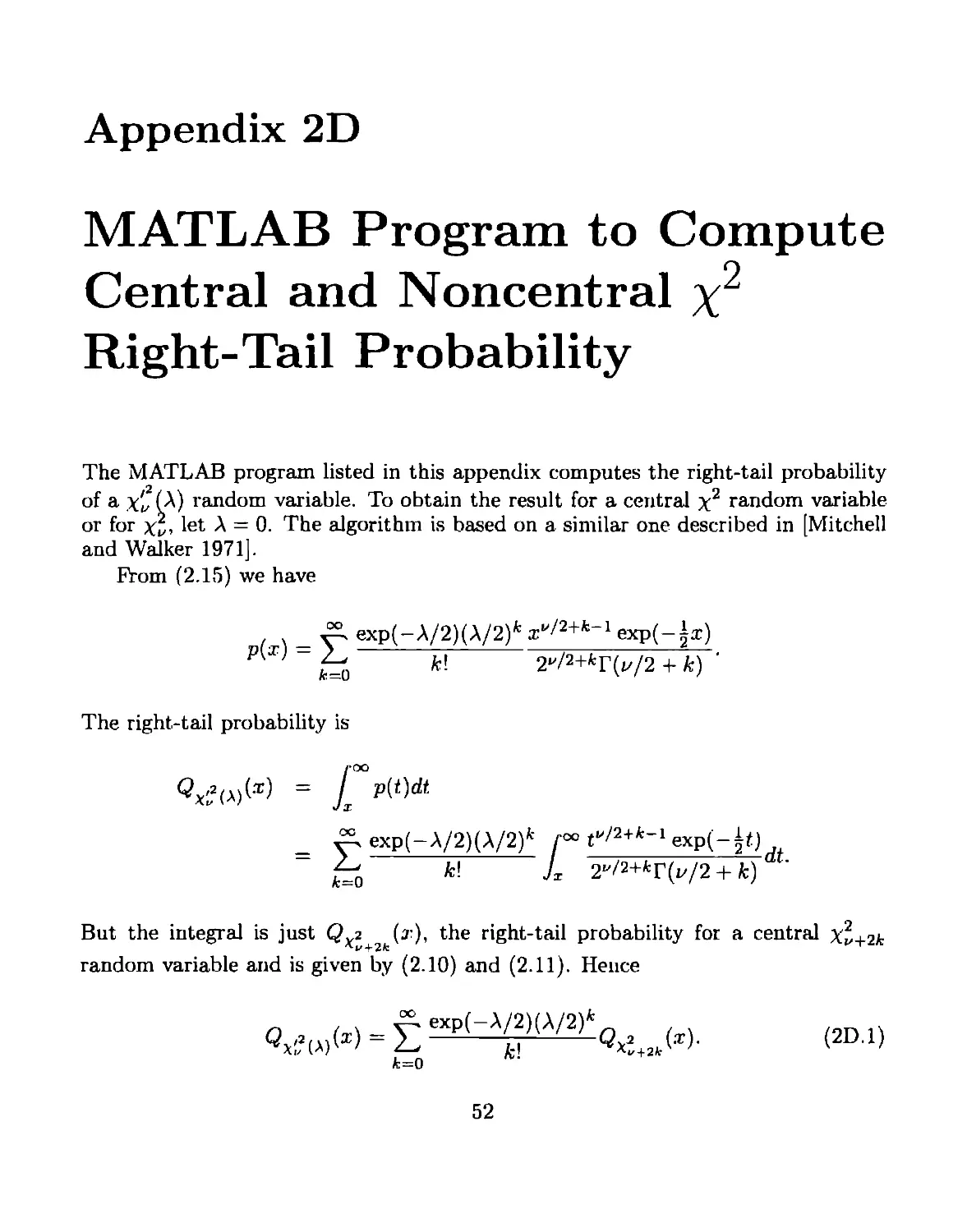
2D MATLAB Program to Compute Central and Noncentral %2 Right-
Tail Probability................................................. 52
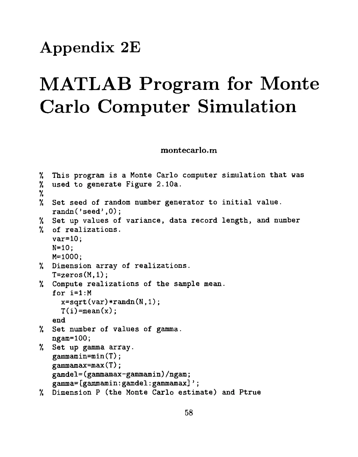
2E MATLAB Program for Monte Carlo Computer Simulation.............. 58
vii
viii
CONTENTS
3 Statistical Decision Theory I 60
3.1 Introduction.................................................... 60
3.2 Summary......................................................... 60
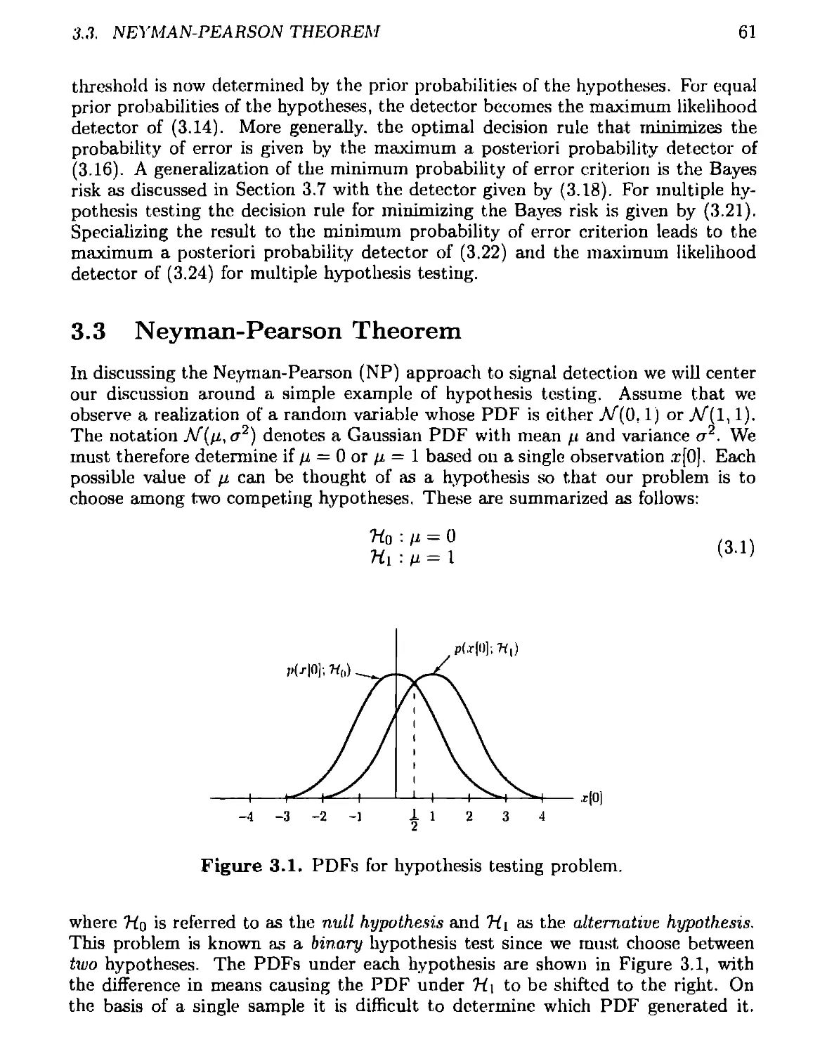
3.3 Neyman-Pearson Theorem.......................................... 61
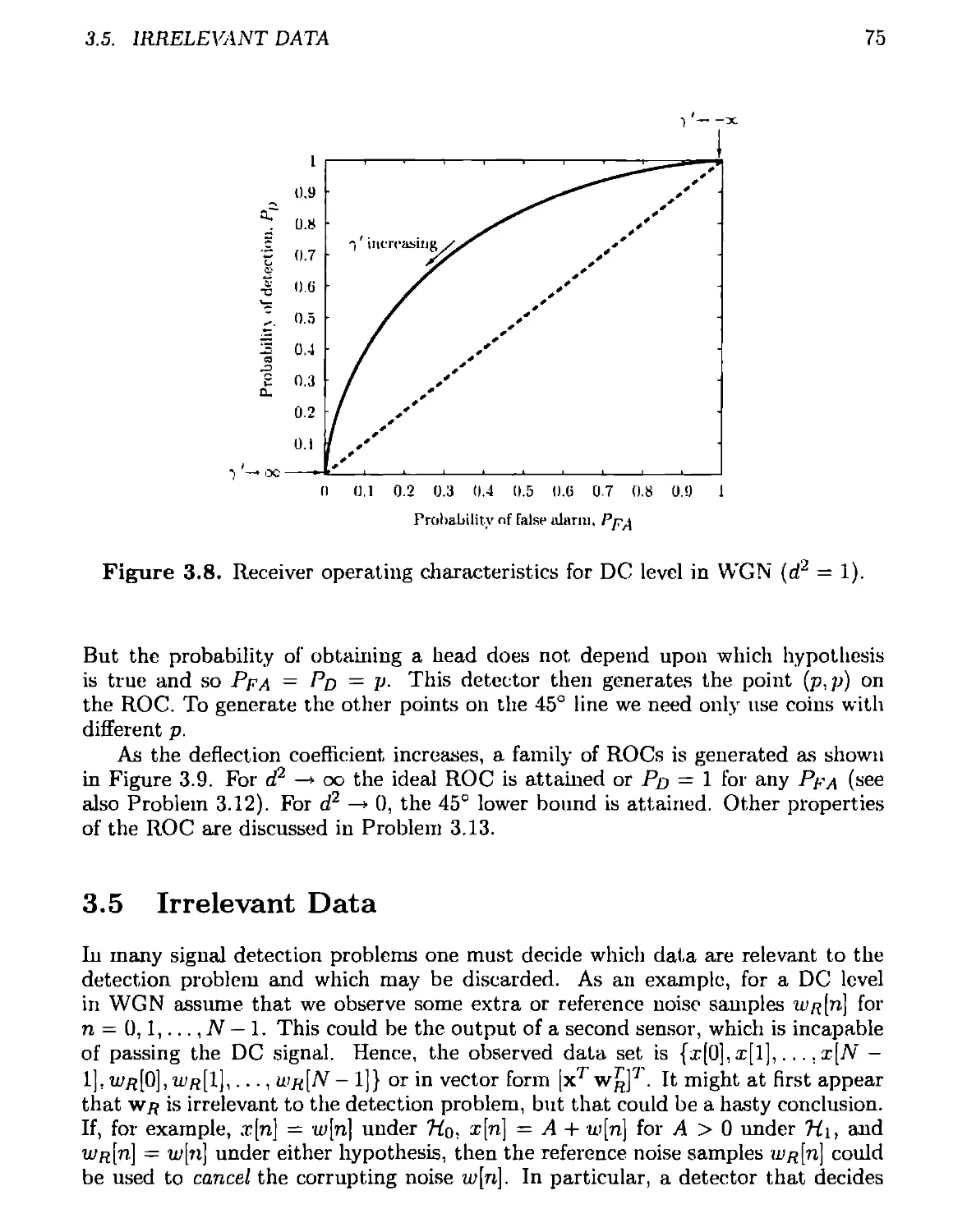
3.4 Receiver Operating Characteristics.............................. 74
3.5 Irrelevant Data................................................ 75
3.6 Minimum Probability of Error.................................... 77
3.7 Bayes Risk ..................................................... 80
3.8 Multiple Hypothesis Testing..................................... 81
ЗА Neyman-Pearson Theorem.......................................... 89
3B Minimum Bayes Risk Detector - Binary Hypothesis................ 90
3C Minimum Bayes Risk Detector - Multiple Hypotheses 92
4 Deterministic Signals 94
4.1 Introduction.................................................... 94
4.2 Summary......................................................... 94
4.3 Matched Filters................................................. 95
4.3.1 Development of Detector .................................. 95
4.3.2 Performance of Matched Filter.............................101
4.4 Generalized Matched Filters.....................................105
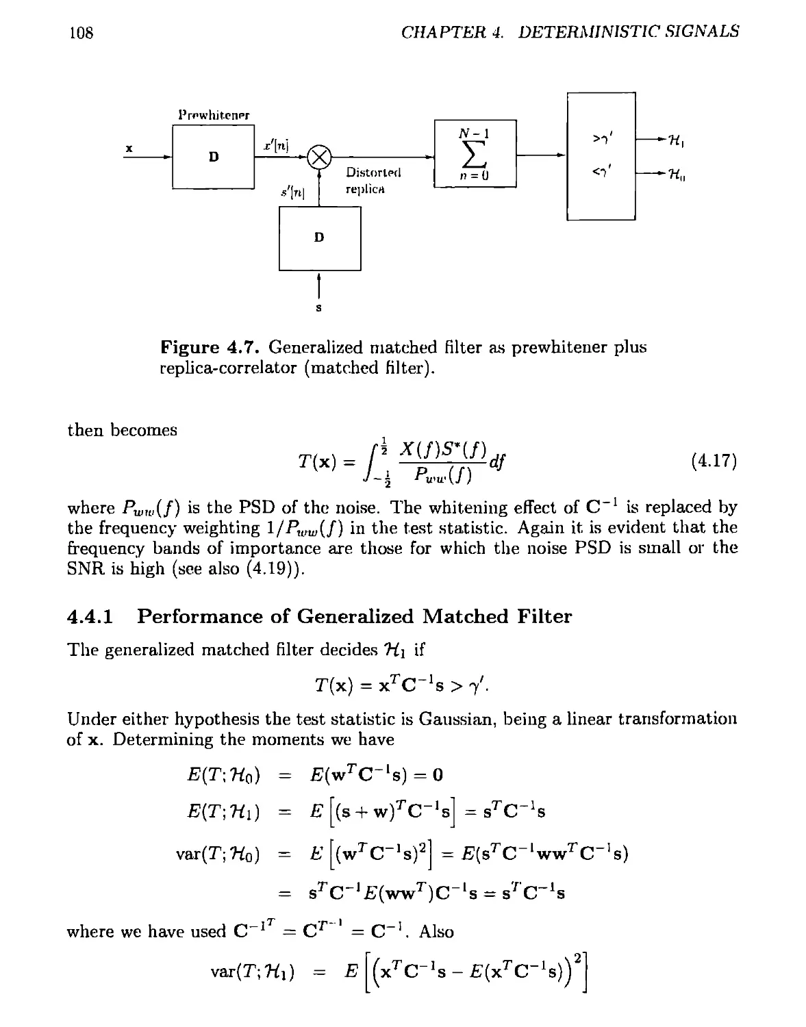
4.4.1 Performance of Generalized Matched Filter.................108
4.5 Multiple Signals ...............................................112
4.5.1 Binary Case...............................................112
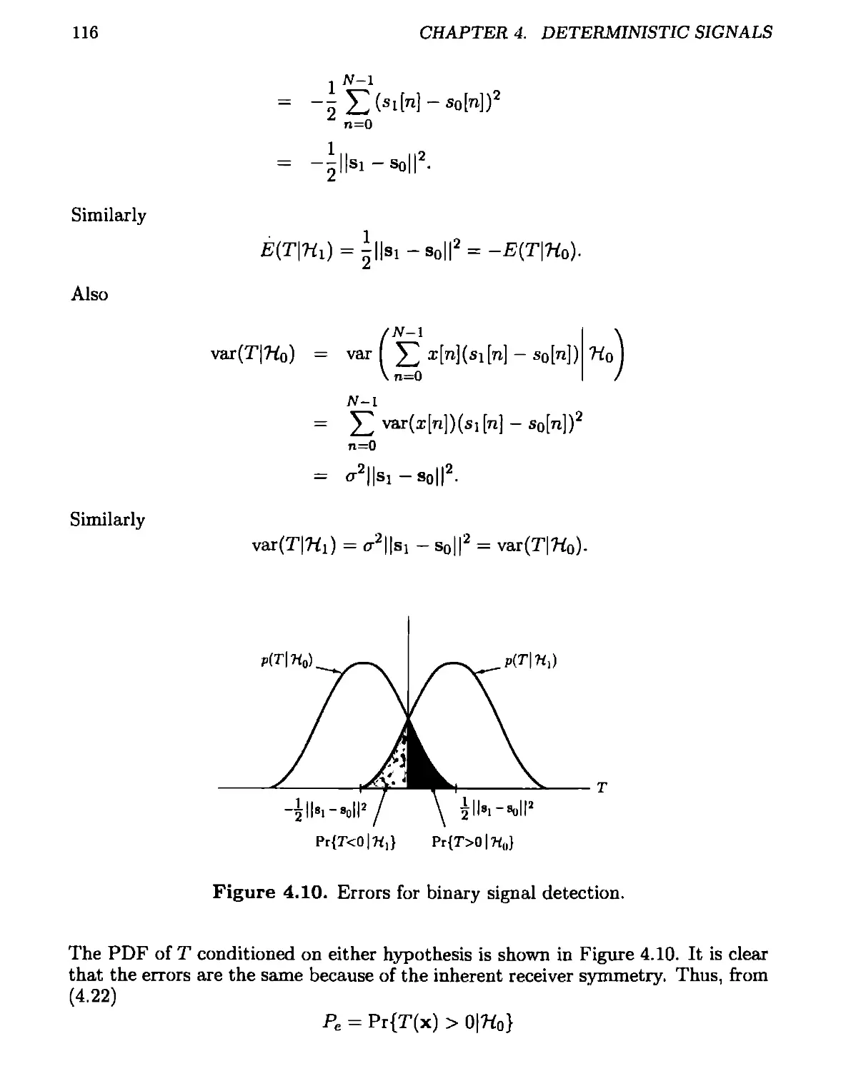
4.5.2 Performance for Binary Case...............................114
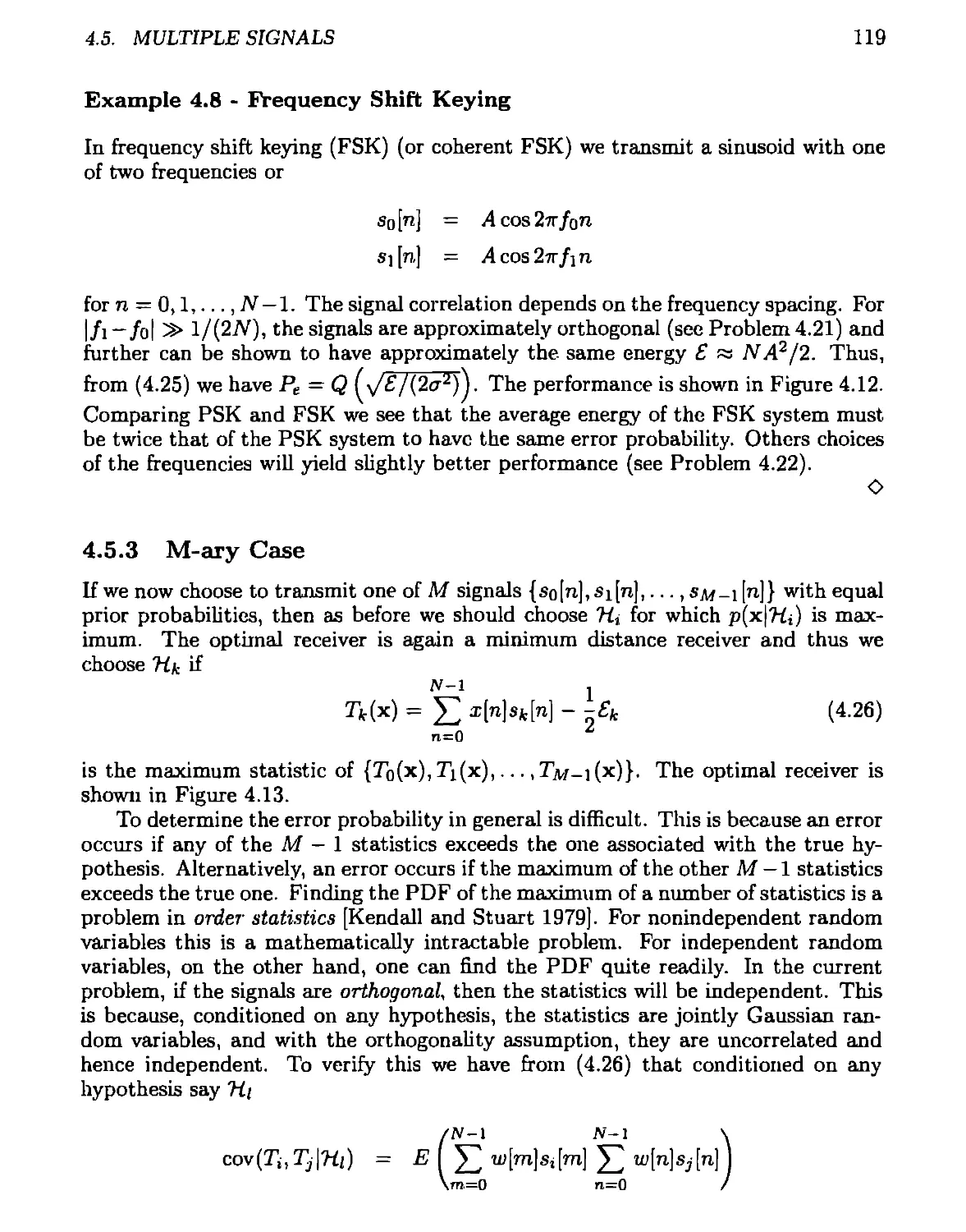
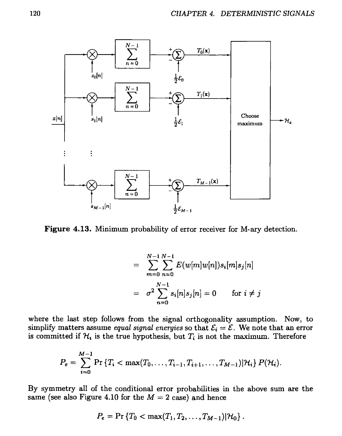
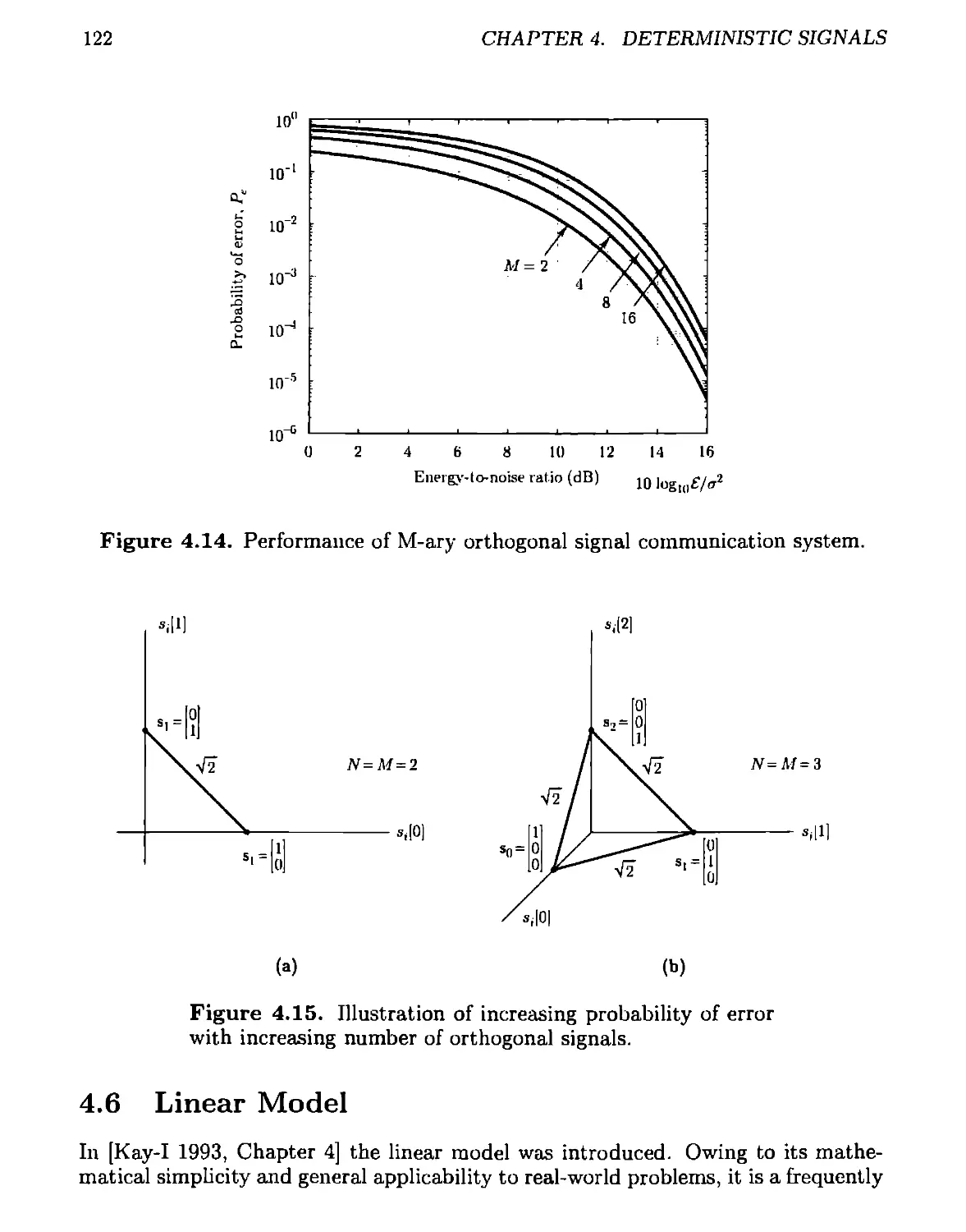
4.5.3 M-ary Case................................................119
4.6 Linear Model...................................................122
4.7 Signal Processing Examples......................................125
4A Reduced Form of the Linear Model................................139
5 Random Signals 141
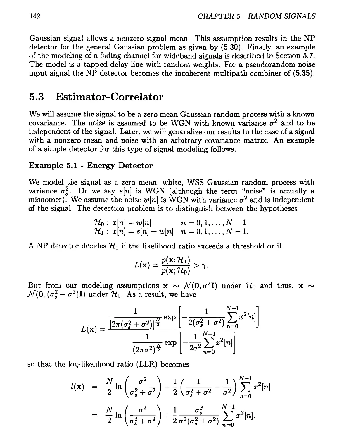
5.1 Introduction....................................................141
5.2 Summary........................................................ 141
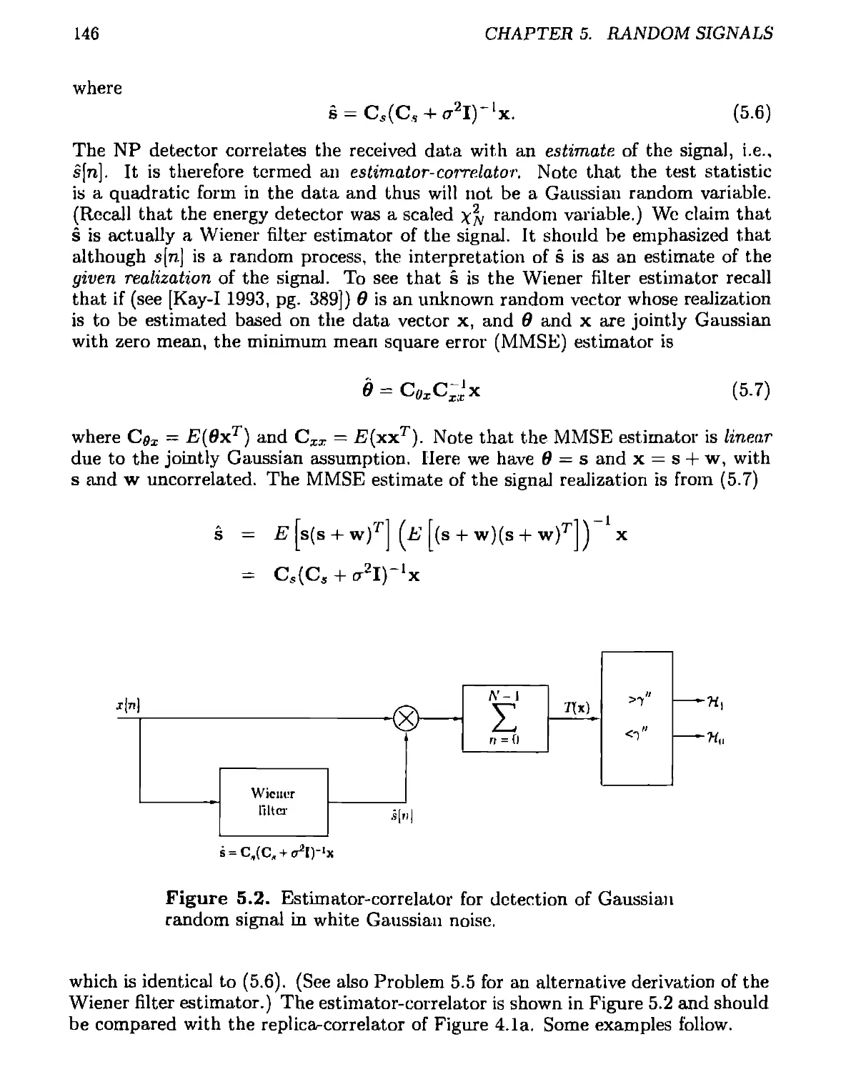
5.3 Estimator-Correlator............................................142
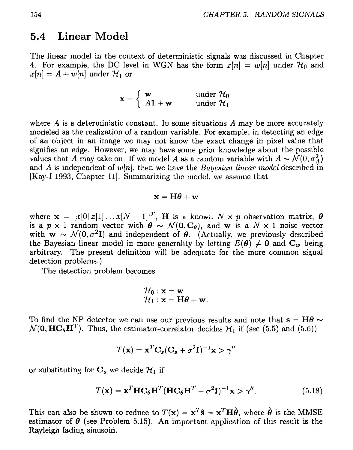
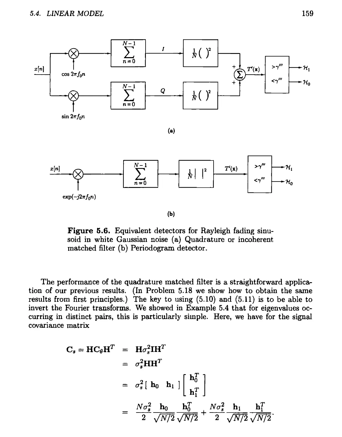
5.4 Linear Model....................................................154
5.5 Estimator-Correlator for Large Data Records 165
5.6 General Gaussian Detection......................................167
5.7 Signal Processing Example ......................................169
5.7.1 Tapped Delay Line Channel Model.........................169
5A Detection Performance of the Estimator-Correlator...............183
CONTENTS
ix
6 Statistical Decision Theory II 186
6.1 Introduction...................................................186
6.2 Summary........................................................186
6.2.1 Summary of Composite Hypothesis Testing 187
6.3 Composite Hypothesis Testing ..................................191
6.4 Composite Hypothesis Testing Approaches........................197
6.4.1 Bayesian Approach........................................198
6.4.2 Generalized Likelihood Ratio Test........................200
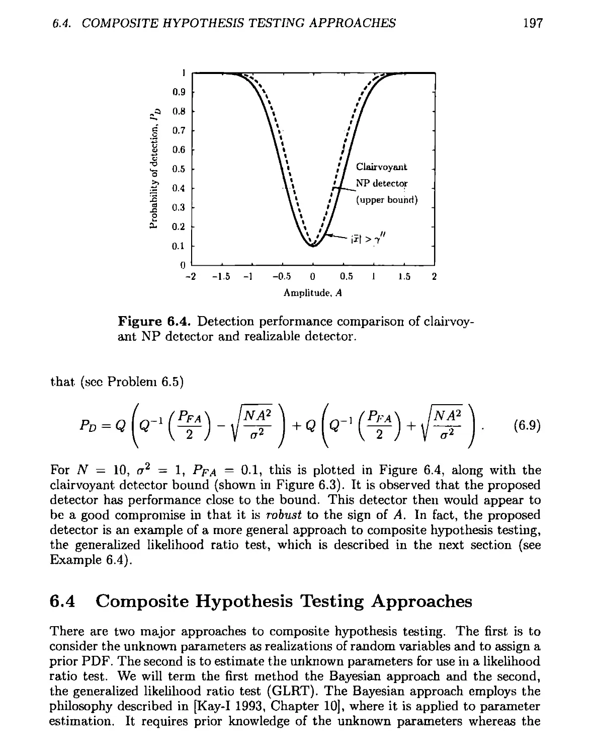
6.5 Performance of GLRT for Large Data Records 205
6.6 Equivalent Large Data Records Tests............................208
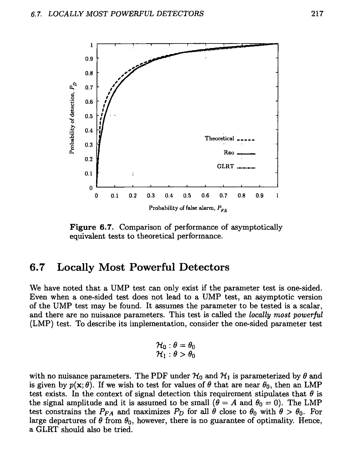
6.7 Locally Most Powerful Detectors................................217
6.8 Multiple Hypothesis Testing....................................221
6A Asymptotically Equivalent Tests - No Nuisance Parameters 232
6B Asymptotically Equivalent Tests - Nuisance Parameters..........235
6C Asymptotic PDF of GLRT.........................................239
6D Asymptotic Detection Performance of LMP Test...................241
6E Alternate Derivation of Locally Most Powerful Test.............243
6F Derivation of Generalized ML Rule..............................245
7 Deterministic Signals with Unknown Parameters 248
7.1 Introduction...................................................248
7.2 Summary........................................................248
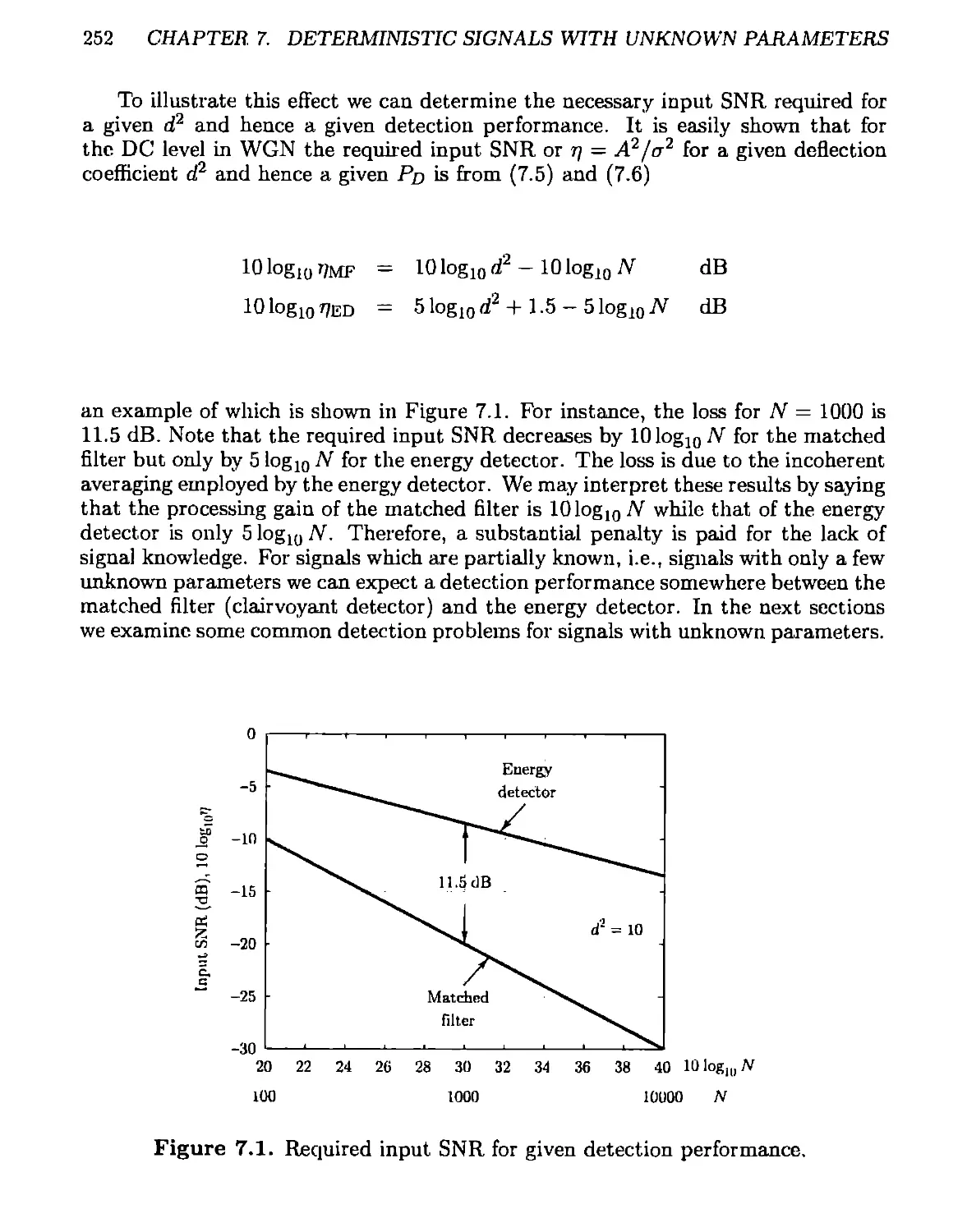
7.3 Signal Modeling and Detection Performance..................... 249
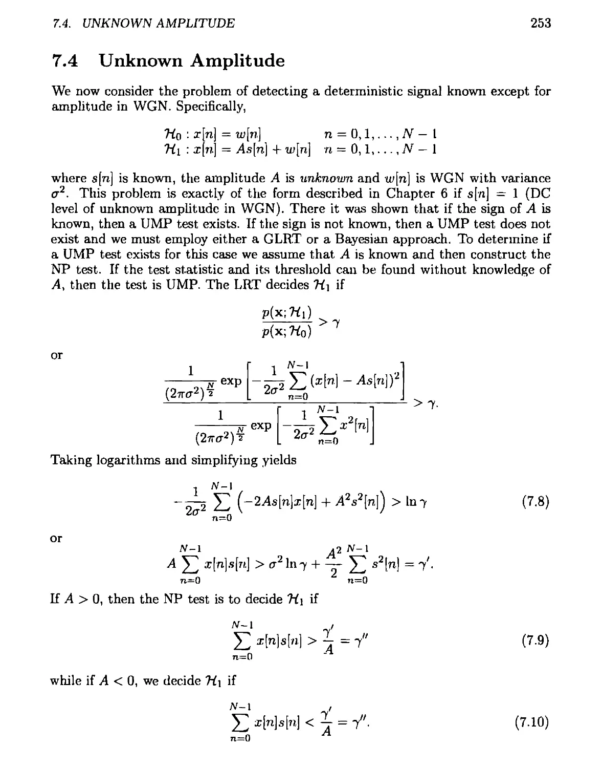
7.4 Unknown Amplitude..............................................253
7.4.1 GLRT.....................................................254
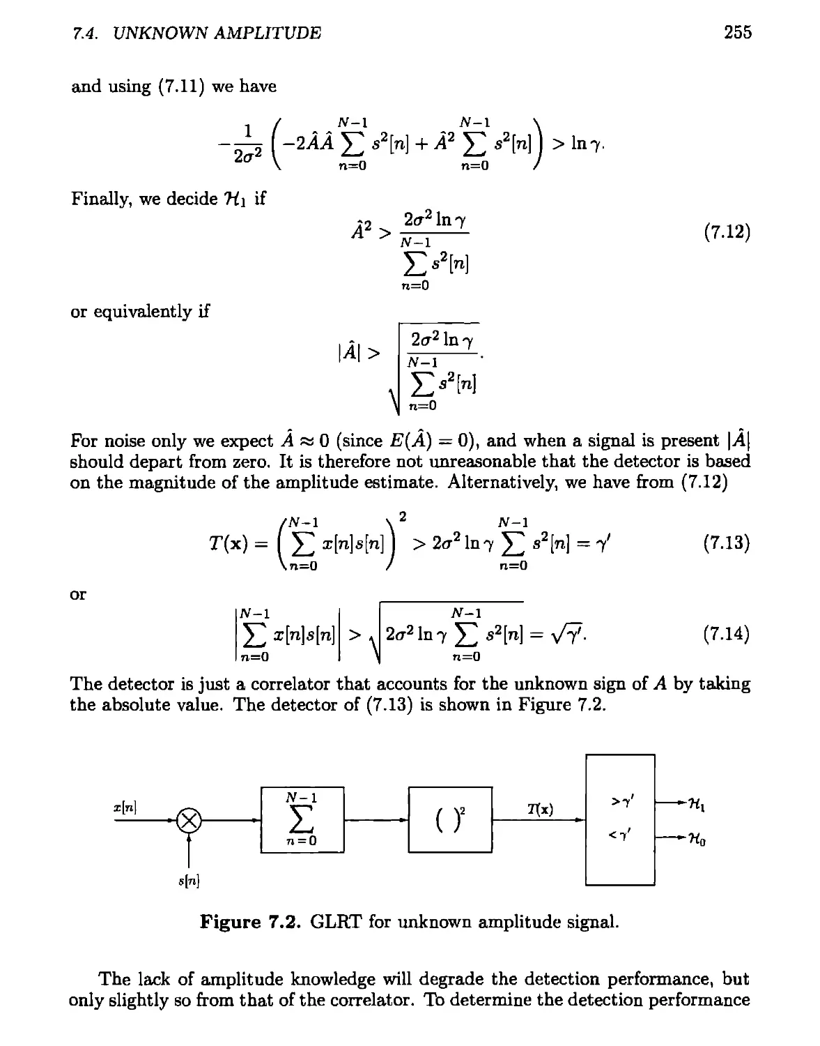
7.4.2 Bayesian Approach........................................257
7.5 Unknown Arrival Time...........................................258
7.6 Sinusoidal Detection.......................................... 261
7.6.1 Amplitude Unknown........................................261
7.6.2 Amplitude and Phase Unknown..............................262
7.6.3 Amplitude, Phase, and Frequency Unknown..................268
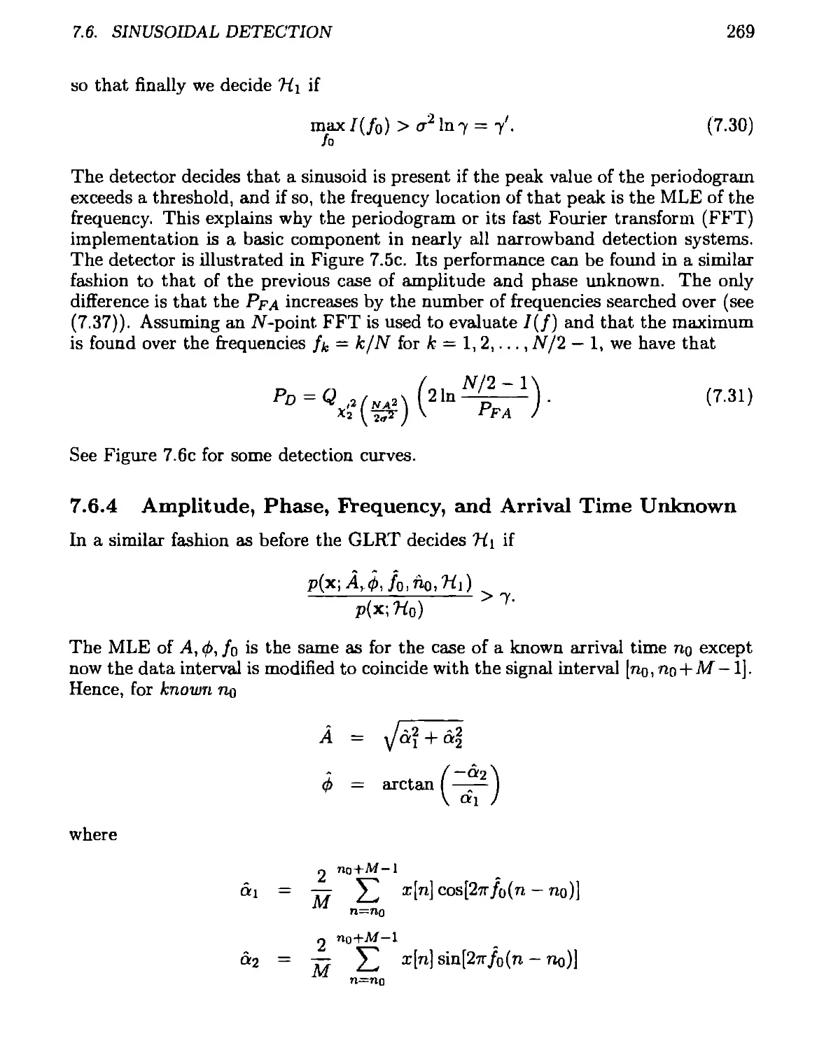
7.6.4 Amplitude, Phase, Frequency, and Arrival Time Unknown . . 269
7.7 Classical Linear Model.........................................272
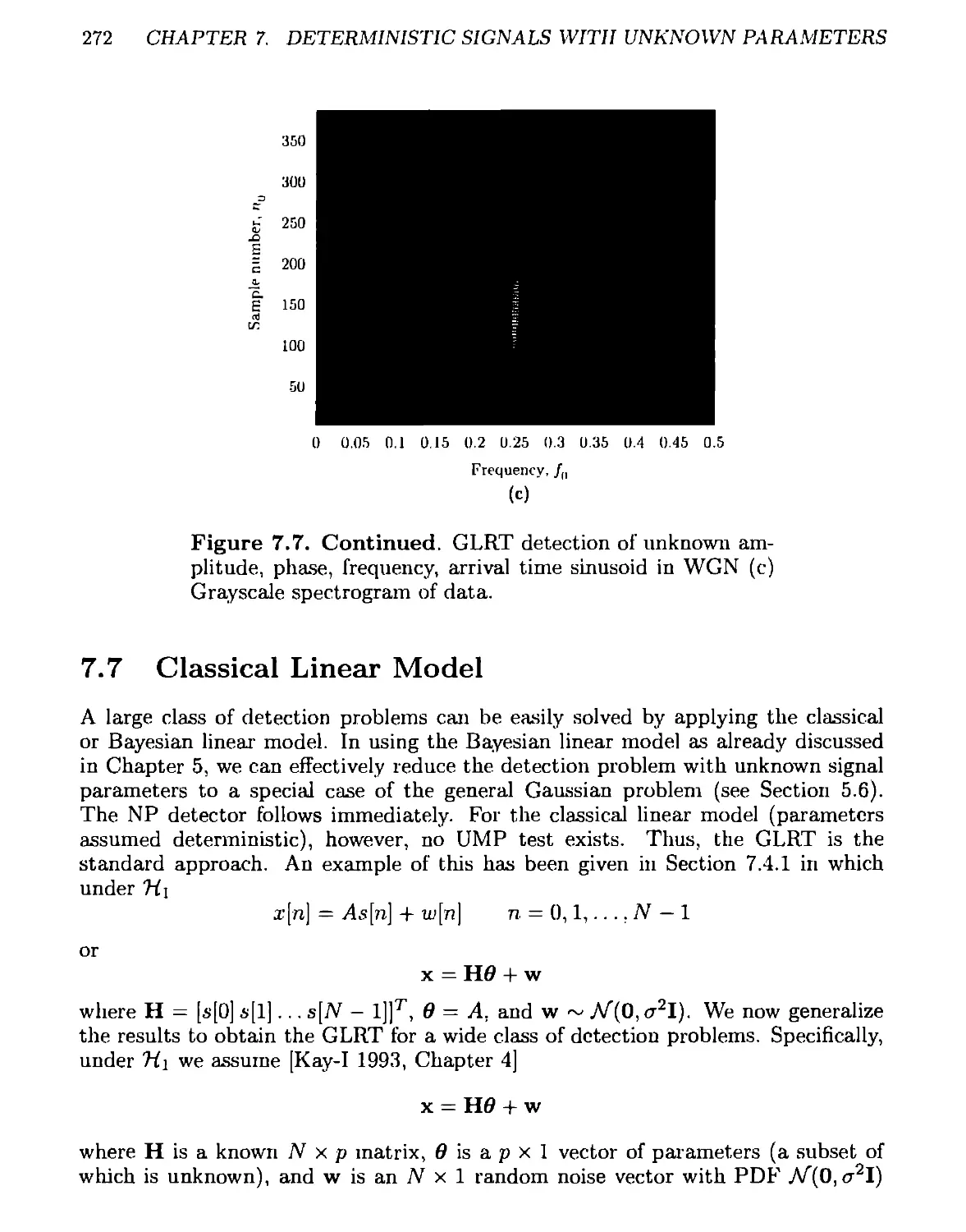
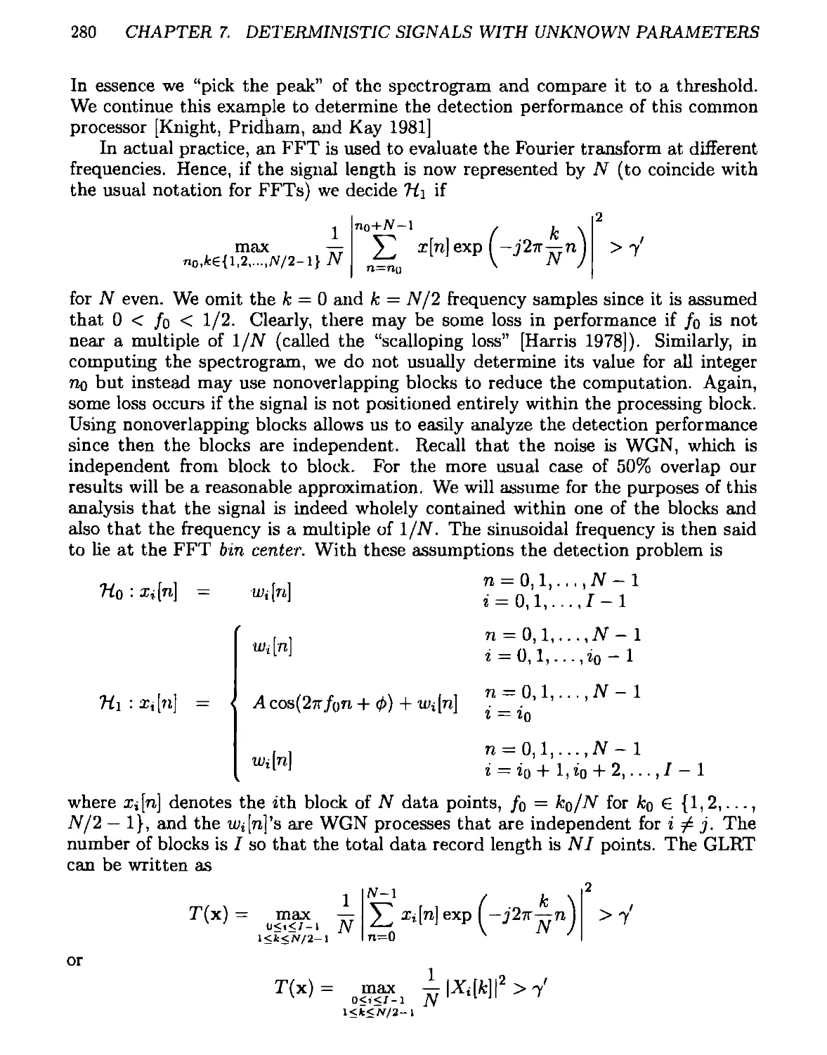
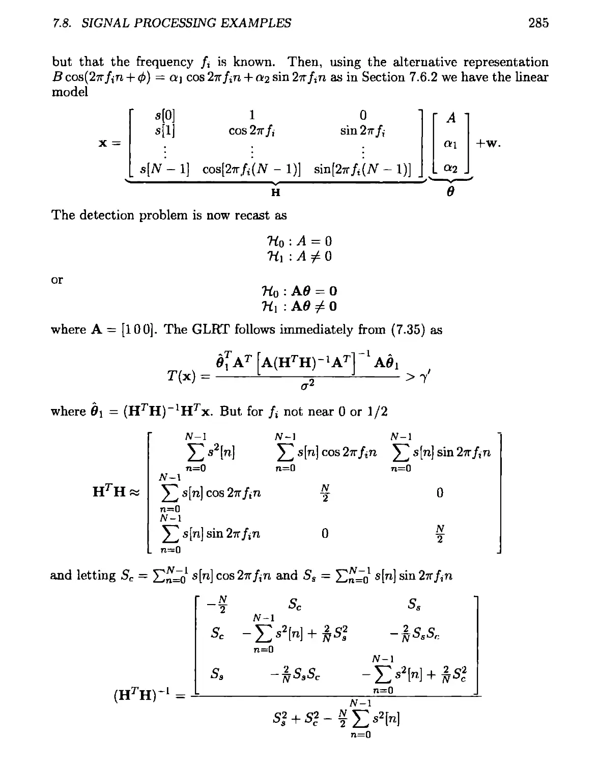
7.8 Signal Processing Examples.....................................279
7A Asymptotic Performance of the Energy Detector .................297
7B Derivation of GLRT for Classical Linear Model..................299
X
CONTENTS
8 Random Signals with Unknown Parameters 302
8.1 Introduction...................................................302
8.2 Summary........................................................302
8.3 Incompletely Known Signal Covariance...........................303
8.4 Large Data Record Approximations ..............................311
8.5 Weak Signal Detection..........................................314
8.6 Signal Processing Example .....................................315
8A Derivation of PDF for Periodic Gaussian Random Process.........332
9 Unknown Noise Parameters 336
9.1 Introduction...................................................336
9.2 Summary........................................................336
9.3 General Considerations.........................................337
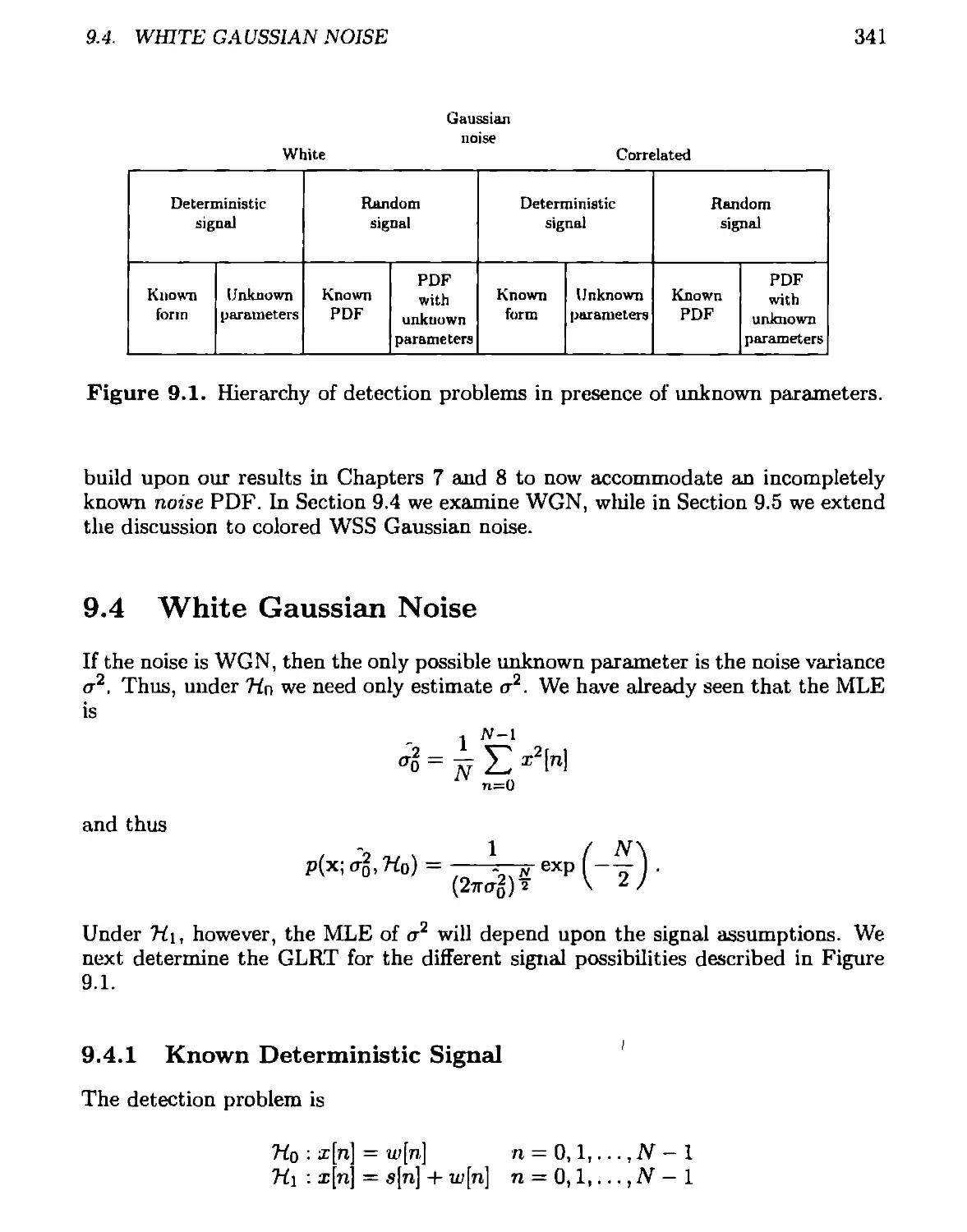
9.4 White Gaussian Noise...........................................341
9.4.1 Known Deterministic Signal...............................341
9.4.2 Random Signal with Known PDF ............................343
9.4.3 Deterministic Signal with Unknown Parameters.............345
9.4.4 Random Signal with Unknown PDF Parameters................349
9.5 Colored WSS Gaussian Noise.....................................350
9.5.1 Known Deterministic Signals..............................350
9.5.2 Deterministic Signals with Unknown Parameters............353
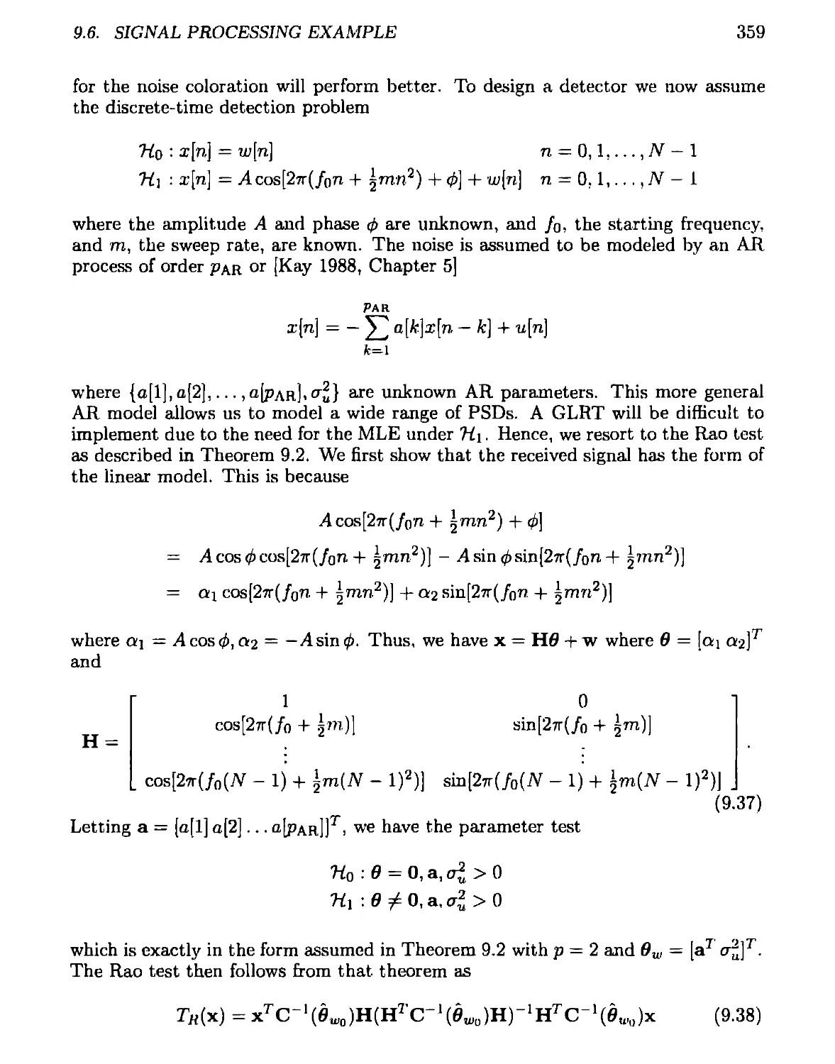
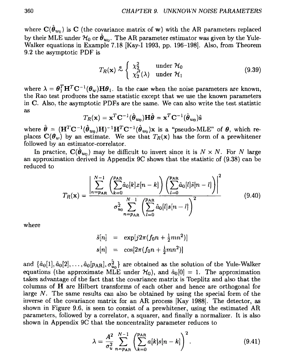
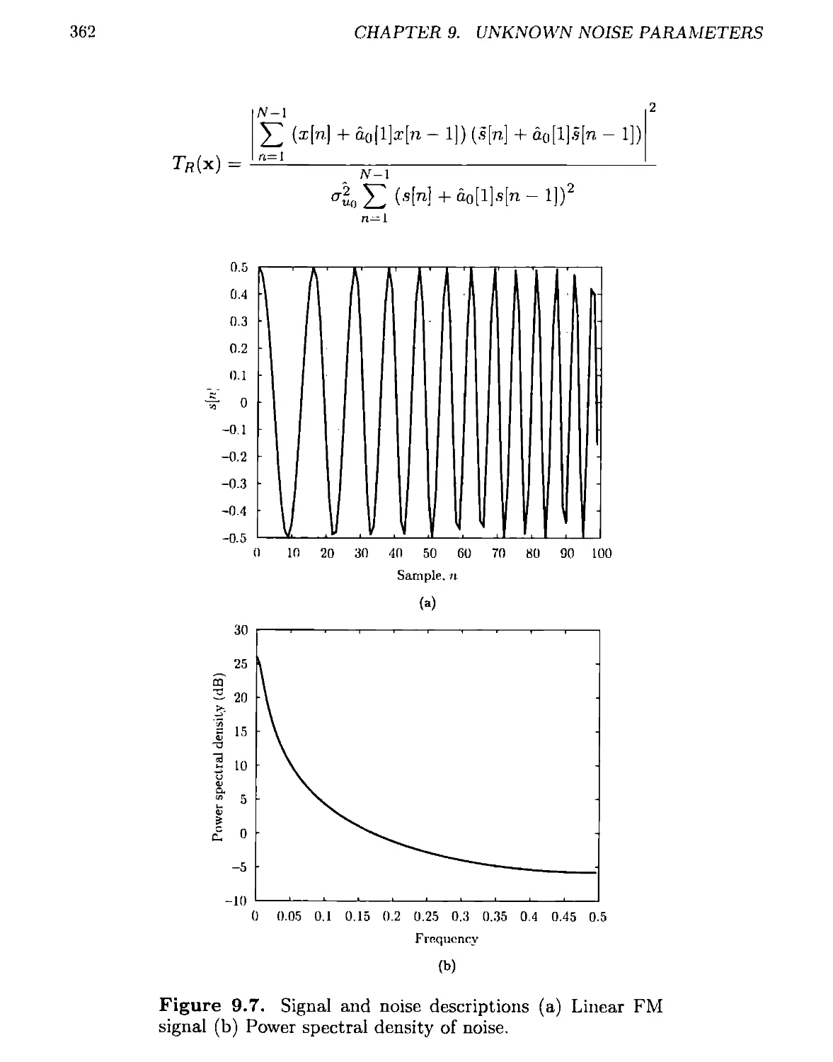
9.6 Signal Processing Example .....................................358
9A Derivation of GLRT for Classical Linear Model for cr2 Unknown . . . 371
9B Rao Test for General Linear Model with Unknown Noise Parameters 375
9C Asymptotically Equivalent Rao Test for Signal Processing Example . 377
10 NonGaussian Noise 381
10.1 Introduction...................................................381
10.2 Summary........................................................381
10.3 NonGaussian Noise Characteristics..............................382
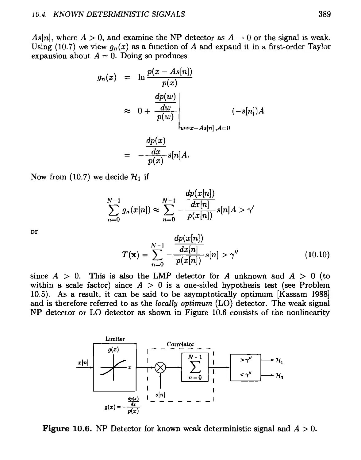
10.4 Known Deterministic Signals....................................385
10.5 Deterministic Signals with Unknown Parameters..................392
10.6 Signal Processing Example .....................................400
10A Asymptotic Performance of NP Detector for Weak Signals.........410
10B Rao Test for Linear Model Signal with IID NonGaussian Noise . . . 413
CONTENTS
xi
11 Summary of Detectors 416
11.1 Introduction...................................................416
11.2 Detection Approaches...........................................416
11.3 Linear Model...................................................427
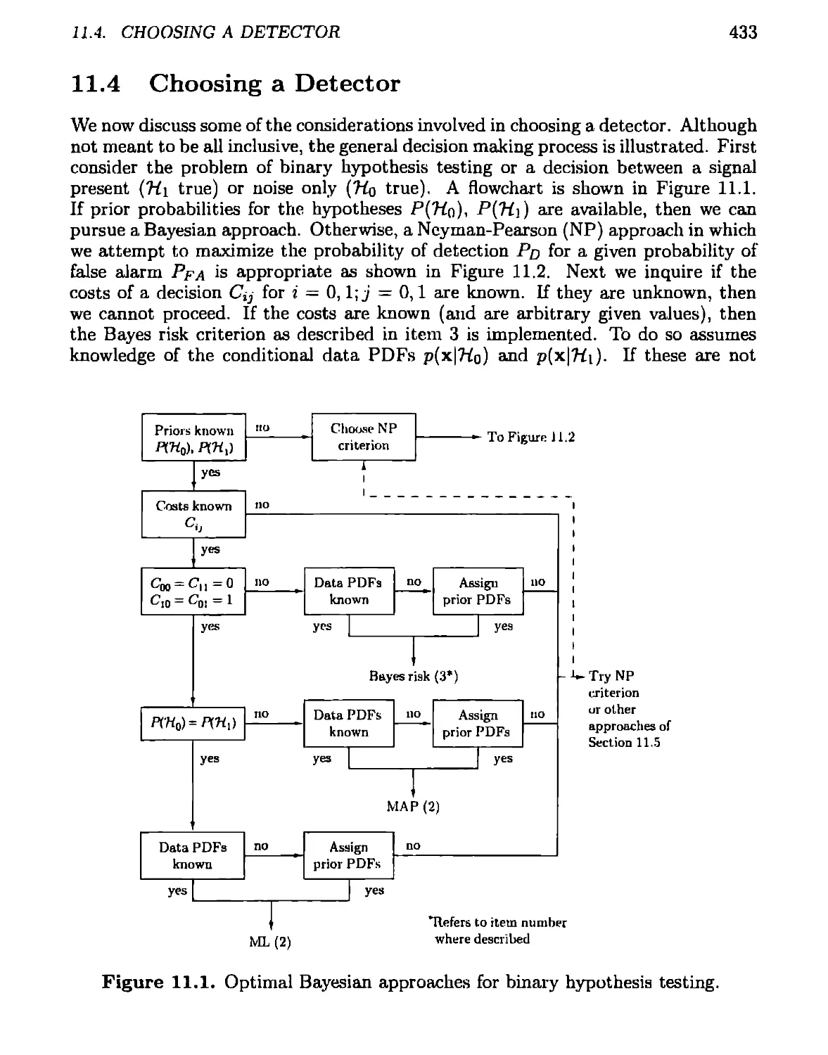
11.4 Choosing a Detector............................................433
11.5 Other Approaches and Other Texts...............................437
12 Model Change Detection 439
12.1 Introduction...................................................439
12.2 Summary........................................................439
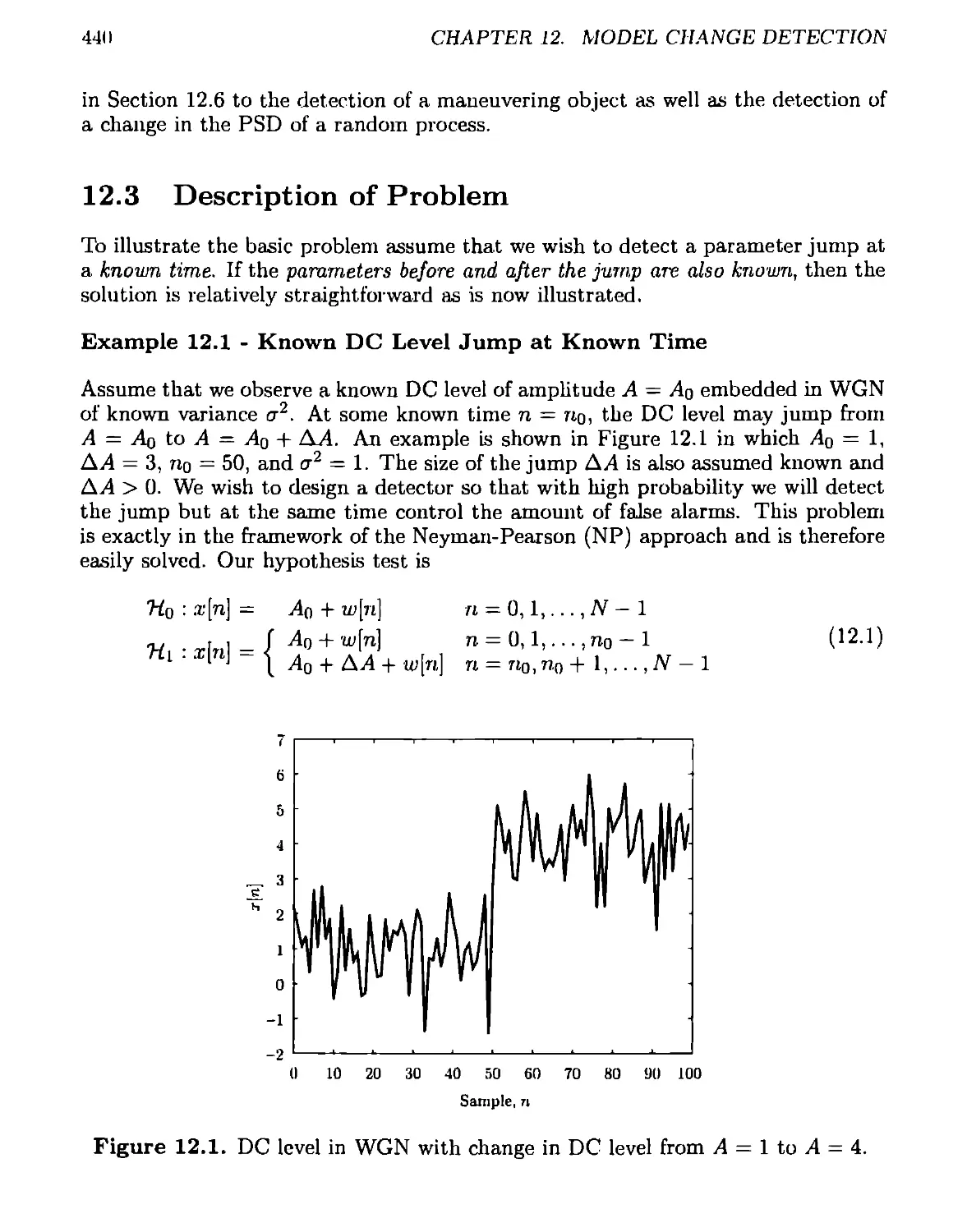
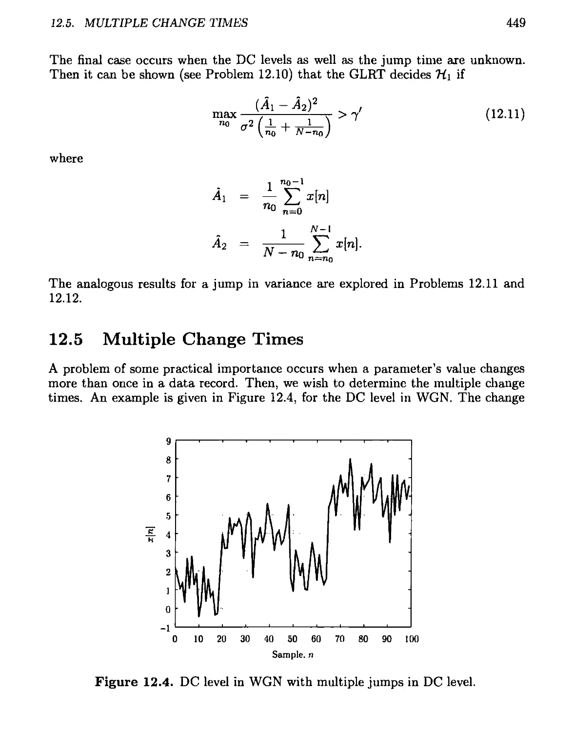
12.3 Description of Problem.........................................440
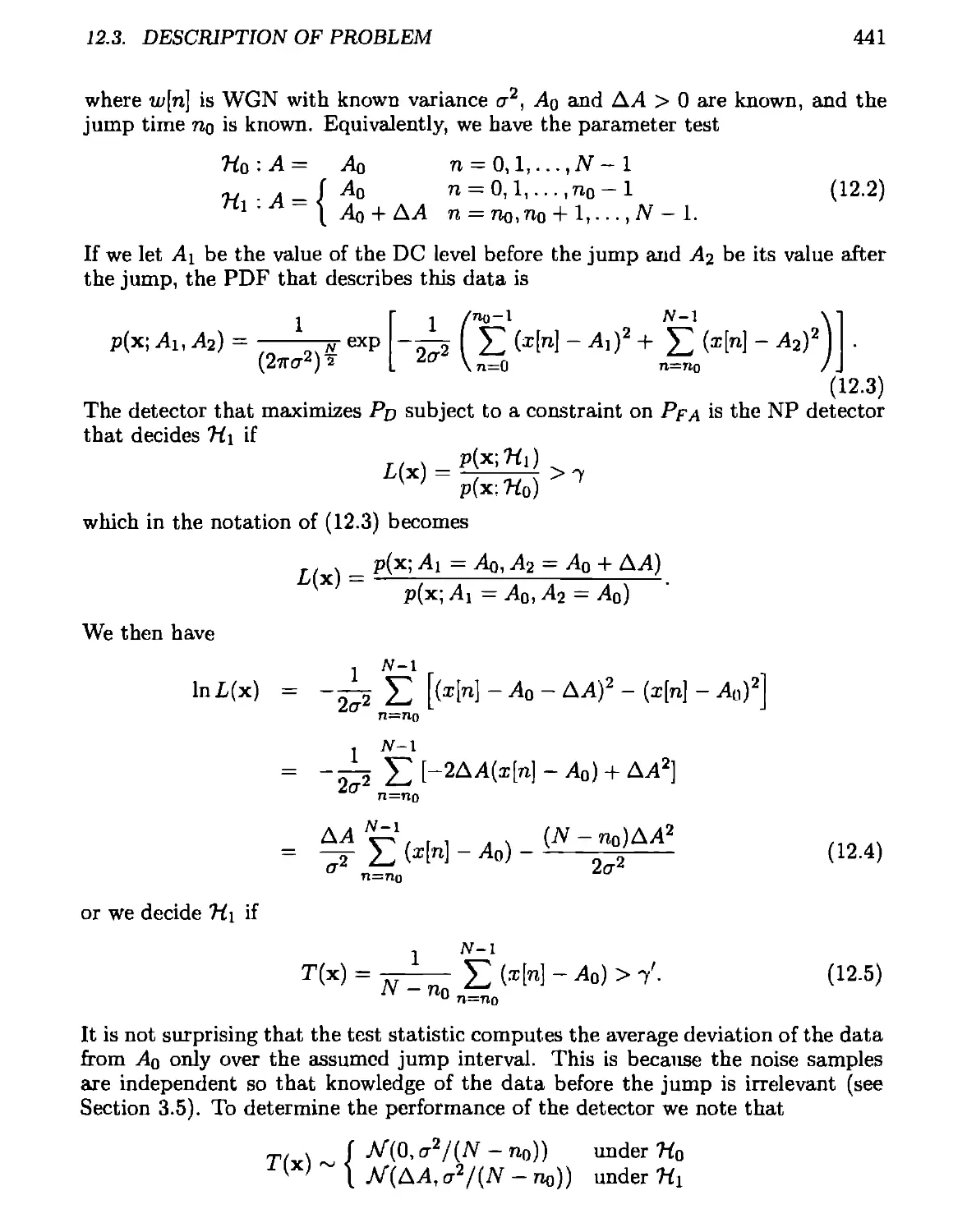
12.4 Extensions to the Basic Problem................................445
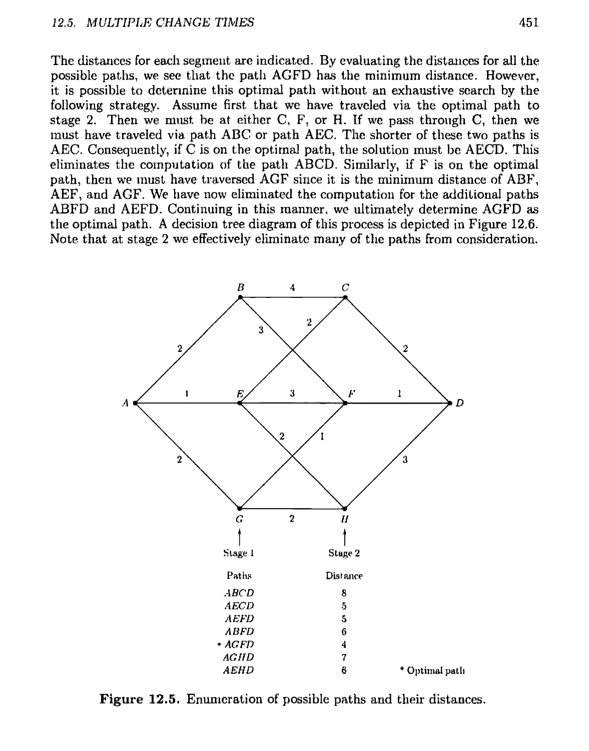
12.5 Multiple Change Times .........................................449
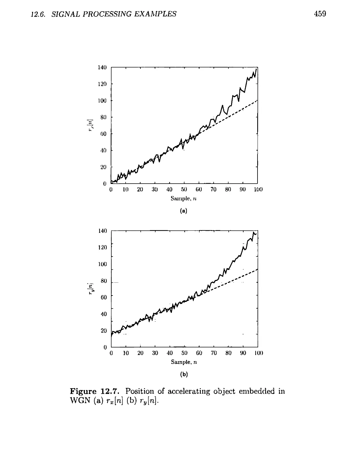
12.6 Signal Processing Examples.....................................455
12.6.1 Maneuver Detection.......................................455
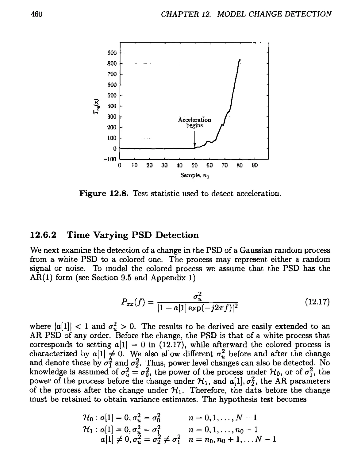
12.6.2 Time Varying PSD Detection...............................460
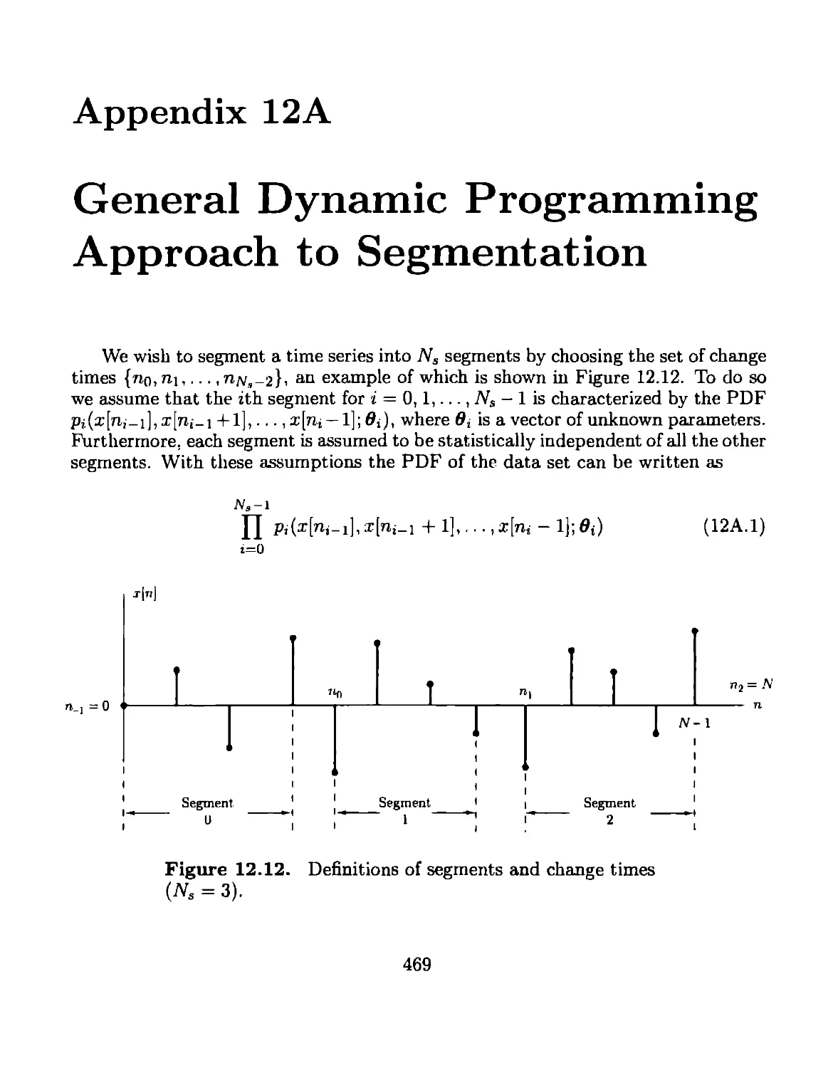
12A General Dynamic Programming Approach to Segmentation............469
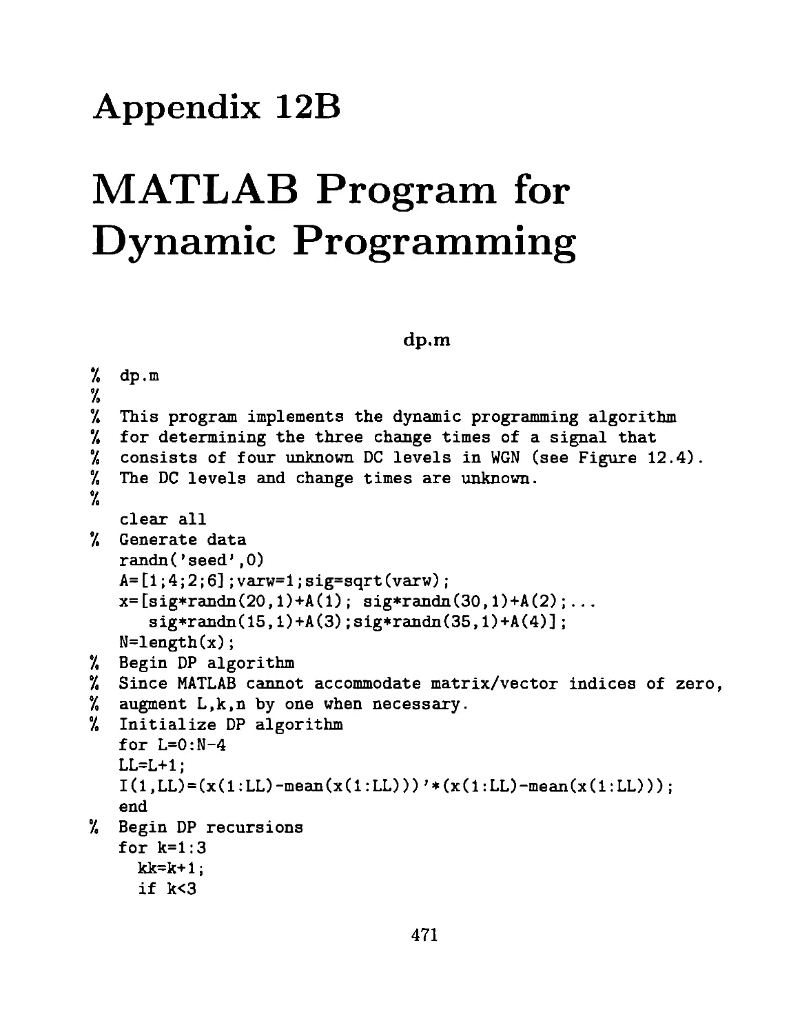
12B MATLAB Program for Dynamic Programming...........................471
13 Complex/Vector Extensions, and Array Processing 473
13.1 Introduction...................................................473
13.2 Summary........................................................473
13.3 Known PDFs.....................................................474
13.3.1 Matched Filter...........................................474
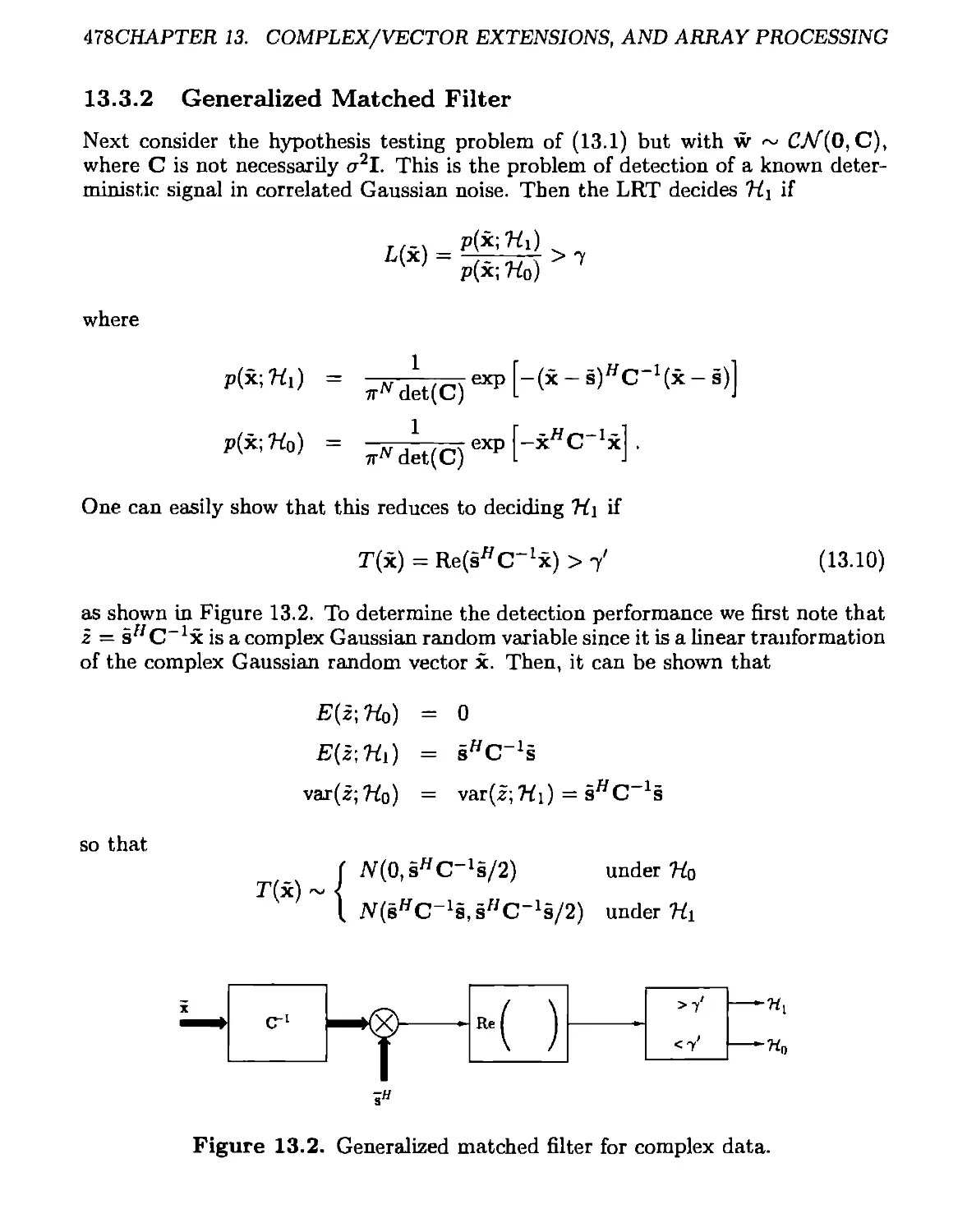
13.3.2 Generalized Matched Filter...............................478
13.3.3 Estimator-Correlator.....................................479
13.4 PDFs with Unknown Parameters...................................484
13.4.1 Deterministic Signal.....................................484
13.4.2 Random Signal............................................486
13.5 Vector Observations and PDFs...................................486
13.5.1 General Covariance Matrix................................490
13.5.2 Scaled Identity Matrix...................................491
13.5.3 Uncorrelated from Temporal Sample to Sample..............491
13.5.4 Uncorrelated from Spatial Sample to Sample...............492
13.6 Detectors for Vector Observations..............................492
13.6.1 Known Deterministic Signal in CWGN.......................492
13.6.2 Known Deterministic Signal and General Noise Covariance . 495
xii
CONTENTS
13.6.3 Known Deterministic Signal in Temporally Uncorrelated Noise 495
13.6.4 Known Deterministic Signal in Spatially Uncorrelated Noise . 496
13.6.5 Random Signal in CWGN....................................496
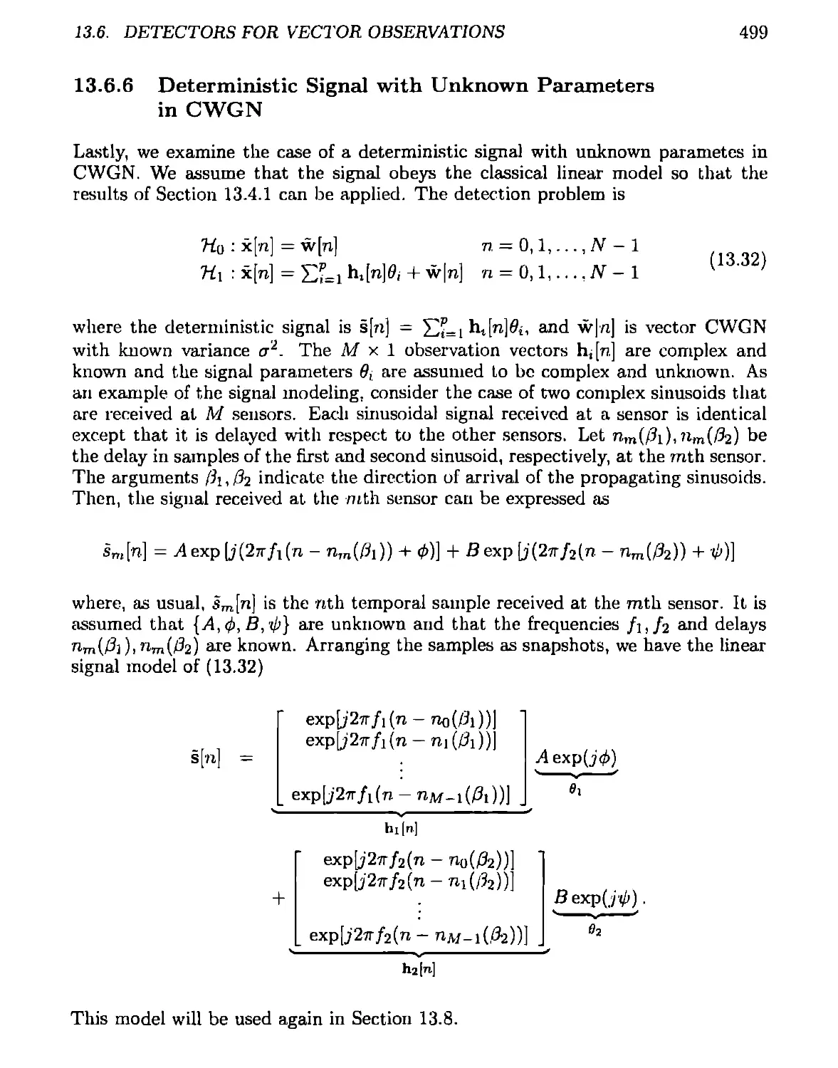
13.6.6 Deterministic Signal with Unknown Parameters in CWGN . . 499
13.7 Estimator-Correlator for Large Data Records....................501
13.8 Signal Processing Examples.....................................508
13.8.1 Active Sonar/Radar.......................................510
13.8.2 Broadband Passive Sonar..................................515
13A PDF of GLRT for Complex Linear Model...........................526
Al Review of Important Concepts 529
Al.l Linear and Matrix Algebra.......................................529
Al.1.1 Definitions .............................................529
Al. 1.2 Special Matrices........................................531
Al.1.3 Matrix Manipulation and Formulas.........................533
Al. 1.4 Theorems................................................535
Al.1.5 Eigendecompostion of Matrices............................536
Al.1.6 Inequalities.............................................537
A 1.2 Random Processes and Time Series Modeling......................537
Al.2.1 Random Process Characterization..........................538
Al.2.2 Gaussian Random Process..................................540
Al.2.3 Time Series Models ......................................541
A2 Glossary of Symbols and Abbreviations
(Vols. I & II) 545
Preface
This text is the second volume of a series of books addressing statistical signal
processing. The first volume, Fundamentals of Statistical Signal Processing.' Esti-
mation Theory, was published in 1993 by Prentice-Hall, Inc. Henceforth, it will be
referred to as [Kay-I 1993]. This second volume, entitled Fundamentals of Statisti-
cal Signal Processing: Detection Theory, is the application of statistical hypothesis
testing to the detection of signals in noise. The series has been written to provide
the reader with a broad introduction to the theory and application of statistical
signal processing.
Hypothesis testing is a subject that, is standard fare in the many books available
dealing with statistics. These books range from the highly theoretical expositions
written by statisticians to the more practical treatments contributed by the many
users of applied statistics. This text is an attempt to strike a balance between
these two extremes. The particular audience we have in mind is the community
involved in the design and implementation of signal processing algorithms. As
such, the primary focus is on obtaining optimal detection algorithms that may be
implemented on a digital computer. The data sets are therefore assumed to be
samples of a continuous-time waveform or a sequence of data points. The choice
of topics reflects what we believe to be the important approaches to obtaining an
optimal detector and analyzing its performance. As a consequence, some of the
deeper theoretical issues have been omitted with references given instead.
It is the author’s opinion that the best way to assimilate the material on detec-
tion theory is by exposure to and working with good examples. Consequently, there
are numerous examples that illustrate the theory and others that apply the theory
to actual detection problems of current interest. We have made extensive use of
the MATLAB® scientific programming language (Version 4.2b)1 for all computer-
generated results. In some cases, actual MATLAB programs have been listed where
a program was deemed to be of sufficient utility to the reader. Additionally, an
abundance of homework problems has been included. They range from simple ap-
plications of the theory to extensions of the basic concepts. A solutions manual is
available from the author. To aid the reader, summary sections have been provided
at the beginning of each chapter. Also, an overview of all the principal detection
approaches and the rationale for choosing a particular method can be found in
’MATLAB is a registered trademark of The Math Works, Inc.
xiii
xiv
CONTENTS
Chapter 11. Detection based on simple hypothesis testing is described in Chapters
3 -5, while that based on composite hypothesis testing (to accommodate unknown
parameters) is the subject of Chapters 6-9. Other chapters address detection in
nonGaussian noise (Chapter 10), detection of model changes (Chapter 12), and
extensions for complex/vector data useful in array processing (Chapter 13).
This book is an outgrowth of a one-semester graduate level course on detection
theory given at the University of Rhode Island. It includes somewhat more material
than can actually be covered in one semester. We typically cover most of Chapters
1-10, leaving the subjects of model change detection and complex data/vector data
extensions to the student. It is also possible to combine the subjects of estimation
and detection into a single semester course by a judicious choice of material from
Volumes I and II. The necessary background that has been assumed is an exposure
to the basic theory of digital signal processing, probability and random processes,
and linear and matrix algebra. This book can also be used for self-study and so
should be useful to the practicing engineer as well as the student.
The author would like to acknowledge the contributions of the many people
who over the years have provided stimulating discussions of research problems,
opportunities to apply the results of that research, and support for conducting
research. Thanks are due to my colleagues L. Jackson, R. Kumaresan, L. Pakula,
and P. Swaszek of the University of Rhode Island, and L. Scharf of the University
of Colorado. Exposure to practical problems, leading to new research directions,
has been provided by H. Woodsum of Sonetech, Bedford, New Hampshire, and by
D. Mook and S. Lang of Sanders, a Lockheed-Martin Co., Nashua, New Hampshire.
The opportunity to apply detection theory to sonar and the research support of J.
Kelly of the Naval Undersea. Warfare Center, J. Salisbury, formerly of the Naval
Undersea Warfare Center, and D. Sheldon of the Naval Undersea Warfare Center,
Newport, Rhode Island are also greatly appreciated. Thanks are due to J. Sjogren
of the Air Force Office of Scientific Research, whose support has allowed the author
to investigate the field of statistical signal processing. A debt of gratitude is owed
to all my current and former graduate students. They have contributed to the
final manuscript through many hours of pedagogical and research discussions as
well as by their specific comments and questions. In particular, P. Djuric of the
State University of New York proofread much of the manuscript, and S. Talwalkar
of Motorola, Plantation, Florida proofread parts of the manuscript and helped with
the finer points of MATLAB.
Steven M, Kay
University of Rhode Island
Kingston, RI 02881
Email: kay@ele.uri.edu
Chapter 1
Introduction
1.1 Detection Theory in Signal Processing
Modern detection theory is fundamental to the design of electronic signal processing
systems for decision making and information extraction. These systems include
1. Radar
2. Communications
3. Speech
4. Sonar
5. Image processing
6. Biomedicine
7. Control
8. Seismology,
and all share the common goal of being able to decide when an event of interest
occurs and then to determine more information about that event. The latter task,
information extraction, is the subject of the first volume [Kay 1993]. The former
problem, that of decision making, is the subject of this book and is broadly termed
detection theory. Other names associated with it are hypothesis testing and decision
theory. To illustrate the problem of detection as applied to signal processing, we
briefly describe the first three of these systems.
In radar we are interested in determining the presence or absence of an approach-
ing aircraft [Skolnik 1980]. To accomplish this task we transmit an electromagnetic
pulse, which if reflected by a large moving object, will indicate the presence of an
aircraft, If an aircraft is present, the received waveform will consist of the reflected
1
2
CHAPTER 1. INTRODUCTION
pulse (at some time later) and noise due to ambient radiation and the receiver
electronics. If an aircraft is not present, then only noise will be present. It is the
function of the signal processor to decide whether the received waveform consists
of noise only (no aircraft) or an echo in noise (aircraft present). As an example, in
Figure 1.1a we have depicted a radar and in Figure 1.1b a typical received waveform
for the two possible scenarios. When an echo is present, we see that the character
of the received waveform is somewhat different, although possibly not by much.
This is because the received echo is attenuated due to propagation loss and possibly
distorted due to the interaction of multiple reflections. Of course, if the aircraft is
detected, then it is of interest to determine its bearing, range, speed, etc. Hence,
detection is the first task of the signal processing system while the second task is
information extraction. Estimation theory provides the foundation for the second
task and has already been described in Volume I [Kay-I 1993]. The optimal de-
tector for the radar problem is the Neyman-Pearson detector, which is described
in Chapter 4. A more practical detector which accommodates signal uncertainties,
however, is discussed in Chapter 7.
A second application is in the design of a digital communication system. An
example is the binary phase shift keyed (BPSK) system as shown in Figure 1.2a
used to communicate the output of a digital data source that emits a “0” or “1”
[Proakis 1989]. The data bit is first modulated, then transmitted, and at the re-
ceiver, demodulated and then detected. The modulator converts a 0 to the waveform
so(i) = cos27rF0f and a 1 to si(t) = cos(27rF0f + %) = — cos27rF0f to allow trans-
mission through a bandpass channel whose center frequency is Fq Hz (such as a
microwave link). The phase of the sinusoid indicates whether a 0 or 1 has been
sent. In this problem, the function of the detector is to decide between the two pos-
sibilities, as in the radar problem, although now, we always have a signal present -
the question is which, signal. Typical received waveforms are shown in Figure 1.2b.
Since the sinusoidal carrier has been extracted by the demodulator, all that remains
at the detector input is the baseband signal, either a positive or negative pulse. This
signal is usually distorted due to limited channel bandwidth and is also corrupted
by additive channel noise. The solution to this problem is given in Chapter 4.
Another application is in speech recognition where we wish to determine which
word was spoken from among a group of possible words [Rabiner and Juang 1993].
A simple example is to discern among the digits “0”, “1”, ..., “9”. To recognize
a spoken digit using a digital computer we would need to match the spoken digit
with some stored digit. For example, the waveforms for the spoken digits 0 and
1 are shown in Figure 1.3. They have been repeated three times by the same
speaker. Note that the waveform changes slightly for each utterance of the same
word. We may think of this change as “noise,” although it is actually the natural
variability of speech. Given an utterance, we wish to decide if it is a 0 or 1. More
generally, we would need to decide among the ten possible digits. Such a problem
is a generalization of that for radar and for digital communications in which only
one of two possible choices need be made. The solution to this problem is discussed
in Chapter 4.
1.1. DETECTION THEORY IN SIGNAL PROCESSING
3
Transmit pulse
Wv
Received waveform - aircraft present
Time
Received waveform - no aircraft
(b)
Figure 1.1. Radar system (a) Radar (b) Radar waveforms.
Time
4
CHAPTER 1. INTRODUCTION
Figure 1.2. Binary phase shift keyed digital communication
system (a) Basic system (b) BPSK baseband waveforms.
1.1. DETECTION THEORY IN SIGNAL PROCESSING
5
Time (sec)
(b)
Figure 1.3. Speech waveforms for digits “zero” and “one”
(a) “Zero” spoken three times (b) “Zero”-portion of utter-
ance.
6
CHAPTER 1. INTRODUCTION
(c)
1.72 1.76 1.8 1.84 1.88 1.92
1.74 1.78 1.82 1.86 1.9
Time (sec)
(d)
Figure 1.3. Continued (c) “One” spoken three times (d)
“One”-portion of utterance.
1.2. THE DETECTION PROBLEM
7
In all of these systems, we are faced with the problem of making a decision
based on a continuous-time waveform. Modern-day signal processing systems utilize
digital computers to sample the continuous-time waveform and store the samples.
As a result, we have the equivalent problem of making a decision based on a discrete-
time waveform or data set. Mathematically, we assume the W-point data set
{z[0], z[l],..., x[N — 1]} is available. To arrive at a decision we first form a function
of the data or T(a;[0], x[l],..., rc[7V — 1]) and then make a decision based on its value.
Determining the function T and mapping it into a decision is the central problem
addressed in detection theory. Although electrical engineers at one time designed
systems based on analog signals and analog circuits, the future trend is based on
discrete-time signals or sequences and digital circuitry. With this transition the
detection problem has evolved into one of making a decision based on the observation
of a time series, which is just a discrete-time process. Therefore, our problem has
now evolved into decision-making based on data, which is the subject of statistical
hypothesis testing. All the theory and techniques developed are now at our disposal
[Kendall and Stuart 1976-1979].
Before concluding our discussion of application areas, we complete the previous
list.
4. Sonar - detect the presence of an enemy submarine [Knight, Pridham, and Kay
1981, Burdic 1984]
5. Image processing - detect the presence of an aircraft using infrared surveillance
[Chan, Langan, and Staver 1990]
6. Biomedicine - detect the presence of a cardiac arrythmia [Gustafson et al. 1978]
7. Control - detect the occurence of an abrupt change in a system to be controlled
[Willsky and Jones 1976]
8. Seismology - detect the presence of an underground oil deposit [Justice 1985]
Finally, the multitude of applications stemming from analysis of data from physical
phenomena, economics, medical testing, etc., should also be mentioned [Ives 1981,
Taylor 1986, Ellenberg et al. 1992].
1.2 The Detection Problem
The simplest detection problem is to decide whether a signal is present, which,
as always, is embedded in noise, or if only noise is present. An example of this
problem is the detection of an aircraft based on a radar return. Since we wish to
decide between two possible hypotheses, signal and noise present versus noise only
present, we term this the binary hypothesis testing problem. Our goal is to use the
received data as efficiently as possible in making our decision and hopefully to be
correct most of the time. A somewhat more general form of the binary hypothesis
8
CHAPTER 1. INTRODUCTION
test was encountered in the communication problem. There our interest was in
deciding which of two possible signals was transmitted. Our two hypotheses in this
case consist of a sinusoid with phase 0° embedded in noise versus a sinusoid with
phase 180° embedded in noise.
It also frequently occurs that we wish to decide among more than two hypothe-
ses. In the speech recognition example, our goal was to determine which digit among
the ten possible ones was spoken. Such a problem is referred to as the multiple hy-
pothesis testing problem. Because we are essentially attempting to determine the
speech pattern or to classify the spoken digit as one of a set of possible digits, it is
also referred to as the pattern recognition or classification problem [Fukunaga 1990].
All these problems are characterized by the need to decide among two or more
possible hypotheses based on an observed data set. As always, the data are in-
herently random in nature, with speech patterns and noise as examples, so that a
statistical approach is necessary. In the next section we model the detection prob-
lem in a form that allows us to apply the theory of statistical hypothesis testing
[Lehmann 1959].
1.3 The Mathematical Detection Problem
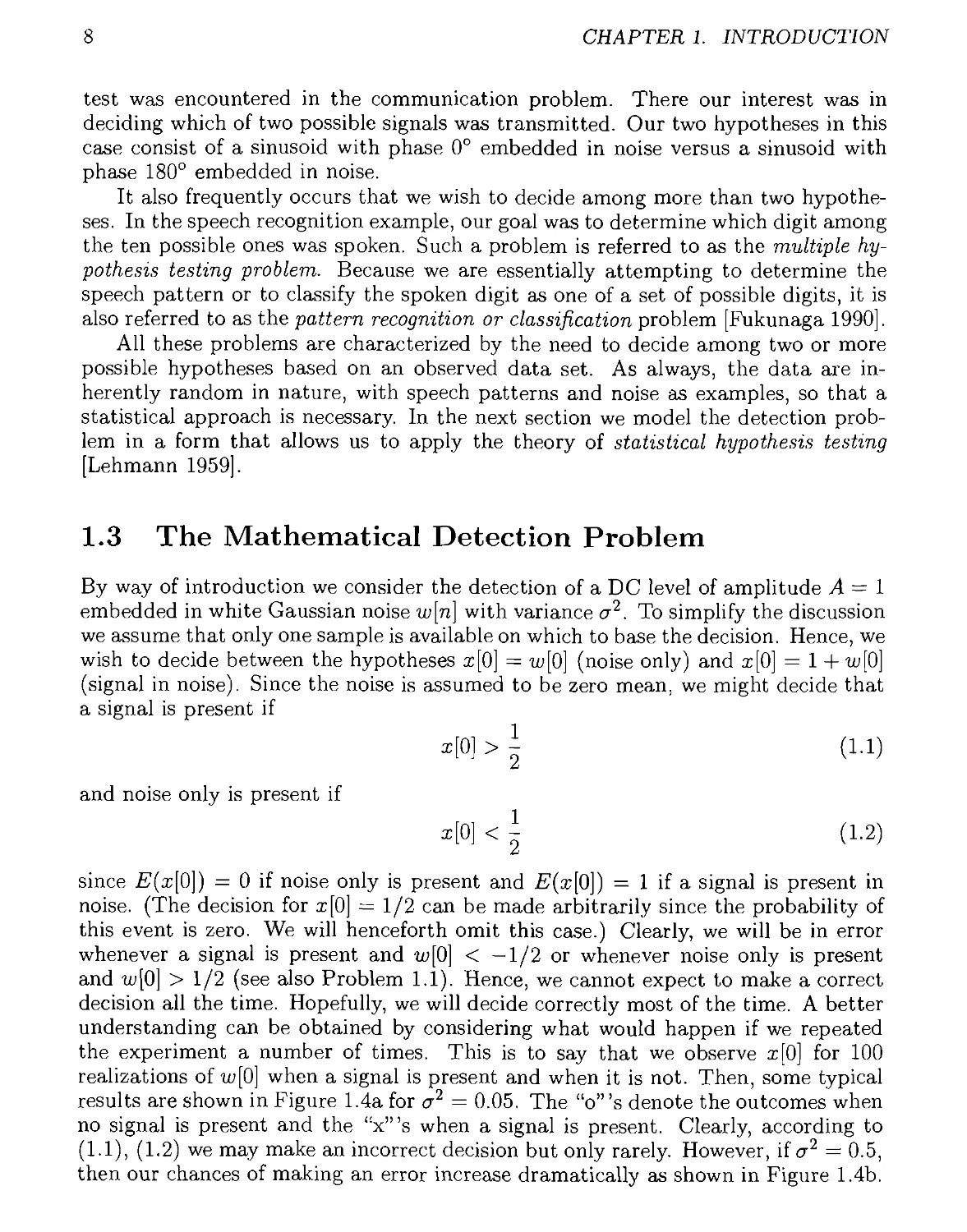
By way of introduction we consider the detection of a DC level of amplitude A = 1
embedded in white Gaussian noise w[n] with variance a2. To simplify the discussion
we assume that only one sample is available on which to base the decision. Hence, we
wish to decide between the hypotheses z[0] = w[0] (noise only) and z[0] = 1 + w[0]
(signal in noise). Since the noise is assumed to be zero mean, we might decide that
a signal is present if
*|0) > ) (11)
£
and noise only is present if
z[0] < | (1.2)
since E^zjO]) = 0 if noise only is present and ^(^[O]) = 1 if a signal is present in
noise. (The decision for z[0] = 1/2 can be made arbitrarily since the probability of
this event is zero. We will henceforth omit this case.) Clearly, we will be in error
whenever a signal is present and w[0| < —1/2 or whenever noise only is present
and w[0] > 1/2 (see also Problem 1.1). Hence, we cannot expect to make a correct
decision all the time. Hopefully, we will decide correctly most of the time. A better
understanding can be obtained by considering what would happen if we repeated
the experiment a number of times. This is to say that we observe x[0] for 100
realizations of w[0] when a signal is present and when it is not. Then, some typical
results are shown in Figure 1.4a for ст2 = 0.05. The “o”’s denote the outcomes when
no signal is present and the 1!x’”s when a signal is present. Clearly, according to
(1.1), (1.2) we may make an incorrect decision but only rarely. However, if a2 = 0.5,
then our chances of making an error increase dramatically as shown in Figure 1.4b.
1.3. THE MATHEMATICAL DETECTION PROBLEM
9
Of course, this is due to the increasing spread of the realizations of w[0] as <r2
increases. Specifically, the probability density function (PDF) of the noise is
p(w[0]) =
1 / 1 2гпЛ
. exp — ——^w 0 .
л/2^2 к 2<т2 L
(1-3)
This is illustrated in Figure 1.5 in which histograms of the data shown in Figure
1.4 have been plotted. The dashed plot is for noise only and the solid plot is for
a signal in noise. The performance of any detector will depend upon how different
the PDFs of z[0] are under each hypothesis. For the same example we plot the
PDFs as given by (1.3) in Figure 1.6 for <r2 = 0.05 and <т2 = 0.5. When noise only
is present, they are
p(z[0]) =
^^exp(-10x2[0])
-^exp(-x2[0])
er2 = 0.05
cr2 = 0.5
and when a signal is embedded in noise, the PDFs are
( rnn_J exP H°W°] “ X)2) °"2 = 0.05
?№]) - | exp _ 1)2) = 0 5_
We will see later that the detection performance improves as the “distance” between
the PDFs increases or as A2/<t2 (the signal-to-noise ratio (SNR)) increases. This
example illustrates the basic result that the detection performance depends on the
discrimination between the two hypotheses or equivalently between the two PDFs
(see also Problems 1.2 and 1.3).
More formally, we model the previous detection problem as one of choosing
between Ho, which is termed the noise-only hypothesis, and Hi, which is the signal-
present hypothesis, or symbolically
Ho : z[0] = w[0] f .
Hi :z[0] = l + w[0].
The PDFs under each hypothesis are denoted by p(x[0]; Ho) and p(x[0]; Hi), which
for this example are
p(x[O];Ho)
p(x[0];Hi)
(1-5)
Note that in deciding between Ho and Hi, we are essentially asking whether z[0]
has been generated according to the PDF p(z[O];Ho) or the PDF p(x[0];Hi). Al-
ternatively, if we consider the family of PDFs
p(x[0]; A) =
-^=exp(-^W0]-4)’)
(1-6)
10
CHAPTER 1. INTRODUCTION
(a)
(b)
Figure 1.4. Realizations of x[0] for signal present and signal
absent (а) ст2 = 0.05 (b) ст2 = 0.5.
1.3. THE MATHEMATICAL DETECTION PROBLEM
1]
(a)
(b)
Figure 1.5. Histograms of x[0] for signal present and signal
absent (a) cr2 = 0.05 (b) ст2 = 0.5.
12
CHAPTER 1. INTRODUCTION
(a)
(b)
Figure 1.6. PDFs of ar[0] for signal present and signal absent
(a) cr2 = 0.05 (b) ст2 = 0.5.
which is parameterized by A, then we obtain p(ar[0];Ho) if A = 0, and p(2}[0];?fi) if
A = 1. We may, therefore, view the detection problem as a parameter test. Given
the observation rr[0], whose PDF is given by (1-6), we wish to test if A = 0 or A = 1
1.4. HIERARCHY OF DETECTION PROBLEMS
13
or symbolically
Hq : A = 0
TYi : A = 1.
(1.7)
This is termed a parameter test of the PDF, a viewpoint that will be useful later
on.
At times it is convenient to assign prior probabilities to the possible occurrences
of TYo and TYi. For example, in an on-off keyed (OOK) digital communication system
we transmit a “0” by sending no pulse and a “1” by sending a pulse with amplitude
A = 1. Hence, the corresponding hypothesis test is given by (1.7). In an actual
OOK system we will transmit a steady stream of data bits. Since the data bits, 0
or 1, are equally likely to be generated by the source (in the long run), we would
expect TYo to be true half the time and TYi the other half. It makes sense then
to regard the hypotheses as random events with probability 1/2. When we do so,
our notation for the PDFs will be p(x[0]|?Yo) and p(rc[0]|7Yi), in keeping with the
standard notation of a conditional PDF. For this example, we have then that
p(x[O]|7Yo)
p(z[0] |7Yi)
which should be contrasted with (1.5) (see also Problem 1.4). This distinction is
analogous the the classical versus Bayesian approach to parameter estimation [Kay-I
1993].
1.4 Hierarchy of Detection Problems
The detection problems we will address will proceed from the simplest to the more
difficult. The degree of difficulty is directly related to our knowledge of the signal
and noise characteristics in terms of their PDFs. The ideal case occurs when we have
exact knowledge of the PDFs. This is explored in Chapters 4 and 5. Then, at least
in theory, we can obtain an optimal detector. When the PDFs are not completely
known, the determination of a good (but possibly not optimal) detector is much
more difficult. This case is discussed in Chapters 7 -9. Another consideration in
designing detectors is the mathematical tractability of the PDF. The Gaussian
PDF is particularly convenient from a theoretical and practical viewpoint and will
be the assumption most often made. In Chapter 10, however, the Gaussian PDF is
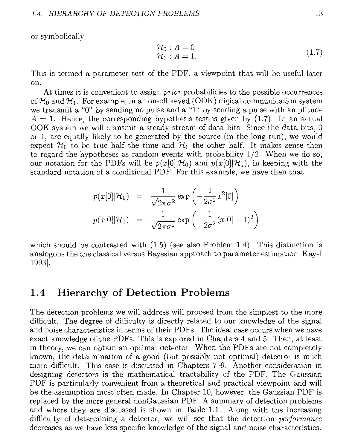
replaced by the more general nonGaussian PDF. A summary of detection problems
and where they are discussed is shown in Table 1.1. Along with the increasing
difficulty of determining a detector, we will see that the detection performance
decreases as we have less specific knowledge of the signal and noise characteristics.
14
CHAPTER 1. INTRODUCTION
I Noise i Signal Gaussian Known PDF Gaussian Unknown PDF NonGaussian Known PDF NonGaussian Unknown PDF
Deterministic Known 4 9 10 *
Deterministic Unknown 7 9 10 *
Random Known PDF 5 9 * *
Random Unknown PDF 8 * * *
* Not discussed (beyond scope of text)
Table 1.1. Hierarchy of detection problems and chapters where discussed.
1.5 Role of Asymptotics
In practice we are principally interested in detecting signals that are weak or signals
whose SNR is small. If this were not the case, then there would be little need
to bother with detection theory in that the signal would not be “buried” in the
noise. This is in contrast to the estimation problem in which we usually desire a
highly accurate estimate. For accurate estimation we are required to control the
SNR so that it is high enough to meet some requirement. It followed then that in
estimation problems an asymptotic or high SNR assumption was sometimes useful.
In detection problems, however, we are generally faced with a low SNR signal so
that our success depends on the data record length. As an illustration, assume we
wish to detect the same DC level as before but we will do so by taking multiple
measurements. Our data then consist of x[n] = w[n] for n = 0,1,..., N — 1 under
TYo and x[n] = A + w[n] for n = 0,1,..., N — 1 under TYi, or more formally we have
the detection problem
TYo : x[n] = w[n] n = 0,1,..., N - 1
TYi : x[n] = A + w[n] n = 0,1,..., N - 1
where w[n] is WGN with variance a2. A reasonable approach might be to average
the samples and compare the value obtained to a threshold 7 so that we would
decide TYi if
1 TV-1
T = й E Ф > т
n=0
(Note that (1-1) is just a special case when N = 1 and 7 = 1/2.) Intuitively, we
expect that as N increases, the detection performance should also increase. To
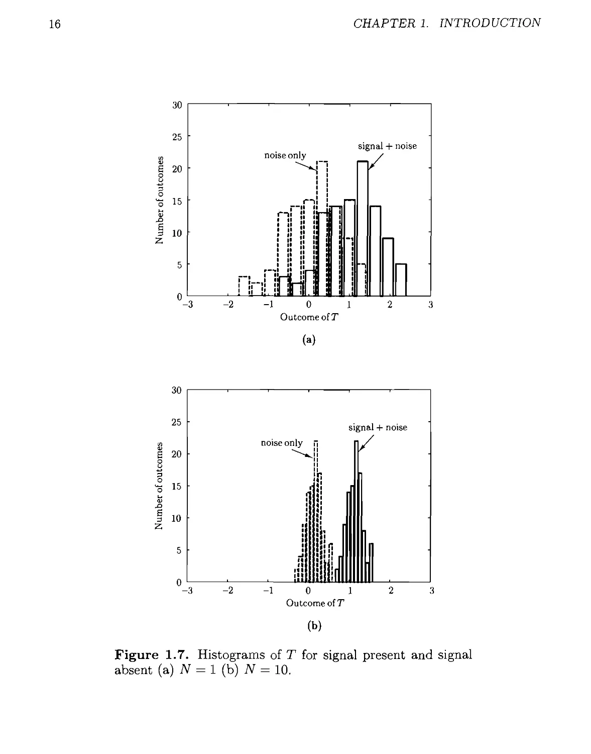
1.6. SOME NOTES TO THE READER
15
justify our intuition we have plotted a histogram of T for N = 1 and N = 10
using ст2 = 0.5 in Figure 1.7. The experiment has been repeated 100 times so that
100 outcomes of T have been generated. It is seen that, as expected, the overlap
between the histograms (which are estimates of the PDFs to within a scale factor)
is less as N increases. To quantify this we use a measure that increases with the
differences of the means or E(T;TYi)— E(T; TYo) and which increases as the variance
of each PDF decreases. Noting that var(T;TYo) = var(T;TYi) (see Problem 1.6) we
have the measure, termed the deflection coefficient,
(£j(T; TYi) - £j(T; TYo))2
var(T; TYo)
It can be shown (see Chapter 4) that the detection performance increases with
increasing d2. For the problem at hand it is easily shown that (see Problem 1.6)
£(T;?Yo) = 0
E(T;?Yi) = A
var(T;TY0) = <t2/N
so that
2 _ A2 _ NA2
d ~ IrffN - ст2
(1-8)
Hence, as intuited, the detection performance improves as the SNR A2/<j2 increases
and/or the data record length N increases. For weak signals, for which А2/ст2 is
small, we require N to be large for good detection performance. This has the effect
of reducing the noise via averaging since the variance of T, which is due to noise,
is ст2/N. As a result, in detection theory asymptotic analysis (as N —> oo) proves
to be appropriate and quite useful. It allows us to derive detectors more easily and
also to analyze their performance. For example, if w[n] consisted of independent
and identically distributed samples of nonGaussian noise, then T would not have
a Gaussian PDF. However, as TV —> oo, we could invoke the central limit theorem
to justify a Gaussian approximation. To determine the detection performance we
would need only to obtain the first two moments of T.
1.6 Some Notes to the Reader
Our philosophy in presenting a theory of detection is to provide the user with the
main ideas necessary for determining optimal detectors, where possible, and good
detectors otherwise. We have included results that we deem to be most useful in
practice, omitting some important theoretical issues. The latter can be found in
many books on statistical theory, which have been written from a more theoret-
ical viewpoint [Cox and Hinkley 1974, Lehmann 1959, Kendall and Stuart 1976-
1979, Rao 1973]. Other books on detection theory that are similar to this one and
16
CHAPTER 1. INTRODUCTION
(a)
(b)
Figure 1.7. Histograms of T for signal present and signal
absent (a) N = 1 (b) N = 10.
REFERENCES
17
which the reader may wish to consult are [Van Trees 1968-1971, Helstrom 1995,
McDonough and Whalen 1995]. In Chapter 11 we provide a “road map” for de-
termining a good detector as well as a summary of the various methods and their
properties. The reader may wish to read this chapter first to obtain an overview.
This text is part of a two-volume series on statistical signal processing. The
first volume, Fundamentals of Statistical Signal Processing: Estimation Theory, is
referenced as [Kay-I 1993]. For a full appreciation the reader is assumed to be
familiar with Volume I, although we have tried to minimize its impact on this text.
When this was not possible, references to Volume I by chapter or page number have
been made.
We have also tried to maximize insight by including many examples and min-
imizing long mathematical expositions, although much of the tedious algebra and
proofs have been included as appendices. The DC level in noise described earlier will
serve as a standard example in introducing almost all of the detection approaches.
It is hoped that in doing so the reader will be able to develop his or her own intuition
by building upon previously assimilated concepts.
The mathematical notation for all common symbols is summarized in Appendix
2. The distinction between a continuous-time waveform and a discrete-time wave-
form or sequence is made through the symbolism rc(t) for continuous-time and ar[n]
for discrete-time. Plots of ar[n], however, appear continuous in time, the points
having been connected by straight lines for easier viewing. All vectors and matrices
are boldface with all vectors being column vectors. All other symbolism is defined
within the context of the discussion.
References
Burdic, W.S., Underwater Acoustic System Analysis, Prentice-Hall, Englewood
Cliffs, N.J., 1984.
Chan, D.S.K, D.A. Langan, S.A. Staver, “Spatial Processing Techniques for the
Detection of Small Targets in IR Clutter,” SPIE, Signal and Data Processing
of Small Targets, Vol. 1305, pp. 53-62, 1990.
Cox, D.R., D.V. Hinkley, Theoretical Statistics, Chapman and Hall, New York,
1974.
Ellenberg, S.S., D.M. Finklestein, D.A. Schoenfeld, “Statistical Issues Arising in
AIDS Clinical Trials,” J. Am. Statist. Asssoc., Vol. 87, pp. 562-569, 1992.
Fukunaga, K., Introduction to Statistical Pattern Recognition, 2nd ed., Academic
Press, New York, 1990.
Gustafson, D.E., A.S. Willsky, J.Y. Wang, M.C. Lancaster, J.H. Triebwasser,
“ECG/VCG Rhythm Diagnosis Using Statistical Signal Analysis. Part II:
Identification of Transient Rhythms,” IEEE Trans. Biomed. Eng., Vol. BME-
25, pp. 353-361, 1978.
18
CHAPTER 1. INTRODUCTION
Helstrom, C.W., Elements of Signal Detection and Estimation, Prentice-Hall, En-
glewood Cliffs, N.J., 1995.
Ives, R.B., “The Applications of Advanced Pattern Recognition Techniques for
the Discrimination Between Earthquakes and Nuclear Detonations,” Pattern
Recognition, Vol. 14, pp. 155 -161, 1981.
Justice, J.H. /‘Array Processing in Exploration Seismology,” in Array Signal Pro-
cessing, S. Haykin, Ed., Prentice-Hall, Englewood Cliffs, N.J., 1985.
Kay, S.M., Fundamentals of Statistical Signal Processing: Estimation Theory,
Prentice-Hall, Englewood Cliffs, N.J., 1993.
Kendall, Sir M., A. Stuart, The Advanced Theory of Statistics, Vols. 1-3, Macmil-
lan, New York, 1976-1979.
Knight, W.S., R.G. Pridham, S.M. Kay, “Digital Signal Processing for Sonar,”
Proc. IEEE, Vol. 69, pp. 1451 1506, Nov. 1981.
Lehmann, E.L., Testing Statistical Hypotheses, J. Wiley, New York, 1959.
McDonough, R.N., A.T. Whalen,Detection of Signals in Noise, 2nd Ed., Academic
Press, 1995.
Proakis, J.G., Digital Communications, 2nd Ed., McGraw-Hill, New York, 1989.
Rabiner, L., B-H Juang, Fundamentals of Speech Recognition, Prentice-Hall, En-
glewood Cliffs, N.J., 1993.
Rao, C.R., Linear Statistical Inference and its Applications, J. Wiley, New York,
1973.
Skolnik, M.I., Introduction to Radar Systems, McGraw-Hill, New York,1980.
Taylor, S., Modeling Financial Time Series, J. Wiley, New York, 1986.
Van Trees, H.L., Detection, Estimation, and Modulation Theory, Vols. I- Hl, J.
Wiley, New York, 1968-1971.
Willsky, A.S., H.L. Jones, “A Generalized Likelihood Ratio Approach to Detection
and Estimation of Jumps in Linear Systems,” IEEE Trans. Automat. Contr.,
Vol. AC-21, pp. 108-112, 1976.
PROBLEMS
19
Problems
1.1 Consider the detection problem
TYo : z[0] = w[0]
TYi : x[0] = 1 + w[0]
where w[0] is a zero mean Gaussian random variable with variance cr2. If the
detector decides TYi if a;[0] > 1/2, find the probability of makirig/ a wrong
decision when TYo is true. To do so, determine the probability of deciding TYi
when TYo is true or Pq = Pr{a;[0] > 1/2; TYo}- For this to be 10-3 what must
cr2 be?
1.2 Consider the detection problem
TYo : ^[0] = w[0]
TYi : x[0] = 1 + w[0]
where w[0] is a uniformly distributed random variable on the interval [—a, a]
for a > 0. Discuss the performance of the detector that decides TYi if rc[0] >
1/2 as a increases.
1.3 We observe the datum rc[O] where ж[0] is a Gaussian random variable with mean
A and variance cr2 = 1. We wish to test if A = Ao or A = —Ao, where Aq > 0.
Propose a test and discuss its performance as a function of Ao-
1.4 In Problem 1.1 now assume that the probability of TYo being true is 1/2. If we
decide TYi is x[0] > 1/2, find the total probability of error or
Pe = Pr{rc[0] > l/2|TY0} Pr{TYo} + Pr{z[0] < l/2|TYi} Pr{TYi}.
Plot Pe versus cr2 and explain your result.
1.5 In Problem 1.1 now assume that we have two samples on which to base our
decision. We decide that a signal is present if
т = Imo] + г[1|) > |.
Determine all the values of ж[0] and ж[1] that will result in a decision that a
signal is present. Plot these values in a plane. Also, plot the point [Р(ж[0]),
Р(ж[1])]7’ assuming TYo is true and then assuming TYi is true. Comment on
the results.
1.6 Verify (1-8) by determining the means and variances of T.
1.7 Using (1.8) determine the number of samples required if the deflection coeffi-
cient is to be d2 = 100 for adequate detection performance and the SNR is
-20 dB.
Chapter 2
Summary of Important PDFs
2.1 Introduction
Evaluation of the performance of a detector depends upon the ability to determine
the probability density function of a function of the data samples, either analytically
or numerically. When this is not possible, we must resort to Monte Carlo computer
simulation techniques. Familiarity with common probability density functions and
their properties is essential to the success of the performance evaluation. In this
chapter we provide the background material that will be called upon throughout the
text. Our discussion is cursory at best due to space limitations. For further details
the reader is referred to [Abramowitz and Stegun 1970, Kendall and Stuart 1976-
1979, Johnson, Kotz, and Balakrishnan 1995], as well as to the specific references
given within the chapter.
2.2 Fundamental Probability Density Functions
and Properties
2.2.1 Gaussian (Normal)
The Gaussian probability density function (PDF) (also referred to as the. normal
PDF) for a scalar random variable x is defined as
— oo < X < oo
(2.1)
where ц is the mean and a2 is the variance of x. It is denoted by Af(/z, ст2) and we
say that x ~ Л/'(^, cr2), where means “is distributed according to.” If ц = 0,
its moments are
E(r")= L1,3'5"'"- 1)"“ "e'™ (2.2)
v ' I 0 n odd. v '
20
FUNDAMENTAL PDFS AND PROPERTIES
21
Otherwise, we use
n—k
where E(xk) is given by (2.2). The cumulative distribution function (CDF) for
p, — 0 and ст2 = 1, for which the PDF is termed a standard normal PDF, is defined
as a, i i
ФМ = /-„^;ет₽ (“/)*
A more convenient description, which is termed the right-tail probability and is the
probability of exceeding a given value, is defined as Q(x) = 1 — Ф(л), where
(2-3)
The function Q(x) is also referred to as the complementary cumulative distribution
function. This cannot be evaluated in closed-form. Its value is shown in Figure
2.1 on linear and log scales. For computational purposes we use the MATLAB
program Q.m listed in Appendix 2C. An approximation that is sometimes useful is
(see Problem 2.2)
QW ~ eXP ( I**) ’ (2'4>
It is shown in Figure 2.2 along with the exact value of Q(x). The approximation
is quite accurate for x > 4. At times it is important to determine if a random
variable has a PDF that is approximately Gaussian. An examination of its right-tail
probability reveals whether this is so. By plotting Q(x) on normal probability paper,
the curve becomes a straight line as shown in Figure 2.3. The normal probability
paper can be constructed as described in Appendix 2B. Also contained there is
the MATLAB program plotprob.m for plotting the right-tail probability on normal
probability paper. As an example, the right-tail probability of the nonGaussian
PDF
/V 11
PM = o^=ex₽
Z V27T
11 / 1 2
-- , exp----x
2 v^T2 \ 2-2
which is a Gaussian mixture PDF, is plotted on normal probability paper in Figure
2.4. The functional form for the right-tail probability is easily shown to be Q(.r)/2 +
Q(l/v/2)/2. The function Q(x) is shown as a dashed straight line for comparison.
If it is known that a probability is given by P = Q("y), then we can determine
7 for a given P. Symbolically, we have 7 — Q~l(P), where Q~i is the inverse
function. The latter must exist since Q(x) is strictly monotonically decreasing.
The MATLAB program Qinv.rn listed in Appendix 2C computes the function Q-1
and can be used to determine 7 numerically.
The multivariate Gaussian PDF of an n x 1 random vector x is defined as
(27r)^deti(C)
exp
(2-5)
22
CHAPTER 2. SUMMARY OF IMPORTANT PDFS
X
(“)
Figure 2.1. Right-tail probability for standard normal PDF
(a) Linear vertical axis (b) Logarithmic vertical axis.
FUNDAMENTAL PDFS AND PROPERTIES
23
Figure 2.2. Approximation to Q function.
Figure 2.3. Q function plotted on normal probability paper.
where p is the mean vector and C is the covariance matrix and is denoted by
.Л/\д, C). It is assumed that C is positive definite and hence C'1 exists. The mean
vector is defined as
[a*]» = E(xi) i = l,2, ...,n
24
CHAPTER 2. SUMMARY OF IMPORTANT PDFS
Figure 2.4. Right-tai] probability for nongaussian PDF on
normal probability paper.
and the covariance matrix as
[C]jj = - E(xiY)(xj - i = 1,2,... ,n; j = 1,2,... ,n
or in more compact form as
C = E[(x-E(x))(x-E(x))T],
Ifp = 0, then all odd-order joint moments are zero. Even-order moments are found
as combinations of second-order moments. In particular, a useful result for ц = 0
is
E(xiXjXkXi) = E(xiXj)E(xkXi) + E(xiXk)E(xjXi) + E(xiXi)E(xjXk). (2.6)
2.2.2 Chi-Squared (Central)
A chi-squared PDF with v degrees of freedom is defined as
{—еД----£2-1exp(— x > 0
22Щ) 2 (2.7)
0 x < 0
and is denoted by Xu- The degrees of freedom v is assumed to be an integer with
v > 1. The function Г(и) is the Gamma function, which is defined as
r(u) = [ tu-1 exp(—t)dt.
Jo
FUNDAMENTAL PDFS AND PROPERTIES
25
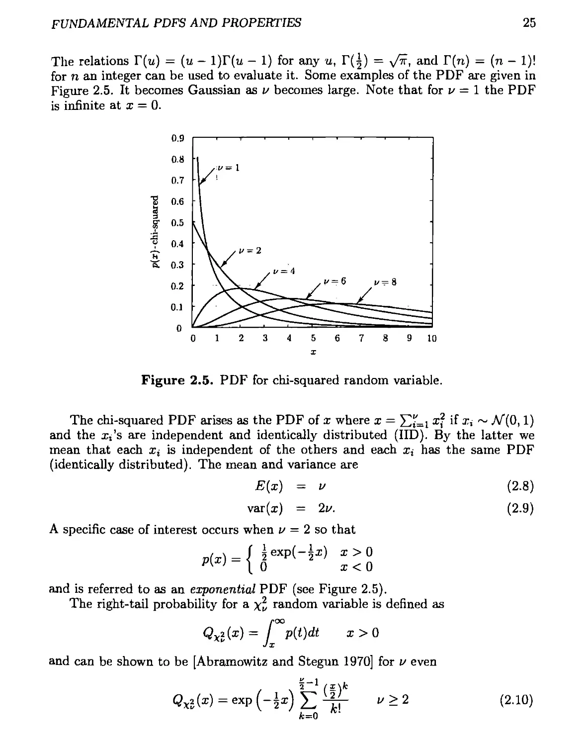
The relations Г(и) = (u — 1)Г(и — 1) for any и, Г(|) = •у/тг, and Г(п) — (n - 1)!
for n an integer can be used to evaluate it. Some examples of the PDF are given in
Figure 2.5. It becomes Gaussian as и becomes large. Note that for v = 1 the PDF
is infinite at x = 0.
Figure 2.5. PDF for chi-squared random variable.
The chi-squared PDF arises as the PDF of x where x = ££=1 xi ~ -^/"(0,1)
and the x^s are independent and identically distributed (IID). By the latter we
mean that each z, is independent of the others and each z, has the same PDF
(identically distributed). The mean and variance are
E(z) = и (2.8)
var(z) = 2v. (2.9)
A specific case of interest occurs when и = 2 so that
exp(—|z) z > 0
pW = ( 3 14 2 I<0
and is referred to as an exponential PDF (see Figure 2.5).
The right-tail probability for a x„ random variable is defined as
Qx2(z) = j p(i)dt z > 0
and can be shown to be [Abramowitz and Stegun 1970] for и even
£ — 1
2 /x\fc
Qx2(z) = exp(-±z) 52 i/> 2 (2.10)
fc=0
26
CHAPTER 2. SUMMARY OF IMPORTANT PDFS
and for и odd
(2-11)
The MATLAB program Qchipr2.in listed in Appendix 2D can be used to numerically
evaluate Qx2(z).
2.2.3 Chi-Squared (Noncentral)
A generalization of the Xv PDF arises as a result of summing the squares of HD
Gaussian random variables with nonzero means. Specifically, if x = x2, where
the z/s are independent and .r, ~ then x has a noncentral chi-squared
PDF with и degrees of freedom and noncentrality parameter A = The
PDF is quite complicated and must be expressed either in integral or infinite series
form. As an integral it is
' . i/—2 г , i .
p(x) = J Ha) 4 exp[-l(z +А)] 7е_!(УА^)
x > 0
x < 0
(2.12)
where 7r(u) is the modified Bessel function of the first kind and order r. It is defined
as
/г(ц) — ----г- / exp(ucos$) sin2r0d# (2.13)
УтгГ(г + Jo
and has the series representation
AW = £
Jt=O
(l-u)2fc+r
А:! Г(г + A + 1) ’
(2.14)
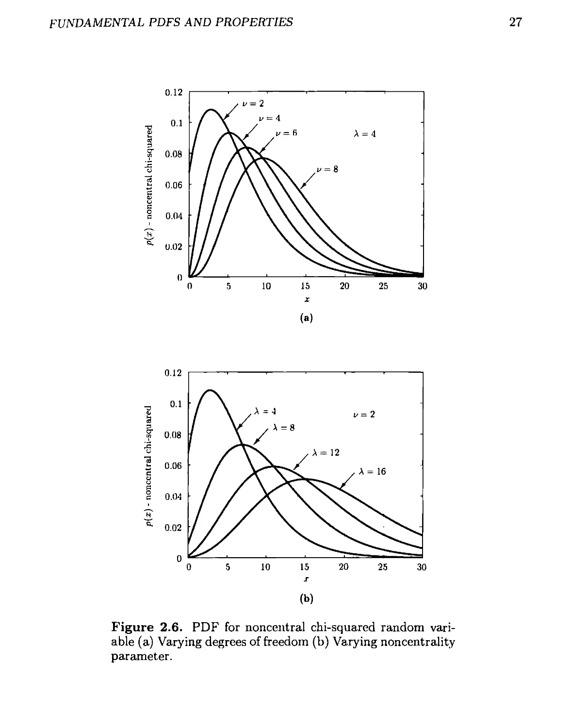
Some examples of the PDF are given in Figure 2.6. Note that the PDF becomes
Gaussian as и becomes large. Using the series expansion of (2.14) the PDF can also
be expressed in infinite series form as
p(z-) =
x* 1 exp[—^(z + A)]
2I и^Щ + fc)
(2-15)
Note that for A = 0, the noncentral chi-squared PDF reduces to the chi-squared
PDF. The noncentral chi-squared PDF with и degrees of freedom and noncentrality
parameter A is denoted by x'u (A).
fundamental pdfs and properties
27
Figure 2.6. PDF for noncentral chi-squared random vari-
able (a) Varying degrees of freedom (b) Varying noncentrality
parameter.
28
CHAPTER 2. SUMMARY OF IMPORTANT PDFS
The mean and variance are
E(x) = v + A
var(x) = 2z/ + 4A. (2.16)
We will denote the right-tail probability as
^x^W^ = /x p^dt x>0
Its value can be numerically determined by the MATLAB program Qchipr2.m given
in Appendix 2D.
2.2.4 F (Central)
The F PDF arises as the ratio of two independent x2 random variables. Specifically,
if
where rri ~ x2,, x2 ~ X22, and -П and x% are independent, then x has the F PDF.
It is given by
( \ 2
I — 1 Mi 1
\Z/2/ I2*1
p(x) = < . . , . x > 0 (2.17)
\ 2 2 J \ V2 )
,0 x < 0
where B(u, v) is the Beta function, which can be related to the Gamma function as
. ВДГ(и)
B(u,v) - . .
Г(и + v)
The PDF is denoted by as an F PDF with 1/1 numerator degrees of freedom
and i/2 denominator degrees of freedom. Some examples of the PDF are given in
Figure 2.7. The right-tail probability is denoted by Qfvi „2 (i) and must be evaluated
numerically [Abramowitz and Stegun 1970]. The mean and variance are
E(x) = 4>2
var(i) = P2 > 4. (2.18)
1>1 (l>2 — 2)2(u2 — 4)
Note that as z/2 —* 00, x —* Xi/>A ~ since i2/t>2 —> 1 (see Problem 2.3).
fundamental pdfs and properties
29
Figure 2.7. PDF for F random variable.
2.2.5 F (Noncentral)
The noncentral F PDF results from the ratio of a noncentral у 2 random variable
to a central x2 random variable. Specifically, if
where X] ~ X^(A) and x2 ~ and %2 are independent, then x has the
noncentral F PDF. It is denoted by F^ iI/2(A) as a noncentral F PDF with i>i
numerator and denominator degrees of freedom and noncentrality parameter A.
Its PDF in infinite series form is
p(x) =
exp
i/i +2k мд
2 ’ 2
• X~2+k 1
(2-19)
Some examples of the PDF can be found in [Johnson and Kotz 1995]. For A — 0
this reduces to the central F PDF (let к = 0 in (2.19)). Its mean and variance are
F(r)
^2(^1 + A)
z/i(z/2 - 2)
1/2 > 2
30
CHAPTER 2. SUMMARY OF IMPORTANT PDFS
var(x) = + + 4>4. (2.20)
(i/2 - 2)2(z/2-4)
The right-tail probability is denoted by Qf^ „2(A)(x) anc^ requires numerical evalu-
ation [Patnaik 1949]. Also, note that asi/2-»oo, F^^X) (see Problem
2.3 ).
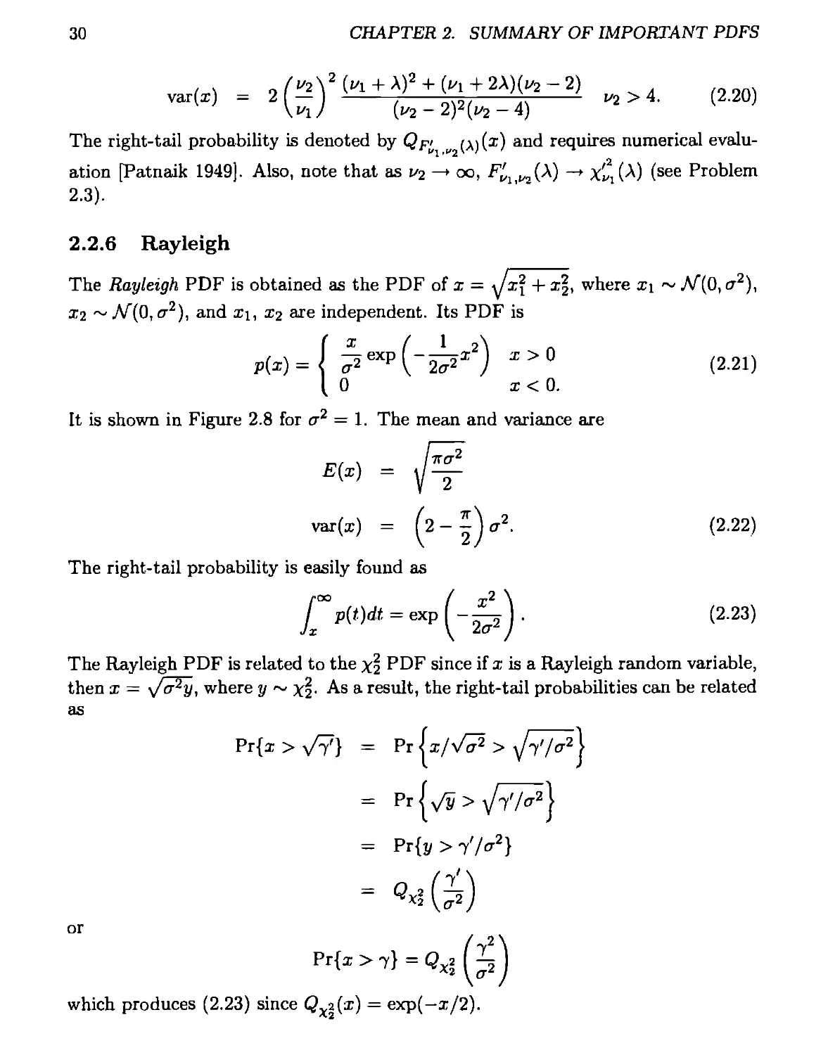
2.2.6 Rayleigh
The Rayleigh PDF is obtained as the PDF of x = H- ^2, where xi ~ Af(0, cr2),
x2 ~ЛГ(0, cr2), and xi, x2 are independent. Its PDF is
f X / 1 л
p(x)=J ^2exp(~2^2x ) X>Q (2.21)
( 0 x < 0.
It is shown in Figure 2.8 for ст2 — 1. The mean and variance are
. /тГСГ2
1 £
var(x) = ^2—^ cr2. (2.22)
The right-tail probability is easily found as
/•°° / x2 \
у p(t)dt = exp ( -^2 J • (2-23)
The Rayleigh PDF is related to the x2 PDF since if x is a Rayleigh random variable,
then x = y/<x2y, where у ~ y2- As a result, the right-tail probabilities can be related
as
Pr{x > x/Y} = Pr lx/y/а2 > /a2}
Pr{x > 7} = QX2
which produces (2.23) since Qxa(x) = exp(—x/2).
fundamental pdfs and properties
31
Figure 2.8. PDF for Rayleigh random variable (ст2 = 1).
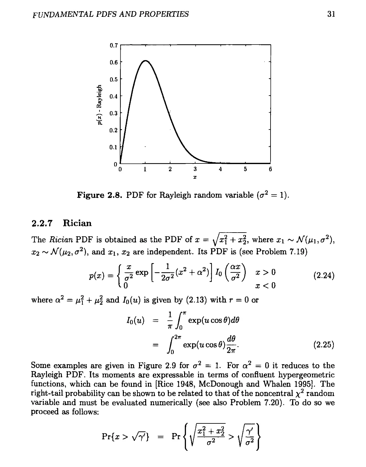
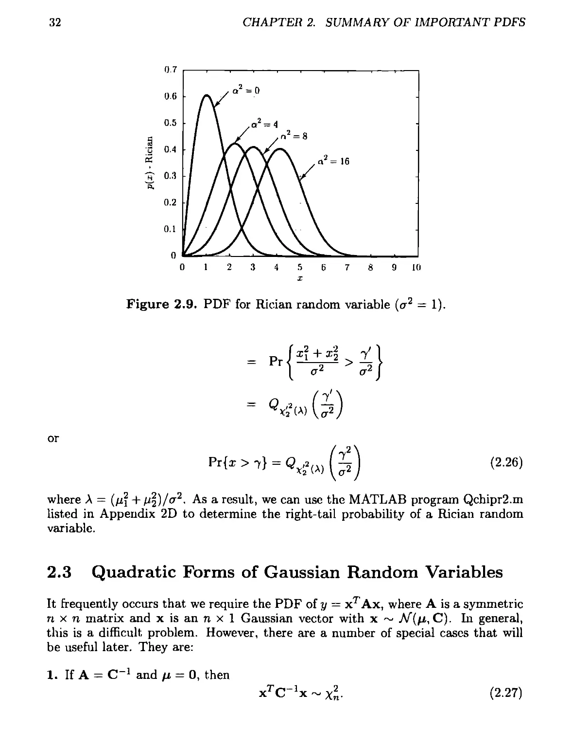
2.2.7 Rician
The Rician PDF is obtained as the PDF of x = у i2 + i^, where Xi ~ A/"(pi,ct2),
X2 ~A/’(№io'2). and ii, X2 are independent. Its PDF is (see Problem 7.19)
p(z) =
X 1 . n _ f Otx\
l^exp + оП?)
lo
i > 0
x < 0
where a2 = p2 + p| and Io(u) is given by (2.13) with r = 0 or
Io(u)
1 fn
— / exp(ucos0)d0
7Г Jo
J2* 7 M do
/ exp(ucos0) —.
Jo 27Г
(2-24)
(2.25)
Some examples are given in Figure 2.9 for ст2 = 1. For a2 = 0 it reduces to the
Rayleigh PDF. Its moments are expressable in terms of confluent hypergeometric
functions, which can be found in [Rice 1948, McDonough and Whalen 1995]. The
right-tail probability can be shown to be related to that of the noncentral x2 random
variable and must be evaluated numerically (see also Problem 7.20). To do so we
proceed as follows:
Pr{i > vV}
Pr
i2 + I2
CT2
32
CHAPTER 2. SUMMARY OF IMPORTANT PDFS
Figure 2.9. PDF for Rician random variable (ст2 = 1).
(xf + x% Y
( a2 a2
/
^(A)
or
(2.26)
where A = (/z2 + p^/a2. As a result, we can use the MATLAB program Qchipr2.m
listed in Appendix 2D to determine the right-tail probability of a Rician random
variable.
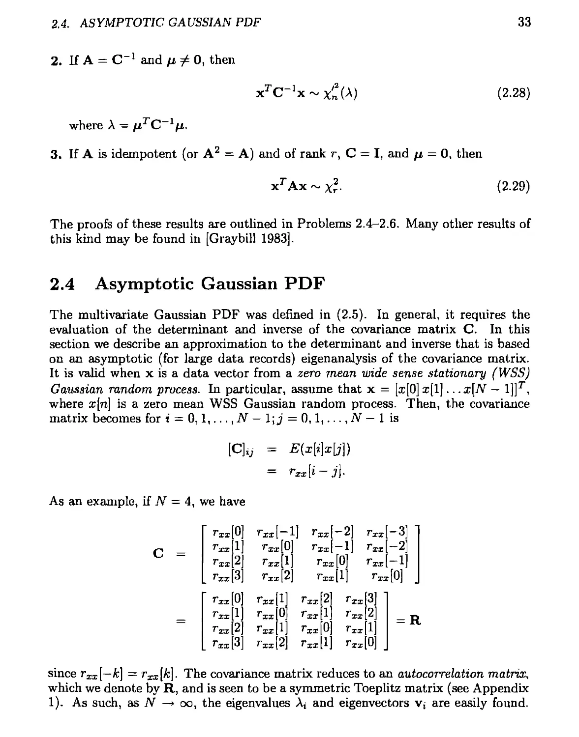
2.3 Quadratic Forms of Gaussian Random Variables
It frequently occurs that we require the PDF of у = xTAx, where A is a symmetric
n x n matrix and x is an n x 1 Gaussian vector with x ~ A/"(/i, C). In general,
this is a difficult problem. However, there are a number of special cases that will
be useful later. They are:
1. If A = C 1 and p = 0, then
xTC
(2.27)
2.4. ASYMPTOTIC GAUSSIAN PDF
33
2. If A = C 1 and p 0, then
xTC-Ix ~ X'n2(A)
where A - pTC 1p.
3. If A is idempotent (or A2 = A) and of rank r, C — I, and p — 0, then
xrAx ~ Xr-
(2.28)
(2.29)
The proofs of these results are outlined in Problems 2.4-2.6. Many other results of
this kind may be found in [Graybill 1983].
2.4 Asymptotic Gaussian PDF
The multivariate Gaussian PDF was defined in (2.5). In general, it requires the
evaluation of the determinant and inverse of the covariance matrix C. In this
section we describe an approximation to the determinant and inverse that is based
on an asymptotic (for large data records) eigenanalysis of the covariance matrix.
It is valid when x is a data vector from a zero mean wide sense stationary (WSS)
Gaussian random process. In particular, assume that x = [x[0] x[l].. .x[N — l]]r,
where x[n] is a zero mean WSS Gaussian random process. Then, the covariance
matrix becomes for i = 0,1,..., N — 1; j = 0,1,..., N — 1 is
[C]ij
^(x[?:]x[/])
j].
As an example, if N — 4, we have
C
0 -] ГХх — 2] Гхх -3] 1
Г11 1 Г XX 0 Г хх ~1] ГХх -2]
Гхх 2 Гхх ] Гх: [0] Гхх -1]
Гхх 3 Гхх 2 Гх: с[1] Гхх [0] J
ГХх 0 Лгх[ Гхх[2 тхх [3]
= Гхх Гхх [1 2 н н ) гхх [0 н* ьГ н н , to = R
Гхх з > Гхх[1 гЖ1[0]
since rXI[—A:] = гхх[й]. The covariance matrix reduces to an autocorrelation matrix,
which we denote by R, and is seen to be a symmetric Toeplitz matrix (see Appendix
1). As such, as N —> oo, the eigenvalues A, and eigenvectors v, are easily found.
34
CHAPTER 2. SUMMARY OF IMPORTANT PDFS
Letting Pxx(f) denote the power spectral density (PSD) of x'[n] we have that as
N —» oo
Ai =
= -^=[ 1 exp(j27r/j) exp(j47r/i) ... exp(j27r(W - 1)Л) ]r (2.30)
for i — 0,1...., N — 1 and fi = i/N. The eigenvalues are equally spaced samples
of the PSD over the frequency interval [0,1] and the eigenvectors are the discrete
Fourier transform (DFT) vectors. (See Problem 2.8 for an example of the deter-
mination of the exact eigenvalues.) The approximation will be a good one if the
data record length N is much larger than the correlation time of x[n]. The latter is
defined to be the effective length of the autocorrelation function (ACF) or letting
M be that length, we require rxx[A:] ss 0 for к > M (see also Problem 2.9). The
derivation of these results can be found in [Gray 1972, Fuller 1976, Brockwell and
Davis 1987]. We next give a heuristic justification. Consider a process whose ACF
satisfies rIX[A;] = 0 for |fc| > 2. This is termed a moving average process of order
one (see Appendix 1). Then, an eigenvector v = [t>o vj ... vy_i]T of R must satisfy
‘ rxx[0] rxx[-l] 0 0 ... O' r- - -
rM[l] rxx[0] rxx[-l] 0 ... 0 ^0 V] Vo 1'1
= A
0 ... о rJT[l] rXI[0] rxx[-l]
0 0 ... 0 rxx[l] rxx[0] W]V-1 V/V—1
or
Tzx[O]vo + rXI[-l]U] = A Vo
rxx[l]vo + rxx[0]vi 4- rIX[-l]v2 = Avi
>’м[1]1’У-3 -I- Гхх[0]иу_2 + rIX[-l]VjV_] = AvjV-2
Гц[1]и?/-2 + rIX[0]vy-i - Avy-].
Ignoring the first and last equations, we have
rix[l]vn_i 4-ra.a.[0]vn + ra:x[-l]vn+1 = Av„ n = 1,2,... AT-2. (2.31)
This homogeneous difference equation is satisfied for 1 < n < N - 2 by vn —
exp(j'27r/n) since then
rIa:[l] exp(—j2tf/) exp(j27r/n) + rxx[0] ехр(;2тг/п)
+ rXi[—1] exp(j’27r/) ехр(л'2тг/п) = Аехр(;2тг/п)
2.4. ASYMPTOTIC GAUSSIAN PDF
35
where
A = r „ [1] exp(-j’27r/) + rxxlO] + ^[-1] ехр(;2тг/)
= 52 rxx[k]exp(-j2irfk) = PXI(f).
k=—oa
Apart from the n = 0 and n = N — 1 equations, the eigenvector is seen to be
[1 ехр(у27г/)... exp(J2irf(N - 1))]T. If we choose fa = i/N for г = 0,1,..., /V — 1,
then we can generate W eigenvectors
vt=-^=[l ехр(>2тгЛ) exp(j47r/i) exp(j’27r(Af - 1)/,) ]T
VN
that are orthonormal as required (see Problem 2.10) and whose corresponding eigen-
values are AT = Pxx(fa)- Clearly, the fact that the first and last equations are in
error will not matter nsN -> oo. (See Problem 2.8 for the exact eigenvalues.) Also,
note that the eigenvectors have been chosen to be complex, even though R is a real
matrix. We could also have represented the eigenvectors in terms of real sines and
cosines (see Problem 2.11), although the complex representation is much simpler.
Since Vtf-i — v* and PXx(.fN-i) = Fxx(fa), the complex eigendecomposition
N-l
r = 52 (2-32)
i=0
where H denotes the complex conjugate transpose will actually produce a real
matrix. See also Problem 2.12 for a simple heuristic derivation of this decomposition.
With the approximation of (2.30) we can now evaluate the determinant and
inverse of R quite simply. It follows that (see Problem 2,13)
det(R) N-l N-l = П = П Pxz(fa) (2.33)
R"1 t=0 i=0 jV-1 , /V-l = E r-v" = S Йл v.v.« i=0 Al i=0 (2-34)
These expressions will be useful in approximating detectors. Additionally, they
can be used to determine an asymptotic form for the Gaussian PDF under the
assumption that i'[n] is zero mean and WSS. From (2.5) with x — [t[0] x[1] ... -
1]]T and (i — 0 we have
W 1 1 T 1
lnp(x) =-—1п2тг — - Indet(R) —-xrR xx
Ct и и
36
CHAPTER 2. SUMMARY OF IMPORTANT PDFS
and using (2.33) and (2.34)
N 1 N—i i ]
lnp(x) = -y In 2тг - - In П Рхх(Л) - -xr 52 p V4vf X
2 Z i=0 z i=0
N 1 N“1 1 yv*1 1
But
where /(/) is termed the periodogram (see [Kay 1988], [Kay-I 1993, pg. 80]). Hence
N 1 / I( f ) \
lnp(x) = - — 1п2тг- - 52 (ln^rr(A)+p •
2 z I=o V r'zxyJO/
(2.35)
An equivalent form is
bp(x) = -у 1п2тг - у 52 J
z Z i=0 ' ^xxkJrJ/ 7V
and as JV —* oo, this becomes
JV TV fl / I(f} \
l„P(x) = ——1п2я - y Д (1пР„(Л + j^j) If-
(2.36)
This was derived in [Kay-I 1993, Appendix 3D] using an alternative approach. The
reader may also wish to refer to [Kay-I 1993, Section 15.9] for the approximate
eigenanalysis in the complex data case.
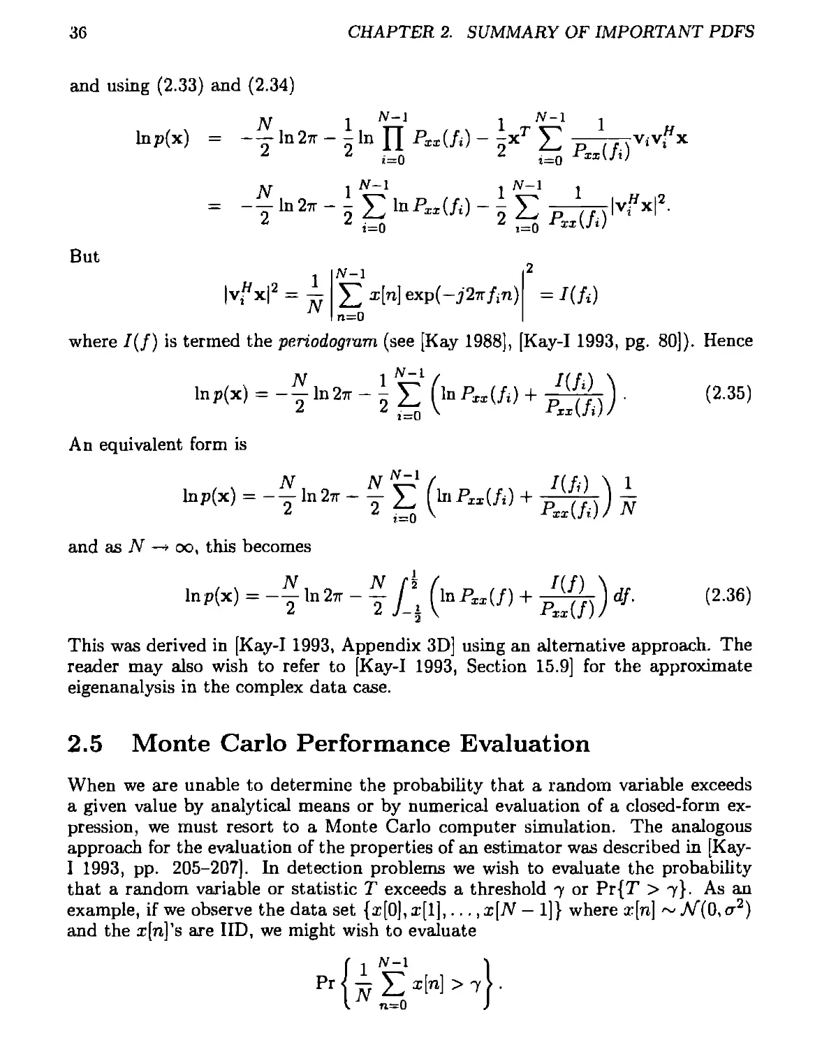
2.5 Monte Carlo Performance Evaluation
When we are unable to determine the probability that a random variable exceeds
a given value by analytical means or by numerical evaluation of a closed-form ex-
pression, we must resort to a Monte Carlo computer simulation. The analogous
approach for the evaluation of the properties of an estimator was described in [Kay-
I 1993, pp. 205-207]. In detection problems we wish to evaluate the probability
that a random variable or statistic T exceeds a threshold 7 or Pr{T >7}. As an
example, if we observe the data set {x[0], a’[l],..., nc[JV — 1]} where a:[n] ~ A/”(0, a2)
and the i[n]’s are HD, we might wish to evaluate
Pr
1 N-l
jv 12 Ф]
n=0
2.5. MONTE CARLO PERFORMANCE EVALUATION
37
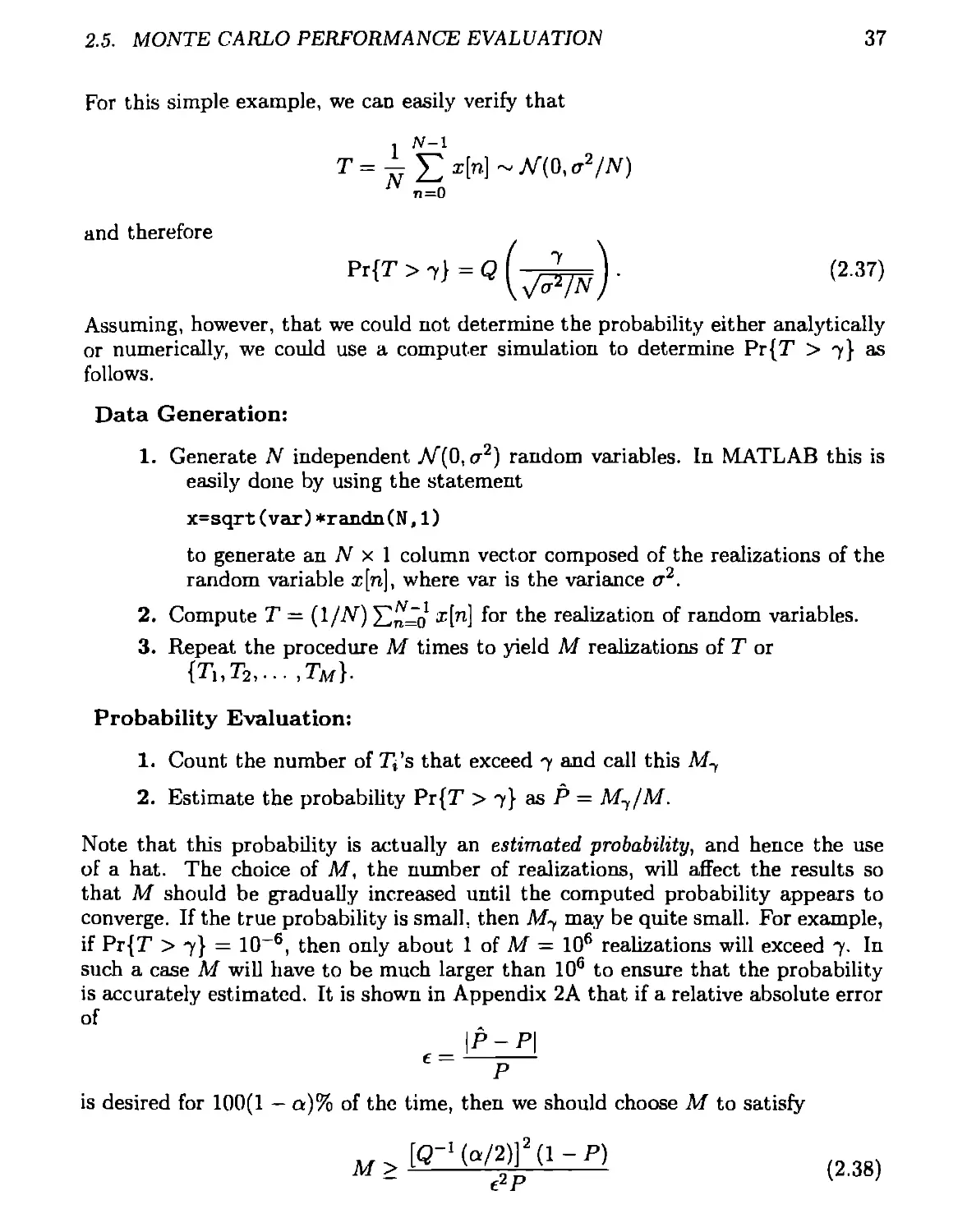
For this simple, example, we can easily verify that
, N-L
71=0
and therefore
Рг(г>^ = <гЫж)- (237)
Assuming, however, that we could not determine the probability either analytically
or numerically, we could use a computer simulation to determine Pr{T > 7} as
follows.
Data Generation:
1. Generate N independent A/"(0, cr2) random variables. In MATLAB this is
easily done by using the statement
x=sqrt(var)*randn(N,1)
to generate an A x 1 column vector composed of the realizations of the
random variable r[n], where var is the variance a2.
2. Compute T = (1/A) x[n] f°r the realization of random variables.
3. Repeat the procedure M times to yield M realizations of T or
{ТьТг,... ,TM}.
Probability Evaluation:
1. Count the number of T,’s that exceed 7 and call this M-,
2. Estimate the probability Pr{T > 7} as P = M-JM.
Note that this probability is actually an estimated probability, and hence the use
of a hat. The choice of M, the number of realizations, will affect the results so
that M should be gradually increased until the computed probability appears to
converge. If the true probability is small, then My may be quite small. For example,
if Pr{T > 7} = 10~6, then only about 1 of M = 106 realizations will exceed 7. In
such a case M will have to be much larger than 106 to ensure that the probability
is accurately estimated. It is shown in Appendix 2A that if a relative absolute error
of
|P~P|
P
is desired for 100(1 — a)% of the time, then we should choose M to satisfy
c2p
(2.38)
38
CHAPTER 2. SUMMARY OF IMPORTANT PDFS
where P is the probability that is being estimated. The required number of re-
alizations is valid for determining Pr{T > 7} using the Monte Carlo realizations
{Ti, T2,..., ?m}, where the realizations are obtained from the generation of in-
dependent random variables. The random variables T, need not be Gaussian in
general, but only UD. As an example, if we wish to determine Pr{T > 1}, which
can be shown to be 0.16, with a relative absolute error of e = 0.01 (1%) for 95% of
the time, then
[<?--(0.025))2 (1-0.16) s
(0.01)20.16
When this approach is impractical, one can use importance sampling to reduce the
computation [Mitchell 1981].
As an example of the Monte Carlo evaluation of (2.37) let N = 10 and a2 —
10. In Appendix 2E we list the MATLAB program montecarlo.m that determines
Pr{T > 7}. We plot the results versus 7 as well as the true right-tail probability
which is <3(7) from (2.37) in Figure 2.10. The number of realizations was chosen to
be M = 1000 in Figure 2.10a and M = 10,000 in Figure 2.10b. The true right-tail
probability as given by (2.37) is shown as a dashed curve while the Monte Carlo
simulation result is shown as a solid curve. The slight discrepancy for M — 1000 is
attributed to statistical error since for M = 10,000 the agreement is much better.
References
Abramowitz, M., LA. Stegun, Handbook of Mathematical Functions, Dover Pub.,
New York, 1970.
Brockwell, P.J., R.A. Davis, Time Series: Theory and Methods, Springer-Verlag,
New York, 1987.
Fuller, W.A., Introduction to Statistical Time Series, J. Wiley, New York, 1976.
Gray, R.M. “On the Asymptotic Eigenvalue Distribution of Toeplitz Matrices,”
IEEE Trans. Inform. Theory, Vol. IT-18, pp. 725-730, Nov. 1972.
Graybill, F.A., Matrices with Applications in Statistics, Wadsworth, California,
1983.
Johnson, N.L., S. Kotz, N, Balakrishnan, Continuous Univariate Distributions,
Vols. 1,2, J. Wiley, New York, 1995.
Kay, S.M., Modem Spectral Estimation: Theory and Application, Prentice-Hall,
Englewood Cliffs, N.J., 1988.
Kendall, Sir M., A. Stuart, The Advanced Theory of Statistics, Vols. 1-3, Macmil-
lan, New York, 1976-1979.
REFERENCES
39
(a)
(b)
Figure 2.10. Monte Carlo computer simulation of Pr{T > 7}
(a) M = 1000 (b) M = 10,000.
40
CHAPTER 2. SUMMARY OF IMPORTANT PDFS
McDonough, R.N., A.T. Whalen, Detection of Signals in Noise, Academic Press,
New York, 1995.
Mitchell, R.L., “Importance Sampling Applied to Simulation of False Alarm Statis-
tics,” IEEE Trans. Aerosp. Elect. Syst., Vol. AES 17, pp. 15-24, Jan. 1981.
Mitchell, R.L., J.F. Walker, “Recursive Methods for Computing Detection Proba-
bilities,” IEEE Trans. Aerosp. Elect. Syst., Vol. AES-7, pp. 671-676, July
1971.
Patnaik, P.B., “The Non-central y2- and F- distributions and their applications,”
Biometrika, Vol. 36, pp. 202-232, 1949.
Rice, S.O., “Statistical Properties of a Sinewave Plus Random Noise,” Bell System
Tech. Jour., Jan. 1948.
Problems
2.1 Show that if T ~ Af(/2, ст2), then
Pr{T>7} = Q(l^y
\ (T /
2-2 Derive (2.4) by noting that
roo J / i \
O(I)=A ^1ирПТ
and using integration by parts. Also, explain why the approximation improves
as x increases.
2.3 Show that as —» oo, an FVJiI/2 random variable becomes а random
variable.
2.4 Verify (2.27) by letting C-1 — DTD, where D is a whitening filter matrix (see
[Kay-I 1993, Chapter 4]).
2.5 Verify (2.28) by the same approach as in Problem 2.4.
2.6 Verify (2.29) by noting that if A is an idempotent matrix of rank r, it is a
symmetric matrix with orthonormal eigenvectors and r eigenvalues equal to
one and the remaining ones equal to zero.
2.7 In this problem we show that if R is an N x N autocorrelation matrix corre-
sponding to the nonwhite PSD PXX(J), then the eigenvalues of R satisfy
-Ptx(/)mIN < A < Ргт(/)мАХ
PROBLEMS
41
where Pii:(/)min and Prz(f)MAX are the minimum and maximum values of
the PSD of x[n], respectively. To do so note that
uTRu
AMAX = max—
where u = [u[0] u[l]... u[N - 1]]T and show that
.i
urRu = \ \U(f)\2Pxx(f)df
J~2
uTu - [\\U(f)\2df
J~2
where U(f) = ^2^=0 exp(— j2irfn). Then, conclude that
A < Amax < Ptz(/)max-
Similarly, show that A > Pei(/)min by utilizing
. urRu
Amin = nuu——•
u UJ U
2.8 In this problem we derive the exact eigenvalues for an autocorrelation matrix
whose elements are
[R]mn = n]
where
Гц[А;] —
cr2(l + b2[l]) fc = 0
cr2^!] k = 1
0 k > 2.
This is a moving average process of order one (see [Kay 1988]). Its PSD is
easily shown to be
Pxx(f) = Гц[0] + 2гц[1] COS27T/.
The equation to be solved for the eigenvalues is (R — AI)v = 0, where v is
an eigenvector. Equivalently, for rIX[l] 0 (since Pxx(f) is assumed to be
nonwhite), we need to solve
R- AI\
Гц[1] /
v = 0.
42
CHAPTER 2. SUMMARY OF IMPORTANT PDFS
Letting c = [fuiO] - X)/rxx [1], we have to find the solutions of Av = 0, where
R-Al
’Cr.r[l]
c 1 0 0 0
1 c 1 0 0
0 0 1 c 1
0 0 0 1 c
Using the results from Problem 2.7 show that for rxx[l] > 0
2 [0] - -Pzx(/)mAX Txx [0] - -Pzx(/)mIN „
rxx[l] r„[l]
Similary, for rxx[l] < 0 we have that —2 < c < 2. The equations to be solved
Av = 0 lead to the homogeneous equation set
t'l + CVq = 0
vn + cvn-i + vn-2 = 0 n = 2,3,... ,7V - 1
V/V-2 + — 0
where v = [voi'i - • vn-i]t- Since |c| < 2, the solutions of the homogeneous
difference equation for n = 2,3,..., N-1 are given by zn, where z — exp(±ji9)
and c — -2cosl9. Hence, the solution is vn = Aexp(j6n) + A* exp(-jf)n) for
any complex A and some в. Next show that l9 must satisy
2тгт
2(7V + 1)
m = 0,1,..., 27V+ 1
for the first and last equations to hold. (Note that cos в is periodic with period
2(/V + 1)). For distinct eigenvalues and hence orthogonal eigenvectors, as well
as to satisfy the constraint |c| < 2. we choose
( 1,3,5,...,7V,7V + 3,JV + 5,...,22V for N odd
( 1,3,5,..., N, N + 2, N + 4...., 2N for TV even.
Finally, show that the eigenvalues are given by
Лтг[0] “1“ 2rZI[l]cos
2тгт
2(7V + 1)
Note that Xi « Pxx{fi) for large N.
2.9 The correlation time of a WSS random process is defined as the value of M
for which |rxa:[M]|/ria..[0] is suitably small, say 0.001. For the WSS random
process whose ACF is гхх[Л] = 0.9^, determine the correlation time. Next,
consider the process x[n] = A where A ~ A/"(0, tr^). Show that the process is
WSS. What is the correlation time of the process? Does this process have the
asymptotic eigendecomposition of (2.30)?
PROBLEMS
43
2.10 The normalized DFT exponential vectors are given by
V» = [ 1 exp(j27r/j) ... exp(j27r/i(N - 1)) ]T
for i = 0.1,..., N — 1 and where — i/N. Prove that they are orthonormal
or that
и f 1 m - n
| 0 m n
2.11 In this problem we obtain a set of real eigenvectors for an autocorrelation
matrix R as N —+ oo. We assume that N is even to simplify the results. Using
(2.30) we first express the asymptotic eigenvectors as V/ = (с/ + js^/^/N,
where
Ci = [ 1 cos(27r/j) ... cos[27r/i(2V — l)j ]7
Si = [0 sin(27r/,) ... sin[27r/i(W - 1)] ]T
and fi — i/N. Noting that sq = s^/a = 0 and сдг_, — c,, s/v_t = — s(, show
that
N-i
R = E Pxz(/i)Viv"
»=0
IN ._____iN / £ IN
Next show that the set of vectors
Co Cl Si c/y/2—i sN/2-1 C/y/2 1
jNjz' y/Nj2'"'' y/Nj2' yfN/2' у/n J
is orthonormal using the results of Problem 2.10 and hence are the real eigen-
vectors. Finally, determine the corresponding eigenvalues.
2.12 A simple heuristic derivation of the asymptotic eigendecomposition of an au-
tocorrelation matrix is examined in this problem. First argue that
1 N-1
[R]mn = rIX[m - n] « — E exp[j27r/,(m - n)]
/v »=0
where fi — i/N and the approximation holds for large N. Then show that
this is equivalent to
JV-1
[R]mn = E
t=0
44
CHAPTER 2. SUMMARY OF IMPORTANT PDFS
where
Vi = --L [ 1 ехрО’2тгЛ) ... exp(j2itfi(N - 1)) ]T
and note that the v/s are orthonormal (see Problem 2.10). Finally, derive
(2.32) and identify the eigenvalues and eigenvectors.
2.13 Show that if R has the eigendecomposition given by (2.32), then
det(R)
R'1
2.14 Modify the MATLAB program montecarlo.m in Appendix 2E to determine
Pr{(l^)E^-Q1z2[n] > 5} if х[тг] ~ А/"(0,5), N = 50, and the samples are
IID. Compare your results against the theoretical probability. Hint: Use the
central limit theorem.
2.15 A detection probability Pp is to be determined via a Monte Carlo computer
simulation. It is known that Pd > 0.8. If the relative absolute error is to
be no more than 0.01 for 95% of the time, how many Monte Carlo trials are
required?
Appendix 2A
Number of Required Monte
Carlo Trials
We estimate P = Pr{T > 7} as P = M7/M, where M is the total number of trials
(or realizations) and is the number of trials for which T > 7. We first determine
the PDF of P. Define a random variable & as follows
Г 1 if Tt > 7
- } 0 if Ti < 7
where Ti is the outcome of the г th trial. The random variable £, is a Bernoulli
random variable with the probability of success (& = 1) as P. Thus, = P and
a natural estimator of P is the sample mean or
_ 1 M
Since the £t’s are IID, we can invoke the central limit theorem to assert that P is
approximately Gaussian for large M. Its mean is
1 M
E(p) =
2=1
M
2=1
and its variance is
/ ! w \
var(P) =
45
46
CHAPTER 2. SUMMARY OF IMPORTANT PDFS
var(&)
M
since the £i’s are IID and hence uncorrelated and all have the same variance. But
var(£) = E(£)-E2(£,-)
= I2 • Pr{7i > 7} - (1 • Pr{7i > 7})2
= P - p2 = P(1 - p)
and thus
and finally we have
The relative error e = (P — P)/P then has the PDF
P-P a Af/n i-P\ e = ~ Jv 0, I . P I MP J
To guarantee that this is not more than e in absolute value for 100(1 — a)% of the
time we require Pr{|e| > e} < q
or 2 Pr{e > e} < a
which results in 2Q 1 ] < a. 1 /1-Р / — X V mp /
Solving for M produces the requirement
[Q-4a/2)]2(l - P)
e2p
Appendix 2B
Normal Probability Paper
To construct normal probability paper for which Q(x) will appear as a straight line,
we first choose the vertical axis range. Typically, we choose the interval [0.0001,
0.9999]. The vertical axis is labeled with the values {г/1,3/2, • • , уь}, where yi =
0.0001 and y^, = 0.9999. Also, L is chosen to be odd and yt = 1 — so that
У(£+1)/2 — 0-5. For the MATLAB program that follows L = 11 and
у = [0.0001 0.001 0.01 0.1 0.3 0.5 0.7 0.9 0.99 0.999 0.9999]7.
The horizontal axis will be the interval [—as shown in Figure
2.11. For у — Q(x) to appear as a straight line we must warp the у values so that
they become Yj — mQ~1(yi) + 1/2. The slope m is found from Figure 2.11 as
_ 2^-1
m iQ-'tyiY
To plot the point (x\, yt) we convert it to = (тг, mQ~l (у») +1/2). To obtain
the true у values (before warping) we put tick marks at Yt — + 1/2 but
label them as yi. The MATLAB program plotprob.m listed below plots the right-
tail probability on normal probability paper. If desired, the Gaussian right-tail
probability Q(x) can also be plotted for comparison.
plotprob.m
function plotprob(x,Qx,xlab,ylab,nor)
7. This program plots a set of right-tail probabilities
7. (complementary cumulative distribution function) on normal
7. probability paper.
7.
7. Input Parameters:
7.
47
48
CHAPTER 2. SUMMARY OF IMPORTANT PDFS
Figure 2.11. Construction of a normal probability paper.
7, x - Real column vector of x values for desired
7, right-tail probabilities
7, Qx - Real column vector of corresponding
7, right-tail probabilities
7. xlab - Label for x axis (enclose in single quotes)
7. ylab - Label for у axis (enclose in single quotes)
7. nor - Set equal to 1 for Gaussian right-tail probability
’/, to be plotted for comparison, and 0 otherwise
7.
7. Verification Test Case:
7.
7. The inputs x= [-5:0.01:5] ’ ;Qx=0.5*Q(x)+0.5*Q(x/sqrt(2));
7. xlab=’x’; ylab=’Right-tail Probability’;nor=l;
7. should produce Figure 2.4.
7.
7. Set up у-axis values.
y=[0.0001 0.001 0,01 0.1 0.3 0.5 0.7 0.9 0.99 0.999 0.9999]’;
7, Set up x-axis limits.
xmax=Qinv(min(y));
7. Warp у values for plotting.
m=(2*min(y)-l)/(2*xmax);
Y=m*Qinv(Qx)+0.5;
7. Check to see if Q(x) (Gaussian right-tail probability)
7. is to be plotted.
APPENDIX 2B
49
if nor==l
xnor= [-xmax: 0.01: xmax] ’;
ynor=m*xnor+0.5;
plot(x, Y, ’ - ’ ,xnor,ynor,’—’)
else
plot(x.Y)
end
xlabel(xlab)
ylabel(ylab)
axis([-xmax xmax min(y) max(y)J);
’/, Determine у tick mark locations by warping.
Ytick=m*Qinv(y)+0.5;
7, Set up у axis labels.
t=[’0.0001’;’ 0.001’;’ 0.01’;’ 0.1’;’ 0.3’;’
’ 0.7’;’ 0.9’;’ 0.99’;’ 0.999’;’0.9999’];
set(gca,’Ytick’,Ytick)
set(gca,’Yticklabels’,t)
grid
0.5’; . ..
Appendix 2С
MATLAB Program to Compute
Gaussian Right-Tail Probability
and its Inverse
Q.m
function y=Q(x)
70 This program computes the right-tail probability
7. (complementary cumulative distribution function) for
7, a N(0,l) random variable.
7.
7. Input Parameters:
7.
7. x - Real column vector of x values
7,
7» Output Parameters:
7.
7» у - Real column vector of right-tail probabilities
7.
7. Verification Test Case:
7.
7. The input x=[0 1 2]’; should produce y=[0.5 0.1587 0.0228]’.
7.
y=0.5*erfc(x/sqrt(2)) ;
50
APPENDIX 2C
51
Qinv.m
function y=Qinv(x)
7, This program computes the inverse Q function or the value
7, which is exceeded by a N(O,1) random variable with a
7, probability of x.
7.
7. Input Parameters:
7,
7, x - Real column vector of right-tail probabilities
7, (in interval [0,1])
7.
7, Output Parameters:
7,
7» у - Real column vector of values of random variable
7.
7. Verification Test Case:
7.
7, The input x=[0.5 0.1587 0.0228]’; should produce
7. y=[0 0.9998 1.9991] ’.
7,
y=sqrt(2)*erfinv(l-2*x);
Appendix 2D
MATLAB Program to Compute
Central and Noncentral y2
Right-Tail Probability
The MATLAB program listed in this appendix computes the right-tail probability
of a x'u (A) random variable. To obtain the result for a central y2 random variable
or for y2, let A = 0. The algorithm is based on a similar one described in [Mitchell
and Walker 1971].
From (2.15) we have
, x = Y» exp(-A/2)(A/2)fe xvl2+k^ exp(-jx)
P T - fc! 2p/2+fer(i//2 + k) '
The right-tail probability is
= / p^dt
~ exp(-A/2)(A/2)fe r°° t^2+k~l exp(-^t)
Ы Jx 2u/'i+kV(y/2 + k)
But the integral is just Qx2 ^(t), the right-tail probability for a central x2+2fc
random variable and is given by (2.10) and (2.11). Hence
O M_v-exp(“A/2)W2>‘n м imn
k=0
52
APPENDIX 2D
53
We consider two cases, depending upon whether и is even or odd. First assume и
is even. Then, v + 2k is also even and (2.10) applies. Letting m = v -h 2k we have
21 — 1
Qx2m^ = exp(-a:/2) £
<=o
To develop a recursion for this term we observe that
TH - Z I
exp(-x/2)
l=Q
Qx^2(z) + 0M-
+ exp(-x/2)(.^2)2i.|
But
x/2 exp(-x/2)(x/2)m22 1
Л,
so that
g(x,m) =g(x,m-2)
TTL 2»
and the recursion is initialized by
Qx2(s) = g(x, 2) = exp(—z/2).
Now for v odd, m = и + 2k will also be odd, and (2.11) applies. Thus,
. X 9O( /?! + expH1) V “ l)!(2:r)f-i
Q'^
and assuming that v > 3 so that m = v + 2k > 3, we have from (2D.1)
exp(—A/2)(A/2)fc Г 1
2Q(s/x) + Q2 (i)
*i/+2fc
(2/ - 1)!
since
OO
fc=o
kl
A:^V'eXp("A/2)(A/2)feO'
2Q(^) + X----------------Qx.2k
kl
f<^=exp(A/2).
fc=0 K'
x
m = 1
54
CHAPTER 2. SUMMARY OF IMPORTANT PDFS
To develop a recursion for Q' 2 (z), assuming m odd
Am
Q'x^x)
exp(—z/2)
У «-Di (2z)/-j
ti (2/-!)!
exp(—x/2)
ч/тг
1=1
2
7Г
, _ . IM— * I
-(2X) 2 2
v A^ + g^rn).
Am -2
But
_g(x, m)
7Г (m — 2)1
— 2 x '----
(m — 2) (m. - 3)
X
= g(x,m-2)~—-
m — 2
(S7^4)!(2:c) 1
where the recursion is initialized with
Q'^) = S^-3) = /^ехР(-ж/2)-
If v = 1, then for к = 0, we have m — v + 2k = 1. In this case
Qx2m^ = 2<?(^)
so that
Q'2(x) = 0.
A]
To determine how many terms of the sum are required, we choose the first M+1
terms so that the truncation error is less than e. To find M we have from (2D.1)
fc!
“ exp(—A/2)(A/2)fc
^+2k
k=M+l
APPENDIX 2D
55
But Qv2 (x) < 1 so that
“ exp(—A/2)(A/2)fe
6 < и
k=M+l
= exp(-A/2)f (A^.f-expt-A/W
fc=0 fc=l K’
- .-exp^jf
k=o K‘
To maintain an error of less than f we require
£(^>exp(-A/2)(1-£).
A-0 A!
For a given e and A, the value of M can be found from (2D.2).
Qchipr2.m
(2D.2)
7.
7.
7.
7.
7.
7.
7.
7.
7.
7.
7.
7.
7.
7.
7.
7.
7.
7.
7.
7.
7.
7.
function P=Qchipr2(nu,lambda,x,epsilon)
This program computes the right-tail probability
of a central or noncentral chi-squared PDF.
Input Parameters:
nu = Degrees of freedom (1,2,3,etc.)
lambda = Noncentrality parameter (must be positive),
set = 0 for central chi-squared PDF
x = Real scalar value of random variable
epsilon = maximum allowable error (should be a small
number such as le-5) due to truncation of the
infinite sum
Output Parameters:
P = right-tail probability or the probability that
the random variable exceeds the given value
(1 - CDF)
Verification Test Case:
56
CHAPTER 2. SUMMARY OF IMPORTANT PDFS
7, The inputs nu=l, lambda=2, x=0.5, epsilon=0.0001
7. should produce P=0.7772.
7, The inputs nu=5, lambda=6, x=10, epsilon=0.0001
7. should produce P=0.5063.
7, The inputs nu=8, lambda=10, x=15, epsilon=0.0001
7» should produce P=0.6161.
7.
7» Determine how many terms in sum to be used (find M) .
t=exp(lambda/2)*(l-epsilon);
sum=l;
M=0;
while sum < t
M=M+1;
sum=sum+((lambda/2)"M)/prod(l:M);
end
7. Use different algorithms for nu even or odd.
if (nu/2-floor(nu/2)) = 0 7. nu is even.
7. Compute k=0 term of sum.
7. Compute Qchi2_nu(x) .
7, Start recursion with Qchi2_2(x).
Q2=exp(-x/2); g=Q2;
for m=4:2:nu 7. If nu=2, loop will be omitted.
g=g*x/(m-2);
Q2=Q2+g;
end
7» Finish computation of k=0 term,
P=exp(-lambda/2)*Q2;
7» Compute remaining terms of sum.
for k=l:M
m=nu+2*k;
g=g*x/(m-2); Q2=Q2+g;
arg=(exp(-lambda/2)*(lambda/2)~k)/prod(1:k);
P=P+arg*Q2;
end
else 7. nu is odd.
7» Compute k=0 term of sum.
P=2*Q(sqrt(x));
7. Start recursion with Qchi2p_3(x) .
Q2p=sqrt(2*x/pi)*exp(-x/2); g=Q2p;
if nu >1
for m=5:2:nu 7» If nu=3, loop will be omitted.
g=g*x/(m-2);
Q2p=Q2p+g;
end
P=P+exp(-lambda/2)*Q2p;
APPENDIX 2D
57
7. Compute remaining terms of sum.
for k=l:M
m=nu+2*k;
g=g*x/(m-2); Q2p=Q2p+g;
arg=(exp(-lambda/2)*(lambda/2)*k)/prod(1:k);
P=P+arg*Q2p;
end
else
7» If nu=l, the k=0 term is just Qchi2_l(x)=2Q(sqrt(x)) .
7. Add the k=0 and k=l terms.
P=P+exp(-lambda/2)*(lambda/2)*Q2p;
7. Compute remaining terms.
for k=2:M
m=nu+2*k;
g=g*x/(m-2); Q2p=Q2p+g;
arg=(exp(-lambda/2)*(lambda/2)*k)/prod(l:k);
P=P+arg*Q2p;
end
end
end
Appendix 2E
MATLAB Program for Monte
Carlo Computer Simulation
montecarlo, m
7, This program is a Monte Carlo computer simulation that was
7. used to generate Figure 2.10a.
7.
7« Set seed of random number generator to initial value.
randn(’seed’,0);
7. Set up values of variance, data record length, and number
7. of realizations.
var=10;
N=10;
M=1000;
7. Dimension array of realizations.
T=zeros(M,1);
% Compute realizations of the sample mean.
for i=l:M
x=sqrt(var)*randn(N,1);
T(i)=mean(x);
end
7. Set number of values of gamma.
ngam=100;
7o Set up gamma array.
gammamin=min(T) ;
gammamax=max(T);
gamdel=(gammamax-gammamin)/ngam;
gamma=[gammamin:gamdel:gammamax]’;
7. Dimension P (the Monte Carlo estimate) and Ptrue
58
APPENDIX 2E
59
7, (the theoretical or true probability) .
P=zeros(length(gamma),1);Ptrue=P;
7. Determine for each gamma how many realizations exceeded
7. gamma (Mgam) and use this to estimate the probability,
for i=l:length(gamma)
clear Mgam;
Mgam=find(T>gamma(i));
P(i)=length(Mgam)/М;
end
7, Compute the true probability.
Ptrue=Q(gamma/(sqrt(var/N)));
plot (gamma, P, ’ - ’, gamma ,Ptrna , ’ — ’)
xlabel(‘gamma’)
ylabel(’P(T>gamma)’)
grid
Chapter 3
Statistical Decision Theory I
3.1 Introduction
In this chapter we lay the basic statistical groundwork for the design of detectors
of signals in noise. The approaches follow directly from the theory of hypothesis
testing. In particular, we address the simple hypothesis testing problem in which
the PDF for each assumed hypothesis is completely known. A much more com-
plicated problem arises when the PDF has unknown parameters. We defer that
discussion until Chapter 6. The primary approaches to simple hypothesis testing
are the classical approach based on the Neyman-Pearson theorem and the Bayesian
approach based on minimization of the Bayes risk. In many ways these approaches
are analogous to the classical and Bayesian methods of statistical estimation theory.
The particular method employed depends upon our willingness to incorporate prior
knowledge about the probabilities of occurrence of the various hypotheses. The
choice of an appropriate approach is therefore dictated by the problem at hand.
Sonar and radar systems typically use the Neyman-Pearson criterion while commu-
nications and pattern recognition systems employ the Bayes risk.
3.2 Summary
The detector that maximizes the probability of detection for a given probability of
false alarm is the likelihood ratio test of (3.3) as specified by the Neyman-Pearson
theorem. The threshold is found from the false alarm constraint. For the mean-
shifted Gauss-Gauss hypothesis testing problem, the detection performance is sum-
marized by (3.10) and is monotonic with the deflection coefficient of (3.9). The
performance of a detector can also be displayed using the receiver operating charac-
teristics as discussed in Section 3.4. In some detection problems a subset of the data
may be discarded as being irrelevant to a decision. This is discussed in Section 3.5,
with the condition for irrelevant data being (3.11). To minimize the probability of
decision error as given by (3.12), we should employ the detector of (3.13), where the
60
3.3. NEYMAN-PEARSON THEOREM
61
threshold is now determined by the prior probabilities of the hypotheses. For equal
prior probabilities of the hypotheses, the detector becomes the maximum likelihood
detector of (3.14). More generally, the optimal decision rule that minimizes the
probability of error is given by the maximum a posteriori probability detector of
(3.16). A generalization of the minimum probability of error criterion is the Bayes
risk as discussed in Section 3.7 with the detector given by (3.18). For multiple hy-
pothesis testing the decision rule for minimizing the Bayes risk is given by (3.21).
Specializing the result to the minimum probability of error criterion leads to the
maximum a posteriori probability detector of (3.22) and the maximum likelihood
detector of (3.24) for multiple hypothesis testing.
3.3 Neyman-Pearson Theorem
In discussing the Neyman-Pearson (NP) approach to signal detection we will center
our discussion around a simple example of hypothesis testing. Assume that we
observe a realization of a random variable whose PDF is either A/”(0,1) or A/”(l, 1).
The notation Af(/r, a2) denotes a Gaussian PDF with mean p and variance a2. We
must therefore determine if p = 0 or p — 1 based on a single observation x[0]. Each
possible value of p can be thought of as a hypothesis so that our problem is to
choose among two competing hypotheses. These are summarized as follows:
Wo : p = 0
Hl : p = 1
(3-1)
where Hq is referred to as the null, hypothesis and Hi as the alternative hypothesis.
This problem is known as a binary hypothesis test since we must choose between
two hypotheses. The PDFs under each hypothesis are shown in Figure 3.1, with
the difference in means causing the PDF under Hi to be shifted to the right. On
the basis of a single sample it is difficult to determine which PDF generated it.
62
CHAPTER 3. STATISTICAL DECISION THEORY I
Figure 3.2. Possible hypothesis testing errors and their probabilities.
However, a reasonable approach might be to decide Hi if x[0] > 1/2. This is because
if x[0] > 1/2, the observed sample is more likely if Wi is true. Or if x[0] > 1/2, we
have from Figure 3.1 that p(x[0];‘Hi) > p(x[0]; Ho). Our detector then compares
the observed datum value with 1/2, the latter being called the threshold. Note that
with this scheme we can make two types of errors. If we decide Wi but Ho is true,
we make a Type I error. On the other hand, if we decide Hq but Hi is true, we
make a Type II error. These errors are illustrated in Figure 3.2. The notation
P(Hi\Hj) indicates the probability of deciding Hi when Hj is true. For example,
P(Hi, Hq) — Pr{;r[0] > 1/2; Tio} and is shown as the darker area, These two errors
are unavoidable to some extent but may be traded off against each other. To do
so we need only change the threshold as shown in Figure 3.3. Clearly, the Type I
error probability (P(7Yi; Hq)) is decreased at the expense of increasing the Type II
error probability (P(Hq]Hi)). It is not possible to reduce both error probabilities
simultaneously. A typical approach then in designing an optimal detector is to hold
one error probability fixed while minimizing the other. We choose to constrain
P(Hi; Ho) to a fixed value, say a. If we view the problem of (3.1) as an attempt to
distinguish between the hypotheses
7i0 z[0] = w[0]
Hi : x[0] = s[0] + w[0]
where s[0] = 1 and w[0] ~ Л/”(0,1), then we have the signal detection problem.
Deciding Hi when Ho is true can be thought of as a false alarm. As a result,
P(Hr,Ho) is referred to as the probability of false alarm, and is denoted by Pfa-
Usually this is a small value, say 10~8, in keeping with the disastrous effects that
may ensue. For example, if we falsely say an enemy aircraft is present, we may
initiate an attack. To design the optimal detector we then seek to minimize the
other error P(Ho‘, Hi) or equivalently to maximize 1 — P(Ho\Hi). The latter is just
3.3. NEYMAN-PEARSON THEOREM
63
P(Hi; Tii) and in keeping with the signal detection problem is called the probability
of detection. It is denoted by Pd- This setup is termed the Neyman-Pearson (NP)
approach to hypothesis testing or to signal detection. In summary, we wish to
maximize Pd = P(7ii;7ii) subject to the constraint Pfa = P(Tii;7io) = a.
Returning to the previous example we can constrain Ррд by choosing the thresh-
old 7 since
PFA = P(Hr,-H0)
= Pr{x[0] > 7; Tio}
roo 1 / 1 \
— I ,— exp I — I dt
A y/2^ \ 2 J
= Q(7).
As an example, if Pfa — 10“3, we have 7 = 3. We therefore decide Tii if z[0] > 3.
Furthermore, with this choice we have
Pd = P(Hi;Wi)
= Pr{i[0] > 7;Tii}
-|(i-l)2] dt
= Q(7 - 1) = Q(2) = 0.023.
The question arises as to whether Pd = 0.023 is the maximum Pd for this problem.
Our choice of the detector that decides TYi if r[0] > 7 was just a guess. Might there
be a better approach?
°o 1
—7= exp
, x/2tt
64
CHAPTER 3. STATISTICAL DECISION THEORY I
Before answering this question we first describe the operation of a detector in
more general terms. The goal of a detector is to decide either Hq or Hi based on an
observed set of data {r[0], x[l],..., x[N - 1]}. This is a mapping from each possible
data set value into a decision. For the previous example the decision regions are
shown in Figure 3.4. A detector then may be thought of as a mapping from the
data values into a decision. In particular, let R\ be the set of values in RN that
map into the decision Hi or
Hi = {x : decide Hi or reject Hq}.
This region is termed the critical region in statistics. The set of points in RN that
map into the decision Ho is the complement set of Hi or Ho — {x : decide Ho or
reject Hi}. Clearly, Ro U Hi = RN since Ro and Ri partition the data space. For
the previous example the critical region was x[0] > 3. The Pfa constraint then
becomes
Pfa = [ pt^Ho'jdx-a. (3.2)
In statistics, a is termed the significance level or size of the test. Now there are
many sets Ri that satisfy (3.2) (see Problem 3.2). Our goal is to choose the one
that maximizes
Pd = I p(x;Hi)dx.
JR}
In statistics, Pd is called the power of the test and the critical region that attains
the maximum power is the best critical region. See Table 3.1 for a summary of the
statistical terminology and the engineering equivalents.
The NP theorem tells us how to choose R\ if we are given p(x;Ho), p(x;Hi),
and a.
3.3. NEYMAN-PEARSON THEOREM
65
Statisticians
Test statistic (T(x)) and threshold (7)
Null hypothesis (Hq)
Alternative hypothesis (Hi)
Critical region
Type I error (decide Hi when Hq true)
Type П error (decide Ho when Hi true)
Level of significance or size of test (a)
Probability of Type II error (/3)
Power of test (1 - /3)
Engineers
Detector
Noise only hypothesis
Signal -I- noise hypothesis
Signal present decision region
False alarm (FA)
Miss (M)
Probability of false alarm (Pfa)
Probability of miss (Pm)
Probability of detection (Pp)
Table 3.1. Cross-Reference of Statistical Terms for Binary Hypothesis Testing
Theorem 3.1 (Neyman-Pearson)
Hi if
L(x.) =
To maximize Pp for a given Pfa = a decide
p(x;Hi)
p(x.;Ho) 7
(3.3)
where the threshold 7 is found from
Pfa = / p(x; Ho)dx = a.
J {x:t(x)>7}
The proof is given in Appendix ЗА. The function L(x) is termed the likelihood ratio
since it indicates for each value of x the likelihood of Hi versus the likelihood of Hq.
The entire test of (3.3) is called the likelihood ratio test (LRT). We next illustrate
the NP test with some examples.
Example 3.1 - Introductory Example (continued)
For the hypothesis test of (3.1) we can easily find the NP test. Assume that we
require Pfa = Ю-3. Then, from (3.3) we decide Hi if
р(х;7й) = ?ЬехР [-|(x[0]-l)2]
p(x; Hq) _exp l.r2
or
exp
-|(x2[0] - 2x[0] + 1 - 3-2[0])
or finally
(3.4)
66
CHAPTER 3. STATISTICAL DECISION THEORY I
At this point we could determine 7 from the false alarm constraint
Pfa — Pr |exp fx[0] — J > 7: Ho| — Ю 3.
This would require us to find the PDF of exp(x[0] — 1/2). A much simpler approach
is to note that the inequality of (3.4) is not changed if we take logarithms of both
sides. This is because the logarithm is a monotonically increasing function (see
Problem 3.3). Alternatively, since 7 > 0, we can let 7 = exp(/3) so that we decide
Hi if
exp ^[0] - > exp(/3)
or
4°1 >/3 + I = ln7 +
.z
Letting 7' = 1П7+1/2 we decide Hj if x[0] > 7'. To explicitly find 7' (or equivalently
7) we use the Pfa constraint
Pfa = Pr{x[0] > 7;Ho) — 10 3
/’oo 1 ( 1 \
/ .— exp I—t2 I dt = 10-3
4' v/2^ \ 2 )
so that 7' = 3. The NP test is to decide Hi if .r[0] > 3. Thus, the detector of the
previous example is indeed optimum in the NP sense in that it maximizes Pp. As
before we find Pp as follows
Pd
Pr{x[0] > 3;Hi}
dt = 0.023.
Note that the detection performance is poor. Although we have satisfied our false
alarm constraint, we will only detect the signal a small fraction of the time. To im-
prove the detection performance we can increase Pfa, employing the usual tradeoff.
For example, if Pfa — 0.5. then the threshold is found from
C°° 1 / 1 , \
0.5 = / — exp I — -t2 ) dt
Jy \ 2 )
as 7' = 0. Then
Pd
1
1
"27Г
1
exp —-(f—I)2 dt
z
exp -^(t-1)2 dt
3.3. NEYMAN-PEARSON THEOREM
67
1 - Q(l) = 0.84.
(Recall that if x ~ cr2), the right-tail probability for a threshold ?' is Q((?' -
/г)Iст). See Chapter 2.) By changing the threshold we can trade off Р?д and Pp.
This point is discussed further in the next section.
Example 3.2 - DC Level in WGN
Now consider the more general signal detection problem
'H.a : j[n] - w[n] n. = 0, 1,.,., A — 1
"Hl : i[n] = A 4- u)[n] n = 0,1,..., TV — 1
where the signal is s[n] = A for A > 0 and w[n] is WGN with variance cr2. The
previous example is just a special case where A — 1, N — 1, and cr2 = 1. Also, note
that the current problem is actually a test of the mean of a multivariate Gaussian
PDF. This is because under TLq, x ~ A/’(0,ct2I) while under Wi, x ~ //(.41, c2!),
where 1 is the vector of all ones. Hence, we have equivalently
Tio R = 0
Wi .p = Al.
We will often use this parameter test, of the PDF interpretation in describing a signal
detection problem. Now the NP detector decides Tli if
Taking the logarithm of both sides results in
which simplifies to
68
CHAPTER 3. STATISTICAL DECISION THEORY I
Since A > 0, we have finally
1 N~l er2 A
,7 £>("!> йл1^+ 2 =y- (3'6)
n=0
The NP detector compares the sample mean x = to a threshold
7'. This is intuitively reasonable since x may be thought of as an estimate of A.
If the estimate is large and positive, then the signal is probably present. How
large the estimate must be before we are willing to declare that a signal is present
depends upon our concern that noise only may cause a large estimate. To avoid
this possibility we adjust 7' to control Pfa, with larger threshold values reducing
Pfa (as well as Pp).
To determine the detection performance we first note that the test statistic
T(x) = (1/N) I[n] is Gaussian under each hypothesis. The means and vari-
ances are
F(T(x);W0)
/] at-1 \
E tv £ )
\ n=0 /
- £(w[n])
n=0
0.
Similarly, — A and
var(T(x); Wo)
/ j N-l
var I
\ n=0
1 JV-1
= 52 var(w[n])
'V n=0
AT
Similarly, var(71(x); Wi) = cr2/./V where we have noted that the noise samples are
uncorrelated. Thus,
2
TM ~ ^°’ & under H°
A/\A,^-) under W].
We have then
Pfa = Pr{T(x)>7';Wo}
= Q
/ ¥ \
\y/^7NJ
(3.6)
3.3. NEYMAN-PEARSON THEOREM
69
and
PD - Pr{T(x) >7';ТЙ}
(3-7)
We can relate Pd to Pfa more directly by noting that the Q function is monoton-
ically decreasing since 1 — Q is a CDF, which is monotonically increasing. Thus,
Q has an inverse that we denote as Q~l. As a result, the threshold is found from
(3.6) as
and
Pd — ч \----------------------...---------------
Q-\Pfa)
= Q
(3.8)
Figure 3.5. Detection performance for DC level in WGN.
70
CHAPTER 3. STATISTICAL DECISION THEORY I
It is seen that for a given Ррд the detection performance increases monotonically
with NA2/<j2, which is the signal energy-to-noise ratio (ENR), An alternative inter-
pretation is explored in Problem 3.5. The detection performance is shown in Figure
3.5 for various values of Ррд. It is sometimes convenient to display the detection
curves on normal probability paper (see Chapter 2). This has the effect of straight-
ening the curves when plotted versus \/ENR as shown in Figure 3.6. The advantage
is an easier reading of the required ENR for a given Рр, especially for Pp’s near
one. The disadvantage is that the abscissa values are not in decibels (dB), which is
customary in engineering. We will usually employ the former approach.
О
The previous example illustrates a particularly useful hypothesis testing prob-
lem called the mean-shifted Gauss-Gauss problem. We observe the value of a test
statistic T and decide Hi if T > 7' and Ho otherwise. The PDF of T is assumed to
be
jV(po,<72) undergo
( Л/’(/Г1,ст2) under Hi
where Pi > po. Hence, we wish to decide between the two hypotheses that differ by
a shift in the mean of T. In the previous example T = i. For this type of detector
Figure 3.6. Detection performance for DC level in WGN-
normal probability paper.
3.3. NEYMAN-PEARSON THEOREM
71
the detection performance is totally characterized by the deflection coefficient d2.
This is defined as
(E(T;Wi)-E(T;?fo))2
var(T; Ho)
(3.9)
(Mi - Mo)2
In the case when /to — 0, d2 — Mi/0-2 таУ be interpreted as a signal-to-noise ratio
(SNR,). Tb verify the dependence of detection performance on d2 we have that
Pd = Q(Q~1(Pfa)~
and using (3.9) we have
(3.10)
since Mi > Mo- The detection performance is therefore monotonic with the deflection-
coefficient. We end this section with another example.
Example 3,3 - Change in Variance
This hypothesis testing example illustrates that a change in the variance of a Gaus-
sian statistic can be used to distinguish between two hypotheses. We observe z[n]
for n = 0,1,..., N — 1, where the x[n]’s are independent and identically distributed
(1Ш). The latter qualification means that the first-order PDF for each ar[r?.] is the
same. Assume that ~ Л/"(0, Cq) under Ho and x[n] ~ _A/"(0, a2) under Hi, where
a2 > (Tq. Then the NP test is to decide Hi if
72
CHAPTER 3. STATISTICAL DECISION THEORY I
i i
-----Decide -------Decide ---------»-l-«---Decide -------•-
(я,) ' (Яо) '-----------------------(Я,)
Figure 3.7. Decision regions for change in variance hypothesis test.
Taking logarithms of both sides we have
1/1 1 \ 2 N,
(^2-^2) W>bi7+yln-2.
\^1 <^0/ n=o 2
Since (Tj > (Tq, we have
1 JV-1
- £ x2[n] > 7'
n=0
where
£ln7 + ln^
7 =—1 _ 1 •
°?
The test statistic is just an estimate of the variance. We decide H\ if the power in
the observed samples is large enough. In particular, if N = 1 we have a detector
that decides Tfi if x2[0] > 7' or equivalently if |rr[0]| > x/77. The decision regions are
shown in Figure 3.7 and are seen to be plausible. The performance of this detector
is examined in Problem 3.9 for N — 2 and in more generality in Chapter 5, where
we discuss the energy detector.
О
Note that for the DC level in WGN and the change in variance examples we dis-
tinguish between two hypotheses whose PDFs have different parameter values.
We do so by estimating the parameter and comparing the estimated value to a
threshold. This is not merely a coincidence but is due to the presence of a suf-
ficient statistic [Kay-1 1993, Chapter 5]. In particular, assume that we observe
3.3. NEYMAN-PEARSON THEOREM
73
x — [x[0] t[1] ... ar[A - l]]r from a PDF that is parameterized by 0. The PDF is
denoted by p(x; 0). (In the DC level in WGN example 0 — A.) We wish to test for
the value of 0 as
Wo 0 = 0o
Wj :0 = 0!.
If a sufficient statistic exists for 0, then by the Neyman-Fisher factorization theorem
[Kay-I 1993, Chapter 5] we can express the PDF as
p(x;0) = p(T(x),0)/i(x)
where T(x) is a sufficient statistic for 0. The NP test, which is
P(x;gi)
p(x; 0q)
then becomes
g№),gt)
g(T(x),g0) T
Clearly, the test will depend on the data only through T(x). In the DC level in WGN
example it can be shown (see Problem 3.10) that the sufficient statistic is T(x) =
(1/N) •rlnl while in the change in variance example T(x) — (1/N) Z^n=o
is a sufficient statistic. In essence the sufficient statistic summarizes all the relevant
information in the data about 0 that is needed to make a decision. (See also Problem
3.11.) Furthermore, if T(x) is an unbiased estimator of 0, then the detector will be
based on an estimate of the unknown parameter. Unfortunately, sufficient statistics
do not always exist, as our final example illustrates.
Example 3.4 - DC Level in NonGaussian Noise
Assume that under Hq we observe N IID samples i[n] = w[n] for n = 0,1,..., N — 1
from the noise PDF p(w[n]) while under Hi we observe i[n] = A -I- w[n] for n =
0,1,..., N — 1. Thus, under Hq we have
v-i
p(x;W0) = Пр(‘тН)
71=0
and under H\ we have
rv-i
p(x;7i1) = Пр(Ф] “ Л)’
n.=0
The NP detector decides H\ if
ЛГ-1
np(z[n] - A)
n=0 _
-------->T
Пр(Ф])
n=0
74
CHAPTER 3. STATISTICAL DECISION THEORY I
If the PDF of the noise is a Gaussian mixture
p(w[n]) = L=exp f-|w2[n]^ + |-|=exp f-^w2[n.|
2 v2tt \ 2 J 2 у 4тг X 4
then the detector becomes
No further simplification Is possible due to the lack of a sufficient statistic for A.
We will explore the nonGaussian detection problem further in Chapter 10.
3.4 Receiver Operating Characteristics
An alternative way of summarizing the detection performance of a NP detector is
to plot Pd versus Pfa- As an example, for the DC level in WGN we have from
(3.6), (3.7), and (3.8)
Pfa
Pd
and
Pd = Q[Q-'(Pfa)-^)
where d2 = NA2/a2. The latter is shown in Figure 3.8 for d2 = 1. Each point on the
curve corresponds to a value of (Pfa, Pd) for a given threshold 7'. By adjusting 7'
any point on the curve may be obtained. As expected as 7' increases, Pfa decreases
but so does Pd and vice-versa. This type of performance summary is called the
receiver operating characteristic (ROC). The ROC should always be above the 45°
line (shown dashed in Figure 3.8). This is because the 45° ROC can be attained by
a detector that bases its decision on flipping a coin, ignoring all the data. Consider
the detector that decides H\ if a flipped coin comes up a head, where Pr{head} = p.
For a tail outcome we decide Hq. Then,
Pfa — Pr{head; Hq}
Pd = Pr{head; Hi}.
3.5. IRRELEVANT DATA
75
Probability of false alarm, Ррд
Figure 3.8. Receiver operating characteristics for DC level in WGN (d2 = 1).
But the probability of obtaining a head does not depend upon which hypothesis
is true and so Ррд — Pp> = p. This detector then generates the point (p,p) on
the ROC. To generate the other points on the 45° line we need only use coins with
different p.
As the deflection coefficient increases, a family of ROCs is generated as shown
in Figure 3.9. For d2 —* oo the ideal ROC is attained or P/j = 1 for any Ррд (see
also Problem 3.12). For d2 0, the 45° lower bound is attained. Other properties
of the ROC are discussed in Problem 3.13.
3.5 Irrelevant Data
In many signal detection problems one must decide which data are relevant to the
detection problem and which may be discarded. As an example, for a DC level
in WGN assume that we observe some extra or reference noise samples w/?[n] for
n = 0,1,... ,N — 1. This could be the output of a second sensor, which is incapable
of passing the DC signal. Hence, the observed data set is {ar[O], x[l],.... x[A' —
1], wr[0], wr[1], ..., ivr[N - 1]} or in vector form [xT w^]7 . It might at first appear
that wr is irrelevant to the detection problem, but that could be a hasty conclusion.
If, for example, ,r[n] = w[n] under Ho, z[n] — A + w[n] for A > 0 under Hi, and
wr[ti.] = w[n] under either hypothesis, then the reference noise samples u»R[n] could
be used to cancel the corrupting noise w[n]. In particular, a detector that decides
76
CHAPTER 3. STATISTICAL DECISION THEORY I
Probability of false alarm,
Figure 3.9. Family of receiver operating characteristics for DC level iu WGN.
Hi if
T = m[0] - wh[0] > у
would yield perfect detection. Under Hq, T = 0, while under Hi, T = A. Of course,
this is an extreme case of perfect statistical dependence. At the other extreme, if wr
is independent of x under either hypothesis, then wr is irrelevant to the problem.
An example of this condition is encountered in the following problem. We observe
{x[0],x[l],... , x[N — 1],.t[N], ... , i[2N — 1]} or x = [xf x?) where xi denotes the
first N samples and x2 the remaining ones. Then, consider the problem
w[n] n = 0,1,..., 2N — 1
Ho : i[n]
Hi : i[n]
f A + w[n] n = 0,1,..., N — 1
[ w[n] n = N,N + 1,...,2N - 1
where w[n] is WGN with variance ст2. The noise samples outside the signal interval
[0, N — 1] are irrelevant and can be discarded since they are independent of the data
samples within the interval. This may also be verified by examining the NP test
that decides Hi if
?(xi,x2;Wi)
----------- *Y
p(xi,x2; Wo)
3.6. MINIMUM PROBABILITY OF ERROR
77
which becomes
iV 1 1 г 1 -1 2JV 1 j г j
,Цт^?еХР [-2^(lIn| - A) ] Д®С<Р [-2^l2'n’
or finally
p(xi;Ho) 7
so that x2 is irrelevant to the detection problem. Thus, in practice, for detection
of signals in WGN we can limit the observation interval to the signal interval. If,
however, the noise is correlated, then for best performance we should also include
noise samples from outside the signal interval in our detector.
The preceding discussion can be generalized using the NP theorem. The likeli-
hood ratio is
L(xi,x2)
p(xi.x2;'Hi)
p(x1,x2;‘Ho)
p(x2|xI;'HI)p(xi;'HI)
p(x2|x1;-Ho)p(xi;-Ho)'
It follows that if
p(x2|x1;'Hi) =p(x2|xi;-H0)
(ЗТ1)
then T(xi,x2) = L(xi) and x2 is irrelevant to the detection problem. A special case
occurs when xi and x2 are independent under either hypothesis and the PDF of x2
does not depend on the hypothesis. Then, (3.11) holds since p(x2; ?fi) = p(x2;?io).
The DC level in WGN with extra noise samples is an example. See also Problems
3.14 and 3.15.
3.6 Minimum Probability of Error
In some detection problems one can reasonably assign probabilities to the various
hypotheses. In doing so, we express a prior belief in the likelihood of the hypotheses.
An example is in digital communications in which the transmission of a “0” or “1”
is equally likely. Then, it is reasonable to assign equal probabilities to Tto (“0"
sent) and (“1” sent). We say that P('Ho) — f’('Hi) = 1/2, where P(7io), P{fH\)
are the prior probabilities of the respective hypotheses. In other applications, such
as sonar or radar, this is not possible. If one is attempting to detect an enemy
submarine, then the likelihood of its appearance can usually not be determined.
This type of approach, where we assign prior probabilities, is the Bayesian approach
78
CHAPTER 3. STATISTICAL DECISION THEORY I
to hypothesis testing. It is completely analogous to the Bayesian philosophy of
estimation theory in which a prior PDF is assigned to an unknown parameter.
With the Bayesian paradigm we can define a probability of error Pe as
Pe. = Pr{decide Ho, Hy true} + Pr{decide Hy, Ho true}
= P(HQ\Hy)P(Hy) + P(Hy\Ho)P(Ho) (3.12)
where P(Hi\Hj) is the conditional probability that indicates the probability of de-
ciding Hi when Hj is true. Note the slight distinction between P(Hf, Hj) of the NP
approach and P(Hi\Hj) of the Bayesian approach. The former is the probability of
deciding H, if Hj is true with no probabilistic meaning assigned to the likelihood
that Hj is true. The latter assumes that the outcome of a probabilistic experiment
is observed to be Hj and that the probability of deciding Hi is conditioned on that
outcome. Using the Pe criterion, the two errors are weighted appropriately to yield
an overall error measure. Our goal will be to design a detector that minimizes Pe.
The derivation for the minimum Pe detector as a special case of the more general
Bayesian detector is given in Appendix 3B. It is shown there that we should decide
if
lW), Р(Щ
p(x|H0) P(W.) 7' 1 '
Similar to the NP test we compare the conditional likelihood ratio to a threshold.
Here, however, the threshold is determined by the prior probabilities. If, as is
commonly the case, the prior probabilities are equal, we decide Hy if
p(*\Hy)>p(*\H0). (3.14)
Equivalently, we choose the hypothesis with the larger conditional likelihood or the
one that maximizes р(х|"Нг) for i = 0,1. This is called the maximum likelihood (ML)
detector. (Actually, we should term this the maximum conditional likelihood. We
defer to common usage in not doing so.) An example follows.
Example 3.5 - DC Level in WGN - Minimum Pe Criterion
We have the detection problem
Hq : x[n] = w[n] n = 0,1,..., AT — 1
Hy : x[n] = A 4- w[n] n = 0,1,..., N — 1
where A > 0 and w[n] is WGN with variance a2. If this is a digital communication
problem where we transmit either So[n] = 0 or si[n] = A (called an on-off keyed
(OOK) communication system), it is reasonable to assume P(Ho) = P(Hy) — 1/2.
The receiver that minimizes Pe is given by (3.13) with 7=1. Hence, we decide Hy
3.6. MINIMUM PROBABILITY OF ERROR
79
if
----^exp
(2тп72)Т
N-l
n=0
----T^exP
(2тга2)Т
лг-1
n=0
Taking logarithms yields
1
2^
N — l
—2A 57 + aaI 2
n=0
> 0
or we decide TYi if x > A/2. This is the same form of the detector as for the NP
criterion except for the threshold (and, of course, the performance). To determine
Pe we use (3.12) and note that
Mo, £)
MA. £)
x ~ <
conditioned on Hq
conditioned on Tti-
Thus
|[mi«i) + miM
A
I [Pr{i < A/2I7Y1} + Pr{z > A/2|7f0}]
Li
A/2 - A
and since Q(—x) = 1 - Q(x), we have finally
(3.15)
The probability of error decreases monotonically with NА2/ст2, which is, of course,
the deflection coefficient.
О
Another form of the minimum Pe detector follows directly from (3.13). We decide
Tli if
p(x|WI)P(W1)>p(x|W0)P(7f0).
But from Bayes rule we have that
адм =
р(х|^)Р(^)
p(x)
80
CHAPTER 3. STATISTICAL DECISION THEORY 1
where the denominator p(x) does not depend on the true hypothesis. In fact, p(x)
is just a normalizing factor that can be written as
p(x) =p(x|Wo)P(7io) +p(x|7ii)P(«i).
As a result we decide Hi if
P(H1|x)>P(H0|x) (3.16)
or we choose the hypothesis whose a posteriori (after the data are observed) prob-
ability is maximum. This detector, which minimizes Pe for any prior probability, is
termed the maximum a posteriori probability (MAP) detector. Of course, for equal
prior probabilities, the MAP detector reduces to the ML detector. The decision
regions for the DC level in WGN with W = 1, A = 1, <72 = 1 are shown in Figure
3.10 for various prior probabilities (see Problem 3.16).
-----Decide Hp-----*-1-*--Decide
<я0) ' (я,)
—----Decide Ho------------Decide H,-----•-
(Яи) ' W
(b)
Figure 3.10. Effect of prior probability on decision regions
(a) MAP detector with P(Ho) — P(Hi) = 1/2 (b) MAP
detector with P(Hq) = 1/4, P(Hi) = 3/4.
3.7 Bayes Risk
A generalization of the minimum Pe criterion assigns costs to each type of error.
Suppose that we wish to design a system to automatically inspect a machine part.
The result of the inspection is either to use the part in a product if it is deemed
satisfactory or else to discard it. We could set up the hypothesis test
TYo : part is defective
Hi : part is satisfactory
3.8. MULTIPLE HYPOTHESIS TESTING
81
and assign costs to the errors. Let Cjj be the cost if we decide Tt, but Ttj is true. For
example, we would probably want C\o > Cbi • И we decide the part is satisfactory
but it proves to be defective, the entire product may be defective and we incur a
large cost (Сю). If, however, we decide that the part is defective when it is not, we
incur the smaller cost of the part only (Cqi). Once costs have been assigned, the
decision rule is based on minimizing the expected cost or Bayes risk H defined as
тг = F(c) = £ £ ctJP(^|^)P(^).
»=0 j=0
(3.17)
Usually, if no error is made, we do not assign a cost so that Cqo — Сц = 0.
However, for convenience we will retain the more general form. Also, note that if
Coo = Си = 0, Сю = Cqi = 1, then 77. — Pt.
Under the reasonable assumption that Сю > Coo, Cqi > Сц, the detector that
minimizes the Bayes risk is to decide 7Yj if
p(x|Hi) (C10 - Cqo)P(Hq) =
p(x|Ho) (C01 -Cn)P(Hi) 7
(3.18)
See Appendix 3B for the proof. Once again, the conditional likelihood ratio is
compared to a threshold.
3.8 Multiple Hypothesis Testing
We now consider the case where we wish to distinguish between M hypotheses,
where M > 2. Such a problem arises quite frequently in communications, in which
one of M signals must be detected. Also, pattern recognition systems make exten-
sive use of the results in distinguishing between different patterns. In addition to
signal detection, this problem also goes by the name of classification or discrim-
ination. Although an NP criterion can be formulated for the M-ary hypothesis
test, it seems to seldom be used in practice. The interested reader should consult
[Lehmann 1959] for further details. More commonly the minimum Pe criterion or
its generalization, the Bayes risk, is employed. We now consider the latter.
Assume that we now wish to decide among the M possible hypotheses
{Tto,Tti,.. • ,7Ya/-i}. The cost assigned to the decision to choose Tti when Tt3 is
true is denoted by C,j. The expected cost or Bayes risk becomes
M-l M-l
тг= £ £ WI^M). (3.19)
i=0 j=Q
For the particular assignment
= (3.20)
82
CHAPTER 3. STATISTICAL DECISION THEORY I
we have that TZ = Pe. The decision rule that minimizes 1Z is derived in Appendix
3C. There it is shown that we should choose the hypothesis that minimizes
M-l
G(x) - £ C0P(«7|x) (3.21)
j=0
over i = 0,1,.... M — 1. To determine the decision rule that minimizes Pe we. use
(3.20). Then
M-l
G(x) = £p(^|x)
Л/-1
= 52 p(^ix)-mix).
J=o
Since the first term is independent of i, Ci(x) is minimized by maximizing P(7Yj|x).
Thus, the minimum Pe decision rule is to decide 7Yfc if
Р(Ш|х)>Р(Ч|х) i^k. (3.22)
As in the binary case we seek to maximize the a posteriori probability. This is
the M-ary maximum a posteriori probability (MAP) decision rule. If, however, the
prior probabilities are equal, then
P(W.|X) = —1 (3.23)
p(x)
and to maximize P(7Yj|x) we need only maximize p(x|7Yi). Hence, for equal prior
probabilities we decide Hk if
p(x|Wfc) > p(x|^) i ± k. (3.24)
This is the M-агу maximum likelihood (ML) decision rule.
Finally, observe from (3.23) that to maximize P(7Yjx) we can equivalently max-
imize p(x\Tli)P('Hi) since p(x) does not depend on i. Equivalently then, the MAP
rule maximizes
1пр(х|^)+1пР(«().
An example follows.
3.8. MULTIPLE HYPOTHESIS TESTING
83
Example 3.6 - Multiple DC Levels in WGN
Assume that we have the three hypotheses
Hq : т[п] = —A + w[n] n = 0,1,..., jV — 1
TYi : x[n] = w[n] n = 0,1,.... N — 1
Hi : x[n] = A + w[n] n = 0,1,..., N — 1
where A > 0 and w[n] is WGN with variance a2. Furthermore, if the prior prob-
abilities are equal or PtHo') — P(Hi) = P(Hi) = 1/3, then the ML decision rule
applies. Consider first the simple case of N = 1. We then have the PDFs shown
in Figure 3.11. By symmetry it is clear from (3.24) that to minimize Pe we should
decide Ho if x[0] < —A/2, Hi if —A/2 < x[0] < A/2, and Hi if .r[0] > A/2. For
multiple samples (A > 1) we cannot just plot the multivariate PDFs and observe
the regions over which each one yields the maximum. Instead we need to derive a
test statistic. The conditional PDF is
i Г i
p(xiw«) = -—ex₽ -7-2 12 (Ф-] ~ л>)2
(2™2)T n=0
where Ao = —A, Aj = 0, A2 = A. To maximize we can equivalently
minimize
o? = E (Ф1 - A,)2.
71=0
-*—Decide Decide —Decide ►
(flu) 1 H, 1 (flj)
(A.)
Figure 3.11. Decision regions for multiple DC levels in WGN (A ~ 1).
84
CHAPTER 3. STATISTICAL DECISION THEORY I
Using a slight manipulation we express D2 as
/v-i
D2 = 52 M74] - 5 + ^ - A)2
n=0
/V-l TV-]
~ 57 (x[n] _ *’)2 + 2(r - Ai) 57 (Ф] _ + N(x - Ai)2
n=0 n-0
N-l
= 57 (Ф-l _ *)2+- A)2,
n—0
It is now apparent that to minimize D2 we choose H, for which A, is closest to .t.
Hence, we decide
Hq if x < —А)1!
Hi if —A/2 < r < A/2
Hz i£ x > A/2.
This detector is a special case of the minimum distance receiver discussed in Chap-
ter 4. Also, it is an example of an M-ary pulse amplitude modulation (PAM)
communication signaling scheme for M = 3. The reader may also wish to refer to
Problem 3.19 in which the use of sufficient statistics is shown to greatly simplify
this problem.
Next we determine the minimum Pe. Note that in the binary case there were
only two types of errors. Here, we have six types and in general there are M2 — M =
M(M - 1) error types. It is therefore simpler to determine 1 — Pe = Pc, where Pc
is the probability of a correct decision. Thus
2
pc = 57miw(4)
i=0
1 2
- ^p^\Ht)
° i=<)
= | [Pr{£ < -A/2|W0} + Pr{-A/2 <x< A/2\Hi} + Pr{i > A/2\H2}\ •
□
Since j- ~ N\Ai,tr2/N) (conditioned on Hi), we have
PROBLEMS
85
so that
(3.25)
Note that Pe has increased over the binary case (see (3.15)) since the detector must
decide among more hypotheses. The general M-axy case is discussed in Problem
3.20.
References
Kendall, Sir M., A. Stuart, The Advanced Theory of Statistics, Vol. 2, Macmillan,
New York, 1979.
Lehmann, E.L., Testing Statistical Hypotheses, J. Wiley, New York, 1959.
Problems
3.1 Determine the NP test for distinguishing between the hypotheses Ho : p = 0
versus Hi : p — 1 based on the observed sample z[0] ~ A/"(p, 1). Then, find
the Type I error {Pfa) and the Type II error {Pm = 1 — Pd, where Pm is the
probability of a miss). Finally, plot Pm versus Pfa-
3.2 For the introductory example of Section 3.3 find two other critical regions to
satisfy Pfa — Ю-3.
3.3 Show that if g{x) is a monotonically increasing function of x, then L(x) > 7 if
and only if <?(L(x)) > 5(7). By monotonically increasing, we mean that the
function g{x) satisfies 5(12) > 5(^1) if and only if 12 > Xi-
3.4 For the DC level in WGN detection problem assume that we wish to have Pfa =
10-4 and Pq = 0.99. If the SNR is 101og10 A2/a2 — —30 dB, determine the
necessary number of samples N.
3.5 For the DC level in WGN detection problem consider the detector that decides
Hi if x > y'. Since x is an estimator of A or A = x, a measure of the estimation
accuracy is E2(A)/var(A). Relate this quantity to the signal ENR.
3.6 Modify Example 3,2 so that now A < 0. Determine the NP detector and its
detection performance to show that it is the same as for A > 0. Hint: Use
Q-J(x) = -Q-1(l-x).
3.7 We observe the HD samples x[n] for n — 0,1,..., N — 1 from the Rayleigh PDF
p(x[n]) = ^exp
<7
1 x2[n]
2 a2
86
CHAPTER 3. STATISTICAL DECISION THEORY I
Derive the NP test for the hypothesis testing problem
Ho : cr2 = erg
7Yi : cr2 = erf > erg.
3.8 Find the NP test to distinguish between the hypotheses that a single sample
i[0] is observed from the possible PDFs
Ho : p(z[0]) = £ exp (—|ж[0]|)
H\ : р(ж[0]) = exp (-±x2[0]) .
Show the decision regions. Hint: You will need to solve a quadratic inequality.
3.9 For Example 3.3 let N = 2 and show that the detection performance is sum-
marized by
±
PD = (PFA)a* •
Note that Pd is monotonically increasing with cr2/crg.
3.10 For the DC level in WGN detection problem discussed in Example 3.2 show
that x is a sufficient statistic for A. Use the identity
JV-l w-i
57 (x[n] — A)2 = 57 z2[n] — 2ANx -I- NA2
n=0 n=0
to effect the factorization.
3.11 The exponential family of PDFs is defined by
p(i;0) — exp [A(0)B(i) 4- C(x) 4- D(0)]
where в is a parameter. Show that the Gaussian PDF with parameter p or
is a special case of this family. Next for the exponential family show that a
sufficient statistic for 0 is T(x) = I2n=o -®(ж[п]) based on the observed data
i[n] for n = 0,1,..., N — 1. Using this result, find the sufficient statistic for
p in the Gaussian PDF. The reader may also wish to refer to [Kay-I 1993,
Problems 5.14, 5.15].
3.12 Design a perfect detector for the problem
Ho : x[0] ~ Щ-с, c]
Hi : i[0] ~ U\\ — с, 1 4- c]
where c > 0 and U\a, 6] denotes a uniform PDF on the interval [a, b], by
choosing c. A perfect detector has Ррд = 0 and Pd = 1.
PROBLEMS
87
3.13 Prove that the ROC is a concave function over the interval [0,1]. A concave
function is one for which
aa(xi) + (1 - a)g(x2) < g(axi + (1 - a)i2)
for 0 < a < 1 and any two points xj and x2. To do so consider two points
on the ROC (pi,Ро(.Р1У) and (p2,Po(p2)) and find Pd for a randomized test.
A randomized test first flips a coin with Pr{head} = a. If the outcome is a
head, we employ the detector whose performance is (pi,Pd(pi)). Otherwise,
we employ the detector whose performance is (p2, Рр(рг)). We decide TYi if the
chosen detector decides H\. Hint: For a given Pfa the detection performance
of the randomized detector must be less than or equal to that of the NP
detector.
3.14 Consider the hypothesis testing problem
under Hq
under TYi
where x = [z[0] x[l]]T is observed. Find the NP test statistic (do not evaluate
the threshold) and explain what happens if p = 0.
3.15 Consider the detection of a signal s[n] embedded in WGN with variance a2
based on the observed samples x[n] for n = 0,1,..., 2N — 1. The signal is
given by
f , J A n = 0,l,...,N -1
| 0 n = Af, Af + 1,..., 2АГ - 1
under Hq and by
Г ] _ f A n = 0,1,... ,1V — 1
s[n) “ { 2A n = N, N + 1,..., 2N - 1
under TYi- Assume that A > 0 and find the NP detector as well as its detection
performance. Explain the operation of the detector.
3.16 In Example 3.5 find the optimal detector if the prior probability P(Hi) is
arbitrary. For N = 1, A = 1, and <r2 = 1, find the detector, including the
threshold, for the prior probabilities P(Hq) = P(Hi) — 1/2 and also for
P(7Yo) = 1/4, P(Hi) = 3/4. Explain your results.
3.17 Assume that we wish to distinguish between the hypotheses Ho : x ~ A/"(0, <r2I)
and Hi : x ~ Л/^д, <r2I) based on x = [x[0] i[l]]T. If P(Hq) = P(Hi), find
the decision regions that minimize Pe. Hint: Show that the decision region
boundary is a line that is the perpendicular bisector of the line segment from
0 to д.
88
CHAPTER 3. STATISTICAL DECISION THEORY I
3.18 Find the MAP decision rule for
TYo : x[0] ~ Л7(0,1)
TYi : x[0] ~ JV(O,2)
if P(7Yo) = 1/2 and also if P(TYq) = 3/4. Display the decision regions in each
case and explain.
3.19 For the simple hypothesis testing problem of this chapter one can show that
an NP test based on the sufficient statistic is equivalent to an NP test based
on the original data [Kendall and Stuart 1979]. In this problem we show how
this result simplifies the derivation of a detector. Consider Example 3.6 and
recall the result of Problem 3.10 that the sufficient statistic for the DC level
is just the sample mean x. Find the ML detector based on the observed value
of the sample mean.
3.20 A general Al-ary PAM communication system transmits one of M DC levels.
Let the levels be {0, ±A, ±2A,..., ±(A1 — l)A/2] for M odd. The received
data x[n] for n = 0,1,..., TV - 1 will be one of the DC levels embedded in
WGN with variance a2. Using the concept of sufficient statistics from Problem
3.19 find the ML detector. Then, show that the minimum Pe is
Q I \ 2~ I
for equal prior probabilities.
3.21 Design a minimum Pe detector to decide among the hypotheses whose PDFs
are
p(i[O]|7Yo) = |exp(-|i[0] + 1|)
p(x[0]|7Yi) = ^exp(-|rr[0]|)
p(i[0]|7Y2) = Jexp(-|z[0] - 1|)
assuming equal prior probabilities. Also, find the minimum Pe.
Appendix ЗА
Neyman-Pearson Theorem
We use Lagrangian multipliers to maximize Pd for a given Pea- Forming the
Lagrangian
F - Pd + MPfa — “)
= / p(x;7ii)dx + A | / p(x;7Yo)dx - a )
JH\ \Jr} /
= [ (p(x;7Yi) + Ap(x;7i0))dx - Ao.
To maximize F we should include x in R\ if the integrand is positive for that value
of x or if
p(x;7Yi) + Ap(x;7Yo) > 0. (3A.1)
When p(x;?fi) + Xp(x\Ho) = 0, x may be included in either 7?o or Since the
probability of this occurrence is zero (assuming that the PDFs are continuous), we
need not concern ourselves with this case. Hence, the > sign in (3A.1) and the
subsequent results can be replaced with > if desired. We choose to retain the >
sign in our development. We thus decide Hi if
p(x;H|)
p(x;Wo)
The Lagrangian multiplier is found from the constraint and must satisfy A < 0.
Otherwise, we decide Hi if the likelihood ratio p(x: H\)/p(x; Ho) exceeds a negative
number. Since the likelihood ratio is always nonnegative, we would always decide
H\., irrespective of the hypothesis, resulting in Ррд = 1. We let 7 = —A so that
finally we decide Hi if
p(x;Hi)
p(x;7fo) 7
where the threshold 7 > 0 is found from Ррд — a.
89
Appendix ЗВ
Minimum Bayes Risk Detector -
Binary Hypothesis
We minimize 1Z as given by (3.17). Note that if Coo = Cn =0, Coi = Сю = 1.
then TZ = Pc and so our derivation also applies to the minimum Pe problem. Now
1 1
i=0 J=O
Let 7?i = {x : decide Hi} be the critical region and Ro denote its complement
(decide Ho). Then,
1Z - CooP(Ho) [ p(x|H0)dx + CoiP(Hi) [ p(x|Hi)dx
•' Ян Яо
+ CwP(Ho) [ p(x|?f0)dx + СцР(?й) [ p(x\Hi)dx..
JRi JRi
But
[ p(x|7C)dx = 1 - [ p(x.\Hi)dx.
•' /?o J
since 7?i and Rq partition the entire space. Using this we have
1Z - CoiP(Tfi) + CooP(Ho)
+ / [(C10P(H0) - CooP(Ho))p(*\H0)
JRi
+ (СцР(Н!) -Со^^ОЖНО]^.
90
APPENDIX ЗВ
91
We include x in 7?i only if the integrand is negative or we decide Hi if
(Go - Coo)P(«o)p(x|Ho) < (Gn -
Assuming Cio > Cbo> Gi > Gi, we have finally
p(x|Ki) (Go ~ Cm)P(H0) =
p(x|W0) (C01-Gi)P(W!) 7‘
Appendix ЗС
Minimum Bayes Risk Detector -
Multiple Hypotheses
We use a slightly different approach than in Appendix 3B. From (3.19)
Л/-1Л7-1
*=E E
<=0 j=0
Let Rj = {x : decide Hi}, where the R^'s for i = 0,1,..., M - 1 partition the space,
so that
Л/-1Л/-1
i=0 j=0 JK'
M-l Л/-1
= E / E C,lJp(x|7iJ)P(HJ)dx
i=0 JR* 1=0
M-l . M-l
= E / E
i=0 JRl j=0
Let C,(x) — ^Li)1 CiiP(Hj\x) be the average cost of deciding Hi if x is observed.
Then
M-l .
R- = E / C'l(x)p(x)dx.
j=0 'R'
Now, each x must be assigned to one and. only one of the Rj partitions. The
contribution to “R, if we assign x to 7?i. for example, is Ci(x)p(x)dx. If, however,
92
APPENDIX ЗС
we assign x to R%,
assign x to Rk if
is minimum for г =
is minimum.
93
the cost contribution is C2(x)p(x)dx. Generalizing, we should
M-l
СДх) = £ СъР(^|х)
7=0
k. Hence, we decide Tfj for which
M-l
j=0
Chapter 4
Deterministic Signals
4.1 Introduction
The problem described in this chapter is the detection of a known signal in Gaussian
noise. This is perhaps the simplest detection problem encountered because the
resultant hypothesis test is a simple versus simple hypothesis. As discussed in
Chapter 3, the optimal test is well known. If the probability of detection is to
be maximized subject to a constant probability of false alarm, then the Neyman-
Pearson criterion is employed, while to minimize the average cost, the Bayesian risk
criterion is used. Furthermore, the resulting test statistic is a linear function of the
data due to the Gaussian noise assumption, and therefore the performance of the
detector is easily determined. The detector that evolves from these assumptions is
termed the matched filter. It has found extensive use in applications in which the
signal is under the designer’s control so that the known signal assumption is valid.
The salient example is in coherent communication systems.
4.2 Summary
The Neyman-Pearson detector for a known signal in WGN is the replica-correlator
as given by (4.3). Alternatively, the matched filter implementation is given by
(4.5) for use in (4.4). The detection performance is summarized in (4.14). When
the Gaussian noise is not white, the Neyman-Pearson detector is given by (4.16)
and its performance by (4.18). For the binary communication problem the optimal
receiver is the minimum distance receiver given by (4.20). Its probability of error
is determined by (4.25). In the M-ary communication case the optimal receiver
is again a minimum distance receiver as summarized by (4.26). Its probability of
error is found for orthogonal signals as (4.28). The general classical linear model
is described in Section 4.6. For the case of known model parameters the Neyman-
Pearson detector is given by (4.29) and is shown to be a special case of the detector
for a known signal in colored noise. In Section 4.7 we apply the theory to multiple
94
4.3. MATCHED FILTERS
95
orthogonal signaling for communications, which illustrates the concept of channel
capacity, and to pattern recognition for images.
4.3 Matched Filters
4.3.1 Development of Detector
We begin our discussion of optimal detection approaches by considering the problem
of detecting a known deterministic signal in white Gaussian noise (WGN). The
Neyman-Pearson (NP) criterion will be used, but as discussed in Chapter 3, the
resulting test statistic will be identical to that obtained using the Bayesian risk
criterion. Only the threshold and detection performance will differ. The detection
problem is to distinguish between the hypotheses
Ho : x[n] = wfn] n = 0,1,.... AT - 1 ,. .,
Hi : x[n] = s[n] + w[n] n = 0,1,..., IV — 1 ' ' '
where the signal s[n] is assumed known and w[n] is WGN with variance a2. WGN is
defined as a zero mean Gaussian noise process with autocorrelation function (ACF)
[A] — £\w[n]w[n + k])
= cr25[k]
where <5[k] is the discrete-time delta function (<5[fc] = 1 if к = 0 and <S[k] = 0 for
k 5^ 0). Such a model can be derived from a continuous-time setup as described in
[Kay-I 1993, pg. 54].
The NP detector decides Hi if the likelihood ratio exceeds a threshold or
L(x) = ^^>7 (4.2)
p(x; Ho)
where x = [z[0] z[l]... x[N — 1]]T. Since
1 1
p(x;wi) = -—^exp ~^~212 (Ф1 -Ф)2
(2тгст2)т [ 2сг2
1 1 1
p(x;H0) = - j/ exp £ x2[n]
(27FCT2)2 [ n=Q J
we have
TV—1 N-l
12 - Ф)2 -12 i2h
. n=0 n=0
96
CHAPTER 4. DETERMINISTIC SIGNALS
Taking the logarithm (a monotonically increasing transformation) of both sides does
not change the inequality (see Section 3.3) so that
1 /N—l N-l \
l(x) = InL(x) = -—2 ( 52 (Ф] - 5Ы)2 - 12 ) > lnT
Zcr \n=o n=0 /
We decide Hi if
. N-1 , N-l
^212 ФЖ - ^212 >ln^-
n=0 n=0
Since s[n] is known (and thus not a function of the data), we may incorporate the
energy term into the threshold to yield
TV—1 , N-l
T(x) = 12 фи™] > <r2hi7+ -12 fi2H
n=0 n=0
Calling the right-hand-side of the inequality a new threshold 7', we decide TYl if
N-l
T(x) = 52 ФЖ > 7 • (4-3)
n=0
This is our NP detector and as expected consists of a test statistic T(x) (a function
of the data) and a threshold 7', which is chosen to satisfy Руд = a for a given a.
We now determine the test statistic for some simple examples.
Example 4.1 - DC Level in WGN
Assume that s[n] = A for some known level A, where A > 0. Then from (4.3),
T(x) = АУ2п=о ®[n]. An equivalent detector divides T(x) by NA to decide TYi if
1 1
T'(X) = NAT{X} = N = i > 7"
n=0
where 7" = 7'/NA. But this is just the sample mean detector discussed in Chapter
3. Its performance has also been described there. Note that if A < 0, the inequality
reverses and we decide TYi if x < 7".
О
Example 4.2 - Damped Exponential in WGN
Now let s[n] — rn for 0 < r < 1. From (4.3) the test statistic is
7V-1
T(x) = £ z[n]r"
n=0
4.3. MATCHED FILTERS
97
and is seen to weight the earlier samples more heavily than the later ones. This is due
to the fact that the signal is decaying as n increases while the noise power remains
constant. The signal-to-noise ratio (SNR) for the nth sample is sz[n]/cr2 = r2n/ст2,
which decreases with n. The detection performance can easily be determined as
described in Section 4.3.2.
О
In general, the test statistic of (4.3) weights the data samples according to the
value of the signal. More weight is reserved for the larger signal samples. Even
negative signal samples are weighted in the same manner because by multiplying
x[n] by .s[n], negative samples yield a positive contribution to the sum. The detector
of (4.3) is referred to as a correlator or replica-correlator since we correlate the
received data with a replica of the signal. The detector is shown in Figure 4.1a.
An alternative interpretation of the test statistic is based on relating the correlation
process to the effect of a finite impulse response (FIR.) filter on the data. Specifically,
if x[n] is the input to an FIR filter with impulse response /i[n], where fi|n] is nonzero
11 10 otherwise
(b)
Figure 4.1. Neyman-Pearson detector for deterministic
signal in white Gaussian noise (a) Replica-correlator (b)
Matched filter.
98
CHAPTER 4. DETERMINISTIC SIGNALS
for n — 0,1,.... N — L, then the output at time n is
y[n.] = Ф - ФМ (4Л)
fc=0
for n > 0. (For n < 0 the output is zero since we assume is also nonzero only
over the interval [0, N - 1].) If we let the impulse response be a ‘"flipped around”
version of the signal or
h[n] = s[A - 1 — n] n — 0,1,..., N — 1 (4.5)
then
y[n] = 5"^ spV - 1 — (n - &)]•
fc=o
Now the output of the filter at time n — N - 1 is
N-1
y\N - i] = $2 SW1
which with a change of summation variable is identical to the replica-correlator.
This implementation of the NP detector is shown in Figure 4.1b and is known as
a matched filter. The filter impulse response is matched to the signal. Figure 4.2
shows some examples. The matched filter impulse response is obtained by flipping
s[n] about n = 0 and shifting to the right by N — 1 samples.
Although the test statistic is obtained by sampling the matched filter output at
time n = N — 1, it is instructive to view the entire output of the matched filter.
For the DC level signal shown in Figure 4.2b, the signal output is given via the
convolution sum in Figure 4.3. Note that the signal output attains a maximum
at the sampling time. This is true in general (see Problem 4.2). When noise is
present, the maximum may be perturbed but it should be intuitively clear that
the best detection performance will be obtained by sampling at n — N — 1. If,
however, the signal does not begin at n = 0, but we assume that it does and use
the corresponding matched filter, poor detection performance may be obtained. An
example is given in Problem 4.3. Thus, for signals with unknown arrival times, we
cannot use the matched filter in its present form. In Chapter 7 we will see how to
modify it to circumvent this problem.
The matched filter may also be viewed in the frequency domain. From (4.4) we
have i
y[n] = P H(/)X(/)exp(J2?r/n)d/ (4.6)
where H(f), X(f) are the discrete-time Fourier transforms of /г[?г] and x[n], respec-
tively. But from (4.5), H(f) = - 1 — n]}, where J7 denotes the discrete-time
Fourier transform. This may be shown to be
H(f) = S*(f)^p[-j2nf(N - 1)] (4.7)
4.3. MATCHED FILTERS
99
Figure 4.2. Examples of matched filter impulse response (N = 5).
(b)
so that (4.6) becomes
У[п] = S*(/)X(/)exp[j27r/(n - (jV - l))]df.
J~2
Sampling the output at n = N — 1 produces
y[N-1] = [\S*(f)X(f)df
J~2
(4-8)
(4-9)
Figure 4.3. Matched filter signal output for DC level signal input (N — 5).
100
CHAPTER 4. DETERMINISTIC SIGNALS
which could also have been obtained from the correlator implementation by using
Parseval’s theorem. Note from (4.7) that the matched filter emphasizes the bands
where there is more signal power. Also, from (4.9) (or equivalently from (4.3)),
when the noise is absent or X(/) = 5(/), the matched filter output is just the
signal energy.
Another property of the matched filter is that it maximizes the SNR at the
output of an FIR filter. In other words, we consider all detectors of the form of
Figure 4.1b but with an arbitrary li[n] over [0,7V — 1] and zero otherwise. If we
define the output SNR as
E2(y[N -
var(y[N- l];ftp)
/N-i \2
- 1 - Л]з[*1 I
\ fc=o /
' /N—i \2'
£ hlN -1 - I
\ fc=0 /
(4.Ю)
then the matched filter of (4.5) maximizes (4.10). To show this let s = [s[0] s[l]...
s[N - 1]]T, h = [h[N — 1] h[N - 2]... h[0]]T and w = [w[0] w[l]... w[N — 1]]T. Then
(hTs) (hTs)
77 ~ E [(hTw)2] ~ hr£(wwT)h
(hTs)2 _ 1 (hTs)2
hr<T2Ih ст2 hTh
By the Cauchy-Schwarz inequality (see Appendix 1)
(hrs)2 < (hTh)(srs)
with equality if and only if h = cs, where c is any constant. Hence
, 1 т
1] < -oSJS
a2
with equality if and only if h — cs. The maximum output SNR is attained for
(letting c = 1)
h[N — 1 — n] - s[n] n = 0,1,... ,N — 1
or equivalently
/i[n] = s[jV — 1 — n] n — 0,1,..., N — 1
4.3. MATCHED FILTERS
101
which is the matched filter. Note that the maximum SNR is r/max = sTs/a2 = 8/a2,
where 8 is the signal energy. One would expect that the performance of the matched
filter detector would increase monotonically with z?max- This will be seen to be the
case in the next section. For the detection problem of a known deterministic signal in
WGN, the NP criterion and the maximum SNR criterion both lead to the matched
filter detector. Since we know that the NP criterion produces an optimal detector,
the maximum SNR criterion also does so for these model assumptions. However,
for nonGaussian noise, as an example, the matched filter is not optimal in the NP
sense but may still be said to maximize the SNR at the output of a linear FIR filter.
(Actually, the matched filter more generally maximizes the SNR at the output of
any linear filter, i.e., even ones with an infinite impulse response (see Problem 4.4).)
This is because in the nonGaussian noise case the NP detector is not linear. For
moderate deviations of the noise PDF from Gaussian, however, the matched filter
may still be a good approximation. See Chapter 10 for a further discussion.
4.3.2 Performance of Matched Filter
We now determine the detection performance. Specifically, we will derive Pp for a
given Pfa- Using the replica-correlator form we decide H} if
t(x) = 12 ФЖ > V-
n=0
Under either hypothesis j;[n] is Gaussian and since T(x) is a linear combination of
Gaussian random variables, T(x) is also Gaussian. Let F(T;H,) and vax(T;'Hi)
denote the expected value and variance of T(x) under Hi. Then
//v-i \
E(TCHo) = E w[n]s[n] = 0
\ n=0 /
(W-l \
У2 (s[nl + w[rz])s[n] I = 8
n=0 /
(/V-l \
w[n]s[n] I
n=0 /
N-l
— У) var(w[n])s2[n]
n=0
JV-1
= о-2 У2 fi2[n]= ^8
71=0
102
CHAPTER 4. DETERMINISTIC SIGNALS
Figure 4.4. PDFs of matched filter test statistic.
where we have used the fact that the w[n]’s are uncorrelated. Similarly, var(T; TiJ —
ct2£. Thus,
„ f JV(O, cr2£) under Tto
{ Л/’(£,сг2£) under Tii
which is shown in Figure 4.4. Note that the scaled test statistic T' = has
the PDF
( JV(0, l) under Tio
I JV(\/£/o’2,1) under Tip
It follows then that the detection performance must increase with or with
8/a2 since as £/cr2 increases the PDFs retain the same shape but move further
apart. To verify this we have from (4.11)
PFA =
PD = Pr{T>7';Tii}
(4-12)
(4-13)
where
Q(x)
r°° 1 ( 1 ,
/ ,— exp I —t dt
z \ 2 J
1 — Ф(гг)
and Ф(гг) is the CDF for а Л/"(0,1) random variable. Now, since a CDF is a mono-
tonically increasing function, Q(i) must be monotonically decreasing and so has an
4.3. MATCHED FILTERS
103
inverse function Q (See Chapter 2 for an evaluation of Q( ) and Q ^-J-) This
allows us to write (4.12) as
У = y/^£Q-\PFA).
Substituting in (4.13) produces
Pd
V^SQ-^Pfa)
(4-14)
As asserted, as rj — E-fcr2 increases, the argument of Q( ) decreases, and Pp in-
creases. The detection performance is summarized in Figure 4.5. The key parameter
is the SNR at the matched filter output, which is the energy-to-noise ratio (ENR)
or £/<r2. These detection curves are identical to those in Figure 3.5. The only
difference is that for the DC level in WGN, the energy is NA2 so that 77 — NA2/a2.
It is apparent from the curves that to improve the detection performance we can
always increase Pfa and/or increase the ENR. The ENR is increased by increasing
the signal energy, either by increasing the signal level (A) or signal duration (N)
in the case of a DC level signal. The shape of the signal does not affect the detec-
tion performance. For example, the two signals shown in Figure 4.6 both yield the
Figure 4.5. Detection performance of matched filter.
104
CHAPTER 4. DETERMINISTIC SIGNALS
Figure 4.6. Signals yielding same detection performance.
same detection performance since their energies are equal. As we will see shortly,
the signal shape does become an important design consideration when the noise is
colored.
The use of a matched filter for signal detection leads to the concept of processing
gain. Processing gain can be viewed as the advantage of making a decision based
on a test statistic, which is an optimal combination of the data, as opposed to a
decision based on a direct examination of the data. It is defined as the SNR of the
optimal test statistic, i.e, the processed data, divided by the SNR of a single data
sample, i.e., the unprocessed data. As an example, consider a DC level in WGN.
If one were to attempt to detect the signal based on only a single sample, then the
performance would be given by (4.14) with
E A2
^7in о 2 *
cr2 a2
By using a matched filter to process N samples the performance improves to
_ E _ NA2
~ a2 ~ a2
The improvement in SNR or т/outA/in is termed the processing gain (PG) or
PG = 101og10^
?7in
= 101og10W dB.
For example, from Figure 4.5 the ENR required to attain Pp = 0.5 for а Руд = 10~3
is about 10 dB. If we required our detector to have Pp = 0.95, the ENR must be
increased by 4 dB. This is attainable if we increase N by a factor of 2.5, since
then the PG will increase by 4 dB. Processing gain considerations are important in
designing sonar/radar systems. See also Problem 4.9 for a further discussion.
Lastly, the matched filter test statistic has the PDF of the mean-shifted Gauss-
Gauss problem (A/^/ii, a2) versus А/\р.2,а2У). Thus, the deflection coefficient char-
acterizes the detection performance as described in Chapter 3. Recall that the
4.4. GENERA LIZED MATCHED FILTERS
105
definition of this coefficient is
2_ ЩТ^-Ер.Но))2
var(T;Ho)
(4-15)
From (4.11) this is d2 — E/a2 or just the SNR at the matched filter output. Not
surprising then, the performance as given by (4.14) increases monotonically with
d2. It should be emphasized that only for the mean-shifted Gauss-Gauss problem
does the deflection coefficient completely characterize the detection performance.
However, it is often used for approximate detection performance evaluation for other
detection problems.
4.4 Generalized Matched Filters
The matched filter is an optimal detector for a known signal in WGN. In many
situations, however, the noise is more accurately modeled as correlated noise. Thus,
we now assume that w ~ Л/”(0, C), where C is the covariance matrix. If the noise is
modeled as wide sense stationary (WSS), then C has the special form of a symmetric
Toeplitz matrix (see Appendix 1). This is because for a zero mean WSS random
process
[C]mn = cov(w[m], ic[n]) = E(w[m]w[nJ) = - n].
Hence, the elements along any NW to SE diagonal of C are the same. For nonsta-
tionaiy noise C will be an arbitrary covariance matrix.
For WGN we assumed that the received data samples were observed over the
signal interval [0, N — 1]. (It is assumed that the signal is zero outside the interval
[0, N — Ij.) The data samples outside this interval are irrelevant since the noise
outside the interval is independent of the noise inside the interval and so can be
discarded. Hence, in the presence of WGN there is no loss in detection performance
by assuming the observation interval to be [0, N- 1] (see also Problem 4.4). However,
for a signal embedded in correlated noise this is not the case. Improved performance
may be obtained by incorporating data samples outside the signal interval into
the detector. Problem 4.5 discusses a somewhat contrived example where perfect
detection is possible by doing so. The reader may also wish to refer to Problem
4.14 in which the optimal detector is described for an infinite observation interval.
In the discussion to follow we assume that, the observed data samples are x =
|.r[0] z[l)... .r[JV — 1]]T. In practice, larger data intervals appear to be seldom used
due to the nonstationarity of the noise samples. However, the reader should bear
in mind that improved detection performance may be possible in some situations.
To determine the NP detector we again determine the likelihood ratio test. (LRT)
with
p(x;Hi)
1 Г 1,
------N----1-------exp - - (x
(2tt) 2 det2 (C)---L
s)rC j(x - s)
106
CHA PTER 4. DETERMINISTIC SIGNA LS
Ho)
1
(2?r)^ det 5(C)
Г 1 r^-1 '
exp — -x C x
where we have noted that under Tio, x ~ C) and under Tii, x ~ X(s, C). In
the WGN case C = cr2I and the PDFs reduce to the oucs in Section 4.3.1. Now, we
decide Hi if
But
/(x) = Г(х - s)rC-1(x — s) - xrC-1xl
= |xTC-lx - 2xTC-1s + sTC-ls - xTC-1xj
— xTC~Ls - -sTC“ls
2
or by incorporating the non-data-dependent term into the threshold we decide Hi
if
T(x) =xTC-’s > Y. (4.16)
Note that for WGN C — a2I the detector reduces to
т
-X. s .
—г > 7
cr2
or
/V-l
XTS = l[n]s[n] > У
n=0
as before. The detector of (4.16) is referred to as a generalized replica-correlator'
or matched filter. It may be viewed as a replicarcorrelator where the replica is the
modified signal s' = C-1s. Then
T(x) = xTC-1s — xTs'
so that we correlate with the modified signal. An example follows.
Example 4.3 - Uncorrelated Noise with Unequal Variances
If w[n] ~ Af(0, cr2) and the w[n]’s are uncorrelated, then C = diag(oQ, a2,..., tr^_j)
and C-1 = diag(l/cr2, 1/cr2,..., l/tr^_j). Hence, from (4.16) we decide Hi if
T(x) =
4.4. GENERALIZED MATCHED FILTERS
107
It is seen that if a data sample has a small variance, then we weight its contribution
to the sum more heavily. Alternatively, under Tti we have
T(x) = y1 Mn]+s[n]s[n]
n=o °" 170
where the noise samples have been equalized or prewhitened since Cw> = I. Thus,
the generalized matched filter first prewhitens the noise samples. In doing so, it also
distorts the signal, if present, to be s'[n] = s[rt]/crn. As a result, after prewhitening
the detector correlates against the distorted signal. The generalized matched filter
can be expressed as
T{x') =
n=0
where x'[n] — z[n.]/<7n. It can be thought of as a prewhitener, which is then followed
by a correlator or matched filter to the distorted signal
О
More generally, for any C that is positive definite, it can be shown that C-1
exists and is also positive definite. Consequently, it may be factored as C*1 =
D7D, where D is a tionsingular N x N matrix. For the previous example, D —
diag(]/<TQ, l/tT] l/ст,v-i). Thus, the test, statistic becomes
T(x) = xTC-‘s
= xTDrDs
T /
= X s
where x' = Dx and s' = Ds. The prewhitening form of the generalized matched
filter is shown in Figure 4.7. To show that the linear- transformation D, called a
prewhitening matrix, does indeed produce WGN, let w' = Dw. Then
Cu/ = E(w'w'T) = F(DwwrDr)
= DE(wwT)DT = DCD7
= D(DrD)"1DT = I.
Alternatively, the generalized matched filter can be derived using a prewhitening
approach as described in Problem 4.11.
If the data record length N is large and the noise is WSS, then the generalized
matched filter may be approximated as shown in Problem 4.12. The test statistic
108
CHAPTER 4. DETERMINISTIC SIGNALS
I
Figure 4.7. Generalized matched filter as prewhitener plus
replica-correlator (matched filter).
then becomes
г(х) = Л Xp}S-(nf}df (4-17)
where PWw(f) is the PSD of the noise. The whitening effect of C-1 is replaced by
the frequency weighting 1/Pww(f) in the test statistic. Again it is evident that the
frequency bands of importance are those for which the noise PSD is small or the
SNR is high (see also (4.19)).
4.4.1 Performance of Generalized Matched Filter
The generalized matched filter decides Tti if
T(x) = xrC’1s > y.
Under either hypothesis the test statistic is Gaussian, being a linear transformation
of x. Determining the moments we have
ВД) = Е(Т;?Й) = var(T;?io) — where we have used C_]T = var(T;7i1) E(wTC-1s) = 0 E [(s + w)TC-1s] — sTC-1s E ^(wTC-Is)2j = fi(s7’C“1wwrC‘ls) sTC“1E(wwT)C-1s = s7C-1s C7”' = C"'. Also = E (xTC-Is - E(xrC-1s))2
4.4. GENERALIZED MATCHED FILTERS
109
= E - E(*))T
= E [(wTC-1s)2] = var(T; HQ).
As in the white noise case we can easily find Руд and Pp. From Chapter 3
Pd = Q (Q~1(Pfa) -
where d2 is the deflection coefficient of (4.15). The latter is easily shown to be
d2 = sTC-1s so that finally
Pd = Q (Q'^Pfa) ~ ^(Hs) . (4.18)
For C = <72I we have (4.14). Note that the probability of detection increases
monotonically with srC-1s, not with E/a2. In the WGN case the signal shape was
unimportant, only the signal energy mattered. Now, however, the signal can be
designed to maximize sTC-1s and hence Pp. An example follows.
Example 4.4 - Signal Design for Uncorrelated Noise with Unequal Vari-
ances
We continue Example 4.3. Since C 1 = diag(l/oQ, 1/cr2,..., l/a^_j) we have
JV-1 2f 1
s [n\
n=0 ffn
If we attempt to maximize this by choice of s[n], we arrive at the conclusion that
we should let s[n] —> oo. Clearly, a practical constraint is necessary. We choose
to constrain the signal energy or we let lLn=o s2[n] = Then using Lagrangian
multipliers to effect the maximization, we maximize
N-1
(TV —1
5 — s2[n]
n=0
Taking partial derivatives yields
dF
ds [fc]
y^-2As[fc]
ak
2s И f ^2 ~
0
fc = 0,1,... ,V —1.
по
CHAPTER 4. DETERMINISTIC SIGNALS
Since A is a constant, we can have l/o^ — A = 0 for at most a single к (assuming
all the tFn’s are distinct). Assume this condition is met for к = j. Then, s[fc] = 0
for the remaining samples or for k j. To determine j we note that under these
conditions
We choose j for which aj is minimum. In other words, we choose to concentrate
the signal energy in the sample that has the minimum noise variance. In this way
the deflection coefficient is maximized.
О
We now generalize this result by considering an arbitrary noise covariance ma-
trix. The optimal signal is chosen by maximizing sTC-1s subject to the fixed
energy constraint sTs = E. Again, making use of Lagrangian multipliers we seek to
maximize
F = sTCTis + A(£ -sTs).
Using the identities (see Appendix 1)
3bTx
cbc
3xTAx
dx
b
2 Ax
for A a symmetric matrix, we have
— = 2СЧ8 - 2As = 0
ds
or
C-1s - As.
Hence, s is an eigenvector of C-1. The eigenvector that should be chosen is the one
that maximizes sTC-1s. But
sTC rs = sTAs = X£.
Thus, we should choose s as the eigenvector of C-1 whose corresponding eigenvalue,
i.e. A, is maximum. (Recall that the eigenvalues of a positive definite covariance
matrix are all real and positive.) Alternatively, since C-1s = As implies that
Cs = (1/A)s, we should choose the signal as the eigenvector of C that has the
minimum eigenvalue. If the eigenvalues of C are distinct, then this choice yields
the unique optimal signal. Thus, if vmjn is the eigenvector associated with the
minimum eigenvalue, then we choose s = >/£vmin. The scaling enforces the energy
constraint since the eigenvector is assumed to be scaled to have unity length. An
example follows.
4.4. GENERALIZED MATCHED FILTERS
111
Example 4.5 - Signal Design for Correlated Noise
Assume that
P
1
P
where p is the correlation coefficient, which satisfies |p| < 1. Then, by solving the
characteristic equation (1 — A)2 — p2 = 0 we find that Ai = 1 4- p, Аг — 1 — p. The
eigenvectors Vj are easily found from (С - АД)у = 0 or
’ 1 - A, p 1 Г Mi
P 1 “A’ J [ [v]2
’ 0 '
0
This can be shown to produce
V1
v2
Assuming p > 0, so that the two noise samples are positively correlated, A2 is the
minimum eigenvalue. Hence, the optimal signal is
The test statistic then becomes
T(x) = xTC“‘s
= ХГС-1\/ЁУ2
— л/£хТ-^-У2
a2
1 - p
(a:[0] -z[l]).
By subtracting the two data samples we are effectively canceling the noise (due to
the positive correlation). However, the signal contribution will not be canceled since
s[l] = — s[0]. Also, the deflection coefficient for this example becomes
d2 = sTC-1s = £v^C-1v2
112
CHAPTER 4. DETERMINISTIC SIGNALS
F 7 1 £
aT2 = Al
1 - p
and as p —» 1, d2 —» oo since the noise is perfectly canceled.
О
Finally, consider the case of a large data record and WSS noise. The detection
performance of the test statistic of (4.17) can be shown to be given by (4.18) but
with d2 — s1 C-1s replaced by
d2
A W)l2
Al Pww(/)
(4.19)
From the deflection coefficient it follows that to maximize detection performance
one should concentrate the signal energy in the frequency band where the noise
PSD is minimum. See also Problem 4.13.
4.5 Multiple Signals
4.5.1 Binary Case
The problem we have been addressing is the detection of a known signal in noise.
Sonar/radar systems make extensive use of the matched filter detector. In a commu-
nication system, however, the problem is slightly different. We typically transmit
one of M signals. At the receiver there is no question as to whether a signal is
present but only which one. The problem then is one of classification (although we
still generally refer to it as detection), which we now discuss.
We begin with the binary detector and later generalize the results. Mathemati-
cally, we have the following hypothesis testing problem
Ho : x[n] = so[n] + w[n] n = 0,1,..., AT - 1
Hi : x[n] = si [n] + w[n] n — 0,1,..., N — 1
where so[ri], sj [n] are known deterministic signals and w[n] is WGN with variance
a2. Because we are considering the communication problem, in which each type of
error is equally undesirable, it makes sense to choose the minimum probability of
error criterion. We then decide H\ if (see Chapter 3)
p(x|Ki) _ P(2fo) :
p(x|7f0) 7 P(Hi)
where we have assumed equal prior probabilities of transmitting so[n] and si[n].
We choose the hypothesis having the larger conditional'likelihood, i.e., the larger
4.5. MULTIPLE SIGNALS
113
p(x|%). As discussed previously, this is the ML rule, Since
1 Г 1 JV“1
p(x|fti) = ———„exp ---j £ (x[n] - sjn])2
(2тга2)т L 2<T n^o
we decide Hi for which
лг-i
Di = 52 (Ф1 - *М)2
n=0
(4.20)
is minimum. This is referred to as a minimum distance receiver. If we consider the
data and signal samples as vectors in Rthen
-D? = (x - Si)T(x - Si)
= l|x-Si||2
where ||£||2 = E^Lq1^2 is the squared Euclidean norm in RN. Hence, we choose
the hypothesis whose signal vector is closest to x.
(a) (b)
Figure 4.8. Example of decision regions (a) Distance com-
parisons (b) Decision regions.
114
CHAPTER 4. DETERMINISTIC SIGNALS
Example 4.6 - Minimum Distance Receiver
For sake of illustration consider the case of N = 2. For all values of x = [x[0] x[l]]T
we wish to determine if so or si was sent. A typical situation is shown in Figure 4.8a,
in which So and si and a given value of x are depicted. We assign x to Tto if ||x—sq||
is smaller than ||x — Si|| and if not, to Tty. As shown in Figure 4.8a, it is clear that
we should assign x to TLq. More generally, the minimum distance receiver divides
up the plane into two regions that are separated by the perpendicular bisector of
the line segment joining the two signal vectors as shown in Figure 4.8b. To the right
of this line, called the decision boundary, we decide Tto and to the left we decide H\.
Hence, we have a simple mapping from the received data samples into a decision.
In higher dimensions (for N > 2) the decision boundary is still the perpendicular
bisector of the line segment joining s0 and sj. In Problem 4.18 we outline the proof
for the more general case.
О
The minimum distance receiver can also be expressed in a more familiar form. Since
Д'-l ЛГ-1 ЛГ-1
Di - 52 *2 ini -2 52x н + 52
n=0 n=0 n=0
we decide TLi for which
Л/-1 1 ДГ-1
= 52 фкм - 5 52
71=0 71=0
N-l ,
= ^2 фки - 2^ (4-21)
n=0 Z
is maximum. (The value of En=d _r2[n] is the same for i = 0 or i = 1.) Tliis
receiver is shown in Figure 4.9 and is seen to incorporate replica-correlators for
each assumed signal. Since the energies of the signals may be different (recall that
the signal output of a correlator is the signal energy), a bias term is necessary as
compensation.
4.5.2 Performance for Binary Case
We now determine Pe for the ML receiver of (4.21). In doing so we will be particu-
larly interested in the question of signal design. As might be expected from Figure
4.8, the best performance occurs when So and Si are farthest apart. Of course, in
practice we must impose a finite energy constraint on the chosen signals. Now the
probability of error Pe is
Pe = P(«i|Ho)P('Ho) + Р(«о|«1)Р(Н1)
4.5. MULTIPLE SIGNALS
115
Correlator Bias
Figure 4.9. Minimum probability of error receiver for binary signal detection.
where P{Hi\Hj) is the conditional probability of deciding Hi given that Hj is true.
Assuming that the prior probabilities are equal, we have
Pe = | + P(«o|«l)]
= | [Pr{Ti(x) > Гб(х)|«0} + Pr{T0(x) > TjWITM]
= ^[Pr{T1(x)-T0(x)>0|'Ho}+Pr{T0(x)-T1(x)>0|«1}]. (4.22)
£
Let T(x) — ТЦх) — 7b(x). Then, from (4.21)
/V-1 .
T(x) = 12 ®[n](«i[n] - So[n]) - -(£1 - fo)
n=0 Z
which is a Gaussian random variable conditioned on either hypothesis. The mo-
ments are
/V-! .
E(T|W0) = 52 s0[n](s1[n] - s0[n]) --(£i - £0)
n=o 2
w-i 1 zv-i 1 лг-i
= 12 «о[Ф1Ы - 2 12 soM - 2 12
n=0 n=0 n=0
116
CHAPTER 4. DETERMINISTIC SIGNALS
1 N-l
= £(sifa]-s0fa])2
z n=0
= -|||S1-Soil2.
Similarly
£(T|Wl) = ^llsi-so||2 = -^(T|Wo).
Also
(N-l
57 ®fa](«ifa] — sofa])
n=0
N-l
= 53 var(M"])(sifa] - «он)2
n=0
= cr2||si-Soli2.
Similarly
vax(T\Hi) = cr2||si - so||2 = var(T|H0).
Figure 4.10. Errors for binary signal detection.
The PDF of T conditioned on either hypothesis is shown in Figure 4.10. It is clear
that the errors are the same because of the inherent receiver symmetry. Thus, from
(4.22)
Pe = Pr{T(x) > O|7io}
4.5. MULTIPLE SIGNALS
117
where conditioned on Ho, T ~Л/”(—— sq||2, ct2||si — sq||2) so that
|||si — Soil2
v/ct2||si - soil27
or finally
1 /||S1 - Soil2 \
2 у a2 )'
(4.23)
As asserted earlier, as ||si — sq||2 increases, Pe decreases, as expected. However,
in choosing the signals in an attempt to minimize Pe, we must impose an energy
constraint. This is because the average power is usually limited (due to FCC regu-
lations or the physics of the transmitting device) and the time duration is limited
(due to the need to transmit symbols at a given rate). We therefore constrain the
average signal energy or £ = j(£o + £i), which assumes equal prior probabilities.
Then
||si — soil2 = sfsi - 2sfs0 Sq'sq
— 2£ — 2sf so
= 2£(l-pa)
where we define ps as
_ sfs0
Ps |(sfsi+sjso)‘
(4.24)
Note that the interpretation of ps is as a signal correlation coefficient since |p3| < 1
(see Problem 4.20). For instance, if sfso =0 or the signal vectors are orthogonal,
then p3 = 0. Thus, the performance of a binary communication system is given by
Pe = Q
g(l-Ps)
2a2
(4.25)
To minimize Pe subject to an average energy constraint, we should choose the signals
to ensure ps — — 1. Some examples follow.
Example 4.7 - Phase Shift Keying
In phase shift keying (PSK) (also called coherent PSK since we assume perfect
knowledge of the signal) we transmit a sinusoid with one of two phases or
so [n] = A cos 2тг/оп
si[n] = Acos(2tt/ou. + 7г) = -Acos27r/on
118
CHAPTER 4. DETERMINISTIC SIGNALS
s.UI
(4, 0)
«о
-,[0]
Figure 4.11. Signal representation for coherent PSK (fo = 0.25).
for n = 0,1,..., N - 1 so that Si = — Sq. For N — 2 the signals appear as shown in
Figure 4.11 for fQ = 0.25. It is easily shown that ps = —1 so that Pe is minimized.
These signals are said to be antipodal. Note that each signal has the same energy
8 « N.4*/2 so that 8 = 8. From (4.25) we have Pe = Q{y/8ja^), which is plotted
in Figure 4.12 versus the ENR, 8/о2. For a typical error rate of 10-8 we require an
average ENR of 15 dB.
О
Figure 4.12. Performance of typical binary signaling schemes.
4.5. MULTIPLE SIGNALS
119
Example 4.8 - Frequency Shift Keying
In frequency shift keying (FSK) (or coherent FSK) we transmit a sinusoid with one
of two frequencies or
Sofa] = Лсоз2тг/оп
«1 fa] — A cos 2тг/1 n
for n = 0,1,..., N — 1. The signal correlation depends on the frequency spacing. For
|fi — fo| 1/(27V), the signals are approximately orthogonal (see Problem4.21) and
further can be shown to have approximately the same energy £ ss AM2/2. Thus,
from (4.25) we have Pe = Q /(2ст2)). The performance is shown in Figure 4.12.
Comparing PSK and FSK we see that the average energy of the FSK system must
be twice that of the PSK system to have the same error probability. Others choices
of the frequencies will yield slightly better performance (see Problem 4.22).
О
4.5.3 M-агу Case
If we now choose to transmit one of M signals {sofa], sifa],..., sjw-i fa]} with equal
prior probabilities, then as before we should choose Hi for which p(x\Hi) is max-
imum. The optimal receiver is again a minimum distance receiver and thus we
choose Hk if
N-i .
= $2 ^fafakfa] “ 9^ (4-26)
is the maximum statistic of {7o(x), Ti(x),..., 7\/_](х)}. The optimal receiver is
shown in Figure 4.13.
To determine the error probability in general is difficult. This is because an error
occurs if any of the M — 1 statistics exceeds the one associated with the true hy-
pothesis. Alternatively, an error occurs if the maximum of the other M — 1 statistics
exceeds the true one. Finding the PDF of the maximum of a number of statistics is a
problem in order statistics [Kendall and Stuart 1979]. For nonindependent random
variables this is a mathematically intractable problem. For independent random
variables, on the other hand, one can find the PDF quite readily. In the current
problem, if the signals are orthogonal, then the statistics will be independent. This
is because, conditioned on any hypothesis, the statistics are jointly Gaussian ran-
dom variables, and with the orthogonality assumption, they are uncorrelated and
hence independent. To verify this we have from (4.26) that conditioned on any
hypothesis say Hi
(N-l N-l \
52 wfaifaifai] 52 wfajsjfa] j
m=0 n=0 /
120
CHAPTER 4. DETERMINISTIC SIGNALS
Figure 4.13. Minimum probability of error receiver for M-ary detection.
2V-1 N-l
= 52 52 £(™["iMn]>i[m]sj[n]
m=0 n=0
JV-1
= a2 52 si[n]sj[n] = 0 for i / j
n=0
where the last step follows from the signal orthogonality assumption. Now, to
simplify matters assume equal signal energies so that £г = £. We note that an error
is committed if Hi is the true hypothesis, but Ti is not the maximum. Therefore
M-l
Pe = 52 Рг {Г; < max(To, • • •, Ti-i, Ti+11TM^)\Hi} P(Hi).
i=0
By symmetry all of the conditional error probabilities in the above sum are the
same (see also Figure 4.10 for the M = 2 case) and hence
Pe = Pr {To < тах(Ть T2,..., TM-i)|H0} •
4.5. MULTIPLE SIGNALS
121
But conditioned on TYq
ЛГ-1 j
r«(x) = 12 фкы -
n=0
M(±£,a2£)
X(-|£,a2£)
for i — 0
for i 7^ 0
(4.27)
as may readily be verified. Thus
Pe
1 - Pr{T0 > max(Ti,T2,..., Tm.JITYq}
1 - Pr{7) < To, T2 < To...., TM-i < To|7Yo}
1- Г Pr{Ti < t,T2 </,... ,TM_! < t\T0 = t/H0}pT0(t)dt
J—oo
,oo M-l
i- / П ^{Тг<1\Н0}рт^.
,=1
where the last step follows from the independence of the Tt’s. Now from (4.27) we
have
/00
фм-1
oo
1
. exp
у/2tt cr 2 £
1
2a2£
dt
where Ф( ) is the CDF for а Л/”(0,1) random variable. Letting и = (t + ^£}/\/(T2£
the probability of error can finally be expressed as
and is seen to depend on the ENR, E/a2. This is plotted in Figure 4.14 for various
values of M. Note that as M increases so does the error probability. This occurs
because the receiver must distinguish between more signals whose intersignal dis-
tances do not increase. To see this we must first realize that for M orthogonal
signals we require N > M, As an example, for N — M = 2 and N = M = 3,
we have the signal space shown in Figure 4.15. The distances between the signals
are the same for M = 2 and M — 3, since the signal energy does not increase with
increasing N. In Figure 4.15 each signal has energy £ = 1. As M increases, we must
choose from among a larger set of signals and therefore, Pe must increase with M.
We will return to this example in Section 4.7 when we consider the communication
problem in more detail.
122
CHAPTER 4. DETERMINISTIC SIGNALS
Figure 4.14. Performance of M-ary orthogonal signal communication system.
Figure 4.15. Illustration of increasing probability of error
with increasing number of orthogonal signals.
4.6 Linear Model
In [Kay-I 1993, Chapter 4] the linear model was introduced. Owing to its mathe-
matical simplicity and general applicability to real-world problems, it is a frequently
4.6. LINEAR MODEL
123
used model. To briefly review, the classical general linear model assumes that the
data vector x can be written as
x — H0 4- w
where x is an W x 1 vector of received data samples or x — [x[0] x[l]... x[N — 1 ]jT,
H is a known N x p full rank matrix with N > p and is termed the observation
matrix, в is a p x 1 vector of parameters, which may or may not be known, and w
is an N x 1 random vector or w = [w[0] w[l]... w[N - l]]r with PDF w ~ A/\Q. C).
For the present discussion 0 is assumed known under Hi with its value denoted by
0[. We may view s = H0i as a known deterministic signal. Under Ho we have
that 0 = 0 so that there is no signal present. Later we will address the detection
problem under the assumption that 0 is unknown (see Chapter 7). Many examples
of this type of modeling have been given in [Kay-1 1993]. A simple example is the
DC level in WGN. which is a special case of the linear model with
H = [ll...l]T
01 = A
C = a3I.
In applying the linear model to the detection problem we must decide if s — H0t
is present or not. Hence, we have
Hq : x — w
Hi : x — H0i + w.
The NP detector immediately follows by letting s = H0j in the detector of (4.16).
We then decide Hi if
T(x) = xTC’1s
= xTC4H0i > У. (4.29)
The performance is given by (4.18) with the appropriate substitution for s. An
example illustrates the detector.
Example 4.9 - Sinusoidal Detection
I
Assume that we wish to detect a sinusoid s[n] = A cos(2tf/o« + Ф) in WGN. Rewrit-
ing s[?i] as s[n] — A cos ф cos 2тг/оп — A sin ф sin 2тг fan and letting a = Acos0 and
b = — Asin0, we then have the detection problem
HQ : X
Hi : x
n] — w[n] n — 0,1,..., N — 1
n] — acos27r/on + 6sin27r/on + w[n] n = 0.— 1
124
CHAPTER 4. DETERMINISTIC SIGNALS
where w[n] is WGN with variance a2. Under Ttj we have the linear model with
1 0
cos 27rfo sin 2tt/o
H —
. cos[27r/o(N - 1)] sin[27r/o(N - 1)] .
a
91 = Ы
C = cr2I.
Note that H is full rank for 0 < fo < 1/2 since the columns are linearly independent
(see Problem 4.26). The NP test statistic from (4.29) is
T(x) = -^xTH0j
(У
or scaling the statistic we have
9 /9 \ T
T'(x) =-xrH01 = ^HTx)
But
w-i
^2 a;[n] cos2?r/o^
TjT. _ n=0
TV x-
У jr[n]sin27rfon
n=0
which is recognized as an estimator of [a b]T (see Problem 4.27 and [Kay-I 1993, pp.
88-90]). Letting the estimator be 0 = [dd]r, we have
T'(x) — aa + bb.
This is just a correlation of the true 0 under TYi, which is 0j = [ad]T, with the
estimate 0. Clearly, if TYo is true, а « « 0 and b ~ E(b) ~ 0 so that
T'(x) ~ 0. If, however, “H\ is true, then a ~ E(a) ~ a and b ~ E(b) ~ b so
that T'(x) ~ a2 4- b2. (If fo = k/N for к = 1,2,..., N/2 - 1, then £T(d) = a and
£T(d) — d). The latter is proportional to signal power. In summary, for the linear
model we correlate the 0 parameter estimate (the “data”) with the true value of 0
under TYj (the “signal”).
О
4.7. SIGNAL PROCESSING EXAMPLES
125
To generalize these results we recall that the minimum variance unbiased (MVU)
estimator of 0 for the general linear model is [Kay-I 1993, pg. 97]
0 = (HrC-1H)_1HTC_1x.
Then, using (4.29) we have
T(x) = xrC'1H0i
= [(НгС“1Н)(НгС-1Н)-1НтС~1х]Г01
- [(HTC'1H)0]T01
= 07’(НгС“1Н)01.
Also, recall that the covariance matrix of the MVU estimator в is = (HrC-1H)-1
Hence, we decide TYi if
T(x) = 0ГС7Ч > y. (4.30)
Referring to (4.16) we now observe that the test statistic is identical to that obtained
for the detection of a known signal s in correlated noise with covariance C if we
make the correspondences
x —» 0
c ->
s —> 0i.
This is not merely a coincidence but stems from the properties of the linear model.
In Appendix 4A we explore this further. Note also that the signal detection problem
is equivalent to
7Y0: 0-0o = O
Hi : 0 = 0i
where s = H0i- This is just a parameter test of the PDF.
Finally, the detection performance is easily found from (4.18) as
Pd = Q (Q-'IPfa) ~ ) . (4.31)
4.7 Signal Processing Examples
We now apply some of the previous results to the communication problem and the
general problem of pattern recognition.
126
CHAPTER 4. DETERMINISTIC SIGNALS
Example 4.10 - Channel Capacity in Communications
In this example we explore the use of block coding to show how nearly errorless
digital communication is possible. A fundamental result is the concept of channel
capacity, which is the maximum rate in bit/sec for errorless communication. Con-
sider a stream of binary digits that are to be transmitted, with one bit occuring
every T seconds. A binary signaling scheme would transmit one of two possible
signals every T seconds. For example, the coherent PSK format would transmit
so(£) = Acos27rFot for a “0” and si(t) = — A cos 2тгF^t for a “1”. (Here we use the
capital letter F to denote continuous-time frequency or frequency in Hz.) Instead,
let us consider what happens if we store L bits, which represent one of 2^ different
messages, and then transmit one of 2L signals. For example, if L = 2 we store 2
bits and then transmit one of the four signals s,(t) = Acos27rF,t for i = 0,1,2,3,
as in an FSK scheme for example. The receiver must then decide which one of the
M — 2L signals was sent. Since we must wait for the L bits to accumulate before
a transmission can be made, the signal that is transmitted can now be LT seconds
long. We will assume that the signals are orthogonal, as for example, in an M-ary
FSK communication system. In such a system the signals will need to be spaced
at least \/LT Hz apart in frequency to satisfy the orthogonality assumption. This
requires approximately 2L/LT Hz of bandwidth.
We have already derived the error probability for M equal energy orthogonal
signals as given by (4.28). It should be emphasized that Pe refers to the error in
detecting which one of the M signals was sent or equivalently which one of the
2l bit sequences was encoded. Thus, Pe is the message error probability, where
the message consists of L bits, not the bit error probability. Now, the energy of
the transmitted continuous-time signal will be L times that of the binary scheme.
Thus, if the available transmitter power is P watts, the energy of the transmitted
continuous-time signal is LPT. In the discrete-time domain this yields approxi-
mately
N-l
£= Ц s2(nA) »
n=0
LPT
where l/Д is the sampling rate. The probability of message error is then from
(4.28)
We plot this versus the ENR per bit or £/{(r2L) = PT/(A<72). In Figure 4.16 we
see that as L increases, Pe decreases, as long as the ENR per bit exceeds some
threshold. In fact as L —» oo, Pe —> 0 if we are above the threshold and Pe —> 1 if
we are below the threshold. The threshold can be shown to be (see Problem 4.29)
PT
Act2
= 21n2
(4.33)
4.7. SIGNAL PROCESSING EXAMPLES
127
Figure 4.16. Probability of error for block encoding.
and hence we require
PT
Act2
> 21n2
in order to drive the error probability to zero. Letting R = 1/T be the transmission
rate in bits/sec, we must ensure that the transmission rate satisfies
r, P V ,
R < „ ол » bits/sec.
2ст2Д1п2 '
The upper limit on transmission rate is called the channel capacity, denoted by
Coo, and is seen to depend on SNR. The SNR is Р/(ст2Д), where we note that the
frequency band is assumed to be [—1/(2Д), 1/(2A)] Hz. In fact,
00 2ст2Д1п2
is a special case of the famous Shannon channel capacity formula for a bandlimited
channel [Cover and Thomas 1991]. If В denotes the low-pass bandwidth in Hz and
the continuous-time noise PSD is
Pww(P) — j q2
|F|<B
|F|>B
128
CHAPTER 4. DETERMINISTIC SIGNALS
then the channel capacity is
C = Blog2(l + SNR)
= +
Now as L —> oo, we have that В —> oo since an orthogonal signaling scheme such as
FSK requires a bandwidth of В = 2L/LT Hz. As В —+ oo, by L’Hospital’s rule we
have
/ P
c°° = limBlog2 1 + ——
B—<oo \ NqlJ
P
No In 2 ’
Since the noise PSD is Nq/2 and the bandwidth is В = 1/(2Д), the total noise
power is er2 = No В = No/(2A) and hence
C - p
°° 2сг2Д1п2
as asserted. The subscript oo in Coo is now seen to indicate the channel capacity of
an infinite bandwidth channel.
Intuitively, as L increases we can increase the energy of each signal since for L
time slots the energy is LPT, However, as L increases the receiver must also now
distinguish between more signals. For high enough SNR the improvement in ENR
due to increasing L more than outweighs the detection degradation due to a larger
number of signals.
О
Example 4.11 - Pattern Recognition (Classification)
In pattern recognition one attempts to determine which pattern from a class of
patterns is present [Fukunaga 1990]. For example, in computer vision applications it
is important to determine the location of an object in a recorded image. If the object
has a different gray level than the background, then recognition of the object can be
accomplished by distinguishing between the two levels. More generally, we might
wish to distinguish between M different gray levels. In a typical image the gray levels
will not fall into M distinct classes but will only “on the average” differ. Thus, the
measured pixel values could be modeled as a random vector because they will depend
on lighting, orientation of the recording device, and many other uncontrollable
4.7. SIGNAL PROCESSING EXAMPLES
129
factors, as well as the innate variability of the image itself. Hence, we choose to
model the pixel values as the random vector x, where x ~ cr2I). This model
will be valid for a region in the image for which the gray level is essentially constant.
In practice, this assumption of local stationarity will be approximately satisfied if the
region is small enough. The different classes are distinguished by their mean value
We term the measured pixel values the feature vector since it is this information
that allows us to discriminate between classes. We also assume that the variability
cr2 of the measured pixel values is the same for all of the classes. Now, using a
Bayesian model for the decision process and assigning prior probabilities to
each of the M classes, we can design an optimal classifier. We need only employ
the MAP decision rule (see Chapter 3) and assign x to class k if
P(Hfe|x) > P(Hi|x) i = 0,1,..., k - 1, к + 1,..., M - 1.
This approach will minimize the probability of error. If the prior probabilities are
equal (each gray level is equally likely), then the MAP rule becomes the ML rule (see
Chapter 3), and we assign x to class к if p(x|?ffc) is maximum. But as was already
shown in Section 4.5.1 for the M — 2 case, this produces a minimum distance
receiver. More generally, for M classes we obtain a sinjilar result and assign x to
if
ЯЫ1Х-М2
is minimum over all Z>2 for i = 0,1,..., M - 1.
As an example, consider the synthetic image of Figure 4.17, which consists of a
50x50 pixel array of four gray levels. The levels are 1 (black), 2 (dark gray), 3 (light
gray), and 4 (white). A noisy image is shown in Figure 4.18, which was obtained by
adding WGN with cr2 = 0.5 to each pixel. It is desired to classify each pixel in the
image as one of the four gray levels. To do so a reasonable approach is to classify
each pixel based on the observed level of that pixel and its neighbors. This assumes
that the level does not change over a small window (local stationarity). Let x[m, n]
denote the observed pixel value at location [m, n] (of Figure 4.18). Then, for a 3x3
window, for example, we base our decision on the data samples
x[m,n] -
jr[m — 1, n + 1]
i[m — 1, n]
x[m - l,n — 1]
z[m, n + 1]
i[m, n]
i[m, n — 1]
x[m + l,n + 1]
+ 1, n]
x[m + 1. n — 1]
To classify pixel [m, n] we must compute
£>2[m, n] = ||x[m,n] - /XillT|||. i = 0,1,2,3
where /x, = i + 1, 1 = [111]7", and || - ||f denotes the Frobenius norm of a matrix.
The latter is defined as
N N
iiaHf = 5252«2[м]
i=i j=i
130
CHAPTER 4. DETERMINISTIC SIGNALS
5 10 15 20 25 30 35 40 45 50
m
Figure 4.18. Noise corrupted image.
4.7. SIGNAL PROCESSING EXAMPLES
131
Figure 4.19. Classification using 3x3 window.
Figure 4.20. Classification using 5x5 window.
132
CHAPTER 4. DETERMINISTIC SIGNALS
for an N x N matrix A, where the [i,j] element is a[?',j]. Next we assign x[m,n] to
class k if D^[m, n] is minimum. The results of applying a 3 x 3 window are shown
in Figure 4.19. The errors contained within the blocks are due to noise. The errors
along the edges (boundaries between the blocks) are due to the change in mean
gray level within the window. Recall that we have assumed all pixels within the
window have the same mean gray level /r,. This is not true at the boundaries of the
blocks. Also, the black border, which is one pixel wide, is a result of our decision
to arbitrarily classify the pixels at the edges of the image as black. This is because
all of the neighbors are not available for these pixels. If we increase the window
size to 5 x 5, then the noise errors are reduced as seen in Figure 4.20. However,
the edge errors increase since the boundary between the blocks is now 2 or 3 pixels
wide. Clearly, for the best “noise smoothing” the window should be large, but for
good edge extraction, the window should be small. In practice, a tradeoff must be
made between these two conflicting requirements.
О
References
Cover, T.A., J.A. Thomas, Elements of Information Theory, J. Wiley, New York,
1991.
Fukunaga, K., Introduction to Statistical Pattern Recognition, 2nd ed., Academic
Press, New York, 1990.
Kendall, Sir M., A. Stuart, The Advanced Theory of Statistics, Vol. 2, Macmillan,
New York, 1979.
Problems
4.1 If s[n] = (—l)n for n = 0,1,2,3 and is zero otherwise, find the impulse response
of the matched filter and the matched filter signal output for all time.
4.2 Using (4.8) show that the signal output of the matched filter is maximized by
sampling the output at n = N — 1.
4.3 Consider the detection of the signal s[n] = Асоз2тг/оп (0 < fo < 1/2) for
n = 0,1,..., N — 1 in the presence of WGN. Find the signal output of a
matched filter at time n = N — 1. Next assume that the signal is delayed by
no > 0 samples so that we receive s [n — no]. Applying the same matched filter
as before, find the signal output at n = N — lasa function of no- You may
assume that N is large enough so that the average value of a sinusoid is zero
when averaged over a few periods.
PROBLEMS
133
4.4 Assume that we wish to detect a known signal s[n] which is nonzero only for
n = 0,1,..., AT — lin WGN with variance cr2. We now allow our observation
interval to be infinite or we observe i[n] for -oo < n < oo. Let 7i[n] be the
impulse response of a linear shift invariant (LSI) filter. Then, the output y[n]
to an input x[n] is given by
y[n) = h‘ln ~ ФИ-
k——oo
If the filter output is sampled at n — N — 1, the output SNR can be defined
as
Show that 77 is maximized by choosing 7i[n] as the matched filter or 7i[n] =
s[N — 1 — n] for n = 0,1,..., N — 1 and h[n] = 0 otherwise. Thus, the use
of noise samples outside the signal interval does not improve the detection
performance if the noise samples are uncorrelated. Hint: Use the assumption
that s[/c] = 0 for к not in the interval [0, N — 1].
4.5 In Problem 4.4 it was shown that the matched filter was optimum even for an
infinite observation interval. In this problem we show that this is not generally
the case when the noise is correlated. Repeat Problem 4.4 but now assume
that the noise samples {w[0], w[l],..., w[N — 1]} are WGN, and that outside
the [0, N — 1] interval the noise is periodic. Thus, w[n] = w[n + IV]. Find the
output SNR T) (use the expression for Problem 4.4) if the LSI filter is
' 1
7i[n] = * —1
0
for n = 0,1,...,AT - 1
n = N, N + 1,..., 2ЛГ - 1
otherwise
and the output is sampled at n = N - 1. Explain your results.
4.6 It is desired to detect the known signal s[n] = Arn for n = 0,1,..., N — 1 in
WGN with variance ст2. Find the NP detector and its detection performance.
Explain what happens as N —> 00 for 0 < r < 1, r = 1, and r > 1.
4.7 A radar signal s[n] = A cos 2тг fan for n — 0,1,..., N — 1 is received embedded
in WGN with variance a2 — 1. A detector is to be designed that maintains
Pfa = IO"8. If fo = 0-25 and N — 25, find the probability of detection versus
A.
134
CHAPTER 4. DETERMINISTIC SIGNALS
4.8 We wish to design a signal for the best detection performance in WGN. Two
competing signals are proposed. They are
Si[n] = A n — 0,1,..., N — 1
s2[n] = A(-l)n n = 0,l,...,W-l.
Which one will yield the better detection performance?
4.9 Consider the detection of s[n] = Acos27r/on for n = 0,1,..., N — 1 in the
presence of WGN with variance cr2. Define the input SNR as the average power
of a signal sample to the noise power. This is approximately 7?jn = (A2/2)/ct2.
Find the output SNR of a matched filter and hence the PG. Next determine
the frequency response of the matched filter and plot its magnitude as N
increases. Explain why the matched filter improves the detectability of a
sinusoid. Assume that 0 < fa < 1/2 and N is large. Hint: You will need the
result that
Л/-1 sin Na
^2 exp(Jcm) = exp \j(N - l)a/2] . 2 .
Osin n
2
4.10 Find the matrix prewhitener D for the covariance matrix
Hint: See Example 4.5 and use the eigenanalysis decomposition VTCV = A,
where V = [vi V2], A — diag(Ai, A2)- Also, recall that VT = V-1.
4.11 Consider the detection of a deterministic signal s in noise w with w ~
Af(O, C). If C-1 — DTD, where D is invertible, we can equivalently base
our detector on the transformed data vector у = Dx. Find the NP detector
by evaluating the LRT based on y.
4.12 From Chapter 2 we know that the eigenvalues of an N x N symmetric Toeplitz
covariance matrix C for a WSS random process w[n] with PSD Pww(f) ap-
proach, as N —> 00,
z = 0,1,...,N- 1
and the corresponding eigenvectors approach
Vi = W I- 1 exp(j27r^) exP0’27r77) ••• exp(j27T^^) ]
for г = 0,1,..., N - 1. Using standard properties of eigenvalues and eigenvec-
tors show that
*(/)£*(/)
Pww(f)
PROBLEMS
135
for large JV, where S(f) - ZZn=o sln] exp(-J2?r/n) and X(/) =
En=o Ф] exp(-J2w/n).
4.13 Using the same asymptotic properties of the eigenvalues and eigenvectors of
C as in Problem 4.12 show that
d2 = sTC
M lW
-Pww(/)
for large N.
4.14 In this problem we determine the optimal linear filter for detecting a known
signal in colored WSS Gaussian noise based on an infinite observation interval.
Thus, we use all the noise samples from outside the signal interval. The
detection problem then becomes
Hq : x[n]
Hi : x[n]
w[n]
— oo < n < oo
0 < n < jV - 1
otherwise
where w[n] is Gaussian noise with a PSD Ршц,(/). The output SNR of an LSI
filter at time n = N — 1 is
Note that since the filter processes data over the infinite observation interval
—oo < n < oo, it will be noncausal in general. Show that r] may be written
in the frequency domain as
Л =
.1 \2
/2^(/)S(/)expL7-27r/(W-l)]d/
2_2__________________________/_
1
J^\H(f)]2Pww(f)df
Next, use the Cauchy-Schwarz inequality (see Appendix 1) or
1
9(fW)df
J~2
2 I 1
< \ Wtfdf \ \h(f)\2df
J 2 J 2
136
CHAPTER 4. DETERMINISTIC SIGNALS
with equality if and only if <?(/) — ch*(f) for c a complex constant to prove
that t) is maximized for
S*(f)exp[-j27r/(7V- 1)]
Pww(/)
4.15 Find the NP detector and its performance for the detection of a known sig-
nal ,s[n] = A for n = 0,— 1, where A > 0, in correlated Gaus-
sian noise. The N x 1 noise vector is characterized by w ~ A/"(0, C), where
C = cr2diag(l, r,..., r'^-1) and r > 0. What happens as N —» oo?
4.16 If in Problem 4.8 we have instead colored WSS Gaussian noise with ACF
rww[/c] = P + cr2<5[/c] and P > 0 so that the covariance matrix is
C = a2I+Pllr
find the better signal. Do so by determining the deflection coefficient d2 —
srC-1s. Explain your results in terms of the PSD of the noise.
4.17 A known signal is to be detected in WSS Gaussian autoregressive noise with
PSD
CT2
Pww(f) |1 + aexp(-j27rf)|2'
Find the asymptotic NP detector (4.17) and show that it can be written
approximately as
1
t(x) = -y 5Z (®[n] + axln ~ i])(s[nl + os(n ~ M)
where it is assumed that rr[n] for n — 0,1,..., N — 1 are observed. Explain
intuitively the operation of the statistic in terms of prewhitening and matched
filtering (correlating). Hint: Note that the noise is whitened by the LSI filter
with the system function A(z) = 1 + az~l.
4.18 For a minimum distance receiver for binary communications prove that the
decision boundary in RN is the perpendicular bisector of the line joining sq
and si. Do this by finding the set of points for which ||x — sq|| = ||x — Si||.
4.19 A binary communication system with N = 2 employs so = [1 — 1]T and
si — [1 1]T. The received signal is embedded in WGN with variance ст2 = 1.
Draw the decision regions in R2 to minimize the probability of error. Do not
assume that P(?fo) — P(R1)- Explain your results.
4.20 Prove that the signal correlation coefficient defined in (4.24) satisfies |ps| < 1.
PROBLEMS
137
4.21 Show that the signals so[n] = Acos27r/on and si[n] = Acos27r/in for n =
0,1,..., N - 1 are approximately orthogonal if |/i — /o| 1/(2JV) and 0 <
fQ < 1/2, 0 < /1 < 1/2. Hint: You can assume that N is large and you will
need the result
i N-l j //V-i
— cosan - —Re exp(jan)
JV n=0 \n=0
= ^Re ^exp(j(JV — 1)
sin Na
2N sin
4.22 For a coherent FSK system find the difference in frequencies that minimizes
the probability of error. Assume that N is large. Hint: First show that
~ sin27r(yx - f0)N
Ps ~ 2N sin 7r(/! - /о)
using the hint in Problem 4.21.
4.23 An on-off keyed (OOK) communication system uses s0[n] = 0 and si [n] —
A cos 2tf/i n for n = 0,1,..., N — 1. Find the probability of error performance
if the signal is embedded in WGN with variance a2. Compare the OOK system
to coherent PSK and coherent FSK on the basis of equal peak power or the
same A. Assume that N is large.
4.24 In a pulse amplitude modulation (PAM) communication system we transmit
one of M levels so that
Si [n] = A, n = 0,1,..., N - 1
for i = 0,1,..., M — 1. If Pe is to be minimized and each signal is equally
likely to be transmitted, find the optimal receiver for WGN of variance a2.
Also, find the minimum Pe if M = 2. If the average signal energy is to be
constrained, how should A$ and Ai be chosen?
4.25 Show that (4.28) reduces to
(which is (4.25) with ps = 0 and 8 — S') for M = 2. Hint: You will need to
transform the variables for the double integral by letting v = и — т/f/cr2 and
138
CHAPTER 4. DETERMINISTIC SIGNALS
also
' = [ 1/^2 -l/x/2 IK
v' ] [ 1/^2 1/л/2 J [ v _ ’
The latter transformation has the effect of rotating the axes by 45°.
4.26 Prove that the matrix H of Example 4.9 is full rank.
4.27 Show that in Example 4.9 [ab]T is an estimator of [ab]T by determining the
mean of the estimator when is true. Assume N is large.
4.28 Assume that we wish to detect a line
s[n] = A + Bn n = 0,1,..., N — 1
in WGN of variance ст2, where A, В are known. Show that the data may be
written in the form of the linear model. Next, determine the NP detector and
its performance.
4.29 Verify that the threshold ENR per bit for errorless communication as L —> oo
is given by (4.33). To do so first rewrite (4.32) as
/ОС
фЛ/-1
•ОС
IPThiM
\ Act2 In 2
1
.— exp
х/2тг
( 1 2^ A
~~V «”•
\ 2 /
Then, show that
lim In Фм 1
M—»oo
PT In M
Act2 In 2
-oo < 21n2
0 -K>21n2
ZAC7
and hence Pe —> 1 if РТ/(Дст2) < 2In2 and Pe —► 0 if PT/(Act2) > 2 In 2.
Hint: Treat M as a continuous variable and apply [/Hospitals rule.
4.30 Prove that the В matrix given by (4A.1) has rank N-1. To do so, omit the last
column to obtain the (N — 1) x (TV — 1) matrix B' = I/v-i — (1/А)1д'-1
Then show that det(B') 0. Hint: Use the identity
det(I/< + AkiJSlk) = det(It + B^kA/cl)
where the dimensions of the matrices are explicitly shown.
4.31 For the classical general linear model prove that 0 = (H7’C_1H)_1H7’C-1x
is a sufficient statistic for 0. You can apply the Neyman-Fisher factorization
theorem [Kay-I 1993, pg. 117] once you have verified the following identity
(x-H0)TC“’(x-H0) = (x-H0)TC~l(x-H0) + (0-0)THrC“lH(0-0).
Appendix 4A
Reduced Form of the Linear
Model
Consider the general linear model x ~ H0 + w. The performance of any detector is
unchanged if we base it on the transformed data у — Ax, where A is an invertible
N x N matrix. We let A be the partitioned matrix
В
p x N
(N-p)xN
where BH = 0. The rows of В are orthogonal to the columns of H. Since there are
p linearly independent columns of H, the rows of В span the (A — p) dimensional
complement subspace. Clearly, В is not unique. As an example, for the DC level
in WGN we have that H = 1. С = o’2!, and BH — 0 implies that the sum of the
elements in each row of В is zero. One possibility is the (A - 1) x N matrix
N-l A j. N-4 1 N 1 _ 1 ~ N 1
В = N N N N
1 _ 1 N-l _x
N N N N
(4A.L)
which is the submatrix formed from the first (A — 1) rows of Ijy — -^1/vljy. (The
subscripts on I and 1 indicate their dimension.) One camshow that the rows of В
are linearly independent (see Problem 4.30). Now we have that
’ (H7'C‘ 1H)-1HrC'1
В
(H0 + w)
‘ (HTC-‘H)-1HTC-1(H0 + w) ’
B(H0 4- w)
139
140
CHAPTER 4. DETERMINISTIC SIGNALS
в + (HTC-1H)-1HTC-1w j Г У1 '
Bw У2
We see that the signal information (whether 0 = 0 or 0 = 0i) is contained in
the first p elements of y. The remaining elements do not depend on the signal.
Furthermore, the two random vectors y] and уг are independent since they are
jointly Gaussian and
^[(У1-0)уГ] = (H7C’1H)-1H7'C“1£(ww7)Br
= (HTC"1H)-1HTBr
= (Н^С^НГ^ВН)7' = 0
since BH = 0. We may therefore discard y2 in any hypothesis testing prob-
lem concerning 0. Since the covariance matrix for yi = (Н^С^Н^Н^С^х
is we have
yi ^ЛГ^^С^Н)-1)
and we note that yi is the MVU estimator of 0 and — (HTC-1H)-1. If a signal
is present 0 = 0] and if not 0 = 0. Our hypothesis testing problem then reduces to
testing whether the mean of a Gaussian random vector is zero or not. Specifically,
we have
Hq : 0~ЛГ(О,(НгС-1Н)-1)
Wi : d~AT(0i,(HTC-1H)-1).
This is the detection problem for a known signal in correlated Gaussian noise with
covariance matrix (HTC_1H)-1. The NP detector is given by (4.16). With the
appropriate substitutions we decide Hi if
T(x) = > у
which agrees with (4.30). In summary, for testing hypotheses about the 0 parameter
of a linear model we may replace the N data samples x by the p data samples
0 = (HTC-1H)-1HrC-1x and use the PDF for 0 or 0 ~ AT(0, (HTC-1H)-1).
Essentially, 0 is a sufficient statistic for 0 (see Problem 4.31) so that there is no
loss of information. Any decision problem can be based on 0 with no degradation
in performance [Kendall and Stuart 1979].
Chapter 5
Random Signals
5.1 Introduction
In the previous chapter we were able to detect signals in the presence of noise by
detecting the change in the mean of a test statistic. This was because the signal
was assumed deterministic, and hence its presence altered the mean of the received
data. In some cases a signal is more appropriately modeled as a random process.
An example is speech, for which the waveform of a given sound depends on the
identity of the speaker, the context in which the sound is spoken, the health of the
speaker, etc. It is therefore, unrealistic to assume that the signal is known. A better
approach is to assume that the signal is a random process with a known covariance
structure. In this chapter we examine the optimal detectors that result from the
random signal model.
5.2 Summary
The NP detector for a zero mean, white Gaussian signal in WGN is the energy
detector which is given by (5.1). Its performance is summarized by (5.2) and
(5.3). Generalizing the signal to allow an arbitrary covariance matrix leads to
the estimator-correlator of (5.5) and (5.6). An eigendecomposition of the signal co-
variance matrix reduces the detector to the canonical form of (5.9). The detection
performance may be determined from (5.10) and (5.11). When the signal can be
modeled using the Bayesian linear model, the estimator-correlator becomes (5.18).
An important special case is the Rayleigh fading sinusoid. The NP detector is the
periodogram statistic, which is given by (5.20). Its detection performance is suc-
cinctly given by (5.23). For FSK communication through a Rayleigh fading channel
the optimal receiver is given by (5.24). The probability of error of (5.25) indicates
the large degradation due to fading. If the signal to be detected can be modeled
as a zero mean, WSS Gaussian random process, then the estimator-correlator can
be approximated by (5.27) for large data records. The most general detector for a
141
142
CHAPTER 5. RANDOM SIGNALS
Gaussian signal allows a nonzero signal mean. This assumption results in the NP
detector for the general Gaussian problem as given by (5.30). Finally, an example
of the modeling of a fading channel for wideband signals is described in Section 5.7.
The model is a tapped delay line with random weights. For a pseudorandom noise
input signal the NP detector becomes the incoherent multipath combiner of (5.35).
5.3 Estimator-Correlator
We will assume the signal to be a zero mean Gaussian random process with a known
covariance. The noise is assumed to be WGN with known variance a2 and to be
independent of the signal. Later, we will generalize our results to the case of a signal
with a nonzero mean and noise with an arbitrary covariance matrix. An example
of a simple detector for this type of signal modeling follows.
Example 5.1 - Energy Detector
We model the signal as a zero mean, white, WSS Gaussian random process with
variance a2. Or we say s[n] is WGN (although the term “noise” is actually a
misnomer). We assume the noise w[n] is WGN with variance a2 and is independent
of the signal. The detection problem is to distinguish between the hypotheses
Ho : a?[n] — w[n] n = 0,1,..., N — 1
Hi : s[n] — s[n] + w[n] n = 0,1,..., N — 1.
A NP detector decides Hi if the likelihood ratio exceeds a threshold or if
L(x)
p(x;7ii)
p(x; Hq)
> T-
But from our modeling assumptions x ~ Af(O,cr2I) under Ho and thus, x ~
Л7(0, (ст2 + ct2)I) under Hi. As a result, we have
L(x) =
1
------------------лГ exP
[2тг(ст2 + ст2)]У
1
2(cr2 + cr2)
/V-l
52x2[n]
71=0
1 /V-l
~2^ E/W
so that the log-likelihood ratio (LLR) becomes
l(x)
N, f cr2 \
N, ( ff2 \
2 П I^ct2 + a2 J
5.3. ESTIMATOR-CORRELATOR
143
Hence, we decide Wi if
/v-i
T(x) = Y, *2м > V- (5.i)
n=0
The NP detector computes the energy in the received data and compares it to a
threshold. Hence, it is known as an energy detector. Intuitively, if the signal is
present, the energy of the received data increases. In fact, the equivalent test statis-
tic T'(x) = (l/7V)E^=o a?2[n] can be thought of as an estimator of the variance.
Comparing this to a threshold recognizes that the variance under Ho is a2 but under
Hi it increases to a2 + a2.
The detection performance can be found by noting that (see Chapter 2)
2 Xn
4-cr2
,2
under Ho
under Hi
the statistic being the sum of the squares of N HD Gaussian random variables. To
find Pfa and Pp we recall that the right-tail probability for a x2 random variable
or (see Chapter 2)
/•co
= P^dt
is
2Q(v5)
2<3(7I) +
y7T
2-1(z\k
A-0 K'
(Л - l)!(2x)M
v > 1 and и odd
v even.
Hence from (5.1)
Pfa =
Pr{T(x) > У-Ло}
(5-2)
and
Pp = Pr{T(x)
'y'
a2 -I- a2
(5-3)
144
CHAPTER 5. RANDOM SIGNALS
Figure 5.1. Energy detector performance (N — 25).
It should be noted that the threshold can be found from (5.2) as explained in
Problem 5.1. Also, the detection performance increases monotonically with SNR,
defined as o2/a2. To see this assume that for a given Pfa the argument in (5.2) is
7'/ct2 = 7". Then, from (5.3)
Pd
and as ct2/ct2 increases, the argument of the Q 2 function decreases and thus Pp
А ДГ
increases. The detection performance of the energy detector is given in Figure 5.1
for N = 25 (see also Problem 5.2 for an approximation).
О
We now generalize the energy detector to signals with arbitrary covariance matrices.
To this end we assume s[n] is a zero mean, Gaussian random process with covariance
matrix Cs. As before, w[n] is WGN with variance a2. Hence
f Af(O, ct2I) under Ho
[ Af(O, Cs + cr2I) under Hi.
5.3. ESTIMATOR-CORRELATOR
145
The NP detector decides Tli if
1
M 1
. . (2tt) t det2(Cs + <T2I)
L(x) - -—--------*---------
exp -|xT(Cs 4-a2I) xx
i 7 i 7Л
------jv exp -—-^x X
(2тга2)т к 2a2 )
Taking logarithms and retaining only the data-dependent terms yields
1
2
T (Cs + a2I)-’
1
or
- (Cs + a2I)-1
.o’
Using the matrix inversion lemma (see Appendix 1)
T(x) = <r2xT
/2
(A 4-BCD)-1 = A-1 — A-1B(DA-1B 4-C-1)-1DA-1
we have upon letting A = a2I, В = D — I, C = Cs
-i=
a2 cr4 \cr2 /
(5-4)
so that
T(x) = xr
1/1 __,
~2 ( —2^ +
-Г
x.
Now let s = (l/tr2)((l/a2)I 4- Cs!) lx. This may be also written as
1 / 1 T
S “ T2 (a2l + Cs ) X
= CS(CS + a2I)-1
x.
-i
X
Hence, we decide Hi if
n
or
/V-l
n=0
(5-5)
146
CHAPTER 5. RANDOM SIGNALS
where
s = C,(C,+ cr2I)-‘x. (5.6)
The NP detector correlates the received data with an estimate of the signal, i.e.,
sfn]. It is therefore termed an estimator-correlator. Note that the test statistic
is a quadratic form in the data and thus will not be a Gaussian random variable.
(Recall that the energy detector was a scaled xjv random variable.) We claim that
s is actually a Wiener filter estimator of the signal. It should be emphasized that
although sfn] is a random process, the interpretation of s is as an estimate of the
given realization of the signal. To see that s is the Wiener filter estimator recall
that if (see [Kay-I 1993, pg. 389]) в is an unknown random vector whose realization
is to be estimated based on the data vector x, and 0 and x are jointly Gaussian
with zero mean, the minimum mean square error (MMSE) estimator is
0 = C^C-Jx (5.7)
where Cgx = £\0xr) and CT3: = £(xxT). Note that the MMSE estimator is linear
due to the jointly Gaussian assumption. Here we have в — s and x = s + w, with
s and w uncorrelated. The MMSE estimate of the signal realization is from (5.7)
s = E |s(s + w)T] ^E ^(s + w)(s + w)rj) x
- CS(CS + ct2I)-1x
s = C,(C, +Л)-‘х
Figure 5.2. Estimator-correlator for detection of Gaussian
random signal in white Gaussian noise.
which is identical to (5.6). (See also Problem 5.5 for an alternative derivation of the
Wiener filter estimator.) The estimator-correlator is shown in Figure 5.2 and should
be compared with the replica-correlator of Figure 4.1a. Some examples follow.
5.3. ESTIMATOR-CORRELATOR
147
Example 5.2 - Energy Detector (continued)
If the signal is white, then Cs = ct2I, and the signal estimator is
s = cr^crjl + cr2!)-^
= -
0-2+ СГ*
This is a zero memory filter that weights the received data by the fixed scale factor
^/(o-s + cr2). If ст2 ст2, the weights are approximately one and for ст2 «С ст2, they
are near zero. See also [Kay-I 1993, pg. 402]. In this case, the detector simplifies
by incorporating the known scale factor into the threshold. Thus, we decide Th if
N-l
/V—1
Ц > т"
71 = 0
+ ст2)
as before.
Example 5.3 - Correlated Signal
Now assume that ЛГ = 2 and
С — ст2 1 ?
- 3 [ p 1
where p is the correlation coefficient between s[0] and s[l]. From (5.5) and (5.6) the
test statistic is
T(x) = xrC5(Cs + cT2I)‘1x.
But instead of expressing the test statistic in terms of x, it is advantageous to let
у = VTx, where
148
CHAPTERS. RANDOM SIGNALS
Then, since VT = V 1 (V is an orthogonal matrix) we have
T(x) = xTWTCsW-1(Ce + ct2I)-1VVtx
= (VTx)T(VTCsV) [v-I(Cs + cr2I)v] ‘vTx
= (VTx)T(VTC.,V) (vTCsV + a2!)’1 VTx.
Now VTCSV = As, where As is the diagonal matrix
As = CTs
1+p 0
0 1 -p
as can be easily verified. The test statistic becomes
T(x) = yTAs(Ae + tr2I)-1y (5.8)
= УТАу
where A is the diagonal matrix
Г Q~s(l+P) n
A_ tr?(l+p) + (T2
o ^2(i-p) '
ст?(1-р) + ст2 .
Thus, we have
n->/v\ _ cts(1 + p) 2fnl । °s(l — P)
1 W ~ ТТЛ 7 . 2У ° + ~27i-----П---2У 1 •
+ P) + ° 07(1 - p) + CT2
The data are first linearly transformed from x to y, after which a weighted energy
detector is applied. Note that if p = 0, i.e., the signal is white, we have just
T(x) - ^5^to2|0]+i/2(l])
2
as in Example 5.2, since yTy = yTWTy = xTx. It is interesting to note that the
effect of the linear transformation is to decorrelate x. To see this we have under "Hi
Cy = E(yyT) = E(VTxxTV)
= VTCXV
= Vt(Cs + ct2I)V
= VTCSV + cr2I
= AsWl
5.3. ESTIMATOR-CORRELATOR
149
which is a diagonal matrix. Similarly, under Hq we have Cv = a2l. Hence, у is
composed of uncorrelated random variables, although of different variances. Because
of the unequal variances, the energy detector weights the squares of y[n] differently.
О
The previous example has introduced the canonical form of the estimator-correlator.
The astute reader will recognize that the decorrelation matrix V is just the modal
matrix for C, (see Example 4.5 and Appendix 1), which is the matrix whose columns
are the eigenvectors of C, (hence VT — V-1 since Ся is symmetric). Also, the
diagonal elements of As are the corresponding eigenvalues of Cs. Since the addition
of a scaled identity matrix to Cs does not change the eigenvectors but only adds
a2 to each eigenvalue, the modal matrix also decorrelates Cx = Cs + a2I. More
generally, let the eigendecomposition of the N x N covariance matrix Cs be
VrCaV = Ae
where V = [vo vi ... vjy_i] for v, the zth eigenvector of Ca and A.s = diag(ASo, AS1,
..., A.?W1) for AS1 the corresponding eigenvalue. (Since Cs is symmetric, ASn is real,
and because it is positive semidefinite, ASn > 0.) Then, from (5.5), (5.6), and (5.8)
the NP test statistic becomes
T(x) = xTCs(Cs -I- <72I)-1x
= УГЛ5(ЛЯ + o-2I)-1y
jv-i л
= £ (5-9)
This is the canonical form of the detector which is shown in Figure 5.3. The weight-
ing coefficients Авп/(АЯт1 + ст2) are actually Wiener filter weights in a transformed
space (see Problem 5.8). For example, if ASu » cr2, the signal component of x
Weighted energy detector
Figure 5.3. Canonical form for detection of Gaussian ran-
dom signal in white Gaussian noise.
150
CHAPTERS. RANDOM SIGNALS
Figure 5.4. Contours of constant PDF for signal only and noise only.
along the vo direction is much larger than that of the noise component. Hence,
the contribution of y[0] to T(x) is weighted more heavily. Considering the previous
example, if p и 1 and a2 a2, then
Аяо + ст2
As,
Asj + o’2
^2(1 + P)
+ p) + °"2
- p)
- p) + <t2
Thus, y[0] is retained and y[l] is essentially discarded. But then the component
of x along vo = [l/\/2 1/V^]T is kept and that along vi = [l/\/2 — l/y^]T
is discarded. The reason for this behavior is illustrated in Figure 5.4, which for
p ~ 1 shows the PDF of the signal to be concentrated along the line = £o- The
component of x along this line is likely to be much larger when the signal is present
than the component along the orthogonal line = —£q. For no signal there is no
preferred direction. Alternatively, the SNR is larger for the j/[0] component than
for the j/[l] component. Since Cy = Aa + cr2I under Hi, the SNRs of the y[0] and
5.3. ESTIMATOR-CORRELATOR
151
y[l] components аге, respectively
Ло
*71
ДУ?[О]) = Адо _ о-?(1+ р) _ 2а]
Ду2 [о]) ст2 ст2 ~ ст2
ДуМ Аа1 ^2(1-р)..п
Ду2[1]) а2 ст2 ~и'
This explains the weighting of the energy detector samples. For the case of nonwhite
noise the canonical detector is discussed in Problem 5.11.
The detection performance of the estimator-correlator is difficult to determine
analytically. This is because the test statistic T(x) as given by (5.9) is a weighted
sum of independent y2 random variables. As a result, we do not obtain the simple
scaled Xn PDFs as we did for the energy detector. In the latter case, since .s[n] is
a white Gaussian process, we have Cs = a]l and АЯп — a] for n = 0,1,..., AT — 1.
Thus, T(x) = (a]/(a] + ст2)) У2[ПЬ Appendix 5A it is shown that for the
detector of (5.9) or equivalently (5.5), (5.6)
roo roo ''L1 1
= / / II q. exp(-jut)—dt
J-y" J—oq n=Q V1 2jctnw 2tt
roo roo W-l 1 -Г,
Pd = I / П а- exp(-jcjt)—dt
J-f" J-oc n=0 — 2jA.Snw 27Г
where
Qn
^n<r2
АЯп + ст2 ‘
(5.10)
(5.П)
The inner integrals are seen to be inverse Fourier transforms (although with a
negative sign for j) and are the PDFs of T(x). Numerical evaluation is necessary
in general. We next present an example in which a closed-form expression can be
found (see also Example 5.5).
Example 5.4 - Paired Eigenvalues of Signal Covariance Matrix
Assume that N is even, so that N = 2M and that
Cs
Ci 0 1 _ Г Ad x M Mx.M
0 Cl ~ M X M M X M
Because of the block-diagonal form of Cs, the signal s can be split into two indepen-
dent subvectors or s = [sf s^]r with each M x 1 subvector having covariance Ci.
We may view the signal vector as being composed of two independent realizations
of the Ad-length signal. This may occur if the signal vectors are obtained succes-
sively in time or obtained as the outputs of two sensors, as in array processing (see
152
CHAPTER 5. RANDOM SIGNALS
Chapter 13). The covariance may be diagonalized by the modal matrix
VTCSV -
where VfCjVi = Ab The matrix Vi is the modal matrix, and Ai is the corre-
sponding diagonal eigenvalue matrix for Сь As a result,
Ai 0
0 Ai
and the eigenvalues of Cs occur in pairs. Letting ASo, AS1,..., XSM-i be the eigen-
values of Ci, and assuming they are distinct, we have from (5.10)
roo M-l ] >
[ П /1--?^ exp(-J^) —
J-<X> „/0 V 1 “ 27r
1 , .dw
----—----exp(-ju)t)—-
1 - 2janu) 27Г
{M-l .
П —-—
H 1 —2janwj
(5.12)
where JZ/ denotes the inverse Fourier transform evaluated at — t. Using a partial
fraction expansion (recall that it is assumed there are no repeated signal eigenvalues
for Ci and hence no repeated an’s)
M-l .. м-i л
TT 1 _________ V-' лп
n=0 J n=0 J n
where
M-l ,
An ~ П J _ Ob
1=0 otn
i^n
Also, it is easy to show that
1 i f зЬехР(-£) t>0
~t U ~ 2jaw/ ( о t < 0
(5.13)
so that (5.12) becomes
1
1 - 2janu
M-l .
ЛП
-— exp
n=0 2Q"
t
2a
0
5.3. ESTIMATOR-CORRELATOR
153
and
Pfa =
dt.
,//
Finally, we have
M-l
2a„
n=0 4 n
(5-14)
where
and similarly
where
ЛГ-1
Pd = 52 exP
n=0
(5.15)
M-l
Вп= П
t=0
i^n
1
Note that the form of Cs chosen is exactly that assumed for the complex Gaussian
PDF if the real and imaginary random vectors are assumed to be independent (see
[Kay-I 1993, pg. 507]). Hence, in the complex data case the detection performance
of the estimator-correlator is simply found from (5.14) and (5.15) for any covariance
matrix (see Problem 13.8).
О
The estimator-correlator can be generalized when the observation noise w[n] is
Gaussian but not white. If the covariance matrix for the noise is Сш, then the NP
detector can be shown to be (see Problem 5.10)
T(x) = xTC~1s (5.16)
where
s = CS(CS + Сш)-1х. (5.17)
Now there is a prewhitener for the noise (the C'1 term) and the Wiener filter, or
equivalently the MMSE estimator for s, is modified appropriately. A canonical form
for the detector is described in Problem 5.11.
154
CHAPTER 5. RANDOM SIGNALS
5.4 Linear Model
The linear model in the context of deterministic signals was discussed in Chapter
4. For example, the DC level in WGN has the form ,r[n] = w[n] under Hq and
x[n] = A + w[n] under Hi or
_ I w
x l Л1 + w
under Hq
under H\
where A is a deterministic constant. In some situations A may be more accurately
modeled as the realization of a random variable. For example, in detecting an edge
of an object in an image we may not know the exact change in pixel value that
signifies an edge. However, we may have some prior knowledge about the possible
values that A may take on. If we model A as a random variable with A ~ jV(0, (Тд)
and A is independent of w[n], then we have the Bayesian linear model described in
[Kay-I 1993, Chapter 11]. Summarizing the model, we assume that
x - H0 + w
where x = [:r[0] x[l]. .. x’pV — I]]1, H is a known N x p observation matrix, в
is a p x 1 random vector with Q ~ jV(O.Cg), and w is a N x 1 noise vector
with w ~ jV(O,(t2I) and independent of в. (Actually, we previously described
the Bayesian linear model in more generality by letting E(0) / 0 and Cw being
arbitrary. The present definition will be adequate for the more common signal
detection problems.)
The detection problem becomes
Hq ; x = w
Hi : x = H0 + w.
To find the NP detector we can use our previous results and note that s = H0 ~
.М(О,НСЙНГ). Thus, the estimator-correlator decides H\ if (see (5.5) and (5.6))
T(x) = x7 Cs(Ca + <r2I)-jx > 7"
or substituting for Ca we decide Hi if
T(x) = xTHCyHT(HC<?Hr + <r2I)-!x > 7".
(5.18)
This can also be shown to reduce to T(x) = xTs = xTH0, where в is the MMSE
estimator of 6 (see Problem 5.15). An important application of this result is the
Rayleigh fading sinusoid.
5.4. LINEAR MODEL
155
Example 5.5 - Rayleigh Fading Sinusoid
This example has been previously described from an estimation viewpoint in [Kay-I
1993, Example 11.1] so that the reader may wish to refer to it. In the Rayleigh
fading model we assume that when the signal is present we. observe
x[n] = A cos(2tt/o« + </>) + w[n] n = 0,1,..., N — 1
where 0 < fo < 1/2 and w[n] is WGN with variance a2. The critical assumption
concerns the modeling of the amplitude and phase. In a time-varying multipath
environment a transmitted sinusoid will appear at the receiver as a narrowband
random process as shown in Figure 5.5. This is because the signal will travel along
different paths in reaching the receiver. The net effect is to cause constructive or
destructive interference, resulting in an unpredictable amplitude and phase. This
is typical of an underwater channel as encountered in t he sonar problem or a tro-
poscatter channel over which a communication system might operate. Furthermore,
WaaaAA
(b)
Figure 5.5. Typical input and output signals for multipath
channel (a) Transmit signal (b) Received signal.
156
CHAPTERS. RANDOM SIGNALS
the propagation characteristics of the channel will change in time due to a moving
transmitter and/or receiver or the nonstationary nature of the channel. This causes
the amplitude and phase of the received sinusoid to change in time as depicted in
Figure 5.5. If our observation interval T is short, then as shown in Figure 5.5, we
can model the received signal as a pure sinusoid, albeit with unknown amplitude
and phase. It is reasonable to assume that they are random variables, independent
of each other. Instead of assigning a PDF to A and 0, however, it is more convenient
to note that
s[n] = Асоз(2тг/оп 4- ф) = асоз2тг/оп 4- bsin2irfan
where a = A cos ф,Ь = —Asin0 and assign a PDF to [a 6]r. Note that the signal
model is now linear in the parameters a and b. For mathematical simplicity as well
as an appeal to the central limit theorem (due to the superposition of the many
multipath arrivals) we assume that
0 =
A<(O,as2I)
and that 0 is independent of w[n]. It follows that s[n] is a WSS Gaussian random
process since
E(s[n]) — E(a) cos 2irfan + E(b) sin 2irfan = 0
and
E(s[n]s[n 4- k\)
— E[(a cos 2тг/оп 4- 6 sin 2тг/оп)(асоз 2тг/о(п + к} 4- bsin27r/o(n. 4- fc))]
= E(a2 cos2ttfan cos2ttfa(n 4- к)) 4- £^(62sin27r/o^sin27r/o(n 4- к))
— a2(cos2Trfancos2irfa(TL 4- к) 4- sin27r/orzsin27r/o(n 4- fc))
= a2 cos 2tt fak
so that s[n] has the ACF rss[A:] = a2 cos 2irfak. Furthermore, one can show that
the PDF of A — у/a2 + b2 is Rayleigh or
A ( A2 \
Р(Л)= Л>0
О Л<0
and the PDF of <p = arctan(—b/a) is U[0,2тг], and A and ф are independent of each
other [Papoulis 1965]. The term “Rayleigh fading” refers to the amplitude PDF.
5.4. LINEAR MODEL
157
1
cos 2tt/o
cos2tt/o(-N ~ 1)
With these assumptions we now have the Bayesian linear model since x — H0 +w,
where
0
sin 2tt/o
sin 2irfa(N - 1)
в ~ Af(O, гт21) and w ~ Af(0,<72I), with 0 independent of w. The NP detector is
easily found from (5.18) as
T(x) = x^HC^H^HC^H7'+ rr2!)’1 x
= а2хгНН7’(СТ2ННг + rr2I)ux.
Recalling the matrix inversion lemma (see Appendix 1)
(A + BCD) ^ A ’ A1B(DA1B + C ‘) ‘DA
and letting A = cr2I, В - <r2H, C - I, D = HT, we have
1 , 1 2„
T(x) = as2xrHHr
— I
H7
X.
But
HTH =
TV-1
57 c°s2 2tt fan
n=0
/V-l
57 cos 2irfon sin 2jrfon
- n=0
and if we assume that N is large and 0 < fo < 1/2 we have
tt-l
57 c°s 2тг/оп sin 2тгfan
n=0
TV—1
57 sin227r/on
n=0
/V-l
57 cos2 2irfon
71=0
57 cos 2тгfQn sin 2irfon
71=0
tt-1
57 sin227r/o’i-
n=0
/V-! д J
57 U + 2cos47r^°n
77=0 '
! JV-1
- 57sin 47r/on ~ 0
2 n=0
N~x (\ 1
57 U ~ 2cos47r^°n
n=0
A
~2
TV
~2
so that HTH » (2V/2)I. Thus
a2xTHHT ( -U - ---IHr I x
s I ZT2 Л-4 JVa? 1
158
CHAPTERS. RANDOM SIGNALS
_2
- -kTHH7x
— -^xJHHTx
/Vo?
XT HHTx
Na? . i
where c — Na1/{Na1/2 + <r2) > 0. Incorporating the positive constant c into the
threshold results in
T-(x) = lx’'HH’-x=±||H’'x||2
where || • || denotes the Euclidean norm. Hence
- /v-i
52 x[n] cos 2nfan
n=0
N-l
J2 ж[п] sin27r/bn-
- n=0
or
T'(x)
N-l \2 (N-l
52 cos2jrfon I + I 52 т[п] sin27r/on
, n=0 J \ 71=0
N
N-l
52 Ф] exp(-j27ryon)
n=0
(5.19)
(5.20)
We decide Hi if T'(x) > y,r/c = 7"'. The detector is shown in Figure 5.6. In
the first implementation as given by (5.19) we correlate the data with the cosine
(“in phase”) and sine (“in quadrature”) replicas. Since the phase is random, one
or both of these outputs (I or Q) will be large in magnitude if a signal is present.
Since the sign of the correlator output can be positive or negative, we square the I
and Q outputs and sum. (See also Problem 5.17 in which it is shown that incorrect
knowledge of ф can lead to poor matched filter detection performance.) This type of
detector is known as a quadrature matched filter or an incoherent matched filter. The
second implementation is the periodogram detector. The Fourier transform of x[n]
is computed, which is followed by a magnitude-squared operation, a scaling by I/N,
and a comparison to a threshold. Usually, the Fourier transform is implemented
as a fast Fourier transform (FFT), which explains the widespread use of FFTs as
narrowband detectors in radar and sonar systems. The periodogram detector can
also be interpreted as a PSD estimator [Kay 1988]. As such, a large spike will be
present at the known frequency fa when a signal is present. For an unknown signal
frequency a similar detector is used (see Chapter 7).
5.4. LINEAR MODEL
159
sin 2rr/on
еэф(->2я/оп)
(Ь)
Figure 5.6. Equivalent detectors for Rayleigh fading sinu-
soid in white Gaussian noise (a) Quadrature or incoherent
matched filter (b) Periodogram detector.
The performance of the quadrature matched filter is a straightforward applica-
tion of our previous results. (In Problem 5.18 we show how to obtain the same
results from first principles.) The key to using (5.10) and (5.11) is to be able to
invert the Fourier transforms. We showed in Example 5.4 that for eigenvalues oc-
curring in distinct pairs, this is particularly simple. Here, we have for the signal
covariance matrix
Cs = HC6HT
HcrflH7
^2HH7
2 . . . . Г ho
0's [ bo hl ] T
L lh J
ДГо-2 h0 hp
2 y/Nj2y/Wl2 +
hi hf
2 y/N]2y/Kj2'
160
CHAPTER 5. RANDOM SIGNALS
Letting ASo = AS( = Nct2/2, vq = ho/i/A^/2, and Vi = h\/y/N/2 we see that
Cs = ASov0Vo + AS1 viv{
where v^V] = (2//V) 5Ln=o cos 2?rfo^ sin 2tt/ou ~ 0 for large N. Thus, vo.vj are
approximately eigenvectors of Cs with corresponding eigenvalues Aso, AS1. The re-
maining N — 2 eigenvalues are zero since Cs has rank two. It is easily verified that
using ASo = AS1 = 7Vct2/2, AS2 = - • • Asn_1 = 0 in (5.10) and noting (5.13) results in
PFA = Pr{T'(X)>7w;?Zo}
= Pr{T(x) >t";7Yo}
(
where
Aso + o’
Nct2ct2/2
Na^/2 + ст2
= ест2/2.
Since 7" = C7'", this reduces to
Pfa - exp
(5.21)
Also, from (5.11) and (5.13)
Pd
7" \
2AS0 /
which results in
= exp
( 1" \
\ Na2J
Pd = exp
(5.22)
To relate Pd to PFA let 77 = NE(A2/2)/ст2 — Nct2/ct2 be the average ENR. Note
that the expected signal energy is £ = 7V-E(.42/2). The threshold is easily found as
Pfa
Using it in (5.22) produces
1
p ___ p
— pFa
(5.23)
5.4. LINEAR MODEL
161
Figure 5.7. Detection performance for Rayleigh fading sinusoid.
The probability of detection increases very slowly with increasing fj — 8/a2 as
shown in Figure 5.7. This is because the sinusoidal amplitude has a Rayleigh PDF,
which is shown in Figure 5.8 for various values of a2. Even as cr? increases, there is
still a high probability that the sinusoidal amplitude will be small. This results in
an average probability of detection that does not increase rapidly with a2.
О
Figure 5.8. PDF for Rayleigh amplitude.
162
CHAPTER 5. RANDOM SIGNALS
Example 5.6 - Incoherent FSK for a Multipath Channel
Another important example is that of communication through a multipath channel.
In particular, we now consider the problem of detecting the signal so[n] = cos 2тг fan
or si[n] — cos27r/in after propagation through a Rayleigh fading channel. It is,
assumed that 0 < fo < 1/2, 0 < /i < 1/2 and that N is large. Hence, at the
channel output we have the detection problem
Ho : x[n] = Ao cos(2tt fan + фо) + w[ri] n = 0,1,..., N — 1
Hi : x[n] = Ai cos(27r/in 4-01) + w[n] n = 0,1,..., N — 1
where w[n] is WGN with variance cr2. We assume the Rayleigh fading model for the
sinusoidal amplitudes and phases and furthermore that the PDF of [Ao фо\Т is the
same as that of [A i 01]7". We wish to design a receiver to minimize the probability
of error Pe. For equal prior probabilities of transmission of each signal we should
decide Hi if
P(xl^i) ,
p(x|fto)
or
----------1-----------exp —-xT(CSl + cr2I)-1x
(2тг) 2 deta(CS1 + cr2I) 2__________________£ >
— ./v Jv—----------— exp - |xT(Cso + <r2I) -1 x
(2тг) 2 det2(CS(, + cr2I) 2 J
Letting H, be the N x 2 observation matrix of the linear model based on the
frequency (see Example 5.5), we have CSt = HiC^Hf — Then, letting
I2 be the 2x2 identity matrix, it follows that
det(Cs, + <r2I) = det(cr2HjH^ + ct2I)
- det(cr2Hf Hi + cr2I2)
~ det(o-2yl2+ ct2I2)
for large N, and is independent of the signal frequency. We have used the identity
of Problem 4.30, and the approximate orthogonality of the columns of H(. Hence,
we have
exp [-|xT(CS] + cr2I)-lx
----F--------------------т > 1
exp — |xT(CSQ + <r2I)-1x
and using (5.4) produces
5.4. LINEAR MODEL
163
or
7'* T'
x si > x so
where So, si are given by (5.6) with Cs replaced by C\o and CS1, respectively. But
from Example 5.5, T(x) = xTso — c7(/o)> where /(/o) is the periodogram as given
by (5.20), and similarly for the other signal. Thus, we decide Hi if
Д/1)>Д/о). (5.24)
ехр(-;2тг/(|п)
Figure 5.9. Incoherent FSK receiver for Rayleigh fading channel.
The receiver is shown in Figure 5.9. To determine Pe we assume that the frequencies
are chosen so that 7(/i) is unaffected by the signal at fo and vice-versa. This means
that the Fourier transform of sq[ti] has a negligible component at f = /]. If the
frequencies are widely separated or |/i -/o| » 1/N, this assumption will be satisfied.
Then, for equal prior probabilities of signal transmission
Pe = ^(P(Wl|Wo) + P(Wo|Wl))
where P(Hi\Hj) is the conditional probability of deciding when Hj is true.
Furthermore, by symmetry we have that P(?fo|Wi) = P(Wi|Wo) and so
Pe = P(H0\Hl)
= Pr{Z(/0)>Z(/1)|W1}
roo
- / Pr{/(/1)<t|/(/o) = ^w1}p/(/,1)m)dt
JO
where Pj(f0)(t\Hi) is the conditional PDF of conditioned on Hi having oc-
cured. But the statistics /(/o) and /(/i) are approximately independent for widely
spaced frequencies. This is because under Hi there is no signal contribution to
164
CHAPTERS. RANDOM SIGNALS
7(/o). and also the noise outputs of the Fourier transform for a white noise input
are independent for widely separated frequencies (see Problem 5.19). Then,
Pe = ГРтЦ^) <t\Hi}p[{M(t\Hi)dt.
J 0
But we can use the results of Example 5.5 to simplify matters. In particular, note
that from (5.22)
Pr{/(/1)<t|W1} = l-PD
where
Pd =exp •
Also, because I(Jo) under Hi is due to noise only (the signal Ai cos(27r/i7i 4- Ф1)
does not contribute to the periodogram at f = fo)t we have from (5.21)
P/(/o)(*l^i) = 4 Pr{/(/o) < t|noise only}
СиЪ
= 4(1-p«)
at
= 4 Г1 - exp(-t/tr2)]
ai l j
= -4 exp(—t/tr2)
a*"
so that
e
f°° Г / t Ml
/о I1 ’ “P (-JM/2 + a*)j “PH/' )*
1
2+1
(5.25)
where p = Eftr1 — NE(A^/2)/(t2. In Figure 5.10 we compare the performance of
the incoherent FSK receiver for a multipath channel with that of a coherent FSK
receiver for a perfect channel. The latter is given by (see Example 4.8)
where 8 is the energy of the deterministic sinusoidal signal. Recall that the received
signals are A cos 2тг/оп and A cos 2тг./'1п, whose energies are approximately equal and
8 и NA2/2. As indicated in Figure 5.10, the Pe reduces very slowly with increasing
average ENR. As in the previous example, this is due to the distribution of Rayleigh
amplitudes. In many communication systems this high error rate is unacceptable.
To reduce it one must rely on diversity techniques as discussed in Section 5.7.
О
5.5. ESTIMATOR-CORRELATOR. FOR LARGE DATA RECORDS
165
Energy-to-noise ratio (dB) 10 login £/<z2(fadiiig)
10 log10f/<r2(uo fading)
Figure 5.10. Comparison of performance for optimal re-
ceivers for perfect channel and Rayleigh fading channel.
5.5 Estimator-Correlator for Large Data Records
For the detection of signals that are WSS Gaussian random processes in WGN, the
estimator-correlator can be approximated for large N by a detector that is based on
the PSD of s[n]. The N x N matrix inversion required to estimate the signal as in
(5.6) can be alleviated. To find the asymptotic form one can invoke the properties
of N x N Toeplitz matrices as N —» oo. This leads to an eigendecomposition in
terms of the PSD values. See Problem 5.20 for a further discussion. An alternative
approach that we now pursue is to start from first principles using the asymptotic
form of the PDF. In [Kay-I 1993, Appendix 3D] it was shown that if i[n] is a zero
mean WSS Gaussian random process with PSD PXx(f), then the log-PDF can be
approximated for large data records by
N N fh Nr? 1(f)
lnp(x) » to2x - - / to
(5.26)
where
ЛГ-1 2
z[n] exp(— j2irfn)
n=0
is the periodogram. The NP detector decides Tii if
Z(x) — lnp(x;TYi) — lnp(x;TYo) > 'y'
166
CHAPTERS. RANDOM SIGNALS
But under TYo, x[n] = and Pxx(f) — o'2, while under TYj, rr[n] = s[n] + w[n] ’
and PxX(f) = Pss(f) + o-2 so that
2
..........................v- P„(/)+’2/'i/
Af fi (PM) P„(f) Jt
= - 2 /_1ln (^ + * + т /_1 /(/) (P„(/) + a^df-
Combining the non-data-dependent term into the threshold and scaling, we decide
Hi if
(5.27)
To interpret this detector we observe that
ГТ/ _ Pss(f)
H{f) - p..(7)+^
(5.28)
is the Wiener filter frequency response H(f) for an infinite length noncausal filter
(see [Kay-I 1993, pg. 405]) and is a real function of frequency. Hence
T(x) - [\ H(f)X(f)X*(f)df
J~2
= [\X(f)(H(f)X(f)ydf
J~2
= P X(f)S*(f)df (5.29)
J 2
where S(/) = T/(/)X(/) is the estimator of the Fourier transform of the signal. (See
also (4.17) with Pww(/) = a2 for a similar test statistic for a known deterministic
signal.) Alternatively, using Parseval’s theorem we have approximately
w-i
T(x) = 52 ФЖ
n=0
where s[n] = 7r-1{ff(/)X(/)}. For the large data record case we estimate the
signal by passing the data through a Wiener filter. Then we correlate the signal
estimate with the data in the frequency domain.
5.6. GENERAL GAUSSIAN DETECTION
167
5.6 General Gaussian Detection
In Chapter 4 we considered the detection of a deterministic signal in WGN while
in this chapter we have addressed the detection of a random signal in WGN. The
most general signal assumption is to allow the signal to be composed of a determin-
istic component and a random component. The signal then can be modeled as a
random process with the deterministic part corresponding to a nonzero mean and
the random part corresponding to a zero mean random process with a given signal
covariance matrix. Also, for generality the noise covariance can be assumed to be
arbitrary. These assumptions lead to the general Gaussian detection problem, which
mathematically is described as
Hq : x ~ w
Hi : x = s + w
where w ~ A/"(0, Cw),s ~ ^^zs,Cs), and s and w are independent. Hence, the
signal can be discriminated from the noise based on its mean and covariance differ-
ences. The NP detector decides Hi if
p(x;W0) 7
1
j exp
(2тг)~г det^ (Cs + Cw)
-|(x-Ms)r(Cs + Cw) '(x-zzj
J. 1 т —,
------------5-------exp — -x C
(2tt) 2 det2 (Cw) 2
Taking the logarithm, retaining only the data-dependent terms, and scaling pro-
duces the test statistic
T(x) = xTC-Ix-(x-Ais)T(Cs+Cw)-1(x-MJ
- xTC~!x - xT(Cs + Сш)-1х
+ 2xT(Cs + СШ)~Ч - /zf (Cs + C,,)-1^.
But from the matrix inversion lemma
C-1 - (C, + CJ-1 = с^сдс, + Cw)-1
so that by ignoring the nondata dependent term and scaling we have
T'(x) = xT(Cs + Cw)-1^ + jxrC;’Cs(Cs + Cw)-lx. (5.30)
The test statistic consists of a quadratic form as well as a linear form in x. As
special cases we have
168
CHAPTER 5. RANDOM SIGNALS
1. Ся = 0 or a deterministic signal with s = p,s. Then
T'(x) = xTCw1A»e
which is our prewhitener and matched filter.
2. д, = 0 or a random signal with s ~ -V(0, Ca). Then
T'(x) = ^xrC“lCs(Cs + Cw)-1x
=
where s = CS(CS4-CW) xx is the MMSE estimator of s. This is a prewhitener
followed by an estimator-correlator.
An example follows.
Example 5.7 - Deterministic/Random Signal in WGN
Assume that we observe z[n] = w[n] under Ho, where w[n] is WGN and i[n] —
s[n] 4-w[n] under Wi, where s[n] ~ N\A,&s) and are IID and independent of w[n].
Thus, s[n] can be thought of as the sum of a deterministic DC level (due to A) and
a white Gaussian process with variance a]. The NP detector follows from (5.30) by
letting Cw = <r2I, p,„ = Al, and Ca — a2I. Hence
T'(x) — xt(<t2I + ct2I) rAl + ^xt-^Ict2I(ct2I + <t2I) гх
2 (7 2
NA 1 <72/<r2
CT2 + a23:+ 2ct2 + a2
which amounts to the sum of an averager, which attempts to discriminate on the
basis of mean x, and an energy detector, which attempts to discriminate on the
basis of variance (1/.ZV) 52^=0 ^2[n].
О
A special case of the general Gaussian problem is the general Bayesian linear
model in which s — H0 with H an N x p matrix and 0 a p x 1 random vector
with в ~ NXpq, С#) and independent of w. Then from (5.30) we have upon letting
= Нм# and Ce = HCflHT
Г (x) = хг(НСвНг + + jxrC-1HCeHr(HCeHT + C.J-’x.
5.7. SIGNAL PROCESSING EXAMPLE
169
5.7 Signal Processing Example
5.7.1 Tapped Delay Line Channel Model
We now apply our previous results to the detection of a signal that has been trans-
mitted through a multipath channel. This is a typical problem encountered in wire-
less communications [Pahlavan and Levesque 1994]. In contrast to the Rayleigh
fading sinusoid example (see Example 5.5) we now generalize the problem to allow
ал arbitrary signal to be transmitted. Furthermore, we employ an explicit model
for the channel effects. This model is the tapped delay line (TDL) or FIR filter as
shown in Figure 5.11. To obtain an intuitive form of the detector we then assume the
transmitted signal to be a pseudorandom noise (PRN) sequence. The reader should
note that this type of signal is useful for communication in a multipath environment
as the wide spectral content results in signal frequencies that fade independently.
One may view this approach as that of frequency diversity [Proakis 1989]. Now the
input-output description of the channel is
p-1
s[n] = 57 h[fc]u[n — fc] (5.31)
fc=o
as shown in Figure 5.11. The TDL weights /i[fc] are usually unknown and may change
with time as the channel characteristics change. If we assume that the weights
change slowly in time, then over the signal interval we can assume that they are
constant. In some situations such an assumption is not valid and so we must employ
a linear time varying filter. The reader may wish to refer to [Kay-I 1993, Example
13.3] in which an estimator of the time varying weights is discussed and [Kay-I 1993,
Example 4.3] in which the nonrandom TDL channel model is described. Although
the tap weights are unknown, their average power can sometimes be determined on
Figure 5.11. Tapped delay line channel model.
170
CHAPTER 5. RANDOM SIGNALS
the basis of physical scattering considerations. With this in mind we assume the
weights to be random variables with zero mean and var(/i[A:]) = cr2. Furthermore,
the scattering is assumed to be uncorrelated so that cov(/i[f], h[j]) = 0 for i £ j.
Such a model is termed the uncorrelated scattering model. Also, the channel model
is referred to as a random linear time invariant channel, model. Finally, to complete
the statistical description we assume that the tap weights are Gaussian random
variables so that
Mo]
Mi]
AT(0,CZl)
(5.32)
h =
h[p- 1]
where С/, = diag(M), cr2. • - -, cr'p_1). In sonar the average power of the tap weights is
referred to as the range scattering function [Van Trees 1971] and in communications
as the multipath delay profile [Proakis 1989]. The transmitted signal u[n] is assumed
known. Note, that the effect of the random channel is to cause the received signal
s[n] to also be random. The signal at the channel output is embedded in WGN of
variance cr2 so that
x[n] = s[n]+w[n]
p-1
h [/c]u[n — k] + w[n].
A:=Q
At this point it is of interest to note that if the transmitted signal were a sinusoid,
then the received signal would also be sinusoidal, although with a random amplitude
and phase. The resulting model would be that discussed in Example 5.5 (see also
Problem 5.24). If the input signal u[n] is nonzero over the interval [0,К - 1], then
the output signal is nonzero over the interval [0, К +p — 2]. Choosing N = K+p— 1
we have the usual detection problem
Hq : r[n] — w[?z] n — 0,1,..., N - 1
: r[n] — s[n] + w[n] n = 0,1,..., N — 1.
Furthermore, because the channel model was chosen to be linear we have the
Bayesian linear model or x = H0 + w. As an example, if К — 2 and p = 4
we have the N x p = (K A-p- 1) xp = 5 x 4 matrix H from (5.31) for n = 0,1,..., 4
as
Mo]
u[l]
0
Mo]
MM
u[0]
Mi]
Mo]
и 1]
H =
0
0
0
0
0
о
0
0
0
0
or [H],j = — j] for i - 0,1....N - 1; j - 0,1,... , p — 1. and the px 1 = 4x 1
TDL weight vector
e = [h[0] h[l] М2] М3]]7'.
5.7. SIGNAL PROCESSING EXAMPLE
171
Also, from (5.32) 0 = h ~ A7(0, C/J and we assume that 6 is independent of w.
In summary, the Bayesian Unear model of Section 5.4 can be applied and hence the
NP detector decides if (see (5.18))
T(x) = xTHCAHT(HC/lHr + <r2I)-2x > 7".
(5.33)
As an illustration, consider the use of a PRN transmit signal. This sequence has
the property that the temporal autocorrelation function is approximately (for large
N) an impulse [MacWilliams and Sloane 1976] or
ruu[fr] = -j-. фгф+im] ~ о'иОД
Л n=0
where, cr.2 = (l/7<) w2[n] = f/A". As a result, since the columns of H are
shifted versions of each other, they are approximately orthogonal. Hence,
H7H « £1.
(5.34)
This allows us to simplifly (5.33) by using the matrix inversion lemma. Letting
A = cr2I, В = H, C = C/t, and D = H7, we have
(Л + нслН7)*1 = -Li-+ h7
cr2 cr4 \ /
so that
where we have used (5.34). But E is a diagonal matrix with [г, z]th element
[E]it -
1
£ +
172
CHAPTER 5. RANDOM SIGNALS
for i = 0,1,... ,p — 1. Also
HTx
K-l
52 ФИ
n=0
к
52 x [n]u [zz ~ 1]
n=l
K+p—2
52 x[n]u[n-(p-l)]
. n=p—1
which is recognized as a correlation of the data z[n] with each delayed replica of the
input signal tz[n]. Letting
K-l+k
z[fc] — 52 — fc]
n=k
we finally have that
p-1 x
T(*l = Z
k=0 L
or we decide Hi if
P-35)
The overall detector structure is shown in Figure 5.12. It may be viewed as an
optimal incoherent multipath combiner. For strong paths or Eo^ » <r2. we weight
the squared-correlator outputs more heavily. The weighting coefficients are actually
the Wiener filter weights. This follows from
K-l+fc
z[A] ~ 52 (s[n] + w[n])u[n — fc]
n=k
K-l+k Ip-1 \
= 52 1 52 _ d + Ф] j ~ k]
n=k \J=0 ]
p-1 K-l+k K-l+k
~ 52 52 u[n _ ^Ju[n ~ fc] + 52 w[n]u[n — k]
1=0 n=k n=k
K-l+k
« 4- 52 — fc]
n=k
5.7. SIGNAL PROCESSING EXAMPLE
173
Figure 5.12. Optimal multipath combiner for random TDL
channel with pseudorandom signal input.
due to the approximate orthogonality of the columns of H. As a result,
—= = \/£/i[fc] + 52 - fc]
n=fc
(5.36)
and
var(\/£/i[/c])
var
£<T2
, K-l+fc
—a2 52 u2[n — = o’2-
£ n=k
The interpretation of £<t2/(£<t2 + <т2) as the Wiener filter weight for the /cth delay
follows from these results.
The detection performance may be obtained by noting that T(x) is in the canon-
ical form of (5.9) and then using the results of Example 5.4. This assumes that the
a£'s occur in distinct pairs. As a simple example, let p = 4 with — 1/6,
ст2 = crj — 1/3- This delay scattering function is shown in Figure 5.13. Note that
the average received signal energy is £ — E(£n=o s2[n]). This can be evaluated as
174
CHAPTERS. RANDOM SIGNALS
1
I
1
6
1 2 3
Figure 5.13. Delay scattering function or multipath profile.
follows:
£ = E(sTs) = tr[E(ssT)]
= tr[£(HhhrH)] = tr(HChHT)
p-i
= tr(ChHTH)ȣj>g
fc=0
where we have used (5.31), (5.32), and (5.34). For the given tap weight variances
of this example we have £ = £. It is easily shown from (5.36) that if we let
y[k] = z[k]/y/E, then у ~ .V(0, ct2I) under Ho and у ~ ^/"(0, £Сд + cr2I) under Hi
so that the derivation in Appendix 5A applies with Cs = £С^. Thus, making use
of (5.14) and (5.15) with ASo = £cr2 and AS] = £cr2 for M = 2, it follows that
/ у/ \ / у» \
Pfa - A)exp ( --— ) + Al exp I --— )
\ 2ao/ \ 2ai/
where
£oqCT2
"° “ £<r2 + a2
Salo2
ai ~ £a2 + a2
“o
Al = 1 _ «Q = 1 ~ Л0-
О]
This simplifies to
4 + 3 Г V'(4 + 6) Pfa «xp 7 «j ^0 £ + 6 + „ exp «J 2£
5.7. SIGNAL PROCESSING EXAMPLE
175
or letting 7'" = 7"/8 and noting that 8 — 8
r, A +3
Pfa = —exp
<5
PD = fl,exp(-^)+Blexp(-^
Also,
where
This simplifies to
Pd = - exp(-37w) + 2 exp(-37w/2). (5.38)
The detection performance is shown in Figure 5.14 as a function of the average
ENR 8/a2. To find the threshold from (5.37) for each 8/a2 we used a fixed point
Figure 5.14. Detection performance for PRN signal trans-
mitted via random TDL signal channel.
176
CHAPTERS. RANDOM SIGNALS
iteration similar to the procedure described in Problem 5.1. Comparing Figure 5.14
to the detection performance of the Rayleigh fading sinusoid in Figure 5.7, we see
that for the same average ENR the detection performance is greatly improved. For
example, at Ррд = 0.01 and Pd — 0.5 we require an average ENR of about 11 dB
for the Rayleigh fading sinusoid but only about 1 dB for the PRN sequence. The
difference can be attributed to the wideband signal that yields frequency diversity
or equivalently the incoherent averaging of the resolvable multipaths.
References
Johnson, N.L., S. Kotz, N. Balakrishnan, Continuous Univariate Distributions,
Vol. 1, J, Wiley, New York, 1995.
Kay, S.M., Modern Spectral Estimation: Theory and Application, Prentice-Hall,
Englewood Cliffs, N.J., 1988.
MacWilliams, F.J., N.J. Sloane, “Pseudo-Random Sequences and Arrays,” Proc.
IEEE, Vol. 64, pp. 1715-1729, Dec. 1976.
Pahlavan, К, A.H. Levesque, “Wireless Data Communications,” Proc. IEEE, Vol.
82, pp. 1398-1430, Sept. 1994.
Papoulis, A., Probability, Random Variables, and Stochastic Processes,
McGraw-Hill, New York, 1965.
Proakis, J.G., Digital Communications, 2nd Ed., McGraw-Hill, New York, 1989.
Van Trees, H.L., Detection, Estimation, and Modulation Theory, Vol. Ill, J. Wiley,
New York, 1971.
Problems
5.1 To find the threshold for an energy detector we use (5.2). For the case of N
even (for N odd we can employ a similar approach)
Ргл=ехр(-^
By letting -у" — у'/2а2 and rearranging terms we have
= — In Ррд + In 1
PROBLEMS
177
To solve for 7" we can use the fixed point iteration
Г
O X t
7t'+1 = -lnPF4+ln
r=l "•
For Ррд — 10 3 and N = 6 find the threshold 7' by iterating with 7q = 1.
5.2 А Хлг random variable can be thought of as the sum of the squares of N 1)
independent random variables. Therefore, for large N it can be approximated
by a Gaussian random variable. This is due to the central limit theorem.
First find an approximation for Qv2 (x) for N large. Then, based on this
A/V
approximation verify that the performance of an energy detector is given by
Po~Q
5.3 Find the NP detector for the problem of a random signal s[n] with mean
zero and covariance matrix Cs = diag(cr20, ,..., ) embedded in WGN
with variance a1. Assume that the data samples observed are i[n] for n —
0,1,..., N — 1. Do not explicitly evaluate the threshold.
5.4 We wish to detect a random DC level A embedded in WGN with variance cr2.
Under Tio, x[n] — w[n] and under Tii, i[n] — A + w[n] for n = 0,1,..., N — 1,
where A ~Af(0, Од). Find the NP detector by first showing that the MMSE
estimator of the signal is
where x is the sample mean and 1 is an N x 1 vector of all ones. Do not
explicitly evaluate the threshold. Hint: Use Woodbury’s identity given in
Appendix 1.
5.5 In this problem we prove that the linear MMSE estimator or Wiener filter is
given by s = CS(CS + a-2I)-1x. If s and w are jointly Gaussian, the MMSE
estimator happens to be linear, and hence s is also the MMSE estimator, as
we have asserted. To do so let s = Wx, where W is an N x N matrix. We
choose W to minimize
J — E [(aT(s - s))2]
for an arbitrary N x 1 vector a. By minimizing this function we will minimize
the MSE for each component of s since, for example, if a = [100... 0]T, then
178
CHAPTER 5. RANDOM SIGNALS
= 0.
J = _E[(s[O] — s[0])2]. To effect the minimization we employ a calculus of
variations approach. We let W = Wopt + c5W, where Wopt is the optimal
value of W and <5W is an arbitrary N x N matrix variation. Then, since the
optimal value of W minimizes J we must have
dJ
de
Show that this yields the result
arE|(s - Woptx)xz] JWZ a = 0.
Next note that a is arbitrary as is <5W. Hence, it must be true that E[(s —
Woptx)xr] = 0, since for the proper choice of a and 5W we can generate
any element of the matrix. For example, if a = [100... 0]T and iWTa —
[0100... 0[r, we have the [1, 2] element of JS[(s — Woptx)x7 ]. Finally, derive
the Wiener filter.
5.6 We wish to detect the N x 1 Gaussian random signal s with zero mean and
covariance matrix Cs = (cr2/2)(llr + l 1 T) in WGN with variance a2. The
vectors are defined as 1 = [111... l]r and I- = [1 (—1) 1 ...(—l)]r (the
latter assumes N is even). If N = 10, plot Pp versus cr2/cr2 for Pfa — 10-2.
Hint: The eigenvectors of Cs with nonzero eigenvalues are 1/y/N and 1~/y/~N
and use (5.10) and (5.11).
5.7 Find the detection statistic in Example 5.3 if p —» 1. Explain why y[l] is
discarded. Hint: Show that s[l] —> s[0] as p —» 1.
5.8 Let W = CS(CS + tr2I)-1 be the Wiener filter matrix. Show that the effect
of the filter on an input vector x is equivalent to first transforming x to
у = VTx, filtering each component of у by A.,n/(ASn + a2) to form y', and
then transforming back to the original space using x' = Vy?. The signal
covariance matrix has the modal matrix V and eigenvalues XSri.
5.9 For the canonical detector of (5.9) assume that N = 4 and that the signal
covariance matrix has eigenvalues {2,2,1,1}. Find Pfa and Pd if «т2 — 1.
5.10 If under Tto we have x = w with w ~ A/”(0, Cw) and under Tty we have
x — s 4- w with s ~ A/”(0, Cs) and the same PDF for w, show that the NP
detector is given by (5.16) and (5.17). The signal and noise random vectors
are assumed to be independent of each other.
5.11 A canonical form for the detector of (5.16), (5.17) or
T(x) = xTC-1Cs(Cs + Сш)‘гх
PROBLEMS
179
can be derived by employing some results from linear algebra. To do so we
need to diagonalize two symmetric matrices by a single linear transformation.
In this problem we show how this is done. Fust define the square-root of the
eigenvalue matrix of Сш as у/Лш = diag( у/АШо, у/AW],..., ^/a22~J and let
Vu, by the modal matrix. Show that АтСц,А = I if A — Vwy/Aw Next
let the modal matrix of В = ATCSA be Vg and the eigenvalue matrix be
Ag. Note that В is symmetric so that Vg is an orthogonal matrix. Then
show that T(x) = xTAB(B + I)-1Arx so that by letting у = VgA'x =
Vgy/Лц, ]V£x we have
T(y) = yrAfl(Afl + I) ly.
Consequently, we have the test statistic for the correlated noise case and
ЛГ-1
T(y) = E
n=0
*B„ + 1
У2{п]
which is referred to as the canonical form. Note that the matrix D = AVg =
Vu)y/Aw 1'Vв simultaneously diagonalizes Ca and Cur since DrCaD - Ag
and DTCWD = I.
5.12 We wish to detect the signal s[n] = Arn for n = 0,1,...,N - 1, where
0 < r < 1 and A ~ A/”(0, </4) in WGN with variance tr2. A and w(n) are
independent of each other. Find the NP test statistic. Hint: Use Woodbury’s
identity in Appendix 1.
5.13 A rank one signal is a random signal whose mean is zero and whose covar iance
matrix has rank one. As such the covariance matrix can be written as Ca =
uuT, where u is an N x 1 vector. Show that the signal s[n] = Ah[n] for
n — 0,1,..., N — 1, where h[n] is a deterministic sequence and A is a random
variable with E(A) = 0 and var(A) = стд is a rank one signal.
5.14 Show the NP detector for a Gaussian rank one signal (defined in Problem
5.13 as a Gaussian random process whose covariance matrix is Ca = cr2 hhr)
embedded in WGN with variance tr2 can be written as
/ЛГ-l \2
= (52 ФФ1) •
\ n—0 /
Also, determine Pfa and Pd- Hint: The test statistic is a scaled Xi random
variable under Hq and Hi.
5.15 Show that 0 = С^Н^НС^Н^ + tr2I)-Ix in (5.18) is the MMSE estimator of
0 by using (5.7).
180
CHAPTERS. RANDOM SIGNALS
5.16 Find s[n] for the Rayleigh fading sinusoid of Example 5.5. You may assume
that N is large. Hint: Note that T(x) = xTs, where s = [s[0] s[l],..., —
1]]T-
5.17 Consider the problem of detecting the signal s[n] = A cos(2tt fan + ф) in WGN
with variance a2. Assume that A is known but that ф is not. The matched
filter
N-i
T(x) = x[n\ A cos 2irfun
n=0
is used, where it has been assumed, incorrectly, that 0 = 0. Find the deflection
coefficient as a function of ф and discuss. You may assume that N is large.
5.18 Find Ррд and Pd for the Rayleigh fading sinusoid of Example 5.5 by deriving
the PDF of (5.20). You should first show that for large N
I = N-l У2 cos2tt fan ~ n=0 f X(0,^) ( ЛГ(0, 4- N2°2\ 4 > under 7Yq under 7Yi
Q = N-l У7 i[n] sin 2тгfan ~ n=0 ( X(0,^) t AT(0, + N2°2\ 4 > under Hq under Hi
and I and Q are uncorrelated under either hypothesis and hence independent
(since they are jointly Gaussian).
5.19 In this problem we show that the Fourier transform of a segment of white
noise is uncorrelated at widely separated frequencies. To do so let
N-l
Wc(f) = Г w[n] cos27r/n
n=0
N-l
Ws(f) = — У2 w[n]sin27r/n
n=0
and W(/) = (Wc(/) WS(/)]T and show that E(W(/0)WT(/i)) « 0 if |/j -
/o| » I/N- Then let W(/) = w[n]exp(-j27r/n) = Wc(f) + jWs(f),
and show that £'(W*(/o)W(/i)) « 0. Note that if the noise is Gaussian, the
Fourier transform outputs will be approximately independent. Hint: Use the
hint in Problem 4.21.
5.20 Consider the estimator-correlator in its canonical form of (5.9). For N large,
the eigendecomposition of Ca for Cs a symmetric Toeplitz matrix is (see
PROBLEMS
181
Chapter 2)
— -Pis(fi)
Vi = -U [1 ехр(727гЛ)...ехрО’27гЛ(ЛГ- 1)) ]T
for i — 0,1,..., N - 1 and where ft = i/N. Use this to show that (5.5) can be
approximated by (5.27). Assume for simplicity that N is even, although the
result holds for any N. Hint: Note that Pss(fN-t) = Pas(fi)- Also, = v*
so that (vfx)2 4- (v^x)2 = 2|vfx|2.
5.21 Discuss the detector given by (5.27) if PS3(f) cr2 for all f. Also, show that
under this assumption
where ras[/c] = P 1{Pas(/)} is the ACF of s[n] and
x ЛГ-1-lfcl
rzx[fc] = -ГТ Ф1Ф + M-
n=0
Hint: First show that
0
J~2
|fc| <AT-1
|fc| > N.
5.22 The asymptotic NP detector was defined in (5.27). If the signal has the PSD
PM =
Po
0
find the test statistic and explain the operation of the detector.
5.23 Find the NP detector for the general Gaussian problem where Сш is the
covariance matrix of the noise and Cs — T]CW for r] > 0 is the covariance
matrix of the signal. The means of the signal and noise are both zero. Next
determine Pfa and Pd- Finally relate Pd to Pfa for N = 2. Hint: Note
that if x ~ J\f (0,C), then xTC-1x ~ where x has dimension N x 1 (see
(2-27)).
182
CHAPTERS. RANDOM SIGNALS
5.24 In the signal processing example of Section 5.7, if u[n] = cos2ttfan for n > 0,
show that the signal at the channel output for n > p — 1 is
A cos(2?r fan + Ф) = a cos 2тг fan + b sin 2тгf^n
where
a
b
p-i
= 57 cos 2тг/о^
fc=o
p-i
= 57 M^l s*112тг/о&-
k=0
Also, for large p show that
b
and a and b are uncorrelated and hence independent (since they are jointly
Gaussian). Hint: For the second part assume that the Fourier transform of
the Ofc sequence or of {<7q, ,..., Op_i} is small at f = 2/o-
Appendix 5A
Detection Performance of the
Estimator-Correlator
In this appendix we derive the detection performance for the estimator-correlator
detector that decides TYi if
T(x) = xTCa(Ca + fr2I)-1x > 7"
where we assume x ~ A^O, tr2I) under Ho and x ~ JV(O, Cs + tr2I) under Hi- As
shown previously (see (5.9))
N-i A
= E
n=0 + °
where у = VTx for V the modal matrix of Ca and ASn the nth eigenvalue of
Ca. Now under either hypothesis у is a Gaussian random vector, being a linear
transformation of x, and since E(y) = 0 under either hypothesis
Cy = E(yyT) = E(VTxxTV) = VTCXV
which becomes
„ _ f tr2I under Hq
y [ Aa + tr2I under H\.
Thus
f JV(O, tr2I) under Ho
~ ( X(0, As 4- tr2I) under Hi.
First consider the probability of false alarm.
Pfa = Pr{T(x)>7//;«o}
183
184
CHAPTER 5. RANDOM SIGNALS
= Pr
TV—i
E
n=0
4 +
\ 2 'I
Asna _2r_1 \ -гу I
ASn+a2 7 ’ J
where z[n] = y[n\/a. We need to find the CDF of T(x) = E]n=o Qn22[n], where
the z[n]’s are IID JV(O, 1) random variables. We can use characteristic functions to
accomplish this. If the characteristic function is defined as
Фх{&) = E[exp(jiux)]
then by using the independence of the z[n]’s we have
0т(ш)
F[exp(jwT)]
E
/ w-i
exp hu anZ2[n]
X n=0
JV-1
JJ E Jexp(jwanz2[n
n=0
N—l
П фг2(апи>).
n=0
The PDF of T is obtained as the inverse Fourier transform of the characteristic
function or
pt(0 =
f°° t . . . .dw
/ 0r(cu)exp(-jcut)— t>0
«/—oo л7Г
0 t < 0
since T > 0 and hence pr(i) — 0 for t < 0. Now z2[n] ~ y2 and the characteristic
function can be shown to be [Johnson and Kotz 1995]
<М(^) =
Л1 y/1 — 2juj
Thus,
N-i г
ФтМ = П =
where
‘an + °
APPENDIX 5A
185
so that
roo z-oo 1 i
Pfa= / П /1 6----exp(-jujt)--dL
Ji" J-oo *=o yl —2januj 27Г
Similarly, we can show that
1 , .
. .= exp( — ?cut)—dt.
y/1 - J ’2тг
Chapter 6
Statistical Decision Theory II
6.1 Introduction
Previously, we had assumed complete knowledge of the PDFs under Hq and 7Yi,
allowing the design of optimal detectors. We now turn to the more realistic problem
in which the PDF is not completely known. For example, the radar return from a
target will be delayed by the propagation time of the signa) through the medium.
As a result, its arrival tinu? is generally unknown. A communication receiver may
not have perfect knowledge of the frequency of a transmitted signal. Thus, in each
case the signal portion of the PDF will be unknown due to an unknown parameter.
Similarly, the noise characteristics may not be known a priori. The noise might be
reasonably modeled as white Gaussian noise but with an unknown variance, Such is
the case in sonar in which the noise power depends upon environmental conditions,
which are not known in advance. The design of good detectors when the PDFs have
unknown parameters is therefore of great practical importance. In this chapter we
review the common approaches to this hypothesis testing problem. In later chapters
(Chapters 7-9) we will apply the theory to determine actual detectors for a wide
range of practical problems. The material in this chapter and in Chapters 7-9 relies
heavily on estimation theory. The reader may wish to review the referenced sections
in [Kay-I 1993].
6.2 Summary
Example 6.1 illustrates the existence of a uniformly most powerful test, one that
yields the maximum Рр for all values of the unknown parameter. When it exists, it
is only for a one-sided parameter test. When such a test does not exist, we can use
the Bayesian approach (6.10), which requires the specification of a prior PDF for the
unknown parameters, or the generalized likelihood ratio test of (6.12). The Bayesian
approach requires a multidimensional integration while the generalized likelihood
ratio test requires the evaluation of the MLEs. The generalized likelihood ratio test
186
6.2. SUMMARY
187
has the asymptotic PDF (as W —* oo) given by (6.23) and (6.24). Other tests that,
are asymptotically equivalent to the generalized likelihood ratio test are the Wald
test and the Rao test. They may be easier to compute iu practice. For no nuisance
parameters (parameters that are unknown but are of no interest) the Wald test is
given by (6.30) and the Rao test by (6.31). The latter does not require an MLE
evaluation. When nuisance parameters are present, the Wald and Rao tests are
given by (6.34) and (6.35). respectively. The Rao test in this case only requires
the MLE under Ho but not under Hi- The asymptotic statistics of the Wald and
Rao tests are identical to those of the generalized likelihood ratio test. For a one-
sided scalar parameter test the locally most powerful test is given by (6.36) and
its asymptotic performance by (6.37). This detector yields the maximum Рд for
weak signals. When testing multiple hypotheses with unknown parameters, a test
that generalizes the maximum likelihood rule is given by (6.40). Under certain
conditions, it reduces to the minimum description length (6.41). These rules are
especially useful for nested hypotheses, which occur in the fitting of models to data.
6.2.1 Summary of Composite Hypothesis Testing
The approaches to the composite hypothesis testing problem and their asymptotic
performances are now summarized.
General Tests
The data x has the PDF p(x;#o,Wo) or p(x|0o; Wo) under Ho and p(x; 0j, Hj) or
p(x|#i; Hi) under Hi- The forms of the PDFs as well as the dimensionalities of the
unknown parameter vectors 0o and 0i may be different under each hypothesis
1. Generalized likelihood ratio test (GLRT)
a. Test
Decide Hi if
p(x;0i,Hi)
Lg(x) = ----x----- > -y
p(x:0o.Ho)
where 0i is the MLE of 0t (maximizes p(x; H,)).
b. Asymptotic performance
No general results.
2. Bayesian approach
a. Test
Decide Hi if
p(x;Hi) /HxIflbWiWjMflj
p(x;H0) I p(X|0o; Ho)p(0o)d0o
188
CHAPTER 6. STATISTICAL DECISION THEORY П
where p(x;?4) is the unconditional data PDF, p(x|0,;7<i) is the condi-
tional data PDF and p(Oi) is the prior PDF.
b. Asymptotic performance
No general results.
Parameter Tests (Two-sided vector parameter)
No Nuisance Parameters
The PDF under Hq and 7<i is the same except that the value of the unknown
parameter vector is different. The PDF is denoted by p(x;0). The hypothesis test
is
Hq : о = oQ
Hi-.e^eo
where в is r x 1.
1. Generalized likelihood ratio test
a. Test
Decide Hi if
where Oi is the MLE under Hi (maximizes p(x; O')).
b. Asymptotic performance
2hiLc(x) ~ <
Xr under Hq
XtM under Hi
where
A = (#i - 0o)TI(flo)(0i - Oq).
1(0) denotes the Fisher information matrix and 0i is the true value under
Hi.
2. Wald test
a. Test
Decide Hi if
Tw(x) = (Oi - Oo)TI(Oi)(Oi - Oq) > 7.
b. Asymptotic performance
Same as GLRT.
6.2. SUMMARY
189
3. Rao test
a. Test
Decide Hi if
dlnp(x;0) T [ dlnp(x;0)
= —Й— o-o,.1 ™Se~
0-0o
7-
b. Asymptotic performance
Same as GLRT.
Nuisance Parameters
The PDF under Ho and Hi is the same except that the value of the unknown
parameter vector is different. The parameter vector is 0 — [0^ 0^]T, where 0r is
r x 1 and 0S (the nuisance parameter vector) is s x 1. The PDF is denoted by
p(x; 0r, 0S). The hypothesis test is
Wo:0 = 0ro,0s
:0/0ГО10я.
1. Generalized likelihood ratio test
a. Test
Decide H\ if
= p(x;0ri,08J >
p(x;0ro,0so)
where 0Г1,0Я1 is the MLE under H\ (unrestricted MLE, which is found
by maximizing p(x;0r,0s) over 0r,0s), and 0SO is the MLE under Ho
(restricted MLE, which is found by maximizing p(x;0ro,0s) over 0S).
b. Asymptotic performance
under Ho
under Hi
where
= (0ri — 0го)Г [lflrer(^r0’0«)
— l0r0s(0ro> ®s)l0s0s (0ro> 0зЦв.,0г(^П)1 0S)] (0Г1 — 0ro)-
0ri is the true value under Hi and 0S is the true value, which is the same
under either hypothesis. The Fisher information matrix is partitioned as
T/n\ _ T/n о 1 _ 1вг0г(^Г10з) ler0o(^r,0s)
I(0)_i(0r,0s) - iMs(0rx)]
_ Г X Г r X S
~~ s x r s x s
190
CHAPTER 6. STATISTICAL DECISION THEORY II
2. Wald test
a. Test
Decide TYi if
2\v(x) = (0ri — ([l 0 (®Г1 — 0T(1) > 7
\ L J fjrur j
where 0i = в^)7" is the MLE under Hi and
[1-1(»)]вгвг =
b. Asymptotic performance
Same as GLRT.
3. Rao test
a. Test
Decide Tlx if
Tpfxi-ainp(x;6,) Г [т-Чв)1 51np(x;fl)
Tr(x) “ ~дёг - в=в t* 1 дег е=ё
where 0 = [0^ is the MLE of 0 under TIq (restricted MLE found
by maximizing p(x; вГ019S) over 0s) and [I-1(0)]e g has been defined in
the previous two test descriptions,
b. Asymptotic performance
Same as GLRT.
Parameter Tests (One-Sided scalar parameter)
No Nuisance Parameters
This test is used for a one-sided hypothesis test whose PDF is the same under Tto
and Tti but differs in the scalar parameter value. The PDF is denoted by p(x; 0).
The hypothesis test is
Ko : 0 = 0O
Tlx ". 0 > 0Q.
1. Locally most powerful test
a. Test
Decide Tlx if
Tlmp(x) =
c)lnp(x; 0)
90
у/Цёд
e=e0
where 1(0) is the Fisher information.
6.3. COMPOSITE HYPOTHESIS TESTING
191
b. Asymptotic performance
T , x a ( Af(O,1) under TYo
lmpW ~ | - 0O), 1) under TYi
where #i is the value under TYi.
6.3 Composite Hypothesis Testing
The general class of hypothesis testing problems that we will be interested in is the
composite hypothesis test. As opposed to the simple hypothesis test in which the
PDFs under both hypotheses are completely known, the composite hypothesis test
must accommodate unknown parameters. The PDF under TYo or under TYi or under
both hypotheses may not be completely specified. We express our uncertainty by
including unknown parameters in the PDFs. For example, if we wish to detect a
DC level with unknown amplitude A in WGN, then under TYi the PDF is
1 1 N~1
p(x; A, TYi) = -------exP S (Ф! ~ Л)2
(27ГСТ2) 2 д=0
(6.1)
Since the amplitude A is unknown, the PDF is not completely specified. We will
highlight this by including the unknown parameter A in the PDF description.
Viewed slightly differently, the PDF under TYi belongs to a family of PDFs, one
for each value of A. The PDF is said to be parameterized by A. In dealing with
unknown parameters, the first step is to design an NP test as if A were known.
Then, if possible, the test should be manipulated so that it does not depend on the
value of A. The resulting test will be optimal since it is the NP test. An example
follows.
Example 6.1 - DC Level in WGN with Unknown Amplitude (A > 0)
Consider the DC level in WGN detection problem
TYo Mn] = u’[n] n = 0,— 1
TYi : x n] = A + w[n] n = 0,1,... ,N — 1
(6.2)
where the value of A is unknown, although a priori we know that A > 0, and u»[n]
is WGN with variance a2. Then, the NP test is to decide TYi if
p(x; A,TYi)
?(x; TYo)
1
-------exp
(27ra2)T
192
CHAPTER 6. STATISTICAL DECISION THEORY II
Taking the logarithm we have
1 / N-1 \
-5^2 НЛЕ x[n] + NA2 j > In 7
\ 71=0 /
or
N-l
A 57 a?[n] > cr2 In 7 +
n=0
Since it is known that A > 0, we have
W-i a2
S Ф1 > Tln'*
n=0 Л
NA2
2
NA
Finally, scaling by 1/N produces the test
1 /Т2 A
T(rt = n j\M1D7+ 2 =y'- (6,3)
71=0
The key question is whether we can implement this detector without knowledge
of the exact value of A. Clearly, the test statistic, which is the sample mean of
the data, does not depend on A but it appears that the threshold 7' does. This
dependence is only illusory as we will demonstrate. Recall from Chapter 3 that
under 7<o> T(x.) = x ~ Af(O, a2/N). Hence,
Pfa = Pr{T(x) >7z;H0}
so that
which is independent of A. Since the PDF of T(x) under Tio does not depend on
A, the threshold, which is chosen to maintain a constant Pfx, can be found and
will not depend on A. Also, since the test is actually the NP detector (see Example
3.2), it is optimal in that it yields the highest Pp for a given Pfa- Note, however,
that Pp will depend on the value of A. More specifically.
Pp = Pr{T(x)>7/;H1}.
6.3. COMPOSITE HYPOTHESIS TESTING
193
But under Tti, T(x) = x ~ NfA, cr2 / N) so that
= q(q~\Pfa)-J^.
\ V °
As expected, Pd increases with increasing A. This is illustrated in Figure 6.1. We
may say that over all possible detectors that have a given Pfa the one that decides
Hi if
1 7V"1 /^2
- X Ф) > ^<Г'<Ргл) (6.4)
n=0 '
yields the highest Pd for any value of A, as long as A > 0. This type of test, when it
Figure 6.1. Dependence of probability of detection on unknown parameter A.
194
CHAPTER 6. STATISTICAL DECISION THEORY II
Figure 6.2. Comparison of performance of UMP test to all
others with same Pfa-
exists, is called a uniformly most powerful (UMP) test. Any other test has a poorer
performance as shown in Figure 6.2. Unfortunately, UMP tests seldom exist. If,
for instance, A could take on any value or —oo < A < oo, then we would obtain
different tests for A positive and A negative. If A > 0, we have (6.4) but if A < 0,
we would decide Hi if (see Problem 6.1)
1 N~l /7?
-^x[n]<-J-Q-\PFA).
n=0 ’
(6-5)
Since the value of A is unknown, the NP approach does not result in a unique test.
The hypothesis testing problem of (6.2) can be recast as the parameter testing
problem
Ho : A = 0
Hi : A > 0.
Such a test is called a one-sided test as opposed to
Ho : A - 0
Hi : A /0
(6-6)
which is a two-sided test. For a UMP test to exist the parameter test must be one-
sided [Kendall and Stuart 1979]. Thus, two-sided testing problems never produce
UMP tests but the one-sided problem may. See also Problems 6.2 and 6.3.
О
When a UMP test does not exist, we are forced to implement suboptimal tests. It
is of interest to compare the performance of the suboptimal test with that of the
optimal NP test. Although the latter will be unrealizable (since we don’t know the
value of the unknown parameters), its performance can be used as an upper bound.
If our suboptimal detector has performance close to that of the NP detector, then
there is little motivation in examining other suboptimal detectors. This situation
6.3. COMPOSITE HYPOTHESIS TESTING
195
is analogous to the use of the Cramer-Rao lower bound on estimator variance as
a comparison tool on the performance of a suboptimal estimator (see [Kay-I 1993,
Chapter 3]). A detector that assumes perfect knowledge of an unknown parameter
to design the NP detector is referred to as a clairvoyant detector. Its performance
is used as an upper bound. We now continue Example 6.1.
Example 6.2 - DC Level in WGN with Unknown Amplitude
When A can take on positive and negative values, the clairvoyant detector decides
Hi if
i N-l
— ^.7;[n] =i >У+ for A > 0
n=0
i N-l
— 57 x hl = x < 7- f°r A < 0.
n=0
The detector is clearly unrealizable since it is composed of two different NP tests,
the choice of which depends upon the unknown parameter A. It provides an upper
bound on performance, which can be found as follows. Under Ho, noting that
x ~ A/\0, cr2/N), we have for A > 0
Pfa = Pr{i>7+;Ho}
= ° (tM <6J)
and for A < 0
PPA = 1 - Q I --
=
For a constant PpA we should choose 7L = — y'+. Next, under Hi, x ~ Af(A, a2/N)
so that for A > 0
Pn =
\ y/<j2[N }
= q(q~4Pfa)->I^ j
which follows from (6.7) and for .4 < 0
PD - 1-Q
\ V°/N /
196
CHAPTER 6. STATISTICAL DECISION THEORY II
Q
-^'+A\
J
= Q (q-\Pfa) -
which is the same as for A > 0. This is shown in Figure 6.3 for N = 10, a2 = 1, and
Pfa = 0.1. The dashed curves indicate the performance if the NP test for A > 0
were used but A was negative and similarly for A < 0. In this case Pd < Pfa,
which is quite poor, as expected.
O
As an example of the use of the clairvoyant detector bound, consider the detector
that decides if
1 N-l
N
n=0
> 7"
(6-8)
which assumes A is unknown and — 00 < A < сю. Large excursions of the sample
mean from zero are chosen to be indications of a signal present. It is easily shown
Figure 6.3. Detection performance of clairvoyant NP detector.
6.4. COMPOSITE HYPOTHESIS TESTING APPROACHES
197
Figure 6.4. Detection performance comparison of clairvoy-
ant NP detector and realizable detector.
that (sec Problem 6.5)
Pd = Q\Q~1(J^}
1 \ & J
(6-9)
For N = 10, rr2 — 1, Ррд — 0.1, this is plotted in Figure 6.4, along with the
clairvoyant detector bound (shown in Figure 6.3). It is observed that the proposed
detector has performance close to the bound. This detector then would appear to
be a good compromise in that it is robust to the sign of A. In fact, the proposed
detector is an example of a more general approach to composite hypothesis testing,
the generalized likelihood ratio test, which is described in the next section (see
Example 6.4).
6.4 Composite Hypothesis Testing Approaches
There are two major approaches to composite hypothesis testing. The first is to
consider the unknown parameters as realizations of random variables and to assign a
prior PDF. The second is to estimate the unknown parameters for use in a likelihood
ratio test. We will term the first method the Bayesian approach and the second,
the generalized likelihood ratio test (GLRT). The Bayesian approach employs the
philosophy described in [Kay-I 1993, Chapter 10], where it is applied to parameter
estimation. It requires prior knowledge of the unknown parameters whereas the
198
CHAPTER 6. STATISTICAL DECISION THEORY II
GLRT does not. In practice, the GLRT appears to be more widely used due to its
ease of implementation and less restrictive assumptions. The Bayesian approach
requires multidimensional integration, which is usually not possible in closed form.
For these reasons our emphasis in succeeding chapters will be on the GLRT.
The general problem is to decide between TLq and TYi when the PDFs depend on
a set of unknown parameters. These parameters may or may not be the same under
each hypothesis. Under TYo we assume that the vector parameter 6q is unknown
while under TYi the vector parameter is unknown. We first discuss the Bayesian
approach.
6.4.1 Bayesian Approach
The Bayesian approach assigns prior PDFs to Oq and In doing so it models the
unknown parameters as realizations of a vector random variable. If the prior PDFs
are denoted by р(во) and p(<?i), respectively, the PDFs of the data are
p(x;7Y0) = yp(x|eo;7Yo)p(eo)deo
p(x;7Yi) = У” р(х|в1;7^|)р(в1)с1в1
where p(x\6i;'Hi) is the conditional PDF of x, conditioned on <4, assuming 74 is
true. The unconditional PDFs p(x;7Yo) and p(x;7Yi) are now completely specified,
no longer dependent on the unknown parameters. With the Bayesian approach the
optimal NP detector decides TYi if
p(x-TYi) [pW^WW
= r-----------------------------> (610)
у р(х|во;?^о)р(во)^о
The required integrations are multidimensional with dimension equal to the un-
known parameter dimension. The choice of the prior PDFs can prove difficult. If,
indeed, one does have some prior knowledge, then one should use it. If not, then a
noninformative prior (see [Kay-I 1993, pg. 332]) should be used. A noninformative
prior is a PDF that is as “flat” as possible. As an example, if we wish to detect
a sinusoid with unknown phase ф and we have no reason to favor any particular
value of ф over another, then ф ~ W[0,2-тг] would be consistent with our lack of
prior knowledge (see also Problem 7.22). A uniform PDF, then, would be a good
choice, although the integration may prove difficult. If, however, the parameter
takes on values over an infinite interval, say —oo < A < oo for the DC level, then
we cannot assign a uniform PDF. More commonly, a Gaussian PDF is chosen with
A ~ jV(0, <Тд) and we let cr^ oo to reflect our lack of prior knowledge. This
approach is illustrated next.
6.4. COMPOSITE HYPOTHESIS TESTING APPROACHES
199
Example 6.3 - DC Level in WGN with Unknown Amplitude - Bayesian
Approach
Assume that for the DC level in WGN A is unknown and can take on values — oo <
A < oo. We assign the prior PDF A ~ Af(O, сгд), where A is independent of w[n].
Note that as <тд —> oo, the PDF becomes a noninformative prior (see also [Kay-I
1993, Problem 10.17]). The conditional PDF under Hi is assumed to be
1 Г 1
p(x|A;Wi) = ------7^ exp -z-j 12 Ж “ Л)2 •
(2тГ(Т2)'2’ L 2(7 n=0 J
Under Ho the PDF is completely known. Hence, according to (6.10) with 0i = A,
the NP detector decides Hi if
roo
p(x;W0) p(x;Wo) >7'
But
p(x;Wi) = f p(x\A;Hi)p(A)dA
J—oo
roo 1 Г 1
= / 2-й exP “ o^2 12 (ф] - Л)2
J-oo (27ГО-2) 2 [2(7 7t=0
~7== exp ( -Д-A* 1 dA-
Letting
1 A2
Q(A) = -2 E M") - A? + т
” ал
we have upon completing the square in A
.2 A*
A +~2
1 2r , 2N , N
Q(A) = ^2 121 +
n=0
(N 1 \ 2 2N л 1 2r .
= “о + ]A------------2xA + ~2 12 X П
1/стЯ.
f A|ar
A2 2Na2A}xxA 1 2
~ 2 a2a2 + 2 12 X W
аА1х a aAlx a л=0
200
CHAPTER 6. STATISTICAL DECISION THEORY II
1
.2
A|t
' ^A|x\2 W2*2 2 l^1
A a2 J a4 A'T+ a2 \
/ n=O
so that
p(x;7A)
p(x; Wo)
1 1 7°°
--------jy i-------/ exP
(27ГСГ2) 2 \fa(T2A
-\qw
Ai
dA
1
--------jv exP
(2тга2) %
-Т=7\/27Г(ТА|хехР
У2™д
/N2xhr^x\
\ /
Taking logaritlims of both sides and retaining only the data dependent terms we
decide Wj if
(x)2 > у
or
|i| > vV. (6.11)
This is similar to the detector we proposed in the previous section. In order to
set the threshold we do not need knowledge of However, if we had assumed
A ~ А7(р,д, Од), then we would need to know р.д and Од (see Section 7.4.2) to
implement the Bayesian detector. The performance of the detector of (6.11) is
derived in Problem 6.7.
О
6.4.2 Generalized Likelihood Ratio Test
The GLRT replaces the unknown parameters by their maximum likelihood estimates
(MLEs). Although there is no optimality associated with the GLRT, in practice,
it appears to work quite well. (Asymptotically, it can be shown that the GLRT is
UMP among all tests that are invariant [Lehmann 1959].) In general, the GLRT
decides Wi if
LG(x) =
p(x; во, Wo)
(6-12)
> 7
where 9\ is the MLE of в\ assuming Wi is true (maximizes p(x; ei,Wi)), and во
is the MLE of во assuming Wo is true (maximizes p(x;0o.Wo)). The approach
also provides information about the unknown parameters since the first step in
determining LG(x) is to find the MLEs. We now continue the DC level in WGN
example.
6.4. COMPOSITE HYPOTHESIS TESTING APPROACHES
201
Example 6.4 - DC Level in WGN with Unknown Amplitude - GLRT
In this case we have Qi — A and there are no unknown parameters under TYq. The
hypothesis test becomes
Hq : A = 0
Hx : A / 0.
Thus, the GLRT decides TYi if
Ьд(х) =
p(x;A,Hx)
p(x; Hq)
> 7-
The MLE of A is found by maximizing
1 I /v-i
p(*\A,Hx) = ———лгехр -т-2 52 Ж “ Л)2
, (27П72) T L 2(7 n=0
This was done in [Kay-I 1993, pp. 163-164] with the result that A = x. Thus,
1 Г 1
,9 2pzexP -^ЕЖ-*)2
, (27ГСТ2 2 [ 2(7 n=Q
g(x) = —;----------/ i /v-i—x--
- 2.N expl-^E^Hl
(27ГСГ2) 2 \ 25(7 n=0 у
Taking logarithms we have
. /JV-l JV-l n-x \
inLG(x) = 21 52 x2[n] -2i E Ф + Ni2 - E x2fnl I
2(7 \n=0 n=0 n=0 /
= -^(-2Nx2 + Nx2)
_ Nx2
= 2^
or we decide Hi if
И > у. (6.13)
The performance has already been given by (6.9). When compared to the clairvoy-
ant detector, there is only a slight loss as shown in Figure 6.4.
О
The GLRT can also be expressed in another form, which is sometimes more conve-
nient. Since di is the MLE under Hi, it maximizes or
p(x; Oi,Hi) = max p(x; Oi,Hi).
в,
202
CHAPTER 6. STATISTICAL DECISION THEORY II
Hence, (6.12) can be written as
maxp(x; H\)
maxpfx; 0O, Wo)
00
(6-14)
For the special case where the PDF under Wo is completely known
maxp(x; 0i, Ti.\)
Lg(X) = -^—7------O, , -
p(x; Wo)
p(x;0i,Wi)
p(x; Wo)
max
0i
or we maximize the likelihood ratio over в] so that
Lg(x) - maxL(x;0j).
0i
(6.15)
See also Problem 6.14. We now illustrate the GLRT approach with a slightly more
complicated example.
Example 6.5 - DC Level in WGN with Unknown Amplitude and Variance
- GLRT
Consider the detection problem
Wo : x[n] = w[n] n — 0,1,..., N - 1
Wi : x[n] = A + w[n] n — 0,1,..., N - 1
where A is unknown with — 00 < A < 00 and w[n] is WGN with unknown variance
a2. A UMP test does not exist because the equivalent parameter test is
Wo : A = 0, er2 > 0
Wi : A ± 0, a2 > 0
(6.16)
which is two-sided. In this example the hypothesis test contains a nuisance param-
eter, which is o'2. Although we are not directly concerned with a2, it enters into the
problem since it affects the PDFs under Wo and Wi- The detector of (6.13) can no
longer be implemented since the threshold is dependent upon the PDF under Wo,
which in turn depends on o'2. The variance can take on any value 0 < <r2 < 00. The
GLRT decides Wi if
p(x;o-2, Wo)
6.4. COMPOSITE HYPOTHESIS TESTING APPROACHES
203
where [A(rf]r is the MLE of the vector parameter = [Aa2]r tinder Wi, and <Tq
is the MLE of the parameter 0o = cr2 under Hq. Note that we need to estimate the
variance under both hypotheses. To find A, a2 we must maximize
i Г i yv-1
P(x;A,ct2,Wi) = ------—exp (r[n] - A)2 .
(2ТГСГ2) 2 [
In [Kay-I 1993, pg. 183] we showed that
A - x
= I £ ж - *)2
n.=0
so that
- - 1 / 7V\
p(x;A,cr2,W|) = ------r-yexp .
(2тгсг2)т \ 2 )
To find a2 we must maximize
1 / 1 л’~1 9 \
p(x; cr2, Wo) - -—-v exp -
(27ГСГ2) 2 \ п=0 у
It is easily shown that
1 N-J
ao = M £ ж2н
n=0
so that
, *9 и, , 1 ( N\
P^\°o-^o) = -----exp I - — 1 .
(27T<72)2 \ 2/
Thus, we have
( 2 \ 2
3
oi 7
or equivalently
cr2
2 In Lq(x) — N In -Д. (6.17)
In essence, the GLRT decides Wi if the fit to the data of the signal A — x produces
a much smaller error, as measured by a2 = (1/N) 12^=0 (zln] ^)2 tllan a fit of no
204
CHAPTER 6. STATISTICAL DECISION THEORY II
signal or ctq = (1/7V) ^2n=o l2[n]- A slightly more intuitive form can be found as
follows. Since
-I ЛГ-1
CT1 = 77 52 (Ф1 ~ x?
n=0
1 N-l
= л? 52 <x2 M _ 2x^x+±2)
n=0
i N-l
= at 52 i2h -x2
n=0
7- = <^-x2 (618)
we have upon using this in (6.17)
/ *2 i ~2\
21nLc(x) = Win 1 1 Г
\ <71 /
/ i2\
= TVln 1 + ^- • (6.19)
\ <7?/
Since ln(l + x) is monotonically increasing with increasing x, an equivalent test
statistic is
x2
П*) = ^-. (6.20)
°1
Comparing this to the known a2 case, we observe that the GLRT has normalized the
statistic by cr2 to allow the threshold to be determined. The threshold is independent
of the true value of <r2 since the PDF of T(x) under "Ho does not depend on a2 (see
also Example 9.2). This is easily established if we let w[n] = tru[n], where u[n] is
WGN with variance one. Then, from (6.20) with x[n] = w[n] (under TLq') we have
/ N-l \2 / N-l \2
( N 52 wlnl) I N 52 )
\ n=0 / _ \ n=0____/
' ' N-l N-l
n 52 - ^)2 n 52 - tr“)2
n=0 71—0
/ N-l \2
hv52uM)
_ \ n=0____/
n 52 (“И _ й)2
n=0
6.5. PERFORMANCE OF GLRT FOR LARGE DATA RECORDS
205
whose PDF does not depend on a2. Similarly, 21nLc(x) as given by (6.19) has a
PDF under Wo that does not depend on a2. The detection performance of the GLRT
of (6.19) will be slightly poorer than for the case when a2 is known. Surprisingly, if
N is large enough, the degradation will be quite small. We explore the large data
record performance in the next section.
6.5 Performance of GLRT for Large Data Records
For large data records or asymptotically (as N —» oo) the detection performance of
the GLRT can be found quite easily. This allows us to set the threshold as well as to
determine the probability of detection. The conditions under which the asymptotic
expressions hold are:
1. when the data record is large and the signal is weak (see Section 1.5) and
2. when the MLE attains its asymptotic PDF [Kay-I 1993, pg. 183].
The theorem is valid when the composite hypothesis testing problem can be recast
as a parameter test of the PDF. Appendices 6A-C contain an outline of the proof.
Consider a PDF p(x; 0) where 8 is a p x 1 vector of unknown parameters and
partition Q as
r x 1
Or
0s
8 =
5X1
where p = r + s. We wish to test if 8r — 8Гц as opposed to 8r / 0ru. The parameter
vector 8S is a set of nuisance parameters, which are unknown but the same under
either hypothesis. Hence, the parameter test is
The GLRT for this problem is to decide Wi if
where 0i = [0^ 0^]г is the MLE of 8 under Wi, termed the unrestricted MLE,
and 8Я0 is the MLE of 8S under Wo or when 8r — 8ro, termed the restricted MLE.
Then, as N —» oo the modified GLRT statistic 21nLc(x) has the PDF
2 In Lg(x) ~ <
X2 under Wo
Xr (A) under Wi
(6.23)
206
CHAPTER. 6. STATISTICAL DECISION THEORY II
where “a” denotes an asymptotic PDF, Xr denotes a chi-squared PDF with r degrees
of freedom, and х'т (A) denotes a noncentral chi-squared PDF with r degrees of free-
dom and noncentrality parameter A (see Chapter 2). The noncentrality parameter
is
a = (0ri -ero)T [iMr(0ro,0J
— (®П)> ®s)] — ®ra) (6-24)
where 9r, is the true value of 0T under W] and 9S is the true value of the parameter
(which is the same under Tto and Wi). The matrices in (6.24) are partitions of the
Fisher information matrix 1(0) (see [Kay-I 1993, pg. 40]). They are defined by
I(0) = I(0r,0j
ТвгоЛОг^з) ler0s(er>0s)
1<?а<?г(вг,0л) l0s&,(dr,ds}
(6.25)
T X r T x s
S X r S X s
Since the asymptotic PDF under Wo does not depend on any unknown parameters,
the threshold required to maintain a constant Pfa can be found. This type of
detector is referred to as a constant false alarm rate (CFAR) detector. In general,
the CFAR property holds only for large data records. For no nuisance parameters
0 is r x 1. The hypothesis test then becomes
and the asymptotic PDFs are given by (6.23) but with
A = (0i - 0о)Т1(во)(б1 - во)
(6.27)
where 0i is the true value of 0 under Wi- Note that when nuisance parameters
are present the noncentrality parameter is decreased and hence Pp is decreased.
This is observed by comparing A for no nuisance parameters or (6.27) with that for
nuisance parameters or (6.24). This is the price paid for having to estimate extra
parameters for use in the detector. We now illustrate the asymptotic performance
with some examples.
Example 6.6 - DC Level in WGN with Unknown Amplitude
We refer to Example 6.4. There we saw that for an unknown amplitude (no nuisance
parameters) we have that 0 = A and 0q = 0 so that r — 1. The asymptotic PDF
of the modified GLRT statistic (see Example 6.4) is from (6.23) and (6.27)
At2
21nLc(x) = -r
/Тл
Xi under Wo
Xi (A) under Wi
6.5. PERFORMANCE OF GLRT FOR LARGE DATA RECORDS
207
where A = A2/(0). But /(A) — N/a2 [Kay-1 1993, pp. 31-32] so that
_ NA2
A 5
For this special case the asymptotic PDFs hold exactly for finite data records since
under Ho
under Hi
and therefore
x f ЛГ(0,1) undergo
o/y/N (Мфл) under Hi.
Squaring the statistic produces a Xi random variable under Ho and a xf (A) random
variable under Hi- The result of this example is not purely coincidental. It can be
shown that for the case of the classical linear model, for which this example is a
special case, the asymptotic statistics are exact for finite data records (see Problems
6.15-6.17).
О
Example 6.7 - DC Level in WGN with Unknown Amplitude and Variance
We refer to Example 6.5. From (6.16) we see that 0 = [Aa2]T so that 0r = A,
Oro — 0, and 6S = a2. Also, p = 2 and r = s = 1. Thus, the asymptotic PDFs are
from (6.23) and (6.24)
under Ho
under Hi
(6.28)
A = А2 [7ЛЛ(О, a2) - 1Ааз(0, а2)7Хг(0, a2) 7aM(0, a2)] .
But from [Kay-I 1993, pg. 41]
1(0) =
<72
0
0
N
2cr4 -
As a result, /дд(0,ст2) = V/ст2, /да2(0,ст2) = /^(O.tr2) = 0, and
_ NA2
a*
208
CHAPTER 6. STATISTICAL DECISION THEORY II
as before. Whereas in Example 6.6 the PDFs were exact, now they are only valid for
large data records. It is interesting to note that for large N the GLRT performance
is the same whether or not a~ is known (see Example 6.6). This is due to the
diagonal nature of the Fisher information matrix. We explore this result further in
Chapter 9. To ascertain how good the large data record approximation is for finite
data records, we compare the receiver operating characteristics (ROC) of the GLRT
as given by (6.28) to that obtained by a Monte Carlo computer simulation. The
ROC based on the asymptotic PDF can be found by observing that a noncentral chi-
squared random variable у with one degree of freedom and noncentrality parameter
A is equal to the square of a random variable x with x ~ jV(\/A, 1). Thus, under
Ho
Pfa
Pr{y > 7'; Wo}
= Pr{i > vViWo}+ Pr{.r <-у/у; Wo}
= 2Q(/y).
Similarly, it can be shown that
Pd - Q(vV - \/A) + Q(У? + /X)
or finally
Pd = Q (q~x +Q (q-1 + v/a)
\ \ & J J \ \ Z / /
(6.29)
where A = NA2/a2. To compare the asymptotic performance of (6.29) with the
true performance as obtained via a Monte Carlo computer simulation we choose
A — 5, a2 — 1. Then, for N = 10 we choose A — y/Xa2/N — >/5/10, and for
N — 30 we choose A — \/Ха2 /N = ^/5/30 so that Pd as given by (6.29) will be
the same. This allows a direct comparison as N increases. The results are shown
in Figure 6.5a for N = 10 and Figure 6.5b for N = 30. The dashed curves are
the theoretical asymptotic ROC (as given by (6.29)), and the solid curves are the
computer-generated results. It is seen that the theoretical asymptotic performance
adequately summarizes the actual performance for data records as short as N = 30
samples.
O
6.6 Equivalent Large Data Records Tests
There are two other tests that have the same asymptotic (as N —» 00) detection
performance as the GLRT. For finite data records, however, there is no guaran-
tee that the performances will be the same. Their main advantage is that these
asymptotically equivalent statistics may be easier to compute. This is especially
6.6. EQUIVALENT LARGE DATA RECORDS TESTS
209
(b)
Figure 6.5. Comparison of theoretical asymptotic per-
formance to actual performance for GLRT (a) N = 10
(b)W = 30.
true of the Rao test for which it is not necessary to determine the MLE under Wi,
leaving only the MLE under Ho to be found. The derivations for these statistics
are outlined in Appendices 6A,B. We summarize the results next.
Consider first the case of no nuisance parameters. We wish to test
Ho :0 = 0Q
Hr.e^e0
210
CHAPTER 6. STATISTICAL DECISION THEORY II
where 6 is an r x 1 vector of parameters. The Wald test decides Hi if
7w(x) = (Oi - 0o)7'l(0i)(01 - 0O) > 7 (6.30)
where 8 i is the MLE of в under H\ or equivalently the MLE of в with no restrictions
on the parameter space. Note that the computation of 7\v(x) may be simpler than
the GLRT
_ p(x;0i,7fi)
G p(x:,00,Ho)
which requires an evaluation of the PDFs. The Rao test decides Hi if
TR(x) = Ta a Й > (6.3D
0=0o 0=0o
In (6.31) we omit the Hi descriptor in the PDF since it is assumed that the PDFs
under Ho and TYi differ only in the value of 0. Alternatively, there is no need to do
so when the PDF is parameterized by 0. The MLE under 7/i need not be found for
this test. This is clearly advantageous when
dlnp(x;0) =
de
cannot be easily solved for the MLE of 0 under Hi. Of the three tests the Rao
test is the simplest computationally. We illustrate these alternative tests with an
example.
Example 6.8 - DC Level in WGN with Unknown Amplitude - Wald and
Rao Tests
From Example 6.4 we have the test
Ho : A = 0
Hi : A ± 0
so that 0 = A and 0o = 0. The Wald test is found by letting 0i — A = x and
1(01) = /(A) = N/a2. Then, from (6.30) the Wald test decides H\. if
Ni2
Tw(x) = ^->7
which is identical to the GLRT or 21nLc(x). The Rao test requires us to find the
derivative of the log-likelihood function but not the MLE of A. Since
(27ГСТ2) 2
г i w-1
д exp -^2 12 Ж “ Л>2
2 L n=o
6.6. EQUIVALENT LARGE DATA RECORDS TESTS
211
we have that
сЛпр(х; A)
dA
1
~2 (Ф1 * Л)
7 n=0
and
dlnp(x; A) _ Nt
OA A=o <^2 '
Also, I(0O) = ЦА = 0) = N/a2. Thus, from (6.31)
2 a2 Nx2
N
which is also identical to the GLRT. In fact, this example is a special case of
the linear model in which all three test statistics are identical (see Problem 6.15).
In general, these three tests will yield different statistics. The advantage of the
alternative tests lies in the hypothesis testing problem for nonlinear signal models
[Seber and Wild 1989] and/or nonGaussian noise. The latter situation is explored
in the next example.
О
Example 6.9 - DC Level in NonGaussian Noise - Rao Test
We wish to detect an unknown DC level in independent and identically distributed
(ILD) nonGaussian noise or
TYo : x[n] = w[n] n = 0,1,.... N - 1
TYi : i[n] — A + w[n] n = 0,1,..., N - 1
where A is unknown and -oo < A < oo and {uj[0], w[l],..., w[N - 1]} are IID with
nonGaussian PDF
p(wlnl) = --------r exp
ааГ(*)2«
1 / w[n] \ 4
2 \ aa /
— oo < w [z?] < oo.
The constant a is
( П1) V
a= = 1.4464.
This PDF is termed a generalized Gaussian or a PDF of the exponential power
class [Box and Tiao 1973]. Its mean is zero and its variance is cr2, which is assumed
known. For a2 = 1 it is shown in Figure 6.6 versus а Af(0,1) PDF. The detection
212
CHAPTER 6. STATISTICAL DECISION THEORY II
w[n]
Figure 6.6. Comparison of generalized Gaussian PDF to Gaussian PDF.
problem is equivalent to a parameter test of the PDF
р(х;Д)
(6.32)
where
for which
_ 1
С~ааГ(|)21
Но : A = О
Hi : A / 0.
Now, because of the nonGaussian nature of the noise the MLE cannot be easily
found. To do so we must minimize
N-l
JW = D Ж - Л)1
n=0
which leads to the solution of a cubic equation, followed by a testing of the roots
to determine the one that minimizes J(A). The GLRT decides Hi if
La(x) - p(^0)
>7
6.6. EQUIVALENT LARGE DATA RECORDS TESTS
213
or
Taking logarithms produces
> 2 In 7
or we decide TYi if
This requires a maximization over A. The Rao test, on the other hand, does not.
From (6.31) we have with 9 = A and 0q — 0
/ t?lnp(x; A) \2 A=0/
I dA
nW f(A = 0)
But from (6.32)
31np(x; A)
dA
2 ул1 / x[n] — A\
a<T \ a<y J
(6.33)
and
31np(x; A)
dA
9 ЛГ-1
aM E
n=0
Also [Kay-I 1993, pg. 32]
/(A) = -E
d2 lnp(x; A)
dA?
214
CHAPTER 6. STATISTICAL DECISION THEORY П
so that from (6.33)
1(A)
6 pv-1
-^E V(tW-A)2
а4ст4 1 J '
Ln=O
67V
Q4<72
which does not depend on A. Hence,
Tr(x)
Note that the statistic is to within a scale factor the square of the third moment.
Under Hq E(x3[n]) = 0 since the PDF is symmetric while under Hi it will be
nonzero.
Lastly, note that the asymptotic PDF of the Rao test will be the same as for
the GLRT. It is from (6.23) and (6.27)
f V2
TRWAh(A)
under Hq
under Hi
where A = A2I(A = 0) = 67VA2/(a4cr2). With respect to Gaussian noise of the same
variance (see Example 6.6) the detection performance will be better since 6/a4 > 1,
and hence the noncentrality parameter is larger. This is because 1(A) for A = 0
can be shown to be minimized when the noise is Gaussian (see Problem 6.20).
О
Next we give the corresponding Wald and Rao tests when nuisance parameters are
present. Consider the parameter test of (6.21). Then, as shown in Appendix 6B,
the Wald test is
tw(x) = (0n - oto)t f [i-1 (^i)l o ) 1 (0n - ero) (6.34)
\L J Prvr/
where Qi = [0n is the MLE of в under Hi (the unrestricted MLE or it
maximizes p(x; в) = p(x; 0Г, ва) over 0r, 0a) and [I~1(ff)]erer is the r x r upper-left
6.6. EQUIVALENT LARGE DATA RECORDS TESTS
215
partition of I *(0). Specifically,
[1-1(<4rflr = (w) ажждо)
where the matrices are defined in (6.25). The Rao test is
Tr(x) =
(6.35)
where 0 = [0^o 0^O]T is the MLE of в under Ho (the restricted MLE or it maximizes
p(x;0rQ,0a) over 0S). Each statistic has the same asymptotic PDF as the GLRT
or 21nL(?(x). Clearly, the Rao test, for which only the MLE under Ho is required,
will be the simplest to determine. We illustrate with an example.
Example 6.10 - DC Level in WGN with Unknown Amplitude and Vari-
ance - Rao Test
Referring to Example 6.5, we have the parameter test
Ho A = 0, cr2 > 0
H\ : A / 0, cr2 > 0
so that 0 = [A <t2]t and 0r = A, 0a — cr2. Furthermore, under Ho, A = 0 so that
0 = [0<t2]t, where <Tq is the MLE of cr2 under Ho or when A = 0. The Rao test is
from (6.35)
TR(X)=№£^)2 [!-!(,)]
Cz /1 . л г. Л J A/l
Д=0,а2=аг
From Example 6.5 we have <Tq = (1/7V) I2n=ol x2[raJ- Now
1 Г 1
p(x; A, a2) = N exp j £ Ж “ Л)2
(27Г<72) У [ 2<T n=0
and
31np(x; A, cr2)
dA
1 JV-i
- “2 12 (ф] - Л)'
° n=0
Evaluated at A = 0, o2 = <Tq, this becomes
31np(x; A, a2}
dA
_ Nx
A=0,a2=ag °0
216
CHAPTER 6. STATISTICAL DECISION THEORY II
Also,
[I*1 (*)]AA = (IaaW -
which is easily evaluated using
!(*) =
()
N
2a^ -
Г N
a
0
Since /4^2(0) = 0, we have
2
Thus,
TR(x)
( Nx \ 2 Су
17^ / TV
\ °b /
Nx2
For this example it can easily be shown that the GLRT and Rao test statistics are
asymptotically the same. Recall that the GLRT statistic was from (6.19) and (6.18)
/ x2 \
2 In Lg(x) = TV In I 1 + — j
- TV hi—
These statistics will be the same if x2/<t2 -C 1 since then ln(l/(l — x)) ~ x for
x <C 1. But for large N, x will approach 0 under TCq and A under Tli, where A is
assumed to be small. For finite data records, however, the statistics will be slightly
different. The Rao test, of course, is easier to determine. The disadvantage is that
it may be somewhat poorer in performance than the GLRT for finite data records.
As an example, we find the actual performance of the Rao test for the conditions
used to generate Figure 6.5a. Choosing A = 5, a2 = 1, N = 10, and A = y/Xo^/N,
we have the results shown in Figure 6.7. The theoretical asymptotic performance
is given by the dashed curve, the GLRT by the dash-dot curve, and the Rao test
by the solid curve. Even for data records as short as N — 10 samples, the Rao test
yields about the same performance as the GLRT, at least for this example.
6.7. LOCALLY MOST POWERFUL DETECTORS
217
Figure 6.7. Comparison of performance of asymptotically
equivalent tests to theoretical performance.
6.7 Locally Most Powerful Detectors
We have noted that a UMP test can only exist if the parameter test is one-sided.
Even when a one-sided test does not lead to a UMP test, an asymptotic version
of the UMP test may be found. It assumes the parameter to be tested is a scalar,
and there are no nuisance parameters. This test is called the locally most powerful
(LMP) test. To describe its implementation, consider the one-sided parameter test
Hq : в = e0
Hx-.e>eQ
with no nuisance parameters. The PDF under Hq and H\ is parameterized by в and
is given by p(x; 0). If we wish to test for values of 0 that are near 0q, then an LMP
test exists. In the context of signal detection this requirement stipulates that в is
the signal amplitude and it is assumed to be small (в = A and 0q = 0). The LMP
test constrains the Pfa and maximizes Pd for all 0 close to 0q with в > 0q. For
large departures of 0 from Oq, however, there is no guarantee of optimality. Hence,
a GLRT should also be tried.
218
CHA PTER 6. STATISTICAL DECISION THEORY II
To derive the LMP test we first consider the NP test or we decide TYi if
P(x;6>)
p(x;0q)
Talcing the logarithm produces
lnp(x; 9) - lnp(x; 9q) > In7.
Assuming that 0 — Oq is small, we have upon using a first-order Taylor expansion of
lnp(x; 0) about 9 = 9q
lnp(x; в) = lnp(x; 0O) + (0 - 9»)
ov e=e0
so that we decide TYi if
dlnp(x;0)
----—------ (9 - 90) > In 7
or since 9 > 90, we decide Hi if
dlnp(x;0) In 7 _ ,
99 o=en 9-9o
The scaled statistic
<31np(x; 9)
i6 36)
is the LMP test. That it maximizes Pp follows from its equivalence to the NP
test under weak signal conditions. Alternatively, it is shown in Appendix 6E to
maximize the slope of the Pp curve with 9 at 9 = 9q. For large data records it is
shown in Appendix 6D that
T ( , a ( jV(0, 1) undergo
~ I Ar(v^)(^i - «'о), 1) under Hi
(6.37)
where (?i is the true value of 9 under Hi and I(9q) is the Fisher information evaluated
at 9ц. Note that
Tlmp(x) = 8l°^x'e>
off e=ou
may be thought of as the one-sided Rao test for a scalar parameter with no nuisance
parameters (see (6.31)). The usual Rao test is for a two-sided test, which necessi-
tates the squaring operation. Finally, from (6.37) we see that the LMP test has the
6.7. LOCA LLY MOST POWERFUL DETECTORS
219
usual detection performance of a mean-shifted Gauss-Gauss detector (see Chapter
3) whose deflection coefficient is
d2 = (0i -0o)Wo).
An example follows. See also Example 8.6.
Example 6.11 - Correlation Testing
Assume we observe IID Gaussian vectors {x[0], x[l]..x[W - 1]}, where each x[n]
is 2 x 1. The PDF is x[n] ~ ЛГ(О, C), where
__ _2 1 P
L p i
or x[n] is bivariate Gaussian. We assume that a2 is known and inquire if p = 0 or
p > 0. The hypothesis test is
HQ : p = 0
Wi : P > 0.
A GLRT would require us to find the MLE of p. In [Kay-I 1993, Problem 9.3] we
showed that this necessitated the solution of a cubic equation. Furthermore, even
if we implemented the GLRT, the asymptotic PDF is not given by (6.23) due to
the one-sided nature of the parameter test (see Problem 6.23). The choice of a
threshold becomes difficult. Instead, we appeal to the LMP test, assuming that p
under TYi is positive and close to zero. To do so we have
JV-1 1 / 1 x
p(x;p)= IT --------i----exp ( --хгЫС 1хГтг])
2тг det
and since det(C) = С"1 = we have lnp(x; p) — —N In 2тт - where c0-' = = <Л1-Р2) = 1 [ 1 -N ct2(1 — p2) L ~P 1 . /V 1 — lncr4(l - p2) - ^2 52 x^HC^xtn] n=0 1 ~p - 1 - p1 1 - p2 -p 1 . 1 - p2 1 - p2 .
Chapter 7
Deterministic Signals with
Unknown Parameters
7.1 Introduction
A problem of great practical importance is the detection of signals that are not com-
pletely known. The lack of signal knowledge may be due to uncertain propagation
effects as in mobile radio or to unknown signal generation mechanisms responsible
for stock market trends, for example. Being able to design effective detectors re-
quires the advanced theory of composite hypothesis testing that was described in
Chapter 6. In this and succeeding chapters we apply that theory to many detection
problems of practical interest. The present chapter examines the detection of deter-
ministic signals with unknown parameters while the next chapter studies detection
of random signals with unknown parameters.
7.2 Summary
The lack of signal knowledge results in a degradation of detection performance when
compared with the optimal matched filter. An illustration of this effect is the energy
detector described in Section 7.3. The detector for the unknown amplitude signal is
discussed in Section 7.4 with the GLRT being given by (7.14) and its performance by
(7.16). A Bayesian detector yields (7.18) as the test statistic and requires knowledge
of a prior Gaussian PDF. In Section 7.5 the detection of a signal whose arrival time
is unknown leads to the GLRT of (7.21) or equivalently (7.22). The important
case of sinusoidal detection is explored in Section 7.6. For an unknown amplitude
and phase the GLRT reduces to a computation of the periodogram at the known
frequency or (7.25). The detection performance is given by (7.28). If the frequency
is also unknown, the GLRT “peak picks” the periodogram or (7.30). Its performance
is given by (7.31). Finally, for an unknown arrival time as well, the GLRT “peak
248
7.3. SIGNAL MODELING AND DETECTION PERFORMANCE
249
picks” the spectrogram which is given by (7.33). Its performance is analyzed in
Section 7.8. In Section 7.7 the classical linear model is discussed. The general
results are summarized in Theorem 7.1. The GLRT is given as the simple closed-
form expression (7.35), as is its detection performance. The theorem has wide
applicability to many practical detection problems. In Section 7.8 some signal
processing applications are described. The performance of the usual narrowband
detector for an active sonar or radar is determined to be (7.38). Also, the GLRT
for detection in the presence of a sinusoidal interference is given by (7.39).
7.3 Signal Modeling and Detection Performance
The general model we shall employ for a deterministic signal with uncertainty is
one whose form is completely known except for a few parameters. For example, if
s[n] = A cos(27r/on + ф), then we may not know the values of the set of parameters
{А. /о, Ф} or those of some subset of these parameters. The two principal approaches
to designing a good detector for this composite hypothesis testing problem were
described in Chapter 6. They are the generalized likelihood ratio test (GLRT) if
the unknown parameters are modeled as deterministic and the Bayesian approach
if they are modeled as realizations of random variables. These two methods employ
fundamentally different philosophies, and so a direct comparison is not possible.
In the classical case of unknown deterministic signal parameters, an optimal
detector, i.e., a uniformly most powerful (UMP) test (one that produces the highest
Pp for all values of the unknown parameters and for a given Pfa) will usually not
exist. The GLRT, a suboptimal detector, will however, usually produce good de-
tection performance. For large data records it can be shown to be UMP within the
class of invariant detectors [Lehmann 1959]. The detection loss incurred by using
a GLRT can be bounded by comparing its performance to that of the clairvoyant
detector as discussed in Chapter 6. The latter assumes perfect knowledge of the
unknown parameters in implementing the NP detector. Therefore, the performance
of the unrealizable but optimal NP detector will be an upper bound on the perfor-
mance of any realizable detector. Usually the GLRT loss will be quite small. An
example was given in Chapter 6 for a DC level with unknown amplitude in WGN.
If the Bayesian philosophy is adopted, then the resulting detector can be said
to be optimal in the NP sense. In effect, the troublesome unknown parameters are
“integrated out,” leaving a simple hypothesis testing problem. The latter is then
easily solved by application of the NP theorem. The difficulty, of course, is in spec-
ifying the prior PDF and in practice, of actually carrying out the integration. Also,
the resulting detector cannot be claimed to be optimal if the unknown parameters
are indeed deterministic or if they are random but with a different prior PDF than
that assumed.
In this chapter we will have occasion to use both signal models. We choose the
one that most nearly models the problem at hand and that is analytically tractable.
From the standpoint of practicality the GLRT is usually easier to implement as
it requires a maximization rather than an integration. This is because numerical
250 CHAPTER 7. DETERMINISTIC SIGNALS WITH UNKNOWN PARAMETERS
maximization, as a last resort, is generally simpler.
Before discussing specific detectors it is instructive to study the importance of
signal information. If a completely known signal is to be detected in WGN with
variance <72, then a matched filter is optimal and its detection performance is given
by (4.14) as
Pd = Q(Q~1(Pfa)-^) (7.1)
where d2 = £/<r2 is the deflection coefficient and E is the signal energy. When un-
known signal parameters are present we can expect the performance of any detector
to be degraded. Clearly, (7.1) provides an upper bound on detection performance
(since it is the clairvoyant detector). The importance of signal information can be
illustrated by comparing the matched filter to a detector which assumes no knowl-
edge of the signal. Consider the detection problem
TYo •’ i'[«] = w[n] n = 0,1,..., N — 1
TYi : :r[n] = s[n] + w[n] n = 0,1,..., 2V — 1
where ,s[n] is deterministic and completely unknown and w[n] is WGN with variance
cr2. A GLRT would decide TYi if
p(x;s[0],...,s^- l],TYi) ,_9,
------------------------> 7 (7-2)
where s[n] for n = 0,1,..., 2V - 1 is the MLE under TYi (see also Problem 7.6 for a
Bayesian approach). To determine the MLE we maximize the likelihood function
p(x;s[0],....s[2V- l],TYi) = -—exp (a'H - s[n])2
(27П72) 2 L 2<7 rZo J
over the signal samples. Clearly, the MLE is s[n] = r[ri]. Thus, from (7.2)
1
(2тг<72)"2
i 7 i \ > 7'
,9 2,»exp
(2tf<72) 2 \ 2(7 n=o /
Taking logarithms produces
1 N-l
^2 E *2ln] > hl7
n=0
or we decide TYi if
/v-i
E x2[nl > 7'- (7-3)
n=0
7.3. SIGNAL MODELING AND DETECTION PERFORMANCE
251
This is just an energy detector, which also resulted from the modeling of the signal
as a white Gaussian random process (see Example 5.1). As in Example 5.1. it has
the form of an estimator-correlator since we decide Tl\ if
Л/-1 /V —i
r(x) = 52м = 52 ФЖ > v
n=0 n—0
(7-4)
where s[n] = x[n]. The detection performance will differ from that in Example 5.1
because of the different modeling assumptions (see also Problem 7.7). It is shown
in Appendix 7 A that for large N the detection performance of the energy detector
(ED) or of (7.4) is given by (7.1) but with the deflection coefficient
(7.5)
Large N means that E/tr2 C N or (E/N)/<j2 C 1, where the latter can be viewed
as the input SNR. Recall that for a matched filter (MF) (the clairvoyant detector)
the performance is also given by (7.1) but with
(7-6)
crz
The loss in performance can be quantified by comparing the deflection coefficients
since Pd is monotonically increasing with d2. This leads to a loss of
10 logI0 = 10log10 ™ dB.
aED
As an example, for a DC level in WGN or s[n] = A the loss is
2fr2 A2
10Iog]0^- = 3-101og10-2 dB (7.7)
crz
since £ = NA2. It is valid if £/cr2 = NA2/tj2 C N or if the input SNR satisfies
A2/cr2 Cl. As N becomes larger, the loss between the matched filter and energy
detector increases. This follows from (7-7) since as N increases, the input SNR
decreases for the same (Ргл, Pd) operating point. In essence, the matched filter
coherently combines the data (Tmf(x) — x[n]) wlhle the energy detector
incoherently combines the data (7ed(x) = z2fa]). A coherent combination
reduces the noise more rapidly (see Problem 7.8).
252 CHAPTER 7. DETERMINISTIC SIGNALS WITH UNKNOWN PARAMETERS
To illustrate this effect we can determine the necessary input SNR required for
a given d? and hence a given detection performance. It is easily shown that for
the DC level in WGN the required input SNR or t] — A2/cr2 for a given deflection
coefficient d2 and hence a given Pp is from (7.5) and (7.6)
10 logw r/MF = 101og10d2 - 101ogION dB
101og10r?ED = 51ogi0d2 + 1.5 - 51og107V dB
an example of which is shown in Figure 7.1. For instance, the loss for IV = 1000 is
11.5 dB. Note that the required input SNR decreases by 101og10 IV for the matched
filter but only by 5 log10 IV for the energy detector. The loss is due to the incoherent
averaging employed by the energy detector. We may interpret these results by saying
that the processing gain of the matched filter is 101og10 N while that of the energy
detector is only 5 log10 IV. Therefore, a substantial penalty is paid for the lack of
signal knowledge. For signals which are partially known, i.e., signals with only a few
unknown parameters we can expect a detection performance somewhere between the
matched filter (clairvoyant detector) and the energy detector. In the next sections
we examine some common detection problems for signals with unknown parameters.
20 22 24 26 28 30 32 34 36 38 40 101ogH)W
100 1000 10000 N
Figure 7.1. Required input SNR for given detection performance.
7.4. UNKNOWN AMPLITUDE
253
7.4 Unknown Amplitude
We now consider the problem of detecting a deterministic signal known except for
amplitude in WGN. Specifically,
TYo : ifn] - w[n] n = 0,1,..., 2V — 1
TYi : x[n] — As[n] + w[n] n = 0,1,..., N — 1
where s[n] is known, the amplitude A is unknown and w[n] is WGN with variance
cr2. This problem is exactly of the form described in Chapter 6 if s[n] = 1 (DC
level of unknown amplitude in WGN). There it was shown that if the sign of A is
known, then a UMP test exists. If the sign is not known, then a UMP test does not
exist and we must employ either a GLRT or a Bayesian approach. To determine if
a UMP test exists for this case we assume that A is known and then construct the
NP test. If the test statistic and its threshold can be found without knowledge of
A, then the test is UMP. The LRT decides TYi if
p(x;7Yi)
p(x; TYo)
or
1
(27ПТ2)"£
/V-J
1 1
exP - z-2 52 (Ф1 - 4s[n])2
2 L 2бТ n—0
1
(27ГСТ2) "2
exp
/V-l
Taking logarithms and simplifying yields
1 /V-J
52 (-2As[n]z[n] + A2s2[n.]) > In 7
n=0
or
/V-l Л2 /V-l
a 52 фи«] > ст21п7 + — 52 s2hi=Y-
71=0 n=0
If A > 0, then the NP test is to decide TYi if
У
52 ФЖ > ^ = 7"
n=0 Л
while if A < 0, we decide TYi if
/V-l ,
52 ФЖ < 7 = V'.
n=0
(7.8)
(7-9)
(7.Ю)
254 CHAPTER 7. DETERMINISTIC SIGNALS WITH UNKNOWN PARAMETERS
In either case the test is UMP and reduces to the usual correlator structure. If,
however, the sign of A is unknown, we cannot construct a unique test. For example,
if we assume A > 0 and use (7.9), then poor results would be expected if A is
actually negative. This is because for A < 0
(N-L \ N-l
52 x[n]s[n] I = A 52 < 0.
n=0 / n=0
Note that when a UMP test does exist so that the test statistic and threshold do
not depend on the value of A, the performance of the detector will depend on the
magnitude of A. The performance of the UMP test for either A > 0 or A < 0 is
easily shown to be (see Problem 7.10)
Pd = Q (Q~4Pfa) -
where
2V-1
A252s2[n]
j2 _ n=0 ______
“ a2'
When the sign of the amplitude is unknown, we must resort to either a GLRT
or a Bayesian approach, as described next.
7.4.1 GLRT
The GLRT decides Tfi if
p(x; А,7Л)
p(x; 7f0)
where A is the MLE of A under Tt\. The latter can be shown to be (see Problem
7.11)
N-l
52 фж
^="<i------- (7-H)
12 s2 И
n=0
so that from (7.8)
1 N~l
——j 52 2As[n]x[n] + A2s2[n]) > In7
n=0
7.4. UNKNOWN AMPLITUDE
255
and using (7.11) we have
. / N-l N—1 \
-^-21 -ma 52 s2w + 52 s2(ni I
Z<T \ n=0 n=0 /
> In 7.
Finally, we decide Hi if
-2 2tr2 In 7
л > N-l
52 s2 И
n=0
(7-12)
or equivalently if
2tr2 In 7
N-l
52 s2 M
n=0
For noise only we expect A m 0 (since E(A) = 0), and when a signal is present |A|
should depart from zero. It is therefore not unreasonable that the detector is based
on the magnitude of the amplitude estimate. Alternatively, we have from (7.12)
N-l
> 2<r2 In 7 52 s2 H = V
n=0
(7-13)
or
N-l
52 ФЖ
n=0
n=0
(7-14)
The detector is just a correlator that accounts for the unknown sign of A by taking
the absolute value. The detector of (7.13) is shown in Figure 7.2.
Figure 7.2. GLRT for unknown amplitude signal.
The lack of amplitude knowledge will degrade the detection performance, but
only slightly so from that of the correlator. To determine the detection performance
256 CHAPTER 7. DETERMINISTIC SIGNALS WITH UNKNOWN PARAMETERS
we first note that (see the derivation of (4.11))
under Ho
under Hi.
Pfa
Thus,
= Pr {|u(x)| > У7;Но}
= Pr|u(x) > +Pr {u(x) < -\/7;Ho}
(7.15)
Similarly,
PD = Pr{|u(x)|
= с(у/7-ла,=-01з2[пА u с(~У7-ле"-01»2|п]
\ ^2еЬЛ2н ) \ »2w
\ \/’2ES»2["I / \ \Л2Е"=О»2Н )
But from (7.15) we have
/7
so that
Pd = Q \Q^(Pfa/2)
or finally
Pd = Q (Q-^Pfa/V -Vd>)+Q (Q-\Pfa/2) 4- )
(7-16)
7.4. UNKNOWN AMPLITUDE
257
Figure 7.3. Detection performance for GLRT and clairvoyant detector.
where d2 = (A2En=o s2[n])/ff2 — 5/<r2 is the deflection coefficient. This perfor-
mance is plotted in Figure 7.3 versus the case of known A. The degradation is seen
to be only about 0.5 dB in ENR for low Pfa’s. These results could also be obtained
more simply by employing the theory of the classical Unear model as described in
Section 7.7.
7.4.2 Bayesian Approach
We now assume that A is a random variable with PDF од) and A is inde-
pendent of w[n]. With these assumptions we have that under "H\
x — sA 4- w
where s = [s[0] s[ 1]... s[AT — l]]r. This is just the Bayesian linear model with H = s
and в = A [Kay-I 1993, pp. 325-326]. From the results in Section 5.6 (see (5.30))
it is easily shown that the NP test is to decide if
Г(х) = хт(нс0нт + сш)“1нрв
+ Jx^C-^CeH7 (HCeHT + Cw)-1 x > У. (7.17)
Here we have H - s, 9 = А, — р.д, Ca = Од, and Сш — cr2I so that
T'(x) = xT (a'^ssT 4- cr2l) spA
258 CHAPTER 7. DETERMINISTIC SIGNALS WITH UNKNOWN PARAMETERS
+ ^2xT(TassT (ffASST + ff2l) ’ x
= ХГ ((Уд SSr + fT2l) S/1A
+ ^xrsxr (cr^ssT + C72l) S.
Using Woodbury’s identity (see Appendix 1)
(cr^ss7 + cr2l) s
_2 „„T
_T _ °A SS
cr2 <?4 , ,
1 ( cr^srss \
<7 2 \ CT2 + Cr^STS У
1
O'2 + (T jSrSS
/1
Thus, we have the NP test statistic
T'(x) = -j——Л2- r xTs + 2 2 J4 2 T .(x^s)2
<r2 +crus's 2cr2(o'2 + crus's)
(7-18)
which is a combination of a correlator (xrs) and a squared-correlator (see also
Problem 5.14). Note that if Од = (J we have T'(x) = ^jXT/xas, which is the known
amplitude case (with цд — A). Also, if ► oo, we have Tz(x) =
which is the Bayesian detector with no prior amplitude knowledge. In order to
implement the Bayesian detector we require knowledge of /хд and When this
information is available, the resultant detector is optimal in the NP sense (highest,
Pu for a given Pfa). unlike the GLRT, which is suboptimal. In Problem 7.12 we
determine the performance of the detector when /хд = 0.
7.5 Unknown Arrival Time
In many situations it is desired to detect a signal whose arrival time, or equivalently
its delay, is unknown. An example might be a radar system in which a detection
indicates an aircraft, and its round trip delay is used to estimate range [Kay-I 1993.
pp. 53 56]. Hence, a GLRT might be employed as a detector/estimator. We now
consider the detection problem
Ho ' r[n] — w[n] n = 0,1,..., N - 1
Hi : x[n] = s[n — no] + w[n] n = 0,1,..., N — 1
7.5. UNKNOWN ARRIVAL TIME
259
where s[n] is a known deterministic signal that is nonzero over the interval [0, M — 1],
no is the unknown delay, and w[n] is WGN with variance ст2. Clearly, the observation
interval [0, N — 1] should include the signal for all possible delays. A GLRT would
decide H\ if
p(x;n0,Hi)
p(x; Ho) 7
where no is the MLE of no- It has been shown [Kay-I 1993, pg. 192] that ho is
found by maximizing
tiq + M— 1
52 x[n]s[n — no] (7-19)
n.=n0
over all possible no. Hence, we correlate the data with all passible delayed signals
and choose no as the value that maximizes the correlation of (7.19). To evaluate
the GLRT note that
no-l J
p(x\nQ,Hi) = П /-—-exp
n=0 V27TCT2
no + M-l
n=no
N-l
1
\/2?гст2
exp “ no])2
n=no+Af
N-l j
1
\/2тгст2
I 2r 1
exp [n]
1
2CT2
П 6X15 ~^2(-2l[n]s[n - no] + S2[n - По])
where 0 < по < N - М. Thus, we have
p(x; no,^i)
P(x; Ho)
no+M—1
П exp
П=По
^2 (-2x[n]s[n - no] + s2[n - no]) .
Taking logarithms we decide H\ if
1
2CT2
no+M-l
n=no
-2x[n]s[n — zio] + s2[n - ho
> In 7.
But
no+Af—1 Af-l
52 s2h - no] = 52 s2(n]= £
n=no n=0
260 CHAPTER 7. DETERMINISTIC SIGNALS WITH UNKNOWN PARAMETERS
so that we decide Hi if
T(x) = 5? x[n]s[n-n0] > |+с721п? = 7- (7.20)
n=no
This says that the GLRT implements a correlation of x[n] with s[n — no] and com-
pares the maximum value, i.e., that obtained when no = no, to a threshold -у'. If the
threshold is exceeded, a signal is declared to be present and its delay is estimated
as no; otherwise noise only is declared. Note that the test statistic may also be
written as
no+M — I
T(x)= тм Ф]а[п-п0] (7.21)
noe[o,N-M] n=no
with this implementation shown in Figure 7.4.
s[n - n(l)
Figure 7.4. GLRT for signal with unknown arrival time.
The determination of the detection performance of the GLRT is difficult. From
(7.21) we need to determine the PDF of the maximum of N — M + 1 correlated
Gaussian random variables. The correlation arises because the same noise samples
enter into the sum for successive values of no- We do not pursue this matter further
but refer the reader to Example 7.5 for an approximation. (Also see Problem 7.13
for a further discussion.)
The use of (7.21) may be undesirable in situations where the delay must be
determined to be less than the sampling interval. In such a case the test statistic
can be implemented in the frequency domain as (see Problem 7.14)
T(x) = max Л X(f) [S(/)exp(-j2ir/n0)]*d/ (7.22)
no6[O,/V-M] J-l
where X(f) = x[n] ехр(->2тг/п) and S(f) = s[n]exp(-j2ir/n) are
the Fourier transforms of x[n] and ,s[n], respectively. Now noninteger values of
delay can be accommodated.
The case of unknown arrival time and unknown amplitude can also be addressed.
In Problem 7.15 it is shown that we decide Hi if
max
no€|O,W—M]
no+M —1
У] x[n]s[n — По]
rt-=71Q
(7.23)
7.6. SINUSOIDAL DETECTION
261
7.6 Sinusoidal Detection
The detection of a sinusoid in WGN is a common problem in many fields. Because
of its wide practical utility, we examine in some detail the detector structures as well
as their performance. The results form the basis for many practical sonar, radar,
and communication systems. The general detection problem is
Ho : x[n] = w[n.] rt. = 0,1,..., N - 1
n, . ,r i _ f w[n] n = 0,1,..., no — 1, ng 4- M,..., N — 1
1 . z[nj — I cos(2ttfan + ф) 4- u’[n] n = np, ?ip 4- 1,..., no 4- M - 1
where w[n] is WGN with known variance <r2 and any subset of the parameter set
{4, /о, ф] may be unknown. The sinusoid is assumed to be nonzero over the interval
[no, no 4- M - 1] with M denoting the signal length and no the delay time. Initially,
we will assume that no is known and that no — 0. The observation interval is then
just the signal interval or [0, N — 1] = [0. M — 1]. Later we will allow for unknown
time delays. We now consider
Hq : x[n] = w(n] n — 0,1,..., N — 1
Hi : ,r[n] = 4cos(2?r/on + Ф) + w[n] n = 0,1,..., N - 1
where the unknown parameters are deterministic. Recall that in Example 5.5 we
assumed that A and ф were unknown but modeled as realizations of random vari-
ables. This Bayesian approach led to the Rayleigh fading sinusoidal model and the
detector as a quadrature matched filter. Our approach now will be to use the GLRT
for the following cases:
1. A unknown
2. 4, ф unknown
3. 4, ф, fo unknown
4. 4, ф, fo, no unknown.
7.6.1 Amplitude Unknown
We have that the signal is 4s[rz], where s[n] = cos(27r,fpn 4- ф) and s[n] is known.
Thus, this is exactly the case studied in Section 7.4. Typically, the sign of the
amplitude is not known. Thus, from (7.13) we decide Hi if
N-1 \ 2
52 M7’-] cos(27r/0n 4-0)1 >7
n=0 /
(7-24)
262 CHAPTER 7. DETERMINISTIC SIGNALS WITH UNKNOWN PARAMETERS
with the detection performance given by (7.16). The MLE of the amplitude is from
(7.П)
N-l
52 z[n] cos(2ttfon 4- 0)
д _ n=0______________________
A N-l
52 cos2 * * (27Г fon 4- Ф)
n=0
2
w Y7 5Z cos(27r/on 4- Ф)
n=0
for /о not near 0 or 1/2. The detector is shown in Figure 7.5a and its performance
is given in Figure 7.6a. Here, we have that £/cr2 ~ N.42/(2a2).
7.6.2 Amplitude and Phase Unknown
When A and ф are unknown, we must assume that A > 0. Otherwise, two different
sets of А, ф will yield the same signal, and thus the parameters will not be identifi-
able. The reader should consider what happens if A — 1, ф = 0 and A = — 1, ф = 7Г.
The GLRT decides Hi if
р(х;Л,0,7й)
p(x;7f0) 7
where А,ф is the MLE and /о is not near 0 or 1/2. Hence, we decide Hi if
-^2 5Z ~ cos(27r/0n 4- Ф)]
n=0 J
1
----------------------------iv exp
ад = <2^—
i N-l
-2^/
1
др exp
(27ra2)v
The MLE for large N can be shown to be approximately [Kay-I 1993, pp. 193-195]
A
4-ai
? . f~Q2
ф = arctan ——
\ ai
where
“i
2 N~1
— 52 x ln] cos 2тг/0п
™ n=0
2 77-1
— 52 ®[n] sin 2тг/оп.
" n=0
c?2
7.6. SINUSOIDAL DETECTION
263
z[n]
cos (2тг/оп +0)
(a)
Quadrature matched filter
exp( j2?r/0n) Periodogram
(b)
exp(-j2irf0n)
0</o<| (c)
o</o<| (d)
Figure 7.5. GLRT for sinusoidal detection (a) Unknown
amplitude (b) Unknown amplitude and phase (c) Unknown
amplitude, phase, frequency (d) Unknown amplitude, phase,
frequency, arrival time.
264 CHAPTER 7. DETERMINISTIC SIGNALS WITH UNKNOWN PARAMETERS
Figure 7.6. GLRT detection performance for sinusoid
in WGN (a) Unknown amplitude (b) Unknown amplitude,
phase.
7.6. SINUSOIDAL DETECTION
265
Figure 7.6. Continued. GLRT detection performance for
sinusoid in WGN (c) Unknown amplitude, phase, frequency.
In deriving the MLE the parameter transformation ai = Acos0, t>2 = —Asin</> has
been employed. Now
ln£o(x) = -^
4V-1 N-l
57 —2ar[n]Acos(27r/on + ф) + 57 A2cos2(27r/ow + Ф)
.71 = 0 71=0
Using the parameter transformation we have di = Acos0, a? = —Asin0 so that
/V-l
57 x[n]Acos(27r/o^ + Ф)
71=0
JV-1 АГ—1
= 57 x[n] cos(2tt fan) A cos ф — 57 a:[n]sin(27r/on)-^sin^
n=0 n=0
TV 9 * 2 \
— тг (Qi +
A
Also, making use of
Jv-i . N
57 cos2(27T/0n + Ф) « —
71=0 Z
266 CHAPTER 7. DETERMINISTIC SIGNALS WITH UNKNOWN PARAMETERS
results in
1
2^
lnLc(x)
AT ~ n ~ N 72
-2y (Qi + аг) + у
N,.2 *2
—2 (“1 +®2
N /-2 -2
^2<Q1 +“2
or we decide Hj if
But
^(“l + al) >ln?-
-2 , -2
Ctj + Ot2
4__L
NN
JV-1 2
52 MnJ exp(-j2irf0n)
71=0
4
= ^(/o)
where Z(/o) is the periodogram [Kay 1988] evaluated at f — /о- Finally, we decide
Hi if
Z(/o) >a2ln7 = V- (7.25)
The form of the detector is identical to that for the Rayleigh fading model. Of
course, the detection performance will be different. This detector is also called
an incoherent or quadrature matched filter and is shown in Figure 7.5b in its two
equivalent forms.
The detection performance can easily be found from Theorem 7.1 since this is
a special case of the classical linear model. This approach is left to the reader
as an exercise (see Problem 7.17). A “first principles” approach first rewrites the
periodogram as
л/о)=е?+^2
where
6
&
JV-i
-y= 52 ^Hcos27r/on
V-W 71=0
T JV-1
-= 52 x[n]sin2Tr/on.
vN n=Q
7.6. SINUSOIDAL DETECTION
267
Then, since СьСг are linear transformations of x, they are jointly Gaussian. For /о
not near 0 or 1/2 it can be shown that if £ = [Ci Сг]7
/ Г ^ф-А cos ей
е-л'| ‘
\ — X^Asin0
under Ho
under Hi
as outlined in Problem 7.18. Since under either hypothesis the random variables
are independent, the PDF is related to the central ,y2 under Ho and the noncentral
y2 under Н]. Specifically, consider the normalized periodogram /(/q)/(<72/2). The
latter is distributed as a PDF under Ho and as a y'22 (A) PDF under Hi, where
( y/N4 cos ф \ 2 f — \/7V 4 sin 2
= ( a/V2 J + ( a/^2 J
AM'2
~2a^
is the noncentrality parameter. As a result
Pfa
Pr{Z(/o) >V,Ho}
(7.26)
Also
Pd
Рг{/(/0)>У;Н1}
Pr№, У .
1<т2/2 0-2/2’
(7.27)
In summary, the detection performance may be written using (7.26) as
Pd — Фу'2(д) f^ln 'j
Л2 \л) \ iFA /
(7.28)
where A = NA2/{2a2'). Using the MATLAB program Qchipr2.m in Appendix
2D some detection curves are plotted in Figure 7.6b. As expected, there is a slight
268 CHAPTER 7. DETERMINISTIC SIGNALS WITH UNKNOWN PARAMETERS
degradation as compared to the previous case of unknown amplitude only. However,
it is less than 1 dB for small Pfa's as can be seen by comparing Figure 7.6b to 7.6a.
See also Problem 7.20, in which Рр is expressed in terms of the Rician PDF, leading
to the Marcum Q function.
Before concluding our discussion, we should note that it is possible to use a
Bayesian approach to detect a sinusoid of unknown amplitude and phase. To do
so one usually chooses a noninformative or uniform PDF for the phase. Then as
described in Problem 7.22, it is possible to obtain the NP detector, which is optimal
under the stated assumptions. The test statistic is again the periodogram evaluated
at f = /о-
7.6.3 Amplitude, Phase, and Frequency Unknown
When the frequency is also unknown, the GLRT decides if
p(x; А, ф,}о,Н\)
p(x;W0)
or
maxp(x; А, ф, /о, Wi)
fo_________________
p(x;Wo) 7’
Since the PDF under Ho does not depend on fo and is nonnegative, we have
p(x; A.0,/o,Wi)
max---------—т----
fo p(x;W0)
> 7-
Also, because the logarithm is a monotonic function we have the equivalent test
In max
Л
p(x; A,0,/o,Wi)
p(x; Wo)
> In 7
and again because of the monotonicity (see Problem 7.21)
p(x;A,0,/o,Wi)
max In----------—г---- > In 7.
fo p(x;7f0)
But from (7.25)
p(x; A, 0,/o,Wi) = I (Jo)
p(x;W0) o-2
(7.29)
7.6. SINUSOIDAL DETECTION
269
so that finally we decide Hi if
maxf(/o) > <r2 In 7 =
fo
(7.30)
The detector decides that a sinusoid is present if the peak value of the periodogram
exceeds a threshold, and if so, the frequency location of that peak is the MLE of the
frequency. This explains why the periodogram or its fast Fourier transform (FFT)
implementation is a basic component in nearly all narrowband detection systems.
The detector is illustrated in Figure 7.5c. Its performance can be found in a similar
fashion to that of the previous case of amplitude and phase unknown. The only
difference is that the Pfa increases by the number of frequencies searched over (see
(7.37)). Assuming an TV-point FFT is used to evaluate /(/) and that the maximum
is found over the frequencies /*. = k/N for к = 1, 2,..., N/2 — 1, we have that
Fb - Q 2 / NA2 \ ^2 In
( 2<r2 J '
A/2 - 1 \
Pfa )
(7-31)
See Figure 7.6c for some detection curves.
7.6.4 Amplitude, Phase, Frequency, and Arrival Time Unknown
In a similar fashion as before the GLRT decides Hi if
p(x; A, 0,/o,no,Hj)
p(x; Ho) 7’
The MLE of A, d, fo is the same as for the case of a known arrival time no except
now the data interval is modified to coincide with the signal interval [no, tiq + M — 1].
Hence, for known no
A = + “2
ф — arctan —— I
\ «1 /
where
2 no+M-l
«I = 52 ^[n]cos[27r/o(n-no)]
n=no
2 no+Af-l
“2 = 52 z[n]sin[27r/0(n - no)]
71=710
270 CHAPTER 7. DETERMINISTIC SIGNALS WITH UNKNOWN PARAMETERS
and fo is the frequency at which the periodogram attains its maximum. Substituting
into (7.29) we have, as in the previous case,
p(x; A, 0,/о, n0, Tii) In0(fo)
П p(x; Ti0) <T2
(7.32)
where
4о(Уо) - M
no+M-l
Ф1 exp(-j2Tr/on)
Finally, to find the MLE of no we need to maximize p(x; А, ф, fo, no, Tii) over no or
equivalently just (7.32). Hence, we decide Tii if
Дю(/о) ।
max-----5— > In 7
no (T2
or
Tno(/o) ,
max------------------------------------=— > In 7
no, fo C>
or finally if
max/no(/0) > 7' (7.33)
no./o
where
.. , 2
1 no+M-1
M/o) = v7 52 ®[n] exp(-j27r/on) .
n=no
The fno(/o) statistic is called the short-time periodogram or spectrogram. The GLRT
thus computes the periodogram for all delays and then compares the maximum to
a threshold. If the threshold is exceeded, the MLE of the delay and frequency is
the location of the maximum. This detector is a standard one in active sonar and
radar. Its performance is described in more detail in Section 7.8. An example of the
spectrogram is shown in Figure 7.7, for which the parameters are A — 1, fo = 0.25,
Ф — 0, M = 128, no = 128, N = 512, and <t2 — 0.5. The SNR is A2/2cr2 = 1 or 0
dB. A realization of т[п] under Tfi is shown in Figure 7.7a. The signal is present in
the interval [no, no + M — 1] = [128,255], although not clearly visible because of the
low SNR. The spectrogram is shown in Figure 7.7b. The maximum clearly indicates
the presence of the signal and occurs at about the correct frequency and delay. A
gray-scale representation of the spectrogram is shown in Figure 7.7c. As a side note,
the frequency estimate /0 = 0.25 is more accurate than the delay estimate no = 141
because of the shape of the spectrogram peak. This result can be shown to be true
in general and is predicted by the CRLB. See [Van Trees 1971] for a discussion of
the CRLB and its dependence on the signal ambiguity function.
7.6. SINUSOIDAL DETECTION
271
Figure 7.7. GLRT detection of unknown amplitude, phase,
frequency, arrival time sinusoid in WGN (a) Time series data
(b) Spectrogram of data.
272 CHAPTER 7. DETERMINISTIC SIGNALS WITH UNKNOWN PARAMETERS
Frequency, f„
(c)
Figure 7.7. Continued. GLRT detection of unknown am-
plitude, phase, frequency, arrival time sinusoid in WGN (c)
Grayscale spectrogram of data.
7.7 Classical Linear Model
A large class of detection problems can be easily solved by applying the classical
or Bayesian linear model. In using the Bayesian linear model as already discussed
in Chapter 5, we can effectively reduce the detection problem with unknown signal
parameters to a special case of the general Gaussian problem (see Section 5.6).
The NP detector follows immediately. For the classical linear model (parameters
assumed deterministic), however, no UMP test exists. Thus, the GLRT is the
standard approach. An example of this has been given in Section 7.4.1 in which
under Hi
x[n] = As[?r] 4- w[n] n = 0,1,.... N — 1
or
x = + w
where H — [s[0] s[l]... s[A — l]]7", в = A, and w ~ JV(O, <r2I). We now generalize
the results to obtain the GLRT for a wide class of detection problems. Specifically,
under Hi we assume [Kay-I 1993, Chapter 4]
x = H0 + w
where H is a known N x p matrix, в is a p x 1 vector of parameters (a subset of
which is unknown), and w is an N x 1 random noise vector with PDF A^OjCr2!)
7.7. CLASSICAL LINEAR MODEL
273
with a2 known. We wish to test if в satisfies the linear equations Ав = b, where
A is a known r x p (with r < p) matrix and b is a known r x 1 vector. The linear
equations are assumed to be consistent or to possess at least one solution. The
hypothesis testing problem is
Ho : Ав = b
Hi : Ав / b.
(7-34)
To illustrate the modeling we consider the following examples.
Example 7. 1 - Unknown Amplitude Signal in WGN
In Section 7.4 we considered the detection of a sinusoid with unknown amplitude
in WGN or we assumed that rr[n] = As[n] 4- w[n] under Hi with A unknown and
i[n] — w[n] under Ho- We can formulate the detection problem as a special case of
the linear model. To do so note that
Ho x n] = w[n] n — 0,1,..., N — 1
Hi : x n] = As[n] -|- w[n] n — 0,1,..., N - 1
can equivalently be written as
Ho ’ rr[n] = As[n] + w n], A — 0 n — 0,1,..., N — 1
Hi : x n] = As[n] 4- w n], A 0 n. = 0.1,..., N — 1
or in vector-matrix form, we have x — Ив 4- w with H = [s[0] s[l]... s[JV — l]]r,
в = A, and
Ho : в = 0
Hi : в / 0.
This is of the form of (7.34) with A = I and b = 0.
О
Example 7. 2 - Sinusoid with Unknown Amplitude and Phase in WGN
As in Section 7.6.2, we assume that i’[n] — Acos(2tt/o^ + Ф) 4- w[n] under Hi and
rr[n] = w[n] under Hq. As a result we can write under Hi
x [n] = A cos ф cos 27Г fon — Asin ф sin 2тг/оп 4- w[n]
= oi cos 2тг/о'п + <*2 sin 2irfon 4- w[n].
Clearly, A — 0 if and only if О] = 02 = 0 since A — ^a2 + a^. Thus, we have that
the detection problem
Ho x[n] = Асоз(2тг/оп 4- ф) 4- w[n , A — 0
Hi : rr[n — Acos(27r/on 4- ф) 4- w[n , A 0
274 CHAPTER 7. DETERMINISTIC SIGNALS WITH UNKNOWN PARAMETERS
is equivalent to
Ho : i[n] = o?i cos 2тг/оп + o?2 sin 2тгfon + w[n], Qi = 02 = 0
Hi : rr[n] = cos27r/on-l- ct2sin27r/on + w[n], a2 + £ 0-
In terms of the linear model we have x = H0 + w where
0
cos 2;r/o sin 2tt/o
COs27T/o(-N - 1) sin27r/o(-N — 1)
0
O1
«2
and the hypothesis testing problem is
Ho : 9 = 0
Hi : в 0.
Note that under Hi we allow в or equivalently A and ф to take on any values in
the range 0 < A < сю, 0 < ф < 2тг. This is the assertion that the parameters are
unknown under Hi.
О
The reader may also wish to refer to Chapter 12 in which the linear model is applied
to detect changes in parameters.
The GLRT for the classical linear model is now summarized as a theorem. The
proof is given in Appendix 7B.
Theorem 7.1 (GLRT for Classical Linear Model) Assume the data have the
form x = H0 + w, where H is a known N x p (N > p) observation matrix of rank
p, в is a p x 1 vector of parameters, and w is an N x 1 noise vector' with PDF
AA(O, cr2I). The GLRT for the hypothesis testing problem
Но' A0 = b
Hi : Ав / b
where A is an r x p matrix (r < p) of rank r, b is an r x 1 vector, and Ав = b is
a consistent set of linear equations, is to decide Hi if
T(x) = 21nLG(x) -
(A0j - b)r [a(H7H)-1At] 1 (A0i - b)
a'2
(7.35)
where
0! = (HTH)-1Hrx
7.7. CLASSICAL LINEAR MODEL
275
is the MLE of 6 under Hi. The exact detection performance is given by
Pfa = Qx*h')
Pd ~
where the noncentrality parameter is
(A0! - b)r [а(НгН)-1Аг]~1 (A0! - b)
The extension of this theorem for cr2 unknown is given in Chapter 9. It is interesting
to observe that for the linear model the asymptotic GLRT performance (see Chapter
6) is exact for finite data records as given by the theorem. An example of the
application of this important theorem follows.
Example 7. 3 - Unknown Amplitude Signal in WGN (continued)
Referring to Example 7.1, we have the classical linear model with
H = [,s[0] s[l] ]r
e = a
and the test
HQ : A = 0
Hi : A 0
so that r=p=l,A = l and b — 0. Applying the theorem we have
^(HrH)^ HTH02
r(x) = —
where
- A = (HTH)-1HTx
N-l
22 Ж8 И
_ n=0______
“ /v-l
52 Ж
ti=0
We decide Hi if
/N-i \2
( 52 ФЖ1)
T(x) = --- <
<T2£%2[n]
n=0
276 CHAPTER 7. DETERMINISTIC SIGNALS WITH UNKNOWN PARAMETERS
This is equivalent to (7.13) with y' as used above equal to 2 Ln 7. The detection
performance is
Pfa = Qx2 (7')
Pd =
where
N-l
A2\2s2[n]
_ fl2(HTH) ^0 = £
Л л-2 xr2 ’
СТ CT (7
But a noncentral y2 random variable with one degree of freedom is the same as the
square of a unit variance Gaussian random variable or
xf(A) = z2
where z ~ A/"(v^A, 1). As a result, we have
PD = Pr{/12(A)>7'}
= Pr {z2 > 7'}
= Pr |z > V77} + Pr {2 <-Vt'J’
= q(vV-x/a) + i-q(-a/Y-x/a)
= q(\/7-^a)+q(\/7+v/a)
and letting A = 0, it follows that Pfa = 2Q(v/T7) so that У77 = ^-1(Ругд/2) and
Pn = Q (<5-> (^) - Д ) + Q (<?- (Аг) + /I)
which agrees with (7.16).
О
Example 7.4 - Compensation for DC Offset
In this example we illustrate how “nuisance parameters” are easily accommodated
with the linear model. These parameters are of no interest to us but because they
are unknown, they must also be estimated. The hypothesis testing problem then is
7.7. CLASSICAL LINEAR MODEL
277
to test a subset of the unknown parameters. We now modify the previous example
to include a DC offset under either hypothesis. This condition can occur due to
amplifier biases or may be inherent in the data as in image processing for which each
pixel value is nonnegative or in financial data, which is also nonnegative. Consider
then the detection problem
Ho : rr[?z = p + w[n] n — 0,1,..., N — 1
Hi : x n = Л«[п] + p + w[n] n = 0,1,..., TV - 1
where s[n] is known but the amplitude A is not, p is the unknown DC offset (nui-
sance parameter), and w[n] is WGN with variance a2. Then, we have the classical
linear model
s[lV - 1]
H
The detection problem is
Ho : A = 0
Hi : Л^О
or equivalently
Ho : A0 = 0
Hi : A0 * 0
where A = [10]. Thus, the classical linear model applies and the GLRT is from
(7.35)
в^Ат [a(HtH)-1At1 lA0j
T(x) =--------------2------J------.
But A(H1’H)-1 AT is a scalar so that
. в[АтА01
T(X) “ o’2A(HrH)-1Ar
and also ArA0i = [0i]?- Now the MLE of 0] is f)i = (HTH)_JHTx, which is
easily found using
HrH
г /v-1
S s2fn]
n=0
ЛГ-1
52s[n]
- n=0
N-l
n=0
N
278 CHAPTER 7. DETERMINISTIC SIGNALS WITH UNKNOWN PARAMETERS
We have that
(HTH)-1
JV-1
N^2s2[n]
n=0
HTx
- JV-1
52x[n]s[n]
M =
A(HTH)"1AT =
JV-1 JV-1 JV-1
ATj2x[n]s[n] - У>[п]22ф]
n=0___________n=0___n=0
N-l /JV-1 \2
wyyw - (yyw
n=0 \n=0 /
I? 1 j и
__________N_________
JV-1 /N-l \2'
^52®2[nl ~ (52sln]
n=0 \n=0 /
The test statistic then becomes
N-l JV-1 JV-1
A^2x[n]s[n]- У>[п]У>[п]
n—0 n—0 n=0
(JV-1 /JV-1
А S2[n] — I s[n]
n=0 \n=0
T(x) =
7.8. SIGNAL PROCESSING EXAMPLES
279
N-l
52 (Ф] - z)s[n]
71=0
2
or we decide Hi if
/JV-1 \2
112 _ гИп1) > t</>
\ 71=0 /
We obtain the intuitive result that we should subtract out the sample mean of the
data before correlating and squaring. A similar result is given in the next section
for sinusoidal interference suppression.
О
In many problems we wish to test 0 — 0 under Hq versus 0/0 under Hi. Such
was the case in Example 7.3. This amounts to testing whether the signal s = H0
is zero or not. Thus, with A = I, b = 0 the GLRT reduces to
{ 1 a2 a2
where s — H0i is the MLE of the signal under Hi- We compare the energy of the
estimated signal to a threshold. Also, we can interpret the test statistic as
T(x)=tfc^0i
since = о-2(НгН)_1. This is similar' to the known signal case except that 0i is
replaced by its MLE (see Section 4.6). Still another interpretation is as an estimator-
correlator (see Problem 7.24). The case of nuisance parameters is described in
Problem 7.25.
7.8 Signal Processing Examples
Example 7.5 - Active Sonar/Radar Detection
In Section 7.6.4 we showed that the GLRT for the detection of a sinusoid of unknown
amplitude, phase, frequency, and time of arrival in WGN was to decide Hi if
2
1
max —
no,/o M
no + M-l
52 x[n] exp(-j27r/on) >?'•
n=7lQ
280 CHAPTER 7. DETERMINISTIC SIGNALS WITH UNKNOWN PARAMETERS
In essence we “pick the peak” of the spectrogram and compare it to a threshold.
We continue this example to determine the detection performance of this common
processor [Knight, Pridham, and Kay 1981]
In actual practice, an FFT is used to evaluate the Fourier transform at different
frequencies. Hence, if the signal length is now represented by N (to coincide with
the usual notation for FFTs) we decide if
max —
n0,fce{l,2,...,/7/2-1} N
no+N — 1
52 z[n] exp
1
for N even. We omit the к = 0 and к = N/2 frequency samples since it is assumed
that 0 < fo < 1/2. Clearly, there may be some loss in performance if fo is not
near a multiple of 1/N (called the “scalloping loss” [Harris 1978]). Similarly, in
computing the spectrogram, we do not usually determine its value for all integer
no but instead may use nonoverlapping blocks to reduce the computation. Again,
some loss occurs if the signal is not positioned entirely within the processing block.
Using nonoverlapping blocks allows us to easily analyze the detection performance
since then the blocks are independent. Recall that the noise is WGN, which is
independent from block to block. For the more usual case of 50% overlap our
results will be a reasonable approximation. We will assume for the purposes of this
analysis that the signal is indeed wholely contained within one of the blocks and
also that the frequency is a multiple of 1/N. The sinusoidal frequency is then said
to lie at the FFT bin center. With these assumptions the detection problem is
nj . г i _ fi n = 0,1,..., IV - 1
TYo • %i [n| — Wi [7i] • _ (-) 1 T _ 1
Wi[n]
n = 0,1.....N - 1
г = 0,1,... ,i0 - 1
ТЙ : Xi [n]
Acos(2tt/oti + Ф) + Wj[n]
n = 0,l,...,N- 1
г = io
Wj[n]
n = 0,1,..., N - 1
i = io + 1, io + 2,..., 7 — 1
where х$[п] denotes the ith block of N data points, fo = ko/N for ко E {1,2,...,
N/2 — 1}, and the Wj[n]’s are WGN processes that are independent for i j. The
number of blocks is I so that the total data record length is NJ points. The GLRT
can be written as
T(x) =
max
N-l
52 2M4exp
n=0
or
T(x) = max
1
N
/ к \
2
7.8. SIGNAL PROCESSING EXAMPLES
281
where Xj/c] is the Arth DFT coefficient for the zth block of data. Note that i is
referred to as the zth range bin since range to target depends on the delay time and
к is the fcth Doppler bin since the frequency /о is related to the Doppler shift. The
spectrogram is then referred to as a range-Doppler map. The overall processor is
shown in Figure 7.8.
Sampled
spectrogram
z,[n| - r. [n + i/V] n = 0. 1,..., N- 1
i = 0.
Figure 7.8. Typical active sonar/radar detector.
We first determine Pfa- Under Ho
r t / -о к
> , Xi [n] exp I -j27T—n
n=0 ' /V '
It has been shown, however, that for a given z the random variables U^k/N),
Vi(k/N) for к — 1,2,...,N/2 — 1 are independent and Gaussian [Kay-I 1993,
282 CHAPTER 7. DETERMINISTIC SIGNALS WITH UNKNOWN PARAMETERS
Example 15.3]. Also, because of the nonoverlapping block assumption the U-s
and V;’s axe independent from block to block. Thus, the set of random variables
{Ui(k/N), Vi(k/Ny} for i = 0,1,..., I - 1; k — 1,2,..., N/2 — 1 are all independent
and Gaussian. Furthermore, they are identically distributed, each with mean zero
and variance Na2/2 [Kay-I 1993, pp. 509-511]. Consequently,
for all i and к and the 7Д(х) are all independent. The probability of false alarm
follows as
Pfa
( 2
Pr max > 7'; Ho >
г 2У 1
Pr j max Т.Дх) > -^\Ho\
t «Л & J
f 27
1 - Pr < max7fifc(x) < —Hq
I i,k
1 - Pr 1 Q Tiik(x) < Ц; Ho -
т-r r 2V 1
1-ПРг|т£Л(х)<-^-;^о}
since all the ТД(х):з are independent. But
Hence
I 2'v/ 1 Г 1
Рг<7|Дх) < — :H0\ = / ° - exp(—u/2)du
I J ./0 L
= 1 — exp(— -f'/a2}.
Pfa = 1 - П (1 - exp(-7'/cr2))
i,k
7.8. SIGNAL PROCESSING EXAMPLES
283
or finally we have
Рр.л = 1 - (1 - exp(-t'/0-2))
(7.36)
where L = I(N/2 — 1) is the number of Doppler and range bins examined. Note
that for a small Р/.-д we must have exp(—У/сг2) <g. 1 so that using (1 — >r)L al - Lx
for x 1
Р/гд rs 1 - (1 - Lexp(-V/cr2)}
= Lexp(—7'/0'2)
= LPfa (bin)
(7.37)
where Pfa(bin) is the probability of false alarm if we examine one bin. Hence, Pfa
increases approximately linearly with the number of bins examined.
To find the probability of detection we first define a detection as a threshold
crossing in the correct range-Doppler bin. This bin corresponds to the actual delay
and frequency of the signal. Hence, Pd is defined as the probability that the max-
imum of the spectrogram occurs in the correct bin, i.e., at i — io, к — ко, when a
signal is present. With this definition we have
Pd
Pr|yTlo,fco(x)>Y;Wi
Рг|т;оЛо(х)>^;7й)
I a )
We need to determine the PDF of 7$01&0(х) under Hi. But for a given delay io
and Doppler bin ко, this is just the periodogram statistic for a sinusoid of unknown
amplitude and phase. We have already evaluated Pd for this case which is given by
(7.27) as
where A — NA'2/(2a2). Making use of (7.37) we have finally that
Fd~q^(^ (21пД)-
(7.38)
Pd ~
(2±\
I о I
As an example, for an active sonar assume that it is desired to attain Pfa =
IO-4, Pd = 0.5 for an input SNR (or А2/2а2) which may be as low as —10 dB.
In practice, the input SNR will decrease as the target’s range from the receiver
increases. Hence, the minimum SNR corresponds to a maximum anticipated target
range. For shorter ranges the increased SNR will yield a higher Pd- Assume that the
maximum detection range is to be 5000 yds. Since the speed of sound in the ocean
284 CHAPTER 7. DETERMINISTIC SIGNALS WITH UNKNOWN PARAMETERS
is about 5000 ft/sec, the maximum round trip delay is 6 sec. For a sampling rate of
2000 samples/sec, as might be used for a low-pass bandwidth of 1000 Hz, the data
record length is NI = 6(2000) = 12,000 samples. We wish to determine the length
of a sinusoidal transmit pulse required to attain the given detection performance.
Hence, from (7.38) with L = I(N/2 — 1) » NJ/2 = 6000 and (A2/2)/cr2 = 0.1 we
have
Pd ~ (2hl 10-4 J •
Signal length in samples
Figure 7.9. Required signal length for design example.
This is plotted in Figure 7.9 versus N. The required signal length is about N — 350
for a pulse length of 350/2000 = 175 msec.
О
Example 7.6 - Detection in Interference
In some military situations it is desired to detect a signal in the presence of an
interference or jammer. A typical jammer is a narrowband or sinusoidal interference.
Hence the detection problem becomes
Hq : x[n = В cos(2tffin + </>) + w[n] n — 0,1,..., N — 1
Hi : x[n = As[n] + В cos(2ttfin + ф) + w[n] n = 0,1,..., N — 1
where w[n] is WGN with variance a2. We assume the signal s[n] is known except for
its amplitude A, and that the amplitude and phase of the interference are unknown
7.8. SIGNAL PROCESSING EXAMPLES
285
but that the frequency fa is known. Then, using the alternative representation
В cos(2ttfan + ф) — ctj cos 2тгfin + «2 sin 27г/,п as in Section 7.6.2 we have the linear
model
s[0] 1 0
s[l] COS 27Г fa sin 2irfa
s[A — 1] cos[27r/](TV - 1)] sin[27r/t(N — 1)]
н
' A '
«i
. Q2 .
+W.
The detection problem is now recast as
Ho : A = 0
Hi : A / 0
or
Ho : AO = 0
Hi : AO # 0
where A = [100]. The GLRT follows immediately from (7.35) as
0^AT Га(НтН)_1Ат1_1 A0i
Г(х) =--------------2-----J-----> у
(J
where (fa = (H7'H)-1HTx. But for not near 0 or 1/2
N-l ЕУн n=0 N-l 57 stn]cos 2tt fan n=0 N-l 71=0 sin27r/,n
HrH« £s[n] cos 27Г fan n=0 N-l N 2 0
57 5fn] sin 2trfan . n=0 0 N 2
and letting Sc = £)n=o s(n] cos27r/jn and Ss — 12п=ог s(n] sin27rfan
N-l
sc -E»2("l + ^s?
n=0
N-l
Ss ~£SsSe -£>2H + ^
_____________________n=0_________
N-l
S? + S?-£2>2[n]
n=0
286 CHAPTER 7. DETERMINISTIC SIGNALS WITH UNKNOWN PARAMETERS
so that
A(HrH)'1
H7x
[-? s. ]
N-l
s.2 + % - £ £ ?[n]
n=0
' TV —1
]Tz[n]s[n]
n=0
TV—I
57 zfa] COS27r/i7l
n=0
N-1
57 д[п] sin 27Г/in
. n=0
It follows that
A0i = A(HTH)-1HTx =
TV—1 Z/V-1 \ /N-l
— 57 z[n]s[n] + Sc I 57 X[n] COS 27Г fin j 4- Sa I 57 X[ra] sin 27r/i72.
n=0\n=0 z\n=0.
S? + S? - T E»2I"I
n=0
and also that
_N
A(HTH)-‘AT =-------------a__-----
n=0
Now we define the Fourier transforms
N-l
S(fi) ~ 52 SH exP(-j27Tfin) =SC- jSa
n=0
N-l
X(fi) = 52 x[n]exp(-j2irfin)
n=0
which are evaluated at f = fa. Then,
A0i =
/v-i 2
52 фмч - -jy Re(A'( л )£*(/.))
n=0________________________
N-l
-W<)i2 + E*2i»]
n=0
7.8. SIGNAL PROCESSING EXAMPLES
287
and
_ N
A(H’’H)-'AT =---------------------2—-----.
WOI2 - % £>2ы
n=O
We have then that
T(x)
N-l 2
£фЖ--Не(Х(/О5*(Л))
n=O_______________.
’N-l 2
’2 lyw-^woi2
,n=O '/V
A better intuitive grasp of the test statistic is provided by expressing it in terms
of the DFT coefficient. Assume first that fi = l/N, i.e., the interference frequency,
lies at the Zth DFT bin center. Then, since [Oppenheim and Schafer 1975]
N-l q N-l
E ФЖ = ff E ww
n=0 Jk=O
where A [A:], S[A:] are the DFT coefficients, we have
T(x) =
N-l , ,
± XX[b]S*[k] - —X[l]S*[l] - —X[N - l]S*[N - I]
__n=0_________________________________________.
Г 1 AT-1 , , 1
°2 E 1ЭД2 - ^1W - ^|S[AT - Z]|2
since A[7V — /] = A*[Z] and S[N — /] = S*[/]. Finally we have the result that
N-l
A E A-[fc]S*[fc]
' 7 N-l '
”2j, E 1ЭД2
k=0
k^l,N-l
or we decide if
/ V
1 N-l | 2 N-l
- £ >-y £ m2=7"
k=0 I k=0
\ h^N-l /
(7.39)
(7-40)
288 CHAPTER 7. DETERMINISTIC SIGNALS WITH UNKNOWN PARAMETERS
Jammer frequency,
/, = 1/ЛГ
Figure 7.10. GLRT for detection of unknown amplitude
signal in presence of sinusoidal jammer.
as shown in Figure 7.10. To interpret our results recall that from (7.13) for an
unknown amplitude signal the GLRT is
/ЛГ-l \2
T(x) = -“n-------------- > 21n7.
n—0
This can also be written as
/ N-1 \2
T(x) = • --------- > 2 In 7.
fc=0
In the presence of a sinusoidal interference the GLRT implements the same detector
as for the unknown amplitude signal case except that it “blanks out” the DFT
PROBLEMS
289
bins that contain the interference. Also, because of the orthogonality of the DFT
sinusoids, the interference will not be present in the remaining bins (see Problem
7.26). In practice, because of leakage, data windowing is used to reduce the spillage
of the interference into adjacent bins [Kay 1988].
References
Harris, F.J., “On the Use of Windows for Harmonic Analysis with the Discrete
Fourier Transform,” Proc. IEEE, Vol. 66, pp. 51-83, Jan. 1978.
Kay, S.M., Modem Spectral Estimation: Theory and Application, Prentice-Hall,
Englewood Cliffs, N.J., 1988.
Knight, W.S., R.G. Pridham, S.M. Kay, “Digital Signal Processing for Sonar,”
Proc. IEEE, Vol. 69, pp. 1451-1506, Nov. 1981.
Lehmann, E.L., Testing Statistical Hypotheses, J. Wiley, New York, 1959.
Oppenheim, A.V., R.W. Schafer, Digital Signal Processing, Prentice-Hall, Engle-
wood Cliffs, N.J., 1975.
Van Trees, H.L., Detection, Estimation, and Modulation Theory, Vol. 3, McGraw-
Hill, New York, 1971.
Problems
7,1 Consider the detection problem
TYo : x[n = w[n] n = 0,1,...,7V—1
Hi : x[n = A + w[n] n = 0,1,.... TV — 1
where w[n] is WGN with variance a2. The DC level is either A = lorA = —1
and is to be modeled as an unknown deterministic constant. Does a UMP test
exist? If not, find the GLRT statistic. Hint: You should be able to show that
A = sgn(z), where sgn(x) = 1 for z > 0 and sgn(z) = —1 for x < 0.
7.2 For the detection problem described in Problem 7.1 use a Bayesian approach.
Assume that A is a random variable with equal probabilities of being either 1
or —1 and is independent of w[n]. Derive the optimal NP test statistic. Hint:
The inequality exp(u) + exp(-u) > 7 is equivalent to |u| > 7'.
7.3 Consider the detection problem
Ho x n = w[n] n = 0,1,...,7V — 1
Hi : x n = rn + w[n] n = 0,1,...»TV — 1
290 CHAPTER 7. DETERMINISTIC SIGNALS WITH UNKNOWN PARAMETERS
where 0 < r < 1 but is otherwise unknown and w[n] is WGN with variance
cr2. Find the GLRT statistic. Hint: The MLE of r cannot be found in closed
form [Kay-I 1993, pg. 178].
7.4 For the detection problem described in Problem 7.1, now assume that A is an
unknown deterministic constant that satisfies -Aq < A < До- The MLE of
A can be shown to be
A = x
, '4°
-Ao if a" < - Ao
if -Ло < x < Ao
if x > Aq.
Find the GLRT statistic. What happens as Ao —► oo?
7.5 For the detection problem described in Problem 7.1 now assume that A is
random with A ~ U[—Ao, Ao] and is independent of w[n]. Find the optimal
NP test statistic. What happens as Ao —> oo? Hint: The integral needed to
find p(x: Hi) can only be found in closed-form as Ao —* oo.
7.6 Consider the detection problem
Ho : .т[п] = w[n] n — 0,1,..., N — 1
Hi : x[n] = s[n] + w[n] n — 0,1,..., N — 1
where w[n] is WGN with variance a2. For a completely unknown deterministic
signal s[n], we use a Bayesian approach and assume that the prior PDF is
approximately uniform. The approximate uniform PDF assumption can be
obtained by assuming s ~ jV(O,afl) if a2 is large. Also, assume s[n] is
independent of w[n]. Find the NP test statistic and interpret the results.
Hint: See Example 5.1.
7.7 For the detection problem
Ho : x[n] = w[0]
Hi : x[n] = A -I- w[0]
where w[0] ~ Af(0, cr2). Assume that A is deterministic and unknown and
show that we decide TYi if |m[0] | > у' using a GLRT. Then, assume that A
is a random variable with A ~ Af(0, <тд) and independent of w[0], and show
that the NP detector is identical (with the same threshold). Finally, if Pp for
the GLRT is denoted by Pp(A) and that for the NP detector denoted by Рд,
explain why
for the NP detector.
PROBLEMS
291
7.8 For a DC level in WGN or x[n] = A + w[n] for n = 0,1,..., AT — 1, consider
the following averagers
?l(x) =
T2(x) =
n=0
coherent
incoherent.
Each one attempts to determine A2, the signal power, by reducing the noise
effects as much as possible. Show that the coherent averager is more accurate
by computing the mean square error. This is defined as
mse - E
(t(x)-A2)2
Hint: The following results will be useful:
mse - var(T(x)) 4- Je(T(x)) — A2]
[Kay-I 1993, pg. 19]. If £ ~ JV(p, cr2), then var(£2) = 4/c2cr2 + 2cr4.
7.9 For a DC level in WGN with N = 100, compute the required input SNRs
for a matched filter detector (г/mf) and an energy detector (г/ed) to attain
Ррд = 10-4 and Pp = 0.99. What is the loss in dB of the energy detector?
7.10 For the detection problem
Ho : j[n] = w[n] n = 0,1,..., N - 1
Hy : x[n] = As[n] + u?[n] n = 0,1,..., AT — 1
where s[n] is known, A is unknown with A > 0, and u?[n] is WGN with
variance cr2, show that a UMP test exists. Find the detection performance.
7.11 If we observe the data x[n] = As[n] + w[nj for n = 0,1,..., AT - 1, where s[n]
is known and iu[n] is WGN with variance cr2, verify that the MLE of A is
given by (7.11).
7.12 In the test statistic given by (7.18) assume that ца = 0. To find the detection
performance first note that
PD = Pr{T'(x)>7';Wi}
= Pr {|xrs| >
and that xrs is a Gaussian random variable. Determine Pp and then in a
similar fashion determine Pfa-
292 CHAPTER 7. DETERMINISTIC SIGNALS WITH UNKNOWN PARAMETERS
7.13 Define a random variable as z — max(i, y), where ~ A/"(0, C). Find the
CDF of z if С = I and hence the PDF. What happens if C is an arbitrary
covariance matrix?
7.14 Show that (7.21) can be written as (7.22) by using Parseval’s theorem.
7.15 Verify (7.23) by extending the result of (7.14), which assumed that no was
known and that no — 0.
7.16 Consider the detection problem
Ho z[n] = w[n] n — 0,1,..., N - 1
Til : = As[n; 0] + w[n] n = 0,1,..., N — 1
where A is unknown, the signal s[n; в] depends upon арх 1 vector of unknown
parameters, and w[n] is WGN with variance a2. Find the GLRT statistic
if ^2n=o ®2[n; 0] does not depend on 0. As an example of the latter, let
s[n; /о] = Acos27r/o'n for 0 < /о < 1/2 and large A.
7.17 Use Theorem 7.1 to find the detection performance of l(/o) for the case of
a sinusoid of unknown amplitude and phase in WGN as discussed in Section
7.6.2. Assume that HrH « (A/2)I. The result is given by (7.28).
7.18 Find the means, variances, and covariance for the random variables
Cl
$2
j N-l
—= ^2 .T[n]cos27r/on.
vN n=0
! N-l
-= ^2 x[n]sin27r/on.
v A n=0
The data are x[n] — A cos(27r/b’'i+</’) + w[n]' where w[n] is WGN with variance
cr2. Assume that fo is not near 0 or 1/2 so that any “double-frequency” term
can be approximated as zero.
7.19 Define a random variable as z — \/x2 + y2, where x ~ A/’(pa;,cr2), у ~
Л1\цу,сг2), and x and у are independent. Show that the PDF of z is the
Rician PDF given by
, ч Л exp [—U-!j(z2 + a2)l lo
p(z) — /j
z>0
z <0
where a2 = p2 + p2 and Io(x) is the modified Bessel function of order zero.
This function is defined as
r2* d9
fo(^) = / exp(z cos0) —.
Jo 2tt
PROBLEMS
293
What PDF results if fix — ц.у = 0? Hint: Transform (x, y) into polar coordi-
nates (r, 0) and use the identity
p,x cos 0 + sin 0 = + p,2 cos(0 - ?/>)
where i/j = arctan(p1/jpx). Then, find the PDF of r — z by integrating the
joint PDF over 0.
7.20 In this problem we express (7.27) in terms of the Marcum Q function, which
is the right-tail probability for a Rician PDF with cr2 — 1 (see Problem 7.19).
The Marcum Q function is defined as
‘OO
z exp -^(z2 + a2) Io(az)dz.
To do so note that from (7.27)
Pd = Pr{x'22(A)>7"}
= Pr{/^)>\/7}
where 7" — 2'y'/a2. Then find the PDF of у X2W by recalling that if x ~
N\px, 1), у ~ АЛру-1) with x,y independent, then x2 + y2 ~ X2 (A), where
A — p2 + p2 and use the results of Problem 7.19. You should be able to show
that
„ ( Ina2 /гу \
Pd = q"
7.21 Prove that the usual GLRT definition for a signal with unknown parameter
vector в in WGN, which is to decide Pti if
p(x;0,7Yi)
p(x;7Y0) 7
is equivalent to
max In L(x; 0) > In 7
where
L(x; 0)
p(x;0,7Yi)
p(x; TYo)
is the LR.
294 CHAPTER 7. DETERMINISTIC SIGNALS WITH UNKNOWN PARAMETERS
7.22 In this problem we derive the NP detector for a randomly phased sinusoid in
WGN. The detection problem is defined as
Ho : x n = u?[n] n = 0,1,..., N — 1
Hi : x n = A cos(27r/on + ф) + w[n] n = 0,1,..., N — 1
where A is an unknown but deterministic amplitude (with A > 0), fo is known,
ф is unknown and is modeled as a uniformly distributed random variable or
ф ~ W[0,2тг], and w[n] is WGN with variance cr2 and is independent of ф. The
resultant detector is UMP with respect to the unknown A. The steps in the
derivation are as follows. First show that the LR is
L(x) =
j /N-l N-l
I \2-2Лт[п]сО8(27г/0п + ^+ У7 712 COS2(27r/on + 0)
2(7“' \ '
\n=0 n=0
&Ф
2тг'
Next use the double-frequency approximation to yield
N-l
L(x) = exp
A 1 г ! г Л
-X >z[n] cos(27T/0n + ф) —.
(T *7T
n=0 J
Then letting /?i — X^n=o r[n] cos2irfan, 02 = ~ f’in27r/on> show
that
N-l
57 cos(2?r/bn + Ф)
n=0
01 cos ф + 02 sin ф
01 + 0%сов(ф - ф)
where ф = arctan(/?2//3]) so that
The function lo(^) is defined in Problem 7.19. In the last step, note that the
integrand is periodic in ф. Finally, show that /q(^) is monotonically increasing
with x so that the test L(x) > 7 is equivalent to 7(/o) > 7Z- As asserted, the
test statistic does not depend on A and the threshold, which is only dependent
on the PDF of 7(/o) under Ho. is also independent of A.
PROBLEMS
295
7.23 It is desired to detect a trend in stock market data. To do so we assume that
the data are modeled as
®[n] — A 4- Bn + w[n] n = 0,1,..., N — 1
where w[n] is WGN with variance cr2. The average stock price A is unknown
but is of no interest to us. More importantly, we wish to test whether В = 0 or
В 7^ 0, i.e., that a trend is present. Find the GLRT statistic for this problem.
What is T(x) if w[n] = 0? Hint: Use Theorem 7.1.
7.24 Show that to test 0 = 0 versus 0 0 for the classical linear model the GLRT
can be written as
x^s
T(x) = — > 7'
CTZ
where s — H0].
7.25 In the classical linear model we let в = [0^ 0f]r, where 0r is r x 1 and 0S
is s x 1. Show that the GLRT for 0Г = 0 versus 0r / 0 (0S are nuisance
parameters) is
Г(х) = > V
where
0r
es
= (HTH)-1HTx
and
4 = ’2[(HTH)-‘]rr
by using Theorem 7.1. Note that is the covariance matrix of 0r (since
Cg — cr2(HTH)-1 [Kay-I 1993, pg. 86]) which is obtained by the partitioning
Finally, show that
[(нтн)-Ч
[(HTH)-J]
[(HTH)-’]rs
[(HrH)-%
r X r r x s
S X r 8 X .S
erT (](HrH)-1]rr)‘1ef
(HTH)-! =
7.26 For the sinusoidal interference г[п] = Всо8(2тгУ;п + </>), where = l/N', show
that
/[fc] = 0 for allfc/LW-f
296 CHAPTER 7. DETERMINISTIC SIGNALS WITH UNKNOWN PARAMETERS
where /[/cj is the 7V-point DFT of the interference. Hence, there is no “leakage”
of the interference into the other DFT bins. Hint: Use the identity
N-l f k '
exp И27Г—n
n=0 ''
for k / rN
where r is an integer [Oppenheim and Schafer 1975].
Appendix 7A
Asymptotic Performance of the
Energy Detector
The energy detector decides TYi if
JV —i
T(x) = 52 x2fn]
n=0
where s[n] — w[n] under Ho, z[n] = s[n] + w[n] under Hi, and w[n] is WGN. If N
is large, then T(x) can be approximated by a Gaussian random variable since it is
the sum of N independent, although not identically distributed random variables
(unless s[n] = A). Thus, we need only find the first two moments to characterize
the detection performance. To do so note that (see Chapter 2)
T'(x) =
T(x)
„2
Xn
\ x'»W
undergo
under Hi
where A = £n=o s2[n]/ff2 = £/cr2. This is because under H\
ул1 / s[n] + w[n]\2
h V * /
and hence the mean of ,r[n]/cr is s[n]/cr. Using the properties of chi-squared random
variables we have
E(T'^Ho) = N
E(T'(x.);Hi) = A + N
var(T'(x);H0) = 2N
var(T'(x);Hj) = 4А + 2ЛГ.
297
298 CHAPTER 7. DETERMINISTIC SIGNALS WITH UNKNOWN PARAMETERS
Now
7;/cr2 — A — 7V\
\/4A + 27V ~ )
so that
/V2NQ-\PFA) - A\
\ x/4A + 2N )
\ V''1 1 24 /
If A/N 1, then by expanding the argument g(x) of Q about x = A/N — 0 in a
first-order Taylor expansion, we have
З(г)
Pfa) ~\/Ъх
\/l 4- 2x
Q~'(Pfa)~
и Q \Pfa) -
The last approximation is valid for large N. Finally, we have
Pd «
which the reader will recognize as the performance of the NP detector for the mean-
shifted Gauss-Gauss problem with deflection coefficient
or since A = £/cr2, we have
2 («Л’)2
d
Appendix 7B
Derivation of GLRT for
Classical Linear Model
The GLRT decides Hi if
io(x) =
p(x;0o)
> 7
where
p(x; 0) = --------exP
(27ГСГ2) 2
- ± (x - H0)r(x - H0)
and 0j is the MLE of 0 under Tfj. Under Hj there are no constraints on 0 other than
that we must exclude the set of 0 for which A0 = b. However, the unconstrained
MLE of 0 or 0 (where we allow 0 to take on any value in Rp) has zero probability
of satisfying A0 = b. The reader may wish to consider for the unknown signal
amplitude case the probability that A = ZZn=o* 52^=0* 6'2[n] satisfies A = 0.
Hence, 0i is equivalent to the unconstrained MLE 0, which for the linear model is
01 = 0 - (HTH)-1HTx.
To find 0q we must find the constrained MLE or the MLE of 0 for which A0 = b.
This is equivalent to the constrained LS estimator (since, w ~ A/"(0, ст2!)), which
has been shown to be [Kay-I 1993, pp. 251-252]
0O = 0i - (HTH)-1Ar [a(HtH)-1At]"1 (A0i - b).
d
Note that A0o = b as required. Thus,
In Lg(x)
299
300 CHAPTER 7. DETERMINISTIC SIGNALS WITH UNKNOWN PARAMETERS
= -^2 [(x - Нву (x - Нв1) - (x - H0of(x - H0o)]
= "2^ [(X " H^T(X - ~ [(x ~ Hdl) + HdH(x " H0i) +Hd]]
= -^2 [~(x " H0i)THd - dTHT(x - H0i) - dTHTHd] .
But (x — H0i)rH — 0 so that
lnLG(x) = -^drH7Hd
2(7 x
= -^(A0i - b)T [A(HTH)-‘AT1 "l A(HTH)-‘HTH
•(HTH)-1AT[A(HTH)-1AT]'1(A01 — b)
(A01 - b)T [a(HtH)-1At]"1 (А»! - b)
2^
(A0! - b)T [A(HTH) -1 AT1-1 (A0j - b)
21nLc(x) ----------!=----^2--------------
which is (7.35). To determine the detection performance we first note that [Kay-I
1993, pp. 85-86]
0! ~V(0,(72(HTH)-1)
so that
A0] — b ~ ^Afl-b^A^H)’^)
( ^0,tr2A(HTH)-1 Ar) undergo
t V(A0i -b.^A^H)-^71) under Wi-
lt has been shown (see Chapter 2) that if x ~ Л////, C), where x is r x 1, then
xTC~lx ~ X'r2(A)
where A — or
xTC~1
Xr for /z = 0
Хг^УС-1//) for/z/O.
APPENDIX 7B
301
As a result, we have upon letting x = A0i — b, /z = 0 under Ho, /z = A0i — b
under Hi, and C = cr2A(HTH)_^AT
f №
21nLG(x)~
I Xr
under Ho
under Hi
where
(A0i - b)T [a(HtH)-1At]'1 (A0i - b)
A=
Hence
Pfa =
Pd = Qx?W^>
which completes the proof of Theorem 7.1.
Chapter 8
Random Signals with Unknown
Parameters
8.1 Introduction
In this chapter we discuss the detection of a Gaussian random signal with unknown
parameters in white Gaussian noise. Although we restrict our discussion to white
noise, the colored noise problem is a simple extension. One need only prewhiten the
data, assuming the noise covariance matrix is known, to reduce the problem to that
of a Gaussian random signal in white Gaussian noise. Since we generally assume the
signal is zero mean, it is the signal covariance matrix that is not completely known.
As we will see, this creates mathematical difficulties in determining the MLE, which
is required by the GLRT. We illustrate this and then proceed to analyze some cases
of practical interest that are mathematically tractable. The use of a large data
record approximation to the PDF for WSS random signals is shown to reduce the
complexity of the GLRT implementation. Finally, the locally most powerful detector
is applied to the detection of a weak signal of unknown power.
8.2 Summary
We first attempt to determine the GLRT for a signal with a covariance matrix known
except for scale. The MLE is found by minimizing (8.5), which unfortunately cannot
be done in closed form. For the special case of a white signal, the MLE is given
by (8.7) and the GLRT by (8.9). Another case of interest is the rank one signal
covariance matrix for which the MLE is given by (8.12) and the GLRT by (8.13).
In general, the GLRT statistic is given by (8.14). For large data records and WSS
signals, some approximations can be made to simplify the MLE determination. The
function to be minimized is (8.16). Some examples for the detection of a signal with
unknown power and a signal with unknown center frequency are given in Section
302
8.3. INCOMPLETELY KNOWN SIGNAL COVARIANCE
303
8.4. If the signal can be assumed to be weak, which is usually the case of interest,
then the locally most powerful detector can be employed. For a signal with unknown
power the detector is given by (8.25). Finally, a practical example of the detection
of periodic random signals with unknown PSD is discussed in Section 8.6. The comb
filter detector (8.31) is derived and its performance illustrated. When the period of
the signal is unknown, some modifications to the GLRT are required and are shown
to alleviate the inconsistency of the GLRT.
8.3 Incompletely Known Signal Covariance
In general, the Bayesian approach to this problem proves to be mathematically
intractable due to the required integration. The GLRT, on the other hand, is more
analytically manageable. As a last resort, the required MLE for the GLRT can be
found numerically. Therefore, we will concentrate on the GLRT approach. The
general problem is to detect a Gaussian random signal s[n] in WGN or
TYo : ®[n = u>[n] n — 0,1,..., N — 1
TLi : i[n = s[n] + u>[n] n = 0,1,..., N - 1
(8-1)
where s[n] is a Gaussian random process with zero mean and covariance matrix Cs
and w[n] is WGN with variance <72. The signal covariance matrix depends upon
some parameters which are unknown. As an example, we might not know the power
of the signal. If s[n] is WSS, then this is equivalent to not knowing ras [0] = E(s2[n]).
For N = 2 the signal covariance matrix is
?"ss[l]
rss[l rss[0]
(8-2)
where p — гм[1]/гзэ [0] is the correlation coefficient and is assumed known. Hence,
the PDF under Hi is
p(x; rss[0],«]) =
1
------i----------exp
27rdet2(Cs + ct2I)
-ixT(Cs + <r2I) ]x
To implement a GLRT we must maximize p(x; rss [0], 7Yi) over rS3 [0] to find the MLE
(see Problem 8.1). Because of the need to analytically evaluate the determinant and
inverse of a covariance matrix, this may be difficult. In general, when the signal
covariance matrix depends upon several unknown parameters, the task is even more
demanding. We generalize this example next.
304
CHAPTER 8. RANDOM SIGNALS WITH UNKNOWN PARAMETERS
Example 8.1 - Unknown Signal Power
Consider the detection problem of (8.1) where the Gaussian random signal is zero
mean and has covariance Cs = PqC with Pq unknown and C known. The previous
example is a special case, in which Pq — r,s[0] and
Hence, we know the signal covariance matrix to within a scale factor. The PDF
under Tii is
p(x;Po,Tii) =
1
------N------i----------------eXP
(2%) 2 det2 (P0C + <T2I)
— ^xt(PoC 4-<t2I)-1x
(8.3)
To implement a GLRT requires us to determine the MLE of Pq. The determinant
and inverse of the covariance matrix is easily found if PqC + ct2! is first diagonalized.
One way to accomplish this is to utilize an eigendecomposition or VrCV = Л,
where V = [vj V2 ... vyv], with v, the zth eigenvector, is the modal matrix of C and
Л = diag(Ai, Аг,..., Ajv), with A, the corresponding ith eigenvalue of C. Since C
is symmetric and positive definite, we have that Vr = V-1 (V is an orthogonal
matrix) and A, is real with A, > 0. Hence, C = VAV'1 and
det(P0C + ct2I) - det(PoVAV*1 + cr2I)
= det[V(P0A + cr2I)V-1]
= det(PoA + ct2I)
w
= П(^ + а2).
i=l
Also, we have
(PoC + a2!)-1 = (PoVAV"1+ <t2I)-1
= ^(PoA + a^V-1]-1
= V(P0A + a2!)"1 VT.
Thus, from (8.3)
lnp(x;Po,?fi)
N i N 1
= 1п2тг - - ^21n(P0Ai + cr2) - -xTV(P0A + cr2I)-1V3x
2 2 i=i 2
N i N i N fvTxl2
= -т'п2’г-2^Ь1(РоА- + ’2)-2^вд77^ <8'4’
8.3. INCOMPLETELY KNOWN SIGNAL COVARIANCE
305
since
Г т -i
Vj X
7 V2X
V x =
T
L V^x J
and PqA + cr2I is a diagonal matrix. To find the MLE of Pq we must minimize
N Г (VT„\2
(8.5)
Differentiating J leads to a very nonlinear equation in Pq, the general solution of
which is unknown. For some special cases, however, we can find Pq. The following
examples describe how this is done.
Example 8.2 - Unknown Signal Power (White Signal)
If all the A/s are equal and say A, = A, then
1 N
J(P0) = 7Vln(P0A + a2) + - - -2 £(vfx)2.
P)A + a-4 “
But
W N
5j(vfx)2 = 5jxTVjvfx
1=1 i=l
N
= x^ijvivfx
— xT\FVTx
= xTx
so that
J(P0) = tfln(P0A + a2) + -* - 2. (8.6)
P)A + <7
This case corresponds to C = VAV-1 = AI or the random signal is white. We now
have upon differentiation
NX XxTx
P0X + a2~ (P0A + a2)2 “ °
306
CHAPTER 8. RANDOM SIGNALS WITH UNKNOWN PARAMETERS
or
as long as Pq > 0. If, however, Pq < 0, then the MLE is Pq = 0 (see Problem 8.2).
This is in accordance with the parameter constraint. Hence, the MLE is
( ( л \ I \
Pq = max 10, I — 57 — ст2 j / Al. (8.7)
\ \"n=o // )
This is reasonable since P((l/-W)E)^=o x2[n]) = + o’2- We will let
тэ+ _ n=0
И° ~ A
where the “plus” superscript is meant to remind us that Pq is the MLE if it is
positive. The GLRT decides Hi if
p(x;P0,7i])
h,LgW = ln p(x;Ho) >1П7
which becomes from (8.4) and (8.5)
1 - /V 1 W-1
ln£G(x) = -~J(Po) + y lncr2 + ^2 52l2lnl-
n=0
Using (8.6) this is
(8-8)
JV-1
57x2[n]
lnLc(x) = _^l„(P„A + <?)-5-5=2-----z
PqA +
ДГ 1 N~l
+ 2'ln'’2+2^El2["1
n=0
w, /PoA
Aa + a2
8.3. INCOMPLETELY KNOWN SIGNAL COVARIANCE
307
, Л , N \P£X + a2 P0A
2ln^CT2+J+2[ PqA + O’2
+ 1 _ ln(M л x
2 |_ \ P0A -I- a2 o’2 J у ст2 J
Now if Pq = 0, 1п1<с(х) — 0, and since In7 > 0 (see Problem 8.3), we choose Hq,
consistent with our intuition. On the other hand, if Pq > 0 so that Pq = P^~,
In Lg(x) = y
But the function g(x) = 1 — Inx — 1 is a monotonically increasing function of x
for x > 1 since dg/dx = 1 — I/x > 0. A plot of this function, which is defined for
x > 1, is shown in Figure 8.1. Thus, its inverse g~x exists for x > 1, and upon
letting x = + 1 > 1 (since Pq > 0), we decide TYi if
or
N
29
> In 7
Figure 8.1. Function required for GLRT of white signal of unknown power.
308
CHAPTER 8. RANDOM SIGNALS WITH UNKNOWN PARAMETERS
But 7' > 0 since (2/N) In 7 > 0 and thus g 1 ((2/N) In 7) > 1. Hence, we decide Hi
if Po > 7Z, where 7' > 0, and also Po > 0 as originally assumed. The assumption
that Pq > 0 is, however, subsumed by the condition Pq > 7'. Finally, since we
decide TYi if Pq > 0 we have from (8.7) that we decide TYi if
N-l
52 x2[n\ > 7". (8.9)
n=0
It is interesting to note in this example that the asymptotic GLRT statistics do not
hold [Chernoff 1954]. Under Hq, for example, the statistics of the MLE of Po given
by (8.7) are that of a random variable that is zero half of the time and Gaussian
for the other half (see Problem 8.4). This is in contrast to the usual asymptotic
statistics of the MLE, which are Gaussian. This type of result is a consequence of
the implicit one-sided parameter testing problem Ho ' Pq = 0 versus TYi : Pq > 0
(see also Problem 6.23).
О
Example 8.3 - Unknown Signal Power (Low-Rank Covariance Matrix)
Another special case of interest occurs when the signal covariance matrix is low-
rank as already discussed in Problems 5.13, 5.14. If, for example, A] / 0, A, — 0
for i — 2,3,..., N, then Ca = PoVAVr reduces to
Ca = PoAiVjvf
which is a rank one matrix. This arises for a random DC level (see [Kay-I 1993,
pg. 49]) in which s[n] = A where A ~ jV(0, стд). In this case, Ca = a^llr so that
Vi — 1/y/N and Aj = Ncr^. The remaining eigenvalues are zero. Also, sinusoids
can be modeled by low-rank covariance matrices as shown in Problems 8.5 and 8.6.
For the rank one covariance matrix the MLE of Po is found from (8.5) by minimizing
/ T \2 -j N
J(P0) = ln(P0A! + cr2) + 2 + (TV - 1) Incr2 + — £(vtTx)2. (8.10)
P0A1 + cr2 ££
Upon differentiation and setting equal to zero we have
as long as Pq > 0. Hence, the MLE is given as
Р0 = та4о.|УГхГ (8.12)
\ Ai /
8.3. INCOMPLETELY KNOWN SIGNAL COVARIANCE
309
As before we let
.2
о
Ai
The GLRT becomes
1
bG(x) =
:---------exp “XT(P
эоС + a2I) 2
1 ( 1 т
-------exp 1 —^x x
(27ГСТ2) 2 \ 2cr
!x
Taking the logarithm and using (8.10) we have
tabcW = -U(Po) + +-LxTx
Z Z ZCT
1 ln(P \ I Г72! 1 ^V1'X)2
TV — 1 2 1 V~'z T \2
TV, 2 1 T
+7lnCT +2^X
1, /Р0А1 \
'2b ^" + 1
1 P0+Ai + a2
2 P0Ai + ст2
1 / N
— |xTx-V
2a2 V
,T.
But VVT = = I so that I — vivf = V1V?- Using this we have
1, ( PqAi
2 l <72
2
2^(vFx)2
1, /PoAi
2 I cr2
1 P0+Ai + a2
2 PqAi + a'
.2
2 ’ 2 0-2
1 (Po+Ai+a2)
1 f Z' Pq~Ai + O'2 PqAi
2
1 1 \ . /Ал
“9---=-------- “ 111 --5~
T2 P0Ai + (72/ \ CT2
fT^ I
•2
310
CHAPTER 8. RANDOM SIGNALS WITH UNKNOWN PARAMETERS
By the same arguments as before we decide Hi if Pq > 7Z or, equivalently, if Po+ > 7',
or if
T(x) = (vfx)2 > 7Z/. (8.13)
As an example, for the random DC level in WGN we have V] = 1/a/N so that
T(x) = Nx2 or finally we decide Hi if
N
Note that if Pq were known we would obtain the same detector (see Problem 5.14).
Thus, the GLRT is UMP in this example. The reader is asked to determine the
performance of this detector in Problem 8.8.
О
An extension of the low-rank covariance matrix to periodic signals is described in
Section 8.6. The analytical difficulties encountered in these examples is typical.
Numerical determination of the MLE is often required. By using the asymptotic
form of the likelihood function as described in the next section, we can reduce the
required computation.
Before proceeding it is worthwhile to summarize the GLRT for the general prob-
lem discussed here. If the signal covariance matrix is denoted by Cs(0), where 0 is
a vector of unknown parameters, the GLRT decides Hi if
р(х;0,?й)
p(x; Wo)
1
----n----i----:-------exP
(2тг) 2 det2(Ca(0) + cr2I)
Lg(x)
-|xT(Cs(0) + a2I)-1x
A
1 (~
------exp -x x x
(27rCT2)V \ 2a2 J
or by taking logarithms and scaling by two
т
21nLG(x) = -lndet(Ca(0) + ст21) + Win ст2 - xr(Cs(0) + cr2!)"^ +
CT2
Using (5.4) we have
- xr(Cs(0) + cr2I) ]x
(7Z
ХГХ T 1 T 1 / 1 т 1
- + Cs ^7 ]x
-^xTCa(0)(Cs(0) + a2!)-^
cr-4
8.4. LARGE DATA RECORD APPROXIMATIONS
311
as in Section 5.3. Hence,
21n LG(x) = -^x2 С5(0)(С5(0) + ct2I)-1x — Indet | 4-1 ) (8.14)
\ a ]
where 0 is the MLE of 0.
8.4 Large Data Record Approximations
If the signal random process is WSS, then for large data records it has been shown
that the log-likelihood ratio is (see Section 5.5)
/(x)
, p(x;7ii)
p(x;Wo)
AT
T
W) W
Psa(f) + O’2 CT2 .
(8.15)
where Pss(f) is the PSD of s[n] and 1(f) is the periodogram. Since only the PSD
of the signal is assumed to have unknown parameters, the MLE can be found by
maximizing /(x). Note that p(x;7Zo) does not depend on the signal parameters.
Hence, the MLE is found by minimizing
PSS(J;O) I(fy
Psa(f',0) + cr2 a2 .
(8.16)
where we now denote the dependence of Pss(f) on 0. Once the MLE is found the
GLRT decides Hi if
p(x;0,'H1)
In Lg(x) - In ———
P(x;7i0)
W -
= --J(0)>ln7
or
-J(0)>7'.
(8-17)
In the special case in which the logarithmic term in the integrand of (8.16) does not
depend on 0, the GLRT decides Tfj if
T(x)= [\H(f-,0)I(f)df>y>
(8.18)
312
CHAPTER 8. RANDOM SIGNALS WITH UNKNOWN PARAMETERS
or since 0 is found by maximizing — J(0)
max pH(f,0)lU)df>i" (8.19)
0 J~2
where H(f', 0) is the Wiener filter or
Pss(f',e)
Note that if numerical minimization of J(0) is required, this may be done by approx-
imating the integrals using FFTs. No matrix inversions or determinant evaluations
are necessary. Some examples follow.
Example 8.4 - Unknown Signal Power
This is the large data record version of Example 8.1. Here we assume Pss(f\ Pq) =
1
PoQ(f) where Q(f)df = 1 so that Pq is the total power in s[n]. The reader
2
may also wish to refer to [Kay-I 1993, Problem 3.16] for the CRLB. From (8.16) the
MLE is found by minimizing
J(Po) =
[ютим
PqQU) i(JY
PoQ(f) + °2 a2 .
(8.20)
Differentiating produces
rfJ(Pp) = P
dP0 J-1
Г QU)______________Q(f)
.P0Q(f) + <?2 (P0Q(/) + a2)2
and setting this equal to zero yields
Q(f)(P0QU) + a2)-QUW)
(PoQ(f) + °2)2
(8.21)
Unfortunately, this cannot be solved for Pq. As an approximation if we assume a
low SNR or PoQ(f) o-2, we have
Q(7)(PoQ(7) +a2)-(?(/)/(/)
4 a/ ~ u
rr^
which yields
\Q(f)UU)-^)df
p^'-^-l-------------
l\Q2(f)df
(8.22)
8.4. LARGE DATA RECORD APPROXIMATIONS
313
assuming Pq > 0. As before, if Pq < 0, we set Pq = 0. The GLRT becomes from
(8.17) and (8.20) to decide Hi if
/* Г .„pcW) 4.Л X
Tx=Ц Г" +J+ poW)+^\d,>y (8-23)
where Pq is given as the solution of (8.21) or by the low SNR approximation of
(8.22). In either case, if Pq < 0, we set Pq equal to zero and hence from (8.23),
T(x) — 0 and we decide Ho-
О
Example 8.5 - Unknown Center Frequency
This example was discussed in [Kay-I 1993, Example 3.12] where we determined the
CRLB. We assume that
PMfc) = Q(J-fc) + Q(-f~fc)
where Q(f) is a low-pass PSD which is zero for f < —fi and f > /2- The center
frequency is fc. We further assume that for all possible center frequencies the PSD
for f > 0 is given by Q(f - fc) and will lie entirely in the [0,1/2] interval. As a
result
a2
does not depend on fc and hence can be omitted from (8.16) in determining the
MLE. The GLRT becomes from (8.19) to decide Hi if
T(x)
Pw(/;/c)
PMfc) + <T2
Q(f - Л)
Q(f-fe) + <T2
and could be implemented as a grid search. For low SNR or Q(f — fc) a2 this
reduces to
P Q(f - fcW)df
CT“ fe .IQ
314
CHAPTER 8. RANDOM SIGNALS WITH UNKNOWN PARAMETERS
which is a spectral correlation of the estimated PSD, i.e., the periodogram 1(f),
with the signal PSD Q(f — fc) shifted to all possible center frequencies. In ac-
cordance with the results of [Kay-I 1993, Example 3.12] we would expect better
estimation/detection performance when Q(f) is narrowband.
О
Some further examples may be found in [Levin 1965] and in Problem 8.10.
8.5 Weak Signal Detection
The detection problem discussed in Example 8.1 can be recast as the parameter
test
Ho : Po - 0
: Po > 0.
This is a one-sided hypothesis test which was studied in Chapter 6. If the signal is
assumed to be weak or Pq small, then the detection problem reduces to a test of a
small departure of Po from zero. In such a case, the locally most powerful (LMP)
detector can be employed. Omitting the normalizing factor y/I(Po) (see (6.36)),
this detector decides Tit if
dlnp(x;P0,7Zi)
dP0
Po=0
(8-24)
The advantage of this detector is that only a partial derivative need be evaluated.
Hence, MLE evaluation is not required. We now explicitly determine the LMP
detector.
Example 8.6 - Locally Most Powerful Detector for Unknown Power Signal
The log-PDF under is given by (8.3) as
lnp(x;P0.Wi) = -^1п27г- lndet(PoC + cr2I) - ^xT(P0C + o-2I)-1x.
it Li Li
To evaluate the derivative we use the following formulas [Kay-I 1993, pg. 73]
dlndetC(0)
de
dc-^e)
de
tr (C-1^)
dc(e)
de
-c~l(e)^fc-\e)
where the N x N covariance matrix C(0) is assumed to depend on the parameter в.
The notations dC(0)/de and dC~x(в)/de denote the N x N matrices whose [i, j]
S.6. SIGNAL PROCESSING EXAMPLE
315
element is 5[С(0)]р/90 and <Э[С 1 (0)]^/д0, respectively. We have upon letting
C(P0) = PoC + <t2I
aW*> = AtT (с-(р„да) + lxTc-(a )^C-WX.
t/j o 2 \ arg / 2 иг\о
But дС(Ро)/дРо — C so that
3hip(x;Po,tti) = _ltr((PflC + rT2I)-1c) + |x7'(PC)C + a2I)-lC(PoC + a2I)-1x.
oPq 2 \ > L
Evaluating the derivative at Po = 0 yields
so that we decide if
xrCx > 2<74 (7 + r^tr(C)^ — 7'. (8.25)
\ /
See Problem 8.12 for the detection performance. As an example, if C is the low-rank
covariance matrix C = AiVjv^. then we decide Tty if
xTAiVivfx > 7'
or
in agreement with the results of Example 8.3. Thus, the GLRT is also the LMP
detector for this example.
О
8.6 Signal Processing Example
In this section we extend the low-rank signal covariance detection problem discussed
in Example 8.3 to the problem of detecting a WSS Gaussian periodic signal of un-
known PSD. This problem arises in many fields. In speech processing the voiced
phonemes are approximately periodic signals [Rabiner and Schafer 1978]. Simi-
larly, many military vehicles have onboard machinery that radiates periodic signals
[Urick 1975]. We first assume the period is known and then briefly describe the
modifications to the detector if it is unknown.
316
CHAPTER 8. RANDOM SIGNALS WITH UNKNOWN PARAMETERS
Example 8.7 - Detection of Periodic Random Signals
The signal that is of interest is a WSS Gaussian random process with PSD Pss(f)
and is periodic with known period M. Consequently, the ACF ras[/c] is also periodic
with period M or rsa[fc + Af] — rss[fc] for all k. Since the ACF is the inverse Fourier
transform of the PSD, we have
rss[fc] = / ’ Pss(f) exp(j27r/fc)dy. (8.26)
Due to the periodicity, it follows that
rss[k + M] = P Pss(f) exp{j2irf(M + fc)] = rss[fc]
which can only be true if exp(j'27r/Af) — 1. This is satisfied for the frequencies
f = 0,1/M, 2/M,..., M/2 (for M even) in the interval [0,1/2]. Thus, the PSD
must be zero at all other frequencies. The PSD is a set of Dirac impulses at these
frequencies or
2 P / ? \ 1
P„(/) = p06(f) + £ M f - - J + PM/28(f - 1/2) 0 < f < -
t=l 4 '
where the total power at f = fi is P{. The “frequency” component at f = 0 is the
DC component, that at 1/M is termed the fundamental and the remaining ones are
termed the harmonics. Since we usually assume s[n] to be zero mean, we let Pq = 0,
and also to avoid power at the Nyquist frequency (/ — 1/2), we let Pm/2 — 0 as
well. Hence,
M_ 1
2 P / i \ 1
1=1 '
Finally, because Pss(—f) — Pss(f) we have
v-1
PM = E
--(f-i)
-</<-
2 * J - 2
where P_, — Pj and Pq = 0. Note that the total power of the signal at /, (contribu-
tion from positive and negative frequencies) is P{. The corresponding ACF is from
(8.26)
L p. / о \
7‘s#] = £ exp V27rMkJ (8‘27)
8.6. SIGNAL PROCESSING EXAMPLE
317
or equivalently
L / i \
rse[fc] = VPt-cos [ 2тг—fc)
. \ M J
1=1
where L = M/2 - 1. This model also arises if the signal is modeled as a sum of
sinusoids with frequencies = i/M or
L
s[n] - Ai cos(2irfin + </>,)
i=l
where each Ai is a Rayleigh random variable with E(A2/2) = Pi, each фг ~ U[0,2тг]
and all the random variables are independent (sec Problem 8.13). Thus, the periodic
random signal is a generalization of the Rayleigh fading model described in Example
5.5.
To simplify the derivation we assume that the data record length is an integral
number of periods or N = KM for К a positive integer. Since this assumption
does not generally hold, the results that we will obtain are approximate. The
approximation, however, will be quite accurate for moderately sized data records.
The problem then is to detect s[n] whose period M is known but whose powers P<
are unknown. The log-PDF under Hi is derived in Appendix 8A as
lnp(x;P,?fy) = - — 1п2тпт2
1 x7 x А Г
?.= 1
(NPj/2
\ <72
КРг/2 I(fiY
NPi/2 + а2 a2 .
where fi - i/M and P = [P] P2 ... Pl]t are the unknown parameters. The log-
likelihood ratio becomes
lnP(x;P,7ii)
p(x;W0)
NPi/2 KJiY
NPt/2 + a2 a2 .
(8.28)
Note the similarity to (8.15). The GLRT is obtained by replacing the p’s in (8.28)
by their MLE. Because of the decoupling Pt is found by minimizing
W - to
It is easily shown that (see Problem 8.14)
(2 \
o,-^(/(A) -<T2)j.
(8.29)
318
CHAPTER 8. RANDOM SIGNALS WITH UNKNOWN PARAMETERS
Note that I(fa) — o’2 is an estimate of the signal PSD and the 1/N factor is the
bandwidth. The result is an estimate of the sum of the signal powers at f = fa
and f = —fk (recall that the power at f = fa is Pfc/2 and that at f = —Д is also
Pfc/2). For the Pt’s which are zero there is no contribution to /(x). The log-GLRT
becomes from (8.28) and (8.29)
1пР(х;Р,7й)
P(x;fto)
L
E
1=1
A>o
NPi .
----n— m
2cr2
у cr2 J
Pi>0
\ °2
L
E
/(Л1/Х1
(8.30)
or we decide “Hi if
L
i=l
where g(x) = max(0,x — 1пж — 1). Note that for fafafaa2 > 1, 5(/(/i)/cr2) > 0
as shown in Figure 8.1. This detector is shown in Figure 8.2. In practice, the
nonlinearity is usually omitted to yield
Ew><
(8.31)
Figure 8.2. GLRT for detection of periodic Gaussian random process in WGN.
8.6. SIGNAL PROCESSING EXAMPLE
319
This test statistic essentially sums up the power at each signal frequency and com-
pares it to a threshold. Heuristically, this operation can be viewed as the limiting
form of (5.27) where Pss(f) —> oo at the signal frequencies and Paa(f) = 0 other-
wise. Hence, the Wiener filter only passes the energy at the signal frequencies and
zeros out the noise power at all other frequencies. This type of detector is referred
to as a comb filter since it filters the data with a filter having passbands centered
about the signal frequencies (which are equally separated as in a comb), followed
by an energy detector in frequency (see also Problem 8.16). To see this we rewrite
the periodogram as
ДЛ)
1
N
where
= «
ехр0'2тг/,-п)
0
n = -(N-1),-(N-2),...,0
otherwise.
This operation is recognized as an FIR filtering of a:[n] with a complex filter with
impulse response hj[n], followed by a squaring and sampling to obtain a power
estimate, and finally a division by I/N, the filter bandwidth, to obtain an estimated
PSD. The frequency response of the zth periodogram filter is easily shown to have
magnitude
IW)I =
sin[lV7r(f-Л)]
N sin[7r(/ - /,)]
Hence, the ith filter has a passband centered about f = fi and has a bandwidth of
about 1/N [Kay 1988]. This interpretation is shown in Figure 8.3.
Other interpretations of the detector of (8.31) are as an estimator-correlator and
an averager followed by an energy detector. We now manipulate the test statistic
into these two equivalent forms. From (8.31) we have upon scaling by two
M , л/,
2 1 2 1
Г(х) = 2£/(Л)= E W
«=1
¥o
since I(—fi) — But it may be shown that
/'(A)
i
N
N-l
52 exp(-j2?r/,n)
n=0
320
CHAPTER 8. RANDOM SIGNALS WITH UNKNOWN PARAMETERS
Figure 8.3. Comb filter detector for periodic Gaussian random signal in WGN.
J /(/,) i = 1,2....,^-!
I 0 i = 0
(8.32)
where x = (1/A) ®[n] (see Problem 8.15). As a result, we can write
2
t(x) = $2
where I'(fi) is the periodogram of the mean compensated data y[n] = x[n] — x.
Also, due to the periodicity of Ir(f) we have I'(fi) — Ir(fi+M) and assuming that
Р(/л//г) is zero leads to
M-l
ТЫ = ЕВД
i=0
8.6. SIGNAL PROCESSING EXAMPLE
321
M-l J N-l z
= 52 v 52 ехр(-;2тгЛп)
t=0 n=0
M-l J N-l N-l
= 52 ]v 52 52 У[тЫ«]ехр[.т27гА(™ - «)]
i=0 m=0 n=0
j N-1W-1 M-l
= TV 52 52 y[mMn] 12 exp[727T/j(m - n)].
m=0 n=0 i=0
But it may be shown that
V'' / -o r i \ ( M for k = 0, ±Af, ±2Af,...
E “f»*) = { о otherwise
i=0 k
since = i/M. As a result, we must have that m — n = rM for r an integer or
m = n + rM for a nonzero contribution to the sum over m and n. It follows that
M 00
T(x) = — J2 52 уЖп +rM]
JV 7l=0r = -OO
N-l j oo
= 52^1# 52 Ф+гЛЛ
n=0 1 r=-oo
where we define y[n] — 0 for n < 0 and n > N - 1. But
1 °°
s[n] = 52 y[n + rM]
for n = 0,1,..., N — 1 is an estimate of s[n] obtained by averaging y[n] over all
available periods for the nth sample. For example, if n = 0, we have s[0] —
(1/K) IZ^Jo1 y^Af]. Note also that s[n] is periodic with period M as required.
Hence,
N-l
r(x) = 52 уНФ] (8-33)
71=0
which is recognized as an estimator-correlator. This implementation is shown in
Figure 8.4.
The averager-energy detector implementation follows by invoking the periodicity
of s[n]. We have from (8.33)
к-i M-l
r(x) = 52 52 +rM]
r=0 n=0
322
CHAPTER 8. RANDOM SIGNALS WITH UNKNOWN PARAMETERS
Figure 8.4. Estimator-correlator for detection of periodic
Gaussian random signal in WGN.
K-l M-l
= 52 52 y[n + rM]s[n]
r=0 71=0
Л1-1 K-l
= 52 12 y\n + rM^
* f\ r
n=0 r=0
M-l
= K 52
71=0
where
1 K~l
s[n] = 52 У^п + rM^
n = 0,1,..., M — 1.
(8.34)
Here we estimate the signal over one period by averaging and follow by an energy
detector (see also Problem 8.16). This is shown in Figure 8.5.
As an example, consider a WSS Gaussian random process consisting of four
harmonically related sinusoids with Rayleigh distributed amplitudes and uniformly
K-l
s|n| = У + rM]
r = 0
Figure 8.5. Averager-energy detector for periodic Gaussian
random signal in WGN.
8.6. SIGNAL PROCESSING EXAMPLE
323
Frequency
(b)
Figure 8.6. Realization of periodic Gaussian random signal
(a) Time series (b) Periodogram.
distributed phases, all of which are independent. A realization of the resulting
periodic signal is shown in Figure 8.6a. The actual realization is given by
s[n] = cos(2tt /on) + -^= cos(2tt(2 /o)n + 7r/3)
+ cos(27r(3/o)n + 7t/7) + | cos(27r(4/o)n + 7t/9)
A M
324
CHAPTER 8. RANDOM SIGNALS WITH UNKNOWN PARAMETERS
4
3
2
1
V 0
-1
-2
-3
-4
0 20 40 60 80 100 120 140
Sample number, n
(a)
Figure 8.7. Realization of periodic Gaussian random signal
in WGN (a) Time series (b) Periodogram.
for n — 0,1,..., N — 1 = 129. The fundamental frequency is /о = l/Ю so that the
period is M — 10. There are К = 13 periods of the signal process. The periodogram
of the signal is shown in Figure 8.6b. As expected, there is power at the frequencies
kfo = 0.1/e for к = 1,2,3,4. Adding WGN with <72 = 1 to the signal produces
the data x[n] shown in Figure 8.7a, with the corresponding periodogram displayed
in Figure 8.7b. The signal averager given by (8.34) is used to estimate the signal
8.6. SIGNAL PROCESSING EXAMPLE
325
4
3
•“ 2
со &
v
3
i1
•a о
5>
” -i
3
S
E -2
Estimated _____
True _____
-4
0 20 40 60 80 100 120 140
Sample number, n
Figure 8.8. Estimated signal and true signal.
over the initial period ([0, M — 1] = [0,9]). This estimate is then replicated over
the remaining 12 periods to yield the signal estimate shown in Figure 8.8. The
solid curve indicates the estimated signal, while the dashed curve is the true signal.
Since the SNRs are relatively high in this example, the signal is easily estimated
and would be easily detectable.
The question as to what to do if the period M is unknown is of considerable
practical interest. It might be supposed that we could implement the test statistic
of (8.31) or T(x) = J2i=l I(fi) for different assumed periods and then choose the
maximum as our test statistic. In doing so. we are computing
2 1
T(x) = £ 1
i=l
(8.35)
for different values of M. For this example the test statistic versus M is shown in
Figure 8.9. It is seen that the statistic does have a local maximum at the correct
value of M — 10 but the maximum value occurs at M = 40, a multiple of the true
value. This is because the test statistic of (8.35) sums the power at frequencies
1/M, 2/M......M/2 — 1, so that as M increases the statistic will always be larger at
a multiple of M. This is a manifestation of the fact that the MLE is not consistent for
this problem. As M increases, we are estimating more parameters (recall the P’s)
and therefore there is no averaging. To remedy this situation we can modify the
GLRT with a factor that causes the MLE to be consistent. Based on the minimum
326
CHAPTER 8. RANDOM SIGNALS WITH UNKNOWN PARAMETERS
Figure 8.9. GLRT statistic as a function of assumed signal period.
description length idea discussed in Chapter 6 we should decide Hi if (see (6.41))
max
м
p(x,P,Hi)
p(x;H0)
м _ -]
2
Note that the number of parameters estimated is M/2 — 1 so that the additional
term forms a penalty factor with the penalty increasing as M increases. Using the
GLRT of (8.30) we decide Hi if
Tz(x) = max
v M
\ a* j 2
In Figure 8.10 the term in brackets is plotted versus M. As desired the effect of
the penalty term is to make the MLE consistent. The maximum now occurs at
the correct period. The reader may also wish to consult [Wise, Caprio, and Parks,
1976] and [Eddy 1980] for further approaches to this problem.
О
8.6. SIGNAL PROCESSING EXAMPLE
327
Figure 8.10. Modified GLRT statistic as a function of assumed signal period.
References
Chernoff, H., “On the Distribution of the Likelihood Ratio,’’ Ann. Math. Statist...
Vol. 25, pp. 573-578, 1954.
Eddy, T.W., “Maximum Likelihood Detection and Estimation for Harmonic Sets,”
J. Acoust. Soc. Am., Vol. 68, pp. 149-155, 1980.
Kay, S.M., Modem Spectral Estimation: Theory and Application, Prentice-Hall,
Englewood Cliffs, N.J., 1988.
Levin, M. J./‘Power Spectrum Parameter Estimation,” IEEE Trans. Inform,. The-
ory, Vol. IT-11, pp. 100-107, 1965.
Rabiner, L.R., R.W. Schafer, Digital Processing of Speech Signals, Prentice-Hall,
Englewood Cliffs, N.J., 1978.
Urick, R.J., Principles of Underwater Sound, McGraw-Hill, New York, 1975.
Wise, J.D., J.R. Caprio, T.W.Parks, “Maximum Likelihood Pitch Estimation,”
IEEE Trans. Acoust., Speech, Signal Process., Vol. ASSP-24, pp.418-423,
1976.
328
CHAPTER 8. RANDOM SIGNALS WITH UNKNOWN PARAMETERS
Problems
8.1 If a random Gaussian signal s[n] embedded in WGN with variance ст2 has the
signal covariance matrix given by (8.2), find the equation to be minimized
that yields the MLE for rss[0].
8.2 Show that J(Pq) as given by (8.6) is monotonically increasing for Pq > Po+
and monotonically decreasing for Pq < Pq . Then, argue that the minimum
of J(Pq') for 0 < Pq < oo is given by (8.7).
8.3 Referring to the problem described in Example 8.2, the GLRT decides H\ if
p(x;P0,Hi)
p(x;?/o) 7‘
Argue why we must have 7 > 1 to avoid Pfa = 1- To do so note that
p(x;?fo) =p(x;P0 = 0,?й).
8.4 Consider the MLE of Po for Example 8.2 as given by (8.7). First show that
under Hq, Pq ~ A/”(0,2<t4/(WA2)) for large data records. Then, find the
asymptotic PDF of the MLE Pq under Hq. Hint: Use the central limit theorem
to find the asymptotic PDF of (1 /N) У2п=0 a'2[n]-
8.5 From Example 5.5 the ACF of a Rayleigh fading sinusoid is rss[/с] = ст2 cos 2тг/оА:.
If 0 < f < 1/2, show that the 3x3 covariance matrix of the signal has rank
two. To do so show that
det [ris[0]] / 0
det f SS ?ss [0] [1] rM[l] ' г 3S [0] /0
but Г ss 0] rss[l rss[2] ‘
det Cs = det f's8 1] rS5[0 rse[l] =0.
_ T'ss [2] rss[l rss[0] _
This can be generalized to show that the N x N matrix Cs has rank two. See
Problem 8.6.
8.6 For the Rayleigh fading sinusoidal model of Example 5.5 the N x N signal
covariance matrix is
iC»l™ = cos[27r/o(m. - n)].
Assuming that 0 < fo < 1/2 show that
Cs = tTgCCT + CTsSST
PROBLEMS
329
where
c = [1 cos27r/o • • • соз[27г/о(ЛГ — I)]]7
s = [0 sin27r/o • • • sin[27r/o(Ar - l)]]r.
Now, if /о = k/N for к = 1,2,..., N/2 — 1, show that crs — 0 and hence that
Vi = c/(\/N/2), V2 = s/(\/2V/2). Also, find the eigenvalues. Hint: Use
N-l /N-l \
sin an = Im j У^ exp (j an) I
n=0 \n=0 /
_ f r . . , ,sinN^
= Im exp[j(N - 1)q/2] . 2
\ SLn 2
8.7 Consider the detection problem of (8.1). If s[n] = Arn for n = 0,1,..., N — 1,
where A ~ АДО, Од) and a2A is unknown, find the GLRT statistic. Hint:
Apply the results of Example 8.3.
8.8 For Example 8.3 the GLRT for a random DC level in WGN is to decide Hi if
x2 > /N. Determine Pfa and Pd for this detector.
8.9 Consider the detection problem of (8.1). Assume that s[n] is WSS with res[fc] =
Pqcos2tt/o& where Pq is unknown and fo = k/N for к = 1,2, ...,W/2 - 1.
Find the GLRT statistic as follows. First note that according to Problem 8.6
Cs = Pqcct + Pqsst
so that C - ccr+ssT and thus vj — с/у/N/2, V2 = s/y/N/2, Ai = Аг = N/2.
Then show that
Pq = max (о, ^(Д/о) - ff2)) •
As in Example 8.3 it may be shown that the GLRT decides Hi if Pq > -у'.
This leads to the GLRT, which decides Hi if I(fo) > -y".
8.10 Using the large data record approximation of Section 8.4, find the GLRT
statistic if s[n] is WSS with low-pass PSD
Pss(f-,6) = P((l+6)f)
where —<5q < S < <5o, <$o 1, and 6 is unknown. The PSD P(f) is known and
assumed to be nonzero only over the frequency range |/| < fi. Furthermore,
(1 + So)fi < 1/2. This type of signal is a model for the effects of Doppler on a
signal transmitted from a moving platform. The factor 6 is referred to as the
dilation factor and gives rise to a compression (<5 < 0) or expansion (<5 > 0)
of the transmitted waveform. Hint: Show that (8.19) applies, assuming that
<5q 1-
330
CHAPTER 8. RANDOM SIGNALS WITH UNKNOWN PARAMETERS
8.11
Using the large data record approximation of Section 8.4, find the GLRT if
s[n] is WSS with
Pss(f\Po) = <
2Po 0</<I
0 - < f < -
U 4 J - 2‘
Po is assumed to be unknown. Explain your results. Hint: Note that g(x) =
x — In x — 1 is monotonically increasing for x > 1.
8.12 Find Pfa and Pd for the LMP detector of (8.25) by invoking the central limit
theorem for large N. Hence, assume that xT Cx is Gaussian. Hint: Use the
formulas for x ~ Cx) [Kay-I 1993, pg. 76]
£(xTAx)
var(xrAx)
tr(ACx)
2tr [(ACr)2] .
8.13 If s[n] = ^,i=i Ai cos(2ttfi.n + </>i) where each A, is a Rayleigh random variable
with E(Af/2) = Pi and each ф-t ~ 77[O, 2ti] and all the random variables are
independent, show that rss[fc] — 52^=1 F>cos27r/ifc.
8.14 Verify (8.29) by using the results of Problem 8.2.
8.15 Verify (8.32) by noting that N = KM and also that
N-l ,
Eexp(-J27r^
f=0 '
KM г = 0
0 i = 1,2,...,f-1.
Hint: Use the identity that for N = KM
N-l K-lM-l
8.16 In this problem we show that an averager is equivalent to a comb filter. The
impulse response of an FIR averager that averages К samples spaced M sam-
ples apart is
1 K-l
12 6[n-rM].
' г=0
Show that the output of this filter to an input i/[n], where y\n] — 0 for n < 0,
at n — N — 1 is
1 K~l
z[N-l] = -£y[(M-l) + rM] = s[M-l\
Л r=0
PROBLEMS
331
if N = KM. In a similar fashion it can be shown that
i X-l
z[7V - 1 - fc] = — V y[(M -l-k) + rM] = s[M-1-k]
K r=0
for к = 0,1,..., M — 1. Find the frequency response of this filter and plot
its magnitude using the hint in Problem 8.6. Why do you think it is called a
comb filter!
Appendix 8A
Derivation of PDF for Periodic
Gaussian Random Process
From (8.27) the [m, n] element of the NxN signal covariance matrix can be written
as
rSJi[m - n]
52 y(e<e"]mn
£
i=-L
t.^0
where e.( = [1 exp[j(27r/Af)?']... exp[j(27r/Af )i(N — l)]]7 and H denotes complex
conjugate transpose so that
(8A.1)
>=-L
i#Q
The vectors e, are orthogonal to each other. Hence, they are the eigenvectors (to
within a scale factor of l/y/N) of Cs with nonzero eigenvalues. This is the critical
assumption that allows us to easily find the PDF. To show that this is true consider
for r,s = ±l,±2,...,±Af/2 - 1 = ±L
ЛГ-1
332
APPEXDIX 8A
333
k-im-i 2
52 52 exp - r)(/
m=0 1=0 iVl
since N — KM. But
еЯе4
K-i M-l
52 52 exp
m=0 Z=0
M-i r 2~
= К £2 exP - r)l
1=0
KM if r = s
0 if r s.
This follows from the orthogonality of the DFT sinusoids (see Appendix 1). Hence,
if we define
E
D
[ e_£ е_£+1 e_i ei ... ]
diag
P-L P-L+\
2 ’ 2
P-i P
2 ’ 2
Nx2L
2L x 2L
2 )
then from (8A.1)
C, = EDEH
and due to the orthogonality of the columns of E, ЕЯЕ = NT. The covariance
matrix of i[n] is
Cx = Cs + <t2I = EDEH 4- ct2I.
Using the matrix inversion lemma we have
c;1 = (ct2I + EDEh)-j
1 1 / 1 \ ~1
- —xl - —rE ( Ея—xE 4-D-1 ] EH
CT2 CT4 \ CT2 /
= -xl — —тЕ I —xl + D-1 ) Ея
CT2 CT4 \ CT2 /
( L \
= _L I _ у ______________^111______e en
a2 .^LNPi/2 + a2 г 1
\ 'i/o /
334
CHAPTER 8. RANDOM SINGALS WITH UNKNOWN PARAMETERS
Next we find the determinant.
det(Cx) = det(a2I + EDEH)
- a2"det(I + ^EDEH).
a2
Using the identity
det(Itf 4- АклВдк) - det(l£ 4- ВдкА^к)
where K, L indicate the dimensions of the matrix, we have
det(Cx) = a2Ndetfl4-4ehED^
\ /
= a2" det fl4-^D^
\ o-2 /
The inverse and determinant can also be found by applying the formulas of Problem
2.13. With these results the log-PDF under "Hi is
lnp(x;P, TYi) = or finally lnp(x; P, 7Y1) = 1п2тг - - Indet(Cx) — -xrCx x L L & N, „ 1, 2N 1 A , (NPJ2 \ 1П27Г Ina2" £ln J +1 Z L £ ' \ (7 J i= — L 1^0 + J_ V Pi/2 |cHxl2 2 a2 2a2 NPi/2 + a2 1 * 1 i/0 N 2\ 1 хГх _i v L4.л_ p>/2 i°"*i2 2 a2 1 ) NPi/2 + а2 a2 \yo N , 2ч 1 xrx
APPEXDIX 8A
335
1 L
in
2 ^4
NPi/2
cr2
+ 1
NPj/2 I(fiY
NPi/2 + a2 a2
z^O
N1 . 2. 1 xTx
--10(2^)---^
, f NPi/2
1П ----2~
\
+ 1
NPj/2 I(fiy
NPi/2 + а2 a2
where
KM =
N-l 2
^2 Ф] ехр(-.7'2яЛп)
n=0
Chapter 9
Unknown Noise Parameters
9.1 Introduction
The problem of detecting a signal in Gaussian noise when the PDF of the noise is
known except for a few parameters, is of considerable practical interest. It is very
seldom that the statistical characterization of the noise is completely known a priori.
Typically, if the noise is WGN, the power may be unknown or if the noise is colored,
the PSD may not be completely known. Matters are further complicated when the
signal is also uncertain. In either case, the resultant hypothesis test has unknown
parameters under both Ho and H\ (due to the noise parameters). It is termed the
doubly composite hypothesis testing problem. In this chapter, we explore a number
of detectors, as well as their performance, that are applicable to this problem.
9.2 Summary
The case of WGN with unknown variance is first discussed. A constant false alarm
rate detector is defined in Section 9.3. The GLRT for a known deterministic signal
is derived in Section 9.4.1 and is shown not to possess the constant false alarm
rate property. For a random signal with a known PDF, the GLRT is difficult
to implement, as shown in Section 9.4.2. For a deterministic signal with unknown
parameters in the form of the linear model, the GLRT and its exact performance are
given in Theorem 9.1. Colored WSS Gaussian noise with unknown power spectral
density parameters is examined in Section 9.5. When the noise is modeled as an
autoregressive process of order one, the ACF and PSD are given by (9.18) and (9.19),
respectively. For a known signal in autoregressive noise the GLRT produces the
detector of (9.22), which is not constant false alarm rate. However, the Rao test for
a signal described by the linear model in zero mean Gaussian noise with an unknown
covariance matrix produces the test of (9.36). Its asymptotic performance is given
in Theorem 9.2 and produces a constant false alarm rate detector. Furthermore, the
asymptotic performance is as good as if the noise parameters were known. Finally,
336
9.3. GENERAL CONSIDERATIONS
337
in Section 9.6 the detection of a linear FM signal in autoregressive noise produces
the Rao test of (9.40) and an asymptotic performance of (9.39) and (9.41). The
detector is shown to outperform a matched filter.
9.3 General Considerations
In designing detectors when the noise PDF is incompletely known, we encounter a
new problem than when only signal parameters are unknown. A primary consid-
eration (and the basis for the NP detector) was to be able to constrain the Pfa-
Recall that the threshold 7' is found from the requirement that Pfa — o, which is
defined as
Ргл = Pr{T(X)>7';W0}
= [°° p(T,Ho)dT
J 7'
where p(T;?fo) is the PDF of the test statistic under Ho. If, however, the PDF of
T(x) is not completely known, then we cannot determine the threshold 7'. As an
example, for the detection of a known DC level (with A > 0) in WGN (see Example
3.2) we decide H\ if
1 a2 A
T<x) = ]v > JVA 1П 7 + 2 = 7'‘ (9Л)
n=0 4 “
Under Ho we have T(x) ~ A/"(0, cr2/./V) so that
(9-2>
and thus 7Z = \/a2 / NQ~X (Pf a)- Clearly, the threshold will depend on the WGN
variance cr2. If it is unknown, then the threshold cannot be determined. One
possible approach would be to estimate cr2, assuming Ho is true, and then let 7' =
\/<t2/NQ~1(Pfa)- This approach, which is sometimes referred to as an estimate
and plug detector, suffers from the property that the estimator
n=0
will be biased when a signal is present. Under Hi, we have that E(a2) = cr2 + A2,
which has the effect of inflating the threshold and thereby reducing Pq. Further-
more, the use of an estimated threshold in (9.2) will cause the true Pfa to be
338
CHAPTER. 9. UNKNOWN NOISE PARAMETERS
different than the computed Pfa- To avoid the effect of the signal induced bias,
one can use additional or reference data samples, known to consist of noise only,
and independent of the signal and noise data to form
1 N-1
°2 = 7? 12
n=0
where are the reference noise samples. The reference noise samples are as-
sumed to be samples of WGN with variance a2, Then we could use
This test statistic can be shown not to depend on the actual value of a2 under Ho-
Hence, the threshold can be set. In fact, T(x, wp) has a Student’s t PDF as shown in
Problem 9.1. The denominator у/a2 /N is sometimes called a normalization factor.
It yields a detector whose Pfa can be constrained by the choice of an appropriate
threshold. This is because the PDF of the statistic under Ho does not depend on a2
(see also Problem 9.3). As a result, independent of the noise power, the threshold
can be chosen to yield a detector with a constant false alarm probability. Such
a detector is called a constant false alarm rate (CFAR) detector. It is not clear,
however, if T(x, wp) is an optimal test statistic, in that it maximizes Рд.
Returning to the standard hypothesis testing problem of a known DC level in
WGN we have
Ho : x[n] = w[n] n = 0,1,..., N - 1 ,Q
H\ : x nj — A + w[n] n = 0, 1,..., N — 1 ' ‘ '
where A is known and w[n] is WGN with unknown variance a2. The PDFs under
Ho and Hi are denoted by p(x;cr2,?fo) and p(x;cr2,?fi), respectively. This is a
composite hypothesis test for which there is no optimal solution. If we are willing
to consider cr2 to be a random variable, and assign to it a prior PDF, then the
resulting Bayes detector can be said to be optimal (see Section 6.4.1). Otherwise,
a GLRT will usually produce good results. We now illustrate the GLRT approach
for this example. The Bayesian approach was considered in Problem 6.6. We will
also apply the Rao test (see Section 6.6), which has the advantage of not requiring
the MLE of the signal parameters, when they too are unknown.
Example 9.1 - GLRT for DC Level in WGN with Unknown Variance
The detection problem of (9.3) is examined when A is known and A > 0. Then, the
GLRT decides Hi if
p(x;a?,Wi)
------~---- > 7
p(x;<rg,W0)
9.3. GENERAL CONSIDERATIONS
339
where cr2 is the MLE of cr2 under Hi- Note that in contrast to the estimate and plug
detector the GLRT estimates a2 under both hypotheses. Also, because of this, the
resultant detector will in general be different than the estimate and plug detector.
Now the MLEs can be shown to be [Kay-I 1993, pp. 176-177]
i w-i
n=0
1 N-l
12 Ж - л)2
2V n=0
so that
£<?(x)
p(x;g?,7fi)
p(x;ffg,7f0)
1
(27ГСГ2)^
exp
1 *-J
(x[n]- A)2
2a2„^o
1
-----=—JTexP
(27Гст^) 2
г i "-1
----— У J2[n]
L 2ff2
Hence, we decide T~tx if
1
----;—]V exp
(27rcrf ) 2
г
,n ~2.jvexP
(2™o) 2
An equivalent test statistic that is slightly more intuitive is
T(x)
1
2A
x -A/2
i zv-i
- У (x[n] - A)2
J n=0
(9-4)
CT1
N
2
340
CHAPTER 9. UNKNOWN NOISE PARAMETERS
where we have used a2 — <t'q — 2 Ax + A2. Note that the GLRT automatically
introduces a normalizing factor (although it is correct only under TYi). It can be
shown (see Problem 9.5) that for weak signals or A —> 0 and hence TV —► oo that
T(x)^
N (2^’ /vb)
under Hq
under Hi.
(9-5)
Unfortunately, under Hq the PDF of T(x) depends on cr2, and therefore, the thresh-
old cannot be set. This example illustrates that in the doubly composite hypothesis
tesing problem the GLRT may not be a CFAR detector, even asymptotically. (Note
that in this example the conditions necessary for the asymptotic PDF of the GLRT
to hold, and thus the PDF under Ho not. to depend on cr2, are violated (see Problem
9.6)).
О
A more common detection problem is when, in addition to cr2 being unknown,
the DC level A is also unknown. In this case the GLRT is an asymptotically CFAR
detector. In fact, we have already addressed this problem in Example 6.5. There
we saw that the GLRT statistic was
( x2
T(x) — 2 In Lg(x) = TV In I 1 4- —
\ *1
where cr2 = (1/-TV) £)n=o (;r[nl — ^)2. Under Ho the asymptotic PDF of 21nLc(x)
was shown to be independent of cr2. Furthermore, in Example 6.7 it was explicitly
shown that
' a f Xi under Ho
~ I X12(A) under Hi
where A = N A2/a2, verifying the CFAR property. (The asymptotically equivalent
Rao test for this problem was studied in Example 6.10). In general, if the detection
problem can be recast as the parameter testing problem of Section 6.5 or
TYo • dr — ^roi ds
H] "• dT dTlj, ds
where 0r has dimension r x 1 (r > 1) and fl, is an s X 1 (s > 0) vector of nui-
sance parameters, then the GLRT will be an asymptotically CFAR detector with
21п£с(х) ~ x2 under Ho-
A point worth mentioning is that the GLRT for the doubly composite hypothesis
testing problem is not found by maximizing the LRT (in contrast to (6.15)). This
is because the PDF must be maximized under both Ho and Hi when there are
unknown noise parameters.
In the next few sections we study the detection of signals in Gaussian noise with
unknown parameters. A hierarchy of problems is summarized in Figure 9.1. We will
9.4. WHITE GAUSSIAN NOISE
341
Gaussian
noise
White Correlated
Deterministic signal Random signal Deterministic signal Random signal
Known form Unknown parameters Known PDF PDF with unknown parameters Known form Unknown parameters Known PDF PDF with unknown parameters
Figure 9.1. Hierarchy of detection problems in presence of unknown parameters.
build upon our results in Chapters 7 and 8 to now accommodate an incompletely
known noise PDF. In Section 9.4 we examine WGN, while in Section 9.5 we extend
the discussion to colored WSS Gaussian noise.
9.4 White Gaussian Noise
If the noise is WGN, then the only possible unknown parameter is the noise variance
cr2. Thus, under Hn we need only estimate cr2. We have already seen that the MLE
is
-1 N-l
ao = jv 52 x2[nl
n=0
and thus
p(x; ffg, HQ) = -—i-g- exp
(27TCTg) 2
N \
2/ ’
Under Hi, however, the MLE of cr2 will depend upon the signal assumptions. We
next determine the GLRT for the different signal possibilities described in Figure
9.1.
9.4.1 Known Deterministic Signal
The detection problem is
Ho ; x[n = w[n] n = 0,1,..., N — 1
Hi : i[n = s[n] + w[n] n = 0,1,..., N — 1
342
CHAPTER 9. UNKNOWN NOISE PARAMETERS
where s[n] is a known deterministic signal. In this case there are no unknown signal
parameters so that the GLRT decides Hi if
where <r? is the MLE of cr2 under Hi- Having already found the MLE under Ho, we
need only find cr2. But this is easily shown to be
JV-l
i
CTi = 7712 (Ф1 “ «2
so that in a similar fashion to Example 9.1 we find that
This generalizes Example 9.1 for which s[n] = A. Alternatively, if we consider the
equivalent test statistic
T(x) =
we have
/V—I 1 jv —1
J2a:[n]s[n] -
___n ____n
When cr2 is known, the NP test is
9.4. WHITE GAUSSIAN NOISE
343
as shown in Section 4.3.1. The only difference is in the normalization factor. It can
further be shown (in a similar fashion to Problem 9.5) that as N —» oo
under Ho
under Hi
where E = Y^n=o s2[n] >s the signal energy. Hence, the detector is not CFAR. One
way to remedy this is to consider the statistic
N-A
£2 ФЖ
as described in Problem 9.9.
9.4.2 Random Signal with Known PDF
We now assume that s[n] is a Gaussian random process with known PDF. The
detection problem then becomes
Ho x[n] = w[n]
Hi : x[n] = s[n] + w[n]
n = 0,
n = 0,-1
where s[n] is a Gaussian random process with zero mean and known covariance
matrix Cs. The noise, as usual, is WGN with unknown variance a2. The PDF
under Hi is
p(x;tr2,W]) =
1
------n------i--------------exP
(2tt) 2 deta (Cs + cr2I)
-ixT(Cs + <t2I) jx
In order to implement the GLRT we must find the MLE of a2 under Hi. To do so
we use the equivalent expression for the PDF based on an eigendecomposition of
the covariance matrix (see Example 8.1). It follows that
lnp(x;cr2,?fi) =
ln(ASi + C72) +
(vfx)2
As, + a2
(9-6)
where Cs has eigenvectors {vj, V2,.... V/y} and corresponding eigenvalues {ASj, AS2,
..., XSN }. The MLE of cr2 is found by minimizing
N
j<°2) = E
i=l
(9-7)
344
CHAPTER 9. UNKNOWN NOISE PARAMETERS
Differentiating and setting equal to zero produces
Ая. + <т2 - (vfx)2
(AS]- +cr2)2
(9-8)
Unfortunately, this cannot be solved analytically. A special case occurs when the
signal is weak or ASi cr2 for all i, which allows the approximation to (9.8)
N
£ (A^ + (vfx)2) =0.
i=l
Solving this produces
i N
i=l
which is equivalent to (see Problem 9.10)
« i i
= tv 12 - ]vtr(Cs)-
n=0
Of course, since cr2 must be nonnegative, the MLE becomes
( i JV-1 i \
ст? = max I 0, — 12 x2[n] - ^tr(C8) I
\ n=0 /
(9-9)
(9.10)
(Recall that we are maximizing the PDF over 0 < cr2 < oo.) The GLRT is from
(9-6)
21nL(j(x) = 21np(x;cr2, Wi) — 21np(x; cr2,?Zo)
rv . f T \2
= -ЛГ1п27г-12 ln(A8j + cr2) + X .•
i=l L As, + cr2
+ЛГ In 2tt + N In cr2 + N
or finally we decide if
(9-11)
where a2 — (1/7V) ^£=0 x2H an<^ °i given by the solution of (9.8). The asymp-
totic PDF will not be given by the standard one of Section 6.5.
9.4. WHITE GA USSIAN NOISE
345
9.4.3 Deterministic Signal with Unknown Parameters
A wide class of detection problems can be easily solved when a2 is unknown if
the signal conforms to the linear model. Recall from Section 7.7 that the classical
linear model assumes that x = H.0 -I- w, where x is the N x 1 data vector. H is an
N x p known observation matrix, 0 is a p x 1 vector of unknown signal parameters,
and w is a random Gaussian vector with w ~ A7(0, o’2!). In contrast to the linear
model discussed in Section 7.7, we now assume that a2 is also unknown. Hence,
the unknown parameter vector is [0Ta2]r. Note that the somewhat inconsistent
use of 0 for the unknown signal parameters only, as opposed to the entire vector
of unknown signal and noise parameters, is done to preserve the usual linear model
notation. Hopefully, the meaning of 0 will be clear from the context. The extension
of Theorem 7.1 to accommodate an unknown noise variance is now given. See
Appendix 9A for the derivation.
Theorem 9.1 (GLRT for Classical Linear Model - cr2 Unknown)
Assume the data have the form x = H.0 + w, where H is a known N x p (N > p)
observation matrix of rank p, 0 is a p x 1 vector of parameters, and w is an N x 1
noise vector with PDF J\f(0,cr2I). The GLRT for the hypothesis testing problem
Ho : A0 = b, ст2 > 0
Hi : A0/b,a2>O (J'
where A is an r x p matrix (r < p) of rank r, b is an r x 1 vector, and AO — b is
a consistent set of linear equations, is to decide H\ if
T(x) = ^P(£G(x)i-l) (9.13)
A-p(A0! -b)T[A(HrH)-1A'r]-1(A01 -b) ,
r xT(I-H(HTH)"lHT)x 7 1
where 0\ = (HTH)-1HTx is the MLE of 0 under H\ or the unrestricted MLE. The
exact detection performance (holds for finite data records) is given by
Pfa = QF^N^b')
Pd = QF'rN_pMh') (9Л5)
where Fr<^_p denotes an F distribution with r numerator degrees of freedom and
N —p denominator degrees of freedom, and F( ^_p(A) denotes a noncentral F distri-
bution with r numerator degrees of freedom, N — p denominator degrees of freedom,
and noncentrality parameter A. The noncentrality parameter is given by
_ (A0l - b)r[A(HTH)-1Ar]-1(A01 - b)
A~ a2
where 0\ is the true value of 0 under Hi-
346
CHAPTER 9. UNKNOWN NOISE PARAMETERS
See Chapter 2 for a discussion of the F distribution. The test leads to a CFAR
detector since Ррд does not depend on cr2. Note that the test statistic is nearly
identical to that when cr2 is known (see Theorem 7.1). The principal difference
(apart from a scale factor) is that the denominator cr2 has been replaced by its
unbiased estimator
2 = —— xT(I - H(H7 H)-1HT)x.
N — p
Also, the PDF as given by (9.15) is exact in that it holds for finite data records. As
expected, though, as A —> oo, the PDFs converge to the usual chi-squared statistics
for the GLRT (see Problem 9.14). We now illustrate the use of this important
theorem with some examples.
Example 9.2 - DC Level in WGN with Unknown Amplitude and Variance
We have already studied this problem in Examples 6.5 and 6.7. Here we apply
Theorem 9.1 to obtain an equivalent test statistic as well as the exact PDF. In
Example 6.7 only the asymptotic detection performance (as N —* oo) was given.
This was because we employed the asymptotic properties of the GLRT. Hence, we
have the detection problem
: x[n] = w[n] n. = 0,1,..., N — 1
Hi : x[n] = A 4- w[n] 'П = 0.1,.... N — 1
where A is an unknown DC level with —oo < A < oo, and w[n] is WGN with
unknown variance cr2. In terms of the classical linear model we have x = H0 + w,
where H = [11 ... I]7 , and в = A. The hypothesis test expressed as a parameter
test is
Ho : A = 0, cr2 > 0
Hy. A / 0, cr2 > 0.
In terms of the classical linear model parameter test of (9.12), this is equivalent to
A = 1, в = A, b = 0 so that r — p — 1. Hence, the test is given by (9.14). Now
HTH = N and Hrx - Ni so that = x, A0i - b = x, and [A(HTH)-1AT]-1 =
A. From (9.14) we have
T(x)
Ax2
(^-1)~7-----KF2
x7 x - Ax2
x2
--------
- 52 (x[n) - X)2
n=0
x2
GV-1R
cr2
9.4. WHITE GAUSSIAN NOISE
347
which agrees with (6.19). This is because for p — r = 1, upon using (9.13)
2
or
2 in Lg(x) — N in [ 1
The detection performance is from (9.15)
Pfa = QF^N-ih')
Pd =
where A = NA2/a2. It is shown in Problem 9.14 that as N —* oo, we obtain the
usual GLRT statistics.
О
Example 9.3 - Signal with Unknown Linear Parameters in WGN with
Unknown Variance
We now extend the results of the previous example to the case where the signal
is s = HO and we wish to test if s — 0 versus s / 0. Since H is assumed to be
full-rank, the equivalent problem is to test 0 — 0 versus 0/0. Using Theorem 9.1
with A = I, b = 0 and r = p, we decide TYi if
TM - _____в^но,
[ ) p xr(I - H(HTH)-1HT)x 7
where 0i = (HTH)-‘HTx is the MLE of 0 under TYi. See also Section 7.7 for some
alternative forms of the test statistic. One interesting interpretation of T(x) follows
as
N - p [(нГн)-1нГх]ГнТн[(нТн)-1Н'гх]
W “ p x^I-H^H)'1#*
N-p хтН(НтН)1Нтх
p xT(I-H(H7’H)-1Hr)x
N-p xrP//x
p XrPjyX
348
CHAPTER 9. UNKNOWN NOISE PARAMETERS
Figure 9.2. Vector space interpretation of detector for linear model.
ДГ-р||Рях||2
p ||P^x||2
(9.16)
where P„ = H(HrH) is the orthogonal projection matrix that projects a
vector onto the columns of H, and Pjj = I — Pyy is the orthogonal projection
matrix that projects a vector onto the space orthogonal to that spanned by the
columns of H (see [Kay-I 1993, pp. 231-232]). Also, ||£|| denotes the Euclidean
norm of the vector %. If we think of the subspace spanned by the columns of H as
a “signal subspace” and the orthogonal subspace as the “noise subspace,” then the
test statistic is an estimated SNR as illustrated in Figure 9.2. As shown there, we
decompose x into its two orthogonal components, P/yx and P/yX, and compute the
ratio of the squared-length of the two vectors. The reader may also wish to consult
[Scharf and Friedlander 1994] for additional interpretations. Finally, note that Pyyx
and P^x are independent Gaussian vectors since
E [(Pyyw)(Pyyw)r] - Рна21Р£
= сг2Р/уРн = О
and Pyy has rank p, while Pjf has rank N — p [Kay-I 1993, Problem 8.12], yielding
the Fp'N-p distribution (see Chapter 2).
О
The Rao test can also be useful for the problem of unknown signal parameters
(not necessarily linear) since the MLE only under TYo need be found. An illustration
9.4. WHITE GA USSIAN NOISE
349
was previously given in Example 6.8. However, a cautionary note is illustrated by
the following example.
Example 9.4 - Signal with Unknown Parameters in WGN with Unknown
Variance
Assume that the signal is given by As[n;a], where —oo < A < oo is unknown and
a is an unknown signal parameter. An example might be the signal Acos27r/on,
where a = fq. The unknown parameter vector is 0 = [А/о<т2] , so that in the
context of the notation of Chapter 6, 0r — .4, 0rt} — 0, and 0S — |/п <т2]г. Now the
Rao test is from (6.35)
Tr(x) =
<Э1пр(х; 0)
d0T
51np(x; 0)
80r
0=0
where 0 = [07rQ 0^fI]T — [0/'осто]7 f°r /о the MLE of /о under Wo- But under Wo
there is no signal since A = 0 and thus /о cannot be expected to be estimable. This
manifests itself as a singular Fisher information matrix for A — 0. For example, in
a similar fashion to [Kay-I 1993, pp. 56-57), we can show that (see Problem 9.16)
Г N 2^ 0 0
1(0) « 0 N-l ~^E"2 0
—► 0 Г N 2a1 0 0 ООО o3 1 1 II о 2^ J
as A -» 0. Clearly, I *(0) does not exist. Of course, the GLRT can always be
used, but requires the MLE of [А /о &2]T under Wj. Hence, the Rao test is limited
to a known signal except for its amplitude. But this problem is easily solved by
employing Theorem 9.1. Thus, the Rao test becomes useful mainly for a linear
signal model in correlated Gaussian noise with unknown noise parameters as shown
in Section 9.5.
О
9.4.4 Random Signal with Unknown PDF Parameters
In general, the GLRT for this problem is difficult to determine analytically. This
was seen to be the case in Section 9.4.2 for a known signal PDF and an unknown
noise variance. When unknown signal parameters are added, the difficulties only
increase. Because of its limited utility, we will not pursue this case further.
350
CHAPTER 9. UNKNOWN NOISE PARAMETERS
9.5 Colored WSS Gaussian Noise
When the noise is correlated with unknown parameters, the MLE under Hi of the
signal and noise parameters can be difficult to obtain. We therefore restrict our
discussion to the case of a deterministic signal for which some solutions are possi-
ble. Before exploring this situation, deterministic signals with unknown parameters
embedded in correlated Gaussian noise with unknown parameters, it should be
mentioned that if the noise covariance is known, then the detectors described in
Chapters 7 and 8 are directly applicable. This is because, for a known noise covari-
ance matrix Cu,, we can prewhiten the data. Factoring C”1 as DTD, where D is an
NxN invertible matrix, we form x' — Dx. Then, x' = Ds + Dw = Dx+w', where
Cu,/ = = I (see [Kay-I 1993, pp. 94-95]). The detection problem then
reduces to one of detecting the signal Ds, which may contain unknown parameters,
in WGN with known variance cr2 — 1.
In practice, we often assume that the noise is WSS. A simple model for WSS
colored noise is the autoregressive (AR) model of order one [Kay 1988, Chapter 5].
It is defined as the output w[n] of a one-pole recursive filter excited at the input by
WGN u[n] or as
w[n] = — a[l]w[n. — 1] -I- u[n] (9-17)
where the AR filter parameter a[l] satisfies |a[l] | < 1 (for stability of the filter) and
u[n] is WGN with variance cr2. If a[l] = 0, then we have our usual WGN model
with cr2 = cr2. The effect of the filter is to color the noise to produce a nonflat PSD
whose ACF can be shown to be (see Problem 9.17)
2
As |a[l]| —► 1, the noise becomes more heavily correlated. The PSD can also be
shown to be (see Problem 9.17)
WW^ |1 -I- a[l] exp(—j2tt/)|2
\f\
(9.19)
some examples of which are shown in Figure 9.3. Hence, a[l] and cr2 control the
bandwidth and total power of the process, respectively. Extensions to model band-
pass processes are given in [Kay 1988, Chapter 5]. We will assume that a[l] and cr2
are unknown and consider deterministic signals.
9.5.1 Known Deterministic Signals
Using the AR model for the noise, we now determine the GLRT when a[l],cr2 are
unknown and the signal s[n] is deterministic and known. We first require the PDF
of the noise samples. An exact expression is difficult to work with, and hence, we use
9.5. COLORED WSS GAUSSIAN NOISE
351
Frequency
(“)
Frequency
(b)
Figure 9.3. Power spectral density of AR process (a) Same
bandwidth but different power (b) Same power but different
band widths.
352
CHAPTER 9. UNKNOWN NOISE PARAMETERS
a, large data record approximation. This has been derived in [Kay-I 1993, Example
7.18] as
lnp(w;a[l],a*) = -у!п2тг- у 1п<т2 - /Д И(/)|2/ш(/Х
where A(f) = 1 4-a[l] exp(-j27r/) and Iw(f) = (1/W)| w[n] exp(-j27r/7i)|2
is the periodogram. This may also be derived based on (2.36) if we note that
i
In |A(f)\2df — 0 [Kay 1988]. The MLE of a[l],cr2 based on this approximation
2
has been shown to be [Kay-I 1993, pp. 196-198]
o’2 = rWw[0]+ a[l]rww[l]
= [\ \A(f)\2Iw(f)df (9.21)
J~2
where
I N—l—k
fwwW = T7 W[n]W[n + k]
n=0
for к > 0 is an estimate of the ACF and
A(f) = 1 + exp(-J27ry).
Thus, we have
N N - N
lnp(w;a[l],<72) = 1п2тг — — In ст2 - —
а л
which is equivalent to p(x; ao[l], Wo) for ао[1],ст20 the MLE of a[l],cr2 under
Wo- The only modification to the PDF when the signal is present is the replacement
of rr[n] by x[n] — s[n]. The GLRT becomes
21n?(^N4^’=iVtai (9.22)
р(х;а0[1],ст20, Ho) a-2,
where
<4 = [\ йо(/)12^(ш
J~2
= l~\\Mf)\2Ix_s(f)df (9.23)
9.5. COLORED WSS GA USS1A N NOISE
353
and
do[l] -
ai[l] =
rIg[l]
rxx[0]
Гг-.5,Х— s[l]
r.T-S1x-4°]
(9.24)
Noting that
/Д M)|2W = l~\ \A(f)X(f)\2df
where X(/) = D^lo1 z[n] exp(—j27r/n) is the Fourier transform of x[n], we have
that approximately for large N (see Problem 9.18)
1
auo = ft 22 Ж + ЙО[1]Х[П - I])2
n=l
1 /v“1
= 77 52 - SW) + ai[l](x[n- 1] - s[n - I])]2. (9.25)
The overall detector is shown in Figure 9.4. An intuitive explanation of the detector
is as follows. Assume that a signal is present. Then, ajl] will be a better estimate
than no[l], since the latter will be based on the data s[n] + w[n]. Futhermore, the
output of the filter Ao(/) will be due to noise as well as the signal, leading to an
inflated estimate of cr2. The overall effect is to produce a large value of the test
statistic or to decide that a signal is present. A similar argument holds for the
noise-only case. We note that the filtering z[n] + a[l]x[n — 1] prewhitens the noise,
since if i[n] — s[n] + w[n], then z[n] -I- а[1]т[п — 1] = (w[n] -+ a[l]w[n - 1]) -I- (s[n] +
a[l]s[n - 1]) = u[n] + (s[n] + a[l]s[n - 1]). The performance of this detector has
been derived in [Kay 1983]. It does not conform to the usual asymptotic GLRT
statistics.
9.5.2 Deterministic Signals with Unknown Parameters
When the signal has unknown parameters as well, the GLRT can be difficult to
determine, even for the simple AR noise model. For signals such as DC levels, si-
nusoids, etc. with unknown amplitudes only, the approximate MLEs required are
tractable and we refer the reader to [Kay and Nagesha 1994] for the details. How-
ever, for a general signal with unknown amplitude we cannot easily do so. An
alternative approach is to use the Rao test. This is because the only MLE required
is under 7f0, which amounts to the MLE of the noise or AR parameters, which have
already been determined to be given by (9.20), (9.21) with w[n] replaced by x[n].
354
CHAPTER 9. UNKNOWN NOISE PARAMETERS
= 1 + ап|1|ехр(-;2тг/)
AM) = 1 + a,|l]exp(-j2Tr/)
Figure 9.4. GLRT for known deterministic signal in colored
autoregressive noise with unknown parameters.
Hence, we now apply the Rao test to the detection problem
Ho ' i[n] = w[n] n = 0,1,..., TV — I
TYi : x[n] — As[n] 4- w[n] n = 0,1,..., N — 1
where A is an unknown amplitude, s[n] is a known deterministic signal, and w[n]
is a Gaussian AR process of order one with unknown parameters a[l] and cr^. The
equivalent parameter test is
Ho : A - 0, |a(l]| < 1,^ > 0
TYi : A/0,|a[l]| < 1,CT2 >0.
This problem is a generalization of Example 6.10 since for a[l] = 0, the colored
noise becomes WGN. To apply the Rao test of Section 6.6 we note that
0 =
Or
0s
where
0r = A
9.5. COLORED WSS GAUSSIAN NOISE
355
es
0W
a[l] ]
and 0ro — 0. In effect, a[l], cr^ are nuisance parameters. The Rao test is
<Э1пр(х;0)Т ]- <?lnp(x;0)
= —ад~ Wl”’—ад—
0=0
where 0 — [0^1 0^]^ = [0 0^Jr is the MLE of 0 under Ho or the MLE of a[l],
when A = 0. Also,
fi-1 (*)Jor = (u(0) - 1м/0)1е;к(0)1мг(*))
Since 0r = A is a scalar, the Rao test reduces to
/ <31np(x; 0) \
\ deT e=e)_______________
1вгвД0)-1^(ё)1^л(0)1мД0)'
(9.26)
To evaluate the numerator we use (3C.5) in [Kay-I 1993, pg. 75], which is valid for
x ~ ,V(p.(0), C(0)). For the problem at hand p depends only on 0r = 0r — A and
C depends only on 05 — 0W — [a[l] <r^]T. It follows that
Hence, we have
= ^^С-'(в.)(х- Д(0Г)).
CjUy uuf
(?lnp(x;0) dAs1’ .. . .
= srC-1 (0u,)(x — As)
(9.27)
where s — [s[0] s[ 1]... s[N — l]]7 and therefore
<Э1пр(х; 0)
dA
. = sT C 1(0Wo)x
0=0
(9.28)
where С(0ШП) is the covariance matrix of w with a[l],rr„ replaced by their MLEs
under Ho- Also, from (3.31) of [Kay-I 1993, pg. 47]
|i(e)fe=[^Гс’|(в)
J
ад”] +2tr[c w~ae~c (в)“ад“]-
(9.29)
356
CHAPTER 9. UNKNOWN NOISE PARAMETERS
Again, for our problem, 0 — [0^ 0J’]7’, where 0r = A is a signal parameter and
0S = [a[l] cr2]7 are noise parameters (nuisance parameters). The signal parameter
is contained only in ^i(0) while the noise parameters are contained only in C(0) or
we have д(0г) and C(0S). As a result, we see that I#r#a (0) — 0 from (9.29) and thus
the Fisher information matrix is block-diagonal (see Problem 9.20). From (9.29) we
have
^г(0) = /лл(0) = ^C-(0W)^
— srC_1(0w)s
since д(А) = As and
/4X(0)-STC-I(flwo)s.
Using (9.28) and (9.30) in (9.26) produces
Tr(x) =
(STC 1(^w0)x)2
sT’C-1(0Wo)s
(9.30)
(9.31)
which is recognized as a incoherent generalized matched filter with normalization.
The detector can be shown to be equivalent for large data records to (see Problem
9.21)
//V-l \2
I £2 Ип] + a0[l]s[n - 1])(i[n] + a0[l]x[n - 1]) j
Tk(x) = ------------------------------------------L (9.32)
+ ao[l]s[n- I])2
n=l
where ao[l] and <r20 are given in (9.24) and (9.25), respectively, and is shown in
Figure 9.5. The asymptotic performance is given by (6.23) and (6.24) with r = 1 as
Tft(x) £
I xf(A)
under TLq
under Wi
(9.33)
where
A - А2/лл(А = 0,а[1],а2)
= A2srC“1(0u,)s
and A is the true value of the amplitude under Hi, 0W is the true value of the noise
parameter. It is interesting to note that if the noise parameters are known and only
A is unknown, then it is easily shown (see Problem 9.22) that the Rao test statistic
is
(sTC 1(0ш)х)2
sTC-1(0w)s
(9.34)
=
9.5. COLORED WSS GA USSIAN NOISE
357
Figure 9.5. Rao test for deterministic signal with unknown
amplitude in colored autoregressive noise with unknown par
rameters.
and the asymptotic performance is again given by (9.33). For either problem r — 1
so that the PDFs are and Xi (A) under Tig and 7Yl, respectively. The only differ-
ence is in the noncentrality parameter. When the noise parameters are unknown,
then A is generally decreased since
A — (0Г1 — ®r0) (®ro > ^s)
— (^ГО! (0ro, (®rt — (9.35)
But for this example, ler0s(0) = 0, and so the noncentrality parameter does not
decrease. Alternatively, the block-diagonal nature of the Fisher information matrix
says that we can estimate the signal amplitude with the same accuracy when C
is known as when it contains unknown parameters (of course only as N —* oo by
using an MLE). In effect, 7д(х) is a function of the signal amplitude estimate (see
Problem 9.23) and its asymptotic performance is unchanged when noise parameters
are present. Likewise, the GLRT, which has the same asymptotic performance,
enjoys this property as well. We generalize these results in the next theorem. See
Appendix 9B for a proof.
Theorem 9.2 (Rao Test for the General Linear Model with Unknown
Noise Parameters)
Assume the data have the form, x = H0 + w, where H is a known N x p (N > p)
observation matrix of rank p, 6 is a p x 1 parameter vector, and w is an N x 1
noise vector with PDF w ~ A/"(0, С(0Ш)) for f)w an unknown q x 1 noise parameter
358
CHAPTER 9. UNKNOWN NOISE PARAMETERS
vector. The Rao test for the hypothesis testing problem
Ho : 6 = 0,0Ш
Н} : 6 ф 0,
decides Hi if
TrM = xrC-1(0wo)H(HrC-1(0wo)H)-1HrC-1(0Wo)x > у (9.36)
where dWQ is the MLE of Gw under Hq or the value obtained by maximizing
р(х;0ш,7^о) =----jy----j-------
(27t)t det5(C(0w))
exp -|xTC !(0ш)х .
A
The asymptotic (as N —> oq) performance is
Pfa =
Pd -
where
A = 0ГНТС"1(0Ш)Н01
and 0i is the true value of в under Hi- The asymptotic performance is the same
whether dw is known or not. If Gw is known, then the Rao test becomes
TR(x) = xrC-1(0w)H(HrC-1(0w)H)-1HTC-1(0w)x > Y.
9.6 Signal Processing Example
We now give an example of the application of Theorem 9.2 to the design of a
detector for a wideband signal. When multiple targets are close together as in
an active sonar or radar, the echos tend to be clumped together in time. To do so
requires a wide bandwidth transmit signal that has good temporal resolution. Recall
that the wider the bandwidth of a signal, the narrower its correlation width [Van
Trees 1971]. Hence, for high resolution [Rihaczek 1985] we desire a wide bandwidth
transmit signal such as a linear FM or
p(t) = cos[27r(F(jt + ^fci2)] 0 < t < T.
The instantaneous frequency is F,(t) = Fo+fct, where Fq is the start frequency in Hz
and к is the sweep rate in Hz/sec. The bandwidth is about kT Hz [Glisson, Black,
and Sage 1970]. In this type of situation the noise coloration will be important
in the detector design, since the noise background in frequency is not flat over the
signal bandwidth (as it is in a narrowband system). Hence, a detector that accounts
9.6. SIGNAL PROCESSING EXAMPLE
359
for the noise coloration will perform better. To design a detector we now assume
the discrete-time detection problem
Hq : x[n] = w[n] n — 0,1,..., N — 1
Tfj : x[n] = Acos[27r(/on + |mn2) + Ф] + w(n] n = 0.1,..., N — 1
where the amplitude A and phase ф are unknown, and fo, the starting frequency,
and m, the sweep rate, are known. The noise is assumed to be modeled by an AR
process of order par or [Kay 1988, Chapter 5]
PAR
z[n] = — У a[/c]x[n — k] + u[n]
fc=i
where {a[l],a[2],..., а[рдн],(Т2} аге unknown AR parameters. This more general
AR model allows us to model a wide range of PSDs. A GLRT will be difficult to
implement due to the need for the MLE under Hi. Hence, we resort to the Rao test
as described in Theorem 9.2. We first show that the received signal has the form of
the linear model. This is because
Acos[27r(/o'n + ^mn.2) + d]
= Acos«/)cos[27r(/on + |mn2)] - Asin</>sin[27r(/on + ^mn2)]
= ai cos[27r(/0n + |mn2)] + a? sin[27r(/o” + 5тг(2)]
where ai — A cos ф, a? = — Asin0. Thus, we have x = H0 -f-w where 0 = [aj аг]Г
and
1 0
cos[2tt(/o + j"1)] sin[27r(/o + |m)]
H —
cos[27r(/o(A' - 1) + - l)2)] sin[27r(/o(A - 1) + ^m(N - I)2)] .
(9.37)
Letting a = [a[l] a[2]... а[рдн]]т, we have the parameter test
Hq : 0 = 0, a, > 0
Hi : 0 / 0, а, ст2 > 0
which is exactly in the form assumed in Theorem 9.2 with p = 2 and 0UI = [a7 tr2]r.
The Rao test then follows from that theorem as
TH(x) =xTC-1(0u,o)H(HrC-1(0Wo)H)-1HTC-1(0Wo)x (9.38)
360
CHAPTER 9. UNKNOWN NOISE PARAMETERS
where C(0Wu) is C (the covariance matrix of w) with the AR parameters replaced
by their MLE under Ho or 0Wu. The AR parameter estimator was given by the Yule-
Walker equations in Example 7.18 [Kay-I 1993, pp. 196-198]. Also, from Theorem
9.2 the asymptotic PDF is
{V2
Й(А)
under Wo
under 7Y]
(9.39)
where A = 0[HTC-t(0w)H0l. In the case when the noise parameters are known,
the Rao test produces the same statistic except that we use the known parameters
in C. Also, the asymptotic PDFs are the same. We can also write the test statistic
TR(x) = xtC~j(0Wo)H0 = xTc-\ew^s
where в = (Н7'С-1(0Шо)Н)-1Н7С-1(0Шо)х is a “pseudo-MLE” of 0, which re-
places C(<?„,) by an estimate. We see that Tr(x) has the form of a prewhitener
followed by an estimator-correlator.
In practice, C(0W(1) may be difficult to invert since it is N x AL For AT large
an approximation derived in Appendix 9C shows that the statistic of (9.38) can be
reduced to
Л-l /PAR \ /PAR
IL ( ЁлоИ-Ф “Ж I £оо[?]»[п. - /)
"=PAR \fc=0___________/ M=0____________
/V I /Par \2
n=PAR \/=0 /
(9.40)
where
s[n] = ехр[72тг(/оп + jtnn2)]
s[n] = cos[27r(/bn + |mn2)]
and {uq[1], do[2],..., oq[par], are obtained as the solution of the Yule-Walker
equations (the approximate MLE under Wo), and do[0] = 1. The approximation
takes advantage of the fact that the covariance matrix is Toeplitz and also that the
columns of H are Hilbert transforms of each other and hence are orthogonal for
large AL The same results can also be obtained by using the special form of the
inverse of the covariance matrix for an AR process [Kay 1988]. The detector, as
shown in Figure 9.6, is seen to consist of a prewhitener, using the estimated AR
parameters, followed by a correlator, a squarer, and finally a normalizer. It is also
shown in Appendix 9C that the noncentrality parameter reduces to
Л2 /V-I
u R=PAR
PAR
YL a[^]s[n - k]
• fc=0
(9.41)
9.6. SIGNAL PROCESSING EXAMPLE
361
Prewhitener
Correlator
Normalizer
An(f) = 1 + a0|fc|exp(-j2Tr/*j
k = 1
Figure 9.6. Rao test for signal processing example.
We now illustrate the detection performance with an example. We choose a
signal with the parameters A — 0.5, fo — 0.05, m = 0.0015, ф = 0, and N - 100.
As shown in Figure 9.7a, the signal has a frequency that sweeps from /о = 0.05 to
/о + mN = 0.2. The noise is modeled by an AR process of order par = 1 with
parameters a[l] — —0.95 and <7^ = 1 so that w[n] = 0.95w[n — 1] + u[n]. Its PSD is
shown in Figure 9.7b. Next, we plot the PSD of the noise (shown dashed) versus the
power spectrum (magnitude-squared Fourier transform) of the signal in Figure 9.7c.
It is seen that most of the frequency content of the signal is indeed over the swept
frequency range [0.05, 0.2]. Also, over this band the noise power changes rapidly.
Hence, it would be expected that a standard matched filter, which does not account
for the noise coloration, would perform poorer than the Rao detector. To first verify
the asymptotic performance of the Rao test we plot the results of a Monte Carlo
simulation for the Rao test of (9.40) versus the asymptotic performance as obtained
from (9.39) and (9.41). For this example, we have from (9.40)
362
CHAPTER 9. UNKNOWN NOISE PARAMETERS
Tr(x) =
N-l 2
52 (Ф1 + ао[1]г[?г - 1]) (s[n] 4- do[l]s[n - 1])
rt= 1
^„12 (sfa] + a0[l]s[n- I])2
n— 1
Frequency
(b)
Figure 9.7. Signal and noise descriptions (a) Linear FM
signal (b) Power spectral density of noise.
9.6. SIGNAL PROCESSING EXAMPLE
363
Frequency
Figure 9.7. Continued (c) Power spectrum of signal and
power spectral density of noise.
where
°u0 — Fxxfd] + do [ 1 ] Fx x [1 ]
and
j .V-l-fc
Гхх[Л] = T7 52 Ф1Ф + k']
1 k=0
for к = 0,1. The asymptotic performance is given by (9.39) with
A2 N-}
a = -2 52 + «[ФЬ* - i])
n=l
from (9.41). In Figure 9.8 we plot the theoretical asymptotic receiver operating
characteristics (shown as a dashed curve) versus the Monte Carlo results for Tr(x).
Note that the agreement is quite close even for the short data record of N = 100
points. Finally, as a basis of comparison we examine the detection performance of
364
CHAPTER 9. UNKNOWN NOISE PARAMETERS
Probability of false alarm, Pf,A
Figure 9.8. Receiver operating characteristics for Rao test.
an incoherent matched filter or
T(x) =
N-l 2
52 ФЖ
n=0
Probability of false alarm, PpA
Figure 9.9. Receiver operating characteristics comparison.
PROBLEMS
365
which assumes that the noise is WGN (see Section 7.6.2 for the analogous result
for a sinusoidal signal). The Monte Carlo results are shown in Figure 9.9. As
expected, the matched filter (shown as the dashed curve) performs poorer. Actually,
in practice the matched filter performance would be even poorer than that shown
in Figure 9.9. This is because its lack of the CFAR property would requir e some ad-
hoc normalization to control the false alarm rate. A degradation in Pfj is t herefore
incurred. The Rao test does not suffer from this deficiency.
References
Bickel, P.J., K.A. Doksuin, Mathematical Statistics, Holden-Day, San Francisco.
1977.
Glisson, Т.Н., C.I. Black, A.P. Sage, “On Sonar Signal Analysis,” IEEE Trans.
Aero. Elect. Syst,, Vol. AES-6, pp. 37-50, Jan. 1970.
Kay, S., “Asymptotically Optimal Detection in Unknown Colored Noise via Au-
toregressive Modeling,” IEEE Trans. Acoust., Speech, Signal Processing, Vol.
ASSP-31, pp. 927-939, Aug. 1983.
Kay, S., V. Nagesha, “Maximum Likelihood Estimation of Signals in Autoregres-
sive Noise," IEEE Trans. Acoust., Speech, Signal Processing, Vol. ASSP-41,
pp. 88-101, Jan. 1994.
Kay, S.M., Modem Spectral Estimation: Theory and Application, Prentice-Hall.
Englewood Cliffs, N.J., 1988.
Kendall, Sir M., A. Stuart, The Advanced Theory of Statistics, Vol. 1, Macmillan,
New York, 1976.
Rihaczek, A.W., Principles of High-Resolution Radar, Peninsula Pub., Los Altos,
Calif., 1985.
Scharf, L.L., B. Friedlander, “Matched Subspace Detectors," IEEE Trans. Signal
Processing, Vol. 42, pp. 2146-2157, Aug. 1994.
Van Trees, H.L., Detection, Estimation, and Modulation, Part III, J. Wiley, New
York, 1971.
Problems
9,1 The Student’s t PDF with и degrees of freedom, denoted as tv, is defined as
p(<) =
r(4i)
— oo < t < oo.
366
CHAPTER 9. UNKNOWN NOISE PARAMETERS
It can be shown [Kendall and Stuart 1976] to be the PDF obtained for the
transformed random variable t — хЦд/у/и}, where x ~ T\f(O.1), у ~ x2, and
x and у are independent. Show that
T(x,wR) =
/Ni
N-l
n=0
~ In
if i‘[n] is WGN with variance cr2 and w/j[n] is WGN with variance cr2 and
independent of w[n]. Hence, the use of T(x, w/?) produces a CFAR statistic.
9.2 For the detection of a known DC level A embedded in WGN with variance cr2,
we consider the statistics
where cr2 is known and
r2(x,Wfl) -
VNx
\ n=0
where cr2 is unknown. Under Hq we have that Ту (x) ~ 1) and 7г(х, w/j) ~
fyv (see Problem 9.1). Plot the PDFs of the two test statistics and compare
for TV = 5 and N = 50. Discuss your results.
9.3 A statistic T(x) is said to be scale invariant if T(ax) = T(x) for any a > 0. If
x = [x[0] x[l]... x[JV — l]]r, where z[n] is WGN with variance cr2, show that
Pfa = Pr{T(x) > 7/;Wo} does not depend on cr2 if T(x) is scale invariant.
It can also be shown that scale invariance is necessary for Pfa not to depend
2
on a.
9.4 We wish to detect an unknown DC level A embedded in WGN with unknown
variance <r2 based on TV data samples. The DC level is known to take on
one of the values ±1. Derive the GLRT and determine if it yields a CFAR
detector. Hint: See Problem 7.1 for the MLE of A.
9.5 For the statistic of (9.4) we determine the asymptotic PDF by using a first-order
Taylor expansion, which assumes that A is small (weak signal assumption).
To do so, first expand T(x) (considered as a function of A) about A — 0. You
should be able to show that
x-4
T(x) « T'(x) = 2
n=0
PROBLEMS
367
where we neglect the term Ax2 since Ax2 ~ A3 << A. Then use T(x) under
Hi and T'(x) under Hq so that the denominator in each case converges to
a2. Finally, verify the PDF of (9.5) for large N. Hint: By Slutsky’s theorem
[Bickel and Doksum 1977] the denominators of T(x) and T'(x) can be replaced
by cr2 before determining the PDF.
9.6 It was asserted that the asymptotic PDF of the GLRT holds for the hypothesis
testing problem (see Section 6.5)
Ho : A = 0, cr2 > 0
Hi : A £ 0, a2 > 0
but not for (see (9.5))
Ho : A = 0, cr2 > 0
Hi : A — Aq,(t2 > 0.
In each hypothesis test we are essentially testing whether the vector pa-
rameter [j4ct2]t lies in a particular subspace of the entire parameter space
Q = {(A,cr2) : —oo < A < oo,cr2 > 0}. For each problem determine the sub-
spaces corresponding to Ho and Hi- Conjecture the conditions under which
the asymptotic PDF of the GLRT is valid.
9.7 Determine the GLRT for the detection of a signal with alternating sign embed-
ded in WGN or for the detection problem
Ho : x[n] = w[n] n = 0,1,..., N - 1
Hi : i[n] = Л(—l)n + to[n] n = 0,1,... ,7V - 1
where A is unknown and w[n] is WGN with unknown variance cr2. Also,
determine the asymptotic performance. What significance does the energy-
to-noise ratio or NA2/a2 have? Hint: The Fisher information matrix is
1(4, a2) =
N/a2 0
0 2N/a4
9.8 Repeat Problem 9.7 but instead determine the Rao test and its asymptotic
performance.
9.9 Show that the PDF of
T(x) =
JV-1
£z[n]s[n]
n=0
TV-1
n=0
where z[n] is WGN with variance cr2 does not depend on cr2. Hint: See
Problem 9.3.
368
CHAPTER 9. UNKNOWN NOISE PARAMETERS
9.10 Verify the result given in (9.9).
9.11 Find the GLRT and its exact performance for the detection of a determinis-
tic signal with unknown amplitude embedded in WGN or for the detection
problem
“Ho : x[n] = w[n] n = 0,1,..., N — 1
“Hi : r[n] = As[n] + w[n] n = 0,1,...,W — 1
where A is unknown, ,s[n] is known with ®2[n] = L and w[n] is WGN
with unknown variance a2.
9.12 Find the GLRT and its exact performance for the detection of a sinusoid in
WGN or for the detection problem
Ho : x[n] = w[n] n = 0,— 1
Hi : x[n] = A cos(27r/o^ + </>)+ w[n] n — 0,1,..., ./V - 1
where А,ф are unknown and can take on values A > 0 and 0 < ф < 2тг, and
w[n] is WGN with unknown variance cr2. Assume that /□ = k/N for к an
integer taking on a value 1 < к < N/2 — 1 (N even). Explain your results.
9.13 Find the GLRT and its exact performance for the detection problem
TYo : .т[п] = w[?z] n — 0,1,.... TV - 1
г i _ J A + ш[п] rz = 0,1,..., 7V/2 — 1
| B + w[n] n = N/2, N/2 A- — 1
for N even, where A, В are unknown, and w[rz] is WGN with unknown variance
a2. Compare your results to the case of an unknown DC level in WGN with
unknown variance as in Example 9.2.
9.14 An Ft'M-p random variable is equivalent to
Xr/r
X2N-p/(N -p)
where the x2 an<^ Xn-p random variables are independent. Argue that as
N —> oo, Xn-p/(N -p)-»l and hence Fr^_p —> y2/r. Hint: Recall that
a xl random variable is the sum of the squares of v IID A/(0,1) random
variables.
9.15 In Example 9.3 interpret the test statistic
Tl. = jV-Pllp»*ll2
1 ' P I|PhxII2
if H = 1 (i.e., the signal is a DC level).
PROBLEMS
369
9.16 Verify 1(0) in Example 9.4. Assume that 0 < /о < 1/2 and make any large
data record length approximations such as
j N-l
— 52 siQ 47г/0П ~ 0
n=0
i N-l
— 52 nsin47r/o« ~ 0.
" n=0
9.17 Verify the ACF and PSD of an AR process of order one given by (9.18) and
(9.19), respectively. To do so first show that the ACF of the output w[n] of a
causal linear shift invariant system with impulse response Л.[п] is
OO
rWw[fc] = 52 жм™ + M]
n=0
if the input to the system is white noise u[n] with variance cr2.
9.18 Show that for large N
1 N-l
/ \ |A(/)X(/)|2d/ « 52 (x[n] + u[l]x[n - I])2
2 П= 1
where A(/) = 1 + a[l] ехр(->2тг/) and X(f) = Mn] ехр(-у2тг/п).
9.19 Consider the detection of an unknown DC level A embedded in WGN with
variance cr2. Based on N data samples, determine the asymptotic performance
of a GLRT when cr2 is known and when cr2 is unknown. Explain your results.
Hint: See Problem 9.7 for the Fisher information matrix.
9.20 Let x ~ A/(/x(as), С(аш)), where x is an N x 1 random vector, so that the
mean depends only on aa (the signal parameter) and the covariance matrix
only on aw (the noise parameter). Show that the submatrices of the parti-
tioned Fisher information matrix
1(0) = I(a3,aw) - *a'°'
Ot a
Ia„,aw
are given by
1
2
‘CkniCkw J у
p-i, .3C(aw) p-iz .3C(aw)
370
CHAPTER 9. UNKNOWN NOISE PARAMETERS
Use the result given in (3.31) of [Kay-I 1993, pg. 47], where в = [atf aj]]7’.
An example of this result was given in Problem 9.19.
9.21 An AR process of order one has the N x N inverse covariance matrix [Kay
1988]
a[l]
a[l]
1 +a2[l]
0 0
a[l] 0
C1
0
0
0
0
0
0
a[l] 1 + a2[l] a[l]
0 a[l] 1
Use this to show that Тд(х) as given by (9.31) is approximately equal to
(9.32). Hint: First show that
C1
where A is the N x N matrix
A =
0
1
a[l]
a[l]
0
0
1
0
0
0
0 '
0
0
a[l]
9.22 Find the Rao test statistic for the detection problem
Hq : x[n] = w[n] n = 0,1,..
Hi : x[n] = As[n] 4- w[n] n = 0,1
n = 0,l,...,AT-l
n = 0,1,...,ЛТ - 1
where A is unknown and w[n] is zero mean Gaussian noise with known co-
variance matrix С(0Ш).
9.23 Show that 2д(х) as given by (9.34) (the noise covariance matrix is known) is
equivalent to
where A is the MVU estimator of A. Recall that for the classical general linear-
model the MVU estimator is в — (H7 C-1H)~lH7'C“4x and its covariance
matrix is Cg = (HTC“1H)~1.
9.24 Find the Rao test statistic for an unknown DC level A embedded in Gaussian
noise with covariance matrix C(Po) — PoQ, where Pq > 0 is unknown and Q
is a known positive definite matrix. Assume that {x[0], ,r[l],..., z[./V — 1]} are
observed.
Appendix 9A
Derivation of GLRT for
Classical Linear Model for cr2
Unknown
The reader may wish to refer to Appendix 7B for the case when a2 is known. The
GLRT decides Ttj if
p(x; 0o, ag)
where
H0)7’(x - H0)
and 6j,<T2 is the MLE of 0, cr2 under "Hi. Under Hi there are no constraints on
0 other than that we must exclude the set of 0 for which A0 = b. However, the
unconstrained MLE of 0 or 0 (where we allow 0 to take on any value in Rp) has zero
probability of satisfying A0 = b. The reader may wish to consider for the unknown
signal amplitude case the probability that A — ^,^0 -z[n]s[n]/ s2[n] satisfies
A — 0. Hence, 0] is equivalent to the unconstrained MLE в, which for the linear-
model is
0i = 0 = (HTH)-1HTx.
The MLE of cr2 under Hi is found by maximizing p(x; 6\. cr2) over cr2. This is easily
shown to produce (see [Kay-I 1993, pp. 176-177])
^^(x-HO.ftx-H^),
371
372
CHAPTER 9. UNKNOWN NOISE PARAMETERS
Hence
/ A '94 1 /
p(x; By, a2) - ---exp I 1 .
(27ГСГ?)? X 2 '
To find Bq we must find the constrained MLE or the MLE of 6 for which A0 = b.
This is equivalent to the constrained least squares estimator (since w ~ Af(O, cr2!)),
which has been shown to be [Kay-I 1993, pp. 251-252]
Bq = By - (HTH)-1AT [a(HtH)-1At]~1 (ABy - b).
Also, it can easily be shown that
a02= l(x-H0o)T(x-H0o)
so that
/ A '94 1 ( N\
p(x; Bq, 0-2) = --y exp I .
(27га2) 2 \ 2 )
Thus, the GLRT is
N
( a2 \ 2
LgM=(^]
\<r2y/
If we let Tz(x) = Lg(x)2/n — 1, which is a monotonically increasing function of
Lq(x), then
Tz(x) = ZL_£1
' 9
(x - H0o)r(x - H0O) - (x - H0i)T(x - Hfr)
(x - H0i)T(x - H0i)
But as shown in Appendix 7B, the numerator reduces to
(A0i - b)T[A(HTH)-1AT]-1(A0i - b)
and the denominator can be reduced as follows
(x-H0])T(x-H01) = (x-H(HTH)-1HTx)T(x-H(HTH)-1HTx)
= xT(I - Н(НТН)'1Н7У(1 - H(HTH)-1HT)x
= xr(I-H(HTH)-1HT)x
so that
= (A0i - b)T[A(HTH)~iA-r]-1(A01 - b)
W xT(I - H(HTH)-1HT)x
APPENDIX 9A
373
To determine the detector performance we consider the equivalent statistic
= (A0t - bHAtlFH)-^]-1^ - b)/<r2 = N(x)
W xT(I - H(HTH)-1Hr)x/cr2 D(x)
and show that the numerator N(x) has the PDF
N(x)~/ undergo (9A1)
Xr (A) under Tti
where
_ (A0i - bffA^HJ-^^-^Aej - b)
A — 5
cr2
and the denominator D(x) has the PDF
n/x'l ~ / X"-P Under W°
} t &-Р Шс1еГ H1
and also that N(x) and D(x) are independent. Hence, normalizing the numerator
and denominator by the corresponding degrees of freedom produces
_ N(x.)/r f FriN-p under Tl0
[ } D(x.)/(N—p) ~ I Ft,n-pM under Wp
Now (9A.1) follows from Theorem 7.1. To find the PDF of D(x) we note that
it is a quadratic form in x or D(x) = xrBx, where the matrix В is В = (I-
H(HrH) 1H-r)/cr2 = Pjj/cr2. The matrix Pjj is the orthogonal projection matrix
(see [Kay-I 1993, pg. 231]). It can be shown (see Problem 8.12 in [Kay-I 1993, pg.
277]) that the projection matrix is idempotent and has rank N — p. Furthermore,
since P^H = 0, we have under "Hi that
D(x) = -^(Hfli + wfP^Hfli+w)
= ^WTPjfW
_ fw\Tp±
where w/cr ~ Л7(0,1). From (2.29) it follows that
D(x) ~
Xn-p under Wo
Хдг_р under Th.
374 CHAPTER 9. UNKNOWN NOISE PARAMETERS
Finally, to show that and Z)(x) are independent under either hypothesis,
we first note that jV(x) is a function of 0i only. It thus remains to be shown
that is independent of Z)(x). To do so we appeal to the theorem that asserts the
independence of a quadratic form xrBx and a linear form drx, where d is a column
vector, if and only if Bd = 0 for x ~ cr2I) [Kendall and Stuart 1976]. To apply
the theorem we let z = aTOi, where a is an arbitrary px 1 vector, so that z is a linear
form in x. Then z — oTOi — a7 (HTH)-1HTx, where d - But
Bd = P^H(HTH) = 0 since P^H — 0. This shows that aT6i is independent
of Z)(x) for all a. Finally, by appealing to characteristic functions it can be shown
that By is independent of D(x) and hence N(x) is independent of Z)(x).
Appendix 9B
Rao Test for General Linear
Model with Unknown Noise
Parameters
Assume the general linear model or x = H0 + w, where H is a known N xp matrix,
0 is an unknown p x 1 parameter vector, and w ~ JV(O, С(0Ш)). The covariance
matrix C is assumed to depend on an unknown q x 1 parameter vector 0W. The
hypothesis test is
Hq 6 = Q.Ow
Hi :0^O,0w.
The Rao test and its asymptotic performance follow from Chapter 6. To avoid
confusion in the definition of 0, we replace the 0 used in Chapter 6 to represent the
total vector of unknown parameters by the vector £, where £ — [0JT 0j]T. Then, we
let 0r = 0 and 0S = 0U, so that
Гя(х)=
dlnp(x;0,0Ш)
дё
т
0=o,0w=0wO
dlnp(x; 0,0Ш)
00
0=о,0и,=0Ш(|
where 0Ши is the MLE of 0Ш under Hq and
Y2
under Ho
under Hi
where A = 0^Iaa(O, 0w)0j (see (6.24)). The noncentrality parameter is a result of
the block-diagonal nature of the Fisher information matrix. Now for the general
linear model it can be shown that (in a similar fashion to [Kay-I 1993, pp. 84-85])
01np(x;0,0w) = HTc-i(0jH(0 _ 0)
uO
375
376
CHAPTER 9. UNKNOWN NOISE PARAMETERS
where в = (HTC-1(0w)H)~JHTC-1(0w)x so that
31np(x; 0, dw)
00
0=о,0и.=0шо
= HTC-1(0Wo)H0.
Also, because of the block-diagonal Fisher information matrix we have
[гЧё)^ = V(i) - (h'-'c-^jh)-1.
This yields
TH(x) - 0rHTC-1(0Wo)H(HTC-1(0wo)H)-1HTC-I(0Wo)H0
- xrC-1(0Wo)H(HrC-1(0wo)H)_1HTC_1(0Wo)H
• (HTC-I(0Wo)H)-1HrC-1(0wo)x
= xTC-*(0Wo)H(HrC-1(0Wo)H)-1HrC-I(0wo)x
and
A = 0fHTC-l(0u,)H0i.
When 0W is known, then using the Rao test for no nuisance parameters, we arrive
at the same test statistic except that the true value of 0W replaces its MLE. Also,
the asymptotic performance is the same.
Appendix 9C
Asymptotically Equivalent Rao
Test for Signal Processing
Example
Since C is a covariance matrix for a WSS random process, we have from Chapter 2
that as N —» oo
yv-1 .
c- = z
rww\Jk)
where Pww(,fk) is the PSD of w[n] evaluated at f = fk = k/N and also
Vfc = (1/УА)[1 ехр0'2тг/*)... exp[j27г/*:(A - I)]]7'. Hence, letting H = [hi h2],
where ht is the ith column of H
h'c'h
ЛГ-1 .
I hi h2 f £ -vtvf | h. h2]
fc=o ^wwUk)
hf "-I
Jg7WA)v‘[v‘h‘
v"h2 ]
N-l j
Pww(fk)
v^h2 ]
ул1 1 Г hf V*.h 1 vkVk h2
k=o . hjvfcv^h! h%vkvgh2
377
378
CHAPTER 9. UNKNOWN NOISE PARAMETERS
But as TV —> oo
yv-i 1
.г v«h - 1 V
_ /4
Jo Pww{f) J
3 я;(/)ял(/)
./-I Pww(/) J
' /4 |W)I2
= - Ai PwUn f J
.0 i # j
where Hi(f) is the Fourier transform of the elements in h, or more explicitly
TV,//) = 52n=o [h»hi exp( —У2тг/п). The last result follows from the fact that hi and
h-2 are Hilbert transforms of each other for large TV so that Hz^f) = —j sgn(f)Hi (/).
Hence
1 ЯГ(/)Я2(Л
-1 Pww(/)
г ~jsgn(/)|Pl(/)|2
i PwM J
0
since |Hi(/)|2/Pww(/) is even in f and sgn(/) is odd in f. Also, note that |Pi(/)|2 —
|Нз(/)|2 — l<S(/)|2, where S(/) — 77{cos[2Tr(/o’i+^2)]}- We have then as TV —» oo
(h’c-’h)-* = Ji (9c.i)
where
Now
Tr(x)
lg(/)|2.4r
-i Pww(/) Л
хтС-1(0шо)Н(НтС-1(0Шо)Н)-1НтС-1(0Шо)х
^хтС-1(0шо)ННгС-1(0Шо)х
^||H7C-1(0Wo)x||2 = ^(ЬГС-Чб^х)2 + (h^C-1(0Wo)x)2]
i|(hi 4-jhafC-'^Jxl2
J\hTC~l(0wo)x\2
APPENDIX 9C
379
where h = hi + jh2 and (3 is obtained from /3 by using 0U,O in PWW(J). But
/v“1 1
hTC ](0Wo)x = vfevfx
k=O *ww\Jlc)
N-l
-- --h7Vl V^X
PWM)
—;------at
Pww(f)
2
where S(f) = 77{ехр[72тг(/оп + |mn2)]}. Finally, for the detection of a linear FM
signal in WSS random noise, we have the approximate Rao test statistic
2
Тд(х) =
'5
Pww(Z)
ri |S(/)|2
Ц Pww(f)
Specifically, for the AR noise model we have
2
Pww(/) =
so that after substitution
yl A0(/)X(/)(A0(/)S(/))*d/ 2
°u0
and by Parseval’s theorem this is approximately
PAR \ /PAR
У^ао[А;]х[п - A;] j I y^dp[Z]s[n — Z]
k=u___________/ \i=o__________
' N-l /PAR \2
12 £ao[Z]s[n - Z] I
"=PAR \Z=0 /
Also, the noncentrality parameter or A = (Н01)ГС_1(0Ш)(Н0]) follows from (9C.1)
as
a = i3e[eY
I 1
380
CHAPTER 9. UNKNOWN NOISE PARAMETERS
since e?Oi = al + — A2- By Parseval’s theorem we have for large TV
Л2 N-l
— У
57 a[A;]s[n — /с]
л=о
Chapter 10
NonGaussian Noise
10.1 Introduction
The Gaussian noise assumption is usually made for mathematical simplicity and
justified by the central limit theorem. For many practical problems of interest it is
entirely adequate and results in easily implemented detectors. However, some noise
cannot be characterized as being Gaussian due to infrequent but high level events.
These events, sometimes referred to as “noise spikes,” are encountered in extremely
low frequency (ELF) electromagnetic noise due to thunderstorms or in under ice
acoustic noise due to iceberg breakup, as examples. In these cases it is important
to model these noise spikes more accurately than the description afforded by the
Gaussian model. A failure to do so leads to poor detection performance. In this
chapter we study the detection of deterministic signals in nonGaussian noise. As
this is a current area of research, we limit our discussion to the key ideas. The
interested reader is referred to [Middleton 1984, Kassam 1988, Poor 1988, Kay and
Sengupta 1991].
10.2 Summary
A general class of nonGaussian PDFs is given by (10.4), which includes the Gaussian
PDF as a special case. For a known deterministic signal in IID nonGaussian noise,
the NP detector is given by (10.7) or by (10.8) for a symmetrized version. In either
case the asymptotic performance can be determined from (10.11). A weak signal
equivalent or the locally optimum detector is given by (10.10). For a deterministic
signal known except for amplitude, the Rao test produces the statistic of (10.19)
with asymptotic performance given by (10.17). The Rao test for a deterministic
signal with unknown parameters as described by the linear model form is given in
Theorem 10.1 (see (10.25)-(10.27)). It is applied in Section 10.6 to the detection
of a sinusoid of unknown amplitude and phase in IID nonGaussian noise. This
381
382
CHAPTER 10. NONG A USSIA N NOISE
produces the Rao test of (10.28) and (10.29) for a generalized Gaussian PDF. Its
asymptotic performance is found from (10.31) and (10.32).
10.3 NonGaussian Noise Characteristics
The simplest type of nonGaussian noise is one for which the samples w[n] are ILD
and for which each sample has a first-order PDF that does not obey the Gaussian
form. We have already encountered several of these PDFs. As an example, the
Laplacian PDF is
p(w[n]) - —^=exp
V 2(7**
— oo < w[n] < oo
(10.1)
where cr2 is the variance or noise power. A Gaussian PDF with the same variance
is
p(w[n]) = 6X15 (“ w2M) • (10-2)
Since each PDF is zero mean, the first two moments agree. In Figure 10.1 we plot
the two PDFs, with Figure 10.1a using a linear vertical axis and Figure 10.1b using a
logarithmic scale. It is seen that the main difference is a heavier-tailed characteristic
for the Laplacian PDF. This has the effect of producing noise samples that are larger
in magnitude than those of the Gaussian PDF. This follows because Pr{|w[n]| > 7}
is larger for the Laplacian PDF (see Problem 10.1). To illustrate this we plot a
time series realization of IID noise samples in Figure 10.2 for each of the PDFs.
The nonGaussian time series exhibits spikes or outliers due to the heavy PDF tails.
It would be expected that any detector would need to account for these outliers so
that the false alarms would not be excessive. We will see shortly that good detectors
for nonGaussian noise typically include nonlinearities or clippers to reduce the noise
spikes.
The degree of nonGaussianity of a zero mean PDF is typically measured by its
kurtosis relative to a Gaussian PDF. This is defined as
_ Е(ш4[п])
72 “ E2(w2[n])
A heavier-tailed PDF will have a larger value of £,(w4[n|) for a given noise power and
hence will have a larger kurtosis. For a Gaussian PDF, 72 = 0 since E(w4[n]) — 3cr4,
while for a nonGaussian PDF, 72 will depart from zero. For the Laplacian PDF
example it can be shown that E(w4[n]) = 6cr4 and hence 72 = 3 (see Problem 10.2).
It is also possible for the kurtosis to be negative, for which E^n/fn)) < 3E2(w2[n])
or whose fourth-order moment is smaller than that of the Gaussian. Such PDFs
10.3. NONGAUSSIAN NOISE CHARACTERISTICS
383
w|n]
(b)
Figure 10.1. Gaussian versus nonGaussian PDF (cr2 = 1)
(a) Linear scale (b) Logarithmic scale.
have tails that fall off more quickly than the Gaussian. As an example, if w[n] ~
U[—y/3a2, >/3cr2], which has a variance of cr2, the fourth-order moment is
E(w4[n])
384
CHAPTER 10. NONGAUSSIAN NOISE
8
6
e
S
I
cO
О
'В'
.5 --------i-------1-------1-------1-------1----Z_|--------1-------1-------1-------
0 50 100 150 200 250 300 350 400 450 500
Sample, n
0 50 100 150 200 250 300 350 400 450 500
Sample, n
Figure 10.2. Realization of Gaussian and nonGaussian noise (cr2 — 1).
9cr4
~5~
so that 72 = —1.2.
A general family of PDFs that encompass the Gaussian, Laplacian, and uniform
PDFs is the generalized Gaussian or exponential power distribution [Box and Tiao
1973]. In Example 6.9 we studied the detection of an unknown DC level in this type
of noise. The generalized Gaussian PDF is
p(w) =
^y=Uxp [ -c2(/3)
\/ ZT* \
(Ю.4)
where
ci(Z?)
^(l(l + /3))
(1 +«г!(1(1 + /?))
10.4. KNOWN DETERMINISTIC SIGNALS
385
C2<Z?)
r(|(i + /3)
Г(|(1 + /?))
for 13 > — 1 and Г(х) is the Gamma function or
roo
Г(х) = / u,1-1 exp(—u)du.
Jo
For /3 — 0 the PDF is Gaussian, while for (3 = 1 it is Laplacian. As /3 -+ —1, it tends
to the uniform PDF (see Problem 10.3). In Example 6.9 we had chosen (3 = —1/2 for
which the tails fall off more quickly than the Gaussian or as exp[—С2(/3)|ш/л/ст2|4]
from (10.4). The Rao detector obtained was found to be based on third-order
moments.
Another useful family of nonGaussian PDFs is the mixture family. An example
of a Gaussian mixture PDF has already been explored in [Kay-I 1993, pp. 150, 289-
291] and further illustrated in Problem 10.7. Other families of PDFs are described
in [Johnson and Kotz 1994] and [Ord 1972].
10.4 Known Deterministic Signals
We now consider the detection of a known signal in IID nonGaussian noise with
known PDF. This discussion extends that of Chapter 4 for which the noise was
WGN (IID with first-order Gaussian PDF). Our usual example of a DC level is
examined first.
Example 10.1 - DC Level in IID NonGaussian Noise
The detection problem is the following
TYo •’ x[n] = w[n] n — 0,1,..., N - 1
7Y] : .r[n] = A 4- w[n] n — 0,1,..., N - 1
where A is known with A > 0 and the w[n] are IID noise’samples with known PDF
p(w[n]). The NP detector decides TL\ if the likelihood ratio exceeds a threshold or
_ p(x;7Yi)
p(x;7Yo) 7'
Due to the IID assumption we have
L(x)
/V—i
J]p(x[n];7Yi)
n=0__________
N-l
J]p(x[n];7Yo)
n=0
386
CHAPTER 10. NONGAUSSIAN NOISE
and we decide Hi if
N-l
In L(x) — 57 1и
n=0
N-l
П р(Ф]- л)
n=0________
N-l
П p(xH
n=0
p(x[n] - A)
p(z[n])
> In 7 = 7Z,
If we let g(x) = ln[p(a; — A)/p(.r)], we decide Hi if
N-l
12 5(XH) > V-
n.=0
For the WGN problem, where p(w[n]) is given by (10.2),
3(z)
Ax A2
cr2 2a2
(10.5)
(10.6)
It is seen that g(x) is linear with x. leading to the sample mean statistic x (substitute
(10.6) in (10.5)). Otherwise, g(x) will be a nonlinear function. As an example, for
the Laplacian PDF we have from (10.1)
( \ } (^ехр(-^х~А]У\
9^) In , г— ч
= /J(lxl “I1” Л1)-
This is shown in Figure 10.3a. A somewhat more intuitive form can be obtained
by letting y[n] = x[n] — A/2 so that under Hq, £(y[n]) = —A/2 and under Hi,
£(y[n]) — A/2, effectively symmetrizing the data. Then from (10.5) we decide H\
if '
N-l
12 2(plnl + Л/2) >
n=0
or
N-l
12 hW) > Y
n=0
10.4. KNOWN DETERMINISTIC SIGNALS
387
where
Figure 10.3. Laplacian PDF nonlinearity (a) Version ap-
plied to original data (b) Symmetric version applied to y[n] =
.r[n] - A/2.
h(y) = g(y + ^/2)
In
4)
p(y + 4)
Then the nonlinearity appears as shown in Figure 10.3b for the Laplacian PDF.
The overall detector is shown in Figure 10.4. The nonlinearity h,(y) acts to limit
the samples that are large in magnitude. This is an attempt by the NP detector to
A
2
Figure 10.4. NP Detector for DC level in IID Laplacian noise.
388
CHAPTER 10. NONGAUSSIAN NOISE
reduce the effect of the noise outliers. Without the limiter the Pd could be reduced
substantially.
О
More generally, for the detection of a known deterministic signal s[n] in IID non-
Gaussian noise with PDF p(w[n]), we decide Hi if
/v-i
52 &»(Ф]) > v
n=0
(Ю.7)
where
The nonlinearity depends on the sample to which it is applied. By defining y[n] =
т[п] — As[n]/2, we decide Hi if
N-l
52 hn(y[n\) > у
n=0
(10.8)
where
(10.9)
is a symmetric limiter. This is shown in Figure 10.5. Note that if p(w) is an even
function (symmetric about w = 0), then h„(y) will be an odd function (antisym-
metric about у = 0). This follows from (10.9) by showing that hn(—y) = —hn(y).
The determination of Ррд and Pd for the detector of (10.8) is difficult due
to the nonlinearity. Hence, we resort to an asymptotic analysis. In the process
we also obtain an equivalent asymptotic detector. We consider the known signal
Limiter
As|n]
р(у-Аф]/2)
p(i/ + As[n|/2)
Figure 10.5. NP Detector for known deterministic signal in
IID nonGaussian noise.
10.4. KNOWN DETERMINISTIC SIGNALS
389
As[n], where A > 0, and examine the NP detector as A —> 0 or the signal is weak.
Using (10.7) we view gn(x) as a function of A and expand it in a first-order Taylor
expansion about A = 0. Doing so produces
5-W = '° p(l)
dp(w)
= 0+-^- (-s(n])4
p(w)
w=i—As[n] ,A=0
dp(x)
= —
p(i)
Now from (10.7) we decide Hi if
dp(z[n])
N-l N-1 , r i
E/.(Ф)) = E - > V
or
N-l
r« = E
n=0
dp(z[n])
dx[n]
p(x[n])
s[n]
(10.10)
since A > 0. This is also the LMP detector for A unknown and A > 0 (to
within a scale factor) since A > 0 is a one-sided hypothesis test (see Problem
10.5). As a result, it can be said to be asymptotically optimum [Kassam 1988]
and is therefore referred to as the locally optimum (LO) detector. The weak signal
NP detector or LO detector as shown in Figure 10.6 consists of the nonlinearity
Figure 10.6. NP Detector for known weak deterministic signal and A > 0.
390
CHAPTER 10. NONGAUSSIAN NOISE
g(x) = — (dp(x)/dx)/p(x) followed by a replica-correlator. Assuming p(x) is even,
g(x) will be odd (see Problem 10.6). Note that for Gaussian noise (actually WGN
since the samples are HD)
dp(x)
= -“Sv
p{x)
dlnp(x)
dx
d , 1 / 1 2\1 1
= -3-ln , „ exp ~—^x = —xx
dx у/2тга2 \ 2ct2 /J a1
so that
1 N-Y
Г(х) = ~2 52 ФЖ
О n
n=0
is a linear function of the data and is a replica-correlator, as expected. The asymp-
totic PDF of T(x) is shown in Appendix 10A to be
where
T(x) £
/ N-l
Afl 0,z(A)52s2h]
under Hq
X n=0 /
(N-l N-l X
л1(л)£а2|п),!(Л)£»2|n] j under Tfi
n=0 n=0 /
(10.11)
/dp(w)\2
00 \ dw J ,
-oo p(w) W
is the Fisher information for the estimator of a DC level A in nonGaussian noise
with PDF p(w) based on a single sample. To verify this let x[0] = A + w[0], where
w[0] has the PDF p(w[0]). Then, the PDF of x[0] is p(x[0] — A; A). The Fisher
information for A is
(10.12)
i(A)
51np(x[0] — A; A)\2
dp(w)
dw
p(w)
dA
dp(w)\2
dw /
p2(w)
w=x[0]—A
2"
p(x[0] — A; A)dx[0]
E
г
10.4. KNOWN DETERMINISTIC SIGNALS
391
/dp(w)\2
= [ —\ p(w)dw
J-oo p2(w)
The quantity i(A) is also referred to as the intrinsic accuracy of a PDF. From (10.11)
we see that the test statistic asymptotically has the performance of the NP detector
for the mean-shifted Gauss-Gauss problem (see Section 3.3). Consequently, from
(3.10) we have that
pd = q(q-1(Pea)->^p) (10.13)
where d2 is the deflection coefficient or from (10.11)
(E(T;Hi)-E(T; H0))2
var(T; Ho)
N-L
= A2i(A) 52 s2W-
n=0
(10.14)
The deflection coefficient for this detector is also related to the efficacy of the test
statistic as defined in Problem 10.10. Also, in comparing two detectors for large
data records we can use the ratio of the deflection coefficients. This measure is
called the asymptotic relative efficiency and is defined in Problem 10.11. It is seen
that the effect of the noise PDF on the asymptotic detection performance is only
via z(A). It is interesting to note that the PDF that yields the smallest i(A) and
hence the poorest detection performance is the Gaussian PDF (see Problem 6.20).
An example follows.
Example 10.2 - Weak Signal Detection in Laplacian Noise
We now assume that the noise is IID and Laplacian as in Example 10.1. The signal
is a known DC level with
s[n] = 1 decides H\ if
A > 0. The weak signal NP detector from (10.10) with
But from (10.1)
dp(x) __
dx = d\np(x) = /~2~ d|x|
p(x) dx V a2 dx
392
CHAPTER 10. NONGAUSSIAN NOISE
Since d\x\/d.x = sgn(r), we have
г(х) = V ^2 IZ «ёпЖ)-
“ n=0
The weak signal detector simply adds the signs of the data samples together. The
nonlinearity is now an infinite clipper since
S(x) _ J 1 ;r > 0
— 1 x < 0.
The asymptotic detection performance is obtained from (10.13) and (10.14). It can
be shown that i(A) = ’Ijo2 [Kay-I 1993, pg. 63] so that the deflection coefficient is
j2 2NA2
“ = ----2~-
If we compare the performance to the Gaussian case, which was derived in Example
3.2 (there it is the exact finite data record performance), we see that the deflection
coefficient in the Laplacian case is doubled. Hence, the asymptotic performance in
Laplacian noise is better than in Gaussian noise. As asserted earlier, the poorest
performance occurs for Gaussian noise.
О
10.5 Deterministic Signals with Unknown Parameters
We confine our discussion to the detection of deterministic signals with unknown
signal parameters. For random signals the approaches are the same except that
the implementation becomes more difficult. When noise parameters are also un-
known, the implementation difficulties increase as well [Kassam 1988]. We refer the
interested reader to [Kay and Sengupta 1991] for the problem of detection of deter-
ministic signals in correlated nonGaussian noise with unknown noise parameters.
The problem that we will address is the detection of a deterministic signal known
except for amplitude in IID nonGaussian noise or
Ho : -E[n] — w[n] n = 0,1,..., N — 1
Hi : ;r[n] = As[n] + w[n] n — 0,1,..., N — 1
where A is unknown, s[n] is known, and w[n] is HD nonGaussian noise with known
PDF p(w[n]). Different cases arise depending upon any partial knowledge of A. If it
is known that A > 0, then the test is a one-sided hypothesis test for which as A —> 0
the optimal NP detector of (10.10) can be implemented. Equivalently, we can apply
the LMP test of (6.36), which can be said to be asymptotically optimal (for large
data records and hence, weak signals). If, on the other hand, A can take on any
10.5. DETERMINISTIC SIGNALS WITH UNKNOWN PARAMETERS
393
value, then the GLRT or the asymptotically equivalent Rao test can be used. The
Rao test has the advantage of not requiring the MLE of A in its implementation.
This is of considerable importance in the nonGaussian problem for which the MLE
can be difficult to obtain. We now illustrate the GLRT and Rao tests when A is
unknown and can take on any value —oo < A < oo. The reader may also wish to
refer to Example 6.9 for the specific case when s[n] — 1 (signal is a DC level) and
p(w[n]) is a member of the generalized Gaussian family. The GLRT decides H\ if
^g(x)
p(x; A,Hi)
p(x; Ho)
where A is the MLE of A under Hi. But
JV-l
р(х;А,?й) = П P(®[n] -
n=0
N-l
p(x;7fo) = П ?(Ф])
n=0
(10.15)
and thus
21nLc(x)
yj р(ф.] - As[n])
(10.16)
since the PDF under Ho does not depend on A. This is as far as we can carry the
derivation. The asymptotic detection peformance will be given by (6.23) and (6.27)
which for 9 — A, r — 1 is
( V2
21nLc(x) Z 4
I Al \Л)
under Ho
under Hi.
(10.17)
where A = A21 (A — 0) and 1(A) is the Fisher information. The Rao test (for no
nuisance parameters) can be more easily implemented since we do not require A.
As per (6.31) we decide Hi if
Tr(x) =
<Э1пр(х; A, Hi)
dA
I(A = 0)
2
394
CHAPTER 10. NONGAUSSIAN NOISE
But from (10.15)
<Э1пр(х; A, Wi)
dA
d N~l
— 52 In p(i-[n] - As[n])
n=0
JV-1
n=0
dp(w)
dw
p(w)
(10.18)
w=z|nj—.4s|r*|
which, when evaluated, at A = 0 yields the Rao test statistic
Tr(x) =
(10.19)
The Rao test statistic is similar to the LO detector of (10.10) except for the squaring
operation (since A can be positive or negative) and the denominator normalization
(required to ensure a CFAR detector). The normalization factor /(A = 0) is found
as follows. Using (10.18) we have
/(A)
t?2lnp(x; A, Hi)
dA2
-E
д N-l
— У
dp(w)
dw
p(w)
w=x|n|—As[n]
N-l
n=0
dp(w)
® dw
dA p(w)
s[n].
(10.20)
w=x[n]—As|n]
But
dp(w)
® dw
dA p(w)
w=x|n]—As[n)
d2p(w)
dw2
p(w)
p2(w)
w=i(n|—As[n]
10.5. DETERMINISTIC SIGNALS WITH UNKNOWN PARAMETERS
395
The first term has zero expectation since
d2p(w)
dw2
p{w~)
d2p(w)
dw2
p(w)
w=i[n|— As[n|
p(x[n] — As[n])cfcr[n]
d2p(w)
-^~—p(w)dw
p(w)
d2p(w)
dw2
dw
dp(w)
ОС
dw
—oo
E
which we assume to be zero. Typical PDFs will satisfy this property. Thus,
d
dA
E
dp(w)
dw
p{w}
w=x(n]-j4s[n]
p(x[n] — As[n])dx[n]
w=x|n| — Лз[п]
— s[n]i(A).
dp(w)\2
dw J
p(w)
dw
Finally, we have from (10.20)
N-l
7(A = 0)=I(A) = i(A)5>2[n].
n=0
(10.21)
396
CHAPTER 10. NONGAUSSIAN NOISE
Therefore, we decide Tl\ if
w-i
*(^)52s2[n]
7л(х) =
(10.22)
n=0
The asymptotic detection performance, which is the same as that of the GLRT, is
given by (10.17). The noncentrality parameter is from (10.21) A = A2?'(A) 52^=6* -s2[n].
Some examples follow.
Example 10.3 - GLRT for DC Level in IID Laplacian Noise -A Unknown
We assume that s[n] = 1 (the signal is a DC level) and that the N IID noise samples
have a first-order PDF given by (10.1). Then, to implement the GLRT we require
the MLE of A or we need to maximize over A
/ i xi /
p(x;A,Hi)= I exp -1/-2$2|х[п]-Д|
or we must minimize
JV-l
n=0
1ЖЖ-
To do so we assume N is even to simplify the derivation. We first observe that J(A)
is differentiable except at the points {x[0], x[l],..., 2r[TV— 1]}. Excluding these points
for the present we have
dJ(A)
. sgn(x[n] - A).
n=0
Recalling that sgn(z[n] — A) — 1 if A < x[n] and sgn(z[n] - A) = —1 if A > x[n], we
can achieve dJ/dA = 0 if A is chosen as the median of the data samples. We denote
the median by Tmec|. Then, half of the samples will yield sgn(x[n] - A) = — 1 and
the other half will yield sgn(z[n] — A) = 1. Note that the median is not unique. For
example, if x[n] = 1,2,4,10, then the median is any value between 2 and 4. The
function to be minimized J(A) is shown in Figure 10.7. The reader should verify
that if 2 < A < 4, then J(A) is minimized and the minimum value is J(A) = 11.
The exclusion of the data points from the minimization can be justified due to the
10.5. DETERMINISTIC SIGNALS WITH UNKNOWN PARAMETERS
397
Figure 10.7. Example of function to be minimized for MLE
of 4 in Laplacian noise.
convexity of J(A). As a result, the possibly local minimum found is actually the
global minimum. The MLE is therefore A — xmed and the GLRT decides Tl\ if
2 In Lg(x)
p(x; xmec[, Tl\)
П P(x;7fo)
-2V^2 -®med| - k[n]|) > 2 In 7-
We can simplify the test statistic somewhat if we “rank order” the data samples as
{xo, Xi,..., ztv-i}, where xq is the smallest value of x[n] and iv-i is the largest
value of x[n]. Then, for N even we choose the median as the midpoint between the
N/2 - 1 and N/2 samples or
X^_, + Xyv
2-med = —------j----~
Noting that the sum of a set of numbers does not depend on the ordering, the GLRT
statistic then reduces to
21n£G(x) = £[|xn| - i+**)l]
V a n=0 3 2
398
CHAPTER 10. NONGAUSSIAN NOISE
If J'med > 0, the samples are aU positive, and thus, the
second sum is zero. Only the positive samples from the first sum contribute. Sim-
ilarly, for imed < 0 only the negative samples from the second sum contribute.
Finally, we have
21nLG(x)
if «Cmed > fi
E -
{н:хп1е1| <xn<0}
If ^med < 0-
The detector (to within a scale factor) sums the magnitudes of the samples that lie
in the interval between zero and the median. Hence, if the median is positive, we
sum the magnitudes from 0 to imed and discard the samples exceeding the median.
Any outliers will then not be important. In fact, any sample with magnitude greater
than the median could be arbitrarily increased in value and still not affect the sum.
For Gaussian noise, on the other hand, we would sum all the samples.
The asymptotic detection performance is given by (10.17) as
2 In Lg(x) ~ <
Xl
xl2(A)
under Ho
under H\
(10.23)
where by using (10.21) the noncentrality parameter is A = A2/(A = 0) =
A2t(A) Z)n=ol fi2[n] ~ 2AM2/cr2 since i(A) = 2/cr2.
О
10.5. DETERMINISTIC SIGNALS WITH UNKNOWN PARAMETERS
399
Example 10.4 - Rao Test for DC Level in IID Laplacian Noise - A Un-
known
Continuing the problem of the previous example we now determine the Rao test.
From (10.22) we decide Hi if
ГД(х) =
/ dp(i[n])\ 2
A_______________/
2N/a2
since s[n] — 1 and i(A) = 2/cr2. But from (10.1) we have
dp(z[n])
dxfn] _ Лпр(.т[п])
р(т[п]) dx[n]
_ l~2~ d|z[n]|
V cr2 dz[n]
= \/Jssn(a:H)
except for a;[n] = 0 for which the derivative is not defined. Since the probability of
actually obtaining x[n] — 0 is zero, we can ignore this possibility. We have
/ЛГ-1 гг \2
I S у I
тл(х) = ^=2-----------
a2
( 1 N~l \ 2
= N I V 52 sgnfchD ) • (10.24)
V 71=0 /
To within a scale factor the Rao test averages the signs of the samples and squares
the result (since A can be positive or negative). The asymptotic detection perfor-
mance is the same as the GLRT (see (10.23)). In contrast to the GLRT, however,
the Rao detector does not sum the samples but only their signs. This approach also
avoids the large contributions due to noise outliers.
О
Before concluding this section, we state a general theorem for the detection of a
signal of the linear model form. This will be useful for a wide variety of practical
problems. The reader should note that this theorem is a generalization of Theorem
7.1 for WGN.
400
CHAPTER 10. NONGAUSSIAN NOISE
Theorem 10.1 Rao Test for Linear Model Signal in IID NonGaussian
Noise
Assume the data have the form, x — H0+w, where H is a known Nxp (N > p)
observation matrix of rank p, в is a p x 1 vector of parameters, and w is an N x 1
noise vector whose elements are IID random variables with known PDF p(w[n\).
The Rao test for the hypothesis testing problem,
HQ .0 = 0
Hi -.0^0
is to decide Hi if
(10,и)
г(Л)
where у = [j/[0] j/[l]... y[N — l]]r with j/[n] = p(z[n]) and
dp(w)
g(w) =---(10.26)
and
/dp(w)\2
~—dw-
J-oo p(w)
The asymptotic (as N —» oo) detection performance is given by
Pfa =
Pd = Q^(a)(Y) (Ю.27)
where
A = г(Л)в{НтН01
for 61 the true value of 0 under Hi-
The proof is given in Appendix 10B. The Rao test for a signal known except for
amplitude is a special case of the linear model and has already been given by (10.22).
An example of the application of this theorem is given in the next section.
10.6 Signal Processing Example
We now apply Theorem 10.1 to the detection of a sinusoid of unknown amplitude
and phase in IID nonGaussian noise. Specifically, the detection problem is
Ho z[n] = w[n] ri — 0,l,...,7V — 1
Hi : x[nj = Acos(27r/bra +</>) + w[n] n = 0,1,...,2V — 1
10.6. SIGNAL PROCESSING EXAMPLE
401
where А, ф are unknown (A > 0, 0 < ф < 2тг for identifiability as discussed in
Section 7.6.2), /о is known and 0 < fo < 1/2, and w[n] are IID noise samples with
PDF given by the generalized Gaussian PDF of (10.4). Note that for /3 = 0 we
have WGN with variance cr2 (the case discussed in Section 7.6.2). We assume that
the noise PDF is known. As in Example 7.2, we first rewrite the data in the linear
model form as x = H0 + w, where
1 0
cos 2тг fo sin 2-rrfo
cos[2tt /q(N — 1)] sin[27r/o(-N — 1)]
0
ft2
for ai — Асозф and a2 — —Asin0. Since 0 < /о < 1/2, we have HTH « (^/2)1
(see [Kay-I 1993, pg. 194]) so that from (10.25)
Гл(х)
£угННгу
г(А)
2
Ni(A)
N-l \2 /N-l \2'
у[n] cos 2tt fan j + I У2 l/H sin ^°n I
n=0 / \n=0 /
2
Ni(A)
N-l 2
У2 У[п] ехр(-у2тг/оп)
n=0
(10.28)
where Fy(/o) is the periodogram of y[n] evaluated at f = fo. To find ?/[n] we use
(10.26) and (10.4)
p(w)
dp(w)
dw _ dlnpfw)
p(w) dw
dw
w
Га*
2
1+0
But
2
d|w|1+0
dw
' d _2_
——w1+fl
dw
d . . _2_
--(-w)l+3
dw{ 1
w > 0
w < 0
402
CHAPTER 10. NONGAUSSIAN NOISE
w > 0
i-0
2
i-0
|w| !+fl Sgn(w)
so that
z > 2c2G3
=--------——
(l + /3)(<r2)ra
1-0
|w|1+3 sgn(w)
and finally
' Г(<(1+/?)) '-fl
2
y[n] = -
a^U+0))
1-0
(10.29)
The normalized nonlinearity
/i(z) = |z| '+flsgn(z)
is plotted in Figure 10.8 for various values of /3. Lastly, we require i(A).
manipulation (see Problem 10.14) this can be shown to be
(А} = 4/a2 Г(|(1 + /3))Г(|-^)
> (1 + /3)2 r2(j(l + /3))
After some
(10.30)
Figure 10.8. Limiter for generalized Gaussian noise.
10.6. SIGNAL PROCESSING EXAMPLE
403
Limiter
»(Л)
Figure 10.9. Rao detector for sinusoid (unknown А.ф) in
IID generalized gaussian noise.
The detector is shown in Figure 10.9. The performance is given by (see (10.27))
Pfa
Pd
Qvl(7) = exp(-7'/2)
(10.31)
where the noncentrality parameter is
A = z(A)||H^l||2
/JV-i 1V-1
as i(A) I У7 cos2 2irfon + У2 sin2 27f/q7i.
\n=0 ?>=П
~ »И)у(а? + «г)
NA2i(A)
2
(10.32)
It. is of interest to determine the effect of the nonGaussian noise. We see that
the detection performance is influenced by the PDF of the noise only via i(A).
Also, recall that Pp is monotonically increasing with A and hence with ?(Л). For
Gaussian noise /3 = 0 and from (10.30), i(A) = l/ст2. Thus, for Gaussian noise
A — NA2/(2a2). For nonGaussian noise it is A = NA2i(A)/2, where i(A) is given
by (10.30). The gain in performance in dB due to the nonGaussian noise is
101og10cr2?(A) = 101og10
4 Г(|(1+/3))Г(|-^)
(1+tf)2 Г2(1(1 + /?))
dB.
This is shown in Figure 10.10 for — 1 < /3 < 3. As expected, the minimum is for /3 =
0 or for Gaussian noise. Also, it is observed that the improvement in performance
can be substantial, especially for the typical heavy-tailed PDFs encountered in
404
CHAPTER 10. NONGAUSSIAN NOISE
Figure 10.10. Asymptotic gain of nonGaussian PDF de-
signed detector to linear detector.
practice ((3 > 0). This result can be interpreted in two ways. First, it is easier to
detect a signal in nonGaussian noise than in Gaussian noise of the same variance.
In essence because of the heavy tails, the nonGaussian noise will have a PDF that
is narrower at w = 0, as seen in Figure 10.1 for the Laplacian PDF. As such, it is
easier to detect a slight shift in the mean due to a signal. But a more important
interpretation says that in the nonGaussian noise environment the Rao test will
yield a substantial performance improvement over a detector designed for Gaussian
noise. The performance improvement, as quantified in Figure 10.10, is the gain of
the Rao detector over a incoherent linear detector that decides Hi if
Wo) ,
This result is discussed further in Problem 10.15.
Finally, if the frequency is unknown, a common situation in practice, a reason-
able approach is to decide Hi if
maxTfl(x) > 7"
fu
or
2
’ТадШ)>7'
This is because the GLRT for an unknown frequency decides Hi if
21д^м.^о;«.)>21п7
p(x; Ho)
10.6. SIGNAL PROCESSING EXAMPLE
405
or equivalently if
p(x; A,d>,f0,7ii)
/0 p(x; Hcf) '
or since the logarithm is a monotonic function, we decide Tit if (see Problem 7.21)
max 2 In-----———------- > 2 In 7.
/0 p(x;7i0)
T(x)
But T(x) is the GLRT statistic for the known frequency case, and is therefore,
asymptotically equivalent to the Rao statistic. Hence, we decide Hl if
тахГд(х) > 7".
/о
Note, however, that the asymptotic performance as given by (10.31) does not apply
in this case. A cautionary note as illustrated by Example 9.4 indicates why the Rao
test cannot be directly applied when the frequency is unknown.
References
Box, G.E.P., G.C. Tiao, Bayesian Inference in Statistical Analysis, Addison-Wesley,
Reading, MA, 1973.
Huber, P.J., Robust Statistics, J. Wiley, New York, 1981.
Johnson, N.L., S. Kotz, N. Balakrishnan, Continuous Univariate Distributions,
Vols. 1,2,, J. Wiley, New York, 1994.
Kassam, S.A, H.V. Poor, “Robust Techniques for Signal Processing: A Survey,” Proc.
IEEE, Vol. 73, pp. 433-481, March 1985.
Kassam, S.A., Signal Detection in Non-Gaussian Noise, Springer-Verlag, New
York, 1988.
Kay, S., D. Sengupta, “Recent Advances in Non-Gaussian Autoregressive Pro-
cesses,” in Advances in Spectrum Analysis and Array Processing, Vol. I,
Prentice-Hall, Englewood Cliffs, N.J., 1991.
Middleton D., “Threshold Detection in non-Gaussian Interference Environments,”
IEEE Trans. Electromagnet. Compat., Vol. EC-26, pp. 19-28, 1984.
Ord, J.K., Families of Frequency Distributions, Griffin’s Stat. Monographs and
Courses, London, 1972.
Poor, H.V., An Introduction to Signal Detection and Estimation, Springer-Verlag,
New York, 1988.
406
CHAPTER 10. NONGAUSSIAN NOISE
Problems
10.1 Determine the probability that the random variable w[n] exceeds SVct2 if the
PDF is Gaussian (see (10.2)) and if the PDF is a Laplacian (see (10.1)). How
do the PDF “tails" describe the high level events?
10.2 Verify that the fourth moment of a Laplacian PDF is £(w4[n]) = 6cr4. Hint:
f£° xk exp(—ax)dx = k\/ak+l for к an integer and a > 0.
10.3 Plot the generalized Gaussian PDF for /3 = —0.5, —0.75, —0.99 and a2 — 1.
What does the PDF converge to as /3 —> — 1?
10.4 Consider the detection problem
Wo : x[n] = w[n] n = 0,1,... ,N — 1
Wi : x[n] = A + w[n] n = 0,1,..., N — 1
where A is known and w[n] are IID samples with Cauchy PDF
, X 1
P\w) — ~Гл------- OO < w < oo.
v ' 7r(l+w2)
Determine the NP test statistic and plot the nonlinearity g{x) =
ln(p(x — A)/p(i)) for 4=1.
10.5 Show that for the detection problem
"Ho ' x n] — w [n] n - 0,1,..., N — 1
Wi : I n] = As[n] + w[n] n = 0,1,..., W - 1
where A is unknown with A > 0, s[n] is known, and w[n] is IID nonGaussian
noise with PDF p(u>[n]), the LMP detector is equivalent to (10.10) (to within
a scale factor).
10.6 Show that if the noise PDF p(w) is even or p(—w) = p(w), then g(w) =
— (dp(w)/dw)/p(w) is odd or g(—w) = —g(w).
10.7 An example of a Gaussian mixture PDF is
/ \ 1 1 ( 1 2\ 1 1 ( 1
pu>) = y= exp --w + - - . exp - —
’ 2^ 2 ) 2y/2^2 2a2 J
for which the random variable is distributed according to a //(0,1) half the
time and according to a Af(0, cr2) the other half. Plot the PDFs and the
nonlinearity p(w) = — (dp(w) / dw) / p(w) for cr2 = 1 and cr2 = 100 and explain
your results.
PROBLEMS
407
10.8 For the detection problem of Problem 10.4 determine the weak signal NP test
statistic assuming that A > 0. Describe the operation of the detector.
10.9 Consider the detection problem
Ho : x[n] = w[n] n - 0,1,..., N — 1
TYi : x[n] = A + w[n] n — 0,1,..., N — 1
where A is known and A > 0, w[n] are IID samples with PDF p(w[n]). The
mean of w[n] is zero and the variance of w[n] is a2. The sample mean or linear
detector is proposed or we decide Hi if
, TV-1
n*) = м 52 ф] > V-
1 n=Q
Find Ррд and Pd for this detector by invoking the central limit theorem.
Discuss the robustness of this detector or how its performance changes if the
form of p(u/[n]) changes but the mean and variance remain the same. If w[n]
is Laplacian with PDF given by (10.1), how much loss does this detector incur
over the weak signal NP detector of Example 10.2? A further discussion of
the robustness issue can be found in [Huber 1981, Kassam and Poor 1985].
10.10 In this problem we describe the efficacy of a test statistic T(x) (i.e., detector).
For the one-sided parameter testing problem
Ho : e = 0
Hl : 6 > 0
we decide Hi if T(x) > 7'. The efficacy of a test statistic T, which measures
its “weak signal” discriminating ability for large data records between the
hypotheses в = 0 and 0 > 0, is
(dE(T-, 0)\2
£(T) = lim lim -- \
' N—>ooe—>0 Nvax(T;e)
where E(T; 0) and var(T; 0) are the mean and variance of T when the expec-
tations are with respect to p(x;0). For the test statistic given by (10.10), let
0 = A and s[n] = 1 to find the efficacy and then by using (10.11), relate it to
the deflection coefficient.
10.11 In this problem we discuss the asymptotic relative efficiency (ARE), which
compares the discriminating ability of two different test statistics for the par
rameter testing problem described in Problem 10.10. It is defined as the ratio
of data samples required to attain a given Pfa and Pd as the data record
408
CHAPTER 10. NONGAUSSIAN NOISE
length goes to infinity. Specifically, the ARE of the test statistic T? with
respect to the test statistic T\ is
ARE21= lim
N—oo N2
where Ni < N2 so that 0 < ARE2j < 1. Consider the detection problem
Hq : x[n] = w[n] n = 0,1,..., N — 1
Hi ; x[n] = A + w[n] n — 0,1,..., N - 1
where A is known and A > 0, and w[n] are HD samples with PDF p(w[n]).
The mean of w[n] is zero and the variance of w[n] is cr2. The LO detector was
given by (10.10). We let this statistic be 7i(x). Compare its performance as
given by (10.11) to that of a sample mean test statistic (i.e., a linear detector)
or one that decides Hi if
i N-l
ы*} = 7/52 xtni > v
YV n=0
by computing the ARE. Assume that for large N the sample mean statistic
T2(x) is Gaussian. Also, show that the ARE is related to the efficacies as
are2j1 = №)/^(t1).
10.12 Verify that the test statistic of (10.24) has the asymptotic PDF of (10.17)
under Hq. Use the central limit theorem and evaluate just the mean and
variance of the test statistic assuming w[n] is Laplacian noise.
10.13 Evaluate the Rao test statistic given by (10.25) if w[n] is WGN with variance
ст2. You should obtain the same results as in Theorem 10.1 for the GLRT by
letting A = I and b = 0. Explain why.
10.14 Verify (10.30) for the intrinsic accuracy of a generalized Gaussian PDF. Hint:
f°° и , Г(р+1)
x exp(-ax)dx = д1/+1~ •
for v > 0 and a > 0.
10.15 For the signal processing example of Section 10.6 consider the detector that
decides Hi if
Ш) , .y
ct2/2 7
where
W,) =
N-l
52 exp(-j27T/on)
n=0
2
PROBLEMS
409
is the periodogram of the data x[n]. This detector was found in Section 7.6.2 to
be the GLRT for the WGN case. In our problem, however, the noise samples
are HD with nonGaussian PDF p(w). The noise mean is zero and its variance
is cr2. Argue that as N —» oo
Ix(fo) a X2
a2/2 ~ /2 (A)
under Wo
under Wi
where A = 7VA2/2cr2, by using the central limit theorem. Then, show that for
large data records the loss in performance relative to the detector of (10.28)
is 101og10O’2z(A) dB. Hint: See Section 7.6.2.
Appendix 10A
Asymptotic Performance of NP
Detector for Weak Signals
from (10.10) we have
1 d In p(x[n])
n=0 1 J
Since the i[n]’s are IID, so are the random variables —dlnp(ar[n])/dz[n] for n =
0,1,..., N - 1. Applying the central limit theorem, we have that T(x) is an asymp-
totically Gaussian random variable. We need only find its mean and variance.
Under Hu
E
d In p(;r[n])
dr[n]
since the PDF p(.r) must approach zero for large x. Hence, E'(T(x);7Yq) = 0. The
variance under Ho is
var(T(x);?fo) = $2 ^["Jvar /
„ \ ax In /
n=0 1 J
Since the mean is zero, we have
f dlnp(j[nl)
V£U' I dx[n]
dlnp(;c) \ 2
dx J
410
APPENDIX 10A
411
/dp(x)\2
°°{ dx ) ,
-oo p(x) 1
- i(A)
and therefore
N-l
var(T(x); Ho) = i(A) s2[n].
n=0
Under Hi
( dlnp(z[n])\ I00 dlnp(i-) , -
E ’ L ~ '4s|nl)lfa'
For A small we have upon using a first-order Taylor expansion about A = 0
p(x — As[n]) ss p(x) —
Using t.liis we have
= _ p d^p(x}dx+ Г d^)dp(x)
\ d;c[n| / J-oo dx J-tx, dx dx
(dp(x)\2
[°° dp{x) J , л t . f°° \ dx ) J
= / —;—d.r 4-As 77. / ------- ' dx
J - oo dx J-oo p(x)
~ Аз[тг]г(А)
so that
N-i
E(T(x)-,H1) = Ai(A)Xs2\n]-
n=0
The variance under H] is found as follows. Noting the independence of the dlnp(i-[n])/<ir[7t]
random variables
var(T(x);'Hi) = У? s2[Ti]var
0\ CLJL J
Now
412
CHAPTER 10. NONGAUSSIAN NOISE
for A small. Using this result we have
var
d In p(z[n])\ 2
dz[n] /
= г(А) — А2з2[п]г2(А)
« г(А)
for A small. Thus,
N-l
var(T(x);?ii) « г(А) 52 s2[n] = var(T(x);?io)
n=0
and
/ N-l
X 0,г(А)£з2[п]
\ n—0
(N-l N-l
Аг(А) 52 s2[n], i(A) 52 s2[n]
n=0 n=0
under TLq
under ?ii.
Appendix 10В
Rao Test for Linear Model
Signal with IID NonGaussian
Noise
The results of Theorem 10.1 are derived in this appendix. The Rao test is from
(6.31) (no nuisance parameters) with 0q = 0
<Э1пр(х; 0)
The PDF is
N-l
p(x;0) = p(x[n] - s[n])
where s[n] = [s]n and noting that the u>[n]’s are IID with PDF p(w[n]). But for the
linear model s = H0 and thus, .s[n] = hniOlt where hni = [H]ni. Now
31np(x; 0)
dff~k
dp(w)
p(u>)
(10B.1)
w=x[n|-s|n]
Evaluating this at в = 0 and hence s[n] — 0 produces
<Э1пр(х; 0)
дёк
= ^2 9(xln] )h.nk
413
414
CHAPTER 10. NONG A USSIAN NOISE
where
dp(w)
g(w) =----
p(w)
Let у = [p(z[O]) p(z[l]). •. g(x[N - l])]r. Then
51np(x; 0)
88
0=o
. ЬрУ .
where h, is the ith column of H, and thus
c?lnp(x; 8}
80
0=o
= HTy
(10B.2)
Now from (10B.1)
[!(»)]«
E
c?lnp(x; 0) t?lnp(x; 0)‘
двк dfy
= E
'N-l N-l
52 5“ s[m])/imfc 52 p(z[n] - «[n])/^
_m=0 n=0
N-l N-l
= 52 52 E - SH)] hmkhnb
m=0 n=0
But the z[n]’s are independent, so that for m n
E [p(z[m] - s[m])g(z[n] - s[n])] = E [p(z[m] - s[m])] E [s(x[n] - s[nj
and
£[p(z[n] - s[n])]
•oo
dp(u>)
p(z[n] — s[n])dz[n]
dz[n]
dp(w)
/ —7—-dw
J—oo div
pM-oo = о
APPENDIX 10В
415
since the PDF p(w) must approach zero for large w. The only contribution to the
sum is for m — n so that
N-l
[l(0)]fcf = 52 hnkhniE [(p(x[n] - s[n]))2].
n=0
But
•OO
—oo
<dp(w)\2
dw
p(w)
p(x[n] — s[n])dx[n]
-oo
—OO
dp(w)\2
dw J
p(w)
dx[n]
izi=x[n]— s[n|
/dp(w)\2
Г°Ш-ат
J-oo P{tU)
г(Л)
so that [I(0)]w - г(Л) hnkhnl or
1(0 = 0) = 1(0) = г(Л)НгН.
Finally, using (10B.2) we have
Тл(х) = (Нту)т(г(Л)НтН)-1НГу
у7,Н(НГН)-1Н7,у
г(Л)
The asymptotic detection performance is the same as for the GLRT for no nui-
sance parameters, and hence, follows from the more general results of Section 6.5.
Specifically,
™ , ч a ( Xp undergo
ТЛ(Х)~| 42(A) under TYl
From (6.27) the noncentrality parameter is given as
A = 0p(0 = O)0i =
Chapter 11
Summary of Detectors
11.1 Introduction
The choice of a detector that will perform well for a particular application depends
upon many considerations. Of primary concern is the selection of an optimality
criterion and a good model for describing the data statistically. The optimality
criterion is usually dictated by the problem goals but may be modified by practical
considerations. Similarly, the data model should be complex enough to describe the
principal features of the data, but at the same time simple enough to allow the use
of a detector that is optimal and easily implemented. For a particular problem we
are neither assured of finding an optimal detector, or if we are fortunate enough to
do so, of being able to implement it. Therefore, it becomes critical to have at one’s
disposal a knowledge of the various detection approaches and the conditions under
which their use may be justified. To this end we now summarize the approaches,
assumptions, and for the linear data model, the explicit detectors obtained. Then,
we will illustrate the decision-making process that one must go through in order
to choose a good detector. Finally, some other detection approaches that are not
discussed in this text are briefly described.
11.2 Detection Approaches
Simple Binary Hypothesis Test
(No unknown parameters)
We wish to decide between the hypotheses TYq or 7Y] based on the observations
x — [x[0] x[l]... x[N - 1]]T.
1. Neyman-Pearson (NP)
a. Data Model/Assumptions
PDFs p(x;7Yo), p(x;7Yi) are assumed known.
416
11.2. DETECTION APPROACHES
417
b. Detector
Decide TYi if
од =
р(х;?й)
p(x;7Yo)
where the threshold 7 is found from the constraint that the probability
of false alarm Pfa satisfies
Pfa = Pr{A(x) > 7; ^0} = a.
c. Optimality Criterion
Maximizes probability of detection Pd — Pr{L(x) > 7; Tti} for a given
Pfa = ot.
d. Performance
No general results.
e. Comments
The test statistic L(x) is known as the likelihood ratio and the detector
is termed the likelihood ratio test (LRT).
f. Reference
Chapter 3
2. Minimum Probability of Error
a. Data Model/Assumptions
Hypotheses are modeled as random events with known prior probabil-
ities P(7Yo), P(H\). Also, the conditional PDFs p(x|7Yo), p(x|?fi) are
assumed known.
b. Detector
Decide TYi if
or equivalently if
P(Wl|x)> P(Wo|x). (11.1)
c. Optimality Criterion
Minimizes the probability of error or
Pe - Pr{L(x) > 7|Wo}P(Wo) + Pr{L(x) < 7|Wi}P(Wi).
d. Performance
No general results.
e. Comments
The decision rule of (11.1) is termed the maximum a posteriori (MAP)
rule. If P(Wo) — P(Wi) = 1/2, then it reduces to deciding if
p(x|?Yi) > p(x|?Yo) and is called the conditional maximum likelihood
(ML) rule.
418
CHAPTER 11. SUMMARY OF DETECTORS
f. Reference
Chapter 3
3. Bayes Risk
a. Data Model/Assumptions
Hypotheses are modeled as random events with known prior probabilities
P(Tto), The conditional PDFs p(x|?fo)1 р(х|?й) are assumed
known. Finally, costs are assigned to various errors, where C4 is the cost
of deciding 7C when Hj is true.
b. Detector
Decide H\ if
р(хЩ (C10 - Cqq) P(7fo) =
p(x|?io) (Col-Cu)P(Wi) 7
where Сю > Coo, Coi > CH.
c. Optimality Criterion
Minimizes the Bayes risk or expected cost
ii = E(C) = ££суР(^|^)Р(^)
1=0 j=0
where P(Hi\Hj) is the probability of deciding Hi when H} is true.
d. Performance
No general results.
e. Comments
If Coo = Ch =0 and Сю = Coi = 1, then R = Pe, and decision rule
reduces to the previous MAP rule of (11.1).
f. Reference
Chapter 3
Simple Multiple Hypothesis Test
(No unknown parameters)
We wish to decide among the hypotheses Hq, Hy,. .., Нм~у.
4. Minimum Probability of Error
a. Data Model/Assumptions
Hypotheses are modeled as random events with known prior probabili-
ties P(Tto), P(Hy),..., P(Hm-i)- Also, the conditional PDFs p(x|?Yq).
p(x\Hy),... ,р(х|Нл/-1) are assumed known.
11.2. DETECTION APPROACHES
419
b. Detector
Decide the hypothesis that maximizes P(?f,|x) or decide Hk if
P(Wdx) > P(^|x) i^k (11.2)
or equivalently if
lnp(x|?Yfe) + InP(ftfc)
is maximum.
c. Optimality Criterion
Minimizes the probability of error or
M-l M-l
Pe = £ £ Р(К\Н^Р(Н,).
1=0 ./=0
d. Performance
No general results.
e. Comments
The decision rule of (11.2) is termed the MAP rule. If the prior proba-
bilities are equal or -Р(Нг) = 1/Af, then the rule reduces to deciding Hk
if
p(x|Wfc) > p(x|K) i^k (11.3)
and is termed the conditional ML decision rule.
f. Reference
Chapter 3
5. Bayes Risk
a. Data Model/Assumptions
Hypotheses are modeled as random events with known prior probabilities
P(7Yo), Pi'Ht), • • •, P(Hm-i)- The conditional PDFs p(x|H0),p(x|H]),
... , р(х|Нд/-1) are assumed known. Finally, costs are assigned to various
errors, where Cij is the cost of deciding when Hj is true.
b. Detector
Decide "Hk if
Q(x)>G(x) i/k
where
M-l
G(x)= £ ^Р(^|х).
420
CHAPTER 11. SUMMARY OF DETECTORS
c. Optimality Criterion
Minimizes the Bayes risk or expected cost
M-l M-l
k = e(c)= £
i=0 j=0
d. Performance
No general results.
e. Comments
If Сц = 0 for i = 0,1,..,, M — 1 and Cij = 1 for i / j, then R. = Pe,
and the decision rule reduces to the MAP rule of (112).
f. Reference
Chapter 3
Composite Binary Hypothesis Test
(Unknown parameters present)
6. Generalized Likelihood Ratio Test (GLRT)
a. Data Model/Assumptions
PDFs under Hq and Hi contain unknown parameters, denoted by 6 о and
в}, respectively. The PDFs are given by p(x; 0q, Hq) and p(x; 0i, Hi) and
are assumed known except for 0q and 0p
b. Detector
Decide Hi if
_ p(x;6i,Hi) >
p(x.;0q,Hq) 7
where 0, is the maximum likelihood estimator (MLE) or Qi maximizes
р(х;0,,^»).
c. Optimality Criterion
None.
d. Performance
No general results.
e. Comments
An equivalent form is to decide Hi if
Lg(x) =
max0] p(x;0i,Hi)
max0Q p(x; 0q,Hq)
The quantity Lg(x) is termed the generalized likelihood ratio,
11.2. DETECTION APPRO A CHES
421
f. Reference
Chapter 6
7. Bayesian
a. Data Model/Assumptions
The unknown parameter vectors 0q and 0] are modeled as random vec-
tors with known prior PDFs p(0o) and p(0j). The conditional PDFs
p(x|0o;7Yo) aad p(x|0i;7Yi) are assumed known.
b. Detector
Decide H\ if
p(x; TYi) = f p(-x\0i;'HA)p(ei)del
* p(x;7io) f p(x\0o;Hi)p(0o)d0o 7‘
c. Optimality Criterion
Same as Neyman-Pearson (item 1) since the unknown parameters are
“integrated out.”
d. Performance
No general results.
e. Comments
See Neyman-Pearson for determination of 7. Integration may be difficult
to implement, depending on choice of priors.
f. Reference
Chapter 6
Composite Binary Parameter Test
(Unknown parameters present but no nuisance parameters)
The PDFs under Ho and Hi are the same except that the value of the unknown
parameter vector 0 is different. The PDF is denoted by p(x; 0), where 0 is
r x 1. The hypothesis (or parameter) test is
Ho : 0 = 0o
Н..0/ 0o.
8. Generalized Likelihood Ratio Test (GLRT)
a. Data Model/Assumptions
PDF p(x; 0} is assumed known except for 0 under H\.
b. Detector
Decide Hi if
. p(x;0i)
Mx) = . - ' > 7
p(*; Oo)
where 0y is the MLE of 0 under Hi (maximizes p(x;0)).
422
CHAPTER 11. SUMMARY OF DETECTORS
c. Optimality Criterion
None.
d. Performance
Asymptotic statistics (as N —► oo) given by
Xr under Hq
XtW under Hi
where
A = (0i - 0o)rI(0o)(0i - 0O).
1(0) denotes the r x r Fisher information matrix and 0i is the true value
under Hi-
e. Comments
Requires MLE under Hi.
f. Reference
Chapter 6
9. Wald test
a. Data Model/Assumptions
Same as GLRT (see item 8a).
b. Detector
Decide Hi if
Tw(x) = (0] - 0o)TI(0i)(0i - 0O) > 7-
c. Optimality Criterion
None.
d. Performance
Same as GLRT (see item 8d).
e. Comments
Requires MLE under Hi-
f. Reference
Chapter 6
10. Rao test
a. Data Model/Assumptions
Same as GLRT (see item 8a).
b. Detector
Decide Hi if
dlnp(x; 0)
0=0o
-1/д X 51np(x;0)
(6o)----дв----
0=0o
11.2. DETECTION APPROACHES
423
c. Optimality Criterion
None.
d. Performance
Same as GLRT (see item 8d).
e. Comments
Requires no MLEs.
f. Reference
Chapter 6
Composite Binary Parameter Test
(Unknown parameters present and nuisance parameters)
The PDFs under Ho and Hi are the same except that the value of the unknown
parameter vector 0 is different. The parameter vector is 0 = [0^ 0T]T, where
0T is r x 1 and 0S (the nuisance parameter vector) is s x 1. The PDF is denoted
by p(x;0r,0a). The hypothesis test is
7i0 : в = вГо, 0S
Hi :0^ 0ro,0s •
The nuisance parameters 0S are unknown under Ho and H\
11. Generalized likelihood ratio test (GLRT)
a. Data Model/Assumptions
The PDF p(x; 0r> 0S) is assumed known except for 0S under Ho and 0r, 0S
under Hi.
b. Detector
Decide Hi if
р(х;0Г1,0Я1)
----------— > 7
р(х;0го,0Л(1)
where 0n, 0SJ is the MLE under Hi (or the unrestricted MLE, which is
found by maximizing p(x; 0r, 0S) over 0r,0s) and 0SO is the MLE under
Hq (or the restricted MLE, which is found by maximizing p(x;0ro,0s)
over 0S).
c. Optimality Criterion
None.
d. Performance
Asymptotic statistics (as N —> oo) given by
2 In Lg(x) ~ <
Xr
x'rW
under Ho
under Hi
424
CHAPTER 11. SUMMARY OF DETECTORS
where
A = (0ri-0ro)7'[l6r6r(0ro,0s)
— 1вг0л(®ГО, (®Г0’ ^s)^-9eer(^r0! (®ri — ®ro)-
0n is the true value of вг under Hi and вя is the true value, which is the
same under either hypothesis. The Fisher information matrix has been
partitioned as
1(0) =I(0r,0s)
l0r0p(0r,0s) lflrfls(0r,0a)
l0e6r(Gr,0S) l050,(0r,0«)
r X r r X s
s x Г S X s
e. Comments
Requires MLEs under Ho and Hi-
f. Reference
Chapter 6
12. Wald Test
a. Data Model/Assumptions
Same as GLRT (see item Ila).
b. Detector
Decide Hi if
Tw(x) = (0ri - ern)T ([r1 (0,)1 д ) 1 (0n - 0rQ) > 7
\L J“r“r /
where f)\ = [0^ 0^]r is the MLE under H\ and
[rl(0)Lr0r = w)’1 •
c. Optimality Criterion
None.
d. Performance
Same as GLRT (see item lid).
e. Comments
Requires MLE under Hi.
f. Reference
Chapter 6
11.2. DETECTION APPROACHES
425
13. Rao Test
a. Data Model/Assumptions
Same as GLRT (see item Ila).
b. Detector
Decide Wi if
Tnfxi - 5Inp(x;0) T 51np(x;0)
Tr(x) - ~d£~ е=ё P (0)U—дёГ~ е=ё>у
where в = [0^ 6^Q]T is the MLE of в under Hq (restricted MLE found
by maximizing p(x; 0Го, ва) over 0e).
c. Optimality Criterion
None.
d. Performance
Same as GLRT (see item lid).
e. Comments
Requires MLE under Hq only.
f. Reference
Chapter 6
Composite Binary One-Sided Parameter Test
(Scalar unknown parameter present and no nuisance parameters)
This test is used for a one-sided hypothesis test whose PDF is the same under
Hq and Hy but differs in the scalar parameter value. The PDF is denoted by
p(x;0). The hypothesis test is
Hq : 0 = 0q
H\.0> 0Q.
14. Locally Most Powerful (LMP) Test
a. Data Model/Assumptions
The PDF p(x;0) is assumed known except for 6 under H\.
b. Detector
Decide H\ if
31np(x; 0)
^LMP(X) =
30 в=в0
where /(0) is the Fisher information and the threshold 7 is given by (as
W -> oo) 7 = Q~1(Pfa)-
426
CHAPTER 11. SUMMARY OF DETECTORS
under Tto
under Hi
Tlmp(x)£
c. Optimality Criterion
Maximizes Pp for a given Ррд if — 3q is positive and small, where
is the true value of 9 under
d. Performance
Asymptotic statistics (as N —> x) given by
V(o,i)
-0oM)
where 0; is the value under Tti-
e. Comments
Can be thought of as the one-sided equivalent of the Rao test (see item
10b) for a scalar 9.
f. Reference
Chapter 6
Composite Multiple Hypothesis Test
We wish to decide among the hypotheses TIq, Tf\,., Нм-i-
15. Generalized Maximum Likelihood Rule
a. Data Model/Assumptions
The data PDFs p(x;9i\'Hl') are known except for the parameter vector
9,, whose dimension may change with the hypothesis.
b. Detector
The generalized ML rule decides if
6 = lnp(x; In det
is maximized for i = fc, where 9, is the MLE of 9 assuming W, is true
(maximizes p(x; 9|?4)). Also, 1(9) is the Fisher information matrix as-
suming W, is true.
c. Optimality Criterion
None.
d. Performance
No general results.
e. Comments
The approach is a hybrid between Bayesian and classical. The first term
of is an estimated likelihood of the data while the second term is a
penalty factor for having to estimate unknown parameters. It extends
the ML rule of (11.3).
f. Reference
Chapter 6
11.3. LINEAR MODEL
427
11.3 Linear Model
When the linear model can be used to describe the data under Hi, explicit detectors
and their performances can be obtained. The linear model can be either classical
or Bayesian. We describe each one separately. Then, we summarize an extension,
termed the nonGaussian linear model.
Classical Linear Model
For the classical linear- model the data under Hi are given by
x = H0 4- w
where x is an N x 1 vector of observations, H is a known N x p observation matrix
with N > p and of rank p, в is a p x 1 vector or parameters (which may be known
or not), and w is an N x 1 noise vector with PDF Л/"(0. C). The PDF of x is
p(x;0) =-----------;----exp Г-Ьх - H0)TC~‘(x - H0) .
M (27t)"/2 det Це) I 'J
16. Known Deterministic Signal
a. Hypothesis Test
Hq : x = w
H\ : x = H0i + w
or
Ho : 0 = 0
H\ : e =
where в] is the known value of в under Hi-
b. Detector
Decide Hi if
T(x) = xTC~is>y
where s = H0i and 7' = \/sTC-1s Q~1(Pfa).
c. Optimality Criterion
Maximizes Pp for a a given Pfa (Neyman-Pearson).
d. Performance
Pd - Q(Q-1(Pfa) - ^C-is).
e. Comments
This is a special case of the generalized matched filter or generalized
replica-correlator. See Example 4.9 for an illustration.
f. Reference
Section 4.6
428
CHAPTER 11. SUMMARY OF DETECTORS
17. Deterministic Signal with Unknown Parameters
a. Hypothesis Test
Hq.x — w
Hi : x = H0 4- w
or
HQ : e = 0
Hl : в / 0
where 0 is unknown under Hi and C = a2I.
b. Detector
Decide Hi if
xrH0i x7s ,
----2— = —Г > T
a1
where 0i = (HrH)-1Hrx is the MLE of 0 under Hi, s — H0i is the
signal MLE, and 7' = QT^Pfa)-
A.p
c. Optimality Criterion
None since this is a GLRT detector.
d. Performance
Pfa =
Pd =
where
_ 0fHTH0i _ s'rs
cr2 cr2
and 0i is the true value of 0 under H\.
e. Comments
This is a special case of Theorem 7.1 with A = I, b = 0, and r = p. It
can be extended to the case of any known C. The test statistic has the
form of an estimator-correlator. See Example 7.3 for an illustration.
f. Reference
Section 7.7
18. Deterministic Signal with Unknown Parameters and Unknown Noise Variance
a. Hypothesis Test
Ho : x = w
H\ : x = H0 -I- w
or
Ho : 0 = 0, a2 > 0
Hi : 0 /0,a2 >0
where 0 is unknown under Hi and C = a2I with cr2 unknown under Hq
and Hi.
11.3. LINEAR MODEL
429
T(x =
d. Performance
where
b. Detector
Decide Hi if
1 XTH0! _ 1 XTS ,
p aj ~ p a* > 7
where 0i = (HTH)-1HTx is the MLE of в under Hi, s — H0] is the
signal MLE, and erf = (xTx — xTH0i)/(N -p) is the minimum variance
unbiased (MVU) estimator of rr2 under H\. The threshold is given by
c. Optimality Criterion
None since this is the GLRT.
Pfa = <Эгр,„_р(7')
PD =
_ 0fHrH0t _ sTs
cr2 cr2
and 0i is the true value of 0 under H\.
e. Comments
This is a special case of Theorem 9.1 with A = I, b = 0, and r — p.
It can be extended to C = cr2V, where V is known and cr2 is unknown.
The test statistic has the form of a normalized estimator-correlator. See
Example 9.2 for an illustration.
f. Reference
Section 9.4.3
General Linear Model - Unknown Noise Parameters
For the general linear model the data under Hi are given by
x - H0 -I- w
where x is an N x 1 vector of observations, H is a known N x p observation
matrix with N > p and of rank p, 0 is a p x 1 vector of unknown parameters,
and w is an N x 1 noise vector with PDF jV(0, C(0u,)), for 0W an unknown
q x 1 noise parameter vector. The PDF of x is
p(x; 0,0Ш) - —— 1, —— exp [-|(x - H0)rC-1 (0w)(x - H0) .
(27r)^2det2(C(0w)) L 2 J
430
CHAPTER 11. SUMMARY OF DETECTORS
19. Rao Test
a. Hypothesis Test
Hq : x = w
Hi : x = H0 + w
Ho : 0 — 0,0W
Hi : 0 / 0,0W.
b. Detector
The Rao detector decides Hi if
Гл(х) = xTC-1(0wo)H01 = xTC"1(0wo)s > V
where
0i = (HTC"1(0Wo)H)-1HTC-1(0Wo)x
is an estimator of 0 under Hi, 0WO is the MLE of 0W under Hq, and
s = H0i is an estimator of the signal. The threshold is given by (as
N^oo) 'Y, = Q-^PFA).
Ap
c. Optimality Criterion
None.
d. Performance
The asymptotic performance (as N —» oo) is
Pfa =
Pd =
where
А = в?’НтС-1(вш)Нв1
and 0i is the true value of 0 under Hi, and also 0W is the true value,
which is assumed to be the same under either hypothesis.
e. Comments
The test statistic has the form of a generalized estimator-correlator. See
Section 9.6 for an illustration.
f. Reference
Section 9.5
11.3. LINEAR MODEL
431
Bayesian Linear Model
For the Bayesian linear model the data under "Hi are given by
x = H0 + w
where x is an N x 1 vector of observations, H is a known N x p observation
matrix with N > pt 0 is a p x 1 random vector with 0 ~ Af(O, Cg), and w
is an W x 1 noise vector with PDF Af (0, cr2I) and is independent of 0. The
PDF of x is
p(x) =-----------7----------exp + tr2I)-1x .
deta (Cfl + cr2I) 2
20. Neyman-Pearson (NP)
a. Hypothesis Test
'Ho ' x — w
"Hi : x = H0 + w.
b. Detector
Decide Hi if
T(x) = xrs > 'y'
where
s = HC0HT(HC9Hr + <r2I)-\
is the minimum mean square error (MMSE) estimator of s = H0.
c. Optimality Criterion
Maximizes Pp for a given Ррд (Neyman-Pearson).
d. Performance
See Section 5.3.
e. Comments
Can be extended to the case of a general known noise covariance matrix
C. See Example 5.5 for an illustration.
f. Reference
Section 5.4
NonGaussian Linear Model
For the nonGaussian linear model the data under Hi are given by
x = H0 + w
where x is an N x 1 vector of observations, H is a known N x p observation
matrix with N > p and of rank p, 0 is a p x 1 vector of unknown parameters,
and w is an N x 1 noise vector with IID components. The PDF of w[n] is
p(w) and is assumed known.
432
CHAPTER 11. SUMMARY OF DETECTORS
21. Rao Test
a. Hypothesis Test
Hq : x = w
7У] : x = H0 + w
or
Ho : в = 0
Ht : e / 0
where в is unknown under Hi.
b. Detector
The Rao test decides Hi if
Гя(х)=y
where у = [y[0] y[l]... y[N — 1]]T with y[n] — g(x[n]) and
5(w) = dlnp(w) dw
г(Л) = r (W, /-oo p(w) W'
The threshold is determined by (as N
-> oo) 7Z = Q 2 (Pfa)-
Лр
c. Optimality Criterion
None.
d. Performance
The asymptotic performance (as N —> oo) is
Pfa =
Pd =
where
A = i(4)0fHTH01
for the true value of 0 under Hi-
e. Comments
See Section 10.6 for an illustration.
f. Reference
Section 10.5
11.4. CHOOSING A DETECTOR
433
11.4 Choosing a Detector
We now discuss some of the considerations involved in choosing a detector. Although
not meant to be all inclusive, the general decision making process is illustrated. First
consider the problem of binary hypothesis testing or a decision between a signal
present (Tfi true) or noise only (TLq true). A flowchart is shown in Figure 11.1.
If prior probabilities for the hypotheses P(Hq), P(Hi) are available, then we can
pursue a Bayesian approach. Otherwise, a Neyman-Pearson (NP) approach in which
we attempt to maximize the probability of detection Pq for a given probability of
false alarm Pfa is appropriate as shown in Figure 11.2. Next we inquire if the
costs of a decision Cy for i — 0,1; j = 0,1 are known. If they are unknown, then
we cannot proceed. If the costs are known (and are arbitrary given values), then
the Bayes risk criterion as described in item 3 is implemented. To do so assumes
knowledge of the conditional data PDFs p(x|7io) and p(x|7fi). If these are not
Try NP
criterion
or other
approaches of
Section 11.5
ML (2)
where described
Figure 11.1. Optimal Bayesian approaches for binary hypothesis testing.
434
CHAPTER 11. SUMMARY OF DETECTORS
Figure 11.2. Optimal Neyman-Pearson approaches for binary hypothesis testing.
known, they we may still be able to implement the Bayes risk test by assigning prior
PDFs to the unknown parameters. Then, the unknown parameters are "integrated
out.” If not, then the Bayesian approach cannot be implemented, Special cases
occur when there is no cost for a correct decision (Coo = Си = 0) and an equal
cost of an incorrect decision (Сю = Coi — 1). Then, the maximum a posteriori
(MAP) rule results as described in item 2. If, furthermore, the prior probabilities
for the hypotheses are equal, the conditional maximum likelihood (ML) rule results
as described in item 2. In all cases, the conditional data PDFs must be known
or priors assigned to any unknown parameters. Otherwise, the Bayesian approach
cannot be implemented and one must resort to the NP criterion. Note that the
Bayes risk test, and MAP/ML rules are optimal in that they minimize the Bayes
risk and probability of error, respectively.
Next, we describe the NP approach as shown in Figure 11.2. When it is possible
to implement, it maximizes Pq for a given Ррд. We first inquire as to whether the
data PDFs jj(x; Wq) and p(x; Hi) are known. If they are not, then we can attempt
to assign prior PDFs to the unknown parameters. If this is not possible, then we
proceed to the suboptimal approaches of Figure 11.3. Otherwise, if the data PDFs
are known, and also the signal obeys the linear model, we are led to a likelihood ratio
test described in item 16. If, however, the linear signal model is not appropriate,
then the more general LRT of item 1 must be implemented. When the data PDFs
are known except for signal parameters, and the signal is linear with parameters
that can be assigned a prior PDF, we have the Bayesian linear model. Consequently,
the LRT of item 20 is appropriate. If there are unknown noise parameters or if the
linear signal model does not apply, then the more general LRT of item 7 is used.
For all of these cases, the resultant LRT is optimal.
11.4. CHOOSING' A DETECTOR
435
From Figure 11.2
no
no
GLRT (17)
Noise 11D
linear signal
model
| yes
Rao (21)
GLRT (8, 11)
Rao (10, 13)
LMP (14)
Noise
paramet ers
unknown
n() GLRT (6)
GLRT (8. 11)
Rao (10. 13)
LMP (14)
Signal
and noise
parameters
unknown
yes
GLRT (18)
Figure 11.3. Suboptimal approaches for composite binary hypothesis testing.
Now assume an NP criterion but with data PDFs that contain unknown param-
eters. The decision-making process is shown in Figure 11.3. Prior PDFs cannot
be assigned to the unknown parameters. The detectors to be described are subop-
timal in that there may exist others that have a higher Pd for a given Pfa- We
begin by assuming that only signal parameters are unknown. If the noise is Gaus-
sian and the linear signal model applies, then the preferred approach is to use the
GLRT as described in item 17. If, however, the noise is Gaussian but the signal
parameters do not follow the linear model, then the GLRT (items 8 or 11), the Rao
test (items 10 or 13), or the locally most powerful (LMP) test (item 14) should be
tried. For nonGaussian noise with HD samples and the linear signal model, the R.ao
test described in item 21 can be applied. Otherwise, for more general nonGaussian
noise and/or more general unknown signal parameters, the GLRT (items 8 or 11),
the Rao test (items 10 or 13), or the locally most powerful (LMP) test (item 14)
should be tried. When only noise parameters are unknown, the GLRT described
in item 6 is appropriate. Finally, for unknown signal and noise parameters we first
determine if the noise is Gaussian. If it is, and furthermore it is white Gaussian
CHAPTER 11. SUMMARY OF DETECTORS
436
noise (WGN) with unknown variance cr2, then for a linear signal model the GLRT
of item 18 applies. For an arbitrary signal model the GLRT (item 11) or Rao test
(item 13) should be used. If the noise is Gaussian but nonwhite so that there are
multiple unknown noise parameters 0w and if the signal model is linear, then the
Rao test described in item 19 is preferred. Lastly, for either nonGaussian noise or
correlated/WGN with an arbitrary signal model, the GLRT (item 11) or Rao test
(item 13) are to be tried.
It should be noted that although the Wald test was described in items 9 and
12 for completeness, it is seldom used for the detection problem. This is because
it requires the MLE under TYi. If that MLE is attainable, then usually the MLE
under Hq is known as well, being a simpler problem. Hence, the GLRT is then the
preferred approach.
Next we refer to Figure 11.4 for the Bayesian approach to multiple hypothesis
testing. The flowchart is nearly identical to the binary case of Figure 11.1. The final
Figure 11.4. Optimal Bayesian approaches for multiple hypothesis testing.
11.5. OTHER APPROACHES AND OTHER TEXTS
437
decision rules are simple generalizations of the binary ones. Note that the Bayes
risk and MAP/ML rules are optimal according to the Bayes risk and minimum
probability of error criteria, respectively. If these approaches cannot be applied
(usually due to unknown parameters in the data PDFs), then the generalized ML
rule described in item 15 can be tried. There is, however, no optimality associated
with it.
11.5 Other Approaches and Other Texts
In addition to the detection methods we have already described there are several
other well-known approaches. We have omitted a discussion of these as they are
beyond the scope of this text. We now briefly allude to these alternative approaches.
In the Neyman-Pearson formulation with unknown parameters it is sometimes pos-
sible to restrict the class of detectors to ones that are invariant to the unknown
parameters. Such an approach, although at times difficult to implement, leads to a
test that is optimal within a restricted class. This test, termed the uniformly most
powerful invariant test, is described in [Lehmann 1959, Scharf 1991]. A test that
can be implemented sequentially, and which sometimes allows better detectability,
is the Wald sequential probability ratio test. It is described in [Kendall and Stuart
1976-1979, Zacks 1981, Helstrom 1995]. In the Bayesian risk approach to detection,
the mandatory choice of the priors for the hypotheses can be alleviated by employ-
ing the minimax approach. In essence, the worst possible risk is minimized. This
technique is described in [Van Trees 1968, McDonough and Whalen 1995]. Finally,
a class of detectors that do not rely on explicit knowledge of the PDF of the data are
termed nonparametric detectors. These detectors will perform much poorer than
the optimal Neyman-Pearson and Bayesian approaches since the assumed knowl-
edge is less. However, the performance will be much more robust, in that similar
performance will be obtained for a wide class of PDFs. Nonparametric detectors are
described in [Cox and Hinkley 1974, Kendall and Stuart 1976-1979, Huber 1981].
For a broad description of detection theory from an engineering viewpoint rec-
ommended texts are [Van Trees 1968, Scharf 1991, McDonough and Whalen 1995,
Helstrom 1995]. A more theoretical discussion of hypothesis testing from a statis-
tical viewpoint can be found in [Lehmann 1959, Rao 1973, Cox and Hinkley 1974,
Graybill 1976, Kendall and Stuart 1976-1979, Zacks 1981].
References
Cox, D.R., D.V. Hinkley, Theoretical Statistics, Chapman and Hall, New York,
1974.
Graybill, F.A., Theory and Application of the Linear Model, Duxbury Press, North
Scituate, Mass., 1976.
438
CHAPTER II. SUMMARY OF DETECTORS
Helstrom, C.W., Elements of Signal Detection and Estimation, Prentice-Hall, En-
glewood Cliffs, N.J., 1995.
Huber, P.J., Robust Statistics, J. Wiley, New York, 1981.
Kendall, Sir M., A. Stuart, The Advanced Theory of Statistics, Vols. 1-3, Macmil-
lan, New York, 1976-1979.
Lehmann, E.L, Testing Statistical Hypotheses, J. Wiley, New York, 1959.
McDonough, R.N., A.D. Whalen, Detection of Signals in Noise, Academic Press,
New York, 1995.
Rao, C.R., Linear Statistical Inference and its Applications, J. Wiley, New York,
1973.
Scharf, L.L, Statistical Signal Processing, Addison-Wesley, Reading, Mass., 1991.
Van Trees, H.L., Detection, Estimation, and Modulation Theory, Vol. I, J. Wiley.
New York, 1968.
Zacks, S., Parametric Statistical Inference, Pergamon, New York, 1981.
Chapter 12
Model Change Detection
12.1 Introduction
Detection of temporal or spatial changes in the characteristics of physical systems is
an important practical problem. In speech the vocal tract changes either smoothly
or abruptly in response to the sound being uttered. Machinery that is operating
satisfactorily may all of a sudden experience difficulty. This may be due, for ex-
ample, to a loss of oil pressure, precipitating a machine failure. In both of these
cases, system parameters have changed in time. Changes in system parameters can
occur spatially as well. Examples are the change in the speed of sound as a sound
wave traverses a boundary such as an air-water interface and the variation of tem-
perature with altitude. These changes may either be abrupt (sound speed at an
interface) or smooth (temperature with altitude). We will concentrate our discus-
sion on the detection of abrupt changes. Our description will of necessity be brief.
For additional approaches and applications the reader is referred to [Basseville and
Nikiforov 1993].
12.2 Summary
Some basic problems of detecting the change time of a DC level are explored. If
the change time is known as well as the DC levels before and after the jump,
then the NP statistic is given by (12.5) and its performance by (12.6) and (12.7).
For a known change time but unknown levels, the GLRT leads to (12.8) as the
test and (12.9), (12.10) as its performance. When additionally the change time is
unknown, the GLRT produces the test statistic of (12.11). For unknown multiple
change times a dynamic programming algorithm is used to reduce the computation
of a GLRT. Specifically, for unknown DC levels and unknown change times, the
dynamic programming algorithm is given by (12.14) and (12.13). An example for
three change times is given. A more general dynamic programming solution to the
change time problem is described in Appendix 12A. Finally, the theory is applied
439
440
CHAPTER 12. MODEL CHANGE DETECTION
in Section 12.6 to the detection of a maneuvering object as well as the detection of
a change in the PSD of a random process.
12.3 Description of Problem
To illustrate the basic problem assume that we wish to detect a parameter jump at
a known time. If the parameters before and after the jump are also known, then the
solution is relatively straightforward as is now illustrated.
Example 12 .1 - Known DC Level Jump at Known Time
Assume that we observe a known DC level of amplitude A — Ao embedded in WGN
of known variance cr2. At some known time n = no, the DC level may jump from
A = Aq to A — Aq + ДА. An example is shown in Figure 12.1 in which Aq — 1,
ДА = 3, no = 50, and cr2 = 1. The size of the jump ДА is also assumed known and
ДА > 0. We wish to design a detector so that with high probability we will detect
the jump but at the same time control the amount of false alarms. This problem
is exactly in the framework of the Neyman-Pearson (NP) approach and is therefore
easily solved. Our hypothesis test is
TYo : »[n] -
TYi : .r[n] =
Ao + w[n]
Aq + w[n]
Ao -I- ДА 4- w[n]
n = 0,1,..., N - 1
n = 0,1,.... no — 1
n = no, no + 1,..., N — 1
(12.1)
() 10 20 30 40 50 60 70 80 90 100
Sample, n
Figure 12.1. DC level in WGN with change in DC level from A = 1 to A = 4.
12.3. DESCRIPTION OF PROBLEM
441
where w[n] is WGN with known variance cr2, Aq and ДА > 0 are known, and the
jump time no is known. Equivalently, we have the parameter test
fto:A = Ao n = 0,1,..., TV- 1
оу . д _ Г Ao n = 0, 1, . . . ,n0 — 1
[ Aq + ДА n = no,no + 1,• • •,N — 1.
(12.2)
If we let Ai be the value of the DC level before the jump and A2 be its value after
the jump, the PDF that describes this data is
p(x; Ai, A2) =
1
---------лг exP
(2тгсг2) 2
1
2a2
The detector that maximizes Pp subject to a constraint on Ррд is the NP detector
that decides H\ if
£(x)
p(x;'Hi)
p(x;7Yo)
which in the notation of (12.3) becomes
= p(x; Ai = Ap, A2 = Ар + ДА)
X p(x; Ai = Ao, A2 = Ao)
We then have
InL(x)
1 лг-1
= “^2 12 [Ж - - ДЛ)2 - Ж - Ai)2]
п=по
1 ЛГ"1
= "о^2 IS [-2ДА(х[п] - Ао) + ДА2]
п=по
(^У-по)ДА2
= Е Ж - -4") - -----
n=7lQ
or we decide Hi if
, N-l
TW = jy—- E Ж - A)) > V-
I ’ I vfl
u n=TlO
(12-5)
It is not surprising that the test statistic computes the average deviation of the data
from Aq only over the assumed jump interval. This is because the noise samples
are independent so that knowledge of the data before the jump is irrelevant (see
Section 3.5). To determine the performance of the detector we note that
T( , J .V(0, cr2/(N - no)) undergo
'X' l Л/ХДА, <t2/(N — no)) under Hi
7
442
CHAPTER 12. MODEL CHANGE DETECTION
which is in the form of the mean shifted Gauss-Gauss problem. Hence, the perfor-
mance is from Chapter 3
PD = Q(Q-l(PFA)-y/&) (12.6)
where
d2
ДА'2
cr2/(N - n0)
(2V - п0)ДА2
(12-7)
is the deflection coefficient. We see that as expected the performance improves as
the length of the data interval after the jump N — n.Q increases and as the jump size
ДА increases. As we observe more data, Pp increases. We can view the required
N — no as the delay time in detecting a jump. For example, if the jump to noise
power is ДА2/сг2 — 1 and we desire Ррд = 0.001 and Pp = 0.99, then from (12.6)
and (12.7) the delay must be at least N — Hq = 30 samples. Note that the threshold
Is determined from
Pfa = Q | 2 , Л. ==? )
\x/<r2/(N - n0)/
as
I ГТ2
and decreases with the data record length. As an example, in Figure 12.2a we have
plotted a realization of r[n] in which Ao = 1, ДА = 1, ng = 50, and a2 - 1.
In Figure 12.2b T(x) (see (12.5)) as a function of TV - 1 (the last sample in the
data record) has been plotted for the realization of Figure 12.2a. Also shown in
the figure are the thresholds 7' for Pfa — 10~3 and Pfa — Ю-6. As N increases,
the threshold 7' decreases since we can expect, a more accurate estimate of the DC
level. If we wish to detect the change earlier, our only option is to allow more false
alarms. In Figure 12,2b it is seen that a delay of about 18 samples is incurred for
Pfa = Ю~6 but only about 4 samples for Pfa = Ю-3.
This example illustrates the typical tradeoffs in parameter change detection. To
detect quickly we require either a large jump and/or a small amount of noise. For
better performance we can choose to allow more delay (assuming, of course, that the
signal remains constant after the jump (see Problem 12.2)). These characteristics
are summarized by the deflection coefficient of (12.7). Also, in practice, we will
need to compute T(x) sequentially in time. Thus, computational procedures such as
sequential least squares [Kay-I 1993, Chapter 8] (see Problem 12.1) and the Kalman
filter are useful [Kay-I 1993, Chapter 13]. More generally, if a sufficient statistic
exists for the parameter of interest, then the computation may be simplified [Birdsall
and Gobien 1973].
О
12.3. DESCRIPTION OF PROBLEM
443
Figure 12.2. Detection of a DC level jump in WGN (a) Re-
alization (b) Test statistic and threshold.
The next example addresses the problem of detecting a change in the variance
of a WGN process.
444
CHAPTER 12. MODEL CHANGE DETECTION
Example 12 .2 - Known Variance Jump at Known Time
We now wish to detect a jump in the variance or power of WGN at a known time
tiq. An example is shown in Figure 12.3 in which the variance jumps from a1 2 = 1
to cr2 = 4 at no = 50. Similar to the previous example, we consider the hypothesis
test
Ho : z[n] - w[n] n = 0,1,..., N - 1
n = 0,1,..., no - 1
n = no, no 4- 1, • - •, N — 1.
W‘ : l|n| = { wj["
where w[n] is WGN with known variance tr2, wjn] is WGN with known variance
and гигИ is WGN with known variance (7q 4- Act2 for Act2 > 0. We further
assume that the noise processes wi [n] and W2[n] are independent of each other. In
terms of a parameter test we have
Ho : cr2 = ctq n = 0,1,..., N — 1
w 2 _ J n - 0,1,... ,n0 - 1
1 I (Tq + Act2 n = no, no 4- 1,... ,N — 1
where (7q and Act2 are known and Act2 > 0. An NP detector decides Hi if
L(x) =
р(х;?й)
pfxj'Ho)
> 7
where
L(x) =
Taking the logarithm and retaining only the data-dependent terms we have
T'(x)
1
2
z2[n]
N-l
-s
n=0
X2 [n]
1 ( y-J X2[n] 3C2[n] \
2 \ <Tn <Tn 4- Act2 /
\ n=7lo 0 n=no о 1 /
1
cr2 4- Act2
12.4. EXTENSIONS TO THE BASIC PROBLEM
445
0 10 20 30 40 50 60 70 80 1)0 100
Sample, n
Figure 12.3. Realization of WGN whose variance jumps from a2 — 1 to cr2 = 4.
or we decide Hi if
/v-l
T(x) = 12 x2W > "A
n = TlQ
This is just the energy detector that was the NP detector for detecting a white
Gaussian random signal in WGN (see Example 5.1). In effect, the jump in variance
can be attributed to a white Gaussian signal that arrives at n — no- Its performance
is given in Chapter 5 and is shown to improve as A<t2/<Tq increases.
О
In both Examples 12.1 and 12.2 we do not actually need to know ДЛ and Act2,
respectively, to implement the NP detector. It is enough to know that they are
both positive. In both these cases the NP test is UMP (see Chapter 3 and Problem
12.4).
12.4 Extensions to the Basic Problem
We now begin to relax the strict assumptions of the previous two examples to
allow for an unknown change time and also unknown parameters before and after
the jump. These assumptions are more representative of the actual situation in
practice. We begin our discussion by examining the case of unknown parameters.
446
CHAPTER 12. MODEL CHANGE DETECTION
Example 12.3 - Unknown DC Levels and Known Jump Time
If we assume that no is known but that the DC levels before the jump Ai and after
the jump A2 are unknown, then the hypothesis testing problem is
Ho : Ai = A2
Hi : Ai / A2.
Hence, we do not assume knowledge of the DC level before the jump Aj or the jump
size ДА = A2 — Ai. Since this is a composite hypothesis test, we will apply the
GLRT (see Chapter 6). We need to retain all of the samples in this case since the
MLE of Ai under Ho and under Hi will be different. A GLRT decides Hi if
. p(x; Ai = Ai, A2 = A2)
V 7 p(x; Ai = A, A2 = A)
where A is the MLE of the DC level under Hq (no jump) and Ai, A2 are the MLEs
of the DC level before the jump and after the jump, respectively. We have from
(12.3) that
ч " 1 /п-0“1 ЛГ—1
p(x; Ai, A2) = --------exp I J (Ф] ~ Л1)2 + 12 ~ A^2
(2тга2) 2 \n=0 n=n0
Finding the MLEs is an easy task with the results being
1 W_1
A = 12 = x
n=0
1 no-1
a2
1
N - n0
N-l
12 XH
n=no
The GLRT becomes
21n£G(x)
1 ГЛ1-1 no-1 W-1
12 (Ф1 -x)2 - 12 (Ф1 - ^i)2 _ 12 w _ ^2)2
Ln=O tz=O n=no
1
a2
У) r2[n] — Nx2 —
. n=o
no —1
52 I2[n] - n0 A2
. n=0
12.4. EXTENSIONS TO THE BASIC PROBLEM
447
N-l
52 z2[n]-(W-n0)4|
Jl=no
= Л [(TV - n0)A2 4- n0A2 - Nx2]
I J
£ [^(A?-Ai) + Ai-x2
Noting that
x
n° л . N ~ no t
NA' + -jy-^
-^(Ai - A?) 4- A2
we have after some simplification that we decide 7/i if
21nLG(x) =
(Aj - A2)2
(12.8)
The GLRT is seen to compute the difference of the estimated levels before and after
the jump (normalized by the standard deviation) and compares the square of this
value to a threshold. The exact PDF is easily found since Ai, A2 are Gaussian and
independent of each other. As usual
Ai — A2 ~
/ V(°’CT2(i + лг^))
under 7/o
under ?/]
so that
21nLG(x) ~
1 Xi2 (A)
under Hq
under 7/]
(12.9)
(12.10)
where
д _ (Ai - A2)2
°2 + N^T0
As expected, the performance increases monotonically with A, which in turn, in-
creases with the jump power-to-noise ratio and the data record lengths of the two
segments. It is also interesting to observe that the best performance occurs when
the jump is at the midpoint of the data record (see Problem 12.9).
О
Next we extend Example 12.1 for known DC levels to accommodate an unknown
jump time.
448
CHAPTER 12. MODEL CHANGE DETECTION
Example 12.4 - Known DC Levels and Unknown Jump Time
Our hypothesis is now given by (12.2) with Aq, ДА > 0 known but with no unknown.
We assume nomln < no < nom„, where presumably nomin 3> 1 and пцтах <gC N — 1 so
that the transition, if it occurs, is not too close to the endpoints of the observation
interval. Using a GLRT we decide H\ if
_ p(x;n0,?Yi)
p(x; Ho) 7
where no is the MLE under Hi- Equivalently, we have (see Chapter 6)
r , x p(x;no,7Yi)
Lg(x) = max —-———
p(x;?Yo)
= max L(x; no)
no
or
lnLG(x) = lnmaxL(x;no) = maxlnL(x;no)
no no
where L(x;no) is just the likelihood ratio from Example 12.1. Thus, from (12.4)
ln£(x;n0) = -^2" 22 (Ф] - Ao)-------------^2------
n=7lQ
so that
. _ , . ДА / r 1 л
In Lg{x) = max > x n - Ao----------—
a1 no ' \ 2
n=B{)
or we decide Hi if
7V-1
T(x) = max £
n=no
The usual asymptotic GLRT statistics do not hold here. Comparing the results
to Example 12.1 we see that the basic difference is that the test statistic is now
maximized over all possible values of no- This is the same result as for the detection
of a signal with an unknown arrival time (see Chapter 7). Here the signal that we
are trying to detect is actually the jump or s[n] — ДА, which is the difference of
the means between the hypotheses.
О
12.5. MULTIPLE CHANGE TIMES
449
The final case occurs when the DC levels as well as the jump time are unknown.
Then it can be shown (see Problem 12.10) that the GLRT decides Hi if
max
no
(Ai - A2)2
W-no)
(12-11)
> ?'
where
1 n° -1
Л = — £ *1”]
, N-l
U n=7lQ
The analogous results for a jump in variance are explored in Problems 12.11 and
12.12.
12.5 Multiple Change Times
A problem of some practical importance occurs when a parameter’s value changes
more than once in a data record. Then, we wish to determine the multiple change
times. An example is given in Figure 12.4, for the DC level in WGN. The change
9
-1------'----1---------1----'----'----1----‘----1----
0 10 20 30 40 50 60 70 80 90 100
Sample, n
Figure 12.4. DC level in WGN with multiple jumps in DC level.
450
CHAPTER 12. MODEL CHANGE DETECTION
times are at no = 20, ni — 50, and пг = 65, the DC levels are A = 1,4,2,6, respec-
tively, and a2 — 1. The problem can be quite complex and is further complicated
when there are unknown parameters. The complexity stems from the large number
of likelihood ratios that must be computed due to the combinatorial explosion with
the number of change times. For example, in Figure 12.4 if we were to enumerate all
possible change times, it would be about 7V3/6 or in general O(NM) for M changes.
To reduce the computational load to a more manageable level we can employ the
technique of dynamic programming (DP). The computation for DP increases lin-
early with M, and the algorithm is easily implemented on a digital computer. We
illustrate the general approach with an example.
Example 12.5 - Unknown DC Levels and Unknown Jump Times
Assume that the DC level changes three times as in Figure 12.4. Then, the problem
is to detect or equivalently to estimate the change times. If we can determine
the MLE of the change times, then any hypothesis test we wish to propose can
be carried out using a GLRT. For example, we might wish to test whether there
are two changes or three changes. To do so would require the evaluation of the
likelihood ratio over all these possibilities. We leave the hypothesis testing problem
to the reader (see Problem 12.13 for an example) and concentrate on the estimation
of the levels and change times.
Assume we have the signal
'Ao n = 0,1,..., no — 1
г, _ Ai n = u0,n0 + I,...,n\ -1
' I J " A% n — n.i,ni + 1, . . . ,n-2 — 1
A3 n = 712, П2 + L • • • , Af - 1
embedded in WGN of variance cr2. We do not assume knowledge of the levels so
that they must be jointly estimated along with the change times. Clearly, if the
change times n,’s were known, the MLE of each level A, would be given by the
sample mean of the data over each segment.
The joint MLE of A = [Aq Ai A2 Аз]7^ and n = [no ni пг]г is found by minimiz-
ing
J(A,n)
По-l r>l - 1
£ ~ Л°)2 + 12 ' Л1)2
71=0 7l=7l(1
П2 - 1 Л/-1
+ 12 - лг)2 + 52 - Лз)2-
/7—771 П = Т12
(12.12)
Dynamic programming, which is a minimization approach, exploits the observation
that not all combinations of По,П1,П2 need be evaluated to find the minimum of
J(A, n). The basic principle can be explained by referring to Figure 12.5. The
objective is for a person to travel from point A to point D by the shortest path.
12.5. MULTIPLE CHANGE TIMES
451
The distances for each segment arc indicated. By evaluating the distances for all the
possible paths, we see that the path AGFD has the minimum distance. However,
it is possible to determine this optimal path without an exhaustive search by the
following strategy. Assume first, that we have traveled via the optimal path to
stage 2. Then we must be at either C, F, or H. If we pass through C, then we
must have traveled via path ABC or path AEC. The shorter of these two paths is
AEC. Consequently, if C is on the optima] path, the solution must be AECD. This
eliminates the computation of the path ABCD. Similarly, if F is on the optimal
path, then we must have traversed AGF since it is the minimum distance of ABF,
AEF, and AGF. We have now eliminated the computation for the additional paths
ABFD and AEFD. Continuing in this manner, we ultimately determine AGFD as
the optimal path. A decision tree diagram of this process is depicted in Figure 12.6.
Note, that at stage 2 we effectively eliminate many of the paths from consideration.
Stage 1 Stage 2
Paths Distance
ABCD 8
AECD 5
AEFD 5
ABFD 6
•AGFD 4
AGHD 7
AEHD 6 • Optimal path
Figure 12.5. Enumeration of possible paths and their distances.
452
CHAPTER 12. MODEL CHANGE DETECTION
AEG
3
I
AECD
AGFD* AEHD
X Eliminated path
* Optimal path
Figure 12.6. Dynamic programming search for optimal path.
In fact, at stage 2 we retain only the three best paths, since the optimal paths must
be via C or F or H. The same process can be repeated for any number of stages.
Since we retain only a fixed number of paths per stage, the computation grows
linearly with the number of stages.
We now apply DP to the multiple change time problem. In doing so, we must
point out that not all problems can be solved this way. Inherent in the approach is
the assumption that the error to be minimized has a certain form that is amenable
to a recursive evaluation and, furthermore, that it exhibits the Markov property. In
terms of the previous example, the Markov property requires that the distance from
C to D does not depend upon how we arrived at C, for example. This allows us to
add the distances without regard to the specifics of the previous paths. Also, the
mathematical formulation of an optimization problem in terms of DP may not be
apparent to the novice and appears to be quite “tricky.” The reader is referred to
[Bellman and Dreyfus 1962, Larson and Casti 1982] for additional discussions and
examples of DP.
To minimize (12.12) over A and n we first note that for given change times
for i = 0,1,2,3, where = 0 and 713 = N. This is just the sample mean for the
data interval [n,_i,ni — 1]. Then, we define
П, — 1
Ai[ni_i,ni - 1] = ~ Л)2.
n=n,_1
(12.13)
12.5. MULTIPLE CHANGE TIMES
453
Note that the minimization of J(A, n) over A and n is equivalent to the minimiza-
tion of
з
J(A,n) = Дг[п<_г,П{ - 1]
i=0
over n. To minimize J(A,n) over no,ni, ng using DP we define
к
п__1 =0,п^ — 1 I —О
where 0 < по < щ < ... < n^.j < L + I. Note that J3 [TV - 1] is the minimum
of J(A, n). We next develop a recursion for the minimum, much the same as the
minimum from A to D in Figure 12.5 was the minimum distance from A to stage 2
plus the distance from stage 2 to D.
к
4[L] = min ^min^^AJni-bni-l]
n^=L+l n_]^0 i—0
k—1
— min min 52 Д4п*-1> n« ~ 1] + Д*г[п*-ь nk - 1]
п^ = ы 1 n_]=o i=0
(к— 1 \
E - i| + &к[пк-ъпк -1]
n_j=0 1=0 J
or finally we have that
4[L] = min (4-j [п*,-! - 1] + Afcfnfc-i, L]). (12.14)
nfc-i
This says that for a data record [0, £], the minimum error for к + 1 segments (k
change times) is the minimum error for the first к segments that end at n = nk-i — 1
and the error contributed by the last segment from n = п^_х to n = L. The solution
to our problem is for к = 3 and L — N — 1.
The procedure to compute the solution, assuming a minimum length segment
of one sample, is as follows:
1. Let к — 0 and compute To [Zj for L = 0,1,..., N — 4 as
L / ’ \2
/q[L] = До[п_1 = 0,по — 1 = L] = 52 (x[n] — A))
n=0
where Aq = (l/(£ + 1)) E„=o x[nL
454
CHAPTER 12. MODEL CHANGE DETECTION
2. Let к — 1 and compute A [£] for L = 1,2,..., N — 3 as
Ii [L] = min (To[no - 1] + Ai[no, L])
l<no<L
where from step 1 we have already determined Iq [no — 1] for no = 1,2,..., N —
3. The term Ai[no,L] is found from (12.13). Also, for each L determine the
value of no that minimizes A [L] and call it no(L).
3. Let к = 2 and compute A[£] for L = 2,3,..., N — 2 as
A[L] = min (A[ni - 1] + A2[ni,L]).
2<r»i <L
To find A[ni — 1] use the results of step 2. Also, A2[ni,L] is found from
(12.13). Again for each L determine the value of ni that minimizes I2[A] and
call it П] (L).
4. Finally let к = 3 and compute A[L] for L — N — 1 as
Iz[L] = min (/2[n2 - 1] 4- Дз[п2, L]).
We denote the minimizing value of n2 as n2(N — 1). Now the minimum of the
function J(A, n) is 7з[ЛГ — 1].
5. The change times are found by using the backward recursion
n2 — n2(N - 1)
П1 = П1(п2 — 1)
n0 — no(ni - 1).
Tb appreciate the recursions involved in the implementation of the DP algorithm
the reader should carry out a simple numerical example. For this example with
A — 1,4,2,6 and no = 20, n\ — 50, n2 = 65, the results are no = 20, h\ = 49, n2 =
65. The MATLAB program dp.m implements this algorithm and can be found in
Appendix 12B, Note that from (12.14) the bulk of the computation is in finding
L
Afc[nfc_1,L]= £ Ж-ЛЛ (12.15)
This is the minimum least squares error when the data record [nfc_i,L] is used
to estimate the mean. As such, the computation may be done recursively using
sequential least squares formulas [Kay-I 1993, pp. 242-244]. Denoting A[m, n] as
12.6. SIGNAL PROCESSING EXAMPLES
455
the sample mean and Jmin[m.,n] as the minimum least squares error for the data
record [m, n], we have the recursions
Afm, n] - A[m, n — 1] H-------------(x[n] - Afm, n - 1])
n — m + 1
Jnun[m.,n] = - 1] 4---—(z[n] - A[m,n - I])2.
n — m + 1
The recursion is initialized with A[0,0] = z[0] and Jmin[0,0] = 0 and proceeds for
each n> m, where m = 0,1,..., N — 1. Note that this approach is easily extendible
to any number of segments if the MLE is easily found once the data record beginning
and end points are known, A more general formulation of the DP approach to
detection of change times is given in Appendix 12A. Speech segmentation via AR
modeling is one application [Svendsen and Soong 1987]. Another is a linear model
whose parameters change from segment to segment. If we have an unknown number
of segments, then techniques such as the MDL (see Chapter 6) are applicable.
12.6 Signal Processing Examples
We now apply our results to some signal processing problems of interest. The first
example addresses the detection of an object’s deviation from a nominal straight
line trajectory. The second example concerns the detection of a change in the PSD
of a random process, from that of a white process to a colored one. The first problem
has application to motion control and also tracking of maneuvering targets while
the second is important for accurate statistical modeling in detectiou/estimation
algorithms.
12.6.1 Maneuver Detection
For an object moving in a straight line we wish to detect if and when it departs
from its nominal straight fine trajectory. The object is assumed to travel in a plane
so that its nominal position at time t = nA is given by
rjn] = гх[0] + ихпД
ry[n] = г,Д0] + иупД
where n > 0 and Д is the time interval between samples. Its initial position
(rx[0], ry[0]) is known, and the velocity (vx,vy) is assumed to be constant and also
known. (This model is slightly different from that in [Kay-I 1993, pp. 456 466] in
which a Kalman tracking filter was applied. Here there is no plant noise. However,
this example may be extended to the former case, although it is tedious.) If at
some time n — no, the object departs from its straight line trajectory, then it will
456
CHAPTER 12. MODEL CHANGE DETECTION
experience an acceleration. Its position then becomes for n > no
’’xH = ^[0] + ^пД + ^(n - гг0)2Д2
ry[n] = ry[0] + vynA + ^(n - по)2Д2
where (ax,ay) denotes the acceleration. To detect this acceleration we will need to
test if ax 0 and/or ay 0 for n > no- Since our knowledge of rx[n], r^fn] will not
be perfect due to sensor errors, we will include these errors in our model as WGN.
A model for our observations then becomes
Лг[п] = rx[0] + ихпД + wx[n]
rjjn] — rjO] 4- и^пД + wy[n]
for n = 0,1,..., no - 1 and
Гг[п] = гж[0] + ПхпД + ^(n - по)2Д2 + iMn]
ry[n] = ry[0] + пупД + ^o,y(n - ?1-о)2Д2 + геу[п]
for n — no, no +1,..., N— 1. The noise processes wx[n] and icy[n] are assumed to be
WGN with the same known variance a2 and independent of each other. With these
assumptions we have a Unear model for the data, and consequently, our detection
problem reduces to a parameter test of the model. The GLRT for the classical linear
model (Theorem 7.1) apphes directly if we make a decision at n = N — 1 > no based
on the observed data set {no, no+1,..., TV—1}. The data prior to n = no is irrelevant
to the problem (since the observation noise is WGN and hence independent) and
can be discarded. Hence, by defining
ei[n] = rx[n] - rx[0] - vxnA
= ^[n] - [0] - Vj/пД
for по < n < N — 1 the linear model becomes
where
= [exfno] t>r[n0 + 1] • Ex[TV - l]]r
12.6. SIGNAL PROCESSING EXAMPLES
457
Ej, = [ey[n0] ej/fno + 1]... £y[W - l]]r
h = [О Д2/2 • (N - 1 - п0)2Д2/2]г
wx — [wx[no] wx[no + 1]. • wx[JV - l]]r
wy — [wy[no] iwy[n0 + 1]... Wy[N - 1]]T
and w ~ AT(O, ct2I). The dimensionalities of x and H are 2(N — no) x 1 and
2(N — no) x 2, respectively. Applying Theorem 7.1 (see Chapter 7) we wish to test
Ho : e = 0
Hi : 6 ± 0.
Letting A = I, b — 0 in Theorem 7.1, the GLRT decides Hi if
rw=^.>y
where 0! = (HTH)-1HTx so that
m, . xrH(HrH)-1Hrx
Г(х) =----!—_2-------.
But HTH = diag(hTh, hTh) = hrhl so that
(hrez)2 + (hrCi/)2
tT2hrh
or finally we decide Hi if
2
(n — пр)2Д2 Л / (n - п0)2Д2
From (12.16) this can be shown to be equivalent to
458
CHAPTER 12. MODEL CHANGE DETECTION
where
0-x
ay
(hTh) ‘
(ЬгН)-1Ьте„ .
is the minimum variance unbiased estimator of the acceleration. Note that under
Ho we have from Theorem 7.1 that T(x) ~ Therefore, it easily follows that
Pfa = exp(- У/2).
In practice, no is usually not known so that T(x) must be computed for all possible
change times. Furthermore, to convert the statistic into one that will quickly detect
the change, it is customary to use a fixed length M-point data window [ng, nQ+M-1]
(where M C N) to compute the statistic. The test statistic is then determined for
all possible ng. The tradeoff, as usual, will be to quickly detect the change, for
which M should be small, while at the same time to prevent excessive false alarms,
for which M should be large. Thus, the statistic that examines the data in the
interval [ng, ng + M — 1] is
7n0 (x)
(n - n0)2A2 r .
-----
nu+M — 1
71=710
(n - Пр)2А2\ 2
2 )
and is computed for each possible manuever time no > 0. An example is now
described. The initial position of an object is (rx[0],ry[0]) = (0,0), its velocity
is (yx,vy) — (1,1), and the sample interval is A = 1. This nominal straight line
trajectory is maintained for n = 0,1,... ,n.g — 1, where ng = 50. For n > no the
object experiences an acceleration of (ax,ay) — (0.03,0.05). If WGN of variance
ст2 = 10 is added to the position to represent the measurement error, then a typical
realization is shown in Figure 12.7. Note that the nominal straight line trajectory
is shown as a dashed line and that the position begins to deviate from it at n0 = 50
due to the acceleration. In Figure 12.8 we plot T,10(x) versus no for a window width
of M = 20. Depending on the threshold chosen, the acceleration will be detected
after a delay of about 30 samples. For example, if the threshold were set at 100,
then the change would be first detected for ng = 65. Since the detection window
[ng, ng + Af - 1] is [ng, ng -I- 19], a detection occurs for the data record [65,84] for a
delay of 35 samples.
12.6. SIGNAL PROCESSING EXAMPLES
459
(a)
(b)
Figure 12.7. Position of accelerating object embedded in
WGN (a) rx[n] (b) ry[n].
460
CHAPTER 12. MODEL CHANGE DETECTION
Figure 12.8. Test statistic used to detect acceleration.
12.6.2 Time Varying PSD Detection
We next examine the detection of a change in the PSD of a Gaussian random process
from a white PSD to a colored one. The process may represent either a random
signal or noise. To model the colored process we assume that the PSD has the
AR(1) form (see Section 9.5 and Appendix 1)
2
= |1 + a[l] exp( — >2тг/)|2 (12Л7)
where |a[l] | < 1 and > 0. The results to be derived are easily extended to an
AR PSD of any order. Before the change, the PSD is that of a white process that
corresponds to setting a[l] = 0 in (12.17), while afterward the colored process is
characterized by a[l] / 0. We also allow different ст2 before and after the change
and denote these by <72 and 02. Thus, power level changes can also be detected. No
knowledge is assumed of <72 = the power of the process under TYo, or of <7j, the
power of the process before the change under TYi, and a[l], <72, the AR parameters
of the process after the change under Tii. Therefore, the data before the change
must be retained to obtain variance estimates. The hypothesis test becomes
7Y0 : a[l] = 0, tT2 = <7q n = 0,1,..., N - 1
Tti : a[l] = 0, = <7? n = 0,1,..., no — 1
a[ 1] 7^ 0, Стц = o’! 7^ o’2 n = no, no + 1,... N — 1
12.6. SIGNAL PROCESSING EXAMPLES
461
r f > P(xi
LgW = —
where under 711 the processes before and after the change are assumed independent.
A GLRT would decide 711 if
; a[l] = 0,ст?)р(х2;д[1],ст^
P(x; <rg)
where Xj = [rr[O] x[l]... t[tiq — 1]]г, x2 = [т[по] т[по 4-1]... x[N - l]]r. Under Hi,
is the MLE of cr? based on xj and а[1],ст2 is the MLE of а[1],ст2 based on x2.
Under TYo, °о is the MLE of ст2 based on x = [z[0] r[l]... r[lV - 1]]T. The MLE of
ст2 under Hq is easily shown to be
1 N~'
a° = w£ *2H
n=0
so that
P(xi£7o) = -—i-^exp(-N/2).
(2тгст2)т
Under TYi for 0 < n < no — 1 we have just a white Gaussian process so that
1 /1 n°~l
p(xi;a[l] = o.a'f) - -—-йд exp
(2ttct2) 2 \ 2t7i n=0
and it follows that
To find the MLE under Hi for n > n0 we need the PDF of an AR(1) process. Бог
the observed data set x' = [т[Л] + 1]... х[Л + К — l]]r this can be shown to be
approximately (for a large data record or large K) [Kay 1988]
1 1 k+A — 1
p(x'; д[1], ст2) - ---—к exp - —g £ (x[n] + а[1]х[п - I])2
(27гст2)т 2ctu n=fe+1
so that
1 ( 1 1 i
р(х2;а[1],ст|) =----- „ exp (^[n] + a[l]i[n - l])2 . (12.18)
(27TCT22)^ \ 2t72n=^+1 /
462
CHAPTER 12. MODEL CHANGE DETECTION
It can be shown that (see Problem 12.15)
a[l]
N-l
У2 т[п]т[п — 1]
n=np+l
jv-i
12 z2[n-l]
n=no + l
(12,19)
Using (12.19) we have
1 JV“1
= v П ' 52 (Ф] + а[1]Ф~ I])2-
N — По , л
n=no + l
(12.20)
n=np + l
N-l
12
(l-a2[l])^£-----------
12 T2[n]
71=710 + 1
г 1 tf-1 1
x E *2("1 (1 - ^PD-
U 71=710
(12.21)
Substituting the MLEs into the numerator of the GLRT test statistic produces
p(xi;a[l] = 0,tr?)p(x2;a[l],a^) =
----exp(—n0/2)---------- 1 N ехр(-(АГ - n0)/2)
(2тг^)г (Зтг^)-^1
and thus
1
N - n0
or using (12.21) this becomes
LG(x) - --------------
/ "Ъ \ I 1
(<7f) 2 । —1
N-l
№—na
71=710
Finally, the GLRT decides H\ if
(_ , \ N—nn
(Mo])2 ) / 1 \ 2
n0 и N-n0 I I i *2Fll /
(ri[o]) 2 (f2[0]) 2 / v a [!]/
W-"O
( i A 2
\1 -a2[l]/
(12.22)
12.6. SIGNAL PROCESSING EXAMPLES
463
To interpret the results more intuitively, we have redefined the power estimates
as autocorrelation estimates for lag zero. Thus, fo[O] = <7q is the estimate of the
process power assuming no change, while fJO] = (1/no) z2[n] and гг[0] =
(l/(Ar - no)) En=n0 3:2Ы are the process power estimates before the change and
after the change, respectively. It is seen then that the first term in Lg(x) measures
the change in process power while the second term measures the change in shape
of the PSD. In either case a change will cause the factor in parentheses to be much
larger than one (see also Problem 12.16).
As an example, consider a random process that changes from a white Gaussian
process with variance cr^ — 5 to an AR(1) process with parameters a[l] = —0.9,
ст2 = 1 at no = 50. A realization of the process is shown in Figure 12.9. Note that
after the change the process exhibits more correlation between samples and hence
does not fluctuate as rapidly. Also, the power after the change increases slightly
to ст2/(1 — a2[l]) = 5.3. If we do not assume knowledge of the change time, then
we must compute the GLRT for each possible no. In Figure 12.10 we have plotted
21пТд(х) using (12.22) for each data record [no, AT - 1] for 10 < no < 90 and
N = 100. The realization of Figure 12.9 has been used. Note that the peak is at
no = 51 and also that the estimated value of a[l] is near the true value once no
exceeds the true change time as shown in Figure 12.11. This is because in computing
2 In Lg(x) for no = 50, we are using the data record [no, N—1] — [50,99] to estimate
a[l]. From Figure 12.11 the value is about a[l] = —0.8. Hence, not only can we
detect the change but we also have access to the new parameters after the change.
Figure 12.9. Random process realization whose PSD
changes from white to colored.
464
CHAPTER 12. MODEL CHANGE DETECTION
Figure 12.10. GLRT detection of PSD change time.
Figure 12.11. Estimated AR(1) filter parameter.
References
Basseville, M., I.V. Nikiforov, Detection of Abrupt Changes: Theory and Applica-
tion, Prentice-Hall, Englewood Cliffs, N.J. 1993.
Bellman, R., S. Dreyfus, Applied Dynamic Programming, Princeton Univ. Press,
Princeton, N.J., 1962.
PROBLEMS
465
Birdsall, T.G., J.О. Gobien, “Sufficient Statistics and Reproducing Densities in
Simultaneous Detection and Estimation,” IEEE Trans, on Info. Theory, Vol.
IT-19, pp. 760-768, 1973.
Kay, S.M., Modem Spectral Estimation: Theory and Application, Prentice-Hall,
Englewood Cliffs, N.J., 1988.
Larson, R.E., J.L. Casti, Principles of Dynamic Programming, Vol. I,II, Marcel
Dekker, New York, 1982.
Svendsen, F.K., F.K. Soong, “On the Automatic Segmentation of Speech Signals,”
1987 Int. Conf. Acoust., Speech, and Signal Processing, Dallas, TX, pp. 77-
80.
Problems
12.1 Let the test statistic of (12.5) be denoted by T[V — 1], indicating that it is
based on the data record [0,7V — 1]. Then show that it can be evaluated
sequentially in time as the data record length TV increases by finding g so that
T[JV] = T[7V - 1] + g(x[N],T[N - 1]). Note that
1 N
u n=T}Q
(12.23)
12.2 Evaluate the test statistic T[7V] of (12.23) for 5 < TV < 14 for the signal
2
s[n] = <
3
0
n = 0,l,...,4
n = 5,6,..., 9
n = 10,11,..., 14.
Note that the signal jumps in level at no = 5 and also at ni = 10. Assume
that Ao = 2 and that there is no noise. What happens for N > 9?
12.3 For the problem described in Example 12.1, plot the delay time as a function
of |ДА|. Assume that the noise variance is a2 = 1 and the desired operating
conditions are Pfa — Ю-3 and Pd = 0.99.
12.4 For Example 12.1 show that the test is UMP with respect to ДА as long as
ДА > 0. In other words, show that the NP detector can be implemented (test
statistic and threshold can be found) without knowledge of ДА.
12.5 If in Example 12.3 the DC level before the jump is known, find the GLRT to
detect a change in level.
466
CHAPTER 12. MODEL CHANGE DETECTION
12.6 A sinusoid s[n] = cos2nfan is observed in WGN with known variance cr2 l
for n — 0, 1,..., N - 1. Find a test statistic to determine if the frequency
at a known time no changes from the known frequency /о to some unknown
frequency. You may assume that N is large and that the frequencies are not
near 0 or 1/2.
12.7 A DC level of known amplitude A is observed in IID noise with PDF p(w[n])
for n = 0,1,.... N — 1. Find LG(x) for a jump in level at a known time no
and having an unknown size ДА.
12.8 To verify the operation of a communications link, a known pilot signal s[n]
is inserted into the transmitted information. At the receiver the pilot signal
is extracted and verified to be present so as to ensure that the link has “not
gone down.” If the link is operating correctly, the pilot signal is received
undistorted. Propose a detector to determine when the pilot signal is absent,
assuming that Th is the hypothesis that the link has “gone down.” Use any
reasonable assumptions about the noise.
12.9 Find no so that the detection performance is maximized in Example 12.3 and
explain your results.
12.10 Verify that for unknown DC levels and an unknown jump time the GLRT
produces (12.11). Hint: Use results of Example 12.3 as well as those of Prob-
lem 7.21.
12.11 A WGN process may exhibit a jump in its variance at a known time 74q- If
the variance Oq before the jump is known but the jump size Дет2 is unknown,
show that the GLRT for this problem is to decide Th if
2 In LG(x) = (AT-n0)
where
1
N -no
N-l
n=no
2
O'
Next, since x — Inx — 1 is monotonic with x for x > 1, simplify the test
statistic. Assume that Дет2 > 0.
12.12 Repeat Problem 12.11, but now assume that under Th the variance before
the jump or cr2 and the variance after the jump or crj are both unknown. Also,
assume that under Tlo the variance cr2 is unknown as well. You should be able
to show that the GLRT decides Th if
2 In LG(x) = AT In
cr"2
l 'V~n°
(cr2) n (а|) ЛГ
PROBLEMS
467
where <т2 is the variance estimator based on the entire data record, <r2 is that
based on the data over the interval [0, no — 1], and is that based on the data
over the interval [no, TV — 1]. Simplify and explain your results if no = N/2
for N even.
12.13 We consider the following multiple change problem
"Ho : x[n] =
Tir : z[n] = <
w[n]
Ло + w n
Л1 + w n
A? + w n
n = 0,1,..., V - 1
n — 0,1,.... no - 1
n — no, no + 1, . . . ,П1 - 1
n — ni, П] + 1..., N — 1
where Aq, A\, A% and no, nj, П2 are unknown and w[n] is WGN with unknown
variance ст2. Show that the GLRT may be written as
where
Lg(x) = max
Пц,П 1 ,712
1 W-l
CT0 = jv E
n=0
1 /по-l nj —1 Л'-J
cti = tv (E (Ф]- + E (Ф1 - ^i)2 + E (Ф1 ~ ^2)2
\ 71=0 П = П(] П=П1
and
1 n°-1
Л = — E
Л1
1
П1 - no
ni —1
E
n=no
Л2
1
N - n-i
yv-i
E
П=П|
12.14 Explain how the DP algorithm in Example 12.5 would have to be modified
if the DC levels for each segment were replaced by straight lines or A + Bn,
where A and В were unknown.
12.15 Verify (12.19) and (12.20) by maximizing р(хг; a[l], 02) given in (12.18).
468
CHAPTER 12. MODEL CHANGE DETECTION
12.16 Show that the first factor is (12.22) is greater than one for ri[0] / гг[0]. The
second factor is also greater than one since for large N, |a[l]| < 1. Hint: First
show that ro[0] = (no/N)ti[0] + ((N — по)/ЛГ)г2[0]. Then use the inequality
aa + (1 — a)b >
а.оЬ'-а ~
for a > 0, b > 0 and 0 < a < 1. Equality holds if and only if a = b. For
a = 1/2 this is the arithmetic mean divided by the geometric mean.
Appendix 12A
General Dynamic Programming
Approach to Segmentation
We wish to segment a time series into Ns segments by choosing the set of change
times {no, n\......n/v.,-2}, an example of which is shown in Figure 12.12. To do so
we assume that the ith segment for i = 0,1,..., Ns — 1 is characterized by the PDF
Pi(x[n,-i], x[ni_i -4-1],, х[п{ —1]; ®i), where is a vector of unknown parameters.
Furthermore, each segment is assumed to be statistically independent of all the other
segments. With these assumptions the PDF of the data set can be written as
JVs-i
П + l],...,i[ni -l];0j) (12A.1)
i=0
Figure 12.12. Definitions of segments and change times
(As = 3).
469
470
CHAPTER 12. MODEL CHANGE DETECTION
where we have defined n_j = 0 and n/v3-i = N. The MLE segmenter chooses
{no,ni,...,nyvs_2,#o,#i> • • •,#/vs-i} as those values that maximize (12A.1) or by
defining
= [i[i] + 1]... x[j]]T
the MLE segmenter must maximize
N,-l
52 lnpj(x[ni_j,ni - l];0i).
i=0
To apply DP let di be the MLE of di based on the ith data segment or x[nj_i, nt —
1] = [х[п<-1] x[nt-i + 1].. .i[n, — 1]]T. Defining
Ai[nj_i,ni - 1] = - lnpi(x[ni_i, щ - 1];0<)
we wish to minimize
Ns-1
52 Ai[ni-i,ni - 1].
i=0
We can now apply the results of Section 12.5 to generate the recursion
Д[Л] = min - 1] + Afc[nfc_i,L]).
If we include the constraint that each segment must be at least one sample in length,
then we have that
4[Ь] = , min (Ik-tlnk-i - 1] + Afc[nfc_i,L]).
The solution to the original problem is obtained for к — Ns — 1 and L = N — 1. To
begin the recursion we need to compute
fo[L] = Ao[n-i,L]
= -hpo(x[n_bL];eo)
= -1про(х[0,£];во)
where 6q is the MLE based on x[0, L] and L — 0,1,..., N — Ns.
Appendix 12В
MATLAB Program for
Dynamic Programming
dp.m
7. dp.m
7.
7. This program implements the dynamic programming algorithm
7< for determining the three change times of a signal that
7a consists of four unknown DC levels in WGN (see Figure 12.4).
7a The DC levels and change times are unknown.
7.
clear all
7a Generate data
randn(’seed’,0)
A=[l;4;2;6];varw=l;sig=sqrt(varw);
x= [sig*randn(20,1)+A(1); sig*randn(30,1)+A(2);...
sig*randn(15,1)+A(3);sig*randn(35,1)+A(4)];
N=length(x);
7a Begin DP algorithm
7a Since MATLAB cannot accommodate matrix/vector indices of zero,
7a augment L,k,n by one when necessary.
7a Initialize DP algorithm
for L=0:N-4
LL=L+1;
1(1,LL)=(x(1:LL)-mean(x(l:LL)))’*(x(l:LL)-mean(x(1:LL)));
end
7, Begin DP recursions
for k=l:3
kk=k+l;
if k<3
471
472
CHAPTER 12. MODEL CHANGE DETECTION
for L=k:N-4+k
LL=L+1;
7, Load in large number to prevent minimizing value of J
7. to occur for a value of J(l:k), which is not computed
J(l:k)=10000*ones(k,1);
7. Compute least squares error for all possible change times
for n=k:L
nn=n+l;
Del=(x(nn: LL) -mean (x (nn: LL)))’*(x(nn: LL) -mean(x (nn: LL)));
J(nn)=I(kk-l,nn-i)+Del;
end
7. Determine minimum of least squares error and change time that
7. yields the minimum
[I(kk,LL).ntrans(L,k)]=min(J(l:LL));
end
else
7. Final stage computation
L=N-1;LL=L+i; J (1:k)=10000*ones(k,1);
for n=k:N-l
nn=n+l;
Del=(x(nn:LL)-mean(x(nn:LL)))‘*(x(nn:LL)-mean(x(nn:LL)));
J(nn)=I(kk-l,nn-l)+Del;
end
[Imin,ntrans(N-l,k)]=min(J(l:N));
end
end
7> Determine change times that minimize least squares error
n2est=ntrans(N-l,3);
nlest=ntrans(n2est-l,2);
nOest=ntrans(nlest-l,1);
7. Reference change times to [O,N-1] interval instead of
7, MATLAB’s [l.N]
nOest=nOest-l
nlest=nlest-l
n2est=n2est-l
Chapter 13
Complex/Vector Extensions,
and Array Processing
13.1 Introduction
In many practical problems of interest the received data samples are actually vec-
tors. Examples are in applications employing multiple sensors, such as radar, sonar,
communications, infrared imaging, and biomedical signal processing. The detector
structures derived in previous chapters can be extended to process these data sam-
ple vectors. The resultant approaches are commonly referred to as array processing
and are described in this chapter. Furthermore, because many of these applications
involve bandpass signals, it becomes convenient to consider the complex envelope of
the signal. As such, we will generalize some of our previous results to the complex
data case. Much of the algebraic manipulations involve the complex extension of
the multivariate Gaussian PDF, which has already been described in [Kay-I 1993,
Chapter 15]. The reader may wish to review that chapter before continuing with
the material of this chapter.
13.2 Summary
The Neyman-Pearson (NP) detectors for complex data are derived in Section 13.3.
The matched filter or replica-correlator is given by (13.3) and its detection perfor-
mance by (13.6) and (13.7). The generalized matched filter is given by (13.10) and
its detection performance by (13.11) and (13.12). Lastly, the estimator-correlator
detector is summarized by (13.14) and (13.15). Its detection performance is de-
scribed in Problem 13.8. When the signal is deterministic with unknown parame-
ters and can be modeled by the complex classical linear model, the GLRT detector
is given by (13.19) and its exact detection performance by (13.20). On the other
hand, if the signal obeys the Bayesian linear model (the unknown parameters are
473
474CHAPTER 13. COMPLEX/VECTOR EXTENSIONS, AND ARRAY PROCESSING
random), then Section 13.4,2 describes the Neyman-Pearson detector. The exten-
sion of the usual detectors to complex vector observations is discussed in Section
13.5 with the detector structures summarized in Section 13.6. In particular, for a
known deterministic signal, the detectors for various covariance assumptions for the
noise are given by (13.26), (13.27), (13.29), and (13.30). If the signal is random,
then Section 13.6.5 describes various detectors. In the case of a deterministic signal
with unknown parameters and a classical linear model assumption, the GLRT is
given by either (13.34) or (13.35). The corresponding exact detection performance
is summarized in (13.36) and (13.37). If the data record is large and the signal
is a WSS multichannel Gaussian random process, then an approximate estimator-
correlator is given by (13.43). Finally, the application of the results of this chapter
is made to active sonar/radar and broadband passive sonar in Section 13.8. The
detectors are given by (13.50) for active sonar/radar and by (13.57) and (13.56) for
broadband passive sonar.
13.3 Known PDFs
We now consider the complex data extensions of the matched filter (or equivalently
the replica-correlator), generalized matched filter, and estimator-correlator detec-
tors. In each case we assume that our goal is to maximize Pp, subject to a constraint
on Pfa, and hence, we employ the NP criterion. As a result, the LRT will be the
optimal detector.
13.3.1 Matched Filter
We begin by considering the detection of a known complex deterministic signal in
complex white Gaussian noise (CWGN). The hypothesis testing problem is
Hq : i[n] = w[n] n = 0,1,..., N - 1
H\ : i[n] = s[n] -I- w[n] n = 0,1,..., N — 1
(13.1)
where s[n] is a known complex signal and w[n] is CWGN with variance cr2 or
w[n] ~ cr2), and all samples are uncorrelated and hence independent. Wc
will use a “tilde” (for example, i[n]) to emphasize that a quantity is complex when
it is necessary to avoid confusion with its real counterpart (for example, x[n]). The
LRT decides Hi if
where x = [£[0] x[l]... — l]]r. But
p(x;Wi)
jv^exP -^(x-s)"(x-s)
7F'V CT'
1
p(x: Hq)
13.3. KNOWN PDFS
475
where H denotes the complex conjugate transpose and s — [s[0] s[l]... - I]]7’.
Thus,
ln£(x) = — —2 [(x — s)^(x — s) — x^x]
- -^2 [~XZ/S - SHX + SHs]
- -^Re(sHx) —UHs.
<r (F
Since s is known, we decide Hi if
T(x) = Rc(sWx) > ~f' (13.2)
or equivalently
/N-l \
T(x) = Re 52 i[n]s*[n] > Y (13.3)
\n=0 /
as shown in Figure 13.1. This is the complex version of a replica-correlator. It
can also be expressed in matched filter form (see Problem 13.2). The detection
performance is easily found, since the sum of independent complex Gaussian random
variables is a complex Gaussian random variable whose real part is a real Gaussian
random variable. Let z — ^Нз*[п] and note that it is a complex Gaussian
random variable with moments
N-l
£(z;H0) = 52 E(f[n])s*[n] = 0
n=0
N I N-l
e&hi) - 52 = E Ж12
n=0 n=0
/N-l \
var(z;7Y0) — var I 52 £[n]s*[n] j
\n=0 /
Hl
Ku
Figure 13.1. Replica-correlator for complex data.
476CHAPTER 13. COMPLEX/VECTOR EXTENSIONS, AND ARRAY PROCESSING
N-l
= £ var(i[n])|s[n]|2
n=0
/V-l
= °2 52 Ж12
n=0
since var(az) = |a|2var(z) and the i[n]’s are uncorrelated. Similarly, under TYi we
have the same variance. Thus,
( CAf(0, a2£) under TYo
| CJ\f(£,a2£) under Hi
(13-4)
where £ = 52n=o |s[n] |2 is the signal energy. Since the real and imaginary parts of
a complex Gaussian random variable are real Gaussian random variables, indepen-
dent of one other, and having the same variance (one-half the total variance of the
complex Gaussian random variable), we have
T(x) - Re(z)
A/'(0,cr2£/2) under TYo
Af(5, a2£/2) under Hi
(13.5)
where we have noted that £ is real. This is just the mean-shifted Gauss-Gauss
problem so that it immediately follows from Chapter 4 that
7
'[^£j2
'/^£f2
Pfa
Pd
(13.6)
(13.7)
or by eliminating the threshold 7' in Pd via 7' = \J<j'1£)2 Q we have
finally that
Pd = Q(Q-\Pfa)- v^) (13.8)
where the deflection coefficient is
“ „2 ‘
(13.9)
Note that d2 is twice the value obtained for the real case. This may be attributed
to the fact that the mean of z under TYi is real (see (13.4)). Hence, the test statistic
retains only the real part of z, causing the variance to be halved. An example
follows.
13.3. KNOWN PDFS
477
Example 13.1 - Complex DC Level in CWGN
If s[n] = Л, where A is complex and known, then from (13.3) the replicaz-correlator
decides TYi if
(Л-l \
z[n]4* j > 7'.
n=0 /
If we let z[n] = u[n] + jv[n] and A = Ar 4- jAj, then this becomes
(/v -1
52 (utnl + - jAj)
n=0
/V-l /V-l
= ar Mni + 52 ’4n]
n=0 n=0
or
T'(x) = ^T(x) = Aru + A/v
where u,v are the sample means of u[n] and v[n], respectively. If we now let x —
й + jv, we have
T'(x) = Re(A*z).
No further simplification is possible unless A is known to be real, in which case,
T'(i) = Aru. This example serves to illustrate that the NP detector for complex
data and parameters does not always mimic the real case. The complex case is
more closely aligned with the 2x1 vector case, consistent with the isomorphism
that exists between complex numbers and 2x1 vectors [Kay-I 1993, Problem 15.5].
The detection performance is given by (13.8) and (13.9) with
лг-1
2ELi5Hi2
2N|4|2
cr2
Note that the performance depends only on the magnitude of A and not its phase.
This is due to the circularly symmetric PDF for a C.M(0,cr2) random variable, i.e.,
no discrimination is possible in angle. See also Problem 13.4.
О
478CHAPTER 13. COMPLEX/VECTOR EXTENSIONS, AND ARRAY PROCESSING
13.3.2 Generalized Matched Filter
Next consider the hypothesis testing problem of (13.1) but with w ~ CJV(O, C),
where C is not necessarily cr2I. This is the problem of detection of a known deter-
ministic signal in correlated Gaussian noise. Then the LRT decides Hi if
=
p(x; Ho)
where
= ^det(C)eXP[~(ii~5)',C~1(ii~§)]
exp
One can easily show that this reduces to deciding Hi if
T(x) = Ке(з^С-1х) > У (13.10)
as shown in Figure 13.2. To determine the detection performance we first note that
z = swC-1x is a complex Gaussian random variable since it is a linear tranformation
of the complex Gaussian random vector x. Then, it can be shown that
E(z;Hq) = 0
E(z’Hi) = swC-1s
var(z;7Yo) = var(z; Hi) = sHC-1s
so that
T(x) ~
n(o, з^с-^/г)
N(sHC-1s,s// C-*s/2)
under Ho
under Hi
Figure 13.2. Generalized matched filter for complex data.
13.3. KNOWN PDFS
479
and therefore
Pfa = Q I 7 | (13.11)
PD = Qb'^HC (13.12)
\ yJsHC~xs/2 /
or using 7Z = \JsHC~xs/2 Q~1(Pfa) we have that
Pd = Q(Q-4Pfa)-'/&)
where the deflection coefficient is
d2 = 2sHC~ ls.
Note that swC-1s is real. The reader is asked to verify these results in Problem
13.5. If C = ct2I, then the detector and its performance reduces to the previous
case. As in Chapter 4, an equivalent form for the detector follows by factoring C-1
as DHD. Then, from (13.10)
T(x) = Re(sHDHDx)
= Re(sz"xz)
where sz = Ds and xz = Dx is a whitened version of x, since = I.
13.3.3 Estimator-Correlator
Consider the detection problem
TYo : [n] = w[n] n = 0,l,...,AT-l
Hi : z[n] = s[n] + w[n] n — 0,1,..., N - 1
where s[n] is a complex Gaussian random process with zero mean and covariance
matrix and w[n] is CWGN with variance a2. This is the problem of detecting a
random signal in CWGN. The LRT decides Hi if
L(x) - H^)
where the PDFs are given by
p(x;Hi)
p(x; Ho)
№(’сГ+^1) exp + ’2lr
1
jy 2 jy exp
1 cW-
480CHAPTER 13. COMPLEX/VECTOR EXTENSIONS, AND ARRAY PROCESSING
The log-likelihood ratio is
InL(x) - -Xя
(C5 + CT2!)-1
x — lndet(Cs + ст2!) + In det .
(13.13)
Using the matrix inversion lemma (see Section 5.3)
(C5 + ст2!)’1 =
A1-A(4i+cfi)
CT2 CT4 \CT2 s J
we have after discarding the non-datardependent terms in (13.13) and scaling by ст2
T(x) = хя-^ C= x = хя§
ст2 \ст2 /
where
Cs(Cs- + ст2!)-15c.
Thus, we decide Wi if
where
T(x) = хя§ > У
§ = Cs(Cs +ст2!)-15c
(13.14)
(13.15)
is the complex MMSE estimator of s (see [Kay-I 1993, pp. 532-535]). Note that
the test statistic T(5c) is real since it is a Hermitian form 5сяАх where Ая = A.
This ensures that 5ся Ax is real since (хяА5с)я = 5сяАя5с — 5tHAx. To verify
that A — Cs(Cs + ст2!)-1 is Hermitian we use the results that (АВ)Я = ВЯАЯ,
the sum of two Hermitian matrices is a Hermitian matrix, and the inverse of a
Hermitian matrix is a Hermitian matrix (see Problem 13.7). The detector is shown
in Figure 13.3. The detection performance of the estimator-correlator can be found
analytically by first transforming to a canonical detector as in Section 5.3. Then,
in the complex case the test statistic is a weighted sum of independent random
variables, where the weights depend on the eigenvalues of Cs and ст2. The general
case is explored in Problem 13.8, while the simple example of a rank one signal
covariance matrix is given next.
s
13.3. KNOWN PDFS
481
s = C, (Cj + <z2I)~!x
Figure 13.3. Estimator-correlator for complex data.
Example 13.2 - Rank One Signal Covariance Matrix
A standard model for the complex envelope of an active sonar or radar return from
a nonfluctuating point target is [Van Trees 1971]
s[n] = A/i[n]
where h[n] is a known complex deterministic signal and A is a complex Gaussian
random variable with A ~ CW(0, o^), which is assumed independent of the ob-
servation noise w[n]. The transmitted signal is h[n], which after reflection from
a target, results in a received signal that is modified in gain and phase. The un-
known gain and phase are modeled via A. Note that this model is a special case of
the complex Bayesian linear model (see [Kay-I 1993, Example 15.11]). With these
assumptions the received signal is a complex Gaussian random process with zero
mean and covariance matrix
[Ci]mn = E(s[m]s*[n]) = Е(АЛ.[т]А*Л*[п|)
= E(|A|2)h[m]h*[n] = a%h[m]h*[n]
or
Cs = cr^hh77
where h = [Л[0] h[l]... h[A - l]]r. The signal covariance matrix is seen to be rank
one, which allows the use of Woodbury's identity in determining s. Thus, from
(13.15)
§ = C5(Cs + ст2!)"1*
= сгдЬЬд(сгдЬЬ/7-I-cr2I)-1x.
Using Woodbury's identity, which for complex matrices is
(A + uu«)-=A-’-^^ (13.16)
' ' l + uHA-1u
482 CHAPTER. 13. COMPLEX/VECTOR EXTENSIONS, AND ARRAY PROCESSING
where u Ls a column vector, we have
Letting Ё = 1^[п]|2) — tr^h^h be the expected signal energy of the received
signal s[n], this reduces to
2
s = d CT/1 hhtfx
£ + <r2
so that from (13.14)
2
c +
or finally we decide Hi if
T'(x) =
N-l
52 i[n]h*[n]
n=0
(13.17)
The test statistic Ls seen to be a quadrature or incoherent matched filter and is
the complex extension of the real rank one detector discussed in Problem 5.14. If
the transmitted signal is h[n] = exp(J2irfon), then this detector is the complex
extension of the NP detector for a Rayleigh fading sinusoid. Note that in this case
the test statistic T'fSCj/N is exactly the periodogram, i.e., no approximations have
been made as were required in Example 5.5,
The detection performance is easily found since z = т[п]/г*[п] is a zero
mean complex Gaussian random variable, and hence, is a scaled random
variable under either hypothesis. Computing the moments we have
E(z;H0) =E&Hi) = 0
since ^(.«[n]) = Е(Л)Л.[п] = 0 and
var(z; TYq)
var(z;7Yi)
(/V-l \ N-l 2 c
У7 «’[n]^*[n] 1 — У? Ж |2 = —2“
n=0 / n=0
/N-l -- \
var I (A/t[n] + w[n])/i*[n] j
\ n=0 /
13,3, KNOWN PDFS
483
/N-l \ /N-l
= var I .4|h,[n]|2 j + var I УХ w[n]h*[n]
\n=0 / \n=0
= ° A ( Y, Ж I2
\ n=0
£2 <72£
— о о -
Thus,
СЛГ(О, сг2£/од) under Hq
, CN\0,a2E/ад + £2/®л) under Hi
and T'(x) = |z|2 = Re2(z)+Im2(z) is a scaled xi random variable under Hq and Hi.
Recall that the real and imaginary parts of a zero mean complex Gaussian random
variable are each zero mean with the same variance (half of the total variance) and
independent of each other. Then,
~X2
under Hq
under Hi
where ст2 = ст2£/ггд and ст2 = cTq + £2/сТд. It follows that
Pfa
Pd
or by eliminating 7"
Pd
1
, l+£/<r2
FA
1
,1+i;
FA
(13.18)
where 77 = £/cr2 is the average ENR. Finally, this same problem is examined for the
case when Л is an unknown deterministic constant and h[n] = exp(j'27r/on) in the
signal processing example of Section 13.8.1.
О
484CHAPTER 13. COMPLEX/VECTOR EXTENSIONS, AND ARRAY PROCESSING
13.4 PDFs with Unknown Parameters
We will limit our discussion to the detection of deterministic and random signals
with unknown parameters in CWGN with known variance cr2. Furthermore, because
of its broad generality we will assume a Unear model for the signal. In the first
case we model the unknown signal parameters as deterministic so that the signal
is deterministic. The complex classical linear model then applies (see [Kay-I 1993,
Example 15.9]). In the second case we will assign a prior PDF to the unknown signal
parameters. This transforms the problem into the detection of a random signal with
known PDF, for which the complex Bayesian linear model can be applied (see [Kay-I
1993, pp. 533-534]). Example 13.2 is a special case of this latter approach.
13.4.1 Deterministic Signal
The detection problem to be considered is
x[n] = w[n] n = 0,1,.... N — 1
i[n] = s[n] + w[n] n = 0,1,..., N — 1
where s[n] obeys the linear model or s — H0 for H a known complex N x p
observation matrix with N > p and rank p, 0 is an unknown px 1 complex parameter
vector, and w[n] is CWGN with known variance cr2. Making use of the complex
classical linear model framework we have under Hq that x = w and under Hi that
x — H0 + w. The equivalent parameter test is
Hq : 0 = 0
Hx : 0 / 0.
The GLRT decides Hi if
_ p(x;0i)
LC(X) p(x;0 = O) 7
where 0i is the MLE of 0 under Hi or the value that maximizes
p(x;0) = / 2JV exp [-^(x -Н0)я(х-Н0) .
7Г <7
13.4. PDFS WITH UNKNOWN PARAMETERS
485
This can be shown to be given by 01 — (НЯН) JHwx [Kay-I 1993, pp. 521-522]
so that the GLRT becomes
2 In Lg(x)
= -Д [(х-Нв1)"(х-Нв1) -хях]
= - 4 [-хЯН01 - ^Нях + в" НЯН01
= -4 [-х^н^н)-1^^! - »^нян(нян)1нях + е”нян01
О’2
0?НЯН01
сг2/2 '
Except for the factor of 2, the GLRT is identical to the real case (let A = I, b = 0
in Theorem 7.1). Hence, we decide Hi if
where T(x) is real. It is shown in Appendix 13A that
T(x) ~
xip under
*2p(A) under
where
_ 0яНяН0
A * cr2/2
and 0\ is the true value of 0 under Hi. Thus the detection performance becomes
Pfa =
Pd =
(13.20)
These results are nearly identical to the real case (see Theorem 7.1) except that
there is a factor of 2 in A. and the degrees of freedom are doubled since we are now
testing 2p real parameters.
^CHAPTER 13. COMPLEX/VECTOR EXTENSIONS, AND ARRAY PROCESSING
13.4.2 Random Signal
We next consider the same detection problem except that we assign a prior PDF to
the unknown parameter vector 0. In doing so, we will transform the problem into
one whose PDF is known. In particular, along with the linear model assumption
for the signal or s = HO, we assume that 6 ~ СЛГ(О, C#), resulting in the Bayesian
linear- model. To summarize this model, we assume that under Hi we observe
x = HO + w, where x is an N x 1 complex data vector, H is a known Nxp complex
observation matrix with N > p, and 6 is a p x 1 complex random vector with
6 ~ СЛГ(О, Cq) and independent of w, which is a N x 1 complex noise vector with
w ~ CA/’(O, cr2I). In [Kay-I 1993, Section 15.8] we studied a slightly more general
form of the Bayesian linear model for which E(G) = pie 0. Note that the signal
s = HO is now random and has the known PDF s ~ СЛ/”(0, НС^НЯ). As such,
the detection problem reduces to the one already discussed in Section 13.3.3. The
optimal NP detector is an estimator-correlator or we decide Hi if
T(x) — хя§ > 7Z
where
§ = СДСг + а2!)"1*
= НС^ЩС^ + о2!)-^
The detection performance is derived in Problem 13.8 with a simple example already
given in Example 13.2.
13.5 Vector Observations and PDFs
In many signal processing systems the observations or data samples are vectors. A
typical example and the one that we will focus on is in array processing in which
multiple sensors each output a voltage at each sample time. If there are M sensors,
then at the nth sample time we would observe the data vector
x0[n]
[n]
i.M-i[n] _
where im[n] is the nth sample at the mth sensor. The data vector x[n] for a
given value of n is sometimes referred to as a snapshot in that it corresponds to the
outputs of an array of sensors at a given time. If we observe the outputs for the time
interval [0, N — 1], then the accumulated data set will be {x[0],x[l],... , x[N - 1]}.
13.5. VECTOR OBSERVATIONS AND PDFS
487
We assume for sake of generality that the data samples are complex. Now it is
convenient to arrange all the data samples in a large vector as
^o[0]
ii[0]
zjw-i[0]
Xo[l]
®1[1]
fo[N - 1]
£m-i[N - 1]
(13.21)
which has dimension MN x 1. The large data vector x is composed of the snapshots
arranged in column order. We will term this arrangement a temporal ordering. It is
the assumed ordering for vector or equivalently multichannel time series processing
[Robinson 1967, Hannan 1970, Kay 1988]. See Figure 13.4a,b for an example, where
this ordering is also referred to as a column rollout [Graybill 1969]. Once we have
done so, our large data vector can be used exactly as before in determining the
different detectors. The only difference is in the structure of the covariance matrix.
It is this structure that allows us at times to simplify and interpret the resulting
detector for array processing. To appreciate this structure we consider noise only.
Then we have that x = w ~ CA/’(0,C), where C is MN x MN. By definition the
covariance matrix is C = Е(ххя) so that from (13.21)
\Lx[N-l] J
Е(х[0]хя[0])
Е(х[1]хя[0])
\
Xя [0] хя[1] ... xH[N-l]]
/
Е(х[0[хя[1]) ... Е(х[0]хя[ЛГ - 1])
Е(х[1]хя[1]) ... Е(х[1]хя[ЛГ -1])
Е(х[ЛГ - 1]хя[0[) E(x[W- 1]хя[1]) ... E(x[N - l]x"[N - 1])
^CHAPTER 13. COMPLEX/VECTOR EXTENSIONS, AND ARRAY PROCESSING
Sensor
number
Time —•-
5[) (°l Soil] |2]
51 |0| 5.(1] 5. 121
x [0| x[l] (a) x|2]
x[0|
* (11
x[2)
3?o [0]
*L[01
*o |1]
5(1 [21
[2]
5(1|0|
*o|l|
x<, |2|
5( [0]
5l |1|
Pl
(b)
(«)
Figure 13,4. Various arrangements for array data (a) Ar-
ray data (b) Temporal ordering (column rollout) (c) Spatial
ordering (row rollout).
C[0,0] C[0,l] ••• C[0, IV —1
C[l,0] C[l,l] ... C[1,N-1
(13.22)
C[/V-l,0] C[N-1,1] ... C[AT — 1, IV — 1]
where
C[m] = E(x[i]x%]) (13.23)
is the M x M “sub”-covariance matrix for the ith and jth vector samples. Note
that CH[z,j] = С[у,г], and thus C is Hermitian as expected. For the case of
scalar CWGN we have already seen that C = <r2I. The latter covariance matrix
is obtained if — 0 for i j and also that = а21м, where Im is the
M x M identity matrix. In the context of array processing C — a2I means that the
noise processes at each sensor are CWGN with variance cr2 and the processes are
uncorrelated between sensors. It is also possible to have C[i, j] = 0 for i j and
C[i, z] not be a scaled identity matrix. Then the noise processes are uncorrelated
at each sensor and between sensors for nonzero time lags, but correlated between
13.5. VECTOR OBSERVATIONS AND PDFS
489
sensors at the same time instant. An example of this for M = 2 and N — 3 is the
covariance matrix
Г C[0,0]
0
0
0
0
C[2,2]
which is block-diagonal. This reduces to multichannel white noise if C[i, z] is the
same for all i or if C[z, j] = S<5jj [Kay 1988]. Another possibility is that the noise
process at each sensor is correlated but the noise processes are uncorrelated from
sensor to sensor. As an example, for M — 2 and N = 3 we have that
C[0,0
C[l,0'
C 2,0:
C[0,l] C[0,2]
C[l,l] Cl,2]
C[2.1] C2,2]
where the [z,j]th block is
E(x[z]xHb’]) = E
i0[t]
Xi[z]
C[z,j]
C =
C =
0
C[l,l]
0
[
Е’(жой^оШ)
£(£1[г]*оЫ)
E(fo[i]xoU]) 0
0 E(xi[z]i|[>])
Hence, each M x M sub-covariance matrix C[z, j] is diagonal. To take advantage
of this structure we will need to define a data vector as
•f’m [0]
[1]
xm\N - 1]
where xm is a vector containing the observed data set at the mth sensor. Then,
due to the uncorrelated assumption between sensors we will have Е(х,х^) = 0 for
i / j. Now the preferred data sample ordering is a spatial ordering in which we
arrange the samples from each sensor into the MN x 1 large data vector
xo
X1
XJ.M
4Q0CHAPTER 13. COMPLEX/VECTOR EXTENSIONS, AND ARRAY PROCESSING
an example of which is shown in Figure 13.4a,c. This arrangement, is also termed a
row rollout. The underbar notation will distinguish this ordering from our previous
one. The covariance matrix then becomes for the M = 2 and N - 3 example
С - £(ххя)
= ’ Е(хох;У) 0
О Ь^Х]^)
_ Coo 0
" О Си
where Си — £’(xjx7w) is the N x N (N = 3 for this example) covariance matrix
for the data, samples from the zth sensor. In this case, since the sensor outputs
are uncorrelated between sensors, the covariance matrix C is block-diagonal with
Л' x jV blocks.
The reason for the two possible orderings stems from the two-dimensional (2-
D) nature of the data set as shown in Figure 13.4a. Since the data sample from
the mth sensor at time n is and we have samples for m = 0, I,.... M — 1;
n — 0,1,..., N — 1, the data form a 2-D M x N array. The large data vector x
corresponds to a “rolling out” of the columns while x is a. rolling out of the rows as
illustrated in Figure 13.4. We will henceforth refer to x as a temporal ordering and
x as a spatial ordering to distinguish between the two possibilities. The former is
advantageous when the samples are temporally uncorrelated while the latter is useful
for uncorrelated samples between sensors or for spatially uncorrelated samples.
In summary, there are four cases of interest. They are:
1. General covariance matrix
2. Scaled identity covariance matrix, as in CWGN
3. Block-diagonal covariance matrix obtained for uncorrelated samples in time
based on x
4. Block-diagonal covariance matrix obtained for uncorrelated samples in space
based on x.
We now determine the PDF for each of these cases for use later on. The data set will
be assumed to be complex Gaussian with a nonzero mean and a given covariance
matrix.
13.5.1 General Covariance Matrix
The PDF is
= 7r^'det(C) €XP H* ~ M)] <13'24)
where Д is the MN x 1 complex mean vector and C is the MN x MN covariance
matrix.
13.5. VECTOR OBSERVATIONS AND PDFS
491
13.5.2 Scaled Identity Matrix
If C — cr2I, then the PDF of (13.24) reduces to
p№ = ^Na2MN exP -^(х-Д)Я(х-Д)
and can also be written in temporally ordered form as
1 / 1 /V“1 \
p(*) = exp ( 52 (xinl ' мМ)Я(х[п] - Д[п]) j (13.25)
where jj,[n] — £(x[n]) or in spatially ordered form as
1 /1 \
P&) = nMNa2MN eXP ( “ ~^2 52 (x™ ~ ^m) (Xm ~ j
where fim =
13.5.3 Uncorrelated from Temporal Sample to Sample
In this case we have that C[z,;] = E(x[?]x^[j]) = 0 for i j, so that from (13.22)
’ C[0,0] 0 ... 0
0 C[l,l] ... 0
0 0 C[7V — 1, TV — 1]
Thus, we have
Л-1
(х-Д)яС-|(х-Д) = ^2(x[n] - p[n])wC-1[n.n](x[n] -p[n])
n=0
.V-l
det(C) = JI det(C[n,n])
71=0
and from (13.24)
p(x)
г /V-1 -i
=---------------------exp - 52 (x[n] - Д[п])ДС - Д[п]) .
tj-MJV JJ det(C[n, n]) n-°
71=0
^CHAPTER 13. COMPLEX/VECTOR EXTENSIONS, AND ARRAY PROCESSING
13.5.4 Uncorrelated from Spatial Sample to Sample
We now assume that Cy = E(xjX^) = 0 for i / j, where Cjj is N x N. Then,
using a spatial ordering for the data samples the covariance matrix for x becomes
0 ... 0
Cu ... 0
0 ...
and in like fashion to the previous case we have
i Г M-l
P(x) = ---XT^l--------exp - YA*™- Дт)ЯС"1т(хт - Дщ)
irMN fj det(C7nm) rn=0
m=0
13.6 Detectors for Vector Observations
We now determine the detectors for various cases of interest.
13.6.1 Known Deterministic Signal in CWGN
The hypothesis test is
Ho : x[n] — w[n] n — 0,1,..., N - 1
Hi : x[n] = s[n] + w[n] n = 0,1,..., N — 1
where s[n] is a known complex deterministic signal and w[n] is vector CWGN with
variance cr2. The latter is defined as w[n] ~ CA/\O, а21м), where w[z] is uncorrelated
with w[j] for i / j or E(w[z]wH[j]) — 0 for г / j. Hence, the covariance matrix
becomes C = £(wwH) = cr2I. The NP detector decides Hi if
L(x) =
p(x;Hi)
p(x; Ho)
> 7-
Using (13.25) with /i[n] = s[n], we have
InL(x)
, rN-i N-l
~2 H (x[N - s[n])H(x[n] - s[n]) - 52 хЯ[п]х[п]
Ln=0 n=0
1
cr2
’N-l
52 ((x[n] — s[n])w(x[n] - s[n]) - xH[n]x[n,
,n=0
1
cr2
N-l
52 XH[n]s[n] — 8Я[п]х[п] 4- sw[n]s[n])
.n=0
13.6. DETECTORS FOR VECTOR OBSERVATIONS
493
or by eliminating the non-data^dependent terms we decide Hi if
(N-l \
sw[n]x[n] j > 7Z.
n=0 /
(13.26)
This is the replica-correlator for complex array data and is shown in Figure 13.5a.
Clearly, this reduces to (13.3) in the scalar case. Note that it is possible to view
Sensors
Replica - correlator - vector observations
(a)
Sensors
Replica - correlator - scalar observations
(b)
Figure 13.5. Replica-correlator for array data (a) Temporal
ordering (b) Spatial ordering.
•ITiCHAPTER 13. COMPLEX/VECTOR EXTENSIONS, AND ARRAY PROCESSING
this detector in two different ways. As written above, we correlate the snapshots
x[n] with the known signal snapshots s[n]. Alternatively,
T(x)
(JV-l M-l
52 52 *тЖ|п]
n=0 m=0
/М-l N-\
Re I 52 52
\m=0 n=0
(M-l \
52)
m=0 /
M-l
5 -
m=0
where Tm(x.m) — Re(s^xm) is the replica^correlator output of the mth sensor.
Hence, the detector correlates the output of each sensor with the known signal at
that sensor and then sums the results over all sensors. This is because the output
of each sensor is independent of all the others. This is shown in Figure 13.5b. In
essence, because the data set is a 2-D array, we can correlate over columns first and
then rows or vice-versa (see Problem 13.15).
The detection performance is easily found from the scalar case. From (13.5) we
have
A/”(0, a2s^lsm/2') under Ti0
1 (Xyy^ ) 1
{ ^(s^lsm,ff2s^sm/2) under Tip
Utilizing the independence of the Tm(xm)’s, it follows that
M-l
T(X) = £ Tm(x,n) - <
rn=0
/ M-l
jv I °, 52
\ m=0
/М-l M-1
•W 52§™§™' 52cr2s"sm/2
\m=0 m=0
under Tio
under Tii •
But E^=o l5m[n]|2 = £, which is the total signal energy, so
that
( 7'
Q
Pfa
Pd
t'-£
4^£j2
13.6. DETECTORS FOR VECTOR OBSERVATIONS
495
or
Pd = Q (Q'UPfa) -
where d2 = 2£/ct2. It is clear that the performance will increase as the signal energy
at each sensor increases and also as the number of sensors increases.
13.6.2 Known Deterministic Signal and General Noise
Covariance
Now we use (13.10) so that the NP detector decides Hi if
7(x) = Re(sHC-1x) > У. (13.27)
Of course if C = cr2I, then we have the previous case. The detection performance
has already been given by (13.12). The only difference now is in the definitions of
s, x, and C. FYom (13.12) it becomes
or
where d2 — 2sHC“1s.
PD = Q(Q-\PFA>)-'/d2)
(13.28)
13.6.3 Known Deterministic Signal in Temporally
Uncorrelated Noise
If the noise is uncorrelated from temporal snapshot to snapshot but correlated
between sensors at the same time instant, then С[г, j] = 0 for i j. Note that
С[г, г] is not diagonal in general. Then,
' c-'fo, 0] 0 0
c~l - 0 c-41,1] . 0
0 0 . С-4ЛГ- 1,N-1] .
and (13.27) reduces to
/N-l \
T(x) = Re I sH[n]C-1[n, n]x[n] j (13.29)
\n=0 /
and the performance follows from (13.28) with d2 = sw[n]C-1[n,n]s[n].
AUG CHAPTER 13. COMPLEX/VECTOR EXTENSIONS, AND ARRAY PROCESSING
13.6.4 Known Deterministic Signal in Spatially Uncorrelated Noise
If the noise processes are uncorrelated from sensor to sensor, but each noise process
is temporally correlated (at any one sensor), then using a spatial ordering we have
Coo1 0 ... O'
0 Cf/ ... 0
о о ...
The NP detector becomes from (13.27) to decide Hi if
7(x) = Re(s"C_1x)
/Л/-1 \
= Re ^s^C-^Xm (13.30)
\ m=0 /
M-l
= 52 > V
тп=0
where = Re(s,^C“Jnxrn) is the generalized matched filter output or replica-
correlator output of the mth sensor. The detection performance follows from (13.28)
with d2 = 2
13.6.5 Random Signal in CWGN
We now turn our attention to the detection of a random signal. The detection
problem is
Hq : x[n] = w[n] n — 0,1,..., N - 1
Hi : x[n = s[n] + w[n] n — 0,1,..., N - 1
where s[n] is a complex Gaussian random process with zero mean and covariance
matrix C, = _E(ssw) and w[n] is a vector CWGN process with known variance ст2,
and is independent of s[n]. Then, (13.14) applies directly so that we decide Hi if
T(x) = хяв > У (13.31)
where
s = Cs(C5 + ct2I)-1x.
Some special cases are of interest. If the signal is spatially and temporally uncorre-
lated (or white), then Cs — crjl and we have
13.6. DETECTORS FOR VECTOR OBSERVATIONS
497
and
2
2 M-l
using a spatial ordering. Then, we decide Tti if
M-l
Г(х) = £ Tm(xm) > T"
m=0
where Tm(xm) — 12n=o l^mHI2 is the energy out of the mth sensor. This is the
sum of the energy test statistics from each sensor (see Example 5.1).
If the signal is only temporally uncorrelated, then since
' Cs[0,0] 0 ... 0
0 Cs[l,l] ... 0
0 0 ... Cs^-1^-1]
and letting s = [s[0] s[l]... s[N - 1]]T, it follows that
s[n] = Cj[n, n](Cs[n, n] + a2I)-1x[n]
and from (13.31)
N-l
Щ) = 52 Xя Жп]
n=0
which is shown in Figure 13.6a.
If the signal is spatially uncorrelated, then since
Cg - Coo 0 0 Cu 0 0
0 0 • Cm-i,m-i
is block-diagonal and letting s — [so§i ... -i]^, it follows that
Sm = Cmm(Cmm 4" O’ I) Xm
and from (13.31)
M-l
Г(х) = 52
m=0
which is shown in Figure 13.6b.
498CHAPTER 13. COMPLEX/VECTOR EXTENSIONS, AND ARRAY PROCESSING
s[n] = Cs[n, n] + rr2I) 1 x|n|
4.
(a)
Sensors
|n] =[C„,„1(C,„n/ + <r!I)-1 x,n]N
(b)
Figure 13.6. Estimator-correlator for array data (a) Tem-
porally uncorrelated signal (b) Spatially uncorrelated signal.
13.6. DETECTORS FOR VECTOR OBSERVATIONS
499
13.6.6 Deterministic Signed with Unknown Parameters
in CWGN
Lastly, we examine the case of a deterministic signal with unknown parametes in
CWGN. We assume that the signal obeys the classical linear model so that the
results of Section 13.4.1 can be applied. The detection problem is
TYo : x[n] = w[n] n — 0,1,..., N - 1
TYi : x[n] = K[n]0, 4- w|n] n = 0,1,..., N - 1
(13.32)
where the deterministic signal is s[n] = ht[n]0t, and w]n] is vector CWGN
with known variance cr2. The M x 1 observation vectors hj[n] are complex and
known and the signal parameters 0, are assumed to be complex and unknown. As
an example of the signal modeling, consider the case of two complex sinusoids that
are received at M sensors. Each sinusoidal signal received at a sensor is identical
except that it is delayed with respect to the other sensors. Let be
the delay in samples of the first and second sinusoid, respectively, at the mth sensor.
The arguments /3i,/32 indicate the direction of arrival of the propagating sinusoids.
Then, the signal received al the mth sensor can be expressed as
sm[n] = Лехр[7(27гЛ(п - nTO(/3i)) + ф)] + В exp [>(27r/2(n - nm(/?2)) + Ф)]
where, as usual, 5m[n] is the nth temporal sample received at the mth sensor. It is
assumed that {А,ф, В, ф} are unknown and that the frequencies /j,/2 and delays
nm(j3i )> Пт(02) are known. Arranging the samples as snapshots, we have the linear
signal model of (13.32)
exp[j'27r/i (n - no(/3i))J
ехр^27г/1(п-т(/31))]
. exp[j'27r/1(n - njn-l(^i))] .
ехр[>27Г/2(п - По(Дг))]
exp[j27r/2(n - ni(/32))]
Aexp(j</>)
ei
Bexp(j0).
. exp[j’27r/2(n - пл/-1(/32))] .
h2[n]
Tliis model will be used again in Section 13.8.
500CHAPTER 13. COMPLEX/VECTOR EXTENSIONS, AND ARRAY PROCESSING
We can now express the signal in (13.32) in the form of the classical linear model
by using a temporal ordering as follows.
s
s[0
s 1
s[N - 1]
p
£>[ЛГ-1]0<
. j=l
hi[0] h2[0] hp[0]
hi[l] h2[l] hp[l]
hj[N-l] h2[AT-l] ... hp[7V -1]
н
Note that the observation matrix H is MN x p since each h<[n] is M x 1.
Now using the linear model results of (13.19), we can implement a GLRT to
decide Hi if
T(x) =
ct2/2
> 7Z
(13.33)
where — (НЯН) 1Hwx. The test statistic can be simplified by letting s = H0i
so that
. хнН(НяН)“1Ннх sHx
r(x> = -----------------= ^/2
52§
__ n=0________
a2/2
using a temporal ordering or equivalently
(13.34)
Г(х) =
Z .. smxm
m=0
ст2/2
(13.35)
using a spatial ordering. The detection performance becomes from (13.20)
Pfa = ^(Y)
13.7. ESTIMATOR-CORRELATOR FOR LARGE DATA RECORDS
501
where
Pd = Qx'2pW^
Л — ----n /r_ " .
(13.36)
(13.37)
13.7 Estimator-Correlator for Large Data Records
As we discussed in Chapter 5, it is possible to implement an estimator-correlator in
the frequency domain if the data record length is large enough or as Л' -» oo. This
followed from an approximate eigendecomposition and subsequent diagonalization
of the signal covariance matrix. In the vector case a similar diagonalization results
in a transformed signal covariance matrix that is block-diagonal. Before motivating
this result we need to define the ACF and PSD for a vector or multichannel WSS
random process. Recall that the covariance matrix of x is
C[0,0] C[0,1] ... C[0,7V-1]
C[l,0] C[l,l] ... C[1,2V — 1]
C[7V—1,0] C[N-1,1] ... С[ЛГ-1,ЛГ-1]
where C[z,j] = .E(x[i]xH[j]). If the multichannel time series x[n] is WSS, then the
covariance matrix С[г, j] only depends on the time lag between the samples. In this
case
C[z,i] = Е(х[г]хяЬ]) = Е(х[г-^]х"[0])
= Е(х*[0]хг[г - j])T.
We will define E'(x*[0]xT[fc]) as the multichannel ACF at lag к or more generally
[Kay 1988], the multichannel ACF is defined as the M x M matrix
R-iiffc] = E(x*[n]xT[n + A:]).
Thus, C[i, j] — Rjifi — j] and the covariance matrix becomes
Note that theMxM matrix along any NW-SE diagonal is the same (termed a block-
Toeplitz matrix). If we define [Лг] = E'(i*[n]®j[n 4- fc]) for i = 0,1,..., M — 1; j =
502CHAPTER 13. COMPLEX/VECTOR EXTENSIONS, AND ARRAY PROCESSING
0,1,..., M — 1, then Tij [A:] is the cross-correlation function between sensors i and j
at lag k. Then the multichannel ACF at lag fc is
Rii[fc] =
roo[fc]
rioffc]
Пн [fc'
ril[t
r0,M-1 [fc]
’l,M-l[fc]
. гм -i,o [fc]
nw-i,i[fc] ... гл/-1,м-1[А] .
The Fourier transform of Rii [/c], which is defined as the Fourier transform of each
element of R^f [Л:], yields
OO
Pix(/) = 52 H£i[fc]exp(-J27r/A)
k—-oo
Pm(f) Poi(/) ... -Ро,л/-1(/)
W) P11(/) ... Pi.m-M)
Pm-i,o(/) ••• Pm-i,m-i(J)
where
oo
52 Hj[fc]exp(-J27r/fc)
fc=—oo
is the cross-PSD between sensors i and j. The terms on the main diagonal are the
auto-PSDs at the sensors or just the usual PSD. The matrix Р±х(/) is termed the
cross-spectral matrix (CSM). It can be shown to be Hermitian and positive definite
(see Problem 13.19).
We now illustrate how the covariance matrix C can be approximately block-
diagonalized, extending the results in Chapter 2. To see this consider a multichannel
process whose ACF satisfies Rix[fc] = 0 for k > 2 (termed a multichannel MA(1)
process). Then from (13.38)
[O RL[-i] о о ... o-i
« Rt[o] R£[-i] о ... о
о о ... RJifi] O] RD-i]
L о о ... о r£[1] R*[0] J
Now define a multichannel sinusoidal matrix as
1л/
1 1л/ехр(>2тг/,)
Vn
exp^Tr/^W - 1)]
13.7. ESTIMATOR-CORRELATOR FOR LARGE DATA RECORDS
503
where = i/N for i — 0,1,..., N — 1 and hence has dimension MN x M, and
Im is the M x M identity matrix. Then, evaluating CVi we have
CV,
1
Tn
R^[0] + RlzM] exp(j27r/«)
+ Rj£[0] ехр0’2тгЛ) + Rjfl-1] exp(j47r/i)
. Rjitl] exp[j27r.ft(W - 2)] + Rj£[0] exp[j27r/j(W - 1)] .
№[0] + Rli[-l]exp(j27r/,)]l
[Rl’itl] exp(-j27r/i) + R^[0] + [-1] exp(j27r/i)] exp(j27r/j)
[R-Iit1] exP(-+ R-Ixl0]] ехр[72тг/,^ - 1)]
Г 1л/Р1х(Л)
1 Im exp(j27r/l)Pji(/i)
U/ ехрЬ’гтгДЛГ - l)]Pli(/i) .
1
Im exp(j27r/t)
Im ехр[у2тг/,(ЛГ -1)]
Р±х(Л) - ^рГ,(Л)
since
Piz(/) = Rzzl-l] exp(j27r/) + R±i[0] + Rii[l]exp(-j27r/)
is the CSM. Now letting i — 0,1,..., N - 1, we have
CJVq Vt ... Удг-! ] =
V
V/v-i
(13.39)
504CHAPTER 13. COMPLEX/VECTOR EXTENSIONS, AND ARRAY PROCESSING
But V is a unitary matrix (which is to say that Vя = V j) since
Г VOWVO V^Vi VgVN-i 1
VfVo V"Vi VfV/v-x
. Vq'V/v-j V?Vn-i .
and
j w-i
v"vz = — 52 Im exp(-j27r/fcn)lAf ехр(;2тг//п) = IM6ki.
n=0
As a result, we have that
VHCV = Pj" (13.40)
and thus C has been approximately block-diagonalized. If the M x M blocks of P J
are diagonal or if
Pli(A) - Pxi(A)
Г РооШ
о
о
PM)
о
о
о о
Рм-1,М-1(Л)
for i = 0,1,..., А - 1, then С is approximately diagonalized. The latter case will
occur if the cross-PSDs are zero or if Pij(f) = 0 for i / j. In this case the WSS
random processes are uncorrelated from sensor to sensor.
We now are able to approximate the estimator-correlator using a WSS assump-
tion for the signal process. The economies in doing so result from the block-diagonal
form of Сд that allow a specialization of the estimator-correlator of Section 13.6.5.
Let Рл be the block-diagonal matrix defined in (13.39) with Pss(/i) replacing
Pxz(/i)- Then, from (13.40) we have for a multichannel WSS signal process and a
large data record that
vHcsv = Pf
where V is a unitary matrix. As a result, the MMSE estimator of s is
i = c.,-(Cs+ CT2i)-1x
= VPfVH(VPjVH + ct2I)'1x
= VPrVH[V(Pl + ct2I)V^]—1x
= VPf(P[ + ст21)-1Уях
VHs = Pf(Pf + <т2ТГхУн*.
13.7. ESTIMATOR-CORRELATOR FOR LARGE DATA RECORDS
505
Due to the block-diagonal property of Pj we have
PT(PT + a2I)-1 =
0
0
РЬ(^-1)(РЬ(Лу-1) + аг1)-’
But
Vя x
N-l
52x[n]exp(-j27r/on)
n=0
N-l
J2x[n]exp(-j27r/in)
n=0
N-l
J2x[n]exp(-j27r/N_jn)
n=0
where X(/) = 52^=0 x[n] exP(— jZirfn) is the Fourier transform of x[n] for n =
0,1,..., N — 1, and letting S(/) be the Fourier transform of s[n], it follows that
S(/o)
S(/i)
S(/n-i)
Combining these results we have that
s(/i) - рГ5(Л)(р£(Л) +
(13.41)
506CHAPTER 13. COMPLEX/VECTOR EXTENSIONS, AND ARRAY PROCESSING
for i = 0,1,.... W — 1. This is the multichannel Wiener filter estimator of the signal
Fourier transform at frequency (see Section 5.5 for the scalar case). The block-
diagonal nature of Pj has resulted in a decoupling in frequency. Finally, we decide
Til if
T(x) = хд§ = хя¥Уя§
= (VHx)HVH~s
= (13-42)
1 i=0
or if
i N-l
?(*) = м E хнШрЬШ(рБШ + > Т'. (13.43)
i=0
If we let Xm(f) be the Fourier transform of the N samples at the mth sensor or
Xm(f) = [X(/)]m and similarly Sm(f) = [S(/)]m, we have from (13.42)
, N-l /Л'Г-l \
Л*) = v E E O)W) (13.44)
and is shown in Figure 13.7. It is seen that an estimator-correlator operates on the
sensor data for a single frequency bin. Then, the estimator-correlator outputs for
each frequency bin are averaged together. Note from (13.41), however, that in gen-
eral Sm(fi) depends on the data at all of the sensors, so that a complete decoupling
has not been obtained. Only if the sensor output processes are uncorrelated from
sensor to sensor, so that Pss(fi) is diagonal, can we claim this. In this instance,
then, we have from (13.41) that
= ₽(/,)]„ = pF7;/j
where is the auto-PSD of the signal at the mth sensor. It follows from
(13.44) that
T(x)
(13.45)
M-l
Im(iim)
m=0
13.7. ESTIMATOR-CORRELATOR FOR LARGE DATA RECORDS
507
Sensors
i = 0.
m = 0,
Figure 13.7. Multichannel estimator-correlator for WSS signal process.
508CHAPTER 13. COMPLEX/VECTOR EXTENSIONS, AND ARRAY PROCESSING
where Tm(xm) is the estimator-correlator based on a single sensor, which in turn
only depends upon the periodogram Im(f) for that sensor. (The reader may wish to
compare (13.45) to (5.27)). In essence we have achieved a decorrelation in time by
applying a Fourier transform but only a decorrelation in space if the sensor outputs
are also uncorrelated. In typical array processing problems the signal is strongly
correlated in space. In fact, this is the principal reason to use multiple sensors - to
exploit this correlation.
An important special case occurs when Pj,(/) is Toeplitz or when Pij(f) de-
pends only on j — i. This will result from the dependence on [fc] on only j — i.
Then, the data are WSS in space. An example is a line array in which the distance
between adjacent sensors is the same (see Problem 13.21). Then, P^(/) can be
approximately diagonalized by a spatial Fourier transform. Alternatively, a 2-D
Fourier transform may be used to approximately diagonalize Cj. This follows be-
cause is now doubly-block Toeplitz, which is to say that it is block-Toeplitz and
each block is Toeplitz (see Problem 13.22). An example of this case is explored
further in the next section.
13.8 Signal Processing Examples
We now utilize some of the previous results in designing detectors for the array
processing problem. A major simplification that can now be made stems from
the assumption that the signal originates at some point in space (either radiated
from a source or reflected by a target) and propagates to the array of sensors. As
such, the form of the signal is the same at all sensors except for the delay due to
the difference in propagation times. The signal source is assumed to be in the far
field so that the signal is constant along a plane, i.e., along a planar wavefront.
We will consider an array of sensors with arbitrary spacings and then specialize
each detector to a uniformly spaced line array, which is a common geometrical
configuration. The direction of propagation of the signal is assumed to be in a
plane. The problem that we will address is to detect a signal, either deterministic
with unknown parameters or random with known PDF, embedded in noise that
is complex Gaussian and uncorrelated in time and space (from sensor to sensor)
with variance a2. The problem is depicted in Figure 13.8. The source emits a real
bandpass signal s(t), which arrives at the mth sensor тт seconds later. As a result,
the signal at the mth sensor is sm(t) — s(t — тт). As is customary in processing
bandpass signals, the complex envelope of sm(t) is extracted (see [Kay-I 1993, pp.
495-496]). The complex envelope of a bandpass signal s(t) is the complex low-pass
signal s(i) defined in the relationship
s(t) = 2Re(s(t) exp(j27rFof))
where Fq is the center frequency of the bandpass signal in Hz. At the mth sensor
we have
s(t-rm) = 2Re(s(t - rm)exp(j27rFo(t - rm)))
13.8. SIGNAL PROCESSING EXAMPLES
509
Sensor
number
- 2Re(s(t - rm) exp(-j27rForm) exp(j27rFot)).
The complex envelope at the mth sensor is seen to be
Sm(t) - s(t - Tm)exp(-j27rFoTm). (13.46)
Based on the positions of the sensors, we can relate rm to to as follows. Let тт =
то+Дтт, where Дтт is the additional time required for the signal to propagate from
the zeroth to the mth sensor. The additional delay is just the distance between the
zeroth and mth sensors along the direction of propagation divided by the propagation
speed c or
» Д^т
Дтт = --------
с
= (rm - ro)Tu
c
510 CHAPTER 13. COMPLEX/VECTOR EXTENSIONS, AND ARRAY PROCESSING
c
where rm is the position of the mth sensor (го = [0 0]T) and u — [cos/3 sin/?]T is a
unit vector opposite to the direction of propagation. Now. from (13.46) the received
complex envelope signal at the mth sensor is
Sm(«) = s(t - to + r’„u/c) exp [-;27гЕ0(т0 - r^u/c)] . (13.47)
Note that the delay depends not only on the sensor location but also on the source
location in azimuth or /3. We now examine two cases of interest. The first case
assumes that the signal is deterministic with unknown parameters, typical of an
active sonar or radar system, while the second case assumes that the signal is a
random process that is WSS with known PSD, typical of a broadband passive sonar
system.
13.8.1 Active Sonar/Radar
We assume a sinusoidal transmitted signal with frequency Fo Hz. The reflected
signal is then also sinusoidal but with frequency Fo + Fp Hz, due to the Doppler shift
of a moving target. The signal at the point of reflection is then s(f) = В cos[2tt(Fo +
Fp)t +1/))] with a corresponding complex envelope s(t) — (B/2) exp[j(2?rFpt + V’)]-
Hence, from (13.47) the complex envelope at the mth sensor is
sm(t) = (B/2) exp [>(27rFD(t - r0 + r^u/c) + 0)] exp [-;27гЕ0(т0 - r£u/c)] .
If we sample the complex envelope at tn = nA, then we have at the mth sensor
the signal sm[n] = sm(nA). Now let FpA = /p and FoA — fo be the frequen-
cies in cycles/sample (or a fraction of the sampling frequency) and also define
Птп(/3) = -r^u/(cA) as the additional propagation delay to the mth sensor in
samples (assumed to be an integer). Then, we have
sm[n] = (B/2) exp [j(27r fDn + <£)] exp [—j27r(/0 + /o)nm(/3)]
where ф = — 2tt(Fo + Fp)ro + ф. Letting B/2 = A and fi — fo + fo we have finally
that
sm[n] = A exp D’(27r/pn + 0)] exp [-^тг^т^/Э)]. (13.48)
It is seen that the received signal at the mth sensor is sinusoidal in time with
amplitude A, frequency /p, and phase ф, and additionally there is a differential
phase —2тг/1П7П(^) that depends on the sensor number. Of course, the latter is due
to the additional propagation time to the mth sensor. We will assume that the
signal length is N samples. Then the time samples for which the signal is present
at the mth sensor are
n = то/Д. + nm(/3), T0/A + nm([3) + 1, tq/A + ^(/3) + N - 1
13.8. SIGNAL PROCESSING EXAMPLES
511
since the delay in samples to the mth sensor is (tq — г^и/с)/Д. In order to ob-
serve the signal at all of the sensors, our data window length must be the signal
length plus the additional delay between the first arriving signal and the last ar-
riving signal or the time interval [т0/Д + nm(/3)min, т0/Д + nm(/3)max + N - 1]. If
Пт(/3)тах. - nm(j3)min is small relative to TV, then the observation interval [то/Д +
та™ (/3)min, то/Д + n7n(^)min + N — 1] will include most of the signal samples at each
sensor. Making this assumption and referencing the first sample to 7о/Д-|-пт(/3)т|п,
we have from (13.48) our signal model
sm[n] = Aexp[j(2n(fDn-+ Ф)] n = 0,1,... ,AT - 1 (13.49)
and for m — 0,1,..., M — 1. It is assumed that the only unknown parameters are A
and ф. For this to be valid we must know /p, the Doppler frequency, /3, the arrival
angle, and то/Д, the arrival time of the signal at the zeroth sensor. In practice,
these are seldom known, and so the GLRT statistic that we will derive will need to
be maximized over these additional parameters. Assuming that the noise is CWGN
in time and space or all the samples are uncorrelated and have variance <r2, we can
apply the GLRT of Section 13.6.6. We need only obtain H based on (13.49). As in
Section 13.6.6, we arrange the signal samples in temporal order as
exp[-j27r/1n0(/3)]
exp[-j27r/injw_i(/3)]
s[0]
s[N - 1]
exp|>27r(/p(N - 1) - /mo(/?))]
expfj27r(/p(N - 1) - finM-1(/?))]
н
Aexp(j</>)
where H has dimension MN x 1. Noting that НЯН = MN, we have from (13.33)
that the GLRT decides 7Y] if
MNBid!
a2/2
> 7'-
But Q is a complex scalar and thus
T(x) =
MN|0i|2
<r2/2
where
0! = (НяН)-1Нях = HHx/(MN)
512CHAPTER 13. COMPLEX/VECTOR EXTENSIONS, AND ARRAY PROCESSING
and
M-l W-l
НЯХ = 52 52 £m[n]exp[-j27r(/Dn - /1Пт(/3))].
m=0 n=0
Then
T(X) MNa2/2
M-l TV—1
52 52 ехр[-;2тг(/рп - /inm(Z?))]
m=0 n=0
(13.50)
The test statistic can be expressed in a slightly more intuitive form by letting
1 M-l
is[n] = — 52 o^exp^n^)] (13.51)
m=0
so that
T(x) =
M 1
o*j2N
N-l 2
52 ехр(-;2тг/рп)
n=0
(13.52)
Now we observe that the test statistic is just the scaled periodogram evaluated at
f = /о of the is[n] data. To discern the effect of the combining operation of
(13.51), we note that the received signal at the mth sensor is
sm[n] = exp[-j27r/Inm(/3)]4exp[j(27r/Dn 4- 0)]
which is a sinusoid whose phase varies according to the sensor number. Of course,
this phase difference is due to the disparity in propagation delays. Now if =
Sm[n] + wm[n], we have
J M-l J M-l
= — 52 Sm[n] ехр[727гЛпт(/Э)] + — 52 ™m[n] exp|j27r/inrn(/?)]
771=0 771=0
j M-l
= Aexp[j(27ryDn4-<^)] + — 52’г'ш[п]ехр[727г/1Птп(/Э)]. (13.53)
M 771=0
The effect of this combining operation is to phase all of the sensor output signals
before adding them, in effect, nullifying the phase differences due to propagation.
This processing step is known as beamforming. It can be shown to be a spatial fil-
tering operation or equivalently a matched filter applied to the spatial data [Knight,
Pridham, and Kay 1981]. The utility is that the signals are added in phase while
the noise is not. As a result, the SNR is enhanced by the spatial averaging. This
improvement is called the array gain and is analogous to the processing gain for
temporal filtering (see Chapter 4). To determine the improvement define the array
gain (AG) as the ratio of the output SNR ?70ut to the input SNR T]m or
AG = 101og10— dB.
^7in
13.8. SIGNAL PROCESSING EXAMPLES
513
The input SNR is 77min = А2/о2 while at the output of the beamformer the SNR is
from (13.53)
A2
?7out. - , x •
var I > 52 exp(;27r/inrn(/S)) j
\ m=0 /
Since wm[n] is IID in m (being CWGN in space), we have that
/ j M-l \ । M-l
varl 52 Wm[n]exp(j27r/inm(^)) j = 52 [wm[n]exp(j27r/1nTn(/?))]
\ m=0 / m=0
, M-l
= 7^2 52 £(|йт[п]|2) = U2/M
m=0
so that AG = 101og10 M dB. The effect of beamforming is to improve the SNR by
a factor of M, where M is the number of sensors. The entire detector is shown
in Figure 13.9. In order to implement beamforming we require knowledge of the
arrival angle 0 of the signal. Note that the beamformer effects spatial processing,
while the periodogram or quadrature matched filter effects temporal processing.
The performance of the detector follows from (13.36) and (13.37) with p = 1 as
Pfa = QX3(Y) = exp(-Y/2)
Pd = Qxi2(A)(?/)
Sensors
Spatial
processing
Temporal
processing
M-l
*b["J = ±
M
771 = 0
Figure 13.9. Active sonar/radar array detector for sinusoidal signal.
5I4CHAPTER J3. COMPLEX/VECTOR EXTENSIONS, AND ARRAY PROCESSING
where
sHs
^2 ~ ^2
MNA2
cr2/2
Note that the noncentrality parameter is increased by MN or 10 log10 Л7+10 log10 N
dB over the single sample case. The first term is the array gain while the second
term is the processing gain.
We next specialize the results to the uniformly spaced line array shown in Figure
13.10. The only difference from the more general case is that the delays can be
explicitly found as
Thn(0) - ~m~T cos^
md
m
(M-l)d
M-l
Sensor
number
Figure 13.10. Geometry for uniformly spaced line array.
13.8. SIGNAL PROCESSING EXAMPLES
515
where we assume that the delays are integer multiples of Д so that nTO(j0) is an
integer. The received signal then becomes from (13.49)
sm[n] - A exp
j(27r(/pn + /i cos 0 m) + ф)
which is a 2-D sinusoid with temporal frequency /p and spatial frequency fs =
fid/(сД) cos /3. The detector of (13.50) reduces to
a'2/2NM
M-l N-l
ES [n] exp [-j'27r(/sm + fDn)]
ni=0 n=0
(13.54)
The test statistic is a scaled 2-D periodogram or quadrature matched filter evaluated
at the known temporal frequency fo and known spatial frequency fa. In practice, /p
and 0 are unknown and thus, fs and /p needed in (13.54) are unknown. The GLRT
then picks the peak of a normalized 2-D periodogram as the detection statistic. Ln
this case a 2-D FFT can be used to efficiently evaluate the periodogram. Lastly,
since the arrival time is also unknown, the entire detector must process sequential
blocks of data in time, which are usually overlapped. In this case the increase in
P[?A will be approximately linear with the number of frequency bins, arrival angles,
and blocks used (see Example 7.5). The detection probability will be the same as
for the known arrival time, arrival angle, and frequency case. See also [Knight,
Pridham, and Kay 1981] for additional practical considerations.
13.8.2 Broadband Passive Sonar
We now assume that the complex envelope of the emitted signal is a broadband
complex WSS Gaussian random process. The noise is assumed to be CWGN as
before. As such we would expect an estimator-correlator structure for the detector.
To simplify the derivation and results we further assume that the data record length
is large enough so that we can use the asymptotic approximation of Section 13.7.
This will hold whenever the data record length is much larger than the correlation
time of the signal, which is the effective length of the signal ACF. The emitted
signal is modeled as a bandpass zero mean real Gaussian random process with
center frequency Fq. We will denote the complex envelope of the emitted signal as
s[n], and note that it will be a. zero mean complex Gaussian random process, which
is assumed to be WSS. The PSD of s[n] is assumed known and is given by Pss(f)-
To apply the results of Section 13.7 we need only determine the CSM. of the signal
or P,fs-(/). Then, from (13.43) we decide Tdi if
i N-l
T&) = /V Z ХЯ(/,)рГ5(/«)(рГз(Л) + а21)-*Х(Л) > У
1 i=0
516CHAPTER 13. COMPLEX/VECTOR EXTENSIONS, AND ARRAY PROCESSING
where
N-l
[X(/,)]m = 52 ^m[n]exp(-j27r/in)
n=0
is the discrete Fourier transform of the data at the output of the mth sensor. To
find the CSM we use
where = E(s*[n]sm[n + A:]) is the cross-correlation between the /th and mth
sensors. The received complex envelope signal at the mth sensor is from (13.47)
sm[n] = ЦпД)
- s(nA - r0 - nm(/3) Д) exp [-j27rFo(ro + пт(/3)Д)]
where we have used nTn(/3) = — г^,и/(сД). Since s[n] = s(nA), we have
srn[n] = s[n - nm(/3) - т0/Д] exp [-j27rFo(To + пт(/3)Д)].
The observation interval should be chosen so that the first arriving signal and the
last arriving signal are included in the data set. Also, the data record length, after
alignment to compensate for the time delays, should be as large as possible. In
practice, it is limited by the stationarity of the signal process. The ACF becomes
Dm [Aj]
= E(s*[n - ni(0) - То/Д].?[п. + k - Птп(/3) - то/Д])
• ехр[>27гГоД(пг(/?) - nm(|0))]
= r55 [A; + nt(j3) - nm(0)] exp [j27rFoД(п/(/3) - nm((3))\
and therefore
[P5i(/)]/m = ЛМШ
= Pas(f) exp (j2Tr(/ + Г0Д)(п/(/?) - nm($))].
Hence, in matrix form we have that
Pss(/) = Рзз(/)е*(/?)еГ(/3)
where e(/3) = [1 exp[-j27r(/-|-FoA)ni((i3)]... exp[-j27r(/ + FoA)nM-i(/3)]]r (recall
that Ho(/3) = 0) or that
Рн(/) = Рй(/)е(^)ей(/3).
13.8. SIGNAL PROCESSING EXAMPLES
517
Note that the CSM has rank one, allowing us to easily invert Pj^(/) + cr2I using
Woodbury’s identity. Using (13.16) and letting e^/J) denote e(/3) for f = fi, it
follows that
(₽£(/,) +a2I)-1 - ^I + P^fi)^^
1 1 Р»(Щ(/Э)е,"(/3)
a2 a4 l + MO,)/a2
and
рТНА)(рТИ/.) + ^21)_1
Pss(A)ei(/3)ef(/3)
1 _ 1 Р^-(Л)е,(/3)егя(/3)
О-2 ст4 1+ MP-s-s(f)/a2
МЩ/о3 \
1 + MPM)/^2 J
^Ж.(3)е"(0)
Ps«(fO+ ^/m ме^)е^
The MMSE estimator of the signal is from (13.41)
s(/.) -
PMi) *?№(/<
/W) + *W м *
(13.55)
or for the mth sensor
PMi)
PM) + °2/m
M-l
52 XMi) exp[j’27r(F0A + fi)nm(0)]
m=0
exp[-j27r(F0A + fi)nm(J3)]-
(13.56)
This is the MMSE estimator for the Fourier transform of the complex envelope or
low-pass signal at f = fi for the mth sensor. Note that it consists of a narrowband
frequency domain beamformer that forms Ss(fi) by properly phasing and then av-
eraging all sinusoidal components at f — fi. This is necessary to compensate for
the phase delay caused by the nm({3) time delay at each sensor. Next, the proper
phasing is included via the exp[—j27r(FoA 4- fi)nm(0)] factor. Finally, the term
M) =
PMi)
PMi) + ^2/M
518CHAPTER 13. COMPLEX/VECTOR EXTENSIONS, AND ARRAY PROCESSING
is a temporal Wiener filter necessary to filter out as much of the CWGN as possible.
After beamforming, the noise power is reduced by a factor of M due to the array
gain and hence the cr1 2/M term in the Wiener filter. The overall detector becomes
from (13.43)
, N-l
Г(х) = ^£Х"(Л)8(Л) (13-57)
JV i=0
N-l /М-l \
= E E • (13.58)
JV t=0 \m=0 /
Effectively, the use of frequency samples has decoupled the detection problem
into one that computes the estimator-correlator based on a narrowband signal
Xm(/i)Sm(/i) (for which we have only one sample at a given frequency), sums
over all sensors according to Т,(х) = SmJo averages the re-
sults over frequency. The entire detector is shown in Figure 13.11. An alternative
representation is from (13.57) and (13.55)
1 N-l н ( n\
= jv § х"(л)я(л)в‘(/5) м x</,)
i N-l
- nm £ я(л)1е"(да(А)12
MN-i j M-l 2
= ту E Я(А) - E Хт(Л)ехрЬ27г(Г0Д + fi)nm(/3)]
*’г=0 Ж m=0
(13.59)
which is seen to consist of a frequency domain beamformer, squarer, Wiener filter,
and frequency averager [Van Trees 1966].
In the special case of a uniformly spaced line array we have that nm(J3) =
-md/(cA) cos/3. The beamformer becomes from (13.56)
1
Se(fi) = -г, E Хт(Л) exp[-j27r(F0A + А)г//(сД) cos/3m]
M m=0
j M-l
= E Xm(/i) exp(-j27T/s7n)
m=0
i M-l N-l
= M E E exp[-j2?r(/s7n + y<n)] (13.60)
m=0 n=0
13.8. SIGNAL PROCESSING EXAMPLES
519
i = O,l.......N-l m = o, I,..., M-l
T((x)
i = 0, 1...N- 1
U( r\- Pjidi)
Рэ,(Л)^/И m = 01.......
Narrowband estimator-correlator
for frequency f,
(b)
Figure 13.11. Broadband passive sonar array detector.
52GCHAPTER 13. COMPLEX/VECTOR EXTENSIONS, AND ARRAY PROCESSING
which is the scaled 2-D discrete Fourier transform of the 2-D data set im[n] with
fa — (FqA + Л)г//(сД) cos/? being the spatial frequency and fi being the temporal
frequency.
hi practice, Fq and /3 are unknown so that the GLRT must maximize over these
parameters. Also, the length of the observation interval N is determined by the
assumed stationarity of the source. See also [Knight, Pridham, and Kay 1981] for
additional practical considerations.
References
Graybill, F.A., Matrices with Applications in Statistics, Wadsworth, Pacific Grove,
Ca., 1969.
Hannan, E.J. Multiple Time Series, J. Wiley, New York, 1970.
Kay, S.M., Modem Spectral Estimation: Theory and Application, Prentice-Hall,
Englewood Cliffs, N.J., 1988.
Knight, W.S., R.G. Pridham, S.M. Kay, “Digital Signal Processing for Sonar,"
Proc. IEEE, Vol. 69, pp. 1451-1506, Nov. 1981.
Robinson, E.A., Multichannel Time Series Analysis with Digital Computer Pro-
grams, Holden-Day, San FYancisco, Ca. 1967.
Van Trees, H.L., “A Unified Theory for Optimum Array Processing," Report No.
4160866, Arthur D. Little, Inc., Cambridge, Mass., August 1966.
Van Trees, H.L., Detection, Estimation, and Modulation Theory, Vol. Ill, J. Wiley,
New York, 1971.
Problems
13.1 A complex sinusoid s[n] = Aexp[j2irfon) is to be detected in CWGN with
known variance cr2 based on i[n] for n = 0,1,..., N—1. If A and fo are known,
determine the NP detector (including the threshold) and its performance.
13.2 Express (13.3) in matched filter form by letting
T(x) = Re
У] h\.n ~ fc]£[fc]
л=о
n=N— 1
and determining h[n].
PROBLEMS
521
13.3 In this problem we rederive the results of Example 13.1 using a real data
formulation. To do so, let the complex observations i[n] = u[n] + ju[n] for
n = 0,1,... ,N — 1 be arranged in a real vector as x = [uTvT]r, where
u = [iz[0] u[l]... u[7V - l]]r and v = [v[0] v[l]... t»[AT - 1]]r. Find the NP test
statistic for the detection problem stated in Example 13.1 by using an LRT
based on the real data vector x. Then, show that the statistics are identical.
Hint: The data vector x will have a real multivariate PDF under 7Гц and Ti.\.
13.4 Let i[0] = Aexp(j^) + w[0), where А,ф are known constants and w[0] ~
CJV(0, cr2). Consider the PDF for the 2x 1 real random vector [Re(i[0]) Im(.r[0])]r.
Plot the PDF contours under 7Tq for which A — 0, and also under 7Ti for the
values A — 1, ф = 0 and A = 1, ф — тг/2. Explain why the value of ф does
not affect the detection performance of an NP detector.
13.5 Verify (13.11) and (13.12) by finding the moments of z — sHC-ls.
13.6 For a complex Gaussian random signal with mean zero and known covariance
matrix C, = <7 21 embedded in CWGN with known variance a2, find the NP
detection statistic. Explain your results.
13.7 Show that
a. (AB)H = ВЯАН
b. A + В is Hermitian if A and В are Hermitian
c. A-1 is Hermitian if A is Hermitian
by using the properties of matrix transposition. Then, show that Cs(Cj +
<t2I)-1 is a Hermitian matrix. Hint: Cs and (C5 + <t2I)-1 commute.
13.8 In this problem we determine the canonical detector for the complex estimator-
correlator and its performance, extending the results of Section 5.3. Since
Cs is a Hermitian and positive semidefinite matrix, it can be diagonalized
as VHCgV = As. The N x N matrix V is the complex modal matrix or
V = [vo V]... vjy_]], where v, is the ith N x 1 eigenvector, and the N x N
matrix Aj is diagonal with [n, n] element Asn, where As,, is the nth eigenvalue.
Since C5 is Hermitian, it follows that the eigenvectors can be chosen to be
orthogonal so that V" = V-1, and also that the eigenvalues are real. Fur-
thermore, because of the positive semidefinite property of Cg, the eigenvalues
are all non-negative. We further assume that the eigenvalues are distinct.
Show that the estimator-correlator of (13.14) may be expressed in canonical
form as
n=0 + a
where у — Next, to find the detection performance note that |j/[n] |2 is a
scaled xi random variable and {'</[0], y[l]..., у [TV—1]} are independent random
522CHAPTER 13. COMPLEX/VECTOR EXTENSIONS, AND ARRAY PROCESSING
variables. Find Ррд and Pp by using the result that if у — 12п=о* An3™ where
the /3г,,'s are distinct with fln > 0, and the ,r„’s are I ID with PDF x2> then the
PDF of у is
where
.V-i j
Cn= 3 l-(3 j/3n
You should be able to show that
V-l
Pfa = 52 ^nexp(-7z/o:„)
n=0
where an — Xsna2/(As„ + O'2) and
V-' ,
л„= П z—y-
7=o 1 - a,/otn
tyi-n
and
where
v-i
Pd = 52 Bnexp(-y/Ain)
n=0
V-l 1
Bn= Э 1 - А.-./А».'
t/n
13.9 lu Example 13.2 let Л[п] = 1 so that s[n] is a complex random DC level with
A ~ СЛГ(0, Од). Determine the NP detector and explain its operation. Also,
find the detection performance.
13.10 Repeat Problem 13.9 but with h[n] = exp(j'27r Jon). Discuss the effect of the
signal, i.e, Л[п], on detection performance.
13.11 We wish to detect the complex deterministic DC level A in CWGN with
known variance cr2 based on the data set f [n] for n = 0.1,..., AT - 1. If A is
unknown, find the GLRT, including the threshold.
PROBLEMS
523
13.12 We wish to detect a complex sinusoid A cxp(j2rr/on) of unknown determin-
istic amplitude A and known frequency fo embedded in CWGN with known
variance cr2. Assuming the observations i[n] for n = 0,1,..., AT — 1, find
the GLRT, including the threshold. How does the detector change if fo is
unknown?
13.13 We wish to detect the signal .s[n] — Ai0i[n] + A202[«]> where А1,Аг are
deterministic and unknown and 0i[n], 02[n] are known orthonormal basis
signals, in CWGN with known variance ст2. Find the GLRT test statistic
based on the observations i[n] for n = 0,1...., N — 1. Next, specialize your
results to the case when 0i[n] = (l/v^V) exp(j2rr/in) for f\ — k/N and
02[n] — (l/v/ЛГ) exp(j’27r/2w),where kJ. are distinct integers with к - I / tN
for г an integer. Hint: Orthonormality means that 52n=o 0j* [n|0j [”] — kj-
13.14 The output of an array of sensors is observed. There are Af — 2 sensors and
N = 3 samples, with {1,2, 3} being observed at the output of the first sensor
and {4,5,6} being observed at the output of the second sensor. Find x[n].
xm and then x, x.
13.15 We define the correlation (inner product) between two N x N matrices A.
В as
JV-1 N-l
(A,B)= Е[А]* [В]0- = 1г(АяВ).
i=0 j=0
Show that this correlation may be computed by correlating over columns first
and then rows or vice-versa. To do so. let A and В be written in column form
as A = [ao ... адг. J and В = [bo ... b/v-J, and also in row form as
. cn-i .
’ -
13.16 A sinusoidal random process is observed at the output of an array as
im[n] = A exp [j(27r(/o'ni + fin) + 0)]
where A is deterministic and 0 is a random variable with 0 ~ Z7[0,2тг]. Show
that the cross-correlation between sensors m and m' is
Гщт'И = |A|2exp [j27r(/0(mz - m) + fak)\ .
524CHAPTER 13. COMPLEX/VECTOR EXTENSIONS, AND ARRAY PROCESSING
13.17 For the cross-correlation given in Problem 13.16, explicitly find Rxi[A],
and C, if M = 2 and N = 3.
13.18 If E(im[l]i^[n]) — 0 for m / m', find Rfz[/f] and Pjz(/) for M = 2 and
N = 3. Is C as given by (13.38) diagonal? What happens if we use a spatial
ordering?
13.19 Prove that the CSM is Hermitian and positive semidefinite. Hint: To show
that it is positive semidefinite let y[n] — £ x[n] and determine the ACF and
PSD of y[?i].
13.20 In (13.45) show that as N —► oo
T(x) - N X /\ p
m=0J~2
and explain.
13.21 The continuous-time output of a uniformly spaced line array as shown in
Figure 13.10 is converted to its complex envelope and then sampled. The
resultant complex discrete-time process can be thought of as a sampling of the
2-D continuous process x(rxi t), where rx denotes the distance along the x axis
and t denotes time. With this interpretation we have that im[7?.] = x(md, nA)
for ?n = 0,1,...,Л/-1;тг = 0,1.....У — 1. If x(rx,t) is WSS in space and
time, then we can define a sampled spatial-temporal ACF as
r[/z, A1] = E(x*(md, + h)d, (п + k) Д).
With this definition we can rewrite the cross-correlation function between
sensors as
r^[A] = E(x*(id, n^)x(jd, (n + А)Д) = r[7 — г, A).
Find if rij[A] = г[г — j, к]. What special form does FtfifA:] have?
13.22 Find Сд if the spatial-temporal ACF is that defined in Problem 13.21 for
M = 2 and N = 3. Explain why it is doubly block-Toeplitz (matrix is Toeplitz
in blocks and each block is Toeplitz). Is it Toeplitz?
13.23 For the uniformly spaced line array shown in Figure 13.10, assume that
/3 = тг/2 (termed a broadside arrival). Show that the GLRT of (13.50) reduces
to
1 2
T(i) = M E/M
where Xm(f) = [n] exp(—jlrrfn) and explain.
PROBLEMS
525
13.24 For the uniformly spaced line array shown in Figure 13.10 assume that 0 —
тг/2. Show that the estimator-correlator of (13.59) reduces to
where
M I ~ |2
= v E |w,)
8=0
1V1 m=0
and explain.
Appendix 13A
PDF of GLRT for Complex
Linear Model
To find the PDF of the GLRT statistic (13.19), we first note that Oi is a complex
Gaussian random vector, since it is a linear transformation of the complex Gaussian
random vector x. Hence, it can be shown (see [Kay-I 1993, Example 15.9]) that 9\ ~
СЛ/Г(01,<т2(Н//Н)-1). As a result, we have from (13.19) that T(x) = 20^C710i,
where = <т2(НяН)-1 is the covariance matrix of 0\. We next let — a + j/3
and Oi = a +j/3 and define the corresponding 2p x 1 real vectors £ = [aT 0T]T and
£ = [aT (3 ]T. Then, the test statistic is equivalent to (see [Kay-I 1993. Appendix
15A])
T(x)=fC7^
where is the 2p x 2p real covariance matrix of the real estimator £. Since
01 ~ CA/”(0i, ), it follows that (see [Kay-I 1993, Chapter 15])
a.
, C, .
L 0 J v
Wc next use the theorem that if x ~ Л/”(/2, C), where x is a real N x 1 random
vector, then xTC-1x ~ Хлг(^), where A — цтС~1р, (see Chapter 2). Then we have
xip
4(A)
under Ho
under Hi
where
A =
526
527
APPENDIX 13 A
But
= 20^ CJ10i
V\
0?HWH01
<t2/2
Appendix 1
Review of Important Concepts
Al.l Linear and Matrix Algebra
Important results from linear and matrix algebra theory are reviewed in this section.
In the discussions to follow it is assumed that the reader already has some familiarity
with these topics. The specific concepts to be described are used heavily throughout
the book. For a more comprehensive treatment the reader is referred to the books
[Noble and Daniel 1977] and [Graybill 1969]. All matrices and vectors are assumed
to be real.
Al.1.1 Definitions
Consider an m x n matrix A with elements ai}, i — 1,2,.... m; j = 1,2,..., n. A
shorthand notation for describing A is
[A]ij — o.jj.
The transpose of A, which is denoted by A.T, is defined as the n x m matrix with
elements aj, or
[A ]ij = Ujj.
A square matrix is one for which m — n. A square matrix is symmetric if
= A.
The rank of a matrix is the number of linearly independent rows or columns,
whichever is less. The inverse of a square n x n matrix is the square n x n matrix
A*1 for which
A-1A = AA-1 - I
where I is the n x n identity matrix. The inverse will exist if and only if the rank
of A is n. If the inverse does not exist, then A is singular.
529
530
APPENDIX 1. REVIEW OF IMPORTANT CONCEPTS
The determinant of a square n x n matrix is denoted by det(A). It is computed
as
n
det(A) =
>=i
where
Qj = (-1)’^.
Mij is the determinant of the submatrix of A obtained by deleting the ith row and
jth column and is termed the minor of а1у. CX] is the cofactor of atj. Note that any
choice of i for i = 1,2,..., n will yield the same value for det (A).
A quadratic form Q is defined as
Q ~ 57 57 .
»=i j=i
In defining the quadratic form, it is assumed that aj, = a,r This entails no loss in
generality, since any quadratic function may be expressed in this manner. Q may
also be expressed as
Q = x7Ax
where x = [zi . in]7 and A is a square n x n matrix with = a,j or A is a
symmetric matrix.
A square n x n matrix A is positive semidejinite if A is symmetric and
x7 Ax > 0
for all real x / 0. If the quadratic form is strictly positive, then A is positive
definite. When referring to a matrix as positive definite or positive semidefinite, it
is always assumed that the matrix is symmetric.
The trace of a square n x n matrix is the sum of its diagonal elements or
tr(A) = J7a”-
«=1
A partitionedmxn matrix A is one that is expressed in terms of its submatrices.
An example is the 2x2 partitioning
Д _ Г Ап A12
[ A21 A22
Each “element” A<7 is a submatrix of A. The dimensions of the partitions are given
as
k x I. к x (n — I)
(m — к) x I (m — к) x (n - 1)
Al.l. LINEAR AND MATRIX ALGEBRA
531
A 1.1.2 Special Matrices
A diagonal matrix is a square n x n matrix with a,} — 0 for i ф j or all elements
off the principal diagonal are zero, A diagonal matrix appears as
' an 0 0 '
0 a22 0
A = 0 0 ann
A diagonal matrix will sometimes be denoted by diag(aji, a22> • • •, flnn). The inverse
of a diagonal matrix is found by simply inverting each element on the principal
diagonal.
A generalization of the diagonal matrix is the square n x n block-diagonal matrix
A- Au 0 0 a22 0 0
0 0 Afejt _
in which all submatrices А.ц are square and the other submatrices are identically
zero. The dimensions of the submatrices need not be identical. For instance, if
k = 2. An might have dimension 2x2 while A22 might be a scalar. If all A„ are
nonsingular, then the inverse is easily found as
’Ац1 0 ... 0
A-1 - 0 Ай1 • • 0
- 0 0 АГ*
Also, the determinant is
k
det(A) = fJdet(A,,).
i=l
A square n x n matrix is orthogonal if
A-1 = AT.
For a matrix to be orthogonal the columns (and rows) must be orthonormal or if
A = [ ai a2 an ]
where a^ denotes the ith column, the conditions
т f 0 for i / i
“^=1 fort=J
532
APPENDIX 1. REVIEW OF IMPORTANT CONCEPTS
must be satisfied. An important example of an orthogonal matrix arises in modeling
of data by a sum of harmonically related sinusoids or by a discrete Fourier series.
As an example, for n even
1
cos
n
со82я^-1)
1
72
4= cos —
v2 Tl
1 2tt§(ti
^со8-Лг
• 2тг(п—1)
sin —4
n
0
• 2тг(й-1)
sm-^i—
2я(|-1)(п-1)
ОШ
0
is an orthogonal matrix. This follows from the orthogonality relationship for i,j =
0,1,..., n/2
n—1
Lcos
27rfci
n
2тгк]
cos------ —
n
0
n
2
71
i
Z = J = 1,2,..., 9 — 1
i=J=O,g
and for ?, ji = 1,2,..., тг/2 — 1
n-1
52 sin
k=0
2тг/сг
71
. 2TTfcj
sm--------- =
71
and finally for i = 0,1,..., n/2; j = 1,2,..., n/2 - 1
» 2irki 2irkj
> cos-------sm-------
n n
= 0.
These orthogonality relationships may be proven by expressing the sines and cosines
in terms of complex exponentials and using the result
у-' ( . 2тг \
) exp j—kl = ndio
\ Ti /
fc=0 4 7
for I = 0,1,..., n — 1 [Oppenheim and Schafer 1975].
An idempotent matrix is a square n x n matrix that satisfies
A2 = A.
This condition implies that A1 — A for I > 1. An example is the projection matrix
A = H(HTH)"1HT
where H is an m x n full rank matrix with m > n.
2 4
Al.l. LINEAR AND MATRIX ALGEBRA
533
A square n x n Toeplitz matrix is defined as
or
[A]ij — Qi—j
Oo a-1 a-2 .. a-(n-l)
A - CZ1 ao a-i .. a-(n-2)
. On —1 2 3 * • ao
(Al.l)
Each element along a northwest-southeast diagonal is the same. If in addition,
а_£ — ak, then A is symmetric Toeplitz.
Al. 1.3 Matrix Manipulation and Formulas
Some useful formulas for the algebraic manipulation of matrices are summarized in
this section. For n x n matrices A and В the following relationships are useful.
(AB)T = BTAT
(A7')"1 = (А-У
(AB)’1 = B^A1
det(AT) = det(A)
det.(cA) = cn det(A) (с a scalar)
det(AB) = det(A)det(B)
det(A-1) 1 det(A)
tr(AB) = tr(BA) П П
tr(ArB) = SS|Al«[B|a.
i=l j=l
In differentiating linear and quadratic forms, the following formulas for the gradient
are useful. SbTx ax " b t?xT Ax —о = 2Ax ox
where it is assumed that A is a symmetric matrix. Also, for vectors x and у we
have
yrx = tr(xyT).
534
APPENDIX 1. REVIEW OF IMPORTANT CONCEPTS
It Ls frequently necessary to determine the inverse of a matrix analytically. To do
so, one can make use of the following formula. The inverse of a square n x n matrix
is
det (A)
where C is the square n x n matrix of cofactors of A. The cofactor matrix is defined
by
- (—l)i+jM,j
where Mij is the minor of Oij obtained by deleting the ?th row and jth column of
A.
Another formula that is quite useful is the matrix inversion lemma
(A + BCD)"1 - A-1 - A-lB(DA-1B + Cr^^DA’1
where it is assumed that A is n x n, В is n x m, C is m x m, and D is m x n,
and that the indicated inverses exist. A special case known as Woodbury’s identity
results for В an га x 1 column vector u, C a scalar of unity, and D a 1 x n row
vector u7. Then,
A ^itTA 1
1 + urA-1u ’
(A + uuT) 1 = A 1
Partitioned matrices may be manipulated according to the usual rules of matrix
algebra by considering each submatrix as an element. For multiplication of parti-
tioned matrices the submatrices that are multiplied together must be conformable.
As an illustration, for 2 x 2 partitioned matrices
An A12
A21 A22
Bu B12
B21 B22
A11B11-I-A12B21 АцВ12 + A12B22
A21BU + A22B21 A21B12 + A22B22
The transposition of a partitioned matrix is formed by transposing the submatrices
of the matrix and applying T to each submatrix. For a 2 x 2 partitioned matrix
Ап A12 ]T _ Afi A^
A21 A22 J [ Af2 A22
The extension of these properties to arbitrary partitioning is straightforward. De-
termination of the inverses and determinants of partitioned matrices is facilitated
by employing the following formulas. Let A be a square n x n matrix partitioned
as
д _ Ац A12 _ к x к к x (тг — к)
~ A21 A22 — (n - fc) x к (n — fc) x (n — fc)
Al.l. LINEAR AND MATRIX ALGEBRA
535
Then,
A'1
(Ап — А^АщАгх) 1
-(A22 — A21 A111A12)-1A2iA111
—(An - Ai2A221A2i) ’A^A^1
(A22 - А21АпА12)-1
det(A) = det(A22) det(An — Ai2A22 A21)
= det(An) det(A22 - A2iAf/A]2)
where the inverses of Ац and A22 are assumed to exist.
Al. 1.4 Theorems
Some important theorems used throughout the text, are summarized in this section.
1. A square nxn matrix A is invertible (nonsingular) if and only if its columns (or
rows) are linearly independent or, equivalently, if its determinant is nonzero.
In such a case, A is full rank. Otherwise, it is singular.
2. A square nxn matrix A is positive definite if and only if
a. it can be written as
A = CCT (A1.2)
where C is also n x n and is full rank and hence invertible, or
b. the principal minors are all positive. (The zth principal minor is the deter-
minant of the submatrix formed by deleting all rows and columns with
an index greater than i.) If A can be written as in (Al.2), but C is not
full rank or the principal minors are only nonnegative, then A is positive
semidefinite.
3. If A is positive definite, then the inverse exists and may be found from (Al.2)
as A"1 = (C-1)r(C-1).
4. Let A be positive definite. If В is an m x n matrix of full rank with m < n,
then BABT is also positive definite.
5. If A is positive definite (positive semidefinite), then
a. the diagonal elements are positive (nonnegative)
b. the determinant of A, which is a principal minor, is positive (nonnegative).
536
APPENDIX 1. REVIEW OF IMPORTANT CONCEPTS
Al.1.5 Eigendecompostion of Matrices
An eigenvector of a square n x n matrix A is an n x 1 vector v satisfying
Av = Av (A1.3)
for some scalar A, which may be complex. A is the eigenvalue of A corresponding
to the eigenvector v. It is assumed that the eigenvector is normalized to have
unit length or vrv = 1. If A is symmetric, then one can always find n linearly
independent eigenvectors, although they will not in general be unique. An example
is the identity matrix for which any vector is an eigenvector with eigenvalue 1.
If A is symmetric, then the eigenvectors corresponding to distinct eigenvalues are
orthonormal or vfy? = dtj, and the eigenvalues are real. If, furthermore, the
matrix is positive definite (positive semidefinite), then the eigenvalues are positive
(nonnegative). For a positive semidefinite matrix the rank is equal to the number
of nonzero eigenvalues.
The defining relation of (A1.3) can also be written as
A[ vi v2 vn ] = ( AiVj A2v2 ... A„v„ ]
or
AV = VA (Al .4)
where
V = [ vj v2 vn ]
A = diag(Ai, A2,..., An).
If A is symmetric so that the eigenvectors corresponding to distinct eigenvalues
are orthonormal and the remaining eigenvectors are chosen to yield an orthonormal
eigenvector set, then V is an orthogonal matrix. The matrix V is termed the modal
matrix. As such, its inverse is V7, so that (Al .4) becomes
A = VAVT
n
= £AiVivf.
i=l
Also, the inverse is easily determined as
A-1 - V^A-’V-1
= VA^V7'
n .
Al.2. RANDOM PROCESSES AND TIME SERIES MODELING
537
A final useful relationship follows from (Al.4) as
det(A) = det(V) det (A) det(V-1)
— det (A)
n
= ПAi-
1=1
It should be noted that the modal matrix V, which diagonalizes a symmetric matrix,
can be employed to decorrelate a set of random variables. Assume that x is a vector
random variable with zero mean and covariance matrix Cx. Then у = Vrx for V
the modal matrix of Cx is a vector random variable with zero mean and diagonal
covariance matrix. This follows from (Al.4) since the covariance matrix of у is
Cy = £(yyT) = E(VrxxrV)
= VTE(xxr)V = VTCXV
= A
where A is a diagonal matrix.
Al.1.6 Inequalities
The Cauchy-Schwarz inequality can be used to simplify maximization problems and
provide explicit solutions. For two vectors x and у it asserts that
(yTx)2 < (yTy)(x'rx)
with equality if and only if у = cx for c an arbitrary constant. As applied to
functions g(x) and h(x), which we assume to be complex functions of a real variable
for generality, it takes the form
g(x)h.(x)dx
< [ |p(a?)|2da: / |/i(i)|2dx
with equality if and only if g{x) — ch*(x) for c an arbitrary complex constant.
A 1.2 Random Processes and Time Series Modeling
An assumption is made that the reader already has some familiarity with basic
random process theory. This section serves as a review of these topics. For those
readers needing a more extensive treatment the text [P apoulis 1965] on probability
and random processes is recommended. For a discussion of time series modeling see
[Kay 1988].
538
APPENDIX 1. REVIEW OF IMPORTANT CONCEPTS
Al.2.1 Random Process Characterization
A discrete random process x[n] is a sequence of random variables defined for every
integer n. If the discrete random process is wide sense stationary (WSS), then it
has a mean
£(;r[n]) = Mx
which does not depend on n, and an autocorrelation function (ACF)
TxifA:] = ^(x[n]z[n + A:]) (Al.5)
which depends only on the lag к between the two samples and not their absolute
positions. Also, the autocovariance function is defined as
cia;[fc] = E [(x[n] - /ix)(x[n + fc] - p-x)] = rxx[A:] -
In a similar manner, two jointly WSS random processes т[п] and y[n] have a cross-
correlation function (CCF)
Txijk] = E(ir[n]y[n + A:])
and a cross-covariance function
с1г/[А:] = E [(x[n] - px)(y[n + A;] - ц„)] = rarsr[fc] - pxpy.
Some useful properties of the ACF and CCF are
rzz[0] — | Гм: [Al] |
rzz[— A:] = ги[А]
r*xy[ Ac] = r^x[A:].
Note that г1х[0] is positive, which follows from (Al.5).
The z transforms of the ACF and CCF defined as
oo
Pzz(z) = 52 rzz[A:)z_fc
— oo
’Pxy(z) = 52 rxyik]z~k
k—~ oo
lead to the definition of the power spectral density (PSD). When evaluated on the
unit circle, PXI(z) and PXy(z) become the auto-PSD, Pxx(f') = Px^expfj^Tr/]), and
cross-PSD, Pxy(f) = Pxy\ex.p[j2Trf]'), or explicitly
OO
Pxx(f) = 52 rXx[A:]exp(-j27r/A:) (Al.6)
fc=—OO
Al.2. RANDOM PROCESSES AND TIME SERIES MODELING
539
oo
Pxy(.f)= 52 riy[fc]exp(-j27r/fc). (Al.7)
fc=—oo
It also follows from the definition of the cross-PSD and the property ryx[/c] = rxy [ -Л]
that
^x(J) -
The auto-PSD describes the distribution in frequency of the power of x[n] and
as such is real and nonnegative. The cross-PSD, on the other hand, is in general
complex. The magnitude of the cross-PSD describes whether frequency components
in .r[n] are associated with large or small amplitudes at the same frequency in y[n],
and the phase of the cross-PSD indicates the phase lag or lead of .r[n] with respect
to y[n] for a given frequency component. Note that both spectral densities are
periodic with period 1. The frequency interval -1/2 < f < 1/2 will be considered
the fundamental period. When there is no confusion, Pxx(f) will simply be referred
to as the power spectral density.
A process that will frequently be encountered is discrete white noise. It is defined
as a zero mean process having an ACF
rIX[fc] = cr2<5[fc]
where 6[A:] is the discrete impulse function. This says that each sample is uncorre-
lated with all the others. Using (Al.6), the PSD becomes
Pxx(f) =
and is observed to be completely flat with frequency. Alternatively, white noise is
composed of equi-power contributions from all frequencies.
For a linear shift invariant (LSI) system with impulse response fi.[n] and with
a WSS random process input, various relationships between the correlations and
spectral density functions of the input process j[n] and output process i/[n] hold.
The correlation relationships are
OO
rxy[Ar] = h[k] /г[1]г1а;[А: - I]
/ = —OO
oo
ryx[A:] = h[-k] - 52 ^[-^rx-Ak - I]
= 4^"] * гухИ - * ГгхИ
— 52 ~ m] 52 — i]
771——OO I.— — OO
540
APPENDIX 1. REVIEW OF IMPORTANT CONCEPTS
where * denotes convolution. Denoting the system function by Ti(z) = Z2nL-oo h[n]z "
the following relationships for the PSDs follow from these correlation properties.
Pxy{z) = И(г)?и(г)
= H{X/z)Pxx{z)
Pyy(z) = H(z)TL(i/z)Pxx(z).
In particular, letting H(J) — W[exp(j'27r/)] be the frequency response of the LSI
system results in
PXy(D =
Pvx(f) =
PvAf) - |h(/)|2pix(/).
For the special case of a white noise input process the output PSD becomes
Pyy(f) = |H(/)|V (A1.8)
since Pxx(f) — o2- This will form the basis of the time series models to be described
shortly.
Al.2.2 Gaussian Random Process
A Gaussian random process is one for which any samples x[no], , x[n/y_i]
are jointly distributed according to a multivariate Gaussian PDF. If the samples
are taken at successive times to generate the vector x = [x[0] x[l].. .x[N — 1]]T,
then assuming a zero mean WSS random process, the covariance matrix takes on
the form
rra[0] ... г1а;[АГ-1]‘
Гхх[1] гх.1:[0] rIX[iV — 2]
Gx — .
. FxxpV-l] Txx[A-2] ... rXI[0]
The covariance matrix, or more appropriately the autocorrelation matrix, has the
special symmetric Toeplitz structure of (Al.l) with a*, = a-^.
An important Gaussian random process is the white process. As discussed
previously, the ACF for a white process is a discrete delta function. In light of the
definition of a Gaussian random process a white Gaussian random process i[n] with
mean zero and variance cr2 is one for which
x[n] ~ N(0. cr2) - oo < n < oo
and
ЛгзДт - n] = E(a;[n]2:[m.]) =0 m n.
Because of the Gaussian assumption, any two samples are statistically independent.
Al.2. RANDOM PROCESSES AND TIME SERIES MODELING
541
Al.2.3 Time Series Models
A useful class of time series models consists of the rational transfer function models.
The time series is modeled as the output of a LSI filter with frequency response
H(f) excited at the input by white noise u[n] with variance ст.2. As such, its PSD
follows from (Al.8) as
Ях(/) = |Я(/)|2а2.
The first time series model is termed an autoregressive (AR) process, which has the
time domain representation
p
i[n] = — 57 M + uln]-
fc=i
It is said to be an AR process of order p and is denoted by AR(p). The AR
parameters consist of the filter coefficients {a[l], a[2],..., a[p]} and the driving white
noise variance ст2. Since the frequency response is
Я(/) = —p—-----------------------
1 + 57 a [A:] exp(—j2jrfk)
fc=i
the AR PSD Is
It can be shown that the ACF satisfies the recursive difference equation
ГгхДО = -
p
-z] к > i
Z=1
p
к = O'
/=1
In matrix form this becomes for к — 1,2,... ,p
?Tx[0 Лех[1]
Ti-lfl rxx[0]
ГХТ [P ~ 1 ] XX [p 2]
Гхх[0] J L a[p] .
Гхх[1]
rxx [2]
Гхх[р]
and
p
= ^Xx[0] + 57°Мг^и-
k=i
542
APPENDIX 1. REVIEW OF IMPORTANT CONCEPTS
Given the ACF samples rIX[A:] for к = 0,1,... ,p, the AR parameters may be de-
termined by solving the set of p linear equations. These equations are termed the
Yule-Walker equations. As an example, for an AR(1) process
f*zz[^] — о[1]гхх[А> 1] /г 1
which can be solved to yield
rM[k] = rIX[Oj (—a[l])fc к > 0
and from
= r*z [0] + a[lKz[l]
we can solve for гхж[0] to produce the ACF of an AR(1) process
2
The corresponding PSD is
2
Pxx(f) = ------------й---------n-
|1 + а[1]ехр(->2тг/)|2
The AR(1) PSD will have most of its power at lower frequencies if a[l] < 0 and at
higher frequencies if a[l] > 0. The system function for the AR(1) process is
and has a pole at z = — а[1]. Hence, for a stable process we must have |a[l]| < 1.
While the AR process is generated as the output of a filter having only poles,
the moving average (MA) process is formed by passing white noise through a filter
whose system function has only zeros. The time domain representation of a MA(q)
process is
Q
x[n] = u[n] 4- b[fc]u[n — к].
k=l
Since the filter frequency response is
H(f) = 1 + У2 exp(-j2Trfk)
fc=i
its PSD is
PXX(J) =
9
1 + J2 exp(-j27r/fc)
k=l
2
a
2
u’
А1.2. RANDOM PROCESSES AND TIME SERIES MODELING
543
The MA(q) process has the ACF
The system function is
9
Н(г) = 1 + £б[ф-‘
fc=l
and is seen to consist of zeros only. Although not required for stability, it is usually
assumed that the zeros satisfy |z,| < 1. This is because z; and 1/z* can both result
in the same PSD, resulting in a problem of identifiability of the process parameters.
References
Graybill, F.A., Introduction to Matrices with Application in Statistics,
Wadsworth, Belmont, Ca., 1969.
Kay, S., Modem Spectral Estimation: Theory and Application, Prentice-Hall, En-
glewood Cliffs, N.J., 1988.
Noble, B., J.W. Daniel, Applied Linear Algebra, Prentice-Hall, Englewood Cliffs,
N.J., 1977.
Oppenheim, A.V., R.W. Schafer, Digital Signal Processing, Prentice-Hall, Engle-
wood CUffs, N.J., 1975.
Papoulis, A., Probability, Random Variables, and Stochastic Processes, McGraw-
Hill, New York, 1965.
Appendix 2
Glossary of Symbols and
Abbreviations (Vols. I II)
Symbols
(Boldface characters denote vectors or matrices. All others are scalars.)
* * complex conjugate convolution denotes estimator
• denotes estimator
denotes complex quantity denotes is distributed according to
a denotes is asymptotically distributed according to
arg maxg(0) [A]., ° [b]i Bmse(0) Xn denotes the value of в that maximizes д(в) ijth element of A zth element of b Bayesian mean square error of 0 chi-squared distribution with n degrees of freedom noncentral chi-squared distribution with n degrees of freedom and noncentrality parameter A
cov(x,y) Cx or Cxx C) covariance of x and у covariance matrix of x covariance matrix of x and у covariance matrix of у with respect to PDF of у conditioned on x complex normal distribution with mean p. and variance cr2 multivariate complex normal distribution with mean fi and covariance C
d2 deflection coefficient
545
546 APPENDIX 2. GLOSSARY OF SYMBOLS AND ABBREVIATIONS
<Ф) <5[n] <5ij A det(A) diag(- • •) e, E Ex Dirac delta function discrete-time impulse sequence Kronecker delta time sampling interval determinant of matrix A diagonal matrix with elements • • • on main diagonal natural unit vector in ith direction expected value expected value with respect to PDF of x
expected value of x assuming Ht true
Ex\f) or E(x\0) conditional expected value with respect to PDF of a-
conditioned on 0
E(x\Ht) £ £ 0 f F F F~[ F л m,n expected value of x conditioned on TLi being true energy average energy signal-to-noise-ratio discrete-time frequency continuous-time frequency Fourier transform inverse Fourier transform F distribution with m numerator and n denominator degrees of freedom
noncentral F distribution with m numerator and n denominator degrees of freedom and noncentrality parameter A
7 (7',7", etc.) H H iW I{0) I or Ir, 1(0) W*) /(/) Im( ) threshold Gamma function conjugate transpose observation matrix inner product of x and у Fisher information for single data sample and scalar 0 Fisher information for scalar 0 identity matrix or identity matrix of dimension n x n Fisher information matrix for vector 0 Partition of 1(0) of dimension r x s periodogram periodogram based on з?[п] imaginary part of . /- I
Z(x) L(x) mse(6|) v — 1 log-likelihood ratio likelihood ratio generalized likelihood ratio mean square error of 0 (classical) mean square error matrix of 0 mean
547
II sequence index
N W.cr2) ЛГ(М-С) 1И1 1 p(x) or pT(x) p(x;0) p(x; Hi) pl-x.-,e,Ht) p(x|0) p(x|%) p(x;0\Hi) length of observed data set normal distribution with mean p and variance a2 multivariate normal distribution with mean p and covariance C norm of ;r vector of all ones probability density function (PDF) of x PDF of x with 0 as a parameter PDF of x when Hi is true PDF of x with в as a parameter when Hi is true conditional PDF of x conditioned on 0 conditional PDF of x conditioned on Hi being true conditional PDF of x conditioned on f) and Hi being true conditional PDF of x conditioned on Hi being true and with в as a parameter
Pd Pe Pfa Р(Нг) P(Hi\x) P P± d Эха2 йТГ Pxx(f) p*v(f) PXX(F) Ф(.т) P Ps Q(x) Q-‘(u) probability of detection probability of error probability of false alarm prior probability of Hi posterior probability of Hi projection matrix orthogonal projection matrix gradient vector with respect to x Hessian matrix with respect to x probability power spectral density of discrete-time process .r[n] cross-spectral density of discrete-time processes rr[n] and v/[n] power spectral density of continuous-time process x(t) cumulative distribution function of Af(0,1) random variable correlation coefficient signal correlation coefficient probability that aAf(0,1) random variable exceeds x value of vV(0,1) random variable which is exceeded with probability of и
QxtS*) QFmn(x) 'f'xx [&] Гц(T) rzjfc] MT) probability that а y2 random variable exceeds x probability that a Xn (^) random variable exceeds x probability that an Fm_n random variable exceeds x probability that an F?nn(A) random variable exceeds x autocorrelation function of discrete-time process a;[n] autocorrelation function of continuous-time process x(t) cross-correlation function of discrete-time processes z[n] and j/[n] cross-correlation function of continuous-time processes x(t) and y(t)
548 APPENDIX 2. GLOSSARY OF SYMBOLS AND ABBREVIATIONS
R-ZZ Re() a2 s[n] s s(0 sgn(x) T(x) Tr(x) Tw(x) t tr(A) *(*) 0 (0) T U\a,b] var(x) var(x;7/i) var(x|0) var(xWj) autocorrelation matrix of x real part variance discrete-time signal vector of signal samples continuous-time signal signum function (— 1 for x > 0 and = — 1 for x < 0) test statistic Rao test statistic Wald test statistic continuous time trace of matrix A unknown parameter (vector) estimator of 0 (0) transpose uniform distribution over the interval [a, b] variance of x variance of x assuming Tti true variance of conditional PDF or of p(x\0) variance of x conditioned on Hi being true modal matrix
U)[n] w u?(t) x(t) X z Z~l 0 observation noise sequence vector of noise samples continuous-time noise observed discrete-time data vector of data samples observed continuous-time waveform Sample mean of x z transform inverse z transform vector or matrix of all zeros
Abbreviations
ACF AG ANC AR AR(p) ARMA BLUE CCF autocorrelation function array gain adaptive noise canceler autoregressive autoregressive process of order p autoregressive moving average best linear unbiased estimator cross-correlation function
549
CDF cumulative distribution function
CFAR constant false alarm rate
CRLB Cramer-Rao lower bound
CSM cross-spectral matrix
CWGN complex white Gaussian noise
DC constant level (direct current)
DFT discrete Fourier transform
EM expectation-maximization
ENR energy-to-noise ratio
FFT fast Fourier transform
FIR finite impulse response
GLRT generalized likelihood ratio test
IID independent and identically distributed
HR infinite impulse response
LLR log-likelihood ratio
LRT likelihood ratio test
LMMSE linear minimum mean square error
LMP locally most powerful
LO locally optimum
LPC linear predictive coding
LS least squares
LSE least squares estimator
LSI linear shift invariant
MA moving average
MAP maximum a posteriori
ML maximum likelihood
MLE maximum likelihood estimator
MMSE minimum mean square error
MSE mean square error
MVDR minimum variance distortionless response
MVU minimum variance unbiased
NP Neyman-Pearson
OOK on-off keyed
PDF probability density function
PG processing gain
PRN pseudorandom noise
PSD power spectral density
RBLS Rao-Blackwell-Lehmann-Scheffe
SNR signal-to-noise ratio
TDL tapped delay line (same as FIR)
TDOA time difference of arrival
2-D two-dimensional
WGN white Gaussian noise
WSS wide sense stationary
Index
Abbreviations, 548
Acceleration, detection of, 458
Ambiguity function, 270
AR (see Autoregressive)
Array gain, 512
Array processing, 473, 486, 499
Arrival time estimation, 259, 448,
463, 511
Asymptotics:
definition, 14
estimator-correlator, 165, 506
Gaussian PDF, 33, 233
generalized likelihood ratio test
performance, 205, 230, 308,
367
generalized matched filter, 108.
134, 135
likelihood ratio, 311, 352
relative efficiency, 391, 407
Autocorrelation:
definition:
complex, multichannel, 501
real, 33
periodic signals, 316
properties, 538, 539
spatial-temporal, 524
Autoregressive, 136, 350, 359, 455,
460, 541
Bayesian approach:
Bayes risk, 60, 81, 418
prior probabilities, 13, 77
unknown PDF parameters, 187
Beamforming, 512, 517
Bernoulli random variable, 45
Bessel function, 26, 31, 292
Beta function, 28
Bins (range, Doppler), 281
Block encoding, 126
Canonical form, for estimator-
correlator, 149, 178, 521
Cauchy-Schwarz inequality, 537
CDF (see Cumulative, distribution
function)
CFAR. (see Constant false alarm rate)
Central limit theorem, 15, 177, 410
Change detection, 439
Channel capacity, 126
Channel models:
Rayleigh fading, 155
Tapped delay line, 169
Characteristic function, 184
Clairvoyant detector, 195
Classical approach, 60
Classification, 8, 81, 128
Clipper, 382
Coherent combining, 251, 291
Comb filter, 319
Communication systems:
Binary FSK (coherent), 119
Binary FSK (incoherent), 162
Binary PSK, 2, 117, 126
551
552
INDEX
Minimum distance receiver, 113,
129
On-off keying, 78, 137
Orthogonal signaling, 119
Pulse amplitude modulation, 84,
88, 137
Wireless, multipath combiner,
172
Complex data, 473
Complex envelope, 508
Complex Gaussian random variable,
476
Computer vision, 128
Confluent hypergeometric function.
31
Constant false alarm rate, 206, 338,
366
Correlation, detection of change in,
460
Correlation, signal, 117
Correlation, temporal vs. spatial, 490
Correlation coefficient estimator, 220
Correlation time, 34, 42
Correlator, 259 (see also matched
filter under Detectors)
Costs, Bayes, 81
Covariance matrix:
definition, 24
inverse for AR(1), 370
multichannel complex, 487, 501
periodic signal, 332
properties of Toeplitz, 33
rank one signal:
real, 179, 308
complex, 481
Critical region, 64
Crosscorrelation:
complex, 502, 516, 523
real, 138
Cross-power spectral density, 502, 538
Cross-spectral matrix, 502, 516, 524
CSM (see Cross-spectral matrix)
Cumulative distribution function, 19,
45
CWGN (see White Gaussian noise,
complex)
Data windowing, 289, 458
DC level in noise: (see also Examples)
definition, 8, 67
Decision regions, 64
Deflection coefficient:
definition, 15
examples, 71, 105, 112
Delay, propagation, in array process-
ing, 509
Delay, differential, in line array, 510,
514
Delay profile, 170
Delay time, for jump detection, 442
Detection problem:
definition, 13
hierarchy, 341
Detectors:
choosing one, 433
energy:
complex, 497
real 72, 142, 148, 168, 250, 445
estimator-correlator:
asymptotic, 165, 506
complex, scalar, 480, 486
complex, vector, 496
real, 145, 153, 154, 165
general Gaussian, 167
generalized matched filter:
complex, scalar’ 478
complex, vector, 495
real, 106, 109
INDEX
553
incoherent matched filter, 158,
160, 266
locally optimum, nonGaussian
noise, 389
matched filter:
complex, scalar, 475
complex, vector, 493
real, 98, 103, 133
minimum distance, 113
nonGaussian noise - NP, 388
nonGaussian noise - Rao, 396
perfect, 76, 86
quadrature matched filter (see
incoherent matched filter)
replica-correlator (see matched
filter)
sample mean, 68, 69
sign, 392, 399
DFT (see discrete Fourier transform)
Discrete Fourier transform, as eigen-
vectors, 34, 43
Discrimination, 81
Dispersive channel. 155
Diversity, 164, 169
Doppler effect, 329, 510
DP (see Dynamic programming)
Dynamic programming, 450, 469
Edge detection, 129
Efficacy, 391, 407
Eigenanalysis of Toeplitz matrix:
asymptotic, 30, 501
bounds, 40
exact, 41
periodic signal, 332
Eigenvalue/eigenvector, 151, 536
Energy detector (see Detectors)
Energy-to-noise ratio, 70, 101
ENR (see Energy-to-noise ratio)
Entropy, 246
Errors:
bit error, 126
message error, 126
probability of, 19, 77
Type I vs. Type 11, 62
Estimate and plug, 228, 337
Estimator-correlator:
asymptotic, 165, 506
Bayesian linear model, 154
canonical form, 149
complex, scalar, 486
complex, vector, 496
definition, 145
periodic signal, 319
unknown signal, 251
Examples:
Active sonar detection, 279
Active sonar detection, array
processing, 510
Broadband passive sonar, array
processing, 515
Change in variance, 71
Channel capacity in communica-
tions, 126
Correlation testing, 219
Damped exponential in WGN, 96
Deterministic/random signal in
WGN, 168
DC level or line in WGN, un-
known signal parameters
223
DC level in nonGaussian noise,
73
DC level in IID nonGaussian
noise, 385
DC level in IID nonGaussian
noise, unknown amplitude -
GLRT, 396
554
INDEX
DC level in IID nonGaussian
noise, unknown amplitude -
Rao, 399
DC level in WGN, single sample,
8, 65
DC level in WGN. known jump
at known time, 440
DC level in WGN, unknown levels
and known jump time, 446
DC level in WGN, known levels
and unknown jump time, 448
DC level in WGN, unknown levels
and unknown jump time, 450
DC level in WGN, multiple
samples, 14, 67, 96
DC level in WGN, multiple
complex samples, 477
DC level in WGN, minimum
probability of error (OOK).
78
DC levels in WGN (PAM), 83
DC level in WGN, unknown
positive amplitude, 191
DC level in WGN, unknown
amplitude, 195
DC level in WGN, unknown
amplitude - Bayesian, 199
DC level in WGN, unknown
amplitude - GLRT, 201
DC level in WGN. unknown
amplitude and variance -
GLRT, 202
DC level in WGN, unknown
amplitude - asymptotic PDF
of GLRT, 206
DC level in WGN, unknown
amplitude and variance -
asymptotic PDF of GLRT,
207
DC level in WGN, unknown
amplitude and variance -
exact PDF of GLRT, 346
DC level in nonGaussian noise -
Rao test, 211
DC level in WGN, unknown
amplitude and variance - Rao
test, 215
DC level in WGN, unknown
var iance, 338
DC offset, detection in presence
of, 276
Deterministic signal in WGN,
unknown amplitude, 253
Deterministic signal in WGN,
unknown amplitude - GLRT,
255
Deterministic signal in WGN, un-
known amplitude - Bayesian,
258
Deterministic signal in WGN,
unknown arrival time, 260
Deterministic signal in WGN.
imknown amplitude and
arrival time, 260
Deterministic signal in WGN,
unknown variance, 341
Deterministic signal in unequal
variance noise, 106
Deterministic signal in AR(1)
noise, unknown AR. parame-
ters, 352
Deterministic signal in AR(1)
noise, unknown amplitude
and AR parameters, 354
Edge detection in image process-
ing, 128
Energy detector, 142
Frequency shift keying, 117
Incoherent FSK for multipath
channel, 162
Incoherent multipath combiner.
173
Interference, detection in presence
of, 284
INDEX
Linear FM signal in AR(p) noise,
unknown amplitude, phase,
and AR parameters, 358
Linear model, classical, linear
signal in WGN, 273, 275
Linear model, classical, linear
signal in WGN with unknown
variance - GLRT, 347
Linear model, classical, linear
signal in WGN with unknown
variance - Rao test, 349
Linear model, classical, sinusoid
in WGN, unknown amplitude
and phase, 273
Maneuver detection, 455
Periodic signal in WGN, 316
Phase shift keying, 117
Power spectral density, detecting
change in, 460
Radar detection, 279
Radar detection, array process-
ing, 510
Random signal in WGN, un-
known variance. 343
Random complex signal in
CWGN, rank one signal
covariance, 481
Random signal in WGN, un-
known signal power, 304
Random white signal in WGN,
unknown signal power, 305
Random low-rank signal in WGN,
unknown signal power, 308
Random WSS signal in WGN,
unknown signal power -
asymptotic detector, 312
Random signal in WGN, un-
known signal power - LMP
detector, 314
Random WSS signal in WGN,
unknown signal center fre-
quency, 313
Rayleigh fading sinusoid, 155
Signal design for unequal variance
noise, 109
Signal design for correlated noise.
Ill
Signal information, importance
of, 250
Sinusoidal signal in WGN, 123
Sinusoidal signal in WGN, un-
known amplitude, 261
Sinusoidal signal in WGN, un-
known amplitude and phase,
266
Sinusoidal signal in WGN, un-
known amplitude, phase. and
frequency, 269
Sinusoidal signal in WGN, un-
known amplitude, phase,
frequency, and time of ar-
rival. 270
Sinusoidal signal in WGN, un-
known amplitude and ran-
dom phase, 294
Sinusoidal signal in nonGaussian
noise, unknown amplitude
and phase, 400
Variance, known jump at known
time, 444
Weak signal in Laplacian noise,
391
Exponential PDF’ family, 86
Fading signal, 155
Fast Fourier transform, 158, 280, 507.
515
Feature vector, 129
FFT (see fast Fourier transform)
Finite impulse response filter, 169,
360, 539
FIR (see Finite impulse response
filter)
556
INDEX
Fisher information, 206, 229, 349,
355, 369, 390
FM signal, 358, 466
Fundamental frequency, 316
Fourier transform:
multichannel, 505
two-dimensional, 508, 515
Frequency shift keying, 119, 162
Frobenius norm, 129
FSK (see Frequency shift keying)
Gamma function, 24, 227
Gaussian random process:
complex, 481
real, 33, 156
Generalized likelihood ratio test, 187-
189, 274, 420, 423 (see also
Hypothesis testing)
Generalized matched filter, 106, 134,
135, 426
Generalized ML rule, 223
GLRT (see Generalized likelihood
ratio test)
Gradient formulas, 533
Harmonic frequency, 316
Hermitian form, 480
Hilbert transform, 360, 378
Histogram, 9
Hypothesis testing:
alternative, 61
binary, 7, 60
complex data, 473
composite, 187, 197, 420, 423,
426
doubly composite, 336
generalized likelihood ratio, 187-
189, 200, 420
locally most powerful, 190, 218,
425
multiple, 8, 81, 418
nested, 222, 230
null, 61
one-sided, 194, 217, 425
parameter test, 12, 67
Rao, 189-190, 210, 215
signal vs. signal plus noise, 9
simple, 60, 416
two-sided, 194
uniformly most powerful, 194
unknown parameters, 187, 197,
221
Wald, 188, 190, 210, 214
HD (see Independent and identically
distributed)
Image signal processing, 128
Importance sampling, 38
Incoherent combining, 251, 291
Incoherent FSK (see Communica-
tions)
Incoherent matched filter (see Detec-
tors)
Independent, and identically dis-
tributed, 25
In-phase signal, 158
Interference suppression, 284
Intrinsic accuracy, 391
Invariance, 200, 249, 366, 437
Irrelevant data, 75, 441, 456
Isomorphism, complex data, 477
Jump, detection of, 439
Kurtosis, 382
Likelihood function for AR, 352
Likelihood ratio test, 65, 78, 202, 334
Limiter, 387
Linear form, 374
INDEX
557
Linear model (Bayesian):
definition:
complex, 486
real 154
examples, 157, 168, 171, 481
summary, 431
Linear model (classical):
definition:
complex, 484
real, 123
detection, 125
examples, 123, 273, 456, 499
GLRT:
complex, 485
real 228, 274
GLRT, unknown variance, 345
nonGaussian noise, 431
Rao, Wald, 228
Rao, unknown noise parameters,
357
Rao, IID nonGaussian noise, 400
reduced form, 139
summary, 427
Line arrays, 508, 514, 518
LMP (see Locally most powerful)
Locally most powerful, 190, 218, 243,
425
Locally optimum (see Locally most
powerful)
Local stationarity, 129
LRT (see Likelihood ratio test)
MA (see Moving average)
Maneuver detection, 458
MAP (see Maximum a posteriori
decision rule)
Marcum Q function, 293
Markov property, in DP, 452
Matched filter (see Detectors)
Matrix:
autocorrelation, 33
block-diagonal, 356, 491, 492, 531
column rollout, 487
determinant, 138, 530, 531
diagonal, 531
eigenanalysis, 536
Hermitian, 480, 521
idempotent, 33, 532
iimer product, 523
inversion:
definition, 529
lemma, 157, 534
Woodbury’s identity:
complex, 481
real, 534
orthogonal, 531
partitioned, 530, 534
positive definite (semidefinite),
530, 535
projection, 348, 532
row rollout, 489
square, 529
symmetric, 529
Toeplitz:
block, complex 501
doubly-block, complex 508
real 33, 533, 540
trace, 530
transpose, 529
unitary, 504
MATLAB, 37, 44
MATLAB programs:
dp.rn, 471
montecarlo.m, 58
plotprob.m, 47
Q.m, 50
558
INDEX
Qinv.m, 51
Qchipr2.m, 55
Maximum a posteriori decision rule,
80, 82, 417
Maximum likelihood decision rule, 78,
82, 223, 417
Maximum likelihood estimator:
center frequency, 313
definition, 200
restricted vs. unrestricted, 205,
299
signal power, 306, 312
MDL (see Minimum description
length)
Mean, jump in, 441, 446, 448
Mean-shifted Gauss-Gauss problem,
70, 104, 442, 476
Minimax approach, 437
Minimization, via DP, 451
Minimum description length, 225, 455
Minimum distance receiver (see
Communications)
Minimum mean square error estima-
tor:
complex, 480
real, 146
Minimum probability of error, 78,
417, 418
Minimum variance unbiased estima-
tor, 125, 370
ML (see Maximum likelihood decision
rule)
MLE (see Maximum likelihood esti-
mator)
MMSE estimator (see Minimum mean
square error estimator)
Modal matrix, 536
Models, detecting parameter change
in, 439, 455, 460
Monte Carlo method, 36, 45, 208
Moving average:
definition, 542
examples, 34, 41
multichannel complex, 502
Multipath, 155, 169
Multipath combiner, 172
MVU (see Minimum variance unbi-
ased estimator)
Neyman-Fisher factorization, 138
Neyman-Pearson criterion:
definition, 63
summary, 416
theorem, 65
Noncentrality parameter, 26
Nonfluctuating point target, 481
Noninformative prior, 198, 290
Nonparametric detection, 437
Normalization of statistic, 204, 338,
360
Normal PDF (see also Probability
density functions):
probability paper, 21, 47, 70
Notational conventions, 17 (see also
Appendix 2)
NP (see Neyman-Pearson criterion)
Nuisance parameters, 202, 214, 276
Observation matrix, 123
On-off keying, 78, 137
OOK (see On-off keying)
Order statistics, 119
Orthogonality, 162, 348, 523
Orthogonal signaling, 119
Outliers, 382
PAM (see Pulse amplitude modula-
tion)
Pattern recognition, 8, 60, 128
INDEX
559
PDF (see Probability density func-
tions)
Period estimation, 325
Periodic signals, 316
Periodogram:
as detector 158, 181, 269, 319,
401, 408, 482, 508, 512, 515
in asymptotic PDF, 36, 165
Phase shift keying, 117, 126
Power spectral density:
definition, 538
detecting change in, 460
estimator, two-dimensional, 515
(see also Periodogram)
Prewhitening matrix, 40, 117, 134,
149, 350, 479, 537
Prior probability (see Probabilities)
Probability density functions:
Cauchy, 406
chi-squared (central), 24, 143, 274
chi-squared (noncentral), 26, 274
complex Gaussian, 473, 478
exponential, 25
exponential family, 86
F (central), 28, 345
F (noncentral), 29, 345
Gaussian, 20, 165
Gaussian mixture, 21, 74, 385,
406
generalized Gaussian, 211, 384
Laplacian, 227, 382
Normal (see Gaussian)
Rayleigh, 30, 156
Rician, 31, 292
Student t, 365
Probabilities:
conditional, 78
detection, 36, 63
error, 19, 78, 117
false alarm, 36, 62
miss, 65, 85
Monte Carlo evaluation, 36
prior, 13, 77, 198, 245
right-tail probability, 21, 47, 52
Processing gain, 104, 134, 251
PRN (see Pseudorandom noise)
PSD (see Power spectral density)
Pseudorandom noise, 169
PSK (see Phase shift keying)
Pulse amplitude modulation, 84, 88,
137
Quadratic form:
definition, 530
derivatives of, 533
moments, 330
PDF, 32, 374
Quadrature matched filter (see Detec-
tors)
Quadrature signal, 158
Radar signal processing, 1, 279, 510
Randomized test, 87
Random variable, complex (see com-
plex Gaussian under Proba-
bility
density functions)
Range-Doppler map, 281
Rank one signal, 179, 308, 481
Rao test, 189-190, 210, 215, 422, 425
Rayleigh fading:
complex, 482
real, 155, 317, 328
Receiver operating characteristics, 74,
208
Replica-correlator (see Matched filter
under Detectors)
Right-tail probability (see Probabili-
ties)
560
INDEX
Robustness, 197, 407, 437
ROC (see Receiver operating charac-
teristics)
Sample mean detector, 68, 168, 477
Scalloping loss, 280
Scattering function, 170
Segmentation, 455, 469
Sequential detection, 437
Sequential least squares, 454, 465
Short-time periodogram, 270
Signal averager, 321, 330
Signal design, 103, 110, 111, 118
Signal-to-noise ratio, 104, 134, 251
Sign detector, 392, 399
Significance level, 63
Sinusoidal detection, 123, 158, 229,
261, 294
Sinusoidal signal, multichannel com-
plex, 502
Sinusoidal signal, as propagating
wave, 499, 510
Snapshot, 486
SNR (see Signal-to-noise ratio)
Sonar signal processing, 279, 358, 510,
515
Spatial frequency, 520
Spatial ordering, 489
Spectrogram, 270, 280
Speech recognition, 2, 455, 469
Statistical terms, 65
Sufficient statistics, 72, 86, 88, 138,
227, 442
Tapped delay line, 169, 360, 539
Target tracking, 455
TDL (see Tapped delay fine)
Temporal ordering, 487
Time series:
scalar, 7
vector (multichannel). 487. 501
Toeplitz (see Matrix)
UMP (see Uniformly most powerful
test)
Uniformly most powerful test, 194
Variance, jump in, 444
Vector space, 348
Wald test, 188, 190, 210, 214, 422,
424
Wavenumber (see Spatial frequency)
WGN (see White Gaussian noise)
White Gaussian noise:
complex, 474, 488
real, 95, 540
White noise:
scalar, 539
vector (multichannel), 489
Wide sense stationary, 33
Wiener filter:
real data, 146, 166, 177, 312, 319,
complex scalar data, 480
complex vector data, 496
complex vector (multichannel)
data, asymptotic, 505
WSS (see Wide sense stationary)
Yule-Walker equations, 541