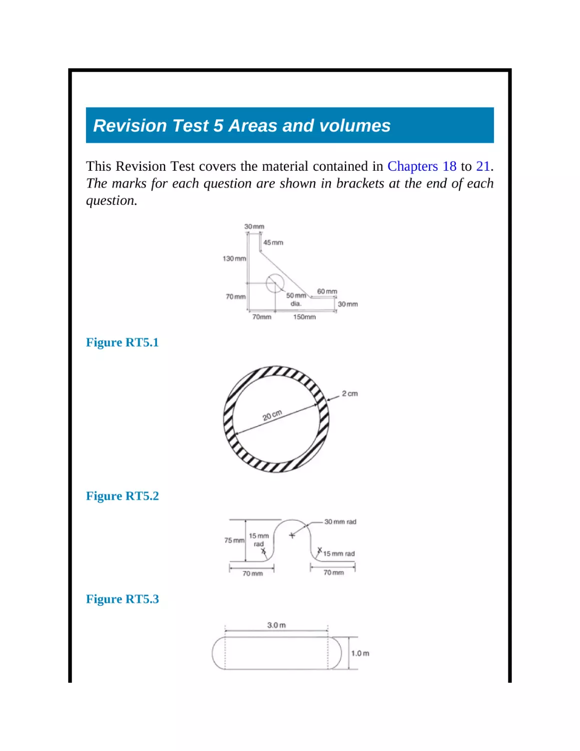
/


Текст
Engineering Mathematics
Eighth Edition
John Bird
Eighth edition published 2017
by Routledge
2 Park Square, Milton Park, Abingdon, Oxon OX14 4RN
and by Routledge
711 Third Avenue, New York, NY 10017
Routledge is an imprint of the Taylor & Francis Group, an informa business
© 2017 John Bird
The right of John Bird to be identified as author of this work has been asserted by him
in accordance with sections 77 and 78 of the Copyright, Designs and Patents Act
1988.
All rights reserved. No part of this book may be reprinted or reproduced or utilised in
any form or by any electronic, mechanical, or other means, now known or hereafter
invented, including photocopying and recording, or in any information storage or
retrieval system, without permission in writing from the publishers.
Trademark notice: Product or corporate names may be trademarks or registered
trademarks, and are used only for identification and explanation without intent to
infringe.
First edition published by Newnes 1999
Seventh edition published by Routledge 2014
British Library Cataloguing-in-Publication Data
A catalogue record for this book is available from the British Library
Library of Congress Cataloging-in-Publication Data
Names: Bird, J. O., author.
Title: Engineering mathematics / John Bird.
Description: 8th edition. | Abingdon, Oxon ; New York, NY : Routledge, 2017. |
Includes
bibliographical references and index.
Identifiers: LCCN 2016055542| ISBN 9781138673595 (pbk. : alk. paper) | ISBN
9781315561851 (ebook)
Subjects: LCSH: Engineering mathematics. | Engineering mathematics–Problems,
exercises, etc.
Classification: LCC TA330 .B515 2017 | DDC 620.001/51–dc23
LC record available at https://lccn.loc.gov/2016055542
ISBN: 978-1-138-67359-5 (pbk)
ISBN: 978-1-315-56185-1 (ebk)
Typeset in Times by
Servis Filmsetting Ltd, Stockport, Cheshire
Visit the companion website: www.routledge.com/cw/bird
Contents
Preface
Section 1 Number and algebra
1
Revision of fractions, decimals and percentages
1.1 Fractions
1.2 Ratio and proportion
1.3 Decimals
1.4 Percentages
2
Indices, standard form and engineering notation
2.1 Indices
2.2 Worked problems on indices
2.3 Further worked problems on indices
2.4 Standard form
2.5 Worked problems on standard form
2.6 Further worked problems on standard form
2.7 Engineering notation and common prefixes
2.8 Metric conversions
2.9 Metric - US/Imperial Conversions
3
Binary, octal and hexadecimal numbers
3.1 Introduction
3.2 Binary numbers
3.3 Octal numbers
3.4 Hexadecimal numbers
4
Calculations and evaluation of formulae
4.1 Errors and approximations
4.2 Use of calculator
4.3 Conversion tables and charts
4.4 Evaluation of formulae
Revision Test 1
5
Algebra
5.1 Basic operations
5.2 Laws of indices
5.3 Brackets and factorisation
5.4 Fundamental laws and precedence
5.5 Direct and inverse proportionality
6
Further algebra
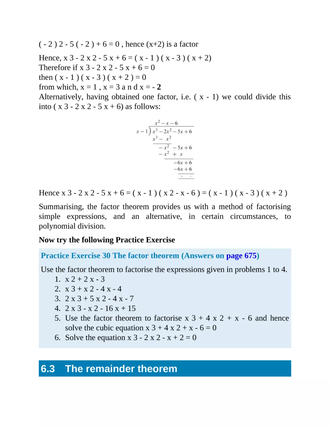
6.1 Polynomial division
6.2 The factor theorem
6.3 The remainder theorem
7
Partial fractions
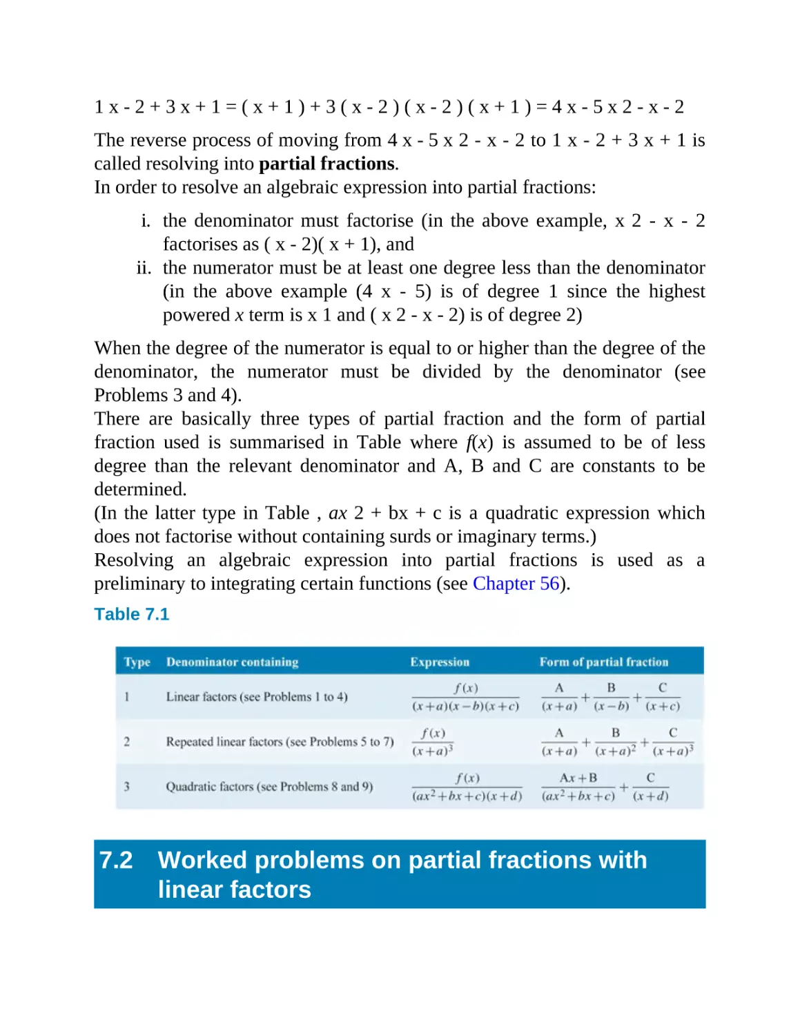
7.1 Introduction to partial fractions
7.2 Worked problems on partial fractions with linear factors
7.3 Worked problems on partial fractions with repeated linear factors
7.4 Worked problems on partial fractions with quadratic factors
8
Solving simple equations
8.1 Expressions, equations and identities
8.2 Worked problems on simple equations
8.3 Further worked problems on simple equations
8.4 Practical problems involving simple equations
8.5 Further practical problems involving simple equations
Revision Test 2
9
Transposing formulae
9.1 Introduction to transposition of formulae
9.2 Worked problems on transposition of formulae
9.3 Further worked problems on transposition of formulae
9.4 Harder worked problems on transposition of formulae
10
Solving simultaneous equations
10.1 Introduction to simultaneous equations
10.2 Worked problems on simultaneous equations in two unknowns
10.3 Further worked problems on simultaneous equations
10.4 More difficult worked problems on simultaneous equations
10.5 Practical problems involving simultaneous equations
11
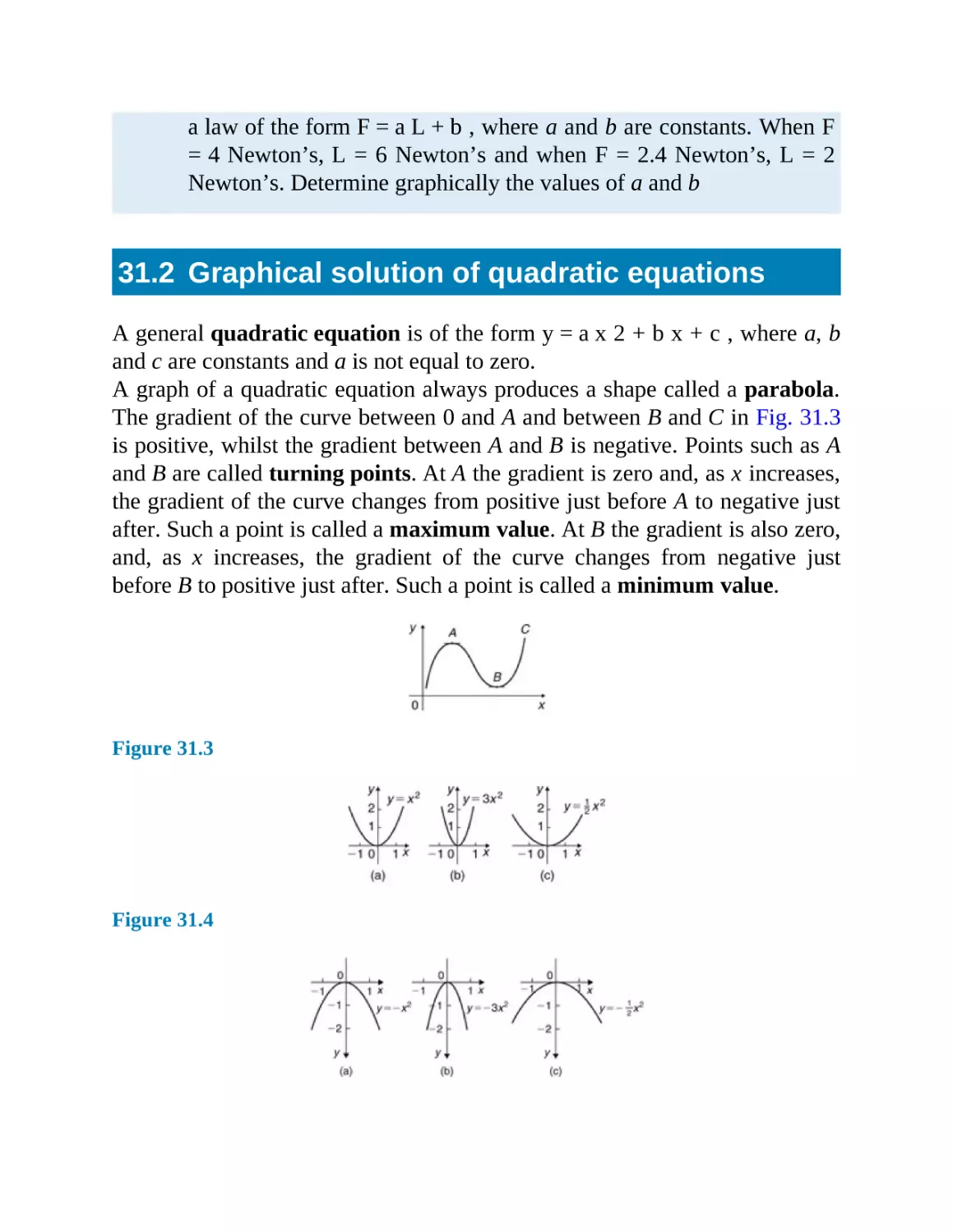
Solving quadratic equations
11.1 Introduction to quadratic equations
11.2 Solution of quadratic equations by factorisation
11.3 Solution of quadratic equations by ‘completing the square’
11.4 Solution of quadratic equations by formula
11.5 Practical problems involving quadratic equations
11.6 The solution of linear and quadratic equations simultaneously
12
Inequalities
12.1 Introduction in inequalities
12.2 Simple inequalities
12.3 Inequalities involving a modulus
12.4 Inequalities involving quotients
12.5 Inequalities involving square functions
12.6 Quadratic inequalities
13
Logarithms
13.1 Introduction to logarithms
13.2 Laws of logarithms
13.3 Indicial equations
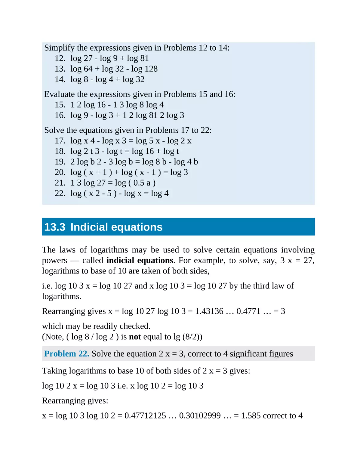
13.4 Graphs of logarithmic functions
Revision Test 3
14
Exponential functions
14.1 Introduction to exponential functions
14.2 The power series for e x
14.3 Graphs of exponential functions
14.4 Napierian logarithms
14.5 Laws of growth and decay
15
Number sequences
15.1 Arithmetic progressions
15.2 Worked problems on arithmetic progressions
15.3 Further worked problems on arithmetic progressions
15.4 Geometric progressions
15.5 Worked problems on geometric progressions
15.6 Further worked problems on geometric progressions
15.7 Combinations and permutations
16
The binomial series
16.1 Pascal’s triangle
16.2 The binomial series
16.3 Worked problems on the binomial series
16.4 Further worked problems on the binomial series
16.5 Practical problems involving the binomial theorem
17
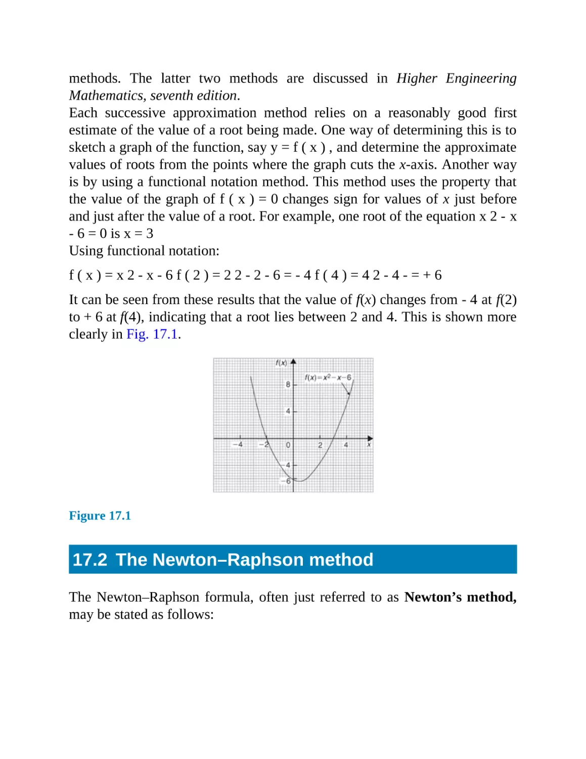
Solving equations by iterative methods
17.1 Introduction to iterative methods
17.2 The Newton–Raphson method
17.3 Worked problems on the Newton–Raphson method
Revision Test 4
Multiple choice questions on Chapters 1–17
Section 2 Areas and volumes
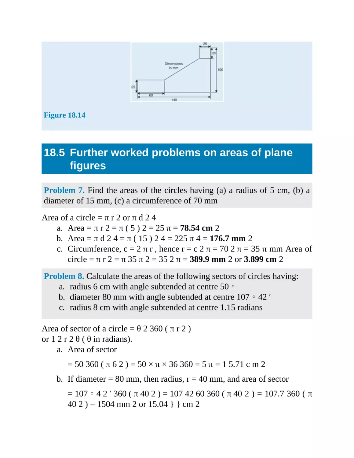
18
Areas of common shapes
18.1 Introduction
18.2 Properties of quadrilaterals
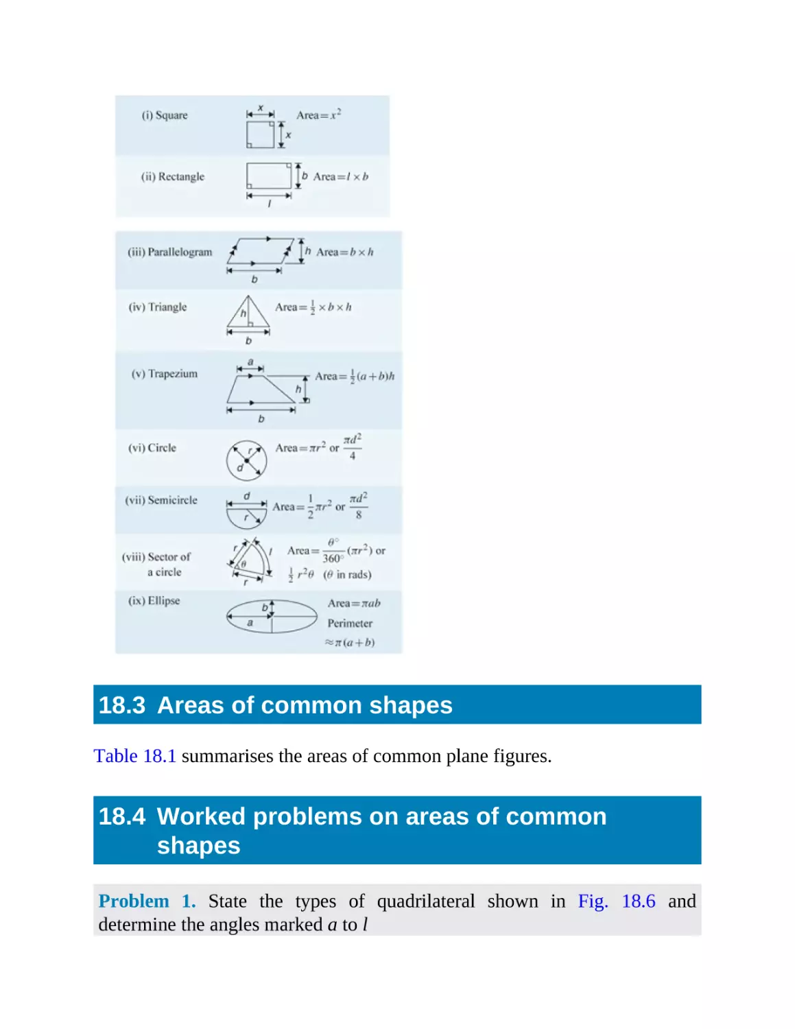
18.3 Areas of common shapes
18.4 Worked problems on areas of common shapes
18.5 Further worked problems on areas of plane figures
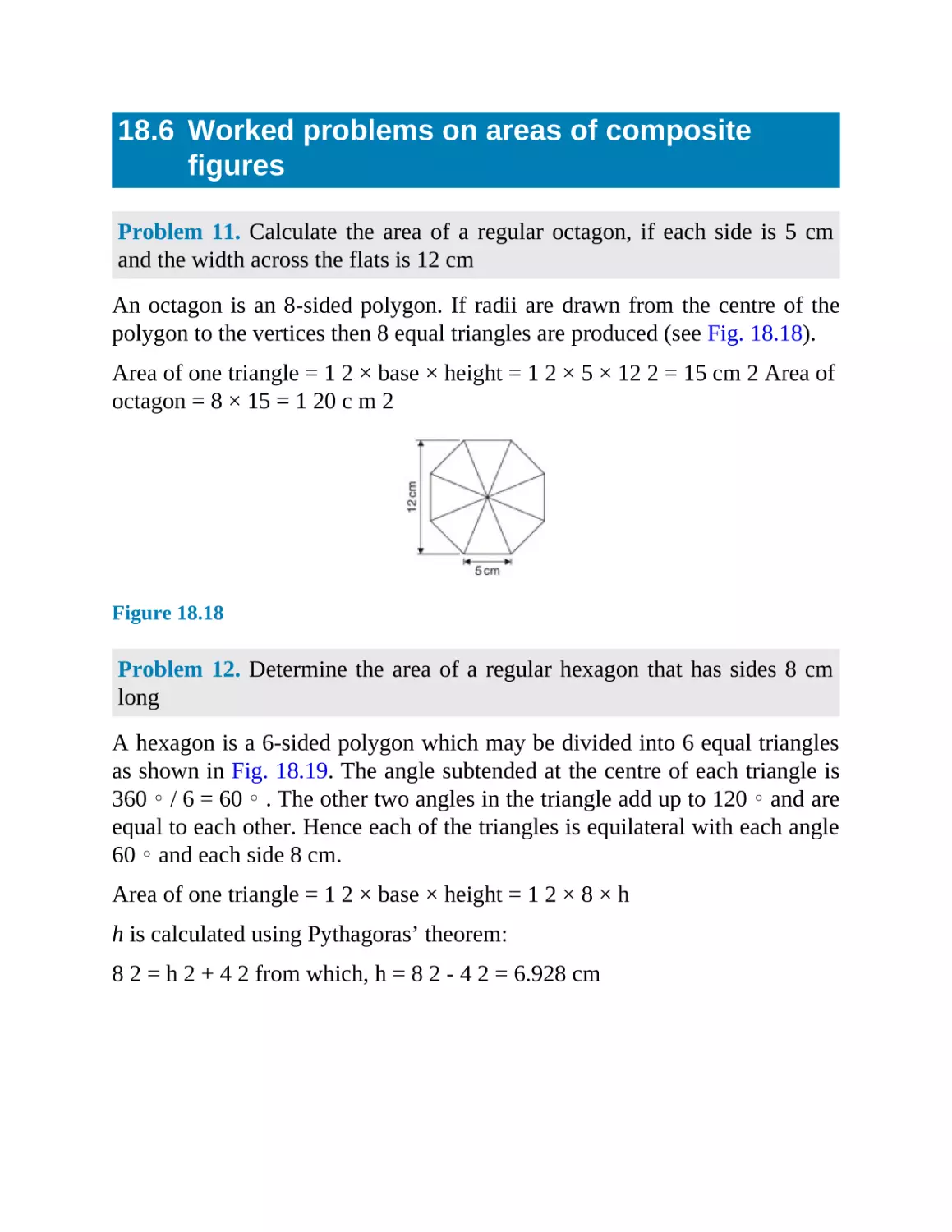
18.6 Worked problems on areas of composite figures
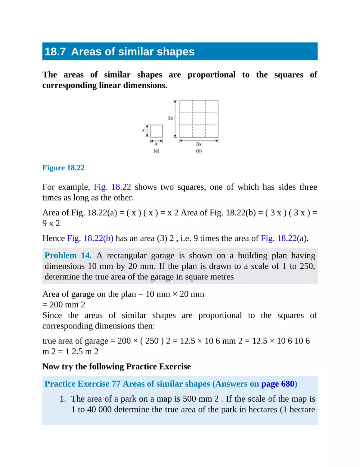
18.7 Areas of similar shapes
19
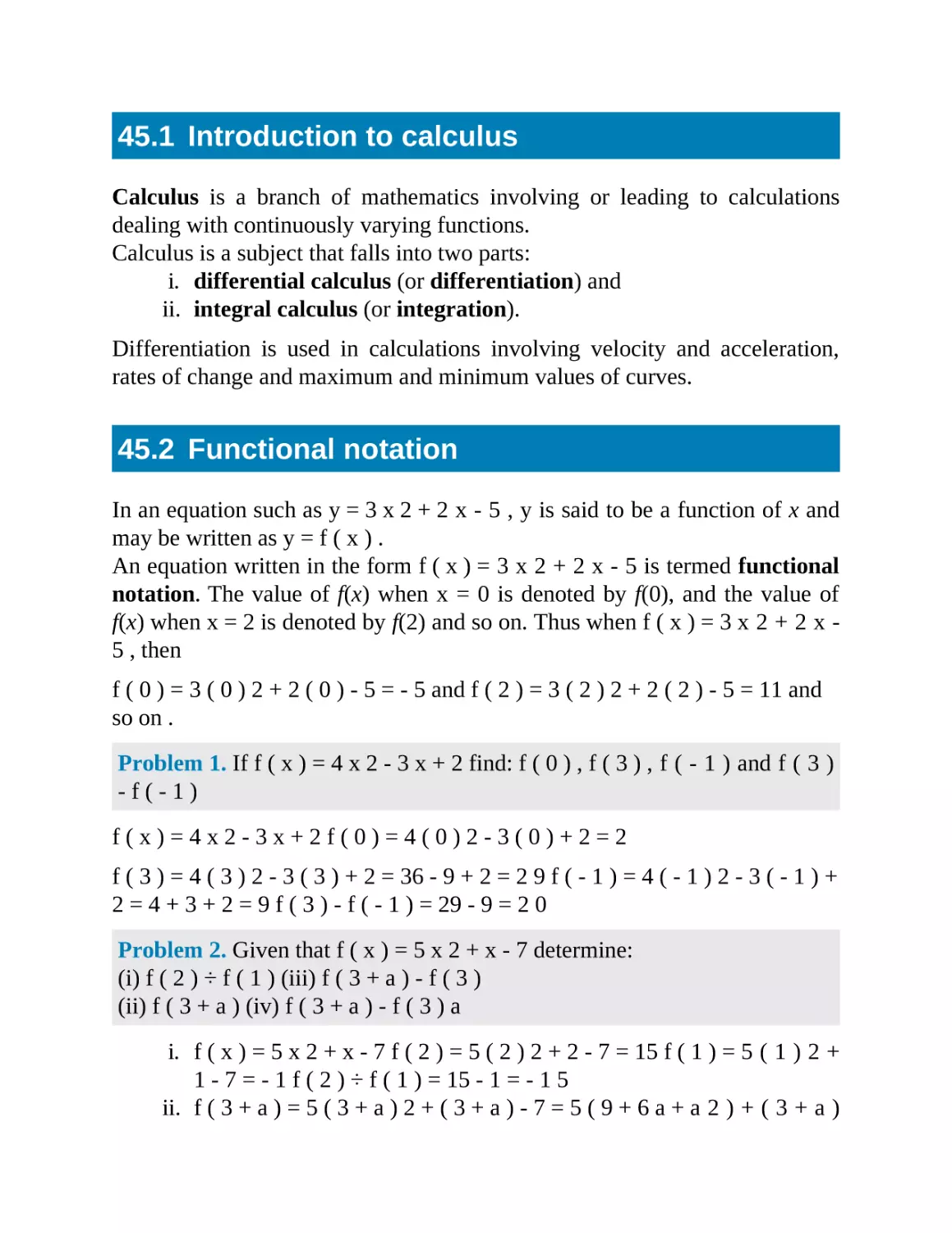
The circle and its properties
19.1 Introduction
19.2 Properties of circles
19.3 Radians and degrees
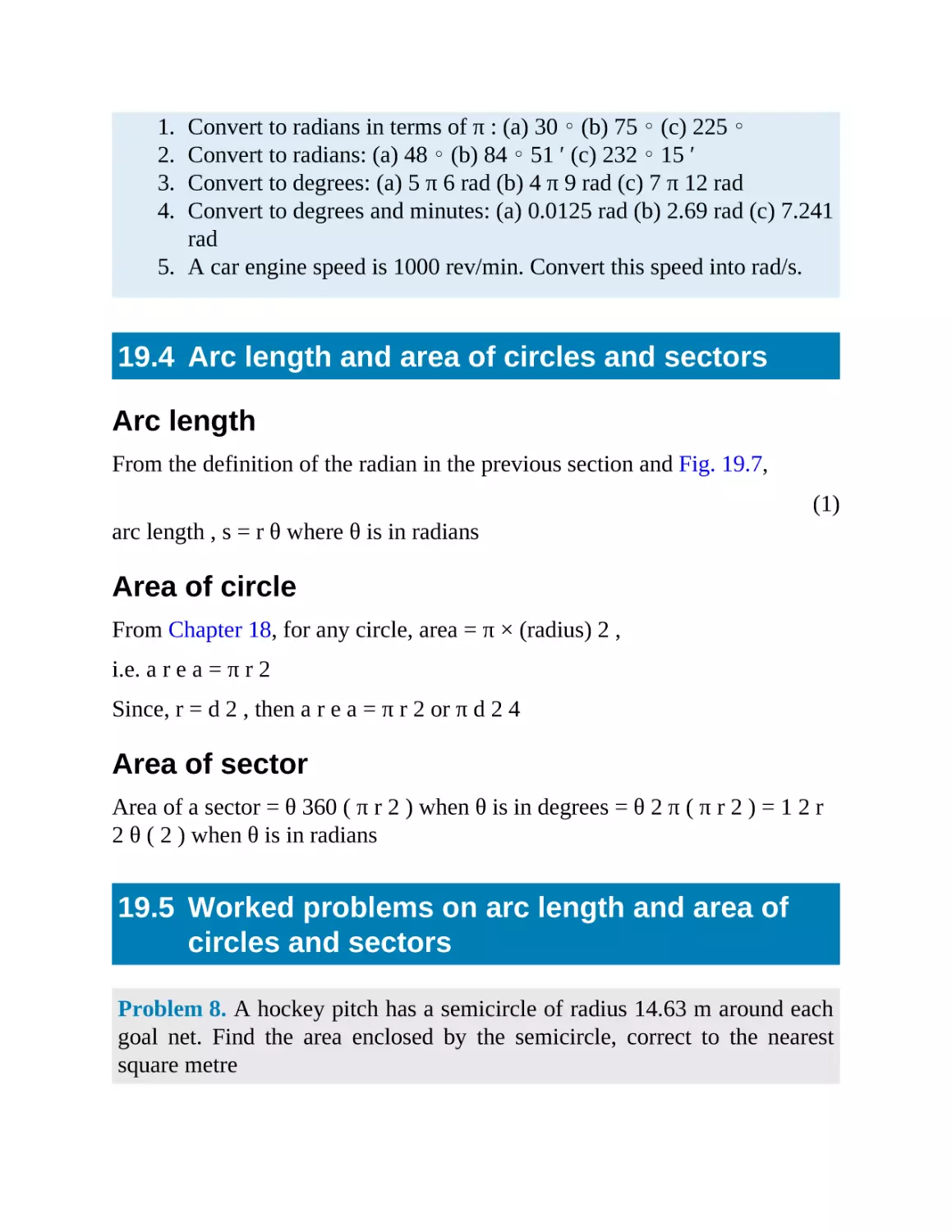
19.4 Arc length and area of circles and sectors
19.5 Worked problems on arc length and area of circles and sectors
19.6 The equation of a circle
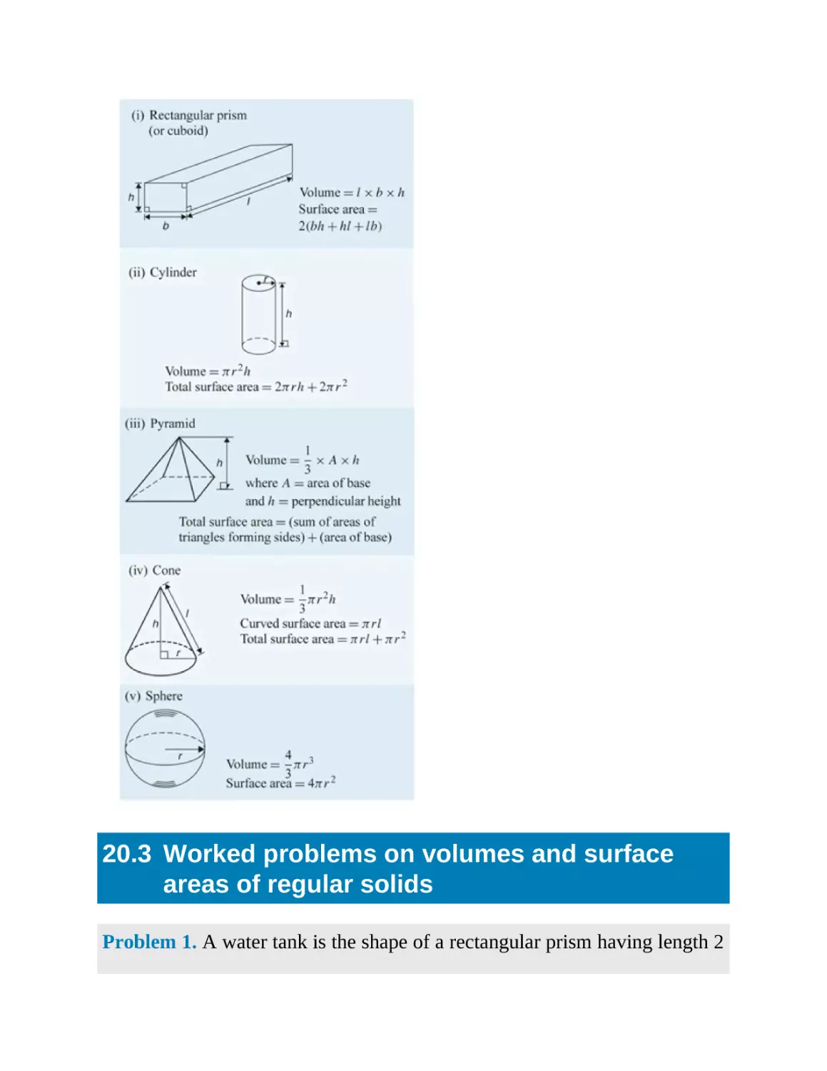
20
Volumes and surface areas of common solids
20.1 Introduction
20.2 Volumes and surface areas of regular solids
20.3 Worked problems on volumes and surface areas of regular solids
20.4 Further worked problems on volumes and surface areas of
regular solids
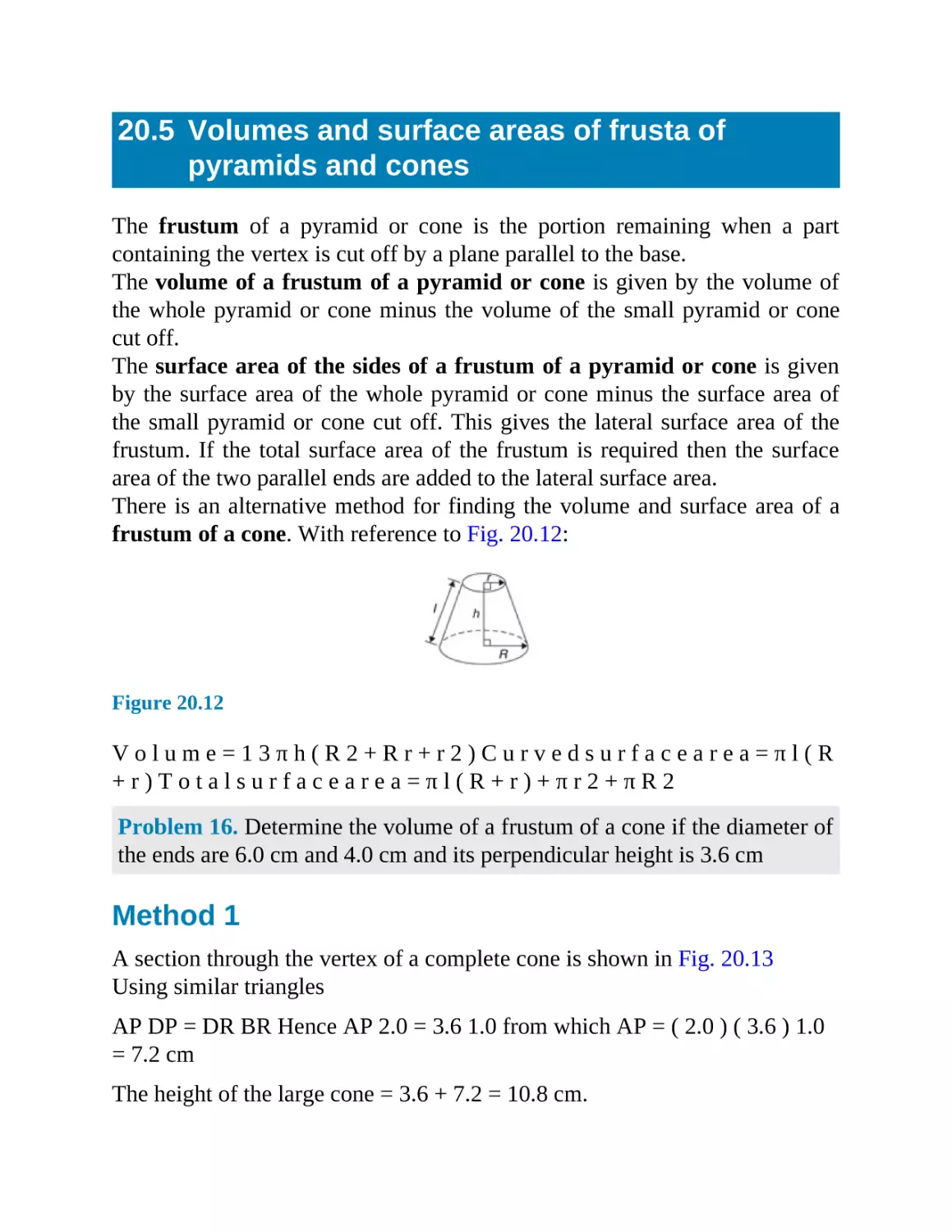
20.5 Volumes and surface areas of frusta of pyramids and cones
20.6 The frustum and zone ofa sphere
20.7 Prismoidal rule
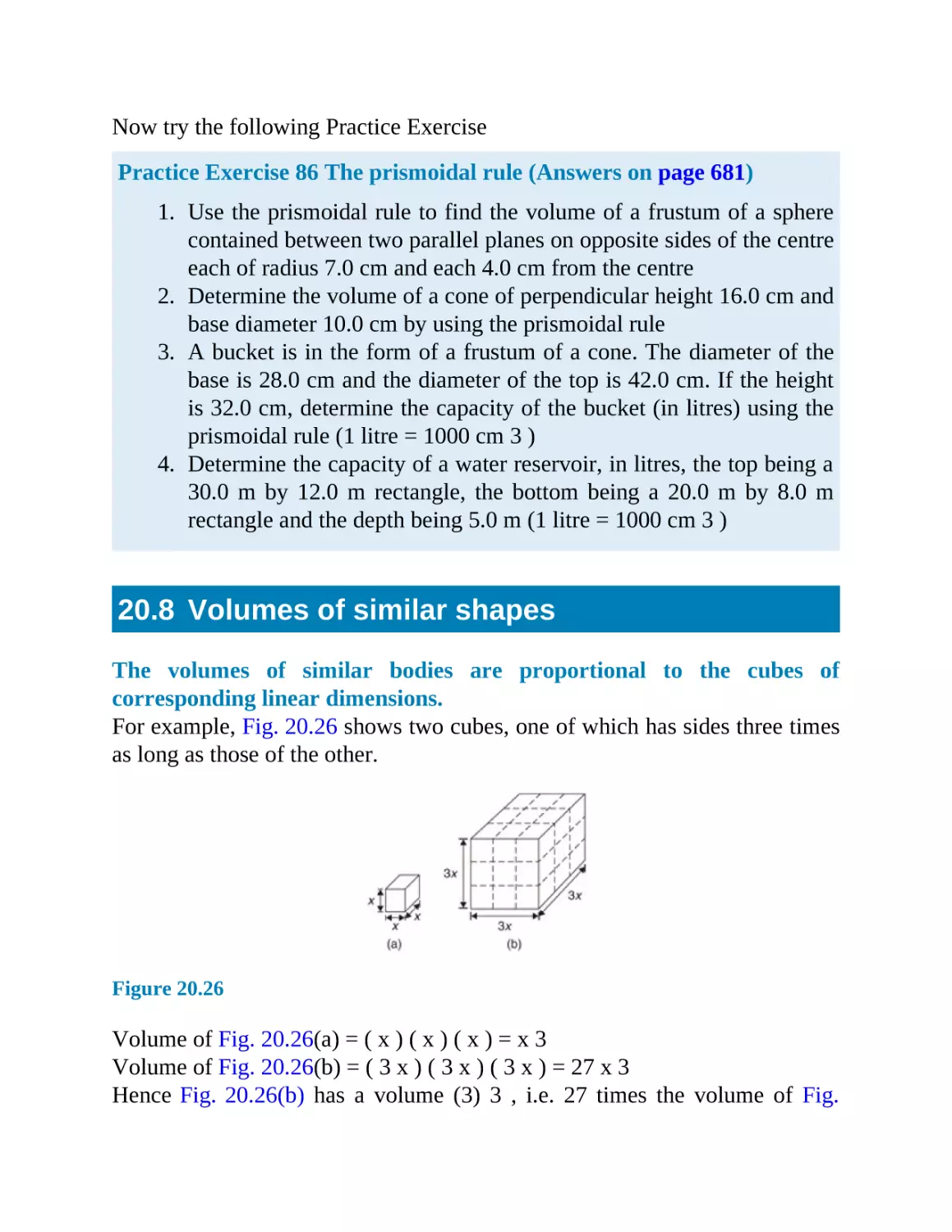
20.8 Volumes of similar shapes
21
Irregular areas and volumes and mean values of waveforms
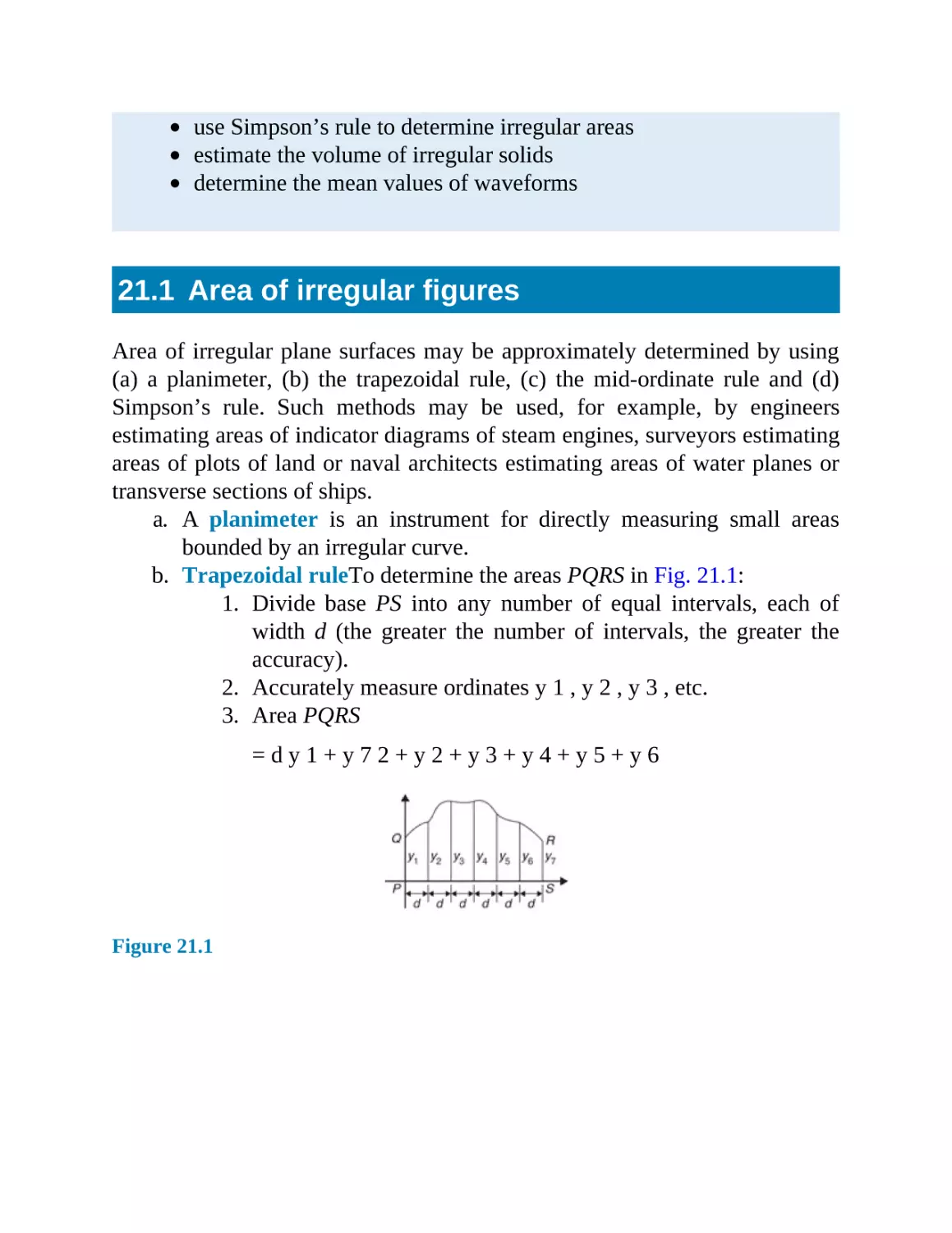
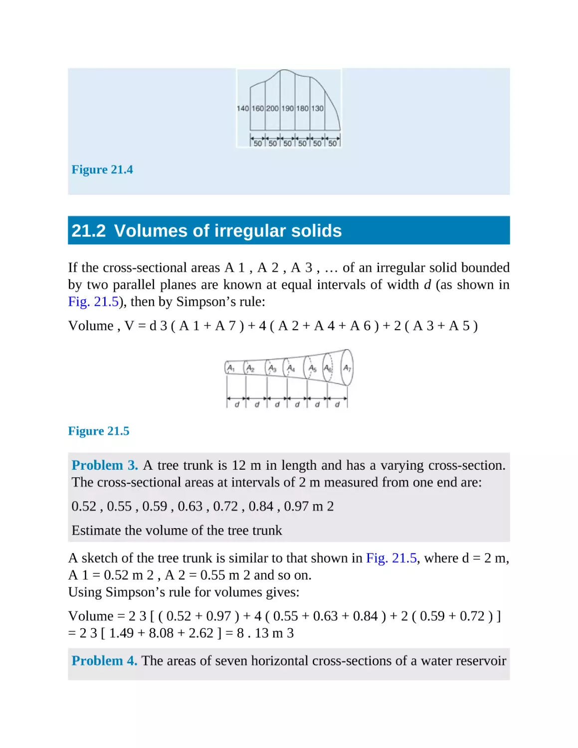
21.1 Area of irregular figures
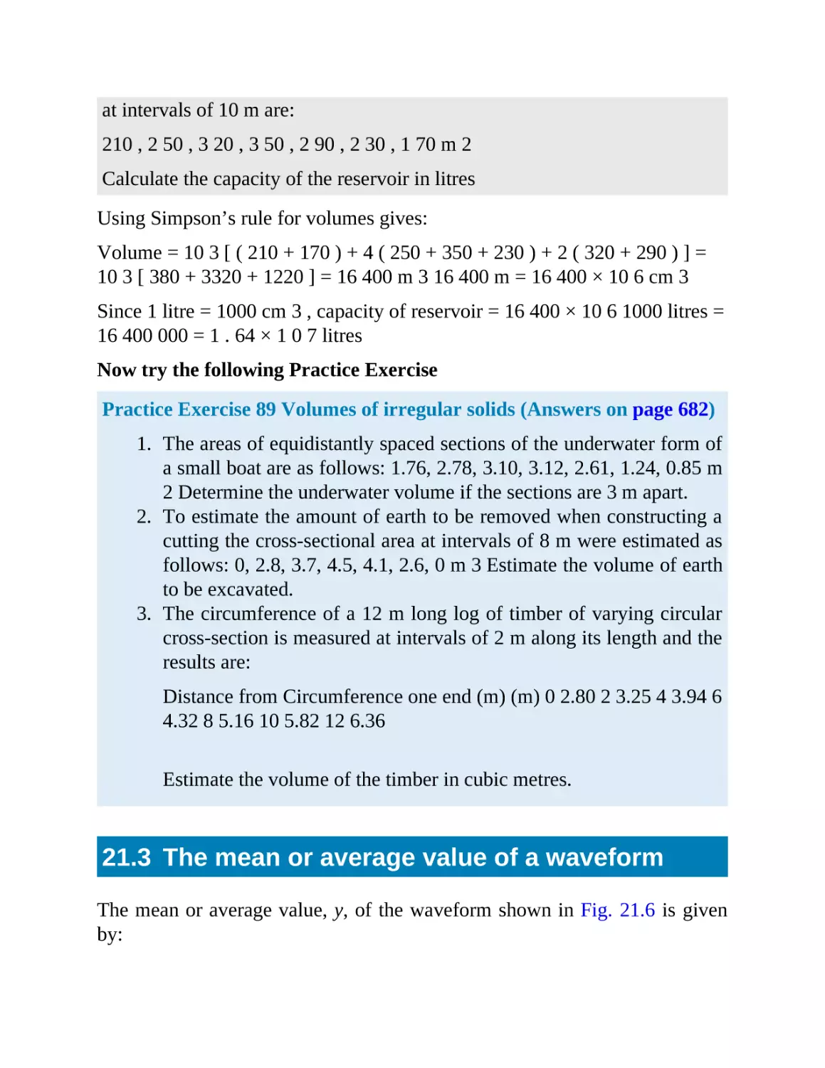
21.2 Volumes of irregular solids
21.3 The mean or average value of a waveform
Revision Test 5
Section 3 Trigonometry
22
Introduction to trigonometry
22.1 Trigonometry
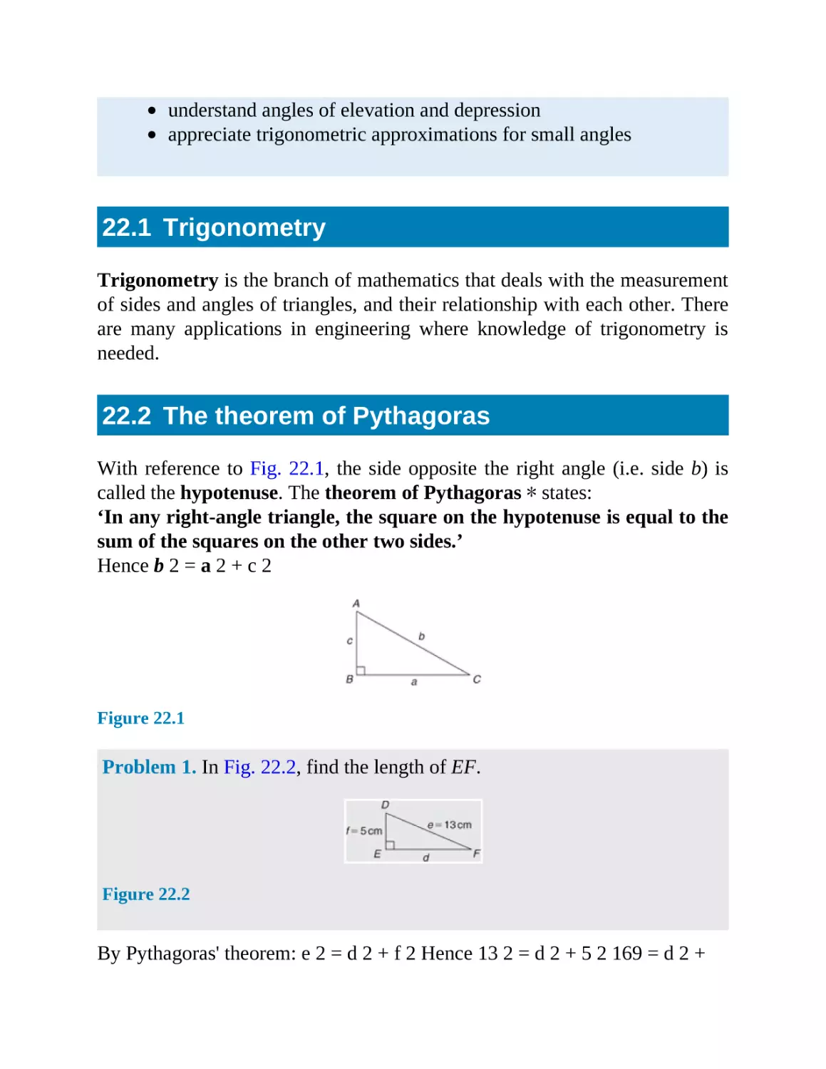
22.2 The theorem of Pythagoras
22.3 Trigonometric ratios of acute angles
22.4 Fractional and surd forms of trigonometric ratios
22.5 Evaluating trigonometric ratios of any angles
22.6 Solution of right-angled triangles
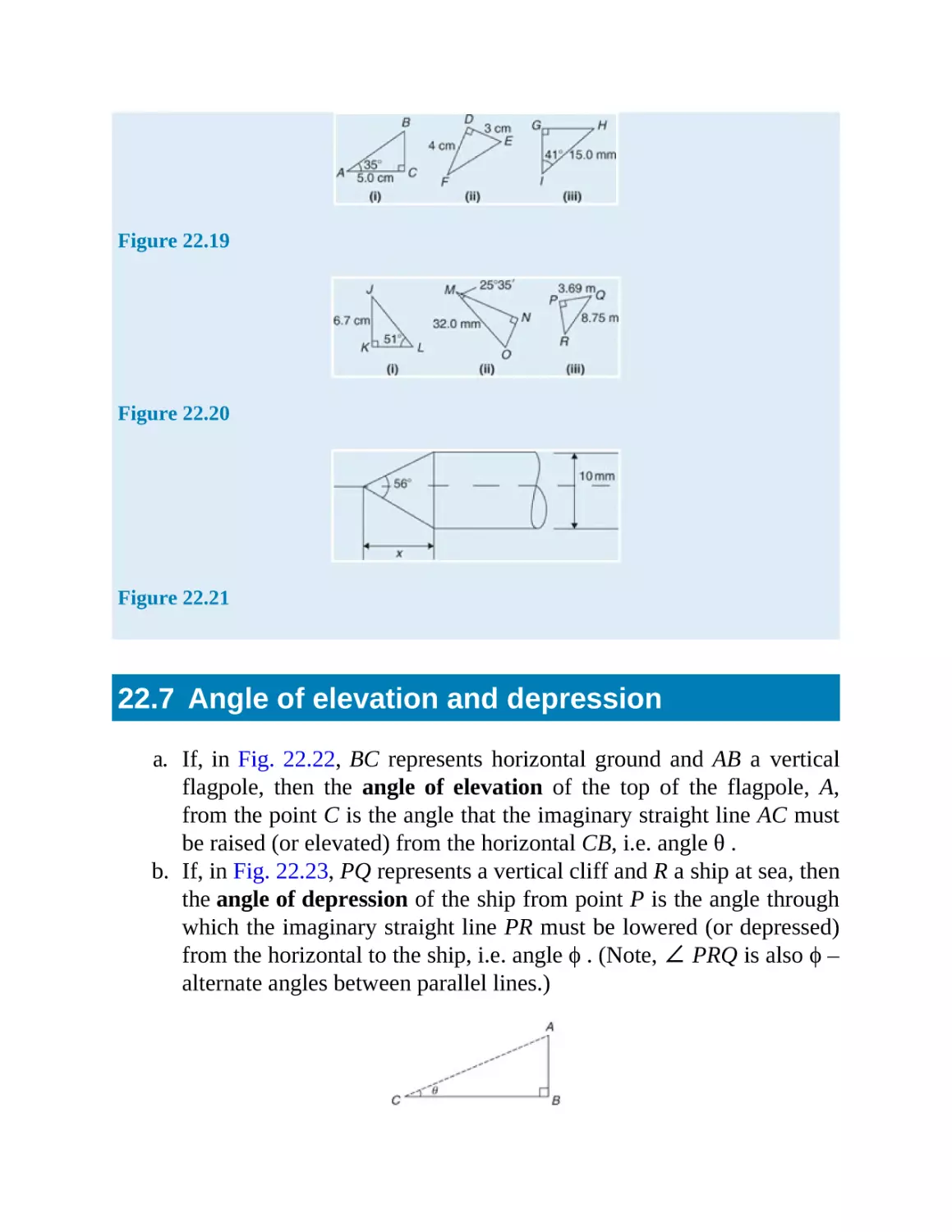
22.7 Angle of elevation and depression
22.8 Trigonometric approximations for small angles
23
Trigonometric waveforms
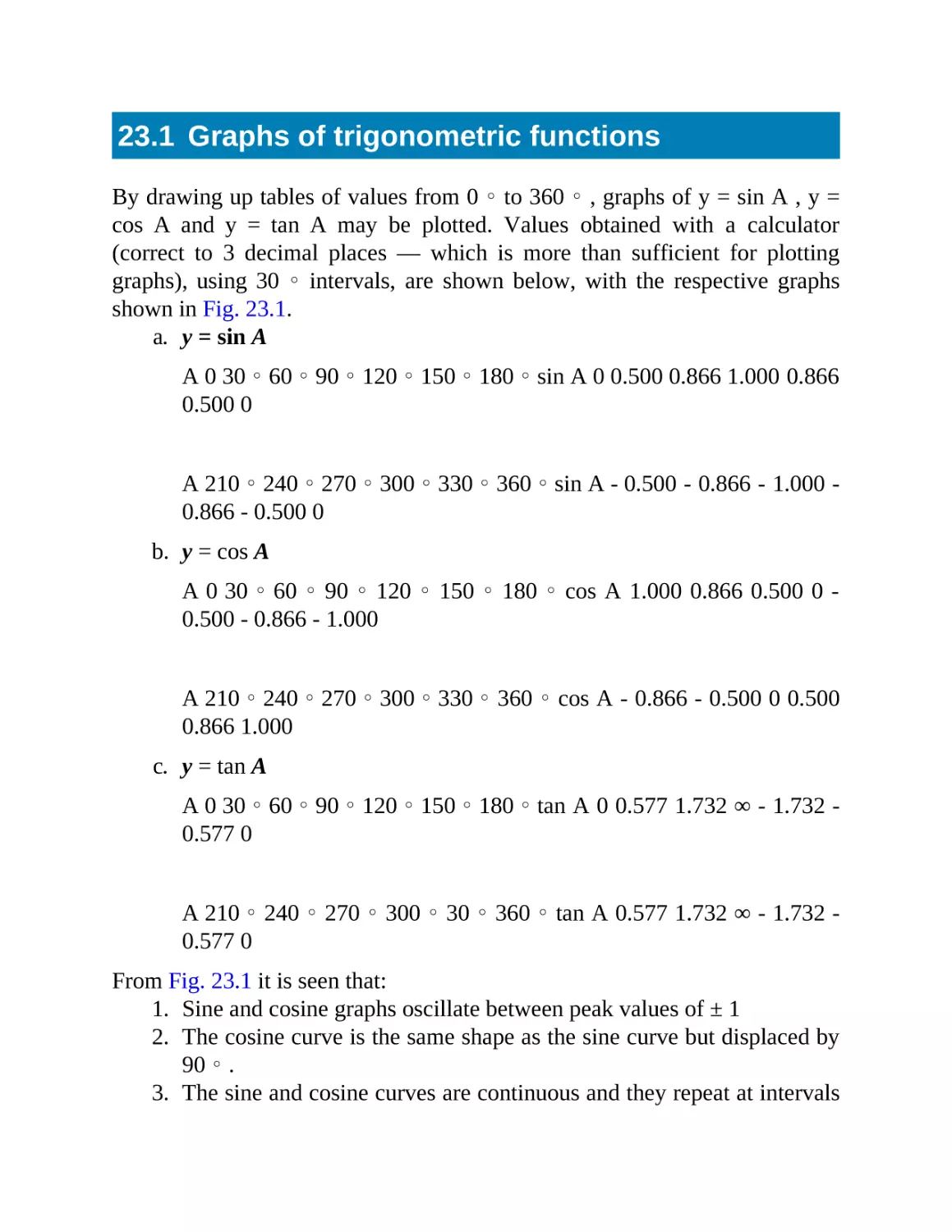
23.1 Graphs of trigonometric functions
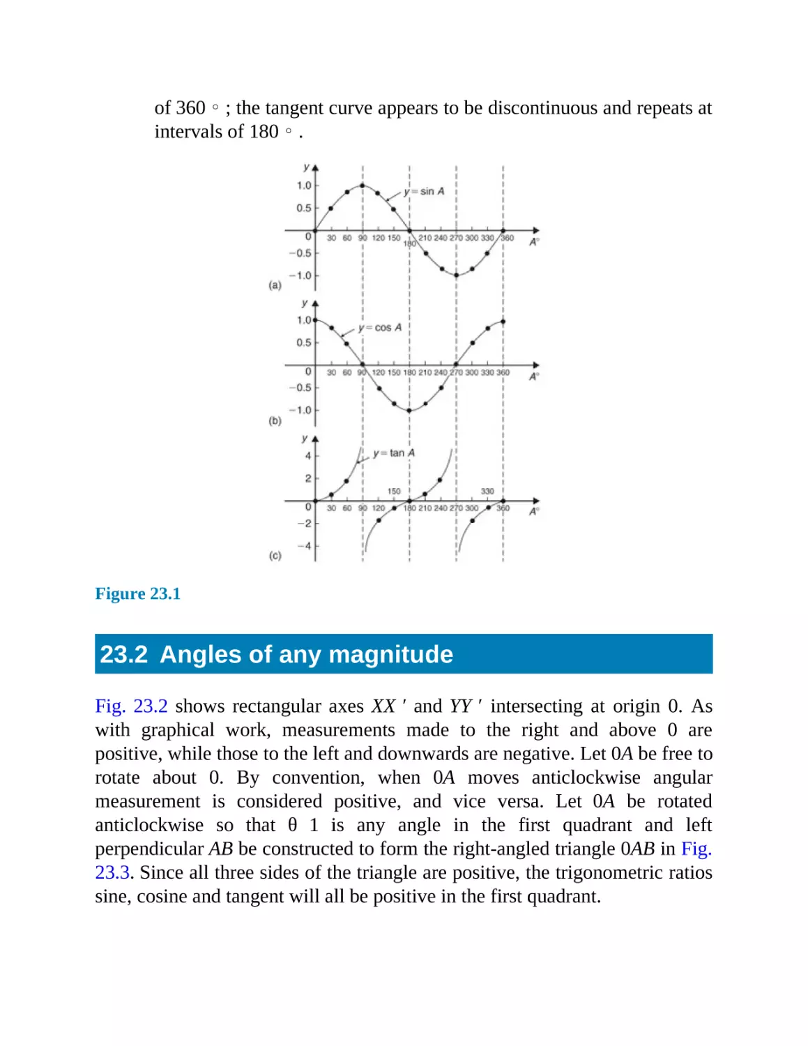
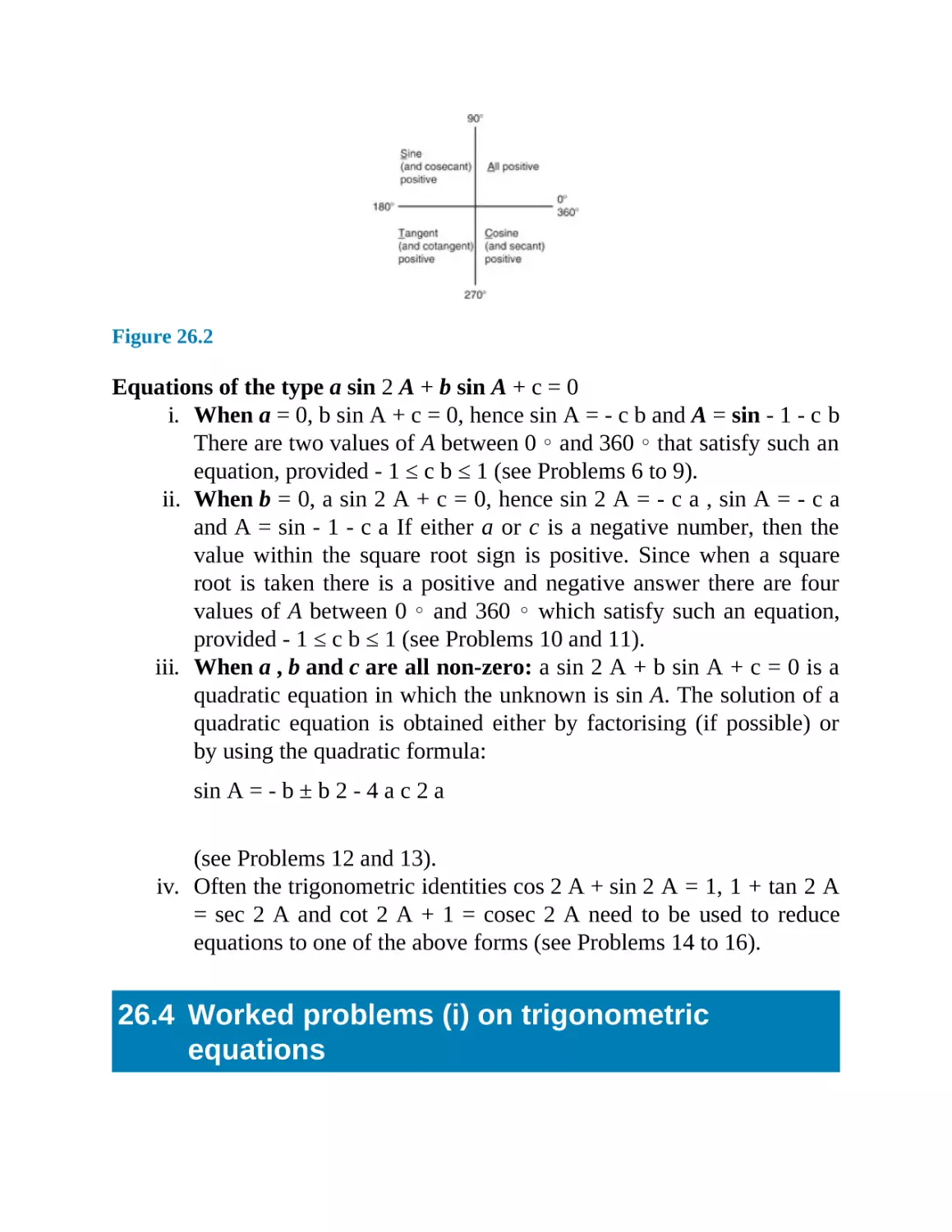
23.2 Angles of any magnitude
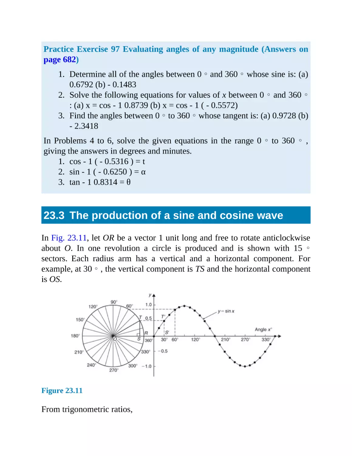
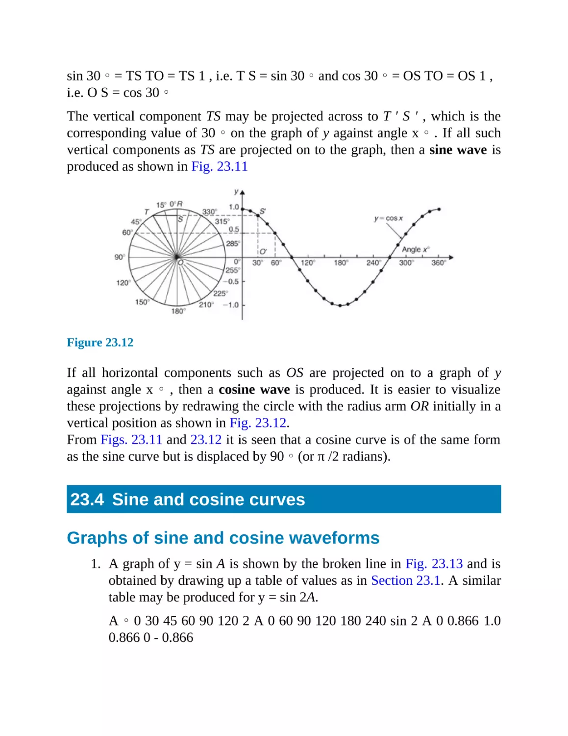
23.3 The production of a sine and cosine wave
23.4 Sine and cosine curves
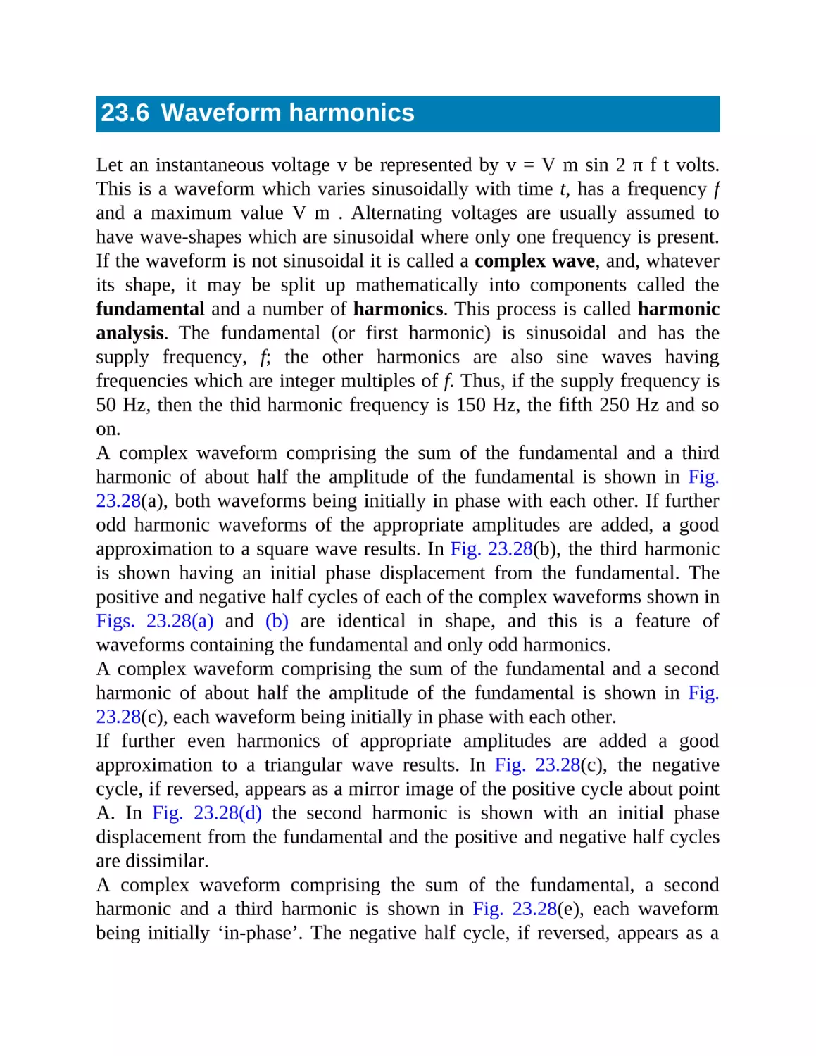
23.5 Sinusoidal form A sin ( ω t ± α )
23.6 Waveform harmonics
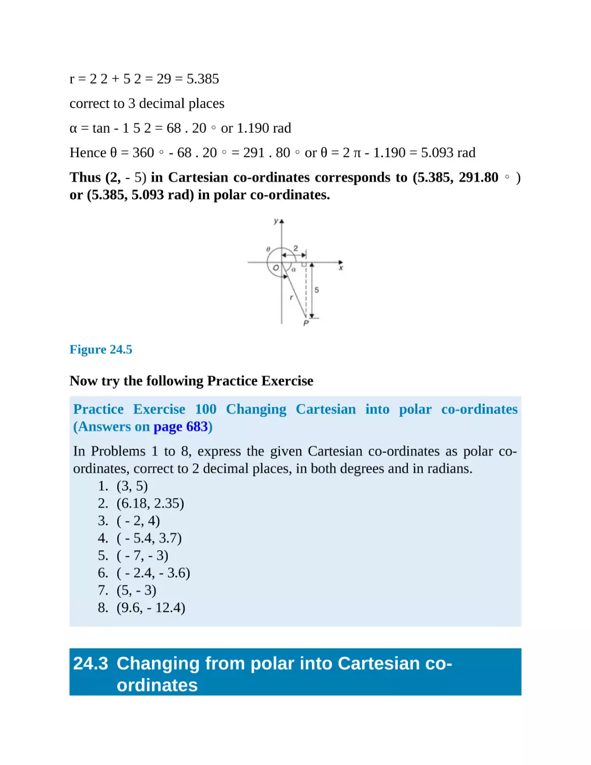
24
Cartesian and polar co-ordinates
24.1 Introduction
24.2 Changing from Cartesian into polar co-ordinates
24.3 Changing from polar into Cartesian co-ordinates
24.4 Use of Pol/Rec functions on calculators
Revision Test 6
25
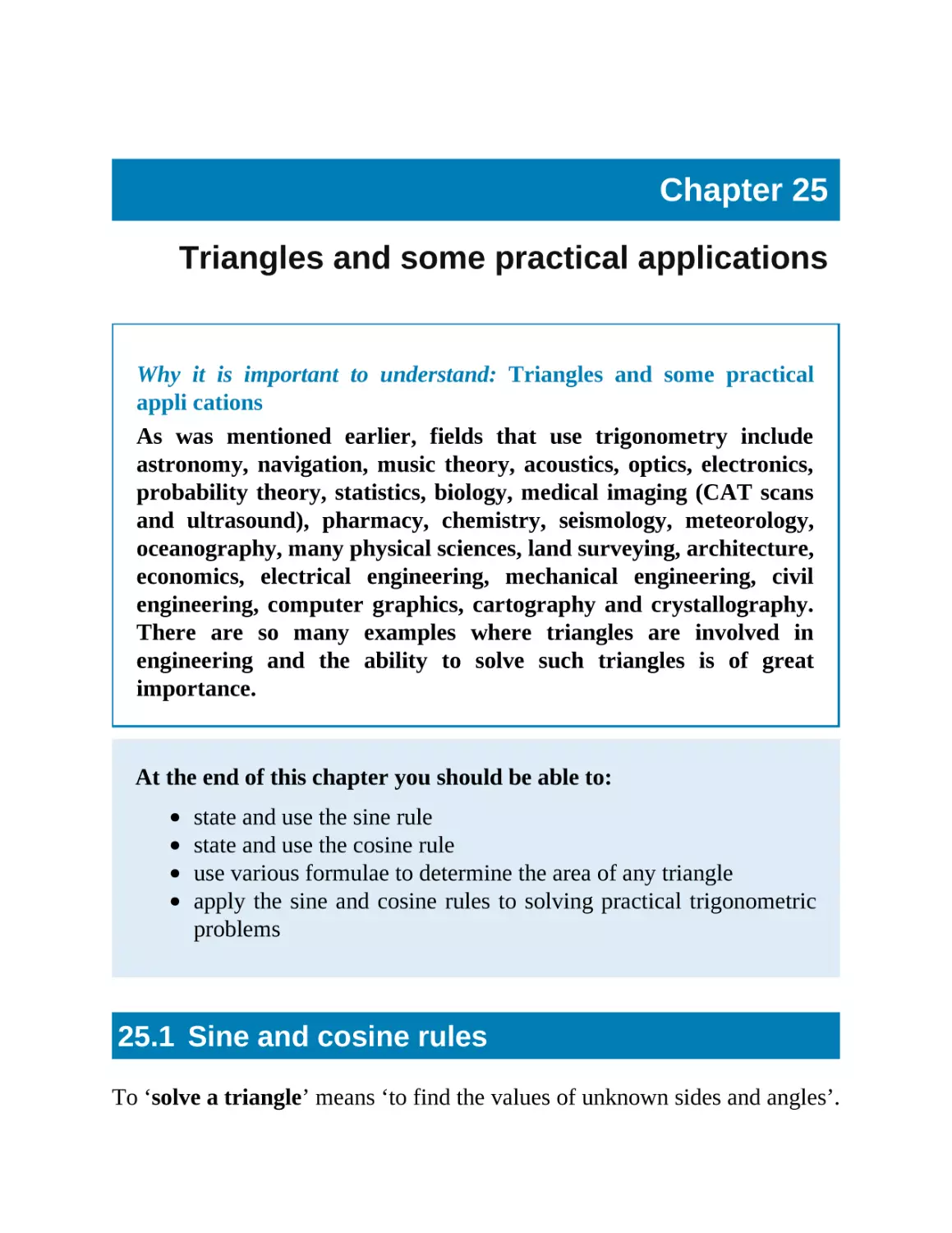
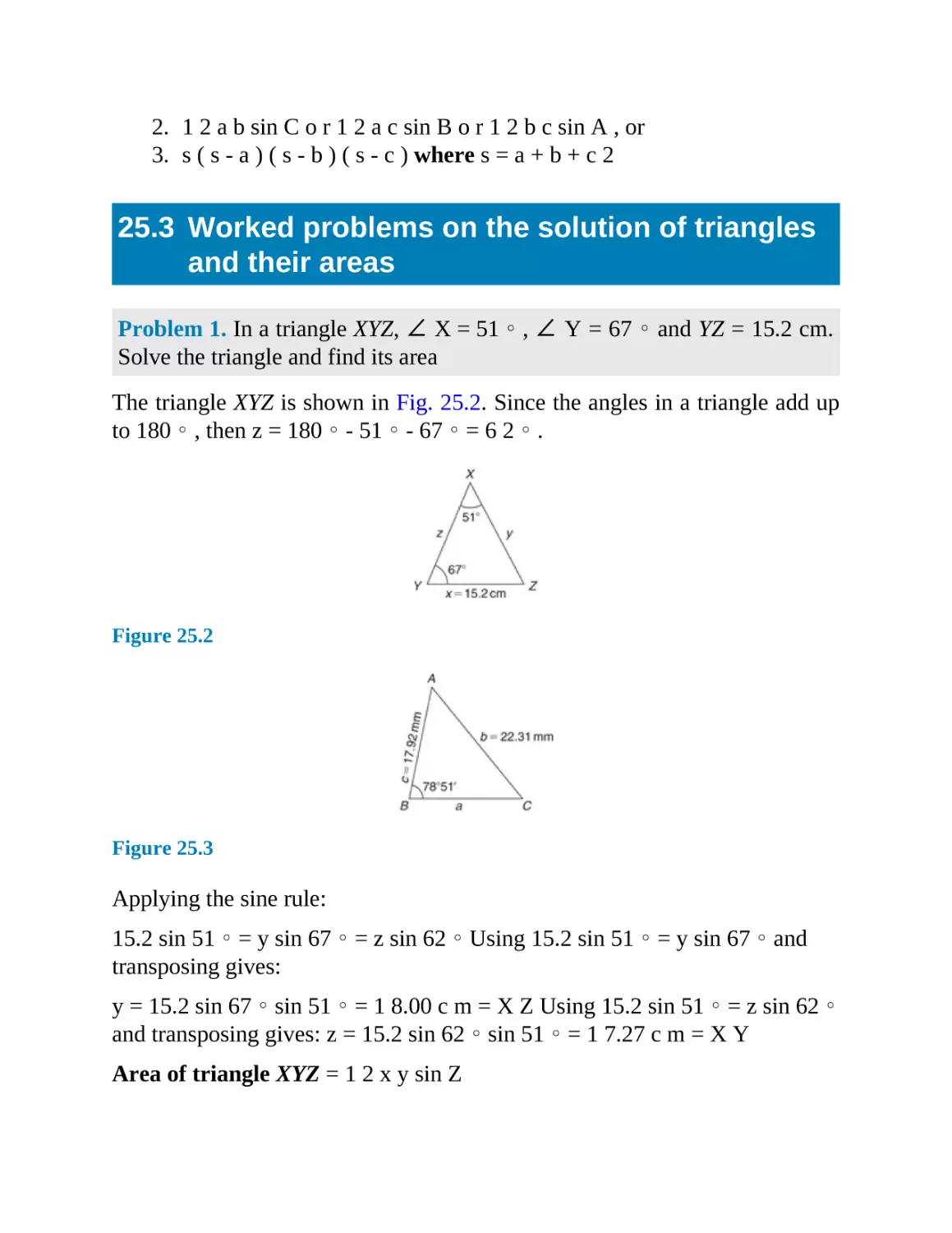
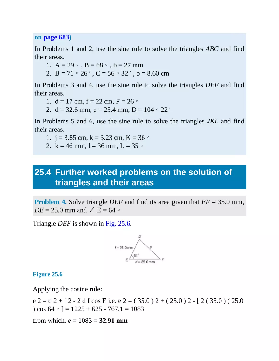
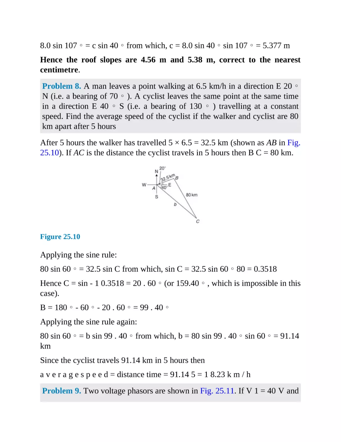
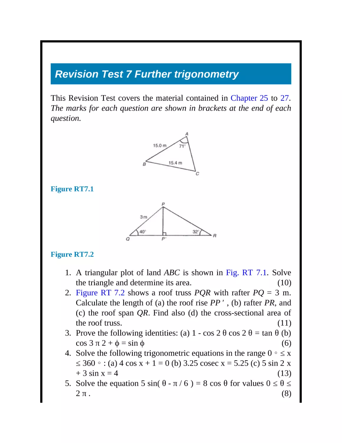
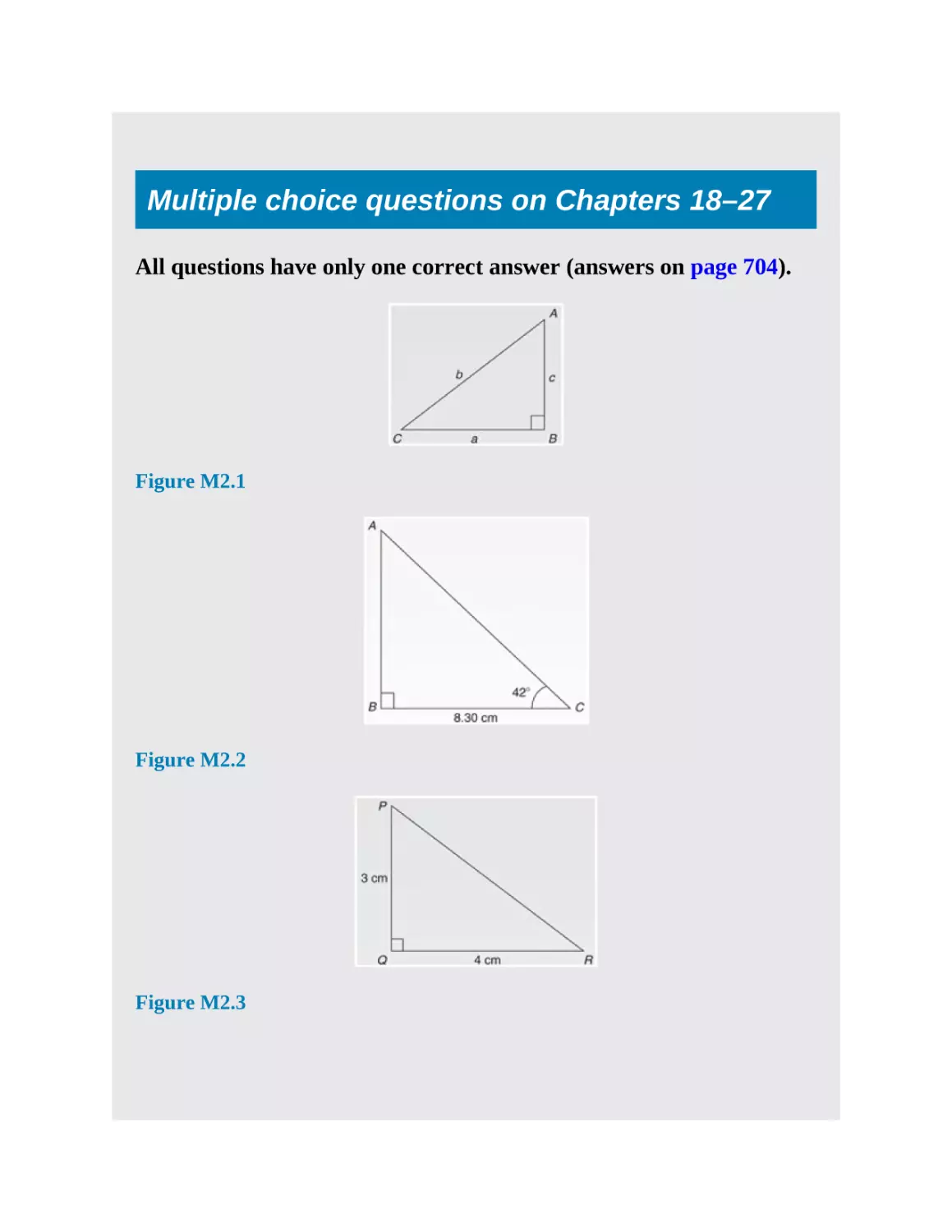
Triangles and some practical applications
25.1 Sine and cosine rules
25.2 Area of any triangle
25.3 Worked problems on the solution of triangles and their areas
25.4 Further worked problems on the solution of triangles and their
areas
25.6 Further practical situations involving trigonometry
26
Trigonometric identities and equations
26.1 Trigonometric identities
26.2 Worked problems on trigonometric identities
26.3 Trigonometric equations
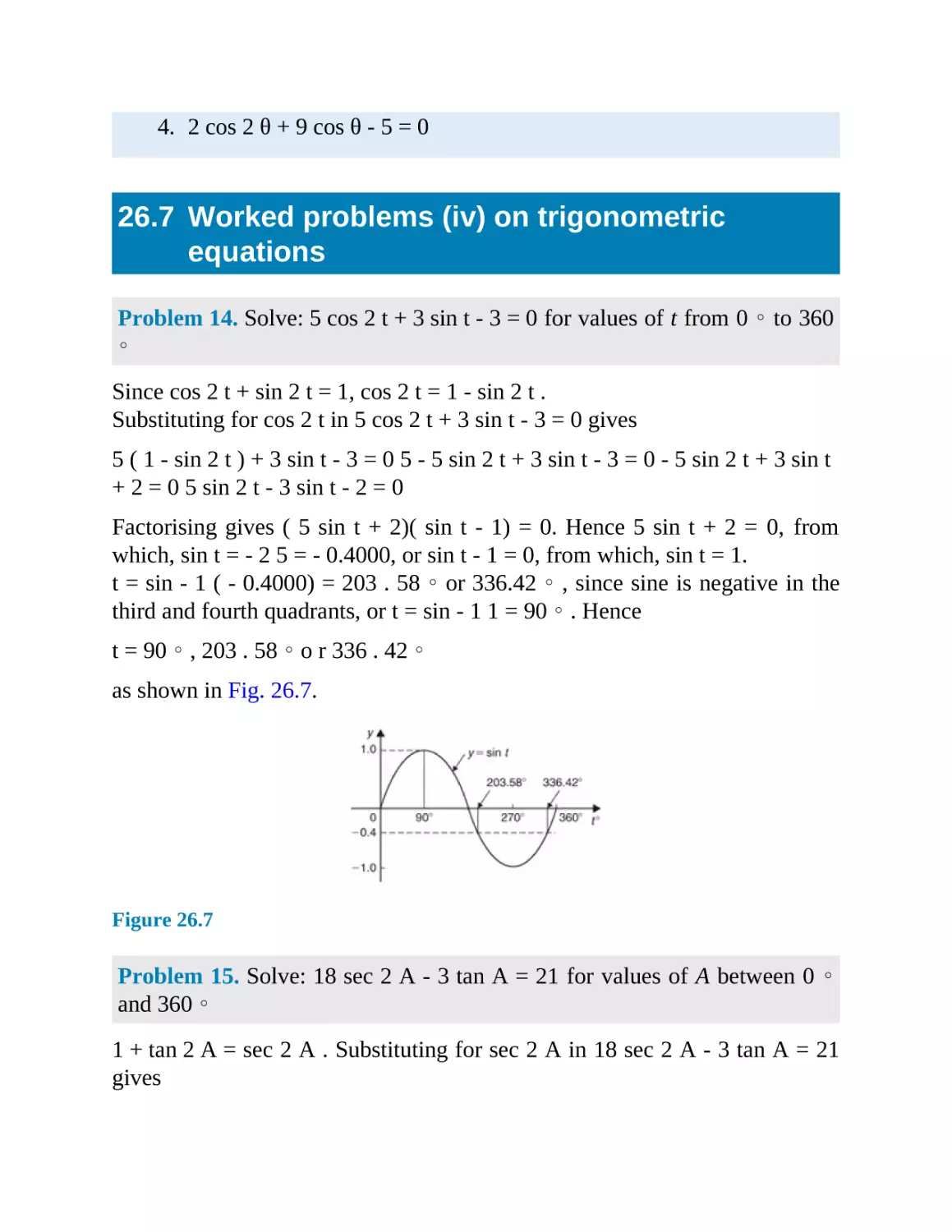
26.4 Worked problems (i) on trigonometric equations
26.5 Worked problems (ii) on trigonometric equations
26.6 Worked problems (iii) on trigonometric equations
26.7 Worked problems (iv) on trigonometric equations
27
Compound angles
27.1 Compound angle formulae
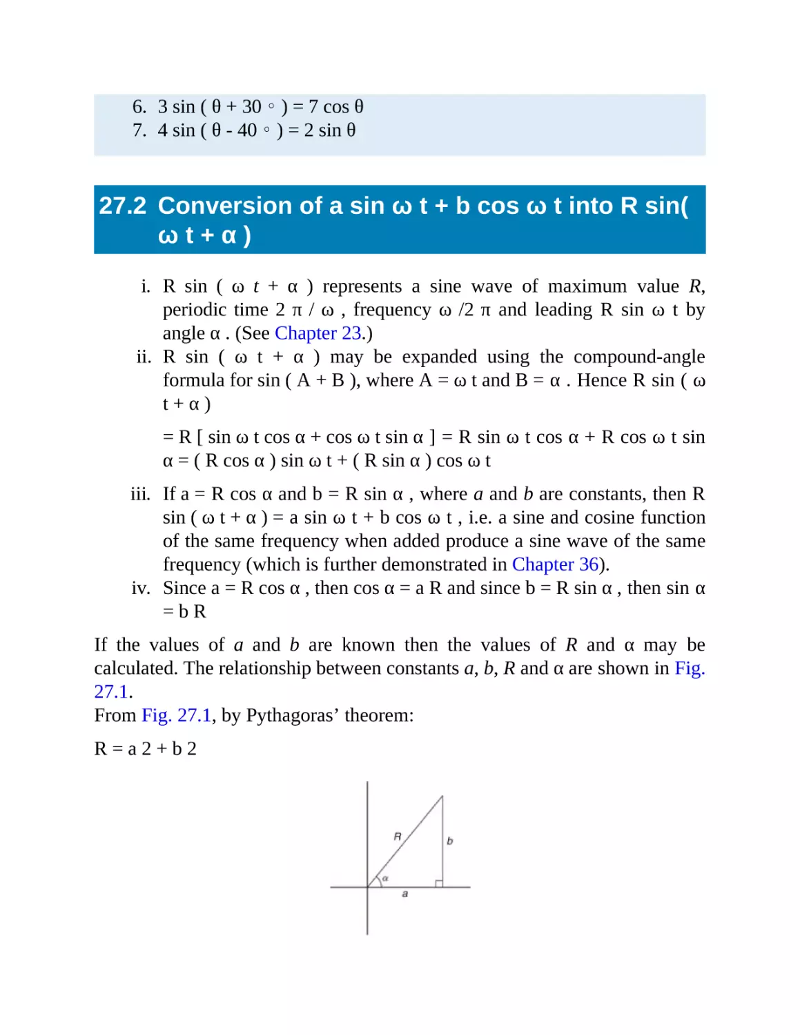
27.2 Conversion of a sin ω t + b cos ω t into R sin( ω t + α )
27.3 Double angles
27.4 Changing products of sines and cosines into sums or differences
27.5 Changing sums or differences of sines and cosines into products
Revision Test 7
Multiple choice questions on Chapters 18–27
Section 4 Graphs
28
Straight line graphs
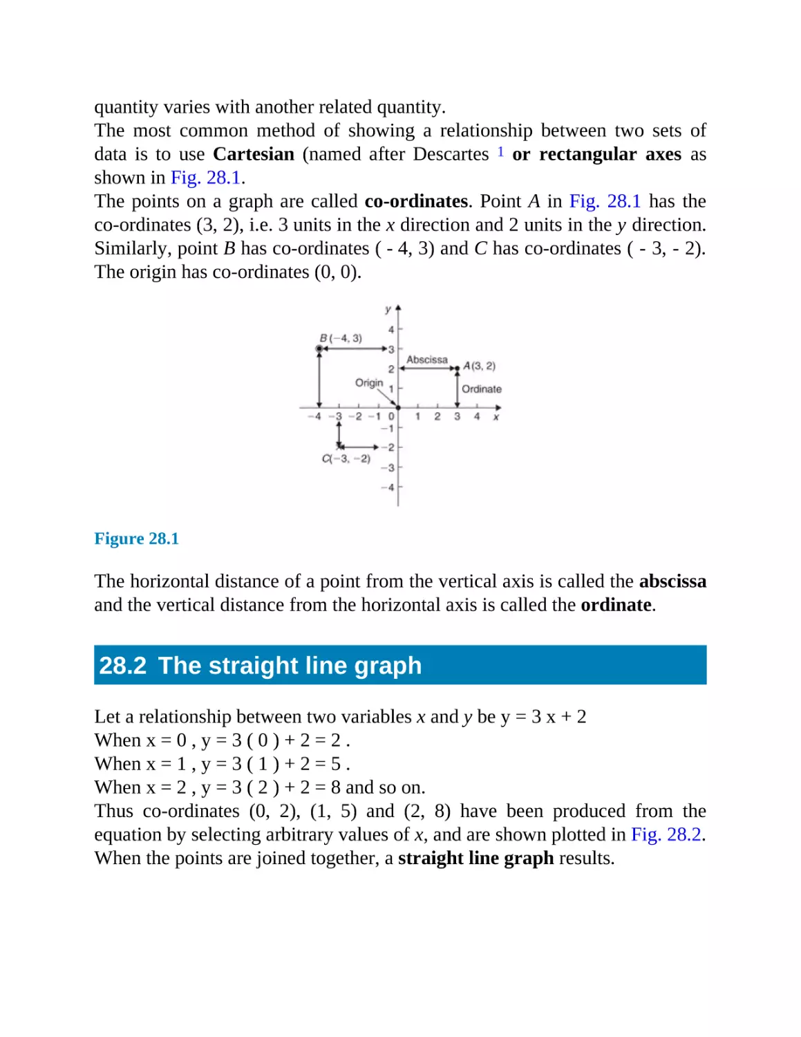
28.1 Introduction to graphs
28.2 The straight line graph
28.3 Practical problems involving straight line graphs
29
Reduction of non-linear laws to linear form
29.1 Determination of law
29.2 Determination of law involving logarithms
30
Graphs with logarithmic scales
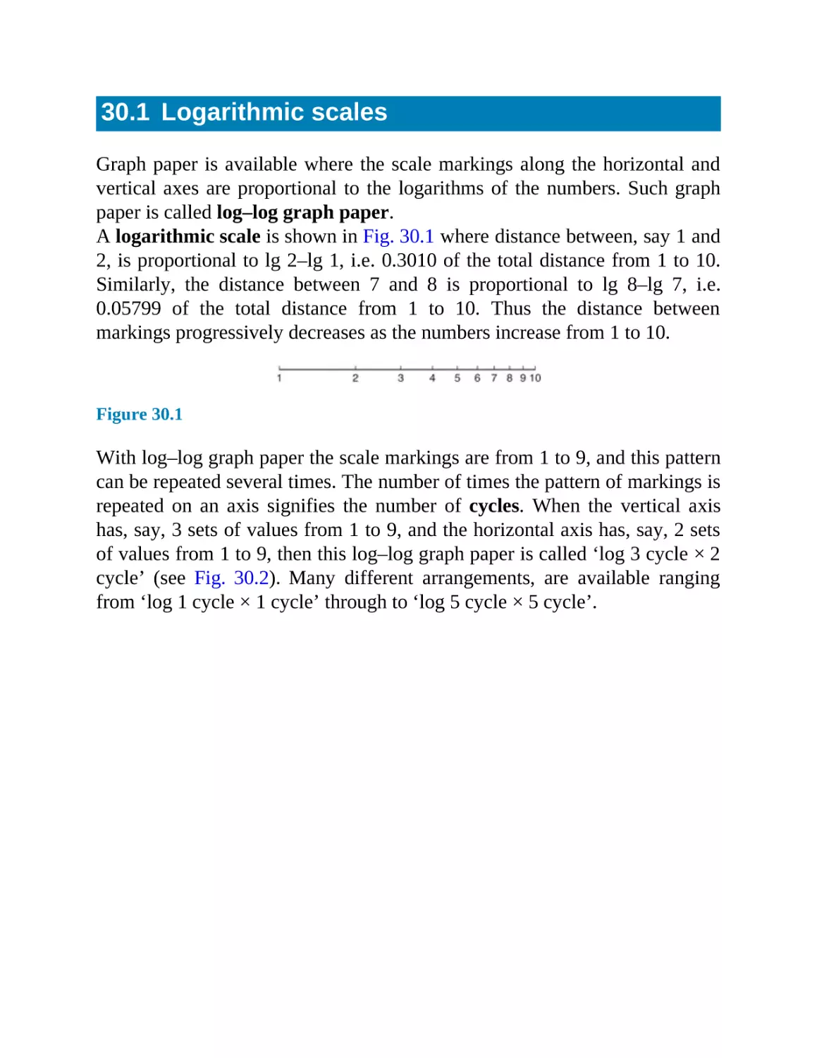
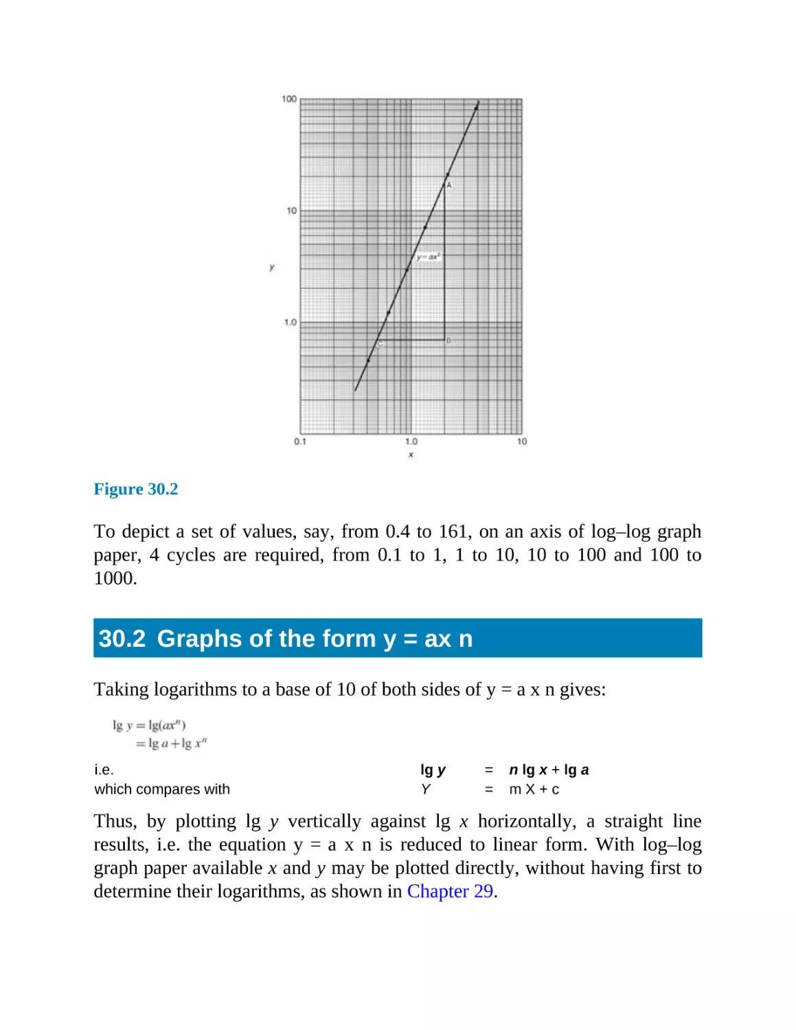
30.1 Logarithmic scales
30.2 Graphs of the form y = ax n
30.3 Graphs of the form y = a b x
30.4 Graphs of the form y = ae k x
31
Graphical solution of equations
31.1 Graphical solution of simultaneous equations
31.2 Graphical solution of quadratic equations
31.3 Graphical solution of linear and quadratic equations
simultaneously
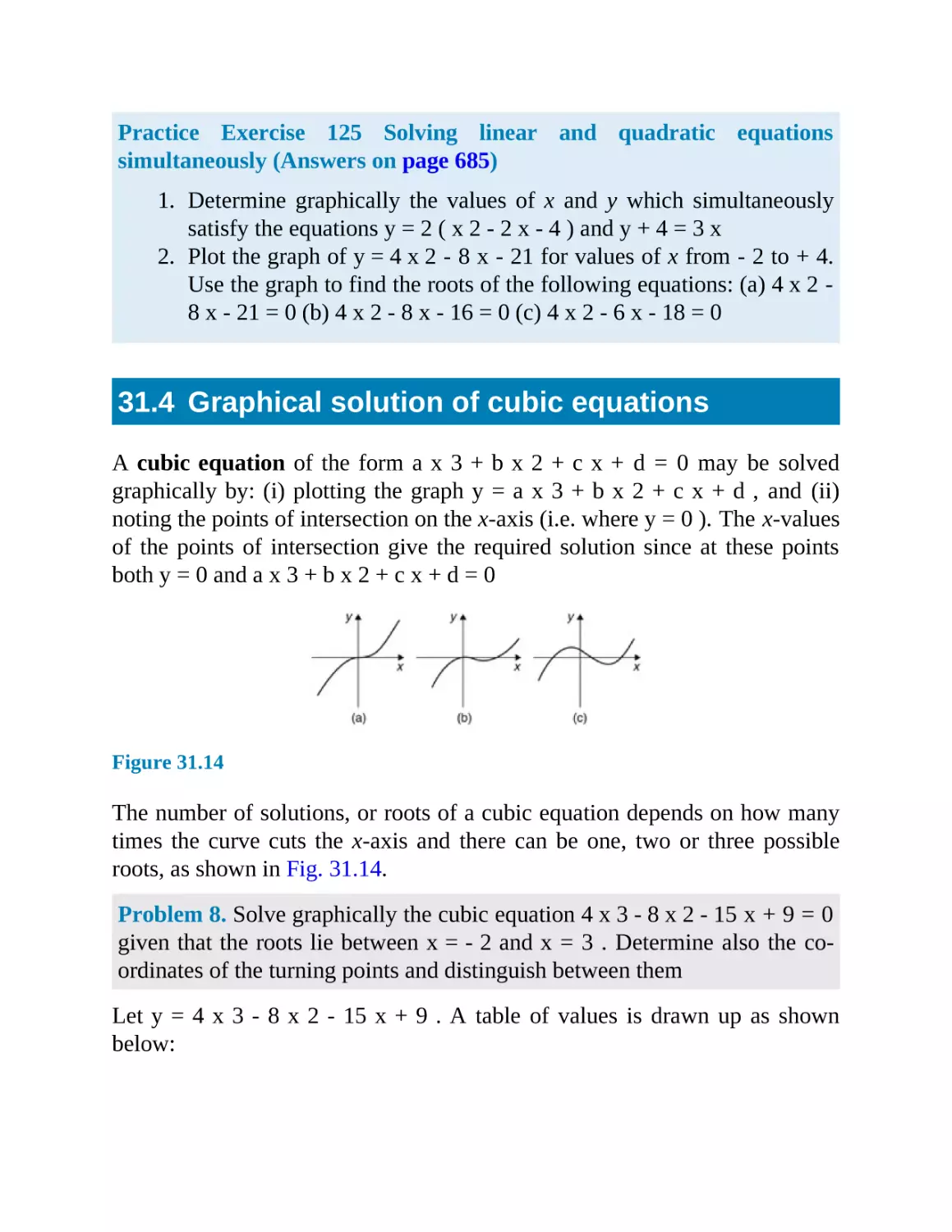
31.4 Graphical solution of cubic equations
32
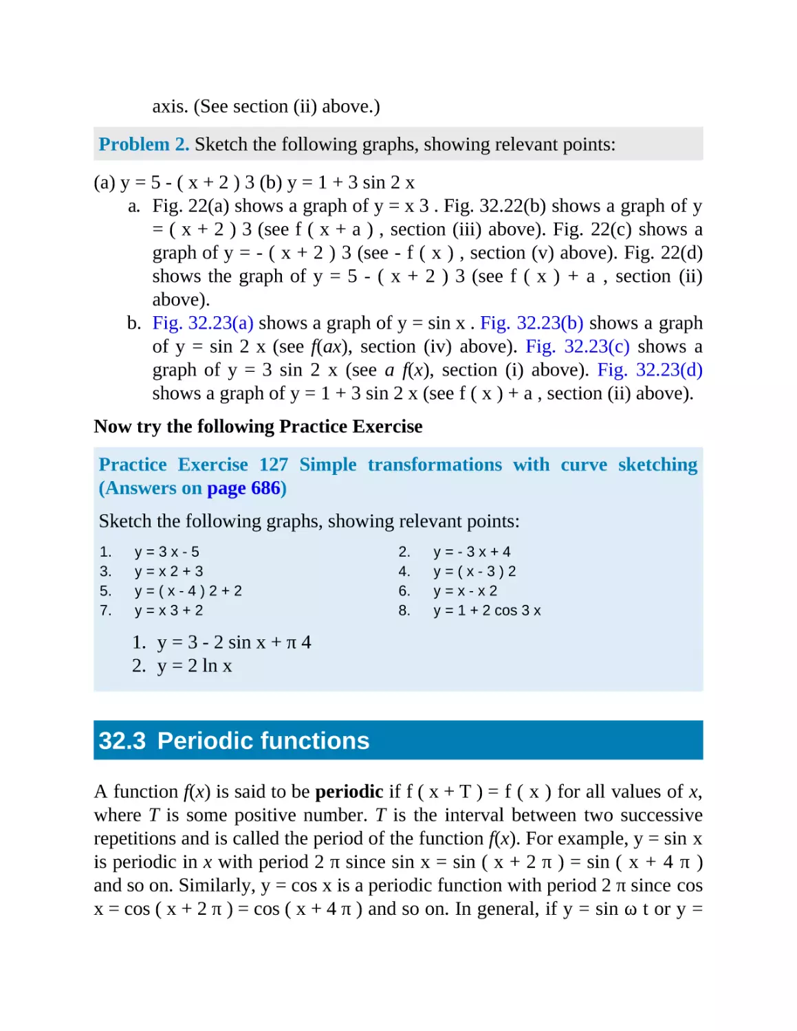
Functions and their curves
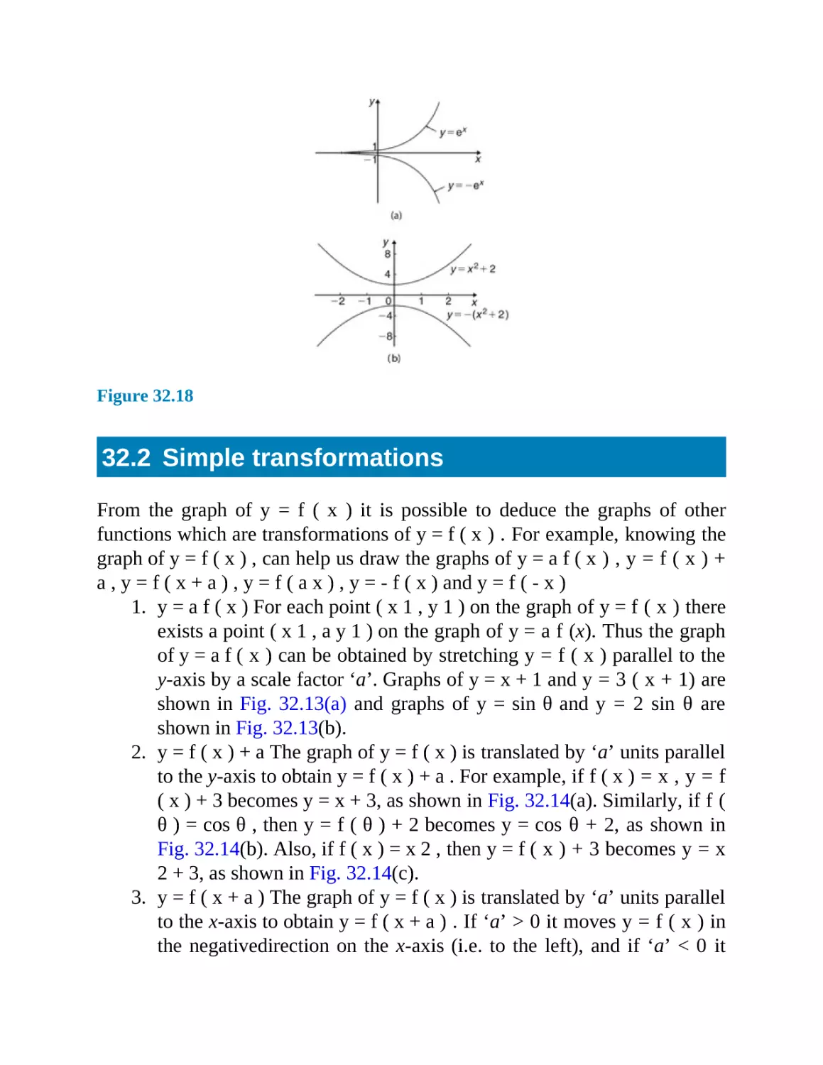
32.1 Standard curves
32.2 Simple transformations
32.3 Periodic functions
32.4 Continuous and discontinuous functions
32.5 Even and odd functions
32.6 Inverse functions
Revision Test 8
Section 5 Complex numbers
33
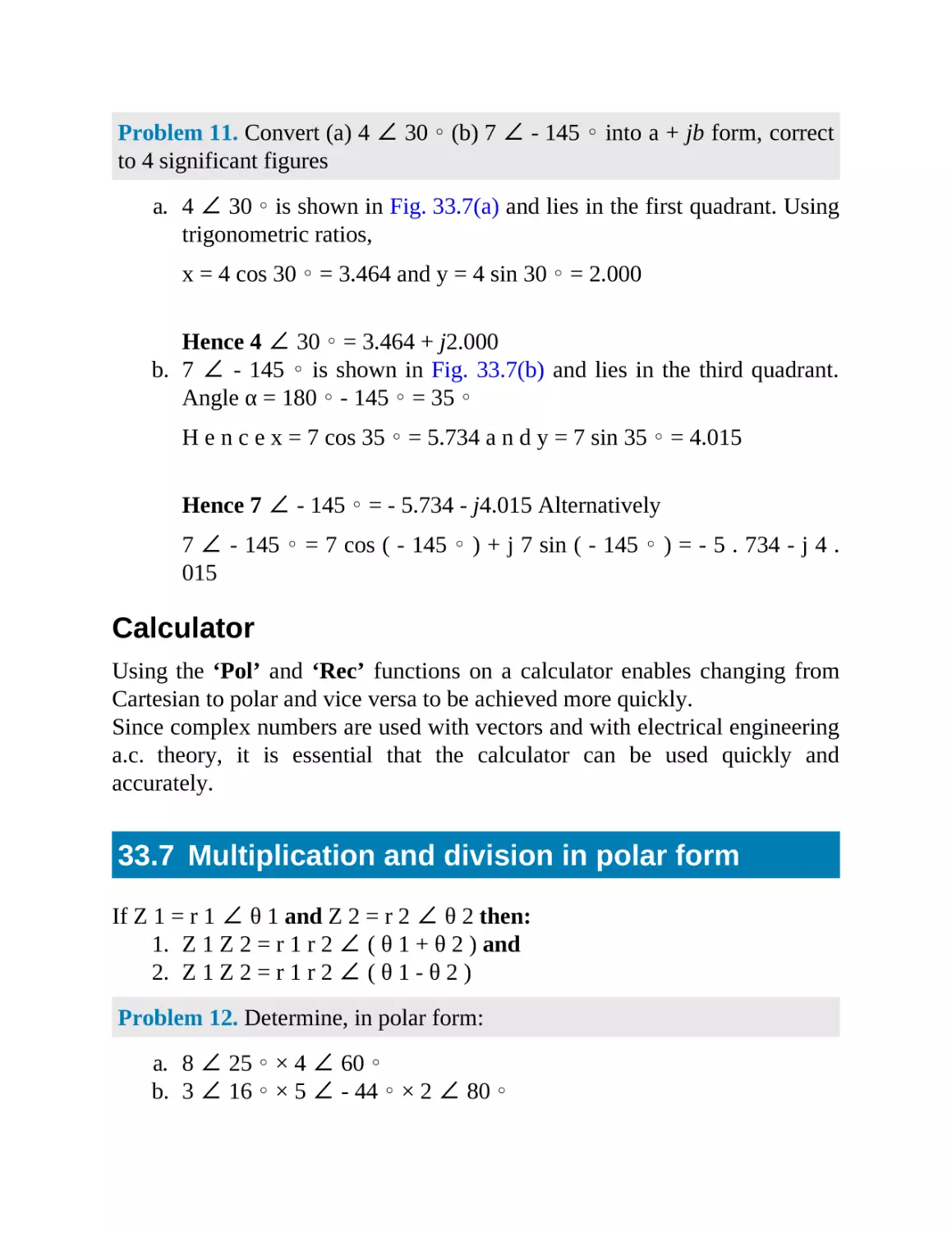
Complex numbers
33.1 Cartesian complex numbers
33.2 The Argand diagram
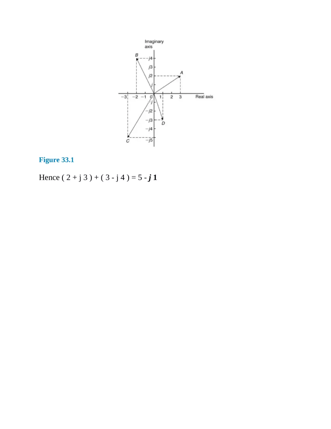
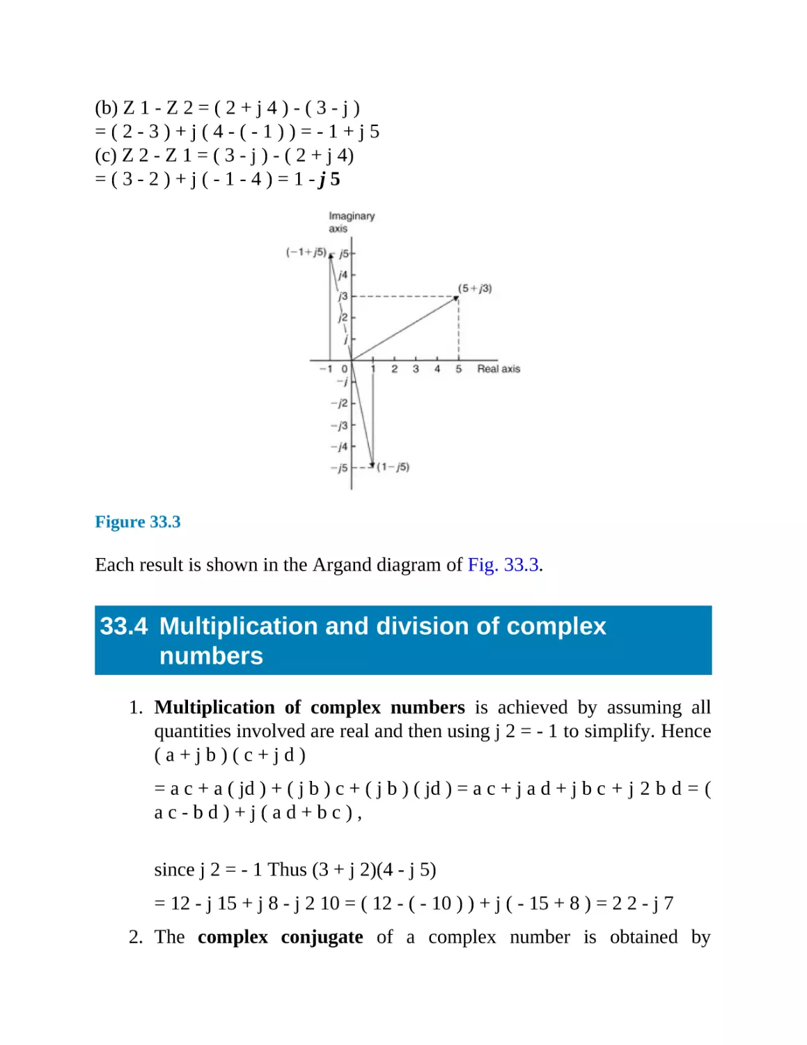
33.3 Addition and subtraction of complex numbers
33.4 Multiplication and division of complex numbers
33.5 Complex equations
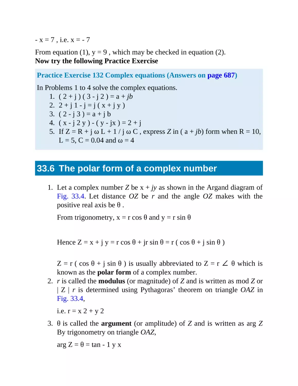
33.6 The polar form of a complex number
33.7 Multiplication and division in polar form
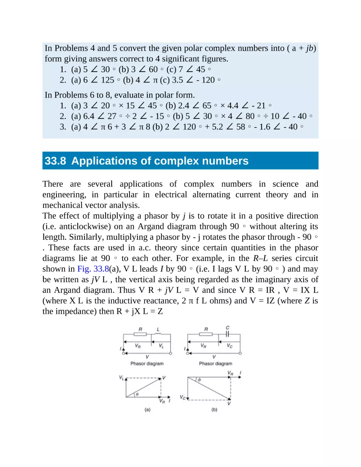
33.8 Applications of complex numbers
34
De Moivre’s theorem
34.1 Introduction
34.2 Powers of complex numbers
34.3 Roots of complex numbers
Section 6 Vectors
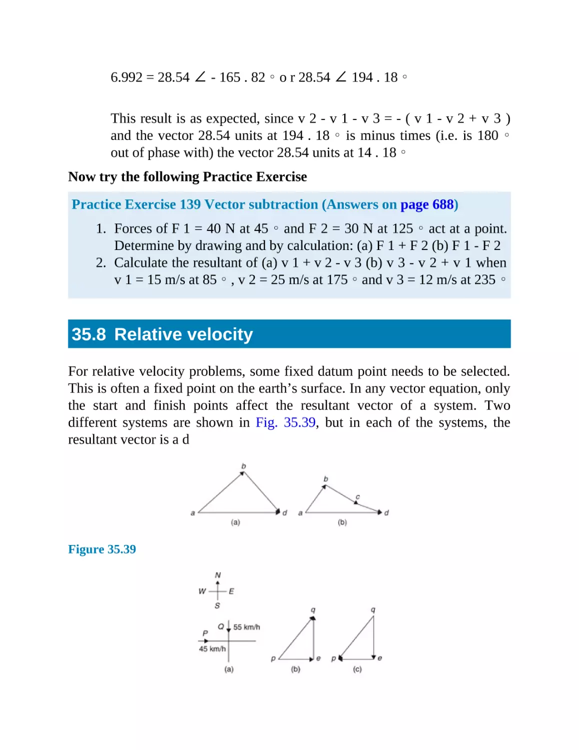
35
Vectors
35.1 Introduction
35.2 Scalars and vectors
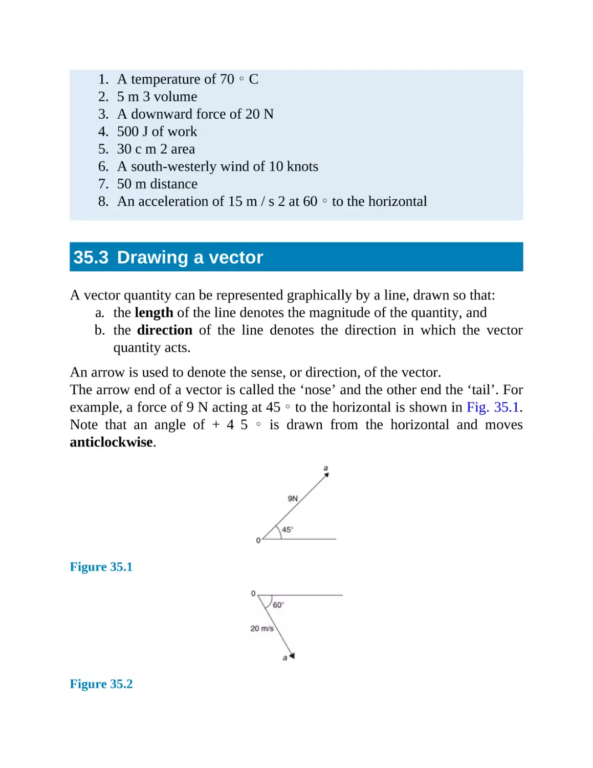
35.3 Drawing a vector
35.4 Addition of vectors by drawing
35.5 Resolving vectors into horizontal and vertical components
35.6 Addition of vectors by calculation
35.7 Vector subtraction
35.8 Relative velocity
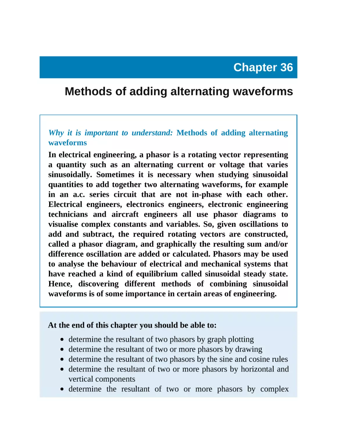
35.9 i , j and k notation
36
Methods of adding alternating waveforms
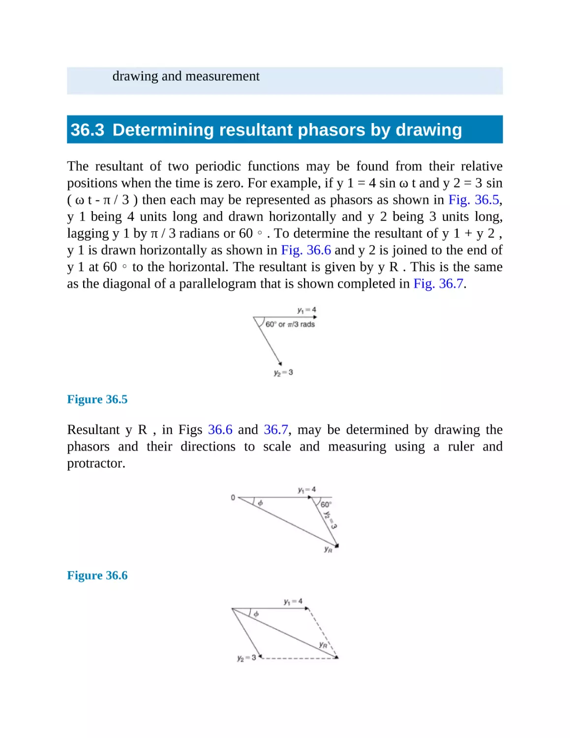
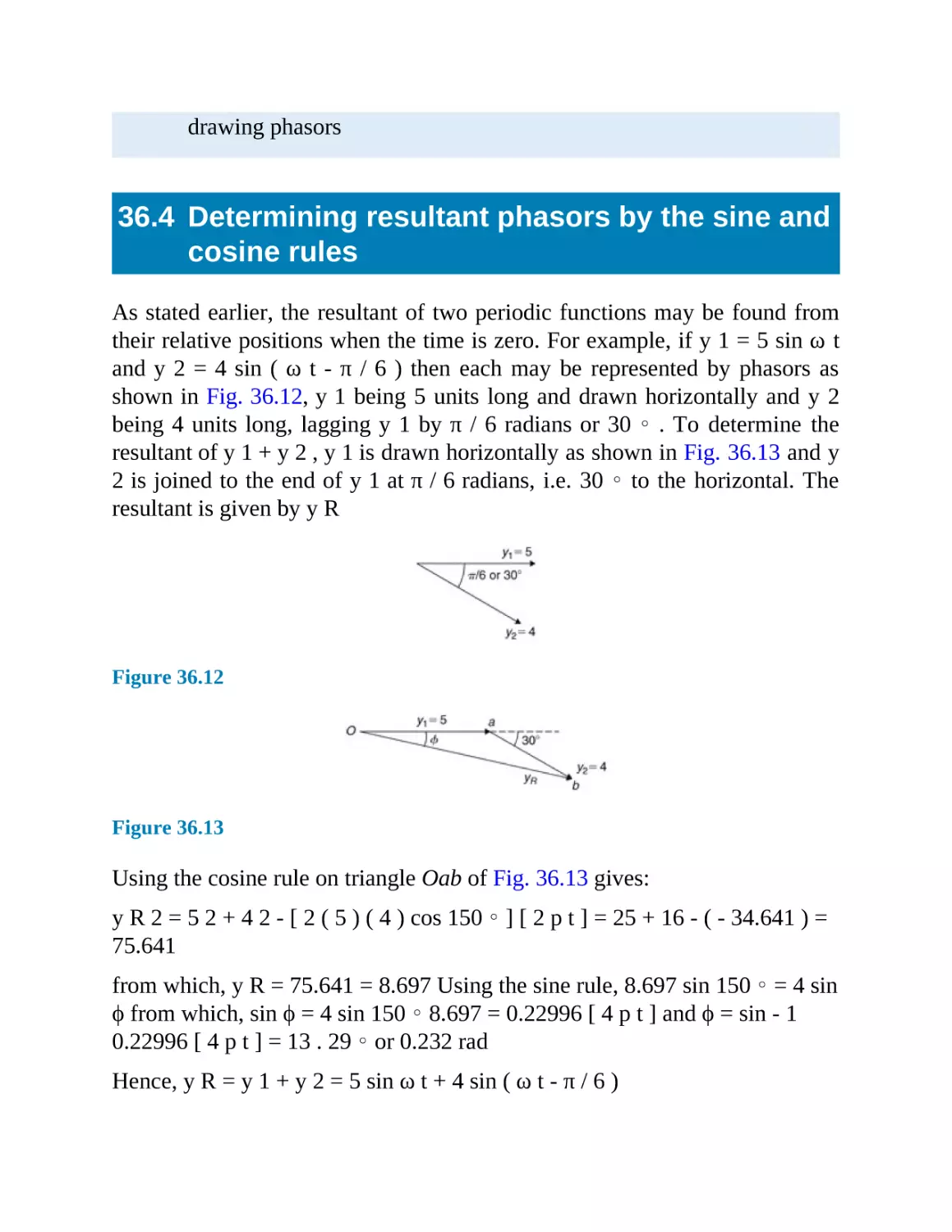
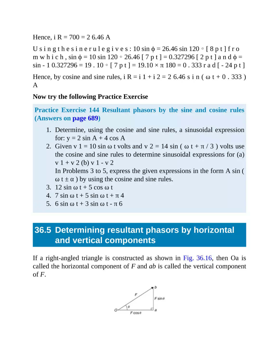
36.1 Combination of two periodic functions
36.2 Plotting periodic functions
36.3 Determining resultant phasors by drawing
36.4 Determining resultant phasors by the sine and cosine rules
36.5 Determining resultant phasors by horizontal and vertical
components
36.6 Determining resultant phasors by complex numbers
Revision Test 9
Section 7 Statistics
37
Presentation of statistical data
37.1 Some statistical terminology
37.2 Presentation of ungrouped data
37.3 Presentation of grouped data
38
Mean, median, mode and standard deviation
38.1
38.2
38.3
38.4
38.5
39
Measures of central tendency
Mean, median and mode for discrete data
Mean, median and mode for grouped data
Standard deviation
Quartiles, deciles and percentiles
Probability
39.1 Introduction to probability
39.2 Laws of probability
39.3 Worked problems on probability
39.4 Further worked problems on probability
39.5 Permutations and combinations
39.6 Bayes’ theorem
Revision Test 10
40
The binomial and Poisson distributions
40.1 The binomial distribution
40.2 The Poisson distribution
41
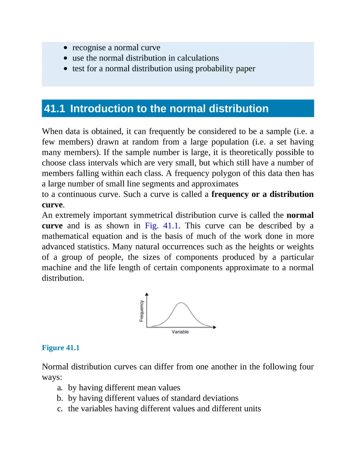
The normal distribution
41.1 Introduction to the normal distribution
41.2 Testing for a normal distribution
Revision Test 11
42
Linear correlation
42.1 Introduction to linear correlation
42.2 The Pearson product-moment formula for determining the linear
correlation coefficient
42.3 The significance of a coefficientof correlation
42.4 Worked problems on linear correlation
43
Linear regression
43.1 Introduction to linear regression
43.2 The least-squares regression lines
43.3 Worked problems on linear regression
44
Sampling and estimation theories
44.1
44.2
44.3
44.4
Introduction
Sampling distributions
The sampling distribution of the means
The estimation of population parameters based on a large sample
size
44.5 Estimating the mean of a population based on a small sample
size
Revision Test 12
Multiple choice questions on Chapters 28–44
Section 8 Differential calculus
45
Introduction to differentiation
45.1 Introduction to calculus
45.2 Functional notation
45.3 The gradient of a curve
45.4 Differentiation from first principles
45.5 Differentiation of y = a x n by the general rule
45.6 Differentiation of sine and cosine functions
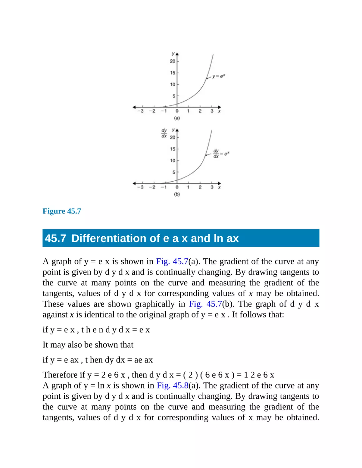
45.7 Differentiation of e a x and ln ax
46
Methods of differentiation
46.1 Differentiation of common functions
46.2 Differentiation of a product
46.3 Differentiation of a quotient
46.4 Function of a function
46.5 Successive differentiation
47
Some applications of differentiation
47.1 Rates of change
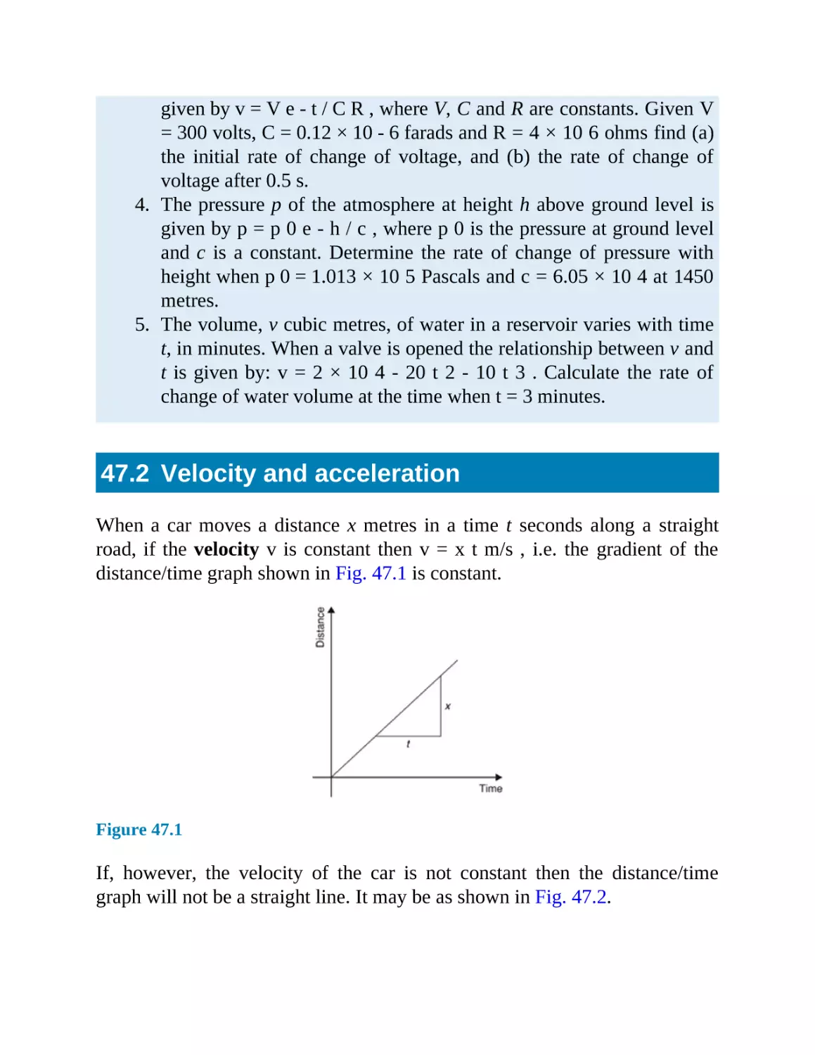
47.2 Velocity and acceleration
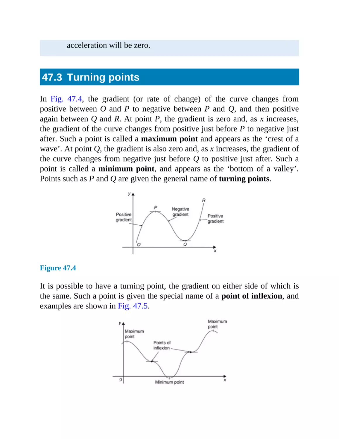
47.3 Turning points
47.4 Practical problems involving maximum and minimum values
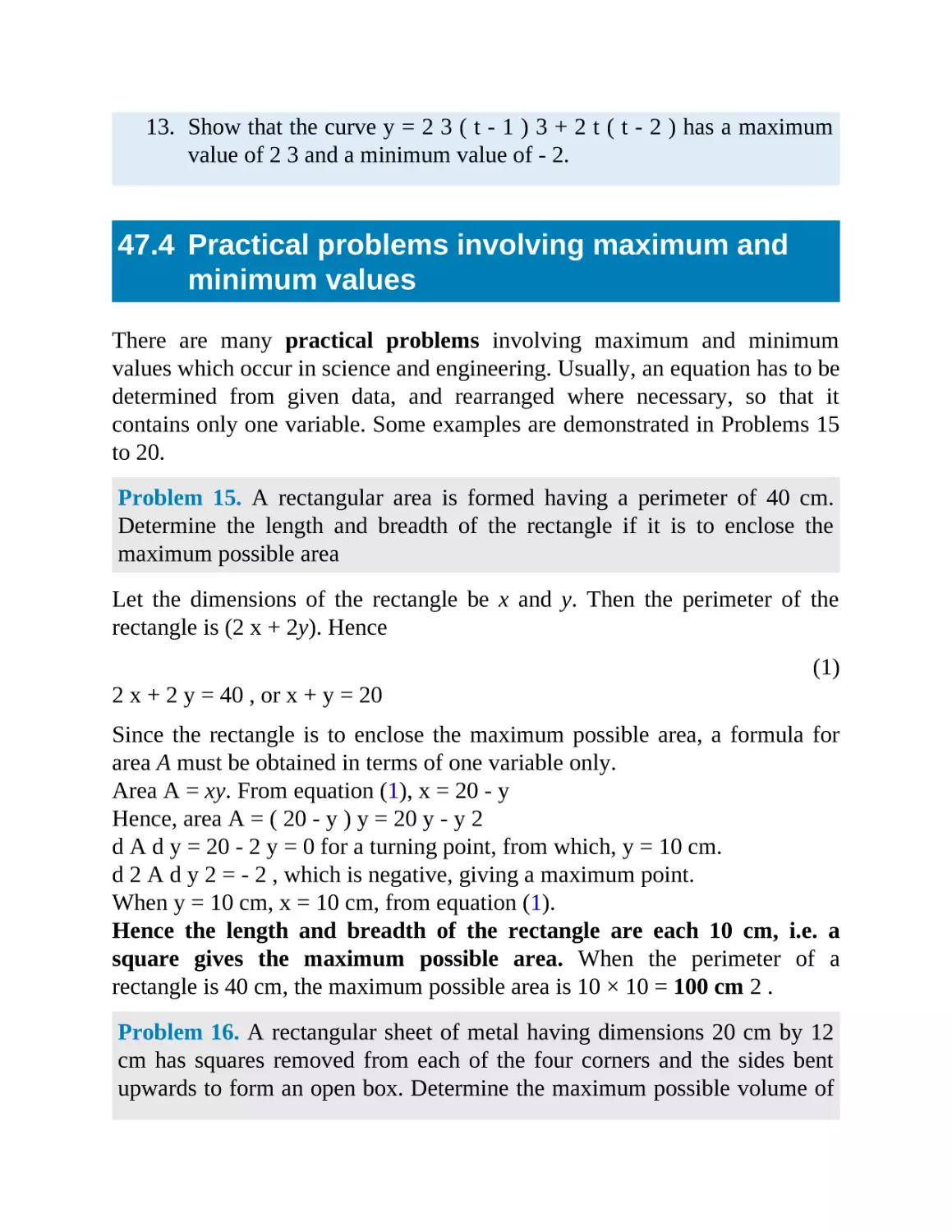
47.5 Points of inflexion
47.6 Tangents and normals
47.7 Small changes
48
Maclaurin’s series
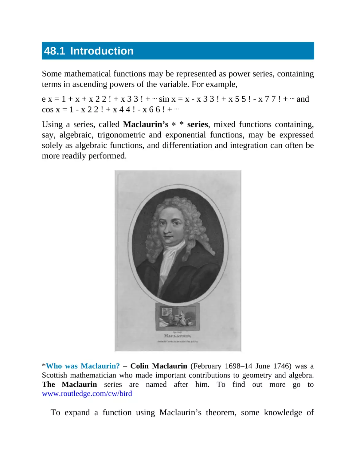
48.1 Introduction
48.2 Derivation of Maclaurin’s theorem
48.3 Conditions of Maclaurin’s series
48.4 Worked problems on Maclaurin’s series
Revision Test 13
49
Differentiation of parametric equations
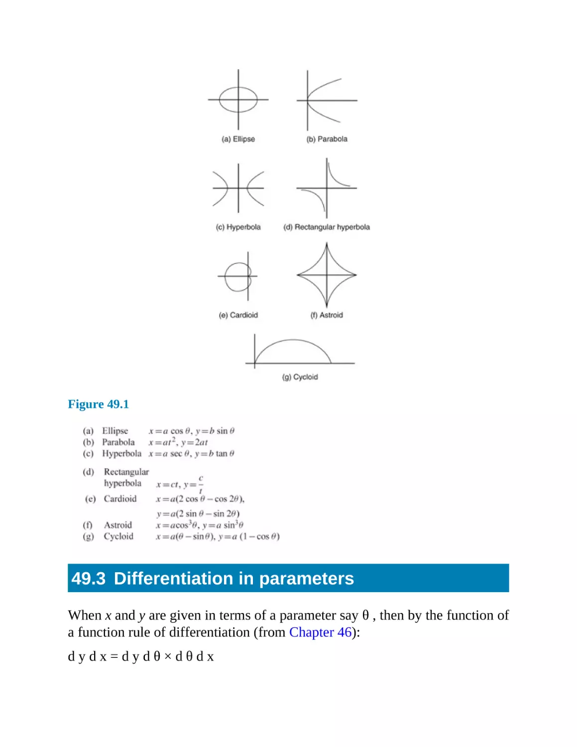
49.1 Introduction to parametric equations
49.2 Some common parametric equations
49.3 Differentiation in parameters
49.4 Further worked problems on differentiation of parametric
equations
50
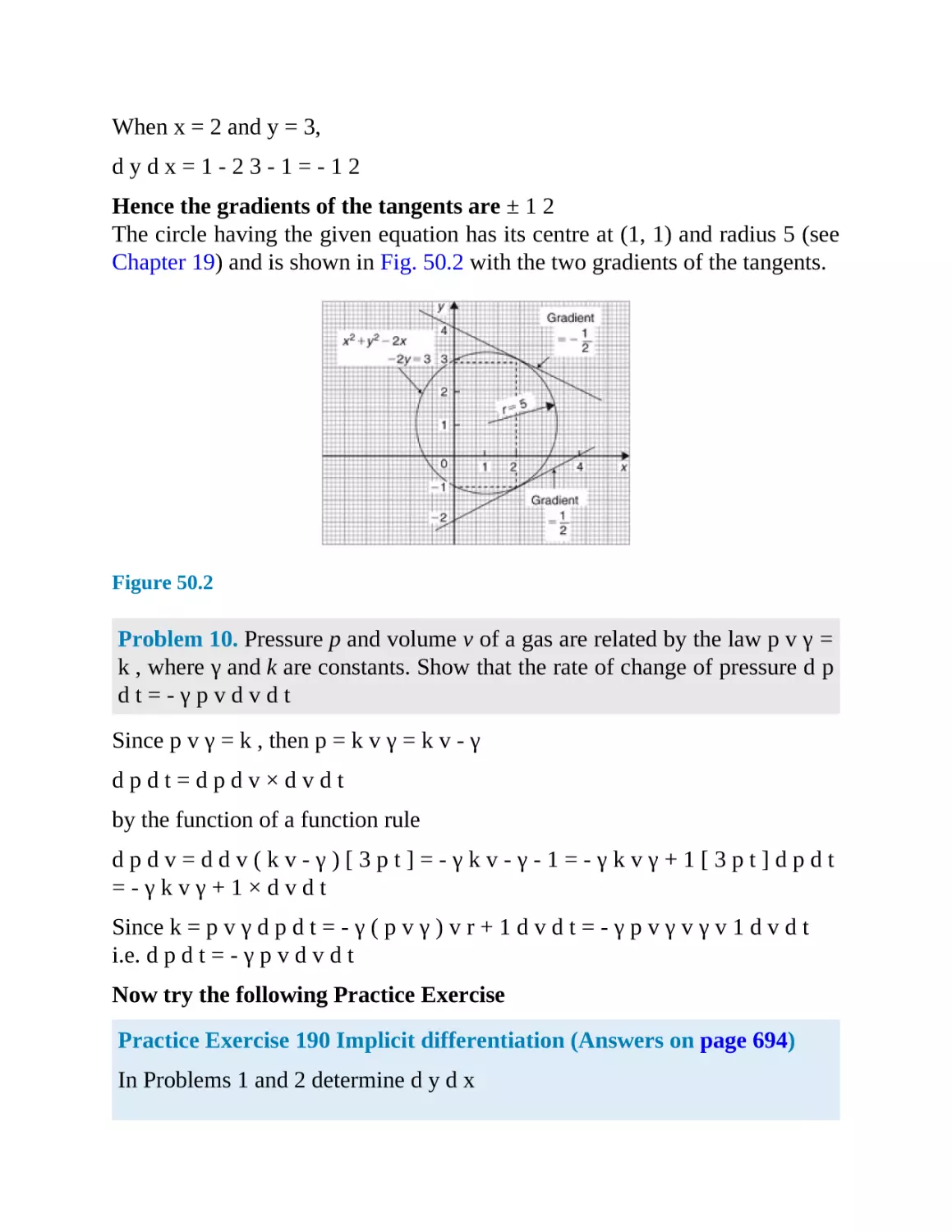
Differentiation of implicit functions
50.1 Implicit functions
50.2 Differentiating implicit functions
50.3 Differentiating implicit functions containing products and
quotients
50.4 Further implicit differentiation
51
Logarithmic differentiation
51.1 Introduction to logarithmic differentiation
51.2 Laws of logarithms
51.3 Differentiation of logarithmic functions
51.4 Differentiation of further logarithmic functions
51.5 Differentiation of [ f ( x ) ] x
Revision Test 14
Section 9 Integral calculus
52
Standard integration
52.1 The process of integration
52.2 The general solution of integrals of the form ax b o l d s y m b o l
n
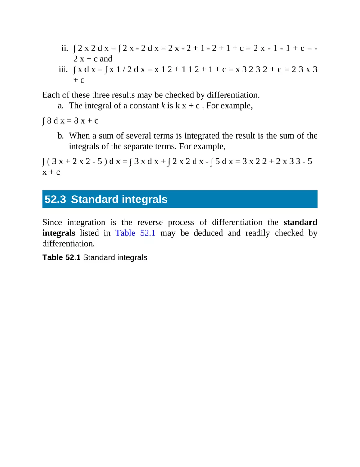
52.3 Standard integrals
52.4 Definite integrals
53
Integration using algebraic substitutions
53.1 Introduction
53.2 Algebraic substitutions
53.3 Worked problems on integration using algebraic substitutions
53.4 Further worked problems on integration using algebraic
substitutions
53.5 Change of limits
54
Integration using trigonometric substitutions
54.1 Introduction
54.2 Worked problems on integration of sin 2 x, cos 2 x, tan 2 x and
cot 2 x
54.3 Worked problems on integration of powers of sines and cosines
54.4 Worked problems on integration of products of sines and cosines
54.5 Worked problems on integration using the sin θ substitution
54.6 Worked problems on integration using the tan θ substitution
Revision Test 15
55
Integration using partial fractions
55.1 Introduction
55.2 Worked problems on integration using partial fractions with
linear factors
55.3 Worked problems on integration using partial fractions with
repeated linear factors
55.4 Worked problems on integration using partial fractions with
quadratic factors
56
The t = tan θ / 2 substitution
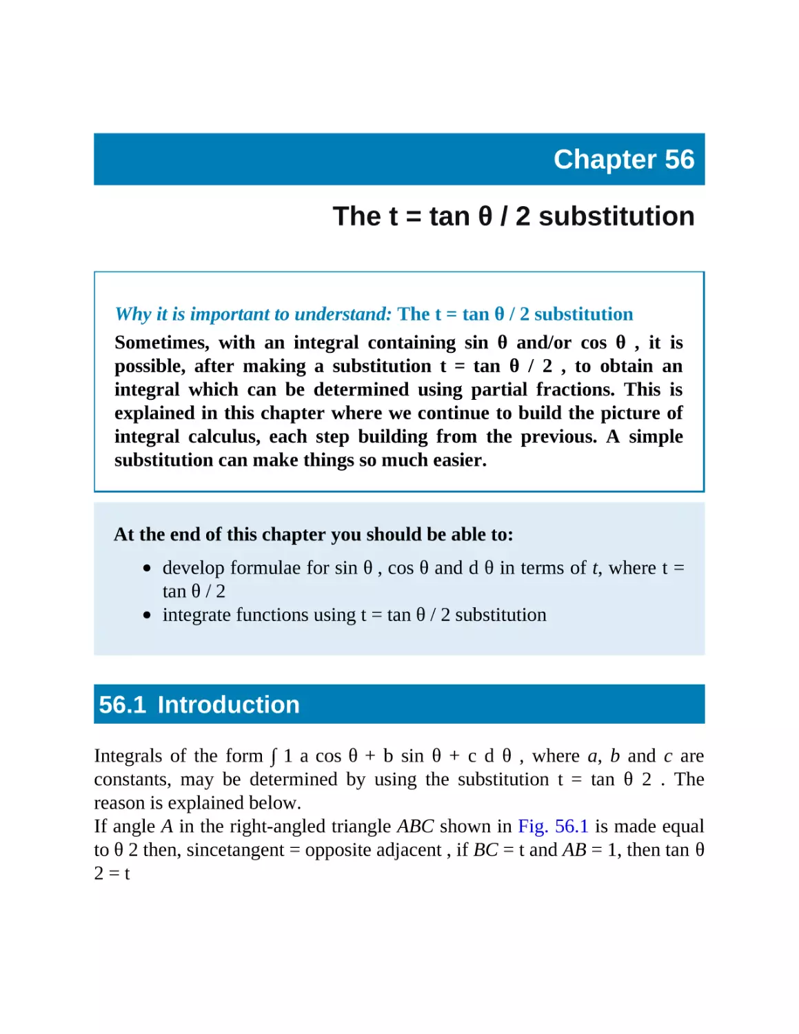
56.1 Introduction
56.2 Worked problems on the t = tan θ 2 substitution
56.3 Further worked problems on the t = tan θ 2 substitution
57
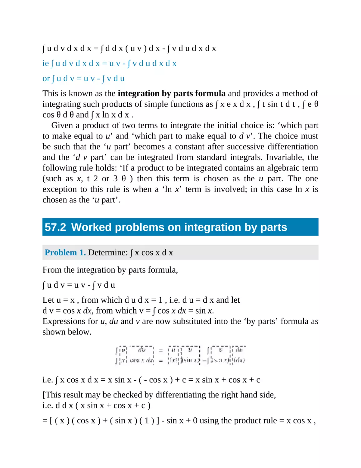
Integration by parts
57.1 Introduction
57.2 Worked problems on integration by parts
57.3 Further worked problems on integration by parts
58
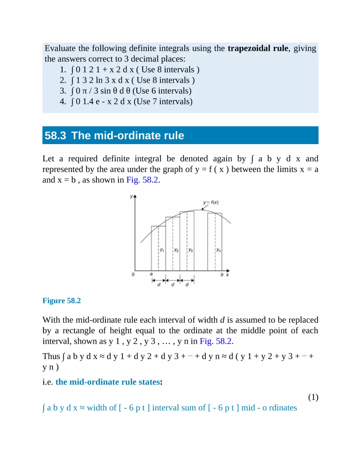
Numerical integration
58.1 Introduction
58.2 The trapezoidal rule
58.3 The mid-ordinate rule
58.4 Simpson’s rule
58.5 Accuracy of numerical integration
Revision Test 16
59
Areas under and between curves
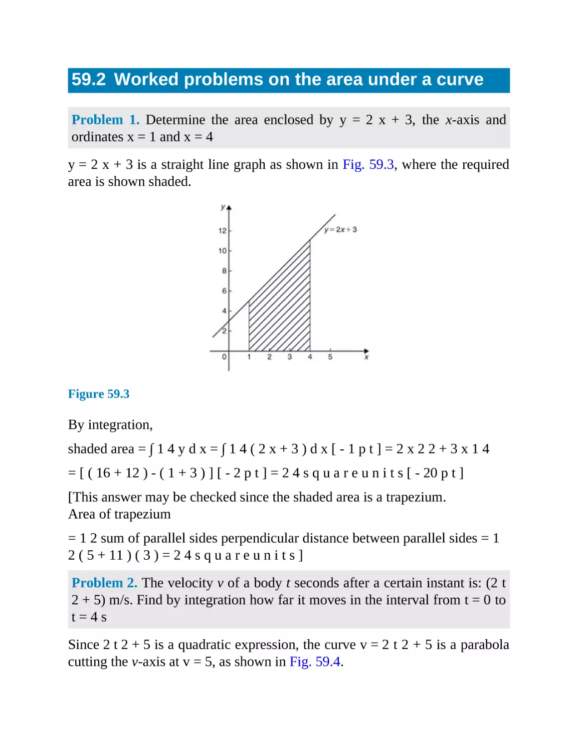
59.1 Area under a curve
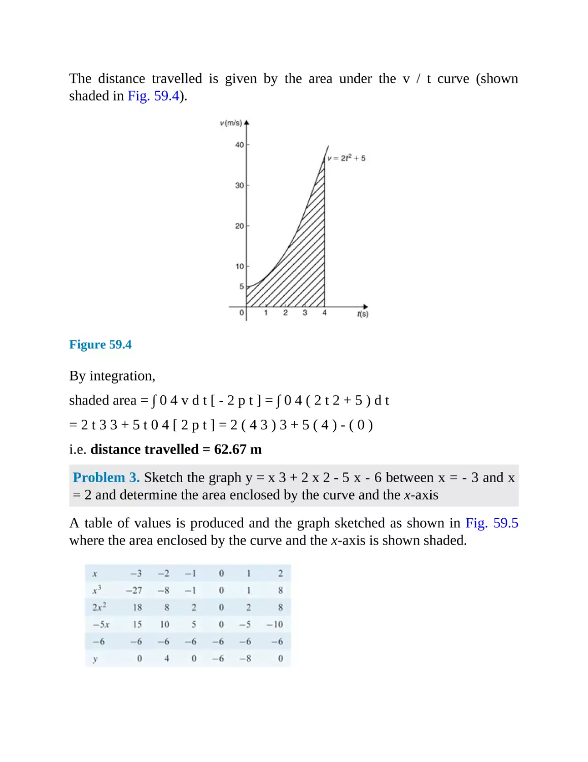
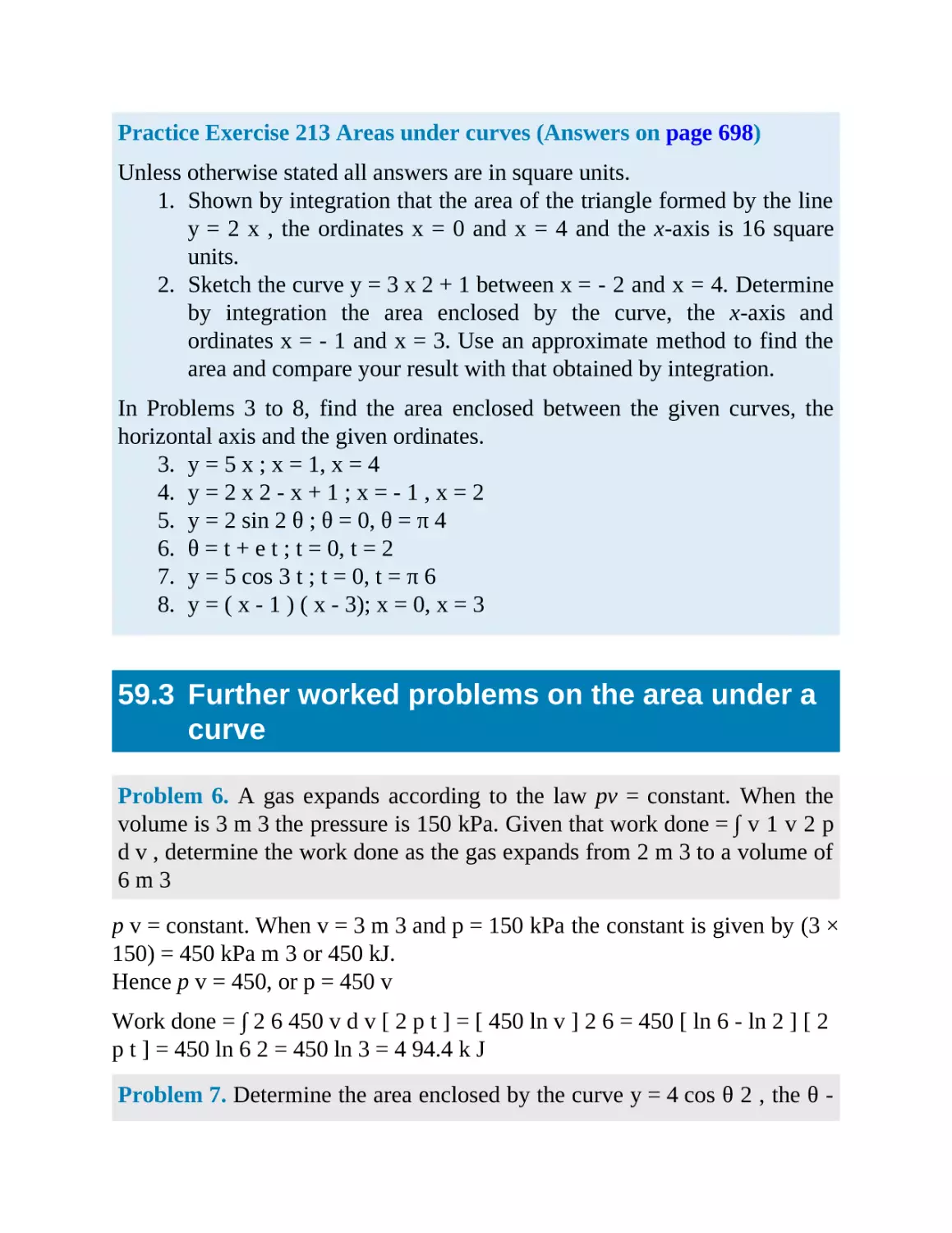
59.2 Worked problems on the area under a curve
59.3 Further worked problems on the area under a curve
59.4 The area between curves
60
Mean and root mean square values
60.1 Mean or average values
60.2 Root mean square values
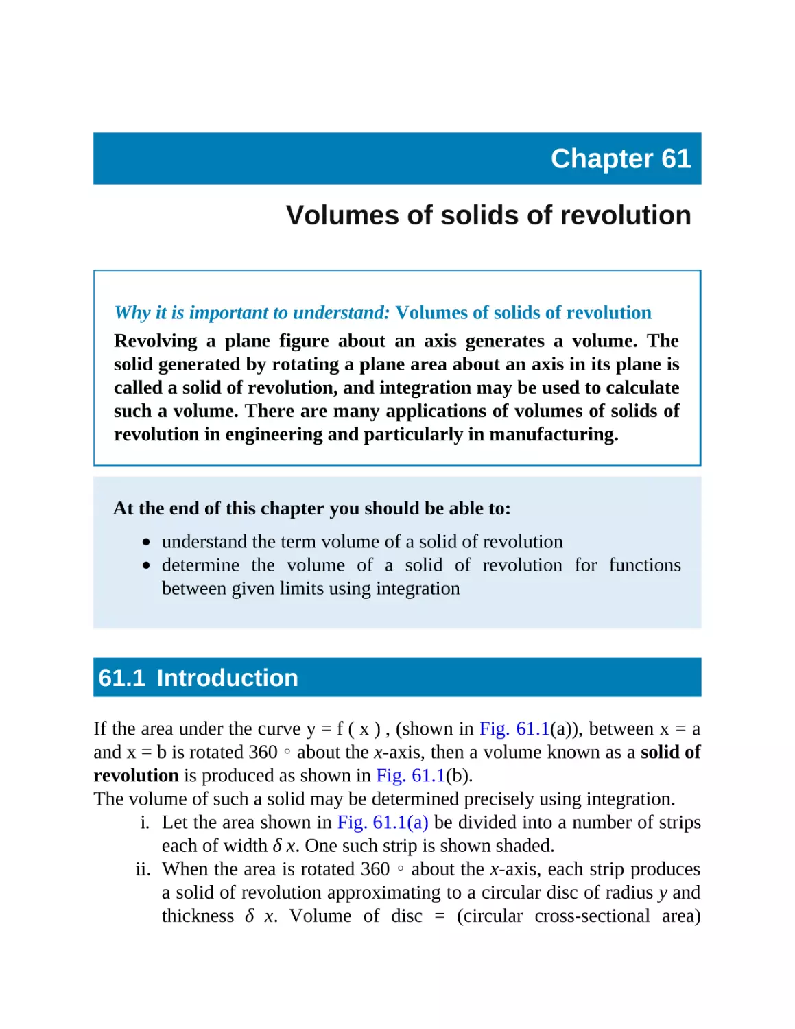
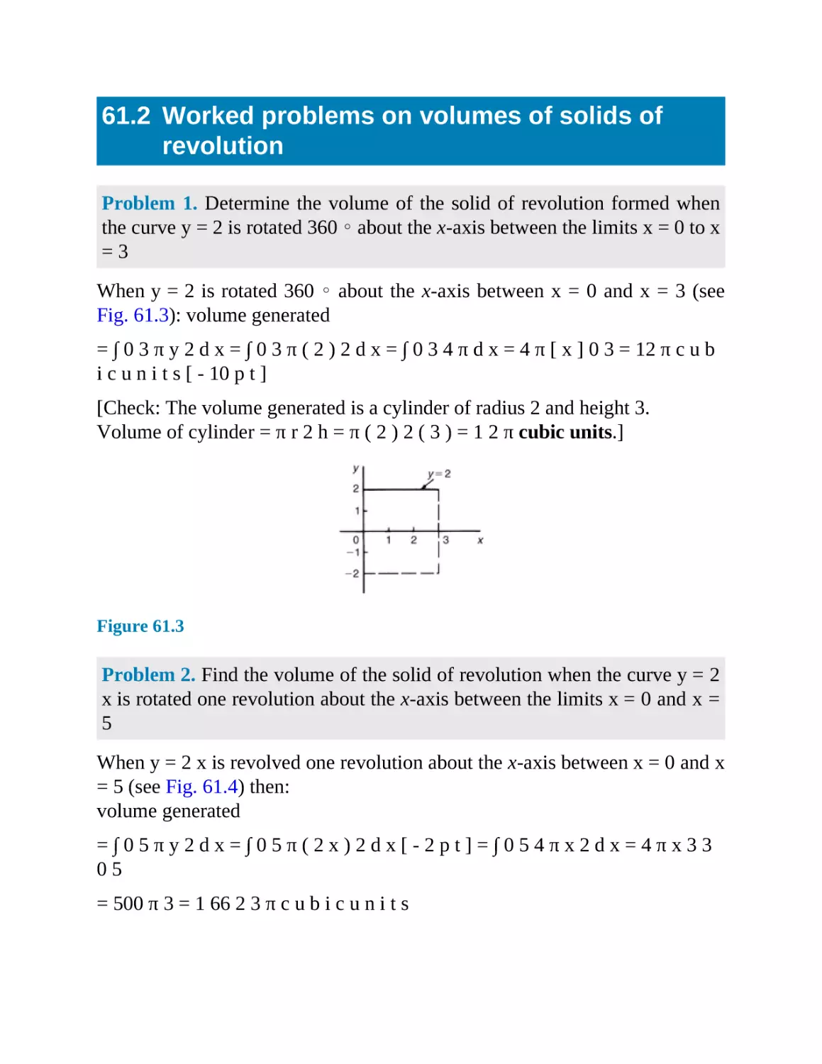
61
Volumes of solids of revolution
61.1 Introduction
61.2 Worked problems on volumes of solids of revolution
61.3 Further worked problems on volumes of solids of revolution
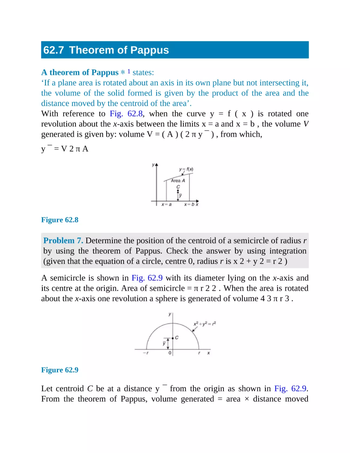
62
Centroids of simple shapes
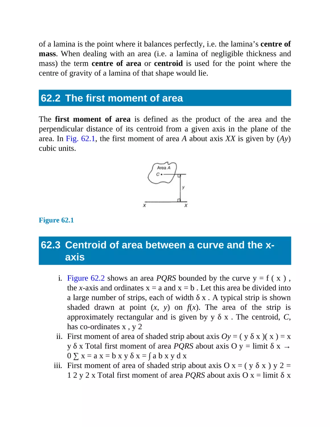
62.1 Centroids
62.2 The first moment of area
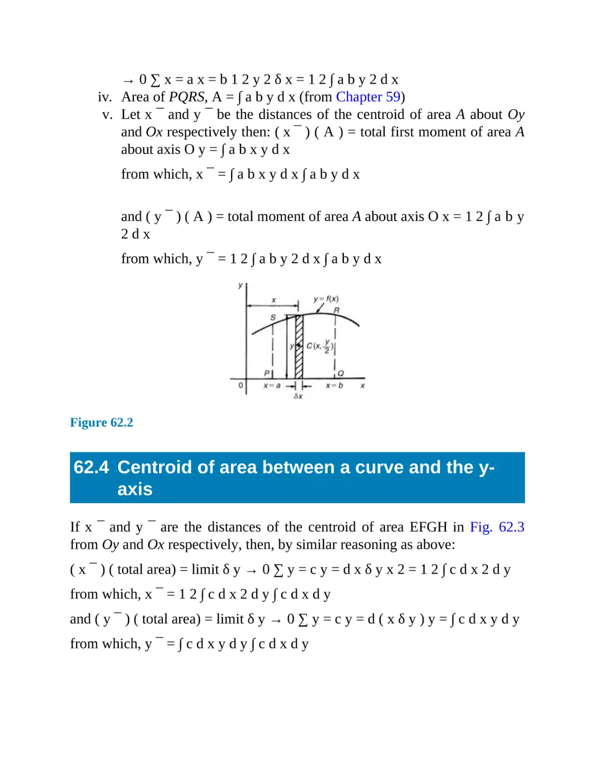
62.3 Centroid of area between a curve and the x-axis
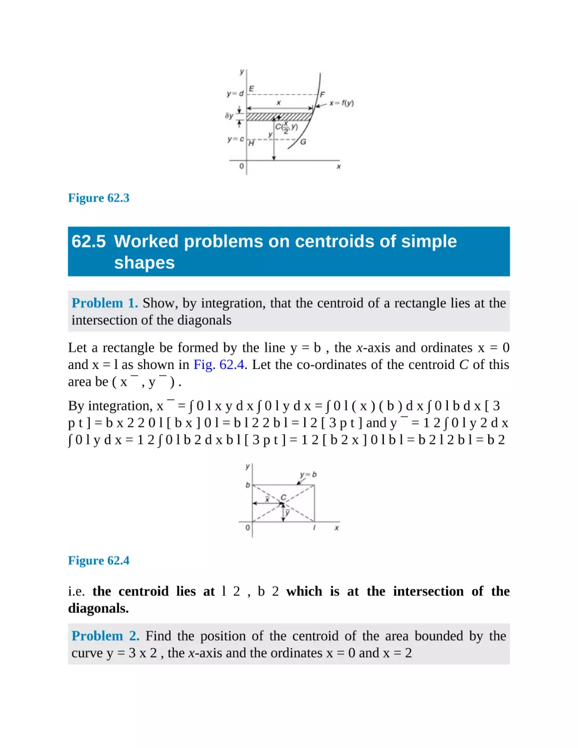
62.4 Centroid of area between a curve and the y-axis
62.5 Worked problems on centroids of simple shapes
62.6 Further worked problems on centroids of simple shapes
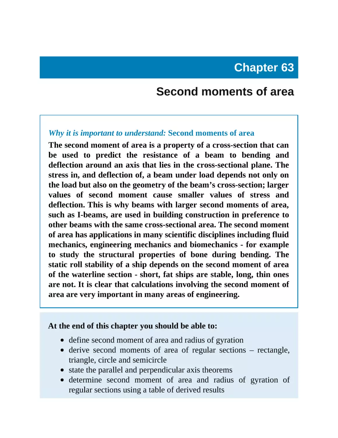
62.7 Theorem of Pappus
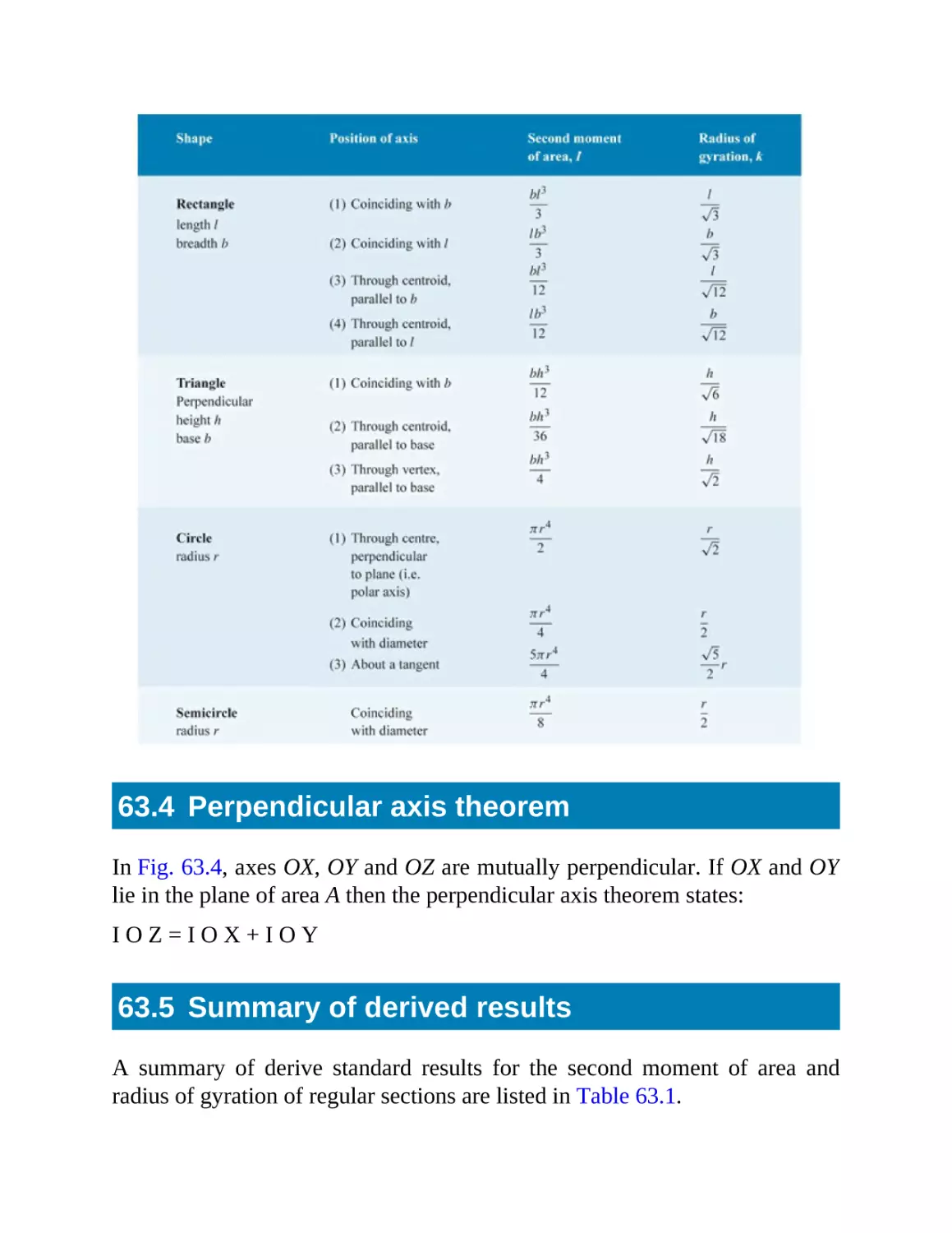
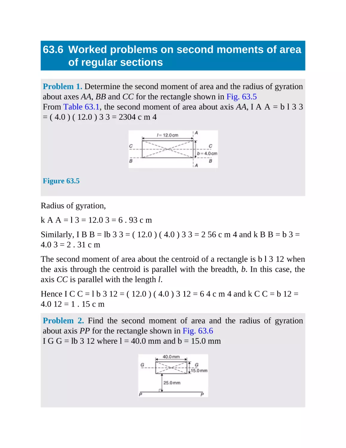
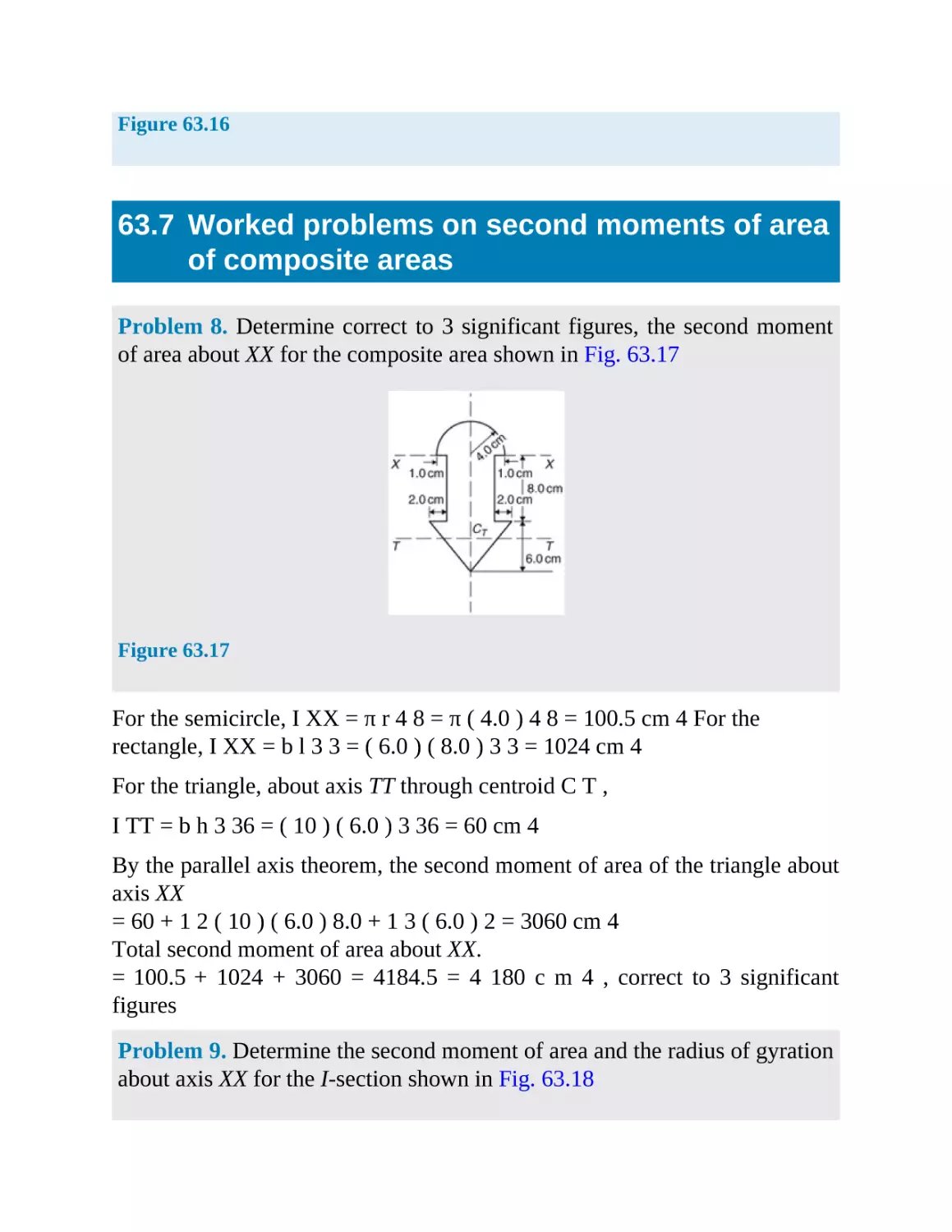
63
Second moments of area
63.1 Second moments of area and radius of gyration
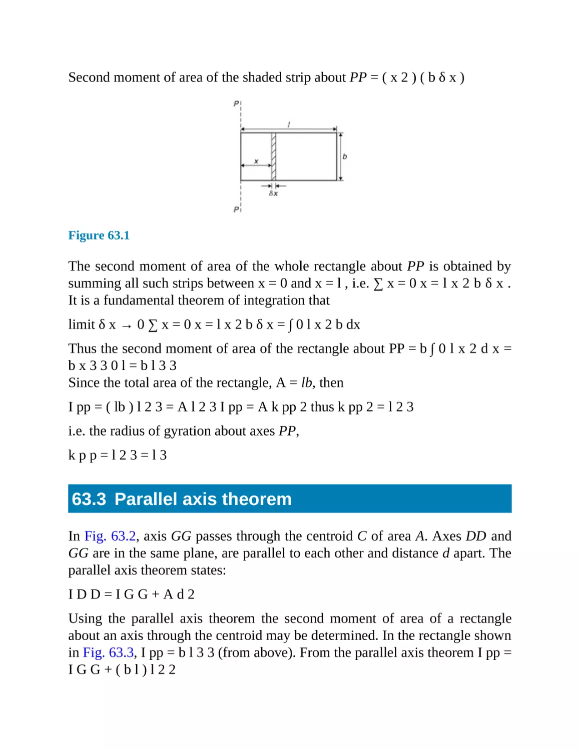
63.2 Second moment of area of regular sections
63.3 Parallel axis theorem
63.4 Perpendicular axis theorem
63.5 Summary of derived results
63.6 Worked problems on second moments of area of regular sections
63.7 Worked problems on second moments of area of composite areas
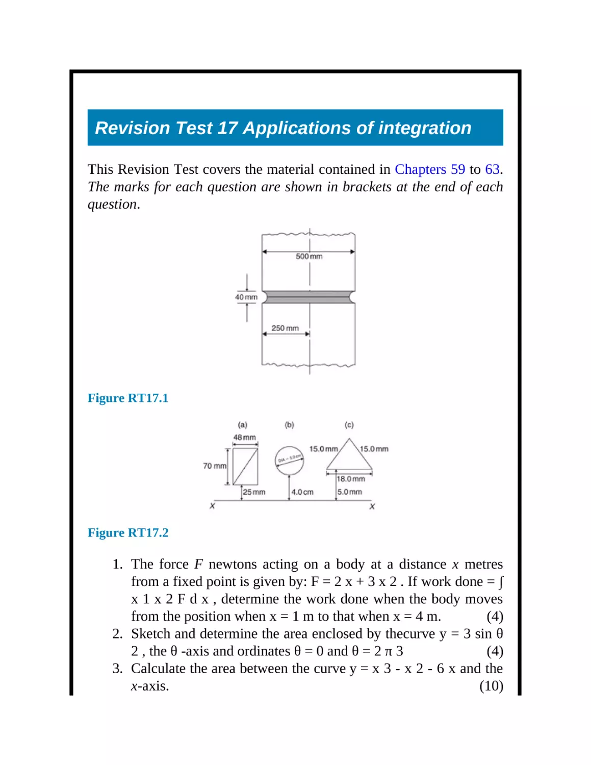
Revision Test 17
Section 10 Differential equations
64
Introduction to differential equations
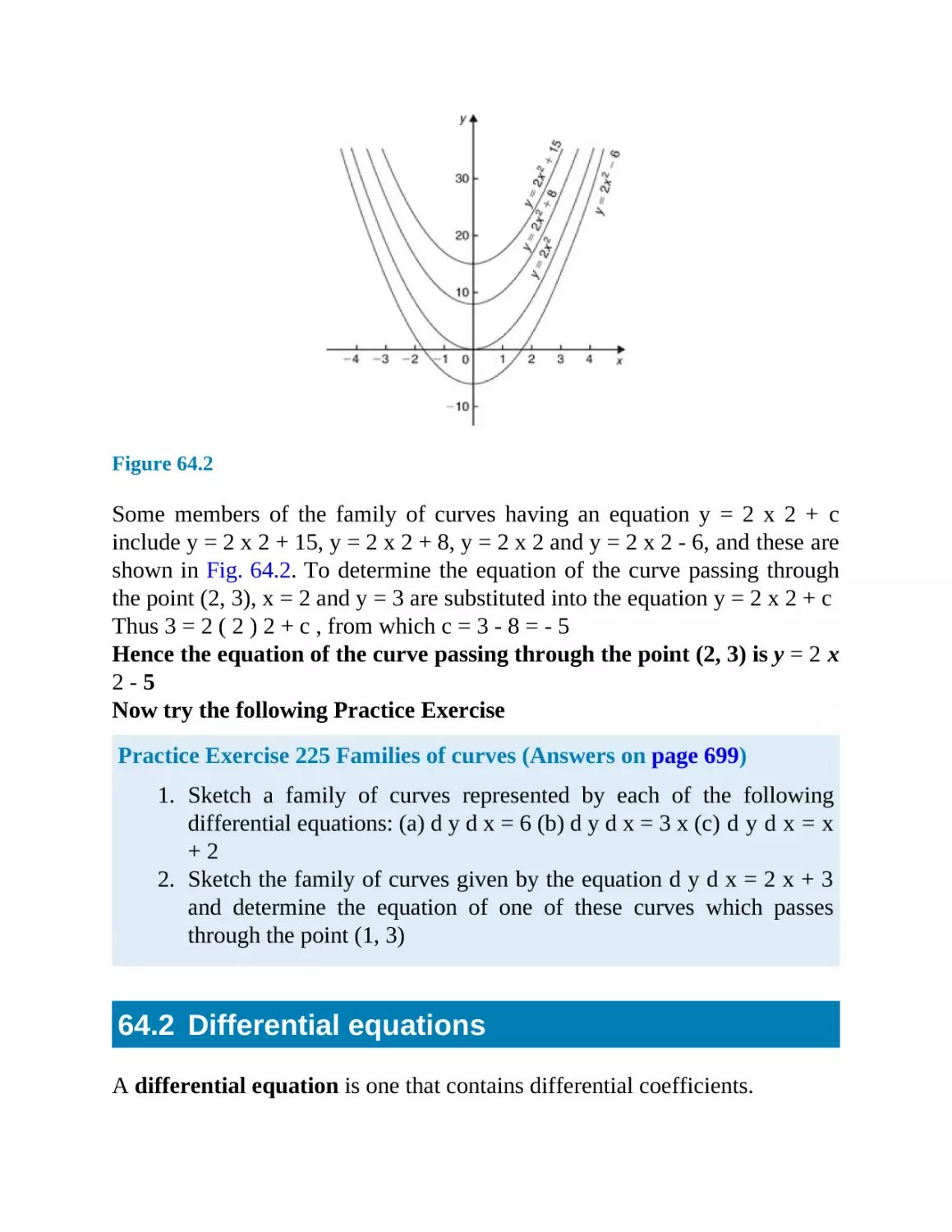
64.1 Family of curves
64.2 Differential equations
64.3 The solution of equations of the form d y d x = f ( x )
64.4 The solution of equations of the form d y d x = f ( y )
64.5 The solution of equations of the form d y d x = f x ) · f y
Revision Test 18
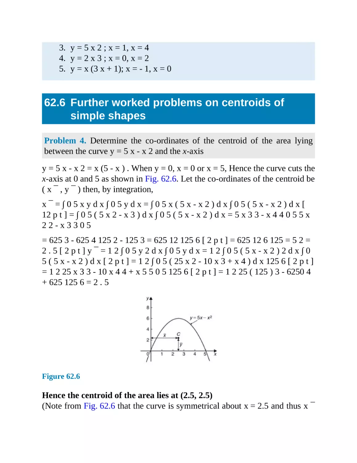
Section 11 Further number and algebra
65
Boolean algebra and logic circuits
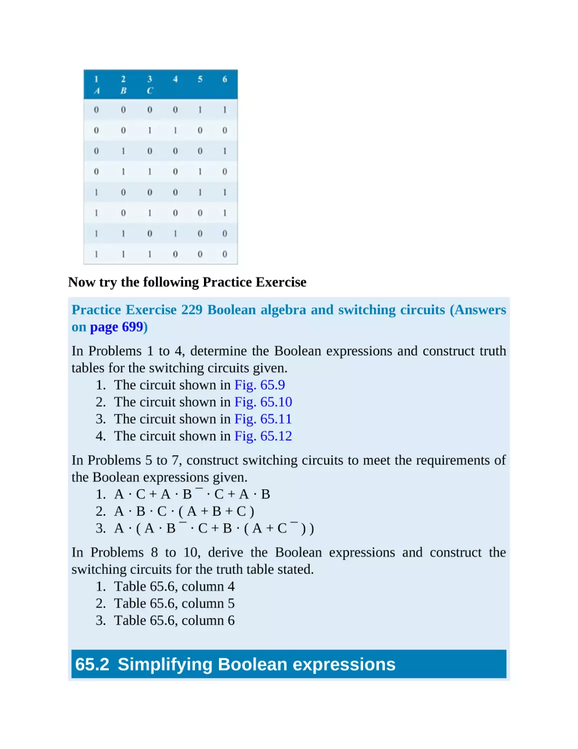
65.1 Boolean algebra and switching circuits
65.2 Simplifying Boolean expressions
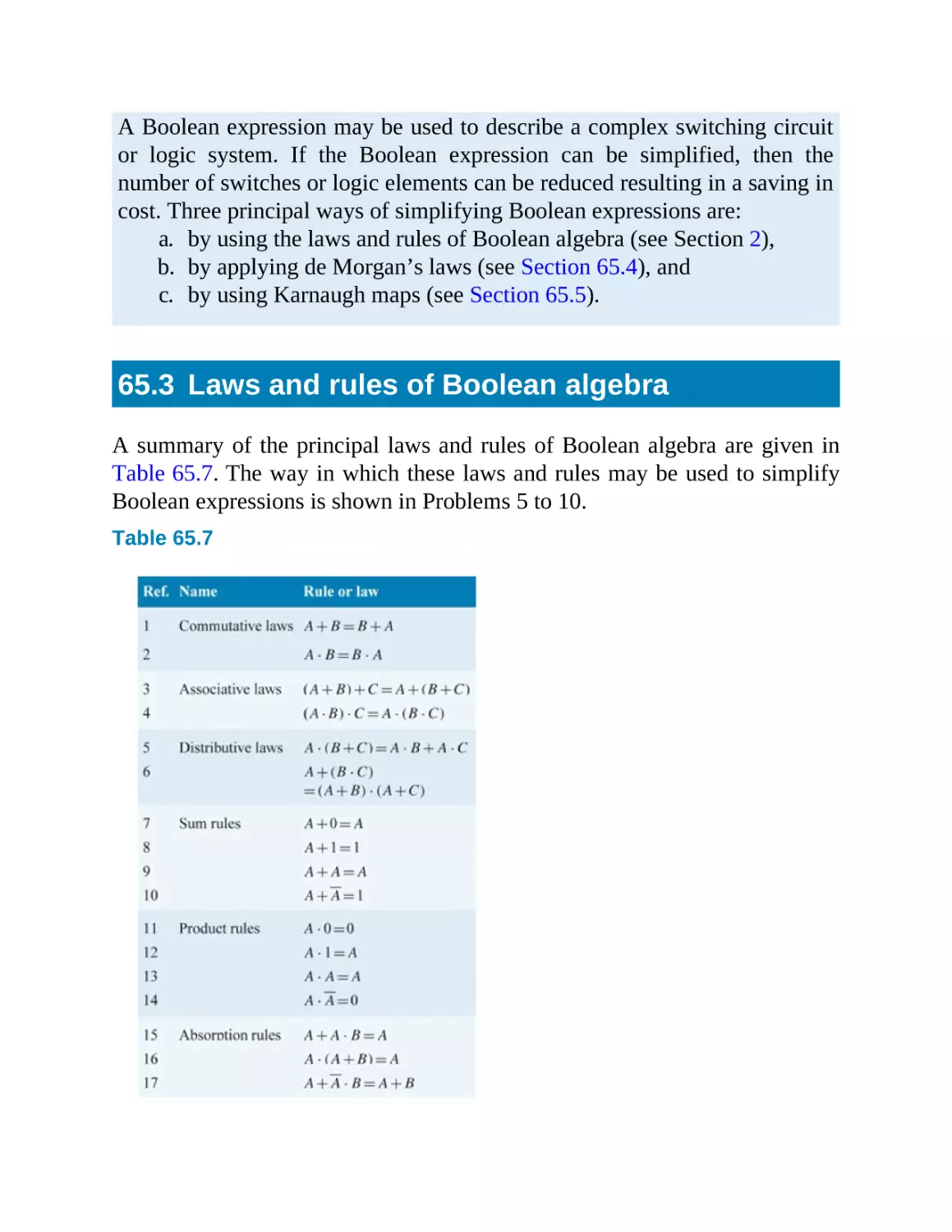
65.3 Laws and rules of Boolean algebra
65.4 De Morgan’s laws
65.5 Karnaugh maps
65.6 Logic circuits
65.7 Universal logic gates
66
The theory of matrices and determinants
66.1 Matrix notation
66.2 Addition, subtraction and multiplication of matrices
66.3 The unit matrix
66.4 The determinant of a 2 by 2 matrix
66.5 The inverse or reciprocal of a 2 by 2 matrix
66.6 The determinant of a 3 by 3 matrix
66.7 The inverse or reciprocal of a 3 by 3 matrix
67
Applications of matrices and determinants
67.1 Solution of simultaneous equations by matrices
67.2 Solution of simultaneous equations by determinants
67.3 Solution of simultaneous equations using Cramers rule
67.4 Solution of simultaneous equations using the Gaussian
elimination method
Revision Test 19
Multiple choice questions on Chapters 45–67
List of essential formulae
Answers to Practice Exercises
Answers to multiple choice questions
Index
Engineering Mathematics
Why is knowledge of mathematics important in
engineering?
A career in any engineering or scientific field will require both basic and
advanced mathematics. Without mathematics to determine principles,
calculate dimensions and limits, explore variations, prove concepts and so on,
there would be no mobile telephones, televisions, stereo systems, video
games, microwave ovens, computers or virtually anything electronic. There
would be no bridges, tunnels, roads, skyscrapers, automobiles, ships, planes,
rockets or most things mechanical. There would be no metals beyond the
common ones, such as iron and copper, no plastics, no synthetics. In fact,
society would most certainly be less advanced without the use of
mathematics throughout the centuries and into the future.
Electrical engineers require mathematics to design, develop, test, or
supervise the manufacturing and installation of electrical equipment,
components, or systems for commercial, industrial, military or scientific use.
Mechanical engineers require mathematics to perform engineering duties in
planning and designing tools, engines, machines, and other mechanically
functioning equipment; they oversee installation, operation, maintenance and
repair of such equipment as centralised heat, gas, water and steam systems.
Aerospace engineers require mathematics to perform a variety of engineering
work in designing, constructing, and testing aircraft, missiles and spacecraft;
they conduct basic and applied research to evaluate adaptability of materials
and equipment to aircraft design and manufacture and recommend
improvements in testing equipment and techniques.
Nuclear engineers require mathematics to conduct research on nuclear
engineering problems or apply principles and theory of nuclear science to
problems concerned with release, control and utilisation of nuclear energy
and nuclear waste disposal.
Petroleum engineers require mathematics to devise methods to improve oil
and gas well production and determine the need for new or modified tool
designs; they oversee drilling and offer technical advice to achieve
economical and satisfactory progress.
Industrial engineers require mathematics to design, develop, test, and
evaluate integrated systems for managing industrial production processes,
including human work factors, quality control, inventory control, logistics
and material flow, cost analysis and production coordination.
Environmental engineers require mathematics to design, planorperform
engineering duties in the prevention, control and remediation of
environmental health hazards, using various engineering disciplines; their
work may include waste treatment, site remediation or pollution control
technology.
Civil engineers require mathematics in all levels in civil engineering structural engineering, hydraulics and geotechnical engineering are all fields
that employ mathematical tools such as differential equations, tensor analysis,
field theory, numerical methods and operations research.
Knowledge of mathematics is therefore needed by each of the engineering
disciplines listed above.
It is intended that this text -Engineering Mathematics - will provide a step by
step approach to learning fundamental mathematics needed for your
engineering studies.
Now in its eighth edition,Engineering Mathematics is an established textbook
that has helped thousands of students to succeed in their exams. John Bird’s
approach is based on worked examples and interactive problems.
Mathematical theories are explained in a straightforward manner, being
supported by practical engineering examples and applications in order to
ensure that readers can relate theory to practice. The extensive and thorough
topic coverage makes this an ideal text for a range of Level 2 and 3
engineering courses. This title is supported by a companion website with
resources forboth students and lecturers, including lists of essential formulae
and multiple choice tests.
John Bird, BSc (Hons), CEng, CMath, CSci, FIMA, FIET, FCollT, is the
former Head of Applied Electronics in the Faculty of Technology at
Highbury College, Portsmouth, UK. More recently, he has combined
freelance lecturing at the University of Portsmouth with examiner
responsibilities for Advanced Mathematics with City and Guilds, and
examining for the International Baccalaureate Organisation. He is the author
of some 130 textbooks on engineering and mathematical subjects with
worldwide sales of over one million copies. He is a chartered engineer, a
chartered mathematician, a chartered scientist and a Fellow of three
professional institutions, and is currently lecturing at the Defence School of
Marine and Air Engineering in the Defence College of Technical Training at
HMS Sultan, Gosport, Hampshire, UK.
Preface
Engineering Mathematics, 8th Edition covers a wide range of syllabus
requirements. In particular, the book is suitable for any course involving
engineering mathematics and in particular for the latest National Certificate
and Diploma courses and City & Guilds syllabuses in Engineering.
This text will provide a foundation in mathematical principles, which will
enable students to solve mathematical, scientific and associated engineering
principles. In addition, the material will provide engineering applications and
mathematical principles necessary for advancement onto a range of
Incorporated Engineer degree profiles. It is widely recognised that a students’
ability to use mathematics is a key element in determining subsequent
success. First year undergraduates who need some remedial mathematics will
also find this book meets their needs.
In Engineering Mathematics, 8th Edition, new material is included on metric
conversions, metric to imperial conversions, numbering systems,
convergence, Bayes theorem, accuracy of numerical methods, Maclaurin’s
series, together with other minor modifications and chapter re-ordering.
Throughout the text, theory is introduced in each chapter by an outline of
essential definitions, formulae, laws and procedures. The theory is kept to a
minimum, for problem solving is extensively used to establish and
exemplify the theory. It is intended that readers will gain real understanding
through seeing problems solved and then through solving similar problems
themselves.
For clarity, the text is divided into eleven topic areas, these being: number
and algebra, areas and volumes, trigonometry, graphs, complex numbers,
vectors, statistics, differential calculus, integral calculus, differential
equations and further number and algebra.
This new edition covers, in particular, the following syllabi:
i. Mathematics for Technicians, the core unit for National
Certificate/Diploma courses in Engineering, to include all or part of
the following chapters:
1. Algebraic methods: 2,5,11,13,14,28,30(1, 4, 6, 8, 9 and 10
for revision)
2. Trigonometric methods and areas and volumes: 18-20,
22-25, 33, 34
3. Statistical methods: 37, 38
4. Elementary calculus: 45, 52, 59
ii. Further Mathematics for Technicians, the optional unit for
National Certificate/Diploma courses in Engineering, to include all
or part of the following chapters:
1. Advanced graphical techniques: 29-31
2. Algebraic techniques: 15,33,37,38
3. Trigonometry: 22-27
4. Calculus: 45-47, 52, 58-60
iii. Mathematics contents of City & Guilds Technician
Certificate/Diploma courses
iv. Any introductory/access/foundation course involving Engineering
Mathematics at University, Colleges of Further and Higher
Education and in schools.
Each topic considered in the text is presented in a way that assumes in the
reader little previous knowledge of that topic.
Engineering Mathematics, 8th Edition provides a follow-up to Basic
Engineering Mathematics, 7th Edition and a lead into Higher Engineering
Mathematics, 8th Edition .
This textbook contains over 1000 worked problems, followed by some 1850
further problems (all with answers at the back of the book). The further
problems are contained within some 243 practice exercises; each Exercise
follows on directly from the relevant section of work, every two or three
pages. In addition, the text contains 243 multiple-choice questions. Where at
all possible, the problems mirror practical situations found in engineering and
science. 571 line diagrams enhance the understanding of the theory.
At regular intervals throughout the text are some 19 Revision Tests to check
understanding. For example, Revision Test 1 covers material contained in
Chapters 1 to 4, Revision Test 2 covers the material in Chapters 5 to 8 and so
on. These Revision Tests do not have answers given since it is envisaged that
lecturers could set the tests for students to attempt as part of their course
structure. Lecturers’ may obtain a set of solutions of the Revision Tests in an
Instructor’s Manual available via the internet - see below.
A list of essential formulae is included in the text for convenience of
reference.
‘Learning by Example’ is at the heart of Engineering Mathematics, 8th
Edition.
JOHN BIRD
Royal Naval Defence College of Marine and Air Engineering, HMS
Sultan, formerly of University of Portsmouth and Highbury College,
Portsmouth
Free Web downloads at http://www.routledge.com/cw/bird
For students
1. Full solutions to the 1850 questions contained in the 243 Practice
Exercises
2. Download multiple choice questions and answer sheet
3. List of essential formulae
4. Famous engineers/scientists - 25 are mentioned in the text
For instructors/lecturers
1. Full solutions to the 1850 questions contained in the 243 Practice
Exercises
2. Full solutions and marking scheme to each of the 19 revision tests named as Instructors guide
3. Revision tests - available to run off to be given to students
4. Download multiple choice questions and answer sheet
5. List of essential formulae
6. Illustrations - all 571 available on PowerPoint
7. Famous engineers/scientists - 25 are mentioned in the text
Section 1
Number and algebra
Chapter 1
Revision of fractions, decimals and
percentages
Why it is important to understand: Revision of fractions, decimals
and percentages
Engineers use fractions all the time, examples including stress to
strain ratios in mechanical engineering, chemical concentration
ratios and reaction rates, and ratios in electrical equations to solve
for current and voltage. Fractions are also used everywhere in
science, from radioactive decay rates to statistical analysis. Also,
engineers and scientists use decimal numbers all the time in
calculations. Calculators are able to handle calculations with
fractions and decimals; however, there will be times when a quick
calculation involving addition, subtraction, multiplication and
division of fractions and decimals is needed. Engineers and
scientists also use percentages a lot in calculations; for example,
percentage change is commonly used in engineering, statistics,
physics, finance, chemistry and economics. When you feel able to do
calculations with basic arithmetic, fractions, decimals and
percentages, with or without the aid of a calculator, then suddenly
mathematics doesn’t seem quite so difficult.
At the end of this chapter you should be able to:
add, subtract, multiply and divide with fractions
understand practical examples involving ratio and proportion
add, subtract, multiply and divide with decimals
understand and use percentages
1.1
Fractions
When 2 is divided by 3, it may be written as 2 3 or 2/3. 2 3 is called a
fraction. The number above the line, i.e. 2, is called the numerator and the
number below the line, i.e. 3, is called the denominator.
When the value of the numerator is less than the value of the denominator,
the fraction is called a proper fraction; thus 2 3 is a proper fraction. When
the value of the numerator is greater than the denominator, the fraction is
called an improper fraction. Thus 7 3 is an improper fraction and can also
be expressed as a mixed number, that is, an integer and a proper fraction.
Thus the improper fraction 7 3 is equal to the mixed number 2 1 3
When a fraction is simplified by dividing the numerator and denominator by
the same number, the process is called cancelling. Cancelling by 0 is not
permissible.
Problem 1. Simplify: 1 3 + 2 7
The lowest common multiple (i.e. LCM) of the two denominators is 3 × 7,
i.e. 21
Expressing each fraction so that their denominators are 21, gives:
1 3 + 2 7 = 1 3 × 7 7 + 2 7 × 3 3 = 7 21 + 6 21 = 7 + 6 21 = 13 21
Alternatively:
1 3 + 2 7 = Step ( 2 ) Step ( 3 ) ↓ ↓ ( 7 × 1 ) + ( 3 × 2 ) 21 ↑ Step ( 1 )
Step1: the LCM of the two denominators;
Step2: for the fraction 1 3 , 3 into 21 goes 7 times, 7 × the numerator is 7
× 1;
Step3: for the fraction 2 7 , 7 into 21 goes 3 times, 3 × the numerator is 3
×2
Thus 1 3 + 2 7 = 7 + 6 21 = 13 21 as obtained previously.
Problem 2. Find the value of 3 2 3 - 2 1 6
One method is to split the mixed numbers into integers and their fractional
parts. Then
323-216=3+23-2+16=3+23-2-16=1+46-16=136=11
2
Another method is to express the mixed numbers as improper fractions.
Since 3 = 9 3 , then 3 2 3 = 9 3 + 2 3 = 11 3
Similarly, 2 1 6 = 12 6 + 1 6 = 13 6
Thus 3 2 3 - 2 1 6 = 11 3 - 13 6 = 22 6 - 13 6 = 9 6 = 1 1 2 as obtained
previously.
Problem 3. Determine the value of
458-314+125
4 5 8 - 3 1 4 + 1 2 5 = ( 4 - 3 + 1 ) + 5 8 - 1 4 + 2 5 = 2 + 5 × 5 - 10 × 1 + 8 ×
2 40 = 2 + 25 - 10 + 16 40 = 2 + 31 40 = 2 31 40
Problem 4. Find the value of 3 7 × 14 15
Dividing numerator and denominator by 3 gives:
Dividing numerator and denominator by 7 gives:
This process of dividing both the numerator and denominator of a fraction by
the same factor(s) is called cancelling.
Problem 5. Evaluate: 1 3 5 × 2 1 3 × 3 3 7
Mixed numbers must be expressed as improper fractions before
multiplication can be performed. Thus,
1 3 5 × 2 1 3 × 3 3 7 = 5 5 + 3 5 × 6 3 + 1 3 × 21 7 + 3 7
Problem 6. Simplify: 3 7 ÷ 12 21
3 7 ÷ 12 21 = 3 7 12 21
Multiplying both numerator and denominator by the reciprocal of the
denominator gives:
This method can be remembered by the rule: invert the second fraction and
change the operation from division to multiplication. Thus:
as obtained previously.
Problem 7. Find the value of 5 3 5 ÷ 7 1 3
The mixed numbers must be expressed as improper fractions. Thus,
Problem 8. Simplify:
13-25+14÷38×13
The order of precedence of operations for problems containing fractions is
the same as that for integers, i.e. remembered by BODMAS (Brackets, Of,
Division, Multiplication, Addition and Subtraction). Thus,
13-25+14÷38×13
Problem 9. Determine the value of
7 6 of 3 1 2 - 2 1 4 + 5 1 8 ÷ 3 16 - 1 2
Now try the following Practice Exercise
Practice Exercise 1 Fractions (Answers on page 672)
Evaluate the following:
1. (a) 1 2 + 2 5 (b) 7 16 - 1 4
2. (a) 2 7 + 3 11 (b) 2 9 - 1 7 + 2 3
3. (a) 10 3 7 - 8 2 3 (b) 3 1 4 - 4 4 5 + 1 5 6
4. (a) 3 4 × 5 9 (b) 17 35 × 15 119
5. (a) 3 5 × 7 9 × 1 2 7 (b) 13 17 × 4 7 11 × 3 4 39
6. (a) 3 8 ÷ 45 64 (b) 1 1 3 ÷ 2 5 9
7. 1 2 + 3 5 ÷ 8 15 - 1 3
8. 7 15 of 15 × 5 7 + 3 4 ÷ 15 16
9. 1 4 × 2 3 - 1 3 ÷ 3 5 + 2 7
10. 2 3 × 1 1 4 ÷ 2 3 + 1 4 + 1 3 5
11. If a storage tank is holding 450 litres when it is three-quarters full,
how much will it contain when it is two-thirds full?
12. Three people, P, Q and R contribute to a fund. P provides 3/5 of the
total, Q provides 2/3 of the remainder, and R provides £8. Determine
(a) the total of the fund, (b) the contributions of P and Q.
1.2
Ratio and proportion
The ratio of one quantity to another is a fraction, and is the number of times
one quantity is contained in another quantity of the same kind. If one
quantity is directly proportional to another, then as one quantity doubles,
the other quantity also doubles. When a quantity is inversely proportional to
another, then as one quantity doubles, the other quantity is halved.
Problem 10. A piece of timber 273 cm long is cut into three pieces in the
ratio of 3 to 7 to 11. Determine the lengths of the three pieces
The total number of parts is 3 + 7 + 11 , that is, 21. Hence 21 parts
correspond to 273 cm
1 part corresponds to 273 21 = 13 cm 3 parts correspond to 3 × 13 = 39 cm 7
parts correspond to 7 × 13 = 91 cm 11 parts correspond to 11 × 13 = 143 cm
i.e. the lengths of the three pieces are 39 cm, 91 cm and 143 cm.
(Check: 39 + 91 + 143 = 273 )
Problem 11. A gear wheel having 80 teeth is in mesh with a 25 tooth gear.
What is the gear ratio?
Gear ratio = 80 : 25 = 80 25 = 16 5 = 3.2
i.e. gear ratio = 16 : 5 or 3.2 : 1
Problem 12. An alloy is made up of metals A and B in the ratio 2.5 : 1 by
mass. How much of A has to be added to 6 kg of B to make the alloy?
Ratio A : B: :2.5 : 1 (i.e. A is to B as 2.5 is to 1) or A B = 2.5 1 = 2.5
When B = 6 kg, A 6 = 2.5 from which,
A = 6 × 2.5 = 15 kg
Problem 13. If 3 people can complete a task in 4 hours, how long will it
take 5 people to complete the same task, assuming the rate of work remains
constant?
The more the number of people, the more quickly the task is done, hence
inverse proportion exists.
3 people complete the task in 4 hours.
1 person takes three times as long, i.e.
4 × 3 = 12 hours,
5 people can do it in one fifth of the time that one person takes, that is 12 5
hours or 2 hours 24 minutes.
Now try the following Practice Exercise
Practice Exercise 2 Ratio and proportion (Answers on page 672)
1. Divide 621 cm in the ratio of 3 to 7 to 13.
2. When mixing a quantity of paints, dyes of four different colours are
used in the ratio of 7 : 3 : 19 : 5. If the mass of the first dye used is 3
1 2 g, determine the total mass of the dyes used.
3. Determine how much copper and how much zinc is needed to make
a 99 kg brass ingot if they have to be in the proportions copper :
zinc: :8 : 3 by mass.
4. It takes 21 hours for 12 men to resurface a stretch of road. Find how
many men it takes to resurface a similar stretch of road in 50 hours
24 minutes, assuming the work rate remains constant.
5. It takes 3 hours 15 minutes to fly from city A to city B at a constant
speed. Find how long the journey takes if
a. the speed is 1 1 2 times that of the original speed and
b. if the speed is three-quarters of the original speed.
1.3
Decimals
The decimal system of numbers is based on the digits 0 to 9. A number such
as 53.17 is called a decimal fraction, a decimal point separating the integer
part, i.e. 53, from the fractional part, i.e. 0.17
A number which can be expressed exactly as a decimal fraction is called a
terminating decimal and those which cannot be expressed exactly as a
decimal fraction are called non-terminating decimals. Thus, 3 2 = 1.5 is a
terminating decimal, but 4 3 = 1.33333 … is a non-terminating decimal.
1.33333 … can be written as 1.3, called ‘one point-three recurring’.
The answer to a non-terminating decimal may be expressed in two ways,
depending on the accuracy required:
1. correct to a number of significant figures, that is, figures which
signify something, and
2. correct to a number of decimal places, that is, the number of figures
after the decimal point.
The last digit in the answer is unaltered if the next digit on the right is in the
group of numbers 0, 1, 2, 3 or 4, but is increased by 1 if the next digit on the
right is in the group of numbers 5, 6, 7, 8 or 9. Thus the non-terminating
decimal 7.6183 … becomes 7.62, correct to 3 significant figures, since the
next digit on the right is 8, which is in the group of numbers 5, 6, 7, 8 or 9.
Also 7.6183 … becomes 7.618, correct to 3 decimal places, since the next
digit on the right is 3, which is in the group of numbers 0, 1, 2, 3 or 4
Problem 14. Evaluate: 42.7 + 3.04 + 8.7 + 0.06
The numbers are written so that the decimal points are under each other. Each
column is added, starting from the right.
42.7
3.04
8.7
0.06
54.50
Thus 42.7 + 3.04 + 8.7 + 0.06 = 54.50
Problem 15. Take 81.70 from 87.23
The numbers are written with the decimal points under each other.
87.23
- 81.70
5.53
Thus 87.23 - 81.70 = 5.53
Problem 16. Find the value of
23.4 - 17.83 - 57.6 + 32.68
The sum of the positive decimal fractions is
23.4 + 32.68 = 56.08
The sum of the negative decimal fractions is
17.83 + 57.6 = 75.43
Taking the sum of the negative decimal fractions from the sum of the positive
decimal fractions gives:
56.08 - 75.43
i.e. - ( 75.43 - 56.08 ) = - 1 9.35
Problem 17. Determine the value of 74.3 × 3.8
When multiplying decimal fractions: (i) the numbers are multiplied as if they
are integers, and (ii) the position of the decimal point in the answer is such
that there are as many digits to the right of it as the sum of the digits to the
right of the decimal points of the two numbers being multiplied together.
Thus
(i)
743
38
5 944
22 290
28 234
1. As there are (1 + 1) = 2 digits to the right of the decimal points of the
two numbers being multiplied together, (74.3 × 3.8), then
7 4.3 × 3 . 8 = 2 82.34
Problem 18. Evaluate 37.81 ÷ 1.7, correct to (i) 4 significant figures and (ii)
4 decimal places
37.81 ÷ 1.7 = 37.81 1.7
The denominator is changed into an integer by multiplying by 10. The
numerator is also multiplied by 10 to keep the fraction the same. Thus
37.81 ÷ 1.7 = 37.81 × 10 1.7 × 10 = 378.1 17
The long division is similar to the long division of integers and the first four
steps are as shown:
17 [ - 9.5 p t ] 378.100000 ¯ 22.24117 . 34 _ _ 38 34 _ _ 41 34 _ _ 70 68 _ _
20
1. 37.81 ÷ 1.7 = 22.24, correct to 4 significant figures, and
2. 37.81 ÷ 1.7 = 22.2412, correct to 4 decimal places.
Problem 19. Convert (a) 0.4375 to a proper fraction and (b) 4.285 to a
mixed number
a. 0.4375 can be written as 0.4375 × 10 000 10 000 without changing its
value,
i.e. 0.4375 = 4375 10 000
By cancelling
4375 10 000 = 875 2000 = 175 400 = 35 80 = 7 16
i.e. 0 . 4375 = 7 16
b. Similarly, 4.285 = 4 285 1000 = 4 57 200
Problem 20. Express as decimal fractions:
( a ) 9 16 and ( b ) 5 7 8
a. To convert a proper fraction to a decimal fraction, the numerator is
divided by the denominator. Division by 16 can be done by the long
division method, or, more simply, by dividing by 2 and then 8:
2 9.00 ¯ 4.50 8 4.5000 ¯ 0.5625
Thus 9 16 = 0 . 5625
b. For mixed numbers, it is only necessary to convert the proper fraction
part of the mixed number to a decimal fraction. Thus, dealing with the
7 8 gives:
8 7.000 ¯ 0.875 i.e. 7 8 = 0.875
Thus 5 7 8 = 5 . 875
Now try the following Practice Exercise
Practice Exercise 3 Decimals (Answers on page 672)
In Problems 1 to 6, determine the values of the expressions given:
1. 23.6 + 14.71 - 18.9 - 7.421
2. 73.84 - 113.247 + 8.21 - 0.068
3. 3.8 × 4.1 × 0.7
4. 374.1 × 0.006
5. 421.8 ÷ 17, (a) correct to 4 significant figures and (b) correct to 3
decimal places.
6. 0.0147 2.3 , (a) correct to 5 decimal places and (b) correct to 2
significant figures.
7. Convert to proper fractions: (a) 0.65 (b) 0.84 (c) 0.0125 (d) 0.282
and (e) 0.024
8. Convert to mixed numbers: (a) 1.82 (b) 4.275 (c) 14.125 (d) 15.35
and (e) 16.2125
In Problems 9 to 12, express as decimal fractions to the accuracy stated:
1. 4 9 , correct to 5 significant figures.
2. 17 27 , correct to 5 decimal places.
3. 1 9 16 , correct to 4 significant figures.
4. 13 31 37 , correct to 2 decimal places.
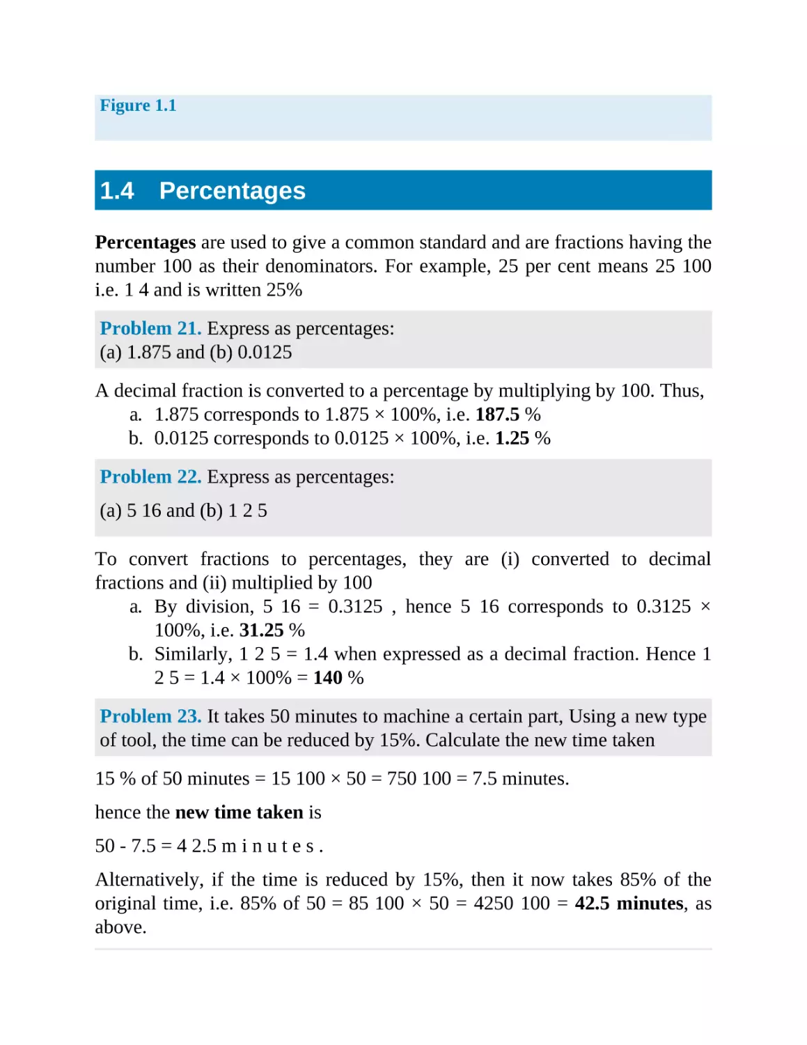
5. Determine the dimension marked x in the length of shaft shown in
Fig. 1.1. The dimensions are in millimetres.
6. A tank contains 1800 litres of oil. How many tins containing 0.75
litres can be filled from this tank?
Figure 1.1
1.4
Percentages
Percentages are used to give a common standard and are fractions having the
number 100 as their denominators. For example, 25 per cent means 25 100
i.e. 1 4 and is written 25%
Problem 21. Express as percentages:
(a) 1.875 and (b) 0.0125
A decimal fraction is converted to a percentage by multiplying by 100. Thus,
a. 1.875 corresponds to 1.875 × 100%, i.e. 187.5 %
b. 0.0125 corresponds to 0.0125 × 100%, i.e. 1.25 %
Problem 22. Express as percentages:
(a) 5 16 and (b) 1 2 5
To convert fractions to percentages, they are (i) converted to decimal
fractions and (ii) multiplied by 100
a. By division, 5 16 = 0.3125 , hence 5 16 corresponds to 0.3125 ×
100%, i.e. 31.25 %
b. Similarly, 1 2 5 = 1.4 when expressed as a decimal fraction. Hence 1
2 5 = 1.4 × 100% = 140 %
Problem 23. It takes 50 minutes to machine a certain part, Using a new type
of tool, the time can be reduced by 15%. Calculate the new time taken
15 % of 50 minutes = 15 100 × 50 = 750 100 = 7.5 minutes.
hence the new time taken is
50 - 7.5 = 4 2.5 m i n u t e s .
Alternatively, if the time is reduced by 15%, then it now takes 85% of the
original time, i.e. 85% of 50 = 85 100 × 50 = 4250 100 = 42.5 minutes, as
above.
Problem 24. Find 12.5% of £378
12.5% of £378 means 12.5 100 × 378 , since per cent means ‘per hundred’.
Hence 12.5% of
Problem 25. Express 25 minutes as a percentage of 2 hours, correct to the
nearest 1%
Working in minute units, 2 hours = 120 minutes.
Hence 25 minutes is 25 120 ths of 2 hours. By cancelling, 25 120 = 5 24
Expressing 5 24 as a decimal fraction gives 0.208 3 ˙
Multiplying by 100 to convert the decimal fraction to a percentage gives:
0.208 3 ˙ × 100 = 20.83 %
Thus 25 minutes is 21 % of 2 hours, correct to the nearest 1%
Problem 26. A German silver alloy consists of 60% copper, 25% zinc and
15% nickel. Determine the masses of the copper, zinc and nickel in a 3.74
kilogram block of the alloy
By direct proportion:
100 % corresponds to 3.74 kg 1 % corresponds to 3.74 100 = 0.0374 kg 60 %
corresponds to 60 × 0.0374 = 2.244 kg 25 % corresponds to 25 × 0.0374 =
0.935 kg 15 % corresponds to 15 × 0.0374 = 0.561 kg
Thus, the masses of the copper, zinc and nickel are 2.244 kg, 0.935 kg and
0.561 kg, respectively.
(Check: 2.244 + 0.935 + 0.561 = 3.74)
Now try the following Practice Exercise
Practice Exercise 4 Percentages (Answers on page 672)
1. Convert to percentages: (a) 0.057 (b) 0.374 (c) 1.285
2. Express as percentages, correct to 3 significant figures: (a) 7 33 (b)
19 24 (c) 1 11 16
3. Calculate correct to 4 significant figures: (a) 18% of 2758 tonnes (b)
47% of 18.42 grams (c) 147% of 14.1 seconds
4. When 1600 bolts are manufactured, 36 are unsatisfactory. Determine
the percentage unsatisfactory.
5. Express: (a) 140 kg as a percentage of 1 t (b) 47 s as a percentage of
5 min (c) 13.4 cm as a percentage of 2.5 m
6. A block of monel alloy consists of 70% nickel and 30% copper. If it
contains 88.2 g of nickel, determine the mass of copper in the block.
7. A drilling machine should be set to 250 rev/min. The nearest speed
available on the machine is 268 rev/min. Calculate the percentage
over speed.
8. Two kilograms of a compound contains 30% of element A, 45% of
element B and 25% of element C. Determine the masses of the three
elements present.
9. A concrete mixture contains seven parts by volume of ballast, four
parts by volume of sand and two parts by volume of cement.
Determine the percentage of each of these three constituents correct
to the nearest 1% and the mass of cement in a two tonne dry mix,
correct to 1 significant figure.
10. In a sample of iron ore, 18% is iron. How much ore is needed to
produce 3600 kg of iron?
11. A screws’ dimension is 12.5 ± 8% mm. Calculate the possible
maximum and minimum length of the screw.
12. The output power of an engine is 450 kW. If the efficiency of the
engine is 75%, determine the power input.
Chapter 2
Indices, standard form and engineering
notation
Why it is important to understand: Indices, standard form and
engineering notation
Powers and roots are used extensively in mathematics and
engineering, so it is important to get a good grasp of what they are
and how, and why, they are used. Being able to multiply powers
together by adding their indices is particularly useful for disciplines
like engineering and electronics, where quantities are often
expressed as a value multiplied by some power of ten. In the field of
electrical engineering, for example, the relationship between electric
current, voltage and resistance in an electrical system is critically
important, and yet the typical unit values for these properties can
differ by several orders of magnitude. Studying, or working, in an
engineering discipline, you very quickly become familiar with
powers and roots and laws of indices. In engineering there are many
different quantities to get used to, and hence many units to become
familiar with. For example, force is measured in Newton’s, electric
current is measured in amperes and pressure is measured in
Pascal’s. Sometimes the units of these quantities are either very
large or very small and hence prefixes are used. For example, 1000
Pascal’s may be written as 1 0 3 Pa which is written as 1 kPa in
prefix form, the k being accepted as a symbol to represent 1000 or 1
0 3 . Studying, or working, in an engineering discipline, you very
quickly become familiar with the standard units of measurement,
the prefixes used and engineering notation. An electronic calculator
is extremely helpful with engineering notation.
At the end of this chapter you should be able to:
use the laws of indices
understand standard form
understand and use engineering notation
understand and use common prefixes
2.1
Indices
The lowest factors of 2000 are 2 × 2 × 2 × 2 × 5 × 5 × 5. These factors are
written as 2 4 × 5 3 , where 2 and 5 are called bases and the numbers 4 and 5
are called indices.
When an index is an integer it is called a power. Thus, 2 4 is called ‘two to
the power of four’, and has a base of
2 and an index of 4. Similarly, 5 3 is called ‘five to the power of 3’ and has a
base of 5 and an index of 3.
Special names may be used when the indices are 2 and 3, these being called
‘squared’ and ‘cubed’, respectively. Thus 7 2 is called ‘seven squared’ and 9
3 is called ‘nine cubed’. When no index is shown, the power is 1, i.e. 2 means
21
Reciprocal
The reciprocal of a number is when the index is - 1 and its value is given by
1, divided by the base. Thus the reciprocal of 2 is 2 - 1 and its value is 1 2 or
0.5. Similarly, the reciprocal of 5 is 5 - 1 which means 1 5 or 0.2
Square root
The square root of a number is when the index is 1 2 , and the square root of
2 is written as 2 1 / 2 or 2 . The value of a square root is the value of the base
which when multiplied by itself gives the number. Since 3 × 3 = 9, then 9 =
3. However, ( - 3 ) × ( - 3 ) = 9, so 9 = - 3. There are always two answers
when finding the square root of a number and this is shown by putting both a
+ and a - sign in front of the answer to a square root problem. Thus 9 = ± 3
and 4 1 / 2 = 4 = ± 2 and so on.
Laws of indices
When simplifying calculations involving indices, certain basic rules or laws
can be applied, called the laws of indices. These are given below.
i. When multiplying two or more numbers having the same base, the
indices are added. Thus
32×34=32+4=36
ii. When a number is divided by a number having the same base, the
indices are subtracted. Thus
3532=35-2=33
iii. When a number which is raised to a power is raised to a further
power, the indices are multiplied. Thus
( 3 5 ) 2 = 3 5 × 2 = 3 10
iv. When a number has an index of 0, its value is 1. Thus 3 0 = 1
v. A number raised to a negative power is the reciprocal of that number
raised to a positive power. Thus 3 - 4 = 1 3 4 Similarly, 1 2 - 3 = 2 3
vi. When a number is raised to a fractional power the denominator of
the fraction is the root of the number and the numerator is the power.
Thus 8 2 / 3 = 8 2 3 = ( 2 ) 2 = 4 and 25 1 / 2 = 25 1 2 = 25 1 = ± 5
(Note that ≡ 2 )
2.2
Worked problems on indices
Problem 1. Evaluate: (a) 5 2 × 5 3 , (b) 3 2 × 3 4 × 3 and (c) 2 × 2 2 × 2 5
From law (i):
a. 5 2 × 5 3 = 5 ( 2 + 3 ) = 5 5 = 5 × 5 × 5 × 5 × 5 = 3125
b. 3 2 × 3 4 × 3 = 3 ( 2 + 4 + 1 ) = 3 7 = 3 × 3 × ⋯ to 7 terms = 2187
c. 2 × 2 2 × 2 5 = 2 ( 1 + 2 + 5 ) = 2 8 = 256
Problem 2. Find the value of:
(a) 7 5 7 3 and (b) 5 7 5 4
From law (ii):
a. 7 5 7 3 = 7 ( 5 - 3 ) = 7 2 = 49
b. 5 7 5 4 = 5 ( 7 - 4 ) = 5 3 = 125
Problem 3. Evaluate: (a) 5 2 × 5 3 ÷ 5 4 and (b) (3 × 3 5 ) ÷ (3 2 × 3 3 )
From laws (i) and (ii):
a. 5 2 × 5 3 ÷ 5 4 = 5 2 × 5 3 5 4 = 5 ( 2 + 3 ) 5 4 = 5 5 5 4 = 5 ( 5 - 4 ) =
51=5
b. ( 3 × 3 5 ) ÷ ( 3 2 × 3 3 ) = 3 × 3 5 3 2 × 3 3 = 3 ( 1 + 5 ) 3 ( 2 + 3 ) =
3635=3(6-5)=31=3
Problem 4. Simplify: (a) (2 3 ) 4 and (b) (3 2 ) 5 , expressing the answers in
index form.
From law (iii):
a. (2 3 ) 4 = 2 3 × 4 = 2 12 (b) (3 2 ) 5 = 3 2 × 5 = 3 10
Problem 5. Evaluate: ( 10 2 ) 3 10 4 × 10 2
From the laws of indices:
( 10 2 ) 3 10 4 × 10 2 = 10 ( 2 × 3 ) 10 ( 4 + 2 ) = 10 6 10 6 = 10 6 - 6 = 10 0
=1
Problem 6. Find the value of:
(a) 2 3 × 2 4 2 7 × 2 5 and (b) ( 3 2 ) 3 3 × 3 9
From the laws of indices:
a. 2 3 × 2 4 2 7 × 2 5 = 2 ( 3 + 4 ) 2 ( 7 + 5 ) = 2 7 2 12 = 2 7 - 12 = 2 - 5
= 1 2 5 = 1 32
b. ( 3 2 ) 3 3 × 3 9 = 3 2 × 3 3 1 + 9 = 3 6 3 10 = 3 6 - 10 = 3 - 4 = 1 3 4
= 1 81
Now try the following Practice Exercise
Practice Exercise 5 Indices (Answers on page 673)
In Problems 1 to 10, simplify the expressions given, expressing the answers
in index form and with positive indices:
1. (a) 3 3 × 3 4 (b) 4 2 × 4 3 × 4 4
2. (a) 2 3 × 2 × 2 2 (b) 7 2 × 7 4 × 7 × 7 3
3. (a) 2 4 2 3 (b) 3 7 3 2
4. (a) 5 6 ÷ 5 3 (b) 7 13 /7 10
5. (a) (7 2 ) 3 (b) (3 3 ) 2
6. (a) 2 2 × 2 3 2 4 (b) 3 7 × 3 4 3 5
7. (a) 5 7 5 2 × 5 3 (b) 13 5 13 × 13 2
8. (a) ( 9 × 3 2 ) 3 ( 3 × 27 ) 2 (b) ( 16 × 4 ) 2 ( 2 × 8 ) 3
9. (a) 5 - 2 5 - 4 (b) 3 2 × 3 - 4 3 3
10. (a) 7 2 × 7 - 3 7 × 7 - 4 (b) 2 3 × 2 - 4 × 2 5 2 × 2 - 2 × 2 6
2.3
Further worked problems on indices
Problem 7. Evaluate: 3 3 × 5 7 5 3 × 3 4
The laws of indices only apply to terms having the same base. Grouping
terms having the same base, and then applying the laws of indices to each of
the groups independently gives:
33×5753×34=3334=5753=3(3-4)×5(7-3)=3-1×54=
5 4 3 1 = 625 3 = 208 1 3
Problem 8. Find the value of:
23×35×(72)274×24×33
23×35×(72)274×24×33=23-4×35-3×72×2-4=2-1×3
2×70=12×32×1=92=412
Problem 9. Evaluate:
(a) 4 1 / 2 (b) 16 3 / 4 (c) 27 2 / 3 (d) 9 - 1 / 2
a. 4 1 / 2 = 4 = ± 2
b. 16 3 / 4 = 16 3 4 = ( ± 2 ) 3 = ± 8 (Note that it does not matter whether
the 4th root of 16 is found first or whether 16 cubed is found first –
the same answer will result).
c. 27 2 / 3 = 27 2 3 = ( 3 ) 2 = 9
d. 9 - 1 / 2 = 1 9 1 / 2 = 1 9 = 1 ± 3 = ± 1 3
Problem 10. Evaluate: 4 1.5 × 8 1 / 3 2 2 × 32 - 2 / 5
4 1.5 = 4 3 / 2 = 4 3 = 2 3 = 8 8 1 / 3 = 8 3 = 2 , 2 2 = 4
and 32 - 2 / 5 = 1 32 2 / 5 = 1 32 2 5 = 1 2 2 = 1 4 Hence 4 1.5 × 8 1 / 3 2 2 ×
32 - 2 / 5 = 8 × 2 4 × 1 4 = 16 1 = 16
Alternatively,
4 1.5 × 8 1 / 3 2 2 × 32 - 2 / 5 = [ ( 2 ) 2 ] 3 / 2 × ( 2 3 ) 1 / 3 2 2 × ( 2 5 ) - 2 /
5 = 2 3 × 2 1 2 2 × 2 - 2 = 2 3 + 1 - 2 - ( - 2 ) = 2 4 = 16
Problem 11. Evaluate: 3 2 × 5 5 + 3 3 × 5 3 3 4 × 5 4
Dividing each term by the HCF (i.e. highest common factor) of the three
terms, i.e. 3 2 × 5 3 , gives:
32×55+33×5334×54=32×5532×53+33×5332×5334×
5432×53=3(2-2)×5(5-3)+3(3-2)×503(4-2)×5(4-3)
= 3 0 × 5 2 + 3 1 × 5 0 3 2 × 5 1 = 1 × 25 + 3 × 1 9 × 5 = 28 45
Problem 12. Find the value of:
32×5534×54+33×53
To simplify the arithmetic, each term is divided by the HCF of all the terms,
i.e. 3 2 × 5 3 . Thus
32×5534×54+33×53=32×5532×5334×5432×53+33×
5332×53=3(2-2)×5(5-3)3(4-2)×5(4-3)+3(3-2)×5(
3 - 3 ) = 3 0 × 5 2 3 2 × 5 1 + 3 1 × 5 0 = 25 45 + 3 = 25 48
Problem 13. Simplify: 4 3 3 × 3 5 - 2 2 5 - 3 giving the answer with
positive indices
A fraction raised to a power means that both the numerator and the
denominator of the fraction are raised to that power, i.e. 4 3 3 = 4 3 3 3
A fraction raised to a negative power has the same value as the inverse of the
fraction raised to a positive power.
Thus, 3 5 - 2 = 1 3 5 2 = 1 3 2 5 2 = 1 × 5 2 3 2 = 5 2 3 2
Similarly, 2 5 - 3 = 5 2 3 = 5 3 2 3
Thus , 4 3 3 × 3 5 - 2 2 5 - 3 = 4 3 3 3 × 5 2 3 2 5 3 2 3 = 4 3 3 3 × 5 2 3 2 × 2
353=(22)3×233(3+2)×5(3-2)=2935×5
Now try the following Practice Exercise
Practice Exercise 6 Indices (Answers on page 673)
In Problems 1 and 2, simplify the expressions given, expressing the answers
in index form and with positive indices:
1. (a) 3 3 × 5 2 5 4 × 3 4 (b) 7 - 2 × 3 - 2 3 5 × 7 4 × 7 - 3
2. (a) 4 2 × 9 3 8 3 × 3 4 (b) 8 - 2 × 5 2 × 3 - 4 25 2 × 2 4 × 9 - 2
3. Evaluate (a) 1 3 2 - 1 (b) 81 0.25 (c) 16 ( - 1 / 4 ) (d) 4 9 1 / 2 In
Problems 4 to 8, evaluate the expressions given.
4. 9 2 × 7 4 3 4 × 7 4 + 3 3 × 7 2
5. ( 2 4 ) 2 - 3 - 2 × 4 4 2 3 × 16 2
6. 1 2 3 - 2 3 - 2 3 5 2
7. 4 3 4 2 9 2
8. ( 3 2 ) 3 / 2 × ( 8 1 / 3 ) 2 ( 3 ) 2 × ( 4 3 ) 1 / 2 × ( 9 ) - 1 / 2
2.4
Standard form
A number written with one digit to the left of the decimal point and
multiplied by 10 raised to some power is said to be written in standard form.
Thus: 5837 is written as 5.837 × 10 3 in standard form, and 0.0415 is written
as 4.15 × 10 - 2 in standard form.
When a number is written in standard form, the first factor is called the
mantissa and the second factor is called the exponent. Thus the number 5.8
× 10 3 has a mantissa of 5.8 and an exponent of 10 3
1. Numbers having the same exponent can be added or subtracted in
standard form by adding or subtracting the mantissae and keeping the
exponent the same. Thus:
2.3 × 10 4 + 3.7 × 10 4 = ( 2.3 + 3.7 ) × 10 4 = 6.0 × 10 4 and 5.9 × 10
- 2 - 4.6 × 10 - 2 = ( 5.9 - 4.6 ) × 10 - 2 = 1.3 × 10 - 2
When the numbers have different exponents, one way of adding or
subtracting the numbers is to express one of the numbers in nonstandard form, so that both numbers have the same exponent. Thus:
2.3 × 10 4 + 3.7 × 10 3 = 2.3 × 10 4 + 0.37 × 10 4 = ( 2.3 + 0.37 ) ×
10 4 = 2.67 × 10 4
Alternatively,
2.3 × 10 4 + 3.7 × 10 3 = 23 000 + 3700 = 26 700 = 2.67 × 10 4
2. The laws of indices are used when multiplying or dividing numbers
given in standard form. For example,
( 2.5 × 10 3 ) × ( 5 × 10 2 ) = ( 2.5 × 5 ) × ( 10 3 + 2 ) = 12.5 × 10 5 or
1.25 × 10 6
Similarly,
6 × 10 4 1.5 × 10 2 = 6 1.5 × ( 10 4 - 2 ) = 4 × 10 2
2.5
Worked problems on standard form
Problem 14. Express in standard form:
(a) 38.71 (b) 3746 (c) 0.0124
For a number to be in standard form, it is expressed with only one digit to the
left of the decimal point. Thus:
a. 38.71 must be divided by 10 to achieve one digit to the left of the
decimal point and it must also be multiplied by 10 to maintain the
equality, i.e.
38.71 = 38.71 10 × 10 = 3.871 × 10 in standard form
b. 3746 = 3746 1000 × 1000 = 3.746 × 10 3 in standard form
c. 0.0124 = 0.0124 × 100 100 = 1.24 100 = 1.24 × 10 - 2 in standard
form
Problem 15. Express the following numbers, which are in standard form, as
decimal numbers: (a) 1.725 × 10 - 2 (b) 5.491 × 10 4 (c) 9.84 × 10 0
a. 1.725 × 10 - 2 = 1.725 100 = 0.01725
b. 5.491 × 10 4 = 5.491 × 10 000 = 54 910
c. 9.84 × 10 0 = 9.84 × 1 = 9.84 (since 10 0 = 1)
Problem 16. Express in standard form, correct to 3 significant figures:
a. 3 8 (b) 19 2 3 (c) 741 9 16
a. 3 8 = 0.375, and expressing it in standard form gives: 0.375 = 3.75 ×
10 - 1
b. 19 2 3 = 19 . 6 ˙ = 1.97 × 10 in standard form, correct to 3 significant
figures
c. 741 9 16 = 741.5625 = 7.42 × 10 2 in standard form, correct to 3
significant figures
Problem 17. Express the following numbers, given in standard form, as
fractions or mixed numbers: (a) 2.5 × 10 - 1 (b) 6.25 × 10 - 2 (c) 1.354 × 10
2
a. 2.5 × 10 - 1 = 2.5 10 = 25 100 = 1 4
b. 6.25 × 10 - 2 = 6.25 100 = 625 10 000 = 1 16
c. 1.354 × 10 2 = 135.4 = 135 4 10 = 135 2 5
Now try the following Practice Exercise
Practice Exercise 7 Standard form (Answers on page 673)
In Problems 1 to 4, express in standard form:
1. (a) 73.9 (b) 28.4 (c) 197.72
2. (a) 2748 (b) 33 170 (c) 274 218
3. (a) 0.2401 (b) 0.0174 (c) 0.00923
4. (a) 1 2 (b) 11 7 8 (c) 130 3 5 (d) 1 32
In Problems 5 and 6, express the numbers given as integers or decimal
fractions:
5. (a) 1.01 × 10 3 (b) 9.327 × 10 2 (c) 5.41 × 10 4 (d) 7 × 10 0
6. (a) 3.89 × 10 - 2 (b) 6.741 × 10 - 1 (c) 8 × 10 - 3
2.6
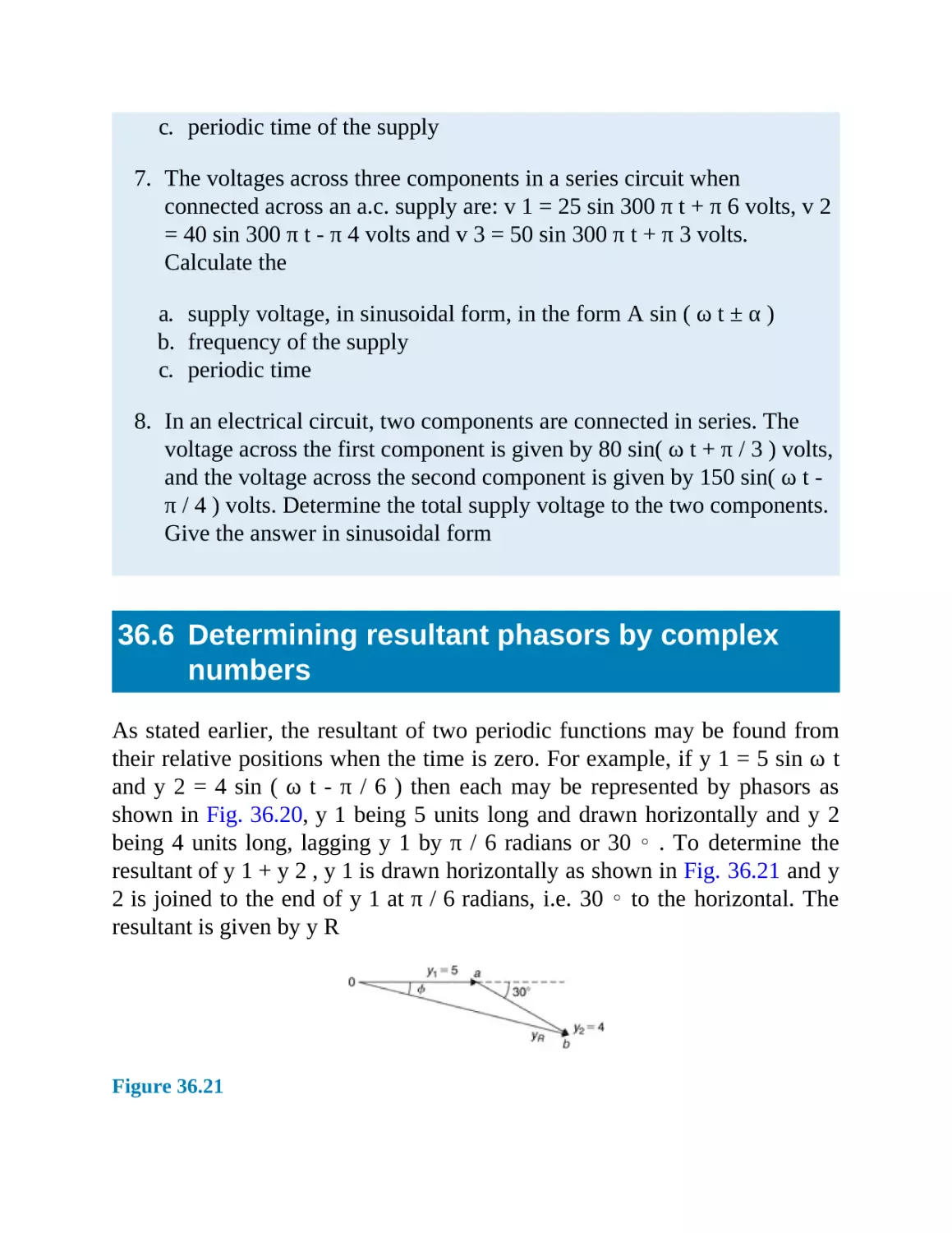
Further worked problems on standard form
Problem 18. Find the value of:
a. 7.9 × 10 - 2 - 5.4 × 10 - 2
b. 8.3 × 10 3 + 5.415 × 10 3 and
c. 9.293 × 10 2 + 1.3 × 10 3 expressing the answers in standard form.
Numbers having the same exponent can be added or subtracted by adding or
subtracting the mantissae and keeping the exponent the same. Thus:
a. 7.9 × 10 - 2 - 5.4 × 10 - 2 = ( 7.9 - 5.4 ) × 10 - 2 = 2.5 × 10 - 2
b. 8.3 × 10 3 + 5.415 × 10 3 = ( 8.3 + 5.415 ) × 10 3 = 13.715 × 10 3 =
1.3715 × 10 4 in standard form
c. Since only numbers having the same exponents can be added by
straight addition of the mantissae, the numbers are converted to this
form before adding. Thus:
9.293 × 10 2 + 1.3 × 10 3 = 9.293 × 10 2 + 13 × 10 2 = ( 9.293 + 13 )
× 10 2 = 22.293 × 10 2 = 2.2293 × 10 3 in standard form.
Alternatively, the numbers can be expressed as decimal fractions,
giving:
9.293 × 10 2 + 1.3 × 10 3 = 929.3 + 1300 = 2229.3 = 2.2293 × 10 3
in standard form as obtained previously. This method is often the
‘safest’ way of doing this type of problem.
Problem 19. Evaluate
a. (3.75 × 10 3 ) (6 × 10 4 ) and
b. 3.5 × 10 5 7 × 10 2 expressing answers in standard form
a. (3.75 × 10 3 ) (6 × 10 4 ) = (3.75 × 6)(10 3 + 4 ) = 22.50 × 10 7 = 2.25
× 10 8
b. 3.5 × 10 5 7 × 10 2 = 3.5 7 × 10 5 - 2 = 0.5 × 10 3 = 5 × 10 2
Now try the following Practice Exercise
Practice Exercise 8 Standard form (Answers on page 673)
In Problems 1 to 4, find values of the expressions given, stating the answers
in standard form:
1. (a) 3.7 × 10 2 + 9.81 × 10 2 (b) 1.431 × 10 - 1 + 7.3 × 10 - 1
2. (a) 4.831 × 10 2 + 1.24 × 10 3 (b) 3.24 × 10 - 3 - 1.11 × 10 - 4
3. (a) (4.5 × 10 - 2 ) (3 × 10 3 ) (b) 2 × (5.5 × 10 4 )
4. (a) 6 × 10 - 3 3 × 10 - 5 (b) ( 2.4 × 10 3 ) ( 3 × 10 - 2 ) ( 4.8 × 10 4 )
5. Write the following statements in standard form:
a. The density of aluminium is 2710 kg m - 3
b. Poisson’s ratio for gold is 0.44
c. The impedance of free space is 376.73 Ω
d. The electron rest energy is 0.511 MeV
e. Proton charge-mass ratio is 9 5 789 700 C kg - 1
f. The normal volume of a perfect gas is 0.02241 m 3 mol - 1
2.7
Engineering notation and common prefixes
Engineering notation is similar to scientific notation except that the power
of ten is always a multiple of 3.
For example, 0.00035 = 3.5 × 10 - 4 in scientific notation, but 0.00035 = 0.35
× 10 - 3 or 350 × 10 - 6 in engineering notation.
Units used in engineering and science may be made larger or smaller by
using prefixes that denote multiplication or division by a particular amount.
The eight most common multiples, with their meaning, are listed in page 18,
where it is noticed that the prefixes involve powers of ten which are all
multiples of 3.
For example,
5 MV means 5 × 1 000 000 = 5 × 10 6 = 5 000 000 volts 3.6 k Ω means 3.6 ×
1000 = 3.6 × 10 3 = 3600 ohms
7.5 μ C means 7.5 ÷ 1 000 000 = 7.5 10 6 or 7.5 × 10 - 6 = 0.0000075
coulombs and 4 mA means 4 × 10 - 3 or = 4 10 3 = 4 1000 = 0.004 amperes
Similarly,
0.00006 J = 0.06 mJ or 60 μ J 5 620 000 N = 5620 kN or 5.62 MN 47 × 10 4
Ω = 470 000 Ω = 470 k Ω or 0.47 M Ω and 12 × 10 - 5 A = 0.00012 A = 0.12
mA or 120 μ A
Table 2.1
A calculator is needed for many engineering calculations, and having a
calculator which has an ‘ENG’ function is most helpful.
For example, to calculate: 3 × 10 4 × 0.5 × 10 - 6 volts, input your calculator
in the following order: (a) Enter ‘3’ (b) Press × 10 x (c) Enter ‘4’ (d) Press ‘ ×
’ (e) Enter ‘0.5’ (f) Press × 10 x (g) Enter ‘ - 6’ (h) Press ‘ = ’
The answer is 0.015 V or 7 200 Now press the ‘ENG’ button, and the answer
changes to 15 × 10 - 3 V
The ‘ENG’ or ‘Engineering’ button ensures that the value is stated to a power
of 10 that is a multiple of 3, enabling you, in this example, to express the
answer as 15 mV
Now try the following Practice Exercise
Practice Exercise 9 Engineering notation and common prefixes
(Answers on page 673)
1. Express the following in engineering notation and in prefix form: (a)
100 000 W (b) 0.00054 A (c) 15 × 10 5 Ω (d) 225 × 10 - 4 V (e) 35
000 000 000 Hz (f) 1.5 × 10 - 11 F (g) 0.000017 A (h) 46200 Ω
2. Rewrite the following as indicated: (a) 0.025 mA = ....... μ A (b)
1000 pF = .....nF (c) 62 × 10 4 V = .......kV (d) 1 250 000 Ω = .....M
Ω
3. Use a calculator to evaluate the following in engineering notation:
(a) 4.5 × 10 - 7 × 3 × 10 4 (b) ( 1.6 × 10 - 5 ) ( 25 × 10 3 ) ( 100 × 10
6)
2.8
Metric conversions
Length in metric units
1 m = 100 c m = 1000 m m 1 c m = 1 100 m = 1 10 2 m = 10 - 2 m 1 m m = 1
1000 m = 1 10 3 m = 10 - 3 m
Problem 20. Rewrite 14,700 mm in metres
1 m = 1000 mm hence, 1 mm = 1 1000 = 1 10 3 = 10 - 3 m
Hence, 14 , 700 mm = 14 , 700 × 10 - 3 m = 1 4.7 m
Problem 21. Rewrite 276 cm in metres
1 m = 100 cm hence, 1 cm = 1 100 = 1 10 2 = 10 - 2 m
Hence, 276 cm = 276 × 10 - 2 m = 2 . 76 m
Now try the following Practice Exercise
Practice Exercise 10 Length in metric units (Answers on page 673)
1.
2.
3.
4.
5.
6.
State 2.45 m in millimetres
State 1.675 m in centimetres
State the number of millimetres in 65.8 cm
Rewrite 25,400 mm in metres
Rewrite 5632 cm in metres
State the number of millimetres in 4.356 m
7.
8.
9.
10.
How many centimetres are there in 0.875 m?
State a length of 465 cm in (a) mm (b) m
State a length of 5040 mm in (a) cm (b) m
A machine part is measured as 15.0 cm ± 1%. Between what two
values would the measurement be? Give the answer in millimetres.
Areas in metric units
Area is a measure of the size or extent of a plane surface.
Area is measured in square units such as mm 2 , cm 2 and m 2 .
The area of the above square is 1 m 2
1 m 2 = 100 c m × 100 c m = 10000 c m 2 = 10 4 c m 2
i.e. to change from square metres to square centimetres, multiply by 10 4
Hence, 2.5 m 2 = 2.5 × 10 4 c m 2
and 0.75 m 2 = 0.75 × 10 4 c m 2
Since 1 m 2 = 10 4 c m 2 then 1 c m 2 = 1 10 4 m 2 = 10 - 4 m 2
i.e. to change from square centimetres to square metres, multiply by 10 - 4
Hence, 52 c m 2 = 52 × 10 - 4 m 2
and 643 c m 2 = 643 × 10 - 4 m 2
The area of the above square is 1 m 2
1 m 2 = 1000 mm × 1000 mm = 1000000 mm 2 = 10 6 mm 2
i.e. to change from square metres to square millimetres, multiply by 10 6
Hence, 7.5 m 2 = 7.5 × 10 6 mm 2
and 0.63 m 2 = 0.63 × 10 6 mm 2
Since 1 m 2 = 10 6 mm 2
then 1 mm 2 = 1 10 6 m 2 = 10 - 6 m 2
i.e. to change from square millimetres to square metres, multiply by 10 - 6
Hence, 235 mm 2 = 235 × 10 - 6 m 2
and 47 mm 2 = 47 × 10 - 6 m 2
The area of the above square is 1 cm 2
1 cm 2 = 10 mm × 10 mm = 100 mm 2 = 10 2 mm 2
i.e. to change from square centimetres to square millimetres, multiply by 100
or 10 2
Hence, 3.5 cm 2 = 3.5 × 10 2 mm 2 = 350 mm 2
and 0.75 cm 2 = 0.75 × 10 2 mm 2 = 75 mm 2
Since 1 cm 2 = 10 2 mm 2
then 1 mm 2 = 1 10 2 cm 2 = 10 - 2 cm 2
i.e. to change from square millimetres to square centimetres, multiply by 10 2
Hence, 250 mm 2 = 250 × 10 - 2 cm 2 = 2.5 cm 2
and 85 mm 2 = 85 × 10 - 2 cm 2 = 0.85 cm 2
Problem 22. Rewrite 12 m 2 in square centimetres
1 m 2 = 10 4 cm 2 hence, 12 m 2 = 12 × 10 4 cm 2
Problem 23. Rewrite 50 cm 2 in square metres
1 cm 2 = 10 - 4 m 2 hence, 50 cm 2 = 50 × 10 - 4 m 2
Problem 24. Rewrite 2.4 m 2 in square millimetres
1 m 2 = 10 6 mm 2 hence, 2.4 m 2 = 2.4 × 10 6 mm 2
Problem 25. Rewrite 147 mm 2 in square metres
1 mm 2 = 10 - 6 m 2 hence, 147 mm 2 = 147 × 10 - 6 m 2
Problem 26. Rewrite 34.5 cm 2 in square millimetres
1 cm 2 = 10 2 mm 2
hence, 34.5 cm 2 = 34.5 × 10 2 mm 2 = 3450 mm 2
Problem 27. Rewrite 400 mm 2 in square centimetres
1 mm 2 = 10 - 2 cm 2
hence, 400 mm 2 = 400 × 10 - 2 cm 2 = 4 cm 2
Problem 28. The top of a small rectangular table is 800 mm long and 500
mm wide. Determine its area in (a) mm 2 (b) cm 2 (c) m 2
a. Area of rectangular table top = l × b = 800 × 500 = 400,000 mm 2
b. Since 1 cm = 10 mm then 1 cm 2 = 1 cm × 1 cm = 10 mm × 10 mm =
100 mm 2 or 1 mm 2 = 1 100 = 0.01 cm 2 Hence, 400,000 mm 2 =
400,000 × 0.01 cm 2 = 4000 cm 2
c. 1 cm 2 = 10 - 4 m 2 hence, 4000 cm 2 = 4000 × 10 - 4 m 2 = 0 . 4 m 2
Now try the following Practice Exercise
Practice Exercise 11 Areas in metric units (Answers on page 673)
1.
2.
3.
4.
5.
6.
7.
Rewrite 8 m 2 in square centimetres
Rewrite 240 cm 2 in square metres
Rewrite 3.6 m 2 in square millimetres
Rewrite 350 mm 2 in square metres
Rewrite 50 cm 2 in square millimetres
Rewrite 250 mm 2 in square centimetres
A rectangular piece of metal is 720 mm long and 400 mm wide.
Determine its area in (a) mm 2 (b) cm 2 (c) m 2
Volumes in metric units
The volume of any solid is a measure of the space occupied by the solid.
Volume is measured in cubic units such as mm 3 , cm 3 and m 3 .
The volume of the cube shown is 1 m 3
1 m 3 = 100 cm × 100 cm × 100 cm = 1000000 cm 2 = 10 6 cm 2 1 litre =
1000 cm 3
i.e. to change from cubic metres to cubic centimetres, multiply by 10 6
Hence, 3.2 m 3 = 3.2 × 10 6 cm 3
and 0.43 m 3 = 0.43 × 10 6 cm 3
Since 1 m 3 = 10 6 cm 3 then 1 cm 3 = 1 10 6 m 3 = 10 - 6 m 3
i.e. to change from cubic centimetres to cubic metres, multiply by 10 - 6
Hence, 140 cm 3 = 140 × 10 - 6 m 3
and 2500 cm 3 = 2500 × 10 - 6 m 3
The volume of the cube shown is 1 m 3
1 m 3 = 1000 mm × 1000 mm × 1000 mm = 1000000000 mm 3 = 10 9 mm 3
i.e. to change from cubic metres to cubic millimetres, multiply by 10 9
Hence, 4.5 m 3 = 4.5 × 10 9 mm 3
and 0.25 m 3 = 0.25 × 10 9 mm 3
Since 1 m 3 = 10 9 mm 2
then 1 mm 3 = 1 10 9 m 3 = 10 - 9 m 3
i.e. to change from cubic millimetres to cubic metres, multiply by 10 - 9
Hence, 500 mm 3 = 500 × 10 - 9 m 3
and 4675 mm 3 = 4675 × 10 - 9 m 3 or 4.675 × 10 - 6 m 3
The volume of the cube shown is 1 cm 3
1 cm 3 = 10 mm × 10 mm × 10 mm = 1000 mm 3 = 10 3 mm 3
i.e. to change from cubic centimetres to cubic millimetres, multiply by 1000
or 10 3
Hence, 5 cm 3 = 5 × 10 3 mm 3 = 5000 mm 3
and 0.35 cm 3 = 0.35 × 10 3 mm 3 = 350 mm 3
Since 1 cm 3 = 10 3 mm 3
then 1 mm 3 = 1 10 3 cm 3 = 10 - 3 cm 3
i.e. to change from cubic millimetres to cubic centimetres, multiply by 10 - 3
Hence, 650 mm 3 = 650 × 10 - 3 cm 3 = 0.65 cm 3
and 75 mm 3 = 75 × 10 - 3 cm 3 = 0.075 cm 3
Problem 29. Rewrite 1.5 m 3 in cubic centimetres
1 m 3 = 10 6 cm 3 hence, 1.5 m 3 = 1.5 × 10 6 cm 3
Problem 30. Rewrite 300 cm 3 in cubic metres
1 cm 3 = 10 - 6 m 3 hence, 300 cm 3 = 300 × 10 - 6 m 3
Problem 31. Rewrite 0.56 m 3 in cubic millimetres
1 m 3 = 10 9 mm 3 hence, 0.56 m 3 = 0.56 × 10 9 mm 3 or 560 × 10 6 mm 3
Problem 32. Rewrite 1250 mm 3 in cubic metres
1 mm 3 = 10 - 9 m 3 hence, 1250 mm 3 = 1250 × 10 - 9 m 3 or 1.25 × 10 - 6
m3
Problem 33. Rewrite 8 cm 3 in cubic millimetres
1 cm 3 = 10 3 mm 3
hence, 8 cm 3 = 8 × 10 3 mm 3 = 8000 mm 3
Problem 34. Rewrite 600 mm 3 in cubic centimetres
1 mm 3 = 10 - 3 cm 3
hence, 600 mm 3 = 600 × 10 - 3 cm 3 = 0.6 cm 3
Problem 35. A water tank is in the shape of a rectangular prism having
length 1.2 m, breadth 50 cm and height 250 mm. Determine the capacity of
the tank (a) m 3 (b) cm 3 (c) litres
Capacity means volume. When dealing with liquids, the word capacity is
usually used.
a. Capacity of water tank = l × b × h where l = 1.2 m, b = 50 cm and h =
250 mm. To use this formula, all dimensions must be in the same
units. Thus, l = 1.2 m, b = 0.50 m and h = 0.25 m (since 1 m = 100 cm
= 1000 mm) Hence, capacity of tank = 1.2 × 0.50 × 0.25 = 0.15 m 3
b. 1 m 3 = 10 6 cm 3 Hence, capacity = 0.15 m 3 = 0.15 × 10 6 cm 3 = 1
50 , 000 c m 3
c. 1 litre = 1000 cm 3 Hence, 150,000 cm 3 = 150 , 000 1000 = 150
litres
Now try the following Practice Exercise
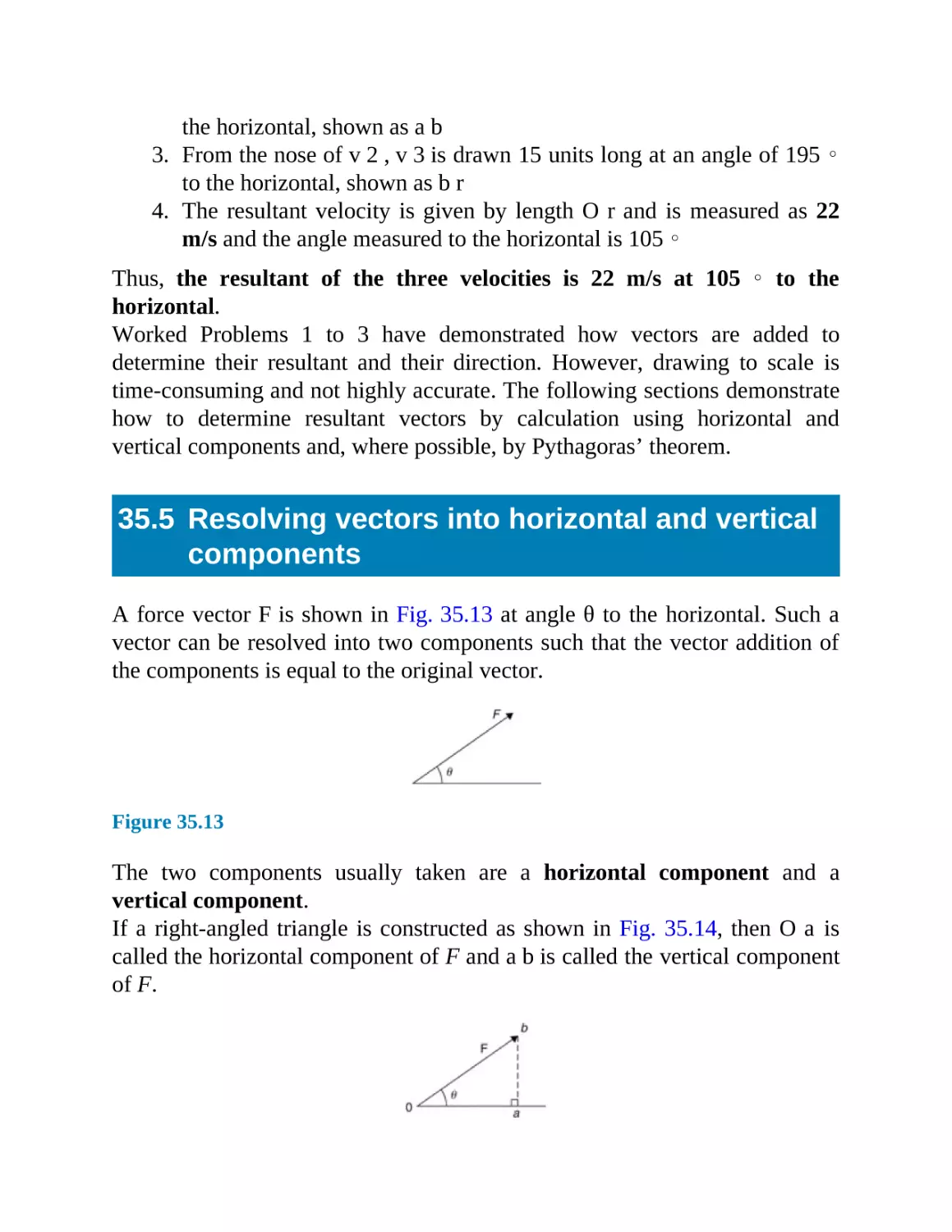
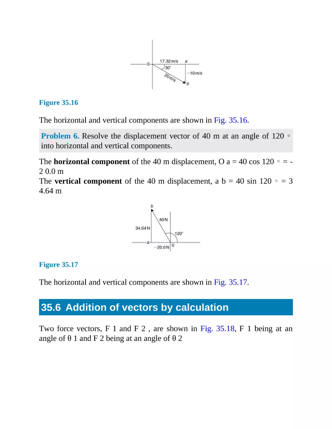
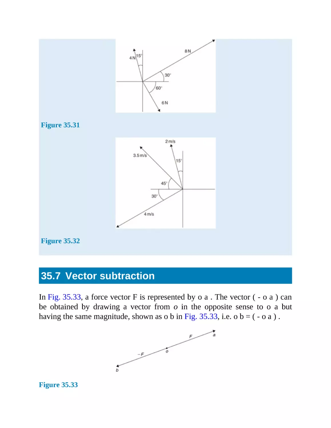
Practice Exercise 12 Volumes in metric units (Answers on page 673)
1.
2.
3.
4.
5.
6.
7.
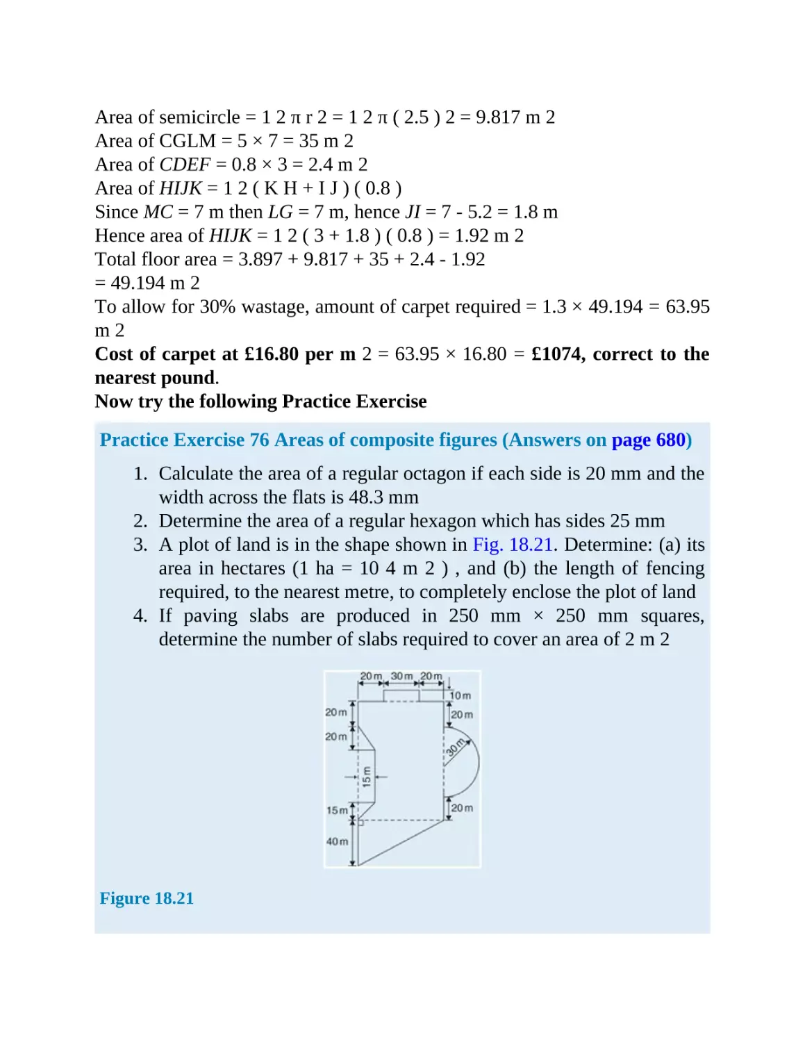
8.
9.
Rewrite 2.5 m 3 in cubic centimetres
Rewrite 400 cm 3 in cubic metres
Rewrite 0.87 m 3 in cubic millimetres
Change a volume of 2,400,000 cm 3 to cubic metres.
Rewrite 1500 mm 3 in cubic metres
Rewrite 400 mm 3 in cubic centimetres
Rewrite 6.4 cm 3 in cubic millimetres
Change a volume of 7500 mm 3 to cubic centimetres.
An oil tank is in the shape of a rectangular prism having length 1.5
m, breadth 60 cm and height 200 mm. Determine the capacity of the
tank in (a) m 3 (b) cm 3 (c) litres
2.9
Metric - US/Imperial Conversions
The Imperial System (which uses yards, feet, inches, etc to measure length)
was developed over hundreds of years in the UK, then the French developed
the Metric System (metres) in 1670, which soon spread through Europe, even
to England itself in 1960. But the USA and a few other countries still prefer
feet and inches.
When converting from metric to imperial units, or vice versa, one of the
following tables (2.2 to 2.9) should help.
Problem 36. Calculate the number of inches in 350 mm, correct to 2
decimal places
350 mm = 350 × 0.03937 inches = 13.78 inches from Table 2.2
Problem 37. Calculate the number of inches in 52 cm, correct to 4
significant figures
52 cm = 52 × 0.3937 inches = 20.47 inches from Table 2.2
Problem 38. Calculate the number of yards in 74 m, correct to 2 decimal
places
74 m = 74 × 1.0936 yards = 80.93 yds from Table 2.2
Problem 39. Calculate the number of miles in 12.5 km, correct to 3
significant figures
12.5 km = 12.5 × 0.6214 miles = 7.77 miles from Table 2.2
Table 2.2 Metric to imperial length
Table 2.3 Imperial to metric length
Problem 40. Calculate the number of centimetres in 35 inches, correct to 1
decimal places
35 inches = 35 × 2.54 cm = 88.9 cm from Table 2.3
Problem 41. Calculate the number of metres in 66 inches, correct to 2
decimal places
66 inches = 66 12 feet = 66 12 × 0.3048 m = 1.68 m from Table 2.3
Problem 42. Calculate the number of metres in 50 yards, correct to 2
decimal places
50 yards = 50 × 0.9144 m = 45.72 m from Table 2.3
Problem 43. Calculate the number of kilometres in 7.2 miles, correct to 2
decimal places
7.2 miles = 7.2 × 1.6093 km = 11.59 km from Table 2.3
Table 2.4 Metric to imperial area
Problem 44. Calculate the number of (a) yards (b) kilometres in 5.2 nautical
miles
a. 5.2 nautical miles = 5.2 × 2025.4 yards= 10532 yards from Table 2.3
b. 5.2 nautical miles = 5.2 × 1.853 km = 9.636 km from Table 2.3
Problem 45. Calculate the number of square inches in 47 cm 2 , correct to 4
significant figures
47 cm 2 = 47 × 0.1550 in 2 = 7.285 in 2 from Table 2.4
Problem 46. Calculate the number of square yards in 20 m 2 , correct to 2
decimal places
20 m 2 = 20 × 1.1960 yd 2 = 23.92 yd 2 from Table 2.4
Problem 47. Calculate the number of acres in 23 hectares of land, correct to
2 decimal places
23 hectares = 23 × 2.4711 acres = 56.84 acres from Table 2.4
Problem 48. Calculate the number of square miles in a field of 15 km 2
area, correct to 2 decimal places
15 km 2 = 15 × 0.3861 mile 2
= 5.79 mile 2 from Table 2.4
Table 2.5 Imperial to metric area
Problem 49. Calculate the number of square centimetres in 17.5 in 2 ,
correct to the nearest square centimetre
17.5 in 2 = 17.5 × 6.4516 cm 2 = 113 cm 2 from Table 2.5
Problem 50. Calculate the number of square metres in 205 ft 2 , correct to 2
decimal places
205 ft 2 = 205 × 0.0929 m 2 = 19.04 m 2 from Table 2.5
Problem 51. Calculate the number of square metres in 11.2 acres, correct to
the nearest square metre
11.2 acres = 11.2 × 4046.9 m 2 = 45325 m 2 from Table 2.5
Problem 52. Calculate the number of square kilometres in 12.6 mile 2 ,
correct to 2 decimal places
12.6 mile 2 = 12.6 × 2.59 km 2 = 32.63 km 2 from Table 2.5
Table 2.6 Metric to imperial volume/capacity
Problem 53. Calculate the number of cubic inches in 123.5 cm 3 , correct to
2 decimal places
123.5 cm 3 = 123.5 × 0.0610 cm 3 = 7.53 cm 3 from Table 2.6
Problem 54. Calculate the number of cubic feet in 144 dm 3 , correct to 3
decimal places
144 dm 3 = 144 × 0.0353 ft 3 = 5.083 ft 3 from Table 2.6
Problem 55. Calculate the number of cubic yards in 5.75 m 3 , correct to 4
significant figures
5.75 m 3 = 5.75 × 1.3080 yd 3 = 7.521 yd 3 from Table 2.6
Problem 56. Calculate the number of US fluid pints in 6.34 litres of oil,
correct to 1 decimal place
6.34 litre = 6.34 × 2.113 US fluid pints = 13.4 US fluid pints from Table 2.6
Table 2.7 Imperial to metric volume/capacity
Problem 57. Calculate the number of cubic centimetres in 3.75 in 3 , correct
to 2 decimal places
3.75 in 3 = 3.75 × 16.387 cm 3 = 61.45 cm 3 from Table 2.7
Problem 58. Calculate the number of cubic metres in 210 ft 3 , correct to 3
significant figures
210 ft 3 = 210 × 0.02832 m 3 = 5.95 m 3 from Table 2.7
Problem 59. Calculate the number of litres in 4.32 US pints, correct to 3
decimal places
4.32 US pints = 4.32 × 0.4732 litres = 2.044 litres from Table 2.7
Problem 60. Calculate the number of litres in 8.62 US gallons, correct to 2
decimal places
8.62 US gallons = 8.62 × 3.7854 litre = 32.63 litre from Table 2.7
Table 2.8 Metric to imperial mass
The British ton is the long ton, which is 2240 pounds, and the US ton is
the short ton which is 2000 pounds.
Problem 61. Calculate the number of ounces in a mass of 1346 g, correct to
2 decimal places
1346 g = 1346 × 0.0353 oz = 47.51 oz from Table 2.8
Problem 62. Calculate the mass, in pounds, in a 210.4 kg mass, correct to 4
significant figures
210.4 kg = 210.4 × 2.2046 lb = 463.8 lb from Table 2.8
Problem 63. Calculate the number of short tons in 5000 kg, correct to 2
decimal places
5000 kg = 5 t = 5 × 1.1023 short tons = 5.51 short tons from Table 2.8
Table 2.9 Imperial to metric mass
Problem 64. Calculate the number of grams in 5.63 oz, correct to 4
significant figures
5.63 oz = 5.63 × 28.35 g = 159.6 g from Table 2.9
Problem 65. Calculate the number of kilograms in 75 oz, correct to 3
decimal places
75 oz = 75 16 lb = 75 16 × 0.4536 kg = 2.126 kg from Table 2.9
Problem 66. Convert 3.25 cwt into (a) pounds (b) kilograms
a. 3.25 cwt = 3.25 × 112 lb = 364 lb from Table 2.9
b. 3.25 cwt = 3.25 × 50.802 kg = 165.1 kg from Table 2.9
Temperature
To convert from Celsius to Fahrenheit, first multiply by 9/5, then add 32.
To convert from Fahrenheit to Celsius, first subtract 32, then multiply by 5/9
Problem 67. Convert 35 ∘ C to degrees Fahrenheit
F = 9 5 C + 32 , hence 35 ∘ C = 9 5 ( 35 ) + 32 = 63 + 32 = 95 ∘
Problem 68. Convert 113 ∘ F to degrees Celsius
C = 5 9 ( F - 32 ) , hence 113 ∘ F = 5 9 ( 113 - 32 )
= 5 9 ( 81 ) = 45 ∘ C
Now try the following Practice Exercise
Practice Exercise 13 Metric/imperial conversions (Answers on page
673)
In the following Problems, use the metric/imperial conversions in Tables 2.2
to 2.9
1. Calculate the number of inches in 476 mm, correct to 2 decimal
places
2. Calculate the number of inches in 209 cm, correct to 4 significant
figures
3. Calculate the number of yards in 34.7 m, correct to 2 decimal places
4. Calculate the number of miles in 29.55 km, correct to 2 decimal
places
5. Calculate the number of centimetres in 16.4 inches, correct to 2
decimal places
6. Calculate the number of metres in 78 inches, correct to 2 decimal
places
7. Calculate the number of metres in 15.7 yards, correct to 2 decimal
places
8. Calculate the number of kilometres in 3.67 miles, correct to 2
decimal places
9. Calculate the number of (a) yards (b) kilometres in 11.23 nautical
miles
10. Calculate the number of square inches in 62.5 cm 2 , correct to 4
significant figures
11. Calculate the number of square yards in 15.2 m 2 , correct to 2
decimal places
12. Calculate the number of acres in 12.5 hectares, correct to 2 decimal
places
13. Calculate the number of square miles in 56.7 km 2 , correct to 2
decimal places
14. Calculate the number of square centimetres in 6.37 in 2 , correct to
the nearest square centimetre
15. Calculate the number of square metres in 308.6 ft 2 , correct to 2
decimal places
16. Calculate the number of square metres in 2.5 acres, correct to the
nearest square metre
17. Calculate the number of square kilometres in 21.3 mile 2 , correct to
2 decimal places
18. Calculate the number of cubic inches in 200.7 cm 3 , correct to 2
decimal places
19. Calculate the number of cubic feet in 214.5 dm 3 , correct to 3
decimal places
20. Calculate the number of cubic yards in 13.45 m 3 , correct to 4
significant figures
21. Calculate the number of US fluid pints in 15 litres, correct to 1
decimal place
22. Calculate the number of cubic centimetres in 2.15 in 3 , correct to 2
decimal places
23. Calculate the number of cubic metres in 175 ft 3 , correct to 4
significant figures
24. Calculate the number of litres in 7.75 US pints, correct to 3 decimal
places
25. Calculate the number of litres in 12.5 US gallons, correct to 2
decimal places
26. Calculate the number of ounces in 980 g, correct to 2 decimal places
27. Calculate the mass, in pounds, in 55 kg, correct to 4 significant
28.
29.
30.
31.
32.
33.
figures
Calculate the number of short tons in 4000 kg, correct to 3 decimal
places
Calculate the number of grams in 7.78 oz, correct to 4 significant
figures
Calculate the number of kilograms in 57.5 oz, correct to 3 decimal
places
Convert 2.5 cwt into (a) pounds (b) kilograms
Convert 55 ∘ C to degrees Fahrenheit
Convert 167 ∘ F to degrees Celsius
Chapter 3
Binary, octal and hexadecimal numbers
Why it is important to understand: Binary, octal and hexadecimal
numbers
There are infinite ways to represent a number. The four commonly
associated with modern computers and digital electronics are
decimal, binary, octal, and hexadecimal. All four number systems
are equally capable of representing any number. Furthermore, a
number can be perfectly converted between the various number
systems without any loss of numeric value. At a first look, it seems
like using any number system other than decimal is complicated
and unnecessary. However, since the job of electrical and software
engineers is to work with digital circuits, engineers require number
systems that can best transfer information between the human
world and the digital circuit world. Thus the way in which a
number is represented can make it easier for the engineer to
perceive the meaning of the number as it applies to a digital circuit,
i.e. the appropriate number system can actually make things less
complicated. Binary, octal and hexadecimal numbers are explained
in this chapter.
At the end of this chapter you should be able to:
recognise a binary number
convert binary to decimal and vice-versa
add binary numbers
recognise an octal number
convert decimal to binary via octal and vice-versa
recognise a hexadecimal number
convert from hexadecimal to decimal and vice-versa
convert from binary to hexadecimal and vice-versa
3.1
Introduction
Man’s earliest number or counting system was probably developed to help
determine how many possessions a person had. As daily activities became
more complex, numbers became more important in trade, time, distance, and
all other phases of human life. Ever since people discovered that it was
necessary to count objects, they have been looking for easier ways to do so.
The abacus, developed by the Chinese, is one of the earliest known
calculators; it is still in use in some parts of the world. Blaise Pascal*
invented the first adding machine in 1642. Twenty years later, an
Englishman, Sir Samuel Morland*, 1 developed a more compact device that
could multiply, add and subtract. About 1672, Gottfried Wilhelm von
Leibniz* perfected a machine that could perform all the basic operations
(add, subtract, multiply, divide), as well as extract the square root. Modern
electronic digital computers still use von Leibniz’s principles.
Computers are now employed wherever repeated calculations or the
processing of huge amounts of data is needed. The greatest applications are
found in the military, scientific, and commercial fields. They have
applications that range from mail sorting, and engineering design, to the
identification and destruction of enemy targets. The advantages of digital
computers include speed, accuracy and man-power savings. Often computers
are able to take over routine jobs and release personnel for more important
work that cannot be handled by a computer. People and computers do not
normally speak the same language. Methods of translating information into
forms that are understandable and usable to both are necessary. Humans
generally speak in words and numbers expressed in the decimal number
system, while computers only understand coded electronic pulses that
represent digital information.
* Who was Leibniz? – Gottfried Wilhelm Leibniz (sometimes von Leibniz) (1 July,
1646–14 November, 1716) was a German mathematician and philosopher.
*Who was Pascal? – See page 146.
*Who was Morland? – Sir Samuel Morland, 1st Baronet (1625–1695), was an
English academic, diplomat, spy, inventor and mathematician of the 17th century, a
polymath credited with early developments in relation to computing, hydraulics and
steam power. To find out more go to www.routledge.com/cw/bird
All data in modern computers is stored as series of bits, a bit being a binary
digit, and can have one of two values, the numbers 0 and 1. The most basic
form of representing computer data is to represent a piece of data as a string
of 1’s and 0’s, one for each bit. This is called a binary or base-2 number.
Because binary notation requires so many bits to represent relatively small
numbers, two further compact notations are often used, called octal and
hexadecimal. Computer programmers who design sequences of number
codes instructing a computer what to do, would have a very difficult task if
they were forced to work with nothing but long strings of 1’s and 0’s, the
‘native language’ of any digital circuit.
Octal notation represents data as base-8 numbers with each digit in an octal
number representing three bits. Similarly, hexadecimal notation uses base-16
numbers, representing four bits with each digit. Octal numbers use only the
digits 0–7, while hexadecimal numbers use all ten base-10 digits (0–9) and
the letters A–F (representing the numbers 10–15).
This chapter explains how to convert between the decimal, binary, octal and
hexadecimal systems.
3.2
Binary numbers
The system of numbers in everyday use is the denary or decimal system of
numbers, using the digits 0 to 9. It has ten different digits (0, 1, 2, 3, 4, 5, 6,
7, 8 and 9) and is said to have a radix or base of 10.
The binary system of numbers has a radix of 2 and uses only the digits 0 and
1.
(a) Conversion of binary to decimal:
The decimal number 234.5 is equivalent to
2 × 10 2 + 3 × 10 1 + 4 × 10 0 + 5 × 10 - 1
i.e. is the sum of term comprising: (a digit) multiplied by (the base raised to
some power).
In the binary system of numbers, the base is 2, so 1101.1 is equivalent to:
1×23+1×22+0×21+1×20+1×2-1
Thus the decimal number equivalent to the binary number 1101.1 is
8 + 4 + 0 + 1 + 1 2 , that is 13.5
i.e. 1101.1 2 = 13.5 10 , the suffixes 2 and 10 denoting binary and decimal
systems of number respectively.
Problem 1. Convert 11011 2 to a decimal number
From above: 11011 2 = 1 × 2 4 + 1 × 2 3 + 0 × 2 2 + 1 × 2 1 + 1 × 2 0 = 16 +
8 + 0 + 2 + 1 = 27 10
Problem 2. Convert 0.1011 2 to a decimal fraction
0 . 1011 2 = 1 × 2 - 1 + 0 × 2 - 2 + 1 × 2 - 3 + 1 × 2 - 4 = 1 × 1 2 + 0 × 1 2 2 +
1 × 1 2 3 + 1 × 1 2 4 = 1 2 + 1 8 + 1 16 = 0.5 + 0.125 + 0.0625 = 0 . 6875 10
Problem 3. Convert 101.0101 2 to a decimal number
101 . 0101 2 = 1 × 2 2 + 0 × 2 1 + 1 × 2 0 + 0 × 2 - 1 + 1 × 2 - 2 + 0 × 2 - 3 +
1 × 2 - 4 = 4 + 0 + 1 + 0 + 0.25 + 0 + 0.0625 = 5 . 3125 10
Now try the following Practice Exercise
Practice Exercise 14 Conversion of binary to decimal numbers
(Answers on page 674)
In Problems 1 to 5, convert the binary numbers given to decimal numbers.
1. (a) 110 (b) 1011 (c) 1110 (d) 1001
2. (a) 10101 (b) 11001 (c) 101101 (d) 110011
3. (a) 101010 (b) 111000 (c) 1000001 (d) 10111000
4. (a) 0.1101 (b) 0.11001 (c) 0.00111 (d) 0.01011
5. (a) 11010.11 (b) 10111.011 (c) 110101.0111 (d) 11010101.10111
(b) Conversion of decimal to binary:
An integer decimal number can be converted to a corresponding binary
number by repeatedly dividing by 2 and noting the remainder at each stage,
as shown below for 39 10
The result is obtained by writing the top digit of the remainder as the least
significant bit, (a bit is a binary digit and the least significant bit is the one on
the right). The bottom bit of the remainder is the most significant bit, i.e. the
bit on the left.
Thus 39 10 = 100111 2
The fractional part of a decimal number can be converted to a binary number
by repeatedly multiplying by 2, as shown below for the fraction 0.625
For fractions, the most significant bit of the result is the top bit obtained from
the integer part of multiplication by 2. The least significant bit of the result is
the bottom bit obtained from the integer part of multiplication by 2
Thus 0.625 10 = 0.101 2
Problem 4. Convert 47 10 to a binary number
From above, repeatedly dividing by 2 and noting the remainder gives:
Thus 47 10 = 101111 2
Problem 5. Convert 0.40625 10 to a binary number
From above, repeatedly multiplying by 2 gives:
i.e. 040625 10 = 0.01101 2
Problem 6. Convert 58.3125 10 to a binary number
The integer part is repeatedly divided by 2, giving:
The fractional part is repeatedly multiplied by 2 giving:
Thus 58.3125 10 = 111010.0101 2
Now try the following Practice Exercise
Practice Exercise 15 Conversion of decimal to binary numbers
(Answers on page 674)
In Problems 1 to 5, convert the decimal numbers given to binary numbers.
1. (a) 5 (b) 15 (c) 19 (d) 29
2. (a) 31 (b) 42 (c) 57 (d) 63
3. (a) 47 (b) 60 (c) 73 (d) 84
4. (a) 0.25 (b) 0.21875 (c) 0.28125 (d) 0.59375
5. (a) 47.40625 (b) 30.8125 (c) 53.90625 (d) 61.65625
(c) Binary addition:
Binary addition of two/three bits is achieved according to the following rules:
These rules are demonstrated in the following worked problems.
Problem 7. Perform the binary addition: 1001 + 10110
1001 + 10110 ̲ 11111 ̲
Problem 8. Perform the binary addition: 11111 + 10101
11111 + 10101 ̲ sum 110100 ̲ carry 11111
Problem 9. Perform the binary addition: 1101001 + 1110101
1101001 + 1110101 ̲ sum 11011110 ̲ carry 1 11
Problem 10. Perform the binary addition: 1011101 + 1100001 + 110101
1011101 1100001 + 110101 ̲ sum 11110011 ̲ carry 111111
Now try the following Practice Exercise
Practice Exercise 16 Binary addition (Answers on page 674)
Perform the following binary additions:
1. 10 + 11
2. 101 + 110
3. 1101 + 111
4. 1111 + 11101
5. 110111 + 10001
6. 10000101 + 10000101
7. 11101100 + 111001011
8. 110011010 + 11100011
9. 10110 + 1011 + 11011
10. 111 + 10101 + 11011
11. 1101 + 1001 + 11101
12. 100011 + 11101 + 101110
3.3
Octal numbers
For decimal integers containing several digits, repeatedly dividing by 2 can
be a lengthy process. In this case, it is usually easier to convert a decimal
number to a binary number via the octal system of numbers. This system has
a radix of 8, using the digits 0, 1, 2, 3, 4, 5, 6 and 7. The denary number
equivalent to the octal number 4317 8 is
4 × 8 3 + 3 × 8 2 + 1 × 8 1 + 7 × 8 0 i . e . 4 × 512 + 3 × 64 + 1 × 8 + 7 × 1 or
2255 10
An integer decimal number can be converted to a corresponding octal number
by repeatedly dividing by 8 and noting the remainder at each stage, as shown
below for 493 10
Thus 4 93 10 = 7 55 8
The fractional part of a decimal number can be converted to an octal number
by repeatedly multiplying by 8, as shown below for the fraction 0.4375 10
For fractions, the most significant bit is the top integer obtained by
multiplication of the decimal fraction by 8, thus
0 . 4375 10 = 0 . 34 8
The natural binary code for digits 0 to 7 is shown in Table 3.1, and an octal
number can be converted to a binary number by writing down the three bits
corresponding to the octal digit.
Thus 437 8 = 100 011 111 2
and 26.35 8 = 010 110.011 101 2
Table 3.1
The ‘0’ on the extreme left does not signify anything, thus 26.35 8 = 10
110.011 101 2
Conversion of decimal to binary via octal is demonstrated in the following
worked problems.
Problem 11. Convert 3714 10 to a binary number, via octal
Dividing repeatedly by 8, and noting the remainder gives:
From Table 3.1 , 7202 8 = 111 010 000 010 2 i . e . 3 714 10 = 1
11010000010 2
Problem 12. Convert 0.59375 10 to a binary number, via octal
Multiplying repeatedly by 8, and noting the integer values, gives:
Thus 0.59375 10 = 0.46 8
From Table 3.1 , 0 . 46 8 = 0.100 110 2 i . e . 0 . 59375 10 = 0 . 10011 2
Problem 13. Convert 5613.90625 10 to a binary number, via octal
The integer part is repeatedly divided by 8, noting the remainder, giving:
This octal number is converted to a binary number, (see Table 3.1)
12755 8 = 001 010 111 101 101 2 i.e. 5613 10 = 1 010 111 101 101 2
The fractional part is repeatedly multiplied by 8, and noting the integer part,
giving:
This octal fraction is converted to a binary number, (see Table 3.1)
0 . 72 8 = 0.111 010 2 i . e . 0 . 90625 10 = 0.111 01 2
Thus, 5613.90625 10 = 1 010 111 101 101.111 01 2
Problem 14. Convert 11 110 011.100 01 2 to a decimal number via octal
Grouping the binary number in three’s from the binary point gives: 011 110
011.100 010 2
Using Table 3.1 to convert this binary number to an octal number gives:
363.42 8 and
363 . 42 8 = 3 × 8 2 + 6 × 8 1 + 3 × 8 0 + 4 × 8 - 1 + 2 × 8 - 2 = 192 + 48 + 3
+ 0.5 + 0.03125 = 2 43 . 53125 10
Now try the following Practice Exercise
Practice Exercise 17 Conversion between decimal and binary numbers
via octal (Answers on page 674)
In Problems 1 to 3, convert the decimal numbers given to binary numbers,
via octal.
1. (a) 343 (b) 572 (c) 1265
2. (a) 0.46875 (b) 0.6875 (c) 0.71875
3. (a) 247.09375 (b) 514.4375 (c) 1716.78125
4. Convert the following binary numbers to decimal numbers via octal:
(a) 111.011 1 (b) 101 001.01 (c) 1 110 011 011 010.001 1
3.4
Hexadecimal numbers
The hexadecimal system is particularly important in computer programming,
since four bits (each consisting of a one or zero) can be succinctly expressed
using a single hexadecimal digit. Two hexadecimal digits represent numbers
from 0 to 255, a common range used, for example, to specify colours. Thus,
in the HTML language of the web, colours are specified using three pairs of
hexadecimal digits RRGGBB, where RR is the amount of red, GG the
amount of green, and BB the amount of blue.
A hexadecimal numbering system has a radix of 16 and uses the following
16 distinct digits:
0 , 1 , 2 , 3 , 4 , 5 , 6 , 7 , 8 , 9 , A, B, C, D, E and F
‘A’ corresponds to 10 in the denary system, B to 11, C to 12 and so on.
(a) Converting from hexadecimal to decimal:
For example
1 A 16 = 1 × 16 1 + A × 16 0 = 1 × 16 1 + 10 × 1 = 16 + 10 = 26 i.e. 1 A 16 =
26 10
Similarly,
2 E 16 = 2 × 16 1 + E × 16 0 = 2 × 16 1 + 14 × 16 0 = 32 + 14 = 4 6 10 and 1
B F 16 = 1 × 16 2 + B × 16 1 + F × 16 0 = 1 × 16 2 + 11 × 16 1 + 15 × 16 0 =
256 + 176 + 15 = 4 47 10
Table 3.2 compares decimal, binary, octal and hexadecimal numbers and
shows, for example, that
23 10 = 10111 2 = 27 8 = 17 16
Problem 15. Convert the following hexadecimal numbers into their decimal
equivalents: (a) 7A 16 (b) 3F 16
a. 7A 16 = 7 × 16 1 + A × 16 0 = 7 × 16 + 10 × 1 = 112 + 10 = 122 Thus
7A 16 = 122 10
b. 3F 16 = 3 × 16 1 + F × 16 0 = 3 × 16 + 15 × 1 = 48 + 15 = 63 Thus, 3
F 16 = 63 10
Problem 16. Convert the following hexadecimal numbers into their decimal
equivalents: (a) C9 16 (b) BD 16
a. C9 16 = C × 16 1 + 9 × 16 0 = 12 × 16 + 9 × 1 = 192 + 9 = 201 Thus
C9 16 = 201 10
b. BD 16 = B × 16 1 + D × 16 0 = 11 × 16 + 13 × 1 = 176 + 13 = 189
Thus, BD 16 = 189 10
Problem 17. Convert 1A4E 16 into a denary number
1A4E 16 = 1 × 16 3 + A × 16 2 + 4 × 16 1 + E × 16 0 = 1 × 16 3 + 10 × 16 2
+ 4 × 16 1 + 14 × 16 0 = 1 × 4096 + 10 × 256 + 4 × 16 + 14 × 1 = 4096 +
2560 + 64 + 14 = 6734 Thus, 1 A 4 E 16 = 6 734 10
(b) Converting from decimal to hexadecimal:
This is achieved by repeatedly dividing by 16 and noting the remainder at
each stage, as shown below for 26 10
Hence 26 10 = 1 A 16
Similarly, for 447 10
Thus 447 10 = 1 B F 16
Table 3.2
Problem 18. Convert the following decimal numbers into their hexadecimal
equivalents: (a) 37 10 (b) 108 10
Hence 37 10 = 2 5 16
Hence 108 10 = 6 C 16
Problem 19. Convert the following decimal numbers into their hexadecimal
equivalents: (a) 162 10 (b) 239 10
Hence 162 10 = A 2 16
Hence 239 10 = E F 16
Now try the following Practice Exercise
Practice Exercise 18 Hexadecimal numbers (Answers on page 674)
In Problems 1 to 4, convert the given hexadecimal numbers into their
decimal equivalents.
1. E7 16 2. 2C 16
2. 98 16 4. 2F1 16
***
In Problems 5 to 8, convert the given decimal numbers into their
hexadecimal equivalents.
1. 54 10 6. 200 10
2. 91 10 8. 238 10
(c) Converting from binary to hexadecimal:
The binary bits are arranged in groups of four, starting from right to left, and
a hexadecimal symbol is assigned to each group. For example, the binary
number 1110011110101001 is initially grouped in
fours as: 1110 0111 1010 1001
and a hexadecimal symbol
assigned to each group as E 7 A 9 from Table 3.2
Hence 1110011110101001 2 = E 7 A 9 16
Problem 20. Convert the following binary numbers into their hexadecimal
equivalents:
(a) 11010110 2 (b) 1100111 2
a. Grouping bits in fours from the right gives:1101 0110 and assigning
hexadecimal symbols to each group gives: D 6 from Table 3.2 Thus,
11010110 2 = D 6 16
b. Grouping bits in fours from the right gives: 0110 0111 and assigning
hexadecimal symbols to each group gives:6 7 from Table 3.2 Thus,
1100111 2 = 6 7 16
Problem 21. Convert the following binary numbers into their hexadecimal
equivalents:
(a) 11001111 2 (b) 110011110 2
a. Grouping bits in fours from the right gives: 1100 1111 and assigning
hexadecimal symbols to each group gives: C F from Table 3.2 Thus,
11001111 2 = C F 16
b. Grouping bits in fours from the right gives: 0001 1001 1110 and
assigning hexadecimal symbols to each group gives: 1 9 E from Table
3.2 Thus, 110011110 2 = 1 9 E 16
(d) Converting from hexadecimal to binary:
The above procedure is reversed, thus, for example,
6CF3 16 = 0110 1100 1111 0011 from Table 3.2
i.e. 6CF3 16 = 1 10110011110011 2
Problem 22. Convert the following hexadecimal numbers into their binary
equivalents: (a) 3F 16 (b) A6 16
a. Spacing out hexadecimal digits gives: 3 F and converting each into
binary gives: 0011 1111 from Table 3.2 Thus, 3F 16 = 1 11111 2
b. Spacing out hexadecimal digits gives: A 6 and converting each into
binary gives: 1010 0110 from Table 3.2 Thus, A6 16 = 1 0100110 2
Problem 23. Convert the following hexadecimal numbers into their binary
equivalents: (a) 7B 16 (b) 17D 16 ***
a. Spacing out hexadecimal digits gives: 7 B and converting each into
binary gives: 0111 1011 from Table 3.2 Thus, 7B 16 = 1111011 2
b. Spacing out hexadecimal digits gives: 1 7 D and converting each into
binary gives: 0001 0111 1101 from Table 3.2 Thus, 17D 16 = 1
01111101 2
Now try the following Practice Exercise
Practice Exercise 19 Hexadecimal numbers (Answers on page 674)
In Problems 1 to 4, convert the given binary numbers into their hexadecimal
equivalents.
1. 11010111 2
2. 11101010 2
3. 10001011 2
4. 10100101 2
In Problems 5 to 8, convert the given hexadecimal numbers into their binary
equivalents.
1. 37 16
2. ED 16
3. 9F 16
4. A21 16
Chapter 4
Calculations and evaluation of formulae
Why it is important to understand: Calculations and evaluation of
formulae
The availability of electronic pocket calculators, at prices which all
can afford, has had a considerable impact on engineering education.
Engineers and student engineers now use calculators all the time
since calculators are able to handle a very wide range of
calculations. You will feel more confident to deal with all aspects of
engineering studies if you are able to correctly use a calculator
accurately.
At the end of this chapter you should be able to:
recognise different types of errors
determine approximate values of calculations
use a scientific calculator in a range of calculations
use conversion tables and charts
evaluate formulae
4.1
Errors and approximations
1. In all problems in which the measurement of distance, time, mass or
other quantities occurs, an exact answer cannot be given; only an
answer which is correct to a stated degree of accuracy can be given.
To take account of this an error due to measurement is said to exist.
2. To take account of measurement errors it is usual to limit answers so
that the result given is not more than one significant figure greater
than the least accurate number given in the data.
3. Rounding-off errors can exist with decimal fractions. For example,
to state that π = 3.142 is not strictly correct, but ‘ π = 3.142 correct to
4 significant figures’ is a true statement. (Actually, π = 3.14159265 …
)
4. It is possible, through an incorrect procedure, to obtain the wrong
answer to a calculation. This type of error is known as a blunder.
5. An order of magnitude error is said to exist if incorrect positioning
of the decimal point occurs after a calculation has been completed.
6. Blunders and order of magnitude errors can be reduced by
determining approximate values of calculations. Answers which do
not seem feasible must be checked and the calculation must be
repeated as necessary. An engineer will often need to make a quick
mental approximation for a calculation. For example, 49.1 × 18.4 ×
122.1 61.2 × 38.1 may be approxi- mated to 50 × 20 × 120 60 × 40
and then, by cancelling,
. An accurate answer
somewhere between 45 and 55 could therefore be expected. Certainly
an answer around 500 or 5 would not be expected. Actually, by
calculator 49.1 × 18.4 × 122.1 61.2 × 38.1 = 47.31 , correct to 4
significant figures.
Problem 1. The area A of a triangle is given by A = 1 2 b h . The base b
when measured is found to be 3.26 cm, and the perpendicular height h is 7.5
cm. Determine the area of the triangle.
Area of triangle = 1 2 b h = 1 2 × 3.26 × 7.5
= 12.225 cm 2 (by calculator).
The approximate values is 1 2 × 3 × 8 = 12 cm 2 , so there are no obvious
blunder or magnitude errors. However, it is not usual in a measurement type
problem to state the answer to an accuracy greater than 1 significant figure
more than the least accurate number in the data: this is 7.5 cm, so the result
should not have more than 3 significant figures.
Thus, a r e a o f t r i a n g l e = 1 2.2 c m 2
Problem 2. State which type of error has been made in the following
statements:
a. 72 × 31.429 = 2262.9
b. 16 × 0.08 × 7 = 89.6
c. 11.714 × 0.0088 = 0.3247, correct to 4 decimal places.
d. 29.74 × 0.0512 11.89 = 0.12 , correct to 2 significant figures.
a. 72 × 31.429 = 2262.888 (by calculator), hence a rounding-off error
has occurred. The answer should have stated: 72 × 31.429 = 2262.9,
correct to 5 significant figures or 2262.9, correct to 1 decimal place.
b. 16 × 0.08 × 7 = 16 × 8 100 × 7 = 32 × 7 25 = 224 25 = 8 24 25 = 8.96
Hence an order of magnitude error has occurred.
c. 11.714 × 0.0088 is approximately equal to 12 × 9 × 10 - 3 , i.e. about
108 × 10 - 3 or 0.108 Thus a blunder has been made.
d. 29.74 × 0.0512 11.89 ≈ 30 × 5 × 10 - 2 12 = 150 12 × 10 2 = 15 120 =
1 8 or 0.125 hence no order of magnitude error has occurred.
However, 29.74 × 0.0512 11.89 = 0.128 correct to 3 significant
figures, which equals 0.13 correct to 2 significant figures. Hence a
rounding-off error has occurred.
Problem 3. Without using a calculator, determine an approximate value of:
(a) 11.7 × 19.1 9.3 × 5.7 (b) 2.19 × 203.6 × 17.91 12.1 × 8.76
a. 11.7 × 19.1 9.3 × 5.7 is approximately equal to 10 × 20 10 × 5 i.e.
about 4
b. (By calculator, 11.7 × 19.1 9.3 × 5.7 = 4.22, correct to 3 significant
figures.)
c. = 2 × 20 × 2 after cancelling, i.e. 2.19 × 203.6 × 17.91 12.1 × 8.76 ≈
80 (By calculator, 2.19 × 203.6 × 17.91 12.1 × 8.76 ≈ 75.3, correct to
3 significant figures.)
Now try the following Practice Exercise
Practice Exercise 20 Errors (Answers on page 674)
In Problems 1 to 5 state which type of error, or errors, have been made:
1. 25 × 0.06 × 1.4 = 0.21
2. 137 × 6.842 = 937.4
3. 24 × 0.008 12.6 = 10.42
4. For a gas pV = c . When pressure p = 1 03 400 Pa and V = 0.54 m 3
then c = 55 836 Pa m 3 .
5. 4.6 × 0.07 52.3 × 0.274 = 0.225
In Problems 6 to 8, evaluate the expressions approximately, without using a
calculator.
1. 4.7 × 6.3
2. 2.87 × 4.07 6.12 × 0.96
3. 72.1 × 1.96 × 48.6 139.3 × 5.2
4.2
Use of calculator
The most modern aid to calculations is the pocket-sized electronic calculator.
With one of these, calculations can be quickly and accurately performed,
correct to about 9 significant figures. The scientific type of calculator has
made the use of tables and logarithms largely redundant.
To help you to become competent at using your calculator check that you
agree with the answers to the following problems:
Problem 4. Evaluate the following, correct to 4 significant figures:
(a) 4.7826 + 0.02713 (b) 17.6941 - 11.8762 (c) 21.93 × 0.012981
a. 4.7826 + 0.02713 = 4.80973 = 4.810, correct to 4 significant figures
b. 17.6941 - 11.8762 = 5.8179 = 5.818, correct to 4 significant figures
c. 21.93 × 0.012981 = 0.2846733 … = 0.2847, correct to 4 significant
figures
Problem 5. Evaluate the following, correct to 4 decimal places:
(a) 46.32 × 97.17 × 0.01258 (b) 4.621 23.76
(c) 1 2 ( 62.49 × 0.0172 )
a. 46.32 × 97.17 × 0.01258 = 56.6215031 … = 56.6215, correct to 4
decimal places
b. 4.621 23.76 = 0.19448653 … = 0.1945, correct to 4 decimal places
c. 1 2 ( 62.49 × 0.0172 ) = 0.537414 = 0 . 5374 , correct to 4 decimal
places
Problem 6. Evaluate the following, correct to 3 decimal places:
(a) 1 52.73 (b) 1 0.0275 (c) 1 4.92 + 1 1.97
a. 1 52.73 = 0.01896453 … = 0 . 019 , correct to 3 decimal places
b. 1 0.0275 = 36.3636363 … = 3 6.364 , correct to 3 decimal places
c. 1 4.92 + 1 1.97 = 0.71086624 … = 0 . 711 , correct to 3 decimal
places
Problem 7. Evaluate the following, expressing the answers in standard
form, correct to 4 significant figures:
(a) (0.00451) 2 (b) 631.7 - ( 6.21 + 2.95 ) 2
(c) 46.27 2 - 31 . 79 2
a. (0.00451) 2 = 2.03401 × 10 - 5 = 2 . 034 × 10 - 5 , correct to 4
significant figures
b. 631.7 - ( 6.21 + 2.95 ) 2 = 547.7944 = 5.477944 × 10 2 = 5 . 478 × 1 0
2 , correct to 4 significant figures
c. 46 . 27 2 - 31 . 79 2 = 1130.3088 = 1 . 130 × 1 0 3 , correct to 4
significant figures
Problem 8. Evaluate the following, correct to 3 decimal places:
(a) ( 2.37 ) 2 0.0526 (b) 3.60 1.92 2 + 5.40 2.45 2
(c) 15 7 . 6 2 - 4 . 8 2
a. ( 2.37 ) 2 0.0526 = 106.785171 … = 1 06.785 , correct to 3 decimal
places
b. 3.60 1.92 2 + 5.40 2.45 2 = 8.37360084 … = 8 . 374 , correct to 3
decimal places
c. 15 7 . 6 2 - 4 . 8 2 = 0.43202764 … = 0 . 432 , correct to 3 decimal
places
Problem 9. Evaluate the following, correct to 4 significant figures:
(a) 5.462 (b) 54.62 (c) 546.2
a. 5.462 = 2.3370922 … = 2 . 337 , correct to 4 significant figures
b. 54.62 = 7.39053448 … = 7 . 391 , correct to 4 significant figures
c. 546.2 = 23.370922 … = 2 3.37 , correct to 4 significant figures
Problem 10. Evaluate the following, correct to 3 decimal places:
(a) 0.007328 (b) 52.91 - 31.76 (c) 1.6291 × 10 4
a. 0.007328 = 0.08560373 = 0 . 086 , correct to 3 decimal places
b. 52.91 - 31.76 = 1.63832491 … = 1 . 638 , correct to 3 decimal places
c. 1.6291 × 10 4 = 16291 = 127.636201 … = 127.636, correct to 3
decimal places
Problem 11. Evaluate the following, correct to 4 significant figures:
(a) 4.72 3 (b) (0.8316) 4 (c) 76 . 21 2 - 29 . 10 2
a. 4.72 3 = 105.15404 … = 105.2, correct to 4 significant figures
b. (0.8316) 4 = 0.47825324 … = 0.4783, correct to 4 significant figures
c. 76 . 21 2 - 29 . 10 2 = 70.4354605 … = 7 0.44 , correct to 4
significant figures
Problem 12. Evaluate the following, correct to 3 significant figures:
(a) 6 . 09 2 25.2 × 7 (b) 47.291 3 (c) 7 . 213 2 + 6 . 418 3 + 3 . 291 4
a. 6 . 09 2 25.2 × 7 = 0.74583457 … = 0 . 746 , correct to 3 significant
figures
b. 47.291 3 = 3.61625876 … = 3 . 62 , correct to 3 significant figures
c. 7 . 213 2 + 6 . 418 3 + 3 . 291 4 = 20.8252991 … , = 2 0.8 correct to 3
significant figures
Problem 13. Evaluate the following, expressing the answers in standard
form, correct to 4 decimal places:
(a) (5.176 × 10 - 3 ) 2
(b) 1.974 × 10 1 × 8.61 × 10 - 2 3.462 4
(c) 1.792 × 10 - 4
a. (5.176 × 10 - 3 ) 2 = 2.679097 … × 10 - 5 = 2 . 6791 × 10 - 5 , correct
to 4 decimal places
b. 1.974 × 10 1 × 8.61 × 10 - 2 3.462 4 = 0.05808887 … = 5 . 8089 × 1
0 - 2 , correct to 4 decimal places
c. 1.792 × 10 - 4 = 0.0133865 … = 1 . 3387 × 1 0 - 2 , correct to 4
decimal places
Now try the following Practice Exercise
Practice Exercise 21 The use of a calculator (Answers on page 674)
In Problems 1 to 9, use a calculator to evaluate the quantities shown correct
to 4 significant figures:
1. (a) 3.249 2 (b) 73.78 2 (c) 311.4 2 (d) 0.0639 2
2. (a) 4.735 (b) 35.46 (c) 73 280 (d) 0.0256
3. (a) 1 7.768 (b) 1 48.46 (c) 1 0.0816 (d) 1 1.118
4. (a) 127.8 × 0.0431 × 19.8 (b) 15.76 ÷ 4.329
5. (a) 137.6 552.9 (b) 11.82 × 1.736 0.041
6. (a) 13.6 3 (b) 3.476 4 (c) 0.124 5
7. (a) 24.68 × 0.0532 7.412 3 (b) 0.2681 × 41 . 2 2 32.6 × 11.89 4
8. (a) 14 . 32 3 21 . 68 2 (b) 4 . 821 3 17 . 33 2 - 15.86 × 11.6
9. (a) ( 15.62 ) 2 29.21 × 10.52 (b) 6 . 921 2 + 4 . 816 3 - 2 . 161 4
10. Evaluate the following, expressing the ans- wers in standard form,
correct to 3 decimal places: (a) (8.291 × 10 - 2 ) 2 (b) 7.623 × 10 - 3
4.3
Conversion tables and charts
It is often necessary to make calculations from various conversion tables and
charts. Examples include currency exchange rates, imperial to metric unit
conversions, train or bus timetables, production schedules and so on.
Problem 14. Currency exchange rates for five countries are shown in Table
4.1
Table 4.1
Calculate:
a. how many euros £ 27.80 will buy in France
b. the number of Japanese yen which can be bought for £ 23
c. the pounds sterling which can be exchanged for 8836.60 Norwegian
kronor
d. the number of American dollars which can be purchased for £ 90,
and
e. the pounds sterling which can be exchanged for 384.60 Swiss francs.
a.
b.
c.
d.
e.
£ 1 = 1.15 euros, hence £ 27.80 = 27.80 × 1.15 euros = 31.97 euros
£ 1 = 140 yen, hence £ 23 = 23 × 140 yen = 3220 yen
£ 1 = 11.30 kronor, hence 8836.60 kr = £ 8836.60 11.30 = £ 782
£ 1 = 1.25 dollars, hence £ 90 = 90 × 1.25 dollars = $ 112.50
£ 1 = 1.20 Swiss francs, hence 384.60 francs = £ 384.60 1.20 = £
320.50
Problem 15. Some approximate imperial to metric conversions are shown
in Table 2
Table 4.2
Use the table to determine:
a. the number of millimetres in 9.5 inches,
b. a speed of 50 miles per hour in kilometres per hour,
c. the number of miles in 300 km,
d. the number of kilograms in 30 pounds weight,
e. the number of pounds and ounces in 42 kilograms (correct to the
nearest ounce),
f. the number of litres in 15 gallons, and
g. the number of gallons in 40 litres.
a.
b.
c.
d.
e.
f.
9.5 inches = 9.5 × 2.54 cm = 24.13 cm
24.13 cm = 24.13 × 10 mm = 241.3 mm
50 m.p.h. = 50 × 1.61 km/h = 80.5 km/h
300 km = 300 1.61 miles = 186.3 miles
30 lb = 30 2.2 kg = 13.64 kg
42 kg = 42 × 2.2 lb = 92.4 lb 0.4 lb = 0.4 × 16 oz = 6.4 oz = 6 oz,
correct to the nearest ounce Thus 42 kg = 92 lb 6 oz, correct to the
nearest ounce.
g. 15 gallons = 15 × 8 pints = 120 pints 120 pints = 120 1.76 litres =
68.18 litres
h. 40 litres = 40 × 1.76 pints = 70.4 pints 70.4 pints = 70.4 8 gallons =
8.8 gallons
Now try the following Practice Exercise
Practice Exercise 22 Conversion tables and charts (Answers on page
674)
1. Currency exchange rates listed in a newspaper included the
following: Calculate (a) how many Italian euros £32.50 will buy, (b)
the number of Canadian dollars that can be purchased for £74.80, (c)
the pounds sterling which can be exchanged for 14 040 yen, (d) the
pounds sterling which can be exchanged for 1754.30 Swedish kronor
and (e) the Australian dollars which can be bought for £55
2. Below is a list of some metric to imperial conversions.
Use the list to determine (a) the number of millimetres in 15 inches,
(b) a speed of 35 mph in km/h, (c) the number of kilometres in 235
miles, (d) the number of pounds and ounces in 24 kg (correct to the
nearest ounce), (e) the number of kilograms in 15 lb, (f) the number
of litres in 12 gallons and (g) the number of gallons in 25 litres.
3. Deduce the following information from the train timetable shown in
Table 4.3 on pages 43 and 44:
a. At what time should a man catch a train at Mossley Hill to
enable him to be in Manchester Piccadilly by 8.15 a.m.?
b. A girl leaves Hunts Cross at 8.17 a.m. and travels to
Manchester Oxford Road. How long does the journey take?
What is the average speed of the journey?
c. A man living at Edge Hill has to be at work at Trafford Park
by 8.45 a.m. It takes him 10 minutes to walk to his work
from Trafford Park station. What time train should he catch
from Edge Hill?
Italy
Japan
Australia
Canada
Sweden
Length
Weight
Capacity
4.4
£ 1 = 1.17 euro
£ 1 = 135 yen
£ 1 = 1.70 dollars
£ 1 = $ 1.60
£ 1 = 10.5 kronor
2.54 cm = 1 inch
1.61 km = 1 mile
1 kg = 2.2 lb (1 lb = 16 ounces)
1 litre = 1.76 pints
(8 pints = 1 gallon)
Evaluation of formulae
The statement v = u + a t is said to be a formula for v in terms of u, a and t.
v, u, a and t are called symbols or variables.
The single term on the left-hand side of the equation, v, is called the subject
of the formulae.
Provided values are given for all the symbols in a formula except one, the
remaining symbol can be made the subject of the formula and may be
evaluated by using a calculator.
Problem 16. In an electrical circuit the voltage V is given by Ohm’s law, i.e.
V = I R . Find, correct to 4 significant figures, the voltage when I = 5.36 A
and R = 14.76 Ω .
Table 4.3 Liverpool, Hunt’s Cross and Warrington → Manchester
Reproduced with permission of British Rail
V = I R = ( 5.36 ) ( 14.76 )
Hence, voltage V = 79.11 V, correct to 4 significant figures.
Problem 17. The surface area A of a hollow cone is given by A = π r l .
Determine, correct to 1 decimal place, the surface area when r = 3.0 cm and
l = 8.5 cm.
A = π r l = π (3.0)(8.5) cm 2
Hence, surface area A = 80.1 cm 2 , correct to 1 decimal place.
Problem 18. Velocity v is given by v = u + a t . If u = 9.86 m/s, a = 4.25 m/s
2 and t = 6.84 s, find v, correct to 3 significant figures.
v = u + a t = 9.86 + ( 4.25 ) ( 6.84 ) = 9.86 + 29.07 = 38.93
Hence, velocity v = 38.9 m/s, correct to 3 significant figures.
Problem 19. The power, P watts, dissipated in an electrical circuit may be
expressed by the formula P = V 2 R . Evaluate the power, correct to 3
significant figures, given that V = 17.48 V and R = 36.12 Ω .
P = V 2 R = ( 17.48 ) 2 36.12 = 305.5504 36.12
Hence power, P = 8.46 W, correct to 3 significant figures.
Problem 20. The volume V cm 3 of a right circular cone is given by V = 1 3
π r 2 h . Given that r = 4.321 cm and h = 18.35 cm, find the volume, correct
to 4 significant figures.
V = 1 3 π r 2 h = 1 3 π ( 4.321 ) 2 ( 18.35 ) = 1 3 π ( 18.671041 ) ( 18.35 )
Hence volume, V = 358.8 cm 3 , correct to 4 significant figures.
Problem 21. Force F newtons is given by the formula F = G m 1 m 2 d 2 ,
where m 1 and m 2 are masses, d their distance apart and G is a constant.
Find the value of the force given that G = 6.67 × 10 - 11 , m 1 = 7.36, m 2 =
15.5 and d = 22.6. Express the answer in standard form, correct to 3
significant figures.
F = G m 1 m 2 d 2 = ( 6.67 × 10 - 11 ) ( 7.36 ) ( 15.5 ) ( 22.6 ) 2 = ( 6.67 ) (
7.36 ) ( 15.5 ) ( 10 11 ) ( 510.76 ) = 1.490 10 11
Hence force F = 1 . 49 × 10 - 11 newtons, correct to 3 significant figures.
Problem 22. The time of swing t seconds, of a simple pendulum is given by
t = 2 π l g Determine the time, correct to 3 decimal places, given that l =
12.0 and g = 9.81
t = 2 π l g = ( 2 ) π 12.0 9.81 = ( 2 ) π 1.22324159 = ( 2 ) π ( 1.106002527 )
Hence time t = 6.950 seconds, correct to 3 decimal places.
Problem 23. Resistance, R Ω , varies with temperature according to the
formula R = R 0 ( 1 + α t ). Evaluate R, correct to 3 significant figures,
given R 0 = 14.59, α = 0.0043 and t = 80
R = R 0 ( 1 + α t ) = 14.59 [ 1 + ( 0.0043 ) ( 80 ) ] = 14.59 ( 1 + 0.344 ) =
14.59 ( 1.344 )
Hence, resistance, R = 19.6 Ω , correct to 3 significant figures.
Now try the following Practice Exercise
Practice Exercise 23 Evaluation of formulae (Answers on page 675)
1. A formula used in connection with gases is R = ( P V ) /T. Evaluate
R when P = 1500, V = 5 and T = 200
2. The velocity of a body is given by v = u + a t . The initial velocity u
is measured when time t is 15 seconds and found to be 12 m/s. If the
acceleration a is 9.81 m/s 2 calculate the final velocity v
3. Find the distance s, given that s = 1 2 g t 2 , time t = 0.032 seconds
and acceleration due to gravity g = 9.81 m/s 2
4. The energy stored in a capacitor is given by E = 1 2 C V 2 joules.
Determine the energy when capacitance C = 5 × 10 - 6 farads and
voltage V = 240 V
5. Resistance R 2 is given by R 2 = R 1 ( 1 + α t ). Find R 2 , correct to
4 significant figures, when R 1 = 220, α = 0.00027 and t = 75.6
6. Density = mass volume . Find the density when the mass is 2.462 kg
and the volume is 173 cm 3 . Give the answer in units of kg/m 3
7. Velocity = frequency × wavelength. Find the velocity when the
frequency is 1825 Hz and the wavelength is 0.154 m
8. Evaluate resistance R T , given 1 R T = 1 R 1 + 1 R 2 + 1 R 3 when
R 1 = 5.5 Ω , R 2 = 7.42 Ω and R 3 = 12.6 Ω
9. Power = force × distance time . Find the power when a force of 3760
N raises an object a distance of 4.73 m in 35 s
10. The potential difference, V volts, available at battery terminals is
given by V = E - I r . Evaluate V when E = 5.62, I = 0.70 and R =
4.30
11. Given force F = 1 2 m ( v 2 - u 2 ) , find F when m = 18.3, v = 12.7
and u = 8.24
12. The current I amperes flowing in a number of cells is given by I = n
E R + n r . Evaluate the current when n = 36. E = 2.20, R = 2.80 and
r = 0.50
13. The time, t seconds, of oscillation for a simple pendulum is given by
t = 2 π l g . Determine the time when π = 3.142, l = 54.32 and g =
9.81
14. Energy, E joules, is given by the formula E = 1 2 L I 2 . Evaluate the
15.
16.
17.
18.
energy when L = 5.5 and I = 1.2
The current I amperes in an a.c. circuit is given by I = V R 2 + X 2 .
Evaluate the current when V = 250, R = 11.0 and X = 16.2
Distance s metres is given by the formula s = u t + 1 2 a t 2 . If u =
9.50, t = 4.60 and a = - 2.50, evaluate the distance
The area, A, of any triangle is given by A = s ( s - a ) ( s - b ) ( s - c )
where s = a + b + c 2 . Evaluate the area given a = 3.60 cm, b = 4.00
cm and c = 5.20 cm
Given that a = 0.290, b = 14.86, c = 0.042, d = 31.8 and e = 0.650,
evaluate v, given that v = a b c - d e
Revision Test 1 Fractions, decimals,
percentages, indices, numbering systems and
calculations
This Revision Test covers the material contained in Chapters 1 to 4.
The marks for each question are shown in brackets at the end of each
question.
1. Simplify (a) 2 2 3 ÷ 3 1 3 (b) 1 4 7 × 2 1 4 ÷ 1 3 + 1 5 + 2 7 24
2. A piece of steel, 1.69 m long, is cut into three pieces in the (9)
ratio 2 to 5 to 6. Determine, in centimetres, the lengths of the
three pieces.
(4)
3. Evaluate 576.29 19.3 (a) correct to 4 significant figures. (b)
correct to 1 decimal place.
(2)
4. Determine, correct to 1 decimal places, 57% of 17.64 g.
(2)
5. Express 54.7 mm as a percentage of 1.15 m, correct to 3
significant figures.
(3)
6. Evaluate the following: (a) 2 3 × 2 × 2 2 2 4 (b) ( 2 3 × 16 ) 2 (
8 × 2 ) 3 (c) 1 4 2 - 1 (d) ( 27 ) - 1 3 (e) 3 2 - 2 - 2 9 2 3 2 (14)
7. Express the following in both standard form and engineering
notation: (a) 1623 (b) 0.076 (c) 145 2 5
(3)
8. Determine the value of the following, giving the answer in both
standard form and engineering notation: (a) 5.9 × 10 2 + 7.31 ×
10 2 (b) 2.75 × 10 - 2 - 2.65 × 10 - 3
(4)
9. Convert the following binary numbers to decimal form: (a)
1101 (b) 101101.0101
(5)
10. Convert the following decimal number to binary form: (a) 27
(b) 44.1875
(6)
11. Convert the following decimal numbers to binary, via octal: (a)
479 (b) 185.2890625
(6)
12. Convert (a) 5F 16 into its decimal equivalent (b) 132 10 into its
hexadecimal equivalent (c) 110101011 2 into its hexadecimal
13.
14.
15.
16.
17.
18.
19.
20.
21.
22.
equivalent.
(6)
Evaluate the following, each correct to 4 significant figures: (a)
61.22 2 (b) 1 0.0419 (c) 0.0527
(3)
Evaluate the following, each correct to 2 decimal places: (a) 36
. 2 2 × 0.561 27.8 × 12.83 3 (b) 14 . 69 2 17.42 × 37.98
(7)
If 1.6 km = 1 mile, determine the speed of 45 miles/hour in
kilometres per hour.
(3)
Evaluate B, correct to 3 significant figures, when W = 7.20, υ =
10.0 and g = 9.81, given that B = W υ 2 2 g
(3)
Rewrite 32 cm 2 in square millimetres.
(1)
A rectangular tabletop is 1500 mm long and 800 mm wide.
Determine its area in (a) mm 2 (b) cm 2 (c) m 2
(3)
Rewrite 0.065 m 3 in cubic millimetres.
(1)
Rewrite 20000 mm 3 in cubic metres.
(1)
Rewrite 8.3 cm 3 in cubic millimetres.
(1)
A petrol tank is in the shape of a rectangular prism having
length 1.0 m, breadth 75 cm and height 120 mm. Determine the
capacity of the tank in (a) m 3 (b) cm 3 (c) litres
(3)
Chapter 5
Algebra
Why it is important to understand: Algebra
Algebra is one of the most fundamental tools for engineers because
it allows them to determine the value of something (length, material
constant, temperature, mass and so on,) given values that they do
know (possibly other length, material properties, mass). Although
the types of problems that mechanical, chemical, civil,
environmental, electrical engineers deal with vary, all engineers use
algebra to solve problems. An example where algebra is frequently
used is in simple electrical circuits, where the resistance is
proportional to voltage. Using Ohm’s law, or V = I × R, an engineer
simply multiplies the current in a circuit by the resistance to
determine the voltage across the circuit. Engineers and scientists
use algebra in many ways, and so frequently that they don’t even
stop the think about it. Depending on what type of engineer you
choose to be, you will use varying degrees of algebra, but in all
instances, algebra lays the foundation for the mathematics you will
need to become an engineer.
At the end of this chapter you should be able to:
understand basic operations in algebra
understand and use the laws of indices
use brackets in an algebraic expression
factorise simple functions
understand and use the fundamental laws of precedence
understand direct and inverse proportionality
apply direct and inverse proportion to practical situations
5.1
Basic operations
Algebra is that part of mathematics in which the relations and properties of
numbers are investigated by means of general symbols. For example, the area
of a rectangle is found by multiplying the length by the breadth; this is
expressed algebraically as A = l × b , where A represents the area, l the length
and b the breadth.
The basic laws introduced in arithmetic are generalised in algebra.
Let a, b, c and d represent any four numbers. Then:
1.
2.
3.
4.
5.
6.
7.
a+(b+c)=(a+b)+c
a(bc)=(ab)c
a+b=b+a
ab = ba
a(b+c)=ab+ac
a+bc=ac+bc
(a+b)(c+d)=ac+ad+bc+bd
Problem 1. Evaluate: 3ab - 2bc + abc when a = 1, b = 3 and c = 5
Replacing a, b and c with their numerical values gives:
3 a b - 2 b c + a b c = 3 × 1 × 3 - 2 × 3 × 5 + 1 × 3 × 5 = 9 - 30 + 15 = - 6
Problem 2. Find the value of 4 p 2 qr 3 , given the p = 2, q = 1 2 and r = 1 1
2
Replacing p, q and r with their numerical values gives:
4p2qr3=4(2)212323=4×2×2×12×32×32×32=27
Problem 3. Find the sum of: 3x, 2x, - x and - 7x
The sum of the positive term is: 3 x + 2 x = 5 x
The sum of the negative terms is: x + 7 x = 8 x
Taking the sum of the negative terms from the sum of the positive terms
gives:
5x-8x=-3x
Alternatively
3x+2x+(-x)+(-7x)=3x+2x-x-7x=-3x
Problem 4. Find the sum of: 4a, 3b, c, - 2a, - 5b and 6c
Each symbol must be dealt with individually.
For the ‘a’ terms: + 4 a - 2 a = 2 a
For the ‘b’ terms: + 3 b - 5 b = - 2 b
For the ‘c’ terms: + c + 6 c = 7 c
Thus
4a+3b+c+(-2a)+(-5b)+6c=4a+3b+c-2a-5b+6c=2a2b+7c
Problem 5. Find the sum of: 5 a - 2 b , 2 a + c , 4 b - 5 d and b - a + 3 d - 4 c
The algebraic expressions may be tabulated as shown below, forming
columns for the a’s, b’s, c’s and d’s. Thus:
+ 5a
+ 2a
Adding gives:
-a
6a
- 2b
+c
+ 4b
+b
+3b
- 4c
-3c
- 5d
+ 3d
-2d
Problem 6. Subtract 2 x + 3 y - 4 z from x - 2 y + 5 z
x - 2 y + 5 z 2 x + 3 y - 4 z Subtracting gives: - x - 5 y + 9 z
(Note that + 5 z - - 4 z = + 5 z + 4 z = 9 z )
An alternative method of subtracting algebraic expressions is to ‘change the
signs of the bottom line and add’. Hence:
x - 2 y + 5 z - 2 x - 3 y + 4 z Adding gives: - x - 5 y + 9 z
Problem 7. Multiply 2 a + 3 b by a + b
Each term in the first expression is multiplied by a, then each term in the first
expression is multiplied by b, and the two results are added. The usual layout
is shown below.
2 a + 3 b a + b Multiplying by a → 2 a 2 + 3 a b Multiplying by b → + 2 a b
+ 3 b 2 Adding gives: 2 a 2 + 5 a b + 3 b 2
Problem 8. Multiply 3 x - 2 y 2 + 4 xy by 2 x - 5 y
3 x - 2 y 2 + 4 x y 2 x - 5 y Multiplying by 2 x → 6 x 2 - 4 x y 2 + 8 x 2 y
Multiplying by - 5 y → - 20 x y 2 - 15 x y + 10 y 3 Adding gives: 6 x 2 - 2 4
xy2+8x2y-15xy+10y3
Problem 9. Simplify: 2 p ÷ 8pq
2 p ÷ 8pq means 2 p 8 p q . This can be reduced by cancelling as in
arithmetic.
Now try the following Practice Exercise
Practice Exercise 24 Basic operations (Answers on page 675)
1.
2.
3.
4.
5.
6.
7.
8.
9.
10.
5.2
Find the value of 2xy + 3yz - xyz, when x = 2, y = - 2 and z = 4
Evaluate 3pq 3 r 3 when p = 2 3 , q = - 2 and r = - 1
Find the sum of 3a, - 2a, - 6a, 5a and 4a
Add together 2 a + 3 b + 4 c , - 5 a - 2 b + c , 4 a - 5 b - 6 c
Add together 3 d + 4 e , - 2 e + f , 2 d - 3 f , 4 d - e + 2 f - 3 e
From 4 x - 3 y + 2 z subtract x + 2 y - 3 z
Subtract 3 2 a - b 3 + c from b 2 - 4 a - 3 c
Multiply 3 x + 2 y by x - y
Multiply 2 a - 5 b + c by 3 a + b
Simplify (i) 3 a ÷ 9 a b (ii) 4 a 2 b ÷ 2 a
Laws of indices
The laws of indices are:
(i)am×an=am+n(ii)aman=am-n
( i i i ) ( } a m ) n = a mn ( i v ) a m / n = a m n ( v ) a - n = 1 a n ( v i ) a 0 = 1
Problem 10. Simplify: a 3 b 2 c × ab 3 c 5
Grouping like terms gives:
a3×a×b2×b3×c×c5
Using the first law of indices gives:
a3+1×b2+3×c1+5
i.e. a 4 × b 5 × c 6 = a 4 b 5 c 6
Problem 11. Simplify:
a1/2b2c-2×a1/6b1/2c
Using the first law of indices,
a1/2b2c-2×a(1/6)b(1/2)c=a(1/2)+(1/6)×b2+(1/2)×
c-2+1=a2/3b5/2c-1
Problem 12. Simplify: a 3 b 2 c 4 a b c - 2 and evaluate when a = 3, b = 1 8
and c = 2
Using the second law of indices,
a3a=a3-1=a2,b2b=b2-1=b
and c 4 c - 2 = c 4 - ( - 2 ) = c 6
Thus a 3 b 2 c 4 a b c - 2 = a 2 b c 6
When a = 3, b = 1 8 and c = 2,
a 2 bc 6 = ( 3 ) 2 1 8 ( 2 ) 6 = ( 9 ) 1 8 ( 64 ) = 7 2
Problem 13. Simplify: p 1 / 2 q 2 r 2 / 3 p 1 / 4 q 1 / 2 r 1 / 6 and evaluate
when p = 16, q = 9 and r = 4, taking positive roots only
Using the second law of indices gives:
p(1/2)-(1/4)q2-(1/2)r(2/3)-(1/6)=p1/4q3/2r1/2
When p = 16, q = 9 and r = 4,
p 1 / 4 q 3 / 2 r 1 / 2 = ( 16 ) 1 / 4 ( 9 ) 3 / 2 ( 4 ) 1 / 2 = ( 16 4 ) ( 9 3 ) ( 4 ) = (
2 ) ( 3 3 ) ( 2 ) = 108
Problem 14. Simplify: x 2 y 3 + x y 2 x y
Algebraic expressions of the form a + b c can be split into a c + b c . Thus
x2y3+xy2xy=x2y3xy+xy2xy=x2-1y3-1+x1-1y2-1=
xy2+y
(since x 0 = 1, from the sixth law of indices).
Problem 15. Simplify: x 2 y x y 2 - x y
The highest common factor (HCF) of each of the three terms comprising the
numerator and denominator is xy. Dividing each term by xy gives:
x2yxy2-xy=x2yxyxy2xy-xyxy=xy-1
Problem 16. Simplify: ( p 3 ) 1 / 2 ( q 2 ) 4
Using the third law of indices gives:
p3×(1/2)q2×4=p(3/2)q8
Problem 17. Simplify: ( m n 2 ) 3 ( m 1 / 2 n 1 / 4 ) 4
The brackets indicate that each letter in the bracket must be raised to the
power outside. Using the third law of indices gives:
(mn2)3(m1/2n1/4)4=m1×3n2×3m(1/2)×4n(1/4)×4
=m3n6m2n1
Using the second law of indices gives:
m3n6m2n1=m3-2n6-1=mn5
Problem 18. Simplify: ( a 3 b c 5 ) ( a b 2 3 c 3 ) and evaluate when a = 1 4
, b = 6 and c = 1
Using the fourth law of indices, the expression can be written as:
(a3b1/2c5/2)(a1/2b2/3c3)
Using the first law of indices gives:
a 3 + ( 1 / 2 ) b ( 1 / 2 ) + ( 2 / 3 ) c ( 5 / 2 ) + 3 = a 7 / 2 b 7 / 6 c 11 / 2
It is usual to express the answer in the same form as the question. Hence
a 7 / 2 b 7 / 6 c 11 / 2 = a 7 b 7 6 c 11
When a = 1 4 , b = 64 and c = 1,
a 7 b 7 6 c 11 = 1 4 7 64 7 6 1 11 = 1 2 7 ( 2 ) 7 ( 1 ) = 1
Problem 19. Simplify: d 2 e 2 f 1 / 2 ( d 3 / 2 e f 5 / 2 ) 2 expressing the
answer with positive indices only
Using the third law of indices gives:
d2e2f1/2(d3/2ef5/2)2=d2e2f1/2d3e2f5
Using the second law of indices gives:
d 2 - 3 e 2 - 2 f ( 1 / 2 ) - 5 = d - 1 e 0 f - 9 / 2 = d - 1 f ( - 9 / 2 ) since e 0 = 1
from the sixth law of indices = 1 d f 9 / 2
from the fifth law of indices.
Problem 20. Simplify: ( x 2 y 1 / 2 ) ( x y 2 3 ) ( x 5 y 3 ) 1 / 2
Using the third and fourth laws of indices gives:
(x2y1/2)(xy23)(x5y3)1/2=(x2y1/2)(x1/2y2/3)x5/
2y3/2
Using the first and second laws of indices gives:
x2+(1/2)-(5/2)y(1/2)+(2/3)-(3/2)=x0y-1/3=y-1/3
or 1 y 1 / 3 or 1 y 3
from the fifth and sixth law of indices.
Now try the following Practice Exercise
Practice Exercise 25 The laws of indices (Answers on page 675)
1. Simplify ( x 2 y 3 z ) ( x 3 yz 2 ) and evaluate when x = 1 2 , y = 2
and z = 3
2. Simplify ( a 3 / 2 bc - 3 )( a 1 / 2 bc - 1 / 2 c ) and evaluate when a =
3, b = 4 and c = 2
3. Simplify: a 5 b c 3 a 2 b 3 c 2 and evaluate when a = 3 2 , b = 1 2
and c = 2 3
In Problems 4 to 10, simplify the given expressions:
1. x 1 / 5 y 1 / 2 z 1 / 3 x - 1 / 2 y 1 / 3 z - 1 / 6
2. a 2 b + a 3 b a 2 b 2
3. p 3 q 2 p q 2 - p 2 q
4. ( a 2 ) 1 / 2 ( b 2 ) 3 ( c 1 / 2 ) 3
5. ( a b c ) 2 ( a 2 b - 1 c - 3 ) 3
6. ( x y 3 z 2 3 ) ( x y 3 z 3 )
7. ( a 3 b 1 / 2 c - 1 / 2 ) ( a b ) 1 / 3 ( a 3 b c )
5.3
Brackets and factorisation
When two or more terms in an algebraic expression contain a common factor,
then this factor can be shown outside of a bracket. For example
ab+ac=a(b+c)
which is simply the reverse of law (v) of algebra on page 49, and
6px+2py-4pz=2p(3x+y-2z)
This process is called factorisation.
Problem 21. Remove the brackets and simplify the expression:
(3a+b)+2(b+c)-4(c+d)
Both b and c in the second bracket have to be multiplied by 2, and c and d in
the third bracket by - 4 when the brackets are removed. Thus:
(3a+b)+2(b+c)-4(c+d)=3a+b+2b+2c-4c-4d
Collecting similar terms together gives:
3a+3b-2c-4d
Problem 22. Simplify:
a2-(2a-ab)-a(3b+a)
When the brackets are removed, both 2a and - ab in the first bracket must be
multiplied by - 1 and both 3b and a in the second bracket by - a . Thus:
a2-(2a-ab)-a(3b+a)=a2-2a+ab-3ab-a2
Collecting similar terms together gives: - 2 a - 2 a b Since - 2a is a common
factor, the answer can be expressed as: - 2 a ( 1 + b )
Problem 23. Simplify: ( a + b ) ( a - b )
Each term in the second bracket has to be multiplied by each term in the first
bracket. Thus:
(a+b)(a-b)=a(a-b)+b(a-b)=a2-ab+ab-b2=a2-b2
A l t e r n a t i v e l y a + b a - b Multiplying by a → a 2 + a b Multiplying by
- b → - a b - b 2 Adding gives: a 2 - b 2
Problem 24. Simplify: (3 x - 3 y ) 2
(2x-3y)2=(2x-3y)(2x-3y)=2x(2x-3y)-3y(2x-3y)=4
x2-6xy-6xy+9y2=4x2-12xy+9y2
Alternatively, 2 x - 3 y 2 x - 3 y Multiplying by 2 x → 4 x 2 - 6 x y
Multiplying by - 3 y → - 6 x y + 9 y 2 Adding gives: 4 x 2 - 12 x y + 9 y 2
Problem 25. Remove the brackets from the expression: 2[ p 2 - 3 ( q + r ) +
q2]
In this problem there are two brackets and the ‘inner’ one is removed first.
Hence, 2[ p 2 - 3 ( q + r ) + q 2 ]
=2[p2-3q-3r+q2]=2p2-6q-6r+2q2
Problem 26. Remove the brackets and simplify the expression:
2a-[3{2(4a-b)-5(a+2b)}+4a]
Removing the innermost brackets gives:
2 a - [ 3 { 8 a - 2 b - 5 a - 10 b } + 4 a ]
Collecting together similar terms gives:
2 a - [ 3 { 3 a - 12 b } + 4 a ]
Removing the ‘curly’ brackets gives:
2 a - [ 9 a - 36 b + 4 a ]
Collecting together similar terms gives:
2 a - [ 13 a - 36 b ]
Removing the outer brackets gives:
2 a - 13 a - 36 b
i.e. - 1 1 a + 3 6 b or 3 6 b - 1 1 a
(see law (iii), page 49)
Problem 27. Simplify:
x(2x-4y)-2x(4x+y)
Removing brackets gives:
2x2-4xy-8x2-2xy
Collecting together similar terms gives:
-6x2-6xy
Factorising gives:
-6x(x+y)
(since - 6x is common to both terms).
Problem 28. Factorise: (a) xy - 3xz (b) 4 a 2 + 16ab 3 (c) 3 a 2 b - 6ab 2 +
15ab
For each part of this problem, the HCF of the terms will become one of the
factors. Thus:
a. xy - 3xz = x ( y - 3 z )
b. 4 a 2 + 16ab 3 = 4 a ( a + 4 b 3 )
c. 3 a 2 b - 6 a b 2 + 15 a b = 3 a b ( a - 2 b + 5 )
Problem 29. Factorise: ax - ay + bx - by
The first two terms have a common factor of a and the last two terms a
common factor of b. Thus:
ax-ay+bx-by=a(x-y)+b(x-y)
The two newly formed terms have a common factor of ( x - y ) . Thus:
a(x-y)+b(x-y)=(x-y)(a+b)
Problem 30. Factorise:
2ax-3ay+2bx-3by
a is a common factor of the first two terms and b a common factor of the last
two terms. Thus:
2ax-3ay+2bx-3by=a(2x-3y)+b(2x-3y)
(2 x - 3 y ) is now a common factor, thus:
a(2x-3y)+b(2x-3y)=(2x-3y)(a+b)
Alternatively, 2x is a common factor of the original first and third terms and 3y is a common factor of the second and fourth terms. Thus:
2ax-3ay+2bx-3by=2x(a+b)-3y(a+b)
( a + b ) is now a common factor thus:
2x(a+b)-3y(a+b)=(a+b)(2x-3y)
as before.
Problem 31. Factorise: x 3 + 3 x 2 - x - 3
x 2 is a common factor of the first two terms, thus:
x3+3x2-x-3=x2(x+3)-x-3
- 1 is a common factor of the last two terms, thus:
x2(x+3)-x-3=x2(x+3)-1(x+3)
( x + 3) is now a common factor, thus:
x2(x+3)-1(x+3)=(x+3)(x2-1)
Now try the following Practice Exercise
Practice Exercise 26 Brackets and factorisation (Answers on page 675)
In Problems 1 to 9, remove the brackets and simplify where possible:
1. ( x + 2 y ) + ( 2 x - y )
2. 2( x - y ) - 3 ( y - x )
3. 2( p + 3 q - r ) - 4 ( r - q + 2 p ) + p
4. ( a + b ) ( a + 2 b )
5. ( p + q ) ( 3 p - 2 q )
6. (i) ( x - 2 y ) 2 (ii) (3 a - b ) 2
7. 3 a + 2 [ a - ( 3 a - 2 ) ]
8. 2 - 5 [ a ( a - 2 b ) - ( a - b ) 2 ]
9. 24 p - [ 2 { 3 ( 5 p - q ) - 2 ( p + 2 q ) } + 3 q ]
In Problems 10 to 12, factorise:
10. (i) p b + 2 p c (ii) 2 q 2 + 8 q n
11. (i) 21 a 2 b 2 - 28ab (ii) 2xy 2 + 6 x 2 y + 8 x 3 y
12. (i) a y + b y + a + b (ii) p x + q x + p y + q y (iii) 2 a x + 3 a y - 4 b x
-6by
5.4
Fundamental laws and precedence
The laws of precedence which apply to arithmetic also apply to algebraic
expressions. The order is Brackets, Of, Division, Multiplication, Addition
and Subtraction (i.e. BODMAS).
Problem 32. Simplify: 2 a + 5 a × 3 a - a
Multiplication is performed before addition and subtraction thus:
2 a + 5 a × 3 a - a = 2 a + 15 a 2 - a = a + 1 5 a 2 or a ( 1 + 1 5 a )
Problem 33. Simplify: ( a + 5 a ) × 2 a - 3 a
The order of precedence is brackets, multiplication, then subtraction. Hence
( a + 5 a ) × 2 a - 3 a = 6 a × 2 a - 3 a [ - 2.5 p t ] = 12 a 2 - 3 a [ - 2.5 p t ] or 3
a(4a-1)}}
Problem 34. Simplify: a + 5 a × ( 2 a - 3 a )
The order of precedence is brackets, multiplication, then subtraction. Hence
a + 5 a × ( 2 a - 3 a ) = a + 5 a × - a = a + - 5 a 2 = a - 5 a 2 or a ( 1 - 5 a )
Problem 35. Simplify: a ÷ 5 a + 2 a - 3 a
The order of precedence is division, then addition and subtraction. Hence
a÷5a+2a-3a=a5a+2a-3a=15+2a-3a=15-a
Problem 36. Simplify:
a÷(5a+2a)-3a
The order of precedence is brackets, division and subtraction. Hence
a÷(5a+2a)-3a=a÷7a-3a=a7a-3a=17-3a
Problem 37. Simplify:
3c+2c×4c+c÷5c-8c
The order of precedence is division, multiplication, addition and subtraction.
Hence:
3c+2c×4c+c÷5c-8c=3c+2c×4c+c5c-8c=3c+8c2+15
- 8 c = 8 c 2 - 5 c + 1 5 or c ( 8 c - 5 ) + 1 5
Problem 38. Simplify:
3c+2c×4c+c÷(5c-8c)
The order of precedence is brackets, division, multiplication and addition.
Hence,
3c+2c×4c+c÷(5c-8c)=3c+2c×4c+c÷-3c=3c+2c×4c
+c-3c
Now c - 3 c = 1 - 3
Multiplying numerator and denominator by - 1 gives:
1 × - 1 - 3 × - 1 i.e. - 1 3
Hence:
3 c + 2 c × 4 c + c - 3 c = 3 c + 2 c × 4 c - 1 3 = 3 c + 8 c 2 - 1 3 or c ( 3 + 8 c
)-13
Problem 39. Simplify:
(3c+2c)(4c+c)÷(5c-8c)
The order of precedence is brackets, division and multiplication. Hence
(3c+2c)(4c+c)÷(5c-8c)=5c×5c÷-3c=5c×5c-3c=5c×
- 5 3 = - 25 3 c
Problem 40. Simplify:
(2a-3)÷4a+5×6-3a
The bracket around the (2 a - 3) shows that both 2a and - 3 have to be divided
by 4a, and to remove the bracket the expression is written in fraction form.
Hence, ( 2 a - 3 ) ÷ 4 a + 5 × 6 - 3 a = 2 a - 3 4 a + 5 × 6 - 3 a = 2 a - 3 4 a +
30 - 3 a = 2 a 4 a - 3 4 a + 30 - 3 a = 1 2 - 3 4 a + 30 - 3 a = 30 1 2 - 3 4 a - 3 a
Problem 41. Simplify:
1 3 of 3 p + 4 p ( 3 p - p )
Applying BODMAS, the expression becomes
1 3 of 3 p + 4 p × 2 p
and changing ‘of’ to ‘ × ’ gives:
13×3p+4p×2p
i.e. p + 8 p 2 or p (1 + 8 p )
Now try the following Practice Exercise
Practice Exercise 27 Fundamental laws of precedence (Answers on page
675)
Simplify the following:
1. 2 x ÷ 4 x + 6 x
2. 2 x ÷ ( 4 x + 6 x )
3. 3 a - 2 a × 4 a + a
4. 3 a - 2 a ( 4 a + a )
5. 2 y + 4 ÷ 6 y + 3 × 4 - 5 y
6. 2 y + 4 ÷ 6 y + 3 ( 4 - 5 y )
7. 3 ÷ y + 2 ÷ y + 1
8. p 2 - 3 p q × 2 p ÷ 6 q + p q
9. ( x + 1 ) ( x - 4 ) ÷ ( 2 x + 2 )
10. 1 4 of 2 y + 3 y ( 2 y - y )
5.5
Direct and inverse proportionality
An expression such as y = 3 x contains two variables. For every value of x
there is a corresponding value of y. The variable x is called the independent
variable and y is called the dependent variable.
When an increase or decrease in an independent variable leads to an
increase or decrease of the same proportion in the dependent variable this is
termed direct proportion. If y = 3 x then y is directly proportional to x,
which may be written as y α x or y = k x , where k is called the coefficient of
proportionality (in this case, k being equal to 3).
When an increase in an independent variable leads to a decrease of the
same proportion in the dependent variable (or vice versa) this is termed
inverse proportion. If y is inversely proportional to x then y α 1 x or y = k /x.
Alternatively, k = x y , that is, for inverse proportionality the product of the
variable is constant.
Examples of laws involving direct and inverse proportional in science
include:
i. Hooke’s*law, which states that within the elastic limit of a material,
the strain ε produced is directly proportional to the stress, σ ,
producing it, i.e. ε α σ or ε = k σ
ii. Charles’s*law, which states that for a given mass of gas at constant
pressure the volume V is directly proportional to its thermodynamic
temperature T, i.e. V α T or V = k T
iii. Ohm’s ∗ law, which states that the current I flowing through a fixed
resistor is directly proportional to the applied voltage V, i.e. I α V or
I=kV
iv. Boyle’s ∗ law, which states that for a gas at constant temperature,
the volume V of a fixed mass of a gas is inversely proportional to its
absolute pressure p, i.e. p α ( 1 / V ) or p = k / V , i.e. p V = k
*Who was Hooke? – Robert Hooke FRS (28 July 1635 – 3 March 1703) was an
English natural philosopher, architect and polymath. To find out more go to
www.routledge.com/cw/bird
Problem 42. If y is directly proportional to x and y = 2.48 when x = 0.4,
determine (a) the coefficient of proportionality and (b) the value of y when x
= 0.65
a. y α x , i.e. y = k x . If y = 2.48 when x = 0.4, 2.48 = k (0.4) Hence the
coefficient of proportionality,
k = 2.48 0.4 = 6.2
b. y = k x , hence, when x = 0.65, y = (6.2)(0.65) = 4.03
*Who was Charles? – Jacques Alexandre C財r Charles (12 November 1746 – 7 April
1823) was a French inventor, scientist, mathematician and balloonist. To find out
more go to www.routledge.com/cw/bird
* Who was Ohm? – Georg Simon Ohm (16 March 1789
July 1854) was a
Bavarian physicist and mathematician. To find out more go to
www.routledge.com/cw/bird
* Who was Boyle? – Robert Boyle FRS (25 January 1627.31 December 1691) was a
natural philosopher, chemist, physicist and inventor. To find out more go to
www.routledge.com/cw/bird
Problem 43. Hooke’s law states that stress σ is directly proportional to strain
ε within the elastic limit of a material. When, for mild steel, the stress is 25
× 10 6 Pascals, the strain is 0.000125. Determine (a) the coefficient of
proportionality and (b) the value of strain when the stress is 18 × 10 6
Pascals
a. σ α ε , i.e. σ = k ε , from which k = σ / ε . Hence the coefficient of
proportionality,
k = 25 × 10 6 0.000125 = 200 × 10 9 pascals
(The coefficient of proportionality k in this case is called Young’s
Modulus of Elasticity.)
b. Since σ = k ε , ε = σ /k Hence when σ = 18 × 10 6 ,
strain ε = 18 × 10 6 200 × 10 9 = 0.00009
Problem 44. The electrical resistance R of a piece of wire is inversely
proportional to the cross- sectional area A. When A = 5 mm 2 , R = 7.02
ohms. Determine (a) the coefficient of proportionality and (b) the crosssectional area when the resistance is 4 ohms
a. R α 1 A , i.e. R = k / A or k = R A . Hence, when R = 7.2 and A = 5,
the coefficient of proportionality, k = (7.2)(5) = 36
b. Since k = R A then A = k / R When R = 4, the cross-sectional area,
A = 36 4 = 9 mm 2
Problem 45. Boyle’s law states that at constant temperature, the volume V
of a fixed mass of gas is inversely proportional to its absolute pressure p. If
a gas occupies a volume of 0.08 m 3 at a pressure of 1.5 × 10 6 Pascals
determine (a) the coefficient of proportionality and (b) the volume if the
pressure is changed to 4 × 10 6 Pascals
a. V α 1 p i.e. V = k / p or k = p V Hence the coefficient of
proportionality,
k = ( 1.5 × 10 6 ) ( 0.08 ) = 0.12 × 1 0 6
b. Volume V = k p = 0.12 × 10 6 4 × 10 6 = 0.03 m 3
Now try the following Practice Exercise
Practice Exercise 28 Direct and inverse proportionality (Answers on
page 675)
1. If p is directly proportional to q and p = 37.5 when q = 2.5,
determine (a) the constant of proportionality and (b) the value of p
when q is 5.2
2. Charles’s law states that for a given mass of gas at constant pressure
the volume is directly proportional to its thermodynamic
temperature. A gas occupies a volume of 2.25 litres at 300 K.
Determine (a) the constant of proportionality, (b) the volume at 420
K, and (c) the temperature when the volume is 2.625 litres
3. Ohm’s law states that the current flowing in a fixed resistor is
directly proportional to the applied voltage. When 30 volts is applied
across a resistor the current flowing through the resistor is 2.4 × 10 3 amperes. Determine (a) the constant of proportionality, (b) the
current when the voltage is 52 volts and (c) the voltage when the
current is 3.6 × 10 - 3 amperes
4. If y is inversely proportional to x and y = 15.3 when x = 0.6,
determine (a) the coefficient of proportionality, (b) the value of y
when x is 1.5, and (c) the value of x when y is 27.2
5. Boyle’s law states that for a gas at constant temperature, the volume
of a fixed mass of gas is inversely proportional to its absolute
pressure. If a gas occupies a volume of 1.5 m 3 at a pressure of 200
× 10 3 Pascals, determine (a) the constant of proportionality, (b) the
volume when the pressure is 800 × 10 3 Pascals and (c) the pressure
when the volume is 1.25 m 3
Chapter 6
Further algebra
Why it is important to understand: Further algebra
The study of algebra revolves around using and manipulating
polynomials. Polynomials are used in engineering, computer
programming, software engineering, in management, and in
business. Mathematicians, statisticians and engineers of all sciences
employ the use of polynomials to solve problems; among them are
aerospace engineers, chemical engineers, civil engineers, electrical
engineers, environmental engineers, industrial engineers, materials
engineers, mechanical engineers and nuclear engineers. The factor
and remainder theorems are also employed in engineering software
and electronic mathematical applications, through which
polynomials of higher degrees and longer arithmetic structures are
divided without any complexity. The study of polynomial division
and the factor and remainder theorems is therefore of some
importance in engineering.
At the end of this chapter you should be able to:
divide algebraic expressions using polynomial division
factorise expressions using the factor theorem
use the remainder theorem to factorise algebraic expressions
6.1
Polynomial division
Before looking at long division in algebra let us revise long division with
numbers (we may have forgotten, since calculators do the job for us!)
For example, 208 16 is achieved as follows:
(1) 16 divided into 2 won't go (2) 16 divided into 20 goes 1 (3) Put 1 above
the zero (4) Multiply 16 by 1 giving 16 (5) Subtract 16 from 20 giving 4 (6)
Bring down the 8 (7) 16 divided into 48 goes 3 times (8) Put the 3 above the
8 (9) 3 × 16 = 48 (10) 48 - 48 = 0 Hence 208 16 = 13 exactly
Similarly, 172 15 is laid out as follows:
Hence 175 15 = 11 remainder 7 or 11 + 7 15 = 11 7 15
Below are some examples of division in algebra, which in some respects, is
similar to long division with numbers.
(Note that a polynomial is an expression of the form
f(x)=a+bx+cx2+dx3+⋯
and polynomial division is sometimes required when resolving into partial
fractions — see Chapter 7).
Problem 1. Divide 2 x 2 + x - 3 by x - 1
2 x 2 + x - 3 is called the dividend and x - 1 the divisor. The usual layout is
shown below with the dividend and divisor both arranged in descending
powers of the symbols.
Dividing the first term of the dividend by the first term of the divisor, i.e. 2 x
2 x gives 2x, which is put above the first term of the dividend as shown. The
divisor is then multiplied by 2x, i.e. 2 x ( x - 1 ) = 2 x 2 - 2 x , which is placed
under the dividend as shown. Subtracting gives 3 x - 3. The process is then
repeated, i.e. the first term of the divisor, x, is divided into 3x, giving + 3,
which is placed above the dividend as shown. Then 3( x - 1 ) = 3 x - 3 which
is placed under the 3 x - 3. The remainder, on subtraction, is zero, which
completes the process.
Thus ( 2 x 2 + x - 3 ) ÷ ( x - 1 ) = ( 2 x + 3 )
[ A check can be made on this answer by multiplying (2 x + 3) by ( x - 1)
which equals 2 x 2 + x - 3 ]
Problem 2. Divide 3 x 3 + x 2 + 3 x + 5 by x + 1
(1) x into 3 x 3 goes 3 x 2 Put 3 x 2 above 3 x 3 (2) 3 x 2 ( x + 1 ) = 3 x 3 + 3
x 2 (3) Subtract (4) x into - 2 x 2 goes - 2 x . Put - 2 x above the d i v i d e n d
(5) - 2 x ( x + 1 ) = - 2 x 2 - 2 x (6) Subtract (7) x into 5 x goes 5. Put 5 above
the dividend (8) 5 ( x + 1 ) = 5 x + 5 (9) Subtract
Thus 3 x 3 + x 2 + 3 x + 5 x + 1 = 3 x 2 - 2 x + 5
Problem 3. Simplify: x 3 + y 3 x + y
(1) x into x 3 goes x 2 . Put x 2 above x 3 of dividend (2) x 2 ( x + y ) = x 3 +
x 2 y (3) Subtract (4) x into - x 2 y goes - x y . Put - x y above dividend (5) x y ( x + y ) = - x 2 y - x y 2 (6) Subtract
(7) x into x y 2 goes y 2 . Put y 2 above divided (8) y 2 ( x + y ) = x y 2 + y 3
(9) Subtract
Thus x 3 + y 3 x + y = x 2 - xy + y 2
The zeros shown in the dividend are not normally shown, but are included to
clarify the subtraction process and to keep similar terms in their respective
columns.
Problem 4. Divide ( x 2 + 3 x - 2) by ( x - 2)
Hence x 2 + 3 x - 2 x - 2 = x + 5 + 8 x - 2
Problem 5. Divide 4 a 3 - 6 a 2 b + 5 b 3 by 2 a - b
Thus
4a3-6a2b+5b32a-b=2a2-2ab-b2+4b32a-b
Now try the following Practice Exercise
Practice Exercise 29 Polynomial division (Answers on page 675)
1.
2.
3.
4.
5.
6.
7.
8.
6.2
Divide (2 x 2 + x y - y 2 ) by ( x + y )
Divide (3 x 2 + 5 x - 2) by ( x + 2 )
Determine (10 x 2 + 11 x - 6 ) ÷ ( 2 x + 3)
Find: 14 x 2 - 19 x - 3 2 x - 3
Divide ( x 3 + 3 x 2 y + 3 x y 2 + y 3 ) by ( x + y )
Find (5 x 2 - x + 4 ) ÷ ( x - 1 )
Divide (3 x 3 + 2 x 2 - 5 x + 4) by ( x + 2)
Determine: 5 x 4 + 3 x 3 - 2 x + 1 x - 3
The factor theorem
There is a simple relationship between the factors of a quadratic expression
and the roots of the equation obtained by equating the expression to zero.
For example, consider the quadratic equation x 2 + 2 x - 8 = 0
To solve this we may factorise the quadratic expression x 2 + 2 x - 8 giving (
x - 2 ) ( x + 4)
Hence ( x - 2 ) ( x + 4 ) = 0
Then, if the product of two number is zero, one or both of those numbers
must equal zero. Therefore, either ( x - 2 ) = 0, from which, x = 2
or ( x + 4 ) = 0, from which, x = - 4
It is clear then that a factor of ( x - 2) indicates a root of + 2, while a factor of
( x + 4) indicates a root of - 4. In general, we can therefore say that:
afactorof(x-a)correspondstoarootofx=a
In practice, we always deduce the roots of a simple quadratic equation from
the factors of the quadratic expression, as in the above example. However, we
could reverse this process. If, by trial and error, we could determine that x = 2
is a root of the equation x 2 + 2 x - 8 = 0 we could deduce at once that ( x - 2)
is a factor of the expression x 2 + 2 x - 8. We wouldn’t normally solve
quadratic equations this way – but suppose we have to factorise a cubic
expression (i.e. one in which the highest power of the variable is 3). A cubic
equation might have three simple linear factors and the difficulty of
discovering all these factors by trial and error would be considerable. It is to
deal with this kind of case that we use the factor theorem. This is just a
generalised version of what we established above for the quadratic
expression. The factor theorem provides a method of factorising any
polynomial, f(x), which has simple factors.
A statement of the factor theorem says:
'ifx=aisarootoftheequationf(x)=0,then(x-a)isafac
toroff(x)'
The following worked problems show the use of the factor theorem.
Problem 6. Factorise: x 3 - 7 x - 6 and use it to solve the cubic equation: x 3
-7x-6=0
Let f ( x ) = x 3 - 7 x - 6
If x = 1 , then f ( 1 ) = 1 3 - 7 ( 1 ) - 6 = - 12 If x = 2 , then f ( 2 ) = 2 3 - 7 ( 2
) - 6 = - 12 If x = 3 , then f ( 3 ) = 3 3 - 7 ( 3 ) - 6 = 0
If f ( 3 ) = 0, then ( x - 3) is a factor – from the factor theorem.
We have a choice now. We can divide x 3 - 7 x - 6 by ( x - 3) or we could
continue our ‘trial and error’ by substituting further values for x in the given
expression – and hope to arrive at f ( x ) = 0.
Let us do both ways. Firstly, dividing out gives:
Hence x 3 - 7 x - 6 x - 3 = x 2 + 3 x + 2
i.e. x 3 - 7 x - 6 = ( x - 3 ) ( x 2 + 3 x + 2)
x 3 + 3 x + 2 factorises ‘on sight’ as ( x + 1)( x + 2)
Therefore
x3-7x-6=(x-3)(x+1)(x+2)
A second method is to continue to substitute values of x into f(x).
Our expression for f (3) was 3 3 - 7 ( 3 ) - 6. We can see that if we continue
with positive values of x the first term will predominate such that f(x) will not
be zero. Therefore let us try some negative values for x: f ( - 1 ) = ( - 1 ) 3 - 7
( - 1 ) - 6 = 0; hence ( x + 1) is a factor (as shown above).
Also, f ( - 2 ) = ( - 2 ) 3 - 7 ( - 2 ) - 6 = 0; hence ( x + 2) is a factor (also as
shown above).
To solve x 3 - 7 x - 6 = 0, we substitute the factors, i.e.
(x-3)(x+1)(x+2)=0
from which, b o l d s y m b o l x = 3 , x = - 1 a n d x = - 2
Note that the values of x, i.e. 3, - 1 and - 2, are all factors of the constant
term, i.e. the 6. This can give us a clue as to what values of x we should
consider.
Problem 7. Solve the cubic equation x 3 - 2 x 2 - 5 x + 6 = 0 by using the
factor theorem
Let f ( x ) = x 3 - 2 x 2 - 5 x + 6 and let us substitute simple values of x like 1,
2, 3, - 1, - 2 and so on.
f ( 1 ) = 1 3 - 2 ( 1 ) 2 - 5 ( 1 ) + 6 = 0 , hence ( x - 1 ) is a factor f ( 2 ) = 2 3 2 ( 2 ) 2 - 5 ( 2 ) + 6 ≠ 0 f ( 3 ) = 3 3 - 2 ( 3 ) 2 - 5 ( 3 ) + 6 = 0 , hence ( x - 3 )
is a factor f ( - 1 ) = ( - 1 ) 3 - 2 ( - 1 ) 2 - 5 ( - 1 ) + 6 ≠ 0 f ( - 2 ) = ( - 2 ) 3 - 2
( - 2 ) 2 - 5 ( - 2 ) + 6 = 0 , hence (x+2) is a factor
Hence, x 3 - 2 x 2 - 5 x + 6 = ( x - 1 ) ( x - 3 ) ( x + 2)
Therefore if x 3 - 2 x 2 - 5 x + 6 = 0
then ( x - 1 ) ( x - 3 ) ( x + 2 ) = 0
from which, x = 1 , x = 3 a n d x = - 2
Alternatively, having obtained one factor, i.e. ( x - 1) we could divide this
into ( x 3 - 2 x 2 - 5 x + 6) as follows:
Hence x 3 - 2 x 2 - 5 x + 6 = ( x - 1 ) ( x 2 - x - 6 ) = ( x - 1 ) ( x - 3 ) ( x + 2 )
Summarising, the factor theorem provides us with a method of factorising
simple expressions, and an alternative, in certain circumstances, to
polynomial division.
Now try the following Practice Exercise
Practice Exercise 30 The factor theorem (Answers on page 675)
Use the factor theorem to factorise the expressions given in problems 1 to 4.
1. x 2 + 2 x - 3
2. x 3 + x 2 - 4 x - 4
3. 2 x 3 + 5 x 2 - 4 x - 7
4. 2 x 3 - x 2 - 16 x + 15
5. Use the factor theorem to factorise x 3 + 4 x 2 + x - 6 and hence
solve the cubic equation x 3 + 4 x 2 + x - 6 = 0
6. Solve the equation x 3 - 2 x 2 - x + 2 = 0
6.3
The remainder theorem
Dividing a general quadratic expression (ax 2 + b x + c ) by ( x - p ) , where p
is any whole number, by long division (see Section 6.1) gives:
The remainder, c + ( b + a p ) p = c + b p + a p 2 or a p 2 + b p + c . This is, in
fact, what the remainder theorem states, i.e.
'if(ax2+bx+c)isdividedby(x-p),textbftheremainde
rwillbeap2+bp+c'
If, in the dividend ( a x 2 + b x + c ) , we substitute p for x we get the
remainder a p 2 + b p + c
For example, when (3 x 2 - 4 x + 5) is divided by ( x - 2) the remainder is a p
2 + b p + c , (where a = 3, b = - 4, c = 5 and p = 2),
i.e. the remainder is:
3 ( 2 ) 2 + ( - 4 ) ( 2 ) + 5 = 12 - 8 + 5 = 9
We can check this by dividing (3 x 2 - 4 x + 5) by ( x - 2) by long division:
Similarly, when (4 x 2 - 7 x + 9) is divided by ( x + 3), the remainder is a p 2
+ b p + c , (where a = 4, b = - 7, c = 9 and p = - 3) i.e. the remainder is: 4 ( - 3
) 2 + ( - 7 ) ( - 3 ) + 9 = 36 + 21 + 9 = 6 6
Also, when ( x 2 + 3 x - 2) is divided by ( x - 1), the remainder is 1(1) 2 + 3 (
1)-2=2
It is not particularly useful, on its own, to know the remainder of an algebraic
division. However, if the remainder should be zero then ( x - p ) is a factor.
This is very useful therefore when factorising expressions.
For example, when (2 x 2 + x - 3) is divided by ( x - 1), the remainder is 2(1)
2 + 1 ( 1 ) - 3 = 0, which means that ( x - 1) is a factor of (2 x 2 + x - 3).
In this case the other factor is (2 x + 3), i.e.
(2x2+x-3)=(x-1)(2x-3).
The remainder theorem may also be stated for a cubic equation as:
' i f ( a x 3 + b x 2 + c x + d ) is divided by ( x - p ) , the r e m a i n d e r w i l l
beap3+bp2+cp+d'
As before, the remainder may be obtained by substituting p for x in the
dividend.
For example, when (3 x 3 + 2 x 2 - x + 4) is divided by ( x - 1), the remainder
is: ap 3 + b p 2 + c p + d (where a = 3 , b = 2, c = - 1, d = 4 and p = 1), i.e. the
remainder is: 3(1) 3 + 2 ( 1 ) 2 + ( - 1 ) ( 1 ) + 4 = 3 + 2 - 1 + 4 = 8.
Similarly, when ( x 3 - 7 x - 6) is divided by ( x - 3), the remainder is: 1(3) 3
+ 0 ( 3 ) 2 - 7 ( 3 ) - 6 = 0, which mean that ( x - 3) is a factor of ( x 3 - 7 x 6).
Here are some more examples on the remainder theorem.
Problem 8. Without dividing out, find the remainder when 2 x 2 - 3 x + 4 is
divided by ( x - 2)
By the remainder theorem, the remainder is given by: a p 2 + b p + c , where
a = 2, b = - 3, c = 4 and p = 2
Hence the remainder is:
2(2)2+(-3)(2)+4=8-6+4=6
Problem 9. Use the remainder theorem to determine the remainder when ( 3
x 3 - 2 x 2 + x - 5) is divided by ( x + 2)
By the remainder theorem, the remainder is given by: a p 3 + b p 2 + c p + d ,
where a = 3, b = - 2, c = 1, d = - 5 and p = - 2
Hence the remainder is:
3 ( - 2 ) 3 + ( - 2 ) ( - 2 ) 2 + ( 1 ) ( - 2 ) + ( - 5 ) = - 24 - 8 - 2 - 5 = - 3 9
Problem 10. Determine the remainder when ( x 3 - 2 x 2 - 5 x + 6) is
divided by (a) ( x - 1) and (b) ( x + 2). Hence factorise the cubic expression
a. When ( x 3 - 2 x 2 - 5 x + 6) is divided by ( x - 1), the remainder is
given by a p 3 + b p 2 + c p + d , where a = 1, b = - 2, c = - 5, d = 6
and p = 1,
i.e. t h e r e m a i n d e r = ( 1 ) ( 1 ) 3 + ( - 2 ) ( 1 ) 2 + ( - 5 ) ( 1 ) + 6
=1-2-5+6=0
Hence ( x - 1) is a factor of ( x 3 - 2 x 2 - 5 x + 6)
b. When ( x 3 - 2 x 2 - 5 x + 6) is divided by ( x + 2), the remainder is
given by
( 1 ) ( - 2 ) 3 + ( - 2 ) ( - 2 ) 2 + ( - 5 ) ( - 2 ) + 6 = - 8 - 8 + 10 + 6 = 0
Hence ( x + 2) is also a factor of: ( x 3 - 2 x 2 - 5 x + 6) Therefore ( x 1 ) ( x + 2)( ) = x 3 - 2 x 2 - 5 x + 6
To determine the third factor (shown blank) we could
i. divide ( x 3 - 2 x 2 - 5 x + 6) by ( x - 1 ) ( x + 2)
or
ii. use the factor theorem where f ( x ) = x 3 - 2 x 2 - 5 x + 6 and hoping
to choose a value of x which makes f ( x ) = 0
or
iii. use the remainder theorem, again hoping to choose a factor ( x - p )
which makes the remainder zero
i. Dividing ( x 3 - 2 x 2 - 5 x + 6) by ( x 2 + x - 2) gives:
Thus ( x 3 - 2 x 2 - 5 x + 6 ) = ( x - 1 ) ( x + 2 ) ( x - 3 )
ii. Using the factor theorem, we let
f ( x ) = x 3 - 2 x 2 - 5 x + 6 Then f ( 3 ) = 3 3 - 2 ( 3 ) 2 - 5 ( 3 ) + 6
= 27 - 18 - 15 + 6 = 0
Hence ( x - 3) is a factor.
iii. Using the remainder theorem, when ( x 3 - 2 x 2 - 5 x + 6) is divided
by ( x - 3), the remainder is given by a p 3 + b p 2 + c p + d , where a
= 1, b = - 2, c = - 5, d = 6 and p = 3. Hence the remainder is:
1 ( 3 ) 3 + ( - 2 ) ( 3 ) 2 + ( - 5 ) ( 3 ) + 6 = 27 - 18 - 15 + 6 = 0
Hence ( x - 3) is a factor.
Thus ( x 3 - 2 x 2 - 5 x + 6 ) = ( x - 1 ) ( x + 2 ) ( x - 3 )
Now try the following Practice Exercise
Practice Exercise 31 The remainder theorem (Answers on page 675)
1. Find the remainder when 3 x 2 - 4 x + 2 is divided by:
(a) ( x - 2) (b) ( x + 1)
2. Determine the remainder when x 3 - 6 x 2 + x - 5 is divided by:
(a) ( x + 2) (b) ( x - 3)
3. Use the remainder theorem to find the factors of x 3 - 6 x 2 + 11 x 6
4. Determine the factors of x 3 + 7 x 2 + 14 x + 8 and hence solve the
cubic equation: x 3 + 7 x 2 + 14 x + 8 = 0
5. Determine the value of ‘a’ if ( x + 2) is a factor of ( x 3 - a x 2 + 7 x
+ 10)
6. Using the remainder theorem, solve the equation: 2 x 3 - x 2 - 7 x +
6=0
Chapter 7
Partial fractions
Why it is important to understand: Partial fractions
The algebraic technique of resolving a complicated fraction into
partial fractions is often needed by electrical and mechanical
engineers for not only determining certain integrals in calculus, but
for determining inverse Laplace transforms, and for analysing
linear differential equations such as resonant circuits and feedback
control systems. This chapter explains the techniques in resolving
expressions into partial fractions.
At the end of this chapter you should be able to:
understand the term ‘partial fraction’
appreciate the conditions needed to resolve a fraction into partial
fractions
resolve into partial fractions a fraction containing linear factors in
the denominator
resolve into partial fractions a fraction containing repeated linear
factors in the denominator
resolve into partial fractions a fraction containing quadratic factors
in the denominator
7.1
Introduction to partial fractions
By algebraic addition,
1x-2+3x+1=(x+1)+3(x-2)(x-2)(x+1)=4x-5x2-x-2
The reverse process of moving from 4 x - 5 x 2 - x - 2 to 1 x - 2 + 3 x + 1 is
called resolving into partial fractions.
In order to resolve an algebraic expression into partial fractions:
i. the denominator must factorise (in the above example, x 2 - x - 2
factorises as ( x - 2)( x + 1), and
ii. the numerator must be at least one degree less than the denominator
(in the above example (4 x - 5) is of degree 1 since the highest
powered x term is x 1 and ( x 2 - x - 2) is of degree 2)
When the degree of the numerator is equal to or higher than the degree of the
denominator, the numerator must be divided by the denominator (see
Problems 3 and 4).
There are basically three types of partial fraction and the form of partial
fraction used is summarised in Table where f(x) is assumed to be of less
degree than the relevant denominator and A, B and C are constants to be
determined.
(In the latter type in Table , ax 2 + bx + c is a quadratic expression which
does not factorise without containing surds or imaginary terms.)
Resolving an algebraic expression into partial fractions is used as a
preliminary to integrating certain functions (see Chapter 56).
Table 7.1
7.2
Worked problems on partial fractions with
linear factors
Problem 1. Resolve 11 - 3 x x 2 + 2 x - 3 into partial fractions
The denominator factorises as ( x - 1)( x + 3) and the numerator is of less
degree than the denominator. Thus 11 - , 3 x x 2 + 2 x - 3 may be resolved
into partial fractions. Let
11 - 3 x x 2 + 2 x - 3 ≡ 11 - 3 x ( x - 1 ) ( x + 3 ) ≡ A ( x - 1 ) + B ( x + 3 )
where A and B are constants to be determined,
i.e. 11 - 3 x ( x - 1 ) ( x + 3 ) ≡ A ( x + 3 ) + B ( x - 1 ) ( x - 1 ) ( x + 3 ) by
algebraic addition.
Since the denominators are the same on each side of the identity then the
numerators are equal to each other.
Thus , 11 - 3 x ≡ A ( x + 3 ) + B ( x - 1 )
To determine constants A and B, values of x are chosen to make the term in
A or B equal to zero.
When x = 1, then 11 - 3 ( 1 ) ≡ A(1 + 3) + B(0)
i.e. 8 = 4A
i.e. A = 2
When x = - 3, then 11 - 3( - 3 ) ≡ A(0) + B( - 3 - 1)
i.e. 20 = - 4B
i.e. B = - 5
Thus 11 - 3 x x 2 + 2 x - 3 ≡ 2 ( x - 1 ) + - 5 ( x + 3 ) ≡ 2 ( x - 1 ) - 5 ( x + 3 )
Check: 2 ( x - 1 ) - 5 ( x + 3 ) = 2 ( x + 3 ) - 5 ( x - 1 ) ( x - 1 ) ( x + 3 ) = 11 3xx2+2x-3
Problem 2. Convert 2 x 2 - 9 x - 35 ( x + 1 ) ( x - 2 ) ( x + 3 ) into the sum
of three partial fractions
Let 2 x 2 - 9 x - 35 ( x + 1 ) ( x - 2 ) ( x + 3 ) ≡ A ( x + 1 ) + B ( x - 2 ) + C ( x
+3)≡A(x-2)(x+3)+B(x+1)(x+3)+C(x+1)(x-2)(x+1)
( x - 2 ) ( x + 3 ) by algebraic addition
Equating the numerators gives:
2 x 2 - 9 x - 35 ≡ A ( x - 2 ) ( x + 3 ) + B ( x + 1 ) ( x + 3 ) + C ( x + 1 ) ( x - 2
)
Let x = - 1 . Then
2 ( - 1 ) 2 - 9 ( - 1 ) - 35 ≡ A ( - 3 ) ( 2 ) + B ( 0 ) ( 2 ) + C ( 0 ) ( - 3 ) i.e. - 24
= - 6 A i.e. A = - 24 - 6 = 4
Let x = 2 . Then
2 ( 2 ) 2 - 9 ( 2 ) - 35 ≡ A ( 0 ) ( 5 ) + B ( 3 ) ( 5 ) + C ( 3 ) ( 0 ) i.e. - 45 = 15
B i.e. B = - 45 15 = - 3
Let x = - 3. Then
2 ( - 3 ) 2 - 9 ( - 3 ) - 35 ≡ A ( - 5 ) ( 0 ) + B ( - 2 ) ( 0 ) + C ( - 2 ) ( - 5 ) i.e.
10 = 10 C i.e. C = 1
Thus 2 x 2 - 9 x - 35 ( x + 1 ) ( x - 2 ) ( x + 3 ) ≡ 4 ( x + 1 ) - 3 ( x - 2 ) + 1 ( x
+3)
Problem 3. Resolve x 2 + 1 x 2 - 3 x + 2 into partial fractions
The denominator is of the same degree as the numerator. Thus dividing out
gives:
For more on polynomial division, see page 60.
Hence x 2 + 1 x 2 - 3 x + 2 ≡ 1 + 3 x - 1 x 2 - 3 x + 2 ≡ 1 + 3 x - 1 ( x - 1 ) ( x
-2)
Let 3 x - 1 ( x - 1 ) ( x - 2 ) ≡ A ( x - 1 ) + B ( x - 2 ) ≡ A ( x - 2 ) + B ( x - 1 )
(x-1)(x-2)
Equating numerators gives:
3x-1≡A(x-2)+B(x-1)
Let x = 1 . Then 2 = - A i.e. A = - 2 Let x = 2 . Then 5 = B
Hence 3 x - 1 ( x - 1 ) ( x - 2 ) ≡ - 2 ( x - 1 ) + 5 ( x - 2 )
Thus x 2 + 1 x 2 - 3 x + 2 ≡ 1 - 2 ( x - 1 ) + 5 ( x - 2 )
Problem 4. Express x 3 - 2 x 2 - 4 x - 4 x 2 + x - 2 in partial fractions
The numerator is of higher degree than the denominator. Thus dividing out
gives:
Thus x 3 - 2 x 2 - 4 x - 4 x 2 + x - 2 ≡ x - 3 + x - 10 x 2 + x - 2 ≡ x - 3 + x - 10
(x+2)(x-1)
Let x - 10 ( x + 2 ) ( x - 1 ) ≡ A ( x + 2 ) + B ( x - 1 ) ≡ A ( x - 1 ) + B ( x + 2 )
(x+2)(x-1)
Equating the numerators gives:
x - 10 ≡ A ( x - 1 ) + B ( x + 2 )
Let x = - 2 . Then - 12 = - 3 A i.e. A = 4 Let x = 1 . Then - 9 = 3 B i.e. B = - 3
Hence x - 10 ( x + 2 ) ( x - 1 ) ≡ 4 ( x + 2 ) - 3 ( x - 1 )
Thus x 3 - 2 x 2 - 4 x - 4 x 2 + x - 2 ≡ x - 3 + 4 ( x + 2 ) - 3 ( x - 1 )
Now try the following Practice Exercise
Practice Exercise 32 Partial fractions with linear factors (Answers on
page 675)
Resolve the following into partial fractions:
1. 12 x 2 - 9
2. 4 ( x - 4 ) x 2 - 2 x - 3
3. x 2 - 3 x + 6 x ( x - 2 ) ( x - 1 )
4. 3 ( 2 x 2 - 8 x - 1 ) ( x + 4 ) ( x + 1 ) ( 2 x - 1 )
5. x 2 + 9 x + 8 x 2 + x - 6
6. x 2 - x - 14 x 2 - 2 x - 3
7. 3 x 3 - 2 x 2 - 16 x + 20 ( x - 2 ) ( x + 2 )
7.3
Worked problems on partial fractions with
repeated linear factors
Problem 5. Resolve 2 x + 3 ( x - 2 ) 2 into partial fractions
The denominator contains a repeated linear factor, ( x - 2 ) 2
Let 2 x + 3 ( x - 2 ) 2 ≡ A ( x - 2 ) + B ( x - 2 ) 2 ≡ A ( x - 2 ) + B ( x - 2 ) 2
Equating the numerators gives:
2 x + 3 ≡ A ( x - 2 ) + B Let x = 2 . Then 7 = A ( 0 ) + B i.e. B = 7 2 x + 3 ≡
A(x-2)+B≡Ax-2A+B
Since an identity is true for all values of the unknown, the coefficients of
similar terms may be equated.
Hence, equating the coefficients of x gives: 2 = A [Also, as a check, equating
the constant terms gives: 3 = - 2A + B. When A = 2 and B = 7,
RHS = - 2(2) + 7 = 3 = LHS]
Hence 2 x + 3 ( x - 2 ) 2 ≡ 2 ( x - 2 ) + 7 ( x - 2 ) 2
Problem 6. Express 5 x 2 - 2 x - 19 ( x + 3 ) ( x - 1 ) 2 as the sum of three
partial fractions
The denominator is a combination of a linear factor and a repeated linear
factor.
Let 5 x 2 - 2 x - 19 ( x + 3 ) ( x - 1 ) 2 ≡ A ( x + 3 ) + B ( x - 1 ) + C ( x - 1 ) 2
≡ A ( x - 1 ) 2 + B ( x + 3 ) ( x - 1 ) + C ( x + 3 ) ( x + 3 ) ( x - 1 ) 2 by
algebraic addition
Equating the numerators gives:
(1)
5 x 2 - 2 x - 19 ≡ A ( x - 1 ) 2 + B ( x + 3 ) ( x - 1 ) + C ( x + 3 )
Let x = - 3. Then
5 ( - 3 ) 2 - 2 ( - 3 ) - 19 ≡ A ( - 4 ) 2 + B ( 0 ) ( - 4 ) + C ( 0 ) i.e. 32 = 16 A
i.e. A = 2
Let x = 1. Then
5 ( 1 ) 2 - 2 ( 1 ) - 19 ≡ A ( 0 ) 2 + B ( 4 ) ( 0 ) + C ( 4 ) i.e. - 16 = 4 C i.e. C =
-4
Without expanding the RHS of equation (1) it can be seen that equating the
coefficients of x 2 gives: 5 = A + B, and since A = 2, B = 3
[Check: Identity (1) may be expressed as:
5 x 2 - 2 x - 19 ≡ A ( x 2 - 2 x + 1 ) + B ( x 2 + 2 x - 3 ) + C ( x + 3 ) i.e. 5 x 2
- 2 x - 19 ≡ A x 2 - 2 A x + A + B x 2 + 2 B x - 3 B + C x + 3 C
Equating the x term coefficients gives:
-2≡-2A+2B+C
When A = 2, B = 3 and C = - 4 then - 2A + 2B + C = - 2(2) + 2(3) - 4 = - 2 =
LHS
Equating the constant term gives:
- 19 ≡ A - 3 B + 3 C RHS = 2 - 3 ( 3 ) + 3 ( - 4 ) = 2 - 9 - 12 = - 19 = LHS ]
Hence 5 x 2 - 2 x - 19 ( x + 3 ) ( x - 1 ) 2 ≡ 2 ( x + 3 ) + 3 ( x - 1 ) - 4 ( x - 1 )
2
Problem 7. Resolve 3 x 2 + 16 x + 15 ( x + 3 ) 3 into partial fractions
Let
3 x 2 + 16 x + 15 ( x + 3 ) 3 ≡ A ( x + 3 ) + B ( x + 3 ) 2 + C ( x + 3 ) 3 ≡ A (
x+3)2+B(x+3)+C(x+3)3
Equating the numerators gives:
(1)
3 x 2 + 16 x + 15 ≡ A ( x + 3 ) 2 + B ( x + 3 ) + C
Let x = - 3. Then
3 ( - 3 ) 2 + 16 ( - 3 ) + 15 ≡ A ( 0 ) 2 + B ( 0 ) + C i.e. - 6 = C
Identity (1) may be expanded as:
3 x 2 + 16 x + 15 ≡ A ( x 2 + 6 x + 9 ) + B ( x + 3 ) + C
i.e. 3 x 2 + 16 x + 15 ≡ A x 2 + 6 A x + 9 A
+Bx+3B+C
Equating the coefficients of x 2 terms gives:
3=A
Equating the coefficients of x terms gives:
16 = 6 A + B Since A = 3 , B = - 2
[Check: equating the constant terms gives:
15 = 9 A + 3 B + C
When A = 3, B = - 2 and C = - 6,
9 A + 3 B + C = 9 ( 3 ) + 3 ( - 2 ) + ( - 6 ) = 27 - 6 - 6 = 15 = LHS ]
Thus 3 x 2 + 16 x + 15 ( x + 3 ) 3 ≡ 3 ( x + 3 ) - 2 ( x + 3 ) 2 - 6 ( x + 3 ) 3
Now try the following Practice Exercise
Practice Exercise 33 Partial fractions with repeated linear factors
(Answers on page 676)
Resolve the following:
1. 4 x - 3 ( x + 1 ) 2
2. x 2 + 7 x + 3 x 2 ( x + 3 )
3. 5 x 2 - 30 x + 44 ( x - 2 ) 3
4. 18 + 21 x - x 2 ( x - 5 ) ( x + 2 ) 2
7.4
Worked problems on partial fractions with
quadratic factors
Problem 8. Express 7 x 2 + 5 x + 13 ( x 2 + 2 ) ( x + 1 ) in partial fractions
The denominator is a combination of a quadratic factor, ( x 2 + 2), which
does not factorise without introducing imaginary surd terms, and a linear
factor, ( x + 1). Let
7 x 2 + 5 x + 13 ( x 2 + 2 ) ( x + 1 ) ≡ A x + B ( x 2 + 2 ) + C ( x + 1 ) ≡ ( A x
+B)(x+1)+C(x2+2)(x2+2)(x+1)
Equating numerators gives:
(1)
7 x 2 + 5 x + 13 ≡ ( A x + B ) ( x + 1 ) + C ( x 2 + 2 )
Let x = - 1. Then
7 ( - 1 ) 2 + 5 ( - 1 ) + 13 ≡ ( A x + B ) ( 0 ) + C ( 1 + 2 )
i.e. 15 = 3 C i.e. C = 5
Identity (1) may be expanded as:
7 x 2 + 5 x + 13 ≡ A x 2 + A x + B x + B + C x 2 + 2 C
Equating the coefficients of x 2 terms gives:
7 = A + C , and since C = 5 , A = 2
Equating the coefficients of x terms gives:
5 = A + B , and since A = 2 , B = 3
[Check: equating the constant terms gives:
13 = B + 2 C
When B = 3 and C = 5, B + 2C = 3 + 10 = 13 = LHS]
Hence 7 x 2 + 5 x + 13 ( x 2 + 2 ) ( x + 1 ) ≡ 2 x + 3 ( x 2 + 2 ) + 5 ( x + 1 )
Problem 9. Resolve 3 + 6 x + 4 x 2 - 2 x 3 x 2 ( x 2 + 3 ) into partial
fractions
Terms such as x 2 may be treated as ( x + 0) 2 , i.e. they are repeated linear
factors
Let 3 + 6 x + 4 x 2 - 2 x 3 x 2 ( x 2 + 3 ) ≡ A x + B x 2 + C x + D ( x 2 + 3 ) ≡
Ax(x2+3)+B(x2+3)+(Cx+D)x2x2(x2+3)
Equating the numerators gives:
3+6x+4x2-2x3≡Ax(x2+3)+B(x2+3)+(Cx+D)x2≡Ax
3+3Ax+Bx2+3B+Cx3+Dx2
Let x = 0 . Then 3 = 3 B i.e. B = 1
Equating the coefficients of x 3 terms gives:
(1)
-2=A+C
Equating the coefficients of x 2 terms gives:
4=B+D
Since B = 1, D = 3
Equating the coefficients of x terms gives:
6 = 3 A i.e. A = 2
From equation (1), since A = 2 , C = - 4
Hence 3 + 6 x + 4 x 2 - 2 x 3 x 2 ( x 2 + 3 ) ≡ 2 x + 1 x 2 + - 4 x + 3 x 2 + 3 ≡
2x+1x2+3-4xx2+3
Now try the following Practice Exercise
Practice Exercise 34 Partial fractions with quadratic factors (Answers
on page 676)
Resolve the following:
1. x 2 - x - 13 ( x 2 + 7 ) ( x - 2 )
2. 6 x - 5 ( x - 4 ) ( x 2 + 3 )
3. 15 + 5 x + 5 x 2 - 4 x 3 x 2 ( x 2 + 5 )
4. x 3 + 4 x 2 + 20 x - 7 ( x - 1 ) 2 ( x 2 + 8 )
5. When solving the differential equation d 2 θ d t 2 - 6 d θ d t - 10 θ =
20 - e 2 t by Laplace transforms, for given boundary conditions, the
following expression for L { θ } results:
L { θ } = 4 s 3 - 39 2 s 2 + 42 s - 40 s ( s - 2 ) ( s 2 - 6 s + 10 )
Show that the expression can be resolved into partial fractions to
give:
L { θ } = 2 s - 1 2 ( s - 2 ) + 5 s - 3 2 ( s 2 - 6 s + 10 )
Chapter 8
Solving simple equations
Why it is important to understand: Solving simple equations
In mathematics, engineering and science, formulae are used to
relate physical quantities to each other. They provide rules so that if
we know the values of certain quantities, we can calculate the values
of others. Equations occur in all branches of engineering. Simple
equations always involve one unknown quantity which we try to
find when we solve the equation. In reality, we all solve simple
equations in our heads all the time without even noticing it. If, for
example, you have bought two CDs, for the same price, and a DVD,
and know that you spent £25 in total and that the DVD was £11,
then you actually solve the linear equation 2x + 11 = 25 to find out
that the price of each CD was £7. It is probably true to say that
there is no branch of engineering, physics, economics, chemistry
and computer science which does not require the solution of simple
equations. The ability to solve simple equations is another stepping
stone on the way to having confidence to handle engineering
mathematics.
At the end of this chapter you should be able to:
distinguish between an algebraic expression and an algebraic
equation
maintain the equality of a given equation whilst applying
arithmetic operations
solve linear equations in one unknown including those involving
brackets and fractions
form and solve linear equations involved with practical situations
evaluate formulae by substitution of data
8.1
Expressions, equations and identities
(3 x - 5) is an example of an algebraic expression, whereas 3 x - 5 = 1 is an
example of an equation (i.e. it contains an ‘equals’ sign).
An equation is simply a statement that two quantities are equal. For example,
1 m = 1000 mm or F = 9 5 C + 32 or y = m x + c .
An identity is a relationship that is true for all values of the unknown,
whereas an equation is only true for particular values of the unknown. For
example, 3 x - 5 = 1 is an equation, since it is only true when x = 2, whereas 3
x ≡ 8 x - 5 x is an identity since it is true for all values of x. (Note ‘ ≡ ’ means
‘is identical to’).
Simple linear equations (or equations of the first degree) are those in which
an unknown quantity is raised only to the power 1.
To ‘solve an equation’ means ‘to find the value of the unknown’.
Any arithmetic operation may be applied to an equation as long as the
equality of the equation is maintained.
8.2
Worked problems on simple equations
Problem 1. Solve the equation: 4 x = 20
Dividing each side of the equation by 4 gives: 4 x 4 = 20 4
(Note that the same operation has been applied to both the left-hand side
(LHS) and the right-hand side (RHS) of the equation so the equality has been
maintained).
Cancelling gives: x = 5, which is the solution to the equation.
Solutions to simple equations should always be checked and this is
accomplished by substituting the solution into the original equation. In this
case, LHS = 4 ( 5 ) = 20 = RHS.
Problem 2. Solve: 2 x 5 = 6
The LHS is a fraction and this can be removed by multiplying both sides of
the equation by 5.
Hence , 5 2 x 5 = 5 ( 6 )
Cancelling gives: 2 x = 30
Dividing both sides of the equation by 2 gives:
2 x 2 = 30 2 i.e. x = 1 5
Problem 3. Solve: a - 5 = 8
Adding 5 to both sides of the equation gives:
a - 5 + 5 = 8 + 5 i.e. a = 1 3
The result of the above procedure is to move the ‘ - 5’ from the LHS of the
original equation, across the equals sign, to the RHS, but the sign is changed
to +
Problem 4. Solve: x + 3 = 7
Subtracting 3 from both sides of the equation gives:
x + 3 - 3 = 7 - 3 i.e. x = 4
The result of the above procedure is to move the ‘ + 3’ from the LHS of the
original equation, across the equals sign, to the RHS, but the sign is changed
to - . Thus a term can be moved from one side of an equation to the other as
long as a change in sign is made.
Problem 5. Solve: 6 x + 1 = 2 x + 9
In such equations the terms containing x are grouped on one side of the
equation and the remaining terms grouped on the other side of the equation.
As in Problems 3 and 4, changing from one side of an equation to the other
must be accompanied by a change of sign.
Thus since 6 x + 1 = 2 x + 9 then 6 x - 2 x = 9 - 1 4 x = 8 4 x 4 = 8 4 i.e. x = 2
Check: LHS of original equation = 6 ( 2 ) + 1 = 13
RHS of original equation = 2 ( 2 ) + 9 = 13
Hence the solution x = 2 is correct.
Problem 6. Solve: 4 - 3 p = 2 p - 11
In order to keep the p term positive the terms in p are moved to the RHS and
the constant terms to the LHS.
Hence 4 + 11 = 2 p + 3 p 15 = 5 p 15 5 = 5 p 5 Hence 3 = p or p = 3
Check: LHS = 4 - 3 ( 3 ) = 4 - 9 = - 5
RHS = 2 ( 3 ) - 11 = 6 - 11 = - 5
Hence the solution p = 3 is correct.
If, in this example, the unknown quantities had been grouped initially on the
LHS instead of the RHS then:
- 3 p - 2 p = - 11 - 4 i.e. - 5 p = - 15 - 5 p - 5 = - 15 - 5 and p = 3 , as before
It is often easier, however, to work with positive values where possible.
Problem 7. Solve: 3( x - 2 ) = 9
Removing the bracket gives: 3 x - 6 = 9 Rearranging gives: 3 x = 9 + 6 3 x =
15 3 x 3 = 15 3 i.e. x = 5
Check: LHS = 3 ( 5 - 2 ) = 3 ( 3 ) = 9 = RHS Hence the solution x = 5 is
correct.
Problem 8. Solve:
4(2r-3)-2(r-4)=3(r-3)-1
Removing brackets gives:
8 r - 12 - 2 r + 8 = 3 r - 9 - 1
Rearranging gives:
8 r - 2 r - 3 r = - 9 - 1 + 12 - 8 i.e. 3 r = - 6 r = - 6 3 = - 2
Check:
LHS = 4 ( - 4 - 3 ) - 2 ( - 2 - 4 ) = - 28 + 12 = - 16
RHS = 3 ( - 2 - 3 ) - 1 = - 15 - 1 = - 16
Hence the solution r = - 2 is correct.
Now try the following Practice Exercise
Practice Exercise 35 Simple equations (Answers on page 676)
Solve the following equations:
1. 2 x + 5 = 7
2. 8 - 3 t = 2
3. 2 x - 1 = 5 x + 11
4. 7 - 4 p = 2 p - 3
5. 2 a + 6 - 5 a = 0
6. 3 x - 2 - 5 x = 2 x - 4
7. 20 d - 3 + 3 d = 11 d + 5 - 8
8. 5( f - 2 ) - 3 ( 2 f + 5 ) + 15 = 0
9. 2 x = 4 ( x - 3)
10. 6(2 - 3 y ) - 42 = - 2 ( y - 1)
11. 2(3 g - 5 ) - 5 = 0
12. 4(3 x + 1 ) = 7 ( x + 4 ) - 2 ( x + 5)
13. 10 + 3 ( r - 7 ) = 16 - ( r + 2)
14. 8 + 4 ( x - 1 ) - 5 ( x - 3 ) = 2 ( 5 - 2 x )
8.3
Further worked problems on simple equations
Problem 9. Solve: 3 x = 4 5
The lowest common multiple (LCM) of the denominators, i.e. the lowest
algebraic expression that both x and 5 will divide into, is 5x.
Multiplying both sides by 5x gives:
5x3x=5x45
Cancelling gives:
(1)
15 = 4 x 15 4 = 4 x 4 i.e. x = 15 4 or 3 3 4
Check:
LHS = 3 3 3 4 = 3 15 4 = 3 4 15 = 12 15 = 4 5 = RHS
(Note that when there is only one fraction on each side of an equation ‘crossmultiplication’ can be applied. In this example, if 3 x = 4 5 then (3)(5) = 4 x ,
which is a quicker way of arriving at equation (1) above.)
Problem 10. Solve: 2 y 5 + 3 4 + 5 = 1 20 - 3 y 2
The LCM of the denominators is 20. Multiplying each term by 20 gives:
20 2 y 5 + 20 3 4 + 20 ( 5 ) = 20 1 20 - 20 3 y 2
Cancelling gives:
4 ( 2 y ) + 5 ( 3 ) + 100 = 1 - 10 ( 3 y ) i.e. 8 y + 15 + 100 = 1 - 30 y
Rearranging gives:
8 y + 30 y = 1 - 15 - 100 38 y = - 114 y = - 114 38 = - 3
Check: LHS = 2 ( - 3 ) 5 + 3 4 + 5 = - 6 5 + 3 4 + 5 = - 9 20 + 5 = 4 11 20
RHS = 1 20 - 3 ( - 3 ) 2 = 1 20 + 9 2 = 4 11 20
Hence the solution y = - 3 is correct.
Problem 11. Solve: 3 t - 2 = 4 3 t + 4
By `cross-multiplication': 3 ( 3 t + 4 ) = 4 ( t - 2 ) Removing brackets gives: 9
t + 12 = 4 t - 8 Rearranging gives: 9 t - 4 t = - 8 - 12 i.e. 5 t = - 20 t = - 20 5 =
-4
Check: LHS = 3 - 4 - 2 = 3 - 6 = - 1 2 RHS = 4 3 ( - 4 ) + 4 = 4 - 12 + 4 = 4 8=-12
Hence the solution t = - 4 is correct.
Problem 12. Solve: x = 2
[ x = 2 is not a ‘simple equation’ since the power of x is 1 2 i.e x = x ( 1 / 2 ) ;
however, it is included here since it occurs often in practice].
Wherever square root signs are involved with the unknown quantity, both
sides of the equation must be squared. Hence
(x)2=(2)2i.e.x=4
Problem 13. Solve: 2 2 = 8
To avoid possible errors it is usually best to arrange the term containing the
square root on its own. Thus
2d2=82i.e.d=4
Squaring both sides gives: d = 1 6 , which may be checked in the original
equation
Problem 14. Solve: x 2 = 25
This problem involves a square term and thus is not a simple equation (it is,
in fact, a quadratic equation). However the solution of such an equation is
often required and is therefore included here for completeness. Whenever a
square of the unknown is involved, the square root of both sides of the
equation is taken. Hence
x 2 = 25 i . e . x = 5
However, x = - 5 is also a solution of the equation because ( - 5 ) × ( - 5 ) = +
25. Therefore, whenever the square root of a number is required there are
always two answers, one positive, the other negative.
The solution of x 2 = 25 is thus written as x = ± 5
Problem 15. Solve: 15 4 t 2 = 2 3
`Cross-multiplying' gives: 15 ( 3 ) = 2 ( 4 t 2 ) i.e. 45 = 8 t 2 45 8 = t 2 i.e. t 2
= 5.625
Hence t = 5.625 = ± 2.372, correct to 4 significant figures.
Now try the following Practice Exercise
Practice Exercise 36 Simple equations (Answers on page 676)
Solve the following equations:
1. 2 + 3 4 y = 1 + 2 3 y + 5 6
2. 1 4 ( 2 x - 1 ) + 3 = 1 2
3. 1 5 ( 2 f - 3 ) + 1 6 ( f - 4 ) + 2 15 = 0
4. 1 3 ( 3 m - 6 ) - 1 4 ( 5 m + 4 ) + 1 5 ( 2 m - 9 ) = - 3
5. x 3 - x 5 = 2
6.
7.
8.
9.
10.
11.
12.
13.
14.
15.
16.
17.
18.
8.4
1-y3=3+y3-y6
1 3 n + 1 4 n = 7 24
x+34=x-35+2
y 5 + 7 20 = 5 - y 4
v-22v-3=13
2a-3=32a+1
x4-x+65=x+32
3t=9
3x1-x=-6
10 = 5 x 2 - 1
16 = t 2 9
y+2y-2=12
11 2 = 5 + 8 x 2
Practical problems involving simple equations
Problem 16. A copper wire has a length l of 1.5 km, a resistance R of 5 Ω
and a resistivity of 17.2 × 10 - 6 Ω mm. Find the cross-sectional area, a, of
the wire, given that R = ρ l / a
Since R = ρ l / a then
5 Ω = ( 17.2 × 10 - 6 Ω mm ) ( 1500 × 10 3 mm ) a
From the units given, a is measured in mm 2 .
Thus 5 a = 17.2 × 10 - 6 × 1500 × 10 3 and a = 17.2 × 10 - 6 × 1500 × 10 3 5
= 17.2 × 1500 × 10 3 10 6 × 5 = 17.2 × 15 10 × 5 = 5.16
Hence the cross-sectional area of the wire is 5.16 mm 2
Problem 17. The temperature coefficient of resistance α may be calculated
from the formula R t = R 0 ( 1 + α t ) . Find α given R t = 0.928 , R 0 = 0.8
and t = 40
Since R t = R 0 ( 1 + α t ) then
0.928 = 0.8 [ 1 + α ( 40 ) ] 0.928 = 0.8 + ( 0.8 ) ( α ) ( 40 ) 0.928 - 0.8 = 32 α
0.128 = 32 α Hence α = 0.128 32 = 0 . 004
Problem 18. The distance s metres travelled in time t seconds is given by
the formula: s = u t + 1 2 a t 2 , where u is the initial velocity in m/s and a is
the acceleration in m/s 2 . Find the acceleration of the body if it travels 168
m in 6 s, with an initial velocity of 10 m/s
s = u t + 1 2 a t 2 , and s = 168 , u = 10 and t = 6
Hence 168 = ( 10 ) ( 6 ) + 1 2 a ( 6 ) 2 168 = 60 + 18 a 168 - 60 = 18 a 108 =
18 a a = 108 18 = 6
Hence the acceleration of the body is 6 m / s 2
Problem 19. When three resistors in an electrical circuit are connected in
parallel the total resistance R T is given by:
1RT=1R1+1R2+1R3
Find the total resistance when R 1 = 5 Ω , R 2 = 10 Ω and R 3 = 30 Ω
1 R T = 1 5 + 1 10 + 1 30 = 6 + 3 + 1 30 = 10 30 = 1 3
Taking the reciprocal of both sides gives: R T = 3 Ω
Alternatively, if 1 R T = 1 5 + 1 10 + 1 30 the LCM of the denominators is 30
RT
Hence
30 R T 1 R T = 30 R T 1 5 + 30 R T 1 10 + 30 R T 1 30
Cancelling gives:
30 = 6 R T + 3 R T + R T 30 = 10 R T R T = 30 10 = 3 Ω , as above .
Now try the following Practice Exercise
Practice Exercise 37 Practical problems involving simple equations
(Answers on page 676)
1. A formula used for calculating resistance of a cable is R = ( ρ l ) / a .
Given R = 1.25 , l = 2500 and a = 2 × 10 - 4 find the value of ρ
2. Force F newtons is given by F = m a , where m is the mass in
kilograms and a is the acceleration in metres per second squared.
Find the acceleration when a force of 4 kN is applied to a mass of
500 kg.
3. P V = m R T is the characteristic gas equation. Find the value of m
when P = 100 × 10 3 , V = 3.00 , R = 288 and T = 300
4. When three resistors R 1 , R 2 and R 3 are connected in parallel the
total resistance R T is determined from 1 R T = 1 R 1 + 1 R 2 + 1 R
3
a. Find the total resistance when R 1 = 3 Ω , R 2 = 6 Ω and R 3
= 18 Ω .
b. Find the value of R 3 given that R T = 3 Ω , R 1 = 5 Ω and R
2 = 10 Ω .
5. Ohm’s law may be represented by I = V / R , where I is the current
in amperes, V is the voltage in volts and R is the resistance in ohms.
A soldering iron takes a current of 0.30 A from a 240 V supply. Find
the resistance of the element.
6. The stress, σ Pascal’s, acting on the reinforcing rod in a concrete
column is given in the following equation: 500 × 10 - 6 σ + 2.67 ×
10 5 = 3.55 × 10 5 Find the value of the stress in MPa.
8.5
Further practical problems involving simple
equations
Problem 20. The extension x m of an aluminium tie bar of length l m and
cross-sectional area A m 2 when carrying a load of F newtons is given by
the modulus of elasticity E = F l / A x . Find the extension of the tie bar (in
mm) if E = 70 × 10 9 N/m 2 , F = 20 × 10 6 N, A = 0.1 m 2 and l = 1.4 m
E = F l / A x , hence
70 × 10 9 N m 2 = ( 20 × 10 6 N ) ( 1.4 m ) ( 0.1 m 2 ) ( x ) (the unit of x is
thus metres) 70 × 10 9 × 0.1 × x = 20 × 10 6 × 1.4 x = 20 × 10 6 × 1.4 70 ×
10 9 × 0.1 Cancelling gives: x = 2 × 1.4 7 × 100 m = 2 × 1.4 7 × 100 × 1000
mm
Hence the extension of the tie bar, x = 4 mm
Problem 21. Power in a d.c. circuit is given by P = V 2 R where V is the
supply voltage and R is the circuit resistance. Find the supply voltage if the
circuit resistance is 1.25 Ω and the power measured is 320 W
Since P = V 2 R then 320 = V 2 1.25 ( 320 ) ( 1.25 ) = V 2 i.e. V 2 = 400 S u
p p l y v o l t a g e , V = 400 = ± 20 V
Problem 22. A formula relating initial and final states of pressures, P 1 and
P 2 , volumes V 1 and V 2 , and absolute temperatures, T 1 and T 2 , of an
ideal gas is P 1 V 1 T 1 = P 2 V 2 T 2 . Find the value of P 2 given P 1 =
100 × 10 3 , V 1 = 1.0 , V 2 = 0.266 , T 1 = 423 and T 2 = 293
Since P 1 V 1 T 1 = P 2 V 2 T 2 then ( 100 × 10 3 ) ( 1.0 ) 423 = P 2 ( 0.266 )
293
‘Cross-multiplying’ gives:
( 100 × 10 3 ) ( 1.0 ) ( 293 ) = P 2 ( 0.266 ) ( 423 ) P 2 = ( 100 × 10 3 ) ( 1.0 )
( 293 ) ( 0.266 ) ( 423 )
Hence P 2 = 260 × 10 3 or 2.6 × 10 5
Problem 23. The stress f in a material of a thick cylinder can be obtained
from D d = f + p f - p Calculate the stress, given that D = 21.5 , d = 10.75
and p = 1800
Since D d = f + p f - p then 21.5 10.75 = f + 1800 f - 1800 i.e. 2 = f + 1800 f 1800
Squaring both sides gives:
4 = f + 1800 f - 1800 4 ( f - 1800 ) = f + 1800 4 f - 7200 = f + 1800 4 f - f =
1800 + 7200 3 f = 9000 f = 9000 3 = 3000
Hence stress, f = 3000
Now try the following Practice Exercise
Practice Exercise 38 Practical problems involving simple equations
(Answers on page 676)
1. Given R 2 = R 1 ( 1 + α t ) , find α given R 1 = 5.0 , R 2 = 6.03 and t
2.
3.
4.
5.
= 51.5
If v 2 = u 2 + 2 a s , find u given v = 24 , a = - 40 and s = 4.05
The relationship between the temperature on a Fahrenheit scale and
that on a Celsius scale is given by F = 9 5 C + 32 . Express 113 ∘ F
in degrees Celsius.
If t = 2 π w / S g , find the value of S given w = 1.219 , g = 9.81 and t
= 0.3132
Applying the principle of moments to a beam results in the following
equation:
F×3=(5-F)×7
where F is the force in newtons. Determine the value of F.
6. A rectangular laboratory has a length equal to one and a half times
its width and a perimeter of 40 m. Find its length and width.
Revision Test 2 Algebra, partial fractions and
simple equations
This Revision Test covers the material contained in Chapters 5 to 8.
The marks for each question are shown in brackets at the end of each
question.
1. Evaluate: 3xy 2 z 3 - 2yz when x = 4 3 , y = 2 and z = 1 2
(3)
2. Simplify the following: (a) 8 a 2 b c 3 ( 2 a ) 2 b c (b) 3 x + 4 ÷
2 x + 5 × 2 - 4x
(6)
3. Remove the brackets in the following expressions and simplify:
(a) (2 x - y ) 2 (b) 4ab - [3{2(4 a - b ) + b (2 - a ) }]
(5)
4. Factorise: 3 x 2 y + 9xy 2 + 6xy 3
(3)
5. If x is inversely proportional to y and x = 12 when y = 0.4,
determine: (a) the value of x when y is 3, and (b) the value of y
when x = 2
(4)
6. Factorise x 3 + 4 x 2 + x - 6 using the factor theorem. Hence
solve the equation: x 3 + 4 x 2 + x - 6 = 0 (6)
7. Use the remainder theorem to find the remainder when 2 x 3 +
x 2 - 7 x - 6 is divided by (a) ( x - 2) (b) ( x + 1) Hence factorise
the cubic expression.
(7)
8. Simplify 6 x 2 + 7 x - 5 2 x - 1 by dividing out.
(5)
9. Resolve the following into partial fractions: (a) x - 11 x 2 - x - 2
(b) 3 - x ( x 2 + 3 ) ( x + 3 ) (c) x 3 - 6 x + 9 x 2 + x - 2
(24)
10. Solve the following equations: (a) 3 t - 2 = 5 t + 4 (b) 4( k - 1) 2(3 k + 2) + 14 = 0 (c) a 2 - 2 a 5 = 1 (d) s + 1 s - 1 = 2
(13)
11. A rectangular football pitch has its length equal to twice its
width and a perimeter of 360 m. Find its length and width. (4)
Chapter 9
Transposing formulae
Why it is important to understand: Transposing formulae
As was mentioned in the last chapter, formulae are used frequently
in almost all aspects of engineering in order to relate a physical
quantity to one or more others. Many well known physical laws are
described using formulae - for example, Ohm’s law, V = I × R , or
Newton’s second law of motion, F = m × a . In an everyday
situation, imagine you buy 5 identical items for £20. How much did
each item cost? If you divide £20 by 5 to get an answer of £4, you
are actually applying transposition of a formula. Transposing
formulae is a basic skill required in all aspects of engineering. The
ability to transpose formulae is yet another stepping stone on the
way to having confidence to handle engineering mathematics.
At the end of this chapter you should be able to:
define ‘subject of the formula’
transpose equations whose terms are connected by plus and/or
minus signs
transpose equations that involve fractions
transpose equations that contain a root or power
transpose equations in which the subject appears in more than one
term
9.1
Introduction to transposition of formulae
When a symbol other than the subject is required to be calculated it is usual
to rearrange the formula to make a new subject. This rearranging process is
called transposing the formula or transposition.
The rules used for transposition of formulae are the same as those used for
the solution of simple equations (see Chapter 8)—basically, that the equality
of an equation must be maintained.
9.2
Worked problems on transposition of
formulae
Problem 1. Transpose p = q + r + s to make r the subject
The aim is to obtain r on its own on the left-hand side (LHS) of the equation.
Changing the equation around so that r is on the LHS gives:
(1)
q+r+s=p
Substracting ( q + s ) from both sides of the equation gives:
(2)
q + r + s - ( q + s ) = p - ( q + s ) Thus q + r + s - q - s = p - q - s i.e. r = p - q s
It is shown with simple equations, that a quantity can be moved from one side
of an equation to the other with an appropriate change of sign. Thus equation
(2) follows immediately from equation (1) above.
Problem 2. If a + b = w - x + y , express x as the subject
Rearranging gives:
w - x + y = a + b and - x = a + b - w - y
Multiplying both sides by - 1 gives:
( - 1 ) ( - x ) = ( - 1 ) ( a + b - w - y ) i.e. x = - a - b + w + y
The result of multiplying each side of the equationby - 1 is to change all the
signs in the equation.
It is conventional to express answers with positive quantities first. Hence
rather than x = - a - b + w + y , x = w + y - a - b , since the order of terms
connected by + and - signs is immaterial.
Problem 3. Transpose v = f λ to make λ the subject
Rearranging gives: f λ = v Dividing both sides by f gives: f λ f = v f i.e. λ = v
f
Problem 4. When a body falls freely through a height h, the velocity v is
given by v 2 = 2gh. Express this formula with h as the subject
Rearranging gives: 2 g h = v 2 Dividing both sides by 2 g gives: 2 g h 2 g = v
2 2 g i.e. h = v 2 2 g
Problem 5. If I = V R , rearrange to make V the subject
Rearranging gives: V R = I
Multiplying both sides by R gives:
R V R = R ( I ) Hence V = I R
Problem 6. Transpose: a = F m for m
Rearranging gives: F m = a
Multiplying both sides by m gives:
m F m = m ( a ) i.e. F = m a Rearranging gives: m a = F Dividing both sides
by a gives: m a a = F a i.e. m = F a
Problem 7. Rearrange the formula: R = ρ l a to make (i) a the subject, and
(ii) l the subject
i. Rearranging gives: ρ l a = R Multiplying both sides by a gives:
a ρ l a = a ( R ) i.e. ρ l = a R
Rearranging gives: aR = ρ l Dividing both sides by R gives:
a R R = ρ l R i.e. a = ρ l R
ii. Multiplying both sides of ρ l a = R by a gives:
ρl=aR
Dividing both sides by ρ gives: ρ l ρ = a R ρ i.e. l = a R ρ
Now try the following Practice Exercise
Practice Exercise 39 Transposition of formulae (Answers on page 676)
Make the symbol indicated the subject of each of the formulae shown and
express each in its simplest form.
1. a + b = c - d - e ( d )
2. x + 3 y = t ( y )
3. c = 2 π r ( r )
4. y = m x + c ( x )
5. I = P R T ( T )
6. I = E R ( R )
7. Q = m c Δ T ( c )
8. S = a 1 - r ( r )
9. F = 9 5 C + 32 ( C )
10. p V = m R T ( R )
9.3
Further worked problems on transposition of
formulae
Problem 8. Transpose the formula: v = u + f t m to make f the subject
Rearranging gives: u + f t m = v and f t m = v - u
Multiplying each side by m gives:
m f t m = m ( v - u ) i.e. f t = m ( v - u )
Dividing both sides by t gives:
f t t = m t ( v - u ) i.e. f = m t ( v - u )
Problem 9. The final length, l 2 of a piece of wire heated through θ ∘ C is
given by the formula l 2 = l 1 ( 1 + α θ ). Make the coefficient of expansion,
α , the subject
Rearranging gives: l 1 ( 1 + α θ ) = l 2 Removing the bracket gives: l 1 + l 1 α
θ = l 2 Rearranging gives: l 1 α θ = l 2 - l 1
Dividing both sides by l 1 θ gives:
l 1 α θ l 1 θ = l 2 - l 1 l 1 θ i.e. α = l 2 - l 1 l 1 θ
Problem 10. A formula for the distance moved by a body is given by: s = 1
2 ( v + u ) t . Rearrange the formula to make u the subject
Rearranging gives: 1 2 ( v + u ) t = s Multiplying both sides by 2 gives: ( v +
u)t=2s
Dividing both sides by t gives:
( v + u ) t t = 2 s t i.e. v + u = 2 s t Hence u = 2 s t - v or u = 2 s - v t t
Problem 11. A formula for kinetic energy is k = 1 2 m v 2 . Transpose the
formula to make v the subject
Rearranging gives: 1 2 m v 2 = k
Whenever the prospective new subject is a squared term, that term is isolated
on the LHS, and then the square root of both sides of the equation is taken.
Multiplying both sides by 2 gives: m v 2 = 2 k Dividing both sides by m
gives: m v 2 m = 2 k m i.e. v 2 = 2 k m
Taking the square root of both sides gives:
v 2 = 2 k m i.e. v = 2 k m
Problem 12. In a right-angled triangle having sides x, y and hypotenuse z,
Pythagoras’ theorem states z 2 = x 2 + y 2 . Transpose the formula to find x
Rearranging gives: x 2 + y 2 = z 2 and x 2 = z 2 - y 2
Taking the square root of both sides gives:
x=z2-y2
Problem 13. Given t = 2 π l g find g in terms of t, l and π
Whenever the prospective new subject is within a square root sign, it is best
to isolate that term on the LHS and then to square both sides of the equation.
Rearranging gives: 2 π l g = t
Dividing both sides by 2 π gives: l g = t 2 π
Squaring both sides gives: l g = t 2 π 2 = t 2 4 π 2
Cross-multiplying, i.e. multiplying each term by 4 π 2 g , gives:
4 π 2 l = g t 2 or g t 2 = 4 π 2 l [ 1.3 p t ] Dividing both sides by t 2 gives: g t
2 t 2 = 4 π 2 l t 2 i.e. g = 4 π 2 l t 2
Problem 14. The impedance of an a.c. circuit is given by Z = R 2 + X 2 .
Make the reactance, X, the subject
Rearranging gives: R 2 + X 2 = Z Squaring both sides gives: R 2 + X 2 = Z 2
Rearranging gives: X 2 = Z 2 - R 2
Taking the square root of both sides gives:
X=Z2-R2
Problem 15. The volume V of a hemisphere is given by V = 2 3 π r 3 . Find
r in terms of V
Rearranging gives: 2 3 π r 3 = V Multiplying both sides by 3 gives: 2 π r 3 =
3V
Dividing both sides by 2 π gives:
2 π r 3 2 π = 3 V 2 π i.e. r 3 = 3 V 2 π
Taking the cube root of both sides gives:
r 3 3 = 3 V 2 π 3 i.e. r = 3 V 2 π 3
Now try the following Practice Exercise
Practice Exercise 40 Transposition of formulae (Answers on page 676)
Make the symbol indicated the subject of each of the formulae shown and
express each in its simplest form.
1. y = λ ( x - d ) d (x)
2. A = 3 ( F - f ) L (f)
3. y = M l 2 8 E I (E)
4.
5.
6.
7.
8.
9.
10.
11.
12.
13.
14.
15.
16.
R = R 0 ( 1 + α t ) (t)
1R=1R1+1R2(R2)
I = E - e R + r (R)
y = 4 a b 2 c 2 (b)
P1V1T1=P2V2T2(V2)
a 2 x 2 + b 2 y 2 = 1 (x)
t = 2 π l g (l)
v 2 = u 2 + 2 a s (u)
A = π R 2 θ 360 (R)
N = a + x y (a)
P1V1T1=P2V2T2(T2)
Z = R 2 + ( 2 π f L ) 2 (L)
The lift force, L, on an aircraft is given by: L = 1 2 ρ v 2 a c where ρ
is the density, v is the velocity, a is the area and c is the lift
coefficient. Transpose the equation to make the velocity the subject.
17. The angular deflection θ of a beam of electrons due to a magnetic
field is given by: θ = k H L V 1 2 . Transpose the equation for V.
9.4
Harder worked problems on transposition of
formulae
Problem 16. Transpose the formula p = a 2 x + a 2 y r to make a the subject
Rearranging gives: a 2 x + a 2 y r = p Multiplying both sides by r gives: a 2 x
+ a 2 y = r p Factorising the LHS gives: a 2 ( x + y ) = r p
Dividing both sides by ( x + y ) gives:
a 2 ( x + y ) ( x + y ) = r p ( x + y ) i.e. a 2 = r p ( x + y )
Taking the square root of both sides gives:
a=rpx+y
Problem 17. Make b the subject of the formula
a=x-ybd+be
Rearranging gives: x - y b d + b e = a
Multiplying both sides by b d + b e gives:
x - y = a b d + b e or a b d + b e = x - y
Dividing both sides by a gives:
bd+be=x-ya
Squaring both sides gives:
bd+be=x-ya2
Factorising the LHS gives:
b(d+e)=x-ya2
Dividing both sides by ( d + e ) gives:
b = x - y a 2 ( d + e ) i.e. b = ( x - y ) 2 a 2 ( d + e )
Problem 18. If a = b 1 + b make b the subject of the formula
Rearranging gives: b 1 + b = a
Multiplying both sides by (1 + b ) gives:
b=a(1+b)
Removing the bracket gives: b = a + a b
Rearranging to obtain terms in b on the LHS gives:
b-ab=a
Factorising the LHS gives: b ( 1 - a ) = a
Dividing both sides by (1 - a ) gives:
b=a1-a
Problem 19. Transpose the formula V = E r R + r to make r the subject
Rearranging gives: E r R + r = V
Multiplying both sides by ( R + r ) gives:
Er=V(R+r)
Removing the bracket gives: Er = VR + Vr
Rearranging to obtain terms in r on the LHS gives:
Er-Vr=VR
Factorising gives: r ( E - V ) = V R
Dividing both sides by ( E - V ) gives:
r=VRE-V
Problem 20. Given that: D d = f + p f - p express p in terms of D, d and f
Rearranging gives: f + p f - p = D d
Squaring both sides gives: f + p f - p = D 2 d 2
Cross-multiplying, i.e. multiplying each term by d 2 ( f - p ), gives:
d2(f+p)=D2(f-p)
Removing brackets gives: d 2 f + d 2 p = D 2 f - D 2 p
Rearranging, to obtain terms in p on the LHS gives:
d2p+D2p=D2f-d2f
Factorising gives: p ( d 2 + D 2 ) = f ( D 2 - d 2 )
Dividing both sides by ( d 2 + D 2 ) gives:
p=f(D2-d2)(d2+D2)
Now try the following Practice Exercise
Practice Exercise 41 Transposition of formulae (Answers on page 677)
Make the symbol indicated the subject of each of the formulae shown in
Problems 1 to 7, and express each in its simplest form.
1. y = a 2 m - a 2 n x (a)
2. M = π ( R 4 - r 4 ) (R)
3. x + y = r 3 + r (r)
4. m = μ L L + r C R (L)
5. a 2 = b 2 - c 2 b 2 (b)
6. x y = 1 + r 2 1 - r 2 (r)
7. p q = a + 2 b a - 2 b (b)
8. A formula for the focal length, f, of a convex lens is 1 f = 1 u + 1 v .
Transpose the formula to make v the subject and evaluate v when f =
9.
10.
11.
12.
5 and u = 6
The quantity of heat, Q, is given by the formula Q = m c ( t 2 - t 1 ) .
Make t 2 the subject of the formula and evaluate t 2 when m = 10, t 1
= 15, c = 4 and Q = 1600
The velocity, v, of water in a pipe appears in the formula h = 0.03 L
v 2 2 d g . Express v as the subject of the formula and evaluate v
when h = 0.712, L = 150, d = 0.30 and g = 9.81
The sag S at the centre of a wire is given by the formula: S = 3 d ( l d ) 8 . Make l the subject of the formula and evaluate l when d = 1.75
and S = 0.80
In an electrical alternating current circuit the impedance Z is given
by:
Z=R2+ωL-1ωC2
Transpose the formula to make C the subject and hence evaluate C
when Z = 130, R = 120, ω = 314 and L = 0.32
13. An approximate relationship between the number of teeth, T, on a
milling cutter, the diameter of cutter, D, and the depth of cut, d, is
given by: T = 12.5 D D + 4 d . Determine the value of D when T =
10 and d = 4 mm.
14. Make λ , the wavelength of X-rays, the subject of the following
formula:
μρ=CZ4λ5na
15. A simply supported beam of length L has a centrally applied load F
and a uniformly distributed load of w per metre length of beam. The
reaction at the beam support is given by:
R=12F+wL
Rearrange the equation to make w the subject. Hence determine the
value of w when L = 4 m, F = 8 kN and R = 10 kN
16. The rate of heat conduction through a slab of material, Q, is given by
the formula Q = k A ( t 1 - t 2 ) d where t 1 and t 2 are the
temperatures of each side of the material, A is the area of the slab, d
is the thickness of the slab, and k is the thermal conductivity of the
material. Rearrange the formula to obtain an expression for t 2
17. The slip, s, of a vehicle is given by: s = 1 - r ω v × 100 % where r is
the tyre radius, ω is the angular velocity and v the velocity.
Transpose to make r the subject of the formula.
18. The critical load, F newtons, of a steel column may be determined
from the formula L F E I = n π where L is the length, EI is the
flexural rigidity, and n is a positive integer. Transpose for F and
hence determine the value of F when n = 1 , E = 0.25 × 10 12 N/m 2
, I = 6.92 × 10 - 6 m 4 and L = 1.12 m
Chapter 10
Solving simultaneous equations
Why it is important to understand: Solving simultaneous equations
Simultaneous equations arise a great deal in engineering and
science, some applications including theory of structures, data
analysis, electrical circuit analysis and air traffic control. Systems
that consist of a small number of equations can be solved
analytically using standard methods from algebra (as explained in
this chapter). Systems of large numbers of equations require the use
of numerical methods and computers. Matrices are generally used
to solve simultaneous equations (as explained in Chapter 67).
Solving simultaneous equations is an important skill required in all
aspects of engineering.
At the end of this chapter you should be able to:
solve simultaneous equations in two unknowns by substitution
solve simultaneous equations in two unknowns by elimination
solve simultaneous equations involving practical situations
10.1 Introduction to simultaneous equations
Only one equation is necessary when finding the value of a single unknown
quantity (as with simple equations in Chapter 8). However, when an
equation contains two unknown quantities it has an infinite number of
solutions. When two equations are available connecting the same two
unknown values then a unique solution is possible. Similarly, for three
unknown quantities it is necessary to have three equations in order to solve
for a particular value of each of the unknown quantities and so on.
Equations that have to be solved together to find the unique values of the
unknown quantities, which are true for each of the equations, are called
simultaneous equations.
Two methods of solving simultaneous equations analytically are:
a. by substitution, and (b) by elimination.
(A graphical solution of simultaneous equations is shown in Chapter 31 and
determinants and matrices are used to solve simultaneous equations in
Chapter 67.)
10.2 Worked problems on simultaneous equations
in two unknowns
Problem 1. Solve the following equations for x and y, (a) by substitution,
and (b) by elimination:
(1)
x + 2 y = - 1 4 x - 3 y = 18
(2)
a. By substitution From equation (1): x = - 1 - 2 y Substituting this
expression for x into equation (2) gives:
4 ( - 1 - 2 y ) - 3 y = 18
This is now a simple equation in y. Removing the bracket gives:
- 4 - 8 y - 3 y = 18 - 11 y = 18 + 4 = 22 y = 22 - 11 = - 2
Substituting y = - 2 into equation (1) gives:
x+2(-2)=-1x-4=-1x=-1+4=3
Thus x = 3 and y = - 2 is the solution to the simultaneous equations.
(Check: In equation (2), since x = 3 and y = - 2 , LHS = 4 ( 3 ) - 3 ( - 2
) = 12 + 6 = 18 = RHS.)
b. By elimination
(1)
x+2y=-1
(2)
4 x - 3 y = 18
If equation (1) is multiplied throughout by 4 the coefficient of x will
be the same as in equation (2), giving:
(3)
4x+8y=-4
Subtracting equation (3) from equation (2) gives:
(2)
4 x - 3 y = 18
(3)
4 x + 8 y = - 4 0 - 11 y = 22
Hence y = 22 - 11 = - 2
(Note, in the above subtraction,
18 - ( - 4 ) = 18 + 4 = 22 )
Substituting y = - 2 into either equation (1) or equation (2) will give x = 3 as
in method (a). The solution x = 3, y = - 2 is the only pair of values that
satisfies both of the original equations.
Problem 2. Solve, by a substitution method, the simultaneous equations:
(1)
3 x - 2 y = 12
(2)
x+3y=-7
From equation (2), x = - 7 - 3 y
Substituting for x in equation (1) gives:
3 ( - 7 - 3 y ) - 2 y = 12 i . e . - 21 - 9 y - 2 y = 12 - 11 y = 12 + 21 = 33
Hence y = 33 - 11 = - 3
Substituting y = - 3 in equation (2) gives:
x + 3 ( - 3 ) = - 7 i . e . x - 9 = - 7 Hence x = - 7 + 9 = 2
Thus x = 2 , y = - 3 is the solution of the simultaneous equations.
(Such solutions should always be checked by substituting values into each of
the original two equations.)
Problem 3. Use an elimination method to solve the simultaneous equations:
(1)
3x+4y=5
(2)
2 x - 5 y = - 12
If equation (1) is multiplied throughout by 2 and equation (2) by 3, then the
coefficient of x will be the same in the newly formed equations. Thus
(3)
2 × equation ( 1 ) gives : 6 x + 8 y = 10
(4)
3 × equation ( 2 ) gives : 6 x - 15 y = - 36
Equation (3) - equation (4) gives:
0 + 23 y = 46 i . e . y = 46 23 = 2
(Note + 8 y - - 15 y = 8 y + 15 y = 23 y and 10 - ( - 36 ) = 10 + 36 = 46 .
Alternatively, ‘change the signs of the bottom line and add’.)
Substituting y = 2 in equation (1) gives:
3 x + 4 ( 2 ) = 5 from which 3 x = 5 - 8 = - 3
and x = - 1
Checking in equation (2), left-hand side = 2 ( - 1 ) - 5 ( 2 ) = - 2 - 10 = - 12 =
right-hand side.
Hence x = - 1 and y = 2 is the solution of the simultaneous equations.
The elimination method is the most common method of solving simultaneous
equations.
Problem 4. Solve:
(1)
7 x - 2 y = 26
(2)
6 x + 5 y = 29
When equation (1) is multiplied by 5 and equation (2) by 2 the coefficients
of y in each equation are numerically the same, i.e. 10, but are of opposite
sign.
(3)
5 × equation ( 1 ) gives : 35 x - 10 y = 130
(4)
2 × equation ( 2 ) gives : 12 x + 10 y = 58 Adding equation ( 3 )
(5)
and (4) gives : 47 x + 0 = 188
Hence x = 188 47 = 4
[Note that when the signs of common coefficients are different the two
equations are added, and when the signs of common coefficients are the
same the two equations are subtracted (as in Problems 1 and 3)]
Substituting x = 4 in equation (1) gives:
7 ( 4 ) - 2 y = 26 28 - 2 y = 26 28 - 26 = 2 y 2 = 2 y Hence y = 1
Checking, by substituting x = 4 and y = 1 in equation (2), gives:
LHS = 6 ( 4 ) + 5 ( 1 ) = 24 + 5 = 29 = RHS
Thus the solution is x = 4, y = 1, since these values maintain the equality
when substituted in both equations.
Now try the following Practice Exercise
Practice Exercise 42 Simultaneous equations (Answers on page 677)
Solve the following simultaneous equations and verify the results.
1. a + b = 7 a - b = 3
2. 2 x + 5 y = 7 x + 3 y = 4
3. 3 s + 2 t = 12 4 s - t = 5
4. 3 x - 2 y = 13 2 x + 5 y = - 4
5. 5 x = 2 y 3 x + 7 y = 41
6. 5 c = 1 - 3 d 2 d + c + 4 = 0
10.3 Further worked problems on simultaneous
equations
Problem 5. Solve:
(1)
3p=2q
(2)
4 p + q + 11 = 0
Rearranging gives:
(3)
3p-2q=0
(4)
4 p + q = - 11
Multiplying equation (4) by 2 gives:
(5)
8 p + 2 q = - 22
Adding equations (3) and (5) gives:
11 p + 0 = - 22 p = - 22 11 = - 2
Substituting p = - 2 into equation (1) gives:
3(-2)=2q-6=2qq=-62=-3
Checking, by substituting p = - 2 and q = - 3 into equation (2) gives:
LHS = 4 ( - 2 ) + ( - 3 ) + 11 = - 8 - 3 + 11 = 0 = RHS
Hence the solution is p = - 2,q = - 3
Problem 6. Solve:
(1)
x8+52=y
(2)
13 - y 3 = 3 x
Whenever fractions are involved in simultaneous equation it is usual to firstly
remove them. Thus, multiplying equation (1) by 8 gives:
(3)
8 x 8 + 8 5 2 = 8 y i.e. x + 20 = 8 y
Multiplying equation (2) by 3 gives:
(4)
39 - y = 9 x
Rearranging equation (3) and (4) gives:
(5)
x - 8 y = - 20
(6)
9 x + y = 39
Multiplying equation (6) by 8 gives:
(7)
72 x + 8 y = 312
Adding equations (5) and (7) gives:
73 x + 0 = 292 x = 292 73 = 4
Substituting x = 4 into equation (5) gives:
4 - 8 y = - 20 4 + 20 = 8 y 24 = 8 y y = 24 8 = 3
Checking: substituting x = 4 , y = 3 in the original equations, gives:
Equation ( 1 ) : LHS = 4 8 + 5 2 = 1 2 + 2 1 2 = 3 = y = RHS Equation ( 2 ) :
LHS = 13 - 3 3 = 13 - 1 = 12 RHS = 3 x = 3 ( 4 ) = 12
Hence the solution is x = 4, y = 3
Problem 7. Solve:
2.5 x + 0.75 - 3 y = 0 1.6 x = 1.08 - 1.2 y
It is often easier to remove decimal fractions. Thus multiplying equations (1)
and (2) by 100 gives:
(1)
250 x + 75 - 300 y = 0
(2)
160 x = 108 - 120 y
Rearranging gives:
(3)
250 x - 300 y = - 75
(4)
160 x + 120 y = 108
Multiplying equation (3) by 2 gives:
(5)
500 x - 600 y = - 150
Multiplying equation (4) by 5 gives:
(6)
800 x + 600 y = 540
Adding equations (5) and (6) gives:
1300 x + 0 = 390 x = 390 1300 = 39 130 = 3 10 = 0 . 3
Substituting x = 0.3 into equation (1) gives:
250 ( 0.3 ) + 75 - 300 y = 0 75 + 75 = 300 y 150 = 300 y y = 150 300 = 0 . 5
Checking x = 0.3 , y = 0.5 in equation (2) gives:
LHS = 160 ( 0.3 ) = 48 RHS = 108 - 120 ( 0.5 ) = 108 - 60 = 48
Hence the solution is x = 0 . 3 , y = 0 . 5
Now try the following Practice Exercise
Practice Exercise 43 Simultaneous equations (Answers on page 677)
Solve the following simultaneous equations and verify the results.
1. 7 p + 11 + 2 q = 0 - 1 = 3 q - 5 p
2. x 2 + y 3 = 4 x 6 - y 9 = 0
3. a 2 - 7 = - 2 b 12 = 5 a + 2 3 b
4. x 5 + 2 y 3 = 49 15 3 x 7 - y 2 + 5 7 = 0
5. 1.5 x - 2.2 y = - 18 2.4 x + 0.6 y = 33
6. 3 b - 2.5 a = 0.45 1.6 a + 0.8 b = 0.8
10.4 More difficult worked problems on
simultaneous equations
Problem 8. Solve:
(1)
2x+3y=7
(2)
1x-4y=-2
In this type of equation the solutions is easier if a substitution is initially
made. Let 1 x = a and 1 y = b
(3)
Thus equation (1) becomes: 2 a + 3 b = 7
(4)
and equation (2) becomes: a - 4 b = - 2
(5)
Multiplying equation (4) by 2 gives: 2 a - 8 b = - 4
Subtracting equation (5) from equation (3) gives:
0 + 11 b = 11
i.e. b = 1
Substituting b = 1 in equation (3) gives:
2a+3=7
2a=7-3=4
i.e. a = 2
Checking, substituting a = 2 and b = 1 in equation (4) gives:
LHS = 2 - 4 ( 1 ) = 2 - 4 = - 2 = RHS
Hence a = 2 and b = 1
However, since 1 x = a then x = 1 a = 1 2
and since 1 y = b then y = 1 b = 1 1 = 1
Hence the solutions is x = 1 2 , y = 1 ,
which may be checked in the original equations.
Problem 9. Solve:
(1)
12a+35b=4
(2)
4 a + 1 2 b = 10.5
Let 1 a = x and 1 b = y
(3)
then x 2 + 3 5 y = 4
(4)
4 x + 1 2 y = 10.5
To remove fractions, equation (3) is multiplied by 10 giving:
10 x 2 + 10 3 5 y = 10 ( 4 )
(5)
i.e. 5 x + 6 y = 40
Multiplying equation (4) by 2 gives:
(6)
8 x + y = 21
Multiplying equation (6) by 6 gives:
(7)
48 x + 6 y = 126
Subtracting equation (5) from equation (7) gives:
43 x + 0 = 86
x = 86 43 = 2
Substituting x = 2 into equation (3) gives:
22+35y=4
35y=4-1=3
y=53(3)=5
Since 1 a = x then a = 1 x = 1 2
and since 1 b = y then b = 1 y = 1 5
Hence the solutions is a = 1 2 , b = 1 5
which may be checked in the original equations.
Problem 10. Solve:
(1)
1 x + y = 4 27
(2)
1 2 x - y = 4 33
To eliminate fractions, both sides of equation (1) are multiplied by 27( x + y )
giving:
27( x + y ) 1 x + y = 27 ( x + y ) 4 27
i.e. 27(1) = 4 ( x + y )
(3)
27 = 4 x + 4 y
Similarly, in equation (2): 33 = 4 ( 2 x - y )
(4)
i.e. 33 = 8 x - 4 y
Equation (3) + equation (4) gives:
60 = 12 x , i.e. x = 60 12 = 5
Substituting x = 5 in equation (3) gives:
27 = 4 ( 5 ) + 4 y
from which 4 y = 27 - 20 = 7
and y = 7 4 = 1 3 4
Hence x = 5,y = 1 3 4 is the required solution, which may be checked in the
original equations.
Now try the following Practice Exercise
Practice Exercise 44 More difficult simultaneous equations (Answers on
page 677)
In Problems 1 to 5, solve the simultaneous equations and verify the results
1. 3 x + 2 y = 14
5x-3y=-2
2. 4 a - 3 b = 18
2a+5b=-4
3. 1 2 p + 3 5 q = 5
5 p - 1 2 q = 35 2
4. c + 1 4 - d + 2 3 + 1 = 0
1 - c 5 + 3 - d 4 + 13 20 = 0
5. 3 r + 2 5 - 2 s - 1 4 = 11 5
3 + 2 r 4 + 5 - s 3 = 15 4
6. If 5 x - 3 y = 1 and x + 4 y = 5 2 find the value of x y + 1 y
10.5 Practical problems involving simultaneous
equations
There are a number of situations in engineering and science where the
solution of simultaneous equations is required. Some are demonstrated in the
following worked problems.
Problem 11. The law connecting friction F and load L for an experiment is
of the form F = a L + b , where a and b are constants. When F = 5.6 , L =
8.0 and when F = 4.4 , L = 2.0 . Find the values of a and b and the value of
F when L = 6.5
Substituting F = 5.6 , L = 8.0 into F = a L + b gives:
(1)
5.6 = 8.0 a + b
Substituting F = 4.4 , L = 2.0 into F = a L + b gives:
(2)
4.4 = 2.0 a + b
Subtracting equation (2) from equation (1) gives:
1.2 = 6.0 a
a = 1.2 6.0 = 1 5 Substituting a = 1 5 into equation (1) gives:
5.6 = 8.0 1 5 + b
5.6 = 1.6 + b
5.6 - 1.6 = b
i.e. b = 4
Checking, substituting a = 1 5 and b = 4 in equation (2), gives:
RHS = 2.0 1 5 + 4 = 0.4 + 4 = 4.4 = LHS
Hence a = 1 5 and b = 4
When L = 6.5, F = a l + b = 1 5 ( 6.5 ) + 4
= 1.3 + 4 , i.e. F = 5.3
Problem 12. The equation of a straight line, of gradient m and intercept on
the y-axis c, is y = m x + c . If a straight line passes through the point where
x = 1 and y = - 2 , and also through the point where x = 3 1 2 and y = 10 1 2
, find the values of the gradient and the y-axis intercept
Substituting x = 1 and y = - 2 into y = m x + c gives:
(1)
-2=m+c
Substituting x = 3 1 2 and y = 10 1 2 into y = m x + c gives:
(2)
10 1 2 = 3 1 2 m + c
Subtracting equation (1) from equation (2) gives:
12 1 2 = 2 1 2 m from which, m = 12 1 2 2 1 2 = 5
Substituting m = 5 into equation (1) gives:
-2=5+c
c=-2-5=-7
Checking, substituting m = 5 and c = - 7 in equation (2), gives:
RHS = 3 1 2 ( 5 ) + ( - 7 ) = 17 1 2 - 7
= 10 1 2 = LHS
Hence the gradient, m = 5 and the y-axis intercept, c = - 7
Problem 13. When Kirchhoff’s laws ∗ * are applied to the electrical circuit
shown in Fig. 10.1 the currents I 1 and I 2 are connected by the equations:
(1)
27 = 1.5 I 1 + 8 ( I 1 - I 2 )
(2)
- 26 = 2 I 2 - 8 ( I 1 - I 2 )
Figure 10.1
Solve the equations to find the values of currents I 1 and I 2
*Who was Kirchhoff? – Gustav Robert Kirchhoff (12 March 1824–17 October
1887) was a German physicist. Concepts in circuit theory and thermal emission are
named 'Kirchhoff's laws' after him, as well as a law of thermochemistry. To find out
more go to www.routledge.com/cw/bird
Removing the brackets from equation (1) gives:
27 = 1.5 I 1 + 8 I 1 - 8 I 2
Rearranging gives:
(3)
9.5 I 1 - 8 I 2 = 27
Removing the brackets from equation (2) gives:
- 26 = 2 I 2 - 8 I 1 + 8 I 2
Rearranging gives:
(4)
- 8 I 1 + 10 I 2 = - 26
Multiplying equation (3) by 5 gives:
(5)
47.5 I 1 - 40 I 2 = 135
Multiplying equation (4) by 4 gives:
(6)
- 32 I 1 + 40 I 2 = - 104
Adding equations (5) and (6) gives:
15.5 I 1 + 0 = 31
I 1 = 31 15.5 = 2
Substituting I 1 = 2 into equation (3) gives:
9.5 ( 2 ) - 8 I 2 = 27
19 - 8 I 2 = 27
19 - 27 = 8 I 2
-8=8I2
I2=-1
Hence the solution is I 1 = 2 and I 2 = - 1
(which may be checked in the original equations).
Problem 14. The distance s metres from a fixed point of a vehicle travelling
in a straight line with constant acceleration, a m/s 2 , is given by s = u t + 1
2 a t 2 , where u is the initial velocity in m/s and t the time in seconds.
Determine the initial velocity and the acceleration given that s = 42 m when
t = 2 s and s = 144 m when t = 4 s. Find also the distance travelled after 3 s
Substituting s = 42 , t = 2 into s = u t + 1 2 a t 2 gives:
42 = 2 u + 1 2 a ( 2 ) 2
(1)
i.e. 42 = 2 u + 2 a
Substituting s = 144 , t = 4 into s = u t + 1 2 a t 2 gives:
144 = 4 u + 1 2 a ( 4 ) 2
(2)
i.e. 144 = 4 u + 8 a
Multiplying equation (1) by 2 gives:
(3)
84 = 4 u + 4 a
Subtracting equation (3) from equation (2) gives:
60 = 0 + 4 a
a = 60 15 = 15
Substituting a = 15 into equation (1) gives:
42 = 2 u + 2 ( 15 )
42 - 30 = 2 u
u = 12 2 = 6
Substituting a = 15 , u = 6 in equation (2) gives:
RHS = 4 ( 6 ) + 8 ( 15 ) = 24 + 120 = 144 = LHS
Hence the initial velocity, u = 6 m / s and the acceleration, a = 15 m/s 2 .
Distance travelled after 3 s is given by s = u t + 1 2 a t 2 where t = 3 , u = 6
and a = 15
Hence s = ( 6 ) ( 3 ) + 1 2 ( 15 ) ( 3 ) 2 = 18 + 67.5
i.e. distance travelled after 3 s = 85.5 m.
Problem 15. The resistance R Ω of a length of wire at t ∘ C is given by R =
R 0 ( 1 + α t ) , where R 0 is the resistance at 0 ∘ C and α is the temperature
coefficient of resistance in / ∘ C. Find the values of α and R 0 if R = 30 Ω at
50 ∘ C and R = 35 Ω at 100 ∘ C
Substituting R = 30 , t = 50 into R = R 0 ( 1 + α t ) gives:
(1)
30 = R 0 ( 1 + 50 α )
Substituting R = 35 , t = 100 into R = R 0 ( 1 + α t ) gives:
(2)
35 = R 0 ( 1 + 100 α )
Although these equations may be solved by the conventional substitution
method, an easier way is to eliminate R 0 by division. Thus, dividing
equation (1) by equation (2) gives:
30 35 = R 0 ( 1 + 50 α ) R 0 ( 1 + 100 α ) = 1 + 50 α 1 + 100 α
‘Cross-multiplying’ gives:
30 ( 1 + 100 α ) = 35 ( 1 + 50 α ) 30 + 3000 α = 35 + 1750 α 3000 α - 1750 α
= 35 - 30 1250 α = 5
i.e. α = 5 1250 = 1 250 or 0.004
Substituting α = 1 250 into equation (1) gives:
30 = R 0 1 + ( 50 ) 1 250 30 = R 0 ( 1.2 ) R 0 = 30 1.2 = 25
Checking, substituting α = 1 250 and R 0 = 25 in equation (2) gives:
RHS = 25 1 + ( 100 ) 1 250 = 25 ( 1.4 ) = 35 = LHS
Thus the solution is α = 0.004 / ∘ C and R 0 = 25 Ω .
Problem 16. The molar heat capacity of a solid compound is given by the
equation c = a + b T , where a and b are constants. When c = 52 , T = 100
and when c = 172 , T = 400 . Determine the values of a and b
When c = 52 , T = 100 , hence
(1)
52 = a + 100 b
When c = 172 , T = 400 , hence
(2)
172 = a + 400 b
Equation (2) – equation (1) gives:
120 = 300 b
from which, b = 120 300 = 0 . 4
Substituting b = 0.4 in equation (1) gives:
52 = a + 100 ( 0.4 )
a = 52 - 40 = 12
Hence a = 12 and b = 0.4
Now try the following Practice Exercise
Practice Exercise 45 Practical problems involving simultaneous
equations (Answers on page 677)
1. In a system of pulleys, the effort P required to raise a load W is
given by P = a W + b , where a and b are constantsIf W = 40 when P
= 12 and W = 90 when P = 22 , find the values of a and b
2. Applying Kirchhoff’s laws to an electrical circuit produces the
following equations:
5 = 0.2 I 1 + 2 ( I 1 - I 2 ) 12 = 3 I 2 + 0.4 I 2 - 2 ( I 1 - I 2 )
Determine the values of currents I 1 and I 2
3. Velocity v is given by the formula v = u + a t . If v = 20 when t = 2
4.
5.
6.
7.
and v = 40 when t = 7 , find the values of u and a. Hence find the
velocity when t = 3.5
y = m x + c is the equation of a straight line of slope m and y-axis
intercept c. If the line passes through the point where x = 2 and y = 2
, and also through the point where x = 5 and y = 1 2 , find the slope
and y-axis intercept of the straight line
The resistance R ohms of copper wire at t ∘ C is given by R = R 0 ( 1
+ α t ) , where R 0 is the resistance at 0 ∘ C and α is the temperature
coefficient of resistance. If R = 25.44 Ω at 30 ∘ C and R = 32.17 Ω
at 100 ∘ C, find α and R 0
The molar heat capacity of a solid compound is given by the
equation c = a + b T . When c = 52 , T = 100 and when c = 172 , T =
400 . Find the values of a and b
For a balanced beam, the equilibrium of forces is given by: R 1 + R
2 = 12.0 kN As a result of taking moments:
0.2 R 1 + 7 × 0.3 + 3 × 0.6 = 0.8 R 2
Determine the values of the reaction forces R 1 and R 2
Chapter 11
Solving quadratic equations
Why it is important to understand: Solving quadratic equations
Quadratic equations have many applications in engineering and
science; they are used in describing the trajectory of a ball,
determining the height of a throw, and in the concept of
acceleration, velocity, ballistics and stopping power. In addition, the
quadratic equation has been found to be widely evident in a number
of natural processes; some of these include the processes by which
light is reflected off a lens, water flows down a rocky stream, or
even the manner in which fur, spots, or stripes develop on wild
animals. When traffic policemen arrive at the scene of a road
accident, they measure the length of the skid marks and assess the
road conditions. They can then use a quadratic equation to
calculate the speed of the vehicles and hence reconstruct exactly
what happened. The U-shape of a parabola can describe the
trajectories of water jets in a fountain and a bouncing ball, or be
incorporated into structures like the parabolic reflectors that form
the base of satellite dishes and car headlights. Quadratic functions
can help plot the course of moving objects and assist in determining
minimum and maximum values. Most of the objects we use every
day, from cars to clocks, would not exist if someone somewhere
hadn’t applied quadratic functions to their design. Solving
quadratic equations is an important skill required in all aspects of
engineering.
At the end of this chapter you should be able to:
define a quadratic equation
solve quadratic equations by factorisation
solve quadratic equations by ‘completing the square’
solve quadratic equations by formula
solve quadratic equations involving practical situations
solve linear and quadratic equations simultaneously
11.1 Introduction to quadratic equations
As stated in Chapter 8, an equation is a statement that two quantities are
equal and to ‘solve an equation’ means ‘to find the value of the unknown’.
The value of the unknown is called the root of the equation.
A quadratic equation is one in which the highest power of the unknown
quantity is 2. For example, x 2 - 3 x + 1 = 0 is a quadratic equation.
There are four methods of solving quadratic equations.
These are: ( i ) by factorisation (where possible) (ii) b y ` c o m p l e t i n g t h
e s q u a r e ' (iii) by using the ` q u a d r a t i c f o r m u l a ' o r (iv)
graphically (see Chapter 31) .
11.2 Solution of quadratic equations by
factorisation
Multiplying out (2 x + 1)( x - 3) gives 2 x 2 - 6 x + x - 3, i.e. 2 x 2 - 5 x - 3.
The reverse process of moving from 2 x 2 - 5 x - 3 to (2 x + 1)( x - 3) is
called factorising.
If the quadratic expression can be factorised this provides the simplest
method of solving a quadratic equation.
For example, if 2 x 2 - 5 x - 3 = 0 , then , by factorising : ( 2 x + 1 ) ( x - 3 ) =
0
Hence either ( 2 x + 1 ) = 0 i.e. x = - 1 2 or ( x - 3 ) = 0 i.e. x = 3
The technique of factorising is often one of ‘trial and error’.
Problem 1. Solve the equations: (a) x 2 + 2 x - 8 = 0 (b) 3 x 2 - 11 x - 4 = 0
by factorisation
a. x 2 + 2 x - 8 = 0.
The factors of x 2 are x and x. These are placed in brackets thus: (x)(x)
The factors of - 8 are + 8 and - 1, or - 8 and + 1, or + 4 and - 2, or - 4
and + 2. The only combination to given a middle term of + 2x is + 4
and - 2, i.e.
(Note that the product of the two inner terms added to the product of
the two outer terms must equal to the middle term, + 2x in this case.)
The quadratic equation x 2 + 2 x - 8 = 0 thus becomes ( x + 4 )( x - 2 )
=0
Since the only way that this can be true is for either the first or the
second, or both factors to be zero, then
either ( x + 4 ) = 0 i.e. x = - 4 or ( x - 2 ) = 0 i.e. x = 2
Hence the roots of x 2 + 2 x - 8 = 0 a r e x = - 4 a n d 2
b. 3 x 2 - 11 x - 4 = 0
The factors of 3 x 2 are 3x and x. These are placed in brackets thus:
(3x)(x)
The factors of - 4 are - 4 and + 1, or + 4 and - 1, or - 2 and 2
Remembering that the product of the two inner terms added to the
product of the two outer terms must equal - 11 x , the only
combination to give this is + 1 and - 4, i.e.
3 x 2 - 11 x - 4 = ( 3 x + 1 ) ( x - 4 )
The quadratic equation 3 x 2 - 11 x - 4 = 0 thus becomes (3 x + 1 )( x
-4)=0
Hence, either ( 3 x + 1 ) = 0 i.e. x = - 1 3 or ( x - 4 ) = 0 i.e. x = 4
and both solutions may be checked in the original equation.
Problem 2. Determine the roots of: (a) x 2 - 6 x + 9 = 0 , and (b) 4 x 2 - 25
= 0 , by factorisation
a. x 2 - 6 x + 9 = 0 . Hence ( x - 3) ( x - 3 ) = 0 , i.e. ( x - 3) 2 = 0 (the
left-hand side is known as a perfect square). Hence x = 3 is the only
root of the equation x 2 - 6 x + 9 = 0
b. 4 x 2 - 25 = 0 (the left-hand side is the difference of two squares, (2
x ) 2 and (5) 2 ) . Thus (2 x + 5 )(2 x - 5 ) = 0
Hence either ( 2 x + 5 ) = 0 i.e. x = - 5 2 or ( 2 x - 5 ) = 0 i.e. x = 5 2
Problem 3. Solve the following quadratic equations by factorising: (a) 4 x 2
+ 8 x + 3 = 0 (b) 15 x 2 + 2 x - 8 = 0 .
a. 4 x 2 + 8 x + 3 = 0 . The factors of 4 x 2 are 4x and x or 2x and 2x.
The factors of 3 are 3 and 1, or - 3 and - 1. Remembering that the
product of the inner terms added to the product of the two outer terms
must equal + 8x, the only combination that is true (by trial and error)
is:
Hence ( 2 x + 3 ) ( 2 x + 1 ) = 0 from which, either ( 2 x + 3 ) = 0 or (
2x+1)=0
Thus, 2 x = - 3 , from which, x = - 3 2 or 2 x = - 1 , from which, x = 12
which may be checked in the original equation.
b. 15 x 2 + 2 x - 8 = 0 . The factors of 15 x 2 are 15x and x or 5x and 3x.
The factors of - 8 are - 4 and + 2, or 4 and - 2, or - 8 and + 1, or 8 and
- 1. By trial and error the only combination that works is:
15 x 2 + 2 x - 8 = ( 5 x + 4 ) ( 3 x - 2 )
Hence ( 5 x + 4 ) ( 3 x - 2 ) = 0 from which
either 5 x + 4 = 0 or 3 x - 2 = 0
Hence x = - 4 5 or x = 2 3 which may be checked in the original
equation.
Problem 4. The roots of quadratic equation are 1 3 and - 2. Determine the
equation
If the roots of a quadratic equation are α and β then ( x - α )( x - β ) = 0
Hence if α = 1 3 and β = - 2 , then
x-13(x-(-2))=0x-13(x+2)=0x2-13x+2x-23=0x2+53
x - 2 3 = 0 Hence 3 x 2 + 5 x - 2 = 0
Problem 5. Find the equations of x whose roots are: (a) 5 and - 5 (b) 1.2 and
- 0.4
a. If 5 and - 5 are the roots of a quadratic equation then:
( x - 5 ) ( x + 5 ) = 0 i.e. x 2 - 5 x + 5 x - 25 = 0 i.e. x 2 - 2 5 = 0
b. If 1.2 and - 0.4 are the roots of a quadratic equation then:
( x - 1.2 ) ( x + 0.4 ) = 0 i.e. x 2 - 1.2 x + 0.4 x - 0.48 = 0 i.e. x 2 - 0 . 8
x - 0 . 48 = 0
Now try the following Practice Exercise
Practice Exercise 46 Solving quadratic equations by factorisation
(Answers on page 677)
In Problems 1 to 10, solve the given equations by factorisation.
1. x 2 + 4 x - 32 = 0
2. x 2 - 16 = 0
3. ( x + 2 ) 2 = 16
4. 2 x 2 - x - 3 = 0
5. 6 x 2 - 5 x + 1 = 0
6. 10 x 2 + 3 x - 4 = 0
7. x 2 - 4 x + 4 = 0
8. 21 x 2 - 25 x = 4
9. 6 x 2 - 5 x - 4 = 0
10. 8 x 2 + 2 x - 15 = 0
In Problems 11 to 16, determine the quadratic equations in x whose roots
are:
1.
2.
3.
4.
5.
6.
3 and 1
2 and - 5
- 1 and - 4
2 1 2 and - 1 2
6 and - 6
2.4 and - 0.7
11.3 Solution of quadratic equations by
‘completing the square’
An expression such as x 2 or ( x + 2 ) 2 or ( x - 3 ) 2 is called a perfect square.
a. If x 2 = 3 then x = ± 3
b. If ( x + 2) 2 = 5 then x + 2 = ± 5 and x = - 2 ± 5
c. If ( x - 3) 2 = 8 then x - 3 = ± 8 and x = 3 ± 8
Hence if a quadratic equation can be rearranged so that one side of the
equation is a perfect square and the other side of the equation is a number,
then the solution of the equation is readily obtained by taking the square roots
of each side as in the above examples. The process of rearranging one side of
a quadratic equation into a perfect square before solving is called
‘completing the square’.
(x+a)2=x2+2ax+a2
Thus in order to make the quadratic expression x 2 + 2 a x into a perfect
square it is necessary to add (half the coefficient of x ) 2 i.e. 2 a 2 2 or a 2
For example, x 2 + 3 x becomes a perfect square by adding 3 2 2 , i.e.
x2+3x+322=x+322
The method is demonstrated in the following worked problems.
Problem 6. Solve 2 x 2 + 5 x = 3 by ‘completing the square’
The procedure is as follows:
1. Rearrange the equations so that all terms are on the same side of the
equals sign (and the coefficient of the x 2 term is positive). Hence 2 x
2+5x-3=0
2. Make the coefficient of the x 2 term unity. In this case this is achieved
by dividing throughout by 2. Hence
2 x 2 2 + 5 x 2 - 3 2 = 0 i.e. x 2 + 5 2 x - 3 2 = 0
3. Rearrange the equations so that the x 2 and x terms are on one side of
the equals sign and the constant is on the other side, Hence
x2+52x=32
4. Add to both sides of the equation (half the coefficient of x ) 2 . In this
case the coefficient of x is 5 2 Half the coefficient squared is therefore
5 4 2 Thus, x 2 + 5 2 x + 5 4 2 = 3 2 + 5 4 2 The LHS is now a perfect
square, i.e.
x+542=32+542
5. Evaluate the RHS. Thus
x + 5 4 2 = 3 2 + 25 16 = 24 + 25 16 = 49 16
6. Taking the square root of both sides of the equation (remembering
that the square root of a number gives a ± answer). Thus
x + 5 4 2 = 49 16 i.e. x + 5 4 = ± 7 4
7. Solve the simple equation. Thus
x = - 5 4 ± 7 4 i.e. x = - 5 4 + 7 4 = 2 4 = 1 2 and x = - 5 4 - 7 4 = - 12
4=-3
Hence x = 1 2 or - 3 are the roots of the equation 2 x 2 + 5 x = 3
Problem 7. Solve 2 x 2 + 9 x + 8 = 0 , correct to 3 significant figures, by
‘completing the square’
Making the coefficient of x 2 unity gives:
x 2 + 9 2 x + 4 = 0 and rearranging gives: x 2 + 9 2 x = - 4
Adding to both sides (half the coefficient of x ) 2 gives:
x2+92x+942=942-4
The LHS is now a perfect square, thus:
x + 9 4 2 = 81 16 - 4 = 17 16
Taking the square root of both sides gives:
x + 9 4 = 17 16 = ± 1.031 Hence x = - 9 4 ± 1.031
i.e. x = - 1 . 22 or - 3.28, correct to 3 significant figures.
Problem 8. By ‘completing the square’, solve the quadratic equation 4.6 y 2
+ 3.5 y - 1.75 = 0 , correct to 3 decimal places
Making the coefficient of y 2 unity gives:
y 2 + 3.5 4.6 y - 1.75 4.6 = 0
and rearranging gives: y 2 + 3.5 4.6 y = 1.75 4.6
Adding to both sides (half the coefficient of y ) 2 gives:
y 2 + 3.5 4.6 y + 3.5 9.2 2 = 1.75 4.6 + 3.5 9.2 2
The LHS is now a perfect square, thus:
y + 3.5 9.2 2 = 0.5251654
Taking the square root of both sides gives:
y + 3.5 9.2 = 0.5251654 = ± 0.7246830 Hence, y = - 3.5 9.2 ± 0.7246830 i.e
y = 0 . 344 or - 1 . 105
Now try the following Practice Exercise
Practice Exercise 47 Solving quadratic equations by ‘completing the
square’ (Answers on page 678)
Solve the following equations by completing the square, each correct to 3
decimal places.
1. x 2 + 4 x + 1 = 0
2. 2 x 2 + 5 x - 4 = 0
3. 3 x 2 - x - 5 = 0
4. 5 x 2 - 8 x + 2 = 0
5. 4 x 2 - 11 x + 3 = 0
11.4 Solution of quadratic equations by formula
Let the general form of a quadratic equation be given by:
ax2+bx+c=0
where a, b and c are constants.
Dividing ax 2 + b x + c = 0 by a gives:
x2+bax+ca=0
Rearranging gives:
x2+bax=-ca
Adding to each side of the equation the square of half the coefficient of the
terms in x to make the LHS a perfect square gives:
x2+bax+b2a2=b2a2-ca
Rearranging gives:
x+ba2=b24a2-ca=b2-4ac4a2
Taking the square root of both sides gives:
x + b 2 a = b 2 - 4 a c 4 a 2 = ± b 2 - 4 a c 2 a Hence x = - b 2 a ± b 2 - 4 a c 2
a
i.e. the quadratic formula is: x = - b ± b 2 - 4 a c 2 a
(This method of solution is ‘completing the square’ – as shown in Section
11.3.) Summarising:
if a x 2 + b x + c = 0
then x = - b ± b 2 - 4 a c 2 a
This is known as the quadratic formula.
Problem 9. Solve (a) x 2 + 2 x - 8 = 0 and (b) 3 x 2 - 11 x - 4 = 0 by using
the quadratic formula
a. Comparing x 2 + 2 x - 8 = 0 with ax 2 + b x + c = 0 gives a = 1 , b = 2
and c = - 8 Substituting these values into the quadratic formula
x = - b ± b 2 - 4 a c 2 a gives x = - 2 ± 2 2 - 4 ( 1 ) ( - 8 ) 2 ( 1 ) = - 2 ±
4 + 32 2 = - 2 ± 36 2 = - 2 ± 6 2 = - 2 + 6 2 or - 2 - 6 2
Hence x = 4 2 = 2 or - 8 2 = - 4 (as in Problem 1(a)).
b. Comparing 3 x 2 - 11 x - 4 = 0 with ax 2 + b x + c = 0 gives a = 3 , b
= - 11 and c = - 4. Hence,
x = - ( - 11 ) ± ( - 11 ) 2 - 4 ( 3 ) ( - 4 ) 2 ( 3 ) = - 11 ± 121 + 48 6 = 11
± 169 6 = 11 ± 13 6 = 11 + 13 6 or 11 - 13 6
Hence x = 24 6 = 4 or - 2 6 = - 1 3 (as in Problem 1(b)).
Problem 10. Solve 4 x 2 + 7 x + 2 = 0 giving the roots correct to 2 decimal
places
Comparing 4 x 2 + 7 x + 2 = 0 with a x 2 + b x + c = 0 gives a = 4 , b = 7 and
c = 2 . Hence,
x = - 7 ± 7 2 - 4 ( 4 ) ( 2 ) 2 ( 4 ) = - 7 ± 17 8 = - 7 ± 4.123 8 = - 7 ± 4.123 8 or
- 7 - 4.123 8
Hence, x = - 0 . 36 or - 1 . 39 , c o r r e c t t o 2 d e c i m a l places.
Now try the following Practice Exercise
Practice Exercise 48 Solving quadratic equations by formula (Answers
on page 678)
Solve the following equations by using the quadratic formula, correct to 3
decimal places.
1. 2 x 2 + 5 x - 4 = 0
2. 5.76 x 2 + 2.86 x - 1.35 = 0
3. 2 x 2 - 7 x + 4 = 0
4. 4 x + 5 = 3 x
5. ( 2 x + 1 ) = 5 x - 3
11.5 Practical problems involving quadratic
equations
There are many practical problems where a quadratic equation has first to
be obtained, from given information, before it is solved.
Problem 11. Calculate the diameter of a solid cylinder which has a height of
82.0 cm and a total surface area of 2.0 m 2
Total surface area of a cylinder
= curved surface area + 2 circular ends (from Chapter 20) = 2 π r h + 2 π r 2
(where r = radius and h = height)
Since the total surface area = 2.0 m 2 and the height h = 82 cm or 0.82 m,
then
2.0 = 2 π r ( 0.82 ) + 2 π r 2
i.e. 2 π r 2 + 2 π r ( 0.82 ) - 2.0 = 0
Dividing throughout by 2 π gives:
r 2 + 0.82 r - 1 π = 0
Using the quadratic formula:
r = - 0.82 ± ( 0.82 ) 2 - 4 ( 1 ) - 1 π 2 ( 1 ) = - 0.82 ± 1.9456 2 = - 0.82 ±
1.3948 2 = 0.2874 or - 1.1074
Thus the radius r of the cylinder is 0.2874 m (the negative solution being
neglected).
Hence the diameter of the cylinder
= 2 × 0.2874 = 0 . 5748 m o r 57.5 c m correct to 3 significant figures
Problem 12. The height s metres of a mass projected vertically upward at
time t seconds is s = u t - 1 2 g t 2 . Determine how long the mass will take
after being projected to reach a height of 16 m (a) on the ascent and (b) on
the descent, when u = 30 m/s and g = 9.81 m/s 2
When height s = 16 m, 16 = 30 t - 1 2 ( 9.81 ) t 2
i.e. 4.905 t 2 - 30 t + 16 = 0
Using the quadratic formula:
t = - ( - 30 ) ± ( - 30 ) 2 - 4 ( 4.905 ) ( 16 ) 2 ( 4.905 ) = 30 ± 586.1 9.81 = 30
± 24.21 9.81 = 5.53 or 0.59
Hence the mass will reach a height of 16 m after 0.59 s on the ascent and
after 5.53 s on the descent.
Problem 13. A shed is 4.0 m long and 2.0 m wide. A concrete path of
constant width is laid all the way around the shed. If the area of the path is
9.50 m 2 calculate its width to the nearest centimetre
Figure 11.1 shows a plan view of the shed with its surrounding path of width
t metres.
Area of path = 2 ( 2.0 × t ) + 2 t ( 4.0 + 2 t ) i.e. 9.50 = 4.0 t + 8.0 t + 4 t 2 or
4 t 2 + 12.0 t - 9.50 = 0
Figure 11.1
Hence t = - ( 12.0 ) ± ( 12.0 ) 2 - 4 ( 4 ) ( - 9.50 ) 2 ( 4 ) = - 12.0 ± 296.0 8 = 12.0 ± 17.20465 8 Hence t = 0.6506 m or - 3.65058 m
Neglecting the negative result which is meaningless, the width of the path, t =
0.651 m or 65 cm, correct to the nearest centimetre.
Problem 14. If the total surface area of a solid cone is 486.2 cm 2 and its
slant height is 15.3 cm, determine its base diameter
From Chapter 20, page 183, the total surface area A of a solid cone is given
by: A = π r l + π r 2 where l is the slant height and r the base radius.
If A = 482.2 and l = 15.3, then
482.2 = π r ( 15.3 ) + π r 2 i.e. π r 2 + 15.3 π r - 482.2 = 0 or r 2 + 15.3 r 482.2 π = 0
Using the quadratic formula,
r = - 15.3 ± ( 15.3 ) 2 - 4 - 482.2 π 2 = - 15.3 ± 848.0461 2 = - 15.3 ±
29.12123 2
Hence radius r = 6.9106 cm (or - 22.21 cm, which is meaningless, and is thus
ignored).
Thus the diameter of the base
= 2 r = 2 ( 6.9106 ) = 1 3.82 c m
Now try the following Practice Exercise
Practice Exercise 49 Practical problems involving quadratic equations
(Answers on page 678)
1. The angle a rotating shaft turns through in t seconds is given by: θ =
ω t + 1 2 α t 2 . Determine the time taken to complete 4 radians if ω
is 3.0 rad/s and α is 0.60 rad/s 2
2. The power P developed in an electrical circuit is given by P = 10 I 8 I 2 , where I is the current in amperes. Determine the current
necessary to produce a power of 2.5 watts in the circuit
3. The sag l metres in a cable stretched between two supports, distance
x m apart is given by: l = 12 x + x . Determine the distance between
supports when the sag is 20 m
4. The acid dissociation constant K a of ethanoic acid is 1.8 × 10 - 5
mol dm - 3 for a particular solution. Using the Ostwald dilution law
K a = x 2 v ( 1 - x ) determine x, the degree of ionization, given that
v = 10 dm 3
5. A rectangular building is 15 m long by 11 m wide. A concrete path
of constant width is laid all the way around the building. If the area
of the path is 60.0 m 2 , calculate its width correct to the neareast
millimetre
6. The total surface area of a closed cylindrical container is 20.0 m 2 .
Calculate the radius of the cylinder if its height is 2.80 m
7. The bending moment M at a point in a beam is given by M = 3 x ( 20
- x ) 2 where x metres is the distance from the point of support.
Determine the value of x when the bending moment is 50 Nm
8. A tennis court measures 24 m by 11 m. In the layout of a number of
courts an area of ground must be allowed for at the ends and at the
sides of each court. If a border of constant width is allowed around
each court and the total area of the court and its border is 950 m 2 ,
find the width of the borders
9. Two resistors, when connected in series, have a total resistance of 40
ohms. When connected in parallel their total resistance is 8.4 ohms.
If one of the resistors has a resistance R x ohms:
a. show that R x 2 - 40 R x + 336 = 0 and
b. calculated the resistance of each
10. When a ball is thrown vertically upwards its height h varies with
time t according to the equation h = 25 t - 4 t 2 . Determine the
times, correct to 3 significant figures, when the height is 12 m.
11. In an RLC electrical circuit, reactance X is given by: X = ω L - 1 ω C
X = 220 Ω , inductance L = 800 mH and capacitance C = 25 μ F .
The angular velocity ω is measured in radians per second. Calculate
the value of ω .
11.6 The solution of linear and quadratic equations
simultaneously
Sometimes a linear equation and a quadratic equation need to be solved
simultaneously. An algebraic method of solution is shown in Problem 15; a
graphical solution is shown in Chapter 31, page 314.
Problem 15. Determine the values of x and y which simultaneously satisfy
the equations: y = 5 x - 4 - 2 x 2 and y = 6 x - 7
For a simultaneous solution the values of y must be equal, hence the RHS of
each equation is equated.
Thus 5 x - 4 - 2 x 2 = 6 x - 7
Rearranging gives:
5 x 2 - 4 - 2 x 2 - 6 x + 7 = 0 i.e. - x + 3 - 2 x 2 = 0
or 2 x 2 + x - 3 = 0 Factorising gives : ( 2 x + 3 ) ( x - 1 ) = 0 i.e. x = - 3 2 or x
=1
In the equation y = 6 x - 7
when x = - 3 2 , y = 6 - 3 2 - 7 = - 16 and when x = 1 , y = 6 - 7 = - 1
[Checking the result in y = 5 x - 4 - 2 x 2 :
when x = - 3 2 , y = 5 - 3 2 - 4 - 2 - 3 2 2 = - 15 2 - 4 - 9 2 = - 16
as above; and when x = 1, y = 5 - 4 - 2 = - 1 as above.]
Hence the simultaneous solutions occur when
x = - 3 2 , y = - 1 6 and when x = 1 , y = - 1
Now try the following Practice Exercise
Practice Exercise 50 Solving linear and quadratic equations
simultaneously (Answers on page 678)
In Problems 1 to 3 determine the solutions of the simulations equations.
1. y = x 2 + x + 1
y=4-x
2. y = 15 x 2 + 21 x - 11
y=2x-1
3. 2 x 2 + y = 4 + 5 x
x+y=4
Chapter 12
Inequalities
Why it is important to understand: Inequalities
In mathematics, an inequality is a relation that holds between two
values when they are different. A working knowledge of inequalities
can be beneficial to the practicing engineer, and inequalities are
central to the definitions of all limiting processes, including
differentiation and integration. When exact solutions are
unavailable, inconvenient, or unnecessary, inequalities can be used
to obtain error bounds for numerical approximation.
Understanding and using inequalities is important in many
branches of engineering.
At the end of this chapter you should be able to:
define an inequality
state simple rules for inequalities
solve simple inequalities
solve inequalities involving a modulus
solve inequalities involving quotients
solve inequalities involving square functions
solve quadratic inequalities
12.1 Introduction in inequalities
An inequality is any expression involving one of the symbols < , > ≤ or ≥
p < q means p is less than q
p > q means p is greater than q
p ≤ q means p is less than or equal to q
p ≥ q means p is greater than or equal to q
Some simple rules
i. When a quantity is added or subtracted to both sides of an
inequality, the inequality still remains. For example, if p < 3
then p + 2 < 3 + 2 (adding 2 to both sides) and p - 2 < 3 - 2
(subtracting 2 from both sides)
ii. When multiplying or dividing both sides of an inequality by a
positive quantity, say 5, the inequality remains the same. For
example,
if p > 4 then 5 p > 20 and p 5 > 4 5
iii. When multiplying or dividing both sides of an inequality by a
negative quantity, say - 3, the inequality is reversed. For example,
if p > 1 then - 3 p < - 3 and p - 3 < 1 - 3 (Note > has changed to < in
each example.)
To solve an inequality means finding all the values of the variable for which
the inequality is true. Knowledge of simple equations and quadratic equations
are needed in this chapter.
12.2 Simple inequalities
The solution of some simple inequalities, using only the rules given in
Section 12.1, is demonstrated in the following worked problems.
Problem 1. Solve the following inequalities:
(a) 3 + x > 7 (b) 3 t < 6
(c) z - 2 ≥ 5 (d) p 3 ≤ 2
a. Subtracting 3 from both sides of the inequality: 3 + x > 7 gives:
3 + x - 3 > 7 - 3 , i.e. x > 4
Hence, all values of x greater than 4 satisfy the inequality.
b. Dividing both sides of the inequality: 3 t < 6 by 3 gives:
3 t 3 < 6 3 , i.e. t < 2
Hence, all values of t less than 2 satisfy the inequality.
c. Adding 2 to both sides of the inequality z - 2 ≥ 5 gives:
z - 2 + 2 ≥ 5 + 2 , i.e. z ≥ 7
Hence, all values of z greater than or equal to 7 satisfy the inequality.
d. Multiplying both sides of the inequality p 3 ≤ 2 by 3 gives:
( 3 ) p 3 ≤ ( 3 ) 2 , i.e. p ≤ 6
Hence, all values of p less than or equal to 6 satisfy the inequality.
Problem 2. Solve the inequality: 4 x + 1 > x + 5
Subtracting 1 from both sides of the inequality: 4 x + 1 > x + 5 gives:
4x>x+4
Subtracting x from both sides of the inequality: 4 x > x + 4 gives:
3x>4
Dividing both sides of the inequality: 3 x > 4 by 3 gives:
x>43
Hence all values of x greater than 4 3 satisfy the inequality:
4x+1>x+5
Problem 3. Solve the inequality: 3 - 4 t ≤ 8 + t
Subtracting 3 from both sides of the inequality: 3 - 4 t ≤ 8 + t gives:
-4t≤5+t
Subtracting t from both sides of the inequality: - 4 t ≤ 5 + t gives:
-5t≤5
Dividing both sides of the inequality - 5 t ≤ 5 by - 5 gives:
t ≥ - 1 (remembering to reverse the inequality)
Hence, all values of t greater than or equal to - 1 satisfy the inequality.
Now try the following Practice Exercise
Practice Exercise 51 Simple inequalities (Answers on page 678)
Solve the following inequalities:
1. (a) 3 t > 6 (b) 2 x < 10
2. (a) x 2 > 1.5 (b) x + 2 ≥ 5
3. (a) 4 t - 1 ≤ 3 (b) 5 - x ≥ - 1
4. (a) 7 - 2 k 4 ≤ 1 (b) 3 z + 2 > z + 3
5. (a) 5 - 2 y ≤ 9 + y (b) 1 - 6 x ≤ 5 + 2 x
12.3 Inequalities involving a modulus
The modulus of a number is the size of the number, regardless of sign.
Vertical lines enclosing the number denote a modulus.
For example, | 4 | = 4 and | - 4 | = 4 (the modulus of a number is never
negative)
The inequality: | t | < 1 means that all numbers whose actual size, regardless
of sign, is less than 1, i.e. any value between - 1 and + 1
Thus | t | < 1 means - 1 < t < 1
Similarly, | x | > 3 means all numbers whose actual size, regardless of sign, is
greater than 3, i.e. any value greater than 3 and any value less than - 3
Thus | x | > 3 means x > 3 a n d x < - 3
Inequalities involving a modulus are demonstrated in the following worked
problems.
Problem 4. Solve the following inequality:
|3x+1|<4
Since | 3 x + 1 | < 4 then - 4 < 3 x + 1 < 4
Now - 4 < 3 x + 1 becomes - 5 < 3 x , i.e. - 5 3 < x and 3 x + 1 < 4 becomes 3
x < 3, i.e. x < 1
Hence, these two results together become - 5 3 < x < 1 and mean that the
inequality | 3 x + 1 | < 4 is satisfied for any value of x greater than - 5 3 but
less than 1
Problem 5. Solve the inequality: | 1 + 2 t | ≤ 5
Since | 1 + 2 t | ≤ 5 then - 5 ≤ 1 + 2 t ≤ 5
Now - 5 ≤ 1 + 2 t becomes - 6 ≤ 2 t , i.e. - 3 ≤ t and 1 + 2 t ≤ 5 becomes 2 t ≤
4 i.e. t ≤ 2
Hence, these two results together become: - 3 ≤ t ≤ 2
Problem 6. Solve the inequality: | 3 z - 4 | > 2
| 3 z - 4 | > 2 means 3 z - 4 > 2 and 3 z - 4 < - 2,
i.e. 3 z > 6 and 3 z < 2,
i.e. the inequality: | 3 z - 4 | > 2 is satisfied when
z>2andz<23
Now try the following Practice Exercise
Practice Exercise 52 Inequalities involving a modulus (Answers on page
678)
Solve the following inequalities:
1. | t + 1 | < 4
2. | y + 3 | ≤ 2
3. | 2 x - 1 | < 4
4. | 3 t - 5 | > 4
5. | 1 - k | ≥ 3
12.4 Inequalities involving quotients
If p q > 0 then p q must be a positive value.
For p q to be positive, either p is positive and q is positive or p is negative
and q is negative.
i.e. + + = + and - - = +
If p q < 0 then p q must be a negative value.
For p q to be negative, either p is positive and q is negative or p is negative
and q is positive.
i.e. + - = - and - + = This reasoning is used when solving inequalities involving quotients as
demonstrated in the following worked problems.
Problem 7. Solve the inequality: t + 1 3 t - 6 > 0
Since t + 1 3 t - 6 > 0 then t + 1 3 t - 6 must be positive.
For t + 1 3 t - 6 to be positive,
e i t h e r (i) t + 1 > 0 a n d 3 t - 6 > o r (ii) t + 1 < 0 a n d 3 t - 6 < 0
1. If t + 1 > 0 then t > - 1 and if 3 t - 6 > 0 then 3 t > 6 and t > 2 Both of
the inequalities t > - 1 and t > 2 are only true when t > 2, i.e. the
fraction t + 1 3 t - 6 is positive when t > 2
2. If t + 1 < 0 then t < - 1 and if 3 t - 6 < 0 then 3 t < 6 and t < 2 Both of
the inequalities t < - 1 and t < 2 are only true when t < - 1, i.e. the
fraction t + 1 3 t - 6 is positive when t < - 1
Summarising, t + 1 3 t - 6 > 0 when t > 2 o r t < - 1
Problem 8. Solve the inequality: 2 x + 3 x + 2 ≤ 1
Since 2 x + 3 x + 2 ≤ 1 then 2 x + 3 x + 2 - 1 ≤ 0
i.e. 2 x + 3 x + 2 - x + 2 x + 2 ≤ 0 ,
i.e. 2 x + 3 - ( x + 2 ) x + 2 ≤ 0 or x + 1 x + 2 ≤ 0
For x + 1 x + 2 to be negative or zero,
e i t h e r (i) x + 1 ≤ 0 a n d x + 2 > 0 o r (ii) x + 1 ≥ 0 a n d x + 2 < 0
1. If x + 1 ≤ 0 then x ≤ - 1 and if x + 2 > 0 then x > - 2. (Note that > is
used for the denominator, not ≥ ; a zero denominator gives a value for
the fraction which is impossible to evaluate.) Hence, the inequality x
+ 1 x + 2 ≤ 0 is true when x is greater than - 2 and less than or equal to
- 1, which may be written as - 2 < x ≤ - 1
2. If x + 1 ≥ 0 then x ≥ - 1 and if x + 2 < 0 then x < - 2 It is not possible
to satisfy both x ≥ - 1 and x < - 2 thus no values of x satisfies (ii).
Summarising, 2 x + 3 x + 2 ≤ 1 when - 2 < x ≤ - 1
Now try the following Practice Exercise
Practice Exercise 53 Inequalities involving quotients (Answers on page
678)
Solve the following inequalitites:
1. x + 4 6 - 2 x ≥ 0
2. 2 t + 4 t - 5 > 1
3. 3 z - 4 z + 5 ≤ 2
4. 2 - x x + 3 ≥ 4
12.5 Inequalities involving square functions
The following two general rules apply when inequalities involve square
functions:
i. if x 2 > k then x > k or x < - k (1)
ii. if x 2 < k then - k < x < k (2)
These rules are demonstrated in the following worked problems.
Problem 9. Solve the inequality: t 2 > 9
Since t 2 > 9 then t 2 - 9 > 0, i.e. ( t + 3)( t - 3 ) > 0 by factorising.
For ( t + 3 ) ( t - 3) to be positive,
e i t h e r (i) ( t + 3 ) > 0 a n d ( t - 3 ) > 0 o r (ii) ( t + 3 ) < 0 a n d ( t - 3 ) < 0
1. If ( t + 3 ) > 0 then t > - 3 and if ( t - 3 ) > 0 then t > 3 Both of these
are true only when t > 3
2. If ( t + 3 ) < 0 then t < - 3 and if ( t - 3 ) < 0 then t < 3 Both of these
are true only when t < - 3
Summarising, t 2 > 9 when t > 3 o r t < - 3
This demonstrates the general rule:
(1)
if x 2 > k then x > k or x < - k
Problem 10. Solve the inequality: x 2 > 4
From the general rule stated above in equation (1): if x 2 > 4 then x > 4 or x <
-4
i.e. the inequality: x 2 > 4 is satisfied when x > 2 o r x < - 2
Problem 11. Solve the inequality: (2 z + 1 ) 2 > 9
From equation (1), if (2 z + 1 ) 2 > 9 then
2 z + 1 > 9 or 2 z + 1 < - 9 i.e. 2 z + 1 > 3 or 2 z + 1 < - 3 i.e. 2 z > 2 or 2 z <
- 4 , i.e. z > 1 o r z < - 2
Problem 12. Solve the inequality: t 2 < 9
Since t 2 < 9 then t 2 - 9 < 0, i.e. ( t + 3 ) ( t - 3 ) < 0 by factorising. For ( t + 3
) ( t - 3) to be negative,
e i t h e r (i) ( + 3 ) > 0 a n d ( t - 3 ) < 0 o r (ii) ( t + 3 ) < 0 a n d ( t - 3 ) > 0
1. If ( t + 3 ) > 0 then t > - 3 and if ( t - 3 ) < 0 then t < 3 Hence (i) is
satisfied when t > - 3 and t < 3 which may be written as: - 3 < t < 3
2. If ( t + 3 ) < 0 then t < - 3 and if ( t - 3 ) > 0 then t > 3 It is not possible
to satisfy both t < - 3 and t > 3, thus no values of t satisfies (ii).
Summarising, t 2 < 9 when - 3 < t < 3 which means that all values of t
between - 3 and + 3 will satisfy the inequality.
This demonstrates the general rule:
if x 2 < k then - k < x < k ( 2 )
Problem 13. Solve the inequality: x 2 < 4
From the general rule stated above in equation (2): if x 2 < 4 then - 4 < x < 4
i.e. the inequality: x 2 < 4 is satisfied when:
-2<x<2
Problem 14. Solve the inequality: ( y - 3 ) 2 ≤ 16
From equation (2), - 16 ≤ ( y - 3 ) ≤ 16 i.e. - 4 ≤ ( y - 3 ) ≤ 4 from which, 3 - 4
≤ y ≤ 4 + 3 , i.e. - 1 ≤ y ≤ 7
Now try the following Practice Exercise
Practice Exercise 54 Inequalities involving square functions (Answers
on page 678)
Solve the following inequalities:
1. z 2 > 16
2. z 2 < 16
3. 2 x 2 ≥ 6
4. 3 k 2 - 2 ≤ 10
5. ( t - 1 ) 2 ≤ 36
6. ( t - 1 ) 2 ≥ 36
7. 7 - 3 y 2 ≤ - 5
8. (4 k + 5 ) 2 > 9
12.6 Quadratic inequalities
Inequalities involving quadratic expressions are solved using either
factorisation or ‘completing the square’. For example,
x 2 - 2 x - 3 is factorised as ( x + 1 ) ( x - 3) and 6 x 2 + 7 x - 5 is factorised as
(2 x - 1 ) ( 3 x + 5)
If a quadratic expression does not factorise, then the technique of ‘completing
the square’ is used. In general, the procedure for x 2 + b x + c is:
x2+bx+c≡x+b22+c-b22
For example, x 2 + 4 x - 7 does not factorise; completing the square gives:
x 2 + 4 x - 7 ≡ ( x + 2 ) 2 - 7 - 2 2 ≡ ( x + 2 ) 2 - 11
Similarly,
x 2 + 6 x - 5 ≡ ( x + 3 ) 2 - 5 - 3 2 ≡ ( x - 3 ) 2 - 14
Solving quadratic inequalities is demonstrated in the following worked
problems.
Problem 15. Solve the inequality:
x2+2x-3>0
Since x 2 + 2 x - 3 > 0 then ( x - 1 ) ( x + 3 ) > 0 by factorising. For the
product ( x - 1 ) ( x + 3) to be positive,
e i t h e r (i) ( x - 1 ) > 0 a n d ( x + 3 ) > 0 o r (ii) ( x - 1 ) < 0 a n d ( x + 3 ) <
0
1. Since ( x - 1 ) > 0 then x > 1 and since ( x + 3 ) > 0 then x > - 3 Both
of these inequalities are satisfied only when x > 1
2. Since ( x - 1 ) < 0 then x < 1 and since ( x + 3 ) < 0 then x < - 3 Both
of these inequalities are satisfied only when x < - 3
Summarising, x 2 + 2 x - 3 > 0 is satisfied when either x > 1 o r x < - 3
Problem 16. Solve the inequality: t 2 - 2 t - 8 < 0
Since t 2 - 2 t - 8 < 0 then ( t - 4 ) ( t + 2 ) < 0 by factorising.
For the product ( t - 4 ) ( t + 2) to be negative,
e i t h e r (i) ( t - 4 ) > 0 a n d ( t + 2 ) < 0 o r (ii) ( t - 4 ) < 0 a n d ( t + 2 ) > 0
1. Since ( t - 4 ) > 0 then t > 4 and since ( t + 2 ) < 0 then t < - 2 It is not
possible to satisfy both t > 4 and t < - 2, thus no values of t satisfies
the inequality (i)
2. Since ( t - 4 ) < 0 then t < 4 and since ( t + 2 ) > 0 then t > - 2 Hence,
(ii) is satisfied when - 2 < t < 4
Summarising, t 2 - 2 t - 8 < 0 is satisfied when - 2 < t < 4
Problem 17. Solve the inequality:
x2+6x+3<0
x 2 + 6 x + 3 does not factorise; completing the square gives:
x2+6x+3≡(x+3)2+3-32≡(x+3)2-6
The inequality thus becomes: ( x + 3 ) 2 - 6 < 0 or ( x + 3 ) 2 < 6
From equation (2), - 6 < ( x + 3 ) < 6
from which, ( - 6 - 3 ) < x < ( 6 - 3)
Hence, x 2 + 6 x + 3 < 0 is satisfied when - 5 . 45 < x < - 0 . 55 correct to 2
decimal places.
Problem 18. Solve the inequality:
y 2 - 8 y - 10 ≥ 0
y 2 - 8 y - 10 does not factorise; completing the square gives:
y 2 - 8 y - 10 ≡ ( y - 4 ) 2 - 10 - 4 2 ≡ ( y - 4 ) 2 - 26 [ - 15.5 p t ]
The inequality thus becomes: ( y - 4 ) 2 - 26 ≥ 0 or ( y - 4 ) 2 ≥ 26
From equation (1), ( y - 4 ) ≥ 26 or ( y - 4 ) ≤ - 26
from which, y ≥ 4 + 26 o r y ≤ 4 - 26
Hence, y 2 - 8 y - 10 ≥ 0 is satisfied when y ≥ 9 . 10 o r y ≤ - 1 . 10 correct to
2 decimal places.
Now try the following Practice Exercise
Practice Exercise 55 Quadratic inequalities (Answers on page 678)
Solve the following inequalities:
1. x 2 - x - 6 > 0
2. t 2 + 2 t - 8 ≤ 0
3. 2 x 2 + 3 x - 2 < 0
4. y 2 - y - 20 ≥ 0
5. z 2 + 4 z + 4 ≤ 4
6. x 2 + 6 x - 6 ≤ 0
7. t 2 - 4 t - 7 ≥ 0
8. k 2 + k - 3 ≥ 0
Chapter 13
Logarithms
Why it is important to understand: Logarithms
All types of engineers use natural and common logarithms.
Chemical engineers use them to measure radioactive decay and pH
solutions, both of which are measured on a logarithmic scale. The
Richter scale which measures earthquake intensity is a logarithmic
scale. Biomedical engineers use logarithms to measure cell decay
and growth, and also to measure light intensity for bone mineral
density measurements. In electrical engineering, a dB (decibel) scale
is very useful for expressing attenuations in radio propagation and
circuit gains, and logarithms are used for implementing arithmetic
operations in digital circuits. Logarithms are especially useful when
dealing with the graphical analysis of non-linear relationships and
logarithmic scales are used to linearise data to make data analysis
simpler. Understanding and using logarithms is clearly important
in all branches of engineering.
At the end of this chapter you should be able to:
define base, power, exponent and index
define a logarithm
distinguish between common and Napierian (i.e. hyperbolic or
natural) logarithms
evaluate logarithms to any base
state the laws of logarithms
simplify logarithmic expressions
solve equations involving logarithms
solve indicial equations
sketch graphs of log 10 x and log e x
13.1 Introduction to logarithms
With the use of calculators firmly established, logarithmic tables are no
longer used for calculations. However, the theory of logarithms is important,
for there are several scientific and engineering laws that involve the rules of
logarithms.
From Chapter 5, we know that: 16 = 2 4
The number 4 is called the power or the exponent or the index. In the
expression 2 4 , the number 2 is called the base.
In another example, we know that: 64 = 8 2
In this example, 2 is the power, or exponent, or index. The number 8 is the
base.
What is a logarithm?
Consider the expression 16 = 2 4
An alternative, yet equivalent, way of writing this expression is: log 2 16 = 4
This is stated as ‘log to the base 2 of 16 equals 4’
We see that the logarithm is the same as the power or index in the original
expression. It is the base in the original expression which becomes the base
of the logarithm.
The two statements: 16 = 2 4 and log 2 16 = 4 are equivalent.
If we write either of them, we are automatically implying the other.
In general, if a number y can be written in the form a x , then the index x is
called the ‘logarithm of y to the base of a’,
i.e. if y = a x then x = log a y
In another example, if we write down that 64 = 8 2 then the equivalent
statement using logarithms is:
log 8 64 = 2
In another example, if we write down that: log 3 27 = 3 then the equivalent
statement using powers is:
3 3 = 27
So the two sets of statements, one involving powers and one involving
logarithms, are equivalent.
Common logarithms
From above, if we write down that: 1000 = 10 3 , then 3 = log 10 1000 .
This may be checked using the ‘log’ button on your calculator.
Logarithms having a base of 10 are called common logarithms and log 10 is
usually abbreviated to lg. The following values may be checked by using a
calculator:
lg 27.5 = 1.4393 … , lg 378.1 = 2.5776 … and lg 0.0204 = - 1.6903 …
Napierian logarithms
Logarithms having a base of e (where ‘e’ is a mathematical constant
approximately equal to 2.7183) are called hyperbolic, Napierian or natural
logarithms, and log e is usually abbreviated to ln.
The following values may be checked by using a calculator:
ln 3.65 = 1.2947 … , ln 417.3 = 6.0338 … and ln 0.182 = - 1.7037 …
More on Napierian logarithms is explained in Chapter 14.
Here are some worked problems to help you understand logarithms.
Problem 1. Evaluate: log 3 9
Let x = log 3 9 then 3 x = 9
from the definition of a logarithm,
i.e. 3 x = 3 2 from which , x = 2 Hence, log 3 9 = 2
Problem 2. Evaluate: log 10 10
Let x = log 10 10 then 10 x = 10
from the definition of a logarithm,
[ - 2 p c ] i.e. 10 x = 10 1 from which , x = 1 Hence, log 10 10 = 1 (which
may be checked by a calculator)
Problem 3. Evaluate: log 16 8
Let x = log 16 8 then 16 x = 8
from the definition of a logarithm,
i.e. ( 2 4 ) x = 2 3 , i.e. 2 4 x = 2 3 from the laws of indices, from which, 4 x =
3 and x = 3 4 Hence, log 16 8 = 3 4
Problem 4. Evaluate: lg 0.001
Let x = lg 0.001 = log 10 0.001 then 10 x = 0.001
i.e. 10 x = 10 - 3 from which x = - 3 Hence, lg 0 . 001 = - 3 (which may be
checked by a calculator)
Problem 5. Evaluate: ln e
Let x = ln e = log e e then e x = e ,
i.e. e x = e 1 from which x = 1 Hence, l n e = 1 (which may be checked by a
calculator)
Problem 6. Evaluate: log 3 1 81
Let x = log 3 1 81 then 3 x = 1 81 = 1 3 4 = 3 - 4 from which, x = - 4
H e n c e , log 3 1 81 = - 4
Problem 7. Solve the equation: lg x = 3
If lg x = 3 then log 10 x = 3
and x = 10 3 i.e. x = 1000
Problem 8. Solve the equation: log 2 x = 5
If log 2 x = 5 then x = 2 5 = 3 2
Problem 9. Solve the equation: log 5 x = - 2
If log 5 x = - 2 then x = 5 - 2 = 1 5 2 = 1 25
Now try the following Practice Exercise
Practice Exercise 56 Introduction to logarithms (Answers on page 678)
In Problems 1 to 11, evaluate the given expression:
1. log 10 10 000 2. log 2 16
2. log 5 125 4. log 2 1 8
3. log 8 2 6. log 7 343
4. lg 100 8. lg 0.01
5. log 4 8 10. log 27 3
6. ln e 2
In Problems 12 to 18 solve the equations:
12. log 10 x = 4
13. lg x = 5
14. log 3 x = 2
15. log 4 x = - 2 1 2
16. lg x = - 2
17. log 8 x = - 4 3
18. ln x = 3
13.2 Laws of logarithms
There are three laws of logarithms, which apply to any base:
i. To multiply two numbers:
log ( A × B ) = log A + log B
The following may be checked by using a calculator:
lg 10 = 1
Also, lg 5 + lg 2 = 0.69897 … + 0.301029 … = 1 . Hence, lg ( 5 × 2
) = lg 10 = lg 5 + lg 2
ii. To divide two numbers:
log A B = log A - log B
The following may be checked using a calculator:
ln 5 2 = ln 2.5 = 0.91629 …
Also, ln 5 - ln 2 = 1.60943 … - 0.69314 … = 0.91629 … Hence, ln 5
2 = ln 5 - ln 2
iii. To raise a number to a power:
log A n = n log A
The following may be checked using a calculator:
lg 5 2 = lg 25 = 1.39794 …
Also, 2 lg 5 = 2 × 0.69897 … = 1.39794 … Hence, lg 5 2 = 2 lg 5
Here are some worked problems to help you understand the laws of
logarithms.
Problem 10. Write log 4 + log 7 as the logarithm of a single number
log 4 + log 7 = log ( 7 × 4 ) by the first law of logarithms = log 2 8
Problem 11. Write log 16 - log 2 as the logarithm of a single number
log 16 - log 2 = 16 2 by the second law of logarithms = log 8
Problem 12. Write 2 log 3 as the logarithm of a single number
2 log 3 = log 3 2 by the third law of logarithms = log 9
Problem 13. Write 1 2 log 25 as the logarithm of a single number
1 2 log 25 = log 25 1 2 by the third law of logarithms = log 25 = log 5
Problem 14. Simplify: log 64 - log 128 + log 32
64 = 2 6 , 128 = 2 7 and 32 = 2 5
Hence, log 64 - log 128 + log 32 = log 2 6 - log 2 7 + log 2 5 = 6 log 2 - 7 log
2 + 5 log 2 by the third law of logarithms = 4 log 2 [ - 1.8 p c ]
Problem 15. Write 1 2 log 16 + 1 3 log 27 - 2 log 5
as the logarithm of a single number
1 2 log 16 + 1 3 log 27 - 2 log 5 = log 16 1 2 + log 27 1 3 - log 5 2 by the
third law of logarithms = log 16 + log 27 3 - log 25 by the laws of indices =
log 4 + log 3 - log 25 = log 4 × 3 25 by the first and second laws of
logarithms = log 12 25 = log 0 . 48
Problem 16. Write (a) log 30 (b) log 450 in terms of log 2 , log 3 and log 5
to any base
a. log 30 = log ( 2 × 15 ) = log ( 2 × 3 × 5 ) = log 2 + log 3 + log 5 by
the first law of logarithms
b. log 450 = log ( 2 × 225 ) = log ( 2 × 3 × 75 ) = log ( 2 × 3 × 3 × 25 ) =
log ( 2 × 3 2 × 5 2 ) = log 2 + log 3 2 + log 5 2 by the first law of
logarithms, i.e. log 450 = log 2 + 2 log 3 + 2 log 5 by the third law of
logarithms
Problem 17. Write log 8 × 5 4 81 in terms of log 2 , log 3 and log 5 to any
base
log 8 × 5 4 81 = log 8 + log 5 4 - log 81 by the first and second laws of
logarithms = log 2 3 + log 5 1 4 - log 3 4 by the laws of indices,
i.e. log 8 × 5 4 81 = 3 log 2 + } 1 4 log 5 - 4 log 3
by the third law of logarithms
Problem 18. Evaluate:
log 25 - log 125 + 1 2 log 625 3 log 5
log 25 - log 125 + 1 2 log 625 3 log 5 = log 5 2 - log 5 3 + 1 2 log 5 4 3 log 5
= 2 log 5 - 3 log 5 + 4 2 log 5 3 log 5 = 1 log 5 3 log 5 = } 13
Problem 19. Solve the equation: log ( x - 1 ) + log ( x + 8 ) = 2 log ( x + 2 )
LHS = log ( x - 1 ) + log ( x + 8 ) = log ( x - 1 ) ( x + 8 ) from the first law of
logarithms = log ( x 2 + 7 x - 8 ) RHS = 2 log ( x + 2 ) = log ( x + 2 ) 2 from
the third law of logarithms = log ( x 2 + 4 x + 4 )
Hence, log ( x 2 + 7 x - 8 ) = log ( x 2 + 4 x + 4 ) from which, x 2 + 7 x - 8 =
x 2 + 4 x + 4 , i.e. 7 x - 8 = 4 x + 4 , i.e. 3 x = 12 and x = 4
Problem 20. Solve the equation: 1 2 log 4 = log x
1 2 log 4 = log 4 1 2 from the third law of logarithms = log 4 from the laws of
indices Hence, 1 2 log 4 = log x becomes log 4 = log x i.e. log 2 = log x from
which, 2 = x
i.e. the solution of the equation is: x = 2
Problem 21. Solve the equation: log ( x 2 - 3 ) - log x = log 2
log ( x 2 - 3 ) - log x = log x 2 - 3 x from the second law of logarithms H e n c
e , log x 2 - 3 x = log 2 f r o m w h i c h , x - 3 x = 2 R e a r r a n g i n g g i v e
s:x2-3=2x
and x 2 - 2 x - 3 = 0 Factorising gives: ( x - 3 ) ( x + 1 ) = 0 from which, x = 3
or x = - 1
x = - 1 is not a valid solution since the logarithm of a negative number has no
real root.
Hence, the solution of the equation is: x = 3
Now try the following Practice Exercise
Practice Exercise 57 Laws of logarithms (Answers on page 679)
In Problems 1 to 11, write as the logarithm of a single number:
1. log 2 + log 3
2. log 3 + log 5
3. log 3 + log 4 - log 6
4. log 7 + log 21 - log 49
5. 2 log 2 + log 3
6. 2 log 2 + 3 log 5
7. 2 log 5 - 1 2 log 81 + log 36
8. 1 3 log 8 - 1 2 log 81 + log 27
9. 1 2 log 4 - 2 log 3 + log 45
10. 1 4 log 16 + 2 log 3 - log 18
11. 2 log 2 + log 5 - log 10
Simplify the expressions given in Problems 12 to 14:
12. log 27 - log 9 + log 81
13. log 64 + log 32 - log 128
14. log 8 - log 4 + log 32
Evaluate the expressions given in Problems 15 and 16:
15. 1 2 log 16 - 1 3 log 8 log 4
16. log 9 - log 3 + 1 2 log 81 2 log 3
Solve the equations given in Problems 17 to 22:
17. log x 4 - log x 3 = log 5 x - log 2 x
18. log 2 t 3 - log t = log 16 + log t
19. 2 log b 2 - 3 log b = log 8 b - log 4 b
20. log ( x + 1 ) + log ( x - 1 ) = log 3
21. 1 3 log 27 = log ( 0.5 a )
22. log ( x 2 - 5 ) - log x = log 4
13.3 Indicial equations
The laws of logarithms may be used to solve certain equations involving
powers — called indicial equations. For example, to solve, say, 3 x = 27,
logarithms to base of 10 are taken of both sides,
i.e. log 10 3 x = log 10 27 and x log 10 3 = log 10 27 by the third law of
logarithms.
Rearranging gives x = log 10 27 log 10 3 = 1.43136 … 0.4771 … = 3
which may be readily checked.
(Note, ( log 8 / log 2 ) is not equal to lg (8/2))
Problem 22. Solve the equation 2 x = 3, correct to 4 significant figures
Taking logarithms to base 10 of both sides of 2 x = 3 gives:
log 10 2 x = log 10 3 i.e. x log 10 2 = log 10 3
Rearranging gives:
x = log 10 3 log 10 2 = 0.47712125 … 0.30102999 … = 1.585 correct to 4
significant figures.
Problem 23. Solve the equation 2 x + 1 = 3 2 x - 5 correct to 2 decimal
places
Taking logarithms to base 10 of both sides gives:
log 10 2 x + 1 = log 10 3 2 x - 5 i.e. ( x + 1 ) log 10 2 = ( 2 x - 5 ) log 10 3 x
log 10 2 + log 10 2 = 2 x log 10 3 - 5 log 10 3 x ( 0.3010 ) + ( 0.3010 ) = 2 x (
0.4771 ) - 5 ( 0.4771 ) i.e. 0.3010 x + 0.3010 = 0.9542 x - 2.3855
Hence 2.3855 + 0.3010 = 0.9542 x - 0.3010 x 2.6865 = 0.6532 x from which
x = 2.6865 0.6532 = 4 . 11 correct to 2 decimal places.
Problem 24. Solve the equation x 3.2 = 41.15, correct to 4 significant
figures
Taking logarithms to base 10 of both sides gives:
log 10 x 3.2 = log 10 41.15 3.2 log 10 x = log 10 41.15 Hence log 10 x = log
10 41.15 3.2 = 0.50449
Thus x = antilog 0.50449 = 10 0.50449 = 3.195 correct to 4 significant
figures.
Problem 25. A gas follows the polytropic law P V 1.25 = C . Determine the
new volume of the gas, given that its original pressure and volume are 101
kPa and 0.35 m 3 , respectively, and its final pressure is 1.18 MPa.
If P V 1.25 = C then P 1 V 1 1.25 = P 2 V 2 1.25
P 1 = 101 kPa, P 2 = 1.18 MPa and V 1 = 0.35 m 3
P 1 V 1 1.25 = P 2 V 2 1.25 i . e . ( 101 × 10 3 ) ( 0.35 ) 1.25 = ( 1.18 × 10 6 )
V 2 1.25 from which , V 2 1.25 = ( 101 × 10 3 ) ( 0.35 ) 1.25 ( 1.18 × 10 6 ) =
0.02304
Taking logarithms of both sides of the equation gives:
log 10 V 2 1.25 = log 10 0.02304 i . e . 1.25 log 10 V 2 = log 10 0.02304
from the third law of logarithms and log 10 V 2 = log 10 0.02304 1.25 = 1.3100 from which, v o l u m e , V 2 = 10 - 1.3100 = 0.049 m 3
Now try the following Practice Exercise
Practice Exercise 58 Indicial equations (Answers on page 679)
Solve the following indicial equations for x, each correct to 4 significant
figures:
1. 3 x = 6.4
2. 2 x = 9
3. 2 x - 1 = 3 2 x - 1
4. x 1.5 = 14.91
5. 25.28 = 4 . 2 x
6. 4 2 x - 1 = 5 x + 2
7. x - 0.25 = 0.792
8. 0.027 x = 3.26
9. The decibel gain n of an amplifier is given by: n = 10 log 10 P 2 P 1
where P 1 is the power input and P 2 is the power output. Find the
power gain P 2 P 1 when n = 25 decibels.
10. A gas follows the polytropic law P V 1.26 = C . Determine the new
volume of the gas, given that its original pressure and volume are
101 kPa and 0.42 m 3 , respectively, and its final pressure is 1.25
MPa.
13.4 Graphs of logarithmic functions
A graph of y = log 10 x is shown in Fig. 13.1 and a graph of y = log e x is
shown in Fig. 13.2. Both are seen to be of similar shape; in fact, the same
general shape occurs for a logarithm to any base.
Figure 13.1
In general, with a logarithm to any base a, it is noted that:
i. log a 1 = 0 Let log a = x , then a x = 1 from the definition of the
logarithm. If a x = 1 then x = 0 from the laws of logarithms. Hence
log a 1 = 0. In the above graphs it is seen that log 10 1 = 0 and log e
1=0
ii. log a a = 1 Let log a a = x , then a x = a , from the definition of a
logarithm. If a x = a then x = 1 Hence log a a = 1. (Check with a
calculator that log 10 10 = 1 and log e e = 1)
iii. log a 0 → - ∞ Let log a 0 = x then a x = 0 from the definition of a
logarithm. If a x = 0, and a is a positive real number, then x must
approach minus infinity. (For example, check with a calculator, 2 - 2
= 0.25, 2 - 20 = 9.54 × 10 - 7 , 2 - 200 = 6.22 × 10 - 61 and so on.)
Hence log a 0 → - ∞
Figure 13.2
Revision Test 3 Simultaneous and quadratic
equations, transposition of formulae,
inequalities and logarithms
This Revision Test covers the material contained in Chapters 9 to 13.
The marks for each question are shown in brackets at the end of each
question.
1. Solve the following pairs of simultaneous equations:
a. 7 x - 3 y = 23 2 x + 4 y = - 8
b. 3 a - 8 + b 8 = 0
(12)
b + a 2 = 21 4
2. In an engineering process two variables x and y are related by
the equation y = a x + b x where a and b are constants.Evaluate
a and b if y = 15 when x = 1 and y = 13 when x = 3.
(4)
3. Transpose the following equations:
( a ) y = m x + c for m ( b ) x = 2 ( y - z ) t for z ( c ) 1 R T = 1
R A + 1 R B for R A ( d ) x 2 - y 2 = 3 a b for y ( e ) K = p - q 1
+ p q for q ( 16 )
4. The passage of sound waves through walls is governed by the
equation:
υ=K+43Gρ
Make the shear modulus G the subject of the formula.
(4)
5. Solve the following equations by factorisation: (a) x 2 - 9 = 0
(b) 2 x 2 - 5 x - 3 = 0
(6)
6. Determine the quadratic equation in x whose roots are 1 and - 3.
7. Solve the equation 4 x 2 - 9 x + 3 = 0 correct to 3 decimal (3)
places.
(5)
8. The current i flowing through an electronic device is given by:
i = 0.005 v 2 + 0.014 v
9.
10.
11.
12.
where v is the voltage. Calculate the values of v when i = 3 × 10
-3.
(5)
Solve the following inequalities: (a) 2 - 5 x ≤ 9 + 2 x (b) | 3 + 2
t | ≤ 6 (c) x - 1 3 x + 5 > 0 (d) (3 t + 2 ) 2 > 16 (e) 2 x 2 - x - 3 <
0
(14)
Evaluate log 16 8.
(3)
Solve: (a) log 3 x = - 2 (b) log 2 x 2 + log x = log 32 - log x (c)
log ( x 2 + 8 ) - log ( 2 x ) = log 3
(11)
Solve the following equations, each correct to 3 significant
figures: (a) 2 x = 5.5 (b) 3 2 t - 1 = 7 t + 2
(7)
Chapter 14
Exponential functions
Why it is important to understand: Exponential functions
Exponential functions are used in engineering, physics, biology and
economics. There are many quantities that grow exponentially;
some examples are population, compound interest and charge in a
capacitor. With exponential growth, the rate of growth increases as
time increases. We also have exponential decay; some examples are
radioactive decay, atmospheric pressure, Newton’s law of cooling
and linear expansion. Understanding and using exponential
functions is important in many branches of engineering.
At the end of this chapter you should be able to:
evaluate exponential functions using a calculator
state the exponential series for e x
plot graphs of exponential functions
evaluate Napierian logarithms using a calculator
solve equations involving Napierian logarithms
appreciate the many examples of laws of growth and decay in
engineering and science
perform calculations involving the laws of growth and decay
reduce exponential laws to linear form using log-linear graph
paper
14.1 Introduction to exponential functions
An exponential function is one which contains e x , e being a constant called
the exponent and having an approximate value of 2.7183. The exponent
arises from the natural laws of growth and decay and is used as a base for
natural or Napierian logarithms.
The most common method of evaluating an exponential function is by using
a scientific notation calculator. Use your calculator to check the following
values:
e 1 = 2.7182818 , correct to 8 significant figures , e - 1.618 = 0.1982949 ,
each correct to 7 significant figures , e 0.12 = 1.1275 , correct to 5 significant
figures ,
e - 1.47 = 0.22993 , correct to 5 decimal places , e - 0.431 = 0.6499 , correct
to 4 decimal places , e 9.32 = 11159 , correct to 5 significant figures , e 2.785 = 0.0617291 , correct to 7 decimal places .
Problem 1. Evaluate the following correct to 4 decimal places, using a
calculator:
0.0256 e 5.21 - e 2.49
[ - 34.5 p t ] 0.0256 e 5.21 - e 2.49 = 0.0256 ( 183.094058 … - 12.0612761
… ) = 4 . 3784 , correct to 4 decimal places .
Problem 2. Evaluate the following correct to 4 decimal places, using a
calculator:
5 e 0.25 - e - 0.25 e 0.25 + e - 0.25
5 e 0.25 - e - 0.25 e 0.25 + e - 0.25 = 5 1.28402541 … - 0.77880078 …
1.28402541 … + 0.77880078 … = 5 0.5052246 … 2.0628262 … = 1 . 2246 ,
correct to 4 decimal places .
Problem 3. The instantaneous voltage v in a capacitive circuit is related to
time t by the equation: v = V e - t / C R where V, C and R are constants.
Determine v, correct to 4 significant figures, when t = 50 ms, C = 10 μ F , R
= 47 k Ω and V = 300 volts
v = V e - t / C R = 300 e ( - 50 × 10 - 3 ) / ( 10 × 10 - 6 × 47 × 10 3 )
Using a calculator,
v = 300 e - 0.1063829 … = 300 ( 0.89908025 … ) = 2 69.7 v o l t s
Now try the following Practice Exercise
Practice Exercise 59 Evaluating exponential functions (Answers on
page 679)
1. Evaluate the following, correct to 4 significant figures: (a) e - 1.8 (b)
e - 0.78 (c) e 10
2. Evaluate the following, correct to 5 significant figures: (a) e 1.629
(b) e - 2.7483 (c) 0.62 e 4.178
In Problems 3 and 4, evaluate correct to 5 decimal places:
1. (a) 1 7 e 3.4629 (b) 8.52 e - 1.2651 (c) 5 e 2.6921 3 e 1.1171
2. (a) 5.6823 e - 2.1347 (b) e 2.1127 - e - 2.1127 2 (c) 4 ( e - 1.7295 - 1
) e 3.6817
3. The length of a bar, l, at a temperature θ is given by l = l 0 e α θ ,
where l 0 and α are constants. Evaluate 1, correct to 4 significant
figures, where l 0 = 2.587 , θ = 321.7 and α = 1.771 × 10 - 4
4. When a chain of length 2L is suspended from two points, 2D metres
apart, on the same horizontal level: D = k ln L + L 2 + k 2 k .
Evaluate D when k = 75 m and L = 180 m.
14.2 The power series for e x
The value of e x can be calculated to any required degree of accuracy since it
is defined in terms of the following power series:
(1)
ex=1+x+x22!+x33!+x44!+⋯
(where 3! = 3 × 2 × 1 and is called ‘factorial 3’)
The series is valid for all values of x.
The series is said to converge, i.e. if all the terms are added, an actual value
for e x (where x is a real number) is obtained. The more terms that are taken,
the closer will be the value of e x to its actual value. The value of the
exponent e, correct to say 4 decimal places, may be determined by
substituting x = 1 in the power series of equation (1). Thus
e1=1+1+(1)22!+(1)33!+(1)44!+(1)55!+(1)66!+(1)
7 7 ! + ( 1 ) 8 8 ! + ⋯ = 1 + 1 + 0.5 + 0.16667 + 0.04167 + 0.00833 + 0.00139
+ 0.00020 + 0.00002 + ⋯ = 2.71828 i.e. e = 2.7183 correct to 4 decimal
places.
The value of e 0.05 , correct to say 8 significant figures, is found by
substituting x = 0.05 in the power series for e x . Thus
e 0.05 = 1 + 0.05 + ( 0.05 ) 2 2 ! + ( 0.05 ) 3 3 ! + ( 0.05 ) 4 4 ! + ( 0.05 ) 5 5 !
+ ⋯ = 1 + 0.05 + 0.00125 + 0.000020833 + 0.000000260 + 0.000000003
and by adding,
e 0.05 = 1.0512711 , correct to 8 significant figures
In this example, successive terms in the series grow smaller very rapidly and
it is relatively easy to determine the value of e 0.05 to a high degree of
accuracy. However, when x is nearer to unity or larger than unity, a very
large number of terms are required for an accurate result.
If in the series of equation (1), x is replaced by - x , then
e-x=1+(-x)+(-x)22!+(-x)33!+⋯e-x=1-x+x22!-x33!
+⋯
In a similar manner the power series for e x may be used to evaluate any
exponential function of the form ae k x , where a and k are constants. In the
series of equation (1), let x be replaced by kx. Then
a e k x = a 1 + ( k x ) + ( k x ) 2 2 ! + ( k x ) 3 3 ! + ⋯ Thus 5 e 2 x = 5 1 + ( 2
x ) + ( 2 x ) 2 2 ! + ( 2 x ) 3 3 ! + ⋯ = 5 1 + 2 x + 4 x 2 2 + 8 x 3 6 + ⋯ i.e. 5 e
2x=51+2x+2x2+43x3+⋯
Problem 4. Determine the value of 5 e 0.5 , correct to 5 significant figures
by using the power series for e x
e x = 1 + x + x 2 2 ! + x 3 3 ! + x 4 4 ! + ⋯ Hence e 0.5 = 1 + 0.5 + ( 0.5 ) 2 (
2 ) ( 1 ) + ( 0.5 ) 3 ( 3 ) ( 2 ) ( 1 ) + ( 0.5 ) 4 ( 4 ) ( 3 ) ( 2 ) ( 1 ) + ( 0.5 ) 5 ( 5 )
( 4 ) ( 3 ) ( 2 ) ( 1 ) + ( 0.5 ) 6 ( 6 ) ( 5 ) ( 4 ) ( 3 ) ( 2 ) ( 1 ) = 1 + 0.5 + 0.125 +
0.020833 + 0.0026042 + 0.0002604 + 0.0000217 i.e. e 0.5 = 1.64872 correct
to 6 significant figures
Hence 5e 0.5 = 5 ( 1.64872 ) = 8.2436, correct to 5 significant figures.
Problem 5. Determine the value of 3 e - 1 , correct to 4 decimal places,
using the power series for e x
Substituting x = - 1 in the power series
e x = 1 + x + x 2 2 ! + x 3 3 ! + x 4 4 ! + ⋯ gives e - 1 = 1 + ( - 1 ) + ( - 1 ) 2 2
!+(-1)33!+(-1)44!+⋯
= 1 - 1 + 0.5 - 0.166667 + 0.041667 - 0.008333 + 0.001389 - 0.000198 + ⋯ =
0.367858 correct to 6 decimal places
Hence 3e - 1 = (3)(0.367858) = 1.1036 correct to 4 decimal places.
Problem 6. Expand e x ( x 2 - 1) as far as the term in x 5
The power series for e x is:
ex=1+x+x22!+x33!+x44!+x55!+⋯
Hence:
e x ( x 2 - 1)
=1+x+x22!+x33!+x44!+x55!+⋯(x2-1)=x2+x3+x42
!+x53!+⋯-1+x+x22!+x33!+x44!+x55!+⋯
Grouping like terms gives:
e x ( x 2 - 1)
=-1-x+x2-x22!+x3-x33!+x42!-x44!+x53!-x55!+⋯=
- 1 - x + 1 2 x 2 + 5 6 x 3 + 11 24 x 4 + 19 120 x 5
when expanded as far as the term in x 5
Now try the following Practice Exercise
Practice Exercise 60 Power series for e x (Answers on page 679)
1. Evaluate 5.6 e - 1 , correct to 4 decimal places, using the power
series for e x
2. Use the power series for e x to determine, correct to 4 significant
figures, (a) e 2 (b) e - 0.3 and check your result by using a calculator
3. Expand (1 - 2 x ) e 2 x as far as the term in x 4
4. Expand ( 2 e x 2 ) ( x 1 / 2 ) to six terms
14.3 Graphs of exponential functions
Values of e x and e - x obtained from a calculator, correct to 2 decimal
places, over a range x = - 3 to x = 3, are shown in the following table.
x - 3.0 - 2.5 - . 0 - 1.5 - 1.0 - 0.5 0 e x 0.05 0.08 0.14 0.22 0.37 0.61 1.00 e - x
20.09 12.18 7.9 4.48 2.72 1.65 1.00
x 0.5 1.0 1.5 2.0 2.5 3.0 e x 1.65 2.72 4.48 7.39 12.18 20.09 e - x 0.61 0.37
0.22 0.14 0.08 0.05
Figure 14.1 shows graphs of y = e x and y = e - x
Figure 14.1
Problem 7. Plot a graph of y = 2 e 0.3 x over a range of x = - 2 to x = 3.
Hence determine the value of y when x = 2.2 and the value of x when y =
1.6
A table of values is drawn up as shown below.
x - 3 - 2 - 1 0 1 2 3 0.3 x - 0.9 - 0.6 - 0.3 0 0.3 0.6 0.9 e 0.3 x 0.407 0.549
0.741 1.000 1.350 1.822 2.460 2 e 0.3 x 0.81 1.10 1.48 2.00 2.70 3.64 4.92
A graph of y = 2 e 0.3 x is shown plotted in Fig. 14.2. From the graph, when
x =2.2, y =3.87 and when y =1.6, x = -0.74
Figure 14.2
Problem 8. Plot a graph of y = 1 3 e - 2 x over the range x = - 1.5 to x = 1.5.
Determine from the graph the value of y when x = - 1.2 and the value of x
when y = 1.4
A table of values is drawn up as shown below.
x - 1.5 - 1.0 - 0.5 0 0.5 1.0 1.5 - 2 x 3 2 1 0 - 1 - 2 - 3 e - 2 x 20.086 7.389
2.718 1.00 0.368 0.135 0.050 1 3 e - 2 x 6.70 2.46 0.91 0.33 0.12 0.05 0.02
A graph of 1 3 e - 2 x is shown in Fig. 14.3.
Figure 14.3
From the graph, when x =-1.2, y =3.67 and when y =1.4, x =-0.72
Problem 9. The decay of voltage, v volts, across a capacitor at time t
seconds is given by v = 250 e - t / 3 . Draw a graph showing the natural
decay curve over the first 6 seconds. From the graph, find (a) the voltage
after 3.4 s, and (b) the time when the voltage is 150 V
A table of values is drawn up as shown below.
t 0 1 2 3 e - t / 3 1.00 0.7165 0.5134 0.3679 v = 250 e - t / 3 250.0 179.1
128.4 91.97
t 4 5 6 e - t / 3 0.2636 0.1889 0.1353 v = 250 e - t / 3 65.90 47.22 33.83
The natural decay curve of v = 250 e - t / 3 is shown in Fig. 14.4.
Figure 14.4
From the graph:
(a) when time t = 3.4 s, voltage v = 80 volts and
(b) when voltage v = 150 volts, time t = 1.5 seconds.
Now try the following Practice Exercise
Practice Exercise 61 Exponential graphs (Answers on page 679)
1. Plot a graph of y = 3 e 0.2 x over the range x = - 3 to x = 3. Hence
determine the value of y when x = 1.4 and the value of x when y =
4.5
2. Plot a graph of y = 1 2 e - 1.5 x over a range x = - 1.5 to x = 1.5 and
hence determine the value of y when x = - 0.8 and the value of x
when y = 3.5
3. In a chemical reaction the amount of starting material C cm 3 left
after t minutes is given by C = 40 e - 0.006 t . Plot a graph of C
against t and determine (a) the concentration C after 1 hour, and (b)
the time taken for the concentration to decrease by half
4. The rate at which a body cools is given by θ = 250 e - 0.05 t where
the excess of temperature of a body above its surroundings at time t
minutes is θ ∘ C. Plot a graph showing the natural decay curve for
the first hour of cooling. Hence determine (a) the temperature after
25 minutes, and (b) the time when the temperature is 195 ∘ C
14.4 Napierian logarithms
Logarithms having a base of ‘e’ are called hyperbolic, Napierian or natural
logarithms and the Napierian logarithm of x is written as log e x , or more
commonly as ln x . Logarithms were invented by John Napier*, a Scotsman
(1550–1617).
The most common method of evaluating a Napierian logarithm is by a
scientific notation calculator. Use your calculator to check the following
values:
ln 4.328 = 1.46510554 … = 1.4651 , correct to 4 decimal places ln 1.812 =
0.59443 , correct to 5 significant figures ln 1 = 0 ln 527 = 6.2672 , correct to
5 significant figures ln 0.17 = - 1.772 , correct to 4 significant figures ln
0.00042 = - 7.77526 , correct to 6 significant figures ln e 3 = 3 ln e 1 = 1
From the last two examples we can conclude that:
log e e x = x
This is useful when solving equations involving exponential functions. For
example, to solve e 3 x = 7 , take Napierian logarithms of both sides, which
gives:
ln e 3 x = ln 7 i . e . 3 x = ln 7 from which x = 1 3 ln 7 = 0 . 6486 , correct to
4 decimal places.
Problem 10. Evaluate the following, each correct to 5 significant figures:
(a) 1 2 ln 4.7291 (b) ln 7.8693 7.8693 (c) 3.17 ln 24.07 e - 0.1762
a. 1 2 ln 4.7291 = 1 2 ( 1.5537349 … ) = 0 . 77687 , correct to 5
significant figures
b. ln 7.8693 7.8693 = 2.06296911 … 7.8693 = 0 . 26215 , correct to 5
significant figures
c. 3.17 ln 24.07 e - 0.1762 = 3.17 ( 3.18096625 … ) 0.83845027 … = 1
2.027 , correct to 5 significant figures.
* Who was Napier? – John Napier of Merchiston (1550 – 4 April 1617) is best
known as the discoverer of logarithms. To find out more go to
www.routledge.com/cw/bird
Problem 11. Evaluate the following:
(a) ln e 2.5 lg 10 0.5 (b) 5 e 2.23 lg 2.23 ln 2.23 (correct to 3 decimal places)
a. ln e 2.5 lg 10 0.5 = 2.5 0.5 = 5
b. 5 e 2.23 lg 2.23 ln 2.23 = 5 ( 9.29986607 … ) ( 0.34830486 … )
0.80200158 … = 2 0.194 , correct to 3 decimal places.
Problem 12. Solve the equation: 9 = 4 e - 3 x to find x, correct to 4
significant figures
Rearranging 9 = 4 e - 3 x gives: 9 4 = e - 3 x
Taking the reciprocal of both sides gives: 4 9 = 1 e - 3 x = e 3 x Taking
Napierian logarithms of both sides gives: ln 4 9 = ln ( e 3 x ) S i n c e log e e
α = α , then ln 4 9 = 3 x
Hence, x = 1 3 ln 4 9 = 1 3 ( - 0.81093 ) = - 0.2703 ,
correct to 4 significant figures.
Problem 13. Given 32 = 70 ( 1 - e - t 2 ) determine the value of t, correct to
3 significant figures
Rearranging 32 = 70 ( 1 - e - t 2 ) gives: 32 70 = 1 - e - t 2 and e - t 2 = 1 - 32
70 = 38 70
Taking the reciprocal of both sides gives: e t 2 = 70 38
Taking Napierian logarithms of both sides gives: ln e t 2 = ln 70 38 i.e. t 2 =
ln 70 38
from which, t = 2 ln 70 38 = 1 . 22 , correct to 3 significant figures.
Problem 14. Solve the equation: 2.68 = ln 4.87 x to find x
From the definition of a logarithm, since 2.68 = ln 4.87 x then e 2.68 = 4.87 x
Rearranging gives: x = 4.87 e 2.68 = 4.87 e - 2.68 i.e. x = 0.3339 , correct to
4 significant figures.
Problem 15. Solve 7 4 = e 3 x correct to 4 significant figures
T a k e n a t u r a l l o g s o f b o t h s i d e s g i v e s : ln 7 4 = ln e 3 x ln 7 4 =
3 x ln e Since ln e = 1 ln 7 4 = 3 x i . e . 0.55962 = 3 x i . e . x = 0.1865 , c o r
r e c t t o 4 significant figures .
Problem 16. Solve: e x - 1 = 2 e 3 x - 4 correct to 4 significant figures
Taking natural logarithms of both sides gives: ln e x - 1 = ln 2 e 3 x - 4
and by the first law of logarithms, ln e x - 1 = ln 2 + ln e 3 x - 4
i.e. x - 1 = ln 2 + 3 x - 4 Rearranging gives: - 1 - ln 2 = 3 x - x i.e. 3 - ln 2 = 2
x from which, x = 3 - ln 2 2 = 1 . 153
Problem 17. Solve, correct to 4 significant figures: ln x - 2 2 = ln x - 2 - ln x
+ 3 + 1.6
Rearranging gives: ln ( x - 2 ) 2 - ln ( x - 2 ) + ln ( x + 3 ) = 1.6 and by the
laws of logarithms, ln ( x - 2 ) 2 ( x + 3 ) ( x - 2 ) = 1.6
Cancelling gives: ln ( x - 2 ) ( x + 3 ) = 1.6 and ( x - 2 ) ( x + 3 ) = e 1.6 i.e. x
2 + x - 6 = e 1.6 or x 2 + x - 6 - e 1.6 = 0 i.e. x 2 + x - 10.953 = 0
Using the quadratic formula,
x = - 1 ± 1 2 - 4 ( 1 ) ( - 10.953 ) 2 = - 1 ± 44.812 2 = - 1 ± 6.6942 2 i.e. x =
2.847 or - 3.8471
x = - 3.8471 is not valid since the logarithm of a negative number has no real
root.
Hence, the solution of the equation is: x = 2.847
Now try the following Practice Exercise
Practice Exercise 62 Napierian logarithms (Answers on page 679)
In Problems 1 and 2, evaluate correct to 5 significant figures:
1. (a) 1 3 ln 5.2932 (b) ln 82.473 4.829 (c) 5.62 ln 321.62 e 1.2942
2. (a) 1.786 ln e 1.76 lg 10 1.41 (b) 5 e - 0.1629 2 ln 0.00165 (c) ln
4.8629 - ln 2.4711 5.173
In Problems 3 to 7 solve the given equations, each correct to 4 significant
figures.
3. ln x = 2.10
4. 24 + e 2 x = 45
5. 5 = e x + 1 - 7
6. 1.5 = 4 e 2 t
7. 7.83 = 2.91 e - 1.7 x
8. 16 = 24 1 - e - t 2
9. 5.17 = ln x 4.64
10. 3.72 ln 1.59 x = 2.43
11. 5 = 8 1 - e - x 2
12. ln ( x + 3 ) - ln x = ln ( x - 1 )
13. ln ( x - 1 ) 2 - ln 3 = ln ( x - 1 )
14. ln ( x + 3 ) + 2 = 12 - ln ( x - 2 )
15.
16.
17.
18.
e(x+1)=3e(2x-5)
ln ( x + 1 ) 2 = 1.5 - ln ( x - 2 ) + ln ( x + 1 )
Transpose: b = ln t - a ln D to make t the subject.
If P Q = 10 log 10 R 1 R 2 find the value of R 1 when P = 160 , Q =
8 and R 2 = 5
19. If U 2 = U 1 e W P V make W the subject of the formula.
20. The work done in an isothermal expansion of a gas from pressure p 1
to p 2 is given by:
w = w 0 ln p 1 p 2
If the initial pressure p 1 = 7.0 kPa, calculate the final pressure p 2 if
w=3w0
21. The velocity v 2 of a rocket is given by: v 2 = v 1 + C ln m 1 m 2
where v 1 is the initial rocket velocity, C is the velocity of the jet
exhaust gases, m 1 is the mass of the rocket before the jet engine is
fired, and m 2 is the mass of the rocket after the jet engine is
switched off. Calculate the velocity of the rocket given v 1 = 600
m/s, C = 3500 m/s, m 1 = 8.50 × 10 4 kg and m 2 = 7.60 × 10 4 kg.
14.5 Laws of growth and decay
The laws of exponential growth and decay are of the form y = A e - k x and y
= A ( 1 - e - k x ) , where A and k are constants. When plotted, the form of
each of these equations is as shown in Fig. 14.5. The laws occur frequently in
engineering and science and examples of quantities related by a natural law
include:
Figure 14.5
1.
2.
3.
4.
5.
6.
7.
8.
9.
10.
Linear expansion l = l 0 e α θ
Change in electrical resistance with temperature R θ = R 0 e α θ
Tension in belts T 1 = T 0 e μ θ
Newton’s law of cooling θ = θ 0 e - k t
Biological growth y = y 0 e k t
Discharge of a capacitor q = Q e - t / C R
Atmospheric pressure p = p 0 e - h / c
Radioactive decay N = N 0 e - λ t
Decay of current in an inductive circuit i = I e - R t / L
Growth of current in a capacitive circuit i = I ( 1 - e - t / C R )
Problem 18. The resistance R of an electrical conductor at temperature θ ∘
C is given by R = R 0 e α θ , where α is a constant and
R 0 = 5 × 10 3 ohms. Determine the value of α , correct to 4 significant
figures, when R = 6 × 10 3 ohms and θ = 1500 ∘ C. Also, find the
temperature, correct to the nearest degree, when the resistance R is 5.4 × 10
3 ohms
Transposing R = R 0 e α θ gives R R 0 = e α θ
Taking Napierian logarithms of both sides gives:
ln R R 0 = ln e α θ = α θ
Hence
α = 1 θ ln R R 0 = 1 1500 ln 6 × 10 3 5 × 10 3 = 1 1500 ( 0.1823215 … ) =
1.215477 … × 10 - 4
Hence α = 1.215 × 10 - 4 , correct to 4 significant figures.
From above, ln R R 0 = α θ hence θ = 1 α ln R R 0
When R = 5.4 × 10 3 , α = 1.215477 … × 10 - 4 and R 0 = 5 × 10 3
θ = 1 1.215477 … × 10 - 4 ln 5.4 × 10 3 5 × 10 3 = 104 1.215477 … (
7.696104 … × 10 - 2 ) = 633 ∘ C correct to the nearest degree.
Problem 19. In an experiment involving Newton’s law of cooling, the
temperature θ ( ∘ C) is given by θ = θ 0 e - k t . Find the value of constant k
when θ 0 = 56 . 6 ∘ C, θ = 16 . 5 ∘ C and t = 83.0 seconds
Transposing θ = θ 0 e - k t gives θ θ 0 = e - k t from which
θ0θ=1e-kt=ekt
Taking Napierian logarithms of both sides gives:
ln θ 0 θ = k t
from which,
k = 1 t ln θ 0 θ = 1 83.0 ln 56.6 16.5 = 1 83.0 ( 1.2326486 … ) Hence k = 1 .
485 × 10 - 2
Problem 20. The current i amperes flowing in a capacitor at time t seconds
is given by i = 8.0 ( 1 - e - t / C R ) , where the circuit resistance R is 25 × 10
3 ohms and capacitance C is 16 × 10 - 6 farads. Determine (a) the current i
after 0.5 seconds and (b) the time, to the nearest millisecond, for the current
to reach 6.0 A. Sketch the graph of current against time
a. Current i = 8.0 ( 1 - e - t / C R ) = 8.0 [ 1 - e 0.5 / ( 16 × 10 - 6 ) ( 25 ×
10 3 ) ] = 8.0 ( 1 - e - 1.25 ) = 8.0 ( 1 - 0.2865047 … ) = 8.0 (
0.7134952 … ) = 5 . 71 a m p e r e s
b. Transposing i = 8.0 ( 1 - e - t / C R ) gives: i 8.0 = 1 - e - t / C R from
which, e - t / C R = 1 - i 8.0 = 8.0 - i 8.0 Taking the reciprocal of both
sides gives:
e t / C R = 8.0 8.0 - i
Taking Napierian logarithms of both sides gives:
t C R = ln 8.0 8.0 - i
Hence
t = C R ln 8.0 8.0 - i = ( 16 × 10 - 6 ) ( 25 × 10 3 ) ln 8.0 8.0 - 6.0
when i = 6.0 amperes,
i.e. t = 400 10 3 ln 8.0 2.0 = 0.4 ln 4.0 = 0.4 ( 1.3862943 … ) =
0.5545 s = 555 ms ,
to the nearest millisecond
A graph of current against time is shown in Fig. 14.6.
Figure 14.6
Problem 21. The temperature θ 2 of a winding which is being heated
electrically at time t is given by: θ 2 = θ 1 ( 1 - e - t / τ ) where θ 1 is the
temperature (in degrees Celsius) at time t = 0 and τ is a constant. Calculate:
a. θ 1 , correct to the nearest degree, when θ 2 is 50 ∘ C, t is 30 s and τ
is 60 s
b. the time t, correct to 1 decimal place, for θ 2 to be half the value of θ
1
a. Transposing the formula to make θ 1 the subject gives:
θ 1 = θ 2 ( 1 - e - t / τ ) = 50 1 - e - 30 / 60 = 50 1 - e - 0.5 = 50
0.393469 …
i.e. θ 1 = 1 27 ∘ C, correct to the nearest degree
b. Transposing to make t the subject of the formula gives:
θ 2 θ 1 = 1 - e - t / τ from which, e - t / τ = 1 - θ 2 θ 1 [ - 2.8 p c ]
H e n c e - t τ = ln 1 - θ 2 θ 1 i . e . t = - τ ln 1 - θ 2 θ 1 S i n c e θ 2 = 1
2 θ 1 t = - 60 ln 1 - 1 2 = - 60 ln 0.5 = 41.59 s
Hence the time for the temperature θ 2 to be one half of the value of θ 1
is 41.6 s, correct to 1 decimal place.
Now try the following Practice Exercise
Practice Exercise 63 The laws of growth and decay (Answers on page
679)
1. The temperature, T ∘ C , of a cooling object varies with time, t
minutes, according to the equation: T = 150 e - 0.04 t . Determine
the temperature when (a) t = 0 , (b) t = 10 minutes.
2. The pressure p pascals at height h metres above ground level is
given by p = p 0 e - h / C , where p 0 is the pressure at ground level
and C is a constant. Find pressure p when p 0 = 1.012 × 10 5 Pa,
height h = 1420 m and C = 71500
3. The voltage drop, v volts, across an inductor L henrys at time t
seconds is given by v = 200 e - R t / L , where R = 150 Ω and L =
12.5 × 10 - 3 H. Determine: (a) the voltage when t = 160 × 10 - 6 s,
and (b) the time for the voltage to reach 85 V.
4. The length l metres of a metal bar at temperature t ∘ C is given by l =
l 0 e α t , when l 0 and α are constants. Determine: (a) the value of l
when l 0 = 1.894, α = 2.038 × 10 - 4 and t = 250 ∘ C, and (b) the
value of l 0 when l = 2.416, t = 310 ∘ C and α = 1.682 × 10 - 4
5. The temperature θ 2 ∘ C of an electrical conductor at time t seconds
is given by θ 2 = θ 1 ( 1 - e - t / T ) , when θ 1 is the initial
temperature and T seconds is a constant. Determine (a) θ 2 when θ 1
= 159 . 9 ∘ C, t = 30 s and T = 80 s, and (b) the time t for θ 2 to fall
to half the value of θ 1 if T remains at 80 s
6. A belt is in contact with a pulley for a sector of θ = 1.12 radians and
the coefficient of friction between these two surfaces is μ = 0.26.
Determine the tension on the taut side of the belt, T newtons, when
tension on the slack side is given by T 0 = 22.7 newtons, given that
these quantities are related by the law T = T 0 e μ θ . Determine also
the value of θ when T = 28.0 newtons
7. The instantaneous current i at time t is given by:
i = 10 e - t / C R
when a capacitor is being charged. The capacitance C is 7 × 10 - 6
farads and the resistance R is 0.3 × 10 6 ohms. Determine:
a. the instantaneous current when t is 2.5 seconds, and
b. the time for the instantaneous current to fall to 5 amperes
Sketch a curve of current against time from t = 0 to t = 6
seconds
8. The amount of product x (in mol/cm 3 ) found in a chemical reaction
starting with 2.5 mol/cm 3 of reactant is given by x = 2.5 ( 1 - e - 4 t
) where t is the time, in minutes, to form product x. Plot a graph at 30
second intervals up to 2.5 minutes and determine x after 1 minute
9. The current i flowing in a capacitor at time t is given by: i = 12.5 ( 1
- e - t / C R ) where resistance R is 30 kilohms and the capacitance C
is 20 microfarads. Determine:
a. the current flowing after 0.5 seconds, and
b. the time for the current to reach 10 amperes
10. The amount A after n years of a sum invested P is given by the
compound interest law: A = P e r n / 100 when the per unit interest
rate r is added continuously. Determine, correct to the nearest pound,
the amount after 8 years for a sum of £ 1500 invested if the interest
rate is 6% per annum
11. The percentage concentration C of the starting material in a chemical
reaction varies with time t according to the equation C = 100 e -
12.
13.
14.
15.
0.004 t . Determine the concentration when (a) t = 0 , (b) t = 100 s,
(c) t = 1000 s.
The current i flowing through a diode at room temperature is given
by: i = i S ( e 40 V - 1 ) amperes. Calculate the current flowing in a
silicon diode when the reverse saturation current i S = 50 nA and the
forward voltage V = 0.27 V
A formula for chemical decomposition is given by: C = A 1 - e - t 10
where t is the time in seconds. Calculate the time, in milliseconds,
for a compound to decompose to a value of C = 0.12 given A = 8.5
The mass, m, of pollutant in a water reservoir decreases according to
the law m = m 0 e - 0.1 t where t is the time in days and m 0 is the
initial mass. Calculate the percentage decrease in the mass after 60
days, correct to 3 decimal places.
A metal bar is cooled with water. Its temperature, in o C, is given by:
θ = 15 + 1300 e - 0.2 t where t is the time in minutes. Calculate how
long it will take for the temperature, θ , to decrease to 36 o C, correct
to the nearest second.
Chapter 15
Number sequences
Why it is important to understand: Number sequences
Number sequences are widely used in engineering applications
including computer data structure and sorting algorithms, financial
engineering, audio compression and architectural engineering.
Thanks to engineers, robots have migrated from factory shop floors
– as industrial manipulators, to outer space – as interplanetary
explorers, to hospitals – as minimally invasive surgical assistants, to
homes – as vacuum cleaners and lawn mowers, and to battlefields –
as unmanned air, underwater and ground vehicles. Arithmetic
progressions are used in simulation engineering and in the
reproductive cycle of bacteria. Some uses of AP’s in daily life
include uniform increase in the speed at regular intervals,
completing patterns of objects, calculating simple interest, speed of
an aircraft, increase or decrease in the costs of goods, sales and
production and so on. Geometric progressions (GP’s) are used in
compound interest and the range of speeds on a drilling machine. In
fact, GP’s are used throughout mathematics, and they have many
important applications in physics, engineering, biology, economics,
computer science, queuing theory and finance. In this chapter,
AP’s, GP’s, combinations and permutations are introduced and
explained.
At the end of this chapter you should be able to:
calculate the n’th term of an AP
calculate the sum of n terms of an AP
calculate the n’th term of a GP
calculate the sum of n terms of a GP
calculate the sum to infinity of a GP
understand and perform calculations with combinations and
permutations
15.1 Arithmetic progressions
When a sequence has a constant difference between successive terms it is
called an arithmetic progression (often abbreviated to AP).
Examples include:
(i) 1 , 4 , 7 , 10 , 13 , … where the c o m m o n d i f f e r e n c e is 3 and (ii) a ,
a + d , a + 2 d , a + 3 d , … where the common difference is d .
General expression for the n ′ th term of an AP
If the 1st term of an AP is ‘a’ and the common difference is ‘d’ then
the n ′ t h t e r m i s : a + ( n - 1 ) d
In example (i) above, the 7th term is given by 1 + ( 7 - 1 ) 3 = 19, which may
be readily checked.
Sum of n terms of an AP
The sum S of an AP can be obtained by multiplying the average of all the
terms by the number of terms.
The average of all the terms = a + 1 2 , where ‘a’ is the 1st term and l is the
last term, i.e. l = a + ( n - 1 ) d , for n terms.
Hence the sum of n terms,
Sn=na+12=n2{a+[a+(n-1)d]}
i.e.Sn=n2[2}}a+(n-1)d]
For example, the sum of the first 7 terms of the series 1, 4, 7, 10, 13, … is
given by
S 7 = 7 7 [ 2 ( 1 ) + ( 7 - 1 ) 3 ] since a = 1 and d = 3 = 7 2 [ 2 + 18 ] = 7 2 [
20 ] = 70
15.2 Worked problems on arithmetic progressions
Problem 1. Determine: (a) the 9th, and (b) the 16th term of the series 2, 7,
12, 17, ...
2, 7, 12, 17, … is an arithmetic progression with a common difference, d, of 5
a. The n ′ th term of an AP is given by a + ( n - 1)d Since the first term a
= 2, d = 5 and n = 9 then the 9th term is: 2 + ( 9 - 1 ) 5 = 2 + ( 8 ) ( 5 )
= 2 + 40 = 42
b. The 16th term is: 2 + ( 16 - 1 ) 5 = 2 + ( 15 ) ( 5 ) = 2 + 75 = 77
Problem 2. The 6th term of an AP is 17 and the 13th term is 38. Determine
the 19th term.
The n ′ th term of an AP is a + ( n - 1 ) d
(1)
The 6th term is: a + 5 d = 17
(2)
The 13th term is: a + 12 d = 38
Equation (2) – equation (1) gives: 7 d = 21, from which, d = 21 7 = 3
Substituting in equation (1) gives: a + 15 = 17, from which, a = 2
Hence the 19th term is:
a + ( n - 1 ) d = 2 + ( 19 - 1 ) 3 = 2 + ( 18 ) ( 3 ) = 2 + 54 = 5 6
Problem 3. Determine the number of the term whose value is 22 is the
series
212,4,512,7,…
2 1 2 , 4 , 5 1 2 , 7 , … is an A P
where a = 2 1 2 and d = 1 1 2
Hence if the n ′ th term is 22 then: a + ( n - 1 ) d = 22
i . e . 2 1 2 + ( n - 1 ) 1 1 2 = 22 ( n - 1 ) 1 1 2 = 22 - 2 1 2 = 19 1 2 n - 1 = 19
1 2 1 1 2 = 13 and n = 13 + 1 = 14
i.e. the 14th term of the AP is 22
Problem 4. Find the sum of the first 12 terms of the series 5, 9, 13, 17, …
5, 9, 13, 17, … is an AP where a = 5 and d = 4
The sum of n terms of an AP,
Sn=n2[2a+(n-1)d]
Hence the sum of the first 12 terms,
S 12 = 12 2 [ 2 ( 5 ) + ( 12 - 1 ) 4 ] = 6 [ 10 + 44 ] = 6 ( 54 ) = 324 [ - . 8 p c ]
Now try the following Practice Exercise
Practice Exercise 64 Arithmetic progressions (Answers on page 679)
1. Find the 11th term of the series 8, 14, 20, 26, …
2. Find the 17th term of the series 11, 10.7, 10.4, 10.1, …
3. The 7th term of a series is 29 and the 11th term is 54. Determine the
sixteenth term.
4. Find the 15th term of an arithmetic progression of which the first
term is 2.5 and the 10th term is 16.
5. Determine the number of the term which is 29 in the series 7, 9.2,
11.4, 13.6 , …
6. Find the sum of the first 11 terms of the series 4, 7, 10, 13 , …
7. Determine the sum of the series 6.5, 8.0, 9.5, 11.0, … , 32
15.3 Further worked problems on arithmetic
progressions
Problem 5. The sum of 7 terms of an AP is 35 and the common difference
is 1.2. Determine the 1st term of the series
n = 7, d = 1.2 and S 7 = 35
Since the sum of n terms of an AP is given by
S n = n 2 [ 2 a + ( n - 1 ) ] d then 35 = 7 2 [ 2 a + ( 7 - 1 ) 1.2 ] = 7 2 [ 2 a +
7.2 ] Hence 35 × 2 7 = 2 a + 7.2 10 = 2 a + 7.2 Thus 2 a = 10 - 7.2 = 2.8 from
which a = 2.8 2 = 14
i.e. the first term, a = 1.4
Problem 6. Three numbers are in arithmetic progression. Their sum is 15
and their product is 80. Determine the three numbers
Let the three numbers be ( a - d ), a and ( a + d )
Then ( a - d ) + a + ( a + d ) = 15 , i.e. 3 a = 15, from which, a = 5
Also, a ( a - d ) ( a + d ) = 80, i.e. a ( a 2 - d 2 ) = 80
Since a = 5 , 5 ( 5 2 - d 2 ) = 80 125 - 5 d 2 = 80 125 - 80 = 5 d 2 45 = 5 d 2
from which, d 2 = 45 5 = 9 . Hence, d = 9 = ± 3
The three numbers are thus (5 - 3), 5 and (5 + 3), i.e. 2, 5 and 8
Problem 7. Find the sum of all the numbers between 0 and 207 which are
exactly divisible by 3
The series 3, 6, 9, 12, … 207 is an AP whose first term a = 3 and common
difference d = 3
The last term is a + ( n - 1 ) d = 207
i . e . 3 + ( n - 1 ) 3 = 207 from which ( n - 1 ) = 207 - 3 3 = 68 Hence n = 68
+ 1 = 69
The sum of all 69 terms is given by
S 69 = n 2 [ 2 a + ( n - 1 ) d ] = 69 2 [ 2 ( 3 ) + ( 69 - 1 ) 3 ] = 69 2 [ 6 + 204 ]
= 69 2 ( 210 ) = 7245
Problem 8. The 1st, 12th and last term of an arithmetic progression are 4,
31.5, and 376.5 respectively. Determine: (a) the number of terms in the
series, (b) the sum of all the terms and (c) the 80th term
a. Let the AP be a, a + d , a + 2 d , … , a + ( n - 1 ) d , where a = 4 The
12th term is: a + ( 12 - 1 ) d = 31.5
i.e. 4 + 11 d = 31.5 , from which, 11 d = 31.5 - 4 = 27.5 Hence d =
27.5 11 = 2.5
The last term is a + ( n - 1 ) d
i . e . 4 + ( n - 1 ) ( 2.5 ) = 376.5 ( n - 1 ) = 376.5 - 4 2.5 = 372.5 2.5 =
149
Hence the number of terms in the series, n = 149 + 1 = 150
b. Sum of all the terms,
S 150 = n 2 [ 2 a + ( n - 1 ) d ] = 150 2 [ 2 ( 4 ) + ( 150 - 1 ) ( 2.5 ) ] =
75 [ 8 + ( 149 ) ( 2.5 ) ] = 85 [ 8 + 372.5 ] = 75 ( 380.5 ) = 2 8537.5
c. The 80th term is:
a + ( n - 1 ) d = 4 + ( 80 - 1 ) ( 2.5 ) = 4 + ( 79 ) ( 2.5 ) = 4 + 197.5 = 2
01.5
Problem 9. An oil company bores a hole 120 m deep. Estimate the cost of
boring if the cost is £ 70 for drilling the first metre with an increase in cost
of £ 3 per metre for each succeeding metre
The series is: 70 , 73 , 76 , … to 120 terms,
i.e. a = 70 , d = 3 and n = 120
Thus, total cost,
S n = n 2 2 a + ( n - 1 ) d = 120 2 2 ( 70 ) + ( 120 - 1 ) ( 3 ) = 60 [ 140 + 357 ]
= 60 ( 497 ) = £ 29 820
Now try the following Practice Exercise
Practice Exercise 65 Arithmetic progressions (Answers on page 679)
1. The sum of 15 terms of an arithmetic progression is 202.5 and the
common difference is 2. Find the first term of the series
2. Three numbers are in arithmetic progression. Their sum is 9 and
their product is 20.25. Determine the three numbers
3. Find the sum of all the numbers between 5 and 250 which are
exactly divisible by 4
4. Find the number of terms of the series 5, 8, 11, … of which the sum
is 1025
5. Insert four terms between 5 and 22.5 to form an arithmetic
progression
6. The 1st, 10th and last terms of an arithmetic progression are 9, 40.5,
and 425.5 respectively. Find (a) the number of terms, (b) the sum of
all terms and (c) the 70th term
7. On commencing employment a man is paid a salary of £ 16 000 per
annum and receives annual increments of £ 480. Determine his
salary in the 9th year and calculate the total he will have received in
the first 12 years
8. An oil company bores a hole 80 m deep. Estimate the cost of boring
if the cost is £30 for drilling the first metre with an increase in cost
of £2 per metre for each succeeding metre
15.4 Geometric progressions
When a sequence has a constant ratio between successive terms it is called a
geometric progression (often abbreviated to GP). The constant is called the
common ratio, r.
Examples include
(i) 1 , 2 , 4 , 8 , … where the common ratio is 2 and (ii) a , a r , ar 2 , a r 3 …
where the common ratio is r
General expression for the n ′ th term of a GP
If the first term of a GP is ‘a’ and the common ratio is r, then
the n ′ th term is : ar n - 1
which can be readily checked from the above examples.
For example, the 8th term of the GP 1, 2, 4, 8, … is (1)(2) 7 = 128, since a =
1 and r = 2
Sum to n terms of a GP
Let a GP be a, ar, ar 2 , ar 3 , … ar n - 1
then the sum of n terms,
(1)
Sn=a+ar+ar2+ar3+⋯+arn-1…
Multiplying throughout by r gives:
(2)
rSn=ar+ar2+ar3+ar4+⋯+arn-1+arn…
Subtracting equation (2) from equation (1) gives:
Sn-rSn=a-arni.e.Sn(1-r)=a(1-rn)
Thus the sum of n terms,
S n = a ( 1 - r n ) ( 1 - r ) which is valid when r < 1
Subtracting equation (1) from equation (2) gives
S n = a ( r n - 1 ) ( r - 1 ) which is valid when r > 1
For example, the sum of the first 8 terms of the GP 1, 2, 4, 8, 16, … is given
by:
S 8 = 1 ( 2 8 - 1 ) ( 2 - 1 ) since a = 1 and r = 2 i . e . S 8 = 1 ( 256 - 1 ) 1 =
255
Sum to infinity of a GP
When the common ratio r of a GP is less than unity, the sum of n terms,
S n = a ( 1 - r n ) ( 1 - r ) , which may be written as S n = a ( 1 - r ) - a r n ( 1 r)
Since, r < 1, r n becomes less as n increases,
i . e . r n → 0 as n → ∞ Hence a r n ( 1 - r ) → 0 as n → ∞ . Thus S n → a ( 1
- r ) as n → ∞
The quantity a ( 1 - r ) is called the sum to infinity, S ∞ , and is the limiting
value of the sum of an infinite number of terms,
i.e. S ∞ = a ( 1 - r ) which is valid when - 1 < r < 1
Convergence means that the values of the terms must get progressively
smaller and the sum of the terms must reach a limiting value.
For example, the function y = 1 x converges to zero as x increases
Similarly, the series 1 + 1 2 + 1 4 + 1 8 + ⋯ is convergent since the value of
the terms is getting smaller and the sum of the terms is approaching a limiting
value of 2,
i.e. the sum to infinity, S ∞ = a 1 - r = 1 1 - 1 2 = 2
15.5 Worked problems on geometric progressions
Problem 10. Determine the 10th term of the series 3, 6, 12, 24, …
3, 6, 12, 24, … is a geometric progression with a common ratio r of 2.
The n ' th term of a GP is ar n - 1 , where a is the first term. Hence the 10th
term is:
( 3 ) ( 2 ) 10 - 1 = ( 3 ) ( 2 ) 9 = 3 ( 512 ) = 1 536
Problem 11. Find the sum of the first 7 terms of
the series, 1 2 , 1 1 2 , 4 1 2 , 13 1 2 , …
1 2 , 1 1 2 , 4 1 2 , 13 1 2 , …
is a GP with a common ratio r = 3
The sum of n terms, S n = a ( r n - 1 ) ( r - 1 )
Hence S 7 = 1 2 ( 3 7 - 1 ) ( 3 - 1 ) = 1 2 ( 2187 - 1 ) 2 = 546 1 2
Problem 12. The first term of a geometric progression is 12 and the 5th term
is 55. Determine the 8th term and the 11th term
The 5th term is given by ar 4 = 55, where the first term a = 12
Hence r 4 = 55 a = 55 12 and
r = 55 12 4 = 1.4631719 …
The 8th term is
a r 7 = ( 12 ) ( 1.4631719 … ) 7 = 1 72.3
The 11th term is
a r 10 = ( 12 ) ( 1.4631719 … ) 10 = 5 39.7
Problem 13. Which term of the series:
2187 , 729 , 243 , … is 1 9 ?
2187, 729, 243, … is a GP with a common ratio r = 1 3 and first term a =
2187
The n ′ th term of a GP is given by: ar n - 1
Hence 1 9 = ( 2187 ) 1 3 n - 1 from which 1 3 n - 1 = 1 ( 9 ) ( 2187 ) = 1 3 2 3
7=139=139
Thus ( n - 1 ) = 9, from which, n = 9 + 1 = 10
i.e. 1 9 is the 10th term of the GP .
Problem 14. Find the sum of the first 9 terms of the series: 72.0, 57.6,
46.08, …
The common ratio,
r = a r a = 57.6 72.0 = 0.8 also a r 2 a r = 46.08 57.6 = 0.8
The sum of 9 terms,
S 9 = a ( 1 - r n ) ( 1 - r ) = 72.0 ( 1 - 0 . 8 9 ) ( 1 - 0.8 ) = 72.0 ( 1 - 0.1342 )
0.2 = 3 11.7
Problem 15. Find the sum to infinity of the series 3, 1, 1 3 , …
3, 1, 1 3 , ... is a GP of common ratio, r = 1 3
The sum to infinity,
S∞=a1-r=31-13=323=92=412
Now try the following Practice Exercise
Practice Exercise 66 Geometric progressions (Answers on page 679)
1. Find the 10th term of the series 5, 10, 20, 40, …
2. Determine the sum to the first 7 terms of the series 0.25, 0.75, 2.25,
6.75, …
3. The first term of a geometric progression is 4 and the 6th term is
128. Determine the 8th and 11th terms.
4. Find the sum of the first 7 terms of the series 2, 5, 12 1 2 , …
(correct to 4 significant figures).
5. Determine the sum to infinity of the series 4, 2, 1, … .
6. Find the sum to infinity of the series 2 1 2 , - 1 1 4 , 5 8 , … .
15.6 Further worked problems on geometric
progressions
Problem 16. In a geometric progression the 6th term is 8 times the 3rd term
and the sum of the 7th and 8th terms is 192. Determine: (a) the common
ratio, (b) the 1st term, and (c) the sum of the 5th to 11th term, inclusive
a. Let the GP be a, ar, ar 2 , ar 3 , … , ar n - 1 The 3rd term = ar 2 and
the 6th term = ar 5 The 6th term is 8 times the 3rd Hence ar 5 = 8 ar
2 from which, r 3 = 8 and r = 8 3 i.e. the common ratio r = 2
b. The sum of the 7th and 8th terms is 192. Hence ar 6 + ar 7 = 192.
Since r = 2, then
64 a + 128 a = 192 192 a = 192 ,
from which, a , the first term = 1
c. The sum of the 5th to 11th terms (inclusive) is given by:
S 11 - S 4 = a ( r 11 - 1 ) ( r - 1 ) - a ( r 4 - 1 ) ( r - 1 ) = 1 ( 2 11 - 1 ) (
2 - 1 ) - 1 ( 2 4 - 1 ) ( 2 - 1 ) = ( 2 11 - 1 ) - ( 2 4 - 1 ) = 2 11 - 2 4 =
2408 - 16 = 2032
Problem 17. A hire tool firm finds that their net return from hiring tools is
decreasing by 10% per annum. If their net gain on a certain tool this year is
£ 400, find the possible total of all future profits from this tool (assuming
the tool lasts for ever)
The net gain forms a series:
£ 400 + £ 400 × 0.9 + £ 400 × 0 . 9 2 + ⋯ ,
which is a GP with a = 400 and r = 0.9
The sum to infinity,
S ∞ = a ( 1 - r ) = 400 ( 1 - 0.9 ) = £ 4000 = total future profits
Problem 18. If £100 is invested at compound interest of 8% per annum,
determine (a) the value after 10 years, (b) the time, correct to the nearest
year, it takes to reach more than £300
a. Let the GP be a, ar, ar 2 , … ar n The first term a = £ 100 and the
common ratio r = 1.08 Hence the second term is ar = (100)(1.08) = £
108, which is the value after 1 year, the 3rd term is ar 2 = (100)(1.08)
2 = £ 116.64, which is the value after 2 years and so on. Thus the
value after 10 years = ar 10 = (100) (1.08) 10 = £ 215.89
b. When £ 300 has been reached, 300 = ar n
i.e. 300 = 100 ( 1.08 ) n and 3 = ( 1.08 ) n
Taking logarithms to base 10 of both sides gives:
lg 3 = lg ( 1.08 ) n = n lg ( 1.08 ) ,
by the laws of logarithms from which,
n = lg 3 lg 1.08 = 14.3
Hence it will take 15 years to reach more than £300
Problem 19. A drilling machine is to have 6 speeds ranging from 50
rev/min to 750 rev/min. If the speeds form a geometric progression
determine their values, each correct to the nearest whole number
Let the GP of n terms by given by a, ar, ar 2 , … ar n - 1
The 1st term a = 50 rev/min.
The 6th term is given by ar 6 - 1 , which is 750 rev/min, i.e., ar 5 = 750
from which r 5 = 750 a = 750 50 = 15
Thus the common ratio, r = 15 5 = 1.7188
The 1st term is a = 50 rev/min.
the 2nd term is ar = (50)(1.7188) = 85.94,
the 3rd term is ar 2 = (50)(1.7188) 2 = 147.71,
the 4th term is ar 3 = (50)(1.7188) 3 = 253.89,
the 5th term is a r 4 = (50)(1.7188) 4 = 436.39 ,
the 6th term is ar 5 = (50)(1.7188) 5 = 750.06
Hence, correct to the nearest whole number, the 6 speeds of the drilling
machine are: 50, 86, 148, 254, 436 and 750 rev/min.
Now try the following Practice Exercise
Practice Exercise 67 Geometric progressions (Answers on page 679)
1. In a geometric progression the 5th term is 9 times the 3rd term and
the sum of the 6th and 7th terms is 1944. Determine: (a) the common
ratio, (b) the 1st term and (c) the sum of the 4th to 10th terms
inclusive.
2. Which term of the series 3, 9, 27, … is 59 049?
3. The value of a lathe originally valued at £3000 depreciates 15% per
annum. Calculate its value after 4 years. The machine is sold when
its value is less than £550. After how many years is the lathe sold?
4. If the population of Great Britain is 65 million and is decreasing at
2.4% per annum, what will be the population in 5 years time?
5. 100 g of a radioactive substance disintegrates at a rate of 3% per
annum. How much of the substance is left after 11 years?
6. If £250 is invested at compound interest of 6% per annum determine
(a) the value after 15 years, (b) the time, correct to the nearest year,
it takes to reach £ 750.
7. A drilling machine is to have 8 speeds ranging from 100 rev/min to
1000 rev/min. If the speeds form a geometric progression determine
their values, each correct to the nearest whole number.
15.7 Combinations and permutations
A combination is the number of selections of r different items from n
distinguishable items when order of selection is ignored. A combination is
denoted by n C r or n r
where n C r = n ! r ! ( n - r ) !
where, for example, 4! denotes 4 × 3 × 2 × 1 and is termed ‘factorial 4’.
Thus,
5 C 3 = 5 ! 3 ! ( 5 - 3 ) ! = 5 × 4 × 3 × 2 × 1 ( 3 × 2 × 1 ) ( 2 × 1 ) = 120 6 × 2
= 10
For example, the five letters A, B, C, D, E can be arranged in groups of three
as follows: ABC, ABD, ABE, ACD, ACE, ADE, BCD, BCE, BDE, CDE, i.e.
there are ten groups. The above calculation 5 C 3 produces the answer of 10
combinations without having to list all of them.
A permutation is the number of ways of selecting r ≤ n objects from n
distinguishable objects when order of selection is important. A permutation is
denoted by n P r or n P r
where n P r = n ( n - 1 ) ( n - 2 ) … ( n - r + 1 ) or n P r = n ! ( n - r ) !
Thus , 4 P 2 = 4 ! ( 4 - 2 ) ! = 4 ! 2 ! = 4 × 3 × 2 2 = 12
Problem 20. Evaluate: (a) 7 C 4 (b) 10 C 6
a. 7 C 4 = 7 ! 4 ! ( 7 - 4 ) ! = 7 ! 4 ! 3 ! = 7 × 6 × 5 × 4 × 3 × 2 ( 4 × 3 × 2
) ( 3 × 2 ) = 35
b. 10 C 6 = 10 ! 6 ! ( 10 - 6 ) ! = 10 ! 6 ! 4 ! = 210
Problem 21. Evaluate: (a) 6 P 2 (b) 9 P 5
a. 6 P 2 = 6 ! ( 6 - 2 ) ! = 6 ! 4 ! = 6 × 5 × 4 × 3 × 2 4 × 3 × 2 = 30
b. 9 P 5 = 9 ! ( 9 - 5 ) ! = 9 ! 4 ! = 9 × 8 × 7 × 6 × 5 × 4 ! 4 ! = 15 120
Now try the following Practice Exercise
Practice Exercise 68 Combinations and permutations (Answers on page
680)
Evaluate the following:
1. (a) 9 C 6 (b) 3 C 1
2. (a) 6 C 2 (b) 8 C 5
3. (a) 4 P 2 (b) 7 P 4
4. (a) 10 P 3 (b) 8 P 5
Chapter 16
The binomial series
Why it is important to understand: The binomial series
There are many applications of the binomial theorem in every part
of algebra, and in general with permutations, combinations and
probability. It is also used in atomic physics where it is used to
count s , p , d and f orbitals. There are applications of the binomial
series in financial mathematics to determine the number of stock
price paths that leads to a particular stock price at maturity.
At the end of this chapter you should be able to:
define a binomial expression
use Pascal’s triangle to expand a binomial expression
state the general binomial expansion of ( a + x ) n and ( 1 + x ) n
use the binomial series to expand expressions of the form ( a + x )
n for positive, negative and fractional values of n
determine the r’th term of a binomial expansion
use the binomial expansion with practical applications
16.1 Pascal’s triangle
A binomial expression is one that contains two terms connected by a plus or
minus sign. Thus ( p + q ) , ( a + x ) 2 , (2 x + y ) 3 are examples of binomial
expression. Expanding ( a + x ) n for integer values of n from 0 to 6 gives the
results shown at the top of page 146.
From the results the following patterns emerge:
i. ‘a’ decreases in power moving from left to right.
ii. ‘x’ increases in power moving from left to right.
iii. The coefficients of each term of the expansions are symmetrical
about the middle coefficient when n is even and symmetrical about
the two middle coefficients when n is odd.
iv. The coefficients are shown separately in Table 16.1 and this
arrangement is known as
Pascal‘s triangle* A coefficient of a term may be obtained by adding the two
adjacent coefficients immediately above in the previous row. This is shown
by the triangles in Table 16.1, where, for example, 1 + 3 = 4, 10 + 5 = 15 and
so on.
1. Pasal’s triangle method is used for expansions of the form ( a + x ) n
for integer values of n less than about 8.
Problem 1. Use the Pascal’s triangle method to determine the expansion of
(a+x)7
Table 16.1
From Table 16.1 the row the Pascal’s triangle corresponding to ( a + x ) 6 is
as shown in (1) below. Adding adjacent coefficients gives the coefficients of
( a + x ) 7 as shown in (2) below.
* Who was Pascal? . Blaise Pascal (19 June 1623.19 August 1662) was a
French polymath. A child prodigy, he wrote a significant treatise on the
subject of projective geometry at the age of sixteen, and later corresponded
with Pierre de Fermat on probability theory, strongly influencing the
development of modern economics and social science. To find out more go to
www.routledge.com/cw/bird
The first and last terms of the expansion of ( a + x ) 7 and a 7 and x 7
respectively. The powers of ‘a’ decrease and the powers of ‘x’ increase
moving from left to right. Hence,
(a+x)7=a7+7a6x+21a5x2+35a4x3+35a3x4+21a2x5
+7ax6+x7
Problem 2. Determine, using Pascal’s triangle method, the expansion of (2
p-3q)5
Comparing (2 p - 3 q ) 5 with ( a + x ) 5 shows that a = 2 p and x = - 3 q
Using Pascal’s triangle method:
( a + x ) 5 = a 5 + 5 a 4 x + 10 a 3 x 2 + 10 a 2 x 3 + ⋯
Hence
( 2 p - 3 q ) 5 = ( 2 p ) 5 + 5 ( 2 p ) 4 ( - 3 q ) + 10 ( 2 p ) 3 ( - 3 q ) 2 + 10 ( 2
p)2(-3q)3+5(2p)(-3q)4+(-3q)5
i.e. (2 p - 3q) 5 = 3 2 p 5 - 2 40 p 4 q + 7 20 p 3 q 2
- 1 080 p 2 q 3 + 8 10 p q 4 - 2 43 q 5
Now try the following Practice Exercise
Practice Exercise 69 Pascal’s triangle (Answers on page 680)
1. Use Pascal’s triangle to expand ( x - y ) 7
2. Expand ( 2 a + 3 b ) 5 using Pascal’s triangle.
16.2 The binomial series
The binomial series or binomial theorem is a formula for raising a binomial
expression to any power without lengthy multiplication. The general
binomial expansion of ( a + x ) n is given by:
(a+x)n=an+nan-1x+n(n-1)2!an-2x2+n(n-1)(n-2)3!
an-3x3+⋯+xn
where, for example, 3! denote 3 × 2 × 1 and is termed ‘factorial 3’.
With the binomial theorem n may be a fraction, a decimal fraction or a
positive or negative integer.
In the general expansion of ( a + x ) n it is noted that the 4th term is:
n(n-1)(n-2)3!an-3x3
The number 3 is very evident in this expression.
For any term in a binomial expansion, say the r’th term, ( r - 1) is very
evident. It may therefore be reasoned that the r’th term of the expansion (a +
x) n is:
n(n-1)(n-2)…to(r-1)terms(r-1)!an-(r-1)xr-1
If a = 1 in the binomial expansion of ( a + x ) n then:
(1+x)n=1+nx+n(n-1)2!x2+n(n-1)(n-2)3!x3+⋯
which is valid for - 1 < x < 1
When x is small compared with 1 then:
(1+x)n≈1+nx
16.3 Worked problems on the binomial series
Problem 3. Use the binomial series to determine the expansion of (2 + x ) 7
The binomial expansion is given by:
(a+x)n=an+nan-1x+n(n-1)2!an-2x2+n(n-1)(n-2)3!
an-3x3+⋯
When a = 2 and n = 7:
(2+x)7=27+7(2)6+(7)(6)(2)(1)(2)5x2+(7)(6)(5)(3
)(2)(1)(2)4x3+(7)(6)(5)(4)(4)(3)(2)(1)(2)3x4+(7
)(6)(5)(4)(3)(5)(4)(3)(2)(1)(2)2x5+(7)(6)(5)(4)(
3)(2)(6)(5)(4)(3)(2)(1)(2)x6+(7)(6)(5)(4)(3)(2)(
1)(7)(6)(5)(4)(3)(2)(1)x7
i.e. (2 + x) 7 = 128 + 448 x + 672x 2 + 560x 3
+ 280 x 4 + 84x 5 + 14 x 6 + x 7
Problem 4. Use the binomial series to determine the expansion of ( 2 a - 3 b
)5
From equation (1), the binomial expansion is given by:
(a+x)n=an+nan-1x+n(n-1)2!an-2x2+n(n-1)(n-2)3!
an-3x3+⋯
When a = 2 a , x = - 3 b and n = 5 :
(2a-3b)5=(2a)5+5(2a)4(-3b)+(5)(4)(2)(1)(2a)3(3b)2+(5)(4)(3)(3)(2)(1)(2a)2(-3b)3+(5)(4)(3)(2)
(4)(3)(2)(1)(2a)(-3b)4+(5)(4)(3)(2)(1)(5)(4)(3)(
2)(1)(-3b)5,
i.e. ( 2 a - 3 b ) 5 = 32 a 5 - 240 a 4 b + 720 a 3 b 2 - 1080 a 2 b 3 + 810 a b 4
- 243 b 5
Problem 5. Expand c - 1 c 5 using the binomial series
c-1c5=c5+5c4-1c+(5)(4)(2)(1)c3-1c2+(5)(4)(3)(3
)(2)(1)c2-1c3+(5)(4)(3)(2)(4)(3)(2)(1)c-1c4+(5)
(4)(3)(2)(1)(5)(4)(3)(2)(1)-1c5
i.e. c - 1 c 5 = c 5 - 5 c 4 + 1 0 c - 10 c + 5 c 3 - 1 c 5
Problem 6. Without fully expanding (3 + x ) 7 , determine the fifth term
The r’th term of the expansion ( a + x ) n is given by:
n ( n - 1 ) ( n - 2 ) … to ( r - 1 ) terms ( r - 1 ) ! a n - ( r - 1 ) x r - 1
Substituting n = 7, a = 3 and r - 1 = 5 - 1 = 4 gives:
(7)(6)(5)(4)(4)(3)(2)(1)(3)7-4x4
i.e. the fifth term of (3 + x ) 7 = 35 ( 3 ) 3 x 4 = 9 45 x 4
Problem 7. Find the middle term of 2 p - 1 2 q 10
In the expansion of ( a + x ) 10 there are 10 + 1, i.e. 11 terms. Hence the
middle term is the sixth. Using the general expression for the r’th term where
a = 2 p , x = - 1 2 q , n = 10 and r - 1 = 5 gives:
( 10 ) ( 9 ) ( 8 ) ( 7 ) ( 6 ) ( 5 ) ( 4 ) ( 3 ) ( 2 ) ( 1 ) ( 2 p ) 10 - 5 - 1 2 q 5 = 252
( 32 p 5 ) - 1 32 q 5
Hence the middle term of 2 q - 1 2 q 10 is - 252 p 5 q 5
Problem 8. Evaluate (1.002) 9 using the binomial theorem correct to (a) 3
decimal places and (b) 7 significant figures
( 1 + x ) n = 1 + n x + n ( n - 1 ) 2 ! x 2 + n ( n - 1 ) ( n - 2 ) 3 ! x 3 + ⋯ ( 1.002
) 9 = ( 1 + 0.002 ) 9
Substituting x = 0.002 and n = 9 in the general expansion for (1 + x ) n gives:
( 1 + 0.002 ) 9 = 1 + 9 ( 0.002 ) + ( 9 ) ( 8 ) ( 2 ) ( 1 ) ( 0.002 ) 2 + ( 9 ) ( 8 ) (
7 ) ( 3 ) ( 2 ) ( 1 ) ( 0.002 ) 3 + ⋯ = 1 + 0.018 + 0.000144 + 0.000000672 + ⋯ =
1.018144672 … Hence, ( 1.002 ) 9 = 1 . 018 , c o r r e c t t o 3 d e c i m a l p l
a c e s = 1 . 018145 , c o r r e c t t o 7 s i g n i f i c a n t f i g u r e s
Problem 9. Determine the value of (3.039) 4 , correct to 6 significant
figures using the binomial theorem (3.039) 4 may be written in the form (1
+ x ) n as:
( 3.039 ) 4 = ( 3 + 0.039 ) 4 = 3 1 + 0.039 3 4 = 3 4 ( 1 + 0.013 ) 4 ( 1 + 0.013
) 4 = 1 + 4 ( 0.013 ) + ( 4 ) ( 3 ) ( 2 ) ( 1 ) ( 0.013 ) 2 + ( 4 ) ( 3 ) ( 2 ) ( 3 ) ( 2 )
( 1 ) ( 0.013 ) 3 + ⋯ = 1 + 0.052 + 0.001014 [ - . 6 p t ] + 0.000008788 + ⋯ =
1.0530228 correct to 8 significant figures Hence ( 3.039 ) 4 = 3 4 ( 1.0530228
) = 8 5.2948 , c o r r e c t t o 6 s i g n i f i c a n t f i g u r e s
Now try the following Practice Exercise
Practice Exercise 70 The binomial series (Answers on page 680)
1.
2.
3.
4.
5.
6.
7.
8.
Use the binomial theorem to expand ( a + 2 x ) 4
Use the binomial theorem to expand (2 - x ) 6
Expand (2 x - 3 y ) 4
Determine the expansion of 2 x + 2 x 5
Expand ( p + 2 q ) 11 as far as the fifth term
Determine the sixth term of 3 p + q 3 13
Determine the middle term of (2 a - 5 b ) 8
Use the binomial theorem to determine, correct to 4 decimal places:
(a) (1.003) 8 (b) (0.98) 7
9. Evaluate (4.044) 6 correct to 2 decimal places.
16.4 Further worked problems on the binomial
series
Problem 10.
a. Expand 1 ( 1 + 2 x ) 3 in ascending powers of x as far as the term in
x 3 , using the binomial series.
b. State the limits of x for which the expansion is valid
a. Using the binomial expansion of (1 + x ) n , where n = - 3 and x is
replaced by 2x gives:
1(1+2x)3=(1+2x)-3=1+(-3)(2x)+(-3)(-4)2!(2
x)2+(-3)(-4)(-5)3!(2x)3+⋯=1-6x+24x2-80x3
+
b. The expansion is valid provided | 2 x | < 1, i.e. | x | < 1 2 or - 1 2 < x <
12
Problem 11.
a. Expand 1 ( 4 - x ) 2 in ascending powers of x as far as the term in x 3
, using the binomial theorem.
b. What are the limits of x for which the expansion in (a) is true?
a. 1 ( 4 - x ) 2 = 1 4 1 - x 4 2 = 1 4 2 1 - x 4 2 = 1 16 1 - x 4 - 2 Using the
expansion of (1 + x ) n
1 ( 4 - x ) 2 = 1 16 1 - x 4 - 2 = 1 16 1 + ( - 2 ) - x 4 + ( - 2 ) ( - 3 ) 2 ! x 4 2 + ( - 2 ) ( - 3 ) ( - 4 ) 3 ! - x 4 3 + . . . = 1 16 1 + x 2 + 3 x 2 16 +
x 3 16 + ⋯
b. The expansion in (a) is true provided x 4 < 1 , i.e. | x | < 4 or - 4 < x <
4
Problem 12. Use the binomial theorem to expand 4 + x in ascending powers
of x to four terms. Give the limits of x for which the expansion is valid
4+x=41+x4=41+x4=21+x412
Using the expansion of (1 + x ) n ,
21+x412=21+12x4+(1/2)(-1/2)2!x42+(1/2)(-1/2)(
- 3 / 2 ) 3 ! x 4 3 + ⋯ = 2 1 + x 8 - x 2 128 + x 3 1024 - ⋯ = 2 + x 4 - x 2 64 +
x 3 512 - ⋯
This is valid when x 4 < 1 ,
i.e. x 4 < 4 or - 4 < x < 4
Problem 13. Expand 1 1 - 2 t in ascending powers of t as far as the term in t
3 . State the limits of t for which the expression is valid
11-2t=(1-2t)-12=1+-12(-2t)+(-1/2)(-3/2)2!(-2t)2
+ ( - 1 / 2 ) ( - 3 / 2 ) ( - 5 / 2 ) 3 ! ( - 2 t ) 3 + ⋯ using the expansion for ( 1 + x
)n=1+t+32t2+52t3+⋯
The expression is valid when | 2 t | < 1,
i.e. | t | < 1 2 or - 1 2 < t < 1 2
Problem 14. Simplify 1 - 3 x 3 1 + x 1 + x 2 3 given that powers of x above
the first may be neglected
1-3x31+x1+x23=(1-3x)13(1+x)121+x2-3≈1+13(-3
x)1+12(x)1+(-3)x2
when expanded by the binomial theorem as far as the x term only,
= ( 1 - x ) 1 + x 2 1 - 3 x 2 when powers of x higher = 1 - x + x 2 - 3 x 2 than
unity are neglected = ( 1 - 2 x )
Problem 15. Express 1 + 2 x 1 - 3 x 3 as a power series as far as the term in
x 2 . State the range of values of x for which the series is convergent
1+2x1-3x3=(1+2x)12(1-3x)-13(1+2x)12=1+12(2x
) + ( 1 / 2 ) ( - 1 / 2 ) 2 ! ( 2 x ) 2 + ⋯ = 1 + x - x 2 2 + ⋯ which is valid for | 2 x
| < 1 , i.e. | x | < 1 2
(1-3x)-13=1+(-1/3)(-3x)+(-1/3)(-4/3)2!(-3x)2+⋯
= 1 + x + 2 x 2 + ⋯ which is valid for | 3 x | < 1 , i.e. | x | < 1 3
Hence 1 + 2 x 1 - 3 x 3
=(1+2x)12(1-3x)13=1+x-x22+⋯(1+x+2x2+⋯)=1+x
+ 2 x 2 + x + x 2 - x 2 2 neglecting terms of higher power than 2 = 1 + 2 x +
52x2
The series is convergent if - 1 3 < x < 1 3
Now try the following Practice Exercise
Practice Exercise 71 The binomial series (Answers on page 680)
In Problems 1 to 5 expand in ascending powers of x as far as the term in x 3
, using the binomial theorem. State in each case the limits of x for which the
series is valid.
1. 1 ( 1 - x )
2. 1 ( 1 + x ) 2
3.
4.
5.
6.
1(2+x)3
2+x
11+3x
Expand ( 2 + 3 x ) - 6 to three terms. For what values of x is the
expansion valid?
7. When x is very small show that: (a) 1 ( 1 - x ) 2 1 - x ≈ 1 + 5 2 x (b) (
1 - 2 x ) ( 1 - 3 x ) 4 ≈ 1 + 10 x (c) 1 + 5 x 1 - 2 x 3 ≈ 1 + 19 6 x
8. If x is very small such that x 2 and higher powers may be neglected,
determine the power series for x + 4 8 - x 3 ( 1 + x ) 3 5
9. Express the following as power series in ascending powers of x as
far as the term in x 2 . State in each case the range of x for which the
series is valid. (a) 1 - x 1 + x (b) ( 1 + x ) ( 1 - 3 x ) 2 3 1 + x 2
16.5 Practical problems involving the binomial
theorem
Binomial expansions may be used for numerical approximations, for
calculations with small variations and in probability theory.
Problem 16. The radius of a cylinder is reduced by 4% and its height is
increased by 2%. Determine the approximate percentage change in (a) its
volume and (b) its curved surface area, (neglecting the products of small
quantities)
Volume of cylinder = π r 2 h
Let r and h be the original values of radius and height.
The new values are 0.96r or (1 - 0.04 ) r and 1.02 h or (1 + 0.02 ) h
a. New volume = π [ ( 1 - 0.04 ) r ] 2 [ ( 1 + 0.02 ) h ] = π r 2 h ( 1 - 0.04
) 2 ( 1 + 0.02) Now (1 - 0.04 ) 2 = 1 - 2 ( 0.04 ) + ( 0.04 ) 2 = ( 1 0.08 ) , neglecting powers of small terms Hence new volume ≈ π r 2 h
( 1 - 0.08 ) ( 1 + 0.02) ≈ π r 2 h ( 1 - 0.08 + 0.02), neglecting products
of small terms ≈ π r 2 h ( 1 - 0.06) or 0.94 π r 2 h , i.e. 94% of the
original volume Hence the volume is reduced by approximately
6%
b. Curved surface area of cylinder = 2 π r h . New surface area
= 2 π [ ( 1 - 0.04 ) r ] [ ( 1 + 0.02 ) h ] = 2 π r h ( 1 - 0.04 ) ( 1 + 0.02 )
≈ 2 π r h ( 1 - 0.04 + 0.02 ) , neglecting products of small terms ≈ 2 π r
h ( 1 - 0.02 ) or 0.98 ( 2 π r h ) , i.e. 98 % of the original surface area
Hence the curved surface area is reduced by approximately 2%
Problem 17. The second moment of area of a rectangle through its centroid
is given by b l 3 12 . Determine the approximate change in the second
moment of area if b is increased by 3.5% and l is reduced by 2.5%
New values of b and l are (1 + 0.035 ) b and (1 - 0.025 ) l respectively.
New second moment of area
= 1 12 [ ( 1 + 0.035 ) b ] [ ( 1 - 0.025 ) l ] 3 = b l 3 12 ( 1 + 0.035 ) ( 1 - 0.025
)3
≈ b l 3 12 ( 1 + 0.035 ) ( 1 - 0.075 ) , neglecting powers of small terms ≈ b l 3
12 ( 1 + 0.035 - 0.075 ) , neglecting products of small terms ≈ b l 3 12 ( 1 0.040 ) or ( 0.96 ) b l 3 12 , i.e. 96 % of the original second moment of area
Hence the second moment of area is reduced by approximately 4%
Problem 18. The resonant frequency of a vibrating shaft is given by: f = 1 2
π k I where k is the stiffness and I is the inertia of the shaft. Use the
binomial theorem to determine the approximate percentage error in
determining the frequency using the measured values of k and I when the
measured value of k is 4% too large and the measured value of I is 2% too
small
Let f, k and I be the true values of frequency, stiffness and inertia
respectively. Since the measured value of stiffness, k 1 , is 4% too large, then
k 1 = 104 100 k = ( 1 + 0.04 ) k
The measured value of inertia, I 1 , is 2% too small, hence
I 1 = 98 100 I = ( 1 - 0.02 ) I
The measured value of frequency,
f 1 = 1 2 π k 1 I 1 = 1 2 π k 1 1 2 I 1 - 1 2 = 1 2 π [ ( 1 + 0.04 ) k ] 1 2 [ ( 1 -
0.02 ) I ] - 1 2 = 1 2 π ( 1 + 0.04 ) 1 2 k 1 2 ( 1 - 0.02 ) - 1 2 I - 1 2 = 1 2 π k 1
2 I - 1 2 ( 1 + 0.04 ) 1 2 ( 1 - 0.02 ) - 1 2
i . e . f 1 = f ( 1 + 0.04 ) 1 2 ( 1 - 0.02 ) - 1 2 ≈ f 1 + 1 2 ( 0.04 ) 1 + - 1 2 ( 0.02 ) ≈ f ( 1 + 0.02 ) ( 1 + 0.01 )
Neglecting the products of small terms,
f 1 ≈ ( 1 + 0.02 + 0.01 ) f ≈ 1.03 f
Thus the percentage error in f based on the measured values of k and I is
approximately [(1.03)(100) - 100], i.e. 3% too large
Now try the following Practice Exercise
Practice Exercise 72 Practical problems involving the binomial theorem
(Answers on page 680)
1. Pressure p and volume v are related by p v 3 = c , where c is a
constant. Determine the approximate percentage change in c when p
is increased by 3% and v decreased by 1.2%
2. Kinetic energy is given by 1 2 m v 2 . Determine the approximate
change in the kinetic energy when mass m is increased by 2.5% and
the velocity v is reduced by 3%
3. An error of + 1.5% was made when measuring the radius of a
sphere. Ignoring the products of small quantities determine the
approximate error in calculating (a) the volume, and (b) the surface
area
4. The power developed by an engine is given by I = k PLAN, where k
is a constant. Determine the approximate percentage change in the
power when P and A are each increased by 2.5% and L and N are
each decreased by 1.4%
5. The radius of a cone is increased by 2.7% and its height reduced by
0.9%. Determine the approximate percentage change in its volume,
neglecting the products of small terms
6. The electric field strength H due to a magnet of length 2l and
moment M at a point on its axis distance x from the centre is given
by:
H=M2l1(x-l)2-1(x+l)2
7.
8.
9.
10.
11.
12.
Show that is l is very small compared with x, then H ≈ 2 M x 3
The shear stress τ in a shaft of diameter D under a torque T is given
by: τ = k T π D 3 . Determine the approximate percentage error in
calculating τ if T is measured 3% too small and D 1.5% too large
The energy W stored in a flywheel is given by: W = k r 5 N 2 , where
k is a constant, r is the radius and N the number of revolutions.
Determine the approximate percentage change in W when r is
increased by 1.3% and N is decreased by 2%
In a series electrical circuit containing inductance L and capacitance
C the resonant frequency is given by: f r = 1 2 π L C . If the values
of L and C used in the calculation are 2.6% too large and 0.8% too
small respectively, determine the approximate percentage error in
the frequency
The viscosity η of a liquid is given by: η = k r 4 ν l , where k is a
constant. If there is an error in r of + 2%, in ν of + 4% and l of - 3%,
what is the resultant error in η ?
A magnetic pole, distance x from the plane of a coil of radius r, and
on the axis of the coil, is subject to a force F when a current flows in
the coil. The force is given by: F = k x ( r 2 + x 2 ) 5 , where k is a
constant. Use the binomial theorem to show that when x is small
compared to r, then F ≈ k x r 5 - 5 k x 3 2 r 7
The flow of water through a pipe is given by: G = ( 3 d ) 5 H L . If d
decreases by 2% and H by 1%, use the binomial theorem to estimate
the decrease in G
Chapter 17
Solving equations by iterative methods
Why it is important to understand: Solving equations by iterative
methods
There are many, many different types of equations used in every
branch of engineering and science. There are straight-forward
methods for solving simple, quadratic and simultaneous equations;
however, there are many other types of equations than these three.
Great progress has been made in the engineering and scientific
disciplines regarding the use of iterative methods for linear systems.
In engineering it is important that we can solve any equation;
iterative methods, such as the Newton–Raphson method, help us do
that.
At the end of this chapter you should be able to:
define iterative methods
state the Newton-Raphson formula
use Newton’s method to solve equations
17.1 Introduction to iterative methods
Many equations can only be solved graphically or by methods of successive
approximation to the roots, called iterative methods. Three methods of
successive approximations are (i) by using the Newton-Raphson formula,
given in Section 17.2, (ii) the bisection methods, and (iii) an algebraic
methods. The latter two methods are discussed in Higher Engineering
Mathematics, seventh edition.
Each successive approximation method relies on a reasonably good first
estimate of the value of a root being made. One way of determining this is to
sketch a graph of the function, say y = f ( x ) , and determine the approximate
values of roots from the points where the graph cuts the x-axis. Another way
is by using a functional notation method. This method uses the property that
the value of the graph of f ( x ) = 0 changes sign for values of x just before
and just after the value of a root. For example, one root of the equation x 2 - x
- 6 = 0 is x = 3
Using functional notation:
f(x)=x2-x-6f(2)=22-2-6=-4f(4)=42-4-=+6
It can be seen from these results that the value of f(x) changes from - 4 at f(2)
to + 6 at f(4), indicating that a root lies between 2 and 4. This is shown more
clearly in Fig. 17.1.
Figure 17.1
17.2 The Newton–Raphson method
The Newton–Raphson formula, often just referred to as Newton’s method,
may be stated as follows:
*Who were Newton and Raphson? – Sir Isaac Newton PRS MP (25 December 1642
– 20 March 1727) was an English polymath. Newton showed that the motions of
objects are governed by the same set of natural laws, by demonstrating the
consistency between Kepler's laws of planetary motion and his theory of gravitation.
To find out more go to www.routledge.com/cw/bird Joseph Raphson was an English
mathematician known best for the Newton – Raphson method for approximating the
roots of an equation. To find out more go to www.routledge.com/cw/bird
if r 1 is the approximate value of a real root of the equation f(x) = 0, then a
closer approximation to the root r 2 is given by:
r2=r1-f(r1)f′(r1)
The advantages of Newton’s method over other methods of successive
approximations is that it can be used for any type of mathematical equation
(i.e. ones containing trigonometric, exponential, logarithmic, hyperbolic and
algebraic functions), and it is usually easier to apply than other methods. The
method is demonstrated in the following worked problems.
17.3 Worked problems on the Newton–Raphson
method
Problem 1. Use Newton’s method to determine the positive root of the
quadratic equation 5 x 2 + 11 x - 17 = 0 , correct to 3 significant figures.
Check the value of the root by using the quadratic formula
The functional notation method is used to determine the first approximation
to the root:
f ( x ) = 5 x 2 + 11 x - 17 f ( 0 ) = 5 ( 0 ) 2 + 11 ( 0 ) - 17 = - 17 f ( 1 ) = 5 ( 1 )
2 + 11 ( 1 ) - 17 = - 1 f ( 2 ) = 5 ( 2 ) 2 + 11 ( 2 ) - 17 = 25
This shows that the value of the root is close to x = 1
Let the first approximation to the root, r 1 , be 1. Newton’s formula states that
a closer approximation,
r 2 = r 1 - f ( r 1 ) f ′ ( r 1 ) f ( x ) = 5 x 2 + 11 x - 17 , thus , f ( r ) = 5 ( r 1 ) 2
+ 11 ( r 1 ) - 17 = 5 ( 1 ) 2 + 11 ( 1 ) - 17 = - 1
f ′ ( x ) is the differential coefficient of f(x), i.e. f ′ ( x ) = 10 x + 11 (see
Chapter 45). Thus
f ′ ( r 1 ) = 10 ( r 1 ) + 11 = 10 ( 1 ) + 11 = 21
By Newton’s formula, a better approximation to the root is:
r 2 = 1 - - 1 21 = 1 - ( - 0.048 ) = 1.05 , correct to 3 significant figures
A still better approximation to the root, r 3 , is given by:
r 3 = r 2 - f ( r 2 ) f ′ ( r 2 ) = 1.05 - [ 5 ( 1.05 ) 2 + 11 ( 1.05 ) - 17 ] [ 10 ( 1.05
) + 11 ] = 1.05 - 0.0625 21.5 = 1.05 - 0.003 = 1.047 ,
i.e. 1.05, correct to 3 significant figures.
Since the value of r 2 and r 3 are the same when expressed to the required
degree of accuracy, the required root is 1.05, correct to 3 significant figures.
Checking, using the quadratic equation formula,
x = - 11 ± 121 - 4 ( 5 ) ( - 17 ) ( 2 ) ( 5 ) = - 11 ± 21.47 10
The positive root is 1.047, i.e. 1.05, correct to 3 significant figures.
Problem 2. Taking the first approximation as 2, determine the root of the
equation x 2 - 3 sin x + 2 ln ( x + 1 ) = 3.5 , correct to 3 significant figures,
by using Newton’s method
Newton’s formula state that r 2 = r 1 - f ( r 1 ) f ′ ( r 1 ) , where r 1 is a first
approximation to the root and r 2 is a better approximation to the root.
Since f x = x 2 - 3 sin x + 2 ln ( x + 1 ) - 3.5 f ( r 1 ) = f ( 2 ) = 2 2 - 3 sin 2 +
2 ln 3 - 3.5 , where sin 2 means the sin of 2 radians = 4 - 2.7279 + 2.1972 3.5 = - 0.0307 f ′ x = 2 x - 3 cos x + 2 x + 1 f ′ ( r 1 ) = f ′ ( 2 ) = 2 ( 2 ) - 3 cos
2 + 2 3 = 4 + 1.2484 + 0.6667 = 5.9151
Hence,
r 2 = r 1 - f ( r 1 ) f ′ ( r 1 ) = 2 - - 0.0307 5.9151 = 2.005 or 2.01 , correct to 3
significant figures.
A still better approximation to the root, r 3 , is given by:
r 3 = r 2 - f ( r 2 ) f ′ ( r 2 ) = 2.005 - [ ( 2.005 ) 2 - 3 sin 2.005 + 2 ln 3.005 3.5 ] 2 ( 2.005 ) - 3 cos 2.005 + 2 2.005 + 1 = 2.005 - ( - 0.00104 ) 5.9376 =
2.005 + 0.000175
i.e. r 3 = 2.01, correct to 3 significant figures.
Since the values of r 2 and r 3 are the same when expressed to the required
degree of accuracy, then the required root is 2.01, correct to 3 significant
figures.
Problem 3. Use Newton’s method to find the positive root of:
( x + 4 ) 3 - e 1.92 x + 5 cos x 3 = 9 ,
correct to 3 significant figures
The function notational method is used to determine the approximate value of
the root:
f ( x ) = ( x + 4 ) 3 - e 1.92 x + 5 cos x 3 - 9 f ( 0 ) = ( 0 + 4 ) 3 - e 0 + 5 cos 0
- 9 = 59 f ( 1 ) = 5 3 - e 1.92 + 5 cos 1 3 - 9 ≈ 114 f ( 2 ) = 6 3 - e 3.84 + 5 cos
2 3 - 9 ≈ 164 f ( 3 ) = 7 3 - e 5.76 + 5 cos 1 - 9 ≈ 19 f ( 4 ) = 8 3 - e 7.68 + 5
cos 4 3 - 9 ≈ - 1660
From these results, let a first approximation to the root be r 1 = 3 .
Newton’s formula states that a better approximation to the root,
r 2 = r 1 - f ( r 1 ) f ′ ( r 1 ) f ( r 1 ) = f ( 3 ) = 7 3 - e 5.76 + 5 cos 1 - 9 = 19.35
f ′ ( x ) = 3 ( x + 4 ) 2 - 1.92 e 1.92 x - 5 3 sin x 3 f ′ ( r 1 ) = f ′ ( 3 ) = 3 ( 7 ) 2
- 1.92 e 5.76 - 5 3 sin 1 = - 463.7
Thus, r 3 = 3 - 19.35 - 463.7 = 3 + 0.042 = 3.042 = 3.04 , correct to 3
significant figures.
Similarly, r 3 = 3.042 - f ( 3.042 ) f ′ ( 3.042 ) = 3.042 - - 1.146 ( - 513.1 ) =
3.042 - 0.0022 = 3.0398 = 3.04 , correct to 3 significant figures.
Since r 2 and r 3 are the same when expressed to the required degree of
accuracy, then the required root is 3.04, correct to 3 significant figures.
Now try the following Practice Exercise
Practice Exercise 73 Newton’s method (Answers on page 680)
In Problems 1 to 7, use Newton’s method to solve the equations given to
the accuracy stated.
1. x 2 - 2 x - 13 = 0 , correct to 3 decimal places
2. 3 x 3 - 10 x = 14 , correct to 4 significant figures
3. x 4 - 3 x 3 + 7 x - 12 = 0 , correct to 3 decimal places
4. 3 x 4 - 4 x 3 + 7 x = 12 , correct to 3 decimal places
5. 3 ln x + 4 x = 5 , correct to 3 decimal places
6. x 3 = 5 cos2x, correct to 3 significant figures
7. 300 e - 2 θ + θ 2 = 6 , correct to 3 significant figures
8. A Fourier analysis of the instantaneous value of a waveform can be
represented by: y = t + π 4 + sin t + 1 8 sin 3 t Use Newton’s method
to determine the value of t near to 0.04, correct to 4 decimal places,
when the amplitude, y, is 0.880
9. A damped oscillation of a system is given by the equation: y = - 7.4
e 0.5 t sin 3t. Determine the value of t near to 4.2, correct to 3
significant figure, when the magnitude y of the oscillation is zero
10. The critical speeds of oscillation, λ , of a loaded beam are given by
the equation:
λ 3 - 3.250 λ 2 + λ - 0.063 = 0
Determine the value of λ which is approximately equal to 3.0 by
Newton’s method, correct to 4 decimal places.
Revision Test 4 Exponential functions,
number sequences, binomial series and
iterative methods
This Revision Test covers the material contained in Chapters 14 to 17.
The marks for each question are shown in brackets at the end of each
question.
1.
2.
3.
4.
5.
6.
7.
8.
9.
10.
11.
12.
13.
14.
Evaluate the following, each correct to 4 significant figures:
(a) e - 0.683 (b) 5 ( e - 2.73 - 1 ) e 1.68
(3)
Expand xe 3 x to six terms.
(5)
Plot a graph of y = 1 2 e - 1.2 x over the range x = - 2 to x = + 1
and hence determine, correct to 1 decimal place, (a) the value of
y when x = - 0.75, and (b) the value of x when y = 4.0.
(6)
Evaluate the following, each correct to 3 decimal places: (a) ln
0.0753 (b) ln 3.68 - ln 2.91 4.63
(2)
Two quantities x and y are related by the equation y = ae - k x ,
where a and k are constants. Determine, correct to 1 decimal
place, the value of y when a = 2.114, k = - 3.20 and x = 1.429.
If θ f - θ i = R J ln U 2 U 1 find the value of U 2 given that θ (3)
f = 3.5 , θ i = 2.5 , R = 0.315 , J = 0.4 , U 1 = 50 .
(6)
Solve, correct to 4 significant figures: (a) 13 e 2 x - 1 = 7 e x (b)
ln ( x + 1 ) 2 = ln ( x + 1 ) - ln ( x + 2 ) + 2
(15)
Determine the 20th term of the series 15.6, 15, 14.4, 13.8, … (3)
The sum of 13 terms of an arithmetic progression is 286 and the
common difference is 3. Determine the first term of the series.
Determine the 11th term of the series 1.5, 3, 6, 12, …
(2) (4)
A machine is to have seven speeds ranging from 25 rev/min to
500 rev/min. If the speeds form a geometric progression,
determine their value, each correct to the nearest whole number.
Use the binomial series to expand: (2 a - 3 b ) 6
(7) (8)
Expand the following in ascending powers of t as far as the
term in t 3 : (a) 1 1 + t (b) 1 1 - 3 t For each case, state the limits
for which the expansion is valid.
(9)
15. The modulus of rigidity G is given by G = R 4 θ L where R is
the radius, θ the angle of twist and L the length. Find the
approximate percentage error in G when R is measured 1.5%
too large, θ is measure 3% too small and L is measured 1% too
small.
(6)
16. The solution to a differential equation associated with the path
taken by a projectile for which the resistance to motion is
proportional to the velocity is given by: y = 2.5( e x - e - x ) + x
- 25 Use Newton’s method to determine the value of x, correct
to 2 decimal places, for which the value of y is zero.
(11)
Multiple choice questions on Chapters 1–17
All questions have only one correct answer (answers on page 704).
1. The relationship between the temperature in degrees Fahrenheit
(F) and the temperature in degrees Celsius (C) is given by: F = 9
5 C + 32. 135 ∘ F is equivalent to: (a) 43 ∘ C (b) 57.2 ∘ C (c)
185.4 ∘ C (d) 184 ∘ C
2. Transposing I = V R for resistance R gives: (a) I - V (b) V I (c) I
V (d) VI
3. 11 mm expressed as a percentage of 41 mm is: (a) 2.68, correct
to 3 significant figures (b) 2.6, correct to 2 significant figures (c)
26.83, correct to 2 decimal places (d) 0.2682, correct to 4
decimal places
4. When two resistors R 1 and R 2 are connected in parallel the
formula 1 R T = 1 R 1 + 1 R 2 is used to determine the total
resistance R T . If R 1 = 470 Ω and R 2 = 2.7 k Ω , R T (correct
to 3 significant figures) is equal to: (a) 2.68 Ω (b) 400 Ω (c) 473
Ω (d) 3170 Ω
5. 1 1 3 + 1 2 3 ÷ 2 2 3 - 1 3 is equal to: (a) 1 5 8 (b) 19 24 (c) 2 1
21 (d) 1 2 7
6. Transposing v = f λ to make wavelength λ the subject gives: (a) v
f (b) v + f (c) f - v (d) f v
7. The value of 2 - 3 2 - 4 - 1 is equal to: (a) 1 (b) 2 (c) - 1 2 (d) 1 2
8. Four engineers can complete a task in 5 hours. Assuming the rate
of work remains constant, six engineers will complete the task
in: (a) 126 h (b) 4 h 48 min (c) 3 h 20 min (d) 7 h 30 min
9. In an engineering equation 3 4 3 r = 1 9 . The value of r is: (a) - 6
(b) 2 (c) 6 (d) - 2
10. Transposing the formula R = R 0 ( 1 + α t ) for t gives: (a) R - R
0 ( 1 + α ) (b) R - R 0 - 1 α (c) R - R 0 α R 0 (d) R R 0 α
11. 2 x 2 - ( x - x y ) - x ( 2 y - x ) simplifies to: (a) x(3 x - 1 - y ) (b)
x 2 - 3 x y - x y (c) x ( x y - y - 1) (d) 3 x 2 - x + x y
12. The current I in an a.c. circuit is given by: I = V R 2 + X 2 When
R = 4.8 , X = 10.5 and I = 15, the value of voltage V is: (a)
173.18 (b) 1.30 (c) 0.98 (d) 229.50
13. The height s of a mass projected vertically upwards at time t is
given by: s = u t - 1 2 g t 2 . When g = 10, t = 1.5 and s = 3.75,
the value of u is: (a) 10 (b) - 5 (c) + 5 (d) - 10
14. The quantity of heat Q is given by the formula Q = m c ( t 2 - t 1
) . When m = 5, t 1 = 20, c = 8 and Q = 1200, the value of t 2 is:
(a) 10 (b) 1.5 (c) 21.5 (d) 50
15. When p = 3, q = - 1 2 and r = - 2, the engineering expression 2 p
2 q 3 r 4 is equal to: (a) - 36 (b) 1296 (c) 36 (d) 18
16. Electrical resistance R = ρ l a ; transposing this equation for l
gives: (a) R a ρ (b) R a ρ (c) a R ρ (d) ρ a R
17. 3 4 ÷ 1 3 4 is equal to: (a) 3 7 (b) 1 9 16 (c) 1 5 16 (d) 2 1 2
18. (2 e - 3 f ) ( e + f ) is equal to: (a) 2 e 2 - 3 f 2 (b) 2 e 2 - 5 e f - 3
f 2 (c) 2 e 2 + 3 f 2 (d) 2 e 2 - e f - 3 f 2
19. The solution of the simultaneous equations 3 x - 2 y = 13 and 2 x
+ 5 y = - 4 is: (a) x = - 2, y = 3 (b) x = 1, y = - 5 (c) x = 3, y = - 2
(d) x = - 7, y = 2
20. 16 - 3 / 4 is equal to: (a) 8 (b) - 1 2 3 (c) 4 (d) 1 8
21. A formula for the focal length f of a convex lens is 1 f = 1 u + 1 v
. When f = 4 and u = 6, v is: (a) - 2 (b) 1 12 (c) 12 (d) - 1 2
22. If x = 57.06 × 0.0711 0.0635 cm, which of the following
statements is correct? (a) x = 16 cm, correct to 2 significant
figures (b) x = 16.09 cm, correct to 4 significant figures (c) x =
1.61 × 10 1 cm, correct to 3 decimal places (d) x = 16.099 cm,
correct to 3 decimal places
23. Volume = mass density . The density (in kg/m 3 ) when the mass
is 2.532 kg and the volume is 162 cm 3 is: (a) 0.01563 kg/m 3
(b) 410.2 kg/m 3 (c) 15 630 kg/m 3 (d) 64.0 kg/m 3
24. (5.5 × 10 2 )(2 × 10 3 ) cm in standard form is equal to: (a) 11 ×
10 6 cm (b) 1.1 × 10 6 cm (c) 11 × 10 5 cm (d) 1.1 × 10 5 cm
25. P V = m R T is the characteristic gas equation. When P = 100 ×
10 3 , V = 4.0 , R = 288 and T = 300, the value of m is: (a) 4.630
(b) 313 600 (c) 0.216 (d) 100 592
26. log 16 8 is equal to: (a) 1 2 (b) 144 (c) 3 4 (d) 2
27. The quadratic equation in x whose roots are - 2 and + 5 is: (a) x 2
- 3 x - 10 = 0 (b) x 2 + 7 x + 10 = 0 (c) x 2 + 3 x - 10 = 0 (d) x 2 7 x - 10 = 0
28. The area A of a triangular piece of land of sides a, b and c may
be calculated using A = s ( s - a ) ( s - b ) ( s - c ) where s = a + b
+ c 2 . When a = 15 m, b = 11 m and c = 8 m, the area, correct to
the nearest square metre, is: (a) 1836 m 2 (b) 648 m 2 (c) 445 m
2 (d) 43 m 2
29. The engineering expression ( 16 × 4 ) 2 ( 8 × 2 ) 4 is equal to: (a)
4 (b) 2 - 4 (c) 1 2 2 (d) 1
30. In a system of pulleys, the effort P required to raise a load W is
given by P = a W + b , where a and b are constants. If W = 40
when P = 12 and W = 90 when P = 22, the values of a and b are:
(a) a = 5, b = 1 4 (b) a = 1, b = - 28 (c) a = 1 3 , b = - 8 (d) a = 1 5
,b=4
31. (16 - 1 4 - 27 - 2 3 ) is equal to: (a) 7 18 (b) - 7 (c) 1 8 9 (d) - 8 1
2
32. Resistance R ohms varies with temperature t according to the
formula R = R 0 (1 + α t ). Given R = 21 Ω , α = 0.004 and t =
100, R 0 has a value of: (a) 21.4 Ω (b) 29.4 Ω (c) 15 Ω (d) 0.067
Ω
33. ( p + x ) 4 = p 4 + 4 p 3 x + 6 p 2 x 2 + 4 p x 3 + x 4 . Using
Pascal’s triangle, the third term of ( p + x ) 5 is: (a) 10 p 2 x 3 (b)
5 p 4 x (c) 5 p 3 x 2 (d) 10 p 3 x 2
34. The value of 2 5 of (4 1 2 - 3 1 4 ) + 5 ÷ 5 16 - 1 4 is: (a) 17 7 20
(b) 80 1 2 (c) 16 1 4 (d) 88
35. log 2 1 8 is equal to: (a) - 3 (b) 1 4 (c) 3 (d) 16
36. The value of ln 2 e 2 lg 2 , correct to 3 significant figures, is: (a)
0.0588 (b) 0.312 (c) 17.0 (d) 3.209
37. 8 x 2 + 13 x - 6 = ( x + p ) ( q x - 3 ) . The values of p and q are:
(a) p = - 2, q = 4 (b) p = 3, q = 2 (c) p = 2, q = 8 (d) p = 1, q = 8
38. If log 2 x = 3 then: (a) x = 8 (b) x = 3 2 (c) x = 9 (d) x = 2 3
39. The pressure p Pascals at height h metres above ground level is
given by p = p 0 e - h / k , where p 0 is the pressure at ground
level and k is a constant. When p 0 is 1.01 × 10 5 Pa and the
pressure at a height of 1500 m is 9.90 × 10 4 Pa, the value of k,
40.
41.
42.
43.
44.
45.
46.
47.
48.
49.
50.
correct to 3 significant figures is: (a) 1.33 × 10 - 5 (b) 75 000 (c)
173 000 (d) 197
The fifth term of an arithmetic progression is 18 and the twelfth
term is 46. The eighteenth term is: (a) 72 (b) 74 (c) 68 (d) 70
The height S metres of a mass thrown vertically upwards at time
t seconds is given by S = 80 t - 16 t 2 . To reach a height of 50
metres on the descent will take the mass: (a) 0.73 s (b) 5.56 s (c)
4.27 s (d) 81.77 s
(2 x - y ) 2 is equal to: (a) 4 x 2 + y 2 (b) 2 x 2 - 2 x y + y 2 (c) 4
x 2 - y 2 (d) 4 x 2 - 4 x y + y 2
The final length l 2 of a piece of wire heated through θ ∘ C is
given by the formula l 2 = l 1 ( 1 + α θ ). Transposing, the
coefficient of expansion α is given by: (a) l 2 l 1 - 1 θ (b) l 2 - l 1
l 1 θ (c) l 2 - l 1 - l 1 θ (d) l 1 - l 2 l 1 θ
The roots of the quadratic equation 8 x 2 + 10 x - 3 = 0 are: (a) 1 4 and 3 2 (b) 4 and 2 3 (c) - 3 2 and 1 4 (d) 2 3 and - 4
The current i amperes flowing in a capacitor at time t seconds is
given by i = 10 ( 1 - e - t / C R ) , where resistance R is 25 × 10 3
ohms and capacitance C is 16 × 10 - 6 farads. When current i
reaches 7 amperes, the time t is: (a) - 0.48 s (b) 0.14 s (c) 0.21 s
(d) 0.48 s
The value of 3.67 ln 21.28 e - 0.189 , correct to 4 significant
figures, is: (a) 9.289 (b) 13.56 (c) 13.5566 (d) - 3.844 × 10 9
The volume V 2 of a material when the temperature is increased
is given by V 2 = V 1 [ 1 + γ ( t 2 - t 1 ) ]. The value of t 2 when
V 2 = 61.5 cm 3 , V 1 = 60 cm 3 , γ = 54 × 10 - 6 and t 1 = 250
is: (a) 213 (b) 463 (c) 713 (d) 28 028
A formula used for calculating the resistance of a cable is R = ρ l
a . A cable’s resistance R = 0.50 Ω , its length l is 5000 m and its
cross-sectional area a is 4 × 10 - 4 m 2 . The resistivity ρ of the
material is: (a) 6.25 × 10 7 Ω m (b) 4 × 10 - 8 Ω m (c) 2.5 × 10 7
Ω m (d) 3.2 × 10 - 7 Ω m
In the equation 5.0 = 3.0 ln 2.9 x , x has a value correct to 3
significant figures of: (a) 1.59 (b) 0.392 (c) 0.548 (d) 0.0625
Current I in an electrical circuit is given by I = E - e R + r .
Transposing for R gives: (a) E - e - I r I (b) E - e I + r (c) ( E - e )
51.
52.
53.
54.
55.
56.
57.
58.
59.
60.
61.
62.
63.
64.
65.
( I + r ) (d) E - e I r
( x ) ( y 3 / 2 ) ( x 2 y ) is equal to: (a) ( x y ) 5 (b) x 2 y 5 / 2 (c)
x y 5 / 2 (d) x y 3
The roots of the quadratic equation 2 x 2 - 5 x + 1 = 0, correct to
2 decimal places, are: (a) - 0.22 and - 2.28 (b) 2.69 and - 0.19 (c)
0.19 and - 2.69 (d) 2.28 and 0.22
Transposing t = 2 π l g for g gives: (a) ( t - 2 π ) 2 l (b) 2 π t l 2
(c) t 2 π l (d) 4 π 2 l t 2
log 3 9 is equal to: (a) 3 (b) 27 (c) 1 3 (d) 2
The second moment of area of a rectangle through its centroid is
given by b l 3 12 . Using the binomial theorem, the approximate
percentage change in the second moment of area if b is increased
by 3% and l is reduced by 2% is: (a) - 6% (b) + 1% (c) + 3% (d)
- 3%
The equation x 4 - 3 x 2 - 3 x + 1 = 0 has: (a) 1 real root (b) 2
real roots (c) 3 real roots (d) 4 real roots
The motion of a particle in an electrostatic field is described by
the equation y = x 3 + 3 x 2 + 5 x - 28. When x = 2, y is
approximately zero. Using one iteration of the Newton–Raphson
method, a better approximation (correct to 2 decimal places) is:
(a) 1.89 (b) 2.07 (c) 2.11 (d) 1.93
In hexadecimal, the decimal number 123 is: (a) 1111011 (b) 123
(c) 173 (d) 7B
6 x 2 - 5 x - 6 divided by 2 x - 3 gives: (a) 2 x - 1 (b) 3 x + 2 (c) 3
x - 2 (d) 6 x + 1
The first term of a geometric progression is 9 and the fourth term
is 45. The eighth term is: (a) 225 (b) 150.5 (c) 384.7 (d) 657.9
The solution of the inequality 3 t + 2 t + 1 ≤ 1 is: (a) t ≥ - 2 1 2
(b) - 1 < t ≤ 1 2 (c) t < - 1 (d) - 1 2 < t ≤ 1
The solution of the inequality x 2 - x - 2 < 0 is: (a) 1 < x < - 2 (b)
x > 2 (c) - 1 < x < 2 (d) x < - 1
50 cm 2 is the same as: (a) 50 × 10 - 6 m 2 (b) 50 × 10 - 4 m 2
(c) 50 × 10 6 m 2 (d) 50 × 10 4 m 2
0.075 m 2 is the same as: (a) 0.075 × 10 6 mm 2 (b) 0.075 × 10 4
mm 2 (c) 0.075 × 10 - 6 mm 2 (d) 0.075 × 10 - 4 mm 2
800 mm 2 is the same as: (a) 800 × 10 6 m 2 (b) 800 × 10 - 4 m 2
(c) 800 × 10 - 6 m 2 (d) 800 × 10 4 m 2
66. 0.45 m 2 is the same as: (a) 0.45 × 10 6 cm 2 (b) 0.45 × 10 - 4
cm 2 (c) 0.45 × 10 4 cm 2 (d) 0.45 × 10 - 6 cm 2
67. 300 mm 3 is the same as: (a) 300 × 10 - 2 m 3 (b) 300 × 10 - 4 m
3 (c) 300 × 10 - 6 m 3 (d) 300 × 10 - 9 m 3
Section 2
Areas and volumes
Chapter 18
Areas of common shapes
Why it is important to understand: Areas of common shapes
To paint, wallpaper or panel a wall, you must know the total area of
the wall so you can buy the appropriate amount of finish. When
designing a new building, or seeking planning permission, it is often
necessary to specify the total floor area of the building. In
construction, calculating the area of a gable end of a building is
important when determining the number of bricks and mortar to
order. When using a bolt, the most important thing is that it is long
enough for your particular application and it may also be necessary
to calculate the shear area of the bolt connection. Ridge vents allow
a home to properly vent, while disallowing rain or other forms of
precipitation to leak into the attic or crawlspace underneath the
roof. Equal amounts of cool air and warm air flowing through the
vents is paramount for proper heat exchange. Calculating how
much surface area is available on the roof aids in determining how
long the ridge vent should run. A race track is an oval shape, and it
is sometimes necessary to find the perimeter of the inside of a race
track. Arches are everywhere, from sculptures and monuments to
pieces of architecture and strings on musical instruments; finding
the height of an arch or its cross-sectional area is often required.
Determining the cross-sectional areas of beam structures is vitally
important in design engineering. There are thus a large number of
situations in engineering where determining area is important.
At the end of this chapter you should be able to:
state the SI unit of area
identify common polygons – triangle, quadrilateral, pentagon,
hexagon, heptagon and octagon
identify common quadrilaterals – rectangle, square, parallelogram,
rhombus and trapezium
calculate areas of quadrilaterals and circles
appreciate that areas of similar shapes are proportional to the
squares of the corresponding linear dimensions
18.1 Introduction
Area is a measure of the size or extent of a plane surface.
Area is measured in square units such as mm 2 , cm 2 and m 2 .
This chapter deals with finding areas of common shapes.
In engineering it is often important to be able to calculate simple areas of
various shapes.
In everyday life its important to be able to measure area to, say, lay a carpet,
or to order sufficient paint for a decorating job or to order sufficient bricks for
a new wall.
On completing this chapter you will be able to recognise common shapes and
be able to find their areas.
18.2 Properties of quadrilaterals
Polygon
A polygon is a closed plane figure bounded by straight lines. A polygon,
which has:
i. 3 sides is called a triangle
ii. 4 sides is called a quadrilateral
iii. 5 sides is called a pentagon
iv. 6 sides is called a hexagon
v. 7 sides is called a heptagon
vi. 8 sides is called an octagon
There are five types of quadrilateral, these being:
i. rectangle
ii. square
iii. parallelogram
iv. rhombus
v. trapezium
(The properties of these are given below.)
If the opposite corners of any quadrilateral are joined by a straight line, two
triangles are produced. Since the sum of the angles of a triangle is 180 ∘ , the
sum of the angles of a quadrilateral is 360 ∘ .
In a rectangle, shown in Fig. 18.1:
1. all four angles are right angles,
2. opposite sides are parallel and equal in length, and
3. diagonals AC and BD are equal in length and bisect one another.
Figure 18.1
Figure 18.2
In a square, shown in Fig. 18.2:
1. all four angles are right angles,
2. opposite sides are parallel,
3. all four sides are equal in length, and
4. diagonals PR and QS are equal in length and bisect one another at
right angles.
In a parallelogram, shown in Fig. 18.3:
Figure 18.3
1. opposite angles are equal,
2. opposite sides are parallel and equal in length, and
3. diagonals WY and XZ bisect one another.
In a rhombus, shown in Fig. 18.4:
1. opposite angles are equal,
2. opposite angles are bisected by a diagonal,
3. opposite sides are parallel,
4. all four sides are equal in length, and
5. diagonals AC and BD bisect one another at right angles.
Figure 18.4
In a trapezium, shown in Fig. 18.5:
1. only one pair of sides is parallel
Figure 18.5
Table 18.1
18.3 Areas of common shapes
Table 18.1 summarises the areas of common plane figures.
18.4 Worked problems on areas of common
shapes
Problem 1. State the types of quadrilateral shown in Fig. 18.6 and
determine the angles marked a to l
Figure 18.6
a. ABCD is a square The diagonals of a square bisect each of the right
angles, hence
a = 90 ∘ 2 = 45 ∘
b. EFGH is a rectangle In triangle FGH, 40 ∘ + 90 ∘ + b = 180 ∘
(angles in a triangle add up to 180 ∘ ) from which, b = 50 ∘ . Also c =
40 ∘ (alternate angles between parallel lines EF and HG).
(Alternatively, b and c are complementary, i.e. add up to 90 ∘ ) d = 90
∘ + c (external angle of a triangle equals the sum of the interior
opposite angles), hence
d = 90 ∘ + 40 ∘ = 1 30 ∘
c. JKLM is a rhombus The diagonals of a rhombus bisect the interior
angles and opposite internal angles are equal. Thus ∠ JKM = ∠ MKL
= ∠ JMK = ∠ LMK = 30 ∘ , hence, e = 30 ∘ In triangle KLM, 30 ∘ +
∠ KLM + 30 ∘ = 180 ∘ (angles in a triangle add up to 180 ∘ ), hence
∠ KLM = 120 ∘ . The diagonal JL bisects ∠ KLM, hence
f = 120 ∘ 2 = 60 ∘
d. NOPQ is a parallelogram g = 52 ∘ (since opposite interior angles of
a parallelogram are equal). In triangle NOQ, g + h + 65 ∘ = 180 ∘
(angles in a triangle add up to 180 ∘ ), from which,
h = 180 ∘ - 65 ∘ - 52 ∘ = 6 3 ∘
i = 65 ∘ (alternate angles between parallel lines NQ and OP). j = 52 ∘
+ i = 52 ∘ + 65 ∘ = 117 ∘ (external angle of a triangle equals the sum
of the interior opposite angles).
e. RSTU is a trapezium 35 ∘ + k = 75 ∘ (external angle of a triangle
equals the sum of the interior opposite angles), hence k = 40 ∘ ∠ STR
= 35 ∘ (alternate angles between parallel lines RU and ST). l + 35 ∘ =
115 ∘ (external angle of a triangle equals the sum of the interior
opposite angles), hence
l = 115 ∘ - 35 ∘ = 8 0 ∘
Problem 2. A rectangular tray is 820 mm long and 400 mm wide. Find its
area in (a) mm 2 , (b) cm 2 and (c) m 2
a. Area = length × width = 820 × 400 = 328 000 mm 2
b. 1 cm 2 = 100 mm 2 . Hence
328 000 mm 2 = 328 000 100 cm 2 = 3 280 c m 2
c. 1 m 2 = 10 000 cm 2 . Hence
3280 cm 2 = 3280 10 000 m 2 = 0 . 3280 m 2
Problem 3. Find (a) the cross-sectional area of the girder shown in Fig.
18.7(a) and (b) the area of the path shown in Fig. 18.7(b)
Figure 18.7
a. The girder may be divided into three separate rectangles as shown.
Area of rectangle A = 50 × 5 = 250 mm 2 Area of rectangle B = ( 75 -
8 - 5 ) × 6 = 62 × 6 = 372 mm 2 Area of rectangle C = 70 × 8 = 560
mm 2
Total area of girder = 250 + 372 + 560 = 1182 mm 2 or 11.82 cm 2
b. Area of path = area of large rectangle - area of small rectangle = (25 ×
20) - (21 × 16) = 500 - 336 = 164 m 2
Problem 4. Find the area of the parallelogram shown in Fig. 18.8
(dimensions are in mm)
Figure 18.8
Area of parallelogram = base × perpendicular height. The perpendicular
height h is found using Pythagoras’ theorem.
BC 2 = CE 2 + h 2 i.e. 15 2 = ( 34 - 25 ) 2 + h 2 h 2 = 15 2 - 9 2 = 225 - 81 =
144
Hence, h = 144 = 12 mm ( - 12 can be neglected).
Hence, area of ABCD = 25 × 12 = 300 mm 2
Problem 5. Figure 18.9 shows the gable end of a building. Determine the
area of brickwork in the gable end
Figure 18.9
The shape is that of a rectangle and a triangle.
Area of rectangle = 6 × 8 = 48 m 2
Area of triangle = 1 2 × base × height.
CD = 4 m, AD = 5 m, hence AC = 3 m (since it is a 3, 4, 5 triangle).
Hence, area of triangle ABD = 1 2 × 8 × 3 = 12 m 2
Total area of brickwork = 48 + 12 = 60 m 2
Problem 6. Determine the area of the shape shown in Fig. 18.10
Figure 18.10
The shape shown is a trapezium.
Area of trapezium
= 1 2 (sum of parallel sides)(perpendicular distance between them) = 1 2 (
27.4 + 8.6 ) ( 5.5 ) = 1 2 × 36 × 5.5 = 9 9 m m 2
Now try the following Practice Exercise
Practice Exercise 74 Areas of plane figures (Answers on page 680)
1. A rectangular plate is 85 mm long and 42 mm wide. Find its area in
square centimetres.
2. A rectangular field has an area of 1.2 hectares and a length of 150 m.
Find (a) its width and (b) the length of a diagonal (1 hectare = 10
000 m 2 ) .
3. Determine the area of each of the angle iron sections shown in Fig.
18.11.
4. The outside measurements of a picture frame are 100 cm by 50 cm.
If the frame is 4 cm wide, find the area of the wood used to make the
frame.
5. A rectangular garden measures 40 m by 15 m. A 1 m flower border
is made round the two shorter sides and one long side. A circular
swimming pool of diameter 8 m is constructed in the middle of the
6.
7.
8.
9.
garden. Find, correct to the nearest square metre, the area remaining.
The area of a trapezium is 13.5 cm 2 and the perpendicular distance
between its parallel sides is 3 cm. If the length of one of the parallel
sides is 5.6 cm, find the length of the other parallel side.
Find the angles p, q, r, s and t in Fig. 18.12(a) to (c).
Name the types of quadrilateral shown in Fig. 18.13(a) to (d), and
determine (a) the area, and (b) the perimeter of each.
Calculate the area of the steel plate shown in Fig. 18.14
Figure 18.11
Figure 18.12
Figure 18.13
Figure 18.14
18.5 Further worked problems on areas of plane
figures
Problem 7. Find the areas of the circles having (a) a radius of 5 cm, (b) a
diameter of 15 mm, (c) a circumference of 70 mm
Area of a circle = π r 2 or π d 2 4
a. Area = π r 2 = π ( 5 ) 2 = 25 π = 78.54 cm 2
b. Area = π d 2 4 = π ( 15 ) 2 4 = 225 π 4 = 176.7 mm 2
c. Circumference, c = 2 π r , hence r = c 2 π = 70 2 π = 35 π mm Area of
circle = π r 2 = π 35 π 2 = 35 2 π = 389.9 mm 2 or 3.899 cm 2
Problem 8. Calculate the areas of the following sectors of circles having:
a. radius 6 cm with angle subtended at centre 50 ∘
b. diameter 80 mm with angle subtended at centre 107 ∘ 42 ′
c. radius 8 cm with angle subtended at centre 1.15 radians
Area of sector of a circle = θ 2 360 ( π r 2 )
or 1 2 r 2 θ ( θ in radians).
a. Area of sector
= 50 360 ( π 6 2 ) = 50 × π × 36 360 = 5 π = 1 5.71 c m 2
b. If diameter = 80 mm, then radius, r = 40 mm, and area of sector
= 107 ∘ 4 2 ′ 360 ( π 40 2 ) = 107 42 60 360 ( π 40 2 ) = 107.7 360 ( π
40 2 ) = 1504 mm 2 or 15.04 } } cm 2
c. Area of sector = 1 2 r 2 θ = 1 2 × 8 2 × 1.15 = 36.8 cm 2
Problem 9. A hollow shaft has an outside diameter of 5.45 cm and an inside
diameter of 2.25 cm. Calculate the cross-sectional area of the shaft
The cross-sectional area of the shaft is shown by the shaded part in Fig. 18.15
(often called an annulus).
Figure 18.15
Area of shaded part = area of large circle - area of small circle
= π D 2 4 - π d 2 4 = π 4 ( D 2 - d 2 ) = π 4 ( 5 . 45 2 - 2 . 25 2 ) = 19.35 } }
cm 2
Problem 10. The major axis of an ellipse is 15.0 cm and the minor axis is
9.0 cm. Find its area and approximate perimeter
If the major axis = 15.0 cm, then the semi-major axis = 7.5 cm.
If the minor axis = 9.0 cm, then the semi-minor axis = 4.5 cm.
Hence, from Table 18.1(ix),
a r e a = π a b = π ( 7.5 ) ( 4.5 ) = 1 06.0 c m 2
and perimeter ≈ π ( a + b ) = π ( 7.5 + 4.5 )
= 12.0 π = 37.7 cm
Now try the following Practice Exercise
Practice Exercise 75 Areas of plane figures (Answers on page 680)
1. Determine the area of circles having a (a) radius of 4 cm (b)
diameter of 30 mm (c) circumference of 200 mm
2. An annulus has an outside diameter of 60 mm and an inside diameter
of 20 mm. Determine its area
3. If the area of a circle is 320 mm 2 , find (a) its diameter, and (b) its
circumference
4. Calculate the areas of the following sectors of circles:
a. radius 9 cm, angle subtended at centre 75 ∘
b. diameter 35 mm, angle subtended at centre 48 ∘ 37 ′
c. diameter 5 cm, angle subtended at centre 2.19 radians
5. Determine the area of the shaded template shown in Fig. 18.16
6. An archway consists of a rectangular opening topped by a semicircular arch as shown in Fig. 18.17. Determine the area of the
opening if the width is 1 m and the greatest height is 2 m
7. The major axis of an ellipse is 200 mm and the minor axis 100 mm.
Determine the area and approximate perimeter of the ellipse
8. If fencing costs £15 per metre, find the cost (to the nearest pound) of
enclosing an elliptical plot of land which has major and minor
diameter lengths of 120 m and 80 m
9. A cycling track is in the form of an ellipse, the axes being 250 m and
150 m respectively for the inner boundary, and 270 m and 170 m for
the outer boundary. Calculate the area of the track
Figure 18.16
Figure 18.17
18.6 Worked problems on areas of composite
figures
Problem 11. Calculate the area of a regular octagon, if each side is 5 cm
and the width across the flats is 12 cm
An octagon is an 8-sided polygon. If radii are drawn from the centre of the
polygon to the vertices then 8 equal triangles are produced (see Fig. 18.18).
Area of one triangle = 1 2 × base × height = 1 2 × 5 × 12 2 = 15 cm 2 Area of
octagon = 8 × 15 = 1 20 c m 2
Figure 18.18
Problem 12. Determine the area of a regular hexagon that has sides 8 cm
long
A hexagon is a 6-sided polygon which may be divided into 6 equal triangles
as shown in Fig. 18.19. The angle subtended at the centre of each triangle is
360 ∘ / 6 = 60 ∘ . The other two angles in the triangle add up to 120 ∘ and are
equal to each other. Hence each of the triangles is equilateral with each angle
60 ∘ and each side 8 cm.
Area of one triangle = 1 2 × base × height = 1 2 × 8 × h
h is calculated using Pythagoras’ theorem:
8 2 = h 2 + 4 2 from which, h = 8 2 - 4 2 = 6.928 cm
Figure 18.19
Hence area of one triangle
= 1 2 × 8 × 6.928 = 27.71 cm 2
Area of hexagon = 6 × 27.71 = 166.3 cm 2
Problem 13. Figure 18.20 shows a plan of a floor of a building that is to be
carpeted. Calculate the area of the floor in square metres. Calculate the cost,
correct to the nearest pound, of carpeting the floor with carpet costing
£16.80 per m 2 , assuming 30% extra carpet is required due to wastage in
fitting
Figure 18.20
Area of floor plan = area of triangle A B C + area of semicircle + area of
rectangle C G L M + area of rectangle C D E F - area of trapezium H I J K
Triangle ABC is equilateral since AB = BC = 3 m and hence angle B ′ CB =
60 ∘
sin B ′ CB = BB ′ / 3 , i.e. BB ′ = 3 sin 60 ∘ = 2.598 m
Area of triangle ABC = 1 2 ( AC ) ( BB ′ ) = 1 2 ( 3 ) ( 2.598 ) = 3.897 m 2
Area of semicircle = 1 2 π r 2 = 1 2 π ( 2.5 ) 2 = 9.817 m 2
Area of CGLM = 5 × 7 = 35 m 2
Area of CDEF = 0.8 × 3 = 2.4 m 2
Area of HIJK = 1 2 ( K H + I J ) ( 0.8 )
Since MC = 7 m then LG = 7 m, hence JI = 7 - 5.2 = 1.8 m
Hence area of HIJK = 1 2 ( 3 + 1.8 ) ( 0.8 ) = 1.92 m 2
Total floor area = 3.897 + 9.817 + 35 + 2.4 - 1.92
= 49.194 m 2
To allow for 30% wastage, amount of carpet required = 1.3 × 49.194 = 63.95
m2
Cost of carpet at £16.80 per m 2 = 63.95 × 16.80 = £1074, correct to the
nearest pound.
Now try the following Practice Exercise
Practice Exercise 76 Areas of composite figures (Answers on page 680)
1. Calculate the area of a regular octagon if each side is 20 mm and the
width across the flats is 48.3 mm
2. Determine the area of a regular hexagon which has sides 25 mm
3. A plot of land is in the shape shown in Fig. 18.21. Determine: (a) its
area in hectares (1 ha = 10 4 m 2 ) , and (b) the length of fencing
required, to the nearest metre, to completely enclose the plot of land
4. If paving slabs are produced in 250 mm × 250 mm squares,
determine the number of slabs required to cover an area of 2 m 2
Figure 18.21
18.7 Areas of similar shapes
The areas of similar shapes are proportional to the squares of
corresponding linear dimensions.
Figure 18.22
For example, Fig. 18.22 shows two squares, one of which has sides three
times as long as the other.
Area of Fig. 18.22(a) = ( x ) ( x ) = x 2 Area of Fig. 18.22(b) = ( 3 x ) ( 3 x ) =
9x2
Hence Fig. 18.22(b) has an area (3) 2 , i.e. 9 times the area of Fig. 18.22(a).
Problem 14. A rectangular garage is shown on a building plan having
dimensions 10 mm by 20 mm. If the plan is drawn to a scale of 1 to 250,
determine the true area of the garage in square metres
Area of garage on the plan = 10 mm × 20 mm
= 200 mm 2
Since the areas of similar shapes are proportional to the squares of
corresponding dimensions then:
true area of garage = 200 × ( 250 ) 2 = 12.5 × 10 6 mm 2 = 12.5 × 10 6 10 6
m 2 = 1 2.5 m 2
Now try the following Practice Exercise
Practice Exercise 77 Areas of similar shapes (Answers on page 680)
1. The area of a park on a map is 500 mm 2 . If the scale of the map is
1 to 40 000 determine the true area of the park in hectares (1 hectare
= 10 4 m 2 )
2. A model of a boiler is made having an overall height of 75 mm
corresponding to an overall height of the actual boiler of 6 m. If the
area of metal required for the model is 12 500 mm 2 determine, in
square metres, the area of metal required for the actual boiler
3. The scale of an Ordnance Survey map is 1:2500. A circular sports
field has a diameter of 8 cm on the map. Calculate its area in
hectares, giving your answer correct to 3 significant figures. (1
hectare = 10 4 m 2 )
Chapter 19
The circle and its properties
Why it is important to understand: The circle and its properties
A circle is one of the fundamental shapes of geometry; it consists of
all the points that are equidistant from a central point. Knowledge
of calculations involving circles is needed with crank mechanisms,
with determinations of latitude and longitude, with pendulums, and
even in the design of paper clips. The floodlit area at a football
ground, the area an automatic garden sprayer sprays and the angle
of lap of a belt drive all rely on calculations involving the arc of a
circle. The ability to handle calculations involving circles and its
properties is clearly essential in several branches of engineering
design.
At the end of this chapter you should be able to:
define a circle
state some properties of a circle – including radius, circumference,
diameter, semicircle, quadrant, tangent, sector, chord, segment
and arc
appreciate the angle in a semicircle is a right angle
define a radian, and change radians to degrees, and vice versa
determine arc length, area of a circle and area of a sector of a
circle
state the equation of a circle
sketch a circle given its equation
19.1 Introduction
A circle is a plain figure enclosed by a curved line, every point on which is
equidistant from a point within, called the centre.
19.2 Properties of circles
i. The distance from the centre to the curve is called the radius, r, of
the circle (see OP in Fig. 19.1).
ii. The boundary of a circle is called the circumference, c.
iii. Any straight line passing through the centre and touching the
circumference at each end is called the diameter, d (see QR in Fig.
19.1). Thus d = 2r.
iv. The ratio circumference diameter = a constant for any circle. This
constant is denoted by the Greek letter π (pronounced ‘pie’), where π
= 3.14159, correct to 5 decimal places. Hence c/ d = π or c = π d or c
=2πr.
v. A semicircle is one half of the whole circle.
vi. A quadrant is one quarter of a whole circle.
vii. A tangent to a circle is a straight line that meets the circle in one
point only and does not cut the circle when produced. AC in Fig.
19.1 is a tangent to the circle since it touches the curve at point B
only. If radius OB is drawn, then angle ABO is a right angle.
viii. A sector of a circle is the part of a circle between radii (for example,
the portion OXY of Fig. 19.2 is a sector). If a sector is less than a
semicircle it is called a minor sector, if greater than a semicircle it is
called a major sector.
ix. A chord of a circle is any straight line that divides the circle into
two parts and is terminated at each end by the circumference. ST, in
Fig. 19.2 is a chord.
x. A segment is the name given to the parts into which a circle is
divided by a chord. If the segment is less than a semicircle it is
called a minor segment (see shaded area in Fig. 19.2). If the
segment is greater than a semicircle it is called a major segment
(see the unshaded area in Fig. 19.2).
xi. An arc is a portion of the circumference of a circle. The distance
SRT in Fig. 19.2 is called a minor arc and the distance SXYT is
called a major arc.
xii. The angle at the centre of a circle, subtended by an arc, is double the
angle at the circumference subtended by the same arc. With
reference to Fig. 19.3, Angle AOC = 2 × angle ABC
xiii. The angle in a semicircle is a right angle (see angle BQP in Fig.
19.3).
Figure 19.1
Figure 19.2
Figure 19.3
Problem 1. Find the circumference of a circle of radius 12.0 cm
Circumference,
c = 2 × π × radius = 2 π r = 2 π ( 12.0 ) = 7 5.40 c m
Problem 2. If the diameter of a circle is 75 mm, find its circumference
Circumference,
c = π × diameter = π d = π ( 75 ) = 2 35.6 m m
Problem 3. Determine the radius of a circle if its perimeter is 112 cm
Perimeter = circumference, c = 2 π r Hence radius r = c 2 π = 112 2 π = 1
7.83 c m
Problem 4. In Fig. 19.4, AB is a tangent to the circle at B. If the circle radius
is 40 mm and AB = 150 mm, calculate the length AO
Figure 19.4
A tangent to a circle is at right angles to a radius drawn from the point of
contact, i.e. ABO = 90 ∘ . Hence, using Pythagoras’ theorem (see page 214):
A O 2 = A B 2 + O B 2 from which, & AO = A B 2 + O B 2 = 150 2 + 40 2 =
1 55.2 m m
Now try the following Practice Exercise
Practice Exercise 78 Properties of circles (Answers on page 681)
1. Calculate the length of the circumference of a circle of radius 7.2
cm.
2. If the diameter of a circle is 82.6 mm, calculate the circumference of
the circle.
3. Determine the radius of a circle whose circumference is 16.52 cm.
4. Find the diameter of a circle whose perimeter is 149.8 cm.
5. A crank mechanism is shown in Fig. 19.5, where XY is a tangent to
the circle at point X. If the circle radius OX is 10 cm and length OY
is 40 cm, determine the length of the connecting rod XY.
6. If the circumference of the earth is 40 000 km at the equator,
calculate its diameter.
7. Calculate the length of wire in the paper clip shown in Fig. 19.6. The
dimensions are in millimetres.
Figure 19.5
Figure 19.6
19.3 Radians and degrees
One radian is defined as the angle subtended at the centre of a circle by an
arc equal in length to the radius.
Figure 19.7
With reference to Fig. 19.7, for arc length s,
θ radians = s r
When s = whole circumference ( = 2 π r ) then
θ=sr=2πrr=2π
i.e. 2 π r a d i a n s = 3 60 ∘ or π r a d i a n s = 1 80 ∘
Thus, 1 rad = 180 ∘ π = 5 7 . 30 ∘ ,
correct to 2 decimal places.
Since π rad = 180 ∘ , then π 2 = 90 ∘ , π 3 = 60 ∘ , π 4 = 45 ∘ and so on.
Problem 5. Convert to radians: (a) 125 ∘ (b) 69 ∘ 47 ′
a. Since 180 ∘ = π rad then 1 ∘ = π /180 rad, therefore
125 ∘ = 125 π 180 c = 2 . 182 r a d i a n s
(Note that c means ‘circular measure’ and indicates radian measure.)
b. 69 ∘ 47 ′ = 69 47 ∘ 60 = 69 . 783 ∘
69 . 783 ∘ = 69.783 π 180 c = 1 . 218 r a d i a n s
Problem 6. Convert to degrees and minutes: (a) 0.749 radians (b) 3 π /4
radians
a. Since π rad = 180 ∘ then 1 rad = 180 ∘ / π , therefore
0.749 rad = 0.749 180 π ∘ = 42 . 915 ∘
0 . 915 ∘ = ( 0.915 × 60 ) ′ = 55 ′ , correct to the nearest minute, hence
0.749 radians = 4 2 ∘ 5 5 ′
b. Since 1 rad = 180 π ∘ then
3 π 4 rad = 3 π 4 180 π ∘ = 3 4 ( 180 ) ∘ = 1 35 ∘
Problem 7. Express in radians, in terms of π : (a) 150 ∘ (b) 270 ∘ (c) 37.5 ∘
Since 180 ∘ = π rad then 1 ∘ = 180/ π , hence
a. 150 ∘ = 150 π 180 rad = 5 π 6 rad
b. 270 ∘ = 270 π 180 rad = 3 π 2 rad
c. 37 . 5 ∘ = 37.5 π 180 rad = 75 π 360 rad = 5 π 24 rad
Now try the following Practice Exercise
Practice Exercise 79 Radians and degrees (Answers on page 681)
Convert to radians in terms of π : (a) 30 ∘ (b) 75 ∘ (c) 225 ∘
Convert to radians: (a) 48 ∘ (b) 84 ∘ 51 ′ (c) 232 ∘ 15 ′
Convert to degrees: (a) 5 π 6 rad (b) 4 π 9 rad (c) 7 π 12 rad
Convert to degrees and minutes: (a) 0.0125 rad (b) 2.69 rad (c) 7.241
rad
5. A car engine speed is 1000 rev/min. Convert this speed into rad/s.
1.
2.
3.
4.
19.4 Arc length and area of circles and sectors
Arc length
From the definition of the radian in the previous section and Fig. 19.7,
(1)
arc length , s = r θ where θ is in radians
Area of circle
From Chapter 18, for any circle, area = π × (radius) 2 ,
i.e. a r e a = π r 2
Since, r = d 2 , then a r e a = π r 2 or π d 2 4
Area of sector
Area of a sector = θ 360 ( π r 2 ) when θ is in degrees = θ 2 π ( π r 2 ) = 1 2 r
2 θ ( 2 ) when θ is in radians
19.5 Worked problems on arc length and area of
circles and sectors
Problem 8. A hockey pitch has a semicircle of radius 14.63 m around each
goal net. Find the area enclosed by the semicircle, correct to the nearest
square metre
Area of a semicircle = 1 2 π r 2
When r = 14.63 m, area = 1 2 π ( 14.63 ) 2
i.e. a r e a o f s e m i c i r c l e = 3 36 m 2
Problem 9. Find the area of a circular metal plate, correct to the nearest
square millimetre, having a diameter of 35.0 mm
Area of a circle = π r 2 = π d 2 4
When d = 35.0 mm , area = π ( 35.0 ) 2 4
i.e. a r e a o f c i r c u l a r p l a t e = 962 mm 2
Problem 10. Find the area of a circle having a circumference of 60.0 mm
Circumference, c = 2 π r
from which, radius, r = c 2 π = 60.0 2 π = 30.0 π
Area of a circle = π r 2
i.e. a r e a = π 30.0 π 2 = 2 86.5 m m 2
Problem 11. Find the length of arc of a circle of radius 5.5 cm when the
angle subtended at the centre is 1.20 radians
From equation (1), length of arc, s = r θ , where θ is in radians, hence
s = ( 5.5 ) ( 1.20 ) = 6 . 60 c m
Problem 12. Determine the diameter and circumference of a circle if an arc
of length 4.75 cm subtends an angle of 0.91 radians
Since s = r θ then r = s θ = 4.75 0.91 = 5.22 cm.
Diameter = 2 × radius = 2 × 5.22 = 10.44 cm.
Circumference, c = π d = π (10.44) = 32.80 cm.
Problem 13. If an angle of 125 ∘ is subtended by an arc of a circle of radius
8.4 cm, find the length of (a) the minor arc, and (b) the major arc, correct to
3 significant figures
Since 180 ∘ = π rad then 1 ∘ = π 180 rad and 125 ∘ = 125 π 180 rad
Length of minor arc,
s = r θ = ( 8.4 ) ( 125 ) π 180 = 1 8.3 c m correct to 3 significant figures.
Length of major arc = (circumference – minor arc) = 2 π ( 8.4 ) - 18.3 = 34.5
cm, correct to 3 significant figures.
(Alternatively, major arc = r θ = 8.4(360 - 125)( π /180)
= 34.5 cm.)
Problem 14. Determine the angle, in degrees and minutes, subtended at the
centre of a circle of diameter 42 mm by an arc of length 36 mm. Calculate
also the area of the minor sector formed
Since length of arc, s = r θ then θ = s /r
Radius, r = diameter 2 = 42 2 = 21 mm
hence θ = s r = 36 21 = 1.7143 radians
1.7143 rad = 1.7143 × (180/ π ) ∘ = 98 . 22 ∘ = 98 ∘ 13 ′ = angle subtended at
centre of circle.
From equation (2),
a r e a o f s e c t o r = 1 2 r 2 θ = 1 2 ( 21 ) 2 ( 1.7143 ) = 3 78 m m 2
Problem 15. A football stadiums floodlights can spread its illumination
over an angle of 45 ∘ to a distance of 55 m. Determine the maximum area
that is floodlit
F l o o d l i t a r e a = area of sector = 1 2 r 2 θ = 1 2 ( 55 ) 2 45 × π 180 from
equation (2) = 1 188 m 2
Problem 16. An automatic garden spray produces a spray to a distance of
1.8 m and revolves through an angle α which may be varied. If the desired
spray catchment area is to be 2.5 m 2 , to what should angle α be set, correct
to the nearest degree
Area of sector = 1 2 r 2 θ , hence 2.5 = 1 2 ( 1.8 ) 2 α from
which, α = 2.5 × 2 1 . 8 2 = 1.5432 radians
1.5432 rad = 1.5432 × 180 π ∘ = 88 . 42 ∘
Hence angle α = 88 ∘ , correct to the nearest degree.
Problem 17. The angle of a tapered groove is checked using a 20 mm
diameter roller as shown in Fig. 19.8. If the roller lies 2.12 mm below the
top of the groove, determine the value of angle θ
Figure 19.8
In Fig. 19.9, triangle ABC is right-angled at C (see Section 19.2 (vii), page
175).
Figure 19.9
Length BC = 10 mm (i.e. the radius of the circle), and AB = 30 - 10 - 2.12 =
17.88 mm from Fig. 19.8
Hence sin θ 2 = 10 17.88 and θ 2 = sin - 1 10 17.88 = 34 ∘ and a n g l e θ = 6
8∘
Now try the following Practice Exercise
Practice Exercise 80 Arc length and area of circles and sectors
(Answers on page 681)
1. Calculate the area of a circle of radius 6.0 cm, correct to the nearest
square centimetre.
2. The diameter of a circle is 55.0 mm. Determine its area, correct to
the nearest square millimetre.
3. The perimeter of a circle is 150 mm. Find its area, correct to the
nearest square millimetre.
4. Find the area of the sector, correct to the nearest square millimetre,
of a circle having a radius of 35 mm, with angle subtended at centre
of 75 ∘ .
5. An annulus has an outside diameter of 49.0 mm and an inside
diameter of 15.0 mm. Find its area correct to 4 significant figures.
6. Find the area, correct to the nearest square metre, of a 2 m wide path
surrounding a circular plot of land 200 m in diameter.
7. A rectangular park measures 50 m by 40 m. A 3 m flower bed is
made round the two longer sides and one short side. A circular fish
pond of diameter 8.0 m is constructed in the centre of the park. It is
planned to grass the remaining area. Find, correct to the nearest
square metre, the area of grass.
8. Find the length of an arc of a circle of radius 8.32 cm when the angle
subtended at the centre is 2.14 radians. Calculate also the area of the
minor sector formed.
9. If the angle subtended at the centre of a circle of diameter 82 mm is
1.46 rad, find the lengths of the (a) minor arc (b) major arc.
10. A pendulum of length 1.5 m swings through an angle of 10 ∘ in a
single swing. Find, in centimetres, the length of the arc traced by the
pendulum bob.
11. Determine the length of the radius and circumference of a circle if an
arc length of 32.6 cm subtends an angle of 3.76 radians.
12. Determine the angle of lap, in degrees and minutes, if 180 mm of a
belt drive are in contact with a pulley of diameter 250 mm.
13. Determine the number of complete revolutions a motorcycle wheel
will make in travelling 2 km, if the wheel’s diameter is 85.1 cm.
14. The floodlights at a sports ground spread its illumination over an
angle of 40 ∘ to a distance of 48 m. Determine (a) the angle in
radians, and (b) the maximum area that is floodlit.
15. Find the area swept out in 50 minutes by the minute hand of a large
floral clock, if the hand is 2 m long.
16. Determine (a) the shaded area in Fig. 19.10, (b) the percentage of the
whole sector that the area of the shaded portion represents.
17. Determine the length of steel strip required to make the clip shown
in Fig. 19.11.
18. A 50 ∘ tapered hole is checked with a 40 mm diameter ball as shown
in Fig. 19.12. Determine the length shown as x.
Figure 19.10
Figure 19.11
Figure 19.12
19.6 The equation of a circle
The simplest equation of a circle, centre at the origin, radius r, is given by:
x2+y2=r2
For example, Fig. 19.13 shows a circle x 2 + y 2 = 9
Figure 19.13
More generally, the equation of a circle, centre (a, b), radius r, is given by:
(2)
(x-a)2+(y-b)2=r2
Figure 19.14 shows a circle ( x - 2) 2 + ( y - 3) 2 = 4
Figure 19.14
The general equation of a circle is:
(3)
x2+y2+2ex+2fy+c=0
Multiplying out the bracketed terms in equation (3) gives:
x2-2ax+a2+y2-2by+b2=r2
Comparing this with equation (4) gives:
2 e = - 2 a , i.e. a = - 2 e 2 and 2 f = - 2 b , i.e. b = - 2 f 2 and c = a 2 + b 2 - r
2 , i.e. r = a 2 + b 2 - c
Thus, for example, the equation
x2+y2-4x-6y+9=0
represents a circle with centre
a=--42,b=--62
i.e. at (2, 3) and radius r = 2 2 + 3 2 - 9 = 2
Hence x 2 + y 2 - 4 x - 6 y + 9 = 0 is the circle shown in Fig. 19.14, which
may be checked by multiplying out the brackets in the equation
(x-2)2+(y-3)2=4
Problem 18. Determine: (a) the radius, and (b) the co-ordinates of the centre
of the circle given by the equation: x 2 + y 2 + 8 x - 2 y + 8 = 0
x 2 + y 2 + 8 x - 2 y + 8 = 0 is of the form shown in equation (4),
where a = - 8 2 = - 4 , b = - - 2 2 = 1 and r = ( - 4 ) 2 + 1 2 - 8 = 9 = 3
Hence x 2 + y 2 + 8 x - 2 y + 8 = 0 represents a circle centre ( - 4, 1) and
radius 3, as shown in Fig. 19.15.
Figure 19.15
Alternatively, x 2 + y 2 + 8 x - 2 y + 8 = 0 may be rearranged as:
x + 4 2 + y - 1 2 - 9 = 0 i.e. x + 4 2 + y - 1 2 = 3 2
which represents a circle, centre ( - 4, 1) and radius 3, as stated above.
Problem 19. Sketch the circle given by the equation: x 2 + y 2 - 4 x + 6 y 3=0
The equation of a circle, centre (a, b), radius r is given by:
(x-a)2+(y-b)2=r2
The general equation of a circle is
x2+y2+2ex+2fy+c=0
From above a = - 2 e 2 , b = - 2 f 2 and r = a 2 + b 2 - c
Hence if x 2 + y 2 - 4 x + 6 y - 3 = 0
then a = - - 4 2 = 2 , b = - 6 2 = - 3 and r = 2 2 + ( - 3 ) 2 - ( - 3 ) = 16 = 4
Thus the circle has centre (2, - 3) and radius 4, as shown in Fig. 19.16.
Alternatively, x 2 + y 2 - 4 x + 6 y - 3 = 0 may be rearranged as:
x - 2 2 + y + 3 2 - 3 - 13 = 0 i.e. x - 2 2 + y + 3 2 = 4 2
Figure 19.16
which represents a circle, centre (2, - 3) and radius 4, as stated above.
Now try the following Practice Exercise
Practice Exercise 81 The equation of a circle (Answers on page 681)
1. Determine: (a) the radius, and (b) the co-ordinates of the centre of
the circle given by the equation x 2 + y 2 - 6 x + 8 y + 21 = 0
2. Sketch the circle given by the equation x 2 + y 2 - 6 x + 4 y - 3 = 0
3. Sketch the curve x 2 + ( y - 1 ) 2 - 25 = 0
4. Sketch the curve x = 6 1 - y 6 2
Chapter 20
Volumes and surface areas of common
solids
Why it is important to understand: Volumes and surface areas of
common solids
There are many practical applications where volumes and surface
areas of common solids are required. Examples include determining
capacities of oil, water, petrol and fish tanks, ventilation shafts and
cooling towers, determining volumes of blocks of metal, ballbearings, boilers and buoys, and calculating the cubic metres of
concrete needed for a path. Finding the surface areas of
loudspeaker diaphragms and lampshades provide further practical
examples. Understanding these calculations is essential for the
many practical applications in engineering, construction,
architecture and science.
At the end of this chapter you should be able to:
state the SI unit of volume
calculate the volumes and surface areas of cuboids, cylinders,
prisms, pyramids, cones and spheres
calculate volumes and surface areas of frusta of pyramids and
cones
calculate the frustum and zone of a sphere
calculate volumes of regular solids using the prismoidal rule
appreciate that volumes of similar bodies are proportional to the
cubes of the corresponding linear dimensions
20.1 Introduction
The volume of any solid is a measure of the space occupied by the solid.
Volume is measured in cubic units such as mm 3 , cm 3 and m 3 .
This chapter deals with finding volumes of common solids; in engineering it
is often important to be able to calculate volume or capacity to estimate, say,
the amount of liquid, such as water, oil or petrol, in differing shaped
containers.
A prism is a solid with a constant cross-section and with two ends parallel.
The shape of the end is used to describe the prism. For example, there are
rectangular prisms (called cuboids), triangular prisms and circular prisms
(called cylinders).
On completing this chapter you will be able to calculate the volumes and
surface areas of rectangular and other prisms, cylinders, pyramids, cones and
spheres, together with frusta of pyramids and cones. Also, volumes of similar
shapes areconsidered.
20.2 Volumes and surface areas of regular solids
A summary of volumes and surface areas of regular solids is shown in Table
20.1.
Table 20.1
20.3 Worked problems on volumes and surface
areas of regular solids
Problem 1. A water tank is the shape of a rectangular prism having length 2
m, breadth 75 cm and height 50 cm. Determine the capacity of the tank in
(a) m 3 (b) cm 3 (c) litres
Volume of rectangular prism = l × b × h (see Table 20.1)
a. Volume of tank = 2 × 0.75 × 0.5 = 0.75 m 3
b. 1 m 3 = 10 6 cm 3 , hence 0.75 m 3 = 0.75 × 10 6 cm 3 = 750 000 cm
3
c. 1 litre = 1000 cm 3 , hence750 000 cm 3 = 750 000 1000 litres = 750
litres
Problem 2. Find the volume and total surface area of a cylinder of length 15
cm and diameter 8 cm
Volume of cylinder = π r 2 h (see Table 20.1)
Since diameter = 8 cm, then radius r = 4 cm
Hence volume = π × 4 2 × 15 = 754 cm 3
Total surface area (i.e. including the two ends)
= 2 π r h + 2 π r 2 = ( 2 × π × 4 × 15 ) + ( 2 × π × 4 2 ) = 4 77.5 c m 2
Problem 3. Determine the volume (in cm 3 ) of the shape shown in Fig.
20.1.
Figure 20.1
The solid shown in Fig. 20.1 is a triangular prism. The volume V of any
prism is given by: V = A h , where A is the cross-sectional area and h is the
perpendicular height.
Hence volume = 1 2 × 16 × 12 × 40 = 3840 mm 3 = 3 . 840 c m 3
(since 1 cm 3 = 1000 mm 3 )
Problem 4. Calculate the volume and total surface area of the solid prism
shown in Fig. 20.2.
Figure 20.2
The solid shown in Fig. 20.2 is a trapezoidal prism.
Volume = cross-sectional area × height = 1 2 ( 11 + 5 ) 4 × 15 = 32 × 15 = 4
80 c m 3
Surface area = sum of two trapeziums + 4 rectangles = ( 2 × 32 ) + ( 5 × 15 )
+ ( 11 × 15 ) + 2 ( 5 × 15 ) = 64 + 75 + 165 + 150 = 4 54 c m 2
Problem 5. Determine the volume and the total surface area of the square
pyramid shown in Fig. 20.3 if its perpendicular height is 12 cm.
Figure 20.3
Volume of pyramid
= 1 3 (area of base) × (perpendicular height) = 1 3 ( 5 × 5 ) × 12 = 1 00 c m 3
The total surface area consists of a square base and 4 equal triangles.
Area of triangle ADE
= 1 2 × base × perpendicular height = 1 2 × 5 × AC
The length AC may be calculated using Pythagoras’ theorem on triangle ABC,
where AB = 12 cm, BC = 1 2 × 5 = 2.5 cm
Hence , AC = AB 2 + BC 2 = 12 2 + 2 . 5 2 = 12.26 cm Hence area of
triangle ADE = 1 2 × 5 × 12.26 = 30.65 cm 2
Total surface area of pyramid = ( 5 × 5 ) + 4 ( 30.65 ) = 1 47.6 c m 2
Problem 6. Determine the volume and total surface area of a cone of radius
5 cm and perpendicular height 12 cm
The cone is shown in Fig. 20.4.
Volume of cone = 1 3 π r 2 h = 1 3 × π × 5 2 × 12 = 3 14.2 c m 3
Total surface area = curved surface area + area of base = π r l + π r 2
Figure 20.4
From Fig. 20.4, slant height l may be calculated using Pythagoras’ theorem
l = 12 2 + 5 2 = 13 cm
Hence total surface area = ( π × 5 × 13 ) + ( π × 5 2 ) = 2 82.7 c m 2
Problem 7. Find the volume and surface area of a sphere of diameter 8 cm
Since diameter = 8 cm, then radius, r = 4 cm.
Volume of sphere = 4 3 π r 3 = 4 3 × π × 4 3 = 2 68.1 c m 3
Surface area of sphere = 4 π r 2 = 4 × π × 4 2 = 2 01.1 c m 2
Now try the following Practice Exercise
Practice Exercise 82 Volumes and surface areas of regular solids
(Answers on page 681)
1. A rectangular block of metal has dimensions of 40 mm by 25 mm by
15 mm. Determine its volume. Find also its mass if the metal has a
2.
3.
4.
5.
6.
7.
8.
9.
10.
11.
12.
density of 9 g/cm 3
Determine the maximum capacity, in litres, of a fish tank measuring
50 cm by 40 cm by 2.5 m (1 litre = 1000 cm 3 )
Determine how many cubic metres of concrete are required for a 120
m long path, 150 mm wide and 80 mm deep
Calculate the volume of a metal tube whose outside diameter is 8 cm
and whose inside diameter is 6 cm, if the length of the tube is 4 m
The volume of a cylinder is 400 cm 3 . If its radius is 5.20 cm, find
its height. Determine also its curved surface area
If a cone has a diameter of 80 mm and a perpendicular height of 120
mm calculate its volume in cm 3 and its curved surface area
A cylinder is cast from a rectangular piece of alloy 5 cm by 7 cm by
12 cm. If the length of the cylinder is to be 60 cm, find its diameter
Find the volume and the total surface area of a regular hexagonal bar
of metal of length 3 m if each side of the hexagon is 6 cm
A square pyramid has a perpendicular height of 4 cm. If a side of the
base is 2.4 cm long find the volume and total surface area of the
pyramid
A sphere has a diameter of 6 cm. Determine its volume and surface
area
Find the total surface area of a hemisphere of diameter 50 mm
How long will it take a tap dripping at a rate of 800 mm 3 /s to fill a
3-litre can?
20.4 Further worked problems on volumes and
surface areas of regular solids
Problem 8. A wooden section is shown in Fig. 20.5. Find (a) its volume (in
m 3 ) , and (b) its total surface area.
Figure 20.5
The section of wood is a prism whose end comprises a rectangle and a
semicircle. Since the radius of the semicircle is 8 cm, the diameter is 16 cm.
Hence the rectangle has dimensions 12 cm by 16 cm.
Area of end = ( 12 × 16 ) + 1 2 π 8 2 = 292.5 cm 2
Volume of wooden section
= area of end × perpendicular height = 292.5 × 300 = 87 750 cm 3 = 87 750
m 3 10 6 = 0 . 08775 m 3
The total surface area comprises the two ends (each of area 292.5 cm 2 ) ,
three rectangles and a curved surface (which is half a cylinder), hence
total surface area = ( 2 × 292.5 ) + 2 ( 12 × 300 ) + ( 16 × 300 ) + 1 2 ( 2 π × 8
× 300 ) = 585 + 7200 + 4800 + 2400 π = 2 0 125 c m 2 or 2 . 0125 m 2
Problem 9. A pyramid has a rectangular base 3.60 cm by 5.40 cm.
Determine the volume and total surface area of the pyramid if each of its
sloping edges is 15.0 cm
The pyramid is shown in Fig. 20.6. To calculate the volume of the pyramid
the perpendicular height EF is required. Diagonal BD is calculated using
Pythagoras’ theorem,
i.e. B D = 3 . 60 2 + 5 . 40 2 = 6.490 cm
Hence EB = 1 2 BD = 6.490 2 = 3.245 cm
Figure 20.6
Using Pythagoras’ theorem on triangle BEF gives
BF 2 = EB 2 + EF 2 from which , EF = BF 2 - EB 2 = 15 . 0 2 - 3 . 245 2 =
14.64 cm
Volume of pyramid
= 1 3 (area of base)(perpendicular height) = 1 3 ( 3.60 × 5.40 ) ( 14.64 ) = 9
4.87 c m 3
Area of triangle ADF (which equals triangle BCF) = 1 2 (AD)(FG), where G
is the midpoint of AD. Using Pythagoras’ theorem on triangle FGA gives:
FG = 15 . 0 2 - 1 . 80 2 = 14.89 cm Hence area of triangle ADF = 1 2 ( 3.60 )
( 14.89 ) = 26.80 cm 2
Similarly, if H is the mid-point of AB, then
FH = 15 . 0 2 - 2 . 70 2 = 14.75 cm ,
hence area of triangle ABF (which equals triangle CDF)
= 1 2 ( 5.40 ) ( 14.75 ) = 39.83 cm 2
Total surface area of pyramid
= 2 ( 26.80 ) + 2 ( 39.83 ) + ( 3.60 ) ( 5.40 ) = 53.60 + 79.66 + 19.44 = 1 52.7
cm2
Problem 10. Calculate the volume and total surface area of a hemisphere of
diameter 5.0 cm
Volume of hemisphere = 1 2 (volume of sphere) = 2 3 π r 3 = 2 3 π 5.0 2 3 =
3 2.7 c m 3
Total surface area
= curved surface area + area of circle = 1 2 (surface area of sphere) + π r 2 =
1 2 ( 4 π r 2 ) + π r 2 = 2 π r 2 + π r 2 = 3 π r 2 = 3 π 5.0 2 2 = 5 8.9 c m 2
Problem 11. A rectangular piece of metal having dimensions 4 cm by 3 cm
by 12 cm is melted down and recast into a pyramid having a rectangular
base measuring 2.5 cm by 5 cm. Calculate the perpendicular height of the
pyramid
Volume of rectangular prism of metal = 4 × 3 × 12 = 144 cm 3
Volume of pyramid
= 1 3 (area of base)(perpendicular height)
Assuming no waste of metal,
144 = 1 3 ( 2.5 × 5 ) (height) i.e. perpendicular height = 144 × 3 2.5 × 5 = 3
4.56 c m
Problem 12. A rivet consists of a cylindrical head, of diameter 1 cm and
depth 2 mm, and a shaft of diameter 2 mm and length 1.5 cm. Determine the
volume of metal in 2000 such rivets
Radius of cylindrical head = 1 2 cm = 0.5 cm and
height of cylindrical head = 2 mm = 0.2 cm
Hence, volume of cylindrical head
= π r 2 h = π ( 0.5 ) 2 ( 0.2 ) = 0.1571 cm 3
Volume of cylindrical shaft
= π r 2 h = π 0.2 2 2 ( 1.5 ) = 0.0471 cm 3
Total volume of 1 rivet = 0.1571 + 0.0471 = 0.2042 cm 3
Volume of metal in 2000 such rivets
= 2000 × 0.2042 = 4 08.4 c m 3
Problem 13. A solid metal cylinder of radius 6 cm and height 15 cm is
melted down and recast into a shape comprising a hemisphere surmounted
by a cone. Assuming that 8% of the metal is wasted in the process,
determine the height of the conical portion, if its diameter is to be 12 cm
Volume of cylinder = π r 2 h = π × 6 2 × 15 = 540 π cm 3
If 8% of metal is lost then 92% of 540 π gives the volume of the new shape
(shown in Fig. 20.7).
Figure 20.7
Hence the volume of (hemisphere + cone)
= 0.92 × 540 π cm 3 ,
i.e. 1 2 4 3 π r 3 + 1 3 π r 2 h = 0.92 × 540 π
Dividing throughout by π gives:
2 3 r 3 + 1 3 r 2 h = 0.92 × 540
Since the diameter of the new shape is to be 12 cm, then radius r = 6 cm,
hence 2 3 ( 6 ) 3 + 1 3 ( 6 ) 2 h = 0.92 × 540 144 + 12 h = 496.8
i.e. height of conical portion,
h = 496.8 - 144 12 = 2 9.4 c m
Problem 14. A block of copper having a mass of 50 kg is drawn out to
make 500 m of wire of uniform cross-section. Given that the density of
copper is 8.91 g/cm 3 , calculate (a) the volume of copper, (b) the crosssectional area of the wire, and (c) the diameter of the cross-section of the
wire
a. A density of 8.91 g/cm 3 means that 8.91 g of copper has a volume of
1 cm 3 , or 1 g of copper has a volume of (1/8.91) cm 3 Hence 50 kg,
i.e. 50 000 g, has a volume
50 000 8.91 cm 3 = 5 612 c m 3
b. Volume of wire
= area of circular cross-section × length of wire.
Hence 5612 cm 3 = area × ( 500 × 100 cm ) , from which, area = 5612
500 × 100 cm 2 = 0 . 1122 c m 2
c. Area of circle = π r 2 or π d 2 4 , hence
0.1122 = π d 2 4 from which d = 4 × 0.1122 π = 0.3780 cm
i.e. diameter of cross-section is 3.780 mm
Problem 15. A boiler consists of a cylindrical section of length 8 m and
diameter 6 m, on one end of which is surmounted a hemispherical section of
diameter 6 m, and on the other end a conical section of height 4 m and base
diameter 6 m. Calculate the volume of the boiler and the total surface area
The boiler is shown in Fig. 20.8
Volume of hemisphere, P
= 2 3 π r 3 = 2 3 × π × 3 3 = 18 π m 3
Volume of cylinder, Q
= π r 2 h = π × 3 2 × 8 = 72 π m 3
Figure 20.8
Volume of cone, R
= 1 3 π r 2 h = 1 3 × π × 3 2 × 4 = 12 π m 3
T o t a l v o l u m e o f b o i l e r = 18 π + 72 π + 12 π = 102 π = 3 20.4 m 3
Surface area of hemisphere, P
= 1 2 ( 4 π r 2 ) = 2 × π × 3 2 = 18 π m 2
Curved surface area of cylinder, Q
= 2 π r h = 2 × π × 3 × 8 = 48 π m 2
The slant height of the cone, l, is obtained by Pythagoras’ theorem on triangle
ABC, i.e.
l=42+32=5
Curved surface area of cone, R
= π r l = π × 3 × 5 = 15 π m 2
T o t a l s u r f a c e a r e a o f b o i l e r = 18 π + 48 π + 15 π = 81 π = 2 54.5
m2
Now try the following Practice Exercise
Practice Exercise 83 Volumes and surface areas of regular solids
(Answers on page 681)
1. Determine the mass of a hemispherical copper container whose
external and internal radii are 12 cm and 10 cm, assuming that 1 cm
3 of copper weighs 8.9 g
2. If the volume of a sphere is 566 cm 3 , find its radius
3. A metal plumb bob comprises a hemisphere surmounted by a cone.
If the diameter of the hemisphere and cone are each 4 cm and the
total length is 5 cm, find its total volume
4. A marquee is in the form of a cylinder surmounted by a cone. The
total height is 6 m and the cylindrical portion has a height of 3.5 m,
with a diameter of 15 m. Calculate the surface area of material
needed to make the marquee assuming 12% of the material is wasted
in the process
5. Determine (a) the volume and (b) the total surface area of the
following solids:
i. a cone of radius 8.0 cm and perpendicular height 10 cm
ii. a sphere of diameter 7.0 cm
iii. a hemisphere of radius 3.0 cm
iv. a 2.5 cm by 2.5 cm square pyramid of perpendicular height
5.0 cm
v. a 4.0 cm by 6.0 cm rectangular pyramid of perpendicular
height 12.0 cm
vi. a 4.2 cm by 4.2 cm square pyramid whose sloping edges are
each 15.0 cm
vii. a pyramid having an octagonal base of side 5.0 cm and
perpendicular height 20 cm
6. The volume of a sphere is 325 cm 3 . Determine its diameter
7. A metal sphere weighing 24 kg is melted down and recast into a
solid cone of base radius 8.0 cm. If the density of the metal is 8000
kg/m 3 determine (a) the diameter of the metal sphere and (b) the
perpendicular height of the cone, assuming that 15% of the metal is
lost in the process
8. Find the volume of a regular hexagonal pyramid if the perpendicular
height is 16.0 cm and the side of base is 3.0 cm
9. A buoy consists of a hemisphere surmounted by a cone. The
diameter of the cone and hemisphere is 2.5 m and the slant height of
the cone is 4.0 m. Determine the volume and surface area of the
buoy
10. A petrol container is in the form of a central cylindrical portion 5.0
m long with a hemispherical section surmounted on each end. If the
diameters of the hemisphere and cylinder are both 1.2 m determine
the capacity of the tank in litres (1 litre = 1000 cm 3 )
11. Figure 20.9 shows a metal rod section. Determine its volume and
total surface area
12. Find the volume (in cm 3 ) of the die-casting shown in Fig. 20.10.
The dimensions are in millimetres
13. The cross-section of part of a circular ventilation shaft is shown in
Fig. 20.11, ends AB and CD being open. Calculate (a) the volume of
the air, correct to the nearest litre, contained in the part of the system
shown, neglecting the sheet metal thickness, (given 1 litre = 1000 cm
3 ) , (b) the cross-sectional area of the sheet metal used to make the
system, in square metres, and (c) the cost of the sheet metal if the
material costs £11.50 per square metre, assuming that 25% extra
metal is required due to wastage
14. A spherical chemical storage tank has an internal diameter of 5.6 m.
Calculate the storage capacity of the tank, correct to the nearest
cubic metre. If 1 litre = 1000 cm 3 , determine the tank capacity in
litres.
Figure 20.9
Figure 20.10
Figure 20.11
20.5 Volumes and surface areas of frusta of
pyramids and cones
The frustum of a pyramid or cone is the portion remaining when a part
containing the vertex is cut off by a plane parallel to the base.
The volume of a frustum of a pyramid or cone is given by the volume of
the whole pyramid or cone minus the volume of the small pyramid or cone
cut off.
The surface area of the sides of a frustum of a pyramid or cone is given
by the surface area of the whole pyramid or cone minus the surface area of
the small pyramid or cone cut off. This gives the lateral surface area of the
frustum. If the total surface area of the frustum is required then the surface
area of the two parallel ends are added to the lateral surface area.
There is an alternative method for finding the volume and surface area of a
frustum of a cone. With reference to Fig. 20.12:
Figure 20.12
Volume=13πh(R2+Rr+r2)Curvedsurfacearea=πl(R
+r)Totalsurfacearea=πl(R+r)+πr2+πR2
Problem 16. Determine the volume of a frustum of a cone if the diameter of
the ends are 6.0 cm and 4.0 cm and its perpendicular height is 3.6 cm
Method 1
A section through the vertex of a complete cone is shown in Fig. 20.13
Using similar triangles
AP DP = DR BR Hence AP 2.0 = 3.6 1.0 from which AP = ( 2.0 ) ( 3.6 ) 1.0
= 7.2 cm
The height of the large cone = 3.6 + 7.2 = 10.8 cm.
Figure 20.13
Volume of frustum of cone
= volume of large cone - volume of small cone cut off = 1 3 π ( 3.0 ) 2 ( 10.8
) - 1 3 π ( 2.0 ) 2 ( 7.2 ) = 101.79 - 30.16 = 7 1.6 c m 3
Method 2
From above, volume of the frustum of a cone
= 1 3 π h ( R 2 + R r + r 2 ) where R = 3.0 cm , r = 2.0 cm and h = 3.6 cm
Hence volume of frustum
= 1 3 π ( 3.6 ) [ ( 3.0 ) 2 + ( 3.0 ) ( 2.0 ) + ( 2.0 ) 2 ] = 1 3 π ( 3.6 ) ( 19.0 ) = 7
1.6 c m 3
Problem 17. Find the total surface area of the frustum of the cone in
Problem 16
Method 1
Curved surface area of frustum = curved surface area of large cone—curved
surface area of small cone cut off.
From Fig. 20.13, using Pythagoras’ theorem:
AB 2 = AQ 2 + BQ 2 from which AB = 10 . 8 2 + 3 . 0 2 = 11.21 cm and AD
2 = AP 2 + DP 2 from which AD = 7 . 2 2 + 2 . 0 2 = 7.47 cm
Curved surface area of large cone
= π r l = π ( BQ ) ( AB ) = π ( 3.0 ) ( 11.21 ) = 105.65 cm 2
and curved surface area of small cone
= π ( DP ) ( AD ) = π ( 2.0 ) ( 7.47 ) = 46.94 cm 2
Hence, curved surface area of frustum
= 105.65 - 46.94 = 58.71 cm 2
Total surface area of frustum
= curved surface area + area of two circular ends = 58.71 + π ( 2.0 ) 2 + π (
3.0 ) 2 = 58.71 + 12.57 + 28.27 = 9 9.6 c m 2
Method 2
From page 190, total surface area of frustum
=πl(R+r)+πr2+πR2
where l = BD = 11.21 - 7.47 = 3.74 cm, R = 3.0 cm and r = 2.0 cm.
Figure 20.14
Hence total surface area of frustum
= π ( 3.74 ) ( 3.0 + 2.0 ) + π ( 2.0 ) 2 + π ( 3.0 ) 2 = 9 9.6 c m 2
Problem 18. A storage hopper is in the shape of a frustum of a pyramid.
Determine its volume if the ends of the frustum are squares of sides 8.0 m
and 4.6 m, respectively, and the perpendicular height between its ends is 3.6
m
The frustum is shown shaded in Fig. 20.14(a) as part of a complete pyramid.
A section perpendicular to the base through the vertex is shown in Fig.
20.14(b)
By similar triangles: CG BG = BH AH
Height CG = BG BH AH = ( 2.3 ) ( 3.6 ) 1.7 = 4.87 m
Height of complete pyramid = 3.6 + 4.87 = 8.47 m Volume of large pyramid
= 1 3 ( 8.0 ) 2 ( 8.47 ) = 180.69 m 3
Volume of small pyramid cut off
= 1 3 ( 4.6 ) 2 ( 4.87 ) = 34.35 m 3
Hence volume of storage hopper
= 180.69 - 34.35 = 1 46.3 m 3
Problem 19. Determine the lateral surface area of the storage hopper in
Problem 18
The lateral surface area of the storage hopper consists of four equal
trapeziums.
From Fig. 20.15, area of trapezium PRSU
= 1 2 ( PR + SU ) ( QT )
Figure 20.15
OT = 1.7 m (same as AH in Fig. 20.14(b)) and
OQ = 3.6 m.
By Pythagoras’ theorem,
QT = OQ 2 + OT 2 = 3 . 6 2 + 1 . 7 2 = 3.98 m
Area of trapezium PRSU = 1 2 ( 4.6 + 8.0 ) ( 3.98 ) = 25.07 m 2
Lateral surface area of hopper = 4 ( 25.07 ) = 1 00.3 m 2
Problem 20. A lampshade is in the shape of a frustum of a cone. The
vertical height of the shade is 25.0 cm and the diameters of the ends are 20.0
cm and 10.0 cm, respectively. Determine the area of the material needed to
form the lampshade, correct to 3 significant figures
Figure 20.17
The curved surface area of a frustum of a cone = π l ( R + r ) from page 190.
Since the diameters of the ends of the frustum are 20.0 cm and 10.0 cm, then
from Fig. 20.16,
r = 5.0 cm , R = 10.0 cm and l = 25 . 0 2 + 5 . 0 2 = 25.50 cm ,
from Pythagoras’ theorem.
Figure 20.16
Hence curved surface area
= π ( 25.50 ) ( 10.0 + 5.0 ) = 1201.7 cm 2
i.e. the area of material needed to form the lampshade is 1200 cm 2 , correct
to 3 significant figures.
Problem 21. A cooling tower is in the form of a cylinder surmounted by a
frustum of a cone as shown in Fig. 20.17. Determine the volume of air space
in the tower if 40% of the space is used for pipes and other structures
Volume of cylindrical portion
= π r 2 h = π 25.0 2 2 ( 12.0 ) = 5890 m 3
Volume of frustum of cone
=13πh(R2+Rr+r2)
where h = 30.0 - 12.0 = 18.0 m,
R = 25.0 / 2 = 12.5 m and r = 12.0 / 2 = 6.0 m
Hence volume of frustum of cone
= 1 3 π ( 18.0 ) [ ( 12.5 ) 2 + ( 12.5 ) ( 6.0 ) + ( 6.0 ) 2 ] = 5038 m 3
Total volume of cooling tower = 5890 + 5038 = 10 928 m 3
If 40% of space is occupied then volume of air space = 0.6 × 10 928 = 6557
m3
Now try the following Practice Exercise
Practice Exercise 84 Volumes and surface areas of frusta of pyramids
and cones (Answers on page 681)
1. The radii of the faces of a frustum of a cone are 2.0 cm and 4.0 cm
and the thickness of the frustum is 5.0 cm. Determine its volume and
total surface area
2. A frustum of a pyramid has square ends, the squares having sides 9.0
cm and 5.0 cm, respectively. Calculate the volume and total surface
area of the frustum if the perpendicular distance between its ends is
8.0 cm
3. A cooling tower is in the form of a frustum of a cone. The base has a
diameter of 32.0 m, the top has a diameter of 14.0 m and the vertical
height is 24.0 m. Calculate the volume of the tower and the curved
surface area
4. A loudspeaker diaphragm is in the form of a frustum of a cone. If the
end diameters are 28.0 cm and 6.00 cm and the vertical distance
between the ends is 30.0 cm, find the area of material needed to
cover the curved surface of the speaker
5. A rectangular prism of metal having dimensions 4.3 cm by 7.2 cm
by 12.4 cm is melted down and recast into a frustum of a square
pyramid, 10% of the metal being lost in the process. If the ends of
the frustum are squares of side 3 cm and 8 cm respectively, find the
thickness of the frustum
6. Determine the volume and total surface area of a bucket consisting
of an inverted frustum of a cone, of slant height 36.0 cm and end
diameters 55.0 cm and 35.0 cm
7. A cylindrical tank of diameter 2.0 m and perpendicular height 3.0 m
is to be replaced by a tank of the same capacity but in the form of a
frustum of a cone. If the diameters of the ends of the frustum are 1.0
m and 2.0 m, respectively, determine the vertical heightrequired
20.6 The frustum and zone ofa sphere
Volume of sphere = 4 3 π r 3 and the surface area of sphere = 4 π r 2
A frustum of a sphere is the portion contained between two parallel planes.
In Fig. 20.18, PQRS is a frustum of the sphere. A zone of a sphere is the
curved surface of a frustum. With reference to Fig. 20.18:
Surface area of a zone of a sphere = 2 π r h
Volume of frustum of sphere
=πh6h2+3r12+3r22
Figure 20.18
Problem 22. Determine the volume of a frustum of a sphere of diameter
49.74 cm if the diameter of the ends of the frustum are 24.0 cm and 40.0
cm, and the height of the frustum is 7.00 cm
From above, volume of frustum of a sphere
=πh6(h2+3r12+3r22)
where h = 7.00 cm, r 1 = 24.0 / 2 = 12.0 cm and r 2 = 40.0/2 = 20.0 cm.
Hence volume of frustum
= π ( 7.00 ) 6 [ ( 7.00 ) 2 + 3 ( 12.0 ) 2 + 3 ( 20.0 ) 2 ] = 6161 c m 3
Problem 23. Determine for the frustum of Problem 22 the curved surface
area of the frustum
The curved surface area of the frustum = surface area of zone = 2 π r h (from
above), where r = radius of sphere = 49.74/2 = 24.87 cm and h = 7.00 cm.
Hence, surface area of zone = 2 π (24.87)(7.00) = 1094 cm 2
Figure 20.19
Problem 24. The diameters of the ends of the frustum of a sphere are 14.0
cm and 26.0 cm respectively, and the thickness of the frustum is 5.0 cm.
Determine, correct to 3 significant figures (a) the volume of the frustum of
the sphere, (b) the radius of the sphere and (c) the area of the zone formed
The frustum is shown shaded in the cross-section of Fig. 20.19
a. Volume of frustum of sphere
=πh6(h2+3r12+3r22)
from above, where h = 5.0 cm, r 1 = 14.0/2 = 7.0 cm and r 2 = 26.0/2
= 13.0 cm. Hence volume of frustum of sphere
= π ( 5.0 ) 6 [ ( 5.0 ) 2 + 3 ( 7.0 ) 2 + 3 ( 13.0 ) 2 ] = π ( 5.0 ) 6 [ 25.0 +
147.0 + 507.0 ] = 1780 c m 3 correct to 3 significant figures.
b. The radius, r, of the sphere may be calculated using Fig. 20.19. Using
Pythagoras’ theorem:
(1)
OS 2 = PS 2 + OP 2 i.e. r 2 = ( 13.0 ) 2 + OP 2 OR 2 = QR 2 + OQ 2 i.e. r 2 =
( 7.0 ) 2 + OQ 2
However OQ = QP + OP = 5.0 + OP, therefore
(2)
r 2 = ( 7.0 ) 2 + ( 5.0 + OP ) 2
Equating equations (1) and (2) gives:
( 13.0 ) 2 + OP 2 = ( 7.0 ) 2 + ( 5.0 + OP ) 2 169.0 + OP 2 = 49.0 + 25.0 +
10.0 ( OP ) + OP 2 169.0 = 74.0 + 10.0 ( OP )
Hence
OP = 169.0 - 74.0 10.0 = 9.50 cm
Substituting OP = 9.50 cm into equation (1) gives:
r 2 = ( 13.0 ) 2 + ( 9.50 ) 2
from which r = 13 . 0 2 + 9 . 50 2 i.e. radius of sphere, r = 16.1 cm
c. Area of zone of sphere
= 2 π r h = 2 π ( 16.1 ) ( 5.0 ) = 5 06 c m 2 , correct to 3 significant
figures.
Problem 25. A frustum of a sphere of diameter 12.0 cm is formed by two
parallel planes, one through the diameter and the other distance h from the
diameter. The curved surface area of the frustum is required to be 1 4 of the
total surface area of the sphere. Determine (a) the volume and surface area
of the sphere, (b) the thickness h of the frustum, (c) the volume of the
frustum and (d) the volume of the frustum expressed as a percentage of the
sphere
a. Volume of sphere,
V = 4 3 π r 3 = 4 3 π 12.0 2 3 = 9 04.8 c m 3
Surface area of sphere
= 4 π r 2 = 4 π 12.0 2 2 = 4 52.4 c m 2
b. Curved surface area of frustum
= 1 4 × surface area of sphere = 1 4 × 452.4 = 113.1 cm 2
From above,
113.1 = 2 π r h = 2 π 12.0 2 h
Hence thickness of frustum
h = 113.1 2 π ( 6.0 ) = 3 . 0 c m
c. Volume of frustum,
V=πh6(h2+3r12+3r22)
where h = 3.0 cm, r 2 = 6.0 cm and
r 1 = OQ 2 - OP 2
from Fig. 20.20, i.e. r 1 = 6 . 0 2 - 3 . 0 2 = 5.196 cm Hence volume of
frustum
= π ( 3.0 ) 6 [ ( 3.0 ) 2 + 3 ( 5.196 ) 2 + 3 ( 6.0 ) 2 ] = π 2 [ 9.0 + 81 +
108.0 ] = 3 11.0 c m 3
d. Volume of frustum Volume of sphere = 311.0 904.8 × 100 % = 3 4.37
%
Problem 26. A spherical storage tank is filled with liquid to a depth of 20
cm. If the internal diameter of the vessel is 30 cm, determine the number of
litres of liquid in the container (1 litre = 1000 cm 3 )
The liquid is represented by the shaded area in the section shown in Fig.
20.21. The volume of liquid comprises a hemisphere and a frustum of
thickness 5 cm.
Figure 20.20
Figure 20.21
Hence volume of liquid
=23πr3+πh6[h2+3r12+3r22]
where r 2 = 30 / 2 = 15 cm and
r 1 = 15 2 - 5 2 = 14.14 cm
Volume of liquid
= 2 3 π ( 15 ) 3 + π ( 5 ) 6 [ 5 2 + 3 ( 14.14 ) 2 + 3 ( 15 ) 2 ] = 7069 + 3403 =
10 470 cm 3
Since 1 litre = 1000 cm 3 , the number of litres of liquid
= 10 470 1000 = 1 0.47 l i t r e s
Now try the following Practice Exercise
Practice Exercise 85 Frustums and zones of spheres (Answers on page
681)
1. Determine the volume and surface area of a frustum of a sphere of
diameter 47.85 cm, if the radii of the ends of the frustum are 14.0 cm
and 22.0 cm and the height of the frustum is 10.0 cm
2. Determine the volume (in cm 3 ) and the surface area (in cm 2 ) of a
frustum of a sphere if the diameter of the ends are 80.0 mm and
120.0 mm and the thickness is 30.0 mm
3. A sphere has a radius of 6.50 cm. Determine its volume and surface
area. A frustum of the sphere is formed by two parallel planes, one
through the diameter and the other at a distance h from the diameter.
If the curved surface area of the frustum is to be 1 5 of the surface
area of the sphere, find the height h and the volume of the frustum
4. A sphere has a diameter of 32.0 mm. Calculate the volume (in cm 3 )
of the frustum of the sphere contained between two parallel planes
distances 12.0 mm and 10.00 mm from the centre and on opposite
sides of it
5. A spherical storage tank is filled with liquid to a depth of 30.0 cm. If
the inner diameter of the vessel is 45.0 cm determine the number of
litres of liquid in the container (1 litre = 1000 cm 3 )
20.7 Prismoidal rule
The prismoidal rule applies to a solid of length x divided by only three
equidistant plane areas, A 1 , A 2 and A 3 as shown in Fig. 20.22 and is
merely an extension of Simpson’s rule (see Chapter 21)—but for volumes.
Figure 20.22
With reference to Fig. 20.22
Volume,V=x6[A1+4A2+A3]
The prismoidal rule gives precise values of volume for regular solids such as
pyramids, cones, spheres and prismoids.
Problem 27. A container is in the shape of a frustum of a cone. Its diameter
at the bottom is 18 cm and at the top 30 cm. If the depth is 24 cm determine
the capacity of the container, correct to the nearest litre, by the prismoidal
rule. (1 litre = 1000 cm 3 )
The container is shown in Fig. 20.23. At the mid-point, i.e. at a distance of 12
cm from one end, the radius r 2 is (9 + 15 ) / 2 = 12 cm, since the sloping side
changes uniformly.
Figure 20.23
Volume of container by the prismoidal rule
=x6[A1+4A2+A3]
from above, where x = 24 cm, A 1 = π ( 15 ) 2 cm 2 , A 2 = π ( 12 ) 2 cm 2
and A 3 = π ( 9 ) 2 cm 2
Hence volume of container
= 24 6 [ π ( 15 ) 2 + 4 π ( 12 ) 2 + π ( 9 ) 2 ] = 4 [ 706.86 + 1809.56 + 254.47
] = 11 080 cm 3 = 11 080 1000 litres = 1 1 l i t r e s , c o r r e c t t o t h e n e a
restlitre
Check: Volume of frustum of cone
= 1 3 π h [ R 2 + R r + r 2 ] from Section 20.5 = 1 3 π ( 24 ) [ ( 15 ) 2 + ( 15 )
( 9 ) + ( 9 ) 2 ] = 11 080 cm 3 (as shown above)
Problem 28. A frustum of a sphere of radius 13 cm is formed by two
parallel planes on opposite sides of the centre, each at distance of 5 cm from
the centre. Determine the volume of the frustum (a) by using the prismoidal
rule, and (b) by using the formula for the volume of a frustum of a sphere
The frustum of the sphere is shown by the section in Fig. 20.24.
Figure 20.24
Radius r 1 = r 2 = PQ = 13 2 - 5 2 = 12 cm, by Pythagoras’ theorem.
a. Using the prismoidal rule, volume of frustum,
V = x 6 [ A 1 + 4 A 2 + A 3 ] = 10 6 [ π ( 12 ) 2 + 4 π ( 13 ) 2 + π ( 12
) 2 ] = 10 π 6 [ 144 + 676 + 144 ] = 5 047 c m 3
b. Using the formula for the volume of a frustum of a sphere:
Volume V = π h 6 ( h 2 + 3 r 1 2 + 3 r 2 2 ) = π ( 10 ) 6 [ 10 2 + 3 ( 12
) 2 + 3 ( 12 ) 2 ] = 10 π 6 ( 100 + 432 + 432 ) = 5 047 c m 3
Problem 29. A hole is to be excavated in the form of a prismoid. The bottom
is to be a rectangle 16 m long by 12 m wide; the top is also a rectangle, 26
m long by 20 m wide. Find the volume of earth to be removed, correct to 3
significant figures, if the depth of the hole is 6.0 m
The prismoid is shown in Fig. 20.25. Let A 1 represent the area of the top of
the hole, i.e. A 1 = 20 × 26 = 520 m 2 . Let A 3 represent the area of the
bottom of the hole, i.e. A 3 = 16 × 12 = 192 m 2 . Let A 2 represent the
rectangular area through the middle of the hole parallel to areas A 1 and A 2 .
The length of this rectangle is (26 + 16 ) / 2 = 21 m and the width is (20 + 12
) / 2 = 16 m, assuming the sloping edges are uniform. Thus area A 2 = 21 ×
16 = 336 m 2 .
Figure 20.25
Using the prismoidal rule,
volume of hole = x 6 [ A 1 + 4 A 2 + A 3 ] = 6 6 [ 520 + 4 ( 336 ) + 192 ] =
2056 m 3 = 2060 m 3 , correct to 3 significant figures.
Problem 30. The roof of a building is in the form of a frustum of a pyramid
with a square base of side 5.0 m. The flat top is a square of side 1.0 m and
all the sloping sides are pitched at the same angle. The vertical height of the
flat top above the level of the eaves is 4.0 m. Calculate, using the prismoidal
rule, the volume enclosed by the roof
Let area of top of frustum be A 1 = ( 1.0 ) 2 = 1.0 m 2
Let area of bottom of frustum be A 3 = (5.0) 2 = 25.0 m 2
Let area of section through the middle of the frustum parallel to A 1 and A 3
be A 2 . The length of the side of the square forming A 2 is the average of the
sides forming A 1 and A 3 , i.e. (1.0 + 5.0 ) / 2 = 3.0 m. Hence A 2 = ( 3.0 ) 2
= 9.0 m 2 .
Using the prismoidal rule,
volume of frustum = x 6 [ A 1 + 4 A 2 + A 3 ] = 4.0 6 [ 1.0 + 4 ( 9.0 ) + 25.0
]
Hence, volume enclosed by roof = 41.3 m 3
Now try the following Practice Exercise
Practice Exercise 86 The prismoidal rule (Answers on page 681)
1. Use the prismoidal rule to find the volume of a frustum of a sphere
contained between two parallel planes on opposite sides of the centre
each of radius 7.0 cm and each 4.0 cm from the centre
2. Determine the volume of a cone of perpendicular height 16.0 cm and
base diameter 10.0 cm by using the prismoidal rule
3. A bucket is in the form of a frustum of a cone. The diameter of the
base is 28.0 cm and the diameter of the top is 42.0 cm. If the height
is 32.0 cm, determine the capacity of the bucket (in litres) using the
prismoidal rule (1 litre = 1000 cm 3 )
4. Determine the capacity of a water reservoir, in litres, the top being a
30.0 m by 12.0 m rectangle, the bottom being a 20.0 m by 8.0 m
rectangle and the depth being 5.0 m (1 litre = 1000 cm 3 )
20.8 Volumes of similar shapes
The volumes of similar bodies are proportional to the cubes of
corresponding linear dimensions.
For example, Fig. 20.26 shows two cubes, one of which has sides three times
as long as those of the other.
Figure 20.26
Volume of Fig. 20.26(a) = ( x ) ( x ) ( x ) = x 3
Volume of Fig. 20.26(b) = ( 3 x ) ( 3 x ) ( 3 x ) = 27 x 3
Hence Fig. 20.26(b) has a volume (3) 3 , i.e. 27 times the volume of Fig.
20.26(a).
Problem 31. A car has a mass of 1000 kg. A model of the car is made to a
scale of 1 to 50. Determine the mass of the model if the car and its model
are made of the same material
Volume of model Volume of car = 1 50 3
since the volume of similar bodies are proportional to the cube of
corresponding dimensions.
Mass = density × volume, and since both car and model are made of the same
material then:
Mass of model Mass of car = 1 50 3 Hence mass of model = (mass of car) 1
50 3 = 1000 50 3 = 0 . 008 k g or 8 g
Now try the following Practice Exercise
Practice Exercise 87 Volumes of similar shapes (Answers on page 681)
1. The diameter of two spherical bearings are in the ratio 2:5. What is
the ratio of their volumes?
2. An engineering component has a mass of 400 g. If each of its
dimensions are reduced by 30% determine its new mass
Chapter 21
Irregular areas and volumes and mean
values of waveforms
Why it is important to understand: Irregular areas and volumes and
mean values of waveforms
Surveyors, farmers and landscapers often need to determine the
area of irregularly shaped pieces of land to work with the land
properly. There are many applications in business, economics and
the sciences, including all aspects of engineering, where finding the
areas of irregular shapes, the volumes of solids, and the lengths of
irregular shaped curves are important applications. Typical
earthworks include roads, railway beds, causeways, dams and
canals. Other common earthworks are land grading to reconfigure
the topography of a site, or to stabilise slopes. Engineers need to
concern themselves with issues of geotechnical engineering (such as
soil density and strength) and with quantity estimation to ensure
that soil volumes in the cuts match those of the fills, while
minimizing the distance of movement. Simpson’s rule is a staple of
scientific data analysis and engineering; it is widely used, for
example, by Naval architects to numerically determine hull offsets
and cross-sectional areas to determine volumes and centroids of
ships or lifeboats. There are therefore plenty of examples where
irregular areas and volumes need to be determined by engineers.
At the end of this chapter you should be able to:
use the trapezoidal rule to determine irregular areas
use the mid-ordinate rule to determine irregular areas
use Simpson’s rule to determine irregular areas
estimate the volume of irregular solids
determine the mean values of waveforms
21.1 Area of irregular figures
Area of irregular plane surfaces may be approximately determined by using
(a) a planimeter, (b) the trapezoidal rule, (c) the mid-ordinate rule and (d)
Simpson’s rule. Such methods may be used, for example, by engineers
estimating areas of indicator diagrams of steam engines, surveyors estimating
areas of plots of land or naval architects estimating areas of water planes or
transverse sections of ships.
a. A planimeter is an instrument for directly measuring small areas
bounded by an irregular curve.
b. Trapezoidal ruleTo determine the areas PQRS in Fig. 21.1:
1. Divide base PS into any number of equal intervals, each of
width d (the greater the number of intervals, the greater the
accuracy).
2. Accurately measure ordinates y 1 , y 2 , y 3 , etc.
3. Area PQRS
=dy1+y72+y2+y3+y4+y5+y6
Figure 21.1
*Who was Simpson? – Thomas Simpson FRS (20 August 1710 – 14 May 1761) was
the British mathematician who invented Simpson's rule to approximate definite
integrals. To find out more go to www.routledge.com/cw/bird
In general, the trapezoidal rule states:
Area = w i d t h o f interval 1 2 first + last ordinate + sum of remaining
ordinates
1. Mid-ordinate ruleTo determine the area ABCD of Fig. 21.2:
1. Divide base AD into any number of equal intervals, each of
width d (the greater the number of intervals, the greater the
accuracy).
2. Erect ordinates in the middle of each interval (shown by
broken lines in Fig. 21.2).
3. Accurately measure ordinates y 1 , y 2 , y 3 , etc.
4. Area ABCD
=d(y1+y2+y3+y4+y5+y6).
Figure 21.2
In general, the mid-ordinate rule states:
Area = width of interval sum of mid - ordinates
1. Simpson’s rule To determine the area PQRS of Fig. 21.1:
1. Divide base PS into an even number of intervals, each of
width d (the greater the number of intervals, the greater the
accuracy).
2. Accurately measure ordinates y 1 , y 2 , y 3 , etc.
3. Area PQRS
=d3[(y1+y7)+4(y2+y4+y6)+2(y3+y5)]
In general, Simpson’s rule states:
Area = 1 3 width of interval × first + last ordinate + 4 sum of even
ordinates + 2 sum of remaining odd ordinates
Problem 1. A car starts from rest and its speed is measured every second for
6 s:
Time t ( s ) 0 1 2 3 4 5 6 Speed v (m/s) 0 2.5 5.5 8.75 12.5 17.5 24.0
Determine the distance travelled in 6 seconds (i.e. the area under the v / t
graph), by (a) the trapezoidal rule, (b) the mid-ordinate rule, and (c)
Simpson’s rule
A graph of speed/time is shown in Fig. 21.3.
Figure 21.3
a. Trapezodial rule (see para. (b) above). The time base is divided into
6 strips each of width 1 s, and the length of the ordinates measured.
Thus
area = ( 1 ) 0 + 24.0 2 + 2.5 + 5.5 + 8.75 + 12.5 + 17.5 = 5 8.75 } } m
b. Mid-ordinate rule (see para. (c) above). The time base is divided into
6 strips each of width 1 second. Mid-ordinates are erected as shown in
Fig. 21.3 by the broken lines. The length of each mid-ordinate is
measured. Thus
area = ( 1 ) [ 1.25 + 4.0 + 7.0 + 10.75 + 15.0 + 20.25 ] = 5 8.25 m
c. Simpson’s rule (see para. (d) above). The time base is divided into 6
strips each of width 1 s, and the length of the ordinates measured.
Thus
area = 1 3 ( 1 ) [ ( 0 + 24.0 ) + 4 ( 2.5 + 8.75 + 17.5 ) + 2 ( 5.5 + 12.5 )
] = 5 8.33 m
Problem 2. A river is 15 m wide. Soundings of the depth are made at equal
intervals of 3 m across the river and are as shown below.
Depth (m) 0 2.2 3.3 4.5 4.2 2.4 0
Calculate the cross-sectional area of the flow of water at this point using
Simpson’s rule
From para. (d) above,
Area = 1 3 ( 3 ) [ ( 0 + 0 ) + 4 ( 2.2 + 4.5 + 2.4 ) + 2 ( 3.3 + 4.2 ) ] = ( 1 ) [ 0 +
36.4 + 15 ] = 5 1.4 m 2
Now try the following Practice Exercise
Practice Exercise 88 Areas of irregular figures (Answers on page 681)
1. Plot a graph of y = 3 x - x 2 by completing a table of values of y
from x = 0 to x = 3. Determine the area enclosed by the curve, the xaxis and ordinate x = 0 and x = 3 by (a) the trapezoidal rule, (b) the
mid-ordinate rule and (c) by Simpson’s rule Use 6 intervals in each
case.
2. Plot the graph of y = 2 x 2 + 3 between x = 0 and x = 4. Estimate the
area enclosed by the curve, the ordinates x = 0 and x = 4, and the xaxis by an approximate method
3. The velocity of a car at one second intervals is given in the following
table:
time t (s) 0 1 2 3 4 5 6 velocity v (m/s) 0 2.0 4.5 8.0 14.0 21.0 29.0
Determine the distance travelled in 6 seconds (i.e. the area under the
v / t graph) using Simpson’s rule
4. The shape of a piece of land is shown in Fig. 21.4. To estimate the
area of the land, a surveyor takes measurements at intervals of 50 m,
perpendicular to the straight portion with the results shown (the
dimensions being in metres). Estimate the area of the land in
hectares (1 ha = 10 4 m 2 )
5. The deck of a ship is 35 m long. At equal intervals of 5 m the width
is given by the following table:
Width (m) 0 2.8 5.2 6.5 5.8 4.1 3.0 2.3
Estimate the area of the deck
Figure 21.4
21.2 Volumes of irregular solids
If the cross-sectional areas A 1 , A 2 , A 3 , … of an irregular solid bounded
by two parallel planes are known at equal intervals of width d (as shown in
Fig. 21.5), then by Simpson’s rule:
Volume , V = d 3 ( A 1 + A 7 ) + 4 ( A 2 + A 4 + A 6 ) + 2 ( A 3 + A 5 )
Figure 21.5
Problem 3. A tree trunk is 12 m in length and has a varying cross-section.
The cross-sectional areas at intervals of 2 m measured from one end are:
0.52 , 0.55 , 0.59 , 0.63 , 0.72 , 0.84 , 0.97 m 2
Estimate the volume of the tree trunk
A sketch of the tree trunk is similar to that shown in Fig. 21.5, where d = 2 m,
A 1 = 0.52 m 2 , A 2 = 0.55 m 2 and so on.
Using Simpson’s rule for volumes gives:
Volume = 2 3 [ ( 0.52 + 0.97 ) + 4 ( 0.55 + 0.63 + 0.84 ) + 2 ( 0.59 + 0.72 ) ]
= 2 3 [ 1.49 + 8.08 + 2.62 ] = 8 . 13 m 3
Problem 4. The areas of seven horizontal cross-sections of a water reservoir
at intervals of 10 m are:
210 , 2 50 , 3 20 , 3 50 , 2 90 , 2 30 , 1 70 m 2
Calculate the capacity of the reservoir in litres
Using Simpson’s rule for volumes gives:
Volume = 10 3 [ ( 210 + 170 ) + 4 ( 250 + 350 + 230 ) + 2 ( 320 + 290 ) ] =
10 3 [ 380 + 3320 + 1220 ] = 16 400 m 3 16 400 m = 16 400 × 10 6 cm 3
Since 1 litre = 1000 cm 3 , capacity of reservoir = 16 400 × 10 6 1000 litres =
16 400 000 = 1 . 64 × 1 0 7 litres
Now try the following Practice Exercise
Practice Exercise 89 Volumes of irregular solids (Answers on page 682)
1. The areas of equidistantly spaced sections of the underwater form of
a small boat are as follows: 1.76, 2.78, 3.10, 3.12, 2.61, 1.24, 0.85 m
2 Determine the underwater volume if the sections are 3 m apart.
2. To estimate the amount of earth to be removed when constructing a
cutting the cross-sectional area at intervals of 8 m were estimated as
follows: 0, 2.8, 3.7, 4.5, 4.1, 2.6, 0 m 3 Estimate the volume of earth
to be excavated.
3. The circumference of a 12 m long log of timber of varying circular
cross-section is measured at intervals of 2 m along its length and the
results are:
Distance from Circumference one end (m) (m) 0 2.80 2 3.25 4 3.94 6
4.32 8 5.16 10 5.82 12 6.36
Estimate the volume of the timber in cubic metres.
21.3 The mean or average value of a waveform
The mean or average value, y, of the waveform shown in Fig. 21.6 is given
by:
y = area under curve length of base , b
Figure 21.6
If the mid-ordinate rule is used to find the area under the curve, then:
y = sum of mid - ordinates number of mid - ordinates = y 1 + y 2 + y 3 + y 4
+ y 5 + y 6 + y 7 7 for Fig. 21.6
For a sine wave, the mean or average value:
1. over one complete cycle is zero (see Fig. 21.7(a)),
2. over half a cycle is 0.637 × maximum value, or 2/ π × maximum
value,
3. of a full-wave rectified waveform (see Fig. 21.7(b)) is 0.637 ×
maximum value,
4. of a half-wave rectified waveform (see Fig. 21.7(c)) is 0.318 ×
maximum value, or 1 π × maximum value,
Figure 21.7
Problem 5. Determine the average values over half a cycle of the periodic
waveforms shown in Fig. 21.8
Figure 21.8
a. Area under triangular waveform (a) for a half cycle is given by:
Area = 1 2 (base)(perpendicular height) = 1 2 ( 2 × 10 - 3 ) ( 20 ) = 20
× 10 - 3 Vs
Average value of waveform
= area under curve length of base = 20 × 10 - 3 Vs 2 × 10 - 3 s = 10 V
b. Area under waveform (b) for a half cycle
= ( 1 × 1 ) + ( 3 × 2 ) = 7 As
Average value of waveform
= area under curve length of base = 7 As 3 s = 2.33 A
c. A half cycle of the voltage waveform (c) is completed in 4 ms. Area
under curve
= 1 2 { ( 3 - 1 ) 10 - 3 } ( 10 ) = 10 × 10 - 3 Vs
Average value of waveform
= area under curve length of base = 10 × 10 - 3 Vs 4 × 10 - 3 s = 2.5
V
Problem 6. Determine the mean value of current over one complete cycle of
the periodic waveforms shown in Fig. 21.9
Figure 21.9
a. One cycle of the trapezoidal waveform (a) is completed in 10 ms (i.e.
the periodic time is 10 ms). Area under curve = area of trapezium
= 1 2 (sum of parallel sides)(perpendicular distance between parallel
sides)
= 1 2 { ( 4 + 8 ) × 10 - 3 } ( 5 × 10 - 3 ) = 30 × 10 - 6 As
Mean value over one cycle
= area under curve length of base = 30 × 10 - 6 As 10 × 10 - 3 s = 3
mA
b. One cycle of the sawtooth waveform (b) is completed in 5 ms. Area
under curve
= 1 2 ( 3 × 10 - 3 ) ( 2 ) = 3 × 10 - 3 As
Mean value over one cycle
= area under curve length of base = 3 × 10 - 3 As 5 × 10 - 3 s = 0.6 }
}A
Problem 7. The power used in a manufacturing process during a 6 hour
period is recorded at intervals of 1 hour as shown below
Time (h) 0 1 2 3 4 5 6 Power (kW) 0 14 29 51 45 23 0
Plot a graph of power against time and, by using the mid-ordinate rule,
determine (a) the area under the curve and (b) the average value of the power
The graph of power/time is shown in Fig. 21.10.
Figure 21.10
a. The time base is divided into 6 equal intervals, each of width 1 hour.
Mid-ordinates are erected (shown by broken lines in Fig. 21.10) and
measured. The values are shown in Fig. 21.10. Area under curve
= ( width of interval ) ( sum of mid-ordinates ) = ( 1 ) [ 7.0 + 21.5 +
42.0 + 49.5 + 37.0 + 10.0 ] = 1 67 k W h ( i.e. a measure of electrical
energy )
b. Average value of waveform
= area under curve length of base = 167 kWh 6 h = 2 7.83 k W
Alternatively, average value
= Sum of mid - ordinates number of mid - ordinate
Problem 8. Figure 21.11 shows a sinusoidal output voltage of a full-wave
rectifier. Determine, using the mid-ordinate rule with 6 intervals, the mean
output voltage
Figure 21.11
One cycle of the output voltage is completed in π radians or 180 ∘ . The base
is divided into 6 intervals, each of width 30 ∘ . The mid-ordinate of each
interval will lie at 15 ∘ , 45 ∘ , 75 ∘ , etc.
At 15 ∘ the height of the mid-ordinate is 10 sin 15 ∘ = 2.588 V
At 45 ∘ the height of the mid-ordinate is 10 sin 45 ∘ = 7.071 V and so on.
The results are tabulated below:
Mid - ordinate Height of mid - ordinate 15 ∘ 10 sin 15 ∘ = 2.588 V 45 ∘ 10
sin 45 ∘ = 7.071 V 75 ∘ 10 sin 75 ∘ = 9.659 V 105 ∘ 10 sin 105 ∘ = 9.659 V
135 ∘ 10 sin 135 ∘ = 7.071 V 165 ∘ 10 sin 165 ∘ = 2.588 V Sum of midordinates = 38.636 V
Mean or average value of output voltage
= sum of mid-ordinates number of mid-ordinate = 38.636 6 = 6.439 } } V
(With a larger number of intervals a more accurate answer may be obtained.)
For a sine wave the actual mean value is 0.637 × maximum value, which in
this problem gives 6.37 V
Problem 9. An indicator diagram for a steam engine is shown in Fig. 21.12.
The base line has been divided into 6 equally spaced intervals and the
lengths of the 7 ordinates measured with the results shown in centimetres.
Determine (a) the area of the indicator diagram using Simpson’s rule, and
(b) the mean pressure in the cylinder given that 1 cm represents 100 kPa
Figure 21.12
a. The width of each interval is 12.0 6 cm. Using Simpson’s rule,
area = 1 3 ( 2.0 ) [ ( 3.6 + 1.6 ) + 4 ( 4.0 + 2.9 + 1.7 ) + 2 ( 3.5 + 2.2 ) ]
= 2 3 [ 5.2 + 34.4 + 11.4 ] = 34 cm 2
b. Mean height of ordinates
= area of diagram length of base = 34 12 = 2.83 cm
Since 1 cm represents 100 kPa, the mean pressure in the cylinder
= 2.83 cm × 100 kPa / cm = 2 83 k P a
Now try the following Practice Exercise
Practice Exercise 90 Mean or average values of waveforms (Answers on
page 682)
1. Determine the mean value of the periodic waveforms shown in Fig.
21.13 over a half cycle
2. Find the average value of the periodic waveform shown in Fig. 21.14
over one complete cycle
3. An alternating current has the following values at equal intervals of
5 ms
Time (ms) 0 5 10 15 20 25 30 Current (A) 0 0.9 2.6 4.9 5.8 3.5 0
Plot a graph of current against time and estimate the area under the
curve over the 30 ms period using the mid-ordinate rule and
determine its mean value
4. Determine, using an approximate method, the average value of a
sine wave of maximum value 50 V for (a) a half cycle and (b) a
complete cycle
5. An indicator diagram of a steam engine is 12 cm long. Seven evenly
spaced ordinates, including the end ordinates, are measured as
follows: 5.90, 5.52, 4.22, 3.63, 3.32, 3.24, 3.16 cm Determine the
area of the diagram and the mean pressure in the cylinder if 1 cm
represents 90 kPa
Figure 21.13
Figure 21.14
Revision Test 5 Areas and volumes
This Revision Test covers the material contained in Chapters 18 to 21.
The marks for each question are shown in brackets at the end of each
question.
Figure RT5.1
Figure RT5.2
Figure RT5.3
Figure RT5.4
1. A swimming pool is 55 m long and 10 m wide. The
perpendicular depth at the deep end is 5 m and at the shallow
end is 1.5 m, the slope from one end to the other being uniform.
The inside of the pool needs two coats of a protective paint
before it is filled with water. Determine how many litres of
paint will be needed if 1 litre covers 10 m 2 .
(7)
2. A steel template is of the shape shown in Fig. RT 5.1, the
circular area being removed. Determine the area of the
template, in square centimetres, correct to 1 decimal place. (7)
3. The area of a plot of land on a map is 400 mm 2 . If the scale of
the map is 1 to 50 000, determine the true area of the land in
hectares (1 hectare = 10 4 m 2 ).
(3)
4. Determine the shaded area in Fig. RT 5.2, correct to the nearest
square centimetre.
(3)
5. Determine the diameter of a circle whose circumference is
178.4 cm.
(2)
6. Convert: (a)125 ∘ 47 ′ to radians (b)1.724 radians to degrees
and minutes
(2)
7. Calculate the length of metal strip needed to make the clip
shown in Fig. RT 5.3.
(6)
8. A lorry has wheels of radius 50 cm. Calculate the number of
complete revolutions a wheel makes (correct to the nearest
revolution) when travelling 3 miles (assume 1 mile = 1.6 km).
9. The equation of a circle is:
(5)
x 2 + y 2 + 12 x - 4 y + 4 = 0 .
Determine (a) the diameter of the circle, and (b) the coordinates of the centre of the circle.
(5)
10. Determine the volume (in cubic metres) and the total surface
area (in square metres) of a solid metal cone of base radius 0.5
m and perpendicular height 1.20 m. Give answers correct to 2
decimalplaces.
(5)
11. Calculate the total surface area of a 10 cm by 15 cm rectangular
12.
13.
14.
15.
16.
pyramid of height 20 cm.
(5)
A water container is of the form of a central cylindrical part 3.0
m long and diameter 1.0 m, with a hemispherical section
surmounted at each end as shown in Fig. RT 5.4. Determine the
maximum capacity of the container, correct to the nearest litre.
(1 litre = 1000 cm 3 .)
(5)
Find the total surface area of a bucket consisting of an inverted
frustum of a cone, of slant height 35.0 cm and end diameters
60.0 cm and 40.0 cm.
(4)
A boat has a mass of 20 000 kg. A model of the boat is made to
a scale of 1 to 80. If the model is made of the same material as
the boat, determine the mass of the model (in grams).
(3)
Plot a graph of y = 3 x 2 + 5 from x = 1 to x = 4. Estimate,
correct to 2 decimal places, using 6 intervals, the area enclosed
by the curve, the ordinates x = 1 and x = 4, and the x-axis by (a)
the trapezoidal rule, (b) the mid-ordinate rule, and (c)
Simpson’s rule.
(12)
A vehicle starts from rest and its velocity is measured every
second for 6 seconds, with the following results:
Time t (s) 0 1 2 3 4 5 6 Velocity v (m/s) 0 1.2 2.4 3.7 5.2 6.0
9.2
Using Simpson’s rule, calculate (a) the distance travelled in 6 s
(i.e. the area under the v/t graph) and (b) the average speed over
this period.
(6)
Section 3
Trigonometry
Chapter 22
Introduction to trigonometry
Why it is important to understand: Introduction to trigonometry
There are an enormous number of uses of trigonometry and
trigonometric functions. Fields that use trigonometry or
trigonometric functions include astronomy (especially for locating
apparent positions of celestial objects, in which spherical
trigonometry is essential) and hence navigation (on the oceans, in
aircraft, and in space), music theory, acoustics, optics, analysis of
financial markets, electronics, probability theory, statistics, biology,
medical imaging (CAT scans and ultrasound), pharmacy,
chemistry, number theory (and hence cryptology), seismology,
meteorology, oceanography, many physical sciences, land surveying
and geodesy (a branch of earth sciences), architecture, phonetics,
economics, electrical engineering, mechanical engineering, civil
engineering, computer graphics, cartography, crystallography and
game development. It is clear that a good knowledge of
trigonometry is essential in many fields of engineering.
At the end of this chapter you should be able to:
state the theorem of Pythagoras and use it to find the unknown
side of a right angled triangle
define sine, cosine, tangent, secant, cosecant and cotangent of an
angle in a right angled triangle
understand fractional and surd forms of trigonometric ratios
evaluate trigonometric ratios of angles
solve right angled triangles
understand angles of elevation and depression
appreciate trigonometric approximations for small angles
22.1 Trigonometry
Trigonometry is the branch of mathematics that deals with the measurement
of sides and angles of triangles, and their relationship with each other. There
are many applications in engineering where knowledge of trigonometry is
needed.
22.2 The theorem of Pythagoras
With reference to Fig. 22.1, the side opposite the right angle (i.e. side b) is
called the hypotenuse. The theorem of Pythagoras ∗ states:
‘In any right-angle triangle, the square on the hypotenuse is equal to the
sum of the squares on the other two sides.’
Hence b 2 = a 2 + c 2
Figure 22.1
Problem 1. In Fig. 22.2, find the length of EF.
Figure 22.2
By Pythagoras' theorem: e 2 = d 2 + f 2 Hence 13 2 = d 2 + 5 2 169 = d 2 +
25 d 2 = 169 - 25 = 144 Thus d = 144 = 12 cm i.e. EF = 1 2 c m
*Who was Pythagoras? – Pythagoras of Samos (Born about 570 BC and died about
495 BC) was an Ionian Greek philosopher and mathematician. He is best known for
the Pythagorean theorem, which states that in a right-angled triangle a 2 + b 2 = c 2.
To find out more go to www.routledge.com/cw/bird
Problem 2. Two aircraft leave an airfield at the same time. One travels due
north at an average speed of 300 km/h and the other due west at an average
speed of 220 km/h. Calculate their distance apart after 4 hours
Figure 22.3
After 4 hours, the first aircraft has travelled 4 × 300 = 1,200 km, due north,
and the second aircraft has travelled 4 × 220 = 880 km due west, as shown in
Fig. 22.3. Distance apart after 4 hour = BC.
From Pythagoras’ theorem:
B C 2 = 1200 2 + 880 2 = 1440000 + 774400 and B C = 2214400
Hence distance apart after 4 hours = 1488 km
Now try the following Practice Exercise
Practice Exercise 91 The theorem of Pythagoras (Answers on page 682)
1. In a triangle CDE, D = 90 ∘ , CD = 14.83 mm and CE = 28.31 mm.
Determine the length of DE
2. Triangle PQR is isosceles, Q being a right angle. If the hypotenuse is
38.47 cm find (a) the lengths of sides PQ and QR, and (b) the value
of ∠ QPR
3. A man cycles 24 km due south and then 20 km due east. Another
man, starting at the same time as the first man, cycles 32 km due east
and then 7 km due south. Find the distance between the two men
4. A ladder 3.5 m long is placed against a perpendicular wall with its
foot 1.0 m from the wall. How far up the wall (to the nearest
centimetre) does the ladder reach? If the foot of the ladder is now
moved 30 cm further away from the wall, how far does the top of the
ladder fall?
5. Two ships leave a port at the same time. One travels due west at 18.4
km/h and the other due south at 27.6 km/h. Calculate how far apart
the two ships are after 4 hours
6. Figure 22.4 shows a bolt rounded off at one end. Determine the
dimension h
7. Figure 22.5 shows a cross-section of a component that is to be made
from a round bar. If the diameter of the bar is 74 mm, calculate the
dimension x
Figure 22.4
Figure 22.5
22.3 Trigonometric ratios of acute angles
a. With reference to the right-angled triangle shown in Fig. 22.6:
1. sin θ = opposite side hypotenuse i.e. sin θ = b c
2. cosine θ = adjacent side hypotenuse i.e. cos θ = a c
3. tangent θ = opposite side adjacent side i.e. tan θ = b a
4. secant θ = hypotenuse adjacent side i.e. sec θ = c a
5. cosecant θ = hypotenuse opposite side i.e. cosec θ = c b
6. cotangent θ = adjacent side opposite side i.e. cot θ = a b
b. From above,
1. sin θ cos θ = b c a c = b a = tan θ , i.e. tan θ = sin θ cos θ
2. cos θ sin θ = a c b c = a b = cot θ , i.e. cot θ = cos θ sin θ
3. sec θ = 1 cos θ
4. cosec θ = 1 sin θ (Note ‘s’ and ‘c’ go together)
5. cot θ = 1 tan θ
Figure 22.6
Secants, cosecants and cotangents are called the reciprocal ratios.
Problem 3. If cos X = 9 41 determine the value of the other five
trigonometric ratios
Figure 22.7 shows a right-angled triangle XYZ.
Figure 22.7
Since cos X = 9 41 , then XY = 9 units and
XZ = 41 units.
Using Pythagoras’ theorem: 41 2 = 9 2 + YZ 2 from which Y Z = 41 2 - 9 2 =
40 units.
Thus, sin X = 40 41 , tan X = 40 9 = 4 4 9 , cosec X = 41 40 = 1 1 40 , sec X
= 41 9 = 4 5 9 and cot X = 9 40
Problem 4. If sin θ = 0.625 and cos θ = 0.500 determine the values of cosec
θ , sec θ , tan θ and cot θ
cosec θ = 1 sin θ = 1 0.625 = 1.60 sec θ = 1 cos θ = 1 0.500 = 2.00 tan θ = sin
θ cos θ = 0.625 0.500 = 1.25 cot θ = cos θ sin θ = 0.500 0.625 = 0.80
Problem 5. In Fig. 22.8 point A lies at co-ord- inate (2, 3) and point B at (8,
7). Determine (a) the distance AB, (b) the gradient of the straight line AB,
and (c) the angle AB makes with the horizontal
a. Points A and B are shown in Fig. 22.8(a). In Fig. 22.8(b), the
horizontal and vertical lines AC and BC are constructed. Since ABC is
a right-angled triangle, and AC = ( 8 - 2 ) = 6 and BC = ( 7 - 3 ) = 4 ,
then by Pythagoras’ theorem:
A B 2 = A C 2 + B C 2 = 6 2 + 4 2 and AB = 6 2 + 4 2 = 52 = 7.211
correct to 3 decimal places
b. The gradient of AB is given by tan θ , i.e. gradient = tan θ = B C A C
=46=23
c. The angle AB makes with the horizontal is given by: tan - 1 2 3 = 3
3 . 69 ∘
Figure 22.8
Now try the following Practice Exercise
Practice Exercise 92 Trigonometric ratios of acute angles (Answers on
page 682)
1. In triangle ABC shown in Fig. 22.9, find sin A, cos A, tan A, sin B,
cos B and tan B
2. For the right-angled triangle shown in Fig. 22.10, find: (a) sin α (b)
cos θ (c) tan θ
3. If cos A = 12 13 find sin A and tan A, in fraction form
4. Point P lies at co-ordinate ( - 3, 1) and point Q at (5, - 4). Determine
(a) the distance PQ, (b) the gradient of the straight line PQ, and (c)
the angle PQ makes with the horizontal
Figure 22.9
Figure 22.10
22.4 Fractional and surd forms of trigonometric
ratios
In Fig. 22.11, ABC is an equilateral triangle of side 2 units. AD bisects angle
A and bisects the side BC. Using Pythagoras’ theorem on triangle ABD gives:
AD=22-12=3
Hence, sin 30 ∘ = BD AB = 1 2 , cos 30 ∘ = AD AB = 3 2
Figure 22.11
and tan 30 ∘ = BD AD = 1 3
sin 60 ∘ = AD AB = 3 2 , cos 60 ∘ = BD AB = 1 2
and tan 60 ∘ = AD BD = 3
Figure 22.12
In Fig. 22.12, PQR is an isosceles triangle with P Q = Q R = 1 unit. By
Pythagoras’ theorem, P R = 1 2 + 1 2 = 2
Hence,
sin 45 ∘ = 1 2 , cos 45 ∘ = 1 2 a n d t a n 45 ∘ = 1
A quantity that is not exactly expressible as a rational number is called a
surd. For example, 2 and 3 are called surds because they cannot be expressed
as a fraction and the decimal part may be continued indefinitely. For
example,
2 = 1.4142135 … , and 3 = 1.7320508 …
From above,
sin 30 ∘ = cos 60 ∘ , sin 45 ∘ = cos 45 ∘ and sin 60 ∘ = cos 30 ∘ .
In general,
sin θ = c os ( 90 ∘ - θ ) a nd c os θ = s in ( 90 ∘ - θ )
For example, it may be checked by calculator that sin 25 ∘ = cos 65 ∘ , sin 42
∘ = cos 48 ∘ and cos 84 ∘ 10 ′ = sin 5 ∘ 50 ′ and so on.
Problem 6. Using surd forms, evaluate: 3 tan 60 ∘ - 2 cos 30 ∘ tan 30 ∘
From above, tan 60 ∘ = 3 , cos 30 ∘ = 3 2 and
tan 30 ∘ = 1 3 , hence
3 tan 60 ∘ - 2 cos 30 ∘ tan 30 ∘ = 3 3 - 2 3 2 1 3 = 3 3 - 3 1 3 = 2 3 1 3 = 2 3 3
1=2(3)=6
Now try the following Practice Exercise
Practice Exercise 93 Fractional and surd forms of trigonometric ratios
(Answers on page 682)
Evaluate the following, without using calculators, leaving where necessary
in surd form:
1. 3 sin 30 ∘ - 2 cos 60 ∘
2. 5 tan 60 ∘ - 3 sin 60 ∘
3. tan 60 ∘ 3 tan 30 ∘
4. (tan 45 ∘ )(4 cos 60 ∘ - 2 sin 60 ∘ )
5. tan 60 ∘ - tan 30 ∘ 1 + tan 30 ∘ tan 60 ∘
22.5 Evaluating trigonometric ratios of any angles
The easiest method of evaluating trigonometric functions of any angle is by
using a calculator. The following values, correct to 4 decimal places, may be
checked:
To evaluate, say, sine 42 ∘ 23 ′ using a calculating means finding sine 42 23 ∘
60 since there are 60 minutes in 1 degree.
23 60 = 0.383 3 ˙ , thus 42 ∘ 2 3 ′ = 42.383 3 ˙ ∘
Thus sine 42 ∘ 2 3 ′ = sine 42.383 3 ˙ ∘ = 0.6741 , correct to 4 decimal places.
Similarly, cosine 72 ∘ 3 8 ′ = cosine 72 38 ∘ 60 = 0.2985 , correct to 4
decimal places.
Most calculators contain only sine, cosine and tangent functions. Thus to
evaluate secants, cosecants and cotangents, reciprocals need to be used.
The following values, correct to 4 decimal places, may be checked:
If we know the value of a trigonometric ratio and need to find the angle we
use the inverse function on our calculators.
For example, using shift and sin on our calculator gives sin - 1
If, for example, we know the sine of an angle is 0.5 then the value of the
angle is given by:
sin - 1 0.5 = 30 ∘ (Check that sin 30 ∘ = 0.5 )
(Note that sin - 1 x does not mean 1 sin x ; also, sin - 1 x may also be written
as arcsin x)
Similarly, if cos θ = 0.4371 then θ = cos - 1 0.4371 = 6 4 . 08 ∘
and if tan A = 3.5984 then A = tan - 1 3.5984 = 7 4 . 47 ∘
each correct to 2 decimal places.
Use your calculator to check the following worked examples.
Problem 7. Determine, correct to 4 decimal places, sin 43 ∘ 39 ′
sin 43 ∘ 39 ′ = sin 43 39 60 ∘ = sin 43 . 65 ∘ = 0 . 6903
This answer can be obtained using the calculator as follows:
1. Press sin 2. Enter 43 3. Press ∘ ”’ 4. Enter 39 5. Press ∘ ”’ 6. Press) 7. Press
= Answer = 0.6902512...
Problem 8. Determine, correct to 3 decimal places, 6 cos 62 ∘ 12 ′
6 cos 62 ∘ 12 ′ = 6 cos 62 12 ∘ 60 = 6 cos 62 . 20 ∘ = 2 . 798
This answer can be obtained using the calculator as follows:
1. Enter 6 2. Press cos 3. Enter 62 4. Press ∘ ”’ 5. Enter 12 6. Press ∘ ”’ 7.
Press) 8. Press = Answer = 2.798319...
Problem 9. Evaluate correct to 4 decimal places:
a. sine 168 ∘ 14 ′ (b) cosine 271.41 ∘
b. tangent 98 ∘ 4 ′
a. sine 168 ∘ 1 4 ′ = sine 168 14 ∘ 60 = 0 . 2039
b. cosine 271 . 41 ∘ = 0.0246
c. tangent 98 ∘ 4 ′ = tan 98 4 ∘ 60 = - 7 . 0558
Problem 10. Evaluate, correct to 4 decimal places:
a. secant 161 ∘ (b) secant 302 ∘ 29 ′
a. sec 161 ∘ = 1 cos 161 ∘ = - 1 . 0576
b. sec 302 ∘ 2 9 ′ = 1 cos 302 ∘ 2 9 ′ = 1 cos 302 29 ∘ 60 = 1 . 8620
Problem 11. Evaluate, correct to 4 significant figures:
a. cosecant 279.16 ∘ (b) cosecant 49 ∘ 7 ′
a. cosec 279 . 16 ∘ = 1 sin 279 . 16 ∘ = - 1 . 013
b. cosec 49 ∘ 7 ′ = 1 sin 49 ∘ 7 ′ = 1 sin 49 7 ∘ 60 = 1 . 323
Problem 12. Evaluate, correct to 4 decimal places: (a) cotangent 17.49 ∘ (b)
cotangent 163 ∘ 52 ′
a. cot 17 . 49 ∘ = 1 tan 17 . 49 ∘ = 3 . 1735
b. cot 163 ∘ 5 2 ′ = 1 tan 163 ∘ 5 2 ′ = 1 tan 163 52 ∘ 60 = - 3 . 4570
Problem 13. Evaluate, correct to 4 significant figures:
(a) sin 1.481 (b) cos (3 π /5) (c) tan 2.93
a. sin 1.481 means the sine of 1.481 radians. Hence a calculator needs to
be on the radian function. Hence sin 1.481 = 0 . 9960
b. cos(3 π / 5 ) = cos 1.884955... = - 0.3090
c. tan 2.93 = - 0.2148
Problem 14. Evaluate, correct to 4 decimal places: (a) secant 5.37 (b)
cosecant π /4
(c) cotangent π /24
a. Again, with no degrees sign, it is assumed that 5.37 means 5.37
radians. Hence sec 5.37 = 1 cos 5.37 = 1 . 6361
b. cosec( π / 4 ) = 1 sin ( π / 4 ) = 1 sin 0.785398 … = 1 . 4142
c. cot ( 5 π / 24 ) = 1 tan ( 5 π / 24 ) = 1 tan 0.654498 … = 1 . 3032
Problem 15. Find, in degrees, the acute angle sin - 1 0.4128 correct to 2
decimal places.
sin - 1 0.4128 means ‘the angle whose sine is 0.4128’
Using a calculator:
1. Press shift 2. Press sin 3. Enter 0.4128 4. Press )
5. Press = The answer 24.380848 … is displayed
Hence, sin - 1 0.4128 = 24 . 38 ∘
Problem 16. Find the acute angle cos - 1 0.2437 in degrees and minutes
cos - 1 0.2437 means ‘the angle whose cosine is 0.2437’
Using a calculator:
1. Press shift 2. Press cos 3. Enter 0.2437 4. Press )
5. Press = The answer 75.894979 … is displayed
6. Press ∘ ”’ and 75 ∘ 53 ′ 41 . 93 ″ is displayed
Hence, cos - 1 0.2437 = 75 . 89 ∘ = 77 ∘ 54 ′ correct to the nearest minute.
Problem 17. Find the acute angle tan - 1 7.4523 in degrees and minutes
tan - 1 7.4523 means ‘the angle whose tangent is 7.4523’
Using a calculator:
1. Press shift 2. Press tan 3. Enter 7.4523 4. Press) 5. Press = The answer
82.357318 … is displayed 6. Press ∘ ”’ and 82 ∘ 21 ′ 26 . 35 ″ is displayed
Hence, tan - 1 7.4523 = 82 . 36 ∘ = 82 ∘ 21 ′ correct to the nearest minute.
Problem 18. Determine the acute angles:
(a) sec - 1 2.3164 (b) cosec - 1 1.1784 (c) cot - 1 2.1273
a. sec - 1 2.3164 = cos - 1 1 2.3164 = cos - 1 0.4317 … = 6 4 . 42 ∘ or
64 ∘ 2 5 ′ or 1.124 radians
b. cosec - 1 1.1784 = sin - 1 1 1.1784 = sin - 1 0.8486 … = 5 8 . 06 ∘ or
58 ∘ 4 ′ or 1.013 radians
c. cot - 1 2.1273 = tan - 1 1 2.1273 = tan - 1 0.4700 … = 2 5 . 18 ∘ or 25
∘ 1 1 ′ or 0.439 radians.
Problem 19. Evaluate the following expression, correct to 4 significant
figures:
4 sec 32 ∘ 1 0 ′ - 2 cot 15 ∘ 1 9 ′ 3 cosec 63 ∘ 8 ′ tan 14 ∘ 5 7 ′
By calculator:
sec 32 ∘ 10 ′ = 1.1813 , cot 15 ∘ 19 ′ = 3.6512 cosec 63 ∘ 8 ′ = 1.1210 , tan 14
∘ 57 ′ = 0.2670
Hence
4 sec 32 ∘ 1 0 ′ - 2 cot 15 ∘ 1 9 ′ 3 cosec 63 ∘ 8 ′ tan 14 ∘ 5 7 ′ = 4 ( 1.1813 ) 2 ( 3.6512 ) 3 ( 1.1210 ) ( 0.2670 ) = 4.7252 - 7.3024 0.8979 = - 2.5772
0.8979 = - 2 . 870 , correct to 4 significant figures.
Problem 20. Evaluate correct to 4 decimal places: (a) sec ( - 115 ∘ ) (b)
cosec ( - 95 ∘ 17 ′ )
a. Positive angles are considered by convention to be anticlockwise and
negative angles as clockwise. Hence - 115 ∘ is actually the same as
245 ∘ (i.e. 360 ∘ - 115 ∘ ) Hence sec( - 115 ∘ ) = sec 245 ∘ = 1 cos
245 ∘ = - 2.3662
b. cosec( - 95 ∘ 4 7 ′ ) = 1 sin - 95 47 ∘ 60 = - 1 . 0051
Problem 21. In triangle EFG in Fig. 22.13, calculate angle G.
Figure 22.13
With reference to ∠ G , the two sides of the triangle given are the opposite
side EF and the hypotenuse EG; hence, sine is used,
i.e. sin G = 2.30 8.71 = 0.26406429 … from which, G = sin - 1 0.26406429
… i.e. G = 15.311360 … Hence, ∠ G = 1 5 . 31 ∘ or 1 5 ∘ 19 ′
Now try the following Practice Exercise
Practice Exercise 94 Evaluating trigonometric ratios (Answers on page
682)
In Problems 1 to 8, evaluate correct to 4 decimal places:
1. (a) sine 27 ∘ (b) sine 172.41 ∘ (c) sine 302 ∘ 52 ′
2. (a) cosine 124 ∘ (b) cosine 21.46 ∘ (c) cosine 284 ∘ 10 ′
3. (a) tangent 145 ∘ (b) tangent 310.59 ∘ (c) tangent 49 ∘ 16 ′
4. (a) secant 73 ∘ (b) secant 286.45 ∘ (c) secant 155 ∘ 41 ′
5. (a) cosecant 213 ∘ (b) cosecant 15.62 ∘ (c) cosecant 311 ∘ 50 ′
6. (a) cotangent 71 ∘ (b) cotangent 151.62 ∘ (c) cotangent 321 ∘ 23 ′
7. (a) sine 2 π 3 (b) cos 1.681 (c) tan 3.672
8. (a) sine π 8 (b) cosec 2.961 (c) cot 2.612
In Problems 9 to 14, determine the acute angle in degrees (correct to 2
decimal places), degrees and minutes, and in radians (correct to 3 decimal
places).
1. sin - 1 0.2341
2. cos - 1 0.8271
3. tan - 1 0.8106
4. sec - 1 1.6214
5. cosec - 1 2.4891
6. cot - 1 1.9614
7. In the triangle shown in Fig. 22.14, determine angle θ , correct to 2
decimal places
8. In the triangle shown in Fig. 22.15, determine angle θ in degrees and
minutes
Figure 22.14
Figure 22.15
In Problems 17 to 20, evaluate correct to 4 significant figures.
1. 4 cos 56 ∘ 19 ′ - 3 sin 21 ∘ 57 ′
2. 11.5 tan 49 ∘ 1 1 ′ - sin 90 ∘ 3 cos 45 ∘
3. 5 sin 86 ∘ 3 ′ 3 tan 14 ∘ 2 9 ′ - 2 cos 31 ∘ 9 ′
4. 6.4 cosec 29 ∘ 5 ′ - sec 81 ∘ 2 cot 12 ∘
5. Determine the acute angle, in degrees and minutes, correct to the
nearest minute, given by: sin - 1 4.32 sin 42 ∘ 1 6 ′ 7.86
6. If tan x = 1.5276, determine sec x, cosec x, and cot x. (Assume x is
an acute angle)
In Problems 23 to 25 evaluate correct to 4 significant figures.
1. ( sin 34 ∘ 2 7 ′ ) ( cos 69 ∘ 2 ′ ) ( 2 tan 53 ∘ 3 9 ′ )
2. 3 cot 14 ∘ 15 ′ sec 23 ∘ 9 ′
3. cosec 27 ∘ 1 9 ′ + sec 45 ∘ 2 9 ′ 1 - cosec 27 ∘ 1 9 ′ sec 45 ∘ 2 9 ′
4. Evaluate correct to 4 decimal places: (a) sin( - 125 ∘ ) (b) tan( - 241
∘ ) (c) cos( - 49 ∘ 15 ′ )
5. Evaluate correct to 5 significant figures: (a) cosec ( - 143 ∘ ) (b) cot(
- 252 ∘ ) (c) sec( - 67 ∘ 22 ′ )
22.6 Solution of right-angled triangles
To ‘solve a right-angled triangle’ means ‘to find the unknown sides and
angles’. This is achieved by using (i) the theorem of Pythagoras, and/or (ii)
trigonometric ratios. This is demonstrated in the following problems.
Problem 22. In triangle PQR shown in Fig. 22.16, find the lengths of PQ
and PR.
Figure 22.16
tan 38 ∘ = P Q Q R = P Q 7.5 hence P Q = 7.5 tan 38 ∘ = 7.5 ( 0.7813 ) = 5 .
860 c m cos 38 ∘ = Q R P R = 7.5 P R hence P R = 7.5 cos 38 ∘ = 7.5 0.7880
= 9.518 cm
[Check: Using Pythagoras’ theorem
(7.5) 2 + (5.860) 2 = 90.59 = ( 9.518 ) 2 ]
Problem 23. Solve the triangle ABC shown in Fig. 22.17
Figure 22.17
To ‘solve triangle ABC’ means ‘to find the length AC and angles B and C’.
sin C = 35 37 = 0.94595 hence ∠ C = sin - 1 0.94595 = 7 1 . 08 ∘ or 7 1 ∘ 5 ′
∠ B = 180 ∘ - 90 ∘ - 71 . 08 ∘ = 18.92 ∘ or 18 ∘ 55 ′ (since angles in a
triangle add up to 180 ∘ )
sin B = A C 37 hence A C = 37 sin 18 . 92 ∘ = 37 ( 0.3242 ) = 1 2.0 m m ,
or, using Pythagoras’ theorem, 37 2 = 35 2 + A C 2 , from
which, AC = 37 2 - 35 2 = 12.0 m m .
Problem 24. Solve triangle XYZ given ∠ X = 90 ∘ , ∠ Y = 23 ∘ 17 ′ and
YZ = 20.0 mm. Determine also its area
It is always advisable to make a reasonably accurate sketch so as to visualize
the expected magnitudes of unknown sides and angles. Such a sketch is
shown in Fig. 22.18
∠ Z = 180 ∘ - 90 ∘ - 23 ∘ 1 7 ′ = 66 ∘ 4 3 ′ sin 23 ∘ 1 7 ′ = X Z 20.0 hence
XZ = 20.0 sin 23 ∘ 1 7 ′ = 20.0 ( 0.3953 ) = 7.906 mm cos 23 ∘ 1 7 ′ = X Y
20.0 hence XY = 20.0 cos 23 ∘ 1 7 ′ = 20.0 ( 0.9186 ) = 18.37 mm
Figure 22.18
[Check: Using Pythagoras’ theorem
(18.37) 2 + (7.906) 2 = 400.0 = ( 20.0 ) 2 ]
Area of triangle X Y Z
= 1 2 (base)(perpendicular height)
= 1 2 ( X Y ) ( X Z ) = 1 2 ( 18.37 ) ( 7.906 ) = 7 2.62 mm 2 .
Now try the following Practice Exercise
Practice Exercise 95 The solution of right-angled triangles (Answers on
page 682)
Solve triangle ABC in Fig. 22.19(i).
Solve triangle DEF in Fig. 22.19 (ii).
Solve triangle GHI in Fig. 22.19(iii).
Solve the triangle JKL in Fig. 22.20 (i) and find its area.
Solve the triangle MNO in Fig. 22.20(ii) and find its area.
Solve the triangle PQR in Fig. 22.20(iii) and find its area.
A ladder rests against the top of the perpendicular wall of a building
and makes an angle of 73 ∘ with the ground. If the foot of the ladder
is 2 m from the wall, calculate the height of the building.
8. Determine the length x in Fig. 22.21.
1.
2.
3.
4.
5.
6.
7.
Figure 22.19
Figure 22.20
Figure 22.21
22.7 Angle of elevation and depression
a. If, in Fig. 22.22, BC represents horizontal ground and AB a vertical
flagpole, then the angle of elevation of the top of the flagpole, A,
from the point C is the angle that the imaginary straight line AC must
be raised (or elevated) from the horizontal CB, i.e. angle θ .
b. If, in Fig. 22.23, PQ represents a vertical cliff and R a ship at sea, then
the angle of depression of the ship from point P is the angle through
which the imaginary straight line PR must be lowered (or depressed)
from the horizontal to the ship, i.e. angle ϕ . (Note, ∠ PRQ is also ϕ –
alternate angles between parallel lines.)
Figure 22.22
Figure 22.23
Problem 25. An electricity pylon stands on horizontal ground. At a point 80
m from the base of the pylon, the angle of elevation of the top of the pylon
is 23 ∘ . Calculate the height of the pylon to the nearest metre
Figure 22.24 shows the pylon AB and the angle of elevation of A from point
C is 23 ∘ and
tan 23 ∘ = A B B C = A B 80
Figure 22.24
Hence, height of pylon AB = 80 tan 23 ∘
= 80 ( 0.4245 ) = 33.96 m = 3 4 m t o t h e n e a r e s t m e t r e .
Problem 26. A surveyor measures the angle of elevation of the top of a
perpendicular building as 19 ∘ . He move 120 m nearer the building and
finds the angle of elevation is now 47 ∘ . Determine the height of the
building
The building PQ and the angles of elevation are shown in Fig. 22.25
In triangle P Q S , tan 19 ∘ = h x + 120 hence h = tan 19 ∘ ( x + 120 )
(1)
i.e. h = 0.3443 ( x + 120 )
Figure 22.25
In triangle P Q R , tan 47 ∘ = h x
(2)
hence h = tan 47 ∘ ( x ) , i.e. h = 1.0724 x
Equating equations (1) and (2) gives:
0.3443 ( x + 120 ) = 1.0724 x 0.3443 x + ( 0.3443 ) ( 120 ) = 1.0724 x (
0.3443 ) ( 120 ) = ( 1.0724 - 0.3443 ) x 41.316 = 0.7281 x x = 41.316 0.7281
= 56.74 m
From equation (2), height of building,
h = 1.0724 x = 1.0724(56.74) = 60.85 m.
Problem 27. The angle of depression of a ship viewed at a particular instant
from the top of a 75 m vertical cliff is 30 ∘ . Find the distance of the ship
from the base of the cliff at this instant. The ship is sailing away from the
cliff at constant speed and 1 minute later its angle of depression from the top
of the cliff is 20 ∘ . Determine the speed of the ship in km/h
Figure 22.26
Figure 22.26 shows the cliff AB, the initial position of the ship at C and the
final position at D. Since the angle of depression is initially 30 ∘ then ∠ ACB
= 30 ∘ (alternate angles between parallel lines).
tan 30 ∘ = A B B C = 75 B C
hence B C = 75 tan 30 ∘ = 75 0.5774 = 129.9 m = i n i t i a l p o s i t i o n o f s
hipfrombaseofcliff
In triangle ABD,
tan 20 ∘ = AB B D = 75 B C + C D = 75 129.9 + x
Hence
129.9 + x = 75 tan 20 ∘ = 75 0.3640 = 206.0 m
from which,
x = 206.0 - 129.9 = 76.1 m
Thus the ship sails 76.1 m in 1 minute, i.e. 60 s, hence,
s p e e d o f s h i p = distance time = 76.1 60 m/s = 76.1 × 60 × 60 60 × 1,000
km/h = 4 . 57 k m / h
Now try the following Practice Exercise
Practice Exercise 96 Angles of elevation and depression (Answers on
page 682)
1. If the angle of elevation of the top of a vertical 30 m high aerial is 32
∘ , how far is it to the aerial?
2. From the top of a vertical cliff 80.0 m high the angles of depression
of two buoys lying due west of the cliff are 23 ∘ and 15 ∘ ,
respectively. How far are the buoys apart?
3. From a point on horizontal ground a surveyor measures the angle of
elevation of the top of a flagpole as 18 ∘ 40 ′ . He moves 50 m nearer
to the flagpole and measures the angle of elevation as 26 ∘ 22 ′ .
Determine the height of the flagpole
4. A flagpole stands on the edge of the top of a building. At a point 200
m from the building the angles of elevation of the top and bottom of
the pole are 32 ∘ and 30 ∘ respectively. Calculate the height of the
flagpole
5. From a ship at sea, the angle of elevation of the top and bottom of a
vertical lighthouse standing on the edge of a vertical cliff are 31 ∘
and 26 ∘ , respectively. If the lighthouse is 25.0 m high, calculate the
height of the cliff
6. From a window 4.2 m above horizontal ground the angle of
depression of the foot of a building across the road is 24 ∘ and the
angle of elevation of the top of the building is 34 ∘ . Determine,
correct to the nearest centimetre, the width of the road and the height
of the building
7. The elevation of a tower from two points, one due east of the tower
and the other due west of it are 20 ∘ and 24 ∘ , respectively, and the
two points of observation are 300 m apart. Find the height of the
tower to the nearest metre
22.8 Trigonometric approximations for small
angles
If angle x is a small angle (i.e. less than about 5 ∘ ) and is expressed in
radians, then the following trigonometric approximations may be shown to be
true:
1. s i n x ≈ x
2. t a n x ≈ x
3. c o s x ≈ 1 - x 2 2
For example, let x = 1 ∘ , i.e. 1 × π 180 = 0.01745 radians, correct to 5
decimal places. By calculator, sin 1 ∘ = 0.01745 and tan 1 ∘ = 0.01746,
showing that: sin x = x ≈ tan x when x = 0.01745 radians. Also, cos 1 ∘ =
0.99985; when x = 1 ∘ , i.e. 0.001745 radians,
1 - x 2 2 = 1 - 0 . 01745 2 2 = 0.99985 ,
correct to 5 decimal places, showing that
cos x = 1 - x 2 2 when x = 0.01745 radians.
Similarly, let x = 5 ∘ , i.e. 5 × π 180 = 0.08727 radians, correct to 5 decimal
places.
By calculator, sin 5 ∘ = 0.08716 , thus sin x ≈ x , tan 5 ∘ = 0.08749 , thus tan
x ≈ x , and cos 5 ∘ = 0.99619 ;
since x = 0.08727 radians,
1 - x 2 2 = 1 - 0 . 08727 2 2 = 0.99619 showing that:
cos x = 1 - x 2 2 when x = 0.0827 radians.
If sin x ≈ x for small angles, then sin x x ≈ 1 , and this relationship can occur
in engineering considerations.
Chapter 23
Trigonometric waveforms
Why it is important to understand: Introduction to trigonometry
Trigonometric graphs are commonly used in all areas of science and
engineering for modelling many different natural and mechanical
phenomena such as waves, engines, acoustics, electronics,
populations, UV intensity, growth of plants and animals and so on.
Periodic trigonometric graphs mean that the shape repeats itself
exactly after a certain amount of time. Anything that has a regular
cycle, like the tides, temperatures, rotation of the earth and so on,
can be modelled using a sine or cosine curve. The most common
periodic signal waveform that is used in electrical and electronic
engineering is the sinusoidal waveform. However, an alternating
a.c. waveform may not always take the shape of a smooth shape
based around the sine and cosine function; a.c. waveforms can also
take the shape of square or triangular waves, i.e. complex waves. In
engineering, it is therefore important to have some clear
understanding of sine and cosine waveforms.
At the end of this chapter you should be able to:
sketch sine, cosine and tangent waveforms
determine angles of any magnitude
understand cycle, amplitude, period, periodic time, frequency,
lagging/leading angles with reference to sine and cosine waves
perform calculations involving sinusoidal form A sin( ω t ± α )
define a complex wave and harmonic analysis
23.1 Graphs of trigonometric functions
By drawing up tables of values from 0 ∘ to 360 ∘ , graphs of y = sin A , y =
cos A and y = tan A may be plotted. Values obtained with a calculator
(correct to 3 decimal places — which is more than sufficient for plotting
graphs), using 30 ∘ intervals, are shown below, with the respective graphs
shown in Fig. 23.1.
a. y = sin A
A 0 30 ∘ 60 ∘ 90 ∘ 120 ∘ 150 ∘ 180 ∘ sin A 0 0.500 0.866 1.000 0.866
0.500 0
A 210 ∘ 240 ∘ 270 ∘ 300 ∘ 330 ∘ 360 ∘ sin A - 0.500 - 0.866 - 1.000 0.866 - 0.500 0
b. y = cos A
A 0 30 ∘ 60 ∘ 90 ∘ 120 ∘ 150 ∘ 180 ∘ cos A 1.000 0.866 0.500 0 0.500 - 0.866 - 1.000
A 210 ∘ 240 ∘ 270 ∘ 300 ∘ 330 ∘ 360 ∘ cos A - 0.866 - 0.500 0 0.500
0.866 1.000
c. y = tan A
A 0 30 ∘ 60 ∘ 90 ∘ 120 ∘ 150 ∘ 180 ∘ tan A 0 0.577 1.732 ∞ - 1.732 0.577 0
A 210 ∘ 240 ∘ 270 ∘ 300 ∘ 30 ∘ 360 ∘ tan A 0.577 1.732 ∞ - 1.732 0.577 0
From Fig. 23.1 it is seen that:
1. Sine and cosine graphs oscillate between peak values of ± 1
2. The cosine curve is the same shape as the sine curve but displaced by
90 ∘ .
3. The sine and cosine curves are continuous and they repeat at intervals
of 360 ∘ ; the tangent curve appears to be discontinuous and repeats at
intervals of 180 ∘ .
Figure 23.1
23.2 Angles of any magnitude
Fig. 23.2 shows rectangular axes XX ′ and YY ′ intersecting at origin 0. As
with graphical work, measurements made to the right and above 0 are
positive, while those to the left and downwards are negative. Let 0A be free to
rotate about 0. By convention, when 0A moves anticlockwise angular
measurement is considered positive, and vice versa. Let 0A be rotated
anticlockwise so that θ 1 is any angle in the first quadrant and left
perpendicular AB be constructed to form the right-angled triangle 0AB in Fig.
23.3. Since all three sides of the triangle are positive, the trigonometric ratios
sine, cosine and tangent will all be positive in the first quadrant.
Figure 23.2
Figure 23.3
(Note: 0A is always positive since it is the radius of a circle.)
Let 0A be further rotated so that θ 2 is any angle in the second quadrant and
let AC be constructed to form the right-angled triangle 0AC. Then 1pt
sin θ 2 = + + = + cos θ 2 = - + = - tan θ 2 = + - = Let 0A be further rotated so that θ 3 is any angle in the third quadrant and let
AD be constructed to form the right-angled triangle 0AD. Then
sin θ 3 = - + = - cos θ 3 = - + = - tan θ 3 = - - = +
Let 0A be further rotated so that θ 4 is any angle in the fourth quadrant and let
AE be constructed to form the right-angled triangle 0AE. Then
sin θ 4 = - + = - cos θ 4 = + + = + tan θ 4 = - + = The above results are summarized in Fig. 23.4. The letters underlined spell
the word CAST when starting in the fourth quadrant and moving in an
anticlockwise direction.
Figure 23.4
In the first quadrant of Fig. 23.1 all of the curves have positive values; in the
second only sine is positive; in the third only tangent is positive; in the fourth
only cosine is positive — exactly as summarized in Fig. 23.4. A knowledge
of angles of any magnitude is needed when finding, for example, all the
angles between 0 ∘ and 360 ∘ whose sine is, say, 0.3261. If 0.3261 is entered
into a calculator and then the inverse sine key pressed (or sin - 1 key) the
answer 19.03 ∘ appears. However, there is a second angle between 0 ∘ and
360 ∘ which the calculator does not give. Sine is also positive in the second
quadrant [either from CAST or from Fig. 23.1(a)]. The other angle is shown
in Fig. 23.5 as angle θ where θ = 180 ∘ - 19 . 03 ∘ = 160 . 97 ∘ . Thus 19.03 ∘
and 160.97 ∘ are the angles between 0 ∘ and 360 ∘ whose sine is 0.3261
(check that sin 160.97 ∘ = 0.3261 on your calculator).
Figure 23.5
Be careful! Your calculator only gives you one of these answers. The second
answer needs to be deduced from a knowledge of angles of any magnitude, as
shown in the following worked problems.
Problem 1. Determine all the angles between 0 ∘ and 360 ∘ whose sine is 0.4638
The angles whose sine is - 0.4638 occurs in the third and fourth quadrants
since sine is negative in these quadrants — see Fig. 23.6.
Figure 23.6
From Fig. 23.7, θ = sin - 1 0.4638 = 27 . 63 ∘ . Measured from 0 ∘ , the two
angles between 0 ∘ and 360 ∘ whose sine is - 0.4638 are 180 ∘ + 27 . 63 ∘ ,
i.e. 207.63 ∘ and 360 ∘ - 27 . 63 ∘ , i.e. 332.37 ∘
Figure 23.7
(Note that a calculator only gives one answer, i.e. - 27 . 632588 ∘ )
Problem 2. Determine all the angles between 0 ∘ and 360 ∘ whose tangent
is 1.7629
A tangent is positive in the first and third quadrants — see Fig. 23.8.
From Fig. 23.9, θ = tan - 1 1.7629 = 60 . 44 ∘ Measured from 0 ∘ , the two
angles between 0 ∘ and 360 ∘ whose tangent is 1.7629 are 60.44 ∘ and 180 ∘
+ 60 . 44 ∘ , i.e. 240.44 ∘
Figure 23.8
Figure 23.9
Problem 3. Solve the equation cos - 1 ( - 0.2348 ) = α for angles of α
between 0 ∘ and 360 ∘
Cosine is positive in the first and fourth quadrants and thus negative in the
second and third quadrants — from Fig. 23.5 or from Fig. 23.1(b).
In Fig. 23.10, angle θ = cos - 1 (0.2348) = 76 . 42 ∘
Figure 23.10
Measured from 0 ∘ , the two angles whose cosine is - 0.2348 are α = 180 ∘ 76 . 42 ∘ i.e. 103.58 ∘ and α = 180 ∘ + 76 . 42 ∘ , i.e. 256.42 ∘
Now try the following Practice Exercise
Practice Exercise 97 Evaluating angles of any magnitude (Answers on
page 682)
1. Determine all of the angles between 0 ∘ and 360 ∘ whose sine is: (a)
0.6792 (b) - 0.1483
2. Solve the following equations for values of x between 0 ∘ and 360 ∘
: (a) x = cos - 1 0.8739 (b) x = cos - 1 ( - 0.5572)
3. Find the angles between 0 ∘ to 360 ∘ whose tangent is: (a) 0.9728 (b)
- 2.3418
In Problems 4 to 6, solve the given equations in the range 0 ∘ to 360 ∘ ,
giving the answers in degrees and minutes.
1. cos - 1 ( - 0.5316 ) = t
2. sin - 1 ( - 0.6250 ) = α
3. tan - 1 0.8314 = θ
23.3 The production of a sine and cosine wave
In Fig. 23.11, let OR be a vector 1 unit long and free to rotate anticlockwise
about O. In one revolution a circle is produced and is shown with 15 ∘
sectors. Each radius arm has a vertical and a horizontal component. For
example, at 30 ∘ , the vertical component is TS and the horizontal component
is OS.
Figure 23.11
From trigonometric ratios,
sin 30 ∘ = TS TO = TS 1 , i.e. T S = sin 30 ∘ and cos 30 ∘ = OS TO = OS 1 ,
i.e. O S = cos 30 ∘
The vertical component TS may be projected across to T ′ S ′ , which is the
corresponding value of 30 ∘ on the graph of y against angle x ∘ . If all such
vertical components as TS are projected on to the graph, then a sine wave is
produced as shown in Fig. 23.11
Figure 23.12
If all horizontal components such as OS are projected on to a graph of y
against angle x ∘ , then a cosine wave is produced. It is easier to visualize
these projections by redrawing the circle with the radius arm OR initially in a
vertical position as shown in Fig. 23.12.
From Figs. 23.11 and 23.12 it is seen that a cosine curve is of the same form
as the sine curve but is displaced by 90 ∘ (or π /2 radians).
23.4 Sine and cosine curves
Graphs of sine and cosine waveforms
1. A graph of y = sin A is shown by the broken line in Fig. 23.13 and is
obtained by drawing up a table of values as in Section 23.1. A similar
table may be produced for y = sin 2A.
A ∘ 0 30 45 60 90 120 2 A 0 60 90 120 180 240 sin 2 A 0 0.866 1.0
0.866 0 - 0.866
A ∘ 135 150 180 210 225 240 2 A 270 300 360 420 450 480 sin 2 A 1.0 - 0.866 0 0.866 1.0 0.866
A ∘ 270 300 315 330 360 2 A 540 600 630 660 720 sin 2 A 0 - 0.866
- 1.0 - 0.866 0
A graph of y = sin 2A is shown in Fig. 23.13.
2. A graph of y = sin 1 2 A is shown in Fig. 23.14 using the following
table of values.
A ∘ 0 30 60 90 120 150 180 1 2 A 0 15 30 45 60 75 90 sin 1 2 A 0
0.259 0.500 0.707 0.866 0.966 1.00
A ∘ 210 240 270 300 330 360 1 2 A 105 120 135 150 165 180 sin 1 2
A 0.966 0.866 0.707 0.500 0.259 0
3. A graph of y = cos A is shown by the broken line in Fig. 23.15 and is
obtained by drawing up a table of values. A similar table may be
produced for y = cos 2A with the result as shown.
4. A graph of y = cos 1 2 A is shown in Fig. 23.16 which may be
produced by drawing up a table of values, similar to above.
Figure 23.13
Figure 23.14
Figure 23.15
Periodic functions and period
1. Each of the graphs shown in Figs. 23.13 to 23.16 will repeat
themselves as angle A increases and are thus called periodic
functions.
2. y = sin A and y = cos A repeat themselves every 360 ∘ (or 2 π
radians); thus 360 ∘ is called the period of these waveforms. y = sin 2
A and y = cos 2 A repeat themselves every 180 ∘ (or π radians); thus
180 ∘ is the period of these waveforms.
3. In general, if y = sin p A or y = cos p A (where p is a constant) then
the period of the waveform is 360 ∘ /p (or 2 π /p rad). Hence if y = sin
3 A then the period is 360/3, i.e. 120 ∘ , and if y = cos 4 A then the
period is 360/4, i.e. 90 ∘
Figure 23.16
Amplitude
Amplitude is the name given to the maximum or peak value of a sine wave.
Each of the graphs shown in Figs. 23.13 to 23.16 has an amplitude of + 1 (i.e.
they oscillate between + 1 and - 1). However, if y = 4 sin A, each of the
values in the table is multiplied by 4 and the maximum value, and thus
amplitude, is 4. Similarly, if y = 5 cos 2 A , the amplitude is 5 and the period
is 360 ∘ /2, i.e. 180 ∘
Problem 4. Sketch y = sin 3 A between A = 0 ∘ and A = 360 ∘
Amplitude = 1 and period = 360 ∘ / 3 = 120 ∘
Figure 23.17
A sketch of y = sin 3 A is shown in Fig. 23.17.
Problem 5. Sketch y = 3 sin 2 A from A = 0 to A = 2 π radians
Amplitude = 3 and period = 2 π / 2 = π rads (or 180 ∘ )
A sketch of y = 3 sin 2 A is shown in Fig. 23.18.
Figure 23.18
Problem 6. Sketch y = 4 cos 2x form x = 0 ∘ to x = 360 ∘
Amplitude = 4 and period = 360 ∘ / 2 = 180 ∘ .
A sketch of y = 4 cos 2 x is shown in Fig. 23.19.
Figure 23.19
Problem 7. Sketch y = 2 sin 3 5 A over one cycle
Amplitude = 2 ; period = 360 ∘ 3 5 = 360 ∘ × 5 3 = 600 ∘
A sketch of y = 2 sin 3 5 A is shown in Fig. 23.20.
Figure 23.20
Lagging and leading angles
1. A sine or cosine curve may not always start at 0 ∘ . To show this a
periodic function is represented by y = sin ( A ± α ) or y = cos ( A ± α
) where α is a phase displacement compared with y = sin A or y = cos
A.
2. By drawing up a table of values, a graph of y = sin ( A - 60 ∘ ) may be
plotted as shown in Fig. 23.21. If y = sin A is assumed to start at 0 ∘
then y = sin ( A - 60 ∘ ) starts 60 ∘ later (i.e. has a zero value 60 ∘
later). Thus y = sin ( A - 60 ∘ ) is said to lag y = sin A by 60 ∘
3. By drawing up a table of values, a graph of y = cos ( A + 45 ∘ ) may
be plotted as shown in Fig. 23.22. If y = cos A is assumed to start at 0
∘ then y = cos ( A + 45 ∘ ) starts 45 ∘ earlier (i.e. has a maximum
value 45 ∘ earlier). Thus y = cos ( A + 45 ∘ ) is said to lead y = cos A
by 45 ∘
4. Generally, a graph of y = sin ( A - α ) lags y = sin A by angle α , and a
graph of y = sin ( A + α ) leads y = sin A by angle α .
5. A cosine curve is the same shape as a sine curve but starts 90 ∘
earlier, i.e. leads by 90 ∘ . Hence
cos A = sin ( A + 90 ∘ )
Figure 23.21
Figure 23.22
Problem 8. Sketch y = 5 sin ( A + 30 ∘ ) from A = 0 ∘ to A = 360 ∘
Amplitude = 5 and period = 360 ∘ / 1 = 360 ∘ .
5 sin ( A + 30 ∘ ) leads 5 sin A by 30 ∘ (i.e. starts 30 ∘ earlier).
Figure 23.23
A sketch of y = 5 sin ( A + 30 ∘ ) is shown in Fig. 23.23.
Problem 9. Sketch y = 7 sin ( 2 A - π / 3 ) in the range 0 ≤ A ≤ 360 ∘
Amplitude = 7 and period = 2 π /2 = π radians.
In general, y = sin ( p t - α ) lags y = sin pt by α / p , hence 7 sin (2 A - π /3)
lags 7 sin 2A by ( π /3)/2, i.e. π /6 rad or 30 ∘
Figure 23.24
A sketch of y = 7 sin (2 A - π /3) is shown in Fig. 23.24.
Problem 10. Sketch y = 2 cos ( ω t - 3 π /10) over one cycle
Amplitude = 2 and period = 2 π / ω rad.
2 cos ( ω t - 3 π /10) lags 2 cos ω t by 3 π /10 ω seconds.
A sketch of y = 2 cos ( ω t - 3 π /10) is shown in Fig. 23.25.
Figure 23.25
Now try the following Practice Exercise
Practice Exercise 98 Sine and cosine curves (Answers on page 682)
In Problems 1 to 7 state the amplitude and period of the waveform and
sketch the curve between 0 ∘ and 360 ∘ .
1. y = cos 3 A
2. y = 2 sin 5 x 2
3. y = 3 sin 4 t
4. y = 5 cos θ 2
5. y = 7 2 sin 3 x 8
6. y = 6 sin ( t - 45 ∘ )
7. y = cos (2 θ + 30 ∘ )
23.5 Sinusoidal form A sin ( ω t ± α )
In Fig. 23.26, let OR represent a vector that is free to rotate anticlockwise
about O at a velocity of ω rad/s. A rotating vector is called a phasor. After a
time t second OR will have turned through an angle ω t radians (shown as
angle TOR in Fig 23.26). If ST is constructed perpendicular to OR, then sin ω
t = ST/OT, i.e. ST = OT sin ω t .
Figure 23.26
If all such vertical components are projected on to a graph of y against ω t , a
sine wave results of amplitude OR (as shown in Section 23.3).
If phasor OR makes one revolution (i.e. 2 π radians) in T seconds, then the
angular velocity, ω = 2 π /T rad/s,
from which , T = 2 π / ω s e c o n d s
T is known as the periodic time.
The number of complete cycles occurring per second is called the frequency,
f
Frequency = number of cycles second = 1 T = ω 2 π Hz
i.e. f = ω 2 π Hz Hence a n g u l a r v e l o c i t y , ω = 2 π f r a d / s
Amplitude is the name given to the maximum or peak value of a sine wave,
as explained in Section 23.4. The amplitude of the sine wave shown in Fig.
23.26 has an amplitude of 1.
A sine or cosine wave may not always start at 0 ∘ . To show this a periodic
function is represented by y = sin ( ω t ± α ) or y = cos ( ω t ± α ), where α is
a phase displacement compared with y = sin A or y = cos A . A graph of y =
sin ( ω t - α ) lags y = sin ω t by angle α , and a graph of y = sin ( ω t + α )
leads y = sin ω t by angle α .
The angle ω t is measured in radians
i.e. ω rad s ( t s ) = ω t radians
hence angle α should also be in radians.
The relationship between degrees and radians is:
360 ∘ = 2 π radians or 180 ∘ = π radians
Hence 1 rad = 180 π = 57 . 30 ∘ and, for example,
71 ∘ = 71 × π 180 = 1.239 rad
Summarising, given a general sinusoidal function y = A sin ( ω t ± α ),
then:
1. A = amplitude
2. ω = angular velocity = 2 π f rad/s
3. 2 π ω = periodic time T seconds
4. ω 2 π = frequency, f hertz
5. α = angle of lead or lag (compared with y = A sin ω t )
Problem 11. An alternating current is given by i = 30 sin ( 100 π t + 0.27)
amperes. Find the amplitude, periodic time, frequency and phase angle (in
degrees and minutes)
i = 30 sin ( 100 π t + 0.27)A, hence amplitude = 30 A. Angular velocity ω =
100 π , hence
p e r i o d i c t i m e , T = 2 π ω = 2 π 100 π = 1 50 = 0 . 02 s or 2 0 m s
F r e q u e n c y , f = 1 T = 1 0.02 = 5 0 H z P h a s e a n g l e , α = 0.27 rad =
0.27 × 180 π ∘ = 1 5 . 47 ∘ or 1 5 ∘ 2 8 ′ l e a d i n g i = 3 0 s i n ( 100 π t )
Problem 12. An oscillating mechanism has a maximum displacement of 2.5
m and a frequency of 60 Hz. At time t = 0 the displacement is 90 cm.
Express the displacement in the general form A sin ( ω t ± α )
Amplitude = maximum displacement = 2.5 m
Angular velocity, ω = 2 π f = 2 π ( 60 ) = 120 π rad/s
Hence displacement = 2.5 sin ( 120 π t + α ) m
When t = 0, displacement = 90 cm = 0.90 m
Hence , 0.90 = 2.5 sin ( 0 + α ) i.e. sin α = 0.90 2.5 = 0.36 Hence α = sin - 1
0.36 = 21 . 10 ∘ = 21 ∘ 6 ′ = 0.368 rad
Thus, displacement = 2 . 5 s i n ( 120 π t + 0 . 368 ) m
Problem 13. The instantaneous value of voltage in an a.c. circuit at any time
t seconds is given by v = 340 sin ( 50 π t - 0.541) volts. Determine the:
a.
b.
c.
d.
e.
amplitude, periodic time, frequency and phase angle (in degrees)
value of the voltage when t = 0
value of the voltage when t = 10 ms
time when the voltage first reaches 200 V and
time when the voltage is a maximum
Sketch one cycle of the waveform
a. Amplitude = 340 V Angular velocity, ω = 50 π
Hence p e r i o d i c t i m e , T = 2 π ω = 2 π 50 π = 1 25 = 0 . 04 s or 4
0ms
Frequency f = 1 T = 1 0.04 = 25 Hz
Phase angle = 0.541 rad = 0.541 × 180 π = 3 1 ∘ l a g g i n g v = 340
sin ( 50 π t )
b. When t = 0,
v = 340 sin ( 0 - 0.541 ) = 340 sin ( - 31 ∘ ) = - 1 75.1 V
c. When t = 10 ms,
then v = 340 sin 50 π 10 10 3 - 0.541 = 340 sin ( 1.0298 ) = 340 sin 59
∘ = 2 91.4 v o l t s
d. When v = 200 volts,
then 200 = 340 sin ( 50 π t - 0.541 ) 200 340 = sin ( 50 π t - 0.541 )
Hence ( 50 π t - 0.541 ) = sin - 1 200 340 = 36 . 03 ∘ or 0.6288 rad 50
π t = 0.6288 + 0.541 = 1.1698
Hence when v = 200 V, time, t = 1.1698 50 π = 7.447 ms
e. When the voltage is a maximum, v = 340 V
Hence 340 = 340 sin ( 50 π t - 0.541 ) 1 = sin ( 50 π t - 0.541 ) 50 π t 0.541 = sin - 1 1 = 90 ∘ or 1.5708 rad 50 π t = 1.5708 + 0.541 =
2.1118 Hence time, t = 2.1118 50 π = 1 3.44 m s
A sketch of v = 340 sin (50 π t - 0.541) volts is shown in Fig. 23.27.
Figure 23.27
Now try the following Practice Exercise
Practice Exercise 99 The sinusoidal form Asin ( ω t ± α ) (Answers on
page 682)
In Problems 1 to 3, find (a) the amplitude, (b) the frequency, (c) the periodic
time and (d) the phase angle (stating whether it is leading or lagging sin ω t )
of the alternating quantities given.
1. i = 40 sin ( 50 π t + 0.29 ) mA
2. y = 75 sin ( 40 t - 0.54 ) cm
3. v = 300 sin ( 200 π t - 0.412) V
4. A sinusoidal voltage has a maximum value of 120 V and a frequency
of 50 Hz. At time t = 0, the voltage is (a) zero and (b) 50 V. Express
the instantaneous voltage v in the form v = A sin ( ω t ± α )
5. An alternating current has a periodic time of 25 ms and a maximum
value of 20 A. When time t = 0, current i = - 10 amperes. Express the
current i in the form i = A sin ( ω t ± α )
6. An oscillating mechanism has a maximum displacement of 3.2 m
and a frequency of 50 Hz. At time t = 0 the displacement is 150 cm.
Express the displacement in the general form A sin ( ω t ± α )
7. The current in an a.c. circuit at any time t seconds is given by: i = 5
sin ( 100 π t - 0.432 ) amperes Determine (a) the amplitude,
frequency, periodic time and phase angle (in degrees) (b) the value
of current at t = 0, (c) the value of current at t = 8 ms, (d) the time
when the current is first a maximum, (e) the time when the current
first reaches 3A. Sketch one cycle of the waveform showing relevant
points
Figure 23.28
23.6 Waveform harmonics
Let an instantaneous voltage v be represented by v = V m sin 2 π f t volts.
This is a waveform which varies sinusoidally with time t, has a frequency f
and a maximum value V m . Alternating voltages are usually assumed to
have wave-shapes which are sinusoidal where only one frequency is present.
If the waveform is not sinusoidal it is called a complex wave, and, whatever
its shape, it may be split up mathematically into components called the
fundamental and a number of harmonics. This process is called harmonic
analysis. The fundamental (or first harmonic) is sinusoidal and has the
supply frequency, f; the other harmonics are also sine waves having
frequencies which are integer multiples of f. Thus, if the supply frequency is
50 Hz, then the thid harmonic frequency is 150 Hz, the fifth 250 Hz and so
on.
A complex waveform comprising the sum of the fundamental and a third
harmonic of about half the amplitude of the fundamental is shown in Fig.
23.28(a), both waveforms being initially in phase with each other. If further
odd harmonic waveforms of the appropriate amplitudes are added, a good
approximation to a square wave results. In Fig. 23.28(b), the third harmonic
is shown having an initial phase displacement from the fundamental. The
positive and negative half cycles of each of the complex waveforms shown in
Figs. 23.28(a) and (b) are identical in shape, and this is a feature of
waveforms containing the fundamental and only odd harmonics.
A complex waveform comprising the sum of the fundamental and a second
harmonic of about half the amplitude of the fundamental is shown in Fig.
23.28(c), each waveform being initially in phase with each other.
If further even harmonics of appropriate amplitudes are added a good
approximation to a triangular wave results. In Fig. 23.28(c), the negative
cycle, if reversed, appears as a mirror image of the positive cycle about point
A. In Fig. 23.28(d) the second harmonic is shown with an initial phase
displacement from the fundamental and the positive and negative half cycles
are dissimilar.
A complex waveform comprising the sum of the fundamental, a second
harmonic and a third harmonic is shown in Fig. 23.28(e), each waveform
being initially ‘in-phase’. The negative half cycle, if reversed, appears as a
mirror image of the positive cycle about point B. In Fig. 23.28(f), a complex
waveform comprising the sum of the fundamental, a second harmonic and a
third harmonic are shown with initial phase displacement. The positive and
negative half cycles are seen to be dissimilar.
The features mentioned relative to Figs. 23.28(a) to (f) make it possible to
recognise the harmonics present in a complex waveform.
Chapter 24
Cartesian and polar co-ordinates
Why it is important to understand: Cartesian and polar co-ordinates
Applications where polar co-ordinates would be used include
terrestrial navigation with sonar-like devices, and those in
engineering and science involving energy radiation patterns.
Applications where Cartesian co-ordinates would be used include
any navigation on a grid and anything involving raster graphics (i.e.
bitmap – a dot matrix data structure representing a generally
rectangular grid of pixels). The ability to change from Cartesian to
polar co-ordinates is vitally important when using complex
numbers and their use in a.c. electrical circuit theory and with
vector geometry.
At the end of this chapter you should be able to:
change from Cartesian to polar co-ordinates
change from polar to Cartesian co-ordinates
use a scientific notation calculator to change from Cartesian to
polar co-ordinates and vice-versa
24.1 Introduction
There are two ways in which the position of a point in a plane can be
represented. These are
a. by Cartesian co-ordinates, (named after Descartes*, i.e. (x, y) and
b. by polar co-ordinates, i.e. (r, θ ), where r is a ‘radius’ from a fixed
point and θ is an angle from a fixed point.
24.2 Changing from Cartesian into polar coordinates
In Fig. 24.1, if lengths x and y are known, then the length of r can be obtained
from Pythagoras’ theorem (see Chapter 22) since OPQ is a right-angled
triangle.
Hence r 2 = ( x 2 + y 2 )
from, which r = x 2 + y 2
*Who was Descartes? – René Descartes (31 March 1596 – 11 February 1650) was a
French philosopher, mathematician and writer. He wrote many influential texts
including Meditations on First Philosophy. Descartes is best known for the
philosophical statement 'Cogito ergo sum' (I think, therefore I am), found in part IV of
Discourse on the Method. To find out more go to www.routledge.com/cw/bird
Figure 24.1
For trigonometric ratios (see Chapter 22),
tan θ = y x
from which θ = t a n - 1 y x
r = x 2 + y 2 and θ = tan - 1 y x are the two formulae we need to change from
Cartesian to polar co-ordinates. The angle θ , which may be expressed in
degrees or radians, must always be measured from the positive x-axis, i.e.
measured from the line OQ in Fig. 24.1. It is suggested that when changing
from Cartesian to polar co-ordinates a diagram should always be sketched.
Problem 1. Change the Cartesian co-ordinates (3, 4) into polar co-ordinates
A diagram representing the point (3, 4) is shown in Fig. 24.2.
Figure 24.2
From Pythagoras’ theorem, r = 3 2 + 4 2 = 5 (note that - 5 has no meaning in
this context). By trigonometric ratios, θ = tan - 1 4 3 = 53 . 13 ∘ or 0.927 rad
[note that 53.13 ∘ = 53.13 × ( π /180) rad = 0.927 rad].
Hence (3, 4) in Cartesian co-ordinates corresponds to (5, 53.13 ∘ ) or (5,
0.927 rad) in polar co-ordinates.
Problem 2. Express in polar co-ordinates the position ( - 4, 3)
A diagram representing the point using the Cartesian co-ordinates ( - 4, 3) is
shown in Fig. 24.3.
From Pythagoras’ theorem r = 4 2 + 3 2 = 5
By trigonometric ratios, α = tan - 1 3 4 = 36 . 87 ∘ or 0.644 rad.
H e n c e θ = 180 ∘ - 36 . 87 ∘ = 143 . 13 ∘ o r θ = π - 0.644 = 2.498 rad .
Figure 24.3
Hence the position of point P in polar co-ordinate form is (5, 143.13 ∘ ) or
(5, 2.498 rad).
Problem 3. Express ( - 5, - 12) in polar co-ordinates
A sketch showing the position ( - 5, - 12) is shown in Fig. 24.4.
r = 5 2 + 12 2 = 13 and α = tan - 1 12 5 = 67 . 38 ∘ or 1.176 rad . Hence θ =
180 ∘ + 67 . 38 ∘ = 247 . 38 ∘ or θ = π + 1.176 = 4.318 rad .
Figure 24.4
Thus ( - 5, - 12) in Cartesian co-ordinates corresponds to (13, 247.38 ∘ )
or (13, 4.318 rad) in polar co-ordinates.
Problem 4. Express (2, - 5) in polar co-ordinates.
A sketch showing the position (2, - 5) is shown in Fig. 24.5.
r = 2 2 + 5 2 = 29 = 5.385
correct to 3 decimal places
α = tan - 1 5 2 = 68 . 20 ∘ or 1.190 rad
Hence θ = 360 ∘ - 68 . 20 ∘ = 291 . 80 ∘ or θ = 2 π - 1.190 = 5.093 rad
Thus (2, - 5) in Cartesian co-ordinates corresponds to (5.385, 291.80 ∘ )
or (5.385, 5.093 rad) in polar co-ordinates.
Figure 24.5
Now try the following Practice Exercise
Practice Exercise 100 Changing Cartesian into polar co-ordinates
(Answers on page 683)
In Problems 1 to 8, express the given Cartesian co-ordinates as polar coordinates, correct to 2 decimal places, in both degrees and in radians.
1. (3, 5)
2. (6.18, 2.35)
3. ( - 2, 4)
4. ( - 5.4, 3.7)
5. ( - 7, - 3)
6. ( - 2.4, - 3.6)
7. (5, - 3)
8. (9.6, - 12.4)
24.3 Changing from polar into Cartesian coordinates
From the right-angled triangle OPQ in Fig. 24.6.
cos θ = x r and sin θ = y r
from trigonometric ratios
Hence x = r c os θ and y = r s in θ
Figure 24.6
If length r and angle θ are known then x = r cos θ and y = r sin θ are the two
formulae we need to change from polar to Cartesian co-ordinates.
Problem 5. Change (4, 32 ∘ ) into Cartesian co-ordinates
A sketch showing the position (4, 32 ∘ ) is shown in Fig. 24.7.
Now x = r cos θ = 4 cos 32 ∘ = 3.39 and y = r sin θ = 4 sin 32 ∘ = 2.12
Figure 24.7
Hence (4, 32 ∘ ) in polar co-ordinates corresponds to (3.39, 2.12) in
Cartesian co-ordinates.
Problem 6. Express (6, 137 ∘ ) in Cartesian co-ordinates
A sketch showing the position (6, 137 ∘ ) is shown inFig. 24.8.
x = r cos θ = 6 cos 137 ∘ = - 4.388
which corresponds to length OA in Fig. 24.8.
y = r sin θ = 6 sin 137 ∘ = 4.092
which corresponds to length AB in Fig. 24.8.
Figure 24.8
Thus (6, 137 ∘ ) in polar co-ordinates corresponds to ( - (4.388, 4.092) in
Cartesian co-ordinates.
(Note that when changing from polar to Cartesianco-ordinates it is not quite
so essential to draw a sketch. Use of x = r cos θ and y = r sin θ automatically
produces the correct signs.)
Problem 7. Express (4.5, 5.16 rad) in Cartesian co-ordinates
A sketch showing the position (4.5, 5.16 rad) is shown in Fig. 24.9.
x = r cos θ = 4.5 cos 5.16 = 1.948
which corresponds to length OA in Fig. 24.9.
y = r sin θ = 4.5 sin 5.16 = - 4.057
which corresponds to length AB in Fig. 24.9.
Figure 24.9
Thus (1.948, - 4.057) in Cartesian co-ordinates corresponds to (4.5, 5.16
rad) in polar co-ordinates.
Now try the following Practice Exercise
Practice Exercise 101 Changing polar into Cartesian co-ordinates
(Answers on page 683)
In Problems 1 to 8, express the given polarco-ordinates as Cartesian coordinates, correct to 3 decimal places.
1. (5, 75 ∘ )
2. (4.4, 1.12 rad)
3. (7, 140 ∘ )
4. (3.6, 2.5 rad)
5. (10.8, 210 ∘ )
6. (4, 4 rad)
7. (1.5, 300 ∘ )
8. (6, 5.5 rad)
9. Figure 24.10 shows 5 equally spaced holes on an 80 mm pitch circle
diameter. Calculate their co-ordinates relative to axes Ox and Oy in
(a) polar form, (b) Cartesian form. (c) Calculate also the shortest
distance between the centres of two adjacent holes.
Figure 24.10
24.4 Use of Pol/Rec functions on calculators
Another name for Cartesian co-ordinates is rectangular co-ordinates. Many
scientific notation calculators possess Pol and Rec functions. ‘Rec’ is an
abbreviation of ‘rectangular’ (i.e. Cartesian) and ‘Pol’ is an abbreviation of
‘polar’. Check the operation manual for your particular calculator to
determine how to use these two functions. They make changing from
Cartesian to polar co-ordinates and vice-versa, so much quicker and easier.
For example, with the Casio fx-991ES PLUS calculator, or similar, to change
the Cartesian number (3, 4) into polar form, the following procedure is
adopted:
1. Press ‘shift’
2. Press ‘Pol’
3. Enter 3
4. Enter ‘comma’ (obtained by ‘shift’ then) )
5. Enter 4
6. Press )
7. Press = The answer is: r = 5 , θ = 5 3 . 13 ∘
Hence, (3, 4) in Cartesian form is the same as (5, 53.13 ∘ ) in polar form.
If the angle is required in radians, then before repeating the above procedure
press ‘shift’, ‘mode’ and then 4 to change your calculator to radian mode.
Similarly, to change the polar form number (7, 126 ∘ ) into Cartesian or
rectangular form, adopt the following procedure:
1. Press ‘shift’
2. Press ‘Rec’
3. Enter 7
1.
2.
3.
4.
Enter ‘comma’
Enter 126 (assuming your calculator is in degrees mode)
Press )
Press = The answer is: X = - 4 . 11 , a n d s c r o l l i n g } } a c r o s s
, Y } = 5 . 66 , correct to 2 decimal places.
Hence, (7, 126 ∘ ) in polar form is the same as ( - 4.11, 5.66) in
rectangular or Cartesian form.
Now return to Practice Exercises 100 and 101 in this chapter and use your
calculator to determine the answers and see how much more quickly they
may be obtained.
Revision Test 6 Trigonometry
This Revision Test covers the material contained in Chapters 22 to 24.
The marks for each question are shown in brackets at the end of each
question.
Figure RT6.1
1. Fig. RT 6.1 shows a plan view of a kite design. Calculate the
lengths of the dimensions shown as a and b.
(4)
2. In Fig. RT 6.1, evaluate (a) angle θ (b) angle α .
(5)
3. Determine the area of the plan view of a kite shown in Fig. RT
6.1.
(4)
4. If the angle of elevation of the top of a 25 m perpendicular
building from point A is measured as 27 ∘ , determine the
distance to the building. Calculate also the angle of elevation at
a point B, 20 m closer to the building than point A.
(5)
5. Evaluate, each correct to 4 significant figures: (a) sin 231.78 ∘
(b) cos 151 ∘ 16 ′ (c) tan 3 π 8 (3)
6. Sketch the following curves labelling relevant points: (a) y = 4
cos( θ + 45 ∘ ) (b) y = 5 sin(2 t - 60 ∘ )
(6)
7. Solve the following equations in the range 0 ∘ to 360 ∘ : (a) sin
- 1 ( - 0.4161 ) = x (b) cot - 1 ( 2.4198 ) = θ
(6)
8. The current in an alternating current circuit at any time t
seconds is given by: i = 120 sin ( 100 π t + 0.274 ) amperes.
Determine:
a. the amplitude, periodic time, frequency and phase angle
(with reference to 120 sin 100 π t )
b. the value of current when t = 0
c. the value of current when t = 6 ms
d. the time when the current first reaches 80 A
Sketch one cycle of the oscillation.
(17)
9. Change the following Cartesian co-ordinates into polar coordinates, correct to 2 decimal places, in both degrees and in
radians: (a) ( - 2.3, 5.4) (b) (7.6, - 9.2).
(6)
10. Change the following polar co-ordinates into Cartesian coordinates, correct to 3 decimal places: (a) (6.5, 132 ∘ ) (b) (3, 3
rad)
(4)
Chapter 25
Triangles and some practical applications
Why it is important to understand: Triangles and some practical
appli cations
As was mentioned earlier, fields that use trigonometry include
astronomy, navigation, music theory, acoustics, optics, electronics,
probability theory, statistics, biology, medical imaging (CAT scans
and ultrasound), pharmacy, chemistry, seismology, meteorology,
oceanography, many physical sciences, land surveying, architecture,
economics, electrical engineering, mechanical engineering, civil
engineering, computer graphics, cartography and crystallography.
There are so many examples where triangles are involved in
engineering and the ability to solve such triangles is of great
importance.
At the end of this chapter you should be able to:
state and use the sine rule
state and use the cosine rule
use various formulae to determine the area of any triangle
apply the sine and cosine rules to solving practical trigonometric
problems
25.1 Sine and cosine rules
To ‘solve a triangle’ means ‘to find the values of unknown sides and angles’.
If a triangle is right-angled, trigonometric ratios and the theorem of
Pythagoras may be used for its solution, as shown in Chapter 22. However,
for a non-right-angled triangle, trigonometric ratios and Pythagoras’
theorem cannot be used. Instead, two rules, called the sine rule and cosine
rule, are used.
Sine rule
With reference to triangle ABC of Fig. 25.1, the sine rule states:
a sin A = b sin B = c sin C
Figure 25.1
The rule may be used only when:
1. 1 side and any 2 angles are initially given, or
2. 2 sides and an angle (not the included angle) are initially given.
Cosine rule
With reference to triangle ABC of Fig. 25.1, the cosine rule states:
a 2 = b 2 + c 2 - 2 b c c o s A or b 2 = a 2 + c 2 - 2 a c c o s B or c 2 = a 2 + b
2-2abcosC
The rule may be used only when:
1. 2 sides and the included angle are initially given, or
2. 3 sides are initially given.
25.2 Area of any triangle
The area of any triangle such as ABC of Fig. 25.1 is given by:
1. 1 2 × base × perpendicular height, or
2. 1 2 a b sin C o r 1 2 a c sin B o r 1 2 b c sin A , or
3. s ( s - a ) ( s - b ) ( s - c ) where s = a + b + c 2
25.3 Worked problems on the solution of triangles
and their areas
Problem 1. In a triangle XYZ, ∠ X = 51 ∘ , ∠ Y = 67 ∘ and YZ = 15.2 cm.
Solve the triangle and find its area
The triangle XYZ is shown in Fig. 25.2. Since the angles in a triangle add up
to 180 ∘ , then z = 180 ∘ - 51 ∘ - 67 ∘ = 6 2 ∘ .
Figure 25.2
Figure 25.3
Applying the sine rule:
15.2 sin 51 ∘ = y sin 67 ∘ = z sin 62 ∘ Using 15.2 sin 51 ∘ = y sin 67 ∘ and
transposing gives:
y = 15.2 sin 67 ∘ sin 51 ∘ = 1 8.00 c m = X Z Using 15.2 sin 51 ∘ = z sin 62 ∘
and transposing gives: z = 15.2 sin 62 ∘ sin 51 ∘ = 1 7.27 c m = X Y
Area of triangle XYZ = 1 2 x y sin Z
= 1 2 ( 15.2 ) ( 18.00 ) sin 62 ∘ = 1 20.8 c m 2 (or area = 1 2 x z sin Y = 1 2 (
15.2 ) ( 17.27 ) sin 67 ∘ = 1 20.8 c m 2 )
It is always worth checking with triangle problems that the longest side is
opposite the largest angle and vice-versa. In this problem, Y is the largest
angle and XZ is the longest of the three sides.
Problem 2. Solve the triangle ABC given B = 78 ∘ 51 ′ , AC = 22.31 mm
and AB = 17.92 mm. Find also its area
Triangle ABC is shown in Fig. 25.3.
Applying the sine rule:
22.31 sin 78 ∘ 51 ′ = 17.92 sin C from which, sin C = 17.92 sin 78 ∘ 51 ′
22.31 = 0.7881
Hence C = sin - 1 0.7881 = 52 ∘ 0 ′ or 128 ∘ 0 ′ (see Chapters 22 and 23).
Since B = 78 ∘ 51 ′ , C cannot be 128 ∘ 0 ′ , since 128 ∘ 0 ′ + 78 ∘ 51 ′ is
greater than 180 ∘ .
Thus only C = 52 ∘ 0 ′ is valid.
Angle A = 180 ∘ - 78 ∘ 51 ′ - 52 ∘ 0 ′ = 49 ∘ 9 ′
Applying the sine rule:
a sin 49 ∘ 9 ′ = 22.31 sin 78 ∘ 51 ′ from which, a = 22.31 sin 49 ∘ 9 ′ sin 78 ∘
51 ′ = 17.20 mm
Hence A = 49 ∘ 9 ′ , C = 52 ∘ 0 ′ and BC = 17.20 mm.
Area of triangle ABC = 1 2 a c sin B
= 1 2 ( 17.20 ) ( 17.92 ) sin 78 ∘ 51 ′ = 1 51.2 m m 2
Problem 3. Solve the triangle PQR and find its area given that QR = 36.5
mm, PR = 26.6 mm and ∠ Q = 36 ∘
Triangle PQR is shown in Fig. 25.4.
Figure 25.4
Applying the sine rule:
29.6 sin 36 ∘ = 36.5 sin P from which, sin P = 36.5 sin 36 ∘ 29.6 = 0.7248
Hence P = sin - 1 0.7248 = 46 ∘ 27 ′ or 133 ∘ 33 ′ When P = 46 ∘ 27 ′ and Q
= 36 ∘ then R = 180 ∘ - 46 ∘ 27 ′ - 36 ∘ = 97 ∘ 33 ′ When P = 133 ∘ 33 ′ and
Q = 36 ∘ then R = 180 ∘ - 133 ∘ 33 ′ - 36 ∘ = 10 ∘ 27 ′
Thus, in this problem, there are two separate sets of results and both are
feasible solutions. Such a situation is called the ambiguous case.
Case 1. P = 46 ∘ 27 ′ , Q = 36 ∘ , R = 97 ∘ 33 ′ , p = 36.5 mm and q = 29.6
mm
From the sine rule:
r sin 97 ∘ 33 ′ = 29.6 sin 36 ∘ from which, r = 29.6 sin 97 ∘ 33 ′ sin 36 ∘ = 4
9.92 m m
A r e a = 1 2 p q sin R = 1 2 ( 36.5 ) ( 29.6 ) sin 97 ∘ 33 ′ = 5 35.5 m m 2
Case 2. P = 133 ∘ 33 ′ , Q = 36 ∘ , R = 10 ∘ 27 ′ , p = 36.5 mm and q = 29.6
mm
From the sine rule:
r sin 10 ∘ 27 ′ = 29.6 sin 36 ∘ from which, r = 29.6 sin 10 ∘ 2 ′ sin 36 ∘ = 9 .
134 m m
Area = 1 2 p q sin R = 1 2 ( 36.5 ) ( 29.6 ) sin 10 ∘ 27 ′ = 9 7.98 m m 2
Triangle PQR for case 2 is shown in Fig. 25.5.
Figure 25.5
Now try the following Practice Exercise
Practice Exercise 102 The solution of triangles and their areas (Answers
on page 683)
In Problems 1 and 2, use the sine rule to solve the triangles ABC and find
their areas.
1. A = 29 ∘ , B = 68 ∘ , b = 27 mm
2. B = 71 ∘ 26 ′ , C = 56 ∘ 32 ′ , b = 8.60 cm
In Problems 3 and 4, use the sine rule to solve the triangles DEF and find
their areas.
1. d = 17 cm, f = 22 cm, F = 26 ∘
2. d = 32.6 mm, e = 25.4 mm, D = 104 ∘ 22 ′
In Problems 5 and 6, use the sine rule to solve the triangles JKL and find
their areas.
1. j = 3.85 cm, k = 3.23 cm, K = 36 ∘
2. k = 46 mm, l = 36 mm, L = 35 ∘
25.4 Further worked problems on the solution of
triangles and their areas
Problem 4. Solve triangle DEF and find its area given that EF = 35.0 mm,
DE = 25.0 mm and ∠ E = 64 ∘
Triangle DEF is shown in Fig. 25.6.
Figure 25.6
Applying the cosine rule:
e 2 = d 2 + f 2 - 2 d f cos E i.e. e 2 = ( 35.0 ) 2 + ( 25.0 ) 2 - [ 2 ( 35.0 ) ( 25.0
) cos 64 ∘ ] = 1225 + 625 - 767.1 = 1083
from which, e = 1083 = 32.91 mm
Applying the sine rule:
32.91 sin 64 ∘ = 25.0 sin F from which, sin F = 25.0 sin 64 ∘ 32.91 = 0.6828
Thus ∠ F = sin - 1 0.6828 = 43 ∘ 4 ′ or 136 ∘ 56 ′
F = 136 ∘ 56 ′ is not possible in this case since 136 ∘ 56 ′ + 64 ∘ is greater
than 180 ∘ . Thus only F = 43 ∘ 4 ′ is valid.
∠ D = 180 ∘ - 64 ∘ - 43 ∘ 4 ′ = 72 ∘ 56 ′
Area of triangle DEF = 1 2 d f sin E
= 1 2 ( 35.0 ) ( 25.0 ) sin 64 ∘ = 3 93.2 m m 2
Problem 5. A triangle ABC has sides a = 9.0 cm, b = 7.5 cm and c = 6.5 cm.
Determine its three angles and its area
Triangle ABC is shown in Fig. 25.7. It is usual first to calculate the largest
angle to determine whether the triangle is acute or obtuse. In this case the
largest angle is A (i.e. opposite the longest side).
Figure 25.7
Applying the cosine rule:
a 2 = b 2 + c 2 - 2 b c cos A
from which,
2 b c cos A = b 2 + c 2 - a 2 and cos A = b 2 + c 2 - a 2 2 b c = 7 . 5 2 + 6 . 5
2 - 9 . 0 2 2 ( 7.5 ) ( 6.5 ) = 0.1795
Hence A = cos - 1 0.1795 = 79.66 ∘ (or 280.33 ∘ , which is obviously
impossible). The triangle is thus acute angled since cos A is positive. (If cos A
had been negative, angle A would be obtuse, i.e. lie between 90 ∘ and 180 ∘ .)
Applying the sine rule:
9.0 sin 79 . 66 ∘ = 7.5 sin B from which, sin B = 7.5 sin 79 . 66 ∘ 9.0 =
0.8198
Hence B = sin - 1 0.8198 = 5 5 . 06 ∘ and C = 180 ∘ - 79 . 66 ∘ - 55 . 06 ∘ = 4
5 . 28 ∘
Area = s ( s - a ) ( s - b ) ( s - c ) , where
s = a + b + c 2 = 9.0 + 7.5 + 6.5 2 = 11.5 cm
Hence
a r e a = 11.5 ( 11.5 - 9.0 ) ( 11.5 - 7.5 ) ( 11.5 - 6.5 ) = 11.5 ( 2.5 ) ( 4.0 ) ( 5.0
) = 2 3.98 c m 2
Alternatively,
area = 1 2 a b sin C = 1 2 ( 9.0 ) ( 7.5 ) sin 45 . 28 ∘ = 2 3.98 c m 2
Problem 6. Solve triangle XYZ, shown in Fig. 25.8, and find its area given
that Y = 128 ∘ , XY = 7.2 cm and YZ = 4.5 cm
Figure 25.8
Applying the cosine rule:
y 2 = x 2 + z 2 - 2 x z cos Y = 4 . 5 2 + 7 . 2 2 - [ 2 ( 4.5 ) ( 7.2 ) cos 128 ∘ ] =
20.25 + 51.84 - [ - 39.89 ] = 20.25 + 51.84 + 39.89 = 112.0 y = 112.0 = 1
0.58 c m
Applying the sine rule:
10.58 sin 128 ∘ = 7.2 sin Z
from which, sin Z = 7.2 sin 128 ∘ 10.58 = 0.5363
Hence Z = sin - 1 0.5363 = 32.43 ∘ (or 147.57 ∘ which, here, is impossible).
X = 180 ∘ - 128 ∘ - 32 . 43 ∘ = 1 9 . 57 ∘
A r e a = 1 2 x z sin Y = 1 2 ( 4.5 ) ( 7.2 ) sin 128 ∘ = 1 2.77 c m 2
Now try the following Practice Exercise
Practice Exercise 103 The solution of triangles and their areas (Answers
on page 683)
In Problems 1 and 2, use the cosine and sine rules to solve the triangles PQR
and find their areas.
1. q = 12 cm, r = 16 cm, P = 54 ∘
2. q = 3.25 m, r = 4.42 m, P = 105 ∘
In Problems 3 and 4, use the cosine and sine rules to solve the triangles XYZ
and find their areas.
1. x = 10.0 cm, y = 8.0 cm, z = 7.0 cm
2. x = 21 mm, y = 34 mm, z = 42 mm
Practical situations involving trigonometry
There are a number of practical situations where the use of trigonometry is
needed to find unknown sides and angles of triangles. This is demonstrated in
the following worked problems.
Problem 7. A room 8.0 m wide has a span roof which slopes at 33 ∘ on one
side and 40 ∘ on the other. Find the length of the roof slopes, correct to the
nearest centimetre
A section of the roof is shown in Fig. 25.9.
Figure 25.9
Angle at ridge, B = 180 ∘ - 33 ∘ - 40 ∘ = 107 ∘
From the sine rule:
8.0 sin 107 ∘ = a sin 33 ∘ from which, a = 8.0 sin 33 ∘ sin 107 ∘ = 4.556 m
Also from the sine rule:
8.0 sin 107 ∘ = c sin 40 ∘ from which, c = 8.0 sin 40 ∘ sin 107 ∘ = 5.377 m
Hence the roof slopes are 4.56 m and 5.38 m, correct to the nearest
centimetre.
Problem 8. A man leaves a point walking at 6.5 km/h in a direction E 20 ∘
N (i.e. a bearing of 70 ∘ ). A cyclist leaves the same point at the same time
in a direction E 40 ∘ S (i.e. a bearing of 130 ∘ ) travelling at a constant
speed. Find the average speed of the cyclist if the walker and cyclist are 80
km apart after 5 hours
After 5 hours the walker has travelled 5 × 6.5 = 32.5 km (shown as AB in Fig.
25.10). If AC is the distance the cyclist travels in 5 hours then B C = 80 km.
Figure 25.10
Applying the sine rule:
80 sin 60 ∘ = 32.5 sin C from which, sin C = 32.5 sin 60 ∘ 80 = 0.3518
Hence C = sin - 1 0.3518 = 20 . 60 ∘ (or 159.40 ∘ , which is impossible in this
case).
B = 180 ∘ - 60 ∘ - 20 . 60 ∘ = 99 . 40 ∘
Applying the sine rule again:
80 sin 60 ∘ = b sin 99 . 40 ∘ from which, b = 80 sin 99 . 40 ∘ sin 60 ∘ = 91.14
km
Since the cyclist travels 91.14 km in 5 hours then
a v e r a g e s p e e d = distance time = 91.14 5 = 1 8.23 k m / h
Problem 9. Two voltage phasors are shown in Fig. 25.11. If V 1 = 40 V and
V 2 = 100 V determine the value of their resultant (i.e. length OA) and the
angle the resultant makes with V 1
Figure 25.11
Angle OBA = 180 ∘ - 45 ∘ = 135 ∘
Applying the cosine rule:
OA 2 = V 1 2 + V 2 2 - 2 V 1 V 2 cos OBA = 40 2 + 100 2 - { 2 ( 40 ) ( 100 )
cos 135 ∘ } = 1600 + 10 000 - { - 5657 } = 1600 + 10 000 + 5657 = 17 257
The resultant
O A = 17 257 = 131.4 V
Applying the sine rule:
131.4 sin 135 ∘ = 100 sin A O B from which, sin A O B = 100 sin 135 ∘
131.4 = 0.5381
Hence angle AOB = sin - 1 0.5381 = 32.55 ∘ (or 147.45 ∘ , which is
impossible in this case).
Hence the resultant voltage is 131.4 volts at 32.55 ∘ to V 1
Problem 10. In Fig.25.12, PR represents the inclined jib of a crane and is
10.0 m long. PQ is 4.0 m long. Determine the inclination of the jib to the
vertical and the length of tie QR
Figure 25.12
Applying the sine rule:
PR sin 120 ∘ = PQ sin R from which, sin R = PQ sin 120 ∘ PR = ( 4.0 ) sin
120 ∘ 10.0 = 0.3464
Hence ∠ R = sin - 1 0.3464 = 20 . 27 ∘ (or 159.73 ∘ , which is impossible in
this case).
∠ P = 180 ∘ - 120 ∘ - 20 . 27 ∘ = 39.73 ∘ , which is the inclination of the
jib to the vertical.
Applying the sine rule:
10.0 sin 120 ∘ = Q R sin 39 . 73 ∘
from which, l e n g t h o f t i e , QR = 10.0 sin 39 . 73 ∘ sin 120 ∘ = 7 . 38 m
Now try the following Practice Exercise
Practice Exercise 104 Practical situations involving trigonometry
(Answers on page 683)
1. A ship P sails at a steady speed of 45 km/h in a direction of W 32 ∘
N (i.e. a bearing of 302 ∘ ) from a port. At the same time another
ship Q leaves the port at a steady speed of 35 km/h in a direction N
15 ∘ E (i.e. a bearing of 015 ∘ ). Determine their distance apart after
4 hours
2. Two sides of a triangular plot of land are 52.0 m and 34.0 m,
respectively. If the area of the plot is 620 m 2 find (a) the length of
fencing required to enclose the plot and (b) the angles of the
triangular plot
3. A jib crane is shown in Fig.25.13. If the tie rod PR is 8.0 long and
PQ is 4.5 m long determine (a) the length of jib RQ and (b) the angle
between the jib and the tie rod
4. A building site is in the form of a quadrilateral as shown in Fig.
25.14, and its area is 1510 m 2 . Determine the length of the
perimeter of the site
5. Determine the length of members BF and EB in the roof truss shown
in Fig. 25.15
6. A laboratory 9.0 m wide has a span roof that slopes at 36 ∘ on one
side and 44 ∘ on the other. Determine the lengths of the roof slopes
7. PQ and QR are the phasors representing the alternating currents in
two branches of a circuit. Phasor PQ is 20.0 A and is horizontal.
Phasor QR (which is joined to the end of PQ to form triangle PQR)
is 14.0 A and is at an angle of 35 ∘ to the horizontal. Determine the
resultant phasor PR and the angle it makes with phasor PQ
Figure 25.13
Figure 25.14
Figure 25.15
25.6 Further practical situations involving
trigonometry
Problem 11. A vertical aerial stands on horizontal ground. A surveyor
positioned due east of the aerial measures the elevation of the top as 48 ∘ .
He moves due south 30.0 m and measures the elevation as 44 ∘ . Determine
the height of the aerial
In Fig. 25.16, DC represents the aerial, A is the initial position of the surveyor
and B his final position.
From triangle ACD, tan 48 ∘ = D C A C , from which A C = D C tan 48 ∘
Figure 25.16
Similarly, from triangle BCD, BC = D C tan 44 ∘
For triangle ABC, using Pythagoras’ theorem:
B C 2 = A B 2 + A C 2 D C tan 44 ∘ 2 = ( 30.0 ) 2 + D C tan 48 ∘ 2
D C 2 1 tan 2 44 ∘ - 1 tan 2 48 ∘ = 30 . 0 2 D C 2 ( 1.072323 - 0.810727 ) =
30 . 0 2 D C 2 = 30 . 0 2 0.261596 = 3440.4
H e n c e , h e i g h t o f a e r i a l , DC = 3340.4 = 5 8.65 m .
Figure 25.18
Problem 12. A crank mechanism of a petrol engine is shown in Fig. 25.17.
Arm OA is 10.0 cm long and rotates clockwise about 0. The connecting rod
AB is 30.0 cm long and end B is constrained to move horizontally
Figure 25.17
a. For the position shown in Fig. 25.17 determine the angle between the
connecting rod AB and the horizontal and the length of OB.
b. How far does B move when angle AOB changes from 50 ∘ to 120 ∘ ?
a. Applying the sine rule:
AB sin 50 ∘ = AO sin B
from which, sin B = AO sin 50 ∘ AB = 10.0 sin 50 ∘ 30.0 = 0.2553
Hence B = sin - 1 0.2553 = 14 . 78 ∘ (or 165.22 ∘ , which is
impossible in this case). Hence the connecting rod AB makes an
angle of 14.78 ∘ with the horizontal. Angle OAB = 180 ∘ - 50 ∘ - 14
. 78 ∘ = 115 . 22 ∘ Applying the sine rule:
30.0 sin 50 ∘ = O B sin 115 . 22 ∘ from which, OB = 30.0 sin 115 . 22
∘ sin 50 ∘ = 35.43 cm
b. Figure 25.18 shows the initial and final positions of the crank
mechanism. In triangle OA ′ B ′ , applying the sine rule:
30.0 sin 120 ∘ = 10.0 sin A ′ B ′ O from which, sin A ′ B ′ O = 10.0
sin 120 ∘ 30.0 = 0.2887
Hence A ′ B ′ O = sin - 1 0.2887 = 16 . 78 ∘ (or 163.22 ∘ which is
impossible in this case).
Angle OA ′ B ′ = 180 ∘ - 120 ∘ - 16 . 78 ∘ = 43 . 22 ∘
Applying the sine rule:
30.0 sin 120 ∘ = OB ′ sin 43 . 22 ∘ from which, OB ′ = 30.0 sin 43 .
22 ∘ sin 120 ∘ = 23.72 cm
Since OB = 35.43 cm and OB ′ = 23.72 cm then
BB ′ = 35.43 - 23.72 = 11.71 cm
Hence B moves 11.71 cm when angle AOB changes from 50 ∘ to
120 ∘
Problem 13. The area of a field is in the form of a quadrilateral ABCD as
shown in Fig. 25.19. Determine its area
A diagonal drawn from B to D divides the quadrilateral into two triangles.
Figure 25.19
Area of quadrilateral ABCD
= area of triangle A B D + area of triangle BCD = 1 2 ( 39.8 ) ( 21.4 ) sin 114
∘ + 1 2 ( 42.5 ) ( 62.3 ) sin 56 ∘ = 389.04 + 1097.5 = 1 487 m 2 .
Now try the following Practice Exercise
Practice Exercise 105 Practical situations involving trigonometry
(Answers on page 683)
1. Three forces acting on a fixed point are represented by the sides of a
triangle of dimensions 7.2 cm, 9.6 cm and 11.0 cm. Determine the
angles between the lines of action and the three forces
2. A vertical aerial AB, 9.60 m high, stands on ground which is inclined
12 ∘ to the horizontal. A stay connects the top of the aerial A to a
3.
4.
5.
6.
7.
8.
point C on the ground 10.0 m downhill from B, the foot of the aerial.
Determine (a) the length of the stay and (b) the angle the stay makes
with the ground
A reciprocating engine mechanism is shown in Fig. 25.20. The crank
AB is 12.0 cm long and the connecting rod BC is 32.0 cm long. For
the position shown determine the length of AC and the angle
between the crank and the connecting rod
From Fig. 25.20, determine how far C moves, correct to the nearest
millimetre when angle CAB changes from 40 ∘ to 160 ∘ , B moving
in an anticlockwise direction
A surveyor, standing W 25 ∘ S of a tower measures the angle of
elevation of the top of the tower as 46 ∘ 30 ′ . From a position E 23 ∘
S from the tower the elevation of the top is 37 ∘ 15 ′ . Determine the
height of the tower if the distance between the two observations is
75 m
Calculate, correct to 3 significant figures, the co-ordinates x and y to
locate the hole centre at P shown in Fig. 25.21
An idler gear, 30 mm in diameter, has to be fitted between a 70 mm
diameter driving gear and a 90 mm diameter driven gear as shown in
Fig. 25.22. Determine the value of angle θ between the centre lines
16 holes are equally spaced on a pitch circle of 70 mm diameter.
Determine the length of the chord joining the centres of two adjacent
holes
Figure 25.20
Figure 25.21
Figure 25.22
Chapter 26
Trigonometric identities and equations
Why it is important to understand: Trigonometric identities and
equations
In engineering, trigonometric identities occur often, examples being
in the more advanced areas of calculus to generate derivatives and
integrals, with tensors/vectors and with differential equations and
partial differential equations. One of the skills required for more
advanced work in mathematics, especially in calculus, is the ability
to use identities to write expressions in alternative forms. In
software engineering, working, say, on the next big blockbuster
film, trigonometric identities are needed for computer graphics; an
RF engineer working on the next-generation mobile phone will also
need trigonometric identities. In addition, identities are needed in
electrical engineering when dealing with a.c. power, and wave
addition/subtraction and the solutions of trigonometric equations
often require knowledge of trigonometric identities.
At the end of this chapter you should be able to:
state simple trigonometric identities
prove simple identities
solve equations of the form b sin A + c = 0
solve equations of the form a sin 2 A + c = 0
solve equations of the form a sin 2 A + b sin A + c = 0
solve equations requiring trigonometric identities
26.1 Trigonometric identities
A trigonometric identity is a relationship that is true for all values of the
unknown variable.
tan θ = sin θ cos θ c o t θ = cos θ sin θ s e c θ = 1 cos θ [ - 1.5 p t ] cosec θ = 1
sin θ and cot θ = 1 tan θ
are examples of trigonometric identities from Chapter 22.
Applying Pythagoras’ theorem to the right-angled triangle shown in Fig. 26.1
gives:
(1)
a2+b2=c2
Figure 26.1
Dividing each term of equation (1) by c 2 gives:
a 2 c 2 + b 2 c 2 = c 2 c 2 i.e. a c 2 + b c 2 = 1 ( cos θ ) 2 + ( sin θ ) 2 = 1
(2)
Hence cos 2 θ + s in 2 θ = 1
Dividing each term of equation (1) by a 2 gives:
a2a2+b2a2=c2a2
(3)
i.e. 1 + b a 2 = c a 2 Hence 1 + t an 2 θ = s e c 2 θ
Dividing each term of equation (1) by b 2 gives:
a 2 b 2 + b 2 b 2 = c 2 b 2 i.e. a b 2 + 1 = c b 2
(4)
Hence cot 2 θ + 1 = c o s e c 2 θ
Equations (2), (3) and (4) are three further examples of trigonometric
identities.
26.2 Worked problems on trigonometric identities
Problem 1. Prove the identity
sin 2 θ cot θ sec θ = sin θ
With trigonometric identities it is necessary to start with the left-hand side
(LHS) and attempt to make it equal to the right-hand side (RHS) or viceversa. It is often useful to change all of the trigonometric ratios into sines and
cosines where possible. Thus
LHS = sin 2 θ cot θ sec θ = sin 2 θ cos θ sin θ 1 cos θ = sin θ ( by cancelling )
= RHS
Problem 2. Prove that:
tan x + sec x sec x 1 + tan x sec x = 1
LHS = tan x + sec x sec x 1 + tan x sec x [ - 1.5 p t ] = sin x cos x + 1 cos x 1
cos x 1 + sin x cos x 1 cos x [ - 1.5 p t ] = sin x + 1 cos x 1 cos x 1 + sin x cos
x cos x 1 [ - 1.5 p t ] = sin x + 1 cos x 1 cos x [ 1 + sin x ] [ - 1.5 p t ] = sin x
+ 1 cos x cos x 1 + sin x [ - 1.5 p t ] = 1 (by cancelling) = RHS
Problem 3. Prove that: 1 + cot θ 1 + tan θ = cot θ
LHS = 1 + cot θ 1 + tan θ = 1 + cos θ sin θ 1 + sin θ cos θ = sin θ + cos θ sin
θ cos θ + sin θ cos θ [ - 1.5 p t ] = sin θ + cos θ sin θ cos θ cos θ + sin θ [ - 1.5
p t ] = cos θ sin θ = cot θ = RHS
Problem 4. Show that:
cos 2 θ - sin 2 θ = 1 - 2 sin 2 θ
From equation (2), cos 2 θ + sin 2 θ = 1, from which, cos 2 θ = 1 - sin 2 θ
Hence, LHS = cos 2 θ - sin 2 θ = ( 1 - sin 2 θ ) - sin 2 θ = 1 - sin 2 θ - sin 2 θ
= 1 - 2 sin 2 θ = RHS
Problem 5. Prove that:
1 - sin x 1 + sin x = sec x - tan x
LHS = 1 - sin x 1 + sin x = ( 1 - sin x ) ( 1 - sin x ) ( 1 + sin x ) ( 1 - sin x ) = (
1 - sin x ) 2 ( 1 - sin 2 x )
Since cos 2 x + sin 2 x = 1 then 1 - sin 2 x = cos 2 x
LHS = ( 1 - sin x ) 2 ( 1 - sin 2 x ) = ( 1 - sin x ) 2 cos 2 x = 1 - sin x cos x = 1
cos x - sin x cos x = sec x - tan x = RHS
Now try the following Practice Exercise
Practice Exercise 106 Trigonometric identities (Answers on page 683)
Prove the following trigonometric identities:
1. sin x cot x = cos x
2. 1 1 - cos 2 θ = cosec θ
3. 2 cos 2 A - 1 = cos 2 A - sin 2 A
4. cos x - cos 3 x sin x = sin x cos x
5. (1 + cot θ ) 2 + ( 1 - cot θ ) 2 = 2 cosec 2 θ
6. sin 2 x ( sec x + cosec x ) cos x tan x = 1 + tan x
26.3 Trigonometric equations
Equations which contain trigonometric ratios are called trigonometric
equations. There are usually an infinite number of solutions to such
equations; however, solutions are often restricted to those between 0 ∘ and
360 ∘ . A knowledge of angles of any magnitude is essential in the solution of
trigonometric equations and calculators cannot be relied upon to give all the
solutions (as shown in Chapter 23). Figure 26.2 shows a summary for angles
of any magnitude.
Figure 26.2
Equations of the type a sin 2 A + b sin A + c = 0
i. When a = 0, b sin A + c = 0, hence sin A = - c b and A = sin - 1 - c b
There are two values of A between 0 ∘ and 360 ∘ that satisfy such an
equation, provided - 1 ≤ c b ≤ 1 (see Problems 6 to 9).
ii. When b = 0, a sin 2 A + c = 0, hence sin 2 A = - c a , sin A = - c a
and A = sin - 1 - c a If either a or c is a negative number, then the
value within the square root sign is positive. Since when a square
root is taken there is a positive and negative answer there are four
values of A between 0 ∘ and 360 ∘ which satisfy such an equation,
provided - 1 ≤ c b ≤ 1 (see Problems 10 and 11).
iii. When a , b and c are all non-zero: a sin 2 A + b sin A + c = 0 is a
quadratic equation in which the unknown is sin A. The solution of a
quadratic equation is obtained either by factorising (if possible) or
by using the quadratic formula:
sin A = - b ± b 2 - 4 a c 2 a
(see Problems 12 and 13).
iv. Often the trigonometric identities cos 2 A + sin 2 A = 1, 1 + tan 2 A
= sec 2 A and cot 2 A + 1 = cosec 2 A need to be used to reduce
equations to one of the above forms (see Problems 14 to 16).
26.4 Worked problems (i) on trigonometric
equations
Problem 6. Solve the trigonometric equation: 5 sin θ + 3 = 0 for values of θ
from 0 ∘ to 360 ∘
5 sin θ + 3 = 0, from which
sin θ = - 3 / 5 = - 0.6000
Figure 26.3
Hence θ = sin - 1 ( - 0.6000). Sine is negative in the third and fourth
quadrants (see Fig. 26.3). The acute angle sin - 1 ( 0.6000 ) = 36 . 87 ∘
(shown as α in Fig. 26.3(b)).
Hence θ = 180 ∘ + 36 . 87 ∘ , i.e. 216.87 ∘ or θ = 360 ∘ - 36 . 87 ∘ , i.e.
323.13 ∘
Problem 7. Solve: 1.5 tan x - 1.8 = 0 for 0 ∘ ≤ x ≤ 360 ∘
1.5 tan x - 1.8 = 0, from which
tan x = 1.8 1.5 = 1.2000
Hence x = tan - 1 1.2000
Tangent is positive in the first and third quadrants (see Fig. 26.4).
The acute angle tan - 1 1.2000 = 50 . 19 ∘
Hence, x = 50.19 ∘ or 180 ∘ + 50 . 19 ∘ = 230.19 ∘
Figure 26.4
Problem 8. Solve for θ in the range 0 ∘ ≤ θ ≤ 360 ∘ for 2 sin θ = cos θ
Dividing both sides by cos θ gives: 2 sin θ cos θ = 1 From Section 26.1, tan θ
= sin θ cos θ hence 2 tan θ = 1 Dividing by 2 gives: tan θ = 1 2 from which, θ
= tan - 1 1 2
Since tangent is positive in the first and third quadrants, θ = 26 . 57 ∘ and
206 . 57 ∘
Problem 9. Solve: 4 sec t = 5 for values of t between 0 ∘ and 360 ∘
4 sec t = 5, from which sec t = 5 4 = 1.2500
Hence t = sec - 1 1.2500
Secant ( = 1/cosine) is positive in the first and fourth quadrants (see Fig.
26.5). The acute angle sec - 1 1.2500 = 36 . 87 ∘ . Hence
t = 36.87 ∘ or 360 ∘ - 36 . 87 ∘ = 3 23 . 13 ∘
Figure 26.5
Now try the following Practice Exercise
Practice Exercise 107 Trigonometric equations (Answers on page 683)
Solve the following equations for angles between 0 ∘ and 360 ∘
1. 4 - 7 sin θ = 0
2. 3 cosec A + 5.5 = 0
3. 4(2.32 - 5.4 cot t ) = 0
In Problems 4 to 6, solve for θ in the range 0 ∘ ≤ θ ≤ 360 ∘
4. sec θ = 2
5. cos θ = 0.6
6. cosec θ = 1.5
In Problems 7 to 9, solve for x in the range - 180 ∘ ≤ x ≤ 180 ∘
7. sec x = - 1.5
8. cot x = 1.2
9. cosec x = - 2
In Problems 10 and 11, solve for θ in the range 0 ∘ ≤ θ ≤ 360 ∘
10. 3 sin θ = 2 cos θ
11. 5 cos θ = - sin θ
26.5 Worked problems (ii) on trigonometric
equations
Problem 10. Solve: 2 - 4 cos 2 A = 0 for values of A in the range 0 ∘ < A <
360 ∘
2 - 4 cos 2 A = 0, from which cos 2 A = 2 4 = 0.5000
Hence cos A = 0.5000 = ± 0.7071 and A = cos - 1 ( ± 0.7071)
Cosine is positive in quadrant one and four and negative in quadrants two and
three. Thus in this case there are four solutions, one in each quadrant (see Fig.
26.6).The acute angle cos - 1 0.7071 = 45 ∘ .
Hence A = 45 ∘ , 135 ∘ , 225 ∘ o r 315 ∘
Figure 26.6
Problem 11. Solve: 1 2 cot 2 y = 1.3 for 0 ∘ < y < 360 ∘
1 2 cot 2 y = 1.3 , from which, cot 2 y = 2 ( 1.3 ) = 2.6
Hence cot y = 2.6 = ± 1.6125, and
y = cot - 1 ( ± 1.6125). There are four solutions, one in each quadrant. The
acute angle cot - 1 1.6125 = 31.81 ∘ .
Hence y = 31.81 ∘ , 148.19 ∘ , 211.81 ∘ or 328.19 ∘
Now try the following Practice Exercise
Practice Exercise 108 Trigonometric equations (Answers on page 684)
Solve the following equations for angles between 0 ∘ and 360 ∘
1. 5 sin 2 y = 3
2. cos 2 θ = 0.25
3. tan 2 x = 3
4. 5 + 3 cosec 2 D = 8
5. 2 cot 2 θ = 5
26.6 Worked problems (iii) on trigonometric
equations
Problem 12. Solve the equation: 8 sin 2 θ + 2 sin θ - 1 = 0, for all values of
θ between 0 ∘ and 360 ∘
Factorising 8 sin 2 θ + 2 sin θ - 1 = 0 gives (4 sin θ - 1 ) (2 sin θ + 1 ) = 0
Hence 4 sin θ - 1 = 0, from which,
sin θ = 1 4 = 0.2500, or 2 sin θ + 1 = 0, from which, sin θ = - 1 2 = - 0.5000
(Instead of factorising, the quadratic formula can, of course, be used). θ = sin
- 1 0.2500 = 14 . 48 ∘ or 165.52 ∘ , since sine is positive in the first and
second quadrants, or θ = sin - 1 ( - 0.5000) = 210 ∘ or 330 ∘ , since sine is
negative in the third and fourth quadrants. Hence
θ = 14 . 48 ∘ , 165 . 52 ∘ , 210 ∘ o r 330 ∘
Problem 13. Solve: 6 cos 2 θ + 5 cos θ - 6 = 0 for values of θ from 0 ∘ to
360 ∘
Factorising 6 cos 2 θ + 5 cos θ - 6 = 0 gives ( 3 cos θ - 2)( 2 cos θ + 3) = 0.
Hence 3 cos θ - 2 = 0, from which,
cos θ = 2 3 = 0.6667, or 2 cos θ + 3 = 0, from which, cos = - 3 2 = - 1.5000
The minimum value of a cosine is - 1, hence the latter expression has no
solution and is thus neglected. Hence
θ = cos - 1 0.6667 = 4 8 . 18 ∘ o r 3 11 . 82 ∘
since cosine is positive in the first and fourth quadrants.
Now try the following Practice Exercise
Practice Exercise 109 Trigonometric equations (Answers on page 684)
Solve the following equations for angles between 0 ∘ and 360 ∘
1. 15 sin 2 A + sin A - 2 = 0
2. 8 tan 2 θ + 2 tan θ = 15
3. 2 cosec 2 t - 5 cosec t = 12
4. 2 cos 2 θ + 9 cos θ - 5 = 0
26.7 Worked problems (iv) on trigonometric
equations
Problem 14. Solve: 5 cos 2 t + 3 sin t - 3 = 0 for values of t from 0 ∘ to 360
∘
Since cos 2 t + sin 2 t = 1, cos 2 t = 1 - sin 2 t .
Substituting for cos 2 t in 5 cos 2 t + 3 sin t - 3 = 0 gives
5 ( 1 - sin 2 t ) + 3 sin t - 3 = 0 5 - 5 sin 2 t + 3 sin t - 3 = 0 - 5 sin 2 t + 3 sin t
+ 2 = 0 5 sin 2 t - 3 sin t - 2 = 0
Factorising gives ( 5 sin t + 2)( sin t - 1) = 0. Hence 5 sin t + 2 = 0, from
which, sin t = - 2 5 = - 0.4000, or sin t - 1 = 0, from which, sin t = 1.
t = sin - 1 ( - 0.4000) = 203 . 58 ∘ or 336.42 ∘ , since sine is negative in the
third and fourth quadrants, or t = sin - 1 1 = 90 ∘ . Hence
t = 90 ∘ , 203 . 58 ∘ o r 336 . 42 ∘
as shown in Fig. 26.7.
Figure 26.7
Problem 15. Solve: 18 sec 2 A - 3 tan A = 21 for values of A between 0 ∘
and 360 ∘
1 + tan 2 A = sec 2 A . Substituting for sec 2 A in 18 sec 2 A - 3 tan A = 21
gives
18 ( 1 + tan 2 A ) - 3 tan A = 21
i.e. 18 + 18 tan 2 A - 3 tan A - 21 = 0 18 tan 2 A - 3 tan A - 3 = 0
Factorising gives ( 6 tan A - 3) ( 3 tan A + 1 ) = 0
Hence 6 tan A - 3 = 0, from which, tan A = 3 6 = 0.5000 or 3 tan A + 1 = 0,
from which, tan A = - 1 3 = - 0.3333. Thus A = tan - 1 (0.5000) = 26 . 57 ∘ or
206.57 ∘ , since tangent is positive in the first and third quadrants, or A = tan
- 1 ( - 0.3333) = 161 . 57 ∘ or 341.57 ∘ , since tangent is negative in the
second and fourth quadrants. Hence
A = 26 . 57 ∘ , 161 . 57 ∘ , 206 . 57 ∘ o r 341 . 57 ∘
Problem 16. Solve: 3 cosec 2 θ - 5 = 4 cot θ in the range 0 < θ < 360 ∘
cot 2 θ + 1 = cosec 2 θ , Substituting for cosec 2 θ in 3 cosec 2 θ - 5 = 4 cot θ
gives:
3 ( cot 2 θ + 1 ) - 5 = 4 cot θ 3 cot 2 θ + 3 - 5 = 4 cot θ 3 cot 2 θ - 4 cot θ - 2 =
0
Since the left-hand side does not factorise the quadratic formula is used.
Thus, cot θ = - ( - 4 ) ± ( - 4 ) 2 - 4 ( 3 ) ( - 2 ) 2 ( 3 ) = 4 ± 16 + 24 6 = 4 ± 40
6
= 10.3246 6 or - 2.3246 6
Hence cot θ = 1.7208 or - 0.3874
θ = cot - 1 1.7208 = 30 . 17 ∘ or 210.17 ∘ , since cotangent is positive in the
first and third quadrants, or θ = cot - 1 ( - 0.3874 ) = 111 . 18 ∘ or 291.18 ∘ ,
since cotangent is negative in the second and fourth quadrants.
Hence, θ = 3 0 . 17 ∘ , 1 11 . 18 ∘ , 2 10 . 17 ∘ o r 291 . 18 ∘
Now try the following Practice Exercise
Practice Exercise 110 Trigonometric equations (Answers on page 684)
Solve the following equations for angles between 0 ∘ and 360 ∘
1. 2 cos 2 θ + sin θ = 1
2. 4 cos 2 t + 5 sin t = 3
3. 2 cos θ + 4 sin 2 θ = 0
4. 3 cos θ + 2 sin 2 θ = 3
5.
6.
7.
8.
9.
10.
11.
12.
12 sin 2 θ - 6 = cos θ
16 sec x - 2 = 14 tan 2 x
4 cot 2 A - 6 cosec A + 6 = 0
5 sec t + 2 tan 2 t = 3
2.9 cos 2 a - 7 sin a + 1 = 0
3 cosec 2 β = 8 - 7 cot β
cot θ = sin θ
tan θ + 3 cot θ = 5 sec θ
Chapter 27
Compound angles
Why it is important to understand: Compound angles
It is often necessary to rewrite expressions involving sines, cosines
and tangents in alternative forms. To do this, formulae known as
trigonometric identities are used as explained previously.
Compound angle (or sum and difference) formulae and double
angles are further commonly used identities. Compound angles are
required for example in the analysis of acoustics (where a beat is an
interference between two sounds of slightly different frequencies),
and with phase detectors (which is a frequency mixer, analogue
multiplier or logic circuit that generates a voltage signal which
represents the difference in phase between two signal inputs). Many
rational functions of sine and cosine are difficult to integrate
without compound angle formulae.
At the end of this chapter you should be able to:
state compound angle formulae for sin ( A ± B ) , cos ( A ± B )
and tan ( A ± B )
convert a sin ω t + b cos ω t into R sin ( ω t + α )
derive double angle formulae
change products of sines and cosines into sums or differences
change sums or differences of sines and cosines into products
27.1 Compound angle formulae
An electric current i may be expressed as i = 5 sin ( ω t - 0.33) amperes.
Similarly, the displacement x of a body from a fixed point can be expressed
as x = 10 sin ( 2 t + 0.67) metres. The angles ( ω t - 0.33) and (2 t + 0.67) are
called compound angles because they are the sum or difference of two
angles.
The compound angle formulae for sines and cosines of the sum and
difference of two angles A and B are:
sin ( A + B ) = sin A cos B + cos A sin B sin ( A - B ) = sin A cos B - cos A
sin B
cos ( A + B ) = cos A cos B - sin A sin B cos ( A - B ) = cos A cos B + sin A
sin B
(Note, sin ( A + B ) is not equal to ( sin A + sin B ) and so on.)
The formulae stated above may be used to derive two further compound
angle formulae:
tan ( A + B ) = tan A + tan B 1 - tan A tan B tan ( A - B ) = tan A - tan B 1 +
tan A tan B
The compound-angle formulae are true for all values of A and B, and by
substituting values of A and B into the formulae they may be shown to be
true.
Problem 1. Expand and simplify the following expressions: (a) sin ( π + α )
(b) - cos (90 ∘ + β )
(c) sin ( A - B ) - sin ( A + B )
a. sin ( π + α ) = sin π cos α + cos π sin α (from the formula for sin ( A +
B )) = ( 0 ) ( cos α ) + ( - 1 ) sin α = - sin α
b. - cos ( 90 ∘ + β ) = - [ cos 90 ∘ cos β - sin 90 ∘ sin β ] = - [ ( 0 ) ( cos β
) - ( 1 ) sin β ] = sin β
c. sin ( A - B ) - sin ( A + B ) = [ sin A cos B - cos A sin B ] - [ sin A cos
B + cos A sin B ] = - 2 cos A sin B
Problem 2. Prove that:
cos ( y - π ) + sin y + π 2 = 0
cos ( y - π ) = cos y cos π + sin y sin π = ( cos y ) ( - 1 ) + ( sin y ) ( 0 ) = - cos
y sin y + π 2 = sin y cos π 2 + cos y sin π 2 = ( sin y ) ( 0 ) + ( cos y ) ( 1 ) =
cos y
Hence cos ( y - π ) + sin y + π 2 = ( - cos y ) + ( cos y ) = 0
Problem 3. Show that
tan x + π 4 tan x - π 4 = - 1
tan x + π 4 = tan x + tan π 4 1 - tan x tan π 4 ( from the formula for tan ( A +
B))
= tan x + 1 1 - ( tan x ) ( 1 ) = 1 + tan x 1 - tan x since tan π 4 = 1
tan x - π 4 = tan x - tan π 4 1 + tan x tan π 4 = tan x - 1 1 + tan x
Hence, tan x + π 4 tan x - π 4
= 1 + tan x 1 - tan x tan x - 1 1 + tan x = tan x - 1 1 - tan x = - ( 1 - tan x ) 1 tan x = - 1
Problem 4. If sin P = 0.8142 and cos Q = 0.4432 evaluate, correct to 3
decimal places: (a) sin ( P - Q ), (b) cos ( P + Q ) and (c) tan ( P + Q ) , using
the compound angle formulae
Since sin P = 0.8142 then
P = sin - 1 0.8142 = 54 . 51 ∘
Thus cos P = cos 54.51 ∘ = 0.5806 and
tan P = tan 54.51 ∘ = 1.4025
Since cos Q = 0.4432, Q = cos - 1 0.4432 = 63.69 ∘
Thus sin Q = sin 63.69 ∘ = 0.8964 and
tan Q = tan 63.69 ∘ = 2.0225
a. sin ( P - Q )
= sin P cos Q - cos P sin Q = ( 0.8142 ) ( 0.4432 ) - ( 0.5806 ) ( 0.8964
) = 0.3609 - 0.5204 = - 0 . 160
b. cos ( P + Q )
= cos P cos Q - sin P sin Q = ( 0.5806 ) ( 0.4432 ) - ( 0.8142 ) ( 0.8964
) = 0.2573 - 0.7298 = - 0 . 473
c. tan ( P + Q )
= tan P + tan Q 1 - tan P tan Q = ( 1.4025 ) + ( 2.0225 ) 1 - ( 1.4025 ) (
2.0225 ) = 3.4250 - 1.8366 = - 1.865
Problem 5. Solve the equation: 4 sin ( x - 20 ∘ ) = 5 cos x for values of x
between 0 ∘ and 90 ∘
4 sin ( x - 20 ∘ ) = 4 [ sin x cos 20 ∘ - cos x sin 20 ∘ ] from the formula for sin
( A - B ) = 4 [ sin x ( 0.9397 ) - cos x ( 0.3420 ) ] = 3.7588 sin x - 1.3680 cos
x
Since 4 sin ( x - 20 ∘ ) = 5 cos x then 3.7588 sin x - 1.3680 cos x = 5 cos x
Rearranging gives:
3.7588 sin x = 5 cos x + 1.3680 cos x = 6.3680 cos x and sin x cos x = 6.3680
3.7588 = 1.6942
i.e. tan x = 1.6942, and
x = tan - 1 1.6942 = 59.449 ∘ or 59 ∘ 27 ′
[ Check : LHS = 4 sin ( 59 . 449 ∘ - 20 ∘ ) = 4 sin 39 . 449 ∘ = 2.542 RHS = 5
cos x = 5 cos 59 . 449 ∘ = 2.542 ]
Now try the following Practice Exercise
Practice Exercise 111 Compound angle formulae (Answers on page 684)
1. Reduce the following to the sine of one angle: (a) sin 37 ∘ cos 21 ∘ +
cos 37 ∘ sin 21 ∘ (b) sin 7 t cos 3 t - cos 7 t sin 3 t
2. Reduce the following to the cosine of one angle: (a) cos 71 ∘ cos 33
∘ - sin 71 ∘ sin 33 ∘ (b) cos π 3 cos π 4 + sin π 3 sin π 4
3. Show that: (a) sin x + π 3 + sin x + 2 π 3 = 3 cos x (b) - sin 3 π 2 - ϕ
= cos ϕ
4. Prove that: (a) sin θ + π 4 - sin θ - 3 π 4 = 2 ( sin θ + cos θ ) (b) cos (
270 ∘ + θ ) cos ( 360 ∘ - θ ) = tan θ
5. Given cos A = 0.42 and sin B = 0.73 evaluate (a) sin ( A - B ) , (b)
cos ( A - B ) , (c) tan ( A + B ) , correct to 4 decimal places.
In Problems 6 and 7, solve the equations for values of θ between 0 ∘ and
360 ∘ .
6. 3 sin ( θ + 30 ∘ ) = 7 cos θ
7. 4 sin ( θ - 40 ∘ ) = 2 sin θ
27.2 Conversion of a sin ω t + b cos ω t into R sin(
ωt+α)
i. R sin ( ω t + α ) represents a sine wave of maximum value R,
periodic time 2 π / ω , frequency ω /2 π and leading R sin ω t by
angle α . (See Chapter 23.)
ii. R sin ( ω t + α ) may be expanded using the compound-angle
formula for sin ( A + B ), where A = ω t and B = α . Hence R sin ( ω
t+α)
= R [ sin ω t cos α + cos ω t sin α ] = R sin ω t cos α + R cos ω t sin
α = ( R cos α ) sin ω t + ( R sin α ) cos ω t
iii. If a = R cos α and b = R sin α , where a and b are constants, then R
sin ( ω t + α ) = a sin ω t + b cos ω t , i.e. a sine and cosine function
of the same frequency when added produce a sine wave of the same
frequency (which is further demonstrated in Chapter 36).
iv. Since a = R cos α , then cos α = a R and since b = R sin α , then sin α
=bR
If the values of a and b are known then the values of R and α may be
calculated. The relationship between constants a, b, R and α are shown in Fig.
27.1.
From Fig. 27.1, by Pythagoras’ theorem:
R=a2+b2
Figure 27.1
and from trigonometric ratios:
α = tan - 1 b a
Problem 6. Find an expression for 3 sin ω t + 4 cos ω t in the form R sin ( ω
t + α ) and sketch graphs of 3 sin ω t , 4 cos ω t and R sin ( ω t + α ) on the
same axes
Let 3 sin ω t + 4 cos ω t = R sin ( ω t + α )
then 3 sin ω t + 4 cos ω t
= R [ sin ω t cos α + cos ω t sin α ]
= ( R cos α ) sin ω t + ( R sin α ) cos ω t
Equating coefficients of sin ω t gives:
3 = R cos α , from which, cos α = 3 R
Equating coefficients of cos ω t gives:
4 = R sin α , from which, sin α = 4 R
There is only one quadrant where both sin α and cos α are positive, and this
is the first, as shown in Fig. 27.2. From Fig. 27.2, by Pythagoras’ theorem:
R=32+42=5
Figure 27.2
From trigonometric ratios:
a = tan - 1 4 3 = 53 . 13 ∘ or 0.927 radians
Hence, 3 sin ω t + 4 cos ω t = 5 sin ( ω t + 0.927 )
A sketch of 3 sin ω t , 4 cos ω t and 5 sin ( ω t + 0.927) is shown in Fig.27.3.
Figure 27.3
Two periodic functions of the same frequency may be combined by
a. plotting the functions graphically and combining ordinates at
intervals, or
b. by resolution of phasors by drawing or calculation.
Problem 6, together with Problems 7 and 8 following, demonstrate a third
method of combining waveforms.
Problem 7. Express: 4.6 sin ω t - 7.3 cos ω t in the form R sin ( ω t + α )
Let 4.6 sin ω t - 7.3 cos ω t = R sin ( ω t + α )
then 4.6 sin ω t - 7.3 cos ω t
= R [ sin ω t cos α + cos ω t sin α ]
= ( R cos α ) sin ω t + (R sin α ) cos ω t
Equating coefficients of sin ω t gives:
4.6 = R cos α , from which, cos α = 4.6 R
Equating coefficients of cos ω t gives:
- 7.3 = R sin α , from which sin α = - 7.3 R
There is only one quadrant where cosine is positive and sine is negative, i.e.
the fourth quadrant, as shown in Fig. 27.4. By Pythagoras’ theorem:
R = 4 . 6 2 + ( - 7.3 ) 2 = 8.628
Figure 27.4
By trigonometric ratios:
α = tan - 1 - 7.3 4.6 = - 57 . 78 ∘ or - 1.008 radians .
Hence,
4.6 sin ω t - 7.3 cos ω t =8.628 sin ( ω t - 1.008)
Problem 8. Express: - 2.7 sin ω t - 4.1 cos ω t in the form R sin ( ω t + α )
Let - 2.7 sin ω t - 4.1 cos ω t = R sin ( ω t + α )
= R [ sin ω t cos α + cos ω t sin α ]
= ( R cos α ) sin ω t + (R sin α ) cos ω t
Equating coefficients gives:
- 2.7 = R cos α , from which , cos α = - 2.7 R and - 4.1 = R sin α , from which
, sin α = - 4.1 R
There is only one quadrant in which both cosine and sine are negative, i.e.
the third quadrant, as shown in Fig. 27.5.
From Fig. 27.5,
R = ( - 2.7 ) 2 + ( - 4.1 ) 2 = 4.909 and θ = tan - 1 4.1 2.7 = 56 . 63 ∘
Hence α = 180 ∘ + 56 . 63 ∘ = 236 . 63 ∘ or 4.130 radians. Thus,
- 2.7 sin ω t - 4.1 cos ω t = 4.909 sin ( ω t - 4.130)
An angle of 236.63 ∘ is the same as - 123.37 ∘ or - 2.153 radians.
Hence - 2.7 sin ω t - 4.1 cos ω t may be expressed also as 4.909 sin ( ω t 2.153), which is preferred since it is the principal value (i.e. - π ≤ α ≤ π ).
Figure 27.5
Problem 9. Express: 3 sin θ + 5 cos θ in the form R sin ( θ + α ), and hence
solve the equation 3 sin θ + 5 cos θ = 4, for values of θ between 0 ∘ and 360
∘
Let 3 sin θ + 5 cos θ = R sin ( θ + α )
= R [ sin θ cos α + cos θ sin α ]
= (R cos α ) sin θ + ( R sin α ) cos θ
Equating coefficients gives:
3 = R cos α , from which , cos α = 3 R and 5 = R sin α , from which , sin α =
5R
Since both sin α and cos α are positive, R lies in the first quadrant, as shown
in Fig. 27.6.
Figure 27.6
From Fig. 27.6, R = 3 2 + 5 2 = 5.831 and
α = tan - 1 5 3 = 59.03 ∘
Hence 3 sin θ + 5 cos θ = 5.831 sin ( θ + 59 . 03 ∘ ) However 3 sin θ + 5 cos θ
= 4 Thus 5.831 sin ( θ + 59 . 03 ∘ ) = 4 , from which ( θ + 59 . 03 ∘ ) = sin - 1
4 5.831 i.e. θ + 59 . 03 ∘ = 43 . 32 ∘ or 136 . 68 ∘ Hence θ = 43 . 32 ∘ - 59 .
03 ∘ = - 15 . 71 ∘ or θ = 136 . 68 ∘ - 59 . 03 ∘ = 77 . 65 ∘
Since - 15 . 71 ∘ is the same as - 15 . 71 ∘ + 360 ∘ , i.e. 344.29 ∘ , then the
solutions are θ = 77.65 ∘ or 344.29 ∘ , which may be checked by substituting
into the original equation.
Problem 10. Solve the equation: 3.5 cos A - 5.8 sin A = 6.5 for 0 ∘ ≤ A ≤
360 ∘
Let 3.5 cos A - 5.8 sin A = R sin ( A + α )
= R [ sin A cos α + cos A sin α ]
= ( R cos α ) sin A + ( R sin α ) cos A
Equating coefficients gives:
3.5 = R sin α , from which, sin α = 3.5 R
and - 5.8 = R cos α , from which, cos α = - 5.8 R
There is only one quadrant in which both sine is positive and cosine is
negative, i.e. the second, as shown in Fig. 27.7.
Figure 27.7
From Fig. 27.7, R = 3 . 5 2 + ( - 5.8 ) 2 = 6.774 and θ = tan - 1 3.5 5.8 = 31 .
12 ∘
Hence α = 180 ∘ - 31 . 12 ∘ = 148 . 88 ∘
Thus 3.5 cos A - 5.8 sin A = 6.774 sin ( A + 148 . 88 ∘ ) = 6.5
Hence, sin ( A + 148 . 88 ∘ ) = 6.5 6.774 from which, ( A + 148 . 88 ∘ ) = sin
- 1 6.5 6.774 = 73 . 65 ∘ or 106 . 35 ∘
Thus, A = 73 . 65 ∘ - 148 . 88 ∘ = - 75 . 23 ∘ ≡ ( - 75 . 23 ∘ + 360 ∘ ) = 284 .
77 ∘ or A = 106 . 35 ∘ - 148 . 88 ∘ = - 42 . 53 ∘ ≡ ( - 42 . 53 ∘ + 360 ∘ ) = 317
. 47 ∘
The solutions are thus A = 284.77 ∘ or 317.47 ∘ , which may be checked in
the original equation.
Now try the following Practice Exercise
Practice Exercise 112 The conversion of a sin ω t + b cos ω t into R sin (
ω t + α ) (Answers on page 684)
In Problems 1 to 4, change the functions into the form R sin ( ω t ± α ).
1. 5 sin ω t + 8 cos ω t
2. 4 sin ω t - 3 cos ω t
3. - 7 sin ω t + 4 cos ω t
4. - 3 sin ω t - 6 cos ω t
5. Solve the following equations for values of θ between 0 ∘ and 360 ∘
: (a) 2 sin θ + 4 cos θ = 3 (b) 12 sin θ - 9 cos θ = 7
6. Solve the following equations for 0 ∘ < A < 360 ∘ : (a) 3 cos A + 2
sin A = 2.8 (b) 12 cos A - 4 sin A = 11
7. Solve the following equations for values of θ between 0 ∘ and 360 ∘
:
a. 3 sin θ + 4 cos θ = 3
b. 2 cos θ + sin θ = 2
8. Solve the following equations for values of θ between 0 ∘ and 360 ∘
:
a. 6 cos θ + sin θ = 3
b. 2 sin 3 θ + 8 cos 3 θ = 1
9. The third harmonic of a wave motion is given by 4.3 cos 3 θ - 6.9 sin
3 θ . Express this in the form R sin ( 3 θ ± α )
10. The displacement x metres of a mass from a fixed point about which
it is oscillating is given by x = 2.4 sin ω t + 3.2 cos ω t , where t is
the time in seconds. Express x in the form R sin ( ω t + α )
11. Two voltages, v 1 = 5 cos ω t and v 2 = - 8 sin ω t are inputs to an
analogue circuit. Determine an expression for the output voltage if
this is given by ( v 1 + v 2 )
12. The motion of a piston moving in a cylinder can be described by: x =
( 5 cos 2 t + 5 sin 2 t ) cm. Express x in the form R sin ( ω t + α ) .
27.3 Double angles
i. If, in the compound-angle formula for sin ( A + B ) , we let B = A
then
sin 2 A = 2 sin A cos A
Also, for example, sin 4 A = 2 sin 2 A cos 2 A and sin 8 A = 2 sin 4
A cos 4 A and so on.
ii. If, in the compound-angle formula for cos ( A + B ) , we let B = A
then
cos 2 A = cos 2 A - sin 2 A
Since cos 2 A + sin 2 A = 1, then cos 2 A = 1 - sin 2 A , and sin 2 A
= 1 - cos 2 A , and two further formula for cos 2 A can be produced.
Thus cos 2 A = cos 2 A - sin 2 A = ( 1 - sin 2 A ) - sin 2 A i.e. cos 2
A = 1 - 2 sin 2 A and cos 2 A = cos 2 A - sin 2 A = cos 2 A - ( 1 cos 2 A ) i.e. cos 2 A = 2 cos 2 A - 1 Also, for example, cos 4 A =
cos 2 2 A - sin 2 2 A or 1 - 2 sin 2 2 A or 2 cos 2 2 A - 1 and cos 6 A
= cos 2 3 A - sin 2 3 A or 1 - 2 sin 2 3 A or 2 cos 2 3 A - 1 and so on.
iii. If, in the compound-angle formula for tan ( A + B ) , we let B = A
then
tan 2 A = 2 tan A 1 - tan 2 A
Also, for example, tan 4 A = 2 tan 2 A 1 - tan 2 2 A and tan 5 A = 2
tan 5 2 A 1 - tan 2 5 2 A and so on.
Problem 11. I 3 sin 3 θ is the third harmonic of a waveform. Express the
third harmonic in terms of the first harmonic sin θ , when I 3 = 1
When I 3 = 1 , I 3 sin 3 θ = sin 3 θ = sin ( 2 θ + θ ) = sin 2 θ cos θ + cos 2 θ
sin θ from the sin ( A + B ) formula = ( 2 sin θ cos θ ) cos θ + ( 1 - 2 sin 2 θ )
sin θ , from the double angle expansions
= 2 sin θ cos 2 θ + sin θ - 2 sin 3 θ = 2 sin θ ( 1 - sin 2 θ ) + sin θ - 2 sin 3 θ , (
since cos 2 θ = 1 - sin 2 θ ) = 2 sin θ - 2 sin 3 θ + sin θ - 2 sin 3 θ
i.e. sin 3 θ = 3 sin θ - 4 sin 3 θ
Problem 12. Prove that: 1 - cos 2 θ sin 2 θ = tan θ
LHS = 1 - cos 2 θ sin 2 θ = 1 - ( 1 - 2 sin 2 θ ) 2 sin θ cos θ = 2 sin 2 θ 2 sin θ
cos θ = sin θ cos θ = tan θ = RHS
Problem 13. Prove that:
cot 2 x + cosec 2 x = cot x
LHS = cot 2 x + cosec 2 x = cos 2 x sin 2 x + 1 sin 2 x = cos 2 x + 1 sin 2 x =
( 2 cos 2 x - 1 ) + 1 sin 2 x = 2 cos 2 x sin 2 x = 2 cos 2 x 2 sin x cos x = cos x
sin x = cot x = RHS .
Problem 14. Solve the equation
cos 2 θ + 3 sin θ = 2 for θ
in the range 0 ∘ ≤ θ ≤ 360 ∘
Replacing the double angle term with the relationship cos 2 θ = 1 - 2 sin 2 θ
gives:
1 - 2 sin 2 θ + 3 sin θ = 2 Rearranging gives: - 2 sin 2 θ + 3 sin θ - 1 = 0 or 2
sin 2 θ - 3 sin θ + 1 = 0
which is a quadratic in sin θ .
Using the quadratic formula or by factorising gives:
( 2 sin θ - 1 ) ( sin θ - 1 ) = 0 from which, 2 sin θ - 1 = 0 or sin θ - 1 = 0 and
sin θ = 1 2 or sin θ = 1 from which, θ = 30 ∘ o r 150 ∘ o r 90 ∘
Now try the following Practice Exercise
Practice Exercise 113 Double angles (Answers on page 684)
1. The power p in an electrical circuit is given by p = v 2 R . Determine
the power in terms of V, R and cos 2 t when v = V cos t
2. Prove the following identities:>
a. 1 - cos 2 ϕ cos 2 ϕ = tan 2 ϕ
b. 1 + cos 2 t sin 2 t = 2 cot 2 t
c. ( tan 2 x ) ( 1 + tan x ) tan x = 2 1 - tan x
d. 2 cosec 2 θ cos 2 θ = cot θ - tan θ
3. If the third harmonic of a waveform is given by V 3 cos 3 θ , express
the third harmonic in terms of the first harmonic cos θ , when V 3 =
1
In Problems 4 to 8, solve for θ in the range - 180 ∘ ≤ θ ≤ 180 ∘ :
4. cos 2 θ = sin θ
5. 3 sin 2 θ + 2 cos θ = 0
6. sin 2 θ + cos θ = 0
7. cos 2 θ + 2 sin θ = - 3
8. tan θ + cot θ = 2
27.4 Changing products of sines and cosines into
sums or differences
i. sin ( A + B ) + sin ( A - B ) = 2 sin A cos B (from the formulae in
Section 27.1), i.e.
(1)
sin A cos B = 1 2 [ sin ( A + B ) + sin ( A - B ) ]
ii. sin ( A + B ) - sin ( A - B ) = 2 cos A sin B i.e.
(2)
cos A sin B = 1 2 [ sin ( A + B ) - sin ( A - B ) ]
iii. cos ( A + B ) + cos ( A - B ) = 2 cos A cos B i.e.
(3)
cos A cos B = 1 2 [ cos ( A + B ) + cos ( A - B ) ]
iv. cos ( A + B ) - cos ( A - B ) = - 2 sin A sin B i.e.
(4)
sin A sin B = - 1 2 [ cos ( A + B ) - cos ( A - B ) ]
Problem 15. Express: sin 4 x cos 3 x as a sum or difference of sines and
cosines
From equation (1),
sin 4 x cos 3 x = 1 2 [ sin ( 4 x + 3 x ) + sin ( 4 x - 3 x ) ] = 1 2 ( sin 7 x + sin
x).
Problem 16. Express: 2 cos 5 θ sin 2 θ as a sum or difference of sines or
cosines
From equation (2),
2 cos 5 θ sin 2 θ
= 2 1 2 [ sin ( 5 θ + 2 θ ) - sin ( 5 θ - 2 θ ) ] = sin 7 θ - sin 3 θ
Problem 17. Express: 3 cos 4 t cos t as a sum or difference of sines or
cosines
From equation (3),
3 cos 4 t cos t = 3 1 2 [ cos ( 4 t + t ) + cos ( 4 t - t ) ] = 3 2 ( cos 5 t + cos 3 t )
Thus, if the integral ∫ 3 cos 4 t cos t d t was required, then
∫ 3 cos 4 t cos t d t = ∫ 3 2 ( cos 5 t + cos 3 t ) d t = 3 2 sin 5 t 5 + sin 3 t 3 + c
Problem 18. In an alternating current circuit, voltage v = 5 sin ω t and
current i = 10 sin ( ω t - π /6). Find an expression for the instantaneous
power p at time t given that p = vi, expressing the answer as a sum or
difference of sines and cosines
p = vi = (5 sin ω t )[10 sin ( ω t - π /6)]
= 50 sin ω t sin ( ω t - π /6).
From equation (4), 50 sin ω t sin ( ω t - π /6)
= ( 50 ) - 1 2 { cos ( ω t + ω t - π / 6 ) - cos [ ω t - ( ω t - π / 6 ) ] } = - 25 [ cos
( 2 ω t - π / 6 ) - cos π / 6 ]
i.e. instantaneous power,
p = 25[ cos π /6 - cos (2 ω t - π /6)]
Now try the following Practice Exercise
Practice Exercise 114 Changing products of sines and cosines into sums
or differences (Answers on page 684)
In Problems 1 to 5, express as sums or differences:
1. sin 7 t cos 2 t
2. cos 8 x sin 2 x
3. 2 sin 7 t sin 3 t
4. 4 cos 3 θ cos θ
5. 3 sin π 3 cos π 6
6. Determine ∫ 2 sin 3 t cos t d t
7. Evaluate ∫ 0 π / 2 4 cos 5 x cos 2 x d x
8. Solve the equation: 2 sin 2 ϕ sin ϕ = cos ϕ in the range ϕ = 0 to ϕ =
180 ∘
27.5 Changing sums or differences of sines and
cosines into products
In the compound-angle formula let ( A + B ) = X and ( A - B ) = Y
Solving the simultaneous equations gives
A = X + Y 2 and B = X - Y 2
Thus sin ( A + B ) + sin ( A - B ) = 2 sin A cos B becomes
(5)
sin X + sin Y = 2 sin X + Y 2 cos X - Y 2 Similarly, sin X - sin Y = 2 cos X +
Y 2 sin X - Y 2 cos X + cos Y = 2 cos X + Y 2 cos X - Y 2 cos X - cos Y = 2 sin X + Y 2 sin X - Y 2
Problem 19. Express: sin 5 θ + sin 3 θ as a product
From equation (5),
sin 5 θ + sin 3 θ = 2 sin 5 θ + 3 θ 2 cos 5 θ - 3 θ 2 = 2 s i n 4 θ cos θ
Problem 20. Express: sin 7 x - sin x as a product
From equation (6),
sin 7 x - sin x = 2 cos 7 x + x 2 sin 7 x - x 2 = 2 cos 4 x sin 3 x
Problem 21. Express: cos 2 t - cos 5 t as a product
From equation (8),
cos 2 t - cos 5 t = - 2 sin 2 t + 5 t 2 sin 2 t - 5 t 2 = - 2 sin 7 2 t sin - 3 2 t = 2
sin 7 2 t sin 3 2 t since sin - 3 2 t = - sin 3 2 t
Problem 22. Show that cos 6 x + cos 2 x sin 6 x + sin 2 x = cot 4 x
From equation (7), cos 6 x + cos 2 x = 2 cos 4 x cos 2 x
From equation (5), sin 6 x + sin 2 x = 2 sin 4 x cos 2 x
Hence cos 6 x + cos 2 x sin 6 x + sin 2 x = 2 cos 4 x cos 2 x 2 sin 4 x cos 2 x
= cos 4 x sin 4 x = c o t 4 x
Problem 23. Solve the equation cos 4 θ + cos 2 θ = 0 for θ in the range 0 ∘
≤ θ ≤ 360 ∘
From equation (7),
cos 4 θ + cos 2 θ = 2 cos 4 θ + 2 θ 2 cos 4 θ - 2 θ 2
Hence, 2 cos 3 θ cos θ = 0 Dividing by 2 gives: cos 3 θ cos θ = 0
H e n c e , e i t h e r cos 3 θ = 0 or cos θ = 0 Thus, 3 θ = cos - 1 0 or θ = cos 1 0 from which, 3 θ = 90 ∘ or 270 ∘ or 450 ∘ or 630 ∘ [ - 2.5 p t ] or 810 ∘ or
990 ∘ and θ = 30 ∘ , 90 ∘ , 150 ∘ , 210 ∘ , 270 ∘ o r 330 ∘
Now try the following Practice Exercise
Practice Exercise 115 Changing sums or differences of sines and cosines
into products (Answers on page 684)
In Problems 1 to 5, express as products:
1. sin 3 x + sin x
2. 1 2 ( sin 9 θ - sin 7 θ )
3. cos 5 t + cos 3 t
4. 1 8 ( cos 5 t - cos t )
5. 1 2 cos π 3 + cos π 4
6. Show that: (a) sin 4 x - sin 2 x cos 4 x + cos 2 x = tan x (b) 1 2 [ sin (
5 x - α ) - sin ( x + α ) ] = cos 3 x sin ( 2 x - α )
In Problems 7 and 8, solve for θ in the range 0 ∘ ≤ θ ≤ 180 ∘ .
7. cos 6 θ + cos 2 θ = 0
8. sin 3 θ - sin θ = 0
In Problems 9 and 10, solve in the range 0 ∘ ≤ θ ≤ 360 ∘ .
9. cos 2 x = 2 sin x
10. sin 4 t + sin 2 t = 0
Revision Test 7 Further trigonometry
This Revision Test covers the material contained in Chapter 25 to 27.
The marks for each question are shown in brackets at the end of each
question.
Figure RT7.1
Figure RT7.2
1. A triangular plot of land ABC is shown in Fig. RT 7.1. Solve
the triangle and determine its area.
(10)
2. Figure RT 7.2 shows a roof truss PQR with rafter PQ = 3 m.
Calculate the length of (a) the roof rise PP ′ , (b) rafter PR, and
(c) the roof span QR. Find also (d) the cross-sectional area of
the roof truss.
(11)
3. Prove the following identities: (a) 1 - cos 2 θ cos 2 θ = tan θ (b)
cos 3 π 2 + ϕ = sin ϕ
(6)
4. Solve the following trigonometric equations in the range 0 ∘ ≤ x
≤ 360 ∘ : (a) 4 cos x + 1 = 0 (b) 3.25 cosec x = 5.25 (c) 5 sin 2 x
+ 3 sin x = 4
(13)
5. Solve the equation 5 sin( θ - π / 6 ) = 8 cos θ for values 0 ≤ θ ≤
2π.
(8)
6. Express 5.3 cos t - 7.2 sin t in the form R sin( t + α ). Hence
solve the equation 5.3 cos t - 7.2 sin t = 4.5 in the range 0 ≤ t ≤
2π.
(12)
Multiple choice questions on Chapters 18–27
All questions have only one correct answer (answers on page 704).
Figure M2.1
Figure M2.2
Figure M2.3
Figure M2.4
Figure M2.5
Figure M2.6
Figure M2.7
Figure M2.8
Figure M2.9
Figure M2.10
1. In the right-angled triangle ABC shown in Fig. M 2.1, sine A is
given by: (a) b / a (b) c / b (c) b / c (d) a / b
2. In the right-angled triangle ABC shown in Fig. M 2.1, cosine C is
given by: (a) a / b (b) c / b (c) a / c (d) b / a
3. In the right-angled triangle shown in Fig. M 2.1, tangent A is
4.
5.
6.
7.
8.
9.
10.
11.
12.
13.
given by: (a) b / c (b) a / c (c) a / b (d) c / a
3 π 4 radians is equivalent to: (a) 135 ∘ (b) 270 ∘ (c) 45 ∘ (d)
67.5 ∘
In the triangular template ABC shown in Fig. M 2.2, the length
AC is: (a) 6.17 cm (b) 11.17 cm (c) 9.22 cm (d) 12.40 cm
( - 4, 3) in polar co-ordinates is: (a) (5, 2.498 rad) (b) (7, 36.87 ∘
) (c) (5, 36.87 ∘ )(d) (5, 323.13 ∘ )
Correct to 3 decimal places, sin ( - 2.6 rad) is: (a) 0.516 (b) 0.045 (c) - 0.516 (d) 0.045
For the right-angled triangle PQR shown in Fig. M 2.3, angle R
is equal to: (a) 41.41 ∘ (b) 48.59 ∘ (c) 36.87 ∘ (d) 53.13 ∘
A hollow shaft has an outside diameter of 6.0 cm and an inside
diameter of 4.0 cm. The cross-sectional area of the shaft is: (a)
6283 mm 2 (b) 1257 mm 2 (c) 1571 mm 2 (d) 628 mm 2
If cos A = 12 13 , then sin A is equal to: (a) 5 13 (b) 13 12 (c) 5
12 (d) 12 5
The area of triangle XYZ in Fig. M 2.4 is: (a) 24.22 cm 2 (b)
19.35 cm 2 (c) 38.72 cm 2 (d) 32.16 cm 2
The value, correct to 3 decimal places, of cos - 3 π 4 is: (a) 0.999
(b) 0.707 (c) - 0.999 (d) - 0.707
The speed of a car at 1 second intervals is given in the following
table:
Time t (s) 0 1 2 3 4 5 6 Speed v (m/s) 0 2.5 5.9 9.0 15.0 22.0
30.0
The distance travelled in 6 s (i.e. the area under the v / t graph)
using the trapezoidal rule is: (a) 83.5 m (b) 68 m (c) 68.5 m (d)
204 m
14. A triangle has sides a = 9.0 cm, b = 8.0 cm and c = 6.0 cm.
Angle A is equal to: (a) 82.42 ∘ (b) 56.49 ∘ (c) 78.58 ∘ (d) 79.87
∘
15. An arc of a circle of length 5.0 cm subtends an angle of 2
radians. The circumference of the circle is: (a) 2.5 cm (b) 10.0
cm (c) 5.0 cm (d) 15.7 cm
16. In the right-angled triangle ABC shown in Fig. M 2.5, secant C is
17.
18.
19.
20.
21.
22.
23.
24.
25.
26.
27.
28.
29.
30.
given by: (a) a b (b) a c (c) b c (d) b a
In the right-angled triangle ABC shown in Fig. M 2.5, cotangent
C is given by: (a) a b (b) b c (c) c b (d) a c
In the right-angled triangle ABC shown in Fig. M 2.5, cosecant A
is given by: (a) c a (b) b a (c) a b (d) b c
The mean value of a sine wave over half a cycle is: (a) 0.318 ×
maximum value (b) 0.707 × maximum value (c) the peak value
(d) 0.637 × maximum value
Tan 60 ∘ is equivalent to: (a) 1 3 (b) 3 2 (c) 1 2 (d) 3
An alternating current is given by: i = 15 sin(100 π t - 0.25 )
amperes. When time t = 5 ms, the current i has a value of: (a)
0.35 A (b) 14.53 A (c) 15 A (d) 0.41 A
The area of the path shown shaded in Fig. M 2.6 is: (a) 300 m 2
(b) 234 m 2 (c) 124 m 2 (d) 66 m 2
Correct to 4 significant figures, the value of sec 161 ∘ is: (a) 1.058 (b) 0.3256 (c) 3.072 (d) - 0.9455
Which of the following trigonometrical identities if true? (a)
cosec θ = 1 cos θ (b) cot θ = 1 sin θ (c) sin θ cos θ = tan θ (d) sec
θ = 1 sin θ
The displacement x metres of a mass from a fixed point about
which it is oscillating is given by x = 3 cos ω t - 4 sin ω t , where
t is the time in seconds. x may be expressed as: (a) 5 sin( ω t +
2.50 ) metres (b) 7 sin( ω t - 36 . 87 ∘ ) metres (c) 5 sin ω t
metres (d) - sin( ω t - 2.50 ) metres
The solutions of the equation 2 tan x - 7 = 0 for 0 ∘ ≤ x ≤ 360 ∘
are: (a) 105.95 ∘ and 254.05 ∘ (b) 74.05 ∘ and 254.05 ∘ (c) 74.05
∘ and 285.95 ∘ (d) 254.05 ∘ and 285.95 ∘
A sinusoidal current is given by: i = R sin( ω t + α ). Which of
the following statements is incorrect? (a) R is the average value
of the current (b) frequency = ω 2 π Hz (c) ω = angular velocity
(d) periodic time = 2 π ω s
If the circumference of a circle is 100 mm its area is: (a) 314.2
cm 2 (b) 7.96 cm 2 (c) 31.83 mm 2 (d) 78.54 cm 2
The trigonometric expression cos 2 θ - sin 2 θ is equivalent to;
(a) 2 sin 2 θ - 1 (b) 1 + 2 sin 2 θ (c) 2 sin 2 θ + 1 (d) 1 - 2 sin 2 θ
A vehicle has a mass of 2000 kg. A model of the vehicle is made
31.
32.
33.
34.
35.
36.
37.
38.
39.
40.
41.
42.
to a scale of 1 to 100. If the vehicle and model are made of the
same material, the mass of the model is: (a) 2 g (b) 20 kg (c) 200
g (d) 20 g
A vertical tower stands on level ground. At a point 100 m from
the foot of the tower the angle of elevation of the top is 20 ∘ .
The height of the tower is: (a) 274.7 m (b) 36.4 m (c) 34.3 m (d)
94.0 m
(7, 141 ∘ ) in Cartesian co-ordinates is: (a) (5.44, - 4.41) (b) ( 5.44, - 4.41) (c) (5.44, 4.41) (d) ( - 5.44, 4.41)
If tan A = 1.4276 , sec A is equal to: (a) 0.8190 (b) 0.5737 (c)
0.7005 (d) 1.743
An indicator diagram for a steam engine is as shown in Fig. M
2.7. The base has been divided into 6 equally spaced intervals
and the lengths of the 7 ordinates measured, with the results
shown in centimetres. Using Simpson’s rule the area of the
indicator diagram is: (a) 32 cm 2 (b) 17.9 cm 2 (c) 16 cm 2 (d)
96 cm 2
The acute angle cot - 1 2.562 is equal to: (a) 67.03 ∘ (b) 21.32 ∘
(c) 22.97 ∘ (d) 68.68 ∘
Correct to 4 significant figures, the value of cosec( - 125 ∘ ) is:
(a) - 1.221 (b) - 1.743 (c) - 0.8192 (d) - 0.5736
The equation of a circle is x 2 + y 2 - 2 x + 4 y - 4 = 0 . Which of
the following statements is correct? (a) The circle has centre (1, 2) and radius 4 (b) The circle has centre ( - 1, 2) and radius 2 (c)
The circle has centre ( - 1, - 2) and radius 4 (d) The circle has
centre (1, - 2) and radius 3
Cos 30 ∘ is equivalent to: (a) 1 2 (b) 2 3 (c) 3 2 (d) 1 3
The angles between 0 ∘ and 360 ∘ whose tangent is - 1.7624 are:
(a) 60.43 ∘ and 240.43 ∘ (b) 119.57 ∘ and 299.57 ∘ (c) 119.57 ∘
and 240.43 ∘ (d) 150.43 ∘ and 299.57 ∘
The surface are of a sphere of diameter 40 mm is: (a) 201.06 cm
2 (b) 33.51 cm 2 (c) 268.08 cm 2 (d) 50.27 cm 2
In the triangular template DEF show in Fig. M 2.8, angle F is
equal to: (a) 43.5 ∘ (b) 28.6 ∘ (c) 116.4 ∘ (d) 101.5 ∘
The area of the triangular template DEF shown in Fig. M 2.8 is:
(a) 529.2 mm 2 (b) 258.5 mm 2 (c) 483.7 mm 2 (d) 371.7 mm 2
43. A water tank is in the shape of a rectangular prism having length
1.5 m, breadth 60 cm and height 300 mm. If 1 litre = 1000 cm 3 ,
the capacity of the tank is: (a) 27 litre (b) 2.7 litre (c) 2700 litre
(d) 270 litre
44. A pendulum of length 1.2 m swings through an angle of 12 ∘ in a
single swing. The length of arc traced by the pendulum bob is:
(a) 14.40 cm (b) 25.13 cm (d) 10.00 cm (d) 45.24 cm
45. In the range 0 ∘ ≤ θ ≤ 360 ∘ the solutions of the trigonometrical
equation 9 tan 2 θ - 12 tan θ + 4 = 0 are: (a) 33.69 ∘ , 146.31 ∘ ,
213.69 ∘ and 326.31 ∘ (b) 33.69 ∘ and 213.69 ∘ (c) 146.31 ∘ and
213.69 ∘ (d) 146.69 ∘ and 326.31 ∘
46. A wheel on a car has a diameter of 800 mm. If the car travels 5
miles, the number of complete revolutions the wheel makes
(given 1 km = 5 8 mile) is: (a) 1989 (b) 1591 (c) 3183 (d) 10 000
47. A rectangular building is shown on a building plan having
dimensions 20 mm by 10 mm. If the plan is drawn to a scale of 1
to 300, the true area of the building in m 2 is: (a) 60 000 m 2 (b)
18 m 2 (c) 0.06 m 2 (d) 1800 m 2
48. An alternating voltage v is given by v = 100 sin 100 π t + π 4
volts. When v = 50 volts, the time t is equal to: (a) 0.093 s (b) 0.908 ms (c) - 0.833 ms (d) - 0.162 s
49. Using the theorem of Pappus, the position of the centroid of a
semicircle of radius r lies on the axis of symmetry at a distance
from the diameter of: (a) 3 π 4 r (b) 3 r 4 π (c) 4 r 3 π (d) 4 π 3 r
50. The acute angle cosec - 1 1.429 is equal to: (a) 55.02 ∘ (b) 45.59
∘ (c) 44.41 ∘ (d) 34.98 ∘
51. The area of triangle P Q R is given by: (a) 1 2 p r cos Q (b) ( s - p
) ( s - q ) ( s - r ) where s = p + q + r 2 (c) 1 2 r q sin P (d) 1 2 p q
sin Q
52. The values of θ that are true for the equation 5 sin θ + 2 = 0 in
the range θ = 0 ∘ to θ = 360 ∘ are: (a) 23.58 ∘ and 336.42 ∘ (b)
23.58 ∘ and 203.58 ∘ (c) 156.42 ∘ and 336.42 ∘ (d) 203.58 ∘ and
336.42 ∘
53. ( - 3, - 7) in polar co-ordinates is: (a) ( - 7.62, - 113.20 ∘ ) (b)
(7.62, 246.80 ∘ ) (c) (7.62, 23.20 ∘ ) (d) (7.62, 203.20 ∘ )
54. In triangle ABC in Fig. M 2.9, length AC is: (a) 14.90 cm (b)
55.
56.
57.
58.
18.15 cm (c) 13.16 cm (d) 14.04 cm
The total surface area of a cylinder of length 20 cm and diameter
6 cm is: (a) 56.55 cm 2 (b) 433.54 cm 2 (c) 980.18 cm 2 (d)
226.19 cm 2
The acute angle sec - 1 2.4178 is equal to: (a) 24.43 ∘ (b) 22.47 ∘
(c) 0.426 rad (d) 65.57 ∘
The solution of the equation 3 - 5 cos 2 A = 0 for values of A in
the range 0 ∘ ≤ A ≤ 360 ∘ are: (a) 39.23 ∘ and 320.77 ∘ (b) 39.23
∘ , 140.77 ∘ , 219.23 ∘ and 320.77 ∘ (c) 140.77 ∘ and 219.23 ∘
(d) 53.13 ∘ , 126.87 ∘ , 233.13 ∘ and 306.87 ∘
An alternating current i has the following values at equal
intervals of 2 ms:
Time t (ms) 0 2.0 4.0 6.0 Current I (A) 0 4.6 7.4 10.8 Time t
(ms) 8.0 10.0 12.0 Current I (A) 8.5 3.7 0
Charge q (in millicoulombs) is given by q = ∫ 0 12.0 i d t . Using
the trapezoidal rule, the approximate charge in the 12 ms period
is: (a) 70 mC (b) 72.1 mC (c) 35 mC (d) 216.4 mC
59. In triangle ABC in Fig. M 2.10, the length AC is: (a) 18.79 cm
(b) 70.89 cm (c) 22.89 cm (d) 16.10 cm
60. The total surface area of a solid hemisphere of diameter 6.0 cm
is: (a) 56.55 cm 2 (b) 339.3 cm 2 (c) 226.2 cm 2 (d) 84.82 cm 2
Section 4
Graphs
Chapter 28
Straight line graphs
Why it is important to understand: Straight line graphs
Graphs have a wide range of applications in engineering and in
physical sciences because of its inherent simplicity. A graph can be
used to represent almost any physical situation involving discrete
objects and the relationship among them. If two quantities are
directly proportional and one is plotted against the other, a straight
line is produced. Examples include an applied force on the end of a
spring plotted against spring extension, the speed of a flywheel
plotted against time, and strain in a wire plotted against stress
(Hooke’s law). In engineering, the straight line graph is the most
basic graph to draw and evaluate.
At the end of this chapter you should be able to:
understand rectangular axes, scales and co-ordinates
plot given co-ordinates and draw the best straight line graph
determine the gradient of a straight line graph
estimate the vertical-axis intercept
state the equation of a straight line graph
plot straight line graphs involving practical engineering examples
28.1 Introduction to graphs
A graph is a pictorial representation of information showing how one
quantity varies with another related quantity.
The most common method of showing a relationship between two sets of
data is to use Cartesian (named after Descartes 1 or rectangular axes as
shown in Fig. 28.1.
The points on a graph are called co-ordinates. Point A in Fig. 28.1 has the
co-ordinates (3, 2), i.e. 3 units in the x direction and 2 units in the y direction.
Similarly, point B has co-ordinates ( - 4, 3) and C has co-ordinates ( - 3, - 2).
The origin has co-ordinates (0, 0).
Figure 28.1
The horizontal distance of a point from the vertical axis is called the abscissa
and the vertical distance from the horizontal axis is called the ordinate.
28.2 The straight line graph
Let a relationship between two variables x and y be y = 3 x + 2
When x = 0 , y = 3 ( 0 ) + 2 = 2 .
When x = 1 , y = 3 ( 1 ) + 2 = 5 .
When x = 2 , y = 3 ( 2 ) + 2 = 8 and so on.
Thus co-ordinates (0, 2), (1, 5) and (2, 8) have been produced from the
equation by selecting arbitrary values of x, and are shown plotted in Fig. 28.2.
When the points are joined together, a straight line graph results.
Figure 28.2
The gradient or slope of a straight line is the ratio of the change in the value
of y to the change in the value of x between any two points on the line. If, as x
increases, ( → ), y also increases ( ↑ ), then the gradient is positive.
In Fig. 28.3(a),
the gradient of A C = change in y change in x = C B B A = 7 - 3 3 - 1 = 4 2 =
2
If as x increases ( → ), y decreases ( ↓ ), then the gradient is negative.
In Fig. 28.3(b),
the gradient of D F = change in y change in x = F E E D = 11 - 2 - 3 - 0 = 9 3=-3
Figure 28.3(c) shows a straight line graph y = 3 . Since the straight line is
horizontal the gradient is zero.
The value of y when x = 0 is called the y -axis intercept. In Fig. 28.3(a) the
y-axis intercept is 1 and in Fig. 28.3(b) is 2.
Figure 28.3
If the equation of a graph is of the form y = m x + c , where m and c are
constants, the graph will always be a straight line, m representing the
gradient and c the y-axis intercept.
Thus y = 5 x + 2 represents a straight line of gradient 5 and y-axis intercept 2.
Similarly, y = - 3 x - 4 represents a straight line of gradient - 3 and y-axis
intercept - 4.
Summary of general rules to be applied when drawing graphs
1. Give the graph a title clearly explaining what is being illustrated.
2. Choose scales such that the graph occupies as much space as possible
on the graph paper being used.
3. Choose scales so that interpolation is made as easy as possible.
Usually scales such as 1 cm = 1 unit, or 1 cm = 2 units, or 1 cm = 10
units are used. Awkward scales such as 1 cm = 3 units or 1 cm = 7
units should not be used.
4. The scales need not start at zero, particularly when starting at zero
produces an accumulation of points within a small area of the graph
paper.
5. The co-ordinates, or points, should be clearly marked. This may be
done either by a cross, or a dot and circle, or just by a dot (see Fig.
28.1).
6. A statement should be made next to each axis explaining the numbers
represented with their appropriate units.
7. Sufficient numbers should be written next to each axis without
cramping.
Problem 1. Plot the graph y = 4 x + 3 in the range x = - 3 to x = + 4 . From
the graph, find (a) the value of y when x = 2.2 , and (b) the value of x when
y=-3
Whenever an equation is given and a graph is required, a table giving
corresponding values of the variable is necessary. The table is achieved as
follows:
When x = - 3 , y = 4 x + 3 = 4 ( - 3 ) + 3 = - 12 + 3 = - 9
When x = - 2 , y = 4 ( - 2 ) + 3 = - 8 + 3 = - 5 and so on .
Such a table is shown below:
The co-ordinates ( - 3, - 9), ( - 2, - 5), ( - 1, - 1) and so on, are plotted and
joined together to produce the straight line shown in Fig. 28.4. (Note that the
scales used on the x and y axes do not have to be the same.)
Figure 28.4
From the graph:
a. when x = 2.2, y = 1 1.8 , and
b. when y = - 3, x = - 1 . 5
Problem 2. Plot the following graphs on the same axes between the range x
= - 4 to x = + 4, and determine the gradient of each.
(a) y = x
(c) y = x + 5
(b) y = x + 2
(d) y = x - 3
A table of co-ordinates is produced for each graph.
a. y = x
b. y = x + 2
c. y = x + 5
d. y = x - 3
The co-ordinates are plotted and joined for each graph. The results are shown
in Fig. 28.5. Each of the straight lines produced are parallel to each other, i.e.
the slope or gradient is the same for each.
Figure 28.5
To find the gradient of any straight line, say, y = x - 3 a horizontal and
vertical component needs to be constructed. In Fig. 28.5, AB is constructed
vertically at x = 4 and BC constructed horizontally at y = - 3.
The gradient of A C = A B B C = 1 - ( - 3 ) 4 - 0 = 4 4 = 1
i.e. the gradient of the straight line y = x - 3 is 1. The actual positioning of AB
and BC is unimportant for the gradient is also given by, for example,
DEEF=-1-(-2)2-1=11=1
The slope or gradient of each of the straight lines in Fig. 28.5 is thus 1
since they are all parallel to each other.
Problem 3. Plot the following graphs on the same axes between the values
x = - 3 to x = + 3 and determine the gradient and y-axis intercept of each.
(a) y = 3 x
(c) y = - 4 x + 4
(b) y = 3 x + 7
(d) y = - 4 x - 5
A table of co-ordinates is drawn up for each equation.
(a) y = 3 x
(b) y = 3 x + 7
(c) y = - 4 x + 4
(d) y = - 4 x - 5
Each of the graphs is plotted as shown in Fig. 28.6, and each is a straight line.
y = 3 x and y = 3 x + 7 are parallel to each other and thus have the same
gradient. The gradient of AC is given by:
C B B A = 16 - 7 3 - 0 = 9 3 = 3
Hencethegradientofbothy=3xandy=3x+7is3.
y = - 4 x + 4 and y = - 4 x - 5 are parallel to each other and thus have the
same gradient. The gradient of DF is given by:
F E E D = - 5 - ( - 17 ) 0 - 3 = 12 - 3 = - 4
Hencethegradientofbothy=-4x+4andy=-4x-5is-4
The y-axis intercept means the value of y where the straight line cuts the yaxis. From Fig. 28.6,
y = 3 x cuts the y -axis at y = 0 y = 3 x + 7 cuts the y -axis at y = + 7 y = - 4 x
+ 4 cuts the y -axis at y = + 4 and y = - 4 x - 5 cuts the y -axis at y = - 5
Some general conclusions can be drawn from the graphs shown in Figs. 28.4,
28.5 and 28.6.
When an equation is of the form y = m x + c , where m and c are constants,
then
1. a graph of y against x produces a straight line,
2. m represents the slope or gradient of the line, and
3. c represents the y-axis intercept.
Figure 28.6
Thus, given an equation such as y = 3 x + 7 , it may be deduced ‘on sight’
that its gradient is + 3 and its y-axis intercept is + 7, as shown in Fig. 28.6.
Similarly, if y = - 4 x - 5 , then the gradient is - 4 and the y-axis intercept is 5, as shown in Fig. 28.6.
When plotting a graph of the form y = m x + c , only two co-ordinates need
be determined. When the co-ordinates are plotted a straight line is drawn
between the two points. Normally, three co-ordinates are determined, the
third one acting as a check.
Problem 4. The following equations represent straight lines. Determine,
without plotting graphs, the gradient and y-axis intercept for each.
(a) y = 3
(c) y = 5 x - 1
(b) y = 2 x
(d) 2 x + 3 y = 3
a. y = 3 (which is of the form y = 0 x + 3 ) represents a horizontal
straight line intercepting the y-axis at 3. Since the line is horizontal its
gradient is zero.
b. y = 2 x is of the form y = m x + c , where c is zero. Hence gradient =
2 and y -axis intercept = 0 (i.e. the origin).
c. y = 5 x - 1 is of the form y = m x + c . Hence gradient = 5 and y -axis
intercept = - 1.
d. 2 x + 3 y = 3 is not in the form y = m x + c as it stands. Transposing
to make y the subject gives 3 y = 3 - 2 x , i.e.
y = 3 - 2 x 3 = 3 3 - 2 x 3 i.e. y = - 2 x 3 + 1
which is of the form y = m x + c
Hence gradient = - 2 3 and y -axis intercept = + 1
Problem 5. Without plotting graphs, determine the gradient and y-axis
intercept values of the following equations:
(a) y = 7 x - 3
(c) y - 2 = 4 x + 9
(e) 2 x + 9 y + 1 = 0
(b) 3 y = - 6 x + 2
(d) y 3 = x 3 - 1 5
a. y = 7 x - 3 is of the form y = m x + c , hence gradient, m = 7 and y axis intercept, c = - 3
b. Rearranging 3 y = - 6 x + 2 gives
y = - 6 x 3 + 2 3 i.e. y = - 2 x + 2 3
which is of the form y = m x + c . Hence gradient m = - 2 and y -axis
intercept, c = 2 3
c. Rearranging y - 2 = 4 x + 9 gives y = 4 x + 11 , hence gradient = 4
and y -axis intercept = 11
d. Rearranging y 3 = x 2 - 1 5 gives
y=3x2-15=32x-35
Hence gradient = 3 2 and y -axis intercept = - 3 5
e. Rearranging 2 x + 9 y + 1 = 0 gives
9 y = - 2 x - 1 i.e. y = - 2 9 x - 1 9
Hence gradient = - 2 9 and y -axis intercept = - 1 9
Problem 6. Determine the gradient of the straight line graph passing
through the co-ordinates:
(a) ( - 2, 5) and (3, 4) (b) ( - 2, - 3) and ( - 1, 3)
A straight line graph passing through co-ordinates ( x 1 , y 1 ) and ( x 2 , y 2 )
has a gradient given by:
m = y 2 - y 1 x 2 - x 1 (see Fig. 28.7)
Figure 28.7
a. A straight line passes through ( - 2, 5) and (3, 4), hence x 1 = - 2, y 1
= 5 , x 2 = 3 and y 2 = 4 , hence gradient
m=y2-y1x2-x1=4-53-(-2)=-15
b. A straight line passes through ( - 2 , - 3) and ( - 1, 3), hence x 1 = - 2,
y 1 = - 3, x 2 = - 1 and y 2 = 3 , hence gradient,
m=y2-y1x2-x1=3-(-3)-1-(-2)=3+3-1+2=61=6
Problem 7. Plot the graph 3 x + y + 1 = 0 and 2 y - 5 = x on the same axes
and find their point of intersection
Rearranging 3 x + y + 1 = 0 gives: y = - 3 x - 1
Rearranging 2 y - 5 = x gives: 2 y = x + 5 and y = 1 2 x + 2 1 2
Since both equations are of the form y = m x + c both are straight lines.
Knowing an equation is a straight line means that only two co-ordinates need
to be plotted and a straight line drawn through them. A third co-ordinate is
usually determined to act as a check.
Figure 28.8
A table of values is produced for each equation as shown below.
x
-3x-1
1
-4
x
12x+212
2
312
0
-1
-1
2
0
212
-3
1
The graphs are plotted as shown in Fig. 28.8.
The two straight lines are seen to intersect at ( - 1, 2)
Now try the following Practice Exercise
Practice Exercise 116 Straight line graphs (Answers on page 684)
1. Corresponding values obtained experimentally for two quantities
are:
x - 2.0 - 0.5 0 1.0 2.5 3.0 5.0 y - 13.0 - 5.5 - 3.0 2.0 9.5 12.0 22.0
Use a horizontal scale for x of 1 cm = 1 2 unit and a vertical scale for
y of 1 cm = 2 units and draw a graph of x against y. Label the graph
and each of its axes. By interpolation, find from the graph the value
of y when x is 3.5
2. The equation of a line is 4 y = 2 x + 5 . A table of corresponding
values is produced and is shown below. Complete the table and plot
a graph of y against x. Find the gradient of the graph.
x - 4 - 3 - 2 - 1 0 1 2 3 4 y - 0.25 1.25 3.25
3. Determine the gradient and intercept on the y-axis for each of the
following equations:
(a)y=4x-2(b)y=-x(c)y=-3x-4(d)y=4
4. Find the gradient and intercept on the y-axis for each of the
following equations: (a) 2 y - 1 = 4 x (b) 6 x - 2 y = 5 (c) 3(2 y - 1 )
=x4
5. Determine the gradient and y-axis intercept for each of the following
equations and sketch the graphs: (a) y = 6 x - 3 (b) y = 3 x (c) y = 7
(d) 2 x + 3 y + 5 = 0
6. Determine the gradient of the straight line graphs passing through
the co-ordinates: (a) (2, 7) and ( - 3, 4) (b) ( - 4, - 1) and ( - 5, 3) (c)
1 4 , - 3 4 and - 1 2 , 5 8
7. State which of the following equations will produce graphs which
are parallel to one another: (a) y - 4 = 2 x (b) 4 x = - ( y + 1 ) (c) x =
1 2 ( y + 5 ) (d) 1 + 1 2 y = 3 2 x (e) 2 x = 1 2 ( 7 - y )
8. Draw a graph of y - 3 x + 5 = 0 over a range of x = - 3 to x = 4 .
Hence determine (a) the value of y when x = 1.3 and (b) the value of
x when y = - 9.2
9. Draw on the same axes the graphs of y = 3 x - 5 and 3 y + 2 x = 7 .
Find the co-ordinates of the point of intersection. Check the result
obtained by solving the two simultaneous equations algebraically.
10. Plot the graphs y = 2 x + 3 and 2 y = 15 - 2 x on the same axes and
determine their point of intersection.
28.3 Practical problems involving straight line
graphs
When a set of co-ordinate values are given or are obtained experimentally
and it is believed that they follow a law of the form y = m x + c , then if a
straight line can be drawn reasonably close to most of the co-ordinate values
when plotted, this verifies that a law of the form y = m x + c exists. From the
graph, constants m (i.e. gradient) and c (i.e. y-axis intercept) can be
determined. This technique is called determination of law (see also Chapter
29).
Problem 8. The temperature in degrees Celsius ∗ and the corresponding
values in degrees Fahrenheit are shown in the table below. Construct
rectangular axes, choose a suitable scale and plot a graph of degrees Celsius
(on the horizontal axis) against degrees Fahrenheit (on the vertical scale).
∘ C 10 20 40 60 80 100 ∘ F 50 68 104 140 176 212
From the graph find (a) the temperature in degrees Fahrenheit at 55 ∘ C, (b)
the temperature in degrees Celsius at 167 ∘ F, (c) the Fahrenheit temperature
at 0 ∘ C, and (d) the Celsius temperature at 230 ∘ F
The co-ordinates (10, 50), (20, 68), (40, 104) and so on are plotted as shown
in Fig. 28.9. When the co-ordinates are joined, a straight line is produced.
Since a straight line results there is a linear relationship between degrees
Celsius and degrees Fahrenheit.
*Who was Celsius? – Anders Celsius (27 November 1701 – 25 April 1744) was the
Swedish astronomer that proposed the Celsius temperature scale in 1742 which takes
his name. To find out more go to www.routledge.com/cw/bird
a. To find the Fahrenheit temperature at 55 ∘ C a vertical line AB is
constructed from the horizontal axis to meet the straight line at B. The
point where the horizontal line BD meets the vertical axis indicates
the equivalent Fahrenheit temperature. Hence 55 ∘ C is equivalent to
131 ∘ F This process of finding an equivalent value in between the
given information in the above table is called interpolation.
b. To find the Celsius temperature at 167 ∘ F, a horizontal line EF is
constructed as shown in Fig. 28.9. The point where the vertical line
FG cuts the horizontal axis indicates the equivalent Celsius
temperature. Hence 167 ∘ F is equivalent to 75 ∘ C
c. If the graph is assumed to be linear even outside of the given data,
then the graph may be extended at both ends (shown by broken line in
Fig. 28.9). From Fig. 28.9, 0 ∘ C corresponds to 32 ∘ F
d. 230 ∘ F is seen to correspond to 110 ∘ C The process of finding
equivalent values outside of the given range is called extrapolation.
Figure 28.9
Problem 9. In an experiment on Charles’s ∗ law, the value of the volume of
gas, Vm 3 , was measured for various temperatures T ∘ C. Results are shown
below.
V m 3 25.0 25.8 26.6 27.4 28.2 29.0 T ∘ C 60 65 70 75 80 85
Plot a graph of volume (vertical) against temperature (horizontal) and from
it find (a) the temperature when the volume is 28.6 m 3 , and (b) the volume
when the temperature is 67 ∘ C
If a graph is plotted with both the scales starting at zero then the result is as
shown in Fig. 28.10. All of the points lie in the top right-hand corner of the
graph, making interpolation difficult. A more accurate graph is obtained if the
temperature axis starts at 55 ∘ C and the volume axis starts at 24.5 m 3 . The
axes corresponding to these values is shown by the broken lines in Fig. 28.10
and are called false axes, since the origin is not now at zero. A magnified
version of this relevant part of the graph is shown in Fig. 28.11. From the
graph:
a. when the volume is 28.6 m 3 , the equivalent temperature is 82.5 ∘ C,
and
b. when the temperature is 67 ∘ C, the equivalent volume is 26.1 m 3 .
*Who was Charles? – Jacques Alexandre César Charles (12 November 1746 – 7
April 1823) was a French inventor, scientist, mathematician and balloonist. Charles'
law describes how gases expand when heated. To find out more go to
www.routledge.com/cw/bird
Figure 28.10
Figure 28.11
Problem 10 In an experiment demonstrating Hooke’s ∗ law, the strain in an
aluminium wire was measured for various stresses. The results were:
S t r e s s N / m m 2 4.9 8.7 15.0 S t r a i n 0.00007 0.00013 0.00021
S t r e s s N / m m 2 18.4 24.2 27.3 S t r a i n 0.00027 0.00034 0.00039
Plot a graph of stress (vertically) against strain (horizontally). Find:
a. Young’s Modulus of Elasticity for aluminium which is given by the
gradient of the graph,
b. the value of the strain at a stress of 20 N/mm 2 , and
c. the value of the stress when the strain is 0.00020
The co-ordinates (0.00007, 4.9), (0.00013, 8.7) and so on, are plotted as
shown in Fig. 28.12. The graph produced is the best straight line which can
be drawn corresponding to these points. (With experimental results it is
unlikely that all the points will lie exactly on a straight line.) The graph, and
each of its axes, are labelled. Since the straight line passes through the origin,
then stress is directly proportional to strain for the given range of values.
*Who was Hooke? – Robert Hooke FRS (28 July 1635 – 3 March 1703) was an
English natural philosopher, architect and polymath who, amongst other things,
discovered the law of elasticity. To find out more go to www.routledge.com/cw/bird
a. The gradient of the straight line AC is given by
A B B C = 28 - 7 0.00040 - 0.00010 = 21 0.00030 = 21 3 × 10 - 4 = 7
10 - 4 = 7 × 10 4 = 70 000 N/mm 2
Thus Young’s Modulus of Elasticity for aluminium is 70 000 N/mm
2.
Since 1 m 2 = 10 6 mm 2 , 70 000 N/mm 2 is equivalent to 70 000 × 10 6
N/m 2 , i.e. 70 × 10 9 N/m 2 (or Pascals).
From Fig. 28.12:
b. the value of the strain at a stress of 20 N/mm 2 is 0.000285, and
c. the value of the stress when the strain is 0.00020 is 14 N/mm 2 .
*Who was Young? – Thomas Young (13 June 1773 – 10 May 1829) was an English
polymath. He is famous for having partly deciphered Egyptian hieroglyphics
(specifically the Rosetta Stone). Young made notable scientific contributions to the
fields of vision, light, solid mechanics, energy, physiology, language, musical
harmony and Egyptology. To find out more go to www.routledge.com/cw/bird
Figure 28.12
Problem 11. The following values of resistance R ohms and corresponding
voltage V volts are obtained from a test on a filament lamp.
R o h m s 30 48.5 73 107 128 V v o l t s 16 29 52 76 94
Choose suitable scales and plot a graph with R representing the vertical axis
and V the horizontal axis. Determine (a) the gradient of the graph, (b) the R
axis intercept value, (c) the equation of the graph, (d) the value of resistance
when the voltage is 60 V, and (e) the value of the voltage when the
resistance is 40 ohms. (f) If the graph were to continue in the same manner,
what value of resistance would be obtained at 110 V?
The co-ordinates (16, 30), (29, 48.5) and so on, are shown plotted in Fig.
28.13 where the best straight line is drawn through the points.
Figure 28.13
a. The slope or gradient of the straight line AC is given by:
A B B C = 135 - 10 100 - 0 = 125 100 = 1 . 25
(Note that the vertical line AB and the horizontal line BC may be
constructed anywhere along the length of the straight line. However,
calculations are made easier if the horizontal line BC is carefully
chosen, in this case, 100)
b. The R-axis intercept is at R = 10 ohms (by extrapolation).
c. The equation of a straight line is y = m x + c , when y is plotted on the
vertical axis and x on the horizontal axis. m represents the gradient
and c the y-axis intercept. In this case, R corresponds to y, V
corresponds to x, m = 1.25 and c = 10 . Hence the equation of the
graph is R = ( 1.25 V + 10) Ω
From Fig. 28.13,
1. when the voltage is 60 V, the resistance is 85 Ω
2. when the resistance is 40 ohms, the voltage is 24 V, and
3. by extrapolation, when the voltage is 110 V, the resistance is 147 Ω .
Problem 12. Experimental tests to determine the breaking stress σ of rolled
copper at various temperatures t gave the following results
Stress σ N / c m 2 8.46 8.04 7.78 Temperature t ∘ C 70 200 280 Stress σ N /
c m 2 7.37 7.08 6.63 Temperature t ∘ C 410 500 640
Show that the values obey the law σ = at + b , where a and b are constants
and determine approximate values for a and b. Use the law to determine the
stress at 250 ∘ C and the temperature when the stress is 7.54 N/cm 2
The co-ordinates (70, 8.46), (200, 8.04) and so on, are plotted as shown in
Fig. 28.14. Since the graph is a straight line then the values obey the law σ =
a t + b , and the gradient of the straight line is:
a = A B B C = 8.36 - 6.76 100 - 600 = 1.60 - 500 = - 0 . 0032
Vertical axis intercept, b = 8 . 68
Hence the law of the graph is: σ = 0 . 0032 t + 8 . 68
When the temperature is 250 ∘ C, stress σ is given by:
σ = - 0.0032 ( 250 ) + 8.68 = 7 . 88 N / c m 2
Rearranging σ = - 0.0032 t + 8.68 gives:
0.0032 t = 8.68 - σ , i.e. t = 8.68 - σ 0.0032
Hence when the stress σ = 7.54 N/cm 2 , temperature
t = 8.68 - 7.54 0.0032 = 3 56 . 3 ∘ C
Figure 28.14
Now try the following Practice Exercise
Practice Exercise 117 Practical problems involving straight line graphs
(Answers on page 685)
a. The resistance R ohms of a copper winding is measured at various
temperatures t ∘ C and the results are as follows:
R ohms ) 112 120 126 131 134 t ∘ C 20 36 48 58 64
Plot a graph of R (vertically) against t (horizontally) and find from it
(a) the temperature when the resistance is 122 Ω and (b) the
resistance when the temperature is 52 ∘ C
b. The speed of a motor varies with armature voltage as shown by the
following experimental results:
n (rev/min) 285 517 615 750 917 1050 V volts 60 95 110 130 155
175
Plot a graph of speed (horizontally) against voltage (vertically) and
draw the best straight line through the points. Find from the graph:
(a) the speed at a voltage of 145 V, and (b) the voltage at a speed of
400 rev/min
c. The following table gives the force F newtons which, when applied
to a lifting machine, overcomes a corresponding load of L newtons
Force F newtons 25 47 64 120 149 187 Load L newtons 50 140 210
430 550 700
Choose suitable scales and plot a graph of F (vertically) against L
(horizontally). Draw the best straight line through the points.
Determine from the graph: (a) the gradient, (b) the F-axis intercept,
(c) the equation of the graph, (d) the force applied when the load is
310 N, and (e) the load that a force of 160 N will overcome. (f) If the
graph were to continue in the same manner, what value of force will
be needed to overcome a 800 N load?
d. The following table gives the results of tests carried out to determine
the breaking stress σ of rolled copper at various temperature, t:
Stress σ ( N / c m 2 ) 8.51 8.07 7.80 Temperature t ( ∘ C ) ) 75 220
310 Stress σ ( N / c m 2 ) 7.47 7.23 6.78 Temperature t ( ∘ C ) 420
500 650
Plot a graph of stress (vertically) against temperature (horizontally).
Draw the best straight line through the plotted co-ordinates.
Determine the slope of the graph and the vertical axis intercept
e. The velocity v of a body after varying time intervals t was measured
as follows:
t ( s e c o n d s ) 2 5 8 11 15 18 v ( m / s ) 16.9 19.0 21.1 23.2 26.0
28.1
Plot v vertically and t horizontally and draw a graph of velocity
against time. Determine from the graph (a) the velocity after 10 s,
(b) the time at 20 m/s and (c) the equation of the graph
f. The mass m of a steel joint varies with length L as follows:
mass , m (kg) 80 100 120 140 160 length , L (m) 3.00 3.74 4.48 5.23
5.97
Plot a graph of mass (vertically) against length (horizontally).
Determine the equation of the graph
g. The crushing strength of mortar varies with the percentage of water
used in its preparation, as shown below***
Crushing strength , F (tonnes) 1.64 1.36 1.07 0.78 0.50 0.22 % of
water used , w % 6 9 12 15 18 21
h.
i.
j.
k.
Plot a graph of F (vertically) against w (horizontally).
Interpolate and determine the crushing strength when 10% of water
is used.
Assuming the graph continues in the same manner extrapolate and
determine the percentage of water used when the crushing strength is
0.15 tonnes.
What is the equation of the graph?
In an experiment demonstrating Hooke’s law, the strain in a copper
wire was measured for various stresses. The results were:
Stress Pascals 10.6 × 10 6 18.2 × 10 6 24.0 × 10 6 Strain 0.00011
0.00019 0.00025 Stress ( Pascals ) 30.7 × 10 6 39.4 × 10 6 Strain
0.00032 0.00041
Plot a graph of stress (vertically) against strain (horizontally).
Determine (a) Young’s Modulus of Elasticity for copper, which is
given by the gradient of the graph, (b) the value of strain at a stress
of 21 × 10 6 Pa, (c) the value of stress when the strain is 0.00030
l. An experiment with a set of pulley blocks gave the following results:
Effort , E ( newtons ) 9.0 11.0 13.6 17.4 20.8 23.6 Load , L (
newtons ) 15 25 38 57 74 88
Plot a graph of effort (vertically) against load (horizontally) and
determine: (a) the gradient, (b) the vertical axis intercept, (c) the law
of the graph, (d) the effort when the load is 30 N and (e) the load
when the effort is 19 N
m. The variation of pressure p in a vessel with temperature T is believed
to follow a law of the form p = a T + b , where a and b are constants.
Verify this law for the results given below and determine the
approximate values of a and b. Hence determine the pressures at
temperatures of 285 K and 310 K and the temperature at a pressure
of 250 kPa
Pressure, p kPa 244 247 252 258 262 267 Temperature , t T K 273
277 282 289 294 300
Footnote
1 Who was Descartes? – See page 239. To find out more go to
http://www.w3.org/1999/xlink)
Chapter 29
Reduction of non-linear laws to linear form
Why it is important to understand: Reduction of non-linear laws to
linear form
Graphs are important tools for analysing and displaying data
between two experimental quantities. Many times situations occur
in which the relationship between the variables is not linear. By
manipulation, a straight line graph may be plotted to produce a law
relating the two variables. Sometimes this involves using the laws of
logarithms. The relationship between the resistance of wire and its
diameter is not a linear one. Similarly, the periodic time of
oscillations of a pendulum does not have a linear relationship with
its length, and the head of pressure and the flow velocity are not
linearly related. There are thus plenty of examples in engineering
where determination of law is needed.
At the end of this chapter you should be able to:
understand what is meant by determination of law
prepare co-ordinates for a non-linear relationship between two
variables
plot prepared co-ordinates and draw a straight line graph
determine the gradient and vertical-axis intercept of a straight line
graph
state the equation of a straight line graph
plot straight line graphs involving practical engineering examples
determine straight line laws involving logarithms: y = a x n , y = a
b x and y = a e b x
plot straight line graphs involving logarithms
29.1 Determination of law
Frequently, the relationship between two variables, say x and y, is not a linear
one, i.e. when x is plotted against y a curve results. In such cases the nonlinear equation may be modified to the linear form, y = m x + c , so that the
constants, and thus the law relating the variables can be determined. This
technique is called ‘determination of law’.
Some examples of the reduction of equations to linear form include:
i. y = a x 2 + b compares with Y = m X + c , where m = a , c = b and X
= x 2 . Hence y is plotted vertically against x 2 horizontally to
produce a straight line graph of gradient ‘a’ and y-axis intercept ‘b’.
ii. y = a x + b y is plotted vertically against 1 x horizontally to produce
a straight line graph of gradient ‘a’ and y-axis intercept ‘b’.
iii. y = a x 2 + b x Dividing both sides by x gives y x = a x + b .
Comparing with Y = m X + c shows that y x is plotted vertically
against x horizontally to produce a straight line graph of gradient ‘a’
and y x axis intercept ‘b’.
Problem 1. Experimental values of x and y, shown below, are believed to be
related by the law y = a x 2 + b . By plotting a suitable graph verify this law
and determine approximate values of a and b
x 1 2 3 4 5 y 9.8 15.2 24.2 36.5 53.0
If y is plotted against x a curve results and it is not possible to determine the
values of constants a and b from the curve. Comparing y = a x 2 + b with Y =
m X + c shows that y is to be plotted vertically against x 2 horizontally. A
table of values is drawn up as shown below.
x 1 2 3 4 5 x 2 1 4 9 16 25 y 9.8 15.2 24.2 36.5 53.0
A graph of y against x 2 is shown in Fig. 29.1, with the best straight line
drawn through the points. Since a straight line graph results, the law is
verified.
From the graph, gradient
a = A B B C = 53 - 17 25 - 5 = 36 20 = 1 . 8
and the y-axis intercept,
b=8.0
Hence the law of the graph is:
y=1.8x2+8.0
Problem 2. Values of load L newtons and distance d metres obtained
experimentally are shown in the following table
Load, L N 32.3 29.6 27.0 23.2 distance, d m 0.75 0.37 0.24 0.17
Load, L N 18.3 12.8 10.0 6.4 distance, d m 0.12 0.09 0.08 0.07
Verify that load and distance are related by a law of the form L = a d + b
and determine approximate values of a and b. Hence calculate the load
when the distance is 0.20 m and the distance when the load is 20 N.
Figure 29.1
Comparing L = a d + b i.e. L = a 1 d + b with Y = m X + c shows that L is to
be plotted vertically against 1 d horizontally. Another table of values is drawn
up as shown below.
L 32.3 29.6 27.0 23.2 18.3 12.8 10.0 6.4 d 0.75 0.37 0.24 0.17 0.12 0.09 0.08
0.07 1 d 1.33 2.70 4.17 5.88 8.33 11.11 12.50 14.29
A graph of L against 1 d is shown in Fig. 29.2. A straight line can be drawn
through the points, which verifies that load and distance are related by a law
of the form L = a d + b
Gradient of straight line,
a = A B B C = 31 - 11 2 - 12 = 20 - 10 = - 2
Figure 29.2
L-axis intercept,
b=35
Hence the law of the graph is
L = - 2 d + 35
When the distance d = 0.20 m, load
L = - 2 0.20 + 35 = 2 5.0 N
Rearranging L = - 2 d + 35 gives:
2 d = 35 - L and d = 2 35 - L
Hence when the load L = 20 N, distance
d = 2 35 - 20 = 2 15 = 0 . 13 m
Problem 3. The solubility s of potassium chlorate is shown by the following
table:
t ∘ C 10 20 30 40 50 60 80 100 s 4.9 7.6 11.1 15.4 20.4 26.4 40.6 58.0
The relationship between s and t is thought to be of the form s = 3 + a t + b t
2 . Plot a graph to test the supposition and use the graph to find approximate
values of a and b. Hence calculate the solubility of potassium chlorate at 70
∘C
Rearranging s = 3 + a t + b t 2 gives s - 3 = a t + b t 2 and s - 3 t = a + b t or s
- 3 t = b t + a which is of the form Y = m X + c , showing that s - 3 t is to be
plotted vertically and t horizontally. Another table of values is drawn up as
shown below.
t 10 20 30 40 50 60 80 100 s 4.9 7.6 11.1 15.4 20.4 26.4 40.6 58.0 s - 3 t 0.19
0.23 0.27 0.31 0.35 0.39 0.47 0.55
A graph of s - 3 t against t is shown plotted in Fig. 29.3.
A straight line fits the points, which shows that s and t are related by
s=3+at+bt2
Figure 29.3
Gradient of straight line,
b = A B B C = 0.39 - 0.19 60 - 10 = 0.20 50 = 0 . 004
Vertical axis intercept,
a = 0 . 15
Hence the law of the graph is:
s = 3 + 0 . 15 t + 0 . 004 t 2
The solubility of potassium chlorate at 70 ∘ C is given by
s = 3 + 0.15 ( 70 ) + 0.004 ( 70 ) 2 = 3 + 10.5 + 19.6 = 3 3.1
Now try the following Practice Exercise
Practice Exercise 118 Reducing non-linear laws to linear form (Answers
on page 685)
In Problems 1 to 5, x and y are two related variables and all other letters
denote constants. For the stated laws to be verified it is necessary to plot
graphs of the variables in a modified form. State for each (a) what should be
plotted on the vertical axis, (b) what should be plotted on the horizontal
axis, (c) the gradient and (d) the vertical axis intercept.
1. y = d + c x 2
2. y - a = b x
3. y - e = f x
4. y - c x = b x 2
5. y = a x + b x
6. In an experiment the resistance of wire is measured for wires of
different diameters with the following results:
R ohms 1.64 1.14 0.89 0.76 0.63 d mm 1.10 1.42 1.75 2.04 2.56
It is thought that R is related to d by the law R = ( a / d 2 ) + b ,
where a and b are constants. Verify this and find the approximate
values for a and b. Determine the cross-sectional area needed for a
resistance reading of 0.50 ohms.
7. Corresponding experimental values of two quantities x and y are
given below
x 1.5 3.0 4.5 6.0 7.5 9.0 y 11.5 25.0 47.5 79.0 119.5 169.0
By plotting a suitable graph verify that y and x are connected by a
law of the form y = k x 2 + c , where k and c are constants.
Determine the law of the graph and hence find the value of x when y
is 60.0
8. Experimental results of the safe load L kN, applied to girders of
varying spans, d m, are show below
Span , d m 2.0 2.8 3.6 4.2 4.8 Load , L kN 475 339 264 226 198
It is believed that the relationship between load and span is L = c /d,
where c is a constant. Determine (a) the value of constant c and (b)
the safe load for a span of 3.0 m
9. The following results give corresponding values of two quantities x
and y which are believed to be related by a law of the form y = a x 2
+ b x where a and b are constants
x 33.86 55.54 72.80 84.10 111.4 168.1 y 3.4 5.2 6.5 7.3 9.1 12.4
Verify the law and determine approximate values of a and b. Hence
determine (i) the value of y when x is 8.0 and (ii) the value of x when
y is 146.5
29.2 Determination of law involving logarithms
Examples of reduction of equations to linear form involving logarithms
include:
i. y = a x n Taking logarithms to a base of 10 of both sides gives:
lg y = lg ( a x n ) = lg a + lg x n i.e. lg y = n lg x + lg a
by the laws of logarithms which compares with
Y=mX+c
and shows that lg y is plotted vertically against lg x horizontally to
produce a straight line graph of gradient n and lg y -axis intercept lg
a
ii. y = a b x Taking logarithms to a base of 10 of the both sides gives:
lg y = lg ( a b x ) i.e. & lg y = lg a + lg b x i.e. lg y = x lg b + lg a
by the laws of logarithms
or lg y = ( lg b ) x + lg a
which compares with
Y=mX+c
and shows that lg y is plotted vertically against x horizontally to
produce a straight line graph of gradient lg b and lg y -axis intercept
lg a
iii. y = a e b x Taking logarithms to a base of e of both sides gives:
ln y = ln ( a e b x ) i.e. ln y = ln a + ln e b x i.e. ln y = ln a + b x ln e
i.e. ln y = b x + ln a
(since ln e = 1 ) , which compares with
Y=mX+c
and shows that ln y is plotted vertically against x horizontally to
produce a straight line graph of gradient b and ln y -axis intercept ln
a.
Problem 4. The current flowing in, and the power dissipated by, a resistor
are measured experimentally for various values and the results are as shown
below
Current, I 2.2 3.6 4.1 5.6 6.8 amperes Power, P 116 311 403 753 1110 watts
Show that the law relating current and power is of the form P = R I n ,
where R and n are constants, and determine the law
Taking logarithms to a base of 10 of both sides of P = R I n gives:
lg P = lg ( R I n ) = lg R + lg I n = lg R + n lg I
by the laws of logarithms
i.e. lg P = n lg I + lg R
which is of the form
Y=mX+c
showing that lg P is to be plotted vertically against lg I horizontally.
A table of values for lg I and lg P is drawn up as shown below
A graph of lg P against lg I is shown in Fig. 29.4 and since a straight line
results the law P = RI n is verified.
Figure 29.4
Gradient of straight line,
n = A B B C = 2.98 - 2.18 0.8 - 0.4 = 0.80 0.4 = 2
It is not possible to determine the vertical axis intercept on sight since the
horizontal axis scale does not start at zero. Selecting any point from the
graph, say point D, where lg I = 0.70 and lg P = 2.78, and substituting values
into
lg P = n lg I + lg R gives: 2.78 = ( 2 ) ( 0.70 ) + lg R from which lg R = 2.78 1.40 = 1.38 Hence R = antilog 1.38 ( = 10 1.38 ) = 2 4.0
Hence the law of the graph is P = 24.0I 2
Problem 5. The periodic time, T, of oscillation of a pendulum is believed to
be related to it length, l, by a law of the form T = k l n , where k and n are
constants. Values of T were measured for various lengths of the pendulum
and the results are as shown below
Periodic time, 1.0 1.3 1.5 1.8 2.0 2.3 T s Length, l m 0.25 0.42 0.56 0.81 1.0
1.32
Show that the law is true and determine the approximate values of k and n.
Hence find the periodic time when the length of the pendulum is 0.75 m
From para (i), if T = k l n then
lg T = n lg l + lg k
and comparing with
Y=mX+c
shows that lg T is plotted vertically against lg l horizontally. A table of values
for lg T and lg l is drawn up as shown below
A graph of lg T against lg l is shown in Fig. 29.5 and the law T = k l n is true
since a straight line results.
From the graph, gradient of straight line,
n = A B B C = 0.25 - 0.05 - 0.10 - ( - 0.50 ) = 0.20 0.40 = 1 2
Vertical axis intercept, lg k = 0.30. Hence
k = antilog 0.30 ( = 10 0.30 ) = 2.0
Hence the law of the graph is:
T = 2 . 0 l 1 / 2 or T = 2 . 0 l
When length l = 0.75 m then
T = 2.0 0.75 = 1 . 73 s
Figure 29.5
Problem 6. Quantities x and y are believed to be related by a law of the
form y = a b x , where a and b are constants. Values of x and corresponding
values of y are:
x 0 0.6 1.2 1.8 2.4 3.0 y 5.0 9.67 18.7 36.1 69.8 135.0
Verify the law and determine the approximate values of a and b. Hence
determine (a) the value of y when x is 2.1 and (b) the value of x when y is
100
From para (ii), if y = a b x then
lg y = ( lg b ) x + lg a
and comparing with
Y=mX+c
shows that lg y is plotted vertically and x horizontally.
Another table is drawn up as shown below
A graph of lg y against x is shown in Fig. 29.6 and since a straight line
results, the law y = a b x is verified.
Figure 29.6
Gradient of straight line,
lg b = A B B C = 2.13 - 1.17 3.0 - 1.0 = 0.96 2.0 = 0.48
Hence b = antilog 0.48 ( = 10 0.48 ) = 3.0, correct to 2 significant figures.
Vertical axis intercept,
lg a = 0.70 , from which a = antilog 0.70 ( = 10 0.70 ) = 5 . 0 , correct to 2
significant figures.
Hence the law of the graph is y = 5.0(3.0) x
a. When x = 2.1, y = 5.0(3.0) 2.1 = 50.2
b. When y = 100, 100 = 5.0(3.0)x
from which 100 / 5.0 = ( 3.0 ) x i.e. 20 = ( 3.0 ) x
Taking logarithms of both sides gives
lg 20 = lg ( 3.0 ) x = x lg 3.0 Hence x = lg 20 lg 3.0 = 1.3010 0.4771 =
2 . 73
Problem 7. The current i mA flowing in a capacitor which is being
discharged varies with time t ms as shown below:
i mA 203 61.14 22.49 6.13 2.49 0.615 t ms 100 160 210 275 320 390
Show that these results are related by a law of the form i = Ie t / T , where I
and T are constants. Determine the approximate values of I and T
Taking Napierian logarithms of both sides of i = Ie t / T gives
ln i = ln ( Ie t / T ) = ln I + ln e t / T = ln I + t T ln e i.e. ln i = ln I + t T ( since
ln e = 1 ) or ln i = 1 T t + ln I
which compares with y = m x + c , showing that ln i is plotted vertically
against t horizontally. (For methods of evaluating Napierian logarithms see
Chapter 14.) Another table of values is drawn up as shown below
A graph of ln i againt t is shown in Fig. 29.7 and since a straight line results
the law i = Ie t / T is verified.
Gradient of straight line,
1 T = A B B C = 5.30 - 1.30 100 - 300 = 4.0 - 200 = - 0.02
Hence T = 1 - 0.02 = - 5 0
Figure 29.7
Selecting any point on the graph, say point D, where t = 200 and ln i = 3.31,
and substituting into
ln i = 1 T t + ln I
gives: 3.31 = - 1 50 ( 200 ) + ln I from which, ln I = 3.31 + 4.0 = 7.31 and I =
antilog 7.31 ( = e 7.31 ) = 1495
or 1500 correct to 3 significant figures.
Hence the law of the graph is, i = 1500 e - b o l d s y m b o l t / 50
Now try the following Practice Exercise
Practice Exercise 119 Reducing non-linear laws to linear form (Answers
on page 685)
In Problem 1 to 3, x and y are two related variables and all other letters
denote constants. For the stated laws to be verified it is necessary to plot
graphs of the variables in a modified form. State for each (a) what should be
plotted on the vertical axis, (b) what should be plotted on the horizontal
axis, (c) the gradient and (d) the vertical axis intercept.
1. y = b a x
2. y = k x l
3. y m = e n x
4. The luminosity I of a lamp varies with the applied voltage V and the
relationship between I and V is thought to be I = k V n .
Experimental results obtained are:
I candelas 1.92 4.32 9.72 V volts 40 60 90
I candelas 15.87 23.52 30.72 V volts 115 140 160
Verify that the law is true and determine the law of the graph.
Determine also the luminosity when 75 V is applied cross the lamp
5. The head of pressure h and the flow velocity v are measured and are
believed to be connected by the law v = a h b , where a and b are
constants. The results are as shown below:
h 10.6 13.4 17.2 24.6 29.3 v 9.77 11.0 12.44 14.88 16.24
Verify that the law is true and determine values of a and b
6. Experimental values of x and y are measured as follows:
x 0.4 0.9 1.2 2.3 3.8 y 8.35 13.47 17.94 51.32 215.20
The law relating x and y is believed to be of the form y = a b x ,
where a and b are constants. Determine the approximate values of a
and b. Hence find the value of y when x is 2.0 and the value of x
when y is 100
7. The activity of a mixture of radioactive isotope is believed to vary
according to the law R = R 0 t - c , where R 0 and c are constants.
Experimental results are shown below
R 9.72 2.65 1.15 0.47 0.32 0.23 t 2 5 9 17 22 28
Verify that the law is true and determine approximate values of R 0
and c
8. Determine the law of the form y = a e k x which relates the
following values
y 0.0306 0.285 0.841 5.21 173.2 1181 x - 4.0 5.3 9.8 17.4 32.0 40.0
9. The tension T in a belt passing round a pulley wheel and in contact
with the pulley over an angle of θ radius is given by T = T 0 e μ θ ,
where T 0 and μ are constants. Experimental results obtained are:
T newtons 47.9 52.8 60.3 70.1 80.9 θ radians 1.12 1.48 1.97 2.53
3.06
Determine approximate values of T 0 and μ . Hence find the tension
when θ is 2.25 radians and the value of θ when the tension is 50.0
newtons
Chapter 30
Graphs with logarithmic scales
Why it is important to understand: Graphs with logarithmic scales
As mentioned in previous chapters, graphs are important tools for
analysing and displaying data between two experimental quantities
and that many times situations occur in which the relationship
between the variables is not linear. By manipulation, a straight line
graph may be plotted to produce a law relating the two variables.
Knowledge of logarithms may be used to simplify plotting the
relation between one variable and another. In particular, we
consider those situations in which one of the variables requires
scaling because the range of its data values is very large in
comparison to the range of the other variable. Log-log and loglinear graph paper is available to make the plotting process easier.
At the end of this chapter you should be able to:
understand logarithmic scales
understand log-log and log-linear graph paper
plot a graph of the form y = a x n using log-log graph paper and
determine constants ‘a’ and ‘n’
plot a graph of the form y = a b x using log-linear graph paper and
determine constants ‘a’ and ‘b’
plot a graph of the form y = a e k x using log-linear graph paper
and determine constants ‘a’ and ‘k’
30.1 Logarithmic scales
Graph paper is available where the scale markings along the horizontal and
vertical axes are proportional to the logarithms of the numbers. Such graph
paper is called log–log graph paper.
A logarithmic scale is shown in Fig. 30.1 where distance between, say 1 and
2, is proportional to lg 2–lg 1, i.e. 0.3010 of the total distance from 1 to 10.
Similarly, the distance between 7 and 8 is proportional to lg 8–lg 7, i.e.
0.05799 of the total distance from 1 to 10. Thus the distance between
markings progressively decreases as the numbers increase from 1 to 10.
Figure 30.1
With log–log graph paper the scale markings are from 1 to 9, and this pattern
can be repeated several times. The number of times the pattern of markings is
repeated on an axis signifies the number of cycles. When the vertical axis
has, say, 3 sets of values from 1 to 9, and the horizontal axis has, say, 2 sets
of values from 1 to 9, then this log–log graph paper is called ‘log 3 cycle × 2
cycle’ (see Fig. 30.2). Many different arrangements, are available ranging
from ‘log 1 cycle × 1 cycle’ through to ‘log 5 cycle × 5 cycle’.
Figure 30.2
To depict a set of values, say, from 0.4 to 161, on an axis of log–log graph
paper, 4 cycles are required, from 0.1 to 1, 1 to 10, 10 to 100 and 100 to
1000.
30.2 Graphs of the form y = ax n
Taking logarithms to a base of 10 of both sides of y = a x n gives:
i.e.
which compares with
lg y
Y
=
=
n lg x + lg a
mX+c
Thus, by plotting lg y vertically against lg x horizontally, a straight line
results, i.e. the equation y = a x n is reduced to linear form. With log–log
graph paper available x and y may be plotted directly, without having first to
determine their logarithms, as shown in Chapter 29.
Problem 1. Experimental values of two related quantities x and y are shown
below:
x 0.41 0.63 0.92 1.36 2.17 3.95 y 0.45 1.21 2.89 7.10 20.79 82.46
The law relating x and y is believed to be y = a x b , where a and b are
constants. Verify that this law is true and determine the approximate values
of a and b
If y = a x b then lg y = b lg x + lg a, from above, which is of the form Y =
mX + c , showing that to produce a straight line graph lg y is plotted
vertically against lg x horizontally. x and y may be plotted directly on to log–
log graph paper as shown in Fig. 30.2. The values of y range from 0.45 to
82.46 and 3 cycles are needed (i.e. 0.1 to 1, 1 to 10 and 10 to 100). The
values of x range from 0.41 to 3.95 and 2 cycles are needed (i.e. 0.1 to 1 and
1 to 10). Hence ‘log 3 cycle × 2 cycle’ is used as shown in Fig. 30.2 where
the axes are marked and the points plotted. Since the points lie on a straight
line the law y = a x b is verified.
To evaluate constants a and b:
Method 1. Any two points on the straight line, say points A and C, are
selected, and AB and BC are measure (say in centimetres).
Then, gradient, b = A B B C = 11.5 units 5 units = 2 . 3
Since lg y = b lg x + lg a, when x = 1, lg x = 0 and lg y = lg a
The straight line crosses the ordinate x = 1.0 at y = 3.5
Hence lg a = lg 3.5, i.e. a = 3.5
Method 2.Any two points on the straight line, say points A and C, are
selected. A has co-ordinates (2, 17.25) and C has co-ordinates (0.5, 0.7)
Since y = a x b then 17.25 = a ( 2 ) b (1)
and 0.7 = a ( 0.5 ) b (2)
i.e. two simultaneous equations are produced and may be solved for a and b.
Dividing equation (1) by equation (2) to eliminate a gives:
17.25 0.7 = ( 2 ) b ( 0.5 ) b = 2 0.5 b
i.e. 24.643 = ( 4 ) b
Taking logarithms of both sides gives
lg 24.643 = b lg 4 and b = lg 24.643 lg 4 = 2.3 , correct to 2 significant
figures.
Substituting b = 2.3 in equation (1) gives:
17.25 = a ( 2 ) 2.3
and a 17.25 ( 2 ) 2.3 17.25 4.925 = 3.5 , correct to 2 significant figures.
Hence the law of the graph is: y = 3.5x 2.3
Problem 2. The power dissipated by a resistor was measured for varying
values of current flowing in the resistor and the results are as shown:
Current, I amperes 1.4 4.7 6.8 9.1 11.2 13.1 Power, P watts 49 552 1156
2070 3136 4290
Prove that the law relating current and power is of the form P = R I n ,
where R and n are constants, and determine the law. Hence calculate the
power when the current is 12 amperes and the current when the power is
1000 watts
Since P = R I n then lg P = n lg I + lg R, which is of the form Y = m X + c ,
showing that to produce a straight line graph lg P is plotted vertically against
lg I horizontally. Power values range from 49 to 4290, hence 3 cycles of log–
log graph paper are needed (10 to 100, 100 to 1000 and 1000 to 10 000).
Current values range from 1.4 to 11.2, hence 2 cycles of log–log graph paper
are needed (1 to 10 and 10 to 100). Thus ‘log 3 cycles × 2 cycles’ is used as
shown in Fig. 30.3 (or, if not available, graph paper having a larger number
of cycles per axis can be used). The co-ordinates are plotted and a straight
line results which proves that the law relating current and power is of the
form P = R I n . Gradient of straight line,
n = A B B C = 14 units 7 units = 2
At point C, I = 2 and P = 100. Substituting these values into P = R I n gives:
100 = R ( 2 ) 2 . Hence R = 100 / ( 2 ) 2 = 25 which may have been found
from the intercept on the I = 1.0 axis in Fig. 30.3.
Figure 30.3
Hence the law of the graph is P = 25 I 2
When current I = 12, power
P = 25 ( 12 ) 2 = 3600 watts (which may be read from the graph).
When power P = 1000, 1000 = 25 I 2
Hence I 2 = 1000 25 = 40
from which, I = 40 = 6 . 32 A
Problem 3. The pressure p and volume v of a gas are believed to be related
by a law of the form p = c v n , where c and n are constants. Experimental
values of p and corresponding values of v obtained in a laboratory are:
p pascals 2.28 × 10 5 8.04 × 10 5 20.3 × 10 6 v m 3 3.2 × 10 - 2 1.3 × 10 - 2
6.7 × 10 - 3
p pascals 5.05 × 10 6 1.82 × 10 7 v m 3 3.5 × 10 - 3 1.4 × 10 - 3
Verify that the law is true and determine approximate values of c and n
Since p = c v n , then lg p = n lg v + lg c, which is of the form Y = m X + c ,
showing that to produce a straight line graph lg p is plotted vertically against
lg v horizontally. The co-ordinates are plotted on ‘log 3 cycle × 2 cycle’
graph paper as shown in Fig. 30.4. With the data expressed in standard form,
the axes are marked in standard form also. Since a straight line results the law
p = c v n is verified.
Figure 30.4
The straight line has a negative gradient and the value of the gradient is given
by:
A B B C = 14 units 10 units = 1.4 ,
hence n = - 1.4
Selecting any point on the straight line, say point C, having co-ordinates
(2.63 × 10 - 2 , 3 × 10 5 ) , and substituting these values in p = c v n gives:
3 × 10 5 = c ( 2.63 × 10 - 2 ) - 1.4
Hence c = 3 × 10 5 ( 2.63 × 10 - 2 ) - 1.4 = 3 × 10 5 ( 0.0263 ) - 1.4 = 3 × 10
5 1.63 × 10 2 = 1 840 , correct to 3 significant figures.
Hence the law of the graph is:
p = 1 840 v - 1 . 4 or p v 1.4 = 1 840
Now try the following Practice Exercise
Practice Exercise 120 Graphs of the form y = a x n (Answers on page
685)
1. Quantities x and y are believed to be related by a law of the form y =
a x n , where a and n are constants. Experimental values of x and
corresponding values of y are:
x 0.8 2.3 5.4 11.5 21.6 42.9 y 8 54 250 974 3028 10410
Show that the law is true and determine the values of a and n. Hence
determine the value of y when x is 7.5 and the value of x when y is
5000.
2. Show from the following results of voltage V and admittance Y of an
electrical circuit that the law connecting the quantities is of the form
V = k Y n , and determine the values of k and n.
Voltage , V v o l t s 2.88 2.05 1.60 1.22 0.96 Admittance , b o l d s y
m b o l Y s i e m e n s 0.52 0.73 0.94 1.23 1.57
3. Quantities x and y are believed to be related by a law of the form y =
m x n . The values of x and corresponding values of y are:
x 0.5 1.0 1.5 2.0 2.5 3.0 y 0.53 3.0 8.27 16.97 29.65 46.77
Verify the law and find the values of m and n.
30.3 Graphs of the form y = a b x
Taking logarithms to a base of 10 of both sides of y = a b x gives:
lg y = lg ( a b x ) = lg a + lg b x = lg a + x lg b
i.e. l g y = ( l g b ) x + l g a
which compares with Y = m X + c
Thus, by plotting lg y vertically against x horizontally a straight line results,
i.e. the graph y = ab x is reduced to linear form. In this case, graph paper
having a linear horizontal scale and a logarithmic vertical scale may be used.
This type of graph paper is called log–linear graph paper, and is specified
by the number of cycles of the logarithmic scale. For example, graph paper
having 3 cycles on the logarithmic scale is called ‘log 3 cycle × linear’ graph
paper.
Problem 4. Experimental values of quantities x and y are believed to be
related by a law of the form y = a b x , where a and b are constants. The
values of x and corresponding values of y are:
x 0.7 1.4 2.1 2.9 3.7 4.3 y 18.4 45.1 111 308 858 1850
Verify the law and determine the approximate values of a and b. Hence
evaluate (i) the value of y when x is 2.5, and (ii) the value of x when y is
1200
Since y = a b x then lg y = (lg b ) x + lg a (from above), which is of the form
Y = m X + c , showing that to produce a straight line graph lg y is plotted
vertically against x horizontally. Using log-linear graph paper, values of x are
marked on the horizontal scale to cover the range 0.7 to 4.3. Values of y
range from 18.4 to 1850 and 3 cycles are needed (i.e. 10 to 100, 100 to 1000
and 1000 to 10 000). Thus ‘log 3 cycles × linear’ graph paper is used as
shown in Fig. 30.5. A straight line is drawn through the co-ordinates, hence
the law y = a b x is verified.
Gradient of straight line, lg b = AB/BC. Direct measurement (say in
centimetres) is not made with log-linear graph paper since the vertical scale is
logarithmic and the horizontal scale is linear. Hence
A B B C = lg 1000 - lg 100 3.82 - 2.02 = 3 - 2 1.80 = 1 1.80 = 0.5556
Figure 30.5
Hence b = antilog 0.5556( = 10 0.5556 ) = 3.6, correct to 2 significant
figures.
Point A has co-ordinates (3.82, 1000).
Substituting these values into y = ab x gives:
1000 = a ( 3.6 ) 3.82 i.e. a = 1000 ( 3.6 ) 3.82 = 7 . 5 , correct to 2 significant
figures.
H e n c e t h e l a w o f t h e g r a p h i s : y = 7 . 5 ( 3.6 ) x
1. When x = 2.5 , y = 7.5 ( 3.6 ) 2.5 = 1 84
2. When y = 1200 , 1200 = 7.5(3.6) x , hence
( 3.6 ) x = 1200 7.5 = 160
Taking logarithms gives: x lg 3.6 = lg 160
i.e. x = lg 160 lg 3.6 = 2.2041 0.5563 = 3 . 96
Now try the following Practice Exercise
Practice Exercise 121 Graphs of the form y = a b x (Answers on page
685)
1. Experimental values of p and corresponding values of q are shown
below:
p - 13.2 - 27.9 - 62.2 - 383.2 - 1581 - 2931 q 0.30 0.75 1.23 2.32
3.17 3.54
Show that the law relating p and q is p = ab q , where a and b are
constants. Determine (i) values of a and b, and state the law, (ii) the
value of p when q is 2.0 and (iii) the value of q when p is - 2000.
30.4 Graphs of the form y = ae k x
Taking logarithms to a base of e of both sides of y = a e k x gives:
ln y = ln ( a e k x ) = ln a + ln e k x = ln a + k x ln e
i.e. ln y = k x + ln a (since ln e = 1 )
which compares with Y = m X + c
Thus, by plotting ln y vertically against x horizontally, a straight line results,
i.e. the equation y = a e k x is reduced to linear form. In this case, graph paper
having a linear horizontal scale and a logarithmic vertical scale may be used.
Problem 5. The data given below is believed to be related by a law of the
form y = a e k x , where a and b are constants. Verify that the law is true and
determine approximate values of a and b. Also determine the value of y
when x is 3.8 and the value of x when y is 85
x - 1.2 0.38 1.2 2.5 3.4 4.2 5.3 y 9.3 22.2 34.8 71.2 117 181 332
Since y = a e k x then ln y = k x + ln a (from above), which is of the form Y =
m X + c , showing that to produce a straight line graph ln y is plotted
vertically against x horizontally. The value of y range from 9.3 to 332 hence
‘log 3 cycle × linear’ graph paper is used. The plotted co-ordinates are shown
in Fig. 30.6 and since a straight line passes through the points the law y = a e
k x is verified.
Figure 30.6
Gradient of straight line,
k = A B B C = ln 100 - ln 10 3.12 - ( - 1.08 ) = 2.3026 4.20 = 0.55 , correct to
2 significant figures.
Since ln y = k x + ln a, when x = 0 , ln y = ln a, i.e. y = a
The vertical axis intercept value at x = 0 is 18, hence a = 18.
The law of the graph is thus: y = 1 8 e 0.55 x
When x is 3.8,
y = 18 e 0.55 ( 3.8 ) = 18 e 2.09 = 18 ( 8.0849 ) = 146
When y is 85, 85 = 18 e 0.55 x
Hence, e 0.55 x = 85 18 = 4.7222
and 0.55 x = ln 4.7222 = 1.5523
Hence x = 1.5523 0.55 = 2 . 82
Problem 6. The voltage, v volts, across an inductor is believed to be related
to time, t ms, by the law v = V e t / T , where V and T are constants.
Experimental results obtained are:
v volts 883 347 90 55.5 18.6 5.2 t ms 10.4 21.6 37.8 43.6 56.7 72.0
Show that the law relating voltage and time is as stated and determine the
approximate values of V and T. Find also the value of voltage after 25 ms
and the time when the voltage is 30.0 V
Since v = V e t / T then ln v = 1 T t + ln V
which is of the form Y = m X + c
Using ‘log 3 cycle × linear’ graph paper, the points are plotted as shown in
Fig. 30.7.
Since the points are joined by a straight line the law v = Ve t / T is verified.
Gradient of straight line,
1 T = A B B C = ln 100 - ln 10 36.5 - 64.2 = 2.3026 - 27.7
Figure 30.7
Hence T = - 27.7 2.3026 = - 1 2.0 , correct to 3 significant figures.
Since the straight line does not cross the vertical axis at t = 0 in Fig. 30.7, the
value of V is determined by selecting any point, say A, having co-ordinates
(36.5, 100) and substituting these values into v = Ve t / T . Thus
100 = Ve 36.5 / - 12.0 i.e. V = 100 e - 36.5 / 12.0 = 2090 volts ,
correct to 3 significant figures.
H e n c e t h e l a w o f t h e g r a p h i s : v = 2 090 e - t / 12.0
When time t = 25 ms, voltage v = 2090 e - 25 / 12.0
= 260 V
When the voltage is 30.0 volts, 30.0 = 2090 e - t / 12.0 hence
e - t / 12.0 = 30.0 2090 and e t /12.0 = 2090 30.0 = 69.67
Taking Napierian logarithms gives:
t 12.0 = ln 69.67 = 4.2438
from which, time t = ( 12.0 ) ( 4.2438 ) = 50.9 ms.
Now try the following Practice Exercise
Practice Exercise 122 Reducing exponential laws to linear form
(Answers on page 685)
1. Atmospheric pressure p is measured at varying altitudes h and the
results are as shown below:
Altitude , h m 500 1500 3000 5000 8000 pressure , p c m 73.39
68.42 61.60 53.56 43.41
Show that the quantities are related by the law p = a e k h , where a
and k are constants. Determine, the values of a and k and state the
law. Find also the atmospheric pressure at 10 000 m.
2. At particular times, t minutes, measurements are made of the
temperature, θ ∘ C, of a cooling liquid and the following results are
obtained:
Temperature θ ∘ C 92.2 55.9 33.9 20.6 12.5 Time t m i n u t e s 10
20 30 40 50
Prove that the quantities follow a law of the form θ = θ 0 e k t ,
where θ 0 and k are constants, and determine the approximate value
of θ 0 and k.
Chapter 31
Graphical solution of equations
Why it is important to understand: Graphical solution of equations
It has been established in previous chapters that the solution of
linear, quadratic, simultaneous and cubic equations occur often in
engineering and science and may be solved using algebraic means.
Being able to solve equations graphically provides another method
to aid understanding and interpretation of equations. Engineers,
including architects, surveyors and a variety of engineers in fields
such as biomedical, chemical, electrical, mechanical and nuclear, all
use equations which need solving by one means or another.
At the end of this chapter you should be able to:
solve two simultaneous equations graphically
solve a quadratic equation graphically
solve a linear and simultaneous equation simultaneously by
graphical means
solve a cubic equation graphically
31.1 Graphical solution of simultaneous equations
Linear simultaneous equations in two unknowns may be solved graphically
by:
1. plotting the two straight lines on the same axes, and
2. noting their point of intersection.
The co-ordinates of the point of intersection give the required solution.
Problem 1. Solve graphically the simultaneous equations:
2x-y=4x+y=5
Rearranging each equation into y = m x + c form gives:
(1)
y=2x-4y=-x+5
Only three co-ordinates need be calculated for each graph since both are
straight lines.
x012y=2x-4-4-20
x012y=-x+5543
Each of the graphs is plotted as shown in Fig. 31.1. The point of intersection
is at (3, 2) and since this is the only point which lies simultaneously on both
lines then x = 3 , y = 2 is the solution of the simultaneous equations.
Figure 31.1
Problem 2. Solve graphically the equations:
1.20 x + y = 1.80 x - 5.0 y = 8.50
Rearranging each equation into y = m x + c form gives:
(2)
y = - 1.20 x + 1.80 y = x 5.0 - 8.5 5.0 i.e. y = 0.20 x - 1.70
Three co-ordinates are calculated for each equation as shown below:
x 0 1 2 y = - 1.20 x + 1.80 1.80 0.60 - 0.60 x 0 1 2 y = 0.20 x - 1.70 - 1.70 1.50 - 1.30
The two lines are plotted as shown in Fig. 31.2. The point of intersection is
(2.50, - 1.20). Hence the solution of the simultaneous equation is x = 2.50, y
= - 1.20
Figure 31.2
(It is sometimes useful initially to sketch the two straight lines to determine
the region where the point of intersection is. Then, for greater accuracy, a
graph having a smaller range of values can be drawn to ‘magnify’ the point
of intersection.)
Now try the following Practice Exercise
Practice Exercise 123 Graphical solution of simultaneous equations
(Answers on page 685)
In Problems 1 to 5, solve the simultaneous equations graphically.
1. x + y = 2 3 y - 2 x = 1
2. y = 5 - x x - y = 2
3. 3 x + 4 y = 5 2 x - 5 y + 12 = 0
4. 1.4 x - 7.06 = 3.2 y 2.1 x - 6.7 y = 12.87
5. 3 x - 2 y = 0 4 x + y + 11 = 0
6. The friction force F Newton’s and load L Newton’s are connected by
a law of the form F = a L + b , where a and b are constants. When F
= 4 Newton’s, L = 6 Newton’s and when F = 2.4 Newton’s, L = 2
Newton’s. Determine graphically the values of a and b
31.2 Graphical solution of quadratic equations
A general quadratic equation is of the form y = a x 2 + b x + c , where a, b
and c are constants and a is not equal to zero.
A graph of a quadratic equation always produces a shape called a parabola.
The gradient of the curve between 0 and A and between B and C in Fig. 31.3
is positive, whilst the gradient between A and B is negative. Points such as A
and B are called turning points. At A the gradient is zero and, as x increases,
the gradient of the curve changes from positive just before A to negative just
after. Such a point is called a maximum value. At B the gradient is also zero,
and, as x increases, the gradient of the curve changes from negative just
before B to positive just after. Such a point is called a minimum value.
Figure 31.3
Figure 31.4
Figure 31.5
Figure 31.6
Figure 31.7
Quadratic graphs
1. y = ax 2 Graphs of y = x 2 , y = 3 x 2 and y = 1 2 x 2 are shown in
Fig. 31.4. All have minimum values at the origin (0, 0). Graphs of y =
- x 2 , y = - 3 x 2 and y = - 1 2 x 2 are shown in Fig. 31.5. All have
maximum values at the origin (0, 0). When y = a x 2 ,
a. curves are symmetrical about the y-axis,
b. the magnitude of ‘a’ affects the gradient of the curve, and
c. the sign of ‘a’ determines whether it has a maximum or
minimum value.
d. y = ax 2 + c Graphs of y = x 2 + 3, y = x 2 - 2, y = - x 2 + 2
and y = - 2 x 2 - 1 are shown in Fig. 31.6. When y = a x 2 + c ,
e.
f.
g.
h.
curves are symmetrical about the y-axis,
the magnitude of ‘a’ affects the gradient of the curve, and
the constant ‘c’ is the y-axis intercept.
y = ax 2 + bx + c Whenever ‘b’ has a value other than zero
the curve is displaced to the right or left of the y-axis. When
b/a is positive, the curve is displaced b/2a to the left of the yaxis, as shown in Fig. 31.7(a). When b/a is negative the curve
is displaced b/2a to the right of the y-axis, as shown in Fig.
31.7(b).
Quadratic equations of the form a x 2 + b x + c = 0 may be solved
graphically by:
1. plotting the graph y = a x 2 + b x + c , and
2. noting the points of intersection on the x-axis (i.e. where y = 0)
The x values of the points of intersection give the required solutions since at
these points both y = 0 and a x 2 + b x + c = 0. The number of solutions, or
roots of a quadratic equation, depends on how many times the curve cuts the
x-axis and there can be no real roots (as in Fig. 31.7(a)) or one root (as in Figs
31.4 and 31.5) or two roots (as in Fig. 31.7(b)).
Problem 3. Solve the quadratic equation 4 x 2 + 4 x - 15 = 0 graphically
given that the solutions lie in the range x = - 3 to x = 2. Determine also the
co-ordinates and nature of the turning point of the curve
Let y = 4 x 2 + 4 x - 15. A table of values is drawn up as shown below:
x - 3 - 2 - 1 0 1 2 x 2 36 16 4 0 4 16 4 x - 12 - 8 - 4 0 4 8 - 15 - 15 - 15 - 15 15 - 15 - 15 y = 4 x 2 + 4 x - 15 9 - 7 - 15 - 15 - 7 9
A graph of y = 4 x 2 + 4 x - 15 is shown in Fig. 31.8. The only points where y
= 4 x 2 + 4 x - 15 and y = 0 are the points marked A and B. This occurs at x =
- 2 . 5 a n d x = 1 . 5 and these are the solutions of the quadratic equation 4 x
2 + 4 x - 15 = 0. (By substituting x = - 2.5 and x = 1.5 into the original
equation the solutions may be checked.) The curve has a turning point at ( 0.5, - 16) and the nature of the point is a minimum.
Figure 31.8
Figure 31.9
An alternative graphical method of solving 4 x 2 + 4 x - 15 = 0 is to rearrange
the equation as 4 x 2 = - 4 x + 15 and then plot two separate graphs—in this
case y = 4 x 2 and y = - 4 x + 15. Their points of intersection give the roots of
equation 4 x 2 = - 4 x + 15, i.e. 4 x 2 + 4 x - 15 = 0. This is shown in Fig.
31.9, where the roots are x = - 2.5 and x = 1.5 as before.
Problem 4. Solve graphically the quadratic equation - 5 x 2 + 9 x + 7.2 = 0
given that the solutions lie between x = - 1 and x = 3. Determine also the coordinates of the turning point and state its nature
Let y = - 5 x 2 + 9 x + 7.2. A table of values is drawn up as shown to the
right. A graph of y = - 5 x 2 + 9 x + 7.2 is shown plotted in Fig. 31.10. The
graph crosses the x-axis (i.e. where y = 0 ) at x = - 0 . 6 a n d x = 2 . 4 and
these are the solutions of the quadratic equation - 5 x 2 + 9 x + 7.2 = 0. The
turning point is a maximum having co-ordinates (0.9, 11.25).
x - 1 - 0.5 0 1 - 5 x 2 - 5 - 1.25 0 - 5 + 9 x - 9 - 4.5 0 9 + 7.2 7.2 7.2 7.2 7.2 y
= - 5 x 2 + 9 x + 7.2 - 6.8 1.45 7.2 11.2
x 2 2.5 3 - 5 x 2 - 20 - 31.25 - 45 + 9 x 18 22.5 27 + 7.2 7.2 7.2 7.2 y = - 5 x 2
+ 9 x + 7.2 5.2 - 1.55 - 10.8
Figure 31.10
Figure 31.11
Problem 5. Plot a graph of: y = 2 x 2 and hence solve the equations: (a) 2 x
2 - 8 = 0 and (b) 2 x 2 - x - 3 = 0
A graph of y = 2 x 2 is shown in Fig. 31.11.
a. Rearranging 2 x 2 - 8 = 0 gives 2 x 2 = 8 and the solution of this
equation is obtained from the points of intersection of y = 2 x 2 and y
= 8, i.e. at co-ordinates ( - 2, 8) and (2, 8), shown as A and B,
respectively, in Fig. 31.11. Hence the solutions of 2 x 2 - 8 = 0 and x
=-2andx=+2
b. Rearranging 2 x 2 - x - 3 = 0 gives 2 x 2 = x + 3 and the solution of
this equation is obtained from the points of intersection of y = 2 x 2
and y = x + 3, i.e. at C and D in Fig. 31.11. Hence the solutions of 2 x
2 - x - 3 = 0 are x = - 1 a n d x = 1 . 5
Problem 6. Plot the graph of y = - 2 x 2 + 3 x + 6 for values of x from x = 2 to x = 4. Use the graph to find the roots of the following equations:
(a) - 2 x 2 + 3 x + 6 = 0
(b) - 2 x 2 + 3 x + 2 = 0
(c) - 2 x 2 + 3 x + 9 = 0
(d) - 2 x 2 + x + 5 = 0
A table of values is drawn up as shown below.
x - 2 - 1 0 1 2 3 4 - 2 x 2 - 8 - 2 0 - 2 - 8 - 18 - 32 + 3 x - 6 - 3 0 3 6 9 12 + 6 6
6 6 6 6 6 6 y - 8 1 6 7 4 - 3 - 14
Figure 31.12
A graph of y = - 2 x 2 + 3 x + 6 is shown in Fig. 31.12.
a. The parabola y = - 2 x 2 + 3 x + 6 and the straight line y = 0 intersect
at A and B, where x = - 1 . 13 a n d x = 2 . 63 and these are the roots
of the equation - 2 x 2 + 3 x + 6 = 0
b. Comparing
(3)
y=-2x2+3x+6
(4)
with 0 = - 2 x 2 + 3 x + 2
shows that if 4 is added to both sides of equation (2), the right-hand
side of both equations will be the same. Hence 4 = - 2 x 2 + 3 x + 6.
The solution of this equation is found from the points of intersection
of the line y = 4 and the parabola y = - 2 x 2 + 3 x + 6, i.e. points C
and D in Fig. 31.12. Hence the roots of - 2 x 2 + 3 x + 2 = 0 are x = 0.5andx=2
c. - 2 x 2 + 3 x + 9 = 0 may be rearranged as - 2 x 2 + 3 x + 6 = - 3, and
the solution of this equation is obtained from the points of intersection
of the line y = - 3 and the parabola y = - 2 x 2 + 3 x + 6, i.e. at points
E and F in Fig. 31.12. Hence the roots of - 2 x 2 + 3 x + 9 = 0 are x =
-1.5andx=3
d. Comparing
(1)
y=-2x2+3x+6
(2)
with 0 = - 2 x 2 + x + 5
shows that if 2 x + 1 is added to both sides of equation (4) the righthand side of both equations will be the same. Hence equation (4) may
be written as 2 x + 1 = - 2 x 2 + 3 x + 6. The solution of this equation
is found from the points of intersection of the line y = 2 x + 1 and the
parabola y = - 2 x 2 + 3 x + 6, i.e. points G and H in Fig. 31.12. Hence
the roots of - 2 x 2 + x + 5 = 0 are x = - 1 . 35 a n d x = 1 . 85
Now try the following Practice Exercise
Practice Exercise 124 Solving quadratic equations graphically (Answers
on page 685)
1. Sketch the following graphs and state the nature and co-ordinates of
their turning points: (a) y = 4 x 2 (b) y = 2 x 2 - 1 (c) y = - x 2 + 3 (d)
y=-12x2-1
Solve graphically the quadratic equations in Problems 2 to 5 by plotting the
curves between the given limits. Give answers correct to 1 decimal place.
1. 4 x 2 - x - 1 = 0; x = - 1 to x = 1
2. x 2 - 3 x = 27; x = - 5 to x = 8
3. 2 x 2 - 6 x - 9 = 0; x = - 2 to x = 5
4. 2x(5 x - 2) = 39.6; x = - 2 to x = 3
5. Solve the quadratic equation 2 x 2 + 7 x + 6 = 0 graphically, given
that the solutions lie in the range x = - 3 to x = 1. Determine also the
nature and co-ordinates of its turning point
6. Solve graphically the quadratic equation 10 x 2 - 9 x - 11.2 = 0,
given that the roots lie between x = - 1 and x = 2
7. Plot a graph of y = 3 x 2 and hence solve the equations (a) 3 x 2 - 8 =
0 and (b) 3 x 2 - 2 x - 1 = 0
8. Plot the graphs y = 2 x 2 and y = 3 - 4 x on the same axes and find
the co-ordinates of the points of intersection. Hence determine the
roots of the equation 2 x 2 + 4 x - 3 = 0
9. Plot a graph of y = 10 x 2 - 13 x - 30 for values of x between x = - 2
and x = 3. Solve the equation 10 x 2 - 13 x - 30 = 0 and from the
graph determine: (a) the value of y when x is 1.3, (b) the values of x
when y is 10 and (c) the roots of the equation 10 x 2 - 15 x - 18 = 0
31.3 Graphical solution of linear and quadratic
equations simultaneously
The solution of linear and quadratic equations simultaneously may be
achieved graphically by: (i) plotting the straight line and parabola on the
same axes, and (ii) noting the points of intersection. The co-ordinates of the
points of intersection give the required solutions.
Problem 7. Determine graphically the values of x and y which
simultaneously satisfy the equations: y = 2 x 2 - 3 x - 4 and y = 2 - 4 x
y = 2 x 2 - 3 x - 4 is a parabola and a table of values is drawn up as shown
below:
y = 2 - 4 x is a straight line and only three co-ordinates need be calculated:
The two graphs are plotted in Fig. 31.13 and the points of intersection, shown
as A and B, are at co-ordinates ( - 2, 10) and (1.5, - 4). Hence the
simultaneous solutions occur when x = - 2 , y = 10 and when x = 1 . 5 , y = 4
Figure 31.13
(These solutions may be checked by substituting into each of the original
equations.)
Now try the following Practice Exercise
Practice Exercise 125 Solving linear and quadratic equations
simultaneously (Answers on page 685)
1. Determine graphically the values of x and y which simultaneously
satisfy the equations y = 2 ( x 2 - 2 x - 4 ) and y + 4 = 3 x
2. Plot the graph of y = 4 x 2 - 8 x - 21 for values of x from - 2 to + 4.
Use the graph to find the roots of the following equations: (a) 4 x 2 8 x - 21 = 0 (b) 4 x 2 - 8 x - 16 = 0 (c) 4 x 2 - 6 x - 18 = 0
31.4 Graphical solution of cubic equations
A cubic equation of the form a x 3 + b x 2 + c x + d = 0 may be solved
graphically by: (i) plotting the graph y = a x 3 + b x 2 + c x + d , and (ii)
noting the points of intersection on the x-axis (i.e. where y = 0 ). The x-values
of the points of intersection give the required solution since at these points
both y = 0 and a x 3 + b x 2 + c x + d = 0
Figure 31.14
The number of solutions, or roots of a cubic equation depends on how many
times the curve cuts the x-axis and there can be one, two or three possible
roots, as shown in Fig. 31.14.
Problem 8. Solve graphically the cubic equation 4 x 3 - 8 x 2 - 15 x + 9 = 0
given that the roots lie between x = - 2 and x = 3 . Determine also the coordinates of the turning points and distinguish between them
Let y = 4 x 3 - 8 x 2 - 15 x + 9 . A table of values is drawn up as shown
below:
A graph of y = 4 x 3 - 8 x 2 - 15 x + 9 is shown in Fig. 31.15.
The graph crosses the x-axis (where y = 0 ) at x = - 1 . 5 , x = 0 . 5 a n d x = 3
and these are the solutions to the cubic equation 4 x 3 - 8 x 2 - 15 x + 9 = 0
Figure 31.15
The turning points occur at ( - 0.6, 14.2), which is a maximum, and (2, - 21),
which is a minimum.
Problem 9. Plot the graph of y = 2 x 3 - 7 x 2 + 4 x + 4 for values of x
between x = - 1 and x = 3. Hence determine the roots of the equation:
2x3-7x2+4x+4=0
A table of values is drawn up as shown below.
A graph of y = 2 x 3 - 7 x 2 + 4 x + 4 is shown in Fig. 31.16. The graph
crosses the x-axis at x = - 0.5 and touches the x-axis at x = 2. Hence the
solutions of the equation 2 x 3 - 7 x 2 + 4 x + 4 = 0 are x = - 0 . 5 a n d x = 2
Figure 31.16
Now try the following Practice Exercise
Practice Exercise 126 Solving cubic equations (Answers on page 685)
1. Plot the graph y = 4 x 3 + 4 x 2 - 11 x - 6 between x = - 3 and x = 2
and use the graph to solve the cubic equation 4 x 3 + 4 x 2 - 11 x - 6
=0
2. By plotting a graph of y = x 3 - 2 x 2 - 5 x + 6 between x = - 3 and x
= 4 solve the equation x 3 - 2 x 2 - 5 x + 6 = 0. Determine also the
co-ordinates of the turning points and distinguish between them
In Problems 3 to 6, solve graphically the cubic equations given, each correct
to 2 significant figures.
1. x 3 - 1 = 0
2. x 3 - x 2 - 5 x + 2 = 0
3. x 3 - 2 x 2 = 2 x - 2
4. 2 x 3 - x 2 - 9.08 x + 8.28 = 0
5. Show that the cubic equation 8 x 3 + 36 x 2 + 54 x + 27 = 0 has only
one real root and determine its value
Chapter 32
Functions and their curves
Why it is important to understand: Functions and their curves
Graphs and diagrams provide a simple and powerful approach to a
variety of problems that are typical to computer science in general,
and software engineering in particular; graphical transformations
have many applications in software engineering problems. Periodic
functions are used throughout engineering and science to describe
oscillations, waves and other phenomena that exhibit periodicity.
Engineers use many basic mathematical functions to represent, say,
the input/output of systems – linear, quadratic, exponential,
sinusoidal and so on, and knowledge of these are needed to
determine how these are used to generate some of the more unusual
input/output signals such as the square wave, saw-tooth wave and
fully-rectified sine wave. Understanding of continuous and
discontinuous functions, odd and even functions and inverse
functions are helpful in this – it’s all part of the ‘language of
engineering’.
At the end of this chapter you should be able to:
recognise standard curves and their equations – straight line,
quadratic, cubic, trigonometric, circle, ellipse, hyperbola,
rectangular hyperbola, logarithmic function, exponential function
and polar curves
perform simple graphical transformations
define a periodic function
define continuous and discontinuous functions
define odd and even functions
define inverse functions
32.1 Standard curves
When a mathematical equation is known, co-ordinates may be calculated for
a limited range of values, and the equation may be represented pictorially as a
graph, within this range of calculated values. Sometimes it is useful to show
all the characteristic features of an equation, and in this case a sketch
depicting the equation can be drawn, in which all the important features are
shown, but the accurate plotting of points is less important. This technique is
called ‘curve sketching’ and can involve the use of differential calculus, with,
for example, calculations involving turning points.
If, say, y depends on, say, x, then y is said to be a function of x and the
relationship is expressed as y = f ( x ) ; x is called the independent variable
and y is the dependent variable.
In engineering and science, corresponding values are obtained as a result of
tests or experiments.
Figure 32.1
Figure 32.2
Figure 32.3
Figure 32.4
Figure 32.5
Figure 32.6
Figure 32.7
Figure 32.8
Figure 32.9
Figure 32.10
Figure 32.11
Figure 32.12
Here is a brief resumé of standard curves, some of which have been met
earlier in this text.
1. Straight line (see Chapter 28, page 279) The general equation of a
straight line is y = m x + c , where m is the gradient and c is the y-axis
intercept. Two examples are shown in Fig. 32.1.
2. Quadratic graphs (see Chapter 31, page 311) The general equation
of a quadratic graph is y = a x 2 + b x + c , and its shape is that of a
parabola. The simplest example of a quadratic graph, y = x 2 , is
shown in Fig. 32.2.
3. Cubic equations (see Chapter 31, page 315) The general equation of
a cubic graph is y = a x 3 + b x 2 + c x + d . The simplest example of
a cubic graph, y = x 3 , is shown in Fig. 32.3.
4. Trigonometric functions (see Chapter 23, page 226) Graphs of y =
sin θ , y = cos θ and y = tan θ are shown in Fig. 32.4
5. Circle (see Chapter 19, page 180) The simplest equation of a circle is
x 2 + y 2 = r 2 , with centre at the origin and radius r, as shown in Fig.
32.5. More generally, the equation of a circle, centre (a, b), radius r, is
given by:
(1)
(x-a)2+(y-b)2=r2
Figure 32.6 shows a circle
(x-2)2+(y-3)2=4
6. Ellipse The equation of an ellipse is:
x2a2+y2b2=1
and the general shape is as shown in Fig. 32.7. The length AB is called
the major axis and CD the minor axis. In the above equation, ‘a’ is
the semi-major axis and ‘b’ is the semi-minor axis. (Note that if b = a
, the equation becomes
x2a2+y2a2=1,
i.e. x 2 + y 2 = a 2 , which is a circle of radius a)
7. Hyperbola The equation of a hyperbola is x 2 a 2 - y 2 b 2 = 1 and
the general shape is shown in Fig. 32.8. The curve is seen to be
symmetrical about both the x- and y-axes. The distance AB in Fig.
32.8 is given by 2a.
8. Rectangular hyperbola The equation of a rectangular hyperbola is x
y = c or y = c x and the general shape is shown in Fig. 32.9.
9. Logarithmic function (see Chapter 13, page 121) y = ln x and y = lg
x are both of the general shape shown in Fig. 32.10.
10. Exponential functions (see Chapter 14, page 127) y = e x is of the
general shape shown in Fig. 32.11.
11. Polar curves The equation of a polar curve is of the form r = f ( θ ) .
An example of a polar curve, r = a sin θ , is shown in Fig. 32.12.
Figure 32.13
Figure 32.14
Figure 32.15
Figure 32.16
Figure 32.17
Figure 32.18
32.2 Simple transformations
From the graph of y = f ( x ) it is possible to deduce the graphs of other
functions which are transformations of y = f ( x ) . For example, knowing the
graph of y = f ( x ) , can help us draw the graphs of y = a f ( x ) , y = f ( x ) +
a , y = f ( x + a ) , y = f ( a x ) , y = - f ( x ) and y = f ( - x )
1. y = a f ( x ) For each point ( x 1 , y 1 ) on the graph of y = f ( x ) there
exists a point ( x 1 , a y 1 ) on the graph of y = a f (x). Thus the graph
of y = a f ( x ) can be obtained by stretching y = f ( x ) parallel to the
y-axis by a scale factor ‘a’. Graphs of y = x + 1 and y = 3 ( x + 1) are
shown in Fig. 32.13(a) and graphs of y = sin θ and y = 2 sin θ are
shown in Fig. 32.13(b).
2. y = f ( x ) + a The graph of y = f ( x ) is translated by ‘a’ units parallel
to the y-axis to obtain y = f ( x ) + a . For example, if f ( x ) = x , y = f
( x ) + 3 becomes y = x + 3, as shown in Fig. 32.14(a). Similarly, if f (
θ ) = cos θ , then y = f ( θ ) + 2 becomes y = cos θ + 2, as shown in
Fig. 32.14(b). Also, if f ( x ) = x 2 , then y = f ( x ) + 3 becomes y = x
2 + 3, as shown in Fig. 32.14(c).
3. y = f ( x + a ) The graph of y = f ( x ) is translated by ‘a’ units parallel
to the x-axis to obtain y = f ( x + a ) . If ‘a’ > 0 it moves y = f ( x ) in
the negativedirection on the x-axis (i.e. to the left), and if ‘a’ < 0 it
moves y = f ( x ) in the positive direction on the x-axis (i.e. to the
right). For example, if f ( x ) = sin x , y = f x - π 3 becomes y = sin x π 3 as shown in Fig. 32.15(a) and y = sin x + π 4 is shown in Fig.
32.15(b). Similarly graphs of y = x 2 , y = ( x - 1 ) 2 and y = ( x + 2 )
2 are shown in Fig. 32.16.
4. y = f ( a x ) For each point ( x 1 , y 1 ) on the graph of y = f ( x ) ,
there exists a point x 1 a , y 1 on the graph of y = f ( a x ) . Thus the
graph of y = f ( a x ) can be obtained by stretching y = f ( x ) parallel
to the x-axis by a scale factor 1 a For example, if f ( x ) = ( x - 1 ) 2 ,
and a = 1 2 , then f ( a x ) = x 2 - 1 2 Both of these curves are shown
in Fig. 32.17(a). Similarly, y = cos x and y = cos 2 x are shown in Fig.
32.17(b).
5. y = - f ( x ) The graph of y = - f ( x ) is obtained by reflecting y = f ( x
) in the x-axis. For example, graphs of y = e x and y = - e x are shown
in Fig. 32.18(a), and graphs of y = x 2 + 2 and y = - ( x 2 + 2 ) are
shown in Fig. 32.18(b).
6. y = f ( - x ) The graph of y = f ( - x ) is obtained by reflecting y = f ( x
) in the y-axis. For example, graphs of y = x 3 and y = ( - x ) 3 = - x 3
are shown in Fig. 32.19(a) and graphs of y = ln x and y = - ln x are
shown in Fig. 32.19(b).
Figure 32.19
Figure 32.20
Figure 32.21
Figure 32.23
Problem 1. Sketch the following graphs, showing relevant points:
(a) y = ( x - 4 ) 2 (b) y = x 3 - 8
a. In Fig. 32.20 a graph of y = x 2 is shown by the broken line. The
graph of y = ( x - 4 ) 2 is of the form y = f ( x + a ) . Since a = - 4, then
y = ( x - 4 ) 2 is translated 4 units to the right of y = x 2 , parallel to
the x-axis. (See section (iii) above.)
b. In Fig. 32.21 a graph of y = x 3 is shown by the broken line. The
graph of y = x 3 - 8 is of the form y = f ( x ) + a . Since a = - 8, then y
= x 3 - 8 is translated 8 units down from y = x 3 , parallel to the y-
axis. (See section (ii) above.)
Problem 2. Sketch the following graphs, showing relevant points:
(a) y = 5 - ( x + 2 ) 3 (b) y = 1 + 3 sin 2 x
a. Fig. 22(a) shows a graph of y = x 3 . Fig. 32.22(b) shows a graph of y
= ( x + 2 ) 3 (see f ( x + a ) , section (iii) above). Fig. 22(c) shows a
graph of y = - ( x + 2 ) 3 (see - f ( x ) , section (v) above). Fig. 22(d)
shows the graph of y = 5 - ( x + 2 ) 3 (see f ( x ) + a , section (ii)
above).
b. Fig. 32.23(a) shows a graph of y = sin x . Fig. 32.23(b) shows a graph
of y = sin 2 x (see f(ax), section (iv) above). Fig. 32.23(c) shows a
graph of y = 3 sin 2 x (see a f(x), section (i) above). Fig. 32.23(d)
shows a graph of y = 1 + 3 sin 2 x (see f ( x ) + a , section (ii) above).
Now try the following Practice Exercise
Practice Exercise 127 Simple transformations with curve sketching
(Answers on page 686)
Sketch the following graphs, showing relevant points:
1.
3.
5.
7.
y=3x-5
y=x2+3
y=(x-4)2+2
y=x3+2
2.
4.
6.
8.
y=-3x+4
y=(x-3)2
y=x-x2
y = 1 + 2 cos 3 x
1. y = 3 - 2 sin x + π 4
2. y = 2 ln x
32.3 Periodic functions
A function f(x) is said to be periodic if f ( x + T ) = f ( x ) for all values of x,
where T is some positive number. T is the interval between two successive
repetitions and is called the period of the function f(x). For example, y = sin x
is periodic in x with period 2 π since sin x = sin ( x + 2 π ) = sin ( x + 4 π )
and so on. Similarly, y = cos x is a periodic function with period 2 π since cos
x = cos ( x + 2 π ) = cos ( x + 4 π ) and so on. In general, if y = sin ω t or y =
cos ω t then the period of the waveform is 2 π / ω . The function shown in
Fig. 32.24 is also periodic of period 2 π and is defined by:
f ( x ) = - 1 , when - π ≤ x ≤ 0 - 1 , when 0 ≤ x ≤ π
Figure 32.24
32.4 Continuous and discontinuous functions
If a graph of a function has no sudden jumps or breaks it is called a
continuous function, examples being the graphs of sine and cosine
functions. However, other graphs make finite jumps at a point or points in the
interval. The square wave shown in Fig. 32.24 has finite discontinuities as x
= π , 2 π , 3 π and so on, and is therefore a discontinuous function. y = tan x
is another example of a discontinuous function.
32.5 Even and odd functions
Even functions
A function y = f ( x ) is said to be even if f ( - x ) = f ( x ) for all values of x
. Graphs of even functions are always symmetrical about the y-axis (i.e. is a
mirror image). Two examples of even functions are y = x 2 and y = cos x as
shown in Fig. 32.25.
Figure 32.25
Odd functions
A function y = f ( x ) is said to be odd if f ( - x ) = - f ( x ) for all values of x
. Graphs of odd functions are always symmetrical about the origin. Two
examples of odd functions are y = x 3 and y = sin x as shown in Fig. 32.26.
Figure 32.26
Many functions are neither even nor odd, two such examples being shown in
Fig. 32.27.
Figure 32.27
Problem 3. Sketch the following functions and state whether they are even
or odd functions:
a. y = tan x
b. f ( x ) = - 2 , when 0 ≤ x ≤ π 2 - 2 , when π 2 ≤ x ≤ 3 π 2 - 2 , when 3 π
2 ≤ x ≤ 2 π and is periodic of period 2 π
a. A graph of y = tan x is shown in Fig. 32.28(a) and is symmetrical
about the origin and is thus an odd function (i.e. tan ( - x ) = - tan x ) .
b. A graph of f(x) is shown in Fig. 32.28(b) and is symmetrical about the
f(x) axis hence the function is an even one, ( f ( - x ) = f ( x ) ) .
Figure 32.28
Problem 4. Sketch the following graphs and state whether the functions are
even, odd or neither even nor odd:
a. y = ln x
b. f ( x ) = x in the range - π to π and is periodic of period 2 π
a. A graph of y = ln x is shown in Fig. 32.29(a) and the curve is neither
symmetrical about the y-axis nor symmetrical about the origin and is
thus neither even nor odd.
b. A graph of y = x in the range - π to π is shown in Fig. 32.29(b) and is
symmetrical about the origin and is thus an odd function.
Figure 32.29
Now try the following Practice Exercise
Practice Exercise 128 Even and odd functions (Answers on page 687)
In Problems 1 and 2 determine whether the given functions are even, odd or
neither even nor odd.
1. (a) x 4 (b) tan 3 x (c) 2 e 3 t (d) sin 2 x
2. (a) 5 t 3 (b) e x + e - x (c) cos θ θ (d) e x
3. State whether the following functions, which are periodic of period 2
π , are even or odd: (a) f ( θ ) = θ , when - π ≤ θ ≤ 0 - θ , when 0 ≤ θ
≤ π (b) f ( x ) = x , when - π 2 ≤ x ≤ π 2 0 , when π 2 ≤ x ≤ 3 π 2
32.6 Inverse functions
If y is a function of x, the graph of y against x can be used to find x when any
value of y is given. Thus the graph also expresses that x is a function of y.
Two such functions are called inverse functions.
In general, given a function y = f ( x ) , its inverse may be obtained by inter-
changing the roles of x and y and then transposing for y. The inverse function
is denoted by y = f - 1 ( x )
For example, if y = 2 x + 1, the inverse is obtained by
1. transposing for x, i.e. x = y - 1 2 = y 2 - 1 2
2. interchanging x and y, giving the inverse as y = x 2 - 1 2
Thus if f ( x ) = 2 x + 1, then f - 1 ( x ) = x 2 - 1 2
A graph of f ( x ) = 2 x + 1 and its inverse f - 1 ( x ) = x 2 - 1 2 is shown in
Fig. 32.30 and f - 1 ( x ) is seen to be a reflection of f(x) in the line y = x .
Figure 32.30
Similarly, if y = x 2 , the inverse is obtained by
1. transposing for x, i.e. x = ± y
2. interchanging x and y, giving the inverse y = ± x
Hence the inverse has two values for every value of x. Thus f ( x ) = x 2 does
not have a single inverse. In such a case the domain of the original function
may be restricted to y = x 2 for x > 0. Thus the inverse is then y = + x . A
graph of f ( x ) = x 2 and its inverse f - 1 ( x ) = x for x > 0 is shown in Fig.
32.31 and, again, f - 1 ( x ) is seen to be a reflection of f(x) in the line y = x
Figure 32.31
It is noted from the latter example, that not all functions have a single inverse.
An inverse, however, can be determined if the range is restricted.
Problem 5. Determine the inverse for each of the following functions:
(a) f ( x ) = x - 1 (b) f ( x ) = x 2 - 4 ( x > 0) (c) f ( x ) = x 2 + 1
a. If y = f ( x ) , then y = x - 1 Transposing for x gives x = y + 1
Interchanging x and y gives y = x + 1 Hence if f ( x ) = x - 1, then f - 1
(x)=x+1
b. If y = f ( x ) , then y = x 2 - 4 ( x > 0) Transposing for x gives x = y +
4 Interchanging x and y gives y = x + 4 Hence if f ( x ) = x 2 - 4 ( x >
0) then f - 1 (x) = x + 4 if x > - 4
c. If y = f ( x ) , then y = x 2 + 1 Transposing for x gives x = y - 1
Interchanging x and y gives y = x - 1 , which has two values. Hence
there is no single inverse of f ( x ) = x 2 + 1, since the domain of f(x)
is not restricted.
Inverse trigonometric functions
If y = sin x , then x is the angle whose sine is y. Inverse trigonometrical
functions are denoted either by prefixing the function with ‘arc’ or by using 1 . Hence transposing y = sin x for x gives x = arcsin y or sin - 1 y .
Interchanging x and y gives the inverse y = arcsin x or sin - 1 x .
Similarly, y = cos - 1 x , y = tan - 1 x , y = sec - 1 x , y = cosec - 1 x and y =
cot - 1 x are all inverse trigonometric functions. The angle is always
expressed in radians.
Inverse trigonometric functions are periodic so it is necessary to specify the
smallest or principal value of the angle. For y = sin - 1 x , tan - 1 x , cosec - 1
x and cot - 1 x , the principal value is in the range - π 2 < y < π 2 . For y = cos
- 1 x and sec - 1 x the principal value is in the range 0 < y < π
Figure 32.32
Graphs of the six inverse trigonometric functions are shown in Fig. 32.32.
Problem 6. Determine the principal values of
( a ) arcsin 0.5 ( b ) arctan ( - 1 ) ( c ) arccos - 3 2 ( d ) arccosec ( 2 )
Using a calculator,
a. arcsin 0.5 ≡ sin - 1 0.5 = 30 ∘ = π 6 rad or 0.5236 rad
b. arctan( - 1) ≡ tan - 1 ( - 1 ) = - 45 ∘ = - π 4 rad or - 0.7854 rad
c. arccos - 3 2 ≡ cos - 1 - 3 2 = 150 ∘ = 5 π 6 rad or 2.6180 rad
d. arccosec( 2 ) = arcsin 1 2 ≡ sin - 1 1 2 = 45 ∘ = π 4 rad or 0.7854 rad
Problem 7. Evaluate (in radians), correct to 3 decimal places: sin - 1 0.30 +
cos - 1 0.65
sin - 1 0.30 = 17 . 4576 ∘ = 0.3047 rad cos - 1 0.65 = 49 . 4584 ∘ = 0.8632
rad
Hence sin - 1 0.30 + cos - 1 0.65 = 0.3047 + 0.8632
= 1.168, correct to 3 decimal places
Now try the following Practice Exercise
Practice Exercise 129 Inverse functions (Answers on page 687)
Determine the inverse of the functions given in Problems 1 to 4.
1. f ( x ) = x + 1
2. f ( x ) = 5 x - 1
3. f ( x ) = x 3 + 1
4. f ( x ) = 1 x + 2
Determine the principal value of the inverse functions in Problems 5 to 11.
1. sin - 1 ( - 1 )
2. cos - 1 0.5
3. tan - 1 1
4. cot - 1 2
5. cosec - 1 2.5
6. sec - 1 1.5
7. sin - 1 1 2
8. Evaluate x, correct to 3 decimal places: x = sin - 1 1 3 + cos - 1 4 5 tan - 1 8 9
9. Evaluate y, correct to 4 significant figures: y = 3 sec - 1 2 - 4 cosec 1 2 + 5 cot - 1 2
Revision Test 8 Graphs
This Revision Test covers the material contained in Chapters 28 to 32.
The marks for each question are shown in brackets at the end of each
question.
1. Determine the gradient and intercept on the y-axis for the
following equations: (a) y = - 5 x + 2 (b) 3 x + 2 y + 1 = 0(5)
2. The equation of a line is 2 y = 4 x + 7. A table of corresponding
values is produced and is as shown below. Complete the table
and plot a graph of y against x. Determine the gradient of the
graph.
x - 3 - 2 - 1 0 1 2 3 y - 2.5 7.5 ( 6 )
3. Plot the graphs y = 3 x + 2 and y 2 + x = 6 on the same axes and
determine the co-ordinates of their point of intersection.
(7)
4. The velocity v of a body over varying time intervals t was
measured as follows:
t seconds 2 5 7 v m/s 15.5 17.3 18.5
t seconds 10 14 17 v m/s 20.3 22.7 24.5
Plot a graph with velocity vertical and time horizontal.
Determine from the graph (a) the gradient, (b) the vertical axis
intercept, (c) the equation of the graph, (d) the velocity after
12.5 s, and (e) the time when the velocity is 18 m/s.
(9)
5. The following experimental values of x and y are believed to be
related by the law y = a x 2 + b , where a and b are constants.
By plotting a suitable graph verify this law and find the
approximate values of a and b.
x 2.5 4.2 6.0 8.4 9.8 11.4 y 15.4 32.5 60.2 111.8 150.1 200.9
6. Determine the law of the form y = a e k x which relates the
following values:
y 0.0306 0.285 0.841 x - 4.0 5.3 9.8
y 5.21 173.2 1181 x 17.4 32.0 40.0
7. State the minimum number of cycles on logarithmic graph (9)
paper needed to plot a set of values ranging from 0.073 to 490.
8. Plot a graph of y = 2 x 2 from x = - 3 to x = + 3 and hence (2)
solve the equations:
9. (a) 2 x 2 - 8 = 0 (b) 2 x 2 - 4 x - 6 = 0
(9)
10. Plot the graph of y = x 3 + 4 x 2 + x - 6 for values of x between
x = - 4 and x = 2. Hence determine the roots of the equation x 3
+4x2+x-6=0.
(7)
11. Sketch the following graphs, showing the relevant points: (a) y
= ( x - 2 ) 2 (b) y = 3 - cos 2 x (c) f ( x ) = - 1 - π ≤ x ≤ - π 2 - x π2≤x≤π2-1-π2≤x≤π
(10)
12. Determine the inverse of f ( x ) = 3 x + 1.
(3)
13. Evaluate, correct to 3 decimal places:
2 tan - 1 1.64 + sec - 1 2.43 - 3 cosec - 1 3.85 ( 4 )
Section 5
Complex numbers
Chapter 33
Complex numbers
Why it is important to understand: Complex numbers
Complex numbers are used in many scientific fields, including
engineering, electromagnetism, quantum physics, and applied
mathematics, such as chaos theory. Any physical motion which is
periodic, such as an oscillating beam, string, wire, pendulum,
electronic signal or electromagnetic wave can be represented by a
complex number function. This can make calculations with the
various components simpler than with real numbers and sines and
cosines. In control theory, systems are often transformed from the
time domain to the frequency domain using the Laplace transform.
In fluid dynamics, complex functions are used to describe potential
flow in two dimensions. In electrical engineering, the Fourier
transform is used to analyse varying voltages and currents.
Complex numbers are used in signal analysis and other fields for a
convenient description for periodically varying signals. This use is
also extended into digital signal processing and digital image
processing, which utilize digital versions of Fourier analysis (and
wavelet analysis) to transmit, compress, restore, and otherwise
process digital audio signals, still images and video signals.
Knowledge of complex numbers is clearly absolutely essential for
further studies in so many engineering disciplines.
At the end of this chapter you should be able to:
define a complex number
solve quadratic equations with imaginary roots
use an Argand diagram to represent a complex number pictorially
add, subtract, multiply and divide Cartesian complex numbers
solve complex equations
convert a Cartesian complex number into polar form, and viceversa
multiply and divide polar form complex numbers
apply complex numbers to practical applications
33.1 Cartesian complex numbers
There are several applications of complex numbers in science and
engineering, in particular in electrical alternating current theory and in
mechanical vector analysis.
There are two main forms of complex number – Cartesian form named after
Descartes 1 ) and polar form – and both are explained in this chapter.
If we can add, subtract, multiply and divide complex numbers in both forms
and represent the numbers on an Argand diagram then a.c. theory and vector
analysis become considerably easier.
1. If the quadratic equation x 2 + 2 x + 5 = 0 is solved using the
quadratic formula then:
x = - 2 ± ( 2 ) 2 - ( 4 ) ( 1 ) ( 5 ) 2 ( 1 ) = - 2 ± - 16 2 = - 2 ± ( 16 ) ( - 1
) 2 = - 2 ± 16 - 1 2 = - 2 ± 4 - 1 2 = - 1 ± 2 - 1
It is not possible to evaluate - 1 in real terms. However, if an operator
j is defined as j = - 1 then the solution may be expressed as x = - 1 ± j
2.
2. - 1 + j 2 and - 1 - j 2 are known as complex numbers. Both solutions
are of the form a + jb, ‘a’ being termed the real part and jb the
imaginary part. A complex number of the form a + jb is called a
Cartesian complex number.
3. In pure mathematics the symbol i is used to indicate - 1 (i being the
first letter of the word imaginary). However i is the symbol of electric
current in engineering, and to avoid possible confusion the next letter
in the alphabet, j, is used to represent - 1
Problem 1. Solve the quadratic equation:
x2+4=0
Since x 2 + 4 = 0 then x 2 = - 4 and x = - 4
i . e . , x = ( - 1 ) ( 4 ) = - 1 4 = j ( ± 2 ) = ± j 2 , ( since j = - 1 )
(Note that ± j 2 may also be written as ± 2 j )
Problem 2. Solve the quadratic equation:
2x2+3x+5=0
Using the quadratic formula,
x = - 3 ± ( 3 ) 2 - 4 ( 2 ) ( 5 ) 2 ( 2 ) = - 3 ± - 31 4 = - 3 ± - 1 31 4 = - 3 ± j 31
4
Hence x = - 3 4 + j 31 4 or - 0.750 ± j 1.392, correct to 3 decimal places.
(Note, a graph of y = 2 x 2 + 3 x + 5 does not cross the x-axis and hence 2 x 2
+ 3 x + 5 = 0 has no real roots.)
Problem 3. Evaluate (a) j 3 (b) j 4 (c) j 23 (d) - 4 j 9
(a) j 3 = j 2 × j = ( - 1 ) × j = - j , since j 2 = - 1
(b) j 4 = j 2 × j 2 = ( - 1 ) × ( - 1 ) = 1
(c) j 23 = j × j 22 = j × ( j 2 ) 11 = j × ( - 1 ) 11
=j×(-1)=-j
(d) j 9 = j × j 8 = j × ( j 2 ) 4 = j × ( - 1 ) 4
=j×1=j
Hence - 4 j 9 = - 4 j = - 4 j × - j - j = 4 j - j 2 = 4 j - ( - 1 ) = 4 j or j 4
Now try the following Practice Exercise
Practice Exercise 130 Introduction to Cartesian complex numbers
(Answers on page 687)
In Problems 1 to 9, solve the quadratic equations.
1. x 2 + 25 = 0
2.
3.
4.
5.
6.
7.
8.
9.
10.
x2-2x+2=0
x2-4x+5=0
x 2 - 6 x + 10 = 0
2x2-2x+1=0
x2-4x+8=0
25 x 2 - 10 x + 2 = 0
2x2+3x+4=0
4t2-5t+7=0
Evaluate (a) j 8 (b) - 1 j 7 (c) 4 2 j 13
33.2 The Argand diagram
A complex number may be represented pictorially on rectangular or Cartesian
axes. The horizontal (or x) axis is used to represent the real axis and the
vertical (or y) axis is used to represent the imaginary axis. Such a diagram is
called an Argand diagram*. In Fig. 33.1, the point A represents the complex
number (3 + j 2) and is obtained by plotting the co-ordinates (3, j2) as in
graphical work. Fig. 33.1 also shows the Argand points B, C and D
representing the complex numbers ( - 2 + j 4), ( - 3 - j 5) and (1 - j 3)
respectively.
33.3 Addition and subtraction of complex numbers
Two complex numbers are added/subtracted by adding/ subtracting
separately the two real parts and the two imaginary parts.
For example, if Z 1 = a + jb and Z 2 = c + jd,
then Z 1 + Z 2 = ( a + j b ) + ( c + jd ) = ( a + c ) + j ( b + d ) and Z 1 - Z 2 = (
a + j b ) - ( c + jd ) = ( a - c ) + j ( b - d )
*Who was Argand? – Jean-Robert Argand (18 July 1786 – 13 August 1822) was a
highly influential mathematician. He privately published a landmark essay on the
representation of imaginary quantities which became known as the Argand diagram.
To find out more go to www.routledge.com/cw/bird
Thus, for example,
(2+j3)+(3-j4)=2+j3+3-j4=5-j1
and ( 2 + j 3 ) - ( 3 - j 4 ) = 2 + j 3 - 3 + j 4 = - 1 + j 7 [ - 1.5 p c ]
The addition and subtraction of complex numbers may be achieved
graphically as shown in the Argand diagram of Fig. 33.2. (2 + j 3) is
represented by vector OP and (3 - j 4) by vector OQ . In Fig. 33.2(a), by
vector addition, (i.e. the diagonal of the parallelogram), OP + OQ = OR . R is
the point (5, - j 1)
Figure 33.1
Hence ( 2 + j 3 ) + ( 3 - j 4 ) = 5 - j 1
Figure 33.2
In Fig. 33.2(b), vector OQ is reversed (shown as OQ ′ ) since it is being
subtracted. (Note OQ = 3 - j 4 and OQ ′ = - ( 3 - j 4 ) = - 3 + j 4 )
O P - O Q = O P + O Q ′ = OS is found to be the Argand point ( - 1, j7)
Hence ( 2 + j 3 ) - ( 3 - j 4 ) = - 1 + j 7
Problem 4. Given Z 1 = 2 + j 4 and Z 2 = 3 - j determine (a) Z 1 + Z 2 , (b)
Z 1 - Z 2 , (c) Z 2 - Z 1 and show the results on an Argand diagram
(a) Z 1 + Z 2 = ( 2 + j 4 ) + ( 3 - j )
=(2+3)+j(4-1)=5+j3
(b) Z 1 - Z 2 = ( 2 + j 4 ) - ( 3 - j )
=(2-3)+j(4-(-1))=-1+j5
(c) Z 2 - Z 1 = ( 3 - j ) - ( 2 + j 4)
=(3-2)+j(-1-4)=1-j5
Figure 33.3
Each result is shown in the Argand diagram of Fig. 33.3.
33.4 Multiplication and division of complex
numbers
1. Multiplication of complex numbers is achieved by assuming all
quantities involved are real and then using j 2 = - 1 to simplify. Hence
(a+jb)(c+jd)
= a c + a ( jd ) + ( j b ) c + ( j b ) ( jd ) = a c + j a d + j b c + j 2 b d = (
ac-bd)+j(ad+bc),
since j 2 = - 1 Thus (3 + j 2)(4 - j 5)
= 12 - j 15 + j 8 - j 2 10 = ( 12 - ( - 10 ) ) + j ( - 15 + 8 ) = 2 2 - j 7
2. The complex conjugate of a complex number is obtained by
changing the sign of the imaginary part. Hence the complex conjugate
of a + jb is a - j b . The product of a complex number and its complex
conjugate is always a real number. For example,
( 3 + j 4 ) ( 3 - j 4 ) = 9 - j 12 + j 12 - j 2 16 = 9 + 16 = 25 [ - 1.8 p c ]
[( a + j b ) ( a - j b ) may be evaluated ‘on sight’ as a 2 + b 2 ]
3. Division of complex numbers is achieved by multiplying both
numerator and denominator by the complex conjugate of the
denominator. For example,
2 - j 5 3 + j 4 = 2 - j 5 3 + j 4 × ( 3 - j 4 ) ( 3 - j 4 ) = 6 - j 8 - j 15 + j 2
20 3 2 + 4 2 = - 14 - j 23 25 = - 14 25 - j 23 25 or - 0 . 56 - j 0.92
Problem 5. If Z 1 = 1 - j 3, Z 2 = - 2 + j 5 and Z 3 = - 3 - j 4, determine in a
+ jb form:
(a) Z 1 Z 2 (b) Z 1 Z 3 (c) Z 1 Z 2 Z 1 + Z 2 (d) Z 1 Z 2 Z 3
( a ) Z 1 Z 2 = ( 1 - j 3 ) ( - 2 + j 5 ) = - 2 + j 5 + j 6 - j 2 15 = ( - 2 + 15 ) + j (
5 + 6 ) , since j 2 = - 1 , = 1 3 + j 1 1
(b)Z1Z3=1-j3-3-j4=1-j3-3-j4×-3+j4-3+j4=-3+j4+
j 9 - j 2 12 3 2 + 4 2 = 9 + j 13 25 = 9 25 + j 13 25 or 0.36 + j 0.52
( c ) Z 1 Z 2 Z 1 + Z 2 = ( 1 - j 3 ) ( - 2 + j 5 ) ( 1 - j 3 ) + ( - 2 + j 5 ) = 13 + j
11 - 1 + j 2 , from part (a) , = 13 + j 11 - 1 + j 2 × - 1 - j 2 - 1 - j 2 = - 13 - j 26
- j 11 - j 2 22 1 2 + 2 2 = 9 - j 37 5 = 9 5 - j 37 5 or 1.8 - j 7.4
( d ) Z 1 Z 2 Z 3 = ( 13 + j 11 ) ( - 3 - j 4 ) , since Z 1 Z 2 = 13 + j 11 , from
part (a) = - 39 - j 52 - j 33 - j 2 44 = ( - 39 + 44 ) - j ( 52 + 33 ) = 5 - j 8 5
Problem 6. Evaluate:
(a) 2 ( 1 + j ) 4 (b) j 1 + j 3 1 - j 2 2
(a)(1+j)2=(1+j)(1+j)=1+j+j+j2=1+j+j-1=j2(1+j)4
=[(1+j)2]2=(j2)2=j24=-4
Hence 2 ( 1 + j ) 4 = 2 - 4 = - 1 2
(b)1+j31-j2=1+j31-j2×1+j21+j2=1+j2+j3+j2612+
22=-5+j55=-1+j1=-1+j
1+j31-j22=(-1+j)2=(-1+j)(-1+j)=1-j-j+j2=-j2
Hence j 1 + j 3 1 - j 2 2 = j ( - j 2 ) = - j 2 2 = 2 , since j 2 = - 1
Now try the following Practice Exercise
Practice Exercise 131 Operations involving Cartesian complex numbers
(Answers on page 687)
1. Evaluate (a) (3 + j 2 ) + ( 5 - j ) and (b) ( - 2 + j 6 ) - ( 3 - j 2) and
show the results on an Argand diagram
2. Write down the complex conjugates of (a) 3 + j 4, (b) 2 - j
3. If z = 2 + j and w = 3 - j evaluate:
a. z + w
b. w - z
c. 3 z - 2 w
d. 5 z + 2 w
e. j ( 2 w - 3 z )
f. 2 j w - j z
In Problems 4 to 8 evaluate in a + j b form given Z 1 = 1 + j 2, Z 2 = 4 - j 3,
Z 3 = - 2 + j 3 and Z 4 = - 5 - j
1. (a) Z 1 + Z 2 - Z 3 (b) Z 2 - Z 1 + Z 4
2. (a) Z 1 Z 2 (b) Z 3 Z 4
3. (a) Z 1 Z 3 + Z 4 (b) Z 1 Z 2 Z 3
4. (a) Z 1 Z 2 (b) Z 1 + Z 3 Z 2 - Z 4
5. (a) Z 1 Z 3 Z 1 + Z 3 (b) Z 2 + Z 1 Z 4 + Z 3
6. Evaluate (a) 1 - j 1 + j (b) 1 1 + j
7. Show that: - 25 2 1 + j 2 3 + j 4 - 2 - j 5 - j = 57 + j 24
33.5 Complex equations
If two complex numbers are equal, then their real parts are equal and their
imaginary parts are equal. Hence
if a + j b = c + j d , then a = c and b = d
Problem 7. Solve the complex equations:
a. 2( x + j y ) = 6 - j 3
b. (1 + j 2 ) ( - 2 - j 3 ) = a + j b
a. 2( x + jy ) = 6 - j 3 hence 2 x + j 2 y = 6 - j 3 Equating the real parts
gives:
2 x = 6 , i.e. x = 3
Equating the imaginary parts gives:
2 y = - 3 , i.e. y = - 3 2
b. ( 1 + j 2 ) ( - 2 - j 3 ) = a + jb - 2 - j 3 - j 4 - j 2 6 = a + jb Hence 4 - j 7
= a + jb Equating real and imaginary terms gives:
a = 4 and b = - 7
Problem 8. Solve the equations:
a. ( 2 - j 3 ) = a + j b
b. ( x - j 2 y ) + ( y - j 3 x ) = 2 + j 3
a. ( 2 - j 3 ) = a + j b
Hence ( 2 - j 3 ) 2 = a + j b i.e. ( 2 - j 3 ) ( 2 - j 3 ) = a + j b Hence 4 - j
6 - j 6 + j 2 9 = a + j b and - 5 - j 12 = a + j b
Thus a = - 5 and b = - 12
b. ( x - j 2 y ) + ( y - j 3 x ) = 2 + j 3 Hence ( x + y ) + j ( - 2 y - 3 x ) = 2
+ j 3 Equating real and imaginary parts gives:
(1)
x + y = 2 and - 3 x - 2 y = 3
i.e. two stimulaneous equations to solve. Multiplying equation (1) by 2 gives:
(2)
2x+2y=4
Adding equations (2) and (3) gives:
- x = 7 , i.e. x = - 7
From equation (1), y = 9 , which may be checked in equation (2).
Now try the following Practice Exercise
Practice Exercise 132 Complex equations (Answers on page 687)
In Problems 1 to 4 solve the complex equations.
1. ( 2 + j ) ( 3 - j 2 ) = a + jb
2. 2 + j 1 - j = j ( x + j y )
3. ( 2 - j 3 ) = a + j b
4. ( x - j 2 y ) - ( y - jx ) = 2 + j
5. If Z = R + j ω L + 1 / j ω C , express Z in ( a + jb) form when R = 10,
L = 5, C = 0.04 and ω = 4
33.6 The polar form of a complex number
1. Let a complex number Z be x + jy as shown in the Argand diagram of
Fig. 33.4. Let distance OZ be r and the angle OZ makes with the
positive real axis be θ .
From trigonometry, x = r cos θ and y = r sin θ
Hence Z = x + j y = r cos θ + jr sin θ = r ( cos θ + j sin θ )
Z = r ( cos θ + j sin θ ) is usually abbreviated to Z = r ∠ θ which is
known as the polar form of a complex number.
2. r is called the modulus (or magnitude) of Z and is written as mod Z or
| Z | r is determined using Pythagoras’ theorem on triangle OAZ in
Fig. 33.4,
i.e. r = x 2 + y 2
3. θ is called the argument (or amplitude) of Z and is written as arg Z
By trigonometry on triangle OAZ,
arg Z = θ = tan - 1 y x
4. Whenever changing from Cartesian form to polar form, or vice-versa,
a sketch is invaluable for determining the quadrant in which the
complex number occurs
Figure 33.4
Problem 9. Determine the modulus and argument of the complex number Z
= 2 + j 3, and express Z in polar form
Z = 2 + j 3 lies in the first quadrant as shown in Fig. 33.5.
Modulus, | Z | = r = 2 2 + 3 2 = 13 or 3.606, correct to 3 decimal places.
A r g u m e n t , arg Z = θ = tan - 1 3 2 = 5 6 . 31 ∘ or 5 6 ∘ 19 ′
In polar form, 2 + j 3 is written as 3.606 ∠ 56.31 ∘ or 3.606 ∠ 56 ∘ 19 ′
Figure 33.5
Problem 10. Express the following complex numbers in polar form:
(a)3+j4(b)-3+j4(c)-3-j4(d)3-j4
a. 3 + j 4 is shown in Fig. 33.6 and lies in the first quadrant. Modulus, r
= 3 2 + 4 2 = 5 and argument θ = tan - 1 4 3 = 53 . 13 ∘ or 53 ∘ 8 ′
Hence 3 + j4 = 5 ∠ 53.13 ∘
b. - 3 + j 4 is shown in Fig. 33.6 and lies in the second quadrant.
Modulus, r = 5 and angle α = 53 . 13 ∘ , from part (a). Argument =
180 ∘ - 53 . 13 ∘ = 126 . 87 ∘ (i.e. the argument must be measured
from the positive real axis). Hence - 3 + j 4 = 5 ∠ 126.87 ∘
c. - 3 - j 4 is shown in Fig. 33.6 and lies in the third quadrant. Modulus, r
= 5 and α = 53 . 13 ∘ , as above. Hence the argument = 180 ∘ + 53 .
13 ∘ = 233 . 13 ∘ , which is the same as - 126 . 87 ∘ Hence ( - 3 - j4)
= 5 ∠ 233.13 ∘ or 5 ∠ - 126.87 ∘ (By convention the principal
value is normally used, i.e. the numerically least value, such that - π <
θ<π)
d. 3 - j 4 is shown in Fig. 33.6 and lies in the fourth quadrant. Modulus, r
= 5 and angle α = 53 . 13 ∘ , as above. Hence (3 - j4) = 5 ∠ - 53.13 ∘
Figure 33.6
Figure 33.7
Problem 11. Convert (a) 4 ∠ 30 ∘ (b) 7 ∠ - 145 ∘ into a + jb form, correct
to 4 significant figures
a. 4 ∠ 30 ∘ is shown in Fig. 33.7(a) and lies in the first quadrant. Using
trigonometric ratios,
x = 4 cos 30 ∘ = 3.464 and y = 4 sin 30 ∘ = 2.000
Hence 4 ∠ 30 ∘ = 3.464 + j2.000
b. 7 ∠ - 145 ∘ is shown in Fig. 33.7(b) and lies in the third quadrant.
Angle α = 180 ∘ - 145 ∘ = 35 ∘
H e n c e x = 7 cos 35 ∘ = 5.734 a n d y = 7 sin 35 ∘ = 4.015
Hence 7 ∠ - 145 ∘ = - 5.734 - j4.015 Alternatively
7 ∠ - 145 ∘ = 7 cos ( - 145 ∘ ) + j 7 sin ( - 145 ∘ ) = - 5 . 734 - j 4 .
015
Calculator
Using the ‘Pol’ and ‘Rec’ functions on a calculator enables changing from
Cartesian to polar and vice versa to be achieved more quickly.
Since complex numbers are used with vectors and with electrical engineering
a.c. theory, it is essential that the calculator can be used quickly and
accurately.
33.7 Multiplication and division in polar form
If Z 1 = r 1 ∠ θ 1 and Z 2 = r 2 ∠ θ 2 then:
1. Z 1 Z 2 = r 1 r 2 ∠ ( θ 1 + θ 2 ) and
2. Z 1 Z 2 = r 1 r 2 ∠ ( θ 1 - θ 2 )
Problem 12. Determine, in polar form:
a. 8 ∠ 25 ∘ × 4 ∠ 60 ∘
b. 3 ∠ 16 ∘ × 5 ∠ - 44 ∘ × 2 ∠ 80 ∘
a. 8 ∠ 25 ∘ × 4 ∠ 60 ∘ = ( 8 × 4 ) ∠ ( 25 ∘ + 60 ∘ ) = 3 2 ∠ 8 5 ∘
b. 3 ∠ 16 ∘ × 5 ∠ - 44 ∘ × 2 ∠ 80 ∘ = ( 3 × 5 × 2 ) ∠ [ 16 ∘ + ( - 44 ∘
) + 80 ∘ ] = 3 0 ∠ 52 ∘
Problem 13. Evaluate in polar form:
(a) 16 ∠ 75 ∘ 2 ∠ 15 ∘ (b) 10 ∠ π 4 × 12 ∠ π 2 6 ∠ - π 3
( a ) 16 ∠ 75 ∘ 2 ∠ 15 ∘ = 16 2 ∠ ( 75 ∘ - 15 ∘ ) = 8 ∠ 6 0 ∘
( b ) 10 ∠ π 4 × 12 ∠ π 2 6 ∠ - π 3 = 10 × 2 6 ∠ π 4 + π 2 - - π 3 = 20 ∠
13 π 12 or 20 ∠ - 11 π 12 or 20 ∠ 195 ∘ or 20 ∠ - 165 ∘
Problem 14. Evaluate, in polar form:
2 ∠ 30 ∘ + 5 ∠ - 45 ∘ - 4 ∠ 120 ∘
Addition and subtraction in polar form is not possible directly. Each complex
number has to be converted into Cartesian form first.
2 ∠ 30 ∘ = 2 ( cos 30 ∘ + j sin 30 ∘ ) = 2 cos 30 ∘ + j 2 sin 30 ∘ = 1.732 + j
1.000 5 ∠ - 45 ∘ = 5 ( cos ( - 45 ∘ ) + j sin ( - 45 ∘ ) ) = 5 cos ( - 45 ∘ ) + j 5
sin ( - 45 ∘ ) = 3.536 - j 3.536 4 ∠ 120 ∘ = 4 ( cos 120 ∘ + j sin 120 ∘ ) = 4
cos 120 ∘ + j 4 sin 120 ∘ = - 2.000 + j 3.464
Hence 2 ∠ 30 ∘ + 5 ∠ - 45 ∘ - 4 ∠ 120 ∘
= ( 1.732 + j 1.000 ) + ( 3.536 - j 3.536 ) - ( - 2.000 + j 3.464 ) = 7.268 - j
6.000 , which lies in the fourth quadrant = 7 . 268 2 + 6 . 000 2 ∠ tan - 1 6.000 7.268 = 9.425 ∠ - 39 . 54 ∘ or 9.425 ∠ - 39 ∘ 32 ′
Now try the following Practice Exercise
Practice Exercise 133 Polar form (Answers on page 687)
1. Determine the modulus and argument of (a) 2 + j 4 (b) - 5 - j 2 (c) j (
2-j)
In Problems 2 and 3 express the given Cartesian complex numbers in polar
form, leaving answers in surd form.
1. (a) 2 + j 3 (b) - 4 (c) - 6 + j
2. (a) - j 3 (b) ( - 2 + j ) 3 (c) j 3 ( 1 - j )
In Problems 4 and 5 convert the given polar complex numbers into ( a + jb)
form giving answers correct to 4 significant figures.
1. (a) 5 ∠ 30 ∘ (b) 3 ∠ 60 ∘ (c) 7 ∠ 45 ∘
2. (a) 6 ∠ 125 ∘ (b) 4 ∠ π (c) 3.5 ∠ - 120 ∘
In Problems 6 to 8, evaluate in polar form.
1. (a) 3 ∠ 20 ∘ × 15 ∠ 45 ∘ (b) 2.4 ∠ 65 ∘ × 4.4 ∠ - 21 ∘
2. (a) 6.4 ∠ 27 ∘ ÷ 2 ∠ - 15 ∘ (b) 5 ∠ 30 ∘ × 4 ∠ 80 ∘ ÷ 10 ∠ - 40 ∘
3. (a) 4 ∠ π 6 + 3 ∠ π 8 (b) 2 ∠ 120 ∘ + 5.2 ∠ 58 ∘ - 1.6 ∠ - 40 ∘
33.8 Applications of complex numbers
There are several applications of complex numbers in science and
engineering, in particular in electrical alternating current theory and in
mechanical vector analysis.
The effect of multiplying a phasor by j is to rotate it in a positive direction
(i.e. anticlockwise) on an Argand diagram through 90 ∘ without altering its
length. Similarly, multiplying a phasor by - j rotates the phasor through - 90 ∘
. These facts are used in a.c. theory since certain quantities in the phasor
diagrams lie at 90 ∘ to each other. For example, in the R–L series circuit
shown in Fig. 33.8(a), V L leads I by 90 ∘ (i.e. I lags V L by 90 ∘ ) and may
be written as jV L , the vertical axis being regarded as the imaginary axis of
an Argand diagram. Thus V R + jV L = V and since V R = IR , V = IX L
(where X L is the inductive reactance, 2 π f L ohms) and V = IZ (where Z is
the impedance) then R + jX L = Z
Figure 33.8
Similarly, for the R–C circuit shown in Fig. 33.8(b), V C lags I by 90 ∘ (i.e. I
leads V C by 90 ∘ ) and V R - jV C = V , from which R - jX C = Z (where X
C is the capacitive reactance 1 2 π f C ohms)
Problem 15. Determine the resistance and series inductance (or capacitance)
for each of the following impedances, assuming a frequency of 50 Hz:
(a) ( 4.0 + j 7.0 ) Ω (b) - j 20 Ω (c) 15 ∠ - 60 ∘ Ω
a. Impedance, Z = ( 4.0 + j 7.0 ) Ω hence, resistance = 4.0 Ω and
reactance = 7.0 Ω . Since the imaginary part is positive, the reactance
is inductive,
i.e. X L = 7.0 Ω .
Since X L = 2 π f L then inductance,
L = X L 2 π f = 7.0 2 π ( 50 ) = 0 . 0223 H or 2 2.3 m H
b. Impedance, Z = - j 20 , i.e. Z = ( 0 - j 20 ) Ω , hence resistance = 0
and reactance = 20 Ω . Since the imaginary part is negative, the
reactance is capacitive, i.e. X C = 20 Ω and since X C = 1 2 π f C
then:
c a p a c i t a n c e , C = 1 2 π f X C = 1 2 π ( 50 ) ( 20 ) F = 10 6 2 π (
50 ) ( 20 ) μ F = 1 59.2 μ F
c. Impedance, Z
= 15 ∠ - 60 ∘ = 15 [ cos ( - 60 ∘ ) + j sin ( - 60 ∘ ) ] = 7.50 - j 12.99 Ω
.
Hence resistance = 7.50 Ω and capacitive reactance, X C = 12.99 Ω
Since X C = 1 2 π f C then c a p a c i t a n c e , C = 1 2 π f X C = 10 6
2 π ( 50 ) ( 12.99 ) μ F = 2 45 μ F
Problem 16. An alternating voltage of 240 V, 50 Hz is connected across an
impedance of (60 - j 100 ) Ω . Determine (a) the resistance (b) the
capacitance (c) the magnitude of the impedance and its phase angle and (d)
the current flowing
a. Impedance Z = ( 60 - j 100 ) Ω . Hence resistance = 60 Ω
b. Capacitive reactance X C = 100 Ω and since X C = 1 2 π f C then
capacitance, C = 1 2 π f X C = 1 2 π ( 50 ) ( 100 ) = 10 6 2 π ( 50 ) (
100 ) μ F = 3 1.83 μ F
c. Magnitude of impedance,
| Z | = 60 2 + ( - 100 ) 2 = 1 16.6 Ω
Phase angle, arg Z = tan - 1 - 100 60 = - 59.04 ∘
d. Current flowing, I = V Z = 240 ∘ ∠ 0 ∘ 116.6 ∠ - 59 . 04 ∘ = 2.058
∠ 59.04 ∘ A
The circuit and phasor diagrams are as shown in Fig. 33.8(b).
Figure 33.9
Problem 17. For the parallel circuit shown in Fig. 33.9, determine the value
of current I and its phase relative to the 240 V supply, using complex
numbers
Current I = V Z . Impedance Z for the three-branch parallel circuit is given
by:
1Z=1Z1+1Z2+1Z3
where Z 1 = 4 + j 3 , Z 2 = 10 and Z 3 = 12 - j 5
Admittance, Y 1 = 1 Z 1 = 1 4 + j 3 = 1 4 + j 3 × 4 - j 3 4 - j 3 = 4 - j 3 4 2 + 3
2 = 0.160 - j 0.120 siemens
Admittance, Y 2 = 1 Z 2 = 1 10 = 0.10 siemens
Admittance, Y 3 = 1 Z 3 = 1 12 - j 5 = 1 12 - j 5 × 12 + j 5 12 + j 5 = 12 + j 5
12 2 + 5 2 = 0.0710 + j 0.0296 siemens
Total admittance , Y = Y 1 + Y 2 + Y 3 = ( 0.160 - j 0.120 ) + ( 0.10 ) + (
0.0710 + j 0.0296 ) = 0.331 - j 0.0904 = 0.343 ∠ - 15 . 28 ∘ siemens
Current I = V Z = VY = ( 240 ∠ 0 ∘ ) ( 0.343 ∠ - 15 . 28 ∘ ) = 8 2.32 ∠ - 1
5 . 28 ∘ A
Problem 18. Determine the magnitude and direction of the resultant of the
three coplanar forces given below, when they act at a point:
Force A , 10 N acting at 45 ∘ from the positive horizontal axis, Force B , 8 N
acting at 120 ∘ from the positive horizontal axis, Force C , 15 N acting at 210
∘ from the positive horizontal axis.
The space diagram is shown in Fig. 33.10. The forces may be written as
complex numbers.
Thus force A, f A = 10 ∠ 45 ∘ , force B, f B = 8 ∠ 120 ∘ and force C, f C =
15 ∠ 210 ∘ .
Figure 33.10
The resultant force
= f A + f B + f C = 10 ∠ 45 ∘ + 8 ∠ 120 ∘ + 15 ∠ 210 ∘
= 10 ( cos 45 ∘ + j sin 45 ∘ ) + 8 ( cos 120 ∘ + j sin 120 ∘ ) + 15 ( cos 210 ∘ +
j sin 210 ∘ ) = ( 7.071 + j 7.071 ) + ( - 4.00 + j 6.928 ) + ( - 12.99 - j 7.50 ) = 9.919 + j 6.499
Magnitude of resultant force
= ( - 9.919 ) 2 + 6 . 499 2 = 11.86 N
Direction of resultant force
= tan - 1 6.499 - 9.919 = 146.77 ∘
(since - 9.919 + j 6.499 lies in the second quadrant).
Figure 33.11
Now try the following Practice Exercise
Practice Exercise 134 Applications of complex numbers (Answers on
page 688)
1. Determine the resistance R and series inductance L (or capacitance
C) for each of the following impedances assuming the frequency to
be 50 Hz.
a. (3 + j 8 ) Ω (b) (2 - j 3 ) Ω
b. j 14 Ω (d) 8 ∠ - 60 ∘ Ω
2. Two impedances, Z 1 = ( 3 + j 6 ) Ω and Z 2 = ( 4 - j 3 ) Ω are
connected in series to a supply voltage of 120 V. Determine the
magnitude of the current and its phase angle relative to the voltage
3. If the two impedances in Problem 2 are connected in parallel
determine the current flowing and its phase relative to the 120 V
supply voltage
4. A series circuit consists of a 12 Ω resistor, a coil of inductance 0.10
H and a capacitance of 160 μ F. Calculate the current flowing and its
phase relative to the supply voltage of 240 V, 50 Hz. Determine also
the power factor of the circuit
5. For the circuit shown in Fig. 33.11, determine the current I flowing
and its phase relative to the applied voltage
6. Determine, using complex numbers, the magnitude and direction of
the resultant of the coplanar forces given below, which are acting at
a point. Force A, 5 N acting horizontally, Force B, 9 N acting at an
angle of 135 ∘ to force A, Force C, 12 N acting at an angle of 240 ∘
to force A
7. A delta-connected impedance Z A is given by:
ZA=Z1Z2+Z2Z3+Z3Z1Z2
8.
9.
10.
11.
12.
13.
Determine Z A in both Cartesian and polar form given Z 1 = ( 10 + j
0 ) Ω , Z 2 = ( 0 - j 10 ) Ω and Z 3 = ( 10 + j 10 ) Ω
In the hydrogen atom, the angular momentum, p, of the de Broglie
wave is given by: p ψ = - j h 2 π ( ± jm ψ ) Determine an expression
for p
An aircraft P flying at a constant height has a velocity of ( 400 + j
300 ) km/h. Another aircraft Q at the same height has a velocity of
(200 - j 600) km/h. Determine (a) the velocity of P relative to Q, and
(b) the velocity of Q relative to P. Express the answers in polar form,
correct to the nearest km/h
Three vectors are represented by P, 2 ∠ 30 ∘ , Q, 3 ∠ 90 ∘ and R, 4
∠ - 60 ∘ . Determine in polar form the vectors represented by (a) P
+ Q + R , (b) P - Q - R
In a Schering bridge circuit, Z x = ( R X - j X C X ) , Z 2 = - j X C 2
, Z 3 = ( R 3 ) ( - jX C 3 ) ( R 3 - jX C 3 ) and Z 4 = R 4 where X C =
1 2 π f C At balance: ( Z X ) ( Z 3 ) = ( Z 2 ) ( Z 4 ) . Show that at
balance R X = C 3 R 4 C 2 and C X = C 2 R 3 R 4
An amplifier has a transfer function, T, given by: T = 500 1 + j ω 5 ×
10 - 4 where ω is the angular frequency. The gain of the amplifier is
given by the modulus of T and the phase is given by the argument of
T. If ω = 2000 rad/s, determine the gain and the phase (in degrees).
The sending end current of a transmission line is given by: I S = V S
Z 0 tanh P L . Calculate the value of the sending current, in polar
form, given V S = 200 V, Z 0 = 560 + j 420 Ω , P = 0.20 and L = 10
Footnote
1 Who was Descartes? – See page 239. To find out more go to
http://www.w3.org/1999/xlink
Chapter 34
De Moivre’s theorem
Why it is important to understand: De Moivres theorem
There are many, many examples of the use of complex numbers in
engineering and science. De Moivre’s theorem has several uses,
including finding powers and roots of complex numbers, solving
polynomial equations, calculating trigonometric identities and for
evaluating the sums of trigonometric series. The theorem is also
used to calculate exponential and logarithmic functions of complex
numbers. De Moivre’s theorem has applications in electrical
engineering and physics.
At the end of this chapter you should be able to:
state de Moivre’s theorem
calculate powers of complex numbers
calculate roots of complex numbers
34.1 Introduction
From multiplication of complex numbers in polar form,
(r∠θ)×(r∠θ)=r2∠2θ
Similarly, ( r ∠ θ ) × ( r ∠ θ ) × ( r ∠ θ ) = r 3 ∠ 3 θ and so on.
In general, de Moivre’s theorem ∗ states:
[r∠θ]n=rn∠nθ
The theorem is true for all positive, negative and fractional values of n. The
theorem is used to determine powers and roots of complex numbers.
34.2 Powers of complex numbers
For example, [3 ∠ 20 ∘ ] 4 = 3 4 ∠ ( 4 × 20 ∘ ) = 81 ∠ 80 ∘ by de Moivre’s
theorem.
Problem 1. Determine, in polar form: (a) [2 ∠ 35 ∘ ] 5 (b) ( - 2 + j 3 ) 6
*Who was de Moivre? – Abraham de Moivre (26 May 1667 – 27 November 1754)
was a French mathematician famous for de Moivre's formula, which links complex
numbers and trigonometry, and for his work on the normal distribution and
probability theory. To find out more go to www.routledge.com/cw/bird
(a) [ 2 ∠ 35 ∘ ] 5 = 2 5 ∠ ( 5 × 35 ∘ ) , from De Moivre's theorem = 3 2 ∠ 1
75 ∘ (b) ( - 2 + j 3 ) = ( - 2 ) 2 + ( 3 ) 2 ∠ tan - 1 3 - 2 = 13 ∠ 123 . 69 ∘ ,
since - 2 + j 3 lies in the second quadrant ( - 2 + j 3 ) 6 = [ 3 ∠ 123 . 69 ∘ ] 6
= 13 6 ∠ ( 6 × 123 . 69 ∘ ) , by De Moivre's theorem
= 2197 ∠ 742 . 14 ∘ = 2197 ∠ 382 . 14 ∘ (since 742.14 ≡ 742 . 14 ∘ - 360 ∘
= 382 . 14 ∘ ) = 2 197 ∠ 2 2 . 14 ∘ (since 382 . 14 ∘ ≡ 382 . 14 ∘ - 360 ∘ = 22
. 14 ∘ )
Problem 2. Determine the value of ( - 7 + j 5 ) 4 , expressing the result in
polar and rectangular forms
( - 7 + j 5 ) = ( - 7 ) 2 + 5 2 ∠ tan - 1 5 - 7 = 74 ∠ 144 . 46 ∘
(Note, by considering the Argand diagram, - 7 + j 5 must represent an angle
in the second quadrant and not in the fourth quadrant.)
Applying de Moivre’s theorem:
( - 7 + j 5 ) 4 = [ 74 ∠ 144 . 46 ∘ ] 4 = 74 4 ∠ 4 × 144 . 46 ∘ = 5476 ∠ 577 .
84 ∘ = 5476 ∠ 2 17 . 84 ∘ or 5476 ∠ 217 ∘ 15 ′ in polar form.
Since r ∠ θ = r cos θ + j r sin θ ,
5476 ∠ 217 . 84 ∘ = 5476 cos 217 . 84 ∘ + j 5476 sin 217 . 84 ∘ = - 4325 - j
3359 i.e. ( - 7 + j 5 ) 4 = - 4325 - j 3359 in rectangular form.
Now try the following Practice Exercise
Practice Exercise 135 Powers of complex numbers (Answers on page
688)
1. Determine in polar form (a) [1.5 ∠ 15 ∘ ] 5 (b) (1 + j 2 ) 6
2. Determine in polar and Cartesian forms (a) [3 ∠ 41 ∘ ] 4 (b) ( - 2 - j
)5
3. Convert (3 - j ) into polar form and hence evaluate (3 - j ) 7 , giving
the answer in polar form
In Problems 4 to 7, express in both polar and rectangular forms:
1. (6 + j 5 ) 3
2. (3 - j 8 ) 5
3. ( - 2 + j 7 ) 4
4. ( - 16 - j 9 ) 6
34.3 Roots of complex numbers
The square root of a complex number is determined by letting n = 1 2 in De
Moivre’s theorem,
i.e. r ∠ θ = [ r ∠ θ ] 1 / 2 = r 1 / 2 ∠ 1 2 θ = r ∠ θ 2
There are two square roots of a real number, equal in size but opposite in
sign.
Problem 3. Determine the two square roots of the complex number (5 + j
12) in polar and Cartesian forms and show the roots on an Argand diagram
( 5 + 112 ) = 5 2 + 12 2 ∠ tan - 1 12 5 = 13 ∠ 67 . 38 ∘
When determining square roots two solutions result. To obtain the second
solution one way is to express 13 ∠ 67 . 38 ∘ also as 13 ∠ ( 67 . 38 ∘ + 360
∘ ), i.e. 13 ∠ 427 . 38 ∘ . When the angle is divided by 2 an angle less than
360 ∘ is obtained.
Hence
5 2 + 12 2 = 13 ∠ 67 . 38 ∘ and 13 ∠ 427 . 38 ∘ = [ 13 ∠ 67 . 38 ∘ ] 1 / 2
and [ 13 ∠ 427 . 38 ∘ ] 1 / 2 = 13 1 / 2 ∠ 1 2 × 67 . 38 ∘ and 13 1 / 2 ∠ 1 2
× 427 . 38 ∘ = 13 ∠ 33 . 69 ∘ and 13 ∠ 213 . 69 ∘ = 3.61 ∠ 33 . 69 ∘ and
3.61 ∠ 213 . 69 ∘
Thus, in polar form, the two roots are: 3.61 ∠ 33.69 ∘ and 3.61 ∠ 146.31 ∘
13 ∠ 33 . 69 ∘ = 13 ( cos 33 . 69 ∘ + j sin 33 . 69 ∘ ) = 3.0 + j 2.0 13 ∠ 213 .
69 ∘ = 13 ( cos 213 . 69 ∘ + j sin 213 . 69 ∘ ) = - 3.0 - j 2.0
Thus, in Cartesian form the two roots are: ± (3.0 + j 2.0)
Figure 34.1
From the Argand diagram shown in Fig. 34.1 the two roots are seen to be 180
∘ apart, which is always true when finding square roots of complex numbers.
In general, when finding the nth root of complex number, there are n
solutions. For example, there are three solutions to a cube root, five solutions
to a fifth root and so on. In the solutions to the roots of a complex number,
the modulus, r, is always the same, but the arguments, θ , are different. It is
shown in Problem 3 that arguments are symmetrically spaced on an Argand
diagram and are 360 ∘ n apart, where n is the number of the roots required.
Thus if one of the solutions to the cube roots of a complex number is, say, 5
∠ 20 ∘ , the other two roots are symmetrically spaced 360 ∘ 3 , i.e. 120 ∘
from this root, and the three roots are 5 ∠ 20 ∘ , 5 ∠ 140 ∘ and 5 ∠ 260 ∘ .
Problem 4. Find the roots of (5 + j 3 ) ] 1 / 2 in rectangular form, correct to
4 significant figures
( 5 + j 3 ) = 34 ∠ 30 . 96 ∘
Applying de Moivre’s theorem:
( 5 + j 3 ) 1 / 2 = 34 1 / 2 ∠ 1 2 × 30 . 96 ∘ = 2 . 415 ∠ 1 5 . 48 ∘ or 2 . 415
∠15∘29′
The second root may be obtained as shown above, i.e. having the same
modulus but displaced 360 ∘ 2 from the first root.
Thus, ( 5 + j 3 ) 1 / 2 = 2.415 ∠ ( 15 . 48 ∘ + 180 ∘ ) = 2 . 415 ∠ 1 95 . 48 ∘
In rectangular form:
2.415 ∠ 15 . 48 ∘ = 2.415 cos 15 . 48 ∘ + j 2.415 sin 15 . 48 ∘ = 2 . 327 + j 0
. 6446 and 2.415 ∠ 195 . 48 ∘ = 2.415 cos 195 . 48 ∘ + j 2.415 sin 195 . 48 ∘
= - 2 . 327 - j 0 . 6446 Hence ( 5 + j 3 ) ] 1 / 2 = 2 . 415 ∠ 1 5 . 48 ∘ a n d
2.415 ∠ 195 . 48 ∘ or ± ( 2.327 + j 0.6446 ) .
Problem 5. Express the roots of ( - 14 + j 3 ) - 2 / 5 in polar form
( - 14 + j 3 ) = 205 ∠ 167 . 905 ∘ ( - 14 + j 3 ) - 2 / 5 = 205 - 2 / 5 ∠ - 2 5 ×
167 . 905 ∘ = 0.3449 ∠ - 67 . 164 ∘ or 0.3449 ∠ - 67 ∘ 10 ′
There are five roots to this complex number,
x-2/5=1x2/5=1x25
The roots are symmetrically displaced from one another 360 ∘ 5 , i.e. 72 ∘
apart round an Argand diagram.
Thus the required roots are 0.3449 ∠ - 67 ∘ 10 ′ , 0.3449 ∠ 4 ∘ 50 ′ , 0.3449
∠ 76 ∘ 50 ′ , 0.3449 ∠ 148 ∘ 50 ′ and 0.3449 ∠ 220 ∘ 50 ′
Now try the following Practice Exercise
Practice Exercise 136 Roots of complex numbers (Answers on page 688)
In Problems 1 to 3 determine the two square roots of the given complex
numbers in Cartesian form and show the results on an Argand diagram.
1. (a) 1 + j (b) j
2. (a) 3 - j 4 (b) - 1 - j 2
3. (a) 7 ∠ 60 ∘ (b) 12 ∠ 3 π 2
In Problems 4 to 7, determine the moduli and arguments of the complex
roots.
1. (3 + j 4 ) 1 / 3
2. ( - 2 + j ) 1 / 4
3. ( - 6 - j 5 ) 1 / 2
4. (4 - j 3 ) - 2 / 3
5. For a transmission line, the characteristic impedance Z 0 and the
propagation coefficient γ are given by:
Z 0 = R + j ω L G + j ω C and
γ=(R+jωL)(G+jωC)
Given R = 25 Ω , L = 5 × 10 - 3 H, G = 80 × 10 - 6 S, C = 0.04 × 10
- 6 F and ω = 2000 π rad/s, determine, in polar form, Z 0 and γ
Section 6
Vectors
Chapter 35
Vectors
Why it is important to understand: Vectors
Vectors are an important part of the language of science,
mathematics, and engineering. They are used to discuss
multivariable calculus, electrical circuits with oscillating currents,
stress and strain in structures and materials, and flows of
atmospheres and fluids, and they have many other applications.
Resolving a vector into components is a precursor to computing
things with or about a vector quantity. Because position, velocity,
acceleration, force, momentum and angular momentum are all
vector quantities, resolving vectors into components is a most
important skill required in any engineering studies.
At the end of this chapter you should be able to:
distinguish between scalars and vectors
recognise how vectors are represented
add vectors using the nose-to-tail method
add vectors using the parallelogram method
resolve vectors into their horizontal and vertical components
add vectors by calculation – horizontal and vertical components,
complex numbers
perform vector subtraction
understand relative velocity
understand i, j, k notation
35.1 Introduction
This chapter initially explains the difference between scalar and vector
quantities and shows how a vector is drawn and represented.
Any object that is acted upon by an external force will respond to that force
by moving in the line of the force. However, if two or more forces act
simultaneously, the result is more difficult to predict; the ability to add two or
more vectors then becomesimportant.
This chapter thus shows how vectors are added and subtracted, both by
drawing and by calculation, and finding the resultant of two or more vectors
has many uses in engineering. (Resultant means the single vector which
would have the same effect as the individual vectors.) Relative velocities and
vector i , j , k notation are also briefly explained.
35.2 Scalars and vectors
The time taken to fill a water tank may be measured as, say, 50 s. Similarly,
the temperature in a room may be measured as, say, 16 ∘ C, or the mass of a
bearing may be measured as, say, 3 kg.
Quantities such as time, temperature and mass are entirely defined by a
numerical value and are called scalars or scalar quantities.
Not all quantities are like this. Some are defined by more than just size; some
also have direction.
For example, the velocity of a car is 90 km/h due west, or a force of 20 N acts
vertically downwards, or an acceleration of 10 m / s 2 acts at 50 ∘ to the
horizontal.
Quantities such as velocity, force and acceleration, which have both a
magnitude and a direction, are called vectors.
Now try the following Practice Exercise
Practice Exercise 137 Scalar and vector quantities (Answers on page
688)
1. State the difference between scalar and vector quantities.
In problems 2 to 9, state whether the quantities given are scalar or vector:
1.
2.
3.
4.
5.
6.
7.
8.
A temperature of 70 ∘ C
5 m 3 volume
A downward force of 20 N
500 J of work
30 c m 2 area
A south-westerly wind of 10 knots
50 m distance
An acceleration of 15 m / s 2 at 60 ∘ to the horizontal
35.3 Drawing a vector
A vector quantity can be represented graphically by a line, drawn so that:
a. the length of the line denotes the magnitude of the quantity, and
b. the direction of the line denotes the direction in which the vector
quantity acts.
An arrow is used to denote the sense, or direction, of the vector.
The arrow end of a vector is called the ‘nose’ and the other end the ‘tail’. For
example, a force of 9 N acting at 45 ∘ to the horizontal is shown in Fig. 35.1.
Note that an angle of + 4 5 ∘ is drawn from the horizontal and moves
anticlockwise.
Figure 35.1
Figure 35.2
A velocity of 20 m/s at - 60 ∘ is shown in Fig. 35.2. Note that an angle of - 60
∘ is drawn from the horizontal and moves clockwise.
Representing a vector
There are a number of ways of representing vector quantities. These include:
1. Using bold print
2. AB → where an arrow above two capital letters denotes the sense of
direction, where A is the starting point and B the end point of the
vector
3. AB ¯ or a ¯ , i.e. a line over the top of letters
4. a ̲ , i.e. an underlined letter
The force of 9 N at 45 ∘ shown in Fig. 35.1 may be represented as:
O a or 0 a → or 0 a ¯
The magnitude of the force is Oa.
Similarly, the velocity of 20 m/s at - 60 ∘ shown in Fig. 35.2 may be
represented as:
O b or 0 b → or 0 b ¯
The magnitude of the velocity is O b .
In this chapter a vector quantity is denoted by bold print.
35.4 Addition of vectors by drawing
Adding two or more vectors by drawing assumes that a ruler, pencil and
protractor are available. Results obtained by drawing are naturally not as
accurate as those obtained by calculation.
(a) Nose-to-tail method
Two force vectors, F 1 and F 2 , are shown in Fig. 35.3. When an object is
subjected to more than one force, the resultant of the forces is found by the
addition of vectors.
Figure 35.3
To add forces F 1 and F 2 :
1. Force F 1 is drawn to scale horizontally, shown as O a in Fig. 35.4.
2. From the nose of F 1 , force F 2 is drawn at angle θ to the horizontal,
shown as a b
3. The resultant force is given by length O b , which may be measured.
This procedure is called the ‘nose-to-tail’ or ‘triangle’ method.
Figure 35.4
Figure 35.5
(b) Parallelogram method
To add the two force vectors, F 1 and F 2 , of Fig. 35.3:
1. A line c b is constructed which is parallel to and equal in length to O a
(see Fig. 35.5).
2. A line ab is constructed which is parallel to and equal in length to O c
3. The resultant force is given by the diagonal of the parallelogram, i.e.
length O b
This procedure is called the ‘parallelogram’ method.
Problem 1. A force of 5 N is inclined at an angle of 45 ∘ to a second force
of 8 N, both forces acting at a point. Find the magnitude of the resultant of
these two forces and the direction of the resultant with respect to the 8 N
force by: (a) the ‘nose-to-tail’ method, and (b) the ‘parallelogram’ method.
The two forces are shown in Fig. 35.6. (Although the 8 N force is shown
horizontal, it could have been drawn in any direction.)
Figure 35.6
(a) ‘Nose-to tail’ method
1. The 8 N force is drawn horizontally 8 units long, shown as O a in Fig.
35.7.
2. From the nose of the 8 N force, the 5 N force is drawn 5 units long at
an angle of 45 ∘ to the horizontal, shown as a b
3. The resultant force is given by length O b and is measured as 12 N
and angle θ is measured as 17 ∘
Figure 35.7
Figure 35.8
(b) ‘Parallelogram’ method
1. In Fig. 35.8, a line is constructed which is parallel to and equal in
length to the 8 N force.
2. A line is constructed which is parallel to and equal in length to the 5
N force.
3. The resultant force is given by the diagonal of the parallelogram, i.e.
length O b , and is measured as 12 N and angle θ is measured as 17 ∘
Thus, the resultant of the two force vectors in Fig. 35.6 is 12 N at 17 ∘ to
the 8 N force.
Problem 2. Forces of 15 N and 10 N are at an angle of 90 ∘ to each other as
shown in Fig. 35.9. Find, by drawing, the magnitude of the resultant of these
two forces and the direction of the resultant with respect to the 15 N force.
Figure 35.9
Using the ‘nose-to-tail’ method:
1. The 15 N force is drawn horizontally 15 units long as shown in Fig.
35.10.
2. From the nose of the 15 N force, the 10 N force is drawn 10 units long
at an angle of 90 ∘ to the horizontal as shown.
3. The resultant force is shown as R and is measured as 18 N and angle θ
is measured as 34 ∘
Thus, the resultant of the two force vectors is 18 N at 34 ∘ to the 15 N
force.
Figure 35.10
Problem 3. Velocities of 10 m/s, 20 m/s and 15 m/s act as shown in Fig.
35.11. Determine, by drawing, the magnitude of the resultant velocity and
its direction relative to the horizontal.
When more than 2 vectors are being added the ‘nose-to-tail’ method is used.
Figure 35.11
Figure 35.12
The order in which the vectors are added does not matter. In this case the
order taken is v 1 , then v 2 , then v 3 . However, if a different order is taken
the same result will occur.
1. v 1 is drawn 10 units long at an angle of 30 ∘ to the horizontal, shown
as O a in Fig. 35.12.
2. From the nose of v 1 , v 2 is drawn 20 units long at an angle of 90 ∘ to
the horizontal, shown as a b
3. From the nose of v 2 , v 3 is drawn 15 units long at an angle of 195 ∘
to the horizontal, shown as b r
4. The resultant velocity is given by length O r and is measured as 22
m/s and the angle measured to the horizontal is 105 ∘
Thus, the resultant of the three velocities is 22 m/s at 105 ∘ to the
horizontal.
Worked Problems 1 to 3 have demonstrated how vectors are added to
determine their resultant and their direction. However, drawing to scale is
time-consuming and not highly accurate. The following sections demonstrate
how to determine resultant vectors by calculation using horizontal and
vertical components and, where possible, by Pythagoras’ theorem.
35.5 Resolving vectors into horizontal and vertical
components
A force vector F is shown in Fig. 35.13 at angle θ to the horizontal. Such a
vector can be resolved into two components such that the vector addition of
the components is equal to the original vector.
Figure 35.13
The two components usually taken are a horizontal component and a
vertical component.
If a right-angled triangle is constructed as shown in Fig. 35.14, then O a is
called the horizontal component of F and a b is called the vertical component
of F.
Figure 35.14
From trigonometry (see Chapter 22, page 213),
cos θ = 0 a 0 b from which, O a = O b cos θ = F cos θ ,
i.e. the horizontal component of F = F cos θ
and sin θ = ab 0 b from which , a b = O b sin θ = F sin θ ,
i.e. the vertical component of F = F sin θ
Problem 4. Resolve the force vector of 50 N at an angle of 35 ∘ to the
horizontal into its horizontal and vertical components.
The horizontal component of the 50 N force, O a = 50 cos 35 ∘ = 4 0.96 N
The vertical component of the 50 N force, a b = 50 sin 35 ∘ = 2 8.68 N
The horizontal and vertical components are shown in Fig. 35.15.
Figure 35.15
(Checking: By Pythagoras, 0 b = 40 . 96 2 + 28 . 68 2 = 50 N
and
θ = tan - 1 28.68 40.96 = 35 ∘
Thus, the vector addition of components 40.96 N and 28.68 N is 50 N at 35 ∘
)
Problem 5. Resolve the velocity vector of 20 m/s at an angle of - 30 ∘ to the
horizontal into horizontal and vertical components.
The horizontal component of the 20 m/s velocity, O a = 20 cos ( - 30 ∘ ) = 1
7.32 m / s
The vertical component of the 20 m/s velocity, a b = 20 sin ( - 30 ∘ ) = - 10
m/s
Figure 35.16
The horizontal and vertical components are shown in Fig. 35.16.
Problem 6. Resolve the displacement vector of 40 m at an angle of 120 ∘
into horizontal and vertical components.
The horizontal component of the 40 m displacement, O a = 40 cos 120 ∘ = 2 0.0 m
The vertical component of the 40 m displacement, a b = 40 sin 120 ∘ = 3
4.64 m
Figure 35.17
The horizontal and vertical components are shown in Fig. 35.17.
35.6 Addition of vectors by calculation
Two force vectors, F 1 and F 2 , are shown in Fig. 35.18, F 1 being at an
angle of θ 1 and F 2 being at an angle of θ 2
Figure 35.18
A method of adding two vectors together is to use horizontal and vertical
components.
The horizontal component of force F 1 is F 1 cos θ 1 and the horizontal
component of force F 2 is F 2 cos θ 2
The total horizontal component of the two forces, H = F 1 cos θ 1 + F 2 cos θ
2
The vertical component of force F 1 is F 1 sin θ 1 and the vertical component
of force F 2 is F 2 sin θ 2
The total vertical component of the two forces, V = F 1 sin θ 1 + F 2 sin θ 2
Since we have H and V, the resultant of F 1 and F 2 is obtained by using the
theorem of Pythagoras. From Fig. 35.19, 0 b 2 = H 2 + V 2 ,
Figure 35.19
i.e. resultant = H 2 + V 2 at an angle given by θ = tan - 1 V H
Problem 7. A force of 5 N is inclined at an angle of 45 ∘ to a second force
of 8 N, both forces acting at a point. Calculate the magnitude of the resultant
of these two forces and the direction of the resultant with respect to the 8 N
force.
The two forces are shown in Fig. 35.20.
Figure 35.20
The horizontal component of the 8 N force is 8 cos 0 ∘
and the horizontal component of the 5 N force is 5 cos 45 ∘
The total horizontal component of the two forces,
H = 8 cos 0 ∘ + 5 cos 45 ∘ = 8 + 3.5355 = 1 1.5355
The vertical component of the 8 N force is 8 sin 0 ∘ and the vertical
component of the 5 N force is 5 sin 45 ∘
The total vertical component of the two forces,
V = 8 sin 0 ∘ + 5 sin 45 ∘ = 0 + 3.5355 = 3 . 5355
From Fig. 35.21, magnitude of resultant vector = H 2 + V 2 = 11 . 5355 2 + 3
. 5355 2 = 1 2.07 N
Figure 35.21
The direction of the resultant vector, θ = tan - 1 V H = tan - 1 3.5355 11.5355
= tan - 1 0.30648866 … = 17 . 04 ∘
Thus, the resultant of the two forces is a single vector of 12.07 N at 17 . 04
∘ to the 8 N vector.
Perhaps an easier and quicker method of calculating the magnitude and
direction of the resultant is to use complex numbers (see Chapter 33).
In this example, the resultant
= 8 ∠ 0 ∘ + 5 ∠ 45 ∘ = ( 8 cos 0 ∘ + j 8 sin 0 ∘ ) + ( 5 cos 45 ∘ + j 5 sin 45 ∘
) = ( 8 + j 0 ) + ( 3.536 + j 3.536 ) = ( 11.536 + j 3.536 ) N or 1 2.07 ∠ 17 .
04 ∘ N
as obtained above using horizontal and vertical components.
Problem 8. Forces of 15 N and 10 N are at an angle of 90 ∘ to each other as
shown in Fig. 35.22. Calculate the magnitude of the resultant of these two
forces and its direction with respect to the 15 N force.
The horizontal component of the 15 N force is 15 cos 0 ∘
Figure 35.22
and the horizontal component of the 10 N force is 10 cos 90 ∘
The total horizontal component of the two velocities,
H = 15 cos 0 ∘ + 10 cos 90 ∘ = 15 + 0 = 15
The vertical component of the 15 N force is 15 sin 0 ∘
and the vertical component of the 10 N force is 10 sin 90 ∘
The total vertical component of the two velocities,
V = 15 sin 0 ∘ + 10 sin 90 ∘ = 0 + 10 = 10
Magnitude of resultant vector
= H 2 + V 2 = 15 2 + 10 2 = 1 8.03 N
The direction of the resultant vector,
θ = tan - 1 V H = tan - 1 10 15 = 33 . 69 ∘
Thus, the resultant of the two forces is a single vector of 18.03 N at 33.69
∘ to the 15 N vector.
There is an alternative method of calculating the resultant vector in this case.
If we used the triangle method, then the diagram would be as shown in Fig.
35.23.
Figure 35.23
Since a right-angled triangle results then we could use Pythagoras’ theorem
without needing to go through the procedure for horizontal and vertical
components. In fact, the horizontal and vertical components are 15 N and 10
N respectively.
This is, of course, a special case. Pythagoras can only be used when there is
an angle of 90 ∘ between vectors.
This is demonstrated in the next worked problem.
Problem 9. Calculate the magnitude and direction of the resultant of the two
acceleration vectors shown in Fig. 35.24.
The 15 m/s 2 acceleration is drawn horizontally, shown as O a in Fig. 35.25.
Figure 35.24
Figure 35.25
From the nose of the 15 m/s 2 acceleration, the 28 m/s 2 acceleration is
drawn at an angle of 90 ∘ to the horizontal, shown as a b
The resultant acceleration, R, is given by length O b
Since a right-angled triangle results, the theorem of Pythagoras may be used.
0 b = 15 2 + 28 2 = 3 1.76 m / s 2 and α = tan - 1 28 15 = 61 . 82 ∘
Measuring from the horizontal, θ = 180 ∘ - 61 . 82 ∘ = 118 . 18 ∘
Thus, the resultant of the two accelerations is a single vector of 31.76 m/s
2 at 118 . 18 ∘ to the horizontal.
Problem 10. Velocities of 10 m/s, 20 m/s and 15 m/s act as shown in Fig.
35.26. Calculate the magnitude of the resultant velocity and its direction
relative to the horizontal.
The horizontal component of the 10 m/s velocity is 10 cos 30 ∘ = 8.660 m / s
, the horizontal component of the 20 m/s velocity is 20 cos 90 ∘ = 0 m / s ,
and the horizontal component of the 15 m/s velocity is 15 cos 195 ∘ = 14.489 m / s .
Figure 35.26
The total horizontal component of the three velocities,
H = 8.660 + 0 - 14.489 = - 5.829 m / s
The vertical component of the 10 m/s velocity is 10 sin 30 ∘ = 5 m / s ,
the vertical component of the 20 m/s velocity is 20 sin 90 ∘ = 20 m / s ,
and the vertical component of the 15 m/s velocity is 15 sin 195 ∘ = - 3.882 m
/s.
The total vertical component of the three forces,
V = 5 + 20 - 3.882 = 2 1.118 m / s
From Fig. 35.27, magnitude of resultant vector,
R = H 2 + V 2 = 5 . 829 2 + 21 . 118 2 = 21.91 m/s
Figure 35.27
The direction of the resultant vector, α = tan - 1 V H = tan - 1 21.118 5.829 =
74.57 ∘
Measuring from the horizontal, θ = 180 ∘ - 74 . 57 ∘ = 105 . 43 ∘
Thus, the resultant of the three velocities is a single vector of 21.91 m/s at
105 . 43 ∘ to the horizontal.
Using complex numbers, from Fig. 35.26,
resultant = 10 ∠ 30 ∘ + 20 ∠ 90 ∘ + 15 ∠ 195 ∘ = ( 10 cos 30 ∘ + j 10 sin
30 ∘ ) + ( 20 cos 90 ∘ + j 20 sin 90 ∘ ) + ( 15 cos 195 ∘ + j 15 sin 195 ∘ ) = (
8.660 + j 5.000 ) + ( 0 + j 20.000 ) + ( - 14.489 - j 3.882 ) = ( - 5.829 + j
21.118 ) N or 2 1.91 ∠ 105 . 43 ∘ N
as obtained above using horizontal and vertical components.
The method used to add vectors by calculation will not be specified – the
choice is yours, but probably the quickest and easiest method is by using
complex numbers.
Now try the following Practice Exercise
Practice Exercise 138 Addition of vectors by calculation (Answers on
page 688)
1. A force of 7 N is inclined at an angle of 50 ∘ to a second force of 12
N, both forces acting at a point. Calculate magnitude of the resultant
of the two forces, and the direction of the resultant with respect to
the 12 N force
2. Velocities of 5 m/s and 12 m/s act at a point at 90 ∘ to each other.
Calculate the resultant velocity and its direction relative to the 12
m/s velocity
3. Calculate the magnitude and direction of the resultant of the two
force vectors shown in Fig. 35.28
4. Calculate the magnitude and direction of the resultant of the two
force vectors shown in Fig. 35.29
5. A displacement vector s 1 is 30 m at 0 ∘ . A second displacement
vector s 2 is 12 m at 90 ∘ . Calculate magnitude and direction of the
resultant vector s 1 + s 2
6. Three forces of 5 N, 8 N and 13 N act as shown in Fig. 35.30.
Calculate the magnitude and direction of the resultant force
7. If velocity v 1 = 25 m/s at 60 ∘ and v 2 = 15 m/s at - 30 ∘ , calculate
the magnitude and direction of v 1 + v 2
8. Calculate the magnitude and direction of the resultant vector of the
force system shown in Fig. 35.31
9. Calculate the magnitude and direction of the resultant vector of the
system shown in Fig. 35.32
10. An object is acted upon by two forces of magnitude 10 N and 8 N at
an angle of 60 ∘ to each other. Determine the resultant force on the
object
11. A ship heads in a direction of E 20 ∘ S at a speed of 20 knots while
the current is 4 knots in a direction of N 30 ∘ E. Determine the speed
and actual direction of the ship
Figure 35.28
Figure 35.29
Figure 35.30
Figure 35.31
Figure 35.32
35.7 Vector subtraction
In Fig. 35.33, a force vector F is represented by o a . The vector ( - o a ) can
be obtained by drawing a vector from o in the opposite sense to o a but
having the same magnitude, shown as o b in Fig. 35.33, i.e. o b = ( - o a ) .
Figure 35.33
For two vectors acting at a point, as shown in Fig. 35.34(a), the resultant of
vector addition is: o s = o a + o b
Figure 35.34
Figure 35.35
Figure 35.36
Figure 35.33(b) shows vectors o b + ( - o a ) , that is, o b - o a and the vector
equation is o b - o a = o d . Comparing o d in Fig. 35.34(b) with the broken
line ab in Fig. 35.34(a) shows that the second diagonal of the ‘parallelogram’
method of vector addition gives the magnitude and direction of vector
subtraction of o a from o b
Problem 11. Accelerations of a 1 = 1.5 m / s 2 at 90 ∘ and a 2 = 2.6 m / s 2
at 145 ∘ act at a point. Find a 1 + a 2 and a 1 - a 2 by (i) drawing a scale
vector diagram, and (ii) by calculation.
1. The scale vector diagram is shown in Fig. 35.35. By measurement,
a 1 + a 2 = 3.7 m / s 2 a t 126 ∘ a 1 - a 2 = 2.1 m / s 2 a t 0 ∘
2. Resolving horizontally and vertically gives: Horizontal component of
a 1 + a 2 , H = 1.5 cos 90 ∘ + 2.6 cos 145 ∘ = - 2.13 Vertical
component of a 1 + a 2 , V = 1.5 sin 90 ∘ + 2.6 sin 145 ∘ = 2.99 From
Fig. 35.36, magnitude of a 1 + a 2 , R = ( - 2.13 ) 2 + 2 . 99 2 = 3 . 67
m / s 2 In Fig. 35.36, α = tan - 1 2.99 2.13 = 54 . 53 ∘ and θ = 180 ∘ 54 . 53 ∘ = 125 . 47 ∘ Thus, a 1 + a 2 = 3 . 67 m / s 2 at 125 . 47 ∘
Horizontal component of a 1 - a 2 = 1.5 cos 90 ∘ - 2.6 cos 145 ∘ = 2 .
13 Vertical component of a 1 - a 2 = 1.5 sin 90 ∘ - 2.6 sin 145 ∘ = 0
Magnitude of a 1 - a 2 = 2 . 13 2 + 0 2 = 2 . 13 m / s 2 Direction of a 1
- a 2 = tan - 1 0 2.13 = 0 ∘ Thus, a 1 - a 2 = 2 . 13 m / s 2 at 0 ∘
Figure 35.37
Figure 35.38
Problem 12. Calculate the resultant of (i) v 1 - v 2 + v 3 and (ii) v 2 - v 1 - v
3 when v 1 = 22 units at 140 ∘ , v 2 = 40 units at 190 ∘ and v 3 = 15 units at
290 ∘ .
1. The vectors are shown in Fig. 35.37. The horizontal component of
v 1 - v 2 + v 3 = ( 22 cos 140 ∘ ) - ( 40 cos 190 ∘ ) + ( 15 cos 290 ∘ ) =
( - 16.85 ) - ( - 39.39 ) + ( 5.13 ) = 2 7.67 u n i t s
The vertical component of
v 1 - v 2 + v 3 = ( 22 sin 140 ∘ ) - ( 40 sin 190 ∘ ) + ( 15 sin 290 ∘ ) =
( 14.14 ) - ( - 6.95 ) + ( - 14.10 ) = 6 . 99 u n i t s
The magnitude of the resultant, R = 27 . 67 2 + 6 . 99 2 = 2 8.54 u n i t
s The direction of the resultant R = tan - 1 6.99 27.67 = 14 . 18 ∘
Thus, v 1 - v 2 + v 3 = 2 8.54 u n i t s a t 14 . 18 ∘ Using complex
numbers,
v 1 - v 2 + v 3 = 22 ∠ 140 ∘ - 40 ∠ 190 ∘ + 15 ∠ 290 ∘ = ( - 16.853
+ j 14.141 ) - ( - 39.392 - j 6.946 ) + ( 5.130 - j 14.095 ) = 27.669 + j
6.992 = 2 8.54 ∠ 14 . 18 ∘
2. The horizontal component of
v 2 - v 1 - v 3 = ( 40 cos 190 ∘ ) - ( 22 cos 140 ∘ ) - ( 15 cos 290 ∘ ) =
( - 39.39 ) - ( - 16.85 ) - ( 5.13 ) = - 2 7.67 u n i t s
The vertical component of
v 2 - v 1 - v 3 = ( 40 sin 190 ∘ ) - ( 22 sin 140 ∘ ) - ( 15 sin 290 ∘ ) = (
- 6.95 ) - ( 14.14 ) - ( - 14.10 ) = - 6 . 99 u n i t s
From Fig. 35.38: the magnitude of the resultant, R = ( - 27.67 ) 2 + ( 6.99 ) 2 = 2 8.54 u n i t s and α = tan - 1 6.99 27.67 = 14 . 18 ∘ , from
which, θ = 180 ∘ + 14 . 18 ∘ = 194 . 18 ∘ Thus, v 2 - v 1 - v 3 = 2 8.54
u n i t s a t 194 . 18 ∘ Using complex numbers,
v 2 - v 1 - v 3 = 40 ∠ 190 ∘ - 22 ∠ 140 ∘ - 15 ∠ 290 ∘ = ( - 39.392 j 6.946 ) - ( - 16.853 + j 14.141 ) - ( 5.130 - j 14.095 ) = - 27.669 - j
6.992 = 28.54 ∠ - 165 . 82 ∘ o r 28.54 ∠ 194 . 18 ∘
This result is as expected, since v 2 - v 1 - v 3 = - ( v 1 - v 2 + v 3 )
and the vector 28.54 units at 194 . 18 ∘ is minus times (i.e. is 180 ∘
out of phase with) the vector 28.54 units at 14 . 18 ∘
Now try the following Practice Exercise
Practice Exercise 139 Vector subtraction (Answers on page 688)
1. Forces of F 1 = 40 N at 45 ∘ and F 2 = 30 N at 125 ∘ act at a point.
Determine by drawing and by calculation: (a) F 1 + F 2 (b) F 1 - F 2
2. Calculate the resultant of (a) v 1 + v 2 - v 3 (b) v 3 - v 2 + v 1 when
v 1 = 15 m/s at 85 ∘ , v 2 = 25 m/s at 175 ∘ and v 3 = 12 m/s at 235 ∘
35.8 Relative velocity
For relative velocity problems, some fixed datum point needs to be selected.
This is often a fixed point on the earth’s surface. In any vector equation, only
the start and finish points affect the resultant vector of a system. Two
different systems are shown in Fig. 35.39, but in each of the systems, the
resultant vector is a d
Figure 35.39
Figure 35.40
The vector equation of the system shown in Fig. 35.39(a) is:
ad=ab+bd
and that for the system shown in Fig. 35.39(b) is:
ad=ab+bc+cd
Thus in vector equations of this form, only the first and last letters, ‘a’ and
‘d’, respectively, fix the magnitude and direction of the resultant vector. This
principle is used in relative velocity problems.
Problem 13. Two cars, P and Q, are travelling towards the junction of two
roads which are at right angles to one another. Car P has a velocity of 45
km/h due east and car Q a velocity of 55 km/h due south. Calculate (i) the
velocity of car P relative to car Q, and (ii) the velocity of car Q relative to
car P.
1. The directions of the cars are shown in Fig. 35.40(a), called a space
diagram. The velocity diagram is shown in Fig. 35.40(b), in which pe
is taken as the velocity of car P relative to point e on the earth’s
surface. The velocity of P relative to Q is vector pq and the vector
equation is p q = p e + e q . Hence the vector directions are as shown,
e q being in the opposite directionto q e From the geometry of the
vector triangle, the magnitude of p q = 45 2 + 55 2 = 71.06 km/hand
the direction of p q = tan - 1 55 45 = 50 . 71 ∘ i.e. the velocity of car
P relative to car Q is 71.06 km/h at 50 . 71 ∘
2. The velocity of car Q relative to car P is given by the vector equation
q p = q e + e p and the vector diagram is as shown in Fig. 35.40(c),
having e p opposite in direction to p e From the geometry of this
vector triangle, the magnitude of q p = 45 2 + 55 2 = 71.06 m/s and
the direction of q p = tan - 1 55 45 = 50 . 71 ∘ but must lie in the third
quadrant, i.e. the required angle is: 180 ∘ + 50 . 71 ∘ = 230 . 71 ∘ , i.e.
the velocity of car Q relative to car P is 71.06 m/s at 230 . 71 ∘
Now try the following Practice Exercise
Practice Exercise 140 Relative velocity (Answers on page 688)
1. A car is moving along a straight horizontal road at 79.2 km/h and
rain is falling vertically downwards at 26.4 km/h. Find the velocity
of the rain relative to the driver of the car
2. Calculate the time needed to swim across a river 142 m wide when
the swimmer can swim at 2 km/h in still water and the river is
flowing at 1 km/h. At what angle to the bank should the swimmer
swim?
3. A ship is heading in a direction N 60 ∘ E at a speed which in still
water would be 20 km/h. It is carried off course by a current of 8
km/h in a direction of E 50 ∘ S. Calculate the ship’s actual speed and
direction
35.9 i , j and k notation
A method of completely specifying the direction of a vector in space relative
to some reference point is to use three unit vectors, i , j and k , mutually at
right angles to each other, as shown in Fig. 35.41.
Figure 35.41
Calculations involving vectors given in i , j and k notation are carried out in
exactly the same way as standard algebraic calculations, as shown in the
worked example below.
Problem 14. Determine: ( 3 i + 2 j + 2 k ) - ( 4 i - 3 j + 2 k )
(3i+2j+2k)-(4i-3j+2k)=3i+2j+2k-4i+3j-2k=-i+5j
Problem 15. Given p = 3 i + 2 k , q = 4 i - 2 j + 3 k and r = - 3 i + 5 j - 4 k
determine: (a) - r (b) 3 p (c) 2 p + 3 q (d) - p + 2 r (e) 0.2 p + 0.6 q - 3.2 r
a. - r = - ( - 3 i + 5 j - 4 k ) = + 3 i - 5 j + 4 k
b. 3 p = 3 ( 3 i + 2 k ) = 9 i + 6 k
c. 2 p + 3 q = 2 ( 3 i + 2 k ) + 3 ( 4 i - 2 j + 3 k ) = 6 i + 4 k + 12 i - 6 j +
9 k = 18 i - 6 j + 13 k
d. - p + 2 r = - ( 3 i + 2 k ) + 2 ( - 3 i + 5 j - 4 k ) = - 3 i - 2 k + ( - 6 i +
10 j - 8 k ) = - 3 i - 2 k - 6 i + 10 j - 8 k = - 9 i + 10 j - 10 k
e. 0.2 p + 0.6 q - 3.2 r = 0.2 ( 3 i + 2 k ) + 0.6 ( 4 i - 2 j + 3 k ) - 3.2 ( - 3
i + 5 j - 4 k ) = 0.6 i + 0.4 k + 2.4 i - 1.2 j + 1.8 k + 9.6 i - 16 j + 12.8
k = 12.6 i - 17.2 j + 15 k
Now try the following Practice Exercise
Practice Exercise 141 The i , j , k notation (Answers on page 688)
Given that p = 2 i + 0.5 j - 3 k , q = - i + j + 4 k and r = 6 j - 5 k , evaluate
and simplify the following vectors in i , j , k form:
Chapter 36
Methods of adding alternating waveforms
Why it is important to understand: Methods of adding alternating
waveforms
In electrical engineering, a phasor is a rotating vector representing
a quantity such as an alternating current or voltage that varies
sinusoidally. Sometimes it is necessary when studying sinusoidal
quantities to add together two alternating waveforms, for example
in an a.c. series circuit that are not in-phase with each other.
Electrical engineers, electronics engineers, electronic engineering
technicians and aircraft engineers all use phasor diagrams to
visualise complex constants and variables. So, given oscillations to
add and subtract, the required rotating vectors are constructed,
called a phasor diagram, and graphically the resulting sum and/or
difference oscillation are added or calculated. Phasors may be used
to analyse the behaviour of electrical and mechanical systems that
have reached a kind of equilibrium called sinusoidal steady state.
Hence, discovering different methods of combining sinusoidal
waveforms is of some importance in certain areas of engineering.
At the end of this chapter you should be able to:
determine the resultant of two phasors by graph plotting
determine the resultant of two or more phasors by drawing
determine the resultant of two phasors by the sine and cosine rules
determine the resultant of two or more phasors by horizontal and
vertical components
determine the resultant of two or more phasors by complex
numbers
36.1 Combination of two periodic functions
There are a number of instances in engineering and science where waveforms
have to be combined and where it is required to determine the single phasor
(called the resultant) that could replace two or more separate phasors. Uses
are found in electrical alternating current theory, in mechanical vibrations, in
the addition of forces and with sound waves.
There are a number of methods of determining the resultant waveform. These
include:
a. by drawing the waveforms and adding graphically
b. by drawing the phasors and measuring the resultant
c. by using the cosine and sine rules
d. by using horizontal and vertical components
e. by using complex numbers.
36.2 Plotting periodic functions
This may be achieved by sketching the separate functions on the same axes
and then adding (or subtracting) ordinates at regular intervals. This is
demonstrated in the following worked problems.
Problem 1. Plot the graph of y 1 = 3 sin A from A = 0 ∘ to A = 360 ∘ . On
the same axes plot y 2 = 2 cos A . By adding ordinates, plot y R = 3 sin A +
2 cos A and obtain a sinusoidal expression for this resultant waveform
y 1 = 3 sin A and y 2 = 2 cos A are shown plotted in Fig. 36.1. Ordinates may
be added at, say, 15 ∘ intervals.
Figure 36.1
For example,
at 0 ∘ , y 1 + y 2 = 0 + 2 = 2 [ 1 p t ] at 15 ∘ , y 1 + y 2 = 0.78 + 1.93 = 2.71 [
1 p t ] at 120 ∘ , y 1 + y 2 = 2.60 + - 1 = 1.60 [ 1 p t ] at 210 ∘ , y 1 + y 2 = 1.50 - 1.73 = - 3.23 and so on
The resultant waveform, shown by the broken line, has the same period, i.e.
360 ∘ , and thus the same frequency as the single phasors. The maximum
value, or amplitude, of the resultant is 3.6. The resultant waveform leads y 1
= 3 sin A by 34 ∘ or 34 × π 180 rad = 0.593 rad .
The sinusoidal expression for the resultant waveform is:
y R = 3 . 6 s i n ( A + 3 4 ∘ ) or y R = 3 . 6 s i n ( A + 0 . 593 )
Problem 2. Plot the graphs of y 1 = 4 sin ω t and y 2 = 3 sin ( ω t - π / 3 ) on
the same axes, over one cycle. By adding ordinates at intervals plot y R = y
1 + y 2 and obtain a sinusoidal expression for the resultant waveform
y 1 = 4 sin ω t and y 2 = 3 sin ( ω t - π / 3 ) are shown plotted in Fig. 36.2.
Ordinates are added at 15 ∘ intervals and the resultant is shown by the broken
line. The amplitude of the resultant is 6.1 and it lags y 1 by 25 ∘ or 0.436 rad
.
Figure 36.2
Hence, the sinusoidal expression for the resultant waveform is:
y R = 6 . 1 s i n ( ω t - 0 . 436 )
Problem 3. Determine a sinusoidal expression for y 1 - y 2 when y 1 = 4 sin
ω t and y 2 = 3 sin ( ω t - π / 3 )
Figure 36.3
y 1 and y 2 are shown plotted in Fig. 36.3. At 15 ∘ intervals y 2 is subtracted
from y 1 . For example:
at 0 ∘ , y 1 - y 2 = 0 - ( - 2.6 ) = + 2.6 at 30 ∘ , y 1 - y 2 = 2 - ( - 1.5 ) = + 3.5
at 150 ∘ , y 1 - y 2 = 2 - 3 = - 1 and so on .
The amplitude, or peak value of the resultant (shown by the broken line), is
3.6 and it leads y 1 by 45 ∘ or 0.79 rad . Hence, y 1 - y 2 = 3 . 6 sin ( ω t + 0 .
79 )
Problem 4. Two alternating currents are given by: i 1 = 20 sin ω t amperes
and i 2 = 10 sin ω t + π 3 amperes. By drawing the waveforms on the same
axes and adding, determine the sinusoidal expression for the resultant i 1 + i
2
i 1 and i 2 are shown plotted in Fig. 36.4. The resultant waveform for i 1 + i 2
is shown by the broken line. It has the same period, and hence frequency, as i
1 and i 2 . The amplitude or peak value is 26.5 A.
Figure 36.4
The resultant waveform leads the waveform of i 1 = 20 sin ω t by 19 ∘ or
0.33 rad .
Hence, the sinusoidal expression for the resultant i 1 + i 2 is given by:
i R = i 1 + i 2 = 26.5 sin ( ω t + 0 . 33 ) A
Now try the following Practice Exercise
Practice Exercise 142 Plotting periodic functions (Answers on page 688)
1. Plot the graph of y = 2 sin A from A = 0 ∘ to A = 360 ∘ . On the
same axes plot y = 4 cos A . By adding ordinates at intervals plot y =
2 sin A + 4 cos A and obtain a sinusoidal expression for the
waveform
2. Two alternating voltages are given by v 1 = 10 sin ω t volts and v 2
= 14 sin ( ω t + π /3) volts. By plotting v 1 and v 2 on the same axes
over one cycle obtain a sinusoidal expression for (a) v 1 + v 2 (b) v 1
-v2
3. Express 12 sin ω t + 5 cos ω t in the form A sin ( ω t ± α ) by
drawing and measurement
36.3 Determining resultant phasors by drawing
The resultant of two periodic functions may be found from their relative
positions when the time is zero. For example, if y 1 = 4 sin ω t and y 2 = 3 sin
( ω t - π / 3 ) then each may be represented as phasors as shown in Fig. 36.5,
y 1 being 4 units long and drawn horizontally and y 2 being 3 units long,
lagging y 1 by π / 3 radians or 60 ∘ . To determine the resultant of y 1 + y 2 ,
y 1 is drawn horizontally as shown in Fig. 36.6 and y 2 is joined to the end of
y 1 at 60 ∘ to the horizontal. The resultant is given by y R . This is the same
as the diagonal of a parallelogram that is shown completed in Fig. 36.7.
Figure 36.5
Resultant y R , in Figs 36.6 and 36.7, may be determined by drawing the
phasors and their directions to scale and measuring using a ruler and
protractor.
Figure 36.6
Figure 36.7
In this example, y R is measured as 6 units long and angle ϕ is measured as
25 ∘ .
25 ∘ = 25 × π 180 radians = 0.44 rad
Hence, summarising, by drawing: y R = y 1 + y 2 = 4 sin ω t + 3 sin ( ω t - π /
3 ) = 6 sin ( ω t - 0 . 44 )
If the resultant phasor y R = y 1 - y 2 is required, then y 2 is still 3 units long
but is drawn in the opposite direction, as shown in Fig. 36.8.
Figure 36.8
Problem 5. Two alternating currents are given by: i 1 = 20 sin ω t amperes
and i 2 = 10 sin ω t + π 3 amperes. Determine i 1 + i 2 by drawing phasors
The relative positions of i 1 and i 2 at time t = 0 are shown as phasors in Fig.
36.9, where π 3 rad = 60 ∘ .
The phasor diagram in Fig. 36.10 is drawn to scale with a ruler and
protractor.
Figure 36.9
Figure 36.10
The resultant i R is shown and is measured as 26 A and angle ϕ as 19 ∘ or
0.33 rad leading i 1 .
Hence, by drawing and measuring:
i R = i 1 + i 2 = 2 6 sin ( ω t + 0 . 33 ) A
Problem 6. For the currents in Problem 5, determine i 1 - i 2 by drawing
phasors
At time t = 0 , current i 1 is drawn 20 units long horizontally as shown by Oa
in Fig. 36.11. Current i 2 is shown, drawn 10 units long and leading by 60 ∘ .
The current - i 2 is drawn in the opposite direction, shown as ab in Fig. 36.11.
The resultant i R is given by Ob lagging by angle ϕ .
Figure 36.11
By measurement, i R = 17 A and ϕ = 30 ∘ or 0.52 rad
Hence, by drawing phasors: i R = i 1 - i 2 = 17 sin ( ω t - 0 . 52 )
Now try the following Practice Exercise
Practice Exercise 143 Determining resultant phasors by drawing
(Answers on page 689)
1. Determine a sinusoidal expression for 2 sin θ + 4 cos θ by drawing
phasors
2. If v 1 = 10 sin ω t volts and v 2 = 14 sin ( ω t + π /3) volts, determine
by drawing phasors sinusoidal expressions for (a) v 1 + v 2 (b) v 1 v2
3. Express 12 sin ω t + 5 cos ω t in the form R sin ( ω t ± α ) by
drawing phasors
36.4 Determining resultant phasors by the sine and
cosine rules
As stated earlier, the resultant of two periodic functions may be found from
their relative positions when the time is zero. For example, if y 1 = 5 sin ω t
and y 2 = 4 sin ( ω t - π / 6 ) then each may be represented by phasors as
shown in Fig. 36.12, y 1 being 5 units long and drawn horizontally and y 2
being 4 units long, lagging y 1 by π / 6 radians or 30 ∘ . To determine the
resultant of y 1 + y 2 , y 1 is drawn horizontally as shown in Fig. 36.13 and y
2 is joined to the end of y 1 at π / 6 radians, i.e. 30 ∘ to the horizontal. The
resultant is given by y R
Figure 36.12
Figure 36.13
Using the cosine rule on triangle Oab of Fig. 36.13 gives:
y R 2 = 5 2 + 4 2 - [ 2 ( 5 ) ( 4 ) cos 150 ∘ ] [ 2 p t ] = 25 + 16 - ( - 34.641 ) =
75.641
from which, y R = 75.641 = 8.697 Using the sine rule, 8.697 sin 150 ∘ = 4 sin
ϕ from which, sin ϕ = 4 sin 150 ∘ 8.697 = 0.22996 [ 4 p t ] and ϕ = sin - 1
0.22996 [ 4 p t ] = 13 . 29 ∘ or 0.232 rad
Hence, y R = y 1 + y 2 = 5 sin ω t + 4 sin ( ω t - π / 6 )
= 8 . 697 sin ( ω t - 0 . 232 )
Problem 7. Given y 1 = 2 sin ω t and y 2 = 3 sin ( ω t + π / 4 ) , obtain an
expression, by calculation, for the resultant, y R = y 1 + y 2
When time t = 0 , the position of phasors y 1 and y 2 are as shown in Fig.
36.14(a). To obtain the resultant, y 1 is drawn horizontally, 2 units long, y 2
is drawn 3 units long at an angle of π / 4 rads or 45 ∘ and joined to the end of
y 1 as shown in Fig. 36.14(b).
Figure 36.14
From Fig. 36.14(b), and using the cosine rule:
y R 2 = 2 2 + 3 2 - [ 2 ( 2 ) ( 3 ) cos 135 ∘ ] = 4 + 9 - [ - 8.485 ] = 21.49
Hence, y R = 21.49 = 4.6357 Using the sine rule: 3 sin ϕ = 4.6357 sin 135 ∘ [
4 p t ] from which, sin ϕ = 3 sin 135 ∘ 4.6357 = 0.45761
Hence, ϕ = sin - 1 0.45761 = 27 . 23 ∘ or 0.475 rad .
Thus, by calculation, y R = 4 . 635 sin ( ω t + 0 . 475 )
Problem 8. Determine 20 sin ω t + 10 sin ω t + π 3 using the cosine and
sine rules
Figure 36.15
From the phasor diagram of Fig. 36.15, and using the cosine rule:
i R 2 = 20 2 + 10 2 - [ 2 ( 20 ) ( 10 ) cos 120 ∘ ] = 700
Hence, i R = 700 = 2 6.46 A
U s i n g t h e s i n e r u l e g i v e s : 10 sin ϕ = 26.46 sin 120 ∘ [ 8 p t ] f r o
m w h i c h , sin ϕ = 10 sin 120 ∘ 26.46 [ 7 p t ] = 0.327296 [ 2 p t ] a n d ϕ =
sin - 1 0.327296 = 19 . 10 ∘ [ 7 p t ] = 19.10 × π 180 = 0 . 333 r a d [ - 24 p t ]
Hence, by cosine and sine rules, i R = i 1 + i 2 = 2 6.46 s i n ( ω t + 0 . 333 )
A
Now try the following Practice Exercise
Practice Exercise 144 Resultant phasors by the sine and cosine rules
(Answers on page 689)
1. Determine, using the cosine and sine rules, a sinusoidal expression
for: y = 2 sin A + 4 cos A
2. Given v 1 = 10 sin ω t volts and v 2 = 14 sin ( ω t + π / 3 ) volts use
the cosine and sine rules to determine sinusoidal expressions for (a)
v 1 + v 2 (b) v 1 - v 2
In Problems 3 to 5, express the given expressions in the form A sin (
ω t ± α ) by using the cosine and sine rules.
3. 12 sin ω t + 5 cos ω t
4. 7 sin ω t + 5 sin ω t + π 4
5. 6 sin ω t + 3 sin ω t - π 6
36.5 Determining resultant phasors by horizontal
and vertical components
If a right-angled triangle is constructed as shown in Fig. 36.16, then Oa is
called the horizontal component of F and ab is called the vertical component
of F.
Figure 36.16
From trigonometry (see Chapter 22, page 215)
cos θ = O a O b from which, Oa = Ob cos θ = F cos θ ,
i.e. t h e h o r i z o n t a l c o m p o n e n t o f F , H = F cos θ and sin θ = ab
Ob from which, [ - 6 p t ] ab = Ob sin θ = F sin θ i.e. t h e v e r t i c a l c o m p
o n e n t o f F , V = F sin θ
Determining resultant phasors by horizontal and vertical components is
demonstrated in the following worked problems.
Problem 9. Two alternating voltages are given by v 1 = 15 sin ω t volts and
v 2 = 25 sin ( ω t - π / 6 ) volts. Determine a sinusoidal expression for the
resultant v R = v 1 + v 2 by finding horizontal and vertical components
The relative positions of v 1 and v 2 at time t = 0 are shown in Fig. 36.17(a)
and the phasor diagram is shown in Fig. 36.17(b).
The horizontal component of v R , H = 15 cos 0 ∘ + 25 cos ( - 30 ∘ ) = Oa +
ab = 3 6.65 V
Figure 36.17
The vertical component of v R , V = 15 sin 0 ∘ + 25 sin ( - 30 ∘ ) = Oc = - 1
2.50 V
Hence, v R = Oc = 36 . 65 2 + ( - 12.50 ) 2 by Pythagoras' theorem [ 3 p t ] =
3 8.72 v o l t s tan ϕ = V H = - 12.50 36.65 = - 1.3441 [ 3 p t ] from which, ϕ
= tan - 1 ( - 0.3411 ) = - 18 . 83 ∘ or - 0.329 rad Hence, v R = v 1 + v 2 = 3
8.72 sin ( ω t - 0 . 329 ) V
Problem 10. For the voltages in Problem 9, determine the resultant v R = v 1
- v 2 using horizontal and vertical components
The horizontal component of v R ,
H = 15 cos 0 ∘ - 25 cos ( - 30 ∘ ) = - 6 . 65 V
The vertical component of v R ,
V = 15 sin 0 ∘ - 25 sin ( - 30 ∘ ) = 1 2.50 V
Hence, v R = ( - 6.65 ) 2 + ( - 12.50 ) 2 [ - 2 p t ] by Pythagoras' theorem [ 4 p
t ] = 1 4.16 v o l t s [ 4 p t ] tan ϕ = V H = 12.50 - 6.65 = - 1.8797 [ 4 p t ]
from which, ϕ = tan - 1 ( - 1.8797 ) = 118 . 01 ∘ or 2.06 rad [ 4 p t ] Hence, v
R = v 1 - v 2 = 1 4.16 sin ( ω t + 2 . 06 ) V
The phasor diagram is shown in Fig. 36.18.
Figure 36.18
Figure 36.19
Problem 11. Determine 20 sin ω t + 10 sin ω t + π 3 using horizontal and
vertical components
From the phasors shown in Fig. 36.19:
Total horizontal component,
H = 20 cos 0 ∘ + 10 cos 60 ∘ = 2 5.0
Total vertical component,
V = 20 sin 0 ∘ + 10 sin 60 ∘ = 8 . 66
By Pythagoras, the resultant, i R = 25 . 0 2 + 8 . 66 2
= 2 6.46 A
Phase angle, ϕ = tan - 1 8.66 25.0 = 1 9 . 11 ∘ or 0.333 rad
Hence, by using horizontal and vertical components,
20 sin ω t + 10 sin ω t π 3 = 2 6.46 s i n ( ω t + 0 . 333 )
Figure 36.20
Now try the following Practice Exercise
Practice Exercise 145 Resultant phasors by horizontal and vertical
components (Answers on page 689)
In Problems 1 to 4, express the combination of periodic functions in the
form A sin ( ω t ± α ) by horizontal and vertical components:
1. 7 sin ω t + 5 sin ω t + π 4
2. 6 sin ω t + 3 sin ω t - π 6
3. i = 25 sin ω t - 15 sin ω t + π 3
4. x = 9 sin ω t + π 3 - 7 sin ω t - 3 π 8
5. The voltage drops across two components when connected in series
across an a.c. supply are: v 1 = 200 sin 314.2 t and v 2 = 120 sin (
314.2 t - π / 5 ) volts respectively. Determine the
a. voltage of the supply (given by v 1 + v 2 ) in the form A sin ( ω t ± α
)
b. frequency of the supply
6. If the supply to a circuit is v = 20 sin 628.3 t volts and the voltage drop
across one of the components is v 1 = 15 sin ( 628.3 t - 0.52 ) volts,
calculate the
a. voltage drop across the remainder of the circuit, given by v - v 1 , in
the form A sin ( ω t ± α )
b. supply frequency
c. periodic time of the supply
7. The voltages across three components in a series circuit when
connected across an a.c. supply are: v 1 = 25 sin 300 π t + π 6 volts, v 2
= 40 sin 300 π t - π 4 volts and v 3 = 50 sin 300 π t + π 3 volts.
Calculate the
a. supply voltage, in sinusoidal form, in the form A sin ( ω t ± α )
b. frequency of the supply
c. periodic time
8. In an electrical circuit, two components are connected in series. The
voltage across the first component is given by 80 sin( ω t + π / 3 ) volts,
and the voltage across the second component is given by 150 sin( ω t π / 4 ) volts. Determine the total supply voltage to the two components.
Give the answer in sinusoidal form
36.6 Determining resultant phasors by complex
numbers
As stated earlier, the resultant of two periodic functions may be found from
their relative positions when the time is zero. For example, if y 1 = 5 sin ω t
and y 2 = 4 sin ( ω t - π / 6 ) then each may be represented by phasors as
shown in Fig. 36.20, y 1 being 5 units long and drawn horizontally and y 2
being 4 units long, lagging y 1 by π / 6 radians or 30 ∘ . To determine the
resultant of y 1 + y 2 , y 1 is drawn horizontally as shown in Fig. 36.21 and y
2 is joined to the end of y 1 at π / 6 radians, i.e. 30 ∘ to the horizontal. The
resultant is given by y R
Figure 36.21
Figure 36.22
In polar form, y R = 5 ∠ 0 + 4 ∠ - π 6 [ 4 p t ] = 5 ∠ 0 ∘ + 4 ∠ - 30 ∘ [ 3 p
t ] = ( 5 + j 0 ) + ( 4.33 - j 2.0 ) [ 4 p t ] = 9.33 - j 2.0 = 9.54 ∠ - 12 . 10 ∘ =
9.54 ∠ - 0.21 rad
Hence, by using complex numbers, the resultant in sinusoidal form is:
y 1 + y 2 = 5 sin ω t + 4 sin ( ω t - π / 6 ) = 9 . 54 s i n ( ω t - 0 . 21 )
Problem 12. Two alternating voltages are given by v 1 = 15 sin ω t volts
and v 2 = 25 sin ( ω t - π / 6 ) volts. Determine a sinusoidal expression for
the resultant v R = v 1 + v 2 by using complex numbers.
The relative positions of v 1 and v 2 at time t = 0 are shown in Fig. 36.22(a)
and the phasor diagram is shown in Fig. 36.22(b).
In polar form, v R = v 1 + v 2 = 15 ∠ 0 + 25 ∠ - π 6 [ 2 p t ] = 15 ∠ 0 ∘ +
25 ∠ - 30 ∘ [ 2 p t ] = ( 15 + j 0 ) + ( 21.65 - j 12.5 ) [ 2 p t ] = 36.65 - j 12.5
= 38.72 ∠ - 18 . 83 ∘ = 38.72 ∠ - 0.329 rad
Hence, by using complex numbers, the resultant in sinusoidal form is:
v R = v 1 + v 2 = 15 sin ω t + 25 sin ( ω t - π / 6 ) [ 3 p t ] = 3 8.72 s i n ( ω t 0 . 329 )
Problem 13. For the voltages in Problem 12, determine the resultant v R = v
1 - v 2 using complex numbers.
In polar form, y R = v 1 - v 2 = 15 ∠ 0 - 25 ∠ - π 6 = 15 ∠ 0 ∘ - 25 ∠ - 30
∘ = ( 15 + j 0 ) - ( 21.65 - j 12.5 ) = - 6.65 + j 12.5 = 14.16 ∠ 118 . 01 ∘ =
14.16 ∠ 2.06 rad
Hence, by using complex numbers, the resultant in sinusoidal form is:
y 1 - y 2 = 15 sin ω t - 25 sin ( ω t - π / 6 ) [ 2 p t ] = 1 4.16 s i n ( ω t - 2 . 06 )
Problem 14. Determine 20 sin ω t + 10 sin ω t + π 6 using complex
numbers.
From the phasors shown in Fig. 36.23, the resultant may be expressed in
polar form as:
i R = 20 ∠ 0 ∘ + 10 ∠ 60 ∘
Figure 36.23
i.e. i R = ( 20 + j 0 ) + ( 5 + j 8.66 ) = ( 25 + j 8.66 ) = 2 6.46 ∠ 1 9 . 11 ∘ A
or 2 6.46 ∠ 0 . 333 r a d A
Hence, by using complex numbers, the resultant in sinusoidal form is:
i R = i 1 + i 2 = 2 6.46 s i n ( ω t + 0 . 333 ) A
Problem 15. If the supply to a circuit is v = 30 sin 100 π t volts and the
voltage drop across one of the components is v 1 = 20 sin ( 100 π t - 0.59 )
volts, calculate the
a. voltage drop across the remainder of the circuit, given by v - v 1 , in
the form A sin ( ω t ± α )
b. supply frequency
c. periodic time of the supply
d. r.m.s. value of the supply voltage
a. Supply voltage, v = v 1 + v 2 where v 2 is the voltage across the
remainder of the circuit
Hence, v 2 = v - v 1 [ - 2 p t ] = 30 sin 100 π t - 20 sin ( 100 π t - 0.59
) [ - 2 p t ] = 30 ∠ 0 - 20 ∠ - 0.59 rad [ - 2 p t ] = ( 30 + j 0 ) - (
16.619 - j 11.127 ) [ - 2 p t ] = 13.381 + j 11.127 [ - 2 p t ] = 17.40 ∠
0.694 rad
Hence, by using complex numbers, the resultant in sinusoidal form is:
v - v 1 = 30 sin 100 π t - 20 sin ( 100 π t - 0.59 ) = 1 7.40 s i n ( ω t + 0
. 694 ) volts
b. Supply frequency, f = ω 2 π = 100 π 2 π = 5 0 H z
c. Periodic time, T = 1 f = 1 50 = 0 . 02 s or 2 0 m s
d. R.m.s. value of supply voltage = 0.707 × 30 = 21.21 v o l t s
Now try the following Practice Exercise
Practice Exercise 146 Resultant phasors by complex numbers (Answers
on page 689)
In Problems 1 to 5, express the combination of periodic functions in the
form A sin ( ω t ± α ) by using complex numbers:
1. 8 sin ω t + 5 sin ω t + π 4
2. 6 sin ω t + 9 sin ω t - π 6
3. v = 12 sin ω t - 5 sin ω t - π 4
4. x = 10 sin ω t + π 3 - 8 sin ω t - 3 π 8
5. The voltage drops across two components when connected in series
across an a.c. supply are: v 1 = 240 sin 314.2 t and v 2 = 150 sin (
314.2 t - π / 5 ) volts respectively. Determine the
a. voltage of the supply (given by v 1 + v 2 ) in the form A sin ( ω t ± α
)
b. frequency of the supply
6. If the supply to a circuit is v = 25 sin 200 π t volts and the voltage
drop across one of the components is v 1 = 18 sin ( 200 π t - 0.43 )
volts, calculate the
a. voltage drop across the remainder of the circuit, given by v - v 1 , in
the form A sin ( ω t ± α )
b. supply frequency
c. periodic time of the supply
7. The voltages drops across three components in a series circuit when
connected across an a.c. supply are:
v 1 = 20 sin 300 π t - π 6 v o l t s , v 2 = 30 sin 300 π t + π 4 v o l t s , a n d v
3 = 60 sin 300 π t - π 3 v o l t s .
Calculate the
a. supply voltage, in sinusoidal form, in the form A sin ( ω t ± α )
b. frequency of the supply
c. periodic time
d. r.m.s. value of the supply voltage
8. Measurements made at a substation at peak demand of the current in
the red, yellow and blue phases of a transmission system are: I red =
1248 ∠ - 15 ∘ A, I yellow = 1120 ∠ - 135 ∘ A and I blue = 1310 ∠
95 ∘ A. Determine the current in the neutral cable if the sum of the
currents flows through it.
Revision Test 9 Complex numbers and
vectors
This Revision Test covers the material contained in Chapters 33 to 36.
The marks for each question are shown in brackets at the end of each
question.
Figure RT9.1
Figure RT9.2
1. Solve the quadratic equation x 2 - 2 x + 5 = 0 and show the
roots on an Argand diagram.
(8)
2. If Z 1 = 2 + j 5 , Z 2 = 1 - j 3 and Z 3 = 4 - j determine, in both
Cartesian and polar forms, the value of: Z 1 Z 2 Z 1 + Z 2 + Z 3
, correct to 2 decimal places.
(8)
3. Three vectors are represented by A , 4.2 ∠ 45 ∘ , B , 5.5 ∠ 32 ∘ and C , 2.8 ∠ 75 ∘ . Determine in polar form the resultant
D , where D = B + C A .
(8)
4. Two impedances, Z 1 = ( 2 + j 7 ) ohms and Z 2 = ( 3 + j 4 )
ohms are connected in series to a supply voltage V of 150 ∠ 0
∘ V. Determine the magnitude of the current I and its phase
angle relative to the voltage.
(6)
5. Determine in both polar and rectangular forms: (a) [ 2.37 ∠ 35
∘ ] 4 (b) [3.2 - j 4.8 ] 5 (c) - 1 - j 3
(15)
6. State whether the following are scalar or a vector quantities:
a. A temperature of 50 ∘ C
b. A downward force of 80 N
c. 300 J of work
d. A south-westerly wind of 15 knots
e. 70 m distance
f. An acceleration of 25 m/s 2 at 30 ∘ to the horizontal (6)
7. Calculate the resultant and direction of the force vectors shown
in Fig. RT 9.1, correct to 2 decimal places.
(7)
8. Four coplanar forces act at a point A as shown in Fig. RT 9.2.
Determine the value and direction of the resultant force by (a)
drawing (b) by calculation.
9. The instantaneous values of two alternatingvoltages are given
by:
υ 1 = 150 sin ω t + π 3 volts and υ 2 = 90 sin ω t - π 6 volts
Plot the two voltages on the same axes to scales of 1 cm = 50
volts and 1 cm = π 6 rad. Obtain a sinusoidal expression for the
resultant υ 1 + υ 2 in the form R sin( ω t + α ): (a) by adding
ordinates at intervals and (b) by calculation.
(13)
10. If velocity v 1 = 26 m/s at 52 ∘ and v 2 = 17 m/s at - 28 ∘
calculate the magnitude and direction of v 1 + v 2 , correct to 2
decimal places, using complex numbers.
(10)
11. Given a = - 3 i + 3 j + 5 k , b = 2 i - 5 j + 7 k and c = 3 i + 6 j - 4
k , determine the following:
1. - 4 b
2. a + b - c
3. 5 b - 3 c
(8)
Section 7
Statistics
Chapter 37
Presentation of statistical data
Why it is important to understand: Presentation of statistical data
Statistics is the study of the collection, organisation, analysis, and
interpretation of data. It deals with all aspects of this, including the
planning of data collection in terms of the design of surveys and
experiments. Statistics is applicable to a wide variety of academic
disciplines, including natural and social sciences, engineering,
government, and business. Statistical methods can be used for
summarising or describing a collection of data. Engineering
statistics combines engineering and statistics. Design of experiments
is a methodology for formulating scientific and engineering
problems using statistical models. Quality control and process
control use statistics as a tool to manage conformance to
specifications of manufacturing processes and their products. Time
and methods engineering use statistics to study repetitive operations
in manufacturing in order to set standards and find optimum
manufacturing procedures. Reliability engineering measures the
ability of a system to perform for its intended function (and time)
and has tools for improving performance. Probabilistic design
involves the use of probability in product and system design. System
identification uses statistical methods to build mathematical models
of dynamical systems from measured data. System identification
also includes the optimal design of experiments for efficiently
generating informative data for fitting such models. This chapter
introduces the presentation of statistical data.
At the end of this chapter you should be able to:
distinguish between discrete and continuous data
present data diagrammatically – pictograms, horizontal and
vertical bar charts, percentage component bar charts, pie diagrams
produce a tally diagram for a set of data
form a frequency distribution from a tally diagram
construct a histogram from a frequency distribution
construct a frequency polygon from a frequency distribution
produce a cumulative frequency distribution from a set of grouped
data
construct an ogive from a cumulative frequency distribution
37.1 Some statistical terminology
Data are obtained largely by two methods:
a. by counting — for example, the number of stamps sold by a post
office in equal periods of time, and
b. by measurement — for example, the heights of a group of people.
When data are obtained by counting and only whole numbers are possible,
the data are called discrete. Measured data can have any value within certain
limits and are called continuous (see Problem 1).
A set is a group of data and an individual value within the set is called a
member of the set. Thus, if the masses of five people are measured correct to
the nearest 0.1 kilogram and are found to be 53.1 kg, 59.4 kg, 62.1 kg, 77.8
kg and 64.4 kg, then the set of masses in kilograms for these five people is:
{ 53.1 , 59.4 , 62.1 , 77.8 , 64.4 }
and one of the members of the set is 59.4
A set containing all the members is called a population. A sample is a set of
data collected and/or selected from a statistical population by a defined
procedure. Typically, the population is very large, making a census or a
complete enumeration of all the values in the population impractical or
impossible. The sample usually represents a subset of manageable size.
Samples are collected and statistics are calculated from the samples so that
inferences or extrapolations can be made from the sample to the population.
Thus all car registration numbers form a population, but the registration
numbers of, say, 20 cars taken at random throughout the country are a sample
drawn from that population.
The number of times that the value of a member occurs in a set is called the
frequency of that member. Thus in the set: { 2 , 3 , 4 , 5 , 4 , 2 , 4 , 7 , 9 } ,
member 4 has a frequency of three, member 2 has a frequency of 2 and the
other members have a frequency of one.
The relative frequency with which any member of a set occurs is given by
the ratio:
frequency of member total frequency of all members
For the set: { 2 , 3 , 5 , 4 , 7 , 5 , 6 , 2 , 8 } , the relative frequency of member
5 is 2 9
Often, relative frequency is expressed as a percentage and the percentage
relative frequency is: (relative frequency × 100)%
Problem 1. Data are obtained on the topics given below. State whether they
are discrete or continuous data.
a. The number of days on which rain falls in a month for each month of
the year.
b. The mileage travelled by each of a number of salesmen.
c. The time that each of a batch of similar batteries lasts.
d. The amount of money spent by each of several families on food.
a. The number of days on which rain falls in a given month must be an
integer value and is obtained by counting the number of days. Hence,
these data are discrete
b. A salesman can travel any number of miles (and parts of a mile)
between certain limits and these data are measured. Hence the data
are continuous.
c. The time that a battery lasts is measured and can have any value
between certain limits. Hence these data are continuous.
d. The amount of money spent on food can only be expressed correct to
the nearest pence, the amount being counted. Hence, these data are
discrete.
Now try the following Practice Exercise
Practice Exercise 147 Discrete and continuous data (Answers on page
689)
In Problems 1 and 2, state whether data relating to the topics given are
discrete or continuous.
1.
a. The amount of petrol produced daily, for each of 31 days, by
a refinery
b. The amount of coal produced daily by each of 15 miners
c. The number of bottles of milk delivered daily by each of 20
milkmen
d. The size of 10 samples of rivets produced by a machine
2.
a. The number of people visiting an exhibition on each of 5
days
b. The time taken by each of 12 athletes to run 100 metres
c. The value of stamps sold in a day by each of 20 post offices
d. The number of defective items produced in each of 10 onehour periods by a machine
37.2 Presentation of ungrouped data
Ungrouped data can be presented diagrammatically in several ways and these
include:
a. pictograms, in which pictorial symbols are used to represent
quantities (see Problem 2),
b. horizontal bar charts, having data represented by equally spaced
horizontal rectangles (see Problem 3), and
c. vertical bar charts, in which data are represented by equally spaced
vertical rectangles (see Problem 4).
Trends in ungrouped data over equal periods of time can be presented
diagrammatically by a percentage component bar chart. In such a chart,
equally spaced rectangles of any width, but whose height corresponds to
100%, are constructed. The rectangles are then subdivided into values
corresponding to the percentage relative frequencies of the members (see
Problem 5).
A pie diagram is used to show diagrammatically the parts making up the
whole. In a pie diagram, the area of a circle represents the whole, and the
areas of the sectors of the circle are made proportional to the parts which
make up the whole (see Problem 6).
Problem 2. The number of television sets repaired in a workshop by a
technician in six, one-month periods is as shown below. Present these data
as a pictogram.
Each symbol shown in Fig. 37.1 represents two television sets repaired. Thus,
in January, 5 1 2 symbols are used to represents the 11 sets repaired, in
February, 3 symbols are used to represent the 6 sets repaired and so on.
Figure 37.1
Problem 3. The distance in miles travelled by four salesmen in a week are
as shown below.
Salesmen P Q R S Distance travelled (miles) 413 264 597 143
Use a horizontal bar chart to represent these data diagrammatically
Equally spaced horizontal rectangles of any width, but whose length is
proportional to the distance travelled, are used. Thus, the length of the
rectangle for salesman P is proportional to 413 miles and so on. The
horizontal bar chart depicting these data is shown in Fig. 37.2.
Figure 37.2
Problem 4. The number of issues of tools or materials from a store in a
factory is observed for seven, one-hour periods in a day, and the results of
the survey are as follows:
Present these data on a vertical bar chart.
In a vertical bar chart, equally spaced vertical rectangles of any width, but
whose height is proportional to the quantity being represented, are used. Thus
the height of the rectangle for period 1 is proportional to 34 units and so on.
The vertical bar chart depicting these data is shown in Fig. 37.3.
Figure 37.3
Problem 5. The number of various types of dwellings sold by a company
annually over a three-year period are as shown below. Draw percentage
component bar charts to present these data.
4-roomed bungalows
5-roomed bungalows
4-roomed houses
5-roomed houses
6-roomed houses
Year 1
24
38
44
64
30
Year 2
17
71
50
82
30
Year 3
7
118
53
147
25
A table of percentage relative frequency values, correct to the nearest 1%, is
the first requirement. Since,
percentage relative frequency = frequency of member × 100 total frequency
then for 4-roomed bungalows in year 1:
percentage relative frequency = 24 × 100 24 + 38 + 44 + 64 + 30 = 12
The percentage relative frequencies of the other types of dwellings for each
of the three years are similarly calculated and the results are as shown in the
table below.
4-roomed bungalows
5-roomed bungalows
4-roomed houses
5-roomed houses
6-roomed houses
Year 1
12%
19%
22%
32%
15%
Year 2
7%
28%
20%
33%
12%
Year 3
2%
34%
15%
42%
7%
The percentage component bar chart is produced by constructing three
equally spaced rectangles of any width, corresponding to the three years. The
heights of the rectangles correspond to 100% relative frequency, and are
subdivided into the values in the table of percentages shown above. A key is
used (different types of shading or different colour schemes) to indicate
corresponding percentage values in the rows of the table of percentages. The
percentage component bar chart is shown in Fig. 37.4.
Figure 37.4
Problem 6. The retail price of a product costing £2 is made up as follows:
materials 10 p, labour 20 p, research and development 40 p, overheads 70 p,
profit 60 p. Present these data on a pie diagram
A circle of any radius is drawn, and the area of the circle represents the
whole, which in this case is £2. The circle is subdivided into sectors so that
the areas of the sectors are proportional to the parts, i.e. the parts which make
up the total retail price. For the area of a sector to be proportional to a part,
the angle at the centre of the circle must be proportional to that part. The
whole, £2 or 200 p, corresponds to 360 ∘ . Therefore,
10 p corresponds to 360 × 10 200 degrees, i.e. 18 ∘ 20 p corresponds to 360 ×
20 200 degrees, i.e. 36 ∘
and so on, giving the angles at the centre of the circle for the parts of the
retail price as: 18 ∘ , 36 ∘ , 72 ∘ , 126 ∘ and 108 ∘ , respectively.
Figure 37.5
The pie diagram is shown in Fig. 37.5.
Problem 7
a. Using the data given in Fig. 37.2 only, calculate the amount of
money paid to each salesman for travelling expenses, if they are paid
an allowance of 37 p per mile
b. Using the data presented in Fig. 37.4, comment on the housing
trends over the three-year period.
c. Determine the profit made by selling 700 units of the product shown
in Fig. 37.5
a. By measuring the length of rectangle P the mileage covered by
salesman P is equivalent to 413 miles. Hence salesman P receives a
travelling allowance of
£ 413 × 37 100 i.e. £ 152.81
Similarly, for salesman Q, the miles travelled are 264 and this
allowance is
£ 264 × 37 100 i.e. £ 97.68
Salesman R travels 597 miles and he receives
£ 597 × 37 100 i.e. £ 220.89
Finally, salesman S receives
£ 143 × 37 100 i.e. £ 52.91
b. An analysis of Fig. 37.4 shows that 5-roomed bungalows and 5roomed houses are becoming more popular, the greatest change in the
three years being a 15% increase in the sales of 5-roomed bungalows.
c. Since 1.8 ∘ corresponds to 1 p and the profit occupies 108 ∘ of the pie
diagram, then the profit per unit is 108 × 1 1.8 , that is, 60 p. The
profit when selling 700 units of the product is £ 700 × 60 100 , that is,
£420.
Now try the following Practice Exercise
Practice Exercise 148 Presentation of ungrouped data (Answers on page
689)
1. The number of vehicles passing a stationary observer on a road in
six ten-minute intervals is as shown. Draw a pictogram to represent
these data
Period of Time 1 2 3 4 5 6 Number of Vehicles 35 44 62 68 49 41
2. The number of components produced by a factory in a week is as
shown below
Day [ - 23 p t ] Mon Tues Wed Number of Components 1580 2190 1840
Day Thurs Fri Number of Components 2385 1280
Show these data on a pictogram
3.
4.
5.
6.
7.
For the data given in Problem 1 above, draw a horizontal bar chart
Present the data given in Problem 2 above on a horizontal bar chart
For the data given in Problem 1 above, construct a vertical bar chart
Depict the data given in Problem 2 above on a vertical bar chart
A factory produces three different types of components. The
percentages of each of these components produced for three, onemonth periods are as shown below. Show this information on
percentage component bar charts and comment on the changing trend
in the percentages of the types of component produced
Month 1 2 3 Component P 20 35 40 Component Q 45 40 35 Component R
35 25 25
8. A company has five distribution centres and the mass of goods in
tonnes sent to each centre during four, one-week periods, is as
shown
Week 1 2 3 4 Centre A 147 160 174 158 Centre B 54 63 77 69 Centre C 283
251 237 211 Centre D 97 104 117 144 Centre E 224 218 203 194
Use a percentage component bar chart to present these data and comment on
any trends
9. The employees in a company can be split into the following categories:
managerial 3, supervisory 9, craftsmen 21, semi-skilled 67, others 44.
Show these data on a pie diagram
10. The way in which an apprentice spent his time over a one-month
period is a follows: drawing office 44 hours, production 64 hours,
training 12 hours, at college 28 hours. Use a pie diagram to depict this
information
11.
a. With reference to Fig. 37.5, determine the amount spent on
labour and materials to produce 1650 units of the product
b. If in year 2 of Fig. 37.4, 1% corresponds to 2.5 dwellings, how
many bungalows are sold in that year
12.
a. If the company sell 23 500 units per annum of the product
depicted in Fig. 37.5, determine the cost of their overheads per
annum
b. If 1% of the dwellings represented in year 1 of Fig. 37.4
corresponds to 2 dwellings, find the total number of houses sold
in that year
37.3 Presentation of grouped data
When the number of members in a set is small, say ten or less, the data can be
represented diagrammatically without further analysis, by means of
pictograms, bar charts, percentage components bar charts or pie diagrams (as
shown in Section 37.2 ).
For sets having more than ten members, those members having similar values
are grouped together in classes to form a frequency distribution. To assist in
accurately counting members in the various classes, a tally diagram is used
(see Problems 8 and 12).
A frequency distribution is merely a table showing classes and their
corresponding frequencies (see Problems 8 and 12).
The new set of values obtained by forming a frequency distribution is called
grouped data.
The terms used in connection with grouped data are shown in Fig. 37.6(a).
The size or range of a class is given by the upper class boundary value
minus the lower class boundary value, and in Fig. 37.6 is 7.65 – 7.35, i.e.
0.30. The class interval for the class shown in Fig. 37.6(b) is 7.4 to 7.6 and
the class mid-point value is given by:
Figure 37.6
upper class boundary value + lower class boundary value 2
and in Fig. 37.6 is 7.65 + 7.35 2 , i.e. 7.5
One of the principal ways of presenting grouped data diagrammatically is by
using a histogram, in which the areas of vertical, adjacent rectangles are
made proportional to frequencies of the classes (see Problem 9). When class
intervals are equal, the heights of the rectangles of a histogram are equal to
the frequencies of the classes. For histograms having unequal class intervals,
the area must be proportional to the frequency. Hence, if the class interval of
class A is twice the class interval of class B, then for equal frequencies, the
height of the rectangle representing A is half that of B (see Problem 11).
Another method of presenting grouped data diagrammatically is by using a
frequency polygon, which is the graph produced by plotting frequency
against class mid-point values and joining the co-ordinates with straight lines
(see Problem 12).
A cumulative frequency distribution is a table showing the cumulative
frequency for each value of upper class boundary. The cumulative frequency
for a particular value of upper class boundary is obtained by adding the
frequency of the class to the sum of the previous frequencies. A cumulative
frequency distribution is formed in Problem 13.
The curve obtained by joining the co-ordinates of cumulative frequency
(vertically) against upper class boundary (horizontally) is called an ogive or a
cumulative frequency distribution curve (see Problem 13).
Problem 8. The data given below refer to the gain of each of a batch of 40
transistors, expressed correct to the nearest whole number. Form a
frequency distribution for these data having seven classes
81 83 87 74 76 89 82 84 86 76 77 71 86 85 87 88 84 81 80 81 73 89 82 79
81 79 78 80 85 77 84 78 83 79 80 83 82 79 80 77
The range of the data is the value obtained by taking the value of the smallest
member from that of the largest member. Inspection of the set of data shows
that, range = 89 - 71 = 18. The size of each class is given approximately by
range divided by the number of classes. Since 7 classes are required, the size
of each class is 18/7, that is, approximately 3. To achieve seven equal classes
spanning a range of values from 71 to 89, the class intervals are selected as:
70–72, 73–75 and so on.
To assist with accurately determining the number in each class, a tally
diagram is produced, as shown in Table 37.1. This is obtained by listing the
classes in the left-hand column, and then inspecting each of the 40 members
of the set in turn and allocating them to the appropriate classes by putting ‘1s’
in the appropriate rows. Every fifth ‘1’ allocated to a particular row is
Table 37.1(a)
Table 37.1(b)
shown as an oblique line crossing the four previous ‘1s’, to help with final
counting.
A frequency distribution for the data is shown in Table 37.2 and lists
classes and their corresponding frequencies, obtained from the tally diagram.
(Class mid-point values are also shown in the table, since they are used for
constructing the histogram for these data (see Problem 9).)
Problem 9. Construct a histogram for the data given in Table 37.2
The histogram is shown in Fig. 37.7. The width of the rectangles correspond
to the upper class boundary values minus the lower class boundary values
and the heights of the rectangles correspond to the class frequencies. The
easiest way to draw a histogram is to mark the class mid-point values on the
horizontal scale and draw the rectangles symmetrically about the appropriate
class mid-point values and touching one another.
Figure 37.7
Problem 10. The amount of money earned weekly by 40 people working
part-time in a factory, correct to the nearest £10, is shown below. Form a
frequency distribution having 6 classes for these data.
80 90 70 110 90 160 110 80 140 30 90 50 100 110 60 100 80 90 110 80 100
90 120 70 130 170 80 120 100 110 40 110 50 100 110 90 100 70 110 80
Inspection of the set given shows that the majority of the members of the set
lie between £80 and £110 and that there are a much smaller number of
extreme values ranging from £30 to £170. If equal class intervals are
selected, the frequency distribution obtained does not give as much
information as one with unequal class intervals. Since the majority of
members are between £80 and £100, the class intervals in this range are
selected to be smaller than those outside of this range. There is no unique
solution and one possible solution is shown in Table 37.3.
Table 37.2
Problem 11. Draw a histogram for the data given in Table 37.3
When dealing with unequal class intervals, the histogram must be drawn so
that the areas, (and not the heights), of the rectangles are proportional to the
frequencies of the classes. The data given are shown in columns 1 and 2 of
Table 37.4. Columns 3 and 4 give the upper and lower class boundaries,
respectively. In column 5, the class ranges (i.e. upper class boundary minus
lower class boundary values) are listed. The heights of the rectangles are
proportional to the ratio frequency class range , as shown in column 6. The
histogram is shown in Fig. 37.8.
Figure 37.8
Table 37.3
Problem 12. The masses of 50 ingots in kilograms are measured correct to
the nearest 0.1 kg and the results are as shown below. Produce a frequency
distribution having about 7 classes for these data and then present the
grouped data as (a) a frequency polygon and (b) histogram.
The range of the data is the member having the largest value minus the
member having the smallest value. Inspection of the set of data shows that:
range = 9.1 - 7.1 = 2.0
The size of each class is given approximately by
range number of classes
Since about seven classes are required, the size of each class is 2.0/7, that is
approximately 0.3, and thus the
class limits are selected as 7.1 to 7.3, 7.4 to 7.6, 7.7 to 7.9 and so on.
The class mid-point for the 7.1 to 7.3 class is 7.35 + 7.05 2 , i.e. 7.2, for the
7.4 to 7.6 class is 7.65 + 7.35 2 , i.e. 7.5 and so on.
To assist with accurately determining the number in each class, a tally
diagram is produced as shown in Table 37.5. This is obtained by listing the
classes in the left-hand column and then inspecting each of the 50 members
of the set of data in turn and allocating it to the appropriate class by putting a
‘1’ in the appropriate row. Each fifth ‘1’ allocated to a particular row is
marked as an oblique line to help with final counting.
A frequency distribution for the data is shown in Table 37.6 and lists
classes and their corresponding frequencies. Class mid-points are also shown
in this table, since they are used when constructing the frequency polygon
and histogram.
A frequency polygon is shown in Fig. 37.9, the co-ordinates corresponding
to the class mid-point/ frequency values, given in Table 37.6. The coordinates are joined by straight lines and the polygon is ‘anchored-down’ at
each end by joining to the next class mid-point value and zero frequency.
Table 37.4
Table 37.5
Figure 37.9
Figure 37.10
A histogram is shown in Fig. 37.10, the width of a rectangle corresponding
to (upper class boundary value — lower class boundary value) and height
corresponding to the class frequency. The easiest way to draw a histogram is
to mark class mid-point values on the horizontal scale and to draw the
rectangles symmetrically about the appropriate class mid-point values and
touching one another. A histogram for the data given in Table 37.6 is shown
in Fig. 37.10.
Problem 13. The frequency distribution for the masses in kilograms of 50
ingots is:
7.1 t o 7.3 3 , 7.4 to 7.6 5 , 7.7 t o 7.9 9 , 8.0 t o 8.2 14 , 8.3 to 8.5 11 , 8.6 t o
8.8 , 6 , 8.9 t o 9.1 2 ,
Form a cumulative frequency distribution for these data and draw the
corresponding ogive
A cumulative frequency distribution is a table giving values of cumulative
frequency for the values of upper class boundaries, and is shown in Table
37.7. Columns 1 and 2 show the classes and their frequencies. Column 3 lists
the upper class boundary values for the classes given in column 1. Column 4
gives the cumulative frequency values for all frequencies less than the upper
class boundary values given in column 3. Thus, for example, for the 7.7 to
7.9 class shown in row 3, the cumulative frequency value is the sum of all
frequencies having values of less than 7.95, i.e. 3 + 5 + 9 = 17 and so on. The
ogive for the cumulative frequency distribution given in Table 37.7 is shown
in Fig. 37.11. The co-ordinates corresponding to each upper class
boundary/cumulative frequency value are plotted and the co-ordinates are
joined by straight lines (— not the best curve drawn through the co-ordinates
as in experimental work). The ogive is ‘anchored’ at its start by adding the
co-ordinate (7.05, 0).
Table 37.6
Figure 37.11
Now try the following Practice Exercise
Practice Exercise 149 Presentation of grouped data (Answers on page
689)
1. The mass in kilograms, correct to the nearest one-tenth of a
kilogram, of 60 bars of metal are as shown. Form a frequency
distribution of about 8 classes for these data
39.8 40.3 40.6 40.0 39.6 39.6 40.2 40.3 40.4 39.8 40.2 40.3 39.9
39.9 40.0 40.1 40.0 40.1 40.1 40.2
39.7 40.4 39.9 40.1 39.9 39.5 40.0 39.8 39.5 39.9 40.1 40.0 39.7
40.4 39.3 40.7 39.9 40.2 39.9 40.0 40.1 39.7 40.5 40.5 39.9 40.8
40.0 40.2 40.0 39.9 39.8 39.7 39.5 40.1 40.2 40.6 40.1 39.7 40.2
40.3
2. Draw a histogram for the frequency distribution given in the solution
of Problem 1
3. The information given below refers to the value of resistance in
ohms of a batch of 48 resistors of similar value. Form a frequency
distribution for the data, having about 6 classes and draw a
frequency polygon and histogram to represent these data
diagrammatically
21.0 22.4 22.8 21.5 22.6 21.1 21.6 22.3 22.9 20.5 21.8 22.2 21.0 21.7 22.5
20.7 23.2 22.9 21.7 21.4 22.1 22.2 22.3 21.3 22.1 21.8 22.0 22.7 21.7 21.9
21.1 22.6 21.4 22.4 22.3 20.9 22.8 21.2 22.7 21.6 22.2 21.6 21.3 22.1 21.5
22.0 23.4 21.2
4. The time taken in hours to the failure of 50 specimens of a metal
subjected to fatigue failure tests are as shown. Form a frequency
distribution, having about 8 classes and unequal class intervals, for
these data
28 22 23 20 12 24 37 28 21 25 21 14 30 23 27 13 23 7 26 19 24 22 26 3 21
24 28 40 27 24 20 25 23 26 47 21 29 26 22 33 27 9 13 35 20 16 20 25 18 22
5. Form a cumulative frequency distribution and hence draw the ogive for
the frequency distribution given in the solution to Problem 3
6. Draw a histogram for the frequency distribution given in the solution to
Problem 4
7. The frequency distribution for a batch of 50 capacitors of similar value,
measured in microfarads, is:
10.5 -- 10.9 2 , 11.0 -- 11.4 7 , 11.5 -- 11.9 10 , 12.0 -- 12.4 12 , 12.5 -- 12.9
11 , 13.0 -- 13.4 8
Form a cumulative frequency distribution for these data
8. Draw an ogive for the data given in the solution of Problem 7
9. The diameter in millimetres of a reel of wire is measured in 48 places
and the results are as shown
2.10 2.29 2.32 2.21 2.14 2.22 2.28 2.18 2.17 2.20 2.23 2.13 2.26 2.10 2.21
2.17 2.28 2.15 2.16 2.25 2.23 2.11 2.27 2.34 2.24 2.05 2.29 2.18 2.24 2.16
2.15 2.22 2.14 2.27 2.09 2.21 2.11 2.17 2.22 2.19 2.12 2.20 2.23 2.07 2.13
2.26 2.16 2.12
a.
b.
c.
d.
Form a frequency distribution of diameters having about 6 classes
Draw a histogram depicting the data
Form a cumulative frequency distribution
Draw an ogive for the data
Chapter 38
Mean, median, mode and standard deviation
Why it is important to understand: Mean, median, mode and
standard deviation
Statistics is a field of mathematics that pertains to data analysis. In
many real-life situations, it is helpful to describe data by a single
number that is most representative of the entire collection of
numbers. Such a number is called a measure of central tendency;
the most commonly used measures are mean, median, mode and
standard deviation, the latter being the average distance between
the actual data and the mean. Statistics is important in the field of
engineering since it provides tools to analyse collected data. For
example, a chemical engineer may wish to analyse temperature
measurements from a mixing tank. Statistical methods can be used
to determine how reliable and reproducible the temperature
measurements are, how much the temperature varies within the
data set, what future temperatures of the tank may be and how
confident the engineer can be in the temperature measurements
made. When performing statistical analysis on a set of data, the
mean, median, mode and standard deviation are all helpful values
to calculate; this chapter explains how to determine these measures
of central tendency.
At the end of this chapter you should be able to:
determine the mean, median and mode for a set of ungrouped data
determine the mean, median and mode for a set of grouped data
draw a histogram from a set of grouped data
determine the mean, median and mode from a histogram
calculate the standard deviation from a set of ungrouped data
calculate the standard deviation from a set of grouped data
determine the quartile values from an ogive
determine quartile, decile and percentile values from a set of data
38.1 Measures of central tendency
A single value, which is representative of a set of values, may be used to give
an indication of the general size of the members in a set, the word ‘average’
often being used to indicate the single value.
The statistical term used for ‘average’ is the arithmetic mean or just the
mean. Other measures of central tendency may be used and these include the
median and the modal values.
38.2 Mean, median and mode for discrete data
Mean
The arithmetic mean value is found by adding together the values of the
members of a set and dividing by the number of members in the set. Thus, the
mean of the set of numbers: { 4 , 5 , 6 , 9 } is:
4 + 5 + 6 + 9 4 i.e. 6
In general, the mean of the set: { x 1 , x 2 , x 3 , ..., x n } is
x ¯ = x 1 + x 2 + x 3 + ⋯ + x n n , written as ∑ x n
where Σ is the Greek letter ‘sigma’ and means ‘the sum of’, and x ¯ (called xbar) is used to signify a mean value.
Median
The median value often gives a better indication of the general size of a set
containing extreme values. The set: { 7 , 5 , 74 , 10 } has a mean value of 24,
which is not really representative of any of the values of the members of the
set. The median value is obtained by:
a. ranking the set in ascending order of magnitude, and
b. selecting the value of the middle member for sets containing an odd
number of members, or finding the value of the mean of the two
middle members for sets containing an even number of members.
For example, the set: { 7 , 5 , 74 , 10 } is ranked as { 5 , 7 , 10 , 74 } , and
since it contains an even number of members (four in this case), the mean of
7 and 10 is taken, giving a median value of 8.5. Similarly, the set: { 3 , 81 ,
15 , 7 , 14 } is ranked as { 3 , 7 , 14 , 15 , 81 } and the median value is the
value of the middle member, i.e. 14.
Mode
The modal value, or mode, is the most commonly occurring value in a set. If
two values occur with the same frequency, the set is ‘bi-modal’. The set: { 5 ,
6 , 8 , 2 , 5 , 4 , 6 , 5 , 3 } has a modal value of 5, since the member having a
value of 5 occurs three times.
Problem 1. Determine the mean, median and mode for the set:
{ 2 , 3 , 7 , 5 , 5 , 13 , 1 , 7 , 4 , 8 , 3 , 4 , 3 }
The mean value is obtained by adding together the values of the members of
the set and dividing by the number of members in the set.
Thus, mean value,
x ¯ = 2 + 3 + 7 + 5 + 5 + 13 + 1 + 7 + 4 + 8 + 3 + 4 + 3 13 = 65 13 = 5
To obtain the median value the set is ranked, that is, placed in ascending
order of magnitude, and since the set contains an odd number of members the
value of the middle member is the median value. Ranking the set gives:
{ 1 , 2 , 3 , 3 , 3 , 4 , 4 , 5 , 5 , 7 , 7 , 8 , 13 }
The middle term is the seventh member, i.e. 4, thus the median value is 4.
The modal value is the value of the most commonly occurring member and
is 3, which occurs three times, all other members only occurring once or
twice.
Problem 2. The following set of data refers to the amount of money in £s
taken by a news vendor for 6 days. Determine the mean, median and modal
values of the set:
{ 27.90 , 34.70 , 54.40 , 18.92 , 47.60 , 39.68 }
M e a n v a l u e = 27.90 + 34.70 + 54.40 + 18.92 + 47.60 + 39.68 6 = £ 3
7.20
The ranked set is:
{ 18.92 , 27.90 , 34.70 , 39.68 , 47.60 , 54.40 }
Since the set has an even number of members, the mean of the middle two
members is taken to give the median value, i.e.
m e d i a n v a l u e = 34.70 + 39.68 2 = £ 3 7.19
Since no two members have the same value, this set has no mode.
Now try the following Practice Exercise
Practice Exercise 150 Mean, median and mode for discrete data
(Answers on page 690)
In Problems 1 to 4, determine the mean, median and modal values for the
sets given.
1. { 3 , 8 , 10 , 7 , 5 , 14 , 2 , 9 , 8 }
2. { 26 , 31 , 21 , 29 , 32 , 26 , 25 , 28 }
3. { 4.72 , 4.71 , 4.74 , 4.73 , 4.72 , 4.71 , 4.73 , 4.72 }
4. { 73.8 , 126.4 , 40.7 , 141.7 , 28.5 , 237.4 , 157.9 }
38.3 Mean, median and mode for grouped data
The mean value for a set of grouped data is found by determining the sum of
the (frequency × class mid-point values) and dividing by the sum of the
frequencies,
i.e. mean value x ¯ = f 1 x 1 + f 2 x 2 + ⋯ + f n x n f 1 + f 2 + ⋯ + f n [ 3 p t ]
=∑(fx)∑f
where f is the frequency of the class having a mid-point value of x and so on.
Problem 3. The frequency distribution for the value of resistance in ohms of
48 resistors is as shown. Determine the mean value of resistance. 20.5–20.9
3, 21.0–21.4 10, 21.5–21.9 11, 22.0–22.4 13, 22.5–22.9 9, 23.0–23.4 2
The class mid-point/frequency values are:
20.7 3, 21.2 10, 21.7 11, 22.2 13,
22.7 9 and 23.2 2
For grouped data, the mean value is given by:
x¯=∑(fx)∑f
where f is the class frequency and x is the class mid-point value. Hence mean
value,
x ¯ = ( 3 × 20.7 ) + ( 10 × 21.2 ) + ( 11 × 21.7 ) + ( 13 × 22.2 ) + ( 9 × 22.7 )
+ ( 2 × 23.2 ) 48 = 1052.1 48 = 21.919 …
i.e. the mean value is 21.9 ohms, correct to 3 significant figures.
Histogram
The mean, median and modal values for grouped data may be determined
from a histogram. In a histogram, frequency values are represented vertically
and variable values horizontally. The mean value is given by the value of the
variable corresponding to a vertical line drawn through the centroid of the
histogram. The median value is obtained by selecting a variable value such
that the area of the histogram to the left of a vertical line drawn through the
selected variable value is equal to the area of the histogram on the right of the
line. The modal value is the variable value obtained by dividing the width of
the highest rectangle in the histogram in proportion to the heights of the
adjacent rectangles. The method of determining the mean, median and modal
values from a histogram is shown in Problem 4.
Problem 4. The time taken in minutes to assemble a device is measured 50
times and the results are as shown. Draw a histogram depicting this data and
hence determine the mean, median and modal values of the distribution.
14.5–15.5 5, 16.5–17.5 8, 18.5–19.5 16,
20.5–21.5 12, 22.5–23.5 6, 24.5–25.5 3
The histogram is shown in Fig. 38.1. The mean value lies at the centroid of
the histogram. With reference to any arbitrary axis, say YY shown at a time of
14 minutes, the position of the horizontal value of the centroid can be
obtained from the relationship A M = Σ ( a m ) , where A is the area of the
histogram, M is the horizontal distance of the centroid from the axis YY, a is
the area of a rectangle of the histogram and m is the distance of the centroid
of the rectangle from YY. The areas of the individual rectangles are shown
circled on the histogram giving a total area of 100 square units. The positions,
m, of the centroids of the individual rectangles are 1, 3, 5, ... units from YY.
Thus
Figure 38.1
100 M = ( 10 × 1 ) + ( 16 × 3 ) + ( 32 × 5 ) + ( 24 × 7 ) + ( 12 × 9 ) + ( 6 × 11
) i.e. M = 560 100 = 5.6 units from YY
Thus the position of the mean with reference to the time scale is 14 + 5.6, i.e.
19.6 minutes.
The median is the value of time corresponding to a vertical line dividing the
total area of the histogram into two equal parts. The total area is 100 square
units, hence the vertical line must be drawn to give 50 units of area on each
side. To achieve this with reference to Fig. 38.1, rectangle ABFE must be
split so that 50 - ( 10 + 16 ) units of area lie on one side and 50 - ( 24 + 12 + 6
) units of area lie on the other. This shows that the area of ABFE is split so
that 24 units of area lie to the left of the line and 8 units of area lie to the
right, i.e. the vertical line must pass through 19.5 minutes. Thus the median
value of the distribution is 19.5 minutes.
The mode is obtained by dividing the line AB, which is the height of the
highest rectangle, proportionally to the heights of the adjacent rectangles.
With reference to Fig. 38.1, this is done by joining AC and BD and drawing a
vertical line through the point of intersection of these two lines. This gives
the mode of the distribution and is 19.3 minutes.
Now try the following Practice Exercise
Practice Exercise 151 Mean, median and mode for grouped data
(Answers on page 690)
1. 21 bricks have a mean mass of 24.2 kg, and 29 similar bricks have a
mass of 23.6 kg. Determine the mean mass of the 50 bricks
2. The frequency distribution given below refers to the heights in
centimetres of 100 people. Determine the mean value of the
distribution, correct to the nearest millimetre
150–156 5, 157–163 18, 164–170 20 171–177 27, 178–184 22, 185–
191 8
3. The gain of 90 similar transistors is measured and the results are as
shown
83.5–85.5 6, 86.5–88.5 39, 89.5–91.5 27, 92.5–94.5 15, 95.5–97.5 3
By drawing a histogram of this frequency distribution, determine the
mean, median and modal values of the distribution
4. The diameters, in centimetres, of 60 holes bored in engine castings
are measured and the results are as shown. Draw a histogram
depicting these results and hence determine the mean, median and
modal values of the distribution
2.011–2.014 7, 2.016–2.019 16, 2.021–2.024 23, 2.026–2.029 9,
2.031–2.034 5
38.4 Standard deviation
(a) Discrete data
The standard deviation of a set of data gives an indication of the amount of
dispersion, or the scatter, of members of the set from the measure of central
tendency. Its value is the root-mean-square value of the members of the set
and for discrete data is obtained as follows:
a. determine the measure of central tendency, usually the mean value,
(occasionally the median or modal values are specified),
b. calculate the deviation of each member of the set from the mean,
giving
(x1-x¯),(x2-x¯),(x3-x¯),…,
c. determine the squares of these deviations, i.e.
(x1-x¯)2,(x2-x¯)2,(x3-x¯)2,…,
d. find the sum of the squares of the deviations, that is
(x1-x¯)2+(x2-x¯)2+(x3-x¯)2,…,
e. divide by the number of members in the set, n, giving
(x1-x¯)2+(x2-x¯)2+(x3-x¯)2+⋯n
f. determine the square root of (e).
The standard deviation is indicated by σ (the Greek letter small ‘sigma’) and
is written mathematically as:
standarddeviation,σ=∑(x-x¯)2n
where x is a member of the set, x ¯ is the mean value of the set and n is the
number of members in the set. The value of standard deviation gives an
indication of the distance of the members of a set from the mean value. The
set: { 1 , 4 , 7 , 10 , 13 } has a mean value of 7 and a standard deviation of
about 4.2. The set { 5 , 6 , 7 , 8 , 9 } also has a mean value of 7, but the
standard deviation is about 1.4. This shows that the members of the second
set are mainly much closer to the mean value than the members of the first
set. The method of determining the standard deviation for a set of discrete
data is shown in Problem 5.
Problem 5. Determine the standard deviation from the mean of the set of
numbers: { 5 , 6 , 8 , 4 , 10 , 3 } correct to 4 significant figures.
The arithmetic mean, x ¯ = ∑ x n = 5 + 6 + 8 + 4 + 10 + 3 6 = 6 Standard
deviation , σ = ∑ ( x - x ¯ ) 2 n
The ( x - x ¯ ) 2 values are: ( 5 - 6 ) 2 , ( 6 - 6 ) 2 , ( 8 - 6 ) 2 , ( 4 - 6 ) 2 , ( 10
- 6 ) 2 and ( 3 - 6 ) 2 .
The sum of the ( x - x ¯ ) 2 values,
i.e. ∑ ( x - x ¯ ) 2 = 1 + 0 + 4 + 4 + 16 + 9 = 34 and ∑ ( x - x ¯ ) 2 n = 34 6 =
5.6˙
since there are 6 members in the set.
Hence, standard deviation,
σ = ∑ ( x - x ¯ 2 ) n = 5 . 6 ˙ = 2 . 380
correct to 4 significant figures.
(b) Grouped data
For grouped data, standard deviation
σ=∑}f(x-x¯)2{∑f
where f is the class frequency value, x is the class mid-point value and x ¯ is
the mean value of the grouped data. The method of determining the standard
deviation for a set of grouped data is shown in Problem 6.
Problem 6. The frequency distribution for the values of resistance in ohms
of 48 resistors is as shown. Calculate the standard deviation from the mean
of the resistors, correct to 3 significant figures.
20.5–20.9 3, 21.0–21.4 10, 21.5–21.9 11, 22.0–22.4 13, 22.5–22.9 9, 23.0–
23.4 2
The standard deviation for grouped data is given by:
σ=∑f(x-x¯)2∑f
From Problem 3, the distribution mean value, x ¯ = 21.92 , correct to 4
significant figures.
The ‘x-values’ are the class mid-point values, i.e. 20.7, 21.2, 21.7, ...,
Thus the ( x - x ¯ ) 2 values are (20.7 - 21.92) 2 ,
(21.2 - 21.92 ) 2 , (21.7 - 21.92 ) 2 , ....
and the f ( x - x ¯ ) 2 values are 3(20.7 - 21.92 ) 2 ,
10(21.2 - 21.92 ) 2 , 11 ( 21.7 - 21.92 ) 2 , ....
The Σ f ( x - x ¯ ) 2 values are
4.4652 + 5.1840 + 0.5324 + 1.0192 + 5.4756 + 3.2768 = 19.9532
∑ f ( x - x ¯ ) 2 ∑ f = 19.9532 48 = 0.41569
and standard deviation,
σ = ∑ { f ( x - x ¯ ) 2 } ∑ f [ 2 p t ] = 0.41569 = 0 . 645 , correct to 3
significant figures.
Now try the following Practice Exercise
Practice Exercise 152 Standard deviation (Answers on page 690)
1. Determine the standard deviation from the mean of the set of
numbers:
{ 35 , 22 , 25 , 23 , 28 , 33 , 30 }
correct to 3 significant figures.
2. The values of capacitances, in microfarads, of ten capacitors selected
at random from a large batch of similar capacitors are:
34.3 , 25.0 , 30.4 , 34.6 , 29.6 , 28.7 , [ - 5 p t ] 33.4 , 32.7 , 29.0 and
31.3
Determine the standard deviation from the mean for these capacitors,
correct to 3 significant figures.
3. The tensile strength in megapascals for 15 samples of tin were
determined and found to be:
34.61 , 34.57 , 34.40 , 34.63 , 34.63 , 34.51 , [ - 5 p t ] 34.49 , 34.61 ,
34.52 , 34.55 , 34.58 , 34.53 , [ - 5 p t ] 34.44 , 34.48 and 34.40 [ - 23
pt]
Calculate the mean and standard deviation from the mean for these
15 values, correct to 4 significant figures.
4. Calculate the standard deviation from the mean for the mass of the
50 bricks given in Problem 1 of Exercise 151, page 396, correct to 3
significant figures.
5. Determine the standard deviation from the mean, correct to 4
significant figures, for the heights of the 100 people given in
Problem 2 of Exercise 151, page 396.
6. Calculate the standard deviation from the mean for the data given in
Problem 4 of Exercise 151, page 396, correct to 3 significant figures.
38.5 Quartiles, deciles and percentiles
Other measures of dispersion, which are sometimes used, are the quartile,
decile and percentile values. The quartile values of a set of discrete data are
obtained by selecting the values of members that divide the set into four
equal parts. Thus for the set: { 2 , 3 , 4 , 5 , 5 , 7 , 9 , 11 , 13 , 14 , 17 } there
are 11 members and the values of the members dividing the set into four
equal parts are 4, 7, and 13. These values are signified by Q 1 , Q 2 and Q 3
and called the first, second and third quartile values, respectively. It can be
seen that the second quartile value, Q 2 , is the value of the middle member
and hence is the median value of the set.
For grouped data the ogive may be used to determine the quartile values. In
this case, points are selected on the vertical cumulative frequency values of
the ogive, such that they divide the total value of cumulative frequency into
four equal parts. Horizontal lines are drawn from these values to cut the
ogive. The values of the variable corresponding to these cutting points on the
ogive give the quartile values (see Problem 7).
When a set contains a large number of members, the set can be split into ten
parts, each containing an equal number of members. These ten parts are then
called deciles. For sets containing a very large number of members, the set
may be split into one hundred parts, each containing an equal number of
members. One of these parts is called a percentile.
Problem 7. The frequency distribution given below refers to the overtime
worked by a group of craftsmen during each of 48 working weeks in a year.
>
25–29 5, 30–34 4, 35–39 7, 40–44 11,
45–49 12, 50–54 8, 55–59 1
Draw an ogive for this data and hence determine the quartile values
The cumulative frequency distribution (i.e. upper class boundary/cumulative
frequency values) is:
29.5 5 , 34.5 9 , 39.5 16 , 44.5 27 , 49.5 39 , 54.5 47 , 59.5 48 [ - 5 p t ]
The ogive is formed by plotting these values on a graph, as shown in Fig.
38.2. The total frequency is divided into four equal parts, each having a range
of 48/4, i.e. 12. This gives cumulative frequency values of 0 to 12
corresponding to the first quartile, 12 to 24 corresponding to the second
quartile, 24 to 36 corresponding to the third quartile and 36 to 48
corresponding to the fourth quartile of the distribution, i.e. the distribution is
divided into four equal parts. The quartile values are those of the variable
corresponding to cumulative frequency values of 12, 24 and 36, marked Q 1 ,
Q 2 and Q 3 in Fig. 38.2. These values, correct to the nearest hour, are 37
hours, 43 hours and 48 hours, respectively. The Q 2 value is also equal to
the median value of the distribution. One measure of the dispersion of a
distribution is called the semi-interquartile range and is given by: ( Q 3 - Q
1 ) /2, and is ( 48 - 37 ) / 2 in this case, i.e. 5 1 2 hours.
Figure 38.2
Problem 8. Determine the numbers contained in the (a) 41st to 50th
percentile group, and (b) 8th decile group of the set of numbers shown
below: 14 22 17 21 30 28 37 7 23 32
24 17 20 22 27 19 26 21 15 29
The set is ranked, giving:
7 14 15 17 17 19 20 21 21 22
22 23 24 26 27 28 29 30 32 37
a. There are 20 numbers in the set, hence the first 10% will be the two
numbers 7 and 14, the second 10% will be 15 and 17 and so on. Thus
the 41st to 50th percentile group will be the numbers 21 and 22
b. The first decile group is obtained by splitting the ranked set into 10
equal groups and selecting the first group, i.e. the numbers 7 and 14.
The second decile group are the numbers 15 and 17 and so on. Thus
the 8th decile group contains the numbers 27 and 28
Now try the following Practice Exercise
Practice Exercise 153 Quartiles, deciles and percentiles (Answers on
page 690)
1. The number of working days lost due to accidents for each of 12
one-monthly periods are as shown. Determine the median and first
and third quartile values for this data
27 37 40 28 23 30 35 24 30 32 31 28
2. The number of faults occurring on a production line in a nine-week
period are as shown below. Determine the median and quartile
values for the data
30 27 25 24 27 37 31 27 35
3. Determine the quartile values and semi-interquartile range for the
frequency distribution given in Problem 2 of Exercise 151, page 396.
4. Determine the numbers contained in the 5th decile group and in the
61st to 70th percentile groups for the set of numbers:
40 46 28 32 37 42 50 31 48 45 32 38 27 33 40 35 25 42 38 41
5. Determine the numbers in the 6th decile group and in the 81st to
90th percentile group for the set of numbers:
43 47 30 25 15 51 17 21 37 33 44 56 40 49 22 36 44 33 17 35 58 51
35 44 40 31 41 55 50 16
Chapter 39
Probability
Why it is important to understand: Probability Chapter 39
Engineers deal with uncertainty in their work, often with precision
and analysis, and probability theory is widely used to model systems
in engineering and scientific applications. There are a number of
examples of where probability is used in engineering. For example,
with electronic circuits, scaling down the power and energy of such
circuits reduces the reliability and predictability of many individual
elements, but the circuits must nevertheless be engineered so that
the overall circuit is reliable. Centres for disease control need to
decide whether to institute massive vaccination or other
preventative measures in the face of globally threatening, possibly
mutating diseases in humans and animals. System designers must
weigh the costs and benefits of measures for reliability and security,
such as levels of backups and firewalls, in the face of uncertainty
about threats from equipment failures or malicious attackers.
Models incorporating probability theory have been developed and
are continuously being improved for understanding the brain, gene
pools within populations, weather and climate forecasts,
microelectronic devices and imaging systems such as computer
aided tomography (CAT) scan and radar. The electric power grid,
including power generating stations, transmission lines and
consumers, is a complex system; however, breakdowns occur, and
guidance for investment comes from modelling the most likely
sequences of events that could cause outage. Similar planning and
analysis is done for communication networks, transportation
networks, water and other infrastructure. Probabilities,
permutations and combinations are used daily in many different
fields that range from gambling and games, to mechanical or
structural failure rates, to rates of detection in medical screening.
Uncertainty is clearly all around us, in our daily lives and in many
professions. Use of standard deviation is widely used when results of
opinion polls are described. The language of probability theory lets
people break down complex problems, and to argue about pieces of
them with each other, and then aggregate information about
subsystems to analyse a whole system. This chapter briefly
introduces the important subject of probability.
At the end of this chapter you should be able to:
define probability
define expectation, dependent event, independent event and
conditional probability
state the addition and multiplication laws of probability
use the laws of probability in simple calculations
use the laws of probability in practical situations
determine permutations and combinations
39.1 Introduction to probability
The probability of something happening is the likelihood or chance of it
happening. Values of probability lie between 0 and 1, where 0 represents an
absolute impossibility and 1 represents an absolute certainty. The probability
of an event happening usually lies somewhere between these two extreme
values and is expressed either as a proper or decimal fraction. Examples of
probability are:
If p is the probability of an event happening and q is the probability of the
same event not happening, then the total probability is p + q and is equal to
unity, since it is an absolute certainty that the event either does or does not
occur, i.e. p + q = 1
Expectation
The expectation, E, of an event happening is defined in general terms as the
product of the probability p of an event happening and the number of
attempts made, n, i.e. E = pn .
Thus, since the probability of obtaining a 3 upwards when rolling a fair dice
is 1 6 , the expectation of getting a 3 upwards on four throws of the dice is 1
6 × 4, i.e. 2 3
Thus expectation is the average occurrence of an event.
Dependent event
A dependent event is one in which the probability of an event happening
affects the probability of another event happening. Let 5 transistors be taken
at random from a batch of 100 transistors for test purposes, and the
probability of there being a defective transistor, p 1 , be determined. At some
later time, let another 5 transistors be taken at random from the 95 remaining
transistors in the batch and the probability of there being a defective
transistor, p 2 , be determined. The value of p 2 is different from p 1 since
batch size has effectively altered from 100 to 95, i.e. probability p 2 is
dependent on probability p 1 . Since transistors are drawn, and then another 5
transistors drawn without replacing the first 5, the second random selection is
said to be without replacement.
Independent event
An independent event is one in which the probability of an event happening
does not affect the probability of another event happening. If 5 transistors are
taken at random from a batch of transistors and the probability of a defective
transistor p 1 is determined and the process is repeated after the original 5
have been replaced in the batch to give p 2 , then p 1 is equal to p 2 . Since
the 5 transistors are replaced between draws, the second selection is said to
be with replacement.
Conditional probability
Conditional probability is concerned with the probability of say event B
occurring, given that event A has already taken place. If A and B are
independent events, then the fact that event A has already occurred will not
affect the probability of event B. If A and B are dependent events, then event
A having occurred will effect the probability of event B.
39.2 Laws of probability
The addition law of probability
The addition law of probability is recognized by the word ‘or’ joining the
probabilities. If p A is the probability of event A happening and p B is the
probability of event B happening, the probability of event A or event B
happening is given by p A + p B (provided events A and B are mutually
exclusive, i.e. A and B are events which cannot occur together). Similarly, the
probability of events A or B or C or … N happening is given by
pA+pB+pC+⋯+pN
The multiplication law of probability
The multiplication law of probability is recognized by the word ‘and’ joining
the probabilities. If p A is the probability of event A happening and p B is the
probability of event B happening, the probability of event A and event B
happening is given by p A × p B . Similarly, the probability of events A and
B and C and … N happening is given by:
pA×pB×pC×⋯×pN
39.3 Worked problems on probability
Problem 1. Determine the probabilities of selecting at random (a) a man,
and (b) a woman from a crowd containing 20 men and 33 women
a. The probability of selecting at random a man, p, is given by the ratio
number of men number in crowd
i.e. p = 20 20 + 33 = 20 53 or 0.3774
b. The probability of selecting at random a woman, q, is given by the
ratio
number of women number in crowd
i.e. q = 33 20 + 33 = 33 53 or 0.6226 (Check: the total probability should be
equal to 1;
p = 20 53 and q = 33 53 ,
thus the total probability,
p + q = 20 53 + 33 53 = 1
hence no obvious error has been made.)
Problem 2. Find the expectation of obtaining a 4 upwards with 3 throws of
a fair dice
Expectation is the average occurrence of an event and is defined as the
probability times the number of attempts. The probability, p, of obtaining a 4
upwards for one throw of the dice, is 1 6
Also, 3 attempts are made, hence n = 3 and the expectation, E, is pn, i.e.
E = 1 6 × 3 = 1 2 or 0 . 50
Problem 3. Calculate the probabilities of selecting at random:
a. the winning horse in a race in which 10 horses are running
b. the winning horses in both the first and second races if there are 10
horses in each race
a. Since only one of the ten horses can win, the probability of selecting
at random the winning horse is
number of winners number of horses i.e. 1 10 or 0 . 10
b. The probability of selecting the winning horse in the first race is 1 10 .
The probability of selecting the winning horse in the second race is 1
10 . The probability of selecting the winning horses in the first and
second race is given by the multiplication law of probability,
i.e. p r o b a b i l i t y = 1 10 × 1 10 [ 3 p t ] = 1 100 or 0 . 01
Problem 4. The probability of a component failing in one year due to
excessive temperature is 1 20 , due to excessive vibration is 1 25 and due to
excessive humidity is 1 50 . Determine the probabilities that during a oneyear period a component: (a) fails due to excessive (b) fails due to excessive
vibration or excessive humidity, and (c) will not fail because of both
excessive temperature and excessive humidity
Let p A be the probability of failure due to excessive temperature, then
p A = 1 20 and p A ¯ = 19 20
(where p A ¯ is the probability of not failing).
Let p B be the probability of failure due to excessive vibration, then
p B = 1 25 and p B ¯ = 24 25
Let p C be the probability of failure due to excessive humidity, then
p C = 1 50 and p C ¯ = 49 50
a. The probability of a component failing due to excessive temperature
and excessive vibration is given by:
p A × p B = 1 20 × 1 25 = 1 500 or 0 . 002
b. The probability of a component failing due to excessive vibration or
excessive humidity is:
p B + p C = 1 25 + 1 50 = 3 50 or 0 . 06
c. The probability that a component will not fail due to excessive
temperature and will not fail due to excess humidity is:
p A ¯ × p C ¯ = 19 20 × 49 50 = 931 1000 or 0 . 931
Problem 5. A batch of 100 capacitors contains 73 that are within the
required tolerance values, 17 which are below the required tolerance values,
and the remainder are above the required tolerance values. Determine the
probabilities that when randomly selecting a capacitor and then a second
capacitor: (a) both are within the required tolerance values when selecting
with replacement, and (b) the first one drawn is below and the second one
drawn is above the required tolerance value, when selection is without
replacement
a. The probability of selecting a capacitor within the required tolerance
values is 73 100 . The first capacitor drawn is now replaced and a
second one is drawn from the batch of 100. The probability of this
capacitor being within the required tolerance values is also 73 100 .
Thus, the probability of selecting a capacitor within the required
tolerance values for both the first and the second draw is:
73 100 × 73 100 = 5329 10 000 or 0 . 5329
b. The probability of obtaining a capacitor below the required tolerance
values on the first draw is 17 100 . There are now only 99 capacitors
left in the batch, since the first capacitor is not replaced. The
probability of drawing a capacitor above the required tolerance values
on the second draw is 10 99 , since there are ( 100 - 73 - 17), i.e. 10
capacitors above the required tolerance value. Thus, the probability of
randomly selecting a capacitor below the required tolerance values
and followed by randomly selecting a capacitor above the tolerance
values is
17 100 × 10 99 = 170 9900 = 17 990 or 0 . 0172
Now try the following Practice Exercise
Practice Exercise 154 Probability (Answers on page 690)
1. In a batch of 45 lamps there are 10 faulty lamps. If one lamp is
drawn at random, find the probability of it being (a) faulty and (b)
satisfactory
2. A box of fuses are all of the same shape and size and comprises 23 2
A fuses, 47 5 A fuses and 69 13 A fuses. Determine the probability
of selecting at random (a) a 2 A fuse, (b) a 5 A fuse and (c) a 13 A
fuse
3. (a) Find the probability of having a 2 upwards when throwing a fair
6-sided dice. (b) Find the probability of having a 5 upwards when
throwing a fair 6-sided dice. (c) Determine the probability of having
a 2 and then a 5 on two successive throws of a fair 6-sided dice
4. Determine the probability that the total score is 8 when two like dice
are thrown
5. The probability of event A happening is 3 5 and the probability of
event B happening is 2 3 . Calculate the probabilities of (a) both A
and B happening, (b) only event A happening, i.e. event A happening
and event B not happening, (c) only event B happening, and (d)
either A, or B, or A and B happening
6. When testing 1000 soldered joints, 4 failed during a vibration test
and 5 failed due to having a high resistance. Determine the
probability of a joint failing due to (a) vibration, (b) high resistance,
(c) vibration or high resistance and (d) vibration and high resistance
39.4 Further worked problems on probability
Problem 6. A batch of 40 components contains 5 which are defective. A
component is drawn at random from the batch and tested and then a second
component is drawn. Determine the probability that neither of the
components is defective when drawn (a) with replacement, and (b) without
replacement
(a) With replacement
The probability that the component selected on the first draw is satisfactory is
35 40 , i.e. 7 8 . The component is now replaced and a second draw is made.
The probability that this component is also satisfactory is 7 8 . Hence, the
probability that both the first component drawn and the second component
drawn are satisfactory is:
7 8 × 7 8 = 49 64 or 0 . 7656
(b) Without replacement
The probability that the first component drawn is satisfactory is 7 8 . There
are now only 34 satisfactory components left in the batch and the batch
number is 39. Hence, the probability of drawing a satisfactory component on
the second draw is 34 39 . Thus the probability that the first component
drawn and the second component drawn are satisfactory, i.e. neither is
defective, is:
7 8 × 34 39 = 238 312 or 0 . 7628
Problem 7. A batch of 40 components contains 5 that are defective. If a
component is drawn at random from the batch and tested and then a second
component is drawn at random, calculate the probability of having one
defective component, both with and without replacement
The probability of having one defective component can be achieved in two
ways. If p is the probability of drawing a defective component and q is the
probability of drawing a satisfactory component, then the probability of
having one defective component is given by drawing a satisfactory
component and then a defective component or by drawing a defective
component and then a satisfactory one, i.e. by q × p + p × q
With replacement:
p = 5 40 = 1 8 and q = 35 40 = 7 8
Hence, probability of having one defective component is:
18×78+78×18
i.e. 7 64 + 7 64 = 7 32 or 0.2188
With replacement:
p 1 = 1 8 and q 1 = 7 8 on the first of the two draws. The batch number is
now 39 for the second draw, thus,
p 2 = 5 39 and q 2 = 35 39 [ 4 p t ] p 1 q 2 + q 1 p 2 = 1 8 × 35 39 + 7 8 × 5
39 [ 4 p t ] = 35 + 35 312 [ 4 p t ] = 70 312 or 0 . 2244
Problem 8. A box contains 74 brass washers, 86 steel washers and 40
aluminium washers. Three washers are drawn at random from the box
without replacement. Determine the probability that all three are steel
washers
Assume, for clarity of explanation, that a washer is drawn at random, then a
second, then a third (although this assumption does not affect the results
obtained). The total number of washers is 74 + 86 + 40 , i.e. 200.
The probability of randomly selecting a steel washer on the first draw is 86
200 . There are now 85 steel washers in a batch of 199. The probability of
randomly selecting a steel washer on the second draw is 85 199 . There are
now 84 steel washers in a batch of 198. The probability of randomly selecting
a steel washer on the third draw is 84 198 . Hence the probability of selecting
a steel washer on the first draw and the second draw and the third draw is:
86 200 × 85 199 × 84 198 = 614 040 7 880 400 [ 5 p t ] = 0 . 0779
Problem 9. For the box of washers given in Problem 8 above, determine the
probability that there are no aluminium washers drawn, when three washers
are drawn at random from the box without replacement
The probability of not drawing an aluminium washer on the first draw is 1 40 200 , i.e. 160 200 . There are now 199 washers in the batch of which 159
are not aluminium washers. Hence, the probability of not drawing an
aluminium washer on the second draw is 159 199 . Similarly, the probability
of not drawing an aluminium washer on the third draw is 158 198 . Hence the
probability of not drawing an aluminium washer on the first and second and
third draw is
160 200 × 159 199 × 158 198 = 4 019 520 7 880 400 [ 8 p t ] = 0 . 5101
Problem 10. For the box of washers in Problem 8 above, find the
probability that there are two brass washers and either a steel or an
aluminium washer when three are drawn at random, without replacement
Two brass washers (A) and one steel washer (B) can be obtained in any of the
following ways:
1st draw
A
A
B
2nd draw
A
B
A
3rd draw
B
A
A
Two brass washers and one aluminium washer (C) can also be obtained in
any of the following ways:
1st draw
A
A
C
2nd draw
A
C
A
3rd draw
C
A
A
Thus there are six possible ways of achieving the combinations specified. If A
represents a brass washer, B a steel washer and C an aluminium washer, then
the combinations and their probabilities are as shown:
The probability of having the first combination or the second, or the third
and so on, is given by the sum of the probabilities,
i.e. by 3 × 0.0590 + 3 × 0.0274, that is 0.2592
Now try the following Practice Exercise
Practice Exercise 155 Probability (Answers on page 690)
1. The probability that component A will operate satisfactorily for 5
years is 0.8 and that B will operate satisfactorily over that same
period of time is 0.75. Find the probabilities that in a 5 year period:
(a) both components operate satisfactorily, (b) only component A
will operate satisfactorily, and (c) only component B will operate
satisfactorily
2. In a particular street, 80% of the houses have telephones. If two
houses selected at random are visited, calculate the probabilities that
(a) they both have a telephone and (b) one has a telephone but the
other does not have a telephone
3. Veroboard pins are packed in packets of 20 by a machine. In a
thousand packets, 40 have less than 20 pins. Find the probability that
if 2 packets are chosen at random, one will contain less than 20 pins
and the other will contain 20 pins or more
4. A batch of 1 kW fire elements contains 16 which are within a power
tolerance and 4 which are not. If 3 elements are selected at random
from the batch, calculate the probabilities that (a) all three are within
the power tolerance and (b) two are within but one is not within the
power tolerance
5. An amplifier is made up of three transistors, A, B and C. The
probabilities of A, B or C being defective are 1 20 , 1 25 and 1 50 ,
respectively. Calculate the percentage of amplifiers produced (a)
which work satisfactorily and (b) which have just one defective
transistor
6. A box contains 14 40 W lamps, 28 60 W lamps and 58 25 W lamps,
all the lamps being of the same shape and size. Three lamps are
drawn at random from the box, first one, then a second, then a third.
Determine the probabilities of: (a) getting one 25 W, one 40 W and
one 60 W lamp, with replacement, (b) getting one 25 W, one 40 W
and one 60 W lamp without replacement, and (c) getting either one
25 W and two 40 W or one 60 W and two 40 W lamps with
replacement
39.5 Permutations and combinations
Permutations
If n different objects are available, they can be arranged in different orders of
selection. Each different ordered arrangement is called a permutation. For
example, permutations of the three letters X, Y and Z taken together are:
XYZ , XZY , YXZ , YZX , ZXY and ZYX
This can be expressed as 3 P 3 = 6 , the upper 3 denoting the number of items
from which the arrangements are made, and the lower 3 indicating the
number of items used in each arrangement.
If we take the same three letters XYZ two at a time the permutations
XY , YX , XZ , ZX , YZ , ZY
can be found, and denoted by 3 P 2 = 6
(Note that the order of the letters matter in permutations, i.e. YX is a different
permutation from XY.) In general, n P r = n ( n - 1) ( n - 2 ) … ( n - r + 1 ) or
n P r = n ! ( n - r ) ! as stated in Chapter 15
For example, 5 P 4 = 5 ( 4 ) ( 3 ) ( 2 ) = 120 or
5 P 4 = 5 ! ( 5 - 4 ) ! = 5 ! 1 ! = ( 5 ) ( 4 ) ( 3 ) ( 2 ) = 120
Also, 3 P 3 = 6 from above; using n P r = n ! ( n - r ) ! gives 3 P 3 = 3 ! ( 3 - 3
) ! = 6 0 ! . Since this must equal 6, then 0! = 1 (check this with your
calculator).
Combinations
If selections of the three letters X, Y, Z are made without regard to the order
of the letters in each group, i.e. XY is now the same as YX for example, then
each group is called a combination. The number of possible combinations is
denoted by n C r , where n is the total number of items and r is the number in
each selection.
In general,
nCr=n!r!(n-r)!
For example,
5C4=5!4!(5-4)!=5!4![2pt]=5×4×3×2×14×3×2×1=5
Problem 11. Calculate the number of permutations there are of: (a) 5
distinct objects taken 2 at a time, (b) 4 distinct objects taken 2 at a time
a. 5 P 2 = 5 ! ( 5 - 2 ) ! = 5 ! 3 ! = 5 × 4 × 3 × 2 3 × 2 = 20
b. 4 P 2 = 4 ! ( 4 - 2 ) ! = 4 ! 2 ! = 12
Problem 12. Calculate the number of combinations there are of: (a) 5
distinct objects taken 2 at a time, (b) 4 distinct objects taken 2 at a time
a. 5 C 2 = 5 ! 2 ! ( 5 - 2 ) ! = 5 ! 2 ! 3 ! = 5 × 4 × 3 × 2 × 1 ( 2 × 1 ) ( 3 ×
2 × 1 ) = 10
b. 4 C 2 = 4 ! 2 ! ( 4 - 2 ) ! = 4 ! 2 ! 2 ! = 6
Problem 13. A class has 24 students. 4 can represent the class at an exam
board. How many combinations are possible when choosing this group?
Number of combinations possible,
n C r = n ! r ! ( n - r ! ) [ 4 p t ] i.e. 24 C 4 = 24 ! 4 ! ( 24 - 4 ) ! = 24 ! 4 ! 20 !
= 1 0 626
Problem 14. In how many ways can a team of eleven be picked from
sixteen possible players?
Number of ways = n C r = 16 C 11
= 16 ! 11 ! ( 16 - 11 ) ! = 16 ! 11 ! 5 ! = 4368
Now try the following Practice Exercise
Practice Exercise 156 Permutations and combinations (Answers on
page 690)
1. Calculate the number of permutations there are of: (a) 15 distinct
objects taken 2 at a time, (b) 9 distinct objects taken 4 at a time
2. Calculate the number of combinations there are of: (a) 12 distinct
objects taken 5 at a time, (b) 6 distinct objects taken 4 at a time
3. In how many ways can a team of six be picked from ten possible
players?
4. 15 boxes can each hold one object. In how many ways can 10
identical objects be placed in the boxes?
5. Six numbers between 1 and 49 are chosen when playing the National
lottery. Determine the probability of winning the top prize (i.e. 6
correct numbers!) if 10 tickets were purchased and six different
numbers were chosen on each ticket.
39.6 Bayes’ theorem
Bayes’ theorem is one of probability theory (originally stated by the
Reverend Thomas Bayes), and may be seen as a way of understanding how
the probability that a theory is true is affected by a new piece of evidence.
The theorem has been used in a wide variety of contexts, ranging from
marine biology to the development of ‘Bayesian’ spam blockers for email
systems; in science, it has been used to try to clarify the relationship between
theory and evidence. Insights in the philosophy of science involving
confirmation, falsification and other topics can be made more precise, and
sometimes extended or corrected, by using Bayes’ theorem.
Bayes’ theorem may be stated mathematically as:
P(A1|B)=P(B|A1)P(A1)P(B|A1)P(A1)+P(B|A2)P(
A 2 ) + ⋯ · [ 6 p t ] or P ( A i | B ) = P ( B | A i ) P ( A i ) ∑ j = 1 n P ( B | A j )
P(Aj)(i=1,2,…,n)
where P(A|B) is the probability of A given B, i.e. after B is observed P(A) and
P(B) are the probabilities of A and B without regard to each other and P(B|A)
is the probability of observing event B given that A is true
In the Bayes’ therorem formula, ‘A’ represents a theory or hypothesis that is
to be tested, and ‘B’ represents a new piece of evidence that seems to confirm
or disprove the theory.
Bayes’ theorem is demonstrated in the following worked problem.
Problem 15. An outdoor degree ceremony is taking place tomorrow, 5 July,
in the hot climate of Dubai. In recent years it has rained only 2 days in the
four-month period June to September. However, the weather forecaster has
predicted rain for tomorrow. When it actually rains, the weatherman
correctly forecasts rain 85% of the time. When it doesn’t rain, he incorrectly
forecasts rain 15% of the time. Determine the probability that it will rain
tomorrow
There are two possible mutually-exclusive events occurring here – it either
rains or it does not rain.
Also, a third event occurs when the weatherman predicts rain.
Let the notation for these events be:
Event A 1
Event A 2
Event B
It rains at the ceremony
It does not rain at the ceremony
The weatherman predicts rain
The probability values are:
P ( A 1 ) = 2 30 + 31 + 31 + 30 = 1 61 (i.e. it rains 2 days in the months June
to September)
P ( A 2 ) = 120 30 + 31 + 31 + 30 = 60 61 (i.e. it does not rain for 120 of the
122 days in the months June to September)
P ( B | A 1 ) = 0.85 (i.e. when it rains, the weatherman predicts rain 85% of
the time)
P ( B | A 2 ) = 0.15 (i.e. when it does not rain, the weatherman predicts rain
15% of the time)
Using Bayes’ theorem to determine the probability that it will rain tomorrow,
given the forecast of rain by the weatherman:
P(A1|B)=P(B|A1)P(A1)P(B|A1)P(A1)+P(B|A2)P(
A 2 ) = ( 0.85 ) 1 61 0.85 × 1 61 + 0.15 × 60 61 = 0.0139344 0.1614754 = 0 .
0863 or 8 . 63 %
Even when the weatherman predicts rain, it rains only between 8% and 9% of
the time. Hence, there is a good chance it will not rain tomorrow in Dubai
for the degree ceremony.
Now try the following Practice Exercise
Practice Exercise 157 Bayes’ theorem (Answers on page 690)
1. Machines A, B and C produce similar vehicle engine parts. Of the
total output, machine A produces 35%, machine B 20% and machine
C 45%. The proportions of the output from each machine that do not
conform to the specification are 7% for A, 4% for B and 3% for C.
Determine the proportion of those parts that do not conform to the
specification that are produced by machine A.
2. A doctor is called to see a sick child. The doctor has prior
information that 85% of sick children in that area have the ‘flu,
while the other 15% are sick with measles. For simplicity, assume
that there are no other maladies in that area. A symptom of measles
is a rash. The probability of children developing a rash and having
measles is 94% and the probability of children with flu occasionally
also developing a rash is 7%. Upon examining the child, the doctor
finds a rash. Determine the probability that the child has measles.
3. In a study, oncologists were asked what the odds of breast cancer
would be in a woman who was initially thought to have a 1% risk of
cancer but who ended up with a positive mammogram result (a
mammogram accurately classifies about 80% of cancerous tumours
and 90% of benign tumors). 95 out of a hundred oncologists
estimated the probability of cancer to be about 75%. Use Bayes’
theorem to determine the probability of cancer.
Revision Test 10 Presentation of statistical
data, mean, median, mode, standard deviation
and probability
This Revision Test covers the material in Chapters 37 to 39. The marks
for each question are shown in brackets at the end of each question.
1. A company produces five products in the following
proportions: Product A 24 Product B 16 Product C 15 Product
D 11 Product E 6 Present these data visually by drawing (a) a
vertical bar chart, (b) a percentage bar chart, (c) a pie diagram.
2. The following lists the diameters of 40 components (13)
produced by a machine, each measured correct to the nearest
hundredth of a centimetre:
1.39 1.36 1.38 1.31 1.33 1.40 1.28 1.40 1.24 1.28 1.42 1.34
1.43 1.35 1.36 1.36 1.35 1.45 1.29 1.39 1.38 1.38 1.35 1.42
1.30 1.26 1.37 1.33 1.37 1.34 1.34 1.32 1.33 1.30 1.38 1.41
1.35 1.38 1.27 1.37
a. Using 8 classes form a frequency distribution and a
cumulative frequency distribution
b. For the above data draw a histogram, a frequency
polygon and an ogive
(21)
3. Determine for the 10 measurements of lengths shown below:
(a) the arithmetic mean, (b) the median, (c) the mode and (d)
the standard deviation. 28 m, 20 m, 32 m, 44 m, 28 m, 30 m, 30
m, 26 m, 28 m and 34 m
(9)
4. The heights of 100 people are measured correct to the nearest
centimetre with the following results:
150 - - 157 c m 5 158 - - 165 c m 18 166 - - 173 c m 42 174 - 181 c m 27 182 - - 189 c m 8
Determine for the data (a) the mean height and (b) the standard
deviation.
(10)
5. Determine the probabilities of:
a. drawing a white ball from a bag containing 6 black and
14 white balls
b. winning a prize in a raffle by buying 6 tickets when a
total of 480 tickets are sold
c. selecting at random a female from a group of 12 boys
and 28 girls
d. winning a prize in a raffle by buying 8 tickets when
there are 5 prizes and a total of 800 tickets are sold (8)
6. In a box containing 120 similar transistors 70 are satisfactory,
37 give too high a gain under normal operating conditions and
the remainder give too low a gain. Calculate the probability that
when drawing two transistors in turn, at random, with
replacement, of having (a) two satisfactory, (b) none with low
gain, (c) one with high gain and one satisfactory, (d) one with
low gain and none satisfactory. Determine the probabilities in
(a), (b) and (c) above if the transistors are drawn without
replacement.
(14)
Chapter 40
The binomial and Poisson distributions
Why it is important to understand: The binomial and Poisson
distributions
The binomial distribution is used only when both of two conditions
are met – the test has only two possible outcomes, and the sample
must be random. If both of these conditions are met, then this
distribution may be used to predict the probability of a desired
result. For example, a binomial distribution may be used in
determining whether a new drug being tested has or has not
contributed to alleviating symptoms of a disease. Common
applications of this distribution range from scientific and
engineering applications to military and medical ones, in quality
assurance, genetics and in experimental design. A Poisson
distribution has several applications, and is essentially a derived
limiting case of the binomial distribution. It is most applicably
relevant to a situation in which the total number of successes is
known, but the number of trials is not. An example of such a
situation would be if the mean expected number of cancer cells
present per sample is known and it was required to determine the
probability of finding 1.5 times that amount of cells in any given
sample; this is an example when the Poisson distribution would be
used. The Poisson distribution has widespread applications in
analysing traffic flow, in fault prediction on electric cables, in the
prediction of randomly occurring accidents, and in reliability
engineering.
At the end of this chapter you should be able to:
define the binomial distribution
use the binomial distribution
apply the binomial distribution to industrial inspection
draw a histogram of probabilities
define the Poisson distribution
apply the Poisson distribution to practical situations
40.1 The binomial distribution
The binomial distribution deals with two numbers only, these being the
probability that an event will happen, p, and the probability that an event will
not happen, q. Thus, when a coin is tossed, if p is the probability of the coin
landing with a head upwards, q is the probability of the coin landing with a
tail upwards. p + q must always be equal to unity. A binomial distribution can
be used for finding, say, the probability of getting three heads in seven tosses
of the coin, or in industry for determining defect rates as a result of sampling.
One way of defining a binomial distribution is as follows:
‘if p is the probability that an event will happen and q is the probability
that the event will not happen, then the probabilities that the event will
happen 0, 1, 2, 3, … , n times in n trials are given by the successive
terms of the expansion of (q + p) n taken from left to right’.
The binomial expansion of ( q + p ) n is:
qn+nqn-1p+n(n-1)2!qn-2p2+n(n-1)(n-2)3!qn-3p3
+⋯
from Chapter 16.
This concept of a binomial distribution is used in Problems 1 and 2.
Problem 1. Determine the probabilities of having (a) at least 1 girl and (b)
at least 1 girl and 1 boy in a family of 4 children, assuming equal probability
of male and female birth
The probability of a girl being born, p, is 0.5 and the probability of a girl not
being born (male birth), q, is also 0.5. The number in the family, n, is 4. From
above, the probabilities of 0, 1, 2, 3, 4 girls in a family of 4 are given by the
successive terms of the expansion of ( q + p ) 4 taken from left to right.
From the binomial expansion:
(q+p)4=q4+4q3p+6q2p2+4qp3+p4
Hence the probability of no girls is q 4 ,
i.e. 0.5 4 = 0.0625
the probability of 1 girl is 4 q 3 p ,
i.e. 4 × 0 . 5 3 × 0.5 = 0.2500
the probability of 2 girls is 6 q 2 p 2 ,
i.e. 6 × 0 . 5 2 × 0 . 5 2 = 0.3750
the probability of 3 girls is 4qp 3 ,
i.e. 4 × 0.5 × 0 . 5 3 = 0.2500
the probability of 4 girls is p 4 ,
i.e. 0.5 4 = 0.0625
Total probability, ( q + p ) 4 = 1.0000
a. The probability of having at least one girl is the sum of the
probabilities of having 1, 2, 3 and 4 girls, i.e.
0.2500 + 0.3750 + 0.2500 + 0.0625 = 0 . 9375
(Alternatively, the probability of having at least 1 girl is: 1 – (the
probability of having no girls), i.e. 1 – 0.0625, giving 0.9375, as
obtained previously.)
b. The probability of having at least 1 girl and 1 boy is given by the sum
of the probabilities of having: 1 girl and 3 boys, 2 girls and 2 boys and
3 girls and 2 boys, i.e.
0.2500 + 0.3750 + 0.2500 = 0 . 8750
(Alternatively, this is also the probability of having 1 - (probability of
having no girls + probability of having no boys), i.e. 1 - 2 × 0.0625 =
0.8750, as obtained previously.)
Problem 2. A dice is rolled 9 times. Find the probabilities of having a 4
upwards (a) 3 times and (b) less than 4 times
Let p be the probability of having a 4 upwards. Then p = 1 / 6 , since dice
have six sides.
Let q be the probability of not having a 4 upwards. Then q = 5 / 6 . The
probabilities of having a 4 upwards 0, 1, 2 … n times are given by the
successive terms of the expansion of ( q + p ) n , taken from left to right.
From the binomial expansion:
( q + q ) 9 = q 9 + 9 q 8 p + 36 q 7 p 2 + 84 q 6 p 3 + ⋯
The probability of having a 4 upwards no times is
q 9 = ( 5 / 6 ) 9 = 0.1938
The probability of having a 4 upwards once is
9 q 8 p = 9 ( 5 / 6 ) 8 ( 1 / 6 ) = 0.3489
The probability of having a 4 upwards twice is
36 q 7 p 2 = 36 ( 5 / 6 ) 7 ( 1 / 6 ) 2 = 0.2791
The probability of having a 4 upwards 3 times is
84 q 6 p 3 = 84 ( 5 / 6 ) 6 ( 1 / 6 ) 3 = 0.1302
a. The probability of having a 4 upwards 3 times is 0.1302
b. The probability of having a 4 upwards less than 4 times is the sum of
the probabilities of having a 4 upwards 0, 1, 2, and 3 times, i.e.
0.1938 + 0.3489 + 0.2791 + 0.1302 = 0 . 9520
Industrial inspection
In industrial inspection, p is often taken as the probability that a component is
defective and q is the probability that the component is satisfactory. In this
case, a binomial distribution may be defined as:
‘ the probabilities that 0, 1, 2, 3, ..., n components are defective in a
sample of n components, drawn at random from a large batch of
components, are given by the successive terms of the expansion of (q +
p) n , taken from left to right’.
This definition is used in Problems 3 and 4.
Problem 3. A machine is producing a large number of bolts automatically.
In a box of these bolts, 95% are within the allowable tolerance values with
respect to diameter, the remainder being outside of the diameter tolerance
values. Seven bolts are drawn at random from the box. Determine the
probabilities that (a) two and (b) more than two of the seven bolts are
outside of the diameter tolerance values
Let p be the probability that a bolt is outside of the allowable tolerance
values, i.e. is defective, and let q be the probability that a bolt is within the
tolerance values, i.e. is satisfactory. Then p = 5%, i.e. 0.05 per unit and q =
95%, i.e. 0.95 per unit. The sample number is 7.
The probabilities of drawing 0 , 1 , 2 , … , n defective bolts are given by the
successive terms of the expansion of ( q + p ) n , taken from left to right. In
this problem
( q + p ) n = ( 0.95 + 0.05 ) 7 [ 3 p t ] = 0 . 95 7 + 7 × 0 . 95 6 × 0.05 [ 3 p t ]
+ 21 × 0 . 95 5 × 0 . 05 2 + ⋯
Thus the probability of no defective bolts is:
0 . 95 7 = 0.6983
The probability of 1 defective bolt is:
7 × 0 . 95 6 × 0.05 = 0.2573
The probability of 2 defective bolts is:
21 × 0 . 95 5 × 0 . 05 2 = 0.0406 and so on.
a. The probability that two bolts are outside of the diameter tolerance
values is 0.0406
b. To determine the probability that more than two bolts are defective,
the sum of the probabilities of 3 bolts, 4 bolts, 5 bolts, 6 bolts and 7
bolts being defective can be determined. An easier way to find this
sum is to find 1 - (sum of 0 bolts, 1 bolt and 2 bolts being defective),
since the sum of all the terms is unity. Thus, the probability of there
being more than two bolts outside of the tolerance values is:
1 - ( 0.6983 + 0.2573 + 0.0406 ) , i.e. 0 . 0038
Problem 4. A package contains 50 similar components and inspection
shows that four have been damaged during transit. If six components are
drawn at random from the contents of the package determine the
probabilities that in this sample (a) one and (b) less than three are damaged
The probability of a component being damaged, p, is 4 in 50, i.e. 0.08 per
unit. Thus, the probability of a component not being damaged, q, is 1 - 0.08,
i.e. 0.92 The probability of there being 0 , 1 , 2 , … , 6 damaged components
is given by the successive terms of ( q + p ) 6 , taken from left to right.
( q + p ) 6 = q 6 + 6 q 5 p + 15 q 4 p 2 + 20 q 3 p 3 + ⋯
a. The probability of one damaged component is
6 q 5 p = 6 × 0 . 92 5 × 0.08 = 0 . 3164
b. The probability of less than three damaged components is given by
the sum of the probabilities of 0, 1 and 2 damaged components.
q 6 + 6 q 5 p + 15 q 4 p 2 [ 3 p t ] = 0 . 92 6 + 6 × 0 . 92 5 × 0.08 [ 3 p
t ] + 15 × 0 . 92 4 × 0 . 08 2 [ 3 p t ] = 0.6064 + 0.3164 + 0.0688 = 0 .
9916
Histogram of probabilities
The terms of a binomial distribution may be represented pictorially by
drawing a histogram, as shown in Problem 5.
Problem 5. The probability of a student successfully completing a course of
study in three years is 0.45. Draw a histogram showing the probabilities of
0, 1, 2, … , 10 students successfully completing the course in three years
Let p be the probability of a student successfully completing a course of
study in three years and q be the probability of not doing so. Then p = 0.45
and q = 0.55. The number of students, n, is 10.
The probabilities of 0, 1, 2, … , 10 students successfully completing the
course are given by the successive terms of the expansion of ( q + p ) 10 ,
taken from left to right.
( q + p ) 10 = q 10 + 10 q 9 p + 45 q 8 p 2 + 120 q 7 p 3 [ 8 p t ] + 210 q 6 p 4
+ 252 q 5 p 5 + 210 q 4 p 6 [ 8 p t ] + 120 q 3 p 7 + 45 q 2 p 8 + 10 qp 9 + p
10
Substituting q = 0.55 and p = 0.45 in this expansion gives the values of the
success terms as:
0.0025, 0.0207, 0.0763, 0.1665, 0.2384, 0.2340, 0.1596, 0.0746, 0.0229,
0.0042 and 0.0003. The histogram depicting these probabilities is shown in
Fig. 40.1.
Figure 40.1
Now try the following Practice Exercise
Practice Exercise 158 The binomial distribution (Answers on page 690)
1. Concrete blocks are tested and it is found that, on average, 7% fail to
meet the required specification. For a batch of 9 blocks, determine
the probabilities that (a) three blocks and (b) less than four blocks
will fail to meet the specification
2. If the failure rate of the blocks in Problem 1 rises to 15%, find the
3.
4.
5.
6.
7.
probabilities that (a) no blocks and (b) more than two blocks will fail
to meet the specification in a batch of 9 blocks
The average number of employees absent from a firm each day is
4%. An office within the firm has seven employees. Determine the
probabilities that (a) no employee and (b) three employees will be
absent on a particular day
A manufacturer estimates that 3% of his output of a small item is
defective. Find the probabilities that in a sample of 10 items (a) less
than two and (b) more than two items will be defective
Five coins are tossed simultaneously. Determine the probabilities of
having 0, 1, 2, 3, 4 and 5 heads upwards, and draw a histogram
depicting the results
If the probability of rain falling during a particular period is 2/5, find
the probabilities of having 0, 1, 2, 3, 4, 5, 6 and 7 wet days in a
week. Show these results on a histogram
An automatic machine produces, on average, 10% of its components
outside of the tolerance required. In a sample of 10 components from
this machine, determine the probability of having three components
outside of the tolerance required by assuming a binomial distribution
40.2 The Poisson distribution
When the number of trials, n, in a binomial distribution becomes large
(usually taken as larger than 10), the calculations associated with determining
the values of the terms become laborious. If n is large and p is small, and the
product n p is less than 5, a very good approximation to a binomial
distribution is given by the corresponding Poisson*distribution, in which
calculations are usually simpler.
The Poisson approximation to a binomial distribution may be defined as
follows:
‘the probabilities that an event will happen 0, 1, 2, 3, … , n times in n
trials are given by the successive terms of the expression
e-λ1+λ+λ22!}}+λ33!}}+⋯
taken from left to right’
The symbol λ is the expectation of an event happening and is equal to n p .
Problem 6. If 3% of the gearwheels produced by a company are defective,
determine the probabilities that in a sample of 80 gearwheels (a) two and (b)
more than two will be defective
*Who was Poisson? – Siméon Denis Poisson (21 June 1781–25 April 1840), was a
French mathematician, geometer and physicist. His work on the theory of electricity
and magnetism virtually created a new branch of mathematical physics, and his study
of celestial mechanics discussed the stability of the planetary orbits. To find out more
go to www.routledge.com/cw/bird
The sample number, n, is large, the probability of a defective gearwheel, p, is
small and the product n p is 80 × 0.03, i.e. 2.4, which is less than 5. Hence a
Poisson approximation to a binomial distribution may be used. The
expectation of a defective gearwheel, λ = n p = 2.4
The probabilities of 0, 1, 2, … defective gearwheels are given by the
successive terms of the expression
e-λ1+λ+λ22!+λ33!+⋯
taken from left to right, i.e. by
e - λ , λ e - λ , λ 2 e - λ 2 ! , … Thus:
probability of no defective gearwheels is
e - λ = e - 2.4 = 0.0907
probability of 1 defective gearwheel is
λ e - λ = 2.4 e - 2.4 = 0.2177
probability of 2 defective gearwheels is
λ 2 e - λ 2 ! = 2 . 4 2 e - 2.4 2 × 1 = 0.2613
a. The probability of having 2 defective gearwheels is 0.2613
b. The probability of having more than 2 defective gearwheels is 1 - (the
sum of the probabilities of having 0, 1, and 2 defective gearwheels),
i.e.
1 - ( 0.0907 + 0.2177 + 0.2613 ) ,
that is, 0.4303
The principal use of a Poisson distribution is to determine the theoretical
probabilities when p, the probability of an event happening, is known, but q,
the probability of the event not happening is unknown. For example, the
average number of goals scored per match by a football team can be
calculated, but it is not possible to quantify the number of goals that were not
scored. In this type of problem, a Poisson distribution may be defined as
follows:
‘the probabilities of an event occurring 0, 1, 2, 3 … times are given by
the successive terms of the expression
e-λ1+λ+λ22!+λ33!+⋯,
taken from left to right’
The symbol λ is the value of the average occurrence of the event.
Problem 7. A production department has 35 similar milling machines. The
number of breakdowns on each machine averages 0.06 per week. Determine
the probabilities of having (a) one, and (b) less than three machines breaking
down in any week
Since the average occurrence of a breakdown is known but the number of
times when a machine did not break down is unknown, a Poisson distribution
must be used.
The expectation of a breakdown for 35 machines is 35 × 0.06, i.e. 2.1
breakdowns per week. The probabilities of a breakdown occurring 0, 1, 2, …
times are given by the successive terms of the expression
e-λ1+λ+λ22!+λ33!+⋯,
taken from left to right. Hence:
probability of no breakdowns
e - λ = e - 2.1 = 0.1225
probability of 1 breakdown is
λ e - λ = 2.1 e - 2.1 = 0.2572
probability of 2 breakdowns is
λ 2 e - λ 2 ! = 2 . 1 2 e - 2.1 2 × 1 = 0.2700
a. The probability of 1 breakdown per week is 0.2572
b. The probability of less than 3 breakdowns per week is the sum of the
probabilities of 0, 1 and 2 breakdowns per week, i.e. 0.1225 + 0.2572
+ 0.2700 = 0.6497
Histogram of probabilities
The terms of a Poisson distribution may be represented pictorially by drawing
a histogram, as shown in Problem 8.
Problem 8. The probability of a person having an accident in a certain
period of time is 0.0003. For a population of 7500 people, draw a histogram
showing the probabilities of 0, 1, 2, 3, 4, 5 and 6 people having an accident
in this period
The probabilities of 0, 1, 2, … people having an accident are given by the
terms of the expression
e-λ1+λ+λ22!+λ33!+⋯,
taken from left to right.
The average occurrence of the event, λ , is 7500 × 0.0003, i.e. 2.25
The probability of no people having an accident is
e - λ = e - 2.25 = 0.1054
The probability of 1 person having an accident is
λ e - λ = 2.25 e - 2.25 = 0.2371
The probability of 2 people having an accident is
λ 2 e - λ 2 ! = 2 . 25 2 e - 2.25 2 ! = 0.2668
and so on, giving probabilities of 0.2001, 0.1126, 0.0506 and 0.0190 for 3, 4,
5 and 6 respectively having an accident. The histogram for these probabilities
is shown in Fig. 40.2.
Figure 40.2
Now try the following Practice Exercise
Practice Exercise 159 The Poisson distribution (Answers on page 691)
1. In problem 7 of Exercise 158, page 413, determine the probability of
having three components outside of the required tolerance using the
Poisson distribution
2. The probability that an employee will go to hospital in a certain
3.
4.
5.
6.
period of time is 0.0015. Use a Poisson distribution to determine the
probability of more than two employees going to hospital during this
period of time if there are 2000 employees on the payroll
When packaging a product, a manufacturer finds that one packet in
twenty is underweight. Determine the probabilities that in a box of
72 packets (a) two and (b) less than four will be underweight
A manufacturer estimates that 0.25% of his output of a component
are defective. The components are marketed in packets of 200.
Determine the probability of a packet containing less than three
defective components
The demand for a particular tool from a store is, on average, five
times a day and the demand follows a Poisson distribution. How
many of these tools should be kept in the stores so that the
probability of there being one available when required is greater than
10%?
Failure of a group of particular machine tools follows a Poisson
distribution with a mean value of 0.7. Determine the probabilities of
0, 1, 2, 3, 4 and 5 failures in a week and present these results on a
histogram
Chapter 41
The normal distribution
Why it is important to understand: The normal distribution
A normal distribution is a very important statistical data
distribution pattern occurring in many natural phenomena, such as
height, blood pressure, lengths of objects produced by machines,
marks in a test, errors in measurements and so on. In general, when
data is gathered, we expect to see a particular pattern to the data,
called a normal distribution. This is a distribution where the data is
evenly distributed around the mean in a very regular way, which
when plotted as a histogram will result in a bell curve. The normal
distribution is the most important of all probability distributions; it
is applied directly to many practical problems in every engineering
discipline. There are two principal applications of the normal
distribution to engineering and reliability. One application deals
with the analysis of items which exhibit failure to wear, such as
mechanical devices – frequently the wear-out failure distribution is
sufficiently close to normal that the use of this distribution for
predicting or assessing reliability is valid. Another application is in
the analysis of manufactured items and their ability to meet
specifications. No two parts made to the same specification are
exactly alike; the variability of parts leads to a variability in systems
composed of those parts. The design must take this variability into
account, otherwise the system may not meet the specification
requirement due to the combined effect of part variability.
At the end of this chapter you should be able to:
recognise a normal curve
use the normal distribution in calculations
test for a normal distribution using probability paper
41.1 Introduction to the normal distribution
When data is obtained, it can frequently be considered to be a sample (i.e. a
few members) drawn at random from a large population (i.e. a set having
many members). If the sample number is large, it is theoretically possible to
choose class intervals which are very small, but which still have a number of
members falling within each class. A frequency polygon of this data then has
a large number of small line segments and approximates
to a continuous curve. Such a curve is called a frequency or a distribution
curve.
An extremely important symmetrical distribution curve is called the normal
curve and is as shown in Fig. 41.1. This curve can be described by a
mathematical equation and is the basis of much of the work done in more
advanced statistics. Many natural occurrences such as the heights or weights
of a group of people, the sizes of components produced by a particular
machine and the life length of certain components approximate to a normal
distribution.
Figure 41.1
Normal distribution curves can differ from one another in the following four
ways:
a. by having different mean values
b. by having different values of standard deviations
c. the variables having different values and different units
d. by having different areas between the curve and the horizontal axis
A normal distribution curve is standardised as follows:
a. The mean value of the unstandardised curve is made the origin, thus
making the mean value, x ¯ , zero.
b. The horizontal axis is scaled in standard deviations. This is done by
letting z = x - x ¯ σ , where z is called the normal standard variate, x
is the value of the variable, x ¯ is the mean value of the distribution
and σ is the standard deviation of the distribution.
c. The area between the normal curve and the horizontal axis is made
equal to unity.
When a normal distribution curve has been standardised, the normal curve is
called a standardised normal curve or a normal probability curve, and
any normally distributed data may be represented by the same normal
probability curve.
Figure 41.2
The area under part of a normal probability curve is directly proportional to
probability and the value of the shaded area shown in Fig. 41.2 can be
determined by evaluating:
∫ 1 2 π e ( z 2 / 2 ) d z , where z = x - x ¯ σ
To save repeatedly determining the values of this function, tables of partial
areas under the standardised normal curve are available in many
mathematical formulae books, and such a table is shown in Table 41.1.
Problem 1. The mean height of 500 people is 170 cm and the standard
deviation is 9 cm. Assuming the heights are normally distributed, determine
the number of people likely to have heights between 150 cm and 195 cm
The mean value, x ¯ , is 170 cm and corresponds to a normal standard variate
value, z, of zero on the standardised normal curve. A height of 150 cm has a
z-value given by z = x - x ¯ σ standard deviations, i.e. 150 - 170 9 or - 2.22
standard deviations. Using a table of partial areas beneath the standardised
normal curve (see Table 41.1), a z-value of - 2.22 corresponds to an area of
0.4868 between the mean value and the ordinate z = - 2.22. The negative zvalue shows that it lies to the left of the z = 0 ordinate.
This area is shown shaded in Fig. 41.3(a) on page 421. Similarly, 195 cm has
a z-value of 195 - 170 9 that is 2.78 standard deviations. From Table 41.1,
this value of z corresponds to an area of 0.4973, the positive value of z
showing that it lies to the right of the z = 0 ordinate. This area is shown
shaded in Fig. 41.3(b). The total area shaded in Fig. 41.3(a) and (b) is shown
in Fig. 41.3(c) and is 0.4868 + 0.4973, i.e. 0.9841 of the total area beneath the
curve.
However, the area is directly proportional to probability. Thus, the
probability that a person will have a height of between 150 and 195 cm is
0.9841. For a group of 500 people, 500 × 0.9841, i.e. 492 people are likely
to have heights in this range. The value of 500 × 0.9841 is 492.05, but since
answers based on a normal probability distribution can only be approximate,
results are usually given correct to the nearest whole number.
Table 41.1 Partial areas under the standardised normal curve
Problem 2. For the group of people given in Problem 1, find the number of
people likely to have heights of less than 165 cm
A height of 165 cm corresponds to 165 - 170 9 , i.e. - 0.56 standard
deviations. The area between z = 0 and z = - 0.56 (from Table 41.1) is
0.2123, shown shaded in Fig. 41.4(a). The total area under the standardised
normal curve is unity and since the curve is symmetrical, it follows that the
total area to the left of the z = 0 ordinate is 0.5000. Thus the area to the left of
the z = - 0.56 ordinate (‘left’ means ‘less than’, ‘right’ means ‘more than’) is
0.5000 - 0.2123, i.e. 0.2877 of the total area, which is shown shaded in Fig.
41.4(b). The area is directly proportional to probability and since the total
area beneath the standardised normal curve is unity, the probability of a
person’s height being less than 165 cm is 0.2877. For a group of 500 people,
500 × 0.2877, i.e. 144 people are likely to have heights of less than 165
cm.
Problem 3. For the group of people given in Problem 1 find how many
people are likely to have heights of more than 194 cm
194 cm correspond to a z-value of 194 - 170 9 that is, 2.67 standard
deviations. From Table 41.1, the area between z = 0, z = 2.67 and the
standardised normal curve is 0.4962, shown shaded in Fig. 41.5(a). Since the
standardised normal curve is symmetrical, the total area to the right of the z =
0 ordinate is 0.5000, hence the shaded area shown in Fig. 41.5(b) is 0.5000 0.4962, i.e. 0.0038. This area represents the probability of a person having a
height of more than 194 cm, and for 500 people, the number of people likely
to have a height of more than 194 cm is 0.0038 × 500, i.e. 2 people.
Figure 41.3
Figure 41.4
Figure 41.5
Problem 4. A batch of 1500 lemonade bottles have an average contents of
753 ml and the standard deviation of the contents is 1.8 ml. If the volumes
of the content are normally distributed, find the number of bottles likely to
contain: (a) less than 750 ml, (b) between 751 and 754 ml, (c) more than
757 ml, and (d) between 750 and 751 ml
a. The z-value corresponding to 750 ml is given by x - x ¯ σ i.e. 750 753 1.8 = - 1.67 standard deviations. From Table 41.1, the area
between z = 0 and z = - 1.67 is 0.4525. Thus the area to the left of the
z = - 1.67 ordinate is 0.5000 - 0.4525 (see Problem 2), i.e. 0.0475.
This is the probability of a bottle containing less than 750 ml. Thus,
for a batch of 1500 bottles, it is likely that 1500 × 0.0475, i.e. 71
bottles will contain less than 750 ml.
b. The z-value corresponding to 751 and 754 ml are 751 - 753 1.8 and
754 - 753 1.8 i.e. - 1.11 and 0.56 respectively. From Table 41.1, the
areas corresponding to these values are 0.3665 and 0.2123
respectively. Thus the probability of a bottle containing between 751
and 754 ml is 0.3665 + 0.2123 (see Problem 1), i.e. 0.5788. For 1500
bottles, it is likely that 1500 × 0.5788, i.e. 868 bottles will contain
between 751 and 754 ml.
c. The z-value corresponding to 757 ml is 757 - 753 1.8 , i.e. 2.22
standard deviations. From Table 41.1, the area corresponding to a zvalue of 2.22 is 0.4868. The area to the right of the z = 2.22 ordinate
is 0.5000 - 0.4868 (see Problem 3), i.e. 0.0132. Thus, for 1500 bottles,
it is likely that 1500 × 0.0132, i.e. 20 bottles will have contents of
more than 750 ml.
d. The z-value corresponding to 750 ml is - 1.67 (see part (a)), and the zvalue corresponding to 751 ml is - 1.11 (see part (b)). The areas
corresponding to these z-values area 0.4525 and 0.3665 respectively,
and both these areas lie on the left of the z = 0 ordinate. The area
between z = - 1.67 and z = - 1.11 is 0.4525 - 0.3665, i.e. 0.0860 and
this is the probability of a bottle having contents between 750 and 751
ml. For 1500 bottles, it is likely that 1500 × 0.0860, i.e. 129 bottles
will be in this range.
Now try the following Practice Exercise
Practice Exercise 160 Introduction to the normal distribution (Answers
on page 691)
1. A component is classed as defective if it has a diameter of less than
69 mm. In a batch of 350 components, the mean diameter is 75 mm
and the standard deviation is 2.8 mm. Assuming the diameters are
normally distributed, determine how many are likely to be classed as
defective
2. The masses of 800 people are normally distributed, having a mean
3.
4.
5.
6.
7.
8.
value of 64.7 kg, and a standard deviation of 5.4 kg. Find how many
people are likely to have masses of less than 54.4 kg
500 tins of paint have a mean content of 1010 ml and the standard
deviation of the contents is 8.7 ml. Assuming the volumes of the
contents are normally distributed, calculate the number of tins likely
to have contents whose volumes are less than (a) 1025 ml (b) 1000
ml and (c) 995 ml
For the 350 components in Problem 1, if those having a diameter of
more than 81.5 mm are rejected, find, correct to the nearest
component, the number likely to be rejected due to being oversized
For the 800 people in Problem 2, determine how many are likely to
have masses of more than (a) 70 kg, and (b) 62 kg
The mean diameter of holes produced by a drilling machine bit is
4.05 mm and the standard deviation of the diameters is 0.0028 mm.
For twenty holes drilled using this machine, determine, correct to the
nearest whole number, how many are likely to have diameters of
between (a) 4.048 and 4.0553 mm, and (b) 4.052 and 4.056 mm,
assuming the diameters are normally distributed
The intelligence quotients of 400 children have a mean value of 100
and a standard deviation of 14. Assuming that I.Q.’s are normally
distributed, determine the number of children likely to have I.Q.’s of
between (a) 80 and 90, (b) 90 and 110, and (c) 110 and 130
The mean mass of active material in tablets produced by a
manufacturer is 5.00 g and the standard deviation of the masses is
0.036 g. In a bottle containing 100 tablets, find how many tablets are
likely to have masses of (a) between 4.88 and 4.92 g, (b) between
4.92 and 5.04 g, and (c) more than 5.04 g
41.2 Testing for a normal distribution
It should never be assumed that because data is continuous it automatically
follows that it is normally distributed. One way of checking that data is
normally distributed is by using normal probability paper, often just called
probability paper. This is special graph paper which has linear markings on
one axis and percentage probability values from 0.01 to 99.99 on the other
axis (see Figs. 41.6 and 41.7). The divisions on the probability axis are such
that a straight line graph results for normally distributed data when
percentage cumulative frequency values are plotted against upper class
boundary values. If the points do not lie in a reasonably straight line, then the
data is not normally distributed. The method used to test the normality of a
distribution is shown in Problems 5 and 6. The mean value and standard
deviation of normally distributed data may be determined using normal
probability paper. For normally distributed data, the area beneath the
standardised normal curve and a z-value of unity (i.e. one standard deviation)
may be obtained from Table 41.1. For one standard deviation, this area is
0.3413, i.e. 34.13%. An area of ± 1 standard deviation is symmetrically
placed on either side of the z = 0 value, i.e. is symmetrically placed on either
side of the 50 per cent cumulative frequency value. Thus an area
corresponding to ± 1 standard deviation extends from percentage cumulative
frequency values of (50 + 34.13)% to (50 - 34.13)%, i.e. from 84.13% to
15.87%. For most purposes, these values area taken as 84% and 16%. Thus,
when using normal probability paper, the standard deviation of the
distribution is given by:
Figure 41.6
Figure 41.7
( variable value for 84 % cumulative frequency ) - [ 1 p t ] (variable value for
16 % cumulative frequency) 2
Problem 5. Use normal probability paper to determine whether the data
given below, which refers to the masses of 50 copper ingots, is
approximately normally distributed. If the data is normally distributed,
determine the mean and standard deviation of the data from the graph drawn
C l a s s m i d - p o i n t v a l u e ( k g ) 29.5 30.5 31.5 32.5 33.5 F r e q u e n
c y 2 4 6 8 9 C l a s s m i d - p o i n t v a l u e ( k g ) 34.5 35.5 36.5 37.5 38.5
Frequency86421
To test the normality of a distribution, the upper class boundary/percentage
cumulative frequency values are plotted on normal probability paper. The
upper class boundary values are: 30, 31, 32, … , 38, 39. The corresponding
cumulative frequency values (for ‘less than’ the upper class boundary values)
are: 2, (4 + 2) = 6, (6 + 4 + 2) = 12, 20, 29, 37, 43, 47, 49 and 50. The
corresponding percentage cumulative frequency values are 2 50 × 100 = 4, 6
50 × 100 = 12 , 24, 40, 58, 74, 86, 94, 98 and 100%.
The co-ordinates of upper class boundary/percentage cumulative frequency
values are plotted as shown in Fig. 41.6. When plotting these values, it will
always be found that the co-ordinate for the 100% cumulative frequency
value cannot be plotted, since the maximum value on the probability scale is
99.99. Since the points plotted in Fig. 41.6 lie very nearly in a straight
line, the data is approximately normally distributed.
The mean value and standard deviation can be determined from Fig. 41.6.
Since a normal curve is symmetrical, the mean value is the value of the
variable corresponding to a 50% cumulative frequency value, shown as point
P on the graph. This shows that the mean value is 33.6 kg. The standard
deviation is determined using the 84% and 16% cumulative frequency values,
shown as Q and R in Fig. 41.6. The variable values for Q and R are 35.7 and
31.4 respectively; thus two standard deviations correspond to 35.7 - 31.4, i.e.
4.3, showing that the standard deviation of the distribution is approximately
4.3 2 i.e. 2.15 standard deviations.
The mean value and standard deviation of the distribution can be calculated
using mean, x ¯ = ∑ f x ∑ f and standard deviation, σ = ∑ [ f ( x - x ¯ ) 2 ] ∑ f
where f is the frequency of a class and x is the class mid-point value. Using
these formulae gives a mean value of the distribution of 33.6 (as obtained
graphically) and a standard deviation of 2.12, showing that the graphical
method of determining the mean and standard deviation give quite realistic
results.
Problem 6. Use normal probability paper to determine whether the data
given below is normally distributed. Use the graph and assume a normal
distribution whether this is so or not, to find approximate values of the mean
and standard deviation of the distribution.
C l a s s m i d - p o i n t V a l u e s 5 15 25 35 45 F r e q u e n c y 1 2 3 6 9 C
l a s s m i d - p o i n t V a l u e s 55 65 75 85 95 F r e q u e n c y 6 2 2 1 1
To test the normality of a distribution, the upper class boundary/percentage
cumulative frequency values are plotted on normal probability paper. The
upper class boundary values are: 10, 20, 30, … , 90 and 100. The
corresponding cumulative frequency values are 1, 1 + 2 = 3 , 1 + 2 + 3 = 6,
12, 21, 27, 29, 31, 32 and 33. The percentage cumulative frequency values
are 1 33 × 100 = 3 , 3 33 × 100 = 9 , 18, 36, 64, 82, 88, 94, 97 and 100.
The co-ordinates of upper class boundary values/ percentage cumulative
frequency values are plotted as shown in Fig. 41.7. Although six of the points
lie approximately in a straight line, three points corresponding to upper class
boundary values of 50, 60 and 70 are not close to the line and indicate that
the distribution is not normally distributed. However, if a normal
distribution is assumed, the mean value corresponds to the variable value at a
cumulative frequency of 50% and, from Fig. 41.7, point A is 48. The value of
the standard deviation of the distribution can be obtained from the variable
values corresponding to the 84% and 16% cumulative frequency values,
shown as B and C in Fig. 41.7 and give: 2 σ = 69 - 28, i.e. the standard
deviation σ = 20.5. The calculated values of the mean and standard deviation
of the distribution are 45.9 and 19.4 respectively, showing that errors are
introduced if the graphical method of determining these values is used for
data that is not normally distributed.
Now try the following Practice Exercise
Practice Exercise 161 Testing for a normal distribution (Answers on
page 691)
1. A frequency distribution of 150 measurements is as shown:
Class mid - point value 26.4 26.6 26.8 27.0 Frequency 5 12 24 36
Class mid - point value 27.2 27.4 27.6 Frequency [ - 18.5 p t ] 36 25
12
Use normal probability paper to show that this data approximates to
a normal distribution and hence determine the approximate values of
the mean and standard deviation of the distribution. Use the formula
for mean and standard deviation to verify the results obtained
2. A frequency distribution of the class mid-point values of the
breaking loads for 275 similar fibres is as shown below
Load ( kN ) 17 19 21 23 Frequency 9 23 55 78
Load ( kN ) 25 27 29 31 Frequency 64 28 14 4
Use normal probability paper to show that this distribution is
approximately normally distributed and determine the mean and
standard deviation of the distribution (a) from the graph and (b) by
calculation
Revision Test 11 The binomial, Poisson and
normal distributions
This Revision Test covers the material contained in Chapters 40 and
41. The marks for each question are shown in brackets at the end of
each question.
1. A machine produces 15% defective components. In a sample of
5, drawn at random, calculate, using the binomial distribution,
the probability that:
a. there will be 4 defective items
b. there will be not more than 3 defective items
c. all the items will be non-defective
(14)
2. 2% of the light bulbs produced by a company are defective.
Determine, using the Poisson distribution, the probability that
in a sample of 80 bulbs: (a) 3 bulbs will be defective, (b) not
more than 3 bulbs will be defective, (c) at least 2 bulbs will be
defective.
(13)
3. Some engineering components have a mean length of 20 mm
and a standard deviation of 0.25 mm. Assume that the data on
the lengths of the components is normally distributed. In a
batch of 500 components, determine the number of components
likely to:
a. have a length of less than 19.95 mm
b. be between 19.95 mm and 20.15 mm
c. be longer than 20.54 mm
(12)
4. In a factory, cans are packed with an average of 1.0 kg of a
compound and the masses are normally distributed about the
average value. The standard deviation of a sample of the
contents of the cans is 12 g. Determine the percentage of cans
containing (a) less than 985 g, (b) more than 1030 g, (c)
between 985 g and 1030 g.
(11)
Chapter 42
Linear correlation
Why it is important to understand: Linear correlation
Correlation coefficients measure the strength of association between
two variables. The most common correlation coefficient, called the
product-moment correlation coefficient, measures the strength of the
linear association between variables. A positive value indicates a
positive correlation and the higher the value, the stronger the
correlation. Similarly, a negative value indicates a negative
correlation and the lower the value the stronger the correlation.
This chapter explores linear correlation and the meaning of values
obtained calculating the coefficient of correlation.
At the end of this chapter you should be able to:
recognise linear correlation
state the product-moment formula
appreciate the significance of a coefficient of correlation
determine the linear coefficient of correlation between two given
variables
42.1 Introduction to linear correlation
Correlation is a measure of the amount of association existing between two
variables. For linear correlation, if points are plotted on a graph and all the
points lie on a straight line, then perfect linear correlation is said to exist.
When a straight line having a positive gradient can reasonably be drawn
through points on a graph, positive or direct linear correlation exists, as
shown in Fig. 42.1(a). Similarly, when a straight line having a negative
gradient can reasonably be drawn through points on a graph, negative or
inverse linear correlation exists, as shown in Fig. 42.1(b). When there is no
apparent relationship between co-ordinate values plotted on a graph then no
correlation exists between the points, as shown in Fig. 42.1(c). In statistics,
when two variables are being investigated, the location of the co-ordinates on
a rectangular
co-ordinate system is called a scatter diagram — as shown in Fig. 42.1.
42.2 The Pearson product-moment formula for
determining the linear correlation coefficient
The Pearson product-moment correlation coefficient (or Pearson correlation
coefficient, for short) is a measure of the strength of a linear association
between two variables and is denoted by the symbol r. A Pearson productmoment correlation attempts to draw a line of best fit through the data of two
variables, and the Pearson correlation coefficient, r, indicates how far away
all these data points are to this line of best fit (how well the data points fit this
new model/line of best fit). The product-moment formula, states:
Figure 42.1
coefficient of correlation,
(1)
r=∑xy∑x2∑y2
where the x-values are the values of the deviations of co-ordinates X from X ¯
, their mean value and the y-values are the values of the deviations of coordinates Y from Y ¯ , their mean value. That is, x = ( X - X ¯ ) and y = ( Y Y ¯ ) . The results of this determination give values of r lying between + 1
and - 1 , where + 1 indicates perfect direct correlation, - 1 indicates perfect
inverse correlation and 0 indicates that no correlation exists. Between these
values, the smaller the value of r, the less is the amount of correlation which
exists. Generally, values of r in the ranges 0.7 and 1 and - 0.7 to - 1 show that
a fair amount of correlation exists.
42.3 The significance of a coefficientof correlation
When the value of the coefficient of correlation has been obtained from the
product moment formula, some care is needed before coming to conclusions
based on this result. Checks should be made to ascertain the following two
points:
a. that a ‘cause and effect’ relationship exists between the variables; it is
relatively easy, mathematically, to show that some correlation exists
between, say, the number of ice creams sold in a given period of time
and the number of chimneys swept in the same period of time,
although there is no relationship between these variables;
b. that a linear relationship exists between the variables; the productmoment formula given in Section 42.2 is based on linear correlation.
Perfect non-linear correlation may exist (for example, the co-ordinates
exactly following the curve y = x 3 ), but this gives a low value of
coefficient of correlation since the value of r is determined using the
product-moment formula, based on a linear relationship.
42.4 Worked problems on linear correlation
Problem 1. In an experiment to determine the relationship between force on
a wire and the resulting extension, the following data are obtained:
Force (N) 10 20 30 40 50 60 70 Extension (mm) 0.22 0.40 0.61 0.85 1.20
1.45 1.70
Determine the linear coefficient of correlation for this data
Let X be the variable force values and Y be the dependent variable extension
values. The coefficient of correlation is given by:
r=∑xy∑x2∑y2
where x = ( X - X ¯ ) and y = ( Y - Y ¯ ) , X ¯ and Y ¯ being the mean values
of the X and Y values respectively. Using a tabular method to determine the
quantities of this formula gives:
Thus r = 71.3 2800 × 1.829 = 0 . 996
This shows that a very good direct correlation exists between the values of
force and extension.
Problem 2. The relationship between expenditure on welfare services and
absenteeism for similar periods of time is shown below for a small
company.
Expenditure ( £ ′ 000 ) 3.5 5.0 7.0 10 12 15 18 Days lost 241 318 174 110
147 122 86
Determine the coefficient of linear correlation for this data
Let X be the expenditure in thousands of pounds and Y be the days lost.
The coefficient of correlation,
r=∑xy∑x2∑y2
where x = ( X - X ¯ ) and y = ( Y - Y ¯ ) , X ¯ and Y ¯ being the mean values
of X and Y respectively. Using a tabular approach:
xy
- 459.2
- 744.8
- 8.9
4.3
- 46.5
xy
- 242.1
- 674.8
∑ x y = - 2172
x2
43.2
25.7
9.4
0
3.7
x2
24.3
62.9
∑ x 2 = 169.2
y2
4886
21580
8
3733
581
y2
2411
7242
∑ y 2 = 40441
Thus r = - 2172 169.2 × 40441 = - 0 . 830
This shows that there is fairly good inverse correlation between the
expenditure on welfare and days lost due to absenteeism.
Problem 3. The relationship between monthly car sales and income from
the sale of petrol for a garage is as shown:
Cars sold 2 5 3 12 14 7 Income from petrol sales ( £ ′ 000 ) 12 9 13 21 17 22
Cars sold 3 28 14 7 3 13 Income from petrol sales ( £ ′ 000 ) 31 47 17 10 9
11
Determine the linear coefficient of correlation between these quantities
Let X represent the number of cars sold and Y the income, in thousands of
pounds, from petrol sales. Using the tabular approach:
The coefficient of correlation,
r = ∑ x y ∑ x 2 ∑ y 2 [ 8 p t ] = 613.4 ( 616.7 ) ( 1372.7 ) = 0 . 667 [ 8 p t ]
Thus, there is no appreciable correlation between petrol and car sales.
Now try the following Practice Exercise
Practice Exercise 162 Linear correlation (Answers on page 691)
In Problems 1 to 3, determine the coefficient of correlation for the data
given, correct to 3 decimal places.
1. X 14 18 23 30 50 Y 900 1200 1600 2100 3800
2. X 2.7 4.3 1.2 1.4 4.9 Y 11.9 7.10 33.8 25.0 7.50
3. X 24 41 9 18 73 Y 39 46 90 30 98
4. In an experiment to determine the relationship between the current
flowing in an electrical circuit and the applied voltage, the results
obtained are:
Current (mA) 5 11 15 19 24 28 33 Applied voltage (V) 2 4 6 8 10 12 14
Determine, using the product-moment formula, the coefficient of correlation
for these results.
5. A gas is being compressed in a closed cylinder and the values of
pressures and corresponding volumes at constant temperature are as
shown:
Pressure kPa 160 180 200 220 Volume m 3 0.034 0.036 0.030 0.027
Pressure (kPa 240 260 280 300 Volume m 3 0.024 0.025 0.020 0.019
Find the coefficient of correlation for these values.
6. The relationship between the number of miles travelled by a group of
engineering salesmen in ten equal time periods and the corresponding
value of orders taken is given below. Calculate the coefficient of
correlation using the product-moment formula for these values.
Miles travelled 1370 1050 980 1770 1340 Orders taken ( £ ′ 000 ) 23 17 19
22 27 Miles travelled 1560 2110 1540 1480 1670 Orders taken ( £ ′ 000 ) 23
30 23 25 19
7. The data shown below refer to the number of times machine tools had
to be taken out of service, in equal time periods, due to faults occurring
and the number of hours worked by maintenance teams. Calculate the
coefficient of correlation for this data.
out of [ - 5.5 p t ] service 4 13 2 9 16 8 7 Maintenance hours 400 515
360 440 570 380 415
Chapter 43
Linear regression
Why it is important to understand: Linear regression
The general process of fitting data to a linear combination of basic
functions is termed linear regression. Linear least squares
regression is by far the most widely used modelling method; it is
what most people mean when they say they have used ‘regression’,
‘linear regression’ or ‘least squares’ to fit a model to their data. Not
only is linear least squares regression the most widely used
modelling method, but it has been adapted to a broad range of
situations that are outside its direct scope. It plays a strong
underlying role in many other modelling methods. This chapter
explains how regression lines are determined.
At the end of this chapter you should be able to:
explain linear regression
understand least-squares regression lines
determine, for two variables X and Y, the equations of the
regression lines of X on Y and Y on X
43.1 Introduction to linear regression
Regression analysis, usually termed regression, is used to draw the line of
‘best fit’ through co-ordinates on a graph. The techniques used enable a
mathematical equation of the straight line form y = m x + c to be deduced for
a given set of co-ordinate values, the line being such that the sum of the
deviations of the co-ordinate values from the line is a minimum,i.e. it is the
line of ‘best fit’. When a regression analysis is made, it is possible to obtain
two lines of best fit, depending on which variable is selected as the dependent
variable and which variable is the independent variable. For example, in a
resistive electrical circuit, the current flowing is directly proportional to the
voltage applied to the circuit. There are two ways of obtaining experimental
values relating the current and voltage. Either, certain voltages are applied to
the circuit and the current values are measured, in which case the voltage is
the independent variable and the current is the dependent
variable; or, the voltage can be adjusted until a desired value of current is
flowing and the value of voltage is measured, in which case the current is the
independent value and the voltage is the dependent value.
43.2 The least-squares regression lines
For a given set of co-ordinate values, ( X 1 , Y 1 ), ( X 2 , Y 2 ) , … , ( X n ,
Y n ) let the X values be the independent variables and the Y-values be the
dependent values. Also let D 1 , … , D n be the vertical distances between the
line shown as PQ in Fig. 43.1 and the points representing the co-ordinate
values. The least-squares regression line, i.e. the line of best fit, is the line
which makes the value of D 1 2 + D 2 2 + ⋯ + D n 2 a minimum value.
The equation of the least-squares regression line is usually written as Y = a 0
+ a 1 X , where a 0 is theY-axis intercept value and a 1 is the gradient of the
line (analogous to c and m in the equation y = m x + c ).
Figure 43.1
values of a 0 and a 1 to make the sum of the ‘deviations squared’ a minimum
can be obtained from the two equations:
(1)
∑Y=a0N+a1∑X∑(XY)=a0∑X+a1∑X2
where X and Y are the co-ordinate values, N is the number of co-ordinates and
a 0 and a 1 are called the regression coefficients of Y on X. Equations (1) and
(2) are called the normal equations of the regression lines of Y on X. The
regression line of Y on X is used to estimate values of Y for given values of X.
If the Y-values (vertical axis) are selected as the independent variables, the
horizontal distances between the line shown as PQ in Fig. 43.1 and the coordinate values ( H 3 , H 4 , etc.) are taken as the deviations. The equation of
the regression line is of the form: X = b 0 + b 1 Y and the normal equations
become:
(2)
∑X=b0N+b1∑Y∑(XY)=b0∑Y+b1∑Y2
where X and Y are the co-ordinate values, b 0 and b 1 are the regression
coefficients of X on Y and N is the number of co-ordinates. These normal
equations are of the regression line of X on Y, which is slightly different to
the regression line of Y on X. The regression line of X on Y is used to estimate
values of X for given values of Y. The regression line of Y on X is used to
determine any value of Y corresponding to a given value of X. If the value of
Y lies within the range of Y-values of the extreme co-ordinates, the process of
finding the corresponding value of X is called linear interpolation. If it lies
outside of the range of Y-values of the extreme co-ordinates than the process
is called linear extrapolation and the assumption must be made that the line
of best fit extends outside of the range of the co-ordinate values given.
By using the regression line of X on Y, values of X corresponding to given
values of Y may be found by either interpolation or extrapolation.
43.3 Worked problems on linear regression
Problem 1. In an experiment to determine the relationship between
frequency and the inductive reactance of an electrical circuit, the following
results were obtained:
Frequency (Hz) 50 100 150 Inductive reactance (ohms) 30 65 90
Frequency (Hz) 200 250 300 350 Inductive reactance (ohms) 130 150 190
200
Determine the equation of the regression line of inductive reactance on
frequency, assuming a linear relationship.
Since the regression line of inductive reactance on frequency is required, the
frequency is the independent variable, X, and the inductive reactance is the
dependent variable, Y. The equation of the regression line of Y on X is:
Y=a0+a1X
and the regression coefficients a 0 and a 1 are obtained by using the normal
equations
∑Y
and ∑ XY
=
=
a0N+a1∑X
a0∑X+a1∑X2
(from equations (1) and (2))
A tabular approach is used to determine the summed quantities.
The number of co-ordinate values given, N is 7. Substituting in the normal
equations gives:
(3)
855 = 7 a 0 + 1400 a 1
(4)
212 000 = 1400 a 0 + 350 000 a 1
1400 × ( 1 ) gives:
(1)
1197 000 = 9800 a 0 + 1 960 000 a 1
7 × ( 2 ) gives:
(2)
1 484 000 = 9800 a 0 + 2 450 000 a 1
( 4 ) - ( 3 ) gives:
(3)
287 000 = 0 + 490 000 a 1
from which, a 1 = 287 000 490 000 = 0.586
Substituting a 1 = 0.586 in equation (1) gives:
855
i.e. a 0
=
=
7 a 0 + 1400 ( 0.586 )
855 - 820.4 7 = 4.94
Thus the equation of the regression line of inductive reactance on frequency
is:
Y = 4 . 94 + 0 . 586 X
Problem 2. For the data given in Problem 1, determine the equation of the
regression line of frequency on inductive reactance, assuming a linear
relationship
In this case, the inductive reactance is the independent variable X and the
frequency is the dependent variable Y. From equations 3 and 4, the equation
of the regression line of X on Y is:
X=b0+b1Y
and the normal equations are
∑ X = b 0 N + b 1 ∑ Y [ 2 p t ] and ∑ XY = b 0 ∑ Y + b 1 ∑ Y 2
From the table shown in Problem 1, the simultaneous equations are:
1400 = 7 b 0 + 855 b 1 212 000 = 855 b 0 + 128 725 b 1
Solving these equations in a similar way to that in Problem 1 gives:
b 0 = - 6.15 and b 1 = 1.69 , correct to 3 significant figures.
Thus the equation of the regression line of frequency on inductive reactance
is:
X = - 6 . 15 + 1.69 Y
Problem 3. Use the regression equations calculated in Problems 1 and 2 to
find (a) the value of inductive reactance when the frequency is 175 Hz, and
(b) the value of frequency when the inductive reactance is 250 ohms,
assuming the line of best fit extends outside of the given co-ordinate values.
Draw a graph showing the two regression lines
a. From Problem 1, the regression equation of inductive reactance on
frequency is: Y = 4.94 + 0.586 X . When the frequency, X, is 175 Hz,
Y = 4.94 + 0.586 ( 175 ) = 107.5 , correct to 4 significant figures, i.e.
the inductive reactance is 107.5 ohms when the frequency is 175 Hz.
b. From Problem 2, the regression equation of frequency on inductive
reactance is: X = - 6.15 + 1.69 Y . When the inductive reactance, Y, is
250 ohms, X = - 6.15 + 1.69 ( 250 ) = 416.4 Hz, correct to 4
significant figures, i.e. the frequency is 416.4 Hz when the inductive
reactance is 250 ohms.
The graph depicting the two regression lines is shown in Fig. 43.2. To obtain
the regression line of inductive reactance on frequency the regression line
equation Y = 4.94 + 0.586 X is used, and X (frequency) values of 100 and
300 have been selected in order to find the corresponding Y values. These
values gave the co-ordinates as (100, 63.5) and (300, 180.7), shown as points
A and B in Fig. 43.2. Two co-ordinates for the regression line of frequency on
inductive reactance are calculated using the equation X = - 6.15 + 1.69 Y ,
the values of inductive reactance of 50 and 150 being used to obtain the coordinate values. These values gave co-ordinates (78.4, 50) and (247.4, 150),
shown as points C and D in Fig. 43.2.
It can be seen from Fig. 43.2 that to the scale drawn, the two regression lines
coincide. Although it is not necessary to do so, the co-ordinate values are also
shown to indicate that the regression lines do appear to be the lines of best fit.
A graph showing co-ordinate values is called a scatter diagram in statistics.
Problem 4. The experimental values relating centripetal force and radius,
for a mass travelling at constant velocity in a circle, are as shown:
Force (N) 5 10 15 20 25 30 35 40 Radius (cm) 55 30 16 12 11 9 7 5
Determine the equations of (a) the regression line of force on radius and (b)
the regression line of force on radius. Hence, calculate the force at a radius
of 40 cm and the radius corresponding to a force of 32 N
Figure 43.2
Let the radius be the independent variable X, and the force be the dependent
variable Y. (This decision is usually based on a ‘cause’ corresponding to X
and an ‘effect’ corresponding to Y)
a. The equation of the regression line of force on radius is of the form Y
= a 0 + a 1 X and the constants a 0 and a 1 are determined from the
normal equations:
∑ Y = a 0 N + a 1 ∑ X and ∑ X Y = a 0 ∑ X + a 1 ∑ X 2 ( f r o m e q u a t i o
ns(1)and(2))
Using a tabular approach to determine the values of the summations gives:
Radius, X Force, Y X 2 55 5 3025 30 10 900 16 15 256 12 20 144 11 25 121
9 30 81 7 35 49 5 40 25 ∑ X = 145 ∑ Y = 180 ∑ X 2 = 4601 X Y Y 2 275 25
300 100 240 225 240 400 275 625 270 900 245 1225 200 1600 ∑ X Y =
2045 ∑ Y 2 = 5100
Thus 180 = 8 a 0 + 145 a 1 and 2045 = 145 a 0 + 4601 a 1 Solving these
simultaneous equations gives a 0 = 33.7 and a 1 = - 0.617 , correct to 3
significant figures. Thus the equation of the regression line of force on radius
is:
Y = 3 3.7 - 0 . 617 X
b. The equation of the regression line of radius on force is of the form X
= b 0 + b 1 Y and the constants b 0 and b 1 are determined from the
normal equations:
∑ X = b 0 N + b 1 ∑ Y and ∑ X Y = b 0 ∑ Y + b 1 ∑ Y 2 ( f r o m e q u a t i
ons(3)and(4))
The values of the summations have been obtained in part (a) giving:
145 = 8 b 0 + 180 b 1 [ 2 p t ] and 2045 = 180 b 0 + 5100 b 1
Solving these simultaneous equations gives b 0 = 44.2 and b 1 = - 1.16 ,
correct to 3 significant figures. Thus the equation of the regression line of
radius on force is:
X = 4 4.2 - 1 . 16 Y
The force, Y, at a radius of 40 cm, is obtained from the regression line of
force on radius, i.e. y = 33.7 - 0.617 ( 40 ) = 9.02 , i.e. the force at a radius
of 40 cm is 9.02 N The radius, X, when the force is 32 Newton’s is obtained
from the regression line of radius on force, i.e. X = 44.2 - 1.16 ( 32 ) = 7.08 ,
i.e. the radius when the force is 32N is 7.08 cm
Now try the following Practice Exercise
Practice Exercise 163 Linear regression (Answers on page 691)
In Problems 1 and 2, determine the equation of the regression line of Y on X,
correct to 3 significant figures.
1. X 14 18 23 30 50 Y 900 1200 1600 2100 3800
2. X 6 3 9 15 2 14 21 13 Y 1.3 0.7 2.0 3.7 0.5 2.9 4.5 2.7
In Problems 3 and 4, determine the equations of the regression lines of X on
Y for the data stated, correct to 3 significant figures.
3. The data given in Problem 1.
4. The data given in Problem 2.
5. The relationship between the voltage applied to an electrical circuit and
the current flowing is as shown:
Current mA 2 4 6 8 10 12 14 Applied voltage (V) 5 11 15 19 24 28 33
Assuming a linear relationship, determine the equation of the regression line
of applied voltage, Y, on current, X, correct to 4 significant figures.
6. For the data given in Problem 5, determine the equation of the
regression line of current on applied voltage, correct to 3
significantfigures.
7. Draw the scatter diagram for the data given in Problem 5 and show the
regression lines of applied voltage on current and current on applied
voltage. Hence determine the values of (a) the applied voltage needed
to give a current of 3 mA and (b) the current flowing when the applied
voltage is 40 volts, assuming the regression lines are still true outside
of the range of valuesgiven.
8. In an experiment to determine the relationship between force and
momentum, a force X, is applied to a mass, by placing the mass on an
inclined plane, and the time, Y, for the velocity to change from u m/s to
v m/s is measured. The results obtained are asfollows:
Force (N) 11.4 18.7 11.7 Time (s) 0.56 0.35 0.55
Force (N) 12.3 14.7 18.8 19.6 Time (s) 0.52 0.43 0.34 0.31
Determine the equation of the regression line of time on force, assuming a
linear relationship between the quantities, correct to 3 significant figures.
9. Find the equation for the regression line of force on time for the data
given in Problem 8, correct to 3 decimal places.
10. Draw a scatter diagram for the data given in Problem 8 and show the
regression lines of time on force and force on time. Hence find (a) the
time corresponding to a force of 16 N, and (b) the force at a time of
0.25 s, assuming the relationship is linear outside of the range of values
given.
Chapter 44
Sampling and estimation theories
Why it is important to understand: Sampling and estimation theories
Estimation theory is a branch of statistics and signal processing that
deals with estimating the values of parameters based on
measured/empirical data that has a random component. Estimation
theory can be found at the heart of many electronic signal
processing systems designed to extract information; these systems
include radar, sonar, speech, image, communications, control and
seismology. This chapter introduces some of the principles involved
with sampling and estimation theories.
At the end of this chapter you should be able to:
understand sampling distributions
determine the standard error of the means
understand point and interval estimates and confidence intervals
calculate confidence limits
estimate the mean and standard deviation of a population from
sample data
estimate the mean of a population based on a small sample data
using a Student’s t distribution
44.1 Introduction
The concepts of elementary sampling theory and estimation theories
introduced in this chapter will provide the basis for a more detailed study of
inspection, control and quality control techniques used in industry. Such
theories can be quite complicated; in this chapter a full treatment of the
theories and the derivation of formulae have been omitted for clarity–basic
concepts only have been developed.
44.2 Sampling distributions
In statistics, it is not always possible to take into account all the members of a
set and in these circumstances, a
sample, or many samples, are drawn from a population. Usually when the
word sample is used, it means that a random sample is taken. If each
member of a population has the same chance of being selected, then a sample
taken from that population is called random. A sample which is not random is
said to be biased and this usually occurs when some influence affects the
selection.
When it is necessary to make predictions about a population based on random
sampling, often many samples of, say, N members are taken, before the
predictions are made. If the mean value and standard deviation of each of the
samples is calculated, it is found that the results vary from sample to sample,
even though the samples are all taken from the same population. In the
theories introduced in the following sections, it is important to know whether
the differences in the values obtained are due to chance or whether the
differences obtained are related in some way. If M samples of N members are
drawn at random from a population, the mean values for the M samples
together form a set of data. Similarly, the standard deviations of the M
samples collectively form a set of data. Sets of data based on many samples
drawn from a population are called sampling distributions. They are often
used to describe the chance fluctuations of mean values and standard
deviations based on random sampling.
44.3 The sampling distribution of the means
Suppose that it is required to obtain a sample of two items from a set
containing five items. If the set is the five letters A, B, C, D and E, then the
different samples which are possible are:
AB , AC , AD , AE , BC , BD , BE , CD , CE and DE ,
that is, ten different samples. The number of possible different samples in this
case is given by 5 C 2 = 5 ! 2 ! 3 ! = 10 , from combination on pages 132 and
368. Similarly, the number of different ways in which a sample of three items
can be drawn from a set having ten members, 10 C 3 = 10 ! 3 ! 7 ! = 120 . It
follows that when a small sample is drawn from a large population, there are
very many different combinations of members possible. With so many
different samples possible, quite a large variation can occur in the mean
values of various samples taken from the same population.
Usually, the greater the number of members in a sample, the closer will be
the mean value of the sample to that of the population. Consider the set of
numbers 3, 4, 5, 6, and 7. For a sample of 2 members, the lowest value of the
mean is 3 + 4 2 , i.e. 3.5; the highest is 6 + 7 2 , i.e. 6.5, giving a range of
mean values of 6.5 - 3.5 = 3 . For a sample of 3 members, the range is, 3 + 4
+ 5 3 to 5 + 6 + 7 3 that is, 2. As the number in the sample increases, the
range decreases until, in the limit, if the sample contains all the members of
the set, the range of mean values is zero. When many samples are drawn
from a population and a sample distribution of the mean values is small
provided the number in the sample is large. Because the range is small it
follows that the standard deviation of all the mean values will also be small,
since it depends on the distance of the mean values from the distribution
mean. The relationship between the standard deviation of the mean values of
a sampling distribution and the number in each sample can be expressed as
follows:
Theorem 1
‘If all possible samples of size N are drawn from a finite population. N p
, without replacement, and the standard deviation of the mean values of
the sampling distribution of means is determined then:
σx¯=σNNp-NNp-1
where σ x ¯ is the standard deviation of the sampling distribution of
means and σ is the standard deviation of the population.’
The standard deviation of a sampling distribution of mean values is called the
standard error of the means, thus
standard error of the means,
(1)
σx¯=σNNp-NNp-1
Equation (1) is used for a finite population of size N p and/or for sampling
without replacement. The word ‘error’ in the ‘standard error of the means’
does not mean that a mistake has been made but rather that there is a degree
of uncertainty in predicting the mean value of a population based on the mean
values of the samples. The formula for the standard error of the means is true
for all values of the number in the sample, N. When N p is very large
compared with N or when the population is infinite (this can be considered to
be the case when sampling is done with replacement), the correction factor N
p - N N p - 1 approaches unit and equation (1) becomes
(2)
σx¯=σN
Equation (2) is used for an infinite population and/or for sampling with
replacement.
Theorem 2
‘If all possible samples of size N are drawn from a population of size N
p and the mean value of the sampling distribution of means μ x ¯ is
determined then
(3)
μx¯=μ
where μ is the mean value of the population’
In practice, all possible samples of size N are not drawn from the population.
However, if the sample size is large (usually taken as 30 or more), then the
relationship between the mean of the sampling distribution of means and the
mean of the population is very near to that shown in equation (3). Similarly,
the relationship between the standard error of the means and the standard
deviation of the population is very near to that shown in equation (2).
Another important property of a sampling distribution is that when the
sample size, N, is large, the sampling distribution of means approximates
to a normal distribution, of mean value μ x ¯ and standard deviation σ x ¯ .
This is true for all normally distributed populations and also for populations
that are not normally distributed provided the population size is at least twice
as large as the sample size. This property of normality of a sampling
distribution is based on a special case of the ‘central limit theorem’, an
important theorem relating to sampling theory. Because the sampling
distribution of means and standard deviations is normally distributed, the
table of the partial areas under the standardised normal curve (shown in Table
41.1 on page 419) can be used to determine the probabilities of a particular
sample lying between, say, ± 1 standard deviation and so on. This point is
expanded in Problem 3.
Problem 1. The heights of 3000 people are normally distributed with a
mean of 175 cm, and a standard deviation of 8 cm. If random samples are
taken of 40 people. predict the standard deviation and the mean of the
sampling distribution of means if sampling is done (a) with replacement,
and (b) without replacement
For the population: number of members, N p = 3000 ; standard deviation, σ =
8 cm ; mean, μ = 175 cm
For the samples: number in each sample, N = 40
a. When sampling is done with replacement, the total number of
possible samples (two or more can be the same) is infinite. Hence,
from equation (2) the standard error of the mean (i.e. the standard
deviation of the sampling distribution of means)
σ x ¯ = σ N = 8 40 = 1 . 265 cm
From equation (3), the mean of the sampling distribution, μ x ¯ = μ = 175
cm .
b. When sampling is done without replacement, the total number of
possible samples is finite and hence equation (1) applies. Thus the
standard error of the means
σ x ¯ = σ N N p - N N p - 1 [ 2 p t ] = 8 40 3000 - 40 3000 - 1 [ 2 p t ] = (
1.265 ) ( 0.9935 ) = 1 . 257 cm
As stated, following equation (3), provided the sample size is large, the mean
of the sampling distribution of means is the same for both finite and infinite
populations. Hence, from equation (3),
μ x ¯ = 175 cm
Problem 2. 1500 ingots of a metal have a mean mass of 6.5 kg and a
standard deviation of 0.5 kg. Find the probability that a sample of 60 ingots
chosen at random from the group, without replacement, will have a
combined mass of (a) between 378 and 396 kg, and (b) more than 399 kg
For the population: numbers of members, N p = 1500 ; standard deviation, σ
= 0.5 kg ; mean μ = 6.5 kg .
For the sample: number in sample, N = 60
If many samples of 60 ingots had been drawn from the group, then the mean
of the sampling distribution of means, μ x ¯ would be equal to the mean of
the population. Also, the standard error of means is given by
σx¯=σNNp-NNp-1
In addition, the sample distribution would have been approximately normal.
Assume that the sample given in the problem is one of many samples. For
many (theoretical) samples:
the mean of the sampling distribution of means, μ x ¯ = μ = 6.5 kg
Also, the standard error of the means,
σ x ¯ = σ N N p - N N p - 1 = 0.5 60 1500 - 60 1500 - 1 [ 3 p t ] = 0.0633 kg
Thus, the sample under consideration is part of a normal distribution of mean
value 6.5 kg and a standard error of the means of 0.0633 kg.
a. If the combined mass of 60 ingots is between 378 and 396 kg, then
the mean mass of each of the 60 ingots lies between 378 60 and 396
60 kg, i.e. between 6.3 kg and 6.6 kg. Since the masses are normally
distributed, it is possible to use the techniques of the normal
distribution to determine the probability of the mean mass lying
between 6.3 and 6.6 kg. The normal standard variate value, z, is given
by
z=x-x¯σ
hence for the sampling distribution of means, this becomes,
z=x-μx¯σx¯
Thus, 6.3 kg corresponds to a z-value of 6.3 - 6.5 0.0633 = - 3.16
0pt15pt standard deviations. Similarly, 6.6 kg corresponds to a zvalue of 6.6 - 6.5 0.0633 = 1.58 0pt18pt standard deviations. Using
Table 41.1 ( page 419), the areas corresponding to these values of
standard deviations are 0.4992 and 0.4430 respectively. Hence the
probability of the mean mass lying between 6.3 kg and 6.6 kg is 0 .
4992 + 0 . 4430 = 0 . 9422 . (This means that if 10 000 samples are
drawn, 9422 of these samples will have a combined mass of between
378 and 396 kg.)
b. If the combined mass of 60 ingots is 399 kg, the mean mass of each
ingot is 399 60 , that is, 6.65 kg. The z-value for 6.65 kg is 6.65 - 6.5
0.0633 , i.e. 2.37 standard deviations. From Table 41.1 ( page 419),
the area corresponding to this z-value is 0.4911. But this is the area
between the ordinate z = 0 and ordinate z = 2.37 . The ‘more than’
value required is the total area to the right of the z = 0 ordinate, less
the value between z = 0 and z = 2.37 , i.e. 0.5000 - 0.4911 Thus, since
areas are proportional to probabilities for the standardised normal
curve, the probability of the mean mass being more than 6.65 kg is
0.5000 - 0.4911 , i.e. 0.0089. (This means that only 89 samples in 10
000, for example, will have a combined mass exceeding 399 kg.)
Now try the following Practice Exercise
Practice Exercise 164 The sampling distribution of means (Answers on
page 691)
1. The lengths of 1500 bolts are normally distributed with a mean of
22.4 cm and a standard deviation of 0.0438 cm. If 30 samples are
drawn at random from this population, each sample being 36 bolts,
determine the mean of the sampling distribution and standard error
of the means when sampling is done with replacement.
2. Determine the standard error of the means in Problem 1, if sampling
is done without replacement, correct to four decimal places.
3. A power punch produces 1800 washers per hour. The mean inside
diameter of the washers is 1.70 cm and the standard deviation is
0.013 cm. Random samples of 20 washers are drawn every 5
minutes. Determine the mean of the sampling distribution of means
and the standard error of the means for the one hour’s output from
the punch, (a) with replacement and (b) without replacement, correct
to three significant figures.
A large batch of electric light bulbs have a mean time to failure of 800 hours
and the standard deviation of the batch is 60 hours. Use this data and also
Table 41.1 on page 419 to solve Problems 4 to 6.
4. If a random sample of 64 light bulbs is drawn from the batch,
determine the probability that the mean time to failure will be less
than 785 hours, correct to three decimal places.
5. Determine the probability that the mean time to failure of a random
sample of 16 light bulbs will be between 790 hours and 810 hours,
correct to three decimal places.
6. For a random sample of 64 light bulbs, determine the probability that
the mean time to failure will exceed 820 hours, correct to two
significant figures.
7. The contents of a consignment of 1200 tins of a product have a mean
mass of 0.504 kg and a standard deviation of 2.3 g. Determine the
probability that a random sample of 40 tins drawn from the
consignment will have a combined mass of (a) less than 20.13 kg,
(b) between 20.13 kg and 20.17 kg, and (c) more than 20.17 kg,
correct to three significant figures.
44.4 The estimation of population parameters
based on a large sample size
When a population is large, it is not practical to determine its mean and
standard deviation by using the basic formulae for these parameters. In fact,
when a population is infinite, it is impossible to determine these values. For
large and infinite populations the values of the mean and standard deviation
may be estimated by using the data obtained from samples drawn from the
population.
Point and interval estimates
An estimate of a population parameter, such as mean or standard deviation,
based on a single number is called a point estimate. An estimate of a
population parameter given by two numbers between which the parameter
may be considered to lie is called an interval estimate. Thus if an estimate is
made of the length of an object and the result is quoted as 150 cm, this is a
point estimate. If the result is quoted as 150 ± 10 cm, this is an interval
estimate and indicates that the length lies between 140 and 160 cm.
Generally, a point estimate does not indicate how close the value is to the true
value of the quantity and should be accompanied by additional information
on which its merits may be judged. A statement of the error or the precision
of an estimate is often called its reliability. In statistics, when estimates are
made of population parameters based on samples, usually interval estimates
are used. The word estimate does not suggest that we adopt the approach
‘let’s guess that the mean value is about ..’, but rather that a value is carefully
selected and the degree of confidence which can be placed in the estimate is
given in addition.
Confidence intervals
It is stated in Section 44.3 that when samples are taken from a population, the
mean values of these samples are approximately normally distributed, that is,
the mean values forming the sampling distribution of means is approximately
normally distributed. It is also true that if the standard deviations of each of
the samples is found, then the standard deviations of all the samples are
approximately normally distributed, that is, the standard deviations of the
sampling distribution of standard deviations are approximately normally
distributed. Parameters such as the mean or the standard deviation of a
sampling distribution are called sampling statistics, S. Let μ S be the mean
value of a sampling statistic of the sampling distribution, that is, the mean
value of the means of the samples or the mean value of the standard
deviations of the samples. Also let σ S be the standard deviation of a
sampling statistic of the sampling distribution, that is, the standard deviation
of the means of the samples or the standard deviation of the standard
deviations of the samples. Because the sampling distribution of the means
and of the standard deviations are normally distributed, it is possible to
predict the probability of the sampling statistic lying in the intervals:
or
mean ± 1 standard deviation,
mean ± 2 standard deviations,
mean ± 3 standard deviations,
by using tables of the partial areas under the standardised normal curve given
in Table 41.1 on page 419. From this table, the area corresponding to a zvalue of + 1 standard deviation is 0.3413, thus the area corresponding to ± 1
standard deviation is 2 × 0.3413, that is, 0.6826. Thus the percentage
probability of a sampling statistic lying between the mean ± 1 standard
deviation is 68.26%. Similarly, the probability of a sampling statistic lying
between the mean ± 2 standard deviations is 95.44% and of lying between the
mean ± 3 standard deviations is 99.74
The values 68.26%, 95.44% and 99.74% are called the confidence levels for
estimating a sampling statistic. A confidence level of 68.26% is associated
with two distinct values, these being, S - ( 1 standard deviation), i.e. S - σ S
and S + (1 standard deviation), i.e. S + σ S . These two values are called the
confidence limits of the estimate and the distance between the confidence
limits is called the confidence interval. A confidence interval indicates the
expectation or confidence of finding an estimate of the population statistic in
that interval, based on a sampling statistic. The list in Table 44.1 is based on
values given in Table 41.1, and gives some of the confidence levels used in
practice and their associated z-values (some of the values given are based on
interpolation). When the table is used in this context, z-values are usually
indicated by ‘ z C ’ and are called the confidence coefficients.
Table 44.1
Any other values of confidence levels and their associated confidence
coefficients can be obtained using Table 41.1.
Problem 3. Determine the confidence coefficient corresponding to a
confidence level of 98.5
98.5% is equivalent to a per unit value of 0.9850. This indicates that the area
under the standardised normal curve between - z C and + z C , i.e.
corresponding to 2 z C , is 0.9850 of the total area. Hence the area between
the mean value and z C is 0.9850 2 0pt15pt i.e. 0.4925 of the total area. The
z-value corresponding to a partial area of 0.4925 is 2.43 standard deviations
from Table 41.1. Thus, the confidence coefficient corresponding to a
confidence limit of 98.5% is 2.43
(a) Estimating the mean of a population when the standard deviation of
the population is known
When a sample is drawn from a large population whose standard deviation is
known, the mean value of the sample, x ¯ , can be determined. This mean
value can be used to make an estimate of the mean value of the population, μ
. When this is done, the estimated mean value of the population is given as
lying between two values, that is, lying in the confidence interval between the
confidence limits. If a high level of confidence is required in the estimated
value of μ , then the range of the confidence interval will be large. For
example, if the required confidence level is 96%, then from Table 44.1 the
confidence interval is from - z C to + z C , that is, 2 × 2.05 = 4.10 standard
deviations wide. Conversely, a low level of confidence has a narrow
confidence interval and a confidence level of, say, 50%, has a confidence
interval of 2 × 0.6745, that is 1.3490 standard deviations. The 68.26%
confidence level for an estimate of the population mean is given by
estimating that the population mean, μ , is equal to the same mean, x ¯ , and
then stating the confidence interval of the estimate. Since the 68.26%
confidence level is associated with ‘ ± 1 standard deviation of the means of
the sampling distribution’, then the 68.26% confidence level for the estimate
of the population mean is given by:
x¯±1σx¯
In general, any particular confidence level can be obtained in the estimate, by
using x ¯ ± z C σ x ¯ , where z C is the confidence coefficient corresponding
to the particular confidence level required. Thus for a 96% confidence level,
the confidence limits of the population mean are given by x ¯ ± 2.05 σ x ¯ .
Since only one sample has been drawn, the standard error of the means, σ x ¯
, is not known. However, it is shown in Section 44.3 that
σx¯=σNNp-NNp-1
Thus, the confidence limits of the mean of the population are:
(4)
x¯±zCσNNp-NNp-1
for a finite population of size N p
The confidence limits for the mean of the population are:
(5)
x¯±zCσN
for an infinite population.
Thus for a sample of size N and mean x ¯ , drawn from an infinite population
having a standard deviation of σ , the mean value of the population is
estimated to be, for example,
x ¯ ± 2.33 σ N
for a confidence level of 98%. This indicates that the mean value of the
population lies between
x ¯ - 2.33 σ N and x ¯ + 2.33 σ N
with 98% confidence in this prediction.
Problem 4. It is found that the standard deviation of the diameters of rivets
produced by a certain machine over a long period of time is 0.018 cm. The
diameters of a random sample of 100 rivets produced by this machine in a
day have a mean value of 0.476 cm. If the machine produces 2500 rivets per
day, determine (a) the 90 confidence limits, and (b) the 97% confidence
limits for an estimate of the mean diameter of all the rivets produced by the
machine in a day
For the population:
standard deviation, σ = 0.018 cm
number in the population, N p = 2500
For the sample:
number in the sample, N = 100
mean, x ¯ = 0.476 cm
There is a finite population and the standard deviation of the population is
known, hence expression (4) is used for determining an estimate of the
confidence limits of the population mean, i.e.
x¯±zCσNNp-NNp-1
a. For a 90% confidence level, the value of z C , the confidence
coefficient, is 1.645 from Table 44.1. Hence, the estimate of the
confidence limits of the population mean,
μ = 0.476 ± ( 1.645 ) ( 0.018 ) 100 2500 - 100 2500 - 1 = 0.476 ± ( 0.00296 )
( 0.9800 ) = 0.476 ± 0.0029 cm
Thus, the 90% confidence limits are 0.473 cm and 0.479 cm. This
indicates that if the mean diameter of a sample of 100 rivets is 0.476 cm,
then it is predicted that the mean diameter of all the rivets will be
between 0.473 cm and 0.479 cm and this prediction is made with
confidence that it will be correct nine times out of ten.
b. For a 97% confidence level, the value of z C has to be determined
from a table of partial areas under the standardised normal curve
given in Table 41.1, as it is not one of the values given in Table 44.1.
The total area between ordinates drawn at - z C and + z C has to be
0.9700. Because the is 0.9700 2 ,0pt16pt i.e. 0.4850. From Table 41.1
an area of 0.48500pt10pt corresponds to a z C value of 2.17. Hence,
the estimated value of the confidence limits of the population mean is
between
x ¯ ± z C σ N N p - N N p - 1 = 0.476 ± ( 2.17 ) ( 0.018 ) 100 2500 - 100
2500 - 1 = 0.476 ± ( 0.0039 ) ( 0.9800 ) = 0.476 ± 0.0038
Thus, the 97% confidence limits are 0.472 cm and 0.480 cm. It can be
seen that the higher value of confidence level required in part (b) results
in a larger confidence interval.
Problem 5. The mean diameter of a long length of wire is to be determined.
The diameter of the wire is measured in 25 places selected at random
throughout its length and the mean of these values is 0.425 mm. If the
standard deviation of the diameter of the wire is given by the manufacturers
as 0.030 mm, determine (a) the 80 confidence interval of the estimated mean
diameter of the wire, and (b) with what degree of confidence it can be said
that ‘the mean diameter is 0.425 ± 0.012 mm’
For the population: σ = 0.030 mm
For the sample: N = 25 , x ¯ = 0.425 mm
Since an infinite number of measurements can be obtained for the diameter of
the wire, the population is infinite and the estimated value of the confidence
interval of the population mean is given by expression (5).
a. For an 80% confidence level, the value of z C is obtained from Table
44.1 and is 1.28. The 80% confidence level estimate of the confidence
interval of
μ = x ¯ ± z C σ N = 0.425 ± ( 1.28 ) ( 0.030 ) 25 [ 3 p t ] = 0.425 ±
0.0077 mm
i.e. the 80% confidence interval is from 0.417 mm to 0.433 mm.
This indicates that the estimated mean diameter of the wire is between
0.417 mm and 0.433 mm and that this prediction is likely to be correct
80 times out of 100
b. To determine the confidence level, the given data is equated to
expression (5), giving
0.425 ± 0.012 = x ¯ ± z C σ N
But x ¯ = 0.425 , therefore ± z C σ N = ± 0.012 i.e. z C = 0.012 N σ =
± ( 0.012 ) ( 5 ) 0.030 = ± 2
Using Table 41.1 of partial areas under the standardised normal curve,
a z C value of 2 standard deviations corresponds to an area of 0.4772
between the mean value ( z C = 0 ) and + 2 standard deviations.
Because the standardised normal curve is symmetrical, the area
between the mean and ± 2 standard deviations is 0.4772 × 2, i.e.
0.9544 Thus the confidence level corresponding to 0 . 425 ± 0 . 012
mm is 95.44%.
(b) Estimating the mean and standard deviation of a population from
sample data
The standard deviation of a large population is not known and, in this case,
several samples are drawn from the population. The mean of the sampling
distribution of means, μ x ¯ and the standard deviation of the sampling
distribution of means (i.e. the standard error of the means), σ x ¯ , may be
determined. The confidence limits of the mean value of the population, μ , are
given by:
(6)
μx¯±zCσx¯
where z C is the confidence coefficient corresponding to the confidence
level required.
To make an estimate of the standard deviation, σ , of a normally
distributed population:
i. a sampling distribution of the standard deviations of the samples is
formed, and
ii. the standard deviation of the sampling distribution is determined by
using the basic standard deviation formula.
This standard deviation is called the standard error of the standard deviations
and is usually signified by σ s . If s is the standard deviation of a sample, then
the confidence limits of the standard deviation of the population are given by:
(7)
s±zCσS
where z C is the confidence coefficient corresponding to the required
confidence level.
Problem 6. Several samples of 50 fuses selected at random from a large
batch are tested when operating at a 10% overload current and the mean
time of the sampling distribution before the fuses failed is 16.50 minutes.
The standard error of the means is 1.4 minutes. Determine the estimated
mean time to failure of the batch of fuses for a confidence level of 90
For the sampling distribution: the mean, μ x ¯ = 16.50 , the standard error of
the means, σ x ¯ = 1.4
The estimated mean of the population is based on sampling distribution data
only and so expression (6) is used, i.e. the confidence limits of the estimated
mean of the population are μ x ¯ ± z C σ x ¯
For a 90% confidence level, z C = 1.645 (from Table 44.1), thus
μ x ¯ ± z C σ x ¯ = 16.50 ± ( 1.645 ) ( 1.4 ) [ 3 p t ] = 16.50 ± 2.30 minutes
Thus, the 90% confidence level of the mean time to failure is from 14.20
minutes to 18.80 minutes.
Problem 7. The sampling distribution of random samples of capacitors
drawn from a large batch is found to have a standard error of the standard
deviations of 0.12 μ F. Determine the 92 confidence interval for the estimate
of the standard deviation of the whole batch, if in a particular sample, the
standard deviation is 0.60 μ F. It can be assumed that the values of
capacitance of the batch are normally distributed
For the sample: the standard deviation, s = 0.60 μ F.
For the sampling distribution: the standard error of the standard deviations,
σ S = 0.12 μ F
When the confidence level is 92%, then by using Table 41.1 of partial areas
under the standardised normal curve,
area = 0.9200 2 = 0.4600 ,
giving z C as ± 1.751 standard deviations (by inter- polation)
Since the population is normally distributed, the confidence limits of the
standard deviation of the population may be estimated by using expression
(7), i.e. s ± z C σ S = 0.60 ± ( 1.751 ) ( 0.12 ) = 0.60 ± 0.21 μ F
Thus, the 92% confidence interval for the estimate of the standard
deviation for the batch is from 0.39 μ F to 0.81 μ F
Now try the following Practice Exercise
Practice Exercise 165 Estimation of population parameters based on a
large sample size (Answers on page 691)
1. Measurements are made on a random sample of 100 components
drawn from a population of size 1546 and having a standard
deviation of 2.93 mm. The mean measurement of the components in
the sample is 67.45 mm. Determine the 95% and 99% confidence
limits for an estimate of the mean of the population.
2. The standard deviation of the masses of 500 blocks is 150 kg. A
random sample of 40 blocks has a mean mass of 2.40 Mg.
a. Determine the 95% and 99% confidence intervals for estimating the
mean mass of the remaining 460 blocks.
b. With what degree of confidence can it be said that the mean mass of
the remaining 460 blocks is 2.40 ± 0.035 Mg?
3. In order to estimate the thermal expansion of a metal, measurements
of the change of length for a known change of temperature are taken
by a group of students. The sampling distribution of the results has a
mean of 12.81 × 10 - 4 m 0 C - 1 and a standard error of the means
of 0.04 × 10 - 4 m 0 C - 1 . Determine the 95 confidence interval for
an estimate of the true value of the thermal expansion of the metal,
correct to two decimal places.
4. The standard deviation of the time to failure of an electronic
component is estimated as 100 hours. Determine how large a sample
of these components must be, in order to be 90% confident that the
error in the estimated time to failure will not exceed (a) 20 hours,
and (b) 10 hours.
5. A sample of 60 slings of a certain diameter, used for lifting
purposes, are tested to destruction (that is, loaded until they
snapped). The mean and standard deviation of the breaking loads are
11.09 tonnes and 0.73 tonnes respectively. Find the 95% confidence
interval for the mean of the snapping loads of all the slings of this
diameter produced by this company.
6. The time taken to assemble a servo-mechanism is measured for 40
operatives and the mean time is 14.63 minutes with a standard
deviation of 2.45 minutes. Determine the maximum error in
estimating the true mean time to assemble the servo-mechanism for
all operatives, based on a 95% confidence level.
44.5 Estimating the mean of a population based on
a small sample size
The methods used in Section 44.4 to estimate the population mean and
standard deviation rely on a relatively large sample size, usually taken as 30
or more. This is because when the sample size is large the sampling
distribution of a parameter is approximately normally distributed. When the
sample size is small, usually taken as less than 30, the techniques used for
estimating the population parameters in Section 44.4 become more and more
inaccurate as the sample size becomes smaller, since the sampling
distribution no longer approximates to a normal distribution. Investigations
were carried out into the effect of small sample sizes on the estimation theory
by W. S. Gosset in the early twentieth century and, as a result of his work,
tables are available which enable a realistic estimate to be made, when
sample sizes are small. In these tables, the t-value is determined from the
relationship
t=(x¯-μ)sN-1
where x ¯ is the mean value of a sample, μ is the mean value of the
population from which the sample is drawn, s is the standard deviation of the
sample and N is the number of independent observations in the sample. He
published his findings under the pen name of ‘Student’, and these tables are
often referred to as the ‘Student’s t distribution’.
Table 44.2 Percentile values ( t p ) for Student’s t distribution with ν degrees
of freedom (shaded area = p )
The confidence limits of the mean value of a population based on a small
sample drawn at random from the population are given by:
(8)
x¯±tCsN-1
In this estimate, t C is called the confidence coefficient for small samples,
analogous to z C for large samples, s is the standard deviation of the sample,
x ¯ is the mean value of the sample and N is the number of members in the
sample. Table 44.2 is called ‘percentile values for Student’s t distribution’.
The columns are headed t p where p is equal to 0.995 , 0.99 , 0.975 , … , 0.55
. For a confidence level of, say, 95%, the column headed t 0.95 is selected
and so on. The rows are headed with the Greek letter ‘nu’, ν , and are
numbered from 1 to 30 in steps of 1, together with the numbers 40, 60, 120
and ∞ . These numbers represent a quantity called the degrees of freedom,
which is defined as follows:
‘the sample number, N, minus the number of population parameters
which must be estimated for the sample.’
When determining the t-value, given by
t=(x¯-μ)sN-1
it is necessary to know the sample parameters x ¯ and s and the population
parameter μ . x ¯ and s can be calculated for the sample, but usually an
estimate has to be made of the population mean μ , based on the sample mean
value. The number of degrees of freedom, ν , is given by the number of
independent observations in the sample, N, minus the number of population
parameters which have to be estimated, k, i.e. ν = N - k . For the equation
t=(x¯-μ)sN-1
only μ has to be estimated, hence k = 1 , and ν = N - 1 .
When determining the mean of a population based on a small sample size,
only one population parameter is to be estimated, and hence ν can always be
taken as ( N - 1 ) . The method used to estimate the mean of a population
based on a small sample is shown in Problems 8 to 10.
Problem 8. A sample of 12 measurements of the diameter of a bar are made
and the mean of the sample is 1.850 cm. The standard deviation of the
sample is 0.16 mm. Determine (a) the 90% confi- dence limits, and (b) the
70% confidence limits for an estimate of the actual diameter of the bar
For the sample: the sample size, N = 12 ; mean, x ¯ = 1.850 cm; standard
deviation s = 0.16 mm = 0.016 cm
Since the sample number is less than 30, the small sample estimate as given
in expression (8) must be used. The number of degrees of freedom, i.e.
sample size minus the number of estimations of population parameters to be
made, is 12 - 1 , i.e. 11
a. The percentile value corresponding to a confidence coefficient value
of t 0.90 and a degree of freedom value of ν = 11 can be found by
using Table 44.2, and is 1.36, that is, t C = 1.36 . The estimated value
of the mean of the population is given by
x ¯ ± t C s N - 1 = 1.850 ± ( 1.36 ) ( 0.016 ) 11 = 1.850 ± 0.0066 cm .
Thus, the 90% confidence limits are 1.843 cm and 1.857 cm. This
indicates that the actual diameter is likely to lie between 1.843 cm and
1.857 cm and that this prediction stands a 90% chance of being correct.
b. The percentile value corresponding to t 0.70 and to ν = 11 is obtained
from Table 44.2, and is 0.540, that is, t C = 0.540 The estimated value
of the 70% confidence limits is given by:
x ¯ ± t C s N - 1 = 1.850 ± ( 0.540 ) ( 0.016 ) 11 [ - 3 p t ] = 1.850 ± 0.0026
cm
Thus, the 70% confidence limits are 1.847 cm and 1.853 cm, i.e. the
actual diameter of the bar is between 1.847 cm and 1.853 cm and this
result has a 70% probability of being correct.
Problem 9. A sample of 9 electric lamps are selected randomly from a large
batch and are tested until they fail. The mean and standard deviations of the
time to failure are 1210 hours and 26 hours respectively. Determine the
confidence level based on an estimated failure time of 1210 ± 6.5 hours
For the sample: sample size, N = 9 ; standard deviation, s = 26 hours; mean, x
¯ = 1210 hours. The confidence limits are given by:
x¯±tCsN-1
and these are equal to 1210 ± 6.5
Since x ¯ = 1210 hours, then
i.e.
±tCsN-1
t C = ± 65 N - 1 s
= ± 6.5
= ± ( 65 ) 8 26
= ± 0.707
From Table 44.2, a t C value of 0.707, having a value of N - 1 , i.e. 8, gives a
t p value of t 0.75
Hence, the confidence level of an estimated failure time of 1210 ± 6.5
hours is 75%, i.e. it is likely that 75% of all of the lamps will fail between
1203.5 and 1216.5 hours.
Problem 10. The specific resistance of some copper wire of nominal
diameter 1 mm is estimated by determining the resistance of 6 samples of
the wire. The resistance values found (in ohms per metre) were:
2.16 , 2.14 , 2.17 , 2.15 , 2.16 and 2.18
Determine the 95% confidence interval for the true specific resistance of the
wire
For the sample: sample size, N = 6 mean,
x ¯ = 2.16 + 2.14 + 2.17 + 2.15 + 2.16 + 2.18 6 = 2.16 Ω m - 1
standard deviation,
s = ( 2.16 - 2.16 ) 2 + ( 2.14 - 2.16 ) 2 + ( 2.17 - 2.16 ) 2 + ( 2.15 - 2.16 ) 2 + (
2.16 - 2.16 ) 2 + ( 2.18 - 2.16 ) 2 6 = 0.001 6 = 0.0129 Ω m - 1
The percentile value corresponding to a confidence coefficient value of t 0.95
and a degree of freedom value of N - 1 , i.e. 6 - 1 = 5 is 2.02 from Table 44.2.
The estimated value of the 95 confidence limits is given by:
x ¯ ± t C s N - 1 = 2.16 ± ( 2.02 ) ( 0.0129 ) 5 [ 4 p t ] = 2.16 ± 0.01165 Ω m 1
Thus, the 95% confidence limits are 2.148 Ω m - 1 and 2.172 Ω m - 1
which indicates that there is a 95% chance that the true specific resistance of
the wire lies between 2.148 Ω m - 1 and 2.172 Ω m - 1 .
Now try the following Practice Exercise
Practice Exercise 166 Estimating the mean of population based on a
small sample size (Answers on page 691)
1. The value of the ultimate tensile strength of a material is determined
by measurements on 10 samples of the materials. The mean and
standard deviation of the results are found to be 5.17 MPa and 0.06
MPa respectively. Determine the 95% confidence interval for the
mean of the ultimate tensile strength of the material.
2. Use the data given in Problem 1 above to determine the 97.5%
confidence interval for the mean of the ultimate tensile strength of
the material.
3. The specific resistance of a reel of German silver wire of nominal
diameter 0.5 mm is estimated by determining the resistance of 7
samples of the wire. These were found to have resistance values (in
ohms per metre) of: 1.12 1.15 1.10 1.14 1.15 1.10 and 1.11
Determine the 99% confidence interval for the true specific
resistance of the reel of wire.
4. In determining the melting point of a metal, five determinations of
the melting point are made. The mean and standard deviation of the
five results are 132 . 27 ∘ C and 0 . 742 ∘ C. Calculate the
confidence with which the prediction ‘the melting point of the metal
is between 131 . 48 ∘ C and 133 . 06 ∘ C’ can be made.
Revision Test 12 Linear correlation and
regression, sampling and estimation theories
This Revision Test covers the material contained in Chapters 42 to 44.
The marks for each question are shown in brackets at the end of each
question.
1. The data given below gives the experimental values obtained
for the torque output, X, from an electric motor and the current,
Y , taken from the supply.
Torque X Current Y 0 3 1 5 2 6 3 6 4 9 5 11 6 12 7 12 8 14 9 13
Determine the linear coefficient of correlation for this data. (16)
2. Some results obtained from a tensile test on a steel specimen
are shown below:
Tensile force (kN) 4.8 9.3 12.8 17.7 21.6 26.0 Extension (mm)
3.5 8.2 10.1 15.6 18.4 20.8
Assuming a linear relationship:
a. determine the equation of the regression line of
extension on force,
b. determine the equation of the regression line of force on
extension,
c. estimate (i) the value of extension when the force is 16
kN, and (ii) the value of force when the extension is 17
mm.
(23)
3. 1200 metal bolts have a mean mass of 7.2 g and a standard
deviation of 0.3 g. Determine the standard error of the means.
Calculate also the probability that a sample of 60 bolts chosen
at random, without replacement, will have a mass of (a)
between 7.1 g and 7.25 g, and (b) more than 7.3 g.
(11)
4. A sample of 10 measurements of the length of a component are
made and the mean of the sample is 3.650 cm. The standard
deviation of the samples is 0.030 cm. Determine (a) the 99%
confidence limits, and (b) the 90% confidence limits for an
estimate of the actual length of the component.
(10)
Multiple choice questions on Chapters 28–44
All questions have only one correct answer (answers on page 704).
Figure M3.1
Figure M3.2
Figure M3.3
Figure M3.4
Figure M3.5
Figure M3.6
Figure M3.7
Figure M3.8
Figure M3.9
1. A graph of resistance against voltage for an electrical circuit is
shown in Fig. M 3.1. The equation relating resistance R and
voltage V is: (a) R = 1.45 V + 40 (b) R = 0.8 V + 20 (c) R = 1.45
V + 20 (d) R = 1.25 V + 20
2. 5 j 6 is equivalent to: (a) j5 (b) - 5 (c) - j 5 (d) 5
3. Two voltage phasors are shown in Fig. M 3.2. If V 1 = 40 volts
4.
5.
6.
7.
8.
9.
10.
11.
and V 2 = 100 volts, the resultant (i.e. length OA) is: (a) 131.4
volts at 32.55 ∘ to V 1 (b) 105.0 volts at 32.55 ∘ to V 1 (c) 131.4
volts at 68.30 ∘ to V 1 (d) 105.0 volts at 42.31 ∘ to V 1
Which of the straight lines shown in Fig. M 3.3 has the equation
y + 4 = 2 x ? (a) (i) (b) (ii) (c) (iii) (d) (iv)
A pie diagram is shown in Fig. M 3.4 where P, Q, R and S
represent the salaries of four employees of a firm. P earns £ 24
000 p.a. Employee S earns: (a) £ 40 000 (b) £ 36 000 (c) £ 20
000 (d) £ 24 000
A force of 4 N is inclined at an angle of 45 ∘ to a second force of
7 N, both forces acting at a point, as shown in Fig. M 3.5. The
magnitude of the resultant of these two forces and the direction
of the resultant with respect to the 7 N force is: (a) 3 N at 45 ∘
(b) 5 N at 146 ∘ (c) 11 N at 135 ∘ (d) 10.2 N at 16 ∘ Questions 7
to 10 relate to the following information: The capacitance (in pF)
of 6 capacitors is as follows: {5, 6, 8, 5, 10, 2}
The median value is: (a) 36 pF (b) 6 pF (c) 5.5 pF (d) 5 pF
The modal value is: (a) 36 pF (b) 6 pF (c) 5.5 pF (d) 5 pF
The mean value is: (a) 36 pF (b) 6 pF (c) 5.5 pF (d) 5 pF
The standard deviation is: (a) 2.66 pF (b) 2.52 pF (c) 2.45 pF (d)
6.33 pF
A graph of y against x, two engineering quantities, produces a
straight line. A table of values is shown below:
x2-1py935
The value of p is: (a) - 1 2 (b) - 2 (c) 3 (d) 0 Questions 12 and 13
relate to the following information. The voltage phasors V 1 and
V 2 are shown in Fig. M 3.6.
12. The resultant V 1 + V 2 is given by: (a) 38.72 V at - 19 ∘ to V 1
(b) 14.16 V at 62 ∘ to V 1 (c) 38.72 V at 161 ∘ to V 1 (d) 14.16
V at 118 ∘ to V 1
13. The resultant V 1 - V 2 is given by: (a) 38.72 V at - 19 ∘ to V 1
(b) 14.16 V at 62 ∘ to V 1 (c) 38.72 V at 161 ∘ to V 1 (d) 14.16
V at 118 ∘ to V 1
14. The curve obtained by joining the co-ordinates of cumulative
15.
16.
17.
18.
19.
20.
21.
22.
23.
24.
25.
26.
frequency against upper class boundary values is called; (a) a
historgram (b) a frequency polygon (c) a tally diagram (d) an
ogive
A graph relating effort E (plotted vertically) against load L
(plotted horizontally) for a set of pulleys is given by L + 30 = 6 E
. The gradient of the graph is: (a) 1 6 (b) 5 (c) 6 (d) 1 5 Questions
16 to 19 relate to the following information: x and y are two
related engineering variables and p and q are constants. For the
law y - p = q x to be verified it is necessary to plot a graph of the
variables.
On the vertical axis is plotted: (a) y (b) p (c) q (d) x
On the horizontal axis is plotted: (a) x (b) q x (c) 1 x (d) p
The gradient of the graph is: (a) y (b) p (c) q (d) x
The vertical axis intercept is: (a) y (b) p (c) q (d) x Questions 20
to 22 relate to the following information: A box contains 35
brass washers, 40 steel washers and 25 aluminium washers. 3
washers are drawn at random from the box without replacement.
The probability that all three are steel washers is: (a) 0.0611 (b)
1.200 (c) 0.0640 (d) 1.182
The probability that there are no aluminium washers is: (a) 2.250
(b) 0.418 (c) 0.014 (d) 0.422
The probability that there are two brass washers and either a steel
or an aluminium washer is: (a) 0.071 (b) 0.687 (c) 0.239 (d)
0.343
( - 4 - j 3) in polar form is: (a) 5 ∠ - 143.13 ∘ (b) 5 ∠ 126.87 ∘
(c) 5 ∠ 143.13 ∘ (d) 5 ∠ - 126 . 87 ∘
The magnitude of the resultant of velocities of 3 m/s at 20 ∘ and
7 m/s at 120 ∘ when acting simultaneously at a point is: (a) 21
m/s (b) 10 m/s (c) 7.12 m/s (d) 4 m/s
Here are four equations in x and y. When x is plotted against y, in
each case a straight line results. (i) y + 3 = 3 x (ii) y + 3 x = 3
(iii) y 2 - 3 2 = x (iv) y 3 = x + 2 3 Which of these equations are
parallel to each other? (a) (i) and (ii) (b) (i) and (iv) (c) (ii) and
(iii) (d) (ii) and (iv)
The relationship between two related engineering variables x and
y is y - c x = b x 2 where b and c are constants. To produce a
27.
28.
29.
30.
31.
straight line graph it is necessary to plot: (a) x vertically against y
horizontally (b) y vertically against x 2 horizontally (c) y x
vertically against x horizontally (d) y vertically against x
horizontally
The number of faults occurring on a production line in a 9-week
period are as shown: 32 29 27 26 29 39 33 29 37 The third
quartile value is: (a) 29 (b) 35 (c) 31 (d) 28
( 1 + j ) 4 is equivalent to: (a) 4 (b) - j 4 (c) j4 (d) - 4
2% of the components produced by a manufacturer are defective.
Using the Poisson distribution the percentage probability that
more than two will be defective in a sample of 100 components
is: (a) 13.5% (b) 32.3% (c) 27.1% (d) 59.4%
The equation of the graph shown in Fig. M 3.7 is: (a) x ( x + 1 )
= 15 4 (b) 4 x 2 - 4 x - 15 = 0 (c) x 2 - 4 x - 5 = 0 (d) 4 x 2 + 4 x 15 = 0
In an experiment demonstrating Hooke’s law, the strain in a
copper wire was measured for various stresses. The results
included
Stress (megapascals) 18.24 24.00 39.36 Strain 0.00019 0.00025
0.00041
When stress is plotted vertically against strain horizontally a
straight line graph results. Young’s modulus of elasticity for
copper, which is given by the gradient of the graph, is: (a) 96 ×
10 9 Pa (b) 1.04 × 10 - 11 Pa (c) 96 Pa (d) 96 000 Pa Questions
32 and 33 relate to the following information: The frequency
distribution for the values of resistance in ohms of 40 transistors
is as follows:
15.5 - - 15.9 3 16.0 - - 16.4 10 16.5 - - 16.9 13 17.0 - - 17.4 8
17.5 - - 17.9 6
32. The mean value of the resistance is: (a) 16.75 Ω (b) 1.0 Ω (c)
15.85 Ω (d) 16.95 Ω
33. The standard deviation is: (a) 0.335 Ω (b) 0.251 Ω (c) 0.682 Ω
(d) 0.579 Ω
34. The depict a set of values from 0.05 to 275, the minimum
number of cycles required on logarithmic graph paper is: (a) 2
(b) 3 (c) 4 (d) 5
35. A manufacturer estimates that 4% of components produced are
defective. Using the binomial distribution, the percentage
probability that less than two components will be defective in a
sample of 10 components is: (a) 0.40% (b) 5.19% (c) 0.63% (d)
99.4% Questions 36 to 39 relate to the following information. A
straight line graph is plotted for the equation y = a x n , where y
and x are the variables and a and n are constants.
36. On the vertical axis is plotted: (a) y (b) x (c) ln y (d) a
37. On the horizontal axis is plotted: (a) ln x (b) x (c) x n (d) a
38. The gradient of the graph is given by: (a) y (b) a (c) x (d) n
39. The vertical axis intercept is given by: (a) n (b) ln a (c) x (d) ln y
Questions 40 to 42 relate to the following information. The
probability of a component failing in one year due to excessive
temperature is 1 16 , due to excessive vibration is 1 20 and due to
excessive humidity is 1 40
40. The probability that a component fails due to excessive
temperature and excessive vibration is: (a) 285 320 (b) 1 320 (c)
9 80 (d) 1 800
41. The probability that a component fails due to excessive vibration
or excessive humidity is: (a) 0.00125 (b) 0.00257 (c) 0.0750 (d)
0.1125
42. The probability that a component will not fail because of both
excessive temperature and excessive humidity is: (a) 0.914 (b)
1.913 (c) 0.00156 (d) 0.0875
43. Three forces of 2 N, 3 N and 4 N act as shown in Fig. M 3.8. The
magnitude of the resultant force is: (a) 8.08 N (b) 9 N (c) 7.17 N
(d) 1 N
44. 2 ∠ π 3 + 3 ∠ π 6 in polar form is: (a) 5 ∠ π 2 (b) 4.84 ∠ 0.84
(c) 6 ∠ 0.55 (d) 4.84 ∠ 0.73 Questions 45 and 46 relate to the
following information. Two alternating voltages are given by: v
1 = 2 sin ω t and v 2 = 3 sin ω t + π 4 volts.
45. Which of the phasor diagrams shown in Fig. M 3.9 represents v
R = v 1 + v 2 ? (a) (i) (b) (ii) (c) (iii) (d) (iv)
46. Which of the phasor diagrams shown represents v R = v 1 - v 2 ?
(a) (i) (b) (ii) (c) (iii) (d) (iv)
47. The two square roots of ( - 3 + j 4) are: (a) ± (1 + j 2) (b) ± (0.71
+ j 2.12) (c) ± (1 - j 2) (d) ± (0.71 - j 2.12) Questions 48 and 49
relate to the following information. A set of measurements (in
mm) is as follows: {4, 5, 2, 11, 7, 6, 5, 1, 5, 8, 12, 6}
48. The median is: (a) 6 mm (b) 5 mm (c) 72 mm (d) 5.5 mm
49. The mean is: (a) 6 mm (b) 5 mm (c) 72 mm (d) 5.5 mm
50. The graph of y = 2 tan 3 θ is: (a) a continuous, periodic, even
function (b) a discontinuous, non-periodic, odd function (c) a
discontinuous, periodic, odd function (d) a continuous, nonperiodic, even function Questions 51 to 53 relate to the following
information. The mean height of 400 people is 170 cm and the
standard deviation is 8 cm. Assume a normal distribution. (See
Table 41.1 on pages 419–420.)
51. The number of people likely to have heights of between 154 cm
and 186 cm is: (a) 390 (b) 380 (c) 190 (d) 185
52. The number of people likely to have heights less than 162 cm is:
(a) 133 (b) 380 (c) 67 (d) 185
53. The number of people likely to have a height of more than 186
cm is: (a) 10 (b) 67 (c) 137 (d) 20
54. [2 ∠ 30 ∘ ] 4 in Cartesian form is: (a) (0.50 + j 0.06) (b) ( - 8 + j
13.86) (c) ( - 4 + j 6.93) (d) (13.86 + j 8)
Section 8
Differential calculus
Chapter 45
Introduction to differentiation
Why it is important to understand: Introduction to differentiation
There are many practical situations engineers have to analyse
which involve quantities that are varying. Typical examples include
the stress in a loaded beam, the temperature of an industrial
chemical, the rate at which the speed of a vehicle is increasing or
decreasing, the current in an electrical circuit or the torque on a
turbine blade. Differential calculus, or differentiation, is a
mathematical technique for analysing the way in which functions
change. There are many methods and rules of differentiation which
are individually covered in the following chapters. A good
knowledge of algebra, in particular, laws of indices, is essential.
This chapter explains how to differentiate the five most common
functions, providing an important base for future chapters.
At the end of this chapter you should be able to:
state that calculus comprises two parts - differential and integral
calculus
understand functional notation
describe the gradient of a curve and limiting value
differentiate simple functions from first principles
differentiate y = a x n by the general rule
differentiate sine and cosine functions
differentiate exponential and logarithmic functions
45.1 Introduction to calculus
Calculus is a branch of mathematics involving or leading to calculations
dealing with continuously varying functions.
Calculus is a subject that falls into two parts:
i. differential calculus (or differentiation) and
ii. integral calculus (or integration).
Differentiation is used in calculations involving velocity and acceleration,
rates of change and maximum and minimum values of curves.
45.2 Functional notation
In an equation such as y = 3 x 2 + 2 x - 5 , y is said to be a function of x and
may be written as y = f ( x ) .
An equation written in the form f ( x ) = 3 x 2 + 2 x - 5 is termed functional
notation. The value of f(x) when x = 0 is denoted by f(0), and the value of
f(x) when x = 2 is denoted by f(2) and so on. Thus when f ( x ) = 3 x 2 + 2 x 5 , then
f ( 0 ) = 3 ( 0 ) 2 + 2 ( 0 ) - 5 = - 5 and f ( 2 ) = 3 ( 2 ) 2 + 2 ( 2 ) - 5 = 11 and
so on .
Problem 1. If f ( x ) = 4 x 2 - 3 x + 2 find: f ( 0 ) , f ( 3 ) , f ( - 1 ) and f ( 3 )
-f(-1)
f(x)=4x2-3x+2f(0)=4(0)2-3(0)+2=2
f ( 3 ) = 4 ( 3 ) 2 - 3 ( 3 ) + 2 = 36 - 9 + 2 = 2 9 f ( - 1 ) = 4 ( - 1 ) 2 - 3 ( - 1 ) +
2 = 4 + 3 + 2 = 9 f ( 3 ) - f ( - 1 ) = 29 - 9 = 2 0
Problem 2. Given that f ( x ) = 5 x 2 + x - 7 determine:
(i) f ( 2 ) ÷ f ( 1 ) (iii) f ( 3 + a ) - f ( 3 )
(ii) f ( 3 + a ) (iv) f ( 3 + a ) - f ( 3 ) a
i. f ( x ) = 5 x 2 + x - 7 f ( 2 ) = 5 ( 2 ) 2 + 2 - 7 = 15 f ( 1 ) = 5 ( 1 ) 2 +
1 - 7 = - 1 f ( 2 ) ÷ f ( 1 ) = 15 - 1 = - 1 5
ii. f ( 3 + a ) = 5 ( 3 + a ) 2 + ( 3 + a ) - 7 = 5 ( 9 + 6 a + a 2 ) + ( 3 + a )
- 7 = 45 + 30 a + 5 a 2 + 3 + a - 7 = 4 1 + 3 1 a + 5 a 2
iii. f ( 3 ) = 5 ( 3 ) 2 + 3 - 7 = 41 f ( 3 + a ) - f ( 3 ) = ( 41 + 31 a + 5 a 2 )
- ( 41 ) = 3 1 a + 5 a 2
iv. f ( 3 + a ) - f ( 3 ) a = 31 a + 5 a 2 a = 3 1 + 5 a
Now try the following Practice Exercise
Practice Exercise 167 Functional notation (Answers on page 691)
1. If f ( x ) = 6 x 2 - 2 x + 1 find f ( 0 ) , f ( 1 ) , f ( 2 ) , f ( - 1 ) and f ( 3)
2. If f ( x ) = 2 x 2 + 5 x - 7 find f(1), f(2), f ( - 1 ) , f ( 2 ) - f ( - 1 )
3. Given f ( x ) = 3 x 3 + 2 x 2 - 3 x + 2 prove that f ( 1 ) = 1 7 f ( 2 )
4. If f ( x ) = - x 2 + 3 x + 6 find f ( 2 ) , f ( 2 + a ) , f ( 2 + a ) - f ( 2 )
and f ( 2 + a ) - f ( 2 ) a
45.3 The gradient of a curve
a. If a tangent is drawn at a point P on a curve, then the gradient of this
tangent is said to be the gradient of the curve at P. In Fig. 45.1, the
gradient of the curve at P is equal to the gradient of the tangent PQ.
b. For the curve shown in Fig. 45.2, let the points A and B have coordinates ( x 1 , y 1 ) and ( x 2 , y 2 ) , respectively. In functional
notation, y 1 = f ( x 1 ) and y 2 = f ( x 2 ) as shown. The gradient of
the chord A B
=BCAC=BD-CDED=f(x2)-f(x1)(x2-x1)
c. For the curve f ( x ) = x 2 shown in Fig. 45.3:
i. the gradient of chord AB
=f(3)-f(1)3-1=9-12=4
ii. the gradient of chord AC
=f(2)-f(1)2-1=4-11=3
iii. the gradient of chord AD
= f ( 1.5 ) - f ( 1 ) 1.5 - 1 = 2.25 - 1 0.5 = 2.5
d. if E is the point on the curve (1.1, f(1.1)) then the gradient of chord
AE
= f ( 1.1 ) - f ( 1 ) 1.1 - 1 = 1.21 - 1 0.1 = 2.1
d. if F is the point on the curve (1.01, f(1.01)) then the gradient of chord
AF
= f ( 1.01 ) - f ( 1 ) 1.01 - 1 = 1.0201 - 1 0.01 = 2.01
Thus as point B moves closer and closer to point A the gradient of the chord
approaches nearer and nearer to the value 2. This is called the limiting value
of the gradient of the chord AB and when B coincides with A the chord
becomes the tangent to the curve.
Figure 45.1
Figure 45.2
Figure 45.3
Now try the following Practice Exercise
Practice Exercise 168 The gradient of a curve (Answers on page 691)
1. Plot the curve f ( x ) = 4 x 2 - 1 for values of x from x = - 1 to x = + 4
. Label the co-ordinates (3, f(3)) and (1, f(1)) as J and K,
respectively. Join points J and K to form the chord JK. Determine
the gradient of chord JK. By moving J nearer and nearer to K
determine the gradient of the tangent of the curve at K.
45.4 Differentiation from first principles
i. In Fig. 45.4, A and B are two points very close together on a curve, δ
x (delta x) and δ y (delta y) representing small increments in the x
and y directions, respectively. Gradient of chord A B = δ y δ x
However, δ y = f ( x + δ x ) - f ( x ) Hence δ y δ x = f ( x + δ x ) - f (
x ) δ x As δ x approaches zero, δ y δ x approaches a limiting value
and the gradient of the chord approaches the gradient of the tangent
at A.
ii. When determining the gradient of a tangent to a curve there are two
notations used. The gradient of the curve at A in Fig. 45.4 can either
be written as:
limit δ x → 0 δ y δ x or limit δ x → 0 f ( x + δ x ) - f ( x ) δ x
In Leibniz* notation, d y d x = limit δ x → 0 δ y δ x In functional notation,
f ′ ( x ) = limit δ x → 0 f ( x + δ x ) - f ( x ) δ x
iii. d y d x is the same as f ′ ( x ) and is called the differential
coefficient or the derivative. The process of finding the differential
coefficient is called differentiation.
* Who was Leibniz? – Gottfried Wilhelm Leibniz (sometimes von Leibniz) (1 July,
1646 – 14 November, 1716) was a German mathematician and philosopher. Leibniz
developed infinitesimal calculus and invented the Leibniz wheel. To find out more go
to www.routledge.com/cw/bird
Summarising, the differential coefficient,
d y d x = f ′ ( x ) = limit δ x → 0 δ y δ x = limit δ x → 0 f ( x + δ x ) - f ( x ) δ
x
Figure 45.4
Problem 3. Differentiate from first principles f ( x ) = x 2 and determine the
value of the gradient of the curve at x = 2
To ‘differentiate from first principles’ means ‘to find f ′ (x)’ by using the
expression
f ′ ( x ) = limit δ x → 0 f ( x + δ x ) - f ( x ) δ x f ( x ) = x 2
Substituting ( x + δ x ) for x gives
f ( x + δ x ) = ( x + δ x ) 2 = x 2 + 2 x δ x + δ x 2 , hence
f ′ ( x ) = limit δ x → 0 ( x 2 + 2 x δ x + δ x 2 ) - ( x 2 ) δ x = limit δ x → 0 2
x δ x + δ x 2 δ x = limit δ x → 0 { 2 x + δ x }
As δ x → 0 , [ 2 x + δ x ] → [ 2 x + 0 ] . Thus f ′ ( x ) = 2 x , i.e. the
differential coefficient of x 2 is 2x. At x = 2 , the gradient of the curve, f ′ ( x
)=2(2)=4
Problem 4. Find the differential coefficient of y = 5 x
By definition, d y d x = f ′ ( x )
= limit δ x → 0 f ( x + δ x ) - f ( x ) δ x
The function being differentiated is y = f ( x ) = 5 x . Substituting ( x + δ x )
for x gives:
f ( x + δ x ) = 5 ( x + δ x ) = 5 x + 5 δ x . Hence
d y d x = f ′ ( x ) = limit δ x → 0 ( 5 x + 5 δ x ) - ( 5 x ) δ x = lim i t δ x → 0 5
δ x δ x = limit δ x → 0 { 5 }
Since the term δ x does not appear in [5] the limiting value as δ x → 0 of [5]
is 5. Thus d y d x = 5 , i.e. the differential coefficient of 5x is 5. The equation
y = 5 x represents a straight line of gradient 5 (see Chapter 28). The
‘differential coefficient’ (i.e. d y d x or f ′ ( x ) ) means ‘the gradient of the
curve’, and since the slope of the line y = 5 x is 5 this result can be obtained
by inspection. Hence, in general, if y = k x (where k is a constant), then the
gradient of the line is k and d y d x or f ′ ( x ) = k .
Problem 5. Find the derivative of y = 8
y = f ( x ) = 8 . Since there are no x-values in the original equation,
substituting ( x + δ x ) for x still gives f ( x + δ x ) = 8 . Hence
d y d x = f ′ ( x ) = limit δ x → 0 f ( x + δ x ) - f ( x ) δ x [ 3 p t ] = limit δ x →
08-8δx=0
Thus, when y = 8 , d y d x = 0
The equation y = 8 represents a straight horizontal line and the gradient of a
horizontal line is zero, hence the result could have been determined by
inspection. ‘Finding the derivative’ means ‘finding the gradient’, hence, in
general, for any horizontal line if y = k (where k is a constant) then d y d x =
0
Problem 6. Differentiate from first principles
f(x)=2x3
Substituting ( x + δ x ) for x gives
f(x+δx)=2(x+δx)3=2(x+δx)(x2+2xδx+δx2)=2(x3+
3x2δx+3xδx2+δx3)=2x3+6x2δx+6xδx2+2δx3
d y d x = f ′ ( x ) = limit δ x → 0 f ( x + δ x ) - f ( x ) δ x = limit δ x → 0 ( 2 x
3 + 6 x 2 δ x + 6 x δ x 2 + 2 δ x 3 ) - ( 2 x 3 ) δ x = limit δ x → 0 6 x 2 δ x + 6
x δ x 2 + 2 δ x 3 δ x = limit δ x → 0 { 6 x 2 + 6 x δ x + 2 δ x 2 }
Hence f ′ ( x ) = 6 x 2 , i.e. the differential coefficient of 2 x 3 is 6 x 2
Problem 7. Find the differential coefficient of y = 4 x 2 + 5 x - 3 and
determine the gradient of the curve at x = - 3
y=f(x)=4x2+5x-3f(x+δx)=4(x+δx)2+5(x+δx)-3[-1
pt]=4(x2+2xδx+δx2)+5x+5δx-3[-1pt]=4x2+8xδx+
4δx2+5x+5δx-3
d y d x = f ′ ( x ) = limit δ x → 0 f ( x + δ x ) - f ( x ) δ x = limit δ x → 0 ( 4 x
2+8xδx+4δx2+5x+5δx-3)-(4x2+5x-3)δx
= limit δ x → 0 8 x δ x + 4 δ x 2 + 5 δ x δ x = limit δ x → 0 { 8 x + 4 δ x + 5
}
i.e. d y d x = f ′ ( x ) = 8 x + 5
At x = - 3, the gradient of the curve
=dydx=f′(x)=8(-3)+5=-19
Differentiation from first principles can be a lengthy process and it would not
be convenient to go through this procedure every time we want to
differentiate a function. In reality we do not have to, because a set of general
rules have evolved from the above procedure, which we consider in the
following section.
Now try the following Practice Exercise
Practice Exercise 169 Differentiation from first principles (Answers on
page 691)
In Problems 1 to 12, differentiate from first principles.
1. y = x
2. y = 7 x
3. y = 4 x 2
4. y = 5 x 3
5. y = - 2 x 2 + 3 x - 12
6. y = 23
7. f ( x ) = 9 x
8. f ( x ) = 2 x 3
9. f ( x ) = 9 x 2
10. f ( x ) = - 7 x 3
11. f ( x ) = x 2 + 15 x - 4
12. f ( x ) = 4
13. Determine d d x (4 x 3 ) from first principles
14. Find d d x (3 x 2 + 5) from first principles
45.5 Differentiation of y = a x n by the general rule
From differentiation by first principles, a general rule for differentiating ax n
emerges where a and n are any constants. This rule is:
if y = a x n t h e n d y d x = a n x b o l d s y m b o l n - - 1
or, if f ( x ) = a x n t h e n f ′ ( x ) = a n x n - 1
(Each of the results obtained in worked problems 3 to 7 may be deduced by
using this general rule.)
When differentiating, results can be expressed in a number of ways.
For example:
i. if y = 3 x 2 then d y d x = 6 x ,
ii. if f ( x ) = 3 x 2 then f ′ ( x ) = 6 x ,
iii. the differential coefficient of 3 x 2 is 6x,
iv. the derivative of 3 x 2 is 6x, and
v. d d x ( 3 x 2 ) = 6 x
Problem 8. Using the general rule, differentiate the following with respect
to x:
(a) y = 5 x 7 (b) y = 3 x (c) y = 4 x 2
a. Comparing y = 5 x 7 with y = a x n shows that a = 5 and n = 7. Using
the general rule, d y d x = a n x n - 1 = ( 5 ) ( 7 ) x 7 - 1 = 3 5 x 6
b. y = 3 x = 3 x 1 2 . Hence a = 3 and n = 1 2
dydx=anxn-1=(3)12x12-1[5pt]=32x-12=32x1
2=32x
c. y = 4 x 2 = 4 x - 2 . Hence a = 4 and n = - 2
dydx=anxn-1=(4)(-2)x-2-1=-8x-3=-8x3
Problem 9. Find the differential coefficient of y = 2 5 x 3 - 4 x 3 + 4 x 5 + 7
y = 2 5 x 3 - 4 x 3 + 4 x 5 + 7 i.e. y = 2 5 x 3 - 4 x - 3 + 4 x 5 / 2 + 7 d y d x =
25(3)x3-1-(4)(-3)x-3-1+(4)52x(5/2)-1+0=65x2+
12 x - 4 + 10 x 3 / 2 i.e. d y d x = 6 5 x 2 + 12 x 4 + 1 0 x 3
Problem 10. If f ( t ) = 5 t + 1 t 3 find f ′ ( t )
f ( t ) = 5 t + 1 t 3 = 5 t + 1 t 3 2 = 5 t 1 + t - 3 2 Hence f ′ ( t ) = ( 5 ) ( 1 ) t 1 1+-32t-32-1=5t0-32t-52
i.e. f ′ ( t ) = 5 - 3 2 t 5 2 = 5 - 3 2 t 5
Problem 11. Differentiate y = ( x + 2 ) 2 x with respect to x
y = ( x + 2 ) 2 x = x 2 + 4 x + 4 x = x 2 x + 4 x x + 4 x i.e. y = x + 4 + 4 x -- 1
Hence d y d x = 1 + 0 + ( 4 ) ( - 1 ) x - 1 - 1 = 1 - 4 x - 2 = 1 - 4 x 2
Now try the following Practice Exercise
Practice Exercise 170 Differentiation of y = a x n by the general rule
(Answers on page 692)
In Problems 1 to 8, determine the differential coefficients with respect to the
variable.
1. y = 7 x 4
2. y = x
3. y = t 3
4. y = 6 + 1 x 3
5. y = 3 x - 1 x + 1 x
6. y = 5 x 2 - 1 x 7 + 2
7. y = 3 ( t - 2 ) 2
8. y = ( x + 1 ) 3
9. Using the general rule for ax n check the results of Problems 1 to 12
of Exercise 169, page 463
10. Differentiate f ( x ) = 6 x 2 - 3 x + 5 and find the gradient of the
curve at (a) x = - 1, and (b) x = 2
11. Find the differential coefficient of y = 2 x 3 + 3 x 2 - 4 x - 1 and
determine the gradient of the curve at x = 2
12. Determine the derivative of y = - 2 x 3 + 4 x + 7 and determine the
gradient of the curve at x = - 1.5
45.6 Differentiation of sine and cosine functions
Figure 45.5(a) shows a graph of y = sin θ . The gradient is continually
changing as the curve moves from O to A to B to C to D. The gradient, given
by d y d θ , may be plotted in a corresponding position below y = sin θ , as
shown in Fig. 45.5(b).
Figure 45.5
i. At 0, the gradient is positive and is at its steepest. Hence 0 ′ is the
maximum positive value.
ii. Between 0 and A the gradient is positive but is decreasing in value
until at A the gradient is zero, shown as A ′ .
iii. Between A and B the gradient is negative but is increasing in value
until at B the gradient is at its steepest. Hence B ′ is a maximum
negative value.
iv. If the gradient of y = sin θ is further investigated between B and C
and C and D then the resulting graph of d y d θ is seen to be a cosine
wave.
Hence the rate of change of sin θ is cos θ , i.e.
i f y = sin θ t h e n d y d θ = cos θ
It may also be shown that:
i f y = sin a θ , d y d θ = a cos a θ
(where a is a constant)
and if y = sin ( a θ + α ) , d y d θ = a cos ( a θ + α )
(where a and α are constants).
If a similar exercise is followed for y = cos θ then the graphs of Fig. 45.6
result, showing d y d θ to be a graph of sin θ , but displaced by π radians. If
each point on the curve y = sin θ (as shown in Fig. 45.5(a)) were to be made
negative, (i.e. + π 2 is made - π 2 , - 3 π 2 is made + 3 π 2 and so on) then the
graph shown in Fig. 45.6(b) would result. This latter graph therefore
represents the curve of –sin θ .
Thus, if y = cos θ , d y d θ = - sin θ
It may also be shown that:
i f y = cos a θ , d y d θ = - a sin a θ
(where a is a constant)
and if y = cos ( a θ + α ) , d y d θ = - a sin ( a θ + α )
(where a and α are constants).
Figure 45.6
Problem 12. Differentiate the following with respect to the variable: (a) y =
2 sin 5 θ (b) f ( t ) = 3 cos 2 t
a. y = 2 sin 5 θ d y d θ = ( 2 ) ( 5 ) cos 5 θ = 1 0 cos 5 θ
b. f ( t ) = 3 cos 2 t f ′ ( t ) = ( 3 ) ( - 2 ) sin 2 t = - 6 sin 2 t
Problem 13. Find the differential coefficient of
y = 7 sin 2 x - 3 cos 4 x
y = 7 sin 2 x - 3 cos 4 x d y d x = ( 7 ) ( 2 ) cos 2 x - ( 3 ) ( - 4 ) sin 4 x = 1 4
cos 2 x + 1 2 sin 4 x
Problem 14. Differentiate the following with respect to the variable:
(a) f ( θ ) = 5 sin ( 100 π θ - 0.40)
(b) f ( t ) = 2 cos ( 5 t + 0.20)
( a ) If f ( θ ) = 5 sin ( 100 π θ - 0.40 ) f ′ ( θ ) = 5 [ 100 π cos ( 100 π θ - 0.40 )
] = 5 00 π cos ( 1 00 π θ - 0 . 40 ) ( b ) If f ( t ) = 2 cos ( 5 t + 0.20 ) f ′ ( t ) = 2
[ - 5 sin ( 5 t + 0.20 ) ] = - 1 0 sin ( 5 t + 0 . 20 )
Problem 15. An alternating voltage is given by: v = 100 sin 200 t volts,
where t is the time in seconds. Calculate the rate of change of voltage when
(a) t = 0.005 s and (b) t = 0.01 s
v = 100 sin 200t volts. The rate of change of v is given by d v d t
d v d t = ( 100 ) ( 200 ) cos 200 t = 20 000 cos 200 t
a. When t = 0.005 s, d v d t = 20 000 cos ( 200 ) ( 0.005 ) = 20 000 cos 1
cos 1 means ‘the cosine of 1 radian’ (make sure your calculator is on
radians — not degrees). Hence d v d t = 1 0 806 v o l t s p e r s e c o n
d
b. When t = 0.01 s, d v d t = 20 000 cos ( 200 ) ( 0.01 ) = 20 000 cos 2 .
Hence d v d t = - 8 323 v o l t s p e r s e c o n d
Now try the following Practice Exercise
Practice Exercise 171 Differentiation of sine and cosine functions
(Answers on page 692)
1. Differentiate with respect to x: (a) y = 4 sin 3 x (b) y = 2 cos 6 x
2. Given f ( θ ) = 2 sin 3 θ - 5 cos 2 θ , find f ′ ( θ )
3. An alternating current is given by i = 5 sin 100 t amperes, where t is
the time in seconds. Determine the rate of change of current when t
= 0.01 seconds
4. v = 50 sin 40 t volts represents an alternating voltage where t is the
time in seconds. At a time of 20 × 10 - 3 seconds, find the rate of
change of voltage
5. If f ( t ) = 3 sin ( 4 t + 0.12 ) - 2 cos ( 3 t - 0.72 ) determine f ′ ( t )
Figure 45.7
45.7 Differentiation of e a x and ln ax
A graph of y = e x is shown in Fig. 45.7(a). The gradient of the curve at any
point is given by d y d x and is continually changing. By drawing tangents to
the curve at many points on the curve and measuring the gradient of the
tangents, values of d y d x for corresponding values of x may be obtained.
These values are shown graphically in Fig. 45.7(b). The graph of d y d x
against x is identical to the original graph of y = e x . It follows that:
if y = e x , t h e n d y d x = e x
It may also be shown that
if y = e ax , t hen dy dx = ae ax
Therefore if y = 2 e 6 x , then d y d x = ( 2 ) ( 6 e 6 x ) = 1 2 e 6 x
A graph of y = ln x is shown in Fig. 45.8(a). The gradient of the curve at any
point is given by d y d x and is continually changing. By drawing tangents to
the curve at many points on the curve and measuring the gradient of the
tangents, values of d y d x for corresponding values of x may be obtained.
These values are shown graphically in Fig. 45.8(b). The graph of d y d x
against x is the graph of d y d x = 1 x
It follows that: if y = ln x , then d y d x = 1 x
It may also be shown that
if y = l n ax , t hen dy dx = 1 x
(Note that in the latter expression ‘a’ does not appear in the d y d x term).
Thus if y = ln 4x, then d y d x = 1 x
Problem 16. Differentiate the following with respect to the variable: (a) y =
3 e 2 x (b) f ( t ) = 4 3 e 5 t
Figure 45.8
a. If y = 3 e 2 x then d y d x = ( 3 ) ( 2 e 2 x ) = 6 e 2 x
b. If f ( t ) = 4 3 e 5 t = 4 3 e - 5 t , then
f ′ ( t ) = 4 3 ( - 5 e - 5 t ) = - 20 3 e - 5 t = - 20 3 e 5 t
Problem 17. Differentiate y = 5 ln 3x
If y = 5 ln 3x, then d y d x = ( 5 ) 1 x = 5 x
Now try the following Practice Exercise
Practice Exercise 172 Differentiation of e a x and ln ax (Answers on
page 692)
1.
2.
3.
4.
Differentiate with respect to x: (a) y = 5 e 3 x (b) y = 2 7 e 2 x
Given f ( θ ) = 5 ln 2 θ - 4 ln 3 θ , determine f ′ ( θ )
If f ( t ) = 4 ln t + 2, evaluate f ′ ( t ) when t = 0.25
Evaluate d y d x when x = 1, given y = 3 e 4 x - 5 2 e 3 x + 8 ln 5x.
Give the answer correct to 3 significant figures
Chapter 46
Methods of differentiation
Why it is important to understand: Methods of differentiation
Calculus is one of the most powerful mathematical tools used by
engineers; this chapter continues with explaining the basic
techniques involved. As was mentioned in the last chapter,
engineers have to analyse varying quantities; further such examples
include the voltage on a transmission line, the rate of growth of a
bacteriological culture, and the rate at which the charge on a
capacitor is changing. This chapter explains how to differentiate
common functions, products, quotients and function of a function –
all important methods providing a basis for further study in later
chapters.
At the end of this chapter you should be able to:
differentiate common functions
differentiate a product using the product rule
differentiate a quotient using the quotient rule
differentiate a function of a function
differentiate successively
46.1 Differentiation of common functions
The standard derivatives summarised below were derived in Chapter 45 and
are true for all real values of x.
The differential coefficient of a sum or difference is the sum or difference
of the differential coefficients of the separate terms.
Thus, if f ( x ) = p ( x ) + q ( x ) - r ( x ) , (where f, p, q and r are functions),
then f ′ ( x ) = p ′ ( x ) + q ′ ( x ) - r ′ ( x ) Differentiation of common functions
is demonstrated in the following worked problems.
Problem 1. Find the differential coefficients of:
(a) y = 12 x 3 (b) y = 12 x 3
If y = ax n then d y d x = a n x n - 1
a. Since y = 12 x 3 , a = 12 and n = 3 thus d y d x = ( 12 ) ( 3 ) x 3 - 1 =
36 x 2
b. y = 12 x 3 is rewritten in the standard ax n form as y = 12 x - 3 and in
the general rule a = 12 and n = - 3
Thus d y d x = ( 12 ) ( - 3 ) x - 3 - 1 [ - 6 p t ] = - 36 x - 4 = - 36 x 4
Problem 2. Differentiate: (a) y = 6 (b) y = 6x
a. y = 6 may be written as y = 6 x 0 , i.e. in the general rule a = 6 and n =
0.
Hence d y d x = ( 6 ) ( 0 ) x 0 - 1 = 0
In general, the differential coefficient of a constant is always zero.
b. Since y = 6x, in the general rule a = 6 and n = 1
Hence d y d x = ( 6 ) ( 1 ) x 1 - 1 = 6 x 0 = 6
In general, the differential coefficient of kx, where k is a constant, is
always k.
Problem 3. Find the derivatives of:
(a) y = 3 x (b) y = 5 x 4 3
a. y = 3 x is rewritten in the standard differential form as y = 3 x 1 / 2 In
the general rule, a = 3 and n = 1 2
Thus d y d x = ( 3 ) 1 2 x 1 2 - 1 = 3 2 x - 1 2 = 3 2 x 1 / 2 = 3 2 x
b. y = 5 x 4 3 = 5 x 4 / 3 = 5 x - 4 / 3
In the general rule, a = 5 and n = - 4 3
Thus d y d x = ( 5 ) - 4 3 x ( - 4 / 3 ) - 1 = - 20 3 x - 7 / 3 = - 20 3 x 7 / 3 = 20 3 x 7 3
Problem 4. Differentiate:
y = 5 x 4 + 4 x - 1 2 x 2 + 1 x - 3 with respect to x
y = 5 x 4 + 4 x - 1 2 x 2 + 1 x - 3 is rewritten as
y=5x4+4x-12x-2+x-1/2-3
When differentiating a sum, each term is differentiated in turn.
Thus d y d x = ( 5 ) ( 4 ) x 4 - 1 + ( 4 ) ( 1 ) x 1 - 1 - 1 2 ( - 2 ) x - 2 - 1 + ( 1 )
- 1 2 x ( - 1 / 2 ) - 1 - 0 = 20 x 3 + 4 + x - 3 - 1 2 x - 3 / 2 i.e. d y d x = 20 x 3
+4-1x3-12x3
Problem 5. Find the differential coefficients of: (a) y = 3 sin 4x (b) f ( t ) =
2 cos 3t with respect to the variable
a. When y = 3 sin 4x then d y d x = ( 3 ) ( 4 cos 4 x ) = 12 cos 4 x
b. When f ( t ) = 2 cos 3t then f ′ ( t ) = (2)( - 3 sin 3 t ) = - 6 sin 3 t
Problem 6. Determine the derivatives of:
(a) y = 3 e 5 x (b) f ( θ ) = 2 e 3 θ (c) y = 6 ln 2 x
a. When y = 3 e 5 x then d y d x = ( 3 ) ( 5 ) e 5 x = 15 e 5 x
b. f ( θ ) = 2 e 3 θ = 2 e - 3 θ , thus f ′ ( θ ) = ( 2 ) ( - 3 ) e - 3 θ = - 6 e - 3
θ=-6e3θ
c. When y = 6 ln 2x then d y d x = 6 1 x = 6 x
Problem 7. Find the gradient of the curve y = 3 x 4 - 2 x 2 + 5 x - 2 at the
points (0, - 2)and (1, 4)
The gradient of a curve at a given point is given by the corresponding value
of the derivative. Thus, since y = 3 x 4 - 2 x 2 + 5 x - 2 thenthe gradient = d y
d x = 12 x 3 - 4 x + 5
At the point (0, - 2), x = 0.
Thus the gradient = 12 ( 0 ) 3 - 4 ( 0 ) + 5 = 5
At the point (1, 4), x = 1
Thus the gradient = 12(1) 3 - 4(1) + 5 = 13
Problem 8. Determine the co-ordinates of the point on the graph y = 3 x 2 7 x + 2 where the gradient is - 1
The gradient of the curve is given by the derivative.
When y = 3 x 2 - 7 x + 2 then d y d x = 6 x - 7
Since the gradient is - 1 then 6 x - 7 = - 1, from which, x = 1
When x = 1, y = 3(1) 2 - 7(1) + 2 = - 2
Hence the gradient is - 1 at the point (1, - 2)
Now try the following Practice Exercise
Practice Exercise 173 Differentiating common functions (Answers on
page 692)
In Problems 1 to 6 find the differential coefficients of the given functions
with respect to the variable.
1. (a) 5 x 5 (b) 2.4 x 3.5 (c) 1 x
2. (a) - 4 x 2 (b) 6 (c) 2x
3. (a) 2 x (b) 3 x 5 3 (c) 4 x
4. (a) - 3 x 3 (b) ( x - 1) 2 (c) 2 sin 3x
5. (a) - 4 cos 2x (b) 2 e 6 x (c) 3 e 5 x
6. (a) 4 ln 9x (b) e x - e - x 2 (c) 1 - x x
7. Find the gradient of the curve y = 2 t 4 + 3 t 3 - t + 4 at the points (0,
4) and (1, 8)
8. Find the co-ordinates of the point on graph y = 5 x 2 - 3 x + 1 where
the gradient is 2
9.
a. Differentiate y = 2 θ 2 + 2 ln 2 θ - 2 ( cos 5 θ + 3 sin 2 θ ) - 2
e3θ
b. Evaluate d y d θ when θ = π 2 , correct to 4 significant
figures
10. Evaluate d s d t , correct to 3 significant figures, when t = π 6 given s
= 3 sin t - 3 + t
11. A mass, m, is held by a spring with a stiffness constant k. The
potential energy, p, of the system is given by: p = 1 2 kx 2 - mgx
where x is the displacement and g is acceleration due to gravity. The
system is in equilibrium if d p d x = 0 . Determine the expression for
x for system equilibrium
12. The current i flowing in an inductor of inductance 100 mH is given
by: i = 5 sin 100 t amperes, where t is the time t in seconds. The
voltage v across the inductor is given by: v = L d i d t volts.
Determine the voltage when t = 10 ms
46.2 Differentiation of a product
When y = u v and u and v are both functions of x,
then d y d x = u d v d x + v d u d x
This is known as the product rule.
Problem 9. Find the differential coefficient of:
y = 3 x 2 sin 2 x
3 x 2 sin 2x is a product of two terms 3 x 2 and sin 2x. Let u = 3 x 2 and v =
sin 2x
Using the product rule:
d y d x = u d v d x + v d u d x ↓ ↓ ↓ ↓ gives: d y d x = ( 3 x 2 ) ( 2 cos 2 x ) + (
sin 2 x ) ( 6 x ) i.e. d y d x = 6 x 2 cos 2 x + 6 x sin 2 x = 6 x ( x cos 2 x + sin
2x)
Note that the differential coefficient of a product is not obtained by merely
differentiating each term and multiplying the two answers together. The
product rule formula must be used when differentiating products.
Problem 10. Find the rate of change of y with respect to x given: y = 3 x ln
2x
The rate of change of y with respect to x is given by d y d x
y = 3 x ln 2 x = 3 x 1 / 2 ln 2 x , which is a product.
Let u = 3 x 1 / 2 and v = ln 2x
Then d y d x = u d v d x + v d u d x ↓ ↓ ↓ ↓ = ( 3 x 1 / 2 ) 1 x + ( ln 2 x ) 3 1 2
x ( 1 / 2 ) - 1 = 3 x ( 1 / 2 ) - 1 + ( ln 2 x ) 3 2 x - 1 / 2 = 3 x - 1 / 2 1 + 1 2 ln 2
x i.e. d y d x = 3 x 1 + 1 2 ln 2 x
Problem 11. Differentiate: y = x 3 cos 3x ln x
Let u = x 3 cos 3x (i.e. a product) and v = ln x
Then d y d x = u d v d x + v d u d x [ 3 p t ] where d u d x = ( x 3 ) ( - 3 sin 3
x ) + ( cos 3 x ) ( 3 x 2 )
and d v d x = 1 x Hence d y d x = ( x 3 cos 3 x ) 1 x + ( ln x ) [ - 3 x 3 sin 3 x
+ 3 x 2 cos 3 x ] = x 2 cos 3 x + 3 x 2 ln x ( cos 3 x - x sin 3 x ) i.e. d y d x =
x 2 { cos 3 x + 3 ln x ( cos 3 x - x sin 3 x ) }
Problem 12. Determine the rate of change of voltage, given v = 5t sin 2t
volts, when t = 0.2 s
Rate of change of voltage
= d v d t = ( 5 t ) ( 2 cos 2 t ) + ( sin 2 t ) ( 5 ) [ - 2 p t ] = 10 t cos 2 t + 5 sin 2
t
When t = 0.2,
d v d t = 10 ( 0.2 ) cos 2 ( 0.2 ) + 5 sin 2 ( 0.2 ) = 2 cos 0.4 + 5 sin 0.4
(where cos 0.4 means the cosine of 0.4 radians = 0.92106)
Hence d v d t = 2 ( 0.92106 ) + 5 ( 0.38942 ) = 1.8421 + 1.9471 = 3.7892
i.e. the rate of change of voltage when t = 0.2 s is 3.79 volts/s, correct to 3
significant figures.
Now try the following Practice Exercise
Practice Exercise 174 Differentiating products (Answers on page 692)
In Problems 1 to 8 differentiate the given products with respect to the
variable.
1. x sin x
2. x 2 e 2 x
3. x 2 ln x
4. 2 x 3 cos 3x
5. x 3 ln 3 x
6. e 3 t sin 4t
7. e 4 θ ln 3 θ
8. e t ln t cos t
9. Evaluate d i d t , correct to 4 significant figure, when t = 0.1, and i =
15t sin 3t
10. Evaluate d z d t , correct to 4 significant figures, when t = 0.5, given
that z = 2 e 3 t sin 2t
46.3 Differentiation of a quotient
When y = u v and u and v are both functions of x
then d y d x = v d u d x - u d v d x v 2
This is known as the quotient rule.
Problem 13. Find the differential coefficient of:
y = 4 sin 5 x 5 x 4
4 sin 5 x 5 x 4 is a quotient. Let u = 4 sin 5x and v = 5 x 4
(Note that v is always the denominator and u the numerator)
d y d x = v d u d x - u d v d x v 2 where d u d x = ( 4 ) ( 5 ) cos 5 x = 20 cos 5
x and d v d x = ( 5 ) ( 4 ) x 3 = 20 x 3 Hence d y d x = ( 5 x 4 ) ( 20 cos 5 x ) ( 4 sin 5 x ) ( 20 x 3 ) ( 5 x 4 ) 2 = 100 x 4 cos 5 x - 80 x 3 sin 5 x 25 x 8 [ - 1
p t ] = 20 x 3 [ 5 x cos 5 x - 4 sin 5 x ] 25 x 8 i.e. d y d x = 4 5 x 5 ( 5 x c o s 5
x-4sin5x)
Note that the differential coefficient is not obtained by merely differentiating
each term in turn and then dividing the numerator by the denominator. The
quotient formula must be used when differentiatingquotients.
Problem 14. Determine the differential coefficient of: y = tan ax
y = tan a x = sin a x cos a x . Differentiation of tan ax is thus treated as a
quotient with u = sin ax and v = cos ax
d y d x = v d u d x - u d v d x v 2 = ( cos a x ) ( a cos a x ) - ( sin a x ) ( - a sin
a x ) ( cos a x ) 2 = a cos 2 a x + a sin 2 a x ( cos a x ) 2 = a ( cos 2 a x + sin 2
a x ) cos 2 a x = a cos 2 a x since cos 2 a x + sin 2 a x = 1 [ - 2 p t ] (see
Chapter 26)
Hence d y d x = a sec 2 a x since sec 2 a x = 1 cos 2 a x
(see Chapter 22)
Problem 15. Find the derivative of: y = sec ax
y = sec a x = 1 cos a x (i.e. a quotient), Let u = 1 and v = cos ax
d y d x = v d u d x - u d v d x v 2 = ( cos a x ) ( 0 ) - ( 1 ) ( - a sin a x ) ( cos a
x ) 2 = a sin a x cos 2 a x = a 1 cos a x sin a x cos a x i.e. d y d x = a s e c a x t
anax
Problem 16. Differentiate: y = t e 2 t 2 cos t
The function t e 2 t 2 cos t is a quotient, whose numerator is a product.
Let u = te 2 t and v = 2 cos t then
d u d t = ( t ) ( 2 e 2 t ) + ( e 2 t ) ( 1 ) and d v d t = - 2 sin t
Hence d y d x = v d u d x - u d v d x v 2 = ( 2 cos t ) [ 2 t e 2 t + e 2 t ] - ( t e 2
t ) ( - 2 sin t ) ( 2 cos t ) 2 = 4 t e 2 t cos t + 2 e 2 t cos t + 2 t e 2 t sin t 4 cos 2
t = 2 e 2 t [ 2 t cos t + cos t + t sin t ] 4 cos 2 t i.e. d y d x = e 2 t 2 c o s 2 t ( 2
tcost+cost+tsint)
Problem 17. Determine the gradient of the curve y = 5 x 2 x 2 + 4 at the
point 3 , 3 2
Let y = 5x and v = 2 x 2 + 4
dydx=vdudx-udvdxv2=(2x2+4)(5)-(5x)(4x)(2x2+4
) 2 [ 6 p t ] = 10 x 2 + 20 - 20 x 2 ( 2 x 2 + 4 ) 2 = 20 - 10 x 2 ( 2 x 2 + 4 ) 2
At the point 3 , 3 2 , x = 3 ,
hence the gradient = d y d x = 20 - 10 ( 3 ) 2 [ 2 ( 3 ) 2 + 4 ] 2 [ 6 p t ] = 20 30 100 = - 1 10
Now try the following Practice Exercise
Practice Exercise 175 Differentiating quotients (Answers on page 692)
In Problems 1 to 7, differentiate the quotients with respect to the variable.
1. sin x x
2. 2 cos 3 x x 3
3. 2 x x 2 + 1
4. x cos x
5. 3 θ 3 2 sin 2 θ
6. ln 2 t t
7. 2 x e 4 x sin x
8. Find the gradient of the curve y = 2 x x 2 - 5 at the point (2, - 4)
9. Evaluate d y d x at x = 2.5, correct to 3 significant figures, given y =
2 x 2 + 3 ln 2 x
46.4 Function of a function
It is often easier to make a substitution before differentiating.
If y is a function of x then d y d x = d y d u × d u d x
This is known as the ‘function of a function’ rule (or sometimes the chain
rule).
For example, if y = (3 x - 1) 9 then, by making the substitution u = (3 x - 1), y
= u 9 , which is of the ‘standard’ from.
Hence d y d u = 9 u 8 and d u d x = 3
Then d y d x = d y d u × d u d x = ( 9 u 8 ) ( 3 ) = 27 u 8
Rewriting u as (3 x - 1) gives: d y d x = 27 ( 3 x - 1 ) 8
Since y is a function of u, and u is a function of x, then y is a function of a
function of x.
Problem 18. Differentiate: y = 3 cos (5 x 2 + 2)
Let u = 5 x 2 + 2 then y = 3 cos u
Hence d u d x = 10 x and d y d u = - 3 sin u
Using the function of a function rule,
d y d x = d y d u × d u d x = ( - 3 sin u ) ( 10 x ) = - 30 x sin u
Rewriting u as 5 x 2 + 2 gives:
dydx=-30xsin(}}5x2+2)}}
Problem 19. Find the derivative of:
y=(4t3-3t)6
Let u = 4 t 3 - 3 t , then y = u 6
Hence d u d t = 12 t 2 - 3 and d y d t = 6 u 5
Using the function of a function rule,
d y d x = d y d u × d u d x = ( 6 u 5 ) ( 12 t 2 - 3 )
Rewriting u as ( 4 t 3 - 3 t ) gives:
d y d t = 6 ( 4 t 3 - 3 t ) 5 ( 12 t 2 - 3 ) = 18 ( 4 t 2 - 1 ) ( 4 t 3 - 3 t ) 5
Problem 20. Determine the differential coefficient of: y = 3 x 2 + 4 x - 1
y=3x2+4x-1=(3x2+4x-1)1/2
Let u = 3 x 2 + 4 x - 1 then y = u 1 / 2
Hence d u d x = 6 x + 4 and d y d u = 1 2 u - 1 / 2 = 1 2 u
Using the function of a function rule,
d y d x = d y d u × d u d x = 1 2 u ( 6 x + 4 ) = 3 x + 2 u [ 6 p t ] i.e. d y d x =
3x+23x2+4x-1
Problem 21. Differentiate: y = 3 tan 4 3x
Let u = tan 3x then y = 3 u 4
Hence d u d x = 3 sec 2 3 x , (from Problem 14), and d y d u = 12 u 3
Then d y d x = d y d u × d u d x = ( 12 u 3 ) ( 3 sec 2 3 x ) = 12 ( tan 3 x ) 3 (
3 sec 2 3 x )
i.e. d y d x = 3 6 t a n 3 3 x s e c 2 3 x
Problem 22. Find the differential coefficient of:
y=2(2t3-5)4
y = 2 ( 2 t 3 - 5 ) 4 = 2 ( 2 t 3 - 5 ) - 4 . Let u = (2 t 3 - 5), then y = 2 u - 4
Hence d u d t = 6 t 2 and d y d u = - 8 u - 5 = - 8 u 5
Then d y d t = d y d u × d u d t = - 8 u 5 ( 6 t 2 ) = - 48 t 2 ( 2 t 3 - 5 ) 5
Now try the following Practice Exercise
Practice Exercise 176 Differentiating a function of a function (Answers
on page 692)
In Problems 1 to 9, find the differential coefficients with respect to the
variable.
1. ( 2 x - 1 ) 6
2. (2 x 3 - 5 x ) 5
3. 2 sin(3 θ - 2)
4. 2 cos 5 α
5. 1 ( x 3 - 2 x + 1 ) 5
6. 5 e 2 t + 1
7. 2 cot(5 t 2 + 3)
8. 6 tan(3 y + 1)
9. 2 e tan θ
10. Differentiate: θ sin θ - π 3 with respect to θ and evaluate, correct to 3
significant figures, when θ = π 2
11. The extension, x metres, of an un-damped vibrating spring after t
seconds is given by:
x = 0.54 cos ( 0.3 t - 0.15 ) + 3.2
Calculate the speed of the spring, given by d x d t , when (a) t = 0 ,
(b) t = 2 s
46.5 Successive differentiation
When a function y = f ( x ) is differentiated with respect to x the differential
coefficient is written as d y d x or f ′ ( x ) . If the expression is differentiated
again, the second differential coefficient is obtained and is written as d 2 y d
x 2 (pronounced dee two y by dee x squared) or f ″ ( x ) (pronounced f
double–dash x). By successive differentiation further higher derivatives such
as d 3 y d x 3 and d 4 y d x 4 may be obtained.
Thus if y = 3 x 4 ,
d y d x = 12 x 3 , d 2 y d x 2 = 36 x 2 , d 3 y d x 3 = 72 x , d 4 y d x 4 = 72
and d 5 y d x 5 = 0
Problem 23. If f ( x ) = 2 x 5 - 4 x 3 + 3 x - 5, find f ″ (x
f ( x ) = 2 x 5 - 4 x 3 + 3 x - 5 f ′ ( x ) = 10 x 4 - 12 x 2 + 3 f ″ ( x ) = 40 x 3 24 x = 4 x ( 10 x 2 - 6 )
Problem 24. If y = cos x - sin x, evaluate x, in the range 0 ≤ x ≤ π 2 , when d
2 y d x 2 is zero
Since y = cos x - sin x, d y d x = - sin x - cos x and d 2 y d x 2 = - cos x + sin
x
When d 2 y d x 2 is zero, - cos x + sin x = 0 ,
i.e. sin x = cos x or sin x cos x = 1
Hence tan x = 1 and x = tan - 1 1 = 45 ∘ or π 4 radsin the range 0 ≤ x ≤ π 2
Problem 25. Given y = 2xe - 3 x show that
d2ydx2+6dydx+9y=0
y = 2xe - 3 x (i.e. a product)
Hence d y d x = ( 2 x ) ( - 3 e - 3 x ) + ( e - 3 x ) ( 2 ) = - 6 x e - 3 x + 2 e - 3 x
d 2 y d x 2 = [ ( - 6 x ) ( - 3 e - 3 x ) + ( e - 3 x ) ( - 6 ) ] + ( - 6 e - 3 x ) = 18 x
e - 3 x - 6 e - 3 x - 6 e - 3 x i.e. d 2 y d x 2 = 18 x e - 3 x - 12 e - 3 x
Substituting values into d 2 y d x 2 + 6 d y d x + 9 y gives:
( 18 x e - 3 x - 12 e - 3 x ) + 6 ( - 6 x e - 3 x + 2 e - 3 x ) + 9 ( 2 x e - 3 x ) [ -
50 p t ]
= 18 x e - 3 x - 12 e - 3 x - 36 x e - 3 x + 12 e - 3 x + 18 x e - 3 x = 0
Thus when y = 2 x e - 3 x , d 2 y d x 2 + 6 d y d x + 9 y = 0
Problem 26. Evaluate d 2 y d θ 2 when θ = 0 given: y = 4 sec 2 θ
Since y = 4 sec 2 θ , then
d y d θ = ( 4 ) ( 2 ) sec 2 θ tan 2 θ (from Problem 15) = 8 sec 2 θ tan 2 θ (i.e. a
product) d 2 y d θ 2 = ( 8 sec 2 θ ) ( 2 sec 2 2 θ ) [ - 2 p t ] + ( tan 2 θ ) [ ( 8 ) (
2 ) sec 2 θ tan 2 θ ] = 16 sec 3 2 θ + 16 sec 2 θ tan 2 2 θ
When θ = 0,
d 2 y d θ 2 = 16 sec 3 0 + 16 sec 0 tan 2 0 = 16 ( 1 ) + 16 ( 1 ) ( 0 ) = 16
Now try the following Practice Exercise
Practice Exercise 177 Successive differentiation (Answers on page 693)
1. If y = 3 x 4 + 2 x 3 - 3 x + 2 find (a) d 2 y d x 2 (b) d 3 y d x 3
a. Given f ( t ) = 2 5 t 2 - 1 t 3 + 3 t - t + 1 determine f ″ (t)
b. Evaluate f ″ (t) when t = 1
In Problems 3 and 4, find the second differential coefficient
with respect to the variable.
c. The charge q on the plates of a capacitor is given by q = C V
e - t C R , where t is the time, C is the capacitance and R the
resistance. Determine (a) the rate of change of charge, which
is given by d q d t , (b) the rate of change of current, which is
given by d 2 q d t 2
d. (a) 3 sin 2 t + cos t (b) 2 ln 4 θ
e. (a) 2 cos 2 x (b) (2 x - 3) 4
f. Evaluate f ″ ( θ ) when θ = 0 givenf( θ ) = 2 sec 3 θ
g. Show that the differential equation d 2 y d x 2 - 4 d y d x + 4
y = 0 is satisfied when y = xe 2 x
h. Show that, if P and Q are constants and y = P cos(ln t ) + Q
sin(ln t), then
t2d2ydt2+tdydt+y=0
i. The displacement, s, of a mass in a vibrating system is given
by: s = ( 1 + t ) e - ω t where ω is the natural frequency of
vibration. Show that: d 2 s d t 2 + 2 ω d s d t + ω 2 s = 0
Chapter 47
Some applications of differentiation
Why it is important to understand: Some applications of
differentiation
In the previous two chapters some basic differentiation techniques
were explored, sufficient to allow us to look at some applications of
differential calculus. Some practical rates of change problems are
initially explained, followed by some practical velocity and
acceleration problems. Determining maximum and minimum points
and points of inflexion on curves, together with some practical
maximum and minimum problems follow. Tangents and normals to
curves and errors and approximations complete this initial look at
some applications of differentiation. In general, with these
applications, the differentiation tends to be straight forward.
At the end of this chapter you should be able to:
determine rates of change using differentiation
solve velocity and acceleration problems
understand turning points
determine the turning points on a curve and determine their nature
solve practical problems involving maximum and minimum
values
determine points of inflexion on a curve
determine tangents and normals to a curve
determine small changes in functions
47.1 Rates of change
If a quantity y depends on and varies with a quantity x then the rate of change
of y with respect to x is d y d x
Thus, for example, the rate of change of pressure p with height h is d p d h
A rate of change with respect to time is usually just called ‘the rate of
change’, the ‘with respect to time’ being assumed. Thus, for example, a rate
of change of current, i, is d i d t and a rate of change of temperature, θ , is d θ
d t and so on.
Problem 1. The length l metres of a certain metal rod at temperature θ ∘ C
is given by: l = 1 + 0.00005 θ + 0.0000004 θ 2 . Determine the rate of
change of length, in mm/ ∘ C, when the temperature is (a) 100 ∘ C and (b)
400 ∘ C
The rate of change of length means d l d θ
Since length l = 1 + 0.00005 θ + 0.0000004 θ 2 , then d l d θ = 0.00005 +
0.0000008 θ
( a ) When θ = 100 ∘ C , d l d θ = 0.00005 + ( 0.0000008 ) ( 100 ) = 0.00013
m/ ∘ C = 0 . 13 m m / ∘ C
( b ) When θ = 400 ∘ C , d l d θ = 0.00005 + ( 0.0000008 ) ( 400 ) = 0.00037
m / ∘ C = 0 . 37 m m / ∘ C
Problem 2. The luminous intensity I candelas of a lamp at varying voltage
V is given by: I = 4 × 10 - 4 V 2 . Determine the voltage at which the light is
increasing at a rate of 0.6 candelas per volt
The rate of change of light with respect to voltage is given by d I d V
Since I = 4 × 10 - 4 V 2 , d I d V = ( 4 × 10 - 4 ) ( 2 ) V = 8 × 10 - 4 V
When the light is increasing at 0.6 candelas per volt then + 0.6 = 8 × 10 - 4 V,
from which, voltage V = 0.6 8 × 10 - 4 = 0.075 × 10 + 4 = 750 volts
Problem 3. Newtons law of cooling is given by: θ = θ 0 e - k t , where the
excess of temperature at zero time is θ 0 ∘ C and at time t seconds is θ ∘ C.
Determine the rate of change of temperature after 40 s, given that θ 0 = 16 ∘
C and k = - 0.03
The rate of change of temperture is d θ d t
Since θ = θ 0 e - k t then d θ d t = ( θ 0 ) ( - k ) e - k t = - k θ 0 e - k t
When θ 0 = 16, k = - 0.03 and t = 40 then
d θ d t = - ( - 0.03 ) ( 16 ) e - ( - 0.03 ) ( 40 ) = 0.48 e 1.2 = 1 . 594 ∘ C / s
Problem 4. The displacement s cm of the end of a stiff spring at time t
seconds is given by: s = a e - k t sin 2 π f t . Determine the velocity of the
end of the spring after 1 s, if a = 2, k = 0.9 and f = 5
Velocity v = d s d t where s = a e - k t sin 2 π f t (i.e. a product)
Using the product rule,
d s d t = ( a e - k t ) ( 2 π f cos 2 π f t ) [ - 3 p t ] + ( sin 2 π f t ) ( - a k e - k t )
When a = 2, k = 0.9, f = 5 and t = 1,
v e l o c i t y , v = ( 2 e - 0.9 ) ( 2 π 5 cos 2 π 5 ) [ - 3 p t ] + ( sin 2 π 5 ) ( - 2 )
( 0.9 ) e - 0.9 = 25.5455 cos 10 π - 0.7318 sin 10 π = 25.5455 ( 1 ) - 0.7318 (
0 ) = 2 5.55 c m / s
(Note that cos 10 π means ‘the cosine of 10 π radians’, not degrees, and cos
10 π ≡ cos 2 π = 1)
Now try the following Practice Exercise
Practice Exercise 178 Rates of change (Answers on page 693)
1. An alternating current, i amperes, is given by i = 10 sin 2 π f t ,
where f is the frequency in hertz and t the time in seconds.
Determine the rate of change of current when t = 20 ms, given that f
= 150 Hz.
2. The luminous intensity, I candelas, of a lamp is given by I = 6 × 10 4 V 2 , where V is the voltage. Find (a) the rate of change of
luminous intensity with voltage when V = 200 volts, and (b) the
voltage at which the light is increasing at a rate of 0.3 candelas per
volt.
3. The voltage across the plates of a capacitor at any time t seconds is
given by v = V e - t / C R , where V, C and R are constants. Given V
= 300 volts, C = 0.12 × 10 - 6 farads and R = 4 × 10 6 ohms find (a)
the initial rate of change of voltage, and (b) the rate of change of
voltage after 0.5 s.
4. The pressure p of the atmosphere at height h above ground level is
given by p = p 0 e - h / c , where p 0 is the pressure at ground level
and c is a constant. Determine the rate of change of pressure with
height when p 0 = 1.013 × 10 5 Pascals and c = 6.05 × 10 4 at 1450
metres.
5. The volume, v cubic metres, of water in a reservoir varies with time
t, in minutes. When a valve is opened the relationship between v and
t is given by: v = 2 × 10 4 - 20 t 2 - 10 t 3 . Calculate the rate of
change of water volume at the time when t = 3 minutes.
47.2 Velocity and acceleration
When a car moves a distance x metres in a time t seconds along a straight
road, if the velocity v is constant then v = x t m/s , i.e. the gradient of the
distance/time graph shown in Fig. 47.1 is constant.
Figure 47.1
If, however, the velocity of the car is not constant then the distance/time
graph will not be a straight line. It may be as shown in Fig. 47.2.
Figure 47.2
The average velocity over a small time δ t and distance δ x is given by the
gradient of the chord AB, i.e. the average velocity over time δ t is δ x δ t . As
δ t → 0, the chord AB becomes a tangent, such that at point A, the velocity is
given by: v = d x d t
Hence the velocity of the car at any instant is given by the gradient of the
distance/time graph. If an expression for the distance x is known in terms of
time t then the velocity is obtained by differentiating the expression.
The acceleration a of the car is defined as the rate of change of velocity. A
velocity/time graph is shown in Fig. 47.3. If δ v is the change in v and δ t the
corresponding change in time, then a = δ v δ t . As δ t → 0, the chord CD
becomes a tangent, such that at point C, the acceleration is given by: a = d v d
t
Figure 47.3
Hence the acceleration of the car at any instant is given by the gradient of the
velocity/time graph. If an expression for velocity is known in terms of time t
then the acceleration is obtained by differentiating the expression.
Acceleration
However,
Hence
a=dvdt
v=dxdt
a=ddtdxdt=d2xdx2
The acceleration is given by the second differential coefficient of distance x
with respect to time t
Summarising, if a body moves a distance x metres in a time t seconds then:
i. distance x = f ( t )
ii. velocity v = f ′ ( t ) or d x d t , which is the gradient of the
distance/time graph
iii. acceleration a = d v d t = f ′ ′ or d 2 x d t 2 , which is the gradient
of the velocity/time graph.
Problem 5. The distance x metres moved by a car in a time t seconds is
given by: x = 3 t 3 - 2 t 2 + 4 t - 1. Determine the velocity and acceleration
when (a) t = 0, and (b) t = 1.5 s
Distance x = 3 t 3 - 2 t 2 + 4 t - 1 m.
Velocity v = d x d t = 9 t 2 - 4 t + 4 m/s
Acceleration a = d 2 x d x 2 = 18 t - 4 m/s 2
a. When time t = 0, velocity v = 9(0) 2 - 4 ( 0 ) + 4 = 4 m/s and
acceleration a = 18 ( 0 ) - 4 = - 4 m/s 2 (i.e. a deceleration)
b. When time t = 1.5 s, velocity v = 9 ( 1.5 ) 2 - 4 ( 1.5 ) + 4 = 18.25 m/s
and acceleration a = 18 ( 1.5 ) - 4 = 23 m/s 2
Problem 6. Supplies are dropped from a helicopter and the distance fallen
in a time t seconds is given by: x = 1 2 gt 2 , where g = 9.8 m/s 2 .
Determine the velocity and acceleration of the supplies after it has fallen for
2 seconds
Distance x = 1 2 g t 2 = 1 2 ( 9.8 ) t 2 = 4.9 t 2 m Velocity v = d v d t = 9.8 t
m/s [ - 1 p t ] and acceleration a = d 2 x d x 2 = 9.8 m/s 2
When time t = 2 s,
velocity v = (9.8)(2) = 19.6 m/s
and acceleration a = 9.8 m/s 2 (which is acceleration due to gravity).
Problem 7. The distance x metres travelled by a vehicle in time t seconds
after the brakes are applied is given by: x = 20 t - 5 3 t 2 . Determine (a) the
speed of the vehicle (in km/h) at the instant the brakes are applied, and (b)
the distance the car travels before it stops
a. Distance, x = 20 t - 5 3 t 2 Hence velocity v = d x d t = 20 - 10 3 t At
the instant the brakes are applied, time = 0 Hence
v e l o c i t y v = 20 m/s = 20 × 60 × 60 1000 km/h = 7 2 k m / h
(Note: changing from m/s to km/h merely involves multiplying by
3.6)
b. When the car finally stops, the velocity is zero, i.e. v = 20 - 10 3 t = 0
, from which, 20 = 10 3 t , giving t = 6 s. Hence the distance travelled
before the car stops is given by:
x = 20 t - 5 3 t 2 = 20 ( 6 ) - 5 3 ( 6 ) 2 [ - 2 p t ] = 120 - 60 = 6 0 m
Problem 8. The angular displacement θ radians of a flywheel varies with
time t seconds and follows the equation: θ = 9 t 2 - 2 t 3 . Determine (a) the
angular velocity and acceleration of the flywheel when time, t = 1 s, and (b)
the time when the angular acceleration is zero
a. Angular displacement θ = 9 t 2 - 2 t 3 rad. Angular velocity ω = d θ d
t = 18 t - 6 t 2 rad/s. When time t = 1 s, ω = 18 ( 1 ) - 6 ( 1 ) 2 = 12
rad/s. Angular acceleration α = d 2 θ d t 2 = 18 - 12 t rad/s. When
time t = 1 s, α = 18 - 12(1) = 6 r a d / s 2
b. When the angular acceleration is zero, 18 - 12 t = 0, from which, 18 =
12 t , giving time, t = 1.5 s
Problem 9. The displacement x cm of the slide valve of an engine is given
by: x = 2.2 cos 5 π t + 3.6 sin 5 π t . Evaluate the velocity (in m/s) when
time t = 30 m
Displacement x = 2.2 cos 5 π t + 3.6 sin 5 π t
Velocity v = d x d t = ( 2.2 ) ( - 5 π ) sin 5 π t + ( 3.6 ) ( 5 π ) cos 5 π t = - 11 π
sin 5 π t + 18 π cos 5 π t cm / s
When time t = 30 ms,
velocity = - 11 π sin ( 5 π × 30 × 10 - 3 ) + 18 π cos ( 5 π × 30 × 10 - 3 ) = -
11 π sin 0.4712 + 18 π cos 0.4712 = - 11 π sin 27 ∘ + 18 π cos 27 ∘ = - 15.69
+ 50.39 = 34.7 cm / s = 0 . 347 m / s
Now try the following Practice Exercise
Practice Exercise 179 Velocity and acceleration (Answers on page 693)
1. A missile fired from ground level rises x metres vertically upwards
in t seconds and x = 100 t - 25 2 t 2 . Find (a) the initial velocity of
the missile, (b) the time when the height of the missile is a
maximum, (c) the maximum height reached, (d) the velocity with
which the missile strikes the ground.
2. The distance s metres travelled by a car in t seconds after the brakes
are applied is given by s = 25 t - 2.5 t 2 . Find (a) the speed of the car
(in km/h) when the brakes are applied, (b) the distance the car travels
before it stops.
3. The equation θ = 10 π + 24 t - 3 t 2 gives the angle θ , in radians,
through which a wheel turns in t seconds. Determine (a) the time the
wheel takes to come to rest, (b) the angle turned through in the last
second of movement.
4. At any time t seconds the distance x metres of a particle moving in a
straight line from a fixed point is given by: x = 4 t + ln ( 1 - t ) .
Determine (a) the initial velocity and acceleration, (b) the velocity
and acceleration after 1.5 s, and (c) the time when the velocity is
zero.
5. The angular displacement θ of a rotating disc is given by: θ = 6 sin t
4 , where t is the time in seconds. Determine (a) the angular velocity
of the disc when t is 1.5 s, (b) the angular acceleration when t is 5.5
s, and (c) the first time when the angular velocity is zero.
6. x = 20 t 3 3 - 23 t 2 2 + 6 t + 5 represents the distance, x metres,
moved by a body in t seconds. Determine (a) the velocity and
acceleration at the start, (b) the velocity and acceleration when t = 3
s, (c) the values of t when the body is at rest, (d) the value of t when
the acceleration is 37 m/s 2 , and (e) the distance travelled in the
third second.
7. A particle has a displacement s given by: s = 30 t + 27 t 2 - 3 t 3
metres, where time t is in seconds. Determine the time at which the
acceleration will be zero.
47.3 Turning points
In Fig. 47.4, the gradient (or rate of change) of the curve changes from
positive between O and P to negative between P and Q, and then positive
again between Q and R. At point P, the gradient is zero and, as x increases,
the gradient of the curve changes from positive just before P to negative just
after. Such a point is called a maximum point and appears as the ‘crest of a
wave’. At point Q, the gradient is also zero and, as x increases, the gradient of
the curve changes from negative just before Q to positive just after. Such a
point is called a minimum point, and appears as the ‘bottom of a valley’.
Points such as P and Q are given the general name of turning points.
Figure 47.4
It is possible to have a turning point, the gradient on either side of which is
the same. Such a point is given the special name of a point of inflexion, and
examples are shown in Fig. 47.5.
Figure 47.5
Maximum and minimum points and points of inflexion are given the general
term of stationary points.
Procedure for finding and distinguishing between stationary points.
i. Given y = f ( x ) , determine d y d x (i.e. f ′ ( x ) )
ii. Let d y d x = 0 and solve for the values of x
iii. Substitute the values of x into the original equation, y = f ( x ) , to
find the corresponding y-ordinate values. This establishes the coordinates of the stationary points. To determine the nature of the
stationary points: Either
iv. Find d 2 y d x 2 and substitute into it the values of x found in (ii).
If the result is: (a) positive --- the point is a minimum one, (b)
negative --- the point is a maximum one, (c) zero --- the point is a
point of inflexion (see section 47.5)
or
v. Determine the sign of the gradient of the curve just before and just
after the stationary points. If the sign change for the gradient of the
curve is:
a. positive to negative — the point is a maximum one
b. negative to positive — the point is a minimum one
c. positive to positive or negative to negative — the point is a
point of inflexion (see Section 47.5).
Problem 10. Locate the turning point on the curve y = 3 x 2 - 6 x and
determine its nature by examining the sign of the gradient on either side
Following the above procedure:
i. Since y = 3 x 2 - 6 x , d y d x = 6 x - 6
ii. At a turning point, d y d x = 0 , hence 6 x - 6 = 0, from which, x = 1
iii. When x = 1, y = 3 ( 1 ) 2 - 6 ( 1 ) = - 3 Hence the co-ordinates of
the turning point is (1, - 3)
iv. If x is slightly less than 1, say, 0.9, then d y d x = 6 ( 0.9 ) - 6 = - 0.6
, i.e. negative If x is slightly greater than 1, say, 1.1, then d y d x = 6
( 1.1 ) - 6 = 0.6 , i.e. positive Since the gradient of the curve is
negative just before the turning point and positive just after (i.e. - * +
), (1, - 3) is a minimum point
Problem 11. Find the maximum and minimum values of the curve y = x 3 3 x + 5 by (a) exam- ining the gradient on either side of the turning points,
and (b) determining the sign of the second derivative
Since y = x 3 - 3 x + 5 then d y d x = 3 x 2 - 3
For a maximum or minimum value d y d x = 0
Hence 3 x 2 - 3 = 0 from which, 3 x 2 = 3 and x = ± 1
When x = 1, y = ( 1 ) 3 - 3 ( 1 ) + 5 = 3
When x = - 1, y = ( - 1 ) 3 - 3 ( - 1 ) + 5 = 7
Hence (1, 3) and ( - 1, 7) are the co-ordinates of the turning points.
a. Considering the point (1, 3): If x is slightly less than 1, say 0.9, then d
y d x = 3 ( 0.9 ) 2 - 3 , which is negative. If x is slightly more than 1,
say 1.1, then d y d x = 3 ( 1.1 ) 2 - 3 , which is positive. Since the
gradient changes from negative to positive, the point (1, 3) is a
minimum point. Considering the point ( - 1, 7): If x is slightly less
than - 1, say - 1.1, then d y d x = 3 ( - 1.1 ) 2 - 3 , which is positive. If
x is slightly more than - 1, say - 0.9, then d y d x = 3 ( - 0.9 ) 2 - 3 ,
which is negative. Since the gradient changes from positive to
negative, the point ( - 1, 7) is a maximum point.
b. Since d y d x = 3 x 2 - 3 , then d 2 y d x 2 = 6 x When x = 1 , d 2 y d x
2 is positive, hence (1, 3) is a minimum value. When x = - 1, d 2 y d
x 2 is negative, hence ( - 1, 7) is a maximum value. Thus the
maximum value is 7 and the minimum value is 3.
It can be seen that the second differential method of determining the nature of
the turning points is, in this case, quicker than investigating the gradient.
Problem 12. Locate the turning point on the following curve and determine
whether it is a maximum or minimum point: y = 4 θ + e - θ
Since y = 4 θ + e - θ then d y d θ = 4 - e - θ = 0 for a maximum or minimum
value.
Hence 4 = e - θ and 1 4 = e θ
giving θ = ln 1 4 = - 1.3863
When θ = - 1.3863,
y = 4 ( - 1.3863 ) + e - ( - 1.3863 ) = 5.5452 + 4.0000 = - 1.5452
Thus ( - 1.3863, - 1.5452) are the co-ordinates of the turning point.
d2ydθ2=e-θ
When θ = - 1.3863 , d 2 y d θ 2 = e + 1.3863 = 4.0 , which is positive, hence
( - 1.3863, - 1.5452) is a minimum point.
Problem 13. Determine the co-ordinates of the maximum and minimum
values of the graph y = x 3 3 - x 2 2 - 6 x + 5 3 and distinguish between
them. Sketch the graph
Following the given procedure:
i. Since y = x 3 3 - x 2 2 - 6 x + 5 3 then
dydx=x2-x-6
ii. At a turning point, d y d x = 0
Hence x 2 - x - 6 = 0 i.e. ( x + 2 ) ( x - 3 ) = 0 from which x = - 2 or x
=3
iii. When x = - 2
y=(-2)33-(-2)22-6(-2)+53=9
[ - 35 p t ] When x = 3 , y = ( 3 ) 3 3 - ( 3 ) 2 2 - 6 ( 3 ) + 5 3 = - 11 5
6
Thus the co-ordinates of the turning points are ( - 2, 9) and 3 , 11 5 6
iv. Since d y d x = x 2 - x - 6 then d 2 y d x 2 = 2 x - 1 When x = - 2, d 2
y d x 2 = 2 ( - 2 ) - 1 = - 5 , which is negative. Hence ( - 2, 9) is a
maximum point. When x = 3, d 2 y d x 2 = 2 ( 3 ) - 1 = 5 , which is
positive. Hence 3 , - 11 5 6 is a minimum point. Knowing ( - 2, 9)
is a maximum point (i.e. crest of a wave), and 3 , - 11 5 6 is a
minimum point (i.e. bottom of a valley) and that when x = 0, y = 5 3
, a sketch may be drawn as shown in Fig. 47.6.
Figure 47.6
Problem 14. Determine the turning points on the curve y = 4 sin x - 3 cos x
in the range x = 0 to x = 2 π radians, and distinguish between them. Sketch
the curve over one cycle
Since y = 4 sin x - 3 cos x then
d y d x = 4 cos x + 3 sin x = 0 , for a turning point,
from which, 4 cos x = - 3 sin x and - 4 3 = sin x cos x
= tan x
Hence x = tan - 1 - 4 3 = 126 . 87 ∘ or 306.87 ∘ , since tangent is negative in
the second and fourth quadrants.
When x = 126 . 87 ∘ , y = 4 sin 126 . 87 ∘ - 3 cos 126 . 87 ∘ = 5 When x =
306 . 87 ∘ y = 4 sin 306 . 87 ∘ - 3 cos 306 . 87 ∘ = - 5
126 . 87 ∘ = 125 . 87 ∘ × π 180 radians = 2.214 rad 306 . 87 ∘ = 306 . 87 ∘ ×
π 180 radians = 5.356 rad
Hence (2.214, 5) and (5.356, - 5) are the co-ordinates of the turning
points.
d 2 y d x 2 = - 4 sin x + 3 cos x
When x = 2.214 rad,
d 2 y d x 2 = - 4 sin 2.214 + 3 cos 2.214 , which is negative.
Hence (2.214, 5) is a maximum point.
When x = 5.356 rad,
d 2 y d x 2 = - 4 sin 5.356 + 3 cos 5.356 , which is positive .
Hence (5.356, - 5) is a minimum point.
A sketch of y = 4 sin x - 3 cos x is shown in Fig. 47.7.
Figure 47.7
Now try the following Practice Exercise
Practice Exercise 180 Turning points (Answers on page 693)
In Problems 1 to 11, find the turning points and distinguish between them.
1. y = x 2 - 6 x
2. y = 8 + 2 x - x 2
3. y = x 2 - 4 x + 3
4. y = 3 + 3 x 2 - x 3
5. y = 3 x 2 - 4 x + 2
6. x = θ ( 6 - θ )
7. y = 4 x 3 + 3 x 2 - 60 x - 12
8. y = 5 x - 2 ln x
9. y = 2 x - e x
10. y = t 3 - t 2 2 - 2 t + 4
11. x = 8 t + 1 2 t 2
12. Determine the maximum and minimum values on the graph y = 12
cos θ - 5 sin θ in the range θ = 0 to θ = 360 ∘ . Sketch the graph over
one cycle showing relevant points.
13. Show that the curve y = 2 3 ( t - 1 ) 3 + 2 t ( t - 2 ) has a maximum
value of 2 3 and a minimum value of - 2.
47.4 Practical problems involving maximum and
minimum values
There are many practical problems involving maximum and minimum
values which occur in science and engineering. Usually, an equation has to be
determined from given data, and rearranged where necessary, so that it
contains only one variable. Some examples are demonstrated in Problems 15
to 20.
Problem 15. A rectangular area is formed having a perimeter of 40 cm.
Determine the length and breadth of the rectangle if it is to enclose the
maximum possible area
Let the dimensions of the rectangle be x and y. Then the perimeter of the
rectangle is (2 x + 2y). Hence
(1)
2 x + 2 y = 40 , or x + y = 20
Since the rectangle is to enclose the maximum possible area, a formula for
area A must be obtained in terms of one variable only.
Area A = xy. From equation (1), x = 20 - y
Hence, area A = ( 20 - y ) y = 20 y - y 2
d A d y = 20 - 2 y = 0 for a turning point, from which, y = 10 cm.
d 2 A d y 2 = - 2 , which is negative, giving a maximum point.
When y = 10 cm, x = 10 cm, from equation (1).
Hence the length and breadth of the rectangle are each 10 cm, i.e. a
square gives the maximum possible area. When the perimeter of a
rectangle is 40 cm, the maximum possible area is 10 × 10 = 100 cm 2 .
Problem 16. A rectangular sheet of metal having dimensions 20 cm by 12
cm has squares removed from each of the four corners and the sides bent
upwards to form an open box. Determine the maximum possible volume of
the box
The squares to be removed from each corner are shown in Fig. 47.8, having
sides x cm. When the sides are bent upwards the dimensions of the box will
be: length (20 - 2x) cm, breadth (12 - 2x) cm and height, x cm.
Volume of box, V = ( 20 - 2 x ) ( 12 - 2 x ) ( x ) = 240 x - 64 x 2 + 4 x 3
d V d x = 240 - 128 x + 12 x 2 = 0 for a turning point.
Figure 47.8
Hence 4(60 - 32 x + 3 x 2 ) = 0, i.e. 3 x 2 - 32 x + 60 = 0
Using the quadratic formula,
x = 32 ± ( - 32 ) 2 - 4 ( 3 ) ( 60 ) 2 ( 3 ) [ - 2 p t ] = 8.239 cm or 2.427 cm .
Since the breadth is (12 - 2 x ) cm then x = 8.239 cm is not possible and is
neglected.
Hence x = 2.427 cm.
d 2 V d x 2 = - 128 + 24 x
When x = 2.427, d 2 V d x 2 is negative, giving a maximum value.
The dimensions of the box are:
length = 20 - 2 ( 2.427 ) = 15.146 cm,
breadth = 12 - 2 ( 2.427 ) = 7.146 cm, and
height = 2.427 cm.
M a x i m u m v o l u m e = ( 15.146 ) ( 7.146 ) ( 2.427 ) [ - 2 p t ] = 2 62.7 c
m3
Problem 17. Determine the height and radius of a cylinder of volume 200
cm 3 which has the least surface area
Let the cylinder have radius r and perpendicular height h.
(1)
Volume of cylinder, V = π r 2 h = 200 Surface area of cylinder, A = 2 π r h +
2πr2
Least surface area means minimum surface area and a formula for the surface
area in terms of one variable only is required.
(2)
From equation (1), h = 200 π r 2
Hence surface area,
A = 2 π r 200 π r 2 + 2 π r 2 = 400 r + 2 π r 2 = 400 r - 1 + 2 π r 2
d A d r = - 400 r 2 + 4 π r = 0 , for a turning point.
Hence 4 π r = 400 r 2 and r 3 = 400 4 π from which, r = 100 π 3 = 3.169 cm .
d 2 A d r 2 = 800 r 3 + 4 π
When r = 3.169 cm, d 2 A d r 2 is positive, giving a minimum value.
From equation (2), when r = 3.169 cm,
h = 200 π ( 3.169 ) 2 = 6.339 cm .
Hence for the least surface area, a cylinder of volume 200 cm 3 has a
radius of 3.169 cm and height of 6.339 cm.
Problem 18. Determine the area of the largest piece of rectangular ground
that can be enclosed by 100 m of fencing, if part of an existing straight wall
is used as one side
Let the dimensions of the rectangle be x and y as shown in Fig. 47.9, where
PQ represents the straight wall.
(1)
From Fig. 47.9, x + 2 y = 100
(2)
Area of rectangle, A = x y
Figure 47.9
Since the maximum area is required, a formula for area A is needed in terms
of one variable only.
From equation (1), x = 100 - 2 y
Hence, area A = x y = ( 100 - 2 y ) y = 100 y - 2 y 2 d A d y = 100 - 4 y = 0 ,
for a turning point, from which, y = 25 m.
d 2 A d y 2 = - 4 , which is negative, giving a maximum value.
When y = 25 m, x = 50 m from equation (1).
Hence the maximum possible area
= xy = ( 50 ) ( 25 ) = 1250 m 2
Problem 19. An open rectangular box with square ends is fitted with an
overlapping lid which covers the top and the front face. Determine the
maximum volume of the box if 6 m 2 of metal are used in its construction
A rectangular box having square ends of side x and length y is shown in Fig.
47.10.
Figure 47.10
Surface area of box, A, consists of two ends and five faces (since the lid also
covers the front face).
(1)
Hence A = 2 x 2 + 5 x y = 6
Since it is the maximum volume required, a formula for the volume in terms
of one variable only is needed. Volume of box, V = x 2 y
From equation (1),
(2)
y=6-2x25x=65x-2x5
Hence volume V = x 2 y = x 2 6 5 x - 2 x 5 = 6 x 5 - 2 x 3 5
d V d x = 6 5 - 6 x 2 5 = 0 for a maximum or minimum value.
Hence 6 = 6 x 2 , giving x = 1 m ( x = - 1 is not possible, and is thus
neglected).
d 2 V d x 2 = - 12 x 5
When x = 1, d 2 V d x 2 is negative, giving a maximum value.
From equation (2), when x = 1, y = 6 5 ( 1 ) - 2 ( 1 ) 5 = 4 5
Hence the maximum volume of the box is given by V = x 2 y = ( 1 ) 2 4 5 = 4
5m3
Problem 20. Find the diameter and height of a cylinder of maximum
volume which can be cut from a sphere of radius 12 cm
A cylinder of radius r and height h is shown enclosed in a sphere of radius R
= 12 cm in Fig. 47.11.
(1)
Volume of cylinder, V = π r 2 h
Using the right-angled triangle OPQ shown in Fig. 47.11,
(2)
r 2 + h 2 2 = R 2 by Pythagoras' theorem, i.e. r 2 + h 2 4 = 144
Figure 47.11
Since the maximum volume is required, a formula for the volume V is needed
in terms of one variable only.
From equation (2), r 2 = 144 - h 2 4
Substituting into equation (1) gives:
V = π 144 - h 2 4 h = 144 π h - π h 3 4
d V d h = 144 π - 3 π h 2 4 = 0 , for a maximum or minimum value.
Hence 144 π = 3 π h 2 4 , from which, h = ( 144 ) ( 4 ) 3 = 13.86 cm . d 2 V d
h2=-6πh4
When h = 13.86, d 2 V d h 2 is negative, giving a maximum value.
From equation (2),
r 2 = 144 - h 2 4 = 144 - 13 . 86 2 4 , from which, radius r = 9.80 cm
Diameter of cylinder = 2 r = 2 ( 9.80 ) = 19.60 cm.
Hence the cylinder having the maximum volume that can be cut from a
sphere of radius 12 cm is one in which the diameter is 19.60 cm and the
height is 13.86 cm.
Now try the following Practice Exercise
Practice Exercise 181 Practical maximum and minimum problems
(Answers on page 693)
1. The speed, v, of a car (in m/s) is related to time t s by the equation v
= 3 + 12 t - 3 t 2 . Determine the maximum speed of the car in km/h.
2. Determine the maximum area of a rectangular piece of land that can
be enclosed by 1200 m of fencing.
3. A shell is fired vertically upwards and its vertical height, x metres, is
given by: x = 24 t - 3 t 2 , where t is the time in seconds. Determine
the maximum height reached.
4. A lidless box with square ends is to be made from a thin sheet of
metal. Determine the least area of the metal for which the volume of
the box is 3.5 m 3 .
5. A closed cylindrical container has a surface area of 400 cm 2 .
Determine the dimensions for maximum volume.
6. Calculate the height of a cylinder of maximum volume that can be
cut from a cone of height 20 cm and base radius 80 cm.
7. The power developed in a resistor R by a battery of emf E and
internal resistance r is given by P = E 2 R ( R + r ) 2 . Differentiate P
with respect to R and show that the power is a maximum when R = r
.
8. Find the height and radius of a closed cylinder of volume 125 cm 3
which has the least surface area.
9. Resistance to motion, F, of a moving vehicle, is given by: F = 5 x +
100 x . Determine the minimum value of resistance.
10. An electrical voltage E is given by: E = ( 15 sin 50 π t + 40 cos 50 π
t ) volts, where t is the time in seconds. Determine the maximum
value of voltage.
11. The fuel economy E of a car, in miles per gallon, is given by:
E = 21 + 2.10 × 10 - 2 v 2 - 3.80 × 10 - 6 v 4
where v is the speed of the car in miles per hour. Determine, correct
to 3 significant figures, the most economical fuel consumption, and
the speed at which it is achieved.
12. The horizontal range of a projectile, x, launched with velocity u at an
angle θ to the horizontal is given by: x = 2 u 2 sin θ cos θ g To
achieve maximum horizontal range, determine the angle the
projectile should be launched at.
13. The signalling range, x, of a submarine cable is given by the
formula: x = r 2 ln 1 r where r is the ratio of the radii of the
conductor and cable. Determine the value of r for maximum range.
47.5 Points of inflexion
As mentioned earlier in the chapter, it is possible to have a turning point, the
gradient on either side of which is the same. This is called a point of
inflexion.
Procedure to determine points of inflexion:
i. Given y = f ( x ) , determine d y d x and d 2 y d x 2
ii. Solve the equation d 2 y d x 2 = 0
iii. Test whether there is a change of sign occurring in d 2 y d x 2 . This
is achieved by substituting into the expression for d 2 y d x 2 firstly a
value of x just less than the solution and then a value just greater
than the solution.
iv. A point of inflexion has been found if d 2 y d x 2 = 0 and there is a
change of sign.
This procedure is demonstrated in the following worked problems.
Problem 21. Determine the point(s) of inflexion (if any) on the graph of the
functio
y=x3-6x2+9x+5
Find also any other turning points. Hence, sketch the graph.
Using the above procedure:
i. Given y = x 3 - 6 x 2 + 9 x + 5 , d y d x = 3 x 2 - 12 x + 9 and d 2 y d
x 2 = 6 x - 12
ii. Solving the equation d 2 y d x 2 = 0 gives: 6 x - 12 = 0 from which,
6 x = 12 and x = 2 Hence, if there is a point of inflexion, it occurs at
x=2
iii. Taking a value just less than 2, say, 1.9: d 2 y d x 2 = 6 x - 12 = 6 (
1.9 ) - 1 2, which is negative. Taking a value just greater than 2, say,
2.1: d 2 y d x 2 = 6 x - 12 = 6 ( 2.1 ) - 12 , which is positive.
iv. Since a change of sign has occurred a point of inflexion exists at x =
2 When x = 2 , y = 2 3 - 6 ( 2 ) 2 + 9 ( 2 ) + 5 = 7
i.e. a point of inflexion occurs at the co-ordinates (2, 7)
From above, d y d x = 3 x 2 - 12 x + 9 = 0 for a turning point
i.e. x 2 - 4 x + 3 = 0
Using the quadratic formula or factorising (or by calculator), the solution is: x
= 1 or x = 3
Since y = x 3 - 6 x 2 + 9 x + 5 , then when x = 1 , y = 1 3 - 6 ( 1 ) 2 + 9 ( 1 ) +
5=9
and when x = 3 , y = 3 3 - 6 ( 3 ) 2 + 9 ( 3 ) + 5 = 5
Hence, there are turning points at (1, 9) and at (3, 5)
Since d 2 y d x 2 = 6 x - 12 , when x = 1 , d 2 y d x 2 = 6 ( 1 ) - 12 which is
negative – hence a maximum point and when x = 3 , d 2 y d x 2 = 6 ( 3 ) - 12
which is positive – hence a minimum point
Thus, (1, 9) is a maximum point and (3, 5) is a minimum point
Figure 47.12
A sketch of the graph y = x 3 - 6 x 2 + 9 x + 5 is shown in Fig. 47.12
Problem 22. Determine the point(s) of inflexion (if any) on the graph of the
function
y = x 4 - 24 x 2 + 5 x + 60
Using the above procedure:
i. Given y = x 4 - 24 x 2 + 5 x + 60 , d y d x = 4 x 3 - 48 x + 5 and d 2
y d x 2 = 12 x 2 - 48
ii. Solving the equation d 2 y d x 2 = 0 gives: 12 x 2 - 48 = 0 from
which, 12 x 2 = 48 and x 2 = 4 from which, x = 4 = ± 2 Hence, if
there are points of inflexion, they occur at x = 2 and at x = - 2
iii. Taking a value just less than 2, say, 1.9: d 2 y d x 2 = 12 x 2 - 48 =
12 ( 1.9 ) 2 - 48 , which is negative. Taking a value just greater than
2, say, 2.1: d 2 y d x 2 = 12 x 2 - 48 = 12 ( 2.1 ) 2 - 48 , which is
positive. Taking a value just less than - 2 , say, - 2.1 : d 2 y d x 2 =
12 x 2 - 48 = 12 ( - 2.1 ) 2 - 48 , which is positive. Taking a value
just greater than - 2 , say, - 1.9 : d 2 y d x 2 = 12 x 2 - 48 = 12 ( - 1.9
) 2 - 48 , which is negative.
iv. Since changes of signs have occurred, points of inflexion exist at x =
2 and x = - 2 When x = 2 , y = 2 4 - 24 ( 2 ) 2 + 5 ( 2 ) + 60 = - 10
When x = - 2 , y = ( - 2 ) 4 - 24 ( - 2 ) 2 + 5 ( - 2 ) + 60 = - 30
i.e. points of inflexion occur at the co-ordinates (2, - 10) and at ( - 2, - 30)
Now try the following Practice Exercise
Practice Exercise 182 Further problems on points of inflexion (Answers
on page 693)
1. Find the points of inflexion (if any) on the graph of the function: y =
1 3 x 3 - 1 2 x 2 - 2 x + 1 12
2. Find the points of inflexion (if any) on the graph of the function: y =
4 x 3 + 3 x 2 - 18 x - 5 8
3. Find the point(s) of inflexion on the graph of the function y = x + sin
x for 0 < x < 2 π .
4. Find the point(s) of inflexion on the graph of the function y = 3 x 3 27 x 2 + 15 x + 17 .
5. Find the point(s) of inflexion on the graph of the function y = 2 x e x.
6. The displacement, s, of a particle is given by: s = 3 t 3 - 9 t 2 + 10 .
Determine the maximum, minimum and point of inflexion of s.
47.6 Tangents and normals
Tangents
The equation of the tangent to a curve y = f ( x ) at the point ( x 1 , y 1 ) is
given by:
y-y1=m(x-x1)
where m = d y d x = gradient of the curve at ( x 1 , y 1 )
Problem 23. Find the equation of the tangent to the curve y = x 2 - x - 2 at
the point (1, - 2)
Gradient, m = d y d x = 2 x - 1
At the point (1, - 2), x = 1 and m = 2 ( 1 ) - 1 = 1
Hence the equation of the tangent is:
y - y 1 = m ( x - x 1 ) i.e. y - - 2 = 1 ( x - 1 ) i.e. y + 2 = x - 1 or y = x - 3
The graph of y = x 2 - x - 2 is shown in Fig. 47.13. The line AB is the tangent
to the curve at the point C, i.e. (1, - 2), and the equation of this line is y = x 3
Normals
The normal at any point on a curve is the line that passes through the point
and is at right angles to the tangent. Hence, in Fig. 47.13, the line CD is the
normal.
It may be shown that if two lines are at right angles then the product of their
gradients is - 1. Thus if m is the gradient of the tangent, then the gradient of
the normal is - 1 m
Hence the equation of the normal at the point ( x 1 , y 1 ) is given by:
y-y1=-1m(x-x1)
Figure 47.13
Problem 24. Find the equation of the normal to the curve y = x 2 - x - 2 at
the point (1, - 2)
m = 1 from Problem 23, hence the equation of the normal is y - y 1 = - 1 m (
x-x1)
i.e. y - - 2 = - 1 1 ( x - 1 ) i.e. y + 2 = - x + 1 or y = - x - 1
Thus the line CD in Fig. 47.13 has the equation y = - x - 1
Problem 25. Determine the equations of the tangent and normal to the curve
y = x 3 5 at the point ( - 1, - 1 5 )
Gradient m of curve y = x 3 5 is given by
m=dydx=3x25
At the point ( - 1, - 1 5 ) , x = - 1 and
m=3(-1)25=35
Equation of the tangent is:
y - y 1 = m ( x - x 1 ) i.e. y - - 1 5 = 3 5 ( x - - 1 ) i.e. y + 1 5 = 3 5 ( x + 1 ) v
or 5 y + 1 = 3 x + 3 [ 3 p t ] or 5 y - 3 x = 2
Equation of the normal is:
y - y 1 = - 1 m ( x - x 1 ) [ 3 p t ] i.e. y - - 1 5 = - 1 3 5 ( x - - 1 )
i.e. y + 1 5 = - 5 3 ( x + 1 ) i.e. y + 1 5 = - 5 3 x - 5 3
Multiplying each term by 15 gives:
15 y + 3 = - 25 x - 25
Hence equation of the normal is:
15 y + 25 x + 28 = 0
Now try the following Practice Exercise
Practice Exercise 183 Tangents and normals (Answers on page 693)
For the following curves, at the points given, find (a) the equation of the
tangent, and (b) the equation of the normal.
1. y = 2 x 2 at the point (1, 2)
2. y = 3 x 2 - 2 x at the point (2, 8)
3. y = x 3 2 at the point - 1 , - 1 2
4. y = 1 + x - x 2 at the point ( - 2, - 5)
5. θ = 1 t at the point 3 , 1 3
47.7 Small changes
If y is a function of x, i.e. y = f ( x ) , and the approximate change in y
corresponding to a small change δ x in x is required, then:
δyδx≈dydx
and δ y ≈ d y d x · δ x or δ y ≈ f ′ ( x ) · δ x
Problem 26. Given y = 4 x 2 - x , determine the approximate change in y if
x changes from 1 to 1.02
Since y = 4 x 2 - x , then d y d x = 8 x - 1
Approximate change in y,
δy≈dydx·δx≈(8x-1)δx
When x = 1 and δ x = 0.02, δ y ≈ [8(1) - 1](0.02) ≈ 0.14
[Obviously, in this case, the exact value of δ y may be obtained by evaluating
y when x = 1.02, i.e. y = 4 ( 1.02 ) 2 - 1.02 = 3.1416 and then subtracting
from it the value of y when x = 1 , i.e. y = 4 ( 1 ) 2 - 1 = 3, giving δ y =
3.1416 - 3 = 0.1416. Using δ y = d y d x · δ x above gave 0.14, which shows
that the formula gives the approximate change in y for a small change in x]
Problem 27. The time of swing T of a pendulum is given by T = k l , where
k is a constant. Determine the percentage change in the time of swing if the
length of the pendulum l changes from 32.1 cm to 32.0 c
If T = k l = k l 1 / 2 [ 4 p t ] then d T d l = k 1 2 l - 1 / 2 = k 2 l
Approximate change in T,
δ T ≈ d T d l δ l ≈ k 2 l δ l ≈ k 2 l ( - 0.1 )
(negative since l decreases)
Percentage error
= approximate change in T original value of T 100 % [ 4 p t ] = k 2 l ( - 0.1 )
k l × 100 % [ 4 p t ] = - 0.1 2 l 100 % = - 0.1 2 ( 32.1 ) 100 % [ 4 p t ] = - 0 .
156
Hence the percentage change in the time of swing is a decrease of 0.156%
Problem 28. A circular template has a radius of 10 cm ( ± 0.02). Determine
the possible error in calculating the area of the template. Find also the
percentage error
Area of circular template, A = π r 2 , hence
dAdr=2πr
Approximate change in area,
δA≈dAdr·δr≈(2πr)δr
When r = 10 cm and δ r = 0.02,
δ A = ( 2 π 10 ) ( 0.02 ) ≈ 0.4 π cm 2
i.e. the possible error in calculating the template area is approximately
1.257 cm 2 .
Percentage error ≈ 0.4 π π ( 10 ) 2 100 % = 0.40 %
Now try the following Practice Exercise
Practice Exercise 184 Small changes (Answers on page 693)
1. Determine the change in y if x changes from 2.50 to 2.51 when (a) y
= 2 x - x 2 (b) y = 5 x
2. The pressure p and volume v of a mass of gas are related by the
equation p v = 50. If the pressure increases from 25.0 to 25.4,
determine the approximate change in the volume of the gas. Find
also the percentage change in the volume of the gas.
3. Determine the approximate increase in (a) the volume, and (b) the
surface area of a cube of side x cm if x increases from 20.0 cm to
20.05 cm.
4. The radius of a sphere decreases from 6.0 cm to 5.96 cm. Determine
the approximate change in (a) the surface area, and (b) the volume.
5. The rate of flow of a liquid through a tube is given by Poiseuilles’s
equation as: Q = p π r 4 8 η L where Q is the rate of flow, p is the
pressure difference between the ends of the tube, r is the radius of
the tube, L is the length of the tube and η is the coefficient of
viscosity of the liquid. η is obtained by measuring Q, p, r and L. If Q
can be measured accurate to ± 0.5%, p accurate to ± 3%, r accurate
to ± 2% and L accurate to ± 1%, calculate the maximum possible
percentage error in the value of η .
Chapter 48
Maclaurin’s series
Why it is important to understand: Maclaurins series
One of the simplest kinds of function to deal with, in either algebra
or calculus, is a polynomial (i.e. an expression of the form a + b x +
c x 2 + d x 3 + … ). Polynomials are easy to substitute numerical
values into, and they are easy to differentiate. One useful
application of Maclaurin’s series is to approximate, to a polynomial,
functions which are not already in polynomial form. In the simple
theory of flexure of beams, the slope, bending moment, shearing
force, load and other quantities are functions of a derivative of y
with respect to x. The elastic curve of a transversely loaded beam
can be represented by the Maclaurin series. Substitution of the
values of the derivatives gives a direct solution of beam problems.
Another application of Maclaurin series is in relating inter-atomic
potential functions. At this stage, not all of the above applications
would have been met or understood; however, sufficient to say that
Maclaurin’s series has a number of applications in engineering and
science.
At the end of this chapter you should be able to:
determine simple derivatives
derive Maclaurin’s theorem
appreciate the conditions of Maclaurin’s series
use Maclaurin’s series to determine the power series for simple
trigonometric, logarithmic and exponential functions
48.1 Introduction
Some mathematical functions may be represented as power series, containing
terms in ascending powers of the variable. For example,
e x = 1 + x + x 2 2 ! + x 3 3 ! + ⋯ sin x = x - x 3 3 ! + x 5 5 ! - x 7 7 ! + ⋯ and
cos x = 1 - x 2 2 ! + x 4 4 ! - x 6 6 ! + ⋯
Using a series, called Maclaurin’s ∗ * series, mixed functions containing,
say, algebraic, trigonometric and exponential functions, may be expressed
solely as algebraic functions, and differentiation and integration can often be
more readily performed.
*Who was Maclaurin? – Colin Maclaurin (February 1698–14 June 1746) was a
Scottish mathematician who made important contributions to geometry and algebra.
The Maclaurin series are named after him. To find out more go to
www.routledge.com/cw/bird
To expand a function using Maclaurin’s theorem, some knowledge of
differentiation is needed. Here is a revision of derivatives of the main
functions needed in this chapter.
y or f ( x )
axn
sin a x
cos a x
eax
ln a x
d y d x or f ′ ( x )
anxn-1
a cos a x
- a sin a x
aeax
1x
Given a general function f(x), then f ′ ( x ) is the first derivative, f ″ ( x ) is
the second derivative and so on. Also, f(0) means the value of the function
when x = 0 , f ′ ( 0 ) means the value of the first derivative when x = 0 and so
on.
48.2 Derivation of Maclaurin’s theorem
Let the power series for f(x) be
(1)
f(x)=a0+a1x+a2x2+a3x3+a4x4+a5x5+⋯
where a 0 , a 1 , a 2 , … are constants.
When x = 0 , f ( 0 ) = a 0
Differentiating equation (1) with respect to x gives:
(2)
f′(x)=a1+2a2x+3a3x2+4a4x3+5a5x4+⋯
When x = 0 , f ′ ( 0 ) = a 1
Differentiating equation (2) with respect to x gives:
(3)
f″(x)=2a2+(3)(2)a3x+(4)(3)a4x2[3pt]+(5)(4)a5x3
+⋯
When x = 0 , f ″ ( 0 ) = 2 a 2 = 2 ! a 2 , i.e. a 2 = f ″ ( 0 ) 2 !
Differentiating equation (3) with respect to x gives:
(4)
f″′(x)=(3)(2)a3+(4)(3)(2)a4x[3pt]+(5)(4)(3)a5x2
+⋯
When x = 0 , f ″ ′ ( 0 ) = ( 3 ) ( 2 ) a 3 = 3 ! a 3 , i.e. a 3 = f ″ ′ ( 0 ) 3 !
Continuing the same procedure gives a 4 = f i v ( 0 ) 4 ! , a 5 = f v ( 0 ) 5 !
and so on. Substituting for a 0 , a 1 , a 2 , … in equation (1) gives:
f(x)=f(0)+f′(0)x+f″(0)2!x2[3pt]+f″′(0)3!x3+⋯
(5)
i.e.f(x)=f(0)+xf′(0)+x22!f″(0)+x33!f″′(0)+⋯
Equation (5) is a mathematical statement called Maclaurin’s theorem or
Maclaurin’s series.
48.3 Conditions of Maclaurin’s series
Maclaurin’s series may be used to represent any function, say f(x), as a power
series provided that at x = 0 the following three conditions are met:
a. f ( 0 ) ≠ ∞ For example, for the function f ( x ) = cos x , f ( 0 ) = cos 0
= 1 , thus cos x meets the condition. However, if f ( x ) = ln x , f ( 0 )
= ln 0 = - ∞ , thus ln x does not meet this condition.
b. f ′ ( 0 ) , f ″ ( 0 ) , f ″ ′ ( 0 ) , … ≠ ∞ For example, for the function f ( x
) = cos x , f ′ ( 0 ) = - sin 0 = 0 , f ″ ( 0 ) = - cos 0 = - 1 and so on; thus
cos x meets this condition. However, if f ( x ) = ln x , f ′ ( 0 ) = 1 0 =
∞ , thus ln x does not meet this condition
c. The resultant Maclaurin’s series must be convergent. In general,
this means that the values of the terms, or groups of terms, must get
progressively smaller and the sum of the terms must reach a limiting
value. For example, the series 1 + 1 2 + 1 4 + 1 8 + ⋯ is convergent
since the value of the terms is getting smaller and the sum of the
terms is approaching a limiting value of 2.
48.4 Worked problems on Maclaurin’s series
Problem 1. Determine the first four terms of the power series for cos x
The values of f ( 0 ) , f ′ ( 0 ) , f ″ ( 0 ) , … in Maclaurin’s series are obtained
as follows:
Substituting these values into equation (5) gives:
f ( x ) = cos x = 1 + x ( 0 ) + x 2 2 ! ( - 1 ) + x 3 3 ! ( 0 ) [ 8 p t ] + x 4 4 ! ( 1 )
+ x 5 5 ! ( 0 ) + x 6 6 ! ( - 1 ) + ⋯ [ - 14 p t ]
i . e . cos x = 1 - x 2 2 ! + x 4 4 ! - x 6 6 ! + ⋯
Problem 2. Determine the power series for cos 2 θ
Replacing x with 2 θ in the series obtained in Problem 1 gives:
cos 2 θ = 1 - ( 2 θ ) 2 2 ! + ( 2 θ ) 4 4 ! - ( 2 θ ) 6 6 ! + ⋯ = 1 - 4 θ 2 2 + 16 θ 4
24 - 64 θ 6 720 + ⋯ [ 8 p t ] i . e . cos 2 θ = 1 - 2 θ 2 + 2 3 θ 4 - 4 45 θ 6 + ⋯
Problem 3. Using Maclaurin’s series, find the first 4 (non zero) terms for the
function f ( x ) = sin x
Substituting the above values into Maclaurin’s series of equation (5) gives:
sin x = 0 + x 1 + x 2 2 ! 0 + x 3 3 ! - 1 + x 4 4 ! 0 + x 5 5 ! 1 + x 6 6 ! 0 + x 7
7 ! - 1 + ⋯ i.e. sin x = x - x 3 3 ! + x 5 5 ! - x 7 7 ! + ⋯
Problem 4. Using Maclaurin’s series, find the first five terms for the
expansion of the function f ( x ) = e 3 x
f(x)
f′(x)
f″(x)
f″′(x)
f iv ( x )
=e3x
=3e3x
=9e3x
= 27 e 3 x
= 81 e 3 x
f(0)
f′(0)
f″(0)
f″′(0)
f iv ( 0 )
=e0=1
=3e0=3
=9e0=9
= 27 e 0 = 27
= 81 e 0 = 81
Substituting the above values into Maclaurin’s series of equation (5) gives:
e 3 x = 1 + x 3 + x 2 2 ! 9 + x 3 3 ! 27 [ 4 p t ] + x 4 4 ! 81 + ⋯ [ 4 p t ] e 3 x =
1 + 3 x + 9 x 2 2 ! + 27 x 3 3 ! + 81 x 4 4 ! + ⋯
i.e. e 3 x = 1 + 3 x + 9 x 2 2 + 9 x 3 2 + 27 x 4 8 + ⋯
Problem 5. Determine the power series for tan x as far as the term in x 3
f ( x ) = tan x [ 4 p t ] f ( 0 ) = tan 0 = 0 [ 4 p t ] f ′ ( x ) = sec 2 x [ 4 p t ] f ′ ( 0
) = sec 2 0 = 1 cos 2 0 = 1 [ 4 p t ] f ″ ( x ) = ( 2 sec x ) ( sec x tan x ) [ 4 p t ]
= 2 sec 2 x tan x [ 3 p t ] f ″ ( 0 ) = 2 sec 2 0 tan 0 = 0 [ 4 p t ] f ″ ′ ( x ) = ( 2
sec 2 x ) ( sec 2 x ) [ 2 p t ] + ( tan x ) ( 4 sec x sec x tan x ) , by the [ - 2 p t ]
product rule , [ 4 p t ] = 2 sec 4 x + 4 sec 2 x tan 2 x [ 4 p t ] f ″ ′ ( 0 ) = 2 sec
4 0 + 4 sec 2 0 tan 2 0 = 2
Substituting these values into equation (5) gives:
f ( x ) = tan x = 0 + ( x ) ( 1 ) + x 2 2 ! ( 0 ) + x 3 3 ! ( 2 ) i . e . tan x = x + 1 3
x3
Problem 6. Expand ln ( 1 + x ) to five terms.
Substituting these values into equation (5) gives:
f ( x ) = ln ( 1 + x ) = 0 + x ( 1 ) + x 2 2 ! ( - 1 ) + x 3 3 ! ( 2 ) + x 4 4 ! ( - 6 )
+ x 5 5 ! ( 24 )
i . e . ln ( 1 + x ) = x - x 2 2 + x 3 3 - x 4 4 + x 5 5 - ⋯
Problem 7. Expand ln ( 1 - x ) to five terms.
Replacing x by - x in the series for ln ( 1 + x ) in Problem 6 gives:
ln ( 1 - x ) = ( - x ) - ( - x ) 2 2 + ( - x ) 3 3 - ( - x ) 4 4 + ( - x ) 5 5 - ⋯
i.e.ln(1-x)=-x-x22-x33-x44-x55-⋯
Problem 8. Determine the power series for ln 1 + x 1 - x
ln 1 + x 1 - x = ln ( 1 + x ) - ln ( 1 - x ) by the laws of logarithms, and from
Problems 6 and 7,
ln 1 + x 1 - x = x - x 2 2 + x 3 3 - x 4 4 + x 5 5 - ⋯ - - x - x 2 2 - x 3 3 - x 4 4 x 5 5 - ⋯ = 2 x + 2 3 x 3 + 2 5 x 5 + ⋯ [ - 22 p t ]
i.e.ln1+x1-x=2x+x33+x55+⋯
Problem 9. Use Maclaurin’s series to find the expansion of ( 2 + x ) 4
f(x)
f′(x)
f″(x)
f″′(x)
=(2+x)4
=4(2+x)3
= 12 ( 2 + x ) 2
= 24 ( 2 + x ) 1
f(0)
f′(0)
f″(0)
f″′(0)
= 2 4 = 16
= 4 ( 2 ) 3 = 32
= 12 ( 2 ) 2 = 48
= 24 ( 2 ) = 48
f iv ( x )
= 24
f iv ( 0 )
= 24
Substituting in equation (5) gives:
( 2 + x ) 4 = f ( 0 ) + x f ′ ( 0 ) + x 2 2 ! f ″ ( 0 ) + x 3 3 ! f ″ ′ ( 0 ) + x 4 4 ! f iv
( 0 ) [ 4 p t ] = 16 + ( x ) ( 32 ) + x 2 2 ! ( 48 ) + x 3 3 ! ( 48 ) + x 4 4 ! ( 24 ) =
16 + 32 x + 24 x 2 + 8 x 3 + x 4 [ - 20 p t ]
(This expression could have been obtained by applying the binomial
theorem.)
Problem 10. Expand e x 2 as far as the term in x 4
f(x)
f′(x)
f″(x)
f″′(x)
f iv ( x )
=ex2
=12ex2
=14ex2
=18ex2
= 1 16 e x 2
f(0)
f′(0)
f″(0)
f″′(0)
f iv ( 0 )
=e0=1
=12e0=12
=14e0=14
=18e0=18
= 1 16 e 0 = 1 16
Substituting in equation (5) gives:
e x 2 = f ( 0 ) + x f ′ ( 0 ) + x 2 2 ! f ″ ( 0 ) + x 3 3 ! f ″ ′ ( 0 ) + x 4 4 ! f iv ( 0 )
+ ⋯ = 1 + ( x ) 1 2 + x 2 2 ! 1 4 + x 3 3 ! 1 8 [ 3 p t ] + x 4 4 ! 1 16 + ⋯ [ 10 p t
] i . e . e x 2 = 1 + 1 2 x + 1 8 x 2 + 1 48 x 3 + 1 384 x 4 + ⋯ [ - 12 p t ]
Problem 11. Produce a power series for cos 2 2 x as far as the term in x 6
From double angle formulae, cos 2 A = 2 cos 2 A - 1 (see Chapter 27).
from which , cos 2 A = 1 2 ( 1 + cos 2 A ) [ 13 p t ] and cos 2 2 x = 1 2 ( 1 +
cos 4 x ) [ 2 p t ]
From Problem 1,
cos x = 1 - x 2 2 ! + x 4 4 ! - x 6 6 ! + ⋯ [ 20 p t ] hence cos 4 x = 1 - ( 4 x ) 2
2 ! + ( 4 x ) 4 4 ! - ( 4 x ) 6 6 ! + ⋯ [ 14 p t ] = 1 - 8 x 2 + 32 3 x 4 - 256 45 x 6
+⋯[-8pt]
Thus cos 2 2 x = 1 2 ( 1 + cos 4 x ) [ 5 p t ] = 1 2 1 + 1 - 8 x 2 + 32 3 x 4 256 45 x 6 + ⋯ [ 1 p t ]
i . e . cos 2 2 x = 1 - 4 x 2 + 16 3 x 4 - 128 45 x 6 + ⋯
Now try the following Practice Exercise
Practice Exercise 185 Maclaurin’s series (Answers on page 693)
1. Determine the first four terms of the power series for sin 2 x using
Maclaurin’s series.
2. Use Maclaurin’s series to produce a power series for e 2 x as far as
the term in x 4 .
3. Use Maclaurin’s theorem to determine the first three terms of the
power series for ln ( 1 + e x ) .
4. Determine the power series for cos 4t as far as the term in t 6 .
5. Expand e 3 2 x in a power series as far as the term in x 3 .
6. Develop, as far as the term in x 4 , the power series for sec 2 x .
7. Expand e 2 θ cos 3 θ as far as the term in θ 2 using Maclaurin’s
series.
8. Determine the first three terms of the series for sin 2 x by applying
Maclaurin’s theorem.
9. Use Maclaurin’s series to determine the expansion of ( 3 + 2 t ) 4 .
Revision Test 13 Differentiation
This Revision Test covers the material contained in Chapters 45 to 48.
The marks for each question are shown in brackets at the end of each
question.
1. Differentiate the following with respect to the variable:
(a) y = 5 + 2 x 3 - 1 x 2 (b) s = 4 e 2 θ sin 3 θ (c) y = 3 ln 5 t cos
2 t (d) x = 2 t 2 - 3 t + 5
2. If f ( x ) = 2.5 x 2 - 6 x + 2 find the co-ordinates at the point (15)
at which the gradient is - 1.
(5)
3. The displacement s cm of the end of a stiff spring at time t
seconds is given by: s = ae - k t sin 2 π f t . Determine the
velocity and acceleration of the end of the spring after 2
seconds if a = 3, k = 0.75 and f = 20.
(10)
4. Find the co-ordinates of the turning points on the curve y = 3 x
3 + 6 x 2 + 3 x - 1 and distinguish between them. Find also the
point(s) of inflexion.
(14)
5. The heat capacity C of a gas varies with absolute temperature θ
as shown: C = 26.50 + 7.20 × 10 - 3 θ - 1.20 × 10 - 6 θ 2
Determine the maximum value of C and the temperature at
which it occurs.
(7)
6. Determine for the curve y = 2 x 2 - 3x at the point (2, 2): (a) the
equation of the tangent (b) the equation of the normal.
(7)
7. A rectangular block of metal with a square cross-section has a
total surface area of 250 cm 2 . Findthe maximum volume of
the block of metal.
(7)
8. Use Maclaurin’s series to determine the first five terms of the
power series for 3 e 2 x .
(7)
9. Show, using Maclaurin’s series, that the first four terms of the
power series for cos 3 x is given by: cos 3 x = 1 - 9 2 x 2 + 27 8
x 4 - 81 80 x 6 + ⋯
(9)
10. Use Maclaurin’s series to determine a power series for e 2 x cos
3 x as far as the term in x 2 .
(9)
Chapter 49
Differentiation of parametric equations
Why it is important to understand: Differentiation of parametric
equations
Rather than using a single equation to define two variables with
respect to one another, parametric equations exist as a set that
relates the two variables to one another with respect to a third
variable. Some curves are easier to describe using a pair of
parametric equations. The co-ordinates x and y of the curve are
given using a third variable t , such as x = f ( t ) and y = g ( t ), where
t is referred to as the parameter. Hence, for a given value of t , a
point ( x , y ) is determined. For example, let t be the time and x and
y are the positions of a particle; the parametric equations then
describe the path of the particle at different times. Parametric
equations are useful in defining three-dimensional curves and
surfaces, such as determining the velocity or acceleration of a
particle following a three-dimensional path. CAD systems use
parametric versions of equation. Sometimes in engineering,
differentiation of parametric equations is necessary, for example,
when determining the radius of curvature of part of the surface
when finding the surface tension of a liquid. Knowledge of standard
differentials and the function of a function rule from previous
chapters are needed to be able to differentiate parametric
equations.
At the end of this chapter you should be able to:
recognise parametric equations – ellipse, parabola, hyperbola,
rectangular hyperbola, cardioids, asteroid and cycloid
differentiate parametric equations
49.1 Introduction to parametric equations
Certain mathematical functions can be expressed more simply by expressing,
say, x and y separately in terms of a third variable. For example, y = r sin θ , x
= r cos θ . Then, any value given to θ will produce a pair of values for x and
y, which may be plotted to provide a curve of y = f ( x ) .
The third variable, θ , is called a parameter and the two expressions for y
and x are called parametric equations.
The above example of y = r sin θ and x = r cos θ are the parametric equations
for a circle. The equation of any point on a circle, centre at the origin and of
radius r is given by: x 2 + y 2 = r 2 , as shown in Chapter 19.
To show that y = r sin θ and x = r cos θ are suitable parametric equations for
such a circle:
Left hand side of equation
= x 2 + y 2 [ - 3 p t ] = ( r cos θ ) 2 + ( r sin θ ) 2 [ - 3 p t ] = r 2 cos 2 θ + r 2
sin 2 θ [ - 3 p t ] = r 2 ( cos 2 θ + sin 2 θ ) [ - 3 p t ] = r 2 = right hand side [ 3 p t ] (since cos 2 θ + sin 2 θ = 1, as shown in Chapter 26) .
49.2 Some common parametric equations
The following are some of the most common parametric equations, and Fig.
shows typical shapes of these curves.
Figure 49.1
49.3 Differentiation in parameters
When x and y are given in terms of a parameter say θ , then by the function of
a function rule of differentiation (from Chapter 46):
dydx=dydθ×dθdx
It may be shown that this can be written as:
(1)
dydx=dydθdxdθ
For the second differential,
d2ydx2=ddxdydx=ddθdydx·dθdx
or
(2)
d2ydx2=ddθdydxdxdθ
Problem 1. Given x = 5 θ - 1 and y = 2 θ ( θ - 1), determine d y d x in terms
of θ
x = 5 θ - 1 , hence d x d θ = 5 y = 2 θ ( θ - 1 ) = 2 θ 2 - 2 θ ,
hence d y d θ = 4 θ - 2 = 2(2 θ - 1)
From equation (1),
d y d x = d y d θ d x d θ = 2 ( 2 θ - 1 ) 5 or 2 5 ( 2 θ - 1 )
Problem 2. The parametric equations of a function are given by y = 3 cos
2t, x = 2 sin t. Determine expressions for (a) d y d x (b) d 2 y d x 2
a. y = 3 cos 2t, hence d y d t = - 6 sin 2t x = 2 sin t, hence d x d t = 2 cos
t From equation (1),
d y d x = d y d t d x d t = - 6 sin 2 t 2 cos t = - 6 ( 2 sin t cos t ) 2 cos t
from double angles, Chapter 27 i.e. d y d x = - 6 sin t
b. From equation (2),
d 2 y d x 2 = d d t d y d x d x d t = d d t ( - 6 sin t ) 2 cos t = - 6 cos t 2
cos t i . e . d 2 y d x 2 = - 3
Problem 3. The equation of a tangent drawn to a curve at point ( x 1 , y 1 )
is given by:
y-y1=dy1dx1(x-x1)
Determine the equation of the tangent drawn to the parabola x = 2 t 2 , y =
4t at the point t
At point t , x 1 = 2 t 2 , hence d x 1 d t = 4 t and y 1 = 4 t , hence d y 1 d t = 4
From equation (1),
dydx=dydtdxdt=44t=1t
Hence, the equation of the tangent is:
y-4t=1t(x-2t2)
Problem 4. The parametric equations of a cycloid are x = 4( θ - sin θ ), y =
4(1 - cos θ ).
Determine (a) d y d x (b) d 2 y d x 2
a. x = 4( θ - sin θ ) hence d x d θ = 4 - 4 cos θ = 4(1 - cos θ ) y = 4(1 cos θ ), hence d y d θ = 4 sin θ From equation (1),
d y d x = d y d θ d x d θ = 4 sin θ 4 ( 1 - cos θ ) = sin θ ( 1 - cos θ )
b. From equation (2),
d 2 y d x 2 = d d θ d y d x d x d θ = d d θ sin θ 1 - cos θ 4 ( 1 - cos θ )
[ 4 p t ] = ( 1 - cos θ ) ( cos θ ) - ( sin θ ) ( sin θ ) ( 1 - cos θ ) 2 4 ( 1 cos θ ) [ 4 p t ] = cos θ - cos 2 θ - sin 2 θ 4 ( 1 - cos θ ) 3 [ 4 p t ] = cos
θ - ( cos 2 θ + sin 2 θ ) 4 ( 1 - cos θ ) 3 [ 4 p t ] = cos θ - 1 4 ( 1 - cos θ
) 3 [ 4 p t ] = - ( 1 - cos θ ) 4 ( 1 - cos θ ) 3 = - 1 4 ( 1 - cos θ ) 2
Now try the following Practice Exercise
Practice Exercise 186 Differentiation of parametric equations (Answers
on page 694)
1. Given x = 3 t - 1 and y = t ( t - 1), determine d y d x in terms of t
2. A parabola has parametric equations: x = t 2 , y = 2t. Evaluate d y d
x when t = 0.5
3. The parametric equations for an ellipse are x = 4 cos θ , y = sin θ .
Determine (a) d y d x (b) d 2 y d x 2
4. Evaluate d y d x at θ = π 6 radians for the hyperbola whose
parametric equations are x = 3 sec θ , y = 6 tan θ
5. The parametric equations for a rectangular hyperbola are x = 2t, y =
2 t . Evaluate d y d x when t = 0.40 The equation of a tangent drawn
to a curve at point ( x 1 , y 1 ) is given by:
y-y1=dy1dx1(x-x1)
Use this in Problems 6 and 7.
6. Determine the equation of the tangent drawn to the ellipse x = 3 cos
θ , y = 2 sin θ at θ = π 6
7. Determine the equation of the tangent drawn to the rectangular
hyperbola x = 5t, y = 5 t at t = 2
49.4 Further worked problems on differentiation of
parametric equations
Problem 5. The equation of the normal drawn to a curve at point ( x 1 , y 1 )
is given by:
y-y1=-1dy1dx1(x-x1)
Determine the equation of the normal drawn to the astroid x = 2 cos 3 θ , y =
2 sin 3 θ at the point θ = π 4
x = 2 cos 3 θ , hence d x d θ = - 6 cos 2 θ sin θ y = 2 sin 3 θ , hence d y d θ =
6 sin 2 θ cos θ
From equation (1),
d y d x = d y d θ d x d θ = 6 sin 2 θ cos θ - 6 cos 2 θ sin θ = - sin θ cos θ = tan θ
When θ = π 4 , d y d x = - tan π 4 = - 1
x 1 = 2 cos 3 π 4 = 0.7071 and y 1 = 2 sin 3 π 4 = 0.7071
Hence, the equation of the normal is:
y - 0.7071 = - 1 - 1 ( x - 0.7071 ) i.e. y - 0.7071 = x - 0.7071 i.e. y = x
Problem 6. The parametric equations for a hyperbola are x = 2 sec θ , y = 4
tan θ . Evaluate (a) d y d x (b) d 2 y d x 2 , correct to 4 significant figures,
when θ = 1 radian
a. x = 2 sec θ , hence d x d θ = 2 sec θ tan θ y = 4 tan θ , hence d y d θ =
4 sec 2 θ From equation (1),
d y d x = d y d θ d x d θ = 4 sec 2 θ 2 sec θ tan θ = 2 sec θ tan θ [ 3 p t
] = 2 1 cos θ sin θ cos θ = 2 sin θ or 2 cosec θ
When θ = 1 rad, d y d x = 2 sin 1 = 2.377, correct to 4 significant
figures.
b. From equation (2),
d 2 y d x 2 = d d θ d y d x d x d θ = d d θ ( 2 cosec θ ) 2 sec θ tan θ [ 2
p t ] = - 2 cosec θ cot θ 2 sec θ tan θ [ 2 p t ] = - 1 sin θ cos θ sin θ 1
cos θ sin θ cos θ
= - cos θ sin 2 θ cos 2 θ sin θ [ 8 p t ] = - cos 3 θ sin 3 θ = - cot 3 θ
When θ = 1 rad, d 2 y d x 2 = - cot 3 1 = - 1 ( tan 1 ) 3 = - 0.2647,
correct to 4 significant figures.
Problem 7. When determining the surface tension of a liquid, the radius of
curvature, ρ , of part of the surface is given by:
ρ=1+dydx23d2ydx2
Find the radius of curvature of the part of the surface having the parametric
equations x = 3 t 2 , y = 6t at the point t = 2
x = 3 t 2 , hence d x d t = 6 t y = 6 t , hence d y d t = 6
From equation (1), d y d x = d y d t d x d t = 6 6 t = 1 t
From equation (2),
d2ydx2=ddtdydxdxdt=ddt1t6t=-1t26t=-16t3
Hence, radius of curvature, ρ = 1 + d y d x 2 3 d 2 y d x 2
=1+1t23-16t3
When t = 2 , ρ = 1 + 1 2 2 3 - 1 6 ( 2 ) 3 = ( 1.25 ) 3 - 1 48 [ 10 p t ] = - 48 (
1.25 ) 3 = - 67.08
Now try the following Practice Exercise
Practice Exercise 187 Differentiation of parametric equations (Answers
on page 694)
1. A cycloid has parametric equations x = 2 ( θ - sin θ ), y = 2(1 - cos θ
). Evaluate, at θ = 0.62 rad, correct to 4 significant figures, (a)s d y d
x (b) d 2 y d x 2 The equation of the normal drawn to a curve at
point ( x 1 , y 1 ) is given by:
y-y1=-1dy1dx1(x-x1)
2.
3.
4.
5.
Use this in Problems 2 and 3.
Determine the equation of the normal drawn to the parabola x = 1 4 t
2 , y = 1 2 t at t = 2
Find the equation of the normal drawn to the cycloid x = 2( θ - sin θ
), y = 2(1 - cos θ ) at θ = π 2 rad.
Determine the value of d 2 y d x 2 , correct to 4 significant figures,
at θ = π 6 rad for the cardioid x = 5(2 θ - cos 2 θ ), y = 5(2 sin θ - sin
2 θ ).
The radius of curvature, ρ , of part of a surface when determining the
surface tension of a liquid is given by:
ρ=1+dydx23/2d2ydx2
Find the radius of curvature (correct to 4 significant figures) of the part of
the surface having parametric equations:
a. x = 3t, y = 3 t at the point t = 1 2
b. x = 4 cos 3 t , y = 4 sin 3 t at t = π 6 rad
Chapter 50
Differentiation of implicit functions
Why it is important to understand: Differentiation of implicit
functions
Differentiation of implicit functions is another special technique,
but it occurs often enough to be important. It is needed for more
complicated problems involving different rates of change. Up to this
chapter we have been finding derivatives of functions of the form y
= f ( x ); unfortunately not all functions fall into this form. However,
implicit differentiation is nothing more than a special case of the
function of a function (or chain rule) for derivatives. Engineering
applications where implicit differentiation is needed are found in
optics, electronics, control and even some thermodynamics.
At the end of this chapter you should be able to:
recognise implicit functions
differentiate simple implicit functions
differentiate implicit functions containing products and quotients
50.1 Implicit functions
When an equation can be written in the form y = f ( x ) it is said to be an
explicit function of x. Examples of explicit functions include
y = 2 x 3 - 3 x + 4 , y = 2 x ln x and y = 3 e x cos x
In these examples y may be differentiated with respect to x by using standard
derivatives, the product rule and the quotient rule of differentiation
respectively.
Sometimes with equations involving, say, y and x, it is impossible to make y
the subject of the formula. The equation is then called an implicit function
and examples of such functions include y 3 + 2 x 2 = y 2 - x and sin y = x 2 +
2xy
50.2 Differentiating implicit functions
It is possible to differentiate an implicit function by using the function of a
function rule, which may be stated as
dudx=dudy×dydx
Thus, to differentiate y 3 with respect to x, the substitution u = y 3 is made,
from which, d u d y = 3 y 2
Hence, d d x ( y 3 ) = ( 3 y 2 ) × d y d x , by the function of a function rule.
A simple rule for differentiating an implicit function is summarised as:
(1)
ddx[f(y)]=ddy[f(y)]×dydx
Problem 1. Differentiate the following functions with respect to x:
(a) 2 y 4 (b) sin 3t
a. Let u = 2 y 4 , then, by the function of a function rule:
dudx=dudy×dydx=ddy(2y4)×dydx[-2pt]=8y3
d y d x [ - 19 p t ]
b. Let u = sin 3t, then, by the function of a function rule:
d u d x = d u d t × d t d x = d d t ( sin 3 t ) × d t d x = 3 cos 3 t d y d x
Problem 2. Differentiate the following functions with respect to x:
(a) 4 ln 5y (b) 1 5 e 3 θ - 2
a. Let u = 4 ln 5y, then, by the function of a function rule:
d u d x = d u d y × d y d x = d d y ( 4 ln 5 y ) × d y d x [ 5 p t ] = 4 y d
ydx
b. Let u = 1 5 e 3 θ - 2 , then, by the function of a function rule:
dudx=dudθ×dθdx=ddθ15e3θ-2×dθdx[7pt]=35
e3θ-2dθdx
Now try the following Practice Exercise
Practice Exercise 188 Differentiating implicit functions (Answers on
page 694)
In Problems 1 and 2 differentiate the given functions with respect to x.
1. (a) 3 y 5 (b) 2 cos 4 θ (c) k
2. (a) 5 2 ln 3 t (b) 3 4 e 2 y + 1 (c) 2 tan 3 y
3. Differentiate the following with respect to y: (a) 3 sin 2 θ (b) 4 x 3
(c) 2 e t
4. Differentiate the following with respect to u: (a) 2 ( 3 x + 1 ) (b) 3
sec 2 θ (c) 2 y
50.3 Differentiating implicit functions containing
products and quotients
The product and quotient rules of differentiation must be applied when
differentiating functions containing products and quotients of two variables.
For example, d d x ( x 2 y ) = ( x 2 ) d d x ( y ) + ( y ) d d x ( x 2 ) , by the
product rule = ( x 2 ) 1 d y d x + y ( 2 x ) by using equation ( 1 ) = x 2 d y d x
+2xy
Problem 3. Determine d d x ( 2 x 3 y 2 )
In the product rule of differentiation let u = 2 x 3 and v = y 2
Thus d d x ( 2 x 3 y 2 ) = ( 2 x 3 ) d d x ( y 2 ) + ( y 2 ) d d x ( 2 x 3 ) = ( 2 x 3
)2ydydx+(y2)(6x2)=4x3ydydx+6x2y2=2x2y2xdyd
x+3y
Problem 4. Find d d x 3 y 2 x
In the quotient rule of differentiation let u = 3 y and v = 2 x
Thus d d x 3 y 2 x = ( 2 x ) d d x ( 3 y ) - ( 3 y ) d d x ( 2 x ) ( 2 x ) 2 [ 1 p t ]
=(2x)3dydx-(3y)(2)4x2[1pt]=6xdydx-6y4x2=32x2
xdydx-y
Problem 5. Differentiate z = x 2 + 3 x cos 3 y with respect to y
d z d y = d d y ( x 2 ) + d d y ( 3 x cos 3 y ) [ 9 p t ] = 2 x d x d y + ( 3 x ) ( - 3
sin 3 y ) + ( cos 3 y ) 3 d x d y [ 9 p t ] = 2 x d x d y - 9 x sin 3 y + 3 cos 3 y d
x d y [ - 34.3 p t ]
Now try the following Practice Exercise
Practice Exercise 189 Differentiating implicit functions involving
products and quotients (Answers on page 694)
1.
2.
3.
4.
5.
Determine d d x ( 3 x 2 y 3 )
Find d d x 2 y 5 x
Determine d d u 3 u 4 v
Given z = 3 y cos 3 x find d z d x
Determine d z d y given z = 2 x 3 ln y
50.4 Further implicit differentiation
An implicit function such as 3 x 2 + y 2 - 5 x + y = 2, may be differentiated
term by term with respect to x. This gives:
ddx(3x2)+ddx(y2)-ddx(5x)+ddx(y)=ddx(2)[5pt]
i.e. 6 x + 2 y d y d x - 5 + 1 d y d x = 0 , [ - 25 p t ]
using equation (1) and standard derivatives.
An expression for the derivative d y d x in terms of x and y may be obtained
by rearranging this latter equation. Thus:
( 2 y + 1 ) d y d x = 5 - 6 x from which, d y d x = 5 - 6 x 2 y + 1
Problem 6. Given 2 y 2 - 5 x 4 - 2 - 7 y 3 = 0, determine d y d x
Each term in turn is differentiated with respect to x:
Hence d d x ( 2 y 2 ) - d d x ( 5 x 4 ) - d d x ( 2 ) - d d x ( 7 y 3 ) = d d x ( 0 )
i.e. 4 y d y d x - 20 x 3 - 0 - 21 y 2 d y d x = 0
Rearranging gives:
( 4 y - 21 y 2 ) d y d x = 20 x 3 [ 5 p t ] i.e. d y d x = 20 x 3 ( 4 y - 21 y 2 )
Problem 7. Determine the values of d y d x when x = 4 given that x 2 + y 2
= 25
Differentiating each term in turn with respect to x gives:
d d x ( x 2 ) + d d x ( y 2 ) = d d x ( 25 ) i.e. 2 x + 2 y d y d x = 0 Hence d y d
x=-2x2y=-xy
Since x 2 + y 2 = 25 , when x = 4 , y = ( 25 - 4 2 ) = ± 3
Thus when x = 4 and y = ± 3, d y d x = - 4 ± 3 = ± 4 3
x 2 + y 2 = 25 is the equation of a circle, centre at the origin and radius 5, as
shown in Fig. 50.1. At x = 4, the two gradients are shown.
Figure 50.1
Above, x 2 + y 2 = 25 was differentiated implicitly; actually, the equation
could be transposed to y = ( 25 - x 2 ) and differentiated using the function of
a function rule. This gives
d y d x = 1 2 ( 25 - x 2 ) - 1 2 ( - 2 x ) = - x ( 25 - x 2 )
and when x = 4, d y d x = - 4 ( 25 - 4 2 ) = ± 4 3 as obtained above.
Problem 8
a. Find d y d x in terms of x and y given 4 x 2 + 2xy 3 - 5 y 2 = 0
b. Evalate d y d x when x = 1 and y = 2
a. Differentiating each term in turn with respect to x gives:
d d x ( 4 x 2 ) + d d x ( 2 x y 3 ) - d d x ( 5 y 2 ) = d d x ( 0 ) i.e. 8 x +
( 2 x ) 3 y 2 d y d x + ( y 3 ) ( 2 ) - 10 y d y d x = 0 i.e. 8 x + 6 x y 2 d
y d x + 2 y 3 - 10 y d y d x = 0
Rearranging gives:
8 x + 2 y 3 = ( 10 y - 6 x y 2 ) d y d x and d y d x = 8 x + 2 y 3 10 y 6xy2=4x+y3y(5-3xy)
b. When x = 1 and y = 2,
d y d x = 4 ( 1 ) + ( 2 ) 3 2 [ 5 - ( 3 ) ( 1 ) ( 2 ) ] = 12 - 2 = - 6
Problem 9. Find the gradients of the tangents drawn to the circle x 2 + y 2 2 x - 2 y = 3 at x = 2
The gradient of the tangent is given by d y d x
Differentiating each term in turn with respect to x gives:
d d x ( x 2 ) + d d x ( y 2 ) - d d x ( 2 x ) - d d x ( 2 y ) = d d x ( 3 ) i.e. 2 x + 2
ydydx-2-2dydx=0
Hence ( 2 y - 2 ) d y d x = 2 - 2 x , from which d y d x = 2 - 2 x 2 y - 2 = 1 - x
y-1
The value of y when x = 2 is determined from the original equation
Hence ( 2 ) 2 + y 2 - 2 ( 2 ) - 2 y = 3 i.e. 4 + y 2 - 4 - 2 y = 3 or y 2 - 2 y - 3 =
0
Factorising gives: ( y + 1)( y - 3) = 0, from which y = - 1 or y = 3
When x = 2 and y = - 1,
dydx=1-xy-1=1-2-1-1=-1-2=12
When x = 2 and y = 3,
dydx=1-23-1=-12
Hence the gradients of the tangents are ± 1 2
The circle having the given equation has its centre at (1, 1) and radius 5 (see
Chapter 19) and is shown in Fig. 50.2 with the two gradients of the tangents.
Figure 50.2
Problem 10. Pressure p and volume v of a gas are related by the law p v γ =
k , where γ and k are constants. Show that the rate of change of pressure d p
dt=-γpvdvdt
Since p v γ = k , then p = k v γ = k v - γ
dpdt=dpdv×dvdt
by the function of a function rule
dpdv=ddv(kv-γ)[3pt]=-γkv-γ-1=-γkvγ+1[3pt]dpdt
=-γkvγ+1×dvdt
Since k = p v γ d p d t = - γ ( p v γ ) v r + 1 d v d t = - γ p v γ v γ v 1 d v d t
i.e. d p d t = - γ p v d v d t
Now try the following Practice Exercise
Practice Exercise 190 Implicit differentiation (Answers on page 694)
In Problems 1 and 2 determine d y d x
1. x 2 + y 2 + 4 x - 3 y + 1 = 0
2. 2 y 3 - y + 3 x - 2 = 0
3. Given x 2 + y 2 = 9 evaluate d y d x when x = 5 and y = 2
In Problems 4 to 7, determine d y d x
4. x 2 + 2 x sin 4 y = 0
5. 3 y 2 + 2 x y - 4 x 2 = 0
6. 2 x 2 y + 3 x 3 = sin y
7. 3 y + 2x ln y = y 4 + x
8. If 3 x 2 + 2 x 2 y 3 - 5 4 y 2 = 0 evaluate d y d x when x = 1 2 and y
=1
9. Determine the gradients of the tangents drawn to the circle x 2 + y 2
= 16 at the point where x = 2. Give the answer correct to 4
significant figures
10. Find the gradients of the tangents drawn to the ellipse x 2 4 + y 2 9 =
2 at the point where x = 2
11. Determine the gradient of the curve 3 x y + y 2 = - 2 at the point (1, 2)
Chapter 51
Logarithmic differentiation
Why it is important to understand: Logarithmic differentiation
Logarithmic differentiation is a means of differentiating
algebraically complicated functions or functions for which the
ordinary rules of differentiation do not apply. The technique is
performed in cases where it is easier to differentiate the logarithm
of a function rather than the function itself. Logarithmic
differentiation relies on the function of a function rule (i.e. chain
rule) as well as properties of logarithms (in particular, the natural
logarithm or logarithm to the base e) to transform products into
sums and divisions into subtractions, and can also be applied to
functions raised to the power of variables of functions. Logarithmic
differentiation occurs often enough in engineering calculations to
make it an important technique.
At the end of this chapter you should be able to:
state the laws of logarithms
differentiate simple logarithmic functions
differentiate an implicit function involving logarithms
differentiate more difficult logarithmic functions involving
products and quotients
differentiate functions of the form y = [ f ( x ) ] x
51.1 Introduction to logarithmic differentiation
With certain functions containing more complicated products and quotients,
differentiation is often made easier if the logarithm of the function is taken
before differentiating. This technique, called ‘logarithmic differentiation’ is
achieved with a knowledge of (i) the laws of logarithms, (ii) the differential
coefficients of logarithmic functions and (iii) the differentiation of implicit
functions.
51.2 Laws of logarithms
Three laws of logarithms may be expressed as:
i. log ( A × B ) = log A + log B
ii. log A B = log A - log B
iii. log A n = n log A
In calculus, Napierian logarithms (i.e. logarithms to a base of ‘e’) are
invariably used. Thus for two functions f(x) and g(x) the laws of logarithms
may be expressed as:
i. ln[ f ( x ) · g ( x ) ] = ln f ( x ) + ln g(x)
ii. ln f ( x ) g ( x ) = ln f ( x ) - ln g ( x )
iii. ln[ f ( x ) ] n = n ln f(x)
Taking Napierian logarithms of both sides of the equation y = f ( x ) · g ( x )
h ( x ) gives :
ln y = ln f ( x ) · g ( x ) h ( x )
which may be simplified using the above laws of logarithms, giving;
ln y = ln f ( x ) + ln g ( x ) - ln h ( x )
This latter form of the equation is often easier to differentiate.
51.3 Differentiation of logarithmic functions
The differential coefficient of the logarithmic function ln x is given by:
d d x ( ln x ) = 1 x
More generally, it may be shown that:
(1)
d d x [ ln f b o l d s y m b o l x ] = f ′ x f ( x )
For example, if y = ln(3 x 2 + 2 x - 1) then,
dydx=6x+23x2+2x-1
Similarly, if y = ln(sin 3x) then
d y d x = 3 cos 3 x sin 3 x = 3 cot 3 x
Now try the following Practice Exercise
Practice Exercise 191 Differentiating logarithmic functions (Answers on
page 694)
Differentiate the following using the laws for logarithms.
1. ln ( 4 x - 10 )
2. ln ( cos 3 x )
3. ln ( 3 x 3 + x )
4. ln ( 5 x 2 + 10 x - 7 )
5. ln 8 x
6. ln ( x 2 - 1 )
7. 3 ln 4 x
8. 2 ln ( sin x )
9. ln ( 4 x 3 - 6 x 2 + 3 x )
51.4 Differentiation of further logarithmic functions
As explained in Chapter 50, by using the function of a function rule:
(2)
ddx(lny)=1ydydx
Differentiation of an expression such as
y = ( 1 + x ) 2 ( x - 1 ) x ( x + 2 ) may be achieved by using the product and
quotient rules of differentiation; however the working would be rather
complicated. With logarithmic differentiation the following procedure is
adopted:
i. Take Napierian logarithms of both sides of the equation.
Thus ln y = ln ( 1 + x ) 2 ( x - 1 ) x ( x + 2 ) = ln ( 1 + x ) 2 ( x - 1 ) 1
2x(x+2)12
ii. Apply the laws of logarithms.
Thus ln y = ln ( 1 + x ) 2 + ln ( x - 1 ) 1 2 - ln x - ln ( x + 2 ) 1 2 , by
laws (i) and (ii) of Section 51.2 i.e. ln y = 2 ln ( 1 + x ) + 1 2 ln ( x 1 ) - ln x - 1 2 ln ( x + 2 ) , by law (iii) of Section 51.2 .
iii. Differentiate each term in turn with respect of x using equations (1)
and (2).
Thus 1 y d y d x = 2 ( 1 + x ) + 1 2 ( x - 1 ) - 1 x - 1 2 ( x + 2 )
iv. Rearrange the equation to make d y d x the subject.
Thus d y d x = y 2 ( 1 + x ) + 1 2 ( x - 1 ) - 1 x [ - 2 p t ] - 1 2 ( x + 2
)
v. Substitute for y in terms of x. Thus d y d x = ( 1 + x ) 2 ( ( x - 1 ) x (
x+2)2(1+x)+12(x-1)-1x-12(x+2)
Problem 1. Use logarithmic differentiation to differentiate y = ( x + 1 ) ( x 2)3(x-3)
Following the above procedure:
i. Since y = ( x + 1 ) ( x - 2 ) 3 ( x - 3 ) then ln y = ln ( x + 1 ) ( x - 2 ) 3
(x-3)
ii. ln y = ln( x + 1 ) + ln( x - 2 ) 3 - ln( x - 3), by laws (i) and (ii) of
Section 51.2, i.e. ln y = ln( x + 1 ) + 3 ln( x - 2 ) - ln( x - 3 ) , by law
(iii) of Section 51.2.
iii. Differentiating with respect to x gives:
1 y d y d x = 1 ( x + 1 ) + 3 ( x - 2 ) - 1 ( x - 3 ) [ - 19 p t ]
by using equations (1) and (2).
iv. Rearranging gives:
dydx=y1(x+1)+3(x-2)-1(x-3)
v. Substituting for y gives:
dydx=(x+1)(x-2)3(x-3)1(x+1)+3(x-2)-1(x-3
)
Problem 2. Differentiate y = ( x - 2 ) 3 ( x + 1 ) 2 ( 2 x - 1 ) with respect to x
and evalualte d y d x when x = 3
Using logarithmic differentiation and following the above procedure:
Since y = ( x - 2 ) 3 ( x + 1 ) 2 ( 2 x - 1 ) then ln y = ln ( x - 2 ) 3 ( x + 1 ) 2 ( 2
x - 1 ) = ln ( x - 2 ) 3 2 ( x + 1 ) 2 ( 2 x - 1 )
i. ln y = ln( x - 2 ) 3 2 - ln( x + 1 ) 2 - ln(2 x - 1) i.e. ln y = 3 2 ln( x - 2
) - 2 ln( x + 1 ) - ln( 2 x - 1 )
ii. 1 y d y d x = 3 2 ( x - 2 ) - 2 ( x + 1 ) - 2 ( 2 x - 1 )
iii. d y d x = y 3 2 ( x - 2 ) - 2 ( x + 1 ) - 2 ( 2 x - 1 )
(v) d y d x = ( x - 2 ) 3 ( x + 1 ) 2 ( 2 x - 1 ) 3 2 ( x - 2 )
-2(x+1)-2(2x-1)
When x = 3 , d y d x = ( 1 ) 3 ( 4 ) 2 ( 5 ) 3 2 - 2 4 - 2 5 = ± 1 80 3 5
= ± 3 400 or ± 0 . 0075
Problem 3. Given y = 3 e 2 θ sec 2 θ ( θ - 2 ) determine d y d θ
Using logarithmic differentiation and following the procedure:
i. Since y = 3 e 2 θ sec 2 θ ( θ - 2 ) then ln y = ln 3 e 2 θ sec 2 θ ( θ - 2 )
= ln 3 e 2 θ sec 2 θ ( θ - 2 ) 1 2
ii. ln y = ln 3 e 2 θ + ln sec 2 θ - ln ( θ - 2 ) 1 2 i.e. ln y = ln 3 + ln e 2 θ
+ ln sec 2 θ - 1 2 ln ( θ - 2 ) i.e. ln y = ln 3 + 2 θ + ln sec 2 θ - 1 2 ln (
θ-2)
iii. Differentiating with respect to θ gives: 1 y d y d θ = 0 + 2 + 2 sec 2 θ
tan 2 θ sec 2 θ - 1 2 ( θ - 2 ) from equations (1) and (2).
iv. Rearranging gives:
d y d θ = y 2 + 2 tan 2 θ - 1 2 ( θ - 2 )
v. Substituting for y gives:
d y d θ = 3 e 2 θ sec 2 θ ( θ - 2 ) 2 + 2 tan 2 θ - 1 2 ( θ - 2 )
Problem 4. Differentiate y = x 3 ln 2 x e x sin x with respect to x
Using logarithmic differentiation and following the procedure gives:
i. ln y = ln x 3 ln 2 x e x sin x
ii. ln y = ln x 3 + ln ( ln 2 x ) - ln ( e x ) - ln ( sin x ) i.e. ln y = 3 ln x +
ln ( ln 2 x ) - x - ln ( sin x )
iii. 1 y d y d x = 3 x + 1 x ln 2 x - 1 - cos x sin x
iv. d y d x = y 3 x + 1 x ln 2 x - 1 - cot x
v. d y d x = x 3 ln 2 x e x sin x 3 x + 1 x ln 2 x - 1 - cot x
Now try the following Practice Exercise
Practice Exercise 192 Differentiating logarithmic functions (Answers on
page 694)
In Problems 1 to 6, use logarithmic differentiation to differentiate the given
functions with respect to the variable.
1. y = ( x - 2 ) ( x + 1 ) ( x - 1 ) ( x + 3 )
2. y = ( x + 1 ) ( 2 x + 1 ) 3 ( x - 3 ) 2 ( x + 2 ) 4
3. y = ( 2 x - 1 ) ( x + 2 ) ( x - 3 ) ( x + 1 ) 3
4. y = e 2 x cos 3 x ( x - 4 )
5. y = 3 θ sin θ cos θ
6. y = 2 x 4 tan x e 2 x ln 2 x
7. Evaluate d y d x when x = 1 given y = ( x + 1 ) 2 ( 2 x - 1 ) ( x + 3 )
3
8. Evaluate d y d θ , correct to 3 significant figures, when θ = π 4 given
y = 2e θ sin θ θ 5
51.5 Differentiation of [ f ( x ) ] x
Whenever an expression to be differentiated contains a term raised to a power
which is itself a function of the variable, then logarithmic differentiation must
be used. For example, the differentiation of expressions such as x x , ( x + 2 )
x , ( x - 1 ) x and x 3 x + 2 can only be achieved using logarithmic
differentiation.
Problem 5. Determine d y d x given y = x x
Taking Napierian logarithms of both sides of y = x x gives:
ln y = ln x x = x ln x , by law (iii) of Section 51.2. Differentiating both sides
with respect to x gives: 1 y d y d x = ( x ) 1 x + ( ln x ) ( 1 ) , using the
product rule
i.e. 1 y d y d x = 1 + ln x
from which, d y d x = y ( 1 + ln x ) [ 6 p t ] i.e. d y d x = x x ( 1 + ln x )
Problem 6. Evaluate d y d x when x = - 1 given y = ( x + 2 ) x
Taking Napierian logarithms of both sides of y = ( x + 2 ) x gives:
ln y = ln ( x + 2 ) x = x ln ( x + 2 ), by law (iii) of Section 51.2.
Differentiating both sides with respect to x gives:
1 y d y d x = ( x ) 1 x + 2 + [ ln ( x + 2 ) ] ( 1 ) ,
by the product rule.
Hence d y d x = y x x + 2 + ln ( x + 2 ) [ 6 p t ] = ( x + 2 ) x x x + 2 + ln ( x +
2 ) [ - 28 p t ]
When x = - 1 , d y d x = ( 1 ) - 1 - 1 1 + ln 1 [ 6 p t ] = ( + 1 ) ( - 1 ) = - 1
Problem 7. Determine (a) the differential coefficient of y = ( x - 1 ) x and
(b) evaluate d y d x when x = 2
a. y = ( x - 1 ) x = ( x - 1 ) 1 x , since by the laws of indices a m n = a m
n Taking Napierian logarithms of both sides gives: ln y = ln ( x - 1 ) 1
x = 1 x ln ( x - 1 ) , by law (iii) of Section 51.2. Differentiating each
side with respect to x gives: 1 y d y d x = 1 x 1 x - 1 + [ ln ( x - 1 ) ] 1 x 2 by the product rule. Hence d y d x = y 1 x ( x - 1 ) - ln ( x - 1 ) x
2 i.e. d y d x = ( x - 1 ) x 1 x ( x - 1 ) - ln ( x - 1 ) x 2
b. When x = 2 , d y d x = ( 1 ) 2 1 2 ( 1 ) - ln ( 1 ) 4 = ± 1 1 2 - 0 = ± 1 2
Problem 8. Differentiate x 3 x + 2 with respect to x
Let y = x 3 x + 2
Taking Napierian logarithms of both sides gives:
ln y = ln x 3 x + 2
i.e. ln y = ( 3 x + 2 ) ln x , by law (iii) of Section 51.2 Differentiating each
term with respect to x gives:
1 y d y d x = ( 3 x + 2 ) 1 x + ( ln x ) ( 3 ) ,
by the product rule.
Hence d y d x = y 3 x + 2 x + 3 ln x = x 3 x + 2 3 x + 2 x + 3 ln x = x 3 x + 2
3 + 2 x + 3 ln x
Now try the following Practice Exercise
Practice Exercise 193 Differentiating [ f ( x ) ] x type functions (Answers
on page 695)
In Problems 1 to 4, differentiate with respect to x
1. y = x 2 x
2. y = ( 2 x - 1 ) x
3. y = ( x + 3 ) x
4. y = 3 x 4 x + 1
5. Show that when y = 2 x x and x = 1, d y d x = 2
6. Evaluate d d x ( x - 2 ) x when x = 3
7. Show that if y = θ θ and θ = 2, d y d θ = 6.77 , correct to 3
significant figures.
Revision Test 14 Further differentiation
This Revision Test covers the material contained in Chapters 49 to 51.
The marks for each question are shown in brackets at the end of each
question.
1. A cycloid has parametric equations given by: x = 5 ( θ - sin θ )
and y = 5 ( 1 - cos θ ). Evaluate (a) d y d x (b) d 2 y d x 2 when
θ = 1.5 radians. Give answers correct to 3 decimal places. (8)
2. Determine the equation of (a) the tangent, and (b) the normal,
drawn to an ellipse x = 4 cos θ , y = sin θ at θ = π 3
(8)
3. Determine expressions for d z d y for each of the following
functions: (a) z = 5 y 2 cos x (b) z = x 2 + 4 xy - y 2
(5)
4. If x 2 + y 2 + 6 x + 8 y + 1 = 0, find d y d x in terms of x and y
5. Determine the gradient of the tangents drawn to the (4)
hyperbola x 2 - y 2 = 8 at x = 3
(4)
6. Use logarithmic differentiation to differentiate y = ( x + 1 ) 2 ( x
- 2 ) ( 2 x - 1 ) ( x - 3 ) 4 3 with respect to x
(6)
7. Differentiate y = 3 e θ sin 2 θ θ 5 and hence evaluate d y d θ ,
correct to 2 decimal places, when θ = π 3
(9)
8. Evaluate d d t [ ( 2 t + 1 ) t ] when t = 2, correct to 4 significant
figures
(6)
Section 9
Integral calculus
Chapter 52
Standard integration
Why it is important to understand: Standard integration
Engineering is all about problem solving and many problems in
engineering can be solved using calculus. Physicists, chemists,
engineers, and many other scientific and technical specialists use
calculus in their everyday work; it is a technique of fundamental
importance. Both integration and differentiation have numerous
applications in engineering and science and some typical examples
include determining areas, mean and r.m.s. values, volumes of
solids of revolution, centroids, second moments of area, differential
equations and Fourier series. Besides the standard integrals covered
in this chapter, there are a number of other methods of integration
covered in future chapters. For any further studies in engineering,
differential and integral calculus are unavoidable.
At the end of this chapter you should be able to:
understand that integration is the reverse process of differentiation
determine integrals of the form a x n where n is fractional, zero, or
a positive or negative integer
integrate standard functions - cos a x , sin a x , sec 2 a x , cosec 2
a x , cosec a x cot a x , sec a x tan a x , e a x , 1 x
evaluate definite integrals
52.1 The process of integration
The process of integration reverses the process of differentiation. In
differentiation, if f ( x ) = 2 x 2 then f ′ ( x ) = 4 x . Thus the integral of 4x is 2
x 2 , i.e. integration is the process of moving from f ′ ( x ) to f(x). By similar
reasoning, the integral of 2t is t 2 .
Integration is a process of summation or adding parts together and an
elongated S, shown as ∫ , is used to replace the words ‘the integral of’. Hence,
from above, ∫ 4 x = 2 x 2 and ∫ 2t is t 2 .
In differentiation, the differential coefficient d y d x
indicates that a function of x is being differentiated with respect to x, the dx
indicating that it is ‘with respect to x ′ . In integration the variable of
integration is shown by adding d(the variable) after the function to be
integrated.
Thus ∫ 4 x d x means `the integral of 4 x [ - 3 p t ] with respect to x ′ , [ - 3 p t
] and ∫ 2 t d t means `the integral of 2 t [ - 3 p t ] with respect to t ′
As stated above, the differential coefficient of 2 x 2 is 4x, hence ∫ 4 x d x = 2
x 2 . However, the differential coefficient of 2 x 2 + 7 is also 4x. Hence ∫ 4 x
d x is also equal to 2 x 2 + 7. To allow for the possible presence of a constant,
whenever the process of integration is performed, a constant ‘c’ is added to
the result.
Thus ∫ 4 x d x = 2 x 2 + c and ∫ 2 t d t = t 2 + c
‘c’ is called the arbitrary constant of integration.
52.2 The general solution of integrals of the form
ax b o l d s y m b o l n
The general solution of integrals of the form ∫ a x n d x , where a and n are
constants is given by:
∫axndx=axn+1n+1+c
This rule is true when n is fractional, zero, or a positive or negative integer,
with the exception of n = - 1.
Using this rule gives:
i. ∫ 3 x 4 d x = 3 x 4 + 1 4 + 1 + c = 3 5 x 5 + c
ii. ∫ 2 x 2 d x = ∫ 2 x - 2 d x = 2 x - 2 + 1 - 2 + 1 + c = 2 x - 1 - 1 + c = 2 x + c and
iii. ∫ x d x = ∫ x 1 / 2 d x = x 1 2 + 1 1 2 + 1 + c = x 3 2 3 2 + c = 2 3 x 3
+c
Each of these three results may be checked by differentiation.
a. The integral of a constant k is k x + c . For example,
∫8dx=8x+c
b. When a sum of several terms is integrated the result is the sum of the
integrals of the separate terms. For example,
∫(3x+2x2-5)dx=∫3xdx+∫2x2dx-∫5dx=3x22+2x33-5
x+c
52.3 Standard integrals
Since integration is the reverse process of differentiation the standard
integrals listed in Table 52.1 may be deduced and readily checked by
differentiation.
Table 52.1 Standard integrals
Problem 1. Determine:
(a)∫5x2dx(b)∫2t3dt
The standard integral, ∫ a x n d x = a x n + 1 n + 1 + c
a. When a = 5 and n = 2 then
∫5x2dx=5x2+12+1+c=5x33+c
b. When a = 2 and n = 3 then
∫2t3dt=2t3+13+1+c=2t44+c=12t4+c
Each of these results may be checked by differentiating them.
Problem 2. Determine: ∫ 4 + 3 7 x - 6 x 2 d x
∫ 4 + 3 7 x - 6 x 2 d x may be written as
∫4dx+∫37xdx-∫6x2dx
i.e. each term is integrated separately. (This splitting up of terms only applies,
however, for addition and subtraction.)
Hence ∫ 4 + 3 7 x - 6 x 2 d x = 4 x + 3 7 x 1 + 1 1 + 1 - ( 6 ) x 2 + 1 2 + 1 + c
= 4 x + 3 7 x 2 2 - ( 6 ) x 3 3 + c = 4 x + 3 14 x 2 - 2 x 3 + c
Note that when an integral contains more than one term there is no need to
have an arbitrary constant for each; just a single constant at the end is
sufficient.
Problem 3. Determine:
(a) ∫ 2 x 3 - 3 x 4 x d x (b) ∫ ( 1 - t ) 2 d t
a. Rearranging into standard integral form gives:
∫2x3-3x4xdx=∫2x34x-3x4xdx=∫x22-34dx=12x
2+12+1-34x+c=12x33-34x+c=16x3-34x+c
b. Rearranging ∫ ( 1 - t ) 2 d t gives:
∫(1-2t+t2)dt=t-2t1+11+1+t2+12+1+c[2pt]=t2t22+t33+c[2pt]=t-t2+13t3+c
This problem shows that functions often have to be rearranged into the
standard form of ∫ a x n d x before it is possible to integrate them.
Problem 4. Determine: ∫ 3 x 2 d x
∫ 3 x 2 d x = ∫ 3 x - 2 . Using the standard integral, ∫ a x n d x when a = 3 and
n = - 2 gives:
∫3x-2dx=3x-2+1-2+1+c=3x-1-1+c[2pt]=-3x-1+c=3x+c
Problem 5. Determine: ∫ 3 x d x
For fractional powers it is necessary to appreciate a m n = a m n
∫3xdx=∫3x1/2dx=3x12+112+1+c[2pt]=3x3232+c=2
x32+c=2x3+c
Problem 6. Determine: ∫ - 5 9 t 3 4 d t
∫-59t34dt=∫-59t34dt=∫-59t-34dt[2pt]=-59t-34+134+1+c
= - 5 9 t 1 4 1 4 + c = - 5 9 4 1 t 1 / 4 + c = - 20 9 t 4 + c
Problem 7. Determine: ∫ ( 1 + θ ) 2 θ d θ
∫(1+θ)2θdθ=∫(1+2θ+θ2)θdθ[2pt]=∫1θ12+2θθ12+θ2
θ12dθ[2pt]=∫θ-12+2θ1-12+θ2-12dθ[2pt]=∫θ-12+2
θ12+θ32dθ[2pt]=θ-12+1-12+1+2θ12+112+1+θ32+
132+1+c[2pt]=θ1212+2θ3232+θ5252+c[2pt]=2θ12
+43θ32+25θ52+c[2pt]=2θ+43θ3+25θ5+c
Problem 8. Determine:
(a) ∫ 4 cos 3 x d x (b) ∫ 5 sin 2 θ d θ
a. From Table 52.1 (ii),
∫ 4 cos 3 x d x = ( 4 ) 1 3 sin 3 x + c = 4 3 s i n 3 x + c
b. From Table 52.1(iii),
∫ 5 sin 2 θ d θ = ( 5 ) - 1 2 cos 2 θ + c = - 5 2 c o s 2 θ + c [ - 24.5 p t ]
Problem 9. Determine: (a) ∫ 7 sec 2 4 t d t (b) 3 ∫ cosec 2 2 θ d θ
a. From Table 52.1(iv),
∫ 7 sec 2 4 t d t = ( 7 ) 1 4 tan 4 t + c [ - 4 p t ] = 7 4 t a n 4 t + c
b. From Table 52.1(v),
3 ∫ cosec 2 2 θ d θ = ( 3 ) - 1 2 cot 2 θ + c [ - 4 p t ] = - 3 2 c o t 2 θ + c
Problem 10. Determine: (a) ∫ 5 e 3 x d x (b) ∫ 2 3 e 4 t d t
a. From Table 52.1(viii),
∫5e3xdx=(5)13e3x+c=53e3x+c
b. ∫ 2 3 e 4 t d t = ∫ 2 3 e - 4 t d t = 2 3 - 1 4 e - 4 t + c = - 1 6 e - 4 t + c =
-16e4t+c
Problem 11. Determine:
(a) ∫ 3 5 x d x (b) ∫ 2 m 2 + 1 m d m
a. ∫ 3 5 x d x = ∫ 3 5 1 x d x = 3 5 ln x + c (from Table 52.1(ix))
b. ∫ 2 m 2 + 1 m d m = ∫ 2 m 2 m + 1 m d m = ∫ 2 m + 1 m d m = 2 m 2 2
+ ln m + c = m 2 + l n m + c
Now try the following Practice Exercise
Practice Exercise 194 Standard integrals (Answers on page 695)
Determine the following integrals:
1. (a) ∫ 4 d x (b) ∫ 7 x d x
2. (a) ∫ 2 5 x 2 d x (b) ∫ 5 6 x 3 d x
3. (a) ∫ 3 x 2 - 5 x x d x (b) ∫ ( 2 + θ ) 2 d θ
4. (a) ∫ 4 3 x 2 d x (b) ∫ 3 4 x 4 d x
5. (a) 2 ∫ x 3 d x (b) ∫ 1 4 x 5 4 d x
6. (a) ∫ - 5 t 3 d t (b) ∫ 3 7 x 4 5 d x
7. (a) ∫ 3 cos 2 x d x (b) ∫ 7 sin 3 θ d θ
8. (a) ∫ 3 4 sec 2 3 x d x (b) ∫ 2 cosec 2 4 θ d θ
9. (a) 5 ∫ cot 2 t cosec 2 t d t (b) ∫ 4 3 sec 4 t tan 4 t d t
10. (a) ∫ 3 4 e 2 x d x (b) 2 3 ∫ d x e 5 x
11. (a) ∫ 2 3 x d x (b) ∫ u 2 - 1 u d u
12. (a) ∫ ( 2 + 3 x ) 2 x d x (b) ∫ 1 t + 2 t 2 d t
52.4 Definite integrals
Integrals containing an arbitrary constant c in their results are called
indefinite integrals since their precise value cannot be determined without
further information. Definite integrals are those in which limits are applied.
If an expression is written as [ x ] a b , ‘b’ is called the upper limit and ‘a’ the
lower limit.
The operation of applying the limits is defined as: [ x ] a b = ( b ) - ( a )
The increase in the value of the integral x 2 as x increases from 1 to 3 is
written as ∫ 1 3 x 2 d x
Applying the limits gives:
∫13x2dx=x33+c13=333+c-133+c=(9+c)-13+c=823
Note that the ‘c’ term always cancels out when limits are applied and it need
not be shown with definite integrals.
Problem 12. Evaluate: (a) ∫ 1 2 3 x d x
(b) ∫ - 2 3 ( 4 - x 2 ) d x
a. ∫ 1 2 3 x d x = 3 x 2 2 1 2 = 3 2 ( 2 ) 2 - 3 2 ( 1 ) 2 = 6 - 1 1 2 = 4 1 2
b. ∫ - 2 3 ( 4 - x 2 ) d x = 4 x - x 3 3 - 2 3 = 4 ( 3 ) - ( 3 ) 3 3 - 4 ( - 2 ) - ( 2 ) 3 3 = { 12 - 9 } - - 8 - - 8 3 = { 3 } - - 5 1 3 = 8 1 3
Problem 13. Evaluate: ∫ 1 4 θ + 2 θ d θ , taking positive square roots only
∫14θ+2θdθ=∫14θθ12+2θ12dθ[2pt]=∫14θ12+2θ-12d
θ[2pt]=θ12+112+1+2θ-12+1-12+114=θ3232+2θ12
1214=23θ3+4θ14[2pt]=23(4)3+44-23(1)3+41[2pt]
= 16 3 + 8 - 2 3 + 4 [ 2 p t ] = 5 1 3 + 8 - 2 3 - 4 = 8 2 3 [ - 27 p t ]
Problem 14. Evaluate: ∫ 0 π / 2 3 sin 2 x d x
∫ 0 π 2 3 sin 2 x d x = ( 3 ) - 1 2 cos 2 x 0 π 2 = - 3 2 cos 2 x 0 π 2 [ 2 p t ] = 3 2 cos 2 π 2 - - 3 2 cos 2 ( 0 ) [ 2 p t ] = - 3 2 cos π - - 3 2 cos 0 [ 2 p t ] = - 3
2(-1)--32(1)=32+32=3
Problem 15. Evaluate: ∫ 1 2 4 cos 3 t d t
∫ 1 2 4 cos 3 t d t = ( 4 ) 1 3 sin 3 t 1 2 = 4 3 sin 3 t 1 2 [ 2 p t ] = 4 3 sin 6 - 4
3 sin 3
Note that limits of trigonometric functions are always expressed in radians—
thus, for example, sin 6 means the sine of 6 radians = - 0.279415 …
Hence ∫ 1 2 4 cos 3 t d t = 4 3 ( - 0.279415 … ) - 4 3 ( - 0.141120 … ) [ 2 p t ]
= ( - 0.37255 ) - ( 0.18816 ) = - 0 . 5607
Problem 16. Evaluate:
(a) ∫ 1 2 4 e 2 x d x (b) ∫ 1 4 3 4 u d u ,
each correct to 4 significant figures
a. ∫ 1 2 4 e 2 x d x = 4 2 e 2 x 1 2 = 2 [ e 2 x ] 1 2 = 2 [ e 4 - e 2 ] = 2 [
54.5982 - 7.3891 ] = 9 4.42
b. ∫ 1 4 3 4 u d u = 3 4 ln u 1 4 = 3 4 [ ln 4 - ln 1 ] = 3 4 [ 1.3863 - 0 ] = 1
. 040
Now try the following Practice Exercise
Practice Exercise 195 Definite integrals (Answers on page 695)
In Problems 1 to 8, evaluate the definite integrals (where necessary, correct
to 4 significant figures).
1. (a) ∫ 1 4 5 x 2 d x (b) ∫ - 1 1 - 3 4 t 2 d t
2. (a) ∫ - 1 2 ( 3 - x 2 ) d x (b) ∫ 1 3 ( x 2 - 4 x + 3 ) d x
3. (a) ∫ 0 π 3 2 cos θ d θ (b) ∫ 0 π 2 4 cos θ d θ
4. (a) ∫ π 6 π 3 2 sin 2 θ d θ (b) ∫ 0 2 3 sin t d t
5. (a) ∫ 0 1 5 cos 3 x d x (b) ∫ 0 π 6 3 sec 2 2 x d x
6. (a) ∫ 1 2 cosec 2 4 t d t (b) ∫ π 4 π 2 ( 3 sin 2 x - 2 cos 3 x ) d x
7. (a) ∫ 0 1 3 e 3 t d t (b) ∫ - 1 2 2 3 e 2 x d x
8. (a) ∫ 2 3 2 3 x d x (b) ∫ 1 3 2 x 2 + 1 x d x
9. The entropy change Δ S, for an ideal gas is given by:
ΔS=∫T1T2CvdTT-R∫V1V2dVV
where T is the thermodynamic temperature, V is the volume and R =
8.314. Determine the entropy change when a gas expands from 1
litre to 3 litres for a temperature rise from 100 K to 400 K given that:
C v = 45 + 6 × 10 - 3 T + 8 × 10 - 6 T 2
10. The p.d. between boundaries a and b of an electric field is given by:
V = ∫ a b Q 2 π r ε 0 ε r d r If a = 10, b = 20, Q = 2 × 10 - 6
coulombs, ε 0 = 8.85 × 10 - 12 and ε r = 2.77, show that V = 9 kV.
11. The average value of a complex voltage waveform is given by:
V A V = 1 π ∫ 0 π ( 10 sin ω t + 3 sin 3 ω t + 2 sin 5 ω t ) d ( ω t )
Evaluate V A V correct to 2 decimal places
12. The volume of liquid in a tank is given by: v = ∫ t 1 t 2 q d t .
Determine the volume of a chemical, given q = ( 5 - 0.05 t + 0.003 t
2 ) m 3 /s, t 1 = 0 and t 2 = 16 s
Chapter 53
Integration using algebraic substitutions
Why it is important to understand: Integration using algebraic
substitutions
As intimated in the previous chapter, most complex engineering
problems cannot be solved without calculus. Calculus has
widespread applications in science, economics and engineering and
can solve many problems for which algebra alone is insufficient.
For example, calculus is needed to calculate the force exerted on a
particle a specific distance from an electrically charged wire, and is
needed for computations involving arc length, centre of mass, work
and pressure. Sometimes the integral is not a standard one; in these
cases it may be possible to replace the variable of integration by a
function of a new variable. A change in variable can reduce an
integral to a standard form, and this is demonstrated in this
chapter.
At the end of this chapter you should be able to:
appreciate when an algebraic substitution is required to determine
an integral
integrate functions which require an algebraic substitution
determine definite integrals where an algebraic substitution is
required
appreciate that it is possible to change the limits when
determining a definite integral
53.1 Introduction
Functions that require integrating are not always in the ‘standard form’
shown in Chapter 52. However, it is often possible to change a function into a
form which can be integrated by using either:
i. an algebraic substitution (see Section 53.2),
ii. trigonometric substitutions (see Chapter 54),
iii. partial fractions (see Chapter 55),
iv. the t = tan θ 2 substitution (see Chapter 56), or
v. integration by parts (see Chapter 57).
53.2 Algebraic substitutions
With algebraic substitutions, the substitution usually made is to let u be
equal to f(x) such that f(u) du is a standard integral. It is found that integrals
of the forms:
k ∫ [ f ( x ) ] n f ′ ( x ) d x and k ∫ f ′ ( x ) n [ f ( x ) ] d x
(where k and n are constants) can both be integrated by substituting u for f(x).
53.3 Worked problems on integration using
algebraic substitutions
Problem 1. Determine: ∫ cos ( 3 x + 7 ) d x
∫ cos ( 3 x + 7 ) d x is not a standard integral of the form shown in Table 52.1,
page 522, thus an algebraic substitution is made.
Let u = 3 x + 7 then d u d x = 3 and rearranging gives d x = d u 3
Hence ∫ cos ( 3 x + 7 ) d x = ∫ ( cos u ) d u 3 = ∫ 1 3 cos u d u , which is a
standard integral = 1 3 sin u + c
Rewriting u as ( 3 x + 7 ) gives:
∫ cos ( 3 x + 7 ) d x = 1 3 sin ( 3 x + 7 ) + c ,
which may be checked by differentiating it.
Problem 2. Find: ∫ ( 2 x - 5 ) 7 d x
(2 x - 5 ) may be multiplied by itself 7 times and then each term of the result
integrated. However, this would be a lengthy process, and thus an algebraic
substitution is made.
Let u = (2 x - 5 ) then d u d x = 2 and dx = d u 2
Hence
∫ ( 2 x - 5 ) 7 d x = ∫ u 7 d u 2 = 1 2 ∫ u 7 d u = 1 2 u 8 8 + c = 1 16 u 8 + c
Rewriting u as (2 x - 5) gives:
∫ ( 2 x - 5 ) 7 d x = 1 16 ( 2 x - 5 ) 8 + c
Problem 3. Find: ∫ 4 ( 5 x - 3 ) d x
Let u = ( 5 x - 3 ) then d u d x = 5 and d x = d u 5
Hence ∫ 4 ( 5 x - 3 ) d x = ∫ 4 u d u 5 = 4 5 ∫ 1 u d u = 4 5 ln u + c = 4 5 l n ( 5
x-3)+c
Problem 4. Evaluate: ∫ 0 1 2 e 6 x - 1 d x , correct to 4 significant figures
Let u = 6 x - 1 then d u d x = 6 and d x = d u 6
Hence ∫ 2 e 6 x - 1 d x = ∫ 2 e u d u 6 = 1 3 ∫ e u d u = 1 3 e u + c = 1 3 e 6 x 1+c
Thus ∫ 0 1 2 e 6 x - 1 d x = 1 3 e 6 x - 1 0 1 = 1 3 [ e 5 - e - 1 ] = 4 9.35 ,
correct to 4 significant figures.
Problem 5. Determine: ∫ 3 x ( 4 x 2 + 3 ) 5 d x
Let u = (4 x 2 + 3 ) then d u d x = 8 x and d x = d u 8 x
Hence
∫ 3 x ( 4 x 2 + 3 ) 5 d x = ∫ 3 x ( u ) 5 d u 8 x = 3 8 ∫ u 5 d u , by cancelling
The original variable ‘x’ has been completely removed and the integral is
now only in terms of u and is a standard integral.
Hence 3 8 ∫ u 5 d u = 3 8 u 6 6 + c = 1 16 u 6 + c = 1 16 ( 4 x 2 + 3 ) 6 + c
Problem 6. Evaluate: ∫ 0 π / 6 24 sin 5 θ cos θ d θ
Let u = sin θ then d u d θ = cos θ and d θ = d u cos θ
Hence ∫ 24 sin 5 θ cos θ d θ [ 2 p t ] = ∫ 24 u 5 cos θ d u cos θ [ 2 p t ] = 24 ∫ u
5 d u , by cancelling [ 2 p t ] = 24 u 6 6 + c = 4 u 6 + c = 4 ( sin θ ) 6 + c = 4
sin 6 θ + c
Thus ∫ 0 π /6 24 sin 5 θ cos θ d θ [ 2 p t ] = 4 sin 6 θ 0 π /6 = 4 sin π 6 6 - ( sin
0 ) 6 = 4 1 2 6 - 0 = 1 16 or 0 . 0625
Now try the following Practice Exercise
Practice Exercise 196 Integration using algebraic substitutions
(Answers on page 695)
In Problems 1 to 6, integrate with respect to the variable.
1. 2 sin ( 4 x + 9 )
2. 3 cos(2 θ - 5 )
3. 4 sec 2 ( 3 t + 1 )
4. 1 2 ( 5 x - 3 ) 6
5. - 3 ( 2 x - 1 )
6. 3 e 3 θ + 5
In Problems 7 to 10, evaluate the definite integrals correct to 4 significant
figures.
7. ∫ 0 1 ( 3 x + 1 ) 5 d x
8. ∫ 0 2 x 2 x 2 + 1 d x
9. ∫ 0 π /3 2 sin 3 t + π 4 d t
10. ∫ 0 1 3 cos ( 4 x - 3 ) d x
11. The mean time to failure, M years, for a set of components is given
by: M = ∫ 0 4 1 - 0.25 t 1.5 d t . Determine the mean time to failure.
53.4 Further worked problems on integration using
algebraic substitutions
Problem 7. Find: ∫ x 2 + 3 x 2 d x
Let u = 2 + 3 x 2 then d u d x = 6 x and d x = d u 6 x
Hence ∫ x 2 + 3 x 2 d x [ 3 p t ] = ∫ x u d u 6 x = 1 6 ∫ 1 u d u , by cancelling, =
1 6 ln u + x [ 3 p t ] = 1 6 l n ( 2 + 3 x 2 ) + c
Problem 8. Determine: ∫ 2 x 4 x 2 - 1 d x
Let u = 4 x 2 - 1 then d u d x = 8 x and d x = d u 8 x
Hence ∫ 2 x 4 x 2 - 1 d x [ 2 p t ] = ∫ 2 x u d u 8 x = 1 4 ∫ 1 u d u , by
cancelling = 1 4 ∫ u - 1 / 2 d u [ 2 p t ] = 1 4 u ( - 1 / 2 ) + 1 - 1 2 + 1 + c = 1 4
u1/212+c[2pt]=12u+c=124x2-1+c
Problem 9. Show that:
∫ tan θ d θ = ln ( sec θ ) + c
∫ tan θ d θ = ∫ sin θ cos θ d θ
Let u = cos θ
then d u d θ = - sin θ and d θ = - d u sin θ
Hence
∫ sin θ cos θ d θ = ∫ sin θ u - d u sin θ = - ∫ 1 u d u = - ln u + c [ 2 p t ] = - ln (
cos θ ) + c [ 2 p t ] = ln ( cos θ ) - 1 + c , [ 2 p t ] by the laws of logarithms
Hence ∫ tan θ d θ = l n ( s e c θ ) + c ,
since ( cos θ ) - 1 = 1 cos θ = sec θ
53.5 Change of limits
When evaluating definite integrals involving substitutions it is sometimes
more convenient to change the limits of the integral as shown in Problems
10 and 11.
Problem 10. Evaluate: ∫ 1 3 5 x 2 x 2 + 7 d x , taking positive values of
square roots only
Let u = 2 x 2 + 7 , then d u d x = 4 x and d x = d u 4 x
It is possible in this case to change the limits of integration. Thus when x = 3
, u = 2 ( 3 ) 2 + 7 = 25 and when x = 1 , u = 2 ( 1 ) 2 + 7 = 9
Hence ∫ x = 1 x = 3 5 x 2 x 2 + 7 d x = ∫ u = 9 u = 25 5 x u d u 4 x = 5 4 ∫ 9 25
u d u = 5 4 ∫ 9 25 u 1 / 2 d u
Thus the limits have been changed, and it is unnecessary to change the
integral back in terms of x.
Thus ∫ x = 1 x = 3 5 x 2 x 2 + 7 d x [ 6 p t ] = 5 4 u 3 / 2 3 / 2 9 25 = 5 6 u 3 9
25 [ 6 p t ] = 5 6 [ 25 3 - 9 3 ] = 5 6 ( 125 - 27 ) = 81 2 3
Problem 11. Evaluate: ∫ 0 2 3 x 2 x 2 + 1 d x , taking positive values of
square roots only
Let u = 2 x 2 + 1 then d u d x = 4 x and d x = d u 4 x
Hence ∫ 0 2 3 x 2 x 2 + 1 d x = ∫ x = 0 x = 2 3 x u d u 4 x = 3 4 ∫ x = 0 x = 2 u
-1/2du
Since u = 2 x 2 + 1 , when x = 2 , u = 9 and when x = 0 , u = 1
Thus 3 4 ∫ x = 0 x = 2 u - 1 / 2 d u = 3 4 ∫ u = 1 u = 9 u - 1 / 2 d u ,
i.e. the limits have been changed
=34u1/21219=32[9-1]=3,
taking positive values of square roots only.
Now try the following Practice Exercise
Practice Exercise 197 Integration using algebraic substitutions
(Answers on page 695)
In Problems 1 to 7, integrate with respect to the variable.
1. 2x(2 x 2 - 3 ) 5
2. 5 cos 5 t sin t
3. 3sec 2 3x tan 3x
4. 2 t 3 t 2 - 1
5. ln θ θ
6. 3 tan 2t
7. 2 e t e t + 4
In Problems 8 to 10, evaluate the definite integrals correct to 4 significant
figures.
8. ∫ 0 1 3 x e ( 2 x 2 - 1 ) d x
9. ∫ 0 π / 2 3 sin 4 θ cos θ d θ
10. ∫ 0 1 3 x ( 4 x 2 - 1 ) 5 d x
11. The electrostatic potential on all parts of a conducting circular disc
of radius r is given by the equation:
V=2πσ∫09RR2+r2dR
Solve the equation by determining the integral.
12. In the study of a rigid rotor the following integration occurs: Z r = ∫ 0
∞ 2 J + 1 e - J ( J + 1 ) h 2 8 π 2 I k T d J Determine Z r for constant
temperature T assuming h, I and k are constants.
13. In electrostatics, E = ∫ 0 π a 2 σ sin θ 2 ε a 2 - x 2 - 2 a x cos θ d θ
where a, σ and ε are constants, x is greater than a, and x is
independent of θ . Show that E = a 2 σ ε x
14. The time taken, t hours, for a vehicle to reach a velocity of 130 km/h
with an initial speed of 60 km/h is given by: t = ∫ 60 130 d v 650 - 3
v where v is the velocity in km/h. Determine t, correct to the nearest
second.
Chapter 54
Integration using trigonometric substitutions
Why it is important to understand: Integration using trigonometric
substitutions
Calculus is the most powerful branch of mathematics. It is capable
of computing many quantities accurately, which cannot be
calculated using any other branch of mathematics. Many integrals
are not ‘standard’ ones that we can determine from a list of results.
Some need substitutions to rearrange them into a standard form.
There are a number of trigonometric substitutions that may be used
for certain integrals to change them into a form that can be
integrated. These are explained in this chapter which provides
another piece of the integral calculus jigsaw.
At the end of this chapter you should be able to:
integrate functions of the form sin 2 x , cos 2 x , tan 2 x and cot 2
x
integrate functions having powers of sines and cosines
integrate functions that are products of sines and cosines
integrate using the sin θ substitution
integrate using the tan θ substitution
54.1 Introduction
Table 54.1 gives a summary of the integrals that require the use of
trigonometric substitutions, and their application is demonstrated in
Problems 1 to 19.
54.2 Worked problems on integration of sin 2 x,
cos 2 x, tan 2 x and cot 2 x
Problem 1. Evaluate: ∫ 0 π 4 2 cos 2 4 t d t
Since cos 2 t = 2 cos 2 t - 1 ( from Chapter 27),
then cos 2 t = 1 2 ( 1 + cos 2 t ) and cos 2 4 t = 1 2 ( 1 + cos 8 t )
Hence ∫ 0 π 4 2 cos 2 4 t d t
= 2 ∫ 0 π 4 1 2 ( 1 + cos 8 t ) d t = t + sin 8 t 8 0 π 4 = π 4 + sin 8 π 4 8 - 0 +
sin 0 8 = π 4 or 0 . 7854
Table 54.1 Integrals using trigonometric substitutions
Problem 2. Determine: ∫ sin 2 3 x d x
Since cos 2 x = 1 - 2 sin 2 x ( from Chapter 27), then sin 2 x = 1 2 ( 1 - cos 2
x ) and sin 2 3 x = 1 2 ( 1 - cos 6 x )
Hence ∫ sin 2 3 x d x = ∫ 1 2 ( 1 - cos 6 x ) d x = 1 2 x - s i n 6 x 6 + c
Problem 3. Find: 3 ∫ tan 2 4 x d x
Since 1 + tan 2 x = sec 2 x , then tan 2 x = sec 2 x - 1 and tan 2 4 x = sec 2 4
x-1
Hence 3 ∫ tan 2 4 x d x = 3 ∫ ( sec 2 4 x - 1 ) d x = 3 tan 4 x 4 - x + c
Problem 4. Evaluate: ∫ π 6 π 3 1 2 cot 2 2 θ d θ
Since cot 2 θ + 1 = cosec 2 θ , then
cot 2 θ = cosec 2 θ - 1 and cot 2 2 θ = cosec 2 2 θ - 1
Hence ∫ π 6 π 3 1 2 cot 2 2 θ d θ
= 1 2 ∫ π 6 π 3 ( cosec 2 2 θ - 1 ) d θ = 1 2 - cot 2 θ 2 - θ π 6 π 3
= 1 2 - cot 2 π 3 2 - π 3 - - cot 2 π 6 2 - π 6 = 1 2 [ ( - - 0.2887 - 1.0472 ) - ( 0.2887 - 0.5236 ) ] = 0 . 0269
Now try the following Practice Exercise
Practice Exercise 198 Integration of sin 2 x , cos 2 x , tan 2 x and cot 2 x
(Answers on page 696)
In Problems 1 to 4, integrate with respect to the variable.
1. sin 2 2 x
2. 3 cos 2 t
3. 5 tan 2 3 θ
4. 2 cot 2 2 t
In Problems 5 to 8, evaluate the definite integrals, correct to 4 significant
figures.
5. ∫ 0 π / 3 3 sin 2 3 x d x
6. ∫ 0 π / 4 cos 2 4 x d x
7. ∫ 0 0.5 2 tan 2 2 t d t
8. ∫ π / 6 π / 3 cot 2 θ d θ
54.3 Worked problems on integration of powers of
sines and cosines
Problem 5. Determine: ∫ sin 5 θ d θ
Since cos 2 θ + sin 2 θ = 1 then sin 2 θ = ( 1 - cos 2 θ ).
Hence ∫ sin 5 θ d θ
= ∫ sin θ ( sin 2 θ ) 2 d θ = ∫ sin θ ( 1 - cos 2 θ ) 2 d θ = ∫ sin θ ( 1 - 2 cos 2 θ +
cos 4 θ ) d θ = ∫ ( sin θ - 2 sin θ cos 2 θ + sin θ cos 4 θ ) d θ = - cos θ + 2 cos 3
θ 3 - cos 5 θ 5 + c
[Whenever a power of a cosine is multiplied by a sine of power 1, or viceversa, the integral may be determined by inspection as shown.
In general, ∫ cos n θ sin θ d θ = - cos n + 1 θ ( n + 1 ) + c and ∫ sin n θ cos θ d
θ = sin n + 1 θ ( n + 1 ) + c
Alternatively, an algebraic substitution may be used as shown in Problem 6,
Chapter 53, page 530]
Problem 6. Evaluate: ∫ 0 π 2 sin 2 x cos 3 x d x
∫ 0 π 2 sin 2 x cos 3 x d x = ∫ 0 π 2 sin 2 x cos 2 x cos x d x
= ∫ 0 π 2 ( sin 2 x ) ( 1 - sin 2 x ) ( cos x ) d x = ∫ 0 π 2 ( sin 2 x cos x - sin 4 x
cos x ) d x = sin 3 x 3 - sin 5 x 5 0 π 2 = sin π 2 3 3 - sin π 2 5 5 - [ 0 - 0 ] = 1
3 - 1 5 = 2 15 or 0 . 1333
Problem 7. Evaluate: ∫ 0 π 4 4 cos 4 θ d θ , correct to 4 significant figures
∫ 0 π 4 4 cos 4 θ d θ = 4 ∫ 0 π 4 ( cos 2 θ ) 2 d θ
= 4 ∫ 0 π 4 1 2 ( 1 + cos 2 θ ) 2 d θ = ∫ 0 π 4 ( 1 + 2 cos 2 θ + cos 2 2 θ ) d θ = ∫
0 π 4 1 + 2 cos 2 θ + 1 2 ( 1 + cos 4 θ ) d θ
= ∫ 0 π 4 3 2 + 2 cos 2 θ + 1 2 cos 4 θ d θ = 3 θ 2 + sin 2 θ + sin 4 θ 8 0 π 4 =
3 2 π 4 + sin 2 π 4 + sin 4 ( π / 4 ) 8 - [ 0 ] = 3 π 8 + 1 = 2 . 178 , correct to 4
significant figures.
Problem 8. Find: ∫ sin 2 t cos 4 t d t
∫ sin 2 t cos 4 t d t = ∫ sin 2 t ( cos 2 t ) 2 d t
= ∫ 1 - cos 2 t 2 1 + cos 2 t 2 2 d t = 1 8 ∫ ( 1 - cos 2 t ) ( 1 + 2 cos 2 t + cos 2 2
t ) d t = 1 8 ∫ ( 1 + 2 cos 2 t + cos 2 2 t - cos 2 t - 2 cos 2 2 t - cos 3 2 t ) d t = 1
8 ∫ ( 1 + cos 2 t - cos 2 2 t - cos 3 2 t ) d t = 1 8 ∫ 1 + cos 2 t - 1 + cos 4 t 2 cos 2 t ( 1 - sin 2 2 t ) d t = 1 8 ∫ 1 2 - cos 4 t 2 + cos 2 t sin 2 2 t d t = 1 8 t 2 sin 4 t 8 + sin 3 2 t 6 + c
Now try the following Practice Exercise
Practice Exercise 199 Integration of powers of sines and cosines
(Answers on page 696)
Integrate the following with respect to the variable:
1. sin 3 θ
2. 2 cos 3 2 x
3. 2 sin 3 t cos 2 t
4. sin 3 x cos 4 x
5. 2 sin 4 2 θ
6. sin 2 t cos 2 t
54.4 Worked problems on integration of products
of sines and cosines
Problem 9. Determine: ∫ sin 3 t cos 2 t d t
∫ sin 3 t cos 2 t d t
= ∫ 1 2 [ sin ( 3 t + 2 t ) + sin ( 3 t - 2 t ) ] d t ,
from 6 of Table 54.1, which follows from Section 27.4, page 268,
= 1 2 ∫ ( sin 5 t + sin t ) d t = 1 2 - cos 5 t 5 - cos t + c
Problem 10. Find: ∫ 1 3 cos 5 x sin 2 x d x ∫ 1 3 cos 5 x sin 2 x d x
= 1 3 ∫ 1 2 [ sin ( 5 x + 2 x ) - sin ( 5 x - 2 x ) ] d x , from 7 of Table 54.1 = 1
6 ∫ ( sin 7 x - sin 3 x ) d x = 1 6 - cos 7 x 7 + cos 3 x 3 + c
Problem 11. Evaluate: ∫ 0 1 2 cos 6 θ cos θ d θ , correct to 4 decimal places
∫ 0 1 2 cos 6 θ cos θ d θ
= 2 ∫ 0 1 1 2 [ cos ( 6 θ + θ ) + cos ( 6 θ - θ ) ] d θ , from 8 of Table 54.1 = ∫ 0
1 ( cos 7 θ + cos 5 θ ) d θ = sin 7 θ 7 + sin 5 θ 5 0 1 = sin 7 7 + sin 5 5 - sin 0
7 + sin 0 5
‘sin 7’ means ‘the sine of 7 radians’ ( ≡ 401.07 ∘ ) and sin 5 ≡ 286 . 48 ∘ .
Hence ∫ 0 1 2 cos 6 θ cos θ d θ
= ( 0.09386 + - 0.19178 ) - ( 0 ) = - 0.0979 , correct to 4 decimal places
Problem 12. Find: 3 ∫ sin 5 x sin 3 x d x
3 ∫ sin 5 x sin 3 x d x
= 3 ∫ - 1 2 [ cos ( 5 x + 3 x ) - cos ( 5 x - 3 x ) ] d x , from 9 of Table 54.1 = 3 2 ∫ ( cos 8 x - cos 2 x ) d x = - 3 2 sin 8 x 8 - sin 2 x 2 + c or 3 16 ( 4 sin 2 x
- sin 8 x ) + c
Now try the following Practice Exercise
Practice Exercise 200 Integration of products of sines and cosines
(Answers on page 696)
In Problems 1 to 4, integrate with respect to the variable.
1. sin 5 t cos 2 t
2. 2 sin 3 x sin x
3. 3 cos 6 x cos x
4. 1 2 cos 4 θ sin 2 θ
In Problems 5 to 8, evaluate the definite integrals.
5. ∫ 0 π / 2 cos 4 x cos 3 x d x
6. ∫ 0 1 2 sin 7 t cos 3 t d t
7. - 4 ∫ 0 π / 3 sin 5 θ sin 2 θ d θ
8. ∫ 1 2 3 cos 8 t sin 3 t d t
54.5 Worked problems on integration using the sin
θ substitution
Problem 13. Determine: ∫ 1 a 2 - x 2 d x
Let x = a sin θ , then d x d θ = a cos θ and d x = a cos θ d θ .
Hence ∫ 1 a 2 - x 2 d x
= ∫ 1 a 2 - a 2 sin 2 θ a cos θ d θ = ∫ a cos θ d θ a 2 ( 1 - sin 2 θ ) = ∫ a cos θ d θ
a 2 cos 2 θ , since sin 2 θ + cos 2 θ = 1 = ∫ a cos θ d θ a cos θ = ∫ d θ = θ + c
Since x = a sin θ , then sin θ = x a and θ = sin - 1 x a
Hence ∫ 1 a 2 - x 2 d x = sin - 1 x a + c
Problem 14. Evaluate: ∫ 0 3 1 9 - x 2 d x
From Problem 13, ∫ 0 3 1 9 - x 2 d x
= sin - 1 x 3 0 3 since a = 3 = ( sin - 1 1 - sin - 1 0 ) = π 2 or 1 . 5708
Problem 15. Find: ∫ a 2 - x 2 d x
Let x = a sin θ then d x d θ = a cos θ and d x = a cos θ d θ
Hence ∫ a 2 - x 2 d x
= ∫ a 2 - a 2 sin 2 θ ( a cos θ d θ ) = ∫ a 2 ( 1 - sin 2 θ ) ( a cos θ d θ ) = ∫ a 2
cos 2 θ ( a cos θ d θ ) = ∫ ( a cos θ ) ( a cos θ d θ ) = a 2 ∫ cos 2 θ d θ = a 2 ∫ 1
+ cos 2 θ 2 d θ ( since cos 2 θ = 2 cos 2 θ - 1 ) = a 2 2 θ + sin 2 θ 2 + c = a 2 2
θ + 2 sin θ cos θ 2 + c since from Chapter 27, sin 2 θ = 2 sin θ cos θ = a 2 2 θ
+ sin θ cos θ + c
Since x = a sin θ , then sin θ = x a and θ = sin - 1 x a
Also, cos 2 θ + sin 2 θ = 1 , from which,
cos θ = 1 - sin 2 θ = 1 - x a 2 = a 2 - x 2 a 2 = a 2 - x 2 a
Thus ∫ a 2 - x 2 d x = a 2 2 [ θ + sin θ cos θ ]
= a 2 2 sin - 1 x a + x a a 2 - x 2 a + c = a 2 2 sin - 1 x a + x 2 a 2 - x 2 + c
Problem 16. Evaluate: ∫ 0 4 16 - x 2 d x
From Problem 15, ∫ 0 4 16 - x 2 d x
= 16 2 sin - 1 x 4 + x 2 16 - x 2 0 4 = 8 sin - 1 1 + 2 0 - 8 sin - 1 0 + 0 = 8 sin
- 1 1 = 8 π 2 = 4 π or 1 2.57
Now try the following Practice Exercise
Practice Exercise 201 Integration using the sine θ substitution (Answers
on page 696)
1. Determine: ∫ 5 4 - t 2 d t
2.
3.
4.
5.
6.
Determine: ∫ 3 9 - x 2 d x
Determine: ∫ 4 - x 2 d x
Determine: ∫ 16 - 9 t 2 d t
Evaluate: ∫ 0 4 1 16 - x 2 d x
Evaluate: ∫ 0 1 9 - 4 x 2 d x
54.6 Worked problems on integration using the tan
θ substitution
Problem 17. Determine: ∫ 1 ( a 2 + x 2 ) d x
Let x = a tan θ then d x d θ = a sec 2 θ and d x = a sec 2 θ d θ
Hence ∫ 1 ( a 2 + x 2 ) d x
= ∫ 1 ( a 2 + a 2 tan 2 θ ) ( a sec 2 θ d θ ) = ∫ a sec 2 θ d θ a 2 ( 1 + tan 2 θ ) = ∫
a sec 2 θ d θ a 2 sec 2 θ since 1 + tan 2 θ = sec 2 θ = ∫ 1 a d θ = 1 a ( θ ) + c
Since x = a tan θ , θ = tan - 1 x a
Hence ∫ 1 ( a 2 + x 2 ) d x = 1 a tan - 1 x a + c
Problem 18. Evaluate: ∫ 0 2 1 ( 4 + x 2 ) d x
From Problem 17, ∫ 0 2 1 ( 4 + x 2 ) d x
= 1 2 tan - 1 x 2 0 2 since a = 2 = 1 2 ( tan - 1 1 - tan - 1 0 ) = 1 2 π 4 - 0 = π 8
or 0 . 3927
Problem 19. Evaluate: ∫ 0 1 5 ( 3 + 2 x 2 ) d x , correct to 4 decimal places
∫015(3+2x2)dx=∫0152[(3/2)+x2]dx
= 5 2 ∫ 0 1 1 [ 3 / 2 ] 2 + x 2 d x = 5 2 1 3 / 2 tan - 1 x 3 / 2 0 1 = 5 2 2 3 tan 1 2 3 - tan - 1 0 = ( 2.0412 ) [ 0.6847 - 0 ] = 1 . 3976 , correct to 4 decimal
places.
Now try the following Practice Exercise
Practice Exercise 202 Integration using the tan θ substitution (Answers
on page 696)
1.
2.
3.
4.
Determine: ∫ 3 4 + t 2 d t
Determine: ∫ 5 16 + 9 θ 2 d θ
Evaluate: ∫ 0 1 3 1 + t 2 d t
Evaluate: ∫ 0 3 5 4 + x 2 d x
Revision Test 15 Integration
This Revision Test covers the material contained in Chapters 52 to 54.
The marks for each question are shown in brackets at the end of each
question.
1. Determine:
a. ∫ 3 t 5 d t
b. ∫ 2 x 2 3 d x
c. ∫ ( 2 + θ ) 2 d θ
(9)
2. Evaluate the following integrals, each correct to 4 significant
figures:
a. ∫ 0 π / 3 3 sin 2 t d t
b. ∫ 1 2 2 x 2 + 1 x + 3 4 d x
(10)
3. Determine the following integrals:
a. ∫ 5 ( 6 t + 5 ) 7 d t
b. ∫ 3 ln x x d x
c. ∫ 2 ( 2 θ - 1 ) d θ
4. Evaluate the following definite integrals:
a. ∫ 0 π / 2 2 sin 2 t + π 3 d t
b. ∫ 0 1 3 x e 4 x 2 - 3 d x
5. Determine the following integrals:
a. ∫ cos 3 x sin 2 x d x
b. ∫ 2 9 - 4 x 2 d x
(9)
(10)
(8)
6. Evaluate the following definite integrals, correct to 4 significant
figures:
a. ∫ 0 π / 2 3 sin 2 t d t
b. ∫ 0 π / 3 3 cos 5 θ sin 3 θ d θ
c. ∫ 0 2 5 4 + x 2 d x
(14)
Chapter 55
Integration using partial fractions
Why it is important to understand: Integration using partial fractions
Sometimes expressions which at first sight look impossible to
integrate using standard techniques may in fact be integrated by
first expressing them as simpler partial fractions and then using
earlier learned techniques. As explained in Chapter 7, the algebraic
technique of resolving a complicated fraction into partial fractions
is often needed by electrical and mechanical engineers for not only
determining certain integrals in calculus, but for determining
inverse Laplace transforms, and for analysing linear differential
equations like resonant circuits and feedback control systems.
At the end of this chapter you should be able to:
integrate functions using partial fractions with linear factors
integrate functions using partial fractions with repeated linear
factors
integrate functions using partial fractions with quadratic factors
55.1 Introduction
The process of expressing a fraction in terms of simpler fractions—called
partial fractions—is discussed in Chapter 7, with the forms of partial
fractions used being summarised in Table 7.1, page 68.
Certain functions have to be resolved into partial fractions before they an be
integrated, as demonstrated in the following worked problems.
55.2 Worked problems on integration using partial
fractions with linear factors
Problem 1. Determine: ∫ 11 - 3 x x 2 + 2 x - 3 d x
As shown in Problem 1, page 68:
11 - 3 x x 2 + 2 x - 3 ≡ 2 ( x - 1 ) - 5 ( x + 3 )
Hence ∫ 11 - 3 x x 2 + 2 x - 3 d x [ 6 p t ] = ∫ 2 ( x - 1 ) - 5 ( x + 3 ) d x [ 6 p t ]
=2ln(x-1)-5ln(x+3)+c
(by algebraic substitutions—see Chapter 53) or l n ( x - 1 ) 2 ( x + 3 ) 5 + c by
the laws of logarithms
Problem 2. Find: ∫ 2 x 2 - 9 x - 35 ( x + 1 ) ( x - 2 ) ( x + 3 ) d x
It was shown in Problem 2, page 68:
2 x 2 - 9 x - 35 ( x + 1 ) ( x - 2 ) ( x + 3 ) ≡ 4 ( x + 1 ) - 3 ( x - 2 ) + 1 ( x + 3 )
Hence ∫ 2 x 2 - 9 x - 35 ( x + 1 ) ( x - 2 ) ( x + 3 ) d x ≡ ∫ 4 ( x + 1 ) - 3 ( x - 2 )
+ 1 ( x + 3 ) d x = 4 l n ( x + 1 ) - 3 l n ( x - 2 ) + l n ( x + 3 ) + c or l n ( x + 1
)4(x+3)(x-2)3+c
Problem 3. Determine: ∫ x 2 + 1 x 2 - 3 x + 2 d x
By dividing out (since the numerator and denominator are of the same
degree) and resolving into partial fractions it was shown in Problem 3, page
69:
x2+1x2-3x+2≡1-2(x-1)+5(x-2)
Hence ∫ x 2 + 1 x 2 - 3 x + 2 d x [ 2 p t ] Hence ≡ ∫ 1 - 2 ( x - 1 ) + 5 ( x - 2 ) d
x
= x - 2 l n ( x - 1 ) + 5 l n ( x - 2 ) + c or x + l n ( x - 2 ) 5 ( x - 1 ) 2 + c
Problem 4. Evaluate:
∫ 2 3 x 3 - 2 x 2 - 4 x - 4 x 2 + x - 2 d x , correct to 4 significant figures
By dividing out and resolving into partial fractions, it was shown in Problem
4, page 69:
x3-2x2-4x-4x2+x-2≡x-3+4(x+2)-3(x-1)
Hence ∫ 2 3 x 3 - 2 x 2 - 4 x - 4 x 2 + x - 2 d x ≡ ∫ 2 3 x - 3 + 4 ( x + 2 ) - 3 ( x
- 1 ) d x = x 2 2 - 3 x + 4 ln ( x + 2 ) - 3 ln ( x - 1 ) 2 3 = 9 2 - 9 + 4 ln 5 - 3 ln
2 - ( 2 - 6 + 4 ln 4 - 3 ln 1 ) = - 1 . 687 , correct to 4 significant figures
Now try the following Practice Exercise
Practice Exercise 203 Integration using partial fractions with linear
factors (Answers on page 696)
In Problems 1 to 5, integrate with respect to x
1. ∫ 12 ( x 2 - 9 ) d x
2. ∫ 4 ( x - 4 ) ( x 2 - 2 x - 3 ) d x
3. ∫ 3 ( 2 x 2 - 8 x - 1 ) ( x + 4 ) ( x + 1 ) ( 2 x - 1 ) d x
4. ∫ x 2 + 9 x + 8 x 2 + x - 6 d x
5. ∫ 3 x 3 - 2 x 2 - 16 x + 20 ( x - 2 ) ( x + 2 ) d x
In Problems 6 and 7, evaluate the definite integrals correct to 4 significant
figures.
6. ∫ 3 4 x 2 - 3 x + 6 x ( x - 2 ) ( x - 1 ) d x
7. ∫ 4 6 x 2 - x - 14 x 2 - 2 x - 3 d x
8. The velocity, v, of an object in a medium at time t seconds is given
by: t = ∫ 20 80 d v v ( 2 v - 1 ) Evaluate t, in milliseconds, correct to
2 decimal places.
55.3 Worked problems on integration using partial
fractions with repeated linear factors
Problem 5. Determine: ∫ 2 x + 3 ( x - 2 ) 2 d x
It was shown in Problem 5, page 70:
2x+3(x-2)2≡2(x-2)+7(x-2)2
Thus ∫ 2 x + 3 ( x - 2 ) 2 d x ≡ ∫ 2 ( x - 2 ) + 7 ( x - 2 ) 2 d x = 2 l n ( x - 2 ) - 7
(x-2)+c
∫ 7 ( x - 2 ) 2 d x is determined using the algebraic substitution u = ( x - 2 ) ,
see Chapter 53
Problem 6. Find: ∫ 5 x 2 - 2 x - 19 ( x + 3 ) ( x - 1 ) 2 d x
It was shown in Problem 6, page 70:
5 x 2 - 2 x - 19 ( x + 3 ) ( x - 1 ) 2 ≡ 2 ( x + 3 ) + 3 ( x - 1 ) - 4 ( x - 1 ) 2
Hence ∫ 5 x 2 - 2 x - 19 ( x + 3 ) ( x - 1 ) 2 d x ≡ ∫ 2 ( x + 3 ) + 3 ( x - 1 ) - 4 (
x - 1 ) 2 d x = 2 l n ( x + 3 ) + 3 l n ( x - 1 ) + 4 ( x - 1 ) + c or l n ( x + 3 ) 2 (
x-1)3+4x-1)+c
Problem 7. Evaluate: ∫ - 2 1 3 x 2 + 16 x + 15 ( x + 3 ) 3 d x , correct to 4
significant figures
It was shown in Problem 7, page 71:
3 x 2 + 16 x + 15 ( x + 3 ) 3 ≡ 3 ( x + 3 ) - 2 ( x + 3 ) 2 - 6 ( x + 3 ) 3
Hence ∫ 3 x 2 + 16 x + 15 ( x + 3 ) 3 d x [ 10 p t ] ≡ ∫ - 2 1 3 ( x + 3 ) - 2 ( x +
3 ) 2 - 6 ( x + 3 ) 3 d x [ 10 p t ] = 3 ln ( x + 3 ) + 2 ( x + 3 ) + 3 ( x + 3 ) 2 - 2
1 [ 10 p t ] = 3 ln 4 + 2 4 + 3 16 - 3 ln 1 + 2 1 + 3 1 [ 10 p t ] = - 0 . 1536 ,
correct to 4 significant figures.
Now try the following Practice Exercise
Practice Exercise 204 Integration using partial fractions with repeated
linear factors (Answers on page 697)
In Problems 1 and 2, integrate with respect to x.
1. ∫ 4 x - 3 ( x + 1 ) 2 d x
2. ∫ 5 x 2 - 30 x + 44 ( x - 2 ) 3 d x
In Problems 3 and 4, evaluate the definite integrals correct to 4 significant
figures.
3. ∫ 1 2 x 2 + 7 x + 3 x 2 ( x + 3 ) d x
4. ∫ 6 7 18 + 21 x - x 2 ( x - 5 ) ( x + 2 ) 2 d x
55.4 Worked problems on integration using partial
fractions with quadratic factors
Problem 8. Find: ∫ 3 + 6 x + 4 x 2 - 2 x 3 x 2 ( x 2 + 3 ) d x
It was shown in Problem 9, page 72:
3+6x+4x2-2x2x2(x2+3)≡2x+1x2+3-4x(x2+3)
Thus ∫ 3 + 6 x + 4 x 2 - 2 x 3 x 2 ( x 2 + 3 ) d x [ 6 p t ] ≡ ∫ 2 x + 1 x 2 + 3 - 4
x(x2+3)dx[6pt]=∫2x+1x2+3(x2+3)-4x(x2+3)dx
∫3(x2+3)dx=3∫1x2+(3)2dx
= 3 3 tan - 1 x 3
from 12, Table 54.1, page 534.
∫ 4 x x 2 + 3 d x is determined using the algebraic substitutions u = ( x 2 + 3).
Hence ∫ 2 x + 1 x 2 + 3 ( x 2 + 3 ) - 4 x ( x 2 + 3 ) d x [ 6 p t ] = 2 ln x - 1 x +
3 3 tan - 1 x 3 - 2 ln ( x 2 + 3 ) + c [ 6 p t ] = l n x x 2 + 3 2 - 1 x + 3 t a n - 1 x
3+c
Problem 9. Determine: ∫ 1 ( x 2 - a 2 ) d x
Let 1 ( x 2 - a 2 ) ≡ A ( x - a ) + B ( x + a ) [ 6 p t ] ≡ A ( x + a ) + B ( x - a ) (
x+a)(x-a)
Equating the numerators gives:
1≡A(x+a)+B(x-a)
Let x = a , then A = 1 2 a and let x = - a ,
then B = - 1 2 a
Hence ∫ 1 ( x 2 - a 2 ) d x ≡ ∫ 1 2 a 1 ( x - a ) - 1 ( x + a ) d x = 1 2 a [ ln ( x - a
) - ln ( x + a ) ] + c = 1 2 a l n x - a x + a + c
Problem 10. Evaluate: ∫ 3 4 3 ( x 2 - 4 ) d x , correct to 3 significant figures
From Problem 9,
∫ 3 4 3 ( x 2 - 4 ) d x = 3 1 2 ( 2 ) ln x - 2 x + 2 3 4 = 3 4 ln 2 6 - ln 1 5 = 3 4
ln 5 3 = 0 . 383 , correct to 3 [ 2 p t ] significant figures.
Problem 11. Determine: ∫ 1 ( a 2 - x 2 ) d x
Using partial fractions, let
1(a2-x2)≡1(a-x)(a+x)≡A(a-x)+B(a+x)≡A(a+x)+B(
a-x)(a-x)(a+x)
Then 1 ≡ A ( a + x ) + B ( a - x )
Let x = a then A = 1 2 a . Let x = - a then B = 1 2 a
Hence ∫ 1 ( a 2 - x 2 ) d x = ∫ 1 2 a 1 ( a - x ) + 1 ( a + x ) d x = 1 2 a [ - ln ( a x ) + ln ( a + x ) ] + c [ 12 p t ] = 1 2 a l n a + x a - x + c
Problem 12. Evaluate: ∫ 0 2 5 ( 9 - x 2 ) d x , correct to 4 decimal places
From Problem 11,
∫ 0 2 5 ( 9 - x 2 ) d x = 5 1 2 ( 3 ) ln 3 + x 3 - x 0 2 = 5 6 ln 5 1 - ln 1 = 1 .
3412 , [ 6 p t ] correct to 4 decimal places
Now try the following Practice Exercise
Practice Exercise 205 Integration using partial fractions with quadratic
factors (Answers on page 697)
1. Determine: ∫ x 2 - x - 13 ( x 2 + 7 ) ( x - 2 ) d x
In Problems 2 to 4, evaluate the definite integrals, correct to 4 significant
figures.
2. ∫ 5 6 6 x - 5 ( x - 4 ) ( x 2 + 3 ) d x
3. ∫ 1 2 4 ( 16 - x 2 ) d x
4. ∫ 4 5 2 ( x 2 - 9 ) d x
Chapter 56
The t = tan θ / 2 substitution
Why it is important to understand: The t = tan θ / 2 substitution
Sometimes, with an integral containing sin θ and/or cos θ , it is
possible, after making a substitution t = tan θ / 2 , to obtain an
integral which can be determined using partial fractions. This is
explained in this chapter where we continue to build the picture of
integral calculus, each step building from the previous. A simple
substitution can make things so much easier.
At the end of this chapter you should be able to:
develop formulae for sin θ , cos θ and d θ in terms of t, where t =
tan θ / 2
integrate functions using t = tan θ / 2 substitution
56.1 Introduction
Integrals of the form ∫ 1 a cos θ + b sin θ + c d θ , where a, b and c are
constants, may be determined by using the substitution t = tan θ 2 . The
reason is explained below.
If angle A in the right-angled triangle ABC shown in Fig. 56.1 is made equal
to θ 2 then, sincetangent = opposite adjacent , if BC = t and AB = 1, then tan θ
2=t
Figure 56.1
By Pythagoras’ theorem, A C = 1 + t 2
Therefore sin θ 2 = t 1 + t 2 and cos θ 2 = 1 1 + t 2
Since sin 2 x = 2 sin x cos x (from double angle formulae, Chapter 27), then
sin θ = 2 sin θ 2 cos θ 2 [ 5 p t ] = 2 t 1 + t 2 1 1 + t 2
(1)
i . e . sin θ = 2 t ( 1 + t 2 )
Since cos 2 x = cos 2 θ 2 - sin 2 θ 2 = 1 1 + t 2 2 - 1 1 + t 2 2
(2)
i . e . cos θ = 1 - t 2 1 + t 2
Also, since t = tan θ 2
d t d θ = 1 2 sec 2 θ 2 = 1 2 1 + tan 2 θ 2 from trigonometric identities,
i.e.dtdθ=12(1+t2)
(3)
from which, d θ = 2 dt 1 + t 2
Equations (1), (2) and (3) are used to determine integrals of the form ∫ 1 a cos
θ + b sin θ + c d θ where a, b or c may be zero.
56.2 Worked problems on the t = tan θ 2
substitution
Problem 1. Determine: ∫ d θ sin θ
If t = tan θ 2 then sin θ = 2 t 1 + t 2 and d θ = 2 d t 1 + t 2
from equations (1) and (3).
Thus ∫ d θ sin θ = ∫ 1 sin θ d θ
= ∫ 1 2 t 1 + t 2 2 d t 1 + t 2 [ 4 p t ] = ∫ 1 t d t = ln t + c [ 2 p t ] Hence & ∫ d θ
sin θ = ln tan θ 2 + c
Problem 2. Determine: ∫ d x cos x
If t = tan x 2 then cos x = 1 - t 2 1 + t 2 and d x = 2 d t 1 + t 2
from equations (2) and (3).
Thus ∫ d x cos x = ∫ 1 1 - t 2 1 + t 2 2 d t 1 + t 2 = ∫ 2 1 - t 2 d t
21-t2
may be resolved into partial fractions (see Chapter 7).
Let 2 1 - t 2 = 2 ( 1 - t ) ( 1 + t ) = A ( 1 - t ) + B ( 1 + t ) = A ( 1 + t ) + B ( 1 t ) ( 1 - t ) ( 1 + t ) Hence 2 = A ( 1 + t ) + B ( 1 - t )
When t = 1 , 2 = 2 A , from which, A = 1
When t = - 1 , 2 = 2 B , from which, B = 1
Hence ∫ 2 d t 1 - t 2 = ∫ 1 ( 1 - t ) + 1 ( 1 + t ) d t [ 3 p t ] = - ln ( 1 - t ) + ln ( 1
+ t ) + c [ 3 p t ] = ln ( 1 + t ) ( 1 - t ) + c [ 3 p t ] Thus ∫ d x cos x = ln 1 + tan
x 2 1 - tan x 2 + c
Note that since tan π 4 = 1 , the above result may be written as:
∫ d x cos x = ln tan π 4 + tan π 2 1 - tan π 4 tan x 2 + c = ln tan π 4 + x 2 + c
from compound angles, Chapter 27
Problem 3. Determine: ∫ d x 1 + cos x
If t = tan x 2
then cos x = 1 - t 2 1 + t 2 and d x = 2 d t 1 + t 2 from equations (2) and (3).
Thus ∫ d x 1 + cos x = ∫ 1 1 + cos x d x
=∫11+1-t21+t22dt1+t2[-2pt]=∫1(1+t2)+(1-t2)1+t2
2dt1+t2[-2pt]=∫dt
Hence ∫ d x 1 + cos x = t + c = tan x 2 + c
Problem 4. Determine: ∫ d θ 5 + 4 cos θ
If t = tan θ 2 then cos θ = 1 - t 2 1 + t 2 and d x = 2 d t 1 + t 2 from equations
(2) and (3).
Thus ∫ d θ 5 + 4 cos θ = ∫ 2 d t 1 + t 2 5 + 4 1 - t 2 1 + t 2 [ 2 p t ] = ∫ 2 d t 1 +
t25(1+t2)+4(1-t2)1+t2[2pt]=2∫dtt2+9=2∫dtt2+32[
2 p t ] = 2 1 3 tan - 1 t 3 + c ,
from 12 of Table 54.1, page 534. Hence
∫ d θ 5 + 4 cos θ = 2 3 tan - 1 1 3 tan θ 2 + c
Now try the following Practice Exercise
Practice Exercise 206 The t = tan θ 2 substitution (Answers on page
697)
Integrate the following with respect to the variable:
1. ∫ d θ 1 + sin θ
2. ∫ d x 1 - cos x + sin x
3. ∫ d α 3 + 2 cos α
4. ∫ d x 3 sin x - 4 cos x
56.3 Further worked problems on the t = tan θ 2
substitution
Problem 5. Determine: ∫ d x sin x + cos x
If t = tan x 2
then sin x = 2 t 1 + t 2 , cos x = 1 - t 2 1 + t 2 and d x = 2 d t 1 + t 2 from
equations (1), (2) and (3).
Thus
∫ d x sin x + cos x = ∫ 2 d t 1 + t 2 2 t 1 + t 2 + 1 - t 2 1 + t 2 [ 22 p t ] = ∫ 2 d t
1 + t 2 2 t + 1 - t 2 1 + t 2 = ∫ 2 d t 1 + 2 t - t 2 [ 22 p t ] = ∫ - 2 d t t 2 - 2 t - 1 =
∫ - 2 d t ( t - 1 ) 2 - 2 [ 11 p t ] = ∫ 2 d t ( 2 ) 2 - ( t - 1 ) 2 [ 11 p t ] = 2 1 2 2 ln
2 + ( t - 1 ) 2 - ( t - 1 ) + c [ 11 p t ]
(see problem 11, Chapter 55, page 544),
i.e. ∫ d x sin x + cos x
= 1 2 ln 2 - 1 + tan x 2 2 + 1 - tan x 2 + c
Problem 6. Determine: ∫ d x 7 - 3 sin x + 6 cos x
From equations (1) and (3),
∫ d x 7 - 3 sin x + 6 cos x [ 6 p t ] = ∫ 2 d t 1 + t 2 7 - 3 2 t 1 + t 2 + 6 1 - t 2 1
+ t 2 [ 24 p t ] = ∫ 2 d t 1 + t 2 7 ( 1 + t 2 ) - 3 ( 2 t ) + 6 ( 1 - t 2 ) 1 + t 2 [ 24 p
t ] = ∫ 2 d t 7 + 7 t 2 - 6 t + 6 - 6 t 2 [ 12 p t ] = ∫ 2 d t t 2 - 6 t + 13 = ∫ 2 d t ( t 3 ) 2 + 2 2 [ 12 p t ] = 2 1 2 tan - 1 t - 3 2 + c
from 12, Table 54.1, page 534. Hence
∫ d x 7 - 3 sin x + 6 cos x [ 9 p t ] = tan - 1 tan x 2 - 3 2 + c
Problem 7. Determine: ∫ d θ 4 cos θ + 3 sin θ
From equations (1) to (3),
∫ d θ 4 cos θ + 3 sin θ = ∫ 2 d t 1 + t 2 4 1 - t 2 1 + t 2 + 3 2 t 1 + t 2 = ∫ 2 d t 4
-4t2+6t=∫dt2+3t-2t2=-12∫dtt2-32t-1=-12∫dtt-34225 16 = 1 2 ∫ d t 5 4 2 - t - 3 4 2 = 1 2 1 2 5 4 ln 5 4 + t - 3 4 5 4 - t - 3 4 + c
from problem 11, Chapter 55, page 544,
= 1 5 ln 1 2 + t 2 - t + c
Hence ∫ d θ 4 cos θ + 3 sin θ
= 1 5 ln 1 2 + tan θ 2 2 - tan θ 2 + c
or 1 5 ln 1 + 2 tan θ 2 4 - 2 tan θ 2 + c
Now try the following Practice Exercise
Practice Exercise 207 The t = tan θ 2 substitution (Answers on page
697)
In Problems 1 to 4, integrate with respect to the variable.
1. ∫ d θ 5 + 4 sin θ
2. ∫ d x 1 + 2 sin x
3. ∫ d p 3 - 4 sin p + 2 cos p
4. ∫ d θ 3 - 4 sin θ
5. Show that ∫ d t 1 + 3 cos t = 1 2 2 ln 2 + tan t 2 2 - tan t 2 + c
6. Show that ∫ 0 π / 3 3 d θ cos θ = 3.95 , correct to 3 significant
figures.
7. Show that ∫ 0 π / 2 d θ 2 + cos θ = π 3 3
Chapter 57
Integration by parts
Why it is important to understand: Integration by parts
Integration by parts is a very important technique that is used often
in engineering and science. It is frequently used to change the
integral of a product of functions into an ideally simpler integral. It
is the foundation for the theory of differential equations and is used
with Fourier series. We have looked at standard integrals followed
by various techniques to change integrals into standard ones;
integration by parts is a particularly important technique for
integrating a product of two functions.
At the end of this chapter you should be able to:
appreciate when integration by parts is required
integrate functions using integration by parts
evaluate definite integrals using integration by parts
57.1 Introduction
From the product rule of differentiation:
ddx(uv)=vdudx+udvdx
where u and v are both functions of x.
Rearranging gives: u d v d x = d d x ( u v ) - v d u d x
Integrating both sides with respect to x gives:
∫udvdxdx=∫ddx(uv)dx-∫vdudxdx
ie ∫ u d v d x d x = u v - ∫ v d u d x d x
or ∫ u d v = u v - ∫ v d u
This is known as the integration by parts formula and provides a method of
integrating such products of simple functions as ∫ x e x d x , ∫ t sin t d t , ∫ e θ
cos θ d θ and ∫ x ln x d x .
Given a product of two terms to integrate the initial choice is: ‘which part
to make equal to u’ and ‘which part to make equal to d v’. The choice must
be such that the ‘u part’ becomes a constant after successive differentiation
and the ‘d v part’ can be integrated from standard integrals. Invariable, the
following rule holds: ‘If a product to be integrated contains an algebraic term
(such as x, t 2 or 3 θ ) then this term is chosen as the u part. The one
exception to this rule is when a ‘ln x’ term is involved; in this case ln x is
chosen as the ‘u part’.
57.2 Worked problems on integration by parts
Problem 1. Determine: ∫ x cos x d x
From the integration by parts formula,
∫udv=uv-∫vdu
Let u = x , from which d u d x = 1 , i.e. d u = d x and let
d v = cos x dx, from which v = ∫ cos x dx = sin x.
Expressions for u, du and v are now substituted into the ‘by parts’ formula as
shown below.
i.e. ∫ x cos x d x = x sin x - ( - cos x ) + c = x sin x + cos x + c
[This result may be checked by differentiating the right hand side,
i.e. d d x ( x sin x + cos x + c )
= [ ( x ) ( cos x ) + ( sin x ) ( 1 ) ] - sin x + 0 using the product rule = x cos x ,
which is the function being integrated.]
Problem 2. Find: ∫ 3 t e 2 t d t
Let u = 3t, from which, d u d t = 3 , i.e. d u = 3 d t and
let d v = e 2 t d t , from which, v = ∫ e 2 t d t = 1 2 e 2 t
Substituting into ∫ u d v = u v - ∫ v d u gives:
∫ 3 t e 2 t d t = ( 3 t ) 1 2 e 2 t - ∫ 1 2 e 2 t ( 3 d t ) [ 1.5 p t ] = 3 2 t e 2 t - 3 2 ∫
e 2 t d t [ - 2 p t ] = 3 2 t e 2 t - 3 2 e 2 t 2 + c Hence ∫ 3 t e 2 t d t = 3 2 e 2 t t 12+c,
which may be checked by differentiating.
Problem 3. Evaluate: ∫ 0 π 2 2 θ sin θ d θ
Let u = 2 θ , from which, d u d θ = 2 , i.e. du = 2 d θ and let
d v = sin θ d θ , from which,
v = ∫ sin θ d θ = - cos θ
Substituting into ∫ u d v = u v - ∫ v d u gives:
∫ 2 θ sin θ d θ = ( 2 θ ) ( - cos θ ) - ∫ ( - cos θ ) ( 2 d θ ) [ 1 p t ] = - 2 θ cos θ +
2 ∫ cos θ d θ [ 1 p t ] = - 2 θ cos θ + 2 sin θ + c [ - 47 p t ]
Hence ∫ 0 π 2 2 θ sin θ d θ [ 1.5 p t ] = 2 θ cos θ + 2 sin θ 0 π 2 [ 1.5 p t ] = - 2
π 2 cos π 2 + 2 sin π 2 - [ 0 + 2 sin 0 ] [ 1.5 p t ] = ( - 0 + 2 ) - ( 0 + 0 ) = 2 [
1.5 p t ] since cos π 2 = 0 and sin π 2 = 1
Problem 4. Evaluate: ∫ 0 1 5 x e 4 x d x , correct to 3 significant figures
Let u = 5x, from which d u d x = 5 , i.e. du = 5 dx and let d v = e 4 x d x ,
from which, v = ∫ e 4 x d x = 1 4 e 4 x
Substituting into ∫ u d v = u v - ∫ v d u gives:
∫ 5 x e 4 x d x = ( 5 x ) e 4 x 4 - ∫ e 4 x 4 (5 d x ) [ 1 p t ] = 5 4 x e 4 x - 5 4 ∫ e
4xdx[1pt]=54xe4x-54e4x4+c[1pt]=54e4xx-14+c[40 p t ]
Hence ∫ 0 1 5 x e 4 x d x = 5 4 e 4 x x - 1 4 0 1 = 5 4 e 4 1 - 1 4 - 5 4 e 0 0 - 1
4 = 15 16 e 4 - - 5 16 [ 1.5 p t ] = 51.186 + 0.313 = 51.499 = 51.5 , [ - 5 p t ]
correct to 3 significant figures.
Problem 5. Determine: ∫ x 2 sin x dx
Let u = x 2 , from which, d u d x = 2 x , i.e. d u = 2 x d x , and
let d v = sin x dx, from which, v = ∫ sin x d x = - cos x
Substituting into ∫ u d v = u v - ∫ v d u gives:
∫ x 2 sin x d x = ( x 2 ) ( - cos x ) - ∫ ( - cos x ) ( 2 x d x ) = - x 2 cos x + 2 ∫ x
cos x d x
The integral, ∫ x cos x dx, is not a ‘standard integral’ and it can only be
determined by using the integration by parts formula again.
From Problem 1, ∫ x cos x dx = x sin x + cos x
Hence ∫ x 2 sin x d x = - x 2 cos x + 2 { x sin x + cos x } + c [ 4 p t ] = - x 2
cos x + 2 x sin x + 2 cos x + c = ( 2 - x 2 ) c o s x + 2 x s i n x + c
In general, if the algebraic term of a product is of power n, then the
integration by parts formula is applied n times.
Now try the following Practice Exercise
Practice Exercise 208 Integration by parts (Answers on page 697)
Determine the integrals in Problems 1 to 5 using integration by parts.
1. ∫ x e 2 x d x
2. ∫ 4 x e 3 x d x
3. ∫ x sin x d x
4. ∫ 5 θ cos 2 θ d θ
5. ∫ 3 t 2 e 2 t d t
Evaluate the integrals in Problems 6 to 9, correct to 4 significant figures.
6. ∫ 0 2 2 x e x d x
7. ∫ 0 π 4 x sin 2 x d x
8. ∫ 0 π 2 t 2 cos t d t
9. ∫ 1 2 3 x 2 e x 2 d x
57.3 Further worked problems on integration by
parts
Problem 6. Find: ∫ x ln x dx
The logarithmic function is chosen as the ‘u part’ Thus when u = ln x, then d
u d x = 1 x i.e. d u = d x x Letting d v = x dx gives v = ∫ x d x = x 2 2
Substituting into ∫ u d v = u v - ∫ v d u gives:
∫ x ln x d x = ( ln x ) x 2 2 - ∫ x 2 2 d x x = x 2 2 ln x - 1 2 ∫ x d x [ 2 p t ] = x 2
2 ln x - 1 2 x 2 2 + c [ 2 p t ] Hence ∫ x ln x d x = x 2 2 l n x - 1 2 + c [ 2 p t ]
or x 2 4 ( 2 l n x - 1 ) + c
Problem 7. Determine: ∫ ln x dx
∫ ln x d x is the same as ∫ (1) ln x d x
Let u = ln x , from which, d u d x = 1 x i.e. d u = d x x and let
d v = 1 d x , from which, v = ∫ 1 dx = x
Substituting into ∫ u d v = u v - ∫ v d u gives:
∫ ln x d x = ( ln x ) ( x ) - ∫ x d x x [ 2 p t ] = x ln x - ∫ d x = x ln x - x + c
Hence ∫ l n x d x = x ( l n x ′ - 1 ) + c
Problem 8. Evaluate: ∫ 1 9 x ln x d x , correct to 3 significant figures
Let u = ln x, from which d u = d x x
and let d v = x d x = x 1 2 d x , from which,
v=∫x12dx=23x32
Substituting into ∫ u d v = u v - ∫ v d u gives:
∫ x ln x d x = ( ln x ) 2 3 x 3 2 - ∫ 2 3 x 3 2 d x x [ 2 p t ] = 2 3 x 3 ln x - 2 3 ∫ x
1 2 d x [ 2 p t ] = 2 3 x 3 ln x - 2 3 2 3 x 3 2 + c [ 2 p t ] = 2 3 x 3 ln x - 2 3 +
c
Hence ∫ 1 9 x ln x d x = 2 3 x 3 ln x - 2 3 1 9
= 2 3 9 3 ln 9 - 2 3 - 2 3 1 3 ln 1 - 2 3 [ 2 p t ] = 18 ln 9 - 2 3 - 2 3 0 - 2 3 [ 2 p
t ] = 27.550 + 0.444 = 27.994 = 2 8.0 , [ - 20.5 p t ]
correct to 3 significant figures.
Problem 9. Find: ∫ e a x cos b x d x
When integrating a product of an exponential and a sine or cosine function it
is immaterial which part is made equal to ‘u’.
Let u = e a x , from which d u d x = a e a x , i.e. du = ae a x dx
and let d v = cos bx dx, from which,
v = ∫ cos b x d x = 1 b sin b x
Substituting into ∫ u d v = u v - ∫ v d u gives:
(1)
∫ e a x cos b x d x = ( e a x ) 1 b sin b x - ∫ 1 b sin b x ( a e a x d x ) = 1 b e a x
sin bx - a b ∫ e a x sin b x d x
∫ e a x sin b x d x is now determined separately using integration by parts
again:
Let u = e a x then du = ae a x dx, and let d v = sin bx dx, from which
v = ∫ sin b x d x = - 1 b cos b x
Substituting into the integration by parts formula gives:
∫ e a x sin b x d x = ( e a x ) - 1 b cos b x - ∫ - 1 b cos b x ( a e a x d x ) = - 1 b
e a x cos b x + a b ∫ e a x cos b x d x
Substituting this result into equation (1) gives:
∫ e a x cos b x d x = 1 b e a x sin b x - a b - 1 b e a x cos b x + a b ∫ e a x cos b
x d x = 1 b e a x sin b x + a b 2 e a x cos b x - a 2 b 2 ∫ e a x cos b x d x
The integral on the far right of this equation is the same as the integral on the
left hand side and thus they may be combined.
∫ e a x cos b x d x + a 2 b 2 ∫ e a x cos b x d x = 1 b e a x sin b x + a b 2 e a x
cos b x
i.e. 1 + a 2 b 2 ∫ e a x cos b x d x = 1 b e a x sin b x + a b 2 e a x cos b x i.e. b
2 + a 2 b 2 ∫ e a x cos b x d x = e a x b 2 ( b sin b x + a cos b x )
Hence ∫ e a x cos b x d x = b 2 b 2 + a 2 e a x b 2 ( b sin b x + a cos b x ) = e a
xa2+b2(bsinbx+acosbx)+c
Using a similar method to above, that is, integrating by parts twice, the
following result may be proved:
(2)
∫ e a x sin b x d x = e a x a 2 + b 2 ( a s i n b x - b c o s b x ) + c
Problem 10. Evaluate: ∫ 0 π 4 e t sin 2 t d t , correct to 4 decimal places
Comparing ∫ e t sin 2 t d t with ∫ e a x sin b x d x shows that x = t , a = 1 and b
= 2.
Hence, substituting into equation (2) gives:
∫ 0 π 4 e t sin 2 t d t [ 1 p t ] = e t 1 2 + 2 2 ( 1 sin 2 t - 2 cos 2 t ) 0 π 4 [ - 1 p t
] = e π 4 5 sin 2 π 4 - 2 cos 2 π 4 [ - 1 p t ] - e 0 5 ( sin 0 - 2 cos 0 ) = e π 4 5 (
1 - 0 ) - 1 5 ( 0 - 2 ) = e π 4 5 + 2 5 [ - 1 p t ] = 0 . 8387 , correct to 4 decimal
places
Now try the following Practice Exercise
Practice Exercise 209 Integration by parts (Answers on page 697)
Determine the integrals in Problems 1 to 5 using integration by parts.
1. ∫ 2 x 2 ln x d x
2. ∫ 2 ln 3 x d x
3. ∫ x 2 sin 3 x d x
4. ∫ 2 e 5 x cos 2 x d x
5. ∫ 2 θ sec 2 θ d θ
Evaluate the integrals in Problems 6 to 9, correct to 4 significant figures.
6. ∫ 1 2 x ln x d x
7. ∫ 0 1 2 e 3 x sin 2 x d x
8. ∫ 0 π 2 e t cos 3 t d t
9. ∫ 1 4 x 3 ln x d x
10. In determining a Fourier series to represent f ( x ) = x in the range - π
to π , Fourier coefficients are given by:
a n = 1 π ∫ - π π x cos n x d x and b n = 1 π ∫ - π π x sin n x d x
where n is a positive integer. Show by using integration by parts that
a n = 0 and b n = - 2 n cos n π
11. The equations:
C = ∫ 0 1 e - 0.4 θ cos 1.2 θ d θ
and S = ∫ 0 1 e - 0.4 θ sin 1.2 θ d θ
are involved in the study of damped oscillations. Determine the
values of C and S
Chapter 58
Numerical integration
Why it is important to understand: Numerical integration
There are two main reasons for why there is a need to do numerical
integration - analytical integration may be impossible or infeasible,
or it may be necessary to integrate tabulated data rather than
known functions. As has been mentioned before, there are many
applications for integration. For example, Maxwell’s equations can
be written in integral form; numerical solutions of Maxwell’s
equations can be directly used for a huge number of engineering
applications. Integration is involved in practically every physical
theory in some way - vibration, distortion under weight or one of
many types of fluid flow - be it heat flow, air flow (over a wing), or
water flow (over a ship’s hull, through a pipe, or perhaps even
groundwater flow regarding a contaminant) and so on; all these
things can be either directly solved by integration (for simple
systems), or some type of numerical integration (for complex
systems). Numerical integration is also essential for the evaluation
of integrals of functions available only at discrete points; such
functions often arise in the numerical solution of differential
equations or from experimental data taken at discrete intervals.
Engineers therefore often require numerical integration and this
chapter explains the procedures available.
At the end of this chapter you should be able to:
appreciate the need for numerical integration
evaluate integrals using the trapezoidal rule
evaluate integrals using the mid-ordinate rule
evaluate integrals using Simpson’s rule
apply numerical integration to practical situations
58.1 Introduction
Even with advanced methods of integration there are many mathematical
functions which cannot be integrated by analytical methods and thus
approximate methods have then to be used. In many cases, such as in
modelling airflow around a car, an exact answer may not even be strictly
necessary. Approximate methods of definite integrals may be determined by
what is termed numerical integration.
It may be shown that determining the value of a definite integral is, in fact,
finding the area between a curve, the horizontal axis and the specified
ordinates. Three methods of finding approximate areas under curves are the
trapezoidal rule, the mid-ordinate rule and Simpson’s rule, and these rules are
used as a basis for numerical integration.
58.2 The trapezoidal rule
Let a required definite integral be denoted by ∫ a b y d x and be represented
by the area under the graph of y = f ( x ) between the limits x = a and x = b as
shown in Fig. 58.1.
Figure 58.1
Let the range of integration be divided into n equal intervals each of width d,
such that nd = b - a , i.e. d = b - a n
The ordinates are labelled y 1 , y 2 , y 3 , … , y n + 1 as shown.
An approximation to the area under the curve may be determined by joining
the tops of the ordinates by straight lines. Each interval is thus a trapezium,
and since the area of a trapezium is given by:
area = 1 2 (sum of parallel sides) (perpendicular distance between them)
then
∫abydx≈12(y1+y2)d+12(y2+y3)d[-3pt]+12(y3+y4)
d+⋯+12(yn+yn+1)d[-3pt]≈d12y1+y2+y3+y4+⋯+yn
+12yn+1
i.e. the trapezoidal rule states:
∫ a b y d x ≈ width of interval 1 2 first + l ast ordinate + sum of remaining
ordinates
Problem 1. (a) Use integration to evaluate, correct to 3 decimal places, ∫ 1 3
2 x d x (b) Use the trapezoidal rule with 4 intervals to evaluate the integral
in part (a), correct to 3 decimal places
a. ∫ 1 3 2 x d x = ∫ 1 3 2 x - 1 2 d x = 2 x - 1 2 + 1 - 1 2 + 1 1 3 = 4 x 1 2
1 3 = 4 [ x ] 1 3 = 4 [ 3 - 1 ] = 2.928, correct to 3 decimal places.
b. The range of integration is the difference between the upper and lower
limits, i.e. 3 - 1 = 2. Using the trapezoidal rule with 4 intervals gives
an interval width d = 3 - 1 4 = 0.5 and ordinates situated at 1.0, 1.5,
2.0, 2.5 and 3.0. Corresponding values of 2 x are shown in the table
below, each correct to 4 decimal places (which is one more decimal
place than required in the problem).
x 2 x 1.0 2.0000 1.5 1.6330 2.0 1.4142 2.5 1.2649 3.0 1.1547
From equation (1):
∫ 1 3 2 x d x ≈ ( 0.5 ) 1 2 ( 2.0000 + 1.1547 ) + 1.6330 + 1.4142 + 1.2649 = 2
. 945 , correct to 3 decimal places .
This problem demonstrates that even with just 4 intervals a close
approximation to the true value of 2.928 (correct to 3 decimal places) is
obtained using the trapezoidal rule.
Problem 2. Use the trapezoidal rule with 8 intervals to evaluate ∫ 1 3 2 x d x
, correct to 3 decimal places
With 8 intervals, the width of each is 3 - 1 8 i.e. 0.25
giving ordinates at 1.00, 1.25, 1.50, 1.75, 2.00, 2.25, 2.50, 2.75 and 3.00.
Corresponding values of 2 x are shown in the table below:
From equation (1):
∫ 1 3 2 x d x ≈ ( 0.25 ) 1 2 ( 2.000 + 1.1547 ) + 1.7889 + 1.6330 + 1.5119 +
1.4142 + 1.3333 + 1.2649 + 1.2060 = 2 . 932 , correct to 3 decimal places
This problem demonstrates that the greater the number of intervals chosen
(i.e. the smaller the interval width) the more accurate will be the value of the
definite integral. The exact value is found when the number of intervals is
infinite, which is what the process of integration is based upon.
Problem 3. Use the trapezoidal rule to evaluate ∫ 0 π / 2 1 1 + sin x d x
using 6 intervals. Give the answer correct to 4 significant figures
With 6 intervals, each will have a width of π 2 - 0 6 i.e. π 12 rad (or 15 ∘ )
and the ordinates occur at 0, π 12 , π 6 , π 4 , π 3 , 5 π 12 and π 2 .
Corresponding values of
1 1 + sin x are shown in the table below:
From equation (1):
∫ 0 π 2 1 1 + sin x d x ≈ π 12 1 2 ( 1.00000 + 0.50000 ) + 0.79440 + 0.66667
+ 0.58579 + 0.53590 + 0.50867 = 1 . 006 , correct to 4 significant [ - 4.5 p t ]
figures
Now try the following Practice Exercise
Practice Exercise 210 Trapezoidal rule (Answers on page 698)
Evaluate the following definite integrals using the trapezoidal rule, giving
the answers correct to 3 decimal places:
1. ∫ 0 1 2 1 + x 2 d x ( Use 8 intervals )
2. ∫ 1 3 2 ln 3 x d x ( Use 8 intervals )
3. ∫ 0 π / 3 sin θ d θ (Use 6 intervals)
4. ∫ 0 1.4 e - x 2 d x (Use 7 intervals)
58.3 The mid-ordinate rule
Let a required definite integral be denoted again by ∫ a b y d x and
represented by the area under the graph of y = f ( x ) between the limits x = a
and x = b , as shown in Fig. 58.2.
Figure 58.2
With the mid-ordinate rule each interval of width d is assumed to be replaced
by a rectangle of height equal to the ordinate at the middle point of each
interval, shown as y 1 , y 2 , y 3 , … , y n in Fig. 58.2.
Thus ∫ a b y d x ≈ d y 1 + d y 2 + d y 3 + ⋯ + d y n ≈ d ( y 1 + y 2 + y 3 + ⋯ +
yn)
i.e. the mid-ordinate rule states:
(1)
∫ a b y d x ≈ width of [ - 6 p t ] interval sum of [ - 6 p t ] mid - o rdinates
Problem 4. Use the mid-ordinate rule with (a) 4 intervals, (b) 8 intervals, to
evaluate ∫ 1 3 2 x d x , correct to 3 decimal places
a. With 4 intervals, each will have a width of 3 - 1 4 , i.e. 0.5. and the
ordinates will occur at 1.0, 1.5, 2.0, 2.5 and 3.0. Hence the midordinates y 1 , y 2 , y 3 and y 4 occur at 1.25, 1.75, 2.25 and 2.75
Corresponding values of 2 x are shown in the following table:
x 2 x 1.25 1.7889 1.75 1.5119 2.25 1.3333 2.75 1.2060
From equation (2):
∫ 1 3 2 x d x ≈ ( 0.5 ) [ 1.7889 + 1.5119
+ 1.3333 + 1.2060 ] = 2 . 920 , correct to 3 decimal places
b. With 8 intervals, each will have a width of 0.25 and the ordinates will
occur at 1.00, 1.25, 1.50, 1.75, … and thus mid-ordinates at 1.125,
1.375, 1.625, 1.875 … . Corresponding values of 2 x are shown in the
following table:
x 2 x 1.125 1.8856 1.375 1.7056 1.625 1.5689 1.875 1.4606 2.125
1.3720 2.375 1.2978 2.625 1.2344 2.875 1.1795
From equation (2):
∫ 1 3 2 x d x ≈ ( 0.25 ) [ 1.8856 + 1.7056 + 1.5689 + 1.4606 + 1.3720 +
1.2978 + 1.2344 + 1.1795 ] = 2 . 926 , correct to 3 decimal places
As previously, the greater the number of intervals the nearer the result is to
the true value of 2.928, correct to 3 decimal places.
Problem 5. Evaluate: ∫ 0 2.4 e - x 2 / 3 d x , correct to 4 significant figures,
using the mid-ordinate rule with 6 interval
With 6 intervals each will have a width of
2.4 - 0 6 , i.e. 0.40 and the ordinates will occur at 0, 0.40, 0.80, 1.20, 1.60,
2.00 and 2.40 and thus mid-ordinates at 0.20, 0.60, 1.00, 1.40, 1.80 and 2.20
Corresponding values of e - x 2 / 3 are shown in the following table:
From equation (2):
∫ 0 2.4 e - x 2 3 d x ≈ ( 0.40 ) [ 0.98676 + 0.88692 + 0.71653 + 0.52031 +
0.33960 + 0.19922 ] = 1 . 460 , correct to 4 significant figures.
Now try the following Practice Exercise
Practice Exercise 211 Mid-ordinate rule (Answers on page 698)
Evaluate the following definite integrals using the mid-ordinate rule,
giving the answers correct to 3 decimal places.
1. ∫ 0 2 3 1 + t 2 d t (Use 8 intervals)
2. ∫ 0 π / 2 1 1 + sin θ d θ (Use 6 intervals)
3. ∫ 1 3 ln x x d x (Use 10 intervals)
4. ∫ 0 π / 3 cos 3 x d x (Use 6 intervals)
58.4 Simpson’s rule
The approximation made with the trapezoidal rule is to join the top of two
successive ordinates by a straight line, i.e. by using a linear approximation of
the form a + bx. With Simpson’s* 1 rule, the approximation made is to join
the tops of three successive ordinates by a parabola, i.e. by using a quadratic
approximation of the form a + bx + cx 2 .
Figure 58.3 shows a parabola y = a + b x + c x 2 with ordinates y 1 , y 2 and
y 3 at x = - d , x = 0 and x = d respectively.
Thus the width of each of the two intervals is d. The area enclosed by the
parabola, the x-axis and ordinates x = - d and x = d is given by:
(2)
∫-dd(a+bx+cx2)dx=ax+bx22+cx33-dd=ad+bd22+c
d 3 3 - - a d + b d 2 2 - c d 3 3 = 2 a d + 2 3 c d 3 or 1 3 d ( 6 a + 2 c d 2 )
Figure 58.3
Thus the area under the parabola between x = - d and x = d in Fig. 58.3 may
be expressed as 1 3 d ( y 1 + 4 y 2 + y 3 ) , from equation (3) and (4), and the
result is seen to be independent of the position of the origin.
Let a definite integral be denoted by ∫ a b y d x and represented by the area
under the graph of y = f ( x ) between the limits x = a and x = b , as shown in
Fig. 58.4. The range of integration, b - a , is divided into an even number of
intervals, say 2n, each of width d.
Since an even number of intervals is specified, an odd number of ordinates, 2
n + 1, exists. Let an approximation to the curve over the first two intervals be
a parabola of the form y = a + bx + cx 2 which passes through the tops of the
three ordinates y 1 , y 2 and y 3 . Similarly, let an approximation to the curve
over the next two intervals be the parabola which passes through the tops of
the ordinates y 3 , y 4 and y 5 and so on. Then
∫abydx≈13d(y1+4y2+y3)+13d(y3+4y4+y5)+13d(y
2n-1+4y2n+y2n+1)
≈13d[(y1+y2n+1)+4(y2+y4+⋯+y2n)+2(y3+y5+⋯+y
2n-1)]
Figure 58.4
i.e. Simpson’s rule states:
(3)
∫ a b y d x ≈ 1 3 width of interval first + last ordinate [ 6 p t ] + 4 sum of even
ordinates + 2 sum of remaining odd ordinates
Note that Simpson’s rule can only be applied when an even number of
intervals is chosen, i.e. an odd number of ordinates.
Problem 6. Use Simpson’s rule with(a) 4 intervals, (b) 8 intervals, to
evaluate
∫ 1 3 2 x d x , correct to 3 decimal places
a. With 4 intervals, each will have a width of 3 - 1 4 i.e. 0.5 and the
ordinates will occur at 1.0, 1.5, 2.0, 2.5 and 3.0 The values of the
ordinates are as shown in the table of Problem 1(b), page 558. Thus,
from equation (5):
∫ 1 3 2 x d x ≈ 1 3 ( 0.5 ) [ ( 2.0000 + 1.1547 ) [ - 3 p t ] + 4 ( 1.6330 +
1.2649 ) [ - 3 p t ] + 2 ( 1.4142 ) ] [ - 3 p t ] = 1 3 ( 0.5 ) [ 3.1547 +
11.5916 [ - 3 p t ] + 2.8284 ] [ - 3 p t ] = 2 . 929 , correct to 3 decimal
[ - 4.5 p t ] places.
b. With 8 intervals, each will have a width of 3 - 1 8 i.e. 0.25 and the
ordinates occur at 1.00, 1.25, 1.50, 1.75, ..., 3.0 The values of the
ordinates are as shown in the table in Problem 2, page 559. Thus,
from equation (5):
∫ 1 3 2 x d x ≈ 1 3 ( 0.25 ) [ ( 2.0000 + 1.1547 ) + 4 ( 1.7889 + 1.5119 +
1.3333 + 1.2060 ) + 2 ( 1.6330 + 1.4142 + 1.2649 ) ] = 1 3 ( 0.25 ) [ 3.1547 +
23.3604 [ - 1 p t ] + 8.6242 ] [ - 1 p t ] = 2 . 928 , correct to 3 decimal [ - 4.5 p
t ] places.
It is noted that the latter answer is exactly the same as that obtained by
integration. In general, Simpson’s rule is regarded as the most accurate of the
three approximate methods used in numerical integration.
Problem 7. Evaluate: ∫ 0 π / 3 1 - 1 3 sin 2 θ d θ , correct to 3 decimal
places, using Simpson’s rule with 6 intervals
With 6 intervals, each will have a width
of π 3 - 0 6 i.e. π 18 rad (or 10 ∘ ), and the ordinates will occur at 0, π 18 , π 9
, π 6 , 2 π 9 , 5 π 18 and π 3
Corresponding values of 1 - 1 3 sin 2 θ are shown in the table below:
θ
0
π 18
(or 10 ∘ )
π9
(or 20 ∘ )
π6
(or 30 ∘ )
1 - 1 3 sin 2 θ
1.0000
0.9950
0.9803
0.9574
θ
2π9
(or 40 ∘ )
5 π 18
(or 50 ∘ )
π3
(or 60 ∘ )
1 - 1 3 sin 2 θ
0.9286
0.8969
0.8660
From equation (5):
∫ 0 π 3 1 - 1 3 sin 2 θ d θ
≈ 1 3 π 18 [ ( 1.0000 + 0.8660 ) + 4 ( 0.9950 + 0.9574 + 0.8969 ) + 2 ( 0.9803
+ 0.9286 ) ] = 1 3 π 18 [ 1.8660 + 11.3972 + 3.8178 ] = 0 . 994 , correct to 3
decimal places.
Problem 8. An alternating current i has the following values at equal
intervals of 2.0 milliseconds:
Charge, q, in millicoulombs, is
given by q = ∫ 0 12.0 i d t . Use Simpson’s rule to
determine the approximate charge in the 12 ms period
From equation (5):
Charge, q = ∫ 0 12.0 i d t ≈ 1 3 ( 2.0 ) [ ( 0 + 0 ) + 4 ( 3.5 + 10.0 + 2.0 ) + 2 (
8.2 + 7.3 ) ] = 62 mC
Now try the following Practice Exercise
Practice Exercise 212 Simpson’s rule (Answers on page 698)
In Problems 1 to 5, evaluate the definite integrals using Simpson’s rule,
giving the answers correct to 3 decimal places.
1. ∫ 0 π / 2 sin x d x (Use 6 intervals)
2. ∫ 0 1.6 1 1 + θ 4 d θ (Use 8 intervals)
3. ∫ 0.2 1.0 sin θ θ d θ (Use 8 intervals)
4. ∫ 0 π / 2 x cos x d x (Use 6 intervals)
5. ∫ 0 π / 3 e x 2 sin 2 x d x (Use 10 intervals) In Problems 6 and 7
evaluate the definite integrals using (a) integration, (b) the
trapezoidal rule, (c) the mid-ordinate rule, (d) Simpson’s rule. Give
answers correct to 3 decimal places.
6. ∫ 1 4 4 x 3 d x (Use 6 intervals)
7. ∫ 2 6 1 2 x - 1 d x (Use 8 intervals) In Problems 8 and 9 evaluate the
definite integrals using (a) the trapezoidal rule, (b) the mid-ordinate
rule, (c) Simpson’s rule. Use 6 intervals in each case and give
answers correct to 3 decimal places.
8. ∫ 0 3 1 + x 4 d x
9. ∫ 0.1 0.7 1 1 - y 2 d y
10. A vehicle starts from rest and its velocity is measured every second
for 8 seconds, with values as follows:
t i m e t ( s ) v e l o c i t y v ( m s - 1 ) 0 0 1.0 0.4 2.0 1.0 3.0 1.7 4.0
2.9 5.0 4.1 6.0 6.2 7.0 8.0 8.0 9.4
The distance travelled in 8.0 seconds is given by ∫ 0 8.0 v d t
Estimate this distance using Simpson’s rule, giving the answer
correct to 3 significant figures
11. A pin moves along a straight guide so that its velocity v (m/s) when
it is a distance x (m) from the beginning of the guide at time t (s) is
given in the table below:
t ( s ) v ( m / s ) 0 0 0.5 0.052 1.0 0.082 1.5 0.125 2.0 0.162 2.5 0.175
3.0 0.186 3.5 0.160 4.0 0
Use Simpson’s rule with 8 intervals to determine the approximate
total distance travelled by the pin in the 4.0 second period
58.5 Accuracy of numerical integration
For a function with an increasing gradient, the trapezoidal rule will tend to
over-estimate and the mid-ordinate rule will tend to under-estimate (but by
half as much). The appropriate combination of the two in Simpson’s rule
eliminates this error term, giving a rule which will perfectly model anything
up to a cubic, and have a proportionately lower error for any function of
greater complexity.
In general, for a given number of strips, Simpson’s rule is considered the
most accurate of the three numerical methods.
Footnote
1 Who was Simpson? – See page 200. To
http://www.w3.org/1999/xlink
find
out
more
go
to
Revision Test 16 Further integration
This Revision Test covers the material contained in Chapters 55 to 58.
The marks for each question are shown in brackets at the end of each
question.
1. Determine: (a) ∫ x - 11 x 2 - x - 2 d x (b) ∫ 3 - x ( x 2 + 3 ) ( x +
3 ) d x (21)
2. Evaluate: ∫ 1 2 3 x 2 ( x + 2 ) d x correct to 4 significant figures.
(11)
3. Determine: ∫ d x 2 sin x + cos x (7)
4. Determine the following integrals: (a) ∫ 5 x e 2 x d x (b) ∫ t 2 sin
2 t d t (12)
5. Evaluate correct to 3 decimal places:
∫ 1 4 x ln x d x ( 9 )
6. Evaluate: ∫ 1 3 5 x 2 d x using (a) integration (b) the trapezoidal
rule (c) the mid-ordinate rule (d) Simpson’s rule. In each of the
approximate methods use 8 intervals and give the answers
correct to 3 decimal places.
7. An alternating current i has the following values at equal
intervals of 5 ms:
Time t (ms) 0 5 10 15 20 25 30 Current i (A) 0 4.8 9.1 12.7 8.8
3.5
Charge q, in coulombs, is given by
q = ∫ 0 30 × 10 - 3 i d t
Use Simpson’s rule to determine the approximate charge in the
30 ms period. (4)
Chapter 59
Areas under and between curves
Why it is important to understand: Areas under and between curves
One of the important applications of integration is to find the area
bounded by a curve. Often such an area can have a physical
significance like the work done by a motor, or the distance travelled
by a vehicle. Other examples where finding the area under a curve
is important can involve position, velocity, force, charge density,
resistivity and current density. Hence, finding the area under and
between curves is of some importance in engineering and science.
At the end of this chapter you should be able to:
appreciate that the area under a curve of a known function is a
definite integral
state practical examples where areas under a curve need to be
accurately determined
calculate areas under curves using integration
calculate areas between curves using integration
59.1 Area under a curve
The area shown shaded in Fig. 59.1 may be determined using approximate
methods (such as the trapezoidal rule, the mid-ordinate rule or Simpson’s
rule) or, more precisely, by using integration.
i. Let A be the area shown shaded in Fig. 59.1 and let this area be
divided into a number of strips each of width δ x. One such strip is
shown and let the area of this strip be δ A.
(1)
Then: δ A ≈ y δ x
The accuracy of statement (1) increases when the width of each strip
is reduced, i.e. area A is divided into a greater number of strips.
ii. Area A is equal to the sum of all the strips from x = a to x = b ,
(2)
i.e. A = limit δ x → 0 ∑ x = a x = b y δ x
iii. From statement (1), δ A δ x ≈ y (3) In the limit, as δ x approaches
zero, δ A δ x becomes the differential coefficient d A d x Hence
limit δ x → 0 δ A δ x = d A d x = y , from statement (3). By
integration,
∫dAdxdx=∫ydxi.e.A=∫ydx
The ordinates x = a and x = b limit the area and such ordinate values
are shown as limits. Hence
(4)
A=∫abydx
iv. Equating statements (2) and (4) gives:
Area A = limit δ x → 0 ∑ x = a x = b y δ x = ∫ a b y d x [ - 3 p t ] = ∫
abf(x)dx
v. If the area between a curve x = f ( y ) , the y-axis and ordinates y = p
and y = q is required, then
area = ∫ p q x d y
Thus, determining the area under a curve by integration merely involves
evaluating a definite integral.
Figure 59.1
There are several instances in engineering and science where the area beneath
a curve needs to be accurately determined. For example, the areas between
limits of a:
velocity / time graph gives distance travelled , [ - 5 p t ] force / distance graph
gives work done , [ - 5 p t ] voltage / current graph gives power and so on .
Should a curve drop below the x-axis, then y ( = f ( x ) ) becomes negative
and f(x) dx is negative. When determining such areas by integration, a
negative sign is placed before the integral. For the curve shown in Fig. 59.2,
the total shaded area is given by (area E + area F + area G).
Figure 59.2
By integration, total shaded area
=∫abf(x)dx-∫bcf(x)dx+∫cdf(x)dx
(Note that this is not the same as ∫ a d f ( x ) d x )
It is usually necessary to sketch a curve in order to check whether it crosses
the x-axis.
59.2 Worked problems on the area under a curve
Problem 1. Determine the area enclosed by y = 2 x + 3, the x-axis and
ordinates x = 1 and x = 4
y = 2 x + 3 is a straight line graph as shown in Fig. 59.3, where the required
area is shown shaded.
Figure 59.3
By integration,
shaded area = ∫ 1 4 y d x = ∫ 1 4 ( 2 x + 3 ) d x [ - 1 p t ] = 2 x 2 2 + 3 x 1 4
= [ ( 16 + 12 ) - ( 1 + 3 ) ] [ - 2 p t ] = 2 4 s q u a r e u n i t s [ - 20 p t ]
[This answer may be checked since the shaded area is a trapezium.
Area of trapezium
= 1 2 sum of parallel sides perpendicular distance between parallel sides = 1
2 ( 5 + 11 ) ( 3 ) = 2 4 s q u a r e u n i t s ]
Problem 2. The velocity v of a body t seconds after a certain instant is: (2 t
2 + 5) m/s. Find by integration how far it moves in the interval from t = 0 to
t=4s
Since 2 t 2 + 5 is a quadratic expression, the curve v = 2 t 2 + 5 is a parabola
cutting the v-axis at v = 5, as shown in Fig. 59.4.
The distance travelled is given by the area under the v / t curve (shown
shaded in Fig. 59.4).
Figure 59.4
By integration,
shaded area = ∫ 0 4 v d t [ - 2 p t ] = ∫ 0 4 ( 2 t 2 + 5 ) d t
=2t33+5t04[2pt]=2(43)3+5(4)-(0)
i.e. distance travelled = 62.67 m
Problem 3. Sketch the graph y = x 3 + 2 x 2 - 5 x - 6 between x = - 3 and x
= 2 and determine the area enclosed by the curve and the x-axis
A table of values is produced and the graph sketched as shown in Fig. 59.5
where the area enclosed by the curve and the x-axis is shown shaded.
Figure 59.5
Shaded area = ∫ - 3 - 1 y d x - ∫ - 1 2 y d x , the minus sign before the second
integral being necessary since the enclosed area is below the x-axis.
Hence shaded area
=∫-3-1(x3+2x2-5x-6)dx-∫-12(x3+2x2-5x-6)dx=x4
4+2x33-5x22-6x-3-1-x44+2x33-5x22-6x-12=14-2
3 - 5 2 + 6 - 81 4 - 18 - 45 2 + 18 - 4 + 16 3 - 10 - 12 - 1 4 - 2 3 - 5 2 + 6 = 3 1
12 - - 2 1 4 - - 12 2 3 - 3 1 12 [ 2 p t ] = 5 1 3 - - 15 3 4 [ 2 p t ] = 2 1 1 12 or 2
1.08 s q u a r e u n i t s
Problem 4. Determine the area enclosed by the curve y = 3 x 2 + 4, the xaxis and ordinates x = 1 and x = 4 by (a) the trapezoidal rule, (b) the midordinate rule, (c) Simpson’s rule and (d) integration
The curve y = 3 x 2 + 4 is shown plotted in Fig. 59.6.
a. By the trapezoidal rule,
Area = width of interval 1 2 first + last ordinate + sum of remaining
ordinates
Selecting 6 intervals each of width 0.5 gives:
Area = ( 0.5 ) 1 2 ( 7 + 52 ) + 10.75 + 16 + 22.75 + 31 + 40.75 = 7
5.375 s q u a r e u n i t s
b. By the mid-ordinate rule, area = (width of interval) (sum of midordinates). Selecting 6 intervals, each of width 0.5 gives the midordinates as shown by the broken lines in Fig. 59.6.
Thus, area = ( 0.5 ) ( 8.5 + 13 + 19 + 26.5 + 35.5 + 46 ) = 7 4.25 s q u
areunits
c. By Simpson’s rule,
area = 1 3 width of interval first + last ordinates + 4 sum of even
ordinates + 2 sum of remaining odd ordinates
Selecting 6 intervals, each of width 0.5, gives:
area = 1 3 ( 0.5 ) [ ( 7 + 52 ) + 4 ( 10.75 + 22.75 + 40.75 ) + 2 ( 16 +
31 ) ] = 7 5 s q u a r e u n i t s
d. By integration, shaded area
=∫14ydx[-5pt]=∫14(3x2+4)dx
=x3+4x14=75squareunits
Integration gives the precise value for the area under a curve. In this
case Simpson’s rule is seen to be the most accurate of the three
approximate methods.
Figure 59.6
Problem 5. Find the area enclosed by the curve y = sin 2 x , the x-axis and
the ordinates x = 0 and x = π /3
A sketch of y = sin 2 x is shown in Fig. 59.7.
Figure 59.7
(Note that y = sin 2 x has a period of 2 π 2 , i.e. π radians.)
Shaded area = ∫ 0 π / 3 y d x = ∫ 0 π / 3 sin 2 x d x = - 1 2 cos 2 x 0 π / 3 = - 1
2 cos 2 π 3 - - 1 2 cos 0 = - 1 2 - 1 2 - - 1 2 ( 1 ) = 1 4 + 1 2 = 3 4 s q u a r e u
nits
Now try the following Practice Exercise
Practice Exercise 213 Areas under curves (Answers on page 698)
Unless otherwise stated all answers are in square units.
1. Shown by integration that the area of the triangle formed by the line
y = 2 x , the ordinates x = 0 and x = 4 and the x-axis is 16 square
units.
2. Sketch the curve y = 3 x 2 + 1 between x = - 2 and x = 4. Determine
by integration the area enclosed by the curve, the x-axis and
ordinates x = - 1 and x = 3. Use an approximate method to find the
area and compare your result with that obtained by integration.
In Problems 3 to 8, find the area enclosed between the given curves, the
horizontal axis and the given ordinates.
3. y = 5 x ; x = 1, x = 4
4. y = 2 x 2 - x + 1 ; x = - 1 , x = 2
5. y = 2 sin 2 θ ; θ = 0, θ = π 4
6. θ = t + e t ; t = 0, t = 2
7. y = 5 cos 3 t ; t = 0, t = π 6
8. y = ( x - 1 ) ( x - 3); x = 0, x = 3
59.3 Further worked problems on the area under a
curve
Problem 6. A gas expands according to the law pv = constant. When the
volume is 3 m 3 the pressure is 150 kPa. Given that work done = ∫ v 1 v 2 p
d v , determine the work done as the gas expands from 2 m 3 to a volume of
6m3
p v = constant. When v = 3 m 3 and p = 150 kPa the constant is given by (3 ×
150) = 450 kPa m 3 or 450 kJ.
Hence p v = 450, or p = 450 v
Work done = ∫ 2 6 450 v d v [ 2 p t ] = [ 450 ln v ] 2 6 = 450 [ ln 6 - ln 2 ] [ 2
p t ] = 450 ln 6 2 = 450 ln 3 = 4 94.4 k J
Problem 7. Determine the area enclosed by the curve y = 4 cos θ 2 , the θ -
axis and ordinates θ = 0 and θ = π 2
The curve y = 4 cos ( θ / 2 ) is shown in Fig. 59.8.
Figure 59.8
(Note that y = 4 cos θ 2 has a maximum value of 4 and period 2 π /(1/2), i.e. 4
π rads.)
Shaded area = ∫ 0 π / 2 y d θ = ∫ 0 π / 2 4 cos θ 2 d θ = 4 1 1 2 sin θ 2 0 π / 2 =
8 sin π 4 - ( 8 sin 0 ) = 5 . 657 s q u a r e u n i t s
Problem 8. Determine the area bounded by the curve y = 3 e t / 4 , the t-axis
and ordinates t = - 1 and t = 4, correct to 4 significant figures
A table of values is produced as shown.
t - 1 0 1 2 3 4 y = 3 e t / 4 2.34 3.0 3.85 4.95 6.35 8.15
Since all the values of y are positive the area required is wholly above the taxis.
Hence area = ∫ 1 4 y d t [ 2 p t ] = ∫ 1 4 3 e t / 4 d t = 3 1 4 e t / 4 - 1 4 = 12 e t
/ 4 - 1 4 = 12 ( e 1 - e - 1 / 4 ) = 12 ( 2.7183 - 0.7788 ) [ 3 p t ] = 12 ( 1.9395 )
= 2 3.27 s q u a r e u n i t s
Problem 9. Sketch the curve y = x 2 + 5 between x = - 1 and x = 4. Find the
area enclosed by the curve, the x-axis and the ordinates x = 0 and x = 3.
Determine also, by integration, the area enclosed by the curve and the yaxis, between the same limits
A table of values is produced and the curve y = x 2 + 5 plotted as shown in
Fig. 59.9.
x - 1 0 1 2 3 y 6 5 6 9 14
Shaded area = ∫ 0 3 y d x = ∫ 0 3 ( x 2 + 5 ) d x [ 1 p t ] = x 3 5 + 5 x 0 3 [ 1 p t
]=24squareunits
When x = 3, y = 3 2 + 5 = 14, and when x = 0, y = 5.
Figure 59.9
Since y = x 2 + 5 then x 2 = y - 5 and x = y - 5
The area enclosed by the curve y = x 2 + 5 (i.e. x = y - 5 ) , the y-axis and the
ordinates y = 5 and y = 14 (i.e. area ABC of Fig. 59.9) is given by:
Area = ∫ y = 5 y = 14 x d y = ∫ 5 14 y - 5 d y = ∫ 5 14 ( y - 5 ) 1 / 2 d y
Let u = y - 5, then d u d y = 1 and dy = du
Hence ∫ ( y - 5 ) 1 / 2 d y = ∫ u 1 / 2 d u = 2 3 u 3 / 2
(for algebraic substitutions, see Chapter 53)
Since u = y - 5 then
∫ 5 14 y - 5 d y = 2 3 [ ( y - 5 ) 3 / 2 ] 5 14 = 2 3 [ 9 3 - 0 ] = 1 8 s q u a r e u n
its
Figure 59.10
(Check: From Fig. 59.9, area BCPQ + area ABC = 24 + 18 = 42 square units,
which is the area of rectangle ABQP)
Problem 10. Determine the area between the curve y = x 3 - 2 x 2 - 8 x and
the x-axis
y=x3-2x2-8x=x(x2-2x-8)=x(x+2)(x-4)
When y = 0, then x = 0 or ( x + 2 ) = 0 or ( x - 4 ) = 0, i.e. when y = 0, x = 0
or - 2 or 4, which means that the curve crosses the x-axis at 0, - 2 and 4. Since
the curve is a continuous function, only one other co-ordinate value needs to
be calculated before a sketch of the curve can be produced. When x = 1, y = 9, showing that the part of the curve between x = 0 and x = 4 is negative. A
sketch of y = x 3 - 2 x 2 - 8 x is shown in Fig. 59.10. (Another method of
sketching Fig. 59.10 would have been to draw up a table of values.)
Shaded area = ∫ - 2 0 ( x 3 - 2 x 2 - 8 x ) d x [ - 2 p t ] - ∫ 0 4 ( x 3 - 2 x 2 - 8 x
)dx=x44-2x33-8x22-20[-2pt]-x44-2x33-8x2204=6
2 3 - - 42 2 3 = 4 9 1 3 s q u a r e u n i t s
Now try the following Practice Exercise
Practice Exercise 214 Areas under curves (Answers on page 698)
In Problems 1 and 2, find the area enclosed between the given curves, the
horizontal axis and the given ordinates.
1. y = 2 x 3 ; x = - 2, x = 2
2. xy = 4; x = 1, x = 4
3. The force F newtons acting on a body at a distance x metres from a
fixed point is given by: F = 3 x + 2 x 2 . If work done = ∫ x 1 x 2 F d
x , determine the work done when the body moves from the position
where x = 1 m to that where x = 3 m.
4. Find the area between the curve y = 4 x - x 2 and the x-axis.
5. Determine the area enclosed by the curve y = 5 x 2 + 2, the x-axis
and the ordinates x = 0 and x = 3. Find also the area enclosed by the
curve and the y-axis between the same limits.
6. Calculate the area enclosed between y = x 3 - 4 x 2 - 5 x and the xaxis.
7. The velocity v of a vehicle t seconds after a certain instant is given
by: v = ( 3 t 2 + 4) m/s. Determine how far it moves in the interval
from t = 1 s to t = 5 s.
8. A gas expands according to the law p v = constant. When the
volume is 2 m 3 the pressure is 250 kPa. Find the work done as the
gas expands from 1 m 3 to a volume of 4 m 3 given that work done =
∫v1v2pdv
59.4 The area between curves
The area enclosed between curves y = f 1 ( x ) and y = f 2 ( x ) (shown shaded
in Fig. 59.11) is given by:
shaded area = ∫ a b f 2 ( x ) d x - ∫ a b f 1 ( x ) d x [ 1 p t ] = ∫ a b [ f 2 ( x ) - f
2 ( x ) ] d x [ - 20 p t ]
Figure 59.11
Problem 11. Determine the area enclosed between the curves y = x 2 + 1
and y = 7 - x
At the points of intersection, the curves are equal. Thus, equating the y-values
of each curve gives: x 2 + 1 = 7 - x , from which x 2 + x - 6 = 0. Factorising
gives ( x - 2 )( x + 3 ) = 0, from which, x = 2 and x = - 3. By firstly
determining the points of intersection the range of x-values has been found.
Tables of values are produced as shown below.
x - 3 - 2 - 1 0 1 2 y = x 2 + 1 10 5 2 1 2 5
x - 3 0 2 y = 7 - x 10 7 5
A sketch of the two curves is shown in Fig. 59.12.
Shaded area = ∫ - 3 2 ( 7 - x ) d x - ∫ - 3 2 ( x 2 + 1 ) d x = ∫ - 3 2 [ ( 7 - x ) - ( x
2 + 1 ) ] d x = ∫ - 3 2 ( 6 - x - x 2 ) d x = 6 x - x 2 2 - x 3 3 - 3 2 = 12 - 2 - 8 3 - 18 - 9 2 + 9 = 7 1 3 - - 13 1 2 = 20 5 6 s q u a r e u n i t s
Figure 59.12
Figure 59.13
Problem 12. (a) Determine the co-ordinates of the points of intersection of
the curves y = x 2 and y 2 = 8 x . (b) Sketch the curves y = x 2 and y 2 = 8 x
on the same axes. (c) Calculate the area enclosed by the two curves
a. At the points of intersection the co-ordinates of the curves are equal.
When y = x 2 then y 2 = x 4 . Hence at the points of intersection x 4 =
8 x , by equating the y 2 values. Thus x 4 - 8 x = 0, from which x ( x 3
- 8 ) = 0, i.e. x = 0 or ( x 3 - 8 ) = 0 Hence at the points of intersection
x = 0 or x = 2 When x = 0, y = 0 and when x = 2, y = 2 2 = 4 Hence
the points of intersection of the curves y = x 2 and y 2 = 8x are (0,
0) and (2, 4).
b. A sketch of y = x 2 and y 2 = 8 x is shown in Fig. 59.13
(c) S h a d e d a r e a = ∫ 0 2 { 8 x - x 2 } d x = ∫ 0 2 { ( 8 ) x 1 / 2 - x 2
}dx
= ( 8 ) x 3 / 2 ( 3 2 ) - x 3 3 0 2 = 8 8 ( 3 2 ) - 8 3 - { 0 } = 16 3 - 8 3 =
83=223squareunits
Problem 13. Determine by integration the area bounded by the three
straight lines y = 4 - x , y = 3 x and 3 y = x
Each of the straight lines is shown sketched in Fig. 59.14.
Figure 59.14
Shaded area = ∫ 0 1 3 x - x 3 d x + ∫ 1 3 ( 4 - x ) - x 3 d x = 3 x 2 2 - x 2 6 0 1
+ 4 x - x 2 2 - x 2 6 1 3 [ 6 p t ] = 3 2 - 1 6 - ( 0 ) [ 6 p t ] + 12 - 9 2 - 9 6 - 4 12-16
=113+6-313[2pt]=4squareunits
Now try the following Practice Exercise
Practice Exercise 215 Areas between curves (Answers on page 698)
1. Determine the co-ordinates of the points of intersection and the area
enclosed between the parabolas y 2 = 3 x and x 2 = 3 y
2. Sketch the curves y = x 2 + 3 and y = 7 - 3 x and determine the area
enclosed by them.
3. Determine the area enclosed by the curves y = sin x and y = cos x
and the y-axis.
4. Determine the area enclosed by the three straight lines y = 3 x , 2 y =
x and y + 2 x = 5
Chapter 60
Mean and root mean square values
Why it is important to understand: Mean and root mean square
values
Electrical currents and voltages often vary with time and engineers
may wish to know the average or mean value of such a current or
voltage over some particular time interval. The mean value of a
time-varying function is defined in terms of an integral. An
associated quantity is the root mean square (r.m.s.) value of a
current which is used, for example, in the calculation of the power
dissipated by a resistor. Mean and r.m.s. values are required with
alternating currents and voltages, pressure of sound waves and
much more.
At the end of this chapter you should be able to:
determine the mean or average value of a function over a given
range using integration
define an r.m.s. value
determine the r.m.s. value of a function over a given range using
integration
60.1 Mean or average values
i. The mean or average value of the curve shown in Fig. 60.1, between
x = a and x = b , is given by: mean or average value,
y ¯ = area under curve length of base
ii. When the area under a curve may be obtained by integration then:
mean or average value,
y¯=∫abydxb-a
i.e. y ¯ = 1 b - a ∫ a b f ( x ) d x
iii. For a periodic function, such as a sine wave, the mean value is
assumed to be ‘the mean value over half a cycle’, since the mean
value over a complete cycle is zero.
Figure 60.1
Problem 1. Determine, using integration, the mean value of y = 5 x 2
between x = 1 and x = 4
Mean value,
y¯=14-1∫14ydx=13∫145x2dx=135x3314=59[x3]14
= 5 9 ( 64 - 1 ) = 35
Problem 2. A sinusoidal voltage is given by v = 100 sin ω t volts.
Determine the mean value of the voltage over half a cycle using integration
Half a cycle means the limits are 0 to π radians. Mean value,
v ¯ = 1 π - 0 ∫ 0 π v d ( ω t ) = 1 π ∫ 0 π 100 sin ω t d ( ω t ) = 100 π [ - cos ω t
] 0 π = 100 π [ ( - cos π ) - ( - cos 0 ) ] = 100 π [ ( + 1 ) - ( - 1 ) ] = 200 π = 6
3.66 v o l t s
[Note that for a sine wave,
meanvalue=2π×maximumvalue
In this case, mean value = 2 π × 100 = 63.66 V]
Problem 3. Calculate the mean value of y = 3 x 2 + 2 in the range x = 0 to x
= 3 by (a) the mid-ordinate rule and (b) integration
a. A graph of y = 3 x 2 over the required range is shown in Fig. 60.2
using the following table:
x 0 0.5 1.0 1.5 2.0 2.5 3.0 y 2.0 2.75 5.0 8.75 14.0 20.75 29.0
Using the mid-ordinate rule, mean value
= area under curve length of base = sum of mid-ordinates number of
mid-ordinates
Selecting 6 intervals, each of width 0.5, the mid-ordinates are erected
as shown by the broken lines in Fig. 60.2.
Mean value = 2.2 + 3.7 + 6.7 + 11.2 + 17.2 + 24.7 6 = 65.7 6 = 10.95
b. By integration, mean value
=13-0∫03ydx=13∫03(3x2+2)dx[4pt]=13[x3+2x]03
= 1 3 [ ( 27 + 6 ) - ( 0 ) ] [ 2 p t ] = 11
The answer obtained by integration is exact; greater accuracy may be
obtained by the mid-ordinate rule if a larger number of intervals are selected.
Figure 60.2
Problem 4. The number of atoms, N, remaining in a mass of material during
radioactive decay after time t seconds is given by: N = N 0 e - λ t , where N
0 and λ are constants. Determine the mean number of atoms in the mass of
material for the time period t = 0 and t = 1 λ
Mean number of atoms
=11λ-0∫01/λNdt=11λ∫01/λN0e-λtdt=λN0∫01/λe-λt
dt=λN0e-λt-λ01/λ=-N0[e-λ(1/λ)-e0]=-N0[e-1-e0]
= + N 0 [ e 0 - e - 1 ] = N 0 [ 1 - e - 1 ] = 0.632 N 0
Now try the following Practice Exercise
Practice Exercise 216 Mean or average values (Answers on page 698)
1. Determine the mean value of (a) y = 3 x from x = 0 to x = 4 (b) y =
sin 2 θ from θ = 0 to θ = π 4 (c) y = 4 e t from t = 1 to t = 4
2. Calculate the mean val ue of y = 2 x 2 + 5 in the range x = 1 to x = 4
by (a) the mid-ordinate rule, and (b) integration
3. The speed v of a vehicle is given by: v = ( 4 t + 3 ) m/s, where t is
the time in seconds. Determine the average value of the speed from t
= 0 to t = 3 s
4. Find the mean value of the curve y = 6 + x - x 2 which lies above the
x-axis by using an approximate method. Check the result using
integration
5. The vertical height h km of a missile varies with the horizontal
distance d km, and is given by h = 4 d - d 2 . Determine the mean
height of the missile from d = 0 to d = 4 km
6. The velocity v of a piston moving with simple harmonic motion at
any time t is given by: v = c sin ω t , where c is a constant.
Determine the mean velocity between t = 0 and t = π ω
60.2 Root mean square values
The root mean square value of a quantity is ‘the square root of the mean
value of the squared values of the quantity’ taken over an interval. With
reference to Fig. 60.1, the r.m.s. value of y = f ( x ) over the range x = a to x =
b is given by:
r . m . s . value = 1 b - a ∫ a b y 2 dx
One of the principal applications of r.m.s. values is with alternating currents
and voltages. The r.m.s. value of an alternating current is defined as that
current which will give the same heating effect as the equivalent direct
current.
Problem 5. Determine the r.m.s. value of y = 2 x 2 between x = 1 and x = 4
R.m.s. value
=14-1∫14y2dx=13∫14(2x2)2dx[3pt]=13∫144x4dx=
4 3 x 5 5 1 4 [ 3 p t ] = 4 15 ( 1024 - 1 ) = 272.8 = 16.5
Problem 6. A sinusoidal voltage has a maximum value of 100 V. Calculate
its r.m.s. value
A sinusoidal voltage v having a maximum value of 100 V may be written as:
v = 100 sin θ . Over the range θ = 0 to θ = π ,
r.m.s. value
= 1 π - 0 ∫ 0 π v 2 d θ [ 3 p t ] = 1 π ∫ 0 π ( 100 sin θ ) 2 d θ [ 3 p t ] = 10 000 π
∫ 0 π sin 2 θ d θ
which is not a ‘standard’ integral. It is shown in Chapter 27 that cos 2 A = 1 2 sin 2 A and this formula is used whenever sin 2 A needs to be integrated.
Rearranging cos 2 A = 1 - 2 sin 2 A gives sin 2 A = 1 2 ( 1 - cos 2 A )
Hence 10 000 π ∫ 0 π sin 2 θ d θ [ 3 p t ] = 10 000 π ∫ 0 π 1 2 ( 1 - cos 2 θ ) d θ
[ 3 p t ] = 10 000 π 1 2 θ - sin 2 θ 2 0 π [ 3 p t ] = 10 000 π 1 2 π - sin 2 π 2 - 0
- sin 0 2 [ 3 p t ] = 10 000 π 1 2 [ π ] = 10 000 2 [ 3 p t ] = 100 2 = 7 0.71 v o l
ts
[Note that for a sine wave,
r.m.s.value=12×maximumvalue.
In this case, r.m.s. value = 1 2 × 100 = 70.71 V]
Problem 7. In a frequency distribution the average distance from the mean,
y, is related to the variable, x, by the equation y = 2 x 2 - 1. Determine,
correct to 3 significant figures, the r.m.s. deviation from the mean for values
of x from - 1 to + 4
R.m.s. deviation
=14--1∫-14y2dx=15∫-14(2x2-1)2dx=15∫-14(4x4-4
x2+1)dx=154x55-4x33+x-14=1545(4)5-43(4)3+44 5 ( - 1 ) 5 - 4 3 ( - 1 ) 3 + ( - 1 ) = 1 5 [ ( 737.87 ) - ( - 0.467 ) ] = 1 5 [
738.34 ] = 147.67 = 12.152 = 12.2 , c o r r e c t t o 3 s i g n i f i c a n t f i g u r
es.
Now try the following Practice Exercise
Practice Exercise 217 Root mean square values (Answers on page 698)
1. Determine the r.m.s. values of:
a. y = 3 x from x = 0 to x = 4
b. y = t 2 from t = 1 to t = 3
c. y = 25 sin θ from θ = 0 to θ = 2 π
2. Calculate the r.m.s. values of:
a. y = sin 2 θ from θ = 0 to θ = π 4
b. y = 1 + sin t from t = 0 to t = 2 π
c. y = 3 cos 2 x from x = 0 to x = π (Note that cos 2 t = 1 2 ( 1 + cos 2 t
) , from Chapter 27)
3. The distance, p, of points from the mean value of a frequency
distribution are related to the variable, q, by the equation p = 1 q + q
. Determine the standard deviation (i.e. the r.m.s. value), correct to 3
significant figures, for values from q = 1 to q = 3
4. A current, i = 30 sin 100 π t amperes is applied across an electric
circuit. Determine its mean and r.m.s. values, each correct to 4
significant figures, over the range t = 0 to t = 10 ms
5. A sinusoidal voltage has a peak value of 340 V. Calculate its mean
and r.m.s. values, correct to 3 significant figures
6. Determine the form factor, correct to 3 significant figures, of a
sinusoidal voltage of maximum value 100 volts, given that form
factor = r.m.s. value average value
7. A wave is defined by the equation:
v = E 1 sin ω t + E 3 sin 3 ω t
where, E 1 , E 3 and ω are constants. Determine the r.m.s. value of v
over the interval 0 ≤ t ≤ π ω
Chapter 61
Volumes of solids of revolution
Why it is important to understand: Volumes of solids of revolution
Revolving a plane figure about an axis generates a volume. The
solid generated by rotating a plane area about an axis in its plane is
called a solid of revolution, and integration may be used to calculate
such a volume. There are many applications of volumes of solids of
revolution in engineering and particularly in manufacturing.
At the end of this chapter you should be able to:
understand the term volume of a solid of revolution
determine the volume of a solid of revolution for functions
between given limits using integration
61.1 Introduction
If the area under the curve y = f ( x ) , (shown in Fig. 61.1(a)), between x = a
and x = b is rotated 360 ∘ about the x-axis, then a volume known as a solid of
revolution is produced as shown in Fig. 61.1(b).
The volume of such a solid may be determined precisely using integration.
i. Let the area shown in Fig. 61.1(a) be divided into a number of strips
each of width δ x. One such strip is shown shaded.
ii. When the area is rotated 360 ∘ about the x-axis, each strip produces
a solid of revolution approximating to a circular disc of radius y and
thickness δ x. Volume of disc = (circular cross-sectional area)
(thickness) = ( π y 2 ) ( δ x)
iii. Total volume, V, between ordinates x = a and x = b is given by:
Volume V = limit δ x → 0 ∑ x = a x = b π y 2 δ x = ∫ a b π y 2 d x
If a curve x = f ( y ) is rotated about the y-axis 360 ∘ between the
limits y = c and y = d , as shown in Fig. 61.2, then the volume
generated is given by:
Volume V = limit δ y → 0 ∑ y = c y = d π x 2 δ y = ∫ c d π x 2 d y
Figure 61.1
Figure 61.2
61.2 Worked problems on volumes of solids of
revolution
Problem 1. Determine the volume of the solid of revolution formed when
the curve y = 2 is rotated 360 ∘ about the x-axis between the limits x = 0 to x
=3
When y = 2 is rotated 360 ∘ about the x-axis between x = 0 and x = 3 (see
Fig. 61.3): volume generated
= ∫ 0 3 π y 2 d x = ∫ 0 3 π ( 2 ) 2 d x = ∫ 0 3 4 π d x = 4 π [ x ] 0 3 = 12 π c u b
i c u n i t s [ - 10 p t ]
[Check: The volume generated is a cylinder of radius 2 and height 3.
Volume of cylinder = π r 2 h = π ( 2 ) 2 ( 3 ) = 1 2 π cubic units.]
Figure 61.3
Problem 2. Find the volume of the solid of revolution when the curve y = 2
x is rotated one revolution about the x-axis between the limits x = 0 and x =
5
When y = 2 x is revolved one revolution about the x-axis between x = 0 and x
= 5 (see Fig. 61.4) then:
volume generated
=∫05πy2dx=∫05π(2x)2dx[-2pt]=∫054πx2dx=4πx33
05
= 500 π 3 = 1 66 2 3 π c u b i c u n i t s
Figure 61.4
[Check: The volume generated is a cone of radius 10 and height 5. Volume of
cone
= 1 3 π r 2 h = 1 3 π ( 10 ) 2 5 = 500 π 3 = 1 66 2 3 π c u b i c u n i t s . ]
Problem 3. The curve y = x 2 + 4 is rotated one revolution about the x-axis
between the limits x = 1 and x = 4. Determine the volume of the solid of
revolution produced
Figure 61.5
Revolving the shaded area shown in Fig. 61.5 about the x-axis 360 ∘
produces a solid of revolution given by:
Volume = ∫ 1 4 π y 2 d x = ∫ 1 4 π ( x 2 + 4 ) 2 d x = ∫ 1 4 π ( x 4 + 8 x 2 + 16
)dx
= π x 5 5 + 8 x 3 3 + 16 x 1 4 = π [ ( 204.8 + 170.67 + 64 ) - ( 0.2 + 2.67 + 16
) ] = 4 20.6 π c u b i c u n i t s
Problem 4. If the curve in Problem 3 is revolved about the y-axis between
the same limits, determine the volume of the solid of revolution produced
The volume produced when the curve y = x 2 + 4 is rotated about the y-axis
between y = 5 (when x = 1) and y = 20 (when x = 4), i.e. rotating area ABCD
of Fig. 61.5 about the y-axis is given by:
volume = ∫ 5 20 π x 2 d y
Since y = x 2 + 4, then x 2 = y - 4
Hence volume = ∫ 5 20 π ( y - 4 ) d y = π y 2 2 - 4 y 5 20
= π [ ( 120 ) - ( - 7.5 ) ] [ 2 p t ] = 1 27.5 π c u b i c u n i t s
Now try the following Practice Exercise
Practice Exercise 218 Volumes of solids of revolution (Answers on page
698)
In Problems 1 to 5, determine the volume of the solid of revolution formed
by revolving the areas enclosed by the given curve, the x-axis and the given
ordinates through one revolution about the x-axis.
1. y = 5 x ; x = 1, x = 4
2. y = x 2 ; x = - 2, x = 3
3. y = 2 x 2 + 3; x = 0, x = 2
4. y 2 4 = x ; x = 1, x = 5
5. xy = 3; x = 2, x = 3
In Problems 6 to 8, determine the volume of the solid of revolution formed
by revolving the areas enclosed by the given curves, the y-axis and the given
ordinates through one revolution about the y-axis.
6. y = x 2 ; y = 1, y = 3
7. y = 3 x 2 - 1; y = 2, y = 4
8. y = 2 x ; y = 1, y = 3
8. The curve y = 2 x 2 + 3 is rotated about (a) the x-axis between the limits x
= 0 and x = 3, and (b) the y-axis, between the same limits. Determine the
volume generated in each case.
61.3 Further worked problems on volumes of
solids of revolution
Problem 5. The area enclosed by the curve y = 3 e x 3 , the x-axis and
ordinates x = - 1 and x = 3 is rotated 360 ∘ about the x-axis. Determine the
volume generated
Figure 61.6
A sketch of y = 3 e x 3 is shown in Fig. 61.6. When the shaded area is rotated
360 ∘ about the x-axis then:
volume generated = ∫ - 1 3 π y 2 d x = ∫ - 1 3 π 3 e x 3 2 d x = 9 π ∫ - 1 3 e 2 x
3 d x = 9 π e 2 x 3 2 3 - 1 3 = 27 π 2 e 2 - e - 2 3 = 9 2.82 π cubic units
Problem 6. Determine the volume generated when the area above the x-axis
bounded by the curve x 2 + y 2 = 9 and the ordinates x = 3 and x = - 3 is
rotated one revolution about the x-axis
Figure 61.8 shows the part of the curve x 2 + y 2 = 9 lying above the x-axis,
Since, in general, x 2 + y 2 = r 2 represents a circle, centre 0 and radius r,
then x 2 + y 2 = 9 represents a circle, centre 0 and radius 3. When the semicircular area of Fig. 61.8 is rotated one revolution about the x-axis then:
volume generated = ∫ - 3 3 π y 2 d x = ∫ - 3 3 π ( 9 - x 2 ) d x
= π 9 x - x 3 3 - 3 3 = π [ ( 18 ) - ( - 18 ) ] = 3 6 π c u b i c u n i t s
Figure 61.7
Figure 61.8
(Check: The volume generated is a sphere of radius 3. Volume of sphere = 4
3πr3=43π(3)3=36πcubicunits.)
Problem 7. Calculate the volume of frustum of a sphere of radius 4 cm that
lies between two parallel planes at 1 cm and 3 cm from the centre and on the
same side of it
The volume of a frustum of a sphere may be determined by integration by
rotating the curve x 2 + y 2 = 4 2 (i.e. a circle, centre 0, radius 4) one
revolution about the x-axis, between the limits x = 1 and x = 3 (i.e. rotating
the shaded area of Fig. 61.9).
Volume of frustum = ∫ 1 3 π y 2 d x = ∫ 1 3 π ( 4 2 - x 2 ) d x = π 16 x - x 3 3
1 3 = π ( 39 ) - 15 2 3 = 2 3 1 3 π c u b i c u n i t s
Problem 8. The area enclosed between the two parabolas y = x 2 and y 2 = 8
x of Problem 12, Chapter 59, page 573, is rotated 360 ∘ about the x-axis.
Determine the volume of the solid produced
The area enclosed by the two curves is shown in Fig. 59.13, page 574. The
volume produced by revolving the shaded area about the x-axis is given by:
[(volume produced by revolving y 2 = 8 x ) - (volume produced by revolving
y=x2)]
i.e. volume = ∫ 0 2 π ( 8 x ) d x - ∫ 0 2 π ( x 4 ) d x = π ∫ 0 2 ( 8 x - x 4 ) d x = π
8 x 2 2 - x 5 5 0 2 = π 16 - 32 5 - ( 0 ) = 9 . 6 π c u b i c u n i t s [ - 3.5 p t ]
Now try the following Practice Exercise
Practice Exercise 219 Volumes of solids of revolution (Answers on page
698)
In Problems 1 and 2, determine the volume of the solid of revolution formed
by revolving the areas enclosed by the given curve, the x-axis and the given
ordinates through one revolution about the x-axis.
1. y = 4 e x ; x = 0; x = 2
2. y = sec x; x = 0, x = π 4
In Problems 3 and 4, determine the volume of the solid of revolution formed
by revolving the areas enclosed by the given curves, the y-axis and the given
ordinates through one revolution about the y-axis.
3. x 2 + y 2 = 16; y = 0, y = 4
4. x y = 2 ; y = 2, y = 3
5. Determine the volume of a plug formed by the frustum of a sphere of
radius 6 cm which lies between two parallel planes at 2 cm and 4 cm
from the centre and on the same side of it. (The equation of a circle,
centre 0, radius r is x 2 + y 2 = r 2 )
6. The area enclosed between the two curves x 2 = 3 y and y 2 = 3 x is
rotated about the x-axis. Determine the volume of the solid formed
7. The portion of the curve y = x 2 + 1 x lying between x = 1 and x = 3
is revolved 360 ∘ about the x-axis. Determine the volume of the solid
formed
8. Calculate the volume of the frustum of a sphere of radius 5 cm that
lies between two parallel planes at 3 cm and 2 cm from the centre
and on opposite sides of it
9. Sketch the curves y = x 2 + 2 and y - 12 = 3 x from x = - 3 to x = 6.
Determine (a) the co-ordinates of the points of intersection of the
two curves, and (b) the area enclosed by the two curves. (c) If the
enclosed area is rotated 360 ∘ about the x-axis, calculate the volume
of the solid produced
Chapter 62
Centroids of simple shapes
Why it is important to understand: Centroids of simple shapes
The centroid of an area is similar to the centre of mass of a body.
Calculating the centroid involves only the geometrical shape of the
area; the centre of gravity will equal the centroid if the body has
constant density. Centroids of basic shapes can be intuitive - such as
the centre of a circle; centroids of more complex shapes can be
found using integral calculus - as long as the area, volume or line of
an object can be described by a mathematical equation. Centroids
are of considerable importance in manufacturing, and in
mechanical, civil and structural design engineering.
At the end of this chapter you should be able to:
define a centroid
determine the centroid of an area between a curve and the x-axis
for functions between given limits using integration
determine the centroid of an area between a curve and the y-axis
for functions between given limits using integration
state the theorem of Pappus
determine the centroid of an area using the theorem of Pappus
62.1 Centroids
A lamina is a thin flat sheet having uniform thickness. The centre of gravity
of a lamina is the point where it balances perfectly, i.e. the lamina’s centre of
mass. When dealing with an area (i.e. a lamina of negligible thickness and
mass) the term centre of area or centroid is used for the point where the
centre of gravity of a lamina of that shape would lie.
62.2 The first moment of area
The first moment of area is defined as the product of the area and the
perpendicular distance of its centroid from a given axis in the plane of the
area. In Fig. 62.1, the first moment of area A about axis XX is given by (Ay)
cubic units.
Figure 62.1
62.3 Centroid of area between a curve and the xaxis
i. Figure 62.2 shows an area PQRS bounded by the curve y = f ( x ) ,
the x-axis and ordinates x = a and x = b . Let this area be divided into
a large number of strips, each of width δ x . A typical strip is shown
shaded drawn at point (x, y) on f(x). The area of the strip is
approximately rectangular and is given by y δ x . The centroid, C,
has co-ordinates x , y 2
ii. First moment of area of shaded strip about axis Oy = ( y δ x )( x ) = x
y δ x Total first moment of area PQRS about axis O y = limit δ x →
0∑x=ax=bxyδx=∫abxydx
iii. First moment of area of shaded strip about axis O x = ( y δ x ) y 2 =
1 2 y 2 x Total first moment of area PQRS about axis O x = limit δ x
→0∑x=ax=b12y2δx=12∫aby2dx
iv. Area of PQRS, A = ∫ a b y d x (from Chapter 59)
v. Let x ¯ and y ¯ be the distances of the centroid of area A about Oy
and Ox respectively then: ( x ¯ ) ( A ) = total first moment of area A
about axis O y = ∫ a b x y d x
from which, x ¯ = ∫ a b x y d x ∫ a b y d x
and ( y ¯ ) ( A ) = total moment of area A about axis O x = 1 2 ∫ a b y
2dx
from which, y ¯ = 1 2 ∫ a b y 2 d x ∫ a b y d x
Figure 62.2
62.4 Centroid of area between a curve and the yaxis
If x ¯ and y ¯ are the distances of the centroid of area EFGH in Fig. 62.3
from Oy and Ox respectively, then, by similar reasoning as above:
( x ¯ ) ( total area) = limit δ y → 0 ∑ y = c y = d x δ y x 2 = 1 2 ∫ c d x 2 d y
from which, x ¯ = 1 2 ∫ c d x 2 d y ∫ c d x d y
and ( y ¯ ) ( total area) = limit δ y → 0 ∑ y = c y = d ( x δ y ) y = ∫ c d x y d y
from which, y ¯ = ∫ c d x y d y ∫ c d x d y
Figure 62.3
62.5 Worked problems on centroids of simple
shapes
Problem 1. Show, by integration, that the centroid of a rectangle lies at the
intersection of the diagonals
Let a rectangle be formed by the line y = b , the x-axis and ordinates x = 0
and x = l as shown in Fig. 62.4. Let the co-ordinates of the centroid C of this
area be ( x ¯ , y ¯ ) .
By integration, x ¯ = ∫ 0 l x y d x ∫ 0 l y d x = ∫ 0 l ( x ) ( b ) d x ∫ 0 l b d x [ 3
p t ] = b x 2 2 0 l [ b x ] 0 l = b l 2 2 b l = l 2 [ 3 p t ] and y ¯ = 1 2 ∫ 0 l y 2 d x
∫0lydx=12∫0lb2dxbl[3pt]=12[b2x]0lbl=b2l2bl=b2
Figure 62.4
i.e. the centroid lies at l 2 , b 2 which is at the intersection of the
diagonals.
Problem 2. Find the position of the centroid of the area bounded by the
curve y = 3 x 2 , the x-axis and the ordinates x = 0 and x = 2
If, ( x ¯ , y ¯ ) are the co-ordinates of the centroid of the given area then:
x¯=∫02xydx∫02ydx=∫02x(3x2)dx∫023x2dx[4pt]=∫0
2 3 x 3 d x ∫ 0 2 3 x 2 d x = 3 x 4 4 0 2 [ x 3 ] 0 2 = 12 8 = 1 . 5
y¯=12∫02y2dx∫02ydx=12∫02(3x2)2dx8=12∫029x4d
x 8 = 9 2 x 5 5 0 2 8 = 9 2 32 5 8 = 18 5 = 3 . 6
Hence the centroid lies at (1.5, 3.6)
Problem 3. Determine by integration the position of the centroid of the area
enclosed by the line y = 4x, the x-axis and ordinates x = 0 and x = 3
Figure 62.5
Let the co-ordinates of the area be ( x ¯ , y ¯ ) as shown in Fig. 62.5.
Then x ¯ = ∫ 0 3 x y d x ∫ 0 3 y d x = ∫ 0 3 ( x ) ( 4 x ) d x ∫ 0 3 4 x d x = ∫ 0 3 4
x 2 d x ∫ 0 3 4 x d x = 4 x 3 3 0 3 [ 2 x 2 ] 0 3 = 36 18 = 2 y ¯ = 1 2 ∫ 0 3 y 2 d
x ∫ 0 3 y d x = 1 2 ∫ 0 3 ( 4 x ) 2 d x 18 = 1 2 ∫ 0 3 16 x 2 d x 18 = 1 2 16 x 3 3
0 3 18 = 72 18 = 4
Hence the centroid lies at (2, 4).
In Fig. 62.5, ABD is a right-angled triangle. The centroid lies 4 units from AB
and 1 unit from BD showing that the centroid of a triangle lies at one-third of
the perpendicular height above any side as base.
Now try the following Practice Exercise
Practice Exercise 220 Centroids of simple shapes (Answers on page 698)
In Problems 1 to 5, find the position of the centroids of the areas bounded
by the given curves, the x-axis and the given ordinates.
1. y = 2x; x = 0, x = 3
2. y = 3 x + 2; x = 0, x = 4
3. y = 5 x 2 ; x = 1, x = 4
4. y = 2 x 3 ; x = 0, x = 2
5. y = x (3 x + 1); x = - 1, x = 0
62.6 Further worked problems on centroids of
simple shapes
Problem 4. Determine the co-ordinates of the centroid of the area lying
between the curve y = 5 x - x 2 and the x-axis
y = 5 x - x 2 = x (5 - x ) . When y = 0, x = 0 or x = 5, Hence the curve cuts the
x-axis at 0 and 5 as shown in Fig. 62.6. Let the co-ordinates of the centroid be
( x ¯ , y ¯ ) then, by integration,
x¯=∫05xydx∫05ydx=∫05x(5x-x2)dx∫05(5x-x2)dx[
12 p t ] = ∫ 0 5 ( 5 x 2 - x 3 ) d x ∫ 0 5 ( 5 x - x 2 ) d x = 5 x 3 3 - x 4 4 0 5 5 x
22-x3305
= 625 3 - 625 4 125 2 - 125 3 = 625 12 125 6 [ 2 p t ] = 625 12 6 125 = 5 2 =
2.5[2pt]y¯=12∫05y2dx∫05ydx=12∫05(5x-x2)2dx∫0
5 ( 5 x - x 2 ) d x [ 2 p t ] = 1 2 ∫ 0 5 ( 25 x 2 - 10 x 3 + x 4 ) d x 125 6 [ 2 p t ]
= 1 2 25 x 3 3 - 10 x 4 4 + x 5 5 0 5 125 6 [ 2 p t ] = 1 2 25 ( 125 ) 3 - 6250 4
+ 625 125 6 = 2 . 5
Figure 62.6
Hence the centroid of the area lies at (2.5, 2.5)
(Note from Fig. 62.6 that the curve is symmetrical about x = 2.5 and thus x ¯
could have been determined ‘on sight’.)
Problem 5. Locate the centroid of the area enclosed by the curve y = 2 x 2 ,
the y-axis and ordinates y = 1 and y = 4, correct to 3 decimal places
From Section 62.4,
x¯=12∫14x2dy∫14xdy=12∫14y2dy∫14y2dy=12y241
4 2 y 3 / 2 3 2 1 4 = 15 8 14 3 2 = 0 . 568 and y ¯ = ∫ 1 4 x y d y ∫ 1 4 x d y = ∫
1 4 y 2 ( y ) d y 14 3 2 [ - 1 p t ] = ∫ 1 4 y 3 / 2 2 d y 14 3 2 = 1 2 y 5 / 2 5 2 1
4 14 3 2 [ - 1 p t ] = 2 5 2 ( 31 ) 14 3 2 = 2 . 657
Hence the position of the centroid is at (0.568, 2.657)
Figure 62.7
Problem 6. Locate the position of the centroid enclosed by the curves y = x
2 and y 2 = 8x
Figure 62.7 shows the two curves intersection at (0, 0) and (2, 4). These are
the same curves as used in Problem 12, Chapter 59 where the shaded area
was calculated as 2 2 3 square units. Let the co-ordinates of centroid C be x ¯
and y ¯ .
By integration, x ¯ = ∫ 0 2 x y d x ∫ 0 2 y d x
The value of y is given by the height of the typical strip shown in Fig. 62.7,
i.e. y = 8 x - x 2 . Hence,
x¯=∫02x(8x-x2)dx223=∫02(8x3/2-x3)223=8x5/252
- x 4 4 0 2 2 2 3 = 8 2 5 5 2 - 4 2 2 3 = 2 2 5 2 2 3 = 0 . 9 [ - 22 p t ]
Care needs to be taken when finding y ¯ in such examples as this. From Fig.
62.7, y = 8 x - x 2 and y 2 = 1 2 ( 8 x - x 2 ) . The perpendicular distance from
centroid C of the strip to Ox is 1 2 ( 8 x - x 2 ) + x 2 . Taking moments about
Ox gives: (total area) ( y ¯ ) = ∑ x = 0 x = 2 (area of strip) (perpendicular
distance of centroid of strip to Ox)
Hence (area) ( y ¯ )
= ∫ 8 x - x 2 1 2 ( 8 x - x 2 ) + x 2 d x i.e. 2 2 3 ( y ¯ ) = ∫ 0 2 8 x - x 2 8 x 2 +
x 2 2 d x [ 5 p t ] = ∫ 0 2 8 x 2 - x 4 2 d x = 8 x 2 4 - x 5 10 0 2 = 8 - 3 1 5 - ( 0
)=445[-6pt]
Hence y ¯ = 4 4 5 2 2 3 = 1 . 8 [ - 6 p t ]
Thus the position of the centroid of the enclosed area in Fig. 62.7 is at
(0.9, 1.8)
Now try the following Practice Exercise
Practice Exercise 221 Centroids of simple shapes (Answers on page 698)
1. Determine the position of the centroid of a sheet of metal formed by
the curve y = 4 x - x 2 which lies above the x-axis
2. Find the co-ordinates of the centroid of the area that lies between
curve y x = x - 2 and thex-axis
3. Determine the co-ordinates of the centroid of the area formed
between the curve y = 9 - x 2 and the x-axis
4. Determine the centroid of the area lying between y = 4 x 2 , the yaxis and the ordinates y = 0 and y = 4
5. Find the position of the centroid of the area enclosed by the curve y
= 5 x , the x-axis and the ordinate x = 5
6. Sketch the curve y 2 = 9x between the limits x = 0 and x = 4.
Determine the position of the centroid of this area
7. Calculate the points of intersection of the curves x 2 = 4y and y 2 4 =
x , and determine the position of the centroid of the area enclosed by
them
8. Sketch the curves y = 2 x 2 + 5 and y - 8 = x ( x + 2) on the same
axes and determine their points of intersection. Calculate the coordinates of the centroid of the area enclosed by the two curves
62.7 Theorem of Pappus
A theorem of Pappus ∗ 1 states:
‘If a plane area is rotated about an axis in its own plane but not intersecting it,
the volume of the solid formed is given by the product of the area and the
distance moved by the centroid of the area’.
With reference to Fig. 62.8, when the curve y = f ( x ) is rotated one
revolution about the x-axis between the limits x = a and x = b , the volume V
generated is given by: volume V = ( A ) ( 2 π y ¯ ) , from which,
y¯=V2πA
Figure 62.8
Problem 7. Determine the position of the centroid of a semicircle of radius r
by using the theorem of Pappus. Check the answer by using integration
(given that the equation of a circle, centre 0, radius r is x 2 + y 2 = r 2 )
A semicircle is shown in Fig. 62.9 with its diameter lying on the x-axis and
its centre at the origin. Area of semicircle = π r 2 2 . When the area is rotated
about the x-axis one revolution a sphere is generated of volume 4 3 π r 3 .
Figure 62.9
Let centroid C be at a distance y ¯ from the origin as shown in Fig. 62.9.
From the theorem of Pappus, volume generated = area × distance moved
through by centroid i.e.
4 3 π r 3 = π r 2 2 ( 2 π y ¯ ) Hence y ¯ = 4 3 π r 3 π 2 r 2 = 4 r 3 π
By integration,
y ¯ = 1 2 ∫ - r r y 2 d x area [ 2 p t ] = 1 2 ∫ - r r ( r 2 - x 2 ) d x π r 2 2 = 1 2 r 2
x-x33-rrπr22[2pt]=12r3-r33--r3+r33πr22=4r3π
Hence the centroid of a semicircle lies on the axis of symmetry, distance
4 r 3 π (or 0.424 r ) from its diameter.
Problem 8. Calculate the area bounded by the curve y = 2 x 2 , the x-axis
and ordinates x = 0 and x = 3. (b) If this area is revolved (i) about the x-axis
and (ii) about the y-axis, find the volumes of the solids produced. (c) Locate
the position of the centroid using (i) integration, and (ii) the theorem of
Pappus
a. The required area is shown shaded in Fig. 62.10.
Area = ∫ 0 3 y d x = ∫ 0 3 2 x 2 d x = 2 x 3 3 0 3 [ 6 p t ] = 1 8 s q u a r
eunits
b. (i)When the shaded area of Fig. 62.10 is revolved 360 ∘ about the xaxis, the volume generated
=∫03πy2dx=∫03π(2x2)2dx=∫034πx4dx=4πx55
0 3 = 4 π 243 5 = 1 94.4 π c u b i c u n i t s
(ii) When the shaded area of Fig. 62.10 is revolved 360 ∘ about the yaxis, the volume generated = (volume generated by x = 3) - (volume
generated by y = 2 x 2 )
= ∫ 0 18 π ( 3 ) 2 d y - ∫ 0 18 π y 2 d y = π ∫ 0 18 9 - y 2 d y = π 9 y - y
2 4 0 18 = 81 π c u b i c u n i t s
(c) If the co-ordinates of the centroid of the shaded area in Fig. 62.10
are ( x ¯ , y ¯ ) then:
1. by integration,
x ¯ = ∫ 0 3 x y d x ∫ 0 3 y d x = ∫ 0 3 x ( 2 x 2 ) d x 18 [ 4 p t ] = ∫ 0 3 2
x 3 d x 18 = 2 x 4 4 0 3 18 = 81 36 = 2 . 25 [ 4 p t ] y ¯ = 1 2 ∫ 0 3 y 2
d x ∫ 0 3 y d x = 1 2 ∫ 0 3 ( 2 x 2 ) 2 d x 18 [ 4 p t ] = 1 2 ∫ 0 3 4 x 4 d x
18 = 1 2 4 x 5 5 0 3 18 = 5 . 4
2. using the theorem of Pappus: Volume generated when shaded area is
revolved about Oy = (area)(2 π x ¯ )
i.e. 81 π = ( 18 ) ( 2 π x ¯ ) [ 4 p t ] from which, x ¯ = 81 π 36 π = 2 .
25
Volume generated when shaded area is revolved about Ox = (area)(2
πy¯)
i.e. 194.4 π = ( 18 ) ( 2 π y ¯ ) [ 4 p t ] from which, y ¯ = 194.4 π 36 π
=5.4
Hence the centroid of the shaded area in Fig. 62.10 is at (2.25, 5.4)
Figure 62.10
Problem 9. A cylindrical pillar of diameter 400 mm has a groove cut round
its circumference. The section of the groove is a semicircle of diameter 50
mm. Determine the volume of material removed, in cubic centimetres,
correct to 4 significant figures
A part of the pillar showing the groove is shown in Fig. 62.11.
The distance of the centroid of the semicircle from
its base is 4 r 3 π (see Problem 7) = 4 ( 25 ) 3 π = 100 3 π mm.
The distance of the centroid from the centre of the
pillar = 200 - 100 3 π mm.
Figure 62.11
The distance moved by the centroid in one revolution
= 2 π 200 - 100 3 π = 400 π - 200 3 mm .
From the theorem of Pappus,
volume = area × distance moved by centroid
= 1 2 π 25 2 400 π - 200 3 = 1168250 mm 3
Hence the volume of material removed is 1168 cm 3 correct to 4
significant figures.
Problem 10. A metal disc has a radius of 5.0 cm and is of thickness 2.0 cm.
A semicircular groove of diameter 2.0 cm is machined centrally around the
rim to form a pulley. Determine, using Pappus’ theorem, the volume and
mass of metal removed and the volume and mass of the pulley if the density
of the metal is 8000 kg m - 3
A side view of the rim of the disc is shown in Fig. 62.12.
Figure 62.12
When area PQRS is rotated about axis XX the volume generated is that of the
pulley. The centroid of the semicircular area removed is at a distance of 4 r 3
π from its diameter (see Problem 7), i.e. 4 ( 1.0 ) 3 π , i.e. 0.424 cm from PQ.
Thus the distance of the centroid from XX is (5.0 - 0.424), i.e. 4.576 cm. The
distance moved through in one revolution by the centroid is 2 π (4.576) cm.
Area of semicircle
= π r 2 2 = π ( 1.0 ) 2 2 = π 2 cm 2
By the theorem of Pappus, volume generated
= area × distance moved by centroid
= π 2 ( 2 π ) ( 4.576 )
i.e. volume of metal removed = 45.16 cm 3
Mass of metal removed = density × volume
= 8000 kg m - 3 × 45.16 10 6 m 3 = 0 . 3613 k g or 3 61.3 g
Volume of pulley = volume of cylindrical disc
- volume of metal removed
= π ( 5.0 ) 2 ( 2.0 ) - 45.16 = 1 11.9 c m 3
Mass of pulley = density × volume
= 8000 kg m - 3 × 111.9 10 6 m 3 = 0 . 8952 k g or 8 95.2 g
Now try the following Practice Exercise
Practice Exercise 222 The theorem of Pappus (Answers on page 699)
1. A right angled isosceles triangle having a hypotenuse of 8 cm is
revolved one revolution about one of its equal sides as axis.
Determine the volume of the solid generated using Pappus’ theorem
2. A rectangle measuring 10.0 cm by 6.0 cm rotates one revolution
about one of its longest sides as axis. Determine the volume of the
resulting cylinder by using the theorem of Pappus
3. Using (a) the theorem of Pappus, and(b) integration, determine the
position of the centroid of a metal template in the form of a quadrant
of a circle of radius 4 cm. (The equation of a circle, centre 0, radius r
is x 2 + y 2 = r 2 )
4.
a. Determine the area bounded by the curve y = 5 x 2 , the xaxis and the ordinates x = 0 and x = 3
b. If this area is revolved 360 ∘ about (i) the x-axis, and (ii) the
y-axis, find the volumes of the solids of revolution produced
in each case
c. Determine the co-ordinates of the centroid of the area using
(i) integral calculus, and (ii) the theorem ofPappus
5. A metal disc has a radius of 7.0 cm and is of thickness 2.5 cm. A
semicircular groove of diameter 2.0 cm is machined centrally around
the rim to form a pulley. Determine the volume of metal removed
using Pappus’ theorem and express this as a percentage of the
original volume of the disc. Find also the mass of metal removed if
the density of the metal is 7800 kg m
Footnote
1 Who was Pappus? – Pappus of Alexandria (c. 290–c. 350) was one of the last
great Greek mathematicians of Antiquity. Collection, his best-known work, is a
compendium of mathematics in eight volumes. It covers a wide range of topics,
including geometry, recreational mathematics, doubling the cube, polygons and
polyhedra. To find out more go to http://www.w3.org/1999/xlink
Chapter 63
Second moments of area
Why it is important to understand: Second moments of area
The second moment of area is a property of a cross-section that can
be used to predict the resistance of a beam to bending and
deflection around an axis that lies in the cross-sectional plane. The
stress in, and deflection of, a beam under load depends not only on
the load but also on the geometry of the beam’s cross-section; larger
values of second moment cause smaller values of stress and
deflection. This is why beams with larger second moments of area,
such as I-beams, are used in building construction in preference to
other beams with the same cross-sectional area. The second moment
of area has applications in many scientific disciplines including fluid
mechanics, engineering mechanics and biomechanics - for example
to study the structural properties of bone during bending. The
static roll stability of a ship depends on the second moment of area
of the waterline section - short, fat ships are stable, long, thin ones
are not. It is clear that calculations involving the second moment of
area are very important in many areas of engineering.
At the end of this chapter you should be able to:
define second moment of area and radius of gyration
derive second moments of area of regular sections – rectangle,
triangle, circle and semicircle
state the parallel and perpendicular axis theorems
determine second moment of area and radius of gyration of
regular sections using a table of derived results
determine second moment of area and radius of gyration of
composite areas using a table of derived results
63.1 Second moments of area and radius of
gyration
The first moment of area about a fixed axis of a lamina of area A,
perpendicular distance y from the centroid of the lamina is defined as Ay
cubic units. The second moment of area of the same lamina as above is
given by Ay 2 , i.e. the perpendicular distance from the centroid of the area to
the fixed axis is squared. Second moments of areas are usually denoted by I
and have limits of mm 4 , cm 4 and so on.
Radius of gyration
Several areas, a 1 , a 2 , a 3 , … at distances y 1 , y 2 , y 3 , … from a fixed
axis, may be replaced by a single area A, where A = a 1 + a 2 + a 3 + ⋯ at
distance k from the axis, such that A k 2 = ∑ a y 2 . k is called the radius of
gyration of area A about the given axis. Since A k 2 = ∑ a y 2 = I then the
radius of gyration, k = I A
The second moment of area is a quantity much used in the theory of bending
of beams, in the torsion of shafts, and in calculations involving water planes
and centres of pressure.
63.2 Second moment of area of regular sections
The procedure to determine the second moment of area of regular sections
about a given axis is (i) to find the second moment of area of a typical
element and (ii) to sum all such second moments of area by integrating
between appropriate limits.
For example, the second moment of area of the rectangle shown in Fig. 63.1
about axis PP is found by initially considering an elemental strip of width δ x
, parallel to and distance x from axis PP. Area of shaded strip = b δ x .
Second moment of area of the shaded strip about PP = ( x 2 ) ( b δ x )
Figure 63.1
The second moment of area of the whole rectangle about PP is obtained by
summing all such strips between x = 0 and x = l , i.e. ∑ x = 0 x = l x 2 b δ x .
It is a fundamental theorem of integration that
limit δ x → 0 ∑ x = 0 x = l x 2 b δ x = ∫ 0 l x 2 b dx
Thus the second moment of area of the rectangle about PP = b ∫ 0 l x 2 d x =
bx330l=bl33
Since the total area of the rectangle, A = lb, then
I pp = ( lb ) l 2 3 = A l 2 3 I pp = A k pp 2 thus k pp 2 = l 2 3
i.e. the radius of gyration about axes PP,
kpp=l23=l3
63.3 Parallel axis theorem
In Fig. 63.2, axis GG passes through the centroid C of area A. Axes DD and
GG are in the same plane, are parallel to each other and distance d apart. The
parallel axis theorem states:
IDD=IGG+Ad2
Using the parallel axis theorem the second moment of area of a rectangle
about an axis through the centroid may be determined. In the rectangle shown
in Fig. 63.3, I pp = b l 3 3 (from above). From the parallel axis theorem I pp =
IGG+(bl)l22
i.e. b l 3 3 = I G G + b l 3 4
Figure 63.2
from which, I G G = b l 3 3 - b l 3 4 = b l 3 12
Figure 63.3
Figure 63.4
Table 63.1 Summary of standard results of the second moments of areas of
regular sections
63.4 Perpendicular axis theorem
In Fig. 63.4, axes OX, OY and OZ are mutually perpendicular. If OX and OY
lie in the plane of area A then the perpendicular axis theorem states:
IOZ=IOX+IOY
63.5 Summary of derived results
A summary of derive standard results for the second moment of area and
radius of gyration of regular sections are listed in Table 63.1.
63.6 Worked problems on second moments of area
of regular sections
Problem 1. Determine the second moment of area and the radius of gyration
about axes AA, BB and CC for the rectangle shown in Fig. 63.5
From Table 63.1, the second moment of area about axis AA, I A A = b l 3 3
= ( 4.0 ) ( 12.0 ) 3 3 = 2304 c m 4
Figure 63.5
Radius of gyration,
k A A = l 3 = 12.0 3 = 6 . 93 c m
Similarly, I B B = lb 3 3 = ( 12.0 ) ( 4.0 ) 3 3 = 2 56 c m 4 and k B B = b 3 =
4.0 3 = 2 . 31 c m
The second moment of area about the centroid of a rectangle is b l 3 12 when
the axis through the centroid is parallel with the breadth, b. In this case, the
axis CC is parallel with the length l.
Hence I C C = l b 3 12 = ( 12.0 ) ( 4.0 ) 3 12 = 6 4 c m 4 and k C C = b 12 =
4.0 12 = 1 . 15 c m
Problem 2. Find the second moment of area and the radius of gyration
about axis PP for the rectangle shown in Fig. 63.6
I G G = lb 3 12 where l = 40.0 mm and b = 15.0 mm
Figure 63.6
Hence I G G = ( 40.0 ) ( 15.0 ) 3 12 = 11 250 mm 4
From the parallel axis theorem, I PP = I GG + A d 2 , where A = 40.0 × 15.0
= 600 mm 2 and d = 25.0 + 7.5 = 32.5 mm, the perpendicular distance
between GG and PP.
Hence, I P P = 11 250 + ( 600 ) ( 32.5 ) 2 = 645 000 m m 4 I PP = A k PP 2
from which, k P P = I PP area = 645 000 600 = 3 2.79 m m
Problem 3. Determine the second moment of area and radius of gyration
about axis QQ of the triangle BCD shown in Fig. 63.7
Using the parallel axis theorem: I Q Q = I G G + A d 2 , where I G G is the
second moment of area about the centroid of the triangle,
Figure 63.7
i.e. b h 3 36 = ( 8.0 ) ( 12.0 ) 3 36 = 384 cm 4 , A is the area of the triangle =
1 2 b h = 1 2 ( 8.0 ) ( 12.0 ) = 48 cm 2 and d is the distance between axes GG
and Q Q = 6.0 + 1 3 ( 12.0 ) = 10 cm.
Hence the second moment of area about axis QQ,
I Q Q = 384 + ( 48 ) ( 10 ) 2 = 5184 c m 4
Radius of gyration,
k Q Q = I Q Q area = 5184 48 = 1 0.4 c m
Problem 4. Determine the second moment of area and radius of gyration of
the circle shown in Fig. 63.8 about axis YY
Figure 63.8
In Fig. 63.8, I GG = π r 4 4 = π 4 ( 2.0 ) 4 = 4 π cm 4 . Using the parallel axis
theorem, I Y Y = I G G + A d 2 , where d = 3.0 + 2.0 = 5.0 cm.
Hence I Y Y = 4 π + [ π ( 2.0 ) 2 ] ( 5.0 ) 2 = 4 π + 100 π = 104 π = 3 27 c m
4
Radius of gyration,
k Y Y = I Y Y area = 104 π π ( 2.0 ) 2 = 26 = 5 . 10 c m
Problem 5. Determine the second moment of area and radius of gyration for
the semicircle shown in Fig. 63.9 about axis XX
The centroid of a semicircle lies at 4 r 3 π from its diameter.
Figure 63.9
Using the parallel axis theorem: I BB = I GG + A d 2 ,
where I BB = π r 4 8 (from Table 60.1) = π ( 10.0 ) 4 8 = 3927 mm 4 ,
A = π r 2 2 = π ( 10.0 ) 2 2 = 157.1 mm 2 and d = 4 r 3 π = 4 ( 10.0 ) 3 π =
4.244 mm Hence 3927 = I G G + ( 157.1 ) ( 4.244 ) 2 i.e. 3927 = I G G +
2830 , from which, I G G = 3927 - 2830 = 1097 mm 4
Using the parallel axis theorem again:
I XX = I G G + A ( 15.0 + 4.244 ) 2
i.e. I X X = 1097 + ( 157.1 ) ( 19.244 ) 2
= 1097 + 58 179 = 59 276 mm 4 or 59 280 mm 4 , correct to 4 significant
figures.
Radius of gyration, k X X = I X X area = 59 276 157.1 = 1 9.42 m m
Problem 6. Determine the polar second moment of area of the propeller
shaft cross-section shown in Fig. 63.10
Figure 63.10
The polar second moment of area of a circle = π r 4 2 . The polar second
moment of area of the shaded area is given by the polar second moment of
area of the 7.0 cm diameter circle minus the polar second moment of area of
the 6.0 cm diameter circle. Hence the polar second moment of area of the
cross-section shown = π 2 7.0 2 4 - π 2 6.0 2 4 = 235.7 - 127.2 = 1 08.5 c m 4
Problem 7. Determine the second moment of area and radius of gyration of
a rectangular lamina of length 40 mm and width 15 mm about an axis
through one corner, perpendicular to the plane of the lamina
The lamina is shown in Fig. 63.11.
Figure 63.11
From the perpendicular axis theorem:
I ZZ = I XX + I YY I XX = lb 3 3 = ( 40 ) ( 15 ) 3 3 = 45 000 mm 4 and I YY
= b l 3 3 = ( 15 ) ( 40 ) 3 3 = 320 000 mm 4 Hence I Z Z = 45 000 + 320 000
= 3 65 000 m m 4 or 3 6.5 c m 4
Radius of gyration,
k ZZ = I Z Z area = 365 000 ( 40 ) ( 15 ) = 2 4.7 m m or 2 . 47 c m
Now try the following Practice exercise
Practice Exercise 223 Second moment of areas of regular sections
(Answers on page 699)
1. Determine the second moment of area and radius of gyration for the
rectangle shown in Fig. 63.12 about (a) axis AA (b) axis BB, and (c)
axis CC
2. Determine the second moment of area and radius of gyration for the
triangle shown in Fig. 63.13 about (a) axis DD (b) axis EE, and (c)
an axis through the centroid of the triangle parallel to axis DD
3. For the circle shown in Fig. 63.14, find the second moment of area
and radius of gyration about (a) axis FF, and (b) axis HH
4. For the semicircle shown in Fig. 63.15, find the second moment of
area and radius of gyration about axis JJs
5. For each of the areas shown in Fig. 63.16 determine the second
moment of area and radius of gyration about axis LL, by using the
parallel axis theorem
6. Calculate the radius of gyration of a rectangular door 2.0 m high by
1.5 m wide about a vertical axis through its hinge
7. A circular door of a boiler is hinged so that it turns about a tangent.
If its diameter is 1.0 m, determine its second moment of area and
radius of gyration about the hinge
8. A circular cover, centre 0, has a radius of 12.0 cm. A hole of radius
4.0 cm and centre X, where OX = 6.0 cm, is cut in the cover.
Determine the second moment of area and the radius of gyration of
the remainder about a diameter through 0 perpendicular to OX
Figure 63.12
Figure 63.13
Figure 63.14
Figure 63.15
Figure 63.16
63.7 Worked problems on second moments of area
of composite areas
Problem 8. Determine correct to 3 significant figures, the second moment
of area about XX for the composite area shown in Fig. 63.17
Figure 63.17
For the semicircle, I XX = π r 4 8 = π ( 4.0 ) 4 8 = 100.5 cm 4 For the
rectangle, I XX = b l 3 3 = ( 6.0 ) ( 8.0 ) 3 3 = 1024 cm 4
For the triangle, about axis TT through centroid C T ,
I TT = b h 3 36 = ( 10 ) ( 6.0 ) 3 36 = 60 cm 4
By the parallel axis theorem, the second moment of area of the triangle about
axis XX
= 60 + 1 2 ( 10 ) ( 6.0 ) 8.0 + 1 3 ( 6.0 ) 2 = 3060 cm 4
Total second moment of area about XX.
= 100.5 + 1024 + 3060 = 4184.5 = 4 180 c m 4 , correct to 3 significant
figures
Problem 9. Determine the second moment of area and the radius of gyration
about axis XX for the I-section shown in Fig. 63.18
Figure 63.18
The I-section is divided into three rectangles, D, E and F and their centroids
denoted by C D , C E and C F respectively.
For rectangle D :
The second moment of area about C D (an axis through C D parallel to XX)
= b l 3 12 = ( 8.0 ) ( 3.0 ) 3 12 = 18 cm 4
Using the parallel axis theorem: I XX = 18 + A d 2 where A = ( 8.0 ) ( 3.0 ) =
24 cm 2 and d = 12.5 cm
Hence I X X = 18 + 24 ( 12.5 ) 2 = 3768 cm 4
For rectangle E :
The second moment of area about C E (an axis through C E parallel to XX)
= b l 3 12 = ( 3.0 ) ( 7.0 ) 3 12 = 85.75 cm 4
Using the parallel axis theorem:
I X X = 85.75 + ( 7.0 ) ( 3.0 ) ( 7.5 ) 2 = 1267 cm 4
For rectangle F :
I X X = b l 3 3 = ( 15.0 ) ( 4.0 ) 3 3 = 3 20 c m 4
Total second moment of area for the I -section about axis XX ,
I X X = 3768 + 1267 + 320 = 5355 cm 4
Total area of I-section
= ( 8.0 ) ( 3.0 ) + ( 3.0 ) ( 7.0 ) + ( 15.0 ) ( 4.0 ) = 105 cm 2 .
Radius of gyration,
k X X = I XX area = 5355 105 = 7 . 14 c m
Now try the following Practice exercise
Practice Exercise 224 Second moment of areas of composite sections
(Answers on page 699)
1. For the sections shown in Fig. 63.19, find the second moment of area
and the radius of gyration about axis XX.
2. Determine the second moment of area about the given axes for the
shapes shown in Fig. 63.20. (In Fig. 63.20(b), the circular area is
removed.)
3. Find the second moment of area and radius of gyration about the
axis XX for the beam section shown in Fig. 63.21.
Figure 63.19
Figure 63.20
Figure 63.21
Revision Test 17 Applications of integration
This Revision Test covers the material contained in Chapters 59 to 63.
The marks for each question are shown in brackets at the end of each
question.
Figure RT17.1
Figure RT17.2
1. The force F newtons acting on a body at a distance x metres
from a fixed point is given by: F = 2 x + 3 x 2 . If work done = ∫
x 1 x 2 F d x , determine the work done when the body moves
from the position when x = 1 m to that when x = 4 m.
(4)
2. Sketch and determine the area enclosed by thecurve y = 3 sin θ
2 , the θ -axis and ordinates θ = 0 and θ = 2 π 3
(4)
3. Calculate the area between the curve y = x 3 - x 2 - 6 x and the
x-axis.
(10)
4. A voltage v = 25 sin 50 π t volts is applied across an electrical
circuit. Determine, using integration, its mean and r.m.s. values
over the range t = 0 to t = 20 ms, each correct to 4 significant
figures.
(12)
5. Sketch on the same axes the curves x 2 = 2 y and y 2 = 16 x and
determine the co-ordinates of the points of intersection.
Determine (a) the area enclosed by the curves, and (b) the
volume of the solid produced if the area is rotated one
revolution about the x-axis.
(13)
6. Calculate the position of the centroid of the sheet of metal
formed by the x-axis and the part of the curve y = 5 x - x 2
which lies above the x-axis.
(9)
7. A cylindrical pillar of diameter 500 mm has a groove cut
around its circumference as shown in Fig. . The section of the
groove is a semicircle of diameter 40 mm. Given that the
centroid of a semicircle from its base is 4 r 3 π , use the theorem
of Pappus to determine the volume of material removed, in cm
3 , correct to 3 significant figures.
(8)
8. For each of the areas shown in Fig. determine the second
moment of area and radius of gyration about axis XX.
(15)
9. A circular door is hinged so that it turns about atangent. If its
diameter is 1.0 m find its second moment of area and radius of
gyration about the hinge.
(5)
Section 10
Differential equations
Chapter 64
Introduction to differential equations
Why it is important to understand: Introduction to differential
equations
Differential equations play an important role in modelling virtually
every physical, technical, or biological process, from celestial
motion, to bridge design, to interactions between neurons. Further
applications are found in fluid dynamics with the design of
containers and funnels, in heat conduction analysis with the design
of heat spreaders in microelectronics, in rigid-body dynamic
analysis, with falling objects and in exponential growth of current
in an R-L circuit, to name but a few. This chapter introduces first
order differential equations – the subject is clearly of great
importance in many different areas of engineering.
At the end of this chapter you should be able to:
sketch a family of curves given a simple derivative
define a differential equation – first order, second order, general
solution, particular solution, boundary conditions
solve a differential equation of the form d y d x = f ( x )
solve a differential equation of the form d y d x = f ( y )
solve a differential equation of the form d y d x = f ( x ) · f ( y )
64.1 Family of curves
Integrating both sides of the derivative d y d x = 3 with respect to x gives y =
∫ 3 d x , i.e. y = 3 x + c , where c is an arbitrary constant.
y = 3 x + c represents a family of curves, each of the curves in the family
depending on the value of c.
Examples include y = 3 x + 8, y = 3 x + 3, y = 3 x and y = 3 x - 10 and these
are shown in Fig. 64.1.
Figure 64.1
Each are straight lines of gradient 3. A particular curve of a family may be
determined when a point on the curve is specified. Thus, if y = 3 x + c passes
through the point (1, 2) then 2 = 3 ( 1 ) + c , from which, c = - 1. The
equation of the curve passing through (1, 2) is therefore y = 3 x - 1.
Problem 1. Sketch the family of curves given by the equations d y d x = 4 x
and determine the equation of one of these curves which passes through the
point (2, 3
Integrating both sides of d y d x = 4 x with respect to x gives:
∫ d y d x d x = ∫ 4 x d x , i.e. y = 2 x 2 + c
Figure 64.2
Some members of the family of curves having an equation y = 2 x 2 + c
include y = 2 x 2 + 15, y = 2 x 2 + 8, y = 2 x 2 and y = 2 x 2 - 6, and these are
shown in Fig. 64.2. To determine the equation of the curve passing through
the point (2, 3), x = 2 and y = 3 are substituted into the equation y = 2 x 2 + c
Thus 3 = 2 ( 2 ) 2 + c , from which c = 3 - 8 = - 5
Hence the equation of the curve passing through the point (2, 3) is y = 2 x
2-5
Now try the following Practice Exercise
Practice Exercise 225 Families of curves (Answers on page 699)
1. Sketch a family of curves represented by each of the following
differential equations: (a) d y d x = 6 (b) d y d x = 3 x (c) d y d x = x
+2
2. Sketch the family of curves given by the equation d y d x = 2 x + 3
and determine the equation of one of these curves which passes
through the point (1, 3)
64.2 Differential equations
A differential equation is one that contains differential coefficients.
Examples include
(i) d y d x = 7 x and (ii) d 2 y d x 2 + 5 d y d x + 2 y = 0
Differential equations are classified according to the highest derivative which
occurs in them. Thus example (i) above is a first order differential
equation, and example (ii) is a second order differential equation.
The degree of a differential equation is that of the highest power of the
highest differential which the equation contains after simplification.
Thus d 2 x d t 2 3 + 2 d x d t 5 = 7 is a second order differential equation of
degree three.
Starting with a differential equation it is possible, by integration and by being
given sufficient data to determine unknown constants, to obtain the original
function. This process is called ‘solving the differential equation’. A
solution to a differential equation which contains one or more arbitrary
constants of integration is called the general solution of the differential
equation.
When additional information is given so that constants may be calculated the
particular solution of the differential equation is obtained. The additional
information is called boundary conditions. It was shown in Section 64.1 that
y = 3 x + c is the general solution of the differential equation d y d x = 3
Given the boundary conditions x = 1 and y = 2, produces the particular
solution of y = 3 x - 1. Equations which can be written in the form
d y d x = f ( x ) , d y d x = f ( y ) and d y d x = f ( x ) · f ( y )
can all be solved by integration. In each case it is possible to separate the y’s
to one side of the equation and the x’s to the other. Solving such equations is
therefore known as solution by separation of variables.
64.3 The solution of equations of the form d y d x =
f(x)
A differential equation of the form d y d x = f ( x ) is solved by direct
integration,
i.e. y = ∫ f ( x ) d x
Problem 2. Determine the general solution of:
xdydx=2-4x3
Rearranging x d y d x = 2 - 4 x 3 gives:
dydx=2-4x3x=2x-4x3x=2x-4x2
Integrating both sides gives:
y = ∫ 2 x - 4 x 2 d x i.e. y = 2 ln x - 4 3 x 3 + c which is the general solution.
Problem 3. Find the particular solution of the differential equation 5 d y d x
+ 2 x = 3 , given the boundary conditions y = 1 2 5 when x = 2
Since 5 d y d x + 2 x = 3 then d y d x = 3 - 2 x 5 = 3 5 - 2 x 5
Hence y = ∫ 3 5 - 2 x 5 d x i.e. y = 3 x 5 - x 2 5 + c which is the general
solution.
Substituting the boundary conditions y = 1 2 5 and x = 2 to evaluate c gives:
1 2 5 = 6 5 - 4 5 + c , from which, c = 1
Hence the particular solution is y = 3 x 5 - x 2 5 + 1
Problem 4. Solve the equation: 2 t t - d θ d t = 5 , given θ = 2 when t = 1
Rearranging gives:
t - d θ d t = 5 2 t and d θ d t = t - 5 2 t
Integrating gives:
θ = ∫ t - 5 2 t d t i.e. θ = t 2 2 - 5 2 ln t + c
which is the general solution.
When θ = 2 , t = 1, thus 2 = 1 2 - 5 2 ln 1 + c from which, c = 3 2
Hence the particular solution is:
θ = t 2 2 - 5 2 ln t + 3 2 i.e. θ = 1 2 ( t 2 - 5 ln t + 3 )
Problem 5. The bending moment M of the beam is given by d M d x = - w (
l - x ) , where w and x are constants. Determine M in terms of x given: M = 1
2 w l 2 when x = 0
dMdx=-w(l-x)=-wl+wx
Integrating with respect to x gives:
M = - w l x + w x 2 2 + c which is the general solution.
When M = 1 2 w l 2 , x = 0.
Thus 1 2 w l 2 = - w l ( 0 ) + w ( 0 ) 2 2 + c from which, c = 1 2 w l 2
Hence the particular solution is:
M = - w l x + w x 2 2 + 1 2 w l 2 i.e. M = 1 2 w ( l 2 - 2 l x + x 2 ) or M = 1 2
w(l-x)2
Now try the following Practice Exercise
Practice Exercise 226 Solving equations of the form d y d x = f ( x )
(Answers on page 699)
In Problems 1 to 5, solve the differential equations.
1. d y d x = cos 4 x - 2 x
2. 2 x d y d x = 3 - x 3
3. d y d x + x = 3 , given y = 2 when x = 1
4. 3 d y d θ + sin θ = 0 , given y = 2 3 when θ = π 3
5. 1 e x + 2 = x - 3 d y d x , given y = 1 when x = 0
6. The gradient of a curve is given by:
dydx+x22=3x
Find the equation of the curve if it passes through the point 1 , 1 3
7. The acceleration, a, of a body is equal to its rate of change of
velocity, d v d t . Find an equation for v in term of t, given that when
t = 0, velocity v = u
8. An object is thrown vertically upwards with an initial velocity, u, of
20 m/s. The motion of the object follows the differential equation d s
d t = u - g t , where s is the height of the object in metres at time t
seconds and g = 9.8 m/s 2 . Determine the height of the object after 3
seconds if s = 0 when t = 0
64.4 The solution of equations of the form d y d x =
f(y)
A differential equation of the form d y d x = f ( y ) is initially rearranged to
give d x = d y f ( y ) and then the solution is obtained by direct integration,
i.e. ∫ d x = ∫ d y f ( y )
Problem 6. Find the general solution of:
dydx=3+2y
Rearranging d y d x = 3 + 2 y gives:
dx=dy3+2y
Integrating both sides gives:
∫dx=∫dy3+2y
Thus, by using the substitution u = ( 3 + 2 y ) — see Chapter 53,
(1)
x = 1 2 ln ( 3 + 2 y ) + c
It is possible to give the general solution of a differential equation in a
different form. For example, if c = ln k , where k is a constant, then:
(2)
x = 1 2 ln ( 3 + 2 y ) + ln k , i.e. & x = ln ( 3 + 2 y ) 1 2 + ln k or & x = ln [ k (
3+2y)]
by the laws of logarithms, from which,
(3)
ex=k(3+2y)
Equations (1), (2) and (3) are all acceptable general solutions of the
differential equation
dydx=3+2y
Problem 7. Determine the particular solution of: ( y 2 - 1 ) d y d x = 3 y
given that y = 1 when x = 2 1 6
Rearranging gives:
dx=y2-13ydy=y3-13ydy
Integrating gives:
∫ d x = ∫ y 3 - 1 3 y d y i.e. x = y 2 6 - 1 3 ln y + c
which is the general solution.
When y = 1, x = 2 1 6 , thus 2 1 6 = 1 6 - 1 3 ln 1 + c , from which, c = 2
Hence the particular solution is:
x=y26-13lny+2
Problem 8. (a) The variation of resistance R ohms, of an aluminium
conductor with temperature θ ∘ C is given by d R d θ = α R , where α is the
temperature coefficient of resistance of aluminum. If R = R 0 when θ = 0 ∘
C, solve the equation for R. (b) If α = 38 × 10 - 4 / ∘ C, determine the
resistance of an aluminum conductor at 50 ∘ C, correct to 3 significant
figures, when its resistance at 0 ∘ C is 24.0 Ω
a. d R d θ = α R is the form d y d x = f ( y ) Rearranging givens: d θ = d
R α R Integrating both sides gives:
∫ d θ = ∫ d R α R i.e. θ = 1 α ln R + c
which is the general solution. Substituting the boundary conditions R
= R 0 when θ = 0 gives:
0 = 1 α ln R 0 + c from which c = - 1 α ln R 0
Hence the particular solution is
θ = 1 α ln R - 1 α ln R 0 = 1 α ( ln R - ln R 0 ) i.e. θ = 1 α ln R R 0 or
α θ = ln R R 0
Hence e α θ = R R 0 from which, R = R 0 e α θ
b. Substituting α = 38 × 10 - 4 , R 0 = 24.0 and θ = 50 into R = R 0 e α θ
gives the resistance at 50 ∘ C, i.e. R 50 = 24.0 e ( 38 × 10 - 4 × 50 ) =
29.0 ohms.
Now try the following Practice Exercise
Practice Exercise 227 Solving equations of the form d y d x = f ( y )
(Answers on page 699)
In Problems 1 to 3, solve the differential equations.
1. d y d x = 2 + 3 y
2. d y d x = 2 cos 2 y
3. ( y 2 + 2 ) d y d x = 5 y , given y = 1 when x = 1 2
4. The current in an electric circuit is given by the equation
Ri+Ldidt=0
where L and R are constants. Shown that i = I e - R t L , given that i
= I when t = 0
5. The velocity of a chemical reaction is given by d x d t = k ( a - x ) .
where x is the amount transferred in time t, k is a constant and a is
the concentration at time t = 0 when x = 0. Solve the equation and
determine x in terms of t
a. Charge Q coulombs at time t seconds is given by the
differential equation R d Q d t + Q C = 0 , where C is the
capacitance in farads and R the resistance in ohms. Solve the
equation for Q given that Q = Q 0 when t = 0
b. A circuit possesses a resistance of 250 × 10 3 Ω and a
capacitance of 8.5 × 10 - 6 F, and after 0.32 seconds the
charge falls to 8.0 C. Determine the initial charge and the
charge after 1 second, each correct to 3 significant figures
6. A differential equation relating the difference in tension T, pulley
contact angle θ and coefficient of friction μ is d T d θ = μ T . When θ
= 0, T = 150 N, and μ = 0.30 as slipping starts. Determine the
tension at the point of slipping when θ = 2 radians. Determine also
the value of θ when T is 300 N
7. The rate of cooling of a body is given by d θ d t = k θ , where k is a
constant. If θ = 60 ∘ C when t = 2 minutes and θ = 50 ∘ C when t = 5
minutes, determine the time taken for θ to fall to 40 ∘ C, correct to
the nearest second
64.5 The solution of equations of the form d y d x =
fx)·fy
A differential equation of the form
d y d x = f ( x ) · f ( y ) , where f(x) is a function of x only and f(y) is
a function of y only, may be rearranged as d y f ( y ) = f ( x ) d x , and then
the solution is obtained by direct integration, i.e.
∫dyf(y)=∫f(x)dy
Problem 9. Solve the equation: 4 x y d y d x = y 2 - 1
Separating the variables gives:
4yy2-1dy=1xdx
Integrating both sides gives:
∫4yy2-1dy=∫1xdx
Using the substituting u = y 2 - 1, the general solution is:
(1)
2 ln ( y 2 - 1 ) = ln x + c
or ln ( y 2 - 1 ) 2 - ln x = c from which, ln ( y 2 - 1 ) 2 x = c
(2)
and ( y 2 - 1 ) 2 x = e c
If in equation (1), c = ln A , where A is a different constant,
then ln ( y 2 - 1 ) 2 = ln x + ln A
i.e. ln ( y 2 - 1 ) 2 = ln A x
i.e. ( y 2 - 1 ) 2 = A x (3)
Equations (1) to (3) are thus three valid solutions of the differential equations
4xydydx=y2-1
Problem 10. Determine the particular solution of d θ d t = 2 e 3 t - 2 θ ,
given that t = 0 when θ = 0
dθdt=2e3t-2θ=2(e3t)(e-2θ)
by the laws of indices.
Separating the variables gives:
d θ e - 2 θ = 2 e 2 t d t i.e. e 2 θ d θ = 2 e 3 t d t
Integrating both sides gives:
∫e2θdθ=∫2e3tdt
Thus the general solution is:
12e2θ=23e3t+c
When t = 0, θ = 0, thus:
12e0=23e0+c
from which, c = 1 2 - 2 3 = - 1 6
Hence the particular solution is:
1 2 e 2 θ = 2 3 e 3 t - 1 6 or 3 e 2 θ = 4 e 3 t - 1
Problem 11. Find the curve which satisfies the equation x y = ( 1 + x 2 ) d y
d x and passes through the point (0, 1)
Separating the variables gives:
x(1+x2)dx=dyy
Integrating both sides gives:
1 2 ln ( 1 + x 2 ) = ln y + c
When x = 0, y = 1 thus 1 2 ln 1 = ln 1 + c , from which, c = 0
Hence the particular solution is 1 2 ln ( 1 + x 2 ) = ln y
i.e. ln ( 1 + x 2 ) 1 2 = ln y , from which, ( 1 + x 2 ) 1 2 = y
Hence the equation of the curve is y = ( 1 + x 2 )
Problem 12. The current i in an electric circuit containing resistance R and
inductance L in series with a constant voltage source E is given by the
differential equation E - L d i d t = R i . Solve the equation and find i in
terms of time t given that when t = 0, i = 0
In the R - L series circuit shown in Fig. 64.3, the supply p.d., E, is given by
E = V R + V L V R = iR and V L = L d i d t Hence E = iR + L d i d t
from which E - L d i dt = R i
Figure 64.3
Most electrical circuits can be reduced to a differential equation.
Rearranging E - L d i d t = R i gives d i d t = E - R i L and separating the
variables gives:
diE-Ri=dtL
Integrating both sides gives:
∫diE-Ri=∫dtL
Hence the general solution is:
- 1 R ln ( E - R i ) = t L + c
(by making a substitution u = E - Ri, see Chapter 53).
When t = 0, i = 0, thus - 1 R ln E = c
Thus the particular solution is:
- 1 R ln ( E - R i ) = t L - 1 R ln E
Transposing gives:
- 1 R ln ( E - R i ) + 1 R ln E = t L 1 R [ ln E - ln ( E - R i ) ] = t L ln E E - R i
=RtL
from which E E - R i = e R t L
Hence E - R i E = e - R t L and E - R i = E e - R t L and
Ri=E-Ee-RtL
Hence current,
i=ER1-e-RtL
which represents the law of growth of current in an inductive circuit as shown
in Fig. 64.4.
Figure 64.4
Problem 13. For an adiabatic expansion of a gas
Cvdpp+CpdVV=0
where C p and C v are constants. Given n = C p C v show that pV n =
constant
Separating the variables gives:
Cvdpp=-CpdVV
Integrating both sides gives:
Cv∫dpp=-Cp∫dVV
i.e. C v ln p = - C p ln V + k
Dividing throughout by constant C v gives:
ln p = - C p C v ln V + k C v
Since C p C v = n , then ln p + n ln V = K ,
where K = k C v
i.e. ln p + ln V n = K or ln p V n = K , by the laws of logarithms.
Hence pV n = e K i.e. p V n = c o n s t a n t .
Now try the following Practice Exercise
Practice Exercise 228 Solving equations of the form d y d x = f ( x ) · f (
y ) (Answers on page 699)
In Problems 1 to 4, solve the differential equations.
1. d y d x = 2 y cos x
2. ( 2 y - 1 ) d y d x = ( 3 x 2 + 1 ) , given x = 1 when y = 2
3. d y d x = e 2 x - y , given x = 0 when y = 0
4. 2 y ( 1 - x ) + x ( 1 + y ) d y d x = 0 , given x = 1 when y = 1
5. Show that the solution of the equation y 2 + 1 x 2 + 1 = y x d y d x is
of the form y 2 + 1 x 2 + 1 = constant
6. Solve xy = ( 1 - x 2 ) d y d x for y, given x = 0 when y = 1
7. Determine the equation of the curve which satisfies the equation x y
d y d x = x 2 - 1 , and which passes through the point (1, 2)
8. The p.d., V, between the plates of a capacitor C charged by a steady
voltage E through a resistor R is given by the equation C R d V d t +
V=E
a. Solve the equation for V given that at t = 0, V = 0
b. Calculate V, correct to 3 significant figures, when E = 25 V,
C = 20 × 10 - 6 F, R = 200 × 10 3 Ω and t = 3.0 s
9. Determine the value of p, given that x 3 d y d x = p - x , and that y =
0 when x = 2 and when x = 6
Revision Test 18 Differential equations
This Revision Test covers the material contained in Chapter 64. The
marks for each question are shown in brackets at the end of each
question.
1. Solve the differential equation: x d y d x + x 2 = 5 given that y
= 2.5 when x = 1.
(5)
2. Determine the equation of the curve which satisfies the
differential equation 2 x y d y d x = x 2 + 1 and which passes
through the point (1, 2).
(6)
3. A capacitor C is charged by applying a steady voltage E
through a resistance R. The p.d. between the plates, V, is given
by the differential equation:
CRdVdt+V=E
a. Solve the equation for E given that when time t = 0 , V
=0.
b. Evaluate voltage V when E = 50 V, C = 10 μ F, R = 200
k Ω and t = 1.2 s.
(14)
Section 11
Further number and algebra
Chapter 65
Boolean algebra and logic circuits
Why it is important to understand: Boolean algebra and logic circuits
Logic circuits are the basis for modern digital computer systems; to
appreciate how computer systems operate an understanding of
digital logic and Boolean algebra is needed. Boolean algebra (named
after its developer, George Boole), is the algebra of digital logic
circuits all computers use. Boolean algebra is the algebra of binary
systems. A logic gate is a physical device implementing a Boolean
function, performing a logical operation on one or more logic
inputs, and produces a single logic output. Logic gates are
implemented using diodes or transistors acting as electronic
switches, but can also be constructed using electromagnetic relays,
fluidic relays, pneumatic relays, optics, molecules or even
mechanical elements. Learning Boolean algebra for logic analysis,
learning about gates that process logic signals and learning how to
design some smaller logic circuits is clearly of importance to
computer engineers.
At the end of this chapter you should be able to:
draw a switching circuit and truth table for a 2-input and 3-input
or-function and state its Boolean expression
draw a switching circuit and truth table for a 2-input and 3-input
and-function and state its Boolean expression
produce the truth table for a 2-input not-function and state its
Boolean expression
simplify Boolean expressions using the laws and rules of Boolean
algebra
simplify Boolean expressions using de Morgan’s laws
simplify Boolean expressions using Karnaugh maps
draw a circuit diagram symbol and truth table for a 3-input andgate and state its Boolean expression
draw a circuit diagram symbol and truth table for a 3-input or-gate
and state its Boolean expression
draw a circuit diagram symbol and truth table for a 3-input invert
(or nor)-gate and state its Boolean expression
draw a circuit diagram symbol and truth table for a 3-input nandgate and state its Boolean expression
draw a circuit diagram symbol and truth table for a 3-input norgate and state its Boolean expression
devise logic systems for particular Boolean expressions
use universal gates to devise logic circuits for particular Boolean
expressions
65.1 Boolean algebra and switching circuits
A two-state device is one whose basic elements can only have one of two
conditions. Thus, two-way switches, which can either be on or off, and the
binary numbering system, having the digits 0 and 1 only, are two-state
devices. In Boolean algebra (named after George Boole ∗ *, if A represents
one state, then A ¯ , called ‘not-A’, represents the second state.
The or-function
In Boolean algebra, the or-function for two elements A and B is written as A
+ B , and is defined as ‘A, or B, or both A and B’. The equivalent electrical
circuit for a two-input or-function is given by two switches connected in
parallel. With reference to Fig. 65.1(a), the lamp will be on when A is on,
when B is on, or when both A and B are on. In the table shown in Fig.
65.1(b), all the possible switch combinations are shown in columns 1 and 2,
in which a 0 represents a switch being off and a 1 represents the switch being
on, these columns being called the inputs. Column 3 is called the output and a
0 represents the lamp being off and a 1 represents the lamp being on. Such a
table is called a truth table.
*Who was Boole? – George Boole (2 November 1815–8 December 1864) was an
English mathematician, philosopher and logician that worked in the fields of
differential equations and algebraic logic. Best known as the author of The Laws of
Thought, Boole is also the inventor of the prototype of what is now called Boolean
logic, which became the basis of the modern digital computer. To find out more go to
www.routledge.com/cw/bird
The and-function
In Boolean algebra, the and-function for two elements A and B is written as
A · B and is defined as ‘both A and B’. The equivalent electrical circuit for a
two-input and-function is given by two switches connected in series. With
reference to Fig. 65.2(a) the lamp will be on only when both A and B are on.
The truth table for a two-input and-function is shown in Fig. 65.2(b).
Figure 65.1
Figure 65.2
The not-function
In Boolean algebra, the not-function for element A is written as A ¯ , and is
defined as ‘the opposite to A’. Thus if A means switch A is on, A ¯ means that
switch A is off. The truth table for the not-function is shown in Table 65.1.
Table 65.1
In the above, the Boolean expressions, equivalent switching circuits and truth
tables for the three functions used in Boolean algebra are given for a twoinput system. A system may have more than two inputs and the Boolean
expression for a three-input or-function having elements A, B and C is A + B
+ C . Similarly, a three-input and-function is written as A · B · C . The
equivalent electrical circuits and truth tables for three-input or and andfunctions are shown in Figs. 65.3(a) and (b) respectively.
Figure 65.3
Figure 65.4
Figure 65.5
To achieve a given output, it is often necessary to use combinations of
switches connected both in series and in parallel. If the output from a
switching circuit is given by the Boolean expression Z = A · B + A ¯ · B ¯ ,
the truth table is as shown in Fig. 65.4(a). In this table, columns 1 and 2 give
all the possible combinations of A and B. Column 3 corresponds to A · B and
column 4 to A ¯ · B ¯ , i.e. a 1 output is obtained when A = 0 and when B = 0
. Column 5 is the or-function applied to columns 3 and 4 giving an output of
Z = A · B + A ¯ · B ¯ . The corresponding switching circuit is shown in Fig.
65.4(b) in which A and B are connected in series to give A · B , A ¯ and B ¯
are connected in series to give A ¯ · B ¯ , and A · B and A ¯ · B ¯ are
connected in parallel to give A · B + A ¯ · B ¯ . The circuit symbols used are
such that A means the switch is on when A is 1, A ¯ means the switch is on
when A is 0 and so on.
Problem 1. Derive the Boolean expression and construct a truth table for
the switching circuit shown in Fig. 65.5.
The switches between 1 and 2 in Fig. 65.5 are in series and have a Boolean
expression of B · A . The parallel circuit 1 to 2 and 3 to 4 have a Boolean
expression of ( B · A + B ¯ ) . The parallel circuit can be treated as a single
switching unit, giving the equivalent of switches 5 to 6, 6 to 7 and 7 to 8 in
series. Thus the output is given by:
Z=A¯·(B·A+B¯)·B¯
The truth table is as shown in Table 65.2. Columns 1 and 2 give all the
possible combinations of switches A and B. Column 3 is the and-function
applied to columns 1 and 2, giving B · A . Column 4 is B ¯ , i.e., the opposite
to column 2. Column 5 is the or-function applied to columns 3 and 4.
Column 6 is A ¯ , i.e. the opposite to column 1. The output is column 7 and is
obtained by applying the and-function to columns 4, 5 and 6.
Table 65.2
Problem 2. Derive the Boolean expression and construct a truth table for
the switching circuit shown in Fig. 65.6
Figure 65.6
The parallel circuit 1 to 2 and 3 to 4 gives ( A + B ¯ ) and this is equivalent to
a single switching unit between 7 and 2. The parallel circuit 5 to 6 and 7 to 2
gives C + ( A + B ¯ ) and this is equivalent to a single switching unit between
8 and 2. The series circuit 9 to 8 and 8 to 2 gives the output
Z=B·[C+(A+B)]
The truth table is shown in Table 65.3. Columns 1, 2 and 3 give all the
possible combinations of A, B and C. Column 4 is B ¯ and is the opposite to
column 2. Column 5 is the or-function applied to columns 1 and 4, giving ( A
+ B ¯ ) . Column 6 is the or-function applied to columns 3 and 5 giving C + (
A + B ¯ ) . The output is given in column 7 and is obtained by applying the
and-function to columns 2 and 6, giving Z = B · [ C + ( A + B ¯ ) ]
Table 65.3
Problem 3. Construct a switching circuit to meet the requirements of the
Boolean expression:
Z=A·C¯+A¯·B+A¯·B·C¯
Construct the truth table for this circuit
The three terms joined by or-functions, ( + ), indicate three parallel branches.
having: branch 1 A a n d C ¯ in series branch 2 A ¯ a n d B i n series and
branch 3 A ¯ a n d B a n d C ¯ in series
Figure 65.7
Table 65.4
Hence the required switching circuit is as shown in Fig. 65.7. The
corresponding truth table is shown in Table 65.4.
Column 4 is C ¯ , i.e. the opposite to column 3
Column 5 is A · C ¯ , obtained by applying the and-function to columns 1
and 4
Column 6 is A ¯ , the opposite to column 1
Column 7 is A ¯ · B , obtained by applying the and-function to columns 2
and 6
Column 8 is A ¯ · B · C ¯ , obtained by applying the and-function to
columns 4 and 7
Column 9 is the output, obtained by applying the or-function to columns 5, 7
and 8
Table 65.5
Problem 4. Derive the Boolean expression and construct the switching
circuit for the truth table given in Table 65.5
Examination of the truth table shown in Table 65.5 shows that there is a 1
output in the Z-column in rows 1, 3, 4 and 6. Thus, the Boolean expression
and switching circuit should be such that a 1 output is obtained for row 1 or
row 3 or row 4 or row 6. In row 1, A is 0 and B is 0 and C is 0 and this
corresponds to the Boolean expression A ¯ · B ¯ · C ¯ . In row 3, A is 0 and
B is 1 and C is 0, i.e. the Boolean expression in A ¯ · B · C ¯ . Similarly in
rows 4 and 6, the Boolean expressions are A ¯ · B · C and A · B ¯ · C
respectively. Hence the Boolean expression is:
Z=A¯·B¯·C¯+A¯·B·C¯+A¯·B·C+A·B¯·C
The corresponding switching circuit is shown in Fig. 65.8. The four terms are
joined by or-functions, ( + ), and are represented by four parallel circuits.
Each term has three elements joined by an and-function, and is represented
by three elements connected in series.
Figure 65.8
Figure 65.9
Figure 65.10
Figure 65.11
Figure 65.12
Table 65.6
Now try the following Practice Exercise
Practice Exercise 229 Boolean algebra and switching circuits (Answers
on page 699)
In Problems 1 to 4, determine the Boolean expressions and construct truth
tables for the switching circuits given.
1. The circuit shown in Fig. 65.9
2. The circuit shown in Fig. 65.10
3. The circuit shown in Fig. 65.11
4. The circuit shown in Fig. 65.12
In Problems 5 to 7, construct switching circuits to meet the requirements of
the Boolean expressions given.
1. A · C + A · B ¯ · C + A · B
2. A · B · C · ( A + B + C )
3. A · ( A · B ¯ · C + B · ( A + C ¯ ) )
In Problems 8 to 10, derive the Boolean expressions and construct the
switching circuits for the truth table stated.
1. Table 65.6, column 4
2. Table 65.6, column 5
3. Table 65.6, column 6
65.2 Simplifying Boolean expressions
A Boolean expression may be used to describe a complex switching circuit
or logic system. If the Boolean expression can be simplified, then the
number of switches or logic elements can be reduced resulting in a saving in
cost. Three principal ways of simplifying Boolean expressions are:
a. by using the laws and rules of Boolean algebra (see Section 2),
b. by applying de Morgan’s laws (see Section 65.4), and
c. by using Karnaugh maps (see Section 65.5).
65.3 Laws and rules of Boolean algebra
A summary of the principal laws and rules of Boolean algebra are given in
Table 65.7. The way in which these laws and rules may be used to simplify
Boolean expressions is shown in Problems 5 to 10.
Table 65.7
Problem 5. Simplify the Boolean expression:
P¯·Q¯+P¯·Q+P·Q¯
With reference to Table 65.7:
P¯·Q¯+P¯·Q+P·Q¯
=P¯·(Q¯+Q)+P·Q¯
=P¯·1+P·Q¯
=P¯+P·Q¯
Reference
05
10
12
Problem 6. Simplify:
(P+P¯·Q)·(Q+Q¯·P)
Problem 7. Simplify:
F·G·H¯+F·G·H+F¯·G·H
With reference to Table 65.7
F·G·H¯+F·G·H+F¯·G·H
=F·G·(H¯+H)+F¯·G·H
=F·G·1+F¯·G·H
=F·G+F¯·G·H
=G·(F+F¯·H)
Reference
05
10
12
05
Problem 8. Simplify: F ¯ · G ¯ · H + F ¯ · G · H + F · G ¯ · H + F · G · H
Problem 9. Simplify:
A·C¯+A¯·(B+C)+A·B·(C+B¯)
using the rules of Boolean algebra
Problem 10. Simplify the expression P · Q ¯ · R + P · Q · ( P ¯ + R ) + Q ·
R · ( Q ¯ + P ) using the rules of Boolean algebra
Now try the following Practice Exercise
Practice Exercise 230 Laws and rules of Boolean algebra (Answer on
page 700)
Use the laws and rules of Boolean algebra given in Table 65.7 to simplify
the following expressions:
1. P ¯ · Q ¯ + P ¯ · Q
2. P ¯ · Q + P · Q + P ¯ · Q ¯
3. F ¯ · G ¯ + F · G ¯ + G ¯ · ( F + F ¯ )
4. F · G ¯ + F · ( G + G ¯ ) + F · G
5. ( P + P · Q ) · ( Q + Q · P )
6. F ¯ · G ¯ · H + F ¯ · G · H + F · G ¯ · H
7. F · G ¯ · H ¯ + F · G · H + F ¯ · G · H
8. P ¯ · Q ¯ · R ¯ + P ¯ · Q · R + P · Q ¯ · R ¯
9. F ¯ · G ¯ · H ¯ + F ¯ · G ¯ · H + F · G ¯ · H ¯ + F · G ¯ · H
10. F · G ¯ · H + F · G · H + F · G · H ¯ + F ¯ · G · H ¯
11. R · ( P · Q + P · Q ¯ ) + R ¯ · ( P ¯ · Q ¯ + P ¯ · Q )
12. R ¯ · ( P ¯ · Q ¯ + P · Q + P · Q ¯ ) + P · ( Q · R + Q ¯ · R )
65.4 De Morgan’s laws
De Morgan’s ∗ laws may be used to simplify not-functions having two or
more elements. The laws state that:
*Who was De Morgan? – Augustus De Morgan (27 June 1806–18 March 1871) was
a British mathematician and logician. He formulated De Morgan's laws and
introduced the term mathematical induction. To find out more go to
www.routledge.com/cw/bird
A+B¯=A¯·B¯andA·B¯=A¯+B¯
and may be verified by using a truth table (see Problem 11). The application
of De Morgan’s laws in simplifying Boolean expressions is shown in
Problems 12 and 13.
Problem 11. Verify that A + B ¯ = A ¯ · B ¯
A Boolean expression may be verified by using a truth table. In Table 65.8,
columns 1 and 2 give all the possible arrangements of the inputs A and B.
Column 3 is the or-function applied to columns 1 and 2 and column 4 is the
not-function applied to column 3. Columns 5 and 6 are the not-function
applied to columns 1 and 2 respectively and column 7 is the and-function
applied to columns 5 and 6.
Table 65.8
Since columns 4 and 7 have the same pattern of 0’s and 1’s this verifies that
A+B¯=A¯·B¯
Problem 12. Simplify the Boolean expression ( A ¯ · B ¯ ) + ( A ¯ + B ¯ )
by using De Morgan’s laws and the rules of Boolean algebra
Applying De Morgan’s law to the first term gives:
A ¯ · B ¯ = A ¯ ¯ + B ¯ = A + B ¯ since A ¯ ¯ = A
Applying De Morgan’s law to the second term gives:
A ¯ + B ¯ = A ¯ ¯ · B ¯ = A · B ¯ Thus, ( A ¯ · B ¯ ) + ( A ¯ + B ¯ ) = ( A +
B¯)+A·B¯
Removing the bracket and reordering gives:
A+A·B¯+B¯
But, by rule 15, Table 65.7, A + A · B = A . It follows that: A + A · B ¯ = A
Thus: ( A ¯ · B ¯ ) + ( A ¯ + B ¯ ) = A + B ¯
Problem 13. Simplify the Boolean expression ( A · B ¯ + C ¯ ) · ( A ¯ + B ·
C ¯ ¯ ) by using De Morgan’s laws and the rules of Boolean algebra
Applying De Morgan’s laws to the first term gives:
A·B¯+C¯=A·B¯¯·C¯=(A¯+B¯¯)·C¯=(A¯+B)·C¯=A
¯·C¯+B·C¯
Applying De Morgan’s law to the second term gives:
A¯+B·C¯¯=A¯+(B¯+C¯¯)=A¯+(B¯+C)
Thus ( A · B ¯ + C ¯ ) · ( A ¯ + B · C ¯ ¯ )
=(A¯·C¯+B·C¯)·(A¯+B¯+C)=A¯·A¯·C¯+A¯·B¯·C
¯+A¯·C¯·C+A¯·B·C¯+B·B¯·C¯+B·C¯·C
But from Table 65.7, A ¯ · A ¯ = A ¯ and C ¯ · C = B · B ¯ = 0
Hence the Boolean expression becomes:
A¯·C¯+A¯·B¯·C¯+A¯·B·C¯=A¯·C¯(1+B¯+B)=A¯·
C¯(1+B)=A¯·C¯
Thus: ( A · B ¯ + C ¯ ) · ( A ¯ + B · C ¯ ¯ ) = A ¯ · C ¯
Now try the following Practice Exercise
Practice Exercise 231 Simplifying Boolean expressions using De
Morgan’s laws (Answers on page 701)
Use De Morgan’s laws and the rules of Boolean algebra given in Table 65.7
on page 622 to simplify the following expressions.
1. ( A ¯ · B ¯ ) · ( A ¯ · B ¯ )
2. ( A + B · C ¯ ¯ ) + ( A · B ¯ + C )
3. ( A ¯ · B + B · C ¯ ¯ ) · A · B ¯ ¯
4. ( A · B ¯ ¯ + B · C ¯ ¯ ) + ( A ¯ · B ¯ )
5. ( P · Q ¯ ¯ + P ¯ · R ¯ ) · ( P ¯ · Q · R ¯ )
65.5 Karnaugh maps
(i) Two-variable Karnaugh maps
A truth table for a two-variable expression is shown in Table 65.9(a), the ‘1’
in the third row output showing that Z = A · B ¯ . Each of the four possible
Boolean expressions associated with a two-variable function can be depicted
as shown in Table 65.9(b) in which one cell is allocated to each row of the
truth table. A matrix similar to that shown in Table 65.9(b) can be used to
depict Z = A · B ¯ , by putting a 1 in the cell corresponding to A · B ¯ and 0’s
in the remaining cells. This method of depicting a Boolean expression is
called a two-variable Karnaugh ∗ map, and is shown in Table 65.9(c).
To simplify a two-variable Boolean expression, the Boolean expression is
depicted on a Karnaugh map, as outlined above. Any cells on the map having
either a common vertical side or a common horizontal side are grouped
together to form a couple. (This is a coupling together of cells, not just
combining two together.) The simplified Boolean expression for a couple is
given by those variables common to all cells in the couple. See Problem 14.
*Who is Karnaugh? – Maurice Karnaugh (4 October 1924 in New York City) is an
American physicist, famous for the Karnaugh map used in Boolean algebra. To find
out more go to www.routledge.com/cw/bird
Table 65.9
(ii) Three-variable Karnaugh maps
A truth table for a three-variable expression is shown in Table 65.10(a), the
1’s in the output column showing that:
Z=A¯·B¯·C+A¯·B·C+A·B·C¯
Each of the eight possible Boolean expressions associated with a threevariable function can be depicted as shown in Table 65.10(b) in which one
cell is allocated to each row of the truth table. A matrix similar to that shown
in Table 65.10(b) can be used to depict: Z = A ¯ · B ¯ · C + A ¯ · B · C + A ·
B · C ¯ , by putting 1’s in the cells corresponding to the Boolean terms on the
right of the Boolean equation and 0’s in the remaining cells. This method of
depicting a three-variable Boolean expression is called a three-variable
Karnaugh map, and is shown in Table 65.10(c).
To simplify a three-variable Boolean expression, the Boolean expression is
depicted on a Karnaugh map as outlined above. Any cells on the map having
common edges either vertically or horizontally are grouped together to form
couples of four cells or two cells. During coupling the horizontal lines at the
top and bottom of the cells are taken as a common edge, as are the vertical
lines on the left and right of the cells. The simplified Boolean expression for
a couple is given by those variables common to all cells in the couple. See
Problems 15 to 17.
Table 65.10
Table 65.11
(iii) Four-variable Karnaugh maps
A truth table for a four-variable expression is shown in Table 65.11(a), the
1’s in the output column showing that:
Z=A¯·B¯·C·D¯+A¯·B·C·D¯+A·B¯·C·D¯+A·B·C·
D¯
Each of the sixteen possible Boolean expressions associated with a fourvariable function can be depicted as shown in Table 65.11(b), in which one
cell is allocated to each row of the truth table. A matrix similar to that shown
in Table 65.11(b) can be used to depict
Z=A¯·B¯·C·D¯+A¯·B·C·D¯+A·B¯·C·D¯+A·B·C·
D¯
by putting 1’s in the cells corresponding to the Boolean terms on the right of
the Boolean equation and 0’s in the remaining cells. This method of depicting
a four-variable expression is called a four-variable Karnaugh map, and is
shown in Table 65.11(c).
To simplify a four-variable Boolean expression, the Boolean expression is
depicted on a Karnaugh map as outlined above. Any cells on the map having
common edges either vertically or horizontally are grouped together to form
couples of eight cells, four cells or two cells. During coupling, the horizontal
lines at the top and bottom of the cells may be considered to be common
edges, as are the vertical lines on the left and the right of the cells. The
simplified Boolean expression for a couple is given by those variables
common to all cells in the couple. See Problems 18 and 19.
Summary of procedure when simplifying a Boolean expression using a
Karnaugh map
a. Draw a four, eight or sixteen-cell matrix, depending on whether there
are two, three or four variables.
b. Mark in the Boolean expression by putting 1’s in the appropriate
cells.
c. Form couples of 8, 4 or 2 cells having common edges, forming the
largest groups of cells possible. (Note that a cell containing a 1 may
be used more than once when forming a couple. Also note that each
cell containing a 1 must be used at least once.)
d. The Boolean expression for the couple is given by the variables which
are common to all cells in the couple.
Problem 14. Use Karnaugh map techniques to simplify the expression P ¯ ·
Q¯+P¯·Q
Using the above procedure:
a. The two-variable matrix is drawn and is shown in Table 65.12.
b. The term P ¯ · Q ¯ is marked with a 1 in the top left-hand cell,
corresponding to P = 0 and Q = 0 ; P ¯ · Q is marked with a 1 in the
bottom left-hand cell corresponding to P = 0 and Q = 1 .
c. The two cells containing 1’s have a common horizontal edge and thus
a vertical couple, can be formed.
d. The variable common to both cells in the couple is P = 0 , i.e. P ¯ thus
P¯·Q¯+P¯·Q=P¯
Problem 15. Simplify the expression X ¯ · Y · Z ¯ + X ¯ · Y ¯ · Z + X · Y ·
Z ¯ + X · Y ¯ · Z by using Karnaugh map techniques
Using the above procedure:
a. A three-variable matrix is drawn and is shown in Table 65.13.
b. The 1’s on the matrix correspond to the expression given, i.e. for X ¯
· Y · Z ¯ , X = 0 , Y = 1 and Z = 0 and hence corresponds to the cell
in the two row and second column and so on.
c. Two couples can be formed as shown. The couple in the bottom row
may be formed since the vertical lines on the left and right of the cells
are taken as a common edge.
d. The variables common to the couple in the top row are Y = 1 and Z =
0 , that is, Y · Z ¯ and the variables common to the couple in the
bottom row are Y = 0 , Z = 1 , that is, Y ¯ · Z . Hence:
X¯·Y·Z¯+X¯·Y¯·Z+X·Y·Z¯+X·Y¯·Z=Y·Z¯+
Y¯·Z
Problem 16. Using a Karnaugh map technique to simplify the expression (
A¯·B¯)·(A¯+B¯)
Using the procedure, a two-variable matrix is drawn and is shown in Table
65.14.
A ¯ · B corresponds to the bottom left-hand cell and ( A ¯ · B ¯ ) must
therefore be all cells except this one, marked with a 1 in Table 65.14. ( A ¯ +
B ) corresponds to all the cells except the top right-hand cell marked with a 2
in Table 65.14. Hence ( A ¯ + B ¯ ) must correspond to the cell marked with
a 2. The expression ( A ¯ · B ¯ ) · ( A ¯ + B ¯ ) corresponds to the cell having
both 1 and 2 in it, i.e.
(A¯·B¯)·(A¯+B¯)=A·B¯
Problem 17. Simplify ( P + Q ¯ · R ¯ ) + ( P · Q + R ¯ ¯ ) using a Karnaugh
map technique
The term ( P + Q ¯ · R ) corresponds to the cells marked 1 on the matrix in
Table 65.15(a), hence ( P + Q ¯ · R ¯ ) corresponds to the cells marked 2.
Similarly, ( P · Q + R ¯ ) corresponds to the cells marked 3 in Table 65.15(a),
hence ( P · Q + R ¯ ¯ ) corresponds to the cells marked 4. The expression ( P
+ Q ¯ · R ¯ ) + ( P · Q + R ¯ ¯ ) corresponds to cells marked with either a 2
or with a 4 and is shown in Table 65.15(b) by X’s. These cells may be
coupled as shown. The variables common to the group of four cells is P = 0 ,
i.e. P ¯ , and those common to the group of two cells are Q = 0 , R = 1 , i.e. Q
¯·R
Thus: ( P + Q ¯ · R ¯ ) + ( P · Q + R ¯ ¯ ) = P ¯ + Q ¯ · R
Problem 18. Use Karnaugh map techniques to simplify the expression:
A·B·C¯·D¯+A·B·C·D+A¯·B·C·D+A·B·C·D¯+A¯·
B·C·D¯
Using the procedure, a four-variable matrix is drawn and is shown in Table
65.16. The 1’s marked on the matrix correspond to the expression given. Two
couples can be formed as shown. The four-cell couple has B = 1, C = 1 , i.e.
B · C as the common variables to all four cells and the two-cell couple has A
· B · D ¯ as the common variables to both cells. Hence, the expression
simplifies to:
B · C + A · B · D ¯ i.e. B · ( C + A · D ¯ )
Problem 19. Simplify the expression A ¯ · B ¯ · C ¯ · D ¯ + A · B ¯ · C ¯ ·
D ¯ + A ¯ · B ¯ · C · D ¯ + A · B ¯ · C · D ¯ + A · B · C · D by using
Karnaugh map techniques
The Karnaugh map for the expression is shown in Table 65.17. Since the top
and bottom horizontal lines are common edges and the vertical lines on the
left and right of the cells are common, then the four corner cells form a
couple, B ¯ · D ¯ , (the cells can be considered as if they are stretched to
completely cover a sphere, as far as common edges are concerned). The cell
A · B · C · D cannot be coupled with any other. Hence the expression
simplifies to
B¯·D¯+A·B·C·D
Now try the following Practice Exercise
Practice Exercise 232 Simplifying Boolean expressions using Karnaugh
maps (Answers on page 701)
In Problems 1 to 11 use Karnaugh map techniques to simplify the
expressions given.
1. X ¯ · Y + X · Y
2. X ¯ · Y ¯ + X ¯ · Y + X · Y
3. ( P ¯ · Q ¯ ) · ( P ¯ · Q ¯ )
4. A · C ¯ + A ¯ · ( B + C ) + A · B · ( C + B ¯ )
5. P ¯ · Q ¯ · R ¯ + P ¯ · Q · R ¯ + P · Q · R ¯
6. P ¯ · Q ¯ · R ¯ + P · Q · R ¯ + P · Q · R + P · Q ¯ · R
7. A ¯ · B ¯ · C ¯ · D ¯ + A ¯ · B · C ¯ · D ¯ + A ¯ · B · C ¯ · D
8. A ¯ · B ¯ · C · D + A ¯ · B ¯ · C · D ¯ + A · B ¯ · C · D ¯
9. A ¯ · B · C ¯ · D + A · B · C ¯ · D + A · B · C · D + A · B ¯ · C ¯ ·
D+A·B¯·C·D
10. A ¯ · B ¯ · C ¯ · D + A · B · C ¯ · D ¯ + A · B ¯ · C ¯ · D ¯ + A · B
·C·D¯+A·B¯·C·D
11. A · B · C ¯ · D ¯ + A ¯ · B ¯ · C ¯ · D ¯ + A ¯ · B · C · D + A ¯ · B
¯·C·D+A·B¯·C¯·D¯+A¯·B¯·C·D¯+A¯·B·C·
D¯
65.6 Logic circuits
In practice, logic gates are used to perform the and, or and not-functions
introduced in Section 65.1. Logic gates can be made from switches, magnetic
devices or fluidic devices, but most logic gates in use are electronic devices.
Various logic gates are available. For example, the Boolean expression ( A ·
B · C ) can be produced using a three-input, and-gate and ( C + D ) by using
a two-input or-gate. The principal gates in common use are introduced
below. The term ‘gate’ is used in the same sense as a normal gate, the open
state being indicated by a binary ‘1’ and the closed state by a binary ‘0’. A
gate will only open when the requirements of the gate are met and, for
example, there will only be a ‘1’ output on a two-input and-gate when both
the inputs to the gate are at a ‘1’ state.
The and-gate
The different symbols used for a three-input, and-gate are shown in Fig.
65.13(a) and the truth table is shown in Fig. 65.13(b). This shows that there
will only be a ‘1’ output when A is 1, or B is 1, or C is 1, written as:
Z=A·B·C
The or-gate
The different symbols used for a three-input or-gate are shown in Fig.
65.14(a) and the truth table is shown in Fig. 65.14(b). This shows that there
will be a ‘1’ output when A is 1, or B is 1, or C is 1, or any combination of A,
B or C is 1, written as:
Z=A+B+C
Figure 65.13
Figure 65.14
The invert-gate or not-gate
The different symbols used for an invert-gate are shown in Fig. 65.15(a) and
the truth table is shown in Fig. 65.15(b). This shows that a ‘0’ input gives a
‘1’ output and vice versa, i.e. it is an ‘opposite to’ function. The invert of A is
written A ¯ and is called ‘not-A’.
The nand-gate
The different symbols used for a nand-gate are shown in Fig. 65.16(a) and
the truth table is shown in Fig. 65.16(b). This gate is equivalent to an andgate and an invert-gate in series (not-and = nand) and the output is written
as:
Z=A·B·C¯
Figure 65.15
Figure 65.16
The nor-gate
The different symbols used for a nor-gate are shown in Fig. 65.17(a) and the
truth table is shown in Fig. 65.17(b). This gate is equivalent to an or-gate and
an invert-gate in series, (not-or = nor), and the output is written as:
Z=A+B+C¯
Figure 65.17
Combinational logic networks
In most logic circuits, more than one gate is needed to give the required
output. Except for the invert-gate, logic gates generally have two, three or
four inputs and are confined to one function only. Thus, for example, a twoinput, or-gate or a four-input and-gate can be used when designing a logic
circuit. The way in which logic gates are used to generate a given output is
shown in Problems 20 to 23.
Problem 20. Devise a logic system to meet the requirements of: Z = A · B ¯
+C
With reference to Fig. 65.18 an invert-gate, shown as (1), gives B ¯ . The
and-gate, shown as (2), has inputs of A and B ¯ , giving A · B ¯ . The orgate, shown as (3), has inputs of A · B ¯ and C, giving:
Z=A·B¯+C
Figure 65.18
Problem 21. Devise a logic system to meet the requirements of ( P + Q ¯ ) ·
(R¯+S)
The logic system is shown in Fig. 65.19. The given expression shows that
two invert-functions are needed to give Q ¯ and R ¯ and these are shown as
gates (1) and (2). Two or-gates, shown as (3) and (4), give ( P + Q ¯ ) and ( R
¯ + S ) respectively. Finally, an and-gate, shown as (5), gives the required
output.
Z=(P+Q¯)·(R¯+S)
Figure 65.19
Table 65.18
Problem 22. Devise a logic circuit to meet the requirements of the output
given in Table 65.18, using as few gates as possible
The ‘1’ outputs in rows 6, 7 and 8 of Table 65.18 show that the Boolean
expression is:
Z=A·B¯·C+A·B·C¯+A·B·C
The logic circuit for this expression can be built using three, 3-input andgates and one, 3-input or-gate, together with two invert-gates. However, the
number of gates required can be reduced by using the techniques introduced
in Sections 2 to 65.5, resulting in the cost of the circuit being reduced. Any of
the techniques can be used, and in this case, the rules of Boolean algebra (see
Table 65.7) are used.
Z=A·B¯·C+A·B·C¯+A·B·C=A·[B¯·C+B·C¯+B·C]=
A·[B¯·C+B(C¯+C)]=A·[B¯·C+B]=A·[B+B¯·C]=A·
[B+C]
The logic circuit to give this simplified expression is shown in Fig. 65.20.
Figure 65.20
Problem 23. Simplify the expression:
Z=P¯·Q¯·R¯·S¯+P¯·Q¯·R¯·S+P¯·Q·R¯·S¯+P¯·Q·
R¯·S+P·Q¯·R¯·S¯
and devise a logic circuit to give this output
Figure 65.21
The given expression is simplified using the Karnaugh map techniques
introduced in Section 65.5. Two couples are formed as shown in Fig. (a) and
the simplified expression becomes:
Z = Q ¯ · R ¯ · S ¯ + P ¯ · R ¯ i.e. Z = R ¯ · ( P ¯ + Q ¯ · S ¯ )
The logic circuit to produce this expression is shown in Fig. (b).
Table 65.19
Now try the following Practice Exercise
Practice Exercise 233 Logic circuits (Answers on page 701)
In Problems 1 to 4, devise logic systems to meet the requirements of the
Boolean expressions given.
1. Z = A ¯ + B · C
2. Z = A · B ¯ + B · C ¯
3. Z = A · B · C ¯ + A ¯ · B ¯ · C
4. Z = ( A ¯ + B ) · ( C ¯ + D )
In Problems 5 to 7, simplify the expression given in the truth table and
devise a logic circuit to meet the requirements stated.
1. Column 4 of Table 65.19
2. Column 5 of Table 65.19
3. Column 6 of Table 65.19
In Problems 8 to 12, simplify the Boolean expressions given and devise
logic circuits to give the requirements of the simplified expressions.
1. P ¯ · Q ¯ + P ¯ · Q + P · Q
2. P ¯ · Q ¯ · R ¯ + P · Q · R ¯ + P · Q ¯ · R ¯
3. P · Q ¯ · R + P · Q ¯ · R ¯ + P ¯ · Q ¯ · R ¯
4. A ¯ · B ¯ · C ¯ · D ¯ + A · B ¯ · C ¯ · D ¯ + A ¯ · B ¯ · C · D ¯ + A
¯·B·C·D¯+A·B¯·C·D¯
5. ( P ¯ · Q · R ) ¯ · ( P + Q · R ) ¯
65.7 Universal logic gates
The function of any of the five logic gates in common use can be obtained by
using either nand-gates or nor-gates and when used in this manner, the gate
selected in called a universal gate. The way in which a universal nand-gate
is used to produce the invert, and, or and nor-functions is shown in Problem
24. The way in which a universal nor-gate is used to produce the invert, or,
and and nand-function is shown in Problem 25.
Problem 24. Show low invert, and, or and nor-functions can be produced
using nand-gates only
A single input to a nand-gate gives the invert-function, as shown in Fig.
65.22(a). When two nand-gates are connected, as shown in Fig. 65.22(b), the
output from the first gate is A · B · C ¯ and this is inverted by the second
gate, giving Z = A · B · C ¯ ¯ = A · B · C i.e. the and-function is produced.
When A ¯ , B ¯ and C ¯ are the inputs to a nand-gate, the output is A ¯ · B ¯
·C¯¯.
By de Morgan’s law, A ¯ · B ¯ · C ¯ ¯ = A ¯ ¯ + B ¯ ¯ + C ¯ ¯ = A + B + C ,
i.e. a nand-gate is used to produce or-function. The logic circuit shown in
Fig. 65.22(c). If the output from the logic circuit in Fig. 65.22(c) is inverted
by adding an additional nand-gate, the output becomes the invert of an orfunction, i.e. the nor-function, as shown in Fig. 65.22(d).
Figure 65.22
Problem 25. Show how invert, or, and and nand-functions can be
produced by using nor-gates only
A single input to a nor-gate gives the invert-function, as shown in Fig.
65.23(a). When two nor-gates are connected, as shown in Fig. 65.23(b), the
output from the first gate is A + B + C ¯ and this is inverted by the second
gate, giving Z = A + B + C ¯ ¯ = A + B + C , i.e. the or-function is produced.
Inputs of A ¯ , B ¯ , and C ¯ to a nor-gate give an output of A ¯ + B ¯ + C ¯
¯
By de Morgan’s law, A ¯ + B ¯ + C ¯ ¯ = A ¯ ¯ · B ¯ ¯ · C ¯ ¯ = A · B · C ,
i.e. the nor-gate can be used to produce the and-function. The logic circuit is
shown in Fig. 65.23(c). When the output of the logic circuit, shown in Fig.
65.23(c), is inverted by adding an additional nor-gate, the output then
becomes the invert of an or- function, i.e. the nor-function as shown in Fig.
65.23(d).
Figure 65.23
Problem 26. Design a logic circuit, using nand-gates having not more than
three inputs, to meet the requirements of the Boolean expression:
Z=A¯+B¯+C+D¯
When designing logic circuits, it is often easier to start at the output of the
circuit. The given expression shows there are four variables joined by orfunctions. From the principles introduced in Problem 24, if a four-input
nand-gate is used to give the expression given, the input are A ¯ ¯ , B ¯ ¯ , C
¯ ¯ and D ¯ ¯ that is A, B, C ¯ and D. However, the problem states that threeinputs are not to be exceeded so two of the variables are joined, i.e. the inputs
to the three-input nand-gate, shown as gate (1) Fig. 65.24, is A, B, C ¯ , and
D. From Problem 24, the and-function is generated by using two nand-gates
connected in series, as shown by gates (2) and (3) in Fig. 65.24. The logic
circuit required to produce the given expression is as shown in Fig. 65.24.
Figure 65.24
Problem 27. Use nor-gates only to design a logic circuit to meet the
requirements of the expressions:
Z=D¯·(A¯+B+C¯)
It is usual in logic circuit design to start the design at the output. From
Problem 25, the and-function between D ¯ and the terms in the bracket can
be produced by using inputs of D ¯ ¯ and A ¯ + B + C ¯ ¯ to a nor-gate, i.e.
by de Morgan’s law, inputs of D and A · B ¯ · C . Again, with reference to
Problem 25, inputs of A ¯ · B and C ¯ to a nor-gate give an output of A ¯ +
B + C ¯ ¯ , which by de Morgan’s law is A · B ¯ · C . The logic circuit to
produce the required expression is as shown in Fig. 65.25
Figure 65.25
Problem 28. An alarm indicator in a grinding mill complex should be
activated if (a) the power supply to all mills is off and (b) the hopper feeding
the mills is less than 10% full, and (c) if less than two of the three grinding
mills are in action. Devise a logic system to meet these requirements
Let variable A represent the power supply on to all the mills, then A ¯
represents the power supply off. Let B represent the hopper feeding the mills
being more than 10% full, then B ¯ represents the hopper being less than 10%
full. Let C, D and E represent the three mills respectively being in action,
then C ¯ , D ¯ and E ¯ represent the three mills respectively not being in
action. The required expression to activate the alarm is:
Z=A¯·B¯·(C¯+D¯+E¯)
There are three variables joined by and-functions in the output, indicating
that a three-input and-gate is required, having inputs of A ¯ , B ¯ and ( C ¯ +
D¯+E¯).
The term ( C ¯ + D ¯ + E ¯ ) is produced by a three-input nand-gate. When
variables C, D and E are the inputs to a nand-gate, the output is C · D · E
which, by de Morgan’s law is C ¯ + D ¯ + E ¯ . Hence the required logic
circuit is as shown in Fig. 65.26.
Figure 65.26
Now try the following Practice Exercise
Practice Exercise 234 Universal logic circuits (Answers on page 701)
In Problems 1 to 3, use nand-gates only to devise the logic systems stated.
1. Z = A + B · C
2. Z = A · B ¯ + B · C ¯
3. Z = A · B · C ¯ + A ¯ · B ¯ · C
In Problems 4 to 6, use nor-gates only to devise the logic systems stated.
1. Z = ( A ¯ + B ) · ( C ¯ + D )
2. Z = A · B ¯ + B · C ¯ + C · D ¯
3. Z = P ¯ · Q + P · ( Q + R )
4. In a chemical process, three of the transducers used are P, Q and R,
giving output signals of either 0 or 1. Devise a logic system to give a
1 output when:
a. P and Q and R all have 0 outputs, or when:
b. P is 0 and (Q is 1 or R is 0)
c. Lift doors should close, (Z), if:
d.
e.
f.
g.
h.
i.
j.
k.
l.
the master switch, (A), is on and either
a call, (B), is received from any other floor, or
the doors, (C), have been open for more than 10 seconds, or
the selector push within the lift (D), is pressed for another
floor
Devise a logic circuit to meet these requirements
A water tank feeds three separate processes. When any two
of the processes are in operation at the same time, a signal is
required to start a pump to maintain the head of water in the
tank. Devise a logic circuit using nor-gates only to give the
required signal
A logic signal is required to give an indication when:
the supply to an oven is on, and
the temperature of the oven exceeds 210 ∘ C, or
the temperature of the oven is less than 190 ∘ C
Devise a logic circuit using nand-gates only to meet these
requirements
Chapter 66
The theory of matrices and determinants
Why it is important to understand: The theory of matrices and
determinants
Matrices are used to solve problems in electronics, optics, quantum
mechanics, statics, robotics, linear programming, optimisation,
genetics, and much more. Matrix calculus is a mathematical tool
used in connection with linear equations, linear transformations,
systems of differential equations and so on, and is vital for
calculating forces, vectors, tensions, masses, loads and a lot of other
factors that must be accounted for in engineering to ensure safe and
resource-efficient structure. Electrical and mechanical engineers,
chemists, biologists and scientists all need knowledge of matrices to
solve problems. In computer graphics, matrices are used to project
a 3-dimensional image on to a 2-dimentional screen, and to create
realistic motion. Matrices are therefore very important in solving
engineering problems.
At the end of this chapter you should be able to:
understand matrix notation
add, subtract and multiply 2 by 2 and 3 by 3 matrices
recognise the unit matrix
calculate the determinant of a 2 by 2 matrix
determine the inverse (or reciprocal) of a 2 by 2 matrix
calculate the determinant of a 3 by 3 matrix
determine the inverse (or reciprocal) of a 3 by 3 matrix
66.1 Matrix notation
Matrices and determinants are mainly used for the solution of linear
simultaneous equations. The theory of matrices and determinants is dealt with
in this chapter and this theory is then used in Chapter 67 to solve
simultaneous equations.
The coefficients of the variables for linear simultaneous equations may be
shown in matrix form. The coefficients of x and y in the simultaneous
equations
x+2y=34x-5y=6
become 1 2 4 - 5 in matrix notation.
Similarly, the coefficients of p, q and r in the equations
1.3 p - 2.0 q + r = 7 3.7 p + 4.8 q - 7 r = 3 4.1 p + 3.8 q + 12 r = - 6
become 1.3 - 2.0 1 3.7 4.8 - 7 4.1 3.8 12 in matrix form.
The numbers within a matrix are called an array and the coefficients forming
the array are called the elements of the matrix. The number of rows in a
matrix is usually specified by m and the number of columns by n and a matrix
referred to as an ‘m by n’ matrix. Thus, 2 3 6 4 5 7 is a ‘2 by 3’ matrix.
Matrices cannot be expressed as a single numerical value, but they can often
be simplified or combined, and unknown element values can be determined
by comparison methods. Just as there are rules for addition, subtraction,
multiplication and division of numbers in arithmetic, rules for these
operations can be applied to matrices and the rules of matrices are such that
they obey most of those governing the algebra of numbers.
66.2 Addition, subtraction and multiplication of
matrices
(i) Addition of matrices
Corresponding elements in two matrices may be added to form a single
matrix.
Problem 1. Add the matrices
(a) 2 - 1 - 7 4 and - 3 0 7 - 4
(b) 3 1 - 4 4 3 1 1 4 - 3 and 2 7 - 5 - 2 1 0 6 3 4
a. Adding the corresponding elements gives:
2-1-74+-307-4=2+(-3)-1+0-7+74+(-4)=-1-10
0
b. Adding the corresponding elements gives:
31-443114-3+27-5-210634=3+21+7-4+(-5)4+
(-2)3+11+01+64+3-3+4=58-9241771
(ii) Subtraction of matrices
If A is a matrix and B is another matrix, then ( A - B ) is a single matrix
formed by subtracting the elements of B from the corresponding elements of
A.
Problem 2. Subtract
(a) - 3 0 7 - 4 from 2 - 1 - 7 4
(b) 2 7 - 5 - 2 1 0 6 3 4 from 3 1 - 4 4 3 1 1 4 - 3
To find matrix A minus matrix B, the elements of B are taken from the
corresponding elements of A. Thus:
a. 2 - 1 - 7 4 - - 3 0 7 - 4 = 2 - ( - 3 ) - 1 - 0 - 7 - 7 4 - ( - 4 ) = 5 - 1 - 14 8
b. 3 1 - 4 4 3 1 1 4 - 3 - 2 7 - 5 - 2 1 0 6 3 4 = 3 - 2 1 - 7 - 4 - ( - 5 ) 4 - ( 2)3-11-01-64-3-3-4=1-61621-51-7
Problem 3. If A = - 3 0 7 - 4 , B = 2 - 1 - 7 4 and C = 1 0 - 2 - 4 find A + B C
A+B=-1-100
(from Problem 1)
Hence , A + B - C = - 1 - 1 0 0 - 1 0 - 2 - 4 = - 1 - 1 - 1 - 0 - 0 - ( - 2 ) 0 - ( - 4
)=-2-124
Alternatively A + B - C
=-307-4+2-1-74-10-2-4=-3+2-10+(-1)-07+(-7)-(2 ) - 4 + 4 - ( - 4 ) = - 2 - 1 2 4 as obtained previously
(iii) Multiplication
When a matrix is multiplied by a number, called scalar multiplication, a
single matrix results in which each element of the original matrix has been
multiplied by the number.
Problem 4. If A = - 3 0 7 - 4 , B = 2 - 1 - 7 4 and C = 1 0 - 2 - 4 find 2 A - 3
B+4C
For scalar multiplication, each element is multiplied by the scalar quantity,
hence
2 A = 2 - 3 0 7 - 4 = - 6 0 14 - 8 3 B = 3 2 - 1 - 7 4 = 6 - 3 - 21 12
and 4 C = 4 1 0 - 2 - 4 = 4 0 - 8 - 16
Hence 2 A - 3 B + 4 C
= - 6 0 14 - 8 - 6 - 3 - 21 12 + 4 0 - 8 - 16 = - 6 - 6 + 4 0 - ( - 3 ) + 0 14 - ( - 21
) + ( - 8 ) - 8 - 12 + ( - 16 ) = - 8 3 27 - 36
When a matrix A is multiplied by another matrix B, a single matrix results in
which elements are obtained from the sum of the products of the
corresponding rows of A and the corresponding columns of B.
Two matrices A and B may be multiplied together, provided the number of
elements in the rows of matrix A are equal to the number of elements in the
columns of matrix B. In general terms, when multiplying a matrix of
dimensions (m by n), by a matrix of dimensions (n by r), the resulting matrix
has dimensions (m by r). Thus a 2 by 3 matrix multiplied by a 3 by 1 matrix
gives a matrix of dimensions 2 by 1.
Problem 5. If A = 2 3 1 - 4 and
B = - 5 7 - 3 4 find A × B
Let A × B = C where C = C 11 C 12 C 21 C 22
C 11 is the sum of the products of the first row elements of A and the first
column elements of B taken one at a time,
i.e. C 11 = ( 2 × ( - 5 ) ) + ( 3 × ( - 3 ) ) = - 19
C 12 is the sum of the products of the first row elements of A and the second
column elements of B, taken one at a time,
i.e. C 12 = ( 2 × 7 ) + ( 3 × 4 ) = 26
C 21 is the sum of the products of the second row elements of A and the first
column elements of B, taken one at a time.
i.e. C 21 = ( 1 × ( - 5 ) ) + ( - 4 ) × ( - 3 ) ) = 7
Finally, C 22 is the sum of the products of the second row elements of A and
the second column elements of B, taken one at a time
i.e. C 22 = ( 1 × 7 ) + ( ( - 4 ) × 4 ) = - 9
Thus, A × B = - 19 26 7 - 9
Problem 6. Simplify
340-26-37-41×25-1
The sum of the products of the elements of each row of the first matrix and
the elements of the second matrix, (called a column matrix), are taken one at
a time. Thus:
340-26-37-41×25-1=(3×2)+(4×5)+(0×(-1))(-2×2)
+ ( 6 × 5 ) + ( - 3 × ( - 1 ) ) ( 7 × 2 ) + ( - 4 × 5 ) + ( 1 × ( - 1 ) ) = 26 29 - 7
Problem 7. If A = 3 4 0 - 2 6 - 3 7 - 4 1 and B = 2 - 5 5 - 6 - 1 - 7 find A × B
The sum of the products of the elements of each row of the first matrix and
the elements of each column of the second matrix are taken one at a time.
Thus:
340-26-37-41×2-55-6-1-7=[(3×2)+(4×5)+(0×(-1))
][(3×(-5))+(4×(-6))+(0×(-7))][(-2×2)+(6×5)+(-3
×(-1))][(-2×(-5))+(6×(-6))+(-3×(-7))][(7×2)+(-4
× 5 ) + ( 1 × ( - 1 ) ) ] [ ( 7 × ( - 5 ) ) + ( - 4 × ( - 6 ) ) + ( 1 × ( - 7 ) ) ] = 26 39 29 - 5 - 7 - 18
Problem 8. Determine
103212131×220132320
The sum of the products of the elements of each row of the first matrix and
the elements of each column of the second matrix are taken one at a time.
Thus:
103212131×220132320=[(1×2)+(0×1)+(3×3)][(1×
2)+(0×3)+(3×2)][(1×0)+(0×2)+(3×0)][(2×2)+(1×
1)+(2×3)][(2×2)+(1×3)+(2×2)][(2×0)+(1×2)+(2×
0)][(1×2)+(3×1)+(1×3)][(1×2)+(3×3)+(1×2)][(1×
0 ) + ( 3 × 2 ) + ( 1 × 0 ) ] = 11 8 0 11 11 2 8 13 6
In algebra, the commutative law of multiplication states that a × b = b × a .
For matrices, this law is only true in a few special cases, and in general A × B
is not equal to B × A .
Problem 9. If A = 2 3 1 0 and
B = 2 3 0 1 show that A × B ≠ B × A
A×B=2310×2301=[(2×2)+(3×0)][(2×3)+(3×1)][(1
×2)+(0×0)][(1×3)+(0×1)]=4923
B×A=2301×2310=[(2×2)+(3×1)][(2×3)+(3×0)][(0
×2)+(1×1)][(0×3)+(1×0)]=7610
Since 4 9 2 3 ≠ 7 6 1 0 then A × B ≠ B × A
Now try the following Practice Exercise
Practice Exercise 235 Addition, subtraction and multiplication of
matrices (Answers on page 702)
In Problems 1 to 13, the matrices A to K are:
A = 3 - 1 - 4 7 B = 5 2 - 1 6 C = - 1.3 7.4 2.5 - 3.9 D = 4 - 7 6 - 2 4 0 5 7 - 4
E = 3 6 2 5 - 3 7 - 1 0 2 F = 3.1 2.4 6.4 - 1.6 3.8 - 1.9 5.3 3.4 - 4.8 G = 6 - 2
H = - 2 5 J = 4 - 11 7 K = 1 0 0 1 1 0
In Problems 1 to 12, perform the matrix operation stated.
1. A + B
2. D + E
3. A - B
4. A + B - C
5. 5 A + 6 B
6. 2 D + 3 E - 4F
7. A × H
8. A × B
9. A × C
10. D × J
11. E × K
12. D × F
13. Show that A × C ≠ C × A
66.3 The unit matrix
A unit matrix, I , is one in which all elements of the leading diagonal ( \ )
have a value of 1 and all other elements have a value of 0. Multiplication of a
matrix by I is the equivalent of multiplying by 1 in arithmetic.
66.4 The determinant of a 2 by 2 matrix
The determinant of a 2 by 2 matrix, i t a i t b i t c i t d is defined as ( i t a d
-itbc)
The elements of the determinant of a matrix are written between vertical
lines. Thus, the determinant of 3 - 4 1 6 is written as 3 - 4 1 6 and is equal to
(3 × 6 ) - ( - 4 × 1 ), i.e. 18 - ( - 4 ) or 22. Hence the determinant of a matrix
can be expressed as a single numerical value, i.e. 3 - 4 1 6 = 22
Problem 10. Determine the value of
3-274
3 - 2 7 4 = ( 3 × 4 ) - ( - 2 × 7 ) = 12 - ( - 14 ) = 26
Problem 11. Evaluate: ( 1 + j ) j 2 - j 3 ( 1 - j 4 )
(1+j)j2-j3(1-j4)=(1+j)(1-j4)-(j2)(-j3)=1-j4+j-j24
+j26=1-j4+j-(-4)+(-6)
since from Chapter 33, j 2 = - 1
=1-j4+j+4-6=-1-j3
Problem 12. Evaluate: 5 ∠ 30 ∘ 2 ∠ - 60 ∘ 3 ∠ 60 ∘ 4 ∠ - 90 ∘
5 ∠ 30 ∘ 2 ∠ - 60 ∘ 3 ∠ 60 ∘ 4 ∠ - 90 ∘ = ( 5 ∠ 30 ∘ ) ( 4 ∠ - 90 ∘ ) - ( 2
∠ - 60 ∘ ) ( 3 ∠ 60 ∘ ) = ( 20 ∠ - 60 ∘ ) - ( 6 ∠ 0 ∘ ) = ( 10 - j 17.32 ) - ( 6
+ j 0 ) = ( 4 - j 1 7.32 ) or 1 7.78 ∠ - 7 7 ∘
Now try the following Practice Exercise
Practice Exercise 236 2 by 2 determinants (Answers on page 703)
1.
2.
3.
4.
5.
6.
Calculate the determinant of 3 - 1 - 4 7
Calculate the determinant of - 2 5 3 - 6
Calculate the determinant of - 1.3 7.4 2.5 - 3.9
Evaluate j 2 - j 3 ( 1 + j ) j
Evaluate 2 ∠ 40 ∘ 5 ∠ - 20 ∘ 7 ∠ - 32 ∘ 4 ∠ - 117 ∘
Given matrix A = ( x - 2 ) 6 2 ( x - 3 ) , determine values of x for
which |A| = 0
66.5 The inverse or reciprocal of a 2 by 2 matrix
The inverse of matrix A is A - 1 such that A × A - 1 = I , the unit matrix.
Let matrix A be 1 2 3 4 and let the inverse matrix, A - 1 be a b c d
Then, since A × A - 1 = I ,
1234×abcd=1001
Multiplying the matrices on the left hand side, gives
a+2cb+2d3a+4c3b+4d=1001
Equating corresponding elements gives:
b + 2 d = 0 , i.e. b = - 2 d
and 3 a + 4 c = 0 , i.e. a = - 4 3 c
Substituting for a and b gives:
- 4 3 c + 2 c - 2 d + 2 d 3 - 4 3 c + 4 c 3 ( - 2 d ) + 4 d = 1 0 0 1 i.e. 2 3 c 0 0 2d=1001
showing that 2 3 c = 1, i.e. c = 3 2 and - 2 d = 1,
i.e. d = - 1 2
Since b = - 2 d , b = 1 and since a = - 4 3 c , a = - 2
Thus the inverse of matrix 1 2 3 4 is a b c d that is, - 2 1 3 2 - 1 2
There is, however, a quicker method of obtaining the inverse of a 2 by 2
matrix.
For any matrix p q r s the inverse may be obtained by:
1. interchanging the positions of p and s,
2. changing the signs of q and r, and
3. multiplying this new matrix by the reciprocal of the determinant of p
qrs.
Thus the inverse of matrix 1 2 3 4 is 1 4 - 6 4 - 2 - 3 1 = - 2 1 3 2 - 1 2
as obtained previously.
Problem 13. Determine the inverse of 3 - 2 7 4
The inverse of matrix p q r s is obtained by interchanging the positions of p
and s, changing the signs of q and r and multiplying by the reciprocal of the
determinant p q r s . Thus, the inverse of 3 - 2 7 4
= 1 ( 3 × 4 ) - ( - 2 × 7 ) 4 2 - 7 3 = 1 26 4 2 - 7 3 = 2 13 1 13 - 7 26 3 26
Now try the following Practice Exercise
Practice Exercise 237 The inverse of 2 by 2 matrices (Answers on page
703)
1. Determine the inverse of 3 - 1 - 4 7
2. Determine the inverse of 1 2 2 3 - 1 3 - 3 5
3. Determine the inverse of - 1.3 7.4 2.5 - 3.9
66.6 The determinant of a 3 by 3 matrix
1. The minor of an element of a 3 by 3 matrix is the value of the 2 by 2
determinant obtained by covering up the row and column containing
that element. Thus for the matrix 1 2 3 4 5 6 7 8 9 the minor of
element 4 is obtained by covering the row (4 5 6) and the column 1 4
7 , leaving the 2 by determinant 2 3 8 9 , i.e. the minor of element 4 is
(2×9)-(3×8)=-6
2. The sign of a minor depends on its position within the matrix, the sign
pattern being + - + - + - + - + Thus the signed-minor of element 4 in
the matrix 1 2 3 4 5 6 7 8 9 is - 2 3 8 9 = - ( - 6 ) = 6 The signed-minor
of an element is called the cofactor of the element.
3. The value of a 3 by 3 determinant is the sum of the products of
the elements and their cofactors of any row or any column of the
corresponding 3 by 3 matrix.
There are thus six different ways of evaluating a 3 × 3 determinant — and all
should give the same value.
Problem 14. Find the value of 3 4 - 1 2 0 7 1 - 3 - 2
The value of this determinant is the sum of the products of the elements and
their cofactors, of any row or of any column. If the second row or second
column is selected, the element 0 will make the product of the element and its
cofactor zero and reduce the amount of arithmetic to be done to a minimum.
Supposing a second row expansion is selected.
The minor of is the value of the determinant remaining when the row and
column containing the 2 (i.e. the second row and the first column), is covered
up. Thus the cofactor of element 2 is 4 - 1 - 3 - 2 i.e. - 11. The sign of element
2 is minus, (see (ii) above), hence the cofactor of element 2, (the signedminor) is + 11. Similarly the minor of element 7 is 3 4 1 - 3 i.e. - 13, and its
cofactor is + 13. Hence the value of the sum of the products of the elements
and their cofactors is 2 × 11 + 7 × 13, i.e.,
3 4 - 1 2 0 7 1 - 3 - 2 = 2 ( 11 ) + 0 + 7 ( 13 ) = 1 13
The same result will be obtained whichever row or column is selected. For
example, the third column expansion is
(-1)201-3-7341-3+(-2)3420
= 6 + 91 + 16 = 113, as obtained previously.
Problem 15. Evaluate 1 4 - 3 - 5 2 6 - 1 - 4 2
Using the first row: 1 4 - 3 - 5 2 6 - 1 - 4 2
= 1 2 6 - 4 2 - 4 - 5 6 - 1 2 + ( - 3 ) - 5 2 - 1 - 4 = ( 4 + 24 ) - 4 ( - 10 + 6 ) - 3 (
20 + 2 ) = 28 + 16 - 66 = - 2 2
Using the second column: 1 4 - 3 - 5 2 6 - 1 - 4 2
= - 4 - 5 6 - 1 2 + 2 1 - 3 - 1 2 - ( - 4 ) 1 - 3 - 5 6 = - 4 ( - 10 + 6 ) + 2 ( 2 - 3 )
+ 4 ( 6 - 15 ) = 16 - 2 - 36 = - 2 2
Problem 16. Determine the value of j 2 ( 1 + j ) 3 ( 1 - j ) 1 j 0 j 4 5
Using the first column, the value of the determinant is:
(j2)1jj45-(1-j)(1+j)3j45+(0)(1+j)31j
= j 2 ( 5 - j 2 4 ) - ( 1 - j ) ( 5 + j 5 - j 12 ) + 0 = j 2 ( 9 ) - ( 1 - j ) ( 5 - j 7 ) = j
18 - [ 5 - j 7 - j 5 + j 2 7 ] = j 18 - [ - 2 - j 12 ] = j 18 + 2 + j 12 = 2 + j 3 0 or 3
0.07 ∠ 8 6 . 19 ∘
Now try the following Practice Exercise
Practice Exercise 238 3 by 3 determinants (Answers on page 703)
1.
2.
3.
4.
5.
6.
7.
Find the matrix of minors of 4 - 7 6 - 2 4 0 5 7 - 4
Find the matrix of cofactors of 4 - 7 6 - 2 4 0 5 7 - 4
Calculate the determinant of 4 - 7 6 - 2 4 0 5 7 - 4
Evaluate 8 - 2 - 10 2 - 3 - 2 6 3 8
Calculate the determinant of 3.1 2.4 6.4 - 1.6 3.8 - 1.9 5.3 3.4 - 4.8
Evaluate j 2 2 j ( 1 + j ) 1 - 3 5 - j 4 0
Evaluate 3 ∠ 60 ∘ j 2 1 0 ( 1 + j ) 2 ∠ 30 ∘ 0 2 j 5
66.7 The inverse or reciprocal of a 3 by 3 matrix
The adjoint of a matrix A is obtained by:
1. forming a matrix B of the cofactors of A, and
2. transposing matrix B to give B T , where B T is the matrix obtained
by writing the rows of B as the columns of B T . Then adj A = B T
The inverse of matrix A , A - 1 is given by
A-1=adjA|A|
where adj A is the adjoint of matrix A and |A| is the determinant of
matrix A.
Problem 17. Determine the inverse of the matrix 3 4 - 1 2 0 7 1 - 3 - 2
The inverse of matrix A, A - 1 = adj A | A |
The adjoint of A is found by:
1. obtaining the matrix of the cofactors of the elements, and
2. transposing this matrix.
The cofactor of element 3 is + 0 7 0 - 3 - 2 = 21
The cofactor of element 4 is - 2 7 1 - 2 = 11 and so on.
The matrix of cofactors is 21 11 - 6 11 - 5 13 28 - 23 - 8
The transpose of the matrix of cofactors, i.e. the adjoint of the matrix, is
obtained by writing the rows as columns, and is 21 11 28 11 - 5 - 23 - 6 13 - 8
From Problem 14, the determinant of 3 4 - 1 2 0 7 1 - 3 - 2 is 113
Hence the inverse of 3 4 - 1 2 0 7 1 - 3 - 2 is
21 11 28 11 - 5 - 23 - 6 13 - 8 113 or 1 113 21 11 28 11 - 5 - 23 - 6 13 - 8
Problem 18. Find the inverse of
15-23-14-36-7
Inverse = adjoint determinant
The matrix of cofactors is - 17 9 15 23 - 13 - 21 18 - 10 - 16
The transpose of the matrix of cofactors (i.e. the adjoint) is - 17 23 18 9 - 13 10 15 - 21 - 16
The determinant of 1 5 - 2 3 - 1 4 - 3 6 - 7
= 1 ( 7 - 24 ) - 5 ( - 21 + 12 ) - 2 ( 18 - 3 )
= - 17 + 45 - 30 = - 2
Hence the inverse of 1 5 - 2 3 - 1 4 - 3 6 - 7
= - 17 23 18 9 - 13 - 10 15 - 21 - 16 - 2 = 8 . 5 - 11 . 5 - 9 - 4 . 5 6 . 5 5 - 7 . 5
10 . 5 8
Now try the following Practice Exercise
Practice Exercise 239 The inverse of a 3 by 3 matrix (Answers on page
703)
1.
2.
3.
4.
5.
6.
Write down the transpose of 4 - 7 6 - 2 4 0 5 7 - 4
Write down the transpose of 3 6 1 2 5 - 2 3 7 - 1 0 3 5
Determine the adjoint of 4 - 7 6 - 2 4 0 5 7 - 4
Determine the adjoint of 3 6 1 2 5 - 2 3 7 - 1 0 3 5
Find the inverse of 4 - 7 6 - 2 4 0 5 7 - 4
Find the inverse of 3 6 1 2 5 - 2 3 7 - 1 0 3 5
Chapter 67
Applications of matrices and determinants
Why it is important to understand: Applications of matrices and
determinants
As mentioned previously, matrices are used to solve problems, for
example, in electrical circuits, optics, quantum mechanics, statics,
robotics, genetics and much more, and for calculating forces,
vectors, tensions, masses, loads and a lot of other factors that must
be accounted for in engineering. In the main, matrices and
determinants are used to solve a system of simultaneous linear
equations. The simultaneous solution of multiple equations finds its
way into many common engineering problems. In fact, modern
structural engineering analysis techniques are all about solving
systems of equations simultaneously.
At the end of this chapter you should be able to:
solve simultaneous equations in two and three unknowns using
matrices
solve simultaneous equations in two and three unknowns using
determinants
solve simultaneous equations using Cramer’s rule
solve simultaneous equations using Gaussian elimination
67.1 Solution of simultaneous equations by
matrices
a. The procedure for solving linear simultaneous equations in two
unknowns using matrices is:
1. write the equations in the form
a1x+b1y=c1a2x+b2y=c2
2. write the matrix equation corresponding to these equations, i.e.
a1b1a2b2×xy=c1c2
3. determine the inverse matrix of a 1 b 1 a 2 b 2 i.e. 1 a 1 b 2 - b
1 a 2 b 2 - b 1 - a 2 a 1 (from Chapter 66)
4. multiply each side of (ii) by the inverse matrix, and
5. solve for x and y by equating corresponding elements.
Problem 1. labelprob62.1 Use matrices to solve the simultaneous equations:
(1)
3x+5y-7=0
(2)
4 x - 3 y - 19 = 0
1. Writing the equations in the a 1 x + b 1 y = c form gives:
3 x + 5 y = 7 4 x - 3 y = 19 [ - 24.5 p t ]
2. The matrix equation is
3 5 4 - 3 × x y = 7 19
3. The inverse of matrix 3 5 4 - 3 is 1 3 × ( - 3 ) - 5 × 4 - 3 - 5 - 4 3 i.e. 3
29 5 29 4 29 - 3 29
4. Multiplying each side of (ii) by (iii) and remembering that A × A - 1 =
I , the unit matrix, gives:
1 0 0 1 x y = 3 29 5 29 4 29 - 3 29 × 7 19
Thus x y = 21 29 + 95 29 28 29 - 57 29 i.e. x y = 4 - 1
5. By comparing corresponding elements:
x = 4 and y = - 1
Checking: equation (1),
3 × 4 + 5 × ( - 1 ) - 7 = 0 = RHS
equation (2),
4 × 4 - 3 × ( - 1 ) - 19 = 0 = RHS
1. The procedure for solving linear simultaneous equations in three
unknowns using matrices is:
1. write the equations in the form
a1x+b1y+c1z=d1a2x+b2y+c2z=d2a3x+b
3y+c3z=d3
2. write the matrix equation corresponding to these equations, i.e.
a1b1c1a2b2c2a3b3c3×xyz=d1d2d3
3. determine the inverse matrix of
a 1 b 1 c 1 a 2 b 2 c 2 a 3 b 3 c 3 (see Chapter 66)
4. multiply each side of (ii) by the inverse matrix, and
5. solve for x, y and z by equating the corresponding elements.
Problem 2. Use matrices to solve the simultaneous equations:
(1)
x+y+z-4=0
(2)
2 x - 3 y + 4 z - 33 = 0
(3)
3x-2y-2z-2=0
1. Writing the equations in the a 1 x + b 1 y + c 1 z = d 1 form gives:
x + y + z = 4 2 x - 3 y + 4 z = 33 3 x - 2 y - 2 z = 2
2. The matrix equation is
1 1 1 2 - 3 4 3 - 2 - 2 × x y z = 33
3. The inverse matrix of
A=1112-343-2-2
is given by
A - 1 = adj A A
The adjoint of A is the transpose of the matrix of the cofactors of the
elements (see Chapter 66). The matrix of cofactors is
14 16 5 - 5 5 - 2 - 5
and the transpose of this matrix gives
adj A = 14 7 16 - 5 - 2 - 5
The determinant of A, i.e. the sum of the products of elements and
their cofactors, using a first row expansion is
1 - 3 4 - 2 - 2 - 1 2 4 3 - 2 + 1 2 - 3 3 - 2 = ( 1 × 14 ) - ( 1 × ( - 16 ) ) +
( 1 × 5 ) = 35
Hence the inverse of A,
A - 1 = 1 35 14 0 7 16 - 5 - 2 5 5 - 5
4. Multiplying each side of (ii) by (iii), and remembering that A × A - 1
= I , the unit matrix, gives
100010001×xyz
= 1 35 14 0 7 16 - 5 - 2 5 - 5 × 33
x y z = 1 35 ( 14 × 4 ) + ( 0 × 33 ) + ( 7 × 2 ) ( 16 × 4 ) + ( ( - 5 ) × 33
) + ( ( - 2 ) × 2 ) ( 5 × 4 ) + ( 5 × 33 ) + ( ( - 5 ) × 2 )
= 1 35 0 - 105 175
=2-35
5. By comparing corresponding elements, x = 2 , y = - 3 , z = 5, which
can be checked in the original equations.
Now try the following Practice Exercise
Practice Exercise 240 Solving simultaneous equations using matrices
Answers on page 703)
In Problems to 5 use matrices to solve the simultaneous equations given.
1. 3 x + 4 y = 0 2 x + 5 y + 7 = 0
2. 2 p + 5 q + 14.6 = 0 3.1 p + 1.7 q + 2.06 = 0
3. x + 2 y + 3 z = 5 2 x - 3 y - z = 3 - 3 x + 4 y + 5 z = 3
4. 3 a + 4 b - 3 c = 2 - 2 a + 2 b + 2 c = 15 7 a - 5 b + 4 c = 26
5. p + 2 q + 3 r + 7.8 = 0 2 p + 5 q - r - 1.4 = 0 5 p - q + 7 r - 3.5 = 0
6. In two closed loops of an electrical circuit, the currents flowing are
given by the simultaneous equations: 1 + 2 I 2 + 4 = 0 5 I 1 + 3 I 2 1 = 0 Use matrices to solve for I 1 and I 2
7. The relationship between the displacement, s, velocity, v, and
acceleration, a, of a piston is given by the equations: s + 2 v + 2 a =
4 3 s - v + 4 a = 25 3 s + 2 v - a = - 4 Use matrices to determine the
values of s, v and a
8. In a mechanical system, acceleration x ¨ , velocity x ˙ and distance x
are related by the simultaneous equations: 3.4 x ¨ + 7.0 x ˙ - 13.2 x =
- 11.39 - 6.0 x ¨ + 4.0 x ˙ + 3.5 x = 4.98 2.7 x ¨ + 6.0 x ˙ + 7.1 x =
15.91 Use matrices to find the values of x ¨ , x ˙ and x
67.2 Solution of simultaneous equations by
determinants
a. When solving linear simultaneous equations in two unknowns using
determinants:
1. write the equations in the form
a1x+b1y+c1=0a2x+b2y+c2=0
and then
2. the solution is given by
xDx=-yDy=1D
where D x = b 1 c 1 b 2 c 2
i.e. the determinant of the coefficients left when the x-column
is covered up,
Dy=a1c1a2c2
i.e. the determinant of the coefficients left when the y-column
is covered up,
and D = a 1 b 1 a 2 b 2
i.e. the determinant of the coefficients left when the constantscolumn is covered up.
Problem 3. Solve the following simultaneous equations using determinants:
3 x - 4 y = 12 7 x + 5 y = 6.5
Following the above procedure:
1. 3 x - 4 y - 12 = 0 7 x + 5 y - 6.5 = 0
2. x - 4 - 12 5 - 6.5 = - y 3 - 12 7 - 6.5 = 1 3 - 4 7 5 i.e. x ( - 4 ) ( - 6.5 ) ( - 12 ) ( 5 )
= - y ( 3 ) ( - 6.5 ) - ( - 12 ) ( 7 )
= 1 ( 3 ) ( 5 ) - ( - 4 ) ( 7 ) i.e. x 26 + 60 = - y - 19.5 + 84 = 1 15 + 28
i.e. x 86 = - y 64.5 = 1 43 Since x 86 = 1 43 then x = 86 43 = 2 and
since & - y 64.5 = 1 43 then y = - 64.5 43 = - 1.5
Problem 4. The velocity of a car, accelerating at uniform acceleration a
between two points, is given by v = u + at, where u is its velocity when
passing the first point and t is the time taken to pass between the two points.
If v = 21 m / s when t = 3.5 s and v = 33 m / s when t = 6.1 s, use
determinants to find the values of u and a, each correct to 4 significant
figures
Substituting the given values in v = u + at gives:
(1)
21 = u + 3.5 a
(2)
33 = u + 6.1 a
1. The equations are written in the form a 1 x + b 1 y + c 1 = 0 i.e. u +
3.5 a - 21 = 0 and u + 6.1 a - 33 = 0
2. The solution is given by
uDu=-aDa=1D
where D u is the determinant of coefficients left when the u column is
covered up,
i.e. D u = 3.5 - 21 6.1 - 33 = ( 3.5 ) ( - 33 ) - ( - 21 ) ( 6.1 ) = 12.6
Similarly, D a = 1 - 21 1 - 33 = ( 1 ) ( - 33 ) - ( - 21 ) ( 1 ) = - 12 and D
= 1 3.5 1 6.1 = ( 1 ) ( 6.1 ) - ( 3.5 ) ( 1 ) = 2.6 Thus u 12.6 = - a - 12 =
1 2.6 i.e. u = 12.6 2.6 = 4.846 m / s and a = 12 2.6 = 4.615 m / s 2 ,
each correct to 4 significant [ - 4.5 p t ] figures
Problem 5. Applying Kirchhoff’s laws to an electric circuit results in the
following equations: ( 9 + j 12 ) I 1 - ( 6 + j 8 ) I 2 = 5 - ( 6 + j 8 ) I 1 + ( 8 +
j3)I2=(2+j4)
Solve the equations for I 1 and I 2
Following the procedure:
1. ( 9 + j 12 ) I 1 - ( 6 + j 8 ) I 2 - 5 = 0 - ( 6 + j 8 ) I 1 + ( 8 + j 3 ) I 2 - (
2+j4)=0
2. I 1 - ( 6 + j 8 ) - 5 ( 8 + j 3 ) - ( 2 + j 4 ) = - I 2 ( 9 + j 12 ) - 5 - ( 6 + j 8
) - ( 2 + j 4 ) = I ( 9 + j 12 ) - ( 6 + j 8 ) - ( 6 + j 8 ) ( 8 + j 3 ) I 1 ( - 20
+ j 40 ) + ( 40 + j 15 )
= - I 2 ( 30 - j 60 ) - ( 30 + j 40 ) = 1 ( 36 + j 123 ) - ( - 28 + j 96 )
I 1 20 + j 55 = - I 2 - j 100 = 1 64 + j 27 Hence I 1 = 20 + j 55 64 + j
27 = 58.52 ∠ 70 . 02 ∘ 69.46 ∠ 22 . 87 ∘ = 0 . 84 ∠ 47 . 15 ∘ A and
I 2 = 100 ∠ 90 ∘ 69.46 ∠ 22 . 87 ∘ = 1 . 44 ∠ 67 . 13 ∘ A
1. When solving simultaneous equations in three unknowns using
determinants:
1. Write the equations in the form
a1x+b1y+c1z+d1=0a2x+b2y+c2z+d2=0a
3x+b3y+c3z+d3=0
and then
2. the solution is given by
xDx=-yDy=zDz=-1D
where D = x b 1 c 1 d 1 b 2 c 2 d 2 b 3 c 3 d 3 i.e. the
determinant of the coefficients obtained by covering up the x
column.
Dy=a1c1d1a2c2d2a3c3d3
i.e., the determinant of the coefficients obtained by covering
up the y column.
Dz=a1b1d1a2b2d2a3b3d3
i.e. the determinant of the coefficients obtained by covering up
the z column.
and D = a 1 b 1 c 1 a 2 b 2 c 2 a 3 b 3 c 3
i.e. the determinant of the coefficients obtained by covering up
the constants column.
Problem 6. A d.c. circuit comprises three closed loops. Applying
Kirchhoff’s laws to the closed loops gives the following equations for
current flow in milliamperes:
2 I 1 + 3 I 2 - 4 I 3 = 26 I 1 - 5 I 2 - 3 I 3 = - 87 - 7 I 1 + 2 I 2 + 6 I 3 = 12
Use determinants to solve for I 1 , I 2 and I 3
1. Writing the equations in the a 1 x + b 1 y + c 1 z + d 1 = 0 form gives:
2 I 1 + 3 I 2 - 4 I 3 - 26 = 0 I 1 - 5 I 2 - 3 I 3 + 87 = 0 - 7 I 1 + 2 I 2 +
6 I 3 - 12 = 0
2. The solution is given by
I1DI1=-I2DI2=I3DI3=-1D
where D I 1 is the determinant of coefficients obtained by covering up
the I 1 column, i.e.
D I 1 = 3 - 4 - 26 - 5 - 3 87 2 6 - 12 = ( 3 ) - 3 87 6 - 12 - ( - 4 ) - 5 87
2 - 12 + ( - 26 ) - 5 - 3 2 6 = 3 ( - 486 ) + 4 ( - 114 ) - 26 ( - 24 ) = 1290
D I 2 = 2 - 4 - 26 1 - 3 87 - 7 6 - 12 = ( 2 ) ( 36 - 522 ) - ( - 4 ) ( - 12 +
609 ) + ( - 26 ) ( 6 - 21 ) = - 972 + 2388 + 390 = 1806
D I 3 = 2 3 - 26 1 - 5 87 - 7 2 - 12 = ( 2 ) ( 60 - 174 ) - ( 3 ) ( - 12 +
609 ) + ( - 26 ) ( 2 - 35 ) = - 228 - 1791 + 858 = - 1161 and D = 2 3 - 4
1 - 5 - 3 - 7 2 6 = ( 2 ) ( - 30 + 6 ) - ( 3 ) ( 6 - 21 ) + ( - 4 ) ( 2 - 35 ) = 48 + 45 + 132 = 129
Thus
I 1 - 1290 = - I 2 1806 = I 3 - 1161 = - 1 129
giving
I 1 = - 1290 - 129 = 10 m A , I 2 = 1806 129 = 14 m A and I 3 = 1161
129 = 9 m A
Now try the following Practice Exercise
Practice Exercise 241 Solving simultaneous
determinants (Answers on page 703)
equations
using
In Problems to 5 use determinants to solve the simultaneous equations
given.
1.
2.
3.
4.
3 x - 5 y = - 17.6 7 y - 2 x - 22 = 0
2.3 m - 4.4 n = 6.84 8.5 n - 6.7 m = 1.23
3 x + 4 y + z = 10 2 x - 3 y + 5 z + 9 = 0 x + 2 y - z = 6
1.2 p - 2.3 q - 3.1 r + 10.1 = 0 4.7 p + 3.8 q - 5.3 r - 21.5 = 0 3.7 p 8.3 q + 7.4 r + 28.1 = 0
5. x 2 - y 3 + 2 z 5 = - 1 20 x 4 + 2 y 3 - z 2 = 19 40 x + y - z = 59 60
6. In a system of forces, the relationship between two forces F 1 and F
2 is given by:
5 F 1 + 3 F 2 + 6 = 0 3 F 1 + 5 F 2 + 18 = 0
Use determinants to solve for F 1 and F 2
7. Applying mesh-current analysis to an a.c. circuit results in the
following equations:
( 5 - j 4 ) I 1 - ( - j 4 ) I 2 = 100 ∠ 0 ∘ ( 4 + j 3 - j 4 ) I 2 - ( - j 4 ) I 1
=0
Solve the equations for I 1 and I 2
8. Kirchhoff’s laws are used to determine the current equations in an
electrical network and show that
i 1 + 8 i 2 + 3 i 3 = - 31 3 i 1 - 2 i 2 + i 3 = - 5 2 i 1 - 3 i 2 + 2 i 3 = 6
Use determinants to solve for i 1 , i 2 and i 3
9. The forces in three members of a framework are F 1 , F 2 and F 3 .
They are related by the simultaneous equations shown below
1.4 F 1 + 2.8 F 2 + 2.8 F 3 = 5.6 4.2 F 1 - 1.4 F 2 + 5.6 F 3 = 35.0
4.2 F 1 + 2.8 F 2 - 1.4 F 3 = - 5.6
Find the values of F 1 , F 2 and F 3 using determinants
10. Mesh-current analysis produces the following three equations:
20 ∠ 0 ∘ = ( 5 + 3 - j 4 ) I 1 - ( 3 - j 4 ) I 2 10 ∠ 90 ∘ = ( 3 - j 4 + 2 )
I 2 - ( 3 - j 4 ) I 1 - 2 I 3 - 15 ∠ 0 ∘ - 10 ∠ 90 ∘ = ( 12 + 2 ) I 3 - 2 I
2
Solve the equations for the loop currents I 1 , I 2 and I 3
67.3 Solution of simultaneous equations using
Cramers rule
Cramers ∗ * rule states that if
a 11 x + a 12 y + a 13 z = b 1 a 21 x + a 22 y + a 23 z = b 2 a 31 x + a 32 y +
a 33 z = b 3
then x = D x D , y = D y D a n d z = D z D
where D = a 11 a 12 a 13 a 21 a 22 a 23 a 31 a 32 a 33 D x = b 1 a 12 a 13 b 2
a 22 a 23 b 3 a 32 a 33
i.e. the x-column has been replaced by the R.H.S. b column
*Who was Cramer? – Gabriel Cramer (31 July 1704–4 January 1752) was a Swiss
mathematician, born in Geneva. His articles cover a wide range of subjects including
the study of geometric problems, the history of mathematics, philosophy and the date
of Easter. Cramer's most famous book is a work which Cramer modelled on Newton's
memoir on cubic curves and he highly praises a commentary on Newton's memoir
written by Stirling. To find out more go to www.routledge.com/cw/bird
D y = a 11 b 1 a 13 a 21 b 2 a 23 a 31 b 3 a 33
i.e. the y-column has been replaced by the R.H.S. b column
D z = a 11 a 12 b 1 a 21 a 22 b 2 a 31 a 32 b 3
i.e. the z-column has been replaced by the R.H.S. b column.
Problem 7. Solve the following simultaneous equations using Cramers rule
x + y + z = 4 2 x - 3 y + 4 z = 33 3 x - 2 y - 2 z = 2
(This is the same as Problem 2 and a comparison of methods may be made.)
Following the above method:
D = 1 1 1 2 - 3 4 3 - 2 - 2 = 1 ( 6 - ( - 8 ) ) - 1 ( ( - 4 ) - 12 ) + 1 ( ( - 4 ) - ( - 9 )
) = 14 + 16 + 5 = 35 D = 4 1 1 33 - 3 4 2 - 2 - 2 = 4 ( 6 - ( - 8 ) ) - 1 ( ( - 66 ) 8 ) + 1 ( ( - 66 ) - ( - 6 ) ) = 56 + 74 - 60 = 70 D y = 1 4 1 2 33 4 3 2 - 2 = 1 ( (
- 66 ) - 8 ) - 4 ( ( - 4 ) - 12 ) + 1 ( 4 - 99 ) = - 74 + 64 - 95 = - 105 D z = 1 1 4
2 - 3 33 3 - 2 2 = 1 ( ( - 6 ) - ( - 66 ) ) - 1 ( 4 - 99 ) + 4 ( ( - 4 ) - ( - 9 ) ) = 60 +
95 + 20 = 175
Hence
x = D x D = 70 35 = 2 , y = D y D = - 105 35 = - 3 and z = D z D = 175 35 =
5
Now try the following Practice Exercise
Practice Exercise 242 Solving simultaneous equations using Cramer’s
rule (Answers on page 703)
1. Repeat problems 3, 4, 5, 7 and 8 of Exercise 240 on page 648, using
Cramers rule
2. Repeat problems 3, 4, 8 and 9 of Exercise 241 on page 651, using
Cramers rule
67.4 Solution of simultaneous equations using the
Gaussian elimination method
Consider the following simultaneous equations:
(1)
x+y+z=4
(2)
2 x - 3 y + 4 z = 33
(3)
3x-2y-2z=2
Leaving equation (1) as it is gives:
(1)
x+y+z=4
Equation ( 2 ) - 2 × equation (1) gives:
(2$'$)
0 - 5 y + 2 z = 25
and equation ( 3 ) - 3 × equation (1) gives:
(2$'$)
0 - 5 y - 5 z = - 10
Leaving equations (1) and (2 ′ ) as they are gives:
(1)
x+y+z=4
(2$'$)
0 - 5 y + 2 z = 25
Equation (3 ′ ) - equation (2 ′ ) gives:
(3$''$)
0 + 0 - 7 z = - 35
By appropriately manipulating the three original equations we have
deliberately obtained zeros in the positions shown in equations (2 ′ ) and (3 ″
).
Working backwards, from equation (3 ″ ),
z = - 35 - 7 = 5 ,
from equation (2 ′ ),
- 5 y + 2 ( 5 ) = 25 ,
from which,
y = 25 - 10 - 5 = - 3
and from equation (1),
x+(-3)+5=4,
from which,
x=4+3-5=2
(This is the same example as Problems 2 and 7, and a comparison of methods
can be made). The above method is known as the Gaussian elimination
method. We conclude from the above example that if
a 11 x + a 12 y + a 13 z = b 1 a 21 x + a 22 y + a 23 z = b 2 a 31 x + a 32 y +
a 33 z = b 3
the three-step procedure to solve simultaneous equations in three unknowns
using the Gaussian ∗ elimination method is:
*Who was Gauss? – Johann Carl Friedrich Gauss (30 April 1777–23 February
1855) was a German mathematician and physical scientist who contributed
significantly to many fields, including number theory, statistics, electrostatics,
astronomy and optics. To find out more go to www.routledge.com/cw/bird
1. Equation ( 2 ) - a 21 a 11 × equation (1) to form equation (2 ′ ) and
equation (3) - a 31 a 11 × equation (1) to form equation (3 ′ ).
2. Equation ( 3 ′ ) - a 32 a 22 × equation (2 ′ ) to form equation (3 ″ ).
3. Determine z from equation (3 ″ ), then y from equation (2 ′ ) and
finally, x from equation (1).
Problem 8. A d.c. circuit comprises three closed loops. Applying
Kirchhoff’s laws to the closed loops gives the following equations for
current flow in milliamperes:
(1)
2 I 1 + 3 I 2 - 4 I 3 = 26
(2)
I 1 - 5 I 2 - 3 I 3 = - 87
(3)
- 7 I 1 + 2 I 2 + 6 I 3 = 12
Use the Gaussian elimination method to solve for I 1 , I 2 and I 3
(This is the same example as Problem 6 on page 650–651, and a comparison
of methods may be made)
Following the above procedure:
1. 2 I 1 + 3 I 2 - 4 I 3 = 26 ( 1 ) Equation ( 2 ) - 1 2 × equation (1) gives:
0 - 6.5 I 2 - I 3 = - 100 ( 2 ′ )
Equation ( 3 ) - - 7 2 × equation (1) gives:
0 + 12.5 I 2 - 8 I 3 = 103 ( 3 ′ )
2. 2 I 1 + 3 I 2 - 4 I 3 = 26 ( 1 )
0 - 6.5 I 2 - I 3 = - 100 ( 2 ′ )
Equation ( 3 ′ ) - 12.5 - 6.5 × equation (2 ′ ) gives:
0 + 0 - 9.923 I 3 = - 89.308 ( 3 ″ )
3. From equation (3 ″ ),
I 3 = - 89.308 - 9.923 = 9 mA ,
from equation ( 2 ′ ) , - 6.5 I 2 - 9 = - 100 , from which, I 2 = - 100 + 9
- 6.5 = 14 mA and from equation (1), 2 I 1 + 3 ( 14 ) - 4 ( 9 ) = 26 ,
from which, I 1 = 26 - 42 + 36 2 = 20 2 = 10 mA
Now try the following Practice Exercise
Practice Exercise 243 Solving simultaneous equations using Gaussian
elimination (Answers on page 703)
1. In a mass-spring-damper system, the acceleration x ¨ m/s 2 , velocity
x ˙ m/s and displacement x m are related by the following
simultaneous equations:
6.2 x ¨ + 7.9 x ˙ + 12.6 x = 18.0 7.5 x ¨ + 4.8 x ˙ + 4.8 x = 6.39 13.0
x ¨ + 3.5 x ˙ - 13.0 x = - 17.4
By using Gaussian elimination, determine the acceleration, velocity and
displacement for the system, correct to 2 decimal places.
1. The tensions, T 1 , T 2 and T 3 in a simple framework are given by
the equations:
5 T 1 + 5 T 2 + 5 T 3 = 7.0 T 1 + 2 T 2 + 4 T 3 = 2.4 4 T 1 + 2 T 2 =
4.0
Determine T 1 , T 2 and T 3 using Gaussian elimination
2. Repeat problems 3, 4, 5, 7 and 8 of Exercise 240 on page 648, using
the Gaussian elimination method
3. Repeat problems 3, 4, 8 and 9 of Exercise 241 on page 651, using
the Gaussian elimination method
Revision Test 19 Boolean algebra, logic
circuits, matrices and determinants
This Revision Test covers the material contained in Chapters 65 to 67.
The marks for each question are shown in brackets at the end of each
question.
Figure RT19.1
1. Use the laws and rules of Boolean algebra to simplify the
following expressions: (a) B · ( A + B ¯ ) + A · B ¯ (b) A ¯ · B
¯·C¯+A¯·B·C¯+A¯·B·C+A¯·B¯·C
(9)
2. Simplify the Boolean expression: A · B ¯ + A · B · C ¯ ¯ using
de Morgan’s laws.
(5)
3. Use a Karnaugh map to simplify the Boolean expression:
A¯·B¯·C¯+A¯·B·C¯+A¯·B·C+A·B¯·C
4. A clean room has two entrances, each having two doors, as (6)
shown in Fig. RT 19.1. A warning bell must sound if both doors
A and B or doors C and D are open at the same time. Write
down the Boolean expression depicting this occurrence, and
devise a logic network to operate the bell using NAND-gates
only. (8) In questions 5 to 9, the matrices stated are:
A=-527-8B=16-3-4C=j3(1+j2)(-1-j4)-j2
D=2-13-5104-62E=-1304-92-571
5. Determine A × B.
6. Calculate the determinant of matrix C.
(4)
(4)
7.
8.
9.
10.
Determine the inverse of matrix A.
(4)
Determine E × D.
(9)
Calculate the determinant of matrix D.
(5)
Use matrices to solve the following simultaneous equations:
(6)
4 x - 3 y = 17 x + y + 1 = 0
11. Use determinants to solve the following simultaneous
equations:
(10)
4 x + 9 y + 2 z = 21 - 8 x + 6 y - 3 z = 41 3 x + y - 5 z = - 73
12. The simultaneous equations representing the currents flowing in
an unbalanced, three-phase, star-connected, electrical network
are as follows:
2.4 I 1 + 3.6 I 2 + 4.8 I 3 = 1.2 - 3.9 I 1 + 1.3 I 2 - 6.5 I 3 = 2.6
1.7 I 1 + 11.9 I 2 + 8.5 I 3 = 0
Using matrices, solve equations for I 1 , I 2 and I 3
(10)
Multiple choice questions on Chapters 45–67
All questions have only one correct answer (answers on page 704).
Figure M4.1
Figure M4.2
1. Differentiating y = 4 x 5 gives: (a) d y d x = 2 3 x 6 (b) d y d x =
20 x 4 (c) d y d x = 4 x 6 (d) d y d x = 5 x 4
2. ∫ (5 - 3 t 2 ) d t is equal to: (a) 5 - t 3 + c (b) - 3 t 3 + c (c) - 6 t + c
(d) 5 t - t 3 + c
3. The gradient of the curve y = - 2 x 3 + 3 x + 5 at x = 2 is: (a) - 21
(b) 27 (c) - 16 (d) - 5
4. ∫ 5 x - 1 x d x is equal to: (a) 5 x - ln x + c (b) 5 x 2 - x x 2 2 (c) 5
x 2 2 + 1 x 2 + c (d) 5 x + 1 x 2 + c
5. For the curve shown in Fig. M4.1, which of the following
statements is incorrect? (a) P is a turning point (b) Q is a
minimum point (c) R is a maximum value (d) Q is a stationary
6.
7.
8.
9.
10.
11.
12.
13.
14.
15.
16.
17.
18.
19.
value
The value of ∫ 0 1 ( 3 sin 2 θ - 4 cos θ ) d θ , correct to 4
significant figures, is: (a) - 1.242 (b) - 0.06890 (c) - 2.742 (d) 1.569
If y = 5 x 3 - 2 , d y d x is equal to: (a) 15 2 x (b) 2 x 5 - 2 x + c
(c) 5 2 x - 2 (d) 5 x - 2 x
∫ x e 2 x d x is: (a) x 2 4 e 2 x + c (b) 2 e 2 x + c (c) e 2 x 4 ( 2 x 1 ) + c (d) 2 e 2 x ( x - 2 ) + c
An alternating current is given by i = 4 sin 150 t amperes, where
t is the time in seconds. The rate of change of current at t =
0.025s is: (a) 3.99 A/s (b) - 492.3 A/s (c) - 3.28 A/s (d) 598.7 A/s
A vehicle has a velocity v = ( 2 + 3 t ) m/s after t seconds. The
distance travelled is equal to the area under the v/t graph. In the
first 3 seconds the vehicle has travelled: (a) 11 m (b) 33 m (c)
13.5 m (d) 19.5 m
Differentiating y = 1 x + 2 with respect to x gives: (a) 1 x 3 + 2
(b) - 1 2 x 3 (c) 2 - 1 2 x 3 (d) 2 x 3
The area, in square units, enclosed by the curve y = 2 x + 3, the
x-axis and ordinates x = 1 and x = 4 is: (a) 28 (b) 2 (c) 24 (d) 39
The resistance to motion F of a moving vehicle is given by F = 5
x + 100 x . The minimum value of resistance is: (a) - 44.72 (b)
0.2236 (c) 44.72 (d) - 0.2236
Differentiating i = 3 sin 2 t - 2 cos 3 t with res- pect to t gives: (a)
3 cos 2 t + 2 sin 3 t (c) 3 2 cos 2 t + 2 3 sin 3 t (b) 6 ( sin 2 t - cos
3 t ) (d) 6 ( cos 2 t + sin 3 t )
∫ 2 9 t 3 d t is equal to: (a) t 4 18 + c (b) 2 3 t 2 + c (c) 2 9 t 4 + c
(d) 2 9 t 3 + c
Given y = 3 e x + 2 ln 3 x , d y d x is equal to: (a) 6 e x + 2 3 x
(b) 3 e x + 2 x (c) 6 e x + 2 x (d) 3 e x + 2 3
∫ t 3 - 3 t 2 t d t is equal to: (a) t 4 4 - 3 t 2 2 t 2 + c (b) t 3 6 - 3 2 t
+ c (c) t 3 3 - 3 t 2 2 + c (d) 1 2 t 4 4 - 3 t + c
The vertical displacement, s, of a prototype model in a tank is
given by s = 40 sin 0.1t mm, where t is the time in seconds. The
vertical velocity of the model, in mm/s, is: (a) - cos 0.1 t (b) 400
cos 0.1 t (c) - 400 cos 0.1 t (d) 4 cos 0.1 t
Evaluating ∫ 0 π / 3 3 sin 3 x d x gives: (a) 2 (b) 1.503 (c) - 18 (d)
6
20. The equation of a curve is y = 2 x 3 - 6 x + 1. The maximum
value of the curve is: (a) - 3 (b) 1 (c) 5 (d) - 6
21. The mean value of y = 2 x 2 between x = 1 and x = 3 is: (a) 2 (b)
4 (c) 4 1 3 (d) 8 2 3
22. Given f ( t ) = 3 t 4 - 2, f ′ ( t ) is equal to:
( a ) 12 t 3 - 2 ( b ) 3 4 t 5 - 2 t + c ( c ) 12 t 3 ( d ) 3 t 5 - 2
23. ∫ ln x d x is equal to:
( a ) x ( ln x - 1 ) + c ( b ) 1 x + c ( c ) x ln x - 1 + c ( d ) 1 x + 1 x
2+c
24. The current i in a circuit at time t seconds is given by i = 0.20 ( 1
- e - 20 t ) A . When time t = 0.1 s, the rate of change of current
is: (a) - 1.022 A/s (b) 0.541 A/s (c) 0.173 A/s (d) 0.373 A/s
25. ∫ 2 3 3 x 2 + x - 2 d x is equal to: (a) 3 ln 2.5 (b) 1 3 lg 1.6 (c) ln
40 (d) ln 1.6
26. The gradient of the curve y = 4 x 2 - 7 x + 3 at the point (1, 0) is
(a) 1 (b) 3 (c) 0 (d) - 7
27. ∫ ( 5 sin 3 t - 3 cos 5 t ) d t is equal to: (a) - 5 cos 3 t + 3 sin 5 t +
c (b) 15( cos 3 t + sin 3 t ) + c (c) - 5 3 cos 3 t - 3 5 sin 5 t + c (d)
3 5 cos 3 t - 5 3 sin 5 t + c
28. The derivative of 2 x - 2 x is: (a) 4 3 x 3 - x 2 + c (b) 1 x - 2 (c) x
- 2 (d) - 1 2 x - 2
29. The velocity of a car (in m/s) is related to time t seconds by the
equation v = 4.5 + 18 t - 4.5 t 2 . The maximum speed of the car,
in km/h, is: (a) 81 (b) 6.25 (c) 22.5 (d) 77
30. ∫ ( x - 3 ) d x is equal to: (a) 3 2 x 3 - 3 x + c (b) 2 3 x 3 + c (c) 1
2 x + c (d) 2 3 x 3 - 3 x + c
31. An alternating voltage is given by v = 10 sin 300 t volts, where t
is the time in seconds. The rate of change of voltage when t =
0.01 s is: (a) - 2996 V/s (b) 157 V/s (c) - 2970 V/s (d) 0.523 V/s
32. The r.m.s. value of y = x 2 between x = 1 and x = 3, correct to 2
decimal places, is: (a) 2.08 (b) 4.92 (c) 6.96 (d) 24.2
33. If f ( t ) = 5 t - 1 t , f ′ ( t ) is equal to: (a) 5 + 1 2 t 3 (b) 5 - 2 t (c)
5 t 2 2 - 2 t + c (d) 5 + 1 t 3
34. The value of ∫ 0 π / 6 2 sin 3 t + π 2 d t is: (a) 6 (b) - 2 3 (c) - 6
(d) 2 3
35. The equation of a curve is y = 2 x 3 - 6 x + 1. The minimum
value of the curve is: (a) - 6 (b) 1 (c) 5 (d) - 3
36. The volume of the solid of revolution when the curve y = 2 x is
rotated one revolution about the x-axis between the limits x = 0
and x = 4 cm is: (a) 85 1 3 π cm 3 (b) 8 cm 3 (c) 85 1 3 cm 3 (d)
64 π cm 3
37. The length l metres of a certain metal rod at temperature t ∘ C is
given by l = 1 + 4 × 10 - 5 t + 4 × 10 - 7 t 2 . The rate of change
of length, in mm/ ∘ C, when the temperature is 400 ∘ C, is: (a)
3.6 × 10 - 4 (b) 1.00036 (c) 0.36 (d) 3.2 × 10 - 4
38. If y = 3 x 2 - ln 5 x then d 2 y d x 2 is equal to: (a) 6 + 1 5 x 2 (b)
6 x - 1 x (c) 6 - 1 5 x (d) 6 + 1 x 2
39. The area enclosed by the curve y = 3 cos 2 θ , the ordinates θ = 0
and θ = π 4 and the θ axis is: (a) - 3 (b) 6 (c) 1.5 (d) 3
40. ∫ 1 + 4 e 2 x d x is equal to: (a) 8 e 2 x + c (b) x - 2 e 2 x + c (c) x
+ 4 e 2 x (d) x - 8 e 2 x + c
41. The turning point on the curve y = x 2 - 4 x is at: (a) (2, 0) (b) (0,
4) (c) ( - 2, 12) (d) (2, - 4)
42. Evaluating ∫ 1 2 2 e 3 t d t , correct to 4 significant figures, gives:
(a) 2300 (b) 255.6 (c) 766.7 (d) 282.3
43. An alternating current, i amperes, is given by i = 100 sin 2 π f t
amperes, where f is the frequency in hertz and t is the time in
seconds. The rate of change of current when t = 12 ms and f = 50
Hz is: (a) 31 348 A/s (b) - 58.78 A/s (c) 627.0 A/s (d) - 25 416
A/s
44. A metal template is bounded by the curve y = x 2 , the x-axis and
ordinates x = 0 and x = 2. The x-co-ordinate of the centroid of
the area is: (a) 1.0 (b) 2.0 (c) 1.5 (d) 2.5
45. If f ( t ) = e 2 t ln 2 t , f ′ ( t ) is equal to: (a) 2 e 2 t t (b) e 2 t 1 t +
2 ln 2 t (c) e 2 t 2 t (d) e 2 t 2 t + 2 e 2 t ln 2 t 1.5pt
46. The area under a force/distance graph gives the work done. The
shaded area shown between p and q in Fig. M4.2 is: (a) c( ln p ln q ) (b) - c 2 1 q 2 - 1 p 2 (c) c 2 ( ln q - ln p ) (d) c ln q p
47. Evaluating ∫ 0 1 cos 2 t d t , correct to 3 decimal places, gives: (a)
48.
49.
50.
51.
52.
53.
54.
0.455 (b) 0.070 (c) 0.017 (d) 1.819
∫ - 1 3 ( 3 - x 2 ) d x has a value of: (a) 3 1 3 (b) - 8 (c) 2 2 3 (d) 16
The value of ∫ 0 π / 3 16 cos 4 θ sin θ d θ is: (a) - 0.1 (b) 3.1 (c)
0.1 (d) - 3.1
∫ 0 π / 2 2 sin 3 t d t is equal to: (a) 1.33 (b) - 0.25 (c) - 1.33 (d)
0.25
The matrix product 2 3 - 1 4 1 - 5 - 2 6 is equal to: (a) - 13 26 (b)
3 - 2 - 3 10 (c) - 4 8 - 9 29 (d) 1 - 2 - 3 - 2
The Boolean expression A + A ¯ .B is equiva- lent to: (a) A (b)
B (c) A + B (d) A + A ¯
The inverse of the matrix 5 - 3 - 2 1 is: (a) - 5 - 3 2 - 1 (b) - 1 - 3
- 2 - 5 (c) - 1 3 2 - 5 (d) 1 3 2 5
For the following simultaneous equations:
3 x - 4 y + 10 = 0 5 y - 2 x = 9
55.
56.
57.
58.
59.
60.
61.
62.
the value of x is: (a) - 2 (b) 1 (c) 2 (d) - 1
The Boolean expression P ¯ · Q ¯ + P ¯ · Q is equivalent to: (a)
P ¯ (b) Q ¯ (c) P (d) Q
The value of j 2 - ( 1 + j ) ( 1 - j ) 1 is: (a) 2(1 + j ) (b) 2 (c) - j 2
(d) 2 + j 2
The Boolean expression: F ¯ . G ¯ . H ¯ + F ¯ . G ¯ . H is
equivalent to: (a) F.G (b) F. G ¯ (c) F ¯ .H (d) F ¯ . G ¯
The value of the determinant 2 - 1 4 0 1 5 6 0 - 1 is: (a) 4 (b) 52
(c) - 56 (d) 8
Given x = 3 t - 1 and y = 3 t ( t - 1) then: (a) d 2 y d x 2 = 2 (b) d
y d x = 3 t - 1 (c) d 2 y d x 2 = 1 2 (d) d y d x = 1 2 t - 1
d d x 3 x 2 y 5 is equal to: (a) 6 x y 5 (b) 3 x y 4 2 y d x d y + 5 x
(c) 15 x 2 y 4 + 6 x y 5 (d) 3 x y 4 5 x d y d x + 2 y
If y = 3 x 2 x then d y d x is equal to: (a) ln 3 + 2 x ln x (b) 6 x 2
x ( 1 + ln x ) (c) 2 x ( 3 x ) x (d) 3 x 2 x ( 2 x ln 3 x )
A solution of the differential equation 3 x 2 y d y d x = y 2 - 3
given that x = 1 when y = 2 is: (a) 3 ln ( y 2 - 3 ) = ln x 2 - ln 4
(b) y = y 3 3 - 3 x 3 y + 13 6 (c) 3 2 ln ( y 2 - 3 ) = 1 - 1 x (d) 2 x
3 = y 2 - 6 ln x - 2
List of essential formulae
Number and algebra
Length in metric units:
1 m = 100 cm = 1000 mm
Areas in metric units:
1 m 2 = 10 4 cm 2 1 cm 2 = 10 - 4 m 2 1 m 2 = 10 6 mm 2 1 mm 2 = 10 - 6 m
2 1 cm 2 = 10 2 mm 2 1 mm 2 = 10 - 2 cm 2
Volumes in metric units:
1 m 3 = 10 6 cm 2 1 cm 3 = 10 - 6 m 3 1 litre = 1000 cm 3 1 m 3 = 10 9 mm
3 1 mm 3 = 10 - 9 m 3 1 cm 3 = 10 3 mm 3 1 mm 3 = 10 - 3 cm 3
Laws of indices:
am×an=am+naman=am-n(am)n=amnamn=amna-n=1
ana0=1
Factor theorem
If x = a is a root of the equation f ( x ) = 0 , then ( x - a ) is a factor of f(x)
Remainder theorem
If ( a x 2 + b x + c ) is divided by ( x - p ) , the remainder will be: a p 2 + b
p + c or if ( a x 3 + b x 2 + c x + d ) is divided by ( x - p ) , the remainder will
be: a p 3 + b p 2 + c p + d
Partial fractions
Provided that the numerator f(x) is of less degree than the relevant
denominator, the following identities are typical examples of the form of
partial fractions used:
f(x)(x+a)(x+b)(x+c)≡A(x+a)+B(x+b)+C(x+c)f(x)
(x+a)3(x+b)≡A(x+a)+B(x+a)2+C(x+a)3+D(x+b)f(
x)(ax2+bx+c)(x+d)≡Ax+B(ax2+bx+c)+C(x+d)
Quadratic formula:
If a x 2 + b x + c = 0 then x = - b ± b 2 - 4 a c 2 a
Definition of a logarithm:
If y = a x then x = log a y
Laws of logarithms:
log ( A × B ) = log A + log B log A B = log A - log B log A n = n × log A
Exponential series:
e x = 1 + x + x 2 2 ! + x 3 3 ! + … . (valid for all values of x)
Arithmetic progression:
If a = first term and d = common difference, then the arithmetic progression
is: a , a + d , a + 2 d , … . .
The n’th term is : a + ( n - 1 ) d
Sum of n terms, S n = n 2 [ 2 a + ( n - 1 ) d ]
Geometric progression:
If a = first term and r = common ratio, then the geometric progression is: a , a
r,ar2,….
The n’th term is: a r n - 1
Sum of n terms, S n = a ( 1 - r n ) ( 1 - r ) or a ( r n - 1 ) ( r - 1 )
If - 1 < r < 1 , S ∞ = a ( 1 - r )
Binomial series:
(a+b)n=an+nan-1b+n(n-1)2!an-2b2+n(n-1)(n-2)3!
an-3b3+….(1+x)n=1+nx+n(n-1)2!x2+n(n-1)(n-2)3
!x3+….
Newton Raphson iterative method
If r 1 is the approximate value for a real root of the equation f ( x ) = 0 , then
a closer approximation to the root, r 2 , is given by:
r2=r1-f(r1)f′(r1)
Areas and volumes
Areas of plane figures:
R e c t a n g l e a m p ; Area = l × b
Parallelogram Area = bxh
Trapezium Area = 1 2 ( a + b ) h
Triangle Area = 1 2 × b × h
Circle Area = π r 2 Circumference = 2 π r
Radian measure: 2 π radians = 360 degrees
For a sector of circle: arc length, s = θ ∘ 360 ( 2 π r ) = r θ ( θ in rad) shaded
area = θ ∘ 360 ( π r 2 ) = 1 2 r 2 θ ( θ in rad)
Equation of a circle, centre at origin, radius r : x 2 + y 2 = r 2
Equation of a circle, centre at (a, b), radius r : ( x - a ) 2 + ( y - b ) 2 = r 2
Ellipse Area = π a b Perimeter = π ( a + b )
Volumes and surface areas of regular solids:
Rectangular prism (or cuboid)
Volume = l × b × h
Surface area = 2 ( b h + h l + l b )
Cylinder
Volume = π r 2 h
Total surface area = 2 π r h + 2 π r 2
Pyramid
If area of base = A and perpendicular height = h then:
Volume = 1 3 × A × h
Total surface area = sum of areas of triangles forming sides + area of base
Cone
Volume = 1 3 π r 2 h
Curved surface area = π r l Total surface area = π r l + π r 2
Sphere
Volume = 4 3 π r 3 Surface area = 4 π r 2
Frustum of sphere
Surface area of zone of a sphere = 2 π r h
Volume of frustum of sphere = π h 6 h 2 + 3 r 1 2 + 3 r 2 2
Prismoidal rule
Volume = x 6 A 1 + 4 A 2 + A 3
Irregular areas
Trapezoidal rule
Area ≈ width of interval 1 2 first + last ordinates + sum of remaining
ordinates ]
Mid-ordinate rule
Area ≈ width of interval sum of mid-ordinates
Simpson’s rule
Area ≈ 1 3 width of interval f i r s t + l a s t ordinate + 4 sum of even
ordinates + 2 sum of remaining odd ordinates
Volume of irregular solids
Volume = d 3 A 1 + A 7 + 4 A 2 + A 4 + A 6 [ 3 p t ] + 2 A 3 + A 5
For a sine wave:
o v e r h a l f a c y c l e , m e a n v a l u e = 2 π × maximum value o f a f u l l w a v e mean value = 2 π × maximum value r e c t i f i e d w a v e f o r m , o f
a h a l f - w a v e mean value = 1 π × maximum value r e c t i f i e d w a v e f
orm,
Trigonometry
Theorem of Pythagoras:
b2=a2+c2
sin C = c b cos C = a b tan C = c a sec C = b a cosec C = b c cot C = a c
Identities:
sec θ = 1 cos θ cosec θ = 1 sin θ cot θ = 1 tan θ tan θ = sin θ cos θ cos 2 θ +
sin 2 θ = 1 1 + tan 2 θ = sec 2 θ cot 2 θ + 1 = cosec 2 θ
Triangle formulae:
S i n e r u l e a sin A = b sin B = c sin C C o s i n e r u l e a 2 = b 2 + c 2 - 2 b
c cos A
A r e a o f a n y t r i a n g l e (i) 1 2 × base × perpendicular height (ii) 1 2 a b
sin C or 1 2 a c sin B or 1 2 b c sin A (iii) [ s ( s - a ) ( s - b ) ( s - c ) ] where s
=a+b+c2
Compound angle formulae
sin ( A ± B ) = sin A cos B ± cos A sin B [ 3 p t ] cos ( A ± B ) = cos A cos B
∓ sin A sin B [ 3 p t ] tan ( A ± B ) = tan A ± tan B 1 ∓ tan A tan B [ - 6 p t ]
If R s i n ( ω t + α ) = a s i n ω t + b c o s ω t , then a = R cos α , b = R sin α ,
R = ( a 2 + b 2 ) and α = tan - 1 b a
Double angles
sin 2 A = 2 sin A cos A cos 2 A = cos 2 A - sin 2 A = 2 cos 2 A - 1 = 1 - 2 sin
2 A tan 2 A = 2 tan A 1 - tan 2 A
Products of sines and cosines into sums or differences:
sin A cos B = 1 2 [ sin ( A + B ) + sin ( A - B ) ] cos A sin B = 1 2 [ sin ( A +
B ) - sin ( A - B ) ] cos A cos B = 1 2 [ cos ( A + B ) + cos ( A - B ) ] sin A
sin B = - 1 2 [ cos ( A + B ) - cos ( A - B ) ]
Sums or differences of sines and cosines into products:
sin x + sin y = 2 sin x + y 2 cos x - y 2 sin x - sin y = 2 cos x + y 2 sin x - y 2
cos x + cos y = 2 cos x + y 2 cos x - y 2 cos x - cos y = - 2 sin x + y 2 sin x y2
For a general sinusoidal function y = A sin ( ω t ± α ) , then
A = amplitude , ω = angular velocity = 2 π f r a d / s , periodic time, T = 2 π ω
seconds , frequency , f = ω 2 π hertz , α = angle of lead or lag ( compared
with y = A sin ω t )
Cartesian and polar co-ordinates
If co-ordinate ( x , y ) = ( r , θ ) then r = x 2 + y 2 and θ = tan - 1 y x
If co-ordinate ( r , θ ) = ( x , y ) then x = r cos θ and y = r sin θ
Graphs
Equations of functions
Equation of a straight line: y = m x + c where m is the gradient and c is the
y-axis intercept
If y = a x n then lg y = n lg x + lg a If y = a b x then lg y = ( lg b ) x + lg a If y
= a e k x then ln y = k x + ln a
Equation of a parabola: y = a x 2 + b x + c
Circle, centre (a, b), radius r: ( x - a ) 2 + ( y - b ) 2 = r 2
Equation of an ellipse, centre at origin, semi-axes a and b: x 2 a 2 + y 2 b
2=1
Equation of a hyperbola: x 2 a 2 - y 2 b 2 = 1
Equation of a rectangular hyperbola: x y = c
Odd and even functions
A function y = f ( x ) is odd if f ( - x ) = - f ( x ) for all values of x
Graphs of odd functions are always symmetrical about the origin.
A function y = f ( x ) is even if f ( - x ) = f ( x ) for all values of x
Graphs of even functions are always symmetrical about the y-axis.
Complex numbers
z = a + j b = r ( cos θ + j sin θ ) = r ∠ θ = r e j θ where j 2 = - 1
Modulus r = z = ( a 2 + b 2 )
Argument θ = arg z = tan - 1 b a
Addition:(a+jb)+(c+jd)=(a+c)+j(b+d)Subtraction
: ( a + j b ) - ( c + j d ) = ( a - c ) + j ( b - d ) C o m p l e x e q u a t i o n s : If
m + j n = p + j q then m = p and n = q M u l t i p l i c a t i o n : z 1 z 2 = r 1 r
2∠(θ1+θ2)Division:z1z2=r1r2∠(θ1-θ2)DeMoivre
′ s t h e o r e m : [ r ∠ θ ] n = r n ∠ n θ = r n ( cos n θ + j sin n θ ) = r e j θ
Statistics and probability
Mean, median, mode and standard deviation
If x = variate and f = frequency then : m e a n x ¯ = ∑ f x ∑ f
The median is the middle term of a ranked set of data.
The mode is the most commonly occurring value in a set of data
Standard deviation σ = ∑ f ( x - x _ ) 2 ∑ f for a population
Bayes’ theorem
P(A1|B)=P(B|A1)P(A1)P(B|A1)P(A1)+P(B|A2)P(
A 2 ) + ⋯ · or P ( A i | B ) = P ( B | A i ) P ( A i ) ∑ j = 1 n P ( B | A j ) P ( A j
)(i=1,2,…,n)
Binomial probability distribution
If n = number in sample , p = probability of the occurrence of an event and q
= 1 - p , then the probability of 0, 1, 2, 3, .. occurrences is given by:
qn,nqn-1p,n(n-1)2!qn-2p2,[3pt]n(n-1)(n-2)3!qn3p3,..
(i.e. successive terms of the ( q + p ) n expansion)
Normal approximation to a binomial distribution:
Mean = n p Standard deviation σ = ( n p q )
Poisson distribution
If λ is the expectation of the occurrence of an event then the probability of 0,
1, 2, 3, .. occurrences is given by:
e-λ,λe-λ,λ2e-λ2!,λ3e-λ3!,..
Product-moment formula for the linear correlation coefficient:
Coefficient of correlation r = ∑ x y [ ( ∑ x 2 ) ( ∑ y 2 ) ]
where x = X - X ¯ and y = Y - Y ¯ and ( X 1 , Y 1 ), ( X 2 , Y 2 ) , .. denote a
random sample from a bivariate normal distribution and X ¯ and Y ¯ are the
means of the X and Y values respectively
Normal probability distribution – Partial areas under the standardised
normal curve – see Table 41.1 on page 419.
Student’s t distribution – Percentile values ( t p ) for Student’s t distribution
with ν degrees of freedom – see Table 44.2 on page 447.
Symbols:
Population number of members N p , mean μ , standard deviation σ .
Sample number of members N, mean x ¯ , standard deviation s.
Sampling distributions mean of sampling distribution of means μ x ¯
standard error of means σ x ¯ standard error of the standard deviations σ s
Standard error of the means
Standard error of the means of a sample distribution, i.e. the standard
deviation of the means of samples, is:
σ x _ = σ N N p - N N p - 1 for a finite population and/or for sampling
without replacement, and
σx_=σN
for an infinite population and/or for sampling with replacement
The relationship between sample mean and population mean
μ x _ = μ for all possible samples of size N are drawn from a population of
size N p
Estimating the mean of a population (
σ known)
The confidence coefficient for a large sample size, ( N ≥ 30 ) is z c where:
The confidence limits of a population mean based on sample data are given
by:
x ¯ ± z c σ N N p - N N p - 1 for a finite population of size N p , and by [ 6 p t
] x ¯ ± z c σ N for an infinite population
Estimating the mean of a population ( σ unknown)
The confidence limits of a population mean based on sample data are given
by:
μx_±zcσx_
Estimating the standard deviation of a population
The confidence limits of the standard deviation of a population based on
sample data are given by:
s±zcσs
Estimating the mean of a population based on a small sample size
The confidence coefficient for a small sample size ( N < 30 ) is t c which can
be determined using Table 61.1. The confidence limits of a population mean
based on sample data given by:
x¯±tcs(N-1)
Differential calculus
Standard derivatives
Product rule: When y = u v and u and v are functions of x then:
dydx=udvdx+vdudx
Quotient rule: When y = u v and u and v are functions of x then:
dydx=vdudx-udvdxv2
Function of a function:
If u is a function of x then: d y d x = d y d u × d u d x
Parametric differentiation
If x and y are both functions of θ , then:
dydx=dydθdxdθandd2ydx2=ddθdydxdxdθ
Implicit function:
ddx[f(y)]=ddy[f(y)]×dydx
Maximum and minimum values:
If y = f ( x ) then d y d x = 0 for stationary points.
Let a solution of d y d x = 0 be x = a ; if the value of d 2 y d x 2 when x = a
is: positive, the point is a minimum, negative, the point is a maximum
Points of inflexion
i. Given y = f ( x ) , determine d y d x and d 2 y d x 2
ii. Solve the equation d 2 y d x 2 = 0
iii. Test whether there is a change of sign occurring in d 2 y d x 2 . This
is achieved by substituting into the expression for d 2 y d x 2 firstly a
value of x just less than the solution and then a value just greater
than the solution.
iv. A point of inflexion has been found if d 2 y d x 2 = 0 and there is a
change of sign.
Velocity and acceleration If distance x = f ( t ) , then velocity v = f ′ ( t ) or d
x d t and acceleration a = f ′ ( t ) or d 2 x d t 2
Tangents and normals
Equation of tangent to curve y = f ( x ) at the point ( x 1 , y 1 ) is:
y - y 1 = m ( x - x 1 ) where m = gradient of curve at ( x 1 , y 1 )
Equation of normal to curve y = f ( x ) at the point ( x 1 , y 1 ) is:
y-y1=-1m(x-x1)
Maclaurin’s series
f(x)=f(0)+xf′(0)+x22!f″(0)+x33!f″′(0)+….
Integral calculus
Standard integrals
y ∫ y d x a x n a x n + 1 n + 1 + c ( except where n = - 1 ) cos a x 1 a sin a x +
c sin a x - 1 a cos a x + c sec 2 a x 1 a tan a x + c cosec 2 a x - 1 a cot a x + c
cosec a x cot a x - 1 a cosec a x + c sec a x tan a x 1 a sec a x + c e a x 1 a e a
x + c 1 x ln x + c tan a x 1 a ln ( sec a x ) + c cos 2 x 1 2 x + sin 2 x 2 + c sin
2 x 1 2 x - sin 2 x 2 + c tan 2 x tan x - x + c cot 2 x - cot x - x + c
t = tan θ 2 substitution
To determine ∫ 1 a cos θ + b sin θ + c d θ let
sin θ = 2 t 1 + t 2 cos θ = 1 - t 2 1 + t 2 a n d d θ = 2 d t 1 + t 2
Integration by parts If u and v are both functions of x then:
∫udvdxdx=uv-∫vdudxdx
Numerical integration
Trapezoidal rule
∫ y d x ≈ width of interval 1 2 first + last ordinates + sum of remaining
ordinates
Mid-ordinate rule
∫ y d x ≈ width of interval sum of mid-ordinates
Simpson’s rule
∫ y d x ≈ 1 3 width of interval first + last ordinate + 4 sum of even ordinates +
2 sum of remaining odd ordinates
Area under a curve:
area A = ∫ a b y d x
Mean value:
mean value = 1 b - a ∫ a b y d x
R.m.s. value:
r.m.s. value = 1 b - a ∫ a b y 2 d x
Volume of solid of revolution:
volume = ∫ a b π y 2 d x about the x -axis
Centroids
x ¯ = ∫ a b x y d x ∫ a b y d x and y ¯ = 1 2 ∫ a b y 2 d x ∫ a b y d x
Theorem of Pappus With reference to the above diagram, when the curve is
rotated one revolution about the x-axis between the limits x = a and x = b ,
the volume V generated is given by:
V=2πAy¯
Second moment of area and radius of gyration
Shape Position of axis Second moment Radius of of area , I gyration , k R e c
t a n g l e (1) Coinciding with b b l 3 3 1 3 length l (2) Coinciding with l l b 3
3 b 3 breadth b (3) Through centroid, parallel to b b l 3 12 1 12 (4) Through
centroid, parallel to l l b 3 12 b 12 T r i a n g l e (1) Coinciding with b b h 3
12 h 6 Perpendicular (2) Through centroid, parallel to base b h 3 36 h 18
height h (3) Through vertex, parallel to base b h 3 4 h 2 base b C i r c l e (1)
Through centre, perpendicular π r 4 2 r 2 radius r to plane (i.e. polar axis) (2)
Coinciding with diameter π r 4 4 r 2 (3) About a tangent 5 π r 4 4 5 2 r S e m i
c i r c l e Coinciding with diameter π r 4 8 r 2 radius r
Parallel axis theorem:
If C is the centroid of area A in the diagram shown then
A k B B 2 = A k G G 2 + A d 2 or k B B 2 = k G G 2 + d 2
Figure A19
Perpendicular axis theorem:
If OX and OY lie in the plane of area A in the diagram shown then
A k O Z 2 = A k O X 2 + A k O Y 2 or k O Z 2 = k O X 2 + k O Y 2
Figure A20
Further number and algebra
Boolean algebra
Laws and rules of Boolean algebra
Commutative Laws: A + B = B + A
A·B=B·A
Associative Laws: A + B + C = ( A + B ) + C
A·B·C=(A·B)·C
Distributive Laws: A · ( B + C ) = A · B + A · C
A+(B·C)=(A+B)·(A+C)
Sum rules: A + A ¯ = 1
A+1=1
A+0=A
A+A=A
Product rules: A · A ¯ = 0
A·0=0
A·1=A
A·A=A
Absorption rules: A + A · B = A
A·(A+B)=A
A+A¯·B=A+B
De Morgan’s Laws: A + B ¯ = A ¯ · B ¯
A·B¯=A¯+B¯
Matrices:
If A = a b c d and B = e f g h then
A+B=a+eb+fc+gd+h
A-B=a-eb-fc-gd-h
A×B=ae+bgaf+bhce+dgcf+dh
A-1=1ad-bcd-b-ca
If A = a 1 b 1 c 1 a 2 b 2 c 2 a 3 b 3 c 3 then A - 1 = B T A where B T =
transpose of cofactors of matrix A
Determinants: a b c d = a d - b c
a1b1c1a2b2c2a3b3c3=a1b2c2b3c3-b1a2c2a3c3[6p
t]+c1a2b2a3b3
Differential equations
First order differential equations
Separation of variables
If d y d x = f ( x ) then y = ∫ f ( x ) d x
If d y d x = f ( y ) then ∫ d x = ∫ d y f ( y )
If d y d x = f ( x ) · f ( y ) then ∫ d y f ( y ) = ∫ f ( x ) d x
Answers
Answers to Practice Exercises
Chapter 1
Exercise 1 (page 5)
1 . (a) 9 10 (b) 3 16 2 . (a) 43 77 (b) 47 63 3 . (a) 1 16 21 (b) 17 60 4 . (a) 5 12
(b) 3 49 5 . (a) 3 5 (b) 11 6 . (a) 8 15 (b) 12 23 7 . 1 7 24 8 . 5 4 5 9 . - 13 126
1 0 . 2 28 55 1 1 . 400 l i t r e s 1 2 . (a) £ 60 (b) £ 36 , £ 16
Exercise 2 (page 7)
1 . 81 c m t o 189 c m t o 351 c m 2 . 17 g 3 . 72 k g : 27 k g 4 . 5 m e n 5 . (a)
2 h 10 min (b) 4 h 20 min
Exercise 3 (page 8)
1 . 11.989 2 . - 31.265 3 . 10.906 4 . 2.2446 5 . (a) 24.81 (b) 24.812 6 . (a)
0.00639 (b) 0.0064 7 . (a) 13 20 (b) 21 25 (c) 1 80 (d) 141 500 (e) 3 125 8 .
(a) 1 41 50 (b) 4 11 40 (c) 14 1 8 (d) 15 7 20 (e) 16 17 80 9 . 0.444 1 0 .
0.62963 1 1 . 1.563 1 2 . 13.84 1 3 . 12.52 mm 1 4 . 2400 t i n s
Exercise 4 (page 10)
1 . (a) 5.7 % (b) 37.4 % (c) 128.5 % 2 . (a) 21.2 % (b) 79.2 % (c) 169 % 3 .
(a) 496.4 t (b) 8.657 g (c) 20.73 s 4 . 2.25 % 5 . (a) 14 % (b) 15.67 % (c) 5.36
% 6 . 37.8 g 7 . 7.2 % 8 . A 0.6 k g B 0.9 k g C 0.5 k g 9 . 54 % , 31 % , 15 %
, 0.3 t 1 0 . 20 , 000 k g 1 1 . 13.5 mm , 11.5 mm 1 2 . 600 k W
Chapter 2
Exercise 5 (page 13)
1 . (a) 3 7 (b) 4 9 2 . (a) 2 6 (b) 7 10 3 . (a) 2 (b) 3 5 4 . (a) 5 3 (b) 7 3
Exercise 6 (page 14)
1 . (a) 1 3 × 5 2 (b) 1 7 3 × 3 7 2 . (a) 3 2 2 5 (b) 1 2 10 × 5 2 3 . (a) 9 (b) 3 (c)
1 2 (d) 2 3 4 . 147 148 5 . 1 9 6 . - 5 65 72 7 . 64 8 . 4 1 2
Exercise 7 (page 16)
1 . (a) 7.39 × 10 (b) 2.84 × 10 (c) 1.9772 × 10 2 2 . (a) 2.748 × 10 3 (b) 3.317
× 10 4 (c) 2.74218 × 10 5 3 . (a) 2.401 × 10 - 1 (b) 1.74 × 10 - 2 (c) 9.23 × 10
- 3 4 . (a) 5 × 10 - 1 (b) 1.1875 × 10 (c) 1.306 × 10 2 (d) 3.125 × 10 - 2 5 . (a)
1010 (b) 932.7 (c) 54100 (d) 7 6 . (a) 0.0389 (b) 0.6741 (c) 0.008
Exercise 8 (page 17)
1 . (a) 1.351 × 10 3 (b) 8.731 × 10 - 1 2 . (a) 1.7231 × 10 3 (b) 3.129 × 10 - 3
3 . (a) 1.35 × 10 2 (b) 1.1 × 10 5 4 . (a) 2 × 10 2 (b) 1.5 × 10 - 3 5 . (a) 2.71 ×
10 3 kg m - 3 (b) 4.4 × 10 - 1 (c) 3.7673 × 10 2 Ω (d) 5.11 × 10 - 1 M e V (e)
9.57897 × 10 7 C kg - 1 (f) 2.241 × 10 - 2 m 3 mol - 1
Exercise 9 (page 18)
1 . (a) 100 k W (b) 0.54 m A o r 540 μ A (c) 1.5 M Ω (d) 22.5 m V (e) 35 G
H z (f) 15 p F (g) 17 μ A (h) 46.2 k Ω 2 . (a) 25 μ A (b) 1 n F (c) 620 k V (d)
1.25 M Ω 3 . (a) 13.5 × 10 - 3 (b) 4 × 10 3
Exercise 10 (page 19)
1 . 2450 mm 2 . 167.5 c m 3 . 658 mm 4 . 25.4 m 5 . 56.32 m 6 . 4356 mm 7 .
87.5 c m
8. (a) 4650 mm (b) 4.65 m
9. (a) 504 cm (b) 5.04 m
10. 148.5 mm to 151.5 mm
Exercise 11 (page 20)
1 . 8 × 10 4 c m 2 2 . 240 × 10 - 4 m 2 o r 0.024 m 2 3 . 3.6 × 10 6 mm 2 4 .
350 × 10 - 6 m 2 o r 0.35 × 10 - 3 m 2 5 . 5000 mm 2 6 . 2.5 c m 2
7. (a) 288000 mm 2 (b) 2880 cm 2 (c) 0.288 m 2
Exercise 12 (page 22)
1 . 2.5 × 10 6 c m 3 2 . 400 × 10 - 6 m 3 3 . 0.87 × 10 9 mm 3 o r 870 × 10 6
mm 3 4 . 2.4 m 3 5 . 1500 × 10 - 9 m 3 o r 1.5 × 10 - 6 m 3 6 . 400 × 10 - 3 c
m 3 o r 0.4 c m 3 7 . 6.4 × 10 3 mm 3 8 . 7500 × 10 - 3 c m 3 o r 7.5 c m 3 9 .
(a) 0.18 m 3 (b) 180000 c m 3 (c) 180 l i t r e s
Exercise 13 (page 25)
1 . 18.74 i n 2 . 82.28 i n 3 . 37.95 y d 4 . 18.36 m i l e 5 . 41.66 c m 6 . 1.98
m 7 . 14.36 m 8 . 5.91 k m
9. (a) 22,745 yd (b) 20.81 km
1 0 . 9.688 i n 2 1 1 . 18.18 y d 2 1 2 . 30.89 a c r e s 1 3 . 21.89 m i l e 2 1 4 .
41 c m 2 1 5 . 28.67 m 2 1 6 . 10117 m 2 1 7 . 55.17 k m 2 1 8 . 12.24 i n 3 1
9 . 7.572 f t 3 2 0 . 17.59 y d 3 2 1 . 31.7 f l u i d p i n t s 2 2 . 35.23 c m 3 2 3
. 4.956 m 3 2 4 . 3.667 l i t r e 2 5 . 47.32 l i t r e 2 6 . 34.59 o z 2 7 . 121.3 l b
28.4 . 409 short tons 2 9 . 220.6 g 3 0 . 1.630 k g
31. (a) 280 lb (b) 127.2 kg
32. 131 ∘ F 33. 75 ∘ C
Chapter 3
Exercise 14 (page 29)
1 . (a) 6 10 (b) 11 10 (c) 14 10 (d) 9 10 2 . (a) 21 10 (b) 25 10 (c) 45 10 (d) 51
10 3 . (a) 42 10 (b) 56 10 (c) 65 10 (d) 184 10 4 . (a) 0 . 8125 10 (b) 0 . 78125
10 (c) 0 . 21875 10 (d) 0 . 34375 10 5 . (a) 26 . 75 10 (b) 23 . 375 10 (c) 53 .
4375 10 (d) 213 . 71875 10
Exercise 15 (page 30)
1 . (a) 101 2 (b) 1111 2 (c) 10011 2 (d) 11101 2 2 . (a) 11111 2 (b) 101010 2
(c) 111001 2 (d) 111111 2 3 . (a) 101111 2 (b) 111100 2 (c) 1001001 2 (d)
1010100 2 4 . (a) 0 . 01 2 (b) 0 . 00111 2 (c) 0 . 01001 2 (d) 0 . 10011 2 5 . (a)
101111 . 01101 2 (b) 11110 . 1101 2 (c) 110101 . 11101 2 (d) 111101 . 10101
2
Exercise 16 (page 31)
1 . 101 2 . 1011 3 . 10100 4 . 101100 5 . 1001000 6 . 100001010 7 .
1010110111 8 . 1001111101 9 . 111100 1 0 . 110111 1 1 . 110011 1 2 .
1101110
Exercise 17 (page 33)
1 . (a) 101010111 2 (b) 1000111100 2 (c) 10011110001 2 2 . (a) 0 . 01111 2
(b) 0 . 1011 2 (c) 0 . 10111 2 3 . (a) 11110111 . 00011 2 (b) 1000000010 .
0111 2 (c) 11010110100 . 11001 2 4 . (a) 7 . 4375 10 (b) 41 . 25 10 (c) 7386 .
1875 10
Exercise 18 (page 35)
1 . 231 10 2 . 44 10 3 . 152 10 4 . 753 10 5 . 36 16 6 . C 8 16 7 . 5 B 16 8 . E
E 16
Exercise 19 (page 36)
1 . D 7 16 2 . E A 16 3 . 8 B 16 4 . A 5 16 5 . 110111 2 6 . 11101101 2 7 .
10011111 2 8 . 101000100001 2
Chapter 4
Exercise 20 (page 38)
1 . order of magnitude error -- should be 2.1 2 . Rounding-off error -- should
add `correct to 4 significant figures' or `correct to 1 decimal place' 3 . Blunder
4 . Measured values, hence c = 55800 Pa m 3 5 . Order of magnitude error
and rounding-off error -- should be 0.0225, correct to 3 significant figures or
0.0225, correct to 4 decimal places 6 . ≈ 30 (29.61 by calculator) 7 . ≈ 2
(1.988, correct to 4 s.f., by calculator) 8 . ≈ 10 (9.481, correct to 4 s.f., by
calculator)
Exercise 21 (page 40)
1 . (a) 10.56 (b) 5443 (c) 96970 (d) 0.004083 2 . (a) 2.176 (b) 5.955 (c) 270.7
(d) 0.1600 3 . (a) 0.1287 (b) 0.02064 (c) 12.25 (d) 0.8945 4 . (a) 109.1 (b)
3.641 5 . (a) 0.2489 (b) 500.5 6 . (a) 2515 (b) 146.0 (c) 0.00002932 7 . (a)
0.005559 (b) 1.900 8 . (a) 6.248 (b) 0.9630 9 . (a) 1.605 (b) 11.74 1 0 . (a)
6.874 × 10 - 3 (b) 8.731 × 10 - 2
Exercise 22 (page 42)
1 . (a) 38.03 e u r o s (b) 119.68 (c) £ 104 (d) £ 167.08 (e) 93.50 d o l l a r s 2
. (a) 381 mm (b) 56.35 k m / h (c) 378.35 k m (d) 52 l b 13 o z (e) 6.82 k g (f)
54.55 l i t r e (g) 5.5 g a l l o n 3 . (a) 7.09 a . m . (b) 52 m i n u t e s , 31.15 m
. p . h . (c) 7.04 a.m.
Exercise 23 (page 46)
1 . R = 37.5 2 . 159 m / s 3 . 0.00502 m o r 5.02 mm 4 . 0.144 J 5 . 224.5 6 .
14230 k g / m 3 7 . 281.1 m / s 8 . 2.526 Ω 9 . 508.1 W 1 0 . V = 2.61 V 1 1 .
F = 854.5 12 . I = 3.81 A 1 3 . t = 14.79 s 14 . E = 3.96 J 1 5 . I = 12.77 A 16 .
s = 17.25 m 1 7 . A = 7.184 cm 2 18 . v = 7.327
Chapter 5
Exercise 24 (page 51)
1 . - 16 2 . - 8 3 . 4 a 4 . a - 4 b - c 5 . 9 d - - 2 e 6 . 3 x - 5 y + 5 z 7 . - 5 1 2 a
+ 5 6 b - 4 c 8 . 3 x 2 - x y - 2 y 2 9 . 6 a 2 - 13 a b + 3 a c - 5 b 2 + b c 1 0 .
(i) 1 3 b ( i i ) 2 a b
Exercise 25 (page 53)
1 . x 5 y 4 z 3 , 13 1 2 2 . a 2 b 1 2 c - 2 , ± 4 1 2 3 . a 3 b - 2 c , 9 4 . x 7 10 y
1 6 z 1 2 5 . 1 + a b 6 . p 2 q q - p 7 . a b 6 c 3 2 8 . a - 4 b 5 c 11 9 . x y 3 z 13
6 1 0 . a 11 6 b 1 3 c - 3 2 o r a 11 6 b 3 c 3
Exercise 26 (page 55)
1 . 3 x + y 2 . 5 ( x - y ) 3 . - 5 p + 10 q - 6 r 4 . a 2 + 3 a b + 2 b 2 5 . 3 p 2 +
p q - 2 q 2 6 . (i) x 2 - 4 x y + 4 y 2 ( i i ) 9 a 2 - 6 a b + b 2 7 . 4 - a 8 . 2 + 5 b
2 9 . 11 q - 2 p 1 0 . (i) p ( b + 2 c ) ( i i ) 2 q ( q + 4 n ) 1 1 . (i) 7 a b ( 3 a b 4 ) ( i i ) 2 x y ( y + 3 x + 4 x 2 ) 1 2 . (i) ( a + b ) ( y + 1 ) ( i i ) ( p + q ) ( x +
y)(iii)(a-2b)(2x+3y)
Exercise 27 (page 57)
1 . 1 2 + 6 x 2 . 1 5 3 . 4 a ( 1 - 2 a ) 4 . a ( 3 - 10 a ) 5 . 2 3 y - 3 y + 12 6 . 2 3
y + 12 - 13 y 7 . 5 y + 1 8 . p q 9 . 1 2 ( x - 4 ) 1 0 . y 1 2 + 3 y
Exercise 28 (page 59)
1 . (a) 15 (b) 78 2 . (a) 0.0075 (b) 3.15 l i t r e s (c) 350 K 3 . (a) 0.00008 (b)
4.16 × 10 - 3 A (c) 45 V 4 . (a) 9.18 (b) 6.12 (c) 0.3375 5 . (a) 300 × 10 3 (b)
0.375 m 3 (c) 240 × 10 3 Pa
Exercise 29 (page 62)
1.2x-y2.3x-13.5x-24.7x+15.x2+2xy+y26.5x+4+8x
- 1 7 . 3 x 2 - 4 x + 3 - 2 x + 2 8 . 5 x 3 + 18 x 2 + 54 x + 160 + 481 x - 3
Exercise 30 (page 64)
1.(x-1)(x+3)2.(x+1)(x+2)(x-2)3.x+12x2+3x-74.(
x-1)(x+3)(2x-5)5.x3+4x2+x-6=(x-1)(x+2)(x+3)x=
1,x=-2andx=-36.x=1,x=2andx=-1
Exercise 31 (page 65)
1 . (a) 6 (b) 9 2 . (a) - 39 (b) - 29 3 . ( x - 1 ) ( x - 2 ) ( x - 3 ) 4 . x = - 1 , x = 2 a n d x = - 4 5 . a = - 3 6 . x = 1 , x = - 2 a n d x = 1.5
Chapter 7
Exercise 32 (page 70)
1.2(x-3)-2(x+3)2.5(x+1)-1(x-3)3.3x+2(x-2)-4(x1)4.7(x+4)-3(x+1)-2(2x-1)5.1+2(x+3)+6(x-2)6.1
+3(x+1)-2(x-3)7.3x-2+1(x-2)-5(x+2)
Exercise 33 (page 71)
1 . 4 ( x + 1 ) - 7 ( x + 1 ) 2 2 . 2 x + 1 x 2 - 1 ( x + 3 ) 3 . 5 ( x - 2 ) - 10 ( x - 2
)2+4(x-2)34.2(x-5)-3(x+2)+4(x+2)2
Exercise 34 (page 72)
1.2x+3(x2+7)-1(x-2)2.1(x-4)+2-x(x2+3)3.1x+3x2
+2-5x(x2+5)4.3(x-1)+2(x-1)2+1-2x(x2+8)5.Proof
Exercise 35 (page 76)
1 . 1 2 . 2 3 . - 4 4 . 1 2 3 5 . 2 6 . 1 2 7 . 0 8 . - 10 9 . 6 1 0 . - 2 1 1 . 2.5 1 2 .
213.61414.-3
Exercise 36 (page 78)
1 . - 2 2 . - 4 1 2 3 . 2 4 . 12 5 . 15 6 . - 4 7 . 2 8 . 13 9 . 2 1 0 . 3 1 1 . - 11 1 2 .
- 6 1 3 . 9 1 4 . 4 1 5 . 10 1 6 . ± 12 1 7 . - 3 1 3 1 8 . ± 4
Exercise 37 (page 79)
1 . 10 - 7 2 . 8 m / s 2 3 . 3.472 4 . (a) 1.8 Ω (b) 30 Ω 5 . 800 Ω 6 . 176 M P a
Exercise 38 (page 80)
1 . 0.004 2 . 30 3 . 45 ∘ C 4 . 50 5 . 3.5 N 6 . 12 m , 8 m
Chapter 9
Exercise 39 (page 84)
1.d=c-e-a-b2.y=13(t-x)3.r=c2π4.x=y-cm5.T=IPR6
. R = E I 7 . c = Q m Δ T 8 . r = S - a S o r r = 1 - a S 9 . C = 5 9 ( F - 32 ) 1 0
. R = pV mT
Exercise 40 (page 86)
1.x=dλ(y+λ)orx=d+ydλ2.f=3F-AL3orf=F-AL33.E=
Mℓ28yI4.t=R-R0R0α5.R2=RR1R1-R6.R=E-e-IrIor
R=E-eI--r7.b=y4ac28.V2=P1V1T2P2T19.x=ay(y2b 2 ) 1 0 . ℓ = g t 2 4 π 2 1 1 . u = v 2 - 2 a s 1 2 . R = 360 A π θ 1 3 . a = N 2
y-x14.T2=P2V2T1P1V115.L=Z2-R22πf16.v=2Lρa
c17.V=k2H2L2θ2
Exercise 41 (page 88)
1.a=xym-n2.R=Mπ+r443.r=3(x+y)(1-x-y)4.L=mrC
Rμ-m5.b=c1-a26.r=x-yx+y7.b=a(p2-q2)2(p2+q2)8
. v = u f u - f , 30 9 . t 2 = t 1 + Q m c , 55 1 0 . v = 2 d g h 0.03 L , 0.965 1 1 .
l = 8 S 2 3 d + d , 2.725 1 2 . C = 1 ω ω L - Z 2 - R 2 , 63.1 × 10 - 6 1 3 . 64
mm 1 4 . λ = a μ ρ C Z 4 n 2 5 1 5 . w = 2 R - F L , 3 k N / m 1 6 . t 2 = t 1 Q d k A 1 7 . r = v ω 1 - s 100 1 8 . F = E I n π L 2 , 13.61 M N
Chapter 10
Exercise 42 (page 92)
1.a=5,b=22.x=1,y=13.s=2,t=34.x=3,y=-25.x=2,y=
56.c=2,d=-3
Exercise 43 (page 94)
1 . p = - 1 , q = - 2 2 . x = 4 , y = 6 3 . a = 2 , b = 3 4 . x = 3 , y = 4 5 . x = 10 ,
y = 15 6 . a = 0.30 , b = 0.40
Exercise 44 (page 95)
1.x=12,y=142.a=13,b=-123.p=14,q=154.c=3,d=45
.r=3,s=126.1
Exercise 45 (page 99)
1 . a = 0.2 , b = 4 2 . I 1 = 6.47 , I 2 = 4.62 3 . u = 12 , a = 4 , v = 26 4 . m = 0.5 , c = 3 5 . α = 0.00426 , R 0 = 22.56 Ω 6 . a = 12 , b = 0.40 7 . R 1 = 5.7
kN , R 2 = 6.3 kN
Chapter 11
Exercise 46 (page 102)
1 . 4 o r - 8 2 . 4 o r - 4 3 . 2 o r - 6 4 . 1.5 o r - 1 5 . 1 2 o r 1 3 6 . 1 2 o r - 4 5
7.28.113or-179.113or-1210.54or-3211.x2-4x+3=
0 1 2 . x 2 + 3 x - 10 = 0 1 3 . x 2 + 5 x + 4 = 0 1 4 . 4 x 2 - 8 x - 5 = 0 1 5 . x
2 - 36 = 0 1 6 . x 2 - 1.7 x - 1.68 = 0
Exercise 47 (page 104)
1 . - 0.268 o r - 3.732 2 . 0.637 o r - 3.137 3 . 1.468 o r - 1.135 4 . 1.290 o r
0.310 5 . 2.443 o r 0.307
Exercise 48 (page 105)
1 . 0.637 o r - 3.137 2 . 0.296 o r - 0.792 3 . 2.781 o r 0.719 4 . 0.443 o r 1.693 5 . 3.608 o r - 1.108
Exercise 49 (page 107)
1 . 1.191 s 2 . 0.905 A o r 0.345 A 3 . 19.38 m o r 0.619 m 4 . 0.0133 5 .
1.066 m 6 . 86.78 c m 7 . 18.165 m o r 1.835 m 8 . 7 m 9 . 12 o h m s , 28 o h
m s 1 0 . 5.73 s o r 0.52 s 1 1 . 400 r a d / s
Exercise 50 (page 108)
1.x=1,y=3andx=-3,y=72.x=25,y=-15and-123,y=-4
133.x=0,y=4andx=3,y=1
Chapter 12
Exercise 51 (page 110)
1 . (a) t > 2 (b) x < 5 2 . (a) x > 3 (b) x ≥ 3 3 . (a) t ≤ 1 (b) x ≤ 6 4 . (a) k ≥ 3 2
(b) z > 1 2 5 . (a) y ≥ - 4 3 (b) x ≥ - 1 2
Exercise 52 (page 111)
1.-5<t<32.-5≤y≤-13.-32<x<524.t>3andt<135.k≤2andk≥4
Exercise 53 (page 112)
1 . - 4 ≤ x ≤ 3 2 . t > 5 o r t < - 9 3 . - 5 < z ≤ 14 4 . - 3 < x ≤ - 2
Exercise 54 (page 113)
1.z>4orz<-42.-4<z<43.x≥3orx≤-34.-2≤k≤25.-5≤t
≤76.t≥7ort≤-57.y≥2ory≤-28.k>-12ork<-2
Exercise 55 (page 114)
1.x>3orx<-22.-4≤t≤23.-2<x<124.y≥5ory<-45.-4≤
z ≤ 0 6 . - 3 - 3 < x < 3 - 3 7 . t ≥ 2 + 11 o r t ≤ 2 - 11 8 . k ≥ 13 4 + 1 2 o r k ≤
- 13 4 + 1 2
Alternatively, k ≥ 1 2 1 + 13 o r k ≤ 1 2 1 - 13
Chapter 13
Exercise 56 (page 117)
rlllll1.42.43.34.-35.136.37.28.-29.11210.1311.2
1 2 . 10 , 000 1 3 . 100 , 000 1 4 . 9 1 5 . 1 32 1 6 . 0.01 1 7 . 1 16 1 8 . e 3
Exercise 57 (page 119)
r l l l l l 1 . l o g 6 2 . l o g 15 3 . l o g 2 4 . l o g 3 5 . l o g 12 6 . l o g 500 7 . l
o g 100 8 . l o g 6 9 . l o g 10 1 0 . log 1 = 0 1 1 . l o g 2 1 2 . l o g 243 o r l o
g 3 5 o r 5 l o g 3 1 3 . l o g 16 o r l o g 2 4 o r 4 l o g 2 1 4 . l o g 64 o r l o g
2 6 o r 6 l o g 2 1 5 . 0.5 1 6 . 1.5 1 7 . x = 2.5 1 8 . t = 8 1 9 . b = 2 2 0 . x = 2
21.a=622.x=5
Exercise 58 (page 121)
r l l l l l l l 1 . 1.690 2 . 3.170 3 . 0.2696 4 . 6.058 5 . 2.251 6 . 3.959 7 . 2.542
8 . - 0.3272 9 . 316.2 1 0 . 0.057 m 3
Chapter 14
Exercise 59 (page 125)
1 . (a) 0.1653 (b) 0.4584 (c) 22030 2 . (a) 5.0988 (b) 0.064037 (c) 40.446 3 .
(a) 4.55848 (b) 2.40444 (c) 8.05124 4 . (a) 48.04106 (b) 4.07482 (c) 0.08286 5 . 2.739 6 . 120.7 m
Exercise 60 (page 127)
1 . 2.0601 2 . (a) 7.389 (b) 0.7408 3 . 1 - 2 x 2 - 8 3 x 3 - 2 x 4 4 . 2 x 1 / 2 + 2
x 5 / 2 + x 9 / 2 + 1 3 x 13 / 2 + 1 12 x 17 / 2 + 1 60 x 21 / 2
Exercise 61 (page 129)
1 . 3.95 , 2.05 2 . 1.65 , - 1.30 3 . (a) 28 c m 3 (b) 116 min 4 . (a) 70 ∘ C (b) 5
minutes
Exercise 62 (page 131)
1 . (a) 0.55547 (b) 0.91374 (c) 8.8941 2 . (a) 2.2293 (b) - 0.33154 (c) 0.13087
3 . 8.166 4 . 1.522 5 . 1.485 6 . - 0.4904 7 . - 0.5822 8 . 2.197 9 . 816.2 1 0 .
0.8274 [ - 2 p t ]
1 1 . 1.962 1 2 . 3 1 3 . 4 1 4 . 147.9 1 5 . 4.901 1 6 . 3.095 1 7 . t = e b + a ln
D = e b e a ln D = e b e ln D a i . e . t = e b D a 1 8 . 500 1 9 . W = P V ln U 2
U 1 2 0 . p 2 = 348.5 P a 2 1 . 992 m / s
Exercise 63 (page 134)
1 . (a) 150 ∘ C (b) 100 . 5 ∘ C 2 . 99.21 k P a 3 . (a) 29.32 v o l t s (b) 71.31 ×
10 - 6 s 4 . (a) 2.038 × 10 - 4 (b) 2.293 m 5 . (a) 50 ∘ C (b) 55.45 s 6 . 30.4 N
, 0.807 r a d 7 . (a) 3.04 A (b) 1.46 s 8 . 2.45 m o l / c m 3 9 . (a) 7.07 A (b)
0.966 s 1 0 . £ 2424 1 1 . (a) 100 % (b) 67.03 % (c) 1.83 % 1 2 . 2.45 m A 1 3
. 142 m s 1 4 . 99.752 % 1 5 . 20 min 38 s
Chapter 15
Exercise 64 (page 138)
l l l l l l l l 1 . 68 2 . 6.2 3 . 85.25 4 . 23.5 5 . 11 th 6 . 209 7 . 346.5
Exercise 65 (page 139)
1 . - 0.5 2 . 1.5 , 3 , 4.5 3 . 7808 4 . 25 5 . 8.5 , 12 , 15.5 , 19 6 . (a) 120 (b)
26070 (c) 250.5 7 . £ 19840 , £ 223 , 680 8 . £ 8720
Exercise 66 (page 141)
1 . 2560 2 . 273.25 3 . 512 , 4096 4 . 812.5 5 . 8 6 . 1 2 3
Exercise 67 (page 143)
1 . (a) 3 (b) 2 (c) 59022 2 . 10 th 3 . £ 1566 , 11 y e a r s 4 . 57.57 M 5 . 71.53
g 6 . (a) £ 599.14 (b) 19 y e a r s 7 . 100 , 139 , 193 , 268 , 373 , 518 , 720 ,
1000 r e v / m i n
Exercise 68 (page 144)
1 . (a) 84 (b) 3 2 . (a) 15 (b) 56 3 . (a) 12 (b) 840 4 . (a) 720 (b) 6720
Chapter 16
Exercise 69 (page 147)
1 . x 7 - 7 x 6 y + 21 x 5 y 2 - 35 x 4 y 3 + 35 x 3 y 4 - 21 x 2 y 5 + 7 x y 6 - y
7 2 . 32 a 5 + 240 a 4 b + 720 a 3 b 2 + 1080 a 2 b 3 + 810 a b 4 + 243 b 5
Exercise 70 (page 149)
1 . a 4 + 8 a 3 x + 24 a 2 x 2 + 32 a x 3 + 16 x 4 2 . 64 - 192 x + 240 x 2 - 160
x 3 + 60 x 4 - 12 x 5 + x 6 3 . 16 x 4 - 96 x 3 y + 216 x 2 y 2 - 216 x y 3 + 81
y 4 4 . 32 x 5 + 160 x 3 + 320 x + 320 x + 160 x 3 + 32 x 5 5 . p 11 + 22 p 10
q + 210 p 9 q 2 + 1320 p 8 q 3 + 5280 p 7 q 4 6 . 34749 p 8 q 5 7 . 700000 a 4
b 4 8 . (a) 1.0243 (b) 0.8681 9 . 4373.88
Exercise 71 (page 151)
1.1+x+x2+x3+…,x<12.1-2x+3x2-4x3+…,x<13.181
- 3 2 x + 3 2 x 2 - 5 4 x 3 + … , x < 2 4 . 2 1 + x 4 - x 2 32 + x 3 128 - . . , x <
2 o r - 2 < x < 2 5 . 1 - 3 2 x + 27 8 x 2 - 135 16 x 3 , x < 1 3 6 . 1 64 1 - 9 x +
189 4 x 2 + … , x < 2 3 7 . P r o o f s 8 . 4 - 31 15 x 9 . (a) 1 - x + x 2 2 , x < 1
(b) 1 - x - 7 2 x 2 , x < 1 3
Exercise 72 (page 152)
1 . 0.6 % d e c r e a s e 2 . 3.5 % d e c r e a s e 3 . (a) 4.5 % i n c r e a s e (b)
3.0 % i n c r e a s e 4 . 2.2 % i n c r e a s e 5 . 4.5 % i n c r e a s e 6 . P r o o f
7 . 7.5 % d e c r e a s e 8 . 2.5 % i n c r e a s e 9 . 0.9 % t o o s m a l l 1 0 . + 7
% 1 1 . P r o o f 1 2 . 5.5 %
Chapter 17
Exercise 73 (page 157)
l l r l 1 . 4.742 , - 2.742 2 . 2.313 3 . 2.648 , - 1.721 4 . - 1.386 , 1.491 5 .
1.147 6 . 0.744 , - 0.846 , - 1.693 7 . 2.05 8 . 0.0399 9 . 4.19 1 0 . 2.9143
Chapter 18
Exercise 74 (page 169)
1 . 35.7 c m 2 2 . (a) 80 m (b) 170 m 3 . (a) 29 c m 2 (b) 650 mm 2 4 . 1136 c
m 2 5 . 482 m 2 6 . 3.4 c m 7 . p = 105 ∘ , q = 35 ∘ , r = 142 ∘ , s = 95 ∘ , t =
146 ∘ 8 . (i) r h o m b u s (a) 14 c m 2 (b) 16 c m ( i i ) p a r a l l e l o g r a m
(a) 180 mm 2 (b) 80 mm ( i i i ) r e c t a n g l e (a) 3600 mm 2 (b) 300 mm ( i
v ) t r a p e z i u m (a) 190 c m 2 (b) 62.91 c m 9 . 6750 mm 2
Exercise 75 (page 170)
1 . (a) 50.27 c m 2 (b) 706.9 mm 2 (c) 3183 mm 2 2 . 2513 mm 2 3 . (a) 20.19
mm (b) 63.41 mm 4 . (a) 53.01 c m 2 (b) 129.9 mm 2 (c) 6.84 c m 2 5 . 5773
mm 2 6 . 1.89 m 2 7 . 15710 mm 2 (b) 471 mm 8 . £ 4712 9 . 6597 m 2
Exercise 76 (page 172)
1 . 1932 mm 2 2 . 1624 mm 2 3 . (a) 0.918 h a (b) 456 m 4 . 32
Exercise 77 (page 173)
1 . 80 h a 2 . 80 m 2 3 . 3.14 h a
Chapter 19
Exercise 78 (page 176)
1 . 45.24 c m 2 . 259.5 mm 3 . 2.629 c m 4 . 47.68 c m 5 . 38.73 c m 6 . 12730
k m 7 . 97.13 mm
Exercise 79 (page 177)
1 . (a) π 6 (b) 5 π 12 (c) 5 π 4 2 . (a) 0.838 (b) 1.481 (c) 4.054 3 . (a) 210 ∘ (b)
80 ∘ (c) 105 ∘ 4 . (a) 0 ∘ 43 ′ (b) 154 ∘ 8 ′ (c) 414 ∘ 53 ′ 5 . 104.72 r a d / s
Exercise 80 (page 179)
1 . 113.1 cm 2 2 . 2376 mm 2 3 . 1790 mm 2 4 . 802 mm 2 5 . 1709 mm 2 6 .
1269 m 2 7 . 1548 m 2 8 . 17.80 c m , 74.07 c m 2 9 . (a) 59.86 mm (b) 197.8
mm 1 0 . 26.2 c m 1 1 . 8.67 c m , 54.48 c m 1 2 . 82 . 5 ∘ 1 3 . 748 1 4 . (a)
0.698 r a d (b) 804.2 m 2 1 5 . 10.47 m 2 1 6 . (a) 396 mm 2 (b) 42.24 % 1 7 .
701.8 mm 1 8 . 7.74 mm
Exercise 81 (page 181)
1 . (a) 2 (b) ( 3 , - 4 ) 2 . C e n t r e a t ( 3 , - 2 ) , r a d i u s 4 3 . C i r c l e , c e
ntre(0,1),radius54.Circle,centre(0,0),radius6
Chapter 20
Exercise 82 (page 185)
1 . 15 cm 3 , 135 g 2 . 500 l i t r e 3 . 1.44 m 3 4 . 8796 cm 3 5 . 4.709 c m ,
153.9 cm 2 6 . 201.1 cm 3 , 159.0 cm 2 7 . 2.99 c m 8 . 28060 cm 3 , 1.099 m
2 9 . 7.68 cm 3 , 25.81 cm 2 1 0 . 113.1 cm 3 , 113.1 cm 2 1 1 . 5890 mm 3 o
r 58.90 cm 2 1 2 . 62.5 minutes
Exercise 83 (page 188)
1 . 13.57 k g 2 . 5.131 c m 3 . 29.32 cm 3 4 . 393.4 m 2
l l l l l l l l l l 5 . (i) (a) 670 cm 3 (b) 523 cm 2 ( i i ) (a) 180 cm 3 (b) 154 cm 2
( i i i ) (a) 56.5 cm 3 (b) 84.8 cm 2 ( i v ) (a) 10.4 cm 3 (b) 32.0 cm 2 ( v ) (a)
96.0 cm 3 (b) 146 cm 2 ( v i ) (a) 86.5 cm 3 (b) 142 cm 2 ( v i i ) (a) 805 cm 3
(b) 539 cm 2
6 . 8.53 c m 7 . (a) 17.9 c m (b) 38.0 c m 8 . 125 cm 3 9 . 10.3 m 3 , 25.5 m 2
1 0 . 6560 l i t r e 1 1 . 657.1 cm 3 , 1027 cm 2 1 2 . 220.7 cm 3 1 3 . (a) 1458
l i t r e (b) 9.77 m 2 (c) £ 140.45 1 4 . 92 m 3 , 92 , 000 l i t r e
Exercise 84 (page 192)
1 . 147 cm 3 , 164 cm 2 2 . 403 cm 3 , 337 cm 2 3 . 10480 m 3 , 1852 m 2 4 .
1707 cm 2 5 . 10.69 c m 6 . 55910 cm 3 , 6051 cm 2 7 . 5.14 m
Exercise 85 (page 195)
1 . 11210 cm 3 , 1503 cm 2 2 . 259.2 cm 3 , 118.3 cm 2 3 . 1150 cm 3 , 531
cm 2 , 2.60 c m , 326.7 cm 3 4 . 14.84 cm 3 5 . 35.34 l i t r e s
Exercise 86 (page 197)
1 . 1500 cm 3 2 . 418.9 cm 3 3 . 31.20 l i t r e s 4 . 1.267 × 10 6 l i t r e s
Exercise 87 (page 198)
1 . 8 : 125 2 . 137.2 g
Chapter 21
Exercise 88 (page 201)
1 . (a) 4.375 s q u n i t s (b) 4.563 s q u n i t s (c) 4.5 s q u n i t s 2 . 54.7 s q u
a r e u n i t s 3 . 63.33 m 4 . 4.70 h a 5 . 143 m 2
Exercise 89 (page 203)
1 . 42.59 m 3 2 . 147 m 3 3 . 20.42 m 3
Exercise 90 (page 206)
1 . (a) 2 A (b) 50 V (c) 2.5 A 2 . (a) 2.5 m V (b) 3 A 3 . 0.093 A s , 3.1 A 4 .
(a) 31.83 V (b) 0 5 . 49.13 c m 2 , 368.5 k P a
Chapter 22
Exercise 91 (page 214)
1 . 24.11 mm 2 . (a) 27.20 c m e a c h (b) 45 ∘ 3 . 20.81 k m 4 . 3.35 m , 10 c
m 5 . 132.7 k m 6 . 2.94 mm 7 . 24 mm
Exercise 92 (page 216)
1 . sin A = 3 5 , cos A = 4 5 , tan A = 3 4 , sin B = 4 5 , [ 11 p t ] cos B = 3 5 ,
tan B = 4 3 [ 11 p t ] 2 . (a) 15 17 (b) 15 17 (c) 8 15 [ 11 p t ] 3 . sin A = 5 13 ,
tan A = 5 12 [ 11 p t ] 4 . (a) 9.434 (b) - 0.625 (c) 32 ∘
Exercise 93 (page 218)
1.122.7233.14.2-35.13
Exercise 94 (page 221)
1 . (a) 0.4540 (b) 0.1321 (c) - 0.8399 2 . (a) - 0.5592 (b) 0.9307 (c) 0.2447 3 .
(a) - 0.7002 (b) - 1.1671 (c) 1.1612 4 . (a) 3.4203 (b) 3.5313 (c) - 1.0974 5 .
(a) - 1.8361 (b) 3.7139 (c) - 1.3421 6 . (a) 0.3443 (b) - 1.8510 (c) - 1.2519 7 .
(a) 0.8660 (b) - 0.1100 (c) 0.5865 8 . (a) 1.0824 (b) 5.5675 (c) - 1.7083 9 . 13
. 54 ∘ , 13 ∘ 32 ′ , 0.236 r a d 1 0 . 34 . 20 ∘ , 34 ∘ 12 ′ , 0.597 r a d 1 1 . 39 .
03 ∘ , 39 ∘ 2 ′ , 0.681 r a d 1 2 . 51 . 92 ∘ , 51 ∘ 55 ′ , 0.906 r a d 1 3 . 23 . 69
∘ , 23 ∘ 41 ′ , 0.413 r a d 1 4 . 27 . 01 ∘ , 27 ∘ 1 ′ , 0.471 r a d 1 5 . 29 . 05 ∘ 1
6 . 20 ∘ 21 ′ 1 7 . 1.097 1 8 . 5.805 1 9 . - 5.325 2 0 . 0.7199 2 1 . 21 ∘ 42 ′ 2 2
. 1.8258 , 1.1952 , 0.6546 2 3 . 0.07448 2 4 . 12.85 2 5 . - 1.710 2 6 . (a) 0.8192 (b) - 1.8040 (c) 0.6528 2 7 . (a) - 1.6616 (b) - 0.32492 (c) 2.5985
Exercise 95 (page 223)
1 . B C = 3.50 cm , A B = 6.10 cm , ∠ B = 55 ∘ 2 . F E = 5 cm , ∠ E = 53 .
13 ∘ , ∠ F = 36 . 87 ∘ 3 . G H = 9.841 mm , G I = 11.32 mm , ∠ H = 49 ∘ 4 .
K L = 5.43 cm , J L = 8.62 cm , ∠ J = 39 ∘ , area = 18.19 cm 2 5 . M N =
28.86 mm , N O = 13.82 mm , ∠ O = 64 ∘ 25 ′ , area = 199.4 mm 2 6 . P R =
7.934 m , ∠ Q = 65 . 06 ∘ , ∠ R = 24 . 94 ∘ , area = 14.64 m 2 7 . 6.54 m 8 .
9.40 mm
Exercise 96 (page 225)
1 . 48 m 2 . 110.1 m 3 . 53.0 m 4 . 9.50 m 5 . 107.8 m 6 . 9.43 m , 10.56 m 7 .
60 m
Chapter 23
Exercise 97 (page 229)
1 . (a) 42 . 78 ∘ a n d 137 . 22 ∘ (b) 188 . 53 ∘ a n d 351 . 47 ∘ 2 . (a) 29 . 08 ∘
a n d 330 . 92 ∘ (b) 123 . 86 ∘ a n d 236 . 14 ∘ 3 . (a) 44 . 21 ∘ a n d 224 . 21 ∘
(b) 113 . 12 ∘ a n d 293 . 12 ∘ 4 . t = 122 ∘ 7 ′ a n d 237 ∘ 53 ′ 5 . α = 218 ∘ 41
′ a n d 321 ∘ 19 ′ 6 . θ = 39 ∘ 44 ′ a n d 219 ∘ 44 ′
Exercise 98 (page 233)
1 . 1 , 120 ∘ 2 . 2 , 144 ∘ 3 . 3 , 90 ∘ 4 . 5 , 720 ∘ 5 . 3.5 , 960 ∘ 6 . 6 , 360 ∘ 7
. 4 , 180 ∘
Exercise 99 (page 236)
1 . (a) 40 m A (b) 25 H z (c) 0.04 s o r 40 m s (d) 0.29 r a d ( o r 16 . 62 ∘ ) l e
a d i n g 40 s i n 50 π t 2 . (a) 75 c m (b) 6.37 H z (c) 0.157 s (d) 0.54 r a d ( o
r 30 . 94 ∘ ) l a g g i n g 75 s i n 40 t 3 . (a) 300 V (b) 100 H z (c) 0.01 s o r 10
m s (d) 0.412 r a d ( o r 23 . 61 ∘ ) l a g g i n g 300 s i n 200 π t 4 . (a) v = 120
sin 100 π t v o l t s (b) v = 120 sin ( 100 π t + 0.43 ) v o l t s 5 . i = 20 sin ( 80
π t - π 6 ) A o r i = 20 sin ( 80 π t - 0.524 ) A 6 . 3.2 sin ( 100 π t + 0.488 ) m
7 . (a) 5 A , 50 H z , 20 m s , 24 . 75 ∘ l a g g i n g (b) - 2.093 A (c) 4.363 A
(d) 6.375 m s (e) 3.423 m s
Chapter 24
Exercise 100 (page 240)
1 . ( 5.83 , 59 . 04 ∘ ) o r ( 5.83 , 1.03 r a d ) 2 . ( 6.61 , 20 . 82 ∘ ) o r ( 6.61 ,
0.36 r a d ) 3 . ( 4.47 , 116 . 57 ∘ ) o r ( 4.47 , 2.03 r a d ) 4 . ( 6.55 , 145 . 58 ∘
) o r ( 6.55 , 2.54 r a d ) 5 . ( 7.62 , 203 . 20 ∘ ) o r ( 7.62 , 3.55 r a d ) 6 . (
4.33 , 236 . 31 ∘ ) o r ( 4.33 , 4.12 r a d ) 7 . ( 5.83 , 329 . 04 ∘ ) o r ( 5.83 ,
5.74 r a d ) 8 . ( 15.68 , 307 . 75 ∘ ) o r ( 15.68 , 5.37 r a d )
Exercise 101 (page 241)
1 . ( 1.294 , 4.830 ) 2 . ( 1.917 , 3.960 ) 3 . ( - 5.362 , 4.500 ) 4 . ( - 2.884 ,
2.154 ) 5 . ( - 9.353 , - 5.400 ) 6 . ( - 2.615 , - 3.027 ) 7 . ( 0.750 , - 1.299 ) 8 .
( 4.252 , - 4.233 )
9 . (a) 40 ∠ 18 ∘ , 40 ∠ 90 ∘ , 40 ∠ 162 ∘ , 40 ∠ 234 ∘ , 40 ∠ 306 ∘ (b) (
38.04 , 12.36 ) , ( 0 , 40 ) , ( - 38.04 , 12.36 ) , ( - 23.51 , - 32.36 ) , ( 23.51 , 32.36 ) (c) 47.02 mm
Chapter 25
Exercise 102 (page 246)
1 . C = 83 ∘ , a = 14.1 mm , c = 28.9 mm , area = 189 mm 2 2 . A = 52 ∘ 2 ′ ,
c = 7.568 cm , a = 7.152 cm , area = 25.65 cm 2 3 . D = 19 ∘ 48 ′ , E = 134 ∘
12 ′ , e = 36.0 cm , area = 134 cm 2 4 . E = 49 ∘ 0 ′ , F = 26 ∘ 38 ′ , f = 15.09
mm , area = 185.6 mm 2 5 . J = 44 ∘ 29 ′ , L = 99 ∘ 31 ′ , l = 5.420 cm , area =
6.133 cm 2 O R J = 135 ∘ 31 ′ , L = 8 ∘ 29 ′ , l = 0.811 cm , area = 0.917 cm 2
6 . K = 47 ∘ 8 ′ , J = 97 ∘ 52 ′ , j = 62.2 mm , area = 820.2 mm 2 O R K = 132
∘ 52 ′ , J = 12 ∘ 8 ′ , j = 13.19 mm , area = 174.0 mm 2
Exercise 103 (page 248)
1 . p = 13.2 cm , Q = 47 . 34 ∘ , R = 78 . 66 ∘ , area = 77.7 cm 2 2 . p = 6.127
m , Q = 30 . 83 ∘ , R = 44 . 17 ∘ , area = 6.938 m 2 3 . X = 83 . 33 ∘ , Y = 52 .
62 ∘ , Z = 44 . 05 ∘ , area = 27.8 cm 2 4 . Z = 29 . 77 ∘ , Y = 53 . 50 ∘ , Z =
96 . 73 ∘ , area = 355 mm 2
Exercise 104 (page 250)
1 . 193 k m 2 . (a) 122.6 m (b) 44 . 54 ∘ , 40 . 66 ∘ , 94 . 80 ∘ 3 . (a) 11.4 m
(b) 17 . 55 ∘ 4 . 163.4 m 5 . B F = 3.9 m , B E = 4.0 m 6 . 6.35 m , 5.37 m 7 .
32.48 A , 14 . 31 ∘
Exercise 105 (page 252)
1 . 40 . 20 ∘ , 80 . 42 ∘ , 59 . 38 ∘ 2 . (a) 15.23 m (b) 50 . 07 ∘ 3 . 40.25 c m ,
126 . 05 ∘ 4 . 19.8 c m 5 . 36.2 m 6 . x = 69.3 mm , y = 142 mm 7 . 130 ∘ 8 .
13.66 mm
Chapter 26
Exercise 106 (page 256)
1--6.Proofs
Exercise 107 (page 258)
1 . θ = 34 . 85 ∘ o r 145 . 15 ∘ 2 . A = 213 . 06 ∘ o r 326 . 94 ∘ 3 . t = 66 . 75 ∘
o r 246 . 75 ∘ 4 . 60 ∘ , 300 ∘ 5 . 59 ∘ , 239 ∘ 6 . 41 . 81 ∘ , 138 . 19 ∘ 7 . ±
131 . 81 ∘ 8 . 39 . 81 ∘ , - 140 . 19 ∘ 9 . - 30 ∘ , - 150 ∘ 1 0 . 33 . 69 ∘ , 213 .
69 ∘ 1 1 . 101 . 31 ∘ , 281 . 31 ∘
Exercise 108 (page 258)
1 . y = 50 . 77 ∘ , 129 . 23 ∘ , 230 . 77 ∘ o r 309 . 23 ∘ 2 . θ = 60 ∘ , 120 ∘ ,
240 ∘ o r 300 ∘ 3 . θ = 60 ∘ , 120 ∘ , 240 ∘ o r 300 ∘ 4 . D = 90 ∘ o r 270 ∘ 5 .
θ = 32 . 31 ∘ , 147 . 69 ∘ , 212 . 31 ∘ o r 327 . 69 ∘
Exercise 109 (page 259)
1 . A = 19 . 47 ∘ , 160 . 53 ∘ , 203 . 58 ∘ o r 336 . 42 ∘ 2 . θ = 51 . 34 ∘ , 123 .
69 ∘ , 231 . 34 ∘ o r 303 . 69 ∘ 3 . t = 14 . 48 ∘ , 165 . 52 ∘ , 221 . 81 ∘ o r 318
. 19 ∘ 4 . θ = 60 ∘ o r 300 ∘
Exercise 110 (page 260)
1 . θ = 90 ∘ , 210 ∘ , 330 ∘ 2 . t = 190 . 10 ∘ , 349 . 90 ∘ 3 . θ = 38 . 67 ∘ , 321
. 33 ∘ 4 . θ = 0 ∘ , 60 ∘ , 300 ∘ , 360 ∘ 5 . θ = 48 . 19 ∘ , 138 . 59 ∘ , 221 . 41 ∘
o r 311 . 81 ∘ 6 . x = 52 . 94 ∘ o r 307 . 06 ∘ 7 . A = 90 ∘ 8 . t = 107 . 83 ∘ o r
252 . 17 ∘ 9 . a = 27 . 83 ∘ o r 152 . 17 ∘ 1 0 . β = 60 . 17 ∘ , 161 . 02 ∘ , 240 .
17 ∘ o r 341 . 02 ∘ 1 1 . θ = 51 . 83 ∘ , 308 . 17 ∘ 1 2 . θ = 30 ∘ , 150 ∘
Chapter 27
Exercise 111 (page 263)
1 . (a) s i n 58 ∘ (b) s i n 4 t 2 . (a) c o s 104 ∘ (b) c o s π 12 3 . P r o o f s 4 . P
roofs
5 . (a) 0.3136 (b) 0.9495 (c) - 2.4678 6 . 64 . 72 ∘ o r 244 . 72 ∘ 7 . 67 . 52 ∘ o
r 247 . 52 ∘
Exercise 112 (page 266)
1 . 9.434 sin ( ω t + 1.012 ) 2 . 5 s i n ( ω t - 0.644 ) 3 . 8.062 s i n ( ω t +
2.622 ) 4 . 6.708 s i n ( ω t - 2.034 ) 5 . (a) 74 . 44 ∘ o r 338 . 70 ∘ (b) 64 . 69
∘ o r 189 . 05 ∘ 6 . (a) 72 . 74 ∘ o r 354 . 64 ∘ (b) 11 . 15 ∘ o r 311 . 98 ∘ 7 .
(a) 90 ∘ o r 343 . 74 ∘ (b) 0 ∘ o r 53 . 14 ∘ 8 . (a) 82 . 90 ∘ o r 296 ∘ (b) 32 .
36 ∘ , 97 ∘ , 152 . 36 ∘ , 217 ∘ , 272 . 36 ∘ o r 337 ∘ 9 . 8.13 s i n ( 3 θ + 2.584
) 1 0 . x = 4.0 s i n ( ω t + 0.927 ) m 1 1 . 9.434 s i n ( ω t + 2.583 ) V 1 2 . x =
7.07 sin 2 t + π 4 cm
Exercise 113 (page 268)
1 . V 2 2 R 1 + cos 2 t 2 . P r o o f s 3 . cos 3 θ = 4 cos 3 θ - 3 cos θ 4 . - 90 ∘ ,
30 ∘ , 150 ∘ 5 . - 160 . 47 ∘ , - 90 ∘ , - 19 . 47 ∘ , 90 ∘ 6 . - 150 ∘ , - 90 ∘ , - 30
∘ , 90 ∘ 7 . - 90 ∘ 8 . 45 ∘ , - 135 ∘
Exercise 114 (page 269)
1 . 1 2 sin 9 t + sin 5 t 2 . 1 2 sin 10 x - sin 6 x 3 . cos 4 t - cos 10 t 4 . 2 [ cos
4 θ + cos 2 θ ] 5 . 3 2 sin π 2 + sin π 6 6 . - cos 4 t 4 - cos 2 t 2 + c 7 . - 20 21
8 . 30 ∘ , 90 ∘ a n d 150 ∘
Exercise 115 (page 270)
1 . 2 s i n 2 x c o s x 2 . c o s 8 θ s i n θ 3 . 2 c o s 4 t c o s t 4 . - 1 4 sin 3 t sin
2 t 5 . cos 7 π 24 cos π 24 6 . P r o o f s 7 . 22 . 5 ∘ , 45 ∘ , 67 . 5 ∘ , 112 . 5 ∘ ,
135 ∘ , 157 . 5 ∘ 8 . 0 ∘ , 45 ∘ , 135 ∘ , 180 ∘ 9 . 21 . 47 ∘ o r 158 . 53 ∘ 1 0 . 0
∘ , 60 ∘ , 90 ∘ , 120 ∘ , 180 ∘ , 240 ∘ , 270 ∘ , 300 ∘ , 360 ∘
Chapter 28
Exercise 116 (page 284)
1 . 14.5 2 . M i s s i n g v a l u e s : - 0.75 , 0.25 , 0.75 , 1.75 , 2.25 , 2.75 G r a
d i e n t = 1 2 3 . (a) 4 , - 2 (b) - 1 , 0 (c) - 3 , - 4 (d) 0 , 4 4 . (a) 2 , 1 2 (b) 3 , 2 1 2 (c) 1 24 , 1 2 5 . (a) 6 , - 3 (b) 3 , 0 (c) 0 , 7 (d) - 2 3 , - 1 2 3 6 . (a) 3 5
(b) - 4 (c) - 1 5 6
7 . (a) a n d (c) , (b) a n d (e) 8 . (a) - 1.1 (b) - 1.4 9 . ( 2 , 1 ) 1 0 . ( 1.5 , 6 )
Exercise 117 (page 290)
1 . (a) 40 ∘ C (b) 128 Ω 2 . (a) 850 r e v / m i n (b) 77.5 V 3 . (a) 0.25 (b) 12
N (c) F = 0.25 L + 12 (d) 89.5 N (e) 592 N (f) 212 N 4 . - 0.003 , 8.73 N / c m
2 5 . (a) 22.5 m / s (b) 6.5 s (c) v = 0.7 t + 15.5 6 . m = 26.8 L 7 . (a) 1.25 t (b)
21.6 % (c) F = - 0.095 w + 2.2 8 . (a) 96 × 10 9 P a (b) 0.00022 (c) 29 × 10 6
P a 9 . (a) 0.2 (b) 6 (c) E = 0.2 L + 6 (d) 12 N (e) 65 N 1 0 . a = 0.85 , b = 12 ,
254.3 k P a , 275.5 k P a , 280 K
Chapter 29
Exercise 118 (page 295)
1 . (a) y (b) x 2 (c) c (d) d 2 . (a) y (b) x (c) b (d) a 3 . (a) y (b) 1 x (c) f (d) e 4
. (a) y x (b) x (c) b (d) c 5 . (a) y x (b) 1 x 2 (c) a (d) b 6 . a = 1.5 , b = 0.4 ,
11.78 mm 2 7 . y = 2 x 2 + 7 , 5.15 8 . (a) 950 (b) 317 k N 9 . a = 0.4 , b = 8.6
(i) 94.4 ( i i ) 11.2
Exercise 119 (page 299)
1 . (a) l g y (b) x (c) l g a (d) l g b 2 . (a) l g y (b) l g x (c) l (d) l g k 3 . (a) l n
y (b) x (c) n (d) l n m 4 . I = 0.0012 V 2 , 6.75 c a n d e l a s 5 . a = 3.0 , b =
0.5 6 . a = 5.6 , b = 2.6 , 37.86 , 3.0 7 . R 0 = 25.1 , c = 1.42 8 . y = 0.08 e
0.24 x 9 . T 0 = 35.3 N , μ = 0.27 , 64.8 N , 1.29 r a d i a n s
Chapter 30
Exercise 120 (page 304)
1 . a = 12 , n = 1.8 , 451 , 28.5 2 . k = 1.5 , n = - 1 3 . m = 3 , n = 2.5
Exercise 121 (page 306)
1 . ( 1 ) a = - 8 , b = 5.3 , p = - 8 5.3 q ( i i ) - 224.7 ( i i i ) 3.31
Exercise 122 (page 307)
1 . a = 76 , k = - 7 × 10 - 5 , p = 76 e - 7 × 10 - 5 h , 37.74 c m 2 . θ 0 = 152 ,
k = - 0.05
Chapter 31
Exercise 123 (page 310)
1 . x = 1 , y = 1 2 . x = 3.5 , y = 1.5 3 . x = - 1 , y = 2 4 . x = 2.3 , y = - 1.2 5 .
x = - 2 , y = - 3 6 . a = 0.4 , b = 1.6
Exercise 124 (page 314)
1 . (a) M i n i m u m ( 0 , 0 ) (b) M i n i m u m ( 0 , - 1 ) (c) M a x i m u m ( 0
, 3 ) (d) M a x i m u m ( 0 , - 1 ) 2 . - 0.4 o r 0.6 3 . - 3.9 o r 6.9 4 . - 1.1 o r 4.1
5 . - 1.8 o r 2.2 6 . x = - 1.5 o r - 2 , M i n i m u m a t - 1.75 , - 0.1 7 . x = - 0.7
o r 1.6 8 . (a) ± 1.63 (b) 1 o r - 0.3 9 . ( - 2.6 , 13.2 ) , ( 0.6 , 0.8 ) ; x = - 2.6 o
r 0.6 1 0 . x = - 1.2 o r 2.5 (a) - 30 (b) 2.75 a n d - 1.50 (c) 2.3 o r - 0.8
Exercise 125 (page 315)
1 . x = 4 , y = 8 a n d x = - 0.5 , y = - 5.5 2 . (a) x = - 1.5 o r 3.5 (b) x = - 1.24
o r 3.24 (c) x = - 1.5 o r 3.0
Exercise 126 (page 316)
1 . x = - 2.0 , - 0.5 o r 1.5 2 . x = - 2 , 1 o r 3 , M i n i m u m a t ( 2.1 , - 4.1 ) ,
M a x i m u m a t ( - 0.8 , 8.2 ) 3 . x = 1 4 . x = - 2.0 , 0.4 o r 2.6 5 . x = - 1.2 ,
0.7 o r 2.5 6 . x = - 2.3 , 1.0 o r 1.8 7 . x = - 1.5
Chapter 32
Exercise 127 (page 324)
1.
2.
3.
4.
5.
6.
7.
8.
9.
10.
Exercise 128 (page 326)
1 . (a) e v e n (b) o d d (c) n e i t h e r (d) e v e n 2 . (a) o d d (b) e v e n (c) o d
d (d) n e i t h e r 3 . (a) e v e n (b) o d d
Exercise 129 (page 328)
1.f-1(x)=x-12.f-1(x)=15(x+1)3.f-1(x)=x-134.f-1(
x ) = 1 x - 2 5 . - π 2 o r - 1.5708 r a d 6 . π 3 o r 1.0472 r a d 7 . π 4 o r
0.7854 r a d 8 . 0.4636 r a d 9 . 0.4115 r a d 1 0 . 0.8411 r a d 1 1 . π 4 o r
0.7854 r a d 1 2 . 0.257 1 3 . 1.533
Chapter 33
Exercise 130 (page 334)
1.x=±j52.x=1±j3.x=2±j4.x=3±j
5 . x = 0.5 ± j 0.5 6 . x = 2 ± j 2 7 . x = 0.2 ± j 0.2 8 . x = - 3 4 ± j 23 4 o r x =
- 0.750 ± j 1.199 9 . x = 5 8 ± j 87 8 o r x = 0.625 ± j 1.166 1 0 . (a) 1 (b) - j
(c) - j 2
Exercise 131 (page 337)
1 . (a) 8 + j (b) - 5 + j 8 2 . (a) 3 - j 4 (b) 2 + j 3 . (a) 5 (b) 1 - j 2 (c) j 5 (d) 16
+ j 3 (e) 5 (f) 3 + j 4 4 . (a) 7 - j 4 (b) - 2 - j 6 5 . (a) 10 + j 5 (b) 13 - j 13 6 .
(a) - 13 - j 2 (b) - 35 + j 20 7 . (a) - 2 25 + j 11 25 (b) - 19 85 + j 43 85 8 . (a)
3 26 + j 41 26 (b) 45 26 - j 9 26 9 . (a) - j (b) 1 2 - j 1 2 1 0 . P r o o f
Exercise 132 (page 338)
1 . a = 8 , b = - 1 2 . x = 3 2 , y = - 1 2 3 . a = - 5 , b = - 12 4 . x = 3 , y = 1 5 .
10 + j 13.75
Exercise 133 (page 341)
1 . (a) 4.472 , 63 . 43 ∘ (b) 5.385 , - 158 . 20 ∘ (c) 2.236 , 63 . 43 ∘ 2 . (a) 13
∠ 56 . 31 ∘ (b) 4 ∠ 180 ∘ (c) 37 ∠ 170 . 54 ∘
3 . (a) 3 ∠ - 90 ∘ (b) 125 ∠ 100 . 30 ∘ (c) 2 ∠ - 135 ∘ 4 . (a) 4.330 + j 2.500
(b) 1.500 + j 2.598 (c) 4.950 + j 4.950 5 . (a) - 3.441 + j 4.915 (b) - 4.000 + j
0 (c) - 1.750 - j 3.031 6 . (a) 45 ∠ 65 ∘ (b) 10.56 ∠ 44 ∘ 7 . (a) 3.2 ∠ 42 ∘
(b) 2 ∠ 150 ∘ 8 . (a) 6.986 ∠ 26 . 79 ∘ (b) 7.190 ∠ 85 . 77 ∘
Exercise 134 (page 344)
1 . (a) R = 3 Ω , L = 25.5 mH (b) R = 2 Ω , C = 1061 μ F (c) R = 0 , L =
44.56 m H (d) R = 4 Ω , C = 459.4 μ F 2 . 15.76 A , 23 . 20 ∘ l a g g i n g 3 .
27.25 A , 3 . 37 ∘ l a g g i n g 4 . 14.42 A , 43 . 83 ∘ l a g g i n g , 0.721 5 .
14.6 A , 2 . 51 ∘ l e a d i n g 6 . 8.394 N , 208 . 68 ∘ f r o m f o r c e A 7 . ( 10
+ j 20 ) Ω , 22.36 ∠ 63 . 43 ∘ Ω 8 . ± m h 2 π 9 . (a) 922 k m / h a t 77 . 47 ∘
(b) 922 k m / h a t - 102 . 53 ∘ 1 0 . (a) 3.770 ∠ 8 . 17 ∘ (b) 1.488 ∠ 100 . 37
∘ 1 1 . P r o o f 1 2 . 353.6 ∠ - 45 ∘ 1 3 . 275 ∠ - 36 . 87 ∘ mA
Chapter 34
Exercise 135 (page 347)
1 . (a) 7.594 ∠ 75 ∘ (b) 125 ∠ 20 . 61 ∘ 2 . (a) 81 ∠ 164 ∘ , - 77.86 + j
22.33 (b) 55.90 ∠ - 47 . 18 ∘ , 38 - j 41 3 . 10 ∠ - 18 . 43 ∘ , 3162 ∠ - 129 ∘
4 . 476.4 ∠ 119 . 42 ∘ , - 234 + j 415 5 . 45530 ∠ 12 . 78 ∘ , 44400 + j
10070 6 . 2809 ∠ 63 . 78 ∘ , 1241 + j 2520 7 . 38.27 × 10 6 ∠ 176 . 15 ∘ , 10
6 ( - 38.18 + j 2.570 )
Exercise 136 (page 349)
1 . (a) ± ( 1.099 + j 0.455 ) (b) ± ( 0.707 + j 0.707 ) 2 . (a) ± ( 2 - j ) (b) ± (
0.786 - j 1.272 ) 3 . (a) ± ( 2.291 + j 1.323 ) (b) ± ( - 2.449 + j 2.449 ) 4 . M o
d u l u s 1.710 , a r g u m e n t s 17 . 71 ∘ , 137 . 71 ∘ a n d 257 . 71 ∘ 5 . M o
d u l u s 1.223 , a r g u m e n t s 38 . 36 ∘ , 128 . 36 ∘ , 218 . 36 ∘ a n d 308 .
36 ∘ 6 . M o d u l u s 2.795 , a r g u m e n t s 109 . 90 ∘ a n d 289 . 90 ∘ 7 . M
o d u l u s 0.3420 , a r g u m e n t s 24 . 58 ∘ , 144 . 58 ∘ a n d 264 . 58 ∘ 8 . Z
0 = 390.2 ∠ - 10 . 43 ∘ Ω , γ = 0.1029 ∠ 61 . 92 ∘
Chapter 35
Exercise 137 (page 354)
1 . A s c a l a r q u a n t i t y h a s m a g n i t u d e o n l y ; a v e c t o r quantity
has both magnitude and direction. 2 . S c a l a r 3 . S c a l a r 4 . V e c t o r 5 .
Scalar6.Scalar7.Vector8.Scalar9.Vector
Exercise 138 (page 361)
1 . 17.35 N a t 18 . 00 ∘ t o t h e 12 N v e c t o r 2 . 13 m / s a t 22 . 62 ∘ t o t h
e 12 m / s v e l o c i t y 3 . 16.40 N a t 37 . 57 ∘ t o t h e 13 N f o r c e 4 .
28.43 N a t 129 . 29 ∘ t o t h e 18 N f o r c e 5 . 32.31 N a t 21 . 80 ∘ t o t h e
30 N d i s p l a c e m e n t 6 . 14.72 N a t - 14 . 72 ∘ t o t h e 5 N f o r c e 7 .
29.15 m / s a t 29 . 04 ∘ t o t h e h o r i z o n t a l 8 . 9.28 N a t 16 . 70 ∘ t o t h
e h o r i z o n t a l 9 . 6.89 m / s a t 159 . 56 ∘ t o t h e h o r i z o n t a l 1 0 .
15.62 N a t 26 . 33 ∘ t o t h e 10 N f o r c e 1 1 . 21.07 k n o t s , E 9 . 22 ∘ S
Exercise 139 (page 364)
1 . (a) 54.0 N a t 78 . 16 ∘ (b) 45.64 N a t 4 . 66 ∘ 2 . (a) 31.71 m / s a t 121 .
81 ∘ (b) 19.55 m / s a t 8 . 63 ∘
Exercise 140 (page 365)
1 . 83.5 k m / h a t 71 . 6 ∘ t o t h e v e r t i c a l 2 . 4 m i n u t e s 55 s e c o n
d s , 60 ∘ 3 . 22.79 k m / h a t E 9 . 78 ∘ N
Exercise 141 (page 366)
1 . i - j - 4 k 2 . 4 i + j - 6 k 3 . - i + 7 j - k 4 . 5 i - 10 k 5 . - 3 i + 27 j - 8 k 6 . 5 i + 10 k 7 . i + 7.5 j - 4 k 8 . 20.5 j - 10 k 9 . 3.6 i + 4.4 j - 6.9 k 1 0 . 2 i + 40
j - 43 k
Chapter 36
Exercise 142 (page 369)
1 . 4.5 sin ( A + 63 . 5 ∘ ) 2 . (a) 20.9 sin ( ω t + 0.63 ) v o l t s (b) 12.5 sin ( ω
t - 1.36 ) v o l t s 3 . 13 sin ( ω t + 0.393 )
Exercise 143 (page 370)
1 . 4.5 sin ( A + 63 . 5 ∘ ) 2 . (a) 20.9 sin ( ω t + 0.62 ) v o l t s (b) 12.5 sin ( ω
t - 1.33 ) v o l t s 3 . 13 sin ( ω t + 0.40 )
Exercise 144 (page 372)
1 . 4.472 sin ( A + 63 . 44 ∘ ) 2 . (a) 20.88 sin ( ω t + 0.62 ) v o l t s (b) 12.50
sin ( ω t - 1.33 ) v o l t s 3 . 13 sin ( ω t + 0.395 ) 4 . 11.11 sin ( ω t + 0.324 )
5 . 8.73 sin ( ω t - 0.173 )
Exercise 145 (page 373)
1 . 11.11 sin ( ω t + 0.324 ) 2 . 8.73 sin ( ω t - 0.173 ) 3 . i = 21.79 sin ( ω t 0.639 ) 4 . x = 14.38 sin ( ω t + 1.444 ) 5 . (a) 305.3 sin ( 314.2 t - 0.233 ) V
(b) 50 H z 6 . (a) 10.21 sin ( 628.3 t + 0.818 ) V (b) 100 H z (c) 10 m s 7 . (a)
79.83 sin ( 300 π t + 0.352 ) V (b) 150 H z (c) 6.667 m s 8 . 150.6 sin ( ω t 0.247 ) V
Exercise 146 (page 376)
1 . 12.07 sin ( ω t + 0.297 ) 2 . 14.51 sin ( ω t - 0.315 ) 3 . 9.173 sin ( ω t +
0.396 ) 4 . 16.168 sin ( ω t + 1.451 ) 5 . (a) 371.95 sin ( 314.2 t - 0.239 ) V (b)
50 H z 6 . (a) 11.44 sin ( 200 π t + 0.715 ) V (b) 100 H z (c) 10 m s 7 . (a)
79.73 sin ( 300 π t - 0.536 ) V (b) 150 H z (c) 6.667 m s (d) 56.37 V 8 . I N =
354.6 ∠ 32 . 41 ∘ A
Chapter 37
Exercise 147 (page 382)
1 . (a) c o n t i n u o u s (b) c o n t i n u o u s (c) d i s c r e t e (d) c o n t i n u o
u s 2 . (a) d i s c r e t e (b) c o n t i n u o u s (c) d i s c r e t e (d) d i s c r e t e
Exercise 148 (page 385)
1 . I f o n e s y m b o l i s u s e d t o r e p r e s e n t 10 v e h i c l e s , w o r k i
n g c o r r e c t t o t h e n e a r e s t 5 v e h i c l e s , g i v e s 3.5 , 4.5 , 6 , 7 , 5
and4symbolsrespectively.2.Ifonesymbolrepresent
s 200 c o m p o n e n t s , w o r k i n g c o r r e c t t o t h e n e a r e s t 100 c o
m p o n e n t s g i v e s : M o n 8 , T u e s 11 , W e d 9 , T h u r s 12 a n d F r i
6.5 3 . 6 e q u a l l y s p a c e d h o r i z o n t a l r e c t a n g l e s , w h o s e l e
n g t h s a r e p r o p o r t i o n a l t o 35 , 44 , 62 , 68 , 49 a n d 41 r e s p e c t i
vely4.5equallyspacedhorizontalrectangles,whose
l e n g t h s a r e p r o p o r t i o n a l t o 1580 , 2190 , 1840 , 2385 a n d 1280
units,respectively5.6equallyspacedverticalrectan
g l e s , w h o s e h e i g h t s a r e p r o p o r t i o n a l t o 35 , 44 , 62 , 68 , 49
a n d 41 u n i t s , r e s p e c t i v e l y 6 . 6 e q u a l l y s p a c e d v e r t i c a l
r e c t a n g l e s , w h o s e h e i g h t s a r e p r o p o r t i o n a l t o 1580 ,
2190 , 1840 , 2385 a n d 1280 u n i t s , r e s p e c t i v e l y 7 . 3 r e c t a n g l
esofequalheight,subdividedinthepercentagesshow
n ; P i n c r e a s e s b y 20 % a t t h e e x p e n s e o f Q a n d R 8 . 4 r e c t a n
glesofequalheights,subdividedasfollows:Week1:
18 % , 7 % , 35 % , 12 % , 28 % W e e k 2 : 20 % , 8 % , 32 % , 13 % , 27 %
W e e k 3 : 22 % , 10 % , 29 % , 14 % , 25 % W e e k 4 : 20 % , 9 % , 27 % ,
19 % , 25 % . L i t t l e c h a n g e i n c e n t r e s A a n d B , t h e r e i s a r e d
uctionofaround8%incentreC,anincreaseofaround7
%incentreDandareductionofabout3%incentreE.9.
Acircleofanyradius,subdividedintosectors,having
a n g l e s o f 7 . 5 ∘ , 22 . 5 ∘ , 52 . 5 ∘ , 167 . 5 ∘ a n d 110 ∘ , r e s p e c t i v
ely.10.Acircleofanyradius,subdividedintosectors
, h a v i n g a n g l e s o f 107 ∘ , 156 ∘ , 29 ∘ a n d 68 ∘ , r e s p e c t i v e l y .
1 1 . (a) £ 495 (b) 88 1 2 . (a) £ 16450 (b) 138
Exercise 149 (page 391)
l p 16.9 p c 1 . T h e r e i s n o u n i q u e s o l u t i o n , b u t o n e s o l u t i o
n i s : 39.3 - 39.4 1 ; 39.5 - 39.6 5 ; 39.7 - 39.8 9 ; 39.9 - 40.0 17 ; 40.1 - 40.2
15 ; 40.3 - 40.4 7 ; 40.5 - 40.6 4 ; 40.7 - 40.8 2 ; 2 . R e c t a n g l e s , t o u c
h i n g o n e a n o t h e r , h a v i n g m i d - p o i n t s o f 39.35 , 39.55 , 39.75
, 39.95 . . . . . a n d h e i g h t s o f 1 , 5 , 9 , 17 , … 3 . T h e r e i s n o u n i q u
e s o l u t i o n , b u t o n e s o l u t i o n i s : 20.5 - 20.93 ; 21.0 - 21.410 ; 21.5
- 21.911 ; 22.0 - 22.4 13 ; 22.5 - 22.9 9 ; 23.0 - 23.4 2 4 . T h e r e i s n o u n i
q u e s o l u t i o n , b u t o n e s o l u t i o n i s : 1 - 10 3 ; 11 - 19 7 ; 20 - 22
12 ; 23 - 25 11 ; 26 - 28 10 ; 29 - 38 5 ; 39 - 48 2 5 . 20.953 ; 21.4513 ;
21.9524 ; 22.4537 ; 22.9546 ; 23.4548 6 . R e c t a n g l e s , t o u c h i n g o n
e a n o t h e r , h a v i n g m i d - p o i n t s o f 5.5 , 15 , 21 , 24 , 27 , 33.5 a n
d 43.5 . T h e h e i g h t s t h e r e c t a n g l e s ( f r e q u e n c y p e r u n i t c l
a s s r a n g e ) a r e 0.3 , 0.78 , 4 , 3.67 , 3.33 , 0.5 a n d 0.2 7 . ( 10.95 2 ) , (
11.45 9 ) , ( 11.95 19 ) , ( 12.45 31 ) , ( 12.95 42 ) , ( 13.45 50 ) 8 . O g i v e 9
. (a) T h e r e i s n o u n i q u e s o l u t i o n , b u t o n e s o l u t i o n i s : 2.05
- 2.09 3 ; 2.10 - 2.14 10 ; 2.15 - 2.19 11 ; 2.20 - 2.24 13 ; 2.25 - 2.29 9 ; 2.30 2.34 2 . (b) R e c t a n g l e s , t o u c h i n g o n e a n o t h e r , h a v i n g m i
d - p o i n t s o f 2.07 , 2.12 . . . . a n d h e i g h t s o f 3 , 10 . . . (c) U s i n g t
hefrequencydistributiongiveninthesolutiontopart
(a) g i v e s : 2.095 3 ; 2.145 13 ; 2.195 24 ; 2.245 37 ; 2.295 46 ; 2.345 48 .
(d) A g r a p h o f c u m u l a t i v e f r e q u e n c y a g a i n s t u p p e r c l a s
s b o u n d a r y h a v i n g t h e c o - o r d i n a t e s g i v e n i n p a r t (c) .
Chapter 38
Exercise 150 (page 394)
1 . m e a n 7.33 , m e d i a n 8 , m o d e 8 2 . m e a n 27.25 , m e d i a n 27 , m
o d e 26 3 . m e a n 4.7225 , m e d i a n 4.72 , m o d e 4.72 4 . m e a n 115.2 ,
m e d i a n 126.4 , n o m o d e
Exercise 151 (page 396)
1 . 23.85 k g 2 . 171.7 c m 3 . m e a n 89.5 , m e d i a n 89 , m o d e 88.2 4 . m
e a n 2.02158 c m , m e d i a n 2.02152 c m , m o d e 2.02167 c m
Exercise 152 (page 398)
1 . 4.60 2 . 2.83 μ F 3 . m e a n 34.53 M P a , s t a n d a r d d e v i a t i o n
0.07474 M P a 4 . 0.296 k g 5 . 9.394 c m 6 . 0.00544 c m
Exercise 153 (page 399)
1 . 30 , 27.5 , 33.5 d a y s 2 . 27 , 26 , 33 f a u l t s 3 . Q 1 = 164.5 cm , Q 2 =
172.5 cm , Q 3 = 179 cm , 7.25 c m 4 . 37 a n d 38 ; 40 a n d 41 5 . 40 , 40 ,
41 ; 50 , 51 , 51
Chapter 39
Exercise 154 (page 403)
1 . (a) 2 9 o r 0.2222 (b) 7 9 o r 0.7778 2 . (a) 23 139 o r 0.1655 (b) 47 139 o r
0.3381 (c) 69 139 o r 0.4964 3 . (a) 1 6 (b) 1 6 (c) 1 36 4 . 5 36 5 . (a) 2 5 (b)
1 5 (c) 4 15 (d) 13 15 6 . (a) 1 250 (b) 1 200 (c) 9 1000 (d) 1 50000
Exercise 155 (page 405)
1 . (a) 0.6 (b) 0.2 (c) 0.15 2 . (a) 0.64 (b) 0.32 3 . 0.0768 4 . (a) 0.4912 (b)
0.4211 5 . (a) 89.38 % (b) 10.25 % 6 . (a) 0.0227 (b) 0.0234 (c) 0.0169
Exercise 156 (page 407)
1 . (a) 210 (b) 3024 2 . (a) 792 (b) 15 3 . 210 4 . 3003 5 . 10 49 C 6 = 10
13983816 = 1 1398382 o r 715 × 10 - 9
Exercise 157 (page 408)
1 . 53.26 % 2 . 70.32 % 3 . 7.48 %
Chapter 40
Exercise 158 (page 413)
1 . (a) 0.0186 (b) 0.9976 2 . (a) 0.2316 (b) 0.1408 3 . (a) 0.7514 (b) 0.0019 4 .
(a) 0.9655 (b) 0.0028 5 . V e r t i c a l a d j a c e n t r e c t a n g l e s , w h o s e
h e i g h t s a r e p r o p o r t i o n a l t o 0.03125 , 0.15625 , 0.3125 , 0.3125 ,
0.15625 a n d 0.03125 6 . V e r t i c a l a d j a c e n t r e c t a n g l e s , w h o s
e h e i g h t s a r e p r o p o r t i o n a l t o 0.0280 , 0.1306 , 0.2613 , 0.2903 ,
0.1935 , 0.0774 , 0.0172 a n d 0.0016 7 . 0.0574
Exercise 159 (page 415)
1 . 0.0613 2 . 0.5768 3 . (a) 0.1771 (b) 0.5153 4 . 0.9856 5 . T h e p r o b a b i
l i t i e s o f t h e d e m a n d f o r 0 , 1 , 2 , . . . . . t o o l s a r e 0.0067 , 0.0337
, 0.0842 , 0.1404 , 0.1755 , 0.1755 , 0.1462 , 0.1044 , 0.0653 , . . . T h i s s h o
wsthattheprobabilityofwantingatool8timesadayis
0.0653 , i . e . l e s s t h a n 10 % . H e n c e 7 s h o u l d b e k e p t i n t h e s t
ore6.Verticaladjacentrectangleshavingheightspro
p o r t i o n a l t o 0.4966 , 0.3476 , 0.1217 , 0.0284 , 0.0050 a n d 0.0007
Chapter 41
Exercise 160 (page 422)
1 . 6 2 . 22 3 . (a) 479 (b) 63 (c) 21 4 . 4 5 . (a) 131 (b) 553 6 . (a) 15 (b) 4 7 .
(a) 65 (b) 209 (c) 89 8 . (a) 1 (b) 85 (c) 13
Exercise 161 (page 424)
1 . G r a p h i c a l l y , x ¯ = 27.1 , σ = 0.3 B y c a l c u l a t i o n , x ¯ =
27.079 , σ = 0.3001 2 . (a) x ¯ = 23.5 kN , σ = 2.9 kN (b) x ¯ = 23.364 kN , σ
= 2.917 kN
Chapter 42
Exercise 162 (page 431)
1 . 0.999 2 . - 0.916 3 . 0.422 4 . 0.999 5 . - 0.962 6 . 0.632 7 . 0.937
Chapter 43
Exercise 163 (page 436)
1 . Y = - 256 + 80.6 X 2 . Y = 0.0477 + 0.216 X 3 . X = 3.20 + 0.0124 Y 4 .
X = - 0.056 + 4.56 Y 5 . Y = 1.142 + 2.268 X 6 . X = - 0.483 + 0.440 Y 7 .
(a) 7.95 V (b) 17.1 m A 8 . Y = 0.881 - 0.0290 X 9 . X = 30.194 - 34.039 Y 1
0 . (a) 0.417 s (b) 21.7 N
Chapter 44
Exercise 164 (page 441)
1 . μ x ¯ = μ = 22.4 cm σ x ¯ = 0.0080 cm 2 . σ x ¯ = 0.0079 cm 3 . (a) μ x ¯
= 1.70 cm , σ x ¯ = 2.91 × 10 - 3 cm (b) μ x ¯ = 1.70 cm , σ x ¯ = 2.89 × 10 3 cm 4 . 0.023 5 . 0.497 6 . 0.0038 7 . (a) 0.0179 (b) 0.740 (c) 0.242
Exercise 165 (page 446)
1 . 66.89 a n d 68.01 mm , 66.72 a n d 68.18 mm 2 . (a) 2.355 M g t o 2.445
M g ; 2.341 M g t o 2.459 M g (b) 86 % 3 . 12.73 × 10 - 4 m ∘ C - 1 t o 12.89
× 10 - 4 m ∘ C - 1 4 . (a) a t l e a s t 68 (b) a t l e a s t 271 5 . 10.91 t t o 11.27
t 6 . 45.6 s e c o n d s
Exercise 166 (page 449)
1 . 5.133 M P a t o 5.207 M P a 2 . 5.125 M P a t o 5.215 M P a 3 . 1.10 Ω m
- 1 t o 1.15 Ω m - 1 4 . 95 %
Chapter 45
Exercise 167 (page 460)
1 . 1 , 5 , 21 , 9 , 61 2 . 0 , 11 , - 10 , 21 3 . p r o o f 4 . 8 , - a 2 - a + 8 , - a 2 a,-a-1
Exercise 168 (page 461)
1 . 16 , 8
Exercise 169 (page 463)
r l l l l l 1 . 1 2 . 7 3 . 8 x 4 . 15 x 2 5 . - 4 x + 3 6 . 0 7 . 9 8 . 2 3 9 . 18 x 1 0 . 21 x 2 1 1 . 2 x + 15 1 2 . 0 1 3 . 12 x 2 1 4 . 6 x
Exercise 170 (page 465)
1 . 28 x 3 2 . 1 2 x 3 . 3 2 t 4 . - 3 x 4 5 . 3 + 1 2 x 3 - 1 x 2 6 . - 10 x 3 + 7 2 x
9 7 . 6 t - 12 8 . 3 x 2 + 6 x + 3 9 . S e e a n s w e r s a b o v e 1 0 . 12 x - 3 (a)
- 15 (b) 21 1 1 . 6 x 2 + 6 x - 4 , 32 1 2 . - 6 x 2 + 4 , - 9.5
Exercise 171 (page 467)
1 . (a) 12 cos 3 x (b) - 12 sin 6 x 2 . 6 cos 3 θ + 10 sin 2 θ 3 . 270.2 A / s 4 .
1393.4 V / s 5 . 12 cos ( 4 t + 0.12 ) + 6 sin ( 3 t - 0.72 )
Exercise 172 (page 468)
1 . (a) 15 e 3 x (b) - 4 7 e 2 x 2 . 5 θ - 4 θ = 1 θ 3 . 16 4 . 664
Chapter 46
Exercise 173 (page 471)
1 . (a) 25 x 4 (b) 8.4 x 2.5 (c) - 1 x 2 2 . (a) 8 x 3 (b) 0 (c) 2 3 . (a) 1 x (b) 5 x
2 3 (c) - 2 x 3 4 . (a) 1 x 4 3 (b) 2 ( x - 1 ) (c) 6 cos 3 x 5 . (a) 8 sin 2 x (b) 12
e 6 x (c) - 15 e 5 x 6 . (a) 4 x (b) e x + e - x 2 (c) - 1 x 2 + 1 2 x 3 7 . - 1 , 16 8
. 1 2 , 3 4 9 . (a) - 4 θ 3 + 2 θ + 10 sin 5 θ - 12 cos 2 θ + 6 e 3 θ (b) 22.30 1 0 .
3.29 1 1 . x = m g k 1 2 . 27.0 v o l t s
Exercise 174 (page 472)
1 . x cos x + sin x 2 . 2 x e 2 x ( x + 1 ) 3 . x ( 1 + 2 ln x ) 4 . 6 x 2 cos 3 x - x
sin 3 x 5 . x 1 + 3 2 ln 3 x 6 . e 3 t 4 cos 4 t + 3 sin 4 t 7 . e 4 θ 1 θ + 4 ln 3 θ 8
. e t 1 t + ln t cos t - ln t sin t 9 . 8.732 1 0 . 32.31
Exercise 175 (page 474)
1 . x cos x - sin x x 2 2 . - 6 x 4 x sin 3 x + cos 3 x 3 . 2 ( 1 - x 2 ) x 2 + 1 2 4 .
cos x 2 x + x sin x cos 2 x 5 . 3 θ 3 sin 2 θ - 4 θ cos 2 θ 4 sin 2 2 θ 6 . 1 t 3 1 1 2 ln 2 t 7 . 2 e 4 x sin 2 x 1 + 4 x sin x - x cos x 8 . - 18 9 . 3.82
Exercise 176 (page 475)
1 . 12 2 x - 1 5 2 . 5 2 x 3 - 5 x 4 6 x 2 - 5 3 . 6 cos 3 θ - 2 4 . - 10 cos 4 α sin
α 5 . 5 2 - 3 x 2 x 3 - 2 x + 1 6 6 . 10 e 2 t + 1 7 . - 20 t cos e c 2 5 t 2 + 3 8 .
18 sec 2 3 y + 1 9 . 2 sec 2 θ e tan θ 1 0 . 1.86
11. (a) 24.21 mm/s (b) -70.46 mm/s
Exercise 177 (page 476)
1 . (a) 36 x 2 + 12 x (b) 72 x + 12 2 . (a) 4 5 - 12 t 5 + 6 t 3 + 1 4 t 3 (b) - 4.95
3 . (a) - V R e - t C R (b) V C R 2 e - t C R 4 . (a) - ( 12 sin 2 t + cos t ) (b) - 2
θ 2 5 . (a) 4 sin 2 x - cos 2 x (b) 48 2 x - 3 2 6 . 18 7 . P r o o f 8 . P r o o f 9 .
Proof
Chapter 47
Exercise 178 (page 479)
1 . 3000 π A / s 2 . (a) 0.24 c d / V (b) 250 V 3 . (a) - 625 V / s (b) - 220.5 V /
s 4 . - 1.635 P a / m 5 . - 390 m 3 / min
Exercise 179 (page 482)
1 . (a) 100 m / s (b) 4 s (c) 200 m (d) - 100 m / s 2 . (a) 90 k m / h (b) 62.5 m
3 . (a) 4 s (b) 3 r a d s 4 . (a) 3 m / s , - 1 m/s 2 (b) 6 m / s , - 4 m/s 2 (c) 0.75 s
5 . (a) ω = 1.40 r a d / s (b) α = - 0.37 rad/s 2 (c) t = 6.28 s 6 . (a) 6 m / s , - 23
m/s 2 (b) 117 m / s , 97 m/s 2 (c) 0.75 s o r 0.4 s (d) 1.5 s (e) 75 1 6 m 7 . 3 s
Exercise 180 (page 485)
1.(3,-9)Minimum2.(1,9)Maximum3.(2,-1)Minimu
m4.(0,3)Minimum,(2,7)Maximum5.Minimumat23,
2 3 6 . ( 3 , 9 ) M a x i m u m 7 . ( 2 , - 88 ) M i n i m u m , ( - 2.5 , 94.25 ) M
a x i m u m 8 . ( 0.4000 , 3.8326 ) M i n i m u m 9 . ( 0.6931 , - - 0.6137 ) M a
x i m u m 1 0 . ( 1 , 2.5 ) M i n i m u m , - 2 3 , 4 22 27 M a x i m u m 1 1 . (
0.5 , 6 ) M i n i m u m 1 2 . M a x i m u m o f 13 a t 337 . 38 ∘ , m i n i m u m
o f - 13 a t 157 . 38 ∘ 1 3 . P r o o f
Exercise 181 (page 489)
1 . 54 k m / h 2 . 90 , 000 m 2 3 . 48 m 4 . 11.42 m 2 5 . R a d i u s = 4.607 c
m , h e i g h t = 9.212 c m 6 . 6.67 c m 7 . P r o o f 8 . H e i g h t = 5.42 c m , r
a d i u s = 2.71 c m 9 . 44.72 1 0 . 42.72 v o l t s 1 1 . 50.0 m i l e s / g a l l o n
, 52.6 m i l e s / h o u r 1 2 . 45 ∘ 1 3 . 0.607
Exercise 182 (page 491)
1 . 1 2 , - 1 2 . - 1 4 , 4 3 . ( π , π ) 4 . ( 3 , - 100 ) 5 . ( 2 , 0.541 ) 6 . M a x a t
0 , 10 , M i n a t 2 , - 2 , p o i n t o f i n f l e x i o n a t 1 , 4
Exercise 183 (page 492)
1 . (a) y = 4 x - 2 (b) 4 y + x = 9 2 . (a) y = 10 x - 12 (b) 10 y + x = 82 3 . (a)
y = 3 2 x + 1 (b) 6 y + 4 x + 7 = 0 4 . (a) y = 5 x + 5 (b) 5 y + x + 27 = 0 5 .
(a) 9 θ + t = 6 (b) θ = 9 t - 26 2 3 o r 3 θ = 27 t - 80
Exercise 184 (page 493)
1 . (a) - 0.03 (b) - 0.008 2 . - 0.032 , - 1.6 % 3 . (a) 60 cm 3 (b) 12 cm 2 4 . (a)
- 6.03 cm 2 (b) - 18.10 cm 3 5 . 12.5 %
Chapter 48
Exercise 185 (page 499)
1 . 2 x - 4 3 x 3 + 4 15 x 5 - 8 315 x 7 2 . 1 + 2 x + 2 x 2 + 4 3 x 3 + 2 3 x 4 3
. ln 2 + x 2 + x 2 8 4 . 1 - 8 t 2 + 32 3 t 4 - 256 45 t 6 5 . 1 + 3 2 x 2 + 9 8 x 4
+ 9 16 x 6 6 . 1 + 2 x 2 + 10 3 x 4 7 . 1 + 2 θ - 5 2 θ 2 8 . x 2 - 1 3 x 4 + 2 45 x
6 9 . 81 + 216 t + 216 t 2 + 96 t 3 + 16 t 4
Chapter 49
Exercise 186 (page 503)
1 . 1 3 2 t - 1 2 . 2 3 . (a) - 1 4 cot θ (b) - 1 16 cos e c 3 θ 4 . 4 5 . - 6.25 6 . y =
- 1.155 x + 4 7 . y = - 1 4 x + 5
Exercise 187 (page 505)
1 . (a) 3.122 (b) - 14.43 2 . y = - 2 x + 3 3 . y = - x + π 4 . 0.02975 5 . (a)
13.14 (b) 5.196
Chapter 50
Exercise 188 (page 508)
1 . (a) 15 y 4 d y d x (b) - 8 sin 4 θ d θ d x (c) 1 2 k d k d x [ 15 p t ] 2 . (a) 5 2
t d t d x (b) 3 2 e 2 y + 1 d y d x (c) 6 sec 2 3 y d y d x [ 15 p t ] 3 . (a) 6 cos 2
θ d θ d y (b) 6 x d x d y (c) - 2 e t d t d y [ 15 p t ] 4 . (a) - 6 ( 3 x + 1 ) 2 d x d
u (b) 6 sec 2 θ tan 2 θ d θ d u [ 15 p t ] (c) - 1 y 3 d y d u
Exercise 189 (page 509)
1 . 3 x y 2 3 x d y d x + 2 y 2 . 2 5 x 2 x d y d x - y [ 11 p t ] 3 . 3 4 v 2 v - u d
v d u [ 11 p t ] 4 . 3 cos 3 x 2 y d y d x - 9 y sin 3 x [ 11 p t ] 5 . 2 x 2 x y + 3
ln y d x d y
Exercise 190 (page 511)
1 . 2 x + 4 3 - 2 y 2 . 3 1 - 6 y 2 3 . - 5 2 4 . - ( x + sin 4 y ) 4 x cos 4 y 5 . 4 x
- y 3 y + x 6 . x ( 4 x + 9 y ) cos y - 2 x 2 7 . 1 - 2 ln y 3 + 2 x y - 4 y 3 8 . 5 [
24 p t ] 9 . ± 0.5774 1 0 . ± 1.5 1 1 . - 6
Chapter 51
Exercise 191 (page 513)
1 . 2 2 x - 5 2 . - 3 tan 3 x 3 . 9 x 2 + 1 3 x 3 + x 4 . 10 ( x + 1 ) 5 x 2 + 10 x 7 5 . 1 x 6 . 2 x x 2 - 1 7 . 3 x 8 . 2 cot x 9 . 12 x 2 - 12 x + 3 4 x 3 - 6 x 2 + 3
x
Exercise 192 (page 515)
1.(x-2)(x+1)(x-1)(x+3){1(x-2)+1(x+1)-1(x-1)-1(
x+3)}2.(x+1)(2x+1)3(x-3)2(x+2)4{1(x+1)+6(2x+
1)-2(x-3)-4(x+2)}3.(2x-1)x+2(x-3)x+13{2(2x+1)
+ 1 2 ( x + 2 ) - 1 ( x - 3 ) - 3 2 ( x + 1 ) } 4 . e 2 x cos 3 x ( x - 4 ) 2 - 3 tan 3
x - 1 2 ( x - 4 ) 5 . 3 θ sin θ cos θ 1 θ + cos θ - tan θ 6 . 2 x 4 tan x e 2 x ln 2 x
4 x + 1 sin x cos x - 2 - 1 x ln 2 x 7 . 13 16 8 . - 6.71
Exercise 193 (page 516)
1 . 2 x 2 x 1 + ln x 2 . 2 x - 1 x 2 x 2 x - 1 + ln ( 2 x - 1 ) 3 . ( x + 3 ) x 1 x ( x
+ 3 ) - ln ( x + 3 ) x 2 4 . 3 x 4 x + 1 4 + 1 x + 4 ln x 5 . P r o o f 6 . 1 3 7 . P r
oof
Chapter 52
Exercise 194 (page 524)
1 . (a) 4 x + c (b) 7 x 2 2 + c 2 . (a) 2 15 x 3 + c (b) 5 24 x 4 + c 3 . (a) 3 x 2 2
- 5 x + c (b) 4 θ + 2 θ 2 + θ 3 3 + c 4 . (a) - 4 3 x + c (b) - 1 4 x 3 + c 5 . (a) 4
5 x 5 + c (b) 1 9 x 9 4 + c 6 . (a) 10 t + c (b) 15 7 x 5 + c 7 . (a) 3 2 sin 2 x + c
(b) - 7 3 cos 3 θ + c 8 . (a) 1 4 tan 3 x + c (b) - 1 2 cot 4 θ + c 9 . (a) - 5 2 cos
e c 2 t + c (b) 1 3 sec 4 t + c 1 0 . (a) 3 8 e 2 x + c (b) - 2 15 e 5 x + c 1 1 . (a)
2 3 ln x + c (b) u 2 2 - ln u + c 1 2 . (a) 8 x + 8 x 3 + 18 5 x 5 + c (b) - 1 t + 4 t
+4t33+c
Exercise 195 (page 526)
1 . (a) 105 (b) - 0.5 2 . (a) 6 (b) - 1 1 3 3 . (a) 0 (b) 4 4 . (a) 1 (b) 4.248 5 . (a)
0.2352 (b) 2.598 6 . (a) 0.2527 (b) 2.638 7 . (a) 19.09 (b) 2.457 8 . (a) 0.2703
(b) 9.099 9 . 55.65 1 0 . P r o o f 1 1 . 7.26 1 2 . 77.7 m 3
Chapter 53
Exercise 196 (page 530)
1 . - 1 2 cos ( 4 x + 9 ) + c 2 . 3 2 sin ( 2 θ - 5 ) + c 3 . 4 3 tan ( 3 t + 1 ) + c 4 .
1 70 ( 5 x - 3 ) 7 + c 5 . - 3 2 ln ( 2 x - 1 ) + c 6 . e 3 θ + 5 + c 7 . 227.5 8 .
4.333 9 . 0.9428 1 0 . 0.7369 1 1 . 1.6 y e a r s
Exercise 197 (page 532)
1 . 1 12 2 x 2 - 3 6 + c 2 . - 5 6 cos 6 t + c 3 . 1 2 tan 2 3 x + c o r 1 2 sec 2 3 x
+ c 4 . 2 9 3 t 2 - 1 3 + c 5 . 1 2 ln θ 2 + c 6 . 3 2 ln ( sec 2 t ) + c 7 . 4 e 4 + 4
+ c 8 . 1.763 9 . 0.6000 1 0 . 0.09259 1 1 . 2 π σ 9 2 + r 2 - r 1 2 . 8 π 2 I k T h
2 1 3 . P r o o f 1 4 . 11 min 50 s
Chapter 54
Exercise 198 (page 535)
1 . 1 2 x - sin 4 x 4 + c 2 . 3 2 t + sin 2 t 2 + c 3 . 5 1 3 tan 3 θ - θ + c 4 . - (
cot 2 t + 2 t ) + c 5 . π 2 o r 1.571 6 . π 8 o r 0.3927 7 . - 4.185 8 . 0.6311
Exercise 199 (page 536)
1 . - cos θ + cos 3 θ 3 + c 2 . sin 2 x - sin 3 2 x 3 + c 3 . - 2 3 cos 3 t + 2 5 cos
5 t + c 4 . - cos 5 x 5 + cos 7 x 7 + c 5 . 3 θ 4 - 1 4 sin 4 θ + 1 32 sin 8 θ + c 6
. t 8 - 1 32 sin 4 t + c
Exercise 200 (page 537)
1 . - 1 2 cos 7 t 7 + cos 3 t 3 + c 2 . sin 2 x 2 - sin 4 x 4 + c 3 . 3 2 sin 7 x 7 +
sin 5 x 5 + c 4 . 1 4 cos 2 θ 2 - cos 6 θ 6 + c 5 . 3 7 o r 0.4286 6 . 0.5973 7 .
0.2474 8 . - 0.1999
Exercise 201 (page 538)
1 . 5 sin - 1 t 2 + c 2 . 3 sin - 1 x 3 + c 3 . 2 sin - 1 x 2 + x 2 4 - x 2 + c 4 . 8 3
sin - 1 3 t 4 + t 2 16 - 9 t 2 + c 5 . π 2 o r 1.571 6 . 2.760
Exercise 202 (page 539)
1 . 3 2 tan - 1 t 2 + c 2 . 5 12 tan - 1 3 θ 4 + c 3 . 2.356 4 . 2.457
Chapter 55
Exercise 203 (page 542)
1 . 2 ln ( x - 3 ) - 2 ln ( x + 3 ) + c o r ln x - 3 x + 3 2 2 . 5 ln ( x + 1 ) - ln ( x 3 ) + c o r ln ( x + 1 ) 5 ( x - 3 ) + c 3 . 7 ln ( x + 4 ) - 3 ln ( x + 1 ) - ln ( 2 x 1 ) + c or ln x + 4 7 x + 1 3 2 x - 1 + c 4 . x + 2 ln ( x + 3 ) + 6 ln ( x - 2 ) + c
or x + ln ( x + 3 ) 2 x - 2 6 + c 5 . 3 x 2 2 - 2 x + ln ( x - 2 ) - 5 ln ( x + 2 ) + c
6 . 0.6275 7 . 0.8122 8 . 19.05 m s
Exercise 204 (page 543)
1 . 4 ln ( x + 1 ) + 7 ( x + 1 ) + c 2 . 5 ln ( x - 2 ) + 10 ( x - 2 ) - 2 ( x - 2 ) 2 +
c 3 . 1.663 4 . 1.089
Exercise 205 (page 545)
1 . ln x 2 + 7 + 3 7 tan - 1 x 7 - ln ( x - 2 ) + c 2 . 0.5880 3 . 0.2939 4 . 0.1865
Chapter 56
Exercise 206 (page 548)
1 . - 2 1 + tan θ 2 + c [ 24 p t ] 2 . ln tan x 2 1 + tan x 2 + c [ 24 p t ] 3 . 2 5
tan - 1 1 5 tan α 2 + c [ 24 p t ] 4 . 1 5 ln 2 tan x 2 - 1 tan x 2 + 2 + c
Exercise 207 (page 549)
1 . 2 3 tan - 1 5 tan θ 2 + 4 3 + c [ 24 p t ] 2 . 1 3 ln tan x 2 + 2 - 3 tan x 2 + 2
+ 3 + c 3 . 1 11 ln tan p 2 - 4 - 11 tan p 2 - 4 + 11 + c 4 . 1 7 ln 3 tan θ 2 - 4 7 3 tan θ 2 - 4 + 7 + c [ 24 p t ] 5 . 1 2 2 ln 2 + tan t 2 2 - tan t 2 + c [ 24 p t ] 6
.Proof7.Proof
Chapter 57
Exercise 208 (page 553)
1 . e 2 x 2 x - 1 2 + c 2 . - 4 3 e - 3 x x + 1 3 + c 3 . - x cos x + sin x + c 4 . 5 2
θ sin 2 θ + 1 2 cos 2 θ + c 5 . 3 2 e 2 t t 2 - t + 1 2 + c 6 . 16.78 7 . 0.2500 8 .
0.4674 9 . 15.78
Exercise 209 (page 555)
1 . 2 3 x 3 ln x - 1 3 + c 2 . 2 x ( ln 3 x - 1 ) + c 3 . cos 3 x 27 2 - 9 x 2 + 2 9 x
sin 3 x + c 4 . 2 29 e 5 x ( 2 sin 2 x + 5 cos 2 x ) + c 5 . 2 θ tan θ - ln ( sec θ )
+ c 6 . 0.6363 7 . 11.31 8 . - 1.543 9 . 12.78 1 0 . P r o o f 1 1 . C = 0.66 , S =
0.41
Chapter 58
Exercise 210 (page 559)
1 . 1.569 2 . 6.979 3 . 0.672 4 . 0.843
Exercise 211 (page 561)
1 . 3.323 2 . 0.997 3 . 0.605 4 . 0.799
Exercise 212 (page 563)
1 . 1.187 2 . 1.034 3 . 0.747 4 . 0.571 5 . 1.260 6 . (a) 1.875 (b) 2.107 (c)
1.765 (d) 1.916 7 . (a) 1.585 (b) 1.588 (c) 1.583 (d) 1.585 8 . (a) 10.194 (b)
10.007 (c) 10.070 9 . (a) 0.677 (b) 0.674 (c) 0.675 1 0 . 28.8 m 1 1 . 0.485 m
Chapter 59
Exercise 213 (page 570)
1 . P r o o f 2 . 32 s q u n i t s 3 . 37.5 s q u n i t s 4 . 7.5 s q u n i t s 5 . 1 s q u
n i t s 6 . 8.389 s q u n i t s 7 . 1.67 s q u n i t s 8 . 2.67 s q u n i t s
Exercise 214 (page 572)
1 . 16 s q u n i t s 2 . 5.545 s q u n i t s 3 . 29.33 N m 4 . 10.67 s q u n i t s 5 .
51 s q u n i t s , 90 s q u n i t s 6 . 73.83 s q u n i t s 7 . 140 m 8 . 693.1 k J
Exercise 215 (page 574)
1 . ( 0 , 0 ) a n d ( 3 , 3 ) , 3 s q u n i t s 2 . 20.83 s q u n i t s 3 . 0.4142 s q u n
i t s 4 . 2.5 s q u n i t s
Chapter 60
Exercise 216 (page 577)
1 . (a) 4 (b) 2 π o r 0.637 (c) 69.17 2 . 19 3 . 9 m / s 4 . 4.17 5 . 2.67 k m 6 . 2
cπ
Exercise 217 (page 578)
1 . (a) 6.928 (b) 4.919 (c) 25 2 o r 17.68 2 . (a) 1 2 o r 0.707 (b) 1.225 (c)
2.121 3 . 2.58 4 . 19.10 A , 21.21 A 5 . 216 V , 240 V 6 . 1.11 7 . E 1 2 + E 3
22
Chapter 61
Exercise 218 (page 582)
1 . 525 π c u b i c u n i t s 2 . 55 π c u b i c u n i t s 3 . 75.6 π c u b i c u n i t s
4 . 48 π c u b i c u n i t s 5 . 1.5 π c u b i c u n i t s 6 . 4 π c u b i c u n i t s 7 .
2.67 π c u b i c u n i t s 8 . 2.67 π c u b i c u n i t s 9 . (a) 329.4 π c u b i c u n i
t s (b) 81 π c u b i c u n i t s
Exercise 219 (page 584)
1 . 428.8 π c u b i c u n i t s 2 . π c u b i c u n i t s 3 . 42.67 π c u b i c u n i t s
4 . 1.622 π c u b i c u n i t s 5 . 53.33 π c u b i c u n i t s 6 . 8.1 π c u b i c u n i
t s 7 . 57.07 π c u b i c u n i t s 8 . 113.33 π c u b i c u n i t s 9 . (a) ( - 2 , 6 ) a
n d ( 5 , 27 ) (b) 57.17 s q u n i t s (c) 1326 π c u b i c u n i t s
Chapter 62
Exercise 220 (page 588)
1 . ( 2 , 2 ) 2 . ( 2.50 , 4.75 ) 3 . 3.036 , 24.36 ) 4 . ( 1.60 , 4.57 ) 5 . ( - 0.833 ,
0.633 )
Exercise 221 (page 590)
1 . ( 2 , 1.6 ) 2 . ( 1 , - 0.4 ) 3 . ( 0 , 3.6 ) 4 . ( 0.375 , 2.40 ) 5 . ( 3.0 , 1.875 ) 6
. ( 2.4 , 0 ) 7 . ( 0 , 0 ) a n d ( 4 , 4 ) , ( 1.80 , 1.80 ) 8 . ( - 1 , 7 ) a n d ( 3 , 23 )
, ( 1 , 10.20 )
Exercise 222 (page 593)
1 . 189.6 cm 3 2 . 1131 cm 3 3 . O n t h e c e n t r e l i n e , d i s t a n c e 2.40
c m f r o m t h e c e n t r e , i . e . a t c o - o r d i n a t e s ( 1.70 , 1.70 ) 4 . (a)
45 s q u n i t s (b) (i) 1215 π c u b i c u n i t s ( i i ) 202.5 π c u b i c u n i t s
(c) ( 2.25 , 13.5 ) 5 . 64.90 cm 3 , 16.86 % , 506.2 g
Chapter 63
Exercise 223 (page 599)
1 . (a) 72 cm 4 , 1.73 c m (b) 128 cm 4 , 2.31 c m (c) 512 cm 4 , 4.62 c m 2 .
(a) 729 cm 4 , 3.67 c m (b) 2187 cm 4 , 6.36 c m (c) 243 cm 4 , 2.12 c m 3 .
(a) 201 cm 4 , 2.0 c m (b) 1005 cm 4 , 4.47 c m 4 . 3927 mm 4 , 5.0 mm 5 .
(a) 335 cm 4 , 4.73 cm (b) 22030 cm 4 , 14.3 cm (c) 628 cm 4 , 7.07 cm 6 .
0.866 m 7 . 0.245 m 4 , 0.559 m 8 . 14280 cm 4 , 5.96 cm
Exercise 224 (page 601)
1 . (a) 12190 mm 4 , 10.9 mm (b) 549.5 cm 4 , 4.18 cm 2 . I A A = 4224 cm 4
, I B B = 6718 cm 4 , I C C = 37300 cm 4 3 . 1350 cm 4 , 5.67 cm
Chapter 64
Exercise 225 (page 606)
1.Sketches2.y=x2+3x-1
Exercise 226 (page 608)
1 . y = 1 4 sin 4 x - x 2 + c 2 . y = 3 2 ln x - x 3 6 + c 3 . y = 3 x - x 2 2 - 1 2
4 . y = 1 3 cos θ + 1 2 5 . y = 1 6 x 2 - 4 x + 2 e x + 4 6 . y = 3 2 x 2 - x 3 6 - 1
7 . v = u + a t 8 . 15.9 m
Exercise 227 (page 609)
1 . x = 1 3 ln ( 2 + 3 y ) + c 2 . tan y = 2 x + c 3 . y 2 2 + 2 ln y = 5 x - 2 4 . P
r o o f 5 . x = a 1 - e - k t 6 . (a) Q = Q 0 e - t C R (b) 9.30 C , 5.81 C 7 . 273.3
N , 2.31 r a d 8 . 8 min 40 s
Exercise 228 (page 612)
1 . ln y = 2 sin x + c 2 . y 2 - y = x 3 + x 3 . e y = 1 2 e 2 x + 1 2 4 . ln x 2 y =
2 x - y - 1 5 . P r o o f 6 . y = 1 1 - x 2 7 . y 2 = x 2 - 2 ln x + 3 8 . (a) V = E 1
- e - t C R (b) 13.2 V 9 . 3
Chapter 65
Exercise 229 (page 621)
1. Z = C . A . B + A ¯ . B
ABCA.BA¯A¯.BA.B+A¯.BZ=C.(A.B+A¯.B)0
0001000001010000100111001101111100000
00101000001101001011110011
2. Z = C . A . B ¯ + A ¯
ABCA¯B¯A.B¯A.B¯+A¯Z=C.(A.B¯+A¯)0001
1010001110110101001001110011100011101
01011111100000011100000
3. Z = A . B . B . C ¯ + B ¯ . C + A ¯ . B
ABCA¯B¯C¯B.C¯B¯.CA¯.B(B.C¯+Z=A.B.(B.
C¯B¯.C+A¯.B)+B¯.C+A¯.B)00011100000001
1100101001010110110011100001101000110
0000101010010101100011001111100000000
4. Z = C . B . C . A ¯ + A . ( B + C ¯ )
ABCA¯C¯B.C.A¯B+C¯A.(B+C¯)B.C.A¯+A.(
B+C¯)Z0001101000001100000001011010000
1110110111000101110101000000011001011
101110001111
5. 6. 7.
5. A ¯ . B ¯ . C + A . B . C ¯
6. A ¯ . B ¯ . C ¯ + A ¯ . B . C + A . B ¯ . C ¯
7. A ¯ . B ¯ . C ¯ + A ¯ . B . C ¯ + A . B ¯ . C ¯ + A . B ¯ . C
Exercise 230 (page 623)
1.P¯2.P¯+P.Q3.G¯4.F5.P.Q6.H.F¯+F.G¯7.F.G¯.H
¯+G.H8.Q¯.R¯+P¯.Q.R9.G¯10.F.H+G.H¯11.P.R+
P¯.R¯12.P+R¯.Q¯
Exercise 231 (page 625)
1.A¯.B¯2.A¯+B¯+C3.A¯.B¯+A.B.C4.15.P¯.Q¯+R
¯
Exercise 232 (page 629)
1.Y2.X¯+Y3.P¯.Q¯4.B+5.R¯.P¯+Q6.P.(Q+R)+P¯.
Q¯.R¯7.A¯.C¯.B+D¯8.B¯.C.A¯+D¯9.D.A+B.C¯10
.A.D¯+A¯.B¯.C¯.D11.A¯.C+A.C¯.D¯+B¯.D¯.A¯+
C¯
Exercise 233 (page 632)
1.
2.
3.
4.
5. Z 1 = A . B + C
6. Z 2 = A . B ¯ + B . C
7. Z 3 = A . C + B
8. Z = P ¯ + Q
9. R ¯ . P + Q ¯
10. Q ¯ . P + R ¯
11. D ¯ . A ¯ . C + B ¯
12. P ¯ . Q ¯ + R ¯
Exercise 234 (page 635)
1.
2.
3.
4.
5.
6.
7.
8.
9.
10.
Chapter 66
Exercise 235 (page 640)
1 . 8 1 - 5 13 2 . 7 - 1 8 3 1 7 4 7 - 2 3 . - 2 - 3 - 3 1 4 . 9.3 - 6.4 - 7.5 16.9 5 .
45 7 - 26 71 6 . 4.6 - 5.6 - 7.6 17.4 - 16.2 28.6 - 14.2 0.4 17.2 7 . - 11 43 8 .
16 0 - 27 34 9 . - 6.4 26.1 22.7 - 56.9 1 0 . 135 - 52 - 85 1 1 . 5 12 1 6 - 3 0 1
2 . 55.4 3.4 10.1 - 12.6 10.4 - 20.4 - 16.9 25.0 37.9 1 3 . A × C = - 6.4 26.1
22.7 - 56.9 C × A = - 33.5 53.1 23.1 - 29.8 H e n c e , A × C ≠ C × A
Exercise 236 (page 641)
1 . 17 2 . - 3 3 . - 13.43 4 . - 5 + j 3 5 . ( - 19.75 + j 19.79 ) o r 27.96 ∠ 134 .
94 ∘ 6 . x = 6 o r x = - 1
Exercise 237 (page 642)
1 . 7 17 1 17 4 17 3 17 2 . 7 5 7 8 4 7 - 4 2 7 - 6 3 7 3 . 0.290 0.551 0.186
0.097
Exercise 238 (page 643)
1 . - 16 8 - 34 - 14 - 46 63 - 24 12 2 2 . - 16 - 8 - 34 14 - 46 - 63 - 24 - 12 2 3 .
- 212 4 . - 328 5 . - 242.83 6 . - 2 - j 7 . 26.94 ∠ - 139 . 52 ∘ o r ( - 20.49 - j
17.49 )
Exercise 239 (page 645)
1 . 4 - 2 5 - 7 4 7 6 0 - 4 2 . 3 5 - 1 6 - 2 3 0 1 2 7 3 5 3 . - 16 14 - 24 - 8 - 46 12 - 34 - 63 2 4 . - 2 5 - 3 3 5 42 1 3 - 10 2 3 10 - 18 1 2 2 3 - 6 - 32 5 . - 1
212 - 16 14 - 24 - 8 - 46 - 12 - 34 - 63 2 6 . - 15 923 - 2 5 - 3 3 5 42 1 3 - 10 2
3 10 - 18 1 2 - 2 3 - 6 - 32
Chapter 67
Exercise 240 (page 648)
1 . x = 4 , y = - 3 2 . p = 1.2 , q = - 3.4 3 . x = 1 , y = - 1 , z = 2 4 . a = 2.5 , b
= 3.5 , c = 6.5 5 . p = 4.1 , q = - 1.9 , r = - 2.7 6 . I 1 = 2 , I 2 = - 3 7 . s = 2 , v
= - 3 , a = 4 8 . x ¨ = 0.5 , x ˙ = 0.77 , x = 1.4
Exercise 241 (page 651)
1 . x = - 1.2 , y = 2.8 2 . m = - 6.4 , n = - 4.9 3 . x = 1 , y = 2 , z = - 1 4 . p =
1.5 , q = 4.5 , r = 0.5 5 . x = 7 20 , y = 17 40 , z = - 5 24 6 . F 1 = 1.5 , F 2 = 4.5 7 . I 1 = 10.77 ∠ 19 . 23 ∘ A , I 2 = 10.45 ∠ - 56 . 73 ∘ A 8 . i 1 = - 5 , i
2 = - 4 , i 3 = 2 9 . F 1 = 2 , F 2 = - 3 , F 3 = 4 1 0 . I 1 = 3.317 ∠ 22 . 57 ∘ A
, I 2 = 1.963 ∠ 40 . 97 ∘ A , I 3 = 1.010 ∠ - 148 . 32 ∘ A
Exercise 242 (page 653)
Answers to Exercises 240 and 241 are as above
Exercise 243 (page 655)
1 . x ¨ = - 0.30 , x ˙ = 0.60 , x = 1.20 2 . T 1 = 0.8 , T 2 = 0.4 , T 3 = 0.2 3 .
Answers to Exercise 240 are as above 4 . Answers to Exercise 241 are as
above
Answers to multiple choice questions
Multiple choice questions on Chapters 1--17 (page 159) 1 . (b) 1 5 . (a) 2 9 .
(b) 4 3 . (b) 5 7 . (d) 2 . (b) 1 6 . (a) 3 0 . (d) 4 4 . (c) 5 8 . (d) 3 . (c) 1 7 . (a)
3 1 . (a) 4 5 . (d) 5 9 . (b) 4 . (b) 1 8 . (d) 3 2 . (c) 4 6 . (b) 6 0 . (c) 5 . (a) 1 9
. (c) 3 3 . (d) 4 7 . (c) 6 1 . (b) 6 . (a) 2 0 . (d) 3 4 . (c) 4 8 . (b) 6 2 . (c) 7 . (a)
2 1 . (c) 3 5 . (a) 4 9 . (c) 6 3 . (b) 8 . (c) 2 2 . (a) 3 6 . (b) 5 0 . (a) 6 4 . (a) 9 .
(c) 2 3 . (c) 3 7 . (c) 5 1 . (a) 6 5 . (c) 1 0 . (c) 2 4 . (b) 3 8 . (a) 5 2 . (d) 6 6 .
(c) 1 1 . (a) 2 5 . (a) 3 9 . (b) 5 3 . (d) 6 7 . (d) 1 2 . (a) 2 6 . (c) 4 0 . (d) 5 4 .
(d) 1 3 . (a) 2 7 . (a) 4 1 . (c) 5 5 . (d) 1 4 . (d) 2 8 . (d) 4 2 . (d) 5 6 . (b)
Multiple choice questions on Chapters 18--27 (page 272) 1 . (d) 1 3 . (c) 2 5
. (a) 3 7 . (d) 4 9 . (c) 2 . (a) 1 4 . (c) 2 6 . (b) 3 8 . (c) 5 0 . (c) 3 . (b) 1 5 . (d)
2 7 . (a) 3 9 . (b) 5 1 . (c) 4 . (a) 1 6 . (d) 2 8 . (b) 4 0 . (d) 5 2 . (d) 5 . (b) 1 7
. (d) 2 9 . (d) 4 1 . (d) 5 3 . (b) 6 . (a) 1 8 . (b) 3 0 . (a) 4 2 . (a) 5 4 . (a) 7 . (c)
1 9 . (d) 3 1 . (b) 4 3 . (d) 5 5 . (b) 8 . (c) 2 0 . (d) 3 2 . (d) 4 4 . (b) 5 6 . (d) 9
. (c) 2 1 . (b) 3 3 . (d) 4 5 . (b) 5 7 . (b) 1 0 . (a) 2 2 . (c) 3 4 . (a) 4 6 . (c) 5 8
. (a) 1 1 . (b) 2 3 . (a) 3 5 . (b) 4 7 . (b) 5 9 . (a) 1 2 . (d) 2 4 . (c) 3 6 . (a) 4 8
. (c) 6 0 . (d) Multiple choice questions on Chapters 28--44 (page 451) 1 .
(d) 1 2 . (a) 2 3 . (a) 3 4 . (d) 4 5 . (b) 2 . (b) 1 3 . (d) 2 4 . (c) 3 5 . (c) 4 6 .
(d) 3 . (a) 1 4 . (d) 2 5 . (b) 3 6 . (c) 4 7 . (a) 4 . (d) 1 5 . (a) 2 6 . (c) 3 7 . (a)
4 8 . (d) 5 . (c) 1 6 . (a) 2 7 . (b) 3 8 . (d) 4 9 . (a) 6 . (d) 1 7 . (c) 2 8 . (d) 3 9
. (b) 5 0 . (c) 7 . (c) 1 8 . (c) 2 9 . (b) 4 0 . (b) 5 1 . (b) 8 . (d) 1 9 . (b) 3 0 .
(b) 4 1 . (c) 5 2 . (c) 9 . (b) 2 0 . (a) 3 1 . (a) 4 2 . (a) 5 3 . (a) 1 0 . (b) 2 1 .
(b) 3 2 . (a) 4 3 . (c) 5 4 . (b) 1 1 . (d) 2 2 . (c) 3 3 . (d) 4 4 . (d) Multiple
choice questions on Chapters 45--67 (page 657) 1 . (b) 1 4 . (d) 2 7 . (c) 3 9 .
(c) 5 1 . (c) 2 . (d) 1 5 . (a) 2 8 . (b) 4 0 . (b) 5 2 . (c) 3 . (a) 1 6 . (b) 2 9 . (c)
4 1 . (d) 5 3 . (b) 4 . (a) 1 7 . (b) 3 0 . (d) 4 2 . (b) 5 4 . (a) 5 . (c) 1 8 . (d) 3 1
. (c) 4 3 . (d) 5 5 . (a) 6 . (a) 1 9 . (a) 3 2 . (b) 4 4 . (c) 5 6 . (a) 7 . (a) 2 0 . (a)
3 3 . (a) 4 5 . (b) 5 7 . (d) 8 . (c) 2 1 . (d) 3 4 . (d) 4 6 . (d) 5 8 . (c) 9 . (b) 2 2
. (c) 3 5 . (d) 4 7 . (a) 5 9 . (a) 1 0 . (d) 2 3 . (a) 3 6 . (a) 4 8 . (c) 6 0 . (d) 1 1 .
(b) 2 4 . (b) 3 7 . (c) 4 9 . (b) 6 1 . (b) 1 2 . (c) 2 5 . (d) 3 8 . (d) 5 0 . (a) 6 2 .
(c) 1 3 . (c) 2 6 . (a)
Index
Abacus, 27
Abscissa, 279
Accuracy of numerical integration, 564
Acute angles, 215
Adding alternating waveforms, 367
Adjoint of matrix, 644
Algebra, 49, 60
Algebraic expression, 74
Amplitude, 231, 234
And-function, 618
And-gate, 629
Angle of depression, 223
elevation, 223
Angles, compound, 260
double, 267
of any magnitude, 227
oflag, 232, 234
of lead, 232, 234
Angular velocity, 234
Approximations, 37
Arbitrary constant of integration, 522
Arc length of sector, 177
of circle, 175
Area, 165
Area between curves, 573
of sector of circle, 177
of triangle, 245
under a curve, 566
Areas of common shapes, 165
composite figures, 171
in metric units, 19
irregular figures, 199
similar shapes, 173
Argand diagram, 335
Argand, Jean-Robert, 335
Argument, 339
Arithmetic progression, 136–39
sum of n terms, 136
Array, 637
Astroid, 502
Average value, 393, 575
of waveform, 203
Base, 11, 28, 115
Bayes theorem, 407
Binary, 28
addition, 30
to decimal, 28
to hexadecimal, 35
Binomial distribution, 410
practical problems, 151
series, 145, 147–151
theorem, 147
Bits, 28
Blunder, 37
BODMAS, 5, 55
Boolean algebra, 617
laws and rules of, 622
Boole, George, 618
Boundary conditions, 607
Boyle, Robert, 58
Boyle’s law, 58
Brackets, 53
Calculations, 39–46
Calculator, 39, 40, 124, 129, 218, 340
Calculus, 459
Cancelling, 3, 4
Cardioid, 502
Cartesian axes, 279
complex numbers, 333
co-ordinates, 238, 239
form, 333
Celsius, 25, 285
Celsius, Anders, 285
Centre of gravity, 585
mass, 585
Centroids, 585
Chain rule, 474
Change of limits, integration, 531
Charles, Jacques, 58, 286
Charles’s law, 58, 286
Chord, 175
Circle, 170, 174–180
equation of, 180, 318
Circumference, 174
Class, 386
interval, 386
limits, 389
Coefficient of correlation, 427
proportionality, 57
Cofactor of matrix, 642
Combinational logic networks, 631
Combination of waveforms, 367
Combinations, 143, 406
Common difference, 136
logarithms, 116
ratio, 139
Completing the square, 102, 113
Complex conjugate, 336
equations, 338
numbers, 333
applications of, 341
powers of, 346
resultant phasor, 374
roots of, 347
waveforms, 236
Compound angle formulae, 260
angles, 260
Computer numbering systems, 27
Conditional probability, 401
Cone, 183
Confidence coefficients, 442
intervals, 442
levels, 442
limits, 442
Continuous data, 382
functions, 324
Convergence, 125, 140
Conversion of a sin ωt + b cos ωt into R sin(ωt + α), 263–7
tables and charts, 41
Co-ordinates, 279
Correlation, coefficient of, 427
linear, 427
significance of, 428
Cosecant, 215
Cosine, 215
curve, 230
rule, 245, 371
wave production, 230
Cotangent, 215
Couple, 625
Cramer, Gabriel, 652
Cramer’s rule, 652
Cube, 11
Cubic equations, 315, 318
units, 20, 182
Cuboid, 183
Cumulative frequency curve, 387
distribution, 387, 390
Cycles of log graph paper, 301
Cycloid, 502
Cylinder, 183
Deciles, 398
Decimal fraction, 7
places, 7
system, 28
to binary, 29
via octal, 31, 32
to hexadecimal, 34
Decimals, 7, 28
Definite integrals, 525
Degree of a differential equation, 606
Degrees, 176
of freedom, 448
De Moivre, Abraham, 346
De Moivres theorem, 346
De Morgan’s laws, 624
Denary number, 28
Denominator, 3
Dependent event, 401
variable, 57
Depression, angle of, 223
Derivatives, 464
Descartes, René, 239
Determinants, 640, 642
to solve simultaneous equations, 649
Determination of law, 285
involving logarithms, 295
Diameter, 174
Difference of two squares, 101
Differential calculus, 459
coefficient, 462
Differential equations, 605, 606
solving s o l v i n g dy dx = f(x) , 607
dy dx = f(y) , 608
dy dx = f(x) . f(x) , 610
Differentiation, 459
applications of, 478
from first principles, 461
function of a function, 474
in parameters, 501
logarithmic, 512
methods of, 469
of axn, 464
of common functions, 469
of eaxand ln ax, 467
of [f (x)]x, 515
of implicit functions, 507
of product, 471
of quotient, 472
of sine and cosine functions, 465
successive, 475
Digits, 7
Direct proportion, 6, 57
Discontinuous function, 324
Discrete data, 382
Distribution curve, 417
Dividend, 61
Divisor, 61
Double angles, 267
Element of matrix, 637
Elevation, angle of, 223
Ellipse, 319, 502
Engineering notation, 17
Equation of a circle, 180
Equations, complex, 338
cubic, 315, 318
graphical solution of, 309
indicial, 120
quadratic, 100–108
simple, 74
simultaneous, 90–9
solving by iterative methods, 154
Newton-Raphson, 155
trigonometric, 256–260
Errors, 37
Estimation of population parameters, large sample size, 442
small sample size, 446
Evaluation of formulae, 42
trigonometric ratios, 21–221
Even function, 325
Expectation, 401
Explicit function, 507
Exponent, 15, 115
Exponential functions, 124
graphs of, 127, 320
series, 125
Extrapolation, 286
Factorisation, 53, 101, 113
Factor theorem, 62
Fahrenheit, 25
False axes, 286
Family of curves, 605
Finite discontinuities, 324
First moment of area, 585
First order differential equations, 606
Formula, 42
quadratic, 104
Formulae, transposition of, 83–89
list of, 661
Fractions, 3
partial, 67–73
Frequency, 234, 382
curve, 417
distribution, 386, 388, 389
polygon, 387, 389
Frustum of pyramids and cones, 189
sphere, 193
Functional notation, 459
Function of a function rule, 474, 507
Functions and their curves, 317
Fundamental, 236
Gaussian elimination, 653
Gauss, Johann, 654
General solution, 606
Geometric progressions, 139–143
sum of n terms, 140
sum to infinity, 140
Gradient of a curve, 460
straight line graph, 280
Graphical solution of equations, 309
Graphs, 279
of cubic equations, 315
exponential functions, 127, 320
linear and quadratic equations simultaneously, 314
logarithmic functions, 121, 320
quadratic equations, 311
simultaneous equations, 309
straight line, 279
trigonometric functions, 226, 318
y = abx, 295, 305
y = aekx, 296, 306
y = axn, 295, 302
Graphs with logarithmic scales, 301
Grouped data, 386
Growth and decay laws, 132
Harmonic analysis, 236
Harmonics, 236
H.C.F., 52
Heptagon, 166
Hexadecimal numbers, 28, 33
to binary, 36
to decimal, 33
Hexagon, 166
Histogram, 387, 388, 395
of probability, 412, 415
Hooke, Robert, 57, 287
Hooke’s law, 57, 287
Horizontal and vertical components, 357, 372
bar chart, 383
Hyperbola, 319, 502
rectangular, 319, 502
Hyperbolic logarithms, 116, 129
Hypotenuse, 214
Identity, 74
trigonometric, 254
i, j, k notation, 365
Imaginary number, 334
Imperial to metric conversions, 22–6
Implicit functions, 507
differentiation of, 507
Improper fraction, 3
Indefinite integrals, 525
Independent event, 401
variable, 57
Index, 115
Indices, 11
laws of, 12, 51
Indicial equations, 120
Industrial inspection, 412
Inequalities, 109–114
involving a modulus, 110
quotients, 111
square functions, 112
simple, 110
Integral calculus, 459
definite, 525
indefinite, 525
Integrals, standard, 522
Integration, 459, 521
areas under and between curves, 566
by parts, 551
centroids, 585
mean values, 575
numerical, 557
of axn, 522
r.m.s. values, 577
second moment of area, 594
volumes, 580
Integration using algebraic substitutions, 528
partial fractions, 541–5
t = t a n θ 2 substitution, 546–550
trigonometric substitutions, 533–9
Intercept, 280
Interpolation, 286
Interval estimate, 442
Inverse functions, 218, 326
linear correlation, 427
matrix, 641, 644
proportion, 6, 57
trigonometric functions, 327
Invert-gate, 630
Irregular areas and volumes, 199
Iterative methods, 154
Karnaugh maps, 625
Kirchhoff, Gustav, 97, 625
Lagging angles, 232, 234
Lamina, 585
Laws of algebra, 49
Boolean algebra, 622
growth and decay, 132
indices, 12, 51
logarithms, 117, 512
precedence, 55
probability, 401
L.C.M., 4
Leading angles, 232, 234
Least-square regression line, 432
Leibniz, Gottfried, 28, 462
Leibniz notation, 462
Length in metric units, 18
Limiting value, 461
Linear and quadratic equations simultaneously, 107
graphically, 314
Linear correlation, 427
extrapolation, 433
factors, 68
interpolation, 433
regression, 432
Logarithmic differentiation, 512–5
graphs, 301, 320
scales, 301
Logarithms, 115
determination of law, 295
graphs of, 121
laws of, 117
Logic circuits, 629
universal, 633
Log-linear graph paper, 305
Log-log graph paper, 301
Lower class boundary value, 386
Maclaurin, Colin, 495
Maclaurin’s series, 494
theorem, 496
Mantissa, 15
Matrices, 636
to solve simultaneous equations, 646
Matrix, 636
adjoint, 644
determinant of, 640, 642
inverse, 641, 644
reciprocal, 641, 644
unit, 640
Maximum and minimum problems, 482
point, 482
value, 311
Mean value of waveform, 203
Mean values, 203, 393–5, 575
Measures of central tendency, 393
for grouped data, 395
Median, 393–5
Metric conversions, 18
Metric to imperial conversions, 22–26
Mid-ordinate rule, 200, 560
Minimum point, 483
value, 311
Minor of matrix, 642
Mixed number, 3
Modal value, 393–5
Modulus, 110, 339
Morland, Sir Samuel, 27
Multiple-choice questions, 159, 272, 451, 657
Nand-gate, 630
Napier, John, 129
Napierian logarithms, 116, 129
Natural logarithms, 116, 129
Negative linear correlation, 427
Newton-Raphson method, 155
Newton, Sir Isaac, 155
Non-terminating decimal, 7
Nor-gate, 631
Normal curve, 417
distribution, 417
equations, regression, 433
probability curve, 418
paper, 422
standard variate, 418
Normals, 491
Nose-to-tail method, 355
Not-function, 618
Not-gate, 629, 630
Number sequences, 136
Numerator, 3
Numerical integration, 557
accuracy of, 564
Octagon, 166
Octal, 28, 31–3
Odd function, 325
Ogive, 387, 390
Ohm, Georg Simon, 58
Ohm’s law, 58
Order of magnitude error, 37
Ordinate, 280
Or-function, 618
Or-gate, 629
Pappus of Alexandria, 590
Pappus’ theorem, 590
Parabola, 311, 502
Parallel-axis theorem, 595
Parallelogram, 166
method, 355
Parameter, 501
Parametric equations, 561
Partial fractions, 67–73
integration of, 541–5
Particular solution, 606
Pascal, Blaise, 28, 146
Pascal’s triangle, 145, 146
Pearson correlation coefficient, 427
Pentagon, 166
Percentage component bar chart, 383, 384
relative frequency, 382, 384
Percentages, 9, 10
Percentiles, 398
Perfect square, 101
Period, 231
Periodic function, 231, 324
plotting, 368
Periodic time, 234
Permutations, 143, 406
Perpendicular-axis theorem, 595
Phasor, 234
Pictograms, 383
Pie diagram, 383, 384
Planimeter, 200
Plotting periodic functions, 368
Point and interval estimates, 442
Points of inflexion, 483, 489
Poisson distribution, 413
Poisson, Siméon, 414
Polar co-ordinates, 239
curves, 320
form of complex numbers, 333, 339
Polygon, 166
Polynomial division, 60
Population, 382
Power, 11, 115
of complex number, 346
series for ex, 125
Practical problems, binomial theorem, 151
maximum and minimum, 486
quadratic equations, 105
simple equations, 78–81
simultaneous equations, 96–9
straight line graphs, 285
trigonometry, 248–252
Precedence, laws of, 55
Prefixes, 17, 18
Presentation of grouped data, 386
statistical data, 381
ungrouped data, 383
Prism, 182
Prismoidal rule, 195
Probability, 400
laws of, 401
paper, 422
Product-moment formula, 427
Product rule, differentiation, 471
Proper fraction, 3
Properties of circles, 174
quadrilaterals, 166
Pyramids, 183
Pythagoras of Samos, 214
Pythagoras’ theorem, 214, 359
Quadrant, 175
Quadratic equations, 100–108
by completing the square, 102
by factorisation, 101
by formula, 104
graphically, 311
Quadratic factors, 71
inequalities, 113
graph, 311, 318
Quadrilaterals, 166
Quartile, 398
Quotient rule, differentiation, 472
Quotients, 111
Radians, 176
Radius, 174, 234
of curvature, 505
of gyration, 594
Radix, 28
Ranking, 394
Raphson, Joseph, 155
Rates of change, 478
Ratio and proportion, 6
Real part of complex number, 334
Reciprocal, 12
of a matrix, 641, 644
ratios, 216
Rectangular axes, 279
co-ordinates, 242
hyperbola, 319
prism, 183
Rectangle, 166
Reduction of non-linear to linear form, 292
Regression coefficients, 433
Regression, linear, 432
Relative frequency, 382
velocity, 364
Reliability, 442
Remainder theorem, 64
Repeated linear factors, 70
Resolution of vectors, 357
Resultant phasor, 369, 371, 372, 374
Rhombus, 166
Right-angled triangles, 222
Root mean square value, 577
Root of complex number, 347
equation, 100
Rounding off errors, 37
Sample data, 382
Sampling and estimation theories, 438
Sampling distributions, 438, 439
of the mean, 439
statistics, 442
Scalar multiplication, 638
quantity, 353
Scatter diagram, 427, 435
Secant, 215
Second moments of area, 594
order differential equation, 606
Sector, 175, 177
Segment, 175
Semicircle, 175
Semi-interquartile range, 399
Separation of variables, 607
Set, 382
Significant figures, 7
Simple equations, 74–81
practical problems, 78
Simpson’s rule, 200, 561
Simultaneous equations, 90–9
by Cramer’s rule, 652
by determinants, 649
by Gaussian elimination, 653
by matrices, 646
graphically, 309
practical problems, 96–9
Sine, 215
curves, 230
rule, 244, 371
Sine wave, 203
production, 229
Sinusoidal form A sin(ωt ±α), 234
Slope, 280
Small changes, 492
Solid of revolution, 580
Solution of differential equations, 607
inequalities, 109
non-right angled triangles, 245
quadratic equations, 100–108
right-angled triangles, 222
simple equations, 74–81
simultaneous equations, 90–9
Space diagram, 365
Sphere, 183
frustum of, 193
Square, 11, 166
root, 12
units, 19, 165
Standard curves, 317
derivatives, 469
deviation, 396
errors of the mean, 439
form, 15
integrals, 521
Stationary points, 483
Statistical terminology, 382
Statistics, 381
Straight line graphs, 279, 280, 317
practical problems, 285
rules for drawing, 280
Student’s t distribution, 446
table of, 447
Subject of formula, 42
Successive differentiation, 475
Sum of n terms of an A.P., 136
Sum to infinity of G.P., 140
Surd form, 217
Surface area of common solids, 182
frusta of pyramids and cones, 189
Surface tension, 505
Switching circuits, 618
Symbols, 42
Table of partial areas under normal curve, 419
Tally diagram, 386, 387, 389
Tangent, 175, 215, 491
Tan θ 2 substitution, 546
Temperature, 25
Terminating decimal, 7
Testing for a normal distribution, 422
Theorem of Pappus, 590
Pythagoras, 214
Transformations, 320
Transposition of formulae, 83–9
Trapezium, 166
Trapezoidal rule, 200, 557
Triangle, 166, 244
area of, 245
Trigonometric approximation for small angles, 225
equations, 256
functions, 318
identities, 254
inverse function, 327
ratios, 215
substitution, integration, 533–9
waveforms, 226
Trigonometry, 213
evaluation of trigonometric ratios, 218
practical situations, 248
right-angled triangles, solution of, 222
Truth tables, 618
Turning points, 311, 482
Two-state device, 618
Upper class boundary value, 386
Ungrouped data, 383
Unit matrix, 640
Universal logic gates, 633
Variables, 42
Vector addition, 355, 358
quantity, 353
subtraction, 362
Vectors, 353
drawing, 354
resolution of, 357
Velocity and acceleration, 480
Velocity, angular, 234
relative, 364
Vertical bar chart, 383
components, 357, 372
Volume, 182
Volumes of common solids, 182
frusta of pyramids and cones, 189
in metric units, 20
irregular solids, 202
similar shapes, 197
solids of revolution, 580
Waveform harmonics, 236
y-axis intercept, 280
Young’s modulus of elasticity, 288
Young, Thomas, 288
Zone of sphere, 193