/


Автор: Antonelli P.L.
Теги: mathematics geometry higher mathematics history of mathematics
ISBN: 1-4020-1556-9
Год: 2003

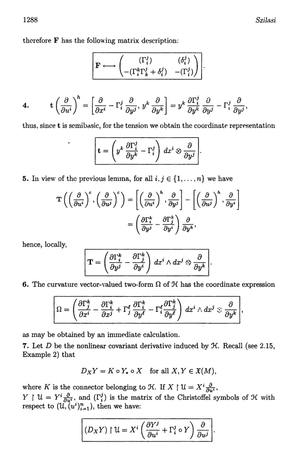
Текст
A C.I.P. Catalogue record for this book is available from the Library' of Congress.
ISBN 1-4020-1556-9 (Vol. 2)
ISBN 1-4020-1555-0 (Vol. 1)
ISBN 1-4020-1557-7 (Set)
Published by Kluwer Academic Publishers,
P.O. Box Γ7, 3300 AA Dordrecht, The Netherlands.
Sold and distributed in North, Central and South America
by Kluwer Academic Publishers,
101 Philip Drive, Norwell, MA 02061, U.S.A.
In all other countries, sold and distributed
by Kluwer Academic Publishers,
P.O. Box 322, 3300 AH DoidrechL The Netherlands.
Printed on acid-free paper
All Rights Reserved
© 2003 Kluwer /Xcademic Publishers
No part of this work may be reproduced, stored in a retrieval system, or Lansmitted
in any form or by any means, electronic, mechanical, photocopying, microfilming recording or
otherwise, without written permission from the Publisher, with the exception
of any material supplied specifically for the purpose of being entered
and executed on a computer system, for exclusive use by the purchaser of the work.
Printed in the Netherlands.
TABLE OF CONTENTS
Preface xv
Part 1 Complex Finsler Geometry 3
Tadashi Aikou
1 Kahler Fibrations 9
1.1 Fibrations 9
1.2 Local Treatments 10
1.3 Bott Connections 13
1.4 Kahler Fibration 18
2 Complex Finsler Bundles 23
2.1 Vector Bundles Over Complex Projective Space 23
2.2 Complex Fuidei Metrics 27
2.3 Bott CoBnectious of Fuislei Vector Bundles 35
2.4 Negativity of Vector Bundles 39
2.5 Special Finsler Vector Bundles . . . 48
3 Kobayashi Metrics 59
3.1 PoincareMetrics . . 59
3.2 Kobayashi Metric 62
3.3 Bounded Domains 65
3.4 Holomorphic Sectional Curvature and Schwarz Lemrna . . 67
Part 2 KCC Theory of a System of Second Order Differential
Equations 83
P.L. Antonelli and I. Bucalaru
1 TheGeometryoftheTangentBundle 91
1.1 The Tangent Bundle 91
1.2 The Vertical Subbundle 93
1.3 The Almost Tangent Structure 94
1.4 Vertical and Complete Lifts 94
1.5 IIuiiiQgeneity 95
2 Nonlinear Connections 97
2.1 Horizonttil Distributions and Horizontal Lifts ... . 97
2.2 Characterizations of a Nonlinear Connection 99
2.3 Curvature and Torsion for a Nonlinear Connection 102
2.4 Aiitoparallel Curves and Symmetries for a
Nonlinear Connection 103
2.5 Homogeneous Nonlinerir Connection 107
vi
Anastasiei and Antonelli
3 Finsler Connections on the Tangent Bundle 109
3.1 The Berwald Connection Ill
3.2 The h and v-Covariant Derivation of a Finsler
Connection 112
3.3 The Torsion of a Finsler Connection 113
3.4 The Curvature of a Finsler Connection 114
3.5 Finsler Connections Induced by a Complete
Parallelism 116
3.6 The Cartan Structure Equations of a Finsler
Connection 118
3.7 , Geodesics of a Finsler Connection 120
3.8 Homogeneous Berwald Connection 121
4 Second Order Differential Equations 123
4.1 Semispray or Second Order Differential Vector Field . . 123
4.2 Nonlinear Connections and Semisprays 125
4.3 The Berwald Connection of a Semispray 127
4.4 The Jacobi Equations of a Semispray 129
4.5 Symmetries for a Semispray 131
4.6 Geometric Invariants in KCC-Theory 132
5 Homogeneous Systems of Second Order Differential
Equations , 1.35
6 Time Dependent Systems of Second Order Differential
Equations 139
6.1 Sprays and Nonlinear Connections on Jets 139
6.2 Variational Equations 144
6.3 The “Film-Space” Approach to Type (B) KCC-Theory . 147
7 The Classical Projective Geometry of Paths 151
7.1 Paths, Parametrized Paths 151
7.2 The Various Geometries of Paths - Finite Equations . . 152
7.3 The Various Geometries of Paths - Differential Equations 153
7.4 Affine Connections 155
7.5 TheFundamentaiprojectiveInvariants 158
7.6 The Projective Parameter and the
Normal Spray Connection 161
7.7 Projective Deviation 165
Part 3 Fundamentals of Finslerian Diffusion
with Applications 177
P.L. Antonelli and T.J. Zastawniak
1 FinslerSpaces 187
1.1 TheTangentandCotangentBuiidle 167
1.2 Fiber Bundles 189
1.3 Frame Bundles and Linear Connections 191
1.4 Tensor Fields 192
1.5 Linear Connections 19-1
1.6 TorsionandcurvatureofaLiiiearConnection .... 196
Table of Contents
vii
1.7 Parallelism 197
1.8 The Levi-Civita Connection on a Riemannian Manifold 197
1.9 Geodesics, Stability and the Orthonormal Frame Bundle 199
1.10 Finsler Space and Metric 200
1.11 FinslerTensorFields 202
1.12 Nonlinear Connections 202
1.13 Affine Connections on the Finsler Bundle 204
1.14 Finsler Connections 206
1.15 TorsionsandcurvaturesofaFinslerConnection . . . 208
1.16 Metrical Fihsler Connections. The Cartan Connection . 210
2 Introduction to Stochastic Calculus on Manifolds 213
2.1 Preliminaries 213
2.2 Ito’s Stochastic Integral 216
2.3 Ito’s Processes. Ito Formula 219
2.4 Stratonovich Integrals 221
2.5 Stochastic Differential Equations on Manifolds .... 221
3 Stochastic Development on Finsler Spaces 227
3.1 Riemannian Stochastic Development 227
3.2 Rolling Finsler Manifolds Along Smooth Curves
and Diffusions 233
3.3 Finslerian Stochastic Development 242
3.4 Radial Behaviour 246
4 Volterra-Hamilton Systems of Finsler Type 249
4.1 Berwald Conjiections and Berwald Spaces 249
4.2 Volterra-Hamilton Systems and Ecology 253
4.3 Wagnerian Geometry and Volterra-Hamilton Systems . 254
4.4 Random Perturbations of Finslerian
Volterra-HamiltonSystems 260
1.5 Random Perturbations of Riemannian
Volterra-Hamilton Systems 262
4.6 Noise in Conformally Minkowski Systems 266
4.7 Canalization of Growth and Development with Noise 267
4.8 Noisy Systems in Chemical Ecology and Epidemiology 271
4.9 Riemannian Nonlinear Filtering 279
4.10 ConformaisignalsandGeometryofFilters 285
4.11 Riemannian Filtering of Starfish Predation 289
5 Finslerian Diffusion, and Curvature 295
5.1 Cartan’s Lemma in Berwald Spaces 296
5.2 Quadratic Dispersion 29δ
5.3 Finslerian Development and Curvature 299
5.4 Finslerian Filtering and Quadratic Dispersion 300
5.5 Entropy Production and Quadratic Dispersion .... 302
6 Diffusion on the Tangent and Indicatrix Bundles 319
6.1 Slit Tangent Bundle as Riemannian Manifold 320
6.2 Au-Development as Riemannian Development with Drift 321
6.3 Indicatrized Finslerian Stochastic Development .... 323
viii
Anastasiei and. Antonelli
6.4 Indicatrized /^-Development Viewed as Riemannian . . 327
Appendix A Diffusion and Laplacian on the Base Space .... 335
A.l Finslerian Isotropic Transport Process 336
A.2 Central Limit Theorem 338
A. 3 Laplacian, Harmonic Forms and Hodge Decomposition 340
Appendix B Two-Dimensional Constant Berwald Spaces .... 343
B. l BerwakFs Famous Theorem 343
B.2 Standard Coordinate Representation 344
B.3 B2(I) with Constant G⅛k 345
B.4 Class B2(2) with Constant Gjk 347
B.5 - B2(r,s) with Constant G^k 348
Part 4 Symplectic Transformation of the Geometry of
T*M; L-Duality 359
D. Hrimiuc and H. Shimada
1 The Geometry of TM and T*M 363
1.1 Connections on TM 363
1.2 Semisprays and Connections 368
1.3 Linear Connections on TM 370
1.4 The Geometry of Cotangent Bundle 373
1.5 LinearConnectionsonT+M . . . 376
1.6 Lagrange Manifolds 378
1.7 Hamilton Manifolds 381
2 Symplectic Transformations of the Differential Geometry
of T* M 385
2.1 Connection-Pairs on Cotangent Bundle 385
2.2 Special Linear Connections on T*M 390
2.3 The Homogeneous Case 395
2.4 /-Related Connection-Pairs 398
2.5 /-Related ^-Connections 403
2.6 The Geometry of a Homogeneous
Contact Transformation 405
2.7 Examples 409
3 The Duality Between Lagrange and Hamilton Spaces .... 413
3.1 The Lagrange-Hamilton L-Duality 413
3.2 L-Dual Nonlinear Connections 417
3.3 L-Dual d-Connections 421
3.4 The Finsler-Cartan L-Duality 426
3.5 Berwald Connection for Cartnn Spaces. Landsberg
and Berwald Spaces. Locally Minkowski Spaces . . 431
3.6 Applications of the L-Duality 435
Table of Contents ix
Part 5 Holonomy Structures in Finsler Geometry 445
L. Kozma
1 Holononiy of Positively Homogeneous Connections 453
1.1 Connections of a Tangent Bundle 453
1.2 Holonomy Group of a Positively Homogeneous Connection 454
1.3 Curvature and Holonomy Algebra of a Positively
Homogeneous Connection 455
1.4 Homogeneous Holonomy of Finsler Manifolds .... 458
1.5 Metrizability of Positively Homogeneous Connections . 458
2 Holonomies of Finsler Vr-Connections 463
2.1 A Topological Group and Its Lie Algebra 463
2.2 Vr-Connections 464
2.3 The Vr-Holonomy Group and Vr-Holonoiny Algebra . . 465
3 Holonomies of the Finsler Vector Bundle 469
3.1 Linear Connections of the Finsler Vector Bundle . . . 469
3.2 Osculation of Finsler Pair Connections 470
3.3 Ziy-Holonomy Groups of the Finsler Vector Bundle . . 472
3.4 Tho Mixed Holonomy Groups 473
4 Holonomies of Special Finsler Manifolds 477
4.1 Berwald Manifolds 477
4.2 Landsberg Manifolds 481
Part 6 On the Gauss-Bonnet-Chern Theorem in
Finsler Geometry 491
Brad Lackey
1 Topological Preliminary 497
2 The Method of Transgression 499
3 The Correction Term 503
4 Special Cases 505
4.1 Riemannian Geometry 505
4.2 The Chern Connection 505
4.3 A Special Family of Finsler Connections 506
Part 7 The Hodge Theory of Finsler-type Geometries 513
Brad Lackey
1 Elliptic Complexes 521
1.1 The Hodge-deRham Complex 521
1.2 Elliptic Complexes 523
1.3 Elliptic Operators 527
1.4 The Hodge Decomposition Theorem 531
2 The Weitzenbock Formula 533
2.1 Complete Positivity 534
2.2 Covariant Formalism 536
2.3 Existence and Uniqueness of a Connection 539
2.4 A Bochner Vanishing Theorem 541
X
Anastasiei and Antonelli
3 Complete Positivity of the Symbol 543
3.1 The Geometric Ratio 543
3.2 Computing the Geometric Ratio 545
3.3 An Example 547
Part 8 Finsler Geometry in the 20th-Century 557
M. Matsumoto
1 Finsler Metrics 565
1.1 Extremals 565
1.2 Finsler Metric 569
1.3 .RandersMetric 574
1.4 (α, β)-Metric 581
1.5 I-Form Metric 587
1.6 m-th Root Metric 592
1.7 Birth of Finsler Geometry 595
2 Connections in Finsler Spaces 601
2.1 Frame Bundles 601
2.2 Linear Connections 607
2.3 Vectorial PYame Bundles 618
2.4 The Theory of Pair Connections 628
2.5 Standard Finsler Connections 644
2.6 Special Finsler Connections 661
3 Important Finsler Spaces 677
3.1 Finsler Space of Dimension 'Γwo 677
3.2 Riemannian Space and Locally Minkowski Space . . . 709
3.3 Stretch Curvature and Landsberg Space 717
3.4 Berwald Space 723
3.5 Wagner Space 735
3.6 Scalar Curvature and Constant Curvature 741
3.7 Finsler Space of Dimension Three 753
3.8 Indicatrix and Homogeneous Extension 775
4 Conformal and Projective Change 783
4.1 Conformal Change 783
4.2 Conformally Flat Finsler Space 790
4.3 Conformal Change and Wagner Space 796
4.4 Projective Change 799
4.5 Douglas Space 814
4.6 Finsler Space with Rectilinear Extremals 827
5 Finsler Spaces with I-Form Metric and with m-th Root Metric 839
5.1 Finsler Spaces with I-Form Metric 839
5.2 Curvature of Two-Dimensional I-Form Metric .... 847
5.3 ConformalChangeofl-FormMetric 851
5.4 Finsler Space with m-th Root Metric 858
5.5 Stronger Non-Riemannian FinsIer Space 867
5.6 Two-Dimensional m-th Root Metrics 874
5.7 Berwald Spaces of Cubic and Quartic Metrics .... 879
Table of Contents
xi
6 Finsler Spaces with (a, ^-Metrics 889
6.1 Fundamental Tensor of Space with (α,∕3)-Metric . . . 889
6.2 C-Tensors of (α, β)-Metrics 894
6.3 Connections for (α, /J)-Metrics 901
6.4 Douglas Space with (a,/J)-Metric 913
6.5 Two-Dimensional Space with (α∕3)-Metric 916
6.6 Strongly Non-Riemannian (α∕3)-Metric 924
6.7 Conformal Change of (α, β)-Metric 928
6.8 Projective Change of (αβ)-Metric 936
6.9 Randers Spaces of Constant Curvature 946
Part 9 The Geometry of Lagrange Spaces 969
Radu Miron, Mihai Anastasiei and loan Bucataru
0 Introduction 973
1 The Geometry of the Tangent Bundle 977
1.1 The Manifold TM 977
1.2 Semisprays on the Manifold TM 984
1.3 Nonlinear Connections 987
1.4 A-Linear Connections 995
1.5 Semisprays, Nonlinear Connections and TV-Linear
Connections 1002
1.6 Parallelism. Structure Equations 1007
2 Lagrange Spaces 1013
2.1 TheNotionofLagrangeSpace 1013
2.2 Geometric Objects Induced on TM by a Lagrange Space 1017
2.3 Variational Problem and Euler-Lagrange Equations . . 1019
2.4 A Noether Theorem 1021
2.5 Canonical Semispray. Nonlinear Connection 1023
2.6 Geodesics in a Finsler Space 1025
2.7 Hamilton-Jacobi Equations 1028
2.8 The Almost Kahlerian Model of a Lagrange Space Ln . 1030
2.9 Metrical Ar-Linear Connections 1033
2.10 Almost Finslerian Lagrange Spaces 1038
2.11 Geometry of φ-Lagrangians 1042
2.12 Gravitational and Electromagnetic Fields 1045
2.13 Einstein Equations of Lagrange Spaces 1047
3 Subspaces in Lagrange Spaces 1053
vτn
3.1 Subspaces L in a Lagrange Space Ln 1053
3.2 Induced Nonlinear Connection 1056
3.3 The Gauss-Weingarten Formulae 1060
3.4 The Gauss-Codazzi Equations 1061
3.5 Totally Geodesic Subspaces 1062
3.6 Lagrange Subspace of Codimension One 1064
3.7 Subspaces in Finsler Spaces 1067
xii
Anastasiei and Antonelli
4 Generalized Lagrange Spaces 1073
4.1 The Notion of Generalized Lagrange Space 1074
4.2 Metrical Ar-Connection in a GfL-Space 1077
4.3 GfL-Metrics Determining Nonlinear Connections . . . 1080
4.4 GL-Metrics Provided by Deformations of
Finsler Metrics 1085
4.5 Almost Hermitian Model of a Generalized
Lagrange Space 1091
5 Rheonomic Lagrange Geometry 1097
5.1 Semisprays on the Manifold TM × R 1097
5.2 Nonlinear Connections on E = TM × R 1099
5.3* VariationalProblem IlOl
5.4 RheonomicLagrangeSpaces 1103
5.5 Canonical Nonlinear Connection 1104
5.6 An Almost Contact Structure on E 1105
5.7 AT-Linear Connection 1107
5.8 Parallelism. Structure Equations for
AT-Linear Connections 1108
5.9 Metrical AT-Linear Connection of a Rheonomic
LagrangeSpace Illl
5.10 Rheonomic Finsler Spaces 1112
5.11 ExamplesofTimeDependentLagrangians 1114
Part 10 Symbolic Finsler Geometry 1125
S. F. Rutz and R. Portugal
1 Computer Algebra for Finsler Geometry 1129
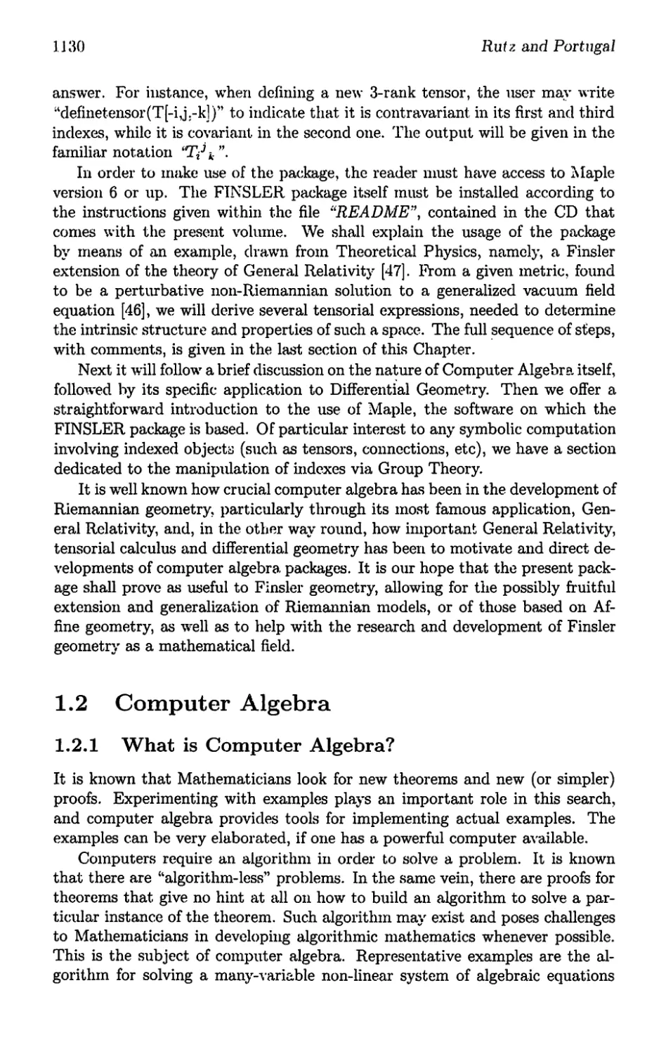
1.1 Introduction 1129
1.2 Computer Algebra 1130
1.3 ManipulationoflndicesviaGroupTheory 1144
1.4 FINSLERPackage 1150
Part 11 A Setting for Spray and Finsler Geometry 1183
Jozsef Szilasi
0 Introduction 1187
1 The Background: Vector Bundles and
Differential Operators 1191
A Manifolds 3191
B Vector Bundles 1195
C SectionsofVectorBundles 1204
D Tangent Bundle and Tensor Fields 1208
E Differential Forms 1218
F Covariant Derivatives 1226
2 Calculus of Vector-Valued Forms and Forms Along the
Tangent Bundle Projection 1237
A Vertical Bundle to a Vector Bundle 1237
B Nonlinear Connections in a Vector Bundle 1245
Table of Contents
xiii
C Tensors Along the Tangent Bundle Projection. Lifts . . 1258
D The Theory of A. Frolicher and A. Nijenhuis 1272
E The Theory of E. Martmez. J. F. Carinena and W. Sarlet 1298
F Covariant Derivative Operators Along the Tangent
Bundle Projection 1314
3 Applications to Second-Order Vector Fields and
Finsler Metrics 1347
A Horizontal Maps Generated by Second-Order Vector Fields 1347
B Linearization of Second-Order Vector Fields 1362
C Second-Order Vector Fields Generated by Finsler Metrics 1369
D Covariant Derivative Operators on a Finsler Manifold . . 1383
Appendix 1399
A.l Basic Conventions 1399
A. 2 Topology 1400
A.3 The Euclidean n-Space Rzl 1401
A.4 Smoothness 1402
A.5 Modules and Exact Sequences 1403
A.6 Algebras and Derivations 1408
A.7 Graded Algebras and Derivations 1409
A.8 Tensor Algebras Over a Module 1411
A.9 The Exterior Algebra 1415
A. 10 Categories and Functors 1419
728
Matsumoto
3.4.3 //-Curvature Dependent on Position Alone
Wc shall recall the A-Curvature tensors of the Berwald, Cartan and Chern-Rund
connections. These are given by
BΓ : H^k = ‰G> - 0rG⅛)GJ + G^jG^k - (⅛),
GΓ: ^fc=Λ¾fc + C⅛,
CΛΓ : K^k = ∂kF^ - (∂rF∣,j)Gk + F[jF*k - (⅛).
If we are concerned with a Berwald space, the Definition 3.4.1.1 and The¬
orem 3.4.1.2 show that both G¾ and F-li. and hence the A-curvature tensors
H and K are functions of position (xτ) alone, but R is not so, because C¾. may
contain (τ∕t).
Definition 3.4.3.1. The sets of n-dimensional Finsler spaces with the
Λ-curvature tensors Hy R and K dependent on position alone are denoted by
Hx(n)y Rx(n) and Kx(n) respectively.
If we denote further by B(n) the set of all n-dimensional Berwald space,
that is,
B(x) = {n-dim. Berwald spaces},
then we have the inclusion relations as follows:
B(n) C Hx(n)y B(n) C Kx(n). (3.4.3.i)
Since (2.5.4.3) and (2.5.5.7) show
yiK^jk=I⅛, H⅛k = ∂iR⅛,
Fn ∈ Kx(ri) is also Fn ∈ Hx(n). Consequently, we have the inclusion relation
Kx(n) C Hx(ri). (3.4.3.2)
Next we introduce the sets:
L(n) = {7i-dim. Landsberg spaces},
5(n) = {n-dim. spaces with zero stretch curvature tensor}.
Then Propositions 3.3.3.1 and 3.4.1.1 lead to the inclusion relations
B(n) C L(rι) C S(n). (3.4.3.3)
Theorem 3.4.3.1. We have the inclusion illations
B(n) C Kx(n) C Hx(ri) C S(n).
Finsler Geometry in the 20th-Century
729
Proof: It is sufficient to show the last relation: (3.3.2.5) can be written as
∑hO7. = yrH∣ιljk Thus H — H(x) implies Σ — 0.
This theorem and (3.4.3.3) give rise to the problem: What are the intersec¬
tions
L(n) ∩ Hx(τι)t? L(n) ∩ Kx(n)t?
Theorem 3.4.3.2. L(n) ∩ Kx(ri) = L(ri) ∩ Hx(n).
Proof: We recall (2.5.5.2):
G⅛=J* + J¾.
Theorem 3.3.3.1 shows G⅛ = F⅛ for Fn ∈ L(n).
We have Rx(ri) C Hx(n) similarly to the case of Kx(n)i but Rx(ri) will be
studied later on.
Now we are especially interested in the twτo-dimensional case. The spaces
we shall consider here are all contained in 5(2). On account of (3.3.2.6) and the
Bianchi identity (3.1.3.14), such a space is characterized by
Ia ,ι — ^R)2 +RI = 0.
Putting G-cj = liemj — Ijtnii (3.1.3.15) and (3.1.3.17) are written as
Hfzhij = (εRGkh + εRi2 mkm∣l)Giji
R-khij = (εRGkh RIτ∏ktrih)Gij.
Then (3.4.3.4) yields H = K for Fn ∈ 5(2). Consequently,
Theorem 3.4.3.3. In the two-dimensional case
Hx(2) = Kx(2).
According to Theorem 3.4.2.1 we have the direct sum expression
B(2) = Bi(2) + B2(2) + B3(2),
Bi(2) = {B — 0, I ≠ const.},
B2(2) = {R = 0, I = const.}
B3(2) = {R ≠ 0. I = const.}.
Let us now, on the other hand, consider Hx(2). Since we have from (3.2.3.15)
LH⅛k.( = ε{(Bj2 ;2 +εIR-i2 )mh - 2(R∖2 +εIR)In}mimtGjk∙
730
Matsumoto
Hence F2 ∈ Hx (2) is characterized by
)2 ÷εIRι2 = 0? R⅛^∣"εIR = 0,
but the latter has been shown in (3.4.3.4). The former gives I;2 R = 0. There¬
fore,
Theorem 3.4.3.4. A two-dimensional Finsler space belongs to Hx(2)i if and
only if Iij = 0 and I;2 = 0.
Hx(2) is expressed by the direct sum Hx(2) = Hi(2) + II2(2) + H3 (2),
H1 (2) = {H = 0, I52≠O, I1j = 0},
H2(2) = {R = 0, I.2 = 0, Ijj = 0},
H3(2) ={Λ≠0, I52 = 0, Ijj= 0}.
Since F2 ∈ B(2) is characterized by Ij = I2 = 0, the above leads to
Corollary 3.4.3.1. Bi(2) = B(2) ∩Hi(2), i = 1,2,3.
In other words, the well-known classification of B(2) (Theorem 3.4.2.1) can
be induced from the classification of Hx('2) (Theorem 3.4.3.4).
We consider the intersection L(2) ∩ Hx(2). From the character Ij = 0 of
L(2) (Proposition 3.3.3.2) we get
L(2) ∩ H1 (2) = {R = 0, I52 ≠ 0, I1 = 0},
L(2)∩⅞(2) ={H = 0, Ij2 = Ij =0},
L(2)∩H3(2) = {R>0, I2 = Ij =0}.
From the Ricci identity (3.1.3.10, b), I;2 = Ij = 0 yield I2 = 0, that is,
I = const. Therefore we get
Theorem 3.4.3.5.
L(2)∩H1(2) DB1(2), L(2)∩Hi(2) = Bi(2), i = 2,3.
Now wre deal with the set Rx(n). We have the Bianchi identity (2.5.2.4, c).
Expressing R[lj∖k in terms of (∙⅛), the identity can be written in the form
R⅛-k + ¾hfcr¾∙ + ¾∕∙⅛ - ∕⅛vC‰ + ‰ = 0,
Qtkij = -¾j] {Ptjk<i ÷ PtirPjki-
We shall restrict our discussion to Finsler spaces Fn having the above Q = 0.
Then Fn ∈ Rx(n)i if and only if
S,∕krRζj + RrtijC^k - R⅛C⅛ = 0. (3.4.3.3)
Finsler Geometry in the 20th-Century
731
Multiplying by yl, we get RijCyk = O, which implies S1^krRζj = O from (2.5.2.6,
e). Thus (3.4.3.3) is reduced to
RreijC^k - R⅛Crtk = 0. (3.4.3.4)
Conversely, from (3.4.3.4) we get R1ijCyk = 0 and hence we get (3.4.3.4).
Therefore, Rl}ij.k = 0 for Fn with Q = 0. Thus
Proposition 3.4.3.1. Suppose a Finsler space Fn has Q = 0. Then Fn belongs
to the set Rx(n), if and only if (3.4.3.4) holds.
If we are concerned with a Landsberg space Fn, then it has Q = O from
Theorem 3.3.3.1. Therefore,
Theorem 3.4.3.6.
(1) Rx(n) C Hx(ri).
(2) Fn belongs to Rx(n) ∩ L(n), if and only if (3.4.3.4) is satisfied.
We are concerned with the two-dimensional case. (3.1.3.11) and (3.1.3.3)
show
Qfkij = Λι >1 - tnm1')Gijmk.
Thus Q =■ 0 is equivalent to 7,ι ,ι = 0, that is, the stretch curvature Σ = 0, from
(3.3.2.6).
Proposition 3.4.3.2. In the two-dimensional case, Q = 0 is equivalent to
l,ι ?i = 0? that is, F2 ∈ S(2).
Thus all F2 ∈ 5(2) have Q = 0. On the other hand, the condition (3.4.3.4)
can be written as
εl RinkfJjmh + ehm1)Gij = 0,
with implies RI = 0. Therefore,
Theorem 3.4.3.7. If a two-dimensional Finsler space with non-zero scalar
curvature R belongs to Rx(2), then it is a Riemannian space.
Thus a non-Riemannian F2 ∈ Rτ(2) has R = 0. and hence the inclusion
B(2) C Rx(T) is false, so that Bfn) C Rxfri) will be not true.
Ref S. Bacso and M. Matsumoto [16], [17]. In their papers ([15] they were
greatly surprised and delighted at the discovery of the following remarkable
fact: For a Douglas space the components W∙jk of the projective Weyl curvature
tensor are functions of position alone. This fact enabled them to consider the
theory of the present section. See Theorem 4.5.2.4.
732
Matsuinoto
3.4.4 C-Reducibility
We are concerned v√ith the C-tensor given by (1.2.2.5) of a Finsler space Fn.
The vanishing of the C-tensor characterizes Riemannian space. Further, in
any two-dimensional Finsler space the C-tensor is written in the simple form
(3.11.10).
Now we shall propose a simple form of the C-tensor. We must pay attention
to the fact that Cijk is symmetric and satisfies Cijkyk = 0∙ The angular metric
tensor hij is also symmetric and satisfies h[jyj = 0. Hence we may put
Cjjk = di,hjk -J- djhki -∣- dkhij->
with some contravariant vector ⅛. By multiplying by y∖ we get ⅛yl = 0. Next,
multiplying by gli, we get Ck = (n + 1)⅛. Consequently we have the form
_ (Cihjk + Cjhki + Ckh,j) .
Cijk ~ (^+i) ∙ t3∙4∙4∙υ
It is remarked that the C-tensor of any two-dimensional case is of the form
(3.4.4.1), because (3.1.1.10) and (3.1.1.2) enable us to write (3.4.4.1).
Definition 3.4.4.1. A Finsler space Fn of dimension n ≥ 3 is called C-reducible,
if the C-tensor is of the form (3.4.4.1).
We deal with a C-reducible Finsler space Fn. First we examine the identity
Chij∖k - Chik∖j = 0. See (3.1.3.12). (3.4.4.1) leads to
(n + l)ChtjIfc = S(jHj){Ch∖khij - hhk
If we construct the contracted T-tensor
Tij = Tijhkghk = LC⅛ + Ciej + Cjti, (3.4.4.2)
then we have Chij∖k — Chik∖j = 0 in the form
h-ijThk -∣- hjhTik ~ hikThj — hhkTij — 0.
Multiplying by ghk and paying attention to 7⅛ = 0, we get Tij = Thij /(n - 1)
with T = Tijg⅛ = LCr∣r. Therefore,
Chij ∣fc = { fc(n2 -1) {h,ħkhij}
(thCijk+tiCιljk+tjC-rιli.,+tkChιj)
L
Consequently, on account of the definition of the T-tensor, we have
Thijk = ∣ -^2 Z j j (3.4 4.3)
Finsler Geometry in the 20th-Century
733
Next we deal with the Λ∙-covariant derivative Chij,k with respect to the
Cartan connection CT :
⅛=¾i)¾⅛1. (3.4.4.4)
Then (2.5.2.14) leads to
∏ _ (hhiCjlo + hijCfl,Q + hjhCuq)
p*'ij - ∙ (3∙4∙4∙5)
Further, from S⅛k = CfkC‰ - CfjC⅛s and (3.4.4.1) we get
qh τ {hikC^ + h^Cik}
bHk aW (n + 1)2
(3.4.4.6)
Ci} = (τ)fty + CiCj' °2 = giiCiCj-
Proposition 3.4.4.1. Let Fn, n ≥ 3, be a C-reducible Finsler space. The
T-tensor, the (y)hυ-torsion tensor and v-curvature tensor of the Cartan con¬
nection CΓ of Fn are written as (3.4.4.3), (3.4.4.5) and (3.4.4.6) respectively.
Now, suppose that Fn, n ≥ 3, is a Landsberg and C-reducible Finsler space.
Then (2.5.2.14, b) is reduced to
Cjkiih ~ Cjkhii = 0,
from which we have C41/,. - C∕llj = 0. Substituting from (3.4.4.4) in the above
and multiplying by ghk, we get immediately
Ci,j-μhij,
We have the Bianchi identity (2.5.2.11, b). For the Landsberg space it is reduced
to Sijkif = θ∙ Fpom (3.4.4.6) this is written as follows: First we get Cijlk =
(n + F)μCijk∙ Therefore S⅛kιe = 0 yields
μ(h>kChjf ÷ hfljCikf ⅛ijChkt hhkCijf^ = 0.
Multiplying by gikghj, we get 2μ(n - 2)Cf = 0. If μ = 0, then Cilj = 0, so
that Cflfjik ~ 0 and hence Fn is a Berwald space from Theorem 3.4.1.3. Next,
Cf =- 0 gives rise to Crijfc = 0 from (3.4.4.1). Therefore we obtain
Theorem 3.4.4.1. If a Landsberg space Fn, n ≥ 3, is C-reducible, then Fn is
a Berwald space.
Ref. Theorem 3.4.4.1, shown by M. Matsumoto [86], was the first of the
Reduction Theorems of Landsberg spaces. See the end of §3.4.2.
734
Matsunioto
Let Fn, n ≥ 3, be a C-reducible Finsler space such that BΓ and CΓ of Fn
have the same ∕ι-curvature tensors. Then (2.5.5.13) with (2.5.2.14,a) gives
Gιkr∣0^¾l0 - ChjrιθC⅛klQ -■ 0.
From (3.4.4.1) it follows that the above can be written as
^[jk]{Cr∣oC^hhk^ij + ChloCiilohjj + GiθCjlo⅛fc} = 0.
Multiplying by hhk, the above gives
(n l)Cr∣oClθ∕ι⅜j (n 3)C∖∣oCj∣o = θ∙
From rank (hij) = n—1 and the assumption n ≥ 3 it follows that the above yields
CrιoCjo = 0, and, if n ≥ 4, then we get C⅛lo = 0; and hence C∕l∣√lo = Phij = 0
from (3.4.4.5). If n = 3 and the metric is positive-definite, then we get Cr.o — 0.
In every case, Theorem 3.4.4.1 shows that Fn is a Berwald space.
Therefore we conclude
Theorem 3.4.4.2. If α C-reducible Finsler space Fn, n ≥ 3, has the common
h-curvature tensors of the Berwald and Cartan connections, then Ct,qC^ = 0
and
(1) n ≥ 4 : Fn is a Berwald space,
(2) n = 3 : Fn is a Berwald space, provided that the metric is positive-definite.
Corollary 3.4.4.1. If a C-reducible Finslcr space Fr∖ n ≥ 3, has vanishing
h-curvature tensor of the Cartan connection, then
(1) ∕ι ≥ 4 : Fn is a locally Minkowski space,
(2) n = 3 : Fn is a locally Minkowski space, provided that the metric is positive-
definite.
Proof: We have the identities
yhFihjk = R*k, OhRjk = ^hjkf
from (2.5.2.5) and (2.5.5.7). Hence Rlhjk = 0 implies Hkjk = 0. Thus Corollary
3.4.4.1 is a special case of Theorem 3.4.4.2. See Theorem 3.2.4.2.
Remark: See §6.2.3 where the existence theorem of C-reducible Finsier spaces
are established.
Finsler Geometry in the 20th-Century
735
3.5 Wagner Space
3.5.1 Generalized Berwald Space
Let us recall the Finsler connection which was given by Theorem 2.6.6.1. There,
the four axioms except (2) are common with those of Definition 2.5.2.1 of the
Cartan connection.
Definition 3.5.1.1. We have a Finsler connection which is uniquely determined
from the fundamental function L(x, y) and a skew-symmetric tensor field T of
(l,2)-type of the system of five axioms:
(1) h-metrical,
(2) (h)h-torsion T,
(3) deflection tensor D = 0,
(4) v-metrical,
(5) (v)v-torsion S1 = 0.
This connection is called a generalized Cartan connection with the torsion T and
is denoted by CT(T) = (F]kiN^ ¾).
Cjk arc components of the C-tensor, which are given by (4) and (5). Here
we suppose that T is (0)p-homogeneous as usual. The symbols (l, ∣) are used to
denote the h and v-covariant differentiations in CT(T).
As has been shown in Theorem 3.4.1.2, a Berwald space is characterized by
Fjk = F*k(x) of CT. Generalizing this notion to CT(T), we propose
Definition 3.5.1.2. A Finsler space with a skew-symmetric tensor T of (1,2)-
type is called a generalized Berwald space (with respect to T), if the connection
coefficients Fjk of CT(T) are functions of position alone.
Now we are concerned with a generalized Berwald space Fn. On account of
(2.4.3.3), Fn is characterized by
Phkij = -Chkjn + ChkrPij- (3.5.1.1)
Since CΓ(T) is h and v-metrical, we have Phkij + Pkhij = θ from the Ricci
identity (b) of (2.4.3.8). Thus the left-hand side of (3.5.1.1) must be skew-
symmetric in (h, A:), while the right-hand side is obviously symmetric in (h,k).
Hence we have Phkij = 0 and Chkj,i = ChkrPjj- Since CT(T) satisfies the D and
[/-conditions, Theorem 2.4.5.1 leads to Pijk = Poijk = θ∙ Therefore (3.5.1.1) is
reduced to
Phkij = θ> Chkjvi = 0. (3.5.1.2)
Under the conditions (3.5.1.2) the Bianchi identity (a) of (2.4.4.4) is reduced to
τ⅛∖k - C^kτrj + τ*C⅛ - TjlrC[k = O1
736
Matsunioto
which is nothing but Th,k = 0, that is, T∕j∙ are functions of position alone.
Conversely, if Chkjii = 0 and T∙tj.k = 0, then (2.4.4.4,a) yields
∙z⅛j] {pihτPjk ~ Pihjk} = θ∙
By the Christoffel process with respect to (∕ι,i,J), the above leads to
Phijk ÷ CijrPrhk — CtijrPrk = 0.
Multiplying by yh and next by y∙i, the above gives
Pijk 4" CijrPok = 0, PiQk = θι
which implies Phijk = 0∙ Therefore we return to the necessary and sufficient
conditions (3.5.1.2). Hence we obtain the following theorem quite similar to
Theorem 3.4.1.3.
Theorem 3.5.1.1. A Finsler space with a generalized Cartan connection CT(T)
is a generalized Berwald space, if and only if the components of T are functions
of position alone and Chijik = 0.
Ref. V. Wagner [167]. The exact formulation of the notion of generalized
Berwald space was given by M. Hashiguchi [46].
For the later use, we shall find the difference of CT(T) with the Cartan con¬
nection CT. Here we denote GT = (FLCTC‰) and CT(T) = (*Fk,7Vj, C‰)
and put
*ηk = ηk + D⅛. (3.5.ι.3)
Since CT(T) has the vanishing deflection tensor, (3.5.1.3) implies
Nl=Gik + D'0k.
The condition gijlk = 0 in CT(T) yields
Dijk 4~ Djik + 2C}jDork = 0, Dijk = 9jrD^k.
Applying the Christoffel process to the above and paying attention to Djik —
Dkij = Tjik (= ffirTfk), we obtain
Dijk = Atjk ~∙ CijD()rk — CjkDθri 4^ CkiDθrj>
2Atjk == Tijk ~ Tjki 4" Tkij.
Multiplying by yl and next by yk, the above yields
Dojk = Aojk - CrkDorQ. A)jO = JO ∙
Consequently we obtain
Dijk = Aijk — Cij(Aork — Cyk-Aθsθ) ~ Cjk(Aθri — C8riAθsθ)
(3.5.1.4)
÷ Cfci(A)rj - C¾Aθsθ)∙
Finsler Geometry in the 20th-Century
737
Proposition 3.5.1.1. The difference Djk = * Fjk-Fjk of CT(T) = (*Fjk1 Nj1 Cijk)
and CT = (FjkiG1jyCjk) is given by (3.5.1.4), where Dlj-κ = gjrDrik and
⅛A-ijk = Iijk ~ Tjki + 7fcij, Tijk — 9jrTfk.
Theorem 3.5.1.2. Let a linear connection T = (Γ*∙fc(τ)) be given in a Finsler
space Fn = (Λ'/, L(xy y)). Ifthe associated Finsler connection *Γ = (Γ*λ,, Γθj, Cjk)
is L-metrical. then Fn is a generalized Bcrwald space with the generalized Cartan
connection *Γ.
Proof: We deal with ,Γ0 = (ΓJfc,Γ⅛j∙,O). (2.4.3.1) and (2.4.3.3) gives P1 = 0
and P2 = 0 of *Γq. Hence (2.2.5.8, b) shows Vh and Vυ = ∂ with respect to
*Γq are commutative, and so we observe
v⅛.v>{⅛(≤)}-4⅞{v'∙(⅞)} = o.
Hence *Γ is h-metrical, and *Γ is a generalized Cartan connection. From ΓJfc =
Tjk(x) it follows that Fn is a generalized Berwald space with *Γ.
3.5.2 Wagner Space
We propose now an interesting class of generalized Cartan connections by taking
special skew-symmetric tensor Tjk as follows:
Definition 3.5.2.1. Let a covariant vector field Si(x) be given in the underlying
manifold M of a Finsler space Fn = (M1 L(x1 yf). Put
Tjk = φ⅛M - δiksj(x),
and construct a generalized Cartan Connection CT(T) with respect to this T.
CT(T) is called a Wagner connection ⅛T(s) with respect to Sj(x). If Fn is a
generalized Berwald space with respect to T1 then Fn is called a Wagner space
with respect to Si(x).
Ref V. Wagner [167]. The name “Wagner space” was given by M. Hashigu-
chi [46].
Let Tjk (x) be a skew-symmetric tensor field in a two-dimensional manifold.
Tf we put T1 — Tfl and observe
q^∣ ηrr rπ2 τ∣2 n-t rτ-∣r ml
21 — lrl — I2I — -112’ 12 — J-r2 ~ i12>
then Tjk is written as Tjk = δjTk — δkTj. Therefore we have
Proposition 3.5.2.1. Any generalized Berwald space of dimension two with
respect to Tjk(x) is a Wagner space with respect to Tfi.
738
Matsumoto
Substituting this TJk = δljsk — δ1ksj in (3.5.1.4), we get the difference of
WΓ(s) from CT :
(a) ¾ = V‰Λ sh=ghrsr, (3.5.2.1)
(b) Vikh = Aw{gikδ>h + C{kyh} + Ckhtf - C>khyi + L2(¾h + ⅛¾).
Λs Theorem 3.5.1.1 shows that a Finsler space with HT(s) is a Wagner space,
if and only if WT(s) satisfies Cfajik = 0 with respect to WΓ(<s). To write this
condition in terms of CT, we use the symbol V the Zi-Covariant differentiation
in WT(s), while (1) is used in CT. We then obtain
(a) VfcCftij; = Cftijlfc - Whijkese, (3.5.2.2)
(b) Wfajkf = Chij.rVζkf + C,jrV1Jki ÷ ChjrVik^ + CfarVjkf.
Using the T-tensor of (3.1.3.12), we change Cfaj.k into C∣itj∣∕c and paying atten¬
tion to
⅛ + (qfc - ⅛½) VJke = L2Sikt + Cjktyi + hjkδie - hjtδik,
we obtain
Whijkl =
(3.5.2.3)
+ {L2ChirSjkf + Chithjk — Chikhje + (h,i,j)}.
From
Vikh=ykδih-yhδik-L2Cikh, Vjtlh = L2Wh, (3.5.2.4)
it is easy to show WfajQg = LTfajg. Consequently,
y kCfaj = Cfaj↑Q — LTfajrs . (3.5.2.5)
Therefore, (3.5.2.2) leads to the
Theorem 3.5.2.1. A Finsler space with WT(.s) is a Wagncr space, if and only
if in CT we have
Cfaj,k = Wfajkrs ,
where the tensor W is defined by (3.5.2.3) with (3.5.2.4).
Next (3.5.2.5) shows
Corollary 3.5.2.1.
(1) If a Wagner space Fn has vanishing T-tensor, then Fn is a Landsbcrg
space.
(2) A Finsler space Fn is a Landsberg space and a Wagner space with respect
to Si(x), if and only if
Cfajik = V'fajrks , Tfajrs = O.
Finsler Geometry in the 20th-Century
739
3.5.3 Wagner Space of Dimension Two
We discuss two-dimensional Wagner spaces in detail and give an interesting
example of Wagner space.
First, in terms of the Berwald frame (£,m), the V-tensor of (3.5.2.1) is
written in the form
⅛{h = {ε(⅛mj ~ Ljmi) - Zmfm>}(4∏¼ - ⅛mfc)
+{(εZ2 + I)mi -
Next, the W-tensor of (3.5.2.3) is written in the form
LWhijkt = εl.2mhmτm3{e{lkmι - ⅛mk) - ImkT∏ι}.
Consequently Theorem 3.5.2.1 together with (3.1.3.6,a) can be stated in the
two-dimensional case as
Theorem 3.5.3.1. A two-dimensional Finsler space is a Wagner space with
respect to Si(x) = sι⅞ + .⅞¾ if and only if the main scalar I satisfies
Ai = εL2s2, Z2 = -Zj2(sι + Is2).
Here, the scalar components $i and s2 should satisfy
Sl;2 = «92, «2;2 = ~ε(sι + Zs2). (3.5.3.1)
Corollary 3.5.3.1.
(1) If a two-dimensional Finsler space F2 is a Wagner space and its T-tensor
vanishes, then F2 is a Berwald space.
(2) If F2 is a Wagner space and a Landsberg space, then F2 is a Berwald space.
Proof: (1) T = 0 means L2 = 0 from (3.1.3.13). Then Theorem 3.5.3.1 leads
to the conclusion. See Proposition 3.4.2.1.
(2) Since F2 is assumed to be a Landsberg space, we have Zi =0, so that
Theorem 3.5.3.1 shows L2S2 = 0. L2 = 0 leads to (1). But, s2 = 0 leads to
si =Ofrom (3.5.3.1).
Now we consider the condition given in Theorem 3.5.3.1 together with (3.5.3.1).
So Z2 = 0 immediately implies F2 to be a Berwald space and hence we may
suppose L2 ≠ 0 in the following. Using the symbols
J = Z;2, Zα = Zα, a =1,2,
for brevity, Theorem 3.5.3.1 gives
(Z2+εZZ1) εZ1
■,1 = —J—’ S2=—-
740
Matsumoto
Hence the two equations of (3.5.3.1) are written in the form
{⅛2 + ε(J + l)∕ι + eZZij2}J - (∕2 + εll1)J-2 = 0,
(3.5.3.2)
(Λj2 - I2)J ~ I∖J∖2 = 0.
By (3.1.3.10) we get
Λj2 = J,l ÷ I2> -f2;2 = j,2 ~ ε{II2 ÷ (∙∕ ÷ 1)Λ}∙
Consequently (3.5.3.2) are equivalent to
*7,α*7 — Iq,J∖2 = 0, α = 1,2.
This is also equivalent to Jli J — IliJi2 = θ, which can be written as (∂iJ)J —
(¾∕) J;2 = 0. Thus, paying attention to J∙2 = ∂J∕∂Θ from (3.1.2.2), we have the
Jacobian ∂(J, Γ)∕∂(x∖θ) = 0. Therefore we conclude
Theorem 3.5.3.2. A two-dimensional Finsler space is a Wagner space, if and
only if the derivative ∂I∕∂Θ of the main scalar I by the Landsberg angle θ is a
function of I.
Example 3.5.3.1. We deal with a two-dimensional Kropina space, a Finsler
space with a Kropina metric L = ot2∕β, given by Definition 1.4.2.2, where
α2 = atj(x)ylyi is a Riemannian metric and β = bi(x)yl. A characterization of
the metric is given by
⅛⅛⅞(Z√?) = 0. (3.5.3.3)
On account of (1.2.2.9) and (2.5.2.17), we get
τ _ β p _ 0 _ ⅛Cjjk q {hjjfk}
L>.i — Ci, Ci.j — , ti.j.k — >3(ijk) ,
so that (3.5.3.3) is written in the form
2βCijk + S(yt){hij (bk - ⅛) } = 0∙ (3.5.3.4)
If we put bi = bi£i + b2r∏i, then (3.5.3.4) is written as
2b↑I + 3εb2 = 0. (3.5.3.□)
Further we have, similarly to (3.5.3.1),
;2 = b2, b2∙2 = -ε(bι ÷ IB2).
By applying (∙2) to (3.5.3.5) and substituting in the above, (3.4.3.5) leads to
(3.5.3.6)
Finsler Geometry in the 20th-Century
741
Therefore, Theorem 3.5.3.2 gives
Theorem 3.5.3,3. A two-dimensional Kropina space is a Wagner space and
(3.5.3.6) holds.
Ref. V. Wagner [167] stated Theorem 3.5.3.2 and showed that for an
F2 with L3 = aigk(x)ylyiyk we have I∙2 = — ∣ — 3εZ2.
See corollary 5.6.2.1. Theorem 3.5.3.2 was precisely proved by M. Matsumoto
[93], See also S. Bacso and M. Matsumoto, [15].
3.6 Scalar Curvature and Constant Curvature
3.6.1 Finsler Space of Scalar Curvature
The present section is devoted to a generalization of the notion of a Riemannian
space of constant curvature to a Finsler space Fn = (M,L(xyy)) with the
Berwald connection BF.
Let v = (vl) be a tangent vector of M at a point x = (xz). The function
A'(z,s∕,v) defined by
Hh,jkyhvly3vk = K(ghjgik - ghkgij')yhviy3vk,
is called the curvature at x of the two-section (y,v).
It should be remarked: Since Hhijk and g⅛ depend on (xz1yt)i K(xyyyv)
differs from K(x,yyy + ∙v), though the two-section coincides with (y>y + v).
Next, although we are concerned with BΓ,
∏hijky = Rhijky = KhijkV = Rhijky = Rijk.
from Proposition 2.5.6.1. In short, the curvature K(xyyiv) is written in the
form
Ri0kvivk = L2Khikvivk. (3.6.1.1)
Definition 3.6.1.1. If the curvature K does not depend on a tangent vector v
at every point (x,y) of the total space T of the tangent bundle T(M), then the
space Fn is said to be of scalar curvature K and K is written as K(xiy).
Therefore Fn is of scalar curvature Ky if and only if
‰ - L2Khik, (3.G.1.2)
holds, because RiQk is symmetric from (2.5.2.13).
We shall derive more convenient equations for K from (3.6.1.2). First we
rewrite (2.5.6.4) in the form
Rijk = ^ ‰)fc<⅞}∙
742
Matsumoto
Substituting from (3.6.1.2) and paying attention to (2.5.2.18), the above yields
(a) Rijk = h,kKj - hljKk, (3.6.1.3)
(b) κj = l{(⅜)∕<j + κtj} = !⅛.
Conversely, (3.6.1.3,a) gives (3.6.1.2), if we put K = Kq/L2. Then the procedure
form (3.6.1.2) to (3.6.1.3) gives rise to (3.6.1.3,b).
Further, we are concerned with the ∕ι-curvature tensor H on the assumption
(3.6.1.3). From (2.3.5.6,a),
Rijkh = Hhijk ÷ 2C'ih,Hrjk∙
Substitution from (3.6.1.3) yields
Hhijk = ∙^∙[jfc]-∣^ {hih^j 4- hjhf'i) (3.6.1.4)
Conversely, (3.6.1.4) yields (3.6.1.3,a) immediately.
Therefore,
Theorem 3.6.1.1. A Finsler space is of scalar curvature, if and only if either
(3.6.1.2) or (3.6.1.3) or (3.6.1.4) holds.
In the two-dimensional case, (3.1.3.10) and also (3.1.1.2) lead to ⅛⅛ =
L2Rhjk. Therefore,
Proposition 3.6.1.1. Any Finsler space of dimension two is of scalar curvature
R (= Gauss curvature).
Let us treat of a Riemannian space with the curvature tensor Rhijk(x)> First
we show that the scalar curvature K does not depend on y. To do so, we change
(hi) and (jk) of (3.6.1.4) and get
Rjkhi = hkiKhj hkhKi.j
+(hkjth ÷ hhjZk) ½l^ — (hkjf, ÷ hijtk) ⅛jft-.
Multiplying by yh and making use of RjkQi = RQtjk = Rijk,
Ryfc = hkiKh,.jyh + hkjKi - (hkjti + h,jtk) .
L
This must be equal to Rijk of (3.6.1.3). Paying attention to Kh.jyh - Kj =
Kj — LKtj, we obtain
^ijk){hij(Kk-LKlk)} = ^
which implies Kk - LKtk = 0 — (L2∕3)K.k, so that K = K(x).
Finsler Geometry in the 20th-Century
743
Consequently, (3.6.1.1) is equivalent to
Rhijk ÷ Rjihk + Rhkji + Rjkhi
= 4RQhjOik ~ %R (QhkQij ÷ QhiQjk)∙
It is easy to show that the above can be written as
(1) 2R∣lijk — Rfljib = 2KQhjQik ~ R (QhkQij + QhiQjk)-
Furthermore, by exchanging i,j for jii
(2) 2Rhjik - Rhljk = 2KghiQjk - R(QhkQji + QhjQik)-
Constructing (1) × 2 + (2), we obtain the well-known equation
Rhijk = R(QhjQik - QhkQij)-
As a consequence,
Proposition 3.6.1.2. A Riemannian space of dimension more than two is of
scalar curvature, if and only if it is of constant curvature.
Ref. The concept of scalar curvature was proposed by L. Berwald in [31],
one of his posthumous papers.
3.6.2 Stretch Curvature of Space of Scalar Curvature
The stretch curvature Σ of a Finsler space F is written as (3.3.2.1). We shall
express Σ of a Finsler space Fn of scalar curvature K(x,y).
Prom (3.6.1.4)
Hhijk + Hihjk = Aljkι{hik ^Rj∙h -
+hhk{κj.i- 1±⅛-) + 2h*<⅛κ*γ
Here,
(a) Ki.h - ⅛⅛ = Mhi + Khhi, (3.6.2.1)
Jb
(b) Mhi = l{ (f) κ.h.i + κ.hei + ⅛t}.
Thus,
∏hijk 4^ H{hjk = A[jk]{hikl∖Ihj ÷ hhk^ij 4" hhiMkj}- (3.6.2.2)
Next (2.5.5.5) gives
∏hijk ÷ Hihjk = Rhijk 4- Rihjk 4“ %(Rhijιk Rhikij)-
744
Matsumoto
Then (2.5.4.9,a) and (3.3.2.3) yield
= ~2ChiPrjk + '∑hijk,
for the right-hand side. Consequently, this, (3.6.2.2) and (3.6.1.3) give
^∙hijk = Ayk^{hlkMhj + hhkMij + hihM∣tj - 2ChzjKk}. (3.6.2.3)
Proposition 3.6.2.1. The stretch curvature tensor Σ of a Finsler space of
scalar curvature K is written in the form (3.6.2.3) where Mhj and Kj are given
by (3.6.2.1,b) and (3.6.1.3,b) respectively.
Now (3.3.2.3) gives
TjhijQ = 2P∕ιij∣0? (3.6.2.4)
and (3.6.2.l,b) leads to
/Or2X
‰= (-)K.h, Mqj = Q.
Then, multiplying by yk, (3.6.2.3) yields
PhijtQ ÷ (τjy (⅛j K. h + hjhK.i + hhiK.j) + KL2Chij = O.
Multiplying by ghj, we have
(n + l)Z∕⅛.i + 3(L2KCi + Pil0) = O, (3.6.2.5)
where Pj = Phijghi = Q∣o∙ Consequently,
Phijl0 + L2KChij = ^(hij) ∙ (3.6.2.6)
Proposition 3.6.2.2
(1) A Finsler space of scalar curvature K satisfies the equation (3.6.2.6).
(2) If a Finsler space of non-zero scalar curvature K satisfies Phij∣o = O, then
it is C-reducible.
We have defined the notion of C-Feducibility as in Definition 3.4.4.1. So,
(3.4.4.1) and (2.5.2.14,a) lead to
= f3∙62∙η
Definition 3.6.2.1. If Fn, n ≥ 3, satisfies (3.6.2.7), then Fn is called P-reducible.
Finsler Geometry in the 20th-Century
745
Proposition 3.6.2.3. If Fn, n ≥ 3. is C-reducible, then Fn is P-reducible.
Equation (3.6.2.6) then gives rise to
Proposition 3.6.2.4. If Fn, n ≥ 3, is of non-zero scalar curvature and
P-reducible, then Fn is C-reducible.
Ref The notion of P-reducibility was given by M. Matsuinoto and H. Shi-
mada [125]. From the standpoint of Proposition 3.6.2.3 we have an interesting
problem: What is a P-reducible Finsler space like?
3.6.3 Numata5S and Shibata5S Theorems
We consider a Finsler space Fn, n ≥ 3, of non-zero scalar curvature K and the
∖∙anishing stretch curvature Σ. For Fn (3.6.2.4) gives PhijiQ = O and hence Fn
is C-reducible from (2) of Proposition 3.6.2.2. Further (3.6.2.5) gives
3KCi + (n + l)K.i = O. (3.6.3.1)
Thus (3.6.2.3) is written in the form
(a) {hikNhj + hh∣ςNfj 4- hhzNkj} = θ> (3.b.3.2)
(b) Λ⅛ = Λ⅞ + ≡⅛⅜.
Substituting from (3.6.3.1) and (3.6.2.1,b), Nij is written as
(2Z∕2∖
oJX ∕
This is symmetric and Mo = θ∙ Then, multiplying by ghj, (3.6.3.2) easily yields
Nh ■
Nij = (^Z¾ ’ N = (3.6.3.3)
On the other hand, (3.6.3.1) gives
½≤1±⅛), (3.6.3.4)
3 (n + l)
while (3.4.4.3) is rewritten in the form
LChij∖k + IhCijk + IiChjk + IjChtk + IkChij
= 1 (π2 1)1 U^fii^jk 4“ hhjhki + hhkhij).
Multiplying by ghz, we get
LCj∖k + tjCk + lkCj = ,
746
Matsmnot o
which can be rewritten as
LCJk = { (7+T) + (⅛j }hJk
+{<⅛j }cic'° ~ ⅛<⅛ ~ ikCj.
Consequently, (3.6.3.4) is rewritten in the form
(>> + ι)Λ∙,j .-(⅝){⅛⅞ + j⅛5}⅛j
÷ (⅛l)(⅞¾ +⅛G)∙
Thus, according to (3.6.3.1), etc. (3.6.3.3) can be written as
for some scalar A. Since we suppose K ≠ 0 and n ≥ 3, the above holds, if and
only if G = 0. This implies Cijk — 0 from the C'-reducibility.
Therefore Proposition 3.6.1.2 leads to
Theorem 3.6.3.1. If a Finsler space Fn, n ≥ 3, is of non-zero scalar curvature
K and its stretch curvature tensor Σ vanishes identically, then Fn is a Rieman-
nian space of constant curvature K.
Propositions 3.3.3.1 and 3.4.1.1 lead to
Corollary 3.6.3.1. If a Landsberg space Fn, n ≥ 3, is of non-zero scalar
curvature K, then Fn is a Riemannian space of constant curvature K.
Corollary 3.6.3.2. If a Benuald space Fn, n ≥ 3, is of non-zero scalar
curvature K, then Fn is a Riemannian space of constant curvature K.
Ref. The author proposed to Mr. S. Numata [132] the problem: To consider
a Berwald space of constant curvature. At that time the author expected some
results similar to Corollary 3.6.3.2. Numata proved Corollary 3.6.3.1. See The¬
orems 30.6 and 30.7 of M. Matsumoto [97], which was already written about
1978. Prof. C. Shibata [149] proved Theorem 3.6.3.1.
Mr. S. Numata moved into education in 1985. Professor C. Shibata died in
1994.
Theorem 3.6.3.2. Let Fn = (Λf, L(x, y)), n ≥ 3, be a Finsler space of non¬
zero scalar curvature K. If an (r)p-homogeneous scalar field S(x,y) on Fn is
h-covariant constant with respect to CT, then S is written in the form S = cLr
with a constant c.
Since 5,∏ = ⅞S-S'.rG[, has the same form with respect to CT, CRT, BΓ and
77T, Theorem 3.6.1.2 is also true with respect to the other three connections.
Finsler Geometry in the 20th-Century
747
Proof: Applying the Ricci identity (2.5.2.4,a) to S and substituting from
(3.6.1.3,a), we get
sιi,j∙ - (j) = -SIr-Rtj = -S∣r(httfi - hriκj) = 0.
From S∣r∕ι[ = S∖i — rSti∕L, the above shows the existence of a scalar Λ such
that
s∣i - = λKi.
This leads to XKq = 0. From Aq = KL2 ≠ 0 we must have A = 0, so that
5∣i = rSti∕L, that is, ∂iS/S = r∂iL∣L. Integration leads to S = cLr, and
Sli = 0 shows c = const.
3.6.4 Isotropy
The scalar curvature K(x,y) of Fn, n ≥ 3, is (O)p-homogeneous and hence
Theorem 3.6.1.2 shows that, if K is ∕ι-covariant constant, then it is necessarily
a constant.
On the other hand, if K is v-covariant constant, that is, a function of po¬
sition alone, then (3.6.1.3,b) leads to Kj = LKtj and hence ∕<7.⅛ = Kgjk-
Consequently (3.6.1.3,a) and (3.6.1.4) are reduced respectively to
(a) Rijk = LK(hiktj - hijtk) (3.6.4.1)
(b) Hhijk = K(ghj9ik — gκk9ij)∙
The former may be written in the form
Hijk ≡ K(gikVj 9ij9k)∙> (3.6.4.2)
So the Bianchi identity (2.5.2.9,b) yields
¾jk){Kli(δhkyj - δ^yk)} = 0.
Contracting in h = k, we get (n —2)(A∣i2∕j-- KιjVι) = θ, which implies AT12- = κyi
with some (-l)p-homogeneous scalar κ. Then the Ricci identity RΓli∣j∙ — K∖jii =
-K∖rRrij is reduced to Kei∖j = (κτ∕i)∣j∙ = 0 = κ∖jyi + κgij = 0. This implies
κ∙ = 0 and Kii = 0. Consequently A is a constant.
Proposition 3.6.4.1. The scalar curvature K of Fn is reduced to a constant,
if
(1) Kii = ∂iK - K.rGri = 0, or
(2) K∖i = K.i = 0,n≥2.
Ref (1) was shown by M. Matsumoto and L. Tamassy [127]. (2), shown
by L. Berwald [31], is well-known as a generalization of the Theorem of Schur.
748
Matsunioto
Definition 3.6.4.1. A Finsler space Fn is said to be of constant curvature K,
if Fn is of constant scalar curvature.
Theorem 3.6.4.1. A Finsler space Fn, n ≥ 3, is of constant curvature Kf if
and only if (3.6.4.1) or (3.6.4.2) holds for a constant K.
The equation (3.6.2.5) leads to
Proposition 3.6.4.2.
(1) Fπ, n ≥ 3, is of scalar curvature and has the vanishing Ci (= C⅛)i then
Fn is of constant curvature.
(2) In Fn, n ≥ 3, of constant curvature Kf Ci satisfies C,ilo∣o = L2KCi = 0.
Consider now a Riemannian space with Ricci tensor Rhi = Rhir- Thus Rhi
is a symmetric tensor. Putting ⅛ = yhRhi,
Ri. j = Rij.
On the other hand, if Fn is of scalar curvature K and ⅛ = ¾, then
(3.6.1.3) yields
3Rj = (n - 2)L2AT∣j + 3(n - l)Kyj.
By U-Covariant differentiation with respect to CT, the above yields
3¾∣i = (n - 2)L(LK∖j∖i + 2^<∣j) + 3(n - 1)(⅛ + gij).
Consequently,
3(¾∣J - ¾∣i) = (n + l)(2∕i^√ - VjK∙i)> (3.6.4.3)
and yiKj — yjK.i = O gives Kj = O, immediately. Hence,
Theorem 3.6.4.2. A Finsler space Fnfn≥3f of scalar curvature is of constant
curvature, if and only if Ri∖j is symmetric, Rd = R<r.
The concept of isotropy of a Riemannian space is about constant curvature.
Thus (3.6.4.2) may be called the H-isotropy of the Finsler space with respect
to the Berwald connection. We shall be concerned with this concept also with
respect to the Cartan and the Chern-Rund connections.
First, we suppose that a Finsler space Fn is K-isotropic with respect to the
Chern-Rund connection CRT. That is, the ∕z-curvature tensor K of CRΓf can
be written in the form
Fhijk = K(ghjgik ~ ghk9ij∖ (3.6.4.4)
for some scalar K. Equation (2.5.4.3) leads to R1jk = K(yjδlk — ykδij) and
(2.5.4.7,a) shows K(C∏ikyj - Chijpk) = θ∙ This gives K = O or Chik = 0∙
Therefore, (3.6.4.4) gives rise to trivial cases only.
Finsler Geometry in the 20th-Century
749
Secondly, we suppose that a Finsler space Fn is R-isotropic with respect to
the Cartan connection CT. That is
Rhijk = R{∂hj9ik ~ 9hk9ij)↑ (3.6.4.θ)
for some scalar R. From (3.1.3.10,a) it follows that every two-dimensional Finsler
space has Rhijk of tins form.
To consider (3.6.4.5), we shall prepare an identity for the tensor R. Mul¬
tiplying by yj, (2.5.2.10,b) gives
⅛l*ji - Rhki<l = p∣}sι0 + R⅛rcrk.
Since the right-hand side is symmetric, we have
Then, (2.5.2.5,a) yields Rkj∖kyj = R%nij∖kymyj + ¾0, and hence the above is
rewritten as
(⅛y∣k-⅛∙∣i)jV = o.
Now, substituting from (3.6.4.5), the above gives ¾hjj — I¾∕ιJl = 0, which
implies (n — 2) R∖k = 0. Thus R = R(x), provided n ≥ 3.
Next, substituting from (3.6.4.5), (2.5.2.9,b) gives
s(ijλ-){β'∙(%5k ~VkSj)} = 0.
Contracting in h = fc, we get R,ι = Xyi for some scalar Λ, provided n ≥ 3. Then
the Ricci identity (2.5.2.4,b) gives
∙R∣<∣j = -RirCij = 0 = (Xyi) Ij = Xgij + yiXj∙
Consequently, A must be equal to zero and hence R = constant.
Now (2.5.2.9,c) yields
R∑(ijk){yi(Pthjk - Rthkj)} = o.
Multiplying by yk and paying attention to (2.5.2.15,d) gives Pthij = P(hjti
provided R ≠ 0. Further (2.5.1.10,c) yields
∑(ijk){Rehij∖k + Sehkr Rlj} = -2RΣ>(ijk){Sehjkyi} = 0,
which implies Sehjk = 0 immediately, provided R ≠ 0.
Summarizing all the above, we have
Theorem 3.6.4.4. If a Finsler space Fn, n ≥ 3, is R-isotropic with respect
to the Cartan connection CΓt then R is a constant. Further, if R ≠ 0, then
the hυ-curvature tensor Phijk of CT is symmetric in j, k, and the v-curvature
tensor S vanishes.
Ref. This theorem was proved by H. Akbar-Zadeh [4]. It is remarkable fact
in the viewpoint of Theorem 3.3.3.3 and BrickelPs Theorem 3.2.2.1.
750
Matsumoto
3.6.5 Ricci Tensor
We have the relations (2.5.4.3,a) between the Zt-Curvature tensors R and K of
CT and CRT, and (2.5.5.5,a) between the A-Curvature tensors K and H of CRT
and BΓ. From these relations we get
Rhijk Hihjk — 2(Rhijk H" Qhijk}y (3.6.5.1)
where we put
Qhijk = PhjrPk - PhkrP^ (3.6.5.2)
Now we are concerned with a Finsler space Fn, n ≥ 3, of scalar curvature
K. Then (3.6.1.4) yields
Hhijk ~ ∏ihjk = A[jh]{hhjRik H" hikR-hj}? (3.6.5.3)
where
κii = κ..j + ⅛⅛-
T21,' ts (3.6.5.4)
= Kgij + ½∙ + K.jyj + K.jyi + ⅛,
O Jj
which is a symmetric tensor. Thus (3.6.5.1) and (3.6.5.3) lead to
Rhijk = 2 A[j]c]∖hhjRik ^∙^ hik∏hj} ~ Qhijk∙ (3.6.5.5)
Conversely, multiplying by yh, (3.6.5.5) leads to (3.6.1.3) immediately. There¬
fore, we obtain a characterization of a space of scalar curvature in CT as follows:
Proposition 3.6.5.1. A Finsler space Fn, n ≥ 3, is of scalar curvature Ki if
and only if the h-curvature tensor R of CT is of the form (3.6.5.5), where Kij
and Qhijk ore given by (3.6.5.4) and (3.6.5.2), respectively.
If K = constant is supposed, then (3.6.5.5) gives a characterization of a
space of constant curvature as
Rhijk — K(phj9ik 9hk9ij) Qhijk' (3.6.5.6)
Next we consider the A-Ricci tensor ⅛j∙ = RΓ∙r of Fn i n ≥ 3, of scalar
curvature K :
Rij = Rihj k9^ = Rhikj 9hk∙
From (2.5.2.8,a) and (2.5.2.9,a) it follows that Rhijk satisfies the identities
Rhijk = ~ Rihjk = ~ Rhikjy
Rhijk ÷ Rhjki -∣- Rhkij ∑(ιjk) = θ∙
Hence Rhijk = Rjkhi does not hold in general, so that Rij is not symmetric.
But the second equation leads to
⅛{‰ + ς,fis7,}-cr¾ = o.
Finsler Geometry in the 20th-Century
751
Thus, if we substitute from (3.6.1.3), then 7⅛ = Rki is obtained. This sym¬
metry can also be obtained from (3.6.5.5) by multiplying by ghj. Therefore,
Proposition 3.6.5.2. If a Finsler space Fnin≥ 3, is of scalar curvature, then
the h-Ricci tensor Rij of CT is symmetric.
Next we are concerned with the conservation law E^∖i= 0 of the Einstein
tensor EJ = Rj — 1/2 Rδj in Riemannian geometry. Let Fn, n ≥ 3, be a Finsler
space of scalar curvature K. Substituting from (3.6.1.3) and paying attention to
(2.5.2.15,c and d), (2.5.2.9,c) can be rewritten as tensor
∑(vfc){‰υ≡⅛ + ‰o∣o¾} = θ∙ (3.6.5.7)
First, multiplying by gtlghk, the above is reduced to
2¾r - Rlj + 2SJ10Er - Sl0Ej = 0, (3.6.5.8)
where R = gtjRlj and Sij = Sijr, S = g,jSij. Next, multiplying by ghiykyei
(3.6.5.7) yields
κ0lj - κjt0 = L2K0 - (⅛)κ,l0 - κt0yj = 0.
If Kii = 0 is supposed, then the above gives E.jl0 = 0 and hence KjlQ — 0.
Thus (3.6.5.8) shows that if we put
Gj = Rj - ∣Λ<5J - 1SA',√ + KrSjyi, (3.6.5.9)
then Gij satisfies the conservation law Gjli = 0.
The supposition E1* = 0, however, gives rise to K = constant from (1) of
Proposition 3.6.4.1. Hence Gj is reduced to
cGj = Aj - l(Λ<5j + KSyiyj). (3.6.5.10)
Therefore we obtain
Theorem 3.6.5.1. In a Finsler space Fn,n≥3i of constant curvature K, then
tensor cGJ, defined by (3.6.5.10), satisfies the conservation law cGjli = 0.
Ref. cGj was defined by H. Rund [146]. C. Shibata [149] shows Propos¬
ition 3.6.5.1 and defined Cj. H. Ishikawa [67] also defined Gτj. They believed,
of course, that Gj is a generalization of Rund’s cGj, before (1) of Proposi¬
tion 3.6.4.1 was proved by M. Matsumoto and L. Tamassy [127].
We deal again with the notion of the E-isotropy, which is defined not by
(3.6.4.4) but rather by
Khijkyhv,y3υk = K(ghjgik - ghk9ij)ykvty3υk. (3.6.5.11)
752
Matsumoto
For an orthonormal frame zτa, a = 1,..., n, at a point x, we put
μ0∣>(x,y) = Khijk(x,y)z^z[z3azl.
Then we get the notion of the mean curvature (with respect to zti)
μa(χ,y) = ∑μab(χ∙y) = κflijkzkz3ag,k,
b
which does not depend on the choice of the frame.
Then the mean curvature with respect to the supporting element y is given
by
μ(x,y) = Khj(x,y)ehP, (3.6.5.12)
where Khj = Khjr *s thθ Λ-Ricci tensor of CRT.
Definition 3.6.5.1. The hypersurface {y ∈ Mx∖Khj(x,y)yhy^ ≈ 1} of the
tangent space Mx is called the K-hypcrplane at x. /1 direction of the principal
curvature at x is such that the radius of the K-Iiyperplane has the extremal
length in that direction.
That is, the direction y is given by
∂k⅛ijyiyi - λ(Kijyiyi - 1)} = 0,
with the Lagrange multiplier λ. Thus we have
{2gik - λ(Kik ÷ Kki + yjKij.k)}yi = 0.
Multiplying by yk the above gives Λ = l∕μ by (3.6.5.12). Hence the above
becomes
{Kik + Kkl + yjKij.k)yz = 2μyk. (3.6.5.13)
Definition 3.6.5.2. A Finsler space is called an Einstein-Finsler space, if it is
homogeneous at every point with respect to the mean curvature, that is, any
direction is a direction of the principal curvature.
Proposition 3.6.5.3. A Finsler space is an Einstein-Finslcr space, if and only
if there exists a scalar field μ(x,y) satisfying (3.6.5.13) for any y.
If a space is assumed to be Riemannian, then (3.6.5.13) is reduced to
Rik = 2μgik,
for the Ricci tensor Rik. That is, the space is the so-called Einstein space.
We return to a Finsler space with the Cartan connection and treat of (3.6.5.13).
Equation (2.5.4.2,a) gives
Kjj = Hi j — CirRjs, Kq j = Rq j, KiQ = RiQ — CirRζs.
Finsler Geometry in the 20th-Century
753
Thus, making use of (2.5.4.5), (2.5.4.7,c) yields ytylKei.k = — C⅛lo∣o∙ Therefore
(3.6.5.13) is written as
-¾)fc ÷ ‰ ~ ^kr ^Qs ~~ ^,∣0∣0 = tyVk)
which implies μ = ¾o∕L2 ∙ Consequently,
Proposition 3.6.5.4. A Finsler space with the Cartan connection is an Einstein-
Finsler space, if and only if the equation
R0k + Rko - CkrR0s - Ckl0t0 =
holds.
Ref. H. Rund [146] defined the notion of the Einstein-Finsler space and
showed the following Theorem 3.6.5.1.
We consider an Einstcin-Finsler space of scalar curvature Fn, n ≥ 3. Pro¬
position 3.6.5.2 shows that Rij is symmetric, and hence the condition above
is
2‰-Cf.r¾-Pfcl0 = ⅛^. (3.6.5.14)
From (2.5.2.13), (3.6.1.2) and (3.6.1.3) we have
Rok = Rrkr = (n — 2)Kk + Kyk, CskrRr0s = L2KCk.
Thus, on account of (3.6.2.5) and (3.6.1.3,b), (3.6.5.14) is written as
L2(n-l)K.k + 2{(n-l)K- 3∙7^j¾x,}yfc = 0.
Multiplying by yki we get (n - l)Ar - Rqq/L2 = 0 and K.⅛ = 0. Therefore (2)
of Proposition 3.6.4.1 leads to
Theorem 3.6.5.1. If an Einstein-Finslcr space Fn, n ≥ 3, is of scalar curvature
Ki then Fn is of constant curvature K.
3.7 Finsler Space of Dimension Three
3.7.1 Moor Frame and Connection Vectors
We are concerned with a Finsler space F3 of dimension three. As in the two-
dimensional case, we first introduce an orthonormal frame field. First we have
the unit vector £ having the components
ti = γ, tz = girfτ = ∂iL.
Li
754
Matsumoto
Throughout the present section, we suppose that C; = C[r is a non-zero
vector field and
gijCiCj =ε>(C)2,. ε2 = ±l, C > 0.
Thus we get a unit vector
tni = ⅞, (3.7.1.1)
c√
which is orthogonal to ⅞ because of Ciyz = 0.
Next, the angular metric tensor h1j = gij — Idj satisfies
(hij — = (hlj - ε2τriimj)mj = 0,
which implies that the matrix (hij — ε2mtmj) has the rank one. Hence we get
a sign ε3 and a unit vector field ni such that
hjj - ε2τni7∏j = ε3nj∙nj, ε3 = ±1. (3.7.1.2)
Therefore we obtain
9ij = + ε2'rnim-j + ε3n,7^∙. (3.7.1.3)
It is obvious that ∏i is orthogonal to both €« and riu. Consequently we obtain
the orthonormal frame field {e^} = {ilfmzinz}1 α = 1,2,3. This is called the
Moor frame field.
Ref. A. Moor [131]. M. Matsumoto [88]. The theory of the present section
is mainly due to Matsumoto [116].
The essential relation among eα) is given by
(£1 0 θ∖
0 ε2 0 I , (3.7.1.4)
0 0 ε3∕
where ει = +1 from ⅞f* = 1. Let (e^) and (g°c^) be the inverse matrices of
(e^) and (gaβ)i respectively. Here
Ri0 } = {fi,ε2mi,ε3ni}. (3.7.1.5)
Now, given a tensor TJk of (l,2)-type, for instance, we put
¾ = ⅛⅜4
which implies, conversely,
Ti — Ta Pi P^ P7'
1jk 1β'<ea)ej ek ,
Finsler Geometry in the 20th-Century
755
A tensor of any type can be written as above in terms of scalars TJy with respect
to the Moor frame. These scalars are called the scalar components of T∙fc.
Example 3.7.1.1. The generalized Kroneckers delta ⅛{Jζ, α, ∙ ∙ ∙ , υ = 1,2,3,
give the symbols
X . _ Xl 23 χA∕ry _ χAμι∕
θα,.>½ — <jα37> 0 ~ 0Γ23 '
which define the so-called ε-tensors :
p. — X j c,ijk _ sλμv i j k
Szjk- 0θ'3'yCl Sj ek , - — 0 fiλ)cμ)ev)∙
Hence δaβy and δλμ,3 are scalar components of the covariant and contravariant
ε-tensors, respectively.
Put E = dot(⅛}) and g = det(<7ij∙). Then (3.7.1.4) gives gE2 = ε1ε2ε3 and
and £ijk — ^ijk∕^∙
Now we shall find the equations similar to (3.1.3.3) and (3.1.3.4) for F3
equipped with the Cartan connection CT. First, the h-covariant derivatives
eα)∣j °f thθ M∞r frame has scalar components given by
(3.7.1.6)
Then,
eα)⅛j = ekaγljgik = (∕⅛γeJjβJ‰σe⅜5)
= H⅛gσβene]∖
Hence the scalar components of eα)jυ∙ are Haβy = H°^fgσβ. Since gaβ are con¬
stants from (3.7.1.4), we have
9otβ∖k =O = (pij⅛)⅛))∣∕c
= Λj(¾≡p)efcb⅛) +
= (gpβH⅛ + gapH>y%.
Consequently, Ha3y + Hjay = 0. Furthermore, e^lj∙ = t1ij = 0, which implies
= 0. Thus the matrices Hy = (Haβy) may be written as
/0 0 0∖
Hy = (Ha3y) = P 0 hy .
∖0 — hy 0 ∕
(3.7.1.7)
756
Matsumoto
where = H23~f∙ Then,
mυ = e2)√ = ≤f,3)ej, =
= H23-,930eiβ∙te]i = h,,ε3nicp.
Similarly, rizj = -h^ε2∏ιzε^. Hence, if we introduce the vector field
hj=hye]∖ (3.7.1.8)
awe obtain
mzlj = ε3rilhji riltj = -ε2mzhj. (3.7.1.9)
The vector field hj is called the h-connection vector.
Next we consider the !/-covariant derivatives e^∣j∙. Denote them as
i⅛)b = K⅛√∙ (3.7.1.10)
In the following most of scalar components are restricted to (0) p-homogeneous.
Since eza^ and ⅛Jj are (0) and (-1) p-homogeneous respectively, we shall mul¬
tiply the latter by L to get the scalar components, as (3.7.1.10), which are
(0) p-homogeneous.
Similar to the case of His, if we put Vrαj7 = V⅛ygpβi then gij∖k = 0 leads to
the skew-symmetry Vβay = — Vqj7. Next, observe
-^el)i∣J = Ij = 9ij ~ = ^lpσei^∙
Multiplying by ¾e7p the above gives
Viβ<y = pj7 - gβigβi = hβy,
which are equal to scalar components of the angular metric tensor ⅛j∙. Con¬
sequently, from (3.7.1.4), the matrices Vy = (Vkj7) may be written as
(θ 92y 93'y∖
-g21 0 u7 , (3.7.1.11)
-p37 -u7 0 ∕
where v-l = I⅛7. Then we get
L7rιi∖j = Le⅛∖j = y2↑⅛)ejj = v2p1gf,je^ep
= (½I7^ + ½37ε3nl)ej^
= (~92-Si + υ7ε3∏i)e]∖
Finsler Geometry in the 20th-Century
757
and similarly
Ln'∣j = (-33√i - vyε2mi)e^f.
Hence, if we use the vector field
v,∙ = v7e}∖ (3.7.1.12)
called the v-connection vector, then (3.7.1.5) leads to
Lm1 ∣j = -Cmj + εynzVj,
(3.7.1.13)
Lnz∣j = -itnj - ε2m1'Vj.
Proposition 3.7.1.1. The Moor frame (t,m,n) satisfies (3.7.1.9) and (3.7.1.13),
where h and v are the h and υ-connection vectors.
Lemma 3.7.1.1. The first scalar component Vi of the v-connection vector v
vanishes identically, that is, v is orthogonal to £.
Proof: Since mt is (0) p-homogeneous, we have τnl∖jyi = 0 and hence (3.7.1.10)
shows Vjyi = 0.
We treated of the covariant derivatives of eα). Here we are concerned with
those of cπ° :
⅛ = (<∕a⅛0)i).j = gaβH0yse↑e^ =
and likewise, for Le^∖j. Thus,
(a) e°* = --H‰<-fe}>, (3.7.1.11)
(b) Le“’|j = -¾ef,e},.
Now we consider the covariant differentiations of arbitrary tensor field. For
instance, Tf of (l,l)-type:
= T⅛kciarf - e∙α∕¾<>)}^
= (⅞αr≡;)+- τ°H⅛y⅛yw.
Thus the scalar components of Tfik are equal to
⅞q,7 = ⅞tt,r≤)+⅛h⅛ - τ;¾, (3.7.1.12)
758
Matsumoto
where Tfir are the ∕ι-covariant derivatives of scalar fields TJ :
Tfir = δrTfi, δr = ∂r-Gir∂i.
Tfin are called the h-scalar derivatives of Tfi.
Similarly the v-scalar derivatives Tfi;7 of Tfi are given by
T3% = LT^∣r≤j + - TμVβy, (3.7.1.13)
which are the scalar components of LTj∣a, where Tfi∖r = ∂rTfi.
Proposition 3.7.1.2.
(1) If a tensor field Tj is (Q)p-homogeneous, then Tfi∖f, = 0.
(2) If the scalar components Tfi of Tj satisfy Tfi = 0, then
T1J7 = 0, T1J7 = -Tfi.
(3) If Tj is (r) p-homogeneous and we denote by Tfi the scalar components of
L~rTj, then the scalar components of L~T+ATj\k are
Tfin + rTfigyl.
Proof:
(1) Tfi.e = LTfi∖r!r + TfiVfi1 - TfiVfi1. (3.7.1.12) shows V1 = (0) from
Lemrna 3.7.1.1.
(2) Tfn = (δiTf)⅛ + Tfff“ - T°H⅛. (3.7.1.7) shows Hζr = 0.
(3) We have first
L(L-rTJ)∣fc =
= L^r+1TJ∣fc — rL~rTJe1)fc,
which implies
L~r+1Tj∣fc = (T⅛γ + rT^1)et)ef ⅛>.
Remark: In opposition to (2) OfProposition 3.7.1.2, Tfi = 0, for instance, does
not imply Tfi3 = 0. In fact,
¾ = + TξH*β - T-Hξ0
= -TfH2μiig"> = -TpaH23353"
= -Tfε3hβ.
Finsler Geometry in the 20th-Century
759
3.7.2 Ricci Identities
The Ricci identities (2.5.2.4) show the commutation laws of h and υ-covariant
differentiations. For a vector field Tz(x,y), for instance, they are written as
=τh‰~τi∖^k:
τ<∖k - τ∙∖k,j = ThPljk - T^hChk - Ti∖hPhk,
m-(⅛) =τ‰
Note three torsion tensors and three curvature tensors appear. We shall denote
their scalar components by the same letters. Since we must pay attention to
their homogeneity, the scalar components are given2 as
-1 ph
Kjk
RZ
-l*'3'γ∙>
⅛jk ■■
■ ⅛
pa
LPijk
pβ
a-76’
L<⅛
ria
L2Skjk ■ ■
q0
*“* or? <J,
Consequently, the first of the Ricci identities is
Ta,β.y -φ = TpR°jil - T°pRp7. (3.7.2.1)
It is noted that the identity Rjk = yrRrjk implies Rβy = T¾7∙
Likewise the second of the Ricci identities is
T∖1.tl -T^β = T<>P⅛1 - T°Cpβy - T*P'y. (3.7.2.2)
We have also FJ7 = ¾γ.
Thirdly, we get
L(ΓΓ⅛)I* = ¾X)<W = Lf.kTi∖j + L2Ti∖j∖k,
which implies
i2ri∣j∣⅛ = (¾ -
Therefore, the third of the Ricci identities is
¾ - (⅞) = TfiS°ιh + {τ>1 -(£)}. (3.7.2.3)
Further we must treat (3.7.1.6) and (3.7.1.10). First, on account of (3.7.1.12)
760
Matsurnoto
and (3.7.1.13),
eα)ι><⅛ = ⅛7,d⅛)e^⅛λ
i⅛)k-U =
L(L⅛)∣j)∣fc = L4⅛)∣j+L2⅛)Ufc
- V∙3 Pi p^p^
~ vaτ.δe3)ej ek ,
Then, the Ricci identities yield
⅛-(7∕<5) = ^-Vjχi,
H0arj - = P⅛ - HipC'6 - V⅛P'δ, (3.7.2.4)
V⅛s-V⅛gsι-b∕δ) = S^s.
First we shall show that (3.6.2.4) is trivial in the case a = 1. Since a of H3y
and Vcf7 is fixed, (3.1.1.12) and (3.7.1.13) lead to
H⅛,s = (5i¾)ej) + H⅛H0pδ - ∏ipH'δ,
(3.7.2.5)
H0r,i = + H'yVp0δ - H%pV'δ,
and the similar equations for V^. Also, (3.7.1.7) gives H⅛1 = 0, so that δ =
11ι-r,i = 0∙ Next V17 = ft7 leads t0 i⅛.s = 0 and VW = ~h⅛'>ι ~ hIs5I-
Consequently (3.7.2.4) are all trivial in the case a = 1.
Next, multiplying by gβa and putting (α,σ) = (2,3), (3.7.2.5) with (3.7.1.7)
and (3.7.1.11) yields
(a) h1,s -√7∕<5) =r ‰ - vpr⅛,
(b) hytδ — — P237<j ~ — VpP^δ∙> (3.∣ .2.6)
(c) V7;<5 - Q129δ3 ~ V'y9δ∖ ~ (7∕<^) = ‰^<5∙
Proposition 3.7.2.1. The h and v-connection vectors h and v satisfy equations
(3.7.2.6).
Finsler Geometry in the 20th-Century
761
3.7.3 Main Scalars
We consider the scalar components Ca-5 of the C-tensor multiplied by L :
Crt37 = FCtjfcThese are symmetric and C∖β-1 = 0 from CljkVl = 0.
Next, from the definition of it follows that
LCi = LC^yl = LCg∙iaeγ = Cα,3.γ∕¼tt>,
which implies
^⅛α = C'ct22^2 + Cc⅛3363.
If we put C222 = £2#? C233 = 62 lr and C333 = 63 J1 then the above shows
Ot: = 2 : LC — ε2H ÷ 63/, oi — 3 ’ 0 = C223-2 -l- J∙
Thus, putting ε = 62^3? we obtain
C⅛ = H1 C%3 = -J1 C33 = I1
(3.7.3.1)
C⅛ = -εl1 C*3=εl1 C33 = J.
These scalars H11 and J are called the main scalars of the space F3. Then it
follows from LCijk = Ca∕31gaλg3μg'rl'eλ')ieμ)je^k that
LCijk = Hmi7∏jmk — εJ{mimj∏k + (i1j1 k)}
(3.7.3.2)
+ I{minjnk + (i1 j1 k)} + Jninj∏k∙
Proposition 3.7.3.1. The scalar components Cctβ~f of the C-tensor multiplied
by L are written in terms of the main scalars H11 and J as Ciβ~, = 0, and
(C222, C223}C,233j C333) = (ε2∏1 — c2∙J, 62/, 63 J)1
and LCijk is written as (3.7.3.2). Furthermore,
LC = ε2(H + εl)1 ε = £2^3«
Example 3.7.3.1. We have defined the C-reducibility by (3.4.4.1). It is written
for a three-dimensional case as
4C∕jfc = hijCk 4^ hjkC,; -∣- hkiCj.
Owing to (3.7.1.1),
4LCljk = LC[3ε2Cmimjmk + ε3{mimjnk + (‰jΛ)}].
762
Matsurnoto
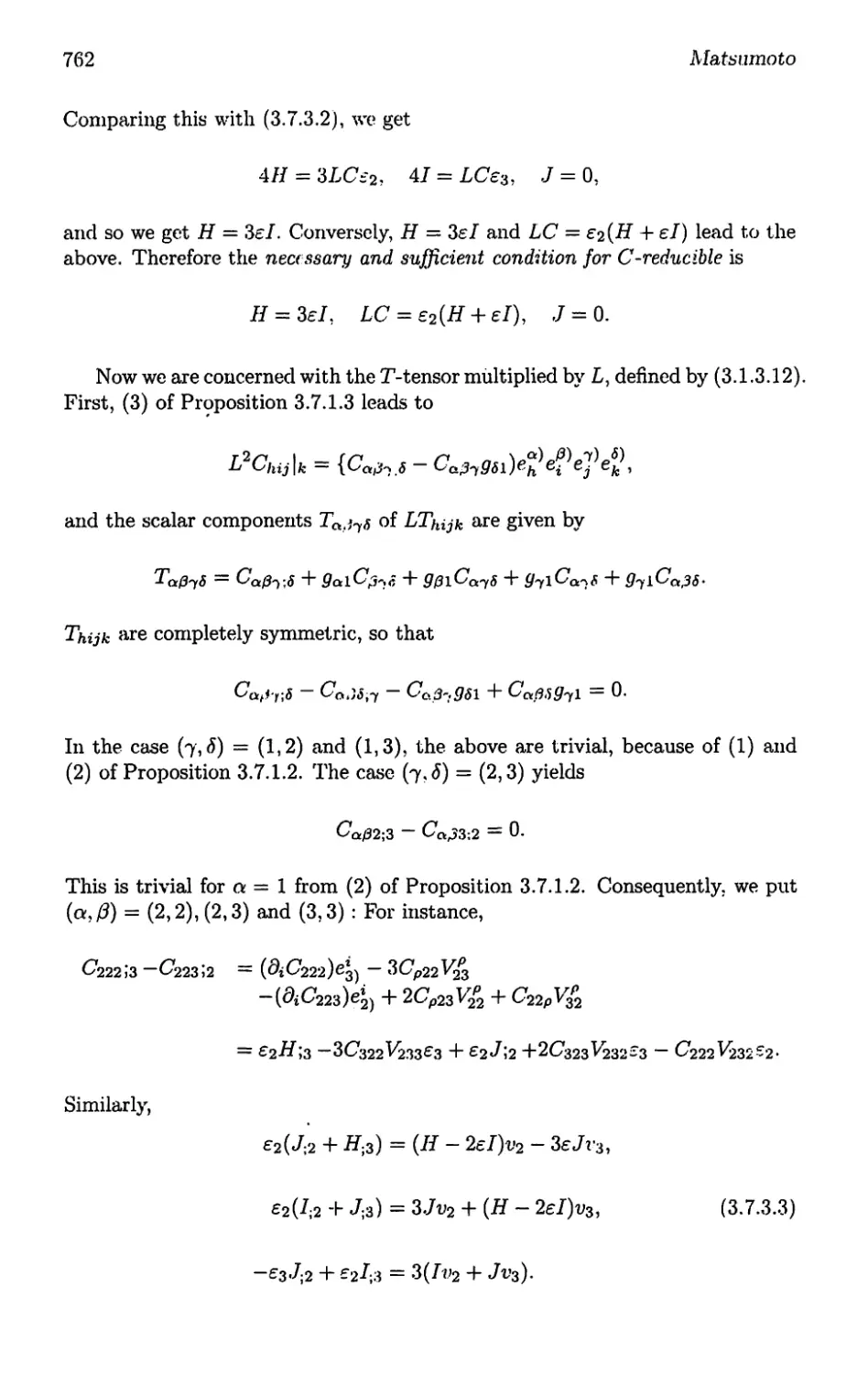
Comparing this with (3.7.3.2), we get
4H = 3LC⅛2, 47 = LCe3, J = O,
and so we get H = 3εl. Conversely, H = 3εI and LC = ε,2(H + εl) lead to the
above. Therefore the necessary and sufficient condition for C-reducible is
H = 3εl, LC = ε2(H + εI), J = O.
Now we are concerned with the T-tensor multiplied by L, defined by (3.1.3.12).
First, (3) of Proposition 3.7.1.3 leads to
L2C∣,ij∖k = {Ca,i.,s ~ Ca^gii)e^e^e1)ei^
and the scalar components Tft.j745 of LThijk are given by
Taβ18 = Caβ1-s + gaιCβ^c ÷ gβiCθtyδ + g^fιCa^ + g^tιCctβδ∙
Thijk are completely symmetric, so that
Caβ'!∙tδ Ct>j5∙-y C(λβ^gδ∖ H- Cctβδg^ι = 0∙
In the case (7, δ) = (1,2) and (1,3), the above are trivial, because of (1) and
(2) OfProposition 3.7.1.2. The case (7, J) = (2,3) yields
C*q/92;3 - Cfα33ζ2 = θ∙
This is trivial for α = 1 from (2) of Proposition 3.7.1.2. Consequently, we put
(ot,β) = (2,2), (2,3) and (3,3) : For instance,
C,222J3 — C223>2 = (βiC222)^3y — 3Cp22V23
-(⅞C223)⅞ + 2Cp23V∕2 + C22pV3p2
= ε2H∖3 — ⅛C322V233ε3 ÷ ε2J∖2 +2C323V232ε3 — C⅛22½32-2∙
Similarly,
ε2(J2 ÷ H3) = (H ~ 2εl)v2 — 3εJv3,
ε2(I.2 ÷ J;3) = 3Ju2 + (H- 2εl)υ3i (3.7.3.3)
- ε3 J∙2 + ε2L3 = 3(Iv2 + Jv3).
Finsler Geometry in the 20th-Century
763
Therefore the scalar components Tαp∙7d* of LT}ljjk are T∖β^ = θ anfI
T2222 = C2⅛2 ÷ 3εJv2∙f
T2223 = C2H,3 ÷ 3εJvα
= — ε2Jf2 ÷ (H ~ 2εZ)v2?
7⅞233 = — ε2J,3 + (H — 2εl)υ^
= ^2Λ2 - 3Jv2,
(3.7.3.4)
T,2333 = β2-f∙,3 “ 3 JV3
= ε3J∖2 ÷ 31^2,
T3333 — ε3Jt3 + 3iv3.
We now consider a three-dimensional Finsler space with the vanishing T-tensor.
Compare Theorem 3.7.3.1 with Proposition 3.1.3.1.
Theorem 3.7.3.1. Let F3 be a Finsler space of the dimension three with the
non-vanishing Ci. The T-tensor of F3 vanishes, if and only if the v-connection
vector v vanishes and all the main scalars are functions of position alone.
Proof: T2233 = T2333 = T3333 = 0 imply
(■f;2) Λs> ,¼> *λβ) = (3ε2 Jt,2> 3β2 J⅛, —3ε3⅛2,3ε3Zr3),
and then T2223 = T2233 = 0 yield
(J7 + ε∕>2 = (H + εZ>3 = 0.
Since H ÷ εl = 0 contradicts C ≠ 0 from the Proposition 3.7.3.1, we have
υ2 = V3 = 0, that is, Vi = 0 from Lemma 3.7.1.1. Then (3.7.3.3) implies
∕f2 = H.3 = I;2 = I,3 = J,2 = J,3 = 0∙ H-1 = /;i = J.1 = 0 from homogeneity.
Hence H, I and J do not depend on y.
3.7.4 Curvatures
First, we introduce an operator on skew-symmetric tensors for frequent use. Let
Tijk, fθr instance, be a tensor of (0,3)-type which is skew-symmetric in (i,j).
Using the ε-tensor given in Example 3.7.1.1, if we define a tensor
*⅛ = ∣εhi‰, (3.7.4.1)
then we get Ty⅛ in the form
Tijk — Cijh Tk .
(3.7.4.2)
764
Matsumoto
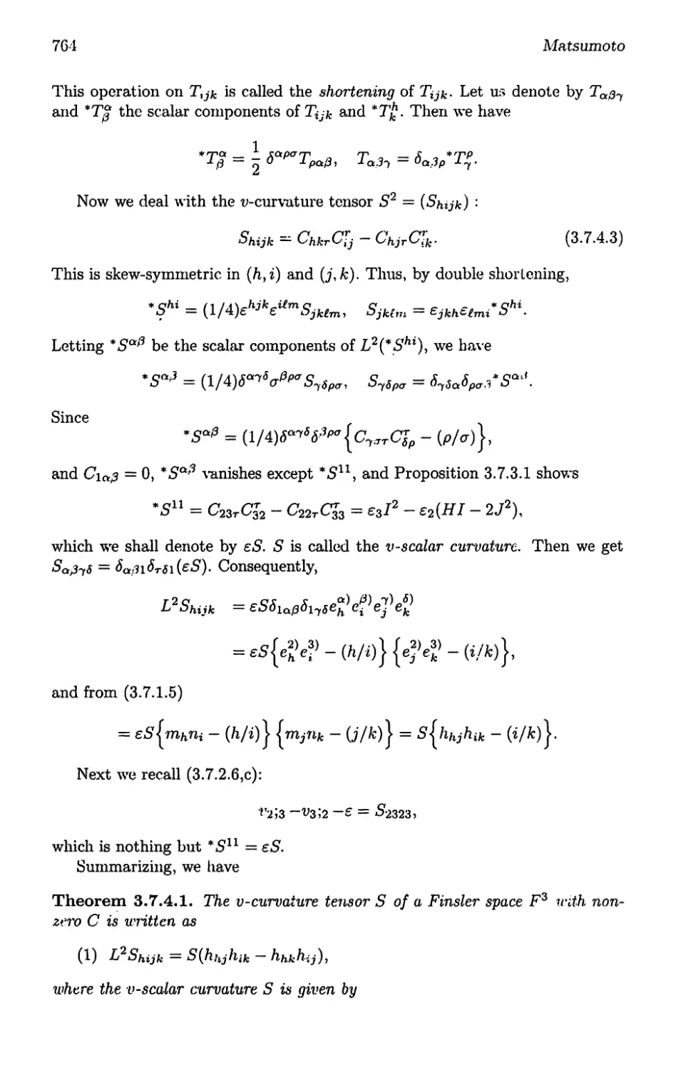
This operation on T1 jk is called the shortening of Tijk - Let us denote by Tag1
and *Tβ the scalar components of Tijk and *T%. Then we have
*⅞o = I δapσTpaβ, Taβ. = δa,3p'T'.
Now we deal with the v-curvature tensor S2 = (Sfajk) ∙
Sfajk — ChkrCij ~~ ChjrC↑k∙ (3.7.4.3)
This is skew-symmetric in {hii) and (j,k). Thus, by double shortening,
*Shi = (l∕4)εhjkεitmS,kem, Sjki,,i = εjkhεtmf Shi.
Letting *Saf, be the scalar components of L2{*Shl), we have
*Sa<3 = (l∕4)5^V',σ⅛pσ, S-,ipσ = δ1saδpσ,3*Saβ.
Since
*Sq'3 = (l∕4)<5^⅛∙^{cιστ¾ - (p∕σ)},
and Cιaβ = 0, *Sa,3 vanishes except *S11, and Proposition 3.7.3.1 shows
*Sn = C23tCJ2 - C22τC3τ3 = S3I2 - ε2{HI - 2 J2),
which we shall denote by εS. S is called the v-scalar curvature. Then we get
Sθlfoδ = δ<xβiδτδi(εS). Consequently,
L2Shijk = εSδlaβδlyδe^e^e↑e^
= εs{ehe? - (λΛ)} {eΓek*- (*∕⅛)}.
and from (3.7.1.5)
= εS{mhni - (h∕i)} {n¾t⅛ - (j∕fc)∣ = s{hhjhik - (i∕k)∣.
Next we recall (3.7.2.6,c):
t'2⅛ — ^352 —ε = ‰23>
which is nothing but *Sn = εS.
Summarizing, we have
Theorem 3.7.4.1. The υ-curvature tensor S of a Finsler space F3 with non¬
zero C is written as
(1) L2Sfajk = S(hιljhik hhkh'j),
where the v-scalar curvature S is given by
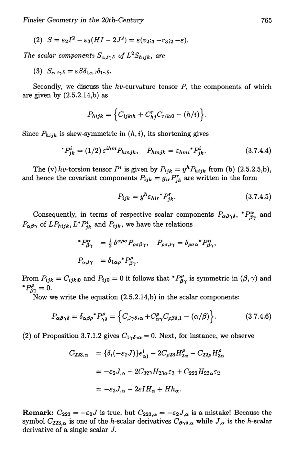
Finsler Geometry in the 20th-Century
765
(2) S = ε2I2 - ε3(HI - 2J2) = s(u2;3 -r3⅛ -ε).
The scalar components Stx^.n of L2Shijky are
(3) So ,i74 =
Secondly, we discuss the ∕n,-curvature tensor P, the components of which
are given by (2.5.2.14,b) as
Phijk = {Cijfcih ÷ ChjCτikιQ ~ (h/?)|.
Since Phijk is skew-symmetric in (∕ι, ∙i), its shortening gives
∙pjfc = (1/2) εihm Phmjky Phmjk = ≡hmi*P⅛. (3.7.4.4)
The (v) ∕ιυ-torsion tensor P1 is given by Pijk = yhPhijk from (b) (2.5.2.5,b),
and hence the covariant components Pijk = QirPfk are written in the form
Pijk = yhεhir*Prjk. (3.7.4.5)
Consequently, in terms of respective scalar components Pctβy⅛, *P‰ and
Paβy of LPhijkyL*Pjk anci Pijky we have the relations
*Pβl = ⅛ δ°cpσ Ppσβyy Ppσβy = ^pσafP^y
Paβy = δlap*P∣fy∙
From Pijk = CijkiQ and PijQ = 0 it follows that *P^ is symmetric in (#,7) and
*¾ = θ∙
Now we write the equation (2.5.2.14,b) in the scalar components:
PaW = δa0f,*P⅛ = {c37i,o +C^Cpi3SΛ - (μ∕β)} ∙ (3.7.4.6)
(2) of Proposition 3.7.1.2 gives C17<5,α = 0. Next, for instance, we observe
C223.q = {⅝(-ε2 J)}⅛) - 2Cp23¾ - C22pH2a
= ~ε2Jfn — 2C2r>3H23ct-3 4- C222H22ac2
= -ε2J,α - 2εIHa + Hha.
Remark: C223 = -ε2J is true, but C223tα = -ε2Jtθl is a mistake! Because the
symbol C⅞23,α is one of the h-scalar derivatives C⅛γ<5,tt while J,ci is the Jι-scalar
derivative of a single scalar J.
766
Matsunioto
Similarly, we obtain
C⅛22,α — ZzH,α ÷ 3εJhα,
C223,a = -z2J,a + (H - 2εΓ)ha. ? 7)
C*233,α = Z2I,cr
and C333jθc = ε3J,a + 3Ihα.
Next, putting (a,β) = (2,3), (3,1) and (1,2) in (3.7.4.6) yields
*P,1j = ‰,2 - C2lf,3 + C‰Cp33,ι - ¾⅛1, (3.7.4.8)
*P12i =-C375,1, *P≡δ = C274,1.
Nov/ we give special attention to Landsberg spaces and Berwald spaces of
dimension three. These are characterized by Chijio = 0 and Chijik = 0 respect¬
ively. From Caβytδ = 0 and (3.7.4.7) we get
H ,0t —— 3f3∙7∕iχ⅛, Ijθc = 3ε,2*7^,Qj
J,α = z2(H - 2εl)hot = -3ε3Jha.
The third equations imply (H+ εΓ)ha = 0, and hence Proposition 3.7.3.1 yields
ha = 0.
Therefore, we obtain
Theorem 3.7.4.2. A Finsler space F3 with non-zero C is a Landsberg space,
if and only if the h-connection vector Hi is orthogonal to the supporting element
y, that is, h↑ ≈ 0, and the main scalars satisfy Hjι = ∕ 1 = Jj = 0.
Theorem 3.7.4.3. A Finsler space F3 with non-zero C is a Berwald space,
if and only if the h-connection vector hi vanishes and all the main scalars are
h-covariant constant.
These theorems can be regarded as generalizations of Propositions 3.3.3.4
and 3.4.2.1, respectively.
Finally, we consider the ^-curvature tensor R. Its components Rhijk is skew-
symmetric in (∕ι,i) and (J, k), and hence double shortening leads to
*Λij = (⅛)εihkε>emRhktm, Rhktm = εhkiεtmj* Ri>.
In terms of scalar components, these are written as
'κ"j - O7⅛λ"**.. (3.7.4.9)
R^fδpσ = δ'γδofipσβ ∏ & ∙
The scalar components of the (v) h-torsion tensor Rijk/L = yhRhijkf L are
Raβ-i = ⅛apδβ^σ*Rpσ. (3.7.4.10)
Finsler Geometry in the 20th-Century
767
Now, from Rhijk we get a tensor Rii and a scalar R as
Rij =ghk Rhikj, R = g'iRij.
The former is the h-Ricci tensor (§3.6.5), which is also written as Rrijr or
gh'* Rihjk, and its scalar components are given by
Rai = gxμSλapSμ.3σrRl,σ = ελ‰<5.Vσ* Rpσ, (3.7.4.11)
where the symbol ∑ is omitted. It follows that the h-scalar curvature R as
λ,p,σ
above is
R = εχδχapδχ,3σ* Rpσga,i = εxε>‰pδχμσ∙ R^
= 2(ειε2∙Λ33 + ε2ε3*Kn +ε3ει*Λ22),
or
R = 2εεp*Rppi ε = ε1ε2ε3. (3.7.4.12)
It is observed from (3.7.4.11) and (3.7.4.12) that, for instance,
Rn = εxδλipδxiσ*Rpσ = ε2*F33 + ε3*F22
= (f - ε2ε3*K11)ει = (f )ει - ε*Rn,
R23 =εχδχ2pδχ3δ*Rfκr
= -εk*R32 = -ε(ε2ε3*J?32).
Consequently,
⅛∕3 = (J⅛)g°'0 - εεaεa*Rβa, (3.7.4.13)
where at the last term we do not sum in a or β. It should be remarked that
*Ra0 is not symmetric in general.
Now we introduce the tensor
— Rij ~ (-J
From (3.7.4.13) it follows that the scalar components of Lij are given by Laβ =
(⅞)<W ~ εεaεi3*Rβa. Thus, if we put
Lhijk — {θhjLjk + QikLhj
-©}■
768
Matsumoto
the scalar components of Lhijk are, for instance,
£1223 — ~022-kl3 ≈ —c∙j(-£61£.3*7?31 ) = J71223>
£1212 = £711 £22 + 9'22Lγι
= ει{ (τ)≡2 - ≡'Λ22} + ε2{ (f )ει - ε*R11}
= <⅛(⅞) — ε3(ε1*Hl1 + ε2*Λ22)
= ε2(f) “ ε2{(f)ε - ε3*∙R33∣ = Ruiz-
Therefore, Lhijk = Rhijk for any (h<i,jik).
Summarizing, we obtain
Theorem 3.7.4.4. The h-curvature tensor R of F3 with non-zero C is written
in the form _
-‰7fc = A[jk]{ghjhLik + 9ikLhj},
where Lij = Rij - (R∕A)gij and Rij = R∙jr.
It is of interest to know the scalar components of the (v) h-torsion tensor
Rijk = yhRhijk∙ From (3.7.4.10), those of R}k∕L are given by
Ra0-1 = 5iλp⅛7σ*∙Rpσff"λ = (W2+⅛AΛp‰
which leads to
R⅛y = (pα2*Λ3σ - ga3*R2σ)δa0y. (3.7.4.14)
3.7.5 Three-Dimensional Bianchi Identities
Among the Bianchi identities of CT we have to consider five as follows:
^j(ijk){Rhijk ÷ (£Chir)(£ Rjk)} = 0, (3.7.5.1)
∑(ijk) {Rmhijtk ÷ (LPmhir)(L 1 Rjk)} = 0, (3. ι .5.2)
LRmhij∖k 4^ (£ Rmhkr) (L Rj,j)
~- (3.7.5.3)
4^ ∙^[ij]{LRmhjkιi ÷ (LPmhir)(Pjk) 4“ Rmhjr(LCjk)] = 0,
L2Rmhfjik - A^{L2Pτnhki∖i - (LPmhri)(LCrkj + (L2Smhir)Pfi] = 0, (3.7.5.4)
∑(ijk){L3Smhij∖k} = ^ (3.7.5.5)
The purpose of the present section is to write these identities in terms of scalar
components.
On account of (3.7.4.9) and (3.7.4.14), we can write (3.7.5.1) in the form
¾hs){(δo3p*R*> + C2∕R3σ - C3aβ*R2σ‰s} = 0.
Finsler Geometry in the 20th-Century
769
Since we may put (∕3.^f∖δ) = (1,2,3), the above is of the form
^Ql^'α23 + Λ^2⅛31 + A‰(5σ∣2 = Aζσ — 0,
where ΛJζ5 is the inside of ( ). Consequently, (3.7.5.1) is equivalent to
δaσ,>*Rpσ + C2∕P3σ - C‰*fi2σ = 0.
According as a = 1,2,3, the above is equivalent to
(a) * R23 - *Ry2 = 0,
(b) *7?31 - *Λ13 = (PI - εI)*R23 - J(*Λ33 - ε*Λ22), (3.7.5.6)
(c) *β12 - *7?21 = I(*R33 - ε*R22} - 2J*R23.
Next we consider (3.7.5.2). If we put
λαp = *7zαpj ? +*¾ (pσ⅛3, _ gσ3*r2p^
then (3.7.5.2) has scalar components
= θ∙
It is obvious that this is equivalent to the simpler equation ∑(37∂){^7<5p^p} — 0.
Thus, as in the case of (3.7.5.1), we can write this identity in the form Apcp = 0
alone, that is,
*¾p + *Ppσ(gσ2*R3p - gσ3'R2p) = 0. (3.7.5.7)
Next we consider (3.7.5.3). This is written in terms of the scalar components
as
⅛sσ(*R⅛σ -SJfεpδσβ*Rpσ)
+W‰ + δ-m,*RapC%p - P⅛*P" } = 0.
In this equation we put (?,<5) = (1,2), (2,3) and (3,1). From Cfp = P1" =
*P1" = 0 and (1) of Proposition 3.7.1.2 it follows that
,¾3 - Sδaε0*R'33 + *P‰1 + *Ra3Cl0 - ‘Ra2Cl0 = 0,
*P"31 - Sδfε3*Ren + 'Ro1Cp3λ
'β √ "p (3.7.5.8)
+ ⅞3lΓ¾2÷¾*p⅛} = 0,
'Ra2 - Sδaε0*Rp2 - *P⅛λ - * Ra3Cl0 + * Ra2Cl0 = 0.
Next we deal with (3.7.5.4) in terms of the scalar components. Paying at¬
tention to the terms L2PnlAfcjIi and Proposition 3.7.1.3, (3.7.5.4) yields
εδaS.0 <⅛ + ⅛ij{*Pσ" ¾ - εSδyσιδaP0^
+ *P0τj - 'Pa.lgδl} = 0.
770
Matsuinoto
The cases (7, δ) — (1,2) and (1,3) are reduced to trivial equations. In the case
(7, J) = (2,3) the above is written in the form
ε<5∏S.,3 - SP⅛) + ¼l{,¾¾ + ∙¾,3} = 0. (3.7.5.9)
Now consider a Landsberg space. This is characterized by the P-tensors = 0.
Then (3.7.5.9) yields Sy3 — 0. Therefore,
Theorem 3.7.5.1. The v-scalar curvature S of a three-dimensional Landsberg
space with non-zero C is h-curvature constant.
Finally, we consider (3.7.5.5). Paying attention to Proposition 3.7.1.2, the
scalar components are
WU(*¾' - 2*s^(hι)} = 0.
Since this is similar in form to the cases (3.7.5.1) and (3.7.5.2), it is reduced to
the e<ιuivalent identity
*S;7 - 2*Sσpgpl = 0.
This is, howτever, a trivial equation, because all *Sσp vanish except *S∏ and
hence
*5.7 = (∂i*Sσp')e⅛ + *SτpVτσp + *SστVτpp
= (⅛*Sσl)⅛ ÷ * Sn Vf1 + *5σl Vr1pp.
The first term vanishes from the homogeneity, and hence (3.7.1.11) leads to
= *S1¼5r + *Sσlhpp = 2*Seτl = 2*Sσpgpl.
We have had (1) of Proposition 3.7.4.1. By making use of this expression of
the.v-curvature tensor S, it is easy to show that (3.7.5.5) is only trivial when
5;i = 0 and hχa = 0.
Therefore we have
Proposition 3.7.5.1. /n a three-dimensional Finsler space with non-zero C1
we have only four classes of the Bicmchi identities (3.7.5.6 ~ 9).
3.7.6 S emi- C- Reducibility
We have defined the notion of C-reducibility in §3.4.4. Generalizing this notion,
we have
Definition 3.7.6.1. If the (7-tensor of a Finsler space Fn with non-zero C is
written in the form
= +≡2⅛)c¾cfc,
then Fn is called semi-C-reducible, where the scalars ρ and q are to satisfy
p + q = 1 and gi>CiCj = £2 (C)2.
Finsler Geometry in the 20th-Century
771
Multiplying by gjk shows that p and q must satisfy p ÷√? = 1. A slight
generalization of scmi-C,-reducibility is given by a special form
Cijk = ∑(ijk) {AjCk}ι (3.7.6.1)
where the tensor Aij must be symmetric and Ao = 0. This is called quasi-C-
reducibility.
Theorem 3.7.6.1. If a three-dimensional Finsler space F3 with non-zero C
is quasi-C-reducible, then F3 is -se/mi-C-reducible and the main scalars must
satisfy
H = ε2LC(l~^, I = ε3LC⅜' J = 0.
Proof: Suppose that F3 with C ≠ 0 is quasi-C-reducible. Then we have from
(3.7.3.2)
LC[Σ(tjfc) {Aijmk}] = Hmimjmk
-^Σ(ijk){-εJfrtimjnk + Iminjnk} + Jninjnk^
By multiplying by m1mjmfe, τnlm^nk, mzn^nk and n1n^nk, we get AijT∏lm^ =
H∕3LC, Ai3mtnj = 0, A⅛n'ni = I/LC and J = 0. Hence,
^ = (⅛)mi,n>+(⅛)"^∙
= (⅜M¾⅝'
and
LCCijk = ε3IX(w{hijCk} + (H- 3εl) ⅛⅛⅛.
Thus we have a semi-C-reducibility, because p/4 = ε3∕∕LC and ε%q = (H —
3εΓ)∕LC satisfy p + q = 1 from Proposition 3.7.3.1.
Now we consider a semi-(7-reducible and Landsberg space F3 with C ≠ 0.
.Owing to Theorem 3.7.4.2 and 3.7.6.1, we have first
h1 = H1 =Z1=J = O.
Theorem 3.7.5.1 shows that S is h-covariant constant, and hence (2) of The¬
orem 3.7.4.1 leads to
/ξα÷λ‰=0, a = 1,2,3, K = H-2εI. (3.7.6.2)
Rom Phijk = CijkiO = 0 of (1) of Theorem 3.3.3.1, (3.7.4.8) yields C3^,2 =
C27 5,3, which is written as
Hi3 = ε27Ch2, J2 — ε2Fh3, 1,3 = 3ε2Ih2.
(3.7.6.3)
772
Matsumoto
Hence (3.7.6.2) are rewritten as
Ih2K = O, IHi2 + C2(AT)2Zi3 = O. (3.7.6.4)
Since I = K = O contradict Proposition 3.7.3.1, (3.7.6.3) and (3.7.6.4) show
that the spaces under consideration are divided into three classes as follows:
(I) I = 0 : h3 = 0, H3 = ε2Hh2,
(II) K = Oih2 = 0, H2 = Z,2 - H3 = Z3 = 0,
(III) IK ≠ 0, h2 = 0 : ZH2 = -ε2(K)2h3i Z2 = ε2Lh3l H3 = Z3 = 0.
Further we consider the identities (3.7.3.2): In our case, they are written as
ε2H3 = Kv2, ε2I2 = K υ3, ε2I3 = 3Zr2.
If F3 belongs to the class (I), then we have ε2H∙3 = Hv2 and v3 = 0. Further
S = O from (2) of Theorem 3.7.4.1. If F3 belongs to the class (II), then H3 =
Z2 = O1 and hence H2 = Z3 = 0 from K = 0, and consequently H and Z satisfy
H a = H.a = Ifa = Ia = 0. Therefore,
Theorem 3.7.6.2. A semi-C-reducible and Landsberg space F3 with non-zero
C has J = Hfι = Ifι = hi = 0 and the h-covariant constant v-scalar curvature
S. All of such spaces are divided into three classes as follows:
(I) I = 0 : h3 = v3 = 0, H3 = ε2Hh2, H3 = ε2Hv2, S = 0,
(II) K (= H - 2εZ) = 0 : h2 = 0, H, I = const.,
(III) IK ≠ 0, h2 = 0 : ZH2 = -ε2(∏)⅛3, Z2 = ε2Kh3,
H3 = Z3 = 0, H3 = ε2Kv2, L2 = ε2Kv3, Z3 = 3ε2Zv2.
If h3 of F3 belonging to the class (II), then ha = 0, α = 1,2,3 and hence
Theorem 3.7.4.3 shows that F3 is a Berwald space. The similar fact holds for
F3 belonging to the class (III), because v.*e have ha = 0 and Hfθt = Zα = 0,
a = 1,2,3. Therefore we obtain
Corollary 3.7.6.1. A semi-C-reducible and Landsberg space with non-zero C
belonging to the classes (II) or (III) is reduced to a Bcrwald space, if and only
if h3 = 0.
The remainder of the present section is devoted to detailed discussion of
spaces belonging to the class (I). They have interesting properties such that the
hυ and v-curvature tensors P and S vanish. Our discussions are especially based
on the Bianchi identities (3.7.5.6) and (3.7.5.8). On account of Z = J = 0, the
former is simply written in the form
*∏23 = *∏32, *H31-*H13 = H*H23, *H12 = *H21. (3.7.6.5)
Fiiisler Geometry in the 20th-Century
773
From C%y = O except Cf2 = H, the latter is also written
*Rax + 'RaxC2ij3 = 0, λ = l,3, *Λ¾2 = 0∙ (3.7.6.6)
To deal with (3.7.6.6), we observe, for instance,
*Λ⅛3 = (∂i*Ra3)ei, + tRpiSaVpoj3 + * RapS3Vp3j3.
In the following we shall regard *Ra3, for brevity, as nine single scalars and
denote then by Raβ. Similarly, t»2 is regarded as a single scalar and denoted by
v, because t»i = υ⅛ = 0. (C0eβy have been regarded as a set of the single scalars
in Proposition 3.7.3.1.)
Then we may write as Ra3∙β and
= Ra3t3 + εa(Rι3ha3 + ⅛3½α,J + ‰‰fl)
+ ε3(Ralh3β + Ra2Vβ).
Consequently, (3.7.6.6) is written
(1) ft√? = Rθl3∖β + Raiε3h3β + Ra2ε3Vβ + Ra3C23
+Ri3εahaβ ∙+ ‰εα‰ + ‰εα‰^ = 0,
(2) q3 = Rσl∙t3 + RalCl3 ~ Rq2^2,3 Ra3^3β
FRliεahaβ + ½iεα½αp' ÷ ¾l^α^3α∕3 = 0,
(3) q.1? = Ra2tβ + Raiε2h2β — Ra3ε2Vβ
÷ ½2^α½α.3 ÷ ¾2^α½α∕3 = θ∙
We calculate (1)2/2-(3)s,j, (3)ι∕j-(2)2^ and (2)33-(I)i^ to eliminate Rctβ'n .
Then (3.7.6.5) yields
R23(ε2Hh2β — C2β) = 0, R23ε2Hvtj — ¾2Cf3 = 0,
(R23H)lβ + R23HCli =0.
The first equations are trivial. The second with β = 3 is trivial, while with
β = 2 we get
T?i2 = ¾3^2^∙ (3.7.6.7)
The third with β = 3 is a consequence of (3.7.6.7) because of Hi3 = ε2Hv from
Theorem 3.7.6.2 and R23⅛ = — R↑2 from (l)23, while with β = 2 it is
(R23H').2 = ⅛3(ff)2∙ (3.7.6∙8)
Then, using (3.7.6.7) and (3.7.6.8) and H.3 = ε2ffv, the above (l)ct0, (2)q^
774
AIatsumoto
and (3)oj are reduced to twelve independent differential equations as follows:
⅞3j2 = — ∙R31 ÷ (⅞3 — ε⅞2)ε2^
⅞3j3 = - -¾2,
¾2j2 = — Rll ~ R12H ÷ (¾2 ÷^⅞1)-2j -^12;3 — -¾3≡3,
I?31;2 = ⅛3^2 - R3iH ~ -R12ε3υ,
‰j3 = -Rll + R33 -3,
Rll∙l2 = %R12ε2 ~ ¾1⅛
-ftιij3 = 2(¾ι - R23H)ε3.
R22t2 = R22,3 = O,
⅞3j2 = -∙2⅞3S3V — R33H)
R33,3 = — 2⅞1 + ⅞3^∙
(3.7.6.9)
Here we shall recall (2) of Theorem 3.7.4.1. In our case, it gives V2,3-V3f2 = ε-
We observe
V2-,3
= (∂tυ2)ei3j - υpVg3 = υ-3
t,3j2
= (∂iv3)e^ - vpV3p2 = (t')2ε2.
Thus,
v;3 = ε + (u)2ε2∙
(3.7.6.10)
Now we consider the integrability conditions Raβ^∙tδ = Raβ-,δ,y of (3.7.6.9).
Making use of = ε2Hv and (3.7.6.10), the conditions are written as
(υ)2C‰ -εR22) = 0,
υ(R11 — ε2R22 ÷ R12Rr ~ R3ιε2υ) = 0,
v{R23 ~ R31ε2H ~ R12εv) = 0,
(3.7.6.11)
v (2⅛2 — Rnε2H) = 0,
v(2R23υ + R33ε3H) — 0.
Since v does not vanish from (3.7.6.10), we have six linear equations (3.7.6.7)
and (3.7.6.11) for Raβ. It is easy to show that these equations yield 3 + (II)2c2 +
(v)2ε3 = 0 or R33 = 0. If the former holds, then we get
HH.3ε2 + vu3ε3 - v{ε2 + (H)2 + (υ)2ε} = -2ε2v = 0,
which contradicts (3.7.6.10). Therefore, ⅛3 = 0 and all Raβ = 0.
Finsler Geometry in the 20th-Century
775
Therefore,
Theorem 3.7.6.3. Let F3 be a three-dimensional semi-C-reducible and Lands¬
berg space with non-zero C. If F3 belongs to the class (I) of Theorem 3.7.6.2,
then the three curvature tensors Ri P and S of the Cartan connection vanish
identically.
Remark: The main subject of the present section was to generalize The¬
orem 3.4.4.1. It is observed that the spaces belonging to the classes (H) and
(III) are near to the Berwald spaces. However the spaces belonging to the class
(I) gave rise to the troublesome problem: iiR = 0?” Let us recall that R ≠ 0
appears in Theorems 3.6.3.1 and 3.6.4.4.
3.8 Indicatrix and Homogeneous Extension
3.8.1 Indicatrix as Riemannian Hypersurface
We consider a Finsler space Fn = (MiL(xiy)). The fundamental function
L(i,,2∕) gives the fundamental tensor gij(xiy) = ∂.∙¾∙(L2∕2), which satisfies
gij(x,y)ytyj = L2(x.y). As it has been shown in §1.2.2, the tangent vector
space Mx at a point x of M is regarded as an n-dimensional Riemannian space
equipped with the Riemannian metric gij(x,y)ytyj with fixed x. It follows that
the Christoffel symbols of Mx :
∣ 9irΦj9rk + ∂kgrj - ∂r9jk) ■
are nothing but the components CJfc of the C-tensor. Hence, the covariant dif¬
ferentiation in this Riemannian space Mx coincides with that of the vertical
connection given by Proposition 2.4.1.1, for instance, the Cartan connection
CΓ and the Hashiguchi connection HΓ.
Further (2.4.3.4) and (2.5.1.2) show that the v-curvature tensor S2 of CT is
just the curvature tensor of the Riemannian space Mx.
We shall recall the indicatrix Ix = {y ∈ Mx∖L(xiy) = 1} defined in §1.2.2.
It is a Iiypersurface of Mxi given by the equation L(xiy) = 1. Let
yz = yz(ua)i a = li...in-1,
be parametric equations of Ix in M :
i(j,∙,y(u)) = 1. (3.8.1.1)
In the following, we restrict our discussions to a Finsler space Fn of dimen¬
sion n more than two, and consider Ix as a Iiypersurface of the Riemannian
space Mx. From (3.8.1.1) we have first
4¾ = 0, = (3.8.1.2)
776
Matsumoto
Bα with the components B1ct are regarded as n — 1 linearly independent vectors
tangent to Ix. The linear independence is, of course, assumed, that is, the matrix
(j¾) is of rank n — 1. Equation (3.8.1.2) shows that the normalized supporting
element ⅛ = ∂iL is the unit normal of Ix. Since we get the frame field (Bla,Γ)
of Mx at every point of Ix, we obtain the dual cofranιe field (Bzq,Λ) :
⅜S∕ = ⅛ BUi = 0,
(iB? = 0, l'ti = 1.
(3.8.1.3)
Also,
BiaB* + titj = δ*. (3.8.1.4)
On Ix we get the induced Riemannian metric gaβ(u) = gij(τ ,y(u))BtaB3f3.
From (3.8.1.2) this is also
9aβ(u) = hij (z, j∕(u))BiB⅛. (3.8.1.5)
According to the theory of subspaces in a Riemannian space, we obtain the
Gauss and Weingarten derivation equations
(a) ∂βBia + CJ1 (x, 2z(u))Bj Bkp = γj,b; + Haβei,
(3.8.1.6)
(b) ∂βC + CJfc (x, y(u))0Bk0 = -BjJBj1
where ∂β = ∂∕∂uP> Ps are Christoffel symbols constructed from g0t3(u), Haβ
is the second fundamental tensor of Ix and Hβ = Hβσgσ^r. H is, of course, a
symmetric tensor.
The second term of the Weingarten equation (b) vanishes because Cjky3: = 0.
Next, differentiating (3.8.1.2) by uti, we have
hijB^+Ii∂βB^ = 0.
Paying attention to (3.8.1.5) and substituting from the Gauss equation (a), we
get Baβ = -gaβ. Thus,
Theorem 3.8.1.1. The Gauss and Weingarten derivation equations of the
indicatrix Ix are
(1) ⅛Bi + CiikB3aB0 = rχ3βjt - ga,(∖
(2) ∂βtl = Bj.
Corollary 3.8.1.1. The indicatrix Ix of a Finsler space F", n ≥ 3, is a totally
umbilical hypersurface with the mean curvature —1.
Thus Ix may be regarded as the unit sphere in a Euclidean space.
X' -' -SA >X
Finsler Geometry in the 20th-Century
777
Next we shall find the Gauss and Codazzi equations which are integrability
conditions of the Gauss and Weingarten equations. They are
ShιjkBaB^B^Bδ = R<χβ^tδ ~ (HcrγHβδ ~ HocδHβ3}∙>
Sh<jklh BaBj0B⅛ = Haβ∙,δ-Haδyij
where Raβ3δ is the Riemannian curvature tensor of Ix. Since we have Haβ =
-gθt3 and Shijk^h = θ, the Codassi equation is trivial. The Gauss equation can
be written in the form
ShijkBaB3B^ Bδ = Raβ')δ — (ga^∣gβδ ~~ (Jaδgβ^fy (3.8.1.7)
Now, let Caj^y and Sctβyδ be the projections of the C-tensor Cijk and the
v-curvature tensor Shijk on Iχ ∙
ca,h = CijkBiaB'βBk, Salhs = ShljkBhaBitBitBki.
Equation (2.5.1.2) yields
Saβ3δ = CaδμCβ,γ — G∏μ<¾∙ (3.8.1.8)
From (3.8.1.6) it follows that the Ricci tensor Raβ = Ra0μ and the scalar
curvature R = Raβga∙3 of Ix are given by
Raβ = Saβ + (n - 2)gaβ, R = S + (n - l)(n - 2), (3.8.1.9)
where Saβ = SjjBaBj0 is the projection of the t>-Ricci tensor Sjj = S⅛h on Ix
and S is the "-scalar curvature S = gaf3Saβ = gzjSij.
3.8.2 Indicatory Tensor and Homogeneous Extension
We have some special tensors, for instance, hij, Pijk, etc., which vanish owing
to multiplying by y∖
Definition 3.8.2.1. A tensor T is called indicatory, if T vanishes owing to
multiplying by yz and yi with respect to any suffices.
That is, = ∙ ∙ ∙ = T)j!c0 = O. Hence ⅛, ¾, P]k^hjk aπc^ the T-tensor Thijk
are all indicatory tensors. Any tensor can be expressed at a point of Ix in terms
of the frame (Bα,l'). An indicatory tensor has no components in I*. More pre¬
cisely,
Proposition 3.8.2.1. IfTj is an indicatory tensor, then it is
Tj=TβBiaB? on Ix,
where Tf = BfBh,.
778
Matsumoto
Proof: From (3.8.1.5) we have
(T*Bf. B⅛)B∖B0j = T*(δik - tkti}{δhj - ljlh),
which is equal to TJ according to the indicatory property.
We shall show some interesting procedure owing to this indicatory property.
Let Hij (resp. Ki3) be (r) (resp. (s)) p-homogeneous indicatory tensors and
suppose that the respective projections Haβ and Kaj on Ix are in the relation
Ha J = μKaβ with a function μ on every Iz. Then Proposition 3.8.2.1 implies
Hij = μKij on Ix. Now, by extending μ all over Mx as a (0) p-homogeneous
function, we get
Hij(x,y) = LrHij(x, ∣) = LrμKij(x, ∣) = Lr-μKij(x,y).
Therefore, L"rHij(x,y) — L~sμKlj(x,y) on Mr.
Definition 3.8.2.2. Let Hij (resp. Kij) be (r) (resp. (s)) p-homogeneous
indicatory tensor fields and suppose that the projections Haβ (resp. Kaβ) on
Ix are in the relation Haβ = μKaβ with a function μ on every indicatrix lx.
Then,
L~rHij = L-sμKij,
with a (0) p-homogeneous function μ owing to the procedure above. This pro¬
cedure is called the homogeneous extension of the relation Haβ = μKaβ.
It should be remarked that the homogeneous extension can be applied only
to indicatory tensors, because we have to use the expression given in Proposi¬
tion 3.8.2.1.
Example 3.8.2.1. We shall again show
Ij Shijk = S(hhjhik ~ h}l,khij) in ,
which has been shown in Theorem 3.7.4.1, provided C ≠ 0. First the projec¬
tions of Shijk and hhijk = hhjhik ~ hhkhij are Raβ^δ ~ {9ay9βδ ~ 9aδ9βy} and
9ay9βδ — 9aδ9βy from (3.8.1.7) and (3.8.1.5). In this case, the indicatrix Ix is
two-dimensional, so that it is well-known that its Riemannian curvature tensor
is of the form
Raβyδ = κ(9afγ9βδ ~ 9aδ9ι3y)>
with the total curvature κ. This may be written as
Rtxβyδ ~ {θay9βδ 9ocδ9βy} = (κ ~ ^-){9ay9βδ ~ 9ctδ9βy)∙>
and apply the homogeneous extension, then we obtain (1) of Theorem 3.7.4.1
without the assumption C ≠ 0, where S = κ - 1.
Since S = O implies κ = 1, we get
Finsler Geometry in the 20th-Century
779
Theorem 3.8.2.1. The v-curvature tensor S of the Cartan connection CT
vanishes at a point x, if and only if the indicatrix Ix is of constant curvature 1.
Roughly speaking, 5 vanishes, if and only if Ix is a unit sphere. We shall
give several examples.
Theorem 3.8.2.2. The v-curvature tensor S of the Cartan connection of a
four-dimensional Finslcr space is written in the form
Shijk = A[jk]{h,hjMik 4^ hikMhj} >
where Mij = Sij — Shi3 ∕⅛.
Proof: We put _
Mhijk = {b>hjMik + h{kMhj}∙
Both Shijk and Mhijk are indicatory and (—2)p-homogeneous. Their projections
on Ix are respectively given by
Saβ^l o and 5∣ {gcn Mβg ÷ gβt },
where Mβs = Sβg - Sgaδ∕½- It follows from (3.8.1.9) that Saβ = Raβ - 2gcxβ
and S = R — 6. Hence,
Λ∕α,? = Na0 Na0 = Ra0 - (≤) ga0.
It is well-known that the conformal curvature tensor of a three-dimensional
Riemannian space Ix vanishes identically, that is, we have
R∙aβ^δ = ∙^-['yδ]{.9ot'Y^βδ <7fl<5 ∙Norγ }.
Therefore (3.8.1.7) easily leads to Sotβ~is = Motβys and the homogeneous exten¬
sion completes the proof.
This special form of Shijk of R4 is quite similar to (3.4.4.6) of a C-reducible
space and to the form of Rhijk of F3.
Next we consider the condition for the Riemannian space Ix to be an Einstein
space, namely, Rcιβ = Rgocβ∕(n — 1)∙ Then (3.8.1.9) shows Saβ = Sgaβ∕(n — 1)
and hence Sij = Shij ∕{n — 1) by the homogeneous extension. Therefore,
Theorem 3.8.2.3. The indicatrix Ix is an Einstein space as a Riemannian
space, if and only if Sij = Shij∕(n-1) holds, where Sij ■— S⅛h and S = Sijgzj.
Corollary 3.8.2.1. If the indicatrix Ix of a four-dimensional Finsler space is
an Einstein space, that is, Sij = Shzj∕⅛, then the v-curvature tensor is
Shijk = (^Q^(hhjhik ~ hhjkhij)>
780
Matsuinoto
Proof: In this case, Mlj of Theorem 3.8.2.2 is equal to Shij/12. Thus, we get
the equation above.
Corollary 3.8.2.2« Ifthe v-Ricci tensor Sij of a four-dimensional Finslcr space
vanishes, the v-curvature tensor Shijk itself vanishes.
This is a special case of Corollary 3.8.2.1. with S = 0.
Ref The problem of Einstein Riemannian space Ix was considered by
Y. Takano, a theoretical physicist, in 1974. Corollary 3.8.2.2 was a great sur¬
prise. See M. Matsumoto [90].
3.8.3 Indicatorization
For any tensor Tj we have
(W*XMWjXk = 0.
and hence Tijh1h h3k is indicatory for any tensor Tj, where hzh = (jzrhrh∙
Definition 3.8.3.1. Let Tf be a tensor of (1,1)- type, for instance. Then the
tensor
pτ,o
τj°=τjhi
(resp.
is said to be obtained from Tf by the indicatorization with respect to the index
i (resp. j). Repeating this procedure successively on all the indices, we finally
get the indicatory tensor *Tf = T$, which is said to be obtained from Tf by
the indicatorization and is called the indicatorized tensor of Tf.
For instance, the indicatorized tensor *Tjk of Tjk is written in the form
*rp rrt (^>rojj⅛+^jTtθ⅛+ZfeT⅛jθ)
J-Ijk — Jijk l
l (titjToQk+fjtkTiOo+tkti'Jojo) itij^kT000
^l^ L2 L3
Proposition 3.8.3.1. The projection of the indicatorized tensor *T of T on Ix
coincides with that of T on Ix.
Because (3.8.1.2) and (3.8.1.3) lead to hl-Bza = B*ft and h⅛Bfi = Bf, we get
{TijhhihPk)B^Bkg = TijBJB}s.
Finsler Geometry in the 20th-Century
781
Theorem 3.8.3.1.
(1) The indicatorized tcnsoi' *C∏j∙∣fc) of the h-coυariant derivative Tiilk in CΓ
of an indicatory tensor Tij is given by
*(rp ∖ _ Tijtk — TijiQlk
{J-Zj>k') — ∙
(2) The indicatorized tensor *(Tij∖k) of the υ-covariant derivative Tij∖k in CT
of an (r) p-homogeneous indicatory tensor Tij is given by
*(Ty∣t) = Ty∣fc + + φ
Proof: (1) From (3.8.1.3) it follows that
*(Ty.fc) = Thlmh,>hljhf = (TMh^h‰h%
= Tijirnhr∣f = Tijik — lkTijiQ∣L.
(2) We have
τij∖mh'kn = ⅞∣fc-(f)τ√l-,
Tmj∖kh? = Ty∣fc -
rp I ((^τnjj∕m)lfc-Tmj J∕7n∣fc)⅞
= Trj∖k T,
T, I I T,kjtj
-Ti3∖lc+ -£-•
Consequently,
Trs∖thrihsjhtk = ITrslfc - (f )τrA}Khsj
= (τis!fc + ¾ii)⅛j - (f )Tj√,fc
= ⅞lfc + ⅞^ + 2≠-(f)r√fc∙
Proposition 3.8.3.2.
(1) The indicatorized tensor *(gij) of the fundamental tensor gij∖ is the angular
metric tensor hij.
(2) The indicatorized tensor *{LChij∖k) of LChij∖k is the T- tensor Tflljk-
782
Matsunioto
Proof: (1) gtjhlhtijc = hhk is obvious. (2) It is a consequence of (2) of The¬
orem 3.8.3.1.
Finally v.τe consider the vanishing of the T-tensor. We denote by Λα∙>π the
covariant derivative of a tensor field Kaβ on the indicatrix Iτ with respect to
the induced connection (Γ'^7) in (1) of Proposition 3.8.1.1.
For the projection Kaβ = K<jBlaBjβ of a tensor field Kij of Fn we have
= ∂^f (Kij B^lBp)
= Kij.kBiaB>0B* + Kij(-σrsBraB° + Γ*7Bj - gα√*)Bjj
+M(-(¾∣ΛA + rsθyBi - gβJi)
= (Kij.k - KrjCrk - Ktrqk)Bi,B^
+Kii)Γδaι + κasrδh - k°=s∙--'b∙∙ - ,
which shows
κaβ,,1 = Kij∖kB⅛⅛B* - + (3 8 3 υ
Now, applying this formula to the C-tensor, we get
Ca0τ,f = Chij∖kB^Bif,B^Bξ.
On account of (2) of Proposition 3.8.3.2 and L = 1, we obtain
ThijkB⅛⅛Bi,B% = (Cpgr∖sh^h^BiβBilB^
= Cpqr∖sBlB^Bl,
and hence we have
Caβr,t = Th,,kB^BiβBifB%. (3.8.3.2)
Since the T-tensor is indicatory, Proposition 3.8.2.1 shows
Theorem 3.8.3.2.
(1) The T-tensor vanishes, if and only if the projection of the C-tensor is
covariant constant on Ix.
(2) If the T-tensor vanishes, then Ix is locally symmetric in the sense of
Riemannian geometry.
Proof: (2) Caβrj - 0 implies Rυtβ^^s — 0 from (3.8.1.7) and (3.8.1.8).
Theorem 3.8,3.3. If the T-tensor of a three-dimensional Finslcr space with
non-zero C vanishes, then Ix is locally flat.
Proof: Theorem 3.7.3.1 implies t√ = 0 and (2) of Theorem 3.7.4.1 gives S =
-1. Hence (1) of Theorem 3.7.4.1 yields Saβ^. = -(ga^fgβι - gaδg>h) by the
projection on Ix. Thus (3.8.1.7) yields = 0.
Chapter 4
Conformal and Projective
Change
4.1 Conformal Change
4.1.1 Geometrical Meaning of Conformal Change
In §1.2.2 the absolute length ∣v∣ of a tangent vector v at a point x of a Finsler
space Fn = (M,L(xiyf) is defined as the value L(xiv)f provided that L(x>y) >
O for any y. On the other hand, if g⅛ (a?, y)ξlζj is positive-definite, then we get
the length ∣v∣3z of v relative to y which is equal to yz⅛∙j (a?, y)vivi .
As to the angle θ between two vectors u and v at xi
COS 0 = -r
y/9ij(xtu)υW y∕gij(x,u)vzυJ
Consequently, the notion of the angle is not symmetric. Thus, the above θ may
be called the angle of v with respect to u. If we take y as uy then we get the
angle of v with respect to y as
L(τ,y)y∕gij(x,y)viυi ’
where yi = gi(x,y)yj.
Definition 4.1.1.1. Let Fn = (Mi L(x,y)) and *Fn = (M,*(x,y)') be two
Finsler spaces on the same underlying manifold M. If the angles of any tangent
vector, with respect to any y in Fn and * Fn, are equal to each other then *Fn
is called conformal to Fn and the change L → *L of the metrics is called a
conformal change of metrics.
783
784
Matsuinoto
Hence *F,'i is conformal to Fn, if and only if
'L2(,x,y)*gpq(x,y)υpv'l(yrVr)(.ysυs) (11 1 1)
- L2(x,y)gpq(x, y)vpvq(*yτvr){"ysυs) = 0
holds for any x, y and v.
The differentiation by υh, v∖ υi and υk of (4.1.1.1) yield the equation con¬
sisting of six terms each of which is of the form
'L2(x,y)"ghi(χ,y)yjyk - L2(x,y)ghi(χ,y)'y*jyk,
which may be rewritten in the form
*L2(x,y),hhi(x,y)yjyk - L2(x,y)hhi(x,y)*y*jyk.
Thus we obtain
‰){*iΛ,⅛⅛!⅛ + 'hjkyhyi) ~ L2(h*hiy*jyk + h*kykyi)} = 0.
If we multiply by yh and next by yk, then the above gives
¾jk){‰Vk - h↑3yk} = 0, *hij = τ2hij,
where τ = *L∕L. Thus the former is rewritten as
^(ijk){hij(τ2yk - *yk)} = 0.
Multiplication by gli leads to Z⅛∕L = *⅛∕*L and hence = τ2gij. Putting
τ = ec(χ"y∖ we obtain = e2cpjj.
We must pay attention to g⅛ = ft⅛(L2∕L), which implies
∂k9ij = Θj9ik (= 2C*ijfc).
Hence, we get ∂∣cc = 0, immediately. Therefore, we have *L = ec^L.
Conversely, this relation gives *g⅛ = e2cgij and i*⅛ = e2c^, and hence
(4.1.1.1.) holds. Therefore,
Proposition 4.1.1.1. The change L →*L of metrics is conformal, if and only
if we have a function c(x) of position alone, satisfying *L = ec'^L.
The function c(x) is called a conformal factor of the conformal change L →
*1.
Remark: As above, we got c = c(α?) from vgij = e2cgij. If we first suppose
*L = ecL with c = c(x.y), then this does not impose any restriction to this
change L → *L, because ec = *L∕L only defines c(x,y) for any L and *L.
Finsler Geometry in the 20th-Century
785
From the conformal change L → *L = ec^L, we obtain
(a) *gij = e2cgij, *gt> = e~2cgi∖ (4.1.1.2)
(b) , j∕i = e2cyi,
(c) ∙L, = e~cti. *Cl = ecC,,
(d) *hij = e2'hij.
Next we have
*Cijk = e2cCijk, *Cijk=cijk. (4.1.1.3)
Thus the C-tensor C = (Cjk) is a conformal invariant.
In the two-dimensional case, (4.1.1.2) and (3.1.1.2,d) yield
⅛ = ecπii, *mτ — e~cmz. (4.1.1.4)
Then (4.1.1.3) and (3.1.1.10) lead to
Proposition 4.1.1.2. The main scalar I of a two-dimensional Finsler space is
a conformal Invariaiit.
Ref The theory of conformal changes of Finsler spaces has been studied from
the early period of Finsler geometry. See M.S. Knebelman [78] and S. Golab
[43, 44]. New theories have been developed since M. Hashiguchi [47].
4.1.2 Conformal Changes OfLandsberg and Berwald Spaces
We consider a conformal change L → *L = ec^L of metrics. Putting F = L2∕2,
we have *F = e2cF and log* F = log F+2c(x). Thus we get a series of conformal
invariants:
Oi log F, ∂i∂j log F, ∂i∂j∂k log F,... .
In particular, Bij = ∂i∂j IogF, is written as
Bij = {9ii ■ (4.1.2.1)
The matrix (¾j ) is non-singular and has the inverse (Blj) given by
Bi> = F(gij - 2t7j). (4.1.2.2)
On account of (1.2.2.2) we get the important fundamental relation
*Gi = Gi - Bir cr, cr = ∂rc(x). (4.1.2.3)
786
Matsunioto
Then the relations between quantities of the Berwald connections are as follows:
(a) *G}=G}- Bfcr, Bif = ∂jB'r, (4.1.2.4)
(b) 'G≈fc = Gjfc-BjJcri Bjrfc = ¾Bjr,
(c) * Gjfcfc = Gjfcfc - Bjfcfccr, Bjrfcfc = ⅞Bjrfc.
Next, from (4.1.1.3) and (4.1.2.4) we have
‰=¾<+⅛ (4.1.2.5)
where the left-hand side is the h-covariant derivative of *Cjk with respect to
the changed Berwald connection *BΓ and
¾ = (⅛qfcBf-CjfcBjJ
+ CiakB% + CjsBf.
Then (2.5.2.14,a) and (3.3.3.1) lead to the relation of (v) hυ-torsion tensors of
the Cartan connections as follows:
*Pjfc = Pjfc + ⅛r. (4.1.2.7)
Definition 3.4.1.1 shows that a Finsler space Fn is a Berwald space, if and
only if G⅛k = 0 identically. Thus (4.1.2.4,c) gives
Theorem 4.1.2.1. A Finsler space Fn is conformal to a Berwald space, if and
only if the hv-curvature tensor G of the Bcrwald connection is written in the
form
G⅛k = B⅛tcr,
where cr(x) is a gradient vector field cr = ∂rc(x).
It is obvious that B^k = ∂i∂j∂kBhr vanishes, if and only if Bhr are homo¬
geneous polynomials in yl of degree two. Since Bhr can be written as
Bhr = - yhyτ, (4.1.2.2')
we have
Corollary 4.1.2.1. A Berwald space Fn remains to be a Berwald space by
any conformal change of metrics, if and only if BtVrk = 0, that is, L2g?J are
homogeneous polynomials in yl of degree two.
We deal that V^0 of (4.1.2.7). (4.1.2.6) gives
¾ = 2(⅛Cjfc)Bsr - CjfcBjr + CjfcBf + CjsBf 1
= 2BsrCjfc∣s - CfBjr + Cj'fcBf + Cij3Bk',
Finslcr Geometry hi the 20th-Century
787
where 'Bzr = Bisr + 2CistBtr. From (4.1.2.2) we get
Bir = ysgir - δisyτ - δrsyi - L2Ci;. (4.1.2.8)
Hence we have ,Blf, = ysgιr — ^yr — δζyz. Consequently, by making use of the
T-tensor of (3.1.3.12), we obtain
¾ = LTjL (4.1.2.9)
where Tjfcft = girTrjkh and Tfcjft = gjsTikh. Therefore,
*Pjfc = Pjfc + T∙⅛c1,. (4.1.2.7')
Theorem 4.1.2.2. A Finsler space Fn is conformal to a Landsberg space, if
and only if the (v) hv-torsion tensor P1 of the Cartan connection is written in
the form
Pik = —Tjfccr,
where = gzsgrtTstjk and cr is a gradient vector field cr = ∂rc(x).
Corollary 4.1.2.2. A Landsberg space remains to be a Landsberg space by any
conformal change, if and only if the T-tensor vanishes identically.
Remark: In the two-dimensional case, Proposition 3.3.3.2 shows that F2 is
Landsberg, if and only if 7ι=o? and (3.1.3.13) shows that the T-tensor vanishes,
if and only if Z;2 = 0. If Iχ = I# = 0, then (3.1.3.10,b) implies Z 2 = 0> and
hence I = constant. Therefore F2 of Corollary 4.1.2.2 is reduced to a Berwald
space with constant I.
4.1.3 Conformally Closed Berwald Space
It is obvious that a conformally changed space of any Riemannian space is a
Riemaimian space, while a conformally changed space of a locally Minkowski
space is not necessarily a locally Minkowski space. Thus we are led to give
Definition 4.1.3.1. Let S be a class of special Finsler spaces and Fn ∈ S. If
any conformally changed space of Fπ still belongs to S, then Fn is said to be
conformally closed as a member of S.
Corollary 4.1.2.1 shows that a Finsler space is conformally closed as a Ber-
wald space, if and only if L2gzi are homogeneous polynomials in yz of degree
two. Corollary 4.1.2.2 shows that a Finsler space is conformally closed as a
Laudsberg space, if and only if the T-tensor vanishes identically.
The purpose of the present section is to give some concrete fundamental
functions of Borwald spaces which are conformally closed as a Berwald space.
To do so we shall recall Finsler spaces with m-th root metric which has been
considered in §1.6. An m-th root metric L(x,y) is given by
Lm = ahi'''k(x)yhyi...yk,
788
Matsumoto
where the coefficients α⅛t∙.. .⅛ (x) are components of a symmetric covariant
tensor field of (0, m)-type and functions of position alone.
It is remarked that we must write Lm as ∖αhi...kyhyt. .. y*i∖, but the symbols
of absolute value is omitted in the following.
In a Finsler space Fn = (Λ∕, L(x,y)) with m-th root metric, we introduce
the symmetric covariant tensor fields ar of (0,r)-type as
ar : = ah,...jp...r(x)yp ...yr/Lm~r. (4.1.3.1)
in—r
a∖ is the normalized supporting element € = ∂Li because
mLm~1∂iL = ma;.p ,r(^)yp -∙∙yr = moiLτrι~1,
l.*Λ - 1
gives = at.
Next, from Lτn~1ai = αip...r7∕p.. .yr
(m - l)Lm~2Cjat + Lm''1∂j(iι = (m - l)aijp.. .ryp-∙-yr*
m — 2
which implies
L∂jai (— L∂jL⅛) ~~ (m l)((Zjj tij(Zj).
Consequently,
(i = aii hij = (m - 1)(<¾ - aiaj),
(4.1.3.2)
gij — (m - 1)%' - (m - 2)aiaj.
We have restricted consideration of m-th root metrics to those called regular
(Definition 1.6.1.2) i.e. the matrix (αij∙) is non-singular. Let (αlj) be the inverse
matrix of (c⅛∙)∙ Then,
gi^{fflv + (m-2)a⅛>}ι ai = airar
(m. - 1)
From Lm~2aijyj = (aijp,,,ryp - ∙ ∙ yr)yj = aiLm~11 we get aij∙P* = ai and
hence
aj=tλ (4.1.3.4)
Now (4.1.3.3) together with (4.1.3.4) yields
I2gij = {L2aij + (m-2)yiyj},
Therefore Corollary 4.1.2.1 leads to
Finsler Geometry in the 20th-Century
789
Theorem 4.1.3.1. A Berwald space with m-th root metric is conformally
closed, if and only if L2aτ^ are homogeneous polynomials in y' of degree two.
Example 4.1.3.1. We shall denote by (jRθ,L(ι/)) the n-dimensional Euclidean
space with an orthonormal coordinate system (τt) where the origin is removed,
equipped with a Minkowski metric L(y), that is (Rq, L(yf) is a Minkowski space.
Thus, (Rξ, L(yf) is a special Berwald space.
(1) (K31L1): (L1)3 = (y1)3 + (2∕2)3 + (j∕3)3 - ⅛W∙
This cubic metric Li has the surviving coefficients am = a222 = a333 = 1
and α123 = ∙ ∙ ∙ = a321 = —1/2. Hence,
τ i 1 1 τ i 3
Lan=aιιiy = alny = y , Lai2 = aι2iy = ai23y = .
Thus, we have typically
I2al1 = (?/1)2 - 4ι∕⅛3, L2α12 = -y1y2 - 2(y3)2.
Therefore Theorem 4.1.3.1 shows that (Λθ,Lι) is conformally closed as a Ber-
wald space, and hence (Z⅛, ec(χ> Li) is an interesting example of a 3-dimensional
Berwald space.
er(l)Lj = ec(l){(i∣1)3 + (3∕2)3 ÷ (y3)3 - 3y1y2y3}1,j.
(2) (⅛L2): (L2)4 = 6(2∕1)W∙
The typical α2j∙ of this quartic metric are
L2αl1 = 2y2y3, L2aj2 = 2yly3, a22 = O, L2a23 = (y1)2,
and hence
L2a11 = -(y1)21 L2a12 = 2y1y2, L2a22 = -4(√2)2, L2α23 = 2y2y3.
Therefore (R%,L2) is conformally closed as a Berwald space, and (Rq i ec^L2)
is a 3-dimensional Berwald space.
(3) (7¾∖ L3) : (L3)- = n∖yly2 ...yn, n ≥ 3.
This n—th root metric of dimension n is called the Berwald-Moor metric (Pro¬
position 3.2.1.2). It is easy to show
L2α11 = -n(n - 2)y1y2, L2ai2 = ny1y2.
Thus (Rq,cc^L3) is an n-dimensional Berwald space for any c(x).
(4) (Rq, L4) : (L4)rn = (√)"1 + ∙ ∙ ∙ + (yn)rn, n ≥ 3.
This metric is called the ecological metric. Clearly,
790
Matsuinoto
Thus (Bn,L4) is not conformally closed as a Berwald space. Namely, there
exists a function c(x) such that (Bθ,ecZ4) is not a Berwald space.
Let us consider two-dimensional Berwald spaces. By Theorem 3.4.2.1 the
set B (2) of all Berwald spaces of dimension two is the direct sum
B(2) = B1(2) + B2(2) + B3(2),
Bι(2) = {F2 ∈ B(2)∣F = 0, I ≠ const.},
B2(2) = {F2 ∈ B(2)∣Λ = 0, I = const.},
B3(2) = {F2 ∈ B(2)∣Λ ≠ 0, I = const.},
Λ∕(2) = Bi (2) + Bi (2) ∙ ∙ ∙ locally Minkowski spaces.
Since the main scalar I is conformally invariant, the set Bc(2) of conformally
closed F2 ∈ B (2) contains B2 (2) ÷ B3 (2). Conversely, F2 ∈ Bc (2) has the
vanishing T-tensor on account of Corollary 4.1.2.2, and hence Z2 = 0 from
(3.1.3.13). Further Iti = Z2 = 0, that is, I = const. Therefore we have
Theorem 4.1.3.2. A Berwald space of dimension two is conformally closed, if
and only if the main scalar is constant. That is,
Bc(2) = B2(2) + B3(2),
where Bc(2) = {conformally closed Berwald spaces of dimension two}.
Ref The notion of conformal closeness was introduced by M. Matsumoto
[117].
4.2 Conformally Flat Finsler Space
4.2.1 Conformally Invariant HMO-Connection
We are concerned with (4.1.2.4,c):
,⅛ =~ Gjfcft - B⅛lccr. (4.2.1.1)
Definition 4.2.1.1. A tensor field Sjkh(x, y) of (3,0)-type is called B-contracting,
if
(1) it is conformally invariant, and
(2) βir = Bi⅛hSikh is regular: det (∕3ιr) ≠ O.
The inverse matrix of (βιτ) is denoted by (Φir).
Finsler Geometry in the 20th-Century
791
Example 4.2.1.1. From (4.1.1.2) and (4.1.1.3) it follows that
L4Cjkh, L4gjkCh, L3gjklh,
are conformally invariant, but L3gjkCh does not satisfy the condition (2) because
of BjkhCh = 0 from the homogeneity and Bjkh = ∂hBjrk.
To examine the condition (2) about the other two, wτe consider the two-
dimensional case. From (4.1.2.8)
B^=yjgir-δiyr-δryi-L2CV',
B⅛ = girgjk - ∑0∙fc)∙m + 2cr^∙} + l'2c‰
B‰ = 2girCjkh - 2∑(jkhj{gjkcy + yjC%h} -L2qrk.h,
where ∑(j∙fc) denotes the interchange of (j, fc) and summation. Next, from
(3.1.1.10), (3.1.1.9) and (3.1.1.11) we have
L2Cjrk = (I∙2 - εl2)mιrmjk - Imtr(Cm)jk - I(Cm)ιrmjk,
where we used the symbols and similar symbols appearing in §2.1.4.
Further we put
Iij = Wj, mjkh = mjmkmh, (Cmm)jkh = Σ>(jhk){Cjmkmh},
and obtain
L3Cirk.h = {(L2-t2 ~ 2εII∙2 - ⅛εl)mir - 2L2(Cm)ir + 2ICir}mjkh
+ 2{Z(∕⅛π)ιr - (L2 - εl2)mtr}(Cmm)jkh
+ 2Imιr (CCm)jkh.
Consequently,
(a) LBVkh = D"mjkh, (4.2.1.2)
(b) Dir = 2L2(Cm)ir - (L2.2 - 2εII∙2)mir.
On account of Example 3.1.1.2, we get det (Dtr) = -4(I.2)2.
Assume Sjkh has non-zero mjmkmh-components S. Then BjrkhSjkh=εSDtr∕L=
βιr, and hence
Proposition 4.2.1.1. In the two-dimensional case, a conformally invariant
Sjh is B-contracting, if and only if Sjkh has non-zero
mjmkmh-components, provided that L2 ≠ 0.
We shall return to the case of general dimension. Let us assume that Fn
has a B-contracting tensor field Sjkh. Then (4.2.1.1) is rewritten as
*G}khS^ = GijkhS^h-βircr,
792
Matsunioto
which is solved for c, as
ci = φi-*φi, φi = ΦirGτjkhS^h. (4.2.1.3)
Here Sjkh, Bjrkh, anf^ Φ⅛ are conformally invariant. Substituting this cl in
(4.1.2.4) , we obtain the following conformally invariant quantities
cG? = G'/ - S^r, cG⅛ = G⅛∙ - B%φr, (4.2.1.4)
c<⅛k = G⅛k - B⅛Φr. (4.2.1.5)
The collection {cG¾ ,c Gj, 0} obviously constitutes a Finsler connection and is
conformally invariant.
DeHnition 4.2.1.2. The conformally invariant connection cBΓ =
{cG¾,cGj,O} is called the HMO-connection with respect to the B-contracting
tensor field S^kh.
Ref. An epoch-making idea for the study of conformal flatness was given by
S. Kikuchi [76]. The notion of HMO-connection is an improvement of the idea
by M. Matsumoto [118]. The name c,HM0υ is derived from Hojo-Matsumoto-
Okubo.
Owing to (2.4.3.1) and (2.4.3.3), the (v) ∕ιυ-torsion tensor cP1 and ∕w-curvature
tensor cP2 of the HMO-connection cBΓ are written as
(a) cP⅛ = -Bjrφr.k, ( 4.2.1.7)
(b) ¾ = ≈G¾t-B^r.i.
Hence, if φi are functions of position alone which is desirable for us, then cP1
vanishes and cP2 is the conformally invariant tensor cG defined by (4.2.1.6).
We shall continue to discuss the two-dimensional case. From (4.2.1.3) the
inverse (Φ⅛) of (Jv) is written in the form
*« - {ι⅛⅛ J<⅛> - "⅛x⅛+(⅛>>"∙
Thus, on account of (3.1.3.16), and using the symbols
J = Z52j Ztt a = 1,2,
(4.2.1.4) gives
φi = {(⅛ + h)J - (J-,2 - 2εIJ)I1}
Zt/ ∖ J ∕
Owing to (3.1.3.10), this is rewritten
Φi = {⅛ + ~ (~)mi, (4.2.1.8)
where we have put, for the later use,
Ka = JtaJ — IaJ,2 α — Ii 2.
(4.2.1.9)
Finslcr Geometry in the 20th-Century
793
4.2.2 Conformally Berwald and Conformally Flat
Spaces
Let Fn = (M,L) be a Finslcr space having a B-contracting tensor S = (Sikh)
and cBΓ the HMO-connection with respect to S. We apply a conformal change of
metrics L → *L = ec^L and get the conformally changed space * Fri = (M* L).
Definition 4.2.2.1. If a Finsler space Fn is conformal to a Berwald space,
then Fn is called conformally Berwald.
Assnme that ' Fn above is a Berwald space, namely, *Ghjk = O. Then
(4.1.2.4) shows *φ[ = O and c,∙ = φi. Thus ⅛ must be a gradient vector field.
Since (4.2.1.6) leads to cGhjk = O in ^Fn, we have also cGhjk = O in Fn. Then
(4.2.1.7,b) shows that cGhjk is the ∕ιv-curvature tensor of cBΓ.
Conversely, suppose that Fn has cGhjk = O and φi, defined by (4.2.1.4), is a
gradient vector field φi = ∂ic(x). By applying the conformal change L → *L =
ec(χ), we obtain the conformally changed space *Fn. Then we get *⅛ = O from
(4.2.1.4) and hence (4.2.1.6) yields *Ghk = O. Consequently *Fn is a Berwald
space.
Therefore we obtain
Theorem 4.2.2.1. Suppose that a Finsler space Fn has a B-contracting tensor
field S and cBΓ the HMO-connection with respect to S. Fn is conformally Ber-
wald, if and only if
(1) φi of (4.2.1.4) is a gradient vector field φι = ∂ic(x),
(2) the hv-curvature tensor cG ofcBΓ vanishes, or the hv-curvature
tensor of the Berwald connection BΓ is of the form
Ghijk= B^kφτ.
Remark: The condition (1) is equivalent to the facts:
Φi∖j = Φj∙1i∙> Φi∙j = O1
with respect to BΓ.
Next, consider the
Definition 4.2.2.2. A Finsler space Fn is called conformally flat, if Fn is
conformal to a locally Minkowski space.
Let the conformally changed space *Fn as above be locally Minkowski. Since
* Fn is a Berwald space with the vanishing Zi-Curvature tensor *H, all the facts
mentioned in Theorem 4.2.2.1 together with its proof are satisfied. Further,
we can refer to an adapted coordinate system (xz) of *Fn in which *Ghj = O
(Proposition 3.2.4.1). Hence (4.2.1.5) and *φi — O yield cGh^ — O. Therefore the
Zi-Curvature tensor cH of the HMO-connection vanishes from (3.5.5.7a).
794
Matsumoto
Conversely, suppose that there exists a gradient φi = ∂ic(x) and cG^k =
cH-jk = 0. Then (2.5.5.7,b) shows that cGf∕j are functions of position alone, and
hence (2.5.5.7,a) gives
c⅛ = ⅞(cG⅛) + cG[j ■ °G^k - g) = 0.
Therefore, as is well-known (§3.2.4) we have a coordinate system (ττ) in which
cG}j = 0. Then *0⅛ = 0 and (4.2.1.5) lead to *G¾ = 0, so that *II⅛k = 0. Thus,
*Fπ is a locally Minkowski space.
Consequently, there is
Theorem 4.2.2.2. Let a Finsler space Fn = (MiL) have a B-contracting
tensor S and the HMO-connection cBΓ with respect to S. Fn is conformally
flat, if and only if
(1) φi of (4.2.1.4) is a gradient vector φi = ∂ιc(x)i
(2) the hv and h-curυature tensors cG, cH of cBF vanish.
Consequently we may state The conditions for Fn to be conformally Berwald
or conformally flat, stated in terms of the HMO-connection cBT1 correspond to
that for Fn to be Berwald or locally Minkowski, stated in terms of the Berwald
connection BΓ.
4.2.3 Conformally Flat Space of Dimension Two
Now we are, in particular, concerned with conformally flat Finsler space of
dimension two. Example 3.1.1.1 and (3.1.3.1) show that φ; = φi(x) is gradient,
if and only if φi = φι⅛+ Φ2mi satisfies
(a) ≠ιj2 = ≠2, (b) ≠252 =-ε(≠ι+ 702),
(c) 01,2 = 02,1
where (4.2.1.8) gives
A'ι (I2+εII1) εlι
*1 = 2J* + J ’ φ2 = -^Γ-
First, we deal with (4.2.3.l,b): Since
j t z f<l ⅛
φl+lφ2=w + 7'
(4.2.3.1) yields
, εh∙2 εI∖J∙>2
Φ2∙,2 = -- + -,
(4.2.3.1)
Finsler Geometry in the 20th-Century
795
and (3.1.3.10,b) gives
A;2 = J,ι + Z2. (4.2.3.2)
It is easy to show that (4.2.3.1,b) is equivalent to Ki=O.
Secondly, consider (4.2.3.1,a): Since (3.1.3.10,c) gives
⅞2 = J2 — ε(Z1 + ZZ2 + Zi J),
(4.2.3.1,a) is written in the form
JJy2 FεIJJyι — (Z2 + εIIι)J-2 = 0.
Substituting J,i = Zi J2/J given from Ki = 0, the above is reduced to K2 = 0.
Finally, (4.2.3. l,c) is written as
^2(εΛ,ι + -^2,2 + εZιZ2 + εZZιj2)
= εJJ,ιZ1 + ΛZ,2(Z2 + <5ZZi).
Substituting JJya = IaJ-y2f α = 1,2, given from Ka = θ, the above is rewritten
Λ2{(Λ)2 + ε(J2)2 +Hιh} .
Γ⅛ , ∖ Λ∙ ∙ ∙ <J * <J f
= J‰+εZ2,2 + ZZι,2 + Z√2).
Further, we have to consider the condition (2) of Theorem 4.2.2.1: cG^k =
G∙jfe — Bζjkφr = 0 where φi is now of the form
φi = ≠1 Λ + 02^Z)
(I2+εII1) εl1 (4.2.3.4)
≠1 = -j , Φ2 = -~ -
We have (3.1.3.16) and (4.2.1.2). Hence the equation c(⅛j∙fc = 0 is written, on
account of (4.2.3.2), as
-2I1th + (J1 + 2Z2)∙mh
= 2εJφ2Lh + {2J≠ι - ε≠2(Jj2 - 2εIJ)}mh.
It is easy to show that on account of (4.2.3.4), this is equivalent to Ki = 0.
Therefore we obtain
Theorem 4.2.3.1. /1 two-dimensional Finsler space F2 with non-zero Z;2 is
conformally Berwaldf if and only if
796
Matsuinoto
(1) Ka = Jta J - IaJ.2 = O, a = 1,2,
(2) the equation (4.2.3.3) holds, where J = L2 and Ia = Zα.
Then the conformally changed space *F2 with *L = ec^L is a
Benvald space where c(.τ) is given by ∂,c(x) = φt of (4.2.3.4).
As shown in $4.1.3, we have B(2) = B↑(2) + B2(2) + B3(2), where F2 ∈
B2(2) + B3(2) has I = const., and hence L2 = 0. Thus ,F2 of Theorem 4.2.3.1
must belong to B∖ (2), that is, it is locally Minkowski. Therefore we have
Corollary 4.2.3.1. A two-dimensional Finslcr space F2 with non-zero L2 is
conformally flat, if and only if the conditions in Theorem 4.2.3.1 are satisfied.
On the othet hand, we treat of F2 with L2 = 0. (4.2.1.2) gives B⅛rk = 0 and
hence *G⅞fc = G⅛fc from (4.2.1.1).
Theorem 4.2.3.2. IfF2 has I.2 = 0, then the hv-curvature tensor G is invari¬
ant by any confoιvmal change.
Corollary 4.2.3.3. If F2 with L2 = 0 is conformally Berwald, then F2 itself
is a Berwald space.
Since L2 = 0 means I = I(x), the metrics of such spaces are already given
concretely by Theorem 3.1.4.1.
Finally, we consider a two-dimensional Landsberg space F2 which is con¬
formally Berwald. F2 has Zj =0, of course.
If F2 has I∙2 = 0, then F2 is a Berwald space, on account of Corollary 4.2.3.3.
On the other hand, if F2 has non-zero L2, then we can apply Theorem 4.2.3.1
to F2. Thus Z<ι = Jj J — I↑Ji2 = 0 gives Jj (= Z2,1) = 0 and hence (3.1.3.10,b):
11;2 — Z2,1 = Z 2 implies Zj2 = 0. Consequently, F2 satisfies Zj = It2 = 0, that
is, it is a Berwald space.
Therefore we obtain
Theorem 4.2.3.3. If a two-dimensional Landsberg space F2 is conformally
Berwald, then F2 itself is a Berwald space.
Ref This theorem is one of the Reduction Theorems of Landsberg spaces
(§3.4.2), a revised version of a theorem which has been shown by R. Yoshikawa
and K. Okubo (1998).
4.3 Conformal Change and Wagner Space
4.3.1 One-Sided Projective Change
We are again concerned with Wagner spaces (§3.5) and show some interesting
facts on conformal changes.
Let Fn = (AZ, L(x, ?/)) be a Finsler space with a Finsler connection FΓ =
(Fjk, Nj, Ujk) and a covariant vector field = (st(a?)) in M. Then
Finslcr Geometry in the 20th-Century
797
'FΓ = ('Fjfc,%∖'¾) givenby
(a) '∕*fc = ∕¾ + <5>fc, (4.3.1.1)
(b) lN'j = N} + yisj,
(c) '¾ = ¾,
do constitute another Finsler connection.
Definition 4.3.1.1. The Finsler connection ,FT = (,Fjkf Nj f Ujk) given by
(4.3.1.1) is said to be obtained from FΓ by one-sided projective change with
respect to s = (sz∙(x)).
We shall examine ∕FΓ. Its deflection tensor '79, (h) Λ-torsion tensor fT and
(v) h υ-torsion tensor ,P1 are immediately given by
(a) fD = D, ,P1 = P11 (4.3.1.2)
(b) ¾ = ¾ + 5>-⅛¾.
The (v) 7ι-torsion tensor ,R1 is given in the form
'Rjk = ^jk + ⅛w{ytδksj - (∂rN])yrsk - sjNk}.
If our discussions are restricted to a p-homogeneous FΓ, then Corollary 2.4.7.1
yields (∂rN'f)yr = and hence
'⅛ = Tljfc + yi(∂ksj - ∂jsk).
Similarly, we have (∂rFjk)yr = 0 and obtain the changed h,-curvature tensor
'Tl2 as
‰ = 7¾k + (δth + U⅛)(∂ksj - ∂jsk).
Theorem 2.4.7.2 shows C7t⅞ = 0, provided that FT satisfies the [Tg-condition.
We obtain
Theorem 4.3.1.1. If a Finsler connection FT of Fn is p-homogeneous and
satisfies the Uz-Conditioni then the connection ,FΓ given from FΓ by one-sides
projective change with respect to sι(x) has the (v) h-torsion tensor ,R1 and the
h-curvature tensor ,R2 such that
' ⅛k = RiJk + 2∕i',Λ. *√fc - ¾∙,J -■ 9J Sk >
'R-hjk = R-hjk + ¾sJfe∙
Corollary 4.3.1.1. Let FΓ be a p-homogeneous Finsler connection satisfy¬
ing the U2~condition. The Finsler connection ,FΓ given from FΓ by one-sided
projective change with respect to a gradient vector field Si(x) has the same
(v) h-torsion tensor R1 and the h-curvature tensor R2 with those of FΓ.
798
Matsumoto
4.3.2 Conformal Change of Wagner Space
We consider now a conformal change L -→* L = ec^L of a Finsler space
Fn = (A∕, L) with the Cartan connection CT = (Fjk,Gzj, Czjk). We can introduce
a one-sided projective change with respect to ci = ¾c(x) :
'F≈t = ⅛ + <5≈cfc,
,Gii=Gij+yicj, 'C*k=C}k.
(4.3.2.1)
Hence, for the conformally changed Finsler space *Fn = (M*L) with the
Finsler connection ,FΓ = ('F1jfc,' Giji, Cijk).
Let us denote by /V the h-covariant differentiation with respect to,FT. From
*Sij = e2c9ij we get
^fc( 9ij) = e {%9ijck ~ 2C∖jr(y Cfc) — 9rj(fii Cfc) ~ ∫7∙r(^jCfc)}
which Clearlyvanishes, and ∣Dzj — O, ,TJfc = 5Jcfc-¾cj from (4.3.1.2). Therefore,
Definition 3.5.2.1 shows that ,FΓ is a Wagner connection ½T with respect to
Ci. If Fn is a Berwald space, then F1Jfc and ,FJfc are functions of position alone.
Thus *Fn is a Wagner space.
Consequently, we obtain
Theorem 4.3.2.1. Let Fn = (M,L) be a Berwald space and L→*L= ccL a
conformal change. Then the changed space *Fn = (M* L) is a Wagner space
with the Wagner connection WT given by (4.3.2.1).
If we are concerned with a generalized Berwald space or a Wagner space,
then the discussions as above may be also applied, and we have
Theorem 4.3.2.2
(1) zl generalized Berwald space remains a generalized Berwald space by any
conformal change.
(2) By any conformal change with a conformal factor c(x), a Wagner space
with respect to Si(x) becomes a Wagner space with respect to Si + C{1
c. = ∂ic(x).
Corollary 4.3.2.1. A Finsler space is conformal to a Berwald space, if and
only if it becomes a Wngner space with respect to a gradient vector field cι(x).
In fact, we have a scalar function c(x) such that c⅛ = ftc(τ). Then the
conformal change L → 'L = e~cL with a conformal factor — c gives rise to the
Berwald space *Fn, as shown by Theorem 4.3.2.1.
Let Fn = (M,L) be a Wagner space with respect to a gradient vector
Ci(x) = ∂ic(x). Then it becomes a Berwald space *Fn = (ΛF,* L) by the con¬
formal change with the conformal factor -c. Let *R and R(c) be the respective
Finsler Geometry in the 20th-Century
799
Λ-curvature tensors of Fn and *F∖ which coincide with each other by The¬
orem 4.3.1.1. Then *Fn is a locally Minkowski space (7l(c) = O), if and only if
* F = O. Therefore,
Theorem 4.3.2.3. A Finsler space Fn = (Λf, L) is conformally flat, if and only
if there exists a gradient vector field cι(z) = ∂i,c(x) such that the conformally
changed space *Fn — (ML = ecL) becomes a Wagner space with respect to ¾
and has the vanishing h-curvature tensor.
Ref. M. Hashiguchi and Y. Ichijyo [51]. Though the existence of a gradient
vector field remains as a problem, this Theorem 4.3.2.3 is interesting from the
standpoint of the theory of Wagner connections.
4.4 Projective Change
4.4.1 Relation Between two Gi
We first consider the quantities Gl(x,y) appearing the differential equations of
geodesic (1.2.2.2) of a Finsler space Fn = (M,L) :
∕ L2 ∖ ∕ ∖
2Gj = 2gijGi = yr∂r∂j J — ¾ J
= (yr∂rL)∂jL + Lyr∂r∂jL - L∂jL.
This leads to defining an operator gj for a scalar field S(x,y) by
2gl(s) = (yr∂rS)∂jS + Syr∂r∂jS - S∂jS. (4.4.1.1)
Then we have Gj(L) = Gj. It is noted that gj is defined independent of Fn.
Let us treat the Berwald connection BΓ = (G^k,Glj,O) of Fn. The h and
t>-covariant derivatives Sti and S.i of S are given by
St = ∂iS - (∂rS)Gri, S.i = ∂iS.
In terms of these covariant derivatives, ρj∙ can be written as
2⅛∙(S) = S0S.j∙ + 2(SS.j.r + S.jS.r)Gr - Skj(S),
where the new operator kj is defined by
kj(S) = S.j-yrS.tr.j. (4.4.1.2)
Now, let *Fn — (M* L) be another Finsler space on the same underlying
manifold M. Then, gj(*L) = *Gj, which is given as
2*Gi = *L0*tj + 2(*hjr + - *L⅛∙(*L),
800
Matsumoto
where Gr appears, not *Gr y and *L;o is in Fn, not in ' Fn. Paying attention to
*A>r + *t*fr = *gjr and *tj*gi, = Vl*L, the above may be rewritten in the form
2*Gi = 2Gi + - 'L*giikj(*L). (4.4.1.3)
Proposition 4.4.1.1. We have the relation (4.4.1.3) between G1 and *Gl of
Finsler spaces Fn = (MyL) and *Fn = (M*L) on the same underlying mani¬
fold My where ’ L-j is the h-covariant derivative of *L in F'i.
We treat of the last term of (4.4.1.3). Let us introduce one more operator
kij by
’ ⅛(S) [= ∂j{ki(S)}] = Svi.j - S.j.z - yrS∙rij . (4.4.1.4)
Since (2.5.5.6,b) yields S->.j = S.j-i and
yrS..r.i.j = yrS.i.,r.j = yτ(S.i.j.r - S.kGlj) = yrS.i.j.,r,
we have
kij(S) = S.j.i - S.i:i - yrS.i.j.r, (4.4.1.5)
4.4.2 Metrics in Projective Relation
We deal with the differential equations of geodesic (1.2.2.1). For any parameter
t preserving the orientation of the geodesic, that is, ds/dt > 0, they may be
written as
d2xl dx∖ ,^dxz .λ a rt
~dP + 2G (*’ di) ^ ^>W ~dt ’ <4'4∙2∙υ
where 7(t) = (d2s∕df2)/(ds/dt).
Definition 4.4.2.1. If any geodesic of a Finsler space Fn = (MyL) coincides
with a geodesic of *Fn = (My* L) as a set of points and vice versa, then the
change L → 9L of the metrics is called projective and Fn is said to be projective
to *Fn.
From (4.4.2.1) it follows that Fn is projective to *Fny if and only if we have
2{7‰)-‰)HV7⅛,,
for any (xy y)y where *7 is defined similarly to 7. Therefore, we have
Theorem 4.4.2.1. A Finsler space Fn = (MyL) is projective to a Finsler
space *Fn — (My* L)y if and only if there exists a (1) p-lιomogεneous scalar field
P(xyy)y called the projective factor, satisfying
*Gi(xyy) = Gi(x,y) + P(xyy)yi.
Suppose that Fn is projective to *Fn. Then we get
*Gij=gij + Pjyi + Pδijy (4.4.2.2)
Finsler Geometry in the 20th-Century
801
where Pj = ¾P. and hence
a*L-(9r*L)∙G1r = *La-CLP).i
is equal to zero. Consequently, *L∙t∪ = 2*ZP and hence
kj(*L) = (*LP).j-yr(*LP).r.j,
vanishes from the (2) p-homogeneity of *ZP. Therefore (4.4.1.3) is of the form
of the equation in Theorem 4.4.2.1.
Proposition 4.4.2.1. Fn = (M,L) is projective to *Fn = (M,* L), if and only
if* L satisfies kj(^L) = 0. The projective factor is given by P = * L.q/2* L where
the h-covariant differentiation (;) is in Fn.
We consider Fn and projectively related *Fn. From (4.4.1.5)
kij(*L) = 0 = Vjji - ‰ - √∙‰∙jr.
In this equation *⅞.j = *hij∕*L is symmetric, so that
(a) *⅛ - %;i = o, (b) yr‰.r = 0.
First we show that (b) is a consequence of (a). In fact, (a) is written as
*L.j.j — *L.i.j = 0, and hence
yr‰-.r = yr(*⅛r-j + ,⅛G‰)
= yτ‰-i-j
= IJ Jj∖i∙r∙3 = y ^-j∖i∙j∙r = 0,
from the (0) p-homogeneity of * Lyi.j. Thus, we get (b).
(a) yields conversely that Fn is projective to *Fn. Because
y∖‰ ~ ‰) = yr(κL.j.i - ‰j) = *Fj - yi‰j = 0,
which is nothing but kj(*L) = 0.
Therefore Proposition 4.4.2.1 leads to
Theorem 4.4.2.2. A Finsler space Fn = (M, L) is projective to a Finsler space
*Fn = (M* L)y if and only if*L satisfies one of the following three equations:
(1) i Fi -yr'Fr.i = 0,
(2) *Λ∙.j - ‰ = 0,
(3) *Fi.j - 'Fj,i = 0,
where (;) is the h-covariant differentiation with respect to the Berwald connec¬
tion of Fn.
802
Matsumoto
Ref. A. Rapcsak [140]. See also M. Matsumoto [107] and M. Matsumoto
and X. Wei [128]. A. Rapcsak’s paper [141] contains an essential mistake.
Theorem 4.4.2.3. If α change Fn = (M, L) → *Fn = (M* L) of the metrics
is conformal and simultaneously projective, then it is homothetic, namely, *L =
ecL with c = const.
Proof: From (4.1.2.3) and Theorem 4.4.2.1 it follows that the change is con¬
formal and projective, if and only if we have
*Gi = Gi- Bircr = Gi + Pyi.
Thus, Py1 = -Bzrcr, that is,
ci = -PBijyi = - ≡ΛW = ∙
Differentiation by yj gives Pgij = f.i(2PIj - LPj).
Thus P ≠ O implies a contradiction “rank (gij) < 2”, and hence P = O and
ci = O.
Ref. T. Aikou [1] showed a generalization of Theorem 4.4.2.3.
4.4.3 Douglas Projective Tensor
We consider the hv-curvature tensor G of the Berwald connection BΓ =
(G¾,<7jl,o) and its behaviour under a projective change of metrics L → *L.
From the projective relation
*G‰) = Gh(x,y) + P(x,y)yh, (4.4.3.1)
we have (4.4.2.2) and hence
(a) *G? = G? + Piyh + P⅞, (4.4.3.2)
(b) *Ghij = G⅛ + Pijyh + Piδ} + Pjδ[,
where Pi = ∂iP and Ptj = ∂jPi. Further, putting Pij k = ∂∣cPij, we get the
relation between Ziv-Curvature tensors G and *G as follows:
*G⅞fc = G** + Pijkyh + Sω∙fc){⅞⅛}. (4.4.3.3)
Since P(x,y) is (1) p-homogeneous, (4.4.3.3) leads to the relation between
Zzv-Ricci tensors Gij = Grijr (= Grrtj = Grirj) :
*Gij — + (n ÷ l)Py∙
Eliminating Pij from this and (4.4.3.3), we have
*r√l _ [*<⅞∙⅛¾∕h + ς(q∙⅛){*<⅞<⅞}]
ijk (n + 1)
_ ch _ lGv kyh + ∑(y∙⅛) {¾∙⅞}]
ijk (n + l)
Finsler Geometry in the 20th-Century
803
Consequently, we obtain a projectively invariant tensor D having the com¬
ponents
(4.4.3.4)
Definition 4.4.3.1. The projectively invariant tensor D given by (4.4.3.4) is
called the Douglas projective tensor, where Gij = G[j∙r.
Ref. J. Douglas [39] found this tensor D. He used the German letter Γj to
denote this tensor, because the Roman letter H was already used to show the
∕w-curvature tensor G. L. Berwald used the letter D in one of his posthumous
paper [31]. In H. Rund ,s monograph [145] the letter B is used to denote the
tensor D (p. 143).
The Douglas projective tensor D obviously satisfies the identities as follows
(a) D⅛fe = ⅛ = ¾, (4.4.3.5)
(b) Z¾r = O,Z⅛o=O.
If we put G = Gr = Gtjgii, then (4.4.32) gives *G = G + (n + 1)P and
(4.4.3.1) is rewritten as
*ch - *Gyh = Gh~Gyh
(n+l) (n+l) ’
which leads to the projective invariant quantities
c'1=g',-(⅛⅛- <4-4∙3∙6>
Consequently, the partial differentiations by yl give a series of projective invari¬
ant quantities. In particular,
(a) Qf (= ∂iQh) = G*- (<?7n+’ (4∙4∙3.7)
(n+ 1)
where Gτ = ∂<G = Grri. Further we get a projectively invariant tensor ¾Q^∙,
which is nothing but the Douglas projective tensor:
D⅛fc = ⅛kQhij = ∂i∂j∂kQh. (4.4.3.8)
From the remarkable equation (4.4.3.8) it follows that
Proposition 4.4.3.1. The Douglas projective tensor D is given by (4.4.3.8). It
vanishes identically, if and only if the projective invariant Qh, given by (4.4.3.6),
are homogeneous polynomials in yz of degree two.
804
Matsumoto
Let us deal with the Douglas projective tensor D of a two-dimensional space.
On account of (3.1.3.16), (3.1.1.11) and (3.1.3.13) we have
LGij = εI2Tn.Tlljy I2 = -f,i;2 ÷ Z 2,
Gij.kyh + ∑(ijk) {C⅛ } = {ε(I2,2 + M)lh + M2τnh}τmmjmk∙
From (3.1.3.10.b) we have I2 = -ζ2,1 + 2Z∕j. Hence,
3L,D⅛fc = —(6Z,1 + εh-2 + 2II2)thmimjmk,
(4.4.3.9)
Z2 — Z 1;2 ÷ Zj2 = Z;2,l ÷ 2Zj2∙
4.4.4 Weyl Projective Tensor
This section is devoted to the ∕ι-curvature tensor H of the Berwald connection
BT = (GijfGil, 0) and its behaviour in a projective change of metrics L → *L.
We shall recall (2.5.5.8,a) which implies
Hrijr-Hjir + ZZ⅛ = O.
The contracted tensor Hij = Hijr is called the h-Ricci tensor. Thus,
Hij-Hji = -Hrij. (4.4.4.1)
For later use we shall put
Hi = ■ (4.4.4.2)
The identity (2.5.5.8,d) gives
H⅛.k = Grlik.r - Gtk≠>
and hence
ye(Hli.k - Hek.i) = 0, Hei.k - Hki.e = 0.
Therefore, from (4.4.4.1) it is easy to show
Hrrij = -(Hij - Hji) = Hi.j - Hj,i. (4.4.4.3)
Next we treat of the (v) h-torsion tensor R1j defined by (2.5.2.4). By a
projective change we have from (4.4.3.2. a)
(a) *Rjk = Kjk + VτPjk + δjpk - δkPj, (4.4.4.4)
(b) Pj = Pj ~ PPjr Pjk = Pj∙,k ~ Pk J ■
We have from (2.5.5.6,b)
(c) Pi.j pj.i — pji.
(4.4.4.4)
Finslcr Geoinetry in the 20th-Century
805
Wo shall eliminate p's from (4.4.4.4,a). On account of (2.5.5.7,a) we get
*⅛zjk = Hfjk + Pjk + yhPjk i + δjPki - ^kPj i∙
Hence we have
Hrjk = ∏rjk “h nPjk + Pk j ~ Pj kι
which is written from (4.4.4.1) in the form
-CHjk - *Hkj) = -(Hjk - Hkj) + (n + l)pjk. (4.4.4.5)
On the other hand, (4.4.4.4) yields
'Rrjr = Rjr + pj0 -(n- l)pj.
From Rjr = Hζjr = Hq jy the above is rewritten as
*¾ = ∏Qj ÷ pj0 - (n - l)pj. (4.4.4.6)
Further (4.4.4.5) gives
-(*HjQ - *f⅛) = -(Hj0 - H0j) + (n + l)pj∙0.
This and (4.4.4.6) yields from (4.4.4.5)
Pj =
(Hj - *∏j)
(n + l)
Consequently this and (4.4.4.5) enable us to rewrite (4.4.4.4,a) as *Wjk =
Wjk where the projectively invariant tensor Wjk is defined by
= ⅛ + (4.4.4.7)
Further (2.5.5.7.a) gives rise to the projectively invariant tensor
ι⅛(=w‰) = ⅛
~ + yhHjk.i + <5⅛fc,} (4.4.4.8)
+^fc> (^∏) ∙
Definition 4.4.4.1. The projectively invariant tensors W1 = (Wj)f) and
W2 = (Wfjk) given by (4.4.4.7) and (4.4.4.8), respectively, are called the Weyl
projective (v) h-torsion tensor and the Weyl projective curvature tensor.
From (4.4.4.7) we get
W¾ (= yhw⅛) = + W,
806
Matsumoto
because of yhRtjk = θ fr°m (2.5.2.8,a). Hence we have
w» VhW°k h (hkHk-hkkHj)
w>k - -rr- - rγ< + ——
(4.4.4.9)
Given a Finsler space Fn having vanishing Weyl projective tensor Wi (4.4.4.9)
gives
-m-h,⅛)
oΓTT) ■
This is of the form (3.6.1.3,a) with Kj = j¾∙∕(n + l), and hence Theorem 3.6.1.1
shows that Fn is of scalar curvature.
We shall show the inverse. Assuming that Fn is of scalar curvature, (3.6.1.4)
gives
H -fn ns' .(hkκk)ej (ekκk)hjh k
Khj — (n — l)Kj.h H γ 1 L n,jKk∙h∙
Paying attention to
2/ Kh
tkκk = lk, hkhκk = κh - Kyh, hkκk.h = κj.h - -±-± + κejeh,
the above is written as
Hhj = (n - 2)∕ς∙.,l + + K(hjh - 2thej).
Li
From Kj.ιlyi = 2Kh - Kyh the above yields
Hoj = (n - 2)Kj + Kyj, Hho = (2n - l)Kh - nKyh,
which leads to ⅛ = (n + l)Ki. Consequently,
πzA = {⅛7Ij}<l‰ - “ κ>ik + a'^Kλ>
which is equal to zero from (3.6.2.1,a).
We obtain, consequently,
Theorem 4.4.4.1. The Weyl projective tensors Ws of α Finsler space Fn,
n ≥ 3, vanish identically, if and only if Fn is of scalar curvature.
If attention is paid to the term n — 2 and the fact that any two-dimensional
space is of scalar curvature (Proposition 3.6.1.1), we can state
Corollary 4.4.4.1. The Weyl projective tensors W’s vanish identically in any
two-dimensional Finsler space.
Ref. The beautiful result of Theorem 4.4.4.1 was proved by Z. Szabii[155].
See also M. Matsumoto [92].
FinsIer Geoinetryr in the 20th-Century
807
4.4.5 Projective Connection
Let us observe (4.4.3.7,b). Since Gij are connection coefficients of the Berwald
connection BΓ and Gij = <7[ιr is a tensor field,
'⅞-g⅛-(⅛I)' '4'4∙5∙1>
together with Pq1j = Gj constitute a Finsler connection.
Definition 4.4.5.1. The Finsler connection PΓ = (P2j,<Sj, 0) is called the
projective connection of a Finsler space.
The h and v-covariant differentiations with respect to PΓ are denoted by
(:, ∙) in the following. (∙) is only a partial differentiation by yi.
Ref. The projective connection PΓ was effectively used by M. Matsumoto
[99], but it was originally introduced by K. Yano [172]. See K. Yano’s mono¬
graph: The theory of Lie derivatives and its applications, North-Holland Publ.
Co., Amsterdam, 1955. It is remarked that PΓ is not projectivcly invariant, in
spite of its naming.
We consider the projective connection PΓ in detail. The deflection tensor
vanishes obviously. The surviving torsions and curvatures are as follows:
(v) h-torsion P1 : Njk, h-curvature P2 : Nijk,
(v) hv-torsion P1 : Ujk, hv-curvature P2 : Z7∕j∙fc,
where we put
(a) ΛΓ* =.‰ = jR‰ (4.4.5.2)
(b) ¾ - ¾ - g¾
w⅝∙⅝-ιw⅜,∙^.
∕j∖ ττh ⅛ ph r∙th (Grij.ky + Gfijδk}
W Gijk - ∂kPij - Gijk (n÷l) ’
(4.4.5.2,c) and (4.4.4.3) yield the identities
Nrrjk = Hljk = -{Hik - Hkj) = Hj.k - Hk.j, (4.4.5.3)
808
Matsumoto
Thus the Ricci identities of PΓ for a contravariant vector X are written as
(a) ¾fc - ¾ = K¾ - X!rNJk,
(b) ¾fc-¾ = Xr¾fc-^¾-
(c) x.yfc-¾,≈o.
The Bianchi identities of PΓ, since Uijleyk = 0, are written as
(a) ∑ω∙fc)⅛} = 0,
(b) ⅛⅜} = O-
(c) ⅛¾ - l⅞.i} = 0,
(d) ⅛‰} = 0,
(e) ∑(wMfc + f^} = 0,
(f) ∑(w{‰ + ⅛JVTfc} = O,
fc⅛4j+⅛¾} = <>.
(h) ⅛ + ⅛‰}=0.
We also introduce the Ricci tensors of PΓ :
Zi-Ricci tensor Nij = Nijr = Hij - ,
2G √n+υ (4.4.5.5)
Ziv-Ricci tensor Uij = UIjr = -f .
(n + 1)
Now we shall write the Douglas and the Weyl projective tensors in terms of
quantities of PΓ.
First, as to the Douglas tensor, from (4.4.3.4), (4.4.5.2) and (4.4.5.5) it
follows that
D⅛k ≈⅛k-± (δf⅛k + δ*Uki). (4.4.5.6)
As to the Weyl tensor, first (2.5.5.8,d) and (4.4.4.1) yield
∏rij∙k = Gik∖j ~ Gjk∖i — ~(∏ij ~~ ∏ji)k - (4.4.5. <)
If we define
mijs(-⅝÷⅞,)i (4.4.5.S)
V* -l∕
then we get conversely
Nij = nMij - Mri. (4.4.5.9)
Finsler Geometry in the 20th-Century
809
Since (4.4.5.5) gives
+H3l-Gijfi) (4.4.5.8')
Vn 1J
we get
⅞Zn°∙ (4∙4∙5∙1°)
∖ιc 1- ι;
Next (2.5.5.8,d) gives
Hzj.k = G1-jk.r - Gik.j,
which implies Hτi-jyτ = 0 and Hir.jyr = -G13-q. Thus (4.4.4.2) gives
TT j + Hjr∙j}yr ÷ {n,Hjj + Hjj)
Hij~ (n-l)
which is rewritten in the form
ττ _ + Hij ~ Gzj;o)
(n-l)
Consequently,
Hi.j = (n+l)Mji. (4.4.5.11)
Now (4.4.4.8) and (4.4.5.2,c) give
wκ -Nh + υhA< {Gjj∙.k + Hjk.i + δiHjk + δjHk.i}
Wijk Nijk + y A[j∙fc] (n ÷ 1)
Therefore (4.4.5.7), (4.4.5.10) and (4.4.5.11) yield
w⅛k = <jfc + ⅛1{5⅛ + δ*Mik}. (4.4.5.12)
Proposition 4.4.5.1. The Douglas projective tensor D and the Weyl project¬
ive curvature tensor W2 are written in terms of the tensors of the projective
connection PT as (4.4.5.6) and (4.4.5.12), where M⅛ is defined by (4.4.5.8).
4.4.6 Projective Invariants Q’s
The Douglas projective tensor D was written as (4.4.3.8) in terms of the pro¬
jective invariant Q. The purpose of the present section is to write the Weyl
projective tensor W in terms of Q’s.
First, similar to the form of definition of the h-curvature tensor H, we define
Qyfc = ¾⅛) {SkQhij + QrijQhτk}- (4.4.6.1)
810
Matsumoto
Though QJ* is projectively invariant, Ql⅛k seems not to be so, because ⅛ =
⅞ — G'k∂r where Grk is not projectively invariant. But, it is observed that
(4.4.3.8), (4.4.3.7,a) and (4.4.3.5,b) lead to
δkQhij = ∂kQ⅛ - Grk∂τQhij
GDh
Therefore (4.4.3.5,a) shows
Qijk = ¾fc){∂k<⅛ - (∂τQij')Qk + <⅛Qhrk}- (4.4.6.2)
Thus
Proposition 4.4.6.1. Q∙jfc, defined by (4.4.6.1), is projectively invariant and
written in the form (4.4.6.2).
(4.4.3.7,b) shows that Q⅛ are not components of a tensor and not connection
coefficients. We shall discuss Q⅛k in detail. The definition (4.4.3.7,b) of is
written as
oh. = P⅛
rιj
(Giδ} + Gjδ[)
(n + l)
(4.4.6.3)
Substituting this in (4.4.6.1), we have
(4.4.6.4)
We have easily
(a) Qrj = 0.
(b) ¾t = 0,
(c) = 0,
Hence
Q∙j = Qij^
are symmetric projective invariants. From (4.4.6.4)
(4.4.6.5)
(4.4.6.6)
Qij — Nij -h
(nJij Jji)
(n + l)
(4.4.6.6')
Finsler Geometry in the 20th-Century
811
_ {(>'-ι)Qij - (nN,j + Nij)}
ii (n-l)
(4.4.6.4) is rewritten as
r ⅞iV,fe+⅞(n2V,⅛+N/..).
Qlik + (^Qik - δhkQtj) = Nijk + ⅛ 1 . (4.4.6.7)
The right-hand side is obviously a tensor, constructed from the ∕ι-curvature
tensor N of PΓ. On account of (4.4.5.8) and (4.4.5.9) we have
Njk — Nkj = (∏ + l)(Afjfc — 7V∕fcj),
nNik + Nki = (n2 - l)Mik.
Consequently, the right-hand side of (4.4.6.7) coincides with the expression
(4.4.5.12) of W{ljk. Therefore
Proposition 4.4.6.2. The Weyl projective curvature tensor W2 is written in
terms of the projective invariants Q ’s as
W⅛k = (⅛k +
(δjQik — δkQij)
(n-l)
where Ql⅛k and Qij are defined by (4.4.6.1) and (4.4.6.6).
Then (4.4.6.5,b) gives immediately
Wkjk = 0. (4.4.6.8)
In the two-dimensional case, W = 0. We must prepare some additional
quantities for later use, because of this.
We first put
Kjk = (n - l)(Hjik - Hk.j). (4.4.6.9)
(2.5.5.6,b) yields
Kjk,i = (n — l)(Hj.i-k — Hk.i.,j)i
and hence (4.4.5.11) leads to
Kjk.i = (n2 - l)(Mij.,k - Mik.,j). (4.4.6.10)
From (4.4.5.1) it follows that
λj∙ -M (MdjGjk + Mi0Gjk)
Mij.,k-Mij..k .
If we define the tensor
Mijk = Mij.k - Mik-.j - 1 UirNrjk, (4.4.6.11)
812
Matsumoto
then (4.4.5.2,a) shows
λ.γ _ 7 fMij∙,k MojGik 1 1 ττ r,r
Mijk-Am∣ (n + 1) ∣ 2l>irRjk,
and hence (4.4.6.10), (4.4.5.8,) and (4.4.4.2) yield
Mijk =
Kjk.i t (HjGik-HkGij) 1
(n2 - 1) (n + I)2 2 ]k'
From (4.4.5.12)
W⅛ = Rjk + Am(ykMjk + δjHk).
Hence
UirRjk = UirXVjk -
(UijHk - UikHj)
(n + 1)
and further (4.4.5.5) gives the right-hand side of this as
_ 2(GijHk — GikHj)
~ Uir^k (iΓ+lj2
Consequently, (4.4.6.12) is rewritten in the form
*⅛ - (S⅛ - 5 <w‰
In the two-dimensional case, W^k = 0, so that
Proposition 4.4.6.3. In the two-dimensional case,
(4.4.6.12)
(4.4.6.13)
(4.4.6.14)
(a) 3M-ijk — Kjk∙i>
(b) 3M0jk = Kjk.
Now we get from (4.4.6.6,)
nNij + Nji = (n + l)Qij - (n - 1) Jij,
and hence (4.4.5.8) leads to
M- ∙ -
υ^(n-l)
(n + 1)'
(4.4.6.15)
We can now write Mijk of (4.4.6.11) as
Mijk - ⅞fc⅛{(⅛j
Jjj-.k 1 _ GirRrjk
(n + 1) J (fl + 1)
Consider the first and second terms of the right-hand side and define, as in
(4.4.6.1),
∏Ofe = AljfcJ{δkQ.j - QrjQrik}. (4.4.6.16)
Finsler Geometry in the 20th-Century
813
λVe recall (4.4.6.6) so that
A (∩ 1 TT (QijGk ~ QikGj)
A\jk]{Qij.k} = ∏0fc (n'+"1) ‘
After direct calculation,
¾i-]{Ji7∖A-∙} = -GirRjk - GrNfjk + A[jk]{JikGj ÷ JjkGi}.
Consequently,
M,jk = (⅛) + [N*k + + d^⅛}J (⅛y ∙
Therefore (4.4.5.12) leads to
Miik = 7⅛- + ∙ (4.4.6.17)
(n - 1) (n + 1)
Γt is notable that in (4.4.6.17), the terms Mijk and Wijk are components
of tensors, but Gr = G1ri is not. Therefore, ∏vfc, defined by (4.4.6.16), do not
constitute a tensor.
But, since W vanishes identically in the two-dimensional case, we have
Proposition 4.4.6.4. In a two-dimensioιιal Finsler space, the tensor Mijk of
(4.4.6.11) is written as ∏υ,t of (4.4.6.16).
Ref. The form (4.4.3.8) of the Douglas projective tensor D is well known
(see K. Yano’s monograph), but Proposition 4.4.6.2 and ∏ of (4.4.6.16) were
first given by S. Bacso and M. Matsumoto [15], ∏.
Finally, let us consider the Bianchi identity (4.4.5.4,f). By substituting from
(4.4.5.6) , (4.4.5.12) and (4.4.6.11), it is rewritten
X(ijk){W⅛j.k + ⅛rNJk - δ}Mijlc - δ⅛Meki} = O.
Summing on h = t, (4.4.3.5) and (4.4.6.8) lead to Σ(ij⅛j{Λ7υjc} = O. Next
(4.4.4.7) , (4.4.6.13) and (4.4.3.5) yields
∑Wfc){⅛r^rJfc} = ∑djk)[D⅛r{W⅛ - yr(Mjk - Mk) - δrjHk +
= ∑(ijki{D⅛rWJk}.
Therefore,
∑Wk){Wthu,,k + DkirWJk - δiMfjk} = O. (4.4.6.18)
If TV’s vanish, then Mijk = O, provided n ≥ 3, and hence ΓLijk = O from
(4.4.6.17). Therefore,
Proposition 4.4.6.5. In the case of dimension n ≥ 3, if the Weyl projective
tensors W ,s vanish, then we have Mijk = ∏ij⅛ = O.
814
Matsuinoto
4.5 Douglas Space
4.5.1 Equations of Geodesics of Remarkable Form
We consider the equations of geodesics (4.4.2.1):
dχi
xz + 2Gz(x, x) = yxτi xi — — ,
which may be written
(a) xl & — & xi + 2Pυ(τ, x) = O, (4.5.1.1)
(b) D⅛(x,yi) = Gl(x,y)yi - Gj(xi y)yz.
We deal, in particular, with the two-dimensional case, and denote
(x1,x2) = (x,y), (y1.,y2) = (p,q).
Let us take x as a parameter of a geodesic and put
∕ = ⅞/ = g „ = rf2y = (pg - qp)
dx p' * dx2 p3
Since D*i(x,y) are (3) ^-homogeneous, we have
Dzj (x, y∖ pi q) = p3D'j (xi y∖ 1, ,
provided p > O. Consequently, (4.5.1.1) may be written
y" = 2{G1(x,y,l,yl)y' -G2(x,y∖ 1,√)}∙
We are using the Berwald connection BΓ = (GJfc, GJ, O), so 2Gτ =
Gjk(x, y)yjyki can be expressed
2Gi(z,τ∕; 1,7√) = Gz11(x,y; 1,√) + 2G{2(x,y; l,y')y'
+ G22(x, y,l,y%∕)2.
Thus, the equation of a geodesic in the two-dimensional case is written in the
form
√' = x3(√)3 + W)2 + ×ιv, + ¾, (4.5.1.2)
where the coefficients X’s of the right-hand side are given by
χ3 = G∞(x,y, W), ¾ = -Gf1CrtJ/; 1,√),
X2 = 2G}2(τ,j∕!l,√) -Gf2(r,j∕jl,√), (4.5.1.3)
-Yi = Gf1Cr1 y, 1,√) - 2G212(x,y, 1,√).
Finsler Geometry in the 20th-Century
815
Suppose that the Finsler space F2 is a Berwald space. Then Gljk of (4.5.1.3)
are functions of (x, y) alone, and hence the right-hand side of (4.5.1.2) is a
polynomial f(x,yiy,) in y' of the degree at most three.
Lemma 4.5.1.1. We consider an ordinary differential equation of second order
having the form
∣d>' 5-y>(SΓ+y≈(S"+γ.(S+‰
with the coefficients Yi = Yi(x,y), i = 0,1,2,3. This special form (D3) is pre¬
served under any transformation of variables (x,y) → (xiy)>
Proof: Direct calculation will show this Lemma. In fact, we put x = f(x,y),
y = g(χi y) and fx = ∕ι,..., gy = #2∙ I∏ any parameter t, we have
x' = fix' + f2y',
x" = fu (®')2 + 2∕12x'√ + ∕22(√)2 + fix" + ∕2√',
and similar forms for y, and y".
Now, if in terms of coordinates (xy y), we have the differential equation
⅛.y.⅛'ty.(⅛'+y.(S+⅛
dx2 ∖aχy ∖ax∕ ∖ax∕
of the form (D3) with the coefficients Yi = Yi(x, y), i = 0,1,2,3, then it is easy
to show that this is transformed into the equation
-b,≈(⅛) ■a"+b,,≈(1)+βι"∣ i) + s≈≈(λ)s
-ts{si+k(∣)}∙-7i{si+si(⅛)}≈{λ÷λ(⅛)}
-γ.{≈.÷y≈(S}{Λ÷∕≈(sr-γ.{Λ÷∕≈(S},.
where Yi = Yi(f(x, 0),0(^,0)), i = 0,1,2,3, and
#12 = f1g2 ~ f291,
Bm = /1011 “ 01/1.1,
B 222 — f2922 — 92 f22,
#112 = 2(∕i012 - 01/12) + /2011 - 02∕ll,
#122 = /1022 ~ 01/22 ÷ 2(∕2012 ~ 02∕12)∙
Since #12 ≠ 0 is naturally assumed, it is easy to observe that the above is
rewritten in the form of (xiy).
816
Matsumoto
The Lemma suggests that the differential equations of the form D3 have
been of interest from a geometrical point of view. Indeed, E. Cartan showed
some relations to the theory of projective connections.
On the other hand, we shall be concerned with differential equations of the
form D3 from the standpoint of Finsler geometry, independent of the dimension.
In the two-dimensional case, (4.5.1.1) gives
(<ZP - pg) _ 2D12(x, y,p,q) = 0
P3 p3
This equation is of the form D3i if and only if D12(xi y;p, q) is a homogeneous
polynomial in (p, q) of degree three.
Definition 4.5.1.1. A Finsler space Fn of the dimension n is called a Douglas
space, if
Dυ(α∙,τ∕) = Gl(x,y)y3 - G3(x,y)yl
are homogeneous polynomials in (yz) of degree three.
Consequently, Berwald spaces constitute a class of special Douglas spaces.
Proposition 4.5.1.1. A two-dimensional Finsler space is a Douglas space, if
and only if the differential equation of any geodesic is of the form D3, namely,
is written in a local coordinate system (x, y) as
S-y∙(^+y≈(¾i,+y∙(?)+^
dx2 ∖dx ∕ ∖ dx ∕ ∖dx ∕
with the coefficients Yi = Y(x,y), i = 0,1,2,3.
4.5.2 Characteristics of Douglas Space
We consider Dlm defined by (4.5.1.1,b).
⅛jD^ = ⅛{G⅛m + G⅛},
∂i∂hDtm = ⅞mj{Gffti2∕m + Gthδ? + Geiδ^},
∂j∂i∂hDim = ⅞ml[Gl0j∕m + ∑w{Gthiδf}],
and finally
∂k∂j∂i∂hDim = ⅛Gfy.fe!∕m + ⅛){⅛O (4.5.2.1)
where ∑(∕li77c) is the symbol similar to ∑(hij).
Summing k = m in (4.5.2.1), we have
∂r∂j∂i∂hDeτ = (n + l)¾i, (4.5.2.2)
where the D-tensor is the Douglas tensor (4.4.3.4). Consequently, if Fn is a
Douglas space, then D must vanish identically.
Finsler Geometry in the 20th-Century
817
Conversely, we easily obtain
∂k∂j∂i∂hDem = Avml[ym∂kD^.ij + E(WJfc){^P^}]. (4.5.2.3)
Hence Dehii = 0 implies that Dlm are homogeneous polynomials in yt of degree
three. Therefore we have
Theorem 4.5.2.1. A FinsUr space is a Douglas space, if and only if the Douglas
tensor D vanishes identically.
Thus, in the two-dimensional case, we are able to establish a Finsler-geometrical
characterization of the differential equation of the form D∙i in Lemma 4.5.1.1.
Since this characterization is stated by the vanishing of a tensor field, Lemma 4.5.1.1
is now trivial.
Since the Douglas tensor is projectively invariant,
Theorem 4.5.2.2. If a Finsler space Fn is projective to a Douglas space, then
Fn is also a Douglas space.
We have an interesting expression (4.4.3.8) of the Douglas tensor D, where
Qh is defined by (4.4.3.6). Therefore,
Theorem 4.5.2.3. A Finsler space Fn is a Douglas space, if and only if Qh =
Gh — Gyh/(n + 1) are homogeneous polynomials in yl of degree two, or Q⅛f =
∂i∂jQh are functions of position alone.
Definition 4.5.2.1. For a Douglas space Fn the projectively invariant functions
Qf⅛ of position alone, are called the characteristics of Fn.
We shall recall Proposition 4.4.6.2, which leads immediately to
Theorem 4.5.2.4. In a Douglas space the components W⅛k of the Weyl pro¬
jective curvature tensor are functions of position alone and written in terms of
the characteristics as
χvh _ A ( QkQij + QtjQrk +SjQik\
wHk-aW∖ (n-l) ∕∙
We shall find the transformation law of the characteristics Q⅛ for a coordin¬
ate change (α∕) → (Tα), for the later use. First, for connection coefficients Gjk
of BT we have the well-known law
S'<i ^7zi a γi γbγc ∣ γ-a γ-i
^rjk ~ + AjfcAa>
Xi = —
“ ∂xa ’
¾ = ⅛x;.
818
Matsumoto
Then,
Gj = GbXbj + (n + 1)1G∙, Yj = XjkXk.
Next, since P⅛k of (4.4.5.1) are connection coefficients of PΓ, they have the
same law as Gljk. Hence (4.4.6.3) yields
θiγα.piχα (GΛ + Gfc5})X1-
QjkXi ~ljkXi
-<, h ■ {GbXi + (n + l)Yj}Xk
r~>a vbvc ∣ va v' v j v j j> k
- r bcAjAk + Λifc ~ 2j(jfc) (nTT)
F= [pgc - ∑<m{ (^⅞}]⅛∙ + ¾- ςW WK
which implies
QjkXf
rα vz Vα V. Ya
jk ~ Y^k ~ ,
γa γk
λ = AjfeAa
i (n+l)'
(4.5.2.4)
Example 4.5.2.1. We have been concerned with a two-dimensional Finsler
space F2 having the equations of geodesics
y” + P(x)y + Q(χ)y = R(χ),
in Example 3.1.6.4. According to Proposition 4.5.1.1, F2 is a Douglas space.
4.5.3 Douglas and Landsberg Space
We shall recall the sets of some special Finsler spaces, given in §3.4.3:
B(n) = {n-dim. Berwald spaces},
L(n) = {n-dim. Landsberg spaces}.
Further we define
D(?i) = {n-dim. Douglas spaces}.
We have the inclusion relations:
B(n) C L(n), B(n) C D(n).
Now we have to consider L(n) ∩Z)(n).
A Finsler space Fn belongs to L(n) ∩ D(n), if and only if
(L) yhGijk = θ> θr Gihjk = Gihjiky
(∙τy1 Dh _ch [Gθk!∕h + ∑(ij∙fc){G0∂^}]
(D) Dijk - Gijk 7-— 0.
Finsler Geometry in the 20th-Century
819
Multiplying by hhe, the latter yields
k _ (Cjjhke + Gjkhje + Gkihjj)
(4.5.3.1)
(4.5.3.2)
(.n + 1)
Since Gnjk are symmetric in (i,Z) from (L), the right-hand side gives
Gijhke + Gkihjf — Gtjhkt + Gkihjj.
Multiplying by gkfi we have
0"=(¾∙ 0-9'⅛
Hence (4.5.3.1) is reduced to
_ G(hijhki + hjkht∣ + hkihjt)
^iejk —
(4.5.3.3)
(n2 - 1)
Since Fn is assumed to be Landsberg, we have P1 = 0 and P2 = 0. Then the
identity (2.5.2.11,b) is reduced to Shijkle = 0. From Shtjk = ChkCrij ~ C^jCrik
and Gihjk = Cijhik, this is Avritten as
CijGhrke 4^ ChkCirje ~~ CnzGhrje ~ ChjGirke = θ∙
Substituting from (4.5.3.3), this implies
C(Chhij Cihhj) = 0,
which gives (n — 2) GCi = 0.
Suppose n ≥ 3. If G = 0, then (4.5.3.2) gives Gij = 0 and (4.5.3.1) leads to
Ghtjk = 0. If Ci = 0, then Gij = C^h = 0 from (L). In any case Fn is reduced
to a Berwald space. Therefore we have L(τι) ∩ D (n) = B(n), n≥ 3.
Next consider the case n = 2. Proposition 3.3.3.2 and (4.4.3.9) give the
assumptions
(4.5.3.4)
(a) Z1 = O, (b) I2i2 = -2ZZ2.
In the following we often use (3.1.3.10) and (3.1.3.14):
(a) S,ι,2 - ¾,ι = --R¾,
(b) S,i;2 — ‰1 = S 2,
(c) S,2;2 - *S,j2,2 = ~^(S,1 + ISi2),
(d) R,2 = -εRI.
Our plan is to show Z 2 = 0 on the conditions (4.5.3.4).
First, applying (4.5.3.5,a,b) to S = Z and S = Z2 respectively, we get
Z2,1 = (4.5.3.6)
(4.5.3.5)
820
Matsunioto
and
A2,2 = Z2,l;2 — Z2ζ2,l
= (Z?Z;2);2 + (2εII2)4
= (-εRII.2 + /?Z;2;2) + 2εI(RL2),
which implies
Z 2,2 = R^I∖2{2) + ^Z;2). (4.5.3.7)
Here and in the following we shall use the abbreviations
A2(2) = ⅛2, Z2(3) = A2;2;2, Zζ2(4) = ⅛2j2j2∙
Secondly, applying (4.5.3.5,c) to Sf = Z2, we get
^=2(Zj2(2) ÷ + -R{Z∙2(2) + ε(Z2)2 + εZZj2(2)}
÷ (2εZZj2),2 + εRI∙i2 + ^ZjR(Z.2(2) ÷ εZZ2) = 0.
By using the equations as above obtained, this can be written in the form
-β{^2(3) + 3εZZ.2(2) + ε(¼)2 + 2Z2Z52 + εl∙2}
rι (4.0.0.0)
+ 2ε(Z2) = 0
Thirdly, applying the differentiation (.ι2) to (4.5.3.8), we get
—εJ7Z{Z∙2(3) ÷ 3εZZ.2(2) ÷ ε(I∙t2f, + 2Z2Zj2 ÷ εl∙2}
÷ Zi{I∙2(4) ÷ 3εZι2Zj2(2) ÷ 3εIZ2(3) + 2εL2L2(2)
+ 4Z(Zj2)2 + 2Z2Z2(2) + -Z2(2)}
+ 4εZ2Z,2j2 = 0.
On account of (4.5.3.4,b) and (4.5.3.8), this is rewritten as
■R{^;2(4) + 6εZZ12(3) + (5εl52 + HZ2 + ε)Z.2(2) f .
z n ∙χ (4.o.o.y)
+ (7Z2 + 6εZ2 + 3)ZZ2} =0.
If R = 0, then (4.5.3.8) gives Z 2 = 0. If R ≠ 0, then we apply the differentiation
(,2) to the inside of {∙∙∙} of (4.5.3.9) giving the quantities L2t2y Z.2(2),2> ⅛3),2
and Z2(4),2∙ We shall use the formulae:
(a1) Z2,i = -Z2,
(a2) Z2.2 = -εZZ2,
(b1) ⅛2),1 = 3εZZ2,
(b2) Zζ2(2),2 = (I2-ε-εZ52)Z2,
(cι) A2(3),1 = (4εZj2 — 7Z2 + ε)Z2,
(C2) ¼3),2 = (3ZZ2 - εZ.2(2) + 4Z - εZ3)Z,2,
Finsler Geometry in the 20th-Century
821
(⅛) ⅛)2 — {-≤*A2(3) + 4∕∕ζ2(2) ÷ 3(/;2)2
-6εI2L2 + 8Z2 ÷ Z4 - llεZ2 ÷ 1}Z.2,
which are easily proved from the equations above.
Applying the differentiation (t2) to the inside of {∙∙∙} of (4.5.3.9), direct
calculation leads to
εZ,2{∕j2(3) ÷ 3εZZj2(2) ÷ ε(⅛)2 + 2Z2Zj2 + εZ2} = O-
The term in {∙∙∙} coincide with that of (4.5.3.8) unexpectedly, which implies
Z 2 = O- Therefore, we get Zji = Z2 = 0, so that F2 is a Berwald space.
Summarizing, we have
Theorem 4.5.3.1. If a Finsler space is a Landsberg space and a Douglas
space, then it is a Bcrwald space and conversely. Also, L(n) ∩ D(n) = B(n)i
independent of the dimension n.
Ref In one of his posthumous papers, published in 1947, L. Berwald proved
the two-dimensional case of Theorem 4.5.3.1 where the signature ε = +1 is
assumed. The proof of this Theorem in the dimension more than two was
given by S. Bacs∂, F. Ilosvay and B. Kis [12], on account of Deicke’s Theorem
(Theorem 3.2.1.2). S. Bacso and M. Matsumoto [14] clarified that Deicke’s
global theorem is not necessary, and modified Berwald,s proof to the case ε =
— 1. Thus the complete proof of this remarkable theorem took about fifty years!
4.5.4 Special Douglas Space
We denote
W(n) = {n-dim. Wagner spaces}.
Then we have B(ri) C W(n) and B(n) C Z)(n), and hence
B(n) C W(ri) ∩ D(n).
The purpose of the present section is to deal with Finsler spaces belonging to
the intersection W(n) ∩ D(n).
We have had the relation (3.5.1.3) between CΓ and the Wagner connection
WΓ(s) = (*F-a,, *F⅛j,Cjk) with respect to Si(x)y given by (3.5.2.1,a). (3.5.2.4)
gives
*Z*qo = 2G∙7 + ^QQflslτ = 2Gi + Z∕2s7 — sq<∕, (4.5.4.1)
which implies
*¾√ - (J) = 2GV + L2girsryi - (J).
Since a Wagner space has functions *FJjb of position alone, the above shows
822
Matsumoto
Proposition 4.5.4.1. For a Wagncr space with the Wagner connection HT(s),
2(G*√ - G⅛i) + L2WW - g^ryi)sr
are homogeneous polynomials in yr of degree three.
It is remarked that for a Douglas space the first term 2Dυ of the above are
homogeneous polynomials in yz of degree three. Therefore we obtain
Theorem 4.5.4.1. Let Fn be a Wagncr space with the Wagner connection
WT(s). Fn is a Douglas space, if and only if
wij = L2WW -9jryi)sτ
are homogeneous polynomials in yl of degree three.
Example 4.5.4.1. As has been shown in Theorem 3.5.3.3, a two-dimensional
Kropina space F2 = (M, L = ot2∕β) is a Wagner space. For an n-dimensional
Kropina space we have (§6.1.2)
9ij = 2τ2α0 + 3τibibj - ^j-)(Ybj + Yjbi) + W)YiYj,
where τ = a∕β and Yj = aιryτ, and
ij = aii BiBi (yiBi + y>βi)
9 2τ2 2fe2τ2 + 62τ4jd
+ Λ .-21,∖vV
∖ b2τ2/ τ,iβ
where Bz = azrbr. Consequently,
Wii = ¾jl{(62α2α'r - a2BiBr + 2βBiyτ) s-^-}.
Every term of the right-hand side is homogeneous polynomial in yz of degree
three, and hence Fn is a Douglas space, provided that it is a Wagner space.
Therefore Theorem 3.5.3.3 leads to
Theorem 4.5.4.2. Let Fn be a Kropina space.
(1) If Fn, n ≥ 3, is a Wagner space, then it is a Douglas space.
(2) F2 is a Douglas space.
Thus a two-dimensional Kropina space is a typical example of a Wagner
space and a Douglas space.
We deal with a two-dimensional Wagner space F2 in the Berwald frame.
Then Wzi is obviously of the form
Wij = εL3(τnW - mHi}mrsr.
Fhisler Geometry in the 20th-Century
823
If we put sl = s\£j ÷ S2∏ii, then (3.1.1.14) leads to IV12 = -L,⅛∕√-P∙ Con¬
sequently,
Corollary 4.5.4.1. A two-dimensional Wagner space with the Wagner con¬
nection HT(s) is a Douglas space, if and only if L3s2∕y∕εg & a homogeneous
polynomial in (y∖y2) of degree three, where Si = srft + S2Tni.
It is noted that s2 depends on yl in general, as has been shown in Ex¬
ample 3.1.1.1. We are interested in this Corollary, by comparing it with Pro¬
position 3.1.4.1: The main scalar I is a function of position alone, if and only if
B = L2 j2yfεg is a homogeneous polynomial in (y1 ,y2) of degree two.
We shall continue to consider Fn ∈ W(n)∩D(n). According to Theorem 4.5.2.3,
we shall find Qh = Gh- Gyh∕(n + F) of Fn. From (3.5.1.3) and (3.5.2.1) we get
¾ + *¾ = 2((7j + Lsitj - L2Cijrsr) - yisj - s0δij.
Definition 3.5.2.1 implies
% = *F⅛-*J¾ = ⅛5o-2∕⅛.
Hence,
*F0≈7∙ = Gj-L2CjX-.sn5j + s⅛,
which implies
*F0rr = G- L2Crsr - (n - 1)sq.
Therefore,
Oh — Γ-*Fλ — ÷ ∕- — ~ — l<s vh∖
q-L2j∞ (n + l)+12 (n + l)ΓoM
r2fl ⅛ l Crwh∖
l 12s + (n + l)Γ
Since the space Fn is assumed to be a Wagner space, the inside of [∙ ∙ ∙ ] is a
homogeneous polynomial in yz of degree two. Consequently,
Theorem 4.5.4.3. Let Fn be a Wagner space with the Wagner connection
WΓ(s). Fn is a Douglas space, if and only if
Vi = L2{(n÷iyr + 2yiCr}sr
are homogeneous polynomials in yz of degree two.
4.5.5 Geodesic OfTwo-Dimensional (α, ∕3)-Metric
For the two-dimensional case (3.1.5.2) and (4.5.1.1) show 2D12 = — (Lxg -
Lyp)∕W. Therefore,
Theorem 4.5.5.1. A two-dimensional Finsler space is a Douglas space, if and
only if (Lxq — Lyp)∕W is a homogeneous polynomial in (p,q) of degree three,
where W is the Weierstrass invariant.
824
Matsumoto
The equation of geodesics is written in the two-dimensional case as (3.1.5.2):
(p<i - <ri>)W + Lxq - Lvp = 0. (4.5.5.1)
Example 4.5.5.1. We consider a two-dimensional space F2 with
L = g{ Arctan } - p{ log ^l + ^)2 } - xq.
We have Lxq = -1, Ly = 0, W = l∕p(p2 + ⅛)2), and (Lxq - Lyp)∕W =
-p(p2 + g2). Theorem 4.5.5.1 shows that F2 is a Douglas space. The equation
of geodesics is written as
pq-qp- P(P2 + <72) = θ, that is, y" = (√)2 ÷ 1.
See Proposition 4.5.1.1.
In the following we consider the equation of geodesics of the two-dimensional
Finsler space F2 with (α, β)-metric L(α,β).
First, owing to the left-hand side of (4.5.1.1), we put
W(C) = Lxq - Lyp + (pq - qp)W, (4.5.5.2)
defined along a curve C = (τ(t),s∕(f)) of F2. If C is regarded as a curve of the
associated Riemannian space R2j then define
R(C) = αxq - αyp + (pq - qp)Wr, (4.5.5.3)
along C, where Wr is the Weierstrass invariant:
Wr = ⅛ = - = ⅛ . (4.5.5.4)
r pq P2
We shall use the notation fi = ∂if and fa = ∂if for a function f(x1,yl),
i = 1,2. Further, by (;) we denote the covariant differentiation for the Levi-
Civita connection 7 = ⅛fc(τ)) R2- Then,
αU),i = θ = aiU) ~ a(L(r)^f0i ~ <*(r)7ji,
which implies
ai(j) ~ aj(i) = a(j)(r)^fθi ~ a(i)(rC⅞j∙
In R?, on account of (4.5.5.4),
axq - ayp = Λ(2)(r)7θl ~ α(l)(r)7θ2
= (jP7oo - 97oo)Wr.
Consequently,
Λ(C) = (P7oo - ?7oo + pq - qpWr,
Finsler Geometry in the 20th-Century
825
which can be written
R(C) = (2∕1j∕⅜ - y2y⅛)Wr.
From a2 = aij(x)yτyi,
i yiy^
&&(r)(3) = ∖tiraQij ~~ tiriasj) ∙
It follow,s that
Wr = , a = det (aij)∙
Now consider F2 with L(α,,5) and W (C). So,
LU>‘ = Li(j) - LU)(r)'liO - L(r)l7ij,
and then L^q- Lyp can be written in the form
Lxq — Lyp = I∕(2)j — L(i);2 ÷ (2∕½00 ~ 3∕27oo)∙
To consider L^.i, define the intrinsic Weierstrass invariant as
Laa _ Laβ Lββ
w = ~βr = ~ ~⅛3 = ^a2^ ‘
Then,
(a) L(j).i = -aw∕⅛Cj + Lβbj.il
(b) Cj = ∕3α(j) - abj.
It is easy to show
acι=δy2, ac2 = -δy1, δ = (62α1r — b1a2r)yτ.
From (a11,a12,a22) = (<⅛2,~a12>an)∕u it follows that
δ = a(b2yl - b1y2), bi = airbr.
Thus,
Lxq - Lvp = δwβ.τyτ - (bι-2 - b2-ιι)Lg.
We shall show that δ can be written in a simple form
b2a2 — 02 = (b2o-tj — bibj)ytyi, b2 = a^bfbj.
Note that
(4.5.5.3')
(4.5.5.4')
(4.5.5.5)
(4.5.5.6)
(4.5.5.7)
(4.5.5.8)
{δ2α11 - blb1,b2a12 - b1b2, b2a22 - b2b2} = a{(b2)2, -b1b2, (δ1)2},
implies b2a2 — β2 = a(b2y1 — b1y2)2 and hence
α(b2α2 - β2) = δ2. (4.5.5.9)
826
Matsiunoto
Finally, we treat of W, From the definitions of w, W and Wr, we have
w(y2)2 = i(1)<i)
= Lαα(a(i))2 + Lα3ft(1)61 + Lββ(bι)2 + LqO!(i)(i)
= w(cι)2 + LtJ7r(√2)2
. =⅛W + wλ≈
Hence, we get
w = + LαWr = wa(b2a2 - β2) + LaWr.
a2
Consequently (4.5.5.4,) leads to
W = {(b2a2 - β2)aw + La}Wr. (4.5.5.10)
Summarizing the above, we get the equation of geodesics as
W(C) = {(b2a2 — β2y)aw +La}R(C) ,.ς,11.
(4.0.0.11)
+ δwβ-ryr - (&1;2 ~ ⅛51)⅛ = 0∙
Theorem 4.5.5.2. In a two-dimensional Finsler space with L(aβ), the equation
ofgeodesics is written in the form (4.5.5.11), where w is the intrinsic Weierstrass
invariant given by (4.5.5.6), δ by (4.5.5.8) and R(C) by (4.5.5.3,) with (4.5.5.4,).
Example 4.5.5.2. We consider the Randers space with L + ex + β. We have
w = 0, so that
W(C) = R(C) -(⅛2-⅛ι)
= {p(<Z + 7oo) - <l(,p + 7oo)} - (.bιv - b∙2x) = 0.
Suppose that a2 = aij(x)yzyi is positive-definite, and take an isothermal co¬
ordinate system (x, y) and a = aE, a > 0, E = √p2 + q2 . Thus,
„,,2 ~vl _ p2 (βx ? - ¾P)
QO ~ (∏00 ~ E ,
a
and W (C) = 0 is written as
ay" + {1 + (.y')2}(axy, - c⅛) = α3{l + (y')2}v'2(bly - b2l).
So the space is not a Douglas space, in general. It is a Douglas space, if and
only if δι2, - bzx = &i;2 - ⅛ι = 0∙ See §6.4.
Example 4.5.5.3. We deal with the two-dimensional Kropina space with L =
a21β. From w = 2∕β3 we get
aw(b2a2 — β2) + Lot = 2b2C^∖ .
pi
Finsler Geometry in the 20th-Century
827
Thus VF(C) = O can be written in the form
α2 5
ab2(y1y20 - √⅛.10 + (αι⅛ - a,2rbι)yrβ-,sys + (⅛2 - ⅛ι) = 0,
which is rewritten
ab2{y" - X3(y')'i - X2(y,)2 - X1y, - Λ'o}
+ {∏ιι½ — tt12½ + (a12½ — c⅛2bι)y,}{bι-ι + (&i;2 + b2∙ι)y' + b2.2(y,)2}
+ 2^h2 “ ⅛ι){aιι + 2ar2y' + a∙22(∕∕,)2}(^1 + b2y,) = 0,
where X’s are defined, as in (4.5.1.3), by 7’s. This comes from Proposition 4.5.1.1
that two-dimensional Kropina spaces are Douglas spaces, as has been stated in
Theorem 4.5.4.2.
Ref. M. Matsumoto and H.-S. Park [125j. The main purpose of considering
the equation of geodesic of a two-dimensional Finsler space with (α, 0)-metric
is to analyze those of the time measure metric given by (1.4.1.3). The process
with a computer may be necessary and desirable.
4.6 Finsler Space with Rectilinear Extremals
4.6.1 Projective Flatness
A geodesic of a Finsler space Fn = (Λ∕, L) is given by the differential equations
(4.4.2.1.) in an arbitrary parameter t where
1 . T2
Gj (= 9iiGi} = - (yτ∂r∂jF - ∂jF), F=-.
If Fn is locally Minkowski and (τt) is an adapted coordinate system, then we
have L — L(y) and hence Gz(x,y) = 0. Thus (4.4.2.1) is reduced to d2xz ∕dt2 =
^(t)dxz∕dt.
Definition 4.6.1.1. A Finsler space is said to be with rectilinear extremals,
if M is covered by coordinate neighborhoods in each of which any geodesic is
represented by n parametric equations
xz = Xq ÷ azτ,
in a parameter τ, where (xzq,(iz) are constants, or by n - 1 linear equations
αλ)iCc* - ⅛) = 0, λ=l,∙∙∙,n-l.
This (a?1) is called a rectilinear coordinate system.
828
Matsumoto
Thus, in a rectilinear coordinate system (xz), along a geodesic curve
dxz _ i(dτ∖ d2xz _ i∕d2τ∖
dt a ∖dt)' dt2 a ∖dt2 ∕
which imply
as in a locally Minkowski space. Consequently (4.4.2.1) yields
2Gi(.τ, ^) = b(*) - ∕√i)} ⅛- ∙
So, in the rectilinear coordinate system (xl), there is a function P(x,y) such
that
Gi(x,y) = P{x,y)yi, (4.6.1.1)
with a (1) p-homogeneous function P(x,y) defined in the coordinate neighbor¬
hood.
The converse is obvious from (4.6.1.1) and (4.4.2.1).
Theorem 4.6.1.1. A Finsler space is with rectilinear extremals, if and only if
it is covered by coordinate neighborhoods in each of which Gz(x,y) are written
in the form (4.6.1.1). This (x*) is a rectilinear coordinate system.
From (4.6.1.1) it follows that
G*=Pjyi + Pδ*, Gijk = Pjkyi + Pjδik + Pkδij,
where Pj = ∂jP and Pjk = ∂kPj.
Proposition 4.6.1.1. In a Finsler space with rectilinear extremals, the Douglas
projective tensor D and the Weyl projective tensors W ,s vanish identically.
This proposition and Theorem 4.4.4.1 lead to
Corollary 4.6.1.1. A Finslcr space with rectilinear extremals is a Douglas
space of scalar curvature.
Example 4.6.1.1. We deal with a two-dimensional Finsler space F2 = (2⅛, L)
where by Rq we denote R2 with (O, O) removed and
L(x,y,p,q) = y~1/2q log ∣z∣, z = p‘
We shall find G1 by applying Piopositiun 3.1.5.2:
M = Llq-Lw = -'- y-V2z,
W = -⅛l = y~λ'2
pq p2q
L0 = Lxp + Lyq = -∣ y~3,2q2 log ∣z∣.
Finsler Geometry in the 20th-Century
829
Hence,
= V~3'292, 2LG2 = ½ y~3'2q2(l - log ∣z∣).
Next consider a new coordinate system (xiy) = (xiy∕y). Since (p, q) =
(p, 2yq)i L is changed to
L(x,y,p,q) = q log∣2j∕z∣.
Then, as above,
2LG1 _ 2LG2 _ q2~
P 9 V ’
So F2 is with rectilinear extremals and (xi y) is rectilinear with P = q2∕2Ly.
In fact, (3.1.5.2) gives the differential equation of geodesics 2yy" = (?/)2,
which defines the family of parabolas y = (x — a)2∕b with constant a and bi
namely, y = ±(7 - α)∕√jδf.
In Definition 4.4.2.1, if *Fn is a locally Minkowski space, then Fn is called
projectively flat.
Definition 4.6.1.2. A Finsler space Fn = (Λz∕,L) is called projectively flat, if
M has a covering {Uσ,σ ∈ Σ} in each domain Uσ of which Fn is projective to
a locally Minkowski space *FJl.
In other words, a projectively flat space Fn = (MiL) has a covering by
coordinate system {Uσi (τl)σ) each of which is an adapted coordinate system of
a locally Minkowski space *F^. Any geodesic of Fn in Uσ is a geodesic of *Fσ
and hence it is written as linear equations in (xz)σ. Therefore, Fn is a rectilinear
coordinate system.
Consider the converse. Let Fn = (M, L) be with rectilinear extremals and
(Uixτ) a rectilinear coordinate system. For each (Ui xt)
Gi = Pyi, Gij = Pjyi + Pδiji
and for a (1) p-homogeneous scalar Si
S.i = diS - (drS)(Piyr + Pδri) = diS - SPi - PdiS.
Hence (1) of Theorem 4.4.2.2. is written as
dr L - *LPi - P∂rL - yrdi(dr*L - *LPr - Pdr*L)
— d^L — yr∂rdr L = O.
This is, of course, satisfied by any *L = *L(ρ). Thus, Fn is projective to the
locally Minkowski space (Ui*L) having the adapted coordinate system (Ui xz).
We can summarize as follows:
830
Matsuinoto
Theorem 4.6.1.2. A Finsler space with rectilinear extremals is a projectively
flat Finsler space, and the converse is true. A rectilinear coordinate system
(U,xt) is an adapted coordinate system of a locally Minkowski space correspond¬
ing to U.
Ref. We shall quote some lines from p. 144 of H. Ruud’s monograph [145]:
A space endowed with a system of general paths is called projectively flat
if there exist coordinate systems in which the paths can be represented by
(n — 1) linear equations. If the space is also a metric space (the paths being the
geodesics) it is called a space with rectilinear geodesics if it is projectively flat
in the above sense.
The Finsler spaces with rectilinear extremals have been studied in the early
days of Finsler geometry in relation to D. Hilbert’s Problem No. 4. See L. Ber-
wald [28, 29] and P. Fung [42].
4.6.2 Finsler Space with Rectilinear Extremals
The purpose of the present section is to give a tensorial characterization of
a Finsler space with rectilinear extremals. On account of Proposition 4.6.1.1,
such a space is a sort of Douglas space. Hence we deal with Finsler spaces with
vanishing Douglas tensor D in the present section.
Let Fn be a Douglas space. Then it has the characteristics (τ) (Defin¬
ition 4.5.2.1). Further, if Fn has rectilinear extremals and has a rectilinear
coordinate system (xl)y then (4.6.1.1) follows, from which
Gij = Pjyi + Pδij, G (= GJ) = (n + 1)P.
Thus, (4.4.3.6) leads to Qh = 0, namely, = 0. Conversely, Qh = 0 in a
coordinate system (rrτ) yields Gh = Gyh/(n+1) of the form (4.6.1.1) and hence
(xi) is a rectilinear coordinate system. Therefore,
Proposition 4.6.2.1. A coordinate system (x1) in a Finsler space is rectilinear,
if and only if Qh = Gh — Gyh/(n + 1) vanish.
Corollary 4.6.2.1. A Finsler space Fn is with rectilinear extremals, if and
only if Fn is a Douglas space and there exists a coordinate system (xl) in which
the characteristics vanish.
Now consider a Douglas space Fn and find the differential equations satisfied
by a rectilinear coordinate system (zα) in terms of a general coordinate system
(τ,). Thus we must pay attention to (4.5.2.4):
∂ixa = Xf, (4.6.2.1)
⅝Xf = QrijX* + YiX<f + YjX*. (4.6.2.2)
Finsler Geonietry in the 20th-Century
831
Here, Q[7 are functions of (xz) alone, because Fn is assumed to be a Douglas
space.
We consider the integrability conditions of (4.6.2.1) and (4.6.2.2). Since the
right-hand side of (4.6.2.2) are symmetric in z, ji ∂3(∂iXa) = ¾(¾∙τα) hold.
Next, in (4.6.2.2), putting
Yjk=∂kYj, Zjk = Yjk-Y3Yk-YrQrki
observe that
xαh{⅞(¾x")} = ∂k(⅛ + <⅛Q⅛ + ∑(0fc){<⅞r*}
+ ∑,i⅛t + YjYk)} + δhk{2YiYj + Qτ,jYr)-
Consequently, (4.4.6.1) leads to
XhaAw{∂k(∂jX*)} = Q⅛k + Aw{δ>Zjk + ¾⅛}.
The integrability conditions of (4.6.2.2) are therefore,
Qijk ÷ ⅛(¾fc ~ ¾*) ÷ Zik ~ ⅛Zij = 0∙
First, summing in h = ii (4.4.6.5,b) leads to Zjk = Zkj from the above and
so
⅛+ij%-⅛¾=0.
Secondly, summing in h = ki (4.4.6.6) lead from the above to Qi3 = (n — l)Z∣j,
which can be written in the form
∂kYj = YjYk + YrQrjk + 7⅛r, (4.6.2.3)
vt 1J
and the above is written in the form
^+(⅞⅛-⅞⅜).h⅛.0,
from Proposition 4.4.6.2.
Therefore, the complete system of differential equations (4.6.2.1), (4.6.2.2)
and (4.6.2.3) are obtained for unknown functions (XaiXfyYi) and the integ¬
rability condition W = 0.
We have to examine further integrability condition of (4.6.2.3). The equa¬
tions (4.4.6.2) and (4.4.6.16) yield
⅛{¾(¾yi)} = Yr<⅛k + (⅛y + ■
which is equal to YrW∙jk + I⅛fc∕(n — 1) from Proposition 4.4.6.2. Therefore,
another integrability condition I⅛7c = 0, is obtained.
832
Matsunioto
As a consequence, the system (4.6.2.1), (4.6.2.2) and (4.6.2.3) yields the
unique solutions (ir α, Xf, Yi) on the assumptions W = 0 and ∏ = 0, if the initial
condition (^o,X<o^iθ) is given such that det (X⅛) ≠ 0. (xa) may be regarded
as a coordinate system neighboring the point Xq = (∑g). Since (4.6.2.2) together
with (4.5.2.4) shows that Qbc —■ 0 in (Tα), this (xa) is a rectilinear coordinate
system. Therefore, the Fn under consideration is with rectilinear extremals
from Corollary 4.6.2.1.
Now, in the case n ≥ 3, PV = 0 gives rise to ∏ = 0 from Proposition 4.4.6.5.
On the other hand, in the case n = 2, W = 0 in any space from Corollary 4.4.4.1
and fly* = Mijk from Proposition 4.4.6.4. Therefore, summarizing all the
above,
Theorem 4.6.2.1. A Finsler space Fn is with rectilinear extremals, if and only
if Fn is a Douglas space and its characteristics Q⅛ (x) satisfy
(1) n ≥ 3 : W = 0, (2) n = 2 : ∏ = 0,
where W and ∏ are given by Proposition 4.4.6.2 and (4.4.6.16) respectively from
(⅛-
On account of Proposition 4.4.5.3 and 4.4.5.4, we have another expression
of this theorem as follows:
Theorem 4.6.2.2. A Finsler space Fn is with rectilinear extremals, if and only
if the Douglas projective tensor D vanishes and
(1) n ≥ 3 : the Weyl projective curvature tensor W vanishes,
(2) n = 2 : the K-tensor, defined by (4.4.6.9), vanishes.
Consider now a two-dimensional Finsler space F2 with rectilinear extremals
in terms of the Berwald frame. From (3.1.3.15)
Hij = RliLj + R.2limj + εRmir∏j,
and (4.4.4.2) gives
Hi = 2Hqi + Hio = L(3Rii + R.2mi).
Hence (3.1.3.8) leads to
Hi∙j = L{3RflLitj + (R∙2,2 ~ εR^,ι)τnimj}
+ tSLRt2Linrij + LR.2tlmilj.
Consequently, (4.4.6.9) gives
Kij = L(3K 2 - ¾,ι)(⅛j - Lj∏∏i). (4.6.2.4)
Finsler Geometry in the 20th-Century
833
Therefore (4.4.3.9) and (4.6.2.4) yield
Corollary 4.6.2.1. A two-dimensional Finsler space is with rectilinear ex¬
tremals, if and only if the main scalar I and the scalar curvature R satisfy
(1) 67 i + εI2-2 + ZH2 = 0, (2) R2,ι - 37? 2 = 0,
where I2 = I2,ι + 2Z2.
Ref. H. Rund [145] wrote: For 7i ≥ 3 Theorem 4.6.2.2 is given by Douglas
[39]. The case n = 2 is treated by Berwald [30].
Z. Szabo [157] and M. Matsumoto [92] considered completely it in the the¬
ory of projectively flat Finsler spaces. The theory of Douglas spaces given by
S. Bacso and M. Matsumoto [15] showed Theorem 4.6.2.1 and the subjects of
§4.6.3.
4.6.3 Rectilinear Coordinate System
In the last section we showed Theorem 4.6.2.1, by finding the integrability con¬
ditions of the differential equations satisfied by a rectilinear coordinate system.
Thus we may state
Theorem 4.6.3.1. In a Douglas space Fny consider the system of differential
equations
(1) ∂,xa = Xfy
(2) ∂jxf = <yijxf + γix? + γixf,
Q)∂jYi = Y¼ + YτQ'!j + τ*⅛,
where Qij(x) and Qtj(x) are defined by
Qh = Gh- Qij = ∂i∂jQh,
Qijk = -'⅛fc]{⅜Q⅛ ~*^ QijQrk}' Qij = Qijr♦
Fn is with rectilinear extremals, if and only if (I)1 (2) and (3) are completely
integrable. Then we get solutions (XayXf1Yi) corresponding to an initial condi¬
tion satisfying det(Λ∖α) ■/- 0. The solution (xa) is a rectilinear coordinate system
ofFn.
Here, we shall add how to find . Consider with the equations of geodesics
(4.4.2.1), which can be written by (4.4.3.6) in the form
834
Matsumoto
Hence, the equations of geodesic are
(⅞ + Qihkykyk)yi - (¾→ Qikyhvk)yi = θ∙ (4.6.3.i)
where yl = dxl∣dt.
Proposition 4.6.3.1. The equations of geodesic of a Finsler space Fn are
Wiitten in the form (4.6.3.1). If Fn is a Douglas space, then Q⅛ in (4.6.3.1) do
not depend on y∖
In the two-dimension case, putting (i,J) = (2,1) in (4.6.3.1), we have the
equation of geodesics in the form
2∕,,∙- Q22(y,)3 ÷ (Q22 ~~ 2Q12)G∕)2 (4 6 3 2)
÷ (2Qi2 ~ Q}ι)y' ÷ Q11 = θ∙
If F2 is a Douglas space, then are functions of (r, y) alone and the Y’s in
the equation of Proposition 4.5.1.1 are given by
n = ½, y≡=2‰-Qi2,
Yi = Q111-ZQ212, Y0 = -Q11-
Example 4.6.3.1. Consider F2 — (Rq1L) where
L(1.κp,,)≈ .xp(∕f⅛)t<2fi-y+ "a>,
which was treated in Examples 3.1.6.4 and 4.5.2.1. The equation of geodesics
is given by
y" + P{x)y, + Q(χ)y = R(x)1
so F2 is obviously a Douglas space. Comparing this with (4.6.3.2),
Q22 = 2Q12 - Q22 = θj Q11 - 2Qi2 = -P> Q11 = Qy ~ R-
Owing to (4.4.6.5,a),
(Qh. Qk Q122, Q211, Q2l2> Q22) = (- ⅞, 0.0, Qy - R,⅛. o),
∖ O O '
and we obtain successively,
∕ 2 P2 P, ∖
(Q112>Q⅛i2>Q112>Q212) = (θ,θι g 3^1θ7,
(Q11>Q12,Q22)=(Q--r-y,O,θ).
Consequently, ∏112 = ∏212 = 0, and hence F2 is with rectilinear extremals.
Finsler Geometry in the 20th-Century
835
Consider the differential equations (1), (2) and (3) of Theorem 4.6.3.1. First
(3) is written as
pγ, 2 P2 P,
(31) ∂xY1 = (Vi)2 - -√∙ + (Qy - ∏)Y2 + Q - -τ- - ⅞-,
o y o
(32) ¾Yι=y2(Yι + f)=⅛y2,
(33) ∂yY2 = (Y2)2.
From (33) we get Y2 = l∕{^(rr) - y} for some function g(x). (32) shows that
there exists a function Y(xyy) such that ∂xY = Yi and ∂yY = Y2. Hence,
y = - log ∣<∕(a:) - 2∕∣ + h(x), Yi = - 9 + h'(x),
(g-y)
for some function h(;r). Then (32) leads to h, + F/3 = 0, and Yi = -g,∕(g —
y) — P/3. Substituting these Yi and Y2 in (3ι), yields
g" + P(x)g, + Q(x)g = R(x).
Consequently, g(x) must be a solution of the geodesic equation. We take a
solution u)(x), and then
Y = w' _ f γ = 1
1 (w - 2∕) 3 ’ 2 (w - y) ’
Next we deal with (2):
(2ι) ∂xXζ = -{P + }x1o + (Qy - R)Xξ,
∖ ft Ya- ) _ α ya
(22) ¾Xi - (w _ ’
9 Ya
(23) ∂yX% = 7 .
(w-y)
The last equation gives X$ = f(x)∕(w — y)2 with some f(x)y and (¾) gives
Xf = f,∕(w -y) - ffw∕(w - y)2, immediately. Thus, (22) leads to
r + P(x)∕' + Q(τ)∕ = 0.
Hence f(x) must be a solution of the homogenous equation of the geodesic equa¬
tion. Now, choose a solution u(x) for a = 1 and υ(x) for a = 2, where u and
v should be chosen as independent of each other, namely, J = u,r — uv, ≠ 0.
836
Matsumoto
Therefore,
χι = u' W 1 = u
1 (W - y) (ω - y)2 ’ 2 (w- y)2 ’
χ2 = v' vw' χ2 _ v
1 (w-y) (w-yY' 2 (w — y)2'
It follows that det (Xf) = J∕(w -y)3.
Consequently. (1) gives easily
where c’s are arbitrary constants. This is a rectilinear coordinate system (τα).
We shall consider now the problem: To find all the rectilinear coordinate
systems of a Finsler space with rectilinear extremals. According to Proposi¬
tion 4.6.2.1, a coordinate system (xt) is rectilinear, if and only if Qh vanish
in (xt). Then (Tα) is also rectilinear, if and only if (Trt) satisfies the equations
obtained from those of Theorem 4.6.3.1 by putting Qh = 0 :
(1) ¾Tα = Xf,
(2) ⅝Xf = YiXf + YjXf, (4.6.3.4)
(3) ∂jYi = YiYj.
To solve this: first (3) shows that Yi must be a gradient vector: There exists
a function R(x) such that Yi = ∂iR(x). Then (3) leads to djdieR = 0, and hence
eR = CiXt + c with constant c’s. Then fteβ = ci = — eRYi. Putting xa = e~lizaf
(1) yields ∂iza = eR(Xf — xaYi}. Thus (2) shows ∂j∂iza = 0, and hence za =
c↑xt + co with constants c’s. Consequently, xa = za/eR = (cfxt + ca)∕(cixt + c).
Conversely, if we put
τα = zαe"κ, cR = c.xi + C) za = c↑xi + ca,
Xf = e~R(c^ - cizae-n∖ Yi = -e~Rcif
with constant c’s, then (x af Xff Yi) are solutions of (4.6.3.4), as is easily verified.
So (x α) is certainly a rectilinear coordinate system.
Therefore,
Theorem 4.6.3.2. Let (xl) and (Trt) be two rectilinear coordinate systems of
a Finsler space with rectilinear extremals. The relation between them is given
by the differential equations (4.6.3.4), namely, the projective change
_o (c"√ + cα)
(cixi + c)
where c’s are constants. Conversely, (xa) which is obtained as above from a
rectilinear coordinate system (xt) is also a rectilinear coordinate system.
Finsler Geometry in the 20th-Century
837
Ref. Theorem 4.6.3.2 was originally proved by M. Matsnmoto [95], and III
of Bacso and Matsumoto [15] gave the revised version of the proof. Compare
this with Corollary 3.2.4.2.
4.6.4 Berwald Space with Rectilinear Extremals
We already have the sets
D(n) = {n-dim. Douglas spaces}, B(n) = {n-dim. Berwald spaces},
are now define
P(n) = {n-dim. projectively flat spaces}.
Clearly, B(n) U P(n) C D(n) and hence the intersection B(n) ∩ P(n) is of
interest.
Consider Fn ∈ B(n) ∩ P(ri). In the case n ≥ 3, Theorem 4.4.4.1 shows
that Fn is of scalar curvature R, and Corollary 3.6.3.2 shows that if R does not
vanish, then Fn is a Riemannian space with constant curvature R, and if R = O,
then Fλ is, of course, locally Minkowski.
The case n = 2 : If F2 is not locally Minkowski, then Proposition 3.4.2.1 and
Theorem 3.4.2.1 show the main scalar I = const., so that the form of L(x,y)
is already known by Theorem 3.4.2.2. Further (3.1.3.14) and Corollary 4.6.2.1
give
R.2 = -εRI, Rj2,i = 3R,2, (4.6.4.1)
which in turn yield
εIR, i + 3R,2 = O. (4.6.4.2)
Also, R-2,2 = —eR$I. The Ricci identities (3.1.3.10) give
R.l;2 = jRj2,1 H" R,2 = 4R,2,
R,2;2 = R;2,2 ~ ε(R,l + ZR,2) = -cR,ι — 2εZR,2∙
From (4.6.4.2) we have
£^R,1;2 ÷ 3R,2j2 = O,
which is rewritten as
3R, 1 + 2ZR,2 = O. (4.6.4.3)
From (4.6.4.2) and (4.6.4.3) it follows that 2εl2 — 9 ≠ O implies R ι = R,2 = O,
and then
R.].2 ~ R,2.1 = -RR∙,2∙
given by (3.1.3.10), shows R = O, namely, F2 is locally Minkovzski, or R = const.
From the first of (4.6.4.1), R = const, implies RI = 0. Thus F2 is locally
Minkowski or Riemannian.
If 2εl2 — 9 = 0, then ε = +1 and Z2 = 9/2, and hence Theorem 3.4.2.2 leads
to L = y2∕0.
Therefore,
838
Matsuinoto
Theorem 4.6.4.1. A Berwald space is with rectilinear extremals, if and only if
(1) n ≥ 3 : (Io)
(Io)
Riemannian space of non-zero constant curvature,
Locally Minkowski space,
(2) n = 2: (2a)
(2b)
(2c)
Ricmannian space of non-zero constant curvature,
locally Minkowski space,
Berwald space withε = +1, I2 = 9/2 and
L = 72∕β where β and 7 are independent
1-forms ofyl.
Ref L. Berwald [30]. He dealt with the case (2c) in detail, but was in error,
a little. Because he used the transformations of coordinates (17.9) and (17.10),
but did not verify that (x,y) are also rectilinear. Theorem 4.6.3.2 certified,
however, that his results are all true.
Chapter 5
Finsler Spaces with I-Form
Metric and with m-th Root
Metric
5.1 Finsler Spaces with I-Form Metric
5.1.1 I-Form Finsler Connection
We shall recall a Finsler space with l-form metric Fn = (Λ∕, L(αα)) and 1-form
linear connection Γl, defined by
Γijk(x) = ⅛⅜oj(j0> (5.1.1.1)
where (btoc) is the inverse of the matrix (a“). Thus Γl has the torsion tensor
τjk (x) = ⅛(¾α; - ⅝∙<⅛). (5.1.1.2)
We have
ti = Laa?, yi = Faa%, gij = Faβofa^ (5.1.1.3)
where F = L2/2, Loi — ∂L∕∂aa and so on.
We showed
2(7i = Tj0 + T00, (5.1.1.4)
where Tijk = girgjsTfk. Consequently (GijiGijk) of Proposition 2.5.5.1 are writ¬
ten as
(a) Gj = Γ≈j + l∕2(TJo + ⅛¾), (5.1.1.5)
(b) Gjfc =Γjfc-1/2 (Tjfc-¾⅛¾).
Definition 5.1.1.1. The 1-form linear connection Γl = (Tjfc(X)) of a Finsler
space Fn = (MiL(aaf) with 1-form is called the 1-form Finsler connection.
The ∕ι-covariant differentiation with respect to it is denoted by (∕).
839
840
Matsumoto
Since (5.1.1.1) shows a^,. = 0, we have easily
Lii = ∂iL-(∂τL)^i
= La{(∂ia*)yr - ⅛ΓJi}
= Layr(∂ia* - α"Γ‰)
= Layra<fll = 0,
Dj = ⅛-r⅛ = o,
Pjk = ¾Γ'θj — I kj = O5
9ij∕k = -^aj∕kai aj
— FaβyaTaja^∕ky = θ∙
Thus Fl has (V,⅛ = 0, D = O and the given T), and (VhL = 0, D = 0, P1 = 0
and the given T). Therefore Theorem 2.6.6.1 leads to (1) of the following:
Theorem 5.1.1.1. In a Finsler space with 1-form metric, the 1-form Finsler
connection Fl = (ΓJfc,Γθj∙,0) is uniquely determined by one of the following
systems of axioms:
(1) the Cartan type: Vh g = 0, the deflection D = O and the given (h) h-torsion T,
(2) the Berwald type: VhL = 0, the deflection D = 0, (v) hv-torsion P1 = 0
and the given (h) h-torsion T.
Proof of (2): We have proved Theorem 2.5.5.1. Similarly we can prove (2)
with little modifications as follows:
∂iF = yrNf, yi∂j∂iF = yi(gjrNf + yr∂jNf).
Then we have
yi∂jNf = NJ + TJq, yryi∂jNJ = ∂jF + T7∙oo,
and thus
Gj = l∕2(gjr NJys + Tj∙0o), Gi = l∕2(N⅛r + ¾).
Consequently,
Gij = 1∕2(F< + Tjr)yr + 1∕22VJ + 1∕2⅜∙¾
= Λ^ + l∕2(T∙0 + ¾¾).
Therefore (IVJ) is determined. Comparing this with that of (5.1.1.5,a), it is seen
that Nj are just equal to Γθj∙.
Finsler Geometry in the 20th-Century
841
We consider the torsion and curvature tensors of Fl. From (5.1.1.1.) we
have
(0k∂j - ∂j∂k)a* = ¼){¾r¾ + I¾ΓΓ }a“
This shows AT∙fcα^ = 0 from (2.5.2.7) and hence K = 0. R⅛k = 0 from the
assumption Ujk = 0 and (2.5.2.6,c). Thus Rjk = 0 from Theorem 2.2.6.1. Next
(2.5.2.7,b) yields F = O and P⅛k = 0 from (2.5.2.6,d). Consequently we have
Proposition 5.1.1.1. The surviving torsion and curvature tensors of the 1-
form Finsler connection Fl is only the (h) h-torsion tensor T.
From (5.1.1.3) we have the C-tensor as
Cijk = 1/2 Fatha°a⅝, (5.1.1.6)
which immediately implies
Cijkjh = 0. (5.1.1.7)
The (h) ∕t-torsion T satisfies (2.4.4.2,a)
∑(ijfc){¾+η‰} = θ> (5.1.1.8)
and (2.4.4.4,a): Tjk k = 0 of the Bianchi identities. The latter is trivial.
Definition 5.1.1.3. Let Fl = (Γ^fc,Γ⅛j-,0) be the 1-form Finsler connection
of a Finsler space Fn with 1-form metric and Cjk and C-tensor of Fn. The
connection Cl = (Γ*fe,Γ⅛j, Cj k) is called the 1-form Cartan connection.
Then Theorem 5.1.1.1. shows that Cl is a generalized Cartan connection
in the sense of Definition 3.5.1.1. Since Γjk are functions of positions alone,
Definition 3.5.1.2 and Proposition 3.5.2.1 lead to
Theorem 5.1.1.2. (1) A Finsler space with 1 — form metric is a generalized
Berwald space with respect to Tjk. (2) F2 with 1-form metric is a Wagncr space
with respect to Tfi.
We have defined the notion of T-Minkowski space as Definition 1.5.3.1. The
set of all T-Minkowski spaces with 1-form metric is a class of locally Minkowski
spaces.
Example 5.1.1.1. We deal with a two-dimensional Finsler space F2 = (Aθ, L)
with 1-form metric
L{a1, a2) = ∖∕(ai)2 + (α2)2 ,
1 1 1 9.1 β2 ι ∙ I O 1
a = y cosx — y~ smx , a = y smx + y cosx .
We have (α1)2 + (α2)2 = (3∕1)2 + (2∕2)2, so that F2 is a locally Minkowski space
with the adapted coordinate system (x1,x2). But we have
842
Matsumoto
∕α,1 (?2^ _ f∞sx1 — sinxl∖ ∕b∖ _ ∕ cost1 sinx1∖
∖αf al) ~ ∖sinα:1 cost1 /’ ∖b2 b^J ~ ∖-sinz1 cost1/’
which implies (T112,T122) = (L0)> and hence F2 is not a T-Minkowski space.
Therefore it is certified that α T-Minkowski space is a special type of locally
Minkowski space.
We shall show an essential role of the 1-form Finsler connection in the theory
of Finsler spaces with 1-form metric in the following. To do so, we first state
and prove a simple fact:
Lemma 5.1.1.1. The spray connection (Γ⅛j∙) of the 1-form Finsler connection
Fl of a Finsler space with 1-form metric L(aa) is characterized by the fact: For
any scalar field S(aa) we have S∕i = 0.
Proof: Putting Sa = ∂S∕∂ac∖ we have
∂iS = Sa(∂ia<t)yr, ∂iS = Saa<*.
For a spray connection (NJ), satisfying
∂iS - (∂τS)Nri = Sa{(∂ia*)yr - a*Nri} = 0,
for any S, we get
(¾<⅛)3∕r - α"ΛΓΓ = ⅛(∕Γji - N3i) = 0.
Thus we get N3i = Γ30i.
Theorem 5.1.1.3. We are concerned with an n-dimensional smooth manifold
which admits n independent 1-forms aa, a = l,...,n. Let Fl = (Γjfc,Γθj,O)
be the 1-form Finsler connection constructed from aa. Then a Finsler space
Fn = (M1L) is with 1-form metric L = L{aa) if and only if the h-covariant
derivative Lii = 0 with respect to Fl.
Proof: Suppose L∕i = 0. If we put vck = bla∂tL1 then ∂rL = acfva. (5.1.1.1)
gives ∂iact = α* Γ,‰. Consequently we have
Lii = ∂iL - (α"vα)Γθi = ∂iL - va∂iaa = 0.
This together with the trivial equations ∂iL — va∂ia°l = 0 yields the Jacobian
∂(Lia11... 1an)∕∂(τl1yl1.. -,yn) = 0 for any i. On the other hand,
∂(α1,...,α")∕c)(2Λ...,j∕n)≠0.
Therefore L is a function of a∖ ..., an.
Ref. The systematic studies of Finsler spaces with 1-form metric have been
begun by M. Matsumoto and H. Shimadci (1978). See Matsumoto [108] and
[110].
Finsler Geometry in the 20th-Century
843
5.1.2 Cartan Connection of Space with I-Form Metric
We are concerned with the Cartan connection CT = (FJk,Gj,Cjk) of a Finsler
space with 1-form metric L(αft). The connection coefficients of its vertical con¬
nection is the C-tensor which is given from (5.1.1.6) and (5.1.1.3) as
⅛ - 1∕2⅛⅛,
¾-‰J∞".
where (Fpa) is the inverse of (Fpa).
We deal with Fjk. Let us define by Djk the difference of Fjk from the 1-form
linear connection Γtjk,
F'k=Γ∖k+D}k. (5.1.2.2)
Then
9ijιk = 9ij∕k ~ %C'ijrD()k ~ Dijk ~ Djik-,
where Dijk = 9jrD^k. Thus, from (1) OfDefinition 2.5.2.1 and of Theorem 5.1.1.1
we get
(a) 2CjkDβrk + Dijk + Djik = 0∙ (5.1.2.3)
Next, from (2) of Definition 2.5.2.1 and Theorem 5.1.1.1 we get
(b) Djik ~ Dkij + Tjik = O. (5.1.2.3)
Applying the Christoffel process (Definition 2.2.5.4) to (a) and paying at¬
tention to (b), we have
(a) Dijk -∣^ Aijk H- CfjDQrk + CjkDQri — CkiDorj = O, (5.1.2.4)
(b) Aijk = l∕2(Tijk ~ Tjki + Tkij).
From (a) we have
DQjk + AQjk + CjkDQrQ = O, DojQ + Aojo = O.
Consequently we obtain
(a) Dijk = -Aijk 4^ Glj Ark 4- CjkAri Ck^Arji (5.1.2.5)
(b) Ar i — AQri — C^Aqsq.
Next we get
Chijik = G}uj∕k ~ (PrGhij) Dqjc — Σ(jlij){ChirDjk}∙
We have (5.1.1.7) and, in terms of the υ-covariant differentiation in CT,
Chij = ∂hCrij = Crij∣h ÷ GsijC^h + CrsjCfh ÷ CrisCjh.
844
Matsurnoto
Then (5.1.2.5) leads to
c⅛,*-c¾∣'∙4∙*
+ ∑(fty){Cr.(Ahrfc-¾Λ⅛ + ¾Λr)}. v
Therefore Theorem 3.4.1.3 gives
Theorem 5.1.2.1. A Finsler space with 1-form metric is a Berwald space, if
and only if we have
C∖j∣hArk H~ ∑ (Jiij) {,C⅛j (Afork Crk^∙sh -h ^'hk^f'')} — θ∙
Next Theorem 3.3.3.1 and Λro = -⅞rθ yield
Theorem 5.1.2.2. A Finsler space with 1-form metric is a Landsberg space, if
and only if we have
C¾∣Λ-4or.θ + ∑(Jιij){CijAhr()} = 0.
We have af^ = 0. Let us treat of the h-covariant derivatives α⅛j = 0 and
a%j = 0 with respect to BΓ and CT
<⅞ = ∂ja? - a*rGrij, a⅞ = ¾a? - a* FTj,
respectively. So, (5.1.1.1) immediately yields
6J⅛ = ⅛ - Gy ■ bka<⅛j = Γ⅛ - F⅛.
Consequently Definition 3.4.1.1 and (1) of Theorem 3.4.1.2 lead to
Proposition 5.1.2.1. A Finsler space with 1-form metric is a Benuald space,
if and only if af.j in BΓ or a“j in CT are functions of position alone.
5.1.3 Two-Dimensional I-Form Metric
We shall consider a two-dimensional Finsler space with 1-form metric in terms
of the Berwald frame
First we deal with the (h) h-torsion tensor T of the 1-form Finsler connection
Fl. If we put
T1 = εT⅛trtimk, T2 = TJfcm√jmfc,
then Example 3.1.1.2 shows that, putting s,k = ifrrik — tjm,j, we get
TJi = (T1f + T2m‰. (5.1.3.1)
Finsler Geometry in the 20th-Century
845
It should be remarked that TJk are functions of position alone. Since (3.1.1.9),
(3.1.1.11) and (3.1.1.12) Ieadto
LTjk.h = {(Tij2 — T2 + εIT∖)(,t + (T2-t2 + ε7ι)ml}sj⅛m⅛,
Ti and T2 must satisfy
(a) T152 = T, T2l2 = -εT1. (5.1.3.2)
(b) T = T2-ε∕T1.
The tensors of (4.1.2.4) and (4.1.2.5) are written as
Aijk = + Aw), ~ Lmj(T↑t∣e + T2ZMfc),
Aq jo = L2Tγr∏j, Ari = Lmτ (Ti ⅞ + Tmi).
Thus (5.1.2.5) gives
D,j∣c = εITι(Cimjmk - f'jmkmi + 4^i∏h')
+ εITmimjT∏k — sij(Tιlk + T2mk), (5.1.3.3)
Dqjk = ~Lτnj(Tι^k -f∙∙ Tττifc).
Therefore (5.1.2.2) gives
Gij = Γjj∙ - Lmi(Tltj + Tmj). (5.1.3.4)
For a scalar field S we shall put
S∕i = S.1Ci + S.2mh (5.1.3.5)
with respect to the 1-form Finsler connection Fl. Then (5.1.3.4) yields
Sii = S∕; + mr (L∂rs)(T1ti + Tmi).
We have (3.1.3.1) and (3.1.1.13). Therefore we get
Sd = 5.ι + εTι552, S,2 = S.2 ÷ εTS2. (5.1.3.6)
Theorem 5.1.1.1 gives ⅞∕j∙ = m⅛∕j = O and we had Chij/k — θ∙ Hence LChij —
ImhmiT∏j implies I∕i = 0. Therefore (5.1.3.6) leads to
Theorem 5.1.3.1. The main scalar I of a Finsler space F2 with 1-form metric
satisfies I∙i = 0, namely, in the Cartan connection CT we have
Ai = ε^1A2, A2 = e(T2 — εTι)752.
Let F2 be a Landsberg space with 1-form metric. Then Proposition 3.3.3.2
gives Ai = 0> and hence Theorem 5.1.3.1 implies Ti = 0 or L2 = 0. Ti = 0
846
Matsunioto
together with (5.1.3.2) show T2 = 0, and hence F2 is T-Minkowski (Defini¬
tion 4.1.1.2). On the other hand, Z2 = 0 with /4 = 0 gives Iι2 = 0, namely,
I = const, from (3.1.3.10,b).
Theorem 5.1.3.2. Let F2 be a two-dimensional Finsler space with 1-form
metric.
(1) If F2 is a Landsberg space, then it is a Bcrwald space,
(2) IfF2 is a Berwald space, then it is a T-Minkowski space or it has constant
main scalar.
Ref. Thus we also got an example of Reduction Theorems (§3.4.3) of Lands¬
berg spaces. We should pay attention to Theorem 3.4.2.2, in which two-dimensional
Berwald spaces with the constant main scalar are classified. The metrics of these
spaces are all 1-form metrics.
We shall find the main scalar I of a general two-dimensional Finsler space
F2 with 1-form metric. First (5.1.1.6) gives
Ci = l∕2Eaa*i Ea = FapσFpσ.
Hence gijCiCj = εI2l!L2 yields I2 = ε l∕2FEpEσFpσ. Putting f = det (‰),
we have
(Fll f12 f22^ = (⅞,-Zj2,F1ι)
Next Faaa = 2F, Fa^aβ = Fa and Faβya7 = 0 yield Ei = 2FGFm∕f(a2)2.
Further Eaaoe = 0 leads to I2 = 4εF4(F∏ι)2∕{∕(α2)2}3. Finally
Fapaβ — Fa
Fiβaβ = Fι, Fβaβ = 2F
gives
gives
2 _ (F2F11 ~ E∖F12)
'' ~ f
2 {2FF11 - (F1)2}
(F2Fn - FiFi2) ‘
Thus we get /(α2)2 = 2FFn — (Fi)2. Therefore we have
Theorem 5.1.3.3. The main scalar I of a two-dimensional Finsler space with
1-form metric is given by
r2 4e-F4(Γααα)2 rt = 1nr9
1 {2FFaa - (jFq)2}3 ’ a 1°r2'
where Fa = ∂F∕∂aa, etc.
Example 5.1.3.1. We deal with the 1-form metric
L = (α1)r(α2)s, r + s = l.
Finsler Geometry in the 20th-Century
847
Applying Theorem 5.1.3.3, we immediately get
12 e(r ~ s)2
TS
Thus ε = +1 or -1, according as rs < 0 or > 0. See (1) and (4) of The¬
orem 3.4.2.2.
5.2 Curvature of Two-Dimensional I-Form
Metric
5.2.1 Scalar Curvature of I-Form Metric
We shall find the scalar curvature R of a two-dimensional Finsler space F2 with
1-form metric, defined by (3.1.3.10). Thus we have to consider the (v) ∕ι-torsion
tensor Ri :
R}k = ¾fe]{⅛G} " GijrGrk} = εLRmi(tjmk - 2kmj). (5.2.1.1)
We have Gij of (5.1.3.4):
Gi = Γ⅛j - Lmi Nj, Nj = T1Ij + Tmj.
By (3.1.1.9), (3.1.1.11) and (5.1.3.2) we get
LNj.k = (Tι∙t2 — T')tjmk + (T;2 + εT± -I- εIT")mjmk
= -εL2T1τnjmk.
Thus we can derive
Gijk -Γikj- miNjZk + (f + εImi}Njmk
(□.2.ι.zj
+ εI-2Tιmzmjmk.
Next we get
GijrG'k = ΓirjΓr0k - LmrTirjNk - miNjtrΓr0k
+ {(Γ + εIml)Nj + εL2T1mtmj}(7nrΓok - εLNk).
Further we have
∂kGi - ¾Γj,j - (∂kL)miNj - L(∂kmi)Nj - Lmi{∂kNj').
We deal with the three terms (∙ ∙ ∙) of the right-hand side. On account of L;k =
0, we get ∂kL = Λ'Γqj⅛. Next, τrilik = 0 gives
∂kmt = τrii.rGrk - mrFrk
= (Γ + εlmi) (εNk - - m,Trifc.
818
Matsumoto
(5.2.1.5)
Next we have
Njlk = Ti^jmk + T↑ττijtk ÷ ‰),
where Sθ∙⅛j denotes the terms which are symmetric in J, k. Thus we have
∂kNj = Njlk + Nj.rGrk + NrFjfi
= 71ι,2⅛∏ι⅛ + Tιmj√fc + L2T1mj ^Nk — —£ 0fc) + ¾fc)∙
Summarizing, (5.2.1.1) yields
R}k = L(T1 - T1'i)m∖t3mk - ⅛mj) + Aw{LNjmrDtrk}.
(5.1.3.3) gives τtιrDtrk = (εtl + Iml)Nk.
Consequently (5.2.1.1) yields
Rjk = Lmi(Ti - T1^jmk - tkmj)y (5.2.1.3)
K = ε(T1-T1,2). (5.2.1.4)
The ∕ι-covariant derivatives (,1, ,2) in this formula are with respect to BT or
CT. We have the simpler ∕ι-scalar derivative in (5.1.3.5) with respect to Fl and
the relation (5.1.3.6). On account of (4.1.3.2) we easily get
R = ε{T.1 - T1.2 - (1 + ⅛)(T1)2} - TT2
T = T2-εITl.
Theorem 5.2.1.1. The scalar curvature R of a two-dimensional Finsler space
with 1-form metric is given by
(1) (5.2.1.4) with respect to BT or CT y
(2) (5.2.1.5) with respect to Fly
where Ti andT⅛ are defined by (5.1.3.1).
Ref This theorem in the positive-definite case was given bv M. Matsumoto
[108].
5.2.2 I-Form Metric with Constant Main Scalar
We have had Theorem 3.4.2.2 where the fundamental functions of two-dimensional
Berwald spaces with the constant main scalar are given. The main purpose of
the present section is to deal with such fundamental functions in detail from the
standpoint of the theory of 1-form metrics.
As has been shown in §1.5.1, each tangent space Mx of a Finsler space
Fn = ∙(Λ∕,L(αα)) with 1-form metric may be regarded as congruent to the
Minkowski space V with the norm L(yocf Thus we have the typical Minkowski
space (VyL(vtx)).
Finsler Geometry in the 20th-Century
849
Let (L, M) be the Berwald frame of (V,L(va)). Then
L = °±-
a ∂va ’
Va
u'=-L'
2 1
Mn =k(-L2,Lι)-
(5.2.2.1)
MaMa = ε gives
hk = ε.
(5.2.2.2)
From 2F = L2 it follows that Faβ = LLaβ + LaLβ and Haβ = LLaβ =
Faβ — FaFβ∕2F are the fundamental tensor and the angular metric tensor of
(V,L(ιrt)), respectively. Hence, according to §3.1.1.1, Ha.? = εMaMβ define
the vector Ma. (3.1.1.14) leads to
(a) L1M2 - L2M1 = h, L1M2 - L2M1 = k,
(5.2.2.3)
(b) ∕ι2 = ε det (Fq3)1 fc2 = j⅛)∙
Now -we deal with F2 = (M, L(αα)), L(αcv) = L(υa). It is easy to verify that
t, = Laa°∖ mi = Ma(⅛, l∖ = Lo‰ mi = Mabia,
La = biotEi, Ma = biami, La = afti, Ma = afmi.
Consequently (5.1.3.1) leads to
εT1 = U12La(L1M2 - L2M1), T2 = U⅛Ma(L1M2 - L2M1),
wrhere we put
UL = TLaTb^b*
βy 3k ' 3 y (5.2.2.4)
= (T1Loc + T2Ma)(LβM1 - L1Mβ).
Therefore (5.2.2.3) gives
εT1 = kU12La, T2 = kU12Ma.
From (5.1.1.2) we get
= (¾α,f - d>1⅛)(δ}b2 - b21bl2).
Hence U°2 are given by
(a) d= det(α*), (5.2.2.5)
(b)
We have Ti = εkAaLa and T2 = kAaΛ4a. We consider kMa.
(kMι.tM,) - (*(- ⅛i), <-(^∙))
850
Matsumoto
Thus, we obtain
T1 = εkAaLa, T2 = (∣ ).40X, (5.2.2.6)
where we put
(λα) = (-α2,α1). (5.2.2.7)
Now we consider 7θ0 in (5.1.1.4). (5.1.3.1) leads to
Tjk = {Tχtj + T2mj)(Pmk - lkm,), T00 = -L2Tim1.
Further we have
mi = Mθtb∖ = -kL2bi1 + kL1⅛.
From (b{ib21blyb2) = (⅛~a2»~α1>α1)∕d we have
∕ 1 2∖ ( kLa(i2 kL0to,ι
(m,m) = (- -r.-r
Consequently,
(a) (To1o, T00) = T(⅛, -αf La), (5.2.2.8)
(b) T = *⅛⅛a∕α⅛ .
Now we are concerned with the Berwald spaces belong in the four classes of
Theorem 3.4.2.2.
[Cl] L2 = (α1)2r(α2)2s, r ÷ s = 1, ε = ±1.
We have
w=(⅞)=(⅞∙⅛)∙
(F f Fi- r2p(2r-l) 2rs s(2s - 1) ~∣
{Fn,Fl2,F22} L∣ (al)2 ,fllo2, (e2)2 ∣
{Hn,H12,H22} = L2rsf - * J-5,--2-}.
I (α1)2 a1a2 (a2)2)
From (5.2.2.1) and Hn = -rsL2∕(a1)2 = ε(Λfι)2 = εh2(a2)2∕L2 we have
∕ Γz2 ∖ 2
h2 = J > (rs > 0, ε = —1), (rs <0, ε = —1).
Thus (5.2.3.2) and (5.2.3.6) give
(a) h = Ξ√E≡⅛! k = ,°1°2,
α'α2 ’ √(-εrs)L2, (5229)
w τH√⅛K-'
Finsler Geometry in the 20th-Century
851
where we define μα by
(μσ) = (rα2,sα1). (5.2.2.10)
Consequently (5.2.3.8) yields
To1o = — ετ(sa2a1 + ra^a2),
T020 = τ(sa2a1 ⅛ rα}α2), (5.2.2.11)
(sA2α1 + rA1a2)
τ _
rs
[C2] L2 = (α1)2K2 = 2F. E = exp(α2∕α1), ε = +1, I2 = 4. (We choose
I = +2.)
We have
Ea = ∕ - TTrt "I λα, Fa = E ι∕a,
l(α1)2 J
where we put
(ι∕α) = (α1 - α2,α1). (5.2.2.12)
Next we get
r 1 — 2α2Pι 2i∕χ „
{F11,F12,F22} = E { ((jl)2 , -r - 1, 2∣.
Hence H22 = E2 = (h∕L)2(α1)2, which implies h = E2 and k = 1/E2. Therefore
we obtain
T1 = , T2 = ∙. (5.2.2.13)
jL L
Hence we have
¾ = (⅛)⅛^α, T20 = - (⅛9÷α∙ (5.2.2.14)
[C3] L2 = B2E2 = 2Fi B2 = (a1)2 ÷ (a2)2, E = exp{p Arctan(a2∕a1)},
p = I∕yfU^P,
We have
⅛ = ⅞2∙ Fr,=E2ζn
where we put
(ζa) = (αι -pa2,a2 +pa1). (5.2.2.15)
Next we have
∕F∖ 2
{Λι, F12,F22} = (-) {B2 - 2pa2ξι,pB2 - 2pa2ξ2,B2 + 2pα1ξ2}.
852
Matsuinoto
Here we remark that pB2 — 2pα2ξ2 = -pB2 + 2pα1ξι. From La = (E∕B)ξa we
have
H (eV(1 ■ h2^2
Hn-\.B) (1+P)(a) -JBEy-
Hence,
⅛ = e2√i+p2,
s2√TT^'
Consequently (5.2.3.6) gives
>4αAα
T1 = AaζaL √1+ P2 , T2 = —— . (5.2.2.16)
L
Finally,
⅛-{s<r⅛jb‰
⅛--{j(r¾)H
(5.2.2.17)
From (5.2.2.9), (5.2.2.13) and (5.2.2.16) it follows that in every case Ti and T2
are of the form Aawon where Aa are absolute scalars and wa satisfies wa∕i = 0.
Hence we have
(Λαwα)∕i = (∂iAa)wa∙ (5.2.2.18)
5.2.3 Locally Minkowski Space with I-Form Metric
According to Theorem 5.1.3.2, if Fn is a Berwald space with 1-form metric, then
(1) it is a T-Minkowski space, or (2) it has the constant main scalar. Hence, if
a locally Minkowski space with 1-form metric is not T-Minkowski, then it has
I = const, and R = O. The present section is devoted to finding such spaces
of dimension two. Thus we consider the spaces treated in the last section wτith
R = O. Equation (5.2.1.5) gives R = O as
(T2 - ε∕T1).1 - T1.2 - (Tl)2 - ε(T2 - ε∕T1)T2 = O.
(5.2.3.1)
[Cl] Tχ.ι = T∖∕itt. Owing to (5.2.2.18), we have from (5.2.2.9b)
T1.1 = (^)Λg‰ t=√Γ^), A% = ∂iAa,
T2.i = -eγ-∙
Next Ti.2 = εT1∕imi ∙ mz are given by
„,1 _ (k\r„a_ (r⅛α2 + sαlα1)
m ~ ∖d) a 2 ~~ tdL
■2 _ (k∖ τ - (ra>°2 + saιfll)
m ~ ∖d) q1 " IdL ∙
Finsler Geometry in the 20th-Century
853
Hence we have
τ _ fT mi (Aami)μa Kal3μaμfi
T1.2 - εT1∕im = --l- = j,2j-2 ,
where we put
KaS = (Aξa∣ - Afaξ)
d 7
Therefore (5.2.3.1) can be written in the form
εt2Λ0 - t!M0 - Ka0μaμ3 = εt2Λ2 - t!Λ,M + M2, (5.2.3.3)
where and in the following we put
Λ = Λαλα, M=Aaμa, N = Aava, Ξ = Aaξa,
A0 = Aζλa, M0≈A%μa, N0 = A%vn, Ξo = A%ξa. (5'2'3’4)
[C2] Similarly to [Cl], we have
id l2 > T2.-l l2 ,
ι a%vQ 9 a? vct m
m1 = - -~jr- , m2 = -L- , T1.2 = Ka-vavβ.
CLLf O,L
Consequently (5.2.3.1) can be written in the form
A0 - 27Vq - Kaβvave = (Λ - N)2. (5.2.3.5)
[C3] Similarly to [Cl], we have
T11 L2√Γ+p2 ’
mι = ½⅛a
dLy∕Γ+^
Kaβξaξe
T1'2 dL2(l+p2)∙
rr _ λ0
τ2∙l l2 ,
= °,^a
dLy∕τ^'
—0
Therefore (5.2.3.1) can be written in the form
(1+P2)Λ0-∕≡0-A'q‰
= (1 +p2)Λ2 - Jv∕i^4V ΛΞ + ≡2.
(5.2.3.6)
Summarizing we obtain,
854
Matsumoto
Theorem 5.2.3.1. Let F2 be a locally Minkowski space with 1-form metric and
not a T-Minkowski space. Then F2 has the constant main scalar I and belongs
to one of the following classes:
(1) L = (α1)r(α2)r, r ÷ s = 1, ε = 1, I2 > 4, or ε = -1 ∙ aa satisfy (5.2.3.3).
(2) L = α1 exp (α2∕α1), ε = +1, I2 = 4. aa satisfy (5.2.3.5).
(3) L — λ∕(α1)2 + (α2)2 exp{p Arctan (α2∕α1)}, p = /∕√4 - ∕2, ε = 1, I2 < 4.
a°t satisfy (5.2.3.6).
5∙3 Confprmal Change of I-Form Metric
5.3.1 I-Form Cartan C-Connection
We consider a conformal change L(aa) → *L = ec^L(aa) of a Finsler space
Fn = (M,L(αtt)) with 1-form metric. Since L(υa) is (1) p-homogeneous in va,
we have
∙L = ec^L{aa) = L(e<x'>aa).
Hence the conformal change of a Finsler metric causes a conformal change
(αft) → (*flα). *αα = ecα°f, of the set (αα), and the changed metric L(*αθf)
is still with 1-form metric.
We deal with the 1-form Finsler connection Fl. Since the inverse (*bia) of
(*αjfc) is (e-c⅛)> we have
*Γ'fc = Vkaaj
of the form
¾ = Γ}jfe + ¾cfc, ck = ∂kc. (5.3.1.1)
Thus the torsion tensor *Tj∙fc of the changed 1-form Finsler connection *F1 is
given by
*T-k=Tik + δijck-δikcj,
which implies
*Tk = Tk + (n-l)ck, Tk-Tfk. (5.3.1.2)
Consequently (5.3.1.1) leads to the conformally invariant connection coefficients
δi-Tk
c∏* = ∏*-(⅛)> (5∙3∙1∙3)
and its torsion tensor
cri _ γn _ (¾^rfe ~ ⅞lj) (5 3 14)
τik~τjk (n.1) ∙ (5∙3∙l∙4)
Finsler Geometry in the 20th-Century
855
Since the C-tensor Cjk is conformally invariant, we give
Definition 5.3.1.1. (1) The Finsler connection cFl = (cΓja,,cΓ⅛j, 0) is called
the 1-form C-Finslcr connection. (2) The Finsler connection cCl = (rΓ*∙fe. cTθj∙, CJfc)
is called the 1-form c-Cartan connection.
Both of them are conformally invariant connections. In the following we
are mainly concerned with cCl and the h and v-covariant differentiation with
respect to it are denoted by (s∣). Then we get
∙⅛-⅛*-<{¾^}∙
From affj = 0 it follows that
= (5.3.1.5)
Next, from (5.1.1.3) and (5.1.1.6) we have easily
ZX _ tyijTk ∩ X Jj ^∂i^k Zrq1 z.X
(a) 5y∙fc-(^i)' (b) (O-3L6)
(C)
Chij*k —
2ChijTk
(71 - 1) ’
where we used Faβ1a7 = 0 and Faβ^aδ = -F1αj7. Thus it is observed that
9ij j 9^ and Chij are all recurrent with respect to the ∕ι-covariant differentiation
of cCl.
We consider the torsion and curvature tensors of cCl. The (h) ∕ι-torsion has
been given by (5.3.1.4),. Next, from (5.3.1.5) and (2.4.3.8a) we have
a _ a _ T {ai*kTj + <lTTj*k}
i*j*k ai*k∙j a[jA:] (n—1)
_ qFC⅞'*⅛ ~ Tk*j)
(n - 1)
= -⅛(¾) - a^ΛcTTk) - α"∣r(¾)
= -<tfC¾) - + ⅛C⅛'Rrjk),
which implies
(5.3.1.7)
856
Matsumoto
Since cCl satisfies the D and (/-conditions, Theorem 2.4.5.1 shows yl (cRijk) =
cRjk, so that (5.3.1.7) leads to
c⅛ = -
yh{Tj.k-Tkij+Tr(cTjk)}
(5.3.1.8)
(n - 1)
Consequently (5.3.1.7) gives
c τjh
t⅛jk ~ ~
δ^{Tjik-Tkij + T,('Tjk)}
(5.3.1.9)
(n - 1)
It is remarkable that cFl is a Finsler connection associated to the linear
connection (T^(.τ)) and -{Tj*k -Tk*j + Tr (cTfk)}∕(n +1) = Tjk are functions
of position alone. We have cRlfk = yhTjk and cRjjk = -δ^Tjk. In fact, we
observe
Tj.k - Tk*j + Tr(cTfk) = ∂kTj - ∂jTk. (5.3.1.10)
Finally we get directly from (2.4.3.1) and (2.4.3.3)
cP⅛=⅜(c¾) -cι⅛=o,
cpAfc = ⅛(cr⅛) - c‰∙ + c'χp∕fc)
= -(ghτcirk).j,
which is equal to zero from (5.3.1.6,b,c).
Summarizing, we have
Proposition 5.3.1.1. The surviving torsion and curvature tensors of the 1-
form c-Cartan connection cCl are as follows:
(h) h-torsioncT : (5.3.1.4), (h) v-torsion cR1 : (5.3.1.8),
(h) hv-torsion C = (CJfc),
h-curvature cR2 : (5.3.1.9), υ-curvature S2 = (S⅛k),
where (5.3.1.10) holds.
It is remarked that in the two-dimensional case we have cT = 0 as has been
shown in §3.5.2.
5.3.2 Conformal T-Flatness
The notion of T-Minkowski space was given by Definition 1.5.3.1 and, as has
been shown in §5.1.1, a Finsler space Fn with 1-form metric is T-Minkowski, if
and only if the torsion tensor T defined by(5.1.1.2) vanishes.
Finsler Geometry in the 20th-Century
857
Now, suppose that Fn is conformal to a T-Minkowski space *Fn with ’T = O.
Then (5.3.1.4) and (5.3.1.8) show that (h) ∕ι-torsion cT and the (h) v-torsion
cR1 of * Fn vanish. Since cT and cR1 are conformally invariant, the torsion
tensor T of Fn satisfies
(5.3.2.1)
(<5jTi.-<5∙Tj
^ (n-l) ^°,
∂kTj - ∂3Tk = O. (5.3.2.2)
Conversely, suppose that the torsion tensor T of Fn satisfies (5.3.2.1) and
(5.3.2.2). On account of the latter we have a function c(x) such that c⅛ (=
∂lc) = -Ti∕(n- 1). We apply the conformal change L(αα) → *L = L(ecαoj,
and then we get (5.3.1.2), that is, *Tk = O and cT∙fe = O from (5.3.2.1). Since
*T is conformally invariant, we have
j i (δrτk-δik∙τj)
τ*~ τ>k (^i) -0ι
which implies *TJfc = O, that is, the changed space *Fn is T-Minkowski.
Therefore,
Theorem 5.3.2.1. A Finslcr space Fn with 1-form metric L(aa) is conformal
to a T-Minkowski space, if and only if the torsion tensor T of the 1-form Finslej'
connection Fl satisfies (5.3.2.1) and (5.3.2.2) where Tj = Tfj. Then there exists
a function c(z) such that c,; (= die) = -Ti∕(n-1) and the conformally changed
space with *L = L(ecact) is T-Minkowski.
Ref M. Matsumoto [HO]. This paper was written based on the idea which
has been given by Y. Ichijyo and M. Hashiguchi [59] concerned with conformally
flat Randers spaces.
In the two-dimensional case, (5.3.2.1) holds always, as has been shown in
§3.5.2. Therefore, a cogent result is
Corollary 5.3.2.1. A two-dimensional Finsler space with 1-form metric is
conformal to a T-Minkowski space, if and only if the contracted T-tensor Tj =
Tfj is a gradient vector field.
We shall recall (2) of Theorem 5.1.3.2. Since the main scalar is conformally
invariant, we obtain further
Theorem 5.3.2.2. .4 two-dimensional Finsler space F2 with 1-form metric is
conformal to a Benuald space, if and only if F2 satisfies one of the following:
(1) F2 has the constant main scalar and its fundamental function is given by
Theorem 3.4.2.2,
(2) The contracted torsion tensor Tj is a gradient vector. Such an F2 is con¬
formal to a T-Minkowski space.
862
Matsumoto
As a consequence it is observed that fajk are useful in the theory of con¬
nections of m-th root metrics. They are defined by (5.4.2.4), similarly to the
Christoffel symbols in a Riemannian metric.
In the following, however, we shall derive a simpler expression of the con¬
nection of a m-th root metric. We start from Llt∙ = c⅜L — (⅛rL)G[ = 0, which
is written as ∂iL = αrGτi = flQQ∣L from (5.4.2.8). From the definition of αυ we
have
Lm 2∂k<ιij = ∂k(aijr...s)yτ ∙∙∙ys-(rn- 2)Lm ilaijfkoo∙ (5.4.2.10)
τn-2
Now we put
Atjk = ({‰G∙2jr∙∙∙s + $iajkr--s ∂jakir∙∙∙s)y ',,y > (5.4.2.11)
and apply the Christoffell process to (5.4.2.10) to get
2Lτn~2fijk = Aijk — (m — 2)Z√rn-4(αij∙∕⅛oo + ajkfiQQ ~ akifjQQ)-
This gives τnLm~2fiQQ = Aoo, and hence the above is rewritten as
2Lm~2fijk = Aijk ~ ∣ rnj^2 }(flu^fcQQ ÷ aJkAiQQ — akiAjoo).
Therefore (5.4.2.9) gives the conclusion
f4(m — l)Lm~11 {λ7⅛,°}
I (m-2) L (5.4.2.12)
„r ( λ i (m - 2MrOO 1
-aij ∣A>rθ + )∙
Proposition 5.4.2.1. The functions Gj(xiy) of a Finslcr space with m-th root
metric are given by the forms (5.4.2.9) and (5.4.2.12) in terms of fijk and Aijk
respectively which are defined by (5.4.2.4) and (5.4.2.11).
We observe that fijk(x,y) are (0) p-homogeneous in (pt), while Aijk are
homogeneous polynomials in (pl) of degree m — 2.
5.4.3 Christoffel Symbols of m-th Order
Generalizing the notion given in §1.6.2, we give
Definition 5.4.3.1. In a Finsler space with m-th root metric (5.4.1.1), the
Christoffel symbols of m-th order are given by
ffifcθ.j...fclp ~⅜~ ∂jaj∙∙∙kthp ~t~ ∙ , , ~∣~ <⅜Q⅛ij∙∙∙fcp} ~ ∂pahij∙∙ki]
2(m - 1) ?
m
{hij--tt,p} =
Finsler Geometry in the 20th-Century
863
where the cyclic permutation is applied to (hij ∙ ∙ ∙ k(.) in {∙ ∙ ∙ } of the right-hand
side.
The generalized Christoffel symbols are functions of position alone. Those
of 2-th order are obviously the so-called Christoffel symbols of the first order
{Λ∕,p}.
Conversely, we shall express ∂pdhi∙∙-x√ in terms of the Christoffel symbols. In
the following we omit the subscripts of ahi-ke∙ The definitions may be written
as
2(m - l){hij ∙ ∙ ∙ kC,p} = ⅛α + ∂id H 1- ⅜α — ∂pd.
Hence we have
2(m — 1)[{hi ∙ ∙ ∙ jkpy ÷ {ι ∙ ∙ ∙jkLp, h} H 1- {thi ∙ ∙ jp, Zc}]
= (m — 2)(‰α + did -I 1- ⅛α) ÷ m∂pa
= (m - 2)[2(m - F){hi ∙ ∙ ∙ £,p} + ∂pa] + m∂pd
= 2(m — l)(m — 2){hi ∙ ∙ √,p} + 2(m - l)¾α.
Consequently,
∂pahi-jkt = {hi∙∙∙ jkp, C} + {i ∙ ∙ ∙ jkf,p,h} + ∙ ∙ ∙
+ {lhi ∙ - ∙ jp, k} — (τn - 2){hi -∙jkl,p}.
This corresponds to the well-known identity
OkQij — TJjk ÷ Tjifc> Fijk — 9jrFrik∙>
in Rieniannian geometry.
^Nbw (5.4.3.1) yields
(∂kdijp...q)yp -∙-yq = {jkθ ∙ ∙ ∙ O,O + {kiθ ∙ ∙ ∙O, j}
+ (τn — 2)[{ijk0* ∙ ∙0,0} — {ijθ ∙ ∙ ∙0, k}].
Thus Aijk of (5.4.2.11) is written as
Aijk =m{kiO--∙O,j}
- (m - 2)[⅛0 ∙ * ∙ O, k} + {jkθ ∙ ∙ ∙ O,z} - {ijkθ ∙ ∙ ∙ 0,0}].
Consequently (5.4.2.12) is written in terms of the Christoffel symbols of m-th
order as
_ {jθ∙∙∙0,t} _ (α¾{0∙∙∙0,r}(m- 2)
a'r ∑,ιn~2 τnLm~ι
(5.4.3.2)
which implies
dirGτ
{0∙∙∙0,z}
mLm~2
(5.4.3.3)
Now we deal with the equations of geodesic:
⅞f+2C√ft⅛=l>.
ds2 ∖ as ∕
864
Msitsunioto
Multiplying by αιr, (5.4.3.3) shows
Theorem 5.4.3.1. The equations of geodesic of a Finsler space with τn-th root
metric are written in the form
where {r ∙ ∙ ∙s,-i} are the Christoffcl symbols ofm-th order.
Ref. M. Matsumoto and K. Okubo [123] have first introduced the Christoffel
symbols of m-th order. In the above equations, if we consider αjrι{r ∙ ∙ ∙ s,ι},
then these quantities contain dxk∕ds in ajr.
Example 5.4.3.1. We shall give all the Christoffel symbols of third order of
dimension two. Denoting (xl,x2) and (p1,p2) as (xiy) and (ρ1q) respectively,
we deal with
L3 = c0p3 + 3cιp2g + 3c2pq2 + c3g3,
with the coefficients cα(τ,ρ), a = O, ∙ ∙ ∙ ,3. Putting ∂ca∕∂x' = cat, we have
{111,1} =
{U1,2} =
{H2,1} =
{112,2} =
Coi
2 ’
(3cu - C02)
4
(cp2 + Cu)
4
C21
2 ’
{222,2}=ψ,
{222,1} = (3C22 ~ C31) ,
{221,2}=cc22p1.).,
{221,l}ψ.
Example 5.4.3.2. We again treat of the two-dimensional quartic metric L of
Example 1.6.1.2. Using the similar notation, we have
{1111,1} = Ψ , {2222,2} = ,
{2221,1}=⅛, {llll,2} = -≤^,
2 6
{1112,1} = ^1 {2221,2}=⅛1,
6 6
{2211,2}=^.
{1112,2} = ≤≡∙,
{2222,1} = - γ-,
{1122,l} = ≤i,
Along a geodesic, we refer to the arc-length s and put (dx∕ds, dy∕ds) = (p,qy)∙
Then L = I and (α∏,α12,α22) = (c∪p2 + c2q2,Zc2pq, c2p2 + C4Q2). Owing to
Finsler Geometry in the 20th-Century
865
Theorem 5.4.3.1, we obtain the equations of geodesic as
+(t)λ+(⅞-)i'v+“w’ - (⅛y ■ “■
+ c2ιp3g + (γ∙)pV + (y-)p<73 + (^)α4 = 0∙
5.4.4 Berwald Connection of m-th Root Metric
From the definition of α⅛r, we may rewrite (5.4.3.3) in the form
{0∙∙∙0,Λ}
G∕ιrO∙ ∙∙θCτ — .
m
Differentiating this by yt and then by yj, we have
tthrO∙ ∙ ∙0gT + (m - 2)ah,r0...0Gr = {i0_—_0,Λ,},
τn-2 T>' 1
⅛rθ-Opij + (m - 2)(¾.,-0-_Opj + ahj∙0-^0pi )
m - 2 τn — 3 m — 3
+ (m - 2)(m - 3)¾0ro. ..qGt = {m- 1){ jj () —0,h}.
m-4 τn-2
These equations may be written as
Lm~3[LahrGri + (m - 2)αfttrGr] = {iθ ∙ ∙ ∙ 0, h}, (5.4.41)
Lm i[L2ah,rGrij + (πι — 2)L(<⅛jrGJ + a⅛jrG⅛) ÷ (m — 2)(m — 3)a∕tyrGr]
= (m - l)⅛'0 ∙ ∙ ∙0,7ι}.
(5.4.4.2)
One more differentiation by yk leads to the ⅞v-curvature tensor G of the Berwald
connection BΓ as follows:
Lm~o[L3ahrGijk + (m - 2)LΣ^ji.)(ahirGjk
÷ (m - 3)ahijrGrk) + (m - 3)(m - 4)ahijkrGr] (5.4.4.3)
= (m - l)(rn — 2){ijkθ ∙ ∙ ∙ 0, ∕ι}.
Multiplying by yh, we obtain
Lm~i[LiyτGrijk + (m - 2)Σ(0fe){L2airGJfc
+ (m - 3)LaijτGk} + (m - 3)(m - 4)<i∕lyfcrGr] (5.4.4.4)
= (m - l)(m - 2){ijfe0 ∙ ∙ ∙0,0}.
866
Matsumoto
Now we are concerned with a Berwald space and Landsberg space. The¬
orem 3.4.1.1 states that a Finsler space is a Berwald space, if and only if
G⅛k -- 0. Therefore (5.4.4.3) gives
Proposition 5.4.4.1. A Finsler space with m-th roots metric is a Berwald
space, if and only if we have
(m - 1){ ijkθ ∙∙∙0,h} = Lm~4∑(ijk∙) [Laflil-Grjk + (m - 3)αhυrG^]
+ Lm' 5(m - 3)(m - 4)a∕l⅛⅛rGr.
It follows from Theorem 3.3.3.1 that a Finsler space is a Landsberg space, if
and only if yhG^k = 0. Therefore (4.4.4.4) leads to
Proposition 5.4.4.2. A Finsler space with m-th root metric is a Landsberg
space, if and only if we have
(m - l)⅛'fcθ ∙ ∙ ∙0,0} = Lm~3Σ(,jk)[LaiτGrk + (m- 3)αyrG⅛]
+ Lm-4(m - 3)(m - 4)ai,kτGr.
Remark: In the above discussions, if we deal with a quartic metric, then the
terms containing m — 4 should be omitted, and in the case of a cubic metric the
terms containing rn — 3 and m — 4 should be omitted.
On the other hand, Theorems 3.3.3.1 and 3.4.1.3 show that a Finsler space is
a Landsberg space and a Berwald space, if and only if C⅛l∙j∣o = 0 and Chipk = 0
respectively in the Cartan connection CΓ. Since we have (5.4.1.8) and α∕llf = 0
and tthuj = 0 in CT, we have
Theorem 5.4.4.1. A Finsler space with m-th root metric is a Landsberg space
or a Berwald space, if and only if α∕1∣7l0 = 0 or ahij∣k = θ respectively.
In particular, we consider a Finsler space Fn with cubic metric. Suppose
that Fn is a Landsberg space, that is, a∏ijlo = 0.
∂kahijιQ = 0 = tthijik -∣" (∂kahijir}y ∙
In Fn the coefficients Ffk of CΓ coincide withGyfc of BΓ (Theorem 3.3.3.1), so
that the above may be written as
Qfiij,k 4^ (^hij∙,r ky = θ∙
Then the Ricci identity (2.5.5.6,b) leads to
a>kij∙,k ÷ [GΛ*j∙fcjr ÷ ∑(hij){asijGhrk}]y = ahipk = 0>
because of α∕,tj = a∣lij(τ) and Gkrkyr - 0.
Finsler Geometry in the 20th-Century
867
Theorem 5.4.4.2. If a Finsler space with cubic metric is a Landsberg space,
then it is a Berwald space.
Rcf. We had also an interesting example of the Reduction Theorem of a
Landsberg space (§3.4.2). J.M. Wegener [168] showed this of two and three-
dimensional cases. See [5] of §1.7.2.
We consider a locally Minkowski space Fn with m-th root metric. In an
adapted coordinate system (xl) (Proposition 3.2.4.1), we have L = L(y) and
Gi = O. Then
(Lm)ji = {ftα.∙...fc(^)}√∙∙∙2∕fc = O,
which implies ∂iay..k = O. Therefore we have
Theorem 5.4.4.3. A Finsler space with m-th root metric is a locally Minkowski
space, if and only if there exists a local coordinate system in which all the coef¬
ficients aj...k of Lm are reduced to constants.
5.5 Stronger Non-Riemannian Finsler Space
5.5.1 Existence of Orthonormal Frames
In §3.1, we developed a satisfactory theory of two-dimensional Finsler spaces
by the full use of Berwald orthonormal frame field (f,τn). Further, in §3.7, we
introduced the notion of Moor orthonormal frame field (£, m, n) on the slight
assumption C ≠ O in a three-dimensional Finsler space.
We shall generalize the notion of these orthonormal frame fields to a Finsler
space of higher dimension as follows:
For a Finsler space Fn = (M, L), if we put
¼j...fc = ⅛⅛∙∙∙¾y Γ≥l,
2r-l
then a sequence of covariant vector fields is given by
⅛ = ⅛i' L2)i = LLijkgik,...,
2√
I∏1)i = ^2s~1Lijk.. .fag*∙∙<. (5.5.1.1)
2s+l
We have L√ = L£i and Lijk = Cijky and hence L1yi = Λ and L2)i = LCi. In the
Riemannian case we have L2) = O alone.
Definition 5.5.1.1. A Finsler space Fn of dimension n ≥ 3 is called strongly
non-Riemannian, if n — 1 vectors L1), ∙ ∙∙ , Ln-1) are linearly independent.
868
Matsuinoto
For α strongly non-Riemannian Finsler space Fn1 we can add one more
vector Lny orthogonal to L1), ∙ ∙ ∙ ,Ln-i) and 9e⅛ a frame field. Further the or¬
thonormalization of these n vectors is possible. The present section is devoted
to strongly non-Riemannian Finsler spaces of dimension ≥ 3.
Ref. M. Matsumoto and R. Miron [121]. We had the Symp. Diff. Geom. in
Debrecen, Hungary, on Aug. 28 - Sept. 3, 1975. At that time the authors met
first and the notion of strongly non-Riemannian space was discussed.
In the following, we deal with the third vector L^i.
τ _ ∂i∂h∂j∂irβeL2 _ ,3 r hj kt
Lihjkt — 2^j -⅛)i — L Lijhkt9 9 ∙
From Lihj = Cihj we get Lihjkt = ∂k∂tCihj∕2 and
⅛ = ⅛≠⅜⅛ (5512)
From Ci = ghiCihj we have
∂kCi = ghi∂kC∙hj - 2Dik, Dik = CariCrsk.
Thus we have
btDik = criabtcrsk + σkaδtcrsi - waricrtkctst,
which implies
∂i∂kCi = gra∂t∂kCτβi + ZCartCrtkCtst - 2∙∑(ikt){σia∂kCrst}.
Consequently,
2L-‰ = gkt∂t∂kCi + UCrat ∂iCrst . .
. (5.□.1.3)
+ 2Crisgtu∂tCrsu-ZCτlaDrs.
We shall write the first three terms of the right-hand side in terms of the
T-tensor defined by (3.1.3.12).
ChiiThijk = Chii (LChij∖k + tkChij)
= LChii (∂kChij - CrijCrhk - chrjcrk - chirσjk) + Dtk
= LChii ∂kChij - LDhrChr - LDirCk, ~ Lr>jr<⅛r + DCk.
where D -~ graDrs = CtsCrr. Consequently,
LCrat ∂iCrst = CrstTrsti + 3LDrsCra - Dti. (5.5.1.4)
Finsler Geometry in the 20th-Century
869
Similarly,
LgtuCis∂tCrsv, = (Trs + 2LDrs)Cis + LCrDri. (5.5.1.5)
where Tr 9 = gtjTlj rs∙
Next, from T1j = LCi∖j + LiCj + tjCi we have
ηι ∣ _ r π I I , [hikCj ÷ hj⅛Ci ÷ ∑(ijfc){(7⅛j — 2Cifj)⅛}]
1 ij∖k ~ -k'-'i∣j∣λ: -∣ J >
which implies
⅞k√fc = 7Γ∣r = L√fcC⅛∣fc + «»~2)g + rM ,
where T = Trsgrs. On the other hand, by making use of
Tij - eicj - tjCi =≈ L(⅛C, - CrC⅛),
we get
^fcGb∙∣fc=√fc(¾G -Crcrj)∖k
= gjk{∂k∂jCi - (∂kCr)CΓj - Cτ∂kCrij
- (∂3Cr - CsC°j)Cfk - (∂rCi - CsC*r)C⅛}
-^⅜⅝c.-2^∙,÷c,¾÷2⅛
Li JL
- cr Dri - σ cs Crsi,
where C2 = Cr Cr. Consequently,
Lgik∂k∂jCi = 17∣r + (2Trs + LCτCs)σis - ^~ 2}-Ci.
L (5.5.1.6)
+ Cr(LDri + 2Tri) - (c2 + -)ti.
Now, substituting (5.5.1.4)1 (5.5.1.5) and (5.5.1.6) in (5.5.1.3), we finally
obtain
3⅛i (ηι-∣r + 2CrTri + 4C-‰i) , or,rn
~7Γ ~ L + ic ri
+ (8Drs + CrC5 + ^)crs (5.5.1.7)
-(6'2 + ι+w)¾-⅛^∙
Since we discuss the independence of L^i — L2)i = LCi and the
last two terms of (5.5.1.7) are out of question and we put
M1 = L2(T[∖r + 2CτTri + 4σstTτsti) + 3L3CτDri (5 5 1 8)
+ L2 (8LDrs + LCrC5 + 47'rs)Cira.
870
Matsumoto
Therefore we obtain
Theorem 5.5.1.1. (1) A Finsler space of dimension four is strongly non-
Riemannian, if and only if!i.Cτ and Mi, given by (5.5.1.8), are linearly inde¬
pendent.
(2) If li, Ci and Mi of a Finsler space of dimension more than four are
linearly dependent, then it is not strongly non-Riemanni an.
Ref. The name “strongly non-Riemannian" was given by M. Matsumoto
and R. Miron at the Syrnp. in Debrecen, 1975, by Prof. F. BrickelFs suggestion.
On account of our definition, the set of all Finsler spaces may be divided in the
three subsets as follows:
(i) the set of all Riernannian spaces,
(ii) the set of all weakly non-Riemannian spaces,
(iii) the set. of all strongly non-Riemannian spaces.
Finsler spaces belonging to the sets (i) and (ii) are called “not strongly non-
Riemannian".
5.5.2 T-Tensors of Cubic and Quartic Metrics
The main problem we consider in the present section is: Finsler spaces with
cubic metric and quartic metric strongly non-Riemannian or not? Since Mi is
of the form (5.5.1.8), it seems that the T-tensor will play an important role in
this problem. Thus, we first deal with the T-tensor of the cubic and quartic
metrics.
We put
L2
Fhi...k = ∂h∂i ■ ■ ■ ∂kF, F = — .
Then we have
(y)⅛⅞⅛⅛L3 = 8F3¾∙* + 4F2(Ffc¾∙ + 0)
+ ±F∖FhiFjk + 0) - 2F(FhiFjFk + 0) <5∙5∙2∙1>
÷ 3F∕l FiFjFk,
(±)∂t∂k∂j∂i∂hL4 = FFhjkt + (FhFijkt + 0)
+ {F∣xiFjkt +110 ∣),
where [δ^∣, for instance, shows the similar five terms obtained by interchanging
indices. In terms of the well-known tensors we have
Finsler Geometry in the 20th-Century
871
(a) Fi = M,i, Fij = g,j, Fijk = 2Cijk, (5.5.2.3)
(b) (L∕2,)t,hijk = Thijk ~ (βh,Cijk +14 ∣) + LEhijkι
where Ehijk = ∑<ijk){ChirCjk}. Next we have
Ftijkf ~ Fhijk ∣< 4“ FijkrChf -∣- FhjkrCtf
4" Fhikr Cjf 4- Fflιji' Ckf ∙
On account of (5.5.2.3) we get
z ∖ 1
(γ)¾fc* = 7⅛ - 2 (ihTijkt + 0)
(I) ((¾⅛ + 0) - L(lhEijkt + 0) <5∙5∙2∙4)
+ (44<⅛ ÷[lθ]),
where we put
TThijkt = TThij k∖i
4“ ∑(hijk)}T CfhErijk ~ hfhCijk}∙
From (5.5.2.4) it follows that Tfli jke must be completely symmetric. In fact,
the Ricci identity leads to
Thijk∖i ~ Thlj(∖k
= ^hij){-c^k ~ LChirSjke-hkhCijt}, (5’5’2’6)
where SJfe£ is the ?;-curvature tensor (2.5.2.6,e) of the Cartan connection. On
account of (5.5.2.6) Thijke = Thijek can be shown.
Consequently we can write (5.5.2.1) and (5.5.2.2) in the following forms:
= 2LThijk ÷ TL2Ehijk ÷ (h>hihjk ÷ ∣~3~∣)> (5.5.2.7)
(1∕8)⅜¾⅛¾%L4 = ZThijkt + ψhTijke + [5]) o nχ
l 1 (5.5.2.8)
÷ (TCrhiTrjkf 4 2Chijhke +∣ 101 )∙
Let us return to the m-th root metric. From (5.4.1.4) we get
Lat∖j = (m - l)(α0∙ - aiaj∖
∙Lu∣j∣⅛ (ττ? 2)(^QiQ,jk -∣- Ujdik 2aiajak)1
Ltthij ∖k T)tt-hijk 4“ 2 y^^,hij(^k
~ {ahir^>jk + ^hi(Zttjttk — Ujk) (lhikttj}∙
2
872
Matsuinoto
Then, from (5.4.1.8) we have
4L7∖ijk = (m- l)(m - 2)[(m - 3)<ιhijk - {m - 2)(αhirατjk + [J])
∣—∣ ∣—∣ (5.5.2.9)
+ m{(ahaijk +14∣) - (ahiajk +13∣)}],
which is also rewritten in the form
2LTh,ijk — ~ 3){(t∏ - l)(m - 2)((Z⅛.j⅛ — ^lWiWj^k)
- 2L(⅛Cijk + H) - (m - 2)(Mihjk + 0 )} (5.5.2.9')
- 2L2(ChirC⅛ + [3]) - (m - 2)(hhihjk + 0).
Now we deal with a cubic metric. Then the terms containing (m — 3) in
(5.5.2.91) are omitted, and we obtain
2LThiik = -(2L2ChiτCjk + hhihjk + [3]). (5.5.2.10)
Then (5.5.2.7) shows that this form of the T-tensor is nothing but ‰¾⅛⅛L3 =
0, that is, characterization of the cubic metric. Therefore,
Theorem 5.5.2.1 A Finsler space is with cubic metric, if and only if the
T-tensor can be written in the form (5.5.2.10).
Similarly, (5.5.2.8) leads to
Theorem 5.5.2.2. A Finsler space is with quartic metric, if and only if the
T-tensor satisfies the equation
2Thijke + WhTijtf +1~5~∣) + (LCrhiTrjkt + 2Chijhtf +1101) = 0.
Ref. Theorems 5.5.2.1. and 5.5.2.2. were first shown in M. Matsumoto and
S. Numata [122] and M. Matsumoto [113], III.
5.5.3 Strongly Non-Riemannian Cubic and Quartic
Metrics
We deal first with the problem of strongly non-Riemannian of cubic metric.
From (5.5.2.10) we have
Tij = -L(CτCrij + 2Dij) -
which implies
Tij lfc= [{(¾^)hii + σc'τii+2Dii K+0 ]
- 2(CiaTrajk + cγτrsik) - Cl3Trk - crτjijk.
Finslcr Geometry in the 20th-Century
873
Hence,
77-∣r = {<'ζ~21) + C2 + 2Op,∙
Q∕~,rsrT^, c∖f^lTStτ f^ιrT,
o∖,>i lrs ZU J-τsti Cy J-τi∙
Consequently, Mi of (5.5.1.8) is written in the form
,w,j{⅜÷^÷w.+3c,pn
+ (CrCs + 8Drs)Crs + CrTri + CisTτs + 2CτatTτsti.
From (5.5.2.10) we have
T = -λ{⅛2^ + C2 + w}'
CrTri = -L(CrCsCrs + 2CrDri) - {⅛^}g.
CrsTrs = -L(2CrisDrs + CrDri) - {⅛±12}cil
CrstTrsti = -3LCisDτs - (⅛)ci.
Thus, we obtain Mi of a cubic metric in the form
_ {TΛ + (n + 4)G}
Mt L2
Therefore, Theorem 5.5.1.1 gives
Theorem 5.5.3.1. A Firisler space with cubic metric of dimension more than
three is not a strongly non-Riemannian space.
Next, we consider the similar problem of a Finsler space with quartic metric.
From Theorem 5.5.2.2 we have
2Thijktghigke = -Tti - 2L(CτTτi + 2C↑sTrs + 2CrstTτsti)
— 4(π + 3)Ci∙
On the other hand, (5.5.2.5) yields
2Thij-xtghigkt = Lr?-],. + L2(CrCsCτis + 3CrDri + 8CrisDrs)
- (n + 2)Ci.
Comparing these equations, we get
LTf ∣r = -Tti - (3n + 10)Ci
- L{σ(2Tri + 3LDri) + 4C'rsfTrst.i} - L2f + 8fr3 + 4Tra)Cris.
∖ Ls ∕
874
Matsumoto
Consequently, we have Λ∕1 of quartic metric in the form
,f _ {Tti + (3n + 10)Ci}
L2
Therefore,
Theorem 5.5.3.2. A Finsler space with quartic metric of dimension more than
three is not a strongly non-Riemannian space.
These two theorems show that a cubic metric and a quartic metric are closely
related to a Riemannian metric in a sense, as naturally conjectured from their
forms. The same may hold on a m-th root metric, though the calculation will
be very complicated.
5.6 Two-Dimensional m-th Root Metrics
5.6.1 Main Scalar of m-th Root Metric
We consider a two-dimensional Finsler space F2 with m-th root metric and shall
find the main scalar J of F2.
If we put
Aij=aij-aiaj, (5.6.1.1)
Aijk — OjIjk ~ ^t^ 2αiUjGfc,
then (5.4.1.3) and (5.4.1.8) give the angular metric tensor h and the C-tensor
in the forms
(a) hy = (m-l)Av
(b) 2LC0fc = (m - l)(m - 2)A0∙a, k 7
Throughout the present section, (y1, y2) are denoted by (p, q). Then we have
AiP + Λ2Q = 0 and Aijtp + Aij2q = 0. Putting u = -p∕q, we get
A12 = tM∏, A22 — «>112 ,
Λi12 = «>1111, >1122 = «>1112, A22 = «>1122-
Thus, we have scalars H and G of degree 2m — 4 and 3m — 6 in (pl) respectively
such that
(Ai15A12-A22) = L2~2mH(q2,-pq.p2), (5 6 13)
(Am, A112, A122, A222) = 2L3'3mG(q3, -pq2,p2q, -p3)∙
It follows from αy = Ay + α1¾ that det (a,j) = L2~2mH(α1p + <ι2q)25 so
that (5.4.1.3,a) yields
det (aij) = L4~2mH. (5.6.1.4)
Consequently, F2 is regular, if and only if H does not vanish.
Finsier Geometry in the 20th-Century
875
Next, (5.6.1.3) gives
det (gij = det (h,j + aia,j)
= (m - 1){j4u(o2)2 - 2A12a1a2 + λ22(aι)2}
= (m - l)L4-2m,H.
Hence the regularity of F2 coincides with that of the metric.
Now we deal with the Berwald frame (/,m). Since miF = (7n1p + m2q)∕L =
0, we may put (mi,m2) = k(-qip). Then hit = c(mι)2 = (m - l)An yields
(mi,m2) = k(-<Z,p), k2 = ε(m - Γ)L2~2mH. (5.6.1.5)
The sign of k depends on the orientation of the vector τ∏i.
From (5.6.1.2) and (5.6.1.3) it follows that (3.1.1.10) gives (m — l)(m -
2)L3^3rnG = -Ik3 and hence (5.6.1.5) yields
2 = (m ~ 2)G2
(m-l)H3'
(5.6.1.6)
Proposition 5.6.1.1. The main scalar I of a two-dimensional Finsler space
with m-th root metric is given by (5.6.1.6) where H and G are scalars defined
by (5.6.1.3).
Ref. M. Matsumoto and K. Okubo [123].
5.6.2 Main Scalar of Cubic Metric
We deal with a two-dimensional cubic metric of a general form
L3 = cqp3 + 3c1p2q + 3c2pq2 + c3q3, (5.6.2.1)
treated of the form in Example 5.4.3.1. Then
L2a1 = aujViV, = c0p2 + 2c1pq + c2q2t
(5.6.2.2)
Lou = alliyt = c0p + c1q.
Hence, from (5.6.1.1),
L4√lu = L3(Lau) - (L2aι)2
= <Z2{(coc2 - cf )p2 + (c0c3 - c1c2)pq + (c1c3 - c2)g2}.
If we put the symmetric quantities Htj as L4Λu = g2Hijyly3', then we have
(Hu, 2Hi2,H22) = (c0c2 - c2,c0c3 - c1c2tc1c3 - c∣), (5.6.2.3)
and (5.6.1.3) gives
(a) L4An = q2Ht L4A12 = -pqHt L4A22=p2Ht
(b) H = Hijyiyi.
876
Matsuinoto
Next we deal with G. Equations (5.6.2.2) and (5.6.2.3) yield
l3(α1n - anaj) ≈ 2qiHljy3.
Hence,
L6Am = L6{(αm — anaι) — 2(an — aιaι)aχ}
= 2L3q2Hijy1 - 2q2 Hijy'y3 (c0p2 + 2c1pq + c2q2)
= 2gV{(HjiC1 - H2jC0')p2 + 2(Hljc2 - H2jc1)pq
+ (⅞cj - H2jC2}q2}.
Thus, if we define the symmetric quantities Gijk as
(Gnι> 3Gfn2,3Gfi22, G222)
= (HιιCι - Hi2cq, 2∏uc2 - Hi2Ci — H22cq, Hιιc^ (5.6.2.5)
÷ ∏ι2c2 — 2¾2C1, -H12C3 - H22c2),
then we have L6A∏ι = 2q3Gijkyiyjyk- Since L6Am = 2G⅛3 from (5.6.1.3), we
obtain
G = Gijkyiyjyk. (5.6.2.6)
Summarizing, we obtain
Theorem 5.6.2.1. The main scalar I of a two-dimensional Finsler space with
cubic metric (5.6.2.1) is given by
εl2 = ~
2H3 ’
where H and G are given by (5.6.2.4) with (5.6.2.3) and (5.6.2.6) with (5.6.2.5),
respectively.
In terms of the coefficients ca, a = 0, ∙ ∙ ∙ , 3, Gijk are given by
2Gfm = 3c0cic2 — 2c3 — cθC3,
2Gfιi2 = 2coc% — CiC2 — C0C1C3,
2Gfi22 = cι⅛ — 2cfc3 ÷ CqC2Cz,
2G222 = C0C3 + 2c3 — 3CiC'2C3.
Example 5.6.2.1. Here two cubic metrics Li and L2 are considered. We shall
write the results only:
M' = *÷Λ =
Finsler Geometry in the 20th-Century
877
The signature ε depends on the sign of pq. Proposition 4.1.1.2 shows that co has
no effect on I.
(L2)3 = 3pq(p + <?),
12 _ {⅛ ~ g)(⅜ + g)(p + Zqij2
8(p2+pq + q2)3 ’
and the signature ε = — 1.
We are concerned with the two-dimensional case of Theorem 5.5.2.1. Equa¬
tions (3.1.1.2), (3.1.1.10) and (3.1.3.13) lead to
Theorem 5.6.2.2. A two-dimensional Finsler space is with cubic metric, if
and only if the main scalar I satisfies
L2 + 3εl2 + 3/2 = 0.
As a consequence, from L2 = ∂I∕∂Θ we are led by the above to Wagner’s
result (cf. Ref. of §3.5.3.3):
Corollary 5.6.2.1. A two-dimensional Finsler space with cubic metric is a
Wagner space.
5.6.3 Main Scalar of Quartic Metric
We are concerned with a two-dimensional quartic metric of a general form
L4 = Cqp4 + 4cip3g + 6c2p2q2 + 4c3pρ3 + c4q4. (5.6.3.1)
Similarly as in the case of a cubic metric, we have
L3 a1 = c0p3 + 3cip2Q + 3c2pq2 + c3c∕3,
T2αιι = Cqp2 ÷ 2cιpg + c2q2.
We calculate L6An = L4(L2αn)-(L3αι )2. If we define the symmetric quantities
Hij kt
(-^111152∕∕1112, 6Hi122, 2B^1222, ¾222)
= (¾,2∕7i,6‰2¾,^4)
= (C0θ2 — cp CqCz ~ ClC2, CqC4 ~ <*2 + 2(cιC3 - C2), CiC4 — C2C3, C2C4 — C2),
(5.6.3.2)
then we get L6An = q2H, H = HijkCyzyjykye∙
Next we have
Lam = cop + cιQ,
L5(anι — anal) = L4(Lam) — (L2an)(L3aι)
= 2q2 Hnjkyi yjyk.
878
Matsumoto
Hence we have
L9Tl111 = L4{L5(α111 - α11α1) - 2(L6A11)(L3a1)}
= ¾ {(∙^lij⅛^l ^2t1fcCθ)P + 3(JL1jj⅛C2 H2ijkC1)p Q
+ 3(Jfli3∙⅛c3 - H2ijkC2')p<12 + (Hιijkc4 - H2ijkC3')qi}y1y3yk-
Thus, if we define the symmetric quantities GhijkCm as
(Guinn, 2Gιιιιi2,5<7∏ιi22,20Gyι 1222,5(7112222,2(7122222, G222222)
= ((7o, 2(7ι, 5(72,20CJ3,5(74,2C?5, G⅛)
= (HqC1 ~ HiCQy HqC2 — H2C0i HqC3 — H3C0 + 2(H1C2 — H2C1),
HqC4- H4Cq + 8(Hr1C3 — H3Cι)iHιC4 — H4Ci ÷ 2(¾C3 — H3C2)y
H2C4 — H4c,2∙) H3 C4 — H4c3)y
(5.6.3.3)
then we get L9Tl111 = 2<∕3G, G = Ghtjktmyhyiyiykyeym-
Theorem 5.6.3.1. The main scalar I of a two-dimensional Finsler space with
quartic metric (5.6.3.1) is given by
31F ’
where H = Hijkeyiyjykye and G = Ghzjkemyhyiy3ykyeym are given by (5.6.3.2)
and (5.6.3.3) respectively.
In terms of the coefficients c’s, GhijkCm are written as
2Gq = 3cqCic2 — c3cθ — 2cJ,
2G⅛ = cιc2 + 2c3 — 3c2C3C4,
12(7ι = 9cqc2 - C4CQ — 2c∪cιC3 — 6c2c2,
12<7δ = C0C4 + 2c1C3C4 + 6c2c2 - 9c4c∣,
6(72 = 3coC2C3 - CqCiC4 - 2C3C?,
6G⅛ = C0C3C4 + 2cιcj - 3c1C2C4,
4(73 = C0C3 - c4c2.
(5.6.3.4)
Example 5.6.3.1. We deal with two quartic metrics Li and L2 :
,2 V√)2
3(pg)4
2 4(p4 + 6p2g2 + Q4)2
3(p2-r72)4
(Li)4 =τ r0(p4 +<Z4),
(L2)4 = pq(p2 + <72)>
ε = +l.
ε = -l.
Example 5.6.3.2. We consider again the strongly spherically symmetric metric
L4 = cop4 + 6c2p2Q2 + c4g4,
Finsler Geometry in the 20th-Century
879
treated in Examples 1.6.1.2 and 5.4.3.2.
(¾, 2Hι, 6∏2> 2j¾, #4) = (coC2,O,coC4 — 3⅛ O, C2C4),
(Go? 2Gυ 5G2,20G3, 5G4,2G5, G6)
= ∕θ c0(9c⅜ - c0c4) 0 0 0 c4(c0c4 - 9⅞' θ∖
∖ ’ 6 ’ ’ ’ ’ 6 /’
Therefore,
χrj2 _ {(9<⅛ - c0c4)(c0p4 - c4q4)pg}2
3{c2(c0p4 + c4g4) - (3ci^ - coc∙ι)(pρ)2}3 '
Now, consider the condition given in Theorem 5.5.2.2. Equations (3.1.3.13)
and (3.1.3.4) yield
LThijk = I∙j2mjιT∏imjTΠ'k> L Epijk = 3fZ 'TTlrmfiTΓljTΓbky
L2Thijk∖t = li2i2mhmimjmkmg - L2^hmjmjmkmi +1~5^∣),
and hence we get
2LThijkt = (I∖2∙2 - 4εl + Y2I3)mhmtmjmkmι - L2^hmjmjmkmi +1^5^∣).
Therefore,
Theorem 5.6.3.2. A two-dimensional Finsler space is with quartic metric, if
and only if the main scalar I satisfies
L2j2 + 10ε∕Z52 + 4Z(3Z2 + 4ε) = 0.
Ref M. Matsumoto [113].
5.7 Berwald Spaces of Cubic and Quartic
Metrics
5.7.1 Berwald Spaces of Dimension Two With Cubic and
Quartic Metrics
Let F2 be a two-dimensional Finsler space with cubic metric. Suppose that F2
is a Berwald space. From Theorem 3.4.2.1 it follows that F2 is locally Minkowski
or has the constant main scalar.
We are concerned with F2 having the constant main scalar. Then The¬
orem 5.6.2.1 shows εl2 + 1/2 = 0, that is, ε = — 1 and I2 = 1/2. Consequently,
Theorem 3.4.2.2 yields L3 = β^f2 and therefore we have
880
Matsunioto
Theorem 5.7.1.1. A two-dimensional Berwald space with cubic metric is either
of the following:
(1) a locally Minkowski space,
(2) L3 = βy2 where β and 7 are 1-forms in yl with ε = — 1 and I2 = 1/2.
Consider a two-dimensional Berwald space F2 with quartic metric. If F2
is not locally Minkowski, then the main scalar 1 is constant, and hence The¬
orem 5.6.3.2 shows Z = 0 or Z2 = 4/3 and ε = -1. In the latter case, The¬
orem 3.4.2.2 yields L4 = β73. Therefore,
Theorem 5.7.T.2. A two-dimensional Bcnvald space with quartic metric is
either of the following:
(1) a locally Minkowski space,
(2) a Riemannian space,
(3) L4 = 0^3 where 0 and 7 are 1-forms in yx with ε = -1 and I2 = ⅛∕Z.
Example 5.7.1.1. We shall again deal with a Finsler space F2 with the strongly
spherically symmetric metric
L4 = cop4 + 6c2p2g2 + C4q4,
treated in Example 5.6.3.2 and others. Tf F2 is a Berwald space, then Proposi¬
tion 5.4.4.1 shows that
{θ,hitτGjk ^1" Ghijr= /l}.
Multiplying by yxyjykyet we get the equations
ahjkτ(,x)y3ykGr3t{x)ysyt = l∕2{jfcst, h}y>ykysyt, h = l,2,
which must hold identically for any y∖ Owing to Example 5.4.3.2, these are
reduced to
l∕2<⅜ιp4 + (2∕3)c02P3Q + c2ιp2q2 + 2c22P√3 - (l∕6)c41√1
= 2(c⅛P2 + c2q2)Glstysyt + 4c2pqG23tysyt,
-(l∕6)c02p4 + 2<⅛ιp3g + c22P2q2 + (2∕3)c4iP53 + 1∕2<*42(Z4
= 2(c2p2 + ciq2)G2stysyt + 4c2pqG1stysyi.
Comparing the coefficients of p4, p3q, p2q2,pq3 and q4 of the above two identities,
we get the following ten equations:
Finsler Geometry in the 20th-Century
881
(1) 4c0G*}1 = c0ι, 4c4G22 = c42,
12c2Gr22 = — c41, i2c2G'1l = — C02,
(2) 6(co<⅛ ÷ c2Gιl) = C02, 6(c2Gr22 ÷ c4Gf2) = c4ι,
(3) 2c2(Gl1 + Gf2) = ^CqG22 + 2c2(Gγ}1 + 4G22) = C21,
(4) 2c2(G}2 + G22) = 2c4G'i1 + 2c2(G22 + 4G*}2) = C22∙
We discuss these equations, dividing, according to either zero or non-zero of
the coefficients co,co,c4, into the four cases (a), (b), (c), (d) as follows:
(a) C0C2C4 ≠ 0. First (1) and (2) give
r,ι _ c01
611-⅞'
rτ2 _ c02
11 12c2 ’
Note (3) and (4) can be rewritten as
c4i(9c2 — coc4) = c,02(9c2 - CoC4) = 0,
(12c2 - coc4)coc4ι + 3(c2c0i - 2c0c2ι)c2c4 = 0,
(12c2 - CQC4)C4C02 + 3(c2c42 - 2c4c22)coc2 = 0.
Thus (a) is divided into two classes as follows:
(αι) 9c2 — Cqc4 = 0. Here, L4 becomes a perfect square and hence the metric
is reduced to a Riemannian metric.
ra _ c4ι
cr22"^l⅛√
r,2 _ C42
^22 “ 4c4
r∖ _ c02
t-τ12 ~, 5
1 4c0
r,2 c4l
G12 4^’
(α2) c4ι = C02 = 0. Then c4 = c4(y) and co = Co(τ), and thus the latter two
equations above are reduced to
epi _ 2c2i c42 _ 2c22
co C2 ’ C4 C2
which implies c2 = ⅛cqc4 with a non-zero constant k. Now it is obvi¬
ous that L4 can be written in a new coordinate system (x, ,y') as L4 =
(p,)4 + c(p,ρ,)2 ÷ (<Z,)4 with a non-zero constant c, so the metric is locally
Minkowski.
(b) c∙2 = O and c0c4 ≠ O. Then (1) gives co = co(∙τ) and c4 = c4(τ∕). Thus
L4 = c0(∙τ)p4 + c4(3∕)g4 : This is obviously locally Minkowski.
(c) c4 = 0 and c0<,2 ≠ 0. Then (1) and (2) give G}1 = cq√4co, G]2 = Co2∕4co,
G22 = θ> G21 = -Co2∕i2c2. Equations (3) and (4) are written as
g2 _ c2,2 _ Cp2 _ C22 _ £02
22 2C2 4c0 2c2 C0
882
Matsumoto
Consequently, C02 = 0 and 2cqc2i ~ c2cqi = 0, which lead to Cq = c*o(x)
and C2 = Coφ(y) for a function φ(y). Therefore,
Li = e0(x)p4 + 6{e0(τ)φ⅛)}ιz2pV,
which is obviously written as L4 = {p,)4 + 6(p'q')2 *n a new coordinate
system (x',p')∙ Therefore, the space is locally Minkowski.
(d) co = c4 = 0 and c2 ≠ 0. We have L4 = 6c2p2Q2 which is a Riernannian
metric.
Summarizing, we have
Proposition 5.7.1.1. If a two-dimensional Finsler space with the strongly
spherically symmetric metric L :
L4 = CqP4 + Sc2p2q2 + c4q4
is a Berwald space, then it is either of the following:
(1) a Riemannian space with either cqc4 = 9c2 or Cq = c4 = 0,
(2) a locally Minkowski space.
5.7.2 Berwald Space of Three-Dimensional Cubic
Metric
The purpose of the present section is to consider three-dimensional Finsler
spaces with cubic metric which are Berwald spaces and locally Minkowksi spaces.
All cubic metrics of dimension three are divided into the following six classes
according to the normal forms: In the notation (xl) = (x,yyz) and (pl) =
(p, Q,r), we have
(a) L3 = cιp3 + c2q3 + C3r3 + Sbpqry cιc2c3b ≠ 0,
(b) L3 = C1p3 + c2q3 + c3r3, cic2c3 ≠ 0,
(c) L3 = cip3 ÷ c2q3 + 6δpQr, cγc2b ≠ 0. (5.7.2.1)
(d) L3 = C1p3 + Sbpqry ci6 ≠ 0,
(e) L3 = Sbpqry b ≠ 0,
(f) L3 = Zapr2 + bq3y ab ≠ 0,
where ci,c2,c3 and a and b are functions of (xyy,z). The metrics belonging to
(a) ~ (e) may be written together as
L3 = cip3 ÷ c2q3 -I- c3r3 + Sbpqry
(5.7.2.2)
Finsler Geometry in the 20th-Century
883
where some of the coefficients ci, C2, Q, b may vanish. But they must be regular
metrics. Since we have of (1.6.1.3) as
Laa = Ciy1, Laij = byk1 i1j,k≈ 1,2,3, but unequal,
the regularity (det(σlj∙) ≠ 0) is written as
(c1C2C3 + 3b3)pqr — L3b2 ≠ 0. (5.7.2.3)
In general, the Christoffel symbols of the third order are of the following six
types:
4∙(iii, ij∙ —— 2¾αu⅛, 4{iii, jJ∙ = 3∂iθ,aj ^jC>ni1
⅛{ijj, i} = 2∂jaiij, 4{⅛', j} = ∂iajjj + ∂jaijj,
k} = ∂iθ>jjk ÷ 2∂jUijk ∂k^>ijjι
4{ijk1 k} = ∂iajkk + ∂jaikk, i>L A: = 1,2,3, but unequal..
We apply Proposition 5.4.4.1 to a cubic metric. The condition for a Berwald
space is written as
2{ijk1h} = ∑ωky{ahirGrjk}1 h1i1j1k = 1,2,3. (5.7.2.4)
We shall write out (5.7.2.4). Putting cij- = ∂j(⅛ and bj = ¾6, we get the
Christoffel symbols
{m, i} = y-, {Hi, j} = -⅛-, {ijj, i} = 0,
f* ∙ ■ h ∙
{ijj> 3} = y - {W> k} = ^2' {ijfc, fc} = 0,
i, j, k = 1,2,3, but unequal.
Consequently, corresponding to these six symbols, (5.7.2.4) gives
(1) 3ciGiii = Ca1 (2)6bGii = -Cij1
(3) CiGijj + 26G¾=0, (4) 2bGkj + 4cjG3ij = cjil (5.7.2.5)
(5) b{G>j+2Giij) = bj, (6) b(Giik + Gijk) + ckG⅛=0.
We shall now deal with each of the metrics (a) ~ (e) of (5.7.2.1), separately.
(a) c1c2c3b ≠ 0 : (1) ~ (4) of (5.7.2.5) give
Ci = Cii r∙k — c⅛
ii 3ci ' ii Gb ’
∩j _ c3i ∩k _ cicJk
3cj , ij 12b2 '
From the symmetric Gkj = Gki1 it follows that the last yields c∣c7∙fc = CjCikl
and hence Cjk = Cjdk with some dk. Thus,
∩k _ _ c⅞⅜^ ∩j _ dj ∩k _ cicjdk
65 ’ 3 ’ ij 12F2 '
884
Matsumoto
Now (5) and (6) are rewritten as
r t⅛h-
(5,) + 2⅛∙ = √ , (6') (cicjclt + 8δ3)<⅛ = 0.
Cji O
According to (6'), we can divide our discussions into two cases as follows:
(αι) di = 0, i = 1,2,3 : Then Cjk = 0, j ≠ k, so that t⅛ are functions c.(xl) of
xt alone. (5,) shows 63∕c1C2C3 = k3 (const.). Consequently,
L3 = c1(x)p3 + c2(y)q3 + C3(z)r3 ÷ 6k(c1C2C3)l'3pqr
which can be rewritten as L3 = (p,)3 + (ρ,)3 + (r')3 + Skp,q,τ, in a new
coordinate system (x, ,y,, z'). Thus the space is locally Minkowski.
(α2) e,CjCfc+8δ3 = 0 : Differentiating this equation by y*, we get from Cjk = Cj⅛c
1 α j 3cibi
Cu 4- 2Cjtlj Γ — 0,
0
which is just (5')∙ So it is not necessary to discuss (5,). Next Cjk = Cjdk
shows OhCjk (= ∂h∂kCj) = cjd∏dk + Cj∂ιldk, which implies ⅛⅛ = ¾⅛.
So, dk is a gradient, ⅛ = ⅞d for some function d(xiyiz), which satisfies
∂k(log ICiI — d) = 0, i ≠ k. Hence log ∣cj — d = gi{xz) for some functions
gi(xt). Putting fi(xl) = exp {ρ⅛(rrτ)}, we obtain
cl = edfi(xl)1 i = 1,2,3, d = d(x, y, z),
8i>3 = -e3dfι(x)f2(y)f3(z).
Consequently, L becomes
L3 = ed{fi(x)p3 + ∕2(p)g3 + f3(z)r3 - 3(∕ι∕2∕s)iz⅛}∙
This is obviously rewritten in the form
L3 = eσ(p3 + q3 + r3 — 3pqr), σ = σ(xyy,z'), (5.7.2.6)
in a new coordinate system (τ,ι∕, c). This is conformal to the Minkowrski
metric Lq :
(L0)3 = P3 + q3 + r3 - 3pqr. (5.7.2.7)
Now, Gjk(x,y, z) of (5.7.2.6) are of the remarkable forms
Ci = Γ,k = C,i = Γti = —
i* ^rji ^rij ^rjk β > (5.7.2.8)
i,j,k = 1,2,3, but unequal.
(b) C1C2C3 ≠ 0, b = 0 : (2) of (5.7.2.5) gives c⅛j = 0, i ≠ J, and hence
L3 = cι(x)p3 + c2(y)q3 + c3(z)r3,
which is clearly a locally Minkowski metric.
Finsler Geometry in the 20th-Century
885
(c) c,3 = O, CiCjb ≠ O : (5.7.2.5) leads immediately to
V) r-
C1=Ci(X)1 C2 = c2(y)1 2ħ = ⅛, i = 1,2,
O c>
G∖, = ⅛, i= 1,2,3, other Gjfc = 0.
Hence, we get b3 = c1(x)c2(y)w(z) for some function ↑υ(z). Thus,
L3 = ci (x)p3 + C2(∕∕)g3 + β(cιc2w)v⅛r,
which is clearly a locally Minkowski metric.
(d) c2 = c3 = 0, c1b ≠ 0 : Then (5.7.2.5), similarly to (c), gives
∕ λ 36ι Cu
cι=cι(a:), — = —,
b Ci
G∖i = b-i, i = 1,2,3, other Gjfc = 0.
Hence we get b3 = c1(x)g(y1 z) with some function g(y,z). Thus we have
L3 = {cι(z)p2 + Gbqr}p1 b3 = a(x)g(y,z).
(e) Ci = c2 = c3 = 0, b ≠ 0 : Then (5.7.2.5) yields only
(¾ = ⅛ , i — 1,2,3, other G'ik = 0.
k ’ Tii JK
Now we consider the case (f). We have al33 = a, a222 = b. The surviving
Christoffel symbols are as follows:
2{113,3} = αι, 4{122,2} = -4{222,1} = 61,
4{233,1} = 4{123,3} = -4{133,2} = α2, 2{222,2} = b2l
4{133,3} = (4∕3){333,1} = α3, 4{223,2} = -4{222,3} = b3.
Then the condition (5.7.2.4) gives only
α2 = bi = δ3 = 0,
Ch = JT- - G22 = ⅛, G333 = ⅛½ other Gjfc = 0.
11 2a 22 6ft 33 4a j
Thus a = a(x,z) and b = b{y).
Summarizing all the above, we obtain
886
Mntsumoto
Theorem 5.7.2.1. The three-dimensional Finsler spaces with cubic metric of
the normal forms (a) ~ (f) of (5.7.2.1) are Berwald spaces, if and only if
(α1) ci = cι(τ), c,2 = c2(y), C3 = C3(2). b3 = fcc1C2C3, k = const. ≠ 0. The
space is locally Minkowski.
(α2) ci = ed∕ι(x), c2 = edf2{y), c3 = ed∕3(z)> d = d{x,y,z), 8b3 = -e3d∕1∕2∕3.
The space is conformal to a Minkowski space with the metric (5.7.2.7).
(b) ci = Cι(τ), C2 = C2(1∕), C3 = C3(z). The space is locally Minkowski
(c) ci = cι(τ), C2 = C2(p), b3 = cχC2w(z). The space is locally MinkowskL
(d) ci = cι(z)1 b3 = cxg{y,z).
(e) The space is conformal to a Minkowski space with the metric (pqr)1^3.
(f) a = a(x, z),b = b(y).
Consequently (cq), (b) and (c) are reduced to the sets of locally Minkowski
spaces, if they are assumed to be Berwald. On the contrary, (α∏) and (θ) give
the sets of interesting Berwald spaces as follows:
Corollary 5.7.2.1. We have three-dimensional Benvald spaces with cubic met¬
ric of two kinds which are conformal to one of the Minkowski metrics
Li = (p3 + q3 + r3 - 3pqr)1/3, L2 = (pgr)1/3.
The conformal factors are arbitrary functions.
Ref The metric Li has been considered by J. Devisme [38] and P. Humbert
([56]), though they did not treat Li as a Finsler metric. See Ref. of §1.6.1 and
[5] or §1.7.2. J. Wegener [168] is only an abstract of his thesis almost without
calcualtions. M. Matsumoto [113], II may be said as an improved version of
Wegener,s as Wegener failed to find an interesting family of Berwald spaces of
dimension three which have the metrics conformal to Li.
Next, we shall find the condition for the Finsler spaces belonging to the
classes (a2), (d), (e) and (f) to be locally Minkowski. On account of The¬
orem 3.4.1.6, we have to obtain the (v) h-torsion tensor R1 of these spaces.
(α2) It is sufficient to consider the metric (5.7.2.6), for then (5.7.2.8) yields
r,i (σiyi + σjy3 + σfcμfc)
G' 3 ’
G* = (^+σ^+σiy^, 3 ,
j 3
Finsler Geometry in the 20th-Century
887
Hence, Σr(G^GJ - GjrG[) = O and Σr(Gj1,GJ - GjrG∏ = O easily proved
and we get components of the (v) h-torsion tensor Λ1 as
Ri = d.Gi _ g Gi = {(<⅞' ~ σkj')yi ~ (σi⅜ - σjk)yk}
J J 3
Rile = ∂kGi - ∂jGik = ^σ*fc ~ σi^yi ~ (σjj ~ σik⅛k}
Consequently, from Rtij = Rjk = 0 it follows that the space is locally
Minkowski, if and only if σ satisfies
∂i∂iσ = ∂j∂k<τ, iyjik = 1,2,3, but unequal. (5.7.2.9)
We treat (5.7.2.9) in detail. It is first remarked that
p'i + Q3 ÷ r3 — Spqr = Ω1Ω2Ω3,
Ω] = p + g + r, Ω2 = p + ωq + ω2r,
2 (-l + √z3)
Ω3 = p + urq + ωr, ω = .
Then,
Ω2Ω3 = {p - ⅛2}2 + (3∕4)(ς - r)2.
This suggests that we should consider the coordinate change (x,y,z) →
(u,v,w) such that
(y ÷ z) /λ∕5∖z x
u = x + y + z, υ = x —, w=(^-μy~z)∙
Using (u,v,w), the metric L under consideration can be written in the
form
L3 = e8{u(υ2 + w2)}, s = s(u, v, w), (5.7.2.10)
and it is easy to show that (5.7.2.9) is written as Svv — ^uw = 0 and
svv + sww = 0. Consequently, s is of the form
s = f(u) + g(y, w), gvv + gww = 0.
Hence g(y1 w) is a harmonic function. Consequently, L is written as
L3 = {e^u}{e^vw'>(υ2 + w2)}. (5.7.2.11)
Since g(y1w) is harmonic, it is well-known that the curvature of the two-
dimensional Riemannian space with the fundamental form ds2 = e9(dv2 +
Dw2) vanishes. Therefore, we have a coordinate system (v,w) in which
e9(υ2 + w2) = v2 + w2, and it is obvious that the metric (5.7.2.11) is
certainly locally Minkowski.
888
Matsumoto
We now turn to the discussions of the Berwald space belonging to (d). (e)
and (f). They have similar properties: the surviving G1jk are G1ii, i = 1,2,3,
only. Thus the surviving components of R1 are R1ij = ∂jGliiyl. Consequently,
the conditions under consideration are easily given as follows:
(d) b3 = cι(x)υ(y)w(z) with some funcitons υ(y) and w(z).
(e) b = u(x)υ(y)w(z) with some functions u(x)iv(y) and w(z).
(f) α = u(x)w(z) with some functions u(x) and w(z).
Summarizing, we obtain
Theorem 5.7.2.2. The conditions for the Berwald spaces with cubic metric
belonging to (az), (d), (e) and (f) of Theorem 5.7.2.1 to be locally Minkowski are
as follows:
(az) L3 ~ eσ(p3 ÷ q3 + r3 - 3pqr)y
∂2σ = ∂y∂zσ, ∂yθ = ∂z∂xσ, ∂2zσ = ∂x∂yσ.
There exists a coordinate system (u,υyw) in which the metric can be written as
L3 = {ef^u}{e^v w∖v2 ÷ w2)},
g(v,w) being a harmonic function.
(d) b3 =ci(x)v(y)w(z'),
(e) b = u(x)υ(y)w(z),
(f) a = u(x)w(z).
Chapter 6
Finsler Spaces with
(α, ∕5)-Metrics
6.1 Fundamental Tensor of Space with (α, β)-
Metric
6.1.1 Components OfFundamental Tensor
We consider a Finsler space Fn = (MyL) with (α, ∕3)-metric L(ayβ)y which has
been defined in §1.4. There, a is a Riemannian metric and β is a 1-form in (yl) :
a2 = aij{x)yty3, β = bi(x)y*.
The space Rn = (My a) is called the associated Riemannian space of Fn. The
regularity of a is supposed and we denote by (αu ) the inverse of (a^).
Throughout the present chapter, we shall use the following notation:
(1) For a function f(ct,β) we put
f _ 9/ . _ ∂f f -∂h ptr
λ da ’ ∂β ’ f12 ∂β ’ t
For instance, we have L∖a + L⅛β = L from the homogeneity of L.
(2) The subscripts i,j,..., are used to denote ⅞,⅞ For instance, a2 =
ars(χ)yrys yields
ctcv∙j — airy , Ototji j -∣- QjOtj — aj,jy βi — bj.
If we put airyr = Yi and aιrbr = Bτ, then
YiY3 _ i.
CkCkij — α∣J ^2 — ∣⅛j
are components of the angular metric tensor of Rn.
889
890
Matsumoto
Now we shall find the fundamental tensor g = (gij) of Fn. Letting F = L2/2,
gij = F[θiij + F11αiαj + F12(Qt⅛∙ ÷ otjbi) ÷ F22bibj.
Hence,
9ij r÷ paij+Pobibj +pι(biYj + bjYl) + p2YjYj,
(6.1.1.1)
with the coefficients
Fi r, F12
P = — , Po = F22, pi = — ,
a a
_ F11 F1
(6.1.1.2)
a2 ct3
The homogeneity of F yields
(a) poβ + PiQ2 = F2, pιp1 + p2α2 = 0.
(6.1.1.3)
For later use we rewrite (6.1.1 J) in the form
Jij = P0>ij H- OiCj H" dτdj 1
(6.1.1.4)
Cl = λbi, di = μci + vYi,
wrhere λ, ∕z and v must satisfy
∖2 1 2 2
λ +μ = Poi μv = pιi 1S=P2∙
(6.1.1.5)
Then, we get the relations
μuβ + v2a2 = 0, pop2-(p1)2 = (M2∙
(6.1.1.6)
6.1.2 Regularity of (α, /?)-Metrics
In the following, we restrict our considerations to regular (α0)-metrics alone,
that is, det (^j∙) ≠ 0. To examine the regularity, we need the following:
Let A = (dij)i b = (δ⅛) and c = (¾) be n ×n, n × 1 and 1 × n matrices,
respectively, and construct the n × n matrix
B = (fyj) = AFbc= (αij + biCj). (6.1.2.1)
We consider the regularity of B, provided that A is regular. Let Azj be the
cofactor of in Λ, and then the inverse A~1 = (αv) of A is given by αυ =
^7∣A∣.
From ∣Λ∣(¾ = α,kAzj = αkiA>z we have
∣B∣ = ∣A∣ + bicjAij = ∣Λ∣(1 + bicjaji). (6.1.2.2)
Thus B is regular, if and only if 1 + biθjθjz does not vanish. In the case of
regular B, the inverse B-1 = (bl∙7) of B is given by
bi(P
W = ∩v - ——
Di (6.1.2.3)
D = 1 + bic.jaz∖
1 bi = airbri c7' = crarjy
Finsler Geometry in the 20th-Century
891
as it is easily verified by direct calculation.
Lemma 6.1.2.1. Suppose that A is regular and construct B as in (6.1.2.1).
The det (⅛∙) = ∣B∣ is given by (6.1.2.2). If D does not vanish, then the inverse
B~1 of B is given by (6.1.2.3).
Now, we divide the construction of gij (6.1.1.4) into two processes as follows:
(a) B = (b,j), bij = paij + clcj,
(b) g = (g-ij): 9ij = bij + didj.
First, for (a), Lemma 6.1.2.1 yields
1B∣=p"∣Λ∣(l + ≡≤).
If ∣B∣ does not vanish, then the inverse B-1 = (6v) is given by
aij ci c?
b^j — — —
p p2D
r2
cl = aιrcr, D = H , c2 = αrscrc5.
P
Secondly, for (b), we get
∣g∣ = ∣B∣(1 + ⅛⅛bi∙7).
From (6.1.1.4) we have
c2 = λ2b2, d2 = arsdrds = μ2b2 + v2a2 + 2μυβ,
cr dr = A(μδ2 + vβ), b2 = arsbrbs.
Consequently,
Isl = pn-2∣4∣{p2 +p(c2 + d2) + c2d2 - λ2(μδ2 + vβ)2}.
Making use of the relations (6.1.1.6), we obtain
M=pn-2μ∣τ,
T = p(p + p0b2 + Pι0) + ⅛0P2 - (P1)2}72>
where -γ2 will often be used in the following:
^f2 = b2a2-β2.
(6.1.2.4)
(6.1.2.6)
(6.1.2.5)
It is obvious that p in (6.1.2.4) does not vanish from (6.1.1.2). Thus ∣p∣ ≠ 0,
if and only if ∣B∣ ≠ 0 and T ≠ 0. By the homogeneity of F, we get other forms
of T as
r=^ + {^⅛-(F22}g
∕L∖2/ Li + Lιιcrγ2∖
892
Matsumoto
Although we supposed ∣B∣ ≠ 0 in the above, will be proved later on.
Theorem 6.1.2.1. An (α, β)-metric L(aβ) is regular, if and only if T of
(6.1.2.4) or (6.1.2.6) does not vanish.
We must have the concrete form of the inverse g~1 = (gti). By direct calcu¬
lation we find, putting
..∩ij
gυ = -- s0b'bj - 51(W + BJyJ) - s2y1y^ (6.1.2.7)
that gijgik = δk. The coefficients of Bkbji BkYj, ykbj and ykYj must vanish,
that is,
(p + Pob2 + Pι∕3)so + (poβ + Pιtt2)βι =0, (1)
(pιb2 + p2β)s0 + (p + Pιβ + P2a2)s1 =0, (2)
(p + Pob2 + P1∕⅛)s1 + (p0∕3 + Pιtt2)s2 = 0, (3)
(pιfc2 +pzβ)sι + (p + pιβ + P2a2)s2 = 0. (4)
Paying attention to (6.1.1.3,b), the pairs (1), (2) and (3), (4) yield respectively
∆so =PO- (y) (poβ + Pitt2),
∆si = (y)(p + Po⅛2 +Pιβ) ~ (^)(Pιft2 +P2β)∙
and
∆sι =Pi- (~)(po^ + Pitt2),
∆s2 = (y)(P + Pob2 +Pιβ) - (y)(Pι⅛2 +P2∣β),
with
Δ = p(p +Pob2 + pιβ) - (poβ + pιtt2)(pι62 + p2β).
By (6.1.1.3,b) we have
(Po^ + Pια2)(pιδ2 + p2β) = -{poP2 - (pi)2}?2,
and hence Δ is nothing but T. Similarly,
PPo - Pl(,Pθβ + Pltt2) = PPo + {P0P2 - (Pl)2}tt2,
Pι(p + Po⅛2 +pιβ) ~Po(pιb2 +P2β)=PPι - P2(P0β + Pitt2)
= PPi - {p0P2 - (pι)2}β>
P2(p + Pob2 + piβ) -pι(pιb2 +p2β) =PP2 + {POP2 - (P1)2)b2.
Finsler Geometry in the 20th-Century
893
Therefore, T ≠ 0 is certainly the condition of the regularity and we obtain
Proposition 6.1.2.1. The inverse fundamental tensor g~1 = (tjυ) of an
(α, β)∙-metric L(a,β)i provided T ≠ 0, is given by (6.1.2.7) with the coefficients
5o, Si and s? such that
Tps0 = pp0 + {p0P2 - (Pι)2}α2,
Tps1 =PPI- {p0P2 - (pι)2}β<
Tps2 = PP2 + {poP2 - (pι)2}δ2∙
Example 6.1.2.1. We are concerned with the Randers metric L = a + β, given
by Definition 1.3.2.1. It is easy to show that
(L\ laa (biYj + bjγi) (β∖vv
9ij ~ ∖a)ciii +bibj + a
gii = (J)β⅛∙ - (^)(Bi1β + B>yi) + ft,2y⅝V∙
6.1.3 Irregular (α∕3)-Metrics
From Theorem 6.1.2.1 it follows that L(α,∕3) is irregular, if and only if T = 0,
that is, F = L2/2 satisfies the differential equation given by (6.1.2.6). This is
written in the form
L1β2 + Lnα(62α2 - β2) = 0. (6.1.3.1)
If Lu = θ, then the above is reduced to Li = 0 which is a contradiction, then
(6.1.3.1) shows that b2 is a function of a and β.
Lemma 6.1.3.1. If a functional relation b2 = /(α,∕3), holds then b2 = ai^bibj
is constant.
Proof: Differentiating this relation by yzt we have
— + f2bi = 0.
a
Multiplying by yz and by Bz, the above gives
ħa + f2β = 0, ∕ι(^)+∕2δ2 = 0.
Since -γ2 = 62α2 — β2 does not vanish, the above yields fι = f2 = 0.
Thus (6.1.3.1) gives the differential equation
Ln b2a 1 n
—— -I =0
Li (62α2 - β2) a ’
satisfied by L where b2 = const. The integration by a leads to
l = c0(β)a
1 √∣62α2 - ∕32∣'
894
Matsumoto
where Cq must be (O) p-homogeneous, so that Cq = const. Further integration
gives
fe2 ≠ 0 : L = Ci √∣b2ft2 - Z?21 + c(∕5),
b2 = 0: L=≤^ + c(fl),
where Ci is a constant and c(β) — (⅛β with a constant c2.
Therefore,
Theorem 6.1.3.1. An (α, ft)-metric L is irregular, if and only ifb2 = const.
and L is of the form:
(1) b2 ≠ 0 : L = ci√∣62α2 — ∕32∣ ÷ c2∕3,
(2) b2 = 0: L=*f + c2β,
where cχ (≠ 0) and c2 are constant.
Example 6.1.3.1. Consider a generalized m-Kropina metric L = am+1β~m,
m ≠ —1,0 (Definition 1.4.2.2). On account of the Theorem 6.1.3.1, it is irregu¬
lar, if and only if m = 1 and b2 = 0. Consequently, if we are concerned with a
Kropina metric (m = 1) in the following, then b2 ≠ 0 is supposed.
6.2 C-Tensors of (<x ∕3)-Metrics
6.2.1 Generalizations of C-Reducibility
We shall recall the notions of C-reducibility and its generalizations which have
been defined in §3.4.4 and 3.7.6.
Definition 6.2.1.1. Let Ci3k be components of the C-tensor of a Finsler space
Fn.
(1) If Cijk are of the form
Cijk = PijQk + PjkQi + PkiQj,
then Fn is called generalized C-reducible, where Pij is a symmetric tensor
satisfying Poj = θ and Qq = 0.
(2) If Cijk are of the form as above with Qi = Ci, then Fn is called quasi-C-reducible.
(3) If Cijk are of the form
Ciik = {(dhj}{/lyCfc+(iJ‘fc)}+
then Fn is called semi-C-reducible, where p ÷ q = 1 and C2 = g^C∖Cj.
Finsler Geometry in the 20th-Century
895
It is obvious that in (3) C2 ≠ 0 is supposed, and p + q = 1 is only a
consequence of its special form.
Example 6.2.1.1. The existence of generalized C,-reducible Finsler spaces Iuis
been shown by T. Okada and S. Numata [136] by long but direct calculations.
(1) Let L(A1B) be a Finsler metric where A2 = a,ij(x)yzyj1 B2 = bij(x)yzyi
and L(A1B) is (1) p-homogeneous in (A1B). If a Finsler space Fn =
(M, L(A1 B)) is non-Riemannian, then Fn is generalized C,-reducible.
(2) Let Frn (resp. Fn) be a Finsler space with a metric Li (resp. L2) and
L(21,22) a two-dimensional Minkowski metric. Then (m + n)-dimensional
product Fm × Fn with the metric L(Lι1L2) is called the Minkowski
product of Fm and Fn with respect to L(zι1z2).
(a) A non-Riemannian Minkowski product of two Riemannian spaces is gener¬
alized (7-reducible.
(b) If L(zι1z2) is not linear homogeneous in (z1,z2)> then the Minkowski
product is quasi-C-reducible, provided that Ci has non-zero length.
6.2.2 Semi-C-Reducibility of (α, ∕3)-Metrics
We consider the C-tensor of a Finsler space Fn with (o',/3)-metric L(a1β). Its
definition Cijk = l∕2Fijfc, F = L2 ∕21 yields immediately
2Cijk — F∖0tijk + FiiiOciOijOck + F222bibjbk
+ ∑(vfc){(^llαi ÷ F12bi)0ijk + (F112θ⅛ + Fι22bi)ajbk}.
From a2 = arsyry3 we have
OlOlijk = ~~ ∑(ijk) {θ⅛jθ⅛} = ~∑(tjfc) ~2 ’
in the notation of (2) of §6.1.1. Next, the homogeneity of F yields Fab*a +
Fab2β = O, a1 b = 1,2. Hence,
Fm = —τ3¾2, F112 = τ2F222> F122 = ~^F222,
where τ = β∕a. Hence the form above of Cijk can be rewritten as
2cijk = ∑wfc) [⅛{(⅞ - + (⅞>}]
- (^) F222YiYjYk + F222bibjbk (6.2.2.1)
+ (^)‰∑(w{⅛) Wfc - Yibjbk}.
896
Matsumoto
Here,
P,=b1-(C.2.2.2)
This vector belongs to the 2-section spanned by (bl, Yi) and is orthogonal to Yi
in Rn : αljpiYj = Piyl = 0.
Substituting bi = pi + (d∕a2)Yi, (6.2.2.1) is rewritten as
2(¾fc = ) ∑(ijk) {kijPk} ÷ F222PiPjPk' (6.2.2.3)
Owing to (6.1.2.7), we construct Ci = Cijkgik- Paying attention to CijklT =
0 and
(a) ⅛iPr = kirB = Pi ,
√ (6.2.2.4)
(b) arsprps = PrBr = krsBrBs = »
we obtain
Ci = μpi,
_ (n + l)F12 ∕72∖ ∕ FF222 _ 3sqFi2∖
μ~ Ipa + ∖ai)∖Tai 2a Γ
Since (6.2.2.4,b) shows that Pi does not vanish because of 72 ≠ 0, Ci = 0 is
equivalent to μ = 0. Suppose μ ≠ 0 and change pi in (6.2.2.3) for Ci/μ. Further,
change kij for the angular metric tensor ∕z.j∙ of Fn :
hij = (-}kij + LL22PiPj
“ 7 ∕∏.2 (6.2.2.5)
= (^ + {⅛--⅛∙
Consequently, (6.2.2.3) can be rewritten in the form
2⅛-(⅛)‰1(ft,jc.)
Theorem 6.2.2.1. Let Fn be a Finsler space with (α, β)∙-metric L(a,β. If the
contracted C-tensor Ci has non-zero length, then Fn is semi-C-reducible.
Therefore the semi-C-reducibility is an interesting and important property
of Finsler spaces with (α,,J)-metric.
Finsler Geometry in the 20th-Century
897
Example 6.2.2.1. Consider the remarkable form (6.2.2.3) of the C-tensor and
suppose that Fn with (α, β)-metric admits a concurrent vector field Xi(x). If
we put p = piXi, ki = kirXr and k = kiXt, then Example 2.5.2.1 and (6.2.2.3)
yield
, F12 ∖
(~)<Pfey + P⅛ + Pjfct) + ‰2PPiPj = θ>
(“) (2P⅛≈ + ⅛>i) + F222p2Pi = 0
If Fi 2P ≠ 0 is assumed then there is a scalar κ such that ki = κ,pt, and hence
kij + +Pf222)piPj = 0,
which implies n = 2 because rank (k.j) = n — 1. So Example 3.1.1.3 shows that
Fn y n = 2, is Riemannian.
On the other hand, if F12 = 0, then F = cιθi2 ÷ C202 with constant c’s, this
being Riemannian. If F12 ≠ 0 and p = 0, then the former gives Pikj +pjki = 0,
and hence
Pikjk}l = -pjkik)l = Phkikjy i.e., kj(pikh -Ph,ki) = θ∙
Hence, we have ⅛ = 0 = kijX∖ so that Xi(x) must be proportional to yl. This
is obviously a contradiction. Therefore, we get
Proposition 6.2.2.1. If a Finsler space with (a,0)-metric admits a concurrent
vector field, then Fn is a Riemannian space.
6.2.3 Cf-Reducible Finsler Spaces
First we consider the Randers metric L = a + 0 (§1.3.2), so that we have the
quantities of the last section as
Thus P = I and q = 0 in the form of the semi-C-reducibility, and hence the
space is C-reducible (§3.4.4).
The purpose of the present section is to find all the C-reducible Finsler
space. It is natural that the dimension n is more than two. In the following
we are concerned with the Cartan connection CT = (Fjfc, CJ, CJfc) where the
U-Covariant differentiation with respect to CJfc is denoted as (∣).
First, from (2.5.2.17) and (2.5.2.18)
(a) Λ∣j = ⅛i , (b) hij∖k = - (M> + MP . (6.2.3.1)
1. 1√
Next, for a C-reducible space Fn we have (3.4.4.3). It follows from Thijkdhk =
LCi∖j + ⅛Cj + IjCi that there is a scalar τ satisfying
G⅛ = τhij - λ°> +l^ . (6.2.3.2)
898
Matsumoto
Then from (6.2.3.1) and (6.2.3.2)
G∣i∣* = τ∣fcΛv-(^ + ≤∣)∕⅛fe
- (⅞ + S½fc + (⅛‰) WA}∙
We have the Ricci identity
c.∖j∖k - ci∖k∖j ≈-crs⅛k.
From (3.4.4.6) we get
Cr⅛k = {^iy}{hikCi - hij0kl
Consequently, the Ricci identity above leads to
hijDk - hikDj = 0,
c*=⅛+(τ)'∙+{⅛-(S⅜}σ<'
From Dkyk = 0 it follows that Dk = 0 because n ≤ 3. Hence,
If we deal with
C2
M = r+(jw (β-2.3∙4)
then (6.2.3.3) together with (6.2.3.2) yields immediately
f 2M lιr. /2Λ∕∖z, /„ n ,~'
M|i “ {(57+1) ~&}Ci~ ("ΓΓi' (6.2.3.o)
Now we shall consider the differential equations which should be satisfied by
a C-reducible metric Li without use of the u-covariant differentiation. First,
(a) ∂iL = ti, (b) ∂jti = . (6.2.3.6)
L
Secondly, it is easy to show that h;j satisfies (6.2.3.1,b) which is rewritten
in the form
¾⅝ = {77⅛}ς(∙W<λ∙>^} - —^fa)} ∙ (6.2.3.7)
*. [Tl ~Γ 1) J Lt
Finsler Geometry in the 20th-Century
899
Thirdly, (6.2.3.2) can be rewritten as
∂jCi = Mhij + { . (6.2.3.8)
Finally, (6.2.3.5) becomes
s∙"⅛-⅛-(¾⅜ <—>
Thus we have obtained the system of five differential equations
(6.2.3.6) ~(6.2.3.9) which should be satisfied by (L, ,⅞,∕⅛j,Ci,M) on each tan¬
gent space Mx of the base manifold M. This system is complete: This is sym¬
bolically written as
∂iYσ = Ff(yr, Yx), (Yx) = (L, (i, hij,Ci, M).
Since our purpose is to find the metric function L(xjy) which is
(1) p-homogeneous, we have to pay attention to certain algebraic additional
conditions. For instance, ⅛yz = L, hijy^ = 0 and Ciy1 = 0.
Now we treat (6.2.3.8): The right-hand side is symmetric in (i, j). and hence
Ci is the gradient of a function with respect to yl. This is, however, obvious
from (3.2.1.1). Introducing G = g~1∕(n+^l∖ we have
2Ci = -(n + l)⅜logG,. (6.2.3.10)
Now we consider the integration of the complete system. Equation (6.2.3.9)
is written as
^m + 2{¾-(⅛i)}m+⅛ = 0∙ <6∙2∙3∙9')
The coefficient of M is equal to ⅛{log(<7L2)}, and hence the above is rewritten
as
∂i(GL2M) ÷ GCi = 0, (6.2.3.9")
which can be integrated on account of (6.2.3.10) and gives
{2ML2 — (n + 1)}G = 2K(x), (6.2.3.10)
where K (x) is a function of position only.
Remark: It is well-known that an ordinary linear differential equation
⅛ + λ(3⅜ = ∕t(x)
has an integration factor exp (∫ λdx) and the equation is rewritten as
d{p(exp ∫ λdx)}∕dx = μexp(∫ λdx). The procedure above from (6.2.3.9’) to
(6.2.3.9”) is quite similar to this one. We shall apply again this procedure to
(6.2.3.7) and (6.2.3.8).
900
Matsumoto
Next, we consider (6.2.3.8), which is rewritten as
⅛c,'+{¾-(⅛)}c-"⅛-⅛∙ <6∙3∙2∙ul
Since the coefficient of C1 of the left-hand side is equal to ∂l Iog(GL), the above
can be written as
∂j(GLCi) = G(LMhij - tiCj).
From (6.2.3.10) and (6.2.3.11) it follows that this is integrated and gives
GLCi = {κ + (n+21)<?}^ + Ki(x), (6.2.3.12)
where Ki(x) are components of a covariant vector field.
Next we deal with (6.2.3.7). Substituting (6.2.3.12), it is written as
∂j(κeiej + κiej + κ,<) = ^κii + κ^hjk + .
Consequently, the above is integrated and gives
Ghij = M⅛±½±⅛±∆d , (6.2.3.13)
where Kij (x) are components of a covariant symmetric tensor.
Here we shall stop the integrations of both equations of (6.2.3.6), because,
multiplying by yzyi, (6.2.3.13) yields
(a) KL2 + 2KqL + Kqq = 0,
v (6.2.3.14)
(b) K = K(x), Kq = Ki(x)y∖ Kqq = Kij(x)yzy3.
The remaining work for us is to examine whether or not the L of (a) gives rise
certainly to a G-reducible Finsler space?
Differentiating by yl,y3 and yk, (6.2.3.14,a) yields
K(L2)ijk + 2KQLijk + 2{KiLjk + (ijk)} = 0. (6.2.3.15)
Because of Li = Λ, Lij = hij∕L and (L2)ijk = ⅛Cijk and
r %Cijk {hijlk + (ijk)}
ijk ~ L Ki ’
(6.2.3.15) can be rewritten as
2(LK + K0)Cijk = S(ijk){hij (⅛⅛- - Kk)}.
If LK + Kq = 0, then the above is reduced to Kq^ ∕L — K1 = 0 and hence Kq/L
is a function of position alone, a contradiction, of course. Thus, the above shows
that Cijk has the form of the C-reducibility.
Finsler Geometry in the 20th-Century
901
Therefore, we have
Theorem 6.2.3.1. A Finsler space Frl of dimension n more than two is
C-Trduciblei if and only if the fundamental function L is given by (6.2.3.14).
In the case K ≠ 0. (6.2.3.14,a) gives
L = bi(x)y' ± >Jaij(x)yiyi ,
h _ K1 _ κ*κi κ∙ ∙
i~ κ' aii ~ K* K ’
which is an (αtf)-metric of the Randers type.
In the case K = 0, we have
_ Kij(x∖yiy>
2Ki(x)yi '
which is an (α, ∕3)-metric of Kropina type. This proves
Corollary 6.2.3.1. The C-reducible Finsler metric is an (or, β)-metric of the
Randers type or the Kropina type, provided that the dimension is more than
two.
Ref. This remarkable result was proved by M. Matsumoto and S. Hojo
[120], only six years after when the notion of (α, ∕J)-metric was proposed by
M. Matsumoto [86].
Finally Theorem 3.4.4.1 leads to
Theorem 6.2.3.2. If a Randers space or a Kropina space of dimension more
than two is a Landsberg space, then it is a Berwald space.
From Corollary 3.4.4.1 we get
Theorem 6.2.3.3. If a Randers space or a Kropina space has vanishing
h-curvature tensor of the Cartan connection, then it is a locally Minkowski space,
provided that the dimension n is
(1) n≥4,
(2) n = 3 and the metric is positive-definite.
6.3 Connections for (α,/J)-Metrics
6.3.1 Berwald Connections of (α, ∕3)-Metrics
We consider a Finsler space Fn = (Mn, L(a,iff) with (α, ,$)-metric and its
associated Riemannian space Rn = (M, a). Throughout the following we are
902
Matsumoto
concerned with the Levi-Civita connection 7 = ('>J√c(x)) ^n∙ θn account of
(2.2.5.3), we get
Yjk = l∕2air(∂kajr + ∂jakr - ∂rajk),
and denote by (, ) the covariant differentiation with respect to 7.
From 7 a pair connection *7 = (7]⅛, 7op θ) is induced in Fn. The h-covariant
differentiation with respect to *7 is also denoted by (, ).
Let us list the symbols in Fn for the later use.
(a) rij = 1/2 (bi,j + ⅛∙ji), sij = 1/2 (bi,j - bj,βi
(b) rj = α‰ sij = airsrj, (6.3.1.1)
(c) ri = brτri = Brrri, si = brsri = Brsri.
It is noted that sij = 1/2 (∂jbi - ∂ibj) and srBr = 0.
Let BT = (Gjk,Gj,0) be the Berwald connection of Fn and put
2C' = ⅛ + 2D<, C∙=⅛ + ⅛
o⅛=⅛ + ⅛
where Dij = ∂jDi and Dijk = ∂kDij. BT is uniquely determined by the system
of axioms given in Theorem 2.5.5.1:
(1) L-metrical.
(2) G}fc-⅞=0,
(3) ⅛Gj-G⅛ = 0,
(4) yrGirj -Gij=0.
Among these axioms (2)~(4) have been satisfied by the quantities given in the
right-hand sides of (6.3.1.2). Thus we have to treat of (1) alone, which is written
as
Lii = ∂iL - Gri∂rL = Lti - DrlLr = 0.
Since we have r
Lti = LiOij + Lzfiyi = Lzbr,iyr,
I V
Lr = LiOir + L2 fir ≈ 1- T>2br,
a
Lii = 0 is written in the form
{LιYr ÷ aL2br)Dr - aL2br,lyr. (6.3.1.3)
From (6.3.1.2) we obtain the h-curvature tensor H of BT in the form
Hihjk = 0¾fc + ⅞fcj{⅛ + ¾D*fc - ¾rP∏, (6.3.1.4)
where 0R is the curvature tensor of the Levi-Civita connection 7 and D1hjr =
9rDjlj.
Finsler Geometry in the 20th-Century
903
Proposition 6.3.1.1. The Bcrwald connection BΓ = (Gijk,Gij. 0) of a Finslcr
space with (ot, β)-metric is given by (6.3.1.2) where the difference tensor Dj is
uniquely determined by (6.3.1.3). The h-curvature tensor H of BV is written in
the form (6.3.1.4).
6.3.2 Berwald Spaces with (α∕3)-Metrics
We shall apply Proposition 6.3.1.1 to the problem: What is the condition for
a Finsler space with (α, β)-metric to be a Berwald space? Owing to Defin¬
ition 3.4.1.1, the condition is that the difference tensor Djk depends on the
position alone.
We consider the assumption bij = 0, that is, the covariant vector field ⅛(x)
is parallel in the associated Riemannian space Rn. Then (6.3.1.3) is reduced
to (LιYr + aL2br)Di = 0, and hence the uniqueness of the solution implies
Dri = 0. Consequently, we have Gljk = 7Jjfe and hence the space is a Berwald
space. Conversely, if Gijk -- Yjk, then we have D1jk = 0 and (6.3.1.3) is reduced
to bitj = 0, provided that L2 ≠ 0. Therefore,
Theorem 6.3.2.1. Let Fn = (Λf, L(aiβf) be a Finsler space with (α, β)-metric
and ∂L∕∂β ≠ 0. The Levi-Civitd connection of the associated Riemannian space
Rn = (M, a) is denoted by 7 and the associated linear Finsler connection by *7.
The vector field bi(x) is parallel with respect to ‰ if and only if coincides
with the Berwald connection of Fn, and so Fn is a Benvald space.
Thus we obtain a special class of Berwald spaces with (α, β)-metric.
Definition 6.3.2.1. A Berwald space with (α, ∕3)-metric is said to be of parallel
type, if bi(χy) is parallel in the associated Riemannian space.
Next we are concerned with a Randers space Fn = (MiL = a + β). Then
(6.3.1.3) is written as
(D∙j^)θrfcJ∕fc = <x(bjti - Dτijbr)yi.
Suppose that Fn is a Berwald space. Then D[j∙ = Γ¾(tf), and hence the left¬
hand side of the above is a quadratic form in (τ∕τ), while the right-hand side is
irrational in (j∕t). Consequently, have
Dikj H- Dtjk = θ> bjti — Dijbr = 0,
where Dlkj = D⅛ark is symmetric in (?', j). Applying the Christoffcl process to
the former, we get Dikj = θ, which implies bjιi = 0 from the latter.
Therefore we have
904
Matsumoto
Theorem 6.3.2.2. A Randers space is a Benuald space, if and only if it is of
parallel type: bij = 0 and Gjk = 7]⅛(λ∙).
Next we deal with a generalized m-Kropina space Fn = (Λf. L = otrn+1β~m,
τn ≠ —1,0. Then (6.3.1.3) is written as
(m + ∖)βDikjyjyk + mα2(⅛< - D^jbr)yj = 0. (6.3.2.1)
Suppose that Fn is a Berwald space. Then (6.3.2.1) are homogeneous polyno¬
mials in (yl) of degree three and the first and second terms contain β and α2,
respectively.
We now prove the following fact be often used later on.
Proposition 6.3.2.1. If a Riemannian space Rn = (M, a) admits a 1-form
β = bi(x)yl such that a2 ≡ 0 (mod/?), then n = 2 and the length of bi vanishes.
Proof: The assumption is that we have another 1-form 7 = Cι(x)yτ such that
α2 = /?7, that is,
Oij = 1/2 (bicj + δjC¾).
Hence (α,∙7∙) is of rank ≤ 2 and hence n = 2. Further the above yields
2fei = bi(cjB3) + δ2ci, det (αy) = - (&1C2 ~ &2C1)~..
The latter shows that cl is not proportional to bi, so that the former gives
cjB> = 0 and b2 = 0.
We continue the discussion of the generalized m-Kropina space Fn having
non-zero b2. Then (6.3.2.1) implies the existence of a covariant vector field fi(x)
such that
DikjUjyk = -ma2fi, (bjιi - D7-jbr)y3 = (πι + l)βfi∙
The former gives Dikj + Dijk = -2majkfi and the Christoffel process leads to
Fikj = m(aljfk ajkfi Q'kifj')∙ (6.3.2.2)
Then the latter gives
bitj = m(frBr)aij + bifj - mbjfi. (6.3.2.3)
Therefore we have
Theorem 6.3.2.3. A generalized m-Kropina space with b2 ≠ 0 is a Beiwald
space, if and only if there exists a covariant vector field fi(x) such that bij is
written as (6.3.2.3). Moreover, the difference Djk = Gjk - yjk(x) is given by
Dikj = akrDjj of (6.3.2.2).
Finsler Geometry in the 20th-Century
905
Example 6.3.2.1. For a Kropina space the assumption b2 ≠ 0 is natural, as
shown in Example 6.1.3.1. Then (6.3.2.2) (m — 1) can be written as
rij = (frB sij = bzfj ~ bj fi<i
in the notation of (6.3.1.1). This is the condition for a Kropina space to be a
Berwald space.
A Berwald space with a generalized m-Kropina metric is not of parallel type
in general. Multiplying by B∖ (6.3.2.3) yields
bi,jBi = 1/2 b2j = b2fj, (6.3.2.4)
which implies fj = ∂jf, f = log γ∕∣^∣. Thus f3 is gradient.
We propose a change of metric as follows:
Definition 6.3.2.2. The change of the pair (α,∕i) → (*α,* β) is called the
f-change where
,α = c~mfa, *β = e~im+1'>fβ,
with f(x) = log √,∣i>2∣.
It is easy to verify that the changed Christoffel symbols *7Jjk are given by
*'∣,jk = '>Jfc +m(fiajk - fjδi∣e - fkδγ∣,
where /» = ∂tf and /’ = atrfr. Then we have *bi = e-(m+1)∕bi and (6.3.2.3)
shows *bij = O in *7. Therefore the changed generalized m-Kropina space *Fn =
(M,* L = (*α)τn+1 (*β)~m) is a Berwald space of parallel type, if Fn is a Berwald
space. Further *L = L holds.
Therefore,
Theorem 6.3.2.4. If a generalized m-Kropina space with δ2 ≠ O is a Berwald
space, then the f-change of the pair (α,β) turns the space into one of parallel
type, without change of the fundamental function.
Example 6.3.2.2. It is easy to verify that Finsler spaces with the following
(α, β)-metrics are of parallel type, if they are Berwald spaces:
(1) c1ct + c2β + ci ≠ O,
(2) cια ÷ c2β ÷ ⅞∙ , c2 ≠ O,
∕n∖ (ciC⅝^⅛C2α.j∙⅜ C3 J2)
W (α+p)
where c’s = const. For instance, we have a slope metric or so-called Matsumoto
metric L = a2∕(a — β) (§1.4.1), which belongs to (3). For this metric, (6.3.1.3)
is written as
(α - 2β)Driaτjyi = a2(b,-ιiyr - Dribτ)-
906
Matsumoto
If Drτ = Drki(x)yk, then the above implies Dkj>yky^ = 0, and hence Dijii = 0.
6.3.3 Locally Minkowski Space with (α√3)-Metric
We consider a Finsler space Fn with (α, ∕3)-metric which is locally Minkowski,
that is, a Berwald space having the h-curvature tensor H.
If Fn is a Berwald space of parallel type, then Gjk = τjfc(z) and H is nothing
but the Riemannian curvature tensor 0R of the associated Riemannian space
Rn.
Definition 6.3.3.1. A locally Minkowski space with (α, ∕3)-metric is said to
be of parallel-flat type, if bi is parallel in the associated Riemannian space Rn
which is locally Hat.
Since Rn = (M, α) is supposed to be locally flat, we have a local coordinate
system (xz) in which are constants and ⅛ are reduced to constants. There¬
fore, the fundamental function L(α, β) does not depend on (x1). Theorem 6.3.2.2
shows
Theorem 6.3.3.1. A Randers space is locally Minkowski space, if and only if
it is of parallel-flat type.
Next we consider a generalized m-Kropina space. Wτe have its difference
tensor given by (6.3.2.2), if it is a Berwald space. Then (6.3.1.4) gives H = 0 as
FijkS H- ∙^[kS]{aikfjS -∣- ajsflk '~ ^fkt} = θ>
fij = m(fi,j + fifj) + (fγ)frfrtiij∙
Since fl is a gradient as it is shown in (6.3.2.4), flj are symmetric. Therefore
we have
Theorem 6.3.3.2. A generalized m-Kropina space is a locally Minkowski space,
if and only if bijj is written in the form (6.3.2.3) and the curvature tensor qR
of the associated Riemannian space is written as
RnjkS = A[ks]{aafjk 4- Ujkfls},»
where fl = ∂i log and flj = m(fltj + flfj) = (m2∕2)frfraij.
We can apply the /-change of the metric which turns the locally Minkovzski
space into flat-parallel.
Ref C. Shibata, H., Shimada, M. Azuma and H. Yasuda [151] and C. Shibata
[148]. These early papers needed very complicated and direct calculations to
studv Finsler spaces with (α, β)-metrics. See S. Kikuchi [74] and M. Matsumoto
[103].
Finsler Geometry in the 20th-Century
907
6.3.4 Equations of Geodesic of (α, ∕2)-Metric
We shall find the functions Gl(x,y) appearing in the equations of geodesic of a
Finsler space with (o, ,6)-metric, that is, solve D1jk with (6.3.1.3). It is rewritten
in the form
-MΛθ “ Sχθ) = (6.3.4.1)
in the notation of (6.3.1.1), because we have ⅛ — L↑Y↑∕a + L⅛bi. Then we have
L2r00 - MrDr. (6.3.4.2)
If we differentiate this by yl and paying attention to L2ιct7- + ⅛⅛ = L22Pi from
(6.2.2.2), then we have
^22Pi^oo + 2L2r∣o = —y 1- ⅝rDri.
Jb
Since we have (6.2.2.5), that is,
k (LL1∖( YiYj∖ττ
hij = J yaij — ~^2~J + LL22PiPji
the substitution in the above yields
o'-(⅞)>,÷⅛κ⅛i
(⅛)⅛
where η = YτDr and ξ = prDr and pl = avrpr = B1 - (β∕a2yyl.
We shall find η and ξ. First (6.3.4.2) may be written as
L2r00 = 2(^ + L2br)Dr = (^∙)τz + 2L26γjDγ.
Next we have
I ∖cr∕ J ∖Qfz>
Eliminating brDr from these equations, we get
η=(⅜)lr°0 -2ξ)∙
Further, multiplying by pιy (6.3.4.3) yields
(6.3.4.3)
(6.3.4.4)
(6.3.4.5)
On account of L22 = (a∕∕3)2ln, we have T of (6.1.2.6) in the form
Ms)‰+⅜)-
908
Matsuinoto
Hence, the above yields
M⅛){(⅛¼÷→
(6.3.4.6)
Consequently, (6.3.4.5) and (6.3.4.6) give η and ξ, and hence (6.3.4.3) can be
rewritten in the form
(6.3.4.7)
Therefore we obtain
Theorem 6.3.4.1» For α Finsler space, with (α, /3)-metric, the functions Gz(x, y)
are of the form 2Gl = 7⅛0 + 2Dz, where ^fjk are Christoffel symbols of the as¬
sociated Riemannian space and Dz are given by (6.3.4.7) with (6.3.4.5) and
(6.3.4.6).
Thus Gz are obtained without use of the inverse fundamental tensor gz∙>i
similarly to the case of dimension two (Proposition 3.1.5.2).
We have, of course, the general equations of geodesic C of Fn in the form
d2zi n^li∕ dx∖
—+ 2Gn(τ,- =0,
cis 2 ∖ dx∕
where s is the arc-length of C in Fn.
For a Finsler space Fn = (M, L(ai 0)), it may be convenient to write the
equations with the Riemannian parameter σ : dσ2 = a2(x,dx). Owing to
(4.4.2.1), we have the equations in the form
"+2o√i,⅛. ∕⅛}"ι (β.3.4.8)
dσ2 ∖ dσJ I (σ,)2 J dσ
where σ, = dσ∕ds. We observe
, = ⅛⅛) = 1
∕√χ>⅛) l^x'V
where we put xt = dx∕dσ. It follows that
„ _ dσz _ ( 1 χ (dL(x,x,)y (dσ∖
σ ds t L2(ιr,z,) J I dσ J ∖ds∕
iLλ{x,x,)j I ∖dσ∕ ∖dσ∕)
Finsler Geometry in the 20th-Century
909
Since a(xi dx∕dσ) = 1 along C, we have do∕dσ = 0, and
dβ _ d{M*)(⅜)}
dσ dσ
-(?) (≠)+fc(⅛
∖dσ ∕ ∖ dσ J ∖ dσ2 ∕
.. . r ∕dxj∖∕dxl∖ , ∕d2xτ∖
, r Z-V ∕d2Xl∖
— γqo + ⅛∙7oo ÷ G — bi( -r-τr- J.
∖ (1(J~ ∕
Consequently,
σ,' t i τ
^7j2 “ “ (y J (r°0 + ^r7oo +
where the arguments yl = dxl ∕dσ. Thus (6.3.4.8) may be written
⅛+^∞+w'= (⅛) (r°°+δr7°°+G) (⅛) ∙
To eliminate G, we multiply by ⅛ and (6.3.4.9) gives
G + 6∏oo ÷ 2δj7?1 = (-y) (roo + ⅛7oo ÷ ^)∙
Substituting from (6.3.3.4), the left-hand side can be rewritten as
(6.3.4.9)
Gf ÷ ⅛7oo ÷ roo
-O
Hence, G + δ,7θ0 + roo = ⅛ηL∕L∙z. Therefore (6.3.4.9) is written in the form
⅛÷⅛ω(⅛)(¾?)
(6.3.4.10)
Theorem 6.3.4.2. In a Finsler space Fn = (Λf,L(α,0)) with (α, β)-metric,
the differential equations of a geodesic C are written in terms of the arc-length
σ of C in the associated Riemannian space Rn = (M,a), as (6.3.4.10), where
yl = dxτ∕dσ.
Example 6.3.4.1. Consider a Randers space with L = a + β. We get
Dt = {r00 - 2as0) + as,0,
and the equations of a geodesic are written as
d2xi i z .fdxj∖ fdxk∖ rt i. x∕dxj∖
+Tjfc(x)( dσ )∖dσ)+ sj^∖dσ ) ~ °'
910
Matsumoto
These are just the equations (14) of G. Randers [139].
Example 6.3.4.2. VVe consider a generalized m-Kropin,a space with L =
∣ιave
Δ = ∕32 + nry2,
f (m+l)72roo I
ξ = maβ (m + l)∆ ’
.{∕froo + ⅜}
”= ma 2Δ
Di
∕m∖rβr0o md2s0∖fi a2pix
∖∆) I 2 + (m + l)JV β J
r ma2 1 i
t(m + l)∕ds°∙
Therefore, the equations of a geodesic are
d2xt ; , .( dχi ∖ ∕ dxk ∖
-^2 + '>i*(χ) (⅛Γ j (ι j7 J
∕ m ∖ r _ 2τnα2so Ii f 2m Ii
+ fc)hoo+(^r∏)}p -{(^τι^}s°=0∙
6.3.5 Generalized Berwald Space with (α, β)-Metric
Suppose that a Finsler space Fn = (M, L(α, /?)) is a generalized Berwald space
with a generalized Cartan connection CΓ(T) = (F*k, FξjiCjk) (§3.5.1). Denote
by (ι, ∣) the h and u-covariant differentiations with respect to CT(T).
First consider a Randers space Fn = (M, L = a + β). We have
aLlk = aijiky*y3 ÷ 0Lbilkyl = 0.
Since Fjk are supposed to be functions of position alone, so are both aij.k and
biik. Hence, the above leads necessarily to
(a) aijlk = 0, (b) bilk = 0. (6.3.5.1)
Let *7 = (7Jfc, 7qj-, 0) be the Finsler connection induced from the Levi-Civita
connection 7 = (7Jfc(x)) of the associated Riemannian space Rn -= (λ∕, q), and
put
⅞=⅛) + Bjfc. (6.3.5.2)
On account of the assumption, the difference Bjk are also functions of position
alone. We have from (6.3.5.2) the (h) ∕ι-torsion tensor
2⅞ = ¾b-¾. (6.3.5.3)
Finsler Geometry in the 20th-Century
911
(6.3.5.4)
(6.3.5.5)
(6.3.5.6)
Now we treat of (6.3.5.1): On account of (6.3.5.2), we get
aijιk — ~arjBik ~ airBjk^
bi∖k = bi,k br ∙^ik'
So the conditions (6.3.5.1) are written as
(a) Bijk + Bjik = θ, (b) bi,k =
where we put Bj7j⅛ = αj∙r¾. (a) and (6.3.5.3) yield
Bijk — (Tijk ~ Tjki ÷ Tkij)∙t Tijk = ajrTik∙
Consequently, (6.3.5.5,b) and (6.3.5.6) follow.
Conversely, suppose that Bijk is defined by (6.3.5.6) and (6.3.5.5,b) holds.
Then (FJfc, Fioj, CJfc) given by (6.3.5.2) is a generalized Cartan connection on
account of Theorem 3.5.2.1 and Fn is a generalized Berwald space because of
⅛w∙
Therefore,
Theorem 6.3.5.1. A Randers space is a generalized Berwald space with re¬
spect to the generalized Cartan connection CT(71), if and only if the covariant
derivative bifk of bi in the associated Riemannian space satisfies
bi,k = brBfk1
where Bijk = αrB[fc is defined by (6.3.5.6). CΓ(T) = (F]k, F⅛j,C1ljk) is given
by (6.3.5.2).
We shall restrict CΓ(T) to a Wagner connection WT(s) with respect to Si(x)
(Definition 3.5.2.1) which has the (h) ∕ι-torsion tensor TJfc = δjSk — δkSj. Then
(6.3.5.6) gives Bjfc of the form
Bjfc = siajk - sjδik, √ = azrsr,
and (6.3.5.5,b) and (6.3.5.2) are written as
bitk = br(s aik — 8iδk), Fjk = zγjfc + s ajk ~ Sjδk.
Therefore we obtain
Theorem 6.3.5.2. A Randcrs space is a Wagner space with respect to sl(F), if
and only if bi satisfies
bι,j = (a-ijB — δibj)sr,
in the associated Riemannian space. The Wagner connection ½T(s) is given by
the. connection coefficients
Fjk = 7,∙fc + (ajkθir - δrjδik)sr.
912
Matsumoto
Next we turn our discussions to a Kropina space Fn also, and suppose that
Fn is a generalized Bervzald space with CT(T). From L = α2∣β we get
∕32Llfc = βaij,kyty3 - a2bi.kyt = O.
Since b2 ≠ O is naturally supposed, Proposition 6.3.2.1 shows a2 O (mod/?).
Hence the above implies the existence of Λ∕(χ∙) such that
(a) ciijik = %aijλk, (b) bilk = 2biλk∙
Owing to (6.3.5.4), these are rewritten respectively in the forms
(a) 2ciijλk = ~Bijk — Bjιk∙. (6 3 5 7)
(b) bi,k = brBrik + 2Biλk. l''',
Since (a) with (6.3.5.3) gives Bz-k of the form
Bijk = 1/2 (Tijk ~ Tjki + Tkij) (6 3 5 8)
aijλk Qjkλ-i -∣- Qki∖j>
we obtain
Theorem 6.3.5.3. A Kropina space with δ2 ≠ O is o generalized Berwald space
with respect to a generalized Cartan connection CΓ (T), if and only if bi satisfies
b-iιj — brBjtj + 2δjAj,
in the associated Riemannian space, where Bijk = QjrBik is given by (6.3.5.8).
CΓ(T) = (⅛, j¾, ¾) is given hyF]k=^k^ B}k.
It is easy to find the condition for a Kropina space to be a Wagner space, as
in the Randers case.
We now return to Randers spaces which are Wagner spaces. From the in¬
teresting idea to choose bi as ⅜, we are concerned with the Wagner connection
WT(5). Then the condition in Theorem 6.3.5.2 is written as
⅛,j = tfaij - bibj, b2 = aijbibj, (6.3.5.9)
and Fjk is written as
F⅛ = 7jjfc + Biajk - bjδik, Bi = airbr∙ (6.3.5.10)
Now consider a Finsler space Fn with a general (α,∕3)-metric, and suppose
that Fn satisfies (6.3.5.9). If we take the Finsler connection (F∙fc,Fθj,C,Jfe)
given by (6.3.5.10), then we observe Qijlk = O and biik = O. Consequently,
Llk = Lιαlfc + T2⅛fc = O. Thus, owing to Theorem 3.5.1.2, this connection is
Finsler Geometry in the 20th-Century
913
a generalized Cartan connection and further, as (6.3.5.10) shows, this is the
Wagner connection WT(δ).
Therefore we obtain
Theorem 6.3.5.4. Suppose that a Riemannian space Rn = (M, α) has a vector
field bi(x) satisfying
bj,j = b a^j bιbj’
then a Finsler space Fn = (Λz∕, L(α,/?), 0 = biyj. with any (a, β)-metric is a
Wagner space with respect to bt. The Wagner connection ITT (6) is given by
(Fjk<FOj>Cjk) where Fjk are ≠l>en by (6.3.5.10).
Ref. S. Bacsδ, M. Hashiguchi and M. Matsumoto [11]. Theorem 6.3.5.4,
added by the suggestion of the second author, is regarded as a generalized of
Theorem 3.4.1.6.
6.4 Douglas Space with (O5ZJ)-Metric
6.4.1 Condition for Douglas Space
The notion of Douglas space has been given in §4.5. According to Defini¬
tion 4.5.1.1, a Finsler space Fn is a Douglas space, if
DυCr,3∕) = Gz(x,y)yj - Gj(xiy)y∖
are homogeneous polynomials in (yz) of degree three. Theorem 4.5.2.1 shows
that Fn is a Douglas space, if and only if its Douglas tensor vanishes identically.
The purpose of the present section is to find the condition for a Finsler space
with (α, β)-metric to be a Douglas space. We mainly deal with Randers space
and Kropina space. Since a Berwald space is a special kind of Douglas space, we
shall obtain some weaker condition for a Douglas space than that for Berwald
space.
Let Fn = (M, L(α,∕3)) be a Finsler space with (α,∕3)-metric. The functions
Gz of Fn is written as
2Gi = ⅛c(x)yiyk + 2Di,
and hence we should be concerned with Dzyi — D^yz. Since Dz is given by
(6.3.4.7), we have
d'∙'' - d'<'' = (⅛)‰){(⅞⅛W+1≈⅛4
These must be homogeneous polynomials in (ι∕t) of degree three. Since pz is
given by (6.2.2.2), we have pzyi - pjyz = Bτyi — B^yz.
Therefore we obtain
914
Matsumoto
Proposition 6.4.1.1. A Finsler space with (ot, β)-metric is a Douglas space, if
and only if
λ" - (S) {(⅜⅛)w - bv>+1=⅛, - ⅛,>}
are homogeneous polynomials in (yz) of degree three.
Wa shall apply this theorem to a Randers space with L = a + β. Then A'j
is reduced to
^=α(⅛√-⅛∕i).
Since a are irrational in yt and ⅛τ∕j — sj0yz are homogeneous polynomial in yi
of degree two, A⅛ are polynomials, if and only if Atj vanish, that is, s⅛ = 0, so
that Sij = 0. In this case Example 6.3.4.1 shows Di = (roo∕2L)yl.
Therefore we obtain
Theorem 6.4.1.1. A Randers space is a Douglas space, if and only if bi satisfies
Qjbi = ∂ibj, that is, β = bi(x)dxz is a derived form. In this case 2Gl = {7)⅛(^) +
bj,k(x)yi∕L}yjyk.
This and Theorem 6.3.2.2. lead to the conclusion: A Randers space is
(1) a Berwald space, if and only if bij = 0,
(2) a Douglas space, if and only if bifj — bj^ = 0.
6.4.2 Kropina Space of Douglas Type
We have already showed interesting results on a Kropina space Fn with L =
0?∣β of Douglas type as Theorem 4.5.4.2:
(1) If Fn, n ≥ 3, is a Wagner space, then it is a Douglas space,
(2) F2 is a Douglas space.
Now we deal with a generalized m-Kropina space Fn with L = am+1β~m,
m ≠ -1,0. Its Dt has been given in Example 6.3.4.2. Then
Dij = Diyj - Djyi
fιma2∖- [(βroo ma2s0y piyj s⅛yj ]
= (—J¼]+ 777τ)- (TTl)J-
In the following we restrict our discussions to a Kropina space (m = 1) with
b2 ≠ 0. Then the above is reduced to
Finsler Geometry in the 20th-Century
915
Since the term ∏)o(B⅛j — Bjyl)∕2b2 are homogeneous polynomials in (yl) of
degree three, it is enough for our purpose to consider
'd'j√¾{,01b∖Γb^-⅛'-⅜)}
Proposition 6.3.2.1 implies α2 ≠ 0(modβ) because of b2 ≠ 0. Thus *Z)υ are
homogeneous polynomials in y∖ if and only if there exist uυ = uk(x)yk such
that
sθ(gy.-⅛). _ (4,y _ √o2zi)=βuij.
Comparing the coefficients of yhyki the above leads to
∑(⅛){M + ^δ3h) ξ - W>i + 4⅛)} = bhυ% + bkui>. (6.4.2.2)
First, multiplying by ahk and next by Bhy the above gives
(glgj _ 2sυ = Bτutτj, (6.4.2.3)
∑(0){√¾ + sjcBi} = b2u% + ⅛Bh⅛', (6.4.2.4)
where sυ = sj,αrj.
Secondly, summing in j = h, (6.4.2.2) yields
n(⅞ ^ s9=δrw^-r+bku^∙ (6∙4∙2∙5>
Substituting Brul1? of (6.4.2.3) in (6.4.2.4), we get
62⅛j' = 2siibk + ∑(ij){Bi⅛ + si(⅛ + },
which implies
b2utr = (n — l)st, b2bru1k = Bt s∣e — b2slk.
Consequently (6.4.2.5) leads to
Then *Pu is written as *D⅛ = a2(s*yi — s^yi)∕2b2 which are certainly
homogeneous polynomials in yi of degree three. As a conclusion, we get (6.4.2.6)
as the condition for Fn to be of Douglas type.
916
Matsumoto
In particular, we consider the two-dimensional case. Since s⅛ is skew-
symmetric and we have the non-zero vector field 61∙, s⅛ can be written as
∙⅝∙ = biVj - bjVi,
with another vector field t∖, independent of bi (cf. Example 3.1.1.2). Then we
get
Bisij (= ¾) = b2vj - (Bivi)bj,
which implies (6.4.2.6).
Therefore we obtain a useful fact as follows:
Proposition 6.4.2.1. In any two-dimensional Finsler space with
(a,β)-metτic, Sij = (¾⅛ — <¾⅛)∕2 is written as
_ (biSj — bjSi)
s,j ~ &
provided that b2 = al^bibj ≠ 0, where Sj = artbrSij.
As a consequence we get the proof of (2) of Theorem 4.5.4.2 and
Theorem 6.4.2.1. A Kropina space Fn1 n ≥ 3, with b2 ≠ O1 is a Douglas
space, if and only if (6.4.2.6) holds.
Remark: It has been shown in Example 6.3.2.1 that a Kropina space is a
Berwald space, if and only if τ∖7∙ = (frBr)Uij and Sij = bifj — bjfi. The lat¬
ter coincides with the condition in Theorem 6.4.2.1, while the former is not
necessary in it.
Ref. M. Matsumoto [115] gave also the condition for a generalized m-Kropina
space to be of Douglas type, though it is rather complicated.
6.5 Two-Dimensional Space with (α∕3)-Metric
6.5.1 Relation Between Berwald Frames
We consider a two-dimensional Finsler space F2 = (M, L(pιff)) and the asso¬
ciated Riemannian space R2 = (M1 a). We have the Berwald frame (f1τn) of
F2 and another Berwald frame (u1v) of R2. We are concerned with the relation
between them.
First, according to the definition of the Berwald frame, we have u of (u, v)
as
ul = -1 Ui=az--1 (6.5.1.1)
a a
where Yi = airyr1 and v is the unit vector orthogonal to u :
Λi = O, υiv, = e, (6.5.1.2)
Finsler Geometry in the 20th-Century
917
where Vi = a^rvr and e = ÷1 is the signature of H2. On account of (3.1.1.2), e
and vi are determined from the angular metric tensor kij of R2 by
∕ YY ∖
k,i = aij = eviVj. (6.5.1.3)
Likewise from (3.1.1.14), we have
det (<iy) = e(uιv2 - u2ι-'ι)2 = , . 2 e 2 1.2 , (6.5.1.4)
j (tl1 V2-U2V1)2
and, as in (3.1.1.9) and (3.1.1.11), we have
au∖ = evτVj, OiUi. j = evjfi9
j . 3 3 (6.5.1.5)
avtj = -uzVj, OtVi. j = — uiVj i
because the main scalar of R2 vanishes.
We deal with the vector field bi(x) given by 0 = bj(x)y*. Putting bt =
B1Ui ÷ B Vi, we have
β = biyi = B1 (-'}yi + Bvi(aui) = αB1,
∖ a ∕
b2 = biBi = B1(-'∖Bi + Bvi(B1ui + Bvi) = + (B)2e.
∖ Ot ∕ Ot
Thus we get B1 = 0/a and b2 - (J∕α)2 = (B)2e. Thus (6.1.2.5) yields
bi = + Bυi, (B)2 = . (6.5.1.6)
Now, from V = yτ∕L and (6.5.1.1) we have F = (a∕L)ul and ⅞ (= LJ =
L1(Yi∕a) + L2bi. Hence (6.5.1.1) and (6.5.1.6) lead to
(a) ei = ( Jui, (b) ei = ( Jui + L2Bvi. (6.5.1.7)
Next we get from (6.2.2.2), (6.5.1.1) and (6.5.1.6) that
∕ βY ∖
pi ( = bi - = Bvi, (6.5.1.8)
and then (6.2.2.5) and (6.5.1.3) yield
{eLJL1 _ _ z _,x9
— F LL22(B) JViVj,
Putting τ∏i = M1Ui + Mvi, the above gives M∖ = 0 and ε(M)2 = eLL1∕a +
LL22{B}2. Thus (6.5.1.6) leads to
mi = Mvi, (M)2 = (i1 + . (6.5.1.9)
918
Matsumoto
Finally, putting mz — ruz + svτ1 we have from (6.5.1.7) and (6.5.1.9)
Lr
⅛mi = 0 = 1- eLzBs. mtmz = εMs.
α
Consequently,
mz = — (j⅜y) (αL2Bu1 — eLvz). (6.5.1.10)
and therefore
Proposition 6.5.1.1. Let (∕,,m) and (u,v) be the Berwald frames of F2 =
(M1 L(a1β)) and R2 = (M1 a) respectively. Then bi and (l1τri) are written in
terms of (u1v) as (6.5.1.6), (6.5.1.7), (6.5.1.9) and (6.5.1.10).
Example 6.5.1.1. We consider a two-dimensional Randers space F2 = (M1L =
a + β) and the associated Riemannian space R2 = (M1 a). Then we have
f, = (∑)"' 4-⅛)"∙+b'"
mz = — (7y7) (aBuz — eLvz). mi = Mvi1
(B)2=e(⅛, (M)2 = ∣.
6.5.2 Main Scalar of (a1 ∕3)-Metric
We consider the main scalar I of a two-dimensional Finsler space F2 with
L(a1β). based on (3.1.1.11).
First, g = det ((7∣j∙) of F2 is given by (3.1.1.14) as g = ε⅛m2 — ⅞∙Wι)2∙ By
(6.5.1.7) and (6.5.1.9) this can be written as
∕LM∖2
εp = J (u1v2 - u2v1y,
and hence (6.5.1.4) and (6.5.1.9) lead to
⅛)∙ » = "<“»>■
Next we have (6.1.2.4): In the case n = 2 it is g = AT. Thus (6.5.1.9) leads
to
Now (6.5.1.9) and (6.5.1.5) give
,ll r , , 7 x ∕M∖
r∏i.j = (MiUj + M2bj)Vi - ∖~)uiv3'
where Mi = ∂M∕∂a and M2 = ∂M∕∂β. Substituting from (6.5.1.6), we get
mi.j = (Mia + M2β) “ M2Bv^Vj.
Finsler Geometry in the 20th-Century
919
Since M is (O) p-homogeneous in (α,β), the above is reduced to
(Mui Af D A
mi.j = - - MzBvijVj.
(6.5.2.2)
On the other hand, we have (3.1.1.11): mi.j = -(fi — ζ∖mi)mj/L. Substi¬
tuting from (6.5.1.7) and (6.5.1.9), this is rewritten as
∕M∖
mi.j = juiVj +
— J (εIM — L2B)viVj.
Lj ∕
Comparing this with (6.5.2.2), wc obtain I = εB(LM)2/(Λ∕)2. Thus (6.5.2.1)
gives
a2BT2
2L(M)3 ’
(6.5.2.3)
and hence (6.5.1.6) and (6.5.2.1) yield
(6.5.2.4)
Theorem 6.5.2.1. The main scalar I of a two-dimensional Finsler space with
(a,β)-metric is given by (6.5.2.3) or (6.5.2.4) where Tz = ∂T∕∂β.
Ref. M. Kitayama, M. Azuma and M. Matsumoto [77].
Example 6.5.2.1. We treat of the Randers metricL = aiβ. Then
T = fl + -V εl2 = — .
V a) i 4α(α + /?)
Example 6.5.2.2. We deal with the generalized m-Kropina metric L = am+1β m,
m ≠ —1,0. Then
τ=(n + V .
,z-2 = m22 {2(m - 1)∕32 - (2m + l)⅛2α2}2
(z∕t + l)(p2 + m72)3
If we put m = 1 here, then we get the one of the Kropina metric L — a2∕β as
follows;
The relation (3.5.3.6) will be verified from the above by direct computations.
920
Matsumoto
6.5.3 Two-Dimensional Landsberg Space with (α, /J)-Metric
We have showed the Reduction Theorem 6.2.3.2 for Landsberg Randers and
Kropina spaces with dimension more than two. Now we shall examine whether
this theorem also holds in the two-dimensional case or not.
According to Propositions 3.3.3.2 and 3.4.2.1, a two-dimensional Finsler
space is a Landsberg space, if and only if the main scalar I satisfies 71 (=
I∙iti) = 0, and it is a Bcrwald space, if and only if Z ι = 12 = 0, that is I∙i = 0.
For the later use, wpe shall find a^y1. β∙tiy∖ bfyjl and 7.¾i where (;) is the
Λ-covariant differentiation in the Berwald connection.
First we have from (6.3.1.2)
. W = ⅛ iyjyi = {∂ibj - br(⅛i + Drji)}yiy∖
which leads to
β-iyi = r0Q - 2brDr. (6.5.3.1)
Secondly we have
L;i = 0 = Lιθi-i + L2β∙4i
which gives a-i = —(L2∕L])/?^, and hence (6.5.3.1) leads to
a.iyi = - (⅞) (rθo - 2brDτ). (6.5.3.2)
Thirdly, for the Riemannian scalar b2 = ajkbjbk, we have
b2y' = b2tiyi = 2aikbjbktiyi = 2aikbj(rki + ski)yi.
Hence, in the notation of (6.3.1.1), we have
6^∕ = 2(ro + so)∙ (6.5.3.3)
Finally, from 72 = b2a2 — β2 we get
7∙2i√ = 2(r0 + s0)α2 - 2∣⅛3 + (^∣)62α}(r00 - 2brDr). (6.5.3.4)
We have Proposition 6.3.2.1: If a2 ≡ 0(mod/?), then n = 2, b2 = 0 and
α2 = βp with a 1-form p. In the following we need another lemma:
Lemma 6.5.3.1. In the two-dimensional case, if there exist two 1-forms λ and
μ satisfying λa2 + μβ2 = 0, them
(1) Q2 ≠ 0 (mod/?) : Λ — μ = 0.
(2) α2 ≡ 0 (mod/?), that is, a2 = βp: There exists a k(x) such that
Λ = kβ and μ = — kp.
Finsler Geometry in the 20th-Century
921
Now we are concerned with a Randers metric £ = α + /£ so that Ex¬
amples 6.3.4.1 and 6.5.2.1 give
i _ (roo - 2α⅛∙0)√ 2 _ 972
υ ~ 2L +a8°' c/ "4^L∙
The former yields
r 9> nr α'(roo - 2αs0)
roo - ^orjy = ,
Z√
and the latter gives
2 2
4εαLZ2√ =
∖ aL ∕
The Randers space F2 with this metric is a Landsberg space, if and only
if I.ill = Lιyt∕L = 0, and hence the above implies (72 — y2a>l∕aL)yl = 0. On
account of (6.5.3.2) and (6.5.3.4), this is written as
2α{α2(r0 + $o) - ∕fr00 + {b2a2 + √2)s0} + 2tt2β(r0 + ,s0) - rθo(δ2α2 + β2) = 0.
Since the first line is irrational in yl and the second line is rational, we must
have
α2(r0 + s0) - ^roo + (b2a2 + 32)sq = 0, (6.5.3.5)
2ot2∕3(r∣) + so) - roθ(b2a2 + β2) = 0. (6.5.3.6)
(1) α2 ≠ 0(mod∕?) : The term b2O2Tqq of (6.5.3.6) must contain β as a
factor, and hence there exists a 1-form Λ such that γqo = βλ. As a consequence,
(3.5.3.6) is reduced to
α2{2(r0 + 3s0) - b2λ} = β2λ.
Applying Lemma 6.5.3.1, we get γq + 3sq = 0 and Λ = 0. Thus we have roo = θ>
that is, Tij = 0 and Rq = 0i so that so = 0.
(2) a2 = βp : From b2 = 0 we have (6.5.3.5) and (6.5.3.6) of the forms
p(r0 + so) - R)θ + βsQ = 0, 2p(r0 + s0) - rθo = 0.
Eliminating tqq, we have so = Tq = 0 and τ,oo = 0.
In any case we get Tqq = so = 0, that is, = 0 and B1Sij = 0. Since the
dimension n is equal to two, these are written as
61,1 = ⅛,2 = &1,2 ÷ ½,ι = 0»
B1(61t2-½,1) = B2(62,1-δ1,2) = O,
which leads to bτj = 0. Therefore Theorem 6.3.2.2 show’s that the space is a
Berwald space.
922
Matsumoto
Theorem 6.5.3.1. If α two-dimensional Randers space is a Landsbcrg space,
then it is a Berwald space.
We restrict our discussions to a positive-definite a2 = aij(x)yτyi and take
an isothermal coordinate system (τ1,x2) such that αlj = {a(x)}2¾∙, a(τ) :> θ∙
Then we have the Randers metric L of the form
L = a(x') ∖Z(yv)2 + (y2)2 + b-i(x)yi- + b2(x}y2.
The Christoffel symbols 7Jfc(τ) are given by
i (θ>jδik + O>fcfiij O>ifijk) ^CL
■ ^fjk ~ a ’ ai - ∂x^ ’
Hence we have the covariant derivatives bij as
, i («i&i — ∩2½)
01,1 = on
a
k k (ui&2 + a2&i)
O2,1 = O21
a
, , (αι½ + α2½)
01,2 = 012
a
1 , l (ai&i — ^2½)
02,2 = 022 H
a
where b⅛ — ∂bi∕∂χi. Then the condition δjj∙ = O means
(αι6ι-α2⅛) 1 , (a>ιb2 + a2bi)
On = -O22 = , 012 = O21 =
a a
This is nothing but the fact that b2 + χ∕^li>ι is a complex analytic function
of x1 + √≡Tx2 and {(δι)2 + (½)2}∕(α)2 = constant. Further ½2 = ½ι yields
bi = ∂f(x)∕∂xτ with some function f(x) and bu = -b22 shows
∂2f l ∂2f
∂x^^∂χ^ a~2a~2 ’
∂x2∂x2
that is, f(x) is a harmonic function.
Therefore we obtain
Corollary 6.5.3.1. A two-dimensional Randers space with
L = α(rr) √(j∕1)2 + (j/2)2 + b1(x)y1 + b2(x)y2
is a Landsberg space, if and only if b2 + χ∕-1 bi is a complex analytic function of
X1 ÷ √≡Tτ2 and {(⅛)2 ÷ (½)2}∕(α)2 = constant. Then the space if a Berwald
space and bi(x) is a gradient vector of a harmonic function of (xl}.
Next we deal with a two-dimensional Kropina space writh the metric L =
a2∕β. Examples 6.3.4.2 and 6.5.2.2 give
9∏i (Λ J- 2 χ(V^~j,1) q2⅛
2D =(^roo + Λo)-⅛
Finsler Geometry in the 20th-Century
923
εz2 = J±
262α2
from bipz = ^i2∕a2 we get
T-OO - 2biDi = ⅛⅞) (roo + ⅛)∙
∖δ2oι2∕∖ β ∕
On the other hand, we have
2εb2a2I2iy' = E)(^,fi -
Hence the Kropina space is a Landsberg space, if and only if (yi2i — 'y2ti2i∕b2 —
^2β∖i∕0)yz = θ> which is simply written as
a2τo - firm = 0. c
(6.5.3.7)
(6.5.3.8)
Since b2 ≠ O is assumed, we have 0? ≠ O (mod/3). Then the above implies the
existence of a function k(x) such that Tq = kβ and Tqo = ka2. The latter shows
∏j = ka,ij, from which w’e get the former. Consequently the condition is only
btyj ÷ bjji — 2kaij.
In the two-dimensional case this is written as
^1,1, = ka,ιiy b2t2 = ka,22> ^1,2 H- ½,ι = 2∕cαi2∙
We consider the linear equations
B1 fι + B2 f2 = k,
-b2f1 + b1f2=^~^ .
From b2 ≠ O these have a unique solution (∕1,∕2)∙ Equations (6.5.3.7) wτith
(6.5.3.8) give ⅛j in the form
&i,i = fcαιι, δ1,2 = fca12 ÷ b1f2 — b2fι,
b2,1 = ka2ι + b2f1 - b1f2, b2,2 = ka22, k = Brfr.
Thus we obtain blj = (βrfr)a,ij + bifj — bjfi, and hence Example 6.3.2.1 shows
that the space is a Berwald space.
Theorem 6.5.3.2. If a two-dimensional Kropina space with b2 ≠ O is a Lands¬
berg space, then it is a Berwald space.
924
Matsumoto
As for a Randers space, we shall refer to an isothermal coordinate sys¬
tem (rr1,x2) and then the Kropina metric may be written as L = {⅛1)2 +
(y2)2}∕(bιy1 +½2∕2)> where ⅛∕(α)2 are newly taken as bi. Thus bιj are nothing
but bij = ∂ibi. Then the Kropina space is a Landsberg space, if and only if
6ιι = 622, 612 = 621,
which means that ½ + √-l⅛ is a complex analytic function of 2,1 + ∖Λ√lz2.
Therefore we obtain
Corollary 6.5.3.2. A two-dimensional Kropina space with the metric
τ ς{(¾∕1)2 + (√2)2}
(b1yl + b2y2)
is a Landsberg space, if and only if bi + √≡T b2 is a complex analytic function
of x1 + √z^Ta:2. Then the space is a Berwald space.
Ref M. Hashiguchi, S. Hojo and M. Matsumoto [48, 49]. The strict proof
of these theorems -were given by the second paper, and the first paper was
concerned mainly with the corollaries.
6.6 Strongly Non-Riemsinnian (α∕5)-Metric
6.6.1 Riemanniem Space with (α, ∕3)-Metric
We have considered a Finsler space Fn — (M,L(a,β)). If β vanishes identic¬
ally, then Fn should be reduced to a Riemannian space (M,α). It is, how¬
ever, possible that Fn with surviving β is a Riemannian space. For instance,
L2 = a2 +β2. The purpose of the present section is to find all the (α, fl)-metrics
which are essentially Riemannian metrics.
The Finsler space Fn is a Riemannian space, if and only if the C-tensor
vanishes identically. Owing to (6.2.2.3), this is given by
z 77» x
(~) (*υPfc + kjkPi + ⅛kiPj) + F222PiPjPk = 0. (6.5.4.1)
Multiplying by pk = akτpr, from PkPk = ^2∕a2 and kjkPk = Pj we get
''∣2F12kij ÷ α(2F12α + y2F222)pipj = O.
If F12 does not vanish, then the rank r of (⅛j∙) ≤ 1. Since ⅛7∙ is the angular
metric tensor, we have r = n — 1, so that n = 2.
Consequently, if n ≥ 3, then we must have Fi 2 = O, which implies f =
Cia2 + c2β2 with constant c’s.
Finsler Geometry in the 20th-Century
925
We deal with the case = 2. From (6.5.1.3) and (6.5.1.8) we have (6.6.1.1)
of the form 3eBFi2 + αB3⅛2 = 0. From (6.5.1.6) this yields
3j3Fι2 - 72F122 = 0. (6.6.1.2)
Provided that Fi2 ≠ 0, Lemma 6.1.3.1 shows b2 = const. Then (6.6.1.2) may
be written as
F122 (3 W _ 2√ = a{log∣F12∣ + (3∕2)log∣⅛2α2 - ∕32∣} =
F12 ^∖2∕l (62α2-∕⅛) ∂β
Hence we get F12∣fe2a2 - 0213' 2 = ca2 with a constant c, and integration with
respect to 0 and then a lead to
F1 = (^)α∕3∣62αtt - 02∖~l'2 + 2c1α,
F = cla2^l-^-Λ∖b2a2-02∖^2+c332,
I (try J
with constants C1,C3.
Therefore we obtain
Theorem 6.6.1.1. A Finslerspace with (α, β) -metric L is a Riemannian space,
if and only if
(1) n ≥ 3 : L2/2 = ciα2 + C2β2,
(2) n = 2 : (a) L2/2 = qα2 + C2β2,
(b) L2/2 = cια2 + c2β2 + (c3β∕b2) √∣δ2α2-∕32∣,
where Fs are constant and b2 of (2,5) is non-zero constant.
Relating to y∕∖b2a2 — β2∣ of (2,5), we shall show
Lemma 6.6.1.1. In the two-dimensional case,
(1) If b2 ≠ 0, then there exist a sign e = ±1 and δ = d∣(x)yz such that
α2 = β2∕b2 + eδ2 and a^bτd^ = 0.
(2) Ifb2 = 0, then there exists 6 — di(x)yt such that ot2 = βδ and a^bidj = 2.
Proof: (1) This is obvious from (a⅛j - bibj∙∕62)Bj = 0, so that (aij - bibj∕b2) is
of rank 1.
(2) If bι ⅛ ≠ 0, then
flu = b↑dι, ci22 = b2d2i
926
Matsuinoto
give di, i = 1,2. Putting det {aij) = A, we have
1/2(6,⅛ + V.) -
→∙W + <.≈W)⅛‰).
then b2 = aijbibj = O leads to (δid2 + Mι)∕2 = a12. Thus we get aij =
(bidj + bjdi)∣2 and ⅛(αυ⅛) = 2.
If bι ≠ 0 and b2 = 0, then we have from b2 = b±B1
> B1 = 0 = α11bι, α11 = 0 = . a22 = 0.
A
Then an = bidι and 2αι2 = δι⅛ give dι and d2.
(2) of Lemma 6.6.1.1 corresponds to Proposition 6.3.2.1.
6.6.2 Essential Vector Fields p and Y
We have defined the notion of strongly non-Riemannian in §5.5. Now, we con¬
sider whether a Finsler space Fn with (α,/3)-metric is strongly non-Riemannian
or not.
The n - 1 vector fields £r), r = 1,... ,n - 1, of Fn are defined by
F ∖ F2
LT)i = ∕Λ-3(⅞⅜¾∙■ ■ ∂t∂m ⅛)gf<∙√2> F=-.
2r-l r-1
Putting Fi...* = ∂ f∙ ∂kF, we have
L1>i = L-1Fi = ei,
_LFijkgik_
-^2)i — 2 - jbci,
⅛i = (^)Fijkem^gtm = (^-)cijk.e.m^gim.
Now, if we put αi...fc = ⅛ ∙ ∙ ∙ ∂ka, then we get
a(ii (= α⅛⅛r) = Y,, aaij + αi¾ = αij∙,
αα⅛'fc + (a,iajk + [3]) = 0,
aaijkf + {aiajkt + [T]) + (α⅛j otfc< + [U) = θ>
OiOtijkim + (aiajkfm + [δ]) + (aijakem + [lθl) = 0,
Finsler Geometry in the 20th-Century
927
where ∣^T∣, etc., have been used in §5.5.2. Thus we obtain
αt = *.
α
∕ _ YiYj ∖
Q;. =i 1^2 all (6.6.2.1)
α
λ _ (⅛+0) 3YiYjYk
a'jk~ + ~^5~ ’
_ (α⅜jQκ + 0) , 3(yiyjαfe,+0) 15YiYjYkYt
aiike - + ’
_ (Yiajkatm + [15]) lb(aijYkYeYm + [w]) IObYiYjYkYfYm
aijkbn ~ + ∙
If we put Fχ = ∂F∕∂a and F2 = ∂F∕∂β, then Fi = F1 + F2 ⅛. Using pi
defined by (6.2.2.2), we obtain
Fi = LLiyi = (^Yi + F3pi.
Thus Li) is a linear combination of the K-vector (⅜) and the p-vector (pi). It
is remarked that (p, K) is an orthogonal pair.
Next L2)i = LCi and (6.2.2.3) yields L2μ = Lμpi. Thus the two-section
spanned by L1) and L2) coincides with the one spanned by the pair (p,lz).
Let us consider the third vector L3). We have
Fijk = Fiaijk + {Oij(Fι1 at + Fι2δj⅛) +1~3~∣} ÷ Fmatajak
+ {ai⅛(Fu2θ!fc + Fi22δfc) +∣^3^]} + F222bibjbk-
Substituting from (6.6.1.1), we have
m(3YiYjYk (‰fc+0)1
= J
{y⅛(⅞⅛ + ⅞⅛)+[a} + ⅛⅛⅛⅛.
Consequently, Fijkg^k are linear combinations of b^ Yi and
j ^k∂^ 1 O∙ij bkgi ∙
From (6.1.2.7) we have
aijYkffjk = - s1∕3 - s2a2^Yi - (s0β + s1a2)(pi + ^∙),
o.ijbkglk =Q- sob2 ~ sι∕?) (pt + ^) - («i&2 + s2β)Yi.
928
Matsumoto
Hence these belong also to the two-section (p, K).
Now we get
Fijkim = ⅛10iijkfm H- {θ⅛jkt(Fι ι Oirn + Fι2b m) +Γ^~l}
+ Fιι(θiijθikim ÷ I 10 I ) + {θiijk (Fi11 <*1‰ + -F122⅛^m) ÷ ∣ 10 ∣ }
+ {αij<*tf(F[↑ιαrn ÷ Fil2&m) + I 15 I } ÷ F112(αijkθitbm + I 20 I )
+ {¾(-F1IlllαkOifOtrn ÷ -F1222⅛W>m) + Lj1θJ }
+ -Fi 112(0ijQkOtfbm +∣ 30 [) + FiiiiiQiajaifcaiam
+ {α⅛(Fιιιι2Qfcα^αm + Fl2222⅛⅛b m) +0}
+ {<⅛t<⅛j⅛⅛(jF'11122θ'm + Fn222bm) + I 10 I } + F22222bibjbkbebm.
We observe that the new elements otijkf and Otijkfm appear in the above, but
(6.6.1.1) shows that these are written by α,ij and Yi similarly to α∣, a^ and otijk∙
Consequently, we have the same situation for Fijkfm as F2 and F2j∙fc.
Therefore, the three-section spanned by (L1), L2)< F3)) is reduced to the two-
section spanned by (p, Y). Thus we have
Theorem 6.6.2.1. Λ∏2∕ Finsler space Fn, n ≥ 4, with (a,β)-metric is not a
strongly non-Riemannian space.
We may be able to conclude that all the vectors Lr), r = 1,2,..., belong to
the two-section spanned by (p, K).
Ref. M. Matsumoto [91].
6.7 Conformal Change of (α, ∕3)-Metric
6.7.1 Conformal Change of Pair (α, β)
We consider a conformal change L(a,β) →*L = ecl∙x'>L{a, β) of a Finsler space
Fn = (M,L(a,β)) with (α,∕3)-metric. From the homogeneity of L we get
*L = L(*α,*0), *α = ecα, *β = ecβ, (6.7.1.1)
similar to the case of 1-form metric (§5.3.1). Consequently, the conformal change
of a Finsler space with (α, ∕3)-metric is really a conformal change of the pair
(α,∕3).
From (6.7.1.1) we have *n2 — *a.j(x)↑fy3 and *β = *bi{x)yl such that
(a) *aij = e2caij, *bi = ecbi, (6.7.1.2)
(b) ,aij = e-2cαij, *Bi = e~cBi,
Finsler Geometry in the 20th-Century
929
where B1 = aftbj. Hence the square b2 = cftblbj of the length of bi in the
associated Riemannian space Rn = {M, a) is a conformal invariant:
,b2=--b2. (6.7.1.3)
The change (α, 0) → (* a* 0) gives rise to the conformal change of Rn : a →
*a = ceα, and hence we get the conformal change of the Christoffel symbols
^jk(x) as follows:
*7j⅛ = ⅛ + δijck + δikcj - ciajk, (6.7.1.4)
where c.; = ¾c(τ) and cl = aljcj.
If we denote simply by *bij the covariant derivative of *bi in the changed
*Rn, then (6.7.1.4) leads to
*bij = ec{bij - cibj + (brcr)aij}. (6.7.1.5)
In the notation of (6.3.1.1) we get
(a) rlj = et {rjj∙ — l∕2(bt∙Cj + bjCi) + {brcr)dij}t
(b) *sij = cc{sij + l∕2(bicj - bjc,i)} (6.7.1.6)
(c) *∙si = si + l∕2{b2ci - (brcr')bi}.
Now we recall Proposition 6.4.2.1 which states that
vanishes in any two-dimensional Finsler space with (α, ∕3)-metric. It is easy to
verify
Proposition 6.7.1.1. For a conformal change of a Finsler space with
(a, 0)-metric, σij, defined by (6.7.1.7), is a conformally invariant tensor.
Now we recall the notion of Douglas space in §4.5. First, consider a Randers
space Fn = (M, L = a+0) of Douglas type. On account of Theorem 6.4.1.1, Fn
is a Douglas space, if and only if Sij = O, that is, bi(x) is locally a gradient vector
bi = ∂ic(x). Thus we get a local function c(x). Then, applying the- conformal
change L = ot + 0→*L = ec(a + 0) with the conformal factor c(x), (6.7.1.6,b)
shows *Sij = ecSij = O, and hence the changed space *Fm is still of Douglas
type. Therefore we have
Theorem 6.7.1.1. Let Fn = (M, L = a + 0) be a Randers space of Douglas
type. Then we have a local function c(x) such that bi = ¾c. Applying the
conformal change L → *L = ecL, the changed space *Fn remains a Rajiders
space of Douglas type.
930
Matsumoto
Secondly we deal with a Kropina space Fn = (M,L = α2∕β). On account
of Theorem 4.5.4.2, any F2 is of Douglas type. On the other hand, Theorem
6.4.2.1 shows that. Fn, n ≥ 3, is of Douglas type, if and only if σ⅛. defined by
(6.7.1.7), vanishes. Therefore Proposition 6.7.1.1 leads to
Theorem 6.7.1.2. Any conformal change of a Kropina space Fn, n ≥ 3, of
Douglas type remains a Kropina space of Douglas type.
Ref. Y. Ichijyo and M. Hashiguchi [59]. The fact that a conformal change of
a Finsler space with (α,β)-metric is nothing but a conformal change of the pair
(α. 0), surprised the author and stimulated to consider the theory of conformal
changes of 1-form metrics. The IH-connection was found by them.
6.7.2 I H- Connect ion
Following the way in which we obtained the HMO-Conneetion in §4.2.1, we shall
find Ci from (6.7.1.5) in the form similar to (4.2.1.3).
Multiplying by *αυ and (6.7.1.5) with (6.7.1.2) yields
(ec*Brr-Brr)
⅛cr = r2—
(n-l)
*bi,r*Bτ = bi,rbr - b2ci + (brcr)bi.
Eliminating the term brcr, the above gives
‰*Br = bi,τBτ - b2ci +
(ec,Bιrr - Bfr)6i
(n-l)
On account of (6.7.1.2) and (6.7.1.3), this is rewritten in the form
{'bi,r*Br - *Bybi∕(n - 1)} _ {bi,τBr - By>i∕(n - 1)}
ci + ‘62 - &2
Consequently, if we put
ltJM--⅞⅛-ι¾ (672 1)
then we get
ci = Mi-*Mi. (6.7.2.2)
Substituting r,∙ of this form in (6.7.1.4), we obtain the conformal invariants
Mijk(x) = 7Jfc + M,⅞ + Mfc<5j - Miajk,
(6.7.2.3)
where Mt = atrMτ. Since Mt{x) is a covariant vector of the manifold M, these
invariants MJfc constitute a linear symmetric connection in M.
Finsler Geometry in the 20th-Century
931
Definition 6.7.2.1. The conformally invariant, linear symmetric connection
(MJfc(τ)), defined by (6.7.2.3) with (6.7.2.1) is called the IHconnection.
Since the ZJf-Connection is linear, its curvature tensor is written in the form
M⅛k(x) = Aw{∂kM⅛ + MTjM⅛}.
It should be remarked that the IZZ-connection is constructed from the pair
(a,β) without any relation to the metric L(a,∕3).
For the later use we have
Proposition 6.7.2.1. Ifbi is parallel in the Riemannian space Rn = (Mia)i
then we have
Mi = O, Mjfc = 7Jfc, Λ⅛=o⅛,
where (7]⅛) is the Levi-Civitd connection Γ and iyRijk the curvature tensor of
Rn.
6.7.3 Randers and Kropina Spaces Conformal to Berwald
Spaces
We shall be mainly concerned with a Randers space and Theorem 6.3.2.2: A
Randers space is a Berwald space, then it is of parallel type.
Novz consider a Finsler space Fn = (Λf, L(α, ∕3)) and the conformally changed
space * Fn which is assumed to be a Berwald space of parallel type. Then Pro¬
position 6.7.2.1 shows *Mi = O and hence (6.7.2.2) yields c¾ = Ml. Thus (6.7.1.5)
gives
bi,j = Mibj - BrMra,j. (6.7.3.1)
Conversely, suppose that Fn has the gradient vector Mi = ⅜c(x) satisfying
(6.7.3.1) . If wre apply the conformal change L → *L = cc^L, then we get
(6.7.1.5) with a = Mii and hence *Mi = O and (6.7.3.1) implies *bij = O, that
is, the changed space *Fn is a Berwrald space of parallel type.
Therefore we have
Theorem 6.7.3.1. A Finsler space Fn = (ΛZ, L(cv, ∕3)) is conformal to a Ber-
wald space of parallel type, if and only if Mi defined by (6.7.3.1) is a gradient
vector field and (6.7.3.1) holds.
Corollary 6.7.3.1. A Randers space is conformal to a Berwald space, if and
only if Mi defined by (G.7.2.1) is a gradient vector field and (6.7.3.1) holds.
We shall rewrite the condition (6.7.3.1). Substituting (6.7.2.1) in it, we have
(6.7.3.1) of the form
+ ⅛ = θ> (67.3.1')
932
Matsumoto
where we put
_ {bi,j - bi,rBrbj∕b2 + Brr(αij - bibj∕b2)∕(n - 1)}
*ij ~ ~β '
~b2rBraij
λ° ^ β ∙
These κij and λij are conformal invariants, as it is easily shown.
We observe
b2rBrbi
κijB3 =0, XijB3 = ^β-i∙
Thus (6.7.3. Γ) implies b2rBr = 0. Next we have
(fc2∙ - b2rBrbj∕b2) b2rBrbj
κi3^f ~ 2 ’ ^z3tf ~ β
Consequently (6.7.3.Γ) gives b2j = 0, so that b2 = const, and (6.7.3.Γ) is
reduced to κij =0. Therefore we have
Theorem 6.7.3.2. The condition stated in Theorem 6.7.3.1 can be described
such that Mi is a gradient vector, b2 is constant and κij =0.
Remark: Mi is not a conformal invariant. The relation (6.7.2.2) shows the
conformal change of Mi, as it is easy to verify.
It is better to state the conditions in Theorem 6.7.3.1 in terms of the
///-connection. Then it is easy to show
Theorem 6.7.3.3. The conditions in Theorem 6.7.3.1 can be described in the
covariant differentiation V with respect to the IH-connection as follows:
(1) X7jMi = ViMj, (2) Vjδi = -biMj.
We shall consider again the conditions for a Randers space and a Kropina
space to be conformal to Berwald spaces without use of the IH-connection. First
we deal with a Randers space Fn with L = a + β. The conformally changed
Randers space * Fn with *L = ecL is a Berwald space, if and only if *bi,j = 0
from Theorem 6.3.2.2. Hence (6.7.1.5) gives
bi;j — cibj + (brcr)a.j = 0.
Thus the symmetric and skew-symmetric parts of bij are respectively written
in the forms
∕ x _ (bicj + bjci + 2brcro,j)
W rij — 2
(b) sij = .
(6.7.3.2)
Finsler Geometry in the 20th-Century
933
Multiplying by Bz, (b) gives cj = (brc,'bj — 2sj)∕b2. Hence (b) is rewritten in
the familiar form
(b¾5j ¾s⅞)
b2
(6.7.3.3)
and (a) is rewritten as
(⅛j ~ bibj ∖ (biSj + bjSi)
b2 J b2
Multiplying by czυ , we get brcr = azrrij∕(n - 1), and hence
rij
aij
(biSj + bjSi)
b2
(6.7.3.4)
where r = az^r^. Then c, can be written as
e _ {rbi∕(n - 1) - 2si}
(6.7.3.5)
b2
Therefore we obtain
Theorem 6.7.3.4. A Randers space with b2 ≠ 0 is conformal to a Berwald
space, if and only if ct of (6.7.3.5) is a gradient vector and the symmetric and
skew-symmetric parts rij,Si3 ofbij are respectively written in the form (6.7.3.4)
and (6.7.3.3).
This stated only the same conditions with those given by Corollary 6.7.3.1,
of course, as it is easily verified.
Next we deal with a Kropina space Fn with L = α2 ∕β. The conformally
changed Kropina space *Fn with *L = ecL is a Berwald space, if and only if,
as Example 6.3.2.1 shows, there exist functions fi(x) satisfying
rij ~ (JrBr) &ij ∙> Sij — b-ifj bjfi.
By (6.7.1.2) and (6.7.1.6) these are written as
(a) rij - l∕2(biCj + b3a) + brcrOi3 = frBra.j
(b) Sij T∕2(biCj bjCi) = bifj bjfi.
u>
Multiplying by Bt, (b) gives
Sj = b2(fi - l∕2c,∙) - Br(fτ - l∕2cr)bj
(6.7.3.6)
(6.7.3.7)
Then it is easy to show
(bjSj bjSj)
b2
(6.7.3.8)
5t
934
Matsumoto
Now we consider (a) of (6.7.3.6). This yields
rzjBj - l∕,2(bicjBj + t)2ci) + brcrbt = frBrbi.
Putting rijBi = ri and Br(cr - fr) = ur, the above is written as
ri - l∕2(brcrbi + b2ci) + ubi = 0.
Multiplying by B1 and putting rιBi = p, we have brcr = p∕b2 ÷ u. Substituting
this in the above, we get
c. = t2n + (u~ P/b2>>bi\ (6.7.3.9)
Consequently (a) of (6.7.3.6) is rewritten in the form
r.. - <bir-> + fe∙*r*) + (υ ~ P∕fe2)i,i⅛ _ uαi.. (6.7.3.10)
rtj - y2 -I- b2 u>u>tj v ∕
Conversely, if we have r1j of (6.7.3.10), s⅛ of (6.7.3.8) and c⅛ of (6.7.3.9)
is a gradient vector, then (6.7.3.9) gives ⅛cl = p∕b2 + u from TiBi = p and
u = brcr - frBr gives frBr = p∕δ2. Consequently (6.7.3.7) gives
f. = .fo ÷ ril. (6.7.3.11)
So the two equations of (6.7.3.6) hold.
Therefore, we obtain
Theorem 6.7.3.5. A Kropina space with b2 ≠ 0 is conformal to a Berwald
space, if and <mly if ci of (6.7.3.9) is a gradient vector, and the symmetric
and skew-symmetric parts rij,slj Ofbij are respectively written in the forms
(6.7.3.10) and (6.7.3.8).
6.7.4 Conformal Flatness of (α, (J)-Metric
The notion of conformal flatness has been given by Definition 4.2.2.2. Since
a locally Minkowski space is a special Berwald space, if a Finsler space Fn is
conformally flat, then it must first satisfy the conditions for Fn to be conformal
to a Berwald space.
We consider a Finsler space Fn = (MiL(pιiβ)) which is conformal to a
locally Minkowski space *Fn = (M.*L = ecL) of parallel-flat type (Defini¬
tion 6.3.3.1). Fn must satisfy the conditions given by Theorems 6.7.3.1. *Fn
has *biyj = O and the vanishing ∕ι-curvature tensor *H⅛k = O which coincides
with the curvature tensor *J¾fc of the associated Riemannian space. Then
Proposition 6.7.2.1 shows M⅛k = *M⅛k = O.
Finsler Geometry in the 20th-Century
935
Conversely, if Fn has M⅛k = 0 and satisfies the conditions in Theorem 6.7.3.1.
then Fn is conformal to a Berwald space *Fn of parallel type, and M-l-k =
= 0 is the Ji-Curvature tensor of *Fn. This is a locally Minkowski space
of parallel-flat type.
Therefore,
Theorem 6.7.4.1. A Finsler space Fn with (α,/3)-metric is conformal to a
locally Minkowski space of parallel-flat type, if and only if Mi of (6.7.2.1) is a
gradient vector, (6.7.3.1) holds and M⅛k vanishes.
Corollary 6.7.4.1. A Randers space is conformally flat, if and only if Mi of
(6.7.2.1) is a gradient vector, (6.7.3.1) holds and M⅛k vanishes.
Next wre deal with a generalized m-Kropina space Fn = (Λf, L = am+1β~τn)
and its conformal flatness. We denote by *Fn the conformally changed locally
Minkovzski space and recall the /-change defined by Definition 6.3.2.2:
(a,0) → (0α,0∕3),
0a = e~mta, 0β = e~(m+1'>tβ,
where f = log √,∣62∣. Then we get two generalized m-Kropina spaces
0F'1 = (Λ∕,u L(a, β)), 0L = L(0a,° β), from Fn,
0*Fn = (M,°* L(a, β)), 0*L = ∙L(0α,° β), from *Fn.
0*Fn is a locally Minkowski space of parallel-flat type. It obviously coincides
with
,0Fn = (M,*° L(a, β)), *0L = 0T(*α,* β).
936
Matsumoto
Because we observe
α
0α
e mta
C
*0α
eea
—>
*/
0⅛
ec(e mta),
e~m*f (eca)
a
and *f = log λ∕∣*62∣ = log λ∕[δ2∣ = f from (6.7.1.3).
vs Therefore we obtain
Theorem 6.7.4.2. A generalized m-Kropina space Fn is Confounally flat, if
and only if the f-change turns Fn to the space 0Fn which satisfies the conditions
in Theorem 6.7.4.1. .
6.8 Projective Change of (α, ∕3)-Metric
6.8.1 /J-Change of (cv, /J)-Metric
As it has been shown by Theorem 4.4.2.1, a Finsler space Fn = (M,L) is
projective to another Finsler space *Fn = (Λf,* L), if and only if there exists a
projective factor P(x,y) such that
*Gl(x,y) = Gl(x,y) + P(τ,y)yi.
Definition 6.8.1.1. Let Fn = (M,L) be a Finsler space and β = bi(x)yz a 1-
form on M. For a given (1) p-homogeneous function /(ξ, η), a change L→*L =
f(L,β) is called a β-change of Fn. In particular, a change L → *L = L + β is
called a Randers change.
Ref M. Hashiguchi and Y. Ichijyo [52], C. Shibata [150] and M. Matsumoto
[98].
We consider the condition for a ∕3-change to be projective, on account of
Theorem 4.4.2.2. Put (∕1,∕2) = (∂f∕∂ξ, ∂f∕∂η) for a /^-change. With respect
to the Berwald connection of Fn, we have from L.{ = O
‰ = f2β-,i, ‰j = (f12ej + f22bjy⅛ + f2β.i.j.
Since F12L + f22β = O and β.i.j = bj-i1 we get
L}i∙j = f22β^,iPj ÷ f2bj∙,ι y
where the symbol Pj = bj — (β∕L)tj is similar to the one given by (6.2.2.2).
Finsler Geometry in the 20th-Century
937
Hence (3) of Theorem 4.4.2.2 leads to the condition
/22(∕⅛ - β.,jpi) = 2f2sij, (6.8.1.1)
where s⅛ = (6i∙∙j - bj,t)∕2. Further Proposition 4.4.2.1. gives the projective
factor P as
2∕P = Mo∙ (6.8.1.2)
Therefore we have
Theorem 6.8.1.1. A 0-change L→ *L = f(L,0) is a Finsler space Fn =
(M, L) is projective, if and only if f(L,0) satisfies (6.8.1.1) where (;) is the
h-covariant differentiation in the Bcnvald connection. Then the projective factor
P is given by (6.8.1.2).
In the case of the Randers change, (6.8.1.1) is reduced only to Sij = 0.
Consequently we have
Corollary 6.8.1.1. A Banders change L → L + 0 is projective, if and only if
the coefficients bi(x) of 0 constitute a gradient vector.
A Finsler space Fτt = (Λf, L(α,∕3)) can be regarded as the ^-changed space
of the associated Hiemannian space Rn = (M,a). Then (;) is (6.8.1.1) is the
covariant differentiation in Rn with respect to the Christoffel symbols 7Jfc(x).
In particular, for a Randers space, we have
Corollary 6.8.1.2. All the geodesics of a Randers space coincide with those
of the associated Ricmannian space (as sets of points), if and only ifbi(x) is a
gradient vector.
This is obvious from Example 6.3.4.1. Now we deal with a Kropina space
Fn with L = a2 /0. In this case we have the ∕‰change a → f(a,0) = a2 /0 and
(6.8.1.1) is of the form
β,iPj ~ β,jPi = βsij ∙
From pi = bi — 0Yi∕a2 of (6.2.2.2) the above may be written as
α2(∕3,i⅛ - βj>i ~ βsij) = β(β,iYj - β,jYi)∙
Both sides are homogeneous polynomials in yl of degree three. Since a2 ≠
0 (mod. 0) is supposed for a Kropina space, we must have skew-symmetric func¬
tions uij(x) such that
(&) β,ibj β,jbi βiiij = βaij,
(b) β,iYj-0tjYi = a2Uij.
938
Matsumoto
(b) can be written in the form
∑(rs) {bτiiQ,sj b∙p.jCt — 2(lγ∙gUij.
Multiplying by αrs and αsj, the above yields
nuij = -2sij, 2∙uir = nbr,i - B^sarz.
The latter gives 2(usj∙ — Ujf) = 2ns ji, that is. 2uij = —nsjj, and hence the
former leads to¾ =0 and uij = 0, provided n ≥ 3. Thus the latter is reduced
to nbj,i = B↑faji, which implies nβti = B*sYi. Now (a), if B*r ≠ 0, is reduced
to Yibj -Yjbi = 0, which is a contradiction because Yi and ⅛ are linearly
independent. Hence we must have Bss = 0, so that bj,i = 0.
Therefore we obtain
Theorem 6.8.1.3. Λ Kropina space Fn i n≥ 3, is projective to the associated
Riemannian space Rn, if and only if bi is a parallel vector field in Rn.
We have treated the equations of geodesics of a Kropina space in Example 6.3.4.2.
Though the equations are of a little complicated form, it will be able to conclude
the above result from them.
6.8.2- ProjectivelyRelated (α, Z3)-Metrics
For a given pair (α,0) on a smooth manifold Mt suppose that we have two
Finslei spaces Fn and *Fn with (α,β)-metrics L(atβ)t and *L(oιtβ) respect¬
ively. Then we may consider whether the change p : L(atβ) → *L(atβ) is
projective or not.
We have had Theorem 6.3.4.1 which gives 2Dz = 2Gz — z7θ0 in the form
D1 = Dχyl ÷ D2pl + -C⅛Sq,
η ηaLLn aL2
Dl = ^' d2 = p⅛l2' d3 = ~lΓ
Hence Theorem 4.4.2.1 shows that p is projective, if and only if
(∙Dl - D1)yi + ('D2 - D2}pi + ('D3 - D3)⅛ = Pyi.
Multiplying by Y,, we have * Di — D↑ =P, and hence we get
(a) tDi-Di=P, (6.8.2.1)
(b) CD2 - D2)pi + ('D3 - Z⅞)⅛ = 0.
(a) gives only the projective factor P. (b), by multiplying by b,, yields
('D2 - D2)72 + (tDs - D3)s0a2 = 0. (6.8.2.2)
Finsler Geometry in the 20th-Century
939
From 72 = b2a2 — β2 ≠ 0 it follows that (b) of (6.8.2.1) is rewritten in form
CD3 - D3)(724 - α2s0pi) = o. (6.8.2.3)
(6.8.2.2) shows that if we put
G = Z¾72 ÷ D3SQθΓ1 (6.8.2.4)
then *G = G is prOjectively invariant.
Therefore p is projective, if and only if one of the following two cases occurs:
(I) *D2 = D2, *D3 = D3, (II) 72s⅛ - a2s0pi = 0, *G = G.
(I) *Σ⅛ = D3 implies L2∕L1 = *L2∣*L∖. From L1α + L2β = L we get
LrIL = *Lr∕'*Ly r = 1,2, which yield *L∕L = c (const.). Then *D2 = D2 holds
obviously. Therefore p is only a homothetic change.
(II) We can rewrite 72s⅛ — 0t2sopl = 0 in the form
<*2(δ⅛0 - 50bi) = β(βsio - S0Vi).
Suppose n ≥ 3. Then Proposition 6.3.2.1 shows a2 ≠ 0 (mod/?), and hence the
above implies that there exist /1 (x) such that
(a) Zr⅛0 ~ sQb: = βfi, (b) βsio - s0Yi = ot2fi.
(a) may be written as
b Sij- Sjbz = fibj.
Multiplying by Bj, we get b2(si+fi) = 0. Consequently we divide our discussions
into two cases as follows:
(III) 52 ≠ 0. Then ∕⅛ = — Si and we have s∕j- = (biSj — bjSι}∕b2. On the
other hand, (b) may be written as
∑(jfc){¼'Sjfc ~ sJfl∙fc} — -2SiCljk.
Multiplying by alky we have Sj = 0 which implies Sij = 0.
(II2) b2 = 0. (β ψ 0 is, of course, assumed.) (a) is reduced to —Sjbi = ft,bj∙
Multiplying by yi, we get Sj = λ¾∙, Λ = -fo∕β, and fi = -λbi. (b) is written
as
β(si0 - λYi) = -λa2bi,
which implies a contradiction a2 ≡ 0 (mod/?), if λ ≠ 0. Thus we have λ = 0 and
SiO = 0.
Therefore the case (II) imposes s⅛j∙ = 0 and (6.8.2.4) gives G = B272. Con¬
sequently 9G = G is nothing but *¾ = i¾. By using (6.3.4.5), (6.3.4.6) and
(6.1.2.6), we have from .s2j = 0
_ atτoaX r (orfX ∖ 1 _ L11
940
Matsumoto
Hence *D2 = D⅛ yields *X = Xy provided roo ≠ 0. Then, integrating *Lu∕*Lι =
Lm∕Lγy we obtain
*L = CiL + C2β. c;s = const.
Therefore, this p is a Randers change, essentially.
If roo vanishes also, then bij = 0 and (6.8.2.2) does not give any condition,
and hence Fn is projective to *Fn without other conditions. Equation (6.8.1.2)
is automatically satisfied and thus Theorem 6.8.1.1 shows that L(αyβ) -→ α is
projective.
Summarizing, we obtain
Theorem 6.8.1.1. The projective changes
p,.Fn = (My L(ayβ)) → *Fn = (M,* L(ayβ))
of Fn, n ≥ 3, are divided into three classes:
(1) homothetic change *L = cLy c = const. (≠ 0),
(2) bi,j ≠ 0, bij = bj,i : Randers change *L = cιL + C2β, with constants
ci (≠ 0), c2.
(3) bitj = 0 : All the Finsler spaces Fn = (My L(ay β)) with the same pair (α, β)
are projective to the common associated Riemannian space Rn = (Mya).
Ref The interesting problem of the present section was proposed by S. Bacso.
S. Bacso and M. Matsumoto [13]. The two-dimensional case, it seems, causes a
complicated situation.
6.8.3 Projectively Flat Randers and Kropina Spaces
According to Theorem 4.6.1.2, a Finsler space Fn is with rectilinear extremals,
if and only if it is projectively flat. Then Theorem 4.6.1.1 shows that Fn is
projectively flat, if and only if it is covered by local coordinate neighborhoods
in each of which Gl(xyy) are written as Gt(xyy) = P(xy y)yt. This (xt) is called
a rectilinear coordinate system.
If we deal with a Finsler space Fn = (My L(ay βf) with (α, ^)-metric, then
(6.3.1.2) shows that (xl) is rectilinear, if and only if
l∕2qJ0 + Di = P√, (6.8.3.1)
where D1 is given by (6.3.4.3). Thus we get
d∕2)1⅛ + (⅜)√ + (⅛)⅛ - 2ξ),∙ + (⅞)⅛ - ⅛.
Multiplying by Yi = airyry we get 1∕27q0 + η = Pa2y and hence the above may
be rewritten in the form
√ ')'oo,,i , ∫α(roo-2ξ)L22-∣ β i∖ (2aL2∖i
-^y+1 τ-ι )(B ’ y J+ 1^lΓΛ o∙ (6-8-3-2)
Finsler Geometry in the 20th-Century
941
Proposition 6.8.3.1. A Finslcr space Fn with (α, β)-metric is projectively
flat, if and only if the space is covered by local coordinate neighborhoods in each
of which (6.8.3.2) holds. This (xl) is a rectilinear coordinate system.
We apply this Proposition to a Ranclers space with L = a + β. Then (6.8.3.2)
is simply reduced to
q27oo - 7oo?/ ÷ 2q3Sq = 0. (6.8.3.3)
Here the first two terms are homogeneous polynomials in yl of degree four, while
the last term is irrational in yτ. Thus (6.8.3.3) implies
(a) Too = ⅛- > (b) «o = 0∙
(b) shows Sij = 0 and (a) is to correspond to (4.6.1.1), that is, the associated
Riemannian space is projectively flat.
Therefore we obtain
Theorem 6.8.3.1. A Randers space Frι = (M,L = a + β) is projectively
flat, if and only if b; is a gradient vector of the associated Riemannian space
Rn = (Λf, α) and Rn is projectively flat.
Remark: Owing to Theorem 4.6.2.1, A projectively flat Randers space Fn
must be a Dougkxs space, and hence Theorem 6.4.1.1 shows that bi is a gradient
vector.
Next we consider the condition for a Kropina space Fn = (M,L = a2 ∕β).
It is, of course, supposed that a2 ≠ 0 (mod^). We shall start our discussions
from (6.8.3.1) directly.
Example 6.3.4.2 gives
ni la ÷ 2 ΛoitBi∕2β-yi)
D = <'5r∞ + a s^- b⅞5 L ~ ■
Hence, multiplying by Yi, (6.8.3.1) leads to
(βr00 + α2so) _ o 9pzv2
p Too - 2∙pq ∙
Substituting this P, (6.8.3.1) can be written as
⅜yA.∙(⅞ _s,o).{lSo+ <⅛s±Λ5)μ., (6.8.3.4)
Only the second term does not contain β as a factor, and hence we must have
functions ∕t(x) such that
y^-⅛ = ∕J∕i.
«2
which may be rewritten in the form
Sij = — (a-irfr)bj.
942
Matsumoto
Multiplying by Bj1 we get sl = b2fli and hence
_ (fiisj bjsi)
Sij ~ &
(6.8.3.5)
Next it is observed in (6.8.3.4) that the right-hand side must contain a2 as
a factor. Thus we must have zθ0 = zl-k(x)y^yk such that
0oo ÷ ~o^zW' (6.8.3.6)
Multiplying by Yii we get 7oo÷^roo/^2 = ⅜⅛u and the above can be written as
zQθ(aτi - YrYi∕a2) = 0. Since kri = ari-YrYi∣ot2 is the angular metric tensor of
the associated Tliemannian space, this implies zζ0 = {ui(z)yt}yr. Then (6.8.3.6)
is reduced to
o 1 0roo 2
7oo + = au^
Substituting this and (6.8.3.5), (6.8.3.4) is reduced to
7oo “ W* + a2s' - s0y' + r0(lB' = 0,
which can be written in the form
ijfc = δijvk + δikvj + s'ajk + B'rjk. (6.8.3.7)
where Vj = Uj + Sj.
Therefore we obtain
Theorem 6.8.3.2. A Kropina space Fn = (MiL = α2∕√) is projectively flat,
if and only if Sij = (biij — bj,i)∕2 is of the form (6.8.3.5) and M is covered by
local coordinate neighborhoods in each of which the Christoffel symbols of the
associated Riemannian space Rn = (Mia) are written in the form (6.8.3.7).
This (xt) is a rectilinear coordinate system in Fn.
Remark: Owing to Theorem 6.4.2.1, (6.8.3.5) means that the Kropina space
is of Douglas type, while (6.8.3.7) seems to be of a complicated situation. See
the next section.
6.8.4 Projectively Flat Kropina Space
We are concerned with the condition for a Kropina space Fn to be projectively
flat, by applying the theory developed in §4.6. Since Fn must be of Douglas
type, the condition (6.8.3.5) may be supposed from the first. Then we get
szq = (soBt - 0sι)∕b2 and D1, given by Example 6.3.4.2, is written as
i (a2si + r00Bi') (a2s0 + r00β)Bi
2b2 b2a2
Finsler Geometry in the 20th-Century
943
If we define
hi ∕1Λ _ (<W + rJkβi)
*⅛*W - £2
then D1 can be written in the simple form
(6.8.4.1)
Di = (1∕2)‰ - ⅛
(6.8.4.2)
where kij∣i = (ijrkik∙ Since kτjk are functions of position alone, we get Dj = ∂jDl
in the form
7j {%koooyiYjI(&ojo H-2fcooj)l/ ^ooo}
r>} = ⅛ + 3-
,2
which implies Drr = fcθr - (n + l)⅛ooo∕^2∙
Consequently, Qh of (4.4.3.6) is given by
where
Qh=0Qh + (l∕2)fcuh0-⅛l,
(6.8.4.3)
V = (1∕2)7oλo-⅛^,
is the Qh of the associated Riemannian space Rn. In the following
denote by putting (0) the quantities of Rn.
Then Q1> = ∂iQh and Q⅛ = ∂jQ^ of (4.4.3.7) are given by
Qhi = 0Qhi + ⅛i - <⅛±⅛⅛1
(6.8.4.4)
we shall
<⅜=0<⅜ + ∕⅛-
(n + l)
(⅛+⅛)
(n+l)
We shall write the latter in the form
(a) Q⅞=0Q⅞+K⅛,
(b) ⅞∙⅞=⅛⅛-t¾ιfφ∙
Now we are first concerned with 0Q⅛ of the associated Riemannian space
Rn. Then (6.8.4.4) yields
(6.8.4.5)
0∩h _~h _ ('YlrVh + 7θr⅞)
^7oi (n + l)
Opft ..ft (⅛⅞+⅛⅞)
T⅛∙ (n + 1)
944
Matsumoto
Thus, putting 07 = 'y[r∕(n + 1), we have 0QJ1jfc of (4.4.6.1) in the form
(a) 0⅛ = 0⅛-<5ħu- + ‰≈
(b) -∣ij = ⅝7= - 7>∙7y + 7≈7j,
where 0R is the curvature tensor of Rn. Then we get 0Qi1 of (4.4.6.6) as
0Qlj = 0Rij + (n - l)7y,
where 0Rij is the Ricci tensor 0Ryr of Rn. The 7y- are symmetric quantities.
The Weyl projective curvature tensor 0W of Rn is given by (4.4.4.8) as
¾h0‰ - 5^0Rv)
(n-l)
We need 0∏y⅛ of (4.4.6.16) in the two-dimensional case. Making use of
¾7⅛ - ¾7⅛ = -'1τ^rijk + ⅞fclb⅛7j “ '∣ij∙7rk}∙
we get
‰ = 0R,1.k - 0Rik,j — (n — 1)7⅛.
In the two-dimensional case, Corollary 4.4.41 implies
0Πo∙fc = ‰--‰. (6.8.4.6)
Now we return the discussions of quantities of Fn itself. Equation (6.8.4.5)
yields;
(a) Qijk = 0Qyfc + K^jk + (⅛ - <⅛)7r. (6.8.4.7)
(b) Kijk = Ayk]{Kijtk +Kij K^k}.
Hence we get
Qij = 0Qij + Kij - (n - 1)^7,∙, (6.8.4.8)
where Ktj = 7<fjr is the symmetric tensor given by
Kij = K^r-K^Kμ (6.δ.4.9)
Next Proposition 4.4.6.2 leads to the Weyl projective curvature tensor of Fn
as
w¾fc = 0Wtjk + Ktlk + ⅛l∑J⅛⅛2 .
tJ ^ bJh- bJ ^ 2 J
Therefore Theorem 4.6.2.1 leads to
Finsler Geometry in the 20th-Century
945
Theorem 6.8.4.1. A Kropina space Fn = (M.L = α2∕∕3), rι ≥ 3, is project¬
ively flat, if and only if (6.8.3.5) holds and
where 0Hz is the Weyl projective curvature tensor of the associated Riemannian
space Rn = (M,a) and K's are defined by (6.8.4.7) and (6.8.4.9).
We shall treat of the two-dimensional case. To do so, we first show
Lemma 6.8.4.1. In a two-dimensional manifold, the tensor
τijk = Tiljk + $j Ttk ~ δhkI∖j, Tik = Tfkr,
vanishes identically for any tensor T of (l,3)-type, provided that Tfjk is skew-
symmetric in j, k.
Proof: For instance, we observe the typical component
τ212 = ⅛2 + T22
— T212 + (¾1 + T222)
= T212 ~ T∙212 = θ∙
Now we have Uijk of Fn from (6.8.4.5) and (6.8.4.8)
∏0fc = 0∏o∙fc + Kijk + KlfRrk - KlfRrj
. (6.8.4.10)
-{(n-l)A¾fc + δrjKik-ΓkKij}yr,
where we put
Kijk = Kijyk ÷ KrijKrk - KlkKrj. (6.8.4.11)
In the two-dimensional case, the inside of {∙ ∙ ∙ } of (6.8.4.10) vanishes on
account of Lemma 6.8.4.1. Therefore Theorems 4.6.2.1 and 4.5.4.2 lead to
Theorem 6.8.4.2. .4 two-dimensional Kropina space is projectively flat, if and
only if
0I⅛∙fc + Kijk + KlfRrk - KlfRrj = 0,
where o∏ is given by (6.8.4.6), the tensor of the associated Riemannian space R2,
0Rrk the Ricci tensor of R2 and K’s are defined by (6.8.4.11) and (6.8.4.5,b).
Consequently the conditions for a Kropina space to be projectively flat are
described in terms of the quantities of the associated Riemannian space and the
tensors constructed from the tensor *7Jtw∙
Ref. S. Bacso and M. Matsumoto [15], IV, which was written as the
applications of the theories developed in the previous papers. See S. Bacso and
M. Matsumoto [15], I and II.
946
Matsumoto
6.9 Randers Spaces of Constant Curvature
6.9.1 The First Condition
The last section is devoted to the theory of Randers spaces Fn = (Mi L = a+β)
of constant curvature K. We have put
2Gi=^^2Dii Gz=⅛j+Dzi
Gjk = "ljk + Djk ∙
In Example 6.3.4.1 it is shown that for the Randers space Fn we get
Di = 0⅛o - 2αs0)¾Γ (6.9.1.1)
2L
If the Riemannian curvature tensor of the associated Riemannian space Rn =
(M, α) is denoted by 0R, then the 7ι-curvature tensor H of the Berwald connec¬
tion BΓ of Fn is given by (6.3.1.4)
Hhjk = °¾∙fc + A[jk]{Dlhj k + DkjDzrk - DzhjrDk}i
which implies
¾ (= ¾Λ') = 0‰ + ^D↑k - Dl,0 + WrD'rk - Drk⅛.
According to Theorem 3.6.1.1, Fn is of constant curvature Ki if and only
if R^k = L2Khfki hfk = δik - Mki holds. From L = a + β we have 4 =
∂kL — Yk∕a + bki and hence the characteristic equation for Fn to be of constant
curvature K is written as
LΛ'{l⅞ - √(⅛ + ⅛) } = ‰ + 2¾ - Di1O (6 9 1 2)
+ 2DrD^,k — DkDir,
where Dz is given by (6.9.1.1).
In the following we shall avoid fractional expressions and separate the ra¬
tional and irrational terms of the arguments yτ. Thus (6.9.1.1) may be written
in the form
LDi = Di3 + aDz2i
D2= βs,0- s0yt, Dt3 = a2st0+r2yt,
where τ,2 = r,oo∕2∙ D1ai a = 2,3, are homogeneous polynomials in yl of degree a.
In the following we shall use the notation Dz1 j = ∂jD2i D2j = ∂jDz3 and so
on to showr the degree in yz clearly. Then we get
L2αDi = ¾ + α¾,
&3k = Ik ÷ βD⅛k ~ D⅛bki
Ez4k = a∖βD{k + ¾) ÷ D2(βYk - a2bk) - Σ⅛Yhi
(6.9.1.1,)
Finsler Geometry in the 20th-Century
947
and similarly, putting E^kh = ‰E⅛k anc^ E⅛kh = we have
L3a3Dkh = E25kh + OiE25kh,
Eikh = ft2(^‰ + E⅛kh) ~ ^0f2^3k^h ~ 3E∖kYh,
E⅛kh = a2(a2Ezkh ÷∕‰J ^ 2α2E3fcY7l
-E⅛(βYk + 2a2bh).
These Ec, c = 5,6, arc obviously symmetric: For instance, we get
Ei6kh = a4(a2 + β2)∂k∂hD'2 + 2aiβ∂k∂hD3
+ 2⅛(2α46fc6fe - β2YkYh) - βDi3(a2akh - YkYh)
+ a‰h){βD∖k(βYh - a2bh) - D2k{a2bh + βYh)
- (∂D3-D3)bkYh}.
Further, we obtain
L2Dik = F4k + aF3k,
F⅛k = ^3,fc ÷ β-¾fc - -^2(r0fc - 5fcθ),
⅛4k = β-¾k ÷ a2^2,k ~~ ∙^3(r0fc ~ 5fcθ)>
L⅛ι0=¾ + <,
¾ = ¾b,0 + 0^ktO “ 4γ2⅞1
¾ = 0^4kiO + q≈2j¾,0 - ⅛rzE24k.
Now, substituting these expressions of D's in (6.9.1.2) ×L4α3, we get the
equation of the form + aB⅛ = 0, where Ag and Bq are homogeneous polyno¬
mials in y2 of degree 9 and 8, respectively. Therefore, Aθ = 0 and Bq = 0 must
hold:
A9 = α2∕3(5α4 + 10α2/?2 + β4)KyiYk
+ a4(a4 + 10α2 β2 + hβ4)Ky2bk
- 2a4β{3a4 + 10α2/?2 + 3β4)∕Ω⅜
+ 4α4∕3S(0‰) + 2α4(5¾ + 2βFiik)
- a2(a2Fik + βFik) + 2(⅛rD2r + Ei6krDr3)
-a2(ErikEi3r + Er3kEi4τ) = 0,
B8 = α2(α4 + IOa2/?2 + bβi)KyiYk + α2j0(5a4 + IOa2/?2 + βi)Kyibk
- a2(a6 + 15a4/?2 + 15a2/?4 + β6)Kδik
+ a2(a4 + 6a2β2 + ∕l4)0%⅛ + 2a2(2a2βFik + SFik)
- a2(βFik + Fi6k) + 2(Ei6kτDr3 + ¾γjD2γ)
-¾¾-α2¾⅞=01
948
Matsunioto
where now and in the following we use the abbreviations:
S = a2+β2, D = a2-β2,
S13 = Q" + 3β2, S31 — 3θc2 + β2.
We now consider the characteristic equations √I9 = 0 and 2⅞ = 0 for Fn
of constant curvature K. First, to eliminate the term Fq from the above, we
construct -Ag — 0B$ = 0 :
Dq2[4S∣3 Ky1Yk + (α4 + 6α2p2 + ∕3*)Kylbk
- ∕3(5α4 + 10λ2∕32 + ∕34)A'¾ + <3S3ι(0‰)
+ 2(α2¾ + ∕3¾) - ¾] + Xik = 0,
where we put
Xlk = 2Eikτ(a2D2 - βDr3) + 2‰(Z⅛ - βDr2)
+ a2⅛r(βEr3k - Erik) + Ejr(i0¾ - α2¾)∙
The last term only does not contain the factor Da2, but it is rewritten, after a
long calculation, in the form
Xik = Da2[-EiirDrlk - EirDr2k + 2(α2¾r + βEikr)sr0
— Gs0Eiik + 2r3{E3k + D2Yk + D3bk)
+ s0{3D2(βYk - a2bk) - Dt3Yk}
+ sJ{Z>ir(Prfc + a2βbk) + a2D2τbk}].
Consequently Ag — βl⅛ = 0 is reduced to
4βSKyiYk + (α4 + 6α2∕32 ÷ β4)Kyibk
- β{bai + IOq2β2 + ∕34)A'¾ + ∕3⅞ι0‰
+ 2(a2Fik+ βFlk)-Fik
- EirD∖k - EirDr2k + 2(a2Eikr + βEikr)sr0 (6.9.13)
- 6a,o¾⅛ + 2r2(E3k + D2Yk + C⅛6⅛)
+ s0{3D2(βYk - a2bk) - DiYk}
+ sr0{D∖r(DYk + a2βbk) + α2¾⅛) = 0.
Next, to eliminate the term F$, we construct ∕3√lg — a2Bg = 0. In the similar
way to the above, we obtain
(α4 + Ga2 β2 + βi)KyiYk + 4a2βSKyibk
- α2(α4 + 10a2β2 + 5∕34)A¾ + α2S13θ‰ + 2α2(3¾ + ¾)
- ¾ - ^4rD2k - a2E3rD∖k (6 9 14)
+ 2α2(∕3¾ + Eikr)sr0 - Ga2S0Eik
+ 2r2(¾ + a2D'2bk + Z⅛yfc) + s0{Di(βYk - a2bk) - a2DiYk}
+ .⅛{A4Ollrδfe + Dir(DYk + a2βbk)} = 0.
Finsler Geometry in the 20th-Century
949
Thus we obtain other expressions (6.9.1.3) and (6.9.1.4) of the characteristic
equations for Fn of constant curvature K.
Now, to eliminate 0⅛ we construct (6.9.1.3) ×α2‰- (6.9.1.4) ×βS3↑ = 0.
Then we get the equation of the form DC⅛ + Dq = 0 where C* and Dq are
homogeneous polynomials in yτ of degree 8 and 9, respectively, and the latter
does not seemingly contain D :
D9 = 3√[{α4∕W3ι(s0)2 + 2α2S13.⅛r2 + βS3l(r2)2}Yk
- α2{α2Sι3(s0)2 + ZβS31s0r2 + Sl3(r2)2}⅛].
If we pay attention to the form t∙2 = 7,2 + βso, then
D9 = 3√[{j6∣S31(t2)2 +2DSt2s0 + βD‰)2}Yk
— α2{‰(t2)2 + 4βDt2s9 + D2(so)2}6⅛].
Hence (βS3↑Yk — ct2S13δfc)(t2)2 must contain P as a factor.
Suppose that we have quadratic forms A2fc of yt satisfying
βS31Yk ~ Oi2Sι3bk = T>λ2fc,
which is rewritten in the form
<x2(3βYk - S13bk - A2fc) + β2(βYk + A2fc) = 0.
We shall restrict consideration to the pair (a, β~) satisfying a2 ≠ 0 (mod β). Then
the above shows there are scalars λfc(r) satisfying
βYk + λ2fc = a2Afc, 3βYk - S13bx - λ2fc = -∕52Afc.
By eliminating λ2fc, the above leads to
α2(bfc + λfc) = β(4Yk - 3βbk + βλk),
which implies ⅛ + λ⅛ = 4Yfc - 3√⅛ + βλk = 0 and hence a contradiction
Yk = βbk-
Therefore t2 ≡ 0 (mod D) must hold.
Proposition 6.9.1.1. Let Fn = (M1L = a + β) be a Randers space of constant
cuniature K. Then we must have a scalar c(x) such that
r2 + βsQ = cD,
provided that 0? ≠ 0 (mod/?).
The condition above may be written in the form
rij + biSj + bjSi = 2c{aij - bibj). (6.9.1.5)
950
Matsumoto
Remark: Recall Proposition 6.3.2.1. The assumption uα2 ≠ 0(mod/3)” does
not give any restriction in the case n ≥ 3.
6.9.2 The Second Condition
We shall return to the starting point with condition (6.9.1.5), because (6.9.1.3)
and (6.9.1.4) are of two complicated forms. From D∕L = a — β it follows that
(6.9.1.1) can be written in the form
Di = aG{ -Gi2i ,
. 1 . 2 . (6.9.2.1)
G∖=⅛ + cy∖ (⅞ = (s0 + W.
Then we obtain'successively
αl⅞ = ¾-tt¾1
¾. = α2⅛Gt1, ¾=⅞G≈,
0t3Djk = ⅛jk ~ a⅛jk>
Γ2jk = a2∂kH'iji P3jk = a2∂kHij-HijYki
where H’s and Γs are homogeneous polynomials in yi. Note,
¾ — oιG∖yk — G2 ki and αP}t0 = ∕¾,o - a∏ijio-
Thus (6.9.1.2) × α3 can be written in the form A5 ÷ 0tB4 = 0, where A$ and
B4 are homogeneous polynomials in yz of degree 5 and 4, respectively. Thus the
necessary and sufficient conditions are given by A& = 0 and B4 = 0 :
A5 = a2[K(βyiYk + a2√fefc - 2α2j0⅝) + 2α2G≈ljjfe - ‰]
+ α2(¾¾ + ¾⅛.)
-2(‰^+⅛Gf)=O,
B4 = a2[K(yiYk + βyibk - Sδik) + 0‰ - 2(⅞λ + ¾,0]
-¾¾-α2¾⅛
+ 2‰G[ + ⅛rG^)=0.
In this section we deal only with the former which does not contain 0R.
Putting,
C] = c ∩ - 2c(⅛,o + 2c∕J),
Ri = ci + 6c(s0 + cβ) + 2srsθ,
Q2k = 0L2(2cyk + c2⅛ + 2csk + srsrk) + (sr⅛ -Ci- 3c2β)Yki
A5 = 0 can be reduced to
K(2awk-βyiγk-<*2yibk)
β⅞ - (U∙‰7∙^∙m)
= a (2sq a. — ⅛ 0 — Ri¾) - 5Q 0Izfc + ylQ2k∙
Finsler Geometry in the 20th-Century
951
Multiplying by Yl, this yields
Q2k = (K0 + RQYk - Kd2bk + sot,o, (6.9.2.3)
and (6.9.2.2) may be written as
(2K.i + Rι)(a2aik - YiYk) = α2(si0,⅛ - sik,o) + Yisok.o + ‰θi,o∙
The left-hand side is symmetric, while the right-hand side is seemingly not
symmetric. But 2s,jjfc is the curl of ⅛ so that
SijJc + SjkJ + SkiJ = 0,
holds. Hence the above can be rewritten in the symmetric form
(2Kβ + R1)(pi2atk — YiYk) = YiSQkfl ÷ YkSQifl — α2(⅜i,fc + ¾i)∙ (6.9.2.4)
Therefore (6.9.2.2) is equivalent to (6.9.2.4) together with (6.9.2.3).
According to the definition of Q2ky if we put
Ai = 2cj + 2csi + (K + c2)bi + srs[, (6.9.2.5)
then (6.9.2.3) is rewritten in the simple form
Ot2Ak = AQYk ÷ SQkioj (6.9.2.3,)
and (6.9.2.4) is of the form 2K∕3+Rι = 2Ao, which is nothing but c∏ = cjyz = 0,
that is, c = const.
We shall rewrite (6.9.2.3’): Operating with ¾, yields
2Y)u4fc = AjYk + AQttjk ÷ Sjk,Q + SQkj,
which leads to YjAk — YkAj = Sjj⅛,o∙ Therefore we have
Proposition 6.9.2.1. The scalar c in Proposition 6.9.1.1 is a constant, and
further Sijji must satisfy
Sij,k = O>ikAj — UjkAi,
where Ai = 2csi + (K + c2)bi + srs1-.
Ref We have two papers on Randers spaces of constant curvature: H. Yas¬
uda and H. Shimada [174], and M. Matsumoto [102]. It seems to the author
that the former proposed the interesting notions iiRCG- and RCT-spaces”, but
their Lemma 1 iiSi = 0” is incorrect. On the other hand, the latter strayed into
(5.3) containing two strange terms.
952
Matsumoto
6.9.3 The Form of 0R
The present section is devoted to the consideration of B½ = 0 which contains the
Riemannian curvature 0R. Owing to Proposition 6.9.1.1 and 6.9.2.1, we have
brtiyr = 2cYi - βsi - (s0 + 2cβ)bi + sQii
<i.9 (6.9.3.1)
ffij — Pij +fi SrQij - (K ÷ c )(Irαij - bibj) - siSj - 2csiji
where pij = siSj. By complicated calculations we get B± = 0 of the form
0RoiOk + MYiYk + 3sfoSfco “ PiQ~ PokYi π
9 0 (6.9.3.2)
+ Oczpik + (poo - oezM)aik = 0,
where the scalar M is defined by
M = {h2 + 1)K + (δ2 - l)c2 - sτsr. (6.9.3.3)
By operating with <9⅛⅜ and using the identity ∑(ιjfc){0¾o⅛} = 0» (6.9.3.2)
yields
2 Rhijk Rhjik H" M(flhiQjk d^ QijQhk ^QikQ hj)
+ 3(s⅛iSjfe — SijShk) QhiPjk ~ QjkPhj QijPhk
~~ QhkPij H" 2(θ>jhPik + QikPjh) = θ∙
Summing to the above the equation which is derived from it by interchanging
i,j and multiplying by 1/2, we obtain
θRhijk = -^∙[j^{MQhjQik + QhkPij -∣" QijPhk H- ^hk^ij} ~ 2ShiSjk∙ (6.9.3.4)
Therefore we have
Proposition 6.9.3.1. Let Fn the Randers space in Propositions 6.9.1.1 and
6.9.2.1. The curvature tensor 0R of the associated Riemannian space must be
of the form (6.9.3.4).
6.9.4 RCG Space and RCT Space
We already obtained the three conditions for a Randers space to be of con¬
stant curvature Ki provided that α2 ≠ 0(mod∕3). Among them the second is of
differential equations for sij :
Sij,k ~ Qik Aj - Ujk-Aii
in the associate Riemannian space. Hence we have to examine the integrability
condition, the Ricci formula:
sijtkth ~ Sijth,k = ~$rj^Rirkh + sri Rjkh’ (6.9.4.1)
On account of (6.9.3.1), (6.9.1.5) and the second condition, we have
Aitj = 2c(K + c2)(l - b2)aij + Msij + 5⅛rj.
Finsler Geometry in the 20th-Century
953
Then it is easy to show by (6.9.3.4) that (6.9.4.1) is written in the form
2c(A' ÷ c2)(l - 62) = 0. (6.9.4.2)
Therefore the constant c must satisfy c = 0 or K + c2 = 0, provided that b2 ≠ 1.
To consider a necessary and sufficient condition for Fn to be of constant
curvature Ki we must deal with
bt.j = r∖j + *∙Γ
which is thought of as the differential equation for ∕⅛. rij is given by the first
condition and Sij by the second one. The integrability condition
δ∣.j,fc — ⅛,fcj = ~⅛°¾fc∙
It is easy to show that this holds on the three conditions as above.
Summarizing all the above we can state
Theorem 6.9.4.1. Let Fn = (MiL = α + β) be a Randers space satisfying
a2 ≠ 0(mod∕3) and b2 ≠ 1. Fn is of constant curvature Ki if and only if the
following three conditions hold
(1) 7*jj + biSj -I- bjS<ι ≡≡ 2c(azj bibj)i
(2) 8ijje = a>ikAj ajkA[i
(3) the curvature tensor 0R of the associated Riemannian space Rn = (Mi a)
is of the form (6.9.3.4),
where Ai = 2csi ÷ (K + c2)bi + srs^i p⅛ = sris1∙ and the constant c is c = 0 or
K + c2 = 0.
Consider now the Bianchi identity
°RhijkJ + ° Rfiikf,j ÷ °Rhiij,k = 0.
It is easy to show that this is written in the form
2Arsri - Mj = 0,
which is equivalent to (6.9.4.2).
Remark: The assumption ς⅛2 ≠ 1” is desirable in the viewpoint of (1) of
Theorem 1.3.2.1.
Ref. On Randers spaces of constant curvature, we have two well-known
papers: ΓI. Yasuda and H. Shimada [174] and M. Matsumoto [102]. But it has
recently been indicated that the former’s proof of Lemma 1 and the latter’s
(5.3) are mistakes. The notions of RCGi -space and RCT-spo.ce proposed by
Yasuda and Shimada, however, are interesting and important.
954
Matsumoto
DeSnition 6.9.4.2. A Randers space of constant curvature K is called
(1) RCGspace : Sij = O,
(2) RCTspace : rij = O and si = O.
The name “RCG" is the abbreviation of uRanders space of constant curvature
with a gradient bi”. For an RC(7-space. Theorem 6.9.4.1 gives
rij = 2c(<iij — bibj), K + c2 = 0, (6 9 4 3)
M = 4K∖ θ Rhijk = 4∕f(αhjΛifc — Q>hkOιij}∙
The associated,Riemannian space is of constant curvature —4c2.
On the other hand, for a RCT-space we have
Brbr,i = Brsri = si = Q,
and hence b2 = const. Thus the name i'RCTn is the abbreviation of 'Randers
space of constant curvature with a translation b”. Theorem 6.9.4.1 gives
c = 0, Ai = Kbi,
(6.9.4.4)
sij,k = K(aikbj-ajkbi), M = (1+P)K.
Bibliography
[1] Aikou, T. (1987) Some remarks on conformal changes Ofgeneralized
Finsler metrics, Rep. Fac. Sci., Kagoshima Univ., (Math., Phys. &
Chem.), 20, 57-61.
[2] Aikou, T. and Hashiguchi, M. (1986) On the Cartan and Ber-
WaldexpressionsofFinslerconnections, Rep. Fac. Sci., Kagoshima
Univ., (Math., Phys. & Chem.), 19, 7-17.
[3] Aikou, T., Hashiguchi, M. and Yamauchi, K. (1990) On Mat¬
sumoto’s Finsler space with time measure, Rep. Fae. Sci.,
Kagoshima Univ., (Math., Phys. & Chem.), 23, 1-12.
[4] Akbar-Zadeh, H. (1963) Les espaces de Finsler et certains de Ieurs
generalisations, Ann. Sci., Eeole Norm. Sup. (3)80, 1-79.
[5] Anastasiei, M. (1996) A historical remark on the connections of
Chern and Rund, Contemporary Math., 196 171-176.
[6] Antonelli, P.L., Ingaxden, R.S. and Matsumoto, M. (1993) The
Theory of Sprays and Finsler Spaces with Applications in Physics
and Biology, Kluwer, Dordrecht.
[7] Antonelli, P.L. and Shimada, H. (1991) On 1-form Finsler connec¬
tions with constant coefficients, Tensor, N.S., 50, 263-275.
[8] Asanov, G.S. (1979) On 1-form Finsler spaces, Preprint No. 195,
Inst, of Math., Polish Acad. Sci., 1-34.
[9] Asanov. G.S. (1985) Finsler Geometry, Relativity and Gauge The¬
ories, D. Reidel Publ. Company, Dordrecht, Holland.
[10] Asanov, G.S. (1990) Two-Dimensional Finsler Spaces, Univ.
Athens, Memo., Vol. for A. Kawaguchi.
[11] Bacso, S., Hashiguchi, M. and Matsumoto, M. (1997) General¬
ized Berwald spaces and Wagner spaces, Anal. Sti. Univ. icAL.
I. CUZAn Iasi, 43, Math., 307-321.
955
956
Mntsumoto
[12] Bacs6, S. Ilosvay, F. and Kis, B. (1993) Landsberg spaces with
common geodesics, Publ. Math. Debrecen, 42, 139-144.
[13] Bascso, S. and Matsumoto, M. (1994) Projective changes between
Finsler spaces with (α, Z3)-metric, Tensor, N.S., 55, 252-257.
[14] Bascso, S. and Matsumoto, M. (1996) Reduction theorems of cer¬
tain Landsberg spaces to Berwald spaces, Pzιbl. Math. Debreccn,
48. 357-366.
[15] Bascso, S. and Matsumoto, M. (1997) On Finsler spaces of Douglas
type. A generalization of the notion of Berwald space, Publ. Math.
Debrecen, 51, 385-406. II. Projectively flat spaces, Publ. Math.
Debrecen, 53 (1998), 385-406. IV. Projectively flat Kropina spaces,
Publ. Math. Debrecen, 56 (2000), 213-221.
[16] Bascsd, S. and Matsumoto, M. (1999) Finsler spaces with the
∕ι-curvature tensor dependent on position alone, Publ. Math. Debre¬
cen, 55, 199-210.
[17] Bascso, S. and Matsumoto, M. (2000) Randers spaces with the
Zi-Curvature tensor H dependent on position alone Publ. Math.
Debrccen, 57, 185-192.
[18] Bao, D. and Chern, S.-S. (1993) On a notable connection in Finsler
geometry, Houston J. Math. 19, 137-182.
[19] Bao, D. and Chern, S.-S. (1996) A note on the Gauss-Bonnet the¬
orem for Finsler spaces, Ann. of Math., 143, 233-252.
[20] Bao, D., Chern, S.-S. and Shen, Z. (2000) An Introduction to
Riemann-Finslcr Geometry, Springer-Verlag.
[21] Barthel, W. (1953) Uber eine Parallelverschiebung mit
Langeninvarianz in Iokal-Minkowskischen Raumen, I, II, em
Arch. Math., 4, 346-365.
[22] Barthel. W. (1954) Uber die Minimalflachen in gefasserte
Finslerraumen, Ann. Mat. Pura Appl., 36 (4), 159-190.
[23] Berwald, L. (1919/20) Ueber die erste Kriimmung der Kurven bci
allgemeiner Massbestimmung, Lotos Prag, 67/68, 52-56.
[24] Berwald. L. (1926) Uber Paralleliibertragung in Raumen mit allge¬
meiner Massbestimmung, Jber. Deutsch. Math.-Verein., 34, 213-
220.
[25] Berwald, L. (1926) Untersuchung der Kriimmung allgemeiner
Raume auf Grund des in ihnen Iierrschenden Parallclismus, Math.
Z., 25, 40-73; 26 (1927), 176.
Finslcr Geometry in the 20th-Century
957
[26] Berwald, L. (1927) Uber Zweidmensionale allgemeine Inetriische
Raume, I, II, J. Reine Angcw. Math., 156, 191-222.
[27] Berwald, L. (1928) Parallelubertragung in allgemeinen Raumen,
Aiti Congr. Intern. Mat. Bolognay 4, 263-270,
[28] Berwald, L. (1929) Uber eine Charakteristisehe Eigenschaft der
allgemeinen Raume Konstanter Kriimrnung rnit geradlinigen Ex-
tremalen, Monatsh. Math. Phys., 36, 315-330.
[29] Berwald, L. (1929) Uber die n-dimensionalen Geometric konstanter
Kriimmung, in denen die Geraden die kiirzesten sind, Math. Z., 30,
449-469.
[30] Berwald, L. (1941) On Finsler and Cartan geometries. III. Two-
dimensional Finsler spaces with rectilinear extremals, Ann. of
Math. 42 (2), 84-112.
[31] Berwald, L. (1947) Ueber Finslersche und Cartansche Geometric
IV. Projektivkriimmung allgemeiner affiner Raume und Finslersche
Raume skalarere Kriimmung, Ann. of Math. 48 (2), 755-781.
[32] Brickell, F. (1965) A new proof of Deicke’s theorem on homogen¬
eous functions, Proc. Amer. Math. Soc., 16, 190-191.
[33] Brickell, F. (1967) A theorem on homogeneous functions, J. London
' Math. Soc., 42, 325-329.
[34] Brickell, F. (1974) Area measures on a real vector space, Global
Analy. Appl. Intern. Sem. Course Trieste 1972, II, 23-32.
[35] Cartan, E. (1934) Les espaces de Finsler, Actual. 79, Paris.
[36] Chern, S.-S. (1948) Local equivalence and Euclidean connections
in Finsler spaces, Sei. Rep., Nat. Tsing Hua Univ., A5, 95-121.
[37] Deicke, A. (1953) Uber die Finsler-Raume mit Ai = 0, Arch. Math.,
4, 45-51.
[38] Devisme, J. (1940) Sur un easpace dont !’element Iineaire est defini
par ds3 = dx3 + dy3 + dz3 — 3dxdydz, J. Math. Pures Appl. 19 (9),
359-393.
[39] Douglas, J. (1927/28) The general geometry of paths, Ann. of
Math., 29 (2), 143-168.
[40] Finsler, P. (1951) Uber Kurvcn und Fldchen in allgemeinen
Rdumen, Dissertation, Gottingen, 1918; Verlag Birkhauser, Basel.
[41] Funk, P. (1929) Uber Geometrie, bei denen die Geraden die
Kiirzesten sind, Math. Ann. 101, 226-237.
958
Matsunioto
[42] Funk, P. (1935) Uber Zweidimensionale Raume, insbesondere
fiber solche mit geradlinigen Extremalen und positiver konstanter
Krummung, Math. Z., 40, 86-93.
[43] Golab, S. (1932) Einige Bemerkungen fiber Winkelmetrik in
Finslerschen Raumen. Verh. Intern. Math. Kongr., Zurich, II, 178-
179.
[44] Golab, S. (1933) Sur la representation conforme de Fespace de
Finsler sur Fespace
[45] Hashiguchi, M. (1971) On the hu-curvature tensor of Finsler spaces,
Rep. Fac. Sci., Kagoshima Univ., (Math., Phys. & Chem.), 4, 1-5.
[46] Hashiguchi, M. (1975) On Wagner’s generalized Berwald spaces,
J. Korean Math. Soc., 12, 51-61.
[47] Hashiguchi, M. (1976) On conformal transformations of Finsler
metrics,- J. Math. Kyoto Univ., 16, 25-50.
[48] Hashiguchi, M., Hojo, S. and Matsumoto, M. (1973) On Landsberg
spaces of two dimensions with (α, β)-metric, J. Koren Math. Soc.,
10, 17-26.
[49] Hashiguchi, M., Hojo, S. and Matsumoto, M. (1996) Landsberg
spaces of dimension two with (α, ∕3)-metric, Tensor, N.S., 57, 145-
153.
[50] Hashiguchi, M. and Ichijyo, Y. (1975) On some special
(α, β)-metrics, Rep. Fac. Sci., Kagoshima Univ., (Math., Phys. &
Chem.), 8, 39-46.
[51] Hashiguchi, M. and Ichijyo, Y. (1977) On conformal transforma¬
tions of Wagner spaces, Rep. Fac. Sci., Kagoshima Univ., (Math.,
Phys. & Chem.), 10, 19-25.
[52] Hashiguchi, M. and Ichijyo, Y. (1980) Randers spaces with recti¬
linear geodesics, Rep. Fac. Sci., Kagoshima Univ., (Math., Phys.
& Chem.), 13, 33-40.
[53] Hashiguchi, M. and Ichijyo, Y. (1982) On generalized Berwald
spaces, Rep. Fac. Sci., Kayoshima Uniu., (Math., Phys. C Churn.),
15, 19-32.
[54] Heil, E. (1966) Eine Charakterisierung Iokal-Minkowskischer
Raume, Math. Ann., 167, 64-70.
[55] Hojo, S. (1980) On geodesics of certain Finsler metrics, Tensor,
N.S., 34, 211-217.
Finsler Geometry in the 20th-Century
959
[56] Humbert, P. (1942) Geometrie plane dans Pespace attache a
Poperateur Δ3, J. Math. Pures Appl., 21 (9), 141-153.
[57] Ichijyo, Y. (1976) Finsler manifolds modeled on a Minkowski space,
J. Math. Kyoto Univ., 16, 639-652.
[58] Ichijyo, Y. (1978) On special Finsler connections with the vanishing
Λv-curvature tensor. Tensor, NS., 32, 146-155.
[59] Ichijyo, Y. and Hashiguchi, M. (1989) On the condition that a
Randersspacebeconformallyflat, Rep. Fac. Sci., Kagoshima Univ.
(Math., Phys. & Chem.), 22, 7-14.
[60] Ingarden, R.S. (1957) On the geometrically absolute optical rep¬
resentation in the electron microscope, Tιuv. Soc. Sci. Lettr., Wro¬
claw, B 34.
[61] Ingarden, R.S. (1987) On physical interpretations of Finsler and
Kawaguchi geometries and the Barthel nonlinear connections,
Tensor, N.S., 46, 354-360.
[62] Ingarden, R.S. (1986) Geometry of thermodynamics, Diff. Geom.
Methods in Theor. Phys., Proc. XV Intern. Conf., Clausthal, 455-
464.
[63] Ingarden, R.S. and Matsumoto, M. (1993) On the 1953 Barthel
connection of a Finsler space and its mathematical and physical
interpretation, Rep. on Math. Phys., 32, 35-48.
[64] Ingarden, R.S., Matsumoto, M. and Tamassy, L. (1997) Vector field
relative Finsler space in two physical examples, Nonlinear World,
4, 8-100.
[65] Ingarden, R.S. and Tamassy, L. (1990) On parabolic trigonometry
in a degenerate Minkowski plane, em Math. Nachr., 145, 87-95.
[66] Ingarden, R.S. and Tamassy, L. (1993) On parabolic geometry and
irreversible macroscopic time, Rep. on Math. Phys., 32, 11-33.
[67] Ishikawa, H. (1980) Einstein tensor in scalar curvature Finsler
spaces, Ann. der Phys., 37, 151-154.
[68] Izumi, H. (1977) On * P-Finsler spaces, I, II, Memo. Defense Acad.
Japan, 16, 133-138; 17 (1977), 1-9.
[69] Kawaguchi, A. (1937) Beziehung zwischen einer metrischer Iinearen
Uebertragung und einer nicht-metrischen in einem allgemeinen
Raum, Akad. Wetensch. Amsterdam, Proc., 40, 596-601.
960
Matsumoto
[70] Kawaguchi, A. (1956) On the theory of non-linear connections II.
Theory of Minkowski spaces and of non-linear connections in a
Finsler space. Tensor, N.S., 6, 165-199.
[71] Kawaguchi, H. (1972) On Finsler spaces with the vanishing second
curvature tensor. Tensor, N.S., 26, 250-254.
[72] Kawaguchi, H. (1978) A Minkowski space closely related to a cer¬
tain special Finsler space, Tensor, N.S., 32, 114-118.
[73] Kikuchi, S. (1968) On some special Finsler spaces, Tensor, N.S.,
19, 238-240.
[74] Kifcuchi, S. (1979) On the condition that a space with (α, β)-metric
be locally Minkowskian, Tensor, N.S., 33, 242-246.
[75] Kikuchi, S. (1987) On positive definite Finsler spaces satisfying the
T-Condition, Tensor, N.S., 45, 77-80.
[76] Kikuchi, S. (1994) On the condition that a Finsler space be con¬
formally flat, Tensor, NS., 55, 97-100.
[77] Kitayama, M., Azuma, M. and Matsumoto, M. (1995) On Finsler
spaces with (α,β)-metric. Regularity, geodesics and main scalars,
J. Hokkaido Univ. Education, (Sect. IIA), 46, 1-10.
[78] Knebelman, M.S. (1929) Conformal geometry of generalized metric
spaces, Proc. Nat. Sci., U.S.A., 15, 376-379.
[79] Kropina, V.K. (1959) On projective Finsler spaces with a metric of
some special form, (Russian), Naucn. Dokl. Vyss. Skoly, Fiz.-Mat.
Nauki, 38-42.
[80] Kropina, V.K. (1961) Projective two-dimensional Finsler spaces
with special metric, (Russian), Trudy Sem. Vektor. Tensor. Anal.,
11, 277-292.
[81] Laugwitz, D. (1958) Die Geometrien von Minkowski, Der. Math.,
Ernst Klett Verlag, Stuttgart, 4, 27-42.
[82] Laugwitz, D. (1965) Differentialgeometrie in Vektorraumen, unter
bcsonderer Berucksichtung der Unendlichdimensionalen Rdumen,
Fredr. Viewcg λr Sohn, Braunschweig, VER Deutsch. Verlag der
Wiss., Berlin.
[83] Lichnerowicz, A. (1949) Quelques theorernes de geometric
differentielle globale, Comment. Math. Helv., 22, 271-301.
[84] Matsumoto, M. (1963) Affine transformations of Finsler spaces, J.
Math. Kyoto Univ., 3, 1-35.
Finsler Geometry in the 20th-Century
961
[85] Matsumoto, M. (1966) A Finsler connection with many torsions,
Tensor, N.S., 17, 217-226.
[86] Matsumoto, M. (1972) On C-reducible Finsler spaces, Tensor,
NS., 24, 29-37.
[87] Matsumoto, M. (1972) ^-transformations of Finsler spaces. I.
Definition, infinitesimal transformation and isometries, J. Math.
Kyoto Univ., 12, 479-512.
[88] Matsumoto, M. (1973) A theory of three-dimensional Finsler spaces
in terms of scalars, Demonst. Math., 6, 223-251.
[89] Matsumoto, M. (1975) On three-dimensional Finsler spaces satis¬
fying the T- and Bp-conditions, Tensor, N.S., 29, 13-20.
[90] Matsumoto, M. (1975) On Einstein’s gravitational field equation
in a tangent Riemannian space of a Finsler space, Rep. on Math.
Phys., 8, 115-121.
[91] Matsumoto, M. (1977) Strongly non-Riemannian Finsler spaces,
Anal. Sti. Univ. “AL. I. CUZA” Iasi, 23, 141-149.
[92] Matsumoto, M. (1980) Projective change of Finsler metrics and
projectively flat Finsler spaces, Tensor, N.S., 34, 303-315.
[93] Matsumoto, M. (1982) On Wagner’s generalized Berwald space of
dimension 2, Tensor, N.S., 36, 303-311.
[94] Matsumoto, M. (1982) Theory of curves in tangent planes of two-
dimensional Finsler spaces, Tensor, N.S., 37, 35-42.
[95] Matsumoto, M. (1983) Projectively flat Finsler spaces of constant
curvature, J. Nat. Acad. Math., India, 1, 142-164.
[96] Matsumoto, M. (1985) The induced and intrinsic Finsler connec¬
tions of a hyper-surfaces and Finslerian projective geometry, J.
Math. Kyoto Univ., 25, 107-144.
[97] Matsumoto, M. (1986) Foundations of Finsler Geometry and Spe¬
cial Finsler Spaces, Kasheisha Press, Otsu, Japan.
[98] Matsumoto, M. (1988) Projectively flat Finsler spaces of dimension
two and an example of projective change, Proc. Fifth Nat. Sem.
Finsler and Lagrange Spaces, Univ. Brasov, 233-239.
[99] Matsumoto, M. (1988) Theory of extended point transformations
of Finsler spaces, II. Fundamental theorems of projective motions,
Tensor, N.S., 47, 203-214.
962
Matsumoto
[100] Matsumoto, M. (1989) A slope of a mountain is a Finsler surface
with respect to a time measure. J. Math. Kyoto Univ., 29, 17-25.
[101] Matsumoto, M. (1989) The inverse problem of variation calculus in
two-dimensional Finsler spaces, J. Math. Kyoto Univ., 29, 489-496.
[102] Matsumoto, M. (1989) Randers spaces of constant curvature, Rep.
on Math. Phys., 28, 249-261.
[103] Matsumoto, M. (1991) The Berwald connection of a Finsler space
with an (α,∕3)-metric, Tensor, N.S., 50, 18-21.
[104] Matsumoto, M. (1991) A special class of locally Minkowski spaces
with (α, ∕3)-metric and conformally flat Kropina spaces, Tensor,
N.S., 50, 202-207.
[105] Matsumoto, M. (1992) Finsler plane with a generalization of
Ingarden-Tamassy,s parabolic metric, Publ. Math. Debrecen, 41,
317-323.
[106] Matsumoto, M. (1992) Theory of Finsler spaces with (a, ∕3)-metric,
Rep. on Math. Phys., 31, 43-83.
[107] Matsumoto, M. (1993) The Tavakol-van Den Berg conditions in the
theories of gravity and projective changes of Finsler metrics, Publ.
Math. Debrecen, 42, 155-168.
[108] Matsumoto, M. (1993) Conformal change of two-dimensional
Finsler space and the curvature of one-form metric, Tensor, N.S.,
53, 149-161.
[109] Matsumoto, M. (1994) Geodesics of two-dimensional Finsler
spaces, Math. Comput. Modelling, 20, 1-23.
[110] Matsumoto, M. (1994) Conformal change of Finsler space with 1-
form metric, Anal. Sti. Univ. iAL. I. CUZAn Iasi, 40 s.I.a., 97-102.
[111] Matsumoto, M. (1995) Two-dimensional Finsler spaces whose
geodesics constitute a family of special conic sections, J. Math.
Kyoto Univ., 35, 357-376.
[112] Matsumoto, M. (1996) Remarks on Berwald and Landsberg spaces,
Contemporary Math., 196, 79-82.
[113] Matsumoto, M. (1996) Theory of Finsler spaces with m-th root
metric II, Publ. Math. Debrecen, 49 (16), 135-155; III, Strongly
non-Riemannian spaces, Anal. Sti. Univ. “AL. I. CUZAn Iasi, 42
s.I.a., 137-148.
[114] Matsumoto, M. (1997) Reduction theorems of Landsberg spaces
with (α,β)-metric, Tensor, N.S., 58, 160-166.
Finsler Geometry in the 20th-Century
963
[115] Matsumoto, M. (1998) Finsler spaces with (α,0)-metric of Douglas
type, Tensor, N.S., 60, 123-134.
[116] Matsumoto, M. (1999) A theory of three-dimensional Finsler spaces
in terms of scalars and its applications, Anal. Sti. Univ. “AL. 1.
CUZAn Iasi, 45 s.I.a., 115-140.
[117] Matsumoto, M. (1999) Conformally closed Finsler spaces, Balkan
J. Geom. Appl., 4, 117-128.
[118] Matsumoto, M. (2001) Conformally closed Finsler spaces, Publ.
Math. Debrecen, 58, 275-285.
[119] Matsumoto, M. and Eguchi, K. (1974) Finsler spaces admitting a
concurrent vector field, Tensor, N.S., 28 239-249.
[120] Matsumoto, M. and Hojo, S. (1978) A conclusive theorem on
C-reducible Finsler spaces, Tensor, N.S., 32, 225-230.
[121] Matsumoto, M. and Miron, R. (1977) On an invariant theory of
the Finsler spaces, Period Math., Hungar., 8, 73-82.
[122] Matsumoto, M. and Numata, S. (1979) On Finsler spaces with a
cubic metric, Tensor, N.S.y 33, 153-162.
[123] Matsumoto, M. and Okubo, K. (1995) Theory of Finsler spaces
with 77i-th root metric: Connections and main scalars, Tensor,
N.S., 56, 93-104.
[124] Matsumoto, M. and Park, H.-S. (1998) Equations of geodesics
in two-dimensional Finsler spaces with (α, ∕2)-metric, Rev. Roum.
Math. Pures Appl., 42, 787-793; II, Tensor, N.S., 60, 89-93.
[125] Matsumoto, M. and Shimada, H. (1977) On Finsler spaces with
the curvature tensors Phijk and Shijk satisfying special conditions,
Rep. on Math. Phys., 12, 77-87.
[126] Matsumoto, M. and Shimada, H. (1978) On Finsler spaces with 1-
form metric, Tensor, N.S., 32, 161-169; II, Berwald-Moor,s metric
L = (y1y2 . ..yn)1'n, Tensor, N.S., 32, 275-278.
[127] Matsumoto, M. and Tamassy, L. (1980) Scalar and gradient vector
fields of Finsler spaces and Iiolononiy groups of nonlinear connec¬
tions, Demonst. Math., 13, 551-564; 14, (1981), 529.
[128] Matsumoto, M. and Wei, X. (1994) Projective changes of Finsler
spaces of constant curvature, Publ. Math. Debrecen, 44, 175-181.
[129] Moor, A. (1952) Uber die Dualitat von Finslerschen und Cartan-
schen Raumen, Acta Math., 88, 347-370.
964
Matsumoto
[130] Moor. A. (1954) Erganzung zu meincr Arbeit [1], Acta Afath., 91,
187-188.
[131] Moor, A. (1957) Uber die Torsion- und Krumrnungsinvarianten der
drei-dimensionalen Finslerschen Raume, Math. Nachr., 16, 85-99.
[132] Nuinata, S. (1975) On Landsberg spaces of scalar curvature, J.
Korean Math. Soc.,12, 97-100.
[133] Numata, S. (1978) On the torsion tensors R∏jk and Phjk of Finsler
spaces with a metric ds = (gij(dx)dxzdχi)1'2 + bι(x)dxz, Tensor,
NS., 32, 27-31.
[134] Okada, T. (1964) Theory of pair-connections, (Japanese, English
summary), Sei. Engin. Rev., Doshisha Univ., 5, 133-152.
[135] Okada, T. (1982) Minkowskian product of Finsler spaces and Ber-
wald connection, J. Math. Kyoto Univ., 22, 323-332.
[136] Okada, T. and Numata, S. (1981) On generalized C-reducible
Finsler spaces, Tensor, N.S., 35, 313-318.
[137] Okubo, K. (1979) Some theorems on ⅛(J<) metric spaces, Rep. on
Math. Phys., 16, 401-408.
[138] Pinl, M. (1964) In memory of Ludwig Berwald, Scripta Math., 27,
193-203; Czechlovakian: Casopis Pesto. Mat., 92 (1967), 229-238.
[139] Randers, G. (1941) On an asymmetric metric in the four-space of
general relativity, Phys. Rev. 590 (2), 195-199.
[140] Rapcsak, A. (1961) Uber die bahntreuen Abbildungen metrischer
Raume1 Publ. Math. Debrecen, 8, 285-290.
[141] Rapcsak, A. (1.962) Die Bestimmung der Grundfunktionen
projektiv-ebener metrischer Raume, Publ. Math. Debrecen, 9, 164-
167.
[142] Roxburgh, I.W. (1992) Post Newtonian tests of quartic metric the¬
ories of gravity, Rep. on Math. Phys., 31, 171-178.
[143] Rund, H. (1951) Uber die Parallelverschiebuiig in Finslerschen
Raumen, Math. Z., 54, 115-128.
[144] Rund, H. (1954) On the analytic properties of curvature tensors in
Finsler spaces, Adath. Ann., 127, 82-104.
[145] Rund, H. (1959) The Differential Geometry of Finsler Spaces,
Springer-Verlag, Berlin-Gottingen-Heidelberg.
[146] Rund, H. (1962) Uber Finslerschen Raume mit speziellen
Krummungseigen-Schaften, Monatsh. Math., 66, 241-251.
Finsler Geometry in the 20th-Century
965
[147] Schneider, R. (1968) Uber die Finslerraume mit Sijki = O, Arch.
Math., 19, 656-658.
[148] Shibata. C. (1978) On Finsler spaces with Kropina metric, Rep. on
Math. Phys., 13, 117-128.
[149] Shibata,, C. (1978) On the curvature tensor Rhijk of Finsler spaces
of scalar curvature, Tensor, N.S., 32, 311-317.
[150] Shibata, C. (1984) On Finsler spaces with an (α,√)-metric, J.
Hokkaido Univ. Education, (Sect. IIA), 35, 1-16.
[151] Shibata, C., Shimada, H., Azurna, M. and Yasuda, H. (1977) On
Finsler spaces with Randers, metric, Tensor, N.S., 31, 219-226.
[152] Shimada, H. (1979) On Finsler spaces with the metric L =
τ∖∕aiιi2..∙-∙^(x)yilyi2 ■ ∙∙yirny Tensor, N.S., 33, 365-372.
[153] Su, B. (1955) On the isometric transformations of minimal hyper¬
surfaces in a Finsler space, (Chinese, English summary), Aca Math.
Sinica, 5, 471-488.
[154] Synge, J.L. (1925) A generalization of the Riernannian line-element,
Trans. Amer. Math. Soc., 27, 61-67.
[155] Szabo, Z.I. (1977) Ein Finslerschen Raurn ist gerade dann von
skalarer Kriirnmung, wenn seine Weylsche Projektivkrummung ver-
schwindet, Acta Sei. Mat. Szeged, 39, 163-168.
[156] Szabo, Z.I. (1980) Finslersche Projektivgeometrie. I Eine glob¬
ale Begriindung der Finserschen Projektivzusammenhange, Acta
Math. Acad. Sei. Hungar., 35, 79-96; II Uber Finslerschen Pro-
jektivbiindel mit Weylscher Projektivkriimmung Null, Acta Math.
Acad. Sei. Hungar., 35, 97-108.
[157] Szabo, Z.I. (1981) Positive definite Finsler spaces satisfying the
T-condition are Riemarmian , Tensor, N.S., 35, 247-248.
[158] Tachibana, S. (1950) On Finsler spaces which admit a concurrent
vector field, Tensor, N.S., 1, 1-5.
[159] Tamassy, L. (1970) Otto Varga in meιnoriarn, Publ. Math. Debre¬
cen, 17, 19-26.
[160] Taylor, J.H. (1925) A generalization of Levi-Civita’s parallelism
and the Frenet formulas, Trans. Amer. Math. Soc., 27, 246-264.
[161] Taylor, J.H. (1925) Reduction of Euler’s equations to a canonical
form. Bull. Amer. Math. Soc., 31. 257-262.
966
Matsumoto
[162] Taylor, J.H. (1926-27) Parallelism and transversality in a sub-space
of a general (Finsler) space, Ann. of Math., 28 (2), 620-628.
[163] Varga, O. (1936) Beitrage zur Theorie der Finslerschen Raume von
Linien-elementen, Lotos Prag., 84, 1-4.
[164] Varga, O. (1941) Zur Differentialgeometrie der Hyperflachen in
Finslerschen Raumen, Deutsch. Math., 192-21.
[165] Varga, O. (1941-43) Zur Begriindung der Minkowskischen Geomet-
rie, ∕lc,Jα Univ. Szeged Sci. Math., 10, 149-143.
[166] Varga, O. (1961) Uber den inneren und induzierten Zusammenhang
fur Hyperflaehen InFinslerschen Raumen, Publ. Math. Debrecen, 8,
208-217.
[167] Wagner, V.V. (1943) On generalized Berwald spaces, C.R. (Dokl.)
Acad. Sci. URSSf N.S., 39, 3-5.
[168] Wegener, J.M. (1935) Untersuchungen der zwei- und dreidimen-
Sionalen Finslersehen Raume mit der Grundform ^aikixfix,kxfl1
Akad. Wetensch. Proc., 38, 949-955.
[169] Wegener, J.M. (1936) Untersuchungen iiber Finslersche Raume,
Lotos Prag., 84, 4-7.
[170] Wirtinger, W. (1923) Uber allgemeine Massbestimmungen, in
welche die geodatischen Linien dutch Iineare Gleichungen darstellt
werden, Monatsh. Math. Phys., 33, 1-14.
[171] Wrona, W. (1938) Neues Beispiel einer Finslerschen Geometrie,
Prace Mat. Fiz., 46, 281-290.
[172] Yano, K. (1942) Les espaces d’e;ements Iineaires a connexion pro¬
jective normale et la geometrie projective generale des paths, Proc.
Phys.-Math. Soe. Japan, 2, 2-24.
[173] Yano, K. (1955) The Theory of Lie Derivatives and Its Applica¬
tions, North Holland Publ., Amsterdam.
[174] Yasuda, H. and Shimada, H. (1977) On Randers spaces of scalar
curvature, Rep. on Math. Phys., 11, 347-360.
[175] Yoshiktiwa, R. and Okubo, K. (1998) Two-dimensional conformally
flat Finsler spaces, Tensor, N.S., 60, 99-108.
PART 9
The Geometry of Lagrange Spaces
Radu Miron, Mihai Anastasiei and loan Bucataru
Contents
0 Introduction 973
1 The Geometry of the Tangent Bundle 977
1.1 TheManifoldTM 977
1.2 Semisprays on the Manifold TM 984
1.3 Nonlinear Connections 987
1.4 JV-Linear Connections 995
1.5 Semisprays, Nonlinear Connections and JV-Linear Connections . 1002
1.6 Parallelism. Structure Equations 1007
2 Lagrange Spaces 1013
2.1 TheNotionofLagrangeSpace 1013
2.2 Geometric Objects Induced on TM by a Lagrange Space 1017
2.3 Variational Problem and Euler-Lagrange
Equations 1019
2.4 A Noether Theorem 1021
2.5 Canonical Semispray. Nonlinear Connection 1023
2.6 Geodesics in a Finsler Space 1025
2.7 Hamilton-Jacobi Equations 1028
2.8 The Almost Kahlerian Model of a Lagrange Space Ln 1030
2.9 Metrical JV-Linear Connections 1033
2.10 Almost Finslerian Lagrange Spaces 1038
2.11 Geometry of (^-Lagrangians 1042
2.12 Gravitational and Electromagnetic Fields 1045
2.13 Einstein Equations of Lagrange Spaces 1047
3 Subspaces in Lagrange Spaces 1053
v77l
3.1 Subspaces L in a Lagrange Space Ln 1053
3.2 Induced Nonlinear Connection 1056
3.3 The Gauss-Weingarten Formulae 1060
3.4 The Gauss-Codazzi Equations 1061
3.5 Totally Geodesic Subspaces 1062
3.6 Lagrange Subspace of Codimension One 1064
3.7 Subspaces in Finsler Spaces 1067
971
972
Miron, Anastasiei & Bucataru
4 Generalized Lagrange Spaces 1073
4.1 The Notion of Generalized Lagrange Space 1074
4.2 Metrical TV-Connection in a GL-Space 1077
4.3 GL-Metrics Determining Nonlinear Connections 1080
4.4 GL-Metrics Provided by Deformations of
Finsler Metrics 1085
4.5 Almost Hermitian Model of a Generalized Lagrange Space .... 1091
5 Rheonomic Lagrange Geometry 1097
5.1 Semisprays on the Manifold TM × R 1097
5.2 Nonlinear Connections on E = TM × R 1099
5.3 Variational Problem IlOl
5.4 RheonQmic Lagrange Spaces 1103
5.5 Canonical Nonlinear Connection 1104
5.6 An Almost Contact Structure on E 1105
5.7 TV-Linear Connection 1107
5.8 Parallelism. Structure Equations for
A7-Linear Connections 1108
5.9 MetricalTV-LinearConnectionofaRheonomicLagrangeSpace . Illl
5.10 Rheonomic Finsler Spaces 1112
5.11 Examples of Time Dependent Lagrangians 1114
Chapter O
Introduction
The geometry of Lagrange spaces, introduced and studied by RAliron in [53],
was extensively examined in the last two decades by many geometers and physi¬
cists. Some international conferences were devoted to debate this subject, mono¬
graphs and proceedings were published [60], [61], [23] [58], [63],[80], [19], [11], in
the last two decades. A large area of applicability of this geometry is suggested
by the connections to Biology, Mechanics, and Physics and also by its general
setting as a generalization of Finsler and Riemann geometries. The Finsler
spaces are particular cases of Lagrange spaces.
As the geometry of the Lagrange spaces is presented here as a subgeometry
of the tangent space TM of a manifold M, we devote the first chapter to the
geometry of the tangent bundle. Due to its special geometrical structure, TM
generates basic tools that play an important role in our study: the Liouville
vector field C, the almost tangent structure J and the concept of semispray.
Also, in the first chapter, some new geometrical structures and notions will
be introduced. By far, the concept of Jionlinear connection is central in our
investigations.
The second chapter presents the Lagrange geometry, by specializing most
of the results developed in the first chapter. So, for a Lagrange space with the
fundamental function L(x,j∕), defined on the total space of the tangent bundle,
the metric tensor is obtained by taking the Hessian of L(xiy) with respect to
the tangential coordinates. The fundamental function L(xyy) is called a regular
Lagrangian provided the Hessian is nondegenerate. Applying the principles of
Analytical Mechanics and using the notions as : variational problem, energy
and the law of conservation, the Noether symmetry, we determine the natural
semispray, the canonical nonlinear connection. Using these geometrical tools,
we derive the fundamental concepts of TV-linear connection, its structure equa¬
tions. All these structures have a geometrical meaning by considering the almost
Kahlerian model on TM induced by the Lagrange space.
From time to time we specialize the results we develop for Lagrange geometry
to the particular case when Lagrange space reduces to a Finsler space. This is
the case when we study the geodesics of a Finsler space. For instance, because
973
974
Miron, Anastasiei k Bucataru
of lack of the homogeneity condition, the length of a curve on M, will depend on
parametrization for a Lagrange space, which is not the case for a Finsler space.
In spite of this a Lagrange space has been certified as an excellent model for
some important problems in Relativity, Gauge Theory, and Electromagnetism.
The geometry of Lagrange spaces gives a model for both the gravitational and
electromagnetic field in a very natural blending of the geometrical structures
of the space with the characteristic properties of these physical fields. These
problems are studied in two sections of the second chapter.
A Lagrange space is a pair Ln = (Mi L(xi y)) where M is an n -dimensional,
smooth manifold and L(xiy) is a regular Lagrangian, defined on the tangent
space TM. For every smooth parametrized curve c : [0,1] → M the action
integral given by the Lagrangian L, may be considered:
∕*1 f]'T
= J0
For a Lagrange space (Λf, L), we define a geodesic as an extremal curve of the
action integral. This is, in fact, a solution of the Euler-Lagrange system of
equations
d ∂L ∂L . i dxl λ
S⅛'-⅛≈-∙' x - -Λ∙ <e^l>
where (.τt(i)) is a local coordinate expression of the curve c(t).
For a regular Lagrangian Li the system of Euler-Lagrange equations (E-
L), is equivalent to the following system of n second order ordinary differential
equations:
d2xi dx
⅛ + 2G%r(t),¾ = 0, (SODE)
dtz at
where
γλ, . 1 ij. ∂2L k ∂L.
g^ = -4s ‰yjdχky dχj)
and
-1
91,j 2 ∂yi∂yi'
The system (SODE) has a geometric character, which means that its right hand
side transforms as a vector field under a change of coordinates on the base
manifold M. This makes the function coefficients G1 to behave in a special
way, such that they are the components of a globally defined vector field on the
tangent space TM. This vector field is generally called a semispray, or a second
order vector field. The coefficients G1 of a semispray will generate a notable
nonlinear connection, whose coefficients are given by
Ni j =
∂Gi
Oyj ’
This nonlinear connection plays a fundamental role in the geometry of TM.
It generates a splitting of the double tangent bundle TTM = NTM φ VTMi
Geometry of Lagrange Spaces
975
which makes possible the investigation of the geometry of TM in an elegant
way. We mention that when L is the square of a function on TMy positively
!-homogeneous in the tangential coordinates (the Lagrange space Ln — (MyL)
is reducible to a Finsler space Fn = (MyF2)), this nonlinear connection is just
the classical Cartan nonlinear connection of the Finsler space Fu.
Due to the above mentioned splitting it is important to study the transport
parallel on TM that preserves the decomposition TTAf = NTAl QVTM. Such
a parallel transport induces a special linear connection on TM, which is called
a distinguished linear connection. This connection preserves the above decom¬
position of the double tangent bundle and moreover, it is metrical with respect
to the metric tensor gij. When L is generated by a Finsler metric, this linear
connection is just the famous Cartan,s metrical linear connection of a Finsler
space.
Starting with these geometrical objects, the entire geometry of TM can
be obtained by studying the curvature and torsion tensors, structure equations,
geodesics, etc. Also, the existence of a regular Lagrangian L on TAly determines
in a natural way, an almost Kaehlerian pseudo-Riemannian structure. This way,
the manifold TM is an almost Kaehlerian one.
The Einstein equations of this pseudo-Riemannian space are derived in the
Section 13 of the second chapter. Using these equations, a Lagrangian theory of
Relativity can be constructed. This theory is important in General Relativity
and Gauge Theory.
The third chapter is dedicated to the geometry of subspaces in a Lag-
range space. In this chapter a Lagrange space is considered with its canon¬
ical TV-linear connection. The regular Lagrangian defining the Lagrange space
Ln = (M, L(xy y)) induces on a given submanifold of Al a regular Lagrangian
and so the notion of Lagrange subspace appears. The geometry of a Lagrange
subspace with respect to canonical TV-linear connection of Ln = (MyL(xyy)) is
studied. In this respect, the Gauss-Weingarten type formulae are determined
and Gauss-Codazzi type equations are investigated. A special attention is paid
to totally geodesic subspaces. The case of Lagrange subspaces of codimension
1 is separately treated. The theory is then applied to the particular case when
our Lagrange space Ln = (MyL(xyy)) reduces to Finsler space.
Many results on the tangent bundle do not depend on a particular funda¬
mental function Ly but on a metric tensor field. For instance, if ^∣j(x) is a
Riemannian metric on Al and σ is a function depending explicitly on xi as well
as on the directional variables yl then, for example,
<Zy(*,2∕) = e2σ^ij(x)
cannot be derived from a Lagrangian, provided ≠ O. Such situations are
often encountered in the relativistic optics. These considerations motivate our
investigation made on the geometry of a pair (Mygij(xyy))y where gij(x,y) is
a nondegenerate, symmetric, of constant signature d-tensor field on TM (i.e.
gij(x. y) transform as a tensor field on Al). These spaces, called generalized Lag-
range spaces [53], [60]. are in some situations more flexible than that OfFinsler
976
Miron, Anastasiei & Bucataru
or Lagrange spaces because of the variety of possible selection for gij(x, y). The
geometric model of a generalized Lagrange space is an almost Hermitian space
which, generally, is not reducible to an almost Kahlerian space. These spaces,
are discussed in Chapter 4.
The Chapter 5 is devoted to the time dependent Lagrangians. In this case
the role of the manifold TM is taken by the manifold TM × IR. We show that
a regular time dependent Lagrangian defines a semispray as well as a nonlinear
connection. Also it induces a Riemmannian metric and an almost contact struc¬
ture on the manifold TM × IR. A canonical N-Iinear connection compatible with
the metric tensor is found. Several examples and applications are provided.
Some sections in the Chapter 2 are dedicated to some applications in Analyt¬
ical Mechanics and Theoretical Physics. Also, for a Lagrange space Ln = (M, L)
or a generalized Lagrange space GLn — (M,gij(x,y)) we study the almost Her¬
mitian model. Finally, we may conclude that in this work we study the sequence:
{Kn} C {Fn} C {Ln} C {GLn}
formed by the classes of Riemannian spaces 1Zn, Finsler spaces Fn, Lagrange
space Ln i and generalized Lagrange spaces GLn.
A similar sequence appears when the explicit dependence of time is taken
into considerations. The geometry of this sequence of spaces is also useful in
Mechanics, Physics and Biology. Some aspects of it will be encountered in
several parts of this Handbook.
Chapter 1
The Geometry of the
Tangent Bundle
The geometry of a Lagrange space over a finite dimensional manifold M has
been introduced and studied as a subgeometry of the geometry of the tangent
manifold TM by R. Miron and his collaborators,[53], [55],[60]. We shall start
by studying the geometry of the tangent bundle (TMiπi M) over a smooth,
real, n- dimensional manifold M. This geometry is one of the most important
field of the modern differential geometry. The tangent bundle TM carries some
natural object fields, as: the Liouville vector field C, the tangent structure J,
the vertical distribution V . They allow us to introduce the notion of a semispray
S, which is a tangent vector field on TMi having the property that J(S) = C.
We will see that we can develop a very consistent geometry of the manifold
TM starting from the notion of semispray. The entire construction is made in
such a way that it will be used for the introduction of the notion of Finsler and
Lagrange spaces on the next chapter.
In this chapter all geometrical object fields and all mappings are considered
to be of Co° class, and we shall express this by the words ’’differentiable” or
’’smooth”.
1.1 The Manifold TM
Let M be a real, n-dimensional manifold of C00-Class. For every local chart
(Uiφ) on p ∈ U C M we denote by (zl)i=Tn the local coordinates induced
by φi that is φ(ρ) = (x'(p)) ∈ 2Rn. We shall denote this by φ = (xl) or
(tf,<∕> = (χ't)). If we have two local charts (Uiφ = (xt)) and (Viψ = (jr))? then
ψ o φ'~1 : (tri) ∈ φ(U ∩ Vr) M xs(χi) ∈ ψ(U ∩ V) is a diffeomorphism. This will
imply that rank(∣≡⅛) = n.
Now let us introduce the tangent space TM of the manifold M. Let pi σ :
I → M be two curves with the images in a domain of local chart U C Af.
977
978
Miron, Anastasiei & Bucataru
We say that the two curves p and σ have a ’’contact of order 1” or the ’’same
tangent line” at the point p ∈ U if: p(0) = σ(0) = p, (0 ∈ ∕), and for any
differentiable function f on U, we have that ⅛(∕op)lt=o = ⅛(∕oσ)∣t=0.The
relation ’’contact of order 1” is an equivalence on the set of smooth curves in
M, which pass through the point p, Let [σ]p be an equivalence class. It will
be called a ’’tangent vector” at the point p ∈ M. The set of tangent vectors at
the point p ∈ M will be denoted by TpM, and we consider the disjoint union
of tangent spaces at all points of M, TM = Up∈mTpM. Consider the canonical
projection π : TM → M defined by π([σ]p) = p. Clearly, π is a surjection and
π"1(p) = TpM, Vp ∈ M.
The set TM carries a natural differentiable structure, induced by that of the
base manifold M, so that the projection π is a differentiable submersion. It will
be described below.
Let us fix a local chart (U, φ = (rrτ)) at a point p ∈ M. Any curve σ : I —>
M, (Imσ C U) that passes through p at t = 0, is analytically represented, in
the given local chart, by xz = xz(t), t ∈ I, φ(p) = zl(0). Then the tangent vector
[σ]p is determined by the coefficients
• dτz
*• = *’(0), √ = ⅛-(0).
at
Then the pair (π-1(t7), Φ), with Φ([σ]p) = (xz,yz) ∈ IR2n, V[σ]p ∈ π~1(C7) is a
local chart on TM. This is called an induced local chart and will be denoted by
(π~1(t∕),Φ = (xz,yz)). The set of all induced local charts determines a differ¬
entiable atlas of C,°o-class on TM. Next on TM we shall consider only induced
local charts. Thus a differentiable atlas Am of the differentiable manifold M
determines a differentiable atlas Atm on TM. Therefore TM is a differentiable
manifold of dimension 2n, the canonical projection π is a differentiable submer¬
sion and the triple (TM, π, M) is a differentiable vector bundle. With respect
to the induced local coordinates, the canonical submersion has the expression
π : (xl,yz) l→ (xz)- At each point p ∈ M, the fibre of this vector bundle is TpM
which is a linear n-dimensional space isomorph to lRn.
If (U,φ = (xτ)) and (V,ψ = (xz)) are local charts around p ∈ M, the local
coordinates (xt) and (£’) are related by xz = xz(χi), with rank(^∙) = n. The
corresponding change of coordinates on TM, induced by (π-1(Z7), Φ = (xl,yz))
and (π-1(V),Φ = (xz,yz)) is given by:
! xz = xz(χi), rank(∣≡}) = n,
.. ∂xi . (1∙1)
V =Myj-
We call (1.1) the change of induced local coordinates formula on TM. As
⅜3- = ⅛⅛ we ^ιave that the Jacobian of ΦoΦ^1 is always positive (it is equal to
det(∣^-)2), so TM is an orientable manifold.
If u ∈ TM, we denote by TuTM the tangent space at u to TM. This is
a 2n-dimensional vector space and the natural basis induced by a local chart
Geometry of Lagrange Spaces
979
(π^1(U), Φ = (χ∙i,yi)) at u is {⅛∣u, ⅛∣⅛}1√∏7? After a change of coordinates
(1.1) on TM, the natural basis of TuTM changes as follows:
∂ I _ ( ∖
∂yi u ∂xi U ∂y^
(1.2)
A vector Xu ∈ TuTM has the form Xu = X2(w)⅛∣u + Yt(u) ∣u with respect
to the natural basis. Under a change of coordinates (1.1) on TM, the coordinates
of the vector Xu ∈ TuTM change as follows:
χi = ‰∙,
∂χ3
yi^∂^γj + ^χj
∂xj ∂x3
(1.3)
A vector field X on M is a differentiable section of the tangent bundle, that is
X : M → TM, such that π 0 X = Idw∙ Denote by χ(M) the set of all vector
fields over M and by T7(M) the set of all real differentiable functions on M.
Then χ(M) with the Lie bracket is a real Lie algebra of infinite dimension and
a module over the ring T7(M). Similarly, we denote by χ(TM) and T(TM) the
set of all vector fields on TM and the set of all real differentiable functions on
TM, respectively.
We may remark here that the tangent space TTM carries two natural pro¬
jections. One is the natural projection τ of the tangent bundle (TTM, τ, TM)
and the second one is the linear map π* induced by π. In local coordinates we
have:
τ : (x, y, X, Y) ∈ TTM ∣→ (x, y) ∈ TM, and
π* : (z, y, X, Y) ∈ TTM ∣→ (z, X) ∈ TM.
From the last formula (1.2) we can see that { ∣u}i=ι^ span an n-dimensional
vector subspace V(u) of TuTM. We call it the vertical subspace and it determ¬
ines an n-dimensional, integrable distribution V : u ∈ TM ∣→ V(u) C TuTM,
which is called the vertical distribution. If we denote by VTM = Uu∈tλ∕V(w),
then VTM is a subbundle of the tangent bundle (TTM,τ,TM) to TM. As
π : TM → M is a submersion it follows that πstsu : TuTM → T7r(u)M is an epi¬
morphism of linear spaces, for Vw ∈ TM, where π.,u is the linear map induced
by π at w ∈ TM. The kernel of π*j1i is exactly the vertical subspace, that is
Y(w) = Ker^u, Vw ∈ TM.
We denote by χv(TM) the set of all vertical vector fields on TM. Then
Xv(TM) is a real subalgebra of χ(TM).
Consider now T*TM the cotangent space of TM at w ∈ TM, that is the
dual space of TuTM. Denote by {c‰∙l∣lx, ⅛∕l∣w} the natural cobasis. In other
980
Miron, Anastasiei &: Bucataru
words {d.rz∣u, ⅜‰} is the dual basis of {⅛∣u, ⅛∣τ∣u}∙ After a change of local
coordinates (1.1) on TM, the dual basis changes as follows:
id χi
dxl =
∂χ3
° ... (1-4)
dyi = dyi + -γjdxi.
∂χJ ∂xj
Another important geometrical object that lives on the tangent space of a
manifold is the almost tangent structure. The almost tangent structure of the
tangent bundle (or the vertical endomorphism) is defined as follows:
τ, ∂ , _ ∂ ,
<9 ch√ ∂yi an
J=- ⅛dxi, or (1.5)
∂yi ' ∂ v j
j⅛)=0∙
Using (1.2) and (1.4) one can check that J is globally defined on TM. For the
almost tangent structure J we have the following properties:
lo J2 = 0;
2o Ker J=Im J=VTM.
From (1.5) we can see that the almost tangent structure is integrable. This
means that the Nijenhuis tensor field of J given by:
Nj(X,Y) = [JX,JY]-J[X,JY]-J[JX,Y]+J2[X,Y]yX,Y e χ(TM∖ (1.6)
vanishes identically.
The almost tangent structure J acts linearly on vector fields that live on
the tangent space TM. We can consider also J*, the almost cotangent structure
that acts on the one forms that live on the tangent space TM. The almost
cotangent structure J* is defined by:
τ*
J = dxl 3 -τ-7, or
⅜i
J*(dyt) = dxl and
J*W) = 0.
(1.5’)
It is globally defined on TM and it has similar properties with the almost
tangent structure.
In the geometry of the tangent bundle it is important to extend some geomet¬
rical objects that live on the base manifold M to the tangent space TM. This
task can be done by using the lifting process. There are two natural important
types of lifts from M to TM, the vertical and the complete lifts.
For every u ∈ TM, one defines the linear map ∕υ,u : T7r(u)M → TuTM as
Zl.,u(Xj(^(w))⅛k(ω) = X≈(7r(u))⅛u. (1.7)
ox' σyl
Geometry of Lagrange Spaces
9S1
We can see that lv,u : 7,π(lz)Λ/ → Vr(u) is a linear isomorphism. It is called the
vertical lift of the tangent bundle. We may also think to the vertical lift lυ as
an Tr(Af)-Iinear map between χ(Λ∕) and χ(TM). In this case lv is defined as
followrs: for every vector field X = Xz-%⅛ ∈ χ(Λf), (lvX)(u) = lviu(Xπ(u))∙ The
vertical lift of a vector field X ∈ χ(Λf) will be denoted also by Xv ∈ χ(TM).
The complete lift Xc of a vector field X = Xz-^~τ ∈ χ(Λf) is defined as
follows:
= + (i.8)
∂xi ∂χi i ∂yl 7
Consider f ⅛ Jr(M) a function on the base manifold M. Denote by fv = f oπ
and fc(x,y) = ∙^yl the vertical and the complete lift, respectively. For the
vertical and the complete lifts we have the following properties:
1° (fX)v = fvχ∖ (fX)c = fvXc + fcχυι vχ ∈ f ∈ 5∙(m).
2o j(xc) = xv, [xυ,rυ] = o, [xυ,yc] = [x,y]u, [xc,yc] = [x,y]c.
A tensor field T of (r,s)-type on TM is said to be a distinguished tensor field,
or a d-tensor field for short if under a change of local coordinates (1.1) on TM,
its local components change as the local components of a (r,s)-type tensor field
on the base manifold.
Example 1.1. J = d]Θ dχi is a (l,l)-type d-tensor field. A vertical vector
field X = Xz(x,y)∙^ is a (l,0)-type d-tensor field. We call it a d-vector field.
Next we shall define and study the homogeneity of some geometrical objects
(as functions, vectors, one-forms) that live on the tangent space TM, with
respect to the fibre coordinates yz.
On the tangent manifold TM, if we change the parametrization of the curve
p : I —> M then the equivalence class [p]p, that is a point of the tangent space
TM, remains unchanged. If we consider an affine transformation of parameter
t — at + 6, t ∈ I, α ∈ JR*
then the coordinates of the vector [p]p are now
xz = xz, yz = ayz.
Theirefore, the change of coordinates (1.1) on the total space TM preserves the
above transformation for the coordinates of a vector.
Let us consider H — {ha : JR → 2R∣α ∈ JR+}, the group of Iiomothetias over
IR. The group H acts as an uniparametric group of transformations on TM, that
preserves the fibres. The action of the group H is given by H ×TM —> TM,
(hα,u) → ha(u), where u = ha(u), a ∈ JR* , is the point (x,y) = (x, ay),
a ∈ JR+.
The orbit of a point uq = (xo,yo) ∈ TM is given by xz = x⅛,yz = ay⅛,
a ∈ 1R+. The tangent vector to the orbit at the point uq is given by
„ - A∣
982
Miron, Anastasiei & Bueataru
The vector field Γ = is called the Liouville vector field. We can easily see
that C is globally defined on TMy it does not vanish on TM and it is a vertical
vector field, that is J(C) = O.
We denote by O : p ∈ M ∣→ Op ∈ TpM, the null section of the tangent bundle
and by TM the tangent bundle with the null section removed. Now we can
formulate:
Definition 1.1. A function f : TM —> IRy that is differentiable on TM and
continuous only on the null section O : M —> TM is called homogeneous of
degree ry (r ∈ Z) on the fibers of TM, (or r homogeneous with respect to yl) if:
f oha = ar fy ∀α ∈ 2R+.
The following Euler theorem holds:
Theorem 1.1. A function f ∈ T(TM) differentiable on TM and continuous
only on the null sections is homogeneous of degree r if and only if
Ccf = yi^-i=τf. (1.9)
The following properties hold:
lo If ∕ι, /2 are r-homogeneous functions, then λι∕ι + λ2∕2> λ1,λ2 ∈ IR is r
-homogeneous, too.
2o If /1 is r-homogeneous and /2 is s-homogeneous, then the function /1 ∙ /2
is (r + s)-homogeneous.
Definition 1.2. A vector field X ∈ χ(TM) is r-homogeneous if
X 0 ha = ar~1h* 0 Xy Va ∈ JR+.
An equivalent Euler type theorem holds:
Theorem 1.2. A vector field X ∈ χ(TM) is r-homogeneous if and only if
CcX = [C, X] = (r - 1)X. (1.10)
Consequently, we can prove:
lo The vector fields ⅛r, are 1 and O-homogcneous, respectively.
2o If f ∈ T(TM) is s-homogeneous and X ∈ χ(TM) is r-homogeneous then
f X is s + r-homogeneous.
3o A vector field on TM:
χ = χWi°+χWi∂
∂xt ∂yl
is r-homogeneous if and only if are homogeneous functions of degree
(r — 1) and X^t are homogeneous functions of degree r.
Geometry of Lagrmige Spaces
983
4o If X ∈ χ(TAf) is a Mioinogeneous vector field and f e Jr(TM) is a s-
Iiomogeneous function, then Xf ∈ Jr(TM) is a (r + s — l)-honιogeneous
function.
5o The Liouville vector field G is !-homogeneous.
6o If f ∈ Jr(TM) is an arbitrary s,-homogeneous function, then are (s-l)-
homogeneous functions.
In the case of (/-forms the definition of homogeneity can be stated as follows:
Definition 1.3. A Q-form ω ∈ A9(TAf) is s -homogeneous if
cj o h*α = asω, Va ∈ JR+.
We have also an Euler type theorem for q-forms:
Theorem 1.3. A q-form ω ∈ A9(TAf) is s-homogeneous if and only if
Crω = sω. (Tll)
Then we have the following properties:
lo If ω ∈ A9(TAf) is s-homogeneous and ω' ∈ A9 (TAf) is s,-homogeneous,
then ω Λ ω, is (s + s,)-homogeneous.
2o If ω ∈ Aq(TM) is s-homogeneous and Xχ,..., Xq are r-homogeneous vector
fields then ω(Az∖,..., Xq) is a r + (s — l)-homogeneous function.
3o dxl (i = 1, ...,n) are O-homogeneous 1-forms.
dyl (i = l,...,n) are !-homogeneous !-forms.
More generally, a vector field T of (l.s)-type is homogeneous of degree r if
CcT = (r — 1)T. As an example we have that the almost tangent structure J
is a (l,l)-type tensor field homogeneous of degree 0. In order to prove this wre
have to show that CcJ = -J∙> that is equivalent to [C∖ JX^] — J[f7, X] = — JXi
VX ∈ χ(TM). This can be done by taking X ∈ {⅛,
Next let us explain wh^do we have to consider that a homogeneous object
is differentiable only on TAf, the tangent space with zero section removed, and
not on the entire tangent space TAf.
If a function f ∈ Jr(TM) is differentiable on TM and it is homogeneous
of degree r, then there exist the functions (φi1⅛..∙is(x)), such that f(x,y) =
Φiιi2- iAx)(yil)λl ' ’, (y*s)λt,> Al + λ2 + I-A5 = r, so f is a polynomial of
degree r with respect to y. If we want to avoid thisj>articular cases, we have
to assume that the function f is of Croo-class on TAf and continuous only on
the null section. A similar remark works also for tensor fields. Next if we are
referring to a homogeneous object this will be supposed to be of Coo-class on
TAf and continuous only on the null section.
984
Miron, Anastasiei &; Bucataru
1.2 Semisprays on the Manifold TM
It is well known that the variational problem applied to a Lagrangian will lead
to a system of second order differential equations. Such a system of differential
equations determines a globally defined vector field, namely a semispray, that
lives on the tangent space of the given manifold. But it is not always the case
when the semispray is induced by a Lagrangian. In this section we shall study
the general theory of a semispray and we shall apply it, latter on, when we shall
speak about Lagrange spaces. So, we start with an 77-dimensional manifold M,
that is the configuration space of a dynamical system governed by a system of
second order ordinary differential equations:
dr
- + 2^^-) = 0. (2.1)
To be more accurate we have to say that each system (2.1) is defined over a local
chart on TM. So, we have a collection of systems (2.1) on every local induced
charts on TM, that are compatible on the intersection of induced local charts.
This compatibility means that under a change (1.1) of local induced coordinates
on TM the left hand side of (2.1) is a d-vector field on TM. This is equivalent
to say that the functions Gz(xi transform according to:
2Gi =
∂χJ ∂χiy ’
(2.2)
Proposition 2.1. The vector field S = yi∙^ — 2(72 (xy y) is globally defined
on TM if and only if the functions Gz(x,y) , defined on domains of induced
local charts, satisfy (2.2) under a change of local coordinates (1.1) on TM.
Proof: It is a straight forward calculation to check that under a change of
coordinates (1.1) on TM we have that
2z⅛ - =
if and only if the functions Gz and Gz are related by (2.2).
Definition 2.1. A vector field S ∈ χ(TM) is called a semispray, or a second
order vector field if JS = C.
Proposition 2.2. A vector field S ∈ χ(TM) is a sem⅛ρray if and only if
on every domain of local charts on TM we have the functions G1 such that
S = vi⅛-2G‰y)⅛t.
The functions Gz(x,y) are called the local coefficients of the semispray. The
functions G1 are supposed to be of Coo-class on TM and continuous only on
the null section.
Geometry of Lagrnnge Spaces
985
Proof: A vector field S = Al(xyy)-^τ ÷ Bl(xyy)-^∙ on TM is a semispray if
and only if JS = Ai(xyy)j^ = C = yt-JLτ. If we take Bz = -2G, we have that
S is a semispray if and only if S = yl-ys — 2Gz(xty)fy.
Proposition 2.3. A rector field S ∈ χ(TM), that is a section on the tangent
bundle (TTMsyTM) is a semispray if and only if S is a section of the bundle
(TTMyIhyTM).
Proof: Let S = Al(xyy)^l - 2G'(x,y)^ a vector field on TM. As ‰ :
(xyyyXyY) ∈ TTM ∣-* (x>X) ∈ TM we have that S is a section of π* if and
only if 7Γ* o 5 = IdτM, that is (xly Al(x, y)) = (xzy yz) and the proof is finished.
Definition 2.2. A smooth curve c : t ∈ 11→ c(t) = (xt(l)) ∈ M is said to be a
path of a semispray S if its complete lift c : t ∈ 11→ c(t) = (ar(t), ⅛-) ∈ TM is
an integral curve of the vector field S.
If 5 = yz∙^y — 2Gz(xyy)∙^ then a smooth curve c on M is a path of S if
and only if c is a trajectory of (2.1). From Proposition 2.1 we have seen that
a collection of compatible systems (2.1) determine a semispray S with local
coefficients Gz.
For a semispray S = yz — 2Gz we consider:
εi(x,y) = 2Gi(x,y)--⅛-yi. (2.3)
The vector field εz(xyy) is a distinguished vector field and it is called the first
invariant of the semispray.
Definition 2.3. A semispray S is said to be a spray if the first invariant εz
vanishes. In this case, from (2.3) it follows that S is a spray if and only if the
functions Gl(xyy) are homogeneous of second order with respect to y.
Next we shall see that every semispray defines a dynamical covariant deriv¬
ative. Using this covariant derivative we can determine an invariant form for
the system (2.1) that gives the paths of the semispray S. We can also study the
variational equations of the semispray’s paths and determine an invariant form
for this using this covariant derivative.
If Xz(xyy) is a d-vector field on TMy we define its dynamical covariant
derivative by:
VXi = S (Xi) + (2.4)
One can be easily proved that VXt is still a d-vector field. Then we can see the
dynamical covariant derivative as a map V : χv(TM) —> χv (TM)y defined by
V (⅛) = VXi4~i-
∂yl ∂yi
Or we can view the dynamical covariant derivative as a map V : χ(M) —>
χv(TM)y defined by V(Xt^) = VA7^∙. One can see that the first definition
can be derived from the second one by composition with the vertical lift.
986
Miron, Anastasiei & Bucatnru
Using the dynamical covariant derivative, the system of equations (2.1) takes
the invariant form:
dτ∙i ([χ
v⅛) = -^,¾. (2∙5)
at at
We may remark here that both sides of the equation (2.5) behave like a vector
field on the base manifold, so they are d-vector fields.
Let c(∕) = (xl(t)) be a trajectory of (2.1). If we perform a variation of this
trajectory into nearby ones according to
Ju(t) = √(t) + εξi(t)
we get the variational equations:
≤e+25≤⅛+2≤≤≤.0, (2,6)
dt2 (lx'jζ ∂yi dt k }
Theorem 2.1. For the variational equations (2.6) we have the equivalent in¬
variant form (Jacobi equations):
V2ξi + ⅛-+ ¾)ξ> = 0. (2.6’)
Here
i = d£_ _ dCFd£_ ∂2Gl gk
∣j ∂χi ∂yi ∂yr + ∂yk∂yi
is the so-called h-covariant derivative of the first invariant εz. It is a (l,l)-type
d-tensor field. Also, Rz k is a (l,2)-type d-tensor field, defined by:
i ∂2Gi ∂2Gi ∂Gr ∂2Gi ∂Gr ∂2Gi
ik ∂xk∂yi ∂χi∂yk ∂yk ∂yi∂yr ∂yi ∂yk∂yr
A vector field (ξτ(t)) along a path c(t) of the semispray S is called a Jacobi
vector field if it satisfies (2.6).
Proof: Denote by:
(2 71
j ∂χi ∂yj ∂yr ∂yi '
It can be proved that BJ is a (l,l)-type d-tensor field. It has been introduced in
[29], for the homogeneous case. This tensor field is called the second invariant
of the given SODE in [46], [33], and [34], or the Jacobz endomorphism in [35].
It is easy to check that the equations (2.6) are equivalent to:
V2ξi + Bijξj = O. (2.8)
All we have to prove now is the following expression of the second invariant:
βj=Λ}fcj∕fc + ¾. (2.9)
Geometry of Lagrange Spaces
987
Let Xz(x,y) be an arbitrary d-vector field, and consider the vector field
'⅛+sfx'>⅛
on TM. We have then:
[S∖X] = (V2Xi + B≈X>)^7.
We may consider also the following expressions of S and X,
y '∂xi ∂yi ∂yi ∂yz
and
X = Xi( A - + v-y,τ-∙
κ<Jxz ∂yz ∂yJ ∂yz
respectively. Then the bracket [5, X] can be expressed as follows:
[S, X] = {V2X* + (R}kyk + ¾)Xj}^t∙
If we compare the above two formulae for [5r,Λ'], and we take into account that
Xz(x,y) is an arbitrary d-vector field, then the second invariant Bj can be ex¬
pressed as in (2.9).
1.3 Nonlinear Connections
As we have seen in the first section of this chapter, the vertical distribution
VTM is a regular, n-dimensional, integrable distribution on the tangent space.
Then it is naturally to look for a complementary distribution of the vertical
one in TM, Such a distribution, that will be called a horizontal distribution
is induced by a nonlinear connection. In this section we introduce the notion
of a nonlinear connection on the manifold TM and some geometric structure
whose existence are equivalent to the existence of a nonlinear connection. We
shall study also the integrability of a nonlinear connection. Then we determine
necessary and sufficient conditions for the integrability of a nonlinear connection
in terms of integrability of some induced geometrical structures.
Let us consider now the tangent bundle (TM, π, M) of the base manifold M .
Consider also, the tangent bundle of the manifold TM, that is (TTM,π*,TM),
where π* is the tangent mapping of the natural projection π. As we know the
kernel of π* is the vertical subbundle (VTM,πv,TM). Its fibres are the linear
vertical spaces V(u) , u ∈ TM.
9⅛8
Miron, Anastasiei & Bucataru
A tangent vector field on TM can be represented in the local natural frame
(⅛,⅛r)onΓΛ∕by
∂ ∂
x∙rM5!t>W
Sometimes we reefer to such a vector field as X = (xz,yz,Xz,Y1) or, shorter,
X = (x,y, X, Y). The mapping π* : TTM —> TM has the local form
π*(x,y,X,Y) = (x,y).
We remark also, that the points of vertical submanifold VTM are of the form
(^2∕,o,y). *
Let us consider the pull-back bundle
τr*(∏f) = TM×πTM = {(u,υ) ∈ TM × TM∖π(u) = π(v)}.
The fibres of π*(71M), i.e., π*(TM) are isomorphic to Tκ(u)M. Then, we can
define the following morphism of vector bundles π! : TTM —> π*(TM) by
π!(Au) = (u,π,,su(Au). It follows that
Ker τr! = Ker τr* = VTM.
According to all these considerations one proves without difficulties that the
following sequence is exact:
0—> VTM→πM -→π* (TM)—>0 (3.1)
Now, we can introduce the notion of a nonlinear connection:
Definition 3.1. A nonlinear connection on the tangent space TM of a manifold
M is a left splitting of the exact sequence (3.1).
Therefore, a nonlinear connection on TM is a vector bundle morphism C :
TTM → VTM, with the property that C o i = lvrM.
The kernel of the morphism C is a vector subbundle of the tangent bundle
(TTM1‰,TM), denoted by (NTM,πχ,TM) and called the horizontal sub¬
bundle. Its fibres N(u) determine a regular n-dimensional distribution u ∈
TM → N(u) C TuTM, that is supplementary to the vertical distribution
u ∈ TM → V (u) C TuTM. Therefore, a nonlinear connection on TM induces
the following Whitney sum:
TTM = NTM (9 VTM. (3.2)
The reciprocal of the above stated property holds true. So, we can formulate:
Theorem 3.1. √1 nonlinear connection N on TM is characterized by the ex¬
istence of a subbundle (N,πχ,TM) of the tangent bundle TM such that the
Whitncy sum (3.2) holds.
Geometry of Lagrange Spaces
989
Consequently, a nonlinear connection N on TM is perfectly characterized
by a distribution N : u ∈ TM → N(u) C TuTAd with the property
TtiTAI = xV(u) ⅛ V(u), ∀u ∈ TM. (3.2,)
As π..u : TuTM → 7,π(u)Λ/ is an epimorphism, from (3.2)’ we can see that
the restriction of π*,u to N(u) from N(u) to Tjr(u)M is an isomorphism. We
denote by lh,u ∙ Tv(u)Al ~* N(n) the inverse map of the above mentioned
isomorphism. We call l∏tu the horizontal lift induced by the given nonlinear
connection. The horizontal lift Ih can be thought also as an T7(M)-Iincar map
between χ(Al) and χ(TAl) and is defined as follows: if X = Xl∙^τ ∈ χ(M) we
define lh(X)(u) = ⅛√Λπ(lt)) = ^(≠)‰u(⅛lφ))∙ The horizontal lift of a
vector field X ∈ χ(AI) will be denoted also by Xh ∈ χ(TAI).
The horizontal lift Ih induced by a nonlinear connection N and the vertical
lift lv are related by:
< J o Ih = Iv ∙
One can prove that if Ih : χ(Al) → χ(TAf) is an 77(Λ∕) -linear map such that
J olh = lvι then N : u ∈ TAI ∏→ N(u) = lh,u(Tπ{u)Af) is a nonlinear connection
on TM.
Using the previous considerations, it is easy to see that the restriction of
the morphism π! : TTM → π* (TAI) to N is an isomorphism of vector bundles.
Using the inverse of this isomorphism π!∣^v we can define a morphism of vector
bundles D : π* (TAf) → TTAl1 such that π! o D = id∣7r∙(tλ∕) ∙ In other words,
D is a right splitting of the exact sequence (3.1). One can easily see that the
bundle ImD coincides with the horizontal subbundle N. The tangent bundle
TTAl will decompose then as a Whitney sum of the horizontal and the vertical
subbundle. We can define now the morphism C : TTM → VTAI on fibres
as being the identity on vertical vectors and zero on the horizontal vectors. It
follows that C is a left splitting of the exact sequence (3.1). Moreover, the
mapping C and D satisfy the relation:
I o C + D o π! = Id7"ΓΛf ∙
So, we have
Theorem 3.2. A nonlinear connection on the tangent bundle (TAl,π,M) is
characterized by a right splitting of the exact sequence (3.1), D : π* (TAI) →
TTAlf such that π! 0 D = Id∣π*(j∙jvf)∙
Now we consider a nonlinear connection N and let Ih the horizontal lift
induced by this nonlinear connection. Denote by ^τ∣u = ⅛,w(⅛∣π(u))∙ We
have that {⅛∙∣u}j=τ^ *s a basis of N(u)f Vu ∈ TAI and under a change of
coordinates (1.1) on TAl we have that:
δ _ ∂χi δ
δxi ,∂xi δχi '
(3.3)
990
Miron, Anastasici <V Bucataru
As π.,w( j7τ∣u) = <⅛∙∣π(u), 11 ∈ TM, then with respect to the natural basis
⅛∣u, ⅛∣τ!ιz} °f TuTM, 5∣r∣w have the following expression:
⅛∙-⅛∙-jw⅛∣- M
The set of functions (TVJ) are defined on domains of induced local charts and
they are called the local Coefficientfi of the nonlinear connection.
Proposition 3.1. To give a nonlinear connection N on the tangent bundle TM
it is equivalent to give a set of functions Nj on every domain of induced local
chart such that on intersections of such domains, they are related by:
∂xl'∙ l k ∂xt dx‘
Proof: The ‘‘if” part is a consequence of (3.3) and the action of the group of
coordinate transformations (1.1).
For the “only if” part we suppose that on every domain of induced local
chart we have a set of functions TVJ such that on the intersection of two domains
the corresponding functions TVj and TVjJ are related by (3.5). Then we may
define ⅛s in (3.4). It is a straight forward calculation to check that (3.3)
is true and then {37τ∣u} span an TV-dimensional subspace TV(u) of TuTM. As
∣u, ∂∣~∣u} are linearly independent, then N(u) and V(u) satisfy (3.2)’.
Example 3.1. Let 7Jfc(^) be the local coefficients of a symmetric linear con¬
nection on the base manifold M. Under a change of local coordinates on M we
have that:
_ ∂xi l ∂xp ∂xq ∂2xi ∂xp ∂xq
∂xl ^pq ∂χi ∂xk ∂xp∂xq ∂χi ∂xk
If we denote by TVJ (#,?/) = rfk(x)yk and we take into account the above law of
transformation wo find that Nj(x,y) satisfy (3.5) so, they are the local coeffi¬
cients of a nonlinear connection.
A nonlinear connection on TM is perfectly determined by some important
geometric structures that live on TM, like the almost complex structures, the
almost product structure, the connection map and the adjoint structure. Next
we shall introduce all these structures and prove that their existence is equivalent
to the existence of a nonlinear connection on TM.
As we saw before, each nonlinear connection TV induces a basis {⅛, g∣τ } of
TuTM that is adapted to the decomposition (3.2)’. The adapted dual basis of
this basis, or the adapted cobasis, is given by {dx∖5yl = dyl + TVJ (z, y)dχi}.
Consequently, the horizontal space TV(w) at each point u ∈ TM is then given
by:
N(u) = {Xu ∈ TuTM1δyi(Xu) = 0}.
Geometry of Lagrange Spaces
991
Consider now the horizontal and the vertical projectors h and υ of the non¬
linear connection, that are determined by the direct decomposition (3.2)’. These
projectors can be expressed with respect to the adapted basis as follows:
h = ∕τ ⅛rf,√, v=K^δyi. (3.6)
δχ- Oy1
From (1.5) we can see that the almost tangent structure J acts on the adapted
basis as follows:
j(∕÷)=/7and j( A)=°∙
δx, ∂yl Oy1
Then we have that for ∀u ∈ TM, the restriction of Ju to the horizontal sub¬
space N(u)1 Ju : N(u) → V(u) is an isomorphism. The inverse map of this
isomorphism is denoted by 0u : Vr(u) → N(u). We may extend this structure O
to the whole TuTM by taking θu := 0u 0 vu. This is equivalent to write:
θ = 0 δyl or <
oxz
⅛>=⅛aud
⅛)=0.
We call the morphism 0 the adjoint structure. It has the properties:
lo θ2 = 0, Im0 = Kcr0 = N;
2o 0 0 J = h1 J oθ = v and consequently Id = 0 0 J -∣- J 0 0.
Conversely, we have:
Proposition 3.2. AnJr(TM)-Iinear morphism 0 : χ(71ΛZ) → χ(TΛ∕) such that
O2 = 0 and Id = 0 0 J + J 0 0
determines a nonlinear connection N = Kerθ.
Proof: Let θ(⅛) = Aj⅛ + and θ(⅛) = C’& + Z⅛s≡7. As θ o
j⅛) + M⅛) = ⅛ wehaveC'i⅛ + r'i⅛∙+^i⅛7 = ⅛ s°cl = δi and
A? = -∑)i. From 0 = 02(⅛) we get that Bif = —AjAj. Denote by Nf = Aj,
then under a change of coordinates (1.1) on TM the set of functions N- obey
the transformation rule (3.5) so they are the local coefficients of a nonlinear
connection N. We have also that 0(⅛ - Nf ^∣7) = 0 and 0(⅛τ) = ⅛ - Nf ⅛-
and the statement is proved.
Proposition 3.3. To give a nonlinear connection N on the tangent bundle TM
it is equivalent to give for every u ∈ TM a linear map Ku : TuTM → Tπ(u)M
such that Ku 0 Ju = π*,u.
Proof: If we have a nonlinear connection N1 then we consider the structure 0
and ηwe define Ku = ‰,n 0 θu. As 0uo Ju = hu and π*jtl 0 hu = 7i∖u, we obtain
Ku 0 Ju = ir»tU.
992
Miron, Anastasiei A Bucataru
CoiB ersely, let Ku : TuTM → Tπ(w)M be a linear map such that Ku o Ju =
π*,u. As π*,u is an epimorphism then Ku is so, Vu ∈ I'M. If we denote by
N(-u) = KerKu we have an n -dimensional distribution on TM. The vertical
distribution V(u) = KerJu is n-dimensional, too and from Ku o Ju = 71yu we
have that Λ'(u) ∩ V(u) = 0 and then (3.2)’ is satisfied.
The map we did use in the above proposition is called the connection map.
The structures Ju, θu,‰,u, l}t.ui ∕v,u, Ku are related by the diagram:
N(u)∙
Next we present two other structures, the almost product structure and the
almost complex structure whose existence are equivalent to the existence of a
nonlinear connection.
Theorem 3.3. To give a nonlinear connection N on the tangent bundle TM
it is equivalent to give an Jr(TM)-Imear morphism JP : χ(TM) → χ(TM) such
that:
JolP = J, IPoJ = -J. (3.7)
Proof: If a nonlinear connection N is given, we define IP : χ(TM) → χ(TM)
as
jprγi- + Yi-) = Xi- - Yi-.
k δxi ∂yi δxi ∂yτ
Then (3.7) is true.
Conversely, let IP : χ(TM) → χ(TM) be an Jr(TM) -linear morphism such
that (3.7) is true. Then in the natural basis, the morphism IP has the form
-ip(⅛0 = ⅛ - 2Ni$> and jp(⅛∙) = -37∙ lt can be shown that under a
change of induced local coordinates (1.1) on TM, the functions Nj satisfy the
formula (3.5) so they are the local coefficients of a nonlinear connection N.
The morphism IP defined on the ”if” part of the proof satisfies also IP2 = Id,
and consequently it is called the almost product structure, of the nonlinear con¬
nection. It has the property that the distribution of eigenvectors corresponding
to +1 is the horizontal distribution and the distribution of eigenvectors corres¬
ponding to — 1 is the vertical distribution. With respect to the adapted basis of
the nonlinear connection, the almost product structure IP has the expression:
IP = 0 dxi — ® δyi = h — v. (3.8)
δxz Oy1
Geometry of Lagrange Spaces
993
Theorem 3.4. To give o. nonlinear connection N on the tangent bundle TM
it is Cquivalt rd to give a T'(TM)-morphism IF : χ(TM) → χ(TM), such that:
IF2 = —Id, and IF o J -¼ J o IF = Id. (3.9)
Proof: If we have a nonlinear connection Nf we consider the adjoint structure
θ and define IF = θ - J. Then IF2 = θ2 - θ o J - J o O + J2 = -(h + v) = -Id.
Also, we have that IFoJ + JoIF = 0oJ + JoΘ = h + v = Id.
Conversely, consider an T7(TAZ)-Iinear morphism IF : χ(TM) → χ(TM)
such that (3.9) are true. If we define Θ = J + IF we have that θ2 = 0 and
θo J + J oθ = Id. According to Proposition 3.2, TV = Ker0 is a nonlinear
connection on TM.
The structure IF is called the almost complex structure of the nonlinear
connection and it has the following expression with respect to the adapted basis:
f-⅛sjs'-⅛sλ,∙ <3∙10>
Let T be a tensor field of (r, s)-type on TM, so T is an F(TM) -linear
morphism T : A1(TAZ) × ∙ ∙ ∙ × A1(TM) × χ(TM) × ∙ ∙ ∙ × χ(TM) → F(TM).
As for every l-forιn ω ∈ A1(TAZ) and every vector field X ∈ χ(TM) we have
the decomposition into a horizontal and a vertical component ω = hω + vω and
X = hX + vX, then T(hω^ + vωι,..., hωr + vωr, hXγ + υX↑, ...,hXs + vXii) is
a sum of 2r+s terms, each of them being a d-tensor field on TAZ. Then wre may
define a d-tensor field of (r,s)-type as a tensor field that reduces to only one
term from those 2r+s possible terms, that is
T(ω1,...,ωr,X1,...,Xs) = T(εlω1f...fεrωrfε1Xlf...fε3Xs)f
where ει, ...,εr,ε1, ...,εs ∈ {h, υ}.
So far we proved that a nonlinear connection is perfectly characterized by
some geometric structures on TM. Next we shall study the connection between
the integrability of a nonlinear connection and the integrability of these geomet¬
ric structures. If TV is a nonlinear connection, according to Frobenius theorem,
we have that TV is integrable if and only if χh(TM) is a Lie subalgebra of χ(TM).
As {⅛} are generators for χh (TM) we have that TV is integrable if and only if
⅛, -=y ∈ χh(TM).
∂xz oxi
'-L -L'
δxi ’ δχi
But if we evaluate the Lie bracket of Uvo vectors from the adapted basis v√c have
that:
. ∂ , δ N k δNk
= R⅛-½-j-, where ⅛ = —J- - —(3.11)
y ∂yk j δχi δxl v '
Then using Frobenius theorem, we have that a nonlinear connection is integrable
if and only if its curvature tensor Rki, that is a d-tensor field of (l,2)-type,
vanishes. For a nonlinear connection TV, we
994
Miron, Anastasiei & Bucataru
define the curvature tensor as
R=-Nh = -⅛h,h], (3.1Γ)
where h is the horizontal projector and Nh is the Nijenhuis tensor of h. We
have that:
R = Rkiidxi S <fc> ⅛; √⅛.
j oyκ
For a nonlinear connection /V on TM we call the weak torsion of the nonlinear
connection, the vertical valued 2-forιn:
t(X, Y) = J[hX, hY] - υ[hXi JY] - v[JX, hY]. (3.12)
With respect to* the adapted basis we have that the weak torsion has the form
t = 1⅛ - ^-)dxk « dxj Θ A =: ⅛d⅛k e dxi V (3.12’)
2 ∂yk ∂tf ’ ∂y' 2 3k ∂y' v ,
We have immediately that JoZ = O and t( JX, Y) = t(X, JY) = t(JX, JY) = 0.
Λ nonlinear connection is said to be symmetric if its weak torsion t vanishes,
., . . ∂N'j ∂Ntk
that is -≡-⅛∙ = -o-÷.
∂yκ ∂y3
The Nijenhuis tensors of the adjoint structure θ, the almost complex struc¬
ture, and the almost product structure are given by:
N9 = Nf = t}kδyk S δyi ® ⅛ + R⅛>yk ⅛) δy* ∙v, A (3.13)
OX Uy
Np = 4Rkidxj Cy dτiS>J-τ. (3.14)
j ∂yκ
Using the above formula (3.13) and (3.14) we can state the following theorem:
Theorem 3.5.
a) A nonlinear connection N is integrable if and only if the corresponding almost
product structure IP is iritegrable, that is the Nijenhuis tensor Njp vanishes.
b) A Symjnetric nonlinear connection is integrable if and only if the almost
complex stnicture ]P is integrable, that is equivalent to say that the adjoint
structure 0 is integrable.
Next we shall study the autoparallel curves of a nonlinear connection. First
wτe define the dynamical covariant derivative induced by a nonlinear connection.
Definition 3.2. The dynamical covariant derivative induced by a nonlinear
connection N is defined by V : χ(M) —> χv(TM), VAr = v(Xc)i where v is the
vertical projector and Xc is the complete lift of X.
In local coordinates we have: if AT = At ∈ χ(M)i then VA = VAτ^∣7,
where:
r)Xi
vxi = ^+^xi∙ (3-15>
The dynamical covariant derivative has the properties:
Geometry of Lagrange Spaces
995
(3.16)
1° V(X + Y) = VX + VY; V(JX) = feXv + ∕vVX;
2o If X = Xie χ(M)y then Xc = X⅛ ÷ vχi⅛∙
More generally, we πιav define the covariant derivative as V : χv(TM)
Xv(TM), by V(X∖χ,y)⅛r) = VXi⅛r, where:
VXi = ^-S^ + A'^-
We can see that if X = Xz (x)-^-, that is X is the vertical lift of a vector on
M, then the formula (3.16) reduces to (3.15).
Definition 3.3. A smooth curve c : t ∈ I C IR ∣→ c(t) = (.τi(t)) ∈ M is called
an autoparallel curve of the nonlinear connection N if its natural lift to TMy
cιt ∈ 11→ c(t) = (xz(t)y ⅛(t)) ∈ TM is an horizontal curve, which means that
the tangent vector field to c(t) is horizontal.
In local coordinates, a smooth curve c(t) = (xl(Z)) is an autoparallel curve
if and only if:
d2xz dxxdχj λ ,n
^dtr+ j(x,^dd~dt -°' (3'17j
Using the dynamical covariant derivative, the invariant equivalent form of (3.17)
is
dτi
v⅛)= 0∙ (3.17’)
In general, a curve c : t ∈ I —> c(t) = (αr(t)iyz(t)) ∈ TM has the tangent
vector c(t) = ⅛ given by
W = A(c(t)) + v(c(t)) = ⅞⅛ + ⅞⅛
at ox1 at oyτ
where ¾^ = ⅛ + ∙ So the curve c is a horizontal curve if and only if
dt dt yvj dt u∙
1.4 TV-Linear Connections
We know that for a manifold M there is no canonical isomorphism between two
tangent spaces TpM and TqM at pyq ∈ M. The existence of such an isomorph¬
ism, which will be called a parallel transport is equivalent to the existence of a
linear connection on the manifold. If the tangent space TM is endowed with a
nonlinear connection Ny then at every point u ∈ TM we have the decompos¬
ition TuTM = N(u) Φ V(u). For two points uyv ∈ TM we are interested to
define a parallel transport between TuTM and TvTM that preserves the above
decomposition. The linear connection that corresponds to such a parallel trans¬
port is called an N-linear connection on TM. We shall see that every nonlinear
connection N on TM determine an TV-linear connection.
996
Miron, Anastasiei & Bucataru
So, an Ar-Iinear connection on TM is a special linear connection D on TM
that preserves by parallelism the horizontal and vertical distributions. In this
section we study such linear connections, we determine all components of tor¬
sions and curvature and we give some examples of such linear connections. The
Cartaifs structure equations of an A-Iinear connection are determined and the
integrability conditions for these equations are studied.
Throughout this section a nonlinear connection N with local coefficients ArJ
is fixed. Let h and υ be the horizontal and vertical projectors induced by A.
Consider also the almost product structure F, the adjoint structure 0 and the
almost tangent structure F induced by the nonlinear connection Ar.
Definition 4.1. A linear connection D (Koszul connection) on TM is called a
distinguished connection (a d-connection for short) if it preserves by parallelism
the horizontal distribution, that is Dh = O.
Proposition 4.1. A linear connection D on TM is a d-connection if and only
if one of the following conditions is true:
lo Dv = O;
2o DF = O.
Proof: As Id = h + υ we have that Dh = O and Dv = O are equivalent. Also,
from h = ∣ (Id + F) and v = ∣(Zd — F) we have that Dh = O and DF = O are
equivalent.
As a d-connection preserves by parallelism the horizontal and the vertical
distributions we have that:
DxY = hDxhY + vDxvYy ∀X, Y ∈ χ(TM).
Proposition 4.2. For a d-connection D on TM the following conditions arc
equivalent:
lo DJ = O;
2o DO = O;
3o DF = O.
Let us prove that DO = O. As DxOY — ΘDxY is horizontal, we have that
DxOY - ODxY = h(DxOY - ΘDxY) = ΘJ(DxOY - 0DxY) = ODxJOY -
OJODxY = ΘDxvY - ODxY = OvDxY - ODxY = ODxY - ΘDxY = O, and
then DO = O.
Conversely, suppose that DO = O. As D preserves the vertical distribution
we have that DxJY — JDxY is a vertical vector field. Consequently, DxJY —
JDxY = v(DxJY-JDxY) = JO(DxJY — JDxY) = JDxOJY-JOJDxY =
JDxhY - JDxY = JhDxY - JDxY = JDxY - JDxY = O. So, we have
proved that DJ = O.
Definition 4.2. A d-connection is called a N-Iinear connection (or a Finsler
connection) if one of the equivalent conditions of the Proposition 4.2. holds
good.
Geometry of Lagrange Spaces
997
With respect to the adapted bειsis an N-Iinear connection has the form:
* , (4.1)
fc = C^X,y'>6^’ D^dyiC^X,1J^d^'
From (4.1) formula we can see that an N-Iinear connection D transports by
parallelism horizontal vectors into horizontals and vertical vectors into verticals.
Moreover, this parallelism acts on the same manner on horizontal and vertical
vectors.
The set of functions Lkj(x,y), C⅛(x,y) are called the local coefficients of an
N-Iinear connection D. Sometimes we refer to an N -linear connection D by the
set DT = (N'j(x,y),L^(x,y),C^x,y)), or by DΓ(N) = (I⅛(x,y),C⅛(x,y))
when the nonlinear connection with the local coefficients Nj is fixed. Under a
change of coordinates (1.1) on TM, we have:
7⅛ _ ^χk r ι ∂χp ∂χq ∂2χk ^χp ^χq
t3 Qχl P9 Qχi Qχj Qχp Qχq Qχi Qχj ’
z,fc = ⅛ ≤≤‰!
ij ∂xl j,q∂xi ∂χj'
So, the horizontal coefficients Lklj of an N-Iinear connection D on TM, have
the same rule of transformation as the local coefficients of a linear connection
on the base manifold M. The vertical coefficients Ckj are the components of a
(l,2)-type d-tensor field.
The next theorem will give us a first example of an N-Iinear connection on
TM.
Theorem 4.1. The map D :χ(TM) × χ(TM) → χ(TM), given by:
DxY = v[hX, υY] + h[vX, DhY] + J[vX, 0Y] + θ[hX, JY] (4.2)
is a N-Iinear connection on TM
We call it the Benuald connection of the nonlinear connection N.
Proof: As all the operators involved in the right hand side of (4.2) are additive
we have that D is additive too, with respect to both arguments. To prove
that DfχY = fDxY, Vf ∈ T(TM), we have to use that vh = hv = Jv =
Oh — 0. Now let us prove that DxfY = X(f)Y + ∕DxY. From (4.2) we
have that Dx fY = f DxY÷ (hX)(∕)υ2(Y) + (vX){f)h2(Y) + (vX){f) JO(Y) +
(hX)(f)0J(Y). As v2 = v, h2 = h, JO = v, and OJ = h we have that Dx f Y =
X(f)Y + f DxY. At this moment we have proved that D is a linear connection
on TM. AsvJ = J and Ov = 0 we have that DxvY = v[hX, vY] + J[vX, 0Y] =
v(DxY), that is Dv = 0 and D preserves by parallelism the vertical distribution.
Consequently, D is a d-connection on TM.
998
Miron, Anastasiei Xr Bucataru
Next, we have that DxΘY = v{hX,vθY]+h[vX,hθY]+J[vX,θ2Y]^[hX,JΘY] =
h[vXtΘY] + Θ[hX, vF] = θ(DxY)t because vθ = Othθ = 0, θ2 = O, and Jθ = v.
So, DO = 0, and D is an JV-Iinear connection.
With respect to the adapted basis, the Berwald connection has the expression
n δ -M δ d 1 d x_dN? δ 1
⅛ δχi “ ⅛xi ’ ∂yil ~ [ ∂yi ∂yk> “ ∂yi δxk ’
„ δ U δ δ 1 n
w δχi <⅜∕,(⅛
Consequently, we have also
tλ ∂ DNf ∂ 1 r, ∂
, D 6 = ~zr~^r and D ∂ = 0.
∂yJ ∂y3 ∂yk w ∂y3
We have then that the local coefficients of the Berwald connection are Lkj =
∂Nk u
and Cf — 0. Sometimes we refer to the Berwald connection by BΓ =
(2Vj,⅛,0)orbyBΓ(7V) = (⅛,0)
Now let us consider V a linear connection on the base manifold M, with
local coefficients 7Jfc(τ), then Nj(xty) = ^k(x)yk are the local coefficients of a
nonlinear connection N on TM. The Berwald connection that corresponds to
this nonlinear connection N has the local coefficients Ifk(x,y) = 7jk(z)i and
C'jk(x,y) - 0.
For an Ar-Iinear connection D on TM we shall associate two operators of
h- and v-covariant derivation on the algebra of d-tensor fields. For each X ∈
χ(TM)t we set:
DxY = DhxY, Dhxf = (ΛX)(∕), ∀F ∈ χ(TΛf), ∀/ ∈ T(TAf). (4.3)
If ω ∈ A1(TAf), we define
(Dhxω)(Y) = (hX)(ω(Y)) - ω{DhxY), ∀T ∈ χ(TΛf). (4.3’)
So we may extend the action of the operator Dx to any d-tensor field by asking
that Dx preserves the type of d-tensor fields, is JR-Iinear, satisfies the Leibnitz
rule with respect to tensor product and commutes with all contractions. We
shall keep the notation Dx for this operator on the algebra of d-tensor fields.
We call it the operator of h-covariant derivation.
In a similar way, for every vector field X ∈ χ(TM) we set:
DvxY = DvχY, Dvxf = (uX)(f), ∀F ∈ χ(TM), Mf ∈ .T(TAf). (4.4)
If ω ∈ A1 (TM)t we define
(Dvxω)(Y) = (vX)(u√y)) - ω(DxY), MY ∈ λ(TAf). (4.4’)
We extend then the action of Dx to any d-tensor field in a similar way as we
did for Dtx. We obtain an operator on the algebra of d-tensor fields on TAf,
this will be denoted also by Dx and will be called the υ-covariant derivation.
Geometry of Lagrange Spaces
999
If T is a d-tensor field of (r, s)-type with local components Tj'.‘.’.'J;'(x, y), then
its h-covariant derivative is a (r, s ÷ l)-type d-tensor field DχT given by:
D⅞Γ = Xfc¾fc⅛∙ Θ ∙ ■ ∙ 3 Θ dxil ⅛ ■■■■. δy>', where : (4.5)
. . δτir"ir ...
∕TU∙∙∙7r _ Jl,,∙Js I T 'il rj-lpi2 "lr∙ ι . ι Γ∣r φlΓ"*r-lPι
1 ji'"j JA’ fiχk ψ ljρk1 jι-js
(4.∙5,)
TP ηniι∙∙∙ir τp rpiι-ir
njlk1pj2-j. ■ ’ ⅞Λ∙jJl ∙√,
The v-covariant derivative of a d-tensor field T of (r, s)-type is a (r5 s ÷ l)-type
d-tensor field DlχT, given by:
C O
DvxT = X⅛" 'rl⅛- ® ∙ ∙ ∙ « -z— ® dxil & ∙ ∙ ∙ ® δyi', where :
λ √1 ∙ J3 ' ftjΛl Qytr
. . ∂Ti'"ir ...
'T'41',∙trl J1-∙∙Jλ i ∕nftι ∏npi'2∙∙∙lr ∣ ∣ /"^r TzI,"h-lP
1jl ∙J3 ∣fc “ Qyk + ¼)k1ji-js + , ’ + ⅛feijl∙∙Jβ
-Gp τil'"ir _ ... _ Gp τil-ir
j 1 fc P32-jt kj-jι-ja-Lp∙
(4.6)
(4-6’)
For an /V-Iinear connection D we consider the torsion T, defined as usual:
T(X5 Y) = DxY - DγX - [X, Y], ∀X5 Y ∈ χ(TM). (4.7)
Theorem 4.2. The torsion of α N-Iinear connection D on TM is completely
determined by the following five d-tensor fields:
, hT(hX, hY) = D^hY - D⅛hX - h[hX, hY],
vT(hX,hY) = →[ΛX,hY],
(h)h — torsion;
(y)h — torsion;
hT(hX,vY) = -D⅛hX - Λ[ΛΛ>r],
vT(h X, vY) = DχvY - ∙υ[∕ιX, vK],
(h)hv — torsion; g)
(y)hv — torsion;
vT(vX,vY) = DvxυY - D^vX - v[rX,υy],
(v)υ — torsion.
Proof: We have that T(X5Y) = T(hX,hY) + T(hX1vY) + T(υX,hY) +
T(yX, vY)i VX,Y ∈ χ(TM). Every vector field from the right hand side of
the previous equality has a horizontal and a vertical component. PYom these
eight components two are zero because T is skew symmetric and one is zero
because h[υX, t»Y] = O. As5 D preserves by parallelism the horizontal and the
vertical distributions, the five components of torsion are given by formula (4.8).
IOOO
Miron, Anastasiei S~ Bucataru
With respect to the adapted basis, the five components of torsion are given
by:
hτf'δxi' δx^ 'τ^iδxk 1^δxk ’
,ri s δ Dfc 9 _fSNJ SNi\ 9
v^r^δxi'δx^ R-"dyk ( δxi δx^∂yk'
hT(— -)-Ck--
∙∂y>'δx^ ^iδxk'
vT(- _) =. pk-9- - (®Ni - ιk )_&-■
∂yt' δχi, ii∂yk ∂y, ijj ∂yk'
(4.81)
An TV-linear connection D is said to be symmetric if the (h)h -torsion and
(υ)v-torsion vanish, that is L⅛i = L^i and C¾ = C⅞.
Next, we study the curvature of an TV-linear connection D. As typically we
consider:
R(Xy Y)Z = DxDγZ - DγDxZ - D[x,Y]Zy ∀X, Yy Z ∈ χ(TM). (4.9)
As D preserves by parallelism the horizontal and the vertical distributions, from
(4.9) we have that the operator R(Xy Y) carries horizontal vector fields into
horizontal vector fields and vertical vector fields into verticals. Consequently
we have the formula:
R(Xy Y)Z = hR(Xy Y)hZ + vR(Xy Y)vZy ∀X, K, Z ∈ χ(TM). (4.9,)
If we take into account that the operator R(Xy K) is skew symmetric with
respect to X and Y we have the theorem:
Theorem 4.3. The curvature of a N-Iinear connection D on the tangent space
TM is completely determined by the following six d-tensor fields:
' R(hXy hY)hZ = DlxDγhZ - D⅛DhxhZ - D[hX,hY]hZ,
R(hXyhY)vZ = DhxD⅛vZ - D⅛D⅛υZ - D[hXyhY]vZ,
R(υX. hY)hZ = D∖DtγhZ - D⅛D∖hZ - D[vX hγ↑hZy
< ' j , (4.10)
R(vX, hY)vZ = D∖ DhγυZ - D*D⅛vZ - D[tfXJlY]vZy
R(yX,vY}hZ = D⅛D⅛hZ - D⅛DvxhZ - D[vXtVY]hZ,
κ R(υXy vY)vZ = DtxD⅛υZ - D⅛DvxυZ - D[vX^Y]vZ.
As the almost tangent structure J is absolutely parallel with respect to the
TV-linear connection D we have that JR(X, Y)Z = R(XyY)JZ, VX, Y, Z ∈
Geonietry of Lagrange Spaces
IOOl
χ(TM). Then the curvature tensor of an Λτ-linear connection D has only three
different components with respect to the adapted basis. These are given by:
R(_L -Ly-L=-Ri _L.
δxk'δχi'δxh h>kδxi'
n, ∂ δ . δ _ ■; δ
‘ ~' Ph }k~δχi' (4∙11)
wAA)A=.s≈ _L
∂yk'∂y>'δxh hikδxi'
The three components given by (4.1.1) are the components of the first, the third
and the fifth d-tensors from (4.10). The other three d-tensors from (4.10) have
the same local components Rrfjk, Prfjk, and Srf jk:
' r(-L -Ly-L = lii. Λ∙
δxk, δχi' ∂yh h ik ∂yl ’
< R^'^dyk=Phlikdyi' (4'n)
R( 9 -L}-L= qi -L
< ∂yk ’ ∂yi' ∂yh h ^k ∂yi
So, an JV-Iinear connection DΓ = (7VJ, L*∙fe, C]fc) has only three local components
Rh jk> phijk> and shjk> and these are Siven bY:
pi δphj δphk ∣ rm τi τm τi ∣ <n pm.
λΛ jk ~ -^rfk faΓ ^*^ 1'hj1'mk ~ LhkLmj + ^hm^jk'
∂Lrfi
< pLk=~w~ cW+c'k"p%' (4-12)
QQi
q i _ 'kj u'~'hk ∣ s-vrn rn r^m s^ιi
°h Jfe “ ~∂yk^ ~∂yp i^ ’ mk ~ ^hk rnj'
Here Ckk∖j denotes the h-covariant derivative of the (l,2)-type tensor field Cjk.
If Xz(xyy) are the components of a d-vector field on TM then from (4.10)
we may derive the Ricci identities of Xz with respect to an N -linear connection
Di although these may be written for every tensor field:
yi yi _ yrn p i γi rrm γι∣ pm
b∣fe - λ *tm jk ^∖m1jk λ ∖mnjk,
< ⅞∣fc= (4∙13)
. *i⅛ - ^i∣fcb = XmSA jk - xi∖ms%.
The Ricci identities for an arbitrary d-tensor field hold also.
1002
Miron, Anastasiei <£r Bucataru
For instance if glj (x, y) is a d-tensor field, then the following formulae of the
commutation of second h- and v-covariant derivative hold:
.9tj∣fc∣A - 9ij∖h∖k = ~~9sjRi9kfi — g^ftRjs∣, ι, - 9ij∖sTskh ~ ,Jij∖sR kk∙>
9ij∖k ∣∕ι - 9ij ∣h∣fc ~ ~~9sjPi fcn ~ 9isPjSkh ~ 9ij\s&Skh ~ 9ij\sPSkh, (4.14)
9ij ∣fc∣Λ - 9ij ∣hIfc = ~9sjSibkh', ~ 9is&jSkh ~~ 9∙j∖s^skh-
Applying the Ricci identities (4.13) to the Iaouville vector field C = yτ-^τ
we deduce some fundamental identities in the theory of TV-linear connections.
Taking into account the h- and ^-deflection tensors Dzj = y^-y d'j = yz∖j we
have from (4.13):
Theorem 4.4. For any N-Iinear connection (LjkiCjk) the following identities
hold:
Dik∖h ~ Dz'h∖k = ysRsikh — DisTakh ~ di9Rskh,
Dik∖h - dih∖k = ysPsikh - DisCskh - disPskhy (4.15)
^fc∣h -■ d*h∣fc = ysSsikh ~ 'sSskh.
The d-torsions and d-curvature tensors of an TV-linear connection (L*∙fc, CJfc)
are not independent. They satisfy the Bianchi identities [60], obtained by writ¬
ing in the adapted basis the following Bianchi identities, verified by the linear
connection D:
Σ[DxT(Yy Z) - R(Xy Y)Z + T(T(Xy Y), Z)] = 0,
(4.16)
Σ[(PxR)([/, Yy Z) + R(T(Xy Y), Z)U] = 0,
where Σ means cyclic summation over Xy Yy Z.
1.5 Semisprays, Nonlinear Connections and TV-
Linear Connections
In this section we study the connections betwreen the geometric objects intro¬
duced in the previous sections: semispray, nonlinear connection and N -linear
connection. For the homogeneous case we shall see that the existence of a spray
is equivalent to the existence of a nonlinear connection. For new recent results
in this framework we refer to [18] and for their applications one can see [15] and
[16]. A different treatment based on the Frolicher-Nijenhuis formalism can be
found in [76].
We start with a theorem due to J. Grifone which states that every semispray
induces a nonlinear connection.
Theorem 5.1. [37] If S is a semispray, then IP = -LsJ is an almost product
structure on TM, that satisfies (3.7).
Geometry of Lagrange Spaces
1003
Proof: We have to prove that the Jr(TM) morphism ZP : χ(TM) → χ(TM).
given bv
IP(X) = -(CsJ)(X) = -[6∖ JX] + J[S,X]
satisfies (3.7). First we prove the formula:
J[JXyS] = JXyVX ∈ χ(TM). (5.1)
As the Nijenhuis tensor Nj of the tangent structure J vanishes, we have that
0 = Nj(SyX) = (C, JX] - J[CyX] - J[SyJX]. But J is 0-homogeneous, that
is [C, JX] - J[CyX] = -JX. Consequently, we have that J[JXy S] = JX.
Now we have that JIP(X) = -J[SyJX] = JX, VX ∈ χ(TM) so, JIP = J.
Also, IPJ(X) = J[SyJX] = -JXy ∀X ∈ χ(TM)and so IPJ = - J. We have
then that (3.7) formulae are true and according to Theorem 3.3 the almost
product structure ZPdetermines a nonlinear connection Non TM.
= j∖s> 5?) - ls> ayl = 3? ~ 2¾F⅛, vfe lιave that the local
coefficients of the induced nonlinear connection are
We can check this directly. Let G1 be the local coefficients of a semispray S.
Then under a change of local coordinates (1.1) on TM we have the formula (2.2).
The functions NJ = satisfy the formula (3.5) and according to Proposition
3.1 they are the local coefficients of a nonlinear connection N on TM.
According to the Theorem 5.1 we have that a semispray determine a non¬
linear connection with local coefficients NJ = As = we have that
the nonlinear connection is symmetric.
Let N be the nonlinear connection induced by a semispray S. As we have
seen in Section 3, a nonlinear connection N determine a horizontal distribution
that is supplementary to the vertical distribution. This means that the direct
sum holds good:
TuTM = N(u) Θ V(u).
The horizontal and the vertical projectors that correspond to the above decom¬
position are given by:
h(X) = i(X- [S, JX] - J[Xy S])
(5.2)
υ(X) = 1(X + [S', JX] + J[X, S]).
Now we shall prove that every nonlinear connection determines a semispray.
Theorem 5.2. If N is α nonlinear connection on TM with h the induced
horizontal projector, then there exists a unique semispray S such that:
S = h[CyS]. (5.3)
Proof: Let S, be an arbitrary semispray on TM and denote by S = hS'. Then
S is a semispray on TMy too. Indeed as Jh = J and J S' = Cy then JS = C.
1004
Miron, Anastasiei & Bucataru
More then that, the semispray S does not depend on the semispray S,. That
is if Sm is another semispray on TM, then hS, = hSn. This is true because if
5" and S” are two semisprays on TM, then J(S' - S'”) = 0 and their difference
S, — S"' is vertical. Consequently hS, = hS”.
Now let’s prove that S = hSt = hS satisfies (5.3). From (5.1) if we take
X = S, then J[JS, S] - JS and because JS = C, we have that J[ C, S] -Γ = 0,
that is equivalent to J{[C, 5] — S) = 0. Consequently, [£7, S] - S is a vertical
vector field so hS = h[ C, S] and (5.3) is true.
If S is a semispray on TM such that (5.3) holds true we have that Sf = [C,, S']
is a semispray and then S = h[C, S] = hS, = S and the theorem is proved.
In local coordinates the semispray induced by a nonlinear connection N with
local coefficients Nj(x,y) is given by:
S = υi- = υi- -Nlvj-
y δxi y ∂xi j J ∂yi
(5,3t)
that is the local coefficients of the induced semispray are 2Gl(x, y) = Nj(x, y)y3.
For a semispray S = ytj⅛ — 2Gi∙^ we consider the induced nonlinear
connection N with local coefficients TVJ = ^∙. Then we have the formula:
s = yi-N- (2G‘ - = yiτ^ -εi-^- = hS- ⅛∙ (5∙4)
ox* 3 ∂yτ ex'- ∂yi ∂yl
The d-vector field 8l(x, y) = 2Gz(x, y) — N⅛(x, y)y3 = 2Gz(x, y) - ^∙yj is called
the first invariant of the semispray.
Definition 5.1. A semispray S is said to be a spray if the first invariant 8τ
vanishes.
We have that a semispray S is a spray if and only if 2Gz(x,y) = ^∙y^
which means that the functions Gl(x,y) are homogeneous of degree two. This
is equivalent to say that S is a homogeneous vector field of degree two on TM.
NXe may express this by saying that a semispray S is a spray if and only if
tcS=[C,S] = S.
Next we shall describe the homogeneity of a nonlinear connection.
If hχ : TM → TM, hχ(x,y) = {x,λy) is the homothetias of ratio Λ, λ ∈
(0, +∞), then (∕ia)*.u ∙ TuTAJ → T∣lχ^TM is an isomorphism of linear spaces,
Vu ∈ TM. If for a nonlinear connection N, we have that
(Λa)*.u(^W) C N(hχ(u)),Vu ∈ TM,
the nonlinear connection is said to be homogeneous. So, a nonlinear connection
is homogeneous if and only if TVJ (τ, λy) = λNz(x, y), that is the local coefficients
of the nonlinear connection are homogeneous functions of degree 1. Using the
Euler type theorem for homogeneous functions, we have that a nonlinear con¬
nection is homogeneous if and only if -^i^yk = Nj- For homogeneous nonlinear
connection we assume that the local coefficients TVJ are of C°c-class on TM and
Geometry of Lagrange Spaces
1005
only continuous on the null section. If the local coefficients A’J of a nonlinear
connection are of Coc-class on whole TM, then Nj(x,y) = '7jk(x)yk∙ In this
particular case, the connection is called linear. The functions ^fj∣c(x) are the
local coefficients of a linear connection on the base manifold M
Proposition 5.2. A nonlinear connection N is homogeneous if and only if
LcJP = 0, where C = yl-^τ is the Liouville vector field and IP is the almost
product structure.
Proof: In local coordinates we have that
∂Ni S
£€jp = (Ni
j oyh, uyτ
£1 V’i .
Thus we have that Cp JP = 0 if and only if = Nj that is the nonlinear
connection is homogeneous.
The (1, l)-type Finsler tensor field CcJP is called the tension of the nonlinear
connection N.
Proposition 5.1.
a) Let S be semispray and N the induced nonlinear connection. Then S is a
spray if and only if it coincides with the semispray induced by N.
b) Let N be a symmetric nonlinear connection on TM and S the induced semis¬
pray. The nonlinear connection induced by S coincides with the given nonlineaι,
connection N if and only if this is homogeneous.
Proof:
a) Let G1 be the local coefficients of the semispray S. Then the induced nonlin¬
ear connection N has the local coefficients Nj = . The semispray S' induced
by N has the local coefficients 2Gn = Njyi = 9⅛j-yj ∙ We have that S = S, if
and only if G,z = G1, that is equivalent to 2Gz = ^j-yj and this means that S
is a spray.
b) Let N be a symmetric nonlinear connection with Nj the local coefficients.
The symmetry means that = The semispray S induced by N has
the local coefficients 2Gl = Njyj. Then the nonlinear connection induced by S
has as local coefficients N'ij = = ⅛(Nj + ^∙yi) = ⅜(λγ> + ¾^3∕fc)∙ The
two nonlinear connections coincide if and only if Nj = N,j, that is equival¬
ent to Nj = ^tyk which means exactly that the nonlinear connection N is
homogeneous.
Now we continue with the study of systems of second order differential equa¬
tions:
d2χi dx
^÷2g≈(.^) = 0j (5.5)
where the functions Gτ are homogeneous of degree two with respect to yz = .
As we have seen in Section 2, each system of (5.5) is defined on local charts on
1006
Miron, Anastasiei & Bucataru
TM and these systems are compatible on the intersections of domains of local
charts. The compatibility means that if Gi(x,y) and Gt(xz,yt) are defined on
π~i(U) and π~1(V) respectively, then on π~1(U ∩ V) we have:
2Gi = ∣≤2G> - -^S^yiyk- (5.6)
ur∙f ox3 oxκ
From the above formula we can see that the required condition for the functions
G1 to be homogeneous of degree two with respect to yz is chart invariant. So,
if Gz are homogeneous of degree two, then Gz are also homogeneous of degree
two. Using the Euler theorem we have that the functions G1 are homogeneous
of degree two if and only if ^∙y3 = 2Gt.
The systems (5.5) are the local equations of the paths of the vector field:
uxl uyz
Then S is a globally defined vector field on TM and it is called a spray. As G1
are homogeneous of degree two, yl are homogeneous of degree one, then S is a
vector field homogeneous of degree two. This is equivalent to say that TpS = S,
where € -yt∙^τ is the Liouville vector field.
The nonlinear connection induced by a spray S is symmetric and homogen¬
eous because the local coefficients Nz are homogeneous of degree one. This is
equivalent, according to Euler’s theorem, to -ξ⅛iryk = Nj-
We consider now a spray S and the induced nonlinear connection N with
(⅛, -^τ) the corresponding adapted basis. From the homogeneity condition,
the first invariant is Sz = 2Gz - ^-y3 = 0 so we have that the spray S is a
horizontal vector field, that is:
s = yiii- (5∙7)
0Xz
Also the autoparallel curves of the nonlinear connection N, namely the solutions
of the system of second order differential equations:
d2jrt .rif dx.dx3 f. ,r oλ
~M2 + = 0 (5∙8)
dtz j dt dt
coincide with the paths of the given spray S.
Let D be the Berwald connection induced by N. Then the horizontal coef¬
ficients are given by
i = dNk = ∂2Gi
3k ∂yi ∂y^Dyk
are homogeneous functions of degree zero. This means that
τi k ∂2Gz k ∂Gz κri
LjkV ∂yi∂yky ∂yi Nj'
Geometry of Lagrange Spaces
1007
Due to the above homogeneity condition we can see that the equations (5.8) are
equivalent to the following equations:
d2xt τi dχi dxk
1- Λ- = 0
dt2 jκ dt dt
(5.9)
Then the equations (5.5), that give the paths of a spray S are equivalent to
the equations (5.8), that give the autoparallel curves of the induced nonlinear
connection are also equivalent to the equations (5.9), that give the geodesics of
the induced Berwald connection.
1.6 Parallelism. Structure Equations
Consider an TV-linear connection DT(N) with the coefficients (LJfc,CJjk) in the
adapted basis {⅛∙, g∣r}.
If c is a parametrized curve on the manifold TMi c : t ∈ I → c(t) =
(zτ(t),ι∕(t)) ∈ TMi with the property that Imc C π~1(U) C TMi then its
tangent vector field c = ½ε can be written in the form:
c = ch + cv
dxl δ δyt ∂
dt δxi ^*^ dt ∂yi'
(6.1)
The curve c is horizontal if ¾∏ = 0, and it is an autoparallel curve of the
nonlinear connection N if = 0, yz = -j~.
We denote
DX DX
— = DiX, DX = - dt, VX ∈ χ(TM). (6.2)
dt dt
Here is the covariant differential along the curve c with respect to the N-
Iinear connection D.
Setting X = Xh + Xv, Xh = X⅛, Xv = Xi^τ we have
DX _ DXh DXυ
dt dt ~*^ dt
(6∙3)
Let us consider the connection one-forms of the TV-linear connection D:
ωij = L}kdxk + σjkδyk.
(6.4)
Then wτe can rewrite the equations (6.3) into the form:
dt ( dt dt J δxi dt dt J ∂yi'
(6∙5)
1008
Miron7 Anastasiei &; Bucataru
The vector X on TM is said to be parallel along the curve c, with respect to
the N-Iinear connection D if = 0. From the equations (6.3) we can see that
the last equation is equivalent to = = 0. Using the formula (6.5) we
determine the following result:
Proposition 6.1. The vector field X = Xl-^τ + Xl∙^ from χ(TM) is par¬
allel along the parametrized curve c in TM, with respect to the N-Hnear con¬
nection DT(N) = (Ljk7Cjk) if and only if its coefficients Xl(x(t)f y(t)) and
Xl(x(t)7y(t)) are solutions of the linear system of differential equations
⅞ + Z"(iw,ff(1))⅛⅛≡ = 0.
at at
A theorem of existence and uniqueness for the parallel vector fields along a
curve c on the manifold TM can be formulated.
A horizontal geodesic of an N-Iinear connection D on TM is a horizontal
curve c : I → TM with the property DcC = 0.
Using (6.1) and (6.5), with Xz = Xz = ¾- = 0 we obtain the following
theorem:
Theorem 6.1. The horizontal geodesics of a N-Iinear connection (Ljk,Cjk)
are Charactenzed by the system of differential equations:
Now we can consider a curve ⅛0 on the fibre TxoM = π-1(zo). It can be
represented by the equations
xz = ⅛, yt = yz(t)f tel.
The above ⅛0 is called a vertical curve of TM at the point xq ∈ M.
A vertical curve ⅛0 is called a vertical geodesic of the N -linear connection
D if Ddv c* = 0.
'-χθ *cO
If we use (6.1) and (6.5) then we have the result:
Theorem 6.2. The vertical geodesics at the point Xq ∈ Mi of the N-Iinear
connection DT(N) = (Lzk7Cjk) are characterized by the following system dif¬
ferential equations
≈' = ⅛⅛-÷ς.(.ft.i,)⅛⅛≈o. m
Obviously, the local existence and uniqueness of horizontal geodesics are
assured if the initial conditions for (6.6) are given. The same consideration can
be made for vertical geodesics (6.7).
If we consider the connection one-forms ωzj (6.4) of a given N-Iinear con¬
nection D and if we take the exterior differential of these 1-forms with respect
Geometry of Lagrangc Spaces
1009
to the adapted dual basis (dx,∖δyz) we can determine the structure equations
of the Ar-Iinear connection D on the manifold TM.
Lemma 6.1. The exterior differential of 1-forms δyz = dyz + Nljdxj are given
by
d(δyi) = ^Rijmdxm A dxi + Bijmδym A dxj (6.8)
where
⅛ = ⅛∙ (6∙8')
Remark. Bzjτn from (6.8)' are the h-coefficients of the Berwald connection.
Lemma 6.2. With respect to a change of local coordinate on TM , the following
2-forms
d(dxz) - dxm A ωlτn
d(δyi) - δym A ωiτn
transform as the components of a d-vector field and the 2-forms
dωij — ωmj A aJzτn
transform as the components of a d-tensor field of type (1,1).
Using these two lemmas, we can formulate the following result:
Theorem 6.3. The structure equations of an N-Iinear connection (Lzjk1Cjk)
on the manifold TM are given by
(0).
d(dxz) - dxm Aωzm =-Ωz
(i). (6 9)
d(δyi) — δym Aωzm = — Ωz { ’
dωtj — ωτrιj A ωzm = -Ωzj
(0). (i).
where Ωl and Ωt are the 2-forms of torsion
(0)
Ωi = ⅛Tijkdxi A dxk + Cijkdx> A δyk
(6.10)
Ωi = ⅛Rijkdχi Adxk + Pijkdχi Λδyk + ∣Sijfc<5√ Λ δyk
and the 2-forms of curvature Ωlj∙ are given by
Vij = ⅛Rjkhd~k ^ dxh + Pjikhdxk Λ δyh + ⅛Sjikhδyk A δyh. (6.11)
IOlO
Miron, Anastasici &■ Bucntarιι
Proof: By means of Lemma 6.2, the general structure equations of a linear
connection on TM are particularized for an N-Iinear connection D in the form
(6.9). Using the connection 1-forms ωlj (6.4) and the formula (6.8), we can
(o). (i).
calculate, without difficulties, the 2-forms of torsion Ω∖ Ω2 and the 2-forms of
curvature Ωlj∙. Then it is very easy to determine the structure equations (6.9).
(O)?
The torsion two-forms Ωz contains the horizontal components of the torsion
of the N-Iinear connection D. We shall call them the horizontal torsion two-
forms of the N-Iinear connection D. For the Berwald connection D induced by
(0).
a nonlinear connection, the horizontal torsion two-forms Ωl vanish if and only if
(i).
the nonlinear connection is symmetric. The torsion two-forms Ωt will be called
the vertical torsion two-forms.
Proposition 6.2. If for an N-Iinear connection D on TM the curvature 2-
forms SV- vanish, then there exists a nonholonomic frame
such that the local coefficients of the connection D are given by:
5Hi ■ 8Hf
- a^fak'
C‘ = =Hi-I
ik ∂yk i a ∂yk'
(6.12)
Here (H“) are the components of the inverse matrix of (∕ΓX). This means
that:
HfHii3 = Sβ and HfWa = <5}.
Proof: If the curvature two-forms of D vanish, then the last structure equations
(6.9) axe:
dω% + ωf Λ ω% = 0, where ωξ = I ∩j i j,α, ∂=l,2n.
∖ υ ωj J
According to the general theory of linear connection, there exists a parallelism on
TM, that corresponds to a frame on the tangent space TM, whose components
with respect to the adapted basis are (Hf ⅛ 2∕))αιb=τ^> such that
dH% + ωcαHf = 0. (6.13)
The parallelism induced by the N-Iinear connection D is path independent and
perfectly determined by the field of frames Hξ. As the N -linear connection
preserves by parallelism the horizontal and the vertical distributions then the
f Hii 0 λ
frame Hf has the form Hf = ,, rr? ∙ We have also that the almost
b b I 0 H4 I
Geometry of Lagrange Spaces
IOll
tangent structure J is absolutely parallel with respect to the TV-linear connec¬
tion D. This will imply that the frame H and the almost tangent structure J
commute. From this we have that Hii = ffi and the field of frames has the form
j 3
(jji Q ∖
n j rri ) ■ The connection one-forms of the JV-Iinear connection D
U rzj J
are given by α>J = H^d(H~1)^ = -dHf(H~1)f. If we take into account the
particular form of the connection one-forms ωζ and the field of frames Hξ we
have that u>j = Hf d(H~1)lj = -dHl(H~1)lj and consequently wre have that the
local coefficients of D are given by (6.12).
The frame {TLα = Vα = -¾⅛^} *s sa^ to be holonomic if there exist
n functions ≠α on the base manifold M such that Hf = ^-1 that is equivalent
to say that the one-forms ηα = Hfdx1 are exact.
Proposition 6.3. A frame Hτ0l is holonomic if and only if the horizontal torsion
(O).
two-forms Ω∖ defined by (6.10)ι, vanish.
(0).
Proof: From (6.10) χ we have that Ωl = 0 if and only if TJfe = 0 and Cnjk = 0,
where TJfe = Lik- - Lτ-k , and Ljfe and Cjfe are given by (6.12). But Cjfe = 0 if
and only if are functions of (τ) only. Then TJfe = 0 if and only if = -^⅛-
and this is equivalent to the fact that Hf are the gradients of n functions φf*
on the base manifold M.
Theorem 6.4. Consider D an N-Iinear connection on TM with local coef-
(0).
Jicients DT(N) = (Ljk1Cjk). The horizontal torsion two-forms Ωl and the
curvature two-forms Ωj∙ vanish if and only if there are local coordinates on the
base manifold such that with respect to the induced coordinates on TM we have
⅛=¾=°∙
Proof: If the curvature two-forms Ωj of the TV-linear connection D1 vanish
then according to the Proposition 6.2 there is a frame H& such that the local
coefficients of the TV-linear connection D are given by (6.12). From Proposition
6.3 we have that the frame Hf is holonomic, that is there exist n functions φa
such that Hf = ^⅛∙. Then, φa are coordinate functions on M1 with respect to
the induced coordinates on TM1 the local coefficients of the N -linear connection
D1 vanish.
The geometrical theory of the tangent manifold TM that we developed in
this chapter will be used in next chapter to study the geometry of Lagrange
spaces. ×
Chapter 2
Lagrange Spaces
The notion of Lagrange spaces was introduced and studied by R. Miron [53].
In this chapter we study the geometry of a Lagrange space as a subgeometry of
the geometry of the tangent bundle of a given manifold. Consequently we shall
use the theory developed in the first chapter and apply it for the case when the
manifold is endowed with a Lagrangian. Since the geometry of Lagrange spaces
includes the geometry of Finsler spaces we shall study Finsler geometry by
specializing the results of Lagrange geometry for the case when the fundamental
function is homogeneous with respect to velocities.
We will adopt the point of view from Miron-Anastasief books [60] and [61].
The book [61] is the translation in English of the first book treating the Lagrange
spaces, written in Romanian and published by the Romanian Academy in 1987.
As such wre will develop the geometry of Lagrange spaces, using the fundamental
concepts from Analytical Mechanics as: integral of action, Euler-Lagrange equa¬
tions, the law of conservation of energy, Noether symmetries, etc. The geometry
of a Lagrange space is mostly derived from the Euler-Lagrange equations. As
these equations will determine a semispray we shall develop the geometry of a
Lagrange space using this canonical semispray, following the methods given in
the first chapter. So the geometry of a Lagrange space is determined by the
geometry of the induced canonical semispray. Consequently, the geometry of a
Finsler space is based on the principles of Analytical Mechanics (see [70]) and
will be developed from the geometry of the canonical spray.The geometry of a
Hamiltonian was developed by R. Miron under the name Hamilton geometry in
[54]. See also the recent book [63].
We have to remark here that J.Kern, [13], studied geometrical problems
derived from the variational problem of a Lagrangian.
2.1 The Notion of Lagrange Space
First we shall define the notion, of a regular, differentiable Lagrangian over the
tangent manifolds TM and TM, where M is a differentiable real manifold of
1013
1014
Miron, Anastasiei & Bucataru
dimension n. Then if we ask for the Lagrangian to be regular and homogeneous
with respect to velocities we have the definition of a Finsler space.
Definition 1.1. A differentiable Lagrangian is a mapping L : (x,y) ∈ TM →
L(x∖y) ∈ Hi, of class on the manifold TM and continuous only on the null
section 0 : M → TM of the projection π : TM → M.
The Hessian of a differentiable Lagrangian L, with respect to yz, has the
elements:
1 r)2T
= (11)
The set of functions g⅛ (x, y) are the components of a d-tensor field, covariant
of order 2, symmetric. This means that under a change of coordinates (1.1) on
TM, they transform according to the following rule:
ħτr fiτs
9^y) = ^ri‰sM.
UXz OX3
To prove the above formula we have to use that
∂L _ cWdL_ and 1 ∂2L _ ∂xτ∂xs∖ ∂2L
∂yi ∂xi ∂yr an 2 ∂yi∂y3 ∂xi ∂x3 2 ∂yr∂y3 ’
Definition 1.2. A differentiable Lagrangian L(x,y) is called regular if the
following condition holds:
rank(pij(τ,2/)) = n, onTM. (1.2)
Now we can give the definition of a Lagrange space:
Definition 1.3. A Lagrange space is a pair Ln = (Λf, L(x, y)) formed by a
smooth, real n-dimensional manifold M and a regular differentiable Lagrangian
L(x,y) for which the d-tensor has a constant signature over the manifold
TM.
For the Lagrange space Ln = (M, L(x,y)) we say that L(x,y) is the fun¬
damental function and g⅛ (xi y) is the fundamental (or metric) tensor. We will
denote by gij the contravariant of the tensor gij. This means that
9ij9,k = ⅛ and g'igjk = ⅛-
Now we define the notion of a Finsler space.
Definition 1.4. We say that a Lagrange space Ln = (M, L(x,y)) reduces to a
Finsler space if there is a scalar function F : TM → IR such that
lo L(x,y) = F2(x,y)∙,
2o F(x, y) is a positive function, it is differentiable on TM and continuous
only on the null section;
Geometry of Lagrangc Spaces
1015
3o F is positively homogeneous of degree one on the fibres of the tangent
bundle TM which means that F(x.λy) = λF(x,y)i VA > 0.
For a Finsler space Fn = (M, F(x, y), the metric tensor (or the fundamental
tensor) (1.1) is given by
1 ∂2 F2
9i^=2∂^ (11>)
Examples.
1° Every Riemannian manifold (Migij(x)) determines a Finsler space Fn =
(MiF(xiy))i where
F(χ,y) = ∖]θij(χ)viyi∙ (i-3)
The fundamental tensor of this Finsler space coincides to the metric tensor
9ij(x) of the Riemannian manifold (M,^j∙(x)).
2o Let us consider the function
F(x,y) = √(3∕1)4 + ∙∙∙ + (3∕n)4 (1.4)
defined in a preferentialxlocal system of coordinate on TM.
∖
The pair Fn = (Λ∕, F(x, υ)),^vith F defined in (1.4) is a Finsler space. The
fundamental tensor field g⅛ can be easy calculated.
Remark. This was the first example of Finsler space from the literature of the
subject. It was given by B. Riemann in 1854.
3c Antonelli-Shimada1S ecological metric is given, in a preferential local sys¬
tem of coordinate on TMi by
F(xiy) = eφLi φ = αιxl (αi are positive constants),
where L = {(3∕1)m + (y2)m H F (yn)m}1∕m m>3im being even.
4o Randers metric. Let us consider the function
F(x,2∕) = α(xiy)-t-β(xiy)i
where α2(τiy) := a,j(x)ylyj is aRiemannian metric and β(xiy) := bi(x)yl
is a differentiable linear function in yz. It can be proved that F(x,y) is
the fundamental metric of a Finsler metric which is called the Randers
metric and has been introduced by G. Randers in [68]. The fundamental
tensor of the Randers space is given by [49]:
gij = ■ --hij + α∣⅛> hij := aij - yiyji di := bi + yii yi :=
It can be shown that the fundamental tensor field gtj is positive definite
under the condition b2 = a⅛bibj < 1 (see the book [22]).
1016
Miron, Anastasiei <Lr Bucataru
5o General Randers space. Let F be the fundamental function of a Finsler
space Fτι = (M, F) and β as in the previous example. Then the function
F(x, y) = F(x, y) + β(x, y),
is the fundamental function of a Finsler space. This was considered and
studied by R. Miron in [56]. The pair (M, F) was called a general Randers
space. The fundamental tensor of the general Randers space (M,F) is
given by
_ i - d:F ι 1 0li
9ij - f *ij + '⅛, ‘i - dyi > ⅛ f dyj
The geometry of Finsler spaces and their applications can be found in several
books :[69], [48], [26], [12], [22]. The first example motivates the following
theorem:
Theorem 1.1. If the base manifold M is paracompact, then there exist func¬
tions F : TM → IR which are the fundamental functions for Finslcr spaces.
Next we shall give examples of Lagrange spaces which do not reduce to
Finsler spaces.
Examples.
1° The following Lagrangian from' electrodynamics
(1.5)
• ∙ 2e
L(x,y) = mc‰(x)ylyj H Ai(x)yl + U(x)
m
where tyij(x) is a pseudo-Riemannian metric, Ai(x) a covector field and U(x) a
smooth function, m, c, e are the well-known constants from Physics, determine
a Lagrange space Ln.
More generally we have the result:
2o The Lagrangian
L(x,y) = F2(x,y) + Ai{x)y' + U(x) (1.5,)
where F(x,y) is the fundamental function of a Finsler space Fn = (M, F(x, ?/)),
Aι(x) is a covector field and U(x) a smooth function gives rise to a remark¬
able Lagrange space, called the Almost Finsler-Lagrange space (shortly AFL-
space),[60].
These two examples reduce to a Finsler space if and only if Ai(x) = 0 and
U(x) = 0.
3o Let Fn = (M,F(x,y)) be any Finsler space and let φ : IR+ → IR a C'λc-
class function. The composition L := φ(F2) defines a differentiable Lagrangian.
Geometry of Lagrange Spaces
1017
This was called by P.L. Antonelli and D- Hrimiuc [13] the ^-Lagrangian asso¬
ciated to the Finsler space Fr,. They showed that if the function φ has the
properties
⅛? (t) ≠ 0, (i)
√ (t) + 2tφ (t) ≠ 0, for every t ∈ Im(F2). (ii)
then L is a regular Lagrangian and thus Ln = (M, L(x. y)) is a Lagrange space.
The case φ(t) = tm''2(τn ≥ 3) of the m-homogeneous Lagrangians L(x,y) —
Fm(xyy) was previously studied by M. Anastasiei and P.^. Antonelli, cite[AA].
There are two another interesting cases: <p{t) = Iogi and φ(t) — et. We shall
see later that the ^-Lagrangian L generates the same spray as the fundamental
Finsler function F. On a similar way, one derives from a regular Lagrangian
a fundamental Finsler function. Indeed, if Ln = (M, L(x.y)) is a Lagrange
space and ψ : IR → JR+ is a function of Co°- class such that ≠(t) ≠ 0,√',(t) ≠
0∀i ∈ Im(L) and the function F(x,y) = v(L(x,y)) is positively homogeneous
of degree 1 in y, then Fn = (MyF(x1y)) is a Finsler space.
4o Using the previous notations the following regular Lagrangian could be
considered:
L(a∙, y) = φ{F2) + Ai(x)yl + U(x).
A study of it was not yet done. We notice that starting with a Lagrange space
Ln = (M,L{xiy))i the general Randers metric F(x,y) = ψ(L(xyy)) + fl(xiy)
could be considered. This general Randers metric deserves also a detailed study.
2.2 Geometric Objects Induced on TM by a Lag-
range Space
We already have seen in the previous section that a Lagrange space Ln =
(M, L(x,y)) determine a symmetric, second order fundamental tensor gij(x,y),
that is called the metric tensor. Next we introduce and study some other im¬
portant geometric objects that naturally correspond to a Lagrange space.
Theorem 2.1. For α Lagrangc space Ln the following properties hold:
lo The functions
_ 1 ∂L
Pi~ 2 ∂yi
are the components of a d-covector field on the manifold TM.
2o The functions
c.k~1 °3l -1⅜⅛ (2,n
υi 4 ∂yz∂yi∂yk 2 ∂yz
are the components of a third order symmetric tensor field. This tensor field is
called the Cartan tensor field of the Lagrange space.
1018
Miron, Anastasiei & Bucataru
3° The 1-form,
θ = Pidri = ~dτi = ^J*(dL) (2.2)
is globally defined on the manifold TM and it is called the Cartan 1-form of the
Lagrangc space Ln. Here J' is the almost cotangent structure (1.5,)
4o The 2-form
ω = dθ = dpi Λ dxi = ⅛d(J*(dL)) (2.3)
is globally defined on the manifold TMf it is a symplectic structure on TM and
it is called the Cartan two-form of the Lagrangc space Ln.
Proof: For the first item of the theorem we have
~ _ ∂L _ ∂xr ∂L _ ∂xr
Pl ∂yi ∂xi ∂yr ∂xi-pr
which proves that pi are the components of a (/-covector field on TM. As
~ _ ∂xr ∂xp ∂xq
Cijk " d^d^d^Crpq
we have that Ct3k are the components of a d-tensor field of (0,3) type. If we
use now that pi are the components of a d-covector field and (2.2) we have that
the Cartan one-form θ is globally defined on TM. Consequently, from (2.3) we
have that the Cartan two-form ω is globally defined. In local coordinates we
‘have that the Cartan two form ω is given by:
1 ∂2L j ,- j i l∂2Lji j i j i j i 1 ∂2L j i 3 i
ω = - r√ ~^-~dy3 Λ dx + - —T7--dx3 Λ dx = gljdy3 A dx + - . n . dx3 Λ dx .
2∂yt∂yJ y 2∂yi∂χJ j 3 j 2∂yi∂χi
From this formula we can see that rank(ω) = 2rank((∕ij) = 2n = dimTM, so the
Cartan two-form ω is nondegenerate and consequently it is a symplectic form.
Proposition 2.1. If the Lagrange space Ln = (M, L(xfy)) reduces to a Finsler
space, that is the fundamental function L(xfy) is positively homogeneous of
degree two with respect to y then we have the following properties:
lo piyi = L;
2o yi := yjiyj ’•= goi = Pι∖
3o C⅛jh := yτCijh = 0, CjQh = C3ho = 0 (the subscript “0” means contrac¬
tion with y);
4o L(x, y') = gij(x, y}yiy3.
Proof: All the above properties can be proved using the homogeneity of the
fundamental function L and the Euler theorem. For the first property, as L is
homogenous of degree two with respect to y, we have:
Geometry of Lagraiige Spaces
1019
For the second property we have to use that pi = ∣ ∣½∙ is homogeneous of degree
one with respect to y. If we use the Euler theorem, we have:
j 0Λ OLsj IdL
For the third property, we use that gij = ∣ ,⅛ ¾j is zerθ homogeneous with
respect to y. Consequently, if we use (2.1), by Euler Theorem we have that
Goj∕ι := yτCijh = yl~A~Γ = θ∙
ci∕
If we combine the first two statements of this theorem we have that
r 1 ∂L i . x i j
L = Yfyiy =giΛx'y⅛y
and the theorem is proved.
Definition 2.1. We say that a Lagrange space Ln = (M,L(x,y)) is reducible
to a Riemannian space if the Lagrangian L(x,y) is positively homogeneous of
degree 2 in yτ and its fundamental tensor field pij∙ does not depend on the
directional variables yz.
The previous definition has a geometrical meaning, since the = 2Cijk =
0 does not depend on the changing of local coordinates. Consequently, a Lag¬
range space Ln is reducible to a Riemannian space if and only if the Cartan
tensor Cijk vanishes on the manifold TM.
2.3 Variational Problem and Euler-Lagrange
Equations
The variational problem can be formulated for differentiable Lagrangians and
can be solved in the case when we consider the parametrized curves, even if the
integral of action depends on the parametrization of the considered curve.
Let L : TM → ∕? be a differentiable Lagrangian and c : t ∈ [0,1] ∣→ (xl(t)) E
U C M be a regular curve (with a fixed parametrization) having the image in
the domain of ajocal chart U of the manifold M. The curve c can be extended
to π"1(t∕) C TM by
C : t ς [∩, 1] 1→ (√(t), ⅜⅛)) ∈ π-1(C∕).
at
Since the vector field ⅛- (03 ∈ [0,1], does not vanish, the image of the mapping
c belongs to TM.
The integral of action of the Lagrangian L on the curve c is given by the
functional
I(c) = ∣∖z⅛)dt. (3.1)
1020
Mironf Anastasiei & Bucataru
Consider the curves
c., : t ∈ [0,1] → (√(Z) + εVz(t)) E M
(3.2)
which have the same end points .τl(0). xz(t) as the curve c, Vz(f) = V%τ(⅛))
being a regular vector field on the curve c, with the property Uτ(0) = V1(I) = 0
and ε a real number, sufficiently small in absolute value, so that Imcε C U.
The extension of a curve cs to TM is given by
dτi dVi
ce-.te [0,1] >→ (ar*(t)+ εV*(t), — + ε-) ∈ π^1(tη.
at at
The integral of action of the Lagrangian L on the curve cε is given by
/*1 dx dV
I(cs)= L(x + εV,^+ε-f-)dt. (3.2’)
Jq at at
A necessary condition for /(c) to be an extremal value of Z(ce) is
⅛=o=O∙ (3.3)
aε
Under our condition of differentiability, the operator is permuting with the
operator of integration.
From (3.2,) we obtain
dl(ε) Γ1 d τ, dx dV.J±
~dΓ = J0 d^x + εv'M+ε^dt∙ <3∙4>
A straightforward calculation leads to:
d τi dx dVxl ∂Lrri ∂LdVi
_L(3r + eV,_+e_)|e=0 = —l
∂L d ∂L∖ i d ( ∂L ∖ i dxi
∂xt dt ∂yi) dt∖ ∂yτ ) dt
Substituting in (3.4) and taking into account the fact that Vz(x(t)) is arbitrary,
we obtain the following theorem.
Theorem 3.1. In order for the functional I(c) to be an extremal value of
I(ce) it is necessary for the curve c(t) = (xz(t)) to satisfy the Euler-Lagrange
equations:
„,r. ∂L d ∂L i dxz t λ
“ ^dt ∂yi ~ °, li ~ ~dt' (3-5)
For the Euler Lagrange operator Ez(L) we have the following properties:
Theorem 3.2. The following properties hold true:
lo Eι{L) is a d-covector field.
Geometry of Lagrange Spaces
1021
2o Ei(L + L') = E1(L) + Ei(L'), Ei(αL) = aEi(L), a ∈ JR
∕ dF∖ c)F
3o Ej — J= 0, VE ∈ JF(TM) with ⅛‰ = 0.
∖dt J ' , ∂y l
The notion of energy of a Lagrangian L can be introduced as in the theor¬
etical mechanics (R.M. Santilli, [70]), by
⅛ = (3.6)
Theorem 3.3. For every smooth curve c on the base manifold M the following
formula holds
dEιj dxl x i dxl /o„.
-τ - -τm, ,∙ - τ. (3.η
Proof: The total derivative with respect to time of the energy (3.6) is given by
dEιj _ dy1 ∂L id,∂L i∂L dyt ∂L _ i ∂L d ∂L i _ dxl
dt dt ∂yi+V dt ∂yi ⅛ ∂xi dt ∂yi ∂xi dt∂yi ’ dt ‘
Theorem 3.4. For any differentiable Lagrangian L(x,y) the. energy El w
conserved along every solution curve c of the Euler-Lagrange equations
W) ~<l<,∙ - ⅛
We may remark here that if L is 2-homogeneous with respect to y1 then the
energy El coincides with the fundamental function L.
2.4 A Noether Theorem
In the previous section, according to the last part of Theorem 3.2, we proved
that the integral of action I(c) = ∫θ1 L(xi ½jy)dt and the integral of action
,'leH'w∙⅛ + TΓ⅛ <4l>
for any differentiable function F(x) on the base manifold Mi give rise to the same
Euler-Lagrange equations E7(L) = 0. .Based on this reason we can introduce:
Definition 4.1. A symmetry of the differentiable Lagrangian L(x,y) is a Cqo
diffeomorphism φ : M × JR → M × JR which transforms the integral of action
I,(c) of L, from (4.1), into the integral of action I(c) = Jθ1 L(x, ^)dt, for any
differentiable function F(x), i.e.
r. . dx,. 11 rτ, dx. dF(x)y „
L(x ’ ~T^dt = Wx' + ~7Γ~^dt (4∙2)
at, at dt
1022
Miron, Anastasiei & Bucataru
For us, it is convenient to study the infinitesimal symmetries of a Lagrangian
L(xyy). Therefore, we start with an infinitesimal transformation on M × JR of
the form
x,i = χt + εVi(xyt)y tf = t + ετ(xyt)y (4.3)
where ε is a real number, sufficiently small in absolute value so that the points
(xlyt) and (x,∖t,) belong to the domain of a local chart U × (ayb) C At x IR.
In the following considerations, the terms of order greater than 1 in ε will
be neglected and Vl(xyt) will be a vector field on U × (ayb).
The inverse of the diffeomorphism (4.3) is
xl = xfi — εVl(x,t), t — t, — ετ(x,t). (4.3,)
Of course, a curve c : t ∈ [0,1] → (x2(f),t) ∈ U × (ayb) has the endpoints
c(0) and c(l).
From (4.2) we deduce that
dt, _ dτ dx,i _ dxl ∕ dVr dxl dτ ∖ . ,
dt + ε dt' dt dt + ε ∖ dt dt dt J
If we substitute (4.4) into (4.2) and wre neglect the terms in ε2, ε3, ..., we
obtain
rdτ ∂L i ∂L (dVi dxi dτ∖ dφ i dxi ,t c.
dt ∂x' ∂y'∖dt dt dt J dt y dt ’ v j
where we set φ(x) = εF(x).
Conversely, if (4.5) is verified, when LyVtyτ are given, it is easily to see that
(4.2) holds, up to the terms of higher order in ε.
The equations (4.5) can be written under the form
,"e'<i->-⅛s + s⅛''∙> = S' <4∙5'>
So, we have the following Noether theorem:
Theorem 4.1. For any infinitesimal symmetry (4.2) of the Lagrangian L(x,y)
and for any function φ(x) the following function
F(L,φ) = — τE1, - φ(j>)
is conserved on the solution curves of the Euler-Lagrange equations Ei(L) = 0,
_ ⅛ _ dx^_
y — dt-
Proof: The equations Ei(L) = 0, yi = ⅞^, Theorem 3.4 and (4.5’) imply the
conclusion of the theorem.
Geometry of Lagrange Spaces
1023
2.5 Canonical Semispray. Nonlinear Connection
The importance of a nonlinear connection for the geometry of the tangent bundle
of a manifold M has been discussed in Chapter 1, Section 3. In this section we
prove that a Lagrange space Ln = (M< L(x, y)) determines a canonical nonlinear
connection which depends only on the fundamental function L(xiy). We start
with a Lagrange space Ln = (M.L(x,y)) and we recall that ¾(L), from (3.5)
is a d-covector and that the fundamental metric tensor of the space, <j7j, is
nondegenerate.
Theorem 5.1. If Ln = (M,L) is a Lagrange space then the system of differ¬
ential equations
dτi
β'iEj(L) =0, V, = ⅞ (5.1)
can be written in the form:
d2xi dx
⅛+2^,^) = ° (5.1’)
where
<52>
Proof: We have the following formula
r,,r. ∂L d OL ∂L . O2L h n dyi dxi i
ε^~∂xi dt∂yi~∂xi ^dyidxhy +~9li dCl' dt~y^
If we multiply it by the contravariant metric tensor gj'1 we have that
ki∏ fτ∖ kir&L l hy πd2χk
g Ei(L) — g {^. dyjQχhV } 2 rft2
which giλκes us the formulae (5.Γ) and (5.2).
The Theorem 5.1. tells us the Euler Lagrange equations for a Lagrange space
are given by a system of n second order ordinary differential equations (5.Γ)∙
According to Chapter 1, Section 2, we have that the systems (5.Γ), defined on
every domain of induced local chart on TM will determine a globally defined
vector field on TM. Consequently we have the theorem:
Theorem 5.2. The system of differential equations (5.Γ) gives the integral
curves of the semispray
s-≈',⅛-∞⅛''>⅜' '5∙3>
where Gt(x,y), the local coefficients of the semispray, are given by (5.2).
1024
Miron, Anastasiei Sc Bucataru
The previous semispray is determined only by the fundamental function
L(x, y) of the given Lagrange space Ln. It will be called the canonical semi spray
of the Lagrange space Ln.
Corollary 5.1. The integral curves of the Euler-Lagrange equations Ez(L) = 0,
⅛ ≈ yt are the integral curves of the canonical semispray S from (5.3).
According to Theorem 5.1, Chapter 1, every semispray S determines a non¬
linear connection. If we apply this result to the canonical semispray S induced
by a Lagrange space, then we have the following theorem:
Theorem 5.3. Every Lagrange space Ln = (M,L) has a canonical nonlin¬
ear connections which depends only on the fundamental functiori L. The local
coefficients of this nonlinear connection are given by
*τi ∂Gi 1 ∂ f i∙.tz ∂2L h ∂L . 1 zc y1.
N j~ ∂yi ~ ^∂yi^-9 f'∂yk∂xh9 ∂xk^'
Proposition 5.1. The nonlinear connection N with local coefficients Nz j, given
by (5.4) is invariant with respect to the Caratheodory transformations
L∖x,y) = L(x,y) + ⅛^yi (5.5)
where φ(x) is an arbitrary smooth function on the base manifold M.
Proof: Indeed, we have
Ei(L‰y)) = E-,(L(x,y) + ⅛) = Ei(L(x,y)).
at
So, Ei(L,(xi y)) = 0 determines the same canonical spray as the one determined
by Ei(L(x,y)) = 0. Thus, Caratheodory transformation (5.5) preserves the
nonlinear connection N.
The nonlinear connection N, whose coefficients are given by (5.4) is called
the canonical nonlinear connection of the Lagrange space Ln.
Example. Let us consider the Lagrange space of electrodynamics, Ln =
(M,L(x,y))i with the Lagrangian L(x,y) given by (1.5), with U(x) = 0. The
canonical semispray has the local coefficients given by:
Gl(χ,y) = ^'yijk(χ)y3yk - g'j(χ)Fjk(x)yk, (5.6)
where 7⅛(z) are the Christoffcl symbols of the metric tensor g^j(x) = rncriij(x)
of the space Ln and Fjk is the electromagnetic tensor
c ∂Ak ∂Aj
^∙^=2^⅛-^)∙
(5.7)
Geometry of Lagrange Spaces
1025
Therefore, the integral curves of the Euler-Lagrange equation are given by the
solution curves of the Lorentz equations:
d2xt i . .dxj dxk i it , z dxk
According to (5.4), the canonical nonlinear connection of the Lagrange space of
electrodynamics Ln has the local coefficients given by
Ntj(®, y) = ^∕jke}yk - gik(x)Fkj (x). (5.9)
It is remarkable that the coefficients Nz j of the canonical nonlinear connection
N of the Lagrange spaces of electrodynamics are linear with respect to yl. This
fact has some consequences:
lo The Berwald connection of the space, has the horizontal coefficients ^∕Jfc (τ).
2o The solution curves of the Euler-Lagrange equations and the autoparallel
curves of the canonical nonlinear connection N arc given by the Lorentz
equation (5.8).
In the last part of this section, we underline the following theorem:
Theorem 5.4. The autoparallel curves of the canonical nonlinear connection
N are given by the following system of differential equations:
⅜f + ^⅛⅛⅞-θ. (S.1O)
where Nzj are given by (5.4).
2.6 Geodesics in a Finsler Space
In this section we shall apply the above theory to the case when the Lagrange
space Ln = (M, L(xfy)) reduces to a Finsler space Fn = (M1 F(x1y)). This
means that L(x,y) = F2(x1y) is homogeneous of degree two with respect to y.
First we shall see that in a Finsler space we can define the notion of arclength
for a smooth curve, which is not true in general in a Lagrange space.
Let c be a parametrized curve on the base manifold M:
c : t ∈ [0,1] κ→ c(t) - (√(i)) ∈ M
(U1 (.τt)) being a local chart on N. The extension c of c to TM is defined by
the equations
dxz
xt = xl(t),yl = [θ> 1]∙
1026
Miron. Anastasiei & Bucataru
Thus the restriction of the fundamental function F(x,y) to c is F(x(t), ⅛(i)),
t ∈ [0,1]. We define the ’’length” of curve c with extremities c(0),c(l) as being
the number
(6.1)
fl dχ
£(<■) = Jo F(x(t),^(t»dt.
The number £(c) does not depend on a change of coordinates on TM. Also
because of the homogeneity of the fundament al function F, £(c) does not depend
on the parametrization of the curve c. So C(c) depends on c, only.
We can fix now a canonical parameter on the curve c, given by the arclength
of c. Indeed, the function s = s(t), t ∈ [0,1], given by
i dx
s(t) = ∕ F(z(τ), —(τ))dτ, t0√ ∈ [0,1]
Jt0 dt
is differentiable, having the derivative:
½ = F(x(t)⅛(t)) >0, t∈[0,l].
at at
So the function s = s(t), t ∈ [0,1], is invertible. Let t = t(s) be its inverse. The
change of parameter 11→ s(t) has the property
dr
F(φ)⅛) = l.
as
(6.2)
Next let us consider the variational problem for the integral (6.1) exactly
as we did in Section 3 for a Lagrangian L. Then, we have that a curve c(t) =
(,τt(t)) is a stationary curve for (6.1) if and only if it satisfies the Euler-Lagrange
equations
dxτ
dt '
∂xi dt ∂yi
(6.3)
Definition 6.1. The curves c = (xz(t)∖ t ∈ [0,1], solutions of the Euler-
Lagrange equations (6.3) are called the geodesics of the Finsler space Fn.
We study now the connection between the Euler-Lagrange equations of the
Lagrangian L(x.y) = F2(x,y) and the fundamental function F(x,y). For this
we have the formula:
d ,∂F∖ ∂ F2 dF∂F i dxi
dtk ∂yz j ∂xz dt ∂yτ dt
(6.3,)
As F2(x, y) = gij(x,y)y'yi we get the following form of the previous Euler-
Lagrange equations
d2xi , <ix, ndF∂F i dxi
(6.3)
Geometry of Lagrange Spaces
1027
where
Gτ(χ1 ?/) = y)yjyk> (6.4)
and the functions 7zjjc being the Christoffel symbols of the fundamental tensor
field gτj. This is given by
i ∕ x 1 irf^9rk ^9jr ^9jk ∖ /r r∖
^fc⅛3∕)=2<∕'⅛7+⅛- ^r)∙ (6∙5)
If we change now to the canonical parameter s, we have F(x1 *■£) = 1. Then the
equations (6.3) become
d2xi i ( dxλdxj dxk
~d^+'yikf~x'Tsh^
(6.6)
Theorem 6.1. The geodesics of α Finsler space Fn in the canonical paramet¬
rization are given by the differential equations (6.6).
A theorem of existence and uniqueness for the solutions of the system of
second order differential equations (6.6) can be formulated.
For a Finsler space Fn1 the energy (3.4) reduces to
F -„idF'2 rf_rt_r
el~vw -f -l-
Then the Theorem 3.4 reduces to
Theorem 6.2. For a Finsler space Fn = (M1F(x1y))f the fundamental func¬
tion F is constant along any geodesic.
As we have seen in the previous section, every Lagrange space determines a
semispray, whose integral curves are the solutions of the Euler-Lagrange equa¬
tions. When the Lagrange space Ln reduces to a Finsler space then the semis¬
pray is given by
s=f⅛-∞‰>)⅛∙
where the local coefficients Gτ(x1y) are given by the formula (6.4). As the
Chrystoffel symbols Yjk from (6.6) are homogeneous of degree zero with respect
to y1 using formula (6.4) we can see that Gl(x1y) are homogeneous of degree
two with respect to y. This is equivalent to say that the vector field S is
homogeneous of degree two. The vector field S is called the canonical spray of
the Firislcr space.
Proposition 6.1. In a Finsler space Fn = (M1F) the integral curves of the
canonical spray are the geodesics in canonical parametrization.
Now, applying the theory from the Section 5, Ch.l, one can derive from
the canonical spray S a canonical nonlinear connection for the Finsler space
Fn = (M1F).
1028
Miron7 Anastasiei &: Bucataru
Definition 6.2. The nonlinear connection determined by the canonical spray
S of the Finsler space Fn is called Cαrtαn nonlinear connection of the Finsler
space.
Theorem 6.3. The Cartan nonlinear connection N has the Cocfficierits
Nij(χ,y) = ~jhirs^y)yrys). (6.7)
This nonlinear connection determines a horizontal distribution which is sup¬
plementary to the vertical distribution. An adapted basis to these two distri¬
butions is given by
δ ∂ ^τi d d
. r = 7 — N- r. 7.
δx1 ∂xl z ∂yi ∂yz
As the coefficients Gz of the canonical spray are homogenous of order two
with respect to y we have that TVJ are homogeneous of order one. Consequently
the canonical nonlinear connection of a Finsler space Fn is homogeneous. Moreover
we have the properties
Nijy3 = ∂yiyj = 2G< = '',tiky3yk =: '',t°°-
Consequently, we have the following theorem:
Theorem 6.4. The autoparallel curves of the Cartan nonlinear connection of
a Finsler space Fn coincide with the geodesic curves of the space, and their
equations can be written as
⅛ = yi'% + = 0. (6.8)
For sprays and nonholonomy in Finslerian setting wτe refer to [31] and [32].
2.7 Hamilton-Jacobi Equations
Let us consider a Lagrange space Ln = (M, L(x,y)) and N(Nlj) be the local
coefficients of its canonical nonlinear connection. The adapted basis (∙^∙, -≈-τ)
oxl oyl
to the horizontal distribution N and the vertical distribution VTM has the
horizontal vector fields — given by
oxl
δ _ ∂ N1 (7 1)
δxi ∂xi l∂yF k '
Its dual is (dxz,δyz}7 with
δyi = dyi + Nijdxj. (7.Γ)
Geometry of Lagrange Spaces
1029
The momenta Pi of the Lagrangc space Ln can be defined by
1 ∂L
Pi ~ ^⅛∂yi
(7.2)
According to Theorem 2.1, pi are the components of a d-covector field. We
consider also the following forms
Θ = Ptdx1, ω = pij(x, y)δyl Λ dτj.
(7∙3)
Proposition 7.1. The two-form ω is globally defined on TMf and it is the
Cartan two form of the Lagrange space Ln. This means that ω is the exterior
differential of the Cartan one-form θ, that is
ω = dθ. (7.4)
Proof: If we use the transformation law of gij, δyτ and dχi we obtain that the
Cartan two-form ω is globally defined on TM. In order to prove (7.4) we have
that
dθ = d(pi A dxi) = Λ dxi)
2 σyt
4⅛⅛λ" + ⅛'⅛">λa∙
' J⅛ ⅛ ~ ⅛⅞>^ λ λ^ + ≈'"⅛' λ λ i'-
The last equality is true because it can be shown that
δ OL δ ∂L
δxm ∂yi δxi ∂ym
Theorem 7.1. The Cartan 2-form ω, given by the equation (7.3), determines
on TM a symplectic structure, which depends only on the fundamental function
L(x, y) of the space Ln.
Proof: Using the previous proposition we obtain that ω, is integrable, i.e. dω =
0, and rank(ω) = dimTΛz∕ = 2n.
Corollary 7.1. The triple (TMfωfL) is a Lagrangian system.
The energy El of the space Ln is given by formula (3.6). Denoting H = ⅛El,
E = ∣L, then the formula (3.6) can be written as:
H = Piyi - E{xfy).
(7.5)
1030
Miron, Anastasiei & Bucataru
But, along the integral curve of the Euler-Lagrange equations (3.5) we have
∂H _ _0C_ _ _d_d£ _ _dpi.
∂xi ∂xi dt ∂yi dt
And from (7.5), we have also
∂H _ i _ d√
dpi V dt '
So, we obtain:
Theorem 7.2. An integral curve of the Euler-Lagrange equations satisfies the
Hatnilton-Jacobi equations
dxz _ ∂H dpi _ ∂H , .
dt ∂pt 1 dt ∂xi ’
where pi = f ^∙.
Corollary 7.2. The energy El of a Lagrange space is conserved along the
integral curves of the Hamilton-Jacobi equations.
2.8 The Almost Kahlerian Model of a Lagrange
Space Ln
A Lagrange space Ln induces a canonical nonlinear connection N. But the
existence of a nonlinear connection on the tangent space TM Js^equivalent to
the existence of some geometric structures on the manifold TM. According
to Theorem 3.4, Chapter 1, an important geometric structure on the manifold
TM whose existence is equivalent to the existence of the canonical nonlinear
connection N is the almost complex structure. This is given by the F{fΓM)-
Iinear mapping F : χ(f,M) —> χ{TM')
rΦ--⅛r⅛>-⅛v-1 *,>
or by tensor field
F = ® dxi + ∕7 S δyi. (8.2’)
∂yz oxz
The almost complex structure F satisfies the property F o F = —Id. As the
canonical nonlinear connection N of a Lagrange space Ln is symmetric, then
according to Theorem 3.5, Chapter 1,
Theorem 8.1. The almost complex structure F is a complex structure, which
means that F is integrable, if and only if the canonical nonlinear connection N
is integrable.
Indeed, the Nijenhuis tensor Np vanishes if and only if
Geometry of Lagrange Spaces
1031
I0 The distribution N is integrable, i.e., R1 jk = 0;
∂Ni ■ ∂Nik
2o The weak torsion vanishes, i.e., tijk = * ,j 7—— = 0.
∂yk ∂y3
As Nij
∂Gi
∂yj
it follows that tljk = 0.
The metric tensor gij(x,y) of the Lagrange space Ln = (M1L(x1y)) and its
canonical nonlinear connection N with local coefficients Nj allow us to introduce
a pseudo-Riemannian structure G on the manifold TM. This is given by the so
called Sasaki lift of the tensor metric
G{x,y} = g-j(x,y)dx' Sdxj + gtj(x,y)δy' ⅛δy3 (8.2)
Theorem 8.2.
1° G is α pseudo-Riemannian structure on the manifold TM determined only
by the fundamental function L(x1y).
2o The horizontal and the vertical distributions N and VTM are orthogonal
with respect to the metric G.
Proof:
lo The tensorial character of pij∙, dxt and δyl will imply that G does not
depend on the transformation of induced local coordinates on TM. Also as
rank(<7fj(x, y)) = n on TM we have that rankCf — 2n on TM.
2o As G(--1 ττ-τ) = 0, (i1j = 1, ...1ri) and —r, 7- generates the horizontal
δx* ∂yi > ∙> > Qyj ©
and the vertical distributions, we have that the two distributions are orthogonal
with respect to G.
Theorem 8.3.
1° The pair (G1JF) is an almost Hermitian structure on TM, determined
only by the fundamental function L(x1y).
2o The almost Symplectic structure associated to the pair (G1JF) is the Cartan
two form ω, which is given by
ω = 9ijδyl ,∖dx'j.
3o The space (TM1G1 F) is almost Kdhleriann.
(8∙3)
1032
Miron, Anastasiei & Bucataru
Proof:
lo Using the definition formula (8.1) of the almost complex structure F and
the definition formula (8.2) of the Sasaki metric G , we have by a direct calcu¬
lation that G(FX,FY) = G(X,Y^X,Y ∈ χ(∏f). So, the pair ( Gi F) is
an almost Hermitian structure on TM.
2:> All equations that give the almost complex structure, (8.1), the Sasaki
lift G, (8.2) and the Cartan two-form ω, (8.3) are expressed with respect the
adapted basis. Then it is easy to prove, using the adapted basis, that the
following formula is true ω(X, Y) = G(FXi Y).
3o As ω isjkaccording to Theorem 7.1, a Symplectic structure on TM we have
that space (TM, G, F) is almost Kahleriann.
The space K2n = (TM,G,F) is called the almost Kahlerian model of the
Lagrange space Ln = (M, L(x,y)).
We can use it to study the geometry of Lagrange space Ln. For instance,
the Einstein equations of the Riemannian space (TMiG) can be considered as
“the Einstein equations” of the Lagrange space Ln.
G.S. Asanov showed [20] that the metric G given by the lift (8.3) does not
satisfy the principles of the Post-Newtonian calculus. This is due to the fact
that the horizontal and the vertical terms of G do not have the same physical
dimensions. This is the reason for R. Miron to introduce a new lift [59] which
can be used in a gauge theory.
Let us consider the scalar field:
Ilsdl2 = gij(^y)yiyj- (8.4)
It is determined only by L(x,y). We assume that ∣∣3∕∣∣ > 0 on TM. Then we
consider the following lift of the fundamental tensor field g^j(xiy) :
α2
G(x, y) = gij(z, y)dxt 3 dxj + J]^∣j20u(τ> yW θ (8∙5)
where a > 0 is a constant, imposed by applications in theoretical Physics. This
is to preserve the physical dimensions of the both members of G.
Let us consider also the tensor field on TM :
and the two form
ω = liidΓ (8J)
where ω is the Symplectic form of the Lagrange space Ln given by (8.3).
For these we have the theorem:
Theorem 8.4.
Io The pair (G, F) is an almost Hermitian structure on TM, which depends
only on the fundamental function L(x,y).
Geometry of Lagrange Spaces
1033
2o The two form ω given by (8.7) is the symplectic structure that correspond
to the pair (GilF).
3o As the symplectic^structure ω is conformal to the Symplectic structure ω,
then the pair (G1IF) is a conformal almost Kdhlerian structure.
^We^can remark now that the conformal almost Kahlerian space K2n =
(TM1G1 IF) can be used for applications in gauge theories which implies the
notion of the regular Lagrangian.
2.9 Metrical √V-Linear Connections
In this section we shall determine some TV-linear connections on the tangent
space TM1 that are compatible with the Riemannian metric G given by (8.2).
These TV-linear connections will be canonically associated with the Lagrange
space Ln. So what we shall prove next is that:
On the manifold TM there exist linear connections D which satisfy the
axioms:
lo D is a metrical connection with respect to G i.e.
DG = 0. (9.1)
2o D preserves by parallelism the horizontal distribution of the canonical
nonlinear connection TV.
3o The almost tangent structure J is absolutely parallel with respect to D1
i.e.1DJ = 0.
We shall see also that depending on the other axioms we add we get one
of the well known TV-linear connections: Cartan, Chern-Rund, Berwald and
Hashiguchi. For a different point of view see [77].
If we consider Dh and Dv the h- and ^-covariant’ derivative induced by
the TV-linear connection D we have that the metricity condition D G = 0 is
equivalent to the following condition
DhxE = 0, DυxG = 0, ∀X ∈ χ(TΛf). (9.Γ)
Moreover the second and the third axioms can be translated as follows:
υ(2⅛⅛(K)) = 0, Λ(Z¼(y))=0,
< υ(Dxh(Y)) = 0, h(Dxυ(Y)) = 0, ∀X ∈ χ(f Λf), (9.2)
, Z⅞J = 0, DvxJ = 0.
Consequently, the linear connection D is an AT-Iincar connection and has the
local coefficients Γ>Γ(ΛT) = (Ltjk,Cjk') which verify the following tensorial equa-
tions:
{7u∣fc — θ> 9ij Ifc — 0
(9.3)
1034
Miron, Anastasiei & Bucataru
where ∣ and ∣ are h- and r-covariant derivative with respect to DΓ respectively.
Conversely, if an N-Iinear connection with the coefficients DT(N) = (LjkiCjk)
verifies the properties (9.2) and (9.3) then it is metrical with respect to G,
which means that the equations (9.Γ) are verified, then the equation DG = 0
is verified also.
Next we shall determine the general solution (L'jk, Cjk) of the tensorial equa¬
tions (9.3).
Theorem 9.1.
1° There exists only one N-Hnear connection DT(N) = (Ljk,Cjk) which
verify the following axioms:
Ai N is the canonical nonlinear connection of the Lagrange space Ln;
9^j∖k = θ fa w h-metrical);
A3 9ij∖k = 0 (it is v-metrical);
A,ι T)k = 0 (it is h-torsion free);
A$ Sjk = 0 (it is v-torsion free).
2o The coefficients (Lzjk, Cz-k) are expressed by the following generalized Chris¬
toff el symbols:
τi — ^r,ir(^9τk i ^9τj δgjkλ
jk 29 ( δχj + 6χk δχτ )
Ci - ^nir(d9rk . ⅛rj ∂gjk
ik 29 l ∂yi + ∂yk ∂yr ’
(9.4)
3o This connection depends only on the fundamental function L(x, y) of the
Lagrange space Ln.
This theorem can be proved in the usual way (see [60]). And this met¬
rical N-Iinear connection will be called the canonical N-Iinear connection of the
Lagrange space and will be denoted be CT(N).
Now we can study the geometry of the Lagrange space Ln using the canonical
metrical connection or using a general metrical connections which satisfy the
axioms Aι, A2, A3.
For the canonical metrical N-Iinear connection we study now the structure
equations. The connection 1-forms ωzj of the N-Iinear connection CT(N) are
given by
ωij = L}kdxk + Ctjkδyk, (9.5)
where Lljk, Cjk are given by (9.4).
Geometry of Lagrange Spaces
1035
Theorem 9.2. The connection 1-forms ωlj of the canonical metrical N-Hnea?'
connection CΓ(N) satisfy the following structure equations
(0).
d(dxl)-dxk ∕∖ωik = ~fΓ
(9.6)
d(δyz) - δyk ∕∖ωtk = ~Ωt
and
ωij-ωkj∕∖ωik = -Ωij (9.7)
(0). (i).
where the 2-forms of torsion Ωl and Ωl are as follows
( (°)-
Ωl = Cljkdxj Λ δyk
(9.8)
(i).
k Ωi = ∣ Rijkdxj A dτk + Pljkdxj A δyk
and the 2-forms of curvature Ωzj are
Ωi, = ⅛ khdxk A dxh + Pj khdxk A δyh + ⅛ khδyk Λ δyh. (9.9)
The d-tensors of curvature Rij kh, Pf kh, Sij kh and the d-tensors of torsion Rijk,
Pijk are given by (4.8,) and (4.12), Chapter !.Differentiating in (9.6) and using
them, in the result one obtains the Bianchi identities.
We remark that besides the canonical metrical AT-Iinear connection CΓ(N) =
(Lijk,Cljk), there are three other remarkable connections like the Berwald con¬
nection BΓ(AT), the Chern-Rund connection RT(AT) and the Hashiguchi con¬
nection HT(AT) these connections have the local coefficients given by
f)Ni- ∂Ni^
BT(N) = (¾∕,0), ΛΓ(iV) = (Ljfc,O), HT(N) = (-^,Qfc)∙
Next we present some properties of the of the canonical metrical connection
CT(Ar):
Proposition 9.1. We have:
lo ∑(0∙fc) Rijk = 0, and Pijk = 9isPsjk is totally symmetric.
9∙> rι . — 1 ∂3 n. C19-,
δ ^ijk — 4 ∂yi∂yjQyk ~ s° τk^
3o The covariant d-tensors of curvature Rjjkh, Pijkhi Sijkh (with Rijkh =
gjsRf hki etc.) are skew-symmetric in the first two indices.
4θ Sijkh = CiksCsjh ~ CihsCsjk.
1036
Miron, Anastasiei <v' Bucataru
These properties can be proved using the property dω = 0, where ω is the
Symplectic structure (7.3), the Ricci identities applied to the metric tensor gij
of the space and the tensorial equations gij-tk = 0, <7zj∣fc = 0.
By the same methods we can study the metrical Ar-Iinear connections DΓ(Af) =
(Ljk, Cjk) which satisfies the axioms Ai, Az, Ai and have a priori given d-tensors
of torsion Tjk and S1jk.
Theorem 9.3.
Io There exists only one N-Iinear connection DT(N) = (Ljk,Cjk) which
satisfies the following axioms:
A,1 N is the canonical nonlinear connection of the space Lagrangc Ln,
^2 9ijIk = 0 (D is h-metrical),
A3 P∙ij∣fc = 0 (5 is v-τnetrical),
A4 The hh-tensor of torsion Tjk is a priori given.
A's The w-tensor of torsion Sjk is apriori given.
2o The coefficients (Ljk,Cjk) of the previous connection are as follows
Lijk = Lijk ÷ ∖9ih{9jτTrkh ÷ 9krTrjh ~ 9hrTrkj)
< _ _ (9.10)
Cjfc = Cjk ÷ ⅜9ih(9jrSrkh ÷ 9krSrjh ~~ 9hrSrkj)-
Here (Ltik,Clik) are the local coefficients of the canonical metrical N-Iinear con-
nection3CΓ(N). _ _
From now on Tjk, Sjk will be denoted simply by Tjk, Sjk.
Proposition 9.2. The Ricci identities of the metrical N-Hnear connection
DT(N) are given by:
' *⅛ι⅛ - *iι⅛ = ×mpL ik - xi∖mτmjk -
< *⅛⅜ - *i∣⅛∙ = χmpm Jk - χi∖mCmik - Xi∖mPmjk, (9.11)
k ¾ - -^fUb = χm⅛n Jk - Xi∖mSmjk.
The previous identities can be extended to a d-tensor field of type (r, s).
The horizontal and the vertical deflection tensor fields Dτj and dj are defined
by:
D1 j =9l∖j, <Tj = yl∖j∙ (9.12)
For these deflection tensor fields, the following properties are satisfied:
Dij = ysLis. - Nij- dij = δij + ysCisj. (9.12’)
Applying the Ricci identities (9.11) to the Liouville vector field yl we obtain:
Geometry of Lagrange Spaces
1037
Theorem 9.4. If DΓ(N) is α metrical N-Imear connection then the following
identities hold
Diyk - Dik∖3 = yτnR⅛ jk - DimTmjk - d'nιR"ljk,
Di3∖k ~ d∖∖j ≈ y'nP'm jk - D'mσnjk - dimPrn3k, (9.13)
dl3∖k ~ dik∖j = yrnSim jk — dimSτ,'jk.
We shall apply this theory next section where we shall use the canonical
metrical TV-linear connection CT(JV), which means TJk = 0 and Sjk = 0. Of
course, a theory of parallelism of vector fields with respect to the connection
DV(N) can be developed.
Now we turn our attention to the particular case, when the Lagrange space
reduces to a Finsler space. In this case, one can demonstrate without difficulties
the following properties of the canonical Cartan nonlinear connection and the
canonical metrical Cartan connection.
Proposition 9.3. The deflection tensor fields of the Cartan metrical connection
CV(N) satisfies the following equations:
Dij=yi∖j=0, dij = yi∖j = δij. (9.14)
Remark. It can be shown also, that for a Finsler space, the Cartan nonlinear
connection N is perfectly determined by the equation
A,1 Di j =0
This way A,ι, A2, ^3, Aι, As constitute Matsumoto’ system of axioms.
They uniquely determine the canonical Cartan nonlinear connection and the
canonical TV-linear connection, see [48]. One proves that this system of axioms
is noncontradictory and minimal.
Proposition 9.4. The following properties hold with respect to Cartan metrical
connection of a Finsler space Fn = (M,F(x,y)):
1. F∣fc = 0, F∣fc = j,yk,
2. F2∣* = 0, F2∣jfc = 2yk,
3- y,∖k = 0, 3∕i∣fc- = g.k.
Proposition 9.5. The Ricci identities of the metrical Cartan connection CΓ(N)
are:
Xi∣k∖h ~ Xi∖h∖k = XrΛ≈ fch - Xi∖rRrkh,
-κifc∣∕l - xi ∣hlfc = xrp* kh - xi∣rσkh - xi∖rPrkh, (s>.i5)
XiIfcIft-XiIfcIfc = XrSjfch.
1038
Miron, Anastasiei & Bucataru
Let us consider the covariant d-tensors of curvature
Rijkh = 9jsR'i kh> Rijkh = 9jsPi kh∙> ⅛ijkh = 9jsSi ⅛∕r
Proposition 9.6. The covariant d-tensors of curvature satisfy the following
identities:
Rijkh + Rjikh = 0, Pijkh + Pjikh — 0, ¾fch + Sjikh = o,
Rijkh + Rijhk = 0, Sijkh + Sijhk = 0.
Proposition 9.7. The Cartan connection CT has the following properties:
Rz0hk = Rthk. Rohk = RZhki SQhk = ®,
Pijk ~ Cijk∖Qs (.Pijk ∙= 9isPSjk) (9.16)
zL(ijfc)(-¾fc) = θ> (Rijk ∙= 9imRmjk)
where ∑(ijk) means the cyclic sum over the indices i,j,k.
Indeed, by applying the Ricci identities to the Liouville d-vector field yτ and
taking into the account that the tensors of deflection satisfy Di j = yl∖j = 0 and
dlj = yl∖j = δτj, we get the first identities (9.16). For the other identities, we
will write the Symplectic structure ω = d(pidxt) in the form ω = δpt A dxl and
write that its exterior differential vanishes, dω = 0.
2.10 Almost Finslerian Lagrange Spaces
We shall apply the theory developed until now in a study of the Lagrange spaces
whose Lagrangians are of the form given in Example 4 from the Section 2.1, that
is
L(x,y) = F2(x,y) + Ai(x)yi + U(x), (10.1)
where F(x, y) is the fundamental function of a Finsler space Fn = (M, F(x,y)),
Ai(x) is a covector field and U(x) is a smooth function.
These Lagrange spaces were introduced by R. Miron as Almost Finsler Lag-
range Spaces (shortly AFL-spaces), see Ch. IX in [60]. We associate to the
AFL-spaces Ln = (M, L(x,yY), with L(x, y) given by (10.1), the Finsler space
Fn = (M, F(x, y)) and we shall indicate by a circle “o” placed over them all the
geometrical objects related to it. For example,
o z λ 1 ∂2F ziλos
⅛<1'ri = 2W (10’2)
is the fundamental metric tensor of Fn, while its Cartan connection is
OO O1O1 O
CΓ(N) = (Fjll, Cjk), where N is the Cartan nonlinear connection of Fn.
Geometry of Lagrange Spaces
1039
And v√e have that
Lf 1 ∂3F2 ^ri 1 ∂ fθi r ,iλox
°'jk~ 4∂yi∂∣F∂yk' i~ 2∂yi^τ,y
9ij\k= o.9ij I* = o, Jffc ≈ 0, Dj= 0, dj=δ-. (10.4)
O q o
The energy of F is ε (x, y) =gij (x, y)yiyj = F2(x, y).
By a direct calculation one finds that the metric tensor of the AFL-space Ln
coincides with that of the Finsler space Fn, that is
9ij(‰y) =9ij &,y\
(10.5)
and so the absolute energy ε(xiy) = gij(x,y)yτyi is equal with the energy of
Fn.
From (10.5) it follows that the metric tensor gij(x,y) is positively homo¬
geneous of degree zero in y. This property provides a local characterization of
AFL-spaces. Indeed, we have
Theorem 10.1. A Lagrange space Ln = (Λf,L(xiyf) is locally an AFL-space
if and only if its metric tensor gij(xiy) = ⅜ ⅛ positively homogeneous of
degree zero in y.
Proof: Assume that g<ij(xiy) is positively homogeneous of degree zero in y and
consider the absolute energy ε(xyy) = gij(x,y∖ylyi of Ln. This function has all
on
the properties of a fundamental function of a Finsler space F = (M,ε(x,y)).
°n ∂2(L-ε)
The fundamental metric tensor of F is gij(x,y). Thus we have n .n . = 0.
oylσyj
Consequently, L- ε = Ai(x)yi + U(x). Therefore, the Lagrangian L is locally
of the form (10.1). The converse was seen in the above.
The canonical semispray of the AFL-space Ln has the local coefficients given
by
(10.6)
where G are the local coefficients of the canonical spray of Fn and
(10∙6,>
is the electromagnetic tensor field of potentials Ai(x).
The integral curves of the Euler - Lagrange equations are the solution curves
of the equations
d2xi <√ f dx.dxj dxk n~i, xdxk 1 ii∂U ,ιrι-λ
+ <1°∙7>
that generalize the Lorentz equations (5.8).
1040
Miron, Anastasiei & Bucataru
Applying (5.4) for Gz given by (10.6), one obtains that the canonical non¬
linear connection of the AFL-space Ln has the local coefficients given by
c. i oi ι oi QTJ
V =nj -Fj + 2 Cjs F⅛k + - Cjs g*h-^. (10.8)
The raising and lowering of indices is done with g-j(x,y).
Let us introduce the d-tensor field
o i 1 o * QTJ
⅛ =Fi~2 Cjs F⅛k - 2 Cjs 9sh∙^. (10.9)
Then we have
Bijyj = Ftf (10.9’)
O i
since Cjs yi = 0. And (10.8) reduces to
Ntj =Nj -Bij. (10.10)
By the Theorem 5.4 we see that the autoparallel curves of the nonlinear
connection of the AFL-space Ln are given by the following differential equation:
d2xl ci . dx dχi dxk xdχi
dP+⅛<1'5)lΓa- = f5<'>Λ- <10∙n>
that is also a generalized Lorentz equation.
This has to be compared with (10.7). It is confirmed that for a general
Lagrange space the solution curves of the Euler - Lagrange equation do not
coincide with the autoparallel curves of the canonical nonlinear connection.
The covariant d-tensor Bij = gikBk has the form
o Io QU
Bij = Fij - 2 Cijs Fshyh - - Cijs 9sh-^. (10.12)
This form shows that Fij (τ) is the skew symmetric part of Bij, that is
Bij = 2^13 ~~ Bji)- (10.13)
Theorem 10.2. The following two assertions are equivalent:
Aj(x) is a gradient, (i)
] o⅛ QU
= (ii)
Proof: If Ai{x) is a gradient, then Fij = 0 and by (10.12), (ii) holds good.
O
Conversely, (i) and (10.12) imply Fij - 2 Cjj3 Ffiyh = 0. A contraction by τ∕j
Geometry of Lagrange Spaces
1041
gives Fij(x)yj = 0, because of Cijs yj = 0. This implies Fij = 0» hence ⅛(z) is
a gradient.
Theorem 10.3. The canonical metrical d-connection CT = (Nj,Llik,C*k) of
the AFLspace Ln has the coefficients
Lijk =Fjk + Cjs B'k + Bijk, Cjk =Cjk (10.14)
where the d-tensor Bjk is given by
B}k = gih(Ckhs Bsj-Cjks Bh). (10.15)
Proof: The second equality in (10.14) is clear from the equality gtj(x,y) =
gij(x,yp Taking into account this equality and inserting in (9.4) the coefficients
o o
TVj∙(rr,2∕) given by (10.10), we first get δkgtj =δk 9ij + 2 Cijs Bk and then, by
a direct calculation, the form of Ljk from (10.14) with Bjk given by (10.15) is
obtained.
Let D,j = yl∖j and dj = yl∖j be the /^-deflection tensor field and the v-
deflection tensor field, respectively, of the AFL-space Ln. Their expanded form
are given in (9.12’). The second equality in (10.14) shows that dj = δj. Making
O i O i
use of the form of L1jk in (10.14), we obtain D⅛ =Dj +Bkjyk + BJ, where Dj
is the Λ-defiection tensor field of the Finsler space Fn. By (9.14) this vanishes.
Using Bjk from (10.15), D* takes the form
Dj = Bj+Cjh Bkyk. (10.16)
o * o i
The equalities Cjk =Cjk and Cjk yk = 0 were repeatedly used.
The equation (10.16) is equivalent with
Dij = Bij+ Cijh Bkyk. (10.16’)
At this point we notice the following consequence of (10.13):
Fij(x) = ⅛Dij-Dji). (10.17)
The equation (10.17) provides a reason to define the /!-electromagnetic tensor
field for any Lagrange space as the d-tensor field ∣(-∕¾ — DjtL with Dij =
SikDk1 where Dj is its /!-deflection tensor field. On the other hand in any
Lagrange space we have also the ^-deflection tensor field dj. Thus we may
define the v-electromagnetic tensor field of any Lagrange space as the d-tensor
field ∣(d1j — dji). It is easy to check that the tensor field Fij (x) given by (10.6,)
satisfies the following Maxwell equations:
Fij∖k + ¾ + Fkt∖j = 0, Fij∖k + Fjk∖i + Fki∖j = 0. (10.18)
1042
Miron, Anastasiei & Bucataru
We shall see later that for any Lagrange space the d-tensor fields ⅛(D⅛-Dji)
and 1(⅛7∙ — dji) satisfy some equations that generalize the Maxvfell equations
(10.18).
2.11 Geometry of √>Lagrangians
Among the examples of regular Lagrangians from Section 1 we included the
so-called Sp-Lagrangians. In this section we treat these Lagrangians from a pure
geometrical point of view following P.L. Antonelli and D. Hrimiuc ,[13],[14]. For
a view on their applications we refer to the monograph [12]. We recall that a
φ-Lagrangian L is associated to a Finsler space Fn = (MiF) by means of a
C,oo-class function φ : 1R+ → IR using a simple composition: L = φ(F2). The
following conditions for <p:
(i) √(t) ≠ 0>
(w)
φ'(t) + 2tφ"(t) ≠ 0,
for any t ∈ Im(F2)i assure that the Lagrangian L = φ(F2) is regular and so the
pair Ln = (Mi L — φ(F2)) is a Lagrange space, called hereafter a Cp-Lagrange
' 1 ∂2F2 1 ∂2L
space, ½e put gij = ana aij =
We have
∂yi~φi-
and thus,
⅛-√(F≈)9a + 2FV(F≈)gg.
n _ 1 ∂F2 _ 1 ∂(gikyiyk) _ k _o
But F∂yi 2 ∂yi 2 ∂yi 9tk'j - Vi'
As in the previous section we shall indicate by a o” put over all the geomet¬
rical objects associated to Fn.
Continuing the work with (a>ij) we find
, ∕ (0 o o ∖
aij = ⅛7 ∖9ij + ViV3 J'
In the conditions (i) and (ii) for <ρ, the matrix
(<jtj∙) is invertible and its inverse is
(11.1)
o''-⅛G,i-27⅛Vri')∙ t11∙2>
o i
Let Nj (xi y) be the coefficients of the Cartan nonlinear connection of Fn
given by (6.7) and Nj be the coefficients of the canonical nonlinear connection of
Geometry of Lagnmge Spaces
1043
the ^-Lagrange space Ln. We have TVJ = where (Gft) are the coefficients of
o z sλi o z
the semispray derived from L as well as Λrj∙= f where (G ) are the coefficients
of the spray derived from F2.
Theorem 11.1. For α φ-Lagrange space Ln = (MiL = <p(F2)) the canonical
connection (Nj) coincides with the Cartan nonlinear connection (Nj) of the
associated Finsler space Fn = (MiF).
Proof: A checking of the equality Nj =Nj by a direct calculation is possible
with some efforts. Here is a simpler argument. Let
s(t)=Z
be the Finsler“arc-length of a curve xz = xz(t) in M. We take s as a path
parameter. Then F(τ(s), ⅛) = 1∙ For L = φ(F)i where φ(t) = φ(t2) we get
d (∂L∖ _ ∂L = ∕ d ^F. _ ∂>F∖
ds ∖ ∂yi ∕ ∂xt ∖ ds ' ∂yi' ∂xz ∕
Thus, the solution curves of the Euler - Lagrange equation for Li called some¬
times the extremals of Ln i coincide with the geodesics of Fn and consequently
Gi =G . It follows Nj =Nji q.e.d.
In the proof of Theorem 11.1 we have seen that the semispray defined by a
φ-Lagrangian is in fact a spray, namely that defined by F2. The true is that
the (^-Lagrangians were discovered looking for Lagrangians that are not in the
form F2, which to generate a spray and not a semispray. The problem arises
in Biology. The first class of such Lagrangians was provided by the homogen¬
eous Lagrangians of degree m > 2 that are obtained for √>(i) = trn∣2. These
Lagrangians were studied by M. Anastasiei and P.L. Antonelli ,[4].
Let CΓ(N) = (LzjkiCjk) be the canonical metrical TV-linear connection of
O O * O *
the √>-Lagrange space Ln and C Γ (TV) = (LjkiCjk) be the canonical TV-linear
connection or the Cartan connection of the Finsler space Fn. Their coefficients
are given by (9.4) with the obvious choices of the fundamental metrics.
Theorem 11.2. Let Ln = (MiL(xiy)) a φ-Lagrange space associated to the
Finsler space Fn = (MiF(xiy)). The coefficients of the canonical metrical
O
N-connections CT(TV) and C Γ (Ar) of these spaces are related as follows:
⅛κ =⅞fc-
(11.3)
, v√' i ι 2(√V - 2(φ")2) 0 o i
+ φ' H 2F2φ"9jky + √(√ + 2F2√') ViVky-
1044
Miron, Anastasici & Biicataru
Proof: We put together the formulae to be used in the calculations, leaving
out the algebraic manipulations. First we notice that for any Coo-class function
ψ : 1R+ → H, putting f(x,y) = ψ(F2(x,y)) we get
½L- f'pi -n ½L-
δχk ∕∙fifc θ'02∕fc f Qyk 2t Vk (Π∙4)
by the Proposition 9.4.
The same Proposition tell us that
"*^ ^,ιkVh ^,ikVh> Qyk ^ik' (H∙5)
Using the form (11.1) of αij one gets
⅛i = g√⅛. 4. 9 √½o, (Th ° .r∕ι °. ∖
δxk φ δxk + ∙ ^ik yj +Ljk Vi''
fin.. fin (H∙6)
⅛=++2*'‰∙ y* +9ι~> ⅛+≡A ∙
Using (11.6) in (9.4) and taking into account (11.2) by some algebra one
finds (11.3).
Theorem 11.3. The canonical metrical N-connection CT(N) of a φ-Lagrange
space has the following properties:
1°∙ Dik ∙,= ⅛ifc = 0,j∕i∣fe = 0,
2o. 4 := √∣fc = *±*P¾'k + B yk y∙, where B =
yi∖k = ciik + Cikflyh,
3o. L∖k = 0,L∖k = -^F2φ',yk, where yi := aijyj
4o. For φ = ata + b, a ≠ 0, α <£ {0, ∣}, ⅛ = aδk, and for φ = αln t + &, α ≠
0,⅛ = 0.
Proof:
lo ∙ The h-deflection tensor field D]i is equal with the h-deflection tensor field
Dk of Fn. By the Proposition 9.3, Dk= 0. From yi = aihyh it follows
y<∖k = ciih∖kυh + aihykk = 0.
2o. We have y,k = ¾. + Ckhyh and Ckhyh is calculated taking into account
that Ckh yh = 0 and yh yh = F2.
3o. L∣fe = 0 by (11.4). Again by (11.4) we get L∖k = 2φf(F2) yk. On the other
hand, yz = a∙jyi = (φ, + 2F2φ") yi. Hence L∖k = 7^^7yi.
Geometry of Lagrange Spaces
1045
4o. It follows by a direct calculation based on 2'.
The vanishing of the Λ-deflection tensor field of CT(Λr) means that TVJ (τ, y) =
Lljk(x,y)yk. By Theorem 5.4, it
follows that the autoparallel curves of the canonical nonlinear connection of
a ⅛2-Lagrange space are given by the following system of differential equations:
d2xl ri z dx.dxjdxk λ rrx
tft⅛,⅛⅛τ∙,- ,11∙7>
The same system gives the geodesics of Fn.
In a √-Lagrange space the torsions of the canonical metrical TV-linear con¬
nection CT(TV)
⅞ = Ljcj - ⅛ = 0, Sjk = Cikj -Cijk = Q
∂N' . SNj SNi
ik ∂yk k>'n->k gxk gxj'
are the same as those of the associated Finsler space, except Cjk which is dif-
ferent, given in Theorem 11.2.
Theorem 11.4. In α φ-Lagrange space the following properties hold true:
I⅛kh = (1 + 24)T¾h,
‰ = (1+A)⅛1
St0kh = AB(δik yh -δj, y∣c), where A := F2.
Proof. All these identities follow from (9.13) and 2o from the Theorem 11.3.
In particular, if φ(t) = at0t + δ, α {0, ∣}, a ≠ 0 we get
‰ = <⅛ ‰ = α⅛.‰. = 0∙ (11-8)
And, if φ(t) = a In t + 6, a ≠ 0, we get
⅛kh = θ' ‰ = 0» ⅝kh = θ∙ (11∙9)
These identities have to be compared with those from (9.16).
2.12 Gravitational and Electromagnetic Fields
Let us consider a Lagrange space Ln = (Λ∕, L(x, y)) endowed with the canonical
metrical TV-linear connection CT(TV) = (LJfc,CJfc).
The covariant deflection tensors DJ and dj can be introduced by
Dij = 9ιsDj∙> dij = gis&j' (12.1)
104υ
Miron. Anastasiei & Bucataru
As the metric tensor g<j is h- and v- covariant constant, then the h- covariant
derivative of these two d-tensor fields is given by:
Pij∖k = VisD j∖k-> dij∖k = 9isd' j∖k
and similar formulae hold for the υ-covariant derivation.
Theorem 12.1. The covariant deflection tensor fields Dij and d⅛ of the ca¬
nonical metrical N-Iinear connection DT(N) satisfy the identities:
!&ij\k Di]ζ∖j = ys Rsijk disR' jkι
- = VsPsijk ~ D>sCsjk ~ disPsjk, (12.2)
<⅞j∣∕c — djfc∣j = V3Ssijk∙
Proof: These identities follow from (9.13) with Tjk = 0,S]λ. = 0.
At the end of the Section 2.10 we have discussed about a reason for the
following
Definition 12.1. The tensor fields
⅞ = ∣(¾∙ - Dji), fij = 1(⅛ - dji) (12.3)
are called the h- and v-electromagnetic tensor field of the Lagrange spaces Ln i
respectively.
It is obvious that with respect to the canonical metrical N -linear connection
CT(N), the υ- electromagnetic tensor fij vanishes.
The terms of h- and ^-electromagnetic fields are motivated not only by the
Lagrangian of electrodynamic or by the almost Finsler Lagrangians but also by
Theorem 12.2. The following generalized Maxwell equations hold:
Pij∖k ÷ Pjk∖i ÷ Pki∖j = ~ ∑(ijk) CiosR3jk,
(12.4)
l⅛∣k + Fjk ∣i + l7⅛i∣j = 0,
where Ciθj = ysCisj.
Proof: We have 2∑jw ⅛ = ∑ω∙fc)(∙E>⅛∣fc - ¾) and by (12.2) we get
2 ∑(yfc) ∙fij∣⅛ = Σ(yt)C‰Vfe ^^ ∙¾jfc ^^ Cois∙Rj⅛)> because d,j = <jy + Cσij.
By (9.16), ∑(vfc) Pijk = θ∙ Now we recall a Bianchi identity (cf. Ch. VIII
in [60]): ∑(jljfc)(Rhjk ~ PjkCrk) = θ∙ This has the following equivalent form:
(Rι>hjk + CoksRhj) = θ,
(Λjλ-)
where the identity Rihjk + Rhijk = 0 was used. Thus we get ∑(ijk) Poijk =
~∑(ijk) CθisRjk∙ Using this in the above the first identity from (12.4) is ob¬
tained.
Geometry of Lagrange Spaces
1047
Let us prove the second one. Again by (12.2), we get 2 F2∙j∣fc =
Σ(y⅛)K¾⅛ - pOikj) + (<⅛ -⅜fc) - (<k>p⅛ - 'AsFf,)]∙ Now we make use of
di⅜.∣j∙ = Co.k∖v a consequence of g.k∖j = 0 and of Dτj = 0, as well as of d↑sPfk =
Pijk + CoihPjic and take into account that Pijk is totally symmetric. We obtain
2 ∑(yfc) ⅞l⅛ = ∑(i>fe)[a0k)Po>7* + ⅛l)⅛ - a-(jk)CoihP^], where aw de-
notes a subtraction after the interchange of the indices j and A:. The right hand
of the later identity can be put in the form yh ∑(ijk) &(jk) (<¾j + CnhsPgj -Phk ,∙)
and it is zero because of the Bianchi identity
ab*)(¾b∣j + C1hsPkj ~ ?hkj) = θ∙
Remarks.
1° If the Lagrange space Ln reduces to a Finsler space Fn then Ci03 = 0 and
the equations (12.4) are much simpler. The equations Cios — 0 holds also
for AFL-space.
2o If the canonical nonlinear connection N is flat, i.e. the distribution N is
integrable, which means that the curvature tensor vanishes, Rhij = 0 then
the previous equations have also a simpler form
If we put
FO = g^(JfrFar
and
hJi = Fij∖jl vJi = Fij ∣j∙, (12.5)
then one proves:
Theorem 12.3. The following laws of conservation hold
( hJiii = ∣{F⅛(Λy - Rji) + Fi>∣rKry},
< (12.6)
I υJ,∣i = 0,
where Rij is the Ricci tensor of the curvature tensor R* jk.
The electromagnetic tensor fields Fy, ∕y∙ and the Maxwell equations were
introduced by R. Miron and M.Radivoiovici, [60].
2.13 Einstein Equations of Lagrange Spaces
Let be a Lagrange space Ln = (M1L) and let us consider its almost Kahlerian
model (TM1G1 F) constructed in Section 8. As we said in that Section, the Ein¬
stein equations of the pseudo-Riemannian space (TM1G) could be considered
as “the Einstein equations” of the Lagrange space Ln. Here we explain this
idea in much more details. The equations to be obtained are basic in what it
could be called a Lagrangian theory of Relativity, thought of as an extension
1048
Miron, Anastasiei <V Ifucataru
of some Finslerian theories of Relativity. The construction which we present
here is only a short and introductory contact with a subject of large interest in
General Relativity and gauge theories, [20], [30],[24],[25], [40],[41],[42],[65],[67],
[75], [78], [79],[81],[82].
On the pseudo-Rieinannian manifold (TM1G) we consider and denote by
DT(N) = (LjkiCjk) the metrical JV-Iinear connection with the torsion TJk and
Sj k apriori given. For the canonical nonlinear connection we use the notation
D (N) = (Ljk,Cjk). The coefficients of DT(N) are given by (9.10) with an
obvious change in notations. The Einstein equation written for the connection
DT(N) on the pseudo-Riemannian manifold (TM1G) is
Ric(D) - f Sc(D) = kT (13.1)
where Ric(D) is the Ricci tensor field and Sc(D) is the scalar curvature of
OT(JV), A; is a constant and T is the energy-momentum tensor field. We shall
express (13.1) in the basis (⅛,^τ) that is adapted to the decomposition of
TuTM1u ∈ TM into horizontal and vertical subspaces. Recall that such de¬
composition is produced by the nonlinear connection N derived from L as it
was showed in Section 2.5.
In order to do this we set (Xα) = (Xi1 -¾), where Xi = and X^ =
The Greek indices will run from 1 to 2n and the indices (i)1 (j)1... will run from
n + 1 to 2n. The local vector fields (Xα)providc a nonholonomic basis that
introduces the coefficients of an holonomy given by
[X3lXy] = W‰Xα (13.2)
They satisfy the following Vranceanu identities
∑ [Xq(W⅛) + W‰W⅛] = 0 (13.3)
(o,∕3,7)
Let be Dχ~tX3 = Γ^7Xq. Then in the basis (Xct) the torsion T and the
curvature K of the JV-Iinear connection D have the components
Tg7 = Γ‰-Γ¾, + ⅜‰ (13.4)
‰ = X4ΓS7 - X7¾ + Γ^Γ≡4 - + I‰W⅝ (13.5)
determined by
T(X7, X0) = T⅞γXα,R(X4, X.)X0 = R‰δXβ (13.6)
In the adapted basis (Xq) the Bianchi identities of D take the form
∑(Dβ‰+‰ΓP = 0, (13.7)
(α.β7)
Geometry of Lagrangc Spaces
1049
£ (Dαyh ÷ T'3T*, - R^) (13.7’)
(aβ^jj
where Dq := Dχa.
If in the preceeding equations the components with respect to Xt = and
λr(i) = are separated, it comes out that among the coefficients Γ%γ we have
η⅛=⅛∙⅛)=⅛ (ι3.8)
the other coefficients, coming in six groups, being zero.
This is a great advantage created by the choice of the basis (Xo) as well as
by the fact that D is an TV-linear connection.
The set of nonholonomy coefficients IVj7 splits in eight groups, five of them
containing only zeros and the other three being given by
TJ7^(t) _ pi τι7∙(i) — T∣7,(*) _ flQ ∩∖
^jk ~ Kjk, W(j)k ~ ~~fyΓwj(k) ~ ~∂yk (13∙9T
The set of components Tj7 of the torsion field T splits into following eight
groups:
τ∙fc = Tjfc,‰ = -cjfc, τjw = -ci * * *jk,‰w = 0,
τj⅝ = Rijk, Tjjjfc = -⅞,τj‰ = PJfc,τjjjw = 0. (13.10)
The components JRj7<j of the curvature tensor field IR when separated appear
in sixteen groups. Only the following ones have no zero elements:
¾-Λ = ®-jjj)th = R}kh^'jk(h) = -1¾fc)h = lftjjjk(h) =
= -lκ∙O)(fe)Λ = pjkh^}(k)(h) = 1⅛)(fc)(ft) = Sjkh (13.11)
We set
Rijkh = QjsRikh, Rijkh = 9jsPikh > Sijkh = 9jsSfkh,
1 2
Rij = Rijs > Sij = SfjslPij= Pfjs1Pij= Pfsj1
R = 9i^ RijtS = gi^Sij. (13.12)
and we have that in the basis (Xo), the Ricci tensor field of the TV-linear con¬
nection Z)Γ(ιV) has the components
1 2
IRjj = R,j,IR.(i)j =Pjj,IRj(j) = — Pijt IR(j)(j) = ¾ (13.13)
The pseudo-Riemannian metric G has the components G0t3 given by
Gij = 9ij, G.ij} = 0» G(i)j = 0» <¾(j) = 9ij (13.14)
1050
Miron, Anastasiei & Bucataru
and its inverse Gα 1 is as follows:
Gij = giiyGi<j'> = O5G{L)j = 0,G(i)0) = gij (13.14’)
Thus, the tensor field Kj = Gfor7IR7 j and the scalar curvature Sc(D) have
in the frame Xoc the components
1 2
IRΛ = R,1,H√jυ =P j,IR* =P j, B⅛> = SiitSc(D) = R +S (13.15)
J JJ JJ J ∖J f J
where R = gljRij,S = gljSij.
Theorem 13.1. The Einstein equations of the Lagrange space Ln = (M1L)
corresponding to the metrical connection DT(N) = (L1jk1Cjk) with the coeffi¬
cients given by (9.10) are as follows:
Rij — -(R + S)gij = kTijl
1 ι . 2 .
¾ - 2^^*^ = j = k'⅛i)jiP j = -kTi(j), (13.16)
where TijlT^jlTi^,T^^ are d-tensor fields, the components of the energy¬
momentum tensor in the basis Xct.
Proof: Making use of the above mentioned formulae, one shows that the equa¬
tions (13.16) are equivalent with (13.1). In the vacuum, that is for Taβ = 0, if
we multiply with G°^ the equation (3.1) written in the form,
JRo∕j - ^Sc{D)Gaι3 = kTa0 (13.17)
we get Sc(D) — nSc(D) = 0, hence Sc(D) = 0 forn > 1.
Thus (13.1) takes the form IRσ0 = 0 and we have
Corollary 13.1. For the vacuum state the Einstcin equations of the Lagrange
space Ln = (M1L) corresponding to the metrical DT(N) whose coefficients are
given by (9.10) are as follows:
1 . 2 .
Rij = 0, Sij = 01Ptj = 01Ptj = 0. (13.18)
Theorem 13.2. The law of conservation, with respect to the metrical connec¬
tion (9.10), for the Lagrange space Ln — (M1L) is given by
1 1 . .1 2 .
[Λ* --(R + S)5J]μ+ P }∣i = 0, [SJ --(R + S)<5J]∣i+ P J∣i = 0 (13.19)
Proof: If we look at (13.17), the conservation law reads as followrs: Dα(IR^ —
jSc(D)δβ) = 0. This is equivalent with (13.19) when it is decomposed in
Geometry of Lagrange Spaces
1051
the frame (Xq) = We notice that since D is metrical, that is
DqGjy = 0, it results
IFta-M + ⅜*tf = θ∙ IR'α75 = θ (13.20)
as in any pseudo-Riemannian space. But the equation Dα (IR^ - ⅛ι^c(∙^)^) =
0 does not reduces to an identity since D has torsion. Thus the conservation
law is not identically verified. There are several explanations of this fact from
a physical point of view (see [40]. We shall give a new form of the Einstein
equations (13.16), following [66].
Theorem 13.3. The Einstein equations (13.16) are equivalent with the follow¬
ing equations
1 h. 1 v 1 2
Rjj — RQij = k TijiSij — -Sgij = k TijiPij= kT^jiPlj= -kTi^jy. (13.21)
z Δ
1
Proof: Multiplying by gτj the first two equations (13.16) and putting T=
g*j TijlT= gτjT(ij) one obtains a system of two linear equations in R and S
which can be solved to give
λ 14 k 1 4
b - -1>τ - τl's - τ ÷<" -2Iri-
Now introducing
h I1 *
Tij= ‰ + _ 1) [—n T +(n — 2) Tigij,
v 1 1 4
Tij= + _ 1) [(n - 2) T —n T]gij,
one obtains the system (13.21).
Conversely, multiplying the first two equations of (13.21) by pυ, one obtains
h .. h v ., v
where T- y7j Tij,T= g1j Tij.
Using these again in (13.21), one easily deduces (13.16). One show’s, [66],
that the conservation law written for the equations (13.21) is more easy to be
handled.
Chapter 3
Subspaces in Lagrange
Spaces
The theory of subspaces in Lagrange spaces was initiated by R. Miron, [53],[55].
He then continued to develop it together with A. Bejancu, [62]. The subspaces
in GfL-spaces were studied also by R. Miron, [61], as well as bv T. Sakaguchi,
[71] ∙
For subspaces in Finsler spaces, the basic results have been obtained by
E. Cartan, O. Varga, H. Rund, M. Haimovici, M. Matsumoto. Many others
researchers were involved in this field. Extended lists of references can be found
in the books [48], [69].
In this chapter the general features of the theory of subspaces in a Lag-
range space are outlined. Assuming that a Lagrange space is endowed with
the canonical metrical AΓ-connection introduced in Section 9 from Ch. 2, one
determines the geometrical objects induced by it on subspaces. The Gauss -
Weingarten type formulae are found and the Gauss - Codazzi type equations
are investigated. The totally geodesics subspaces are discussed in details. The
theory is then applied to subspaces in Finsler spaces. The case of subspaces of
codimension one completes chapter.
vm
3.1 Subspaces L in a Lagrange Space Ln
Let Ln = (MiL) be a Lagrange space provided with the canonical nonlinear
connection N given by (5.4), Ch. 2 as well as with the canonical metrical
AT-Connection D from Theorem 9.1, Ch. 2.
v
Consider M a smooth manifold of dimension mi 1 < m < ni immersed in the
manifold Al by an immersion i :M→ M. The immersion i induces an immersion
1053
1054
Miron, Anastasiei & Bucataru
Ti: T M→ TM such that the following diagram is commutative:
T M → TM
πl 1 π
M -U M
As the whole theory will be a local one, we confine ourselves to the case when
V V V
i is an embedding and identify i(M) with M. In other -words, M will be a
submanifold of M.
Let (uoc),a = l,...,τn be local coordinates on M. Then the immersion i can
be given by
xz = xz(ua), rank I ∖ = m (1.1)
For (ua, va) local coordinates on T M, the immersion Ti has the form
xl = χt(ua), rank (
∖ ∂ua
∂xi
yz = -z—υ°l.
y ∂u<*
(1.2)
The Greek indices a,β,... will run from 1 to ?7i. The Einstein convention on
summation will work also for them.
v
The rank of the mapping Ti is 2m. It applies the vertical distribution V:
√ v
(uiυ) →V(uλ,)C T(utt,) M in the vertical distribution V on TM. This follows
from the above commutative diagram. It follows also noticing that for the
1 κ ∕ ∂ ∂ ∖ rτ,1ir j ( O ∂ ∖ ''
natural basis 77—, -÷-- on TM and -—, -— on T M we have
∖∂x1 ∂yτ J ∖∂ua' ∂va J
∂ _ ∂x^~∂~ ∂yi ∂
∂ua ∂ua ∂xi + ∂ua ∂yi ’
∂ _ ∂xi ∂
∂va ∂ua ∂yi ‘
(1.3)
From (1.3) it follows that the Liouville vector field C on T M is the restric¬
tion of the Liouville vector field C on TM to T M, that is
C=va-^-=C ..
∂υa ITM
(1-4)
The restriction of the Lagrangian L to T M is
L (u, υ) = L(α∙(ω), j∕(w)) (1.5)
Geometry of Lagrange Spaces
1055
Let be ga^
1 ∂2 L
= 2∂u°W Usmg (1’3) oneobtams
V _ ∂xl ∂xj
9αβ~ ∂∙ua∂wi9τi
(1.6)
Thus the functions (gQ$) define a d-tensor field on T M with rank (ρα3) = m.
∂xi v
Let ξl = b° a vector field along T M . Since we have gθci3 ξaξ3 =
gijζlζ'i » it follows that the tensor field ga^ has a constant signature.
Concluding, we have
vm . v
Theorem 1.1. The pair L = (M,L (u, υ)) is a Lagrange space. It is called a
subspace of Ln.
If one puts
c)x^
Bi(U) = gj(α = 1,..,m) {L7)
one obtains m local vector fields (¾) on We have
yi = B⅛u)v*. (1.8)
We shall use the notations
i)2τi
b∙- = ‰⅛3'¾-*'"b- <19>
The formulae (1.3) take the form
= β"feτ + jδ°'α¾≈, ¾7 = j0≈⅜i (1∙3)
For the basis (dx∖dyz) and (dua,dv0e) we have
dxi = Bia(u)dua, dyi = Bia(u)dυoc + Bjα(u)duα. (1.3”)
As (-¾) are m linearly independent vector fields tangent to M, a vector field
ξl(xi y) is normal to M along T M if on T M we have (x(u)i y(u, v))Btaξj = 0,
for every a = l,...,m. There exist, at least locally, n — m unit vector fields
Bta(u< v)(a = 1.2,....n — m) that are normal to M and mutual orthogonal, that
is
9i3BiaB3b = 0,gijBiaB3b = δab(a,b = 1, ...,n - m) (1.10)
The indices α, 6, c,... will range over {1,2,..., n — m}.
The unit normal vector fields Bla(u, ∙v) are determined up to an orthogonal
transformation, that is
Bia,=Aba,Bl,(Aha,)eO(n-m)
(1.11)
1056
Miron, Anastasiei <V Bucataru
Sunimarizing, we may say that at every point (u, ι>) ∈ T M we have a moving
frame
π = ((w,l-).-Bi(w).⅛v)).
Remark 1.1. The moving frame has n linearly independent vector fields. It
is convenient to regard it as a frame in the vertical subspace V(lz,v) C T(tt,v)Λ/.
We do this in the following.
The dual frame 7£* of 7? is
IV = {(u, υ),Bf(uiv),Bf(u, υ)}.
The duality conditions read as follows:
Biα = ⅛ B'aB% = 0, BiaB? = 0, B‘aB$ =C
B‘+ B≈B? = <5J
One deduces that (1.10) is equivalent with
dapB? — 9ijBβ> δabBj = 9ij∙^a (1∙13)
The restrictions of d- tensor fields on TM to T M can be represented using
π.
For instance
gij=vga0B^Bf + δb3B↑B^
ya3 (1∙14)
9ij —9 Blβ⅛ + δabB'aBl.
In our theory a notion of mixed d- tensor field appears. Such an object is
defined by a set of functions T^'3[ ζ∙ ∙(u, v) that behaves live the coefficients of
a d- tensor field on TM with respect to the indices i, j, k,..., like the coefficients
√
of a d- tensor field on T M with respect to the indices <xiβ,... and as the
coefficients of a tensor with respect to the indices a,b, c,... and the orthogonal
group O(n — m). For instance, BτaiB^ glj.δab are mixed d- tensor fields.
3.2 Induced Nonlinear Connection
V ∙√τn ∙v∙ v
Let N be a nonlinear connection for the Lagrange subspace L = (M,L). We
v°t f δ ∂ ∖
denote by N β (u, v) its local coefficients and by I —-, 1 the adapted basis
vα
with the cobasis (d-uα,⅛0t), where δva = dυa+ N3 dvr.
v vm
Definition 2.1. A nonlinear connection N of L is said to be induced by the
canonical nonlinear connection N if the following equation holds good
δva = B-kδyt.
(2.1)
Geometry of Lagrange Spaces
1057
Vm q
A change of local coordinates (u, υ) → (u, r) in L produces δvt* = —7δv
OUli
which assures that the equation (2.1) has a geometrical meaning.
Theorem 2.1. The local coefficients of the induced nonlinear connection N arc
given by
N3= B'i,(NjBjβ + ¾3) (2.2)
Proof: One writes (2.1) in the form dυe,+ Nl3 du^ = B°t(dyl + Njdxj) and one
uses (1.3”). The identification of the coefficients of du°c gives (2.2), q.e.d.
We may put (dxl, δyz) in the form
dxi = Bladutγ, δyi = Btaδva + BzaHf]ldua, (2.3)
where
H° = B^(N'Bi + Bia) (2.4)
is a mixed d- tensor field. It follows that dxi = Bladu°l and δyl = B^δυa iff
Haa = 0.
Now we intend to construct an operator of relative or mixed covariant deriva¬
tion V in the algebra of the mixed d- tensor fields. It suffices to define the action
of V on functions and on the vector fields of type Xz(x(u), y(u))t X°l(u, v), Xa(u, v).
In order to simplify the notations we agree that the indices different in their
nature i, α, a imply also a difference between the geometric objects to which
they are assigned. Thus Xτ is thought of as different from Xa.
Definition 2.2. Let D be the canonical metrical AT-Connection of Ln. An
operator D is called a coupling of D with N if it satisfies
DXi = DXi modulo (2.3) (2.5)
We have DXi = dXl + Xj ωj, where ω'j = Likdxk + Czkδyk are connection
1-forms for D. Similarly, we put
DXi = dXi + Xiωj,ωj=Lja dua+ Cja δva (2.6)
Using dx^' and δyl from (2.3) in DX1, the condition (2.5) gives
C= L}kBka + CikBkH*, Cja= CijkBa (2.7)
∙/ V
It results that D depends only on L. One easily see that D Xz takes the
form
DXi = X∖aduoc + Γ'μ<Λ (2.8)
1058
Miron, Anastasiei &: Bucataru
where
¾ = δσXi ÷ Xj Ljα,Xi∖α = ∂αXi + Xj Cj^ (2.9)
Definition 2.3. An operator Dτ given by
DτXα = Bf D X∖ for Xi = BiαXα (2.10)
is called the induced tangent connection by D.
We set
DtXq = dXa + X0ωβ, ωf3 = L‰duf + C^δυi (2.11)
A direct calculation gives
L‰ = B<⅛ + B¾ ζγ), C‰ = B"⅛ ⅛ (2.12)
One easily checks that
DγXa = Xζiduβ + Xa∣z3<5√3 (2.13)
where
= δ,3χa + X">¾,Xα∣.j = ⅛Xa +
yin
It result that Dτ defines an AT- linear connection for L .
Remark 2.1. In general the torsion. G¾. = Lfh - Lfβ does not vanish while
we have Sfh = Cfh - Cf3 = 0.
Definition 2.4. An operator Dλ- given by
D1Xft = Bf D Xi, forXi = BiaXa (2.14)
is called the induced normal connection by D.
Again, we set
D1 Xa = dXa ÷Xbωf,ωf = Lahdul + C6ft∕t'7 (2.15)
and we find
Laby = Bf(δyBi + Bl Lj J, C⅛ = Bt(∂yBi + Bib Cjy) (2.16)
And in this case we can write
P∙lXo = Xfadua + Xo∣αΛ>α, (2.17)
where
xlo = <5c,X0 + XbLla, Xo∣q = ∂aXa + XbCξa. (2.18)
After these preparations wre can define V.
Geometry of Lagrange Spaces
1059
Definition 2.5. A relative (mixed) covariant derivation for the Lagrange space
Ln and its subspace L is an operator V defined by the following conditions:
V/ = <Z∕,for any function on T Mj
VXi =D Xi,XXα = DτXα,XXα = Dj-χa.
∙v i
The connection 1 - forms ω,j∙, and ωb will be called the connection 1 - forms
of V.
Theorem 2.2. The structure equations of V are as follows:
d(du°t) — du0 Λ ω% = —Ωα,
λ . (2.19)
d(δυa) -δυβΛωβ = -Ωα,
and
yi vh vi V *
d ujj — ujj Λ ωh= — Ωj,
dω% - ωyβ Λ ω° = -Ωg, (2∙20)
dωb - ωb Λ ω* = -Ωg,
where the 2- foιrns of torsions Ωα,Ωα are given by
Ωt, = ^TlXdua K dul + CjLdu0 A δvt,
2 (2.21)
Ω = -J‰duβ A dut + Pβyduβ A δυ>,
∖'a √i
with Pβy = ∂y Nb -L*β, and the 2- forms of curvature Ωj∙,Ω^ and ΩjJ are
given by
Ω^ = ∣ Rja3 dua ,∖ duβ+ Pja3 dua A δv0 + ∣ Sja3 δva A δvβ
Ωg = ^R‰dυP A dus + P‰.,duP Λ δυ^ + A ⅛y*>
Ω° = ∣¾flduα A duβ + Pfn 3dua ^ δυθ + ⅛Sξa3δυa A δvβ
Proof: It is achieved by tedious computations,
vι vι ∙v∙i V
The functions (βjaβ, Pjaβ> Sjotf3) define the curvatures of Di the functions
(¾7<p, ¾⅛?) Sive t^ιe curvatures of Dτ and the functions (Rbotβ, Pbaβ> Sbaβ)
give the curvatures of D^l.
1060
Miron, Anaatasiei & Bucataru
Their expressions are obtained during the computations proving the The¬
orem 2.3. We write down only the following ones. The others are similar.
i ∙vi -.ti j3 j,i v∙s vi /i
Rjαβ Ljoe -Ljβ -h LjotLsQ LjjLsα + Cjl Rilt3
<l . √ Vi Vs Vi '. s .'i 0 . ∕9oω
Rjαβ= ∂β Ljn ~δ<* Cj0 + LjaCs3 - Cj etaLsa - Cj1 ∂βNt±
‰= ¾ cja -∂a Cje + CsjaCs3 - C sj3 c∖a
The following notations will be used:
√ √h
Ωy=Ωij∙ ghjl Ωqj3 = Ωαb = Ω^ab (2.23)
3.3 The Gauss-Weingarten Formulae
We arc interested to find the moving equations of the moving frame R on the
Vm V V
subspace L = (M1 L(u1υ)). These equations are called the Gauss - Weingarten
formulae.
Theorem 3.1. The following Gauss - Weingartcn formulae holds good
V⅞ = B*Π",VBi = -j¾I⅛
(3.1)
where
ILa = Ha0duβ + Ka0δυβ
(3.2)
IL0 = g0yδabILb,
(3.2’)
and
Haa3 = Ba(δ0Bia + Bi LjJ, Kaβ = BfBi Cjy .
(3.3)
v∙i
Proof: First we have VBla = B⅛yduγ+Ba∖yδvγ = (δ1Bza+B3a Ljl -BβLaι)duy
(∂yB∖ + BiCj1 -BiβC^δυV
We rearrange this taking into account (1.12) and we obtains the first equation
(3.1) with 11“ given by (3.2) and (3.3). Then we apply V to the equation
gijBiaBi = 0 and gijBiaB3b = δab and we use the equations Vt∕7j, = 0, Vδab = 0.
One obtains the second equation from (3.1) with given by (3.2,), q.e.d.
It is not difficult to check that Haβ and Kaβ are mixed d- tensor fields. They
are called the second fundamental d- tensor fields of the immersion i.
We notice the following consequences of the Gauss - Weingarten equations:
lo Vgaβ = 0,
2o V⅛ = 0, if, and only if, H*0 = K*β = 0
3o The following formulae hold good
¾ - Ha0a = BfB6fc, Cijk(BiaHb0 - BaβHba)K*3 - K%a = 0. (3.4)
Geometry of Lagrange Spaces
1061
4o = 0 implies ¾ = H‰.
5o We have
W = BilΠ"v0i+ BtαVυ°l (3.5)
It results
vrn
i) If Vv°f = 0, then ∖7yl is normal to L ,
,n
ii) If H*j = K*3 = 0, then Vy1 is tangent to L .
3.4 The Gauss-Codazzi Equations
The Gauss-Codazzi equations of the immersion i are nothing but the integrabil¬
ity conditions of the system of Pfaff equation (3.1).
vm
Theorem 4.1. The Gauss - Codazzi equation for a Lagrange subspace L of
the Lagrange space Ln are as follows:
Bq Bβ Ωj,j -flaβ = ∏,5α A ∏Q1
⅛Ω0-Ωa6 = Π7δΛ∏2, (4.1)
-BiaBi Ωij= δab(d∏ba + I⅛ Λ ω%-ΠcaΛ ωbc),
where ∏ao = 5c..3∏<Γ
Proof: The first equation (3.1) can be expanded to
(*) dBia + Bi^-B^ = Bi∏ba.
We exterior differentiate the both sides of this equation and we find
dBiΛ 'ωj +Bid 'ωj -dBi0 Λ = dBtb .∖ ∏b + BjdlIb.
We insert here dBlθc taken from (*) and take into account the second equation
(3.1) . We obtain
-Bi ⅛ +Biβtfa = Biβ∏aa Λ ∏'j + Bj(d∏" + ΠJj Λ ωξ - ∏b Λ α⅛o).
Multiply this equation by gijBjf3 = gβ1Bf and one gets the first equation
(4.1) .
If one multiplies the same equation by gtjBja = δabB^ one gets the third
equation (4.1).
For proving the second equation (4.1) one exterior differentiates the second
equation (3.1) written in the form
dBj + B><⅛-Bjlvb = -B⅛∏?.
1062
Miron, Anastasiei & Bucataru
The Gauss - Codazzi equations could be also expressed in terms of curvature
7 rn
tensors of L and of L'∖ using (2.21).
As we have used Λτ-connectioπs with torsions, the set of Gauss - Codazzi
equations has to be completed with the equations
d(dxi) - dxjf∖ ωj= -Ω7 modulo (2.3))
d(∂'√) - δyj∕. ωj≈ -Ωl ( modulo (2.3))
,m
in order to get all the fundamental equations of the subspaces L in the Lag-
range space Ln.
3.5 Totally Geodesic Subspaces
Consider a curve c in T Mi given in a local chart by the equations
uα = uα(t)ivα = va(t)it ∈ I C B
It may be thought of as a curve in TM of equations
√ = √(u(t)),√ = Bl(u(t)⅛α(t)
dua
We consider the vector fields —7— and
dt
δυa dva .<α' , ... ,,.λdu'j
dt dt dt
(5.1)
(5∙2)
(5∙3)
(5∙4)
along the curve c. m
dua δva Y τ
We say for brevity that the vector fields —, — are tangent to L . In
CLu CLu
V
fact they are tangent to TM. We associate tot them the d-vector fields
⅛ - ≡⅛≤∙
⅞ = Bia(u(t))δ-^- +HS(u(t),v(t))B∙(u(t),v(t))^-
and we say, again for brevity, that they are tangent to Ln. These are tangent
_ _ _ . ,. du°t δva .
to TM as images of —7— and -3— by ,z..
at at
Definition 5.1. The Lagrange subspace L is called totally geodesic of the
first type if along to any curve c given by (5.1).the vector field is tangent
v τ∏
to L .
Geometry of Lagrange Spaces
1063
<5t∕j
Looking at — from (5.1) we see that it has a tangential component and a
duα ''j
normal one, namely v(t))B∖∖(u(t), ∙υ(t))-η-. As the curve c is arbitrary
dt
we get
x m
Theorem 5.1. The subspace L is totally geodesic of the first type if, and only
if, the mixed d-tensor field vanishes.
On account of the Gauss - Weingarten formulae one obtains
v∙τn
Proposition 5.1. If L is a totally geodesic subspace of the first type, then
ττa Tja
liaβ - tiβa∙
∖∕m
Proposition 5.2. If L is a totally geodesic subspace of the first type, then
any horizontal curve for L is an horizontal curve for Ln.
A geometrical meaning of the condition “totally geodesic of first type” is as
follows.
As -we know, the curve c is an autoparallel curve with respect to the nonlinear
dua δvot
connection N if —— = va and -5— = 0.
dt dt
√7n
Theorem 5.2. If the subspace L is totally geodesic of the first type in the
√
space Ln, then any autoparallel curve c with respect to the nonlinear connection
v
N is autoparallel curve of the canonical nonlinear connection N of the Lagrange
space Ln.
Proof: If the subspace L is totally geodesic of the first type and the curve c is
dx^ ∙ dua
autoparallel then = 0 and from (5.4) it follows — = -¾-— = Biava and
dt dt
δyi
— = 0. Thus c is an autoparallel curve of the canonical nonlinear connection
at
N, q.e.d.
v7∏
As for Ln, we may say that in the subspace L a horizontal geodesic for the
induced tangent connection Dτ is a horizontal curve c I —— = 0 J for which
Dτ fdua∖
dt ∖ dt )
vm
Proposition 5.3. If c is a horizontal geodesic for L , then along it we have
5yi = = τra dua du0
dt a a dt ’ i dt∖dt J a0 dt dt
(5.5)
1064
Miron, Anastasiei Sc Bucataru
Proof: The first equation (5.5) follows from the second equation (5.4). Then,
using again (5.4), we have
V ∕ ctτlλ _ V ∕ i duc,∖ (3j) i dua ∕ dua∖ (3i2) a dua du0
dt {~dt)~di ∖fa~dΓ) ~ n a~dt ∖~dΓJ - α3 dt dt '
q.e.cl.
m
Definition 5.2. The subspace L in the Lagrange space Ln is called totally
y∙7∏
geodesic of the second type if any horizontal geodesic of L is also a horizontal
geodesic of Ln.
v m
Theorem 5.3. The subspace L is totally geodesic of the second type if, and
only if, the mixed tensor fields and H°β vanish.
Proof: If a curve c is a horizontal geodesic for L and Lm, on account of (5.5)
it follows H“ = 0 and H“3 + H%a = 0. But H“ = 0 implies H‰3 = +Hβa∙
Hence H%3 = 0. The converse easily follows from (5.5).
√τ∏- v
A vertical geodesic of L through a point Uq E M, is a curve (5.1) with the
conditions ua = uθ,
vm
Definition 5.3. A subspace L in Ln is called totally geodesic of the third type
∙^m
if any vertical geodesic of L is a vertical geodesic of Ln.
Theorem 5.4. The subspace L of the Lagrange space Ln is totally geodesic of
the third type if, and only if, the second fundamental tensor field vanishes.
Proof: If a curve c given by (5.1) is a vertical geodesic for L , we have by (5.4)
that = 0, hence xl = xi0 and = Then we have <== >
dt dt dt dt ∖ dt J
■ δva n Λj∏c* ∖7 (δvi ∖
∏S5α⅛" = L ∖ and it follows that the condition -7- M- = 0
a a dt a aii dt dt dt ∖ dt J
is equivalent with K‰3 = 0 since Kpa = q.e.d.
3.6 Lagrange Subspace of Codimension One
v m
Now we deal with Lagrange subspace L in the case when its codimension
n —mis one, that is m = n — 1. The theory developed before applies and some
important peculiarities appear.
In this case the indices a,d,^f... will run from 1 to n — 1. VVe have only one
Geometry of Lagrange Spaces
1065
unitary normal vector field N1 given by
gijBiαNi = 0,gijNiN* = 1 (6.1)
w. n—1
The moving frame on L is 7?, = {(u, t>), -¾(u), Nz(ui u)} a∏d its dual is
7£* = {(u, »•)» Nι(u, v)} and we have
= ⅛ B'αNi = 0, NiB- = 0, NiNi = 1
(6.2)
BαBjl + NiNj = δj
Also, it follows that along T M we have
= gijBi,Nj = gtjNi (6.3)
V a ,√θf∕3 . .
9ij =9αβ BfBi3j + NlNj,g'> =g BlαB>β + N'N3 (6.4)
The functions (Ha) reduces now to
Ha = Ni(NtjB>a + Bia) (6.5)
and we have
dxi = Ba(u)du*∖δyi = Bia(u)δva + Ni(u,v)Ha(uiv)dua (6.6)
We notice that the functions Hct define a d-covector field on T M. The
Vi vi
coupling operator D has the coefficients Lja and Cja given by
Lja= LijkBa + C,jkNk Ha, Cja= CijkBk (6.7)
where, (Ljfc,C,Jfc) are the coefficients of the canonical metrical A^-connection of
Ln.
The coefficients of the induced tangent connection Dτ have the same form,
but the functions Lja and Cja are those from (6.7).
By a direct calculation one shows that
9ij∖a = θ){7ij∣α = θ (θ∙8)
9aβ∖'γ = = θ (^∙9)
v V
The equation (6.8) are equivalent with D gij = 0. If we apply D to the
√ v
equality gijNlN^ = 1 we obtain gij{D Nl)N∙^ = 0. Thus D N1 has no normal
components.
The operator of relative covariant derivation V acts as follows:
W = d∕, ∕∈^(TM) (61O)
VXi =D Xi, VXa = DτXa
1066
Miron, Anastasiei & Bucataru
The corresponding connection 1-fonns are ω,j and u^.
The structure equations of V are the following
d(duα) — du i Λ u^ = —Ωα,
d(δvθt) - δυ0 A u$ = -Ωrt,
.i J 'i (6'11>
d uj — Uj Λ ωh= — Ωj,
duβ - u⅛ A u1 = -Ωαj
where Ωnt, Ωα, Ωj∙, Ω^ are given by (2.21) and (2.22).
' ∙√n~l
Theorem 6.1. For a subspace of codimension one L of the Lagrange space
Ln, the Gauss - Weingarten formulae are as follows:
VBia = 7V1Πq, VNi = -B^Π3, (6.12)
where
∏α = Haβdup + Kaβδυl3, ∏β =g^l Hγ
and
Ha,3 = Ni(δβBia + Bi Li3),Ka,i = NiB3a ⅛ (6.13)
Proof: WehaveVBl = Bil7ΛP+Bl∣7<5υT' = (δ^Bi+B3a Ljy - BiβL'iy')du'+
Vi .
(⅛γ-¾ + Bix Cj1 -BfaCg1)δvy. On the other hand, taking into account that
δtj = BtφBj + NiNj, we can write VBia = Btφ(BjVBit) + Ni(NjBix) that is
nothing but the decomposition of VBla in tangential and normal components.
Now inserting the coefficients LJzγ and C<j1 in the tangential component we
get BjVBix = Bj(δyBix - Biaι)duy + Bj(∂1Bia)δυy = 0 since the functions Bia
depend on (√γ) only.
If we are doing the same for the normal components of VBta we find ∏α :=
NiVBta = Ha3du0c + Kctβδv0, for Haβ given by (6.13). Thus the first equation
(6.12) is proved. Now we prove the second equation (6.12). As we already know,
VNt has only tangential component. Thus we may write VNt = B⅛X0 for
unknown X,j. IYom the second equation (6.3) we infer that VNj = gijVNl =
gijBtiX0. Then we Covariantly derive in BaNi — O and we get (VBtcx)Ni +
BtaVNi = O, equivalently ∏α + Bagtj BjjX0 = O and by the first equation (6.3)
it results ∏rt + gaβXf3 = O. Hence X0 = q.e.d.
As in the general case, Haβ and Ka3 are called the second fundamental
tensors of the Lagrange subspace Ln~1 in Ln.
The integrability conditions of the system of Pfaff equations (6.12) give the
Gauss - Codazzi equations.
Geometry of Lagremgc Spaces
1067
s n--l
Theorem 6.2. For α Lagrange subspace of codimension one L of the Lag¬
range space Ln the Gauss - Codazzi equations are as follows
BaBβ = ∏√ ∏α
(6.14)
-B*t.V>Ωd=dΠo + Π,,Λ^
,n-l
In order to obtain the fundamental equations of the subspace L in Lf!
we have to add at the equations (6.14) the following ones
d(dxt) — dx^Λ Uj= — Ω2 modulo (6.11))
d(βyl) — δyL∖ ωj= —Ωl ( modulo (6.11))
By particularizing for m = n — 1 the results from Section 5 on the totally
geodesic subspaces we obtain
∙v∙n-1
Theorem 6.3. For a Lagrange subspace of codimension one L in the Lag-
range space Ln we have
vn-1
I0L is totally geodesic of the first type if, and only if the d-covector Ha
vanishes.
vn-l
2o L is totally geodesic of the second type if and only if, Ha = 0, Haj = 0.
vn-l
3o L is totally geodesic of the third type if, and only if, Kap = 0.
3.7 Subspaces in Finsler Spaces
We shall apply the theory of Lagrange subspaces to the subspaces in Finsler
spaces in order to get the main part of the geometry of Finslerian subspaces.
For more details and different points of view we refer to [50].
Let Fn = (M, F(x, yf) be a Finsler space endowed with the canonical Cartan
nonlinear connection N of local coefficients
(7∙1>
where 7Jfc (x, y) are the Christoffel symbols of the metric tensor field of Fn:
1 ∂2F2
(7∙2)
The basis adapted to the distributions N and V is
JL-jv>JL Q .= JL
’ ∂xi i∂yi, l' ∂yi'
(3.1)
1068
Miron, Anastasiei &; Bucataru
We assume that Fn is also endowed with the Cartan metrical connection
of local coefficients DΓ(N) = (Fjk,Cjk) given by the generalized Christoffel
symbols
Fjk = η9ih(⅛9hk + δk9jh. ~ δkgjk)
* 1 . <7∙3>
cjk = ^qlh^3hk + ∂kgjh - ∂h9jk)
Of course, here F(xi y) is homogeneous of degree 1, the functions gij(xy y) are
homogeneous of degree zero, the functions F]k(xyy) are homogeneous of degree
zero and the functions Cjk(x,y') are homogeneous of degree -1. As usual, the
homogeneity is with respect to (?/).
√
Let M be a submanifold of M given locally by the equations (1.1). Then
√
T M is a submanifold of TM and is locally given by
∕ fiχi ∖
xτ = xi(uα),rαnk ( -— I ≈ m
v 7 ∖ ∂ua J
∂xi
yl = 7mv°c
∂ua
(7.4)
V
Here m denotes the dimension of M. The Greek indices will run from 1 to m.
The Einstein convention on summation will work for them, too.
We keep the notations from the preceding sections. Thus (1.3) and (1.4)
hold good.
v v
Let F (u,u) = F(x(u),y(u, v)) be the restriction of F to T M. It follows
v v
Q F ∂F ∂xi ∂ F λj v
-— = 7^—— and va-— =F. Thus F is homogeneous of degree 1 with
∂v°l oyl ∂ua ∂vot
∂ ∂χi ∂
respect to υa. Then one uses -— = ——∙^-r in order to check that
∂va ∂un ∂y'
√ 1 ∂2 F
(7'5)
V ∂xi ∂χj
verifies^=—
Thus we have
Vm v v
Theorem 7.1. The pair F = (M,F (u, ι∙)) is a Finslcr space. It is called a
Finsler subspace of the Finsler space Fn.
Let Bla(u, v),α, 6,... = l,...,m the unit normal vector fields given by the
equations
9ijBiaBi=0,gijBiaBi=δab (7.6)
We consider the moving frame F, = ((u,u), ¾(u), Bla(u,vY) that is determ¬
ined up to an orthogonal transformation (1.12). Its dual F' = ((u, υ), Bf(u, υ),
Bf(u,υ)) is determined by the equations (1.12) and then (1.14) holds good.
Geometry of Lagrange Spaces
1069
The induced nonlinear connection N essentially provided by δvα has the
property
δυα = Bfδyi (7.7)
and its local coefficients α given by (2.2). They are homogeneous functions of
degree 1 in (va).
The cobasis adapted to N is connected with that adapted to N as follows:
d.F = B∖du<∖δyi = Bτaδva + B↑lH*dua (7.8)
where H® is the mixed tensor field from (2.4).
The coupling D of the metrical Cartan connection D with the induced non¬
linear connection N is defined by
DXi= DXi( modulo (7.8)) (7.9)
√i ∖<i
Its connection 1-forms are given by (2.6) and its local coefficients (FjotiCjot)
are as follows:
Fja= FjkBia + CijkBkHg, Cja= CijkBka (7.10)
The induced tangent connection Dτ by D is defined by
PτXrt = Bf D Xi for Xi = BiaXcc (7.11)
Its local coefficients (-¾, C“7) are as follows:
¾ = Bf(Biih + B* Fjy), Cfy = Bf B⅛ Cjy (7.12)
We notice that the torsion 5ι‰ = Cfjy - Cfι3 = 0 but the torsion T⅞y =
Fβy — Ff3 is different from zero except if = 0.
The induced normal connection Dλ^ by D is defined by
D-lXλ = Bf D Xi for X1 = BiaXa. (7.1Γ)
It has the local coefficients
Fga = Bf(δyB,b + Bl Fjy), Cga = Bf(∂yBib + B^ ξ7) (7.12’)
v/ ∖/ m
The connections D,Dτ, Dλ^ are depending only on Fn and its subspace F .
The mixed (relative) covariant derivative V is defined by the requirements
Vf = df,f EF(TM)
VX' =D Xi, VXα = DτXa, VXα = DtXa.
1070
Mironf Anastasiei & Bucataru
Theorem 7.2. The structure equations of the relative covariant derivative V
are (2.19) and (2.20) with the 2-form of torsions given by (2.21) and the 2-form
of curvature given by (2.2Γ). And the curvature tensor fields are written using
√i . *
the local coefficients (Fand (F{fpCξy).
∙'.m
Theorem 7.3. The Gauss - Weingarten formulae of the subspace L in Fn
are as follows:
VB^ = B≈Π^,VB≈ =-Bχ3
(7.13)
where
∏" = Hft0dw3 + K⅛δvf,,T⅛ = <r⅛tπh1
(7.14)
and
¾ = Bf(δ0Bia + Bi Fj0), Kf0 = BfBi Cj0
(7.15)
The mixed tensor H*βfK*p are called the second fundamental tensors of
y τn
the Finsler subspace L in Fn. One easily checks that
Vgij = 0, Vgaβ = 0, Vδab = 0 (7.16)
v7∏
Theorem 7.4. The Gauss - Codazzi equations of the Finsler subspace L in
the Finsler space Fn are given by
B⅛tBβ Ωij ^l>afl — ∏∕3α A 11“ ,
BiaBiQij -Ωo6 = IJ7tΛ∏Z, (7.17)
-BiaBi ∩ij= 6ab(d∏-ba + ∏* Λ ⅛5 - ∏≡ Λωrδ)
where ITαα ffa0TIa O,7ld nij= Qj∏nii , Ωq∣3 = ^737Ω^, Ωq(j = <5(,cΩ^.
The Gauss - Codazzi (7.16) together with the equation
d(dxl) - dxh∖ Wj= —Ωi( modulo (7.8))
d(¾,) — δyj∕∖ Wj= —Ω'( modulo (7.8))
v∙7∏
provide the fundamental equations of the Finsler subspaces L in the Finsler
space Fn.
The totally geodesic Finsler subspaces of the first, second and third type
can be defined and characterized as in Section 5. Also, a theory of Finslerian
hypersurfaces can be developed.
Geometry of Lagrange Spaces
1071
For a theory of subspaces in generalized Lagrange spaces we refer to Ch. 9
in [61]. For hypersurfaces in generalized Lagrange spaces see [44].
An approach to Finsler submanifolds in which the vertical submanifolds
over TM and 7’ M are playing essential roles was recently provided by A.
Bejancu, [27], [28]. A completely different approach to the geometry OfFinslerian
submanifolds, in that the theory of connection is not involved at all, is proposed
by Z. Shen,[72].
Chapter 4
Generalized Lagrange
Spaces
The most natural generalization of the notion of Lagrange space is that intro¬
duced and studied by R. Miron in [53], with the name of generalized Lagrange
space. See also [57], [2], [3] and [5].
The notion was suggested by the fact that in many properties of the Lag-
range space only the metric tensor field g~j(xyy) is involved. In other words,
many properties of a Lagrange space do not depend on the Lagrangian L it¬
self but on gij(x, y) only. Thus a generalized Lagrange space was defined as a
pair which consists of a smooth manifold and a d-tensor field gy (a?, y) of rank
n, symmetric and of constant signature. The Finsler and Lagrange spaces are
examples of generalized Lagrange spaces. But there exist generalized Lagrange
spaces that are not reducible to Lagrange spaces, that is, their metric tensors
are not provided by regular Lagrangians. The geometry of generalized Lagrange
spaces is developed with the same devices as the geometry of Lagrange spaces.
That is, one associate to a generalized Lagrange space a nonlinear connection
and then a canonical metrical connection is found. Using it the main geomet¬
rical objects of a generalized Lagrange space are investigated. The structure of
generalized Lagrange space is lifted to an almost Hermitian structure on TM
and its canonical metrical N-Iinear connection appears as an almost Hermitian
connection on TM.
This fact makes clearer the geometrical meaning of the theory of generalized
Lagrange spaces. Certain generalized Lagrange spaces are encountered in Gen¬
eral Relativity, Relativistic Optics, Biology. These will be treated with more
details.
1073
1074
Miron7 Anastasici &: Bucataru
4.1 The Notion of Generalized Lagrange Space
Let 9ij(x>y) bθ a sθt θf real functions defined in each coordinate neighborhood
on TM such that on overlaps we have
∂x''
9ij{χ{χ),y{χ,y)) = ^(χ)-^(χ)gkh(x,y) (1∙1)
In the terminology used above (gij(x,y)) is a d-tensor field. By (1.1),
the symmetry gtj(x,y) = 9ji(x,y) the signature of gij{xiy) and the condition
Aet{9ij(x7y∖) ≠ 0 are not affected by a change of coordinates on TM.
Thus, we may introduce
Definition 1.1. A d-tensor field 9ij(x,y) on TM is said to be a generalized
Lagrange metric^ shortly a GL-metric, if
1. gii(x,y) = ∂ji(x, ?/), i.e. it is symmetric,
2. det(pij(τ,2/)) ≠ 0, i.e. it is regular,
3. The quadratic form gij(x,y)ξlξi, (ξl) ∈ Hn has constant signature. In
particular, if this quadratic form is positive definite, 9ij(xi y) is called a positive
definite GL-metric.
Definition 1.2. The pair GLn = (M, gij(x,y)) is called a generalized Lagrange
space, shortly a GL-space.
Example 1.1. Let a,ij(x) be the local components of a Riemannian metric
on M (always exists if M is paracompact). Then gij(x,y) =
where φ is a smooth function on TM is a positive definite GL-metric. The
function φ could be the absolute energy of the Riemannian metric aij(x), that
is φ(x7y) = aij(x)yiyj.
Remark 1.1. We shall see that the GL-space GLn = (M,gij(x,y)) with
9ij(x>y) from Example 1.1 is not reducible to a Lagrange space provided that
∂φ
■£= 0. With φ(x7 y) = alj(x)yzyi, the Example 1.1 assures the existence of
essential GL-metrics on paracompact manifolds.
Definition 1.3. A GL-metric 9ιj(x,y) will be called reducible to a Lagrangian
metric, shortly an L-metric if there exists a smooth function L : TM → R such
that
1 c)2L
S'1M = 2d^ (L2)
If (1.2) holds, then L is a regular Lagrangian and the pair Ln = (AL, L) is a
Lagrange space. Notice that L in (1.2) is not uniquely determined. It may be
replaced with and only with L,(x.y) = L(x,y) + Ai(x)yi + U(x)i where Ai is a
d-covector field and U is a smooth function on M.
There exists a possibility to identity the L-metrics among GL-metrics as
Geometry of Lagrange Spaces
1075
follows. One associates with any GL-metric the d-tensor field
r =1 (^9ik ®9ik ⅜fcλ
u'fc 2 ∖ ∂yi ∂yi ∂yi J
(1.3)
This is symmetric in the subscripts j,k. Denoting by (gjk) the inverse of the
matrix (gij), the functions (gik(x,yY) define also a symmetric d-tensor field of
type (2,0). We shall use (pυ) and (gij) for raising and lowering the indices of a
d-tensor field. We put
Cijk := gihChjk,⅛k := gihCjkh = glhCjhk
(1.4)
Notice that Cjk is symmetric in the subscript J, k while Ajk is not so.
For an L-metric, Ctjk reduces to and is totally symmetric. It
follows that
Theorem 1.1. A GL-metric gij(x,y) is an L-metric if and only if Cijk is
totally symmetric or, equivalently Azjk = Azkj, providing that Cijk ≠ θ∙
Proof: The condition that Cijk is totally symmetric is equivalent with
Ogij Ogik
∂yk ∂yl
(1.5)
The condition (1.5) is the integrability condition of the PDE (1.2) in the
unknown L. Thus, locally there exists a solution Lu of (1.2) defined on π-1 (C7),
where (U,φ) is a local chart on M.
Let (Ua)aeA he a covering of M with coordinate neighborhoods. Choose a
smooth partition unity (αα)α∈A subordinated to (Ua). Let Lua be the solution
of (1.2) on Ua. Then L = aaLua is a regular Lagrangian whose metric
α∈A
tensor is gij(x,y).
An easy calculation shows
Proposition 1.1. Forn > 1, the GL-metric from the Example 1.1 is an L-
metric if and only if = 0, k = 1,2,..., n.
Definition 1.4. A GL-metric on TM is called a Finslerian metric^shortly an
F-metric, if there exists a function F : TM → R+, smooth on TM and only
continuous on null section, which is positively homogeneous of degree 1 in yz
and satisfies
(1-6)
When (1.4) holds, F is a fundamental Finsler function and Fn = (M,F) is
a Finsler space. Notice that if F does exist, it is uniquely determined by (1.4)
1076
Miron, Anastasiei <fc Bucataru
because of its p-homogeneity. Here p is for positively. The p-homogeneity will be
always understood with respect to y = (yi). By (1.4), a necessary condition for
a GL-metric on TM to be an F-nιetric is that to be p-homogeneous of degree
zero, that is f]ij(x, λ, y) = gij(x,y),λ > 0,λ∈M. So we are led to consider
GL-metrics on TM which are p-homogeneous of degree zero. These may not be
L-metrics nor F-metrics. See, for instance, the GL-metric from the Example
1.1 with φ(x,y) actually depending on y and being p-homogeneous of degree
zero.
Definition 1.5. An L-metric g⅛ (a,, y) on TM will be called a Finsler - Lagrange
metric, shortly an FL-metric, if one of its Lagrangians has the form
L(x,y) = F2(x>y) + Ai(x)yz + U(x)i
(1.7)
where F is a fundamental Finsler function , Ai is a d-covector field and U a
smooth function on M. The pair (M, L) with L given by (1.5) is an AFL-space.
Proposition 1.2. A GL-metric on TM which is p-homogeneous of degree zero
is an L-metric if and only if it is an FL-metric.
Proof: An FL-metric is clearly a positive homogeneous of degree zero GL-
metric. Conversely, suppose that we have (1.2) with gij(x,y) p-homogeneous of
degree zero. Let us put F2(x,y) = gij{x∙ty)yzy^ Then by (1.5) and the Euler
theorem on homogeneous functions,
and L has the desired form, q.e.d.
∂2F2
∂yk∂yh ^ 29kh'
Hence
∂2{L - F2)
∂yk∂yh
= 0,
Proposition 1.3. A GL-metric on TM is an FL-metric if and only if
∂yk
(1.8)
Proof: If gij(x,y) is an FL-metric, then (1.8) holds by (1.3) and the Euler
theorem on homogeneous functions. Conversely, let gij(x,y) be a GL-metric
that satisfies (1.8). We consider the function ε(x, y) = gtj(x,y)yzyi∙ Using
∂ε(x, p)
(1.8) two times, we find QykQyh = ¾fc⅛∙ Therefore, gij(x,y) is an L-metric. It
r!π-
satisfies (1.5) that allows us to put (1.8) into the form -^~^y3 = 0 which says
that gij(xiy) is p-homogeneous of degree zero. The Proposition 1.2 applies to
complete the proof.
Riemannian metrics enter also in the above scheme.
Definition 1.6. A positive definite GL-metric gij(x, p) on TM is said to be a
Riemannian metric if it does not depend on y.
The dependence of a GL-metric gtj(x,y) on y only can be also taken into
consideration but with some precautions.
Geometry of Lagrange Spaces
1077
Definition 1.7. A GL-metric grj(x,y) is called locally Minkowski if in any
point, (x, y) there exists a system of coordinates on TM in which it depends on
y only.
Example 1.2. Let F : TM —* R.^ be given by
F(y) = ((yv)m + ... + (yn)m)l'm,rn > 3,m ∈ IN (1.9)
Then ^ij(y) = is a locally Minkowski F-metric and gtj(x,y) =
e'^y^^tlj(y), with φ a smooth function on TM, is a locally Minkovski GL-metric.
Example 1.3. Another interesting GL-metric is
^∙(x,2∕) = e≠^7⅛(2∕), (1.10)
with φ a smooth function on TM.
This is an L-metric if and only if φ does not depend on y. If this happens it
becomes an F-metric which is conformal to a locally Minkovski F-metric. For
φ = α,iXi (ai constants, usually positive), (1.10) reduces to the Antonelli metric
which is very useful in Biology as was extensively discussed in the book [12, Ch.
Ill],
Example 1.4. The GL-metric
9ij(z,V) = o,ij(x) + (1 - yiyj (1.11)
where aij(x) is a Riernannian metric, yi = aik(x)yk and n(x,y) is a smooth
function on TM was used by R. Miron in Relativistic Optics, [64]. Indeed,
the symmetry of gij(x, y) is clear. We have det(gij(x,y)) ≠ 0 since the met¬
ric gtj(x,y) is invertible. As it is easy to check, its inverse is gjk(x,y) =
ajk(x)—7 τ(^~u2(x,y))yjyk, where a(x,y) = l+(l-u2(x,y))∖∖y∖∖2,u(x,y) =
α(τ, y)
⅛)'M2 = α^(^∙
4.2 Metrical N-Connection in a GL-Space
Let N(Nj) be a nonlinear connection on TM. We know that such a connection
always exists if M is a paracompact manifold. As we have seen before, an
L-metric determines a nonlinear connection which was called canonical. This
is no longer true for any GL-metric. Though there are some classes of GL-
metrics determining nonlinear connections, to be discussed later, we first develop
a general theory taking an arbitrary nonlinear connection N having no weak
torsion, that is
For an L-metric, (2.1) holds good.
We denote as usual by DT(N) = (Lzk,Czk) an N-Iinear connection on TM
and by ∣fc and ∣⅛ the ∕ι- and v-covariant derivative defined by it.
Definition 2.1. An N-Iinear connection OT = (L<fc,Cjfc) on TM is compatible
with the GL-Iiietric (gij(x. y)) or it is called metrical if
9ij∖k — θ)Pij∣fe - θ∙
A geometrical meaning of the conditions (2.2) is given bellow.
Let X(Xi) be a d-vector field on TM. It may be thought of as defining an
horizontal vector field Xh = Xtor a vertical vector field Xz = Xz∙^.
Let c be a parametrized curve on TMi c :t ∈ I → c(t) = (xz(t)iyz(t)) such
that Imc C π~1(U) C TM.
In Section 6 of Ch. 1, the covariant differential along the curve c with respect
to an N-Iinear connection of a vector field and more general of d-tensor fields
DXh DXi x DXi . dxk ∙1 δyk
was defined. If one puts = —— then —r— = Xh—— +
CtC CLT CLb CLb Clb
and for (g⅛) we have
⅛.9fi∣⅛+su∣.⅛- (2.3)
Let be the norm ∣∣X∣∣ of the d-vector field X(Xz) given by
∣m2 = gij(τ,y)XiXi (2.4)
Theorem 2.1. Let c be any curve on TM of local equations xz = xz(t)iyz =
DXi
yz(t)it ∈ I C IR. Then all the d-vector fields X(Xz) with —— = 0 have ∣∣X∣∣2
dt
constant on the curve c if and only if (2.2) holds good.
Proof: On the curve c we have
and in the our hypothesis, -⅞- = ¾iXzXj. Therefore, ∣∣X∣∣2 is constant on
c if and only if ~ θ∙ By (2.4) and having in mind that c is an arbitrary
curve on TMi it follows that ∣∣X∣∣2 is constant on c if and only if (2.2) holds
good.
There exists a general procedure to solve the tensorial equations of the type
(2.2) that may be called Christoffel process. For instance, one expands gij∖k = O
in the form
= Llik9hj + Ljk9ihτ
Geometry of Lagrangc Spaces
1079
one cyclically permutes the subscript i,j,k and one adds the three equalities
such obtained after the one is multiplied by -1. If the difference Ll-,j — LfJi is
apriori given as ⅛, then I⅛ is completely determined.
Theorem 2.2. Let GLn = (M,gij(xi y)) be α GLspace. Then
i) there exists an unique N-Hnear connection CT(N) that is metrical with
respect to (gij(x,y)) and has the torsions TJk = 0 and R*k = 0.
ii) the coefficients (LjkiCjk) of CV(N) are given by
τi — -∩ih (i $9hk _ $9Jk A
ik ~ 29 V δxk + δχJ δxh J ’
Proof: One applies the Christoffel process to the tensorial equation pij∙∣fc = 0,
taking Lzjk — Lkj := Tjk = 0. One obtains LJk from (2.5). Then one applies
the Christoffel process to the tensorial equations gij∖k = 0, taking CJk — Ckj :=
SJfc = 0. One obtains CJfc from (2.5). The uniqueness of CΓ in (i) follows by
contradiction.
Remark 2.1. If we take the torsion TJfc and SJk as priory given, the tensorial
equations (2.2) can be also solved and the solution is that from (9.10) with
appropriate notations.
The metrical AT-Iinear connection depends only on (gij) and (ATJ). We
may call it canonical metrical N-Hnear connection of the GL-space GLn =
(M,Py(X1J/)).
The others torsions as well as the curvatures of CΓ(AT) appear in the Ricci
identities or the commutation formulae
¾-‰ = χ¾-χi∣1∙‰,
⅛ - Xi∣h∣fc = xι∙prifc - XfrCrkh - Xi∖rPkh,
Xi∖r∖h-XiMk=XrSrih, (2.6)
where (Xt(xyy)) denotes a d-vector fields.
Theorem 2.3. The metrical N-Hnear connection CT(N) has the following
properties:
lo Rijkh + Rijhk = θ> Rijkh ^∏ Rijhk = 0,
2° Rf,jkh -H Rjikh ~ θ> Rijkh H^ Rjikh = 0, Rijkh H- Rjikh ~ 0,
3° Rikh = Rikh = $ikh = θ*
4o Ri3 = Rji.
Proof: I0 follows directly from the expressions of Rj1kh and Rj1kh. 2o — 4o
are consequences of the commutation formulae of h- and v-covariant derivatives
written for g⅛(x, y) and making use of (2.2). The calculations are similar with
those from the Riemannian geometry.
1080
Miron, Anastasiei &: Bucataru
4.3 GL-Metrics Determining Nonlinear Connec¬
tions
It is useful to find GL-metrics that determine nonlinear connections. If this is
the case for a GL-metric g>j(xi ?y), then the canonical TV-linear connection of
the corresponding GLspace depends only on gij(x,y) and so its geometry does
depend only on gjj(x,y).
We shall discuss the GL-metrics determining nonlinear connection following
the scheme from the paper [51] but in our notations and terminology giving also
our proofs.
So far the most important GL-metrics determining nonlinear connections are
the L-metrics called variational in [51]. These were characterized in Theorem
1.1. The d-tensor fields Cijk and will continue to play an important role
here. We recall that for a regular Lagrangian we have considered in Ch. 2, §2
the one form θjj = -∙γ-τd,τ* and the two form ωjj = dθιj- By (7.3) from Ch.
z σy
2 if follows that the condition L is regular is equivalent with the condition ω∑j
is non-degenerate. So the later condition can be taken as a definition for the
regularity of a smooth function on TM. We recall also that the energy of L is
—g-'∙-
On the other hand, for any GL-metrics (<7ijGr> $/)) on TM one may consider
the 1 form
θg = Vidx,,yi = 9ik(x,y)yk
as well as the 2-form ωg := dθg. We associate to any GL-metric gij(xiy) a
smooth function on TM called the absolute energy of it, given by
ε(χ,y) = 9ij{‰y)yτy, = ytyl
1 ∂2ε(x y)
Then the d-tensor field #* of components g∙Λxiy) = - ■ comes into
j 2 oyloyJ
the play.
(3.1)
Lemma 3.1. The following formulae hold good.
⅛⅛y* = Cikhykyh + 9ikyk = Ci0° + y"
9ii = 9tj + 2Cjikyk + 2Cijkyk + ^^ykyh.
Definition 3.1. A GL-space GLn = (M.gij(x.y)) is said to be with weakly
regular metric or the GL-metric gij(x,y) is called weakly regular if the absolute
energy ε is a regular Lagrangian or (Λf, ε) is a Lagrange space.
The theory of Lagrange spaces applied to (M. ε) says that if the GL-metric
gij(χ,y) is weakly regular, then the functions Nj(x,y) given by
λ ∂Gi i 1 . ∙ ∕ ∂2ε k ∂ε∖ ,n oλ
= ⅜Γ G = 4fl (∂^y ~w) (3’2)
Geometry of Lagrange Spaces
1081
(3.3)
define a nonlinear connection on TM that depends on gij(.riy) only.
The functions Gz(x,y) from (3.2), giving a semispray on TMi can be put in
the form
G∖χ.y) = ∣g*° Cgjrho., +
Here Qf υ) denotes the inverse of the matrix (^l*∙). It exists since ε is,
by hypothesis, a regular Lagrangian. VZe may associate to ε the one form
1 Os
θε = ^-⅛-dxt and the 2-form ωε = dθε. The theory of Lagrange spaces says
2 (Jy
that ε is a regular Lagrangian if and only if ωf is non-degenerate. For this reason
the weakly regular GL-metrics are called also s-regular in [51].
Let us consider a d-tensor field K of type (1.1) of components
K}(τ,y) = gihg*hj(x,y) (3.4)
The following assertion is obvious.
Proposition 3.1. A GL-metric is weakly regular if and only if K is non¬
degenerate, that is det(Λj(τ,2/)) ≠ O.
Let us come back to the one form θg and the 2-form ωg for any GL-metric
S= (9ij(r>y))∙ We have
, ∂L
1 ∂2L
Proposition 3.2. If g is an L-metric, that is gij(x>y) = - Q^i Qyj > ^en ⅜ ~
Θel and therefore ωg = uel .
1 ∂El 1 ∂ ( ∂L ∖ 1 ∂L
Proof: Indeed, we have = --⅛i ∖y>∙^J - --⅛i = tfgij since the
other two terms cancel. If we calculate ωg, we find ωg = d(gi]zykdxl) =
1 Z ξ‰ _ ⅛>*Λ dxj ∕∖dxz + (gij + *⅜^-yk∖ dyj ∕∖dxz. The factor of the second
2 ∖ oxj oxl J ∖ oyj )
term can be put in the form gnt (δ1} + ph* ^sk yk] and so the following d-tensor
y j OyJ 1
field comes into the play
Bj = δk + 2Akkyk
(3.5)
Proposition 3.3. The 2-form ωg of the GL-metric g is non-degenerate if and
only if the d-tensor field (Bj) given by (3.5) is non-degenerate, that is
det(B'5) ≠ O.
Proof: The absence of the terms dyj Λ dyk in the expression of ωg shows that
it is non-degenerate if and only if de↑,(gl}lBj ) ≠ O or, equivalently, det(Bj) ≠ O
since det(c∕i∕l) ≠ O, q.e.d.
Definition 3.2. A GL-metric (gij(x,y)) is called regular in Miron1S sense,
briefly Miron regular, if det(Bjl) ≠ O.
1082
Miron, Anastasiei & Bucataru
Corollary 3.1. For an L-metric, the condition of Miron regularity is equivalent
with the condition that the energy El of L is a regular Lagrangian.
Proof: By the Proposition 3.3 the condition of Miron regularity is equivalent
with the condition that ωg is non-degenerate. But by the Proposition 3.2,
ωg = ueL) hence El is a regular Lagrangian, q.e.d.
Thus a case in which ωg = <jJel with El a regular Lagrangian appears. We
may wonder if there exist situations in which θg = OL9 for L9 a smooth function
1 ∂2L
on TM. In such a situation, we should have 7- - -.--r = gtsBf- and so the Miron
2 ∂yl∂yi j
regularity condition would be equivalent with the condition that Lg is a regular
Lagrangian. We have
Proposition 3.4. For a GL-metric g — (gij(xiy)) there exists a Lagrangian
Lg such that θg = Ol9 if and only if Cijo = Cjio.
Proof: If there exists Lg such that θg = Θl9> we have gikyk = x^τ⅛∙ This
1 ∂2L
implies 2Cjio + gij = - . . c∕-. A change of j and i gives Cjio = Ciio. Con-
2 σylσyJ
1 ∂L
versely, the system of PDE, - -^-4 = gik,yk in the unknown Lg can be solved
z Cfy
(j*i ∕ * ∕ ■
if the integrability conditions -∑∙≠ = τ-4,w = qikyk, are satisfied. An easily
∂y3 ∂yi
calculation shows that these conditions are equivalent with Cijo = Cjiθ. Of
course, Lg is first locally found. Then using a smooth partition of unity on M
a global Lg is constructed, q.e.d.
The Proposition 3.4 suggests that a new class of GL-metric be introduced.
Definition 3.3. A GL-metric g = (gij(x,y)) is called weakly variational if
Cijo = Cjio.
An explanation for the term weakly variational is as follows. For L-metrics
g called also variational metrics we have ωg = uel, where El is a Lagrangian.
The condition θg = Ol9 implies ωg = u⅛9. By the Proposition 3.2 we see that
any L-metric or any variational metric is weakly variational with Θg = Θel∙
We recall that Og = Ol9 implies
5S¾→∙b>, <3'6>
This fact suggests to define a d-tensor field 79 of type (0,2) with local com¬
ponents
7¾(∙*J∕) = 9io(x,y)B,j(x,y) (3.7)
Proposition 3.5. For a GL-metric g the following conditions are equivalent:
lo The d-tensor field ^g of components (3.6) is a metric.
Geometry of Lagrange Spaces
1083
2o g is Miron regular and weakly variational.
1 ∂2L
3o ''ig is the Hcssian of a regular Lagrangian, that is ylj = - QyiQyj for Lg a
regular Lagrangian.
Proof: If lo holds, the symmetry griBj = gjsBf implies Cij0 = Cjiθ, that is g is
weakly variational. As det(71j∙) ≠ 0 implies det(BJ) ≠ 0, g is also Miron regular.
Thus lo implies 2o. If 2o holds, the condition of weakly regular implies (3.6).
Hence 7« is the Hessian of the Lagrangian Lg. The condition Miron regular
implies, in view of (3.7), that det(7.j) ≠ 0, hence Lg is a regular Lagrangian.
Concluding, 2o implies 3o. That 3o implies 2o is clear. The Proposition is
completely proved.
A subclass of weakly variational GL-metrics is provided by those GL-metrics
for which θg = θε. They will be called weakly normal, the term normal being
reserved for those GL-metrics for which Ai o = 0. We have
Proposition 3.6. A GL-metric is weakly normal if and only if Ci00 = Oo
40=o.
Proof: By the Lemma 3.1, the equality gij(x,y)yj = holds if and only if
2 07/
Ci00 = 0 or equivalently A00 = 0, q.e.d.
By Proposition 3.6, any normal GL-metric is weakly normal, too. We notice
that a normal GL-metric is also Miron regular (BJ = ∂'J∙).
Proposition 3.7. If the GL-metric gij(x, y) is weakly normal then rγg = g* and
the absolute energy ε is positively homogeneous of degree 2.
Proof: In our hypothesis the second formula in the Lemma 3.1 reduces to g*j =
gij + 2Cjio and from (3.7) it follows g*j = yij. The equality gij(x,y)yj = ∣ ~
∂c
yields 2ε = yiττ~ and by the Euler theorem on homogeneous functions, the
absolute energy ε is positively homogeneous of degree 2, q.e.d.
In [52], R. Miron has considered under the name regular the GL-metrics
that are wreakly regular and weakly normal. We have
Proposition 3.8. If a GL-metric (gij(x,y)) is regular then the d-tensor field
(gij(x,yf) L positively Ibomogcneous of degree zero in (tt∕,)∙
Proof: For a regular GL-metric we have g*j = g⅛ + ~^^yk- results g*jytyj =
gijyiyj = ε(χ,y). From the second equality we deduce y*^^~- = 2ε(xfy). Thus
the energy ε is positively homogeneous of degree 2. Hence (gij(x, y) is positively
homogeneous of degree zero, q.e.d.
1084
Miron, Anastasiei & Bucataru
A geometrical meaning of the regularity conditions was established by M.
Hashiguchi, [38], as follows.
Let us assume that the G7λmetric gij(x,y) is regular and positively defined.
Then F(x,y) = ∖∕ε(x,y) is the fundamental function of a Finsler space and
the arc length s of a curve c : xl = xl(t),t ∈ [0,1] can be considered. It does
not depend on the parametrization of c because F is positively homogeneous of
degree 1 in y.
We take a variation cs : xl = xt(t) + εVl(t) of c with fixed end points A(O)
and B(I) like in Section 3 of Ch. 2. Then we consider the integral of action
Z(ce) of the Lagrangian F on the curve cε.
For this we find that the necessary condition for I (c) to be an extremal value
for Z(f’r), that,is
is equivalent with
f1 ∖2L
Jo ∣A*
1
dt
vidt+vi^i∖10=w
dxz
dt
(3.4)
As in the case of Finsler space, we call a geodesic on M a curve c that satisfies
the Euler - Lagrange equation
∂F d ∂F „ i dxi
∂xl dt ∂yz dt
(3.5)
One says that the variational problem for F just we presented is regular
fl ∂2F2 ∖
if det 1 -■ i-∙-∙. 1 ≠ 0. Thus the condition weakly regular for the GL-metric
∖ oy oyJ j
gij(x, y) is equivalent with the regularity of the variational problem for y∕ε(x, y).
.∂F
If a curve c is geodesic the vector (Vl) which satisfies Vz-7-: = 0 is called
oyz
transversal to the curve c. The vector (Vt) with the property gijyzV^ = 0 is
dxz
called orthogonal to the curve c. Recall that yz = .
The curves that satisfy (3.5) and have the end points in the transversal
directions, satisfy (3.4), too. These will be geodesics.
In general, the transversality does not coincide with the orthogonality. But
we have a result of M. Hashiguchi,[38]:
Theorem 3.2. If a GLspace GLn = (M,gtj(x,y)) is with Tegularpositively
defined metric, then
(i) The variational problem for the Lagrangian y∕ε(xi y) is regular,
(ii) rPransversality does coincide with the orthogonality.
Proof: (i) was proved in the above.
Geometry of Lngrangc Spaces
1085
(ii) From = lpυ√ + ~⅛±yW and 2° it follows = j,9irf.
.∂F 1
Thus = ~p9ij^lyj∙ Hence the transversality coincides with the ortho¬
gonality, q.e.d.
4.4 GfL-Metrics Provided by Deformations of
Finsler Metrics
Let Fn = (M, F) be a Finsler space with M a smooth manifold and F : TM →
R, (x,y) -÷ F(x,y). Assume that TM is endowed with a Finsler Tform 0i(x,y)
and set 3 = 3i(xyy∖yl. Then *F, = L(F,β) in some conditions on L is so that
*Fn = (M* F) is a new Finsler space. It is said that * Fn is obtained from Fn
by a ∕3-change [50],[45].
Typical for *Fn are the Randers and Kropina spaces which are obtained
from a Riemannian space by particular /Tchanges.
Let gij{xiy) be the Finsler metric tensor of Fn. If one wishes the construc¬
tion of a new Finsler metric *⅛j which depends on gij(x,y), then because of
the linear structure of the set of Finsler tensor fields of a given type, the most
general choice is
,9tAχ,y) = p(χ>y)<⅛(χ>y') + (44)
for p and σ two Finsler scalars and Bij (aτ, y) a symmetric Finsler tensor field of
type (0,2). We may say that *g⅛ is obtained from g⅛ by a B-change.
It is clear that *g⅛ is no longer a Finsler metric except if some strong con¬
ditions on p,σ and Bij are imposed. Metrics similar to (4.1) appear in [21] and
[24] from physical considerations.
In order to relax such conditions we do not ask *plj∙ be a Finsler metric but
a generalized Lagrange metric, that is a GrL-metric.
As such (*pij) has to satisfy
a) det(*<jij) ≠ 0 and
b) The quadratic from *gij(x, ι∕)ξtξj, (ξτ) ∈ IRn, to be of constant signature.
Even this minimal requirements are not easy to be fulfilled except for some
particular σ, p and Bij,
By our best knowledge the following two particular forms of the GfL-metric
(4.1) were studied
t9iA^y) = ^αtx^giA^y)- (4∙2)
This class of GL--metrics contains the Miron-Tavakol metrics used by them in
General Relativity, [67], and the Antonelli metrics which were introduced by P.L.
Antonelli for some studies in Biology and Ecology, [11], [19].
*9a 0> ?/) = 9a (χ, y) + <Aχ> y')yιyj . y* = 9ιj (®, yW ■ (4∙3)
1086
Miron, Anastasiei &: Bucataru
Particular forms of the GL-metric (4.3) were used by R. Miron in Relativistic
Geometrical Optics. See also [60], ch.XII.
Some particular forms of the GL-metric
'9ij(x,y) = 9ij(x,y) + σ(x,y)Bi(x,y)Bj(x,y), (4.4)
with Bi(xjy) = gij(xiy)Bj(xjy) for βi(x,y) a given Finsler vector field were
introduced by R.G. Beil in order to develop his interesting unified field theory,
see [24], [32] and the references therein. These were called Beil metrics. As such
we refer to *g⅛ in (4.4) as to the Beil metric, too.
This section is mainly devoted to the geometry of the GL-metrics (4.4).
First we assert that the functions (⅛j) from (4.4) define for σ > 0 a positive
definite GL-metric.
Indeed, it is clear that (*gij) are the components of a symmetric d-tensor
field. We look for the inverse of the matrix (*gij) in the form
*√fe = Vfc - *σBjBk (4.5)
with *σ to be determined. From *gα*gjk = <⅛ it follows that *σ = -—— -∏,
7 t 1 ÷ σB2
with B2 — BiBt = gijBlBi (the length of B with respect to ρ^∙). Thus we have
Vfc = 9ili - τ-^B^Bk. (4.6)
Consequently, we have det⅛υ) ≠ 0.
The quadratic form Φ(ξ) = *gtjξlξj = g1jξiζj + σ(B½ξfe)2 is clear positive
definite in our hypothesis.
Remark 4.1. The GL-metric (4.4) appears in papers by R.G. Beil ([24],[25])
for Fn a pseudo-Riemanniaii space or a Minkowski space.
We notice that for B1 = yt in (4.4) one obtains a general version of the Synge
metric which was used by R. Miron for a geometrical theory of Relativistic
Optics (cf. [60], ch.XI).
In the following we shall assume Bt ≠ yt and use the ideas and techniques
from [60], ch.XI.
As we know, a necessary and sufficient condition for *<7ij∙ to be reducible to
an L-Inetric is the symmetry in all indices of the Cartan tensor field *Cijk =
Ia * ∙
2¾ 9ij i∙θ∙
∂k*gij = ∂i*gkj. (4.7)
Using (4.4) this condition becomes
σkBiBj - σiBkBj + σ(∂kBi ■ Bj - ∂iBk ■ Bj)+
. . . (4.θ)
-iσ(Bi ‘ ∂kBj - Bk ∙ ∂iBj) = 0, σk := ¾σ.
Multiplying it by B∙7 one gets
B‰Bi - σiBk) + σB2(∂kBi - ∂iBk)+
(4.9)
+σ(Bi ∙ ∂kBj ∙ B3 - Bk∂iBj ∙ B>) = 0.
Geometry of Lagrange Spaces
1087
If (4.8) is an identity, then (4.9) should be an identity for any σ and B1. But
for Bj = Bi(x) and σ = F2y (4.9) reduces to ykBi — yiBk = 0 which is not an
identity for any Bi. Thus in general *pij(x,2∕) is not reducible to an !-metric.
We have a case when *9ij(xy y) is an !-metric as follows.
Proposition 4.1. Assume Bj = Bj(x). If σ(xfy) = f(Bt(x)yi) for a smooth
function f : IR -→ IR, then *g⅛ is an L-metric.
Indeed, it is easy to check that, in these hypotheses, (4.8) identically hold.
Notice that we do not know which is L such that *ρ⅛7 = -⅛∂i∂jL.
We recall that *gtj(x,y) is called weakly regular if its absolute energy
<ε-(x, y) := *gij(x.y)y'y, = F2(x,y) + σ(x,y)(Biylf, (4.10)
is a regular Lagrangian i.e. the matrix with the entries
⅛hCκ,S∕) = l<⅞Af, (4.11)
is of rank n.
A direct calculation yields
<!kh = 9kh + ∣<⅛ι∕32 + β{σkβh + σhβk) + σβt-βh + σββkh, (4.12)
β := Bi(a∙,y)yi,βk ■= ∂kβ, βkk ■= ∂k∂hβ. σkh := ∂k∂hσ, σk := ∂kσ (4.12,)
It is hopeless to decide if akk is invertible or not. However we have some
interesting particular cases.
Proposition 4.2.
a) IfB is orthogonal to the Liouville vector field C = y1c⅞, then *gij is weakly
regular and akh(x,y) = 9kh(x,y)∙
b) If Bi = Bi(2 ) and σ(xfy) = f(6) for some smooth function f : R → Rf
then *gij is weakly regular if and only if 1 + φ(β)B2 ≠ 0, where 2φ(β) =
β2f" + 4;5f, + 2f, f' = f" = and we have
dp dp*
akh(x,y) = 9kh(x,y) + φ(x,y)Bk(x)Bh(x). (4.13)
Proof: a) The condition B orthogonal to C is equivalent to β = 0. Thus
ε(x,y) = F2(xiy) and so akh = 9kh∙
b) By a direct calculation one finds (4.13). Hence (akh) has the same form
as *gk∣l with σ replaced by φ. The conclusion follows.
We keep the hypothesis Bi = Bi(x) and σ = f(β), β ≠ 0. From (4.13)
■we see that we have again akk = gkh when φ = 0. The differential equation
1088
Miron, Anastasiei &: Bucataru
β2f" + 4∕3∕' + 2/ = 0 takes the form (32ff + 2$/)' = 0 and so its general
solntion is f(3) = + a, b ∈ IR. The metric *6Λj becomes
*<∕.J = 9ij + + β≈^)βj(∙τ)∙ (4∙14)
Notice that although *⅛j∙ is an L- metric, we do not yet know the Lagrangian
L.
The absolute energy of *glj is now S = F2 + a(Fi(x)y*) +b and the Lagrange
space Ln = (M, 5) is an almost Finslerian Lagrange space.
We may put (4.13) into the form
⅛λ(∙t, y) = *9kh + (⅛02f" + 2∕V') BkBh- (4.13’)
Thus we see that a^h = *9kh if and only if f is a solution of the differential
equation
⅛f"02 + 20 f' = O i.e. f(β) = c-⅛, c, de R.
* p
We know that *gkh is an L-metric (in previous hypothesis). The condition
Q>kh = *9kh gives L in the form L(x,y) = 3(x,y) + Ai(x)yi + t∙'∙(x), where Ai is
a covector and y a scalar. Inserting here 5 we get
I(r,ι∕) - F2(x,y)+c(Bi(x,y)yl)2 - f +Ai(x)y'+ι!∙(x), c,deTR.' (4.14)
Bi(x)yl
Therefore we found a case when *g⅛ is an L-metric with L of explicit form
(4.14),∙
Remark 4.2. In the hypothesis of a) in Proposition 4.2, is not necessarily
an L-metric. If σ(x, y) and Bi(x,y) are positively homogeneous of degree O,
then *9ij(x, y) is so and (M,*py) is a generalized Finsler space in Izumi’ sense
(see [39]).
Remark 4.3. The condition B orthogonal to C is equivalent with the condition
B is tangent to the indicatrix bundle I(M) C TM.
Caution. The conditions β = O and Bi = Bi(x) are incompatible since they
lead to B = O.
Remark 4.4. If in (4.14’) we take d = O, A1 = O, ≠ = O, c > O, then *F2 :=
L(x,y) is positively homogeneous of degree 2 and so *Fn = (M* F) becomes a
Finsler space. Notice that *F is getting from F by a .3 change and in this case
*gij reduces to a Finsler metric.
Remark 4.5. An interesting Beil metric can be associated to a Finsler space
Fn with an (α, 0)-metric. Here a2 = ciij(x)y,yj and 3 = bi(x)yl, where α⅛j is a
Riemannian metric an bi a covector field on M. One may consider
*9ij(x,y) = <*ij(x) + σ(x,y)bi(x)bj(x), (4.15)
Geometry of Lagrange Spaces
1089
where σ is a Finsler scalar such that l÷σδ2 ≠ 0 for b2 = αijbibj. This GL-metric
is not reducible to an L- metric or a Finsler metric. The previous discussion
applies, too.
In Finsler geometry as well as in their generalizations, the nonlinear connec¬
tions play an important role. For instance these connections allow us to work
with d- objects and so to keep and check easily the geometrical meaning of
calculation in local coordinates.
A nonlinear connection always exists if M is paracompact. But the nonlinear
connections derived from or associated in a way to a GL -metric are much more
useful. There are no possibilities to find nonlinear connections for any GL-
metric. But as we have already shown in Section 3 there arc some classes of
GL-metrics for which such possibilities exist.
Given the GL-metric (4.4), we cannot derive a nonlinear connection from
it. But since it is constructed with gij(xiy), we may take into consideration the
O
Cartan nonlinear connection (ΛτJ) of the Finsler space Fn and then all possible
O
nonlinear connections have the form Nj =N1j — Aj with Alj(x,y) an arbitrary
Finsler tensor field of type (1,1).
We consider
Fjk = τ9ih∖δi9hk + δk9jh ~ δh9,k),
1 . . . (4∙1θ)
cjk = 29th^i9hk + ‰S * * * 9ih ~ ∂h9jk),
where ¾ = ¾- Njdk-
0 o z
The Cartan connection has the local coefficients CΓ(7V) = (7Vj-, FJjfc, CJjfc).
This is V - and h-metrical and two torsions of it vanishes.
Now we replace in the right side of (4.16) the metric gij by *g⅛ and the
0
operator ¾ by sδj = dj — Njdk + Ajdk and denote the results in the left side
by sFjk and sCJjfc, respectively. Thus we get a Finsler connection sCΓ(N) =
(NjsFjksCjk) which we call standard metrical connection of the GL-metric
S
This connection is metrical i.e. *P. .∣fe — θ, *9ij ∣ k = 0 and its h(hh)- torsion
and v(vυ)-torsion λranish. It is clear that it depends on Aj but if AJ is given
apriori it is the unique Finsler connection with the above properties. For AJ = 0
we set *F := sF and *C := sC. Thus we have
¾ =* ⅛ + ∣*√h(A∙⅛,‰ + Ask∂s* ghj - A'h∂s'gjk)
tCijk = *Cjfe. “
The first equation in (4.17) takes also the form
3Fjtk =∙ Fjik +∙ CkisA3j +* CjisA3lt gihAlh*Cjkl. (4.17,)
1090
Miron, Anastasiei & Bucataru
Remark 4.6. If (*gij) reduces to an L-metric or to a
Finsler metric, (4.17) becomes
∙⅛-∙⅛+<M ,4ir>
∙clt - ∙⅛-
We notice the following possible choices of Alj : λ(x,y)δj, ylyj, Bτyj, yτBj,
Bi Bj.
By (4.4) we find
∙Fijk = B'sF]k + gh ∖δj(BkBk) + δk(BkBj) - δh(BjBk')]+
+^*gih(vjBkBk + σkBkBj - σkBjBk),
'Cijk = B'sC>k + σ- gih {∂j(BkBk) + ∂j(BhBj) - ∂j{BjBk)]+ (4‘1S)
+∣*fflh⅛¾⅛ + <rkBkBi - σkBjBk),
with
B* = <⅛ - *σBiBs, σk := δkσ, σk := ∂kσ, *σ = σ∕(l + σS2). (4.18,)
Now, sFijk and sCjk are easily deduced from (4.17).
Remark 4.7. The matrix B' is invertible. Its inverse is (B~1)(. = ^.÷σBsB∕c.
As such from (4.18) we can find F and C as depending on*F and *C.
In order to evaluate the torsions and curvatures of ’ CT (cTV) it is more con¬
venient to put (4.18) into the form
*F]k = Fiik +Λk,
3 3 o3 (4.19)
*C⅛ = ¾+Λjfc, for
Λ*∙fc = ⅛"gih[sk(σBjBk) + δj(σBhBk) - δh(σBjBk)]+
-*σBiBhFjhk
Aijk = ^*gih[δ>k("BjBk) + f)j(σBkBk) - ∂k(σBjBk)]+
-*σB'BhCijk.
The torsions of *CΓ(cN) are as follows.
¾ = 0, *Λ}fc = ¾., ¾=0
*pjk = pjk ~ ⅛j and *cjk from (4∙4)∙
(4.20)
Geometry of Lagrange Spaces
1091
As for the curvatures we have
∙Sjikh = Sjikh+ λj ikh + (C'jk ki3h+ ⅛kCt,h - (⅛∕∕l)) (4.21)
A ikh = ∂h λjk + λ'λλ'λ -(k∕h), (4.21')
where -(k∕h) means the subtraction of the proceeding terms with k replaced
by h,
*Pjlkh = Pjlkh + ‰ΛJfc- Λ*∙h∣fe - ¾∣∣fe- Ajh||fc+
. oi o o (4∙2-)
+⅛¾ ÷ ∂k Kjh -CijsKshk+ KijsPftk- AjsΛ‰,
where ∖∖k denotes a covariant derivative constructed with K1jk.
*Rjikh = Rjihh + Kjikh + (¾Λih ÷ KsjkF1sh - (k∕h))+ KsjgRfshk (4.23)
where
Kj1kh = δhK1jk + KsjkK1sh — (k∕h). (4.23’)
Thus we have a sample of calculation for the geometrical objects associated
to the (7L-metric of the form (4.4). For more details and for physical consider¬
ations we refer to [9] , [10] and [25].
4.5 Almost Hermitian Model of a Generalized
Lagrange Space
Let GLn = (M,gij(x,y)) be a generalized Lagrange space and (TMyτyM) be
the tangent bundle of manifold M. Assume that M is paracompact and fix a
nonlinear connection N on TM. When will be possible, we shall take as N one
of the nonlinear connections studied in the previous sections. The nonlinear
connection N determines on a natural way an almost product structure P on
f δ ∂ ∖
TM. Namely, if ( —r, ) is an adapted basis to the distribution HTM and
∖∂x1 ∂yiJ
VTMy then
P(δ∕δxi) = δ∕δxiy P(∂∕∂yi) = -∂∕∂yi.
Also, the nonlinear connection N determines an almost complex structure F on
TM:
F(δ∕δi) = -∂∕∂yiy F(∂∕∂yi) = δ∕δxi. (5.2)
As we know, a TV-linear connection on TM is a linear d-connection D on TM
with the property DF = 0.
The nonlinear connection N being fixed, we say also that a linear d-connection
D on TM with the property DF = 0 is the TV-Iift to TM of a TV-linear connec¬
tion.
1092
Miron, Anastasiei & Bucataru
Consider the fundamental d-tensor field gij(x,y) of a generalized Lagrange
space GLn. Taking into account the rule of transformation of the adapted
cobasis (d.τ∖⅛τ) to a changing of local coordinates on TM, one verifies that
G(x, y) = gij(x, y)dxl ⅛ι dxj + gij(x,y)δyl δyj (5.3)
is a tensor field, globally defined on TM, covariant of order 2, symmetric, nonde¬
generate and its restrictions to the horizontal distribution HTM and to the
vertical distribution VTM are nondcgencratc.
Therefore, G is a metrical structure on the manifold TM. It is called the
N-Iift to TM of the metric gij(x,y)∙
The form (5.3) of the metric G implies:
Proposition 5.1. The horizontal distribution H and the vertical distribution
V are orthogonal with respect to G.
Also, we have:
Theorem 5.1. The pair ((7,F) is an almost Hcrmitian structure on the man¬
ifold TM.
Proof: From (5.2) and (5.3) we get
G vf ∖∂yi),IF ∖∂yi)jg ∖δχi'δχi J ~ 9l^x'y> ~ g ∖∂yi' ∂tf J ’
From here we conclude G(FX1FK) = G(X1K)1VX, Y ∈ X(TM) q.e.d.
Theorem 5.2. Let G be a Riemannian metric on the manifold TM, of rank n
on the vertical distribution VTM, N the orthogonal distribution on VTM and
F the almost complex Structureyn TM. Then there exists a unique generalized
Lagrange metric gij(x,y) on TM whose N-Iift is just G.
Proof: Let Nj(x,y) be the functions on TM, uniquely determined from the
Z β ∂ ∂ ∖ ∕ δ (j ∖
equation G I ~ τrτ 1 = θ∙ Let ( -r-÷, -r—r ) be the adapted basis to
∖ ∂xi j ∂yJ ∂yk J ∖ δxl ∂yt J
N and V. In this adapted basis G takes the form
G = hij(x, y)dx1 C dx1 ÷ gijδιf C δy1.
The condition G(FX,FΓ) = G(X,Y), VX,Y e Λ,(TM) implies hij = gij.
Now it is obvious that G is then TV-Iift of g⅛ (x, y) q.e.d.
The theorems 5.1 and 5.2 show that there exists a bijectiye^correspondence
between the set of almost Hennitian structure {((7, F)} on TM and the set of
pairs (GLn = (M,gij(x,y)),N).
Geometry of Lagrange Spaces 1093
The space H2n = (7∖V∕, ((7, F)) will be called the N-almost Hurnitian model
of the generalized Lagrange space GLn = (AT, gij(x,y)) endowed with a nonlin¬
ear connection N.
Proposition 5.2. The N-almost Hcrmitian model H2n is an Hermitian space
if and only if the d-tensor field R↑fk and tijk vanish.
Proof: H2n is an Hermitian space if and only if the almost complex structure
F is integrable. By (3.13) from Ch. 1 the integrability of F is equivalent to the
vanishing of the weak torsion and of the curvature of the nonlinear connection
n i∙e∙ tjk = ⅛ = 0∙ cl∙e∙d∙
It is important to establislrthe relations between the metrical linear connec¬
tions with respect to G on TM and the metrical TV-linear connections in the
generalized Lagrange space GLn.
Definition 5.1. A linear connection D(N) on TM is called an N-almost
Hermitian connection if it is a TV-linear connection with respect to TV and it
is metrical with respect to the TV-Iift G of the fundamental tensor gtj(x,y) of
the generalized Lagrange space GLn.
Theorem 5.3. There exists a bijective correspondence between the set {D(N)}
of the N-almost Hermitian connections on TM and the set {LΓ(TV)} of the
metrical N-Iinear connections with respect to the generalized Lagrange metric
gij(χ,y)-
Proof: If D(N) is an TV-almost Hermitian connection on TM, then from its
properties as d-connection and from DF = 0 we deduce that it has, in the
(δ ∂ ∖
y-j, -Q^i j > the coefficients (Ljk(x, y), Cijk(x, y)). Since D(N) is
metrical with respect to (7, from (5.3) it follows gij∖k — θ, 9ij∖k = 0. Therefore
D(N) determines a unique metrical d-connection LT(N) in the space GLn =
(M,gij(x,y)). Conversely, the TV-Iift to TM of a metrical TV-linear connection
in GLn = (M,gij(x,y)) is obviously an almost Hermitian connection, q.e.d.
Corollary 5.1. The lift D(N) of the canonical metrical linear N- connection
CT(N) characterizes this connection.
Corollary 5.2. There exists a unique N-almost Hermitian connection D(N)
for which h(hh)- and υ(vυ)-torsions Tjk — ~'^kj^ $}k = 9^en. D(N)
is the N-Hft to TM of the metrical N-Iincar connection LT(N) described in
Remark 2.1.
We consider in the N-almost Herrnitian model H2n of the generalized Lag-
range space GLn the 2-form
Θ(X, Y) = (7(FX, Y), X, Y ∈ X(TM). (5.4)
1094
Miron, Anastasiei & Bucataru
We say that H2n is an almost Kahler space if the 2-form θ is closed:
dθ = 52 {χf>(Y, Z) - 0([Λr, r], Z)} = 0. (5.5)
x.y,z
here and in the following Σ means cyclic sum. We write the equalities (5.4)
and (5.5) in local coordinates. Denote by {Xq} = I 1 , Xi = -=-^
∖δxz ∂ylJ δxl
= the local frame adapted to the horizontal and vertical distributions.
We get the components
@ij ~ θ> ~ 9ij-> @i(j) — 9ij' ^(00) θ- (5∙θ)
In the coframe (δ2Z}0e)i dual of the frame {Λα}, the exterior differential dθ
reads:
dθ = ±jKafrδ'Σ,a Λ δ%P Λ δlZr. (5.7)
The formula (5.5) leads to
Ka01 = £ (Daθ0y + TΓ*0Θ1,-.), (5.8)
α,3,-7
where T is the torsion of the connection D(N), which is the TV-Iift of a TV—linear
connection on TM.
We have:
Proposition 5.3. The coefficients Kaβy of the differential form dθ are given
by the following d-tensor fields
Nijk = ~(Rij9kh ÷ Rjjc9ih ÷ N^igjh),
Xij{k) — ~(9kj∖i ~ 9ki∖j ÷ 9ih-Pjk ~ 9jkT*ik - ^ij9hk)i .
, . , (u.U)
= (9ij∖k ~ 9ik∖j ÷ ^ik9jh ~ ^ij9kh ÷ Sjk9ih)ι
κ(i)(i)(k) = 0'
Therefore we have:
Theorem 5.4. The N-almost Hermitian model H2n of a generalized Lagrange
space GLn is an almost Kdhlerian space if and only if the canonical connection
CΓ(N) of the space GLn has the properties:
lo 52 Rhii9hk = o,
(i,J,fc)
2o
3‘
9ih,Pfljk 9jhP*∖k — 0
Cijk is totally symmetric .
Geometry of Lagrange Spaces
1095
Proof: If H2n is an almost Kahlerian space then dθ = 0 and, hence, Kijk =
Kii(k) ~ = 0∙ These conditions are equivalent to those from the state¬
ment of the theorem, q.e.d.
Chapter 5
Rheonomic Lagrange
Geometry
In many problems from Mechanics, Physics and Variational Calculus the time
dependent Lagrangians called also the nonautonomous Lagrangians are playing
an important role. They are smooth functions L : TM × IR → IR, (x, y, t) →
L(z,3∕,tf).
The geometrical background of the problems from Mechanics in that the ex¬
plicit dependence of time occurs was called uRheonomic Geometry”. This is the
reason for the using the terms uRheonomic Lagrange Geometry”, uRheonornic
Finsler Geometry” and uRheonomic Riemannian Geometry”.
A rheonomic Lagrange space is a pair RLn = (Λ∕, L(x,yi t)), where L is a
regular time dependent Lagrangian. Using the same methods as in the geometry
of Lagrange spaces we shall develop the geometry of rheonomic Lagrange spaces,
in particular of rheonomic Finsler spaces. The rheonomic GL-metrics could be
also considered.
We use ideas, techniques and results from the theories previously construc¬
ted by M. Anastasiei, [1], M. Anastasiei and H. Kawaguchi, [6],[7],[8], M. de
Leon, [47].
5.1 Semisprays on the Manifold TM × R
Let be a smooth manifold and (71Λ∕,π,Λf) its tangent bundle. Then TM is
a smooth manifold of dimension 2n, n = dim M. If we consider the manifold
TM × IR it can be fibered in obvious manners over IR, TM, M and M × IR. All
these four fibrations are useful for giving geometrical meaning for the results
involving time dependent Lagrangians. In order do not choose one we shall
use the special differentiable structure on TM × IR as product of IR with the
manifold TM fibered over M.
Let (xi), i: = 1,..., n be local coordinates on M and (aτt, yl) the corresponding
local coordinates on TM. Then we shall take (x∖y∖t) as local coordinates on
1097
1098
Miron, Anastasiri ⅛ Bucataru
E := TM × IR. And it is obvious that a change of coordinates (x1,yl,t) →
(x∖yl,i) should be as follows
a∙i = xi(x',...,xn),yi = ^(x)yk ,t = φ{t)
(1.1)
with rank ∣ ⅞τ ) = n and √' := ⅜l ≠ 0. Of course, we mav take on IR only
∖∂xk J ' dt
one chart, that is t — t or we may consider the affine changes of charts on ]R,
that is t = at + b, a ≠ 0, α, b ∈ IR.
The natural basis ( τr-r, r, — ] transforms as follows:
∖∂xl ∂yl ∂tj
∙∂ _ ∂xl ∂ ∂yi ∂ ∂ _ ∂xl ∂ ∂ _ z ∂ .
∂χi ∂χi ∂xi "*^ ∂χi ∂yi ’ ∂yi ∂χi ∂yit ∂t ∂t
For a point u ∈ E, u = (x, y, t), we put
f ∂ ∖ f ∂ ∖
VuE = span and V0,uE = span 1J .
These are well-defined subspaces of TuE of dimension n and 1, respectively. The
use of the letter V is to remind that these subspaces are,respectively, vertical
with respect to the first two fibrations of TM × IR, above mentioned. Later, we
shall consider VuE Θ Vq,uE which is the vertical subspace with respect to the
third fibration of TM x IR.
Q
Bv (1.2), the vector field C = is well-defined. It is called the Liouville
oyz
vector field. An almost tangent structure J : X(E) → X(E) given by
j(⅛)-⅛'j(⅛)-°'j(s)=° <13>
can be considered. Indeed, we have J2 = 0. Moreover, the Nijenhuis tensor
field Nj = 0. Hence, J is integrable, that is J is a tangent structure. Another
tangent structure J, on E is given by
√⅛)=o∙4⅛Hj'(s)=s <u∙>
A semispray on E is a vector field on E with the property JS = C. Locally
S has the form
<,4>
Here the sign and the factor 2 were chosen for convenience.
The functions {Gl(z, ?/, t), Gq (x, y, t)} called the coefficients of the semispray
S transform under a change of coordinates (1.1) as follows:
2G≈=2∣∣G≈-‰ (1.5)
σyJ ox?
Geometry of Lagrangc Spaces
1099
Go = √Go.
The integral curves of S are the solutions of the following system of differ¬
ential equations
r]γi dll*
-j~ =3∕1(σ),-^- +2G≈(ι∙(σ),j∕(σ),t(σ)) = 0, (1.6)
ασ aσ
— + Go(x(σ), j∕(σ),t(σ)) =0.
aσ
This is equivalent with the following one
d2xi
^+2G∙(x(σ),2∕(σ),t(σ))=O1
^ + Go(x(σ),v(σ),t(σ))=0,v^^-.
aσ aσ
When Go ≡ 1, we may take t = σ and this system reduces to the second
order differential equation (SODE):
d2xi . dτi
⅛+2Gt(x(t),2∕(t),t)=O,3∕t = ¾-.
αtz at
For this reason a semispray S is called sometimes a SODE. The !-parameter
group defined by C, that consists of homotheties on fibres of TM1 leads to a
notion of homogeneity with respect to yz for geometrical objects on E. This
notion is defined as in Section 1 of Ch. 1. Thus, a smooth function f : E → R
is homogeneous of degree r in y if and only if Ccf = τf1 a vector field X on
E is homogeneous of degree r in y iff LcX = (r — 1)X and an 1-form ω on
E is homogeneous of degree r in y if and only if Ceω = τω. The local vector
fields —, are homogeneous of degree 1,1,0, respectively and the 1-form
ot oxτ oyl
dt1dxz1dyl are
homogeneous of degree 0,0,1, respectively.
A semispray S is homogeneous of degree 2 in y if and only if the functions
Gi and Go are homogeneous of degree 2 and 1, respectively. A semispray that
is homogeneous of degree 1 is called a spray. If one considers the deviation
S* = CcS — S1 we have that S is a spray if and only if S* = 0.
5.2 Nonlinear Connections on E = TM × R
In the following we put t = yo and we introduce the Greek indices α, β,...
ranging on the set {0,1,2,...,n}.
A it nonlinear connection on E is a smooth distribution N : u ∈ E → Nu C
TuE1 u ∈ E which is supplementary to the distribution V θ ¼ι : u ∈ E →
VuE φ VotuE. The distribution N may be given using a local basis
4 = ⅛-‰.<)⅛~‰-')S M
IlOO
Miron, Anastasiei &: Bucataru
where the signs ” were chosen for convenience. The coefficient (JV∕) and (Λr°)
transform by (1.1) as follows:
~i ⅞h 37'' ⅛ ∂⅞∕i n°--JN° <99∖
*h0χi ∂xh^j ∂χi' Nhdxi 'pn> (2’2)
Conversely, a set of local functions (N∕,N°) satisfying (2.2) determines ⅛
hence it determines the nonlinear connection N. The formulae (2.2) are equi-
∂χi ^' ∙ ∂ ∙ ∂ ∙
valent with δ> = We set ∂q = -,∂i = -τ-τ. then the basis (⅞,∂<,⅞) is
j ∂xj ∂t ∂yi
adapted to the decomposition
TuE = Nu ⅛ Vu Θ ‰ u ∈ E (2.3)
The dual basis of (¾,⅛,⅛) is (δxl ,δyτ ,δt) with
δxi = dxi, δyi = dyi + Njdxj, δt = dt + Nfdxi (2.4)
After a change of coordinates (1.1) we have
dxl = δy* = ^-δyj, δt = φ,δt (2.5)
∂χJ σx3
We associate to a nonlinear connection N the d-tensor fields Rjk and R®k
given by
Rfk = δkNft — δjNk (2.6)
We have
Theorem 2.1. The horizontal distribution N is integrable if and only if the
d-tensor fields Rjk and Rfk vanish.
Proof: By a direct calculation we find [¾∙, ⅛] = Rfkδa. Therefore, the distri¬
bution N is involutive, hence integrable, iff Rfk = 0, q.e.d.
Theorem 2.2. Every semispray S on E, of local coefficients (G∖ (7o) determ¬
ines a nonlinear connection on E with local coefficients
Nj
9Gi no=<*L-
∂yj ’ j ∂yj
(2.7)
Conversely, if a nonlinear connection of coefficients (Nj,Nf) is given, then the
functions
Gi = Njyj, Go = Nfyj (2.8)
are local coefficients of a semispray on E.
Proof: One derives in (1.5) with respect to (j∕j) and after some arrangements
it comes out that the functions (Nj) and (Nf) from (2.7) verify (2.2). For
converse, one multiply in (2.2) by yj. It results that the functions (G∖Go)
given by (2.8) verify (1.5), q.e.d.
Notice that if the semispray S is homogeneous of degree 2, the function
(Nj,Nf) from (2.7) are homogeneous of degree 1 and 0, respectively.
Geometry of Lagrange Spaces
IlOl
5.3 Variational Problem
Let be c : [0,1] → M × R be a smooth curve on M × IR such that c([0,1]) is
contained in coordinate neighborhood U × (α,b) on M × IR. We put c(σ) =
(x7(σ),t(σ)),σ ∈ [0.1] and consider the following prolongation c* of c to E =
TM × IR:
dτi
c* -.σ→ (αr,(σ), -^-(σ),⅛(σ)),σ ∈ [0,1] (3.1)
at
A time dependent (rheonomic or nonautonomous) Lagrangian L : T M ×R→
IR is said to be differentiable if it is of class Ca on E = E∖{(x, 0,0)} and only
continuous in the rest.
Let L be a differentiable Lagrangian. The integral of action of the Lagrangian *
L on the curve c is the functional
f^∙ dx
J(c) = jθ 1,^σ^dσ^,t^dσ'
(3.2)
Let Vt(x) be a local vector field on U with the property
Vi(√(0)) = Vi(√(l)) = O. (3.3)
The curves ce : σ → (xl(σ) + εVl(σ), i(σ)) on U × (α, 6), where Vt(σ) =
Vl(z(σ)) and ε is a real number, sufficiently small in absolute value, have the
same end points as the curve c (ε = O).
The integral of action of L on the curves cε is
f1 dx dV
I(cε) = ∕ L(ιr(σ)+εV(σ), —+ε-,t(σ))dσ.
Jq dσ dσ
A necessary condition for /(c) to be an extremal value of 7(cε) is
⅛)
dε
L = 0
(3.4)
As usual, see also Section 3 in Ch. 2, one obtains
Theorem 3.1. In order for the functional I(c) to be an extremal value of I(cε)
it is necessary that the curve c be a solution of the Euler - Lagrange equations
Ei(L) :=
∂L
∂xi
A
dσ
dxτ
dσ
(3.5)
One easily checks that (Ei) behave like a covector field on the curve c. Thus
the equation Ei(L) = O has a geometrical meaning.
The following operator on c:
_L_ AA
∂xi dσ ∂yi
(3.5’)
1102
Miron. Anastasiei & Bucataru
has the properties
Ei(L + L,) = Ei(L) + Ei(L,), Ei(α,L) = o,Ei(L), α ∈ IR (3.6)
E.: (l+⅛ =Ei(L)
for every smooth function Lq : M → IR.
The energy of the Lagrangian L is the function
¾≈√g-L M
We notice that El = 0 if and only if L is homogeneous of degree 1.
We have t
Theorem 3.2. On every integral curve c of the Euler-Lagrange equations (3.5),
the variation of the energy El is given by
dE^ _ _dEndt_
dσ ∂t dσ ( ’
Proof: One derives in (3.7) with respect to σ and one uses (3.5).
For t = σ and φ(t) = t, Vt ∈ IR, the Theorem 3.2 reduces to a classical result:
dEjj OEl
dt ∂t
along the integral curves of the equations Ei(L) = 0.
Now we consider the Poincare 1-form
θ = ^dxi - El<⅛
∂yl
and its differential ω = dθ = d (⅞~ ∣ —
∖∂yzJ ∂xt
A curve c : IR → M × IR,t →
(dx"z ∖ de*
zl(t), -r-, t) I. The tangent vector field along of c* is -r- =
dt J dt
d2xz ∂ ∂
dt2 ∂yi "*^ ∂t'
We recall that a vector field X on E is said to be characteristic for ω if the
inner product iχω vanishes. We have
(3.8’)
(3.9)
Λ (dxz — yzdt).
(xz(t),t) is prolonged to E as the curve
dxz ∂
dt ∂xz
Theorem 3.3. If the curve c is a solution of the Eulcr - Lagrange equation
de*
Ei(L) = 0, then the vector field -∑- is characteristic for the 2-form ω = dθ.
dt
Proof: We write dω = <piΛψz1 where φt = d (τrr] —^?dt and ≠l = dxz-yzdt.
∖ oyz J oxz
. ∕ de* ∖ f de* ∖
It is obvious that ψz ( — ) = 0. And ψi ( -7- ) = 0 by virtue of the Euler -
∖ dt ) ∖ dt )
Geometry of Lagrange Spaces 1103
dc*
Lagrange equations. From iχω = φi(X)yl - φρbτ{X∖ for X = — it follows
_ de , ~ . . ∩ 1
that -7- is characteristic for ω. q.e.d.
dι
A Noether type theorem for Lagrangians L(t,x,y), can be found like as in
the autonomous case.
5.4 Rheonomic Lagrange Spaces
A time dependent Lagrangian LtE = TM × IR → IR which is of Coc class on
E = E∖ {($, O, O), z ∈ M} and continuous on the complement of this set, is said
to be regular if the matrix with the entries
1 ∂2L
(4’1}
is of rank n on E. It is easy to check that the functions 9ij(x,y) are the
components of a d-tensor field of type (0,2), symmetric and nondegenerate.
This will be called the metric tensor field of the Lagrangian L(xiyit).
Definition 4.1. A pair RLn = (M, L(xiyi t)), where L is a regular Lagrangian
whose metric tensor field is of constant signature on E is called a rheonomic
Lagrange space.
It is obvious that the notion of rheonomic Lagrange space generalizes that
of Lagrange space.For several examples see the last section of this chapter.
The geometry of the rheonomic Lagrange spaces will be developed in a sim¬
ilar way with that of the Lagrange spaces.
We shall consider the contravariant d-tensor field defined by (g^(x,y, t))∙
The Euler - Lagrange equations (3.5) take the following form
⅛ + 2Gi (x, y, t) + N⅛ (x, y, t) tf- = O, yi = ⅛7, (4.2)
ασji aσ aσ
where
1 ∂2T
= (4.3’)
Proposition 4.1. By a change of coordinates (1.1), Gt and Nq transform as
follows
∞, - 5°i - S’1- ⅛, - S⅛ <4∙4>
1104
Miron, Anastasiei & Bucataru
Proof: We know that the left side in (4.2) defines a d-veetor field, that is we
must have
(Fxi —■ ~ ~
+ 2G≈(5∙, y, t) + N⅛(x, y, t) =
∂xi fd2xl ft~,.z . __.z ,xdt∖
= -⅛i ⅛+2G(X’ y't>+λ°0γ' y-t⅛)
This implies (4.4) as it can be seen by some computations. An important
consequence of (4.4) is
Theorem 4.1. For any rheonomic Lagrange space RLn there exists a family of
semisprays S with the coefficients G1 given by (4.3) and with arbitrary coefficient
G0.
We notice that G7 from (4.3) depends on L only.
G0 from Theorem 4.1 has to satisfy Gq = <p,G0, otherwise being arbitrary.
In the case t = t, — = 1, the Euler - Lagrange equations have the form
dσ
(Fxi
+ 2Gτ(xiyit) + N⅛(x,yit) =0
and the functions (Nθ) define a d-vector field.
5.5 Canonical Nonlinear Connection
For a rheonomic Lagrange space RLn = (Mi L) we consider the semispray S
with the coefficients ((7l,Gf0) with G1 given by (4.3) and Gf0 given apriori with
the property G0 = √G0.
The semispray S determines a nonlinear connection N with the coefficients
(NJ,Nθ) from (2.7). Here (NJ) depend on L only. The horizontal distribution
is integrable if, and only if, R⅛k = 0, Eθfc = 0. Here R1ik depend on L only.
A simpler theory is obtained if t = t, = 1. In this case we have
dσ
Theorem 5.1. Let RLn = (MiL) be a rheonomic Lagrange space. Then there
exists a nonlinear connection N on E whose coefficients (NJ, Ni) are completely
determined by L.
Proof: If we set
g°=12⅛ ™
the coefficients (GliG0) define a semispray depending on L only. Then NJ =
∂Gi ∂G^
and N? = ——- are the local coefficients of a nonlinear connection that
∂yi 3 ∂y1
depends on L only, q.e.d.
Geometry of Lagrange Spaces
1105
The nonlinear connection given by the Theorem 5.1 is called canonical. Its
coefficients are as follows
λtj 1 0 ∖ ih( ∂2L k ∂L∖1 λγ0 1 ∂2L
- 4 ∂yi Γ ∖∂yh∂x>~ v ∂xh ∕] ’ N}~ 2 ∂yi∂t
Let (∂'.,<9a) be the basis adopted to the decomposition of TuE in the sum
(2.3) of horizontal and vertical subspaces.
The Lie brackets of the local vector fields from this basis are given by
[¾,<5h] = Rfh∂a, [¾,⅛] = ⅛,ΛΓf⅛, [⅛,¾] = 0 (5.3)
For the corresponding cobasis (δx∖δy°t) we have
1
d(dxi) = 0, d(⅛α) = ~R°hdxh Λ dxi + B‰Sy0 Λ dx3 (5.4)
where
B⅛ = ∂0Nf. (5.5)
Let c : σ ∈ I C R → (χ(σ), y(σ)yt(σ)) ∈ E be a curve on E. Its tangent
de
vector field — is given by
dσ
de _ dxi δya ∙
dσ dσi+dσa
(S-S)
Uv Ut
δyct
We say that the curve c is horizontal if -7- = 0. Such a curve exists and it
dt
is unique if some initial conditions are provided.
An horizontal curve c on E for which
dχi
yz = is called an autoparallel curve with respect to the nonlinear connec-
dt
tion N. The autoparallel curves with respect to N are solutions of the system
of differential equations
d⅛ .τif dx '
—z- ÷ TVJ Lr, —,t
dt? 3 k ’ dt'
dx3 fdt at∩ ∕ dx ∖ dx3
-T- = °, -T- + Nj X, -j7,t -J-
dt dσ j ∖ dt J dσ
(5.7)
They exist and are unique in appropriate initial conditions.
5.6 An Almost Contact Structure on E
Let be the rheonomic Lagrange space RLn = (M,L(x1y,t)) endowed with the
canonical connection N and (δi,∂a') the basis adapted to the decomposition of
TuE produced by N.
1106
Miron, Anastasiei & Bucataru
We introduce the F(E)- linear mapping F : X(E) → X(E) given by
F(∂'l) = -∂i, F(∂i) = ⅞,F(⅛) = 0 (6.1)
It follows that F is a tensor field of type (1,1) on E with rank F = 2n and
satisfying F3 + F = 0.
Theorem 6.1. For any rheonomic Lagrange space RLn = (M,L(x,y,t)) the
manifold E carries an almost contact structure (IF, ∂q, δt) with F given by (6.1).
Proof: We have ⅛(∂'fc) = 0 and using (6.1) one easily verifies that F2 =
—I + ∂q ® δt, q.e.d
Let Njf be the Nijenhuis tensor field associated to F.
Nf(X, Y) = F2[X, K] + [FX, FY] - F[FX, K] - F[X, FY], X, Y ∈ X(E)
(6-2)
The almost contact structure (F,∂o,δt) is said to be normal if
Nf(X, Y) + d(δt)(X, Y)∂q = 0∀X, Y ∈ X(E) (6.2,)
Theorem 6.2. The almost contact structure (F,∂o,δt) is normal if, and only
if, the following equations hold good
Λ⅞ = 0, Bjft - Bihi = 0, Bjft = 0, Bj0 = 0, Bj0 = 0 (6.3)
Proof: One writes (6.2,) for X, Y ∈ {⅛⅛⅛} and one uses (5.3) as well as
the properties of F. It results that (6.2,) is equivalent with (6.3), q.e.d.
The condition B^h = 0 means that the coefficients Nj do not depend on t.
The last two equations in (6.3) say that the coefficients TVf depend only on
(√).
Let us take again φ = identity, that is t = to and let us put
G = gijdxt ® dχi + gijdyl 0 ⅛√ + δt 0 δt (6.4)
It is obvious that G is a tensor field of type (0,2) on E and if the matrix
(gij) is positive definite, then G is a Riemannian metric on E. The distribution
N,Vq,V are mutual orthogonal with respect to G.
A direct checking confirms that the following formula holds good.
G(FX,FY) = G(X,Y) - δt(X)δt(Y),∖∕X,Y ∈ X(E) (6.5)
Therefore, the following theorem is true.
Theorem 6.3. For any rheonomic Lagrange space RLn = (M,L), the manifold
carries a metrical almost contact structure (F,∂o,δt,G).
Geometry of Lagrange Spaces
1107
Remark 6.1. λVe may also define a tensor field F* of type (1.1) on E by
putting
F*(¾) = ⅛,F*(⅛) = 6,,F*(%) = 0.
It results that rankF* = 2n, F*3 — F = 0 andjF*2 = I — ∂'∪ 3 δt. Therefore,
(F*, ⅛> δt) is an almost paracontact structure on F. The following compatibility
with G holds:
<7(F*X,F*Y) = G(X, Y) - ⅞(X)50(Y),X,Y∈ A,(F).
Thus (F* 1∂oiδtiG) is a metrical almost paracontact structure on E.
5.7 TV-Linear Connection
The notion of parallel transport on the manifold E = TM × IR will be studied
using the nonlinear connection TV as in Section 4 of Ch. 1.
As such we consider the decomposition
TuE = Nu e Vu Θ ⅛,u, ∀u ∈ E (7.1)
and we define a parallel transport between TuE and TvEyu,v ∈ E which
preserves this decomposition. The linear connection that corresponds to such a
parallel transport is called a d-connection.
This is a linear connection Dχ,X ∈ Af(F) (in KoszuΓsense) on F which
carries horizontal vector fields to horizontals and vertical vector field to verticals.
Here we shall assume that t remain unchanged i.e. t = t and we require for a
d connection the supplementary condition Dχ∂o = 0 as in [1]. This condition
has a geometrical meaning with respect to (1-1).
In a rheonomic Lagrange space we shall take the nonlinear connection with
local coefficients (Nj,Nj) given by (5.2) and we shall determine the metrical
TV-linear connections.
Definition 7.1. An TV-linear connection on F is a d-connection D on E such
that
(FxTF)(Y) := DxIFY - F(DxY) = 0, ∀X, Y ∈ /V(F) (7.2)
Therefore, a linear connection on F is an TV-linear connection if
Dxh = 0, Dxv = 0, Dx∂q = 0, DxF = 0∀X ∈ A,(F,) (7.3)
where h and v are horizontal and vertical projectors (projections on the first
two factors, respectively, in (7.1)).
In the basis (¾,⅛) adapted to the decomposition (7.1) an TV-linear connec¬
tion looks as follows:
Dδhδj = I'jhδi> Dδh,∂j = Lljh∂iι D∂h⅛ = =
D^ = C}^D^j = C}^ (7.4)
IlOS
Miron, Anastasiei & Bucataru
where the functions (Lljh(xf yf i)) behave under the coordinate transformation
(1.1) as the local coefficients of a linear connection on the manifold M and the
functions Cjα(xfyft) define d-tensor fields. Given the IV-Iinear connection Df
the set of functions DT(N) = ^Ltjh,C^ is uniquely determined. Conversely,
given such a set DT(N)f define a linear D connection by (7.4) requiring that
Dx∂q = 0. One easily checks that such a linear connection is an TV-linear
connection on E.
Any Ar-Iinear connection Df that can be given as we just have seen by
DT(N) = (jLjhfCjhfClj0^ f induces algorithms of h- and υα-derivations denoted
by ∣fc and ∣α, respectively. For a d-vector field (Xt) we have
X{k = δkXi + XhLihk, Xi∖α = ∂aXi + xhσha (7.5)
For a scalar ∕ we have
5.8 Parallelism. Structure Equations for
TV-Linear Connections
Consider an Af-Iincar connection given in the adapted basis (¾, ∂a) by OT(AT) =
(L∙ft,⅛(α = 0,i).
Let c be a curve on E parametrized by tf that is, c(t) = (xt(t)fyz(t)ft) in a
coordinate neighborhood on E.
The tangent vector field along of c can be written as
∙,n dχiχ 4. δyi⅛ j- δy°f)
c(i) ~dtδi + ~⅛di + ~dtd° (81)
We put
DX DX
— = D6Xf DX = =--dt (8.2)
dt at
for any vector field on E along the curve c.
For X = Xlδi + Xτ∂j + Xo∂of one obtains
DX -(χi dχk + γiι δyk , ViI ⅛°A s,(χidχk, ViI δyk , Vi l⅛0A a
nr ~ r∣uir+x ⅛+x loιr)δi+kx'k^dΓ+x u~dΓ+⅛)d'
+ (⅛⅞+*⅛⅞+*0∣∙τ)4> <8∙3>
If we introduce the 1-form connection α>] of the AT-Iinear connection D,
ω∙ = L*kdxk + σjkδyk + C⅛δy0 (8.4)
Geometry of Lfigrange Spaces
1109
dX 1
—— takes the form
dt
DX _ ∕dXi
dt ∖ dt
⅛⅞t
dt
dx'i+ + γ".<)a ÷dx∖
~dΓ + +x Λ di + ^dΓdo
(8.5)
⅛ = 0,--t>.
dt dt
DX
The vector field X on E is said to be parallel along the curve c if —— = 0.
_nt
DX
By (8.5), the condition = 0 is equivalent with
dXi . γm⅛ _ dXi
dt dt dt
It follows
Proposition 8.1. A vector field X = X1 δl ÷ Xz ∂i + Xo¾ on E is parallel
along the curve c in E with respect to the N-Hnear connection D if, and only
if, its coefficients Xz, X1 satisfy the system of differential equations
d⅛~' ∣ r7rn(rr -. ∕∖ ∩
—+ Z (αr.j,,t)-= 0
and X^(x(t),y(t),t) = constant.
Au horizontal geodesic of an TV-linear connection D on E is an horizontal
curve c on E with the property D^c = 0.
Theorem 8.1. The horizontal geodesics of a N-Iinear connection DT(N) =
(Ljk,Cjk.Cjo) are solutions of the system of differential equations:
d2xl τi , xdχi dxk _ δya
(8.6)
δya
Proof: We recall that a curve c : t → (^(t),2∕(i),t) is horizontal if -3— = 0.
dt
dχi
Thus for such a curve we have c(t) = ——⅜. The condition D^c = 0 is then
dt
equivalent with the first equation from (8.6), q.e.d.
The curves cxo : t → (xQ>yt(t),t) ∈ E,xq ∈ M are called vertical curves on
E at the point Xq ∈ M. A vertical curve ci∙0 is called a vertical geodesic of the
TV-linear connection DΓ(TV) = ^cxf,cxo = 0.
Theorem 8.2. The vertical geodesics of the N-Iinear connection DT(N) =
(⅛cjιt) are given by:
χi=χi>⅛f+c^x°'y't^^r+=0 (8∙7)
(Xv Cvv Cvv (vv
IllO
Miron, Anastasiei & Bucataru
Proof: If one takes xz — τ0, c from (8.1) reduces accordingly. Then it results
that the condition Z)c∙...ocro = 0 is equivalent with the second equation from
(8.6), q.e.d.
The local existence and uniqueness of horizontal and vertical geodesics is
assured in appropriate initial conditions.
Before proving the structure equations of an Ar-Iinear connection we notice
the following
Lemma 8.1. By α change of coordmates (1.1) on E with t — t, the 2-forms
d(dxz) - dxm Λ ωlm,
d(δyi)-δymΛωim, d(δt)
behave like the components of a d-vector field and the 2-form duS- — ωjl Λ ωlm
behave'like the- components of a d-tensor field of type (1.1).
The proof is achieved by a direct calculation.
Theorem 8.3. For an N-Hnear connection DΓ(N) — C,Jfc, Q0) on the
manifold E the following structure equations hold good
d(dxz) — dxm Aωzn = —Ω∖
W)-⅜rn^⅛ = -Ω∖ (8.8)
d(δy0) = -Ωo
and
dωlj — Qn ,Λ ωzrrι = —Ω* (8.8’)
where Ωz,Ωz and Ωo are the 2-form of torsion:
ili = ⅛Tjl,dx3' A dxh + C,jhdχi A δyh + Clj0dxi Λ δy0,
1 1
iii = -Kjhdχi A dxh + P}hdχi A δyh + -SJ0⅛? A δyh + Btj0dxi Λ⅜o + Cij0δy* Λ⅜o1
Ωo = ±R°hdxi Λ dxh + B0jhdxi Λ δyh + B⅛<fc3 A δy0 (8.9)
and the 2-forms of curvature ΩJ are given by
Ω* = ±R⅛kdxh Λ dxk + Pjhkdxh Λ δyk + A δyk+
+Pjhodχh ^ ⅛° + sjθksV° ^ sVk (8∙1θ)
where we set
rni ri τi τyi ni τi ci r1* f~,,i
1 jh j^jh *'hj'∙*jk Ujk -L,kjι ^jk ~'-' jk ^hj
Geometry of Lagrange Spaces
Illl
Rjihk ≈ δkIΛh - ShL‘k + L'fitLimk - Lii∣tLimh + c‰<fc + σmA,
P3ikn = ∂oLijh - δkCija + LfhCima - CfaCihk + C‰B‰ + ⅛⅛ (8.11)
sii<,k = ‰cjα - ⅛c'Jfc ÷ cfaσmk - cfkcima,{a = h,a = O).
Proof: The formulae (8.8) and (8.8’) are obtained by a tedious calculation
taking into account (8.4), the form of d(δyl) given in (5.4), as well as
dL}h = δkL}hdxk + ∂kLijhδyk + ∂uLijhδy0
and similar formulae for dCjh and dCj0.
The d-tensor field of components Rj1 hk, Pj1 ha, Sj1 ak are called the curvatures
of DT(N).
If the exterior differentiation operator is applied to the equations in (8.8)
and (8.9) and in the result one uses (8.8) and (8.9), a set of identities, called
the Bianchi identities, is obtained.
5.9 Metrical JV-Linear Connection of a Rheo-
nomic Lagrange Space
Let be DΓ(N) = (∙LJfc,ClJt) a TV-linear connection for a rheonomic Lagrange
space with the metric tensor field g-ij (a?, y, t). We are interested in a compatibility
condition of DT(N) and gtj(x1y, t) which to allow the determination of DT by
the time dependent Lagrangian L only. _
We have previously defined, in (6.4), the TV-Iift G of gij(x,y,t) on E. As
the TV-linear connection D given by TDΓ is living also on E we may take the
compatibility between g⅛ and DT as being the compatibility between G and D,
that is, D is metrical with respect to G.
Definition 9.1. An TV-linear connection D is called a metrical TV— linear
connection for a rheonomic Lagrange space if
DxG = OyVXe X(E) (9.1)
If one writes the equation (9.1) in the adapted basis (δt,∂a), it comes out
that it is equivalent with
9ij∖k = θ> 9ij Ifc = θ> 9ιj Io = θ (9∙2)
If we look at (9.2) as to a system of equations in the unknown ^L}fc, CJfc, CJ0),
we may check without difficulties that a solution of it is as follows:
L}k = ^9lh(J>j9hk + δk9jh ~ δh9jk),
1112
Miron, Anastasiei & Bucataru
1
Cjk = 2^h^9hk + ∂k9jh ~ ∂h9jk),
c⅛ = ∖gih∂0gjh.
(9∙3)
Theorem 9.1. Let RLn = (M, L(x, y, t)) be α rheonomic Lagrange space.
Assume that RLn is endowed with the nonlinear connection N given by (5.2).
Then there exists an unique N-Iinear connection DΓ(N) = (z,jfc. Ciik, Cj0 ) on
E such that (9.2) holds and the torsion d-tensor fields Tfii = Q,Sfi. = 0. The
coefficients from DΓ(N) are given by (9.3).
Proof: One applies the Christoffel process to the first two equations from (9.2)
using Tjk = 0 and Sjfc = 0, respectively. It comes out that Lljk and Cfik. are
given by (9.3). Then one checks that Cj0 from (9.3) makes (⅛jjo = 0 an identity.
Thus the existence is proved. The uniqueness follows by contradiction.
Remarks. 1° The functions Cj0 are determined by N since the following for¬
mula holds good
q0 = IgihOhNf (9.4)
2o The result from Theorem 9.1 can be extended to the case that the torsions
Tjk and Sjk are apriori given.
3o The metrical TV-linear connection provided by the Theorem 9.1 depends
only on L. It will be called the canonical metrical ιV-connection of the rheonomic
Lagrange space RLn = (M,L(x,y,t)) and it will be denoted by CΓ(N).
5.10 Rheonomic Finsler Spaces
As we have seen before, the homogeneous of degree 2 autonomous Lagrangians
led us to the realm of Finsler geometry. The condition of homogeneity is also
natural for time dependent Lagrangians and it provides us with the rheonomic
Finsler space.
Definition 10.1. A rheonomic Finsler space is a pair RFn = (M,F{xiyit))
where F is a real function on TM × IR which is positive, positively homogeneous
of degree 1 in y, of class Co° on TM ∖ {0} × IR and only continuous in the points
1 ∂2F2
(x,o,t) and its metric tensor field gtj(x,y,t) = j is positive defined.
From this definition it follows that the pair (M,L = F2(x, y,t)) is a rheo¬
nomic Lagrange space. Thus we can use the theory of rheonomic Lagrange
spaces for developing the geometry of rheonomic Finsler spaces. The following
d-tensor fields
r _1 ∂3L _ 1 ∂3L
~ 4 ∂yi∂yi∂yk’ °ijo ~ 4 ∂y*∂yi∂t
will be called the Cartan tensor field of the rheonomic Finsler space RFn .
Geometry of Lagnmge Spaces
1113
These tensor fields are completely symmetric and we have
We put
S^ = ^’^=C*° (103)
and we note that Cijk0 is also completely symmetric.
A repeated usage of the Euler theorem on homogeneous functions gives
Theorem 10.1. The Lagranglan L defining an RFn space has the form
L(r,y,t) = gij(χ,y,l)yty3 (10-4)
For an RLn space (MiL)1 the nonlinear connection derived from L wrill be
called the Cartan nonlinear connection of it.
Theorem 10.2. The local coefficients Nj and Nj of the Cartan nonlinear
connection of an RFn space (M1 L) are as follows:
pji _ ∂Gl O _
i - ∂yi' 3 ~91°
(10.5)
where Gi = '}jky^yk and Yjk are the Christoffel symbol constructed withgij(x,y, t).
Proof: By (5.2) the form of Nf is clear. In order to obtain the form of Nj1 one
inserts L from (10.4) in the first formula (5.2) and one perforins the demanded
calculations.
The canonical metrical AT-Iinear connection of an RFn space (M, L) will be
called the Cartan connection of it. Its coefficients Jiave the same form as in
(9.3) but the local vector fields ⅜ = ft — AZf ∂j — Nf — are constructed with the
functions given by (10.5). Using these coefficients one easily checks that
Gijk = gis Csjki Cijo = 9is Csjo (10.6)
We note that the coefficients Cjo take also the form
ri - -nih (9gh° -I- θ9hi - d9j°∖
j° 29 V dyi ∂t ∂yh J ’
The Cartan connection defines as usual the h- and v-covariant derivatives of
d-tensor fields.
Theorem 10.3. The following formulae hold good
⅛ = ⅛⅛,,√∣fc = <W∣o = Cij0yi
(10.8)
1114
Miron, Anastflsiei & Bucataru
proof: The equality gi1∖ιz = θ can be written as
⅛ = Lijk + L}tk (io.9)
with Lijk = QjhLkk and it is clear that Lijk = Lkjl. Then we find that Lijk can
be put in the form
Lijk = 'Jijiz ~ N* Cjks ~ NkCijs + Λj Ciks ~~ QioLjko ~ QkoCijfj + QjoCiko (10.10)
Transvecting (10.10) by yk one obtains
Lijkyk = '∣ijkyk - NskykCljs - ^Cijo (10.11)
Substituting the identity Nkyk = ^∕pqypyq in (10.11) and multiplying it by
gis one obtains
⅛vfc = yiiyk - yrpηypyqck - ^σι0.
Inserting this in y^k = Lijkyj - Nk one obtains the first formula (10.8).
The second formula (10.8) is immediately since Cijkyk = 0. Finally, we have
2z*'°= ⅛ + c'lj°v3 = c'i°yj, q e∙d'
By direct calculation we find
Theorem 10.4. The following properties hold good:
F∣2fc = --Qi9^F2∖k = gkiyi, F2Io = ¾- (10.12)
5.11 Examples of Time Dependent Lagrangians
As in the case of time independent Lagrangians many properties of a time
dependent Lagrangian L depend only on p,7∙ (x, y, t) and not of L itself. Thus the
possibility to consider the geometry of the pair (M,gij(xyy,t)) appears. Such
a pair will be a generalized rheonomic Lagrange space. The geometry of
these spaces parallels that of GL spaces. The most important case is that in
which gij(x,y,t) is not provided by a Lagrangian.
In [64] , R. Miron and T. Kawaguchi studied the geometry of the manifold
M endowed with the d-tensor field
hij(x,y) = ∙yα(x) + (11.1)
where 7⅛∙ is a Riemannian metric on Mi c denotes the light speed and y, =
'!ij(χ}yi∙
Geometry of Lagmnge Spaces
1115
The geometry of the pair (ΛΛ hij(x,y)) is useful in electrodynamics and
relativistic optics. If it happens that the Riemannian metric 7t∙j∙ depends also
on time, then the pair with
9ti(x,y,t) = -,ij(x,t) -I- ^yiVi (11.2)
is a generalized rheonomic Lagrange space. It is not reducible to a rheonomic
Lagrange space. Indeed, if g⅛ from (11.2) would be provided by a Lagrangian,
then the d-tensor field —has to be completely symmetric. But this condition
∂yk
leads in view of (11.2) to yt = 0, which is a contradiction.
We notice that if (M, gij(xi y,t)) is a generalized rheonomic Lagrange space,
the absolute energy ε(x,ytt) = gij(x,y,t)ylyi could provide in certain cases a
regular time dependent Lagrangian.
Another examples of time dependent Lagrangians are provided by
Theorem 11.1. Let be the functions gij(x,y,t) given by
<7v(^3∕>i)-2 dyi&yj ■
If these functions are positively homogeneous of degree zero in y and do not
depend on t then the function L has the form
L(x, y, t) = Z(x, y) + Ai(xi t)yi ÷ U(rr, t) (11.3)
where L is a regular time independent Lagrangian which is positively homogen¬
eous of degree 2 in y, Ai is a d-covector field and U is a function.
Proof: Let us put Lfx, y) = gij(xiy)ylyi. By the homogeneity of g⅛ it results
1 (fiL (fit L LA
~ n ■. = Qi, . Hence —χ . - -. = 0 and the form (11.3) of L follows, q.e.d.
2 ∂yl∂yJ ™ ∂y'∂yi
A particular form of (11.3) was used in electrodynamics:
L(x, v, t) = gij(x, t)υlvi + at(xi t)vt + A(x, i) (11.4)
Here (yt) is the velocity vector.
The pair (Migij(x, t)) is called a rheonomic Rieinannian space and its geo¬
metry is called the rheonomic Riemannian geometry.
In the variational problems with constraints given by the equations gn (.r, y) =
0, α = 1,2...m, the method of Lagrange may ask for time dependent Lagrangians
L'(x,y,t) = L(x,y) + λa(t)ga(x,y) (11.5)
for some parameters λa. These Lagrangians may be not regular.
For more details and for a time dependent Lagrangian appearing in the three
bodies problem we refer to the paper [8].
Bibliography
[1] Anastasiei, M. (1994) On the geometry of time-dependent Lagrangians,
Mathematical and Computing Modelling, Pergamon Press, 20,no 4/5, 67-
81.
[2] Anastasiei, M. (1996) Finslcr connections in generalized Lagrange spaces,
Balkan Journal of Geometry and Its Applications, I, no. 1, 1-9.
[3] Anastasiei, M. (1996) A class of generalized Lagrange spaces, An. St. Univ.
“ALL Cuza” Iasi T. XLII, Suplimentf S.Iaf Matematica, 261-266.
[4] Anastasiei, M. and Antonelli, P.L. (1996) The differential geometry of Lag¬
rangians which generate sprays, in Lagrange and Finsler Geometry. Applic¬
ations to Physics and Biology, Kluwer Acad. PubL FTPH, no. 76, 15-34.
[5] Anastasiei, M. and Bucataru, I. (1997) Jacobi fields in generalized Lagrange
spaces, Reυ. Roumaine Math. Pures AppL 42, 9-10,689-698.
[6] Anastasiei, M. and Kawaguchi, H. (1989) Geometry of time dependent
Lagrangians. Non-linear connections, Tensor N.S. 48,273-282.
[7] Anastasiei, M. and Kawaguchi, H. (1989) Geometry of time dependent
Lagrangians. M-connections, Tensor N.S. 48, 283-293.
[8] Anastasiei, M. and Kawaguchi, H. (1990) Geometry of time dependent
Lagrangians. Applications, Tensor N.S. 49, 296-304.
[9] Anastasiei, M. and Shimada, H. (1997) The Beil metrics associated to a
Finsler metrics, Balkan J.Geometry AppL 3(2), 1-16.
[10] Anastasiei. M. and Shimada. M. (2000) Deformations of Finsler metrics,
Finslerian Geometries, Kluwer Acad. PubL FTPH, 109, 53-67.
[11] Antonelli, P.L. (ed.) (2000) Finslerian Geometries. A Meeting of Minds,
Kluwer Acad. PubL (FTPH) 109.
[12] Antonelli, P.L., Ingarden, R.S. and Matsumoto, M. (1993) The Theory
of Sprays and Finsler Spaces with Applications in Physics and Biologyf
Kluwer Acad. PubL FTPH 58.
1117
1118
Miron, Anastasiei Λ? Bucataru
[13] Antonelli, P.L. and Hriininc, D. (1996) A new class of spray-generating
Lagrangians, Lagrange and Finsler Geometry. Applications to Physics and
Biology, Kluwer Acad. PubL FTPH 76, 8T92.
[14] Antonelli, P.L. and Hrimiuc, D. (1996) On the theory of φ- Lagrange
manifolds with applications in Biology and Physics, Nonlinear World 3,
299-333.
[15] Antonelli, P.L. and Bucataru, I. (2001) Volterra-Hamilton production
models with discounting: general theory and worked examples, Nonlinear
Analysis: Real World Applications 2, 337-356.
[16] Antonelli, P.L. and Bucataru, I. (2001) On Holland’s frame for Randers
space and its applications in physics, Steps in Differential Geometry,
Kozma, L. (ed.) et al., Proceedings of the Colloquium on Differential Geo¬
metry, Debrecen, Hungary, July 25 -30, 2000. Debrecen: Univ. Debrecen,
Institute of Mathematics and Informatics, 39-54.
[17] Antonelli, P.L. and Bucataru, I. (2001) Finsler connections in an holonomic
geometry of a Kropina space, Nonlinear Studies 8(1), 171-184.
[18] Antonelli, P.L. and Bucataru, I. (2001) New results about the geometric in¬
variants in KCC-theory, Analele Univ. iiALLCuzan Iasif tom XLVIIi S.La
2, ,405-420.
[19] Antonelli, P.L. and Miron, R.(eds.) (1996) Lagrange and Finsler Geometry.
Applications to Physics and Biology, Kluwer Acad. PubL FTPH 76.
[20] Asanov, G.S. (1985) Finsler Geometry, Relativity and Gauge Theories, D.
Reidel PubL Co., Dordrecht.
[21] Aringazin, A.K. and Asanov, G.S. (1988) Problems of Finslerian theory of
gauge fields and gravitation, Reports on Mathematical Physics 25,183-241.
[22] Bao, D., Chern, S.S. and Shen, Z. (2002) An introduction to Riemann-
Finsler Geometry, Graduate Texts in Mathematics 200, Springer-Verlag.
[23] Bao, D., Chern, S.S. and Shen, Z. (eds.) (1995) Finsler geometry, Contem¬
porary Mathematics, AMS, 196.
[24] Beil, R.G. (1995) Comparison of unified field theories, Tensor NS. 56,
175-183.
[25] Beil, R.G. (2000) Equations of motion from Finsler geometric methods,
Finslerian Geometries, Kluwer Acad. PubL FTPH 109, 95-111.
[26] Bejancu, A. (1990) Finsler Geometry and Applications, Ellis Harwood Ltd.
[27] Bejancu, A. (2000) On the theory of Finsler submanifolds, Finslerian Geo¬
metries, Kluwer Acad. PubL FTPH 109, 111-131.
Geometry of Lagrange Spaces
1119
[28] Bejancu, A. and Farran5 H.R. (2002) Geometry of Pseudo -Finslerian Sub¬
manifolds, Klmver Acad.Publ.
[29] Berwald5 L. (1947) On systems of second order ODE’s whose integral curves
are topologically equivalent to the system of straight lines, Annals of Math¬
ematics 48(22),93-215.
[30] Brandt, H.E. (2000) Finslerian fields, Finslerian Geometries, Kluwer Acad.
Publ. FTPH 109, 131-139.
[31] Bucataru5 I. (2002) Nonholonomic frames on Finslcr geometry, Balkan
Journal of Geometry and its Applications 7(1), 13-27.
[32] Bucataru51. (1999) The Jacobi fields for a spray on the tangent bundle, XII
Yugoslav Geometric Seminar (Novi Sad, 1998), Novi Sad J. Math. 29(3),
69-78.
[33] Cartan5 E. (1933) Observations sur Ie memoir precedent, Math. Zeitschrift
37, 619-622.
[34] Chern5 S.S. (1939) Sur la geoιnetrie d’un systeme d’equations differentialles
du second ordre, Bull. Sci. Math. 63, 206-212.
[35] Crampin, M., Martinez, E. and Sarlet, W. (1996) Linear connections for
systems of second-degree ordinary differential equations, Ann. Inst. Henri
Poincare 65(2), 223-249.
[36] Douglas, J. (1928) The general geometry of paths, Ann of Math. 29, 143-
169.
[37] Grifone5 J. (1972) Structure presque-tangente et connexions I, II, Ann.
Inst. Henri Poincare 22(1), 287-334, 22(3), 291-338.
[38] Hashiguchi5 M. (1984) On generalized Finsler spaces, An. stiint. Univ.
“ALLCuzan Iagi, XXX, 69-73.
[39] Izumi5 H. (1991) On the Geometry of Generalized Metric Spaces, I. Con¬
nections and identities, Publicationes Mathematicae, Debrecen 39, 113-134.
[40] Ikeda, S. (1995) Advanced Studies in Applied Geometry, Seizansha, Sagami-
hara.
[41] Ingarden5 R.S. (1987) On Physical interpretations of Finsler and Kawagu¬
chi spaces, Tensor N.S. 46, 354-360.
[42] Ishikawa5 H. (1981) Note on Finslerian relativity, J. Math. Phys. 22(5),
995-1004.
[43] Kern5 J. (1974) Lagrange geometry, Arch. Math. 25, 438-443.
[44] Kitayama5 M. (2000) Hypersurfaces in generalized Lagrange spaces, Fins-
Ierian Geometries, Kluwer Acad. Publ. FTPH 109, 179-193.
1120
Miron, Anastasiei &: Bucataru
[45] Kitayama. M. (2000) Geometry of transformations of Finsler metrics. Ph.
D. Thesisy University “Al. I. Cuza” Ia⅛i, Romania.
[46] Kosambi, D.D. (1933) Parallelism and path-space, Muth. Zeitschrift 37,
608-618.
[47] De Leon, M. and Rodrigucz, P.R. (1989) Methods of Differential Geometry
in Analytical Mechanics, North-Hollaiid, 73-124.
[48] Matsumoto, M. (1986) Foundations of Finsler Geometry and Special Fin-
sler Spaces, Kaisheisha Press, Otsu.
[49] Matsumoto, M. (1992) Theory OfFinsler spaces with (a, β) -metric, Rcp.
Math. Phys. 31, 43-83.
[50] Matsumoto, M., (1985) The induced and intrinsic Finsler connections of
a hypersurface and Finslerian projective geometry, J. Math. Kyoto Univ.
25, 107 -144.
[51] Mestdag, T., Szilasi, J. and Toth, V. (to appear) On the geometry of
generalized Lagrange metrics, Publ. Math. Debrecen.
[52] Miron, R. (1983) Metrical Finsler structures and metrical Finsler connec¬
tions J. Math. Kyoto Univ. 23-2, 219-224.
[53] Miron, R. (1986) A Lagrangian theory of relativity, (I,II) An. St. Univ.
“Al.I.Cuza” Iagi, S.Ia., Mat. 32, 37-62, 7-16.
[54] Miron, R. (1989) Hamilton geometry, An. St. Univ. tiALLCuzaff Iagi,
S.Ia., Mat. 35, 33-85.
[55] Miron, R. (1994) Lagrange geometry, Math. Comput. Modelling 20(4/5),
25-40.
[56] Miron, R. (1996) General Randers spaces, Lagrange and Finsler Geometry,
(P.L. Antonelli and R. Miron, eds.) Kluwer Acad. Pub., FTPH 76,123-140.
[57] Miron, R. (1996) Some problems in the geometries of Finsler type, Con¬
temporary Mathematics, Finsler Geometry 196, 187-195.
[58] Miron, R. (1997) The Geometry of Higher-Order Lagrange Spaces, Applic¬
ations to Mechanics and Physics, Kluwer Acad. PubL FTPH 82.
[59] Mirnn. R. (2000) The homogeneous lift to tangent bundle of a Finsler
metric, Publicationes Mathematicae, Debrecen, 57(3-4), 445-453.
[60] Miron, R. and Anastasiei, M. (1994) The Geometry of Lagrange Spaces:
Theory and Applications, Kluwer Acad. Publ., FTPH 59.
[61] Miron, R. and Anastasiei, M. (1997) Vector Bundles and Lagrangc Spaces
with Applications to Relativity, Geometry Balkan Press, Bucure§ti.
Geometry of Lagrauge Spaces
1121
[62] Miron, R., Bejancu, A., A non-standard theory of Finsler subspaces, Coll.
Math. Soc. J. Bolyai, 46, 1984, 815-851.
[63] Miron, R., Hrimiuc, D., Shimada, H. and Sabau, S.V. (2001) The Geometry
of Hamilton and Lagranye Spaces, Kluwer Academic pub., FTPH 118.
[64] Miron, R. and Kawaguchi, T. (1991) Relativistic geometrical optics, Int.
Journal of Theoret. Physics 30, 1521-1543.
[65] Miron, R., Watanabe, S. and Ikeda, S. (1987) Some connections on tangent
bundle and their applications to the general relativity. Tensor N.S. 46, 8-
22.
[66] Miron, R., Ro§ca, R., Anastasiei, M. and Buchner, K. (1992) New aspects
of Lagrangian relativity, Found, of Physics Letters 5(2), 141-171.
[67] Miron, R., Tavakol, R., Balan, V. and Roxburg, I. (1993) Geometry of
space-time and generalized Lagrange gauge theory, Publ. Math. Debrecen
42, 3-4, 215-224.
[68] Randers, G. (1941) On asymmetric metric in the four space of general
relativity, Phys. Rev. 59, 195-199.
[69] Rund, H. (1959) The Differential Geometry of Finsler Spaces, Grundlehr.
Math. Wiss., Springer -Verlag, Berlin 101.
[70] Santilli, M.R. (1978) Foundations of Theoretical Mechanics, I: The Inverse
Problem in Newtonian Mechanics, Springer-Verlag.
[71] Sakaguchi, T. (1986) Subspaces in Lagrange spaces, Ph. D. Thesis, Uni¬
versity wALLCuzaw Ia§i, Romania.
[72] Shen, Z. (1998) Finsler geometry of submanifolds, Math. Ann. 311(3), 549-
576.
[73] Shibata, C. (1984) On invariant tensors of /^-changes of Finsler metrics, J.
Math. Kyoto Univ. 24(1), 163-188.
[74] Shimada, H. (1990) Cartan-Iike connections of special generalized Finsler
spaces, Differential Geometry and Its Applications. World Scientific, Singa¬
pore, 270-275.
[75] Stavrinos, P.C. (2000) On the linearized field theory of Finslcr and Lag-
range spaces, Algebras, Groups and Geometries 17(3), 351-360.
[76] Szilasi, J. (1998) Notable Finsler connections on a Finsler manifold, Lec-
tureas Matemdticas 19, 7-34.
[77] Tamassy, L. (2000) Point Finsler spaces with metrical linear connections,
Publicationes Mathematicae. Debrecen T. 56 fasc. 3-4, 643-655.
1122 Miron, Anastasiei & Bucataru
[78] Vacaru, SI. (1997) Locally anisotropic gravity and strings, Ann. Physics
256(1), 39-61.
[79] Vacaru, S.L (2001) Anholonomic soliton-dilaton and black hole solutions
in general relativity, J. High Energy Phys. 4, 1-48.
[80] Vacaru, SI. (1998) Interactions, Strings and Isotopies in Higher Order
Anisotropic Superspaces, Hadronic Press, Palm Harbor, USA.
[81] Vargas, J.G. and Torr, D.G. (1996) Canonical Connections OfFinsler Met¬
rics and Finslerian Connections on Riemannian Metrics, General Relatiihty
and Gravitation 28(4), 451-469.
[82] Zet, Gh. (1994) Lagrangian geometrical models in physics, Math. Comput.
Modelling, 20(4/5), 83-91.
PART 10
Symbolic Finsler Geometry
S.F. Rutz and R. Portugal
Contents
1 Computer Algebra for Finsler Geometry 1129
1.1 Introduction 1129
1.2 ComputerAlgebra 1130
1.2.1 What is Computer Algebra? 1130
1.2.2 Application to Differential Geometry 1131
1.2.3 Using Maple 1132
1.3 Manipulation of Indices via Group Theory 1144
1.4 FINSLERPackage 1150
1.4.1 DescriptionofUserFunctions 1151
1.4.2 General Functions 1151
1.4.3 Geometric Functions 1152
1.4.4 WorkedExamples 1155
Chapter 1
Computer Algebra for
Finsler Geometry
1.1 Introduction
In this Chapter we shall present the FINSLER package, a computer algebra
program based on Maple, which proposes itself as a tool for pure and applied
mathematicians alike, as well as for mathematical modelling based on differen¬
tial geometry and/or ordinary differential equations in diverse fields of science.
It derives the expressions of several geometric objects defined for Finsler spaces
from a given metric, and may also be used in the absence of one, as in KCC-
theory. Needless to say, the Riemannian and Affine geometries are also covered,
as special cases. In defining a metric, the user provide either the expression
of a metric function, or else enter each component of the metric tensor, and
therefore there is enough freedom to work with Lagrange and Generalized Lag-
range geometries. The main contribution of this package, as compared to others
available in several computer algebra softwares, is the freedom to allow direction
(j/—)dependence in the expressions of any objects, indexed or not, considered,
whereas other packages restrict the user to Riemannian-Iike expressions.
This is the first release of the FINSLER package, a preliminary version
having being presented in a meeting in 2000 [50]. It has been tested, used
[2, 4, 5] and improved upon for at least 2 subsequent years. It will be developed
further, to incorporate more built in (pre-defined) tensors, to allow automatic re-
evaluation under transformation of coordinates, and other features that proves
necessary or convenient. The present version requires the user to determine a
(finite) number n of dimensions, as well as to give arbitrary names to the 2 sets
of n coordinates, internally referred to as κX[i]", for positional, and αT[i]", for
directional coordinates, the (upper) index iii" ranging from 1 to n. By default,
the indexes in the output adopt the names of the positional (base manifold)
Ar-Coordinates. It should be noted the difference between input notation, to
be adopted by the user, and Oiitput notation, produced by the package as an
1129
1130
Rutz and Portugal
answer. For instance, when defining a new 3-rank tensor, the user may write
udefinetensor(T[-i,j.-k])” to indicate that it is contravariant in its first and third
indexes, while it is covariant, in the second one. The output will be given in the
familiar notation ‘T/ i. ”.
In order to make use of the package, the reader must have access to Maple
version 6 or up. The FINSLER package itself must be installed according to
the instructions given within the file “README”, contained in the CD that
comes with the present volume. We shall explain the usage of the package
by means of an example, drawn from Theoretical Physics, namely, a Finsler
extension of the theory of General Relativity [47]. I5Yom a given metric, found
to be a perturbative non-Riemannian solution to a generalized vacuum field
equation [46], we will derive several tensorial expressions, needed to determine
the intrinsic structure and properties of such a space. The full sequence of steps,
with comments, is given in the last section of this Chapter.
Next it will follow* a brief discussion on the nature of Computer Algebra itself,
followed by its specific application to Differential Geometry. Then we offer a
straightforward introduction to the use of Maple, the software on which the
FINSLER package is based. Of particular interest to any symbolic computation
involving indexed objects (such as tensors, connections, etc), we have a section
dedicated to the manipulation of indexes via Group Theory.
It is -well known how crucial computer algebra has been in the development of
Riemannian geometry, particularly through its most famous application, Gen¬
eral Relativity, and, in the other way round, how important General Relativity,
tensorial calculus and differential geometry has been to motivate and direct de¬
velopments of computer algebra packages. It is our hope that the present pack¬
age shall prove as useful to Finsler geometry, allowing for the possibly fruitful
extension and generalization of Riemannian models, or of those based on Af¬
fine geometry, as well as to help with the research and development of Finsler
geometry as a mathematical field.
1.2 Computer Algebra
1.2.1 What is Computer Algebra?
It is known that Mathematicians look for new theorems and new (or simpler)
proofs. Experimenting with examples plays an important role in this search,
and computer algebra provides tools for implementing actual examples. The
examples can be very elaborated, if one has a powerful computer available.
Computers require an algorithm in order to solve a problem. It is known
that there are “algorithm-less” problems. In the same vein, there are proofs for
theorems that give no hint at all on how to build an algorithm to solve a par¬
ticular instance of the theorem. Such algorithm may exist and poses challenges
to Mathematicians in developing algorithmic mathematics whenever possible.
This is the subject of computer algebra. Representative examples are the al¬
gorithm for solving a many-variable non-linear system of algebraic equations
Symbolic Finsler Geometry
1131
using Grobner basis method, algorithms for analytical integration based on the
Risch-Norman method, and Prelle-Singer algorithms for solving ordinary differ¬
ential equations.
The success of earlier numerical languages, such as Fortran, would lead one
to think that computers could only help with floating point numbers. Computer
algebra is a more recent area of Computer Science, where exact solutions and
analytical manipulation of algebraic expressions are expected. Of course, there
are problems in science and engineering that can only be solved by approxima¬
tion. This is not the case in pure Mathematics, where the main tool is analytical
symbol manipulation. The computer algebra systems can help in applications
which require tedious and lengthy calculations. They also help in calculations
that are too difficult to correctly perform by hand.
Macsyma and Reduce are in the first generation of computer algebra sys¬
tems for wide purpose use. In the 80’s, Maple and Mathematica were released
providing modern interfaces and graphic capabilities. Mathematica’s aggressive
marketing has helped these systems to be widely known. The list of computer
algebra systems available nowadays is large, and we could not describe all of
them here. We will focus our attention on the Maple system, which has many
useful packages, is a full programming language, and has an open-source struc¬
ture.
1.2.2 Application to Differential Geometry
The area of differential geometry poses very difficult implementation problems
for computer algebra. The main objects to be manipulated are tensors, spinors
and differential forms. The two main kinds of programs perform either (1)
component calculations or (2) analytical manipulations. Programs of kind (1)
calculate components of tensors or indexed objects. For example, in Riemannian
geometry, one can calculate the components of the Christoffel symbols and the
Riemann tensor for a specific metric. This kind of calculation is lengthy and
error prone. Many programs are available for this in Riemannian geometry. The
most complete one is GRTensorII [23] developed by K. Lake and collaborators in
Queen’s University at Kingston, Canada, which runs in Maple or Mathematica.
A large part of the package is devoted to General Relativity. A database of
metrics is available with a friendly interface. For Finsler geometry, the FINSLER
program which is described ahead seems to be so far the only one available.
Programs of kind (2) allow the user to perform analytical manipulation with
geometrical objects. In general, the programs work with indexed objects in
explicit index notation. All programs developed so far are not efficient when
the number of indices is large. This problem is discussed in the next section,
where an efficient method for index manipulation is described. MathTensor [36]
and TTC [22] provide tools for tensor manipulation and applications to General
Relativity. They can be used for both component and abstract calculations and
have a large number of commands, operators, and pre-defined objects. MathT-
ensor and TTC run in Mathematica. The Riegeom package [39] runs in Maple
and is intended for abstract tensor manipulation as well.
1132
Rutz and Portugal
1.2.3 Using Maple
Introduction
This section is a Maple tutorial highlighting the main commands for simplify¬
ing expressions, plotting, Linear Algebra, Calculus and differential equations.
Commands for calculations in Finsler geometry are given ahead. References
[19, 35, 20, 57, 27] provide a more complete introduction to this powerful lan¬
guage.
We suppose the reader has already launched a Maple section and she or he
sees the worksheet, which is the user interface that can be saved in a file usually
with extension .mws. The worksheet has four main types of lines: (1) command
input lines usually in red preceded by the prompt signal “>”, (2) text input lines
usually in black after clicking the capital T-button of the toolbar, (3) output
lines usually in blue, and (4) plot output. Lines (3) and (4) cannot be edited.
Maple has an help on line system. To obtain help about a Maple function
one has to put an interrogation mark before the function name, for example
> 7diff
shows the help page for command diff which calculates partial derivatives. One
can also browse the help on line after clicking on button Help on the left top of
the worksheet, and then clicking button Introduction.
Usually Maple works with exact numbers
> (34*3 + 7/11) ^2;
1274641
121
The result is a rational number. To get a floating point number one uses com¬
mand eυαlf (evaluate in floating point)
> evalf (7o) ;
10534.22314
The character percent % stores the last calculated value, which is the rational
number. One can have 50-digits approximation
> evalf [50] (0∕0%) ;
10534.223140495867768595041322314049586776859504132
Another way to get floating pointing number is by entering a floating pointing
number in the input
> 4∕3*sin(2.);
1.212396569
How can one get more digits in this case? One has to assign the number of digits
to the global variable Digits. Let us check the default value before changing it
> Digits;
Symbolic Finsler Geoinctry
1133
10
> Digits := 20;
Digits := 20
Let us see Euler number with 20 digits
> exp(l.);
2.7182818284590452354
One can wτork with irrational numbers
> ((l+sqrt(5))∕2)*2;
qhp5)≡
> expand (7,);
Note that the input was not modified until the user demanded it. This is a
general rule (with few exceptions). The expressions are not modified until the
user asks for it. Let us see another example
> sin(2*Pi*n)∕5!;
1Lsin(2πn)
Someone might expect the output zero, since sine of a multiple of 2π is zero. A
little thought will change one’s mind, since there is no reason to suppose that
n is an integer number. Nothing was told about n, and it not reasonable to
expect that Maple -would assume that it is integer. This can be done though
> assume(n,integer);
> sin(2*Pi*n)∕5!;
0
> cos(Pi*n);
(-l)n^
For now on, Maple considers n as an integer variable, and receives a tilde to
vzarn the user. One can avoid the tilde
> Interface(Showassumed=O);
It is very important to notice that π must be written with capital P as Pi. The
variable pi has no relation to Mathematical constant π. Before continuing, let
us remove the assignment of n
1131
Rutz and Portugal
n := ,∏,J
7∣ := n
Let us see some examples with complex numbers. One wishes to find a root of
a complex number
> z := (-8)^(1∕3);
z==(-8)1'3
No success, since Maple did not simplify the result. The rule we mentioned
above is here again. Let us demand simplification
> simplify(z);
1 + Z√3
The variable I (capitalized) stands for χ∕-T. The user can change for J by issu¬
ing command interface (imaginaryunit=J). Complex numbers are simplified
to the form α + b I. For example
> (3+4*I)∕(l+I);
This automatic simplification does not happens if there is a symbolic variable
in the expression. For example
> z := (3+4*I)∕(l+a*I);
3 + 47
Z 1 + Ia
In this case one must issue command eυalc (evaluate in complex context)
> evalc(z);
3 λ a 4 a a ∖
!+a? + 4 1W +1 ⅛ “ 3 1W)
Inside evalc all symbols are supposed to be real, except the ones which were
declared complex by command assume. The real part, and the modulus of z
are
> normal(evalc(Re(z))) ;
3 + 4 a
1 + d2
> evalc(abs(z));
5
√1 + α2
The variable I is reserved. The user cannot make an assignment such as
Symbolic Finslcr Geometry
1135
I := 1;
Error, illegal use of an object as a name
The are many other reserved variables in Maple. The user cannot assign them.
Most of them are protected against assignment. In the case of variable lr, the
error message is enigmatic and does not help the user to understand what is
going on.
Data Types
It is important to know data types in order to use Maple efficiently. Outputs of
many commands are data types, and in order to manipulate them, one needs to
know them. The main data types are: lists, sets, arrays, tables, and sequences.
Let us see an example
> x^8+2*x^7-13*x^6-24*x^5+43*x^4+58*x^3-67*x~2-
> 36*x+36;
x8 + 2√ - 13x6 - 24x5 + 43x4 + 58x3 - 67 x2 - 36x + 36
> solution-sequence := solve(%);
solution-sequence := —3, 3, —1, —2, —2, 1, 1, 1
The result is a sequence of roots, which appears repeated because of root mul¬
tiplicity. The root 1 has multiplicity 3 and the root -2 has multiplicity 2. One
can convert the sequence of roots to a list of roots
> solution-list := [ solution-sequence
> 1;
solution-list ;= [-3, 3, -1, -2, -2, 1,1,1]
Lists preserve the ordering and repetition of the elements. Another data type
is the type set
> solution-set := {
> solution-sequence };
solutionset ;= {—1, 1, —2, —3, 3}
Sets do not preserve ordering and automatically remove repetitions. The solu¬
tion-list has 8 elements, which agrees with the polynomial degree, while the
solutionset has 5 elements. One can select an element from a data type (called
object) using the following notation
OBJECT [ element position ]
For example, let us select the fourth element of the solution-sequence
> solution-sequence[4];
—2
1136
Rutz and Portugal
The last element of Solution-Ust is
solution-list [-1];
1
The negative number in the last example indicates the counting goes from right
toward left. The size of a list or a set is obtained issuing command nops (number
of operands). Lists can be converted to sets and vice-versa
> convert( solution_set, list);
[-1, 1, —2, -3, 3]
The following examples show usual operations with sets
> {1,2,3} union {a,b,c,d};
{1, 2, 3, α, 5, ci d}
> % intersect {3,a,c,w,z};
{3, cι, c}
> 0∕0% minus %;
{1, 2, bi d}
If one wants to create a list or a set which has a guiding rule, one can issue
command seq to create a sequence, and wrap the result with square or curly
brackets.
> { seq(ithprime(i), i=1..10) };
{2, 3, 5, 7, 11, 13, 17, 19, 23, 29}
The list of the first 10 Mersenne numbers is
> [ seq(2^i-l, i=l..10) ] ;
[1, 3, 7, 15, 31, 63, 127, 255, 511, 1023]
We have seen how to select a single element from a data type. To extract a part
of a data type one must use the following notation
OBJECT[ a .. b ]
where a is lhe position of the first element and b is the position of the last
element in the part one wants to select. For example
> Iistl := [a, b, c, d, e];
Iistl := [α, bi c, di e]
> sublist := listl[2..4];
Symbolic Finslcr Geometry
1137
sublist := [δ, c, d]
Simplifying Expressions
The command simplify is the main simplifying command. It applies several
simplifying rules to an expression in order to find the “simplest” one. These
rules include simplification of built-in functions, manipulation of radicals and
powers, expansion or normalization of the expression. Sometimes it does not
perform the desired simplification. In this case, one can use one of many specific
simplifying commands available. We present some of them ahead. Let us see
one simple example where it works out perfectly
> expr :=
> cos (theta) ^6+3*cos (theta) ^4*sin(theta) ^2+3*cos (theta) ^2*
sin(theta)^4+sin(theta)^6;
expr := cos(0)6 + 3 cos(0)4 sin(0)2 + 3 cos(0)2 sin(0)4 + sin(0)°
> simplify(expr);
1
If the command simplify receives a set of equations in the second argument, the
expression is simplified taking those equations as side relations. If there is only
one side relation, it must be enclosed by curly brackets in order to be a set. For
example, suppose one wants to calculate the value of α4 + δ4 ÷ c4 wrhere α, b,
and c satisfy the following side relations a + b + c = 3, a2 + b2 + c2 = 9, and
α3 ÷ b3 + c3 = 24
> SR := {a+b+c=3,
> a^2+b^2+c^2=9,a^3+b^3+c^3=24};
SR '.= {<z -∣- b 4- c = 3, o>2 + b2 + c2 = 9, a3 -F b3 H- c3 = 24}
> simplify(a^4+b^4+c^4, SR);
69
If we have a monomial (product of terms), we can replace the product of 2 terms
by a number using simplify with side relations. For example, to replace a b by
10 in the expression a be, the command subs does not help
> expr := a*b*c;
expr a be #
> subs( a*b=10, expr);
abc
On the other hand, using simplify with side relations
> simplify( expr, {a*b=10});
1138
Rutz and Portugal
IOc
A very useful option of simplify is the one exemplified below
> expr := simplify(sqrt(x^2*y~2));
cxpr := ∖/x2 y2
> simplify(expr, symbolic);
χy
Note that simplify with no options does not simplify the expression ∖∕.r2 y2 to
xy, which is ,desirable in some situations. The option symbolic tells simplify to
allow formal symbolic manipulation without considering the analytical content
of the variables.
To expand an expression, one uses command expand. For example
> expr := (x+sin(2*theta))^2;
expr := (rr + sin(2 θ))2
> expand(expr);
x2 + 4 sin(0) cos(0) x + 4 cos(0)2 sin(0)2
Note that tvro expansion were accomplished, an usual polynomial expansion
and a trigonometric expansion. It is possible to inhibit the expansion of a
sub-expression by putting the sub-expression in the second argument. In the
following example, if suffices to put the name of the function.
> expand(expr, sin);
x2 + 2 sin(2 0) x + sin(2 0)2
The inverse action is performed by factor.
> factor(%);
(x + sin(20))2
The command combine performs also the inverse of expand. For example
> combine( 2*sin(theta)*cos(theta) );
sin(2 0)
> combine( ln(a) + ln(b), symbolic );
ln(α b)
The last example needs the option symbolic, similar to the command simplify.
We saw examples of the command convert converting data types. This
command can also simplify expressions. For example
> expr := (l+I)*(exp(-I*x)-I*exp(I*x))∕2;
expr := (^ + j
> expand(convert (7β,trig)) ;
Symbolic Finsler Geometry
1139
cos(x) + sin(aτ)
convert(cosh(x),exp);
convert(arcsinh(x),ln);
In (a; + χ∕x2 + 1)
Linear Algebra
The commands for Linear Algebra are in a package called LinearA Igebra, which
must be loaded
> With(LinearAlgebra):
Usually a semicolon ends the command line. The colon used above inhibits
printing the output, which is a long list of all functions of the package Linear-
Algebra. Let us start defining matrices
> A := Matrix( [ [1,2,3], [4,5,6] ] );
A Γ 1 2 3 1
4 D 6
> B := Matrix( [ [a,b], [d,e] ] );
Next examples show what are the operators for Matrix algebra.
Sum
> A + A;
^ 2 4 6
8 10 12
Multiplication by a scalar
> 3*B;
' 3(i 3b '
3d 3e
Matrix product
> B . A;
a + 4b 2a + 5b 3α÷66
d ÷ 4 e 2d-F 5e 3d + 6e
Matrix power
> B^(-l);
1140
Rutz and Portugal
" e b ^
αt~ bd a e — bd
d a
ae — bd ae — bd _
A matrix element can be changed in the following way
> A[1,2] := 77;
A112:= 77
Checking out
> A;
‘ 1 77 3 '
. 4 5 6
An alternative way to define matrices is
> C := < <alpha, beta> ∣ <gamma,delta> >;
The lines are split by a vertical bar and each line is wrapped by < ∙ ∙ ∙ >. See
more details in ?MVshortcuts. The names of the commands of the package
LinearAlgebra are capitalized and meaningful. For example, Tracei Ranki and
RowDimension are the commands for calculating trace, rank, and number of
rows of a matrix. There are many commands to build new matrices from old
ones. A useful one is DiagonalMatrixi which has a list of matrices as input. It
creates a block-diagonal matrix
> DiagonalMatrixC[A,B,1] ) ;
' 1 77 3 0 0 0 '
4 5 6 0 0 0
0 0 0 a b 0
0 0 OdeO
_ 0 0 0 0 0 1 _
Eigenvectors and eigenvalues can be calculated by issuing command Eigen¬
vectors
> val,vec := EigenvectorsC MatrixC [[0,l], [epsilon,0]] ) );
√ε
1
1
vali vec :=
-√ε
√ε
1
Note that we used multiple assignment of variables val and vec taking advantage
of the fact that the output is a sequence of 2 elements. Let us select the first
eigenvector (first column of vec.
> vl := vec[1..2,1];
Symbolic Finsler Geometry
1141
vl :=
1 ’
∕ε
1
Let us check if this eigenvector corresponds to the first eigenvalue
simplify(A . vl - val[l]*vl, symbolic);
’ 0 ^
0
The option -symbolic must be used because of symbol e. The command simplify
with no option does not simplify fully. A different output form for Eigenvectors
is
> vec := Eigenvectors(A, Output=Iist);
vec :=
^Γ '
“ 1 -
Z
■ 1_ ■
η-
∖∕ε, 1, <
√ε
►
1
I
1—i
√ε
1
V
1
The output is a list of lists, of each eigenvalue, its multiplicity, and the set
of corresponding eigenvectors. The set has more than one element when the
eigenvalue is degenerated. The first eigenvector can be selected in the following
form
> vec[l] [3] [1] ;
1
1
The norm of this vector is (do not forget the option EuclideaJi)
> Norm(vec[l][3] [1], Euclidean);
Defining Functions
Maple has many built-in functions, including trigonometric, hyperbolic, elliptic,
hypergeometric, and Bessel functions. The complete list is in Vinifcn help pages.
Although the list is long, the users need to define their own functions, for ex¬
ample generalizing or specializing some known Maple function. The user defined
and built-in functions are treated by Maple in the same way. One can differ¬
entiate, integrate, or calculate limits of these new functions. To define a new
function, one can employ the arrow operator (->, dash and greater characters).
For example, the. function f(τ) = if defined as
> f := x -> (x^2-l)∕(x^2+l);
. x2 — 1
f := χ → —
x2 ÷ 1
We can evaluate the function in a point and calculate the derivative
> f(D;
1142
Rutz and Portugal
O
simplify( diff(f(x), x) );
4
(x2 + I)2
An alternative command to define a function is unαpply. For example
> F := unapply( sin(a*x), x) ;
F := x → sin(αx)
The operator D differentiate functions. The output is a new function (not an
algebraic expression). For example
> D(F)(O);
' F := x → αcos(αz)
Ordinary Differential Equations
The main command for solving ODEs is dsoh>e, for example
> ODE := x^4*diff(y(x),x,x) + (x*diff(y(x),x) - y(x))^3 = 0;
ODE := .τ4 (⅛ y(x)) + (x (£ y(α:)) - y(∙τ))3 = 0
> dsolve(ODE);
y(x) = (-arctan(-= 1 ) + .C2) or, y(x) = (arctan(-7== 1 ) + .C,Z} x
∖J-X +-Clx2 v-1 + -Cl x2
Note that there are two integration constants _C1 and _C2. These constants are
determined by the initial conditions. Next example shows the syntax for this
case
> IC := y(l) = 1.3, D(y)(l) = 3.4;
IC := y(l) = 1.3, D⅛)(l) = 3.4
> dsolve( {0DE,IC}, y(x));
y(τ) = —arctan
z2Γ 13
+ arctan(->+— x
Note that in the last command, both the ODE and the initial conditions are
put in a set, and the function y(x) appears explicitly. The syntax for systems
of ODEs is similar. For example, the system
> ODE_system := {diff(f(x),x) = g(x),
> diff(g(x),x) = -exp(f(x)),
> diff(h(x),x,x) = g(x)∕f(x)};
ODEsystem := {⅛f(x) =g(α;), ^g(,τ) = -ef<1>, ⅛h(j) =
is solved by the command
> dsolve(ODE-system, {f(x),g(x),h(x)});
Symbolic Finsler Geometry
1143
{f(x) = ln(l .C3 - 1 tanh(l x vZC3 + ∣ .C4 ∖ΓC3)2 .C3)},
{g(*) = fW}. ∣h(x) = yy ∣⅛1 ιixdx + -Clx + .Cs[
Note that Maple returned the explicit solution only for /(τ). The functions p(x)
and h(x) are given in terms of /(τ). To obtain an explicit solution automatically,
one must use the option explicit as the third argument of dsolve.
The command odeadvisor classifies ODEs. It leaves in the package DEtools.
> With(DEtoolsjOdeadvisor);
[odeadvisor]
For example, the ODE
> ODE := exp(y(x)+sin(x))*diff(y(x),x)=l;
ODE := e(y(^)+sinGτ)) (∣y(λ.)) = 1
is separable
> Odeadvisor(ODE);
[-separable]
what means that one can put the functions of y to one side of the equation, and
the functions of x on the other side. See Vodeadvisor for more details.
Maple can solve numerically ODEs with no free parameters. The solution
is a function that returns a floating point approximation for a give value of the
variable. For example
> Mathieu_ODE := diff(y(x),x,x)-cos(2*x)*y(x);
Mathieu-ODE := (⅛y(z)) - cos(2rr) y(τ)
> IC := y(O)=l, D(y)(O)=l;
IC := y(0) = 1, D(p)(O) = 1
> F := dsolve( { Mathieu.ODE, IC }, y(x), numeric):
Let us check what is the value of y(x) for and ∙^y(x) for x = 1
> F(I);
[x = 1, y(z) = 2.45032122804124298, ⅛y(z) = 1.56805429249998096]
To plot the solution, one can use the command odeplot of the package plots.
> plots[odeplot](F,[x,y(x)], 0..6*Pi);
1144
Rutz and Portugal
3
2
1
O
18
1.3 Manipulation of Indices via Group Theory
Tensor Symmetries as Permutation Groups
The connection between Group Theory and Tensor Calculus was established
a long time ago. For instance, Weyl [56] showed the relation of the symmetric
group and group rings to tensor symmetries and tensor expressions respectively;
Littlewood [30] developed tools in group representation theory to address the
problem of determining the dimension of the space generated by tensor monomi¬
als. Recently, Fulling et al. [18] used these tools to determine the number of
independent monomials up to order 12 built out of the Riemann tensor and its
covariant derivative.
Here we describe efficient algorithms for abstract tensor manipulation using
Computational Group Theory, which is the area of Group Theory that deals
with algorithms to calculate all sort of structures associated with groups. The
main problem in tensor manipulation consists in simplifying tensor expressions,
which can be solved if one knows an efficient algorithm that puts tensor ex¬
pressions into the canonical form. Ref. [38] shows that the problem of finding
the canonical form of a generic tensor expression reduces to finding the canon¬
ical forms of single tensors. At this point, the group-theoretic approach is the
natural language to express the problem, since all information about a single
tensor can be represented by Group Theory, and can be efficiently processed
using Computational Group Theory [52, 29, 12, 11, 21, 13]. See also [32].
Tensors obey permutation symmetries, which are a set of tensor equations
of the form
Ti' -i" =eσTσ^ -in∖ (1.1)
where σ(i∖ - ∙ ∙ in) is a permutation of ii ♦ ∙ ∙ in and eσ is either 1 or —1. This
Symbolic Finsler Geometry
1145
kind of symmetry can be described by a subgroup of the symmetric group.
For tensors with no dummy indices, this is the only group to be considered.
For tensors with dummy indices, one has to deal with two groups: the group
that describes the permutation symmetries and the group that describes the
symmetry of interchange of dummy indices. These groups act on a standard
index configuration, generating sets of equivalent configurations. These sets are
double cosets, which have algorithms studied in Computational Group Theory
[11, 28, 15]. The most important concept for simplifying tensor expressions is
the determination of canonical forms, which correspond to canonical represent¬
atives of single cosets for free indices and double cosets for dummy indices. The
algorithms described here and the algorithms of ref. [38] allow the manipula¬
tion of expressions built out of indexed objects obeying permutation symmetries,
such as tensors, spinors, objects with gauge indices, and so on, with commutat¬
ive or anticommutative properties. On the other hand, these algorithms do not
solve yet the problem when there are algebraic constraints, such as the cyclic
symmetry of the Riemann tensor.
Manipulation of dummy indices can also be found in general algebraic ex¬
pressions with sums and multiple integrals. For instance, the calculation of
Feynman diagrams in Quantum Field Theory generates a large number of mul¬
tiple integrals of the propagators, which can in principle be reduced using the
algorithms of this work by Canonicalizing the integration variables.
We use the abstract-index notation for tensor expressions such as described
in Penrose and Rindler’s book [37]. We take Lovelock and Rund [31] as a
general reference for Tensor Calculus. Ref. [38] describes in details how a
generic tensor expression can be converted into a sum of single tensors. To
summarize, a generic tensor expression can be expanded so that it is a sum of
tensor monomials. Each monomial is merged into a single tensor that inherits
the symmetries of the original tensors. If each single tensor can be put into
the canonical form, then the original tensor expression also can. At this point
the problem consists of finding the canonical form of a single tensor obeying
permutation symmetries.
In the present context, we need only three kinds of information about a
tensor: sign, index configuration, and symmetries. For example, if one wants
to find the canonical form of Tcba knowing that the rank-3 tensor T is totally
antisymmetric, one starts with
{+1, [c, b, a]}
and ends up with
{-l,[0,6,c]}.
The natural canonical configuration is — Tabc.
In order to use a group-theoretical approach for this kind of manipulation
we have to represent the symmetry as some group, which acts on the index
configuration and on the sign. The permutation symmetries of a rank-?* tensor
from the group-theoretic point of view is a subgroup of external direct product
H Θ Sn, where Sn is the symmetric group on the set of points {1,2, ∙ ∙ ∙ ,n}
1146
Rutz and Portugal
and H the group ({+l, —1}, x ) with multiplicative operation. Let us call this
subgroup as S. Now we describe formally how S acts on a tensor. Each element
of S is a pair consisting of a sign (±1) and a permutation. The sign of a
permutation π will be denoted by eπ. So, an element s ∈ S- has the form (eπ, π),
where eπ = ±1 and π ∈ Sn. The action of s on a totally contravariant rank-n
tensor expressed in terms of components is
(sT)illj∙"ln =eπτilιri^-,i-π, (1.2)
where the notation ⅛ means that the subscript of i is the image of point 1 under
the action of permutation π. This notation clearly shows that the permutation
acts on the positions of the indices and seems to be superior to the one used
in (1.1). We also say that a permutation acts on a tensor component meaning
that it is the component of the action of the permutation on the tensor.
Without loss of generality, we take
Tili2'in (1.3)
as the standard configuration. All other configurations are obtained by acting
permutations of H ® Sn on (1.3). A generic configuration is denoted by T^"'jrι.
We use the sequence of j's (Ji --∙jn) as a generic permutation of Λ ∙ ∙ ∙in.
The index configuration T^x^2^"jn is equivalent to Tzιz2''"ln if and only if there
is an element of S such that
(sτp∙2-in = (1.4)
or, in other words, if and only if there is an element (+l,π) ∈ S such that
the lists JiJ2 , ∙ ∙ j∏ and iι* z2∙ ∙ ∙ ∙ inπ are exactly the same. The set of index
configurations equivalent to Ttll2"ln is given by the action of S over Tzιt2'"ln.
The cardinality of this set is the order of S (∣∣S∣).
Let TZ1” z'21t ”■lnir be an index configuration which is not equivalent to ±Tzιl2'"ln
(i.e. both +π and —π are not in S). The set of configurations equivalent to
T11 π i2π∙∙∙tnπ ∣s tjιe rjgjlt coset 0f 5 in # ® snι which contains (+l,π). The
number of index configurations equivalent to Tzιπ js ∣5∣j since all cosets
of S in H ® Sn have cardinality ∣5∣.
Let us consider the permutation symmetries of the Riemann tensor. Usually,
no one describes the symmetry of a tensor in index notation by listing all equi¬
valent index configurations. In general, one gives a few equations and skips the
ones that can be obtained from the original equations. Let Rαbcd be a rank-4
tensor with the following permutation symmetries.
Rabcd = _Rbacd, (1.5a)
Rαbcd = Rcdab. (1.5b)
From these equations we can obtain
Rabcd _ Rabdc
(1.6)
Symbolic Finsler Geometry
1147
Note that one can describe the symmetries of Rabcd by using a different set. of
equations, for example eqs. (1.5b) and (1.6). In group-theoretic language, this
is equivalent to describe a group by its generators. In the above example, the
generating set K for the symmetry of Rabcd, described by eqs. (1.5), is
∕< = {—(1,2),+(1,3)(2,4)}. (1.7)
The notation —(1,2) stands for (—1, (1,2)). The symmetry group S is the group
generated by K (<K>)
S = {+id, -(1,2), —(3,4), +(1,2)(3,4), +(1,3)(2,4),
-(1,32,4), -(1,4,2,3), +(1,4)(2,3)}. (1.8)
The set of configurations equivalent to the standard configuration Rabcd is given
by the action of all elements of S on Rabcd, which yields
{Rabed Rbacd Rabde Rbadc Rcdab Rcdba Rdcab Rdcba j (1 θ)
The number of equivalent configurations is 8, the order of S. Now consider
Racbd, whic}1 is not in se⅛ (1.9). This index configuration is obtained from
Rabcd by the action of +(2,3). Neither +(2,3) nor —(2,3) are in S. The set
of configurations equivalent to Racbd is the right coset of S in H 0 ∣S4, which
contains +(2,3). This coset is obtained by multiplying each element of S by
+(2,3):
S *. (+(2,3)) = {+(2,3), -(1,3,2), -(2,3,4), +(1,3,4,2),
+(1,2,4,3), -(1,2,4), -(1,4,3), +(1,4)}. (1.10)
The action of this coset on Rabcd generates all index configurations equivalent
to Racbd. The group generated by {(1,2), (1,3)(2,4)} is the dihedral group of
order 8 (-Ds)∙ Then, the symmetry of the Riemann tensor given by (1.8) is the
largest subgroup of H 0 D$, which does not contain (—l,id).
Dummy Indices
So far, we have dealt with free indices. We consider now dummy indices. Sup¬
pose that T is a fully contracted rank-2n tensor with symmetry S. We define
the standard configuration as
Tdldld2d2 ∙∙∙ d"dn. (1.11)
Our first task is to determine the configurations that are equivalent to (1.11).
We know that the dummy index names can be interchanged. For example, the
configuration
τd2 ⅛ dl dl ∙ ∙ ∙ d" dn (1.12)
is equivalent to (1.11) and is obtained by the action of the element +(1,3)(2,4)
on (1.11). This element is not in S in general. If the metric is symmetric, the
configuration
2dld,d2⅛ ∙∙∙ d"dn (1.13)
114δ
Rutz and Portugal
is also equivalent, to (1.11) and is obtained by the action of the element +(1,2).
If the metric was antisymmetric, one would use instead —(1,2) and the reasoning
that follows would similarly apply with this sign taken into account. What is
the group that describes these kinds of symmetries? Let D be a subgroup of
H O S2n generated by
Kd = { ÷(1,2), +(3,4), ∙ ∙ ∙ , +(2n - 1,2n),
+ (1,3)(2,4), +(3,5)(4,6), ∙∙∙ , +(2n - 3,2n - l)(2n - 2,2n)},
(1.14)
with the base bD = [1,3, ∙ ∙ ∙ , 2n —1]. Kd is a strong generating set with respect
to bD. The action of D on configuration (1.11) yields all configurations that
can be obtained from (1.11) by interchanging dummy index names or by using
the symmetry of the metric.
Besides the action of D, we consider the action of S. If we take configuration
(1.11) as the starting point, similarly to what we have done for the free index
case, we have to apply D first, followed by S in order to obtain all configurations
equivalent to (1.11). This order is crucial. If one applied an element of S first,
the positions of the dummy indices would change and the application of D on
this new configuration vrould make no sense. It would not be an interchange of
dummy index names nor an interchange of contravariant index to a covariant
one inside a pair. Let us see an example. Suppose that S = {+?d, +(2,3)}.
Let us apply +(2,3) on configuration (1.11) followed by +(3,5)(4,6) ∈ D. We
obtain
Td'd3d3d,dld2 -∙-d^dn, (1∙15)
which is not equivalent to (1.11) at all. The reverse order is perfectly fine. Let
us apply +(3,5)(4,6) first, followed by +(2,3):
Td'd3dld3d3d2 ∙-∙d"dn. (1.16)
The configuration above is equivalent to (1.11).
The set (C) of all configurations equivalent to (1.11) is given by the action
of S × D on (1.11), i.e.
C = {(sdT)d'dld3d2 -∙∙dndn, seS, deD}. (1.17)
The set S × D is the double coset of S and D in H Θ S2n that contains the
identity +id. The cardinality of this set is ∣S∣∣D∣∕∣5 ∩ D∖.
Consider a fully contracted configuration (Ti) that is not equivalent to (1.11).
One can take (1.15) as an example. Suppose that Ti is obtained by acting g on
(1.11) . Then g £ S × D. The set of all configurations equivalent to Ti is given
by the action of the double coset S × g × D on (1.11). The cardinality of this
set is ∣S∣∣Z)∣∕∣5r7 ∩ D∖, where S9 is the conjugate set g~1 × S × g [21].
Symbolic Finsler Geometry
1149
Discussion on the Efficiency of the Algorithms
The ideas described in the previous sections allow one to use algorithms of the
computational group theory to manipulate tensor indices. A detailed descrip¬
tion of these algorithms with illustrative examples are presented in [32]. In
this section, we present the timing of these algorithms. The complexity of the
general algorithm to find double coset canonical representatives is known to be
exponential in the worst case [11, 21]. On the other hand, the symmetries of
tensor expressions are special cases of subgroups of H 0 ‰, and actual veri¬
fications show that in practical applications the algorithm is efficient enough.
The symmetries of the Riemann tensor are one of the most complex that occur
in practice. Therefore, monomials built out of Riemann tensors are examples of
complex tensor expressions. We have implemented the algorithms that canon-
icalize tensor in Maple and have developed a program that generates at random
Riemann monomials of any degree (number of Riemann tensors) with all in¬
dices contracted (Riemann scalar invariants). For each Riemann monomial we
calculate the time to find the canonical representative. We use a PC with a
processor of 1.2 GHz. The vertical axis of the plot of Fig. 1 is the mean value
of 40 timings for each monomial. The horizontal axis is the degree. We have
eliminated all timings of vanishing results.
Figure 1.1: Timing to find the canonical form of a Riemann monomial versus the
number of indices. The dashed line is a fitting curve of the form y = 3.3 × 10~8 z4,
where x,y are the horizontal and vortical axis respectively.
From Fig. 1 one cannot prove that the algorithm is polynomial. It only shows
that the implementation in Maple can handle monomials with large number of
indices. The storage space is very low in order to produce the data. If we try
1150
Rutz and Portugal
to fit. the simulated curve by a polynomial of the form y = axN, for N < 4
the dashed curve passes above the experimental curve, and for N > 4 the
dashed curve passes below for most of the points. The best polynomial using
the least square method is y = 3.3 × IO-8 x4. Notice that the deviation from
the polynomial curve depends on the degree due to the fact that 40 timings give
vzorse and vrorse statistics with increasing degree.
1.4 FINSLER Package
In this section we shall describe the FINSLER package written in Maple [24]
programming language. This package is developed from a previous Riemann
package [40], and allows tensorial component calculations in differential geo¬
metry and for some tensor abstract manipulations. The user can perform tensor
algebra operations, such as addition, multiplication or contraction of tensors.
It is also possible to create new tensors with defined symmetries and to apply
Maple functions to the tensor components.
One can define new tensors, and many kinds of symmetries can be given at
the moment of their definition. The tensors can be symmetric or antisymmetric
in all indices, symmetric or antisymmetric in two or three indices, or they can
have the symmetry of a symmetric bi vector-tensor. The last kind of symmetry
is useful to describe tensors which present the same symmetry as the Riemann
curvature tensor.
The functions of the package detect errors in tensor expressions. If the types
of index in each side of a tensor equation do not match, the functions point out
an error. The same occurs if the indices are contracted in the same level. The
contraction must be performed between a contravariant index and a covariant
one, obeying Einstein’s summation convention.
Usually, tensors are objects with many components, then it is desirable to
have a tool to apply a function to all components at the same time, with a simple
command. This is realized by tmαp and amap functions. They are similar to
map function of Maple library. The tmap function prints the results but does not
assign them, while amap prints the results and assigns them to the components
of the tensor in question.
The interface of the package is friendly. Contravariant indices are displayed
in upper position and covariant ones in lower position. The indices can be
displayed either as numeric ones or with the pame of the coordinates. There
are also aliases for symbolic derivatives.
In order to make use of this package one must have Maple 6 or higher, then
either read the file “Finsler.mpl” or use the command wWith(Finsler)if it is
into Maple’s library. For precise instructions on how to install and access the
package, the reader is referred to the file “ReadMe” contained in the CD that
comes with this volume. The user is then expected to define the Dimension,
followed by symbols for the Coodinates and DCoordinates, each set with as
many elements as the Dimension previously declared. Next the user may enter
either a metric function and/or a connection. By ^connection” we actually mean
Symbolic Finsler Geometry
1151
the spray coefficients Gτ, as in
y + 2Gi(x, 2∕) = 0,
as
the several possible connection coefficients, such as Cartan’s, being derived later
from the input G1. Note that the solutions of the above equation are not assumed
to be sprays, the first KCC-invariant el (see the KCC example below) may be
non-zero. If a metric function is not defined there will be no possibility of getting
indices up or down from the inbuilt tensors’ original definitions. If a connection,
in the sense just described, is not defined it will be derived from the metric.
1.4.1 Description of User Functions
The user functions can be divided in five main groups that are:
- General functions: to manipulate tensor or indicial objects.
- Geometric functions: to perform applications to Differential Geometry.
- Interface functions: to change the format of the output to satisfy the
user’s need. These functions do not influence the way in which the expressions
are saved.
- Clear functions: to clear one or some components or the whole tensor.
- File handling functions: to save or read tensors or indicial objects from a
file.
The importance of each function can vary according to the application of the
package. We believe that the main ones are: definetensor, show, evalt, tmap,
calc, tdiff and tddiff in the general functions group and coordinate, Dcoordinate,
metric and metricfunction in the Geometric functions group. We -will briefly
describe those here. For a complete description of the RIEMANN package,
upon which FINSLER is based, see [40].
1.4.2 General Functions
definetensor defines tensors. The components of the tensors will be calcu¬
lated automatically using the expression and the symmetries given in the defin¬
ition. The allowed symmetries are symmetric, antisymmetric, Riemann, diag¬
onal, sparse, symm[i,j] and antisymm[i,j].
show prints the values of the components of a tensor. If the indices given are
numerical or have coordinate names, the value of a specific component will be
returned. Otherwise, the value of all components of the type described by the
indices will be printed and the value returned is NULL when the tensor has not
been defined. The results will be stored and will not be calculated again.
evalt evaluates a tensor expression in components. This function performs
the tensor algebra. It can add, multiply or contract tensors. The algebra is
calculated by components, and just the independent ones are printed, evalt
does not assign any result.
tmap(f,T) applies /to the components of the tensor T, and tmap(f,T=expr)
applies ∕ to the components of expr. This function does not assign the results.
1152
Rutz and Portugal
calc(T=expr) calculates the components of the tensor T using the components
of the expression expr. The tensor must have been defined. This function does
not print the results, just a message Calculated T, which can be suppressed by
the switch DisplayTensor.
tdiff is an inert function to differentiate components of tensors. The inert
function tdiff ∖n the call tdiff(T,x) will be substituted by the active diff whether
the indices of T become numerical ones in evaluation processes. Generally, x is
the tensor CoordinateNamefi].
tddiff works as tdiff, but in tddiff(T,y) the parameter y generally is the tensor
D Coordinate Namefi].
1.4.3 Geometric Functions
codiff(T,x) calculates the covariant derivative of the tensor T with respect to
x. The connection name can be changed by assigning a new name to the variable
ChristoffelName. Generally, x is the tensor CoordinateNamefi].
connection gives values to the components of the variable SprayNamefi]. The
way to call this function is connection] G1,G2, ...), the number of arguments
being equal to value of the variable Dimension and their ordering corresponding
to that of the (x-) coordinates. The built-in tensors can be calculated after the
connection has been defined, even in the absence of a metric, but in this case
it will not be possible to move indices up or down from the tensors’ original
definitions.
coordinates defines the coordinates. There are two ways to call this function.
In the call coordinates^ ), the coordinates are entered interactively. The call
coordinates(xl, x2,...} defines xlt x2 ... as the coordinates. The number of ar¬
guments must be equal to value of the variable Dimension. A generic coordinate
can be referred as x[i], where i is an integer less or equal than Dimension and x
is the value of the global variable CoordinateName.
Dcoordinates defines the second set of variables, Dcoordinates. It works as
coordinates for the directional coordinates.
metric gives values to the components of the metric tensor. There are two
ways to call this function. In the call metric] ), the components are entered
interactively. In the call metric] gll,g22, ...), the diagonal components must
be given first, followed by the non-diagonal ones. The built-in tensors can be
calculated after the metric has been defined; as the values of the inverse metric
are used, these should be simplified before proceeding.
metricfunction gives value to the square of the metric function, in which case
the components of the metric tensor are derived from.
As new geometric built-in tensors, apart from those already defined in RIEMANN,
we have:
G[i]: SprayNamefi], defined as
Gi = (1/2) Γj* y⅛k,
where ΓJ∙λ. corresponds to the Christoffel symbols of the 2nd kindf ChristoffelNamefi,-
j>-k]) and yl to the directional coordinates (DcoordinateNamefi]). It is derived
Symbolic Finsler Geometry
1153
directly from the metric, as in the Riemannian case, or, in the absence of a met¬
ric, it may be assigned directly by the user. Note that Riemannian definitions
used in the Finsler context, as Γ*ji. above, are allowed ^-dependency.
N[i,-j]: NOnlinearCOiinectionNameii,-j], defined as
G[i,-j,-k]: SprayConnectionNamc [i,-j,-k], defined as
∂Gii . .
¾ = √ = ¾λγγ
j oyκ, j
B[i,-j]: DeviationTensorName[i,-j]∖ defined as
Bij = 2∂jGi + 2GrG}r - yr∂rGij - GtrGrj.
NLR[i,-j,-k]: NonlinConnCurvatureName[i,-j,-k], defined as
NLR}k = h∂kBij-∂jBik).
O
B[i,-j,-k,-l]: TcnsorBijklName[i,-j,-k,-l], defined as
Bljk = ∂lNLR}k.
B[i,-j,-k,-l]: DOuglasTensorName[i,-j,-k,-lj∖ defined as
Gjfci = ⅛Gjfc.
K(vl, v2, ...): GaussBenvaldCurvatureName[], defined as
Ba ViVj
K(√) = 7 Aτ77r τ ⅞∙
(<jij9ki ~ 9u9jk) VlVUjkyl
The arguments vl, u2,... correspond to the components of the vector V, and the
number of arguments must be equal to value of the variable Dimension.
C[-i,-j,-k]: CartanTcnsorName[-i,-j,-k]j defined as
<¾fc = j ⅛.<7o∙
C[i]: CartanVectorNameii], defined as
ci = σjk<fk.
1154
Rutz and Portugal
h[-i,-j]: Angu⅛rMu trie Name[-i,-j], defined as
h.j = F ∂i∂jF,
where F is the metric function, corresponding to the square root of the variable
metricfunction.
l[i]: UnitTangentNamcfi], defined as
ιi = yi∕F,
where, again, F corresponds to the square root of the variable metricfunction.
m[i]: UnitN ormalName[i], defined as
mi = Ci/C,
where C = y∕g-ιj CiCi is the norm of the Cartan vector.
Hdiff(T,x): calculates the horizontal 5-derivative of the tensor T with respect
to a parameter x, defined as
<j∕fe,>-5∙≈⅛)-w'(⅛)=a-κ⅛-
Generally, x is the tensor CoordinateName[i].
Gammastar[i,-j,-k]: CartConnectionName[i,-j,-k], defined as
Gαm≡⅛ = Γ⅛ = (1/2) gil [ (⅛) + (⅛) - (⅛)].
S[i,-j,-k,-h]: CartS CurvatureName [i,-j,-kt-l]i defined as
sijld = F2(cikrc^h-cirhcjk).
P[i,-j,-k,-h]: CartPCuτvatureName[i,-jf-k,-l], defined as
pjfch = F (δ1cikh+Γ⅛ σkh - Γ⅛ cjh - r⅛ σfcr
- gim(δmcjkh - rjjre crfch - ∏jn cjτh - r⅛n cjkr)
Ci ft r∣m ∣ r*> sis τ-ι*i /">m τn∙i ∕nσn∖ jr
km ∖yr^jh + 1 st <-'jh ~ i jτ ush “ 1 hr Ujs) L
+ c%(δrσmh+r;j c‰, - rj,∙ιr cish - rh,r cims) r).
RC[i,-j,-k,-h]: CartRCuruatureName [i,-j,-k,-I], defined as
PCJfch = (∂kΓ*,h - ∂lΓ^∂kGl) - (∂hτγk - ∂lΓjik∂hGl)
+ C'jm(∂k∂hGm - ∂h∂kGm - G⅛∂kGl + G%∂hG,)
∣ -p*i ∙p*m p*i ∏∙m
+ 1 mkL jh ~ i τn∕ι1 jk ∙
KK[i,-j,-k,-h]: KCurvaturcName[i,-j,-k,-l}', defined as
KK}kh = (%Γ⅛ - ⅛Γ∙≈ ¾G1) - (⅛Γ*i - ⅛Γ∙^hG')
∣ τ*i τ-∣*τn -p*i τ-**77i
+ i τnfci jh ~ 1 τnhi jk ∙
Symbolic Finsler Geometry
1155
1.4.4 Worked Examples
In this section we shall work out specific examples using the FINSLER pack¬
age, deriving explicit expressions for several tensor quantities defined as built-in
tensors and some tensor and vector quantities defined as new objects of interest
for the particular application at hand, using previously defined tensors and com¬
mands in the new definitions, therefore showing how the user may extend the
package to suit his/her particular needs.
KC C-theory
As a first example, drawn from Antonelli’s model of interaction between two
species of corals in the Great Barrier Reef of Australia [1], a set of sprays is
considered with no metric having been defined, but still it is possible to derive
the expressions of the Deviation tensor and others that are helpful in analyzing
the stability of such dynamical processes.
> Iibname := Iibnanie, ‘D:/FINSLER/finsler‘Iwith(Finsler):
> Dimension := 2:
> coordinates(xl,x2);
The coordinates are:
X 1 = xl
X 2 = x2
> Dcoordinates(N 1,N2);
The d-coordinates are:
Y 1 = Nl
Y 2 = N2
> Gl :=-l∕2*(-alphal*Nl^2-alpha2*(m∕(m-l))*Nl*N2 -alphal∙(N2∕Nl)^(m-2)∕(m-l)*N2^2):
> G2 := -l∕2*(-alphιι2∙N2^2-alphal,(m∕(m-l))*Nl*N2 -alpha2*(Nl∕N2)'(m-2)∕(m-l)',NΓ2):
> connection(Gl,G2);
G xl
G >2
> definetensor (epsilon [i] =N [i,-j]*Y[j] - 2*G[i]);
c i = N i j Y ji - 2 G i
1 κ,2 1 a2mNlN2 1 αl (jfj)°n 2)
= 2°1n1 +2-^i-÷2^4^i
, , n9 (^LL'∖(m~2) λ∏2
2 2 m — 1 2
m — 1
> evalt(epsilon[i]);
€ i = O
∏56
Rutz and Portugal
> show(B[i,-j]);
B ” 31 = -±nt(-2α22N22(^)m - α2 N2αl m Nl + mα22 N? (^)tn
+ 3αl(^)rn Nlma2(^)m N2 + 4αl(^)m Nla2N2
Nl N2 Nl
Nl'f N9 V 7 ΛΓ*>
+ αl2 ( — )m Nl2 m - 4αl (—)m Nl α2 (—)m N.2 - 2 αl2 Nl2 (~-)m
Nl Nl N2 Nl
No
+ 2 ci22 N22 - α22 N22 m + 2 αl2 Nl2 ()<2 m)
Nl
Mt) M∩ ι
- al2 Nl2 (^)<2m> m - 2αl (~)m Nlma2 N2) ∕(m - I)2
B li li= ∖m Nl(-2a22 Ni? — a2 N2alm Nl + ma22 N? (Zl^)m
4 NZ N2
NQ Nl N9.
+ 3 al ()7n Nl rna2(-^)m N2+4al (~)m Nl a2N2
+ a12 t'Tpm m2m~i ttl Nla2 (777>)m ns ~ 2 a12 n*2 (⅛frn
+ 2 a22 N? - a22 N?m + 2al2 Nl2 (^)(2*π>
Nl
-al2 Nl2 (^)<2m) m - 2al (^)m Nlma2N2) ∕(N2(m - I)2)
B χi = ^>n Nl!(m a22 Nt? (^)'n - N2al m Nl
N9 N1 N#
+ 3al(^≤Γ Nlma2(^)'"N2 + al2(^)mNl2m
- 4al Nla2 (¾m N2-2a22 NI?
JVj JV JV^q
- a22 m - al2 Nl2m + 2a22 (^)(2m)
N* N1
- 2 al2 Nl2 (-^)m + 4 al Nl a2 (—)m N2
Nl N2
- 2a2 (^)m N2al mNl + 2al2 Nl2) ∕(NI (m - I)2)
B li l£=lm(-ma22NS2(^)OT+4al(^)’"Nla2(^)’"N2
n n N2 N2 Nl
+ 2al2 Nl2 (i±)"∙ - 3al (^Γ Nlma2(^Γ N2
+ a2 N2almNl - al2 (—)tn Nl2 m - 2a22 (—)<2,"> N?
Nl' yN2,
+ a22(^∣)<2m, N22ni-2al2Nl2 lalNla2(^)ra N?
+ 2a2(^-)m NSal m Nl + 2 a22 N? (^)m + al2 Nl2 m) /(m- I)2
Symbolic Finsler Geometry
1157
> show(NLR[i,-j-k]);
NLR xl xix2 =-→n(-2α22Λ⅛2(¾,r,-α2Λ'2αlmNJ + mα22.V4,2(¾"'
4 A 2 N2
N0 Nl N2
H- 3 cd (—■ )rn Nl m a2 (-- )m N2 ÷ 4 cd (— )7n Nl α2 N2
+ αl2 (~)m Nl2 m -4al(-)m Λ'lα2 (-■-■)”' NS - 2αl2 Nl2(-~)m
A1 Nl N2 ' ∖ 1
∖r∏
+ 2 aJ2 N22 - a22 N22 m ÷ 2 c⅛l2 Nl2 ( — ∕2 Tn)
Nl
- αl2 Λ72 (^∕2m> m - 2αl (^)m Nlma2 N:!) ∕(NS(m - I)2)
Nl A1 I
NLR x*x,.t = -Im(-mo2a Ns? (^)m + 4αl(^> Λ⅛α2(^)" NS
No N2 Nl
+ 2 αl2 Nl2 (τ2)7n - 3 αl (— )w Nl m α2 (—)fn N2 ÷ α2 Mgcd m Nl
Nl Nl N2
- αl2 (—)m Nl2 m-2a22 (—)(2">) ns2 + q22 (^)(2'∙0 N2i m
Nl N2 N2
- 2 αl2 Nl2 - 4 cd Nla2(-J-)τn N2 ÷ 2 α2 (— )7n M2αl m Nl
xN2 N2
÷ 2<x22 N22 (^~)m + "I2 Nl2 m) ∕(NI (m - I)2)
> show(B[i,-j,-k,-l]);
B x,xι xt x2 = -ym(-2ma22 NS? - a2 NSalmNl + m2 a22 N^
4 N2 N2
N9 NI N2
4- 3cd (^≡)m Nlma2(-j÷yrn N2-6αl (^≤)rn Nlma2 N2
h^<) MΛ MQ
+ 4al(⅛^)m Nla2NS-al2(-^')mm2Nl2+ 4al2(-^)m Nl2m
Nl Nl Nl
- 4 al (^)m Nl <12 (⅛" N2- 4 al2 Nl2 (^)m + 4 λ12 Nl2 (^)<2 m>
/V 1 /V 1V1 IN 1
- 6al2 Nl2 (^)(2m) m + 2al2 Nl2 (^)(2m) m2
+ 2al (^)m m2 a2 N2Nf) /(NSNl (m - I)2)
B x, xi xl xg = im(3 al2 Nl2 m - 3rna22 Λ22 (¾m - al2 ( ~)wrn2 Nl2
4 Nl Nz Nl
+ m2 a22 NS? (^∕)m - 4al(^)m Nlma2 NS
+ 2al m2 u2 NJNl - Sal2 Nl2 (^)'2m> >n
Λ1 Nl
+ 2al2 Nl2 (^)<2m, m2 + 2al2 Nl2 (^)(2m) - 2al2 Nl2 (^)m
+ 2a22 N22 (^7,)m - 2a22 NS? + a22 NS2 τn) ∕(N2i (m - I)2)
1158
Rutz and Portugal
B r2 xl
2↑∙ = -im(-4 α2 (~)"i N.<?Ot 1 m Nl — 3αI2 (-^jYα Nl2 m
+ 3mα22 Nli2 (^/-)": + αl2 m2 Nl2 -5α22 (¾<2m, Xfi2 m
N2 Nl ft 2
+ 2a2 (-^)m Wal >n2 Nl + 2a22 (^)'2m, Xfi2 m2
- m2 a22 NS2 (^)m ÷ 2cd2 Nl2 (^)m
+ 2α22 (Jf )<2m> NS2 - 2α22 Xfi2 (^)m
+ αl2 Nl2 m — 2αl2 Nl2) ∣(Nl2 (m — I)2)
B x2 ι2 xi zff = ⅛m(4ma22 NI? (^)m - m2 a22 N22 (^)m
/VP NI „ N,>
-4αl( — )m Nl a2 (-~-)m N2-2al2 (-^-)m Nl2 m
In ] 1V & i. \ 1
+ 3 αl (¾m M rrι a2 (^-)τn N2 - a2 N2al m Nl
Nl ft 2
+ αl2 (—)m m2 Nl2 - 6α22 (—)<2m> Xfi2 m
Nl N2
+ 4α22 (—)<2m> Xfi2 + 2α22 (¾<2"∙> Xfi2 m2
N2 N2
Nl Nl
-6a2(-)m N2almN14-4alNla2(-)m N2
+ 2a2 <l±yn N2al m2 Nl -4a22 N? (^)”‘) /(NSNl (m - I)2)
> show(G[i,-j,-k,-l]);
G xl
,N2κm , λ. ,
1 mτn(m-2)al
χi xl xl = ~2 Nl
G x, xι xl ,i
N 2
1 ^^mm^τn~2^al
N2
, 1mα2(⅛"∙X52(m-2)
G χ, χ1 ll - -
G
xl
xl
Lr χl
1 mα2(-r N2(m-2)
xl λ2 = ^2 ⅛
N2
1 (m - 2) αl (^j)m m
λ2 ~' = ~2 N^
r,,.. _ I
g ' xt x'i j3 - 2 xi
Nt2
1 (-)mmalNl2(m-2)
r, χl , , - — i Nl
G il> χ2 XS - - 7^3
1 (m - 2)α2(--)mrn
2 N2
Symbolic Finsler Geometry
1159
Eigenvectors of H[i,-j].
> With(Iinalg):
> HH := convert(HCi,-j],matrix):
> eigenvalues (HH);
0. - i τn(-2 a2 (— )fn N2 αl m Nl - α22 N22 m - αl2 Nl 2m + 2 a22 N22
4 N2
Mt; V ∕ A/'? V/
+ 6αl (-7r)m Nl ma2 (∈-)m ATi - ol2 Nl2 (⅛^√2 ",> m - α22 (—)'2 N22 m
Nl N 2 Nl N2
+ 2ma22 N22(-)m -2a2N2 alm Nl -2al(-)m Nl m a2 N2
N 2 Nl
+ 2 αl2 (^)7n Nl2 m - 8αl (^y)τn Nl a2 (^)m N2 - 4αl2 Nl2
- 4a22 NS2 (-)τn + 2αl2 Nl2 + 2αl2 Nl2 ( —)<2"9 + 2a22 (—)<2™) N22
N2 Nl N2
Nl Nf>
+ 4 al Nl a2 ( )rn N2 + 4al(-Yn Nl a2 N.2)/Cm2 - 2 m + 1)
N2 Nl
Finsler geometry
Riemannian geometry, curved spaces and tensorial calculus were already complicated
enough for even more generalized frameworks for theories of gravity to be attempted
without strong motivation, either theoretical or experimental (1). But the advent of
other geometries than Euclidean, and so the possibility of other models for physical
space, has been realized ever since Gauss himself. Riemann, in his famous lecture
[41], did not restrict himself to what became known as Riemannian geometry when he
pushed forward the very concept of space. So the freedom is there to explore larger
possibilities to model our reality and maybe find out new and yet unobserved natural
behaviour such as it has been with the bending of light. Paul Finsler [17] followed
the steps led by Riemann and Gauss, in the tradition of the Gottingen school, and
now computer algebra came to make it possible to perform the prohibitively complex
calculations that taking his geometry as model for physical space-time and gravity
makes necessary.
Apart from attempts at a theoretical unification of gravitation and electromagnetic
phenomena in a single geometrical framework, Finsler space were also considered in a
purely gravitational context, either as formal propositions of new theoretical structures
and field equations [33, 9, 10, 25, 54, 53, 34], or more directly concerned with exploring
possible observational consequences, either in the cosmological [55] or local (solar
system) setting [7, 44, 14, 6, 42, 43], prior to a full theoretical proposition. In any
case, the first derivation of an explicit non-Riemannian solution (even if just in a
perturbative sense) to a Finsler gravitational field equation [46] was made possible
only by means of computer algebra programming.
A first explicit non-Riemannian solution to a generalized field equation [46] was
produced by means of Computer Algebra [47] as the first order perturbation of the
1At one time [26] the attempt to formulate an unifying theory for gravity and electromag¬
netism led to unsuccessful attempts at Finsler [17] and other generalized geometrical modelling
of natural phenomena.
1160
Rutz and Portugal
Riernannian 1 parameter family of metrics known a& the Schvzarzschild solution (to
Einstein’s field equations):
ds2 = .λ d*^2 . . + r2dΩ2 - (1-—)dt2 + ε(l--)dΩ⅛ (1.18)
(1 - 2m!r) ∖ r J ∖ r J
where dΩ = ∖/dθ2 + sin2 θdφ2 and the perturbation parameter ε is considered small
(ε2 ≈ 0). This solution has been obtained by S. F. Rutz in 1992 [45].
Both Riemannian (ε = 0) and non-Riemannian (ε ≠ 0) families of metrics are
solutions to vacuum field equations, valid outside matter, and are invariant under
SO (3), leading to the so-called spherical symmetry [48], proper to model physical
systems such as space-time in the vicinity of massive stars or black holes.
The effect of the parameter mi which stands for the mass of the star or black hole
and relates to the curvature of the Riemannian manifold, is well-known. In order to
determine the contribution of the non-Riemannian term in (1.18), let us take m = 0.
In the Riemannian case (ε = 0), this leads directly to the so-called Minkowsky metric,
a strictly flat space, with straight lines as geodesics, a classical model for physical
space-time, as described in Special Relativity. As it is well-known, geodesics represent
the trajectories of test particles or light rays under the action of the gravitational field
produced by the mass m, is this case, in empty space. But the notion of straight lines
as trajectories of free particles precedes Newton, dating back to Galileo. Nevertheless,
just by allowing for non-Riemannian models of space-time, one arrives at
ds2 = dr2 + r2dΩ2 - dt2 + e<Kldt, (1.19)
as a possible description for empty space. In what such model differs from the classical
view? To try to answer this, let us now make use of the Computer Algebra package
FINSLER [50] to determine the expressions of some Finslerian tensors taking (1.19)
as input, and considering (ε2 ≈ 0).
Spray theoretical results
As mentioned before, (1.19) solves a generalized vacuum field equation, this resulting
from the fact that Berwald ,s deviation tensor is identically zero up to order ε,
> Iibname I=Iibname, *Dι∕FINSLER∕finsler*Iwith(Finsler):
> simpfcn(x->simplify(normal(taylor(x,epsilon=0,2),expanded),radical));
> Dimension := 4ι
> coordinates(r,theta,phi,t)ι
> Dcoordinates(dr,dth,dph,dt):
The coordinates are :
X 1 = r
X 2 = 0
X 3 = φ
X i = t
tY assigned to DCoordinateName*
Symbolic Finslcr Geometry
1161
The d — coordinates are :
Y 1 = dr
Y 2 = dth
Y 3 = dph
Y 4 = dt
A := (1 - 2*m∕r):
domg := sqrt(dtlΓ2 + sin(theta)^2*dph^2):
F4 := dr^2∕A + r^2*domg^2 - A*dt^2 + epsilon*A*domg*dt;
FO := subs(m=0,F4);
F4 := —m + r2 (dth? + sin(0)2 dph2) - (1 — —dt2
+ ε (1 - ∖∕dth2 + sin(0)2 dph2 dt
FO := dr2 + r2 (dth? ÷ sin(0)2 dph?) — dt2 + ε y/dllι2 + sin(0)2 dph2 dt
metricfunction(FO):
The components of the metric are :
9 τ r = 1
_ 2 1 dt sin(0)2 dph2
9 θ θ~r + 2 (d^2 + sin(0)2dp∕ι2)(3∙2) 6
_ 1 dt dth sin (θ)2 dph
9 β φ ~ ~ 2 (dtħ2 + sin(θ)2 ⅛Λ2)<≈∕2> ε
_ 1 dth
9 θ 2 y dth? + sin(0)2 dph2
2 ∙ ∕λ∖2 1 dtsin(0)2 dth2
9φφ = r smW + 2 (^ + sin(g)2⅜⅛2)(3/2) ε
_ 1 sin(0)2 dph
9 φ 2 ydtfl2 -|_ sin(0)2 dph?
9 t t = -1
Metric function:
> show(ds2□);
ds2 := dr2 + r2 (dth2 + sin(0)2 dph?) — dt2 + ε ∖/dth? + sin(0)2 dpi? dt
"' F: =evalt (sqrt (ds2 [])) ;
F := ydr2 ÷ r2 (dth? + sin(0)2 dph?) — dt2 + ε ∖/dth? + sin(0)2 dph? dt
Spray coefficients:
show(G[i]);
Gr = (—i r dth? — r sin(0)2 dph2)
11.62
Rutz and Portugal
θ _ 1 2 dr dth — sin(0) cos(0) dph? r 2∖
2 r ' '
c, & _ dph (dr sin(0) + cos(0) dth r) 2
rsiπ(0) +U(ε)
r< t 1 √dth2 + sin(0)2 dph2 dr 2λ
g =2 r ε + °(ε )
Nonlinear connection:
r
> show(N[i,-j]);
N r e = — r dth
Nr d> = ~r sin(0)2 dph
n O r= dth +0^2}
r
Nβ e = — + O(ε2)
r
N θ φ = -sin(0) cos(0) dph + O(ε2)
N β r = + °(ε2)
⅛⅛cosg) +
sin (0) '
N % = 0rsin(0) + cos(0)d<⅛r * 2
τsin(0)
n t τ _ 1 √<¾⅛2+sin(0)2<⅛⅛2 ε + 2
2 r
N l β = 1 r o drdth ε + O(ε2)
2 y/dth? + sin(0)2 dph? r
Nt ψl dr^θfdph ε + o(g2)
2 >/dth2 + sin(0)2 dph2 r
Spray connection:
> show(G[i,-j ,-k]);
G β r β = i + O(ε2)
a 1 dth _v z ox
r 0 = n —r ■ a — 75 ^ ε, + 0(ε )
2 ∖/dth2 + sin(0)2 d↑)h2 r
G ',∙ r φ = - + 0(ε2)
r
p t _ 1 dph sin(0)2 , 2
2 r y/dth2 + sin(0)2 dph2
G r θ •» = —r
r t _ 1 drsin(0)2 dph2 2
θ θ 2 (dth? + sin(0)2 dph2)(W r 5 + 0(6 )
Symbolic Finsler Geometry
1163
G 'f' θ
_ cos(0)
φ sin(0)
+ 0(ε2)
_ _ 1 dr dthshι(θ)2 dph . 2.
2 (dth2 + sin(0)2 ⅛Λ2)<3 * ∙'2> r 6
G r & $ = — rsin(0)2
G θ <t, .⅜ = — sin(0) cos(0) + O(ε2)
Γ t _ 1 drsin(θ)2dth2 c 2
φ φ 2 (dth2 + sin(0)2 dph2)(3/2) r
Deviation tensor:
show(B[i,-j]);
B i j = O(ε2)
Nonlinear curvature:
> show(NLR[ij-j ,-k]);
NLR i j fc = 0
Tensor Bijkl:
> show(B[i,-j ,-k,-l]);
BtJfcZ=O
From this we have also that Berwald ,s curvature tensor R1jkI = O(ε2). Most compon¬
ents of Douglas’ tensor GJfci (2) are also zero up to order ε, the non-zero ones being(3):
Douglas tensor:
sin(0)2 dph2
Gt r θ
r θ
Gt r φ
show(G[i,-j ,-k,-l]);
= 1 sπ∏t∕j- apn f 2}
2 (dth2 + sin(0)2 ⅛∕ι2)(3z2> r
_ 1 dth sin(θ)2 dph , 2.
φ 2 (dtft2 + sin(0)2 dph2)<≡∕2> r v° ,
. = 1 sin(P)2 dth2 e + 0 2
2 (dth2 + sin(0)2 ⅛∕ι2)(3/2) r
3 dr sin (0)2 dph2 dth , 2.
2 (dth2 +saa(θ)2 dph2)(^ r £ + ,
1 dr ⅛in(0)2 dph (2 dth2 — sin(0)2 dph2) r,f 2λ
2 ⅛+s⅛w⅛⅞2)^)r g+°(g)
1 dr dth sin(0)2 (-2sin(0)2 dph2 + dth2) r., -λ
β * ≠ = - 2 (⅛⅞2 + sin(g)2⅛⅛2)(^)r ≡ + °(≡^)
G
θ θ θ = —
G t e
θ
2We have the symbol GJfci for Douglas’ tensor in the computer package due to the special
nature of the symbol Dt usually reserved for differentiation in Computer Algebra.
3The components that may be obtained by the symmetry properties of the tensor in ques¬
tions are not shown.
1164
Rutz and Portugal
t _ 3 dr sin(θ)4 dth2 dph ∏(-2∖
φ φ φ 2 (dth2 ÷ sin(0)2 dph2)^2) r " ^*^
Note that every non-zero component of Gijkl is of the form Gtjkl, where none of the lower
indexes is t, which implies that we have Riemann-Iike (Berwald) geodesic equations for
xτ ≠ £, and the correction to the t-geodesic equation is independent of dt. Geodesics
for (1.18) have been explicitly worked out in [46].
This result shows that such spaces are non Berwald. It also means they are not pro-
jectivcly flat as well. From Berwald’s deviation tensor we have that the Flag curvature
K is also zero up to order ε,
Gauss-Berwald (“Flag”) curvature:
> K:=K(a,b,c,d);
K = 0(ε2)
which means that the space is of constant curvature, which implies that it is of scalar
curvature, which in turn, by Szcabo theorem [3], implies that WeyFs projective tensor
is also zero up to order ε, = 0(ε4J. But, as Dougleis7 projective tensor Π}∙jm =
∂j∂k∂ι(Gt — {X∕b)∂aGaxi) is not zero up to order ε, the non-zero components being
derived as:
def inetensor(Pi[i] ≡ G[i] - (l∕5)*(N[a,-a] )*Y[i])jshow(Pi[i]);
π i = G i - ∣ N a a Y i
1 5 r2 dth2 sin(0) + 5 r2 sin(0)3 dph2 + 4 dr2 sin(0) + 2 dr cos(0) dth r 1 ru 2×
'10 ^h√0) + tε}
θ _ 1 6 sin(0) dth dr — 5 cos(0) r sin(0)2 dph2 — 2 cos(0) r dth2 π. 2∖
“ ιδ ^⅛√0) + tε}
⅛ _ 1 dph (3 drsin(0) + 4cos(0) dthr) ∩. 2.
π - 5 7⅛√0) (e,
1 (2 drsin(Θ) + cos(0) dihr) dt 1 √dth? + sin(θ)'2 dph2 dr . 2>,
= - 5 + 2 r ε + O(ε)
definetensor(Pi[i,-j]=tddiff(Pi[i] ,Y[j])) jshow(Pi[i,-j]) ;
π t j = tddiffj(π τ)
r _ 14 dr sin(0) ÷ cos(0) dth r . 2.
π r 5 rsin(0) ε
r 1 5 r dth sin(0) + dr cos(0) λz 2×
π * = ^5 ½) + 0(£)
7r r φ = — rsin(0)2 dph + O(ε2)
π s r = 7 — + O(ε2)
5 r
1 3 drsin(0) - 2cos(0) dthr 2λ
β = 5 ⅛ + 0(6 ’
π θ φ = -sin(0) cos(0) dph + O(ε2)
π * r = 5 ⅛fc+0(ε2)
5 r
Q
Symbolic Finsler Geometry
1165
* _ 4 dph cos(0) f 2
π *^5 sin(S) +0G)
<λ 13 dr sin(0) + 4cos(0) dth r f 2λ
π c = 7 ~z ■. fax + O(√)
5 rsιn(0∙)
t 2 dt 1 y∕dih2 ÷ sin(0)2 dph2
π r = --~ + - -X — ε + O(,
5 τ 2 r
π t _ 1 cos(0) dt 1 dth dr _
5 sin(0) 2 .y∕dιfι2 4- sin(0)2 dph2 r
π ' = 1 ⅛⅛sin(S)2 dr £ ψ 2
2 r ∖/dthi + sin(S)2 dpti2
t 1 2 drsin(0) + cos(0) dthr . 2,
π t = ~r : Γ U(ε J
5 rsm(0)
tstZ=Simplify(convert(evalt(Pi[a,-a]),polynom));
tst := 0
> def inetensor(Pi[i,-j,-k] =tddiff(Pi[i,-j],Y[k]));show(Pi [i,-j,-k]);
w ’ i k = tdd⅛0rt(π i j)
π r r r = -∣i+O(ε2)
5 r
r 1 cos(0) l z 2λ
π r e = "5^ + 0(£)
r 1 cos(0) ι r,z 2λ
π β r = -5^ + 0(£)
π τ e θ = -r + O(ε2)
π τ φ φ = —rsin(0)2 + O(ε2)
π β r » = I i + O(ε2)
5 r
TF ∖ r = 7 - + O(ε2)
5 r
θ 2 cos(0) ι r,f 2.
π θ θ — — 7 . /∕lλ + O(ε )
5 sm(0)
π θ ψ φ = —sin(0) cos(0) ÷ O(ε2)
* φ r <>=t→O(≡2)
D r
i, _ 4 cos(S) , 2
π β *-5^j+O(5)
Q 1
π ’ φ r = ≤A + O(ε2)
O r
ψ _ 4 cos(S) ∙ 2χ
π * β"5Z√S) +0(€ }
π t r β = i . ε + O(ε2)
2 y/dth2 + sin(0)2 dph2 r
1166
Rutz and Portugal
= 1 _ ⅜⅛sin(e)2 ε + 2
2 r √dth2 + sin(0)2 dph2
π t r t = -∣ - + O(ε2)
5 r
1 dth ∣ θ, 2∖
2 y/dth2 + sin(0)2 dph'2 r
1 drsin(0)2 dph2 λ,
2 (dth2 + sin(0)2 ⅛⅛2)(3∕2) r ψ uv" *
_ 1 dth dr sin(0)2 dph , 2.
2 (dth2 + sin(0)2 dp∕ι2)(3/2) r £ + ε
5 sm(0)
t _ 1 dph sin(0)2 , 2
2 r y/dth2 + sin(0)2 dph2
t _ 1 dth drsin(0)2 dph 2
T φ 0 - 2 (dth2 + sin(S)2 ⅛Λ2)(3∕2) r ε + '
t _ 1 sin(0)2 dr dth2 2∖
φ φ 2 (dth2 + sin(0)2 dph2)W2) r ’ £
πt lr = -∣l + O(ε2)
π<, 1Ξ⅛1 + O(e2)
5 sin (0) z
Douglas Projective tensor:
.> definetensor(Pi[i,-j,-k,-1]=tddiff(Pi[i,-j,-k],Y[1]));show(Pi [i,-j,-k
> ,→1);
τr j k ι — tddiffι{τr j k)
t _ 1 sin(0)2 dph2 ι r.. 2λ
π r β β “ 2 (dth2 + sin(0)2 ⅛Λ2)<3∕2) γ e + 0(e )
t _ _ 1 dth sin(0)2 dph 2.
r θ φ 2 (dth2 + sin(θ)2 dph2)(3/ '2) r£
t 1 dt∕ιsin(0)2 dph 2λ
τ * 2 (dtft2 + sin(S)2⅛>Λ2)<2'2>γε + 0^ε
t - 1 sin(0)2 rf⅛2 , n, 2λ
π τ φ φ 2 (dth2 + sin(S)2 ⅛>Λ2)<s/2) r ε + υ^e '
t _ 1 sin(0)2 dph2 2
π 9 r *-2 (d⅛2 + sin(S)2dpΛ2)<3 2>rε+
t _ dth shι(θ)2 dph 2
p 2 (dth2 + sin(0)2 dph2)V'2') r w "*^ £
Symbolic Finsler Geometry
1167
θ
φ~ 2
t _1 sin(0)2 dph2 2
θ θ r 2 (dth? + sin(0)2 dph2)(3W r £
t _ 3 dr sin(0)2 dph2 dth f 2∖
θ θ e 2 (dth? + sin(0)2 dρh2)W2> r ° "*"
_ 1_ dr sin(0)2 dph (2 dth? - sin(0)2 dph2) . ∩/ 2∖
(dth? + sin(0)2 dpΛ2)<5''2> r
_ 1 dihsin(0)2 dph . 2∖
θ φ r “ “ 2 (dth2 + sin(0)2 dph2)(W r * + }
_ 1 dr sin(0)2 dph (2 dth2 — sin(0)2 dph?) * , 2χ
φ θ 2 (dtfι2 + sin(0)2 dph2)<5∕2> r
_ 1 dth dr sin(0)2 (-2sin(0)2 dph2 + dth?
θ φ φ 2 : ^ ^ : --
π
θ
(dth2 + sin(0)2 dp∕ι2)<5''2) r ε + O(ε )
_ 1 dt∕ιsin(0)2 dph f 2.
θ 2 (dth? ÷ sin(0)2 dph2)(3W r £ +
. = 1 sin(⅜2dt⅛2 2
φ 2 (dth2 + sin(0)2dph2)<3∕2)r k j
= _ 1 dth sin(θ)2 dph e Q( 2.
2 (dth? + sin(0)2 dpλ2)<s/2) r "
_ 1 dr sin(0)2 dph (2 dth? - sin(0)2 dph2) , ∩/ 2∖
θ θ 2 (dth2 + sin(0)2 dph2)(5/2) r
1 dth dr sin(0)2 (—2sin(0)2 dph? + dth2) , 2∖
2 (dth2 + sin(0)2 dph2)<5''2> r £ £
= i sin(0)2 dth2 ( 2
2 (dth2 + sin(0)2 dp∕⅛2)<3''2> r
_ 1 dth dr sin(0)2 (—2sin(0)2 dph2 + dth2
θ~~2 17 ≈^~ i
Φ T
φ τ
φ θ
φ θ
φ =
K
Φ Φ
π
Φ Φ
(di∕z2 + sin(0)2 dph2)(5/2) r £
ir _ 3 sin(0)4 dr dth2 dph , 2.
π φ φ φ ~ ~ 2 (dth? +sin(θ)2 dph2)^ r 5 + }
which implies that these spaces are not projectiυely Berwaldy or not projectively equi¬
valent to a Berwald space.
Finally, the non-zero components of Dfjki ≡ D0jkι = 9 tmiτn G1jkly are
> def inetensor(DO[-j ,-k,-1]=g[-i,-m]*Y[m]*G [i,-j ,-k,-l]) jshow(DO[-j ,-k,
> -U);
DO r θ
DO r θ
DO r φ
DO j k ι=Qi mV m G τ j k ι
_ 1 <⅛sin(fl)2⅞>⅛2 , 2.
2 (dth2 + sin(0)2 dph2)(3S2) r
_ 1 dt sin(0)2 dph dth ∣ ∩f 2x
φ ~ 2 (dt⅛2 + sin(^)2⅛Λ2)(3∕2)r S + '
_ 1 dt sin(0)2 dph dth ( 2^
θ 2 (dih2 + sin(0)2 dph2)<3-z2) r &
1168
Rutz and Portugal
DO
θ
DO
θ
DO
DO
DO
DO
DO β
DO β r
DO o θ r
ε + 0(ε2)
_ 1 dt dth2 sh∖(θ}2
■ “ “2 {dth2 + sin(0)2 ⅛∕i2)(3 2> r
__ _ 1 dt sin(0)2 dpti2 A-0(fΛ∖
θ 2 (dth2 + sin(0)2 (7p∕ι2)<3'2> r
_ 1 dt sin(0)2 dph dth - . ∩/ ≡∖
2 2 {dth2 + sin(0)2 dph2)c3 '2) r c
_ 1 dtsin(0)2⅛⅛2 2
2 (dth2 + sin(0)2 dph2y312> r k
3 dt drsin(0)2 dph2 dth r., 2∖
D0 9 9 9 = 2 (^⅛⅛W^e + 0(6 }
1 dt dr sin (0)2 dph (2 dth2 — sin(0)2 dph2} ru o.
9 φ = -2 s+0(£)
_1 dt sin(0)2 dph dth -,∩f-2x
D° 9 φ r - 2 (d⅛2+ sin(0)2 ⅛Λ2)<≡∕2>rε + °cε }
1 dt dr sin(0)2 dph (2 dth2 — sin(0)2 dph2) 1 rxt 2λ
* 9 = -2 (d⅛2+sin(0)2 ⅜⅛2)(V2)r ε + )
_ 1 dt dth drsin(0)2 (—2sin(0)2 dph2 + dth2
φ φ “ 2 x ^'
(dth2 + sin(0)2 ⅛λ2)<5/2) r ε + O(ε )
1 dt sin(0)2 dph dth , 2.
2 (dZ∕ι2 + sin(0)2 dp∕ι2)<3'2> r 5
_ 1 dtdth2 sin(0)2 2×
2 (dth2 + sin(0)2 ⅛∕ι2)(3/2) r
tλγ. 1 dt sin(0)2 dph dth , 2.
D0 ≠ θr = 2 (d⅛2+sin(⅛⅜⅛2)<3∕^ε + °(g }
_ 1 dt dr sin(0)2 dph (—2 dth2 + siπ(0)2 dph2) 2∖
φ ° θ 2 (dth2 + sin(0)2 dph2Y5/2) r ε+ ε
1 dt dth dr sin(0)2 (—2sin(0)2 dph2 + dth2} r,l 2x
* 9 * = 2 (dt⅛2 + sin(g)2⅜⅛2)(5∕2)r ε + O(ε )
tλλ 1 dt dth2 sin(θ}2 ι 2x
φ φ r~~2 (ΛΛ2 + sin(0)2 ⅛Λ2)(3∕3) r g +
θ
DO φ r θ =
DO φ
Φ =
_ 1 dt dth drsin(0)2 (—2sin(0)2 dph2 + dth2) 2.
D° φ φθ'2 (dth2 + ^θ)2dph2}^2)r 5 + 0(5 }
_ 3 dt sin(0)4 dr dth2 dph e ∣ ∩∕c,2∖
φ φ φ 2 (dth2 + sin(0)2 dph2γ5t^) r "
what tells us that such spaces arc non Lajidsberg.
So, in a spray-like perspective, we have that the geodesics of (1.19) are corrected
only for the t coordinate, that such correction is independent of dt, and that the
geodesics deviate linearly from one another. In particular this last feature connects
our model to the classical intuition about trajectories in empty space-time.
Wo say (1.19) is an almost flat space, since Rjkl = 0 and most components of Djid
Symbolic Finsler Geometry
1169
are also zero, in the given order of approximation.
Cartan-type metrical results
In a metrical perspective, using Cartan,s formalism for Finsler spaces, we have, to
begin with, that Cartan’s tensor Cijk is not only nonzero, but actually proportional
to the perturbation parameter ε,
Cartan tensor:
• show(C[-i,-j,-k]);
_ 3 dt sin(0)2 dph2 dth
' 0 β β ~ ^4 (dtħ2 + sin(0)2 ⅛>Λ2)<5/2) £
_ 1 dt sin(0)2 dph (2 dth? - sin(0)2 dph2)
β θ f~ 4 (ΛΛ2+⅛ι(0)2⅛A2)<5'2> S
__ 1 sin(0)2 dph?
0 θ t 4 (dth? + sin(0)2 dpK2)(3W £
_ 1 dt dt∕ιsin(0)2 (—2sin(0)2 dph2 + dth2)
θ'" φ 4 (dtfι2 + sin(0)2 c⅛∕ι2)<5∕2l
p _ 1 dthsin(0)2 dph
e φ t ~ ^^ 4 (d⅛2 + sin(0)2 dph2y3m e
_ _ 3 dt sin(0)4 dth2 dph
φ φ φ 4 (dth? + sin(0)2 <⅛Λ2)(5z2) w
_ 1 sin(0)2 dth2
φ 9 t ~ 4 (dth2 + Sin(O)2 ⅛∕l2)<3∕2) ε
Cartan vector:
> show(C[i]);
C 0 = _ 1 dth dt ε - Ofc2I
4 (dth? + sin(0)2 dph2)(3W r4
r< Φ _ _1 dtdph Ofo2A
4 (dth2 + sin(0)2 dph2)(3/2> r4
4 yt∕ dth? + sin(0)2 dph? r2
This tells us that spaces endowed with (1.19) as metric function are not Riemannian.
Actually, such spaces would be Riemannian if and only if ε = O, when would have
a Minkowsky metric (in the relativistic sense). The same is true for (1.18), which is
Riemannian if and only if ε — O, when we would have the Schvzarszchild metric.
The fact that spaces with a metric as (1.19) are non-Landsbcrg, as stated before,
gives us that Cartan’s curvature tensor Pjkt is not zero up to order ε. But we have
that Cartan’s curvature tensor Sijki is identically zero up to the same, order:
Cartan connection:
> show (Gammastar [i, - j , -k] ) ;
θ 11 dt sin(0)2 dph? . 2
Gammastar r θ = - - 7 3,,.,2 , ♦ /m2~J~Γ2√n∕2∖ ε + 0(e )
τ 4 r3 (dth + sιιι(0)2 dph y3(2)
1170
Butz and Portugal
Gammastar φ
1 dtdthdph , 2
4 (dth2 + sin(0)2 ⅛>⅛2)<3∕2> r3 ’ +
Gammastar t
Gammastar θ
Gammastar *
_ 1
r Φ ~
Gammastar t τ φ =
Gammastar r θ θ =
1 dth z-∙s √ o ∖
τ θ = o —z∙ . λ— ε + 0(ε~)
2 y/ dth2 + sin(0)2 dph2 r
_ 1 dt dth dp∕ιsin(0)2 2.
4 (dth2 + sin(0)2 cfp∕t2)^3 '21 r3 Z
1 dt dth2 4 o ∕ √2
4 r3 (dth2 + sin(0)2 dph2)<W &
1 dph sin(0)2 + 0 2
2 r ∖Jdth2 + sin(0)2 dph2
. 1 d⅜sin(0)2⅜⅛2 2
4 (dth2 + sin(0)2 dph2Y3>2^ r
i γ 1 dtfι dt sin(0)2 dph ι rxf 2λ
Gammastar r θ ψ ; ' ε + O(ε )
* 4 (dtfι2 + sin(0)2⅛∕ι2)(3∕2)r i
. θ 1 dtsin(0)2 dph dr (2 dth2 - sin(0)2 dph2)
Gammastar β φ = -j rs^ + s^dph^
Gammastar φ e « = + O(ε)
sιn(0)
dth2 d⅜sin(0)2
ε + Q(ε2)
Gammastar τ φ φ = —r sin(0)2 — 4 -- ————, ~ , ,
φ v , 4 (dth2 + sin(0)2 ⅛∕r)(3/2) r
φ φ = —sin(0) cos(0) + O(ε)
dt dth2 dphsin(θ)2 dr ι 2λ
— ε + O(ε )
ε + 0(ε2)
Gammastar φ φ
Gammastar t φ
Gammastar θ
= 3
φ 4 r3 (dth2 + sin(0)2 t⅛∕ι2)<5' 2>
_ 1 sin(0)2 dth2 dr , 2.
φ 2 r (dth'2 + sin(0)2 ⅛>∕ι2)<3/2) €
1st Cfcxrtan curvature tensor (Torsion):
> show(S[i,-jf-k,-h]);
Sijkh = O(ε2)
2nd Cartan curvature tensor:
> show(P[i,-j,-k,-h]);
r ∖j'dr2 + r2 dtlι2 + r2 sin(0)2 dph2 — dt2 dth, dt sin(0) 2 dph2 .
2P θ e e-3 (Jt^+'siλ(0)2 dph^)(^r £ + °(e
2P r o o φ = ■
(—2 dth2 + sin(0)2 dph,2) dph, sin(0)2 dt ∖/ dr2 + r2 dth2 + r2 sin(0)2 dph2 - dt2
(dth,2 + sin(0)2 dp∕ι2)<5z2> τ β
r 1 ∖∕dr2 + r2 dth2 + r2 sin(0)2 dph2 — dt2 sin(0)2 dph2 2×
2P e » t = - f⅛+sin(β)MpΛ=)<≡∕2)r ≈ + θ(≈ )
Symbolic Finsler Geometry
1171
2P r e o o =
( — 2 dth2 + sin(0)2 dph2) dphsin(θ)* i 2 dt ∖/ dτ2 ⅛- r2 dth2 + τ2 υin(0)2 dnh* — dt2 2^
(dth2 + sin(0)2 dph2)'-' 2> r
2P Q φ φ —
(—2sin(0)2 dph2 + dth2) sin(0)2 dt dth y∕dr2 + r2 dth2 + r2 sin(0}2 dph2 - dt2
(dth2 + sin(0)2 dph2ys, 2) r ^*^
_ 1 √dr2 + r2 dth2 + r2 sin(0)2 dph2 - dt2 dth sin(0)2 dph 2
2P 0 φ t ~ 2 (dth2+sin(0)2dph2yv>'2>7 ε + O(ε )
1 χ/dτ2 + r2 dth2 + r2 sin(0)2 dph2 - dis'sin(0)2 dph2 2
2P θ t ° = ~ 2 (dth? + sin(θ)2 dph2yz '2) τ £ + °<ε )
r _ 1 dr2 + r2dth2 + τ2 sin(0)2 dph2 — dt2 dth sin(0)2 dph 2
θ t * 2 (dth2 + sin(0)2 dp∕ι2)(3∕≡> r £ ^*^
2P r <, θ θ =
(—2 dth2 + sin(0)2 dph2) dph sin(0)2 dt vzdr2 + r2 dth2 + τ2 sin(0)2 dph2 — dt2
(dth2 + sin(0)j dph2)f~' '2> r
2P r ψ 0 ψ =
(—2sin(0)2 dph2 + dth2) sin(0)2 dt dth κ∕dr2 ÷ r2 dth2 + r2 sin(0)2 dph2 — dt2
(dth2+sin(θ)2 dph2y*'2>r 5 + (
_ 1 .∕dτ2 ÷ r2 dth2 ÷ r2 sin(0)2 dph2 - dt? dth sin(0)2 dph * 2
2 * θ t 2 (dth2 + sin(0)2 dph2)(3'2> r ~ "*^
2P r φ φ θ —
(—2sin(0)2 dph2 + dth2) sin(0)2 dt dth χ,/dr2 + r2 dth2 + r2 sin(0)2 dph2 — dt2
(dth2 + sin(0)2 dph2yz>W r
φ φ
2P r φ
_ v∙,dr2 + r2 dth2 + r2 sin(0)2 dph2 - dt2 dth2 dt sin(0)4 dph ∩∕β.2-i
(dth2 + sin(0)2 dph2ys '2) r ^*^
1 y/ dr2 + r2 dth2 + r2 sin(0)2 dph2 — dt2 dth2 sin(0)2 2
φ t ~ ~ 2 (dth2 + sin(0)2 dpΛ2)(∙2∕2) r e + O(ε )
1 √ dr2 ⅛ τ2 dth2 + r2 sin(0)2 dph2 — dti dth sin(0)2 dph n∕β,2∖
2P φ t θ - - (dth2 + sin(0)2 dph2)(3/2) r £ + }
r 1 ^dτ2 + r2 dth2 + r2 sin(0)2 dph2 — dt2 dth2 sin(0)2 2
2P φ t φ = - J (d⅛2+sin(β)2⅛Λ2)<3∕2>r « + »(')
r _ 1 vzdr2 + τ2 dth2 + r2 sin(0)2 dph2 - dt2 sin(0)2 dph2 2
2P t θ * 2 (dth2 + sin(0)2 dph2)Wi) r "*"
_ 1 √dr2 + r2 dth2 ÷ τ2 sin(0)2 ⅜>⅛2 - dt2 dth sin(θ)2 dph 2
2 t 0 φ 2 (dth2 + sin(0)2 dph2)<3/2) r
r _ 1 1/ dr2 + r2 dth2 + r2 sin(0)2 dph2 — dti dth sin(0)2 dph 2
t φ θ 2 (dtlι2 + sin(0)2 dph2y if 2> r
r _ 1 χ∕dr2 + r2 dth2 + r2 sin(0)2 dph2 — dt2 dth2 sin(0)2 2
2P t φ φ - - - (dth2 + sin(θ)2 dph2y2∕2> r £ + {£~'
_ 1 y/ dτ2 ÷ r2 dth2 + r2 sin(0)2 dph2 — dt2 sin(0)2 dph2 2
2 (dth2 + sin(0)2 dph2)<3∕z) r3 ε ÷ ε
e _ 1 γzdr2 + τ2 dth2 + r2 sin(0)2 dph2 — dt2 dth sin(θ)2 dph 2
2 φ t 2 (dth2 + sin(0)2 dpΛ∙2)<3∕a) r3 ε + ε
2P θ
1172
Rutz and Portugal
0 _ 1 ∖ 'dr2 + r2 dth2 + r2 sin(0)2 dph2 - di2 sin(0)j dph2 2
(dth2 +sin(θ)2dph2y3∕2>r3 ε+
o _ 1 ∖∕dr2 + τ2 dth2 ⅛ r2 sin(0)2 dph2 - dt2 dt∕ιsin(0)2 dph 2
r t φ 2 (dth2 + sin(0)2 dp∕ι2)<3∕2> r3 ° t
or, <. 1 ∖zdr2 + r2 dth2 + r2sin(0)2 dph2 — dt2 dth dτ>h 2x
2P ~ "* t=2 (^÷sin(0)2⅛∕t2)(3∕υr3 -ε÷O(e≡)
φ _ 1 y∕dr2 ÷ r2 dth2 + τ2 sin(0)2 dph2 - dt2 dth2 2
r>t 2 (dth2 +sin(0)2 dph2)<3'2>r3 ε^h }
φ _ 1 √ dr2 + τ2 dth2 + r2 sin(0)2 dph2 — dt2 dth dph 2
r t θ '^ 2 (dth2 -J- sin(0)2 dp∕ι2)<3∕2> r3 e 4- O(ε )
_ a 1 >/ dr2 + r2 dth2 + r2 sin(0)2 dph2 ~ dt2 dth? 2
2P > * l 2 * = - 2 (^ +sinOT⅛<^>r* e + °(£ ’
2P φ β e t> =
(2 dth? — sin(0)2 dph?} cos(0) dt dph ∖/dr- + r2 dth2 + r2 sin(0)2 dph2 — dt2
(dth? + sin(0)2 dpΛ2)(5/≡) sin(0) r2
+O(ε2)
2P φ θ θ φ =
2
(2 dth2 — 7sin(0)2 dph2} dth cos(0) dt y/dr2 + r2 dth2 + r2 βin(0)2 dph? — dP
(dth2 + sin(0)2 dph2y5>'2) sin(0) r2
ε + O(ε2)
3 y dr2 + r2 dth2 + r2 sin(0)2 dph2 — dt2 dph cos(0) dth
2 r2 (dth2 + sin(0)2 dpλ2)(∙*∙'2) sin(0)
2P φ θ ψ e =
1 (2 dth2 - 7sin(0)2 dph2) dth cos(0) dt y/ dr2 + r2 dth2 ÷ r2 sin(0)2 dph2 - dt2 2
2 (dth2 + sin(0)2 dp∕ι2)(r√2) sin(0) r2 ε + ε
2P φ θ ψ φ =
(2 dth2 — sin(0)2 dph2) cos(0) dt dph sin(0) ∖/dr2 ÷ r2 dth2 + r2 sin(0)2 dph2 — dt2
(dth? + sin(0)2 dph2)(5'2) r2
+O(ε2)
2P φ θ φ t =
1 (dth2 — sin(0)2 dph2} cos(0) √,dr2 + r2 dth2 + r2 sin(0)2 dph2 — dt2 3
2 (dth2 + sin(0)2 dp∕ι2)(3/2) sin(0) r2 £ ^*" 5
φ _ 3 y/ dr2 + r2 dth2 ÷ r2 sin(0)2 dph2 — dt2 dph cos(0) dth 2
θ t θ 2 r2 (dth2 + sin(0)2 dp⅛2)<3∕2> sin(0) £
2P φ θ t =
1 (dth2 — sin(0)2 dph2) cos(0) vzdr2 ÷ r2 dth2 + r2 sin(0)2 dph2 — dt2 2
2 (dt∕ι2 + sin(0)2 dph2)(s∕2> sin(0) r2 £ £
⅛P φ t e θ = - ∖∕'dr- + r2 dth2 + r2 sin(0)2 dph2 — dt2 dph
(2 dth sin(0)2 dph2 cos(0) r + 2 dth2 dr sin(0) + 2 dth3 cos(0) r — sin(0)'s dph2 dr} ∣
(sin(0)r3 {dth2 + sin(0)2 dp/i2)<5/2))e + O(c2)
Symbolic Finsler Geometry
1173
2 P * t e φ = — — ∖ dr2 + r2 dth2 + τ2 sin(0)2 dph2 — dt2
(-sin(0)i dph4 cos(0) r - 2 dr dth sin(0)3 dph2 + dr dth3 sin(0) + cos(0) dth4 r)
(sin(0)r? (dth2 + sin(0)2 dph2)^5 *2,)ε + O(ε2)
2P φ t φ a = — ^yzdr2 + r2 dth2 ÷ r2sin(0)2 dph2 -■ dt2
(—sin(0)4 dphi co⅝(0) r — 2 dr dth sin(0)3 dph2 + dr dth3 sin(0) + cos(0) dth4 r)
(sin(0) r3 (dth2 + sin(0)2 dp∕ι2∕5^}β ÷ O(ε2)
2P φ t φ φ = — ∖∕dr2 + r2 dth2 + r2 sin(0)2 dph2 — dt2 sin(0) dph dth
(2 cos(0) r sin(0)2 dph2 + 2 cos(0) r dth2 + 3 sin(0) dth dr) ∣
(r3(dth2 + sin(0)2 dp/i'2/5/2) )ε + O(ε2)
t _ 1 √ dr4 + r2 dth- + τ2 sin(0)2 dph2 — dt2 sin(0)2 dph2 2
r θ θ 2 (dth2 + sin(0)2 dpΛ2)<3 '2> r β
t _ 1 χ dr2 + r2 dth2 + r2 sin(0)2 dph2 — dt2 dth sin(0)2 dph 2
r θ φ ~ 2 (dt∕ι2 +sin(0)2 dpΛ2p∕2>r f + °(ε )
t _ 1 ∖∕dr2 + r2 dth2 -f- r2 sin(0)2 dph2 — dt2 dt∕ιsin(0)3 dph 2
r φ θ 2 (dth2 4- sin(0)2 dph2)(3'2> r £
t _ 1 √, dr2 + r2 dth2 + r2 sin(0)2 dph2 — dt2 dth2 sin(0)2 2
r φ φ 2 (dth2 + sin(0)2 dph2)W2'> r ^*^
y t _ 3 √,dr2 + r2 dth2 + r2 sin(0)2 dph2 — dt2 dr sin(0)2 dph2 dth
θ & θ ~ ~ 2 (dth2 + sin(0)2 dpΛ2)(5∕2) r £ +
2P t θ θ φ = √d7τ+ τ2 dth2 + r2 sin(0)2 dph2 - dt2 sin(0) dph
(dth sin(0)2 dph2 cos(0) r + 2 dth2 dr sin(0) + dth3 cos(0) r — sin(0)3 dph2 dr) ∣
(r(dth2 + sin(0)2 dph2)^5^2^)ε + O(ε2)
2P t a φ o = dr2 + r2 dth2 + r2 sin(0)2 dph2 - dt2 sin(0) dph
(dth sin(0)2 dph2 cos(0) r + 2 dth2 dr sin(0) + dth3 cos(0) r — sin(0)3 dph2 dr) ∣
(r(dth2 + sin(0)2 cp⅛2)t5∕2½ε + O(ε2)
2P t θ <, φ = -i √dr2 + r2 dth2 + r2 sin(0)2 dph2 - dt2 sin(0) dth
(2 dth'i cos(0) r ÷ 2 dth sin(0)2 dph2 cos(0) r + dth2 dr sin(0) — 2 sin(0)3 dph2 dr) ∣
(r (dth2 + sin(0)2 dp⅛2)<5' 2>)ε + O(ε2)
2P t φ θ θ = dr2 + r2 dth2 + r2 sin(0)2 dph2 — dt2 sin(0) dph
(2 dth sin(0)2 dph2 cos(0) r + 2 dth2 dr sin(0) -f- 2 dth3 cos(0) r - sin(0)3 dph2 dr) ∣
(r (dth2 + sin(0)2.dp/i2/5/2))e.' + O(ε2)
1171
Rutz and Portugal
2P t φ o = -1 v dr2 ÷ r2 dth2 + r2 sin(0)2 dph2 - dt2 sin(0)
(- sin(0)4 1ip∕ι4 c.'>√<?) r — 2 dr dth sin(0)3 dph2 + dr dth3 sin(0) + cos(0) dt∕ι4 r) ∣
(r (dth2 + sin(0)2 dph2) 2^)ε + O(ε2)
2P t φ φ e = - vz<ir2 + r2 dthi + r2 sin(0)~ dph2 — dt2 sin(0)
(-sin(0)4 dτ>.⅞4 cos(0) r - 2 dr dth sin(0)3 dph2 + dr dth3 sin(0) + cos(0) dth4 r) ■
(r (dth? + sin(0)2 dph2)<^2'>)ε + O(ε2)
2P t φ φ φ = - vzdr2 + r2 dth2 + r2 sin(0)2 dph2 — dt2 sin(0)3 dph dth
(2 cqs(0) r sin(0)2 dρh2 + 2 cos(0) r dth2 + 3 sin(0) dth dr) ∣
(r(dth2 + sin(0)2 dph2)^5/2))e + O(ε2)
This result implies that the curvature of the tangent spaces to (1.19) is zero, that
is. given a fixed point in the manifold one could find y'-coordinates such that the
tangent space at that point is Euclidean, as in Riemannian spaces. Note that such
^-transformations are not allowed in Finsler spaces independently of its correspondent
^-transformations, such being considered as an illustration here.
Note also that BrickelΓs theorem [8], that says that Siiki = 0 implies that the space
must be Riemannian, does not apply here, since (1.19) is not positive-definite. The
metric (1.19) thus provide an example of how BrickelΓs theorem fails if its assumptions,
particularly regarding positive-definiteness, are not met.
As for the third Cartan’s curvature tensor, Λ*fct, given as RC}kι in the output
beiow to differ from Berwald’s curvature tensor TCjkh *t is ≡dso zer0 uP to order ε> as
it is zero up to such order the curvature tensor K}kh
3rd Cartan curvature tensor:
> show(RC[i,-j ,-h,-k]);
RC i j * h = O(ε2)
Curvature tensor K:
show(KK[i,-j,-h,-k]);
KKijlth = O(ε2)
This shows that, although (1.19) is a first order departure of a Riemannian flat space,
we have that 1 among the 3 Cartan’s curvature tensors, namely Pijkh is not zero in
the same order of approximation.
Frame fields
In order to express (1.19) in terms of frame fields, or tetrads, as such fields are known
in Relativity, let us now first look at the 3 dimensional metric produced by taking the
coordinate r to be constant, or dr = 0, thereby still preserving the non-Riemannian
character in
dsl = r2dΩ2 - dl2 + ε<∕Ωdt. (1.20)
The Moor frame for such 3 dimensional metric is given, up to first order of ap¬
proximation in ε, by the vectors (nl.n2,n3) whose components arc, respectively:
Symbolic Finsler Geometry
1175
dth 1 dth ∖ dth? 4- sin(0)2 dρh2 dt 2
λzr2 dth2 + r2 sin(0)2 dph2 — dt2 2 (r2 dth2 + r2 sin(0)2 <⅛>Λ2 -dt2)r* 2) +"
dph 1 dph ∖' dth? + sin(0)2 dph2 dt 2
v r2 dth2 + r2 sin(0)2 dph2 - dt'2 2 (r2 dth2 + τ2 sin(0)2 dph2 - dt2)(3- 2> ' +
dt 1 dt? χ/ dth? + sin(0)2 dph2 * ∩' 2>
√7- dth2 + r2 sin(0)2 dph2 - dt2 2 (r2 dth2 + r2sin(0)2 dph2 - di2)O∕2) - + - V
0 _ dth dt y∕dthi + dph? - dph2 cos(0)2
r √-r2 dth2 - r2 dph2 + r2 dph2 cos(0)2 + dt2 (- dth2 - dph2 + dph2 cos(0)2)
1 dthr(-dth2 — dph? 4- dph2 cos(0)2) 2
2 (-r2 dth2 — r2 dph2 + r2 dph2 cos(0)2 + dt2)<3'2) ' ^*^
5 φ _ dph dt χ/dth2 4- dph2 — dph? cos(0)2
τ ∖ -τ2 dth2 — τ2 dph? ÷ r2 dph2 cos(0)2 + dt2 ( — dth? — dph2 + dph? cos(0)2)
1 dphr(-dth2 - dph2 + dph2 cos(0)2) 2
2 (—r2 dth2 — r2 dρh2 + r2 dph2 eos(0)2 + dt2)<3 2> β ^*^
λ t _ dth? ÷ dph2 — dρh2 cos(0)2 r
n^e ~ √ -r2 dth2 - r- dph2 + r2 dph2 cos(0)2 ÷ dt2
1 dt3 2
^*^2 (—τ2 dth2 — r2 dph2 + r2 dph2 cos(0)2 + dt2)(∙"/2) r
2 θ _ dt
r x/dth? + dph2 — dph? cos(0)2 ∖/-r2 dth^2 — r2 dph? + r2 dph? cos(0)2 + dt2
■f vz-r2 dth2 — r2 dph2 + r2 dph2 cos(0)2 + dt2 ( — dth? — dph2 + dph2 cos(0)2) dth r ∣
(r4 dph? cos(0)4 - 2r4 dph? cos(0)2 + 2 r2 dt2 dph2 cos(0)2 - 2r4 dph2 dth? cos(0)2
+ r4 dph? — 2r2 dt2 dph2 + 2r4 dph2 dth2 + r4 dth? ÷ dt4 — 2 r2 dt2 dth2)ε + O(e2)
r5 φ = dph dt
r vz dth? 4- dph? - dph? con(0)2 -r2 dth? — r2 dph2 4^ r2 dph2 cos(0)2 + dt2
+ -∙√ -r2 dth2 - r2 dph2 4- τ2 dph? cos(0)2 + dt2 (— dth2 — dph? + dph? cos(0)2) dphr ∣
{r4, dph? cos(0)4 — 2 r4 dph4 cos(0)2 4- 2 r2 dt2 dph2 cos(0)2 — 2 r4 dph2 dth? cos(0)2
⅛ τ4 dph4 -2r2 dt2 dph2 + 2t4 dph? dth2 + r4 dth4 + dt4 -2r2 dt2 dth2)ε + O(ε2)
t (—dth2 — dph? 4- dph2 cos(0)2) r
y/dth? + dph2 — dph? cos(0)2 vz —r2 dth2 — r2 dph2 + r2 dph2 cos(0)2 + dt2
— i>∕—τ2 dth2 — τ2 dph2 + r2 dph2 co?;(0)2 + dt2 dt3 ∣(r(r4 dph4 cos(0)4
— 2r4 dph? cos(0)2 4- 2r2 dt2 dph2 cos(0)2 - 2r4 dph? dth? cos(0)2 + r4 dph4
— 2 r2 dt? dph2 + 2 τ4 dph? dth2 + r4 dth4 + dt4 - 2 r2 dt2 dth2))ε + O(ε2)
The frame above reproduce the metric (1.20) in the given order of approximation, as
dsl = (nliτιli +∏2i∏2j + n3ι∏3j)dxtdxj,
with dxl = dθy dφy dt ≡ dthi dph, dt. In order to produce the actual frame for the 4
dimensional metric (1.19), we may use the Collaring theorem from Differential Topo¬
logy to claim that there exists a vector field in the 4 dimensional Finsler space given
by (1.19) which is normal to its subspace dr = 0, given by (1.20). It is important
to note that the fact that a Finsler metric like (1.19) can be expressed in terms of a
frame field, thus pointing out to the generalization of the powerful calculus in tetrad
1176 Rutz and Portugal
fields from its usual Riemannian framework in General Relativity to Finsler spaces, is
of central importance to the development of generalized theories of gravity, that may
allow for non straight behaviour of particle trajectories in empty space-time, such as
has been recently suggested by deep space observations.
As further steps, we want to determine such a frame field, and also to similarly
work out the (tetrad) frame field for the 4 dimensional metric (1.18), and therefore
proceed to determine an axially symmetric non-Riemannian solution to the generalized
gravitational field equation, in the line described in [49]. The physical consequences
of a vacuum metric -with non-vanishing Pj∖,∙ will also be addressed elsewhere.
Bibliography
[1] Antonelli, P.L., Auger, P. and Bradbury, R. (1998) Corals and starfish wave's on
the analytical trophodynaιnics and 2-patch aggregation methods, Mathl. Com-
put. Modelling 27(4), 121-135.
[2] Antonelli, P.L., Bucataru, N. and Rutz, S.F. (to appear) 2 and 3 Dimensional
Finsler spaces and applications, Publ. Math. Debrecen 62, 3-4.
[3] Antonelli, P.L., Ingarden, R.S. and Matsumoto, M. (1993) The Theory of Sprays
and Finsler Spaces with Applications in Physics and Biology. Kluwer Academic
Press, Dordrecht, 350.
[4] Antonelli, P.L., Maculan, N., Portugal, R., Rutz, S.F. and Sabau, S. (2001)
Transient-states analysis of a 2-species dynamical ecological model via KCC-
theory, Nonlinear Studies 8(3), 283-295.
[5] Antonelli, P.L., Rutz, S.F. and Sabau, S. (2002) A study of cell division cycle by
means of KCC-theory, Open Systems and Information Dynamics 9(3), 223-238.
[6] Aringazin, A.K. and Asanov, G.S. (1985) Finslerian post-Riemannian corrections
to the equations of geodesics, General Relativity and Gravitation 17(12), 1153-
1163.
[7] Asanov, G.S. (1979) On Finslerian relativity, Il Nuovo Cimento 49, 221-246.
[8] Bao,D., Chern, S. and Shen, Z. (2000) An Introduction to Riemann-Finsler Geo¬
metry, Springer-Verlag, Berlin.
[9] Bogoslovsky, G. Yu. (1977) A special-relativistic theory of the locally anisotropic
space-time, I, II, Il Nuovo Cimento 40B(l), 99-115, 116 -134.
[10] Bogoslovsky, G. Yu. (1992) From the Weyl theory to a locally anisotropic space¬
time, Classical and Quantum Gravity 9, 569-575.
[11] Butler, G. (1984) On computing double coset representatives in permutation
groups, Computational Group Theory, (M.D. Atkinson, ed.) Academic Press,
283-290.
[12] Butler. G. (1985) Effective computation with group homomorphisms. J. Sym¬
bolic Comp. 1, 143-157.
[13] Butler, G. (1991) Fundamental algorithms for permutation groups, Lecture Notes
in Computer Science,559, Springer-Verlag, Berlin.
[14] Coley, A.A. (1982) Clocks and gravity, General Relativity Gravitation 14, 1107-
1114.
[15] Conway, J.H. (1984) An algorithm for double coset enumeration?, Computational
Group Theory, ( M.D. Atkinson, ed.) Academic Press, p.33.
1177
1178
Rutz and Portugal
[16] D’Inverno, R. (1992) Introducing EinstcinrS Relativity. Clarendon Press, Oxford.
[17] Finsler, P. (1918) Uber Kurven und Fldchcn in Allgemeinen Rdumen1 Disserta¬
tion, Gottingen.
[18] Fulling, S.A., King, R.C., Wybourne, B.G. and Cummins, C.J. (1992) Normal
forms for tensor polynomials: I. The Ricmann tensor, Class. Quantum Grav. 9,
1151-1197.
[19] Heal, K.M., Hansen, M. and Rickard, K. (1997) Maple V Learning Guide,
Springer-Verlag1 New York.
[20] Heck, A. (1996) Introduction to Maplc1 Second edition, Springer-Verlag, New
York.
[21] Hoffmann, C.M. (1982) Group-theoretic algorithms and graph isomorphism, Lec¬
ture Notes in Computer Science, 136, Springer-Verlag, Berlin.
[22] http://baldufa.upc.es/ttc/
[23] http:/∕grtensor.phy.queensu.ca∕
[24] http:/∕www.maplesoft .com
[25] Ishikawa, H. (1981) Note on Finslerian relativity, Journal of Mathematical Phys¬
ics 22(5), 995-1004.
[26] Kilmister, D.A. and Stephenson, G. (1954) An axiomatic criticism of unified
Field theories - I, II. Nuovo Cimento 11, Suppl. 91-105, 118-140.
[27] Kofler1 M. (1997) Maple: An Introduction and Reference, Addison-Wesley.
[28] Laue, R. (1982) Computing double coset representatives for the generation of
solvable groups, Lecture Notes in Computer Science, 144, Springer-Verlag, Ber¬
lin, 65-70.
[29] Leon1 J.S. (1980) On an algorithm for finding a base and a strong generating set
for a group given by generating permutations, Math. Comp. 35, 941-974.
[30] Littlewood, D.E. (1944) Invariant Theory, Tensors and Group Characters, Phil.
Trans. R. Soc. A 239, 305-365.
[31] Lovelock1 D. and Rund, H. (1975) Tensors, Differential Forms and Variational
Principles, John Wiley & Sons, New York.
[32] Manssur, L.R.U., Portugal, R. and Svaiter, B.F. (2002) Group-theoretic ap¬
proach for symbolic tensor manipulation, International Journal of Modern Phys¬
ics C, 14(7), 859-879.
[33] Matsumoto, M. (1975) On Einstein’s gravitational Field equation in a tangent
Riemannian space of a Finsler space, Reports on Mathematical Physics 8, 103-
108.
[34] Matsumoto, M. (1986) Foundations of Finsler Geometry and Special Finsler
Spaces, Kaiseisha Press.
[35] Monagan, M., Geddes, K., Heal, K., Labahn, G. and Vorkoetter, S. (1997) Maple
V Programming Guide, Springer-Verlag, New York.
[36] Parker, L. and Christensen, S.M. (1994) MathTensor, A System for Doing
Tensor Analysis by Computer, Addison-Wesley.
[37] Penrose, R. and Rindler1 W. (1992) Spinors and space-time: Volume 1, Two-
Spinor Calculus and Relativistic Fields, Cambridge University Press, Cambridge.
Symbolic Finsler Geometry
1179
[38] Portugal, R. (1999) Algorithmic simplification of tensor expressions, Journal of
Physics A: Mathematical and General 32, 7779-7789.
[39] Portugal, R. (2000) The Riegeom package: abstract tensor calculations, Com¬
puter Physics Communications 126, 261-268.
[40] Portugal, R. and Sautu, S.L. (1997) Applications of Maple to general relativity,
Computer Physics Communications, 105, 233 - 253.
[41] Riemann, B. (1892) Uber die Hypothesen, welche der Geometrie zugrunde liegen,
Habilitationsvortrag, Werkc, 272-287, Leipzig.
[42] Roxburgh, I.W. (1991) Finsler spaces with Riemamiian geodesics, General Re¬
lativity and Gravitation 23(9), 1071-1080.
[43] Roxburgh, I.W. (1992) Post Newtonian limit of Finsler space theories of gravity
and solar system tests, General Relativity and Gravitation 24, 419-431.
[44] Roxburgh, I.W. and Tavakol, R.K. (1979) Non-Riemann geometrizable effects in
the gravitational one-body problem, General Relativity and Gravitation 10(4),
307-312.
[45] Rutz, S.F. (1992) A Finsler Generalisation of Einstein’s Vacuum Field Equa¬
tions, Relativity Seminars, School of Mathematical Sciences, Queen Mary &
West field College, University of London.
[46] Rutz, S.F. (1993) A Finsler generalisation of Einstein’s vacuum field equations,
General Relativity and Gravitation 25, 1139-1158.
[47] Rutz, S.F. (1993) Symmetry and Gravity in Finsler Spaces, Ph.D. Thesis, Queen
Mary & Westfield College, University of London.
[48] Rutz, S.F. and McCarthy, P.J. (1993) The general four dimensional spherically
symmetric Finsler metric, Gen. Rel. Grav. 25, 589-602.
[49] Rutz, S.F. and Paiva, F.M. (2000) Gravity in Finsler spaces, Finslerian Geo¬
metries: A Meeting of Minds, Kluwer, Dordrecht 233-244.
[50] Rutz, S.F. and Portugal, R. (2001) FINSLER: A computer algebra package for
Finsler geometries, Nonlinear Analysis 47, 6121-6134. (2001).
[51] Rutz, S.F. and Portugal, R. (to appear) FINSLER: A computer algebra package
for Finsler geometries, in: Antonelli, P.L. (ed.), Handbook on Finsler Geometry,
Kluwer Academic Press.
[52] Sims, C.C. (1971) Computation with permutation groups, Proceedings of the
Second Symposium on Symbolic and Algebraic Manipulation (Los Angeles 1971),
(S.R. Petrick, ed.) ACM, New York.
[53] Takano, Y. (1974) Gravitational field in Finsler spaces, Lettere al Nuovo Cimento
10(17), 747-750.
[54] Tavakol, R.K. and Van der Bergh, N. (1986) Viability criteria for the theories of
gravity and Finsler spaces, General Relativity and Gravitation 18, 849-859.
[55] Walker, A.G. (1944) Completely symmetric spaces, Journal of The London
Mathematical Society 19, 219-226.
[56] H. Weyl (1946) The Classical Groups, Princeton University Press, Princeton.
[57] Wright, F. (2001) Computing with Maple, Chapman & Hall/CRC.
PART 11
A Setting for Spray and Finsler Geometry
Jozsef Szilasi
Contents
0 Introduction 1187
1 The Background: Vector Bundles and
Differential Operators 1191
A Manifolds 1191
B Vector Bundles 1195
C Sections of Vector Bundles 1204
D Tangent Bundle and Tensor Fields 1208
E Differential Forms 1218
F Covariant Derivatives 1226
2 Calculus of Vector-Valued Forms and Forms Along the
Tangent Bundle Projection 1237
A Vertical Bundle to a Vector Bundle 1237
B Nonlinear Connections in a Vector Bundle 1245
C Tensors Along the Tangent Bundle Projection. Lifts 1258
D The Theory of A. Frolicher and A. Nijenhuis 1272
E The Theory of E. Martmez, J. F. Carihena and W. Sarlet . . 1298
F Covariant Derivative Operators Along the Tangent Bundle
Projection 1314
3 Applications to Second-order Vector Fields and
Finsler Metrics 1347
A Horizontal Maps Generated by Second-Order Vector Fields . . 1347
B Linearization of Second-Order Vector Fields 1362
C Second-Order Vector Fields Generated by Finsler Metrics . . 1369
D Covariant Derivative Operators on a Finsler Manifold .... 1383
Appendix 1399
A.l Basic Conventions 1399
A.2 Topology 1400
A.3 The Euclidean n-Space Rn 1401
A.4 Smoothness 1402
A.5 Modules and Exact Sequences 1403
A.6 Algebras and Derivations 1408
A.7 Graded Algebras and Derivations 1409
A.8 Tensor Algebras Over a Module 1411
A.9 The Exterior Algebra 1415
A. 10 Categories and Functors 1419
1185
Chapter O
Introduction
The aim of the present study is to give a systematic and fairly comprehensive
account of the fundamentals of a manifold endowed with a second-order differ¬
ential equation or, in particular, a Finsler metric. ‘Fairly comprehensive* does
not mean ‘complete’ or ‘encyclopaedic’ as the size of the Handbook limits the
length.
Philosophy
Any author who undertakes to work out a conceptual and calculative ap¬
paratus for Finsler geometry should first make a choice between the possible
geometric frameworks under discussion. At the start two approaches offer them¬
selves: that of principal fibre bundles and that of vector bundles. The theory
of Finsler connections based on principal bundles was constructed in a mas¬
terly way and in full detail by M. Matsumoto in the nineteen-sixties [52], [53].
The theory of Matsumoto is a self-contained entity, nothing can be taken away
from it, and nothing essential can be added to it without impairing the whole
construction. It is a cornerstone of the edifice of modern Finsler geometry.
Within the framework of vector bundles the road branches off in at least
three directions; among these, however, there are crosswalks.
(1) The fundamental structure is vγm, the tangent bundle of the tangent
manifold of the base manifold M.
(2) The geometric framework is provided by Vtm , the vertical bundle to the
vector bundle tm ∙
(3) The theory is developed in terms of the transverse bundle τjzτv, written
in more detail as (TM ×m TMiτιiTM)1 in other words, the pull-back bundle
formalism is utilized.
The theory built on the first choice was founded by J. Grifone [36]. This
direction is being followed and enriched by the work of N. L. Youssef, and
the papers written during the last ten years by the present author and his
collaborators also belong here. The exposition is based on the vertical bundle in
a monograph by A. Bejancu [9] and in a monograph by M. Abate and G. Patrizio
1187
1188
Szilasi
[1]. We find an exposition based on the pull-back bundle in the papers of H.
Akbar-Zadeh and his followers as well as in the excellent theses by P. Dazord
and by J.-G. Diaz. The foundations of such a theory tire outlined in a brilliant
review by P. Dombrowski [30], which inspired an interesting early paper of Z.
I. Szabo [71]. Taking a great leap forward in time, impressive arguments for
this approach are provided in a paper dating from 2000 by M. Crampin [20],
Let us point out here that the vector bundle associated to the Finsler bundle of
Matsumoto is just the pull-back bundle τjJfTjvf.
Which vector bundle should then be chosen as the fundamental geometrical
structure? To come to a decision, we should also consider the technical tools
available as Calculative apparati in the different cases. On ttm we can certainly
use the whole arsenal of differential geometry; besides classical tensor calculus,
also the calculus of differential forms and the apparatus of covariant derivatives.
Further efficient and elegant tools are provided by the Frolicher-Nijenhuis calcu¬
lus of vector-valued differential forms. It was J. Grifone who made a systematic
use of this in Finsler geometry and elsewhere (see e.g. [37]).
It is a strong practical argument in favour of the pull-back bundle that it
has rank n as opposed to rank 2n for ttm, so in calculations with coordinates
they will not be duplicated. On the pull-back bundle, as on any vector bundle,
covariant derivative operators may be defined, although the introduction of
torsion is not self-evident. Problems arise in connection with the definition
of exterior differentiation and hence of the Lie derivative. All these difficulties,
however, had been solved by the beginning of the 1990’s. Indeed, by that time E.
Martmez, J. Carinena and W. Sarlet had worked out the calculus of differential
forms along the tangent bundle projection, which offers adequate technical tools
for any geometric theory on the pull-back bundle t^1tm . It is important that the
calculus of Martmez, Carinena and Sarlet can be identified with the Frolicher-
Nijenhuis calculus if the latter is restricted to semibasic differential forms and
tensors. (In applications to Finsler geometry, this restriction does not impair
generality!)
All these considerations together give us convincing arguments in favour of
the following decision:
In this work the theory will be formulated in the pull-back vector bundle
= (TM ×m TM, p1,TM).
As a consequence,
the main technical tools are Lhe Frolicher-Nijenhuis calculus as applied
to semibasic scalar- and vector-valued forms over TM, and covariant
derivatives in t^tm-
As to the covariant derivatives, let us remark here that in the majority of
cases we apply a Berwald derivative coming from a nonlinear connection.
4 Setting for Spray and Finsler Geometry
1189
Structure
The structure of the work is more or less implied by the fundamental frame¬
work just set up. In shaping the exposition, that it be self-contained was one of
our top priorities, especially since, to the best of our knowledge, this is the first
systematic work to proceed along these lines.
Chapter 1 contains the fundamentals of manifolds, vector bundles, covariant
derivative operators in vector bundles, basic differential operators on a manifold
and all other notions to be used later. In addition, some indispensable results
will also be stated here, so that the reader will not be forced to look for them
in other books. Proofs are generally omitted; the reader is referred to our
main sources [15], [35], [44], [61] concerning the basic theory. The Appendix is
actually a supplement to this chapter (and partly to the next): it provides a
glossary of notational conventions, set-theoretical and topological concepts and
summarizes the necessary algebraic background.
Chapter 2 forms the backbone of the study. The general constructions
presented in Chapter 1 are to be applied to the pull-back bundle zt¾-tm. The
main topics are:
(1) to work out, starting from scratch, a fairly comprehensive theory of nonlin¬
ear connections in the generality of vector bundles, specializing the treat¬
ment to the tangent bundle later when the set of tools available becomes
larger;
(2) to work out the Frolicher--Nijenhuis theory;
(3) to present the elements of the Martmez -Carihena-Sarlet theory and to
relate it to the Frolicher-Nijenhuis theory;
(4) to discuss covariant derivative operators in t*mtm, in particular, the Ber-
wald derivative induced by a nonlinear connection. (This is what is tra¬
ditionally called ζthe theory of Finsler connections’.)
In this chapter, as well as in the next chapter, most of the results are proved
in detail.
Chapter 3 demonstrates how the general theory works in practice. It is
applied to a geometric treatment of second-order differential equations and (not
independently!) to a deduction of the theorems providing the foundations of the
theory OfFinsler manifolds. What is called here, with a permissible sloppiness, a
second-order differential equation, will appear in the main text as a second-order
vector field. Some related notions are semisprays and sprays. (In the case of a
second-order vector field we require smoothness everywhere, while semisprays
and sprays are not necessarily differentiable and are of class C1 in the zero
vectors, respectively. In addition, sprays are homogeneous of degree 2.) Any
second-order vector field (semispray, spray) generates a nonlinear connection,
and hence a Berwald derivative in This Berwald derivative is an efficient
tool in the study of the Iinearizability properties of a second-order vector field as
1190
Szilasi
the theorems of Martniez and Carihena show. We build up the theory of Finsler
manifolds in an unconventional manner. Instead of a Lagrange function or an
energy function, we start with a metric tensor which leads to a Finsler manifold
if it satisfies the ‘normality’ condition of M. Hashiguchi. In the course of the
exposition, the regularity conditions due to R. Miron are of great importance
for a better understanding of the fine details of metric properties.
Intended audience
To comprehend this wrork no prior knowledge of connection theory or Finsler
geometry is required, and the author believes that he indeed succeeded in
presenting a self-contained treatment of the subject at the level of an interested
graduate student. The work is, however, addressed also to interested physicists
and biologists. Let me hope that it will in fact prove to be useful (at least as a
work of reference) and stimulating for a broader readership not versed in dealing
with the conceptual and technical apparatus exposed here. The foundation is
firm, but the theory is still far from complete, and this may prove a challenge
for further work.
Acknowledgements
In preparing this work I have enjoyed throughout the close cooperation with
my PhD student R. L. Lovas, who has critically read the whole of the manu¬
script. He was of especial help to me in elaborating the Martinez-Carinena-
Sarlet theory and some proofs in this part are due to him. He also usefully
cooperated in making some proofs more precise or simpler. My thanks are
due to Tom Mestdag (Universiteit Gent), who perused the -whole of Chapter 2.
This work was realized with the partial financial support of the OTKA project
T-03205S (Hungary).
Chapter 1
The Background: Vector
Bundles and Differential
Operators
A. Manifolds
1.1. An n-dimensional topological manifold (or briefly a topological n-manifold)
is a second countable Hausdorff space M which is locally homeomorphic to the
Euclidean n-space Rn. If U C M is an open set and u is a homeomorphism of LC
onto an open subset of Rn then the pair (U,n) is called a chart for M. If (el)JL1
is the dual of the canonical basis of Rn, the functions ul := e*ou (1 ≤ i ≤ n)
are mentioned as the coordinate functions of the chart. Instead of (U, u) we
frequently write (U, (,ul)Γ=ι)∙
A family (Uα,‰)α∈A of charts on M is an atlas on M if (tlα)tt∈Λ forms a
cover of M.
1.2. The requirement of second count ability for a topological manifold M is
equivalent (among others) to the following properties:
(1) M is σ-compact. i.e., M is the union of a sequence of compact parts of M.
(2) M is paracompact (i.e.. every open covering of M has a locally finite
refinement) and the number of connected components of M is at most
countable.
Using topological dimension theory it can be shown that any topological manifold
admits a finite atlas. For a proof of this important fact we refer to [35], Vol. 1,1.1.
1.3. An atlas A = (lltt,nα)tt∈j4 for a topological n-manifold Af is said to be
smooth if any two charts in A overlap smoothly in the following sense:
1191
1192
Szilasi
all of the chart changes
ua o u~1 : u4(Utt ∩ l⅛) → ua(Ua ∩ U73) ((α, β') ∈ A × A, Uq ∩ Up ≠ 0)
are smooth (between open subsets of IRπ).
A smooth atlas A on M is called complete if A contains each chart in M
that overlaps smoothly with every chart in A. A complete smooth atlas on M
is said to be a smooth structure on M. It can easily be seen that each smooth
atlas on M is contained in a unique complete atlas, and hence determines a
unique smooth structure on M. A smooth manifold is a topological manifold
furnished with a smooth structure.
By a typical abuse of notation, we usually write M for a smooth manifold,
the presence of the smooth structure being understood.
1.4. Let M and N be smooth manifolds. A continuous map f : M -→ N is
said to be smooth if for each point p ∈ M and each chart (V, z) on N with
/(p) ∈ there is a chart (U,u) on M with p ∈ U such that f(U) G V and
the map x 0 f 0 u~1 is smooth (as a mapping of open subsets of Euclidean
spaces, see A.4.). The set of smooth maps M → N is denoted by C00 (M, N).
A smooth map f ∈ C00(MyN) is called a diffeomorphism if it is bijective and
f~1 ∈ C00(NyM) is also smooth.
In particular, a smooth function on a manifold M is a smooth map
f : M → IR. (IR, as a smooth manifold, will be described in a moment; see
1.8, Example.) For the set of all smooth real-valued functions on M we use the
shorthand C00(M) := Coo(M1IR). C00(M) is a real commutative algebra (as
well as a commutative ring) under the usual pointwise operations.
Unless otherwise stated, in our forthcoming considerations
the term ‘manifold’ wrill mean ‘smooth manifold’ of dimension at least
two and assumed to be connected; all ‘maps’ are also ‘smooth maps’
1.5. The support of a smooth function f ∈ C00(M) is
supp(∕) := closure of {p ∈ M ∣ f(p) ≠ 0}.
The existence of a number of fundamental differential geometric objects (con¬
nections, covariant derivatives, Riemannian metrics, etc.) depends on the fol¬
lowing fact:
Any smooth manifold M admits smooth partitions of unity: if (,Uα)α∈A is an
open cover of M, then there exists a family (fa)aeA of smooth functions on M
satisfying the following conditions:
PU 1. Vp ∈ M, Va ∈ A : fa(p) ≥ 0;
PU 2. Va ∈ A : supp(∕a) C Uq, i.e. (fa) is subordinate to (Uq);
PU 3. (supp(∕q))q∈½ is a locally finite family;
PU 4. Vp € M : ∑ fa(p) = 1.
α∈A
A Setting for Spray and Finslcr Geometry
1193
1.6. Cocycles. Let GL(k) be the group of all k × k invertible real matrices
(λ, ∈ N*; cf. A.5(5)). A GL(k)-cocycle on a manifold M is a family
y = (Uly''∣ij)ijeι such that
(i) (Ut)t∙∈ι is an open cover of M;
(ii) if (i, j) ∈ I × I and Ui ∩ Uj ≠ 0 then ς<.j∙ : 'll. ∩ Uj → GL(k) is a smooth
map;
(iii) if (i, j, k) ∈ I × I × I and Ui ∩ Uj ∩ U⅛ ≠ 0 then for each point p ∈
Ui ∩ Uj ∩ Uk
7ij(p)ljk(p) = '}ik(.P)'
As an immediate consequence of (iii) we obtain:
∙(iv) Vi ∈ 1: 7h(p) = 1⅛; V(w) ∈ I × 1: -γij∙(p) = (^∕ji(p))~1,
for an appropriate choice of p ∈ M (l∕c is the unit k × k matrix).
Two GL(k)-cocycles on M are called equivalent if they are contained in a
common GL(k)-cocyle. It can easily be checked that this is indeed an equi¬
valence relation; the set of equivalence classes of GL(k)-cocycles on M will be
denoted by H1 (M; GL(k)).
1.7. Let M be an n-dimensional manifold. The tangent space to M at a point
p is the real vector space of linear functions v : Coo(M) → R satisfying the
Leibniz rule
υ(∕p) = v(∕)<7(p) + f(p)v(g) for all ∕,g ∈ C00(M).
If (U, u) = (U, (u,)^-ι) is a chart on M with p ∈ U then the functions
(⅛)p : f e c°°W ~ (⅛)p W = := Di(fou-1)u(p) (l≤i≤n)
are tangent vectors to M and we have the following important
Basis theorem, . ⅛ a basis for the tangent space TpM f and
■ ( ∂ ∖
v = v(uz) γ-Q~~i J for v ∈ TpM.
If ]α, b[ C R is an open interval and c : ]α, 6[ → M a smooth map, i.e. a curve
in M, then the velocity of c at t ∈]α,6[ is the tangent vector
c(t) ∈ TcwM given by
c(t)(f) := (f 0 c)'(f) for all f ∈ C0°(Λ∕).
Suppose we are given a chart (U, (ul)il=1) around c(t). Then, applying the basis
theorem, we get
c(t)=⅛≡(t)y)(⅛) =∑(,λc≡(⅛) ∙
t=l ∖υu ∕ c(t) i=ι ∖au ∕c(t)
1194
Szilasi
1.8. Let M and N be manifolds and f : M → N a smooth map. The tangent
map to f at a point p ∈ M is the map (f*)p : TpM -→ Tf^N given by
(Λ)p(O ∙= v(h o f) for all v ∈ TpM and h ∈ Coo(Λr)∙
If P is another manifold and h : N —> P is a smooth map, then we have the
following global version of the chain rule:
[(Λ o ∕).]p = (Λ∙,)∕(p) o (f,)p for all pξ,M.
We say that f is an immersion at p if (f*)p is injective, and a submersion
if (f*)p is surjective. The map f is called an immersion or a submersion if the
relevant property holds at every p ∈ M.
A manifold M is a submanifold of a manifold M provided
(1) M is a topological subspace of M;
(2) the canonical injection i: M → M is an immersion.
Example. Let r := Ir. Then (R, (∙r)) is a chart, {(R, (r))} is an atlas for K,
which defines a smooth structure (called canonical) on R. According to 1.7, let
(⅛) := for a11 φ e t s κ∙
Then ((⅛)t) is a basis for TfR. Now suppose we arc given a curve
c : ] α, b [ → M in M. For the velocities of c we have
c(t) = (c.)t (-P} , t ∈]<ι,δ[.
∖ar Jt
Indeed, if f is any smooth function on M, then
c(t)(Λ := (/ ° c)'(t) = (⅛) (/ ° c) == (c.)t (jL) (∕),
which proves our claim.
1.9. Let V be an n-dimensional real vector space, b = (biffssl a basis for Vi and
b* := (δi)Γ=ι the dual of b. The map
ψb : V → Rπ, υ i→ ψb(υ) := (bl (v),..., bn(v))
is a linear isomorphism, hence (V, φp) is a global chart for V, which makes it a
manifold. (The smooth structure obtained in this way does not depend on the
choice of b.) Fix a point p ∈ V and consider the map
∣p ‘ V → TpVi v ∣→ lp(P) := c(0),
where c : t ∈ R ∣→ c(t) := p ÷ tv. Then
⅛ω = ∂(0)⅛=7fc(0)(^)(A) =f>(υ)⅛} ;
τ=l × 7P i=l × 7P
A Setting for Spray and Finsler Geometry
1195
in particular
√⅛) = ∑¾(⅛) =(⅛) d≤i≤n)∙
1=1 × zP × zP
From this it follows that ιp is a linear isomorphism; it will be mentioned as the
canonical identification of V and the tangent space TpV.
B. Vector Bundles
1.10. Fibred manifolds. A triple (E,π,M) is said to be a, fibred manifold if
E and M are manifolds and π : E → M is a surjective submersion. Then E is
called the total space, π the projection, and M the base space. For each point
p ∈ M, the subset Ep := π-1(p) of E is called the fibre over p.
An elementary but important example of fibred manifolds may be construc¬
ted as follows.
Let M and N be manifolds and let M × N have the product topology.
If (Uc^Zq)o∈a and (Vβ,yβ)βeB are atlases for M and N respectively, then
(tlα × Vβ, xa × Vβ)(a,β)eA×B is an atlas for M × N and it gives rise to a smooth
structure on the product. The smooth manifold obtained in this way is said to be
the product manifold of M × N. It follows immediately from the corresponding
definitions that the natural projection maps
prι : M × N -→ M, (p, q) → p; pr2 : M × N → N, (p, q) f→ q
are smooth. The triple (M × N,pr1,M) is a fibred manifold called a trivial
fibred manifold over M; its fibres (M × N)p = {p} × N (p ∈ M) are canonically
diffeomorphic to N.
Notes. (1) From now on, the product M × N of two manifolds will tacitly be
assigned the product smooth structure described above.
(2) We shall frequently denote a fibred manifold by the same symbol as we
use for its projection, thus the shorthand for (E,π,M) will ‘officially’ be π.
However, by an abuse of language, we shall also speak of a ‘fibred manifold E∖
This usage needs some carefulness: there are several instances where the same
manifold is the total space of different fibred manifolds.
1.11. Sections. Let (E, π, M) be a fibred manifold.
(1) A smooth map s : M → E is said to be a section of π if it satisfies the
condition τros = ⅛. The set of all sections of ∏ will be denoted by Γ(π).
(2) Suppose that U C M is an open submanifold. A local section of π with
domain U is a smooth map s∙: U → E satisfying the condition π 0 s = 1∏. For
sets of local sections we use the following notations:
Γu(π) — the set of all local sections of π with domain U;
Γioc(π) — the set of all local sections of π regardless of domain;
1196
Szilasi
Γp(τr) — the set of all local sections whose domains contain the point ρ.
An important property of fibred manifolds is that Γιoc(π) ≠ 0, i.e., any fibred
manifold admits local sections. In fact, it can be shown that a smooth surjection
π ∖ E —> M is a submersion if and only if for each point p ∈ M Γp(π) ≠ 0. For
a proof the reader is referred to [13].
1.12. Vector bundles. (1) A fibred manifold (E,, π, M) is called a (real) vector
bundle of rank k (k ∈ N) if the following conditions are satisfied:
VB 1. For each point p ∈ Mf the fibre Ep is a ^-dimensional real vector
space.
VB 2. For each point p ∈ Mf there exists an open neighbourhood H of p
and a diffeomorphism φ : π-1(U) -→U×Rfc such that
(i) prι o φ = π f π~1(U), i.e., the diagram
π-1 (U) U × Rfc
π Γ π-1(U)∖^
U
is commutative;
(ii) for each q ∈ U, the map
φ2 := pr2o{φ∖ Eq) : Eq → Rfc
is a linear isomorphism.
A pair (U, ∣p) having the properties formulated in VB 2 is called a vector bundle
chart for π. A family (⅛,<pi)i∈z is said to be a vector bundle atlas for π if
(⅛)t∈ι is a cover of M.
(2) Let (Ef π, M) be a vector bundle of rank k, and let (V, (p) be a vector
bundle chart for π. Suppose that (lt,u) = (It, (uz)JL1) is a chart on M such
that U C V. Consider the canonical basis (e⅛)∙L1 of Kfc and its dual (et)jLl. If
xl := u* o π, y3 := e∙7 o pr⅛ o φ (1 ≤ i ≤ nf 1 ≤ j ≤ k)
then (π'^1 (U), ((st)i=1> 0∕j)j=ι)) is a chart for the manifold Ef called an adapted
chart to the vector bundle chart (V, (p). The family
(x,2∕) := ((⅛,(2∕‰)
will be mentioned as an adapted local coordinate system on E.
(3) If (EfπfM) and (E,fπ'fM') are vector bundles then a vector bundle
homomorphismf or a bundle map from π to π,, consists of a pair
f : E -→ Ef, ∕ : M → M,
A Setting for Spray and Finsler Geometry
1197
of smooth maps, satisfying the following condition:
The diagram
E -^-→ E'
πl b'
M ► M,
f
is commutative, and the induced maps fp.Ep —► ^f(p) are linear for all p ∈ M.
If, in addition, f is a diffeomorphism, then we speak of a (vector bundle)
isomorphism. In the particular case M, = Ma bundle map of the form (∕, Im)
is called a strong bundle map or M-morphism and denoted simply by f.
By abuse of language, instead of a bundle map (∕, f) : π —> π, we shall also
speak of a ‘bundle map fιE→Ef∖ cf. 1.10, Note (2).
(4) A vector bundle (Efiπ'iM) is called a (vector) subbundle of the vector
bundle (F, π, M) if Ef C Ei π, = π f E, and the canonical inclusion
i: E, —> E is a strong bundle map.
Notation. The category of vector bundles will be denoted by VB. More pre¬
cisely, the category VB has as its objects all vector bundles and as its morph¬
isms all bundle maps. For each manifold Mi VB(M) denotes the subcategory
constituted by vector bundles over M and M-morphisms. If k is a natural num¬
ber, VkB stands for the full subcategory of vector bundles of rankfc. Finally,
VkB(M) := VkB ∩ VB(M) is the subcategory of all vector bundles of rank A; over
M with Λ∕-morphisms as morphisms. (We recall the notion of category and
morphism in the Appendix; see A. 10.)
1.13. Construction of vector bundles. (1) Let us first suppose that (E, π, M)
is a vector bundle of rank k over the n-dimensional base space M, and let
(⅛, (pi)tei be a vector bundle atlas for π. Then the mappings
7 O : ⅛ ∩Kj > GL(k), q ∣→ r}ιj(q) ∙= (f∕7i)g o (iPj)q 1
((u)∈l×f; ⅛∩⅛√o)
together with the cover (IU)2∙∈/ constitute a GL(k)-cocycle
7 := (‰7υ)ij∈J
for Mi called a structure cocycle for π.
(2) Our next goal is to sketch that, conversely, any GL(k)-cocycle 7 on M
determines, up to a bundle isomorphism, a vector bundle π of rank k over M
such that a structure cocycle for π is the given 7.
Starting from the cocycle 7 := (Ui,7ij)tj∈/, consider the disjoint union
Ey := LJ Ui × Rfe := U {ι} xUi x Rfe.
ie∕ iei
1198
Sziktei
Define a relation ~ on E1 by setting
(iip,υ) ~ (j,q,w) : (p = q ∈ ⅛∩⅛) and w = 7ji(p)(v).
Due to the cocycle properties 1.6, (i)-(iv) this is an equivalence relation. Let
[(Lp√υ)) bθ the equivalence class of (i,p, υ), and E1 := E1/ ~ the set of all
equivalence classes. Define the projection π7 : E1 —> M by π7[(i,p, -υ)] :=p. Now
it is not difficult to check that the triple (E1,πliM) obtained so is a vector
bundle of rank k over M for which 7 is a structure cocycle. If 7 is also a
GL(k)-cocycle on M and 7 is equivalent to 7 (in the sense of 1.6) then the
vector bundle (E7,π7,M) constructed from 7 is isomorphic to (E7,7r7,M).
This means that the isomorphism class [π7] depends only on the equivalence
class [7] ∈ H1(M, GL(k)). Denoting by Vectk(M) the set of strong bundle
isomorphism classes of vector bundles of rank k over M, we can conclude:
Bundle classification theorem. There is a canonical bijective correspondence
Vectk(Af) <→ H1(M, GL(k)) .
(3) The construction principle sketched a moment ago can frequently be
realized in the following form.
Consider an n-dimensional manifold M. Let VS(k) be the category of k-
dimensional real vector spaces, Ob(VS(k)) the class of its objects (cf. A. 10).
Assume that
(i) a map M → Ob(VS(k)), p >→ Ep is given;
(ii) there is an open cover (⅛)i∈j of M and a family ((<Pi)p)i∈ι of linear
isomorphisms
(φi)p : Ep →^Rk, pζ Ui
such that
( 7 :=
I 7tj : Ui ∩Uj → GL(k), q ~ 7y∙(9) := (φi)q o (φj-)-ι (Ui ∩ Uj ≠ 0)
is a GL(k)-cocycle for M.
If
E := U Ep := U^{p} × ⅛ π : E -→ M, π({p} × Ep) := p,
then there is a unique smooth structure on E which makes (E. ττ,Af) into a
vector bundle of rank k with a structure cocycle 7.
1.14. Applications 1: pull-backs. Let (E, π, M) be a vector bundle and let
f : N -→ M be a smooth map. Assign to each point q ∈ N the vector space
Ef(q) and consider the disjoint union
γe := ,⅛s∕ω = ρ⅛rωx‰∙
A Setting for Spray and Finsler Geometry
1199
Suppose that (Vi>ys)t∈∕ is a vector bundle atlas for π, and let (Vi,')ij)ij∈j be
the corresponding structure cocycle (1.13(1)). If φi(p) := (vi0∕(p) (z ∈ Γ) then
(√i)p 0 (√j)p 1 = (t,ι)∕(p) o (^j)∕(p) = (^,^√ o ∕)(p)>
for every (i, j') ∈ I × I and p∈Ul∩Uj, furthermore the family
(Ui,'lijof)i,jel, Ui-.= f-1(Vi)
is a GL(k)-cocycle on N. Thus, by 1.13(3), there is a vector bundle
(f*E, ∕*π, N)
of rank k over N with a structure cocycle (⅛,7ij 0 f)ijel. This vector bundle
is called the pull-back ofπ by f. The total space of ∕*π is just the fibre product
N ×mE~ {(q,z) &N X E ∣ ∕⅛) =π(z)},
therefore f*E is a (closed) submanifold of Nx 2?. The projection of the pull-back
bundle is
pri f N ×m E =: 7∏,
so, by a slight abuse of notation, instead of (f*E, f*π, N) we also write (f*E, πi, N)
or (N×mE,tγ1,N). If
π2 := pr2 Γ N ×Λ∕⅛
then (7r2, ∕) is a bundle map from ∕*π to τr:
f*E = NxME E
N > M
f
If we identify each fibre (J*E)q with Ef(qy itself, then we can characterize
the pull-back construction as follows.
The pull-back of a vector bundle (F, π, Λ∕) by a smooth map f : N → M is
1200
Szilasi
a vector bundle (f*E, f*πi N) such that:
PB 1. (fκE)q = Ef(q) for all q ∈ N.
PB 2. The diagram
f*E > E
H b
N > M
f
where the top arrow means a fibrewise identical map
is commutative.
PB3. If E is trivial, i.e. equal to M × Ra∖ then f*E = NxHHk
and f*π = pτγ.
PB 4. If V C M is an open subset, U := ∕-1(V) C N,
Ev := π"1(V) C E, (∕*E)u := (∕*π)^1(U), then
f*Ev = (f*E)ui and we have the following commutative diagram:
1.15. Applications 2: linear algebra for vector bundles.
The process described in 1.13 allows us to construct new vector bundles
from old ones using fibrewise the algebraic operations which one employs in
linear algebra fur vector spaces and homomorphisms. (These purely algebraic
constructions are briefly summarized in A.5, A.6, A.8 and A.9.) In other words,
any smooth functor (or multifιmctor) can be canonically extended from the
category VS of finite-dimensional real vector spaces to the category VB(M) to
obtain new vector bundles. For later use, we list here some typical examples.
Let (Tri)Jl0 be a series of vector bundles in VB(M) (m ∈ N*, πo is the
A Setting for Spray and Finsler Geometry
1201
shorthand for (E, τr, Λf)). Then we obtain the following vector bundles:
Bundle
Total space
πβ - the dual of π
E* := U El
p∈M p
πι @ 7r2 ~ Whitney sum of πι and
7T2
Ei φ E2:= U (Ei)p Θ (E2)p
pEM
Hom(πι,π2) - homomorphism
bundle
Horn (Eι, E2) =
:= U Hom((B1)pt(B2)p)
p∈ΛZ
End(π) := Hom(π,π) - endo¬
morphism bundle
End(B)= U End(Bp)
P∈Λ∕
πι 5} π2 -- tensor product of τrι and
π2
Ei 0 E2 := LI (Ei)p 0 (E2)p
pEM
Λsπ - sth exterior poιυer of π
∕∖sE:= U AS(EP);A°E:=M × R,
AsE := M × {0}, s > rankτr
k
Λπ := 0 Λτn π - exterior algebra
m=0
bundle of π (Ze := rankπ)
k
,∖E := 0 Arn E
m=0
Tsπ - bundle of covariant tensors
of order s on E
TsB:= U TsBp= U Ls(Bp) =
p∈M r p∈M
sτ-,. s
= U ® B* =: ⅛⅛B*
PENI p
Trπ - bundle of contravariant
tensors of order r over π
TrB := U TrBp =
P∈M p
= U Lr(E*) = U ®Bp=:®B
ρ∈Λ∕ v p, pςM p
T$7F := Trπ0Tsπ - bundle of type
(r, s) tensors over π
(of contravariant order r, covariant
order s)
TτsE := TrB ® T5B =
= B® ■ ∙ ∙ ® B® B* ¾∣ ■ ∙ -® B∖
r times s times
A∕π - bundle of antisymmetric co¬
variant tensors of order £ over π;
A∕π = Λzπ*
AeE := U Az(Bp) = U Λi'
pent κ p' pζ,M
e;=
=: ,∖eE*
k
Aπ := φ A^π - bundle of forms
Z=O
over π;
Aπ = Λπ*
S^π - bundle of symmetric covari¬
ant tensors of order £ over π
Remark. The Whitney sum and the tensor product of several vector bundles
in VB(M) may be defined by recursion.
The main steps in a unified justification of these constructions are the fol¬
lowing:
(i) Let T : VS → VS be a covariant smooth functor. If (Ui,7v)jj∈z is a
1202
Sziliisi
structure cocycle for the vector bundle (Ei τr, Λf), then the maps
‰) : U1 ∩Uj → GL(f(Kk)), p^^ij)(p) := ‰∙(p))
(U,∩Uj≠0; (i,j)6lxl)
are also smooth, and
(*) (¼. ‰))m∈∕
is a (7L(3r(Kfc))-cocycle for M. In view of 1.13(2) there exists a unique vector
bundle Sr(π) ∈ VB(M) with structure cocycle (*) and fibres (isomorphic to)
3r(Ep)i p ∈ M.
(ii) If Sr: yS → VS is a contravariant smooth functor, then in the preceding
construction we have to consider the new cocycle (⅛,3r(7ij1))ij∈/ instead of
(*); while if J is a contra-covariant smooth bifunctor i then we have to form the
cocycle
(V((⅛(⅛)wtf∙
In light of these special cases, the extension of the construction to other
functors and multi-functors is immediate.
1.16. Consider the vector bundles (F,π, M) and (F, p, M). The canonical iso¬
morphisms
F* 0 Fp → L(Fp,Fp) (p∈M)
(cf. A.8,1(f)) induce a strong bundle isomorphism
π* ® ρ = Hom(π, ρ) .
More generally, let (Fj,πi,Λf) (1 ≤ i ≤ s) and (F, p, M) be vector bundles.
We may construct the bundle L(ττι,..., π5; ρ) whose fibre at a point p ∈ M is
the vector space of s-linear maps (Fi)p × ∙ ∙ ∙ × (Es)p → Fp. Then
L(πi,..., πs; ρ) = L(πi 0 ∙ ∙ ∙ 0 πs; ρ) = π↑ ® ∙ ∙ ∙ 0 π* 0 ρ .
1.17. To conclude this overview on the basic constructions we recall the follow¬
ing fundamental result:
For every vector bundle π ∈ VB(M) there exists a vector bundle
ρ ∈ VB(M) such that π θ ρ is trivial.
For a well-readable proof (which strongly depends on the finite atlas theorem
(1.12)) the reader is referred to [15] or [35], Vol. I, 2.23.
1.18. Let (F, π, M) and (F', π,, M) be two vector bundles over Mi and suppose
that f : π → π, is a strong bundle map. For any point p ∈ Mi let us consider
the linear map fp:=f ∖ Ep. The rankrk(fp) is called the rank of f at p. Put
Kel/ == p∈uMκcr^' 1= p≡uMlm^'
With this notation we have:
zl Setting for Spray and Finsler Geometry
1203
(1) The mapping p t→ rk(fp) of M into the discrete topological space N is
lower semi-continuous.
(2) The following conditions are equivalent:
(i) The function p ∈ M ∙→ rk(fp) ∈ N is continuous, and therefore
(since M is connected) constant.
(ii) Ker f is a vector subbundle of E.
(iii) Tm / is a vector subbundle of Ef.
For a proof see [28], VoLIII, (16.17.5).
1.19. Exact sequences. Let a finite sequence
(Eit πii M) (0 ≤ i ≤ m; m ≥ 2)
of vector bundles be given. A sequence (∕ι, /2) of two strong bundle maps
written in the form
77∣ 71 77> /2 t 771
£/0 * * -C-2
is said to be exact or exact at Ei (or at πι) if, for each point p ∈ Mi the
sequence ((∕ι)p, (∕2)p) of two linear maps
(E0)p (El)p (E2)p
of real vector spaces is exact, i.e. (see A.5(8)), Im(∕ι)p = Ker(∕2)p.
A longer sequence
771 /1 . ττt fa v TTt j-> fm r-∣
jC∕Q ► Λl ► -C'2 ► ∙ ∙ ∙ > -E'τn-1 * ^τn
of strong bundle maps is called an exact sequence if each sequence (∕s, ∕i+ι) is
exact at Ei for 1 ≤ i ≤ m — 1. In particular, an exact sequence of the form
(.) 0 -→ E1 -½> E2 → E3 -→ 0
with the trivial bundles (M × {0},prι,M) and hence zero bundle maps at the
ends, is called a short exact sequence. By a slight abuse of language, instead of
an ‘exact sequence of strong bundle maps’ we also speak of an ‘exact sequence
of vector bundles’.
Notice that if Eo -→ Ei -→ E⅛ is an exact sequence then the strong
bundle maps /1 and /2 satisfy the equivalent conditions of 1.18(2), and the
bundles Im/1 and Ker/2 are therefore defined and equal. Exactness of the
short sequence (*) means that /2 is injective, Im/2 = Ker/3, and that /3 is
surjective.
A strong bundle map s⅛ : E$ → ¾ is said to split the short exact sequence
(*) if
/3 o s2 — 1fj;
1204
Szilasi
then S3 is also mentioned as a (right) splitting of (*). (Second countability of
the common base space guarantees that splittings of a short exact sequence do
exist.) Since 1∕3 is surjective, S2 is injective and the image of S2 is a Whitney
summand in E2'
E'2 = Im/2 Θ Ims2∙
To any right splitting S2 of (*) there exists a unique (necessarily surjective)
strong bundle map
si : E2 ~→ Ei
such that
5ι 0 /2 = ⅛
and the sequence of strong bundle maps
0 <— Ei 4— E2 <— E3 <— 0
Sχ Sj
is also exact. $i is said to be the (bundle) retraction associated with /2 and
complementary to S2 (cf. A.5, Proposition 2).
C. Sections of Vector Bundles
1.20. If (B,π, M) is a vector bundle then the set Γ(π) of all sections of π is a
C00(M)-module under the pointwise operations
(si + S2)(p) := Sι(p) + S2(p), (∕s)(p) := /(p)s(p)
(s, Si, S2 ∈ Γ(π); f ∈ C00(M); p ∈ M). The zero element of this module is the
zero ‘section 0 given by
p ∈ M ÷→ o(p) := the zero vector 0p =: 0 of Ep.
If U C M is an open submanifold, then Γu(π) is a C00(U)-module in the
same way. The following result is of basic importance:
The C00 (M)-module Γ(π) is finitely generated and projective.
Of course, this does not imply that Γ(π) possesses a basis. However, for each
point p ∈ M there exists an open neighbourhood U of p such that Γ∏ (π) has a
basis, called a frame or a local basis for π over U.
Indeed, choose a vector bundle chart (U, <p) around p, and let (e⅛) ∙Li be the
canonical basis of Kfc (k = rank(π)). Then the maps
εi : q ∈ U ∣→ εi(q) := φ~1 (q, ei) (1 ≤ i ≤ k)
are clearly local sections of π, and (ε⅛ (q)) JL1 is a basis of the real vector space Eq
for any point q ∈ U . Hence (βj)^1 is a basis of the Coc (lC)-module Γ∏(π). By
shrinking U if necessary, we can suppose that π^1 (U) is the domain of an adapted
A Setting for Spray and Finslcr Geometry
1205
locf.il coordinate system ((xt)JL1, ('Z∕j)J=ι)∙ Then for any section σ ∈ Γ(π) we
have the coordinate expression
k
σ ∣U = σjcj∙, where σj1 := y3o σ (1 ≤ j ≤ A:).
J=i
1.21. Push-forwards of sections. If (/,/) is a bundle map from the vector
bundle (Ei π, M) into the vector bundle (E', π', M,) and f_ is a (Iiffcomorphism,
then for any (local) section s of π,
/#(s) ∙.= fosof~1
is a (local) section of π,, called the push-forward of s by f:
The map f# : Γ(ττ) → Γ(π,) obtained so is a module homomorphism under the
ring isomorphism
(∕^1)* : Cou(M) → Croo(Mz), h <→hof~1.
In particular, if f is a strong bundle map then ∕≠ is a homomorphism of Co° (M)-
modules.
Via push-forwards, each exact sequence of vector bundles gives rise to an
exact sequence of modules of sections: if
Z7, f°<C1 ∙f1vZ7
-OQ * M * Ej2
is an exact sequence of M-morphisms, then
<Z⅛ Γ(τr1)
is an exact sequence of (Ccwi(M)-Iinear maps of) Coo(M)-modules.
1.22. Let (E, π, M) be a vector bundle, and let f : N —> Af be a smooth map.
A section of π along the map f is a smooth map σ : N → E such that πoσ = f.
The set of sections of π along f will be denoted by Γy(π). Γ/(π) is evidently a
Coo(JV)-.module; now we show that there is a canonical isomorphism
Γ(Γπ)≥Γz(π)
1206
Szilasi
given by
(*) s ∈ Γ(∕*π) ∏→ σ := π2 o 5 ∈ Γy(π)>
where π2 := p?’2 t Ar × m E (see 1.14):
In fact, σ := π2 o s is a smooth map, and it is indeed a section along f since
7roσ = πcπ2θs = f θ πι o s = f.
The correspondence (♦) is invertible, its inverse 4pulls σ ∈ Γ∕(π) back’ to the
section (lw,σ) ∈ Γ(∕*π).
1.23. Canonical isomorphisms of modules of sections. For explicit or
implicit later use, we list here some canonical isomorphisms of basic importance.
Let (E,π,M) and (Efiπf,M) be vector bundles.
(1)
Γ(π*) ⅛ (Γ(π)f
The idea of the proof is quite clear. If σ ∈ Γ(τr*), we define an element σ in
(Γ(%))t by
σ(s)(p) := σ(p)(s(p)),
where s ∈ Γ(π) and p ∈ M. Then σ(s) is indeed a smooth function on M1
and it is easy to check that the map σ ∈ Γ(π) ∏→ σ ∈ (Γ(π))* is an injective
homomorphism of Ccxj(M)-Inodules. After that, employing first a local argu¬
ment and using a partition of unity in the next step, it may be shown that the
correspondence σ ∣→ σ is surjective as well.
(2)
Γ(π ® √) ≤ Γ(τr) 0σ∞(M) Γ(√)
This isomorphism can be established by the following reasoning. In view of
the definition of the tensor product (see A.8), the module Γ(τr) Θc∞(Λ∕) Γ(π,) is
generated by elements of the form σ 0 σ', where σ ∈ Γ(π), σ, ∈ Γ(π'). We may
therefore define a map
ft : Γ(τr) 0t7∙>(M) Γ(√) → Γ(π S π')
by the rule that, for each point p ∈ M,
α(σ 0 σ')(p) = σ(p) C σ'(p),
A Setting for Spray and Finsler Geometry
1207
and using (Af)-Iinear extension to the whole module. Then a is an injective
homomorphism of C00(Ad)-modules. To check that a is also surjective, first we
establish the result locally, and then, by a partition of unity we piece together
the local sections to obtain the desired global section.
Using the fundamental relations (1) and (2), the following isomorphisms can
easily be deduced:
(3a) Γ(T,(π)) ≥ Ts(Γ(π)) = L⅛)(Γ(π)),
(3b) Γ(Tr(π)) ≥ Tr(Γ(π)) S i⅛)((Γ(π))') ≥ ‰w(Γ(τr∙)),
(3c) Γ(TJ(π)) ≤ Tζ(Γ(π)) = Tr(Γ(π)) O Ta(Γ(τr)),
(4a) Γ(λγtγ) = Λ(7∞(Λ∕)Γ(τr),
(4b) Γ(Λ⅛*) ≥ Λ⅛,Γ(π*) = Λ^w(Γ(π))* a (⅛ew)c∞(Λ∕)(Γ(π)),
(5) Γ(S√τr)) - S√Γ(π)) = ‰)cw(Γ(π)).
It will be convenient to denote the Coo(Ad) -modules
Γ(T√7Γ)), Γ(Tr(π)), Γ(TJ(π)) and (Λs7γ*)
by
Γs(τr), Γr(π), Γg(π) and Λ5(π),
respectively. Then Γ^(π) stands for the full tensor algebra of Γ(π). Elements
of Γ^(π) will also be called π-tensor fields of type (r, s) (r-fold contravariant,
s-fold covariant) on the base manifold Af.
We emphasize that in virtue of the listed results a π-tensor field of type (r, s)
can always be regarded as a Coo(Af)-Inultilinear map
[Γ(π)]* × ∙ ∙ ∙ × [Γ(τr)]* × Γ(ττ) × ∙ ∙ ∙ × Γ(π) -→ Coo(Af).
r times s times
1.24. Pseudo-Riemannian and Riemannian vector bundles. Let (E,, π, Af)
be a vector bundle. A pseudo-Riemannian metric in π is a section g of S2(7r)
such that for each point p ∈ Ad, the symmetric bilinear form gp : Ep × Ep
→Kis non-degenerate. Then the pair (π,p), or simply π, is called a pseudo-
Riemannian vector bundle. If, in particular, the bilinear forms gp are positive
definite on the vector spaces Ep, then g is said to be a Riemannian metric in
π, and (π,p), or just π, is called a Riemannian vector bundle.
Every vector bundle admits Riemannian metrics. Indeed, local existence is
clear, and we may glue the local sections with the help of a partition of unity
on Ad, since the positive definite sections form a convex open set.
1208
Szilasi
Any psendo-Riemannian metric g in π determines a strong bundle isomorph¬
ism b : z ∈ E → b(2) =: zb ∈ E* between π and π* by the rule
zb(w) := gp(z, w) for all p ∈ M; z. w ∈ Ep.
The inverse of b is denoted by jj: b and ⅛ are called the musical isomorphisms
with respect to g.
D. Tangent Bundle and Tensor Fields
In our forthcoming discussion M is an n-dimensional manifold,
in accordance with 1√.
1.25. IfTM := UTpMand
p∈Λf p
τjvf : TM → M, v m tm(v) := p, if υ ∈ TpM
then (TM, τy↑, M) is a vector bundle of rank n. More precisely, there is a unique
smooth structure on the set TM such that (TM, tm,M) is a
fibred manifold (the tangent spaces TpM being the fibres) and such that the
following condition is satisfied:
TB. For each chart (U, (ul)JL1) on M, the mapping
v ∈ (U) t→ {tm(υ), υ('U1),..., υ(wn)) ∈ U × Rn
is a diffeomorphism.
From these it follows that (TM,tm,M) is indeed a vector bundle, called the
tangent vector bundle, or more briefly the tangent bundle of the manifold M.
The total space TM is also mentioned as the tangent manifold to M.
Next, suppose that f : M → N is a smooth map. The tangent map of f is
the map ∕* : TM → TN whose restriction to a tangent space TpM is given in
1.8. Then (/*,/) is a bundle map between the tangent bundles (TM,tm,M)
and (TN,tn,N):
TM ■ - >TN
M -^~→ N
1.26. Vector fields. The sections of tm are called vector fields on M. Thus a
vector field X assigns to every point p ∈ M a tangent vector X(p) =: Xp of TpM
such that the map M → TM obtained so is smooth. For the Ccw (M)-module
of vector fields on M we use the specific notation X(M) := Γ(¾)∙
A basic feature of the module X(M) is that it can be canonically identified
with the C00(M)-module, Der C00(M), of derivations of the algebra C00(M).
Indeed, any vector field X on M acts as a derivation on C00(M) by the rule
f e Coo(M) → Xf, (Xf)(p) := X(p)(f) (p ∈ M).
A Setting for Spray and Finsler Geometry
1209
Conversely, every derivation on C00(M) comes from a vector field.
Henceforth, whenever convenient, we will consider vector fields to be deriva¬
tions on Coo(M) without any comment or notational change. This interpreta¬
tion enables us to define the Lie bracket [X, V] of two vector fields X1Y ∈ X(M)
by
[X,Y]f := X(Yf) - Y(Xf) for all f ∈ Cx (M).
This bracket operation is skew-symmetric, bilinear' over the real numbers and
satisfies the Jacobi identity
[x, [y, z]] + [y, [z1 x]] + [z, [x, yj] = o (x, y, z ∈ x(m)).
The Lie bracket, though R-bilinear, is not Cx,(M)-bilinear. In fact, for any
function f ∈ Coc(M) and vector fields X, Y e X(M) we have
[∕X, y] = /[X, y] - (Yf)X and [X, fY] = /[x, y] ÷ (xf)Y.
Anyway, we see that the pair (X(M)1 [, ]) is a Lie algebra over R; a prototype
of Lie algebras.
Local description. With the conventions of 1.1, let (U, u) = (U, (ul)f^1) be
a chart on M. The maps
A ; z e C-(U) l→ := Di(f O u-1) OU (1 ≤ i ≤ n)
(cf. 1.7) are local vector fields defined on U, called the coordinate vector fields of
the chart (U1u). In view of the basis theorem in 1.7, (⅛∙)i~1 is a frame for tm
over 'll in the sense of 1.20. Thus, for any vector field X on M1 the restriction
X f U can uniquely be represented in the form
*∣" = ∑><",⅛∙
2 = 1
More generally, consider a domain V of M. By a frame field on V we mean
a family (Xi)JL1 of vector fields on V such that (X7(p))JL1 is a basis of TpM
for each point p ∈ V. The frame field (X7)JL1 is said to be holonomic1 if there
exists a family of charts (Uα, (t⅛)JL1)tt∈A such that ('Uα)α∈√ι covers V and
Xi Γ Uα = (1 ≤ i ≤ n). A frame field is anholonomic if it is not holonomic.
Remark. A frame field (X7)JL1 formed by globally defined vector fields
Xi ∈ X(M) is also called a parallelization of the manifold. A manifold which ad¬
mits a global parallelization is said to be parallelizable. The real line IR endowed
with the canonical smooth structure (1.8, Example) is obviously parallelizable:
the natural vector field
d ( d∖
— : IR → TR, t ∏→ ( — )
dr ∖arj
1210
Szilasi
provides a parallelization for R. More generally, the real vector spaces Rn
(n ∈ N) as manifolds (cf. 1.9) are parallelizable: if the maps
DirC∞(r)→IP.1 f~Dif (l≤i≤n)
arc the standard partial derivatives in IRn (see A.4), then (A)7=ι is a frame field
(called natural) on Rn. Further well-known examples of parallelizable manifolds
are the spheres S1i S3 and S7. For a good introduction to the subject the reader
is referred to [15].
A frame field defined on a (proper) domain of a manifold M is also mentioned
as a local parallelization of M.
1.27. /-relatedness. Let f : M -→ N be a smooth map. We say that two
vector fields X ∈ X(M) and Y ∈ X(TV) are /-related, denoted as X ~ Yt if
∕* o X = Y o ∕, i.e., if the diagram
TM f'-> TN
M > N
f
is commutative. It can readily be seen that
X y Y <=> (∀∕ι ∈ Co°(N) -.Yhof = X(h o ∕)).
Using this observation, we obtain: if X ~ Xi and Y y Yi, then
(1) λX + μY y λX1 + μY1 (λ, μ ∈ R);
(2) (hof)X~hX1 (he Coo(N))-
(3) [x,rjγ[Xι,y1].
Now suppose that f is a diffeomorphism. Then (∕*, f) is a bundle isomorph¬
ism between tm and τ∕√, and the general construction described in 1.21 yields
for any vector field X on M the push-forward vector field
/#* ι=ΛoXo∕-1∈X(AΓ).
Then, obviously, X <y f#X-
Let us finally consider a fibred manifold (EtπtM). A vector field
ξ ∈ X(Δ') is said to be projectable on M if there is a smooth map
X : M -→ TM such that X o π = π* o ξ:
E —→ TE te > E
M > TM > M
X TM
A Setting for Sprny and Finsler Geometry 1211
Then
tm o X c 7γ = tm oπ*oξ = πoτEtξ = π.
Since π is surjective and therefore it has a right inverse, we conclude that tm o
X = Im- This means that X is actually a vector Held on M. In view of the
construction, ξ ~ X.
π
1.28. Flows.
In this subsection I denotes α nonempty open interval of the real line.
(1) Let X be a vector field on the manifold M. A curve c : I → M is said
to be an integral curve of X if c = X o c.
Local description. Choose a chart (U, it) = (U, (√)gsl) for M. If
X Γ U = fl := Xt o ιt~1, ct := ul o c, then c is an integral curve of
X if, and only if,
c,'= ∕l o (c1,... ,cn) (1 ≤ i ≤ n),
or, equivalently, if the curve
u o c : c~1(U) C I → u(U) G Kn
in Kn is a solution of the ordinary differential equation (abbreviated as ODE)
√ = ∕(a≈), f-.= (f1,...,r).
(2) A smooth map φ : K × M —> M is said to be a dynamical system or flow
on M if for all p ∈ M and s, t ∈ K we have
FLOWl. <p(O,p)=p.
FLOW 2. <p(s, φ(tip)) = φ(s + tip).
For any fixed point p ∈ M, the curve
Cp : K -→ Mi t ∏→ cp(t) := φ(tip)
is called the flow line of p, the image cp(!R) of the flow line cp is called the orbit
of p. The map
φ : M → TMi p ∣→ <p(p) := cp(0)
is a vector field, the velocity field of the flow φ.
Observe that the flow lines are integral curves of the velocity field of a flow.
Indeed, let us denote by X the velocity field of φ. Consider the flow line cp of
a point p ∈ M. Then
X(cp(O))=X(p) := ⅞3(p) ==cp(θ).
1212
Szilasi
so the assertion holds automatically for the parameter 0. If t ∈ IR is arbitrary
and q := cp(t), then for all s ∈ K we have
<⅛(s) := φ(s,q) = φ(s,φ(t,p)) =φ(s + t,p) = ⅛(s + i),
therefore cg(0) = cp(∕∙), and hence
X[cp(t)] = X(q) = p(q) = cg(0) = cp(t),
as we claimed.
(3) A subset W C IR × M is called radial, if it contains {0} × AI and the
intersection W ∩ (IR × {p}) is connected for all p ∈ M. A local flow on the
manifold Al is a smooth map from a radial open set W C JR × M into M such
that the conditions FLOW 1,2 are satisfied for all s, t, p for which both sides
of the relations are defined. The flow lines and the velocity field of a local flow
may be introduced in the same way as in the global case. (Of course, then the
domain of a flow line is a proper open interval of R, in general.)
Now the fundamental existence and uniqueness theorem for ODE may be
translated into the language of manifolds as follows.
Integrability theorem for vector fields. Every vector field is the velocity
field of a unique, maximal local flow; on a compact manifold even a global one.
(tMaximality1 means the maximality of the domains of flow lines.)
1.29. One-forms. The dual (T*AI, τ^,M) of the tangent bundle tm is called
the cotangent bundle of M (T*M := (TM)*; cf. 1.15). Similarly to the foregoing,
the shorthand for the cotangent bundle of Al will be ⅛. The C°°(M)-module
of sections of τ⅛, denoted by A1(M) := Γ(τjf1), is the module of the one-forms
on Al. In view of 1.23(1) we obtain:
A'(M) S (Γ(tm)Γ = (X(M))' = Homc~w(X(M),C°°(M))
=: Lc≈w(X(M)).
Taking into account that the tangent spaces TpM may be identified with the
second dual spaces (TpM)we may also write
1 1∙23(1)
(λi(m)Γ = [Γ(⅛)1* ≥ γ((⅛)*)⅛γ(tm) = x(m),
hence [X(Al)]** ≈ X(Al).
For any smooth function f on M, the map
X ∈ X(M) m Xf ∈ C00(M)
is an element of (X(Al))*, therefore the isomorphism A1 (M) = (X(Al))* assures
the existence of a unique one-form df ∈ A1 (M) such that
df(X) = Xf for all X ∈ X(Al).
∕
A Setting for Spray ειnd Flnsler Geometry 1213
df is called the exterior derivative, or simply the differential, of f.
It may easily be seen that the differential of a constant function is zero.
Conversely, due to the connectedness of M, if f ∈ Coc(M) satisfies df = 0, then
f is constant.
We also recall a much deeper result:
The Cy2'(M)-module A1(M) is generated by differentials.
For a proof the reader is referred to [35] Vol. I, pp. 117-118.
1.30. Tensor fields. Let (r, s) ∈ Nx N, r÷s, ≠ 0. A section of the tensor bundle
Tg(τΛf) is called a tensor field (or, by abuse of language, a tensor) of type (r, s)
on M (contravariant of order r, covariant of order s)∙ The Co° (M)-module of
type (r,s) tensor fields on M is denoted by 7J(Λf); Tθ(Λf) := Coc(M). The
direct sum (M) := φ 7^(Λf) is said to be the (full) tensor algebra of
(r,s)∈N×N
M.
Examples.
1 1 l∙23(3b) η
(1) 7i(M)r=Γ(‰) ≥ Tj(X(M))
≡ Homc-(M)((X(M))*1 C°c(M)) = (X(M))** ≡ X(M).
(2) 0V(M) := Γ(TθTM) ≥ T?(X(M)) = Homc-w(X(Λf), C∞(M))
= (X(M))* = √l1(M).
(3) Let s ≥ 1. Then
Ts(M):= T?(M) := Γ(Tstm) S TsX(M) = LJww(X(M))1
i.e., T3(M) may be identified with the module of Coo(Λ∕)-multilinear maps
(X(M))s → Co°(M).
Consider a smooth map f : M → N. If A ∈ tJ^(N)f and
(∕*λ)p(vι,... 1 υs) := A∕(p)((∕.)p(vι),..., (Λ)p(υs))
for each point p ∈ M and vectors v. ∈ TpM (1 ≤ i ≤ s∙)1 then f*A ∈ 7θ(M)1 is
called the pull-back of A by f.
(4) Keep the assumption s ≥ 1. We also have the canonical isomorphism
(M) ≥ LJww(XfM)1X(M)).
1214
bzιlasι
Indeed,
i ι 1n 1.23(2)
T’ (M) := Γ(T^tλ∕) = Γ(τ⅛ 0 t*m 0 ∙ ∙ ∙ ¾ ⅛) ≥
≥ X(M) 0 A1 (M) 0 ∙ ∙ ∙ 0 A1 (M)
≥ (A1(M) 0 ∙ ∙ ∙ 0 A1 (M)) 0 X(M)
1 29
S Homc∞(Λf)((∙A1(Λ∕) ∙ ∙ ∙ 0 A1(M))',X(M)) ⅛
“ Homc-(M)(X(Λ∕)0 ∙ ∙ ∙ SX(M), X(M))^Lscxw(X(M), X(M)),
taking into account the definition of the tensor product of modules (see A.8(l))
in the last step. Thus, the elements of T’(M) may be interpreted as (M)-
multilinear maps
X(M) × ∙ ∙ ∙ × X(M) → X(M).
-'
s times
For this reason, tensor fields of type (1, s) will also be mentioned as vector valued
(covariant) tensor fields of order s. In particular, if s = 1, we see that there is
a canonical isomorphism
T11 (M) ⅛ Endcoo(M) X(M).
The unique tensor field lm of type (1.1) which corresponds to the identity
homomorphism lχ(M) is called the unit tensor field on M. tw>asa section of
Tm Θ ⅛, acts by the rule
p ∈ M → lm(p) ∈ T11(TpM); lm(p)(g,v) := a(v); υ ∈ TpMy a ∈ (TpM)*.
(5) A (pseudo-) Riemannian manifold (Mig) is a manifold M with a (pseudo-)
Riemannian metric g on tm (cf. 1.24). Then g is also called a (pseudo-) Rieman-
nian metric on M. In view of the cited definition, a (pseudo-) Riemannian
metric g ∈ iTq (M) is a symmetric tensor field such that
gp : TpM × TpM → R is ∣ ≡P∙
3p v p [ positive definite
at any point p ∈ M. As we have learned above (see 1.24) in the general case, a
pseudo-Riemannian metric g gives rise to the musical (strong bundle) isomorph¬
isms
brΓM-≠T*M and JιΓM→TM,
inverse to each other. They induce Lsomorphisms between the modules of sec¬
tions, denoted by the same letter, in a natural manner. To be explicit,
b : X ∈ X(M) m Xb ∈ A1(M), Xb(Y) = g(Xi Y) for all Y ∈ X(M);
H : 0 ∈ A1(M) ∣→ 0« ∈ X(M), p(08, Y) = Θ(Y) for all Y ∈ X(M).
A Setting for Spray and Finsler Geometry
1215
The gradient of a function f ∈ C00(M) (with respect, to g)∙ is the vector field
grad f := (df)t. Then
p(grad∕, Y) = (df)(Y) = Yf for all Y ∈ X(M).
1.31. Contractions. There is a unique Coo(AZ)-Iinear map
tr : EndX(M) ⅛ T11(M) → Coo(M),
called trace or (1,1)-contraction such that
tr(X θ) := lm(Θ, X) for all X ∈ X(M) and θ ∈ A1(M).
This map can be extended to tensors of higher order as follows. Assume that
A ∈ T⅛(M) (r,s ∈N*), and let two indices i, j be given such that 1 ≤ i ≤ r
and 1 ≤ j ≤ s. Consider the map
A] : (A1(M))r~1 × (X(M))s~1 → T11(ΛZ),
(011... ,θr-∖ x1,... ,xs -1) ∙→ Aj(01,..., <r-11 X1,..., xβ-1)
defined by
¾∖...,0r-1,X1,...,Λ∙s-ι)(0,X) ==
i j
= A(0l1... ,0,...,θr~1,X1,...,X,...,Xs-1)
for any one-form θ and vector field X on M. Then the map
cj ■. Ts(M) → 0^Z11 (M), A<→cijA := tr o Aj
is C00(M)-Iinear. This map is called the contraction of the contravariant index
i and the covariant index j.
1.32. Tensor derivations. A map D : T*(M) → T'(M) is said to be a tensor
derivation on M if it satisfies the following conditions:
DOI. tD is R-Hnear.
DO 2. T) is type-preserving, i.e., fD(7ζ(M)) C 9ζ(M)
for each (r, s) ∈ N × N.
DO 3. T) obeys the Leibniz rule tD(A(⅛ B) = tDAB + A⅛) T)B for any
tensor fields A and B on M.
DO 4. tD commutes with all contractions.
Now we summarize some of the most important consequences of DO I-DO 4.
1216
Szilasi
(1) Tensor derivations are local operators or differential operators in the fol¬
lowing sense: if tD is a tensor derivation on M, A ∈ CΓ^(Λ∕) and U C M is
an open set, then
A ∣∙ U = 0 ≠> TA f U = 0.
Indeed, let p be any point in ll. There is a smooth function f on M such
that /(p) = 0 and f(q) = 1, if q ∈ M ∖ U. Then A = fA = f<& A, and in
view of DO 3 and DO 2 we have
TA = T(f⅛A) = Tf⅛A + f⅛TA = (Tf)A +fTA.
Thus (DA)(p) = (Tf)(p)A(p) + f(p)(TA)(p) = 0; hence TA f U = 0.
(2) Tensor derivations arc natural with respect to restrictions. That is, if T
is a tensor derivation on M and U is an open set of M, then there is a
unique tensor derivation Du on U such that
Tu (A Γ U) = (DA) f U for all tensors A on M
or the following diagram commutes:
OI(M) TI(U)
1
TI(Af) —-→ TI(U)
Γκ
Du is called the restriction of D to 'll, and henceforth we omit the sub¬
script U.
(3) Product rule. Let D be a tensor derivation on M. If A ∈ CTJ(M) then
(U4)(01,..., θr, Xl,..., X) = D[A(01, ...,θr,Xi,..., Xs)]
r
-∑A(θ1,...,lDθi,...,θτ,X1,...,Xs)
ι=l
S
-∑A(θl,...,f>r,X1,...,'DXj,...,Xs)
J= ι
(θi ∈ ∙A1(M), 1 ≤ i ≤ r, Xj c X(M), 1 ≤ j ≤ .,).
(4) Theorem of T. J. Willmore. Any tensor derivation of the full tensor
algebra T; (M) is completely determined by its action over the smooth func¬
tions and vector fields on M. Conversely, given a vector field Z ∈ X(M)
and an Wl-Iinear map Dq : X(M) —> X(M) satisfying the condition
TQ(fX) = (Zf)X + /D0(X) for all f ∈ C∞{M), X ∈ X(M),
A Setting- for Spray and Finsler Geometry
1217
there exists α (necessarily unique) tensor derivation D on M such that
1D r C00(M) = Z and D Γ X(M) = T>o.
For an enjoyable proof the reader is referred to [61].
(5) Extension to π-tensor fields. Let (E,π,M) be a vector bundle and
let us consider the tensor algebra Γ*(π) of π-tensor fields on M. We
also define a tensor derivation fD : Γ*(τr) —> Γ*(π) by the requirements
DO I-DO 4 of 1.32. Then the properties 1.32, (l)-(3) are valid without
any change. A strict analogue of Willmore1S theorem is also true in this
generality. For its fundamental importance we restate the result:
Theorem (generalized Willmore1S theorem).
(i) Any tensor derivation of the full tensor algebra Γ*(π) is
completely determined by its action over the smooth functions of
the base space and the sections in Γ(π).
(ii) Given a vector field X on M and an R-Unear map
Do : Γ(π) —> Γ(π) such that
D0(∕σ) = (Xf)σ + /D0(σ) for all f ∈ Coo(M), σ ∈ Γ(τr)
there exists a unique tensor derivation tD along π satisfying
D Γ Co°(M) = X and D f Γ(π) = D0.
1.33. The Lie derivative. Let a vector field X ∈ X(M) be given. There exists
a unique tensor derivation dχ on M such that
dχf := Xf for all f ∈ Coo(M)-,
dxY := [X, K] for all Y ∈ X(M).
The operator dχ is called the Lie derivative with respect to X.
In fact, for all functions f ∈ Coo(M) and vector fields X ∈ X(M) we have
dxfγ := [x, fY] = (Xf)Y + f[x, y] = (Xf)Y + fdxγ-
therefore the assumptions of Willmore’s theorem are satisfied with the choice
D0 : X(M) → X(M), Y → D0(y) := [X,y].
Corollaries. (1) For any vector fields X, Y on M,
⅛jc,y] = [dχ, dγ] := dχ o dγ — dγ o dχ.
Indeed, it may be immediately checked that d[χ,γ] and [dχ, dγ] coincide on
Coo(M) and X(M), and therefore they are equal by Willmore1S theorem.
1218
Szilasi
(2) Let .4 ∈ tJ^(M)y B ∈ T*(M) ≥ Ls (X(M)yX(M)) (s ≥ 1). Tn view of the
product rule 1.32(3), for the Lie derivative dχA of A and dχB of B we obtain:
dxA(x1, ...,xs) = xμ(x1 x3)] -∑>(x1,..., [x,xi],.. .,xs),
t=l
s
dxB(Xl,. ..,X3) = [X.B(Xι,... ,X3)] - ∑B(Xι,..., [X, Xi],..., X3)
i=l
(Xi ∈ X(M)y 1 ≤ i ≤ s)
Dynamic interpretation. Let two vector fields, X and Y be given on M. Suppose
that X is the velocity field of the local flow φ : W C K × M → M (see 1.28),
and denote by φt the map p ∣→ φ(typ) if (typ) ∈ W for a fixed i ∈ R. Then we
have
dxγ = [X, Y] = Umn ∣((φt-1)≠r -Y) = Iim ∣(K - (φt)*Y) .
* 'U t Γ ’U t
For a proof the reader is referred to [61] or [80].
E. Differential Forms
We continue to let M be an n-dimensional, connected manifold.
1.34. A differential form of degree k (∈ N*) on the manifold M qt an exterior
form of degree ky or a k-form for short, is a section of the vector bundle Λfc⅛ =
AfcTjVf- Accordingto 1.23(4b),
Γ(Λfc⅛) - (⅛ew)c∞(Λ∕)(X(M)),
therefore any ⅛-form a on M may be regarded as a Coo(M)-Xnultilinear map
(X(M))k —> Coo(M) which is skew-symmetric:
α(Xσω,...,Xσ(fc)) = ε(σ)α(X1,...,Xfc)
for every permutation σ ∈ Θ⅛ and vectoi’ fields Xi ∈ X(M) (1 ≤ i ≤ k). For
the Czx5(M)-ITiodule of fc-forms on M we use the notation
Ak(M) := Γ(Λ⅛.
We put Ao(M) := C°0(M), then the direct sum
A(M) := «• Ak(M)
fe=O
A Setting for Spray and Finsler Geometry
1219
becomes a graded algebra over the ring Cctt(Af) with the wedge product defined
by
(αA,J)(⅞...Jw) :=
= ∕j7∣ ΣL ε(σ)Q(Xσ(1),..., Xσ(k))fl(Xσ(k+i), ’ ∙ .,Xσ(k+e))
’ σ∈efc4-i
(α ∈ Ak (Mf β ∈ A*(Mf Xi G X(Af), 1 ≤ i ≤ k + £) cf. A.9(2)). This
algebra is said to be the exterior or Grassmann algebra of the manifold M. The
Grassmann algebra is associative and graded commutative:
a∕∖β = (-l)w√ A a for all a ∈ Ak(M) and β ∈ Ae(M).
A(Af), considered as an algebra over R, is generated by smooth functions and
their differentials since, as we indicated in 1.29, the C00(Af)-Inodule A1 2(Af) is
generated by differentials.
1.35. Volume manifolds. A volume form on an n-dimensional manifold Af is
an n-form μ ∈ An(Af) such that μ(p) ≠ O for all p ∈ Af; Af is called orientable if
there exists a volume form on Af. A volume form μ on Af assigns an orientation
μp ∈ An(TpM) to each tangent space of M; then a basis (5⅛)n=1 of TpM is called
positive if μp(bχ,..., bp) > 0.
Due to the connectedness of Af, we have the following results:
(1) M is orientable if and only if there is an n-form μ ∈ An(Af) such that
any n-form v ∈ An(Af) may be written in the form p = fμ, for some
f ∈ Coo(M).
(2) If Af is orientable then M has exactly two orientations.
A pair (Af, μ) is said to be a volume manifold if μ is a volume form on Af.
Now assume that (M,g) is an oriented (pseudo-) Riemannian manifold.
Then there exists a unique volume form μg on Af such that for any point p ∈ M
and any positive orthonormal basis (bi)1i=1 of TpM we have
(∕zfl)p(^lι ∙ ∙ ∙ > bn) = 1∙
The volume form μg is said to be the Riemannian volume form on Af.
1.36. Divergence and Laplace-Bcltrami operator. Let (Af, μ) be a volume
manifold. If X is a vector field on Af, then the Lie derivative dχμ is an n-
form again. Hence, taking into account 1.35(1), there exists a unique function
divμ X ∈ Cctt(Af) such that
dχμ = (divμX)μ;
this function is called the divergence of the vector field X with respect to μ.
1220
Szilasi
If f is a nowhere zero smooth function on M then f μ is also a volume form,
and for the divergence of X with respect to fμ we have
divzμX = divμX + jX/.
Indeed, using the Leibniz rule DO 3 in 1.32,
(divyμ X)fμ :=. dx(fμ) ≈ (Xf )μ + fdxμ = j(Xf)fμ + (divμ X)fμ,
whence the result.
Now let, in particular, (M1g) be a (pseudo-) Riemannian manifold. Then
we define the divergence divp X of a vector field X ∈ X(M) with respect to g to
be the divergence of X with respect to the Riemannian volume form μg, i.e.,
(div9 X)μg := dxμg.
Finally, the Laplace-Beltrami operator on functions on an orientable (pseudo-)
Riemannian manifold (M, g) is defined by the formula
Δ := divg o grad.
If a metric tensor g is fixed on M1 we omit the subscript g.
1.37. Bundle-valued forms, wedge product, wedge-bar product. Let a
vector bundle (E1 τr, M) be given, and consider the tangent bundle th of M.
(1) Using the construction principle sketched in 1.13(3), we can build a
vector bundle
Ak⅛,π)∈VB(M) (⅛∈N*)
whose fibre at a point p ∈ M consists of the skew-symmetric Zc-Iinear maps
TpM × ∙ ∙ ∙ × TpM -→ Ep.
A π-valued (or, less consistently, E-valued) k-form on M is a section of the
bundle Ak(τM<7τ);
Ak(M,π) := Γ(Alc(τM,π))
is the C°o(M)-nιodule of π-valued A>forms on M. (An alternative notation:
Ak(M1 E).) We extend the definition to the case k = 0 by
A0(M,π) := Γ(π).
Any π-valued fc-form K on M may be canonically identified with the skew-
symmetric Zc-Iinear map _
K : (X(M))k → Γ(π)
given by
[⅛(X1,..., ¾)] (p) := K(p)(X1(p),..., ¾(p))
A Setting for Spray and Finsler Geometry
1221
for every point p ∈ M and vector fields Λ^ι,..., Xk on M. (For a proof we refer
to [35], Vol. I, 2.24.) Henceforth we shall use the canonical isomorphism .
Λ*(ΛΛπ)≥L‰(X(M),Γ(π))
obtained in this way without any comment.
(2) Next, consider the direct sum
Λ(Λf,τr) := φ Λfr(Λ∕,π)
fc=0
and define the wedge product α A L of a fc-form α ∈ Aκ (Ad) and a π-valued
l-form L ∈ A*(M, π) by the formula
(α∆L)(X1,...,‰):=
= ~j^^∖ ε(σ)α(A^σ(i),..., Xσ(fc))L(Xσ(fe+1),..., Xσ(fc+^)
σ∈<Sfc+2
{Xi ∈ X(Af), 1 ≤ i ≤ k + Z,). Then α A L ∈ Afc÷*(Af,π), and A(Af,π) becomes
a graded left module over the graded ring A(M) with the wedge product as
the scalar multiplication. This action of A(Af) on A(Af,π) is effective in the
following sense: if α,∕3 ∈ A(Af) and
a A K = β A K for all K ∈ A(Af, π)
then a = fl. Notice that the C'oo(Af)-bilinear correspondence
a 0 σ ∈ A(Af) Θc^(Λf) Γ(π) ∙→ α A σ ∈ A(Af, π)
induces a canonical isomorphism of graded A(M)-modules
A(M) Θc'√m) ∏π) → A(Af,π).
We shall consider these modules identical under this isomorphism and write
α ® σ = cv A σ whenever it is convenient.
(3) Now consider the endomorphism bundle End(τr) (see 1.15) and the mod¬
ule A(M, End(π)) of End (π)-valued forms on M. For later use, we define a
seemingly artifical ‘multiplication’
(Ω, L) ∈ A(M, End(π)) × A(M, π) ∙→ Ω[L] ∈ A(Λf, π)
as follows: if Ω ∈ Afc(Λf, End(π)), L ∈ Ae(M, π), then
Ω[L](X1,...,‰) =:
= ⅛ Σ ^)n(⅞D>-¼))(‰i)l∙∙∙>⅞+o))
’ σεsk+e
1222
Szilasi
for all vector fields Xi,...,Xk+ε θn M∙ With the help of this product, each
Ω ∈ Λ(Λf, End(π)) determines a Coo(Af)-Iincar map
Ω : σ ∈ Γ(π) ∏→ Ω(σ) := Ω[σ] ∈ A(Λf,π),
and the correspondence
Ω ∈ A(Λf,End(τr)) ∣→Ω∈ Hoi∏c^(m) (Γ(π),Λ(Af, π))
defines a natural isomorphism of Cco(M)-modules.
More generally, consider the map
a : Ω ∈ Ak(M, End(π)) ∣→
given by
α∩(L) :=. Ω[L] for all L ∈ A(Af, π).
It can easily be checked that α∩ is a graded A(Λf )-module homomorphism of
Λ(Λf,π), i.e., if a ∈ Aj(M) and L ∈ Ae(M1π), then
α∩(α Λ L) = (—l)j7α ∕∖ a∩(L).
Conversely, it may be shown that any graded A(Λf )-homomorphism of A(M, π)
is of the form α∩.
(4) Next we turn to the special case when the role of the vector bundle π
is played by the tangent bundle τ¾∙ Then a tλ∕-valued form on M is called a
vector-valued form on M and w’e write 3(M) as a shorthand for A(M,tm)- In
detail,
Bfe(Af) := Ak(M,τu) := Γ(Ak(τM,TΛ/)) (k > 0);
B0(Af) := X(Af), B(Af) := ⅛⅛tBk(M) = A(M,tm).
Now we are in a position to define an important action of tB(M) on A(M).
Namely, let the wedge-bar product of a fc-form a ∈ Ak(M) and a vector-valued
Morm L ∈ B(Af) be the (k +1 - l)-form λλ L given by
(oiaL)(Xi, ... ,X⅛4√-ι) :=
= .∣,fc 1- 1<j 52 ε(σ)a(L(Xσw,..., Xσ(r)), Xσ(<+ι)> ∙ ∙ ∙ > Arσ(f+t-i)),
' σ∈efc+e-ι
where Xi ∈ X(M)-, 1 ≤ i ≤ k +1 - 1, and k > 0;
αΛZ,==0, if α G-A0(M) = Coo(M).
A Setting for Spray and Finsler Geometry 1223
Examples. 1. Let L ∈ B1(M) = A1(Mi tλi) = T11(M). Then
k
(α ∙.L)(Λ1 ,...,Xk) = ∑α(X1,... ,L(Xi),... ,Xk)
j = l
for any k (≥ l)-form a and vector fields Λ∖,.... ¾ on M. In particular, for
the unit tensor field ∕λ∕ ∈ T11(Λf) we have the relation
α r. lm = kct-
2. Suppose that L ∈ Be(M) = Ae(MiTm) (f ∈ N), and let α be a one-form on
M. Then a * L ∈ Ae(M) and for any vector fields A∖,..., ¾ on M we have
α∕.L(X1,...,¾) = l £ ε(σ)α[L(Xσw,...,Xσw)] = ψ(Xl,...,¾)]1
‘ σ∈β<
therefore
Gf λL = a o L for all a ∈ A1 (M).
In particular, a^L = a(L) if f = 0, i.e., if L ∈ X(M). (Compare this with
1.38(1) !)
(5) We also define the wedge-bar product of two vector-valued forms:
(i) KM := 0, if K ∈ Bq(M) ---- X(M);
(ii) if K ∈ Bk(M)i k ∈ N* and L ∈ Be(M)i then KM ∈ Be+k~1(M)i
given by
K*L(Xli...iXk+e-1)∙.=
= Mk — 1)! ∙ ∙ ∙ > Aσ(^)),Xσ(f+i),..., Xσ(^ψ⅛-i)]
'^ σ∈6fc÷∕-ι
(Xi ∈ X(Af)i 1 - 1). Then, in particular,
K ∖X = K(X), if AeB1(Af) and X ∈ S0(Af) = X(Af);
A a L = A o L, if A ∈ B1(Af), L ∈ B(Af).
Lemma. Ifa is a one-form, and A m a rectnr-vahιed one-form on M, then for
any vector-valued forms K, L on M we have the ‘associativity ’ properties
a Λ (A λ L) = (α λ A) X L, A Λ (A’ λ L) = (A λ A) Λ L.
Proof. Since αΛ A = αoA, α λ (A a L) = αo(A AL), A λ A = AoA, Aλ (A λL) =
A o (A λ L), the assertion is an immediate consequence of the definitions of the
wedge-bar products. □
1224
Szilasi
1.38. The substitution operator. (1) Let X be a vector field on the manifold
M. If A is a fc-form or vector-valued A:-form on M (k ≥ 1) and
iχA(X21..., Xk) := A(X, X2,..., Xk) (Xi ∈ X(Af), 2 ≤ i ≤ k)1
then iχA is a differential form (resp. a vector-valued form) of degree k — 1. We
extend this definition to the case k = 0 by putting
ixf := 0, if f e (M) and ixY := 0, if Y ∈ tB0(M) = X(M).
Notice that for a one-form a ∈ A1(M) we have
ixot = a(X);
in particular, for the differential of a function f ∈ Cc**(M)1
iχdf = X(f).
The map ix : A(M) → A(M) (rcsp. B(M) → B(M)) defined in this way
is called the substitution operator induced by X. ix is a graded derivation of
degree — 1 of the graded algebra A(M) in the sense of A.7(2), therefore
⅛(α Λ β) = ixot A 0 + (-l)feα Λ iχβ for all a ∈ Ak(M)1 β ∈ A(M).
As for the wedge product of a ‘scalar’ fc-form a ∈ A(M) and a vector-valued
form L ∈ B (M), we have a completely similar relation:
iχ(a ∕∖L) = ixa A L + (-l)feα A ixL.
It follows immediately from the definition that
ixa = 0, iχL = 0 for all a ∈ A(M)1 L ∈ B(M).
It may also readily be seen that if a ∈ Ak(M) (resp. L ∈ Bf (M)) (k1t ≥ 1)
satisfies iχa = 0 (resp. ixL = Oj for every vector field X on M, then a = 0
(resp. L = Q).
(2) Next we offer a Straightforvzard generalization of the notion of a substi¬
tution operator to bundle-valued forms. Let (E1 π1 M) be a vector bundle over
M and X a vector field on M. The substitution operator
iχ : A(M1 π) → A(M 1 π) induced by X is defined word for word as above:
ixσ := 0, if σ ∈ A0(M1π) = Γ(τr);
ixL(X21...,Xk) := L(X,X2,... ,X⅛), if LεAk(M1π)1 k ≥ 1
(Xi ∈ X(A∕); 2 ≤ i ≤ k). Then ix is clearly Coo(M)-Iinear, and for any bundle¬
valued k(≥ l)-forms L1 ixL ∈ Ak~1 (M, π). As for the action A(M) on A(M1 π)
(see 1.37(2)), we have:
ix(a ∕∖ L) = iχa A L + (—l)fccι A ixL for all a ∈ Ak(M)1 L ∈ A(M1 π).
A Setting for Sprny and Finsler Geometry
1225
1.39. The exterior derivative. Let α be a A:-form on the manifold M1 and
define a map
dα : [X(Λf)]*u → Cft>(Λf)
as follows:
(i) if α is a 0-form, i.e. a smooth function on M1 then da is the differential
of a described in 1.29;
(ii) if a ∈ Aft(M)1 k ≥ 1, then
fc+ι
da(Xl,..., Xk+1) := ∑(-l)i+1 Xi[α(Xι,... ,Xi, ... , ¾+ι)]
t=l
+ ∑ (-l)i+M‰^].^ι1∙-∙,¾,∙∙∙.¾,∙∙∙.¾+ι)
l≤i<j≤fc+l
(Xi ∈ X(M)1 l≤i≤k + l1Xi means that Xi has to be deleted).
In both cases da is a (kA l)-form on M1 called the exterior derivative of a. The
map
d : A(M) → A(M)1 a da
is said to be the exterior differential on the Grassmann algebra A(M). The
exterior differential is a graded derivation of degree 1, i.e., we have
d(a Λβ) = (da) A β + (-l)fcα Λ dβ for all α ∈ Ak (M), β ∈ Λ(Λf).
1.40. Fundamental identities. To conclude this section, here is a short list of
standard results, all of them expressed also in terms of the graded commutator
(see A.7, Lemma 2). Let X and Y be vector fields on the manifold M. Then
(1) iχ ° iγ + iγ o iχ = 0 <≠=> [fχ, iγ] = 0,
(2) i[xiγ] = dχ oiγ - iγ o dχ <≠=≠> ηχ,y] = [⅛>iγ],
(3) dχ=iχod + doiχ <=> dχ = [iχ1d]1
U) ⅛,Y] = dχ o dγ - dγ o dχ <=≠> d[χ,y] = [dχ1 dγ]1
(5) dχod = dodχ <=> [dχ,d] = 0,
(6) d2 = 0 <s=≠> l[d,d]=O.
Formula (3), a ‘magic’ formula of H. Cartan, is particularly useful.
1226
Szilasi
F. Covariant Derivatives
1.41. Definition. Let (2s,π, M) be a vector bundle. A covariant derivative
operator or simply a covariant derivative in π is a map
V : X(M) × Γ(π) → Γ(π), (X,σ) ∣→ Vxσ
which, for any vector fields X and Y on M1 any sections σ, σι, σ2 in Γ(π), and
any function f in C00(M), satisfies
COVD 1. V χ -f-y σ = V χσ + Vy σ.
COVD 2. t Vfx<? = χσ.
COVD3. Vx(σι ÷σ2) = Vxσι + Vχσ2.
COVD 4. ■ Vχ(∕σ) = (X∕)σ + /Vxσ.
Then the section Vxσ is called the covariant derivative of σ with respect to
X.
Remarks. (1) Let V be a covariant derivative in π. Then, for any section σ of
7Γ, the map
Vσ : X(M) → Γ(π), X ∣→ (Vσ)(X) := Vxσ
is Coo(Al)-Iinear, in view of COVD 2. Vσ is called the covariant differential of
σ. A section of π is said to be parallel if its covariant differential vanishes.
Observe that, according to 1.37(1), Vσ ∈ A1(Λ1, π). From COVD4 we
obtain that the map
σ ∈ Γ(π) ∣→ Vσ ∈ A1 (M1 π)
has the following property:
(*) V(∕σ) = df A σ + /Vσ for all f ∈ C00(M), σ ∈ Γ(π).
Conversely, a covariant derivative operator in π may also be defined as an IR-
Iinear map V : Γ(π) → A1 (M1 π) satisfying the condition (*); then the operator
Vx := iχ 0 V : Γ(π) → Γ(π) is the covariant derivative with respect to the
vector field X on M.
(2) Before proceeding, we point out two important features of a covariant
derivative operator. First, it is clear from our preceding discussion that Vxσ is
tcnsorial in X1 therefore the value of Vx σ at a point p ∈ M depends only on
X(p)∙ Hence we may define Vvσ for any individual tangent vector vζTM as
follows:
Vl,σ :— (Vxσ)(p), if X ∈ X(M) satisfies X(p) = υ.
Secondly, the dependence of Vxσ on σ is more delicate. However, by a standard
ζbump function reasoning’ (see e.g. [62], Lemma 1.3), it can easily be shown
that the map σ ∈ Γ(π) ∣→ Vσ ∈ A1 (M1 π) is a (first order) differential operator
A Setting for Spray and Finsler Geometry
1227
analogously to 1.32(1), i.e., if a section σ ∈ Γ(π) vanishes on a neighbourhood
of a point p ∈ M then Vσ is also zero ‘near p∖
(3) Suppose that V1 and V2 are two covariant derivative operators in (E, π, Λ∕);
then their difference
V1 -V2 : Γ(π) →Λ1(M,τr)
is C (M)-Iinear. Hence, in view of 1.37(3), there is a unique bundle-valued
form D ∈ A1(Λ∕, End(π)) such that
V1 σ - V2σ = D[σ] for all σ ∈ Γ(π).
D is called the difference form of the covariant derivatives V1 and V2. Con¬
versely, given any covariant derivative V in π and any form
D ∈ A1 (M, End(π)), the map
V : σ ∈ Γ(π) ∣→ Vσ := Vσ + D[σ]
is again a covariant derivative in π.
(4) Suppose that π is a trivial vector bundle with a total space M × Rfc.
Then there exists a unique covariant derivative V in π such that the constant
sections (i.e., sections of the form p ∈ M ∣→ (p,v) ∈ M × Rfc with a constant
υ) are parallel. V is called the trivial covariant derivative in π. Using this fact
and a partition of unity argument, it follows that every vector bundle admits a
covariant derivative operator.
1.42. Induced covariant derivatives. (1) A covariant derivative operator
V in π induces naturally a covariant derivative V* in the dual bundle π* such
that for any sections s’ ∈ Γ(π*), σ ∈ Γ(π) and any vector field X on M
(V√)(σ) ==X[β∙(σ)]-s*(Vχσ).
Clearly, this relation determines V* uniquely.
Taking into account that by the canonical isomorphisms listed in 1.23 we
have
Γ(End(ττ)) ⅛ Γ(π* Θ π) ⅛ Γ(π*) O Γ(π) [Γ(π)]* 0 Γ(π)
= Homσoo(jv∕)(Γ(π),Γ(π)),
a covariant derivative V may be obtained in End(π) as follows:
(VχL)(σ) := VχL(σ) — L(Vχσ),
for all L ∈ Γ(End(π)), σ ∈ Γ(π), X ∈ X(M). We shall write V instead of Vc
and V, this abuse of notation is common and should not lead to confusion.
More generally, using the second version of Willmore,s theorem (1.32(5)),
we conclude that given a vector field X on M, there exists a unique tensor
derivation Vχ ofΓ↑(π) such that
Vχf = Xf for all ∕ ∈ Coo(M),
122S
Szilasi
and Vχσ is the covariant derivative of σ with respect to X for all σ ∈ Γ(ττ).
It may easily be checked that if A ∈ ΓJ(π) is a π-tensor field on M, then the
map
X ∈ X(AZ) h→ VxA ∈ Γ∏π)
is Coc(AZ)-Iinear. This fact enables us to adopt the following
Definition. The covariant differential of a π-tensor field A ∈ ΓJ(π) is the
C°o(AZ)-multilinear map V A given by
V A(X, s1y..., sr, σ1,... , σs) := (Vx A) (s1,..., sr, σ1 y..., σs)
for all X ∈ X(ΛZ), √ ∈ [Γ(π)]* (1 ≤ i ≤ r), σj ∈ Γ(π) (1 ≤ j ≤ s). If V A = 0,
then A is said'to be parallel (with respect to V).
(2) Given vector bundles π, ∈ VB(M) with covariant derivative operators
V1 (1 ≤ i ≤ 2), there is a unique covariant derivative V on the tensor product
bundle 7∏ Θ π2 such that for any vector field X on M we have
Vx(σχ 0 σ2) = (Vxσι) ® σ2 + σι £ Vxσ2; σι ∈ Γ(πι), σ2 ∈ Γ(π2).
Similarly, if Φ is a section of H0m(π1,π2), the formula
(VχΦ)(σ) := V⅛(Φ(σ)) - Φ(V⅛(σ)); σ ∈ Γ(τr), X ∈ X(M)
defines a covariant derivative operator in H0m(π1,π2).
1.43. Covariant exterior derivative. Let V be a covariant derivative oper¬
ator in the vector bundle (E,, π, M). The map
dv : Λ(M,τr) → Λ(M,τr), K ∈ 4fc(M,π) → d?K ∈ Λfc+1(M,τr)
given by
(i) <FK := VΛ', if K ∈ Λ0(M,π) = Γ(π);
fc+1
(ii) fiK{Xl,..., Xfc+ι) := ∑(-l)i+1 Vχ, [∕f(Xι,..., Xi,..., Xfc+1)]
i= 1
l<i<j≤fc+l
(XiEl(M), 1 ≤i≤ k + l)
is called the covariant exterior derivative (or gauge exterior derivative) with
respect to V.
An illustrative particular case: if K ∈ √L1(AZ,π), then
df7K(Xy Y) = Vx[K(Y)] - Vy[K(X)] - K[X, Y] for all X, Y ∈ X(AZ).
A Setting for Spray and Plnsler Geometry
1229
As for the wedge product of forms and bundle-valued forms defined in 1.37(2)
and the operator
α : A(λ∕, End(π)) -→ Hornzl ( λ/) (A (ΛΛ π),A(Λ∕, π)),
we obtain:
(iii) dv(α Λ L) = da A L + (-l)feα A dvL; a ∈ Ak(M), L ∈ A(M, π).
(iv) dv(αn(L)) = adτςι(L) I (-l)kandvL, i.e.,
dv(Ω[L]) = (drΩ)[L] + (-l)*Ω[dvL]; Ω ∈ Aλ=(Λ∕,End(π)), L∈A(M,π).
(Notice that in the term dvΩ V means the operator V described in 1.42(1).)
1.44. Curvature. The curvature Λv of a covariant derivative operator V in
a vector bundle (E, π, M) is the End(π)-valued 2-form on M defined by
Pv(X, Y)(σ) = VxVyσ - VγVxσ - Vlχ,y1σ
for any vector fields X, Y on M and any section σ in Γ(π). It is easy to verify
that the map
(X, Y, σ) ∈ X(M) × X(M) x Γ(π) → Bv (X, Y)σ ∈ Γ(τr)
is indeed trilinear over (M) and skew-symmetric in the first two arguments.
Lemma 1. For any section σ ∈ Γ(τr) we have
d*(dvσ) = R*[σ].
Proof, Let X^, Y ∈ X(M). By the definition of dv and using the skew-symmetry
of jRv in X and Y in the last step, we obtain:
[dv(dvσ)](X,y) = Vχ[(dvσ)(y)] - Vy[(<Zvσ)(X)] - (drσ)[X,y]
= VxVrσ - VrVχσ - V1χ,γjσ = R(X, y)(σ) = Λ[σ](%,y).
Lemma 2. For any bundle-valued form K ∈ A(M, π),
dv(dv K) = Rv[K].
Proof In view of the isomorphism A(M) 0c-*(M) ∏7r) ~ A(M∙> π) (see 1.37(2)),
it is enough to check that the assertion is true for K := a A σ; a ∈ Ak (M),
σ ∈ Γ(π). Using formula (iii) of 1.43 and Lemma 1, we obtain:
dv(dvX) = dv(dv(α A σ)) = dv(dα∙ A σ + (—l)feα A dvσ) = d2a A σ
+ (-l)fc+1dα A dvσ + (—l)kda A dvσ ÷ (—l)2fcα Λ dv (dvσ)
= a A dv(dvσ) = α A Λv[σ] = 7?v[a Λ σ] = Λv[K]. π
1230
SziLtJtsi
Proposition (Differential Bianchi identity). The curvature satisfies the relation
dvRv =0.
First proof. Let σ ∈ Γ(π). By 1.43(iv), dv(R[σ]) = (dvR)[σ] + R[dvσ]. Hence,
by Lemmas 1 and 2,
(dvR)[σ] = dv(<Γ(dvσ)) - dv(dv(dvσ)) = 0.
Second proof. We apply a slightly longer but more direct argument. Consider
Rv as a map
(X, Y) ∈ X(M) × X(M) >→ Rv (X, Y) ∈ End(Γ(τr)) ≥ Γ(End(τr))
and extend V to End(π) according to 1.42. Our task is to verify that
(dvRv)(X, Y,Z) = Vx(Rv(Y,Z)) - Vr(Rv(X,Z)) + Vz(Rv(X,Y))
- Rv([X, Y], Z) + Rv([X, Z],Y) - Rv([Y, Z],X) = 0.
Since the expression on the left is tensorial in X, Y and Z, we may assume that
[X, Y] = [X, Z] = [Y, X] = 0. Thus, for any section σ ∈ Γ(π),
[(dvRv)(X, Y,X)](σ) = [Vχ(Rv(Y,Z))](σ) - [Vγ(Rv(X, Z))](σ)
+ [Vz(Rv(X, Y))](σ) = Vχ(Rv(Y,X)σ) - Λv(Y,X)(Vχσ)
- Vγ(Λv(X, Z)σ) + Rv(X, X)(Vγσ) + Vz(Rr(X, Y)σ)
— Λv(X, Y)(Vzσ) = VχVγVzσ — V ,γV zVγ<τ — VyV zV χσ
÷ VzVyVχσ — VyVχVz<τ + VyVzVχσ + VχVzVyσ — VzVχVyσ
H- VzVχVyσ — VzVyVχσ — VχVyVz<7 ÷ VyVχVzσ = 0. O
1.45. Proposition. If a vector bundle has a covariant derivative operator
whose curvature is zero, then any point of the base manifold has a neighbourhood
on which there exists a frame consisting of parallel sections.
Strategy of proof. Consider a vector bundle (E, π, Ad) of rank k over an n-
dimensional base manifold M. Let V be a covariant derivative operator in π
with vanishing curvature Rv. Let us pick a point p ∈ M and choose a chart
(U, (∙ul)JL1) around p. By Remark 2 in 1.41, the covariant derivatives Vi :=
V & with respect to the local vector fields 7⅛ have a well-defined meaning.
∂ui υzl
The condition that Rv = 0 is equivalent to the property that the operators Vi
all commute with each other, i.e.,
A Setting for Spray and Finsler Geometry
1231
Next, we apply the classical theorem of FrobeniustS on the local existence of an
integral manifold with prescribed tangent spaces. (For an appropriate formula¬
tion of the theorem the reader is referred to [80] Chapter 1, §9; see also Exercise
5 there). This allows us to solve the system of partial differential equations
V,σ = 0, 1 ≤ i ≤ n
with prescribed σ(p) ∈ Ep. Hence, assigning a basis (σ3∙(p))j∙zsl of Ep we obtain
a family of sections (σj∙)j-1 which provides a local frame on a neighbourhood of
p and has the property ¾σj = 0; 1 ≤ i ≤ n, 1 ≤ j ≤ k. Since the last property
implies that the sections σj∙ are parallel, the truth of the Proposition follows.
1.46. Metric derivatives. Let (π,p) be a pseudo-Riemannian vector bundle
over the base space M. A covariant derivative V in π is said to be compatible
with the metric g, or metric derivative if the metric g is parallel with respect to
V, i.e., Vp = 0. This means that the following Ricci identity holds:
Xff(σι,σ2) = p(Vχσι,σ2) +ff(σι, Vχσ2) for all X ∈ X(M); σ1,σ2 ∈ Γ(π).
Proposition and definition. Every pseudo-Riemannian vector bundle admits
O
a metric derivative. Notably, let V be any covariant derivative in (τr, p); consider
O
the covariant differential Cb := Vp, and define 6 ∈ A1(M,End(π)) by
p(6(Λ^,σ1),σ2) := Cb(X, σ1,σ2) for all X ∈ X(M)∙,σ1,σ2 ∈ Γ(τr).
0 1
Then V := V ÷ ∣C, i.e., the map
o 1
σ ∈ Γ(π) f→ Vσ := Vσ ÷ -C[σ]
is a metric covariant derivative in π. Cb and C are called the lowered Cartan
O
tensor and the Cartan tensor of (π,p) with respect to V, respectively. (The
common term Cartan tensor will also be used for Cb and C.) Cb is symmetric
in its second two variables, i.e.,
eb(X,σι,σ2) = eb(X,σ2,σι) for all X ∈ X(M); σ1,σ2 ∈ Γ(π).
Proof of the statement. Tn virtue of Remarks (4) and (3) in 1.41, a covariant
o 01
derivative V certainly exists in (π,p) and V := V÷ ∣C is a covariant derivative
again. From the definitions (see also 1.42 (2)),
C⅛(Λ^, σj,σ2) := (V<∕)(X,σl,σ2) = (Vχ<j)(σι,σ2) = X[g(σι,σ2)]
- fl(Vχσι,σ2) - g(σ1, Vχσ2) (X ∈ X(M); σ1,σ2 ∈ Γ(ττ)),
1232
Szilasi
hence C⅛, is indeed symmetric in its second two variables. By using 1.42(2)
repeatedly we obtain readily
(Vχc,)(συσ2) = X[p(σι,σ2)] -ff(Vχσι,σ2) -s(σι, Vχσ2) = Λ⅛(σι,σ2)]
-p(Vχσ, + ^e(X,σι),σ2) - g(σ1,Vxσ2 + ^e(X,σ2)) = X[p(σι,σa)]
o ol 1
-p(Vχσι,σ2) -fl(σι, Vχσ2) - -Cb(X,σι,σ2) - -Ci(X,σ2,σι)
= (Vχa)(σι,σ2) - eb(X,σι,σ2) = (Vj - C⅛)(X,σ1,σ2) = 0
(X ∈ X(M); σ1,σ2 ∈ Γ(π)), therefore V is metric. □
Lemma. Let V be α metric derivative in a pseudo-Riemannian vector bundle
(π, g). Then the curvature has the following skew-symmetry property:
g(R*(X,Y)σ1,σ2) = -g(Rv (X,Y)σ2,σ1)
for all X,Y ∈ X(Af); σi,σ2 ∈ Γ(π).
Proof. Let X and Y be fixed vector fields on the base space of π, and let σ be
any section in Γ(π). By the tensoriality of Rv we may assume that [X, K] = 0.
Then, using the metric property of V, we have
s(Λv(X, Y)σ, σ) = g(VχVγσ, σ) - 5(Vy Vχσ, σ) = X[g(Vγσ, σ)]
- <∕(Vyσ, Vχσ) - Y[p(Vχσ, σ)] + ρ(Vχσ, Vy σ)
= l[X(rp(σ,σ)) - y(Xfl(σ,σ))] = 1[X, Y]5(σ,σ) = 0,
whence the statement.
1.47. D-manifolds. If D is covariant derivative operator in the tangent bundle
TA/, then, by a quite common abuse of language, D is said to be a covariant
derivative operator on the manifold M. Thus D is a map from X(M) × X(M)
into X(M) satisfying the axioms COVDI-COVD 4; or, equivalently, D is an
K-Iinear map
X e X(Af) ∣→ DX ∈ Λ1(Λf, TA/) “ T} (Af)
such that
D(fX) = df⅛X + fDX for all f ∈ Coc(M), X € X(M).
Following the terminology of Lang’s book [45], a pair (M, D) consisting of a
manifold and a covariant derivative operator on the manifold will be called a
D-manifold.
A Setting for Spray and Finsler Geometry
1233
Definition. Let (Λf, D) be a 79-manifold. The exterior covariant derivative of
the unit tensor field i-m e Tj(M) is said to be the torsion tensor field (briefly
the torsion) of D1 and it is denoted by Td :
1 α Lm ∣.
D is called torsion-free, if Td = 0.
It follows immediately that for any vector fields X1 Y on M we have
Tdex, Y) = DxY - DγX - [X, Y].
Corollary. (The algebraic Bianchi identity for D-manifolds).
If (Λ∕, D) is a D-manifold, then its curvature tensor field Rd and torsion
tensor field Td satisfy
dDTD = RD[LM] .
Indeed, according to 1.44, Lemma 2, dDTD = dDdDt-M = RD [⅛]∙
Remark 1. EvTiluating both sides of the relation dDTD = Rd [tΛf] on a triple
(X, Y, Z) of vector fields on M we obtain
6 ((DxTd)(Y,Z) + Γd(Td(X,Y),Z))= © Rd(X1Y)Z.
(X1Y1Z) (X1Y1Z)
In particular, if D is torsion-free, we have
Rd(X, Y)Z + Rd(Y, Z)X + Rd (Z1 X)Y = 0 for all X, Y, Z ∈ X(M).
( (5 means cyclic sum for the 'variables’ X1 Y, Z'1 i.e., if we are given an expression
(λ',Y.Z)
of the form A(X, Y, Z)1 then
6 A(X, Y, Z) := A(X, Y, Z) + .-!(Y, Z1X) + A(Z1 X1 Y).)
(X1Y1Z)
Remark 2. If D is a torsion-free covariant derivative on M1 then the Lie
bracket of two vector fields may be expressed in terms of covariant derivatives.
This enables one to express the exterior derivative of a differential form in terms
of D. Namely, 1.39(ii) leads to the formula
fc+l
da(X1,... ,Xfe+ι) = ∑H)i+‰P1,∙ ..,Xi,..., ‰ι),
t=l
where a ∈ Ak(M) (k ∈ N,), Xi ∈ X(M), l≤i≤k + l.
1.48. Locally affine structures.
Definition. An atlas A = (Uα, ⅛)Γ≡ι)a∈A of a manifold M is said to be a
locally affine structure on M if all its transition maps
f ∂u1a ∖
laβ : P ∈ Uq ∩ Uβ ∣→ ‰β(p) := I —-÷(p) I ∈ GL(n) ((α, β) ∈ A × √4)
∖ ∂ua J
are constant.
1234
Szilasi
Lemma and definition. Assume that A = (llα. (⅛)JL1)tt∈Λ a l°caMy affine
structure on the manifold M. For all a ∈ A, let
n n n fl
d-xy∙.= γjx(Yi)- i∕ι,y∈x(U r = ∑y⅛∙
Then the family (Da) a determines a well-defined covariant derivative
operator D on M, called the covariant derivative arising from the locally af¬
fine structure A. D is torsion-free and has zero curvature.
The proof is a routine verification.
Proposition. Any covariant derivative operator D on a manifold M which has
zero curvature ,and torsion arises from a locally affine structure on M.
Proof. Since D has zero curvature, 1.45 Proposition shows that any given p ∈ M
has a neighbourhood which admits a local frame (A√)JL1 with the property
DχiXj = 0 (1 ≤ i,j ≤ n). Since D is torsion-free we have [Xi,Xj∙] = 0
(1 ≤ i,j ≤ n). This guarantees (see e.g. [13], Proposition 11.5.2) that there is
a chart around p such that Xi = (1 ≤ i ≤ n). These charts give rise to a
locally affine structure on Λ/ with the desired property. □
1.49. The Levi-Civita derivative.
We conclude this preparatory chapter with a very well-known but
crucial result. The method of its proof, the iChristoffcl trick’ is al¬
most equally important and will appear several times later on.
The fundamental lemma of (pseudo-) Riemannian geometry. Let (M, g)
be a pseudo-Riemannian manifold. There exists a unique covariant derivative
operator D on M, called the Levi-Civita derivative (of g) such that
LC1. D is metric, i.e. Dg = 0.
LC 2. D is torsion-free, i.e. Td = 0.
Proof. (1) Let X, Y, Z be arbitrary vector fields on M. For the uniqueness,
we express g(DχY, Z) in terms which do not involve the covariant derivative
operator D. To do this, we write down the metric property LC1 three times,
permuting cyclically the vector fields X, Y, Z:
Xg(Y, Z) = g(DxY, Z) + g(Y, DxZ),
Yg(Z, X) = g(DγZ, X) + g(Z, DγX),
Zg(X, Y) = g(DzX, Y) + g(X, DzY).
Adding the first two relations, subtracting the third, and using the property
LC 2 we obtain:
2g(DxY,Z) = Xg(Y,Z)+ Yg(Z,X) — Zg(X,Y) — g(X,∖Y,Z])
+ .ρ(y,[z,Λ-]) + ff(z,[x,r])
A Setting for Spray and Finsler Geometry
1235
This is the so-called Koszul formula, which implies the uniqueness.
(2) As to the existence, for fixed vector fields X, Y on M let a be the map
Z ∈ X(M) ∣-* a(Z) := the right-hand side of the Koszul formula.
It may be easily checked that a is a Coo(Af)-Iinear map from X(AZ) into Coo(Af),
i.e. a ∈ A1(Af). The musical isomorphism between A1(Af) and X(Af) described
in 1.30(5) guarantees that there is a unique vector field, namely DχY := a#,
such that
2g(DχYZ) = a(Z) for all Z ∈ X(M).
Now a straightforward, but tedious calculation shows that this way of defining
D actually leads to a covariant derivative operator on Af which satisfies LC1
and LC 2. □
Chapter 2
Calculus of Vector-valued
Forms and Forms along the
Tangent Bundle Projection
A. Vertical Bundle to a Vector Bundle
In this part (Eyπy Al) is a vector bundle of rank k over
the n-dimensional base manifold M; k,neW.
2.1. The vertical subbundle of te∙
Consider the tangent map π* : TE → TAI. The pair (π*,7r) is a bundle
map between the tangent bundles te and tm (see 1.25). Let z ∈ E. The vector
space
VzE := Ker(‰)z C TzE
is called the vertical subspace of TzEy and the vectors of VzE are mentioned as
vertical vectors at z. As the linear maps (π*)2 are all surjective, we see that
dim VzE = dim TzE — dim Tπ(z)Λf = n + k — n = k = rank π.
For each point p ∈ AI the fibre Ep is a submanifold of E. Denote the canonical
inclusion Ep —÷ E by jp. Then π o jp is the constant map Ep → {p}y therefore
(π.)z o [(⅛).]z = 0 for all z ∈ Ep.
From this it follows that
Im [(jp)*]z C VzE for all z ∈ Ep.
On the other hand, the map
[(jp).]t-.TtEf→TtE
1237
1238
Szilasi
is obviously injective, hence
dimIm [(Jp).], = dim Tz Ep = k = dim Vz .E.
Thus we conclude the following result:
Lemma. VzE = Im [(Jp)*]2 for all p ∈ M and z ∈ Ep; therefore we have a
canonical isomorphism VzE = TzEp. □
Now consider the subset
VE'.= U VzE
z£E
of TEj and let Vπ be the natural projection
VE → Ei w ∈ VzE ∙→ Vπ(w) := z.
Then VE carries a unique smooth structure such that (V Ei VπiE) becomes
a vector subbundle of te∙ This vector bundle (abbreviated, according to our
practice, by Vπ) is said to be the vertical bundle to π, or, as suggested by the
Lemma, the bundle along the fibres.
2.2. Canonical maps. The map
i : (z, z') ∈ E ×m E ∣→ i(z, z') := [(jp).]z(⅛(zz)) (P := π(z) = τr(z'))1
where bz is the canonical identification of Ep = Ea^ with TzEp (see 1.9), defines
a strong bundle isomorphism
π*τr —> Vπ,
displayed more vividly by the diagram
E×mE —→ VE
7rd 1yπ
E E
Ie
(see also 1.14). The canonical isomorphism i is said to be the big vertical morph¬
ism. It may naturally be prolunged to a strung bundle map
E ×m E —> TEi this prolongation will also be denoted by i. In particular, we
have the useful map
v£e : E → TEi z ∏→ v⅛(z) := i(07r(2), z)
(θπ(z) hj the zero vector of 5,π(z))∙ v^-E is called the small vertical lift (a term
of P. Michor, see [56]).
A Setting for Spray and Finsler Geometry
1239
A further important canonical map is the vertical projection
vprχ := π2 o i-1 : VE -→ E.
The pair (ypfE, π) yields a bundle map Vπ —÷ π, called the canonical surjection
of Vz7r onto π. These maps may be arranged in the diagram
ExmE
VE vpr~E ~~^ E
y7r π
E π
Roughly speaking, vprE picks off the ‘second component/ z, of i(z, z,), whereas
Vi∖ : VE -→ E yields the ‘first component’ z. (As for the latter remark, the
precise relation is Vπ = te f VE = πι 0 i-1).
2.3. The canonical short exact sequence arising from π. Let us first
consider the pull-back bundle π⅛ of the tangent bundle Tm by π. This bundle
is also said to be the transverse bundle to π. In view of 1.14, the total space of
the transverse bundle is E × m TM, the fibre over a point z ∈ E is the vector
space {z} × Tκ(z}M = Tπ(z)M, and we have the commutative diagram
E×mTM -~^-→ TM
M 1 ™
E > M
π
where pi := π*TΛ∕ := prι ∖ E × m TM, p2 := pr2 Γ E xm TM.
Lemma and definition. The map
j : TE → E ×m TM, w ∈ TzE ∣→ j(w) := (z, (π*)z(w))
defines a surjective strong bundle map between te and the transverse bundle
π*TM∙ If, by a slight abuse of notation, i : E ×m E -→ TE means the big
vertical morphism composed with the canonical inclusion VE c→ TE, then the
sequence
0 → E ×m E → TE -i→ E ×il TM — 0
or, more accurately
0 > 7Γ*π -→ TE -^→ 7Γ*TjJ∫ —> 0
is a short exact sequence of vector bundles, called the canonical short exact
sequence constructed from π.
1240
Szilasi
Proof, j is clearly a strong bundle map. The surjectivity of j may easily be seen
using local coordinates. Thus the sequence is exact at π*τw∙ As i is injective,
the sequence is exact at ττ*π. Imi = Vπ by 2.2. For any point z ∈ E and vector
w ∈ TzEi
j(w) = (a, (τr.)4u>)) = 0 ∈ {z} × Tπ(z∙)M <⅛≠> w ∈ VzE,
hence Imi = Vπ = Kerj, and the sequence is exact at tr. □
Remark. The strong bundle map j : τ% → π*τ1↑[ may be interpreted as a
π*TΛ∕-valued one-form on Ei i.e. we can write
j ∈ Λ1(E,τr*τjw) := Γ(Aι(τs,π*TM)).
Indeed, j may be considered as the map
z ∈ E ∣→ j2 := (π*)z ∈ Hom(TzE,Tπ(s)M) ⅛ Hom(TzE,
2.4. Vertical vector fields. A section of the vertical bundle Vrπ is called a ver¬
tical vector field on E. For the Co° (E)-module of vertical vector fields we shall
use the convenient notation Xv(E) instead of Γ(Vπ). Now we summarize some
basic facts concerning vertical vector fields which we shall need in subsequent
sections.
(1) A vector field ξ ∈ X(E) is vertical if and only if, ξ ~ 0. The Lie bracket
of two vertical vector fields is vertical, hence Xv(E) is a subalgebra of the
Lie algebra X(E).
These assertions are immediate consequences of 1.27(1), (3).
(2) ξ ∈ X(E) is vertical if, and only if, for each f ∈ Coo(M)i ξ(f o π) = 0.
This is obtained directly from the definitions (see also 1.8).
(3) Consider the big vertical morphism i: E ×m E —÷ VE. The map
Ce : E → VEi z >→ Ce(z) := i(z, z)
is a vertical vector field, called the canonical vector field, or the radial
vector field, or the Liouville vector field on E. Obviously
vprg(CE(z)) = z for all z E Ei
and Ce is the unique vertical vector field on E which satisfies this relation.
Using an adapted chart (τr-1('ll), ((xt)J,d, (yj)l-=1)) on E (see 1.12(2)) it
is easily verified that
fc o
Ce tπ-1(U)=g√^j .
/1 Setting for Spray and Finsler Geometry
1241
Now we show that Ce is the velocity field of the flow
•/:Rx E→E, (t.z)>→etz.
Let zq be a point of E, and let us consider the flow line
Cz0 : t ∈ R *—> et zq ∈ E
of zq . Then
71 ∕ *^) ∖ ∕ i.) ∖
<∙'-o(θ) = ∑(≈* o '),(°) ( ‰7 ) + ∑(≡'* o c-o)'<°) ( j⅛ )
7 =1 × × ~0 7 = 1 × ZO
-Σ<H⅛) ■
2=1 ∖ & ∕ Z0
since the functions xl oczo = ul o π o c∙0 are obviously constant, while
vi o f⅛(t) — ety'(z0) (i ∈ K). Thus
≠ f 7r~1(tl) = Ce rπ^1(U),
as we claimed.
(4) More generally, let z ∈ E be a fixed point. Then the map
iz : u ∈ E,π(z) ∣→ iz(u) := i(z,u) ∈ V2E
is a linear isomorphism, called the vertical lift from Eκ(z) into VzE. The
image i2(w) of an individual vector u ∈ Eκ(zy is also mentioned as the
vertical lift of u into VzE1 and we use for iz(u) the more vivid notation
√(2).
(5) The vertical lift of a section σ ∈ Γ(π) is the vertical vector field
σv ∈ Xv(E) defined by
σv(z) := [σ(ττ(z))] ↑(z) for all z ∈ E.
Then
vprjζ o σv = σ o π,
therefore σv is fibrewise constant. Its expression in an adapted local co¬
ordinate system ((αt)J=1> (2∕j)√=ι) θn τr-1 (H) is
σv f π-1(U) = ∑(σj o π)-f-, ff3 ~ V3 o σ (1 = i = ⅛)∙
j=ι dy3
Granting this, the following formulae are easy to see:
(i) (σι + σ2)v = (σi)v + (σ2)v (σl,σ2 ∈ Γ(π)),
(ii) (∕σ)v = (/ o τr)σv (/∈ Co°(M), σ ∈ Γ(π)),
(iii) [σ1,σ2]=θ (σ1,σ2 ∈ Γ(π)).
1212
Szilasi
(6) A vertical vector field ξ ∈ Xv(E) is the vertical lift of a section if and
only if for any section σ in Γ(π). [σv,ξ] = 0.
Necessity is evident from the last relation (iii). Using an adapted local
coordinate system on E, sufficiency may also be easily verified.
Remark. As to the vertical lift Xv ∈ Xv(TM) of a vector field X on M, a
more conceptual reasoning will be presented in 2.31(2).
2.5. The deleted bundle for π. Consider the zero section
o : p ∈ M ∙→ o(p) := 0p ∈ Ep
of π. Then o(M) is a closed submanifold of E (see e.g. [35], Vol I., 3.10 Ex. 5);
by abuse of language, this submanifold will also be mentioned as the zero section
of 7Γ. Let
E:= pUf⅛∖{0p}, πι=πr⅛.
Then E is the complement of o(M) in E, hence it is an open submanifold. The
triple (E,π, M) is obviously a fibred manifold, moreover a fibre bundle; i.e., it
has the following property:
Local triviality. For each point p ∈ M there exists an open neighbourhood
U of p in M and a diffcomorphism φ : π~1(lt) →U× (Rfc ∖ {0}) such that
pr1oφ = ⅛ [⅛-1(U). (C.f. 1.12, VB2.)
The fibre bundle (E, π, M) is called the deleted bundle for π and is usually
denoted by π.
2.6. Homogeneity. Consider the deleted bundle (E, π, M) and let r be a real
number.
O
Definition 1. A real-valued function f : E → R is said to be
O
(i) positive-homogeneous of degree r, if for each positive t ∈ R and each z ∈ E
f(tz) = Γ∕(z);
(ii) homogeneous of degree r, where r is an integer, if the above condition
holds for all real t ≠ 0.
O
Lemma 1. Let f : E —> R be a smooth function. In order that f is positive-
homogeneous of degree r, it is necessary and sufficient that Cεf = rf.
Proof. The statement is merely a transcription of Euler’s classical theorem on
homogeneous functions into a vector bundle context. □
A Setting for Spray and FinsIcr Geometry
1243
We note in particular that if f is homogeneous of degree r, then the iEuler
relation’ Cεf = rf holds. On the other hand, this implies only positive¬
homogeneity, and not homogeneity.
The following simple observations will play an important role in subsequent
sections.
O
Lemma 2. Let f be α real-valued function on E which is smooth on E.
O
(1) If f is positive-homogeneous of degree 0 on E and continuous on Ef then
f is constant along the fibres; hence there is a smooth function /o on M
such that f = fo v π.
O
(2) If f is positive-homogeneous of degree 1 on E and continuously differenti¬
able (i.e., of class C1) on E, then f is linear on the fibres (P. Dombrowski’s
‘clever observation’ [29]).
O
(3) If f is positive-homogeneous of degree r on E and r-times continuously
differentiable on E, then f is a polynomial of degree r on the fibres.
Example 1. If ((x1)JL1, (j∕j')j-1) is an adapted local coordinate system on E1
then the xl,s are homogeneous functions of degree 0 and the yj's of degree 1 on
their domain.
Definition 2. (a) A map ξ : E → TE1 z t→ ξ(z) ∈ TzE is said to be homogen¬
eous of degree r1 where r is an integer, if
O OO
(i) ξ is smooth on E (and hence ξ f E ∈ X(E))1
(ii) [‰ξ] = (r-l)ξ.
(b) The maps a : z ∈ E ∣→ a(z) ∈ A(TzE) and
A : z e E >→ A(z) ∈ ⅛w((TzE)fc, T2E) (fc ∈ N*)
are said to be homogeneous of degree r (∈ Z) if
(i) a and A are smooth on E (i.e. a f E ∈ A(E)1A f E ∈ tB(E))1
(ii) dcεoc = ra1 dcEA = (r — 1)A.
Example 2. Continuing Example 1, the coordinate vector fields
(1 ≤ i ≤ n) are homogeneous of degree 1, the vector fields (1 ≤ j ≤ k) are
homogeneous of degree 0. Dually, the one-forms dxt are homogeneous of degree
0; the one-forms dyi are homogeneous of degree 1. The Liouville vector field
Ce is homogeneous of degree 1.
O O
In general, a vector field ξ ∈ X(E) and a one-form a ∈ A1(E) are homogen¬
eous of degree r (r ∈ Z) if, and only if, their components, relative to any adapted
1244
Szilasi
local coordinate system ((~t)∙l=ι? (2∕j)‰ι) f°r Ei have the following homogeneity
properties:
{ξτl is positive-homogeneous of degree r — 1,
ξyi is positive-homogeneous of degree r;
{α (a⅛r) is positive-homogeneous of degree r,
α (⅛) *s Pos^ive-homogeneous of degree r - 1 (1 ≤ i ≤ n, 1 ≤ j ≤ k).
O
Proposition. A continuous vector field ξ : E —> TE, smooth on Ef is
(1) α vertical lift if, and only if ξ is vertical and homogeneous of degree 0;
(2) projectable on M if and only if [C⅛, ξ] is vertical.
Expressing ξ in an adapted local coordinate system, both assertions can be
verified by a straightforward calculation.
2.7. Basic and semibasic forms. (1) A differential form a ∈ A(E) is called
basic, if it is the pull-back of a form on M by π; semibasic if i^a = 0 for every
vertical vector field ξ ∈ Xv (E).
(2) A vector-valued form K ∈ tB(E) = A(EiTs) is called semibasic if it is
vertical-valued and iξK = 0 for all ξ ∈ 3cv(E).
Semibasic (resp. vector-valued semibasic) forms constitute a subalgebra of
A(E) (resp. a submodule of S(E)), denoted by Aq(E) (resp. 2⅛(^))∙
Lemma. A differential form on E is basic if and only if it is semibasic and
homogeneous of degree 0. IZl
Remark. We shall also need the analogous concept of a semibasic and a vector¬
valued semibasic covariant tensor field on E. The definition is self-evident:
A ∈ 7θ (E) and B ∈ T* (E) are called semibasic if A and B kill every sequence
(ξι, ∙ ∙ ∙ j Cs) ∈ [3l(E1)]5 which contains (at least one) vertical vector field and B
is vertical valued. We agree that elements of C°o(E) are semibasic tensors as
well.
2.8. Vector fields along π. A section of the transverse bundle π*¾ is called
a vector field along π. The terminology is justified by 1.22, which assures that
Γ(π*τjw) =
So any section σ in Γ(π*TΛ∕) can be considered as a smooth map
σ : E → TM satisfying ¾ o σ = π. For the <7oc(E,)-module of vector fields
along π we shall use the convenient notation X(π). Now, in view of 1.21, the
canonical short exact sequence arising from π leads to the exact sequence of
Co° (A1)-Inodules
0 -→ Γ(τr*π) ¼ X(E) -⅛ X(π) -→ 0.
A Setting for Spniy and FinsIer Geometry
1245
To simplify the symbolism, we shall usually omit the push-forward sign # and
write, by a slight abuse of notation,
0 -→ Γ(7Γ*τr) -U X(F) j→ X(π) -→ 0.
Remark. Let Der(π) denote the real vector space of R-Iinear maps
θ : Cx (M) → Crx(E) satisfying
θ(fg) = θf(∂ 0 π) ÷ (/ o π)⅜ for a11 f'9 <≡ C00(Af).
Then Der (τr) is canonically isomorphic to X(π) (cf. 1.26); the canonical iso¬
morphism is the map
θ ∈ Der(π) ∣→ X ∈ X(π),
X : z ∈ E → Xz ∈ (E ×m TM)z = {z} × T<z)M ⅛ ¾Af
given bv
Xzf := (θf){z) for all f ∈ Coo(M).
Indication of proof. A routine calculation shows that Xz, defined by the above
rule, is indeed a tangent vector to M at π(z). Using coordinate expressions, it
is easily verified that the map
X : z ∈ E ∣→ Xz E (E ×m TM)z ≈ T<z}M
is smooth, therefore X ∈ Γ(πβTΛf) =∙ X(π).
Conversely, let X ∈ X(π). If
(X∕)(z) ι= Xzf for all z ∈ E
(regarding Xz as an element of Tπ(2)Λf), then for any functions ∕, g in Coo(M)
and point z in E we have
[-^(/<∕)](z) := Xz(fg) = (X∕),9(π(z)) + f(π(z))Xzg =
= [Xf (g o π) + (/ o 7r)X<7] (2).
This means that X may be interpreted as an element of Der(π).
B. Nonlinear Connections in a Vector Bundle
We keep the hypotheses and notations of the preceding section.
2.9. Horizontal subbundles, horizontal vector fields. A subbundle Hπ of
Te is said to be horizontal if te = Hπ QVπ. Wc denote the total space of Hπ
by HE, the fibre over a point z by HzE. The subspace HzE of TzE is called
1246
Szilasi
the horizontal subspace at z (with respect to the choice of Hπ). Since, for each
point z e E, the map
π* r HzE : HzE → T<z}M
is obviously a linear isomorphism, it follows that
rank(Hrτr) = dim M = n,
while the manifold HE is (2n + k)-dimensional.
The C00(E)-Inodule of sections of Hπ is denoted by Xλ(E), the elements
of Xh(E) are called horizontal vector fields on E. The horizontal vector fields
constitute a finitely generated projective module over C00(E). However, in
general, Xh(E) does not form a Lie subalgebra of the Lie algebra X(E).
The Whitney decomposition te = Hπ Θ Vπ leads to the direct sum decom¬
position
X(E) = Xh(E) Φ Xv(E)
of Coo(E) -modules.
2.10. Horizontal maps. A (right) splitting of the short exact sequence
0 —> π*7r -→ te -^→ τr*TΛf —► 0
is said to be a horizontal map for π. In other words, a strong bundle map
Jf : πs, τ1v —► te (or Jf : E × m TM —> TE)
is a horizontal map for π if
j o Jf — 1tγ*tm∙
The retraction associated with i, complementary to Jf (cf. A.5, Proposition 2)
is called the vertical map belonging to Jf and denoted by V. Then the sequence
0 <— π*π <— te <— tγ*tλ∕ <— 0
v x
is also a short exact sequence of strong bundle maps. So we have
Voi = lπ*π, VoJf = O.
Due to the second countability of the base space, horizontal maps for a vector
bundle π do exist. However, in general there is no canonical way of specifying a
horizontal map.
The relation between the horizontal subbundles and the horizontal maps is
quite obvious. If Jt : k*tm → te ⅛ a horizontal map for π, then Im Jf is a
horizontal subbundle of te . Conversely, any horizontal subbundle of te may be
obtained as the image of a horizontal map.
A Setting for Spray and Finsler Geometry
1247
2.11. Basic geometric data. We associate the following objects to any hori¬
zontal map Jf.
(1) h := Jf o j - the horizontal projector. It has the properties
h2 = h, Im h = Im K Ker h = V'π,
therefore h is indeed a projector which projects te onto J-Ctv along Vπ.
(2) v := Ite — h - the vertical projector belonging to Jf. Obviously,
v = i o V, v2 = v, Im v = Vπi Ker v = Im Jf.
(3) K = υprE °v ∙ the connector or Dombrowski map belonging to Jf. Then,
evidently, (I<, π) is a bundle map from te into π, so we have the commutative
diagram
TE -½→ E
τ4 lπ
E > M.
TV
Furthermore,
K f VE = vprE or, equivalently, K oσv = σoτv (σ ∈ Γ(π)).
Indeed, for each point z ∈ Ei
K[σv(z)] := vprE o v(σv(z)) 2= τv2 θ i-1(σv(z))
= π2 o i~1 o i(z, σ(π(z))) = σ(π(z)).
Note. Specifying a horizontal map Jf : tv*tm → te for π, the notation hχ,
Vtt and Kqc would be more accurate for the horizontal projector, the vertical
projector and the connector belonging to Jf than h, v and Ki respectively.
However, the suffix Jf may be omitted without any risk of confusion in most
cases.
(4) Ih : X ∈ X(Af) ∣→ fh(X) =: Xh ∈ Xh(E) -- the horizontal lift with respect
to Jf, defined by
Xh(z) := Jf(z, X[π(z)]) for all z ∈ E.
Then Xh is called the (Jf - ) horizontal lift of X. Notice that
τv. o Xh = X o 7Γ, i.e. Xh ~ X.
1 π
Now, using 1.27(2), it follows that
(fX)h = (fo -π)Xh for all ∕ ∈ Coo(M).
On the other hand, employing a local argument involving coordinates, it is
straightforward to check that
Xll(f O 7Γ) = (Xf) O π for all f ∈ Cm(M).
1248
Szilasi
Lemma 1. Suppose given a horizontal map TC for π. Then the map
(A,σ) ∈ X(M) × Γ(π) >→ [Aft,σv] ∈ X(E)
has the following properties:
(i) [Aft,σv]∈Xv(E),
(ii) ^-bilinear,
(iii) [(/A)λ, σv] = (/ O π)[A∖ σv] (/ ∈ Cjo(M)),
(iv) [A'λ, (∕σ)v] = (/o π)[Aft, σv] + ((A∕) o π)σv.
Proof. Routine verification.
(5) Ω : (ξ, η) ∈ X(E) × X(E) → Ω(ξ, η) ■.= -v[h ξ, h η] ∈ X(E)
- the curvature of the horizontal map Jf. Ω is evidently Xv (E)-valued and
skew-symmetric. It may be seen in a moment that Ω is Co° (E)-bilinear as well.
Hence Ω ∈ Λ2(E, Vπ), i.e., Ω is a Vrπ-valued 2-form on E. The curvature of
Jf measures ‘how far the Lie bracket of two Jf-horizontal vector fields deviates
from the horizontal’. The horizontal subbundle ImJf, as an n-plane field on Ei
is integrable if and only if the curvature of Jf vanishes; in this case the horizontal
subspaces are tangent to a submanifold of E (cf. 1.45).
Lemma 2. Let Ω be the curvature of the horizontal map TC and consider the
map
ρ : X(M) × X(M) → Xv(E), (A, K) -→ β(A, Y) := Ω(Aft, Yh).
Then
(i) ρ(x,y) = [x, y]h - [x∖y't],
(ii) vprs o g(X, y) = -K o [Xfe,yh], where K is the connector belonging to
Ti.
Proof. As Xh - Xi Yh ~ Yi it follows that
[Aft, 1'λ] = h[A'11 Kλ] + v[Aft, yh] ~ [A, y].
This implies that h[Ah, yh] ~ [A. y], since v[Aλ, yft] ~ 0. On the other hand,
[A,y]h ~ [A,y]; therefore
h[Ah,yft] = [A,y]A,
and β(A,y) := -v[Ah,yft] = h[Aft, yh] - [Aft.yh] = [A,y]h - [Aft,y'∙∙],
whence (i). The relation (ii) is an immediate consequence of the definitions. □
A Setting for Spray and Finsler Geometry
1249
2.12. Definition. (1) A vector-valued 1-form h ∈ A1(E,te) = 7{(E) is said
to be a horizontal projector for π, if it is a projector with kernel VE, i.e.,
h2 = h and Kerh = VE.
(2) A connector K for π is a map from TE to E such that
CON1. (^∙∖π) is a bundle map from te onto π.
CON 2. K ∣ VE = vprE∙
Lemma 1. If h ∈ A1(E, te) is a horizontal projector for π, then there is a
unique horizontal map IH : 7γ*tλ∕ —> te for π such that CK o j = h.
Proof. Uniqueness. Suppose that CKi and CK2 are two horizontal maps satisfying
CKi 0 j = h and CK2 0 j = h. Then (IHi — %) 0 j = O. Since j has right inverses,
we conclude that CKi = %∙
Existence. Let v := lτ∕? — h. Choose any horizontal map
IHq ∙ 7i^*¾ —► te, and define IH := hoIHq. Since Im v = VE = Imi and joi = 0,
it follows that
j 0 h = j 0 (1te — v) = j- jov = j,
and hence
joIH = johoIHo=joIKo = lπ*TΛf-
Thus IH is a horizontal map for π. Let ⅛ be the horizontal projector belonging
to IKq, and vq = Ite ~ bo- Then
IHoj = hoIHoθj = hoho = ho(lτβ- vo) = h,
as was to be shown.
The horizontal map constructed in Lemma 1 is called the horizontal map
belonging to (or induced by, etc.) the horizontal projector h.
Lemma 2. Let K : TE —> E be a connector for π. There is a unique horizontal
map CK ιπ*tm —> te for π such that
vprE 0 (1te - o j) =
and therefore ImIH = KcrK.
Proof. Uniqueness. Suppose that the horizontal maps IHi and IH2 have the
desired property. Let us denote by hi, Vi and h2, V2 the horizontal and the
vertical projectors belonging to IHi and CK21 respectively. Then
VprE 0 (vι — v2) = 0. Since vprE is an isomorphism along the fibres of Vπ, it
follows that Vi = V2, and hence hi = h2, IHi = CK2>
Existence. Using CON1, consider the map
v : z E E t→ vz := i2 0 Kz ∈ Hom(713E,, VzE).
1250
Szilasi
In virtue of CON 2, for every point z ∈ E and section σ ∈ Γ(π) we have
Kz oiz[σ(π(z))] = Kz[σv(z)] = σ(π(z));
therefore
vz = iz o (Kz o iz) o Kz = iz o Kz = vz.
Hence v projects TE onto VE, and consequently, h = Ite - v is a horizontal
projector for τr. In view of Lemma 1 there is a unique horizontal map JC such
that Jf o j = h. Then for any vector w € TzE we have
vprE o (1te - Jf o j)(w) = vprβ(v(w)) = π2 o i-1 o i(z, Kz(w)) = Kz(w),
which ends the proof.
The horizontal map constructed in Lemma 2 is called the horizontal map
belonging to (induced by, etc.) the connector K. Next we point out that a
horizontal subbundle of te; a horizontal map, a horizontal projector and a
connector for π are all ‘equivalent’ geometric concepts.
Corollary. Among the sets of horizontal subbundles Hrv ofτE, horizontal maps,
horizontal projectors and connectors for π, a bijective correspondence is estab¬
lished by the following scheme:
htt := Jfoj
Hrv *τn2→lπ horizontal map Jf s
z* horizontal projector for rv
s, ⅛ := vprE o (1te - Jf o j)
connector for rv
Jfh ∙= Ii ° Jfo
τ √, horizontal map for π
Hrv m<—► π horizontal projector h x τ. z. 1 x
∖ Kh := vprE o (1te - h)
connector for rv
ττr Ker A — Hττ . ∙∣∙r
Hπ <—> connector K
h∕√ : W ∈ Tz E ∙→ h∫c(w) :=
= w — iz(Kz(w))
√, horizontal projector for π
∖ Jfκ ∙= h# o Jfo
horizontal map for rv
(JCo is an arbitrary horizontal map for π).
Terminology. (1) For the equivalent concepts described by the Corollary the
common term nonlinear connection will be used as well. By a slight abuse of
language we shall also speak of a nonlinear connection given by a horizontal
map, or a horizontal projector, and so on.
(2) Given a manifold M, a nonlinear connection (a horizontal map, etc.) on
M is (by abuse of language again) a nonlinear connection in the tangent vector
bundle tλ∕ (a horizontal map for τ.v, etc.).
A Setting for Spray and Finsler Geometry
1251
2.13. Behaviour on the zero section. Let the zero section o : M —÷ E of
π be given, and suppose that ((xl)JL1, (yj')∣=ι) is an adapted local coordinate
system on an open subset π^1(U) of E. A trivial calculation shows that
(°*)γ(⅛0 = (⅛) (1≤i½n) for all p ∈ U.
∖ ∕ p ∖ ∙ ∕ c(p)
∕ ∖k
Since I ( τ⅛ ) ) . 1 ≤ j ≤ fc, is a basis for Vorp∖E. it follows that
∖W /hp)7j=1
To{p)E = (o*)p(TpM) Θ Vo(p)E.
Thus we have a natural horizontal map
Jf0 ∙ {°(P)} × tpm ,→ Mp(TpM) C To(p)E
over the zero section. It is hardly to be expected that any horizontal map acts in
this way on o(Λf), however, this property would be convenient for our purposes.
So we make the following compromise.
We drop the requirement of differentiability of a horizontal map
(horizontal projector, connector, horizontal subbundle) over the zero
section, and assume that all horizontal maps coincide with the map
Jf0 : {o(p)} × TpM → Mp(TpM)
on the zero section.
We shall see in the course of our investigations that this convention is in harmony
with the demands and some characteristic features of Finsler geometry.
2.14. Homogeneity of nonlinear connections. (1) Let t∈R*. The map
ctε : E → E, z ∣→ ctβ(z) := tz
is called a dilation of E. (As we have seen in 2.4(3), the vector field generating
the flow of positive dilations c^cpt is just the canonical vector field G⅛. This
motivates the choice of notation ctε.) Analogously, the dilations of π*TM :=
E × M TM are the maps
cπ*TM : (z>v} ∈ e ×m TM ∙→ (tz,v) ∈ E ×M TM (t ∈ R*).
Lemma 1. For every t ∈ Ra we have
ctε o VprE = vprE o ((⅛)* Γ Ve) ∙ 0
(2) A horizontal map Jf : k’tm -→ te is said to be homogeneous if it satisfies
HO. (4xpi).o^ = ^o⅛x⅛/ for all t ∈ R.
1252
Szilasi
Lemma 2. Let (K : k*tm —► te be a horizontal map, and let h, K and Hπ :=
ImIK be the horizontal projector, the connector and the horizontal subbundle
belonging to TC, respectively. The following conditions are equivalent:
HO. K is homogeneous.
Hl. ho (⅛)slc = (ctε)* oIi for all t ∈Ikψ.
H 2. Ko (⅛)x = Cjζ o K for all t ∈ Rj_.
H 3. HtzE = (cts')^HzE for all z ∈ Ei t ∈ Rj..
Indication of proof. The equivalence of H 0 and H 2 is an easy consequence of
Lemma 1. We show that HO implies Hl; in the other cases the argument is
similar.
Choose a point z ∈ Ei a vector w ∈ Tz Ei and let t ∈ Rj.. Then
(4)toh(w) = (⅛),O1Hoj(w) = (⅛).o!K(z, (π.)z(w)) ⅛0 IK(t:, (‰)j(w))
= IK(tz, (π o ⅛).(w)) = M,(tz, (π.)tz [(⅛).(w)])
= IKo j((⅛)√w)) = ho (⅛).(w),
so H1 holds.
Remark 1. If a nonlinear connection is given by the assignment of a horizontal
projector, a connector, or a horizontal subbundle, then, naturally, homogeneity
is defined by H1, H 2 and H 3, respectively. Due to the next observation, this
definition is consistent in the case of horizontal projectors.
Lemma 3 and definition. A horizontal projector h ∈ IB1 (E) satisfies Hl if,
and only if it is homogeneous of degree 1 as a vector-valued foιm, i.e., if
H 4. ⅛⅛h = 0
holds. The vector-valued one-form
t := -dc⅛h ∈ !B1(-E)
is said to be the tension of the nonlinear connection given by h.
We omit the simple proof.
Remark 2. The tension of a nonlinear connection is a semibasic vector-valued
form. Indeed, for any vector field ξ on E we have
t(ξ) := -(⅛h)(ξ) = -[Ce, hξ] + h[C⅛, ξ] = [hξ, Ce] - h[hξ, Ce] = v[hξ, C⅛].
Thus t is vertical-valued and t(ξ) =0 whenever ξ is vertical.
A Setting for Spray and Finsler Geometry
1253
Corollary. A nonlinear connection is homogeneous if and only if, the hori¬
zontal lift of any vector field is homogeneous of degree 1.
Proof Since dcEh is semibasic and Xh(E) is locally generated by the horizontal
lifts of vector fields on M1 dcEh is determined by its action on vector fields of
the form Xh (X ∈ X(M)). Using the result of the preceding calculation,
(dcεh)(,Xh) = -v[X'i,C⅛] = [<⅞,Xh],
since Xh ~ X and C⅛ ~ 0 imply that [C⅛, λrh] is vertical. Thus we have the
following chain of equivalent statements:
h is homogeneous -84- dcEh = 0 <=> ∖∕X ∈ X(M) : (⅛κh)(A'h) = 0
<=> [Cχ,Xh] = 0 <≠≠>: Xh is homogeneous of degree 1.
2.15. Nonlinear covariant derivatives.
Lemma. Let σ and s be sections of π. Suppose that f is a smooth function on
M that vanishes at a point p. Ifσ = σ + fs, then
υpτE o ((σ.)p - (σ,)p) = (d∕)p ® s(p).
Proof. Choose a (small enough) neighbourhood U of p in M, and suppose that
(π"1(U), ((xl)JL1, (pj)j-1)) is an adapted chart on E. If, over It,
k k k
σ = σjεj∙, s = 5⅛> σ = ∑ ^εj (c^∙ 1∙^θ), then
J=1 J = I J = I
{l≤i≤n,i<j<k).
n ( ∂ ∖
For any vector v — ∖' vl ( -^∙ J ∈ TvM,
∖∂ul J „ i
i—1 × zP
<^∙>.w-∑∙'(⅛)ιl + ∑∑^ω(⅛) ,ι.
t=l x z σ(p) i=l j=l χ y z σ(p)
and we have a completely analogous expression for (σ*)p(v) (notice that σ(p) =
σ(p)). Hence
(σ.)p(υ) - (σ.)p(υ) = XL ∑? "*⅜τ(pMp) (7r7)
t=ι j=ι t,u W¼)
= W)p(v)∑^(p)(^7) ,
J-I ∖ S ∕σ(p)
and therefore
vprE [(o⅛)p(v) - (σ.)p(υ)] = (rf∕)p(υ)s(p) = [(<)p ® s(p)] (v). D
1254
Szilasi
Definition. A nonlinear covariant derivative operator or simply a nonlinear
covariant derivative in the vector bundle (E,, π,M) is a map
V : Γ(π) → A1 (M, π) ≡* A1 (M) Γ(π)
which satisfies the following conditions:
NCD 1. If o is the zero section of π, then Vo = O.
NCD 2. If σ ∈ Γ(π) and, at a point p ∈ M, σ(ρ) ≠ 0, then
Vσ is smooth in a neighbourhood of p.
NCD 3. For any sections σι, σ⅛ in Γ(π) such that σι(p) = σ2(p),
we have
(Vσ1)(p) - (Vσ2)(p) = vprE o ((σi).(p) - (σ2)√p)).
If, in addition,
NCD 4. V(tσ) = tVσ for all σ ∈ Γ(π), t∈K
then V is called a homogeneous nonlinear covariant derivative operator.
Example 1. If V is a covariant derivative operator in π, then V is a
homogeneous nonlinear covariant derivative as well.
Indeed, NCDl is satisfied according to Remark (2) in 1.41. NCD 2 holds
automatically, while NCD 4 is an immediate consequence of formula (*) in 1.41.
To check NCD 3, observe that σ± may be written in the form
σι = σ2 + /s; f ∈ C00(M)i f(p) = 0; s ∈ Γ(π).
Now, using the cited formula (*) and the preceding Lemma, we obtain
(Vσ1)(p) - (Vσ2)(p) = [V(∕β)] (p) = (d∕)p ® s(p) + /(p)(Vσ)(p)
= (<i∕)p <? s(ρ) = vprB 0 ((σι).(p) - (σ2).(p)),
as was to be proved.
Proposition. If V : Γ(π) → A1 (M, π) is a homogeneous nonlinear covariant
derivative operator in π, then
V(fσ) = df Θ σ ÷ f Vσ /or all f ∈ Cx (M). σ ∈ Γ(π).
Proof. Let p be a point of M. Using the homogeneity of V and NCD 3, it
follows at once that
[V(∕σ)](p) - /(p)(Vσ)(p) = [V(∕σ)](p) - [V(∕(p)σ)](p) nSP3
= vprB 0 [(∕σ).(p) - (/(p)σ).(p)].
A Setting for Spray and Finsler Geometry
1255
Since fσ = f(p)σ + (/ - f(p))σ and (/ - /(p))(p) = O, the above lemma yields
the relation
VpTE o [(fσ).(p) - (/(p)σ).(p)] = [d(f - /(p))]p ∙.>σ(p) = (df)p ® σ(p),
thereby proving the proposition.
Example 2. Let K : π*r^ -→ te be a horizontal map for π, and ∕< the
connector belonging to IK. Then
V3c : Γ(π) →Λ1(Λ∕,π), σ ∏→ V3tσ := K o σ,
is a nonlinear covariant derivative operator for π.
Indeed, NCD 2 is satisfied automatically. According to the convention de¬
clared in 2.13,
Ho(p>E := K0({o(p)} × TpM) := Mp(TpM) for all p ∈ M.
Thus for every vector v ∈ Tp M we have
(Vκo)p(υ) = Ko(p) [(<‰)p(υ)] = vprε o (1tc(j>)e - K0 o j) (p,)p(υ)
= vprjE((o.)p(υ)-Jf0(o(p).υ)) = vprE((o.)p(v) - (o,)p(v)) = 0.
This means that Vrκo — 0, therefore NCD1 also holds. Finally, let σχ and σ%
be two sections in Γ(π) such that σ↑(p) = σ2(ρ). Denoting by v the vertical
projector belonging to J<, we have
(V3%)(p) - (V3tσ2)(p) = vprε o v o ((σi),(p) - (σ2).(p))
= vprε 0 ((σι).(p) - (σ2).(p)),
since, as can be seen from the proof of the lemma, (σι)*(p) — (σ2)*(p) is vertical¬
valued. Thus NCD 3 is also valid for Vrκ.
If, in addition,
(*) (⅛)β θ IK = IH 0 ⅛*TM f°r *∈⅛
then
c1e o K = K 0 (c⅛)* for alU ∈ IR
also holds (and conversely). Therefore we get
Vx(tσ) = Ko (fσ)* = K 0 (ctε 0 σ). = K 0 (⅛)κ 0 σ*
= ciε 0 K 0 σ* = fV3tσ
for any section σ in Γ(π) and real number t. So we conclude that under the
homogeneity condition (*) becomes α homogeneous nonlinear covariant de¬
rivative.
1256
Szihisi
Example 3. If V is a covariant derivative operator in π, then the map
IHr : (σ(p),υ) e E ×m TM h→ JCv(σ(p), υ)
:= (σ.)p(v) - (υprli f ½rωE)^1((Vσ)p(υ)) ∈ TE
(σ ∈ Γ(π)) is a horizontal map for π and = V. Then
ttv hvι=ttvoj, Kv := vprE o (1γe - hv), H*E := Imttv
are called the horizontal map, the horizontal projector, the connector, and the
horizontal subbundle induced by V, respectively. These are clearly homogeneous
in the sense discussed in 2.14, moreover they satisfy the ‘strong homogeneity
condition’ giv&i by formula (*) in the preceding Example.
2.16. Berwald derivative in Vπ.
Proposition 1. Let a horizontal map TC be given in π. There is a unique
covariant derivative operator V : X(E) × Xv(E) —> Xv(E) in Vir such that
Vcrvsv = 0 for all σ1 s ∈ Γ(π);
Vxnsv = [X∖ sv] for all X ∈ X(M)1 s ∈ Γ(π)
where Xh is the ^-horizontal lift of X ∈ X(M).
Proof (1) Since X(E) = Xh(E) φ Xv(E)1 and the C∞(E)-modules Xh(E) and
Xv(E) are locally generated by the tt-horizontal lifts and the vertical lifts of
vector fields on M1 V is uniquely determined by the prescribed conditions.
(2) Next, we show that there is a unique map
Vo : Xv(E) × Xv(E) → Xv(E)
satisfying formally the rules COVDI-COVD 4 (i.e., Vo is Coo(E)-Iinear in
its first variable, additive in its second variable, and obeys the Leibniz rule
Voζfη = (ξf )η + for all ξ,z/ ∈ Xv(E)1 f ∈ Coc(E)) such that
V^vδ∙v = O for allσ,s ∈Γ(π).
By the above argument, the uniqueness statement is clear again. The ex¬
istence will be established by a local construction. Choose an adapted chart
(π-1(lX), ((z‰(⅛))forK If
k r)
ηeXv(E), η fπ-1(U) =
then let
V^(7∕ f π-1(U)) := (∑ξ√)for all ξ ∈ Xv(E).
A Setting for Spray and Finsler Geometry 1257
It can be seen at once that the operator
Vo : Xv(E) × Xv(π~1(U)) → Xv(7r^,U))
satisfies the conditions COVD 1-COVD4. In virtue of the definition and 2.4(2)
it is also clear that
Vξ(σv [ π^1 (U)) = O for all σ ∈ Γ(π), ξ ∈ Xv(E).
So it remains only to check that the construction of Vo is consistent: if (U, (∙ul)'L1)
and (U, (¾) are overlapping charts, then Vξ(τ∕ f π^1(U)) and (η f
π-1(U)) coincide on π-1(U ∩ U). We may assume that U is the domain of a
vector bundle chart as well; let ((≡t)<L1, (yj)j=1) be the corresponding adapted
local coordinate system on π-1(U). There exist unique smooth functions
Aej ιU∩U→R, (1≤J√≤A:)
such that
= (A; o π) 7^7 (1 ≤ j ≤ k).
∂y3 j ' ∂ye ∖ -J - >
(Here, and in the next short calculation, we use the summation convention: for
any pair of indices, if one is up and the other is down, we mean summation from
1 to k.) The matrix (Aj) is obviously invertible, let (Bje) := (Aj)-1. Suppose
that η f π-1(U) = Then rj£ = (B⅛ o π)τy∙7, and
:= (ξ⅛f)A.
Over π"1(U ∩ U) we have
= <(β> →d = (βMΓ oπ)(ξ√)^r = (ξ√) A,
as -was to be checked.
(3) Having constructed the map V0, let finally V be defined as follows:
Vξ7∕ := V°ξτ∕ + v[hξ, η] for all ξ ∈ £(E), η ∈ Xv(E),
where h and v are the horizontal and the vertical projector belonging to JC It
may be seen at once that V is additive in both its variables. For any smooth
function f ∈ Co°(E) we have
v∕ξf7:= vv(∕ξ),7 + v[h(∕ξ),η] = fV°<r∣ + ∕v[hξ,η] - v((η∕)hξ) = /Vξ∏;
Vξ∕∏ := V°ξ fη + v[hξ, fη] = fV°ξr∕ + ∕v[hξ, η] + [(vξ)∕]j? + v[(hξ)∕]ι;
= /Vξ∕/ + [(vξ + hξ)f]η = (ξf)η + /Vξr∕,
so V is indeed a covariant derivative operator in Vπ. □
1258
SziIasi
Remark. The covariant derivative operator described by Proposition 1 is said
to be the Berwald derivative induced by ⅛C in Vπ. The operator Vo constructed
in the course of the proof is called the canonical υ-covariant derivative in Vrτr.
In the case of the vertical bundle Vtm to ¾, the whole tangent bundle ttm
and the pull-back bundle t^tm we shall present a direct definition of Vo later,
see 2.33 and 2.42, Example 2.
Proposition 2. (Jaak Vilms) Let be a horizontal map for π, v the ver¬
tical projector belonging to ^C, and Ω the curvature of IH. If V is the Berwald
derivative induced by W in Vπ then
dvv = Ω.
Proof. It is enough to check that the formula is true for pairs of vector fields of
the form
(σv, sv), (σv, Xh), (Xh, Yh∖, σ, s ∈ Γ(π); X, Y ∈ X(M).
In the first two cases the right-hand side vanishes automatically. The left-hand
side also gives zero, since, c.g.,
(dvv)(σv,Xh) V= Vσ∙vXh - Vxι>vσv - v[σv,Xh] = -[Xh,σv] + [Xh,σv] = 0.
In the third case
(<ivv)(x',,yfc) = vχhvγh - vγhvxh - v[xh,yh]
= -v[hX'*,hy'*] = Ω(Xh,yh),
as was to be proved.
C. Tensors Along the Tangent Bundle Projection.
Lifts
Basic conventions
(1) From now on the tangent bundle of a fired n-dimensional manifold M will
be denoted by (TM, τ, M), abbreviated as t. This r wall also be mentioned
as the tangent bundle projection.
(2) For coordinate calculations we choose a chart (K, (ul)∙^ι) θ∏ Af and em¬
ploy the induced chart
(τ~1(U), (rt,2∕1)), xz := uτ oτ, yz :v ∈ τ-1(U) ∣→ yl(v) := v(u2)
(1 ≤ i ≤ n) on TM. The Einstein summation convention will be used:
an index occurring twice in a product, once as a subscript and once as a
superscript is to be summed from 1 to n (a superscript in a denominator
acts as a subscript).
A Setting for Spray and Finsler Geometry
1259
(3) The big vertical morphism
τ*τ —≠ Vτ, TM × ai TM -→ VTM
will be denoted by i. the strong bundle surjection
τ∏vι ->τ*τ, w ∈ TTM ∏→ (tγλ∕(w). τiκ(w)) ∈ TM ×m TM
will be denoted by j, as in the general case discussed in 2.2 and 2.3. Thus
we can form the canonical short exact sequence
0 —> τ'τ -→ Ttm -→ τ*τ —> 0,
or written otherwise,
0 —> TM ×m TM → TTM -½→ TM ×m TM —<∙ 0
arising from τ.
(4) C stands for the Liouville vector field on TM, fv := f o τ is the vertical
lift of a function f ∈ Coo(M) into Coo(TM).
2.17. Vector fields along τ. (1) A section of the transverse bundle τ'τ is
called a vector field along τ. As we have learned in 1.22 and 2.8, there is a
canonical isomorphism
Γ(τ*τ) ≥ Γτ(τ).
We repeat how this isomorphism may be established.
The fibres of τ*τ are the n-dimensional real vector spaces
{υ} × 7,τ^u)M = Tr(υ)M, v ∈ TM;
therefore any section X in Γ(τ*τ) acts by the rule
X : v ∈ TM ∣→ X(v) = (v,X(v))
where X : TM → TM is a smooth map such that τ o X = τ:
TM τ > M
X /∕τ = Xoτ
TM
In these terms, the map
X ∈ Γ(τ*τ) ∣→ X ∈ Γτ(τ)
1260
Szilasi
is an isomorphism of Coc(TΛ∕)-modules. We shall use the convenient,
tneutraΓ notation X(τ) for these isomorphic modules, so
X(τ) := Γ(τ*τ) = Γr(τ).
(2) There is a distinguished section
δ : v ∈ TM ÷→ ∂'(v) := (v1 v) ∈ TM × m TM
in Γ(τ*τ), called the canonical vector field along τ. δ corresponds to the identity
map Itm under the isomorphism Γr(τ) = Γ(τ*τ) and it is in a close relationship
with the Liouville vector field, namely
i o δ = C.
(3) For any vector field X on M1 the map
X : TM -→ TM ×MTM, v ∣→ X(v) := (v, X □ τ(t∙))
is a section of τ*τ, called the lift of X into X(τ) or a basic vector field along
the tangent bundle projection. X may be identified with the map
X o τ : TM → TM. Obviously, {X ∣ X ∈ X(M)} generates the Coo(TM)-
module X(τ) locally. In particular, the sections
—* ⅛0τ = υeτ~1(u)l→ (υ'(⅛∙)τ{i)) (1≤i≤n)
form a local basis for X(τ).
(4) Let X ∈ X(M). Notice that for any tangent vector v e TM1
ioX(u) := i(v,χθφ)) = i√X(τ(t,))) 2:U4) [X(τ(υ))]1(v) Xv(v),
therefore
ioX = Xv.
(Less pedantically, instead of i o X1 j o ξ (ξ ∈ X(TM)), etc., we shall also write
LY, jξ, etc.)
2.18. The vertical endomorphism. Consider the canonical short exact se¬
quence
0 —> TM × u TM -U TTM -i→ TM × m TM —> 0.
Due to its peculiarity, we may form the composition
J .= ioj: TTM —>TTM
which is a particularly important canonical object. J is said to be the ver¬
tical endomorphism of TTM or the canonical almost tangent structure on TM.
Obviously, J is a TΛf-morphism from ttm into t*γm > he., J ∈ End(τ-rΛ∕)∙ Since
End(ττM) ≤ S1(TM) := Λ1(TM,w) ≡ Endt.,(TM)(£(TM)) ≥ T1(TM),
A Setting for Spray and Finsler Geometry
1261
we have an abundance of possibilities for an appropriate interpretation of J.
Erom the definition,
J2 = iojoioj = io0oj = 0,
i.e., J is α nilpotent endomorphism. Having a look at the diagrams
we see at once that
Irn J = Im i = Kerj = Ker J = VTM
and
ImJ = Ker J = Xv(TM).
(As for the abuse of notation, see 2.8.) It follows that a vector field ξ on TM
is vertical if, and only if, Jξ = O; in particular
JXv = O for all X ∈ X(M).
Coordinate description. Consider an induced chart (τ-1(ll)1((αj*)iLι>(3∕t)2≡ι))
on TM. If v ∈ τ-1(U) and w = wi (⅛)u + wn+i ∈ TvTM, then
J(w) = ioj(w) = J = (w*(⅛)τf =wi (⅛)^,
therefore
τ f ∂ ∖ ∂ r f ∂ ∖ _
J I τr~ I = τr~* J I τr~ 1 = O (l≤ιS n) .
∖∂xl) ∂yz' ∖∂yz J v
Remark. With the help of the vertical endomorphism J the notion of a semi-
basic form (see 2.7) on TM may be reformulated as follows:
α ∈ A(TM) is semibasic if ij^a = O for all ξ ∈ X(TM)∖
A ∈ B(TM) is semibasic if J o A = O and ijξA = O for all ξ ∈ X(TM).
2.19. Fundamental relations. Suppose that JC is a horizontal map on M
and let V be the vertical map belonging to Jf (2.10). Then we have the ‘double
exact sequence’
i J
0 ≠ TM ×λ∕ TAf TTM ≠ TAf × m TM ≠ 0.
v
1262
Szilasi
The defining relations are
Irni = Kerj ≠> joi = 0, j o JC = 1ta∕×λ,tλ∕,
IinJC = KerV => VoJC = O1 V o i = Itm ×mTM ∙
We recall that
h := JC o j and v = Ittm — h
arc the horizontal and the vertical projectors belonging to JC. We obtain imme¬
diately that
v = i o V1
Joh = J1 ho J = O .
Jov = O1 voJ = J
It is also clear from the definitions (see 2.11(4) and 2.I7(3)) that the hori¬
zontal lift of a vector field X on M is just
Xh = MoX.
For any vector fields X, Y on M we have
jχh = xv, j[xh,yh] = [x,y]v∙
Indeed,
JXh = i o j o JC o X = i o X 2 =(4) χv.
As for the second relation, in the course of the proof of Lemma 2 in 2.11 we
have already shown that h[Xh, Yh] = [X1 Y]h. Hence
j[xh, yft] = j o h[xh, yft] = j[x, y]fc = [x, y]v.
Lemma. The map
F:= JCoV-ioj = JCoV-J
is an almost complex structure on the manifold TM, i.e,
FeB1 (TAf) ≥ 711 (TAf) and F2 = -1ttm.
Proof. F2 = (JCoV-ioj)o (JCoV-ioj) = JCo (VoJC) o V-io QoJC) o V
—JCo(Voi)oj + J2 = -ioV — JCoj = —(v + h) = — Ittm, and the tensoriality
of F is obvious. □
The almost complex structure F is called the almost complex structure as¬
sociated to JC. Wc obtain immediately fruin the definition and the preceding
relations the following formulae:
F o J = h,
JoF = v;
Foh = - J,
hoF = Fov = J + F,
voF = - J
A Setting for Spray and Finsler Geometry
1263
2.20. Complete lifts. The complete lift of a smooth function
f ∈ Coo(M) into Coo(TM) is the smooth function
r : TM → R, V → fc(y) := (<)τ(√t>)∙
Then
(fh)c = fchv + fvhe for all f, h ∈ Co°(Λ∕).
Local description, fc f τ-1(U) = y, oτ) =y' (jj⅛c) '> ⅛ particular
(uiγ = yi (1 ≤ i ≤ n).
Notice that (locally)
c>' - cGi(Sy)2 -, c⅛,> (sy - *, (sy -
therefore the complete lift of a function is positive-homogeneous of degree 1.
By the same calculation we obtain that
Xv fc = (Xf)v for all f ∈ Coo(M) and X ∈ X(M).
Lemma 1. Any vector field on TM is uniquely determined by its action on the
complete lifts of smooth functions on M.
Proof. Let ξ be a vector field on TM. It is enough to check that if ξfc = 0 for
any function f ∈ Cς*i(M), then ξ = 0. Applying this condition we have
0 = ⅛ξ(σ2)c) = ⅛ξ(2∕7v) = (ξ∕c)∕v + ∕c(ξ∕v) = ∕c(ξ∕v).
Since f ∈ Co°(M) is arbitrary, we readily infer with the choices f := u∖ 1 ≤
i ≤ n that
ξ(,ττ) = 0 for all i ∈ {1,..., n}.
Hence ξ is vertical and, locally, we obtain that
ξrτ-1(u) = ξ(√)A = (ξ(√)c)^ = o.
This proves the lemma.
Corollary 1 and definition. For any vector field X on M there is a
unique vector field Xc on TM such that
Xcfc = (Xf)c for all f ∈ Co°(M).
Xc is said to be the complete lift of X. □
1264
Szilasi
Corollary 2. Let X be a vector field on M. Then
XcΓ = (AV)v for all f ∈ C∞(M).
Proof. Using the same trick as above, we have on the one hand
∣xc(∕2)c = xc<Jcfv) = (xcΓ)∕v + fc(xcΓ) = (Xf)cfv + fc(xcfv)-
On the other hand,
⅛χc(f2r = ∣ w2)c = [∕w)]c = fe(χf)v+fv(χf)c-
Comparing the right-hand sides of these relations, we obtain, that
X'7v = (XfΓ- □
Coordinate expression. Let X Γ U = and suppose that
Then
ξi = Xcχi = Xe(ui)v c°= 2 (Xui)v = (Xi)v = Xioτ (l≤i≤n)
and
_ f fiχi ∖
ξi = Xc'yi = Xc(ui)c := (Xui)c = (Xi)c = y> = J (1 ≤ i ≤ n),
therefore
Xc r τ-∖U) HXi O τ) A + J√gl c. J 0 .
uxl ∖ ouj J uy
In particular,
( ∂∖c ∂ Z1 < . < X
M = (1=i=n)-
Corollary 3. (1) JXc = Xv, jXc = X for all X ∈ X(M).
(2) If K is a horizontal map on M with horizontal projector h, then
EXc = Xa for all X ∈ X(M).
Proof. The first relation is ^obvious from the coordinate expressions. Writing
this in the form i o jXc = iA", it follows that jXc = X. Thus
Xa 2= IK o X = J{o jXc = hXc. α
A Setting for Sprny and Finsler Geometry
1265
Corollary 4 (Local basis principles). If (Xi)JL1 ⅛ α frame field on a domain
U C M, then
((X.v)(,=ι∙ (Xf)(L1) and ((X1y)(L11 (Xf)(L1)
are frame fields on TM with domain 'r~1(tl). □
This last observation provides a convenient tool for tensorial constructions
on TM. Namely, it may be stated that in order to determine uniquely a tensor
field on TMy it is sufficient to specify its action on the vertical and on the
complete (or on the horizontal) lifts of vector fields on M.
Example. Let a fc-form α ∈ Ak(M) (k ∈ N*) be given. The prescription
⅛vqv(=0, av(Xcly...yXt):= [a(Xly...yXk)Y
for all XyXl ∈ X(M) (1 ≤ i ≤ n)
determines uniquely a fc-form αv on TM, called the vertical lift of a. The
vertical lift of a vector-valued fc-form on M may be defined in the same way. In
particular, the vertical lift Av of a vector-valued one-form
A ∈ B1(M) = T{(M) is given by
Av(Xv) = 0, Av(Xc) = [A(X)]v for all X ∈ X(M).
More specifically, for the vertical lift of the unit tensor field cm ∈ T}(Λf) we
obtain:
⅛(Xv) = 0, ⅛(Xc) = Xv for all X ∈ X(M).
In view of 2.18 and Corollary 3 this means that
Lemma 2. For any vector fields Xy Y on M and function f ∈ Coo(M) we have
(X + Y)c = Xc + Ycy (fX)c = fvXc + ∕cXv;
[X, Y]c = [Xc,Yc], [Xv, Yc] = [X, Y]v;
[C,Xv] = -Xv, [C,Xc] = 0.
The proof is a routine verification. To convey a possible pattern, we check
the third and the last relation. Let f ∈ Coo(M). Then
[x,y∣7c := (pcr]f)c = [X(y∕)]c - [y(x∕)]c
= xc(rc∕c) - yc(xc∕c) = [xc, y°]∕c,
hence, by Lemma 1, [X, Y]c = [Xc,Yc]. Similarly,
[CyXc]fc = C(Xcfc) - Xc(Cfc) = C(Xf)c - Xcfc = (Xf )c - Xcfc = 0,
and so [C, Xc] = 0.
1266
Szilasi
2.21. One-forms along τ. (1) To make the relationship between the invest¬
igated objects more transparent, first we have a look at the general situation.
Let (E,π, M) be a vector bundle, and consider the pull-back of the cotan¬
gent bundle (T*M,τ*,M) by π. Then we obtain the vector bundle π*τ* =
(E ×m T*M,pιy E), displayed by the commutative diagram
E×mT'M —⅛→ TM
Pi '=prl f E ×mT*M,
Pi τ*
P2 '=pr2 F E ×mT'M
π*τ* is called the transverse cotangent bundle to π, This bundle is strongly
isomorphic to the dual of the transverse bundle π*τ to π (2.3), i.e.,
Indeed, the fibres of π*τ and π*τ* over a point z ∈ E are the vector spaces
{z} × T,7r(3.)lV/ and {z} × Tπ^2^Λ∕
which are dual to each other. Thus 1.23(1) can be applied to conclude
Γ(ττ*τ*) ¾ [Γ(π*τ)]* ⅞ [X(π)f ■
(2) Now we turn to the case when the role of the vector bundle (E, π, M)
is played by the tangent bundle (TMiτ, M). Then we obtain the transverse
cotangent bundle τ*τ* = (TM ×yfT*Miτ∖iTM)i diagrammatically
TM × mTM —» TM
Ti ι= prι f TM × m T*M,
n τ*
τ2 := pr2 Γ TM × m T*M.
TM γ ^M ’
In view of our preliminary remarks, τ*τ* = (τβτ)*, therefore
Γ(τ*τ*) ⅛ [Γ(τ∙τ)f ¾ LX(τ)l* =: X*(τ) ■
For either of these isomorphic Cc40(TM)-Inodules we use the convenient notation
Λ1(τ); elements of A1(τ) are said to be one-forms along τ. As in the dual case
of vector fields along τ, a section α ∈ Γ(τ,τ*) acts as follows:
J a : v ∈ TM ∣→ q(u) := (v,α(v)) ∈ TM ×m T*My
I a ∈ Coo(TM,T*M)y τ* O a = τ.
We shall freely use the identification
a ∈ Γ(τ*τ*) <—> a ∈ C∞(TM,T*M), τ* o a = τ.
A Setting for Spray and Finsler Geometry
1267
Example. Let α be a one-form on M. Then the map
α : v ∈ TM ∣→ α(υ) := (υ,α[τ(υ)]) ∈ TM ×m T'M
is a section of τ*τ* = (τ*τ)t, which corresponds to the map
Qoτ ∈ Coo(TΛf,T*Af) under the above identification, α is called the lift of
a into A1(τ) or a basic one-form along τ. Clearly, A1(τ) is locally generated
by the set {q ∣ a ∈ A1(M)} of all basic one-forms along τ. In particular, the
sections
dui <—> dul o τ : υ ∈ τ^1(U) t→ (n, (dul)r(v)) (1 ≤ i ≤ n)
form a local basis for A1(τ).
Lemma. The Cqc(TM)-module of one-forms along τ is canonically isomorphic
to the module of semibasic one-forms on TM, the canonical isomorphism being
given by the map
α ∈ A1 (τ) ∣→ (α)0 ∈ A1(TAf),
∀ξ ∈ X(TAf) : (α)0(ξ) := α(jξ).
Under this isomorphism the basic one-forms along τ and the vertical lifts of
one-forms on M correspond to each other:
(α)0 = αv for all α∈ A1(Af).
Proof (1) For every vector field ξ on TMi
• (≡)o(Jξ) ==S(joiojξ) = α(0ξ) = 0,
so (α)o is indeed semibasic.
(2) The map a ∈ A1(τ) ∣→ (α)o ∈ Λ⅛(TM) is injective. In fact, if
(α)o = (θ)0, then α(jξ) = ∕3(jξ) for all ξ ∈ X(TAf). As j : X(TAf) → X(τ) is
surjective, this implies that a = β.
(3) We show that the map α t→ (α)o is surjective as well. Let β be any
semibasic one-form on TAf. Consider the map a given by
a(X) := β(MX) for all X ∈ X(τ),
where JC is an arbitrary horizontal map on Af. Then a is well-defined. Indeed,
if Jfi is another horizontal map on Af, then
J(Jf1X - JfX) = i o j o Jf1(X) - i o j o JC(X) = iX - iX = 0,
hence JfiX'—JCX^ is vertical, and so ∕2(Jf1X) = β(JfX), therefore α(X) does not
depend on the choice of Jf. Since the Coo(TAf)-Iinearity is obvious, a ∈ A1(τ).
For every vector field ξ on TAf we have
(α)o(ξ) ■■= ≡(jξ) ■= 0(3C o jξ) = 0(hξ) = ∕3(ξ - vξ) = β(ξ) - ∕3(JFξ) = β(ξ)
1268
Szilasi
(h and v are the projectors belonging to IK, F is the almost complex structure
associated to IH), therefore (α)o = /3, which proves the surjectivity.
(4) Let, finally, α ∈Λ1 (M). For every vector field X on M,
(δ)o(Xc) := S(jXc) 2∙2° ≤o,'∙ 3 S(X) = o(X) o τ = (α(X))v = (αv)(Xt),
whence (α)o = qv. □
2.22. Tensor fields and differential forms along τ. (1) In 1.23 we intro¬
duced the terminology ςπ-tensor field’ and the notation ΓJ(π) for the module
of type (r, s) π-tensor fields. Thus, in particular, we may also speak of Tτ-
tensor fields’ and the Coo(TM)-module ΓJ(τ*τ). According to the general case,
Γg(τ*τ) is constituted by the Cqq (TM)-multilinear maps
[Γ(τ*τ)]* × ∙ ∙ ∙ × [Γ(τ*τ)]ζ × Γ(τ*τ) × ∙ ∙ ∙ × Γ(τ*√) -→ C~q(TM).
r times s times
In view of our previous considerations,
[Γ(τ*τ)]∙ “ Γ(τ*τ*) ≈ [X(τ)]* =: Λ1(τ), Γ(τ*τ) = X(τ),
so ΓJ(τ*τ) may be regarded as the C00(TTW)-Inodule of multilinear maps
Al(τ) × - ×Λ1 (τ) × X(τ) × ∙ ∙ ∙ × X(τ) — Cx(TM).
r times s times
By abuse of notation, we shall write T⅛(τ) instead of ΓJ(τ*τ);
7j(τ) := θ T£(t). Elements of TJ(τ) will usually be mentioned as tensor
(r,s)∈N×N
fields of type (r,s) along τ. As in the special cases discussed in 2.17 and 2.21,
any tensor in TJ (τ) may be identified with a smooth map
A : TM -→ TJM (:= TsTM) satisfying τrs o A = τ
(Tg is the canonical projection of TJM onto M). In particular, the basic tensor
fields along τ are of the form A o τ, A ∈ T* (M), denoted by A. A is also called
the lift of A into T^(τ).
(2) In view of 1.23(4b),
Ak(τ) := Afc(τ*τ) := Γ(Λfc(τ*τ)*) - Λkc^τ^Γ(Tτ)
~ λC∞(TM)(γ(t*t))* = aC∞(TAf) L^(τ)Γ -
(k ∈ N, A0(τ) := Coo(TM)), so elements of Ak(τ) may be regarded as skew-
symmetric Co° (TM )-multilinear maps
X(τ) × ∙ ∙ ∙ × X(τ) → Coo(TM).
k ti∏ιc∙h
A Setting for Spray and Finsler Geometry
1269
A*(τ) is called the module of k-forms along τ, A(τ) := Φ Afe (τ) is the Grass-
Ar=I
mann algebra of differential forms along τ (with multiplication given by the
wedge product). B(τ) := A(τ) 0 X(τ) is the (7oc(TM)-rnodule of τ*τ-valued
forms, or simply vector-valued forms along τ. So a vector-valued k-form along
τ may be interpreted as a skew-symmetric Co° (T1Af)-Inultilinear map
jε(τ) × ∙ ∙ ∙ × x(τ) -→ x(τ),
A times
if fc∈N*; B0(τ) :=X(t).
Lemma 1. Let k ∈ N*. AA(t) « canonically isomorphic to the Cac (TM)-
module Aq(TM) of semibasic k-forms on TM, the canonical isomorphism being
given by
f a ∈ Ak(τ) →(⅛∈Λξ(TM),
I (α)o(ξι,...,ζfe)∙∙=α(jξ1,...,jξfe) ½∈X(TΛf), 1 ≤ i ≤ k).
In the same way, there is a canonical isomorphism
tBk(τ) ≡*2k0(TM) I,
given by
'a ∈ Bfc(τ)∙→ (A)0 ∈ tB⅛(TM)
∖(A)0(ξι,...jξfc)==⅛,-..Jξfc) ½∈X(TΛf), l≤i≤k).
Finally, the elements of T%(τ) and Tl(τ) may be identified with the semibasic
tensors in tJ%(TM) and ¾(TM) respectively, by the same construction.
The proof is essentially the same as the proof of the analogous Lemma in 2.21
and is omitted. Notice, carrying on the analogy, that under the isomorphism
Ak(τ) = Aq(TM) the basic Jc-forms along τ and the vertical lifts of fc-forms on
M correspond to each other:
(α)o = αιv for all a ∈ Ak (M).
Lemma 2. Let k ∈ N*. For any (k + l)-form a ∈ Ak+1(M), the map
( a : TM —> Afc(TAf), v ∏→ dy ∈ Afc(Tτ(υ)Af)
( av(vι,...,vk) ι=aτ^(v,v1,...,vk) (vieTτ^M, l≤i≤k)
is a k-form along τ. In particular, if k = 1 then
a : TAf → K, υ ∣→ α(ι>) := otτ(υ}(v)
1270
Szilasi
is α smooth function on TM. More specifically,
df = fc for all f ∈ Coo(M).
Similarly, for any vector-valued (k + l)-form √1 ∈ 'Bk+1(M), the map
f A : υ ∈ TM → At, ∈ Lsfckow(Tr(u)M,TT(v)M),
( .4v(tι,...,ι⅛) := Aτ(v~l(υ,v1,...,υk)
is a vector-valued k-form along τ.
Proof. Routine verification.
Note. Tensor fields along the tangent bundle projection are also called Finsler
tensor fields, see e.g. Z. I. Szabo’s paper [71]. This concept of Finsler tensor
fields is essentially the same as M. Matsumoto’s concept in the principal bundle
framework.
2.23. Finsler metrics, Sasaki lift, Kahler lift.
Definition 1. A Finsler metric on a manifold M is a pseudo-Riemannian or
Riemannian metric in the pull-back bundle τ*τ, i.e., a type? (0,2) tensor field
along τ. having the following properties:
Fl. g is symmetric, i.e., g(X, K) = g(Y, X) for any vector fields X, K along
τ.
F 2. g is non-degenerate, i.e., the symmetric bilinear form gυ : Γτ^M × Tτ^M
→ R is non-degenerate for all υ ∈ TM
or
F* 2. g is positive definite, i.e., for any v ∈ TM, gv : Tτ^M x Tτ(v)M →R is
a positive definite bilinear form.
If g satisfies the stronger condition F* 2, we say that g is a positive definite
Finsler metric on M. A manifold endowed with a Finsler metric is said to be a
generalized Finsler manifold. If g is a positive definite Finsler metric on M, the
(M, g) - or simply M - is called a positive definite generalized Finsler manifold.
In a generalized Finsler manifold (M, g) the real number
IMlv ■=- √li⅛(ω, «')l
is said to be the norm or length of the vector
w ∈ (TM ×m TM)v = {?;} x 71τ(υ)Λf
with respect to the ‘supporting element’ υ∖ ∣∣w∣∣ := ∣∣w∣∣w is also mentioned as
the absolute length of w.
A Setting for Spray and Finsler Geometry
1271
Example. If (M,<7λ∕) is a pseudo-Riemannian manifold then (Λ∕,‰) is a gen¬
eralized Finsler manifold. From another direction, if (M,g) is a generalized
Finsler manifold and there is a pseudo-Riemannian metric g1∖[ on M such that
g = Pλ∕? then we say that (M,p) reduces to α pseudo-Riemannian manifold.
Remark. In accordance with a more systematic view on generalized Finsler
manifolds and Finsler manifolds in Chapter 3, smoothness of a Finsler metric
will be required, only over the deleted bundle τ*τ.
Definition 2 and lemma. Suppose that. 9< is a horizontal map on the manifold
M. Let V and F be the vertical map and the almost complex structure belonging
to Jf, respectively. Consider a symmetric tensor field g ∈ T2(r) along ι^.
(i) The map gs given by
<7s(ξ, V) ■■= S(Vξ, Vτ7) + <z(jξ, ∙iη) for all ξ, η ∈ X(TM)
is a symmetric tensor field of type (0,2) on TM, called the Sasaki lift of
g. If g is a Finsler metric on M, then gs is a pseudo-Riemannian metric
on TM.
(ii) Let
<7κ(ξ, r∕) := .9s(ξ,Fη) for all ξ, η ∈ X(TM).
Then gκ is a two-form on TM, called the Kdhler lift of g.
Concerning the Sasaki lift and the Kahler lift, we have the following relations:
(1) gs(Xv, Yv) = gs(Xh, Yh) = g(X, Y), gs(X∖ Yh) = 0
for all X,y ∈X(Λ7).
(2) 9s(ξ,η) = <7s(Fξ,Fr?) (ξ,77 ∈ X(TM)), i.e., gs is ‘Hermitian’ with respect
to the almost complex structure F.
(3) gκ(Xv,Yv) = gκ(Xh,Yh) = 0, gκ(Xv,Yh) = -gκ(Yh,Xv)
(X, Y ∈ 3C(M)), therefore gκ is indeed a two-form on TM.
Proof It is enough to verify that the formulae (l)-(3) are valid. Applying the
results collected in 2.19, we get
gs(Xv, Yv) = g(V 0 LY, V 0 iP) + g(j 0 iX, j 0 iY) = g(X, Y),
gs(Xh, Yh) = g(V 0 KX, V 0 ft?) + p(j 0 JfX, j 0 JΓY) = g(X, Y),
gs(Xv, Yh) = g(V 0 LY, V c KY) + p(j 0 iX, j 0 KY) = 0,
whence (1). Taking into account that
F√Yv = F 0 JXh = hXh = Xh and FXh = F 0 hXh = -JXh = -Xv,
1272
Ssilasi
we obtain
gs(FXv, FYv) = gs(Xh, Yh) = <7(Xv, Yv)1
/'(FXh1 FYh) = gs(-Xv, - Yv) = gs(Xv, Yv)1
gs(FX',FYh) = gs(Xh,-Yv) = 0 = gs (XvtYk),
which proves (2). In a similarly way,
gκ(Xv, rv) := ps(Xv,FKv) = g~(Xyr,Yh) = 0, gκ(Xh,Yh) = 0.
Finally,
gκ(X<,,Yh) := gs(Xv,FYk) = -gs(Xv,Yv) = -/(Yv1Xv) '=>
= -gs(Yk,Xk) = -/(Yh1FXv) =: -/(Yh1 Xv).
•This concludes the proof of the lemma.
D. The Theory of A. Frolicher and A. Nijenhuis
In this section E is an m-dimensional manifold
satisfying the conditions fixed in 1.^.
2.24. Generalities on graded derivations of √L(-Z?). The purely algebraic
concept of a graded derivation of a graded algebra is presented in the Appendix,
see A.7. In the case of the Grassmann algebra A(E) the smooth structure of E
involves some important analytical consequences to be compared with properties
(1) and (2) of tensor derivations in 1.32.
Lemma 1. Graded derivations of the Grassmann algebra A(E) are local oper¬
ators: if D : A(E) → A(E) is a graded derivation, then for each open subset
U of E and each differential form a ∈ A(E) such that a Γ U = 0, we have
(Da) r U = 0.
The proof is identical with the proof of the analogous statement for tensor
derivations. .
Lemma 2. Graded deiivations of the Grassmann algebra A(E) are natural with
respect to restrictions in the sense of 1.32(2).
Strategy of proof. Let D : A(E) —> A(E) be a graded derivation. Suppose that
U is a nonempty open subset of E and let a be a differential form on U. Choose
a point p ∈ U. Let f ∈ Coc(E) be a ζbump function’ at p such that
Im/ = [0,1], supp(∕) C It,
∕ is identically 1 in a neighbourhood of p.
A Setting for Spray and Finsler Geometry
1273
Define the operator Dtc as follows:
( (Dua) (p) := (D.3)(p), where
( 0 ∙= (/ F U)α over IL and 0 := 0 outside ll.
Then:
(1) D∏ is well-defined, i.e., it does not depend on the choice of the bump
function f. (This is a consequence of Lernma 1.)
(2) Du is a graded derivation of .A(U).
(3) Du has the desired naturality property.
(4) Du is uniquely determined by the naturality condition. □
The operator Du is called the restriction of D to U. By a less confusing
abuse of notation, instead of Du we shall also write D.
Proposition. Every graded derivation on A(E) is determined by its action on
A0(E) = Coo(E) and A1 (E) ~ [X(E)]* = X*(E).
Proof. Let D be a graded derivation of degree r on A(E). Due to Lemma 2,
we can restrict ourselves to a chart (U, (x1)™ 1) on E. Since D is additive, it is
sufficient to consider only fc-forms of the form
a = fdτil Λ∙∙∙Λ dxik, f ∈ Coo(U).
Then, taking into account Appendix A.7, Lemma 1,
tD(fa) = (Df) A dxil A ∙ ∙ ∙ A dxik+fD(dxi' A ∙ ∙ ∙ A dx'k)=(T)f) A dxil A ∙ ∙ ∙ A dxi'
k
+ f ∑(-l)rσ'1W1 Λ ∙ ∙ ∙ Λ Ddιi> Λ ∙ ∙ ∙ Λ <ix'h,
J=I
which proves the Proposition.
Corollary. Every map A0(E) © A1(E) —> A(E) satisfying the formal rules for
a graded derivation can be uniquely extended to a graded derivation of A(E). □
2.25. Algebraic derivations.
Definition. A graded derivation D of A(E) is said to be algebraic or of type z*
if it acts trivially on the smooth functions, i.e., D Γ C00(E) = 0.
Note. Substitution operators Zξ (ξ ∈ X(E), see 1.38) are the prototypes of
algebraic graded derivations, hence the term ‘type z√.
Lemma. Any algebraic derivation is determined by its action on the module of
one-forms.
1274
Szikisi
Proof. Let D : A(E) → A(E) be an algebraic derivation of degree r. First
observe that D is Coc(E)-Iinear: for every function f ∈ C (E) and differential
form a ∈ A(E) v√e have
O(∕α) = D(J Λ a) = (tDf) ,∖ o ÷ (—l)0r∕ Λ (2)α) = f ,∖ (Da) = f(Da).
Since every differential form may be represented locally as a Ccv (E)-Iinear com¬
bination of one-forms and D is natural with respect to restrictions, the assertion
immediately follows. □
Note. We see that the algebraic derivations have a tensorial character, hence
the attribute ‘algebraic’.
Proposition. If L ∈ D1(E) is a vector-valued t-from on E then the map
iL : A(E) —> .A(E), a ∣→ i]ja := q.7.L
(see 1.37(4)) is an algebraic derivation of degree I - 1 of A(E). Conversely, if
D : A(E) → A(E) is cm algebraic derivation of degree £ — 1 ≥ —1, then there
is a unique vector-valued I-from L on E such that D = ijj.
Proof. Using the definition of the wedge-bar product introduced in 1.37(4), a
somewhat lengthy but straightforward calculation shows that
il(a Λ 0) := (α Λ 0) λL = (αΛL) Λ 0 + (-l)fr<'-% Λ (0 ∖L)
for every a ∈ Ak (E), 0 ∈ A(E); therefore is a graded derivation of degree
t-1 oi^A(E).
Conversely, suppose that D : A(B) → A(B) is a graded derivation of degree
I - 1 ≥ -1. Define a map L : .A1(B) × [X(Bψ → Coo(E) by the rule
i(α,ξι, ∙ ∙ ∙ ,ξ<) := (2>α)(ξι,∙ ∙ ∙ ,ξr)i « ∈ A1(B), Ci ∈ X(E) (1 ≤ i ≤ *)∙
Then L is automatically Coc (E)-multilinear and skew-symmetric in its vector
field variables. Since D is algebraic and hence tensorial, for any function f ∈
Coo(E) we have
L(fa, ξl,...,ξl)~ [Φ(∕α)](ξ1,..., ξe) = /(Da)(ξ1,..., ξe) =:
= fL(a, ξe),
therefore L ∈ A1(E,te) = 2e(E).
Now, in view of 1.37(4), Example (2) for any one-form a € A1(E) and vector
fields ξι,..., ξe on E we have
ka(ξι,.. .,ξe) = aλL(ξι,...,&) = a(L(ξ1,.. . ,&)) = L(a,ξ1,.. .,ξ^)
= (‰)(ξ1,...^);
consequently ij,a = Dα, as was to be proved. The uniqueness of the desired
vector-valued Morm is clear. □
A Setting for Spray and Finslcr Geometry
1275
2.26. The main theorem.
Lemma and definition. (1) Let K be a vector-valued k-form on E. Then
dκ ■= [⅛,<i] := iκ°d - (-l)'5^'1do iκ
is a graded derivation of degree k on A(E), called the Lie derivative with respect
to K or a (graded) derivation of type d* of A(E).
(2) The map K ∈ A(E) ∏→ ⅛ ∈ DerA(E) is an injectite map from the
Grassmajin algebra A(E) into the graded Lie algebra of graded derivations of
A(E).
Proof. The purely algebraic first assertion is a consequence of A.7, Lemma 2.
As for the second assertion, for any function f ∈ Coo(E) we have
dκf =(iκod- (-l)kd o iκ)f = iκdf := df.^.K = dfoK
(see 1.37(4), Example (2)). Now it is readily seen that dχ1 = <⅛2, implies
K1 = K2. □
Theorem. (A. Frolicher and A. Nijenhuis). (1) Every graded derivation T)
of A(E) of degree k can be written uniquely as D = dκ + i∑, where K is a
vector-valued k-form, L is a vector-valued (A; + T)-form on E.
(2) In a decomposition. T) — dκ + it, L vanishes if, and only if, [D, d] = 0;
K vanishes if, and only if, iD is an algebraic derivation.
(3) If K ∈ IJ0(E), i.e.f if K is a vector field ξ on E, then dκ coincides with
the 'ordinary, Lie derivative dξf∙ if L ∈ B0(E)f i.e., if L is a vector field η on
E, then ij, coincides with the substitution operator induced by L.
(4) If L is a vector-valued one-form on E, i. e.
L ∈ tB1(E) := A1(Efτε) = T}(E), then for every k-form a on E we have
iiα(ξι,...,ξfc) = ∑α(6,...,⅜∙,...,ω (ξieX(E), 1 ≤ i ≤ k).
j=l
In particular, ibEa = ka.
Proof. (1) Let ξb ∈ X(E) (1 ≤ i ≤ k) be fixed but arbitrarily chosen vector
fields on E. The map
f ∈ C∞(E) ~ (D∕)(ξ1,... ,ξfc) ∈ Cx(E)
is obviously a derivation of the real algebra Coo(E)f so by 1.26 it comes from
a unique vector field on E. It is reasonable to denote this vector field by
K(ξlf...fξk). Then
(φ∕)(ξι,.. ∙,ξk) = κ(ξ1 ,...,ξk)f = df(K(ξl,...,ξk)) for all ∕ ∈ Cx(E).
1276
Szilasi
Thus we obtain a map
K : [X(E)]fe → X(E)1 (ξ1,..., ξfc) M E(ξ1,..., ξfc),
which is clearly C00(E)-Inultilinear and skew-symmetric; therefore K is a vector¬
valued fc-form on E. By the construction of K, for any function f ∈ Cyo(E) we
have 'Df = df o K = dχf (see the proof of the Lemma). From this it follows
that D — dκ is an algebraic derivation of degree k of A(E). Thus, in view of
the Proposition in 2.25, there is a unique vector-valued (k ÷ l)-form L on E
such that tD -djζ = i,L- Hence tD = dχ ÷ 1l∖ this proves that D has the desired
decomposition. The uniqueness of the vector-valued forms K and L is clear
from the argument.
(2) Now we turn to the second assertion. Using the graded Jacobi identity
(see A.7 (3)), the fact [⅛d] = 0 (1.40(6)), the definition of ⅛, and the graded
anticommutativity, we have
0 = (-l)fc-1[⅛, [d,d]] + (—l)fe-1(d, [d,⅛]] + (-1),∙⅛ [⅛,d]]
= (-l)fc-1 ∙ (-1)⅛ [⅛.d]] - [⅛⅛] = -2[d,⅛] = 2(-l)‰d].
Hence
[®,d] = [⅛,d] + [⅛,d] = [iι,d] =: ⅛-
In view of the preparatory Lemma, the map L >→ d^ is injective. So we may
conclude that [D,d] = 0 if, and only if, L = 0.
If K = 0, then tD = c⅛ + i[, is obviously an algebraic derivation. Suppose,
conversely, that D is algebraic. Then for any function f ∈ Co°(E) we have
0 = Df = dκf + iι,f = dκf = iκdf.
In virtue of the Proposition in 2.24, this implies that iχ = 0, whence K = 0.
This concludes the proof of assertion (2).
(3) If L := η ∈ X(E) = B0(E), then, in view of Example (2) of 1.37(4),
iηα := aλη = a(η) for any one-form a on E,
so we obtain the substitution operator induced by η. If
K := ξ ∈ X(E) = B0(E), then dξ := [iξ,d] is the usual Lie derivative with
respect to ξ, cf. 1.40(3).
(4) Our last assertion is merely a restatement of the result 1.37(4),
Examplc(I). □
Remark, ⅛fc. = d. Indeed, for any A:-form a on E we have
⅛κα := [ztβ, d]α = it,εda — dit,εa = (k ÷ l)dα — kda = da.
2.27. Summary. For the reader’s convenience and for easy reference, we sum¬
marize the main results of subsections 2.24 -2.26.
A Setting for Spray and Finslcr Geometry 1277
1. The graded derivations of the Grassmann algebra A(E) are local and, with
respect to restrictions, natural operators.
2. Every graded derivation is determined by its action on the ring of smooth
functions and on their differentials.
3. Each graded derivation T) of degree t — 1 ≥ -1 that acts trivially on
A0(F) = Croc(E) is uniquely determined by a vector-valued form L of
degree f. over E, namely D = iL. If σ is a one-form on E, then
uα(ξι,...,ξz) = α(E(ξι,...,ξf)) (ξi ∈ X(E), 1 ≤ i ≤ £),
and i,L is determined by this rule.
4. Each graded derivation D of degree k which commutes with d, i.e. satisfies
Dod = (-l)fedoD, is uniquely determined by a vector-valued form K of
degree k such that
D = dχ = [i∕<, d] = iκ o d — (—l)k 1d o ⅛.
For any function f ∈ Coo(E) we have dχf = iκ°df, and dχ is determined
by this relation.
5. Every graded derivation of degree k of A(E) is the sum of two graded
derivations of degree fc, one of each of the kinds mentioned in 3 and 4.
2.28. The Frolicher-Nijenhuis bracket.
Lemma. The graded commutator of two algebraic (resp. Lie) derivations is
also an algebraic (resp. Lie) derivation.
Proof. Let K ∈ 3fc(E), L ∈ fBt(E). In view of 2.27,3,4 it is enough to show
that
[⅛,u] F C00(E) = O and [[⅛, dL],d] = 0.
The first of these relations is obvious. Applying the graded Jacobi identity and
2.27,4, we obtain that
O = (-l∕[d,[⅛,⅛]] + (-l)fc[⅛,[⅛,d]] + (-l)w[⅛>[⅛M
= (-l∕[d,[dκ,⅛]].
This proves the second relation.
Corollary 1 and definition. For any two vector-valued forms K ∈ fLk(E),
L ∈ fLt(E) there exists a unique vector-valued (k + f)-form [Ki L∖ on E such
that
[⅛,⅛] = d[κtL].
The vector-valued form [A, L] is said to be the Frolicher-Nijenhuis bracket of K
and L.
1278
Szilasi
Proof. In view of the previous Lemma, [⅛,⅛] is a Lie derivation of degree
k ÷Z of A(E). Then 2.27, 4 guarantees that there exists a unique vector-valued
(k + ^)-form F ∈ Bk+e(E) such that [⅛, ⅛] = ⅛. Now with the only possible
choice [λr, L] := F our claim follows.
Proposition. (1) The real vector space B(E) θ Bk(E) of vector-valued
k—Q
forms on E is a graded Lie algebra with the multiplication given by the Frdlicher-
Nijenhuis bracket. Thus for any vector-valued forms Ki ∈ Bk'(E} (1 ≤ i ≤ 3)
we have the graded anticommutativity
[Kl,K2] = -(-l)k^[K2,K1]
and the graded Jacobi identity
(-l)fc*¾, [K2, K3]] + (-l)fc***[K2, [K3, K1]] + (-1)*^[K3, [K1,K2]] = 0.
(2) The unit tensor field le ∈ Tj(F) = B1(E) is in the centre of the algebra
B(E), i.e.,
[A⅛] = 0 for all K e B(E).
(3) The map K ∈ B(E) ∣→ dκ ∈ Der A(E) is an injective homomorphism of
graded Lie algebras.
(4) If K, L ∈ Bq(E) = X(E)1 then [K, L] is the usual Lie. bracket of vector
fields.
(5) IfK ∈ Bq(E) = X(E), L ∈ Be(E), then [KiL] is the Lie derivative of L
with respect to K.
Proof. (1) d[κljA'2] := [⅛,t⅛2] = ⅛ o⅛2 - (-l)fclfc2⅛2 o ⅛ =
-(-l)fc>t≈(⅛o⅛ - (-1)⅛∙⅛1 o⅛2) = -(-l)felfc2[⅛,⅛] =:
d-(-i)fcιJ⅛2[A'2,κ1], whence the graded anticommutativity. The graded Jacobi
identity may be obtained in the same way.
(2) Taking into account the Remark in 2.26, we have
⅛Λd = [⅛.⅛b] = [⅛,rfl 2 = 40∙
(3) This property is an immediate consequence of the definitions.
(4) For the moment let us denote [, ]fn and [, ]Lie the Frolicher-Nijenhuis
bracket and the Lie-bracket, respectively. Then for any vector-valued null-forms
K := ξ, L := η on E we have
dκf2=4iκodf = <V(K) = ξf,
and similarly, ⅛/ = ηf, d[K,L]™f = [C z∕]fn∕∙ θn the other hand,
d[κ,L]∞f = l<iκ,dιj]f = [dξ, dη]f = dξ(dηf) - dη(dξf)
= dξ(ηf) - ⅛(ξ∕) = ξ(ηf) - η(ξf) =: [ξ, ∏]l*V,
A Setting for Spray and Finsler Geometry
1279
therefore [£,tj]fn = [£,??]Lie.
(5) Again, let ξ ∈ X(E) and K := ξ. Then, on the one hand, for any function
f ∈ C00(E) we have
<⅛,L]f = ⅛.L]<tf = df O [ξ, L].
Hence, for any f-tuple (ξι,.. .<ξe) (ξi ∈ X(E), 1 ≤ i ≤ £),
(¾l]∕)(6,∙ ∙ ∙ ,ω = <([<. %,∙ ∙ ∙ ,ω) = (K, i]<ξl ⅛γlf.
On the other hand,
d[ξ,i]/ = [<⅞, dL]f = di(iιdf) - d11(ξf) = dξ(iLdf) - ibd(ξf)
=dξ(iljdf) — d(ζf)^L.
Applying 1.33, Corollary (2) and 1.37(4), Example (2), we evaluate the right¬
hand side on the /-tuple (ξι,..., ξ<). We obtain:
(dξ(⅛<i∕) - d(ξ∕)' O(ξι.∙ ••■&) = <(('W)(6, ∙ ∙ ∙ .&))
c
- ∑M ∙ ∙ ∙, [ξ,ξj], ∙ ∙.,ξr) - d(ξ∕)(L(6, ∙ ∙ ■ ,ξ<))
j=ι
= ξ[d∕(L(ξι,... ,ξt))] - L(ξι ωttΓ)-df(∑ L(ξι,..., [ξ,ξj],... ,ξ<))
S=I ∕
= ξWξl,... ,ξt)f) - L(ξ1,... ,ξz)(ξ∕) - (∑ L(ξι,..., [ξ,ξj),... ,ξc))/
S=I ×
e.
= (⅛, i(ξι,... ,ωj - ∑i(ξι, ∙ ∙ ∙ XX]. ∙ ∙ ∙,ξz))/ = (d√>)(ξι, ∙ ■ ∙.ξ<)∕∙
J=I
Comparing the two results we conclude that [ξ, L] = dξL. □
Corollary 2. If ξ is α vector-valued 0-form, i.e., a vector field, and K is a
vector-valued one-form on E, then for all 7] ∈ X(E) we have
[ξ, K]η = (dξK)η = [ξ, E(t7)] - E[ξ, τ7], [K, ζ]η = [E(t7), ξ] - E[t7, ξ]. □
2.29. Fundamental formulae.
Theorem. Let K, L and Q be vector-valued forms on E, of degree k, I and q
respectively. Then the following relations hold:
1 [⅛r,⅛] =⅛λλ∙ - (-l)*l^w^1,⅛Λi,
2 [⅛, ⅛] = ⅛λ k + (-l∕i(κ,L]
3 [A',L]λQ = [Aλ<2,L]-(-l∕<fc-1>7<Λ[(ρ,L]
÷(-l)fe*+1([AΛQ,K] - (-l)fc<*-1>LΛ[Q,K])
1280
Szilasi
Proof. (1) Since the graded commutator of two algebraic derivations is algebraic
(2.28, Lemma), it is enough to check that both sides of 1 act in the same way
on A1 (E). This may be seen as follows.
For any one-form a on E we have on the one hand
[⅛,it]α = ⅛(⅛a) - 2 =' 3 ⅛(α ° £)
-(-l)<*-1X'-1)⅛(αoK),
On the other hand, taking into account 1.37, Lemma,
iL κ κa := a a (LΛK) = (α-/.L) 7 K = (α o L) λK = iκ(ad).
Similarly, iκ ? L<*f = i>L(a ° K), so we obtain the desired formula.
(2) To verify formula 2, observe first that for any function f ∈ Coc(E),
[⅛-,⅛]/ = ⅛(⅛∕) - (-l)<fc"1>z⅛(W) = iκ(iLdf) = iκ(df*L)
= (df x L)λ K 1∙37, ⅛,mma df λ (£ λ K) = iL λ κdf = dL-κf.
therefore [⅛,⅛] — ⅛λk acts trivially on Coo(E), hence this operator is an
algebraic derivation. On the other hand, applying in the first step the graded
Jacobi identity and graded anticommutativity, we have
[h'κ>⅛],d] = ['⅛,[⅛>d]] + (-l)fc^^f~1 [⅛, [⅛d]] 2’2= 4 (-l)ke~e~1[d[j,dκ]
= (-1)‰⅛] = (- 1)⅛,L] = H)‰]4
In virtue of the main theorem in 2.26, [⅛ ⅛] can be written uniquely as
[⅛, ⅛] = dp ÷ i>G∖ F, G ∈ 3(E);
hence [[iκ, ⅛], d] = [ic,d]. Since the map
G ∈ 3(E) κ→ dG := [⅛, d] ∈ DerΛ(E)
is injective, we may conclude that the algebraic part of [⅛⅛] is (—1∕s[k,lj.
This ends the proof of formula 2.
(3) For a proof of relation 3 the reader is referred to our main source, the
Frolicher-Nijenhuis paper [33]. □
Corollary. Let ξ and η be vector fields, K and L vector-valued one-forms on
the manifold E. Then we have:
(i) [⅛>u] =¾ξ),
(ii) ⅛1 ⅛] = i∙Loκ — iκoL,
(iiii) [⅛.⅛] = ⅛(ξ)-⅛Λb
(iv) [⅛, ⅛] = ⅛oK - l[Λ',L]∙ O
A Setting for Spray and Finsler Geometry 1281
2.30. The Nijenhuis torsion.
Lemina. The Fjoliclicr-Nijenhuis bracket of two vector-valued one-forms K, L
on E acts by the rule
[∕<,L](ξ,η) = [I<ξ, Lη] ÷ [Lξ, Kη] ÷ (λ'o L + LoK)[ξ,η]
-K[Lξ, y] - A'[ξ, Lη] - L[Kξ, z/] - L[ξ, Kη[
(ξ,η~X(E)).
Proof. We start with the definition
d[κ,L} ∙= [⅛> dL\ = dκ θ ⅛ + djj o ⅛∙
The graded derivation dκ odι + dιjo dκ is of type d*, so it is determined by its
action on the smooth functions on E. For any function f ∈ Cx*(E) we have
dκ o d,L{f) + d∑j° dκ(f) = dκ(ibdf) + djj(iκdf) = dκ(df o L) ÷ dι,(df o Λ')
= dκa + drβ := [ij<, d]α ÷ [iz,, d]a = iκda — diκa + iιjd∣3 — di[βy
where a := df o L and β := df o K are one-forms on E. We evaluate the four
terms on the right-hand side on a pair (ξyη) ∈ X(E) × X(E).
(iκda)(ξyη) := (daaK)(ξ,η) = da(Kξiη) ÷ da(ξiKη)
= (Kξ)a(η) - ηa(Kξ) - a[Kξy η] + ξa(Kη) - (Kη)a(ξ) - α[ξ, Kη]
= (Kξ)df(Lη) - ηdf(L o ∕<(ξ)) - df(L[Kξy η]) + ξdf(L o K(η))
- (Kη)df(Lζ) - df(L[ζ, Kη]) = Kξ[Lη(f)] - η((L o K(ξ)f)
- L[Kξ, η]f + ξ(L o K(η)f) - Kη[Lξ(f)] - L[ξ, Kη]f
(we used 1.37(4), Example(I) and the definition of the operator d, see 1.39).
So we have obtained
(1) (iκda)(ζ, η) = (Kξ)[(Lη)f] - (Kη)[(Lξ)f] - (L[Kζy η] + L[ξy Kη])f
— η(L o K(ξ)f) + ζ(L o K(η)f).
A similar calculation yields the following relations:
(2) - d(iκa)(ξy η) = (L o K[ξ, η])f - ξ(L o K(η)f) ÷ η(L o K(ξ)f)y
(3) (iLd3)(ξiη) = (Lζ)[(Kη)f] - (Lη)[(Kξ)(f)]
- (K[Lξy η] + A[ξ, Lrj])f - η(K o L(ζ)f) + ξ(K o L(η)f)y
(4) - d(iLβ)(ξ. η) = (K o L[ξ,η])f - ξ(Λ' o L(η)f) + η(K o L(ξ)f).
Adding both sides of (l)-(4), the last two terms on the right-hand side cancel
in pairs, and we obtain the right-hand side of the desired relation. As for the
left-hand side, we have
(⅛Lj∕)(e.∏) = =df([K,L](ξ,η)) = ([K∙,L](ξ, η))f.
Comparing the two results, the assertion follows.
1282
Szilasi
Note. Applying the fundamental formula 2.29.3, a shorter proof of the Lemma
is also available. However, we did not prove that formula, so we felt more
convincing to provide an independent deduction.
Definition. Let K be a vector-valued one-form on E. The vector-valued two-
form
ΛΓk==1[K,K]
is said to be the Nijenhuis torsion of K.
Remark. Let K ∈ ,B1(E,). Nκ = 0 if, and only if d?K = 0.
Indeed, on the one hand, [⅛,⅛] = ⅛ o⅛- (—l)1'1c⅛ o⅛ = 2⅛, on
the other hand [⅛,c⅛] =: d[∕<,κ]> therefore
⅛ ~ c⅛tfι∕<] = ⅛vκ∙
Corollary. For the Nijenhuis torsion Nχ of a vector-valued one-form
K ∈ tB1(E) we have
Nκ(ξ,η) = [Kξ, Kη] + K2[ξ, y] - 7<lA'ξ,τ>] - K[ξ, Kη] for allξ,ηe X(E) .
Example. Suppose that (E, π, M) is a vector bundle and IK is a horizontal map
for 7Γ. Let h, v and Ω be the horizontal and the vertical projector belonging to
Jt and the curvature of K, respectively (see (1), (2) and (5) in 2.11). Then
Ω —-Nh = —^[h,h] ∙
Indeed, for any vector fields ξ, η on E we have
^rh(ξ,r∕) = [hξ,hτj] + h[ξ, η] - h[hξ, τj] - h[ξ,hη] = [hξ,hη]
+ h[vξ, hr/ + vr∕] — h[ξ, hη] = [hξ, hr/] + h[vξ, hr/] - h[ξ, hr/]
= [hξ, M ~ h[hξ,M] = v[hξ,hη] = -Ω(ξ,η)∙
Due to the graded Jacobi identity for the Frolicher-Nijenhuis bracket, it
follows immediately that
[h,Ω] = 0 .
This relation is called the general Bianchi identity for the nonlinear connection
given by JC (It may be easily shown that if Ii arises from a covariant derivative
operator in π according to 2.15, Example 3, then the general Bianchi identity
reduces to the differential Bianchi identity deduced in 1.44.)
For the tension (see 2.14, Lemma 3) of Jf, as an immediate consequence of
2.28, Proposition (5) and 2.28, Corollary 2, we obtain the relation
t = [h,C⅛] .
A Setting for Spray and Finsler Geometry
1283
2.31. Vertical apparatus.
In this subsection we work on the tangent bundle (TMyτy M) of an
n-dimensional manifold M.
(1) We begin by summarizing some further basic facts about the vertical
endomorphism J of TTM which we shall need.
1. The Nijenhuis torsion Nj of J vanishes.
To prove this, it is enough to check that Nj vanishes wrhen its arguments are
a pair of complete lifts; a vertical lift and a complete lift; and a pair of vertical
lifts, respectively. Taking into account that for any vector fields X, Y on M:
jχc = xv, jxv = o, j[x∖ rc] = j{x, y]v = o, etc.
(see 2.20), and applying 2.30, Corollary, we obtain
Nj(Xc,Yc) = [JA'c, JYc] + J2[Xc,yc] - J[JXc,Yc} - J∖Xc, JYc]
= [xv, γ v] - j[xv, yc] - j[xc, yv] = o.
Similarly,
Nj(XvyYc) = [JXvyJYc] - J[JXvyYc] - J[XvyJYc] = -J[Xv,Yv] = 0,
and finally Nj(Xvy Yv) = 0, as was to be shown.
2. d2j = 0
This is obvious, since d2 = dwj (see 2.30, Remark).
3. For any vector field X on M we have
[J,Xc] = [J,Xv] = 0 .
Indeed, in virtue of 2.28, Corollary 2 and 2.20, Lemma 2,
[j, xc]yc = [jyc, xc] - j[yc, %c] = [yv, xc] - j[y, %]c
= [y x]v - [y, x]v = o,
[J, Xc]yv = [jyv, Xc] - J[yv, Xc] = O, therefore [J, Xc] = 0.
A similar calculation verifies the second relation.
4. ∣[J,C,] = J
The straightforward proof is left to the reader.
5. Ifη ∈ X(TM) and Jη = C, then J[Jξ,η] = Jζ for all ξ ∈ X(TM).
Indeed, the vanishing of Nj leads to
o = 5∣∙λ J](ξ<η) = [Jξ> Jr)] ~ J[Jξ,η] ~ j[ξ, Jr∣] = [jξ, C] - J[Jξ,τ7] - J[ξ, C],
1284
Szilasi
hence J[Jξ, η] = [Jξ, C] - J[ξ, C].
On the other hand, applying property 4, we get
jξ = μ,c,]ξ 2∙28=c°r∙2 [jξ,q _ j[ξ,<7∣;
whence the desired relation.
(2) According to the main results of the Frolicher-Nijenhuis theory (see 2.27),
two graded derivations are associated to the vertical endomorphism
J ∈ 1B1(TM) = √L1(Λf, τ): the algebraic derivation ij of degree O and the Lie
derivation
dj := [ij,d] = ij o d - do ij
of degree 1. ij and dj are said to be the vertical derivation and the vertical
differentiation on TM, respectively. In view of 2.27, these operators have the
following characteristic properties:
k
ij r Coo(TM) = O, (Oα)(ξ1,... ,ξfc) = ∑ α(ξι,..., Jξi, ...,ξfc)
(α ∈ Ak (TM), ξi ∈ X(ΓM)? 1 ≤ i ≤ k)
djf = ijdf = df o J for all f ∈ Ctx(TM)
Corollary 1. [ic,ij] = 0, [ic>⅛7] = ij, [dj,dc] = dj, [ij, dj] = 0.
Proof. We apply relations 2.29, (i)-(iv), and the definition of the Frolicher-
Nijenhuis bracket. Then we get
[⅛> v] = ijc = θ? [ic, dj] = dje - i[c,j] = i
[dji de] =∙ ⅛7,c] = dj, [ij, dj] = dji - i[jιj] = 0. □
Coordinate expression. Let (τ-1(U), ((z2)7=ι> G∕t)C=ι)) be an induced chart on
TM. For any function f ∈ Coo(TM) and for all i ∈ {1,... ,n} we have
djf(τi) =d/= <tf(f∏)' djf(l∏} = 0-
∖∂xl J ∖∂xl J ∖ oxl J ∖∂yτ J ∖∂yt J
therefore
⅛f ∖τ~∖U) = ∑^dxi.
Lemma, (i) A function F ∈ C00(TM) is the vertical lift of a smooth function
on M if, and only if, djF = 0.
(ii) A vertical vector field ξ ∈ X(T1M) is the vertical lift of a vector field on
M if, and only if, [Yv, ξ] = 0 for all Y ∈ X(M).
A Setting for Spray and Finsler Geometry 1285
Proof, (i) Tlie assertion is an immediate consequence of the above local formula.
(ii) Necessity is evident. For the converse implication suppose that [yv,ξ] =
0 for any vector field Y on M. Since ξ is vertical, by 2.4(2) we find for any
function f e Ctχ,(M) that:
o = [yv,ξ]Γ = rv(ξ∕c) - ξ(κ'√c) 2= vv(ξ∕c) - ξ(Yfr = vv(ξ∕c)∙
From this it follows that dj(ζfc) = 0, hence, according to part (i), the function
ξfc is a vertical lift. Applying 2.20, Lemma 1 and the fact that Xvfc [X ∈
X(M)) is always a vertical lift, we conclude that the vector field ξ ∈ Xv(TM)
is indeed a vertical lift of a vector field on M. □
Corollary 2. A vertical vector field ξ ∈ Xv(7'M) is the vertical lift of a vector
field on M if and only if [J, ξ] = 0.
Proof In view of the above property 3 the necessity of the condition is obvious.
Conversely, suppose that [J, ξ] = 0. Then for any vector field Y on M we have
o = μ,ξ]yc 2∙28,=or'2 μγ<≈,ξ] _ j[yc,ξ] = [γ∖ξ] - j[γc,ξ].
Since Yc ~ Y (see e.g. the coordinate expression given in 2.20) and ξ ~ 0, it
follows that [Vc,ξ] ~ 0 (see 1.27), hence J[Yc, ξ] = 0 and we conclude that
[Yv,ξ] = 0 for all Y ∈ X(M).
By the preceding lemma this implies that ξ is the vertical lift of a vector field
on M. □
Definition. (1) The map J* given by
J*/:=/, ∕∈ C∞(TM);
< Jr*α(ξι, - ∙ ∙, ξfc) := a(Jξ1,..., Jξk); a ∈ Ak(TM), ξi ∈ X(TM)1
(1 ≤ i ≤ k)
is said to be the adjoint operator of J.
(2) Let
θjL := [J, L] for all L ∈ Ve (TM), t ≥ 1.
Then L is called θj-closed if ΘjL = 0; θj-exact if there is a vector-valued
(£ - l)-form K ∈ tBt~i(TM) such that L = θjK.
Theorem (E. Ayassou). Let L ∈ tBt(TM) (£ ≥ 1) be a θj-closed vector-valued
form. 7'he necessary and sufficient condition for L to be locally
θj-exact is that
(£—1)!J*L + Jo(v∕-1L = 0.
For a proof the reader is referred to Ayassou’s thesis [6].
1286
Szilasi
2.32. Applications to nonlinear connections on a manifold.
Suppose that is a horizontal map on a manifold Af and consider
the horizontal projector
the almost complex structure
the curvature
h-IHoj (2.11∕(1))
F:= IHoV- ioj (2.19, Lemma)
Ω = -∣[h,h] (2.11∕(5); 2.30,
Example)
the tension
t = [h, C] (2.14 Lemma 3; 2.30,
Example)
belonging to Jf. First of all we attach a further geometric object to Jf.
Definition. The vector-valued two-form
T:= [J,h] ∈ S2(TAf)
is said to be the torsion of Jf (or of the nonlinear connection ‘represented’ by
Jf).
Lemma. The torsion of a nonlinear connection is a semibasic vector-valued
‘wo-form. More precisely, if T is the torsion of a horizontal map TC on M, then
for any vector fields X, Y on M we have
t(xc,yc) = [x∖ yv] - [γ∖xv] - [x,y]v ∈ xv(TΛf)
(Xh and Yh are the ^-horizontal lifts of X and Y) and T is completely de¬
termined by this formula.
Proof. Applying the first box-formula from 2.30 and taking into account that
J oh ÷ h o J — J (see the first box in 2.19), for any vector fields ξ, η on TAf
we have
T(ξ, τ7) = [Jξ, hη] + [hξ, Jη] ÷ J[ξ, η] - J[hξ, η] - J[ξ, hη]
-h[Jξ,η]-h[ξ,Jη].
From this it follows at once that T vanishes if one of its arguments is vertical;
therefore T is determined by its action on pairs of the form (Xc, Yc), where
(X,Y) ∈ X(Af) × X(Af). Since
jχc = xv, hxc = xh, j[xc, yc] = j[x, y]c = [x, y]v, etc.
(see 2.20), we obtain that
τ(xc, yc) ±= [xv, γh] + [x∖ yv] + [x, y]v - j[xh, yc] - j[xc, γh]
-h[xv,yc] -h[xc,yη.
A Setting for Spray and Finsler Geometry
1287
The last two terms on the right-hand side vanish automatically because [Xv, Yc]
and [Xc, Yv] are vertical vector fields. Observe that
o 2 =3 [J, yc] xh = [A'v,yc] - .7[x∖yc] = [x,y]v - j[x'l,yc].
Hence j[xh,yc] = [χy]v, Jixc,y'*] = -j[y∖xc] = -[y,x]v = [x,y]v,
and we obtain the desired formula. □
Coordinate expressions. According to our basic conventions (see the beginning
of section C), let (τ^1 (U), ((xl)7=ι>0∕)∙L1)) be an induced chart on TM. Con¬
sider the Iiolonomic frame ((⅛) , (⅛7) ) over τ~1 W anc^ t^ιe ^oca^ ^,ase
(M=ιfor*w∙
1. For alH ∈ {1,..., n} we have
y,Bf ∈C-∞(τ-1(U)) (l≤ij≤n).
(Recall that the smoothness of Jf is not required on the zero section; see the
box at the end of 2.13.) Since j o = Ittm, it follows that (Afi) = ($). Let,
as usual, Γ3i := -Bji (1 ≤iij ≤ π). Then we have
ικ(⅛)=(⅛y=⅛-rij⅛∙ (i≤*≤n)∙
The functions are called the Chrisioffel symbols of with respect to the
chart (U, (ιtl)JLl).
O U ( 9 ∖ _ . /7 ∂ ∖h rj ∂ ∖ _ ( ∂ ∖h r( ∂ ∖2ΛS
2' h(‰i) h((‰J +ri⅜,J ∖Λii) +riho ∖‰J
= -L-r^A
∂xt ^t ∂yj ’
l√Ak∩ (JL∖ = A-√AA = wA AkA.
∖∂yiJ 1 v ∖∂xi J ∂xi ∖∂xi) t ∂yi' ∖¾i/
thus the projectors h and v have the following matrix representations:
∕ (δj) o∖ ∕ 0 0 ∖
h <—> . , v «—> I- .
∖-(ri) oj1 Vri)
(= Fo i (A^ = h (A^ = A_ w A.
∖∂yiJ V⅛iJ ∖∂χiJ ∂χi i∂yj'
1288
Szilasi
therefore F has the following matrix description:
P : : f (∏) (<5f) ∖
∖-(r^ri+<⅛) ~(ri)j
' ∂ j ∂ k ∂ I k ∂r3i o , ∂
Γ ∙ ?/ = ιr — Γ7
∂xi t ∂yi' ∂yk∖ ∂yk ∂yi 1 ∂yi'
thus, since t is semibasic, for the tension we obtain the coordinate representation
t=6∕aH-γ∏
∖ ∂yk j ∂yj
5. In view of the previous lemma, for all z, j ∈ {1,..., n} we have
far? _ ar)∖ ∂
y ∂yi ∂yi J ∂yk ,
hence, locally,
(dr* ar)λ
( ∂y> ∂yi J
p∖
dxl Λ dχi ® —r
∂yk
6. The curvature vector-valued two-form Ω of Jf has the coordinate expression
( dSl-dJl +w≤-W⅛
I ∂xi ∂χi j ∂ye l ∂ye J
as may be obtained by an immediate calculation.
7. Let D be the nonlinear covariant derivative induced by Jf. Recall (see 2.15,
Example 2) that
DxY = KoY, o X for all Λ, Y ∈ X(M),
where K is the connector belonging to Jf. If X Γ U =
Y Γ 'll = Yl⅛, and (Γj) is the matrix of the Christoffel symbols of Jf with
respect to (U, (ul)f=1), then we have:
≡"∙χC÷lHs;-
A Setting for Spray and Finsler Geometry
1289
Indeed,
(DxY) f U = K O Y. O Xi A = A'∙ (vprrw ovoF.,Λ)
= X’ (vpr7,w o v ( A o Y + Al (A o y) ))
= ((⅛) + g (⅛ or)) = (Al + π oy)
Proposition 1. For the horizontal projector, the curvature two-form, the tor¬
sion two-form and the tension of a nonlinear connection the following relations
hold:
[h,Ω] = O 1 r 1 r 1
[J Ω] [h T] ∣ 9enera,l Bianchi identities’, [C,Ω] = [h, t].
Proof. The first relation has been obtained in 2.30. To verify the remaining
two formulae, we apply the graded Jacobi identity for the Fi-Olicher- Nijenhuis
bracket in both cases.
(1) [J, [h, h]] + [h, [h, J]l + [h, [J, h]] = 0, hence -2[J, Ω] = -2[h, [h, J]], which
yields [J,Ω] = [h,T].
(2) [C, [h, h]] + [h, [h, C]] - [h, [C, h]] = 0, hence [C, [h, h]] = -2[h, [h, C]], and
[C,Ω] = [h,t]. □
Corollary 1. If a nonlinear connection is homogeneous then its curvature two-
form is also homogeneous of degree 1. □
Proposition 2. For any vector fields X,Y on M we have
[j,F](A'v,yv) = o, [j,F](xv,yfe) = τ(xh,γh),
[j,F](xh,yft) = -(Ω + Foτ)(xh,yh).
Proof. We check only the third relation, the calculations in the other two cases
are similar but shorter. Applying the last box in 2.19, the first box-formula in
2.30 yields the following:
[j, f](xa, y^) = [jχl∖ Fyft] + [FXh, jγh] + [xh, yA] - j[fxa, yA]
- j[xa, fγa] - f[jxa, yft] - f[xa, jγh] = -[xv, yv] - [xv, yv]
+ [xa, yh] + j[xv, yft] + j{xh, yv] - f[xv, y't] - f[xa, yv]
= [xA,yA] - F([xv,yh] + [xλ,i'v]) = [xa, yft] - [x,y]h
- f([.ya, yv] - [yA, av] - [x, y]v) = -(ω + f o t)(xa, yft)
(in the last step the preliminary lemma and 2.11, Lemma 2 were applied). □
1290
Szilasi
Corollary 2. (1) The following properties are equivalent for a nonlinear con¬
nection:
(1) [ΛF] = 0,
(ii) Ω = 0 and T = 0.
(2) If the torsion of a nonlinear connection vanishes then its curvature two-form
may be expressed as the Frdlicher-Nijenhuis bracket of the associated almost
complex structure and the vertical endomorphism. Formally,
Ω = [F,J]. □
Proposition S. Suppose that the horizontal map Jf is of class C1 on its whole
domain. Let D be the nonlinear covariant derivative operator induced by tK.
Then % is homogeneous, if and only if,
{DxYγ = [Xλ, yv] for all X, Ye X(M).
In this case D becomes a covariant derivative operator on M.
Proof. We apply a local argument. If X f U = Xi , Y Γ U = Yi , and
(Γf) is the matrix of the Christoffel symbols with respect to (U, (u*)JL1), then
we have the following chain of equivalent statements:
[Xh,yv] = (DχY)v <≠=> ^(ykoYoτ)=Γ1ioYoτ (l≤i,j≤n)
<=≠> ∀υ C TpU: gl(t,)3∕fc(y (p)) = Γ>(y(p)) (i ≤ i,j ≤ n)
. ∂Γj
Γ' r TpM = ykj^(υ) (P ∈ U; 1 ≤ i,j ≤ n)
<≠=> Γ? Γ TpM are linear functions (1 ≤ i, j ≤ n)
4=> the functions Γf are positive-homogeneous of degree 1
<=> yk⅛± = Γj (1 ≤ i,j ≤ n) <≠=> t = 0 <≠=≠∙ Jf is homogeneous.
(At the step (*) wc∙ used 2.6, Lemma 2 (2).)
Now, applying 2.11, Lemma 1, we infer immediately that D is a covariant
derivative operator on M. □
Corollary 3. Under the conditions of Proposition S, the torsion and the curvature
of the covariant derivative operator D and the horizontal map TC are related as
follows:
(td(x, y))v=τ(xc, γc), (rd(x, y))v=[Ω(xc, yc), zv]i x, γ ∈ x(M).
A Setting for Spray and Finsler Geometry
1291
2.33. The induced Berwald derivative in ttm∙
In this subsection we continue to assume that Of is a horizontal map on a man¬
ifold M. h and v denote the horizontal and the vertical projectors belonging to
OC, F is the associated almost complex structure; Ω and T are the curvature and
the torsion of Of, respectively; t is the tension ofOf.
(1) The Berwald derivative induced by 0( in Vτ according to Proposition 1 in
2.16 may be explicitly given as follows:
Vξ Jη = J[vξ, η] + v[hξ, Jη] for all ζ, 7/ ∈ X(TM).
In fact, the map V : X(TM) × Xv(TM) -→ Xv(TM) is indeed a covariant
derivative operator and for any vector fields X, Y on M we have
vx.yv = vxv jγl1 = j[xv, y'1] ÷ v[hxv, yv] = o,
vχhyv = vχhjyh = j[vxh,yλι] + v[x'l1 jyh] = [xft,yv];
therefore the requirements of 2.16, Proposition 1 are satisfied. Notice that the
canonical v-covariant derivative Vo in Vτ is the map given by
V}ξ Jη = J[Jξ, η] for all ξ, η ∈ X(TM).
This is an immediate consequence of the general rule because vo J = J, ho J = 0
(sec the first box in 2.19). Observe that we may also write
V}ξ Jη = [J, Jη]ξ for all ξ, η ∈ X(TM).
Indeed, on the one hand
[J,^R2-28=oγ∙2 [Jξ,Λ>] - J[ξ,Λ∕],
on the other hand
0 2 =11[Λ j](ξ,r∕) = [Jξ, Jη] - J[Jξ, '∕] - J[ξ, Jη],
therefore J∖Jξ, η] = [J, Jη∖ξ∙
We also remark that in this case the well-definedness of Vo may easily be
deduced. Indeed, suppose that Jfj = Jη, η ∈ X(TM). Then η -η is vertical,
therefore η = η + Jξ, ξ ∈ X(TM), and so
V⅛Jη ■.= J[Jζ,η∖ = J[Jζ,T) + Jξ] = J[Jζ,η] = V}ξ,7η.
Lemma 1. For any vector fields ξ, 7/ on TM we have
VξJη = - J[F, Jη]ξ = v[ξ, Jη] - J[Fξ, Jη].
1292
Szilasi
Proof. O = i [ J, J] (Fξ, η) = [J o Fξ, Jη] - J[J o Fξ,»,] - J[Fξ, Jη] =
[vξ, Jη∖ - J[vξ, 77] - √[Fξ, Jη], hence v[ξ, Jη] - J[Fξ, Jη∖ - v[ξ, Jη] - [vξ, Jη] +
∙Λv<>7?] = ∙zlvξ> j)i + v[hξ, >M∙
We have obtained the defining relation for Vξ Jη. □
(2) Now we prolong the operator V into a covariant derivative operator V
i∏ zΓγm∙ For any two vector fields ξ, η on TM let
Vξτj := VξV∕j + FVξ Jη.
Then V is indeed a covariant derivative operator in tt?j and it extends V since
VξJη := VξvJτ∕ + FVeJ2Tj = VξJη. V is said to be the Berwald derivative
in ttm (or on the manifold TM) induced by JC. For simplicity, the extended
operator will also be denoted by V from now on.
Summing upj the Berwald covariant derivative V induced by Jf in ttm
operates by the following rules of calculation:
VjξJη = J[Jξ,η]
=S> VχvFv = 0
Vhξ Jη = v[hξ, Jη]
=> S7x∏Yv = [Xh,Yv]
Vjξhτ∕ = h[l7ξ, η]
=> VxvKλ = 0
VhξlM? = h 0 F[hξ, Jη]
=≠- vxκYtι = F[x∖yv]
(ξ,τj∈X(TΛf); X,Y ∈X(M)).
Remark. Other equivalent formulations are also possible and may be useful.
For example, the first box-formula yields
Vjξvτj = J[Jξ,Fτj] or Vvξvτj = J[vξ,Fτj]
since v = J 0 F. From the second box-formula we obtain
Vhξv77 = VhξJFτ∕ = v[hξ, V?;] = v[hξ, η] - v(hξ, hη] 21= 5)
= v[hξ,?;] + Ω(ξ,τ∕),
and so on.
Basic properties.
1. The Berwald derivative V induced by Jf on TM is ialmost tangent∖ i.e.
VJ = 0.
2. V is an ‘almost complex’ derivative, i.e. VF = 0.
3. The horizontal and the vertical projector are parallel with respect to V,
i.e., Vh = Vv = 0.
4. VC = v + t.
A Setting for Spray and Finsler Geometry 1293
5. The torsion tensor Jield Tv of V may be represented in the form
Tv ≈ Q + F o T.
In particular, if the horizontal map 0~C has vanishing torsion then its
curvature two-form coincides with the torsion tensor field of the Berwald
derivative induced by TC in ttm'∙
T = 0 =≠∙ Ω = Γv ∣.
Properties 1-3 may be verified without any difficulty. Now we prove relations
4 and 5.
(i) Choose a vector field η ∈ X(TM) such that Jη = C. Then for any vector
field ξ on TM we have
(VC)(ξ) = VξJη--J[vζ,η] + v[hξ,C].
In view of property 5 in 2.31 and Remark 2 in 2.14, the right-hand side is just
vξ + tξ, which proves formula 4.
(ii) Let X and Y be any two vector fields on M. Using the above box¬
formulae and the box-formulae in 2.19, we obtain:
Tv(A'v, Yv) = VχvVv - VyvXv - [Xv, yv] = 0,
τv(xv, γh) = vxvγh - vy.hχv - [xv, yλ] = -[γh, Xv] - [xv, yh] = o,
Tv(Xλ, Yλ) = Vxn Yh -XγhXh - [Xh,yh] = F([Xh, γv] - [Yλ,Xv])
- h[Xft, Ya] - v[Xfc, Yh] = F([Xh, Yv] - (γ',1 Xv] - J[Xh, Yfc])
+ Ω(Xh,Yh) = (Ω + FoT)(Xh,yk);
whence property 5.
(3) We define the vertical Berwald differential (or briefly V-Berwald differ¬
ential') Xj : TJ(TM) → Tr+1(TM) and the horizontal (briefly h-) Benuald
differential Vh : Trs(TM) →Ts+1(TM) as follows:
jξ(Vj½) := VjξA, ⅛(V',A) := VhξΛ for all A ∈ Trs(TM), ξ ∈ X(TM).
Notice that, in particular,
Vj Jη = [J, Jη] ∈ T[(TM) for all η ∈ X(TM)1
so Vj is just the canonical v-covariant derivative in Vτ; cf. 2.16, Remark.
Example. Vj(7 = J, V,lC = t,asa consequence of property 4. From this it
follows that a nonlinear connection is homogeneous if, and only if, the induced
h-Berwald differential V,' satisfies the condition V,l(7 = 0.
1294
Szila^i
Lemma 2. Suppose that A ∈ T] (TM) is a semibasic (symmetric or skew-
syjmnctric) tensor field on TM. Then
(Vj-A)(Xc) = dx.A for all X ∈ X(λf);
explicitly, for any vector fields Xι,...,Xs on M we have
(Vx.A)(X1c,..., Xcs) = (dx.A)(X1c,...,Xes) = [Xv, A(X1c,...,Xsc)].
Proof. Since the vector fields [Xv, Xlc] (1 ≤ i ≤ .$) are vertical and A is semibasic.
1.33 Corollary (2) leads to
dχvΛ = [Xv,A(X1c,...,X5c)].
On the other hand, according to the above Remark,
• VχvXc = VχwXc + VxvkXf = J[Xv,FXc] + VxvX2λ
= J[Xv, FXf] ∈ Xv(TAf) (1 ≤ i ≤ s),
therefore
(VχvA)(X1c,..., Xf) *'=(3) Vχv(A(Xf, ∙ ∙ ∙, Xf))
- ∑ A(Xc1,..., VχvXf,..., Xf) = Vxv (A(X1',..., Xf))
t=l
= Vχv(J O FA(Xf,... .Xsc)) = J[Xv,FA(X1c,..., XJ)]
= [J, Xv]FA(X1c,..., Xc3) - [J o FA(X1c,..., Xsc),Xv] = [Xv, A(X1c,..., Xsc)]
(we applied in the last steps the final box-formula in 2.19; 2.28, Corollary 2;
and 2.31, 3). This concludes the proof.
(4) Now we turn to the curvature tensor Rv and the torsion tensor Tv of
the Berwald derivative V on TM. By the following table we define three ‘partial
curvatures’ and five ‘partial torsions’.
R(ξ,η)ζ -.= R^(hξ,hη)Jζ
horizontal or Riemann curvature
P(ξ.η)ζ := R*(hξ,Jη)Jζ
mixed or Berwald curvature
Q(ξ,η)ζ := R*(Jξ,Jη)Jζ
vertical curvature
‰)==hTv(hξ,hη)
h-horizontal torsion
‰) ∙.= hT*(hξ,Jη)
Λ-mixed torsion
R‰) := vTv(hξ, hτ?)
t’-horizontal torsion
P‰) c=vTv(hξ,J∏)
v-mixed torsion
Q‰) ==vTv(Jξ,⅜)
υ-vertical torsion
A Setting for Spray and Finslcr Geometry
1295
(ξ,77, ζ ∈ X(TiW)). Evidently, R, P, Q, R1, P1, Q1 aresemibasic tensors; Rv is
uniquely determined by the three partial curvatures, Tv is uniquely determined
by the five partial torsions.
Basic properties (continued).
6. The Riemann curvature of the Berwald derivative V induced by TC on TM
is related to the curvature of by the formula
‰K = (v⅝λ)
(ξ,η,ζe X(TM)).
Proof. Applying the box-formulae for the Berwald derivative V, the second
observation in the above Remark, Lemma 1, and some elementary properties of
Ω and F, we obtain:
R,(C77X := - VhηVhξJrζ - V[hξ,hτ∕]Λrζ = [h/?} Jrζ]]
+ Ω(ξ, [hr/, jς]) - v[hr∕, [hξ, Jζ]] - Ω(r∕, [hξ, Jζ])
- v[[hξ, hr/], Jζ] + J[F[hξ,hr/], Jζ] = v([hξ, [hr/, Jζ]]
+ [hr/, [J<, hξ]] + [Jζ, [hξ, hr/]]) + J[F o v[hξ, hr/], Jζ]
+ J[F o h[hξ,hr/], Jζ] -Ω(h[J<,ξ],r∕) - Ω(ξ,h[Jζ,r/])
= J[J<,FΩ(ξ,r/)] - Ω(Vjζξ,r∕) - Ω(ξ, Vjζr∕) = (VjcΩ)(ξ,r∕);
this verifies the assertion.
7. Suppose that TC is homogeneous. In this case
(i) if Jζ = C then R(ξ,η)ζ = Ω(ξ,τ?) for all ζ,η ∈ X(TAf);
(ii) VcΩ = Ω;
(iii) the vanishing of R is equivalent to the vanishing of Ω.
Proof. From the preceding calculation we get
R(ξ,r∕)ζ= J[<7,FΩ(ξ,r/)] - Ω([(7,ξ],r∕) - Ω(ξ, [(7,r∕]).
Since [J, C] = J, J o F = v and v o Ω = Ω, the first term on the right-hand side
is
[J, C]FΩ(ξ, η) - [Ω(ξ, η), C] = [C, Ω(ξ, 7/)] + Ω(ξ, η),
therefore
R(ξ,*>)C = Ω(ξ,^) + [CΩ(ξ,r∕)] - Ω([C, ξ], η) - Ω(ξ, [C,, η])
= Ω(ξ,r∕) + (dσΩ)(ξ,r∕).
1296
Szilasi
Due to the homogeneity of Jf, Ω is also homogeneous of degree 1 (2.32, Corollary
1), so dcΩ = 0 and R(ξ,τ∕)ζ = Ω(ξ,τ∕). Then
(Vc∩)(ξ,η) = (VjcΩ)(ζ,η) S R(ξ,η)ζ = Ω(ξ, η) (ξ,η ∈ X(TM)),
whence Vc,Ω = Ω. Finally, we infer immediately that in the homogeneous case
R = O <≠=> Ω = 0.
8. The Berwald curvature of the Berwald derivative V induced by Jf on TM
acts by the rule
P(Xc, Yc)Ze = [[Xh, yv], Zv] for all X, Y, Z ∈ X(M).
P is symm∣etric in its second and third argument. If, in addition, the
torsion of TC vanishes then P is (totally) symmetric.
Proof-. P(Xc,Yc)Zc := Rv(hXc,JYc)JZc = Rv(Xh,Yv)Zv = Vλ-hVyvZv -
VyvVxllZv - V(Xh)yv]Zv = —Vyv[Xh,Zv] - V[χh,yv]Zv.
The second term on the right-hand side vanishes, since the vector field
[X'i,rv] is vertical and so it may be combined from vertically lifted vector
fields. Applying Lemma 1 and the Jacobi identity, the first term may be formed
as follows:
-Vyv [Xh, Zv] = -VyvJFlXh, Zv] = -v[yv, [Xh, Zv]] + J[FKv, [Xh, Zv]]
= -[yv, [xh, zv]] + j[yh, [xh, zv]] = -[yv, [xh, zv]]
= [xh, [zv, γv]] + [zv, [yv, xh]] = [[xh, yv], zv]∙,
hence P(Xc,Yc)Zc = [[Xh,yv],Zv], as we claimed. We see at the same time
that
P(Xc, Zc)Yc = [[Xh, Zv],Yv] = P(Xc, Yc)Zc.
If the torsion vanishes, then [Xh, yv] — [yh, Xv] — [X, y]v = 0 (see 2.32, Lemma)
and we conclude that
p(xc, yc)zc = [[xh, yv], zv] = [[yh, xv], zv] + [[x, y]v, zv]
= [[Yh,Xv],Zv] = P(Yc,Xc)Zc,
thus proving the (total) symmetry of P.
9. Suppose that TC is homogeneous and has vanishing torsion, i.e.,
[h,C] = 0 and [J,h] = 0.
Then the Berwald curvature of the Berwald derivative V induced by Jf has
the following further properties:
(i) i77P = 0 for any vector field η ∈ X(TM) satisfyi7ig Jη = C;
(ii) dcP = — 2P, i.e. P is homogeneous of degree 2,
(iii) VjP is (totally) symmetric.
A Setting for Spray and Finsler Geometry
1297
2.20, Lemma 2 _jy-v jγ∙∕ij ∣ ry-v _ q
Proof. Let Xi Yi Z be arbitrary vector fields on M.
(i) Due to the symmetry of P, to verify the first relation it is enough to check
that P{Xciη)Yc = 0. Applying the rules of calculation for V, the homogeneity
of the horizontally lifted vector fields (2.14, Corollary) and Lemma 1, we obtain
that
P(Xciη)Yc:= Rf7(hXci Jη)JYc = R^(X∖C)Yv= VxrtcYv-XcV xκYv
- V[.γ∕l.cι^v = - vc√f[x∖ yv] = -v[c, [x∖ yv]]
+ j[Foc,[x∖yv]] = [[x∖yv],c] + j[Foc,[x∖yv]].
Since F := Jf o V — J and C = i o δi we have
F c C = H oV o io δ — J o C = H o δ =: η.
Clearly, the vector field η also has the property Jfj = Ci therefore, in view of
2.31, Property 5, we conclude that
J[FoC,[Xh,yv]] = -J[JF[XhiY'r]ifj∖ = -JF[XhiYv] = - [xhi yv].
Hence
p(xciη)γc = [[x∖yv],c] - [x∖yv] = - [[yv, c], x'1] - [[c,xh],yv]
,yv
This concludes the proof of the first relation.
(ii) Next we check the homogeneity property of P. Since the Lie bracket
of the Liouville vector field and a complete lift vanishes, we have the following
simple expression for the Lie derivative dcP'∙
(dcP)(Xc,Yc,Zc') = [C,P(Xc,Yc,Zc)] = [C, [[Xa, yv],Zv]]∙
By a repeated use of the Jacobi identity; 2.20, Lemma 2 and the homogeneity
of Hi the right-hand side may be formed as follows:
[c,, [[∙χ∙fe, yv], zv]∖ = -[[xh, yv], [zv, c]] - [zv, [c, [xh, yv]]]
= - ∏xh, yv], zv] + [zv, [xh, [yv, <τ]j] + [zv, [yv, [c, xλ]]]
= - [[xh, yv], zv] - [[xh, yv]1 zv] = -2P(xc,yc)zc.
Thus, de P = —2P, as we claimed.
(iii) The proof of the symmetry of V7P is very similar to the preceding
argument and is left to the reader (or consult with [77]).
10. The vertical curvature Q of V vanishes.
This is an immediate consequence of the definition.
1298
Sziktsi
11. For the partial torsions of the Berwald derivative V induced by Jf on TM
we have
7= FoT, S = O1 R1=Ω, P1=O, Q1 = O.
Proof. In view of property 5, Tv = Ω + FoT. Since Ω and T are semibasic and
hoF = Fov1 voF = — J (see the last box in 2.19), it follows that hoTv = FoT
and v o Tv = Ω, which imply the stated relations.
E. The Theory of E. Martmez, J. F. Carinena and
W. Sarlet
In this section the main arena of our considerations is the pull-back vector bundle
τ*τ of the tangent bundle (TΛf,τ, M) of an n-dimensional manifold M. According
to 2.17(1) and 2.21(2), X(τ) and A1(τ) denote the Cro°(TΛf)-modules of vector fields
and one-forms along τ; A(τ) is the Grassmann algebra of differential forms along r,
'B(τ) = yt(τ) ® X(τ) is the Crtci (TM)-module of vector-valued forms along τ. All the
basic conventions fixed at the beginning of section C will be preserved; in particular,
the Einstein summation convention will be applied. For the convenience of the reader,
we collect here some basic notational conventions concerning τ*τ-tensor fields and
vector fields on TM.
ξ,,η> C>∙∙∙
vector fields on TM
xv,xc
the vertical and the complete lift of X ∈ X(M)
x,y,z,...
general sections in X(τ)
x,y,z,...
basic vector fields in X(τ)
δ : υ h→ (v, v)
the canonical vector field along τ
general sections in A1 (τ)
a,βyyy...
basic one-forms along τ
KyLi...
vector-valued forms along τ
(α)o,(K)o
the semibasic form and the vector-valued form
on TM associated to a and Ky respectively
δ∈Λfc(τ)
the fc-form along τ associated to a ∈ Λfc+1(Λf)
A ∈ Bfc(τ)
the vector-valued ⅛-form along τ associated
to A ∈ 'Bfc+1(M)
A Setting for Spray and Finsler Geometry
1299
2.34. The vertical exterior derivative on Λ(r). A Frolicher-Nijenhuis
type theory of graded derivations of A(τ) was elaborated by E. Martinez,
J.F. Carinena and W. Sarlet in the early nineties of the last century, and our
brief account is based on their fundamental paper [50]. There are strict analogies
to the classical theory, but interesting new phenomena also appear.
The first steps are the same as in 2.24.
Lemma 1. The graded derivations of Λ(τ)
(1) are local operators in the sense of2.2⅛, Lemma 1;
(2) are natural with respect to restrictions (cf. 2.24, Lemma 2).
Every graded derivation of A(τ) is determined by its action on
A0(τ) = Ctx(TM) and on the basic one-forms along τ.
The proof parallels that of Lemmas 1, 2 and the Proposition in 2.24.
Proposition. The action of a graded derivation ofA(τ) over Ctx(TM) is com¬
pletely determined by its action on the vertical and the complete lifts of smooth
functions on M.
Proof Let T>: A(τ) → A(τ) be a graded derivation. Choose a point
v ∈ TM. Let (It, (ut)il=ι) be a chart around τ(v), and consider at the same time
the induced chart (τ^1(U), ((zτ)Jl=1), Q∕τ)F=ι))∙ We maY suppose that xi(v) =
yl(v) = 0 (1 ≤ i ≤ n). Shrinking U if necessary, any function f ∈ Ctx(TM)
may be represented locally in the form
∕ f T-1 (U) = f(υ)l + fixt + fn+iy∖
where 1 : M → R, q ∣→ l(ρ) := 1; fi,fn+i ∈ C∞(τ^1(U)), fi(υ) = ⅛r(v),
∕n+l(υ) = ^∙(ι∣) (1 ≤ i ≤ n). (For a standard proof of this basic result the
reader is referred to [61], p. 8.) Since x, = (u,)v, y‘ = (u,)c (1 ≤ i ≤ n), we
may also write
f r τ^1 (11) = f(υ)l + fi(ui)v + ∕n+i(ui)c.
Now
Df r τ-1 (11) Lem=a 1 D(f r τ-1(tl)) = (D∕i)(√)v + fiD(ui)v
+ (Dfn+i)(uiy + fn+iD(ui)c,
hence
2W) = ½W(φ(wi)v)(υ) + ⅛(υ)(φ(ui)c)W>
CJJs (Jy
which proves our claim.
Lemma 2 and definition. There is a unique graded derivation
dv : A(τ) —> √L(τ) of degree 1 such that
((dvf)(X) := df(iX) for all f ∈ Ctx(TM) and X ∈ X(τ);
[dvα := 0 for all a ∈ A1(M).
1300
Szilasi
dv is said to be the vertical exterior derivative (or briefly v-exterior derivative,)
on <A(τ) (or in τ*τ).
Proof. It may be seen at once that cΓ Γ C00(TM) is a graded derivation of
degree 1. Thus the assertion is an immediate consequence of Lemma 1.
Coordinate expression. Let (τ^1(U), ((√)‰1, (√)JL1)) be an induced chart
on TM. For every function f ∈ C00(TM) we have df f τ-1(U) ≈ j3⅛dxl +
⅛^idy∖ therefore
dv∕(¾==d∕(⅛)=^⅛) = ⅛t (l≤i≤n),
hence
<f7rτ-ι(u) = ^i∙
Properties.
1. dvα = ka for all a ∈ Ak(M) (k ∈ N* ); in particular, for every function
f ∈ Coo(M) we have (Γfc = df.
Proof. (1) First we check the statement for one-forms. Since the question is
local, it is sufficient to consider a differential df (f ∈ Coo(M)). According
to 2.22, Lemma 2, df = fc, hence for any basic vector held X along τ we have
dv2f(X) = (dv∕c)(X) := d∕c(iX) = d∕c(Xv) = Xvfc 2=°
= (X∕)v = 4f(X)oτ = <(X).
This proves that dvfc = df.
(2) Now we turn to the general case. Due to the local character of the
problem, our reasoning may also be local. Suppose that a ∈ Ak(M), k ∈ N*.
Choose a chart (U, (ul)τiL1) on M. At any point p ∈ U and for any vectors
v, Vi,..., Vk-ι ∈ TpM we have
aυ(vι,...,vk-ι) := ap(v,vι,... ,vk-ι)
= ¾...u(p)(c^1)p Λ ∙ ∙ ∙ A (dulk)p(v, vi,..., vk..ι)
= klail'.'ik(p) Alt(<⅛ll)p 0 ∙ ∙ ∙ 0 (dulit)p(v,vι,..., υfc~1)
k
= (k - l)!∑(-l)j-⅛1..ji(p)v(√j) Alt(d√l)p ⅛* ∙∙∙ 0 (dutj~1)p
J=I
0 (dulj+1)p 0 ∙ ∙ ∙ 0 (dulk)p(vι,... ,vk-ι)
k
= l)j~1¾...ijfe (p)duil A ∙ ∙ ∙ A duiJ A ∙ ∙ ∙ A duik (v, v↑,... vk),
J = I
A Setting for Spray and Finsler Geometry
1301
therefore
k
α f τ~1 (U) = J2(-l)∙7-1 (α'j1...,l. o τ)dui' Λ ∙ ∙ ∙ Λ du⅛ A ∙ ∙ ♦ A duik.
J=I
From this, taking into account that dv(duij) = dui', and applying A.7, Lemma
1 we conclude the desired result.
2. ∣ <Γ o dv = 01
Proof, dv odv = ∣[dv, dv] is a graded derivation of degree 2, which kills the basic
one-forms by the definition of dv. Since for any function f on M and vector
field X in 3C(Λ7) we have
dv O dv(∕c) i dv< := 0, (dv∕v)(X) = (iX)∕v 2'=(4) Xv fv 2≡0 0,
it follows from Lemma 1 and the above Proposition that dv o dv = 0. □
2.35. Algebraic derivations on A(τ).
Definition. A graded derivation of √l(τ) is said to be algebraic or of type i* if
it vanishes on the smooth functions on TM.
Remark. To characterize the algebraic derivations of √4(τ) we need the concept
of wedge-bar product of a form and a vector-valued form along τ. This may be
introduced in the same way as in the classical case (cf. 1.37(4)). Namely, let
α∈ Afc(τ), L∈⅜).
(1) If k = 0, then oλZ := 0.
(2) If k > 0, then a∖L ∈ Ak+*~1 is given by
αΛL(X1,...,‰rι)
:= Wfc-1)! ∑ ε(σ)S(L(Xσ(i),... ,Xσ^)),Xσ(z+i),∙ ∙ ∙ ,Xσ(<+fc-i))
σ∈(3fc∙+√-ι
(Xi ∈X(τ), l≤i≤k + e-l).
In particular,
(3) a ∖L = a o Lt if a ∈ A1(τ);
(4) a∖L = α(Z), if a ∈ A1(τ), L e 30(τ) := X(τ);
k
(5) aΛL(X1,...,Xk) = ^a(Xl,...,L(Xl),...,Xk),
i=l
if a ∈ √tfe(τ) (k > 0) and L ∈ B1 (τ).
1302
Szilasi
Keeping these in mind, the next result may be proved by the same argument
as the analogous Proposition in 2.25.
Proposition. If L ∈ (τ) is α vector-valued C-form along τ then the map
: √l(τ) —> √l(τj, d ∣→ := a ~ L
is an algebraic derivation of degree £— 1 ofA(τ). Conversely, for every algebraic
derivation tD of degree I — 1 ≥ — 1 there exists a unique vector-valued I-form L
along τ such that tD = i^.
2.36. u-Lie derivations of Λ(τ).
Lemma 1. Suppose that 1D is a graded derivation of A(τ) which vanishes on
the vertical lifts of smooth functions on M. Then there exist unique graded
derivations Di, D2 of Λ(τ) such that Di is algebraic, [D2,dv] = 0 and D =
Di + D2.
Proof Let D be of degree k. In view of 2.34, Lemma 1 it follows immediately
that the prescription
∫D2/ := Df for all f ∈ C00(TM)
[D2a := (-l)kdv(Da) for all a e A1(M)
determines a graded derivation D2 : A(τ) -→ Λ(τ) of degree k. Let
Di := D — D2. Then, evidently, Di is an algebraic derivation of Λ(τ). We show
that D2 satisfies the condition [D2,dv] = 0. For this it is enough to check that
[D2,dv] kills the vertical and the complete lifts of smooth functions on M and
the basic one-forms. For every smooth function f and one-form a on M we
have
[®2> dv]∕v = D2(<i7v) - (—l)fcdv(D2∕v) = -(-l)⅛Wv) = 0,
[D2,dv]∕c = D2(dv∕c) - (-l)fcdv(D2∕c) 2"=1 '-D2tf - (-l)fcdvB∕c
= (—l)*dvDdf - (-l)fcdvDiy = 0,
[D2,dv]δ = Ddvδ - (-l)fcdvD2δ = -(-l)2fcdv 0 dv(Dα) 2 =’2 0.
Thus the property [D2, dv] = 0 indeed holds, and the existence of the desired
graded derivations is proved. It may easily be seen that the definition of D2
(and hence Di) is forced by the requirements, so the uniqueness is obvious. □
Lemma 2 and definition. Let K be a vector-valued ⅛-form along τ. Then
<% := [⅛,<Γ] = ⅛ O <Γ _ (-l)*-ldv O ik
is a graded derivation of degree k of √4(τ), called the v-Lie derivation with respect
to K. Then we also speak of a (graded) derivation of type dζ of Λ(τ).
_A Setting for Spray and Finsler Geometry
1303
Lemma 3. √4 graded derivation D of √l(τ) is a v-Lie derivation if, and only if,
it vanishes on the vertical lifts of smooth functions on M and [D,dv] = 0.
Proof, (a) Necessity. Let K ∈ Dfc(τ^). For every function f ∈ Coo(M) we have
[⅛<d∕v = ⅛rf'7v - (-i)fc-1<r⅛r = o-o = o.
The other condition is also satisfied: applying the graded Jacobi identity, prop¬
erty 2 in 2.34 and the graded anticommutativity, we obtain
0 = (—i)fc^1 [[⅛,<Γ],<Γ] + (—i)fc^1 [[<r,<r],⅛] - [[dv,⅛].dv]
= 2(-i)*-‰dv],<*v].
whence [⅛,dv] = 0.
(b) Sufficiency. Suppose that Tf : Λ(τ) -→ Λ(τ) is a graded derivation of
degree k which vanishes on the basic functions and obeys the condition [D, dv] —
0. Then the requirements
∫DF := 0 for all F ∈ Coc (TM)
[Dα := T)a for all a ∈ A1(TM)
define an algebraic derivation of degree A:—1. Thus, according to the Proposition
in 2.35, there is a unique vector-valued Zc-form K along τ such that D = i%.
Next we show that d^ = Tf. We have to check that the two derivations coincide
on the. vertical and the complete lifts of smooth functions on M and on the
basic one-forms. Let f ∈ Co°(M). Evidently, d^fv = 0 = D∕v, while
⅛∕c = iκd' fc - (-l)*~1dv⅛∕c = ikdf = Vdf := Vfc.
Finally, for any one-form α ∈ A1 (M) we have
⅛a = ⅛dva - (-l)fc~1dv⅛Q = -(-l)fc"1dvDα = (-l)fcdvDα
= T)(Γa = Do,
because (—l)kdv o D = D o dv by the condition [D, dv] = 0. This concludes the
proof.
Theorem. (Preliminary classification). Let D be a graded derivation of degree
f ofA(τ). If Tf vanishes on the basic functions, then there exist unique vector¬
valued forms K ∈ 3^+1(τ) and L ∈ tBe(τ) such that
V = iii + dt .
Proof, (a) Existence. In view of Lemma 1, D may be decomposed as
D = Tfi + Tf 2, where Di is an algebraic derivation, and [D2,dv] = 0∙ 2.35,
Proposition, and Lemma 3 above guarantee that there exist vector-valued forms
JC ∈ l∕+1(τ), L ∈ tBe(τ) such that Di = i%, D2 = Thus D = i⅛ + c^.
1304.
Szilasi
(b) Uniqueness. Suppose that D = i%ι + dv^ = ⅛2 + ¾ ∙ From Lemma 1
and 2.35, Proposition it follows at once that ⅛ι = i^ and hence Ki = I<2∙
The remaining relation d~ =d~ may be written in the form [⅛1-f2, dv] = 0,
thus the derivation O := ⅛ jr3 is both an algebraic and a υ-Lie derivation.
Hence D ∣* Coo(T1Af) = 0, further
i)α = i><Γa = (-l∕dvδα = 0 for all a ∈ Λ1(M);
therefore ⅛ = ⅛1-l2 = θ> = -^2∙ This finishes the proof.
2.37. ∕ι-Lie derivations of √4(τ).
In this subsection we assume that a horizontal map
J< : TM × M TM -→ TTM is given.
Lemma 1 and definition. (1) There is a unique graded derivation dh :
Λ(τ) —> Λ(τ) of degree 1 such that
(dhf)(X) := df (JCX) for all f ∈ Coo(TM)i X ∈ X(τ);
dha = da for all a ∈ A1(M).
dh is said to be the horizontal exterior (or briefly Zι-exterior) derivative on A(τ)
(or in τ^τ) with respect to the horizontal map JC
(2) For every vector-valued k-form K along τ the map df~ := [⅛,dh] is a
graded derivation of A(τ) of degree k, called the Zi-Lie derivation with respect
to K. Then we also speak of a (graded) derivation of type ⅛ of Λ(τ).
Lemma 2. dhfv = dyfc for all f ∈ Coo(M).
Proof It is enough to check that for any vector field X on M we have (dhfv)(X) =
(dvfc)(X). But this is immediate. On the one hand
(dhΓ)(X) := (JCX)fv = Xhfv = Xcfv = (Xf)∖
using in the last step 2.20, Corollary 2, and taking into account in the preceding-
step that X,1 — Xc is obviously vertical. On the other hand,
(dvΓ)(X) (iX)Γ = Xv fc =° (A7)v
which concludes the proof.
Lemma 3. For every one-form a ∈Λ1(τ) and vector fields X, Y along τ we
have
dhS(X,Y) = (KX)S(Y) - (KY)S(X) - S(j[JCX, JC?]).
A Setting for Spray and Finder Geometry
1305
Proof. (1) We shall use a local argument. Choose a chart ('ll, (ul)f=l) on M and
consider the induced chart (τ^1(ll), ((xl)-L1, (*∕z)⅛=ι)) υn TM. Then α, X and
Y may be represented in the form
α j r-1(U) = Q.<⅛i, X f -r-1(U) ≈ Λ'⅛, Y f τ-1(U) = Y⅛
respectively, where αi, Xt, Y1 (1 ≤ i ≤ n) are smooth functions on τ~1(ll).
Notice that . .
J⅛=j(⅛) =⅛ (1 = i = n)
(see 2.20, Corollary 3).
(2) Observe that.
(IHX)? = Xi, (TCY)xi = Yi (l≤i≤n).
Indeed, if X is a vector field on M and X ∖ U = Xτ ^∙, then
(HX)? = Xhxi = Xc(ui)v = (Xuiγ = Xioτ (1 ≤ i ≤ n)
which implies the desired relations.
(3) ptX,MY] r T-1 (U) = ([KA, tt⅜∙) A + ([IKA,MY]yi)∙^,
therefore
j[MX,MY] r τ^l(ll) (=> ([MX,MY]τi)^ ≡ [(MX)Yi - (MY)Xi]⅛.
(4) After these preparations, we now see that
dhα f τ^1(U) = dh∂ti A dui + δiidhdui = dh&i A dui + ∂iid2ui = dhoti A dui,
therefore, over τ^1(U),
dhα(X.Y) = (dhαi)(X)fai(Y) - (dhαi)(Y)d^i(X) = [(HX)⅞]Yi
- [(HY)αi]Xi = (HX)(¾Pi) - αi(TCX)Yi - (CKY)(αiXi)
+ α,(MY)Xi (MX)a(Y) - (MY)a(X) - a(j[MX,MY]).
This concludes the proof.
Proposition. Let a be a k-form along τ. Then
~ k÷l *
(dhS)(X1,..., A'fc+1) = ∑(-1Γ, (MXi) [α(X1 ,...,Xt,..., A'fc+1)]
i=l
* *
+ ∑ (-l)i+ja(j[MXi,MXj],X1,...,Xi,...,Xj,...,Xk.^)
l≤i<j≤k+l
*
(Xi ∈ X(τ), 1 ≤ i ≤ k ÷ 1; Xi means that Xi has to be deleted.)
1306
SzHasi
Strategy of proof. We define a ‘‘new” operator dh by the box formula and
check that dh is a graded derivation of Λ(τ) of degree 1. The operators dh and
dh obviously coincide on Coo(TM), moreover, due to Lemma 3, they are also
identical on Λ1(τ). Then 2.34, Lemma 1 guarantees that dh = dh, thus proving
the Proposition.
Theorem. (Fine classification). Let D be a graded derivation of degree k of
A(r). There exist unique vector-valued forms Ki ∈ 3fc+1(τ) and
Λ'21X3 ∈ 3fe(τ) such that
tD = if> + cΓL + d ~r
K 1 K∙2 Λ,3
Proof, (a) Existence. Let Xi,...,X]i be arbitrarily chosen and temporarily
fixed vector fields along τ. In view of 2.20, Lemma 1 the map
fc ∈ C00(TM) → (T∕v)(X1,... ,X⅛) ∈ Coo(TM) (/ ∈ Coo(Al))
determines a, unique vector field on TM; we denote this vector field by
φ(Xι,..., X⅛). Our first claim is that
^(X1,...,Xfc)∈Xv(TM).
To show this, let ξ := √j(Xi ,..., X⅛) for brevity. Then for any function f ∈
C00(Al) we have
ξ((∕2)c) = 2ξ(ΓΓ) = 2∕vξ(∕c) + 2∕cξ(∕v)
(cf. 2 20, proof of Lemma 1). On the other hand,
ξ((∕2)e) := [D(∕2)v](X11 ..., Xk) = [D(Γ)2](⅞, ∙ ∙ ∙,Xk)
= 2Γ(∙Dn(X1,...,Xk) = 2Γζ(Γ).
Comparing the two results we conclude that ξ vanishes on the vertical lifts of
smooth functions on M, therefore it is indeed vertical.
Now let the map K3 be defined by
∕<3(X1,...,Xfc) := Vφ(X1 Xfc),
where V is the vertical map belonging to J<. Then K3 is obviously C00(TM)-
Hiultilinear and skew-symmetric, hence K3 ∈ T>k(τ). We show that the operators
t⅛ and T coincide on the basic functions. Indeed, for any function f ∈ C00(Al)
we have
(⅛3r )(X1,..., Xfc)r=([⅛3, ∕]Γ)(X1,..., X*)=(⅛s(d'7'))(Xι, ∙.., Xk)
2,35(3> Lemma2
:= [iΛ'3(%l, ∙ ∙ ∙, Xk)]fc = [i 0 Vφ(X1,..., Xt)]∕c = [vφ(X1,..., Xlc)]fc
= φ(X1,..., Xk)fc := (®D(X1,... ,Xk)
A Setting for Spray and Finsler Geometry 1307
(using the fact that √>(Xι Xk) is vertical). Since D - dh~ kills the basic
' ^3
functions, the theorem of preliminary ^classification in 2.36 guarantees the ex¬
istence of unique vector-valued forms K1 ∈ Efe+1(τ) and ¾ ∈ 3fc(τ) such that
iD - dh~ + dv~ , whence
Λ 3 Λ 1 K 2
fD = iτ> + d~, 4- .
^∙1 K2 ^3
Thus the desired decomposition of iD indeed exists.
(b) Uniqueness. Suppose that we have two decompositions for T:
D = if> + cΛt, + df~ = J, + d~ 4- dγ .
Λl K 2 K3 jbl L∙2 Ij3
Then
⅛ L ÷ ⅛ τ = d⅛ ~ ⅛ ∙
K2 — L>2 L3 A3
Since the left-hand side operator kills the basic functions, so does the right-hand
side operator. Thus for any function f ∈ Coc(M) and vector fields Λj,..., ¾
along τ we have
[(⅛j-⅛Vv](Xi,...,Λ) = [(⅛ -⅛3)dhr](Xι,...,Xfc)
= [5C(L3(Xi, ∙ ∙ ∙, ⅛) - K3(x1,..., Xfc))] fv = 0.
from this it follows that the horizontal vector field K,(L3(X1,..., Xk)-
K3(X1i.. ∙,X∣c)) is also vertical, therefore it is the zero vector field. Since Jf is
injective, we conclude that L3 = ⅛3. As we have already seen, the uniqueness
of the other two vector-valued forms is assured by the theorem of preliminary
classification. □
2.38. Relations with the classical theory.
We assume that a horizontal map Jf is specified in for τ.
Lemma. If β is a semibasic form on TM, then djβ and d⅛β are also semibasic.
Proof. Since (locally) every semibasic form may be expressed as a C00(TM)-
Iinear combination of wedge products of semibasic one-forms, it is sufficient to
verify the assertion for a semibasic one-form β ∈ Aq(TM). Due to the fact that
β is semibasic, we have
ijβ = 0, ihβ = β.
therefore
djβ = ijdβy dhβ = ihdβ - dβ.
Now an immediate calculation shows that ijdβ and ihdβ- dβ both kill the pairs
of the form
(xv,yv), (xv,yh), (xh,yv) (x,y ∈x(Λf))
thus proving the lemma.
130δ
Szilasi
Proposition 1. For every form ci along τ we have
(dvS)o = dj(a)0
Proof. It is sufficient to show that the relation is true for 0-forms and one-fonns
along τ. If a ~ f ∈ Clx(TM) =: Λ0(τ), then
(S)0 := f € Clx(TM) =: Λ°(TM),
while for any vector field ξ on TM we have
(dv∕)o(ξ) := (dv∕)(jξ) := tf(iojξ) = df(Jξ) = (djf)(ξ) = (dj(f)0){ξ∖
therefore (dvf)0 = dj(f)0.
As for the second case, it is enough to check the relation for basic one-forms.
If a ∈ A1(M), then dva := 0. On the other hand, (α)o = αv (see 2.22(2)), thus
for any vector fields X, Y on M we have
(dj(α)o)(Xc, Yc) = (djαv)(Xo, Yc) = (ijdav)(Xci Yc) = dav(X∖Yc)
+ da≈v(Xc, Fv) = Xvαv(Yc) - Ycαv(Xv) - αv([Xv, Yc]) + Xcαv(Yv) - Yvαv(Xc)
- αv([Xc, Yv]) = Xv(α(Y))v - αv([X, Y]v) - Yv[α(X)]v - α([X, Y]v) = 0.
(We applied some frequently used relations from 2.20.)
This concludes the proof of Proposition 1.
Corollary !♦ For any k-form a along τ we have
fc+ι *
<Γa(X1,.. .,Xk+1) = ∑(-l),+1(iXi)S(X1 Xi,... ,Xfc+ι)
2 = 1 *
+ ∑ (-l)i+∙'S(V[⅛,⅛],...,Xi,...,Xj,...,¾+1)
l≤i<j<k
where V is the vertical map belonging to an arbitrarily chosen horizontal map;
*
Xi ∈ 3C(τ), 1 ≤ i ≤ k + 1; Xi means that Xi has to be deleted.
Proof. Any section Xi may be represented in the form Xi = jξl, ξi ∈ I(TM);
then Jξi = iXi (l≤i≤fc + l). Applying repeatedly that (o)o is semibasic, we
Λ Setting for Spray and Finsler Geometry
1309
obtain:
(dvα)(Xl,... ,Λ+ι) = (dvα)(jξ1,... ,jξfc+1) = (dvα)0(ξ1,...,ξk+ι) Pr°=S' 1
= (dj(α)o)(ξι....,ξfc+ι) = (vd(α)o)(ξι,∙ ∙ ∙ ,ξfc+ι)
fc-∣-l A,,+ l
=E<*(≤)o‰ ∙ ■ ∙, Jξi, - - ∙, ξfc+ι) =E(-l)i÷1 (Jξi)[(tt)o(ξ1, ∙ ∙ ∙ ,ξi, - ∙ ■, ξfc+1)
i=l ι=l
+ E (-l)i^(α)o([Jξi,ξj] + fe,Jξi],ξι,... ,ξj,...,ξj,... ,ξk+ι)
l≤*<J≤fc+l
fc+ι ~
= E<-1)i+1 <i⅛)≡(*ι, ∙ ∙ ■, x<, ∙ - ∙, Xfc+J)
i=l
+ E (-l)i+jS(j½ξj] +j[ξt,Jξj],Xι,...,Xi,...,Xj,...Xfc+ι).
l≤i-j≤A + l
Since Nj = 0, we have
0 = [Jξi, Jξj∙] - J[Jξi, ξj] - J[ξi, jξ>] = i(V[iXi, iXj] - j[Jξi,ξj] - j[ξi, Jξj],
hence j[Jξi,ξι7] + j[ξi, Jζj] = V[iAr2, iXj∙]. This concludes the proof.
Proposition 2. For any k-form a and vector-valued form L along τ we have
⅛oL0(q)° = (⅛ α)°
where F is the almost complex structure associated to an arbitrarily chosen ho¬
rizontal map.
Proof. The equality holds trivially if a is a 0-form, i.e. ~a smooth function on
TM. Consider a one-form a along τ, and suppose that L is of degree £. Let F
be associated to a horizontal map 3-C; then by 2.19, Lemma
Foi = JfoVoi-Iojoi = Jf.
For any vector fields ξι,... on TM we have
(⅛oL0 (S)o) (ξι, ■ ■ ■, ξt) = (δ)o (FL0(ξ1 ,.••,&))= (α)o (F o iL(jξ1...., jξf))
= (α)o(%L(jξι, ■ ∙ ∙, jξe)) = S(j o XL(jξ1,..., jξz))
= ≡(Z(jξι,. ∙ ∙ ,jξz)) = (⅛α)(jξι,..., jξz) = (ii S)o(ξι,... ,ξf),
whence the assertion.
Corollary 2. Under the preceding condition,
(¾ α)o = Γ2fol0, (θi}° '
1310
Szilasi
Proof. (d£ α)0 = ((⅛ o d'- (-1)' ldr o ⅛)α)0 = (⅛<Γα)0-
(-l)w(d¾5))0 = ⅛oz0(dvα)0 - (-ir-1dj(⅛δ)o =
⅛oL0 o^(a)θ - (-1)* oiFoΣl,(a)θ = [*Fo∑o' ⅛∕](a)θ∙ □
Proposition 3. Let h be the horizontal projector belonging to the horizontal
map J<. For every form a along τ we have
(dhα)o = ⅛(α)o ∙
Proof Due to the preparatory Lemma, the asserted relation makes sense. All
we need to check is that for every 0-form f ∈ Cxi(TM) and basic one-form
a ∈ Λ1(τ) (α ∈ A1(M)) the relation is true. The first case is immediate: for
any vector field £ on TM we have
(dh∕)0ξ := dhf(jξ) := df(Xo jξ) = df(hξ) = (⅛d∕)(ξ)
= (⅛∕)(ξ) = (⅛(∕)o)(ξ)∙
To verify the relation for a basic one-form α, let X and Y be any two vector
fields on M. On the one hand, we have
(dhδ)o(Xft, Yh) = dha(jXh, jYh) = fa(X, Y) = (dα(X, K))v.
On the other hand,
(⅛(α)o)(Xh,yft) = (dhav)(Xh,Yh) = (ihda'')(Xh,Yh) - (dav)(Xh,Yh)
= (dav)(Xh,Yh) = Xhav(Yh) - Yhav(Xh) - av([XA,yh])
= XA(a(y))v -yA(a(X))v-a’([X,y]A)
= (Xa(Y) - Ya(X) - a([X,y]))v = ((da)(X,Y))v
(taking into account some frequently used relations).
We conclude that (dha)a = (⅛ft)o, which finishes the proof.
Corollary 3. Keeping the hypothesis of Proposition 3, let a vector-valued form
L ∈ B*(τ) be given. Then
(⅞5)0= [⅛oLi√⅛K5)p ∙
Proof, (d⅛a)o = ((⅛ o dh - (-l)e~1dh o ⅛)α)0 = (⅛ dAa)0-
(-1∕^, (dh(ii α))0 = ivozn(dha)0 - (-Y)t-χdh(iι a)o =
(iFoZ0 o ⅛ “ (~1)' l,⅛ o ⅛o∑0)(α)o = ⅛o∑0>⅛](a)o∙ □
2.39. Lie derivatives on the mixed tensor algebra along τ.
We continue to assume that a horizontal map (K is specified in τ.
Let a vector field ξ on TM be given. Applying a ‘reasonable’ version of
Willmore’s theorem on tensor derivations (see 1.32) we may define three tensor
derivations of ‘Lie-type’ on the mixed tensor algebra T^(τ):
A Setting for Spray and Finsler Geometry
1311
(1) Vertical Lie derivative with respect to ξ:
⅛f := ξf for all ∕∈ C=" (TM),
Lp7 := V[ξ,i?] for all y∈X(τ)
(2) Horizontal Lie derivative with respect to ξ:
⅛f == ξ/ for all J ∈ Coo(TM),
Z%Y ■= j[<,Kp] for all V∈X(τ)
(3) Total Lie derivative writh respect to ξ:
⅛f := ξf for all f ∈ Coo(TM)1
ZcY := V[vξ,i?] + j[hξ, Jf?] for all Y ∈ X(τ)
Remark. (1) It is immediate to check that these operators indeed obey the
condition of Willmore’s theorem, i.e. Z^(fY) = (ξ∕)T + fCvξY1 etc.
(2) If, in particular, o ∈ Λ(τ), i.e. a is skew-symmetric, then so are ££ α,
Zlξa and Lξ5. Moreover, the Lie derivatives with respect to ξ are graded de¬
rivations of A(τ) of degree zero. The operators Lv, Zh and Z are related to
the exterior derivatives dv and dh via ςH. Cartan’s magic formulae’; namely, the
following relations are true:
⅛ = iX o dv + rfv 0 iX = [⅛> rfv] =: d⅛>
⅛x = ⅛ o dh + dh o= ∣⅛,<∕λ] =: d'~,
= iχ o dv + dv o iχ = (Γ~,
Lκχ = iχ°dh + dh<>ii = dh-
(X ∈ X(τ)); cf. 1.40(3).
(3) The operator Z^ was introduced by H. Akbar-Zadeh in the context of
Finsler geometry in terms of local coordinates; see his fundamental paper [3].
The operators Z^ and Zξ were proposed by R. L. Lovas recently; see [47].
2.40. Torsion and curvature revisited.
Lemma. Let a horizontal map Jf : τ*τ —> t⅛'λj be given. There exist unique
vector-valuedforms T∈Φ2(τ), Ω∈ 332(τ) and Ψ ∈ 33(τ) such that
⅞ = M, ⅛ + ⅞ = -l[dft,dfe].
1312
Szilasi
Proof. (1) First we show that [dh, dv] satisfies the conditions of Lemma 3 in 2.36.
Taking into account Lemma 2 in 2.37, for any function f ∈ Coc(M) we have
[dft. rf'']∕v = dh(<Γfv) + d' (dhfv) = dv(dvfc) 2 = 2 0∙
Next, according to the graded Jacobi identity for graded derivations,
0 = [A [dv, dvj] + [dv, [dv, dh]] + fdv, [<Λ dvl] = 2[dv, [dv, <Zλ]] ,
hence [[dh,dv]1dv] = 0, as was to be checked. We conclude that [dft,dv] is a
υ-Lie derivation of degree 2 of Λ(τ), and this proves the first assertion.
(2) For any smooth function f on M we have
[AA∕v = 2dh(dhfv) = 2dft(dv∕c) 2¾ 1 2dhdf := 2ddf = 0,
i.e., [dh, dh] vanishes on basic functions. Now the theorem on preliminary clas¬
sification in 2.36 guarantees the existence and uniqueness of the desired vector¬
valued forms Ω and Ψ along τ. □
Corollary. Keeping the hypothesis and notation of the Lemma, consider the
torsion T = [h, J] and the curvature Ω = — ∣[h, h] of TC. Then
T ≈ (T)0, Ω = (Ω)o .
Proof. (1) Notice first that
(d~, α)θ = c⅛(α)o for all a ∈ Λ(τ).
Indeed, applying the Lemma and the results of 2.38 we get
(⅛ α)θ = (dh(dvS))0 + (dv(d⅛))0 = ⅛(dv5)0 + dj(dha)0
= dhdj(a)0 + djdh(a)0 = [⅛,dj](α)o = ⅛tJ](⅛o = ⅛(α)o∙
Now, on the one hand, for any smooth function f and vector fields ξ, η on
TM we have
(⅛(∕)o)(ξ,τ7) = (dτf)(ξ,η) = (iτdf)(ξ,η) = df(T(ξ,η)) = T(ξ,τ7)(∕).
On the other hand,
(¾∕)0(ξ.∙'?) = (<⅞∕)(jξ> 3rl) = = rfv∕(T(jζ,jη))
= ⅛,jη)(∕)=T0(ξ,»?)(/).
Comparing the two results, it follows that T = (T)o∙
(2) Arguing as above, observe first that
(i⅛ δ)o + (⅞ δ)o = ⅛(S)o for all a ∈ Λ1(τ).
A Setting for Spray and Finsler Geometry
1313
Indeed, (⅛α)0 + (¾⅛ = -j([dh,d,l]α)0 = -(dh(dhα))o = -dh(dhot)o =
-dh °⅛(∩)o = -∣[⅛∙,⅛](α)0 = cLιth h](α)o — dςi(α)Q. Next we operate
with both sides of the relation on a smooth function f ∈ Coc(TM) =: A0(τ) =
Aq(TM)1 and evaluate the resulting two-forms on a pair of vector fields (ξ1η) ∈
Jf(TM) x Jf(TM). We have on the one hand
(d∩(f)0)(ξ,η) = (⅛∕)(ξ√∕) = (⅛df)(ξ1η) = df(Q(ξ1η)) = Ω(ξ, η)(f).
On the other hand,
4
((⅛∕)o + (⅞∕)o)(ξ√?) = (⅛∕)(jξ,jτ?) = (⅛rfv∕)(jξ>Γ∕)
= <iv∕(Ω(jξJ'7)) = [i∏(jξ j∏)](∕);
therefore Ω(ξ,τ∕) = iΩ(jξ, jη) for any vector fields ξ, η on TM. Hence Ω = Ωo,
which concludes the proof of the corollary.
Remark. In the light of the last result, the τ*τ-tensors T and Ω defined by-
⅛ = [d∖d'] and ii +^ = -i[dh,dA]
respectively, may also be regarded as the torsion and the curvature of the non¬
linear connection defined by the horizontal map : τ*τ → ttm-
2.41. Summary. We survey the main results of this section.
1. The graded derivations of the Grassmann algebra A(τ) of forms along τ
are local and, with respect to restrictions, natural operators.
2. Every graded derivation of A(τ) is determined by its action on the vertical
and the complete lifts of smooth functions on M, and on the basic one-
forms along τ.
3. Every graded derivation of degree t — 1 ≥ —1 that acts trivially on
Ctoo(TM) is uniquely determined by a vector-valued form L of degree
£ along τ, namely T = ι^∙ If 5 is a one-form along τ, then α = α o L1
and is determined by this rule.
4. Specifying a horizontal map IK for τ, we have two exterior derivative op¬
erators on A(τ), the υ-exterior derivative dv and the Λ-exterior derivative
dh. These are graded derivations of degree 1 of A(τ) defined by
dvf = df o i, dvα = 0 (/ ∈ C∞(TΛf), α ∈ A1(M))
and
dh∕ = d∕oj{, dhα = dα (f ECoo(TM)1 α∈ A1(M)),
respectively. Their action on an arbitrary fc-form α along τ is given by
the second box-formula in 2.38 and the box-formula in 2.37, respectively.
1314
Szilasi
5. Each graded derivation D of degree k of Λ(τ) which vanishes on the ba¬
sic functions and commutes with dv, i.e., satisfies D o dv= (—l)⅛'oD, is
uniquely determined by a vector-valued form K ∈ T>k (τ) such that
D = ¾ := [⅛,rfv] = i⅛ o <Γ - (—l)fc~1dv o iii.
6. Each graded derivation D of Λ(τ) which acts trivially on the basic func¬
tions may be uniquely represented in the form D = ⅛- ÷ ¾;
K ∈ B*+1(τ), L ∈ B^(τ). is the degree of D. (Preliminary classific¬
ation theorem of Martmez, Carinena and Sarlet.)
7. Every graded derivation tD of degree k of √l(τ) may be uniquely represented
in the form
φ = ⅛. +4 +4 >
λ i l∖ 2 K 3
where K1 ∈ Sfc+l(τ); K2, K3 ∈ !Bfc(τ) and dh~3 := [⅛.3,dh].
(Fine classification theorem of Martmez, Carinena and Sarlet.)
F. Covariant Derivative Operators Along the
Tangent Bundle Projection
In this section we assume that a horizontal map Jf is specified for τ and consider the
‘double exact’ sequence
O → TM ×m TM ≠ TTM ⅛ TM ×m TM → 0.
V Si'
As in the foregoing, our canonical objects are
δ : v ∈ TM h→ δ(v) := (viv) - the canonical field along τ,
C := i o δ - the Liouville vector field on TM,
J := i o j - the vertical endomorphism on TTM.
We shall need the basic geometric data associated to Jf:
h:=Jfoj, v := Ittm ~ h, F := Jf o V - i o j = Jf o V — J;
t = [h, (7] (tension), T = [J, h] (torsion),Ω = — i[h,h] (curvature);
some of these will be re-interpreted later.
2.42. v- and ∕ι-covariant derivatives.
Definition 1. A v-covariant derivative operatori or briefly a v-covariant deriv¬
ative in τ*τ is a map
Dv : X(τ) × X(τ) → X(τ), (X, Y) m D∖Y
A Setting for Spray and Finsler Geometry
1315
which, for any vector fields X1 Y, Z along τ and any function f in Coc(TM)1
satisfies
v-COVDl. D'~+~yZ = d⅛Z + D^Z.
v-covd2. dvvy - fD'~ y.
JΛ Λ
v-COVD3. D∖(Y + Z) = D⅛Y + D∖Z.
v-COVD4. D∖fY = [(iX)/] Y + fD∖Y = [(dv∕)(X)] Y + ∕D⅛Y.
Remark 1. Let a vector field X along τ be given. The map
Y ∈ X(τ) r→ D∖Y ∈ X(τ)
can be extended to a unique tensor derivation of T’ (τ) such that
D∖f := (dv∕)(X) := (iX)/ for all f ∈ C∞ (TA/).
As a matter of fact, axioms v-COVD3 and v-COVD4 are exactly what is
needed to apply a ‘reasonable’ variant of Willmore’s theorem (see 1.32, (4), (5))
to obtain the desired extension. _ _
If A ∈ TJ(τ), then the map X ∣→ Dv~A is Coo(TAf)-Iinear since the tensor
derivations
D⅛+hy and fD1~+hD⅛ (f1he Co°(TM))
agree on Coo(TM) and X(τ).
These observations justify the following
Definition 2. Let a v-covariant derivative operator Dv in τ*τ be given. The
v-covαriαnt differential of a tensor field A ∈ TJ(τ) is the tensor field DvA ∈
given by
(DvA)(X, a1,...,ar,X1,...,Xs):= (DJiA) (a1,...,ar,X1,...,Xβ)
for all X,Xt ∈ X(τ) and cP ∈ A1(τ); ↑≤i≤s, l≤j≤r. A is said to be
v-parallel if DvA = O.
Definition 3. The maps Tor(Dv) and Curv(Dv) given by
Tor(Dv)(X1 Y) := D~,Y - D^X - V[iX, iY] and
Curv(Dv)(X, Y, Z) := D∖D'~Z - D^D∖Z - D^ ^jZ (X1 Y1Ze X(τ))1
where V is the vertical map belonging to an arbitrarily chosen horizontal map,
are called the torsion and the curvature of the v-covariant derivative operator
Dv.
1316
Szilasi
Remark 2. It may immediately be seen that Tor(Dv) ∈ T2(τ),
Curv(Dv) ∈ T3(τ). Since [iX,i?] is vertical, i is injective, and iV[iX,iT] =
v[LY,iY] = [LY,iY], Tor(Dv) and Curv(Dv) do not depend on the choice of the
horizontal map.
Example 1. If D is a covariant derivative operator in τ*τ and
D∖Y := D.%Y for all X, Y ∈ X(τ),
then Dv is a v-covariant derivative operator in τ*τ, called the v-covariant de¬
rivative induced by D.
Example 2. The map
Vv : (X, Y) ∙→ V⅛? := j[iX, JC?],
where JC is an arbitrarily chosen horizontal map for τ, is a v-covariant derivative
operator, called the canonical v-covariant derivative in τ*τ. IfV is the Berwald
derivative induced by JC in ttm (see 2.33), then we have
Vjξ Jη = iVjξjτ∕ or, equivalently, Vi⅛iY = iV⅜Y
(ξ,77 ∈ X(TM); X = jξ, Y =jη). Indeed,
iVjξj∏ = i o j[<z<> o jv] = J{Je M] = J[jξ, *?] = Vjξ Jη
(see the first box in 2.33). An immediate consequence is that Vv has a purely
ivertical character∖ i.e., Vv does not depend on the choice of the horizontal
map. Moreover, for any vector fields ξ, 77, ζ on TM we have
(Tor(Pv))0(ξ, η) = Q1(ξ,τ?) := vTv(Jξ, Jη) 2¾11 0,
(Curv(Pv))0(ξ,∏,<) = Q{ξ,η)ζ := lF(Jξ,Jη)Jζ 2¾1° 0;
therefore the canonical v-covariant derivative in τ*τ has vanishing torsion and
curvature.
Notice finally that
Vvδ = lχ(τ) .
Indeed, for any vector field ξ on TM we have
(Vv<5)(jξ) = V⅛δ = j[Jξ,!W] 2 ⅛ 5 jξ,
since JJC5 = i o j o JC<5 = i o ∂' = C.
Definition 4. An h-covariant derivative operator, or briefly an h-covariant
derivative in τ*τ is a map
Dh: aε(τ) × x(τ) → x(τ), (x, Y) >→ d⅛y
A Setting for Spray and Finsler Geometry
1317
which, for any vector fields Xy Yy Z along τ and any function f in Cx (TM).
satisfies
h-COVDl. = DhχZ + d⅛¾-
h-COVD2. Db-Y = fDl~Y.
J Λ Λ
h-COVD3. D∖(Y + Z) = DhkY + Dh%Z.
h-COVD4. DhkfY = [(1KA')∕]P + fDhχY = [(√7)(%)]r + fD⅛Y.
Remark 3. We may copy the^chain of ideas in Remark 1 to obtain tensor deriv¬
ations Dl⅛ : T∙(τ) -→ T*(τ) (X ∈ X(τ)), and define the h-covαriαnt differential
DhA ∈ 7J+ι(τ) of a tensor field A ∈ T£(t). Notice that
Dh f Coo(TM) = dh ∣^ Coo(TM). A tensor field A along τ is called h-parallel if
DhA = 0.
Example 3. If D : X(TM) × X(τ) → X(τ) is a covariant derivative operator
in τ*τ and
DhχY := D,κχY for all X,Y e X(τ)
then Dh is an h-covariant derivative operator in τ*τ, called the h-covariant
derivative induced by D and ⅝.
Example 4. The map
Vh : (X,Y) H→ V⅛Y' := V[JfA,i?]
is an ∕ι-covariant derivative operator in τ*τ, called the Berwald h-covariant de¬
rivative in τ*τ induced by Jf. If V is the Berwald derivative in tγm determined
by Jf then we have
Vhξ Jη = iVj!lξjr? for all ξ, η ∈ X(TM).
In particular,
(Vλ^)o = t := the tension of Jf .
Indeed, for any vector field ξ on TM we have
(V'1<5)0(ξ) := i[(V⅛)jξ] = iVjhξ<5 = v[hξ, C] = t(ξ);
see 2.22, Lemma 1, and cf. 2.14, Remark 2.
By reason of this relation, the (1,1) tensor field
t := V't<?
along τ will also be called the tension of the horizontal map 5C. Notice that
t(X) = V[(KX, C] for all X ∈ X(τ).
1318
Szilasi
2.43. Relations with the exterior derivatives dv and dh.
Proposition 1. If Vv is the canonical υ-covariant derivative in T*(τ)t then
for any k-form a along τ we have
dvii = (A? + 1) Alt Vvo .
Proof. Let X∖,..., X∣c+1 be arbitrary vector fields along τ. Then
(fc+l)(AltVvS)(A'1,...,¾+ι) = ^ ∑ ε(σ)(Vvα)(Xσ(1),...X(i+υ)
<7∈θkrl
= ⅛ Σ ^ω(V⅛,tυ≡)(Xσ(2),.. . , Xσ(fc+1)) l∙ =3)
' 'T∈βfc+1
= ⅛ ∑ ε(σ)[(iXσ(υ)α(Xσ(2),∙..,X(..+υ)
‘ σC-6λ.bl
fc+1 ~
^^ 53 tt(Xσ(2)ι ∙ ♦ ∙ j ^Xa(1) A-σ(i), . . . , Xσ(fc+i))j
z=2
&+1 *
= ∑(-l)i+1(iA'i) [δ(X1,. ..,Xi,... ,Xfc+1)]
i=l
1 A=+1
~ ^ki 53 53 e(σ)cv(Xσ(2) J ∙ ♦ ∙ ) j[iXff(1)j ∙ ∙ ∙ > Xσ(fc÷l))∙
” σ∈6fc+1 t=2
Using elementary combinatorial tricks, the second expression on the right¬
hand side can be formed as follows:
2nd term
- fc+ L Hc
= fc! Σ ∑(-l)σw≡(σ)SG[iXσ(i),⅛i)],Xσ(2),∙∙∙,‰ω,...,Xσ(fc+1))
σ ∈ S j t—=2
* *
= ∑ (-l)i-1(-l)⅛G[iXi,IKXj],X1,...,Xi,∙.-,Xi,∙.∙,‰ι)
l<i<j⅛fc+l
* ♦
+ ∑ (-l)i(-lΓ≡α[iAi,IKXj],X1,...,Xi Xi,...,Xk+1)
l<j<i≤k-rl
* ♦
= - ∑ (-l)i κ'<≡(j[iAi> K⅜] + jβ<X, ⅛], X1 X Xfc+1).
Here, as we have learned in the proof of 2.38, Corollary 1,
j[iXi, JfXj] + jfKXi,i⅞] = V[iXi,i¾];
so we obtain the desired formula. □
A Setting for Spray and Finsler Geometry
1319
Proposition 2. Suppose that the torsion of the horizontal map Jf vanishes,
and let Vh be the Berwald h-covariant derivative induced by TC. Them for every
k-form a along τ we have
dha = (fc + l)AltVh5
Proof. The proof is Iiy induction on k. The case k = 0 is trivial, since dh f
Coo(TAf) = Dh Γ Coo(TAf) is true for every /^-covariant derivative operator
Dh.
(1) Let k = 1. In view of 2.37, Lemma 3, for any vector fields X, Y on M
we have
dha(X,Y) = Xha(Y) - Yha(X) - S(j[Xft, Yλ]).
Since T = 0, [Xft, Yv] - [Yh,Xv] - [X, Y]v = 0. Hencc
i(j[xh, yft]) 2=β [x, κ]v = [xh, γv] - [γft, xv] = i(V[xh, yv] - v[ya, xv]),
therefore
j[xh, ya] = v[xa, yv] - v[ya, yv] = v⅞ γ - v⅛ x.
From this it follows that for any vector fields X, Y along τ we have
{dha){X,Y) = (KX)S(Y) - α(V~ Y) - (KY)S(X) + 3(V⅛X)
= (Vfeα)(X, Y) - (Vha)(Y,X) = [2(Alt Va)S](X, Y).
Thus the formula is valid for one-forms along τ.
(2) Next, let k ≥ 2 and suppose that the assertion holds for positive integers
less than k. Then a, at least locally, can be written as the sum of terms of
the form β Λ 7 with degZ? < k, deg 7 < k. For simplicity we may assume that
a = β Λ Let £ := deg/?- Then for any vector fields Xι,..., Xfe+1 along τ we
1320
Szilasi
have
(dha)(Xi ‰1) = Idh (3 Λ 7)](A'1,..., Xk+1)
= ((dh∣3) Λ ~/ + (- l)c3 A dl'~l)(Xl.... ,⅞fe+1)
∣ iu∕l _ /M - ~(c7)(d ∙ ∙' ’ Xσ(t+l)) t(Xσ(t+2')ι ∙ ∙ ∙ : Aσ(⅛+χj)
'' M ,^ ^∈β*+l
+ ^(⅛-⅛+'I)7<~1)f ∑ Φ⅛¾α)....,⅛)(^)(⅞+1),...,¼M))
= 7∣7fc⅛ Σ
*' '', σ∈βt+1
+ l!(fc-Z)!t~υ' ∑ f(σ)⅛υ,...Xm)Al^
>' <T∈βfc4-l
= ^i7fc⅛ Σ ε(σ)(Vh(3^7))(Xσ(i),---,Xσ(fc+ι))
*× '* σ∈6fc+ι
= ^fe+J⅞ Alt(Vft(3s7))(*ι,∙∙∙,‰ι)∙
Thus
dha = dh(β Λ 7) = Alt(V"(∕3 ® 7)) = Alt(Vh Alt(0 » 7))
= (fc + 1) Alt(Vh(∕3 ^ 7)) = (fc + 1) Alt VfcS,
as was to be shown.
2.44. Covariant derivatives in τ*τ.
Example 1. Let a v-covariant derivative operator Dv and an h-covariant de¬
rivative operator Dh be given in τ*τ. Then the map
D : (ξ, X) ∈ X(TM) × X(τ) >→ DξX ~ D∖X + D^X ∈ X(τ)
is a covariant derivative operator in τ*τ which induces the starting v- and
h-covariant derivatives Dv and Dhi respectively (see 2.42, Examples 1,3). Sup¬
pose, in particular, that the canonical υ-covariant derivative Vv and the Berwald
h-covariant derivative Vh are given. Then the resulting covariant derivative op¬
erator
V : (ξ,X) ∈ X(TM) × X(τ) H→ VξX := V⅛X + V⅛X ∈ X(τ)
is called the Bcrwald derivative in τ*τ induced by J<. It is related with the
Berwald derivative induced by J< in ttm by the following formula:
VξJτ∕ = iVξjτ; for all ζ, η ∈ X(TM).
A Setting for Spray and Finsler Geometry
1321
Indeed, taking into account 2.42, Examples 2,4, wc get
iVξjη = iV^ir∕ + iVjξj∙z/ = iVjvojfov.-jτ} + iVj⅛jr7
= ^vζJη + VhξJη = Vξ Jη.
By a slight abuse of notation, the Bervrald derivative in τ*τ will also be
denoted by V in what follows. For a convenient reference, we present the basic
rules for calculation in the next box:
Vl⅞? =j[iX,Jf?], ≈ VpCY, i?]: X, r∈X(τ) .
Another formulation: for any vector fields ξ,η ∈ X(TAl) we have
Vjξj>7 = j[Jξ,7}], Vhξj7? = V[hξ,√η].
If, in particular, ξ = Xc, η = Yc (Xi Y ∈ X(M)), it follows that
vxvp = o, vχfcP = v[xft,rv]∙
(Compare this list of formulae with the first box in 2.33 !)
Definition. A covariant derivative operator D in τ*τ is said to be associated
to the horizontal map TC if Dδ = V.
Remark. The map Dδ : ξ ∈ X(TM) ∣→ (Dδ)(ξ) := Dξδ ∈ X(τ) is said to be the
deflection of D,1 Dy δ and Dhδ are called the v-deflection and the h-deflection,
respectively. It can be seen at once that D is associated to TC if, and only if,
Dhδ = 0 and Dyδ = 1x(t).
Example 2. Let V be the Berwald derivative induced by Jf in τ'τ. Then
VJ = t o j + V ,
where t is the tension of Jf (see 2.42, Example 4). From this it follows that V
is associated to TC if, and only if, 3f is homogeneous.
2.45. Torsions and partial curvatures.
Definition 1. Let D be a covariant derivative operator in τ*τ.
(1) The τ * τ-valued two-forms
Th(D) :=dDj and Tv(D) := dDV
are said to be the horizontal and the vertical torsion of D, respectively.
(2) The maps 7 and S given by
7(X,Y) := Th(D)(JfX, Jf?) and S(X,?) := Th(D)(JfX, i?) (X,Y ∈ X(τ))
1322
Szilasi
are called the h-horizontal and the h-mixed torsion of D (with respect to IH),
respectively. T will also be mentioned as the torsion of Di while for S we use
the term Finsler torsion as well. D is said to be symmetric if T = 0 and S is
symmetric.
(3) The maps R1, P1 and Q1 given by
R1(X1P) := Tv(D)(lKX,XY), P1(X1P) := Tv(D)(fKX,iY) and
Q1(X1P) := Tv(D)(iX,iY) for all X,Y ∈ X(τ)
are called the v-horizontal, the v-mixed and the v-vertical torsion of Di respect¬
ively.
Remark 1. We have learned in 2.2 that j can be interpreted as a τ*τ-valued
one-form on TMi i.e., j ∈ Λ1(TM,τ*τ). Hence Th(D) and Tv(D) belong to
A2(TMiτ*τ). Th(D) does not depend on any horizontal map, while Tv(D)
strongly depends on so the naming of these forms seems to be illogical at
first sight. The terms ‘torsion’ for T and ‘Finsler torsion’ for S, as well as the
notion of symmetry of D are borrowed from [27].
Remark 2. In view of 1.43, for any vector fields ξ, η on TM we have
Th(D)(ξ.η) = Dijη - ⅛∙ξ - j[⅜,⅜ Tv(D)(ξ1η) = DξVη - DηVξ -⅛j^.
Lemma 1. All of the partial torsions of a covariant derivative operator D in
τ*τ are tensorial, namely 7, S, R1, P1, Q1 are tensor fields of type (1,2) along
τ. For any vector fields X, Y along τ we have
7(X,Y) = DaiiY - DaiiX - jpCX, JCp]1
s(x,P) = -Diix - jpcx,iP] = -Diix + vii>x,
r1(x,P) = -v[xx,ky],
P1 (X. Y) ≈ DaciY - VpCX1 iY] = DaciY - VaciY,
Q1 (X1 P) = DiiY - Dii-X - V[iX1 iP] = Tor(Pv)1
(R1)0 = Ω
where V is the Benvaid derivative in τ*τ induced by Jf. Dv is the v-covariant
derivative arising from D, and Ω is the curvature of Oi.
Proof. The verifications are all easy, and even trivial.
Corollary. A covariant derivative operator in τ*τ is the Berrvald derivative
induced by a given horizontal map if and only if its Finsler torsion and v-
mixed torsion vanish.
A Setting For Spray and Finsler Geometry
1323
Lemma 2. The horizontal torsion Th(D) is completely determined by the tor¬
sion 7 and the Fmsler torsion S. Explicitly, for any vector fields ξ, η on TM
we have
Th(D)(ξ,η) = T0ξ,jτ?) +S0ξ,⅜) - S077,Vξ).
Proof This follows from Remark 1 and Lemma 1 by an immediate calculation.
Lemma 3. Let D be a covariant derivative operator in τ*τ. If D is associated
to the horizontal map Jf, then for every vector field X along τ we have
S(δ,X) = 0, P1 (X,δ) = t(X).
If in addition, Jf is homogeneous then P1( ∙ ,5) = 0.
Proof. Applying Lemma 1 and the condition Dδ = V, we obtain:
8(δ, X) = -⅛5-jp<5,iX] = -X÷j[iX,Jfδ].
In the second term of the right-hand side J o Jf (5) = C, therefore
2.31,5 implies that j[iX, Jf5] = X. This proves the first relation. Similarly,
P1(X,<5) herSSlal Djdtδ - V<κ%δ = (Dhδ)(X) - (V<5)(JtX)
2.44, Remark^ Ex. 2 _(?o j + =
thus the second relation is also true. In the homogeneous case t vanishes, and
hence P1 (∙, δ) = 0. □
Proposition 1∙ Under our basic assumption that a horizontal map TC is spe¬
cified for τ, let two type (1,2) tensor fields S and P be given along τ. Suppose
that
S(δy ∙) = 0 and P(∙,δ) = -t.
Then there is a unique covariant derivative operator D in τ*τ such that
(1) D is associated to Jf,
(2) the Finsler torsion of D is S,
(3) the v-mixed torsion of D is P.
Proof. Prescribing the Finsler torsion and the u-mixed torsion for a covariant
derivative operator in τ*τ, the rules for calculation are forced by Lemma 1 (see
the second and the fourth relation there). So we have at most one possibility to
define the desired operator, namely: let, for any vector fields X and lz along τ,
¾r==v^y-s(x,y),
nκ⅝y - vrκ⅛y + P(x,y).
Then D is clearly a covariant derivative operator in τ*τ (cf. 1.41 (3)); our only
task is to check that the requirements (l)-(3) are satisfied by D. But this is
immediate:
1324
Szilasi
(a) For any vector field X along τ we have
(Dvδ)(X) = D∖δ := D.lχδ := V.χδ - S(δ, X) = X,
(Dhδ){X) = Dhiδ := Dλ.λ<5 := Vm.⅛5 + P(Xt δ) = -t(X) + t(X) = 0,
therefore D<5 = V, i.e. D is associated to 5<.
(b) Let, as above, S and P1 be the Finsler torsion and the υ-mixed torsion of
D, respectively. For any vector fields Xt Y along τ we have
§(X, ?) Le"= a 1 -DiγX + Vii-X = -Vij>X + S(X, Y) + V1yX = S(X, Y),
P1(X, Y) Leto= a 1 Pm⅞F- VmχY= Vm⅞? + P(Xt Y)- Vm√Y= F(X, Y"),
wlιich proves the Proposition.
Definition 2. Let D be a covariant derivative operator in τ*τ. Then the maps
R, P and Q given by
R(X,y)Z := Rd (XXtMY)Zt
P(X,y)Z := Rd (XXtIY)Zt
Q(XtY)Z ■= RD(iX,iY)Z,
are said to be the horizontal or Riemann curvature, the mixed or Berwald
curvature and the vertical or Berwald-Cartan curvature of D (with respect to
J€), respectively.
Remark 3. It may be seen at once that R, P and Q are type (1,3) tensor
fields along τ and Rd is completely determined by them.
Note. For a good, systematic study on the geometric interpretation of the
‘partial curvatures’ R, P and Q in Finslerian case the reader is referred to the
thesis [26] and the short communication [25] of J.-G. Diaz; see also [27]. The
best recent account on the subject in a geometric flavour is probably Z. Shen’s
monograph [69].
Lemma 4. Let D be a covariant derivative operator in τfτ. If D is associated
to the horizontal map 91, then for any vector fields X, Y along τ we have the
following relations:
R(x,yμ = r1(x,v), p(x, γ)δ = p1(x,P), Q(x,r)J = Q1(x,κ)>
If in addition, the Finsler torsion is symmetric, then Q( ∙, ∙ )δ = Q1 = 0.
Proof. Since Dδ = V and therefore
D<κχδ = 0, Dvkδ = X, for all X ∈ X(τ),
A Setting for Spray and Finsler Geometry
1325
the first three relations may be obtained by an easy calculation. To prove the
remaining assertion, start from the relation
Q(X,Y)δ = Q1(λ', Y) = ¾? - DiγX - V[1X,iK].
If the Finsler torsion S is symmetric, then
o = s(x, Y) - s(y, x) = D.i^γ - D.γX - j[rκx, i?] + jpdς ix].
Hence ~
Q(x? γ)δ = j[πx, iκ] - j[j<y, i%] - v[ix, iP].
Representing X and Y in the form X = jξ, Y = jη (ξ,η ∈ X(TM)), it follows
that
j(Q(jξJ∏)<5) = >∕[hξ∙ Jη] - <ΛM> ∙7ξ] - v[Jξ, Jη]
= J[ξ, Jη] + J[Jξ, ∏] - [Jξ, Jη] = -Nj(ξ, η) = 0,
which completes the proof of the lemma.
Proposition 2. Let D be α covariant derivative operator τ*τ. Assume, that D
is associated to the horizontal map and that D is symmetric. Then for any
vector fields X, Y along τ we have the following relations:
(1) [ix,ir] = i(¾r-¾x),
(2) pdr, i?] = i(pχi -P1CY,?))- 5C(S(x, y ) + d#x),
(3) [MX, MY] = —iR1 (X, Y) + M(DjijiY - Djii-X).
Proof, (a) In virtue of Lemma 4, Q1 = 0. This yields immediately relation (1).
(b) The vanishing of T implies by Lemma 2 and Remark 2 that for any vector
fields ξ, η on TM we have
(*) Dξjη - Dηjξ - j[ξ, ∏] = S(jξ, Vη) - S(jη. Vξ).
With the choice ξ := MX, η := iY from this it follows that
-Dii-X - j[%X,i?] = S(X,?),
hence
(*») hpCX, i?] = -M(S(X, ?) + Dii-X).
On the other hand, according to Lemma 1,
P1 (X, Y) = DjijiY - V[MX,iY],
and so
(»**) v[MXΛY]=i(DjiχY-P∖X,Y)).
1326
Szihisi
Adding the relations (**) and (* ♦ ♦ ), the desired formula (2) drops out.
Next, let in (*) ξ := fKX. η KY. Then we find:
D^Y - D<χγX - jpGY, KY∖ = 0:
hence _
hp(XlKy] = K(D<κχY - D^γX).
On the other hand, using Lemma 1 again, we get
v[%x, K?] = io vpdr,ικy] = -iR1(x,y).
Adding the last two relations, we obtain the relation (3). This concludes the
proof.
2.46. The Bianchi identities. Ricci formulae.
Notation. We shall follow the convention mentioned in 1.47, Remark: if we are given
an expression A(Ah5XajAs), we shall denote by Θ A(Λh, X2, A3) the cyclic sum
A (Xi, X2, X3) + -4(X2, X31 Xi)1+3A(X31 Xi, X2).
Theorem. Let D be a covariant derivative operator in τ*τ. Then its curvature
tensor field Rd ∈ T3 (τ) satisfies
dDdD] = -Rp[j] — the algebraic Bianchi identity,
dDRd = 0 — the differential Bianchi identity
Proof. These results are obvious consequences of 1.43, Lemma 2 and 1.43, Pro¬
position, as special cases.
Proposition 1. Let D be a covariant derivative operator in τ*τ. Assume that
D is associated to the horizontal map K and that D is symmetric. Then we
have the following set of Bianchi identities:
I
© R(X11X2)X3 = -163S(R1(X1,X2),X3)
II
1S3‰ ιR)(X2,X3,r) = 1<S3P(X3,R1(X1,X2))K
III
16(⅛Q)⅛,V)=O
IV
(⅛ιR)(x2,x3,y) + ‰sp)(⅛j11y) - ‰3P)(x2,Xι,y)
+Q(R1(x2,x3),x1)y + R(s(xι,x3),x2)y - R(δ(x1,x2),x3)y
+P(x3,τ(Xι,x2))y - p(x2,τ(x1.x3))y = o
V
(¾p)(x1,x3,y) - (¾p)(Xι,x2,y) + ‰lQ)(x3,x2,y)
+Q(τ(x1,x3),x3)y - Q(τ(Xι,x2),x3)y + p(S(Xι,x3),x2)y
-p(S(x2,Xι),x3)y = 0
(Xi, X2, X3, Y are arbitrary vector fields along τ).
A Setting for Spray and Finsler Geometry
1327
Proof. We check only the first three relations, in the remaining two cases the
calculation is similar.
(1) We evaluate both sides of the algebraic Bianchi identity on a triplet
(J<Xι, J∙CX2,XX3). Applying 1.43 and the vanishing of 7, we get
[dD(dDj)](5{Xi, MX21MX3) = Daf jfι (JdJ)(MX21MX3) - Daf jf,j (JdJ)(MX11MX3)
+ Daf*,t (d^XlKXi, IHX2) - (doj)([MX1, MX2], MX3) + (doj)([!KXl, IKX3], IKX2)
- (doj)([IKX2, IHX3], MX1) = -ιS3(doj)([MX1, MX2], MX3).
Since
(dβj)([MX1,MX2],MX3) = (dr,j)(Moj[MX1,MX2],MX3)
÷ (drj)(i oV(MX11MX2)1MX3) = ~(dDj)(MX31ioV[MX11 MX2])
= -S(X31V[MX11MX2]) = —S(—R1(X11X2)1 X3) = S(R1(X11X2)1X3)1
it follows that
dD(dDj)(MXi, MX21MX3) = -1S3S(R1(Xl,X2),X3).
On the other hand, according to the definition given in 1.37 (3),
Rn[j](MX11 MX21MX3) = ∣(Rd (MX11MX2)J(MX3) + Rd(MX21MX3)J(MXi)
+ Rd(MX31MX1)J(MX2) - Rd(MX21MX1)J(MX3) - Rd(MX11MX3)J(MX2)
— Rd(MX31MX2)J(MX1)) = <S Rd(MX11MX2)X3 = SR(X11X2)X3.
l,2f3 1,2,3
This concludes the proof of the first Bianchi identity.
(2) In view of the differential Bianchi identity,
0 = (1dRd(^X1, JfX2jJfA3) = e3⅛χ1 [R(X2,X3)] - Λd ([Jf Aι, Jf A2], Jf A3)).
Using the product rule 1.32 (3), wre get
[R(A2j A3)] = β (Dχχ 1R)(X2, A3) + 6 R(D3f-j X2,X3)
÷ ιθ3^(^2,¾XιA'3)∙
Observe that from 2.45, Proposition 2 (3) it follows that
jpHXi, IHXj] = Xj - . Xi (1 ≤ i ≠ j ≤ 3).
1328
Szilasi
Thus
ι<5 Λd([MXi,M⅛,J{⅛) = 6Rd(% oj[KX1,X⅛],KX3)
+ ^^(ioVfKXj, KX2J1KX3) = 6 R(Dw⅝1X21X3)
- e∕(⅛Λ⅛ - 163P(X31 VfKXi1KX2])
= i63(R‰1X2,X3) + R(X21 Dwλ,X3)) + i63P(X3,R(Xi1X2)),
and we obtain the desired relation.
(3) Again, our starting point is the differential Bianchi identity. Applying
-2.45, Proposition 2 (1), we get
Q = dD Rd (iX1,iX2,iX3) = & ¾ [Q(X2jX3)] - © RD([iXi,iX2],iX3)
1.2,3 ∙ -1 1,293
= Q)(⅞. ⅞) + 1‰(Q‰1 λ∙2, x3) + q(x2, Dlkt x3))
- ⅛3rdw⅛<J2 - ⅛Λ)>⅛) = 16 (⅛Q)⅛ ,⅛)
+ 16 Q(⅛,‰⅛) - 63Q(⅛Λ.⅞) - 1e3Q(¾1X2,X3)
17a9o ±9a7o Λ7a7o
+ ,6 Q(⅛2X1,X3) = 6 (DljflQ)(X21X3)1
I9A7O m I7A9O
thereby proving the third Bianchi identity.
Corollary. Under the hypotheses of the Proposition,
1β3Q(XllX2)X3 = O.
Proof. Replacing Y := δ in the third Bianchi identity, and taking into account
2.45, Lemma 4, the formula drops out. □
Proposition 2. Hypothesis as above.
(1) The Berwald curvature P, the Finsler torsion S and the v-mixed torsion
P1 of D satisfy
P(X, Y)Z - P(Z, Y)X = ‰8)(X, Y) - (‰s)(y, z)
+ S(P1(Z1Y)1X)-S(P1(X1K)1Z)
for all X,Y,ZeX(τ).
(2) The Berwald-Cartan curvature. Q is related with the Finsler torsion S by
the followi7ig formula:
Q(X, Y)Z = S(S(Z, X), Y) - S(S(K, Z), X)
+ (¾S)(X1Z)-(⅛S)(y,Z);
X, Y, Z are arbitrary vector fields along τ.
A Setting for Spray and Finsler Geometry
1329
Proof. Applying Proposition 2 in 2.45, evaluate both sides of the algebraic Bi¬
anchi identity on a triplet of form (J<X, iY1 JfZ) in the first case, and on a
triplet (iX,i?, MZ) ∈ (X(TM))3 in the second case. □
Proposition 3. Let D be α symmetric covariant derivative operator in τ*τ,
associated to the horizontal map Jf. If A is a type (1,2) Unsor field along τ,
then we have the following Ricci formulae:
(1) (D^D.γA - D.^D^A - ⅛- ∏√)(Z1,Z2)
= P(X, Y)A(ZlfZ2) - A(P(X, y∙)Zι, Z2 ) - A(Z1,P(X, y)Z2),
(2) (fiiχD∙ιγA ~ Mi√ ~ ^[iχ,iγp4)(Zι, Z2)
= Q(X, Y)A(Zl, Z2) - A(Q(X, y)Z1, Z2) - A(Z1, Q(X, Y)Z2),
(3) (D^-^D^yA — D^D^A — Z)∣jr^j5fy∣A)(Zι, Z2)
= R(X,Y)A(Z1, Z2) - A(R(X, Y)Zι, Z2) - A(Z1, R(X, Y)Z2)
(Xf Yf Zι, Z2 are arbitrary vector fields along τ).
We omit the straightforward but lengthy proof.
2.47. The Berwald derivative induced by in τ*τ. Let V be the Berwald
derivative induced by Jf in t*t according to 2.44, Example 1. In that example
we also described the intimate relation between the Berwald derivatives arising
from Jf in ttm on the one hand, and in τ*τ on the other. In 2.22 we have found
a canonical correspondence between the semibasic covariant (and vector-valued
covariant) tensor fields on TM and the covariant (resp. vector-valued covariant)
tensor fields along τ. These facts enable us to translate the results of 2.33 into
the pull-back framewτork without any difficulty.
The torsions and the curvatures of the Berwald derivative V in τ*τ will be
denoted by T, S, R1, P1, Q1, and R, P, Q, respectively.
O O
1. (T)0 = T:= the torsion of (K, (R1)0 = Ω:= the curvature of (K.
Indeed, for any vector fields X, Y on M we have
(7)o(xc,yc) := iτ(jxcjyc) = iτ0(x,P) = i(vxAy - vrAx - j[xh,yh])
= i(V[xh, yv] - v[yh, xv] - j[xfc, yh]) = v[xh, yv] - v[yh, xv]
- j[x'l,yfc] = [A'h,yv] - [y'1,xη - [x,y]v = τ(xc,yc).
Similarly, for any vector fields ξ, η on TM,
(R1)o(ξ,77) = iR1(jξ, jτ7) 2'4s' L=nma 1 Ω(ξ,π).
1330
Szilasi
Thus the torsion and the h-horizontal torsion of the Berwald derivative
induced by 0~C in τ*τ may be regarded as the torsion and the curvature of
W, respectively.
O
O 1
O i
S = 0,
P1 =0,
Q1 =0.
In view of our above remarks, these are immediate consequences of 2.33, 11;
see also 2.45, Corollary.
p(x,y)z = v[[x∖yv],zv], q = o,
(VhVvZ)(X,P) - (VvVhZ)(Y,X) = P(XfY)Z
(X1Y1ZeX(M)1 Z eX(τ)).
In fact, the first two of these relations correspond to 2.33, 8 and 2.33, 10,
while the third may be checked by an easy calculation.
__ O
4. The tension t of TC and the Berwald curvature P of V are related by
P(X1Y)A = -(Vvt)(Y1 X) for all X, Y ∈ X(M).
Indeed, taking into account 2.44, Example 2 and 2.31, 5, we obtain:
P(X, Y)δ := Vxx Vyvδ - VγvVχκδ - V[χft,yv]A = Vx* Y - Vyvt(X)
- j[[Xfe, Yv], TC o A] = V[Xλ, Yv] - (Vvt)(Y, X) - V[Xλ, Yv]
= —(Vvt)(Y,X).
We assume now that V is associated to the horizontal map Jf.
Notice that in view of 2.44, Example 2 our assumption is equivalent to the
homogeneity of JC
5. For any vector fields X, Y along τ we have:
[iX,iY] = i(ViχY — Vij>X)1
[IKX1 iY] = iVwjiY - IKVii>X1
[TCX,TCY] = -IR1(X1Y) + IK(Vm5Y - VwpX).
This is an immediate consequence of 2.45, Proposition 2.
A Setting for Spray and Finsler Geometry
1331
6. The Bianchi identities for the Berwald derivative V, induced by and as¬
sociated to the horizontal map fK, reduce to the following:
I
& R(Xi1X2)X3 = O
II
ι63(V5tjfR)(X2, X31 Y) = ©.P(X3, R1 (X1-X2))?
IV
(Vijfι R)(X21 X3,Y) + (VxjfaP)(X3, X1 1 ?)
-(V^3P)(X2,Xi,?) = 0
V
(VijfaP)(X11X3,?) = (Vijf3P)(X11X21?)
7. Under the homogeneity of TC, the Benuald curvature P of V is totally
symmetric.
This property has already been proved in the tangent bundle framework
under the condition that the torsion of vanishes; see 2.33, Property 8. In
the present situation another efficient reasoning, due to J.-G. Diaz [26], is also
O
possible. Observe first that, by the vanishing of S, 2.46, Proposition 2(1) implies
that
P(X, Y)Z = P(Z, Y)X for all X, Yi Z ∈ X(τ).
O O
Since P1 also vanishes, 2.45, Lernma 4 leads to the relation P( ∙, ∙ )δ = 0. Thus,
~ O -~, ~
replacing Y := δ in the fifth Bianchi identity, we obtain that P(XiY)Z =
o ~ ~ ~
P(XiZ)Y. This concludes the proof.
O O ~ O ~
8. Let the (1,1) tensor field R along τ be defined by R(X) := R(δ, X)δ.
Then for all XiY ∈ X(τ) we have
R(X,Y)δ = j [(VijfR) (?) - (VtfR)(X)].
O
Proof. We follow the argument presented in [26]. Since P( ∙, ∙ )δ = 0 and S7hδ =
0, the fourth Bianchi identity yields
(VlvR)(Z, Yi δ) = 0 for all Xi Y,Z ∈ X(τ).
In detail,
Vi^(R(Z, Y)δ) - R(Vi^Z, Y)δ - R(Zi ViχY)δ - R(Zi Y)X = 0.
Hence _ _
Vijf (r(K)} = R(X, Y)δ + R(VijfY) + R(<5, Y)X,
1332
Szilasi
therefore
(vtf r) (K) = R(X, Y)δ + R(<51 Y)X,
and, consequently,
(vijf r) (K) - (vif.⅛) (X) = 2R(zY, Y)δ + R(δ, Y)X - R(<5, X)Y.
Here, by the first Bianchi identity, R(δ, Y)X — R(δ, X)Y = R(X, Y)δi which
concludes the proof.
9. In the homogeneous case the Riemann, curvature of the Berivald derivative
is determined by the v-horizontal torsion, namely
R(X, Y)Z = (V.^R1)(X, Y) for all X,Y, Ze X(τ)
(cf. 2.33, 6).
Proof. In view of the assumption S7hδ = 0 and Property 7 above, the fourth
Bianchi identity yields
(Vi^R)(X,y,6) = 0 for allX,y,Z∈X(τ).
In detail, taking into account 2.45, Lemma 4,
0 = Vijj(R(X, Y)δ) - R(Vi2%, Y)δ - R(X, Vi^K)δ - R(X, Y)Z
= vif (r1(x,v)) - R1(vifx1 Y) - R(X, vifv) - r(x,y)z
= (VifR1)(X1V) - R(X1V)Z1
whence the statement.
10. In the homogeneous case for the Riemann curvature of the Berwald deriv¬
ative the following are equivalent:
(1) R = 0;
(2) R(., ∙)δ = R1 =0;
(3) R(δ, ∙ )δ = 0.
This is an immediate consequence of the above properties 8 and 9; sec
also 2.33, Property 7.
2.48. A theorem of M. Crampin on Berwald derivatives.
Theorem. Let D be a covariant derivative operator in τ*τ such that
Dv = Vv, i.e.i the v-covariant derivative induced by D is the canonical v-
Covariant derivative.
A Setting for Spray and Finslcr Geometry
1333
(a) If Jf is α horizontal map for τ then the following two conditions are
equivalent:
(i) (¾,P1)(X, Z) = (⅛P1)(X. Y) for all X,Y,~Zζ X(τ);
(ii) P(%, Z)Y = P(X, Y)Z for all X,Y,Z ∈ X(τ).
(P1 and P are the υ-mired torsion and the Berwald curvature of D with respect
to JC, respectively).
(b) If either of conditions (i) and (H) holds for one horizontal map. then
both of them hold for all horizontal maps.
(c) Condition (i), and hence (U), is necessary and sufficient for there to be
some horizontal map Jf on M which induces D as the Berwald derivative arising
from 5C.
Proof. (1) Note first that Dyr = Vv implies that
S = 0, Q1 = 0 and Q = 0,
see e.g. 2.45, Lemma 1 and 2.42, Example 2.
(2) To prove (a), we start from the Jacobi indentity
(*) [[jfx,iY],iz] + [[iY,iZ],jfx] + [[iz,κx],iY] =o
(x,r,z∈x(τ)).
Next we express the brackets in terms of covariant derivatives. The calculation is
somewhat lengthy, but quite straightforward. For example, using the expression
for P1 in 2.45, Lemma 1 and the vanishing of S and Q1, the first term in (*)
may be formed as follows:
[[JfX,iY],iZ] = [iV[fKX, i?], iZ] + [Jf oj[JfX,iY],iZ] = [iZλκ*y,iZ]
- [iP1(X, Y),iZ] - [XDtγX,iZ] = iDlθκsγZ - iDliDκ^Y
~ ⅛(i.f∕ + iPi⅛(P1(A,y)) - + iPl(¾A,Z) + X⅞¾,X.
Analogously, we get similar expressions for the second and the third term of
(*). Adding all these, and operate by V on both sides of the equality obtained,
after some easy steps we arrive at the relation
p(x, z)γ - p(x, y)z = (¾p1)(i, z) - (⅛p1)⅛ ?).
This concludes the proof of assertion (a).
(3) Suppose that (ii) holds for a horizontal map Jf. We show that then (ii)
is valid for any other horizontal map Jf .
Observe that Jf — Jf is vertical-valued, since
J o (jf - Jf) = i o j o Jf - i o j o Jf = i - i = 0.
1334
Szilasi
From this it follows that Oi and Ot are related as follows:
Jf = Jf + ioA1 Λ∈T11(τ).
If PJs the Berwald curvature of D with respect to Jf1 then for any vector fields
Xi Y, Z along τ we have
P(X1Z)Y - P(XtY)Z = Rd(JfXJZ)Y - Rd(AXtiY)Z
= P(XtZ)Y-P(Xt Y)Z + Q(A(X)1 Z) - Q(Λ(X)1 Y)Z = 0,
thus proving assertion (b).
(4) Both of conditions (i) and (H) are necessary. Indeed, if D is the Ber-
wald derivative induced by a horizontal map, then its v-mixed torsion vanishes
according to 2.47, 2, therefore (i) holds automatically. Notice that (ii) is valid
also in its own rights in virtue of 2.33, 8.
(5) Finally, we turn to the proof of the sufficiency of (i). Suppose that (i)
holds for a horizontal map Jf. In view of 2.45, Corollary, we have to find a
horizontal map ft which has vanishing v-mixed torsion P1. As vre have just
seen, ft and Jf are related by ft = Jf + i o Ai where A is a type (1,1) tensor
field along τ. Then the relationship between the corresponding vertical maps is
V = V-Aoj. Thus for any vector fields Xi Y in X(τ) we have
P1 (X, K) = r⅛χY - V[ftx, i?] = nκγy + Diλi^γ - vpfx,ir]
- V[iA(X),iY] = P1 (Xi Y) + Diλ^Y + A oj[JfX,iy] - Diλ^Y
+ 2⅛Λ(X) = P1(X1Y) + (DlγA)(X)t
therefore A has to satisfy the partial differential equation
(Dif,A)(X) = -P1(X1Y).
Relation (i) is just the condition of complete integrability of this equation, which
concludes the proof of the theorem.
2.49. ∕ι-basic covariant derivatives in τβτ.
We confirm our assumption that a horizontal map 0~C is specified for
τ. V means the Berwald derivative induced by Jf in τ*τ.
Lemma 1. If D is a covariant derivative operator in τ*τi then the map D
defined by ~ ~
DξY := DhξY + VvξV; ξ ∈ X(TM), Y ∈ X(τ),
zs also a covariant derivative operator in τ*τ. For the Berwald curvature P of
D we have
P(X, Y)Z = -j[yv, JfD YhY] for all XiYiZ ∈ X(M).
A Setting for Spray and Finsler Geometry
1335
Proof. D is obviously a covariant derivative operator in τ*τ (cf. 2.44, Example
1). Taking into account that [Xh,Yv] is a vertical vector field and using the
rules of calculation for V, we obtain:
P(X tY)Z = Dχ∣ιDγvZ — Dγv DχhZ — D^χhtγv↑Z
= -bγvDxκZ = -j[Yv5 fKDχκZ↑.
□
Definition. A covariant derivative operator D in τ*τ is said to be h-bαsic if
O
there is a covariant derivative D on M such that
Dx∏Y = DxY for all Xt Y5 ∈ X(M).
C
Then D is called the base covariant derivative belonging to D.
Lemma 2. A covariant derivative operator D in τ*τ is h-basic if and only if
the covariant derivative D defined in Lemma 1 has vanishing Berwald curvature.
Proof (a) Necessity. If D is ∕ι-basic with the base covariant derivative operator
O
Dt then by Lemma 1 for any vector fields Xt Yt Z on M we have
p(x,γ)2= -j[yv,⅛r] = -j[yv,(pxy)h] = o,
since the Lie bracket gives a vertical vector field.
(b) Sufficiency. IfP = O5 then, according to Lemma 1, j[Yv, ⅝DχhZ] = 0,
or equivalently,
J[Yv, MDχh Z] = 0 for all Xt Yt Z ∈ X(M).
Applying 2.31, 3 we have
0 = [Jt YvγKDχhZ = [i⅛Z>Yv] - J[t}φχhZt Yv],
therefore
[ιDχhZt Yv] = 0 for all Y ∈ X(M).
In virtue of 2.31, Lemma (ii), from this it follows that
ιDxκZ is a vertical vector field for all XtZ ∈ X(M).
O
Thus there is a possibility to define a covariant derivative operator D on M by
the rule
(XtZ) *→DxZt DχZι=DχhZ for all X5Z ∈ X(M).
This proves that D is an h-basic covariant derivative operator with the base
O
covariant derivative D. □
1336
Szilasi
Example. Consider the Berwald derivative V induced by JC in τ*τ.
O
(1) V is h-basic if, and only if, there is covariant derivative operator D on
M such that
DxY=V[Xh, Kv], or equivalent!), (bxY)v ~- [X∖ Kv] for all X, Y ∈ X(M).
Indeed, this is obvious from the rule of calculation Vχ⅛y = V[X'h, yv]. Now
Lemma 2 implies immediately that V is h-basic if, and only if, the Berwald
O
curvature P of V vanishes.
O
(2) Suppose that V is 7ι-basic with the base covariant derivative D. We
O O
express the Riemann curvature R and the ^-horizontal torsion 7 of V in terms
O ^O
of the curvature tensor field Rd and the torsion tensor field Td of D. Let X,
Y, Z be vector fields on M. Then
i⅛(x,y)f = ∖Rv(xh,γh)z = ι(yχhvγkz- vγhyχhz- v[x*>yft)z)
= i(yxκV[Yh,Zv] - VykV[Xh, Zv] - Vh|X).,yhlZ - Vv[x⅛,yh1Z)
= ι(vχhbγz - vγhbxz - v(x.y]hz) = v(μγft, (bγzγ↑ - [yft, (bxzγ↑
- [[x, y]h, zη) = (bxbγz - bγbxz - blx,γyzγ = (Rh(x, γ)zγ,
hence
R(X, Y)Z = R°(X, Y)Z for all X, Y, Z ∈ X(Λf).
Thus an h-basic Berwald derivative has vanishing curvature if, and only if, the
curvature tensor field of its base covariant derivative operator vanishes.
According to 2.47, 1 and the Lemma in 2.32, we have
j(x, Y) = vτ(xc, γc) = v([xh, yv] - [yfc, xv] - [x, y]v)
= v(bxγ -bγ x- [x, y])v = v o iτ⅛(x, y) = t°d(x, y),
i.e.,
T(X, P) = VT(Xc, yc) = T»(X, r) for all X, Y ∈ X(M).
Prom this it follows that for an h-basic Berwald derivative V the following are
equivalent:
(i) V has vanishing /!-horizontal torsion.
(ii) The torsion of the given horizontal map vanishes.
(iii) The base covariant derivative belonging to V is torsion-free.
(3) Next we show that V is h-basic if, and only if, the tension t of JC is
basic.
Λ Setting' for Spray and Finsler Geometry
1337
Necessity. Suppose that V is ∕ι-basic, i.e. there is a covariant derivative
O
operator D on M such that
[Xh, Yv] = (bχY)v for all X, Y ∈ X(M).
Then the Lie brackets [Xh, Yv] (X,Y ∈ X(M)) are vertical lifts, hence, accord-
ing to the Proposition in 2.6, are homogeneous of degree 0:
[C, [Xh, Yv]J = -[Xh, Yv] for all X, Y ∈ X(M).
Thus, using the Jacobi identity, we obtain:
0 = [Xh, [Yv, C]] + [Yv, [C, Xh]] + [C, [Xh, Yv]]
= [Xh, Yv] + [Yv, [C,,Xh]] - [Xh, Yv] = [Yv, [Xh,C]].
This implies by 2.31,Lemma(ii) that [Xh,C] = it(X) is a vertical lift. There¬
fore there is a type (1,1) tensor field A on M such that t(X) = A(X) for all
X ∈ X(M), proving that t is basic.
Sufficiency. Suppose that there is a (1,1) tensor field A on M satisfying
A(X) = t(X) = V[Xh, C] for all X ∈ X(M).
Then, again by the Jacobi identity,
0 = [Xv, [Yh, C]] + [Yh, [C,Xv]] + ∖C, [Xv, Yh]] = [Xv, (A(Y))v]
- [Yh, Xv] + [C, [Xv, Yh]] = [Xv, Yh] + [C, [Xv, Yh]],
hence
[C, [Xv, Yh] = -[Xv, Yh] for all X, Y ∈ X(M).
By the Proposition in 2.6 from this it follows that
[Xv, Yh] is α vertical lift for all X, Y ∈ X(M).
Now, as in the proof of Lemma 2, we conclude that there is a (unique) covariant
O
derivative operator D on M such that
Vχ∣> Y = V[Xh, Yv] = DxY for all X, Y ∈ X(M),
therefore V is 7ι-basic. This concludes the proof of our statement.
Lemma 3. Suppose that D is and h-basic covariant derivative operator in τ*τ
O
with the base covariant derivative D. Let ho be the horizontal projector arising
O
from D according to 2.15, Example 3. Then we have
iDχh<5 = Xh - Xho for all X ∈ X(M)-,
therefore ho coincides with h if, and only if, the h-deflection Dhδ of D vanishes.
1338
Szilasi
Proof. Notice first that in view of 2.16, Example 3 and 2.33, Proposition 3 we
have
[Xho, C] = 0, (bχY)v = [Xh% Yv] for all X, Y ∈ X(M).
Keeping these in mind, we apply a local argument. Let ('ll, (ul)JLl) be a chart
on M and (τ~1(U), ((x2)Γ=p G∕*)Γ=i)) ^ιe induced chart in TM. Then the co¬
ordinate expression of δ is 3∕*⅛, and over τ-1(ll) we get:
I(DxhS) = i⅛ (⅛) = i[(%h√)⅛ + yibx⅛]
= (xhyi)⅛+vi(bχ⅛y, = (xhυi)⅛ + yi[xh°, ⅛]
= (Xhyi) A + [Xλ°, C-] - (Xh°yi)⅛ = Xh - Xh°.
□
Remark. Suppose that D is a covariant derivative operator in τ*τ with van¬
ishing h-deflection, i.e. Dhδ = 0. In view of Lemma 3 in order that D be
∕ι-basic it is necessary that Jf be homogeneous and smooth on its whole domain
of definition TM ×m TM. In particular, if D = V is the Berwald derivative
induced by Jf, then the only condition is the smoothness of Jf on TM ×m TM1
since Vh5 = t = the tension of (K (see 2.42, Example 4).
Proposition 1. Suppose that JC is a homogeneous horizontal map and let D be
an h-basic covariant derivative operator m τ*τ. Then
Dhδ = 0 if and only if P1 = 0.
O
Proof Let D be the base covariant derivative belonging to D1 and let us denote
O
by h,Q the horizontal projector arising from D. According to 2.45, Lemma 1, for
any vector fields X, Y on M we have
iP1(A''l,yh) = iDχhγ- [x'ι,yv] = (bxγy - [xft,yv∣
= [x',o,yv]-[xh,yv],
therefore
P1 = 0 <≠=> [Xh°, yv] = [Xh, yv] for all X, Y ∈ X(M).
Next we show that the last property is equivalent to the coincidence of ho and
h'1 this, in virtue of Lemma 3, yields the Proposition.
Since Xh - Xh° is obviously a vertical vector field, the property
[Xh - Xh°1Yv] = 0 for all Y ∈ X(M)
implies by 2.31, Lemma (ii) that Xh — Xh° is a vertical lift. Hence, in view of
2.31, Corollary 2, [J1 Xh - Xh°] = 0. Choose a vector field ξ on TM such that
A Setting for Spray and Finsler Geometry
1339
Jξ = C. Then it follows that
0 = [J, Xh - X'h°]ξ = [C, Xh - A'feu] - J[ξ, Xh - Xfe°]
= - J[ξ, Xh - xfe°] 2 =5 Xhα - Xh
(since h and ho are homogeneous). Thus Xh = Xh" for all X ∈ X(M), hence
h = ho. This concludes the proof.
Proposition 2. Suppose that the horizontal map 'Jf ⅛ everywhere continuous
on its domain. Let D be an h-basic covariant derivative operator with the base
O
covariant derivative D. Then
Dhδ = t if, and only if P1 = 0.
Proof (a) Necessity. Let X ∈ X(M). By the condition, iDxκδ = [A"h,C] (see
also 2.42, Example 4). On the other hand, according to Lemma 3, iDχhδ =
Xh — Xh°. Thus, by the homogeneity of ho, we obtain
[C, Xh - Xh°] = [C,Xh] = -(Xh -Xh°),
i.e., Xh-Xh* is homogeneous of degree 0. Locally this means that the vertical
vector field Xh — Xhn has positive-homogeneous component functions of degree
zero. Since these functions are continuous on their domain of definition and
smooth outside the zero section, it follows from 2.6 Lemma 2(1) that they are
vertical lifts. (More directly, we may also refer to 2.6, Proposition (1).) Hence
for any vector field Y on M we have
o = [xfe - xha, yv] = [xfe, yv] - [xfe°, yv]1
therefore
i P1(Xh1Kfe) = (bxγ)v - [xfe,yv] = [xfe°,yv] - [xfe1yv] = o.
Thus P1 = 0, as we claimed.
(b) Sufficiency. If P1 = 0, then, according to 2.45, Lemma 1,
DχhY = V[Xfe, iK] for all X ∈ X(Af)1 Y ∈ X(τ).
In particular,
Dxκδ = V[X∖ C] = t(X) for all X ∈ X(M),
whence Dhδ = t. This concludes the proof of the Proposition.
Comment. The concept of h-basic covariant derivatives (under the name ‘linear
Finsler connections’) was introduced by M. Hashiguchi [39]. The importance of
these covariant derivatives lies in the fact that a large class of special Finsler
manifolds may be efficiently investigated with the help of an appropriate h-basic
covariant derivative operator; see Y. Ichijyδ,s important papers [40], [41] and
the papers of Sz. Szakal and J. Szilasi [73], [74]. In the next chapter we shall
also present some application.
1340
Szilasi
2.50. Hessian, gradients, Cartan tensors.
Definition 1. Let D be a covariant derivative operator in τ*τ. The Hcssian
of a smooth function F on TM is the second υ-covariant differential
HυF ■.= DvDvF,
where Dv is the υ-covariant derivative induced by D.
Remark 1. For any vector fields Xy Y along τ we have
HdF(X, Y) = [Dv(-D'F)](X, Y) = Dik(DvF(Y)) - DvF(DikY)
• = (iX)(iY(F)) - (iDikY)F.
Let, in particular, V be the Berwald derivative induced by a horizontal map in
τ*τ. Then, for any vector fields Xy Y on My
HvF(Xy Y) = Xv(VvF) - (iVχvP)F = Xv(VvF).
If (U,(u*)Jsl) is a chart on My and (τ-1(lt), ((z,)Γ=ι> (yl)i=↑)) is the induced
chart on TMy then we have the following coordinate expression for FrvF:
v ( ∂ ∂ ∖ _ ∂2F . . <,
∖∂ui ’ ∂ui ) ∂yi∂yi1 = t> J = n∙
Lemma 1. Let D be a covariant derivative operator in τ*τ.
(1) If the v-vertical torsion Q1 of D vanishes, then the Hessian HdF of any
smooth function F on TM is a symmetric type (0,2) tensor field along τ.
(2) If D has vanishing v-vertical torsion Q1 and vertical curvature Q, then
DvHdF is a totally symmetric type (0,3) tensor field along τ for all F ∈
Coo(TM).
Proof. Let X, Y, Z be vector fields along τ.
(1) HdF(X,Y) - HdF(Y,X) = ([iX,iY] - i(Dlχ∕ - DikX))F
= —iQ1(X, Y) F = 0, so HdF is indeed symmetric.
(2) Dv(HdF)(X,Y,Z) = (DikHπ F)(Y,Z) = 1X(HdF(Y,Z))
-HoF(D.kY, Z) - HoF(Y,DikZ) = iX(iY(iZ)F) - iX(iDikZ)F
-(iDikY)(iZ)F + (iDir, χkZ)F - (IY)(IDikZ)F + (iDikDikZ)F.
Interchanging the variables X, Y and subtract, we obtain:
Dv(HdF)(XiYiZ) - Dv(HdF)(Y,X,Z) = [iX,iY](iZ)F
- i(DikY - DikX)(iZ)F + i(Duι>tχi>.pιfkyZ)F
- (i(DikDii. - DiyDik)Z)F = —IQ1(X1Y)(IZ)F - (iQ(X, Y)Z)F = 0.
A Setting for Spray and Finsler Geometry
1341
Thus Dv(HdF) is symmetric in its first two variables. Since HdF is
symmetric, the symmetry of Dv(HdF) in the second two variables is obvious.
This concludes the proof.
In the rest of this subsection g will be a pseudo-Riemannian metric in τ*τ, i.e.,
a Finsler metric on AL (cf. 2.23). We continue to assume that a horizontal map
JC is specified for τ.
Lemma 2. Let F be α smooth function on TAF
(1) Consider the Sasaki lift gs ∈ fJQ(TAf) of g. There is a unique vector
field grad F on TAf such that
gs(gwd F, ξ) = (dF)(ξ) for all ξ ∈ X(TM).
(2) There is a unique vector field gradv F along τ such that
<7(gradv F, X) = (dvF)(X) for all X ∈ X(τ).
(3) There is a unique vector field grad,l F along τ such that
p(grad⅛ F, X) = (dhF)(X) for all X ∈ X(τ).
Proof. All assertions are obvious consequences of the non-degeneracy of gs and
g (cf. 1.30(5)). □
The vector field grad F on TAL is called the gradient of F, while the vector
fields gradvF and gradh F along τ are said to be the v-gradient and the h-
gradient of F, respectively.
Lemma 3. Let F be a smooth function on TAL. Then
grad F = i gradv F + JC gradh F.
Proof. For any vector field X along τ we have
ps(vgradF,LX) ÷= 5(V VgradF1 VLY) + s(j vgradF,jLY)
= P(VgradFX).
On the other hand, taking into account 2.23, Lemma,
.Ps(VgradF1LY) ps(gradF,iX) := dF(LY) = (rfvF)(X);
therefore g(V grad F, X) = (dvF)(X). From these it follows that
V grad F = gradv F, or equivalently, v grad F = i gradv F.
We obtain by a similar argument that h grad F = JC grad,t F. This concludes
the proof.
1342
Szilasi
Remark 2. Let f ∈ C°o(M). Then gradv∕v is obviously zero, so
grad∕v = Jfgradzt ∕v, i.e. the gradient of a vertically lifted function is a hori¬
zontal vector field on TM.
Lemma 3. Let D be a covariant derivative operator in τ*τ. Suppose that D
has vanishing v-vertical torsion and that D is v-metrical, i.e., Dv g = 0. Then
HdF(X, Y) = g(Dik gradv F, Y) for all XtYe X(τ).
Proof. As we have learned,
HdF(XtY) = iX((iK)F) - (iDljiY)F
= i⅛radv F, Y) - p(gradv F, DliY).
Since D is ^-metrical,
iXp(gradv F, Y) = g(D.* gradv F, K) + .9(gradv F, ⅛?),
whence the desired formula.
Note. This result is a strict analogue of Lemma 49 in [61], Chapter 3. We shall
see in the next subsection that v-metrical covariant derivatives with vanishing
v-vertical torsion do exist in ∙z*τ.
Definition 2. The first Cartan tensor of the Finsler metric g is the type (1,2)
tensor field C along τ given by
g(Q(XiY)iZ) = (STg)(XiYiZ) for all XiYiZ e X(τ),
where Vv is the canonical v-covariant derivative in τ*τ. The lowered tensor
Cb = Vvg is also called the first Cartan tensor of g.
Remark 3. (a) Since Vv is an ‘intrinsic’ operator in the calculus along τ. the
first Cartan tensor introduced here depends only on gi contrary to the Cartan
tensor defined in 1.46(b).
(b) The lowered first Cartan tensor is symmetric in its last two variables.
Indeed, for any vector fields Xi Yi Z along τ we have
e√x,y.z) = (Vvp)(x,y,z) = (vi^p)(r,z)
= iX(g(Yt Z)) - ff(Viiy, Z) - g(Y, Vii-Z) = eb(X, Zt Y),
since g is symmetric.
(c) For any vector fields Xi Yi Z on Mi we have
ei,(x,y,z) = xvp(y,z).
A Setting for Spray and Fineler Geometry 1343
If (U, (ut)f=n) is a chart on My and (τ~1(lt), ((.ri)"=ι> 0∕)S=ι)) is the induced
chart on TMy then we obtain the following coordinate expressions for C⅛ and C:
e ( 5 S d_\ = ∂gjk = ∕ S 5_\
j ∂ui' OuJ ’ ∂uk j ∂yi ’ 9jk * OiP ’ ∂uk j 'r
if 6 (A> A) = ⅛ A’ then <⅞ = 9tk 1 ≤ M,* ≤ »
I σut ∂uj 1 j ∂ut j ∂yt
((gti) is the inverse of (pt∙j); summation convention is used).
Lemma 4. The first Cαrtαn tensor of a Finslcr metric g vanishes if, and only if,
g reduces to a pseudo-Riemannian metric on M (in the sense of 2.23, Example).
Proof, (a) Suppose that g = where Qm is a pseudo-Riemannian metric on
M. Then for any vector fields Xy Yy Z on M we have
(V'‰)(X, Yy Z) = Xvgκ1(Yy Z) = Xy(gM(Yy Z))v = 0,
thus Ci, := Vv(j = Vy gm = 0∙
(b) Conversely, the vanishing of Cl, implies immediately that g is basic, since
the components of g are vertical lifts. □
Definition 3. A Finsler metric g is said to be variational if there is a smooth
function F on TM such that g = H^F.
Corollary. The first Cartan tensor of a variational Finsler metric is symmetric,
the lowered first Cartan tensor is totally symmetric.
This is an immediate consequence of Lemma 1.
Remark 4. If g = HdF (F ∈ Coo(T,Λf)), then for any vector fields Xy Yy Z
on M we have
e√x,y,z) := (vv(j∕vF))(A,r,z) = (vχvffvF)(y,z)
= xy ((tfvF)(y,z)) = xv(yv(zvF)).
In local coordinates (cf. Remark 3, (c)),
( g g = ∂3F
b yc⅛i ’ ∂u∙i ’ ∂uk J ∂yi∂↑p∂yk ’ = 2>J> λ = n∙
Definition 4. The second Cartan tensor of the Finsler metric g with respect
to the horizontal map Jt' is the type (1,2) tensor field Ch along τ given by
g(eh(XyY)yZ) = (yhg)(XyYyZ) for all XyYyZ ∈ X(τ),
where V is the Berwald derivative induced by Jf in τ*τ. The lowered tensor
Cj, = Vhg will also be mentioned as the second Cartan tensor of g.
1344
Szilasi
Remark 5. It may be checked immediately that the lowered second Cartan
tensor of a Finslcr metric is symmetric in its last two variables.
Lemma 5. Let g be a Variatioiial Finsler metric, namely g = F,
F ∈ Cc,° (TM). Then the second Cartan tensor of g operates as follows:
tf(X, Y, Z) = -(iP(X, Y)Z)F + Zv(Yv(XhF)) for all X, Y, Z ∈ X(Λ∕).
Proof. Taking into account 2.44, Example 1, we get:
ef(X, Y, Z) := (χhg)(X, Y, Z) = (Vχfcfl)(P, Z) = Xh(g(Y, Z)) - g(Xχl. Y, Z)
-g(Y, Vλ-ftZ) = Xh(Yv(ZvF)) - g(V[Xh,Y'],Z) - g(Y,V[Xh, Zv])
= Λfc(yv(zvF)) - [xh,yτ](zvF) + (iVμffc,rv1z)F - yv([A∙h, zv]F)
+ (iPyv V[Xλ, Zv])F = Yv(Z' (XhF)) + J[yv, (K O V[λ''*1 ZvIJF
Since [Kv, Zv] = 0, the first term in the right hand side equals to
Zv (Yv (XtlFf). In the second term
O V{Xh, Zv] 2= (F + J)[Xλ, Zv] = F[Xλ, Zv],
therefore, applying 2.28, Corollary 2; 2.31,3 and 2.47,3,
j[yv,5Cov[A∙∖zv]] = - j[F[xft, zv], yv] = μ1 yv]F[x'∖ zv]
- [joF[xh,zv],yv] = -[[xh,zv],yv] = [[zv,yv],xft] + [[yv,xh],zv]
= -iv[[xh,yv],zv] = -iP(x,γ)z.
This concludes the proof.
A note on terminology. In a classical Finslerian context the first and the second
Cartan tensor were called the Cartan torsion and the Landsberg curvature,
respectively, by Z. Shen in [69].
2.51. A Miron-type metric derivative.
In this subsection (M,g) is a generalized Finsler manifold in the
sense of 2.23. We assume that a horizontal map (K is also given on
M.
Lemma. Let C and Qh be the first and the second Cartan tensor of g, respect-
O O
ively. If C and Ch are defined by
g(e(x, Y), z) := eb(x, γ, z) + ei,(γ, z, x) - eb(z, x, γ)
and
g(eh(x,γ), z) := ef(x, γ, z) + e'l(r, z, x) - ep(z,x, Y)
~ ~ ~ OO
(X,y,Z ∈ X(τ)), then C and Gh are well-defined symmetric type (1,2) tensor
fields along τ.
A Setting for Spniy and Finsler Geometry
1345
Proof. Well-definedne&s is assured by the non-degeneracy of g. the symmetries
are consequences of Remarks 3 and 5 in 2.50. □
Proposition. Suppose that the horizontal map Jf has vanishing torsion and let
O O
V be the Berwald derivative induced by Jf in τ*τ. If Q and Cλ are the tensors
given by the Lemma, then the rules
DiχY ■■= vijfy+ie(x,y)
D*χY ■■= ^.κχY+1^h(X,Y)
(X, Y ∈ X(τ)) define a symmetric, metric derivative D in τ*τ. More explicitly,
for any vector fields ξ on TM and Y in X(τ) we have
~ ~ ~ 1 o o ι
Dξγ = j[vξ, Mr]+v[hξ, ir] + - (e(Vξ, r) + efe(jξ, r)).
The partial torsions of D are
7=0, s = -∣e, (R1)0 = ∩ = -l[h,h],
p1 = leh, Q1 = o
Proof. (1) First we check that D is a v-metric covariant derivative operator, i.e.
Dyrg = 0. This is an immediate calculation: for any vector fields Xi Yi Z on M
we have
(Dvg)(Xi Yi Z) = (Dχvp)(y, Z) = Xv(g(Yi Z)) - g(Dx^Yi Z) - g(Yi Dx.Z)
= eb(x,y,f) - iff(e(x,y),z) - ∣<7(y,e(x,z)) = eb(x.y,z)
- ifl(e(A, Y), Z) - ⅛)WZ, X), y) = eb(x, y, z) - eb(x, y, zy = o.
(2) We obtain similarly that D is h-metrici i.e. Dhg = 0. Indeed,
(da9)(x1 y, Z) = (Vhy)(x, y, Z) - ±g(eh(x, P), z) - lg(γ, eh (x, z))
= ef(x, y, z) - ∣(ef (x, y, z) + eξ(γ, z, x) - eξ(z, x, y))
- ∣(eh(z, x, y) + ⅛(x, y, z) - e(∙(y, z, x)) = o.
1346
Szilasi
(3) Now we calculate the (^-horizontal) torsion T of D. According to 2.45.
Lemma 1, for any vector fields X, Y along τ we have
∙T(X, F) = Dκjiγ - DκγX - jptx, 9<y] = Vκiy - - j[xx, wy]
+ ∣eh(x, y) - ∣eh(y, x) = ⅜(x, Y).
In view of 2.47, 1 and the condition of the Proposition
(T)0 = T= torsion of CK = 0,
therefore 7 = 0, as we claimed.
(4) For the Finsler torsion of D we get
~ — ~ ~ 1 o _ _ i o _ ~ ~
s(x,y) = -DiγX + vii>x = --e(γ,x) = --e(x,r) = ⅛y,x)
(X, Y ∈ X(τ)), thus S is symmetric.
(5) 2.45, Lemma 1 and the definition of D imply immediately that
O
P1 = lch. Finally, for any vector fields Xi Y on M we have
Ql(x,y) - dx.y - dy,x - v[xv, yv] = le(x,r) - le(y,x) = o,
so D has vanishing v-vertical torsion.
This concludes the proof.
Comment. The idea of the above construction of the metric derivative D is
from R. Miron’s paper [57], for a coordinate version see also [59], pp. 184-
185. As a matter of fact, under some further regularity conditions on gi which
will be discussed in 3.9, and by means of the classical tensor calculus, Miron
was also able to derive a horizontal map that depends only on the metric. His
metric derivative is built upon this canonical horizontal map, whose intrinsic
construction will be indicated in 3.15, Remark.
Chapter 3
Applications to
Second-Order Vector Fields
and Finsler Metrics
A. Horizontal Maps Generated by Second-Order
Vector Fields
3.1. Second order vector fields and geodesics.
(1) In this subsection I will denote an open interval of R. The velocity field c : t ∈
11→ c(t) ∈ Tf(t)M of a curve c: I → M will also be mentioned as the canonical
lift of c into TM. The velocity field c of the canonical lift c is said to be the
acceleration vector field of c.
(2) As in the foregoing, the Einstein summation convention will be used in coordin¬
ate calculations.
Lemma 1. Consider a curve c : I —> M. Choose a chart (It, (tιt)P=1) on M
such that c-1(ll) ≠ 0. Let (τ^1(lt), ((.τl)JL1, (^1)Γ=ι)) be the induced chart on
TM. Ifci ∙.= ui oc (1 ≤i ≤ ri), then
c(t) = (ci)'(t)f⅛'j +(ci)'W⅛) for all t e c~1(U). □
∖9χ ∕t{i) ∖°y Jetty
Lemma 2. A curve y : I → I'M is the canonical lift of a curve c: I —> M if,
and only if, 7 = ‰ o 7.
Proof. If 7 = c, then τ07 = τ0c = c, and we have
d . ∖ d f d ∖ ,
7 = c = C9 0 — = ∖τ 0 7)* 0 — = τ* 0 7* 0 — = τ* 0 7.
dr dr ∖ dr J
1347
1348
Szilasi
Conversely, suppose that 7 = τ* c 7. Let c := τ 0 7. Then
. ( . d ( d∖
c = (τ 0 7)* 0 — = τ51t 0 7# 0 — = τ* 0 7 = 7,
αr ∖ ar J
so 7 is the canonical lift of c. (As for the representation of c, see 1.8, Example
and 1.26, Remark.) □
Definition 1. A vector field ξ on TM is said to be a second-order vector field
over M if it satisfies the condition Jξ = C (or, equivalently, jζ = δ).
Note. Second-order vector fields are frequently mentioned as semisprays or
second-order ordinary differential equations (abbreviated as SODE). We follow
here the usage of Lang’s book [45], but we shall also use the term ‘semispray’
with a seemingly slight, but essential difference; see 3.5.
Remark. Any (finite) convex combination of second-order vector fields is a
second-order vector field: if (ξi)t=ι is a family of second-order vector field∙s over
M and (∕i)⅛sl is a family of non-negative smooth functions on TM such that
k k
fi = 1 := the 1-valucd constant function on TM, then is also a
z=l z=l
second-order vector field over M.
Lemma 3 and definition. A vector field ξ : TM —÷ TTM is a second order
vector field, if and only if, the coordinate expression of ξ with respect to any
induced chart (τ-1(ll), ((x*)2=p (z∕*)S=i)) ⅛ 0f the following form:
fl i~i
ξ r τ-1(U) = ⅛ + ξ⅛ e ∈ C∞(τ-1(U)), 1 ≤ i ≤ n.
oxl oyl
The functions ξt = ξ(yl) (or G1 := — ⅜ξ(3∕l)j 1 ≤ i ≤ n) are called the forces
defined by ξ with respect to the given chart.
The proof is an easy calculation.
Proposition. For a vector field ξ on TM, the following properties are equi¬
valent:
(1) ξ is a second-order vector field.
(2) ‰ oξ = 1tλ./.
(3) Each integral curve 7 of £ is equal to the canonical lift of τ 07, in other
words, (τ 0 7)' =7.
Proof. (1) ≈=> (2) Using the coordinate expression of ξ, according to Lemma 3
for any vector w ∈ TM we have
τ∙.(ξ(w)) = yi(w) (^-) = w,
∖t*t ∕r(w)
A Setting for Spray and Finsler Geometry
1349
so τste o ξ = lτjw.
==^ (V Let ξ [ τ 1(U) = X1 + Then for all w ∈ τ-1(U) we
have
^L"∙λH⅛∙w,i⅛),)∙jM⅛L'
hence X1 = yi (1 ≤ i ≤ n). In view of Lemma 3 this means that ξ is a
second-order vector field.
(2) => (3) Let 7 :1 -→ TM be an integral curve of ξ, i.e. 7 = ξ c 7. Then
τste 0 7 — τ* 0 ξ 0 7 = 7, therefore 7 is the canonical lift of τ 0 7 by Lemma 2.
(3) ==> (2) We again consider an integral curve 7 : I -→ TM of ξ, and
assume that 7 is a canonical lift. Then, according to Lemma 2,
7 = 7-ste 07 = (τ* oξ) 07.
Novz we use the fact that given a vector w ∈ TM, there is an integral curve
7 ∙= 7w with 7w(O) = w (see 1.28). This implies immediately that τte oξ = 1TA/,
and concludes the proof.
Definition 2. Let a second-order vector field ξ over M be given. A curve c : I
→ M is said to be a geodesic with respect to ξ if its canonical lift is an integral
curve of ξ, in other words c = ξ 0 c. This relation is also called the second-order
differential equation for the curve c, determined by ξ.
Coordinate expression. Let ξ f τ~1(U) = 3∕l⅛ + If c : I —> M is a
geodesic with respect to ξ, then applying Lemma 1 and Lemma 3 we get
cl" = ξ' 0 c; cz := uz 0 c, 1 ≤ i ≤ n.
If we introduce the functions Gz := — ∣ξ*, the above relation takes the form
G. ctlf + 2Gt oc = 0 (1 ≤ i ≤ n .
By a slight abuse of language, G is also called the differential equation of the
geodesics with respect to ξ.
3.2. Some technical results.
Lemma 1. Let ξ be a second-order vector field over M. Then
(1) J[Jη,ξ] = Jη for all η ∈ X(TM).
(2) J[Xc,ξ] = O for all XeX(M).
Proof. The first relation is merely a restatement of 2.31,5. According to 2.31,
3 and 2.20, Lemma 2, we have
0 = [J,Xc]ξ = [Jξ>Xc] - J[ξ,Xc] = [C,Xc] - J[ξ,Xc] = J[Xc,ξ],
thus proving the second relation.
1350
Szilasi
Corollary. If ξ : TM —> TTM is a second-order vector field, then for any
vector field X on M
[Xc,ξ] is a vertical vector field;
[Xv.ξ] is a projectable vector field, namely [Λ"v.ξ] ~ X.
Proof. The first assertion is obvious from the above relation (2). According
to the relation (1), J[Xv,ξ] = J[JXciξ] = JXc, so [Xv,ξ] and Xc differ in a
vertical vector field:
[Xv,ξ] = Xc + η, 7? ∈ Xv(TM).
Since Xc + η ~* X, the second assertion is also true.
Lemma 2. Let Jf be a horizontal map for τ. If ξ is a second-order vector field
over M, then
(1) Xh = h[Xv, ξ] for all XeX(M);
(2) h[ξ, h]=IKoV, therefore F = h[ξ,h]-J,
where h, V and F are the horizontal projector, the vertical map and the almost
complex structure belonging to ⅝, respectively.
Proof. (1) As we have just seen, [Λ^v, ξ] = Xc + η, where η ∈ Xv(TM). Hence
h[Xv,ξ] = hXc = Xh.
(2) For any vector field X on M we have
h[ξ, h]Xv = h[Xv, ξ] = Xh, M o V(Xv) = IK o V o i(X) = IK(X) = Xh;
h[ξ, h]Xh = -h[X∖ ξ] + h[X∖ ξ] = 0, IK o V(Xh) = IK o V o IK(X) = 0,
therefore h[ξ, h] = Jf o V. □
Definition. Let Jf be a horizontal map for τ and let ξ be a second-order vector
field over M. The horizontal Lie-derivative Lξ with respect to ξ (see 2.39 (2))
is said to be the dynamical derivative with respect to ξ.
Note. If Jf is generated by the second-order vector field ξ, then the operator
Lc is usually called the dynamical covariant derivative, see e.g. [49], [50], [51].
It was introduced by J. F. Carinena and E. Martmez in [14] under the name
‘generalized covariant derivative’.
Lemma 3. With the above notation we have
⅛δ = Vξ.
A Setting fur Sprayr and Finsler Geometry
1351
Proof. According to 2.39(2), = j[ξ, ft o J], or equivalently,
= J[ξ, ft o 5]. The vector field ζ - ft cδ is vertical, since
J(ξ - ft o δ) = C - i o j o % o δ = C - C = 0.
Hence, by Lemma l(l),ζ-fto∂' = J[ξ - ft o ∂', ξ] = J[ξ, ft o 5], therefore
f⅛δ = V(ι^δ) = Vξ - V o ft o δ = Vξ. π
Proposition. If ξ is α second-order vector field over M, then
(1) [iξ,ij]=∣c,
(2) [⅛,dj] = de + ⅛ξ]<
(3) [ij,dξ] = i[jfξ].
Proof. Relations (1), (2) and (3) are immediate consequences of 2.30 Corollary
(i), (ii) and the second fundamental formula in 2.29, respectively. □
3.3. Second-order vector fields and horizontal maps.
Remark 1. If ξ is a second-order vector field, then the vector field
ξ* = [C, ξ] — ξ is called the deviation of ξ. Clearly, ξ* ‘measures’ the non¬
homogeneity of ξ. ξ* is a vertical vector field, since, applying 3.2, Lemma 1(1),
Jξ* = J[C,ξ]-Jξ = C-C = O.
Lemma 1 and definition. Let ft : TM × m TM —> TTM be a horizontal
map for τ. Then ξj< := ft o δ is a second-order vector field, called associated to
ft. ξj< satisfies the relation
h[C,ξικ] = ξχ.
Proof. The first observation is obvious: joξ3τ=jofto∂' = <5. To prove the
second, consider the deviation ξjr := [C,ξrκ] — ξjt- of ξj<. Since it is vertical,
0 = hξjf = h[C,ξjc] - hξιχ = h[C,ξχ] - ft o j oξrκ = h[C,ξg<] - ξχ,
whence the statement.
Coordinate description. Let a chart (U, (ul)p=1) on M be given. Let us consider
the induced chart (τ-1(lt), ((zl)F=1, (2∕*)Γ=ι))∙ K (∏) is the matrix of the Chris-
toffel symbols of ft with respect to (U, (ut)JL1), then the second-order vector
field ξj< associated to ft may be represented as follows:
⅛t<,m = ⅛->'⅛.
In other words, the forces defined by ξjt- with respect to the chart (τ-1(ll), (τ, y))
Tl
are the functions — yzΓ3i∖ 1 ≤ j ≤ rι.
1352
Szilasi
Definition. Let TC be a horizontal map for τ, and let V be the vertical map
belonging to Jf. A curve c : I —► M is said to be a geodesic of the nonlinear
connection given by Jf (or briefly a geodesics of [K) if V o c = 0, i.e. if the
acceleration vector field of c is ‘horizontal with respect to TC.
Proposition 1. The geodesics of a horizontal map Jf are exactly the geodesics
of the second-order vector field associated to JC.
Proof Let ζjc be the second-order vector field associated to Jf. Consider a
curve c : I → M on M.
(a) If c is a geodesic of ξj<, i.e. c = ξχ o c, then Voc = VoJfotfoc = O, so
c is also geodesic with respect to ξ.
(b) Conversely, let c be a geodesic of Jf, i.e. let Voc = O. For any t ∈ R,
the following statements are true:
(1) c(t) = i o Ve(f) + hc(t) = hc(t).
(2) ξj<c(t) = Ko <5(c(t)) = (Wo j) o (Ko δ)c(t) = hξχ(c(t)).
(3) J(ξ∙χc(t) - c(t)) = C(c(i)) - i o j(c(t)) = C(c(t)) - i(c(t), τ.(c(t))
= C,(c(t)) - i(c(f),c(t)) 2'^3) C(c(t)) - C(c(t)) = 0.
Thus
O (=’ h(ξ3<e(t) - c(t)) (2)=(1) ξχ(c(t)) - c(i),
therefore ξχ o c = c, proving that c is a geodesic with respect to ξχ. □
Theorem 1. (a) Any second-order vector field ξ over M determines a hori¬
zontal map Jf for τ with the horizontal projector
h = ∣(lττM + [Λξ])∙
The horizontal lift by TC of a vector field X on M is
Xh := KX = hXc = 1 (Xc + [Xv, ξ]).
(b) The second-order vector field associated to TC is
^=ξ+∣ξ* = ∣(ξ+[c',ξ]).
Z Z
Ifξ is homogeneous of degree 2, then ξjc = ξ and TC is a homogeneous horizontal
map.
(c) The torsion of Jf vanishes.
A Setting for Spray and Finsler Geometry
1353
Proof. (1) Applying 3.2, Lemina 1(2), we get
[J,ξ]Xc = [Xv,ξ] - J[Λ-,ξ] = [Xv,ξ].
So if h is a horizontal projector in the sense of 2.12 and 0~C is the horizontal map
induced by h (see 2.12, Lemma 1), then the horizontal lift of a vector field X
on M with respect to Jf is indeed ∣(Xc + [Xv,ξ]).
(2) Next we show that h is indeed a horizontal projector, i.e. h2 = h and
Kerh = Xv (TM).
For any vector field X on M we have
h(Xv) = I (Xv - J[Xv, ξ]) = ∣(Xv - Λv) = 0,
therefore Xv(TM) C Kerh, and h2 f Xv(TM) = h Γ Xv(TM) holds automatic¬
ally. Now we prove the converse relation Kerh C Xv(TM).
If η ∈ Kcr h, then
0 = 2h(η) := η+ [Jη,ξ] - J[η,ξ],
hence
Jη = J2[η,ξ∖-J[Jη,ξ] = -Jη.
From this we obtain that Jη — 0, and so η ∈ Xv (TM). Thus
Kerh C Xv(TM) is also true, therefore Kerh = Xv(TM).
Now we turn to the proof of h2(Xc) = h(Xc). Starting with the definition
of h,
h2(Xc) = lh(Xc + [J,ξ]Xc) = ∣h(Xc + [Xv,ξ] - J(Xc, ξ]) 3∙2-⅛,mal
= l(hxc + h[xv,ξ]).
Since by 3.2, Corollary, [Xv7ξ] ~ X, furthermore Xc ~ X1 it follows that
[Xv,ξ] - Xc ~ 0. Hence [Xv,£] - Xc ∈ Xv(TM) = Kerh, therefore h[Xv,ξ] =
hXc, and we obtain the desired relation h2(Xc) = hXc.
This concludes the proof of part (a).
(3) ξικ := JCo <5 = Jfoj oξ = hξ, where ξ is an arbitrary second-order vector
field over M. According to the definition of h, and arguing as in the proof of
3.2, Lemma 3, we obtain:
hξ = 1 (ξ + [c, ξ] - J[ξ, ζ]) = l(ξ + [C,ξ] - ξ+ξ)
= l(ξ + [c,ξ]) = ξ+lξ*.
1354
Szilasi
If £ is homogeneous of degree 2, i.e. [C, £] = £, then £j< = £. In this case Ji is
homogeneous as well. Indeed, for any vector field X on M we have
[Xh,c] = i[xc,cι + ∣[[xv,ξ],q = ∣[[xv,ξ],q
= -5([k.q, *vl + [[C xv],ξ]) = i([ξ,Xv] + [Xv,ξ]) = 0.
This proves part (b).
(4) We check that Jf has vanishing torsion.
T j= [J, h] = J ([J, 1ttm] + [J, [J, ξ]]) = 1 [J, [J, <]].
In view of the graded Jacobi identity,
0 = (-i)10μ, [J, ξ]] + (-i)11μ, [ξ, J]] + (-i)01[ξ, M = 2[J, [J,ξj],
therefore T = 0.
This concludes the proof.
Remark 2. The horizontal map (or the horizontal projector) described by The¬
orem 1 will usually be mentioned as the horizontal map (or horizontal projector)
generated by the given second-order vector field. Notice that two second-order
vector fields generate the same horizontal map if, and only if, their difference is
a vertical lift.
Indeed, let the horizontal maps Jfi and Jf2 be generated by the second-order
vector fields £1 and £2, respectively. Obviously,
Jf1=Jf2 *=≠> [J,ξι -ξ2] = 0.
Since £1 — £2 is a vertical vector field, the last relation is equivalent to the fact
that £1 — £2 is the vertical lift of a vector field on M.
Coordinate description. As usual, choose a chart ('ll, (ul)JL1) on M, and consider
the induced chart (τ-1(ll), ((zi)^sl, (2∕i)it=1)) on Let
£ Γ τ-1(lt) = τ∕l⅛ - 2Gi∙^. Then for the horizontal map Jf generated by £
we have
(⅛) ~ (⅛)h “ ⅛ ((a⅛^)c + [(⅛)v,f])
= 1 (-∂- + -2GU-0-ħ = JL _ 2≤1
2 (στ1 T [ch∕* 'U ∂χJ ∂yi J J ∂xi ∂yi ∂yi
(1 ≤ i ≤ n),
therefore the Christoffel symbols of Jf with respect to (1X, (wi)F=ι) are t^e func¬
tions
∂G>
∂yi ’
1 ≤ M ≤ n
A Setting for Spray and Finsler Geometry
1355
The second-order vector field ξyc associated to TC has the coordinate expression
∂x, σyJ ∂yt
The components of the torsion of are
/7 JL Y ( d ∖c∖ ( ∂G^ _ ∂Gk∖ ∂ = Z ∂2Gk _ ∂2Gk ∖ ∂
∖∖dul/ ’ ∖thP∕ ) γ∂yj ∂yi J ∂yk ∖∂yj∂yi ∂yz∂yj) ∂yk
(1 ≤ i,j ≤ k),
as we expected.
Corollary 1. A second-order vector field ξ over M is horizontal with respect
to the horizontal map generated by ζ according to Theorem 1 if, and only if,
ξ is homogeneous of degree two.
Proof hξ = TC o δ = ξj<- = ξ + ∣ξ*, so hξ = ξ if, and only if,
ξ* = [C, ξ] — ξ = 0, i.e. ξ is homogeneous of degree two. □
Corollary 2. Let ξ be a second-order vector field on TM, and let h be the
horizontal projector arising from ξ according to Theorem 1. Then for any smooth
function F on TM we have
2dhF = d(F - CF) - iξddjF + djiξdF .
Proof. 2dhF = diττuF + dμ,ξlF 226, =emark dF + ⅛ζlF = dF + djdiF-
dξdjF = ’ dF + djiξdF + djdiξF — iςddjF — diςdjF = dF + djiζdF-
iξddjF — diξdjF.
Here iξdjF = djF{ζ) = (dF o J)(ξ) = dF(C) = CF, whence the desired
formula. □
Corollary 3. Suppose that the horizontal map TC is generated by the second-
order vector field ξ. Then for any vector field X on M we have
J[Xh,ξ]=Xh-Xc.
Proof. In view of Theorem 1(a), Xh = (2h — Ittm) Xh = [J>ξ]X,1 =
[Xv,ξ] - J[Xh,ξ] = 2Xh -Xc- J[Xh, ξ], hence J[Xh,ξ] =Xh- Xc. □
Corollary 4. Ifξ is a second-order vector field on TM and TC is the horizontal
map generated by ξ, then JLh = ⅛ξ∙
Proof. We have only to show that and operate in the same way on X(τ)
(see 2.39). For any vector field Y on M we have
1356
Szilasi
On the other hand,
i∙c^y = v∣ξ, y v] τ=1 v(yc - 2Yh) = v yc = γc - h yc = yc - γh,
therefore
⅛Y = ZvξY for all Y ∈ X(M).
To complete the proof we check that
Z1IfY = ZvξfY for all f ∈ C00(TM).
Indeed,
⅛fY -=j{^(fY)]^f^Y+i(U)Yh = f^Y + (U)Y,
⅛fγ'~ v[ξ, i(∕r)] = fχviγ+v(ξf)Yv = fχvξγ+(ξf)γ,
and this ends the proof.
Corollary 5. With the same assumption as above, we have
[ξ, i?] = -KY + iL∣y for all Y ∈ X(τ).
Proof, [ξ,iy] = ‰j[ξ,ιy]+ioV[ξ,iy] = ‰j[<,iy]+i^y. Sincei°j[ξ,iy] =
—J[iy,ξ] = — iY by 3.2, Lemma 1(1), and X'f = X^ according to the previous
Corollary, we obtain the desired formula. □
Theorem 2. Any horizontal map with vanishing torsion is generated by a
second-order vector field according to Theorem 1(a).
Proof (after E. Ayassou [6]). Let TC be the given horizontal map and h the
horizontal projector belonging to TC. Consider the vector-valued one-form
L = 2h — Ittm ∙ Since
T=[J,h] =: θjh = O,
it follows that
ΘjL = 2θjh — Θj1ttm — 0>
thus L is 0j-closed. On the other hand, using the first box in 2.19,
J LiJoL = LoJiJoL = 2h o J — J ~i 2 J oh — J — —2J -I- 2⅛7 — O,
so L satisfies the condition of Ayassou,s theorem in 2.31. Therefore L is locally
θj-exact: there is a vector-valued 0-form, i.e. a vector field ξ defined on an open
set O C TM such that
L∖O = θjξ = [Jiξ].
We may suppose that O is the domain of an induced chart
(τ^1(U), ((x,t)∙L1, G∕)F=ι))∙ Next we show that among these solutions there is
a second-order vector field. Let ξ Γ τ-1(ll) = + Then
' ,s ∖‰iJ ∂yi ∂χl + I ∂yi ∂xi ) ∂y∙1 ’ ∂yi ∂yi ∂yP
A Setting for Spray and Finsler Geometry
1357
so L may be represented over τ 1 (U) by the 2n × 2n matrix
(⅛L &x*\ ( ∂X3∖
∖~w)J
If the ChristofFel symbols of tJf with respect to U constitute the n×n matrix (Γj),
then, according to the local description of h given in 2.32. L can be represented
by the matrix
( W O ∖
∖-2(Γ>) -(<5f)/
The equality of these matrices yields the relations
<>1> ⅞-⅛--2∏ α≤^≤">-
The first of them implies
Xj = yj + (P)v, 1 ≤ j ≤ n,
with some smooth functions ∕j over U.
Now we introduce the following new functions over U:
XΛ=√, e-=ζj-yk(^) (l≤J≤n)∙
Then
. vi ∂ ∂ i ∂ i ∂
ξu''~x ∂7i+ξ∂^~v∂^i+ξ∂yi
is a second-order vector field over U (see 3.1, Lemma 3), and solves the problem,
since
_ 9-×l=jl (ξj _ ∕ f _ -L(χi _ («)v)
∂yl ∂x, ∂yl ∖ ∖∂ukJ ) ∂xt^ '
_ ∂ξJ _ ∂,Y∙1 _ (∂pV MJiY _ _ -
∂yi ∂xi ∖∂ui) + ∂xi t'
i.e. the functions X∙7, ξi satisfy (ii), while (i) holds automatically.
From this local result we conclude that there is a locally finite open cover
(⅛)i∈j of M and a family (ξt )ic∕ of second-order vector fields such that τ^1(tlj)
is the domain of ξ⅛ and L Γ τ-1(U2) = [J, ξl] (i ∈ 1). Now let (Λ)i∈z bθ a
1358
Szilasi
partition of unity subordinate to (Uj1∈∕ (see 1.5). Then ξ := y^(∕¾)vξ⅛ is
τ∈∕
a well-defined second-order vector field over M (cf. 3.1, Remark) satisfying
L = [J,ξ]. Thus h = ∣(1ttλ∕ + [∙Aξ])> therefore IH is generated by ξ. □
Note. Theorem 1, at least in this intrinsic presentation, was discovered inde¬
pendently by M. Crampin and J. Grifone; see [16], [17] and [36]. Theorem 2 is
due to M. Crampin [18], but it was also deduced by E. Ayassou, independently,
in his thesis [6].
Proposition 2. The horizontal map generated by a second-order vector field
ξ is homogeneous if, and only if, there exists a second order vector field ξ on
TM and a vector field X on M such that ξ is homogeneous of degree two, i.e.
[C,ξ]=ξ andξ = ξ + X∖
Proof Let be the horizontal map generated by ξ; h and v the horizontal and
the vertical projector belonging to IH; t the tension of IH. Then
2h = Ittm ÷ [<Aξ]∙
(a). Sufficiency. Suppose that ξ = ξ ÷ Xv, where Jξ = C, [C, ξ] = ξ and
X ∈ X(Λf). Then for any vector field Y on M we have
2t(yc) = 2[yh,c] τheor±miw
[yc,c] + [[yv,ξ + xv],c]
2.20, Lemma 2
= [ξ,yv] + [yv,ξ] = o,
hence IH is homogeneous.
(b) Necessity. Suppose that IH is homogeneous, and so t = [h, C] = 0. Let
ξ := hξ. Then ξ is a second-order vector field again, namely ξ = ξj<. We show
that ξ is homogeneous of degree two.
Indeed, 2hξ = ξ + [C,ξ], hence ξ = hξ = h[C,ξ]. On the other hand,
0 = [h,C]ξ = [hξ2C] - h[ξ,C], therefore h[C,ξ] = [C,hξ] = [C, ξ]. Thus we
conclude that [C, ξ] = ξ.
Next wre prove that vξ is a vertical lift. Let η be an arbitrary vector field on
TM. Then we obtain
[J,vξ]77 = [J∙z∕,vξ] - J[η,vξ] = [Jη, vξ] - J[r∕,vξ] - [J, v](η,ξ) = -[v∏,C]
- ∙¾ ξ] + jfv V. £1 + vlj *b ξ] + v[∏, C] = - [v, C]η - J[h v, ξ] + v[Jη, ξ]
= v[Λ∕,ξ] - J[hτbξ] = i([Jj7,ξ] - [J,ξ]([^,ξ]) - J[η, ξ] - J[[J,ξh,ξ])
= 5([^.e] + J[μ∏,ξ],ξ] - {J[Jη, α<] - ∙⅜.fl - ∙∕[[⅜, ξ] - Jh,ξ].ξ])
= - [⅜>ξ] - ⅛ξ] + J[η, ξ]) = 0,
A Setting for Spray and Finsler Geometry
1359
taking into account that T=[J, h] = 0 implies [J, v] = 0 (step (1)); [v, C] = 0
according to the homogeneity of Jf (step (2)), and applying 3.2, Lemma 1(1)
(step (3)). Thus [J,vξ] = 0, therefore by 2.31, Corollary 2, vξ is indeed a
vertical lift: there is a vector field X on Λf, such that vξ = Xv. So we get
<--=hξ + vξ = ξ + Xv,
where the second-order vector field ξ is homogeneous of degree two. This con¬
cludes the proof.
Corollary 6. If Jf is α homogeneous horizontal map with vanishing torsion,
then there exists a second-order vector field which is homogeneous of degree two
and generates Jf according to Theorem 1.
Indeed, this is an immediate consequence of Theorem 2 and Proposition 2.
3.4. The Berwald derivative induced by a second-order vector field.
Let ξ be a second-order vector field over M and Jf the horizontal map generated
by ξ. Then the Berwald derivative induced by Jf in τ*τ or on TM is said to be
the Berwald derivative induced by ξ in τ*τ or on TM, respectively.
Coordinate description. Let (U, (τz1)JL1) be a chart on M and
(τ-1(U), ((zi)7=1> (z∕t)Γ=ι)) be the induced chart on TM. Suppose that
ξfτ-1(U) = ∕⅛-2G⅛.
oxκ uyh,
Then, as we have learned in 3.3, the Christoffel symbols of the horizontal map
Jf generated by ξ are the functions
βy.= ^, 1<i,k≤n.
∂yl
Let V be the Berwald derivative induced by Jf in τ*τ. Then for all
iyj ∈ {1,... ,n} we have
V . 9 _ yi Γ 0 _ pfe ∂ ∂ 1 _ ∂G↑ ιv? o 1, ∂ r∙k ∂
v( JLτ)fc Quj “ v [aαri ∂f?' ⅜7J “ ∂y> V ° 1 ~ ∂uk ’
where G‰∙ := ¾⅞- = Qyj⅛yi∙ These functions are called the Christoffel symbols
of the Berwald derivative V with respect to the chart (U, (ι?) ∙L1). Thus
∂ui ~ ∂uk ’ 1 ≈ iΛ = n
Remark. In terms of the Berwald derivative, Theorems 1, 2 in 3.3 may be
partly restated as follows:
The necessary and sufficient condition for a horizontal map Jf to be derived
from a second-order vector field is that the (h-horizontal) torsion of the Berwald
derivative induced by JC in r*τ vanishes.
1360
Szilasi
Indeed, this is obvious from the relation (7)o = T (see 2.47,1).
Corollary 1. If V is the Berwald derivative in τ^τ induced by a second-order
vector field, then its Berwald curvature is totally symmetric.
This is an immediate consequence of Property 8 in 2.33.
Corollary 2. Suppose that V is an h-basic Berwald derivative induced by a
second-order vector field. Then the base covariant derivative D belonging to V
has vanishing torsion.
Indeed, according to 2.49, Example, for any vector fields X, Y on M we
have (T⅛(X, T))v = T(Xc, Kc) = 0.
Lemma 1. Let V be the Berwald derivative induced by the second-order vector
field ξ in τ*τ. Then
VξX = CfX + t(X) for all X € X(τ).
Proof. It is enough to check the formula for an arbitrary basic vector field X.
Starting with the definitions, we have
i(VξX - CfX) = i(VhξX + VvξX) - J[ξ, Xλ] = v[hξ, Xv] + J[vξ, Xft]
- J[ξ,Xh] = v[hξ,Xv] - J[hξ,Xh].
Since the torsion of the horizontal map generated by ξ vanishes, we get
0 = [J, h](ξ,Xh) = [C,Xh] + [hξ,Xv] + J[ξ,Xλ] - <7[hξ,Xλ] - J[<, Xh]
- h[C,X'∙] - h[ξ, Xv] = [C,Xh] + v[hξ,Xv] - J[hξ,Xh].
Hence v[hξ,Xv] — J[hξ,Xh] = [Xh,C] = t(Xc) = it(X)1 and we obtain the
desired relation. □
Corollary 3. Under the hypothesis of Lemma 1 we have
iVξX = [Xh,Cr] + Xc - Xh, or equivalently, VξX = Vt(Xc) + V(Xc).
Indeed, we have seen in the proof of 3.3, Corollary 4 that
iL⅛X = Xc-Xh.
Lemma 2. Let JC and V be the horizontal map and the Berwald derivative
generated by the second-order vector field ξ. Then the tension of TC may be
expressed as follows:
t = Vvcfδ.
A Setting for Spray and Finsler Geometry
1361
Proof. For any vector field X on M we have
x(Vvφ)(X) = i(Vχvi*<5) x2∙ L=““a 3 i(Vχ∙Vξ) = J[Xv, Jf o Vξ].
Since
0 = [J, Xv] JC o Vξ = [J o X o Vξ, Xv] - J[JC o Vξ, Xv] = [v ξ, Xv] + J[Xv, JC o Vξ],
it follows that
(VvΛ^<5)(X) = V[Λ'v. vξ] for all X ∈ X(M).
We have learned that t(X) = V[Xh,C]. so our only task is to check the
equality [Λ^v,vξ] = [Xfe,(7]. We apply the vanishing of the torsion of (K. This
gives
0 = [J,h](Λ'ft,ξ) = [Xv,hξ] + [Xh,C] + J[Xh,ξ] - J[Xft,ξ] - J[Xλ,hξ]
-h[Xv,ξ]-h[X'l,C].
On the right-hand side
h[Xfc,C] = 0, .7[X',,hξ] = J[A∙h,ξ]3∙3∙ = t∙ 3Xh-Xc, h[Xv,ξ) 3∙2,1'=ma'2 Xh,
therefore
[Xh, C] = 2Xh -Xe - (Xv,hξ] 3'3'=h l [A'v,ξ] - [Λ^v,ξ] 4 [λ'v, vξ] = [Λv, vξ].
This completes the proof.
3.5. Semisprays and sprays. By a semispray on the manifold M we mean
a map ξ : TM → TTMi v ∈ TM ∣→ ξ(y) ∈ TvTMi satisfying the following
conditions:
SPRl. Jξ = C (or, equivalently, jξ = <5).
O
SPR2. ξ is smooth on TM.
A spray on M is a semispray ξ having the following properties:
SPR3. ξ is of class C1 over TM.
SPR4. ξ is homogeneous of degree 2, i.e. [C,ξ] = ξ.
A spray is called quadratic if it is of class C2 over TM.
Remarks. (1) According to 2.6, Lemma 2(3), the quadratic sprays arc those
second-order vector fields which are homogeneous of degree 2.
(2) The concepts and results treated in 3.1-3.4 remain valid either without
any change or with immediate modifications in the formulation if the second-
order vector fields are replaced by semisprays, and the second-order vector fields
with homogeneity of degree 2 are replaced by sprays. For their importance, we
reformulate here the main results of 3.3.
1362
Szil<ιsi
Theorem of M. Crampin and J. Grifone. (i) Any scτnispray
ξ : TM —> TTM generates a horizontal map on M with the horizontal projector
∣ (1TTM ÷ [Λ ξ]) ∙ The associated semispray of this horizontal map is ∣ (ξ+[C, ξ]).
If, in particular, ξ is a spray, then the associated semispray is ξ itself and the
horizontal map generated by ξ is homogeneous.
(ii) A horizontal map is generated by a semispray in the above sense if, and
only if, its torsion vanishes. □
Proposition. Suppose ξ is a spray over M, and V is the Berwald derivative
induced by ξ in τ*τ. Then for any vector fields X, Y along τ we have
Rv(ξ,iX)Y = O.
Proof. It is^ enough to check that for any vector fields X, Y on M we have
R^7 (ξ,Xy')Y = O. To see this, we start with the definition:
Λv(ξ, Xv)γ = vξvx.y - Vχv vξi> - Vlξ,χv1y = -vx. vξy - vκ,λ∙v1y.
Since ξ generates a homogeneous horizontal map, t = O. Thus, applying 3.4,
Corollary 3, we get
i vxv vξP = j[xv, κvξy] = j[xv, rκvyc] = [xv, j o κ o vyc]
= [xv, v yc] = [xv, yc] - [jvv, h yc] = [x, y]v - [xv, yA].
On the other hand,
• V7 -0, ∙ V7 xs^ i ∙ x^^7 τz- ^∙2, L<sιnπιa. 2(1) , ___
ιV[ξιχvjy = ιVh[ξ,χv1y + ιVv[ξ,χv1y = -ιvxh5∙
= -iov[xft,yv] = -[xft,yv],
taking into account that v[ξ,JYv] can be combined from vertical lifts. Hence
iΛv(ξ,xv)y = -[yft,xv] + [Arh,yv] + [y,x]v = -t(yc,xc) = o.
This gives the desired conclusion. □
B. Linearization of Second-Order Vector Fields
In this section ξ will be a second-order vector field on the manifold M, and V
denote the horizontal map and the Berwald derivative generated by ξ. We define the
notion of V-Iinearizability and Iinearizability of a second-order vector field, and estab¬
lish necessary and sufficient conditions for the characterizations of these properties.
Except for a minor modification, our treatment follows the line of the paper [49] of E.
Martmez and J. Carinena.
A Setting for Spray and Finsler Geometry
1363
3.6. The Jacobi endomorphism.
Definition. The type (1,1) tensor field Φ along r given by
Φ(X) := V[ξ, JiX] for all X ∈ X(τ)
is said to be~the Jacobi endomorphism deternιined by ξ. The semibasic tensor
field Φ := (Φ)o ∈ T>q(TM) corresponding to Φ according to 2.22, Lemma 1 is
called the Jacobi endomorphism determined by ξ on TM.
Coordinate description. With the hypothesis and notations of 3.3, let
ξ r r-(U) = √⅛ -G‘ := g, G>k := ^ (1 ≤ i,j,k≤ n).
As we have learned, IK ⅛ = ⅛ - G3i-^j, and so V⅛ = G3i g≡τ, = ⅛
(1 ≤ i ≤ n). If
φ(⅛)=Φi⅛ (l≤i≤n),
then we get by an easy calculation that
= 2 S - g*g' + 2g*c⅛ - Vk S ≈ 2 ⅛ - g*g> -
therefore, locally,
Φ = (2 - G3kGf - ξ(Gl)) d⅛β⅛ .
(Φ^) is the matrix of Φ with respect to the chart (It, (u1)JL1) on M; then the
matrix of the semibasic tensor Φ is the 2n × 2n matrix
Remark. For any vector field Y along τ we have
[ξ, JiY] = Ji 0 j[ξ, JiY] + i 0 V[ξ, JiY] = Jitf Y + i Φ(Y).
Due to this observation and 3.3, Corollary5, we obtain the following useful
relations:
[ξ,iY] = -JfY + i^Y,
[ξ,JfY] = Jf(L^Y) + iΦ(P)
Lemma 1. Φ = —v[h,ξ] = — ([h,ξ] + F + J).
Proof. Let X be a vector field on M. Since Φ is semibasic, Φ(Xv) = 0. On
the other hand, Φ(Xλ) := iΦ(jXλ) = iΦ(X) = v[ξ,Xh] = -v[h,ξ](X,1),
v[h,ξ](Xv) = 0; whence the first equality. Furthermore,
([h, ξ] + F + J) (Xv) = —h[Λ-v, ξ] + Xh 3,2' L~ ma 2 -Xh + Xh = 0,
([h,ξ] + F + J)(Xh) = [Xλ,ξ] - h[JCh, ξ] - Xv + Xv = v(Xh,ξ] = -Φ(Xh),
so the second equality is also valid.
∕ 0 0λ
k(φj) o/
1364
Szilasi
Lemma 2. For any l ector field X along τ we have
Φ(X) = R1(X,∂')- ^hχ^ξδ.
Proof. Taking into account 3.2, Lemma 3, V⅞.Lj∂ + Φ(X) = V⅞Vξ÷
V[ξ, JfX] = VpfX, vξ] + V[ξ, JfX] = VpfX, ξ] - V[JfX, hξ]+
V[ξ, JfX] = -VpfX, Jf o £] = R1 (X, 5). □
Lemma 3. The curvature of the horizontal map generated by ξ and the Jacobi
endomorphism determined by ξ on TM arc related as follows:
3Ω = -[J,Φ].
Proof. Since the torsion T := [J, h] of Jf vanishes, Corollary 2(2) in 2.32 implies
that [J, F] = — Ω. Thus Lemma 1 leads to the relation
[J, Φ] = -[J, [h, ξ]} - [J, F] - [J, J] = -[J1 [h,ξ]] + Ω.
Applying the graded Jacobi identity and 3.3, Theorem 1(a), we get
0 = (-l)10[J, [h,ξ]] + (—l)ll[h, [ξ, J]] + (-l)01[ξ, [J,h]] = [J, [h,ξ]]
+ [h, [J, ξ]] = [J, [h, ξ]] + [h, 2h - lττw] = [J, [h, ξ]] - 4Ω;
therefore [J, Φ] = — 3Ω, as was to be proved.
Corollary 1. The h-horizontal torsion of the Berwald derivative induced by ξ
m τ*τ and the Jacobi endomorphism Φ determined by ξ are related as follows:
-3R1(X,y) = (V⅜Φ)(P) - (Vp)(X) for all X1Y ∈ X(M).
Proof. In view of the preceding lemma, for any vector fields X1 Y on M we have
- 3Ω(xh, γh) = [j1 Φ](Xh, γh) = [xv, Φ(rh)] + [φ(xλ), yv]
+ (j o φ + φ o j)[xh, γh] - j[Φ(xh)1 γh] - j[xh1 Φ(yh)] - φ([xv,yft])
- Φ([x∖yv]) = [xv, Φ(y,1)] - [yv, Φ(xh)]
(repeatedly using the fact that Φ is semibasic). Since
ll(Xh,Yh) 2∙45∙ L=“““ 1 (R1)o(Xλ, Yh) = iR1(j o XX, j O XY) = iR1(X, Y),
Φ(Xft) ■.= (I0)(Xh) = i Φ(j o XX) = i Φ(X),
it follows that
-3R1(X,K) = V[Xv,iΦ(P)] - V[Kv,iΦ(X)].
A Setting for Spray and Finsler Geometry
1365
Now observe that
o = [J, xvwφ(y) = [iΦ(P). xvι - jpfΦ(Y),xv].
Hence
v[xv,iΦ(Y)] = Vo j[xv,j<φ(y)] =j[xv,α<Φ(y∙)]
= vχv(Φ(γ)) = (v⅛Φ)(n
Similarly, V[Yv,iΦ(X)] = (V^,Φ)(X). This concludes the proof.
Corollary 2. If the Jacobi endomorphism determined by ξ is v-parallel, i.e.
Vv Φ = 0, then the Riemann curvature of V, as well as the curvature ofJthe
horizontal map generated by ξ vanish. We have the same conclusion if Φ is
basic, i.e. Φ = φ, φ ∈ T} (M). □
Proposition. Suppose that the Berwald derivative arising from the second-
order vector field ξ has vanishing Berwald curvature and the Jacobi endomorph¬
ism determined by ξ is v-parallel. Then the tension of the horizontal map gen¬
erated by ξ is parallel.
O ~
Proof. In view of 2.47, Property 4, the vanishing of P implies that Vvt = 0.
O
Also due to the vanishing of P, from 2.47, Property 3 we obtain
0 = (VhVvZ)(YtX) - (VvVhZ)(XtY) = VγκVχ^Z - (VvZ)(VyhX)
— V χv∖7γhZ,
hence for all X, Y ∈ X(Λf), Z ∈ X(τ) we have
(*) Vχv VyfcZ = VyfcVχvZ - (VvZ)(VyfcX).
~ o
~ Since Φ is v-parallel, Corollary 1 yields R1 = 0. Thus, by Lemma 2.
Φ = -VhZ⅛δ. Now, for any vector fields Xi Y on M we get
0 = (VvΦ)(X, Y) = (VχvΦ)(Y) = Vχv(Φ(Y)) = -VχvVyfcψ
= (vvε⅛δ)(VγhX) - VγhVx>,^δ34, l= ma2 t(vγl,x) - vy√t(x))
= t(VyhX) - (Vγhi)X -t(Vγ∏X) = -(Vht)(Y,X),
therefore Vht = 0. This completes the proof.
3.7. The r-linearizability of a second-order vector field.
Definition. A second-order vector field ξ over M is said to be linearizable in
velocities, or briefly V-Iinearizablei if there is a chart (U, (ut)J-1) around any
point of M such that the forces G1 := — ⅛ξ(ul)c (1 ≤ i ≤ n) defined by ξ are of
the form
G,i = (Ajoτ)√+6ioτ; Aj,bi∈C∞(U) (l≤iij≤n) .
1366
Szilasi
Theorem (E. Martmez and J. Carinena). Let ξ be a second-order vector field
on the manifold M. The following assertions are equivalent:
(1) £ is V-Iinearizable.
(2) The Berwald derivative induced by ξ has vanishing curvature, i.e. its
Riemann- curvature and Berrvald curvature vanish.
(3) The tension of the horizontal map generated by ξ is basic and the Berwald
derivative induced by ξ has vanishing Riemann curvature.
(4) The Berwald derivative induced by ξ is h-basic and its base covariant de¬
rivative has vanishing curvature.
Proof. Our reasoning follows the scheme
(1) (2) -≠≠> (3) Φ≠∙ (4) =Φ (1).
(1) => (2) If ξ is U-Iinearizable, then in a suitable induced chart
(τ-1(ll), ((xt)∣L1, Q∕l)iLι)) the coordinate expression of ξ is
ξrτ-1(U)=√⅛-2G⅛ G≈ = (Λ≈oτ)√+6≈oτ (1 ≤ i ≤ n)
∖jju uy
(see the above box-formula). According to the coordinate descriptions presented
in 2.32 and 3.3, the ChristofFel symbols of the horizontal map and the Berwald
derivative generated by ξ are
Gii=Aiioτ and Gjjb=O (1 ≤ i, j, k ≤ n),
respectively. Thus for all i, j, k ∈ {1,... , n} we have
⅛ (^ ^∖ ^ 2AL 3 v ΓΓ∕ ∂ ∖h ∂ 1 al
jr ∖∂ui> ∂∏3 J - v [[kauJ
= v [[τ⅛ - gW> ⅜r] - ⅛] =v[c⅜37>⅛] =0'
therefore the Berwald curvature of V vanishes. Similarly, an easy calculation
O
shows that R = 0.
(2) => (3) Indeed, according to 2.49, Example, the tension t is basic if, and
only if, V is ∕ι-basic, i.e. P = 0.
(3) => (4) This is also an immediate consequence of the results in 2.49,
Example.
O
(4) =≠∙ (1) Let D be the base covariant derivative belonging to V. Since
O
the horizontal map generated by ξ has vanishing torsion, D is also torsion-free
(see 2.49, Example). As a torsion-free covariant derivative operator on M with
A Setting for Spray and Finsler Geometry
1367
zero curvature, according to 1.48. Proposition, D is arising from a locally affine
structure (Uft. (⅛)JL1)q∈λ on M such that- for any vector fields X and Y =
Vt⅛- on Uq we have DχY = X(yt)7⅛. Then, in particular, D~iv. -⅛ = 0
'∙f'iOι 'ju<.∙k ^u*,
(1 ≤ i,j ≤ n, a ∈ A). Now choose an arbitrary member (U, (ul)il=ι) of the
locally affine structure (the family index is omitted for simplicity). Let, jis usual,
ξ Γ τ~1 (U) = 2∕l⅛ -2Gz-^τ. Since V is Λ-basic, for any indices z, j ∈ {1,..., n}
we have
n=(b -L∖'=∖(±.∖h <_LY1 = [JL_^_L _L1=^ JL
∖ 1⅛ ∂ui ) , [ ∖ ∂ui) ’ ∖ ∂υi ) J [ ∂xi l ∂yk ' ∂yi J jz ∂yk'
therefore G^ = = 0 (1 ≤ i,j,k ≤ 0). This shows that the Christoffel
symbols of Jf are vertical lifts. In other words, there exist smooth functions
Aj ∈ Coo(U) such that
G*j = Alj o τ, 1 ≤ i, j ≤ n.
Since G^ := ^∙, we conclude immediately that
Gi = (A}oτ)yj + bioτ∙, 6i∈Coo(U), l≤i≤n.
This completes the proof of the Theorem.
3.8. The Iinearizability of second-order vector fields.
Lemma. Let Φ be the Jacobi endomorphism determined by a second-order vec¬
tor field ξ. Over any induced chart (τ-1(U), ((z2)∙L1, (≡∕τ)⅛ι)) we have
(VhΦ) (&, ⅛) = (⅛ - Gi + G* Φ< - G<Φθ ⅛ (1 ≤ M ≤ n),
where (Φf) is the matrix of Φ with respect to the chart (U, (ul)JL1).
Proof. Immediate calculation.
Definition. A second-order vector field ξ on M is said to be linearizable if
around any point of M there is a chart such that the forces defined by ξ are of
the form
Gi = A}yj + Bijxj + Ci∙i A},Bij,CieR, l≤i,j≤n.
Theorem (E. Martmez and J. Carinena). A second-order vector field ξ is
linearizable if, and only if, it induces an h-basic Berwald derivative and the
Jacobi endomorphism determined by ξ is parallel with respect to the Berwald
derivative.
1368
Szilasi
Proof, (a) Necessity. Suppose that ξ is linearizable. Then, obviously, ξ is υ-
Iinearizable as well. Thus the preceding theorem guarantees that ξ induces an
h-basic Berwald derivative in τrτ. It remains only to check that VΦ = 0. This
can be done by an easy calculation.
Let (U, (ut)"-1) be a chart on M such that the forces defined by ξ with
respect to this chart have the form given by the box-formula. Then
c. » ⅛fts‰‰.⅛.0 (1
∂yτ k ∂yκ ∂xl ∂xk
therefore the components of the Jacobi endomorphism Φ (see 3.6) are the con¬
stant functions
Taking into account the preliminary Lemma, it follows at once that VΦ = 0.
(b) Sufficiency. Suppose that the Berwald derivative V induced by ξ is h-
O ~
basic with the base covariant derivative Di and let the Jacobi endomorphism Φ
O
determined by ξ be parallel. Then by 3.7, Corollary 2, R = 0. Hence, according
O
to 2.49, Example, Rd = 0. Since the torsion of the horizontal map generated
by ξ vanishes, we also have Td = 0. Thus, as in the proof of the preceding
O
theorem, D is arising from a locally affine structure on M. It follows that
°
around any point of M there is a chart (U, (uz)Γ=ι) such that Z) a A = 0,
∕>ut σu
and consequently Gijk = = 0 (1 ≤ iijik ≤ n; Gi := -⅛ζ(ul)ci as above).
Then, over τ^^1(U), the coordinate expression of the tension t reduces to
t = -⅛√0⅛
(cf. 2.32,4). In view of the Proposition in 3.6, t is parallel, i.e. Vt = 0. Hence
for alii, k ∈ {1,..., n} we have
o = (Vftt) (⅛, ⅛ = (V^y. t)⅛ = -V(-5f)* G3i 5⅛ -1 (<¾
- 3G‘ ∂
∂xk ∂yj ’
therefore the functions G31 = (1 ≤iij ≤ri) are constant over τ 1(U).
Since = — 0 (1 ≤ z, j ≤ n)> the components of Φ (see 3.6) reduce
to
Φi=2^-G{Gtfc (l≤i,J≤n).
Applying the Lemma, by the condition VΦ = 0 we obtain that
≤⅛ = ≤⅛ = 0,
∂xk ∂yk
1 = L J, k ≤ n;
A Setting for Spray and Finsler Geometry
1369
hence the functions Φ⅛∙ are constant. This implies that (1 ≤ i,j ≤ n) are
also constant functions.
From these we infer immediately that the forces defined by ξ have the desired
form
Gi = A}yj + Bijχi + Ci-, A},Bj,CieR, 1 ≤ i,j ≤ n. □
C. Second-Order Vector Fields Generated
by Finsler Metrics
In this section by a FinsUr metric we mean a pseudo-Riemannian metric in the
deleted bundle τ*τ. Thus a Finsler metric g ∈ Γ(S2(τ*τ)) is a smooth map
O
v ∈ TM ∣→ gv ∈ L}ym(To^M) such that gv is non-degenerate. As we have learned,
g may also be interpreted as a non-degenerate, symmetric C00 (TM)-bilinear map
X(τ) × X(τ) → C'^ (TM). According to 2.23, a pair (M,g) is called a generalized
Finsler manifold, if g is a Finsler metric in τ*τ. Then, by a slight abuse of language,
we also say that Al is a generalized Finsler manifold with the Finsler metric g. We
shall frequently need the smooth function
E-.= ∣s(<5,5) :TM →R;
it is called the (absolute) energy of (M,g).
3.9. The regularity conditions of R. Miron.
Definition 1. A Finsler metric <7 ∈ T§(t) is said to be regular in Miron’s sense,
or briefly regular, if its first Cartan tensor has the following properties:
M.reg.l. eb(X,∂√) = 0 for all X ∈ 3t(τ).
M.reg.2. The map A: X ∈ X(τ) → A(X) := X + C(X, δ) ∈ X(τ)
is injective.
Coordinate description. Let (U, (t?)?=1) be a chart on M and consider the
induced chart (τ-1(ll), ((τt)JL1, (yi)f-↑)) on TM. Taking into account 2.50,
Remark 3(c), for all i ∈ {1,..., n} we have
(1)
A (⅛) = 2⅛∙ + e (⅛t>y3 3⅛r) = + y3 ¾r∕fc ⅛
(2)
Thus the regularity conditions take the following local form:
1370
Szilasi
M.reg.l <=
=* yjyk ¾r =0 (1 =i ≤ n)
> over any induced chart
M.reg.2 4=
=⅛> det ⅛ + yi ^-9ek) ≠ θ
Note. Conditions M.reg.l, 2 were introduced by R. Miron in [57], in the above
coordinate form.
Lemma 1. If the Finsler metric g satisfies the condition M.reg.l, then the
energy ∣<y(5, δ) is positive-homogeneous of degree 2.
Proof. CE = ∣<7(ff(δ,δ)) = ⅜ ((Voff)(5, <5) + 2g(Vcδ,δ)) = j Cb (<5, δ, δ)+
5(6J)M=81 g(δ,δ) = 2E. □
Definition 2. Let (M, g) be a generalized Finsler manifold.
(1) By the canonical one-form of (Mig) we mean the one-form
θ9 : ξ ∈ X(TM) >→ θg(ξ) := p(j ξ, δ) ∈ Ccc(TM) on TMi
or the one-form
θg : X ∈ X(τ) → ¾(X) := g(Xi δ) ∈ Cx(TM) along τ.
O
(2) The differential ωg := dθg of the canonical one-form on TM is said to be
the fundamental two-form of (Mig).
Lemma 2. Ifωg is the fundamental two-form of the generalized Finsler mani¬
fold (Mi g), then
= 9(A(iξ)ijη) for all ξiη ∈ X(TM)i
where A is the (1,1) tensor defined in M.reg.2.
Proof. We may assume that ξ = Xc, X ∈ X(M). Then Jξ = Xyi jξ = Xi and
a straightforward calculation leads to the result:
ωg(X∖η) = (dθg)(Xv,η) = Xvθg(η) - ηθg(Xv) - θg([X∖η]) = Xvg(jη,δ)
- θ(j[Xv> ∏]. <5) = (Vχvfl)(j η, δ) + <z(Vλ--j r∣, δ) ÷ <y(j η, Vx.δ)
~ 9 (J[^v> o∙⅛ δ) = eb(X, j η, δ) + 0(Vχvj η, δ) + <y(j η, X)
- s(Vλ-'j η, δ) = eb(X, δ, j η) + g(X, j η) = g(G(X, δ), j η) + g(X, j η)
= 9(.A(X)tjη').
A Setting for Spray and Finsler Geometry
1371
Corollary 1. The fundamental two-form of a generalized Finsler manifold
is non-degenerate if and only if the metric satisfies the regularity condition
M.reg.2.
Proof Necessity. Suppose the assertion is false, i.e. ωg is non-degencrate,
but the map A : X(τ) → X(τ) is not injective. Then there is a non-zero
vector field X on Af such that A(X) -- 0, and so for all η ∈ X(TM) we have
0 = g(A(X),]η) = ωg(Xy,η). Since Xv ≠ 0, this is a contradiction.
Sufficiency. Arguing locally, choose an induced chart
(τ-1 (U), ((zi)"=ι. (√)"=ι)) ∞ TM, as usual. Let A = 3¾∙
(1 ≤ i ≤ n). Then, by Lemma 2,
ωs ⅛> ⅛) = 9 (a (&) ,j(⅛y)) =0 (1 ≤ i,j ≤ n).
Thus, with respect to the given chart, ωg can by represented by a 2n × 2n matrix
of form
∕ (Bij) (-gikAkj)∖
∖(gkjAi) 0 )
Since det(z⅛) ≠ 0 by M.reg.2, this matrix is regular, and hence ωg is non¬
degenerate. □
Lemma 3. Let E be the energy of the generalized Finsler manifold (M,g), and
let 9e := VvVvE. Under the condition M.reg.l we have:
(i) g(X,δ) = (IX)E = gE(X,S) for all X ∈ X(τ).
(ii) 9e(X1 Y) = g(A(X), Y) for all Xi Y ∈ X(M).
Proof Starting with the condition M.reg.l, 0 = C⅛(X, J, J) = (V.^^)(5,5) =
iX(p(M))-2p(Viχ,<U) = 2(ιX)E-2g(Xiδ); henceg(Xiδ) = (iX)E. Moreover,
since E is positive-homogeneous of degree 2 by Lemma 1, 9e(X, δ) = (VvVvE) (X, δ) =
(Vijf(VvE))(J) = VijfVcE-VvE(VijfJ) = 2(iX)E-VvE(X) = (iX)Ei as
desired. Thus part (i) is proved.
Relation (ii) can also easily be deduced. We have on the one hand gE(X, Y) =
(VvVvE)(X1Y) 2∙50∙⅛markl χy(Y''E) = Xvg(Y,δ). On the other hand,
g(A(X),Y) Lem=a2 ω9(Xv,γ<=) = dθg(Xv,Yc) = Xvθg(Yc) - Ycθg(Xv) -
θg([Xv, Yc]) = Xvθg(Yc) = Xvg(Y, δ), whence (ii). □
1372
Szilasi
Lemma 4. The following properties are equivalent for a generalized Finsler
manifold (M,g):
(1) (M,g) satisfies the regularity condition M.reg.l.
(2) The canonical one-form can be expressed by the energy function
E = ⅛g(δ, δ) as follows:
θg = dvE or θg = (dvE)0 = dvE o j = djE .
Proof. We have learned in the proof of Lemma 3 that
eb(j ξ, δ, δ) = 2(Jξ)E - 2g(j ξ, δ) for all ξ ∈ X(TM).
Thus
M.reg.l <=½ ∀ξ ∈ X(TM) : Cb(j ξ,δ, δ) = 0
∀ξ∈ X(TM) ι g(jξ,δ) = (Jξ)E
<=► ∀ξ ∈ X(TM) : θg(ξ) = (djE)(ξ) 4=> θg = djE
2.38^P∞p.lg d,ε
y LJ
O
Definition 3. (1) A one-form a on TM (or on TM) is said to be a Hilbert one-
form (other terms: Poincare or Poincare-Cartan one-form), if it is semibasic
and dj-closed, i.e. if ija = 0 and dja = 0.
(2) A one-form a along τ (or along τ) is called a Hilbert one-form, if (α)o is
a Hilbert one-form.
Remark. The vertical lift αv of a one-form a on M (or, what is essentially the
same, a basic one-form a ∈ <A1(τ)) is a trivial example of a Hilbert one-form.
A one-form a along τ is a Hilbert one-form if, and only if, dva = 0. Indeed,
(dva)o = dj(a)o by 2.38, Proposition 1.
Corollary 2. If a generalized Finsler manifold satisfies the condition M.reg.l,
then its canonical one-form is a Hilbert one-form.
Proof. This is an immediate consequence of Lemma 4 and the property
dvodv = 0 (see 2.34). ’ □
3.10. Semi-Finsler manifolds.
Lemma 1. Let g be a variational Finsler metric, namely g = Vv Vv L,
O
L ∈ Cqc(TM). If El := CL — L, then the canonical one-form of the generalized
Finsler manifold (M, g) can be expressed as follows:
θg = djEL = (dvEL)n
A Setting for Spray and Finsler Geometry
1373
Thus O9 is α Hilbert one-form. The fundamental two-form ωg := dθg has the
property
ijωg — O ∙
Proof. (1) For any vector field ξ on TM we have
0a(ξ) ∙∙= ff(jξ,δ) = VvVvL(jξ,∂") = (Vjc(VvL))(J) = VjξVcL
- VvL(VjξJ) = VjξCL - VvL(jξ) = Jξ(CL) - (Jξ)L
= Jξ(L7) = Wj⅛)(ξ)∙
(2) ijωs = ijddjEL =7 —ijdjdEL 2∙31⅛ur∙2 djijdEh 2'31=5(2)
= d2jEL 2 ='20. q
Remark 1. With the notations of the lemma, the function El is said to be the
energy function associated to L.
Corollary. If g is a variational Finsler metric, namely g = Vv VvL. and satis¬
fies M.reg.l,, then the absolute energy E = ⅜g(δ,δ) and the energy function El
associated to L differ only in a vertical lift.
Proof. By the preceding lemma and by 3.9, Lemma 4 we obtain
Og = djE = djEL, hence dj(E — El) = 0∙ This implies by 2.31, Lemma (i)
that E — El is the vertical lift of a smooth function on M. □
Definition. A generalized Finsler manifold (M, g) is said to be a semi-Finsler
manifold if g is variational and satisfies the condition M.reg.2. If g = VvVvL,
then the function El := CEl — El is called principal energy.
Note. The attribute ‘semi’ refers to the fact that homogeneity properties con¬
cerning the metric are not required.
Lemma 2. For the principal energy we have djEL ≠ θ? and hence dEL ≠ 0.
Proof. Let g be the given variational Finsler metric. Since M.reg.2 is assumed,
the fundamental two-form ωg is non-degenerate. So we have
n z . Lemmal . ,j τ-1 2.27 . , , r-l 2.31, Cor. 1 .
0 ≠ icωg = ZcddjEL = -ZcdjdEL = -ZjdEL
+ d jiedEL = —djEL + dj{CEι,) = djEL,
as we claimed.
Proposition 1 and definition. Suppose that (M,g) is a semi-Finsler man¬
ifold: g = El := CL — L, El = CEl — El . Then there is a unique
O
second-order vector field ξ on TM such that
iξθjg = —dEL.
1374
Szilasi
ξ is called the canonical second-order vector field for the semi-FinsIer manifold
(M, g) (or simply for g).
Proof. Dne to the non-degeneracy of ωg and Lemma 2, there is a unique vector
O
field ξ on TM satisfying i^ωg = -dEιj∙ So our only task is to show that ξ is a
second-order vector field, i.e. Jξ = C. This can be done by a quite immediate
calculation:
2.29, Cor.(i) . . . . Lemmal ... ∙ jz?
τJξωg = ~ 1Ljiξ<jJg = -ijiξωg = zja⅛L
= djdcEb — djEi 2'31,=^or 1 dcdjEb ÷ djE⅛ — djE[,
= } icddjEjj + died.jEl = icωg,
thus, again by the non-degeneracy of ωg, Jξ = C. □
Remark 2. Keeping the conditions and notations of the Proposition, we have
dξωg — 0. Indeed, d^ωg 1'4=^ iξdωg -⅛- dicωg = -ddEι = 0.
Furthermore, observe that ωg = dθg = ddjEL =: ¾ by Lemma 1. wel
O
is said to be the Lagrange two-form of the Lagrangian El : TM → R, cf. [2],
p. 210. Thus the canonical second-order vector field for g is the unique vector
field on TM such that
⅛uel = -d(CEl - El)■
Using the terminology of [2] again, this means that ξ is the Lagrange vector field
for the Lagrangian El-
Lemma 3. Let (M, g) be a generalized Finsler manifold, ωg the fundamental
O
two-form of (M,g). Assume that ξ is a second-order vector field on TM and
h is the horizontal projector arising from ξ according to 3.3, Theorem 1. If
Γ := [J, ξ], then the following properties are equivalent:
(1) iγωg = 0.
(2) u√h77,h<) = O for all η,ζe X(TM).
Proof. From the theorem quoted we know that Γ = 2h— Ittm> hence Γoh = h,
Γ o v = —v. Thus, applying part (4) of the Theorem in 2.26,
ipωg(hη,hζ) = ωg(Γ ohη,hζ) + cup(h7∕,Γ o hζ) = 2ωp(h7?, hζ),
irωg(hη,vζ)=ωg(hη,'vζ)-ωg(hη,vζ) 3∙9'⅛lma20j
irωg(vηyvζ) = -2ωg(yη, vζ) = 0,
whence the assertion.
Remark 3. Property (2) in Lemma 3 is usually expressed as follows: ‘the
horizontal subbundle Imh is Lagrangian for ωg∖
A Setting for Spray and Finsler Geometry
1375
Proposition 2. Let (Mi g) be a Stmi-Finsler manifold, and let ξ be the canon-
O
ical second-order Vectorfieldfor g. Then the horizontal subbundle Iinh C TTM
is Lagrangian for the fundamental two-form ωg., i.e.
ω√hr∕,hζ) =0
for all η,ζ<Ξ X(TM).
Proof. As above, we assume that g = VvVvL. Let
a := iξω9 ÷ dE∑j = iξddjE[j + d(CEjf) — dEjj.
According to 3.3, Corollary 2,
iξddjEjj + d(CEιf) — dEjj = djiξdEι, — 2dγtEιj.
Thus, since 0 = dμ,h] = ⅛ o ⅛ + ⅛ o dj, it follows that
dja = —2djdh&L = 2d⅛djEL = 2iγtddjEL — 2diγidjE]j
π. π 2.26, Th. .
— 2∕lγlfjJg ZliJg — l2h-lτTMωff — iγ,lιJg
(taking into account that djEL is semibasic, and so ihdjEι, = djEff}. But
q = 0, therefore irωg = 0, which implies by Lemma 3 that Imh is a
Lagrangian subbundle for ωg. □
Proposition 3. Hypothesis as in Proposition 2. For any basic vector fields X,
Y in X(τ) we have
(⅛g)(x,γ) + (,c∣eb)(x, γ,δ) + eb(x,y,vξ) = o.
Proof. By Remark 2, the fundamental two-form ωg has the property
dξθjg = 0. Thus
0 = (⅛ωg)(Xv, Yh) = ξωg(X∖ Yh) - ω9([ξ, Xv], Yh) - ωg(Xv, [ξ, Ka]).
Next, we express the three terms on the right-hand side with the help of the
metric tensor g.
(1) ωs(Xv, Yh) 3∙9' L=mma2 g(A(X), Y) = g(X, Y) + g(Q(X, δ), Y)
= g(X,Y) + ei(X,Y,δ).
(2) [ξ,Xv] 3∙6'¾mark -χΛ + i£|X, hence α⅛([ξ,Xv], Yh) = -ωg(Xh,Yh)
+ ωg(it⅛X, Yh) Pr='2 ω5(iJLξX, Yh) 3∙9⅛lma2,9(⅛,∣X), Y)
= p(i,∣x,γ) + eb(4x,γ,δ).
(3) Also by the box-formula in 3.6, Remark, [ξ, Ya] = !K(jCξ Y) + i Φ(Y);
therefore ω9(Xv, [ξ, Ya] = ω9(Xv, Y) + ωg(Xv, i Φ(Y))
= fl(A(X), Z^Y) = s(X, £aY) + eb(X, Λξ Y, J).
1376
Szilasi
Thus
o = ξff(x, γ) - <r(⅛x, Y) - ff(x, Y) + ξet,(x, γ, δ) - e⅛(t∣x, Y1 δ)
- e⅛(x,tξY,δ) 3-2'⅛mma3 (^g)(x,Y) + (^eb)(x, γ,5) + eb(x, γ,vξ)1
which concludes the proof.
3.11. Finsler manifolds.
Definition 1. A covariant or a τ*τ-valued covariant tensor field T along τ is
said to be homogeneous of degree k ∈ Z if
VδT = kf,
where Vv is the canonical v-covariant derivative, or equivalently, the v-part of
an arbitrary Berwald derivative in τ*τ. In particular, a Finsler metric will be
called homogeneous, if it is homogeneous of degree 0.
Lemma 1. Let g be α Finsler metric in τ*τ. g is homogeneous if, and only if,
its components gij '∙= 9 (j⅛r, ⅛) are positive-homogeneous functions of degree
0, i.e.
∕⅛-0 (l≤M≤t)
holds over any induced chart (τ~1(U), ((zi)Γ=ι> (2∕*)i=ι)) on TM. If g is homo¬
geneous, then its first Cartan C tensor has the following properties:
(1) C(5,X) = 0, for all X ∈ X(r).
(2) VJC = -C, i.e. C is homogeneous of degree —1.
Proof. For any vector fields X, Y on M we have
(VJg)(X1Y) = (Vcg)(X1Y) = C(g(X, Y))1
since e.g. VcA1 =j[C, Xft] = 0, being [C,Xh] vertical. Thus, in particular,
(VJg) (⅛,⅛)= Cg0 =y¾;
this leads immediately to the local criterion of the homogeneity of g. Next we
assume that g is homogeneous. Then
g(β(δ, X), Y) := (V⅛)(X, Y) = 0 for all X, Y ∈ X(τ),
which implies by the non-degeneracy of (/ the relation C(5, .) = 0.
Finally we show that C is homogeneous of degree —1. Let X, Y, Z be
arbitrary basic vector fields along τ. The homogeneity of g yields
o = (Vc!7)(e(X, y), Z) = C⅛(C(X, P), Z) - 9(Vc(C(X, P)), Z),
A Setting for Spray and Finsler Geometry
1377
hence
<7((vσe)(Z P), z) = σ⅛(e(x, P), z) = c((vχv <7χp, z)) = c(xv9(γi z))
= [C,Xv]g(Y,Z) + Xv(C9(Y,Z)) = -Xyg(Y,Z) = -g(C(X, P), Z),
and so, again by the non-degeneracy of g, we conclude the desired relation
vσe = -e. ” ' o
Definition 2. Λ Finsler metric g in τ*τ is said to be normal, if its first Cartan
tensor satisfies the condition
C(X,J)=0 for all X ∈ X(τ)
Coordinate expression. Given a chart (U, (ul)JL1) on Mi let the local expression
of g be gadui Θ dvi. If C (⅛, = Cf1 ⅛- then, as we have learned in 2.50i
¾ = gtk ⅜jr (1 ≤ i,j, k ≤ n). Thus
e(⅛->5) =e(⅛'2∕j δ⅛^) (l≤i≤n),
which yields the following local criterion:
g is normal
y ∂yi
O (1 ≤ i, k ≤ n)
Definition 3. By a Finsler manifold we mean a manifold endowed with a
normal Finsler metric.
Example. Suppose that (M,g) is a generalized Finsler manifold satisfying
M.reg.l, 2. Consider the absolute energy E := ±g(δ,δ), and let
9e = VvVvE. Then (M,9e) is a Finsler manifold, called associated to (M,g).
Indeed, due to M.reg.l, by 3.9, Lemma 3 we get
gε(X, P) = g(A(X), P) for all Xi Y ∈ X(M).
According to M.reg.2, A is injective, so it follows that 9e is non-degenerate.
Let Ce be the Cartan tensor of 9e- Applying 3.9, Lemma 3(i) twice and taking
into account 2.45, Example 2, for any vector fields Xi Y on M we have
9e(Ce(X, δ)i P) := (Vχv <∕β)(5, P) ≈ Xv9E(δi P) - <^(Vχv J, P)
= Xv(YvE) - 9e(X,Y) = Xv(YvE) - (VvVvE)(Xv,Vv)
= Xv(YvE) - Xyr(YvE) = 0,
hence, by the non-degeneracy of 9e> (⅛(X,δ) = 0. Thus the metric 9e is
normal, as we claimed.
1378
Szilasi
Elementary properties.
1. Every Finsler manifold satisfies the regularity conditions M.reg.l, 2. In
particular, if (M, g) is a Finslcr manifold, then it coincides with its asso¬
ciated Finsler manifold (M,gβ).
Indeed, if C(∙,5) = 0, then C⅛(∙,5, <5) holds automatically. The tensor A
in M.reg.2 reduces to the identity map ljι,^5 so 3.9, Lemma 3(ii) leads to the
relation Qe = 9∙
2. If (M, g) is a Finsler manifold, then g is variational, namely
g = gE = VvVvE, where E := ⅛g(δ,δ) is the absolute energy.
This is obvious by Property 1.
3. The absolute energy of a Finsler manifold is positive-homogeneous of de¬
gree 2; the metric tensor and the first Cartan tensor are homogeneous of
degree 0 and degree — 1, respectively.
Proof. We have shown in 3.9, Lemma 2 that under the condition M.reg.l E :=
⅛g(δ,δ) is positive-homogeneous of degree 2. Then g is also homogeneous: for
any vector fields X1Y on M we have
(VJp)(X1K) = (Vcp)(X,K) = C(g(X,Y)) 1 C(9b(X,Y)) = C(Xv(KvE1))
= [c,, xv](κvs) + xv(C(YvE)) = -xvyve+xv([<7, yv]E + yv(ce))
= -2Xv(YvE) + 2Xv(YvE) = 0;
hence VJp = 0. The homogeneity of g implies by Lemma 1 that 6 is homogen¬
eous of degree —1. □
O
4. - The absolute energy E : TM —> R can be uniquely extended to a C1
function E : TM → R.
By the second-degree positive-homogeneity of E this is a consequence of the
next
Observation. Let U C Rn be a non-empty open set and
f : U × (Rλ' ∖ {0}) —> R a smooth function. If f is positive-homogeneous of
degree 2 in its ⅛Lk-variables, then f can be uniquely prolonged to a C1 function
f∙Mn→R.
In view of the conceptual importance of this fact, we present here the elementary
proof.
We are obviously forced to define / by /(p, 0) := 0 for all p ∈ U. We shall show
that all partial derivatives Dif, l≤i≤n + ⅛ exist and are continuous at every point
(p,0) ∈U×Kfc. Two cases arc distinguished.
A Setting for Spmy and Finsler Geometry
1379
(1) 1 ≤ i ≤ n. Then A∕(p,O) = ^hn^^ + fo,θ)—^---- = O. On the other
hand, Dif is also positive-homogenous of degree 2. Indeed, for all λ ∈ K'4 we
have
Dj(pAv) = tao ⅛÷⅛h∕⅛
= λ3 /(P + ⅛,V)-7(P,V) = A2Dj/(p t,λ
Next we check that for every sequence (fpj,Vj)) of points of U × Rfc such that
Iim (pjiι,j) — (p,0), the sequence ((A∕)(pj, v>)) tends to 0. We may suppose
that all of the vectors t>j∙ differ from zero, since (Pt∕)(Pj,0) = 0(j ∈N*). Then
(Dif)(pj, ι⅛) = ∣∣¾∙H2(DJ) (pj, , j ∈ N*.
Here ∣∣¾∣∣2 tends zero as (pj,vj) —> (p,0), while (Dif) (pj, ∣pjjj) is bounded.
Therefore (A∕)(Pj,½) tends to zero as (pj,Vj) → (p,0).
(2) n + 1 ≤ i ≤ n + k. Then
Di7(p,0) = Iim 7⅛.⅛)-7(p,0) = lim tj(p,el)-f(p,θ)
v z i→0 t t-→o+ t
= f¾.t7(p,<∙0 = θ∙
In this case the functions Dif are positive-homogeneous of degree 1 since for all
λ ∈ IR+ we have
Dif(pAv) = Iim 7⅛,λu + te,)-7(P,λυ)
j , t~→O t
. λ ft, ⅛±i±w⅛l> . >(a/)(P1 „>.
Now the proof can be completed by the above argument.
In what follows E will mean the extended energy function.
5. The canonical one-form of a Finslcr manifold (M,g) is the Hilbert one-
form Θg = djE, the fundamental two-form is ωg = ddjE. Both θg and ωg
are homogenous of degree 1, i. e.
d(jθg = 0g∙i d(ju)g = a)g.
We also have
icωg = θg, ijωg = 0.
1380
Szilasi
Proof. Since (Myg) satisfies M.reg.l, θg = djE by 3.9, Lemma 4. Thus
dcθg = dcdjE 2∙31⅛or'1 djdcE - djE = 2djE - djE = θβ,
dcωg = dcdθg L =(,) ddcθg = dθg = ωg,
ic^'g — icdθg 1 — 3' dcθg — dicθg = θg — dicdjE = θg∖
while the relation ijωg = 0 is an immediate consequence of Property 2 and 3.10,
Lemma 1. □
6. The canonical second-order vector field ξ of a Finsler manifold (My g) is
given by the iEuler-Lagrange equation-
iξtωg = -dE'y ωg = ddjE, E = -ρ(∂', δ) ,
and ξ is homogeneous of degree 2, i.e. [C, ξ] = ξ.
Proof. JDue to the second-degree positive-homogeneity of Ey the principal energy
El = Ee reduces to Ey and 3.10, Proposition 1 leads to the given form of the
Euler-Lagrange equation. Now
i[C7,ξ]k>p — dciξWg — iξdcωg = —dcdE — iξθ>g — —dcdE + dE
1'=(8) -ddcE + dE = -dE = iξωg,
hence [C, ξ] = ξ. □
7. The canonical second-order vector field of a Finsler manifold can be pro¬
longed to a C1 map ξ : TM —> TTM such that ξ f TM ∖ TM = 0,
therefore ζ is a spray over M.
This is a consequence of the second-degree homogeneity of the canonical second-
order vector field and the above Observation, ξ is called the canonical spray of
the Finsler manifold and will be denoted simply by ξ.
8. The first Cartan tensor of any Finsler manifold has the following pro¬
perties:
(i) C5 is totally symmetric;
(ii) v C = 0, ⅛C∣, = 0.
Indeed, the metric tensor is variational, as we pointed out in 2. Furthermore,
by the Corollary in 2.50, the lowered Cartan tensor of any variational Finsler
metric is totally symmetric, so (i) is true. This implies (ii), since C( ∙, ∂') = 0.
A Setting for Spray and Finsler Geometry
1381
9. If ξ is the canonical spray of the Finsler manifold (M,g) and V is the
Bt ru,ald derivative generated by ξ, then
V⅜g = θ ■
Pntof. Since ξ is homogeneous of degree 2, the horizont al map IK generated
by ξ is homogeneous according to 3.3, Theorem 1(b). Thus the tension of Jf
vanishes, and 3.4, Lemma 1 yields the relation Vξ — . Taking into account
Property 8(ii), this relation and 3.10, Proposition 3 give the result. □
10. Under the preceding conditions, let us consider the second Cartan tensor
Qh := S7hg of g with respect to the horizontal map generated by the canon¬
ical spray ξt. Then:
(i) Ch is homogeneous of degree 0, i.e. VζGh = 0.
(ii) e't = -vξe.
(hi) Cλ is symmetric, Cj1 is totally symmetric.
(iv) isQh = 0, iδtf = 0.
Proof, (i) Since g and Jf are both homogeneous, for any vector fields X, Y, Z
on M we have
<7(Vσeft(X,P),Z) = Cg(6fl(X,Y),Z)-C((∖7x∣,g)(Y,Z)) = C(Xflg(Y,Z))
= [C, Xh∖9{Y, Z) + Xh(Cg(Y, Z)) = Xh(ycg(Y, Z)) = 0,
therefore VcCft = VJGft = 0, as we claimed.
(ii) By 3.5, Proposition, for any vector field X on M we have
0 = Λv(ξ, Xv) = Vξ o Vχv — Vχv o Vξ - V[ξιχvp Since Lξ = Vξ as we have
just seen, 3.3, Corollary 5 yields [ξ,Xv] = -Xh ÷ i VξX. Hence
Vξ o Vχv - Vχv o Vξ - Vi ξ7ξ γ = -Vχh.
Now we operate by both sides of this relation on the metric tensor g. Since
Vξp = 0 by 9, this yields
VξVχv0 - V. = ~Vχh^.
For any vector fields K, Z on M, we have on the one hand
-(Vxfcff)(P1Z)=: -⅛(X,Y,Z).
On the other hand,
(Vξvxvffχp,z) - (vιvξλ-ff)(P,z) = ξ((vx.ff))(P,z)) - (vλ∙vff)(vξP,z)
- (vxvffχp, vξz) - eb(vξx, y, z) = ξcb(x, P, z) - Gb(vξΛ, P, z)
- eb(%, vξP,z) - βb(x,P, vξz) = (vecb)(x,P,z),
1382
Szilasi
therefore
g(Qh(X,Y),Z) = <%(X,Y,Z) = -(Vξeb)(X,y,Z).
Finally, using Vξ<; = 0 again, we get
(vξe,)(f, γ 1 z) = s((vξe)(x, γ}, z},
whence
eh(x,y) = -(vξeχx,y) for aiι x,y ∈ x(M).
This concludes the proof of (ii).
(iii) Since C is symmetric and VξC remains obviously symmetric, it follows
from (ii) that 6λ is symmetric, and hence Cf is totally symmetric.
(iv) The homogeneity of IH implies by 3.3, Theorem 1 that IH o δ = ξ.
Applying this, for any vector fields X, Y on M we have
g(eh(s,x),γ) = (Vξftp)(x,y) = (vjcoβfl)(x,y) = (vξff)(x,y) ⅛ o.
Thus Ch(<5, ∙) = 0 and (iii) leads to the conclusion i$Qh = 0, ⅛Cf = 0. □
11. Hypothesis as above. Choose a chart (U, (u*)JLι) on M, and let
(τ~1(U), ((τt)^~1, ⅛t)JL1)) be the induced chart on TM. Then the forces
G1 := -∣ξ(y1) defined by the canonical spray of(M,g) with respect to the
chart (U, (ut)F=ι) can expressed as follows:
σ-l∙>C,. (1≤M≤")∙
We have the relations
∂E i ∂Gj
^ = Ir ~
∂xl ∂yt
(1 ≤ i ≤ n).
The coordinate expression for ξ can be deduced by a straightforward but
lengthy calculation. As for the remaining, using repeatedly the second-degree
positive-homogeneity of E, we get:
λ i∂Gj i ∂ ( k ∂2E ∂E∖ , ∂2E i k ∂3E
&yi y ∂yi v ∂xk∂yi ∂χi J ∂xi∂yj i)yi∂xk∂yi
i O2E i ∂2E k ∂2E ,. ∂2E i ∂2E ∂E
V ∂yi∂χi ∂xi∂yi ∂xk∂yi ∂yi∂χi ∂xi∂yi ∂xi'
whence the result.
Comment. The approach to Finsler manifolds sketched here was strongly in¬
spired by M. Hashiguchi,s paper [38]. More usually, the concept of Finsler
manifolds is built on the notion of the fundamental function ([53], [67], or on
A Setting for Spray and Finsler Geometry
13∂3
the Minkowski norm, ([7]) or on the energy function [36]. For example, the
definition accepted by Grifone in [36] sounds as follows:
‘Let a function E : TM -→ R be given. Assume:
(1) ∀ι∙ ∈ TM : E(u) ≥ O, E(O) = 0.
. O
(2) E is of class C on 7'Mf smooth on TM.
(3) E is positive-homogeneous of degree .2.
(4) The two-form ddjE is non-degenerate.
Then (MfE) is said to be a Finsler manifold with the energy E.’
According to Property 4, our Definition 3 leads to this concept, if we as¬
sume that g(δfδ) is non-negative over TM. Finsler manifolds defined by a
fundamental function, called Finsler-Lagrangianf will appear in 3.13.
D. Covariant Derivative Operators on a Finsler
Memifold
3.12. The fundamental lemma of Finsler geometry.
Definition. A horizontal map Jf : TM × m TM → TTM is called conservative
with respect to a C1 function F : TM -→ R if
XhF = 0 for all X ∈ X(1W);
more concisely, if
dhF = t} or ⅛F = 0
(dh is the Λ-exterior derivative on √l(τ) with respect to JC, see 2.37, Lemma 1; ⅛
is the Lie derivative with respect to the horizontal projector h, see 2.26.) A ho¬
rizontal map on a Finsler manifold is said to be conservative, if it is conservative
with respect to the absolute energy.
Theorem. (Fundamental lemma of Finsler geometry.) Given a Finsler mani¬
fold (Mfg), there exists a unique horizontal map
JC : TM x M TM → TTM
called the canonical horizontal map (of g) such that
CHI. The torsion of Tf vanishes.
CH 2. JC is homogeneous.
CH 3. JC is conservative.
The canonical horizontal map is generated by the canonical spray of the
Finsler manifold.
1384
Szilasi
Proof, (a) Existence. Let ξ be the canonical spray of (ΛΛ g) and Jf the horizontal
map generated by ξ. Then the horizontal projector belonging to JC is
h = (Ittm + [Λ in¬
Theorem 1 in 3.3 guarantees that Jf satisfies CH1 and CH 2, so we have only
to check that Jf is conservative.
Let V be the Berwald derivative induced by Jf. For every X ∈ X(M) we
have
XhE = l*ft(fl(V)) = l((Vχkp)(M) + 2,g(Vχfc<5,5)) = ∣e'l(X,<U)
+ 5('V[Xh,C],5)
homogeneity Igh 3.11,_10(iv) θ
This proves the existence.
(b) Uniqueness. Assume that Jf : TM × λ/ TM → TTM is a horizontal
map satisfying CH 1-CH3. Let h, T and Xh be the corresponding horizontal
projector, the torsion of JC and the horizontal lift of a vector field X ∈ X(M) by
J⅛, respectively. Next we show that h = h. The proof is done in several steps.
(1) We first prove that ImJf is a Lagrangian subbundle for the fundamental
two-form ωg, i.e.
ωg (X~h i Y~h) = 0 for all X, Y ∈ X(M).
Indeed, ωg(x∖γh) = dθg(x∖γh) = Xh θ9 (Yh) - Yhθg(Xh) - θ9([Xh, Y⅛
3∙1=,δ Xh dj E(Yh) - YhdjE(Xh) - djE([x∖γ~h]) = Xh(YvE) - Y~h(XvE)
- J[XhiYh]E = [Xλ, Yv]E + Yv(XhE) - [yλ,Xv]E - Xv(YhE) - [X,Y]vE
cg3 Qχhyv] _ [y⅛ χv] _ y∩ 2.32. Lemma (f(Xc,Yc))S °g1 0.
(2) The second-order vector field := Jf o δ associated to TC is a spray.
According to 3.3, Lemma 1, ξyf = h[(7,ζ^.]. Since TC is homogeneous by the
condition CH 2,
o = [h. <¾ = [hξ5c,C] - h[ξ5p q = [ξ5p q + ξs;
hence [C,ξ⅜] = ξ⅜∙ Thus ξjf is indeed a spray.
(3) We show that the canonical spray ξ equals ξj<. Let X be an arbitrary
vector field on M. Then
(iξ3-cω9)(Xv) = ω9(ξ3f.A'') = -ω9(A∖ξjf)3'9'⅛m,na2-ff(A,jξ.j-c)
= -g(X,δ') = -θg(Xc) 3 =’5 -djE(Xc~) = -XvE
= -(dE)(Xv) 3⅛6 (iξω9)(λ-).
A Setting for Sprav and Finsler Geometry
1385
Since ξ^t∙ is horizontal with respect to J{, in view (1) iξ~,ωfj is completely de¬
termined by its action over {Xv ∣ X ∈ X(M)}. The same is true for ⅛ωπ, so we
conclude
Qx ωP = ⅛ω9'
By the non-degeneracy of ω9 this implies the desired equality ξ,jc = ξ.
(4) Conditions CHI, CH2 imply by 3.3, Corollaiy 6 that may be gener¬
ated by a spray ξ, thus
h = ⅛(1ttm + [Λξ])∙
According to Theorem 1(b) in 3.3, this implies ξyf = ξ. Hence, by (3), ξ = ξ
and we obtain h = h.
This concludes the proof of the theorem.
Note. The fundamental lemma of Finsler geometry is due to J. Grifone [36]; the
proof presented here differs essentially from Grifone’s deduction of the theorem.
The nonlinear connection determined by the canonical horizontal map is also
mentioned as the canonical nonlinear connection of the Finsler manifold. The
corresponding horizontal projector is called the Barthel endomorphism e.g. in
[75]∙
3.13. The equations of A. Rapcsak.
Definition 1. By a Finsler-Lagrangian we mean a function L : TM -→ K,
having the following properties:
FL1. L is continuous.
FL 2. L : TM —> R is smooth.
FL 3. L is positive-homogeneous of degree 1.
FL4. If E := ∣L2, then the two-form ω := ddjE is non-degenerate.
E is called the energy associated to L, ω is the fundamental two-form de¬
termined by L. A Finsler-Lagrangian L is said to be positive, if it satisfies
FL 5. L(v) ≥ O for all v ∈ TM; L(v) = O if, and only if, v = O.
Lemma 1. If L : TM —> R is a Finsler-Lagrangian, then
(1) djL is homogeneous of degree O;
(2) icddjL = O, therefore the two-form ddjL is degenerate.
Proof. dcd,,L 2∙31⅛or 1 djdcL - djL = djL - djL = O;
icddjL = icddjL + d([djL)C) = icddjL + dicdjL 1 =(3) dcdjL ® O. □
Lemma 2. Let L : TM —> R be a Finsler-Lagrangian, E the energy associated
to L. If g := SΓrVy,'E, then (M,g) is a Finsler manifold. The metric tensor g
is related to the fundamental two-form ω by
(ff)o(ξ, η) = ω(Jζ,η) for all ξ,η ∈ X{TM).
1386
Szilasi
Proof, (g)o(ξ,η) 2'2^'⅛mmal g(jξ,jη) := VvVvE(jξ,jη) = (Vjξ(VvE))jι/ =
Jξ(Jη(E)) - VvE(Vjξjr∕) 3∙44=ex1 Jξ(Jη(E)) - WE(j[Jξ,η]) = Jξ(Jη(E))~
J[Jξ, η]E. An immediate calculation yields the same expression also for ω( Jξ, η)f
so we have = jξ, for ξ, η g
Due to the non-degeneracy of ωi from this it follows that g is non-degenerate.
Finally, we obtain by the calculation of 3.11, Example that g is normal. □
Remark 1. (1) The Finsler manifold (Af,p) obtained in this way is called
the Finsler manifold determined by the Finsler-Lagrangian L. Then we speak
simply of the Finsler manifold (M, L).
(2) The canonical spray of the Finsler manifold (Λf, L) is given by the Euler-
Lagrange equation
itω = -dE-t E := ∣L2,ω := ddjE .
Indeed, this follows from Lemma 2 and 3.11,6, since
∣p(<5, 5) = ivvVvE(<U) = ∣(VσCE- VvE(Vcδ))
2'44=x l ∣(4E-VvE(j[C,Mo5]))
3.2, Ummal(I) = 1 _ 2£) = β
(3) The non-degeneracy of the fundamental two-form ω guarantees that for
O
any one-form a ∈ A1(TAf) there exists a unique vector field αs (read: a sharp)
O
on TM such that iαaω = a. Thus we obtain a module isomorphism from
O O
A1(TAf) onto X(TM), called the sharp operator with respect to ω (cf. 1.30(5)).
Using this language, the canonical spray of (Af, L) is simply ξ := — (dE)^ over
TAf; ξ(0) := 0.
Lemma 3. If (Af, L) is a Finsler manifold and ξ is its canonical spray, then
iξddjL = 0.
Proof Let 3f be the canonical horizontal map for (Λf,L), i.e. the horizontal
map generated by the canonical spray (3.12, Theorem). As usual, we denote by
h the corresponding horizontal projector. Let X be an arbitrary vector field on
Λf.
(i) ⅛ddjL(X') = ddjL(ζ, X') = -XvdjL(ξ) - djL([ξ, Xv]) =
-XvdL(C) - dL(J[ξ, Xv]) 3-2’Lelimal<1) _XvL + XvL = 0.
(ii) iξddjL(Xh) = ddjL(ξ, Xh) = ξ(XvL) - XhL - J[ξ, Xh]L 33=°r∙3
ξ(JVvL) - XhL + XhL - XcL = [ξ, Xv]L + Xv(ξL) - XcL 3'3,τ= 1(a) -2X⅛+
A Setting for Spray and Finsler Geometry
1387
Xv(ξL) = -2d∏L(Xh) + Λ^v⅛iL(ξ) = O, taking into account that is conser¬
vative and ξ is horizontal by 3.3, Corollary 1.
This concludes the proof.
Lemma 4. Let L : TM —> E be α positive Finsler-Lagrangian, and assume
O * _
that ξ is a spray over M. Then, over TM, the canonical spray ξ of the Finsler
m,anifold (M, L) may be represented in the form
ζ≈t--⅜C-L(iiddjL)* ,
where the sharp operator is taken with respect to the fundamental two-form of
(M,L).
Proof Let E := ∣Z2 be the energy associated to L. Then
iξddjE = iξd(LdjL) = iξ(dL A djL + LddjL) = (ξL)djL — dL(CL)
+ LiiddjL = QdjE -dE + LicddjL 31='5 O-icddjE
L L
+ iξddjE + Li^eddjt)∣ddjE = iξ+stc+ι^ddjι^ddjE.
Since ddjE is non-degenerate, this leads to the desired relation. □
Lemma 5 and definition. Let a ∈ Aq(TM), A ∈ Bq(TM), i.e. let a be
a semibasic, A a vector-valued semibasic form on TM. If ξ is a second-order
vector field (or a semispray) over M, then
α0 := iξa and Aq := iξA
are also semibasic forms, which do not depend on the choice of ξ. a0 and A0
are called the potential of a and A, respectively.
Proof. Since the difference of two second-order vector fields is vertical, the po¬
tential is well-defined, α0 and A0 remain obviously semibasic. □
Lemma 6. If a semibasic form is homogeneous of degree r ∈ Z, then its poten¬
tial is homogeneous of degree r + 1.
Proof. Let a ∈ Aq+1(TM) (k ∈ N) be homogeneous of degree r + l. By Lemma
5, in forming a0 we may take a spray ξ. Then for any vector fields Xi,... ,Xk
on M we obtain:
(dc(iξα))(Xf,..., Xf) 1≡2> C[(fξα)(Xf,..., Xf)]
k
- ∑(iξ√)(Xf,..., [C, Xf],..., Xf) 2∙2°'⅛mma2 C(α(ξ, Xf,..., Xf))
i=l
= (dσα)(ξ, Xf,..., Xf) + α([C, ξ], Xf,..., Xf) = ra(ξ, Xf,..., Xf)
+ ft(ξ,Xf1..., Xf) = (r + l)(iξα)(Xf,..., Xf).
1388
Szilasi
Since a semibasic form is fully determined by its action on the complete lifts
of vector fields, it follows that dcofi = (r + l)cι0. □
Lemma 7. Let a be a semibasic k-form onTM. Assume that a is homogeneous
of degree τ and k + r ≠ 0. Then we have
* = ^ΛM> + dja0).
n, T l
If in particular, a is dj-closed i.e. dja = 0, then a may be reconstructed from
its potential, namely
For a proof see [24], p. 196.
Lemma 8. Let a ∈ A1 (TM) be a Hilbert one-form. If a is homogeneous of
degree 0, then (da)° is semibasic.
Proof Choose a spray ξ over M. Let be the (homogenous) horizontal map
generated by ξ according to 3.3, Theorem 1. As usual, we denote by h the
corresponding horizontal projector.
For any vector field X on M we have
(dα)0(Xv) = (iξdα)(Xv) = da(ζ,Xv) = -Xva(ζ) - α([ξ,Xv]) = Xv⅛a+
α(h[Xv,ξ]) 3∙3,τ= 1(a) -Xvα0 + a(Xh) Le™a7 -Xva0 + dja0(Xl1) =
-XvCi0 + doP(X'v) = 0 (at the steps denoted by an asterisk we used that a is
semibasic). This proves the assertion.
Lemma 9. Let TC be a horizontal map, h the horizontal projector belonging to
TC. If oris a semibasic one-form on TM, then ⅛ck is also semibasic and we
have
d⅛a = h* da,
where h* is the adjoint operator ofh in the sense of 2.31, Definition (1).
Proof. Since a is semibasic, d⅛a := i⅛da — di⅛a = ⅛lda — da. It may immedi¬
ately be checked that the pairs of the form
(xv,yv),(xv,y'l),(x∖yv); x,γ ∈ x(m)
kill the two-form ihda — da, so ⅛α is indeed semibasic. On the other hand, for
any vector fields X, Y on M we have
dha(Xlt,Yh) = (ihda - da)(Xh,Yh) = da(Xh,Yh} = (∖Yda)(Xh,Yh),
therefore d⅛a = h*dα. □
A Setting foi' Spray and Finsler Geometry
1389
Definition 2. Let φ :TM →Rbea function. Assume:
O
(1) ∕ is smooth on TM.
(2) φ is positive-homogeneous of degree 1, i.e. C⅛ = φ.
If ξ is a spray, then ξ := ξ + ψC is called a projective change of ξ. Two sprays, ξ
O
and ξ are said to be projectively equivalent if there is a smooth function φ : TM
-→ IR such that ξ = ξ ÷ φC holds over TM.
Elementary properties.
(1) If ξ := ξ ÷ φC is a projective change of ξ, then ξ is a spray.
_ _ O
Indeed, Jξ = C is obviously valid, ξ is automatically smooth on TM. Since
[C, ξ] = [C, ξ] + [C, ψC] = ξ + (Cφ)C = ς + φC = ξ,
ξt is homogeneous of degree 2. Now, using the Observation in 3.11,4, ξ can be
extended to a C1 map from TM into TTM, so it is indeed a spray (in this
sense).
(2) Ifξ and ξ are projectively equivalent sprays, i.e. ξ = ξ + φC
O
{φ ∈ Coo(TM)), then φ is positive-homogeneous of degree 1.
Indeed, ξ + φC = ξ = [C, ξ] = [C, ξ] + (Cφ)C, hence Cφ = φ.
(3) The projective equivalence of sprays is an equivalence relation, the equi¬
valence classes are called projective sprays.
(4) Two sprays over the same manifold are projectively equivalent if, and only
if, their geodesics differ only in a strictly increasing parameter transform¬
ation.
Definition 3. (1) A manifold endowed with a spray is said to be a spray man¬
ifold. Two spray manifolds (M,ξ) and (M,ξ) are called projectively equivalent
if ξ and ξ represent the same projective spray.
(2) A spray manifold (M, ξ) is said to be projectively equivalent to a Finsler
manifold (M, L) if ξ is projectively equivalent to the canonical spray of (M, L).
In this case we also say that (M,ξ) is Finsler-metrizable in a broad sense or
projectively Finslcr.
Remark 2. A spray manifold is called Finsler metrizable in a natural sense if
there exists a Finsler-Lagrangian on the manifold whose canonical spray is the
given spray. Sprays with this property are also called variational, this is another
important concept of Iiietrizability.
1390
Szilasi
Theorem. Suppose (M1 ξ) is a spray manifold. Let L : TM —> R be a posi¬
tive Finsler-Lagrangian. Thefollowing conditions are equivalent to (Myξ) being
projectively equivalent to the Finslcr manifold (M1L).
RAP 1. iξddjL = 0.
RAP 2. d⅛djL = 0, where h is the horizontal projector of the
nonlinear connection generated by ξ.
Proof, (a) Let ξ be the canonical spray of (M1L). Assume that RAPl holds.
Then Lemma 4 implies ξ = ξ — C, therefore (M, L) is projectively equivalent
to (Λf,ξ). Conversely, if ζ = ξ + φC (φ ∈ Cot(TM)), then
iζddjL = iξddjL - φicddjt Lemn,al1(2)' 3 O.
Thus RAP1 holds if and only if (M,ξ) is projectively equivalent to (M1 L).
(b) Next we show that the conditions RAP1, RAP 2 are equivalent. Assume
RAP 1. To prove RAP 2, we first notice that due to the homogeneity of h,
dh 0 de - de o ⅛ = ⅛c] = θ>
hence
dcdbdjL = dhdcdjL Lem^al(1) o,
therefore the semibasic two-form dhdjL is homogeneous of degree 0. Applying
Lemma 7, it follows that
(*) dbdjL = l[(dj⅛dji)° + dj(dbdjL)°].
Since the torsion of the nonlinear connection generated by ξ vanishes, we have
dj ° ⅛ + ⅛ 0 dj = [dj1 ⅛] =: d[j,h] = θ∙
Using this, we get
djdbdjL ≈ -dbd2jL 2∙3=,x 0,
thus the first term on the right-hand side of (*) vanishes. Now we turn to the
second term. The Hilbert one-form djL is homogeneous of degree 0 by Lemma
1(1), so Lemma 8 assures that iξddjL is semibasic. Hence
(dbdjL)n = iξdhdjL lje≡n9 iξh,ddjL = iξddjL r∙c,≡a3 o.
This concludes the proof that RAP1 implies RAP 2.
Conversely, assume RAP 2. Then, by the preceding argument,
iξddjL = iςh*ddjL 1,e,≡a9 iξdbdjL R-P2 0,
thus RAP 2 implies RAP 1. □
A Setting for Spray and Finsler Geometry
1391
Note. Both RAP1 and RAP 2 provide, in the form of second-order par¬
tial differential equations, necessary and sufficient conditions for the Finsler-
Inetrizability of a spray in a broad sense. Their coordinate versions were dis¬
covered by the Hungarian geometer Andras Rapcsak in the early 1960s, so we
refer to them as the Rapcsdk equations of metrizability. The index-free deduc¬
tion presented here is from [78]. For further information the reader is referred
to [78], Rapcsak’s papers [64]—[66], and Z. Shen’s book [69].
3.14. The Finslerian Berwald derivative. Berwald manifolds and loc¬
ally Minkowski manifolds.
Theorem 1. Let (M,g) be a Finsler manifold, E := ⅛g(δ,δ) the absolute energy
of(M, g). There exist a unique horizontal map Jf over M and a unique covariant
derivative operator D in τ*τ satisfying the following conditions:
B.covd.l. The Finsler torsion S of D vanishes.
B.covd.2. The v-mixed torsion P1 of D vanishes.
B.covd.3. D is associated to Jf, i.e. Dδ = V.
B.covd.4. The (h-horizontal) torsion 7 of D vanishes.
B.covd.5. (JfX)E = O for all X ∈ X(M), i.e. Jf is conservative.
The horizontal map Jf is the canonical horizontal map of g, and D the
Berwald derivative generated by Jf.
Proof. The existence is clear: if Jf is the canonical horizontal map of g and V
is the Berwald derivative generated by Jf, then V and Jf have obviously the
properties B.covd.l-B.covd.5.
Conversely, suppose that a horizontal map Jf over M and a covariant de¬
rivative operator D in τ*τ satisfy the conditions B.covd.l-B.covd.5. Then, in
view of 2.45, Corollary, the first two of these conditions imply that D is the Ber-
wald derivative induced by Jf. According to 2.44, Example 2, B.covd.3 yields
the homogeneity of Jf. Due to B.covd.4 and 2.47,1, the torsion of Jf vanishes.
Thus, taking into account B.covd.5, we conclude that Jf satisfies CHI--CH 3,
therefore, by the uniqueness statement of the fundamental lemma of Finsler
geometry, Jf is the canonical horizontal map of g. □
Note. The covariant derivative operator characterized by Theorem 1 may rightly
be mentioned as the Tinslerian Berwald derivative’ on (M,g). The first axio¬
matic description of the Finslerian Berwald derivative is due
T. Okada [60].
1392
Szilasi
Theorem 2 and definition. Let (Ady g) be a Fiusler manifold. The following
conditions are equivalent:
Berw. 1. The Finslerian Bcrwald derivative on (Myg) is h-basic, i.e.
there is a covariant derivative operator D on M such that
[X∖ Kv] = (DxYy for all Xy Y ∈ X(M)
(the horizontal lift is taken with respect to the canonical
horizontal map).
Berw. 2. The Berwald curvature of the Finslerian Berwald derivative
vanishes.
Berw. 3. The canonical spray of (Λ∕, g) is everywhere smooth.
If one, and hence all, of these conditions are satisfied then (My g) is said to
be a Berwald manifold.
Proof. The equivalence of Berw. 1 and Berw. 2 has already been proved, see
2.49, Example.
Berw. 1 =Φ∙ Berw. 3 Let ξ be the canonical spray of (Myg)y and let ξ be
an arbitrary (everywhere) smooth spray on TM. Such a spray certainly exists:
the spray arising from a covariant derivative operator on M is smooth. If h is
the horizontal projector belonging to the canonical horizontal map, then ξ = hξ.
Since h is everywhere smooth by Berw. 1, we conclude that the canonical spray
of (M, g) is also smooth everywhere.
Berw. 3 =≠> Berw. 1 Let X and Y be arbitrary vector fields on M.
Observe that [Xh, Kv] is homogeneous of degree 0. Indeed,
[c, [x∖ γv]] = -[x∖ [yv, c]] - [rv, [cr, xλ]] = [xh, [cf, yv]] = -[xhy y v].
As ξ is everywhere smooth by the condition Berw. 3, so are the horizontal
projector h = ∣(lττΛf + [J,ξ]) and hence the vector field [Xh,yv] as well.
Thus by 2.6, Proposition(I), [Xh,yv] is a vertical lift. Now, as in the proof of
Lemma 2 in 2.49, it follows that there is a covariant derivative operator D on
M such that
[Xhy yv] = (Dxγγ for all Xy Y ∈ X(M).
This concludes the proof.
Note. Due to Z. I. Szabo,s activity, the positive definite Berwald manifolds are
completely classified [72].
Theorem 3 and definition. Let (My g) be a Fmsler manifold. The following
A Setting for Spray and Finslcr Geometry
1393
conditions are equivalent:
Mink. 1. The Finslerian Benrald derivative on (Mig) is h-basic and the
curuature of the base covariant derivative vanishes.
Mink. 2. The Finslerian Berwald derivative has vanishing curvature, i.e.
both its Riemann curvature and Berwald curvature vanish.
Mink. 3. The canonical spray of (M, g) is v-lincarizable.
Mink. 4. The geodesics with respect to the canonical spray are
‘rectilinear’ in the sense that around each point of M
there is a chart such that over the induced chart on TM
the differential equation of the geodesics takes the form
xt,' = O (1 ≤ i ≤ n) .
Mink. 5. Around each point of M there is a chart such that over
the induced chart we have
roughly speaking, the absolute energy of the Finsler manifold
‘does not depend on the position’.
If one, and hence all, of these conditions are satisfied then (M, g) is said to
be a locally Minkowski manifold.
Proof In view of the V-Iinearizability theorem of Martmez and Carihena (3.7),
conditions Mink. 1-Mink. 3 are equivalent.
Mink. 3 4=≠> Mink. 4 Assume that the canonical spray ξ of (M, g) is υ-
Iinearizable. Then around any point of M there is a chart (U, (vz)p=1) such that
over the induced chart (τ-1(U), G∕t)^=ι)) the forces
Gz := — ∣ξ(?/) are of the form
Gt = (A} Oτ)yj + bioη A},bi ∈ Coo(Il) (1 ≤ i, j ≤ n).
Since ξ is a spray, the functions Gz are positive-homogeneous of degree 2. The
relation CGz = 2Gz (1 ≤ i ≤ n) leads to
-(Aj oτ)yi =2blor (1 ≤ i ≤ n),
hence Azi o τ = O and bz o τ = O (1 ≤ i,j ≤ n). Therefore all of the forces vanish
over τ^^1(ll), which proves Mink. 4. The converse is clear.
Mink. 3 <≠=≠> Mink. 5 If ξ is v-linearizable then, as we have just seen,
around any point of M there is a chart (U, (ut)JL1) such that the forces Gz =
— ⅜ξ((vτ)c) (1 ≤ i ≤ n) vanish. This implies by 3.11,11 that over τ^1(U)
1394
Szilasi
Thus Mink. 3 implies Mink. 5.
Conversely, assume Mink. 5. Then around each point of M there is a chart
(U, (ωt)gsl) such that over τ-1(ll) we have = 0 (1 ≤ i ≤ n). Applying again
3.11,11, it follows that
therefore ξ is u-linearizable.
3.15. The Cartan, the Chern-Rund and the Hashiguchi derivative.
Lemma 1. Let Λ be a horizontal map for τ, with vanishing torsion. Let V
be the Berwald' derivative induced by TC (other objects defined by ⅛ will also be
distinguished by a ‘bar’). Assume that
: X(TM) × X(τ) → X(τ)
is a Co° (TM)-bilinear map, and let the tensors l',v, ψh be given by
Vv(XiY) := ⅛(iX, Y), ψh(XiY) := ≠(CHX, Y) for all Xi Y ∈ X(τ).
(1) The map
D : (ξ, Y) ∈ X(TM) × X(τ) ∣→ DξY := VξY + ψ(ξi Y) ∈ X(τ)
is a covariant derivative operator inτ*τ. For the h-horizontal, the Finsler,
the v-mixed and the v-vertical torsion of D we have:
T(XiY) = vh(XiY) - vh(YyX),
S(XiY) = -ψv (YiX)i
Pl(X,Y) =ψh(XiY)i
Q1(XiY) = ψv(XiY)-ψv(YiX)
(XiY ∈ X(τ)). tT vanishes if, and only if, ψh is symmetric; Q1
vanishes if, and only if, ψv is symmetric.
(2) If g is a (not necessarily normal) Finsler metric in τ*τ, then for any
o ~ ~ O
vector fields ξ on TM; Y, Z in X(τ) we have
(Dig)(Y, Z) = eb(Vξ, Y, Z) + ebh(jξ, Y, Z) - <z(≠(ξ,Y), z)
-g(Y,ψ(ξ,Z)),
where C is the first Cartan tensor of g, and C is the second Cartan tensor
of g with respect to Λ.
A Setting for Spray and Finsler Geometry
1395
Proof. D is obviously a covariant derivative operator (cf. 1.41(3)). Since the
corresponding torsions of V vanish by 2.47; 1,2, we get immediately the formu¬
lae for T, S, P1 and Q1. The expression for Dξg may also be obtained by an
easy calculation. □
Lemma 2. Let g be α variational FinMer metric, namely g = ∖TX7yL
O _
(L ∈ C'x↑TM)). Suppose that M is a conservative horizontal map for L, with
vanishing torsion. Then the second Cartan tensor β⅛ of g with respect to ft is
totally symmetric.
Proof. According to 2.50, Lemma 5, we have
¾ (X, Y, Z) = -(i P(X, Y)Z)L + Zy(Yx(XhL)) for all X, Y, Z ∈ X(Af)
where P is the Berwald CurxTiture of the Berwald derivative induced by ft. Since
ft is conservative, XhL = 0. On the other hand, the vanishing of the torsion of
ft implies by 2.33,8 that P is totally symmetric, whence the statement. □
Proposition. Let (M,g) be a Finsler manifold. Assume that ft is a conser¬
vative horizontal map with vanishing torsion and V is the Berwald derivative
induced by ft. Let ≠: X(TAf) ×X(τ) —> X(τ) be a C°c (TM)-bilinear map and
define the tensors ψy,'ψh ∈ T2(τ) as above. Consider the covariant derivative
operator
D : (ξ, Y) ∈ X(TM) × X(τ) >→ DξY := VξY + √>(ξ, Y) Cz X(τ).
(1) D is h-metrical, i.e. Lfi1 g = 0, and D has vanishing h-horizontal torsion
if, and only if, ,ψh = ∣Sh.
(2) D is v-metrical, i.e. Dy g = 0, and D has vanishing v-vertical torsion if,
and only if, ψy = ∣C.
Proof. Assume that Dhg = 0 and T = 0. Let X, Y, Z be arbitrary vector fields
along τ. Taking into account Lemma 1(2), the first condition yields
g(eh(X, Y), Z) = g(∙ψh(X, Y), Z) + g(Y, f>h(X, Z)).
Permuting the letters cyclically, we get
χeft(Y, Z), X) = g(ψh(Y, Z), X) + g(Z, ⅛∖Y, X)),
-g(V∖Z,X),Y) = -g(*∖Z,X),Y)-g(X,^(Z,Y)).
Since C^ is totally symmetric according to Lemma 2, and ψh is also symmetric
by the vanishing of T (see Lemma 1 (1)), adding these three equations we obtain
^g(Sh(X,Y),Z) = g(ψh(X,Y),Z).
1396
SziIasi
By the non-degeneracy of gi this leads to the desired relation ψh = ∣C∖
Conversely, if ζ h = ∣Ch, then 7 = 0 by Lemma 1. Furthermore, applying
the total symmetry of β{l, for any vector fields X, Y, Z along τ we have
(Dhg)(X,Y,Z) = (Dy-cig)(Y,Z) = ΛX(g(Y,Z)) - g(V^xY,Z)
-g(Y^Z) - ^g(Qh(X,Y),Z) - ±g(Y,eh(X,Z)) = (Vhg)(X,Y,Z)
- g(eh(X,Y),Z) = g(Qh(X, Y),Z) - g(Qh(X, K), Z) = 0.
This concludes the proof of (1). Assertion (2) may be verified similarly; note,
that in this case the necessary symmetry properties of C are guaranteed by the
structure (see 3.11,8). □
Corollary 1. Let (Mig) be a Finsler manifold, the canonical horizontal map
of g. There is a unique covariant derivative operator D in τ*τ satisfying the
following co7iditions:
C.covd.l. D is v-metrical, i.e. Dvg = 0.
C,covd.2. D is h-metrical, i.e. Dhg =t 0.
C.covd.3. The (h-horizontal) torsion of D vanishes.
C.covd.4. The v-vertical torsion of D vanishes.
The covariant derivative operator D acts by the following rules for calcula¬
tion:
dixy = ^lχY+^χ,γ)=j[iχ,^y] + le(χ,γ)
dkxy = v5^y + left(x,y) = v[iκx,iy] + ^efe(x,?)
(V is the Berwald derivative induced by Jf, i.e. the Finslerian Berwald deriv¬
ative; XiY ∈ X(r)). In particular, for any basic vector fields X, Y along τ we
have
dxyy = ∣e(x.y), Dχhγ = v[xh,γv] + ⅛eh(x,γ) .
D is associated to Jf:
∣r>⅛ = v~∣.
Proof. Both the existence and the uniqueness of D is an immediate consequence
of the Proposition. Since Jf is homogeneous, according to 2.44, Example 2, V
O
is associated to JC, Lu. VJ = V. So, for any vector field ξ on TMi we have
(Dδ)ξ = Dςδ = vξ5+le(Vξ, δ) + iehG <, δ) = v(ξ) + ∣e(Vξ, <$)
+ ∣eft(ju)3⅛lov(ξ).
This concludes the proof.
A Setting for Spray and Finsler Geometry
1397
Note. The covariant derivative operator given by the Corollars- is said to be
the Cαrtαn derivative. The first axiomatic description of this derivative is due
to M. Matsumoto. The present treatment is based on [75], [76] and Crampin’s
paper [20].
Remark. Let (Λ∕, r∕) be a generalized Finsler manifold satisfying the regularity
conditions M.reg.1,2. Then, as we have seen in 3.11, Example, (M,gE) is a
Finsler manifold, if gE ∙= VvVvA1, E := ⅛g(δ,δ). Let 0{yh, be the canonical
horizontal map of gE. With the help of TCgε we may construct the covariant
derivative operator described in 2.51, Proposition. The covariant derivative ob¬
tained in this way is called the Miron derivative or the Miron- Cartan derivative
on the generalized Finsler manifold (M.g). If, in particular, (M,g) is a Finsler
manifold, then the Miron derivative reduces to the Cartan derivative.
Corollary 2. Hypothesis as in Corollary 1. There exists a unique covariant
derivative operator D in τ*τ with the following properties:
Ch.-R.covd.l. Dv := Vv = the canonical v-covariant derivative.
Ch.-R.covd.2. D is h-metrical, i.e. Dhg = O.
Ch.-R.covd.3. The h-horizontal torsion of D vanishes.
The rules of calculation for this derivative are
DiχY = v1*r=j[ix,m
r>,κjfy = v,fiy + leh(x, y) = vpd∖ i y] + ⅛eh(x, y)
(X,Y ∈X(τ)). In particular,
Dx.Y = (f DxκY = V[Xll,Yv] + ^eh(X,Y) for all X, Y ∈ X(M) .
D is associated to TC, i.e. Dδ = V.
Corollary 3. Hypothesis as above. There exists a unique covariant derivative
operator D in τ*τ with the following properties:
H.covd.l. D is v-metrical, i.e. Dvg = O.
H.covd.2. The v-vertical torsion of D vanishes.
H.covd.3. Dh := V∖
The rules of calculation with respect to D are the following:
dixy = vix.y + le(x,y)=j[ii',j{y] + ⅛,y),
Z Z
D =y = v x,y = vp<x,iy]
JT .Λ JIA l j
1398
Szikisi
in particular.
dx,y = ∣e(x, P), Dχhγ = v[xh, rv]
for all X, Y ∈ X(τ); X, Y ∈ X(M).
D is associated to the canonical horizontal map, i.e. Dδ = V. □
Note. The covariant derivative operators given by these corollaries are called
the Chem-Rund and the Hashiguchi derivative, respectively. The former was
discovered by S.S. Chern in 1948, and independently, by H. Rnnd in 1951. The
two operators were identified by M. Anastasiei in 1996 (!), see [4].
Appendix
A.l. Basic Conventions
(1) To shorten statements, we sometimes use the symbols V (read: ‘for
all’, ζfor any’, etc.), => (read: ‘implies’, ‘if..., then’), <=> (read: ‘logically
equivalent’, ‘if, and only if’). The notation a = b means that the objects denoted
by the symbols a and b are the same; its negation is written a ≠ b. The symbol
*:=’ means that its left-hand side is defined by the right-hand side, the symbol
‘=:’ is used analogously.
(2) Throughout our study the language and symbolism of naive set theory
will be applied. The meaning of the symbols ∈, ∩, U, 0 is common. If A and
B are sets, we use the symbol A C B to mean that A is contained in B but
may be equal to B. We have products (or Descartes products) of sets, say finite
products A x B, or Ai × ∙ ∙ ∙ x An, and products of families (see below) of sets.
(3) If f : A —> B is a map of one set into another, we write a t→ /(α)
to denote the effect of f on an element a ∈ A. In order to save parentheses,
sometimes we write fa rather than /(α). For every set SiIs denotes the identity
map of S onto itself. When it is clear which set we mean, we write simply 1.
Let f : A → B be a map, and A, a subset of A. The restriction f to A, is
the map f f A, : A, → B defined by (/ Γ A,)(α) := /(α) for all a ∈ A,.
(4) Let A and I be two sets. By a family of elements of A, having I as the
set of indices we mean a map f : I → A, which is written as (αj)i∈;, or simply
(ai) when no confusion can arise. In particular, if Z = {1,... ,n}, we also write
(αt)Γ=ι a∏d speak of a finite sequence of elements of A. A ‘double family’ (<¾)
(with 1 ≤ i ≤ mi 1 ≤ j ≤ n; mi n are positive integers) is called a matrix with
m rows and n columns (or m × n matrix) over the set A.
We may also speak of a family (Ai)ιeι of subsets of A, then Ai C A for all
i ∈ I. The union, intersection and the product of the family (At),∙∈∕ is denoted
by
U Aj, ∩ Ai and X Aii
id e∈∕ ier
respectively. For an extremely clear axiomatic treatment of these subtle con¬
cepts the reader is referred to the book of M. Eisenberg [32].
1399
1400
Szilasi
(5) Let S be a set, (A7) i,-j and (Bj) jej two families of subsets of S. (Bj)J(=j
is said to be a refinement of (Λ)i∈∕ If for every j ∈ J there is an index i ∈ I
(depending on j) such that B3 C A.
(6) If f : A → S and g : B -→ S are maps, then A×sB denotes the fibre
product of A and B over S relative to f and g. The elements of /1 ×s B are the
ordered pairs (α,b) ∈ A × B such that f(a) = g(b); briefly
A ×s B := {(α,δ) ∈ A × B ∣ /(α) = g(b)}.
(T) Following Bourbaki, we say that a map f : A -→ B is injective, if
a ≠ b => f(a) ≠ f(b), surjective, if given an element b ∈ B there is at least
one a ∈ A such that f(a) = b, bijective if both injective and surjective. A
bijective map of a set S onto itself is also called a permutation of S. The set
of all permutations of S is denoted by G(S). If S = {1,... ,n}, we write Gn in
place of G(S).
(8) If f : A → B and g : B → C are two maps, then we have a composition
map go f such that, g o f(a) := ty[∕(α)] for all a ∈ A. A diagram
of maps is said to be commutative if go f = h. Similarly, a diagram
A -i-→ B
ftl
C > D
k
is commutative, if g o f = k o h.
(9) The symbols N, Z, Q, R and C denote the natural numbers, integers,
rationale, reals, and complexes. Again as Bourbaki, we denote by N*, IR*, EL∣.,
Rζ etc. the positive integers, the non-zero reals, the non-negative reals and
the set of positive reals, respectively. A mapping into R or C will be called a
function.
A.2. Topology
A topological space is a set S in which a family T of subsets, called open sets, has
been specified with the following properties: S and 0 are open, the intersection
of any two open sets is open, the union of every family of open sets is open.
Such a family T is called a topology on S.
A Setting for Spray and Finsler Geometry
1401
The reader is expected to be familiar with the basics of point set topology,
but, for convenience, we present here some of the vocabulary we use.
Let S be a topological space with a topology 7.
(1) A set H C S is closed, if its complement is open. A neighbourhood
of a point p ∈ S is any set that contains an open set containing p. (S, T) is
a Hausdorff space, if distinct points of S have disjoint neighbourhoods. S is
connected if it is not possible to express S as a union of two disjoint non-empty
open sets. 7' C T is a base for 7 if every member of 7 is a union of members of
7f. S is second countable if it has a countable base.
(2) An open cover of S is a subfamily of 7 whose union is S. S is compact
if every open cover of S has a finite subcover.
(3) A family (AJ,√∙√ of subsets of S is locally finite if for every a ∈ S there
is a neighbourhood 'll of a such that
{i ∈ I 1U ∩ Ai ≠ 0}
is finite.
(4) If T is another topological space, a map f : S → T is said to be
continuous if the inverse image of an open set (in T) is open in S. f is continuous
at a point a ∈ S if given a neighbourhood V of f (α) there exists a neighbourhood
U of a such that /(U) C V. A continuous map which admits a continuous inverse
map is called a homeomorphism. A continuous map f : S -→ T is said to be a
local homeomorphism if any point a ∈ S has an open neighbourhood which f
maps homeomorphically onto an open neighbourhood of f (α) in T.
A.3. The Euclidean n-Space Rn
(1) Let n ∈ N’. Rn is defined as the set of all ‘n-tuples’ a = (α1,...,αn) of
real numbers α∖ i.e. its elements are the sequences (q*)∣L1 of n real numbers;
R1 := R. With the law of composition
α + b = (a‰ + (∕3i)Γ=l := (α1 + P4,... 1 αn + ∕Γ)
and with the map
RxΓ → R", (λ, α) ∣→ (Aλ1, ..., λαn)
Rn is an n-dimensional real vector space. The usual or canonical basis of Rn
is (βj)"-1, where ei := (0,.... 1,..., 0), with the 1 in the zth place. The linear
functions
el : a ∈ Rn >→ e1(α) := at ∈ R (1 ≤ i ≤ n)
constitute the dual basis (e*)∙J=ι of the basis (e⅛). Then
1 if i = j
0 if i ≠ j ’
1402
Szilasi
δlj is called the Kronecker symbol.
(2) In IRn the standard inner product is defined by
(α, b) := £ aiβi, if a = ⅛1. b = (∕3‰;
z—1
thus IRn becomes a Euclidean vector space. The norm of a vector v ∈ Rn is
Il?;Il := (υ√υ)ly2. By an open ball in Rn centered at a point a and of radius
ρ ∈ 1R4-, we mean the set
C(a;e):= {p ∈ Rn ∣ ∣∣? - α∣∣ < β}.
We define a set U C IRn to be open if for each point a ∈ 'll there is an open ball
B(α; ρ) such that B(a∖ ρ) C 'll. It is easy to verify that this defines a topology
on IRn, called the ordinary topology. We agree once and for all that
IRn is endowed with the ordinary topology .
A.4. Smoothness
Let a non-empty open set 'll C IRn be given, and let f be a function with
domain U.
(1) The zth partial derivative of f at a point p ∈ U is
if the limit exists. (In the particular case n = 1 e⅛ is nothing but the 1 ∈ IR, and
we get the derivative f,(p) ∙). If the partial derivatives Fι∕,..., Dnf exist for
every p ∈ 'll, and the functions
Dif : 'll → IR, p ∙→ Dif(p) (1 ≤ i ≤ n)
are continuous, then ∕ is called continuously differentiable or of class C1 on 'll,
denoted by f ∈ C1(U). We agree that the continuous functions are of class C0.
(2) Now we may define inductively the notion of a k-fold continuously dif¬
ferentiable function: f is of class Ck (k ∈ N*) on U if Dif exists and is of class
Cfe-1 for allz ∈ {1,..., n}. We say that f is smooth on U if f is of class Ck for
every k ∈ N. As in the case C1, we denote these classes of functions on U by
Ck(U) and C∞(U).
(3) Let finally a map F : U -→ IRτn be given. If (tj)J=1 is the dual of the
canonical basis of IR"1, then the functions Fj := F oF (1 ≤ j ≤ m) are called
the (Euclidean) coordinate functions of F. F is said to be of class Ck (or Cpo)
on U, if each of the coordinate functions of F belongs to the class Cfc(U) (or
Ccc (U)).
A Setting for Spray and Finslcr Geometry
1403
A.5. Modules and Exact Sequences
In the sequel K will mean a commutative ring with unit element 1.
(1) Λ commutative group (V, +) (or simply V) is said to be a module over
K, or a K-module, if a map
K × V -→ V, (α, v) ∣→ av
is given, having the following properties:
a(v + w) = av ÷ aw, (a + β)v = av + βv,
(aβ)v = a(βv), Iv = v
(in these conditions v and w are arbitrary elements of V, sometimes called
vectors', a and β are arbitrary elements of K, called scalars').
If, in particular, K is a field, then we obtain the notion of a vector space
over K.
A non-empty subset W of a K-module V is called a submodule of V, if
v, w ∈ W ==> v + w ∈ W; a ∈ K, v ∈ V ==> av ∈ V.
When V is a vector space, its submodules are called vector subspaces (or simple
subspaces if no confusion can arise).
(2) There is a strong analogy between K-modules and vector spaces over a
field, at least at the level of basic concepts (linear dependence and independ¬
ence, system of generators, basis, etc.), so we do not repeat here these common
definitions. However, we have to emphasize that most of the results concerning
these concepts do not generalize to K-modules.
A K-module V possessing a basis is said to be free. If V is a finitely-generated
free module, then any two bases of V have the same cardinality, called the
dimension of V and denoted by dimκV or simply dimV.
(3) Let V and W be K-modules. A (K-) homomorphism or a K-Iinear map
of V into W is a map f : V → W such that
f(au + βv) = af(u) + βf(v) for all u, v ∈ V and for all a,β ∈ K.
If W = V then f is called an endomorphism of V. An isomorphism of V onto
W is a bijective homomorphism of V onto W.
We denote by Hoι∏κ(V, TV) the set of all K-Iiomomorphisms of V into IV;
Hor∏κ(V TV) can immediately be made into a K-module. If f ∈ Homκ(V, TV),
then the kernel
Ker f := ∕^,(0) := {v ∈ V ∣ /(υ) = 0} C V
of f is a submodule of V7. Clearly, f is injective if, and only if, Ker f — {0}.
Similarly, the image
Imf := /(V) := {∕(v) ∈ W ∣ v ∈ V} C W
1404
Szilasi
of f is a submodule of W.
(4) Let V be a K-module. End∣<(V) := Homκ(V, V) with the laws of com¬
position
U∖g)'→ f+ g, (f,g)ι→f°g
is a ring with unit element ly, called the ring of endomorphisms of the module
V. An endomorphism f ∈ Endκ(V) is said to be a projection (or projector) if
f2 --=f°f = f.
The bijective eιιdomorphisms of V are called automorphisms. The set GL(V)
of all automorphisms of V is a subgroup of the group Θ(V) of all permutations
of the set V. This group GL(V) is said to be the general linear group of the
module V.
(5) Let us denote by Matn(K) the ring of n × n matrices
over K, and let GL(tλ, K) be the set of all invertible n × n matrices with elements
in K:
GL(n, K) := {A ∈ Matn(K) ∣ there is B ∈ Matn(K) such that AB = BA = ln},
ln := (∂J) ∈ Matn(K) is the unit matrix of order n.
Now let V be a finitely generated free module over K, and let Φ = (⅛)JL1 be
a basis of V. Then the map
'M∙b : f ∈ Endκ(V) ∣→ Λ⅛(∕) =: (αj) ∈ Matn(K),
/(⅛) = Σ⅛6⅛> 1 ≤ J ≤ n
z=l
is a ring-isomorphism of the ring of endomorphisms of V onto the ring of n x n
matrices over K. It follows immediately that the relations
∕∈ GL(V) and ⅛(∫)∈GL(n,K)
are equivalent.
Note. If K := R, then we shall write GL(n) rather then GL(n, K).
(G) If V is a K-nιodule, the K-module V* := Hoι∏κ(V, K) of linear forms or
functionals on V is called the dual of V; V** := (V*)’ is the bidual of V, etc.
The map
(cv : V -→ V**, UH→cv(v)
∈ V* : cy(u)(£) := Z(t’)
is a K-Iinear injection, called the canonical injection of Vinto V**.
A Setting for Spray and Finsler Geometry
1405
Lemma 1. Assume that V is a finitely generated free module, over K. Then:
(i) The dual V' of V is also a free module. If (bi)”=l is a basis a for V. and
b1 is the functional such that
bi(bj) = δtj = the Kronecker symbol (1 ≤i,j ≤ n),
then (bt)i=i is a basis for V*.
(ii) The canonical injection Cy is an isomorphism of V onto Vιr*. □
Given a basis ⅛)JL1 for V as in the lemma, we call the basis (6*)∙L1 the dual
n n
basis to (6i)2-ι∙ If v = ∑vjbj, then bl(υ) = z∕∖ hence υ = ^f)z{v)bi. Thus
J=I i=l
bz may rightly be called the ith coordinate function with respect to the basis
n
(MF=ι∙ θn the other hand, if f = then
i=l
W = Σ λ≈foi ( Σ2 t'jf>j) = Σ λ<lzi>
i=l ×j=l ∕ i=l
so f(v) can be obtained as the usual dot product of n-tuples, cf. A.3(2).
(7) Let ½,..., Vk (k ≥ 2) be submodules of a given K-module V. The sum
of these submodules is
Vi H 1- Vk := {vι H 1- υk ∈ Vz ∣ vi ∈ ⅛, i ≤ i ≤ k}.
The submodules ¼,..., Vk are said to be linearly independent if each vector
υ ∈ Vi H + Vk has a unique expression in the form
v = t>ι H 1- vk with Vi ∈ ¼,..., vk ∈ Vk.
In this case we say that ¼, H 1- Vk is the direct sum of the sequence (½) and
we write
Vi φ ∙ ∙ ∙ θ Vk or φ Vi.
i— 1
It may immediately be seen that
V = ½Φ½ <=≠> V = Vi+V2 and ½∩½ = {0};
then the submodules ½ and V2 are called complementary.
Proposition 1. Let V be a K-module, and let H be a submodule of V. The
following conditions are equivalent:
Φι H is a direct summand in V, i.e. there is a submodule N of V such that
H = V.
1406
Szilasi
Φ2 There is α projection f ∈ End(Vr) such that f(V) = H.
Φ3 There is a homomorphism h :V —> H such that h(v) = v for all v ∈ H.
The proof is easy and may be found c.g. in [34], §17, no. 4.
(8) Let Vi, V2, V3 be three K-modules, f1 : V1 → V2, f2 : V2 -→ V3 be
homomorphisms. The pair (∕ι,∕2) is said to be an exact sequence if ImJi =
KerJ2. Then we also say that the diagram
V1 → V2 V3
is an exact sequence at V2. Similarly, a diagram
v1 → v2 ⅛> v3 A ¼
consisting of four K-modules and three homomorphisms is called exact if the
diagrams
¼-A,⅝¼ι, 2≤i≤3
are exact at ¼. Then we also speak of an exact sequence; ‘longer’ exact se¬
quences are defined analogously.
Now let V and VV be K-modules, f : V —> TV a K-homomorphism. Let the
module consisting of one element (the zero element) be denoted by O. Obviously,
there is only one homomorphism from O to V, and from V onto O, so it is
unimportant to give a name or a special symbol to these ‘trivial’ homomorphisms
in the exact sequences where they appear. We also recall that the factor module
V/H of V by a submodule H consists of the cosets v + H (y ∈ V), endowed
with a ‘natural’ K-module structure.
After these preparations, we have the following
Lemma, (a) For O → V -→ W to be an exact sequence, it is necessary and
sufficient that f be injective.
(b) For V -→ W -→ O to be exact, it is necessary and sufficient that f be
surjective.
(c) Assume that V is a submodule ofW; i: V —> TV is the canonical injection
(i.e. i(v) := v for all v ∈ V); j : W —> W/V is the canonical surjection (i.e.
j(w) := w + V for all w ∈ W). Then the diagram
O→V→W-^ W7V → O
is an exact sequence.
(d) The diagram
O -→ Ker/ -U V W A IV∕Im∕ — O
is an exact sequence (again, i and j are the canonical injection and surjection,
respectively). □
A Setting for Spray and Finsler Geometry
1407
Proposition 2. Let the diagram
SEQ 0 → U V Λ TV → 0
be an exact sequence. The following conditions are equivalent:
(i) There exists a homomorphism s : W —> V such that gos = lw.
(ii) There exists a homomorphism r : V —> U such that r o f = Iy.
When this is so, we have
V = Ini f Φ Ker r, V = Ker g φ Im s,
and the map
f Θ s : U φ W —> V, (u, w) ∙→ /(u) + s(w)
is an isomorphism.
This is an important fact, whose proof is easy, see e.g. [12] or/and [46]. The
map s is called a linear section, while r is called a linear retraction associated
with f. SEQ is said to be split, if it satisfies the equivalent conditions (i),
(ii). Then s and r are also mentioned as a right and a left splitting of SEQ,
respectively; and sometimes we write
0 → U τ± V ½. W → 0.
r s
(9) Proposition 3. Let P be a K-module. The following conditions are
equivalent:
(i) Given a ^-homomorphism f : P -→ W and a surjective K-homomorphism
g : V —> W, there is a homomorphism h : P —> V making the following
diagram commutative:
P
y/ f
v~∏→w -o∙
(ii) Every exact sequence 0 —> V —>W —> P —>0 splits.
(iii) P is a direct summand of a free module, i.e. there is a K-module V such
that PφV is free.
For a proof the reader is referred to S. Lang,s Algebra [46]. If one -- and
hence all - of the conditions (i) - (iii) are satisfied then P is said to be a projective
module.
1408
Szilasi
A.6. Algebras and Derivations
(1) Let ¼,..., Vn (∙n ≥ 2) and TV be K-modules. A map
∕r½×-..×K-→^
is said to be ^-multilinear (n-tinear, multilinear) if it is linear in each variable. If
½ = ∙ ∙ ∙ = Vn := V, we also say that f is a multilinear map on V; in particular,
a multilinear map Vn → K is called a multilinear (more precisely, n-linear)
function or form on V.
Notation, We denote by L(½,...,Vn; TV), Ln(V,W) and Ln(Vr) the sets of
multilinear maps ½ × ∙ ∙ ∙ × Vn -→ TT, Vn → W and n-linear forms Vn -→ K,
respectively.
(2) By an algebra over K (or a K-algebra) we mean a K-module A endowed
with a K-bilinear map A × A -→ A called multiplication and written by juxta¬
position. An algebra A is said to be associative if
a(bc) = (ab)c for all α, b, c ∈ A
and commutative if
ab = ba for all α, b ∈ A.
e ∈ A is a unit element of the algebra A if
ea = ae = a for all a ∈ A.
If A has a unit element, then it is clearly unique.
Suppose A and B are K-algebras. A K-Iinear map f : A → B is called a
homomorphism of algebras if f preserves products, i.e. f(ab) = f(a)f(b), for
all a,b ∈ A. If B = A, we speak of an endomorphism (of algebras). A bijective
homomorphism of algebras is said to be an isomorphism.
(3) A K-algebra A with the multiplication
[,]ιA×A→A, (a,b) ∏→ [a,b]
is said to be a Lie algebra over K if:
LIE 1. [α, a] = 0 for all a ∈ A.
LIE 2. [a, [b, c]] + [b, [c, a]] + [c, [a, b]] = 0 for all a, b, c ∈ A.
The identity LIE 2 is called the Jacobi identity. LIE 1 implies immediately that
[α, b] = — [b, α] for all α, b ∈ A.
If B is an associative K-algebra with the multiplication (α, b) ∣→ αb, then the
new multiplication
(α, b) ∈ B × B ∣→ [α, b] := ab — ba ∈ B
.A Setting for Spray and Finsler Geometry
1409
makes B into a Lie algebra.
(4) Let A be a K-algebra. A map 0 : A —* A is said to be a derivation of A
if:
Derl. 0 is K-Iinear.
Der 2. θ(ab) = (θa)b ÷ a(0b) for all α, b ∈ A.
An immediate example: if A is the algebra of smooth functions ∕ : R -→ R
and 0 is the map defined by θ(f) := f' for all f ∈ Coo(R) (cf. A.4), then θ is a
derivation in the above sense.
Lemma. Let K be a K-algebra and 0 a derivation of K.
(i) If K has a unit element e ≠ 0, then 0(e) = 0.
(ii) If A is associative, then
n
Θ(aγa2 .. . αn) = CLi ∙«∙ αi-ι0(αl)αj+ι... an for all αι,..., an ∈ A.
i=l
(iii) If Oi and O2 are derivations of A, then [0ι, O2] := Oi o02 - 02 o Oi is again
a derivation.
Proof. From e2 = e we obtain 0(e) = 0(e2) = (0e)e + e(0e) = 0e + 0e, hence
Oe = 0. (ii) follows from Der 2 by induction on n. (iii) may be checked by an
easy calculation. □
A.7. Graded Algebras and Derivations
(1) A K-algebra A is said to be a graded algebra of type Z if A is the direct sum
of a sequence (An)n∈z, of submodules such that
ArnAn C Arn+n for all m, n e Z.
The elements of An (n ∈ Z) are called homogeneous of degree n. If A admits a
unit element ei it is always understood that e is of degree 0. The zero element
of A = φ An is homogeneous of any degree, but a homogeneous element a ≠ 0
7l∈Z
belongs to only one An. Then the notation deg(α) := n may correctly be used.
Analogously, a K-algebra A is said to a graded algebra of type N if it has a
direct decomposition A = φ An such that
n∈N
AmAn G Arn+n for all ?n, n e N.
Then A can be identified with a graded K-algebra of type Z by setting An := 0
for n ≤ —1. Whenever we refer to a graded algebra A = Φ An we shall mean
n∈N
this particular gradation of type Z.
1410
Szilasi
We call a graded K-algebra A of type 2 (graded) commutative, respectively
(graded) Qnticommutative if for all non-zero homogeneous elements α. b of A we
have
ab = (-i)d⅛(")d<κWfeα, respectively ab = -(-l)d^Wd^h‰.
(2) Let A= φ An be a graded K-algebra (in the above sense). A derivation
n∈N
0 of A is said to be of degree r, where r ∈ Z, if
0(An) C An+r for all n ∈ N.
By a graded derivation of degree r (r ∈ Z) of A we mean a derivation θ : A → A
of degree r which satisfies the relation
0(aτ∏an) = (0am)an + (-l)rnr(0αn) for all m,n ∈ N and am ∈ Arn, αn ∈ An .
(Then a graded derivation of even degree r is a derivation of degree r.)
Lemma 1. Assume that A = φ An is an associative graded K-algebra. If θ is
n∈N
a graded derivation of A of degree r (r∈Z), then
n
⅛(α1... an) = ∑(-l)r("•*+→m<->)α1... aj-1 (0ai)a,∙+1... an ,
ι=l
where aj ∈ Aznj, 1 ≤ j ≤ n.
This can easily be verified by induction on n.
Corollary. If two derivations (respectively graded derivations) of the same de¬
gree coincide on a set of homogeneous generators of an associative (respectively
graded associative) algebra, then they are identical.
Indeed, this is an immediate consequence of A.6, Lemma (ii), and the above
Lemma 1.
Lemma 2. (a) If θ is a graded derivation of odd degree r then θ2 := θ o θ is a
derivation of degree 2r.
(b) Let θr and θs be graded derivations of degree r and s, respectively. Then
their graded commutator
[0r,0fl] -0rθ⅜-(-l)ra0gQ0r
is a graded derivation of degree r + s.
Proof. Let a graded K-algebra A = φ An be given. Assume that θr and θs are
graded derivations of A of degree r and s, respectively. Choose a ∈ A so that
deg(α) = n. For every b ∈ A we have
θr(θ,(ab)) = θr((θta)b + (-I)nsα0s(6)) = (.θr(θsa))b + (-l)<'+n>r(0,α)(flr6)
+ (-l)ns(θra)(θsb) + (-I)n<,+r>α0r(0s6).
A Setting for Spray and Finsler Geometry
1411
If θr = θs =: θ and r = s is odd, we obtain that θ o θ is a derivation of degree
2r. This proves (a).
If we interchange θr and θs in the above relation and subtract (- l')rsθβ(Θr(ab))
from θr(θs(ab)) we get
[0r, 0s](<ιfe) = ((0rA]α)6+ (-l∕r+5,nα[0rX]i>,
which proves (b).
(3) A graded K-algebra A= ∈) An with the multiplication
n∈H
[JrAxA→A, (α,6)>→M
is said to be a graded Lie algebra if the multiplication satisfies the following two
conditions:
Grad.Liel. [flm,o∏] = ( 1) [Q∙7i,,Qm] for all a-m G Am, Qn c An.
Grad-Lie 2. (-l)mρ[αm, [αn,⅜]] + (-l)nnι[α∏, [α<pΛm]]
÷ ( l)g [ug, [⅜b fyi]] = θ for all om G Am, Qn G An, Qg G Ag.
The second relation is called the graded Jacobi identity.
Proposition. The set of the graded derivations of a graded algebra becomes a
graded Lie algebra with the graded commutator given by Lemma 2.
The proof is a straightforward, but tedious computation. The graded Lie
algebra of all graded derivations of A will be denoted by Der A.
A.8. Tensor Algebras Over a Module
We continue to let K be a commutative ring with unit element. For
the rest, we assume that
all modules are finitely generated free modules over K .
Some of the results do not depend on this assumption, these will be
marked by an asterisk.
(1) Let ¼ and ½ bθ K-modules.
K-bilinear map
There is a K-module ½ ∙≥√ ¼ and a
Θ : ½ × ½ → ½ Θ V2, (α, b) ∣→ G>(q, b) =: a Θ b
with the following universal property: whenever W is a K-module
and ∫ : ½ × ½ → W a bilinear map, there exists a unique K-Iinear map
1412
SziLisi
f : ½ V2 -→ W7 such that the diagram
V1 × V2 —½ Co V2
xx^∖^ 7
W
commutes. Then the pair (V1 √) ½,0) (or by an abuse of language, simply
½ 0 ½) is said to be a tensor product of V1 and V2. (¼ ® V2,0) is unique
up to a unique isomorphism in the sense that if (V1QV2, 0) is also a tensor
product of Vi and V2, then there exists a unique isomorphism φ : V1 >:> V2
→ V10V2 of K-modules which makes the following diagram commutative:
V1 × V2 --'s,-→ V1 ® V2
⅛7
vlev2
For a careful proof of this not too deep, but fundamental result the reader
is referred to [15]. Note that the existence and uniqueness of a tensor product
is true without our box-assumption. As for the notations, when we want to
emphasize the ring K we write V1 ⅛ V2 instead of ½ Θ V2.
Basic properties.
(a) * K 0 V = V for every K-module V.
(b) * The tensor product is associative: if ½, V2, V3 are K-modules, then there
exists a unique isomorphism (½ Q V2) 0 V⅞ -→ V1 0 (V2 0 V3) such that
(α 0 b) 0 c ∙→ a 0 (b O c) for all a ∈ V1, b ∈ V2 and c ∈ V3∙
(c) * For every integer k ≥ 2 and K-modules V1,..., V∣i there is a unique K-
module V1 Θ ∙ ∙ ∙ 0 Vfc and K-Hiultilinear map
^½x∙∙∙×Vt→Vι0...e½:
with the above universal properly, and we have the canonical identifica¬
tions
Vι0(V20...0Vfc) = (Vι0∙..0Vfc-ι) SVfc = V1QV2 0∙∙∙Θ Vfc.
(d) * The tensor product is commutative: V1 G V2 is canonically isomorphic to
V2 Θ Vi via the map a 0 b >→ b Q a (a ∈ V1, b ∈ V2).
A Setting for Spray and Finsler Geometry
1413
(e)* For any three K-Iiiodules ½, ½, W we have the canonical isomorphisms
~Homκ(½,Homκ(½, Hz)) = L(¼, Vr2JV) = Homκ(¼ Θ ½,Hz) ∣;
see e.g. [46j, p. 607.
(f) If V and W are K-modules, then there is a canonical isomorphism
7* ΘV7≥Homκ(⅛Hz) .
Proof. Consider the map
f : V* × W -→ Homκ(Vr, W), (£, w) f→ /(Λ w)
defined by
f(t,w)(v) := l(υ)w for all v ∈ V.
Then f is a obviously bilinear, so by the universal property there is a unique
K-Iinear map f : V* 0 W → Hom∣<(Vr, IV) such that f = f 0 0. Then
f(£ 0 w)(v) = f(£, w){v) = f(y)w for all £ ∈ V*, v ∈ V, w ∈ W.
Actually f is an isomorphism, the inverse isomorphism can be constructed as
follows. Choose a basis (⅛)P=1 for V, and let (6t)2=1 be the dual basis. If
n
g : φ ∈ Homκ(V, Wr) ∙→ g(φ) := ]Γ b' 3 e ® W>
i=l
then, as an easy calculation shows, g = f~1. □
Corollary. diιn(Vr 0 IV) = (dim V)(dim W). □
(g) If ½,..., Vk are K-modules with bases (⅛,ι)^21,..., (⅛,⅛)^=1, then
½ <0 ∙ ∙ ∙ O Vk is a free K-module and the family
(⅛i,l ® , ∙, Θ
is a basis for ½ 0∙ ∙ ∙ ∙ 0 VJc.
(h) There is a unique K-module isomorphism
rV1*>>→Vrfe*→(½^∙∙.0V
such that
n
t(Z1⅛∙ ∙ ∙βrffc)(vιK∙ ∙ ∙2rfc) = ∏⅜i) for allfi ∈ V*, υi ∈ Vi (1 ≤ i ≤ ⅛).
1414
Szilasi
Proof. Let a map f : Vf × ∙ ∙ ∙ × ½* → (V1 ∙ ∙ ∙ 0 Vk)* be defined by
n
f(t∖... ,<fc)(v1 ∙ ∙ ∙ ® vk) := {p(ri); li € ⅛*, υi ∈ Vi (1 ≤ i ≤ fc).
i=l
f is evidently K-Inultilinear, so Property (c) guarantees that there is a unique K-
Iinear map l : Vf 0 ∙ ∙ ∙ 0 Vf -→ (Vl '<∙ ∙ ∙ ∙ 0 Vje)* such that f = lo 0. Using bases,
it may easily be checked that l is an isomorphism, the desired isomorphism,
between Vf & 0 Vf and (∣∕⅛0∙∙∙ 0 Vk)*.
(i) If Vi,..., Vk are K-modules, then we have a canonical K-module isomorph¬
ism
∣ Vi 0 ∙ ∙ ∙ 0 Vk ⅛ L(Vf,..., ½5~κj^.
This may be proved in the same way as the previous property.
(j) We have a canonical K-module isomorphism
V1*0∙→V^L(V1,...,Vfe; K) .
(i) Λ.5, Lemmal
Indeed, V1* 0 ∙ ∙ ∙ 0 Vf ⅛ L(V1*+,..., Vf*] K) ≈ L(V1,..., Vfc; K).
(2) Let V be a K-module. For every natural number r we define the rth
tensor power of V by
K, r = 0,
Tr(V) :=
r = 1,
r ≥ 2.
The elements of Tr(V) are called contrαυαriαnt tensors of order r on V. From
the associativity of the tensor product, we obtain a bilinear map
Tr(V) × T9(V) → Tr÷9(V),
which makes the direct sum
T∙(V) := Θ Tr(V)
r∈?;
into an associative, graded K-algebra. called the Contravariant tensor algebra
of V.
Analogously, for every natural number s let
T.(V) :=
s = 1,
s≥2.
A Setting for Spray and Finsler Geometry
1415
T6(Vr) is said to be the module of covariant U τιsors of order s on V. As before.
T.(V) := Θ T6(V)
s∈N
is an associative, graded K-algebra, called the covariant tensor algebra of V.
Finally, we define the module of type (r, s) (contravariant of order r, covari¬
ant of order s) tensors on V as the tensor product
TJ(V) := Tr(V)CTs(V).
We agree that
Tθ(V) := Tr(V), Ts(V) := Ts(V), Tg(V) := K.
If r > 0 and s > 0, the elements of TJ(V) are also called mixed tensors of type
(∙r, s). We have a canonical isomorphism
TJ(V)«TjI(V) = Tj+r'(V).
This enables us to make the direct sum
t:(v) = ® τj(v)
(r,β)∈N×h
into an associative algebra over K, called the mixed tensor algebra of V.
Due to our considerations in (1), we have the following canonical K-module
isomorphisms:
Tr(V) ~ Lr(V*), T6(V) ≈ L8(V),
Tr(V*)⅛(Tr(V))*⅛Tr(V),
TJ(V) = L((V*)r, Vs; K),
T*(V) = Homκ(Vs, V)
Thus the mixed tensors of type (r, s) on V may be regarded as K-multilinear
maps
V* x × Vζ × V × × V -→ K.
r times s time*
The last isomorphism in the box provides a convenient and frequently used
interpretation for the type (l,s) (s ≠ 0) tensors on V: they may be considered
as vector-valued K-multilinear maps
V × ∙ ♦ ∙ × V → V.
s time*
A.9. The Exterior Algebra
From now on we shall assume that the ring K contains the field Q of
rational numbers, so that for all a ∈ K, q ∈ Q’ we have q~1a ∈ K,
and q~1a is the only element of K satisfying q(q~1a) ≈ α.
1416
Snlasi
(1) Let n ∈ IV and consider the permutation group <5n. Among the elements
of Θn there are the transpositions, which interchange two consecutive integers
without affecting the others, and which generate <5n. We denote by ε the
signature function, the only homomorphism <5n → Za such that
ε(σ) = -1 for all transpositions σ ∈ Θn.
Now let V be a K-module. If f ∈ T71(V) = Ln(V) and σ ∈ Θn, then we
define the function σf by
(σ∕)(t∙ι,..., v„) := /(u<τ(i).... Λ,σ(n>) for all υi,...,υn ∈ V.
Clearly, then σf ∈ Tn(V). ∕ ∈ Tn(V) is said to be symmetric, respectively
skew-symmetric, if
σf = f, respectively σf = ε(σ)f for all σ ∈ βn.
The notion of a symmetric or skew-symmetric vector-valued covariant tensor
is analogous. The symmetric, as well as the skew-symmetric covariant tensors
constitute submodules of Tn(V), denoted sometimes by Lgym(V) and ¾ew(V),
respectively. For the module of skew-symmetric tensors of order n on V we prefer
the notation An(V); the elements of Aπ(V) are called n-foi'ms on V. If W is also
a K-module, Lnkevf(V, W) denotes the K-module of W-valued skew-symmetric
K-multilinear maps defined on Vn.
A symmetric or skew-symmetric bilinear form B on V is said to be non¬
degenerate, if there exists no vector v ≠ 0 in V such that B(v,w) = 0 for all
w ∈ V.
The map
Alt: Tn(V) → Tn(V), f ~ Alt(∕) == ⅛ ∑ ≡(σ)σ∕
’ σ∈βn
is a projection onto An(V), i.e. AltoAlt = Alt and Alt(∕) = f for all f ∈
An(V). Alt is called the alternator in Tn(V).
(2) Let V be a K-module.
(a) Assume that k ∈ N, k ≥ 2. There is a K-module Λk(V) and a skew-
symmetric K-multilinear map
A : V×∙ ∙ ∙×V → Λfe(V), (t’i,... Vk) t→ Λ(vι,..., Vk) =: Vi A ∙ ∙ ∙ A υj⅛
k times
with the following universal property:
If W is a K-module and f is a skew-symmetric multilinear map of
V × ∙ ∙ ∙ × V (k copies) into Wf then there is a unique K-Hnear map
A Setting for Spray and Finsler Geometry
1417
f : A* (V) —> W such that the diagram
V x ∙ ∙ ∙ v V Afc (V)
7
W
commutes.
The pair (Afc(V)1A), or by abuse of language, Afc(V) is said to be a
⅛th exterior power of V, the elements of Afc(V) are called k-vectors. As
the tensor product of modules, (Λfc(V),Λ) is also unique up to a unique
module-isomorphism, so we may speak of the kth exterior power of V.
(b) Let A0(V) := K, A1(V) := V, A(V) := Θ Λfc (V). For each pair of
fc∈N
positive integers (r, s) there exists a unique bilinear map
Λr(V) × Λ'ς(V) → Ar÷s(V),
called the wedge or exterior product and denoted also by A, such that if
Ui,..., ur , vγ,..., vs ∈ V then
(«1 Λ∙∙∙Λwr, Vi Λ∙∙∙Λ¾) >→u1 Λ∙∙∙ Awr Λvι Λ∙∙∙Λ e⅛.
The wedge product makes A(V) into a graded K-algebra which is associative
and (graded) commutative.
This algebra is said to be the exterior algebra, or the Grassmann
algebra of the K-module V.
A sketchy proof of this important result may be found e.g. in Lang’s
Algebra [46], for a detailed argument the reader is referred to [15].
(c) Let diι∏κ V = n. If k > n, then Afc(V) = 0. Assume that (6»)£=i *s a basis
of V. If 1 ≤ k ≤ n, then Afc(V) is also a finitely generated free module,
and the k-vectors
bil A ∙ ∙ ∙ A bift, i' j <C ∙ ∙ ∙ <s. i]c
form a basis of Λfc(V). We have:
dta^*(',>-Θ = (⅛' ∙⅛^∞≈2".
(d) Let a map
f:y*×∙∙∙×v;→Afc(v), (£l fk')>→f(e1,...,tk)
k times
1418
Szilasi
be defined by
/(i1,... ,tk)(υl,... ,ι⅛) := i ∑ ε(<7K1(vσ(i)) ∙ ∙ ∙‰))
’ σ∈βi.
= (Alt(f1 :?■■■ ® lk))(vι, ...,υk)
(½ ∈ V, 1 ≤ i ≤ k). / is obviously K-multilinear, so the universal property
of the tensor power leads to a unique (‘natural’) K-Iinear map
∕ : Λfc(V*) → Aj⅛(V) which makes the diagram
r ×..∙×r —(v*)
A√n
commutative. It may be readily shown that ∕ is actually an isomorphism
of K-modules, thus we have:
Λfe(V*)≤ Afc(V)
From this it follows that
A(V) =≈ φAt(V)⅛Λ(∏
fc∈N
In the text we shall exclusively use this interpretation of the exterior al¬
gebra of V*. Then the wedge product described by (b) has the following
meaning:
f^9= (∖t∕) Alt(-f®-9)
for all f ∈ Λfc(V*) ≥ Afc(V), g ∈ Λz(V*) ≡ Az(V). f 0 g, as an element
of Lk+e(V), operates by the rule
(/ 0 g)(υ1,..., vk,vk+1,..., υk+e) = f(v1,..., vk)g(υk+1,..., vk+f-)
(υi ∈ V, 1 ≤ i ≤ k +£). A convenient way to compute wedge products is
provided by the formula
(∕^p)(''ι,∙∙∙,t⅛+r) = ]Γ ε(σ)∕(υσ(1j,... ,υσ(fc))p(vσ(fc+ι),...,⅛(fc+r)).
σ∈ei⅛+*
where &k+£ is the subset of consisting of permutations σ such that
σ(l) < σ(2) ∙ * ∙ < σ(k) and σ(k + 1) < ∙ ∙ ∙ < σ(k ÷ £).
A Setting for Spray and Finsler Geometry
1419
A.10. Categories and Functors
We tacitly accept the von Neumann-Bernays-Godel axiom system of set theory.
(A derivative of this system is presented in detail in the book of M. Eisenberg
[32] cited before.) This enables us to speak legitimately of ‘larger totalities'
than sets, called classes. The axioms specify the behavior of classes. A set is
by definition a class which is a member of some class.
(1) A category 21 consists of
(i) a class Ob(21) of objects;
(ii) for any two objects A, B ∈ 0b(2l) a set Mor(A, B) called the set
of morphisms of A into B;
(iii) for each triple (A, Bi C) of objects a lawτ of composition (i.e. a map)
Mor(A, B) × Mor(B, C) -→ Mor(A, C) which assigns to a ∈ Mor(A, B)
and β ∈ Mor(B, C) an elements β o a ∈ Mor(A, C).
These obey three axioms:
CATl. Any two sets Mor(A, B) and Mor (A',B,) are disjoint unless
A = A, and B = B,, in which case they are equal.
CAT 2. For each object A in 0b(2l) there is a morphism idy⅛. ∈ Mor(A, A)
such that if a ∈ Mor(A, B) then a o id a = a = ids oα.
CAT 3. The law of composition is associative (when defined), i.e. if
a ∈ Mor(A,B), β ∈ Mor(B,C), 7 ∈ Mor(C,P), then
7 o (β o α) = (7 o β) c a.
Usually we write a : A —> B or A -→ B for a ∈ Mor(A, B). By abuse of
language, we sometimes refer to the class of objects as the category itself, if it
is clear what the morphisms are meant to be.
(2) Assume that 21 and 93 are categories. A covariant functor F of 21 into 93
is rule which associates with each object A in 0b(2l) an object F(A) in Ob(93),
and with each morphism a ∈ Mor(A, B) a morphism F(a) ∈ Mor(F(A), F(B))
satisfying the following conditions:
FUN1. F(idχ) = idp7.4) f°r all A ∈ 0b(2l).
FUN 2. If a ∈ Mor(A, B), β ∈ Mor(B, C) then F{β o α) = F(β) o F(α).
The notion of a contravariant functor from 21 into 93 is analogous, only
the arrows are reversed. Formally, a contravariant functor F associates with
each morphism a ∈ Mor(A, B) a morphism F(α) ∈ Mor(F(B), F(A)) satisfying
FUN 2,. If a ∈ Mor(A, B), β ∈ Mor(B, C) then F(β o a) = F(α) o F(β).
1420
Szilasi
Sometimes a functor is denoted by writing instead of F(a) in the case of
a covariant functor, and by writing α*, if F is a contravariant functor (cf. e.g.
1.25 and 1.30, Example(3)).
In a similar way, one may define functors of several variables covariant in
some of their variables and contravariant in others. For this procedure, the
reader is referred to Mac Lane’s book Homology [48].
Example, (a) Let 21 be the category of K-modules: Ob(21) is the class of K-
modules and
Mor(V, TV) := Homκ(V, TV) for all V, W ∈ Ob(2l).
Consider at the ,same time the category 25 of graded K-algebras. Then Ob(S)
consists of the graded algebras over K and the morphisms are those K-algebra
homomorphisms which respect the graduations, i.e. the graded algebra homo¬
morphisms ([12], III, §3, no. 1). If
A : V ∈ Ob(21) ∣→ A(V) := the exterior algebra of V,
and the map
f ∈ Mor(VJV) ∙→ Λ(∕) ∈ Moγ(a(V),Λ(TV))
is determined by
^(∕)G>ι ^ ∙∙∙^ι⅛)≡ /(υi) A ∙∙ ∙ A f(vk) for all v1,.. .vk ∈ V,
then A is a covariant functor from 21 into S.
(b) In particular, let VS be the category of the finite-dimensional real vector
spaces. In this case for any two objects V, W ∈ Ob(VS)
Mor(V, TV) = Homa(V, TV) =: L(V, TV).
A covariant functor F from VS into VS is said to be smooth if the maps
L(VJV) →L(F(V), F(TV))
are smooth as maps between smooth manifolds. (Recall that in view of 1.9 every
finite-dimensional real vector space carries a natural smooth structure.) If
F(V) := Afc(V) or F(V) := Tfc(V) (V ∈ Ob(VS))
then F is a smooth functor.
Bibliography
[1] Abate, M. and Patrizio, G. (1994) Finsler metrics - a global approach,
Lecture Notes in Mathematics 1951, Springer-Verlag, Berlin.
[2] Abraham, R. and Marsden, J.E. (1978) Foundations of Mechanics,
Second Edition, Benjamin-Cummings, Reading, Mass.
[3] Akbar-Zadeh, H. (1963) Les espaces de Finsler et certains de Ieurs
generalisations, Ann. Scient. Ec. Norm. Sup. 80(3), 1-79.
[4] Anastasiei, M. (1996) A historical remark on the connections of Chern
and Rund, in: Finsler Geometry, D. Bao, S.-S. Chern and Z. Shen
(eds.), American Mathematical Society, Providence, 171-176.
[5] Antonelli, P.L, Ingarden, R. and Matsumoto, M. (1993) The The¬
ory of Sprays and Finsler Spaces with Applications in Physics and
Biology, Kluwer Academic Publishers, Dordrecht.
[6] Ayassou, E. Komigan (1985) Cohomologics definies pour une 1-forme
Vectorielle plate, These de Doctorat, Universite de Grenoble.
[7] Bao, D., Chern, S.S. and Shen, Z. (2000) An introduction to Riemann-
Finsler geometry, Graduate Texts in Mathematics 200, Springer-
Verlag, Berlin.
[8] Bacsδ, S. and Matsumoto, M. (1997) On Finsler spaces of Douglas
type. A generalization of the notion of Berwald spaces, Publ. Math.
Debrecen 51, 385-406.
[9] Bejancu, A. (1990) Finsler Geometry and Applications, Ellis Hor-
wood, New York.
[10] Besse, A.L. (1978) Manifolds all of whose geodesics are closed, Ergeb-
nisse der Math. 93, Springer-Verlag, Berlin.
[11] Besse, A.L. (1987) Einstein manifolds, Ergebnisse der Math. 3. Folge,
10, Springer-Verlag, Berlin.
[12] Bourbaki, N. (1989) Elements of Mathematics, Algebra 1, Chapters
1-3, Springer-Verlag, Berlin.
1421
1422
Szilasi
[13] Brickell, R. and Clark, R.S. (1970) Differentiable Manifolds, Van Nos¬
trand Reinhold, London.
[14] Carinena, J.F. and Martmez, E. Generalized Jacobi equation and
inverse problem in classical mechanics, in: Integral Systems, Solid
State Physics and Theo7τj of Phase Transitions. Part 2: Symmetries
and Algebraic Structures in Physics, Nova Science Publishers, 59-64.
[15] Conlon, L. (2001) Differentiable Manifolds, Second Edition,
Birkhauser Advanced Texts, Boston.
[16] Crampin, M. (1971) On horizontal distributions on the tangent
bundle of a differentiable manifold, J. London Math. Soc. 3(2), 178-
182.
[17] Crampin, M. (1981) On the differential geometry of the Euler-
Lagrange equation and the inverse problem of Lagrangian dynamics,
J. Phys. A: Math. Gen. 14, 2567-2575.
[18] Crampin, M. (1983) Generalized Bianchi identities for horizontal dis¬
tributions, Math. Proc. Camb. PhiL Soc. 94, 125-132.
[19] Crampin, M. (1983) Tangent bundle geometry for Lagrangian dy¬
namics, J. Phys. A: Math. Gen. 16, 3755-3772.
[20] Crampin, M. (2000) Connections of Bervrald type, Publ. Math. Debre¬
cen 57, 455-473.
[21] Crampin, M. and Ibort, L.A. (1987) Graded Lie algebras of deriva¬
tions and Ehresmann connections, J. Math. Pures et Appl. 66, 113—
125.
[22] Dazord, P. (1969) Proprietes globales des geodesiques des espaces de
Finsler, These (575), Publ. Dep. Math. Lyon.
[23] del Castillo, L. (1976) Tenseurs de Weyl d’une gerbe de directions,
C.R. Acad. Sc. Paris Scr. A 282, 595-598.
[24] de Leon, M. and Rodrigues, P.R. (1989) Methods of Differential Geo¬
metry in Analytical Mechanics, North-Holland, Amsterdam.
[25] Diaz, J.-G. (1972) Quelques proprietes des tenseurs de courbure en
geometrie finslerienne, C.R. Acad. Sci. Paris 274, 569-572.
[26] Diaz, J.-G. (1982) Etude des tenseurs de courbure en geometrie
finslerienne, These de 3eme cycle, no 118, Lyon.
[27] Diaz, J.-G and Grangier, G. (1976) Courbure et Iiolonomie des
variet.es Ansleriennes, Tensor, N.S. 30, 95-109.
A Setting for Spray and Finsler Geometry
1423
[28] Dieudonne, J. (1972,1974) Treatise on Analysis III, IV, Pure and
Applied Mathematics, IO -III, IV, Academic Press, New York.
[29] Dombrowski, P. (1962) On the geometry of the tangent bundle, J.
Reine Angew. Math. 210, 73-88.
[30] Dombrowski, P. MR, 37 #3469.
[31] Douglas, J. (1928) The general geometry of paths, Ann. of Math.
29(2), 143-168.
[32] Eisenberg, M. (1970) Axiomatic Theory of Sets and Classes, Holt,
Rinehart and Winston, New York.
[33] Frolicher, A. and Nijenhuis, A. (1956) Theory of vector-valued differ¬
ential forms, Proc. Kon. Ned. Ak. Wet. Amsterdam 59, 338-359.
[34] Godement, R. (1969) Algebra, Kershaw, London.
[35] Greub, W., Halperin, S. and Vanstone, R. (1972,1973) Connections,
Curvature and Cohomology I, II, Pure and Applied Mathematics, 47-
I, II, Academic Press, New York.
[36] Grifone, J. (1972) Structure presque tangente et connexions I, II,
Ann. Inst. Fourier Grenoble 22(1) 287-334, 22(3), 291-338. (1972).
[37] Grifone, J. and Muzsnay, Z. (2000) Variational Principles for Second-
order Differential Equations, World Scientific, Singapore.
[38] Hashiguchi, M. (1958) On parallel displacements in Finsler spaces, J.
Math. Soc. Japan 10, 365-379.
[39] Hashiguchi, M. (1988) Some remarks on linear Finsler connections,
Rep. Fac. Sci. Kagoshima Univ. (Math., Phys. & Chem.) 21, 25-31.
[40] Ichijyo, Y. (1976) Finsler manifolds with a linear connection, J. Math.
Tokushima Univ. 10, 1-11.
[41] Ichijyo, Y. (1978) On the Finsler connection associated with a linear
connection satisfying P∣tkj = 0, J. Math. Tokushima Univ. 12, 1-7.
[42] Klein, J. (1982) Geometry of sprays, Proc, of the Iutam-Isimm Sym¬
posium on Analytical Mechanics, Torino, 177-196.
[43] Klein, J. (1992) Connexions in Lagrangian dynamics, Atti della Ac-
cademia delle Scienze di Torino, SuppL n.2 al vol. 126, 33-91.
[44] Kolar, I., Michor, P. and Slovak, J. (1993) Natural Operations in
Differential Geometry, Springer-Verlag, Berlin.
[45] Lang, S. (1999) Fundamentals of differential geometry, Graduate
Texts in Mathematics 191, Springer-Verlag, Berlin.
1424
Szilasi
[46] Lang, S. (2002) Algebra, Graduate Texts in Mathematics, (Revised
Third Edition) 211, Springer-Verlag, Berlin.
[47] Lovas, R.L. (2002) Lie derivatives and Killing vector fields in Finsler
geometry, to appear in Proc. Non-Euclidean Geometry in Modern
Physics.
[48] MacLane, S. (1963) Homology, Die Grundlehren dcr Mathematischen
Wissenschaften 114, Springcr-Xerlag, Berlin.
[49] Martinez, E. and Carinena, J.F. (1996) Geometric characterization
of linearisable second-order differential equations, Math. Proc. Camb.
Phil. Soc. 119, 373-381.
[50] Martinez, E., Carifiena, J.F. and Sarlet, W. (1992) Derivations of
differential forms along the tangent bundle projection, Differential
Geometry and its Applications 2, 17-43.
[51] Martinez, E., Carinena, J.F. and Sarlet, W. (1993) Derivations of
differential forms along the tangent bundle projection II, Differential
Geometry and its Applications 3, 1-29.
[52] Matsumoto, M. (1970) The Theory of Finsler Connections, PubL of
the Study Group of Geometry 5, Department of Math. Okoyama
Univ.
[53] Matsumoto, M. (1986) Foundations of Finsler Geometry and Special
Finsler Spaces, Kaiseisha Press, Saikawa, Otsu.
[54] Michor, P. (1987) Remarks on the Frolicher-Nijenhuis bracket, Pro¬
ceedings of the Conference on Differential Geometry and its Applica¬
tions, Brno 1986, D. Reidel, 197-220.
[55] Michor, P. (1989) Graded derivations of the algebra of differential
forms associated with a connection, Differential Geometry, Proceed¬
ings, Peniscola 1988, Springer Lecture Notes 1410, 249-261.
[56] Michor, P. (1996) The Jacobi flow, Rend. Sem. Mat. Univ. Pol.
Torino 54(4), 365-372.
[57] Miron, R. (1983) Metrical Finsler structures and metrical Finsler con¬
nections, J. Math. Kyoto Univ. 23(2), 219-224.
[58] Miron, R., Aikou, T. and Hashiguchi, M. (1993) On minimality of
axiomatic systems of remarkable Finsler connections, Rep. Fac. Sei.
Kagoshima Univ. (Math., Phys. & Chem.) 26, 41-51.
[59] Miron, R. and Anastasiei, M. (1994) The Geometry of Lagrange
Spaces: Theory and Applications, Kluwer Academic Publishers,
Dordrecht.
A Setting for Spray and Finsler Geometry
1425
[60] Okada, T. (1982) Minkowskian product of Finsler spaces and Berwald
connections, √. Math. Kyoto Univ. 22(2), 323-332.
[61] O’Neill, B. (1983) Serni-Riemannian Geometry with Applications to
Relativity, Academic Press, New York.
[62] Petersen, P. (1998) Riemannian geometry, Graduate Texts in Math¬
ematics 171, Springer-Vcrlag, Berlin.
[63] Poor, W.A. (1981) Differential Geometric Structures, McGrawr-Hill,
Newr York.
[64] Rapcsak, A. (1961) Uber die bahntreuen Abbildungen metrischer
Raume, Publ. Math. Debreccn 8, 285-290.
[65] Rapcsak, A. (1962) Uber die Metrisierbarkeit affinzus-
Samenhangender Bahnraume, Ann. Mat. Pura Appl. (Bologna)
(IV) 57, 233-238.
[66] Rapcsak, A. (1962) Die Bestimmung der Grundfunktionen projektiv-
ebener metrischer Raume, Publ. Math. Debrecen 9, 164-167.
[67] Rund, H. (1959) The differential geometry of Finsler spaces, Die
Grundlehren der Mathematischen Wisscnschaften 101, Springer-
Verlag, Berlin.
[68] Saunders, D.J. (1989) The Geometry of Jet Bundles, Cambridge Uni¬
versity Press, Cambridge.
[69] Shen, Z. (2001) Differential Geometry of Spray and Finsler Spaces,
Kluwer Academic Publishers, Dordrecht.
[70] Shen, Z. (2001) Lectures on Finsler Geometry, World Scientific,
Singapore.
[71] Szabo, Z.I. (1980) Uber Zusammenhange vom Finsler-Typ, Publ.
Math. Debrecen 27, 77-88.
[72] Szabo, Z.I. (1981) Positive definite Berwald spaces (Structure theor¬
ems on Berwrald spaces), Tensor N.S. 35, 25-39.
[73] Szakal, Sz. and Szilasi, J. (2001) A new approach to generalized Ber-
wald manifolds I, SUT Journal of Mathematics 37(1), 19-41.
[74] Szakal, Sz. and Szilasi, J. (2002) A new approach to generalized Ber-
wald manifolds II, Publ. Math. Debrecen 60, 429-453.
[75] Szilasi, J. (1998) Notable Finsler connections on a Finsler manifold,
Leet. Matemdticas 19, 7-34.
1426
Szilasi
[76] Szilasi, J. and Vincze1 Cs. (2000) A new look at Finsler con¬
nections and special Finsler manifolds, Acta Math. Acad. Paed.
Nywtgyhdziensis 16, 33-63.
[77] Szilasi, J. and Vattarnany1 Sz. (2000) On the projective geometry of
sprays, Diff. Geom. Appl. 12, 185-206; reprinted: Ibid. 13 (2000),
97-118.
[78] Szilasi1 J. and Vattamany1 Sz. On the Finsler-Inetrizabilities of spray
manifolds, Periodica Mathematica Hungarica 44(1), 81-100.
[79] Tamassy, L. and Matsumoto, M. (1979) Direct method to characterize
conformally Minkowski Finsler spaces, Tensor N.S. 33, 380-384.
[80] Taylor, M.E. (1996) Partial differential equations I, Basic theory, Ap¬
plied Mathematical Sciences 115, Springer-Verlag, Berlin.
[81] Vilms, J. (1968) Curvature of nonlinear connections, Proc. Amer.
Math. Soc. 19, 1125-1129.
[82] Yano1 K. and Ishihara1 S. (1973) Tangent and Cotangent Bundles,
Marcel Dekker Inc., New York.
[83] Yano, K. and Ledger, A. (1964) Linear connections on tangent
bundles, J. London Math. Soc. 39, 495-500.
[84] Youssef, Nabil L. (1982) Sur les tenseurs de courbure de la connexion
de Berwald et ses distributions de nullite, Tensor, N.S. 36, 275-279.
[85] Youssef, Nabil L. (1994) Semi-projective changes, Tensor, N.S. 55,
131-141.
Index
(α, β)-metric;
β-change of, 936
Benvild connections of, 901
Berwald spaces with, 903
conformal change of, 928
conformal flatness of, 934
connections for, 901
C-tensors of, 894
Douglas space with, 913
geodesic of, 907
irregular, 893
main scalar of, 918
projective change of, 936
Projectively related, 938
regularity of, 890
semi-C-reducibility of, 895
strongly non-Riemannian, 924
two-dimensional space with, 916
1-form Cartan C-connection, 854
1-form Finsler connection, 850,839-842, 844,
845, 854, 857, 955
1-form linear connection, 591, 592, 839, 843
1-form metric, 345, 441, 587, 588, 591,
839-848, 852, 854, 856-858, 928, 930,
962, 963
conformal change of, 854, 928, 962
two-dimensional, 844, 847
scalar curvature of, 847
with constant main scalar, 848
Adjoint operators, 263, 264, 277, 286, 538,
1285, 1388
Affine connections, 153, 155, 156, 158,
204-206, 211, 487, 533, 537, 575
Almost contact structure, 976, 1105, 1106
Almost Hermitian model, 1091
Almost KahIerian model, 1030
Almost tangent structure, 91, 94, 96, 99, 109,
114, 117, 119, 140, 364, 973, 980, 983,
991, 996, 1000, 1011, 1033, 1098, 1260
Autoparallel curves, 93, 103, 104, 106, 121,
122, 129, 130, 136, 144, 157, 994, 995,
1006, 1007, 1025, 1028, 1040, 1045,
1063, 1106
Barthel connection, 458, 459, 478, 672-676,
969
Base space, 7, 9, 18, 21, 48, 57, 189, 190, 204,
291, 335, 453, 607, 620, 622, 627, 641,
1195, 1197, 1204, 1217, 1231, 1232,
1246
Berwald connection, 111, 112, 115, 116,
119-123, 127-129, 133, 136, 137, 249,
250, 252, 253, 258, 296, 302, 349, 361,
368, 431-433, 441, 447, 475, 477, 478,
481, 482, 560, 656-659, 668, 685, 689,
716, 718, 721, 723, 724, 741, 748, 786,
793, 794, 799, 801, 802, 804, 807, 814,
865, 901- 903, 920, 936, 937, 946, 964,
997, 998,1006,1007,1009,1010,1025,
1035, 1425
characterization of, 478
homogeneous, 121
Berwald frames, 250, 252, 257, 258, 677, 680,
681, 685, 695, 739, 822, 832, 844, 849,
875, 916, 918
relation between, 916
Berwald manifolds, 450, 477
Berwald space;
characteristics, 723,
conformal changes of, 785
conformally, 793
conformally closed, 787, 789, 790
generalized, 352, 353, 735-737, 798, 841,
910-912, 955, 958, 961, 966
with (α, β)-metric, 910
of cubic metrics, 879
of dimension two, 185, 726, 737, 790, 879
of Quartic metrics, 879
two-dimensional, 343, 726, 727, 790, 846,
848, 880
with rectilinear extremals, 837, 838
Berwald’s theorem, 343
1427
1428
Index
Bianchi identities, 171, 197, 252, 614, 616,
635, 638, 640, 648, 654, 657, 687, 729,
730, 733, 735, 747, 768, 770, 772, 808,
813, 841, 953, 1002, 1035, 1046-1048,
1111, 1230, 1233, 1282, 1289, 1326-
1329, 1331, 1332, 1422
three-dimensional, 768
Bochner vanishing theorem, 541, 553
Bott eonnections, 9, 13, 16-20, 22, 23, 35-39,
43, 45, 50, 51, 53, 67, 71, 76
Bounded domains, 65, 66
BrickelPs theorem, 710, 712, 713, 749, 1174,
1422
Bundles;
ample line, 40, 41
cotangent, 91, 92, 187, 188, 251, 373, 381,
385, 389, 425, 429, 1212, 1266
connection pairs on, 385
geometry of, 373, 381, 385
fiber, 139, 188-191
Finsler, 7, 23, 47, 52, 75, 204, 210, 211,
324, 325, 486, 1188
complex, 23, 74
flat, 50, 52
projectively flat, 52-58
projectively flat Finsler, 52-58
special, 48
vector,
flat Finsler, 50, 52
holomonies, 450, 469
modeled on a complex Minkowski
space, 48-51, 53, 57, 58
negative, 43^45, 77
frame, 191-195, 197, 199, 200, 228, 231,
• 235, 236, 238, 240, 322, 331, 464,
601-603, 607, 611, 615, 616, 618-622,
624, 625, 627-629, 633, 640
structure, 601, 602
indicatrix, 184, 248, 319, 323, 327, 328,
331, 332, 335, 337, 338, 355, 458, 483,
1088
orthonormal frame, 199, 200, 228, 231,
235, 236, 238, 240, 322, 331
positive line, 40
slit tangent, 201, 202, 242, 271, 319, 320,
322, 323, 378, 405
tangent, 7, 9, 24, 30, 43, 48, 62, 75, 79,
90-94, 97, 98, 100, 101, 109, 121, 124,
147, 174, 182-184, 187, 188, 190,
200-202, 204, 208, 210, 242, 251, 261,
262, 267, 271, 291, 319, 320, 322, 323,
363, 370, 373, 376-378, 381, 385, 389,
405, 423-425, 429, 440, 442, 449, 453,
457, 458, 487, 618, 620, 626, 629, 640,
660, 670, 741, 971, 973-975, 977,
979-982, 985, 987-993, 1013, 1015,
1023, 1091, 1097, 1119-1121, 1157-
1189, 1208, 1212, 1220, 1222, 1232,
1237, 1239, 1258, 1260, 1266, 1270,
1283, 1298, 1314, 1331, 1422-1424,
1426
eonnections, 453
geometry of, 75, 174, 363, 442, 485
vector, 7, 9, 11, 14, 23, 24, 31, 34-36, 39,
42-53, 55, 56, 75-77, 174, 366, 441,
449, 450, 469-475, 482, 495, 517, 518,
523-525, 527, 529, 531, 533, 536, 537,
540, 541, 543, 569, 678, 988, 989,1120,
1187-1189, 1191, 1195-1208, 1217,
1218, 1220, 1222, 1224, 1226-1232,
1237-1239, 1242, 1245, 1246, 1250,
1254, 1257, 1266, 1282, 1298
sections of, 1204
vectorial frame, 618, 620, 621, 624, 625,
627-629, 633, 640
distributions in, 624
vertical, 363, 364, 368, 374, 449, 469, 481,
1187, 1237, 1238, 1240, 1258
Canalization, 267, 268, 270, 313
Cartan connection, 210-212, 233-236, 239,
241, 243, 271, 274, 319-322, 325, 327-
329, 413, 427-429, 431, 433, 434, 436,
437, 473, 474, 646, 647, 650, 654, 656,
658, 659, 661, 667, 673, 675, 684, 686,
688, 709, 712, 716, 718-721, 723, 733-
737, 749, 752, 753, 755, 775, 779, 786,
787, 798, 841, 843, 845, 855, 856, 859,
860, 866, 871, 897, 901, 910-913, 1037,
1038, 1043, 1069, 1089, 1113, 1169
Cartan ^-connection, 487, 674, 675
Cartan spaces, 390, 411, 413, 425, 428, 429,
431-438, 440, 441, 710
Ciirtan structure, 109, 118, 123
equations, 109, 118, 123
Cartan’s lemma, 296
Categories, 1419
Central limit theorem, 185, 335, 336, 338
Chemical ecology, 253, 271, 314, 316, 350
Chem connection, 495, 496, 505, 507
Chern-Rund connection.., 654-G56, 659, 668,
689, 716, 718, 728, 748, 1035
Complete circular domains, 27-29, 66
Complete lift, 94, 95, 105-107, 122, 124, 131,
132, 145, 980, 981, 985, 994, 1263,
1283, 1297-1299, 1302, 1303, 1313,
1388
Index
1429
Complete parallelism, 116, 117
Complete positivity, 518, 534, 543, 544
Complex Finsler geometry, 3, U, 39,43,45,76
Complex Finsler metrics, 7, 27, 28, 30-33,
45, 50, 52, 54, 59, 70, 78
Complex projective space, 23, 26, 30, 40
Conformal change, 257, 714, 783-787, 793,
796, 798, 854, 857, 858, 928-932, 955,
962
of 1-form metric, 854
Conformal signals, 285, 288-292
Conformal T-flatness, 856
Connection;
coefficients, 54, 158, 195, 203, 208, 243,
244, 252, 253, 260, 263, 264, 266, 267,
296, 300, 302, 323, 477, 536, 538, 607,
609, 631, 644, 645, 654-656, 660, 664,
666, 671, 675, 715, 735, 807, 810, 817,
818, 843, 854, 911, 1151
existence of, 539
pairs, 308, 385-390, 392, 394, 396, 398-
403, 406, 408, 409
uniqueness of, 539
vectors, 753, 756, 757, 760, 763, 766
Correction term, 221, 495, 496, 499, 500, 503,
506, 507
Covariant derivation, 112, 137, 149, 453, 454,
459, 471, 482, 574, 998, 1046, 1057,
1059, 1065
Covariant derivative, 103, 104, 112, 113, 115,
129-131, 136, 145, 146, 166, 195, 196,
198, 199, 205-209, 250, 251, 279, 296,
368, 371, 377, 391, 394, 409, 422, 432,
436, 437, 455, 477, 500, 501, 506, 507,
518, 523, 533, 536, 537, 587, 599, 611,
614, 617, 631-633, 666, 681, 685, 709,
733, 755-758, 781, 782, 786, 799, 800,
842, 844, 848, 911, 922, 929, 985, 986,
994, 995, 999, 1001, 1002, 1033, 1034,
1046, 1069, 1070, 1078, 1079, 1091,
1113, 1144, 1152, 1188, 1189, 1192,
1226-1235, 1253-1258, 1282, 1288,
1290-1293, 1314-1326, 1329, 1332-
1342, 1345, 1350, 1366, 1368, 1376,
1383, 1391-1398
operators, 1188, 1189, 1226-1230, 1232,
1234, 1235, 1254-1258, 1282, 1290-
1292, 1314-1317, 1319-1326, 1329,
1332, 1334-1340, 1342, 1345, 1366,
1383, 1391, 1392, 1394-1396
Covariant differentiation, 250, 285, 609, 614,
631, 635, 637, 645, 647, 654, 657, 661,
666, 671, 685, 686, 717, 721, 725, 735,
738, 748, 757, 759, 775, 798, 801, 807,
824, 839, 843, 855, 897, 898, 902, 910,
920, 932, 937
Covariant formalism, 536
C-reducibility, 732, 744, 746, 761, 770, 771,
894-897, 900
generalizations of, 894
Cubic metrics, 258, 592-595, 789, 858, 866,
867, 870, 872-877, 879, 880, 882, 883,
886, 888, 963
Benvald spaces of, 592
main scalar of, 875
strongly non-Riemannian, 872
T-tensors of, 870
Curvature;
constant, 74, 75, .170, 435, 707, 741, 743,
746, 748, 750, 751, 753, 779, 837, 838,
946, 948, 949, 951-954, 961-963, 1164
of two-dimensional 1-form metric, 847
scalar, 181, 183, 184, 198, 264, 265, 279,
280, 288, 291, 296, 297, 299, 302, 314,
350, 435, 442, 686, 688, 719, 720, 727,
731, 741-748, 750, 751, 753, 764, 767,
770, 772, 777, 806, 828, 833, 837, 847,
848, 959, 964-966, 1048, 1050, 1164
stretch, 717-720, 722, 728, 731, 743-746
tensor, 37, 43-45, 67, 71, 77,102, 115, 116,
133, 148, 153, 168, 196, 209, 249, 255,
264, 274, 280, 287, 296, 298, 373, 377,
394, 402, 416, 422, 432, 434, 436, 437,
470, 478, 486, 574, 587, 614, 616, 634,
638, 640, 645-648, 657, 658, 660, 671,
672, 676, 686, 688, 689. 712, 714-724,
726, 728, 731, 733, 734, 742, 744, 746,
748-750, 759, 764-766, 768, 770, 772,
775, 777-780, 786, 792-794, 796, 797,
799, 802-805, 809, 811, 817, 832, 841,
855, 856, 865, 871, 901-903, 906, 931,
934, 935, 944-946, 952, 953, 956, 958,
960, 963-965, 993, 994, 1001, 1002,
1047, 1049, 1070, 1150, 1163, 1169,
1170, 1174, 1233, 1294, 1326
D-conditions, 639
Deicke’s theorem, 709-712, 714, 715, 821, 957
de Rham’s cohomology, 185, 487
de Rham’s decomposition theory, 473, 475,
476, 479, 481, 487
Differential operators, 14, 141, 285, 304, 305,
340, 352, 517, 521, 523-525, 529-531,
533, 541, 710, 711, 1189, 1191, 1216,
1226
Diffusion, 177, 181-185, 230-233, 237-242,
246, 262-264, 267-271, 273, 274, 278,
280-283, 293, 295, 298, 302, 304-307,
1430
Index
309, 310, 313, 315, 319, 322-325, 327,
328, 335, 336, 338-340, 349-355
Douglas projective tensor, 160, 802-804, 809,
813, 828, 832, 1164, 1166
Douglas space, 731, 814, 816-818, 821-824,
826-828, 830-834, 837, 913, 914, 916,
929, 941
characteristics, 816
condition for, 913
special, 821
with (α, β)-metric, 913
Drift, 181, 184, 269, 274, 296, 305, 313, 314,
319-322, 327, 328, 331, 349, 351, 550
Dual d-connections, 421
Dual nonlinear connections, 417-419, 421
Ecology, 173, 182, 184, 252, 253, 271, 314,
316, 349, 350, 352, 355, 411, 1085
Electromagnetic fields, 974, 1039, 1041,
1045-1047, 1159
Elliptic complexes, 336, 341, 517, 518, 521,
523, 525, 527, 531, 533, 534, 536, 539,
541, 543, 553
Elliptic operators, 286, 521, 527, 529, 531
Entropy production, 184, 296, 300, 302, 314,
317, 350
Epidemiology, 271
Euciidean n-space, 187, 1191, 1401
Euclidean space, 242,262,494, 550, 596, 776,
789, 1192
Euler-Lagrange equations, 183,199,268,270,
379, 974, 1013,1019-1027,1030,1039,
1040, 1043, 1084, 1101-1104, 1380,
1386, 1422
Exact sequences, 9, 10, 14, 24, 26, 30, 453,
525, 988, 989, 1203-1205, 1239, 1244,
1246, 1259-1261, 1314, 1403, 1406,
1407
Exterior algebra, 340, 517, 518, 1201, 1415,
1417, 1418, 1420
Extremals, 66, 67, 70, 74, 379, 419, 565, 568,
571, 600, 699, 752, 827-830, 832, 834,
836-838, 940, 957, 958, 974, 1020,
1043, 1084, 1101
rectilinear, 827-830, 832-834, 836-838,
940, 957, 958
regularity, 567, 573
/-related connection pairs, 398, 399
/-related Φ-connections, 403
Fibrations, 9, 10,12-23, 33-35, 37-39, 50-52,
54, 1097, 1098
Filters, 181,183,184,179-281, 285, 289, 293,
296, 300-302, 314, 317, 350, 353
geometry of, 285, 289
Film space, 89, 147
Finite equations, 152. 154, 696
Finsler-Cartan L-duality, 426
Fu*.sler connection, 23, 50,109-121,123, 127,
173, 204, 206-211, 249, 256, 260, 350,
353, 390, 427, 428, 431, 432, 439, 442,
463, 469, 481, 486-488, 493, 499, 506,
644-647, 650-655, 658-661, 664-667,
669-675, 717, 718, 725, 726, 735, 737,
792, 796-798, 807, 839-842, 844, 845,
854-857, 859, 860, 903, 910, 912, 955,
959, 961, 996, 1089, 1117, 1118, 1120,
1121, 1187, 1189, 1339, 1423-1426
l-form,
geodesics, 120
induced, 664-667, 669, 670, 726
metrical, 210, 211, 661, 1120, 1424
standard, 644, 667
special, 486, 661, 959
special family of, 506
Finsler geometry;
birth of, 595
computer algebra for, 1129
symbolic, 1125, 1131, 1133
Finsler manifolds, 7, 48, 49, 67, 69-73, 75-77,
184, 210, 229, 233, 235, 237, 239, 241,
242, 266, 295, 299, 319, 327, 335, 336,
339, 341, 353, 378, 379, 440, 442, 449,
450, 455, 457, 458, 463, 470, 476, 477,
485, 487, 488,495, 509, 519, 959,1121,
1189, 1190, 1270, 1271, 1339, 1344,
1369-1383, 1385-1387, 1389-1393,
1395-1397, 1423, 1425, 1426
Finsler metric;
defoπnations of, 1085, 1117
fundamental function, 7,28,30, 32, 50, 65,
.569-571
indicatrix, 569
Finsler pair connections, 450, 469, 470, 472,
473, 481, 482
osculation of, 450, 470
Finsler space;
conformally flat, 790, 794, 966
C-reducible, 732-734, 895, 897, 900, 961,
963, 964
important, 677
of dimension two, 677, 726, 742, 794
of dimension three, 753
rheonomic, 1097, 1112
of scalar curvature, 741, 744, 751, 753
stochastic /^-rolling of, 237
stochastic ∕w-ro∏ιng of, 239
stronger non-Riemannian, 567
Ivdex
1431
with (α. β)-metrics, 584, 587, 725, 726,
827, 896, 897, 903, 907, 908, 913, 914,
916, 919, 925, 928-930
with 1-form metric, 345, 587, 588, 839-
844, 846, 848, 857, 962
with m-th root metric, 592, 593, 858-860,
862, 864, 866, 867, 875
with rectilinear extremals, 827, 828, 830,
830
Finsler structure, 49, 55, 64, 68, 75, 77, 517,
547, 661, 662, 1120, 1424
induced, 661, 662
Finsler tensor fields, 95, 101, 102, 105, 107,
108,111-115,130,144, 202-209, 1005,
1085, 1089, 1270
Finsler-type geometries, 513, 539
Finsler V-connections, 463
Finsler vector, 17, 31, 34, 35, 45-53, 75, 77,
95, 116, 123, 126, 129, 130, 132, 146,
148, 202-210, 233, 235, 240, 256, 449,
450, 469-475, 482, 1086
field, 95, 116,123,126,129,130,146,148,
202-210, 235, 240, 256, 470, 475, 1086
Finslerian;
applications, 177
connections, 463, 469, 501, 1122
curvature, 295, 296, 299
development, 299, 324
diffusion, 177,183,184,235,237,239,242,
244-246, 293, 295, 296, 302, 319, 323,
351
filtering, 184, 281, 300
isotropic transport, 336
stochastic development, 242, 320, 323,
327
Volterra-Hamilton systems, 260, 349
FINSLER package, 1129-1131, 1150, 1151,
1155, 1160, 1179
Flat space, 288, 793, 794, 829, 837, 956,1160,
1168, 1174
conformally, 288, 793, 794
of dimension two, 794
Functors, 1200-1202, 1419, 1420
Fundamental tensor, 449, 469, 477, 526, 546,
548, 550, 570, 573-575, 577, 587, 588,
593, 596-598, 617, 618, 617, 648, 672,
711, 723, 775, 781, 849, 859, 889, 890,
893, 908,1015-1017,1019,1027,1032,
1064, 1066, 1070, 1093
Gauss-Bonnet-Chem theorem, 491, 494, 495,
505, 509
Gauss-Codazzi equations, 975, 1061
Gauss-Weingarten formulae, 975, 1060
Geodesics, 120-122, 136, 157, 199, 200, 249,
257, 259, 260, 271, 275, 302, 343, 346,
348, 354, 368, 419, 438, 459, 576, 579,
580, 590, 594, 597, 599, 693-696,
698-701, 705, 707, 708, 814, 818. 824,
826, 829, 830, 833, 834, 937, 938, 956,
958, 960, 962, 963, 973, 975, 1007,
1008, 1025-1027, 1043, 1045, 1053,
1084, 1109, 1110, 1160, 1164, 1168,
1177, 1179, 1347, 1349, 1352, 1389,
1393, 1421
of remarkable form, 814
Geometric invariants, 89, 123, 132, 1118
Geometric objects,'91, 107, 413, 416, 1002,
1017, 1057, 1129, 1192, 1286
Geometric ratio, 518, 543, 545, 547-550
Graded algebras, 1219, 1224, 1272, 1409,
1411, 1420
Gravitational fields, 974, 1045, 1159
Group theory, 1130, 1144, 1145, 1149, 1177
Growth, 129,182,183,222,253,263,267,268,
280, 349, 351, 354, 581
Hamilton-Jacobi equations, 382, 1028, 1030
Hamilton manifolds, 363, 381, 382, 387, 409,
419, 423, 426, 440
Hamilton spaces, 382, 413, 440
Hannonic forms, 184, 335, 336, 340, 354, 517,
541, 542
Hashiguclu connection, 76, 659, 661, 669, 718,
775, 955, 958, 1033, 1035, 1424
derivative, 1394, 1398
theorem, 256,384,440, 714, 723, 736, 955,
958, 1084, 1190
H-Covariant derivatives, 112, 115, 130, 371,
377, 391, 432, 666, 733, 755, 758, 781,
786, 800,842, 844, 848, 986, 999,1001,
1314, 1316, 1317, 1319, 1320
H-curvature, 274, 411, 432, 634, 657, 686, 689,
715, 726, 728, 734, 742, 748, 750, 766,
768, 770, 793, 794, 797, 799, 804, 807,
809, 811, 856, 901-903, 906, 934, 935,
946, 956
HMO-coimection, 790, 792-794, 930
conformally invariant, 790
IIodge decomposition, 335,336, 340, 351,509,
517, 531, 541, 553
manifold, 40, 41
theorem, 335,336, 341, 351, 509, 517, 531,
553
star, 518
Hodge theory, 185, 336, 513, 517-519, 541
Hodge-de Rham complex, 517-519, 521, 523,
527, 537, 543
1432
Index
Holomorphic sectional curvature, 59, 61, 62,
67-74, 79
Holonomy algebra, 450, 453, 455-457, 465,
467
Holonomy structures, 445, 463
Homogeneity, 29, 34, 36, 37, 39, 95, 136, 137,
143, 144, 147, 154, 157, 166, 168, 201,
251, 319, 323, 378, 389, 390, 407, 454,
460, 470, 482, 568, 570, 571, 573, 580,
641, 643-645, 674, 678, 683, 702, 703,
708, 759, 763, 770, 791, 801, 889-891,
895, 928, 974, 981, 983, 1004, 1006,
1007, 1018, 1026, 1068, 1076, 1099,
1112, 1115, 1242-1244, 1251, 1252,
1254-1256, 1'296, 1297, 1330, 1331,
1339, 1351, 1359, 1361, 1373, 1376,
1378, 1380, 1382, 1384, 1390, 1391
Homogeneous connections, 370, 396, 408,
449, 450, 453-456, 463, 469, 477, 481,
482
positively, 458-460, 463, 469, 482
Homogeneous contact transformation, 385,
398, 405, 409, 411, 430, 440-442
geometry, 405, 409, 430
Homogeneous extension, 775, 777-779
Homogeneous holonomy, 457, 458, 477
Homogenous systems, 135
Horizontal distributions, 38, 97,101, 109,116,
125, 143, 144, 147, 203-205, 210, 366,
371, 381, 987, 992, 996, 1003, 1028,
1033, 1092, 1100, 1104, 1422
Horizontal lifts, 13, 14, 21, 22, 36, 37, 97, 98,
141, 145, 197, 203, 205, 206, 210, 211,
227-241, 244, 320-322, 330, 367, 456,
460, 465, 473, 989, 1247, 1253, 1256,
1262, 1265, 1286, 1352, 1353, 1384,
1392
Horizontal maps, 7, 21, 453, 454, 470,
481-483,1246-1252,1256,1258, 1261,
1264, 1267, 1271, 1282, 1286, 1290,
1291, 1293, 1304, 1307-1311, 1313-
1317, 1319, 1321-1326, 1329-1331,
1333, 1334, 1336, 1338-1341, 1343,
1347, 1350-1360, 1362, 1364-1366,
1368, 1381, 1383-1386, 1388, 1391,
1392, 1394-1396
hi,-holonomy groups, 472, 473
///-connection, 930, 932
Indicatory tensor, 777, 778, 780, 781
Indicatrix, 27-29, 65, 67, 73, 184, 244, 248,
319, 323, 327, 328, 331, 332, 335-338,
355, 458, 460, 479, 483, 506, 507,
571-575, 577-579, 583, 585, 589, 590,
680, 682-684, 714, 775, 776, 778, 779,
782, 1088
length of, 680
Indices, 96, 164, 188, 191, 196, 198, 202, 208,
253, 282. 297, 298, 327, 328, 340, 363,
375, 418, 421, 422, 428, 495, 522-524,
533, 538, 544, 572, 612, 666, 711, 780,
870, 1035, 1038, 1040, 1047, 1048,
1054-1057, 1064, 1068, 1073, 1086,
1099, 1131, 1144-1152, 1213, 1257,
1367, 1399
manipulation of, 1144
Induced nonlinear connection, 123, 125-127,
136, 143, 144, 1003, 1005-1007, 1056,
1057, 1069
Invariant distributions, 474
Isotropy, 747, 748, 751
Ito’s formula, 219, 220, 233, 241, 245-247,
265, 325, 354
Ito’s processes, 219-221
Ito’s stochastic integral, 181, 216-218, 292
Jacobi endomorphism, 130, 132, 986,
1363-1365, 1367, 1368
Jacobi equations, 104,106,108,129,131, 137,
166, 200, 382, 420, 986, 1028, 1030,
1422
Jacobi fields, 166, 173, 200, 1117, 1119
Jacobi identity, 197, 615, 635, 1209, 1276-
1278, 1280, 1282, 1289, 1296, 1297,
1303, 1312, 1337, 1354, 1358, 1364,
1408, 1411
Jacobi vector, 104, 106, 108, 130-132, 986
Jacobian, 92, 152, 166,187,188,190, 303, 345,
681, 691, 740, 842, 978
Jets, 90, 139, 143, 148, 523, 1425
Kahler fibrations, 9, 18-22, 33, 35, 39
local treatments, 10
lift, 1270
manifold, 7, 9, 72
metrics, 7, 30, 33-35, 43, 49, 50, 56, 57,
59
submersion, 56, 57
KCC theory, 97, 123, 132, 139, 143, 144, 147,
148, 1118, 1155, 1177
type (Λ), 97, 148
type (B), 139, 143, 144, 147
Kobayashi characterization, 43, 44
Kobayaslii metric, 59. 62-64, 66, 68, 70, 74,
76-78
Kobayashi theorem, 44, 46
Kodaira’s embedding theorem, 41, 77
Kropina space, 173, 413, 429-431, 436, 437,
Index
1433
439, 441, 740, 741, 822, 826, 827, 901,
904-906, 910, 912-914, 916, 920, 922-
924, 930-938, 940-942, 945, 956, 962,
1085, 1118
conformal to Berwald space, 931
of Douglas type, 914, 916, 930, 942
Projectively flat, 942, 956
Lagrange geometry, 378, 425, 440-442, 973,
1013, 1097, 1119, 1120
rheonomic, 1097
Lagrange-Hamilton L-duality, 413
Lagrange manifolds, 378-381, 419, 420, 423,
1118
Lagrange metrics, 1074, 1076, 1085, 1092,
1093, 1120
generalized (G7,-metrics), 1085, 1092,
1093, 1120
Lagrange spaces, 173,174, 354, 381, 440, 441,
961, 969, 973-977, 984, 1011, 1013,
1014, 1016-1019, 1023-1025, 1027-
1034, 1037-1044, 1046, 1047, 1050,
1053, 1055, 1059, 1061-1064, 1066,
1068, 1071, 1073, 1074, 1080, 1081,
1088, 1091-1094, 1097, 1103-1107,
1109, 1111, 1112, 1114, 1115, 1117,
1119-1121, 1424
almost Finslerian, 1016, 1038, 1088
Einstein equations of, 1032, 1047, 1050
generalized (GL-space), 972, 975, 976,
1071, 1074, 1091, 1093, 1094, 1103,
1114, 1117, 1119
geometry, 441, 969, 973-975, 977, 1011,
1013, 1032, 1034, 1097, 1120, 1424
rheonomic, 1097, 1103-1107, 1111, 1112,
1114, 1115, 1117
subspaces in, 1053, 1064, 1121
Lagrange subspace of codimension one, 1064
Lagrangian, 173, 259, 267, 268, 378, 379, 389,
401, 413, 414, 425, 426, 430, 441, 570,
858, 973-976, 984, 1013, 1014, 1016,
1017, 1019-1022, 1024, 1026, 1029,
1033, 1038, 1039, 1042, 1043, 1046,
1047, 1054, 1073-1076, 1080-1084,
1087, 1088, 1097, 1101-1103, mi¬
ll 15, 1117, 1118, 1120-1122, 1374,
1375, 1379, 1384-1387, 1389, 1390,
1422, 1423
Landsberg angle, 252,254, 277, 680, 683, 720,
740
Landsberg manifolds, 450, 477, 481, 483, 487
Landsberg space, 7, 48, 250, 433, 436, 481-
483, 486-488, 499, 714, 717, 720-724,
727, 728, 731, 733, 738, 739, 746, 766,
770-772, 775, 787, 796, 818, 821,
844-846, 866, 867, 901, 921-924, 956,
958, 962, 964
Laplacian, 181, 184, 185, 252, 304, 335, 336,
340, 341, 517, 518, 525, 527, 531, 533,
534, 538-543, 545, 551, 553
Levi-Civita connection, 158, 170, 197-199,
211, 212, 227, 228, 231, 243, 244, 263,
267, 280, 287-290, 321, 436, 437, 449,
459, 505, 585, 597, 618, 645, 646, 648,
650, 673-676, 726, 824, 902, 903, 910,
931
two-dimensional, 920, 958
with (α, β)-metric, 920, 958
Lie algebra, 52, 93, 191, 196, 286, 290, 449,
456, 463-464, 474, 479, 603, 979,1209,
1240, 1246, 1275, 1278, 1408, 1409,
1411, 1422
Linear connections, 7, 36, 38, 99, 109-112,
116, 119, 194-198, 254, 256, 260,
368-371, 376, 390, 392, 404, 409, 416,
421, 434, 449, 450, 454, 459, 469, 470,
472, 473, 475, 477-481, 591, 592,
607-611, 613-618, 627, 630, 631, 638,
671, 673, 737, 839, 843, 856, 973, 975,
976, 990, 995-1002, 1005, 1007-1011,
1033-1037, 1045, 1046, 1048, 1049,
1058, 1073, 1078-1081, 1091, 1093,
1094, 1107-1113, 1423
special, 109, 390, 975, 996
Linear differential operators, 285, 523, 524,
531
Linearization, 1362
Locally Minkowski space, 48, 256, 257, 343,
346, 431, 434, 435, 437, 441, 481, 573,
574, 587, 591, 709, 715, 716, 726, 734,
787, 790, 793, 794, 799, 828-830, 838,
841, 842, 852, 854, 867, 880, 882, 886,
901, 906, 934, 935, 962
with 1-form metric, 852
with (α, β)-metrics, 906, 962
Main scalar, 274, 277, 279,343, 677, 678, 682,
687-689, 691-693, 710, 720, 722, 726,
727, 739, 740, 761, 763, 766, 771, 785,
790, 823, 833, 837, 845, 846, 848, 852,
854, 857, 874-880, 917-920, 960, 963
Metrizability, 449, 453, 458-460, 1389, 1391
-Minkowski;
functionals, 27, 28, 65
metrics, 256, 258, 266, 271, 273, 301, 410,
684, 789, 884-886, 895
space, 27, 29, 48-51, 53, 57, 58, 73-76,
242, 243, 256, 257, 266, 276, 343, 346,
1434
Index
353, 432, 434, 435, 437, 440, 441, 481,
486, 573, 574, 587, 588, 591, 709, 714-
716, 726, 734, 787, 789, 790, 793, 794,
799, 828-830, 838, 841, 842, 846, 848,
852, 854, 856, 857, 867, 880, 882, 886,
901, 906, 934, 935, 959, 960, 962, 1086
flat-parallel, 587, 906
systems, 266
Mixed Iiolonomies, 469, 475
Mixed Iiolonomy groups, 450, 469, 473-476
Modr frame, 753-755, 757, 867, 964, 1174
m-th root metric, 438,592-594, 787-789, 839,
858-860, 862, 864-867, 871, 874, 875,
962, 963
basic tensors of, *858
Berwald connection of, 865
Cartan connection of, 859
Christoffel symbols of m-th order, 594
geodesics of, 594
main scalar of, 874
two-dimensional, 874
Negativity of vector bundles, 39
A’-linear connections, 36-39, 48-50, 71, 109,
110, 194, 195, 409, 449, 609, 960, 973,
975, 976, 995-1002, 1007-1011, 1033-
1037, 1043, 1045, 1046, 1048, 1049,
1058, 1073, i078-1080, 1091, 1093,
1094, 1107-1113, 1117
metrical, 1033-1037, 1043, 1045, Γt)46,
1048, 1073, 1079, 1093, 1107, Illl-
1113
structure equations for, 1107, 1108, 1110
Noethcrtheorem, 973,1013,1021,1022,1103
Noise, 181, 183, 261-263, 265-271, 276, 280,
285, 301
Noisy systems, 271
Nonlinear connections, 36, 48, 97-109, 11,
112, 115, 116, 118-123, 125-127, 129,
130, 133, 136, 137, 139, 141-145, 148,
202, 203, 206, 234, 243, 271, 363, 364,
373, 374, 385, 387, 396, 417-421, 425,
426, 428, 431, 449, 454, 486, 487, 526,
959, 963, 973-976, 987-998, 1002-
1007, 1010, 1023-1025, 1027, 1028,
1030, 1031, 1033, 1034, 1036-1038,
l∏40, 1042, 1013, 1045, 1047, 1048,
1056, 1057, 1063, 1067, 1069, 1073,
1077, 1080, 1081, 1089, 1091, 1093,
1099, 1100, 1104, 1105, 1107, 1112,
1113, 1362, 1188, 1189, 1245, 1250-
1253, 1282, 1286, 1289, 1290, 1293,
1313, 1352, 1385, 1390, 1426
canonical, 419, 973, 1023-1025, 1027,
1028, 1030, 1031, 1033, 1034, 1036,
1040, 1042, 1045, 1047, 1048, 1063
Numata’s theorem, 745, 746, 872, 895, 963,
964
Orthonormal frames, 200, 263, 264, 274, 677.
752-754, 867
bundles, see Bundles, orthonormal
field, 677, 753, 754, 867
process, 263, 264
Osculation, 450, 469-473, 486
P1-processes, 650, 653, 656, 657, 659
Pair connection, 450, 469, 470, 472, 473, 481,
482, 628, 629, 631, 633, 635, 638-641,
643, 644, 902, 964
theory, 628, 629, 640, 964
Parallel displacement, 21, 48, 49, 197, 199,
465, 478, 479, 574, 597, 598, 618, 640,
655, 664, 1423
Parallel transport, 109, 199, 228, 229, 231,
232, 234, 241, 450, 454, 455, 473, 477,
975, 995, 1107
Parallelism, 109-111, 113, 114, 116, 117,119,
174, 197, 203-205, 233, 254, 255, 287,
371, 453, 471, 597, 598, 616, 617, 655,
956, 965, 966, 996, 997, 1000, 1007,
1010, 1033, 1037, 1108, 1120
Paths, 136, 143, 144, 151-155, 157-160, 174,
215-221, 223, 230, 237, 239, 240, 270,
278, 337, 351, 353, 370429, 438, 459,
575, 830, 957, 985, 1006, 1006, 1119,
1423
paιametrized, 151
various geometries of, 153, 957
Poincare metrics, 59-63, 70, 1102, 1372
Poincare theory’, 181
Projective change, 161, 165, 255, 256, 258,
259, 783, 796-799, 802, 804, 836, 936,
940, 956, 961-963, 1389, 1426
of (α, β)-metrics, 936, 956
one-sided, 796-798
Projective;
connection, 159, 161, 163, 486, 807, 809,
816
theory of, 816
deviation, 165, 166
equations, 166
flatness, 52, 53, 827
invariants, 158, 159, 169, 803, 809-811
Jacobi field equations, 166
parameters, 160-162, 166, 168
relation, 800, 802
metrics in, 800
Index
1435
Quadratic dispersion, 184, 293, 295, 296, 298,
300, 302, 314, 315
Quartic metrics, 592, 594, 789, 858, 864, 866,
870, 872-874, 877-880, 964
Berwald spaces of, 879
main scalar of, 877
strongly non-Riemannian, 872, 874
T-tenson of, 870
two-dimensional, 864, 877-879
Radial behaviour, 246-248
Radial vector field, 1240
Randers metric, 429, 436-438, 442, 574,
576-579, 584, 588, 593, 897, 919, 921,
922, 965, 1015, 1017
asymmetric, 574
tensor, 442
Randers spaces, 173, 413, 429^131, 436, 442,
576, 577, 579, 683, 826, 857, 901, 903,
904, 906, 909-914, 918, 921, 922, 924,
929, 931-933, 935, 937, 941, 946, 949,
951-954, 956, 958, 959, 962, 966,1015,
1016, 1118, 1120
conformal to Berwald space, 931, 932
of constant curvature, 442, 946, 949,
951-954, 962
of dimension two, 578
ρrojectively flat, 940, 941
ΛCG-space, 952-954
RCT space, 952-954
Rectilinear coordinate system, 827-830, 832,
833, 836, 940-942
Rectilinear extremals, 827-830, 832-834,
836-838, 940, 957
Reducibility, 450, 469, 473, 475, 478, 732,
744-746, 761, 770, 771, 894-897, 900
C-reducibility, 563, 732, 744,746, 761, 770,
894, 900
semi-C-reducibility, 770, 771, 895-897
Ricci;
condition, 198
curvature, 40, 55, 57, 198, 264, 280, 287
formula, 614, 654, 657, 952, 1079, 1326,
1329
identities, 116, 117, 133, 137, 196, 208,
456, 639, 650, 672, 688, 730, 735, 747,
749, 759, 760, 808, 837, 866, 871, 898,
1001, 1002, 1036-1038, 1079, 1231
tensor, 314, 748, 752, 767, 777, 780, 802,
804, 808, 944, 945, 1047-1049
Riemannian;
development, 229, 244, 296, 321
filtering, 289
geometry, 170, 172, 181, 182, 198, 201,
211, 280, 287, 302, 303, 306, 307,
350-354, 449, 505, 518, 519, 543, 574,
582, 751, 782, 858, 863, 1079, 1097,
1115, 1130, 1131, 1159, 1234, 1425
gradient, 289, 305
Iiypersurfacc, 775
manifold, 48, 79, 170, 185, 197, 199, 200,
227, 229, 230, 232, 235-237, 239, 243,
244, 267, 291, 296, 298, 319-323, 327,
335-337, 339, 354, 395, 436, 437, 442,
450, 451, 476, 485, 494, 495, 498, 499,
506, 509, 517, 518, 617, 618, 672, 673,
1015, 1048, 1160, 1214, 1219, 1220,
1234, 1271
metric, 7, 48,184, 198, 199, 239, 244, 262,
263, 268, 273, 287, 289, 291, 295, 302,
319, 320, 327, 328, 331, 333, 382, 387,
408, 429, 450, 451, 470, 472, 479, 482,
517, 527, 545, 551, 570-574, 576, 584,
587, 594, 618, 645, 672-674, 683, 906,
707, 709, 712, 713, 740, 775, 776, 858,
862, 874, 881, 882, 889, 924, 975, 1015,
1016, 1033, 1049, 1074, 1076, 1077,
1088, 1092, 1106, 1114, 1115, 1122,
1192, 1207, 1208, 1214, 1270, 1271,
1341, 1343, 1369
conformally flat, 263
nonlinear filtering, 279
norm, 289, 305
space, 7, 286-288,440, 480-483, 485, 572,
575, 579, 580, 585, 587, 618, 645, 650,
665, 676, 680, 681, 683, 693, 705, 709,
710, 712-715, 722, 723, 725, 726, 731,
732, 741-743, 746, 748, 775, 776, 779,
780, 787, 824, 837, 838, 868, 870, 873,
874, 880, 882, 887, 889, 895, 897, 901,
903, 904, 906, 908-913, 916, 918, 924,
925, 928, 929, 931, 934, 937, 938,
940-943, 945, 946, 952-954, 961, 962,
975, 976, 1019, 1032,1047,1051,1085,
1086, 1115, 1174, 1178
with (α, β)-metric, 924
stochastic development, 227, 232, 243,
323, 331
Volterra-Hamilton systems, 183, 262
Scalar curvature, see Curvature, scalar
Finsler space of, 741, 744, 750, 751, 753
stretch curvature of, 743
Schwarz lemma, 67, 68, 76
Schwarz-Pick lemma, 60
Second-order vector fields, 124, 974, 984,
1189, 1347-1362, 1365-1367, 1369,
1373-1375, 1380, 1384, 1387
1436
Index
Semisprays, 123-133, 140-143, 145, 146,
368-370, 380, 419, 973, 974, 976, 977,
984-986,1002-1005,1013,1023,1024,
1027, 1039, 1043, 1081, 1097-1100,
1104, 1189, 1348, 1361, 1362, 1387
canonical, 419, 1013, 1023, 1024, 1039
Shibata’s theorem, 438, 442, 719, 745, 746,
965, 1121
Shrink, 717, 718, 1204, 1299
Smooth curves, 21, 48, 104, 120, 121, 124,
197, 198, 200, 206, 210, 228-230,
233-237, 254, 261, 368, 378, 616, 640,
978, 985, 995, 1021, 1025, 1101
Smoothness, 187, 221, 282, 307, 1189, 1271,
1287, 1338, 1402
Sobolev embedding theorem, 531
Sobolev norms, 527-529
Spray, 126, 127, 135-137, 144, 147, 148,
152-155, 157, 158, 16O-1G2, 165, 167,
169, 172, 369, 370, 431, 459, 569, 570,
626, 627, 629, 632, 646, 652, 660, 666,
669. 725, 842, 985, 1002, 1004-1007,
1013, 1017, 1024, 1027, 1028, 1039,
1043, 1099, 1118, 1119, 1151, 1162,
1168, 1183, 1189, 1361, 1362, 1380-
1384, 1386, 1387, 1389-1393, 1425,
1426
setting for, 1183, 1189
Spray connection, 157, 158, 161, 626, 627,
629, 632, 639, 646, 652, 660, 666, 669,
725, 842, 1162
normal, 161
Stability, 77, 78, 199, 200, 265, 279, 351, 352,
1155
Standard connections, 667
induction of, 667
Starfish, 173, 182, 184, 271, 280, 281, 289,
349-351, 1177
devastation, 184, 271
predation, 280, 289, 349-351
Stochastic calculus, 213, 216, 218-221, 262,
290, 352, 353
Stochastic development, 227, 232, 242-246,
319, 320, 323, 327, 331
Stochastic differential equations, 181, 220,
221, 231, 238, 241, 244-246, 262-264,
267, 276, 280, 281, 326, 351-354
Stochastic integrals/integration, 216,218-220,
353, 354
Stratonovich integrals/integration, 221, 224,
262, 276, 282, 284-287, 292
Stretch, 717-720, 722, 728, 731, 743-745
Stretch curvature, 717-720,722, 728,731,743
tensor, 718-720, 722, 728, 744, 745
Structure tensors, 14
Subspaces, 13, 93, 98,191,192,194,203, 204,
217-219, 289, 453, 454, 456, 463, 475,
476, 481, 523, 602, 603, 607, 610,
619-621, 624, 660, 671, 776, 975, 979,
990, 991,1048, 1053, 1055,1056,1059,
1061-1064, 1066-1071, 1098, 1105,
1121, 1175, 1194, 1237, 1245, 1246,
1248, 1403
dense, 217-219
in Finsler spaces, 1053, 1067, 1068, 1070,
1121
in Riemannian space, 776
in Lagrange spaces, 975, 1053,1062-1064,
1121
Lagrange, 975, 1056, 1061, 1062, 1064,
1066, 1067
totally geodesic, 1062, 1063, 1067
Sjmunetry, 105, 106, 108, 122, 127, 131, 132,
137, 199, 403, 420, 421, 535, 571, 572,
667, 712, 713, 723, 751, 756, 973,1005,
1232, 1296, 1297, 1322, 1341, 1396
Sjmiplectic transformation, 359, 385, 439
Szabo’s theorem, 49, 50, 78, 243, 355, 450,
459, 477-481, 487, 714, 806, 833, 965,
1188, 1270, 1392, 1425
Tensor algebras, 1150,1151, 1207,1213,1216,
1217, 1310, 1411, 1414, 1415
Tensor fields, 94-96, 101, 102, 105, 107, 108,
111-114, 116, 122, 130, 144, 192-196,
202-209, 287, 370-372, 376, 377, 383,
387, 390, 391, 394, 403, 416, 424, 425,
428, 486, 569, 570, 573, 605-607, 611,
614, 617, 621, 622, 628, 631, 633-635,
639, 643-645, 651, 663, 670-672, 679,
714, 723, 735, 737, 757, 758, 778, 782,
788, 790-793, 807, 817, 975, 980, 981,
983, 986, 993, 997-1002, 1005, 1009,
1014, 1015, 1017-1019, 1027, 1030,
1032, 1036, 1037, 1039-1042, 1044-
1050, 1055-1057, 1060, 1063, 1064,
1067, 1069, 1070, 1073-1075, 1078,
1080-1083, 1085, 1086, 1089, 1092-
1095, 1098, 1100, 1103, 1106-1108,
1110-1115, 1207, 1208. 1213, 1215,
1217, 1223, 1228, 1233, 1244, 1265,
1268, 1270, 1271, 1278, 1293, 1294,
1298, 1315, 1317, 1322-1324, 1326,
1329, 1331, 1334, 1336, 1337, 1340,
1342-1344, 1363, 1376
Theorjr of;
Frolicher and Nijenhuis, 1272, 1423
Martinez, Carinena and Sarlet, 1298
Index
1437
Tinie dependent Lagrangians, 173, 976, 1097,
1103, 1111, 1112. 1114, 1115, 1117
geometry of, 173, 1117
T-Minkowski space, 591. 592, 841, 842. 846,
852, 854, 856-858
Topological group, 189, 455, 463
Topological space, 189, 213, 214, 1203, 1400,
1401
Topology, 61, 187-189, 494, 521, 1175, 1195,
1400-1402
Torsion, 16, 18, 37, 38, 96, 102, 109, 113-115,
118-121, 127, 128, 133, 167, 168, 184,
196, 198, 199, 208-211, 249, 250,
254-256, 260, 273, 276, 319-322, 328,
330, 353, 372, 377, 393, 408, 416, 422,
432, 458, 470, 472, 478, 486, 496,
499-501, 533, 536, 537, 541, 591, 592,
611, 614, 616, 633, 634, 638, 640,
645-647, 653-658, 660, 665-669,
671-676, 684, 688, 710, 711, 714, 718,
720, 721, 725, 726, 733, 735, 759, 765,
766, 768, 786, 787, 792, 797, 804, 805,
807, 839-841, 844, 847, 854-857, 859,
860, 886, 887, 910, 911, 961, 964, 975,
994, 996, 999, 1000, 1002, 1009-1011,
1031, 1034-1036, 1045, 1048, 1049,
1051, 1058, 1059, 1062, 1069, 1070,
1077, 1079, 1089, 1090, 1093, 1094,
1110, 1112, 1170, 1188, 1233, 1234,
1281-1283, 1286, 1288-1291, 1293-
1296, 1298, 1311-1316, 1319-1325,
1328-1334, 1336, 1340, 1342, 1344-
1346, 1352, 1354-1356, 1359-1362,
1364, 1366, 1368, 1383, 1384, 1390,
1391, 1394-1397
connector, 393
equiprojective, 167
fields, 208, 209
of a Finsler connection, 113, 208
of a linear connection, 196
of a nonlinear connection, 102
vector, 710, 711
weak, 102
Transgression, 494, 495, 499, 500
method, 499, 500
Two-forms. 119-121, 127, 128, 130, 380, 420,
543, 544, 987, 1010, 1011, 1018, 1029,
1031-1033, 1080, 1271, 1286, 1288
1290, 1293, 1313, 1321, 1370, 1371,
1373-1375, 1379, 1383-1388, 1390,
L’-conditions, 638-640, 644, 647, 654, 661,
735, 856
{/-processes, 650, 652- 654, 659, 660
l7-connections, 487, 757, 760, 763
V-Covariant derivatives, 112, 113, 117, 371,
394, 409, 631-633, 635, 637, 645, 647,
657, 661, 666, 681, 709, 717, 725, 735,
747, 748, 756, 759, 781, 799, 807, 843,
855,897,898,910,998, 999, 1002,1033,
1034, 1046, 1078, 1079, 1113, 1258,
1291, 1293, 1314-1316, 1318, 1320,
1322. 1332, 1340, 1342, 1376, 1397
V-holonomy group, 473, 476
Vanishing theorems, 45-48, 78, 518, 541-543,
553
Variational problem, 199, 565, 568, 570, 699.
973, 974,1013, 1019, 1026, 1084,1101,
1115
Vector bundles, see Bundles, vector
Vector-relative connections, 670, 672
Vector-valued forms, 527, 534, 642, 1188,
1214, 1222-1224, 1237, 1244, 1249,
1252, 1265, 1269, 1274-1282, 1285,
1286, 1288, 1298, 1301-1303, 1306,
1307, 1309-1311, 1313, 1314, 1329,
1356, 1387, 1415, 1416, 1423
Vertical lifts, 94, 98, 103, 129, 203, 206, 364,
619, 627, 981, 985, 989, 995, 1238,
1241, 1242, 1244, 1256, 1259, 1265,
1267, 1272, 1273, 1392
Vertical subbundle, 9, 11, 16, 18, 19, 33, 38,
52, 93, 97,365,374, 398, 987, 989,1237
Volterra-Hamilton systems, 182,183,249,253,
254, 259-265, 300, 349, 351
Wagner connection, 256, 257, 259, 260, 265-
267, 271, 276, 737, 798, 799, 821-823,
911-913
Wagner space, 256, 257, 260, 266, 276, 411,
735, 737-741, 796, 798, 799, 821-823,
841, 877, 911-914, 955, 958
conformal change of, 796
of dimension two, 739
Wagnerian geometry, 254, 259, 266
Weitzenbock formula, 45, 517, 518, 533, 534,
538, 539, 541, 553
Weyl tensor, 153,170, 172, 494, 731,804-806,
808, 809, 811, 813, 817, 823, 832, 944,
945, 965, 1144. 1164. 1177, 1179, 1421
Weyl transformation, 575
Weierstrass;
covariant, 823
invariant, 568, 702, 824-826
form, 568, 693, 702
function, 694, 695
Zero-forms, 543