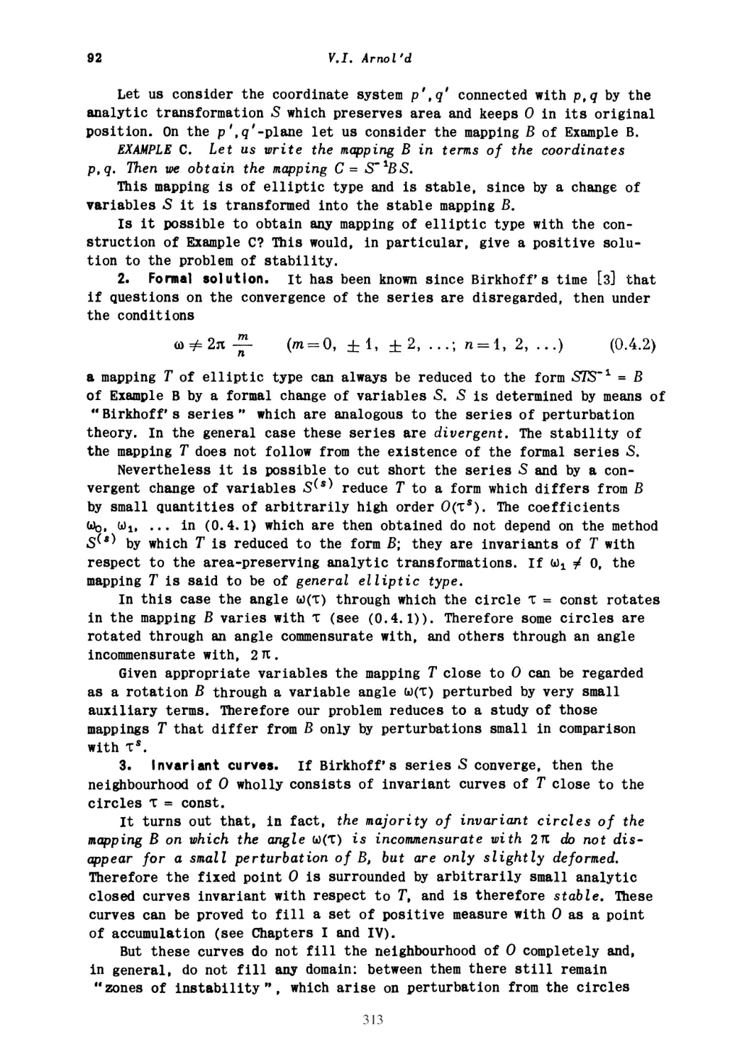
/


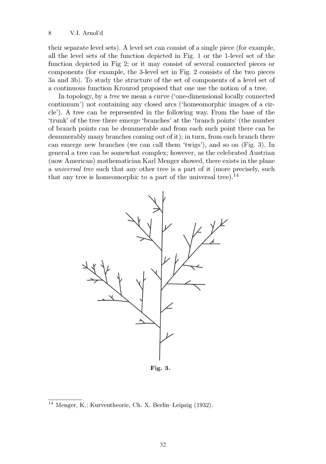
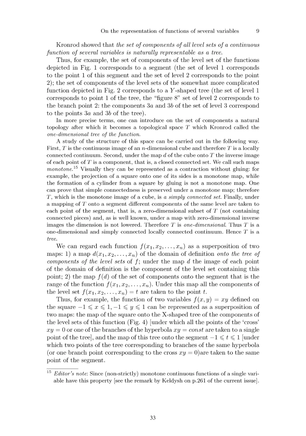
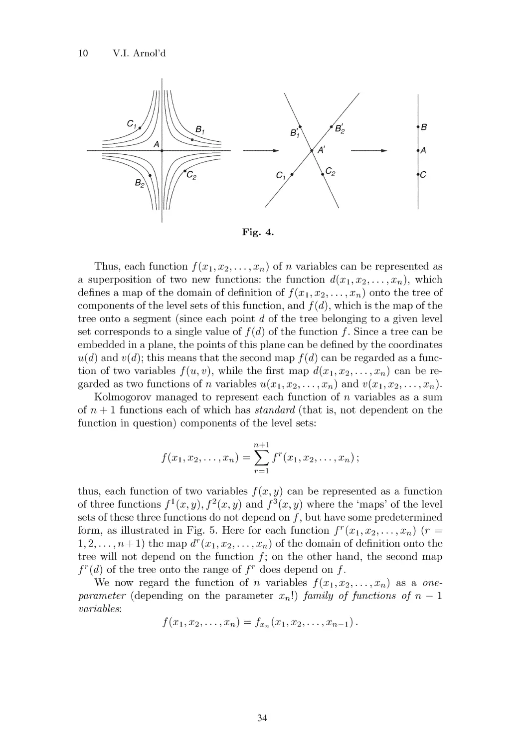


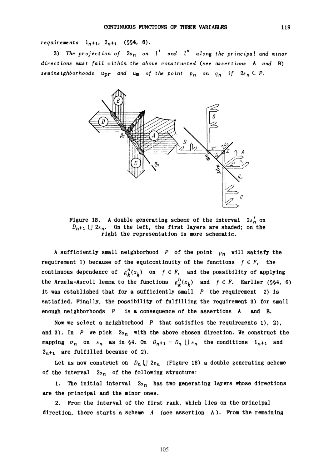


Текст
VLADIMIR I. ARNOLD
Collected Works
4y Spri
ringer
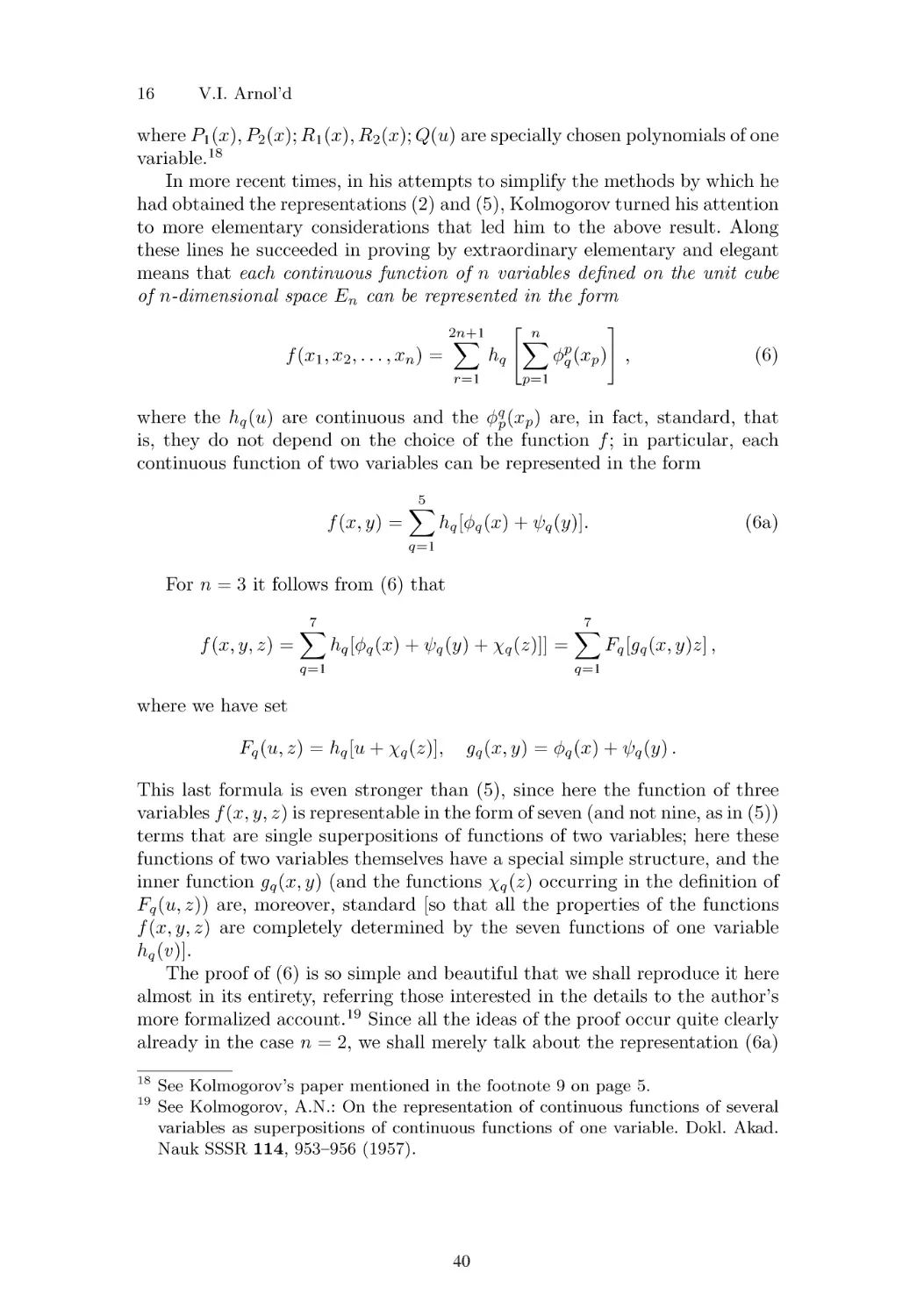
VLADIMIR I. ARNOLD
Collected Works
VLADIMIR I. ARNOLD
Collected Works
volume ι
Representations of Functions, Celestial Mechanics
and KAM Theory, 1957-1965
VLADIMIR I. ARNOLD
Collected Works
VOLUME I
Representations of Functions, Celestial Mechanics
and KAM Theory, 1957-1965
Edited by
Alexander B. Givental
Boris A. Khesiti
Jerrold E. Marsden
Alexander N. Varchenko
Victor A. Vassilev
Oleg Ya. Viro
Vladimir M. Zakalyukin
Sprin
ger
Vladimir I. Arnold
Russian Academy of Sciences
Steklov Mathematical Institute
ul. Gubkina 8
Moscow 117966
Russia
Editors
A.B. Givental, B.A. Khesin, J.E. Marsden, A.M. Varchenko,
V.A. Vassilev, O.Ya. Viro, V.M. Zakalyukin
ISBN 978-3-642-01741-4 e-ISBN 978-3-642-01742-1
DOI 10.1007/978-3-642-01742-1
Springer Dordrecht Heidelberg London New York
Library of Congress Control Number: 2009931933
© Springer-Verlag Berlin Heidelberg 2009
This work is subject to copyright. All rights are reserved, whether the whole or part of the material
is concerned, specifically the rights of translation, reprinting, reuse of illustrations, recitation.
broadcasting, reproduction on microfilm or in any other way, and storage in data banks.
Duplication of this publication or parts thereof is permitted only under the provisions of the
German Copyright Law of September 9, 1965, in its current version, and permission for use must
always be obtained from Springer. Violations are liable to prosecution under the German
Copyright Law.
The use of general descriptive names, registered names, trademarks, etc. in this publication does
not imply, even in the absence of a specific statement, that such names are exempt from the
relevant protective laws and regulations and therefore free for general use.
Cover design: WMXDesign GmbH, Heidelberg
Printed on acid-free paper
Springer is part of Springer Science+Business Media (www.springer.com)
Preface
Vladimir Igorevich Arnold is one of the most influential mathematicians of our time.
V.I. Arnold launched several mathematical domains (such as modern geometric mechanics,
symplectic topology, and topological fluid dynamics) and contributed, in a fundamental
way, to the foundations and methods in many subjects, from ordinary differential equations
and celestial mechanics to singularity theory and real algebraic geometry. Even a quick
look at a partial list of notions named after Arnold already gives an overview of the variety
of such theories and domains:
KAM (Kolmogorov-ArnokHVloser) theory,
The Arnold conjectures in symplectic topology,
The Hubert-Arnold problem for the number of zeros of abelian integrals,
Arnold's inequality, comparison, and complexification method in real algebraic geometry,
Arnold-Kolmogorov solution of Hubert's 13th problem,
Arnold's spectral sequence in singularity theory,
Arnold diffusion,
The Euler-Poincare-Arnold equations for geodesies on Lie groups,
Arnold's stability criterion in hydrodynamics,
ABC (Amold-Beltrami-Childress) flows in fluid dynamics,
The Arnold-Korkina dynamo,
Arnold's cat map,
The Arnold-Liouville theorem in integrable systems,
Arnold's continued fractions,
Arnold's interpretation of the Maslov index,
Arnold's relation in cohomology of braid groups,
Arnold tongues in bifurcation theory,
The Jordan-Arnold normal forms for families of matrices,
The Arnold invariants of plane curves.
Arnold wrote some 700 papers, and many books, including 10 university textbooks. He
is known for his lucid writing style, which combines mathematical rigour with physical and
geometric intuition. Arnold's books on Ordinary differential equations and Mathematical
methods of classical mechanics became mathematical bestsellers and integral parts of the
mathematical education of students throughout the world.
VII
Some Comments on V.I. Arnold's Biography and Distinctions
V.L Arnold was born on June 12, 1937 in Odessa, USSR. In 1954-1959 he was a student at
the Department of Mechanics and Mathematics, Moscow State University. His M.Sc.
Diploma work was entitled "On mappings of a circle to itself." The degree of a "candidate
of physical-mathematical sciences" was conferred to him in 1961 by the Keldysh Applied
Mathematics Institute, Moscow, and his thesis advisor was A.N. Kolmogorov. The thesis
described the representation of continuous functions of three variables as superpositions of
continuous functions of two variables, thus completing the solution of Hubert's 13th
problem. Arnold obtained this result back in 1957, being a third year undergraduate student. By
then A.N. Kolmogorov showed that continuous functions of more variables can be
represented as superpositions of continuous functions of three variables. The degree of a "doctor
of physical-mathematical sciences" was awarded to him in 1963 by the same Institute for
Arnold's thesis on the stability of Hamiltonian systems, which became a part of what is
now known as KAM theory.
After graduating from Moscow State University in 1959, Arnold worked there until 1986
and then at the Steklov Mathematical Institute and the University of Paris IX.
Arnold became a member of the USSR Academy of Sciences in 1986. He is an Honorary
member of the London Mathematical Society (1976), a member of the French Academy of
Science (1983), the National Academy of Sciences, USA (1984), the American Academy of
Arts and Sciences, USA (1987), the Royal Society of London (1988), Academia Lincei
Roma (1988), the American Philosophical Society (1989), the Russian Academy of Natural
Sciences (1991). Arnold served as a vice-president of the International Union of
Mathematicians in 1999-2003.
Arnold has been a recipient of many awards among which are the Lenin Prize (1965,
with Andrey Kolmogorov), the Crafoord Prize (1982, with Louis Nirenberg), the Loba-
chevsky Prize of Russian Academy of Sciences (1992), the Harvey prize (1994), the Dannie
Heineman Prize for Mathematical Physics (2001), the Wolf Prize in Mathematics (2001),
the State Prize of the Russian Federation (2007), and the Shaw Prize in mathematical
sciences (2008).
One of the most unusual distinctions is that there is a small planet Vladarnolda,
discovered in 1981 and registered under #10031, named after Vladimir Arnold. As of 2006 Arnold
was reported to have the highest citation index among Russian scientists.
In one of his interviews V.L Arnold said: "The evolution of mathematics resembles the
fast revolution of a wheel, so that drops of water fly off in all directions. Current fashion
resembles the streams that leave the main trajectory in tangential directions. These streams
of works of imitation are the most noticeable since they constitute the main part of the total
volume, but they die out soon after departing the wheel. To stay on the wheel, one must
apply effort in the direction perpendicular to the main flow."
With this volume Springer starts an ongoing project of putting together Arnold's work
since his very first papers (not including Arnold's books.) Arnold continues to do research
and write mathematics at an enviable pace. From an originally planned 8 volume edition of
his Collected Works, we already have to increase this estimate to 10 volumes, and there
may be more. The papers are organized chronologically. One might regard this as an
attempt to trace to some extent the evolution of the interests of V.L Arnold and cross-
fertilization of his ideas. They are presented using the original English translations, when-
VIII
ever such were available. Although Arnold's works are very diverse in terms of subjects,
we group each volume around particular topics, mainly occupying Arnold's attention
during the corresponding period.
Volume I covers the years 1957 to 1965 and is devoted mostly to the representations of
functions, celestial mechanics, and to what is today known as the KAM theory.
Acknowledgements. The Editors thank the Gottingen State and University Library and the Caltech library
for providing the article originals for this edition. They also thank the Springer office in Heidelberg for its
multilateral help and making this huge project of the Collected Works a reality.
March 2009 Alexander Givental
Boris Khesin
Jerrold Marsden
Alexander Varchenko
Victor Vassiliev
Oleg Viro
Vladimir Zakalyukin
IX
Contents
1 On the representation of functions of two variables in the form /[$*)+ уАу)\
Uspekhi Mat. Nauk 12, No. 2, 119-121 (1957); translated by Gerald Gould.............. 1
2 On functions of three variables
Amer. Math. Soc. Transl. (2) 28 (1963), 51-54. Translation ofDokl. Akad.
NaukSSSR 114:4 (1957), 679-681.........................................]..................................... 5
3 The mathematics workshop for schools at Moscow State University
Mat. Prosveshchenie 2, 241-245 (1957); translated by Gerald Gould........................ 9
4 The school mathematics circle at Moscow State University:
harmonic functions (in Russian)
Mat. Prosveshchenie 3 (1958), 241-250.................................................................... 15
5 On the representation of functions of several variables as a superposition
of functions of a smaller number of variables
Mat. Prosveshchenie 3, 41-61 (1958); translated by Gerald Gould.......................... 25
6 Representation of continuous functions of three variables
by the superposition of continuous functions of two variables
Amer. Math. Soc. Transl. (2) 28 (1963), 61-147. Translation of Mat. Sb. (n.S.)
48 (90): 1 (1959), 3-74 Corrections in Mat. Sb. (n.S.) 56 (98) :3 (1962), 392 ............ 47
7 Some questions of approximation and representation of functions
Amer. Math. Soc. Transl. (2) 53 (1966), 192-201. Translation ofProc. Internat.
Congress Math. (Edinburgh, 1958), Cambridge Univ. Press, New York, 1960,
pp. 339-348.............................^^^
8 Kolmogorov seminar on selected questions of analysis
UspekhiMat. Nauk 15, No. 1, 247-250 (1960); translated by Gerald Gould.......... 144
9 On analytic maps of the circle onto itself
Uspekhi Mat. Nauk 15, No. 2, 212-214 (1960) (Summary of reports announced
to the Moscow Math. Soc); translated by Gerald Gould......................................... 149
10 Small denominators. I. Mapping of the circumference onto itself
Amer. Math. Soc. Transl. (2) 46 (1965), 213-284. Translation oflzv.
Akad. Nauk SSSR Ser. Mat. 25:1 (1961). Corrections inlzv. Akad. Nauk
SSSRSer. Mat. 28:2 (1964), 479-480...................................................................... 152
XI
11 The stability of the equilibrium position of a Hamiltonian system
of ordinary differential equations in the general elliptic case
Soviet. Math. Dokl. 2 (1961). Translation of Dokl. Akad. Nauk
SSSR 137:2 (1961), 255-257 ^^^^^^^^^^^^^^^^^^^^^^^^^^^^^^^^^^^^^^^^ss 224
12 Generation of almost periodic motion from a family of periodic motions
Soviet. Math. Dokl. 2 (1961). Translation of Dokl. Akad. Nauk
SSSR 138:1 (1961) /3-/5...........................*.............................................................. 227
13 Some remarks on flows of line elements and frames
Soviet. Math. Dokl. 2 (1961). Translation of Dokl. Akad. Nauk
SSSR 138:2 (1961), 255-257 ^^^^^^^^^^^^^^^^^^^^^^^^^^^^^^^^^^^^^^^^ss 230
14 A test for nomographic representability using Decartes' rectilinear abacus
(in Russian)
UspekhiMat. Nauk 16:4 (1961) ............................................................................... 233
15 Remarks on winding numbers (in Russian)
Sibirsk. Mat. Z. 2:6 (1961), ^7^7J........................................................................ 236
16 On the behavior of an adiabatic invariant under slow periodic variation
of the Hamiltonian
Soviet. Math. Dokl. 3 (1962). Translation of Dokl. Akad. Nauk
SSSR 142:4 (1962), 758-761 .^^^^^.^^^^L.^^^^^^^^^^^^^^^^^^^^^^^^.^.^^^^2^
17 Small perturbations of the automorphisms of the torus
Soviet. Math. Dokl. 3 (1962). Translation of Dokl. Akad. Nauk
SSSR 144:2 (1962), 695-698, Corrections in Dokl. Akad. Nauk
SSSR, 1963, 150:5, P55............................................................................................. 248
18 The classical theory of perturbations and the problem of stability
of planetary systems
Soviet. Math. Dokl. 3 (1962). Translation of Dokl. Akad. Nauk
SSSR 145:3 (1962), 487-490^^^^^^^^^^^^^^^^^^^^^^^^^^^^^^^^^^^^^^^^^ 253
19 Letter to the editor (in Russian)
Mat.Sb. (n.S.) 56 (98):3 (1962), 392^^^^^^^^^^^^^^^^^^^^^^^^^^^^^^^^^^ss^25^
20 Dynamical systems and group representations at the Stockholm
Mathematics Congress (in Russian)
[/^/M^fcH^fMJj ^ .................259
21 Proof of a theorem of A. N. Kolmogorov on the invariance
of quasi-periodic motions under small perturbations of the Hamiltonian
Russian Math. Surveys 18 (1963). Translation of Uspekhi Mat. Nauk
18:5(1963), 75-^0...................................................................................................2
22 Small denominators and stability problems in classical
and celestial mechanics (in Russian)
Problems of the motion of artificial satellites. Reports at the conference on general
applied topics in theoretical astronomy (Moscow, 20-25 November 1961), USSR
Academy of Sciences Publishing House, Moscow, 1963, pp. 7-17.......................... 295
XII
23 Small denominators and problems of stability of motion in classical
and celestial mechanics
Russian Math Surveys 18 (1963). Translation ofUspekhiMat. Nauk
18:6 (1963), 91-192, Corrections in Uspekhi Mat Nauk 22:5 (1968), 276............. 306
24 Uniform distribution of points on a sphere and some ergodic properties
of solutions of linear ordinary differential equations in a complex region
Soviet Math Dokl 4 (1963). Translation ofDokl. Akad. Nauk
SSSR 148:1 (1963), 9-12 ..........................................................................................413
25 On a theorem of Liouville concerning integrable problems of dynamics
Amer. Math Soc. Transl. (2) 61(1967) 292-296. Translation ofSibirsk
Mat.Z. 4:2(1963)....................................................................................................^
26 Instability of dynamical systems with several degrees of freedom
Soviet Math Dokl. 5 (1964). Translation of Dokl. Akad. Nauk
SSSR 156:1 (1964), 9-72..........................................................................................423
27 On the instability of dynamical systems with several degrees of freedom
(in Russian)
Uspekhi Mat. Nauk 19:5 (1964), 181 .......................................................................428
28 Errata to V.I. Arnol'd's paper: "Small denominators. I."
Izv. Akad. Nauk SSSR Ser. Mat. 28, 479-480 (1964);
translated by Gerald Gould......................................................................................433
29 Small denominators and the problem of stability in classical
and celestial mechanics (in Russian)
Proceedings of the Fourth АН-Union Mathematics Congress (Leningrad,
3-12 July 1961), vol. 2, Nauka, Leningrad, 1964, pp. 403-409...............................4ЪЪ
30 Stability and instability in classical mechanics (in Russian)
Second Math. Summer School, Part 11 (Russian), Naukova Dumka, Kiev,
1965,pp. 85-119...................................................................................................... 4
31 Conditions for the applicability, and estimate of the error, of an averaging
method for systems which pass through states of resonance in the course
of their evolution
Soviet Math. Dokl. 6 (1965). Translation of Dokl. Akad. Nauk SSSR
161:1 (1965), 9-12 ................................................................................................... 477
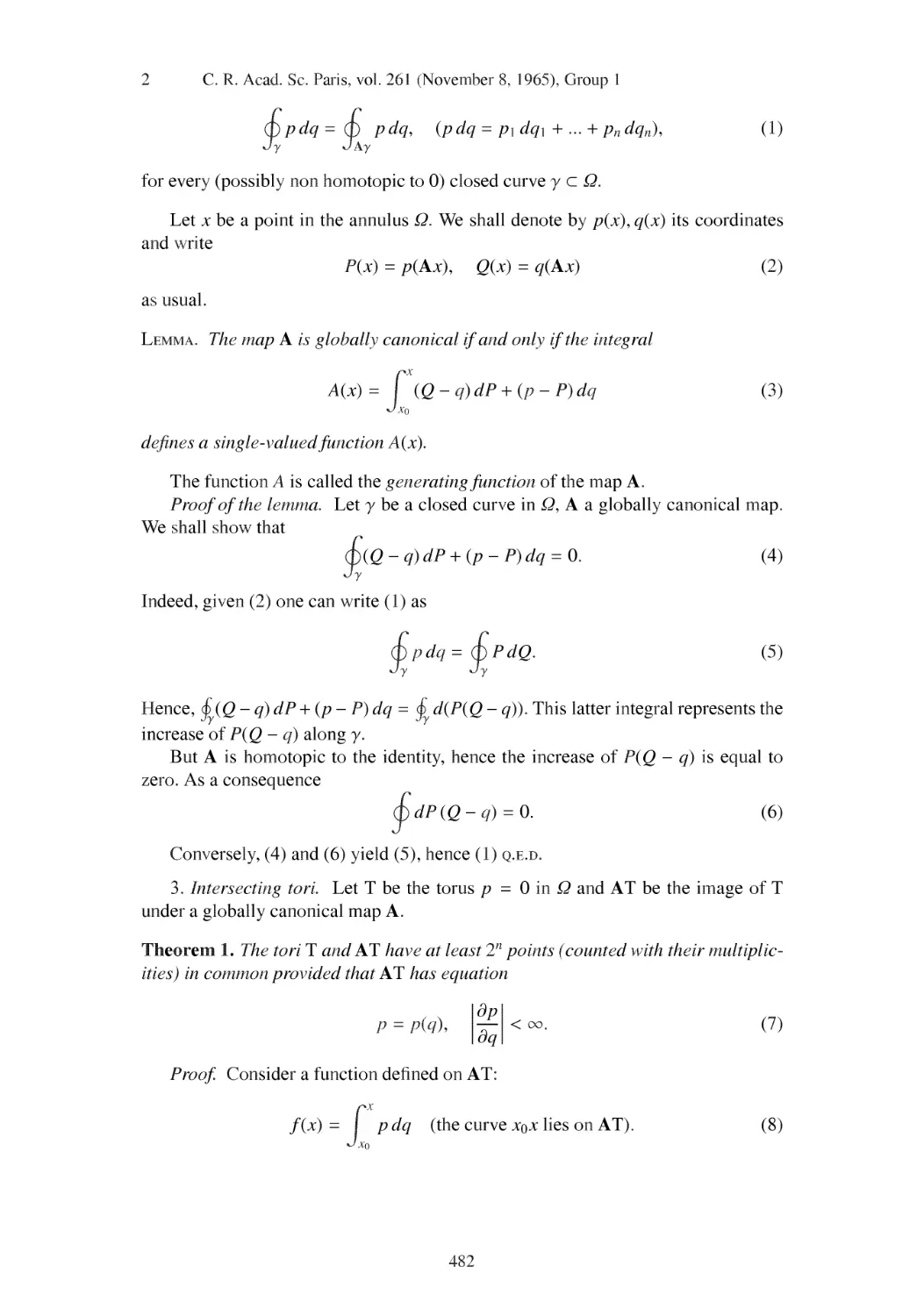
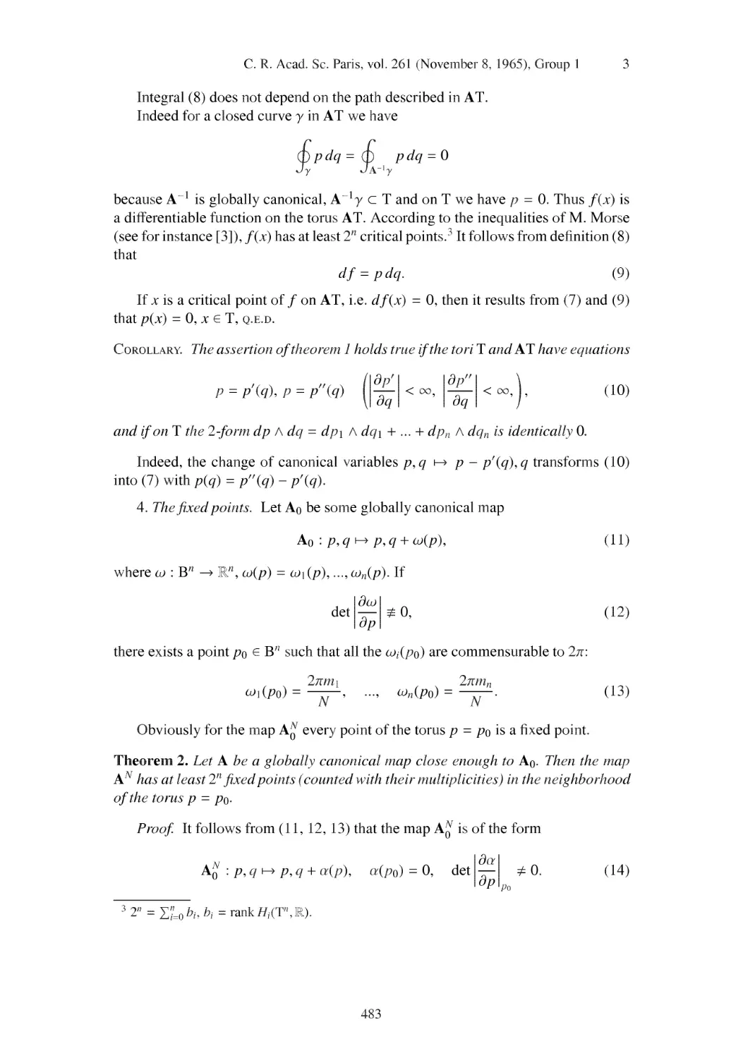
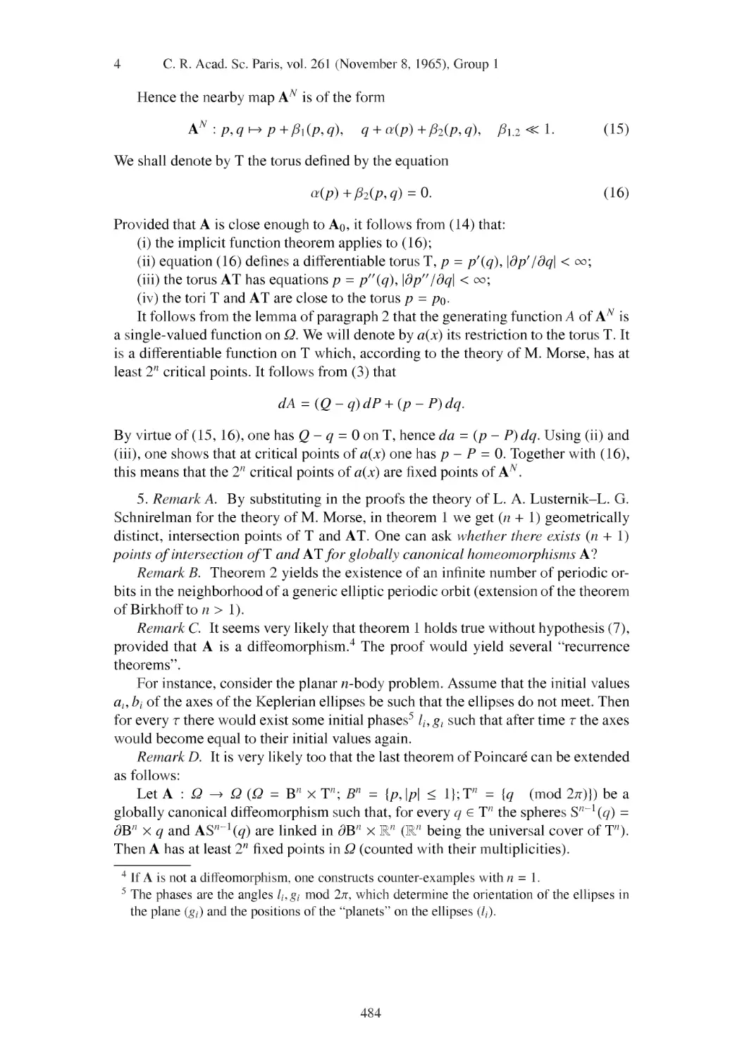
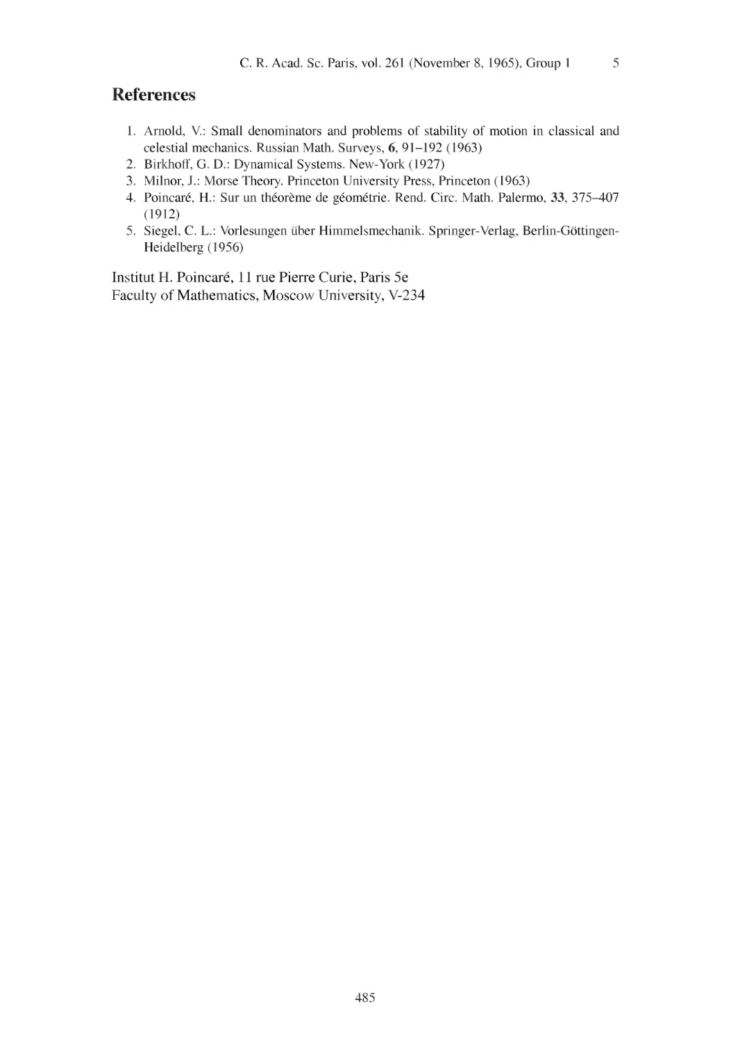
32 On a topological property of globally canonical maps
in classical mechanics
Translation of Sm une propriete topologique des applications globalement
canoniques de la mecanique classique. С R. Acad. Sci. Paris 261:19
(1965) 3719-3722; translated by Alain Chenciner and Jaques Fejoz......................481
XIII
ON THE REPRESENTATION OF
FUNCTIONS OF TWO VARIABLES IN THE
¥ОКМХ[ф(х)+ф(у)]*
V.I. Arnol'd
translated by Gerald Gould
1. Kolmogorov proved [1] that the set of functions of two variables repre-
sentable as a certain combination of continuous functions of one variable and
addition is everywhere dense in the space C(E2) of continuous functions
defined on the square E2. It follows immediately from our result proved below
that this is not true for the simplest combinations: the set of functions of the
form χ[φ(χ) + φ (у)] even turns out to be nowhere dense in C(E2) .
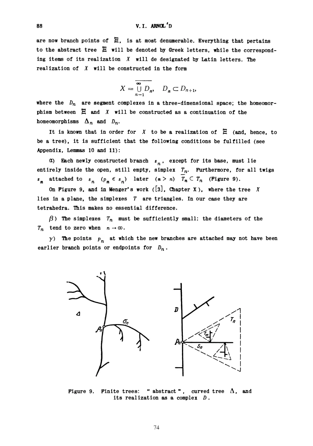
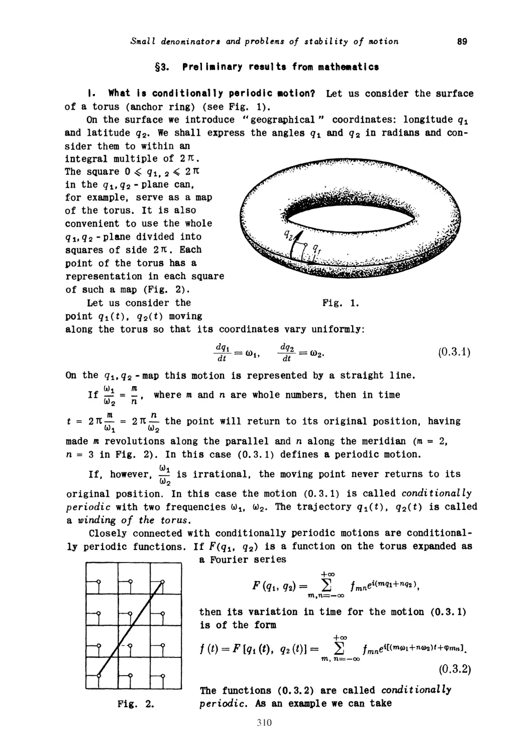
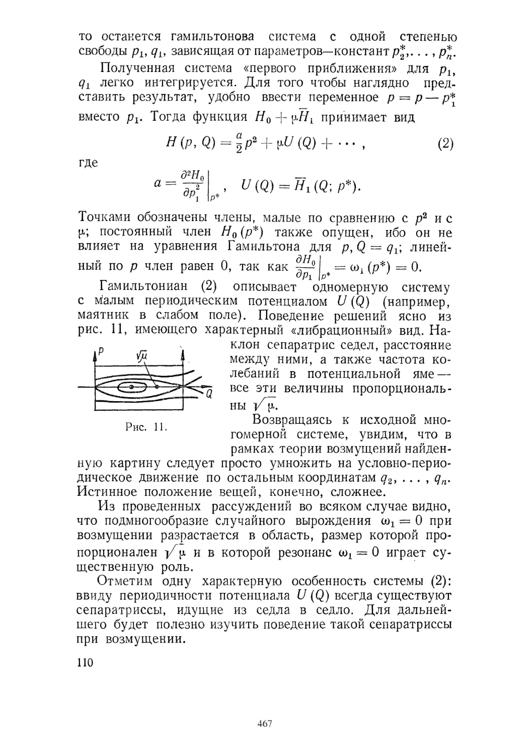
Fig. 1.
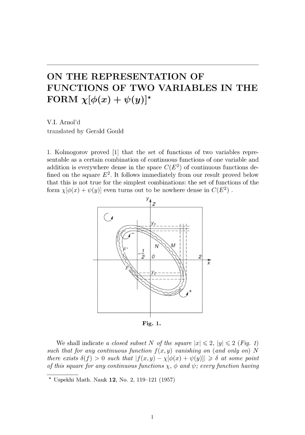
We shall indicate a closed subset N of the square \x\ ^ 2, \y\ ^ 2 (Fig. 1)
such that for any continuous function f(x,y) vanishing on (and only on) N
there exists 6(f) > 0 such that \f(x,y) — χ[φ(χ) + ф(у)}\ ^ δ at some point
of this square for any continuous functions χ, φ and φ; every function having
Uspekhi Math. Nauk 12, No. 2, 119-121 (1957)
1
2 V.I. Arnol'd
TV as its level set is 'with a neighbourhood' non-representable in the form
х[ф(х)+ф(у)] · An example of such a set N is the ellipse (x + y)2 + ^x~^ = 1.
We shall prove this. Since f(x,y) is of constant sign outside the ellipse
we can assume that f(x,y) > 0 there. Then clearly there exists δ > 0 such
that /(ж, у) > 2δ at all points in the region G = (x + y)2 + ^~^ > |, that
is, outside the ellipse Μ = (χ + у)2 + ^~^ = | Suppose that there exist
continuous functions φ (ж), ф (у), χ(ζ) such that \/(х,у)—х[ф(х) — ф(у)]\ < δ^
for all (ж,?/), 2 ^ ж, у ^ 2. Then the inequality χ[0(χ) + г/>(г/)] < ^ holds on
TV and the inequality χ[φ(χ) + φ (у)] > δ holds on M.
The largest open connected sets G~ D TV and G+ D G* where χ[φ(χ) +
φ (у)] < δ and χ[φ(χ) + г/>(г/)] > ^ respectively, are separated by the closed
set F where χ[φ(χ) + φ (у)] = δ (that is, each continuum intersecting G~ and
G+ also intersects F), because the continuous function χ[φ(χ) + φ (у)] on a
continuum takes all values between any two given values. By a well-known
theorem (Theorem Ε in [2]) the boundary of G+ has a component F' С F
already separating G~ and G+, and hence Μ and TV. We claim that the
continuous function φ(χ) + φ (у) is constant on F'. Indeed, suppose that, on
the contrary, z\ = ф{х) + ф(у)\а < Ф(х) + Ф(у)\ъ = ^2, where α, b G F'. Then
in a sufficiently small neighbourhood of a there is a point a' G G+ where
0(x) + ф(у) < z\ + Z23Zl, and in a sufficiently neighbourhood of b there is a
point b' G G+ where </>(x) + г/>(г/) > Z2 — ^2^i· Therefore on a polygonal line
joining a' and b' in G+ there is a point с where ф(х)+ф(у) = Zl\Z2; also there
is a point с on the continuum F' where </>(x) + ф(у) = Zl\Z2 · Consequently,
Х^яО+г/^г/)]^/ = x[^(x) + V;(l/)]|c, which contradicts the conditions c' G G+,
ceF'.
We denote by ζ the unique value of ф(х)-\-ф(у) at points of F'. Then on the
intervals χ = — |, у G [1.1,1.22] and χ = — |, у G [—0.62, —0.5] intersecting Μ
and TV there are points ( — J>, г/χ) and ( — |, г/2) at which ф{х)+ф(у) = ζ. There
is such a point (xi, г/2) on the interval on which the line у = г/2 intersects the
strip between Μ and TV for χ > 0.
It follows from the equalities**
Ф{-\)+ФШ =z,
ф(-\) + ФЫ = *,
0(xi) +Ф(У2) = Ζ
that ф(х\) + ф(у\) = ζ and X^^O+VK^)] = 5. However, it is easy to see that
the point (хьг/ι) lies in G, therefore χ[0(χι) + φ (у 2)] > ^· This contradiction
proves the 'stable' non-representability of f(x,y) in the form χ[φ(χ) + φ (у)]',
* Translator's note: This should be |/(ж,г/) — х[</>(ж) + г/>(г/)]| < 5.
* Translator's note: This should be G+ D Μ.
** Translator's note: The second of these inequalities contains a misprint. It should
read ф{-\) +Ф{У2) = ζ.
2
On the representation of functions of two variables 3
in particular, for the function /(ж, у) = (ж + у)2 -\-\{х — у)2 — 1 we can choose
2. LA. Weinstein proved that the class of continuous functions of the form
χ[φ(χ) +Ф(у)] that are strictly monotone in each variable is a closed subset of
C(E2). Here the strict monotonicity is essential: we claim that the function xy
is not representable in the form χ[φ(χ) + φ (у)] even though it is the uniform
limit of the sequence of functions ехр(1п(х + ^)+1п(г/+^)); which do have the
form χ[φ(χ) + φ (у)] (where фп(х) = фп(х) = Ы(х + ±) and χ(ζ) = exp(z)).
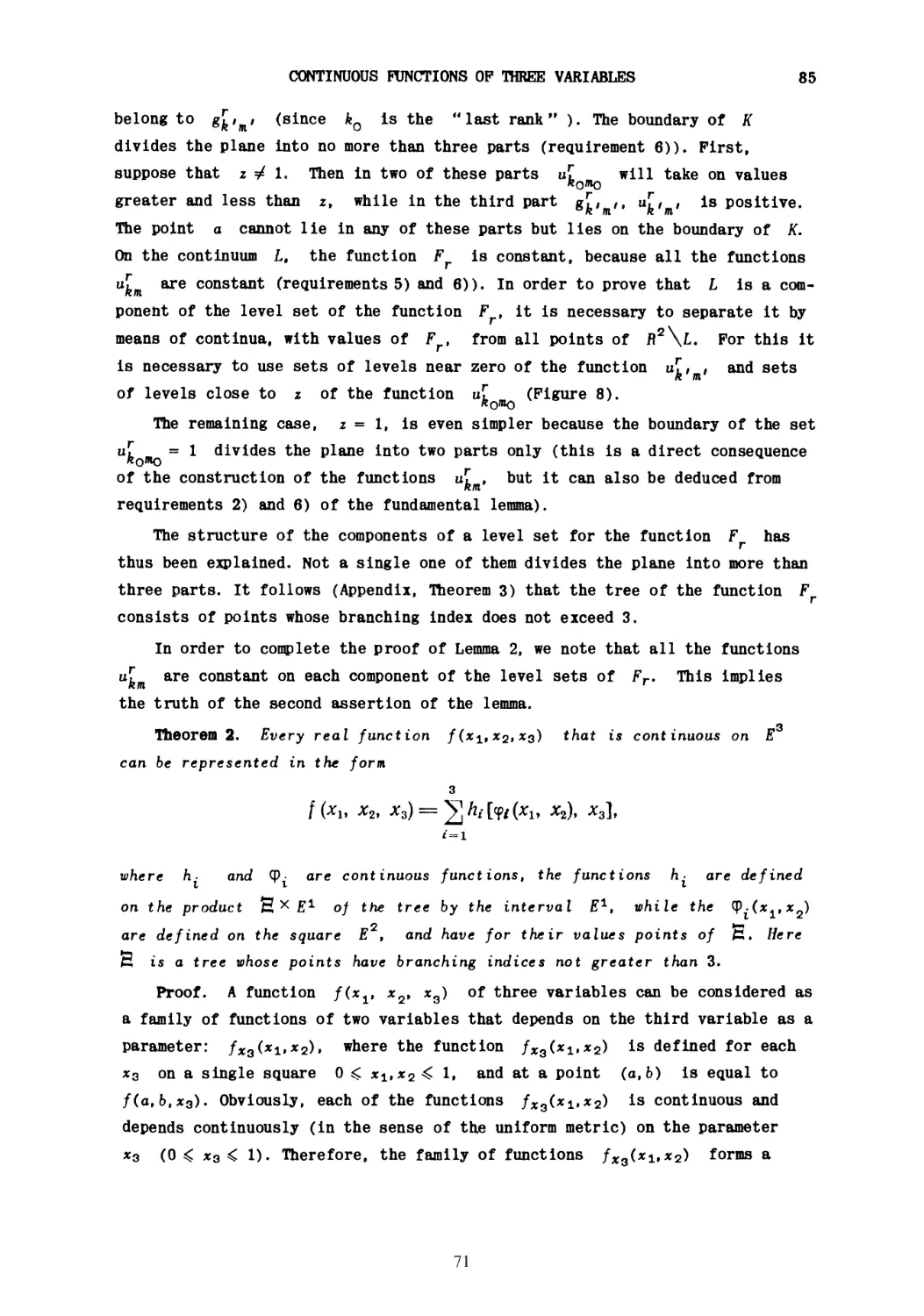
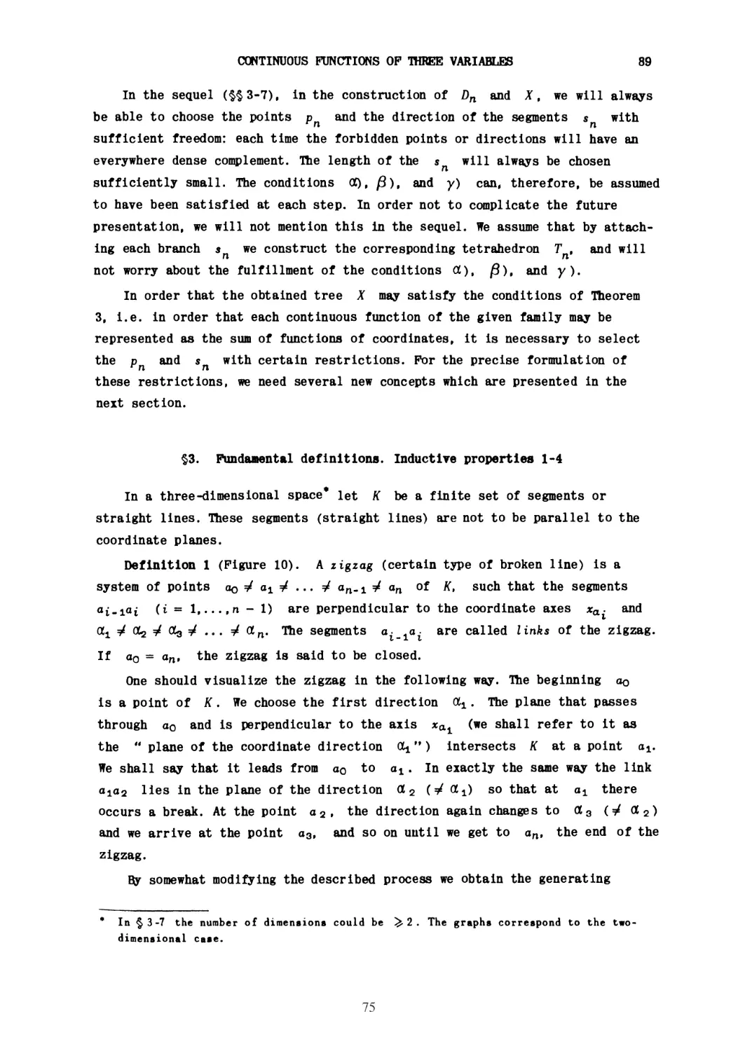
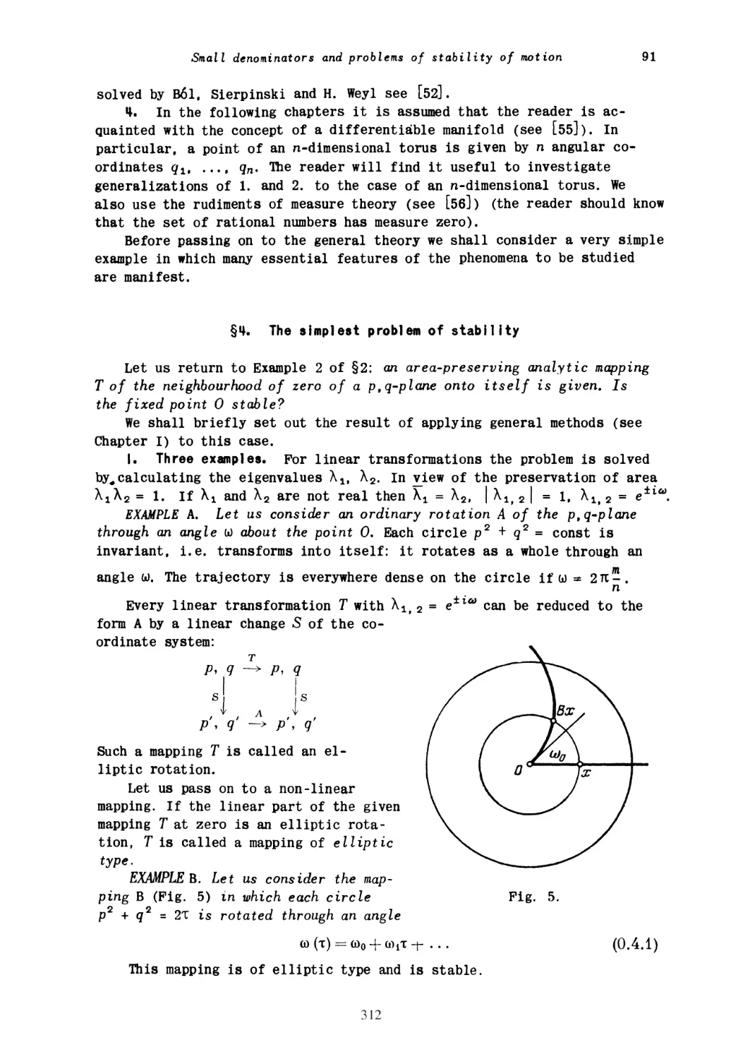
Fig. 2.
In fact, if χ[φ(χ) + φ (у)] = xy everywhere in the square х,г/ G [0,1],
then the function ф(х) + ф(у) would take the same value at the points (0, 0),
(0,1), and (1,0). Indeed, any two of these three points can be joined by a
polygonal line having no common points with the set xy = 0 apart from the
end points, and also by a polygonal line lying entirely in this set. If ф{х) +
ф(у) took different values a and b at these end points (see Fig. 2), then the
intermediate value ^^ would be taken both on the set xy = 0 and outside
a+b\
2
this set, which would mean that x(^J^) = 0 and χ{9ή^-) > 0 simultaneously.
This contradiction proves that ф(0)+ф(0)
φ(0) + φ(0) = φ(1) + φ(ΐ) and therefore
0 = хШ + ФЩ=х[4
= ф(0)+ф(1) = ф(1) + ф(0); hence
(1)+^(1)] = 1.
(ж), φ (у), χ(ζ) such that
In other words, there do not exist any functions
χ[φ{χ) + ф(у)\ =ху.
We also point out that the first example of a continuous function not
representable in the form χ[φ(χ) + ф(у)] (obtained simultaneously by A.A. Kirillov
and the author), namely, the function /(ж, у) = min(x, у) (where ж, у е [0,1])
can also be approximated to arbitrary precision by functions of the form
χ[φ(χ) + Ф(у)].
Received 26 December 1956
3
4 V.I. Arnol'd
References
[1] Kolmogorov, A.N.: On the representation of continuous functions of several
variables as a superposition of continuous functions of a smaller number of
variables. Dokl. Akad. Nauk SSSR 108, No, 2 (1956).
[2] Krondov, A.S.: On functions of two variables. Usp. Mat. Nauk 5, No, 1 (1950).
4
ON FUNCTIONS OF THREE VARIABLES
V.I. ARNOL'D
In the present paper there is indicated a method of proof of a theorem
which yields a complete solution of the 13th problem of Hilbert (in the sense
of a denial of the hypothesis expressed by Hilbert).
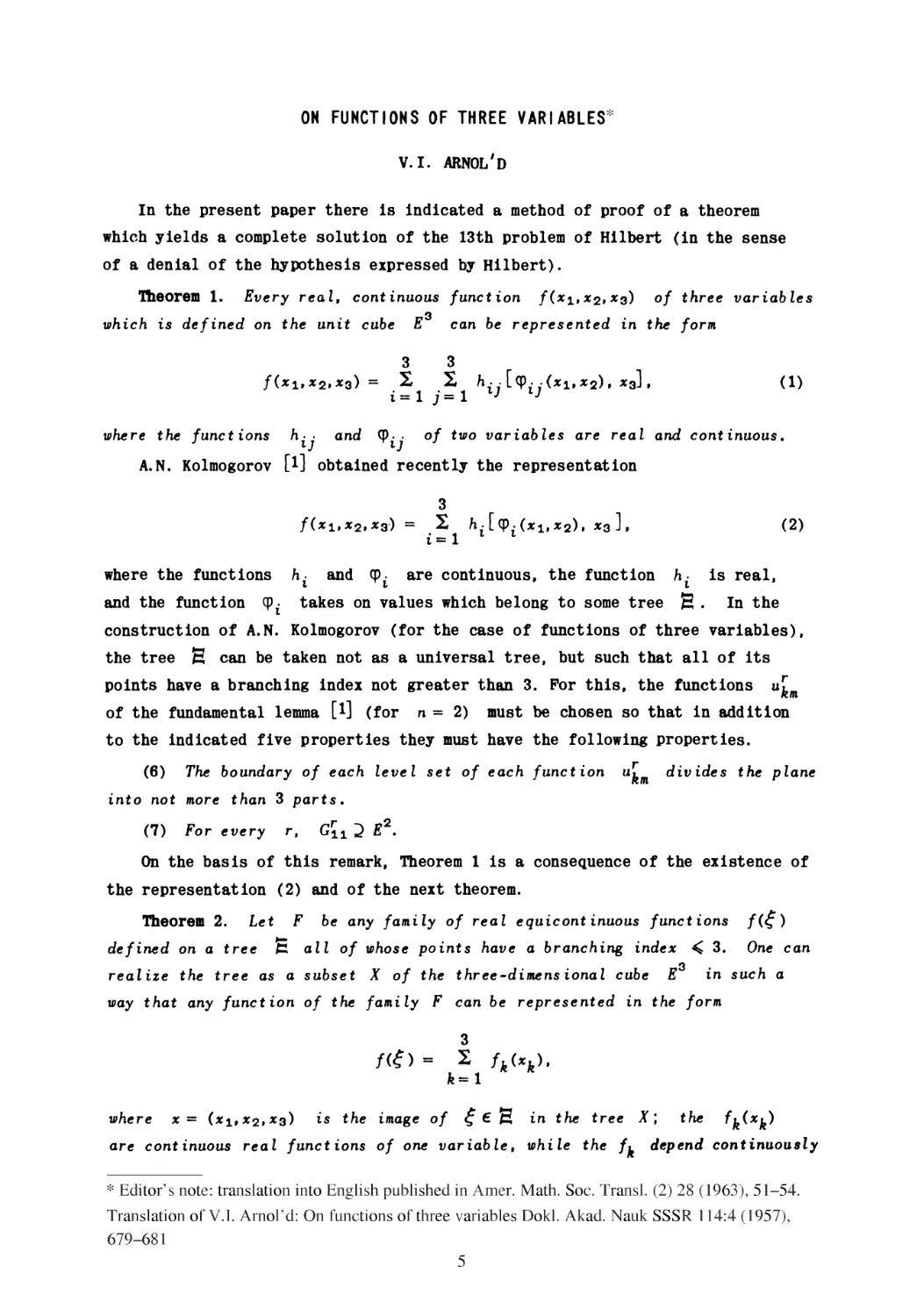
Theorem 1. Every real, continuous function /(*1,*2»*з) of three variables
which is defined on the unit cube Ε can be represented in the form
/{«1,«2.*з) = Σ Σ h- · [φ··(*ι,*2). *3J »
i = 1 j = 1 lJ lJ
where the functions h- · and φ. . of two variables are real and continuous.
lJ lJ
A.N. Kolmogorov Μ obtained recently the representation
(1)
о
/(*1,*2.*3-) = Σ h.[(p.(xitX2)t X3],
i= 1 l l
(2)
where the functions hi and φ^ are continuous, the function h^ is real,
and the function φ^ takes on values which belong to some tree S . In the
construction of A.N. Kolmogorov (for the case of functions of three variables),
the tree S can be taken not as a universal tree, but such that all of its
points have a branching index not greater than 3. For this, the functions u[
Rill
of the fundamental lemma [4 (for η = 2) must be chosen so that in addition
to the indicated five properties they must have the following properties.
(6) The boundary of each level set of each function и· divides the plane
into not more than 3 parts.
(7) For every r, Gr±1 2 E2.
On the basis of this remark, Theorem 1 is a consequence of the existence of
the representation (2) and of the next theorem.
Theorem 2. Let F be any family of real e qui continuous functions f(£)
defined on a tree β all of whose points have a branching index К 3. One can
3
realize the tree as a subset X of the three-dimensional cube Ε in such a
way that any function of the family F can be represented in the form
3
/(£) - Σ fk(xk)t
where x= (х±,Х2,хэ) is the image of ςβ д in the tree X \ the fK(xK)
are continuous real functions of one variable, while the /· depend continuously
* Editor's note: translation into English published in Amer. Math. Soc. Transl. (2) 28 (1963), 51-54.
Translation of V.I. Arnol'd: On functions of three variables Dokl. Akad. Nauk SSSR 114:4 (1957),
679-681
5
52
V.I. ARNOL'D
on f (in the sense of uniform convergence).
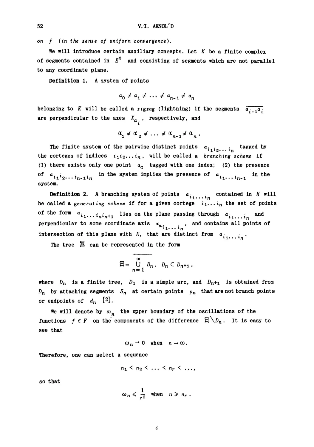
We will introduce certain auxiliary concepts. Let К be a finite complex
of segments contained in E3 and consisting of segments which are not parallel
to any coordinate plane.
Definition 1. A system of points
aQ4 a^4 ... 4 an^¥ α„
belonging to К will be called a zigzag (lightning) if the segments a~~cT
are perpendicular to the axes Xa , respectively, and
i
The finite system of the pairwise distinct points a- · ,· tagged by
lll2···ln
the corteges of indices ίιΐ2.·.ίη· wil1 be called a branching scheme if
(1) there exists only one point aQ tagged with one index; (2) the presence
of a · ν in the system implies the presence of a ■ in the
system.
Definition 2. A branching system of points α· ,· contained in К will
ιι···ln
be called a generating scheme if for a given cortege i±...in the set of points
of the form α· ί„ν„+<1 lies on the plane passing through a· · and
1* * * П П'Х "1· · · "Π
perpendicular to some coordinate axis *_. . , and contains all points of
ati...tn
intersection of this plane with K, that are distinct from a· . .
il. . . in
The tree Ε can be represented in the form
fi- U^ Dnt DnCVb
n= 1
where Dn is a finite tree, D± is a simple arc, and Ζ)η+ι is obtained from
Dn by attaching segments Sn at certain points pn that are not branch points
or endpoints of dn
We will denote by ωη the upper boundary of the oscillations of the
functions f e F on the components of the difference n . It is easy to
see that
Therefore, one can select a sequence
Πι < П% < ... < Пг < ...,
so that
1_
Г2
соп < — when η > nr .
6
ON FUNCTIONS OP THREE VARIABLES 53
The realization X of the tree Η in E3 is constructed in the form
Д-1
where D^ is a complex of segments which realize Dn in such a way that the
images S^ of the arcs Sn are segments that are not perpendicular to the
coordinate axes.
00
Hie inductive construction of D^ is performed so that U D^ is a tree
n= 1
[2], and that the following conditions are satisfied.
(1) Every function f e F can be represented on Dn in the form
/(^) = feJi/^). (3)
where the /j?(*fc) depend continuously on /.
(2) The tree ϋ'η has for every point aQ a generating system issuing
from a±t and whose initial direction <tQ can be chosen arbitrarily.
(3) Let An be the set of points D^ which is the image of the branch
points of Ξ. Tbere exists a denumerable set Bn Q D*n , ΒηΓ\ An = 0 such that
the zigzag aQ ... an, which begins at aQ € Dn ni has no points in common
with An and no coincident points a= a., \4 j.
1 J
(4) If nr < η < nr+1 , then
\fk<*S-fkr^\< (8 + -^l^-) ~2. (4)
4 nr+1 - nr r2
This proof of the possibility of the inductive construction of the trees
D'n , and of the functions /jj with properties (1) to (4), is too complicated
to be given here. Roughly speaking, at each step the attached segment Sn+i is
chosen of very short length; its direction, and the way of mapping of Sn+! on
S^+i are selected so as to guarantee the fulfillment of properties (2) and (3)
by Dri+i· The preservation of equality (3), in the transition from η to
η + 1, on the newly attached segment Sn+lt requires the introduction of a
correction /? 1 - /? , for at least one of the functions /£ , on the
projection S'+1 on the axis x^ . For the preservation of equality (3) on the
earlier constructed tree Dn, it is necessary to compensate for this correction
by means of new corrections for the functions f? on a number of other segments.
The exact method of the introduction of these corrections, we will not present
here. We only note the following: these corrections must be such that inequality
(4) will be preserved for η' = η + 1; if S^+i is chosen small enough, and if
7
54
V.I. ARNOL'D
its direction is chosen appropriately, it must be possible to produce it for
every function /£ on a finite system of non-intersecting segments of the axis
*k . In the proof of this possibility one makes use of the fact that the tree
D'n has properties (2) and (3).
The proof of the existence of the continuous function
fk(xk) = lim fk(xk)
n-»oo
and of the validity of the equation
/<£) = ]Σί fk(xk)
on the entire X, is not complicated.
I express my sincere thanks to A.N. Kolmogorov for the aid and advice I
have received from him in the preparation of this work.
Bibliography
[l] A,N. Kolmogorov, On the representation of continuous functions of several
variables by superpositions of continuous functions of a smaller number of
variables, Dokl. Akad. Nauk SSSR 108 (1956), 179-182. (Russian)
[2] K. Menger, Kurventheorie, Teubner, Leipzig, 1932.
Translated by:
H.P. Thielman
8
THE MATHEMATICS WORKSHOP FOR
SCHOOLS AT MOSCOW STATE
UNIVERSITY*
V.I. ArnoPd
Moscow
translated by Gerald Gould
The mathematics workshop for schools at Moscow State University in the
name of Lomonosov came into existence in 1935. The organizers of the
workshop were: the now-deceased Corresponding Member of the Academy of
Sciences of the USSR L.G. Shnirel'man, Professor L.A. Lyusternik (now
Corresponding Member of the Academy of Sciences of the USSR), and Doctor
I.M. Gel'fand (now Corresponding Member of the Academy of Sciences of the
USSR).
The activities of the workshop proceed in two streams: twice a month (on
Sundays) lectures on mathematics are given by professors and instructors at
Moscow State University and other institutes (separately for the pupils of the
7-8 class and for pupils of the 9-10 class) and sections of the mathematics
workshop meet weekly under the guidance of students and (more rarely)
postgraduate students of the university.1 The annual Mathematical Olympiad is, in
a certain sense, the culmination of the activities of the circle; here the directors
of the mathematics workshop traditionally play a large role in bringing this
about.
General information on the activities of the mathematics workshop in the
1955/56 academic year is given in the preceding issue of "Matematicheskh
Prosveshchenie"; there one can find the list of lectures given in that year.2
The series "Popular lectures on mathematics" published by Gostekhizdat will
give an idea of the character of these lectures.3 The main part of this series of
books by Moscow authors consists in expositions of the lectures given in the
mathematical circle for schools at Moscow State University. Here we wish to
shed light on the activities of the sections of the circle (the early part of these
* Mat. Prosveshchenie 2, 241-245 (1957)
1 It was only at the very beginning of the activities of the workshop that professors
of Moscow State University were also involved in the work of the sections.
2 Dynkin, E.B., Girsanov, IV.: The nineteenth School Mathematical Olympiad in
Moscow. Mat. Prosveshch. 2, No. 1, 187 (1957).
3 Editor's note: See the paper by N.B. Beskin on pp. 275-290 of this issue.
9
2 V.I. Arnol'd
activities is well reflected in the series of books "Library of the mathematical
circle", also published by Gostekhizdat).
The 'lessons' of a section take place in the form of a discussion: the
supervisor of the section introduces the topic of study to the participants; 5-10
minutes is set aside for each problem; then the solution is explained and
the supervisor continues his talk on the topic being studied. Each individual
problem is not difficult (most of the pupils manage it in 5-10 minutes). At the
end of the lesson the pupils are given (usually more difficult and sometimes
very difficult) homework problems, which are collected at the beginning of the
next lesson.
Below we give a summary account of two lessons of the workshop (a section
for 10 pupils) on the themes "Variation of a curve" and "Harmonic functions".
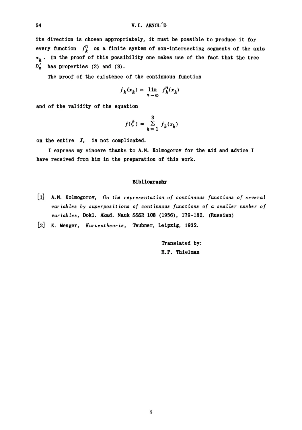
Variation of a curve
We are given a line segment AB of length 1. If this line segment is
illuminated by parallel rays, then the length of the shadow thrown onto various
lines will vary from 0 to 1. More precisely, the length of the projection of the
segment onto lines lying in the same plane will, in general be different for
different lines; however in all cases it will be between 0 and 1. The length of
the projection of AB onto a line I is called the variation of the segment AB
in the direction I (Fig. 1); we shall denote it by Vi(AB) or simply by V\ if it
is clear which segment we are referring to.
Fig. 1.
Fig. 2.
It is intuitively obvious that the mean value of the 'shadow' over all
directions exists and that it is between 0 and 1. More precisely, this means that if
we divide the 360° angle into η equal parts, and take the arithmetic mean
vn
vh + vl2 + ---vln
10
Mathematics workshop for schools at Moscow University 3
of the variations of the segment AB in the directions Ζ 1,^2,
then the limit
К
In (Fig. 2),
lim Vn
n—>oo
exists and К lies between 0 and 1.
This number К is called the mean variation or simply the variation of the
unit segment AB.
This number is not very difficult to find;4 it is equal to - ~ 0.637. However,
we shall not find it now, but calculate it later via an indirect route (Problem 7)
Nevertheless, we shall use the fact that this limit exists from the very outset.
Problem 1. What is the variation of a segment of length a?
Solution. Since, clearly, the variation of such a segment in any given
direction is a times as large as that of a unit segment parallel to it, and the
limit of this quantity, that is, the mean variation of the segment of length a,
is equal to К a.
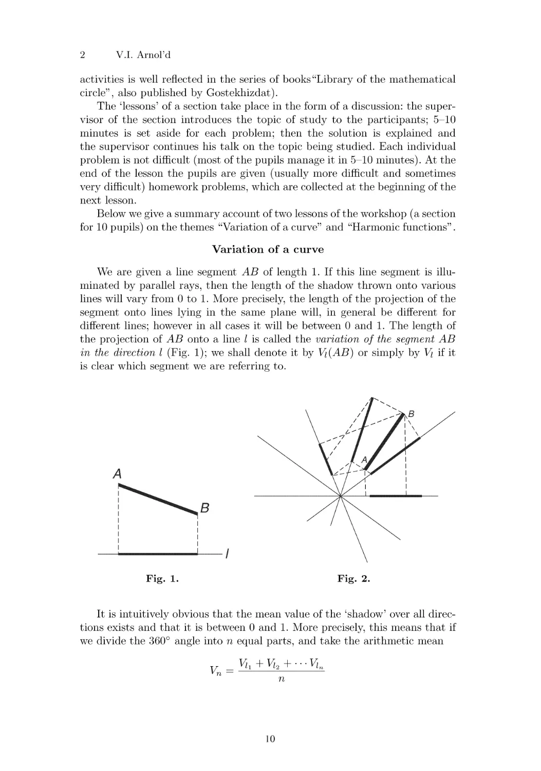
We define the variation of a polygonal line in some direction to be the
sum of the lengths of the projections of its component line-segments ('links')
in this direction (Fig. 3).
Fig. 3.
Problem 2. Determine the variation of a square of side 1 in the directions of
its sides and its diagonals.
Solution. Clearly, the variation of the square in the direction of each side
is equal to 2, and in the direction of a diagonal is equal to 2\/2.
The mean variation of a polygonal line over all directions, or simply the
variation of the polygonal line over all directions is defined, as above, via the
passage to the limit: V = lim™-^ Vn, where Vn is the arithmetic mean of the
variations of the polygonal line along the η directions of the sides of a regular
n-gon.
See, for example, the book Yaglom, A.M., Yaglom, I.M.: Elementary problems in
a non-elementary setting. Gostekhizdat, Moscow (1954), Problem 147b.
11
4 V.I. Arnol'd
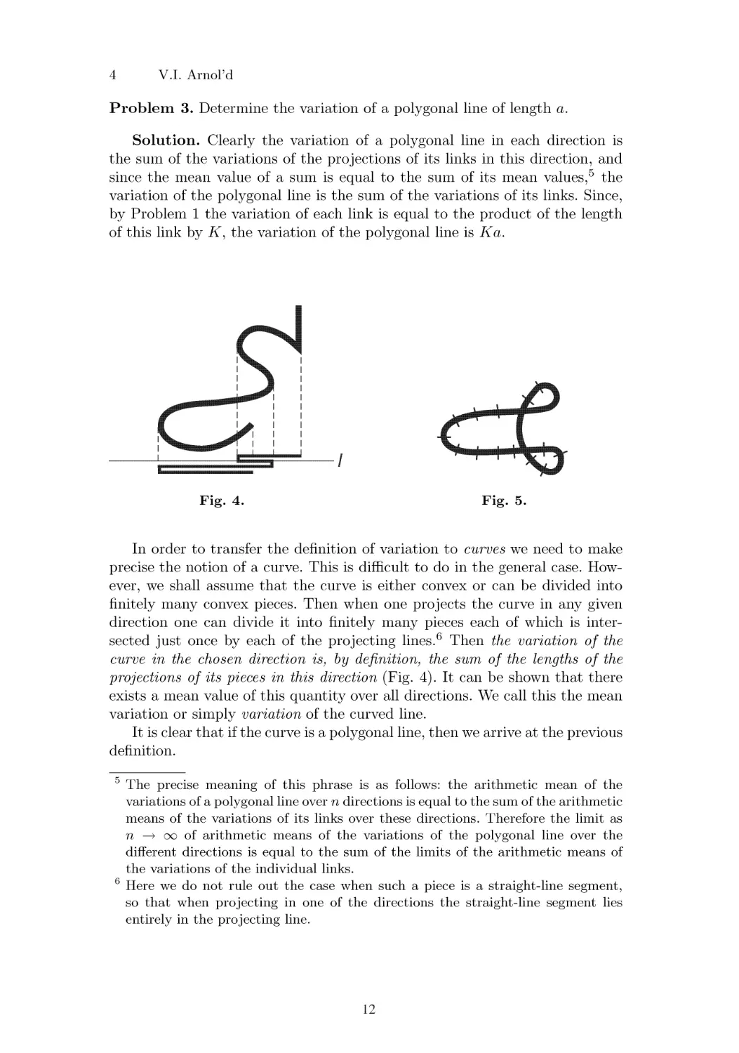
Problem 3. Determine the variation of a polygonal line of length a.
Solution. Clearly the variation of a polygonal line in each direction is
the sum of the variations of the projections of its links in this direction, and
since the mean value of a sum is equal to the sum of its mean values,5 the
variation of the polygonal line is the sum of the variations of its links. Since,
by Problem 1 the variation of each link is equal to the product of the length
of this link by K, the variation of the polygonal line is Ka.
Fig. 4.
Fig. 5.
In order to transfer the definition of variation to curves we need to make
precise the notion of a curve. This is difficult to do in the general case.
However, we shall assume that the curve is either convex or can be divided into
finitely many convex pieces. Then when one projects the curve in any given
direction one can divide it into finitely many pieces each of which is
intersected just once by each of the projecting lines.6 Then the variation of the
curve in the chosen direction is, by definition, the sum of the lengths of the
projections of its pieces in this direction (Fig. 4). It can be shown that there
exists a mean value of this quantity over all directions. We call this the mean
variation or simply variation of the curved line.
It is clear that if the curve is a polygonal line, then we arrive at the previous
definition.
The precise meaning of this phrase is as follows: the arithmetic mean of the
variations of a polygonal line over η directions is equal to the sum of the arithmetic
means of the variations of its links over these directions. Therefore the limit as
η —» oo of arithmetic means of the variations of the polygonal line over the
different directions is equal to the sum of the limits of the arithmetic means of
the variations of the individual links.
Here we do not rule out the case when such a piece is a straight-line segment,
so that when projecting in one of the directions the straight-line segment lies
entirely in the projecting line.
12
Mathematics workshop for schools at Moscow University 5
Problem 4. Find the variation of a circle of diameter D.
Solution. First we choose some direction. The diameter having this
direction divides the circle into two pieces, namely, into two arcs each of which
is intersected by any line perpendicular to the chosen direction in at most one
point. Hence the variation of the circle in the chosen direction is equal to 2D.
Clearly the variation in any other direction is the same, therefore the mean
variation of the circle is equal to 2D.
We now select several points on the curve and join them successively by
straight lines (Fig. 5). Then we obtain a polygonal line. It can be shown that
for sufficiently good curves (for example, for all convex curves) the limit of
the lengths of these polygonal lines exists, provided that as these polygonal
lines vary the length of the largest link of the lines tends to zero. This limit
is called the length of the curve.
It can also be proved that for curves that can be divided into finitely many
convex pieces the limit of the variations of these polygonal lines exists as the
length of the largest link tends to zero.
Problem 5. Find the limit which the variation of a polygonal line inscribed
in a "sufficiently good" curve of length a tends to when the polygonal line
varies so that the length of its largest link tends to zero.
Solution. Since for each polygonal line of length an the variation is equal
to Kan and an —> a for "sufficiently good" curves, the limit of the variations
of the polygonal lines is equal to К a.
Problem 6. Prove that the variation of a ('sufficiently good') curve of length
a is equal to К a.
Solution. It suffices to observe that one can inscribe in such a curve a
polygonal line with arbitrarily small links whose variation along each of the
η given directions coincides with the variation of the curve. Therefore, once
the limit in Problem 5 exists it is equal to the variation of the curve.
Problem 7. Find the numerical value of Κ, that is, the variation of a segment
of length 1.
Solution. Since, on the one hand, a circle of diameter D has length D
and hence variation KirD (Problems 5 and 6) while, on the other hand
(Problem 4), the variation of this circle is equal to 21}, it follows that К = -.
By the width of a curve with respect to a given direction we mean the
smallest distance between two lines of this direction that enclose the curve.
A curve has constant width if its width with respect to all directions is the
same. Examples of a curve of constant width are the circle and the so-called
Rello triangle consisting of three equal arcs of a circle (Fig. б).7 With the help
7 There is a lot of information about curves of constant width in the book: Yaglom,
I.M., Boltyanskii, V.G.: Convex figures. Gostekhizdat, Moscow (1951).
13
6 V.I. Arnol'd
of variation one can obtain a very elegant proof of the following Barbier's
Theorem:
Problem 8. Prove that all curves of constant width h have the same length
π/г.
Solution. This follows from the fact that the variation of each such curve
in any direction is equal to 2/г; see the reults of Problems б and 7.
Fig. 6.
Here is another problem which at first glance appears to be rather
complicated:
Problem 9. A curve L of length 22 is contained in a circle С of radius 1.
Prove that there is a line intersecting L in at least 8 points.
Solution. The variation of L is equal to - · 22 > 14 (Problems б and 7).
On the other hand, the length of the projection of L in any direction does not
exceed 2 (L is contained in C\). Hence for some directions certain parts of the
projection of L will be covered by the projections of separate arcs of L more
than 7 times (that is, at least 8 times). This completes the proof.
We now turn to an account of the lesson devoted to the topic "Harmonic
functions".
The conclusion of this article will appear in the next issue
14
в шкальном математическом кружке при мгу*
В. И. Арнольд
(Москва)
(Окончание)
Гармонические функции
Две первые задачи не имели отношения к основной теме. Для
полноты освещения занятия кружка мы приводим их; близкая к ним
по методу решения третья задача
являлась подготовительной к четвертой, с
которой, по существу, и начиналась тема.
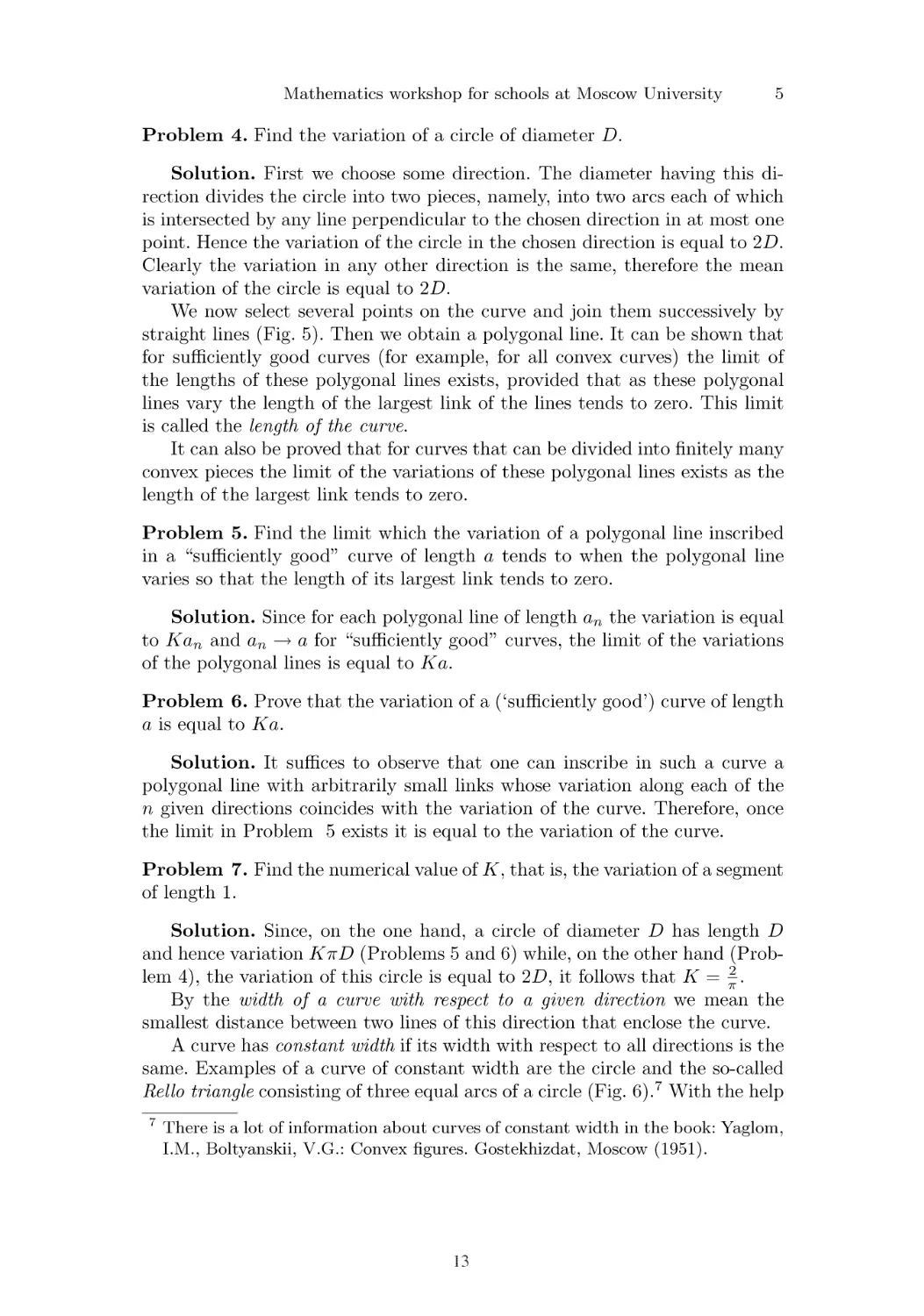
Задача 1. Найти наибольшее и
наименьшее значения выражения
a sin φ 4- Ь cos φ (а и Ь положительны).
Решение· Проведем два
взаимно-перпендикулярных луча ОМ и ON и построим
прямоугольный треугольник ОАВ с катетами
ОА = а и АВ^=ЬУ расположив их так, как на
рис. 1 (прямые углы MON и ОАВ ориентированы против часовой стрелки).
Обозначим угол AON через φ, тогда, проектируя ломаную ОАВ на ось ОМ
(проекции направленные!), получаем *):
(О В') = пр. ОВ = пр. О А + пр. АВ ~ a sin φ + Ь cos φ.
Если вращать треугольник ОАВ вокруг вершины О, то угол φ
изменяется; наибольшее и наименьшее значения проекции (ОВ') достигаются, когда
отрезок ОВ коллинеарен ОМ, т. е. когда tg<p = -r-; они равны Υ а*-\-Ъг и
Задача 2. Доказать, что если
ах cos φΙ -f- a2 cos ф2 +... + ап cos φ„ = 0 (1)
и
«ι COS (φ, + 1) + «2 COS (φ2 + 1) + .·· + йт COS (<pm + Π = 0 (2)
(все коэффициенты α/ положительны), то и при любом α
«ι COS (φ + α) + α2 COS (φ2 + «) + - + «т COS (<?„, + β) = 0. (3)
ι) (ОВ9) — величина направленной проекции.
* Editor's note: V.I. Arnol'd: The school mathematical circle at Moscow State University:
harmonic functions. Published in Mat. Prosveshchenie 3 (1958), 241-250
15
242
В. II. АРНОЛЬД
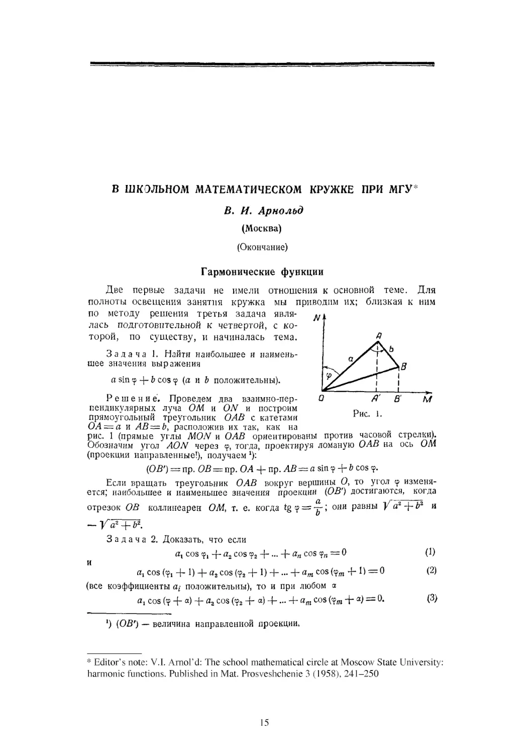
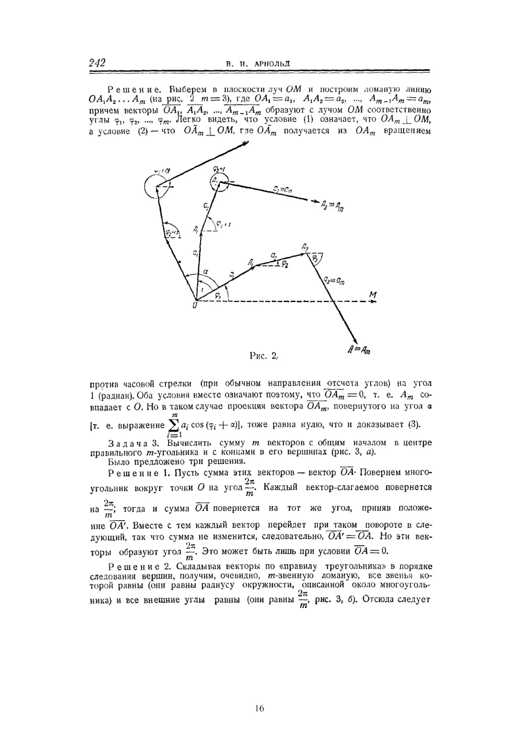
Решение. Выберем в плоскости луч ОМ и построим ломаную линию
ΟΑλΑ2.. .Ат (на рис. 2 т~3), где QAi=zgiy АхАг = аг, ..., Am_}Am = amt
причем векторы OAv AtA2, ..., Ат_1Ат образуют с лучом ОМ соответственно
углы φ,, φ2, ..., <pm. Легко видеть, что условие (1) означает, что ОАт [^ОМ,
а условие (2) — что ОЛт_]_СШ, гле 0Лт получается из ОЛ^ вращением
Ъ*4п
Рис. Я- " т
против часовой стрелки (при обычном направлении отсчета углов) на угол
1 (радиан). Оба условия вместе означают поэтому, что ^ОАт = 0, т. е. Ат
совпадает с О. Но в таком случае проекция вектора ОАт, повернутого на угол α
т
[т. е. выражение У) а-ь cos (φ; -f- <*)]> тоже равна нулю, что и доказывает (3),
1 = 1
Задача 3. Вычислить сумму т векторов с общим началом в центре
правильного /η-угольника и с концами в его вершинах (рис. 3, а).
Было предложено три решения.
Решение 1. Пусть сумма этих векторов — вектор ОА· Повернем
многоугольник вокруг точки О на угол —. Каждый вектор-слагаемое повернется
на —; тогда и сумма ОА повернется на тот же угол, приняв
положение ОА'. Вместе с тем каждый вектор перейдет при таком повороте в
следующий, так что сумма не изменится, следовательно, ОА' = ОА. Но эти век-
2тх —
торы образуют угол —. Это может быть лишь при условии ОА — 0.
Решение 2. Складывая векторы по «правилу треугольника» в порядке
следования вершин, получим, очевидно, m-звенную ломаную, все звенья
которой равны (они равны радиусу окружности, описанной около
многоугольника) и все внешние углы равны (они равны —, рис. 3, б). Отсюда следует
16
В ШКОЛЬНОМ МАТЕМАТИЧЕСКОМ КРУЖКЕ ПРИ МГУ 243
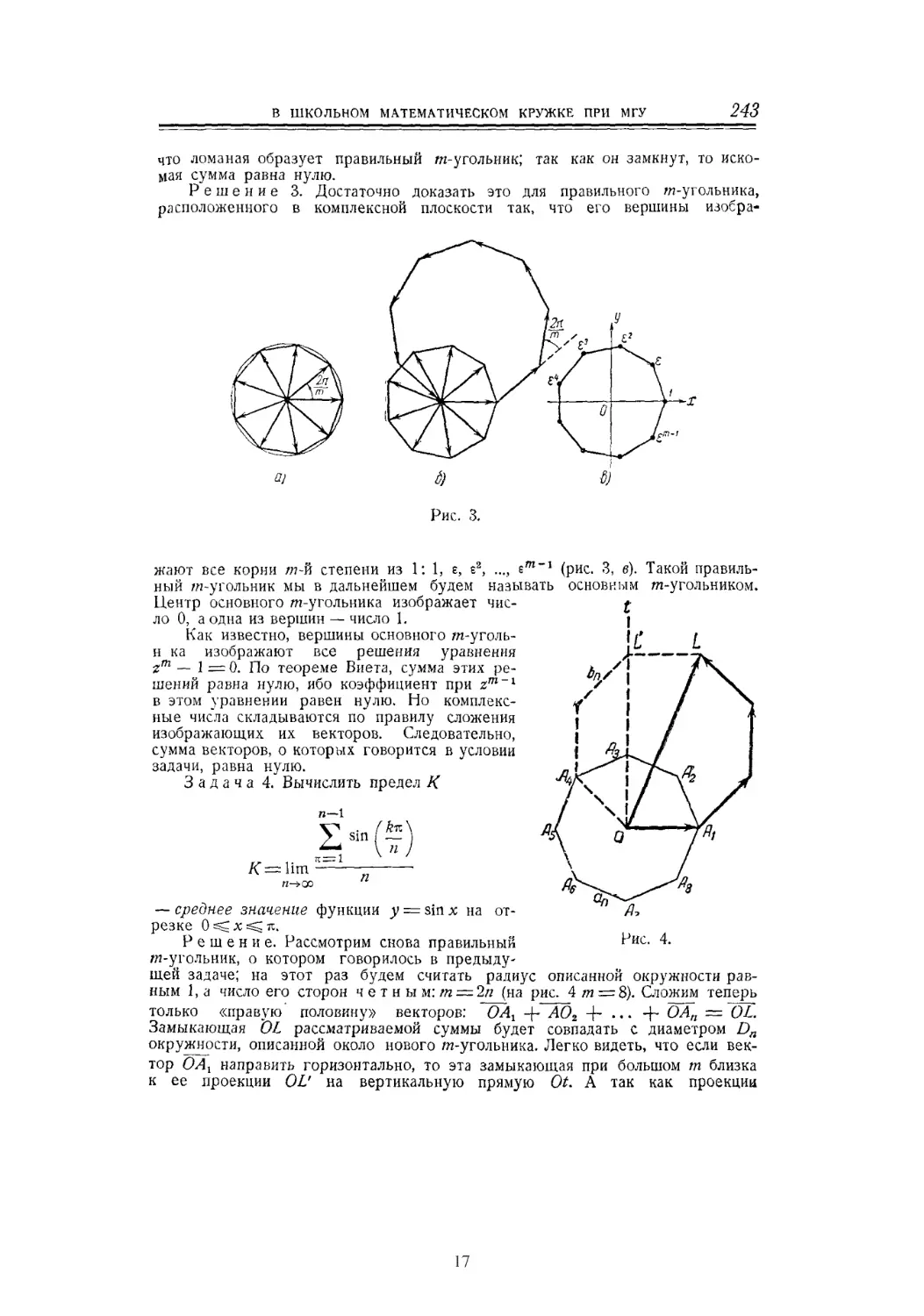
что ломаная образует правильный m-угольник; так как он замкнут, то
искомая сумма равна нулю.
Решение 3. Достаточно доказать это для правильного m-угольника,
расположенного в комплексной плоскости так, что его вершины
изображу
жают все корни m-й степени из 1: 1, ε, ε2,
ный /и-угольник мы в дальнейшем будем называть
Центр основного m-угольника изображает
число 0, а одна из вершин — число L
Как известно, вершины основного т-уголь-
н ка изображают все решения уравнения
zm — 1 = 0. По теореме Виета, сумма этих
решений равна нулю, ибо коэффициент при zm~l
в этом уравнении равен нулю. Но
комплексные числа складываются по правилу сложения
изображающих их векторов. Следовательно,
сумма векторов, о которых говорится в условии
задачи, равна нулю.
Задача 4. Вычислить предел К
п-\
(рис. 3, в). Такой правиль-
основкым т-угольником*
Σ>(ΐ)
Рис. 4.
К=Пт^—п ■
— среднее значение функции у = sin x на
отрезке Ο^χ^π.
Решение. Рассмотрим снова правильный
m-угольник, о котором говорилось в
предыдущей задаче; на этот раз будем считать радиус описанной окружности
равным 1, а число его сторон чет ним: т = 2/2 (на рис. 4 /я =8). Сложим теперь
только «правую' половину» векторов: ~ΟΑλ -f- Л02 4- ··· + ОАп =1Э1.
Замыкающая OL рассматриваемой суммы будет совпадать с диаметром Dn
окружности, описанной около нового m-угольника. Легко видеть, что если
вектор 0Αλ направить горизонтально, то эта замыкающая при большом т близка
к ее проекции OV на вертикальную прямую Ot. А так как проекции
17
244
В. И. АРНОЛЬД
единичных векторов ОА1У ОА2, ..., ОАп на эту вертикаль равны как раз
. Λ Λ . 2π .π . 4π . 2π . (/г — 1)«
sin 0 = 0, sin — = sin —, sin — — sin —, ..., sinv -— ,
m η m η η
A,
то среднее значение К равно пределу, к которому стремится частное ~. Но
• л bn Dn t
из подобия m-угольников, изображенных на рис. 4, ясно, что " ——^ (радиус
ОЛ1 = 1)> где ал —2sin —, а Ьп=1> Следовательно,
я-1
У.йпГ^
lim
л=о
= Ητη—-—= lim —— = lim
n'*O0n-2sin7r
2n
l.m I 1:^1 = 1: Ш***-
«->oo 1 π π
2/2
27г
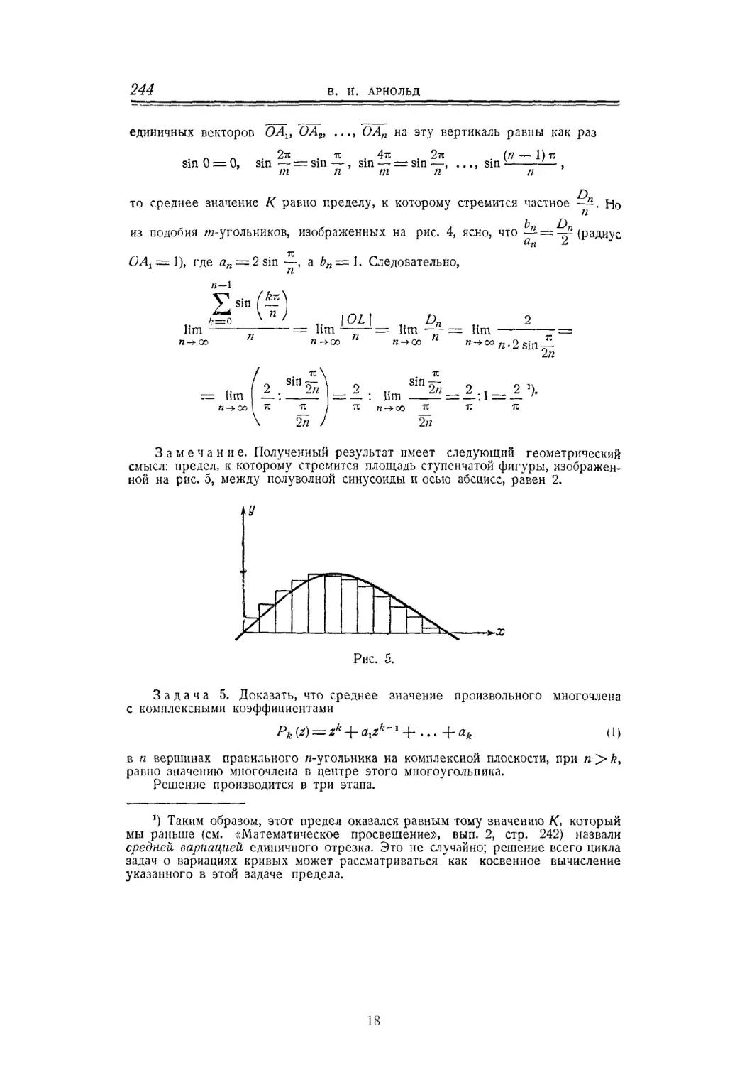
Замечание. Полученный результат имеет следующий геометрический
смысл: предел, к которому стремится площадь ступенчатой фигуры,
изображенной на рис. 5, между полуволной синусоиды и осью абсцисс, равен 2.
Рис. 5.
Задача 5. Доказать, что среднее значение произвольного многочлена
с комплексными коэффициентами
Pk(z) = zk + alzk~*+...+ak
(1)
в η вершинах правильного л-угольника на комплексной плоскости, при η > k>
равно значению многочлена в центре этого многоугольника.
Решение производится в три этапа.
*) Таким образом, этот предел оказался равным тому значению К, который
мы раньше (см. «Математическое просвещение», вып. 2, стр. 242) назвали
средней вариацией единичного отрезка. Это не случайно; решение всего цикла
задач о вариациях кривых может рассматриваться как косвенное вычисление
указанного в этой задаче предела.
18
В ШКОЛЬНОМ МАТЕМАТИЧЕСКОМ КРУЖКЕ ПРИ МГУ 245
1°. Пусть сначала Pk(z)~zk и правильный /z-угольник является
основным (см. решение 3 задачи 3). Тогда сумма k-x степеней комплексных чисел,
изображаемых вершинами /г-угольника, равна нулю при любом & < /ζ.
( 2π , . . 2π\
В самом деле, при замене каждого числа ζ на ζ I cos {-ism — =ζ·&
2π ,
а каждое зна-
ыногоугольник переходит в себя / он поворачивается на
2тг/г
2nk
чение ζ" умножается на £* = cos —^-{-ism-—φ 1. Значит, сумма
значений zk в вершинах /г-угольника не меняется и в то же время умножается на ik.
Следовательно, она может равняться только нулю.
Это же рассуждение непосредственно переносится и на случай
Pk(z) = az\
2°. Так как среднее значение Ρι(ζ)^=αζι (\ζζΙζζη) в вершинах
основного л-угольника равно нулю, то и среднее значение суммы zk -\- axzk~l -\- ...
,..-\-ak_^z равно нулю. Следовательно, среднее значение многочлена Ρ χ (ζ}
в его вершинах равно а& т. е. Р*(0).
У
*—
1 /\
z*t' Ϋ2
1 д
[ \
да у, Zn
f *
/
—4,?= ε"''
Рис. 6.
3°. Обозначим теперь комплексные числа — вершины основного
«-угольника Ай через ζ° = 1, ζ° = *, ^з^6*» ···* ^л—6***1 (Рис- 6) и рассмотрим
произвольно расположенный одноименный правильный многоугольник А с
вершинами ζν ζζ, ..., ζη. Очевидно, правильный многоугольник А можно получить
из Л0 поворотом, гомотетическим расширением (или сжатием) и
параллельным переносом. Другими словами, найдутся два таких комплексных числа а и
β, что
«1==в^ +
(/=1, 2
п).
Здесь модуль а равен отношению сторон многоугольников А и А0,
аргумент — углу поворота, а ^ — комплексное число, изображаемое центром
многоугольника А.
Теперь заметим, что среднее значение многочлена (1) в вершинах
zv z2i ..., ζη равно
2[Ρ*(α*? + Ρ)
Σ <?*<*?)
/=1
19
246
В. И. АРНОЛЬД
где
есть многочлен k-и степени относительно ζ [той же, что и Р& (ζ)},
принимающий в точках 2°, 2°, ...,г£ соответственно значения Ρ(ζγ), Ρ(ζ2), ..., Ρ(ζη),
Поэтому среднее значение Pk (ζ) в точках zv zit ..., ζη равно среднему
значению Qk (ζ) в точках ζ°, j?°, ..., ^, τ. е. (см. этап 2°) равно
<?л(0) = Р* + «1р*-1+...+ап.1р + ав.
Но Qk (0) совпадает с значением многочлена Pk (z) в центре
многоугольника Д что и завершает доказательство.
Пусть f(z)— некоторая функция комплексного переменного ζ.
Рассмотрим последовательность правильных л-угольников (« = 3, 4, 5, ...),
вписанных в определенную окружность комплексной плоскости, и
последовательность средних арифметических f(z) в вершинах этих
многоугольников. Если при η—* оо эти средние арифметические стремятся
к определенному пределу, не зависящему от выбора вписанных в
окружность многоугольников, то этот предел
tt->OQ П
называется средним значением функции f{z) no окружности.
Из задачи 5 следует, что среднее значение произвольного
многочлена по любой окружности равно значению этого многочлена в
центре окружности.
Можно говорить не только о среднем значении функции в смысле
среднего арифметического, но и о среднем геометрическом
функции f(z) по некоторой окружности. Под этим понимается
действительное неотрицательное число
lim^\f(zl)\\/(zt)\...\/(z„)\
Я->00
^значение корня арифметическое!), где zi — также вершины правильного
/г-угольника, вписанного в окружность.
Рассмотрим задачу, связанную с понятием среднего геометрического
функции на окружности.
Задача 6. Доказать теорему: если многочлен Pk (z) степени k не имеет
корней внутри или на окружности, то его среднее геометрическое на этой
окружности равно модулю его значения в центре окружности.
Решение проведем снова в три этапа.
1°. Пусть сначала окружность есть окружность \z\ = l, правильные
«-угольники — основные, а многочлен Рг (2) = ζ -(- а. (Очевидно, | а \ > 1, так
как иначе корень Рх (ζ) лежал бы внутри окружности.)
Рассмотрим произведение
(ζχ + α) α)+(*... (ζη + α).
20
В ШКОЛЬНОМ МАТЕМАТИЧЕСКОМ КРУЖКЕ ПРИ МГУ 247
Эти комплексное число есть значение многочлена
Fn (г) = \г-(- гх)\ [ζ-(- ζ,)}...[ζ - ( - ζη)\
в точке ζ —а. «Старший коэффициент» многочлена Fn(z) при гп равен
единице, а корни его равны — zv — z21 ..., — zn; поэтому Fn (ζ) ξ= ζη — ( — Ι)71»
Следовательно,
Fn[a) = an^-{-lf и I a" | - 1 ^ | Fn (a) | ^ ( a* [ + 1.
Но так как | a | > 1, то
lim i^l«r+l= lim ν/Μ?ΓΖΓ1^|ίζ[ί
Π->00 /2-»Ό0
откуда lim j//^ (я) = | я |, что и доказывает теорему в этом частном случае.
2°. Так как, очевидно, среднее геометрическое произведения равно
произведению средних геометрических, то доказываемая теорема справедлива и
для любого многочлена Pn(z), все корни которого по модулю больше 1, так
как такой многочлен есть произведение сомножителей вида (ζ + я,·), где —щ
— корни Рп (ζ).
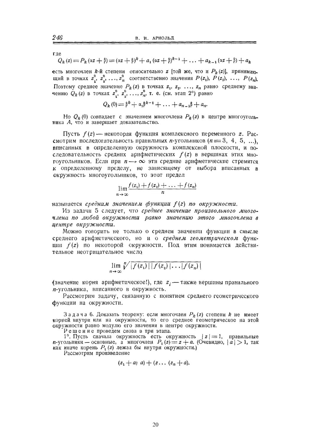
3°. Наконец, пусть данная окружность S *- произвольная, имеющая центр
в точке, изображающей комплексное число β, а радиус а; ее уравнение \ ζ— ji | = a*
Рассмотрим преобразование комплексной плоскости
Оно переводит единичную окружность ] ζ ) — 1 и круг J z j =С 1 соответственна
в окружность S и в ограничиваемый его круг.
Подставим в данный многочлен Рп (ζ) вместо ζ выражение αζ -}- ?. Получим:
Pn(** + t) = Qn(*)\
при этом значения многочлена Qn (z) в вершинах основного л-угольника равны
значениям Рп (ζ) в вершинах я-угольника, вписанного в S (ср. с решением
задачи 5). Все корни Q (ζ) лежат вне круга | ζ \ ^ 1 [все корни Ρ (ζ) лежат вне
круга, ограниченного S); среднее геометрическое Рп (ζ) по окружности S равна
среднему геометрическому Qn(z) по окружности |г| = 1. Но это последнее
среднее вычислено в п. 2°; оно равно | Qn (0) | — \Рп (β) [, ч. т, д.
Рис. 7.
Задача 7. На плоскости имеются две фиксированные точки Л я В (рис. 7).
Рассмотрим функцию 0=/(Λί) точки Μ этой плоскости, равную углу 0
(наименьшему, отсчитываемому против часовой стрелки), на который поворачивается
луч МЛ до совмещения с MB. Доказать, что среднее значение функции f(M)
21
248
В. И. АРНОЛЬД
по любой окружности S, не пересекающей лучей АР и BQ, равно значению
f(M) в центре О окружности1).
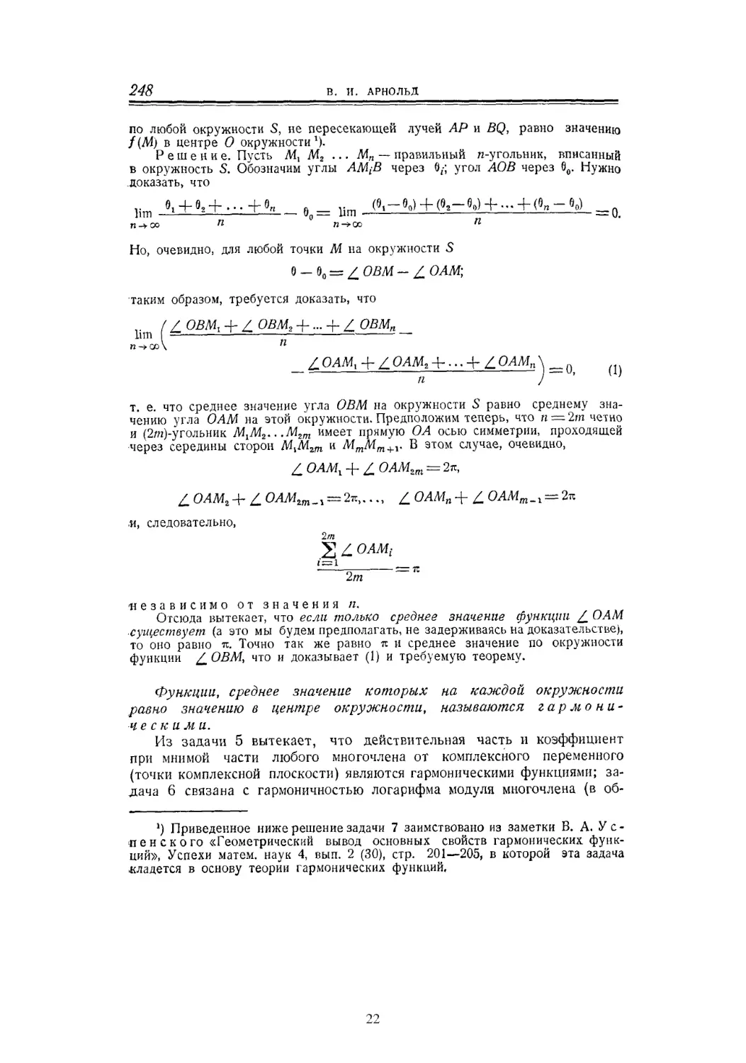
Решение. Пусть Λί, М2 ... Мп — правильный η-угольник, вписанный
в окружность 5. Обозначим углы АЩВ через 0,·; угол ЛОВ через θ0. Нужно
доказать, что
цт »ι + »«+.··+»η ео= lim (8,-60) + (92-e0) +-. + (()„-6,) _q
Но, очевидно, для любой точки Μ на окружности S
θ - θ0 = £ ΟΒΜ-Ζ. ΟΑΜ;
таким образом, требуется доказать, что
lim f Z OBMt + Ζ ΟΒΜ2 +... + Ζ ОШп
£ОАМх + £ОАМ2 + ... + £ОАМп\^ (1)
т. е. что среднее значение угла ОВМ на окружности S равно среднему
значению угла О AM на этой окружности. Предположим теперь, что п = Ъп четно
и (2/я)-угольник М1М2.. .М2т имеет прямую ОА осью симметрии, проходящей
через середины сторон М^М2т и Мттт+1. В этом случае, очевидно,
£ОАМ1 + £ОАМш = 2п,
Ζ OAM2ArL ОАМгт^^2^..у Δ ΟΑΜη+£ ОАМт_г^2к
и, следовательно,
2т
Σ Ζ OAMt
г"=1
2/и
независимо от значения /г.
Отсюда вытекает, что если только среднее значение функции £ О AM
существует (а это мы будем предполагать, не задерживаясь на доказательстве),
то оно равно π. Точно так же равно π и среднее значение по окружности
функции Δ ОВМ, что и доказывает (1) и требуемую теорему.
Функции, среднее значение которых на каждой окружности
равно значению в центре окружности, называются
гармоническими.
Из задачи 5 вытекает, что действительная часть и коэффициент
при мнимой части любого многочлена от комплексного переменного
(точки комплексной плоскости) являются гармоническими функциями;
задача 6 связана с гармоничностью логарифма модуля многочлена (в об-
*) Приведенное ниже решение задачи 7 заимствовано из заметки В. А. Ус-
лен с к о го «Геометрический вывод основных свойств гармонических
функций», Успехи матем. наук 4, вып. 2 (30), стр. 201—205, в которой эта задача
кладется в основу теории гармонических функций.
22
В ШКОЛЬНОМ МАТЕМАТИЧЕСКОМ КРУЖКЕ ПРИ МГУ 249
ласти, где многочлен не имеет корней), задача 7 дает геометрический,
пример гармонической функции.
Гармонические функции играют выдающуюся роль в математике,
физике и технике. Для примера упомянем здесь о задаче нахождения
распределения температур в произвольной плоской однородной
пластинке. Ясно, что если распределение температур — установившееся,
т. е. самопроизвольного перераспределения температур не происходит,
то оно дается гармонической функцией, ибо если бы среднее значение
температуры на малой окружности было, например, больше
температуры в центре О, то точка О нагревалась бы.
Очевидно, что заданная в некоторой области гармоническая
функция может принимать наибольшее и наименьшее значения
лишь на границе этой области, ибо если бы наибольшее значение
достигалось во внутренней точке О, то среднее значение по
окружности с центром в О не могло бы совпадать со значением в О. Это
предложение называется принципом максимума и играет большую
роль в теории гармонических функций. Из него следует, что
значения гармонической функции в области полностью определяются ее
значениями на границе этой области: так, например, распределение
температур на пластинке определяется температурами на крае
пластинки. Действительно, если бы существовали две разные гармонические
функции, то их разность (которая, очевидно, тоже будет
гармонической функцией) была бы равна нулю на границе области и отлична от
нуля где-то внутри нее; но это противоречит тому, что гармоническая
функция принимает наибольшее и наименьшее значения на границе.
Функции, заданные в отдельных точках плоскости, например в
центрах квадратов бумаги «в клетку», называются функциями на сетке.
Гармонической функцией на сетке называется такая, у которой
значение в каждой точке равно среднему арифметическому ее значений
в соседних точках. Как и для гармонических функций на плоскости,
здесь можно показать, что наибольшее и наименьшее значения
гармоническая на сетке функция принимает на границе сетки и что
значения гармонической функции на сетке однозначно определяются ее
значениями в граничных узлах сетки.
При математическом приближенном решении задач, связанных с
гармоническими функциями, их часто заменяют гармоническими на сетке
функциями. Таким образом, например, можно вычислить температуру
в точке однородной плоской пластинки, если известна температура на
краю. Для этого пластинка делится на мелкие квадратики, где
температура предполагается неизменной, и выписывается условие
гармоничности на сетке, состоящей из центров квадратиков: среднее
арифметическое температур соседей данного квадратика равно его собственной
температуре; решение задачи удобно проводить методом
последовательных приближений.
Легкая задача 8 касается одного важного свойства гармонических,
функций на сетке [см. также задачу 20 на стр. 269.—Ред.].
23
250
В. И. АРНОЛЬД
Задача 8. В каждой клетке бесконечного листа клетчатой бумаги
написано натуральное число, равное среднему арифметическому чисел, стоящих
в четырех соседних клетках. Доказать, что во всех клетках написано одно и
то же число.
Решение. Четыре соседа-числа в такой таблице, как указано в условии,
не могут быть все больше его и не могут быть все меньше его. Вместе с тем
среди любого количества натуральных чисел всегда есть наименьшее п. Все
четыре его соседа равны я, так как они не меньше /г, и если хотя бы одно
было больше, то среднее арифметическое тоже было бы больше /?, тогда кэк по
условию оно равно п.
Точно так же соседи этих соседей равны η и т. д. Так мы убеждаемся,
что все числа в клетках равны п.
24
ON THE REPRESENTATION OF
FUNCTIONS OF SEVERAL VARIABLES AS
A SUPERPOSITION OF FUNCTIONS OF A
SMALLER NUMBER OF VARIABLES*
V.I. ArnoPd
Moscow
translated by Gerald Gould
In this paper we wish to give an account of several recent papers by Moscow
mathematicians devoted to the question in the title of this paper. §1 contains
the definition of superposition of functions and the statement of Hubert's 13th
problem relating to superpositions. §2 is devoted to superpositions of smooth
functions. In §3 we present several very recent papers, in spite of the fact
that the content of that section is now perhaps only of historical interest.
The principal topic there is the description given by Kronrod of "the tree of
components of a function of several variables", which is a concept whose
popularization would seem to be very desirable (although the connection between
this concept and the problems considered in our paper has proved to be less
close than it originally appeared). The reader interested only in the strongest
(and, moreover, the simplest in its method of proof) result relating to the
representation of continuous functions of several variables as superpositions
of functions of a smaller number of variables can, after looking at the
introductory §1 go straight to §4, missing out §2-3. In addition, the smaller print
in this paper means, as usual, that the corresponding material is auxiliary
and omitting it will not affect the reader's understanding of what follows.
1. One of the problems of the famous problem book by Polya and Szego1
begins as follows:
"Do functions of three variables exist at all?1
The meaning of this question is as follows. Suppose that we have two
functions of two variables u(x,y) and v(y,z). We now consider a new
function of two variables w(u,v) and substitute our functions in place of и and
v. Then the function w[u(x,y),v(y,z)] now depends on the three variables
x, у and z. Thus, by substituting in place of the arguments и and ν of the
function of two variables w(u,v) the new functions of two variables we obtain
* Mat. Prosveshchenie 3, 41-61 (1958)
1 Polya, G., Szego, G.: Problems and theorems of analysis, part I. Moscow, Section
II, Problems 119 and 119a.
25
2 V.I. Arnol'd
a function of three variables (one can even obtain a function of four variables
w[u(x, г/), v(z, £)]; we call this function a single superposition formed from the
functions of two variables η, ν and w. It is clear that all the properties of this
function are determined by our three functions of two variables. Polya and
Szego's question (which, however, was not formulated in their book in all its
breadth) is as follows: can all functions of three variables be reduced to such
a superposition (or a somewhat more complicated superposition) of functions
of two variables, or do there in fact exist functions that are "essentially of
three variables" which cannot be reduced to functions of two variables.
Note first of all that if one can also use discontinuous functions, then
the answer to Polya and Szego's question is clearly negative.2 Thus the only
question of interest is whether or not all continuous functions of three variables
are representable as superpositions of continuous functions of two variables.
In fact, a discontinuous function и = ф(х,у) enables one to map the (ж, у) plane
bijectively onto the line и [the fact that the set of pairs (x,y) of numbers and the
set of numbers и have the same cardinality means precisely that these sets can be
bijectively mapped onto each other]. We now choose any function of three variables
F(x,y,z) and define the function ф(и, z) by the equality
ф[ф(х,у),г] = F(x,y,z);
this is possible because each pair of values (ж, у) corresponds to a unique value
и = ф(х,у) and we can take φ(η,ζ) to be equal to the corresponding value of
F(x,y,z)3
For the simplest continuous functions of three variables it is not hard to
find representations of them as superpositions of continuous functions of two
variables. For example, the function
F{x,y,z) =xy + yz
can be represented in the form
F = w[u(x,y),v(y,z)],
where
w(u,v) = u-\- υ, u(x, y) = χ + г/, v(y,z)=yz.
For the somewhat more complicated function
F(x, y, z) = xy + у ζ + zx
it is already impossible to represent it as a simple superposition of functions of
two variables;4 However, it is possible to represent it as a double superposition
of functions of two variables, that is, in the form
2 See the solution of problem 119 in Polya and Szego's book.
3 It suffices to require that no two distinct pairs (x, у) correspond to the same value
и = ф(х,у); here, for values й not belonging to the range of the function ф(х,у)
the function φ(ΰ,ζ) can be defined arbitrarily.
4 See Polya and Szego's book.
26
On the representation of functions of several variables 3
w{u[p(x, г/), q(y, z)], v[r(y, z), s(z, x]} ;
it suffices merely to set
w(u, v) = и + ν
and
u(p,q) =p + q, p(x,y)=xy, q(y,z)=yz, v(r,s) = s, s(z,x) = zx.
In general, all entire rational functions of several variables can by definition
be obtained from their arguments by means of a multiple application of the
operations of addition and multiplication, that is, they are the result of a
multiple superposition of functions of not more than two variables
ф(х,у) =х + У, ф(х,у)=ху, f(x)=x + a, g(x)=ax,
that is, the result of a multiple substitution of the arguments of these functions
by more complex expressions formed by means of the same functions. By
analogy with this, the rational functions are obtained as superpositions of six
of the simplest functions of not more than two variables:
χ
ф(х,у) =х + у, ф(х,у)=ху, х(х,у) = -,
У
f(x) = χ + α, g(x) = ax, h(x) = — .
If a segment of ж is a function of known segments a, 6, c,..., then in order to be
able to construct it using a ruler and compasses, it is necessary and sufficient
that this function be homogeneous of the first dimension and that it be a
superposition of these same simplest functions and the function у = χ/χ. All
the elementary functions can be represented as superpositions obtained via
those same functions and in addition certain special functions of one variable,
such as
y/x, ex, ln(x), sin(x), and others.
The simplest examples of algebraic functions going outside the limits of the
class of elementary functions are provided by the roots of algebraic equations;
the arguments of these functions are the values of the coefficients of the
equations. But the roots of equations of the first, second, third and fourth degrees
are, as is well known, elementary functions of the coefficients obtained as the
result of superposition of those same functions of two variables, the sum, the
difference, the product and the quotient, and (for equations of these 2nd-4th
degrees) functions of the single variable y/x (here η = 2 in the case of a
quadratic equation and can be equal to 2 or 3 in the case of equations of
the 3rd and 4th degrees). For equations of the 5th and higher degrees such a
representation is not possible in general; this was shown by Abel. However,
the roots of equations of the 5th and 6th degrees can be expressed in terms of
the coefficients by means of superpositions of certain more complex analytic
27
4 V.I. Arnol'd
functions of two variables; these representations can be used for the practical
calculation of the roots of equations; in particular for nomographic solution
of equations.
Attempts to obtain a representation of roots of 7th-degree equations as a
superposition of suitable functions have not been crowned with success. Using
algebraic transformations the general 7th-degree equation
X7 + CLiX6 + CL2X5 + CLiX6 + CL^ + CL^X3 + CL^X + αγ = 0
can be reduced to the form
x7 + ax3 + bx2 + ex + d = 0
where a, b and с are elementary (algebraic) functions of the coefficients
αχ, α2,..., αγ of the original equation, therefore they are expressed in terms
of these coefficients as superpositions composed of simple functions of two
variables. Thus, the question of the possibility of representing the roots of a
7th-degree equation by superpositions of functions of two variables reduces to
the problem of finding such a representation for the special function of three
variables a, 6, с of the roots of the equation written above.
To date it is not known whether this function of three variables (which is
easily seen to be analytic) can be represented as a superposition of analytic
functions of two variables. Nevertheless, Hubert managed to show that certain
analytic functions of three variables are not such superpositions.
Hubert's result is in connection with the following situation. If a function of
three variables is a superposition of functions of two variables, then among the
partial derivatives of the superposition and the functions of which it is composed
there exist fully determined analytic relations. Therefore if all analytic functions of
three variables are represent able in such a form, then the space of coefficients of the
series expansion of the functions of two variables involved in this superposition can
be mapped analytically onto the space of coefficients of the expansion of functions of
three variables; but this is not possible, since the latter space has a greater dimension
(here we are restricted by the definite but large number of first coefficients of the
expansion, that is, the first partial derivatives).
In his lecture at the 1900 International Mathematical Congress held in
Paris the celebrated German mathematician David Hubert posed 23
problems awaiting solution.5 The thirteenth of these "Mathematical problems" of
Hubert's was as follows:
Can the roots of the equation
x7 + ax3 + bx2 + ex + 1 = 0
be represented as superpositions of continuous functions of two variables ?
5 Hubert, D.iMathematische Problemen; Gesammelte Abhandlungen, vol.3, No.17
(1935). [Editor's note: Translation of this work of Hubert's will appear in the next
issues of Mat. Prosveshch.]
28
On the representation of functions of several variables 5
Hubert conjectured that the answer to this question would turn out to
be negative; in that case the more general question of whether all functions
of three variables are superpositions of continuous functions of two variables
would be solved at the same time.
2. The first results touching on Hubert's 13th problem were obtained
under the assumptions that the superpositions have some special form, for
example, under conditions restricting the 'single' superpositions; they all supported
Hubert's conjecture.6 The strongest result here is the result of A.G. Vitushkin
who succeeded in constructing a polynomial such that neither the polynomial
itself nor any function sufficiently close to it (in the sense of uniform
convergence) can be decomposed into a simple superposition of continuous functions
of two variables in any region or in any system of coordinates.
Further results are in connection with restrictions imposed on the
functions involved in the superposition. As already recalled, Hubert had noted
earlier that it was impossible to obtain all the analytic functions of three
variables as superpositions of analytic functions of two variables. Important
results in this direction were obtained by Vitushkin,who by using his theory of
multidimensional variations of functions and sets showed that not all I times
continuously differentiable functions of three variables can be represented as
superpositions of [|Z] times7 differentiable functtons of two variables all of
whose derivatives of order [|Z] satisfy Lipschitz conditions.8
In Kolmogorov's interpretation9 Vitushkin's results are connected with
the difference of the 'dimensions' of the corresponding function spaces. As
Pontryagin and Shnirel'man had already proved in 1932, the dimension of
a compact metric space (for example, a cube in Euclidean space) can be
defined in the following way. We cover our space with 'small' sets of diameter
ε. Clearly, the number Ν(ε) of sets required to do this will increase as ε
gets smaller; here it can be shown that Ν(ε) increases as -^, where η is the
6 The simplest examples of this kind already appear in the book of Polya and
Szego; a number of other examples (due to A.Ya. Dubovitskii and R.A. Minlos)
are given in the book:Vitushkin, A.G.: On multidimensional variations. Moscow
(1955).
7 Here the square brackets indicate the integer part.
8 It also follows from this result that there exists in a three-dimensional cube
an analytic function (of three variables) satisfying a Lipschitz condition with
Lipschitz constant 1 such that no functions close to it (including the function
itself) can be represented as an 5-fold superposition of two variables satisfying a
Lipschitz condition with some constant L\ (s and L\ are given in advance), and
there exists an unbounded differentiable function satisfying a Lipschitz condition
with Lipschitz constant 1 which is not a superposition of functions of two variables
satisfying a Lipschitz condition. See Vitushkin's book referred to in footnote 6.
9 Kolmogorov, A.N.: Estimates of the minimum number of elements of ε-nets in
various function classes and their application to the question of the representation
of functions of several variables as superpositions of functions of a smaller number
of variables. Usp. Mat. Nauk 10, No.l, 192-195 (19??).
29
6 V.I. Arnol'd
dimension of the space; thus the dimension η can be defined as the limit
logW(e)-
lim inf
ε^Ο
logs
For infinite-dimensional spaces this limit is equal to infinity. However, in
a number of cases the number Ν(ε) can increase as the function 1 : exp(zfe),
where к is some constant which one can provisionally call the "dimension of
the infinite-dimensional space". Thus for infinite-dimensional spaces the role
of dimension is played by the limit10
lim inf
ε^Ο
log log Ν(ε)
logs
For the space of functions f(x\,X2,---,Xn) of n arguments defined on an
η-cube, where the functions are I times differentiable in all their arguments
and are such that all the partial derivatives of order I satisfy a Holder condition
of order ce,11 the above-defined dimension can be considered to be equal to
' + a
Hence it follows, in particular, that the set of I times differentiable functions
of three arguments is in a certain sense 'richer in its elements' than the set
of [|Z] times differentiable functions of two arguments satisfying a Lipschitz
condition (that is, a Holder condition of order 1); hence it follows that it is
impossible to express all the first functions as superpositions of the last ones.
10 Instead of the number Ν(ε) of sets of diameter ε completely covering the
(compact) space one could choose the number Μ (ε) of points of an ε-net, that is, the
smallest number of points such that each point of the space is at a distance of
at most ε from at least one of the chosen points, or the maximum number Κ (ε)
of points such that the distance between any two of them is greater than ε. It is
curious to note that the same definition of the dimension of function spaces was
arrived at (almost at the same time) by Shannon [Shannon, C.E.: The
mathematical theory of communication, Urbana (1949); in the Russian translation of
Shannon's work (in the collection "Theory of transmission of electric signals in
the presence of noise". Inost. Lit., Moscow (1953)) the corresponding place was
omitted for some reason] which started from arguments relating to "the theory of
information": in the space of the transmitted information Κ (ε) is the maximum
number of 'ε-different signals' that cannot be confused by the receiver provided
that the distortion of the information in the transmitter does not exceed ε.
11 A function f(x) satisfies a Holder condition of order a if there exists a number
С such that for each χι, x2 in the domain of the function
\f(xi)-f(x2)\ <C\Xl~x2
|2
A function of several variables is said to satisfy a Holder condition if it satisfies
this condition as a function of each of its variables.
30
On the representation of functions of several variables 7
3. However, in the domain of all continuous functions Hubert's conjecture
has proved to be false.
In the spring of 1956 Kolmogorov succeeded in showing that every
continuous function of η variables (n > 4) defined on an η-cube is a superposition
of continuous functions of the three variables.12 The main tool in his
construction is the one-dimensional tree of components of level sets of a function
introduced by Kronrod.13
Fig. 1. Fig. 2.
By the level set of a function we mean the collection of all points in the
domain of the function at which the function takes some fixed value. For
example, if the function of a point of part of the land surface represents the
height at this point above sea level, then the level set will consist of all points
of the locality having the same height above sea level; in topography these
level sets are called contour lines. In Figs. 1 and 2 we have depicted simple
functions of two variables and the 'maps' of the level sets of these functions
(that is, a partition of the squares on which the functions are defined into
12 Kolmogorov, A.N.: On the representation of continuous functions of several
variables by superpositions of continuous functions of a smaller number of variables.
Dokl. Akad. Nauk SSSR 108, 179-182(1956); English transl. in Amer. Math Soc.
transl. Ser. 2, vol. 17, 369-373 (1961).
13 Kronrod, A.S.: On functions of two variables. Usp. Mat. Nauk 5, No.l, 24-134
(1950).
31
8 V.I. Arnol'd
their separate level sets). A level set can consist of a single piece (for example,
all the level sets of the function depicted in Fig. 1 or the 1-level set of the
function depicted in Fig 2; or it may consist of several connected pieces or
components (for example, the 3-level set in Fig. 2 consists of the two pieces
3a and 3b). To study the structure of the set of components of a level set of
a continuous function Kronrod proposed that one use the notion of a tree.
In topology, by a tree we mean a curve ('one-dimensional locally connected
continuum') not containing any closed arcs ('homeomorphic images of a
circle'). A tree can be represented in the following way. From the base of the
'trunk' of the tree there emerge 'branches' at the 'branch points' (the number
of branch points can be denumerable and from each such point there can be
denumerably many branches coming out of it); in turn, from each branch there
can emerge new branches (we can call them 'twigs'), and so on (Fig. 3). In
general a tree can be somewhat complex; however, as the celebrated Austrian
(now American) mathematician Karl Menger showed, there exists in the plane
a universal tree such that any other tree is a part of it (more precisely, such
that any tree is homeomorphic to a part of the universal tree).14
Fig. 3.
Menger, K.: Kurventheorie, Ch. X. Berlin-Leipzig (1932).
32
On the representation of functions of several variables 9
Kronrod showed that the set of components of all level sets of a continuous
function of several variables is naturally representable as a tree.
Thus, for example, the set of components of the level set of the functions
depicted in Fig. 1 corresponds to a segment (the set of level 1 corresponds
to the point 1 of this segment and the set of level 2 corresponds to the point
2); the set of components of the level sets of the somewhat more complicated
function depicted in Fig. 2 corresponds to a У-shaped tree (the set of level 1
corresponds to point 1 of the tree, the "figure 8" set of level 2 corresponds to
the branch point 2: the components 3a and 3b of the set of level 3 correspond
to the points 3a and 3b of the tree).
In more precise terms, one can introduce on the set of components a natural
topology after which it becomes a topological space Τ which Kronrod called the
one-dimensional tree of the function.
A study of the structure of this space can be carried out in the following way.
First, Τ is the continuous image of an η-dimensional cube and therefore Τ is a locally
connected continuum. Second, under the map d of the cube onto Τ the inverse image
of each point of Τ is a component, that is, a closed connected set. We call such maps
monotone.15 Visually they can be represented as a contraction without gluing: for
example, the projection of a square onto one of its sides is a monotone map, while
the formation of a cylinder from a square by gluing is not a monotone map. One
can prove that simple connectedness is preserved under a monotone map; therefore
T, which is the monotone image of a cube, is a simply connected set. Finally, under
a mapping of Τ onto a segment different components of the same level are taken to
each point of the segment, that is, a zero-dimensional subset of Τ (not containing
connected pieces) and, as is well known, under a map with zero-dimensional inverse
images the dimension is not lowered. Therefore Τ is one-dimensional. Thus Τ is a
one-dimensional and simply connected locally connected continuum. Hence Τ is a
tree.
We can regard each function f(x\,X2,..., xn) as a superposition of two
maps: 1) a map d(x\,X2,..., xn) °f tne domain of definition onto the tree of
components of the level sets of /; under the map d the image of each point
of the domain of definition is the component of the level set containing this
point; 2) the map f(d) of the set of components onto the segment that is the
range of the function f(x\,X2,---,Xn)· Under this map all the components of
the level set /(xi, #2, · · · ? xn) = t are taken to the point t.
Thus, for example, the function of two variables f(x,y) = xy defined on
the square — 1 ^ χ ^ 1, — 1 ^ у ^ 1 can be represented as a superposition of
two maps: the map of the square onto the X-shaped tree of the components of
the level sets of this function (Fig. 4) [under which all the points of the 'cross'
xy = 0 or one of the branches of the hyperbola xy = const are taken to a single
point of the tree], and the map of this tree onto the segment — 1 $C t ^ 1 [under
which two points of the tree corresponding to branches of the same hyperbola
(or one branch point corresponding to the cross xy = 0)are taken to the same
point of the segment.
15 Editor1 s note: Since (non-strictly) monotone continuous functions of a single
variable have this property [see the remark by Keldysh on p.261 of the current issue].
33
10 V.I. Arnol'd
Fig. 4.
Thus, each function f(x\,X2,---,Xn) of n variables can be represented as
a superposition of two new functions: the function d{x\,X2,... ,^n), which
defines a map of the domain of definition of /(χχ, £2, · · ·, #η) °nt° the tree of
components of the level sets of this function, and /(d), which is the map of the
tree onto a segment (since each point d of the tree belonging to a given level
set corresponds to a single value of f(d) of the function /. Since a tree can be
embedded in a plane, the points of this plane can be defined by the coordinates
u(d) and v(d); this means that the second map f(d) can be regarded as a
function of two variables /(ix, v), while the first map d(xi,X2,..., xn) can be
regarded as two functions of η variables u(x\, X2,..., xn) and v(x\, X2,..., xn)·
Kolmogorov managed to represent each function of η variables as a sum
of η + 1 functions each of which has standard (that is, not dependent on the
function in question) components of the level sets:
n+l
f(xi,X2,...,Xn) = ^/Γ(Χι,Χ2,···^η);
r=l
thus, each function of two variables f(x,y) can be represented as a function
of three functions fl(x, г/), /2(ж, у) and /3(ж, у) where the 'maps' of the level
sets of these three functions do not depend on /, but have some predetermined
form, as illustrated in Fig. 5. Here for each function /г(ж1,Ж2, · · · ,#n) (r =
1, 2,..., n + 1) the map dr(x\,X2, · · ·, xn) of the domain of definition onto the
tree will not depend on the function /; on the other hand, the second map
fr(d) of the tree onto the range of /r does depend on /.
We now regard the function of η variables f(x\,X2,---,Xn) as a one~
parameter (depending on the parameter xn\) family of functions of η — 1
variables:
f(xi,X2,-..,Xn) = ίχη(χ1ιχ2ι···ιχη-ΐ)·
34
On the representation of functions of several variables 11
Fig. 5.
In this case we have
f(xi,X2,...,Xn) = ίχη{χ1ιχ<2τ-ιχη-ΐ)
n+1
= Χ^/ίη(^1^2,...,^η-ΐ)
r=l
n+1
r=l
n+1
= ^/Γ(^Γ(^ι,χ2,...,^η_ι),χη), (1)
r=l
where cT (x\, ^2, · · ·, Xn-ι) is a maP °f the domain of definition of the function
frx (x\,X2, · · · ,^n-i) which, as we have said, is independent of the value of
the parameter xn (the components of the level sets of the function fr are
standard!) and fxn(dr) = fr(dr,xn) is the map of the point of the 'standard
tree' dr onto the range of fr (which now depends onxn). By introducing the
system of coordinates (ur, vr) onto the plane of the tree dr we obtain:
f(xi,X2,-..,Xn) =
η
, Χ2·) · · · ι Xn— 1
, Χ2·) · · · ι Xn— 1 ),*η); (2)
r=l
35
12 V.I. Arnol'd
in other words, we have a representation of an arbitrary function f of η
variables as a sum of η functions each of which can be represented as a
superposition of a function of three variables fr(ur, vr,xn) and two functions
ur(xi,X2,.. ·,xn-i) and vr(xi,X2,.. .Xn-i) of η — 1 variables. In the case
when η > 3 we can apply the same process to the functions ur and vr of
η — 1 variables, so that we can eventually represent a function of η variables
f(x\,X2,.. ·, xn) as a superposition of functions of three variables. Thus, the
function $(х\,Х2,хз,ха) can now be represented in the form
4
f(xi,X2,хз,x±) = Σ fr(uT(xux2,жз), υτ(χι,χ2,Χ3),x±) 5 (2a)
r=l
[we recall once more that the function of four variables / = /1+/2+/3+/4 can
be obtained as a superposition consisting of a single function of two variables
0(/\ /2) = fl + f2]· For η = 3 we obtain in this way only the representation
3
f(x,y,z)=J2fr(dr(x,y) z), (3)
r=l
Fig. 6.
where бГ(ж, у) is a map of the square (ж, г/) onto the tree (which can be defined
by two functions of two variables) and the fr(dr, z) are defined on the set of
36
On the representation of functions of several variables 13
pairs (cT, z) where ζ ranges over the segment and dr ranges over the tree, that
is, functions of three variables that can, however, be defined on some special
two-dimensional set, which is the direct product of the tree and the segment
(see Fig. 6).
Recently it became clear16 that the results of Kolmogorov can be improved:
any continuous function of η variables can be represented as a sum of 3n
functions each of which can be represented as a superposition obtained by
substituting in the function of two variables in place of one of the arguments
the function of η — 1 variables.
The proof of this result is based on the fact that the trees dr featuring above
can be located in a three-dimensional cube (u,v,w) so that each function
defined on any of them can be decomposed into a sum of three functions
depending only on one of the coordinates
f(dr)=f(/) + f(/) + XrK). (4)
Hence from (1) we obtain:
η
f(xi,X2,...,Xn) = Σ fxAdT"(ЖЪ^2, · · · ,Xn))
η
= Σ)[#ϋη {иГ{х\,Х2, · · · , Xn-l)) + Φχη (VT(X1,X2, · · · , Xn-l))
+XrXn(wr(xUX2, . . . ,Xn-l))
η
= ^2[фГ(иГ(хЪХ2, . . .,Xn-l),Xn) + ФГ^Г{ХЪХ2, · · .,Xn-l),Xn)
+Xr(wr(x1,x2,..., xn-i),xn).
In particular, as applied to functions of three variables we obtain instead of
(3):
3
/(ж, г/, ζ) = ^2[фг(иг(х, у), ζ) + ψΓ(νΓ(χ, у), ζ) + xr(wr(x, у), ζ)] . (5)
r=l
Thus, each continuous function of three variables can be represented as a sum
of 9 functions each of which is a single superposition of functions of two
variables. This then is the answer to the question posed by Hubert.
In the proof of the decomposition (4) an essential role is played by the fact
that in Kolmogorov's construction one can, as it turns out, avoid only trees having
exceptional branch points of the third order (that is, points at which a single branch
emerges from the main 'trunk'). Next it is easy to see that the simplest 'Y-shaped'
tree can be arranged in the square (u,v) so that any function f(u,v) defined on it
16 Arnold, V.I.: On functions of three variables. Dokl. Akad. Nauk SSSR 114, 679-
681 (1957).
37
14 V.I. Arnol'd
can be represented as the sum of two functions of a single variable: in fact, if in
Fig. 7a we define arbitrarily the function ф{и) on the interval (0, |), then we can
define the function ^(г;) on the interval (0, |) since the sum φ(ίΐ)+ψ(ν) on О A of the
tree coincides with f(u,v); next, we define the function φ(ν) on the interval (|, l)
so that the sum of ф{и) + ^(г;) on the interval AB of the tree coincides with f(u,v);
finally, we can define ф{и) on the interval (|,l) so that the sum ф{и) + ^(г;) on
the interval AC of the tree coincides with f(u,v); thus the function f(u,v) defined
on the tree can be represented as the sum ф(и) + ψ(ν). If the tree has two branch
points, that is, it has the form depicted in Fig. 7b, then the function f(u, v) defined
on it can also be represented as a sum ф(и) + φ (ν) ; we merely need to start from
the definitions of the functions ф{и) and ^(г;) on the interval (|, l), assuming that
on the interval DC of the tree the sum ф{и) + ^(г;) coincides with f(u,v), and
then define the functions ф(и) and φ(ν) in the same way as before, so that the sum
ф(и) + ^(г;) on the entire tree coincides with the function f(u, v). In the same way,
any function defined on a tree with finitely many third-order branch points can be
represented as a sum of two functions of one variable. For functions defined on a tree
with infinitely many branch points, the above procedure fails; nevertheless, such a
tree can be located in a three-dimensional cube such that a function defined on it can
be represented as a sum of three functions depending on the separate coordinates.
Ϊ
Ι β
к
V.
V У
У
/
—ι
С
—►
1_
~2 ь)
Fig. 7b.
It turns out that the complicated constructions that we have been talking
about are superfluous for obtaining the final result. In the next section we
give a much more direct route enabling one to obtain stronger theorems.
4. The above discussion enables one to answer in the negative the question
posed by Polya and Szego whether there exist functions of three variables;
more precisely this means that all continuous functions of three variables can
be reduced to superpositions of continuous functions of two variables and all
38
On the representation of functions of several variables 15
the properties of a function of three variables /(^1,^2,^3) are completely
determined by certain functions of two variables, namely, the nine functions
ur,vr,wr(r = 1,2,3) and the nine functions φΓ,ψΓ,χΓ (r = 1,2,3) featuring
in the representation (5). It is now natural to pose the question: do there exist
functions of two variables ?
The precise meaning of the latter question is as follows. A superposition
F[h{f2{... /„_!(/„)))...]
of any number of functions of one variable is, of course, a function of one
variable and one cannot obtain functions of more than one variable in this
way. However, if we add to our supply of functions of one variable just one
'standard' function of two variables, say, the sum
g(x,y) =x + y,
then superpositions composed of g(x, y) and functions of one variable can now
be functions of any number of variables; thus, for example, the (n — l)-fold
superposition of the function g
g(g(g... д(д(хг,х2),хз), ...,xn-i),Xn) = x\ + ^2 + ··· + xn-\ +%n
is a function of η variables. Here there arises the question: can all continuous
functions of two or more variables be represented as superpositions of this
kind ? This is the question we have in mind when we ask whether there exist
('artificial') functions of two variables. [More precisely, here we could ask: is
our supply of functions of two variables essentially exhausted by one such
function g(x,y) = χ + у?]
If we restrict ourselves to the simplest representations of functions of two
variables as a superposition of the function g(x,y) and continuous functions
of one variable, then the answer to the question of the possibility of obtaining
all functions of two variables will be negative; thus, one can show by quite
elementary means that the set of functions defined on a square that are rep-
resentable in the form ί[φ{χ) + φ (у)] (/, φ, φ are continuous functions of one
variable) not only fails to coincide with the set of all continuous functions,
but is even nowhere dense and non-closed.17 On the other hand, Kolmogorov
had proved even before he had obtained the representation (2) that any
continuous function of η variables can be approximated to within any degree of
accuracy by a superposition of continuous functions of one variable and the
sum g = χ + y\ thus, for example, any function f(x,y) of two variables can
be approximated arbitrarily closely by an expression
Ρλ{χ) · QiR^x) +y]+ P2{x) - Q[R2{x) + y],
See Arnold, V.I.: On the representation of functions of two variables in the form
χ[φ(χ) + ф(у)]. Usp. Mat. Nauk 12, No.2, 119-121 (1957).
39
16 V.I. Arnol'd
where Pi (ж), P2(x)', Ri(x), -^2(^)5 Q(u) are specially chosen polynomials of one
variable.18
In more recent times, in his attempts to simplify the methods by which he
had obtained the representations (2) and (5), Kolmogorov turned his attention
to more elementary considerations that led him to the above result. Along
these lines he succeeded in proving by extraordinary elementary and elegant
means that each continuous function of η variables defined on the unit cube
of η-dimensional space En can be represented in the form
2n+l
f(xi,X2,...,Xn) = Σ k>
q
^2фря(хр)
(б)
where the hq(u) are continuous and the ф^(хр) are, in fact, standard, that
is, they do not depend on the choice of the function /; in particular, each
continuous function of two variables can be represented in the form
5
f(x,y) = ^2^д[фд(х)+фд(у)}. (6а)
q = l
For η = 3 it follows from (6) that
7 7
f(x,V,z) =^2^[фд(х) + фд(у) + xg(z)}} = ^Fq[gq(x,y)z),
q=l q=l
where we have set
Fq(u,z) = hq[u + xq(z)\, gq(x,y) = фд(х) + фя(у).
This last formula is even stronger than (5), since here the function of three
variables /(ж, г/, ζ) is representable in the form of seven (and not nine, as in (5))
terms that are single superpositions of functions of two variables; here these
functions of two variables themselves have a special simple structure, and the
inner function gq(x,y) (and the functions xq(z) occurring in the definition of
Fq(u, z)) are, moreover, standard [so that all the properties of the functions
f(x,y,z) are completely determined by the seven functions of one variable
hq(v)}.
The proof of (6) is so simple and beautiful that we shall reproduce it here
almost in its entirety, referring those interested in the details to the author's
more formalized account.19 Since all the ideas of the proof occur quite clearly
already in the case η = 2, we shall merely talk about the representation (6a)
18 See Kolmogorov's paper mentioned in the footnote 9 on page 5.
19 See Kolmogorov, A.N.: On the representation of continuous functions of several
variables as superpositions of continuous functions of one variable. Dokl. Akad.
Nauk SSSR 114, 953-956 (1957).
40
On the representation of functions of several variables 17
of an arbitrary continuous function f(x,y) of two variables χ and y. The
possibility of such a representation is proved in several stages.
1°. The 'inner' functions фд(х) and фд(у) of the representation (6a) are
completely independent of the function f(x,y) to be decomposed.
J
L
Π
Fig. 8.
Γ
To define these functions we require certain preliminary constructions. We
consider a 'town' consisting of a system of identical 'blocks' (non-intersecting
closed squares) separated by narrow 'streets' all of the same width; see Fig. 8.
We homothetically reduce our 'town' TV times; for the centre of the homothety
we can take, for example, the point A\\ we obtain a new 'town', which we call
'a town of rank 2'. The 'town of rank 3' is obtained in exactly the same way
from the 'town of rank 2' by a homothetic reduction with homothety coefficient
jj\ the 'town of rank 4' is obtained by a homothetic TV-fold reduction by the
'town of rank 3', and so on. In general, the 'town of rank fc' is obtained from
the original 'town' (which we call 'the town of the first rank') by an TV^-fold
reduction (with the centre of the homothety at A\\ incidentally the choice of
the centre of the homothety is of no importance in what follows).
We call the system of 'towns' constructed above the 1st system. The 'town
of the first rank of the gth system' (q = 2,..., 5) is obtained from the 'town'
41
18 V.I. Arnol'd
depicted in Fig. 7^ by moving the point A\ to the point Aq by a parallel
translation. It is not difficult to see that the 'streets' of the 'town' can be
chosen sufficiently narrow so that a point of the plane will be covered by at
least three blocks of our five 'towns of the first rank'. In the same way, the
'town of the kth rank' of the qth system (k = 2, 3,... : q = 2,..., 5) is obtained
from the 'town of the kth rank of the first system' by a parallel translation
taking the point A\ to the point A^ where A\ and A1^ are obtained from the
points A\ and Aq by a homothety taking the 'town of the first rank' of the
first system (that is, our original 'town') to the 'town of the kth rank' of the
same first system; here each point of the plane will belong to 'blocksJ of at least
three of the five 'towns' of any fixed rank k.
We define the function
Фд(х, у) = фд(х) + фд(у) (q = 1, 2,..., 5)
so that it divides any two 'blocks' of each 'town' of the system q, that is, so
that the set of values taken by Фд(х,у) on a certain 'block' of the 'town of
kth rank' (here к is an arbitrary fixed number) of the qth system does not
intersect the set of values taken by Фд(х, у) on any other 'block' of the same
'town'. Here, of course, it suffices to consider the function Фя(х, у) on the unit
square (and not on the entire plane).
In order that the function Фд(х, у) = фд(х)+фд(у) divide the 'blocks' of the 'town
of the first rank' we can require, for instance, that on the projections of the 'blocks'
of the 'town' onto the χ axis фд(х) differs very slightly from the various integers and
on the projections of the 'blocks' on the у axis фд(х) differs very slightly from the
various multiples of л/2 (because m + n\/~2 = m -\- η \/~2 for integers m,n,m' ,nf ,
only if m! — m,nf = n). Here, these conditions do not, of course, determine the
functions фд(х) and фд(у) (on the 'streets' the function Фд = фд + фд can in general
be defined completely arbitrarily for the moment); using this we can select limits
on the values of фд(х) and фд(у) on the 'blocks' of the 'town of the second rank' so
that the function Фд(х,у) = фд(х) +$q(y) divides not only the 'blocks' of the 'town
of the first rank' but also the 'blocks' of the 'town of the second rank'.20 In similar
fashion, by bringing into consideration 'towns' of subsequent ranks and refining each
time the values of the functions фд (χ) and фд (у), in the limit we obtain continuous
functions фд(х) and фя(у) (one can even require that they be monotone) satisfying
the conditions in question.
2° By contrast, the functions hq(u) of the decomposition (6a) depend
essentially on the original function f(x,y).
To construct these functions we prove first of all that any continuous
function f(x,y) of two variables χ and у defined on the unit square can be
represented in the form
Translator's note: This should be Fig. 8.
The designated programme can be carried out if N is sufficiently large (so that
the blocks of subsequent ranks do not join on to blocks of the previous ones).
Kolmogorov chose N = 18.
42
On the representation of functions of several variables 19
f(x,y) = 5>^ *Фд(х,у)) + 1Лх,У), (7)
q=l
where the Фд(х,у) = фд(х) + фч(у) are the functions constructed above, and
Mi =max\fi(x,y)\ < -max\f(x,y)\ = -Μ, (7a)
тах\НМ(\Фд(х,у)\^±М, q = l,...,5. (7b)
We choose the rank к sufficiently large so that the oscillation21 of the
function f(x,y) on each 'block' of any of the 'towns of rank fc' does not
exceed |M; this, of course, is possible since as к increases the 'blocks' decrease
(ii)
without limit. Next, let p\ ' be a certain 'block' of a 'town of the first system'
(and of the chosen rank fc); then on this 'block' the (continuous) function
Ф\(х,у) takes values belonging to a certain segment Z\^ of the real line
(where, in view of the definition of the function Φ1? this segment does not
intersect segments of values taken by Φ\ on any of the other 'blocks'). We
now define the function h\ on the segment Z\^ to be a constant equal to
one third of the value taken by /(ж, у) on any interior point M^ of the block
Pi (it does not matter which). (We call this point the 'centre of the block'.)
In similar fashion we define the function h[ on each of the other segments
defined by the values of Ф\(х,у) on the 'block' of the 'town of rank fc' of
the first system; here all the values of h\ * will be at most |M in modulus
(since the value of f(x,y) at the 'centre' of any 'block' will not exceed Μ in
modulus). We now define in arbitrary fashion the function h\ (u) at those
values of the argument и at which it has not already been defined, with the
proviso that it be continuous and that inequality (7b) should hold; we define
all the other functions hq (u)(q = 2,..., 5) in similar fashion.
We now prove that the difference
5
/i(ж, у) = /(ж, У)~ Σ hi1] (φ*(χ> 2/))
satisfies condition (7a), that is,
|/i(s0,2/o)| ^lM>
where (xq?2/o) is an arbitrary point of the unit square. This point belongs
(as indeed do all the points of the plane) to at least three blocks of 'towns of
rank fc'; therefore there certainly exist three of the five functions h\ *(Фд(х, у))
taking at the point (xq?2/o) a value equal to one third of the value of f(x,y)
21 that is, the difference between the largest and smallest values
43
20 V.I. Arnol'd
at the 'centre' of the corresponding 'block', that is, differing from |/(xo?2/o)
by not more than jgM (since the oscillation of f(x,y) on each block does
not exceed \M); the sum of these three values hq *(Фд(хо,уо)) differs from
f(xo,yo) in modulus by at most |M. But since each of the remaining two
numbers hq )(Фд(хо1 у о)) does not exceed |M in modulus (in view of (7)), we
obtain
|/i(zo,2/o)| = \f(xo,yo) -^2^д1)(Ф(х0,Уо))
q=l
6 3 б
and
which proves (7a).
We now apply the same representation (7) to the function fi (ж, у) featuring
in (7); we obtain
5
/l(x,i/)=X)ft(2)(^(^i/))+/2(x,i/)
q = l
or
5 5
f(x,y) =^^1\фд(х,у)) + ^}гд2\фд(х,у) + f2(x,y)),
g=l g=l
where
5 /5\2
М2=тах|/2(ж,2/Ж g^i < ( β )M
max \^2\фд(х,у)) < 1-Μλ < l- ■ Ъ-М (q = 1,2,... , 5).
Next we apply the decomposition (7) to the function /2 (ж, у) so obtained,
and so on; after an η-fold application of this decomposition we obtain
/(х,^)=^^1)(Ф,(х,2/)) + ^^2)(Ф,(х,2/)) + ...
q=\ q = \
5
+ Σ^Ϊ-ι\Φ4{χΛ)) + ί2{χΛ),
q=l
where
M2=max|/n(a:,2/)|^ (J\ Μ
and
s-l
max
\кя8\Фд(х,у)\^и^\ Μ ((/ = 1,2,...,5; s = 1,2,... ,η - 1)).
The last estimates show that asn^oo
44
On the representation of functions of several variables 21
q=\ q = \
5
+Σ^η)(φ^^)) + ···'
q=l
where the infinite series on the right hand side converges uniformly, as does
each of the five series
h[1\0q{x,y)) + h^(0q(x,y)) + --- + h^(0q(x,y)) + ··· (5 = 1,2,···, 5).
This enables us to introduce the notation
hq(u) = hql\u) + hq2\u) + --- + hqnHu) + --- (g = l,2,..., 5).
Thus, we finally obtain
5 5
q=l q=l
which is the required decomposition (6).
In conclusion we note that the representations (2), (5) and (6) are of purely
theoretical interest, since they use essentially non-smooth functions such as
the Weierstrass function;22 therefore for practical purposes these
representations are, it would seem, useless (in contrast with the representations (recalled
earlier) of roots of equations of the 5th and 6th degrees as superpositions of
functions of two variables). Thus the results that we have obtained do not
remove the problem of finding convenient representations of, say, roots of 7th
degree equations.
It is also unclear to what extent the decomposition (6) can be further
improved; for example, the question of the uniqueness of the choice of the
function h has not been solved. Also there are no methods enabling one to
represent a given smooth function as a superposition of functions that are also
relatively smooth; the strongest result in this direction remains the purely
negative results of Vitushkin. Positive results of this kind would be of enormous
interest.
We note one further result of Kolmogorov that goes in another direction. He
proved that for each function of two variables defined on a square there exists a sum
22 In view of the results of Bari (see Bari, N.K.: Memoire sur la representation finie
des functions continues. Math. Ann. 103, 145-248 and 590-653 (1930), one can
represent each continuous function of one variable as a superposition of absolutely
continuous functions. It therefore follows from (6) that each continuous function
of η variables can be represented as a superposition of monotone functions of one
variable and the sum function g(x, y) = x + y; however, these monotone functions
are also essentially non-smooth.
45
22 V.I. Arnol'd
of the form φ(χ) + φ (у) that best approximates this function. It can also be shown
that for any (even everywhere discontinuous) bounded real function / defined on
a compact set and any continuous function g defined on the same set there is a
continuous function φ such that the deviation of ф(д) from / is a minimum. In
particular, for each bounded function f(x) there is a continuous function ф{х) best
approximating it (in the sense of uniform convergence).
46
REPRESENTATION OF CONTINUOUS FUNCTIONS OF THREE VARIABLES BY
THE SUPERPOSITION OF CONTINUOUS FUNCTIONS OF TWO VARIABLES*
V.I. ARNOl/D
Contents
Introduction 61
Part I. Proof of Theorem 2 65
§1. Fundamental lemma 66
§2. Proof of Theorem 2 78
Part II. Proof of Theorem 3 87
§3. Fundamental definitions. Inductive properties 1-4 89
§4. Inductive preservation of property 1 94
§5. Lemma on generating schemes 98
§6. Inductive preservation of generating schemes 102
§7. Inductive preservation of the decomposition of functions .... 107
§8. Arithmetic lemma 112
§9. Inductive preservation of property 4 116
§10. Proof of Theorem 3 127
Appendix. The space of the components of the level sets of a continuous
function 128
A. Construction of the metric space Tr 129
B. Two representations connected with a continuous function .... 131
C. Singly connected sets 133
D. Trees 135
E. Structure of trees 137
F. Realization of trees 141
Concepts and theorems of point-set topology used without further comment . 145
Bibliography 147
Introduction
The present work is devoted to the proof of the following theorem, which
was stated in an earlier note
Theorem 1. Every real continuous function /(х±,Х2,хэ) of three variables,
defined on the unit cube Ε , can be represented in the form
S 3
f (*i, *2> *з) =■■ Σ Σ А'Д?// (*ι> *Λ *з],
* Editor's note: translation into English published in Amer. Math. Soc. Transl. (2) 28 (1963), 61-147
Translation of V.LArnol'd: On the representation of continuous functions of three variables by
superpositions of continuous functions of two variables, Mat. Sb. (n.S.) 48 (90): 1 (1959), 3-74
Corrections in Mat. Sb. (n.S.) 56 (98):3 (1962), 392
47
62
v.i· arnol'd
where /ι· · and φ. . are real continuous functions of two variables.
For the proof of this theorem in note [1], use was made of two theorems
whose complete proofs were not given in that paper. Here are these theorems.
Theorem 2. Every continuous function f(x±,X2*x3) defined on Ε can be
represented in the form
3
f (*i, *2, *з) = S Ы [φ/ (Xlf Xj, X3l
where h- and ф· are continuous functions', the functions h- are real and
are defined on the product Η x E1 of the tree (see [3], Chapter Χ) Ε by the
interval Ε , while the functions ψ·(χ±,Χ2) are defined on a square and have
for their values points of Ξ. Here S is a tree, whose points have a branching
index not greater than 3.
Theorem 3. Let F be any family of real, e qui-continuous functions /(<?)
defined on the tree С all of whose points have a branching index ^ 3. Then
one can realize the tree in the form of its homeomorphic image X, a subset of
the three-dimensional unit cube Ε , in such a way that every function f of
the family F can be represented in the form
where x~ (*1,*2»*з) *s tne image in X of the element ζ € Ξ, f(x) = ί(ζ),
and the fy(xu) are continuous real functions of one variable. Here fy
depends continuously on f in the sense of uniform convergence.
Theorem 2 (with the exclusion of the last phrase) is contained in a work of
A.N. Kolmogorov [2]. Its proof is also outlined there, but the proofs of the
lemmas used there were not published. In Part I of the present work there are
presented the proofs of these lemmas for the
case when the branching index of the points of
the obtained tree is not greater than 3. After
that, the Theorem 2 given above is derived from
these lemmas.
For greater explicitness, let us consider
the case η = 2 of the lemmas of the note [2].
The proofs (as well as the formulations) of
these lemmas are somewhat different from those
given by A.N. Kolmogorov. This is due to the
introduction of the items 6) and 7) into the
fundamental lemma, and to our desire to obtain
Figure 1. Representation
in the form φ(χ) + φ (у)
of a function given on a
K-type tree.
48
CONTINUOUS FUNCTIONS OP THREE VARIABLES
63
Theorem 2 in the formulation given above.
Theorem 3 is proved in the second part of this work. The ideas behind this
theorem are quite simple.
Let a continuous function f(£) (ζ 6 Δ) be given on а У- type tree
(Figure 1). Then there exist continuous functions /1(x) and f2(y) such that
fi(x) + /2(y) = f(£) if x and У аге tne coordinates of the point ξ ε Δ.
The proof can be accomplished, for example, as follows.
Suppose that the function f±(x) on AB is equal to f(£i) for a point
ξι € LN whose abscissa is x. In order that / = f± + /2 on KL, one has to
define f2(y) on DE as /2(y) = /(ξ2) - /1(x), where £2 € ^ ie the point
with coordinates x,y. Hereby, /2=0 a^ the point £. Let f2(y) = 0 on
EF also. Finally, in order that / = f1 + /2 on LAf, one has to set
/j/*') = /(^3). where ξ3 e LM is the point of LAf with abscissa x\ It is
easily seen that the constructed functions f±(x) and /2(y) are the desired
ones.
It is easy to devise an analogous construction for the function given on a
more complicated tree (Figure 11). In general, we have the following type of
theorem.
Every finite tree, whose branch points are of index not greater than 3,
can be mapped homeomorphically onto a flat segment-like complex К such that
every continuous function /(£) is representable on К in the form
ί(ζ) ~ fi(*) "*" /2(y)» where χ and у are the coordinates of the point
Theorem 3 asserts that an analogous result holds in the three-dimensional
space for any tree whose points have a branching index not greater than three.
The proof is very involved, but can be reduced in essence to the considerations
given above, and to the transition to the infinite tree from finite trees.
Theorem 1 is a direct consequence of Theorems 2 and 3. Taking the risk of
possibly confusing the reader, who could derive the proof himself, we
nevertheless present a simple argument.
From Theorem 2 it follows that one can express the function /(*i,*2. *з)
as the sum of three functions \(£;.*э) d = 1.2,3) from the product of the
tree (ξ- € Ξ), none of whose points have a branching index greater than 3,
by the segment (x € Ε1): (ξ-, χ3) e Ex E1. Theorem 3 asserts that the
function h(£) on such a tree can be expressed as the sum of three continuous
* A tree with a finite number of points.
** The reader can easily construct the proof of this theorem after he reads §3-7.
Whether it is possible to give an analogous representation for an infinite tree,
is not known.
49
64
V.I. ARNOL'D
functions h-(x-) (j = 1,2,3) of the coordinates %· of some realization
χ (£) of the tree Й in the three-dimensional space. These functions h-(x-)
depend continuously on the decomposed function /i(£) (in the sense of uniform
convergence) if the function h belongs to the same family F of equi-
continuous functions on the tree Ε for which the realization is constructed.
The functions \(£^»*з) that are obtained from Theorem 2 can be considered to
be such a family of functions hi(£) on the tree E, which depend continuously
on the parameter x2 € E1, and they are, therefore, equi-continuous. Applying
Theorem 3, we find a realization of В in the form X С Е2.
3
In the decomposition /(*i,*2»*3) = Σ /ι.(ί.,*3), ξ. = Φ·(*ι,*2) is a
ΐ=1ι ι t t
point of the tree Ε and depends continuously on x± and x2 (Theorem 2).
Hence, after the realization of tt in the form X, every coordinate χ e X
becomes a real, continuous function of x± and x2. If ζ^ = Φ;(*ι»*2) and
the ;th coordinate of the point χ that is realized by ζ· is φ,··(χι·%2)·
then, in view of Theorem 3, the decomposition of Η·(ζ·,χ3), as a function of
3 l l
h{ (ζ-), into the sum Σ h-· (χΛζ:)) can be written in the form
xo l j — ι lJ x0 J l
3
hi [£/ (*i, x2), Хз] = Σ Α// [?// (*i> ^2), *з].
Therefore,
3 3
/(*1,*,,*з)= Σ 2 *//[Т.7(^^)Дз],
which ie the assertion of Theorem 1.
About two months after the completion of our work [1], A.N. Kolmogorov [2]
strengthened the Theorem 1 by showing that every continuous function on the
three-dimensional cube is representable in the form
7
f (Χχ, Хъ Хз) = 2 hi [<Ρ/Ί (*ι) + Ψί2 (*г) ~\- φ/з (*з)]>
i = l
where the functions /1. and φ are continuous; the functions φ^ are,
however, selected once for all independently of /. Prom this result of
A.N. Kolmogorov it follows that the three-dimensional cube can be imbedded in
a seven-dimensional space so that any continuous function on the cube will be
expressible as the sum of continuous functions of (seven-dimensional)
coordinates. According to the work Μ, an analogous representation for a
square can be realized in a five-dimensional space. Prom this it follows
50
CONTINUOUS FUNCTIONS OP THREE VARIABLES
65
directly that in a five-dimensional space we can place our tree β , once for
all, so that any function continuous on it is expressible as the sum of
continuous functions of the coordinates (while in our Theorem 3 the representation
in the three-dimensional space depended on the family F). But by modifying the
methods of the note И, one can obtain a representation of the tree S which
is valid for all continuous functions / in the three-dimensional space also.
In the constructions of the first and second parts of the present work, use
is being made of the tree of the components of the level sets, which was
introduced by A.S. Kronrod. The essential information about this tree can be found in
the Appendix. The Appendix and each of the two parts of this work are independent
of each other.
I take this opportunity to thank my teachers A.G. Vituskin and
A.N. Kolmogorov for their constant attention, counsel and help. In particular,
I am indebted to A.N. Kolmogorov for the final formulation of the fundamental
"inductive lemma" of the second part.
PART I
Proof of Theorem 2
Here we shall prove Theorem 2. The fundamental lemma of the work [2] and
Lemma 2 are proved in such a formulation that the tree S, under consideration
in Theorem 3, consists of points whose branching index does not exceed 3.
The following notations will be used:
Я2 is the plane of the (x,y) points; E2 is the closed unit square in
this plane, i.e., the set of points (x,y) with O^x^l, 0 < у < 1.
The metric in the plane is defined as the distance
Ρ ((*1, Уд, (*2, У2)) = m3X (| *1 — X2 И ί/l — ί/2 i)·
U^(A) denotes a tf-neighborhood of the set A, i.e. the set of all
points in the plane whose distance from the set A is less than d (d > 0).
A is the closure of A .
A polygon is a closed broken line that does not intersect itself. An open
polygon Q is the part of the plane lying inside a polygon, while a closed
Polygon Q is the closure of the open polygon.
An open polygonal band is the part of the plane bounded by two noninter-
secting polygons, one of which lies inside the other (is separated by the
other from infinity). A closed polygonal band is the closure of an open one.
51
66 V.I. ARNOL'D
The set of the level с of a function u(x,y) is the set of points (x,y)
such that u(x,y) = с
A list of the topological terms used in this work is given at the end of
the Appendix.
§1. Fundamental lemma
Suppose that we are given a finite number of nonintersecting regions g
in a plane, and that over each region there is a hill и . The set of hills
ffl
form a "mountain country" G. Suppose that we are given not only one
mountain country G (Figure 2) but an infinite sequence Г of such mountain
countries,
(?ι,(?2,... ,(?£» · · ·»
where the "country of rank k" G^ consists of some finite number m» of
hills u, of rank k (m = 1,...,*.) over the regions g, ; no two regions
of a given mountain country intersect each other (Figure 2). For large k,
the country G^ has more hills, but their bases, the regions g, , are
smaller.
Finally, let us suppose (and this is not shown in Figure 2) that we are
given three such sequences of countries Гг (г = 1,2, 3), namely, three systems
Г . Each of them consists of mountain countries G£ (k = 1,2,...), and each
mountain country G£ consists of hills u£m (m = 1 m^).
In the fundamental lemma there are constructed three such systems of hills
u[ satisfying a number of requirements. For example, every hill иГ is
Kill Rm
constructed in such a way that over every region grR'm' (k' > k) it possesses
a horizontal plane (requirement 5).
Fundamental lemma. It is possible to define on the plane R a system of
real functions ιιΓ (χ,у), with indices lying within the limits
l^r^3, l^fe<00, l<m<m^,
and having the following properties'.
1) O^uj^l.
2) ui ¥ 0 just on the region g£ whose diameter is less than d, > 0;
d, -» 0 as k -»00; u^m = 1 on the set g^+x m* only.
3) Two sets gL and gjT , with the same indices r and k, but
m У m , do not intersect,
2
4) For any given k, and for every point of the square Ε , it is true
that
52
CONTINUOUS FUNCTIONS OP THREE VARIABLES
67
3 mk
o<c< Σ Σ *4n<c,
r = l m = l
where с and С are constants independent of k.
5) The function цГ is constant on each set
km
r when k > k but m and m
arbitrary.
6) The boundary of each level set
of the function ιιΓ is connected and
**·«
/ with the same index
divides the plane R4
at most,
7) For every r,
The functions
into three parts
ukm
*r D E*
and the sets
&km witn tne saffie inuex r = r0 will
be called functions and sets of the one
system ro, while those with the same
index k (and arbitrary г and m)
will be said to be functions and sets
of the same rank. The index m will
be called number. Obviously, for any N
the totality of functions (sets) of
rank not higher than N In each system
will be finite.
ищштщг
Figure 2. System of mountain
countries. All the horizontal
planes Я2 are actually in the
same plane.
It is known that for every ε > 0, the bounded region Ε D Ε
plane Λ2 can be enclosed (covered) by means of closed squares Ρε
sides are parallel to the coordinate axes, in such a way that the set of
of the
whose
Figure 3. Lebesgue covering. The
squares of one system are lined,
those of another system are black,
those of the third one are white.
The functions <?£ are constructed
for the black squares Pg .
squares can be divided Into three
systems pgw , 1 ^ г ^ 3, whereby the
distance between any two squares of one
system will be greater than 6/2
(Lebesgue covering, Figure 3). Tbese
squares are the cells of the regions
All the successive constructions
for each г are done Independently.
During each of the constructions of the
functions u[ , г is kept fixed.
ftm
The sets «[_ (m = 1 m,) are
*km
53
68
V.I. ARNOL'D
obtained from the squares p£ , where 6^ > 0. The selection of the number
ε^ will be described later. The regions g!T will be obtained by means of a
''dilatation" of the PL in such a way that P£, С gru С <£ , where (£
is the closure of the square which is an (ε^ /6)-neighborhood of
pekm · %/e(Pekm> - <£t. <see Pi^re 3>·
It is obvious that if лц 4 и2, p(Q^,m · <?g.m ) > ek/6' Therefore
p<«U· «ί.2>»efe/e ·
Ibis means that by this construction the requirement 3) of the fundamental
lemma will be satisfied.
In order to fulfil the requirement 2), it is obviously necessary that
6^ ~» 0 as k -»oo . It will become obvious that this condition will be
fulfilled by the construction given below.
This construction is divided into several stages. Everything that is
constructed at the nth stage will carry the superscript η together with that
of the system r.
In general, all notations are constructed so that Ai" should be read as
follows: the object A is constructed for the function u (or the set g) of
the system г of rank k and number m, i.e. for u£w (g£m) at the nth
stage. The letters have the following designations:
Ρ is the square cell.
Q is an approximation to g from within.
A
Q is an approximation to g from without.
xO is an approximation to the set of the level и = χ (0 < χ < 1) and to
the boundary of the set of the level и = χ when χ = 0 and χ = 1.
xθ is an approximation to the boundary of the set of the level
u = χ (0 < χ < 1).
For example, **®euri den°tes the approximation to the boundary of the
set of the level ur, = x< constructed at the nth stage.
km *
We start the construction of the g£m at the feth stage, but at the nth
stage (n > k) we construct the (n - k + l)st approximation to g£m from
within and from without: Q™, С g^ С Q™m. Hereby ^3Q^ and g£m
is determined as U (?£? , i.e. as the sum of the dilated approximations
from within.
The functions ui are constructed with the aid of their level sets. The
km.
construction is begun at the feth stage where one constructs the first
approximation °θ£* - Q£* \ <?£* to the set of the zero level. At the
54
CONTINUOUS FUNCTIONS OP THREE VARIABLES
69
next stage one constructs the first approximations to the sets of the levels
1/2 and 1, and to certain other levels, and the second approximations to the
zero level. At each stage there appear first approximations to new levels, and
one makes successive approximations to the earlier used levels. Each
approximation is a closed polygonal band imbedded in the preceding approximation, while
the level set itself is the intersection of all its approximations. The values
of the function и on each of such level sets are selected so that uf is
km
continuous, positive on gj^, larger than 1/2 on Pg but does not exceed
1 anywhere. The requirements 1) and 4) of the fundamental lemma will thus be
satisfied.
We shall make use of an elementary geometric lemma whose proof will be
omitted. It is sufficient to examine Figure 4 to convince oneself of the truth
of this lemma.
Case 1) Case 2)
Figure 4. The polygons Q are black.
m
The band В is lined.
Geometric lemma. Let A be a closed polygonal band whose width (i.e. the
smallest distance between the boundaries of the polygons) is greater than a
positive number d. Let the Q (m — l,...,AO be closed nonintersecting
polygons.
1) If the diameter of each of the polygons Q does not exceed dt then
it is possible to construct a polygon S which is strictly inside the band A,
separates the boundary of the band A, and does not intersect the polygons
Qn (»n= 1 M).
2) If another closed polygonal band В lies strictly inside the band A,
and if the polygons Q do not intersect the boundaries of A and B, then
the polygon S, which separates the boundaries of A and does not intersect
0. can be drawn strictly within the band A so that its intersection with В
m *
will be an interval (segment).
We now begin the construction at the first stage.
In order to fulfil the requirement 7) of the fundamental lemma, we set
55
70
v.i. arnol'd
εχ = ι, ηι = ι, Pr1± = E2.
Qn =
We construct the squares (Figure 5)
^Ж^/ШЩ
4
1
^
This is the first approximation to g£±t for we see that
^ϊί ε «li 2 Qii · Q[l \ <?ίί = °°ϊί is called the first approximation to the
boundary g![± . This is a closed polygonal band of width 1/12.
If ε2 < (1/12H3/4), then the squares
Qp - (m = l,...,/n2) can be taken for the 0
in the geometric lemma,* while the first
approximation to the boundary of gj± plays
the role of A .
With this selection of ε2, we start the
second stage (Figure 6). For this ε2 we
construct the squares
^//////ШУМ/ЯШ
Figure 5. 1 is the boundary
of P5lt 2 is the boundary of
Qil, 3 is the boundary of
Qit The shaded band °(f1\
is the first approximation
to the boundary of the
region g[1.
pr nr = 0r2 = U
£2m' v£2/n γε2/η 1
г2/в(Рг2т);
ri
ε2ηι
2/ΐ2(Ρε2Β,) (--l.-...-а)· ""«β Q62m
are the first approximations to the regions
<?г\шшЧ
squares Q^
gr2/B. while the °θ£.= <&\<ί*. arethe
first approximations to their boundaries.
It will be convenient to perform the
construction so that the boundaries of the
regions gjT and g£/m/ do not intersect. It can happen that this requirement
is not fulfilled for the first approximation: the band
However, on the basis of the geometric lemma one can draw a
polygon within this band which separates Qr^ from infinity and winds among
the squares Q~ without touching them. This polygon, naturally, can be
C> 2/H
enclosed in the closed polygonal band °0^ which will be the second
approximation to the boundary of gr±1 or to the boundary of the set of the level
ur±1 = 0. (This explains the use of the left 0 superscript.) The band °0^
determines the second approximation Q^ to gr1± and can be represented in
the form Q[l \ Q\\ .
At the second stage we construct also the first approximations to certain
other level sets of the function ur±1 . It is easy to see that, since
ε2 < (3/4H1/12), one can find a square <?£ m* which will lie entirely within
Pr .
°Or^ may intersect the
It is the first approximation to the set of the level 1 for the function
The construction of the squares is described after the formulation of the
fundamental lemma (see Figure 3). For the region E, which occurs there, one
should take Q^i·
56
CONTINUOUS FUNCTIONS OP THREE VARIABLES 71
u[v while the band *θ![2 = Q^· \ (?| щ«, is the first approximation to the
boundary of this set.
Next, in order to satisfy the requirement 4), we construct the set of the
level 1/2. The boundaries of Pr±1 and Q^* are at a distance of 1/12 from
each other, while e2 < (3/4H1/12). Therefore, applying the geometric lemma
to the band between Pr11 and Q^J, we construct a polygon, and then a closed
band 1/20^2, which winds among the squares Q^2n Ы = 1 /»2> without
touching them, lies within Q^J, and separates Pr1± from infinity. The band
1 Φli becomes the first approximation to the set of the level 1/2 for the
function ur1±. The successive approximations 1/2 Q™ (n > 2) are constructed
within this band.
Finally, one constructs at the second stage the first approximations to the
sets of the levels of the function ur1± that contain g^m' and one determines
the values ur11 on these sets.
First of all we discard forever those squares θ£ which were found to
lie outside Q![2 (and, hence, outside O^). Tbe remaining squares
Qp (m € А/Г±) (excluding Qg *) lie in the ring-shaped regions into which
Q^l is divided by the finished bands °0^2, l/20j2 and ^. Each ring-
shaped region is an open polygonal band which separates (£ «, and everything
that lies within it, from infinity.
Let us consider any one square (?£ _^ (лцэ^Л^2, m 4 m*). We take the
closure of the polygonal band in which the given square lies, for the band A
of the geometric lemma; the remaining squares Qg m (m 4 mo) we take for
the Q , and the band °θ£2 = Op2 \ θ£2 for the band B. In accordance
xm xc2/n ь^/по ^г^о
with this lemma, we now draw the polygon S, which intersects °0^2 in an
interval, separates Qg ♦ from infinity, lies inside the open polygonal band
between the finished bands, and does not touch the squares Qg (m 4 *o).
This polygon 5 can be enclosed in a closed polygonal band dt which has the
same properties, in such a way that d U Op is also a closed polygonal
x r2 b2*o
band (Figure 6). It is Оц» the first approximation to the level set, for
the function ur1±t that contains g^· ^e value x0 of the function uri±
on this level set is determined below.
Adding the band x°(f£ to the finished ones, we choose from the M[* a
new m 4 /n0» m 4 m*, and construct by the same method an XlO*1> and so on,
until the set M[* is exhausted and every square Q^ m (m € м£± ) is
enclosed in the first approximation to some level set of the function u^.
These approximations are polygonal closed nonintersecting bands. The sets
*i@r2 _ xior*\oi2 are called Θ-type closed bands. Each of them divides
11 11 ^$Щ\
57
72
V.I. ARNOL'D
the plane into three parts: the Qj
the part that contains
г 2
Ο0Γ2
^11
ε2Λ{'
the part that contains
V2
and
(Figure 6). They are the first approximations to
the boundaries of the level sets of
containing g2 '- " "12
*11
52/n;
<*i e "ίΐ
m^ 4 m ).
Finally, let us determine the values
Between the boundary of the set gr±1
and l/20[2v the function ur1± will
increase from 0 to 1/2, while between
and W, from 1/2 to 1.
г 2
1/2,
ί0Γ2
^11
Figure 6. ТЪе thin lines are first
stage constructions. The black
squares are the Q£ . There
should be many more of them but
then one would not be able to see
anything on the figure. The black
square at the center is Oi *.
χθ2"1
Only a few of the bands containing
the squares are shown; the second
stage is not completed.
1/2^2
The bands *lO^ are divided by
into two classes: p± outer bands lying
outside and p2 inner ones.
Let us reorder them by means of an index
j = j(i) in the order determined by their
separation from infinity: the outer ones
from 1 to pv the inner ones from
p± + l to p± + p2. Let us spread out
the increase of u from 0 to 1/2
uniformly among the outer bands, by
letting the jth band be an approximation
to the set of the level ur1± = j/2(p1 + l).
For the inner bands of uniform increase
from 1/2 to 1, we let the ;th band
be the approximation to the set of the level 1/2 + (j - p1)/2(p2 + 1).
Thus we have obtained the following objects at the second stage:
->r2
<е2я
0r2
Vll
and
4\
to the sets
g2*
and their
and
V2
^11
to the
г
«11
and its
1) ТЪе first approximations
boundaries.
2) Tbe second approximations
boundary.
3) The first approximations to the set of the level 1 of the function
u^ and to its boundary, to the set of the level 1/2, and to the sets of
the levels of u^ on which the g2/n. (mi 4 m*; m € M[*) lie, and also to
the boundaries of these sets, (Χ*
Г2
'ε2**'
V2
^11 '
4) ТЬе values χ ι of the function и±1
sets that contain them (not yet constructed).
i/20r2
on the
xiQri
v1±t
4*11
«2m-
and on the level
Hie approximations to the open sets are open polygons containing the
preceding approximations, while the approximations to the closed sets are
58
CONTINUOUS FUNCTIONS OP THREE VARIABLES
73
closed polygons, polygonal bands, and θ-type bands contained within the
preceding approximations.
We note that the construction at the second stage of the functions and sets
of rank 2, is exactly the same procedure (if one disregards the scale ε2) as
that used at the first stage for the construction of the functions and sets of
rank 1.
In general, after the nth stage we will have:
1) the first stage of the construction of the functions and sets of the
nth rank, the second stage of the construction of the functions and sets of the
(n - l)st rank, and so on up to the (n-l)st stage of the construction of uL
2) the nth approximations Q™ and °0™ to the set g^ and its
boundary, respectively;
3) the (n-l)st approximation to the level sets of the function uriv
which we began to construct at the second stage, and the (n - 2)nd
approximations to those level sets which we began to construct at the third stage, and
so on up to the first approximations **0™ and *i0™ to the level sets of
u«„ that contain the gr , and to the boundaries of these level sets. Here
mi € ^n » *·©· /ri£ runs through those values from 1 to mn for which the
corresponding squares <?£ . do not lie within Q^n , (1 < k < n\ m' ^ m.),
but lie inside Q™;
4) the values x^ of the function ur±1 on grnm (m € Af™).
We have the following results.
1°. The approximations to the open sets are open polygons whose boundaries
do not intersect each other (nor, in particular, the small squares Qi = 5in ).
These approximations contain the preceding ones.
2°. Tbe approximations to the closed sets are closed polygons, closed
polygonal, or polygonal θ-type bands enclosed in the preceding approximations.
The polygons that are the boundaries of these approximations do not intersect
the other polygons constructed at the nth stage (nor, in particular, the
boundaries of the small squares θ£ ).
3°. Each one of the bands *Ю™, and each of the xi&rn ^ £ yrn)
contained in it, separates Q™m· from infinity, while **Θ™, besides that,
separates from the rest of Q~n С XW™ the first approximation to the set
tnmi 11
We call attention to the fact that the notation alwaya reflects the number of
the stage at which an object is constructed and not the number of the
approximation. For example, Qc?1- i· the firat approximation to gg .
59
74
V.I. ARNOL'D
g;" which lies on the set of the level и\< - χ..
°П/Я^ 11 I
4 . The values of иглл are uniformly distributed on gr (m e M™\
11 ПЛ1 11 ' ·
The last phrase has the following meaning by definition.
Let the bands A and В be constructed at the nth stage of the
approximation to the set of the levels a and b of the function uriv where a
and 6 are determined up to the nth stage. Suppose that at the (n - l)st
stage there was no band (of the approximation to the set of the level u£ )
between A and В, but at the nth stage such bands C^ (i = l,...,p)
were constructed (the numbering of the C^ is from A to B). It the value
x^ of the function u^ on the level set for which C^ is the first
approximation is equal to i(b - a)/(p +1) then the values of u[A on яг are said
11 °П/Я
to be distributed uniformly between A and B. The condition 4) requires that
the values of u\. on g[_ be so constructed between any two bands A and
1 l> Tim
В of the indicated type.
The (n + l)st stage begins with the selection of an ε^+1 . Since any two
of the polygons that bound the nth stage approximations to all level sets of
all the functions и*я (k ^ n) and to their boundaries do not intersect
(provided they are not identical), there exists a positive number d such that
the distance between any two distinct polygons is greater than d. We choose
εη+ι 80 that εη+ι < 3c*/4· Tnis εη+ι Ре™**8 us to carry out the first
stage of the construction of the sets g^± m and °* tne functions "„+lm.
the second stage of the construction of g[" and ι/, and so on up to the
"ПЛ1 ГИЛ
nth stage of the construction of g^ and ur2m .
Since we now assume that we have gone through the stages of rank less than
η + 1 for ur1±, and since they are entirely analogous for the remaining g£w
and иГ (k < n), we consider only, as an example, the first stage of the
construction of the sets g^+1 and of the functions i/+1m .
For εη+1 we construct a Lebesgue covering with the squares PE m of
the nth approximations Q™ to gr±1 from without. We divide this covering
into three systems Pg m, and construct with them the first approximations
to itr from within and from without,
°n*
12 β
(m = 1,... ,/ηΛ+ι)
and the first approximations to the boundaries of g^
Олгл+l Агл+l ν лгл+l / « ч
06rl+1m = Vsn+1m М^я+1т (m = 1,..., mn+1).
60
CONTINUOUS FUNCTIONS OP THREE VARIABLES
75
(The squares Q£ m will be called the small squares.)
Since εη+± < 3J/4, one can now proceed with the second stage of the
construction of g^ and ι/ , and so on to the nth stage of the construction
0nm nw °
е*ш and «£.·
Suppose all this has been done. Then one has to carry out the (n + l)st
stage of the construction of gr±1 and ur1±.
Let us consider any closed band *0™ which is an approximation to the set
of the level χ of the function ur1±. If χ = 0, or χ = 1/2, then *0™
will not intersect the sets Qrun (k 4 n). It can intersect the squares
Qg m ~ 0ε , but their diameters are less than d, which is less than or
equal to the width of the band. Therefore, applying the geometric lemma, and
expanding the polygon 5 up to the closed polygonal band which winds within
the band xO™ without touching the small squares, we obtain the bands
°°iil+1 and l/2°iin+1 that satisfy all the requirements 1° to 4°.
If χ = 1, then 10£1ri+1 will be *θ£ ^V . a band that already has been
constructed, since we assume that the nth stage of the construction of the
functions ur2fa+ has been completed.
If χ 4 0, 1/2, or 1, then the band **0™ contains the approximation
Qi? . to gru (k ^ n), which was constructed at the nth stage, and this
band contains, therefore, also the band °θί" 1 that has been constructed at
bkni
the (n + l)st stage. Since this band, which contains Ο™ , and is con-
A bkmi
tained in Q~n , does not intersect the small squares, one can choose it for
the band В in the geometric lemma, while for the band A of that lemma, we
can take **0™ . Applying the lemma, we obtain a polygon 5 which 1)
intersects the band °(£tn** in an interval, 2) separates V/1*1 from °0^n+1,
С£Л1{ 11 11
3) lies inside **0™ , and 4) winds among the small squares without touching
them. Dilating 5 to the closed polygonal band d, which has the properties
2), 3), and 4) and which is such that ХЮГЛ^1 = d U &/1*1 is also a closed
ii ^kmi
polygonal band (that this is possible is obvious), we obtain the following
approximation %iO^{1^1 to the set of the level u^± = *{.
*i®rn+i = x{0rn+i XOg^.1 is the next approximation to the boundary of
this level set.
Having completed the indicated operation for all the bands **0™, we
will have the set of all closed polygonal nonintersecting bands X(f^
that separate 10^1ri+1 from infinity. These bands will be referred to as
finished bands.
Let us begin to construct first approximations to the level sets of the
61
76
V.I. ARNOL'D
function ur1± that contain the sets g^+1 of rank η + 1.
The boundaries of the finished bands XiO[" * do not intersect the small
squares. Let us consider the numbers m that correspond to those small squares
that lie in Q™ 1, and do not lie in any of the finished bands. The set of
all such m, we denote by M™*1 . The small squares Qrzn*\ U € Af^"*1)
must be included in the first approximations to the level sets. The finished
bands divide the Qr£ 1 into open polygonal bands which contain the small
squares. In each of these bands we proceed exactly as it was described in the
performance at the second stage. The only difference is that we now have more
finished bands. As a result, we obtain the bands xWr±* x and the Θ-type
bands ^Θ^ 1 which are approximations to the level sets and their
boundaries. The values x^ in each open band between two finished bands are
distributed uniformly.
In this manner one can accomplish the construction by building at each stage
objects that have the properties 1°, 2°, 3°, 4°!
Suppose that all stages have been completed.
We define g[ as U Q[l .
°КГП ι ИГЛ
I = к
The level sets of the function u£m which contain the sets g£/m/ (k9 > k)
are defined as the intersections of the corresponding polygonal bands, the
approximations. The values of the function on these levels are determined at
the k th stage.
On all regions g£m the functions u£m are extended by continuation.
Below it is proved that this can be done, and that the obtained functions will
satisfy all the requirements of the fundamental lemma.
It is obvious that ε^ ~» 0 when k -»oo . Recalling how the squares Ρ
were constructed, we see that U{; pKm· is an everywhere
pkimjcerkm(ki> k)
dense set on g£ . Because of this, the sum ΣΓ of all level sets on which
we determined u£ is everywhere dense in grkm . We shall show that the
function иГ is uniformly continuous on the set Σ^.
Without restricting the argument, we will set k = m = 1, and will give
the proof only for ur±1 = u.
Let ε > 0 be given. At each (n + l)st stage one can find between any
two bands "O^i 1. yOr±" at least one square (?£ + m . if the construction
of the levels u = χ and и = у began before the (n + l)st stage. Indeed,
the width of the open band On between *0™ and yO™ is greater than dt
while the squares P£ have diameters less than d and enter into
62
CONTINUOUS FUNCTIONS OP THREE VARIABLES
77
Lebesgue covering in such a way that one of them Pp ^^ has points in (f1.
This square, and with it
A г n+i ~n+i* n+1
QP — will, obviously, fall into the open band Or
n+im
between x(f^ * and yO\" . But at the (a + l)st stage (n > 1) the
values between the newly constructed band were distributed uniformly. Therefore,
the largest interval between the values of и on two level sets, whose
approximations are neighboring bands of the nth stage, will decrease by two at each
stage. Hence, there exists a stage k such that if *θ£ and roTjl are
neighboring bands, then \x - y\ < ε/2.
Let us select δ = 6L
^fc+i ' SuPP°se tnat p(<*ib) < δ . Then the points α
and b are separated by one band Znr
(f±i only, since the distance between the
polygons that bound the bands is greater than ε^+1 = δ . Hence, there exists a
"km
band 0™ which is not separated from α and 6 by any other band. But it
is obvious that at such points the function и differs from ζ by less than
ε/2 (the rank k is chosen in this way). Therefore, | u(a) - u(b) \ < ε, and
the function u is thus uniformly continuous on the everywhere dense set of the
compact g .
This function can be extended (and in a unique manner) over the set ~g .
We set u = 0 outside of g . Such a continuation of the functions
will satisfy the requirements 1) to 7) of the fundamental lemma.
Indeed, the fulfillment of the
requirements 1), 2), 3), and 7) is obvious.
The condition 4) is satisfied with the
constants с = 1/2 and С = 3, because for
any k each point of E2 is covered by at
least one, and by not more than three squares
P£, for some m and г. But on these
bkm
squares 1/2 ^ цГ ^ 1. The level sets
km
1/2 were constructed especially for
this purpose.
The condition 5) will be fulfilled if
**'«'
С
&km
because
CO
oo
?iv=Uft>£ П Q.r;,m'E. П Xm'0
i-k' i=k' + l i=k'+l
knu
Figure 7. The bands are
constructed at the nth stage.
In the shaded area и
differs from the value on the
level и = ζ (whose
approximation is the middle band
Ζ0Γ^ ) by less than ε/2.
that is, the set g£/m/ is contained
entirely in the level set of urhm. If g£,m, С Λ2\«Ί._ , then и
*km'
k'm1
grkimi . The boundaries of g£m and g£/m/ do not intersect, by their
definition. Each of these sets is a region, and hence there can occur no
63
78
v.i. arnol'd
other cases.
The condition 6) is also satisfied. This is obvious for the sets of the
levels 0 and 1. (It is easy to see that each of the remaining level seta of the
function urkm is obtained as the intersection of a sequence of closed polygonal
bands, and it is, therefore, connected, and divides the plane into two parts,
one containing the set where иГ = 0, the other one where ui = 1.) The
fzm km
boundaries of the level sets of u[ that contain g[, , , divide the plane
km к П
into not more than three parts because they are obtained as the intersection of
sequences of closed polygonal Θ-type bands. The boundaries of the remaining
level sets of u£m (with the exception of the 0 level set for which 6) is
trivial) coincide with exactly these sets because none of such level sets
contains points of the open set
gkirrij C- gkm
which is everywhere dense in g£m , and consists of all points of g[ that
belong to the sets of higher rank of the same system.
Ibis completes the proof of the fundamental lemma.
§2. Proof of Theorem 2
Let u[ be functions that satisfy the conditions of the fundamental lemma,
gf be sets on which the functions are positive, and let dk and 0 < с ^ С
be the constants occurring in that lemma. For the purpose of constructing the
representation of a function of three variables in the form indicated in
Theorem 2, we first decompose a function of two variables into an absolutely
and uniformly convergent series of the functions u^m .
Lemma 1. Suppose that we are given on the square Ε a family F of
continuous functions which form a compact in the uniform metric (i.e. the
family consists of uniformly bounded and e qui -continuous functions it, and
is closed with respect to uniform convergence). Then every function f 6 F
can be represented in the form
oo 3 m^
fW=S22aU)KL(4 (1)
where the coefficients αΓ are independent of x, depend continuously (in the
sense of the uniform metric) on the f € F and are such that
oo
I arkm (/) \<akt /J ak< oo,
64
CONTINUOUS FUNCTIONS OP THREE VARIABLES
79
where the a, depend only on the family F ,
For the proof of this theorem we need the following proposition.
Lemma on the approximation by means of a linear combination of functions of
rank k. Let f(x) be a continuous real function on Ε , and let
max | / (x) | < M.
x£E*
Let k be a positive integer, and
max \f(x)-f(y)\<h.
Ρ {x, U) <dk
Then one can determine coefficients br , independent of x, such that
/(x) = S (*)+/?(*), (2)
where
3 mk
ЗД = 2 2U4W, (3)
|#(x)|<(i_JL)m + 8*. (4)
Hereby one can select the b" so that they depend continuously (in the sense
of the uniform metric) on f(x)t and satisfy the inequality \ br | < М/С.
Proof. We pick a point *£ in each one of the sets g^ , and set
br = f(xrL ) /C. Obviously, the br depend continuously on / and I Ьг I ^ М/С.
m J km m J · m ■
Next we will show that the inequality (4) is fulfilled at each point χ 6 Я2.
The R(х) is determined by means of (2) and (3) for the given choice of
br . Let us keep the arbitrary point χ € Ε2 fixed. Prom the properties 2)
and 3) of the functions urL (see the fundamental lemma) it follows that at
nm
most three of the functions иГ , for a given k , will be different from
urn
zero at each point % , and these will correspond to different r. Suppose
that for the given point χ these functions are u[ (r = 1,2,3). Then,
for the given point x, we have
3 3
5 (*) = Σ brmrllkmr (X) = — 2 / (xkmr) "km, (*).
Let us suppose at first that x^m (r = 1,2,3) and χ were selected so
fortunately that they coincided: x[ = χ (г = 1,2,3). Then s(x) would be
R.mr
S' (x) = -Jr 2 f (*) »4 W = 7Г- Σ «**, (x) (5)
65
80
v.i. arnol'd
and R(x) would be, correspondingly,
R'(x) = f(x)-S'(x). (6)
But from the requirement 4) of the fundamental lemma it follows that
8
0<C<3 Ukmr(x)<C.
r = l
Therefore, we have the following estimate for R(x),
\R'(x)\~\f(x)-S'(x)\ = \f(x)\(l--±-)^M(l-^). (7)
The same estimate for R'(x), defined by the equations (5) and (6) holds,
obviously, also without the hypothesis that *£ = χ (r = 1,2,3). In order
to appraise R(x) in the general case, we consider
\R(x)-R'(x)\ = \S(x)-S'(x)\ =
3 3
= 4" I 2 [/ (*ί«Γ) - / Ml "ί«Γ W|<7-2 f (/km) - f (X) I и'щп, (χ).
Since (see condition 2) of the fundamental lemma) the diameter of the region
g^m is less than d^t we have that
\R(X)-R^X)\<± ok 2"imrW
C r=--l
or, on the basis of property 4) of the fundamental lemma, that
\R(x)-R'(x)\<bh.
This, in combination with (7), establishes the lemma.
let
Proof of Lemma 1. Let f € F be a real function continuous on E2, and
sup |/(*)|<Λ1 = Λί0, sup \f(x)-f(y)\=h.
x£E\ feF χ£Ξ*, yei:*, f£F
p(*. y)<dk
As k -»oo, Sk -♦ 0. Therefore, one can select a k1 = fei(F) so large that
δ, < cMQ/2C. Applying the lemma on the approximation, with k = klt and
assuming that αΓ = b£, we obtain
66
CONTINUOUS FUNCTIONS OP THREE VARIABLES
81
moreover
sup \R1(x)\<M0(\^^) + ikl<MJl-^:)9
xe&.feF \ c] \ 2C/
where the a£ depend continuously on f € F$ and
1 *i*' С С
Setting 1 - c/2C= Θ, and 6MQ = Mlt we obtain
sup \Ri(x)\<Mx.
It is obvious that the R±(x) that correspond to all possible /ef, form a
compact F±, as a continuous image of a compact. In particular, these R±(x)
are uniformly bounded and equi-continuous. Furthermore, each function R e F1
depends continuously on the corresponding function / e FQ . Let us introduce
the notation
sup [Ri(x)-Ri(y)\ = Vh.
We can repeat the preceding argument, and in conclusion obtain a fe2 = k2(F)
such that
*ι(*)=Σ ^^(^"UW + ^W
r-1 m-i
where
sup |Λ2(χ)|<ΘΜ1 = θ2Λ4
*e£2, /6^
and the a£ depend continuously on R1 € Flt and, hence, on f e FQ.
Furthermore,
I ft.m I ^ c c
Continuing in the same way, we obtain the sequence
moreover
67
82
V.I. ARNOL'D
sup \Rn+i(x)\<*Mn = P M> (8)
where the οΓ depend continuously on / € F, and
Κ^Κ^^^β" О)
кл+1т ι ^ с с
(η = 0,1,2,..., if we use the notation RQ(x) = /(*)).
Let us introduce the notation
/-0 /-0 r-l m = l
Then it is obvious that
/(*) = S„ (*) + *„(*).
Prom the inequalities (8) and (9) it can be seen that the sequence Sn(x)
(n = 1,2,...) converges to /(*) absolutely and uniformly, and that
|aj" | < ak = M6iml/C (t = 1,2,...).
This proves the lemma, since one may set a£ = 0 when k4 k^ (i = 1,2,...)
and then obtain (1) from (10).
In the proof of Theorem 2 use is made of the following result.
Lemma 2. The space of the components of the level sets of the function
oo rnk
^(*0)=Σ£Σ"ί*(*»>
£=1 m = l
is α tree wit/ι a branch point index not greater than three.
Every function
oo mk
/γ(*.*)=Σ Σ «ml» (*)
Λ-1 m-l
is constant on each component of a level set of the function F if the ajj"
are such constants that the series (*) converges uniformly and absolutely.
Proof of Lemma 2. Let г be fixed. First, let us prove that all the
components of the level sets of the function F (x,y) are 1) components of the
level sets of the function urkm (k = 1, 2,...; m = 1 m^), 2) boundaries of
such components, 3) separate points which are intersections of sequences of
the sets gj^*, (fc-»oo).
68
CONTINUOUS FUNCTIONS OP THREE VARIABLES
83
Let us pick a point α in the plane. The point α belongs either to an
infinite number of the sets gj*m, or there exists a " last rank n kQ > 0
after which the point α does not belong to any g£m (k > kQ).
Let us consider the first case. We will prove that such a point is a
component of the level sets of the function F . Suppose that the point α belongs
to an infinite sequence { g£ . } . Prom the condition 3) of the fundamental
lemma it follows that the k^ are all distinct. We shall assume that fe+ > k-.
One can easily deduce from the fundamental lemma (requirements 2) and 5)),
that if the sets g£m and g£/m/ intersect, and if k' > k, then gj\ , С gjj* .
In the proof of the fundamental lemma given above, this result is obtained
automatically (see the proof of the fact that the requirement 5) is fulfilled).
Therefore, we have a sequence of inscribed sets g[ D g£ D ... 7)a.
In this connection, Л g[. - a, since the diameters of the sets g[
i = l feimi kimi
tend to zero as i -· oo (requirement 2) of the fundamental lemma).
On the boundary M- of each set g[. ., the value of the function F is
less than that at the point a. Indeed, all the functions иГ (k > k ·) are
zero on M^ (this is a direct consequence of the requirements 2) and 5) of
the fundamental lemma), while all the functions u[ (k < k) take on the
fun. ι
same values as at the point α (requirement 5)). At the point a, however,
all the functions uru. . (/ > i) are positive, and, therefore,
к j ill j
α> 1 *k J J
Fr(a) = Σ ~ Ζ иГ(а) is greater than F on M·.
r fe=l k2 *=1 km r l
But each continuum that contains a, intersects some set of the AT
00
because U M. separates a from all the points of R2\a (Figure 8).
i= 1 l
This means that on each continuum that contains a one can find a point b
where Fr(b) 4 Fr(a), but this indicates precisely that α is a component of
the level sets of the function F .
Now, let us consider the second case. Suppose the point a € g£ does
not belong to any g£ (k > ko). Then a will belong to a continuum K,
the set of a nonzero level ζ of the function u£ „ .
KQlllQ
Let us assume at first that К does not contain the regions g£m (k > k0).
Then 0 < ζ < 1. We will prove that li Is a component of a level set of the
function Fr.
Let us select two sequences zi and z^ (i = 1,2,...) which converge
to ζ from above and from below, and which are such that the sets M'· and
M* of the levels z^ and z* (i = 1,2,...) of the function u"k do not
contain the regions gi" and 0<z"<z<z+<l. TCiis can be done because
69
84
V.I. ARNOl/D
Ο < ζ < 1 and the regions g£m constitute a denumerable set. The continua M*
less than z~, and all of them together, i.e. U (M+UA/7), separate
1 i=l l l
and Mit obviously, separate К from the points where u£ is greater than
00
ζ · and
К entirely from all points of R2\K, since at every point of R2\K, иГ
is greater than some z^ or less than some z^ . On K, as well as on the
sets AT and M~ , the function F does not change since all the terms with
ul (k > ko) are zero in view of the assumption on the absence on К, М. and
M~ of the sets g[ . But the values of Fr on K, on M· and on M~ are
different, because all terms u[ with k < k0 are the same on these continua
fan
(requirement 5)), all the terms u^m with k > k0 are equal to zero, while
the function u£ is equal to ζ on К, to zi on Mit and to z"T on м[.
Figure 8. Representation of all types of components. In the
third case ζ 4 1. The gj\ , are lined. The case ζ = 1
is left to the reader.
Each continuum Μ 4 Kt but containing K, intersects U (Λ/ U M~)
t=l l l
(Figure 8). Therefore it has points where Fr differs from the values of Fr
at the points of К . This means that К is a component of the set of levels
of the function Fp.
In the remaining case the proof is analogous to the one given above, and we
will only indicate it. If the set К Э α of the level u£ = ζ contains
gjj", /, then the component of the level set of the function Fr that contains
a will be L, the boundary of К (Fig. 8). Actually, the point a does not
70
CONTINUOUS FUNCTIONS OP THREE VARIABLES
85
belong to g£/m/ (since kQ is the "last rank" ). The boundary of К
divides the plane into no more than three parts (requirement 6)). First,
suppose that ζ 4 1« Then in two of these parts u£ will take on values
greater and less than z, while in the third part g[, ,, u[, , is positive.
The point a cannot lie in any of these parts but lies on the boundary of K.
On the continuum L, the function F is constant, because all the functions
u£m are constant (requirements 5) and 6)). In order to prove that L is a
component of the level set of the function F , it is necessary to separate it by
means of continua, with values of F , from all points of fl2\L. For this it
is necessary to use sets of levels near zero of the function ui, , and sets
л m
of levels close to ζ of the function u£ (Figure 8).
The remaining case, ζ = 1, is even simpler because the boundary of the set
u£ =1 divides the plane into two parts only (this is a direct consequence
of the construction of the functions u^, but it can also be deduced from
requirements 2) and 6) of the fundamental lemma).
The structure of the components of a level set for the function Fr has
thus been explained. Not a single one of them divides the plane into more than
three parts. It follows (Appendix, Theorem 3) that the tree of the function Fr
consists of points whose branching index does not exceed 3.
In order to complete the proof of Lemma 2, we note that all the functions
u[ are constant on each component of the level sets of Fr. This implies
the truth of the second assertion of the lemma.
Theorem 2. Every real function /(*1,*2»*з) that is continuous on Ε
can be represented in the form
3
f(xl9 X2, *з) = 2й/[<Р*(*1> *г)> *з!»
where h· and φ· are continuous functionst the functions h· are defined
on the product Ξ x E1 of the tree by the interval E1, while the Φν(*1»Λ2^
are defined on the square Ε , and have for their values points of £S. Here
Ξ is a tree whose points have branching indices not greater than 3.
Proof. A function f(xv *2> *3) of three variables can be considered as
a family of functions of two variables that depends on the third variable as a
parameter: /χ3(*ι,*2)· where the function /%3(%1(%2) is defined for each
xq on a single square 0 ^ *i,*2 ^ 1» апс* а^ а Point (a,b) is equal to
/(a,b,x3). Obviously, each of the functions /Xg(xi,x2) is continuous and
depends continuously (in the sense of the uniform metric) on the parameter
*з (0 < xq < 1). Therefore, the family of functions fXQ(xi,x2) forms a
71
86
v.i. arnol'd
compact. Hence, we can apply the Lemma 1 and obtain
oo 3 mk
ил*» **) = 2 2 2 а*».(*зК,»(*1. *«)·
Λ = 1r = i m = l
oo
Since | a£ (*3)| < afe , and Σ afe < oo , it follows that each of the series
km k= 1
oo ™k
f'jxu *)= Σ Σ *ίΛ(*3ΚΛ(*ι. **) (г= 1, 2, 3)
/г = 1 m = l
converges absolutely and uniformly. (But by the fundamental lemma only one of
the uj" (m = l,...,m.) is different from zero at any given point.) We shall
show that f (x±, x2) depends on x3 continuously (in the same sense).
Хз оэ
Indeed, suppose ε > 0. We can select N so large that Σ α, < ε/4.
k = N *
Since the aj" (x3)ur^m(xlt x2) depend continuously on *3, the same thing must
be true for the finite sum. Hence there exists a δ > 0 such that if
| у - ζ Ι < δ then
sup ι 2 Σ akJy)ukm(xi> *·)- Σ Σ ^(2Κ™(*ι> *2)|<7
(r=l,2,3).
But since
sup J Σ Σ "ίη(ν)"ίη(χΐ'*ύ- Σ Σ iw^fe- ^2)|<2 Σ **< f
_ I ZJ ^«imlW"im№·^- ZJ ^
we find that for | у - ζ| < δ , it is true that
sup I P (*lf *,) - /J(xlf ^)|<e (r = 1, 2, 3).
дг1§ x&e* у
Now we apply Lemma 2 and see that for any given x3, each of the functions
x3 β [θ,l] is constant on each component of the level set of one of the con-
oo 1 mk
structed functions Fr(*„,*„) = Σ — Σ uru(xllx2) which does not depend
12 fe=l fe2 m=l ftffl
on /(*lt*2,*g).
Let us consider (see Appendix) the tree of components of the level sets of
the function Fr(xltx2). The mapping t(a) = 4>r(xltx2) associates with each
point χ of the square E2 = A a point <Pr of the tree T* which represents
72
CONTINUOUS FUNCTIONS OP THREE VARIABLES
87
the component t of the level set of Fr(xltx2) that contains (xltx2)- We
can consider this mapping as a function ΦΓ(*ι,*2) defined on the square and
with values from the tree. If one wishes, one can realize the tree on a plane.
This mapping can then be written with the aid of two real functions defined on
the square. The mapping t(a) is continuous. The functions f (xltx2) generate
on τ functions fx (φΓ) which are equal to the values of f (*i,x2) at any
point of the component t of the counterimage of φΓ on E2. Because of Lemma
2, this value is the same at all points of this component. It is obvious that
the obtained functions f (φΓ) are continuous on Ί* and depend continuously
XQ
on xq. Therefore, one may consider the family fr (φΓ) (x3 e [θ,l]) as a
continuous real function /г(*з,Фг) on the product of the tree by the interval
of variation of x3:
frXt(Xu *2) = П*з. Tr(*i, X2)).
From the three trees Τ r (r = 1,2,3) we can compose a single tree Э. By
Lemma 2, each of the three trees consists of points whose branching indices are
1, 2 or 3. The tree £, obviously, can be constructed so that it has the same
property. Each of the functions /г(*з,Фг) (г = 1,2,3) can be extended
continuously over the product of the entire tree Ё by the interval (it does not
matter in what way this is done). Let us denote this extension by /ιΓ(φΓ,χ3)
(г = 1,2,3). From the relation (1), Lemma 1, we obtain in this notation
3
/(*ι· *2. *з) = 2 M<Pr(*i> XtifXsl
r-l
This completes the proof of Theorem 1.
PART II
Proof of Tbeorem 3
We shall now construct the tree X С Е3 mentioned in Theorem 3. This tree
is to be homeomorphic to the universal tree Ε which does not have points
whose branching index is greater than 3. The latter tree, as is well known
(see Appendix, Theorem 5), can be obtained by attaching branches. More
precisely, S can be represented in the form
oo
S=UA„, Δηα Δπ+1>
where Δη is a finite tree (curved complexes), Δχ is a simple arc and Дп+!
is obtained from Δη by attaching at the point pn (which is not a branch
point) simple arcs ση (Figure 9). We note that the set of points pn that
73
88
V.I. ARNOL'D
are now branch points of S, is at most denumerable. Everything that pertains
to the abstract tree Ε will be denoted by Greek letters, while the
corresponding items of its realization X will de designated by Latin letters. The
realization of X will be constructed in the form
X
: U Dnt Dn С Dn+l,
where the Dn are segment complexes in a three-dimensional space; the homeomor-
phism between Ε and X will be constructed as a continuation of the
homeomorphisms Δπ and Dn.
It is known that in order for X to be a realization of Ё (and, hence, to
be a tree), it is sufficient that the following conditions be fulfilled (see
Appendix, Lemmas 10 and 11):
(X) Each newly constructed branch s , except for its base, must lie
entirely inside the open, still empty, simplex Tn. Furthermore, for all twigs
s attached to s (p € s) later (m > n) TnC Tn (Figure 9).
On Figure 9, and in Menger's work ([з], Chapter X), where the tree X
lies in a plane, the simplexes Τ are triangles. In our case they are
tetrahedra. Ibis makes no essential difference.
β) The simplexes Tn must be sufficiently small: the diameters of the
Tn tend to zero when η -»oo.
y) The points ρ at which the new branches are attached may not have been
earlier branch points or endpoints for Dn .
AK
У
,/<!
.<и
Sn
ii
/"1
я
Figure 9. Finite trees: " abstract", curved tree Δ, and
its realization as a complex D.
74
CONTINUOUS FUNCTIONS OP THREE VARIABLES
89
In the sequel (§§3-7), in the construction of Dn and X , we will always
be able to choose the points ρ and the direction of the segments s with
η η
sufficient freedom: each time the forbidden points or directions will have an
everywhere dense complement. The length of the s will always be chosen
sufficiently small. The conditions ОС), β), and у) can, therefore, be assumed
to have been satisfied at each step. In order not to complicate the future
presentation, we will not mention this in the sequel. We assume that by
attaching each branch sn we construct the corresponding tetrahedron Τ , and will
not worry about the fulfillment of the conditions ОС), β), and y).
In order that the obtained tree X may satisfy the conditions of Theorem
3, i.e. in order that each continuous function of the given family may be
represented as the sum of functions of coordinates, it is necessary to select
the ρ and s with certain restrictions. For the precise formulation of
these restrictions, we need several new concepts which are presented in the
next section.
§3. Fundamental definitions. Inductive properties 1-4
In a three-dimensional space* let К be a finite set of segments or
straight lines. These segments (straight lines) are not to be parallel to the
coordinate planes.
Definition 1 (Figure 10). A zigzag (certain type of broken line) is a
system of points oq 4 a± 4 ... 4 anmml 4 an of Kt such that the segments
αι-ιαί (i = 1 η - 1) are perpendicular to the coordinate axes xa. and
&i 4 &2 4 ОСз 4 ... 4 ttn. The segments а^^ are called links of the zigzag.
If a0 = an, the zigzag is said to be closed.
One should visualize the zigzag in the following way. The beginning ao
is a point of К. We choose the first direction 0^ . The plane that passes
through ao and is perpendicular to the axis xai (we shall refer to it as
the " plane of the coordinate direction 0^") intersects if at a point a±.
We shall say that it leads from ao to a± . In exactly the same way the link
a±a2 lies in the plane of the direction ОС 2 (4 0t±) so that at a1 there
occurs a break. At the point a2, the direction again changes to 0C3 (4 ОС 2)
and we arrive at the point a3, and so on until we get to an, the end of the
zigzag.
3y somewhat modifying the described process we obtain the generating
* In §3-7 the number of dimensions could be ^-2. The graphs correspond to the two-
dimensional case.
75
90 V.I. ARNOL'D
scheme that was defined in note [1]. A more descriptive definition will be
given here.
Definition 2 (Figure 11). The beginning of the generating scheme is the
point a0 € К .
Figure 10. The zigzag Figure 11. A generating scheme
a0a^а2<iЗа4.а6ае. from the point ao._If one
includes the point a, then the
obtained double generating
scheme will be of the class of
the point ao·
The beginning is also called the end of rank 0. We choose a coordinate direction
(X0 and draw through the point a0 the plane of this direction. In general, it
will have several points of intersection with К in addition to the point a<>
We shall call this plane a plane of rank 1, and these points, ends of rank 1.
The plane of rank 1 leads from ao into each of the ends of rank 1.
Next, this process is continued. At each end о of rank η we select a
coordinate direction (X different from the one along which we arrived at this
end.* Through α we pass the plane of this direction. If this plane does not
pass through any other point of К besides a, we do no more to this point a;
it is called a free end. If, however, a is not a free end, then we obtain
points of intersection of the plane with K, which are called ends of rank
η + 1. In this manner the constructed plane of rank η + 1 leads away from
the nonfree end of rank η and leads to ends of rank η + 1.
If this process terminates, i.e. if all the ends of some rank N are free
ends, and if all ends of all ranks as pairwise distinct,** then the entire
* That is, different from the direction of the plane of rank η at whose
intersection with К the point a lies.
** This means that in the construction we do not arrive at the same point twice.
76
CONTINUOUS FUNCTIONS OP THREE VARIABLES
91
structure is called a generating scheme which leads from the point a0 in the
direction a0 . N is called the rank of the scheme.
In this manner, a generating scheme (or system) consists of a beginning oq.
of " supporting n planes of different ranks, and of ends of different ranks.
We will need a certain generalization of generating systems, a double
generating system. It differs from the simple one defined above only in that
from some of its points (ends) one draws two planes, and not just one. In this
way, all three directional coordinate planes that pass through such a point,
can be supporting planes in a double scheme if one of these planes leads into,
and the other two away from the point. Double systems can be obtained, for
example, by combining simple ones which have only the beginning in common, or by
connecting to some nonfree end о of a simple scheme A a generating system
B, for which a is the beginning, and which has no common points with A
except a.
Every free end a of a double (or simple) generating system can be
connected to the beginning a0 by a unique zigzag all of whose points are ends of
a scheme, and all of whose links lie in the supporting planes of the scheme.
If there were several such zigzags, then the ends of the scheme could not be
pairwise distinct. ТЪе indicated zigzags are called zigzags of the scheme. They
are finite, not closed, and do not contain closed parts.
Definitions of stability. We shall say that two zigzags (generating schemes)
on К are of the same type if their points can be put into a one-to-one
reciprocal correspondence in such a way that corresponding points lie on the
same segments (straight lines) of K,* while the corresponding links are
perpendicular to the same coordinate axis.
We shall say that the zigzag a0...an is not longer than the zigzag
bo-··Ьп (m > n) if it is of the same type as a part Ь0...Ьп of the second
one.
A generating scheme A is not longer than a generating scheme В if one
can set up a correspondence between their zigzags under which all zigzags of
A are not longer than the corresponding zigzags of B. The types of the
generating schemes which are not longer than a given one form a finite set.
We shall say that a generating scheme A that begins at oq is stable
if ao has such a neighborhood that the generating schemes of the points of
К that lie in this neighborhood are not longer than A. For example, the
complex К of Figure 11 admits a generating scheme, beginning at any point
* No branch points can lie within a segment of a segment-like complex K. The
complex of Figure 11 consists of 5 segments. This remark does not apply to the set
of straight lines of К .
77
92
v.i. arnol'd
with an arbitrary first direction. Here, for any point, except for the branch
points A, B, and the end points C, D of the zigzag that issue from B, the
scheme is stable.
The zigzags of the same type produce a mapping of the set of all their
beginnings (initial points) into the set of their ends. Ibis mapping is linear
and nondegenerate (because the segments of К are not perpendicular to the
coordinate axes). We will make frequent use of these facts in what follows.
ТЪе set of all points of К which are vertices of zigzags that issue from
the point ao are called the class of points accessible from oq, or simply
the class of the point oq on K. The class of a set of points is defined in
an analogous way. We call attention to the fact that the class of a point, and
hence the class of a denumerable set is a denumerable set. All generating
schemes of a point oq, and of points belonging to the class of oq lie in
the same class.
Now we can formulate the inductive lemma which will be proved in §§4-9.
Let us return to the function / on the tree E.
Suppose that ωη is the upper boundary of the variation of the functions
f e F on the component difference Ε\Δη. As η -»οο , ωη-* 0.
Indeed, if S' is a realization of Ξ constructed (see Appendix, Theorem
5) on the plane, then F will give rise to a family F* of equi-continuous
functions defined on the planar continuum E'. Since the diameter (see
condition β, and Figure 9) of the triangles Tn tends to zero when η -»οο , and
since every component Ε \Δ'η lies in the triangle Tn (m > n), it follows
that for large enough η the diameter of the component n will be so
small that the oscillation of any function /' € F1 will be arbitrarily small
on every component. Therefore one can pick a sequence
Λι<Λι<...<Λ,<....
so that ωη ^ 1/r2 when η > nr .
We shall next list the inductive properties of the tree Dn, of the
homeomorphism of Δη on D, and of the functions /£(*£> (» ^ n; k- 1.2,3).
Here the tree D is a realization of Δη. D lies in a three-dimensional
cube of a segment-like complex whose segments are not perpendicular to the
coordinate axes.
1. Let A be the set of points of Dn which are images of the branch
points* of Ε that lie on Δη. Let Kn be the set of straight lines whose
segments form Dn , and let Cn be the class of the set of vertices of the
* More precisely, one should say of the " points pm " because Theorem 4 is not
proved in the Appendix. In the sequel, branch points can be taken as the points
78
CONTINUOUS FUNCTIONS OP THREE VARIABLES
93
closed zigzags on Kn.
Then:
a) Cn is at most denumerable,
b)
Cn does not intersect An
(and hence not the class An on Kn),
c) no two points of An belong to the same class on Kn .
2. On Dn there is a finite number of simple generating schemes such
that from any point oq e Dn one can start in any direction to generate the
scheme of one of the " canonic " type.
3. Every function f e F is representable on Dn in the form
3
f(x) = Σ /£(*fc). where the x^ are the coordinates of the point χ e Dn,
k = 1
and the /£(*^) are continuous functions which depend continuously on f(x).
4. If
< η ^ ηΓ+ι, then
/*(**)-#(**)! <[3 +
η — nr
Inductive lemma. If the tree Dn, the homeomorphism of Δη on Dn, and
the functions /l(*jl) (fe = 1,2,3; m ^ n) have the properties 1 to 4, then
one can construct a tree Dn+1» a napping of Δη+ι on Z)n+i» and functions
,n+l
f, (xn), with the same properties, by attaching to the point pn a branch-
segment sn that is not perpendicular to the coordinate axes.
Scheme of proof:
i indicates the property i of the tree Dnt of the homeomorphism Δη
onto Dn, or of the function /£(*jl)· In the section that appears in any
rectangle, the property i +1 is derived from the properties that are
connected with this section by means of arrows.
79
94
v.i. arnol'd
§4. Inductive preservation of property 1
We will assume that Dn has the property 1, and we will show what
conditions have to be imposed on sn in order that this property may be preserved
on 0 +1. The conditions that one finds are not very restrictive: the
direction may be chosen from an everywhere dense set of the second category;*
the length can be arbitrarily small.
Let us now assume that on Kn, that is on Dnt to which there have been
added rays which extend the segments Dn, the following conditions hold:
a) the class Cn of the points of closed zigzags is at most denumerable;
b) the points of closed zigzags of Kn are not accessible on Kn from
the points of An which are the images on Dn of the branch points of Η ;
c) no two points of An are such that one is accessible from the other
on Kn.
Let us first restrict the selection of the direction of sn in such a way
that the condition a) is guaranteed on Dn+i. The number of the types of
zigzags is at most denumerable for every choice of snt because the type is
determined by the initial and successive straight lines of Kn and by the
direction of the path, i.e. by a finite sequence of elements of a finite set.
For each type there either is no closed zigzag, or there is one, or else all
zigzags of the given type are closed. This follows from the linearity of the
corresponding type of mapping of the initial straight line onto a finite one.
In case that all zigzags of a type are closed, we say that a closed zigzag is
stable. Obviously, it is sufficient that there be no closed zigzags on Kn+i
in order that condition a) be satisfied on Dn^1.
Suppose that Dn+! has been constructed, and that the segment sn is not
perpendicular to the axes. The stable closed zigzags can occur only among
zigzags which have a common point with the straight line I that supports sn.
Let Μ be such a point. It can be taken for the beginning of a closed
zigzag. Suppose that the equations of the straight line I in the system of
coordinates in which the origin 0 has been translated to pn are given as
X2 ■== &Xii X3 == CXj_4
where neither b nor с are zero, because the segment sn is not parallel
to the coordinate planes. For the sake of definiteness, let us assume that a
closed zigzag issues from the point M(x0lbx0lcx0) in the direction x1 and
falls on I for the first time again exactly at the point Μ where it arrives
from the direction x2. Let the straight line at which the zigzag arrives at
* That is, from the complement of the sum of a denumerable number of nowhere dense
sets.
80
CONTINUOUS FUNCTIONS OP THREE VARIABLES
95
the ith step, have the equations x2 = b{x^ + β^, *з = с{х{ + у. . Neither
one of the coefficients ί>(, and c{ can be zero. The second point of the
zigzag has the coordinates *ο»&ι*ο + β ι» <?ι*ο + yi · If the second direction
is, for example, x2t then the coordinates of the third point will be
Μθ + βΐ--β2 h v , Q . Mo + βΐ — β2 , „
" > #1*0 T" Pl> C2 7 "" \ T2-
02 σ2
In general the coordinates of each point depend linearly on x0t and the
coefficients are determined by the intermediate straight lines. We assume that
the zigzag does not intersect I before it is closed. Then the last point will
have the coordinates
because the direction x2 will lead to the point xo,bx0,cx0, and one obtains
bx0 = l2x0 + λ2. For stable closure it is necessary that the equation be
satisfied for all x0, i.e. b = Z2 and λ2 = 0. Hence, such a closed zigzag will
be stable only if I lies in the plane *2 = l2x±. The corresponding directions
I will be called forbidden directions.
If the zigzag closes after it has been on I several times, a necessary
condition for stability is blcJ = l0, where l0 is some constant depending
on Kn and on the type of the zigzag. Here i is the difference between the
number of arrivals of the zigzag on I from the direction x2 and the number
of departures from I in this direction; j has a similar meaning for the
direction x3. If the direction of I is not a forbidden one (i.e. blcJ 4 io).
then there can exist no closed zigzags of the considered type. Suppose that
do - I)2 + i2 + i2 4 0· Tben the directions I for which bV = l0 form
nowhere a nondense set (a curve) in the space of directions. Therefore all
directions which are forbidden by some types of zigzag for which
do - l)2 + i2 + j2 4 0, lie on a denumerable set of smooth curves and
constitute an everywhere dense set of the second category of forbidden directions.
If, however, i = 0, j = 0, and l0 = 1, then the closed zigzag will be
stable for Ь and с arbitrary, and, in particular, if we direct I along
the straight line q on whose segment qn e Dn the point pn lies, where
the branch sn is attached. It is true here that some, but not all, points of
the zigzag (namely those lying on I and q) will run together. But it is
easy to see that on Kn there is defined a stable zigzag and that the points
of q will belong to its class. But on q there are points An. This yields
a contradiction with the condition c) which is satisfied by D .
The final result is as follows: one can choose the direction from an
81
96
V.I. ARNOL'D
everywhere dense set of the second category so that Dn+i will satisfy the
condition a).
Let us now go over to the condition c). We consider two branching points of
Ε whose images lie on Dn (in An). The sn must be chosen so that it will
be impossible to connect the points from An in Лп+Х by means of a zigzag.
For zigzags which do not contain points of sn, this is already so, because
the condition c) is satisfied on Dn. The set of pairs of points An is
denumerable. So is the set of all types of zigzags. Let us consider one of
these types and one of the pairs. The requirement that a zigzag of this type
connects these points leads to forbidden directions I for which such a
connection can occur, and, just as in the preceding proof, all forbidden
directions lie on a denumerable set of smooth curves. The condition b) leads to
the same type of requirement for the points An and closed zigzags Кп-ц.
We must now concern ourselves with the fulfillment of condition b) for the
points of Λη+ιΜη (lying on sn) and with condition c) for pairs of such
points Λη+ι of which at least one lies on sn. Having selected in the manner
described the direction I from the everywhere dense set of the second
category (from the complement of the forbidden directions), we map ση on sn.
Thus we have constructed Κη+ι· Let us put on I the points of the class
An. This denumerable set must not intersect the images of the branching points
of S on sn. The same prohibition applies to the set of points of the closed
zigzags on Kn+± and the classes (on Kn+i) of these points. The set of
forbidden points or, as we shall say, the "taboo set" is at most denumerable
because of the way in which I is chosen.
The requirements a) and b) will be fulfilled on Dn+lt while the
requirement c) will hold on Dn if we do not map the branching points of S
into the forbidden points sn. Such a mapping of sn on I for which the
requirement c) on Dn+i is also satisfied, will now be described. Here the
segment sn may be arbitrarily small. This fact will be used later.
Let us now assume that we have chosen sn and its size. On sn there is
a taboo set (at most denumerable) which cannot contain the images a of
branching points ОС of S that lie on ση. The mapping must be homeomorphic,
and we must take care that the points a are inaccessible to each other on
Let us arrange the branching points of S on ση into a sequence
0Ll9 0t2..... (Tbe point ρ is not included in this sequence.) Hie denumerable
set is everywhere dense on ση.* Therefore, a similar** mapping of this set on
* If this is not the case then we add to the points CL some points C^ .
** That is, an order preserving.
82
CONTINUOUS FUNCTIONS OP THREE VARIABLES
97
an everywhere dense set sn can be extended to the homeomorphism ση on sn.
We still have to map the points ОС on sn. Since there are no ends ση among
the 0ί{, the images ai of the CL i are distributed in the interval s'n whose
closure is sn.
Let us consider on sn a denumerable system of intervals δ·, 1 ^ k < oo,
1 < i ^ i^t such that
Ч ь
1) for every k (J δ. = sn ,
i = l
,1c fi
2) each of the intervals δ;,...,δ., is less than ε, ; ε, -♦ 0 when
1 lk k k
► 00
J
If each of the intervals contains at least one point CL j , then the points
(j = l,2fo.e) form an everywhere dense set sn. Let us arrange all these
intervals into one sequence δ^ (I = 1,2,...).
Let us assume that the directions on ση and sn have been selected so
that pn and pn are the left endpoints.
First step. We pick a nonforbidden point a± on δ1β It will be the
image of a point <Χ1# The points of the class of ax form on sn а
denumerable set. We add this set to the taboo set.
Second step. The point 0^ divides ση into a left and a right part.
Let α jj be a point OL with smallest subscript in the left part, while CL {r
has the same meaning for the right part. The point a^ divides the intervals
δ into those that lie to the left of alt those that lie to the right of alt
and those that contain a1( Among the intervals that do not lie to the right
of alt with a subscript greater than 1, we select the one with the smallest
subscript. On it we pick a nonforbidden point to the left of αχ. This will
be ο{,, the image of OL i^a We add to the taboo set all points of the class
of о{,. We select from the remaining intervals δ which are not to the left
of ait the one with the smallest subscript. In this interval we pick a
nonforbidden point a£r to the right of а±. We add to the taboo set the points of
the class of o{r.
After the nth step, ση will be divided into 2n intervals by the 2n -1
points <Xlt Otip (Xir, ain, Qt£lr, •••.αίΓΓβ.ίΓ ·
n-1 times
The (n + l)et step. In each one of the 2n intervals we pick a point with
the smallest subscript and denote this subscript in the left-most interval by
then by i^ lr ,..., in the right-most one by irr###r ·
n-1 times n-1 times
The mapping of these 2n points & in χ» α irr r °a *n takes place
83
98
V.I. ARNOLO
in exactly the same way as described in the second step. The image of ОС, the
point a, is always picked in the interval 8 which is not to the left of ОС . ,
the left end of the interval (ОС {, ОС у ) from which ОС was picked, and not to
the right of ОС у . Hereby one picks the interval with the smallest subscript
from all the intervals 8 having the given property. In the interval 8, the
point α is picked between o{ and aj from the nonforbidden points. Then
one adds to the taboo set all the points of the class of the point o. After
this one constructs the image of the next point (X until the (n + l)st step
is completed.
The proofs that the mapping of the points ОС on α is defined after the
performance of all steps for all ОС, that this is a similar (order preserving)
mapping, and that by the thus generated homeomorphism ση and sn retain the
properties a), b), and c), can be accomplished without difficulty.
§5. Lemma on generating schemes
Before we start the proof of the possibility of preserving the inductive
properties 2, 3, and 4, let us investigate more closely generating schemes of
segment-like complexes K. It is immaterial whether these schemes are simple
or double.
If one omits the beginning in a generating scheme, then the remainder can
be considered as the set of intersecting generating schemes starting with the
ends of the first rank (of the shortened system).
Lemma 1 (Figure 12). If the shortened systems A{ of a given system A
are stable, and the initial point oq is not a branch point of K, then A
is stable.
Proof. Let 6j > 0 be such a number that an Si-shift* of the initial
points a- of the shortened schemes will not lengthen these systems (see
definition of stability in §3). Furthermore, from the stability of A{ it
follows that the a· are not branching points of K. Since the complex К
is a closed set, there exists an 62 > 0 such that the plane, which is
parallel to the first plane of the scheme A and which is at a distance of at
least 62 from it, intersects only those segments of К which contain a0
and the points a^.
By taking ε < min (ε1#ε2), we obtain an ε-neighborhood of the point a0.
The existence of this neighborhood proves the stability of the scheme A.
♦ We recall that the distance between the points (xltx2,X3) and (*1»*2,*з) i*
max (| X{ -xi I ).
Ki<3
84
CONTINUOUS FUNCTIONS OP THREE VARIABLES 99
Figure 12. The generating scheme аос^аг has rank 1. The layers
of generating schemes of semineighborhoods are shaded.
Lemma 2. If no vertex of a generating scheme is a branching point, then
the generating scheme is stable.
Proof. The proof is accomplished by induction. If the rank of the scheme
is zero and the point oq is a free end, and not a branching point of K,
then, obviously, there exists in К a neighborhood of the point oq. which is
composed of points with the same property (see Figure 12, where the points a1
and a2 are shown with the mentioned neighborhoods of stability). If the
assertion of the Lemma 2 has been proved for a scheme of rank n, then its
truth for a scheme of the next higher rank follows from Lemma 1.
Lemma 3. Suppose that the generating scheme A with initial point a is
stable. Then for every positive 6 there exists a positive number δ such that
every supporting plane that corresponds to the scheme A and leads away from
the point b of В is at a distance not greater than 6 from the
corresponding plane of the scheme A, provided that the initial point b is nearer than
δ to the initial point a.
Proof. The generating scheme A has a finite number of supporting planes
Π Γ (α) of each direction г = 1,2,3.
For the scheme В which leads away from the point 6 in the interval of
stability of the scheme A, there are defined planes, points, and zigzags of
the scheme В that correspond to planes, points, and zigzags of the scheme Д.
(The converse is in general not true, because the zigzags of the scheme В can
terminate earlier.)
Let us consider the planes П^(Ь). (This is the notation for the plane
which corresponds to the plane Π J (a) in the scheme A.)
85
100
v.i. arnol'd
The coordinate xr is the same for all the points Wr.(b)\ it depends
linearly on any coordinate of the initial point b. It follows from this and
from the finiteness of the number of supporting planes of the scheme A, that
for every point b in a sufficiently small neighborhood of the point α all
planes of the scheme В are nearer than ε to the corresponding planes of
the scheme A.
We note that the segments of a complex are always assumed to be non-
perpendicular to the coordinate axes, prom the finiteness of the number of the
segments it follows that their inclination to the coordinate planes is bounded
from below. Hence, Lemma 3 implies that a sufficiently small change of the
beginning of a scheme will produce an
arbitrarily small shift of the vertices of the
scheme. These vertices will not disappear.
These properties will be referred to as the
continuous dependence of a stable generating
system on its beginning. A finite number of
stable generating schemes A{ depend in a
uniformly continuous manner on the beginning,
in the sense that for every ε > 0 there
exists a 8 > 0 which is the same for all
these schemes.
Lemma 4 (Figure 13). Let us assume that
the class of the point b does not contain a
closed zigzag. Let A be a stable generating scheme which starts at a, and
let В be a stable generat ing scheme with beginning at b, whose first
direct ion is the same as that along which the scheme A leads into 6. Then
the points a and b have neighborhoods ua and ufc such that if the scheme
A (this is a scheme that corresponds to A but its beginning is at a € ua)
passes through the point b 6 u,, then the scheme В (which corresponds to
В but leads away from b € u·) has no points in common with A , provided
b' 4 b".
Proof. Let us consider the set of points of the schemes A and β.
Suppose that the shortest distance between two points is η > 0. We will pick
for the points a and b neighborhoods ufl and u^ such that if a' e uQ,
b' € u,, then the points of the schemes A' and в' will be at a distance
less than 77/3 from the corresponding points of the schemes A and B. Such
neighborhoods can be found in view of the remark relative to the Lemma 3. These
are the neighborhoods sought.
Indeed, let a', b' and b" be the points mentioned in the hypothesis of
Figure 13. Relative to Lemma
4. The thick arrows represent
the generating systems.
86
CONTINUOUS FUNCTIONS OP THREE VARIABLES
101
the lemma. Suppose that the point у lies on A1 and в' (Figure 13). As a
point of A1, it has a mate <X on A . As a point of B1, it has a mate β
on B. We will prove that CL and β coincide. Indeed, in the opposite case
they would be at some distance not less than η from each other. But the point
у is at a distance less than η / 3 from its mate β, and at a distance less
than 77/З from ОС for the same reason. The obtained contradiction proves that
ot = β. But this implies that the zigzag that connects b with β in В lies
entirely in Ai in the opposite case one could connect b with β (= CL) by
means of a zigzag through Л in a different way. But the class of the point b,
by the hypothesis of the lemma, contains no closed zigzags. The scheme A1 is
not longer than A. It contains y, which corresponds to Ot, and it contains
b", which corresponds to 6. This implies that A1 contains a zigzag
connecting b and у of the same type as the zigzag (b CL) ε A . On the basis of
similar arguments, the zigzags (bβ) = (bOL) and (b'y) are of the same type.
The zigzags b'y and b"y must, therefore, also be of the same type. This,
however, contradicts the nondegeneracy of the corresponding type of linear
transformation because the points б' and b" had been assumed to be distinct.
This contradiction establishes Lemma 4.
In §8 we will make use of still another property of stable systems. We shall
call it the property N. A scheme A which leads away from the point oq € K,
has the property N if the point (Xq lies on the segment Δ С К, where it
possesses neighborhoods* ui and u2 (in the case when a0 is an endpoint of
K, 0to has a one-sided neighborhood) such that for all points oq ε u1 there
exists a generating scheme Α'(oq) of the same type and not longer than Д,
and for all points α'ό ε u2 there exists a generating scheme Α' (α'ό) of the
same type not longer than A .
Examining Figure 12 one can understand that these types do not necessarily
coincide, but may all three (type A, type Д', and type A") be different.
The following lemma is true:
Lemma 5. Every stable generating scheme has the property N .
Thus Lemma 5 can be deduced from Lemma 6 just as Lemma 2 can be deduced
from Lemma 1.
Lemma 6. Let A be a generating scheme that starts at oq in K. If
each of the shortened schemes A{ of the scheme A has the property Ν , and
the point ao is not a branching point of K, then the scheme A has the
property N,
The proof of Lemma б is analogous to the proof of Lemma 1.
* That is, intervals which lie on Δ and hare aQ for a limit point.
87
102
v.i. arnol'd
We introduce now the concept of a generating scheme (system) of intervals.
For this purpose we consider a generating scheme of points of the interval
и of the complex K. Suppose they are all of the same type (as, for example,
those of the scheme A1 of the points of the interval ua in the definition
of the property N). The set of corresponding points of these schemes form
intervals in which the zigzags of one type map the interval u. The
corresponding planes of these systems form layers. If the parallel layers do not
intersect then we have a generating scheme of the interval u. It consists of
the intervals of a scheme analogous to the ends which lie in the intersection
of К with the layers of the scheme that are analogous to the planes. The
interval of a scheme of rank 0 is u; the set of all planes of the first
direction of the schemes of the points и is a layer of rank 1. It will lead
from u and will lead to the intervals of rank 1. And so on. Prom the
combinatorial viewpoint, a generating scheme of intervals is constructed in the
same way as a generating scheme of points. In place of free ends we have here
free intervals.
The following concept was not introduced for the schemes (systems) of points.
An interval of a layer is the intersection of the layer with the coordinate axis
that is perpendicular to the layer. The generating schemes of points u
associate with each point и a point in each interval of the scheme and a
plane in each layer. Ibis defines a linear mapping и on each interval of the
layer.
Applying the Lemmas 2, 3, and 5 to the tree Dn which has the inductive
properties 1 and 2, we can establish that Dn has a generating scheme that
leads from the point pnt and from each point of the class pn. This scheme
(system) is stable, has the property N and depends continuously on its
beginning. The scheme exists because Dn has the inductive property 2, and
the class of the point pn does not contain branching points in view of
property 2. Thus, the lemmas are applicable to this scheme.
§6. Inductive preservation of generating schemes
In §4 it was shown how one can add to Dn a branch sn, as small as we
please, in such a way that Ζ)η+! would have property 1. In order that Dn^1
may have the inductive properties 2, 3, and 4, it is necessary that sn be
small enough. Having chosen the direction of the straight line I in
accordance with §4, having selected ε > 0 sufficiently small, and then sn in the
ε-neighborhood pnt as described in §4, we find that all four inductive
properties hold on the constructed tree Z)n+i ·
88
CONTINUOUS FUNCTIONS OP THREE VARIABLES
103
In this section it will be proved that if Dn has the properties 1 and 2.
and if the direction I has been chosen correctly, then there exists an ε > 0
such that if sn is placed in the ε-neighborhood of pnt then Ζ)η+! possesses
the inductive property 2.
In accordance with the property 2, the tree Dn has a finite set of types
of canonical generating schemes. We shall transform these types somewhat. We
shall try to obtain a finite number of generating schemes Α ι which pass
through pn and which are such that for every δ > 0 there exists an ε > 0
such that the planes of the canonic schemes of points lying outside a δ-
neighborhood of the beginning ai of the scheme A1 will not intersect the
ε-neighborhood of pn.
Suppose that the existing canonic types do not possess this property. Since
the number of types is finite, one of them must be nonregular. By this we mean
that this type contains generating canonic schemes which have planes arbitrarily
close to pn if there is no scheme that passes through pn. We select from the
sequence of initial points of the indicated schemes, a sequence that converges
to a, and we consider the set of limit points of the set of points of all
these schemes. This set of limit points cannot be a generating scheme. But it
contains pnt and by adding to some of its points (their number is, obviously,
finite) their generating schemes, we obtain the generating scheme of the point
a. The added points are all distinct from each other and from those that
existed before, because in the class of pn there are no points of closed
zigzags.
By Lemma 2, the obtained system is stable. Therefore, there must exist a
neighborhood of the point a such that the generating schemes which start in
this neighborhood must be schemes that correspond to this point, because of
stability. Let us replace (in this neighborhood of a) the nonregular type
of generating schemes by the schemes that correspond to а. ТЪе obtained types
will be considered to be canonic. It is clear that the remainder of the
canonic nonregular type is regular. This can be proved easily by making use of
the linearity of the corresponding mappings.
Having performed this operation with all the old nonregular types, we
obtain new canonic types; we shall call them simply canonic types. A finite
number of the points α have canonic schemes passing through pn. All non-
regular types are now in the intervals of stability of these schemes A{. Prom
the linearity of the mapping of the neighborhood of a^ into the neighborhood
of pn with the aid of the corresponding zigzags of the canonic schemes, there
follows the following assertion.
For every δ > 0 there exists an 6 > 0 such that the E~neighborhoods
89
104
v.i. arnol'd
of the point pn can be intersected by the planes of only those new canonic
schemes whose beginnings lie in a 8 - neighborhood of the points a-, and which
correspond to the A- in the sense of stability.
Let A^ be a canonic generating scheme
that leads away from ai and passes through
pn. We shall consider the following generating
schemes (Figure 14):
B^t the scheme that leads away from pn
in the same direction along which A arrived
Figure 14. The thick arrows .
represent generating
schemes. C^, the generating scheme, leading away
from pnt whose first direction is different
from the ones along which A- leaves pn and arrives at pnt and from the
first direction of B-. (In case pn - α·, the scheme B- is not defined,
and we do not consider it.)
All these schemes pass through pn, and they are, therefore, stable.
According to the inductive condition 1, the constructed generating schemes
have no points in common besides pnt and the β. and A. satisfy condition
4.
Let us consider the set of all the points of all three schemes. Let the
positive number η be the least distance between any two points of this set.
Applying Lemma 4 to Д. and В., we find a δ - neighborhood of the point av,
* i *
and an ε-neighborhood of the point pn such that A^ and β J will not
intersect if their beginnings lie in the indicated neighborhoods (for the
definitions of A' and β' see Lemma 4). Applying Lemma 3 to the schemes
А-, В±, С-, we find a δ2 > 0 and an ε2 > 0 such that all the points of
A1·, B*.t C1· will be at a distance greater than η/3 from their
corresponding points of Α., Β·, С provided that the beginning of A1, lies in a δ2-
neighborhood of α·, and the beginnings of the remaining schemes in an ε2-
neighborhood of pn. Here C' is a scheme of the same type as C^ but
shorter.
Let us choose a positive number δ less than δ1 and δ2. For this we
find an ε3 > 0 such that the ε3-neighborhood of pn is intersected by the
planes of only those canonic generating schemes whose beginnings lie in δ -
neighborhoods of the points a. and whose first directions are the same as
those of Д. . We choose a positive number ε less than 6lt ε2, and ε3.
From the finiteness of the number of types Ai it follows that all the
numbers ε and δ can be chosen uniformly for all t. Consequently, we can
90
CONTINUOUS FUNCTIONS OP THREE VARIABLES
105
obtain a system of δ - neighborhoods of the points at, and ε - neighborhoods
of the pn such that the following statements are true.
A) The ε-neighborhood of pn is intersected by the planes of only those
canonic schemes whose beginnings lie in δ - neighborhoods of the points α·,
and which correspond to A - .
B) The schemes A^ and B^ do not intersect if their beginnings lie in
the indicated δ- and ε-neighborhoods.
C) In the transition from А-, В., С. to A1., β'., С'· the points of
Ъ Ъ Ъ III*
these schemes will be shifted over distances less than η/З provided the
beginnings remain within the indicated neighborhoods.
Recalling the meaning of the positive number η , we see that if the
beginnings lie in the indicated neighborhoods, then the schemes В J, С J cannot
have any points in common besides the beginning. The same thing is true for
C' and Λ', β' and A1. .
ι ιι t
Let us inscribe a parallelepiped Ρ in the obtained neighborhood of pn.
The edges of the parallelepiped are to be parallel to the coordinate axes, its
center is to be at pn, and one of its diagonals is to lie on qn. Inside Ρ
we attach to qn at pn a segment 2s n in the direction I (see §3)
(Figure 15),
έ=Λ
J A
B'
inn
C'\
_sl
T\
4n
l>
—>
д
Ly 1L
•J \r
JJ
Figure 15. The attaching of sn.
Figure 16. Generating scheme
leading away from the point α on Dn+i.
The length of the segment sn will be restricted from above. In order to
preserve property 2 on Dn+i, it is sufficient that 2sn С Р. We shall prove
this.
If the planes of the canonic generating scheme Dn, which leads away from
some point of Dn, do not intersect 2sn, then the scheme will remain to be
a generating scheme also on Dn+± . In particular, this is known to be the case
for all points that lie outside the δ -neighborhoods of the points a^. From
91
106
v.i. arnol'd
the property A) it follows that it is sufficient to construct a generating
scheme leading away from each point of the 8 - neighborhood of α
direction of A^. Let A be such a point. The canonic scheme A1
away from о on Dn in the first direction of the scheme A.
in the first
which leads
corresponds to
because the δ - neighborhood is smaller than the interval of stability.
Suppose that A intersects 2sn at the point χ. Then A1· intersects qn
in some point χ1 \ χ 4 χ if a - av.* In the sequel we will assume that
The first direction of this plane is
Suppose that x" is the point of intersection of this
Ai
a 4 α·. Let us pass a plane through χ
the same as that of
c..
x 4 χ and x.
Let us construct (Figure 16) generating schemes c' and B*. leading away
from the points χ
ι ι
Prom the properties B) and C) of the ε- and 8-neighbor-
a:
ι
hoods it follows that the schemes A and В., as well as the schemes
and C'. have no points in common, while B^ and c' have only the beginning
in common. It is easy to see that the planes A*., β', c\ that do not pass
through χ, χ
cannot intersect P.
All the thus far considered generating schemes led away from Dn. With
their aid one can construct, however, schemes which will lead away from an α
on Dn+± . The scheme A J does not lead to Dn+i only because the point χ
is not free on it. Let us select a direction at this point for the first plane
of the scheme С The obtained plane intersects Dn^1 (in addition to the
point x) also at the point x" and at points of the first rank of the scheme
c'. Prom the points of the first rank we leave along directions, along which
we pass to c'. β' leads away from the point x" on D . Since these schemes
do not intersect, except at the point x"t because they cannot have any points
in common with A^t and since the planes of the schemes Д|, B^, C^ do not
intersect Ρ (except for the four planes which are here being considered and
pass through χ, χ , χ ),
from a to Dn+i. In case
we obtain a generating scheme that leads away
ai = Pn*
and a e 2s r
one does not have to
Figure 17. Generating scheme
that leads from χ on Z)n+i.
construct χ ; the scheme C- is
constructed at the point χ1 (Figure 17). The
proof is analogous to the preceding one.
The proof of the inductive fulfillment
of the property 2 on /)n+i under the
conditions of the fulfillment of the properties
1 and 2 on Dn, will be finished as soon as
we give the finite number of types of
generating schemes. But we have actually done
In case
a{, the scheme Ai remains a generating scheme on /Vi+i ·
92
CONTINUOUS FUNCTIONS OP THREE VARIABLES
107
this in the construction of the generating schemes leading away from α . Indeed,
it is easy to see that the set of types of schemes, which are here used (schemes
di, b|, and Cj) is finite, because they are not longer than the schemes Д.,
£., С. which are the schemes of the canonic type on Dn.
§7„ Inductive preservation of the decomposition of functions
Ibis section contains the construction of the representation of a function
(defined on a finite tree Dn) in the form of the sum of functions of the
coordinates.
Lemma 7. Let A be a scheme that leads away from a point oq of a complex
Kt and let f(x) be a function, defined on Kt which differs from zero at
the point do only. Then there exists functions of the coordinates x, of the
point χ such that for every point χ € К
з
f(x)= 2f*(Xk). (*)
where the functions fu(x) differ from zero only at those points of the kth
axis which are the intersect ions of this axis with the planes of the scheme A.
Proof. Let us assume that /?(*ju) s °- If w© substitute /? into the
right-hand side of equation (*) then this equation will fail to hold only at
the point of rank 0 of the scheme A . We will call the function /£(*„) the
zeroth approximation to /^ί*^)· The function of the nth approximation,
/£(*,), will be constructed in such a way that the following conditions hold.
1) If the function /£(*l) is substituted for /^Ul) in the equation (*),
then this equation will fail to hold only at the points of rank η of the
scheme A .
2) fl(xk) = /fe"1^) (n = 1,2,...), if the point xfe of the Hh axis
does not lie on planes of rank η of the scheme A .
The functions of the zeroth approximation possess the property 1), and if
the rank of the scheme A is N , then the / (xk) will satisfy, obviously,
all the requirements of Lemma 7. If the /Щ"1^) аге constructed so that the
conditions 1) and 2) hold, then we set
The expression f(x) - /ri"1(«) = Δη(χ)> the nth disjoint, is different from
zero at the points of rank η - 1 of the scheme A . Let α be such a point,
93
108
v.i. arnol'd
and suppose that the plane π t which leads away from this point, intersects
the fcth axis at the point x^(a). Prom the definition of the generating system
it follows that all the xk(a), that correspond to different α and n, are
distinct. Introducing corrections Δ£(*^) = Δη(α) for /£"*(*£) at the points
xk(a)t we set /£(*fe) = /fc'Vfc) + Δ£(**)· It is obvious that /£(*fe) has the
properties 1), 2). Hence, one can construct all the /£ 1(*l)· This completes
the proof of Lemma 7.
Lemma 8. Let A be a scheme which leads away from the interval s of the
complex K, and let f(x) be a continuous function, defined on K, and
differing from zero on s only. Then there exist continuous functions /l(*)
of the coordinates of the point χ such that for every point χ € К
ά
f(x) = Σ h fa),
ft-l
where the functions fu(xu) are different from zero only on the intervals of
the layers of the scheme A.
The proof of this assertion is analogous to the proof of Lemma 7. All
points and planes are replaced by intervals and layers, while the functions
which differ from zero at separate points are replaced by continuous functions
differing from zero only on separate nonintersecting intervals at whose ends
they are zero. In particular, the disjoints and corrections will be such
functions.
Lemma 9. The assert ions of Lemmas 7 and 8 are true for double schemes.
Proof. The proof of this lemma is again accomplished with the aid of the
distribution of corrections. At the points (intervals) from which two planes
(layers) issue, one may ignore one of them, obtain a simple system and make use
of the Lemma 7 (8). But then the corrections and disjoints of all ranks will
be equal. One can decrease the size of the corrections if one makes use of both
issuing planes (layers) for the "distribution of the corrections along two
directions" .
Suppose, for example, that the planes π1 and 7г2 of the directions x1
and x2» respectively, lead away from the point a . In order that the
equation (*) may hold at the point a0, one may set
Δί (Xl) = bV (x), f\ (Xl) = f Ϊ (Xl) + Δ} (*,).
Δ^ {xt) = γ,Δ1 (χ), f\ (Xl) = /° (at2) + Δ^ (χ2),
3
where, as before fl(xk)==0, A1 (x) - / (x) — 2 fl(Xk) and where Tl, γ2>0,
94
CONTINUOUS FUNCTIONS OP THREE VARIABLES
109
У± + У2 = lo 'nien tne equation (*) will fail to be satisfied at all ends of
rank 1, and one has to introduce the correction at a greater number of points
than one would have had to if one had ignored π2 by assuming that y2 = 0.
In the final construction of the functions /,(χ,) in §9, use will be made
of the distribution along two directions.
Lemma 10. Suppose that we are given on a segment-like complex К two
cont inuous funct ions: an "old" one,
/(*)= Sm*o.
where the /jl(*l) are continuous functions of the coordinates x, of the
point χ € K, and a "new" one f(x), which differs from the old one only
on the interval s that possesses on К a generat ing scheme A (simple or
double). Then one can find "corrections for f\" which are cont inuous
functions gfc(*fe)» differing from zero only on the intervals of the layers of
the scheme A, and which are such that if one writes fu(xu) ~ fh^xh^ "^ ^h^h^1
then on the entire complex К
3
fw = S μ**)·
k = l
Lemma 10 is a direct consequence of the Lemmas 8 and 9 if one introduces
the function g(x) = f(x) - f(x). The process of the distribution of the
corrections along two directions, which leads to the construction of the
3
gfe(xfe) ( Σ gfc(*fc) = g(*)), determines the disjoints Δη(χ), the corrections
k — 1
A£(*fe) = )£(*)ЛР(*). and the approximations g£(*fe) = β*"1^) + ^k(xk)u П
is clear that one may consider the functions /%,) = /,(χ,) + g?(*i) as
3
approximations to the ί^χ^}'* tne disjoints f(x) - Σ /£(*^) and
k — 1
corrections /"(*£> - /{β1(*{) wil1 hereby be the same. The construction of
the /£(*£> (* = 1.2,3; η = 0,1, 2,... ,7V + 1), which was described above,
will be called the distribution of corrections.
Lemma 11. For the preservation on D +1 of the inductive property 3, it
is sufficient that the interval 2sn have a generat ing scheme on Dn (J 2sn .
The expansion of f(x) as a sum of functions fi of the coordinates can
be accomplished through the introduction of correct ions for f, with the aid
of the distribution of correct ions along two direct ions determined, in
general, by the double generating scheme of 2sn .
Proof. Suppose that on Dn U 2sn, the interval 2sn has a generating
95
по
v.i. arnol'd
scheme. On Dn, every continuous function can be expressed as the sum of
functions of coordinates (inductive requirement 3n). We select for the old
3
function fn(x) = Σ /£(*fc)' and for the new unction, f(x) on Dn+! . On
k = 1
Dn (J 2sn we define this function so that the difference between it and the old
function on 2sn is an even function relative to the midpoint of 2s n. Then
we will have the conditions of Lemma 10, from which follows the possibility of
the representation of f(x) on Z)n+i as the sum of functions of the coordinates
by the method of the distribution of the corrections along two directions. If
each correction depends continuously on the expanded function (and this can,
obviously, be obtained from the conditions of Lemmas 7-11), then the expansion
3
f(x) = Σ f? 1(xb) depends continuously on /. In §7 every correction depends
fe= 1 * *
continuously on the expanded function.
If the branch sn is constructed as indicated in §§3-5, then the
requirements 1^+i and 2n+i will be satisfied on Dn^1 . The last requirement means
that there exists on Dn+i a finite number of canonic generating schemes of
intervals. For this it is only necessary that (§5) the direction of sn be
chosen correctly and that the branch sn lie in a sufficiently small
neighborhood Ρ of the point pn .
Lemma 12. Suppose that the conditions ln and 2n are fulfilled on Dn .
If sn lies in a small enough neighborhood Ρ С Ρ of the point pn , then
2sn has a generating scheme on Dn [j 2sn.
Proof. Let us consider the above constructed canonic generating schemes
of the points 2sn on Dn^1 with a given first direction (Figure 17). When
χ changes on 2snt then x' runs through a one-sided neighborhood и of
the point pn on qn. Because of the stability of the schemes A and C,
there exists a semineighborhood u on the same side of pn for whose points
all schemes A' and all schemes C1 will be of the same type (Lemma 5).
The points and parallel planes A and С do not intersect in pairs
(excepting at the point pn). From the continuous dependence of a' and C'
on the initial point x' it follows that if x' changes in a sufficiently
small neighborhood of the point pn, then the points and planes of the schemes
A' and c' will be as close as we please to the corresponding elements of the
schemes A and С . Let η > 0 be the least of the distances between any
plane π of one of the schemes At С and a point (not on π ) of one of these
schemes. Let ε > 0 be the radius of a neighborhood of the point pn such
that the planes and points of the schemes A and С are shifted by not more
than η/З when the point x' varies over the ε-neighborhood of pn. Then
96
CONTINUOUS FUNCTIONS OP THREE VARIABLES 111
the intersection u with the ε-neighborhood of pn will yield a semineighborhood
of the point pn which is an interval u having on Dn^1 nonintersecting
generating schemes (see §5) A* and C*.
This follows from the fact that all schemes A1 and c' are of the same
type; any two parallel layers of these schemes will, obviously, not be
separated by a distance greater than 77/З. If we now place the segment 2sn
in a small enough neighborhood P1 of the point pn (namely such that x'
falls into u ) then the interval 2s'n will have a generating scheme on Dn^1
whose first direction will coincide with the first direction of A .
From the Lemmas 11 and 12 it follows that for the preservation of the
inductive property 3 on Ζ)η+ι it is sufficient that the segment sn be small
and have a properly chosen direct ion (§§3-5).
In §7 use is made of a generalization of the Lemma 12.
By the ^-characteristic χ„ of a generating scheme Au of the interval
u on К we shall mean the set of directions of the generating layers of the
intervals of rank less than N referred to these intervals. The N -
characteristic χ^ and К determine uniquely the elements of the scheme Au
whose rank does not exceed N. *
Lemma 13. Suppose that the conditions ln and 2n are fulfilled on Dn .
For every N > 0, there exist a neighborhood P(N) of the point pn and
generating schemes of intervals и С P(N) such that
1) Among them there exist schemes Au with any ^-characteristic .
1 av2
2) The intervals of the schemes A*-N and A ", different from u, do
no
t intersect if the first direct ions of these schemes are distinct.
3) If the intervals u^ € P(N), u% С P(N) do not intersect, then none
of the intervals of the schemes A" and A " will intersect.
J J Ui u2
The proof of Lemma 13 is analogous to the proof of Lemma 12, and is left
to the reader.
Up to now our constructions have not depended on whether the function /
belongs to the class F which is mentioned in the inductive lemma. In §9 the
expansion constructed here will depend on F. This will not destroy the
possibility of expanding any function on Dn into the sum of functions of the
coordinates. We can, obviously, without loss of generality, assume that F is
a compact. It is easy to see that within the limits of F, the continuous
dependence of fn on / is uniform.
* In the JV-characteriatic one can indicate the directions of the layers that lead
away from the intervals which are not in the scheme Au , because this scheme
may terminate earlier with a free end.
97
112
v.i. arnol'd
§8. Arithmetic lemma
In this section there are proved two lemmas with whose aid there will be
obtained, in the next section, corrections along two different directions.
Lemma 14. Let
a-Vb
L h I r —
d,
where
Let
where
a\, \b\, |c|<3ffl,
I d | <1.
a' = a -f Δα,
Ι Δα | < 1 + e,
O<e<0< 1.
(1)
(2)
(3)
(4)
(5)
(6)
Then one can determine numbers &b(a,b, c, Δα) and Дс(а,Ь,с, Δα) such
that if
b'-~b + Δ6, с = с + Дс
then
Δ6
I 6'| , I c' |< 3 + θ + ε,
а' + b' + с = d
Δα !
30
I Ac I <; max |
and, such that
the dependence of Δο and Ac on a,b,c, Δα, which vary
within the restrict ions (1) to (6), be continuous and that
as Δα ~~* 0, Δδ апс/ Δο will tend to zero.
Proof. We shall prove first that under the conditions of the lemma
(7)
(8)
(9)
(10)
(П)
(12)
\b + c\ <4 + 0.
Indeed, from (1) it follows that b + с = d - a. Therefore,
|b + c|<|d|+|a|. But since according to (2) and (3), | α | < 3 + Θ, | d\ < 1.
it follows that | Ь + с | < 4 + Θ. Prom (12) and (2) we obtain
2(3 + 0)±(6 + c)>2 + fl. (13)
In order to satisfy the requirements of the lemma, we define Δο and Ac
Δ6 = — γ*Δα, 0 < γ/> < 1 f
Ac = —γ^Δα, 0<γ,<1.
(14)
98
CONTINUOUS FUNCTIONS OP THREE VARIABLES
113
If yh+ yc= 1, then (9) will be fulfilled.
If here yfo and yc depend continuously on a, b,ct Δα 4 0, then (11) is
satisfied. In order to select yb and yc so that the inequalities (8) will
not be violated, we introduce
X,- = 3 + G-6 + 4> xe- = 3 + 0-c+«
з + e + fc + i, \с+=з + е + с +
2
(15)
These numbers, which are positive because of (2), give the leeway which one has
for the introduction of the corrections Δ 6 and Ac; thus, for example, ΛΓ
shows how much one may add to b in order that the sum b' may not exceed
3 + θ + ε/2 (see (8)).
The inequality (13) shows the correction Δα, which does not exceed 2 in
absolute value, can be made to satisfy (8) by selecting y, and у in (14)
between 0 and 1. Namely, if Δα > 0, we set
and if Δα < 0, we let
4
к+к'
ч
ν + к '
?с =
' Те =
tf
tf + ^+'
λΓ
λΓ + Κ
Τ* = » Τ* = -ζ Γ" · (16b)
4 + λ," λ, + λ.
We shall prove that (l)-(7), (14), (15), (16a), and (16b) imply (8), (9),
(10), (11). Indeed, (9) is satisfied because of the obvious equation yfo + у = 1.
Prom (12), (13), and (15) we obtain
2<λ?+λ± = 2(3 + β + -J) ±(b + c)< 15, (17)
and therefore, y, and у will depend continuously on a,btc, Δα when
Δα^Ο. Since 0 < у,, у < 1, the condition (11) is satisfied. Prom (5),
(6), and (7) it follows that
|Δα| .<-Ι+ΐ-<ι.
χ± + χ ±
Therefore, | АЬ | < λ^ , | Лс | < Ac . But from (15) it follows that
and because of (7), (14), (16a), and (16b), | b' | < 3 + θ + ε, | c'| < 3 + θ + ε,
i.e. (8) is fulfilled. It remains to prove that (10) holds. In case | Δα| < ε,
(10) is, obviously, a consequence of the relations 0 < yfo < 1, 0 < у < 1.
Prom (15) and (2) it follows that Afe c > 6/2. Hence, in view of (17),
99
114
v.i. arnol'd
y^ > ε/ЗО. Prom this we have in accordance with (14) that
|Ab|, |Дс| > I Δα Ι ε/30. Therefore, in case |Δα| >Ε it follows that
|Δδ| > ε2/30, I Ac | > e2/30. But since (see (14) and (16))
| Ab| + | Ac | = |Δα| , it now follows that | Ab | < | Δα | - ε2/30,
| Δc| < | Δα | - ε2/30, namely the condition (10) and Lemma 14 have been proved.
Lemma 15. Let
a-\-b-\-c = d (1)
\a | , | b | , |c|<3 + 0, (2)
|d|<l+6. (3)
Let
where
d'=d + Ad, (4)
I Ad | < 1 + ε, (5)
0<θ<1, 0<ε<1. (6)
Then one can determine the numbers &a(a,b, c, Δα1) and Ab(ct,b,c, Δα1) so that
if
a' = a + Aa, b' = b + Ab (7)
then
a'-\- b' + с = d', (8)
α'|<3 + θ + ε, |6'|<3+0 + ε, (9)
|α-Δ6|<3Η-0-|--1 (10)
and that
the dependence of Δα and Ab on atb,c, and Δα1, which
vary within the given (see (l)-(6)) limits, will be con- \ (11)
tinuous, and if Δα* ~* 0 then Δα and Ab will go to zero.
Proof. For the fulfillment of the inequalities (9) it is sufficient that
0 < Δα < λί or — λ" < Δα < 0,
0<Δ6<Χμ or — λ^<Δ6<0,
(12)
(13)
where
λ+ = 3 + θ + ε - α, λ" = 3 + 0 + ε + α,
λ£ -3-1-0 -|- ε - b, λ^ = 3 + θ + ε + 6,
since α and b satisfy relation (2).
In order that (10) be satisfied, it is sufficient that
0<Δ6<λί2 or -λ;2<Δ6<0, (14)
100
CONTINUOUS FUNCTIONS OF THREE VARIABLES
115
where
X+ = 3 + θ + ± + α, λ^2 = 3 + θ + \ - a, (15)
again because of (2).
Setting now
\t = min (λ£, λί2), λ^ = min (λ^, λ^), (16)
we find that
>-ί + λα+>2, λΓ + λ">2. (17)
Indeed, by (1) we have, a + d = cf - с Therefore, |a + b|^|cf|+|c|
and, by (2) and (3),
|α + 6|<4 + θ + ε. (18)
But because of (13), λ* + λ£χ = 6 + 2θ + 2ε - (α + b). Hence, it follows
from (18) that λα + λ^± > 2. At the same time we have, in view of (13) and
(15), that λ* + λ£2 = 6 + 2θ + 2ε > 2. In accordance with (16), the first
inequality of (17) has been established; the second one can be proved to be
valid in a similar way.
Now we set
Aa = yaAdf Ab^^Ad, (19)
where if Ad > 0,
and if Ad < 0,
^"^iTif γ"
Τα
λ7 + λ:
λί
λα +V
*Γ
*α +**
16), (19),
•
(20a),
and
(20b)
(20a)
(20b)
We shall prove that (l)-(7), (13), (15), (16), (19)
imply (8), (9), (10), and (11).
Indeed, from (20) we obviously obtain у + у, = 1, which implies (8) in
view of (19), (1), (4), and (7). From (2), (13), (15), and (16) it follows that
every λ is positive, and, hence, that 0 < ya < 1, 0 < yfe < 1. Since, if
Ad 4 0, the у and y, depend continuously on athtct and Ad (see (20a)
and (20b)), it now follows that (11) must be fulfilled because of (19).
Finally, from (17), (3), and (16) we obtain
" <-ψ-<1. Τ^<-^<'· (2.)
К + λί 2 λ- + \b
101
116
v.i. arnol'd
Taking into account the fact that λ is positive, we obtain with the aid of
(20a), (20b), (19) and (21) the inequalities
0<Δα<λί or -Χ7<Δα<0,
0<Δ6<λί or —λ7<Δ6<0,
These inequalities and (16) imply the relations (12) and (14). Prom (12) follows
(9), and (14) implies the inequality (10). This completes the proof of Lemma 15.
§9. Inductive preservation of property 4
In this section it will be shown how one must distribute the corrections in
the method of §7 in order to fulfil the inductive requirement 4n+i .
In §3 we introduced the numbers nr. The oscillation of any function / of
the considered class F on any component of the complement of Д„ in Ε does
not exceed 1/r2 provided η > nr . In particular, this will be the case on
each branch ση if η > nr .
We will denote by /n(<f) the function defined on Δη which coincides on
Δη with f € F, and also its continuous extension (over any Лщ (η > η) and
on the entire S) which is constant on each component of the complement of An
in Э. That such an extension exists, and is unique, follows directly from the
fact that the intersection of Δα with the closure of each component Ε\Δη
consists of one point. The function which corresponds to /"(£) on Dn we
will denote by fn(x) on X. Let us introduce the function
gm{x) = fm(x)_fnr(x) (1)
(nr < m < nr+i). On Dn this function is zero, depends continuously on
f € F, and does not exceed 1/r2 anywhere in view of the definition of r
and fm(x).
Let nr ^ η < nr+la Suppose that Dn and /£(*^) are determined so that
the requirements ln, 2n, 3n, and 4n are satisfied. Then (for η - nr this is
trivial)
\П(хк)~П'Ш\<(з + -^~^. (2)
Our problem consists of selecting sn and /£ 1(xj1) so that the requirements
3n+! and 4n+i will be fulfilled.
Prom here on, till the end of this section, r will be kept fixed. In
order to shorten the formulas in all estimates, the factor 1/r will be
102
CONTINUOUS FUNCTIONS OP THREE VARIABLES
117
omitted. Thus, the inequality (2) will be written now in the form
I /* (хн) - IV (хм) I < 3 + пп~Пгп . (2')
This can be considered as a temporary change of the scale of the /-axis, or
one can suppose that we are confining ourselves to the case г = 1, 1/r2 = 1,
because the remaining cases can be treated in an analogous manner.
Thus, let us assume that on Dn the requirements ln, 2n, 3n, and 4n are
satisfied. Then on Dn
3
г"М = У, &(**)> (3)
where g£(*fe) =/£(**)"" fkr^xk^ when n > Пг' and when n = Пг' gk^xk^ = °·
gn(x) = 0. As usual, the x^ are the coordinates of the point x. In (3)
x e Dn . The fulfillment of the requirement 4n on Dn means that
lfift(*ft)l <3 + 0„, (4)
where we have introduced the notation
(5)
We will construct Dn^1 in accordance with §7, and will select functions
g? 1(xfz)> which depend continuously on / e F, in such a way that if
χ e Dn+1
Σέί^Μ- gn+1(x), (6)
ΙβΑ+1(**)Ι <3 + β,Μ.,. (7)
Here, nr<n+l^nr+i, and one has to assume that
iTl{xk) = rkr{Xk)-\-u+1{Xk), (8)
in order to prove 3n+x and 4n+i .
When η increases from nr to nr+i, then θη increases from 0 to 1,
and when η increases by 1, θη increases each time by l/(nr+i - nr). We
choose ε , 0 < ε < l/irtr+i - nr). Then θη + ε < θη+± . This will be kept
fixed in the remainder of this section.
Construction of 2sn . On Dn there exists a point pn where sn is to
be attached.
Let us consider the rays l' and l" (Figure 18), into which the point
103
118
V.I. ARNOL'D
pn divides the line containing qn. When the direction sn has been chosen,
then the three coordinates which pass through 2s n will intersect these rays.
Let us now select the direction 2sn so that one of these rays l' (it will
be called the principal ray) will intersect the planes of one direction; this
direction will be called the principal direction. The planes of the remaining
two directions will intersect the ray l" (it will be called the minor
direction). One of these planes is chosen arbitrarily and is called the minor
plane. Finally, this entire operation can be performed by not picking sn from
the forbidden directions of §4, which is now assumed. The direction sn has
been chosen.
The following assertions are true.
A. Prom every sufficiently small semineighborhood upr of the point pn
on the principal ray, one can start on Dn a double scheme A of the interval
upr so that two layers will lead away from the intervals of ranks 1,2, ...,iV,
where N is taken equal to [зо/ε2] + 1 (in order to have iV62/30 > 1), and
such that among the directions of the layers of rank 1 there is no principal
direction.
Prom every sufficiently small semineighborhood um of the point pn on a
minor ray one can start on Dn a double scheme β of the interval um so
that two layers will lead away from the intervals of ranks 1,2,...,N, and
that the first direction is the principal one. The symbol N has the same
meaning here as in the preceding paragraph. The scheme С with the same N-
characteristic can be started from the semineighborhood upr if this
neighborhood is small enough. Finally, if the interval um is sufficiently small,
then, on Dnt one can start from this neighborhood a double generating scheme
D whose first direction is a minor direction and for which the splitting takes
place in the intervals of ranks 1, 2,... ,N .
B. If the mentioned semineighborhoods upr and um are small enough,
then the intervals in the construction of A will not intersect except for
those which coincide by construction (on I1 and l").
These assertions are consequences of Lemma 13 of §7.
The segment 2sn of the direction selected above, is attached to pn in
the neighborhood Ρ of pn which is now chosen in such a way that the
following three requirements are satisfied:
1) The oscillation of each function £ь(*ь)» which corresponds to f 6 F,
in Ρ must be less than 6/4.
2) The neighborhood Ρ must be so small that under the condition that
sn С Р it is possible to map On on sn (see §4), and to satisfy the
104
CONTINUOUS FUNCTIONS OP THREE VARIABLES
119
requirements ln+1» 2n+x (§§4, 6).
3) The project ion of 2sn on I and I along the principal and minor
directions must fall within the above constructed (see assertions A and B)
semineighborhoods upr and um of the point pn on qn if 2sn С P.
Figure 18. A double generating scheme of the interval 2sή on
^n+i U 2sn· 0n the left, the first layers are shaded; on the
right the representation is more schematic.
A sufficiently small neighborhood Ρ of the point pn will satisfy the
requirement 1) because of the equicontinuity of the functions / € F, the
continuous dependence of g£(*fc) on / € F, and the possibility of applying
the Arzela-Ascoli lemma to the functions g£(*fc) and f e F. Earlier (§§4, 6)
it was established that for a sufficiently small Ρ the requirement 2) is
satisfied. Finally, the possibility of fulfilling the requirement 3) for small
enough neighborhoods Ρ is a consequence of the assertions A and B.
Now we select a neighborhood Ρ that satisfies the requirements 1), 2),
and 3). In Ρ we pick 2sn with the above chosen direction. We construct the
mapping on on sn as in §4. On Dn+i = Dn (J sn the conditions ln+i and
2n+± are fulfilled because of 2).
Let us now construct on Dn (J 2sn (Figure 18) a double generating scheme
of the interval 2sn of the following structure:
1. The initial interval 2sn has two generating layers whose directions
are the principal and the minor ones.
2. From the interval of the first rank, which lies on the principal
direction, there starts a scheme A (see assertion A). From the remaining
105
120
V.I. ARNOL'D
intervals of the first rank to which the layer of the first direction leads,
there issues the scheme С (see assertion A).
3. Prom the intervals of the first rank to which the layer of the minor
direction leads, there start in the same way the schemes В (from ищ), and
D (from the rest).
This construction is actually a generating scheme (double one). Indeed, the
schemes А, В, C, D, and Dn do not intersect (except in the general intervals
on ирГ and um). Since (except for the initial intervals) these schemes do
not have intervals on upr and ищ, their layers of rank greater than 1 do
not intersect upr and um, and hence not 2sn. The layers of the first
rank do not intersect 2sn because of the definitions of the principal and
minor directions.
We will call the obtained scheme the large scheme.
Each zigzag of the large scheme which leads away from 2s n either passes
through at least N intervals distinct from 2snt where the large scheme
splits, or else terminates with a free end of lower rank. In any case, from all
the intervals of rank 1,2, ... ,N in the large scheme, which enter into the
schemes A and C, and from the intervals of ranks 2,3, ... ,N +1 in the large
scheme, which enter into the schemes В and D, there issue two layers. This
follows from the assertions A and B.
Construction of the functions g£ *(*£)< We have seen (see (3)), that on
D
3
k - 1
This formula can be considered to be the definition of g(x) in the coordinate
parallelepiped, stretched out over Dn in the product of the regions of
definition of the functions g£(*^) (* = i»2»3)- 0n ^n+i» there is defined
the function gn+1(*) = fn+1(x) - /%*). The function gjj+1(*fc) is to be
found so that on Dn^1 we would have
r+iw = 2rf+1(**). и
A-l
In this manner, when χ e D, and, in particular, at the point pn,
3
We determine gn+1(x) on 2sn so that the function
gn+1(x)-gn(x) = \(x) (9)
106
CONTINUOUS FUNCTIONS OP THREE VARIABLES
121
on 2sn be even relative to the middle of this interval. It is obvious that
the function Δ0(*) is defined and continuous on Dn \J 2sn and is different
from zero only on 2sn.
We shall determine the functions g£ 1(xfi) so that the equation (*) is
fulfilled everywhere on Dn [j 2sn . We can do this by distributing the
corrections along two directions that correspond to the larger scheme.
For the zeroth approximation to g£+1(*fc) we take °g? Vl) = Sfc^fc)· If
one substitutes the zeroth approximation in equation (*) for g? 1(*^)» the
equation will be destroyed only on 2s n. We obtain the first approximation
from the zeroth one by making corrections on the intervals of the layers of
rank 1 of the large scheme. If χ € 2snt and if, for example, x^ and *2
are points (of these intervals of layers) that correspond to *, we obtain
Al(*) = TA>(x),
But then if γ1 + y2 = 1, and if
ig?+l(jci)=°g;+1(^)+Ai(*i).
the equation (*) will be vitiated on the intervals of the first rank only. In
general, for the (i-l)st approximation the equation (*) will be destroyed on
Dn U 2sn only on tne intervals of the large scheme of rank ί - 1. The ith
approximation is then obtained from the (i - l)st one by making corrections
on the intervals of layers of rank i of the larger scheme. If χ belongs to
the layer u of rank i - 1 of the large scheme, and if, for example, u2
and u3 are intervals of layers that issue from u, while *2(*) 6 u2» and
x3(x) € u3 correspond to x, and if the (i - l)st disjoint at the point χ
is
Δζ-iW = g*+4x)- Σ ''Y^iXk), <10>
A-l
then we set
К(х2(х)) = ъЬ-Лх)> nn
bi(Xs(x)) = bbi-i(x)>
107
122
V.I. ARNOL'D
where y2 + уз = 1. (We do not assume that y2 and y3 are constants. They
are functions of x, and will be determined later.) Now we suppose that
'g£+1 (χ2) = i-ig»*1 (χ2) + Δ2'(**) and so on (12)
and that the ith approximation is constructed so that the equation (*) is
vitiated only on the intervals of rank i of the large scheme. The process
described in §7 is called the distribution of corrections. Thanks to the
construction of the large scheme, it proceeds in two directions when 1 < i < N
or 2 < i < N + 1, and later terminates as in the case of a simple generating
scheme when all intervals of some rank remain free.
We still have to take care of γ1 and y2, for every distribution of the
corrections, so that (see (7))
f'^+1l<3 4-9„+1
and all corrections Δί(*ι) will be continuous, will vanish at the ends of the
intervals of the layers of the large scheme, and will depend continuously on
χ and f € F. Under these conditions the equation (*), i.e. (6), will be
satisfied because of the results of the lemmas of §7; and, in view of (5), (6),
(7), and (8), the fulfillment of the conditions 3n+x and 4n+! will have
been established.
Lemma 16. Suppose that the layer of the direct ion x^ leads to the
interval и of rank i ^ 1 of the large scheme, and that the layers of the
directions %2 апа* *з lead away from it. Let χ 6 u. Then
1/-1ё*+1Ы1<3 + 0п (Л =1,2,3), (13)
|Σ,_1«2+1(**)|<ι- 04)
Λ = 1
Proof. Since u is an interval of rank i, it has not been touched
previously in the distribution of the corrections: ll£fc(*fc) = ^xk^' Hence
(13) follows from (4), while (14) follows from the estimate of gn(x) (see
definition gn(x)).
Lemma 17. In the hypotheses of Lemma 16, let Δ · Αχ) be continuous on
u, vanishing at the ends of the disjoint и (see (10)), and depend
continuously on f 6 F. Furthermore, suppose that
ΙΔ,.^Ι <1+ε.
Under these conditions one can find correct ions Δ2(χ), Δ з (х) so that
108
CONTINUOUS FUNCTIONS OP THREE VARIABLES
123
1) | Ai(x)\ , | Δ£(χ)| <max
\^-1(x)\-~
2) I'^'WI. l'g?+1(*s)|<3 + e,,+1,
3) Δί(χ) + Δί(χ) = -Δ/_1(χ),
4) Δ2(*) ancf Δ*(χ) ί^ίΠ depend continuously on f 6 F, ancf, when
A^el(%) -» О, Д5(%) ~* 0 ancf Δι3(*) "~* 0. (Here it is assumed in accordance
with (12), that ^1^(хк) = Ι'^1(χ^ + **<**(*»■>
Proof. The numbers a= ^g^Ui), Ь = £"^+1(*2). с = {"^+1(*з).
d = gn(*) (by Lemma 16), and s = Δ{-1(χ), θ = б , and ε satisfy the
conditions of the arithmetic Lemma 14. The conclusions of that lemma coincide in
these notations with the conditions of the present lemma if one sets
Δο"(χ) = Δ6, Δί(χ) = Αε.
Remark. It is obvious that Lemmas 16 and 17 remain valid if one makes a
permutation of xl9 x2, хз in their hypotheses and conclusions.
Lemma 18. If the first disjoints Δο(*)» Δ±(χ), Δ2(χ) do not exceed
1 + ε:
Ι Δ0(χ)| <l+e, | Δ±(χ)\ <1+ε, |Да(х)|<1+е,
and if the fund ions of the first and second approximations g. (x,),
gi (χι ) are less than 3 + #n+i :
I Yk+1(Xk) К 3 4- <Wi, 12gnk+1(xk) |< 3 + fln+lf
then one can find g? (xb)*
|£*+1(**)Ι<3 + Θ„+1,
so that the equation (·) will be satisfied. If Δ0(*) and Δ±(χ), g£ and
gn , depend continuously on χ and f 6 F, then g· (x,) can 6e
selected to be continuously dependent on χ and f 6 F.
Proof. The Lemma 17 is in this case applicable to all intervals of the
large scheme whose rank is greater than zero and from which issue (lead away)
two layers. This is true, because in the use of Lemma 17 for the distribution
of corrections the Δ^ decreases only when i increases. Making use of the
conclusion 1) of Lemma 17, we see that if from the beginning of the large
scheme up to a given one of its intervals there have been N intervals from
which issued two layers, then in this distribution of corrections the quantity
Δ . is less than max (|ΐ + ε-;νε2/3θ|,ε). But in the large scheme each
zigzag with a free end either has at least N first intervals from which two
109
124
V.I. ARNOL'D
layers issue, not counting the beginning, or all intervals of the zigzag up
to the free one, included, have two issuing layers. Bearing in mind that
NZ2/30 > 1, we see that in both cases all corrections Δ .„ are in absolute
value less than ε . In the further distribution of the corrections with the
aid of simple generating schemes of intervals of rank N + 1, as in Lemma 8
within §7. the functions gj!(*p wil1 receive corrections whose absolute value
is less than ε , on the new intervals. But on these intervals
| gnk+1(xk) | < | gnk{xk) |+ε<3 + θ„ + ε<3 + θη+1,
and since on the intervals of lower rank the inequality follows from Lemma 17
(rank > 1 ) and from the hypothesis of Lemma 18 (rank 0 and 1), the latter
lemma is proved.
If one now determines Δ0, Δ1§ Δ2, *g£ 1» 2g£ 1 so that they satisfy
the conditions of Lemma 18, then, obviously, the construction of the function
g£ ί under the requirements 3n+! and 4n+! will have been accomplished. Let
us first consider the distribution and corrections from the interval of the
zeroth rank 2sn. Here Δ0(χ) = gn+1(*) - gn(x). °g£+1(*fc) = «£<**>· Δ°(χ)
depends continuously on χ and /, and vanishes at the ends 2s n of the
disjoint. For the sake of definiteness, let us assume that the coordinates of the
principal and minor directions of the point χ € 2sn are x1 and x2. Let
ui яла "2 be the corresponding intervals of the first rank of the large
scheme, and let x' € щ, χ" б u2 be points which correspond to χ (Figure
18). We will write also χ1(χ)ι χ2(*). *(*i). *(*г)» *(*'), *2(*ί). etc. to
indicate this correspondence.
Lemma 19, If the point χ lies in the above-defined neighborhood Ρ of
the point pnt then
|2fii(^*)|< l-l-e;
if χ € 2s„ then
J n*
Ι Δ0(χ)| = I гя+1 (*)-£"(*) I <l+e.
Proof. At the point pn = (pnvPn2'Pn3) € Dn
3
k 1
(see definition gn(x))>
\ёп{Рп)\ <1.
Because of the conditions on the neighborhood P, we find that in it
110
CONTINUOUS FUNCTIONS OP THREE VARIABLES
125
\gnk(xk)-gnk(Pnk)\ <-?-.
Using this and the preceding inequality, we obtain the first conclusion of the
lemma.
The function | gn+1(x) - gn(x) | is even (see the definition of gn(x)) on
2sn, and it vanishes at the endpoints of this segment. Therefore, it will be
sufficient to establish the second conclusion of the lemma on sn.
$y the definition of gn we have
gn+l(Pn)-8n(Pn) = 0
and
\8n+1(x)-gn+l(P„)\<i-
The first requirement on Ρ guarantees the fulfillment of the inequality
4
which together with the preceding inequality proves Lemma 19.
Lemma 20. For every χ 6 2sn one can find Δί(χ) and Aj(x) [ we will
write also Δι(*ι) and Δ2(*2) for &i(x(xi)) and Δ2(χ(*2)) respectively]
such that
1) Δ[(χ) + Δ\(χ) = A0(x),
2) | ^+1(**)Ι = \°gnk+1(xk) + ΔΚ^)Ι < 3 + θ„+1.
3) |°g;+1(*i)-Δ£(*(*ι)) 1<з + e„ + |,
4) Δι(χ) and Δ (x) depend continuously on χ and Aq(ac), and when
Δ0(χ) "· 0 so does Δ^(χ) - 0.
Proof. The numbers
a = ogn + i (^ ft = ogn ы (^ c = og/н ι (Хз),
s = g"-bi(jc), θ , 0л and ε
satisfy (because of the fulfillment of condition 4n and by the definition of
Θη and ε in Lemma 19) all the requirements of the arithmetic Lemma 15.
Applying it, we obtain the conclusion of Lemma 20 if we set
Δ}(*) = Δα, Δί(χ) = Δ6.
In particular, for this definition of Δ£ and ^£+\ we have
Ι Δι W К 1 +e and | ^+1(**) | < 3 + 0я+г
In order that the condition of Lemma 18 be satisfied, it is still necessary
to determine Δ£ and 2g£+1 so that | Δ3(*) | < 1 + ε and
111
126 V.I. ARNOL'd
| 2g£+1(*fc)I < 3 + #n+i. Por those intervals of the large scheme where it
splits, i.e. for all, except u2 С ит, this can be done with the aid of Lemma
17.
We introduced the point χ"(χ) with the coordinates x'L whereby the
point x" and its coordinates are functions (linear) of the point x, or of
any of its coordinates, and conversely. We thus have
The remaining functions of the first approximation coincide with the
functions of the zeroth approximation. Let us suppose that in accord with the
distribution of the corrections along the directions of the large scheme,
X + 1(x[) = X+l(x[)+tt(x[), ^re M(x\) = - M(x(x[)).
Because of the choice of Δ\(χ) (see Lemma 20),
ι Δ*(*;)ΐ<ι + β.
Lemma 21. In terms of the above notation
Γ£?+1Κ)Ι<3 + Θ„+1.
Proof. According to conclusion 3) of Lemma 20,
ι °g;+1 to) - Δ2 (x(x$ 1 < 3 + к + L·,
where x^ is the coordinate of an arbitrary point χ € 2s„, in particular
x(x"). In view of the first requirement on Ρ (and u", obviously, lies in
P).
\°gn1+l(xi)-°gnl+1(x'1)\ <£A-
Whence,
I og«+i (χ) _ Al(x(Xl)) |< 3 + θ„ + |ε < 3 + 0Π+1,
4
which was to be proved, because Ai(x'i) = -Δ2 (χ(χι)).
Since each successive correction does not exceed, in the above described
process, the preceding disjoints, we obtain from the mentioned fact that
Ι Δι(*ϊ)| ^ 1 + ε, the result that |Δ3(*)| < 1 + ε. Bearing in mind Lemma 21,
we can convince ourselves that our chosen Δ?(χ,) does, indeed, satisfy the
conditions of Lemma 18. This lemma has been proved, and we obtain functions
g£+1(xfe) that fulfil all the requirements that were stated in the beginning
of this section, and the inequalities (6) and (7). If we suppose (see (8)) that
112
CONTINUOUS FUNCTIONS OP THREE VARIABLES
127
then we obtain a decomposition which has the properties 3n+lf 4η+! .
This completes the proof of the inductive lemma, because for η = 1, it is
trivial.
00
Thus, the tree X = (J Dn, the homeomorphism of X on Й, and the
n= 1
decomposition of a function from F into the sum of functions of the
coordinates on Dn have been constructed under the requirements of the
inductive lemma.
§10. Proof of Theorem 3
As a result of the application of the processes described in the preceding
section, one obtains trees Dn that are realizations of Δη, where
00
X = (J Dn realizes Ε in the form of a subset of the three-dimensional
n- 1
space.
On each tree, every function / € F can be represented as
f(*) = 2 «(**),
where the continuous functions /£ of the coordinates xfe of the point χ € D
depend continuously on F. The sequence /£(*£> converges uniformly as
η —oo. This follows from the fact that | /£(*fc) - /£Γ(*^) I is not greater
than 4/r2 when nr < η < ηΓ+ι and, hence,
itf(**)-#(**)i<f;£ <n>nr)·
Let us denote by /^(*^) the limits of these sequences. The sum of these three
functions is a continuous function /(дс1,дс2»*з)· Por the point (x±,x2,xq) € Dnt
3
2 ^ W = f (x) for a11 m > n-
k-l
Therefore we have also for the limit the result
3
2 M**)== f(x) at eacn Point x£Dn for any л.
* = 1
00
But (J Dn is an everywhere dense subset of its closure in X . The
n- 1
113
128 V.I. ARNOL'd
3
continuous functions f(x) and Σ /.(χ.) coincide, therefore, on the
k = 1 k k
entire tree X.
The proof will be complete if we can establish the continuous dependence of
fk(xk) on /.
Let ε > 0 be given. Let us consider an N so large that
| /£(*£> - /*<**> | < ε /3 for all η > N and for all fn , fk which correspond
to any function / 6 F.
In view of the requirement 3n, the functions /£(*fc)» wi^h a fixed η = Ν,
depend continuously on / 6 F. Therefore, / has a neighborhood of radius δ
such that for /' € F and | /' - /| < δ it is true that
| f'kN(xk) - /*(*&) I < ε /3 for all xk. Prom this it follows that for every
ε > 0 there exists a δ > 0 such that if | /' - f\ < δ, then
I f'k^k* " fk^xk* I < ε' wnicn was to be proved.
In this manner, for every family F of real e qui-continuous functions /(<f)
defined on a tree Ξ, each of whose points has a branching index less than or
equal to 3, one can realize the tree in the form of a subset X of the three-
dimensional cube Ε in such a way that every function of the family F can
be represented in the form
where χ — (*1,*2»*з) is the image of ζ 6 С in the tree X, the fh(xh)
are continuous real functions of a single variable, and /, depends
continuously on f in the sense of uniform convergence.
This is Theorem 3.
It implies Theorem 1, as was indicated in the Introduction.
APPENDIX
ТЪе space of the components of the level sets of a continuous function
That the set of the components of the level sets of a continuous function,
defined on a square, is a tree is clear from Figure 19. Here we will assign an
exact meaning to these words by following A.C. Kronrod Μ who introduced
the concept of the space of the components of level sets, and K. Menger [3]
who has made a study of trees. The theorems proved below are the main tools in
both parts of the work. At the end of the Appendix there is placed (for the
nonspeciallsts) a list of the basic concepts of point-set topology.
114
CONTINUOUS FUNCTIONS OP THREE VARIABLES
129
A. Construction of the metric space T,
Let a continuous real function f(a) be given on a continuum A (Figure
19). The set of a level, or a level set, is the set of all points a for which
f(a) has the same value. The set of a level is thus a closed set; the level
sets do not intersect, and constitute
all of A. Each set of a given level
consists of components, continua that
do not intersect each other.
Let us consider the entire set Tr
of all components of all level sets of
the continuous function /(α). Τ*
will be called the space of components
of the level sets of /(a). We define
a metric on this space so that Tr
becomes a metric space. The components
of the level sets of f(a) are subsets
of A and are points in Tr. Any
given component will be denoted, the
first time, by a capital letter, and
after that by the same small letter.
As is known, the oscillation of a
function on a set is the difference
between its upper boundary and its
lower boundary on the given set. The
oscillation of a continuous function on
a compact is finite and non-negative.
Let K1 and K2 be components of
a level set of a continuous function
f(a) on a continuum A. Qy P(Ki,#2).
Figure 19. The set of levels, the
space of components, and the graph
of the function. Some components
are denoted by numbers. The
branching index of the points 1, 5σ,
в e Tf is 1, of the points 2, 4a,
4σ, 5α is 2, of the point 3 is 3.
The corresponding components thus
do not divide A, divide A into
2 parts, or into three parts,
respectively.
we denote the lower boundary of the
oscillation f(a) on all continua F С A that contain K1 and K2 '
Γ\ (Κι, K2) - inf [max / (a) - min / (a)].
If one now defines the distance between points k1 and k2 of the space
of components as p(kltk2) = P(KltK2), then Tr becomes a metric space. It
is, indeed, obvious that
0 < Ρ (kl9 k2) = ρ (k2i kx) < ρ (kl9 *8) + Ρ (*з. k2).
In order to prove that p(kltk2) = 0 implies k1 = k2, we have to make
115
130
v.i. arnol'd
use of the next lemma.
Lemma 1. For every open set Ε (Ε С A) which contains a component К of
a level set of a function f(a) that is continuous on the continuum A% there
exists α δ> 0 such that if p(ktky) < δ, then the component K± is con-
tained in E,
Proof. If the lemma were not true (Figure 20), there would exist a sequence
of components Kn such that p(ktkn) < 1/n even though, for every n, Kn
would contain a point bn exterior to Ε . But
by the definition of p(ktkn) there exist for
η = 1, 2, ... continua Fn С A, each of which
contains К and Kn with the same n, and such
that the oscillation of f(a) on Fn is less
than 2/n. Therefore, the values of / on Fn
must differ from the values of f(a) at the
points of К by less than 2/n. The sequence
of the points bn (n = 1,2,...) that are exterior
to Ε have, because of the compactness of a\e ,
a limit point b € a\e. The lower topological
limit It Fn of the connected subsets Fn of the
compact A is not empty, since it contains К .
Thus the upper topological limit It Fn is
connected. At the points of the upper limit, f(a)
takes on the same value as on Kt because in
every neighborhood of such a point there are points of Fn for every η (no
matter how large), but these f(a) will differ from f(a) (a € K) by less than 2/n.
The upper limit, obviously, contains also K£ and b € a\e. This
contradicts the fact that К isa component contained in Et because the
upper limit, a connected set where f(a) is constant, must lie entirely in
one component. This establishes the lemma.
On the basis of Lemma 1, it follows from p(klt k2) = 0 that K1 and K2
both lie in any given open set if this set contains either K± or K2. But
this can happen only if K± = K2 because otherwise the distance between K1
and K2 in A would be positive.
The metric in Tr has thus been defined. The topology induced by this
metric in Tr coincides with that of the work [4] if A is locally connected.
A.S. Kronrod introduces a topology in Τ with the aid of neighborhoods which
are defined as sets К that intersect with some open sets Ε С A. It can be
easily seen that the topology on 7\ depends only on the decomposition of A
into components.
Figure 20. For Lemma 1.
If for every p(k,kn) the
components Kn have points
bn exterior to Et then
К will have a point Ь
exterior to_ E. The heavy
curve is ltF„.
116
CONTINUOUS FUNCTIONS OP THREE VARIABLES
131
B. Two representations connected with a continuous function
Let us consider two representations, or mappings (Figure 19):
1. t(a) maps A on Tr and mates any point a of the continuum A with
the point t €. Trt where t is the component Τ С A which contains a.
2. f(t) maps Tr into the real axis f and mates any point t € Tr with
a number /, the value of f(a) at the points of the component TCA that
corresponds to t € Tr ,
The use of the same letter / for f(a) and f(t) should not lead to any
misunderstanding because these functions have entirely different definitions.
We will say that the function f(a) defined on A generates the function f(t)
on Tr.
If A is locally connected, then each of these mappings is continuous.
1. Since f(a) is continuous, it is true that for every ε > 0 there
exists a δ > 0 such that the oscillation of f(a) on any set of diameter
less than 8 is less than ε . Because of the local connectedness of Л, any
8-neighborhood of a point a € A has a connected subneighborhood u$(a).
Obviously, if b is contained in u$(a), the components К and K, of the
level sets that contain a and b are such that p(fea,feb) < ε.
2. If felt k2 are t*° points of Tr that correspond to Klt K2t and if
p(kltk2) < ε , a1 e K\t a2 £ Kr>t then | /(αϊ) - f(a2) | < ε, because the
oscillation of a function is not less than its increment. Thus,
|/(fci) -/<*2>l < ε.
The continuity of t(a) and f(t) has thus been proved.
If on A there is given a continuous function g(a) which is constant
on each component of every level set of the function f(a), then g(a) also
generates a continuous function g(t) on Tr (namely one which is equal to
g(a) at each point of the corresponding component), and we have g(t(a)) = g(a).
Indeed, for every ε > 0 there exists a 8 > 0 such that the oscillation of
g(a) on any set of diameter less than 8 is less than ε. Let E$(T) be a
8 - neighborhood of the component Τ С At i.e. the set of points of A all of
whose points are nearer than a distance δ from 7. By Lemma 1, t(T) has
in Tr a neighborhood all of whose components lie in the interior of Ε$(Τ).
Hence, we have found, for the given ε > 0, a neighborhood of the point
t e Tf in which | g(t) - g(t±) | < ε . This establishes the continuity of
g(t).
Let us now consider the counterimages of points for the mappings t(a)
and f(t). The counterimage t e Tr is a component Τ С Л, i.e., a connected
set.
117
132
V.I. ARNOL D
Definition [7]. A continuous mapping is said to be monotone if the
counterimage of every point is connected.
By means of a monotone mapping one can transform a square with its boundary
into a sphere, but not into a torus as we will see later. A monotone
transformation is, so to speak, a contraction without "gluing together". Under
monotone mappings there are preserved certain topological properties of sets.
It is for this reason that the monotoneness of
t(a) yields some information on the space Tr-
In the mapping /(t), the counterimage of a
point is the set of all points Tr where f(t)
takes on one value, i.e. the set of all components
of a set of one level of f(a).
Prom here on, A will be assumed to be
locally connected, so that the functions t(a)
and f(t) are continuous.
Lemma 2. Every point t € Tr has a
neighborhood u(t) as small as we please (i.e. for
every open subset Ε С Tr that contains t,
there exists an open set u(t), t 6 u(t) С Ε )
such that its boundary consists of some points of two level sets of f(t).
Proof. Let Τ be the component that corresponds to t, and let (X be
the value of f(a) at the points of T. Let us consider (see Figure 21) the
f(a) - α | < ε . Ег contains Τ,
Figure 21. To Lemma 2. The
construction of the
neighborhood EeT of the
component T.
open set Ee of all points a € At where
and let ЕгТ denote the component of Eg that contains Τ (Εεγ is a region
because A is locally connected. If a point lies in Ε^γ, then the entire
component containing this point of the level set f(a) will, obviously, lie
in ΕΕγ. It is clear that on the boundary of ЕгТ, f(a) = Ot ± ε . We shall
show that the image u£(t) of the region Егт under the mapping t(a)
satisfies the requirements of Lemma 2 for a small enough positive ε.
1. Uc-(t) is an open set in Tr that contains t € Tr .
This assertion is established by the application of Lemma 1 to Εεγ and
to the components contained in this region.
2. Suppose that К is a component which under the mapping t(a) is
transformed into one of the boundary points of u£(t); then К is contained
in the boundary of Ε^γ .
The truth of this assertion can be proved by the application of Lemma 1
to the regions containing К .
3. For a sufficiently small positive ε, the oscillation of the function
118
CONTINUOUS FUNCTIONS OP THREE VARIABLES
133
f(a) on Εε , and on the continuum E^j is as small as we please. This implies
that for a positive ε, small enough, "ε(0 is an arbitrarily small
neighborhood of t.
This proves Lemma 2.
It follows from Lemma 2 that a level set of the function f(t) is a zero-
dimensional subset of Tr, since each of its points has an arbitrarily small
neighborhood whose boundary is not intersected by the level set.
We have thus proved the next theorem.
Theorem 1. The real continuous function f(a), defined on a locally
connected continuum. A is the product of two continuous mappings', a monotone
mapping t (a) of the continuum A on the space Tr of the components of the
level sets of the functions /(a), and a mapping f(t) of the space Tr on
the real axis, under which the counter image of every point f is of zero
dimension. The function g(a), which is continuous on A and constant on each
component of the set of the level f(a), generates a function g(t) continuous
on Tr such that g(a) = g (t (a) ) .
С Singly connected sets
Definition. A locally connected continuum Μ is said to be singly
connected [7] if it cannot be represented as the sum of two continua whose
intersection is not connected.
For example, the circle and the torus are not singly connected.
Remark. This definition is equivalent to the following ones.
A locally connected continuum is singly connected if every compact subset
of it that divides it has a component that divides it.
A locally connected continuum is singly connected if every continuous
mapping of it on a circle is homotopic to a mapping on a point.
It does not follow from singly connectedness that every simple closed curve
on Μ can be contracted, without breaking it, into a single point.
Lemma 3 L'J. The monotone image Fq of a locally connected continuum F±
is a singly connected, locally connected continuum.
Lemma 4 Ш. Under a monotone mapping of a compact, the complete counter-
image of a continuum is a continuum.
Proof of Lemma 4. In the opposite case, this complete counterimage could
be divided into two nonintersecting closed sets A and B, whose images A
and β' would intersect. If c' were a point of intersection of the images,
then its counterimage would intersect A and β, while at the same time it
119
134
v.i. arnol'd
would lie in A (J B, and hence would not be connected. Therefore, the mapping
would not be monotone.
Proof of Lemma 3. F2, the continuous image of a locally connected
continuum, is a locally connected continuum. Let A2 and B2 be continua in F2,
A2 U B2 = ?2. In view of Lemma 4, the counterimages of A2 aQd #2 » the sets
A± and Blt are continua. Obviously,
A±(J B± = F±. Therefore, A± Π Β± is
connected in view of the singly
connectedness of F±. But A2 Π Β2 is the image
of A1 Γ\ Βχ and hence is a connected set.
This completes the proof of Lemma 3.
Lemma 5 The Euclidean cubes of
any dimension, and the spheres of
dimensions 2 and higher, are singly connected.
Proof. Let us assume the opposite,
and suppose, for the sake of definiteness,
that the square Ε = A [j B, where A and
В are continua whose intersection A f] В
consists of two nonintersecting compacts,
i.e. А П В = F1 U F2 . Let the distance
between F1 and F2 be greater than
h > 0. We will consider spherical
neighborhoods with radius h/3 of all points
of Fi and F2. These neighborhoods
cover FiU F2. It is possible to select
from them a finite number of neighborhoods, and it is clear that they can be
so chosen that Fi and F2 are covered, but their coverings do not intersect
(Figure 22). It is obvious that the square is broken up by a finite number of
curves each of which consists of a finite number of circular arcs, into parts
of three types: those which are part of the covering of Flt those which
belong to the covering of F2 and remaining ones. The coverings of F± and
F2 are at a distance greater than h/3 from each other. Therefore the
remaining regions separate them. Let a e F1 and b e F2. Every broken line*
that intersects α and b must intersect one of the regions of the remaining
points. We consider it an obvious fact for Ε (a cube or sphere) that among
the considered regions there is one G which separates a and b. We note
only that this assertion is not true for a torus and other nonsingly connected
sets. The continua A and В both contain a and b . Hence G contains
Figure 22. To Lemma 5. If it
were true that A [j В = F,
Α Π Β = Fi U F2, then the
region G, which separates the
point α 6 Fi from the point
b £ F2, would intersect the
sets A, B that connect a and
b. This would contradict that
G is connected because
A f)B = FxU F2 lies in the
exterior of G.
* And, hence, every continuum.
120
CONTINUOUS FUNCTIONS OP THREE VARIABLES
135
some points of A (which are not in B) and points of В (which are not in
A, because Α 0 Β - F± (J F2). Both sets Α Π Gt Β Π G are closed and do not
intersect, and their sum is G, because A U Β = Ε. This contradicts the
connectedness of G. This contradiction shows that the hypothesis on the
incorrectness of Lemma 5 was false. Hence Lemma 5 is true.
B^ combining Theorem 1 and Lemmas 3 and 5, we obtain the following
important property of Tf .
Figure 23. To Lemma 6. The locally connected one-dimensional
continuum Τ that contains the cycle ambna can be broken
into two connected parts (B is the heavy curve, A = Τ \ Β)
by means of a nonconnected intersection.
Theorem 2- The space of the components of the level sets of a continuous
function defined on a singly connected locally connected continuum is a singly
connected locally connected continuum. In particular, the space of the
components of the level sets of a function that is continuous on a cube of any
dimension and on a sphere of dimension greater than 1 is such a continuum,
D. Trees
Definition. A tree is a locally connected continuum that does not contain
homeomorphic images of a circle [3].
Since a tree is a locally connected continuum, any two points of it can be
connected by a closed arc, and since the tree does not contain a homeomorphism
of a circle, the arc is unique.
Lemma 6 [4. A one-dimensional singly connected continuum is a tree.
Proof. Let us assume that such a continuum has two points α and b
[Figure 23], which can be connected by nonintersecting arcs amb and anb.
In view of the one-dimensionality of T, the point α has a neighborhood Ut
whose closure does not contain b, and whose boundary is of zero dimension.
121
136
v.i. arnol'd
Let KaU be the component of the point α in this neighborhood. Because of
the local connectedness of 7, KaU is an open set in 7. Let us consider
Τ\Καυ. This closed set consists of the components, continua Ta, so that
7 = (KaU) \J(\JTa)- In particular, among these continua there is a component
a
7a Э Ъ. Let us suppose that В = Ta. and A = τ\β. Obviously, A \J В = 7,
о b
β is a continuum, and Л is a compact. We will show that A is connected.
Indeed, from the fact that 7= (KaU) (j (\jTa), it follows that
a
t\b = (KaU)\J ( U Τα) = U ((/WU Γα). It is easy to see that each set
α-φ a, αφ a,
(KaV)[J Ta is connected. This implies that т\в , and hence Л, is connected.
Let us show also that Α Π Β contains the boundary of U . Indeed
Α Π Β = Β Π т\в , i.e. Λ Π β is the boundary of β = TaL and, hence, is
о
contained in the boundary KaU , which is contained in the boundary of U .
Each of the arcs amb and anb intersects the boundary of Ut since α is
in the interior of U, and b is in its exterior. Suppose that μ and ν
are the first points of intersection of these arcs with the boundary of U
starting from α. ΑΠ Β contains μ and vt since it is obvious that these
points are not contained in KaU, but do lie in β, namely in the boundary
of В . Prom the zero-dimensionality of the boundary of (J it follows that
Α Π β is not connected, because a zero-dimensional connected set cannot have
two distinct points. Thus, we have obtained a decomposition of 7 into the
sum of two continua A and β whose intersection is not connected. This
means that 7 is not a singly connected, locally connected continuum. This
contradiction to the hypothesis of the lemma proves that 7 cannot contain
homeomorphisms of a circle. Hence, 7 is a tree, which was to be proved.
Lemma 7. The space of the components of the level sets of a real
continuous function defined on a compact is at most one-dimensional.
Proof. Prom Lemma 2 it follows that each point t € T, has an arbitrarily
small neighborhood whose boundary is contained in the sum of two level sets of
f(t) and is, therefore, either empty or zero-dimensional. Therefore, the
space Tr is at most one-dimensional.
It is obvious that the space Tr can be zero-dimensional only in the case
that the function / is a constant. Eliminating this case, when Tr is a
single point, we can draw the following conclusion from Theorem 2, and from
the Lemmas в and 7.
Theorem 3 [4]. The space of the components of the level sets of a real
continuous function defined on a locally connected, singly connected continuum,
is a tree.
122
CONTINUOUS FUNCTIONS OP THREE VARIABLES
137
The space of the components of the level sets of a real continuous function
defined on an n-dimensional cube or on a sphere of dimension η > 2 is a tree.
The branching index of a point of a tree is the number* of parts
(components) into which the tree falls after the given point is removed from the tree.
If the tree Τ is the space of the components of the level sets of a
continuous function, then the branching index of a point of the tree is related
to the structure of the component to which this point belongs.
Theorem 3 [4] # The number of parts into which a component of a level set
of a continuous function divides the region of definition of this function is
equal to the branching index of the corresponding point of the space of the
components.
Proof. Indeed, the mapping f(a) sets up a single-valued correspondence
between the region of definition of the function / and the space of the
components (Figure 19).
E. Structure of trees
We have seen that any two points of a tree can be connected by means of a
simple arc, and by just one exactly. With the aid of this property one can
obtain, following Menger Μ. a convenient representation of trees, and can
study their structure by reducing the investigation to finite trees, i.e. to
trees with a finite number of branching points. We will confine ourselves to
the consideration of trees which do not have any points with a branching index
greater than three, since we use only this type of tree in Parts I and II of
the present work.
Let Ε be a tree whose points have branching indices not greater than 3.
From the compact Ε we pick a denumerable everywhere dense set A : а^аг,...
The pair of points alt a2 determines in Ε a unique simple arc alta2, which
we denote by σ0 . From the remaining points a3,<u,... we pick the first
point that is not contained in σ0, and we denote it by o"3 . There is a
unique simple arc αια3 in Ё. We denote by p± the point nearest to a3
on the arc σ0 . (This point may happen to be αϊ or a2.) Next, we denote
the arc ~ά^ρ1 by olt and, setting σ0 = Δι, Δλυ o1 = Δ2, we see that
when i=l. the simple arc a{, the point p1 and the finite trees Δ{,
Δ ·+ 1 have the following properties:
l£) Δί+1 = 4(и^,
* Or the power, or cardinal number of the set of parts, if this set ia infinite.
123
138
v.i. arnol'd
3p Δ^ contains all points a» (k ζ i + 1).
If the finite trees Δ^ (t = l,...,n) are constructed, and all Δ +1 ,
Δ{, σ^, p. (i = l,...,n-l) satisfy the conditions 1), 2.), 3), then it
is easy to construct Δη+1. Рог this purpose we select, from the points of A
that have not been included in Δ^, the point with the smallest subscript. Let
it be an+2. In view of 3 +1) the subscript of this point is greater than n.
Hence, if we include it in Δ^+1 we guarantee the fulfillment of condition 3 ).
The simple arc a1an^2 ^ ^ tnat connects these points is uniquely determined.
Suppose that on is the first point from α .. on a 7a . rt . We denote the
simple arc αη+ηρ„ by σ. ТЪеп the conditions 1 ) and 2 ) are satisfied.
In this manner we can determine Δ , σ , ρ for all n > 1, and the
conditions ln), 2n), 3n) are all satisfied.
Each finite tree Δ^ has no point whose branching index is greater than
3. Indeed, in the opposite case there would be four simple arcs adr
(r = 1 ,..., 4) that would intersect at a. Let us denote by Br the set of
those points of the tree that can be connected with α by means of simple
arcs that intersect the arc ad (excluding, obviously, the point a). Such
sets, for different r, will intersect each other, because the simple arc
that connects two points of Ar is unique. The components of the set E\a
(which is open in the locally connected continuum E) are open. Hence, any
two points of such a component can be connected by a simple arc. This shows
that every set Br constitutes an entire component of E\a. Therefore, there
should be at least four such components. But this is impossible, because the
branching index of every point of the tree is less than 4.
Because of condition 3^), and of the fact that A is everywhere dense
U Δ„ = Ξ.
00
The subsets E\ U Δ do not divide
oo n= 1
E, because U Δ is connected, and
In
through the addition of some limit points
to a connected set, its connectedness is
not destroyed. In particular, the points
00
of the set E\ U Δ do not divide the
n= 1
tree Ε into separate parts. The points
of a tree which do not divide the tree are
called ends of the tree.
Figure 24. The heavy curve is Δ2;
Δι and Δ2 do not satisfy the
requirement 4) of Lemma 8.
124
CONTINUOUS FUNCTIONS OP THREE VARIABLES
139
Before we give the conclusions of the study of the structure of a tree, we
will change the construction of Δη so that the points ρ will not be ends of
An. Suppose, for example, that σ0 has for one of its ends a2 the point ρ .
We join ση to σ0, and obtain a simple arc which we denote by Oq. If one
of the ends of σ0 is ρ , then we join σ to aj, and obtain the simple
Π2 Π2 дг
arc Gq - Oq U σ , and so on, until either the end σ0 is not a p point
n2 pr r m
for any n, or ad infinitum. In the first case we set σ0 = a°ew . In the
N
second case, let I be a limit point of the ends a0. It will not divide Ё ,
because it it did, then I would separate a1 from some point a € A,* and
I would then belong to one of the sets Δη. By the construction of ση, I
could not be a limit point of ends of A„. It follows that I 4 pm for any w,
and we have obtained for this second case that a§ew = a^l. After such a
treatment of both ends of σ0, we pick from the arcs ση the first one which is
not contained entirely in a§ew, and repeat the same treatment of its ends.
Hereby we will not touch the completed arcs; and, continuing this process, we
will obtain a new system A°ew, p„ew', a°ew, whose elements we will denote
simply by Δη, ρηι ση. This system will have, in addition to the properties
1), 2), 3), also the property
4) Pm 4 Pn if m¥ n'**
We have thus proved the following lemma.
Lemma 8. Every tree f5 whose points have no branching index greater than
3 can be represented in the form
^ = U Δ„,
η =1
where the Δη are finite trees composed of arcs On attached at the points
pn so that:
1) A1 = a0,
2) Δη+1 = Δηυση.
3) σηΓ)Δη
П
Pn»
4) ρ 4 ρ if η 4 η, and the points p are not ends of Δ^.
One can show that only the points pn have a branching index greater than
two, and that Lemma 8 without the condition 4) is true for every tree. This
implies the next theorem.
Theorem 4 Μ. Every tree Ε consists of a set that is everywhere dense
* Because the components of I are regions.
** The old p's could coincide (Figure 24) if one connected successively two branches
to p, the end of Δ. The new construction prevents this, and since Δ has no
points with branching index greater than 3, property 4) is satisfied.
125
140
V.I. ARNOL D
Figure 25. To Theorems 4,
6, 7.
in β and is composed of the points of an at most denumerable set of simple
arcs which do not intersect pair-wise in more than one point, and of a set
consisting of the ends of £ (which can be everywhere
dense in p. and have the power of the continuum).
The branching index of the points of EZ is at
most denumerable, and greater than two only in a
denumerable set of points (namely, at the points
of intersect ion of simple arcs indicated above).
It is obvious that the representation of the
tree in the form of Lemma 8 is not unique. The
proof of Theorem 4 will not be given here, because
this theorem is not being used in the present
work.
Let us also consider the structure of the
components of the remainder Ε \^дг · T^1^s se^ *s
open in E; its components are regions, and in
each of them any two points can be connected by
means of a simple arc, without passing outside the
component.
Lemma 9. Let Ε, σ , ρη, Δ^ (η = 1,2,...)
be the objects defined in Lemma 8. Then the following statements are true.
1. The boundary of every component К of the set fi \ Δ^ consists of one
point, namely of the point ρ (m = m(N,K) ^ N ).
00
2. Any two points of £ \ U Δ lie in different components of ft \Δ«
η ~ 1
for N sufficiently large.
Proof. 1. Let us suppose that this boundary has two distinct points a,
b e Δ Π Κ (Figure 26, 1). The points a and b have nonintersecting
connected neighborhoods because Ε is locally connected. Suppose that
a e и Π Κ is a point of the first of these neighborhoods ua, and
b' € иь П К one of the second neighborhood. The points a' and b' can be
connected by means of a simple arc which lies entirely in K, while the points
a and b belong to Δ^ as points of the boundary of К and can, therefore,
be connected by a simple arc ab in Δ γ. The arcs ab and a b do not
intersect. Prom the fact that it is possible to connect a and a' by a
simple arc in ua, and b and b' by a simple arc in ub, we conclude that
in Ё there is a curve aa'b'ba that contains a homeomorph of the circle.
Thus, the boundary of К must be a single point.
Since
00
U σ is everywhere dense in Ε (by Lemma 8), there exists an
n=0 n
126
CONTINUOUS FUNCTIONS OF THREE VARIABLES
141
arc σn that intersects the region K.
Among such arcs, let σ be the one
Since Am+1 contains this arc
(condition 2), Lemma 8), and since Δ does not intersect
K,
with least subscript. Obviously, m> N.
intersects
Δ,
_m . Therefore (condition 3), Lemma 8) the truth of the first
statement has been established.
the boundary of K. But this boundary is a single point that belongs to l*n
and, hence, to Δ
Figure 26c To Lemma 9. The heavy line is
the tree Δ^ .
1. If the boundary of a component of the
complement of Δ^ had two distinct
points a and b, then Ε would
contain a homeomorph of a circle.
ΔΛ
For sufficiently large /V,
separate any two points a,
ΛΝ
will
b €Ё\ U
n =
2. Suppose that a and b are two points of E\ U Δ , acd and bed
n- 1
are simple arcs connecting a and b with the point d e Alt с is the last
point away from d that lies on both these arcs (Figure 26, 2). This point can
coincide with only one of the points a, 6, dt and we can, therefore,
assume that a 4 c. In this case с separates a from dt for if α and d
should belong to the same component of the open set E\c, one would be able to
connect them by a simple arc not passing through c, and Ε would contain a
homeomorph of the circle, because this arc would not coincide with the simple
arc acb. Therefore, с ε Δ^ for some /V because it can be seen from Lemma
00
8 that the points do not divide Ε . This Δ^ separates a
n= 1
from b , for the points a and b can be connected by a simple arc acb,
and hence by no other one. This establishes Lemma 9,
Realization of trees
All trees can be imbedded homeomorphically in a plane. We construct a
planar set that is homeomorphic to a given tree £ whose points have branching
indices not greater than three. In this we follow Menger И.
127
142 V.I. ARNOL'D
oo
Let β = U Δη be the representation given in Lemma 8. We will select
n= 1
in the plane a straight line segment and an open triangle T0 containing s0.
Let us map σ0 on s0 homeomorphically with the aid of the homeomorphism flt
Then there will be on s0 a point p1 which is the image of px. We can
construct an open triangle Tlt of diameter less than d1 (this positive
number will be defined later) with vertex at plt which does not intersect
D1 = s0» except at the point plt and whose closure lies in T0.
We select within T1 a point and connect it with p1# Then we obtain a
segment slt We map σχ homeomorphically on s1# We have constructed a
homeomorphism /2 of Δ2 on D2 = s0 (J slt
Suppose that we have constructed on H2 complexes of segments (segment -
like complexes) Di from the segments s^ with the aid of the triangles Τ
and the points p^, and also let /i+1 be the homeomorphism Δ^+1, on #£+1»
where t, ;' = 1,2,..., η - 1 (see Figure 9) and
3.) D.nr.-Pi.
4t) (Л2\Т.)П.1=Р1.
5) if t > ;, Г П T. = 0 or else Т. С Т.,
6·) the diameter 7V is less than сГ > О,
7£) fi maps Δ^ the same way as fi_1 (t > 1).
Let the arbitrary positive number d be given. On t\ n there exists, in
general, a point pn e σ^ (k < n) (if there is no such point, then Λ^ is
the resulting tree). The homeomorphism / determines, on Z)^, a point
ρ € s,, the image of pn. It is easy to select in the triangle Tfe a small,
open triangle Τ so that the following conditions hold:
1) one of this triangle's vertices is p^,
2) \CTk.
3) Tn does not intersect sfe,
4) 7 does not intersect T- (i < n) if 7\ does not lie in 7-,
5) the diameter TR is smaller than dn.
Having picked in Τ a point, and connected it to pn, we obtain a
segment which we denote by s . Obviously, by mapping ση homeomorphically on
s , we determine the required homeomorphism /n+1 on Δ^ so that the
conditions 1) to 7) will be satisfied. We have thus proved the truth of the
following lemma.
128
CONTINUOUS FUNCTIONS OP THREE VARIABLES 143
___
Lemma 10. Let ft= |J Δη be the representation given in Lemma 8. Let d
n- 1 n
he a positive number. In the plane Η one can construct (with the aid of the
segments s^, the points pRt and the triangles Tn) complexes Dn and
homeomorphisms fn'. Δ^ -* Dn such that the conditions 1 )-7 ) are satisfied
for any η — 2, 3, . о . .
Now, let Ε, Δη, Dn, ση, sn, pn§ pn$ Tn, fn (n = 1,2,.. .) be such a
system of objects, and suppose that d > 0, d — 0 as n-»oo.
η η
00
Lemma 11. In the notation given above, X— \J D is a tree that is
n= 1 n
homeomorphic to £ , and the homeomorphism can be constructed so that it
coincides with f on Δ if η = 1, 2, ... .
J η η J
Proof. We define a sequence of mappings f' (n = 1,2,...) of Й in Xt
namely on D , so that on Δ , /' coincides with / . We obtain f' on Ε
rf η1 η* J η J η J η
as / (φ^(ξ)): the product of a continuous mapping q>n of all of Ε on Δ ,
and / which transfers Δ on D homeomorphically. Such a mapping will
coincide with / on Δ^ if φ^ keeps every point of Δ^ unchanged. We have,
therefore, defined a mapping φ^ on Δ^ so that ф^( ζ) = ζ (ξ β Δ^). Every
component К С Ε\Δ has a unique boundary point ρ (m - m(K,n) > n) in
η ' m
accordance with assertion 1 of Lemma 9. Let us set Φη(£) = Pn(K n) (^ 6 ^) ·
Now, φ (ζ) is everywhere defined; we will show that this mapping is continuous.
The point ζ ε Η\Δ has a neighborhood К which is transformed into the same
point as ξ. We still have to prove the continuity at the points of Δ . We
will point out a neighborhood for such a point ξ, which will be transformed
into an arbitrarily previously given neighborhood ug . A connected
neighborhood ν С и; of the point ξ will do. (This neighborhood exists because of
the local connectedness of E·) The points r/ of this neighborhood of ξ
will go into its interior by the transformation φ . Indeed, this is obvious
for the points r/ € Δ . Let η β ΕΧΔ^. Then 77 will be contained in
some component К of the set Ε\Δ . Let ρ = p(Ktn)t be the boundary of
К . Firstly, ρ e v, because the points η and ξ of the region ν can be
connected by a simple arc lying in ν . On this arc one can find a point of
the boundary К because the initial point 77 of this arc belongs to К
while the end ξ does not belong to K; this is the point ρ (Lemma 9).
Secondly, the image of ρ under the mapping φ^ is ρ by the definition of
φ . The continuity of φ has thus been proved, and it implies the
continuity of f'n({) = /„№„(£))·
The sequence of mappings f' (n = 1,2,...) converges uniformly on Ε .
Let a positive ε be given. Prom the fact that dn — 0, it follows that
129
144
v.i. arnol'd
for η > N(£) dn < ε . We will show that at every point ξ 6 Ε, and for any
n> N(£), p(/^(£), /#(ε)(£)) < ε. This follows from the fact that the image
of ξ under the mapping /' lies in the triangle Γ (m > N(E)), when
^n € Dyv(e)'
or on D^ in accordance with the conditions 1) to 7) of Lemma 10.
Figure 27. To Lemma 11. The heavy line tree
DQ is homeomorphic to Δβ that separates
ζ and r/ . Some of the triangles Τ
(η > 6) have been drawn, for which ρ € Z)fl
Among them Τ
(£,A0
and Г
(η. Λ0
w > h
have been shaded. They contain the images of
ξ and η under all mappings /' (m > Ю.
Thus, / = lim fn is a continuous mapping. Obviously, it coincides with
n -»co
/n on Δ^. We shall prove that to distinct points of Ε there correspond
distinct images in X.
This is obvious for the points ξ € U Δ
00 Π- 1
points <f and 77 of E\ U Δ lie, for sufficiently large
n
N, in
The
D
N
Π τ
(η, АО'
(Figure 27). From the condition 5) of Lemma 10 we now see that
0, which shows that /(<f) 4 /(η)- In exactly the same way,
different components, Klt K2 of the complement of Δ^ (Lemma 9). From this,
and from the definition of /' with the aid of properties 3) and 4) of
Lemma 8, it follows that from some Μ on (M > N) the images ξ, η under
/' (m > M) lie in different triangles Γ,^ ^ν, T,_ 1/4, whose closures
intersect
00
one can consider the case when ξ € U Δ, 77 € E\ U Δ . The image of
n= 1 n n- 1
the entire tree S under the mapping / contains all of D t and hence it
is X . Therefore, / is a reciprocal one-to-one continuous mapping of the
compact Ε on X, i.e. it is a homeomorphism. This implies that X is a
tree. Lemma 11 has thus been established.
The process used in the proofs of Lemmas 10 and 11 for the construction of
the tree X, and of the mapping / in accord with the conditions 1) to 4)
of Lemma 8, for Ε, Δ
(η =1,2,...) and d — 0, can be called
~n' n rn η
the method of attaching branches. Our result can then be formulated as follows.
130
CONTINUOUS FUNCTIONS OP THREE VARIABLES 145
Theorem 5 L3J . Let there be given a tree £ whose points have no branching
indices greater than three; then one can construct in the plane, by the method of
attaching branches, a tree Xt homeomorphic to E, and a homeomorphism f
between β and X .
The next more general theorem can be proved in an analogous way.
Theorem 6 [3]. Eve ry tree Й has a homeomorphic linage in the plane.
A set Μ is said to be universal for a class A if each set A has a
α α
homeomorphic image in M.
Theorem 7 L3J · If in the representation of Theorem 4 the set of points of
intersection of the simple arcs is everywhere denset and if the branching
index of β at every one of its points is η (respectively, denumerably
infinite),then the tree is universal for the class of all trees whose branching
index does not exceed η (respectively, for all trees). The trees which are
described above do actually exist.
Theorems 6 and 7 are not used in this work. The reader can provide the
proofs himself, or he can find them in the work [3]. We note without proof that
the space of the components of the level sets of a continuous function defined
on a square can be a universal tree. An example (for the case η = 3) is the
function F(xty) constructed in Part I (§ 2) of this work.
Concepts and theorems of point-set topology used without further comment
1. Concepts (M, Chapters VII and VIII; И; Μ; Μ).
Metric space. Topological space. Open and closed sets, boundary. Continuous
mapping and homeomorphism. Everywhere dense set. Connectedness.
A compact is a metric space in which one can select from every infinite
sequence a convergent subsequence. A continuum is a connected compact. The
component of a point of a set (or simply a component of a set) is the largest
connected subset that contains the given point.
A set is locally connected if every neighborhood* of any point contains a
subneighborhood of this point.
A set is zero-dimensional if in any neighborhood of each of its points
there is a neighborhood of the same point whose boundary is empty.
A set is one-dimensional if in any neighborhood of each of its points
there lies a subneighborhood of the same point whose boundary is zero-
dimensional.
* Here and in the sequel, a neighborhood of a point is any open set containing
this point.
131
146
v.i. arnol'd
A region is an open connected set. A simple arc is a set that is homeomorphic
to a segment of a straight line. The set A separates В from С if every
continuum that contains В and С contains A. If A separates b € В С М
from с € С С Л/, then one says that A divides Μ.
The point χ belongs to the upper topological limit Ji Μ· of the sets
Mi (t = 1,2,...) if in every one of its neighborhoods there lie points of an
infinite number of the sets Mi . The point belongs to the lower topological
limit It AT if in every one of its neighborhoods there are points of all but
a finite number of the sets M· .
2. Theorems.
A metric space which is a continuous image of a compact is a compact, of a
continuum is a continuum, of a locally connected continuum is a locally
connected continuum [6].
A reciprocal one-to-one continuous mapping of a compact is a homeomorphism
A continuous mapping of a compact is uniformly continuous.
The components of a compact are continua; the components of an open set in
a connected space are regions [6].
In a region of a locally connected continuum any two points can be connected
by means of a closed arc (Й; [7]; M).
The intersection of a decreasing sequence of continua F1 3 F2 Ώ F3 D ...
is a continuum и.
If the sets В С Μ and С С М lie in different components of m\a,
then A separates В from С If the closed set A of a locally connected
continuum Μ separates В from C, then В and С lie in different
components of M\A.
A set that consists of two noncoinciding simple arcs with common ends
contains a simple closed arc (homeomorph of a circle). The sum of four simple
arcs aa*, a'b', b'b, ba have the same property if a b Πδα=0 and
аа'П bb' = 0.
In a compact, the upper topological limit of a sequence of connected sets
is connected, provided the lower topological limit is not empty и.
A connected zero-dimensional set consists of one point
A uniformly continuous function defined on a set that is everywhere dense
in a compact, can be extended to a function over the entire compact. This
extension is unique.
A reciprocal one-to-one, and similar (order preserving) correspondence
between two sets s1 and s2. where s± is a denumerable everywhere dense
subset of a segment J, and s2 is a denumerable everywhere dense subset of a
132
CONTINUOUS FUNCTIONS OP THREE VARIABLES 147
segment I2, can be extended to a homeomorphism between the segments. Such an
extension is unique.
References
[l] V.I. Arnol d. On functions of three variables, Dokl. Akad. Nauk SSSR 114
(1957), 679-681. (Russian)
[2] A.N. Kolmogorov, On the representation of continuous funct ions of several
variables by the superpos it ion of continuous funct ions of a smaller number
of variables, ibid 108 (1956), 179-182. (Russian)
[з] К. Menger, Kurventheorie, Teubner, Leipzig, 1932.
[4] A.S. Kronrod, On functions of two variables, Uspehi Mat. Nauk 5, No. 1
(35) (1950), 24-133.
[5] A.N. Kolmogorov, On the representation of continuous functions of several
variables in the form of the superposition of continuous functions of one
variable and addition, Dokl. Akad. Nauk SSSR 114 (1957), 953-956. (Russian)
[б] F. Hausdorff, Mengenlehre, Dover, New York, 1944.
[7] S. Kuratowski, Topologie. Vol. II, 2eme ed. , Monogr. Mat., Tom XXI, Warsaw,
1952.
[δ] W. Hurewicz and W. Wallman, Dimension theory, Princeton Univ. Press,
Princeton, N.J., 1941.
[9] A.S. Parhomenko, What is a curve!, GITTL, Moscow, 1954 (Russian); German
transl. , VEB Deutscher Verlag der Wissenschaften, Berlin, 1957.
Translated by:
H.P. Thielman
133
SOME QUESTIONS OF APPROXIMATION AND
REPRESENTATION OF FUNCTIONS*
V. I. ARNOL Ό
1. Statement of the problem. Let / and g be functions of two variables.
Then
Fix, y, z) = f[x, g(y, z)]
is a function of the three variables χ, γ and z. This is an example of a
superposition constituted of the functions / and g.
In general, a superposition constituted of given function, or a superposition
of given functions, means a function which is obtained by substitution of some
of the functions in place of the arguments in other functions of the set.
Superposition is a fundamental idea in analysis. For instance, the elementary
functions are, by their definition, those functions which are superpositions of the
functions a (x9 y) = χ + у, b {χ, у) = ху, с {χ, у) = х* and the known functions of
one variable, logx, sin%, etc.
Obviously a superposition constituted of functions of two variables can be a
function of an arbitrary number of variables. Here we shall consider the converse
problem: which functions of several variables are superpositions of functions of
a smaller number of variables.
The problem is due to D. Hilbert. The roots of the equations of 5th and 6th
degree are superpositions of functions of two variables, when considered as
functions of the coefficients. For equations of 7th degree it has not been possible
to find such a representation; the representation reduces to functions of three
variables. This led Hilbert to pose the following problem (the 13th of his
"Mathematical Problems** [*]):
Is every analytic function of three variables a superposition of continuous
functions of two variables? Is the root x{a, b, c) of the equation
7 4 7
x + ax + bx + ex + 1 = 0
a superposition of continuous functions of two variables?
It is necessary to consider the class of functions of which the superposition
is constituted. It is easy to see [2] that any function of three variables can be
represented as a superposition of functions of two variables by a proper choice
of the latter functions. On the other hand, we have:
Theorem 1 (D. Hilbert). There is an analytic function of three variables
* Editor's note: translation into English published in Amer. Math. Soc. Transl. (2) 53 (1966), 192-201
Translation of V.LArnol'd: Some questions of approximation and representation of functions. Proc.
Internat. Congress Math. (Edinburgh, 1958), Cambridge Univ. Press, New York, 1960, pp. 339-348
134
APPROXIMATION AND REPRESENTATION OF FUNCTIONS 193
which is not a superposition of infinitely differentiable functions of two variables.
This can be explained in the following way: the number of independent
coefficients of the Taylor series up to order η for functions of three variables is of
order η , and for functions of two variables is of order η . Consequently, if a
function of three variables is a superposition of a particular *form (for example,
f[x, g(y, z)]) of infinitely differentiable functions of two variables, then the
coefficients of a sufficiently high order in its Taylor series must obey some
relation depending on the form of the superposition (for the simplest form given above
it is enough to take coefficients for terms up to fourth order). The different types
of superposition form a countable set; there is an analytic function of three
variables which does not obey any of the corresponding relations. It cannot be a
superposition of analytic functions of two variables of any form whatever.
This explains the posing of the problem of the possibility of reduction to
superpositions of continuous functions. Hilbert expected that a reduction of this
type would also be not always possible.
For superpositions of the simplest forms this is actually the case [2,3,4],
2. Superpositions of smooth functions. Vituskin [5,4] showed that if the
resolution of an arbitrary smooth function (having ρ derivatives) of three
variables into a superposition of functions of two variables is possible, then this
requires a lowering of the order of smoothness one and a half times.
We consider the class of functions given on the л-dimensional unit cube En
which have all parital derivatives up to order ρ inclusive and are such that their
pth order partial derivatives all satisfy a Holder condition of degree 0 < α < 1. '
Definition. The class of all such functions will be denoted by F ; here
p *
η is the dimension, ρ + a the smoothness, and (p + a)/n the quality of the
functions of the class.
We note that, for example, functions which obey a Lipschitz condition
(Holder condition of degree 1) have smoothness 2.
Theorem 2 (Vituskin). There is a function of class F1} a which cannot be
represented as a superposition of functions of better quality and of smoothness
> 1, i.e. functions of classes Fm g with {q + /3)/m > (p + a)/n, q > 1.
For example, a function of three variables of smoothness 3 cannot always be
represented as a superposition of functions of two variables of smoothness greater
than 2.
1) A function A* j, *2> " ' * %„) obeys a Holder condition of degree α with constant
Μ if \f(x)-f(y)\<M\\x-y\\a.
135
194
ν. ι. arnol'd
This result, which was obtained in a very complicated way by means of the
theory of multidimensional variation [4], created by Vituskin on the basis of work
of Kronrod, Adel'son-Vel'skii, Landis and others [6] has since then been related
by Kolmogorov [?] to the concepts of Shannon's information theory. The
considerations which arise in this connection have independent interest, going far beyond
the limits of the Hilbert problem which stimulated their development (see also the
report of Kolmogorov "Linear dimension of topological vector spaces").
3. Entropy of function classes. Three decimal figures are needed to give the
position of a point of the interval (0, 1) with an accuracy of 0.001. To give a
point of a segment with accuracy e the number of decimal places needed is,
log l/б and for a point of an л-dimensional cube л log l/e figures are needed. It
therefore makes sense to talk of "the number of signs which are necessary to
specify a function f €. F with accuracy e" where F is some class of functions.
This number is the "minimal capacity of a table of functions". It is known how
much the capacity of a table of functions increases with an increase in the number
of variables, and how it decreases when the smoothness of the functions increases
(interpolation of high order!). It turns out that the minimal capacity of a table of
functions of class Fn (C) to accuracy e has an order of growth (l/e)n'^P a' as
€ —► 0. Here Fn (C) means the class of functions f 6 Fn for which 1Л and
ρ, α ' ' ρ, α '; 1
the absolute values of the derivatives of order <p do not exceed С and which
obey the Holder condition with constant С In information theory it is convenient
to consider not decimals to the base ten but binary decimals. For this reason
logarithms to the base 2 occur in the exact formulations below.
Let X be a totally bounded* set in the metric space /?. By definition for
any e > 0 there is a finite set of points R such that X is covered by the balls
of radius e with centers at these points (б-net in R for X).
Definitions. Let
η
N£(X) be the minimal number of points of an б-net in R for X;
N (X) be the minimal number of sets of diameter 2e covering X;
Μ (X) be the maximal number of б-different signals in X, i.e. the maximal
number of points of X such that balls of radius e with centers in these points do
not intersect.
Then
tf J(X) = log 2N?(X), H((X) = log 2N£(X), Ce(X) = bg2Mf(*)
are called respectively the 6-entropy of X relative to R9 the б-entropy of X
and the 6-capacity of X.
Translator's note. I.e. precompact.
136
APPROXIMATION AND REPRESENTATION OF FUNCTIONS 195
It is easy to show that
н*(Х) < с μ) < н μ) < н*(х).
By a table to accuracy e for a function of a given class we mean a choice of O's
and l's by means of which this function is determined with accuracy e at every
point. The number of tables formed of η signs is 2n. Consequently, the result
of Vituskin which shows that Η (X) is the minimal capacity of a table of functions
of class X with accuracy € in the case when X is compact in the space С ' is
natural.
Estimates of H£ have been given for a series of important classes [8>9,11]:
(A) for the class of functions of η complex variables analytic in a region
G = Π?_ , G. (where G. is a region in the complex plane) uniformly bounded by
some constant С and considered on К = П?_ л К. (where К. is a continuum
contained in G.)
lira ΓΓ=1;
f-o C{K, C)(iogiA)n+1
here C(Gf K) is the geometrical characteristic of G and К calculated in the
regular manner defined in [9].
(B) In С8*11] it was proved that
Theorem 3 (Vituskin and Kolmogorov).
fci Π//(ρ+α) fcl n^p +a)
UJ - € p,a ~ [( )
where 0 < к < К are constants not depending on e.
It is easy to show by means of these formulas for q > 1 that the
superposition of any fixed type of functions of quality (q + β)/τη of a given compact
family Fm g(C,) cannot give all the functions of a compact family Fn a(C) if
the quality of the latter is worse than ((p + a)/n < (q + β)/τη).
Roughly speaking the point is that the minimal capacity of a table of
functions of class Fn a(C) is of order (1/0Λ' ρ and the capacity of the table of
all functions of class F™ ^(C,) which enter into a superposition of a concrete
form is of order (l/c)"1^*®. If the representation of all functions of class
Fn (C) by such superpositions of functions of class Fm n{C.) is possible, then
a sufficiently full table of all the functions entering into the superposition could
replace a table of the superposition functions to accuracy e; consequently
1) The continuous functions on a compact with metric p(f, g) - max \f — g|
137
196 V. I. ARNOL'D
(l/€)n/{p+a) <К(1/е)т^^+/3) where 0 < К < <*> is independent of <r. This means
that n/{p + a) < m/(q + β): if the representation is possible, then it has to be in
terms of functions of quality not better than the functions which are represented.
By the well-known method of condensation of singularities we now construct a
function of the class F1} a(C) which cannot be represented by any superposition
of functions of the classes Fm q(C,) for any possible C, and (q + β)/m >
(p + a)/n. This is the theorem of Vituskin.
4. Superpositions of continuous functions. Hubert's problem, however, is
concerned not with smooth but with continuous functions. In this domain the
results have turned out contrary to his hypothesis.
In 1956 Kolmogorov showed [12] that any continuous function given on the
л-dimensional cube En for η > 3 has a representation
η
f{xv "\xn)= ^ ^r[V «i<*i'"'' χη-ύ* &χν' ·' >xn -ι)]
where the functions g of η — 1 variables and the functions h of 3 variables are
real and continuous.
Applying this representation several times one can see that any continuous
function of η > 4 variables is a superposition of continuous functions of 3
variables.
The proof is very complicated. The basic apparatus used is the tree of
components of the level sets of a function, introduced by Kronrod.
A level set of a function f(x) is a set of all the values of x in its domain
of definition for which, for some c, f(x) - c,
A component of a level set is any connected piece of the level set. On
Diagram 1 the level sets for 0 < с < 1/2 consist of one component those for
1/2 < с < 2/3 of two components, and for 2/3 < с < 1 of one.
A function is a map of its domain of definition onto its range of values. This
map can be represented as the product of the following two maps:
(1) A map of the domain of definition onto the set of components of the level
sets, each point being put into correspondence with the component to which it
belongs.
138
APPROXIMATION AND REPRESENTATION OF FUNCTIONS
197
С RR>><£>
+ 0
Figure 1. The level sets for 0, l/2, 2/3 Figure 2. The tree of components of the
and 1 are designated, by the values to level sets of the function of Figure 1. The
which they correspond. 2/3 and 2/3 are components are designated as in Figure 1.
the two components of the level set for 2/3.
(2) A map of the set of components onto the set of values: each component
goes into the value which the function takes on that component.
Let the domain of definition be a compact set F.
If the function is continuous then a "natural topology" is introduced for the
set of components. Let A be a component and U any open set in F which
contains Л. Then the set of all components of level sets which meet U form a
neighborhood U * of the component A.
Now the first map is continuously montonic ' and the second continuous
with zero-dimensional inverse images. It follows that the space of components
is a locally connected simply connected continuum, i.e. a tree [1^14]. It is
called the tree of the function.
The connection of this with the function is very simple. For instance, the
function of Figure 1 has a tree which is homeomorphic to the horn shown in
Figure 2. The number of segments into which a point of the tree divides the tree
is equal to the number of parts into which the corresponding component of the
level sets divides the domain of definition.
One of numerous noteworthy properties of trees [12] makes use of the result
that there is a universal tree in the plane (one which contains a homeomorphic
image of any tree). The functions which appear in the superposition indicated
above and in later superpositions have trees which are universal, or almost
universal, and this is an indication of the serrated nature of their graphs.
1) I.e. the inverse image of each point is connected.
139
198
ν. ι. arnol'd
The Hubert problem was formulated for functions of three variables, and the
Kolmogorov theorem does not answer it. However, it turned out that, after a
further complication in the construction and on arranging a tree in three-space in
such a way that any function on it is represented as a sum of functions of the
coordinates, one can represent any continuous function given on the three
dimensional cube in the form
3 3
f(xv xv %3) = Σ Σ ΗΛφΛχν x2), %3]
i - 1 / = 1
where h and φ are real continuous functions of two variables.
This proves, contrary to Hilbert's hypothesis, that any continuous function of
η > 3 variables can be represented as the superposition of continuous functions
of two variables.
Finally, soon after this Kolmogorov succeeded in proving the following theorem.
Theorem 4. Any function continuous on the η-dimensional cube can be
represented in the form
Д w
2/j + l f
f{xv ···,*„)= Σ χλ
;=ι Ι
where у and φ are real continuous functions of one variable.
Every continuous function, therefore, is a superposition of continuous
functions of a single variable and of a single particular function of two variables,
namely addition.
The method of the present article is more elementary than that of [12] and
[*5] and does not use the concept of a tree. The proof of Theorem 4 can easily
be understood in the note [16].
The functions φ·· are standard and independent of f(x^t · · · , x ). The
construction in [16] can be regarded, for this reason, as a method of using the
standard functions
η
Φί{χν---> χη) = Σ Ф^(х) U = ι,···, 2п + ι)
/=1
to imbed a special л-dimensional cube Еп homeomorphic to F in (2л + l)
-dimensional space. The function f(x<,, · · ·, χ ) induces a continuous function
/(<£j,···, ^2/ϊ+ 1^ on ^' ^ ^as ^e notewortny property that any continuous
function f (φγ% * · ' , 02л+ 1^ on F can ^ represented as the sum of functions
\Хф) of the coordinates of a point in F.
Problems. The results obtained can be reduced to the following table:
140
APPROXIMATION AND REPRESENTATION OF FUNCTIONS 199
χ. Functions
>v used
Functions \.
represented ^v
Cn Ί
p + a
P,a
Fn
1 °° 1
An
Cm
+
+
+
+
q+β-κΒ
рТП
4,β
-
ч
s
Ν
Ч
Ν
Ч
q<\
q + β
g+fi>(p + a)mjn,q* 1
or N.
<E (/> + a) m/n ? \v
?
?
OO
-
-
-
-
■'— "1
Am
-
-
-
-
Here Cn is the class of all continuous functions on the л-dimensional cube,
F^ all the infinitely differentiable functions, An the analytic functions; the
sign -f means that all the functions of the class on the left are superpositions of
functions of the class above (m < n). From this the following problem arises
naturally:
Problem. Can every function of the class Fn be represented as a super-
p>α
position of functions of the class F™ β for {q + β)/τη = (ρ + α)/η? for
{q + β)/τη > (ρ + α)/η - e (б > 0) (m < η)?
Can every function of the class F^ or of An be represented as a
superposition of functions of F™ η ? of F™?
The study of particular forms of superposition reveals very remarkable
properties of classes of functions which can be represented as superpositions of a
given form [^]. We derive the following problem.
Problem 2. Find the simplest superposition of functions of m <n vanables
in terms of which one can represent (a) a given function of η variables; (b) a
given class of continuous functions of η variables; (c) all continuous functions of
η variables. Investigate analogous problems for approximation with arbitrary
degree of accuracy.
For a more practical approach to such problems see Ρ8].
141
200
ν. ι. arnol'd
The estimate of Η in Theorem 3 is coarse in so far as the constants к and
К are not determined. It is not clear how they depend on C, η, ρ and a; the
asymptotic behavior of Η is unknown, i.e. for which function ф{е) (supposedly,
for constants), is
и<
lim T = 1.
f-o0(f)(i/f)B/(P+e)
The difficulty of this question is clear if we note that in the case of the
Euclidean metric, which is by far the easiest case, it corresponds to the problem
of the densest packing of balls and the most economical covering of space by
balls.
Problem 3. Improve the estimate of Η given in Theorem 3. Establish the
asymptotic behavior of Η (Fn a(C)) for e —> 0.
Since the 6-entropy Η (F) characterizes the minimal capacity of a table of
functions of class F to accuracy e, a knowledge of the behavior of Η is
essential for an estimate of different methods of approximating given functions, of
introducing them to machines and of storing them in the memory of the machine.
However, what is important here are the values of Η for small but finite e.
Problem 4. For various classes (Fn (Q etc.) give accurate estimates of
Η for finite e. Investigate methods of tabulation by means of which the capacity
of the table approximates to the minimal value. Estimate the increase in the
difficulty of using a tabulation with decrease of its capacity.
BIBLIOGRAPHY
[l ] D. Hubert, Gesammelte Abhandlungen, Vol. 3, Springer, Berlin, 1935.
[2 ] G. Polya and G. Szego, Aufgaben und Lehrsatze aus der Analysis, Die
Grundlehren der mathematischen Wissenschaften, Vols. 19, 20, Springer,
Berlin, 1925; 2nd ed., 1954; Photographic reproduction, Dover, New York,
1945; Russian transl., ONTI, Moscow, 1938. MR 15, 512; MR 7, 418.
[З ] V. I. Arnol d, On the representability of a function of two variables in the
form у[ф(х) + ф{у)\, Uspehi Mat. Nauk 12 (1957), no. 2 (74), 119-121.
(Russian) MR 19, 841.
[4 ] A. G. Vituskin, On multidimensional variations, GITTL, Moscow, 1955.
(Russian) MR 17, 718.
[5 ] , On Hilbert9s thirteenth problem, Dokl. Akad. Nauk SSSR 95 (1954),
701-704. (Russian) MR 15, 945.
[6 ] A. S. Kronrod, On functions of two variables, Uspehi Mat. Nauk 5 (1950),
no. 1 (35), 24-134. (Russian) MR 11, 648.
142
APPROXIMATION AND REPRESENTATION OF FUNCTIONS 201
[7 ] A. N. Kolomogorov, Estimates of the minimal number of e-nets in various
function classes and their application to the problem of representation of
functions of several variables by superposition of functions of a smaller
number of van able s, ibid. 10(1955), no. 1, 192. (Russian)
[g ] ? On certain asymptotic characteristics of completely bounded metric
spaces, Dokl. Akad. Nauk SSSR 108(1956), 385-388. (Russian) MR 18, 324
[9 ] V. D. Erohin, a) On conformal transformations of rings and the fundamental
basis of the space of functions analytic in an elementary neighborhood of an
arbitrary continuum, ibid. 120 (1958), 689-692. (Russian) MR 21 #1529.
b) Asymptotic theory of the e-entropy of analytic functions, Dokl. Akad.
Nauk SSSR 120 (1958), 949-952. (Russian) MR 21 #1530.
[lO] A. G. Vituskin, Absolute e-entropy of metric spaces, ibid. 117(1957), 745 —
747; English transl., Amer. Math. Soc. Transl, <2) 17(1961), 365-367.
MR 23 #A2032.
[ll] ? Best approximations to differentiable and analytic functions, Dokl.
Akad. Nauk SSSR 119(1958), 418-420. (Russian) MR 21 #787.
[l2] A. N. Kolmogorov, On the representation of continuous functions of several
variables by superpositions of continuous functions of a smaller number of
variables, ibid. 108(1956), 179-182. (Russian) MR 18, 197.
[l3] C. Kuratowski, Topologie. II, Espaces compacts, espaces connexes, plan
euclidien, Monografie Matematyczne, Vol. 21, Warsaw, 1950. MR 12, 517.
[l4] K. Menger, Kurventheorie, Chap. 10, Teubner, Berlin, 1932.
[15] V. I. Arnol'd, On fun ctions of three variables, Dokl. Akad. Nauk SSSR 114
(1957), 679-681. (Russian) MR 22 #2668.
[l6] A. N. Kolmogorov, On the representation of continuous functions of many
variables by superpositions of continuous functions of one variable and
addition, ibid. 114(1957), 953-956. (Russian) MR 22 #2669.
[l7l Li Dja Gon, The representation of functions of two variables in the form
у[ф{х) + ф(у)]9 Suhakkamulli Mat. Fiz. 1 (1957), 22-28. (Korean)
[18] M. R. Sura-Bura, The approximation of functions of many variables by means
of functions each of which depends on one variable, Vycisl. Mat. 2 (1957),
3-19. (Russian) MR 20 #413.
[19] A. G. Vituskin, Some estimates from the tabulation theory, Dokl. Akad.
Nauk SSSR 114(1957), 923-926. (Russian) MR 20, #2868.
[20] N. S. Bahvalov, On the composition of finite difference equations in the
approximate solution of the Laplace equation, ibid. 114(1957), 1146-1148. (Russian)
Translated by J. L. B. Cooper
143
KOLMOGOROV SEMINAR ON SELECTED
QUESTIONS OF ANALYSIS*
V.I. ArnoFd and L.D. Meshchalkin
translated by Gerald Gould
The seminar was concerned with two groups of questions.
I. Ш-posed problems in analysis and mechanics, that is, problems whose
solutions are everywhere discontinuously dependent on the parameter, in the
main, 'problems with a small denominator'.
The simplest example of a problem with small denominators is the
equation
9(ζ + 2πμ)-9(ζ) = /(ζ), (1)
where f(z) is given and g(z) is an unknown function of period 2π. The solution
is formally given by the Fourier series
d(z) = У2 /о П \ 7 exp(mz),
'—f βχρ(2πζημ) - 1
where fn is the Fourier coefficient of f(z).
If μ is rational, then some of the denominators will be zero, while if μ
is irrational, then some of the denominators will be arbitrarily small. The
convergence of the series is determined by the arithmetical properties of μ;
for sufficiently small f(z) the solution exists for almost all μ (in the sense of
Lebesgue measure). The dependence of the solution on μ is everywhere
discontinuous in general. Nevertheless, series of this kind occur both in analysis and
in applications. They were first encountered in astronomy. "The difficulties
encountered in celestial mechanics due to the existence of small denominators
and the approximate commensurability of the mean motions relate to the very
nature of things and cannot be avoided." (Poincare).
The lectures by Vakhaniya on boundary-value problems with data on the
entire boundary for the vibrating-string equation, by Boyarskii and Vakhaniya
on singularities of shells of negative curvature, by Arnol'd on maps of the
circle onto itself, and by Kolmogorov on certain problems of classical mechanics
* Uspekhi Mat. Nauk 15, No. 1, 247-250 (1960)
144
2 V.I. Arnol'd and L.D. Meshchalkin
contained a survey of material put together here ([1] -[14]). Apart from
problems that, like (1), are formally immediately soluble, certain problems have
been considered that require perturbation theory even for their formal
solution. It has not been possible to establish convergence of power series of a
small parameter, which is usually required here (see, for example, [10]). To
get round these difficulties Kolmogorov ([13]) applied Newton's rapidly
convergent method. Of the new results along these lines we note the following:
1. An analytical investigation of maps of the circle onto itself enabling one,
for example, to carry over results in the study of the vibrating-string equation
on an ellipse to curves that are analytically close to an ellipse (V.I. Arnol'd).
2. A presentation of the results of [13] in terms of maps of the annulus,
enabling one, for example, to solve D. Birkhoff's celebrated problem on the
motion of a point on a billiard table in the case when the table is analytically
close to an ellipse (Kolmogorov).
3. Establishing the analytic independence of solutions obtained by
Newton's method on a small parameter and the monogenic (in the sense of В ore!)
dependence ([15]) of solutions of certain problems on a parameter playing
the role of μ in (1) (Arnold). The conjecture that the first dependence was
non-analytic, and the second was monogenic was expressed by Kolmogorov
([14])·
The lecture by Artsimovich and Leontovich was devoted to questions of
"magnetic traps", which are necessary for the realization of controlled
thermonuclear reactions. A rigorous qualitative study of the behaviour of a charged
particle in magnetic fields of certain configurations is, it would seem,
reminiscent of the analysis of problems of billiard type [16].
The consideration of an ill-posed problem shouldconclude with a discussion
of the actual meaning of the mathematical result. In applications ill-posedness
turns up after passing to the limit (for example, as certain parameters tend to
0 or сю: instances or such parameters are time in qualitative theory, viscosity
in hydrodynamics, and thickness in the theory of shells). The interpretation
of the mathematical model (in which the passage to the limit is carried out
just before the solution of the problem: the parameters are set equal to 0 or
oo) must consist in indicating which properties of the model correspond to
which properties of the prelimit model. Such an interpretation can be produced
only in a very small number of cases. However, such properties apparently
can be interpreted in this way and have a real meaning, and not merely for
"structurally stable" properties in the sense of Andronov and Pontriyagin [17].
II. Some sessions were devoted to the study of mathematical models of the
turbulent motion of an incompressible viscous liquid. In his opening remarks on
this theme Kolmogorov pointed out the following two main conclusions from
experimental material which must lie at the basis of one's considerations:
1. As the viscosity ν decreases the laminar solutions of stationary problems
usually become either unstable, or the stability is so slight that it is not
actually observed.
145
Kolmogorov Seminar on Analysis 3
2. As ν —>· 0 the decrease in smoothness of the solutions observed in
practice is so strong that the order of dissipation of the energy per unit mass
depends only on the typical veleocity of a typical path, and not on v.
Kolmogorov put forward for consideratikon the solution of the system
(2)
where
Du
~Dt "
Dv
~Dt "
du
дх
D
~Dt
A
dp
дх
dp
ду
ди
ду
д
_ °2
дх2
vAu
ν Αν ,
+ 7 sin у ,
f д д
дх ду '
д2
ду2
1
with periods 2α and 2π with respect to χ and г/, respectively, and
v(x,y)dx= u(x,y)dy = 0. (3)
; «/ —π
He expressed the conjecture that for small ν there must be a structurally stable
solution (that is, there is a non-trivial invariant measure μν in the (u, v) space)
such that μν —>· 0 as ν —>· 0, where the limit measure is concentrated on the
continuous functions. Among other models we note the following, proposed
by G.I. Barenblatt:
Du _ d2u
However, none of the models confirms Kolmogorov's conjecture, which remains
open. Yaglom and Volevich have made a survey of papers by Burgess and Hopf
closely related to this topic [18]-[20].
Meshchalkin and Sinai have, with the help of straightforward calculations
with continued fractions, managed to investigate completely the question of
the stability of the laminar solution
7
и = — sin г/, ν = 0
ν
of equations (2), (3). Thus it turns out, in particular, that for a < π the
laminar soltion is always stable, while for a > π (for a fixed velocity profile,
that is, for ^ = const) one can always find a 70^ such that for ν < щ the
laminar solution is unstable. These arguments involving artificial models are
Translator's note: This should be isq ·
146
4 V.I. Arnol'd and L.D. Meshchalkin
justified by the fact that already the proof given by Wasow and Lin [21]-
[23] of the stability of a Couette flow and the proof of the instability at high
speeds of a Poiseuille planar flow based on computer calculations is not in total
compliance with the mathematics. The results of Lin were even declared to be
erroneous, because Petrov [24] presented a proof of the stability of Poiseuille
planar flow at all speeds. However, at the seminar V.B. Lidskh indicated a
flaw in Petrov's proof (see [25]).
V.I. Arnol'd and L.D. Meshchalkin
References
[I] Bourguin, D.G., Duffin, R.:The Dirichlet problem for the vibrating string, Bull.
Amer. Math. Soc. 45, 851-859 (1939).
[2] John, F.: The Dirichlet problem for a hyperbolic equation. Amer. J. Math. 63,
141-154 (1941).
[3] Sobolev, S.L.: An example of a well-posed boundary-value problem for the
equation of a vibrating string with conditions on the whole of the boundary.
Dokl. Akad. Nauk SSSR 109, 707 (1956).
[4] Aleksandryan, R.A.: On the Dirichlet problem for the string equation and the
completeness of a system of functions in a disc. Dokl. Akad. Nauk SSSR 73,
869-872 (1950).
[5] Vakhaniya, R.A.: On a boundary-value problem with conditions on the whole
of the boundary for a hyperbolic system equivalent to the string equation.
Dokl. Akad. Nauk SSSR 116, 906-909 (1957).
[6] Vlasov, V.Z.: On the membrane theory of shells of rotation. Izv. Akad. Nauk,
Ser. Tekh. Nauk No. 5, 55-84 (1955).
[7] Sokolov, A.M.: Calculation of shells of negative curvature. Izv. Akad. Nauk,
Ser. Tekh. Nauk No. 5, 85-101 (1955).
[8] Poincare, H.: On curves defined by differential equations. Gostekhizdat,
Moscow-Leningrad (1947).
[9] Denjoy, Α.: Sur les courbes, definies par les equations differentielles a la surface
du tore. Journ. de Math. 11, 333 (1932).
[10] Cremer, H.: Uber die Schrodersche Funktionalgleichung und das Schwarzsche
Eckenabbildungsproblem. Ber. Sacs. Acad. 84, 291-384(1932).
[II] Siegel, C.L.: Iterations of analytic functions. Ann. of Math. No. 4, 607 (1942).
[12] Kolmogorov, A.N.: On dynamical systems with integral invariants on the torus.
Dokl. Akad. Nauk SSSR 93, 763-766 (1953).
[13] Kolmogorov, A.N.: On the preservation of conditionally periodic motion under
a small variation in the Hamiltonian function. Dokl. Akad. Nauk SSSR 98,
No. 4 (1954).
[14] Kolmogorov, A.N.: General theory of dynamical systems and classical
mechanics. Proc. Internationial Mathematical Congress (Amsterdam), 315-333 (1954).
[15] Borel, E.: Lecons sur les functions monogenes. Paris (1917).
[16] Artsimovich, L.A.: Studies in controlled thermonuclear reactors in the USSR.
Usp. Fiz. Nauk SSSR 66, No. 4 (1958).
[17] Andronov, Α.Α., Pontryagin L.C.: Structurally stable systems. Dokl. Akad.
Nauk SSSR 14, 247-250 (1937).
147
Kolmogorov Seminar on Analysis 5
[18] Burgers, J.M.: Correlations problems in a one-dimensional model of turbulence.
Proc. Akad. Sci. Amst. 53, 247-260, 393-406, 718-742 (1950).
[19] Burgers, J.M.: Statistical problems connected with the solution of a simple
non-linear partial differential equation. Proc. Akad. Sci. Amst. B57, No. 4,
403-433 (1954).
[20] Hopf, E.: Statistical hydromechanics and functional calculus. J. Rat. Mech.
Analysis. 1, No.l, 87-123 (1952).
[21] Wasow, W.: One small disturbance of plane Coutte flow. J. Res. Nat. Bur.
Stand. 51. 195-202 (1953).
[22] Wasow, W.: Asymptotic solution of the differential equation of hydrodynamic
stability in a domain containing a transition point. Ann. Math. 58, 222-
252(1953).
[23] Lin, C.C.: The theory of hydrodynamic stability. Cambridge University Press,
Cambridge (1955).
[24] Petrov, G.I.: Application of Galerkin's method to the problem of the stability
of the flow of a viscous liquid. Prikl. Mat. Mekh. 4, No. 3 (1940).
[25] N.I. Pol'skii, On the convergence of certain methods of analysis, Ukr. Mat. Zh.
7, No. 1 (1955), 56-70.
148
ON ANALYTIC MAPS OF THE CIRCLE
ONTO ITSELF*
V.I. Arnol'd
translated by Gerald Gould
After the appearance of the papers by Siegel [1], [2] and Kolmogorov [3], [4]
problems with small denominators lost their unapproachability.
One problem of this kind is the following. Let ί(φ) be a continuous function
of period 2 π with φι + ί(φ\) > Φ2 + ϊ(φ2) fc>r Φι > Φ2· Then the function
Τ (φ) = φ + ί(φ) determines in natural fashion a map Τ of the circle of points
exp(z^) onto itself. If ί(φ) = a, then Τ is a rotation through an angle a. The
map Ψ(φ) = φ + φ (φ) can also be regarded as a change of variable on the
circle.; the new variable at the point φ is ^(0), and the new variable at the
point Τ(φ) is Ψ(Τ(φ)). We say that the change of variable Ψ (φ) converts Τ
into Τ' if Τ'[φ(Τ(φ)\ = Ψ [Τ (φ)]: Τ' is Τ written in terms of the parameter
Ψ(φ). Clearly, T' is a map of the circle onto itself, namely, Τ' = ΨΤΨ~ι.
Poincare's Problem. Under what conditions can Τ he converted into a
rotation under a suitable change of variable ?
Poincare [5] introduced the rotation number of T. It is necessary that the
rotation number of Τ be equal to a. Denjoy [6] proved that if the rotation
number a of Τ is incommensurable with 2π and ^| is of bounded variation,
then the required change of variable exists.
Many authors have considered the Dirichlet problem for the string
equation in a rectangle and in an ellipse. In order to reduce the general case to
these two cases one has to solve Poincare's problem. It is therefore natural
to restrict the admissible changes of variable by insisting on smoothness and
solving Poincare's problem for smooth T.
Until now this has only been achieved for analytic transformations that
'are slightly different from a rotation'. The idea is as follows.
Let t(0) = t0 +1(0) = to + Ση^ο ^n exP(^n^) be the Fourier expansion of
the given function. Poincare's problem is equivalent to the functional equation
Ψ[φ + ί(φ)] = Ψ {φ) + ct or, which is the same,
ψ(φ + 1(φ)-ψ(φ)=α-1{φ). (1)
* Uspekhi Mat. Nauk 15, No. 2, 212-214 (1960) (Summary of reports announced
to the Moscow Math. Soc.)
149
2 V.I. Arnol'd
Suppose that a — ί(φ) is small. We select a change of variable Ψ {φ) such
that Τ = ΨΤΨ (that is, the Τ in the parameter Ψ (φ)) differs from a rotation
by an angle much smaller than T. For this we define φ from the 'equation of
first approximation' (cf. (1)
φ(φ + α)- ψ(φ) = -ϊ(φ). (2)
The Fourier coefficients of φ (φ) (if they exist) are
Ψη = -, 1^7—, (n = ±l,±2,...)· (3)
1 — exp(znce)
If a is commensurable with 2π, then there will be zeros in some of the
denominators in the above equation, while if it is incommensurable, then there
will be arbitrarily small denominators in the above equation. By a well-known
theorem in the metric theory of Diophantine approximation, for almost all χ
there exists с > 0 such that
m
>Т~Ш (4)
for all integers m and n. It is easy to see that the Fourier series with
coefficients (3) converges to the smooth solution (2) if ί(φ) is a sufficiently
smooth function, and that χ = -^ satisfies (4). Making the change of
variable Ψ (φ) = φ + ψ (φ) we find that Τ = ΨΤΨ~1: φ -> φ + ίι(φ), where
ίι(φ) = to + φ (φ + ί(φ)) — φ (φ + ce), and ίι(φ) is obtained on substituting
Ψ (φ) in place of φ. We now estimate the difference between Τ and a rotation
by an angle a:
ί\φ) -a = t0-a + φ(φ + ί(φ)) - φ (φ + a)
άφ\
to — α+ ■
β(φ)-α).
ώφ
One naturally expects that \ί(φ) — a\ ~ e implies that \ф\ ~ е and
it can be shown that |to — ol\ ~ e2, so that \ί(φ) — a\ ~ e2. We proceed with
the transformation Τ in the same way as with Τ and for each approximation
the 'error' \ί^η\φ) — a\ is squared. The rapid convergence typical of Newton's
method paralyses the effect of small denominators.2
A transformation Τ is said to be analytic if the function ί(φ) is analytic
in a strip enclosing the real axixs.
Theorem For с > 0, R > 0 there exist Μ > 0 and ρ > 0 such that if an
analytic transformation Τ of the circle satisfies the conditions
1°. \ί(φ)-α\<Μ for \1тф\ < Д,
a m
ι >> -
^3
2°.
2π η
>4 (m = l,2,...; n = ±l,±2,...),
n6
Newton's method was first used for a similar purpose by Kolmogorov [4].
150
On analytic maps of the circle onto itself 3
where a is the rotation number of T, then there exists a change of variable Ψ
that is analytic in the strip \1тф\ < ρ and converts Τ into a rotation through
an angle a.
In [8] more complicated theorems of this type are proved. It turns out, in
particular, that the power series in a small parameter proposed by Poincare
converge. The space of maps of the circle onto itself is studied, and we consider
certain approaches to the question of typicality and exceptionality of various
cases.
It is interesting to note that the requirement 2° is essential: the change
of variable in Denjoy's theorem (mentioned earlier) can even turn out to be
not absolutely continuous in spite of the fact that Τ is analytic and -^ is
irrational.
Received 8 December 1959
References
[1] Siegel, C.L.: Iterations of analytic functions. Ann. of Math. 43, 608-612 (1942).
[2] Siegel, C.L.: Uber die Normalform analytischer Differentialgleichungen in der
Nahe einer Gleichgewichtslosung. Nachr. Acad. Wiss. Gottingen 5, 22 (1952).
[3] Kolmogorov, A.N.: On dynamical systems with an integral invariant on the
torus. Dokl. Akad. Nauk SSSR 93, 763-766 (1953).
[4] Kolmogorov, A.N.: On preservation of conditionally periodic motions under
a small variation of the Hamiltonian function. Dokl. Akad. Nauk SSSR 98,
527-530 (1954).
[5] Poincare, H.: Sur les courbes definies par les equations differentielles (III par-
tie). J. de Math, pures et appl, 4 serie, 167-244 (1885) . (Oeuvres d' Henri
Poincare, tome I, Paris, Imprimerie Gauthier-Villars, pages 90-158.)
[6] Denjoy, Α.: Sur les courbes definies par les equations differentielles a la surface
du tore. J. de Math, pures et appl. IX, No.11, 333 (1932).
[7] John, F.: The Dirichlet problem for a hyperbolic equation. Amer. J. Math. 63,
141-154 (1941).
[8] Arnol'd, V.I.: Small denominators I: Mappings of the circumference onto itself.
Izv. Akad. Nauk Ser. Mat. 25, 21-86 (1961); English transl. in Amer. Math.
Soc. Transl. (2) 46, 213-284 (1965).
151
SMALL DENOMINATORS. I
MAPPINGS OF THE CIRCUMFERENCE ONTO ITSELF *
V. I. ARNOLD
In the first part of the paper it is shown that analytic mappings of the cir»
cumference, differing little from a rotation, whose rotation number is irrational and
satisfies certain arithmetical requirements, may be carried into a rotation by an
analytic substitution of variables. In the second part we consider the space of
mappings of the circumference onto itself and the place occupied in this space by
mappings of various types. We indicate applications to the investigation of
trajectories on the torus and to the Dirichlet problem for the equation of the string.
Introduction
Continuous mappings of the circumference onto itself were studied by Poin~
care (see [1], Chapter XV, pp» 165—191) in connection with the qualitative
investigation of trajectories on the torus. The problem of Dirichlet for the equation
of the string can be reduced to such mappings, but the topological investigation
turns out here to be insufficient (see [5]). In the first portion of the present
paper we attempt an analytic refinement of the Denjoy theorem completing the
theory of Poincare* [2].
Suppose that F(z) is periodic, F (ζ + 2π) = F(z), real on the real axis and
analytic in its neighborhood, with F' (z) ^ - 1 for Im ζ « 0. Then to the mapping
of a strip of the complex plane defined by ζ —* Az == ζ + F(z) there corresponds
an orientation~preserving homeomorphism В of the neighborhood of the points
w(z) β elzt
w « w(z) —* w {Az) = Bw.
In this sense we say that A is an analytic mapping of the circumference onto it~
self.
*
Suppose that the rotation number of A is equal to 2πμ. From Denjoy's
theorem it follows that for irrational /x. there exists a continuous inversible real
function φ{ζ) of the real variable z, periodic in the sense that
φ(ζ + 2π) = φ(ζ) + 2π
and such that
φ(Αζ) = φ{ζ) + 2πμ. (Ι)
♦We assume that the reader is acquainted with the results of the papers [4 (pp. 165—
191, 322-335) and [2]f which appear in the textbooks [3] (pp. 65-76) and [4] (pp.442-456).
* Editor's note: translation into English published in Am. Math. Soc. Transl. (2) 46 (1965), 213-284
Translation of V.I. Arnol'd: Small denomnators. I. Mapping the circle onto itself. Izv. Akad.
Nauk SSSR Ser. Mat. 25:1 (1961). Corrections in Izv. Akad. Nauk SSSR Ser. Mat. 28:2 (1964),
479-480
152
214
V. I. ARNOL ' D
We shall say that φ is a new parameter and that when expressed in the parameter
φ the transformation A becomes a rotation by the angle 2πμ. Such a function φ
must be unique up to an additive constant.
In §1 it is shown that for certain irrational μ9 in spite of the analyticity of
F(z), the function φ in (1) may turn out not to be absolutely continuous. The
idea of this example с oasis ts of the following. Since under rotations of the
circumference length is preserved, the reduction of a transformation to a rotation by
an appropriate choice of parameter amounts to the determination of the invariant
measure of the transformation. In the case of a rational rotation number the in*
variant measure is concentrated, as a rule, at separate points, the points of the
cycles of the transformation. However, if the rotation number is irrational, but
can be approximated extremely well by rationals, then die invariant measure
retains its singular character, though it is distributed everywhere densely on the
circumference.
The following conjecture appears to be plausible:
There exists a set Μ С [0, l] of measure 1 such that for each μ 6 Μ the
solution of the equation (1) for any analytic transformation A with rotation
number 2πμ is analytic.
At present this is proved only for analytic transformations sufficiently close
to a rotation by the angle 2πμ (§4, Theorem 2). The proof consists in the con»
smiction of the solution of equation (1) by means of the solution of equations of
the form
Β(ζ + 2πμ)-8(ζ)=/(ζ). (2)
In the solution of this equation by the use of Fourier series, there appear small
denominators, making the convergence difficult. The calculation of the successive
corrections, adapting the solution of the equation (2) to the equation (1), is
carried out by a method of the type of Newton's method, aflrd the rapid convergence
of this method guarantees the possibility of realizing not only all the
approximations of the theory of perturbations, but also the passage to the limit.
*Note added in proof. As this paper was going to press the author learned of the work
of A. Finzi [38]9 [39]„ From the results of [38] it follows that if the rotation number of a
sufficiently smooth mapping of the circumference onto itself satisfies certain arithmetical
requirements, then the transformation may be converted into a rotation by a continuously
differentiable change of variables. Thus the method of A. Finzi does not require that the
transformation be close to a rotation. This partly confirms the conjecture stated above. A.
Finzi notes, however, that he does not see how to extend his method to the case when a
higher smoothness of the substitution of variables is required. The present paper contains
a partial answer to some of the questions posed by Finzi. For a partial answer to some of
the questions posed here the reader is referred to the Finzi papers.
153
MAPPINGS OF THE CIRCUMFERENCE ONTO ITSELF
215
Newton's method was applied for a similar purpose by A- N. Kolmogorov [6]e
Theorem 2 of the present paper is in a way a discrete analogue of his theorem on
the preservation of conditionally periodic motions under small changes of the
Hamilton's function. In distinction to [6] we have no analytic integral invariants
at our disposal, but rather we seek them. Moreover, we prove (in Theorem 2) the
analyticity of the dependence on a small parameter б, from which there follows
the convergence of all the series in powers of e that are usual in the theory of
perturbations.
A direct proof of the convergence of these series has not been achieved, and
A. N. Kolmogorov has even conjectured (before studying the paper [7] of K. L.
Siegel) that they might diverge.
Another conjecture of Kolmogorov, stated by him in the report [8], turned out
to be true: questions in which small denominators play a role are connected with
the monogenic functions of Borel [9]. For our case this is established in §§7,8
and used in §11*
Certain important problems with small denominators were solved by K. L.
Siegel (see [7], [33], [34]^ [35]). There is a direct connection between mappings
of the circumference and the problem of the center for the Schroeder equation: £s
it possible to make an analytic substitution of variables φ(ζ) = ζ + byZ + ·«·
which will convert a mapping of the neighborhood of the origin of the complex
plane, given by the analytic function f(z) « β^ηιμζ + <*2z + * *ч f ^nto a rotat^OTl
by the angle 2?τμ?
The result of Siegel in [7] is analogous to our Theorem 2 and may be obtained
by the same method. The problem of the center is a singular case of the problem
of the mapping of a circumference whose radius, in the singular case· is equal to
zero. In comparison with the general case the position here is simpler, since the
solution (the Schroeder series ) may be formally written down directly. The
application of Newton's method also gives the Schroeder series; in distinction to
Theorem 2, each coefficient of the solution will be exactly defined after a finite
number of approximations»
In the second part of the paper we cite the classical mappings of the cir»
cumference onto itself and discuss the question of the typicality of various cases.
In §9 we introduce the function μ(Τ) (rotation number) on the space of mappings
of the circumference. Further we study, for rational (§10) and irrational (§11) μ9
the level sets μ{Τ) « μ from the point of view of their structure (Theorems 6 and
7)and density (Theorems 5 and 8). Of greatest importance from the topological
In a report to the Moscow Mathematical Society on January 13, 1959-
154
216
ν. ι. arnol'd
point of view are the rough mappings (the word "rough" being taken in the sense
of Andronov and Pontrjagin [10]) with normal cycles and rational rotation numbers;
these mappings form an open everywhere dense set. From the point of view of
measure in finite -dimensional subspaces the ergodic case also is typical. In §12
we consider the two-dimensional subspace of mappings χ —* χ + α + e cos χ.
In §§13 and 14 the preceding results are applied to the qualitative
investigation of trajectories on the torus and to the Dirichlet problem for the equation
of the string.
I wish to express my thanks to A. N. Kolmogorov for his valuable advice and
assistance.
Parti
On analytic mappings of the circumference onto itself
The basic content of the first part of this paper is contained in §§4—6
(Theorem 2). For an understanding of the proof of Theorem 2 (§§5,6) it is necessary
to study subsections 2.1 and 2.3 of §2 and subsection 3.3 of §3. For the lemmas
on implicit functions and on finite increments contained in §3 one may turn at need
to the references. Each of §§1, 2, 7 may be read independently of all the rest.
In §8 we prove a generalization of Theorem 2 (Theorem 3), used in the second
portion of the paper»
§1. The case when the new parameter is not an absolutely
continuous function of the old parameter
1.1. In this section we construct an analytic mapping A of the circumference
C9 subsets G (n я 1, 2, · · ·) of the circumference and integers Nn (n = 1, 2* · · · )
such that:
1. mes G —»0 as η —♦ oo„
2. ANn (C\Gn) С С„.
3. The rotation number μ of the transformation A is irrational.
This transformation A cannot be converted into a rotation by an absolutely
continuous change of variables. Indeed, let φ be a continuous parameter in which
the transformation becomes a rotation by the angle 2πμ (φ exists from Denjoy's
theorem). Suppose that G С С. The measure of the set ф(0 of values ф(х)9
χ € G9 coincides with the measure of ф{А С), since these sets superpose under
a rotation. Therefore it follows from condition 2 that:
2π — mes φ (Gn) < mes ψ (6τη)
*Note added in proof. This result was also obtained by V- A. Pliss in the paper [43]f
published while this paper was being printed.
155
MAPPINGS OF THE CIRCUMFERENCE ONTO ITSELF
217
and
mescp (Gr»)^ Jt.
In view of condition 1, φ is not an absolutely continuous function on С
1.2. For the construction we use the following lemmas.
Lemma a. Let the transformation A of the circumference be semistable
forward and analytic in the neighborhood of the real axis9 and suppose that the
points ζ^,ζ^** ^izfc-i) (0 < к < η) form a cycle, i.e., A(zn^ - Zq. Then for
any € > 0 there is in the indicated neighborhood of the real axis a transformation
A differing from A by less than e and having exactly one cycle9 in fact Zq,
zl»""' zn~V
Proof. We construct a correction Δ(ζ) analytic in the strip in question,
vanishing at the points Zq, Zj,···, zn-\ &&& positive on the remainder of the
real points·
Put
Л'00 = Л(2) + е'Д(£);
for sufficiently small e* > 0,| e'A(z) | < б in the indicated strip and A "(z) is a
transformation of the circumference. Evidently the transformation (A )n moves
forward all the points ζ not less than the transformation An; furthermore the
points zq, - · ·, zn^ move by 2ягш, and the remaining points by not less than 2frm.
Lemma α is proved.
Definition. Suppose that Л is a transformation of the circumference С and
that G is a set on С We shall say that the transformation A has property 2 re»
lative to G and N if AN (C\G) С G.
Lemma j8. Given a transformation A with the single cycle Zq9· · · ,z j and
any € > 0, then A possesses property 2 relative to the set G of points of the
^neighborhood of the cycle and any N exceeding some /Vq (e).
Proof. Suppose that ζ ι <x < z.f where χ.χ. is one of the arcs into which
the cycle divides the circumference. The points Akn (x) (n = 1, 2, ·· ·) lie on
the arc z^z. and form a monotone sequence (for more details see §10). Therefore
it follows that in the case when the transformation A is semistable forward (the
case of backward semis tability is completely analogous),
Indeed, suppose that λ is the limit of the monotone sequence A n(x). Then λ
is invariant with respect to An and belongs to a cycle satisfying the inequalities
Zi < λ < Zy
*This means that for some integers m9 η and any real z, An(z) > ζ + 2тт9 with
equality attained»
156
218
V. I. ARNOL* D
Thus
1\тЛ*ч1(х) = А1(х}).
ft-* oo
The same is true for the other intervals into which the cycle divides the
circumference.
Consider the points x. = z- + e. By what has been proved, beginning with
some N^{e)9 all the points ANxt lie in an e-neighborhood of the cycle. Evidently
that /Vq is the one desired.
Lemma y. Suppose that the transformation has property 2 relative to G and
/V, and suppose that e > 0. Then there exists α δ > 0 such that each transformation
В differing from A by less than δ has property 2 relative to N and the e-neighbor-
hood of G.
Proof. The lemma follows in an obvious way from the continuous dependence
of AN on A.
Lemma S. Suppose that A is a semistable forward trans formation, B(z) =
4 (z) + h9 h > 0. Then the rotation number μ of the transformation В is strictly
larger than the rotation number m/n of the transformation A.
Proof. Evidently μ >m/n. In addition Bn (z) > An(z) and therefore В does
not have a cycle of order n. Hence μ > m/n.
Lemma e (degenerate case of Liouville's theorem). If the inequality
| a- m/n | < c/\ η | for any с > 0 has an infinite set of irreducible solutions m/n>
then the number a is irrational.
Proof. If a= p/qf then for η > q
I
since the quotient m/n is irreducible, so that | pn — qm \ ^ 0 for q <n.
1.3. The transformation A is formed as a limit of a sequence of
transformations An with rational rotation numbers. Beginning with the transformation
ζ —» Α γ (ζ), we shall suppose that it has the following properties:
12. A j is analytic in the strip | Im ζ \ < R9 and in this strip | Л j(2) | < C/2.
2j. The rotation number of A1 is rational: μ^ = р^/цу
3la. A j is semistable forward.
^lb" ^1 nas exactly one cycle.
The existence of such an Α γ is evident: from each Α γ with property 1^
one may obtain, with an appropriate choice of & > 0, A ^ = Л Г + A with properties
lj, 2 γ and 3j, and then one may correct A^ to A^ using Lemma a. The
subsequent transformations A are obtained from the preceding ones by using a
157
MAPPINGS OF THE CIRCUMFERENCE ONTO ITSELF
219
process based on the following Induction Lemma·
Induction Lemma. Suppose that 8 > 0 and suppose given transformations
Ak (k ~ 1, 2, · · ·, л) and R > О, С > 0 such that
ln„ For |lm ζ | < R the А к are analytic and satisfy the inequalities
i Ak (z) - ,l/t._, (z) | < JL (Л0 (ζ) ^ 0).
2Л. ГЛе rotation numbers of the A^ are rational and for к > 1
Pk_ __ /V-i ι - '
3„. Л iL 15 semistable forward and has a unique cycle.
Then one may construct a transformation A +1 such that the sequence At
(λ = 1, 2,···, τι + 1) will have properties l^+jt ?·η+ι· 3Л+1 я/irf
4/i +1" I ^n : ι (s) — 4n (2) I < δη /or lm ζ - 0.
Proof» Consider the transformation Αχ: ζ —» Α (ζ) + λ9 λ> 0. Evidently
there exists a XQ > 0 such that for λ < XQ
\Λλ(χ)-Αη(ζ)\<^τ (\\mz[<R).
\Αλ(ζ)-Λη(ζ)\<0ΐ (lm^-0)
and the rotation number of A\ is strictly larger than pn/qn (Lemma δ) and less
than
P± _, 1
qn : я2(тах^)2
(continuity of the rotation number, see §9). Suppose that the rotation number of
A^ is μ. We select a rational number Ρη+ι/<7Λ+ι?
Among all the λ for which the rotation number of Αχ is ΡΛ+χ/<7η + ι w^ select
the largest. Suppose that it is Xj. The transformation A\ has the properties
1„+1» 2 +i9 4„+p and, as is easily seen, is semistable forward. We apply Lemma
α to it. Then we obtain a transformation A +. satisfying all the requirements of
the Induction Lemma.
1.4. The transformation A^ satisfies requirements lj, 2j, 3j of the Induction
Lemma for the same C9 /?. We shall describe the choice of δ in carrying out the
induction from AR to An+V We denote by G* the б-neighborhood of the single
158
220
ν. ι. arnol'd
Λη+i-mini-^. _M
cycle A , where e > 0 is chosen so that the measure of G* is less than 2~n~ .
By Lemma β there is an N such that An has property 2 relative to G* and Nn.
By Lemma γ there exists a δ* > 0 for which the transformation A has property 2
relative to Nn and to a G^-neighborhood of G* of measure 2 n if on the real
axis
U(z) -.!„(*) |< 6„.
Choose
2 ' H
(we formally take δη = 0). Applying the Induction Lemma, we obtain An+y
If the transformations Лл, η « 1, 2, · · ·, are constructed in the way
described, then, in view of property 1 this sequence converges uniformly in the
strip | Im z\ < R, so that the limit A is an analytic transformation. Evidently
Ι Λ (ζ) - Λ (ζ) |< 2 Ι -Ίλ+ι (ζ) - Ak (ζ) J <; 2 δ»(γ) < *» (ΐ™ = - °)
for any η and therefore Л has property 2 relative to Gn and /V^, η - 1, 2, · · ·.
From property 2 and the continuity of the rotation number, we conclude on the
basis of Lemma € that the rotation number of A is irrational. Indeed, for any η
Ρ °° [ °° I
Thus all three properties of subsection 1.1 are satisfied, so that A is the
desired trans forma don.
1.5· Remark. Considering the example just constructed, it is not difficult to
see that a transformation A with the indicated properties may be found in any
family of analytic transformations
ζ->ΛΔζ = ζ-\-\ + Ρ(ζ)
and therefore in any neighborhood of any transformation with an irrational rotation
number, given only that the family has the following property: among the trans»
formations An^ there are no rotations. Probably the family ζ —»ζ + Λ + ^ cos ζ
has this property; in this case an example may be given by a simple analytic
formula.
§2. On the functional equation </ (s л. 2πμ) - g (з) == f{&)
*Hilbert[12] gave this equation as an example of an analytic problem with a nonana*
lytic solution. It is encountered in investigations on the metric theory of dynamical
systems (see [13]f [14] )f and is the simplest example of a problem with small denominators.
Added in proof. This paper was already in press when the author became acquainted
with the paper [40] of A. Wintner in which this equation was apparently first studied from
a modern point of view.
159
MAPPINGS OF THE CIRCUMFERENCE ONTO ITSELF 221
2.1. Suppose that f(z) is a function of period 2π9 μ a real number. It is
required to define from the equation
?(* + 2πμ)—£(z)=/(z.) (1)
a function g(z) having period 2π.
in case the equation (1) is solvable, evidently
j/(z)flfc-0.
0
Furthermore, if g(z) is a solution, then g(z) + С is also a solution.
Therefore we shall consider only right sides which are in the mean equal to zero and
seek only solutions in the mean equal to zero· In each function φ(ζ) on [θ, 2π\
we single out the constant part
Φ -= ~^\ <p(z)dz
and the variable part
φ (ζ) =ср(г) — φ.
The equation / = 0 is thus a necessary condition for the solvability of equation
(1). By a solution of (1) we shall from now on always understand the variable
part g{z).
If μ = m/nf i.e., is rational, then for the existence of a solution it is
necessary that
since this sum may be expressed in terms of the solution in the form
24-;-2^-2π±)-2,(ζ + 2πΑ),
and in these two sums the terms are identical. If such a condition is satisfied,
then a solution exists but it is defined only up to an arbitrary function of period
2π/η, since such a function satisfies the homogeneous equation
Now if μ is irrational, then the equation has a unique solution; in fact,
1) For irrational μ equation (1) cannot have two distinct continuous solutions.
Proof. The difference of two continuous solutions of equation (1) satisfies
the equations
?(ζ + 2π) _g(s)==u,
£(ζ + 2πμ)~;?(2)=0;
160
222
ν. ι. arnol'd
i»e., this continuous function has two incommensurable periods. Such a function
is a constant (see [*5], pp. 55—56); it takes on one and the same value at all
points Ink + 2πμΙ, which form an everywhere dense set. Since
]g(z)dz = 07
0
then the constant in question is zero.
2) For an irrational μ equation (1) cannot have two measurable solutions not
coinciding almost everywhere.
Proof. Again we consider the difference of two solutions of (1) and denote it
by g(z). It can be considered as a function on the circumference, since it has
period 2π. By condition 1
i.e., g(z) does not change under a rotation through the angle 2πμ. Therefore the
set Ε of points of the circumference where g(z) > a is invariant under a rotation
through the angle 2πμ* If the function g(z) is constant almost everywhere, then
this constant, as in case 1), is zero. If g(z) is not constant, then for some a
the set Ea has a measure satisfying 0 < meas EQ < 2π. But it is well known that
a set invariant with respect to rotations by an angle noncommensurable with
2firms measure zero or a complete measure (see, for example, [3]; for the proof it
is sufficient to use the theorem on points of density). Thus g(z) = 0 almost
everywhere.
If the function f(z) is expanded into the Fourier series
/(Z)= 2/„«"»,
ηφΟ
then for die Fourier coefficients of g(z) we have
i.e.
gne^m — gn = /n,
e l ΠφΟ
For rational μ some of the denominators vanish. For irrational μ there are
arbitrarily small denominators. We note that
j e2,an — 1 I >| μΛ _ ,и 1 (3)
for any integer η and some integer m. Therefore the smaliness of the
denominators in (2) depends on the approximation of μ by rational numbers.
Lemma 1 (see [16]). Suppose that e > 0. For almost every (in the sense of
Lebesgue measure) μ with 0 <μ < 1 there exists а К > 0 such that
Ιμη-»'!>-£τ- (4)
161
MAPPINGS OF THE CIRCUMFERENCE ONTO ITSELF 223
for any integers m and η > 0.
Proof. We select any К > 0 and estimate the measure of the set E^ of
points μ, 0 < μ < 1, not satisfying the inequality (4), which we rewrite in the
form
m
n η -
> K
n2+* '
This set contains all the points m/n with circumferences of radius K/n2+€. For
a fixed η the number of these points will be equal to η + 1, and the common
length of the circumferences (on [0, l]) will be equal to K/nl €. Therefore
°° К
n=l
The set of points μ, for which the number К required in the lemma does not
exist, is contained in Ε „ for any К > 0, so that this measure is less than
c{e)K for any K; i.e., it is equal to zero.
2.2. We shall show that for almost all μ small denominators worsen the
convergence of the series (2) only a little.
Lemma 2 (see [l7])· The series
rt=]
_L 1
„i+« | «μ — mn\
о ^ л ι
converges for any e > 0 and any integers m 9 if μ is such that
\μη — ιη\^--^~ (A'>0, 0<δ<ε) (6)
for all integers m and η > 0.
Proof. Without loss of generality we may suppose that | μη — mn | < 1. We
consider series Si of the same type as 5, but in which the summation is extended
only over those indices η = n\l* for which
-~ < | μη? - m^ |< -1 (i = 0, 1, 2, . . . ; fift, > 4°). (7)
The series S. taken together contain all the terms of S, so that it is sufficient
to prove that
2 <?«<«>.
To estimate S^ we note that from (6) the successive indices ny\ η£+ι of terms
of the series S^ are significantly far apart: since from (7) there follows the
inequality
! μ (ni' — ra*4i) —ro
ΚΙ 62
224
ν. ι. arnol'd
from (6) we deduce
1 -^ К
where
iVi -= min (njj) —пФ)·
0<fc<oo
Therefore we obtain
ι
Λ'{>(2'-Ά')1+ε-δ· (8i
Evidently n^1' > N.9 and more generally ny' > kNp so that in view of (5), (7),
(8) we have
c.<r V 2 =-±_.V-i- = —-—_£(ε|/η (L(e,/O>0),
5» < 21+"5Й^ Ь21 fr-iT^) = Ζ/ (ε, δ, Α') θ1.
Here
so that
ΣΔ'«
as was required to be proved.
*
As is well known, if f(x) is a function ρ + e times differentiable, then its
Fourier coefficients have an order of decrease
/ 1 \Ρ+ε
/» = °(τ) ·
and if
/.»o(4->
1 xPfl+ε
then /(#) is differentiable ρ + £ times- From this and from inequality (3) and
Lemmas 1 and 2, applied to the series (2), we obtain the following result:
// the function f(z) is ρ + 1 + e + δ times differentiable f then for almost all
μ equation (1) has a ρ + e times differentiable solution.
On the other hand, it is not hard to construct examples for which the number
*I.e.f a function whose pth derivative satisfies a Holder condition of degree €:
I/"»(* +A)-/<»»>(*) |< GV.
163
MAPPINGS OF THE CIRCUMFERENCE ONTO ITSELF
225
μ can be approximated by rationale so well that in spite of the rapid decrease of
the numerators f the series (2) converges slowly or not at all. So even if f(z)
is analytic there may appear cases where g(z) is not analytic but is infinitely
differentiable? or even only differentiable finitely many times, or only continuous,
or even discontinuous, or the solution is not measurable (see [*4]9 [17]).
2.3. Consider the equation (1) in the class of analytic functions. To
investigate this case we recall two lemmas concerning the Fourier coefficients of
analytic functions.
Lemma 3· If the function f(z) of period 2π in the strip |lm ζ \ < R is ana-
lytic and in this strip \ f(z) \ < C, then its Fourier coefficients satisfy the
inequalities
\fn\ < 6V-i*|K.
Proof. By definition, θ7τ
0
From the periodicity of f(z)e~lnz9
2r.fi τ
\f(z)e-™dz= J f(z)c-''»:dz,
so that
/«=2ΪΓ \ /(z)e-in*dz
14-;τ
for any τ € [- R9 /?]. Integrating in the case η > 0 along the line τ = - R and
for η < 0 along г = R, we obtain
о
as was required to be proved.
Lemma 4. Suppose that the Fourier coefficients of f(z) satisfy the
inequalities | / | < Ce~\ n I R. Then f(z) is analytic and satisfies for | Im ζ | < R - 8f
0 < δ < R9 the inequality
and its derivative satisfies the inequality
*A. N. Kolmogorov has conjectured that this last case is realized whenever the
series Σηφ0|/2|/|β2^ -l|2 diverges.
164
226 V. I. ARNOl'd
Proof. For | Im ζ \ < R - δ, 0 < δ < R it is evident that
| einz|< eln Ι (β~δ>.
I fneinz | < Ce~ ι Ή δ
Therefore
and
In the same way
2 | /ne*™ | < 2 2 Ce~nb <
2 I /uiW12 | < 1С 2 «β"ηδ <
1С
1 — <Γ
20
n-=o (1-е-8)2
In the strip | Im ζ | < R — δ the series converge absolutely uniformly* The lemma
is proved.
Now it is not difficult to investigate the analytic solutions of equation (1).
Theorem 1. Suppose that f(z) = / (z) is an analytic function of period 2π
and that, for \ Im ζ | < R, \ f(z) \ < C. Let μ be irrational, К > 0 and
m
μ
>ί <9)
/ι
for any integers m and η > 0. Then the equation
g(z + &m)-g(z)=f(z)
has an analytic solution g(z) = g'(z), and for |Im ζ | < R — 28 and any δ < 1,
0 < δ < Κ/2,
\е(*)\<Ш· (10)
k'WKlg. (ii)
Proof. Applying Lemma 3 for the estimate of the Fourier coefficients / of
the function f(z), and using inequalities (3) and (9), we obtain from (2)
Ι«„Κχ«!Π»Ι«. (12)
We note the simple inequality
valid for any δ > 0. In fact ρ In χ < ρ In (p/e) + xf since the function ρ In x - χ
has its maximum at χ - p. Putting χ = δ | η |, we obtain (13). Applying (13) to
(12) (for ρ = 2), we have
Ce-\n\Ke\n\b _ Ce~ 1 n ' (R~b)
so that from Lemma 4 we obtain in the strip | Im ζ \ < R — 2δ:
165
MAPPINGS OF THE CIRCUMFERENCE ONTO ITSELF
227
Ι?(Ζ)Ι<¥(Γ^)' '^(ζ)Κ^(ι2^-5)2'
Since | 1 - e~5| > 8/2 for δ < 1, we therefore obtain the inequalities (10) and
(11). The theorem is proved.
Remark 1. Evidently the solution is real if f(z) is real on the real axis.
Remark 2. If the function f(z9 λ) depends analytically on a parameter λ, then
the solution (under the conditions of Theorem 1) also depends analytically on that
parameter.
2.4. We consider equation (1) for complex μ. In this case the solution of the
homogeneous equation
£(ζ + 2πμ)-£(ζ) = 0
is any doubly periodic function with periods 2π and 2πμ9 so that the solution of
the problem is certainly not unique. If we require that g(z) be analytic in a strip
of width greater than | Im 2πμ |, then the solution of (1) is defined uniquely up to
a constant. Indeed, a strip of that width contains a parallelogram of periods, and
a solution of the homogeneous equation analytic in it is bounded in the entire
plane; i.e., it is a constant. The condition g = 0 singles out the unique solution
which is given by the series (2). This series converges for any nonreal μ, but we
are interested in estimates, and thus we must exclude neighborhoods of rational μ.
We shall denote by Mr„ the set of points μ of the rectangle in the complex plane
0 < Re μ < 1, | Im μ | < г such that for all integer m, η the inequality
К
>
is satisfied. It is evident that along with μ the points μ, 1 - μ and 1 - μ are
also contained in ili^.
Instead of inequalities (3) we have
| e*niz — 11 > min (4p , л | ζ — m | ) (14)
for any complex ζ with some integer и. We shall prove (14). If | e mz - 1 | > jv
then (14) is proved. If | e2mz - 1 | < i then we join the points 1 and e2mz by
a segment and consider the integral
2πί
^ [ ^L = 1 (1η62πίζ__ In 1)^2 — m,
ι J w 2m v 7
where In w is one of the branches of the logarithm and In 1 = 2mmf m an integer.
Since the segment of integration lies entirely in the circle
166
228 V. I. ARNOL* D
and in this circle | w | > ~, we have
e2niz
I [ —
I J w
1
Therefore
< 2 I e27liz — 1
Ι ζ — m |< — I e^Az — II,
as was required to be proved.
If μ € Мг^9 then by applying (14) to ζ = μη we find
| β2πιμη — 1 | > mm ^-y , -^r) ·
Thus, ί/ μ € Д/д, where К < 1/277, i&e/i
| €a«iix» — 1 | > UE*L .
ι ι ^ w.
Theorem 1 . Suppose that f(z) = / (z) is ατι analytic function of period 2π
and that \ f(z) \ < С for | Im ζ \ < R9 and suppose that μ € Mr^9 К < 1/27Г. Then
the equation
?(ζ + 2πμ)- g(z) = /(z) (1)
Aas a/2 analytic solution g(z) = g (z), and for |lm (z — 27τμ) | < Я - 2δ a/id aray
δ<1, 0 <δ<Κ/2,
Proof. From formula (2) and Lemma 3r we have
I - eiri2 I ^ Ce ein (2-2πμ+2πμ)# (17)
1 ση" Ι ^ 2πΐ;χη j
But for I Im (ζ - 2ττμ) | < R - 2δ
| ein (2-2-μ) I <^ el η ι (R—2δ)^
so that it follows from (17) that
I a einz [ <- _^£
|δη 1 e—2πιμη '
Since 1 - μ С ilf^, we have from (15),
which means that
0~2δ ' n ] r?
a einz I < — —
Hence from (13) it follows that the series g{z) and g'(z) converge, and
accordingly the inequalities (16) are valid (see the proofs of Theorem 1 and Lemma 4).
Remark 1. Remark 2 to Theorem 1 applies also to Theorem 1 .
167
MAPPINGS OF THE CIRCUMFERENCE ONTO ITSELF
229
Remark 2. Let us fix the function / and the number ζ and consider the
dependence of the solution just found on μ:
g(H)= Σ eUn_i einz- (2).
ηφΟ
The function g(/z) is analytic in the upper and lower half-planes, but the axis
Im μ = 0 is a cut. On it the series (2) converges almost everywhere, but to an
everywhere discontinuous limit. That does not prevent us in §7 from
differentiating the solution with respect to μ even for Im μ = 0 if we make use of the ideas
of Borel [9]. For the time being we shall take the formula
ηφΟ V }
el
to have a meaning only in the upper and lower half-planes separately.
§3. Lemmas necessary for the proof of Theorem 2
3.1. Lemma 5. If at each point of the segment ζχζ2 the function f(z) is
analytic and | df/dz \ < L9 then \ f(z2) - f(z^) \ < L \ z2 - ζχ \.
Proof. Indeed,
from which it follows that
z2
\f (^2) ~ f (zt)\ <\\^-\\dz\^L\z2~ ζ
Remark. The example f{z) = elzf ζ χ = 0, ζ2~2π shows that in the complex
domain the theorem on the finite increment in the form
/fo>)-/(*i) =^ψ-(4-ζ1)
or
dfd)
dz
z2-
|/(**)-/(*ι)| =
is invalid.
3.2. Lemma 6 (on implicit functions). Suppose that the functions ^(б), Ф (*, Δ)
are analytic and that for \ € | < £q, | Δ | < Δ0
|F(e)|<Mlf | Φ (ε, Δ)|< Μ21 Δ |,
where Μχ/(1 - Μ2) < Δ0/3 and M2 < 1/6. Then
1. The equation Δ + F (t) + Ф(е, Δ) = 0 has analytic solution Δ* (e)9 satisfying
for I * I < €o tne ™еЯиа1*сУ I ^*U) | < Μγ/{1 - M2).
2. The equation Δ + F(e) + Φ(ε, Δ) = Δ1 has a solution Δ = Δ(Δ1# e),
168
230
ν. ι. arnol'd
analytically depending on Aj and e, | Δ, | < Aq/6, \e\ < €q9 where
|A(Alf ε)-Δ4Β)|<2|Δ1
Proof. The disk | A | < Μχ/(1 - M2) lies, when Μχ/{1 - M2) < Δ0, | e | < 6Qt
in the region where | F (e) | < Μχ9 | Ф(е, A) | < if 2 | Δ |f and therefore under the
transformation A —> — Fie) — Ф(е, A) is carried inside itself:
|^(ε) + Φ(ε, Δ)|<Μ1 + Γ^Μ2 = Τ^.
The fixed point of the transformation is the desired solution Δ* (б). Analyticity
follows from the usual theorem on implicit functions , since
g|-(A + F(8)+O(e,A)) + 0,
which follows from the estimate of <?Φ/<9Δ using Cauchy's integral formula: for
|Δ|<2Δ0/3,Μ<*0
дФ
дА
<
Μ2Δο
3.
<
2. Under the transformation w —> w + Ф(и;, б) the point Δ* (б) goes into
- F(f), and the point w of the disk | w — Δ* (e) | < 2 | Aj | into the point
w + Φ (Δ* (ε), ε) + [Φ (w, ε) - Φ (Δ* (ε), β)].
Since under the conditions of the lemma
|ΦΚε)-Φ(Δ-(ε),ε)|<|Δ1|
for the points of this disk (Lemma 5), the image of the disk | w - Л*(б) | < 2 | Δ* |
contains the entire disk | w + F (e) \ < Δχ and has the point A(Alt б), going into
Aj — F(e). This point satisfies the inequality
and the equation
|Δ-Δ·|<2|Δ!|
Δ = ΔΧ — F(e) —Φ(ε, Δ).
Uniqueness and analyticity follows from the inequality | <9Φ/<9Δ | < —.
Remark. It is easy to see that if under the conditions of Lemma 6 the functions
F(e) and Ф(б, Δ) are real for real б, Δ, then Δ* (б) and Δ(Δχ, б) are real for
real AJt e.
3.3. Newton's method (see [18], [19]). Suppose that
we are seeking a solution of the equation f(x) = 0
(Figure 1). We determine χ roughly as xQ and find the
point of intersection x« of the tangent at Xq to the
curve у « f(x) with the χ axis:
0СЛ — Xn
/fro)
/' (xo)
Figure 1
169
MAPPINGS OF THE CIRCUMFERENCE ONTO ITSELF
231
Further, we define successively
Xn — %n—ι χ, f \
and estimate the rapidity of convergence of the process. Suppose that χ is the
desired solution and | #Q - χ | = e. Then the deviation of the curve from its
tangent at the point #Q has order e at the point #, which means that | я, - χ \ is
a quantity of order б2. Thus after the nth step the error will be of order 2ra,
which represents extraordinarily fast convergence.
We shall apply a similar method to the solution of a linear functional equation
approximated by the equation considered in §2. The rapid convergence will
paralyze the denominators appearing at each step.
§4. Theorem 2 and the Fundamental Lemma
4.1. Heuristic considerations. The transformation
ζ -* ζ + 2яμ
is a rotation of the circumference. The transformation
ζ -> ζ -\- 2πμ + eF(z)
is a rotation perturbed by the term eF(z)9 which is small along with e. Its rotation
number, even if F = 0, may be different from 2πμ. However, we may seek Δ =
Δ (б) such that the transformation
z-^z + 2πμ + Δ + ε F(z)
will have a rotation number equal to 2πμ. We shall show that for numbers μ that are
normally approximable by rational numbers, and sufficiently small €t
1) Δ(e) depends analytically on e;
2) the transformation ζ —► ζ + 2πμ + Δ + eF(z) may be converted into a
rotation through the angle 2πμ by an analytic substitution of variables φ(ζ) «
ζ + g(z).
Here g(z) is a correction small with e, and property 2) means that
φ (ζ + 2πμ + Δ (ε) + ε F(z), ε) - φ (ζ, ε) + 2πμ.
or, what is the same thing (the dependence of g on € is implied),
g{z + 2πμ + Δ + bF(z)) -g(z) = -A -zF(z). (1)
This equation differs from that considered in §2 only by small quantities of
second order, and therefore it is natural in the first approximation to choose
Δ = Δ (б) so that the right side of equation ( 1) will be equal to zero in the mean:
Ai = — εΡ
*Here we cite no exact assumptions and estimates. They are given in the paper [18]
in a very general form, which, however, does not include the arguments of the following
sections.
170
232
ν. ι. arnol'd
and to seek gj(z) as the solution of the equation
ή(ζ + 2πμ)-£ι(2) = -β^(ζ).
The gj thus defined has order e and in the variable φγ = ζ — gj our transformation
u 2-*ζ + 2πμ + Δ1(ε)-[-β^(3)
has the form
φ! (ζ + 2πμ + Δχ (ε) + eF (ζ)) = ζ -f 2πμ + Δχ + ε F
+ gx {ζ + 2πμ + Δχ + eF) = ζ + gl (z) -f- 2πμ
+ [gi (ζ + 2πμ + Δχ + sF) - gl (z - 2πμ)]
+■ [ft (2 + 2πμ) - gl (ζ) + ef(z)} -f- (Δχ -f ε F).
The last two terms vanish because of the choice of Aj and g^(z) and we obtain
<Pi (^) -> <Pi (2) + 2πμ -l-^ (ζ, ε).
Now the "perturbation" has the form
F2 (2, ε) = gl (z + 2πμ -ί- Δ! + eF) - ?1 (г + 2ημ) = СЩ^- (Δ, + eF).
Here dgi/dz, as also gj, is a quantity of order e, and, since the same relates
to the second factor, the perturbation in the parameter φ γ has order б . With the
transformation
φι-xp! -!-2πμ -\-F*
one may proceed in the same way and define a "correction to the frequency"
Δ2 and a new parameter φ2 such that the transformation
φι -► φι Η- 2πμ -|- Δ2 -f /Λ,
in the parameter φ<χ goes into the transformation
Ψ 2 —> φ·2 -γ 2πμ -f /*τ3,
where F^ ~ e . However, here in the parameter ζ the transformation
<h —>ψι Η- 2πμ r Л2-|- /Λ>
will not have the form
z-+z-Y 2πμ f Δ -f ε/<"\
Therefore we need to begin with the transformation
ζ -> ζ -;- 2πμ -j- AL (ε) -Γ Δ/ (Δ2) -{- ε Λ';
then with a proper choice of Δ, (Δ2) we may in the parameter φγ obtain the
transformation
Φι->Φι + 2πμ -!- Δ2-;-Κ(φ,),
and in the parameter φ~ the transformation
(ί2~>φ2 -f- 2πμ -j- /*a,
and so forth. The rapid convergence of the method (F ^ € ) makes it
possible to carry out the limit transition and in the limit to obtain a new parameter
171
MAPPINGS OF THE CIRCUMFERENCE ONTO ITSELF 233
φ{ζ9 б) and a final correction Δ (б) with the properties 1) and 2).
The usual method of solution of our problem in the theory of perturbations
would consist in seeking Δ (б) and φ(ζ9 б) in the form of series in powers of б,
while the coefficients of the series would be successively determined by equation
(1) in the first approximation, in the second, and so forth· The proof of
convergence of such series by direct .estimates has not been achieved, though it
results from the following fundamental theorem of this paper.
4.2. Theorem 2. Suppose given α family of analytic transformations of the
circumference, depending analytically on two parameters б, Δ;
ζ -> Λ (ζ, ε, Δ) == ζ Υ 2πμ + Δ + F (ζ, ε) (2)
and numbers R > 0, е. > О, К > О, L > О such that
1) F(z + 2n, e) = F(z, с);
2) for Im г = Im ( = 0 we always have Im F (z, e) = 0;
3) for |Im>| <R, |e|<e0
\F(z, «;)|<L|e|; П)
4) the irrational number μ for any integers m and η satisfies the inequality
L -K* (4)
I ~ η J ^ J η \ό
Then there exist numbers e and R , 0 < б < 6q, 0 < R < /?, and functions
Δ (б), φ(ζ, б), real for real б and ζ and analytic for | б| < б 9 \hn z\ < R , such
that
φ (Α (ζ, ε, Δ (ε)), ε) = φ (ζ, ε) + 2πμ. (5)
This theorem is proved in §6 on the basis of the following lemma.
Fundamental Lemma. Suppose given a family of analytic transformations of
the circumference, depending analytically on the parameters e, Δ:
ζ -> Α0 (ζ, ε, Δ) = ζ -f 2πμ + Δ + F (ζ, ε) + Φ (ζ, ε, Δ) (6)
and numbers RQ > 0, б0 > 0, Χ > 0, δ > 0, С > 0, 0 < Δ0 < 1 such that
1) F(z + 2η-, б) = F(z, б) Ф(г + 2тг, б, Δ) = Φ (ζ, б, Δ);
2) /or Im z = Im б = Im Δ = 0 always Im F = Im Φ = 0;
3) /or |Imz| <Я0> |б| < б0, |Δ| <Δ0
\F(z, e)|<C<68, (7)
|Φ(ζ, ε, Δ)|<6|Δ|; ^ (8)
4) iAe irrational number μ for any integers m and η satisfies the inequality
(4);
5) the number δ satisfies the inequalities
172
234
ν. ι. arnol'd
6<Ж> δ<^' (9)
δ<1, (10)
and moreover
C<^. (11)
Then there exist analytic functions ζ(φ9 t)9 A(At, e), F ±(ф9 ()9 Ф\\фу e> Δ\)
such that
1. Identically
ζ[Λ(φ, ε, Ax), ε] - Λ0[ζ(φ, ε), ε, Δ(Δχ, ε)], (12)
where
Αχ (φ, ε, ΔΟ = φ + 2πμ + At + ί\ (φ, ε) + Oj (φ, ε, Δχ). (13)
2. РХ(Ф + 2π, β) = ^(φ, ε), Φ^φ + 2π, ε, Δχ) = Φ^φ, ε, Δι); ζ(φ+2π, ε)=
ζ (φ, ε) + 2π.
3. For Imcp = ΙωΔ!= Ιωε = 0 always Ιταζ ~ ImA = lmF1 = 1тФх=0.
4. For |Ail<C, |1тср|<Я0-70, |ε|<ε0
(14)
(15)
(16)
(17)
The Fundamental Lemma shows that small (of order C) perturbations of the
rotation ζ —* ζ + 2πμ may be compensated by the change in the parameter ζ —» φ
for Δ = Δ (Δ j, e), so that in the new parameter the difference from a rotation will be
of order С . The proof of the lemma is given in the next section.
4.3. In §11 we shall use the following assertion.
Corollary to Theorem 3. Suppose that the irrational number μ satisfies in-*
equality (4) of Theorem 29 and suppose that R > 0. Then there exists a C(R9K)> 0
such that if the transformation
Az : z~^z -f 2πμ -f F(z)
has a rotation number 2πμ and \ F{z) \ < С for | Im z\ < R9 then Az may be
converted into a rotation by the angle 2πμ by an analytic change of variables.
Proof. Consider the function
F(z)
Ι*Ί(φ,«0Ι<^
>
ΙΦαίφ,β,ΔΟΚδ'ΙΔιΙ»
(J
ζ (φ, ε) — φ |<-ρ- ,
[A(Alf ε)|<Δ0> |
\dz
Ι ^φ
0Δι
<2,
<2.
F, (ζ) =
max \F(z)\
ImzKR
173
MAPPINGS OF THE CIRCUMFERENCE ONTO ITSELF
235
and the family of transformations
Αεζ : z->z -f 2πμ + eFl (ζ),
satisfying the conditions of Theorem 2 for L - 1, since | Fj (z) \ < 1 for | Im ζ \ <R.
According to Theorem 2, there exists an б (R9 K) > 0 such that for β < e the
transformation
ζ -> ζ + 2πμ + Δ (ε) + eF^z)
can be converted into a rotation through the angle 2ττμ. Choose С (/?, X) < б .
Then, if | F(z) | > С for | Im ζ \ < R9 there exists a A such that
ζ -+ ζ + 2πμ + Δ 4- F(z)
can be turned by an analytic transformation of coordinates into a rotation through
the angle 2πμ9 since
F(z)= max \F(z)\F1(z),
| Imz|<R
and
max|F(z)|<C<e/.
But the rotation number of Az is equal to 2πμ9 from which it follows that Δ = 0
(see item 2 in the proof of Theorem 4 in §10, where it is shown that for an
arbitrarily small Δ the rotation number of the transformation ζ —> ζ + 2πμ + Δ + F(z)
is larger than 2πμ). The corollary is proved·
The assertion of the corollary may be obtained directly as well, using
constructions analogous to those of Theorem 2. Because of the absence of the
parameters € and Δ, these constructions will be less clumsy.
4.4. Remark on the multidimensional case. All the constructions of §§2-8
may be considered to be multidimensional if we replace a point of the circumference
by a point of a torus of к variables. Condition 4) of Theorem 2 is replaced by the
following condition of "incommensurability** for the vector μ:
Κ-4μ,π)|>^ (18)
for any integer vector η = (/&q, · ·· , n^). Here (μ, η) is the scalar product
For sufficiently large ω condition (18) is satisfied for almost all vectors μ.
Without dwelling in detail on the formulations and proofs of all the
inequalities, lemmas and theorems for the multidimensional case, we present only one
result.
Multidimensional Theorem 2. Suppose that μ = (μ^, · · ·, μ^.) is a vector with
incommensurable components such that for any integer vector η
174
236
ν. ι. arnol'd
|ΐϊ0 + (μ, η)\ >-=г-.. ·
ГАегс there exists an e{R, C, k) > 0 swcA ίλαί /or iAe vector field F (z) on the
torus, analytic and sufficiently small, \F(z)\ < e /or |lm ζ | < /?, there exists a
vector a for which the transformation
7->7+a-\-F&)
of the torus into itself is converted into
φ —> φ -1 2πμ
by an analytic substitution of variables.
§5 Proof of the Fundamental Lemma
5.1. Construction of ζ (φ, e), Δ(Δ1? e), /^(0, e) and Фх(0, б, Δ^. The
function z(<£, e) is constructed as the inverse to
Ф(з,8) = г^я(г, ε), (Ι)
and the function A(A«,i)as the inverse to Δ^Δ, e). In subsection 4.1 we saw
these functions had to be chosen so that the expression
g(AQ(z,e, Δ), e)-g{z, s)-\-F(z, e) - Δ -|- Φ (s, ε, Δ)
would be small. Without defining Δ(Δ«, e) for the time being (i.e., considering Δ
as an independent variable) we define g*(z, e, Δ) as the solution of the equation
χ* (z -f 2πμ, ε, Δ) - ,<■* (;, ε, Δ) -= - Ρ{ζ, ε) - Φ>, ε, Δ). (2)
Expressing the transformation AQ (see §4, formula (6)) in terms of the parameter
f (s, ε, Δ) =z-rg'(z, ε, Δ),
we obtain
φ* \Λ0{ζ, ε, Δ), ε, Δ] = ζ -f 2πμ -!- Δ - Ρ (ζ, ε) +Ф(г, ε, Δ)
- .§* (г + 2πμ, ε, Δ) -j- g* (.·!„ (г, ε, Δ)) — .с* (г + 2πμ, ε, Δ),
or, transforming the right side by means of (2),
φ*[Λ0(ζ- ε, Δ), ε, Δ] =z + g*(z> ε, Δ) + 2πμ +Δ +/?(e)+ Φ(β, Δ)
+ g*M0(z> ε- Δ)> ε> Δ]—£*(ζ + 2πμ, ε, Δ).
Thus from (l) we obtain
φ* [A0 (ζ, ε, Δ), ε, Δ] = φ* (ζ, ε, Δ) + 2πμ + Δ + Ϊ (ε) + Φ (ε, Δ) +
+ §* [Л0 (ζ, ε, Δ), ε, A]—g'(z + 2iqi, ε, Δ).
We define Δΐ(ι) as the solution of the equation
Aj(e)+F(e) + Φ(ε,Δ0(ε)) = 0 (4)
175
MAPPINGS OF THE CIRCUMFERENCE ONTO ITSELF 237
and put
g* (ζ, ε, b*Q{e)) = g{z,e). (5)
Now the new parameter φ(ζ, б) is defined by equations (5) and (1). We represent
(3) in the form
φ [Α0 (ζ, ε, Δ), ε] = φ (ζ, ε) + 2πμ + Δχ (ε, Δ) + Κ (ζ, ε) + Φχ (ζ, ε, Δ), (6)
where
Λ (ζ. e) = g(zi, ε) —g(zIb ε), (7)
Φχ (ζ, ε, Δ) = g (ζΠΙ, ε) — g (zb ε), (8)
Δχ(ε, Δ) = Δ + ^(ε) + Φ(ε, Δ), (9)
Ζ! = ζ + 2πμ + ^ (ζ, ε) + Φ (ζ, ε, Δ^ (ε)), (10)
£„ = ζ + 2πμ, (И)
ζΙΠ - ζ + 2πμ + Ρ (ζ, ε) + Δχ (ε, Δ) + Φ (ζ, ε, Δ). (12)
We define ζ (φ, e) from (1), ΔίΔχ, е) from (9), and write
^(φ, ε) = ^(ζ(φ, ε), ε), (13)
Φχ (φ, ε, Δχ) - Φχ (ζ (φ, ε), ε, Δ (Δχ, ε)), (14)
Αχ (φ, ε, Δι) - φ [AQ (ζ (φ, ε), ε, Δ (Δχ, ε)), ε]. (15)
5.2. We shall prove that the functions just constructed are those sought.
Assertions 1, 2, and 3 of the Fundamental Lemma are satisfied in an obvious way*
The proof of assertion 4 is based on the following estimates.
1°. Estimate of Δ£(^). On the basis of the inequalities (10), (11) of §4,
Lemma 6 of §3 is applicable to equation (4). Here Μγ = С, Μ2 = δ, and since
С /Δο * / i
<^f ,
(see formulas (10), (11) of §4),
Ι Δο (ε) Ι < -jZTb '
Taking into account that δ < j, we find for | £ | < eft that
! Л,*(в)!<2С. (16)
2°. Estimate of g(z9 e). Inequality (16) makes it possible to estimate the
right side of equation (2). For | Im ζ | < R9 \ ( \ < eQf Δ = Δί(^) , from (16) and
inequalities (7), (8), (10) of §4 it follows that
]F(z, ε) + Φ(ζ, ε, Δ) | < 2C + 2δ - 2C<4C. (17)
Applying Theorem 1 of §2 to equation (2), we obtain on the basis of (5), (17) and
176
238
ν. ι. arnol'd
condition 4) of the Fundamental Lemma that for | Im z\ < Rq — 2δ, | e | < eQ and
any δ< 1, 0<S</?0/2,
SAC
li(M)l<ew, SM<
dg
dz
from which, in view of inequality (9) of §4,
С | dg (ζ, ε)
16-4C
Kb*
<■£· C18)
|g(z,8)|<-gr, | 57
Since С < δ8 by inequality (7) of §4, it follows that
[g(z,e)|<6.
Therefore under the mapping ζ —> φ{ζ, e) = ζ + g(z9 e) the strip
|Imz|<i?0 — 2δ
goes into a region containing the strip
|Imq>|</?0 — 3δ.
In the latter the inverse function is analytic, since | дф/dz \ > i for| Im ζ \ < RQ - 2δ.
In the same way one proves inequality (16) of §4.
3°. Estimate of F^ {φ, e). Suppose that | Im ζ \ < /?Q - 3δ, | e \ < e0- Since,
from inequality (16) and conditions 3) and 5) of the Fundamental Lemma,
/Μφ, «Ο -^τι(^(φ, ε), ε),
the imaginary parts ζ* and ζ,, (see (10) and (11)) do not exceed Rq — 2δ.
Applying Lemma 5 of §3, we find on the basis of (17) and (18) that for | Im ζ | <
|*<*.β)|< Ϊ5? · (19>
We note that the appearance of С in this inequality is the most essential feature
of the proof of Theorem 2.
For | Im φ | < /?0 - 4δ and \e\ < fQ we have from 2°
|Imz(<p, е)|<Д0-Зб,
and therefore estimate (14) of §4 follows from (19) in view of the definition of
^1 (ф, е) and inequality (10) of §4.
4°. Estimate of | Δ(Δχ, e) - AqU) |. The equation
Δ = Δ1-*Γ(ε)-Φ(ε,Δ),
defining A(Aj, e), belongs to the type considered in Lemma 6 of §3. We have
seen (see (16)) that | AqU) | < 2C, from which, on the basis of formula (11) of §4,
it results that
177
MAPPINGS OF THE CIRCUMFERENCE ONTO ITSELF
239
K(e)l<-~. (20)
Thus Lemma 6 is applicable, and for | Δχ | < С < Δ0/6, \e\ < eQ
|Δ(ΔΧ, β)-Δ;(ε)|<2|Δ1|. (21)
Comparing (20) and (21), we find that for | e | < £0, | Δχ | < С
|Δ(Δ1? 8)|<}Д0.
For I e I < 60, Ι Δ I < (2/3)Δ0, from Cauchy's formula we have
ЭФ
Ж"
<
6Δο
Ac
3
(see inequalities (8), (10) of §4). Estimate (17) of §4 is proved since it is
evident that
ал
1 +
дФ
<2.
5°. Estimate of | Φ^ (φ, e, Δ^) |. Let us set up the difference Zjjj - Zj. From
formulas (12) and (10) it is equal to
Δχ + Φ (ζ, ε, Δ (Дь ε)) - Φ (ζ, ε, Δ^ (ε)).
From Lemma 5 of §3, for | Im ζ \ < RQ9 \e\ < eQt \&г\< Δ0/6
ΙΦ (sfef Δ(ΔΧ, ε))-Φ (ζ, ε, Δ^ε)) ]< | Δ - Δ,*,| ,
since Ι <9Φ/<9Δ | < 1. Comparing the inequality just obtained with inequality (21),
we have
I zih — zi I < 3 Ι Δχ Ι
(22)
Applying Lemma 5 of §3 to the right side of (8), on the basis of (22), (18) and
inequalities (7), (10) of §4 we find that
|*ι(ζ,βιΔ)|<-§-3|Δ1|<δ*|Δι| (23)
under the condition that | б| <: £q, | Aj | < Δ0/6,
| Im (ζ + Δι + F + Φ) |< Д0 — 2δ·
This last inequality is satisfied if
| Im ζ |< #0 - 66, | Δ21 < 6\ | β |< ε0.
Indeed, then
\F -ί-Φ|<δ + 2δΔ0<3ό
(see formulas (7), (8), (17) of §4 and inequality (20)) in both the terms Zjj, and
zv For | Im φ | < RQ - 7δ, | Δχ | < С we have, from 2°,
178
240
ν. ι. arnol'd
|Im2|</?0 —6δ.
Therefore estimate (15) of §4 follows from (23)·
The Fundamental Lemma is proved.
§6. Proof of Theorem 2
6.1. Construction of ζ (φ9 e) and Δ (б). We put Φ = 0 in the Fundamental
Lemma, and as F(z9 e) we take the function F(z9 e) of Theorem 2. We choose
Sj > 0 so that
I)
Σδ<
< -/ , where ftrt - δ
i_
о
(" = 2,3,
2) fli<
Ivi
«1
I
36
Let 6δ|2 < Δ0 < 1, R = Д0, X be the same as in the condition of the theorem. Let
Le' < C- = δ} , 0 < € < e0> С γ and 5j be respectively 6q, С and 5 of the
Fundamental Lemma. Then all the hypotheses of that lemma are satisfied, and for
lIm Φχ | <R -7δν \e\ <€ 9 | Δχ | < Cl9 we find that
φι->φι + 2πμ + Δ14-^1(φ1, ε)-!-Φ1(φ1, ε, Δ^,
where
Ι*Ί(<Ρι, ε)|<δί8 = δ.Γ,
ί Φι (Φι, β, ΔΟΚδίίΔχΚδί)
Δι Ι
!ζ(φι, ε) — φ1|<δ1,
|Δ(Δ„ ε)|<Δ
9
dz
dtf!
2,
Μ
*
(ί)
(2)
(3)
<4)
(3)
More generally, if the functions
Δ^Δ*, ε), Fk(<pk, ε), Φ,(φΑ., ε, ΔΑ·), φ^ (φΛ, ε) .
Λ(Φα·, ε, ΔΑ·),
are defined for /с = 1, 2, · · ·, η and satisfy the conclusion of the Fundamental
Lemma with ζ replaced by ф*к^9 φ by фк, RQ by Λ^-j, Я0 ~ 7^ *>y Лд. = #£-i~
7δ*> Δ0 ЬУ Ч-V Л0 ЬУ Ak-V Al by ^, δ by 8k9 CbyCr δ£2 for each
к = 1, 2, · · ·, л, then we may introduce functions фп + л and Δη+γ such that the
conclusion of the Fundamental Lemma will be valid for them for к = 1, 2f · · ·,
η + 1. Indeed,inequalities (9) and (10) are satisfied for 8n from the definition of
5j, (11) follows from the inequality Сд.+1 = C| < (1/6) Сд., and all the other
*0q denotes z9 Cq denotes Δυ; Δ1_1 (Дь e) -: Δ (Δι, ε).
179
MAPPINGS OF THE CIRCUMFERENCE ONTO ITSELF
241
Conditions of the lemma enter into the conclusion (of course, for the functions
with the preceding index). Therefore we may consider all the functions indicated
above as having been constructed. The functions Φη-\(φη9 f)> Δ^^ζΔ^, f)
(n = N9 N - 1, · · ·, 1) define the functions
ζ<Ν4ψΝ, ε) = ζ(φι(...(φΝ, ε)...), ε), (6)
ΔΓ(Δν, ε) = Δ(Δ1(...(ΔΛ·, ε)...), ε). (7)
Put ΔΝ = 0, and suppose that Δ(^}(0, e) = Δ(/ν)(*). Then
Δ (ε) = НтЛ(ЛТ) (ε),
Дг-уОО
ζ (φ, ε) - limz(Y)(cp, ε).
,\->οο
For the basis of the convergence of А(УУ)(е) and z(yV) (<£, <r) we note first of all
that from the definition of δ^, for ω > 0
1ιπι2Νδ£- 0.
N-+oo
6.2. Convergence of A<W)(f). The functions А^> (Δ^, €), as follows from
formula (7) and from inequality (17) of §4, are defined for | e \ < eQ, |Δ yy | < Sh2.
Since
3A<"> _ 3Δ ^ΔΝ-1
ΘΔΝ 5Δχ ' ' ' дД^ '
in the indicated region, on the basis of (5), the inequality
is satisfied, and since
| ΔΝ [Ajv-hl (. . . (Ajif, ε). . . ε), ε] ] < 6$
if I Δ^ I < δ^2 Ш > /V), therefore from Lemma 5 of §3,
| Δ0" [Δ* (ΔΝ+1. . . (Δ*, ε) ... , ε), ε] - Δ<Ν) (0, ε) |< 2Ν 6
Ν·
Thus in view of (7) we deduce that
|A(JV>(8)-Aw(8)|<2w6}f,
from which it immediately follows that Δ<Λ> (f) converges for |б | < 6q, and also
that Л(е) is analytic.
6.3. Convergence of z"'(ф, e)- From the Fundamental Lemma, the functions
Фп-1 (фП9 f) are defined for | Im фп \ < R9 \ e \ < €q, and, in view of (3), differ
from their arguments фп by less than δ^, so that
|Imq>n_i(q>n, ε)|<7?η-ι.
180
242 V. I. ARNOL'D
Thus formula (6) defines ζ^^{φ9 e) in the strip
η
|1тср|<Дп = До-72вА.
λ'=1
From condition 1) on the choice of δρ all these strips contain the strip | Im φ \ <
/?/8, so that all the functions z*N' (ф9 е) are defined in the latter.
Since
Μ
IM<Pn+1 · · · (<Рл/. ε)> · · ·. «) -Φ*К 2 δ*>
fc=iV
and this sum, from the definition of δβ, is not larger than 2δ^, we find from (6)
that
dz{N)
|ζ<*>(φ, ε)-ζ<Μ>(φ, β) |< '
0φ
2блг.
On the basis of (3),
so that
dz<N>
dy
<2N,
„W
(φ, ε)-Ζ(Μ)(φ, ^Кг^в,»,
which proves the uniform convergence of z^"' {φ, e) for | Im φ \ < R/89 \e\ < e0.
6.4. We shall define φ(ζ9 e) as the inverse to ζ(φ7 e). From inequalities
(1) and (2) and from the fact that δ —> 0 as η —> e» it results that
φ (ζ, ε)-^φ(ζ, ε) + 2ημ
when ζ —> Α (ζ9 €9 Δ (б)). Theorem 2 is proved.
§7. On monogenic functions
7.1. The concept of monogeneity. In the investigation of the dependence
of the solutions of equation (1) of §2 on the parameter μ we encounter functions
analytic in the upper and in the lower half-
plane, and everywhere discontinuous on the .
real axis. All the functions, Δ^, gn, φη, Fr9 Φ^
constructed in §6, considered as functions of
μ9 have these properties (see §8). These
functions belong to the type called by Borel
[9] monogenic.
The monogenic functions of Borel are defined on the set Ε = (J ™_^ E^,
where E^ С S^+i are Per^ect compact subsets of the complex plane. In our case
E^ is the set Μ5 of points μ of the rectangle | Im μ \ < R9 0 < Re μ < 1 of the
Figure 2
181
MAPPINGS OF THE CIRCUMFERENCE ONTO ITSELF
243
complex plane, for which
m К К (jr 1 \
i.e», the set formed by rejecting from the rectangle | Im μ \ < R9 0 < Re μ < 1 the
circles Cm/n β, shaded in Figure 2, of radii K/\ η |3 with centers at rational
points m/n.
Definition. A function /(μ) is said to be uniformly differentiable on a
perfect compact set F of the complex plane, and the function #(μ) its derivative,
if for any € > 0 there exists a 8{e) such that
|/№-'<^-Ε(μ,)|<ε,
ι μι — μ-2 ι
whenever | μ1 — μ3 |< δ, | μ2 ~ μ3|<δ» μι, μ2> V>s£F-
A function is monogenic on £ = U ~=i ^£ ^ lt ls uniformly differentiable on
each £,.
In particular, a uniformly differentiable function on Ε is monogenic on
E- U
1=1 ^A» and conversely a function monogenic on £ = |J ][=1 £fe is
uniformly differentiable on E. Such functions will be called monogenic on E9 in
distinction to those that are monogenic on Ε = U ^=1 £^.
The following properties of monogenic functions are evident.
1) From monogenicity on Ε = U T^i £& follows continuity of the derivative
on Ek.
2) If Γ is a rectifiable curve joining two points α and β in E^, then
$/'(μ)*μ = /(β)-/(α).
Γ
3) If a function is analytic in a neighborhood of each point of a set, it is
monogenic on the set.
4) If Ε ^ contains a region, then a function in it which is monogenic on
Ε = U £=1 Ek is analytic.
An example of a nonanalytic monogenic function was constructed in §2, as
is proved in subsection 7.4 (see Lemma 10; the fact that g(^) is not analytic
for Im μ = 0 is left to the reader to prove).
Properties of monogenicity of a function may essentially depend on its region
of definition Ε = UT-+E, and on the decomposition of Ε into the E^. If the
rapidity of decrease of the components of the complements to the £» is
sufficiently great, then, as Borel proved, monogenic functions on Ε = U^=i^^
have many properties of analytic functions (Cauchy integral, infinite
differentiability, uniqueness of the monogenic prolongation). The question as to which of
these properties are preserved in our case will be left aside, since in the sequel
182
244
ν. ι. arnol'd
(§§8 and II) we use only the definition of uniform differentiability.
The class of functions monogenic on Ε = UT =\Ε^ depends not only on Ε
but also on Ei. However, if Ε is obtained by using another system of sets, Ε =
Uk=lFk*Fk£Fk+l> su<* that
E^FutzEto (α<1<β),
then the class of functions monogenic on Ε = (J £=1 E^ and on Ε = (J ~=1 F^
coincide. The sets Λίί£ (Figure 2) are not convenient for the investigation of
monogenic functions because of the complex character of the intersections of the
disks С , χ. Making use of the above remark, we replace these sets by another
system of sets Ni such that:
1. MfK(ZN%CM^.
2
то
2. The set N% is obtained from the rectangle
| Im μ | < R, Re μ 6 [0, l] by deleting noninter-
se с ting· open disks.
The construction of the N^ (K < 1/9) is
Figure 3
given in subsection 7.2; it is complex and may be
omitted by the reader.
7.2. Construction of the /V^. The transformation of the M^ into the /VJ£
consists of two operations. First the disks being deleted are diminished to disks
С , ~ so that in the system С m/n ^ (m = 0, 1, · · ·; η - 1, 2, · · ·) there are no
"bridges" (see Figure 3), i.e., triples of disks of which the smallest intersects
both the larger, while these latter do not intersect one another. Then the disks
С are increased to disks С _ / ^ so that two such disks either do not intersect
m/nt л
or else one lies inside the other. Here it is necessary to order them so that
С ZDC 3 С
m_ — m_ к — —
η ' η ' η ' 2
С™,к-Скк-С^,2к
η η η
Then
η ' 2 η * η
and after deletion from the rectangle of the disks С m , v there remains a set
/V(£, having both of the needed properties.
Lemma 7. Suppose that the disks С » ν and С t ^ (n > q) intersect
183
MAPPINGS OF THE CIRCUMFERENCE ONTO ITSELF
245
and К < 1/9- Then η > 2q , i.e., the smaller disk is much smaller than the
larger.
Proof. Indeed, the sum of the radii of the circles is larger than the distance
between their centers, so that
— + ->
Ρ
Я
Since pn - qm 4 0, then
m
η
>
m
η |
and
K(n* + q3)>q2n2\
rn view of the inequality η > q we obtain
K(n3 + q*)>q\
or
пз >? о3.
к ч
Taking into account the fact that К < l/99 we have
**>9g* — q3>8q\
as was required to be proved.
Operation 1: Construction of the С » ^ This construction consists of an
infinite number of successively realized stages such that after the wth stage
disks С т/пк (0 < m < η) have been constructed with the following properties:
Ал. No disk Cm / K (nl > n) can join a disk C'm^ to a disk
С ™~/ ^(лт<п) if these disks С m » v and С , v do not intersect
each other.
- "£' с с .
в . с
— , Α'
We begin with the first stage. Suppose that С ^/j ^ = C^ /j ^. Then the
property В j is satisfied. Property Aj is also satisfied, since the diameter of
the disk С /п к (пг > 1) is less than
2K , г , ^ ι χ
and the distance between the disks С
and С j /j β is larger than
1 _ 2K > 4- -
The first stage is done.
0/l,K
Figure 4
184
246
v.i. arnol'd
Now we suppose that we have successively performed η — 1 stages. We
consider any disk С « С , ^ (Figure 4). Suppose that 0 is its center, AB the
diameter lying on the real axis, Ε and D the means of АО and OB, The disk С
can only intersect with those disks С ^ , ^ v (n^ <n) for which Cm^/„^ v in-
tersects with С (because of property В,, к < η — 1). Further, all such disks
С m ι β intersect also one with another (as a consequence of property
Ak> к < n - !)·
Now we arrange the disks in the order of decrease of rc2 (ье., of the growth
of the disks):
Ci = Cm2 . (rc = rc2i0 > n2il > . . . > п2Л > 1).
·, κ
n2,i
From Lemma 7, n2 i > 2/i2 i+1 (0 < i < I - 1), so that η > 2l and I < log2/i.
Thus, the circumferences of the disks Cmo/ ν yield in their intersection with
the diameter AB not more than 2 log^ft points. Therefore among the portions
into which these points divide the segment BD and the segment AEt there is at
least one length larger than K/ArP logyi. Now the diameter of the circumference
С / К (n\> и)> which intersects with C, by Lemma 7 does not exceed
К К
Яи4 \"
8rc4 ^ 4w3 Jog2 л '
We take the ends В and A closest to 0 of the largest pieces of BD and AE,
which we denote by B'D and A'E', as the ends of the diameter of С / ~.
Such a choice does not contradict property В . It is clear that if the circumference
С j = С ι β (η γ > η) intersects С т/п &, then it lies inside С, and among
the disks С x v (n0 < n) can only intersect the С,·. But since the diameter
т2/п2,К 2 - ^ ι
of С j is less than the lengths οί Β D and Л £ , therefore Cj can only
intersect those Ct- which are intersected by С m/n #· Therefore property An is also
satisfied, and thus we have given the construction of the nth stage.
At the conclusion of all the stages one obtains a system of disks С m/n χ
with the following properties:
A. No disk С conjoin С and С if fy > rc2> ηχ^> пг
—\ к —2. к —3, к
and С f]C = 0.
п2 пя
B. С „ с С с С
тг 2 η η
Property В follows from В , and property A from A if /&2 > n^, and
from A if n^ > re2.
Operation 2: Construction of the С т * *,. Now we shall enlarge the disks
185
MAPPINGS OF THE CIRCUMFERENCE ONTO ITSELF
247
of the system С'т/лД.
By a tail С = С , „ we shall mean the collection of all the С m .. . v
(n. > n) which may be joined to С by a monotone finite chain of pairwise
intersecting disks C'mjk/njk9K (0<k< l.)z
m ■
Obviously, if the disk С* enters into the tail of the disk C2, then the tail
of Сj always enters into the tail of C2. Moreover, if the tails of C^ and C2
intersect, then one of the tails lies entirely in the other. We shall prove this
fact. We suppose on the contrary that the disks C^ and C2 may be joined to a
common disk of their tails, C^, by monotone
chains. Two such chains at the same time
join Cj and C2· Of the chains joining C*
and С2 we select one consisting of the
smallest number of disks. In this chain only
successive disks intersect one another (see л
Figure 5
Figure 5; in the system of circles drawn
there the shaded tail is the largest). If this
chain is monotone, then our assertion is proved. If the chain is not monotone,
then there is a disk in it which joins two preceding it, which contradicts property
A of operation 1. Thus, if two tails intersect, then one of them contains the
other.
Suppose that α and β are the upper and lower bounds of the points of the
real axis covered by the tail of the disk С = С*т/п #· The disk with diameter
αβ will also be a disk C" / v. From what has been stated above it follows
that the circumferences of two such disks do not intersect. Evidently С mjR ^D
C' /„ v* We shall show that
C" dC
η η
Indeed, on the basis of Lemma 7, it is easy to estimate the measure of the
tail of С Suppose that the disk Cj belongs to the tail of С and the monotone
chain joining C, to С consists of N disks. Since each of those following them
is not less than 8 times smaller than the preceding one, the sum of their
diameters does not exceed the diameter of С for any /V. Therefore it is evident
*It is easy to see that if two tails intersect as point sets, then they have a common
disk.
**But they can touch.
186
248
V. I. ARNOL'D
that α and β are distant from Cm »n % by not more than 1/7 of the diameter of
Cm,n £, and from the center m/n by not more than 9/7 of the radius of Сщ/Л %-
Hence it follows that
С" а С
η η
The construction of the /V^ is complete.
7.3. Differentiation of sequences. The passage to the complex plane of μ
was undertaken largely for the sake of the following lemma, which is not valid if
by the set /V£ is meant its part lying on the real axis.
Lemma 8. Suppose that the sequence /η(μ) of functions, monogenic on the
set Nji, converges there uniformly to {(μ), and
that the derivatives converge uniformly to #(μ).
Then /(μ) is monogenic on N% and /'(μ) = g(μ).
Proof. Suppose that e > 0. We may choose
δ > 0 so that
/ (μι) — / Ы
μι — μ2
g (μβ) < ε
Figure 6
when I μ x - μ3 Ι < 8f Ι μ2 - μ3 Ι < δ, μρ μ2, μ 3 €
NR
If δ > 0 is sufficiently small, then all of these points lie in one component
of /Vg.
We shall show that in such a case the points μρ μ2 may be joined in /V~ by
a rectifiable curve Γ such that the following conditions are satisfied:
1) for any point μ € Γ | μ - μ3 | < 2δ;
2) the length of Γ is less than 2 | μ^ - μ2 |·
Indeed, let us join the points μ1 and μ2 by a segment μ^μ? (see Figure 6).
This segment may intersect certain disks C^ by the deletion of which from the
rectangle | Im μ | <R9 Re μ € [0, l] the set /V(£ was formed. These disks are
disjoint and do not separate μ^ from μ 2 in /V^, since the points μ1 and μ2 lie in
one component. The disks C^ excise on μιμ2 nonintersecting intervals Δ.. We
replace each such interval Δ;. by the smaller of the two arcs into which μιμ2
divides the circumference С .f and denote this arc by y^. The length of Δ. is
increased by such a substitution by not more than π/2 times, and therefore the
length of Γ will be less than 2 | μι - μ2 |. The distance | μ 1 - μ2 |, by
hypothesis, does not exceed 25, so that all the points of y. are less than δ units
distant from the midpoint of Δ^.. This last point, as well as all the points of the
segment μ1μ2, lies in the disk | μ ^ — μ 2 | < δ, so that for any point μ € y«
| μ- -μ:)|<2δ.
Thus the curve Γ is the one desired.
187
MAPPINGS ON THE CIRCUMFERENCE ONTO ITSELF 249
2. We have already noted that if φ (μ) is monotone in iVii and Γ is a recti-
fiable curve with endpoints μ^ and μ2> ^еп
^φ'(μ)ο?μ = φ(μ2) — φ(μι).
г
(For the proof it is only necessary to equate the integral to the integral sum.)
Applying this equation to the curve Г constructed above and to the function
fni(i)> which is monogenic by hypothesis, we obtain
^ /ή (μ) άμ = fn (μ2) — /n (μχ).
г
In view of the uniform convergence of the / to / and / to g9 we may pass to
the limit on left and right:
)g{μ)dμ = f(μ2)—f(μί).
г
3- Now we shall estimate
/ (μ2) - / (μι)
— g (μ3)
μ2 — μι
To this end we consider the integral
\ (g (μ) — δ (μβ)) άμ = f (μ2) — / (μχ) — (μ2 - μχ) g (μ3).
г
We have
Ι \(g(v) — «(μ3)) ^μ \<\\8 (Ю —g Ы 11 ^μ |< max | g (μ) - g (μ8) |·2 | μ2 — μχ |,
Ι г Ι г μ6Γ
since the length of Γ is less than 2 | μ2 "" ^i I·
Thus,
|^Κ^ζΖίΐω._§(μ,)|<2ιωΐχ|ί(μ)-?(μ8)|.
Ι μ2 —μι ι ^г
The right side of the last inequality, from property 1) of the curve Γ, is twice
the increment of #(μ) on a segment of length less than 2δ, and, in view of the
uniform continuity of the function #(μ) on the compactum N*i9 tends to zero
along with δ. Lemma 8 is thus proved.
7.4. Functions of several variables and operations on them. In what follows
we shall need functions analytic in one variable and monogenic in the others.
*
Suppose that the variable ζ is angular (varies in the strip Im ζ € (ab)) and
has period 2π9 the variables e and Δ vary in the neighborhood of zero, and
* The boundaries may depend on μ.
** I.e., as ζ increases by 2f7, functions of ζ have increments of 0 or 277.
188
250 ν. ι. arnol'd
Definition. The function f(z9 б, Δ, μ) is analytic in z, б, and Δ, and
monogenic in μ € /V^ if the series
/(ζ, ε, Δ, ^ = S/,mn(^^emAn,
in which the coefficients are monogenic functions of μ 6 NS, converges along
with its derivative with respect to μ uniformly for μ Ε iV~ and z, б, Δ, varying
in the indicated regions.
Evidently such a function is continuous, while
a) for fixed μ it is analytic in z, б, Δ and
b) for fixed z, б, Δ it is monogenic in μ €. /V£.
Property b) follows from Lemma 8.
Lemma 9. Suppose that the functions h.(z9 б, Δ, μ) are monogenic with
respect to μ 6 Ε and analytic in z, б, Δ. Then the following functions have the
same property in the corresponding regions:
1) the functions
\(zf ε, Δ, μ) + /22(ζ, ε, Δ, μ), ^(ζ, ε, Δ, μ)Α2(ζ, ε, Δ, μ),
ΜΜΖ> ε, Δ, μ), ε, Δ, μ), /гг (ζ, ε, Α2(ζ, ε. Δ, μ), μ);
2) i^e solution φ\ζ9 €, Δ, μ) of the equation h (φ, e9 Δ, μ) = ζ;
3) iAe solution у (ζ, б, Δ, μ) of the equation h{z9 б, y, μ) = Δ;
4) the partial derivatives of h with respect to z, б, Δ;
5) the integral with respect to a parameter f2n h(z, 6r Δ, μ)</ζ;
while in all these cases the usual rules of differentiation apply; for example, in
case 2) ^
<9φ θμ
θμ dh
дф
The proof repeats well-known arguments from standard analysis and will be
omitted.
Lemma 10. Suppose that the function f(z9 б, Δ, μ) — f is analytic with
respect to ζ in the region \ Im ζ | < R; б, | б | < 6Q; | Δ | < Δ0 and is monogenic
with respect to μ 6 N*l9 and suppose that in the indicated region
ι/κ*. |f k*.
Then the solution of the equation
g(z + 2πμ, ε, Δ, μ) — g (ζ, ε, Δ, μ) = / (ζ, ε, Δ, μ)
is monogenic with respect to μ Ε Ν% and analytic with respect to ζ in the
189
MAPPINGS OF THE CIRCUMFERENCE ONTO ITSELF 251
region | Im (z - 2πμ) \ < R - 2δ, б, | € \ < 60> Δ» | Δ I < Aq» wn^e ™ l^s region
\S\<
I #μ
4C
#δ3
dg
<
dz
С + L 103
<
8C
#δ4
θζΰμ
dz2·
<
IOC
^ C + L 1JP
4 K2 57
tf2 δ6
Proof. The solution is given for fixed μ by the series (2) of §2:
vi A>. ε, Δ) _,_
ηφο
„2πϊημ
of which it is required to establish the uniform convergence for | Im(z — 2πμ) \ <
R — 25, since
/η(μ, ε, Δ) = Σ/η*ζ(μ)ε*Δζ.
But the uniform convergence of diis series has been established in §2 along
with the desired estimates of g and dg/dz in the proof of Theorem l', since
о
Estimates of the other derivatives are obtained by differentiation of the series
using the usual formulas and taking account of inequality (13) of §2.
§8. On the dependence of the constructions of Theorem 2 on μ
8.1. We have seen, in subsection 7.4, that the solution of the linear equation
(1) of §2 depends on μ monogenically. In the present section we shall prove the
monogenicity with respect to μ of the functions Δ , F , Φ , g , Δ'η' constructed
in §6.
It turns out that the region of monotonicity contracts as η increases (by
I Im 2πμ \ at each step) and die author has not been able to establish whether the
solution of equation (1) of §4 depends monogenically on μ.
The monogenicity of Δ^η* with respect to μ for real μ is used in §11.
There we shall also make use of the s ma lines s (uniformly with respect to n) of
(9Δ(/ι)/φ for small e.
In order to shorten complicated expressions in this section the argument e
will be dropped in all functions. This is similar to the way in which we earlier
ignored the dependence on μ and took only z, ф, б, Δ as arguments.
The construction of Δ^4μ) was carried out in the following way.
Step by step we constructed new parameters φη = φη(φη-ι> μ) an(i quantities
Δη_ι = Δ^,^ίΔ^, μ) such that the transformation
φη_ι^ φη_χ + 2πμ + Δη-ι{Δη, μ) + Fn_x ((pn_b μ) + Φη_ι (ψη-ι, Δη-ι(Δλ> μ) μ)
is converted into the transformation
190
252
V. I. ARNOL D
(1)
<P« -> φ„ + 2πμ + Δη + Fn (φ„, μ) + Φη (φ„, Δ„, μ)
with significantly smaller F and Φ, where φ0 = ζ, FQ = F, Φ0 = 0, Δ0 = Δ.
Further, we constructed Δ^η4μ) such that the transformation
ζ -+ ζ + 2πμ + Δ(η) (μ) + F (ζ)
converts, in the variable φη, into the transformation
Φη -* Ψη f 2πμ + Fn (ψη, μ) + Φ„ (φη, 0, μ),
to which end we put
ΔΓ1 (μ) = ΔΑ. (ΔΐηΛ (μ), μ) (к = 0, 1, ... , η - 1),
Δ(„η,(μ) = 0.
Thus we obtained
Δί,'ι)(μ) = Δ<'"(μ).
Theorem 3. Under the conditions of Theorem 2, for sufficiently small e > 0,
0 < К < 1/9
Δ(μ)^1^Δ(η)(μ),
n->oo
where the functions А'лЧ/х) are monogenic with respect ίο μ 6 Ν £ (г > 0) and
under these conditions \ dtsSn'/dp. \ <6L\e\.
The proof of this theorem rests on the following lemma, which repeats the
Fundamental Lemma (see §§4 and 5).
Lemma 11. Suppose we are given a family of analytic mappings of the cir-
cumference9 depending analytically on Δ and monogenically on μ 6 iV~,
z^A0{z, Δ, μ) = ζ + 2πμ + ^(ζ, μ) + Δ -\-Φ{ζ, Δ, μ)
and numbers RQ > 0, 1/9 > К > 0, δ > 0, С > 0, 0< Δ0 < 1, 0 < г < 1/2/r, 2nr <
Rq - 5δ siicA ίΑοί
1) F(z 4 2jt, μ) =-- F (ζ, μ), Φ (ζ + 2π, Δ, μ) = Φ (ζ, Δ, μ);
2) /·0Γ Imz = Ιιημ = Im Δ = 0 always lmF = 1юФ =г 0;
3) for |Imzj</?0, μ6Λ'κ, |Δ|<Δη
<C,
dF(z, μ)
δμ
Φ (ζ, μ, Δ)
0Φ (ζ, μ, Δ)
4) iAe number δ satisfies the inequality
К2
5-104 ;
#μ
е t
■<
<δ2|Δ|,
<δ2|Δ|;
(2)
(3)
(4)
(5)
(6)
5) С = δ27, Δ0 = δ36.
Then there exist functions ζ(φ, μ), ΔίΔ^, μ) analytic in φ, Δ^ and mono·
191
MAPPINGS OF THE CIRCUMFERENCE ONTO ITSELF 253
genie in μ € ΝΓΚ such that
1. Identically
2(Λ(φ, μ, Aj), μ) = Λ0(ζ(φ, μ), Δ (Alf μ), μ),
where
Αι (Φ. μ» Δι) = φ + 2πμ + Δτ + Fx (φ, μ) + Φχ (φ, μ, Аг).
2. /\(φ + 2π, μ) = *,1(φ, μ), Φχ (φ + 2π, μ, Δχ) - Φχ (φ, μ, Δχ),
2 (φ + 2π, μ) = ζ (φ, μ) -f 2π.
3. For Ιπιφ = 1тЛх = ^μ = 0 alwaysImζ =ΙπιΔ = ImF^ =■ ΙιηΦχ = 0
4. For ! Δι Κ δ28, | Im φ |< /?0 — 7δ — |Ιπι2πμ|, μ 6 NrK the functions
constructed above are analytic in φ9 Δ^, monogenic in μ € N^and the following
relations hold:
\Fi
< —
^ δ6 '
ΙΦιΚ^ΙΔχΙ,
dFx
θμ
дФг
θμ
I θζ
\θμ
ад
θμ
<r °2
^ β13 »
<ρ>ΙΔι[>
I< c
Π*5* ό7 '
<4C,
|Δ(Δ2, μ)|<Δ0,
(φ, μ) —φ|<-§-,
ад
адх
dz 1
θψ I
|<2,
<2.
(<)
(8)
(9)
(10)
(11)
(12)
(13)
(14)
(15)
(16)
8.2. The proof of Lemma 11 is more complicated than the proof of the
Fundamental Lemma. The construction repeats the considerations of subsections 5.1
with the difference that μ changes from a fixed real number to an independent
complex variable. In the construction of Δ(Δ^), ζ{φ), g, Fj and Δ1? following
subsections 5.1, one uses integration with respect to z, the solution of equation
(1) of §2, the construction of an inverse function and the substitution of a function
into a function. From the lemmas of subsection 7.4 all of these operations do not
lead out of the class of functions monogenic in μ € /V^ and analytic with respect
to ζ, Δ, φ9 Δ^ in the corresponding regions.
Therefore special attention need be directed only to inequalities (9), (10),
(11), and (12), which are not in the Fundamental Lemma. Their proof is based on
the following estimates.
192
254
V. I. ARNOL D
1°. Estimate of dg*/dp. On the basis of subsections 5.1, 7.4, and in view
of the conditions of the lemma, for |lm ζ \ < /?0, μ € Nr^9 \ Δ | <. AQ
dF_
δμ
<2C,
ЭФ
δμ
<2Й*|А0|<2С.
Thus the right side of equation (2) of §5 has a derivative with respect to μ
not exceeding AC. Applying Lemma 10, we find that
ι „· I <r 16C
\8 l<-7F*T>
dz
dz2 |
EL·'
3μ
ay
δζδμ
<
<
<
<
Kb9
32C
#δ4 '
40C
#δ5 ·
5.103C
Κ2 δ6 '
b-l(FC
Α2 δ7
(17)
(18)
(19)
(20)
(21)
for |Ιπφ-2πμ)|<Λ —2δ, μζ^, | Δ | < Δ0.
2°. Estimate of dts^/βμ. From equation (4) of §5 and subsection 7.4 it
follows that
δμ
dF дФ
δμ + δμ
' ал
Estimating Δ* as in 1° of subsection 5.2, we find that
K|<2C<^.
For Ι Δ I < Δ0/2, using Cauchy's integral formula, we find from (4) that
дФ
δ2Δ0
u|<v=26<i
дФ
ЯД
<ϊ
дФ
ад
<1.
Accordingly |l + ЭФ/^Δ | > 1/2 for | Δ | < Δ0/2. Therefore, on the basis of (3),
(5), and Lemma 9,
аДл|<2(С + й*Д0).
i δμ
In view of (6), S Aq < C, so that
δΑη
δμ
<4C
for μ € NrN.
3°. Estimate of dg/θμ. From subsections 7.4 and 5.1,
(22)
(23)
193
MAPPINGS OF THE CIRCUMFERENCE ONTO ITSELF
255
d*g a*g'
+
ay
dAl
(24)
όζθμ Οζθμ ' dzdA θμ
First we shall estimate dg*/d& and d2g*/dzd&. We note that the equation
£*(* + 2πμ, Δ, μ)-£*(ζ, Δ, μ) = —У (ζ, μ)—Φ(*, Δ, μ)
on differentiation with respect to Δ gives the equation
-^-(ζ + 2πμ, Δ, μ) _-JL· (*, Δ, μ) = — g^
of the same form with respect to dg*/d&9 and we may use Lemma 10. To this end
we estimate <?Φ/<9Δ using Cauchy's integral formula: for | Im ζ | </?,|Δ| < \/2
\дФ\
\дА\
%>-
2δ2 Δ0 ^ /Χ2
Δ0
<4δ2
From Lemma 10, for | Im (ζ - 2πμ) \ < RQ - 2δ, | Δ | < Δ0/2, μ€ ΝΓΚ
av
<
4δ2
[ яд ^21 ^ #δ4
Substituting these estimates, and also estimates (20), (21) and the estimate of
Δ* from point 2°, into formulas (23) and (24), we find that
3μ
<
5C №
JO ό6
16
Kb
AC
CIO4
θζθμ
5·103£ _32^ ,r CIO4
for | Im (z - 2/τμ) | < « - 2δ, μ € Λ^.
4°. Estimate of ^ΔίΔ^, μ)/<3μ. Analogously to subsection 2°, we have
ад
#μ
а/1 аФ
+ '
#μ #μ
"^7 »
ад
and if I Δ J < Aq/2, then, as in point 2°, we obtain
ад
θμ
<4C.
In order that the inequality j Δ j < AQ/2 should be satisfied it is sufficient that
Ι Δ1 I < δ27. For then, as was shown in §5, | Δ£ | < 2C, | Δ - Δ£ | < 2 | Аг |, and
since C = 627 , then for | Δ 2 | < δ27 we have
|Δ(Δ1ιμ)|<4δ27<^ = ^.
Thus, for | Aj | < δ27, μ€ΝΓκ.
Ι θΔ (Ль μ)
9μ
<4С.
(25)
194
256
V. I. ARNOL D
At the same time we have shown that for | Δ^ | < δ the estimates of point
1° are valid*
5°. Estimate of dF^/βμ· From subsections 5.1 and 7.4 we have
dFi (*, μ)
θμ
"^(«ι·μ) ^(ζπ»μ)
θμ
+
ΰμ
Ы
^(*ι,μ) ^(ζιι,μ)"
dz
dz
2κ
dg(*i, μ)
dz
Ιθμ + 3μ ~τ~ д^ θμ у
where
Ζί = ζ + 2πμ + Ρ (ζ, μ) + Φ (ζ, μ, Δ0 (μ)),
ζπ = 2 + 2πμ.
(26)
(27)
(28)
The first two brackets on the right side of (26) may be estimated by using the
lemma on finite increments. Lemma 5 of §3- We have
dg(*i) **(*и)
θμ
δμ
<Ι*-*"ΐ|έ&
putting their estimates in place of Zj — Zjj and 5 g/dpdz9 we obtain
0*(*i) ^(zn)
and analogously
|0*(*ι> **(*ιι>
az
az
#μ
<
#μ
<
4·10*£2
КЧР
д^_\. 40С
AC =
160 C*
tfo5
The last term on the right side of (26) may be estimated using inequalities (3),
(5), (22), (18) and does not exceed
32C(4C + 2Q<200C2
#6*
Kb* ·
Thus
δμ
, r2 Γ4-10* , 9 160^ 2001 5-104 ^2
< ° L KW + Ζ tfo5 "* tf δ* ] ^ #2δ7
All of these estimates are valid if the arguments Zj and Zjj do not leave
the region | Im (z - 2πμ) | < Rq - 2δ, where the estimates of g and its derivatives
operate. To this end it suffices, for example, that | Im z\ < /?0 - 3δ. Indeed,
then
\F(z, μ)+Φ(ζ,μ, Δ^μ)) |< 2C < δ,
i.e.,
| Im (zi — 2πμ) |< R0 — 26.
Thus, for | Im ζ | < RQ - 3δ, μ € NrK, | Δχ | < δ27
195
MAPPINGS OF THE CIRCUMFERENCE ONTO ITSELF
257
dFx 1 5>104r2
#2ό7
(29)
6°. Estimate
of (<9/<9μ)(Δ - Δ*). We have
^(4 (*,.„)-д;*))-·^-»^;
by the lemma on finite increments,
έ<*-Α»>
<
d2A (Al μ)
ΘΔχθμ
,Δ —Δ0|.
We estimate | <92A(Alf μ)/3Δ±3μ9 using the Cauchy integral, as the derivative
of <9Δ/<9μ. For | Aj | < δ27, as follows from (25), |ЭА/о>| < 4C. Therefore in
the disk | Aj | < δ27/2 always
|_^Δ_| ^ ЬС_^ о
Ι ^Δχ^μ ι ^ δ^
2
In particular, | 32Δ/<9Δ ^<9μ | < 8 when |Aj|< δ28. Since
\Ь-&\<*\ЬгЪ
then for \Al\ <d2s, μ£ΝΓκ
θμ
(A (Alf μ)-ΑΣ (μ)) |< 16 Ι Δχ Ι
(30)
to
7°. Estimate of (д/θμ) [Φ(Δ (Aj, μ)) - Φ(Δ* (μ))]. This derivative is equal
ΘΦ(Δ) дф(\) ΘΦΘΔ{Δ1) дф(\) д&о
θμ
θμ ' ΘΔ θμ
ΘΔ
θμ
The first difference may be estimated using the lemma on finite increments: for
|Δ| < Δ0/2, μ€ΝΓκ, |Im z\ <R
ΘΦ(Δ) ΘΦ(Δ )
δμ θμ
<
д*Ф
θμθΔ
|Δ-Δ0"|<!
Δι Ι
(here | 32Φ/θμθΔ | is estimated using the Cauchy integral: | <?2Φ/<9μ<?Δ | <
2δ2|Δ0|/Ι|Δ0|=4δ2).
The second difference may be written in the form
ag(A)/aA(AJ дК) j дК(дФ(А) ^(До)) (31ч
~τ3Δ~~ V θμ θμ J ~*~ θμ \ ΘΔ ΘΔ /' ν
where the first term is estimated with the use of inequality (30) and does not ex-
ceed 16 | Δ1 |, since | (9Φ/<9Δ | < 1 (see point 2°) and the second term, from the
lemma on finite increments, does not exceed
^ ЦЙ | Δ (ДО-^К* С ?214,1.
196
258
V. I. ARNOL D
Here the only new estimate is that of <92Φ/<9Δ . То find it we employ the
expression for the second derivative obtained from the Cauchy integral:
ал2
<2
2δ2Δ0 _16
Δ0\2 ~ б24
ш
for J Δ J < Δλ/2, for which, as we have seen in point 4°, it is sufficient that the
inequality | Дг | < δ27 should be satisfied. Comparing all three estimates, we
find that
|^.[«(Δ) —Φ(Δί)ΐ|<8Λ·ΐΔ1| + 16|Δ1| + 128 58|Δ1|.
Finally we have
\θμ
[Φ (Δ (Δ1? μ)) - Φ (Δ; (μ))] < 1001 Δχ |
(32)
for Ι Δχ Ι < 8гь9 \1т z\<R0^eNrK.
8°. Estimate of (д/θμ) Φ^ζ, μ, A(Alt μ)). It is convenient for us first to
consider the function of z9 μ and Δ^, and not of ζ, μ, and Δ. We have
ΘΦΧ
θμ
dg(*m) de(zi)
θμ
θμ J
+
dz 3z J θμ + dz
dzm dzi
[ 3μ θμΐ
where
(33)
ζι = ζ + 2πμ + Ρ{ζ, μ) + Φ(ζ, μ, Δ^μ)), (27)
zm = z + 2πμ + Δχ + F (ζ, μ) + Φ (ζ, μ, Δ (Δχ, μ)) +ΔΧ. (34)
The first two brackets on the right side of (33) may be estimated as in point 5°:
4 (*ni) дё (zi>
δμ
θμ
<
Pg
θμθζ
I ^ C 10% Ι Λ I
\zm — ^ιΚ^^Γ^ΙΔιΙ,
since
«ία — ζϊ = Δχ + Φ (ζ, μ, Δ) - Φ (2, μ, Δ* (μ))
and, using the estimate (22) of §5,
|sm —ziKSjAil.
Analogously,
dg (zm) dg (Zj) \ дгг
dz
dz J θμ
<
dz2
I Zui — Zi
θζί
θμ
40 С
ЛГб5
3|ΔΧ|
Ζπ + θμ' θμ+ θ/± θμ
.40СО|А ι/0 у ar\ ^ 1600 C ι л
where the factor \3ζ^/3μ | is estimated using conditions 3) of Lemma 11 and
estimate (22), taking account of the fact that С < 1. It remains for us to estimate
197
MAPPINGS OF THE CIRCUMFERENCE ONTO ITSELF 259
(θ/θμ) (zm - Zj). We have
-in - Zi = Δχ + Φ (ζ, μ, Δ (Δΐ5 μ)) - Φ (ζ, μ, Δ^ (μ)).
From estimate (32) we find that
£(*πι-*ι)< 100^1,
Where |Δχ| <δ28, μβΝΓκ.
Thus,
а2 Ι θμ 5μ;|^ιυυΙΔιΐ^"<Τδ5-!ΔιΙ·
Comparing the estimates of all three terms of the right side of equation (33), we
find that
— Φιίζ u Δ(Λ nUl<rC10NlA ; . 1600c ι л ί , C10*IA , ^ С 10s. A ,
All of these estimates have been derived under the hypothesis that | Aj | <
δ28, μ € NrK and that Zj, zm do not leave the strip | Im (z - 277μ) | < RQ - 2δ,
where Lemma 10 operates. For this it is sufficient, for example, that | Im ζ \ <
Rq — 4δ, since then
\&! + F(z, ε) + Φ(ζ, ε, Δ) |<ό + 2C + 1С < 2δ,
I Im (zm — 2πμ) | < RQ — 4δ + 20 = R0 — 2fi.
6°. Estimate of dz/θμ. The function g(z, μ) is defined for
|Im(z — 2πμ)|<#0 — 2fi.
Therefore die following function is also defined in that strip:
<p(z> μ) = ζ + §{ζ,μ).
Since in that strip | g (ζ, μ ) < 8 \ (see (6), (17)), then the image of this strip
as ζ —* φ contains the strip
|Im(q> —2πμ)|</ϊ0 —3β,
which as φ —> ζ goes into a region containing the strip
| Im (z — 2πμ) |< R0 — 4ό.
From subsections 5.1 and 7.4 it follows that
dz 3μ
ι~τ~ dz
From inequality (18) and conditions 4), 5) of Lemma 11, | dg/dz \ < ±-, Thus,
applying estimate (23), we obtain
dz_
θμ
198
260
V. I. ARNOL D
for | Im {z - 2πμ) \ < Rq - 2δ9 μ 6 /V^ and, in particular, for
| Im (φ — 2πμ) |< B0 — 3δ.
10°. Estimate of (д/θμ) Fг(ф, μ), {д/θμ) Φι(φ9 μ, Δχ). From subsection
5Л,
Λ (φ, μ)=Α(^(φ,μ), μ),
Φχ (φ, μ, Δ0 = Φχ (ζ (φ, μ), μ, Δ (Δ1? μ)).
if
The function ζ (φ9 μ) is defined for j Im (φ - 2πμ) | < /?Q — 3δ, μ С /V^, and
|lm(z —2πμ)|<Λ0 — 46,
then for this ζ there exists a φ such that 2 = ζ(φ9 μ) and
|Ιηι(φ —2πμ)|</?0 —3δ.
The functions FjU), Φ^ί*) are defined for |Im ζ | < ftn — 4δ and therefore
the functions Fj(<£, μ), Φ}(0, μ, Aj) are defined for
j Im φ | <^ i?0 — | Im 2πμ | — 56
under the hypothesis that | Im 2πμ j < Rq — 5δ, i.e., that 2πμ <Rq~ 5δ. In this
region
"#μΓ ~ "du~ + θζ~~ΰμ' θμ "~~ Ί?μΓ "·" dz 0μ »
where in the calculation of дФ^/θμ the independent variables are taken to be z,
μ and Δ^ as in point 8°.
For the estimation of dF^/dz and дФ/dz we use the Cauchy integral.
Staying at a distance δ from the boundary of the strip, where the estimates of
Fj and Φ| are known, we see from the estimates of 3° and 5° of §5 that
dFx
dz
<
4C2
5Φ!
az
<
3C | Δ21
for | Im ζ | < R0 - 5δ. Applying estimates 5°, 8° and 9°, we find from (35) that
\3Fi
Ι <?μ
o-WC2 10*C 4C2
#2δ7
χ2δ6 ό6
0μ
С-10» [Ail , 3C I At I 1047
^ Χ*δ' "^ δ6 Χ2δ6
Thus, for
|Αι|<ίΜ, μ€ΛΓκ, 2»·<Λ0-5δ, |1т<р|<Я0 —|ΐπι2πμΙ —63
we have
1^ι(φ,μ)Κ§?, |Φι(<ρ,μ.Δι)Ι<- ^
0*Ί
0μ
<21
! сЗФг
Ι %
199
MAPPINGS OF THE CIRCUMFERENCE ONTO ITSELF
261
since
(6)
In exactly the same way all the remaining estimates 1°—9°, in view of
conditions 4) and 5) of Lemma 11, may be brought into the form (7)—(16).
Lemma II is proved.
8.3. Proof of Theorem 3- Theorem 3 is derived from Lemma 11 in the same
way as Theorem 2 was derived from the Fundamental Lemma in §6.
We choose δ^ > 0 such that
!)Σδη<^, where δη = δ^ (η -2,3,...),
λ'*
2)δ><5^·
Η
Let R ~ /?q, Κ be the same as in condition of Theorem 2, μ £ A
6f, Ζ,ε0 < C1 , where
16π(η-^ι)
Δ0
(35)
С г = δι7,
and C\9 $ι are respectively the С and δ of Lemma 11. Then from inequalities
(7)-(l6) we obtain
dFx
θμ
I фг К ib Ι Δι I < б? i дг [ = δΐ ι Δ! ι
kesiAii
5»1
9ФД
3μ
for
R
i6n(nfl>
|Δ1|<616= 6f<6f, |^φ,|<ίϊ0-7δ1-|Ιω2κμ| = Λ1> μ£Νκ
Thus, we again find ourselves in the conditions of Lemma 11, but with a decrease
of 7δ1 + R/S(n + 1) in the radius of Ry Since
00
2 Sn < "g- ι
71=1
then we may carry out η successive approximations, and the last will operate for
] Im φη | <
Я
8(«+l)
16-(rt-h3)
, μ € л к
ΔΛ|<δ?+1.
200
262
V.I. ARNOL D
Omitting the usual (see §6) proof of the convergence of the approximations
for real μ, we estimate \3ί^η^/3μ |.
From subsection 8.1 it follows that
9AJ"> _дЬк дАк 0Δ&
θμ θμ ' д&к±χ 3μ
Putting С^ = 8ψ9 on the basis of Lemma 11 we find that
If
then
Since
then
ад£>|
ΰμ
<4CfrK+2
d\(rt)
0Dik-\-i
ΰμ
адй
к+-\
<ck+u
э^
θμ
ΰμ
<§Ck+v<Ck.
#μ
#μ
-ο,
:&с,.
Theorem 3 is proved.
Remark. In exactly the same way we may prove the monogenicity of the
functions gn, Fn9 Φ , φη and obtain analogous estimates.
Part II
On the space of mappings of the circumference onto itself
The problem of studying the dependence of the rotation number on the
coefficients of the equation was posed by Poincare [1]. The consideration of the
rotation number as a function on the space of mappings makes it possible to
elucidate questions concerning typical and exceptional cases.
Angular coordinates of a point on a circumference will be denoted by small
greek letters; φ and φ + 2π are one and the same point of the circumference. We
shall use capital letters to denote transformations:
Τ : φ ~> Τφ.
We shall consider only continuous one-to-one direct (orientation-preserving)
transformations. As an example one may cite the rotation through the angle
θ : φ —-* φ + θ. To each transformation we assign a "displacement," namely a
201
MAPPINGS OF THE CIRCUMFERENCE ONTO ITSELF 263
function on the circumference showing how much each point is displaced. We shall
denote a displacement by the same letter as the transformation, but in lower case :
T:<f^T9 = <t+t{<t).
Here ί(φ) is the displacement. If Γ is a rotation through the angle θ9 then
t(<f>) = θ. Generally speaking, a shift, as also φ9 is defined only up to a multiple
of 2π. However, if we define t {φ) at one point, we may uniquely continue it by
continuity.
If Γ is a smooth transformation, then ί(φ) is a smooth periodic function:
ί(φ + 2π) = ί(φ).
We denote by
7Λρ = φ+ί<">(φ)
the nth power of the transformation of T. In connection with this notation we
suppose that branches of i'n'(0) are chosen to correspond to the branches of
1(ф):
tin) (φ) = ί(η_χ) (φ) + t {Τη-ι (φ)) (n = 2, 3 , .. .).
Under this condition Ρη'(φ) is called a displacement with η steps.
§9. The function μ (Τ) and its level sets
We consider the spaces
CD^DCD · · · =)Cn=) ... ΖΧ?°°=)Λ
of one-to-one direct mappings of the circumference onto itself, continuous,
continuously and infinitely differentiable, and analytic in the neighborhood of the
real axis, with the topologies usual in these spaces. Each successive topology
is stronger than the preceding one and each of the spaces is everywhere dense in
the preceding one.
Poincare [1] defined for each transformation Γ € С the rotation number
2πμ. Thus on the space С there is given a function μ(Γ). The following theorem
was stated by Poincare without proof.
Theorem 4. The function μ(Τ) is continuous at each point of C.
Proof. We shall show that μ(Τ) is continuous at the point Tq.
Suppose given a point e > 0. We choose a number η > 2,/e such that
1 2
*If Τ lies in one of the spaces С , С , · · ·, Λ without distinction as to which one,
then we shall call Τ a smooth transformation.
202
264
ν. ι. arnol'd
Then under the transformation
Π.-φ^φ + ί^ίφ)
each point is shifted by more than 2nm. Indeed, if some point were shifted less,
and another point more, then there would be a point shifted by exactly 2nm9 i.e.,
a point which is fixed for T^m Then, evidently, in spite of the choice of n, we
would have
m
n η
If all the points were shifted by less than 2πτη, then we would have μ < m/n,
which again contradicts the choice of n.
Analogously one proves that each point is shifted in the course of η steps
through less than 277(7/1 + 1). Thus
2nm < tin) (<p)< 2rt (те -И).
In view of the continuity of ί^η'(φ)9
2лт + η < tf0 (φ)< 2π (m + 1) — η
for some 77 > 0, and in view of the continuous dependence of T^n* on Τ there
exists a δ > 0 such that
μ(η)(φ)-4η)(φ)!<η.
as soon as the transformation Τ differs from Tq by less than δ:
I * (φ) — *o (φ) 1< ft.
For such Τ
Iztrn < t{n) (<p)< 2π (m + 1),
so that
Thus, Ι μ (Τ) - μ(Τ0) \ < ζ for | t(<f>) - ί0(φ) | < δ. The theorem is proved.
Remark. Even in very nice cases the function μ(Τ) is only continuous. For
example, consider the family of transformations
Th: φ-^φ + й + 0,1 sin2φ,
where A is a parameter. By what has been proved, μ(Τ*) is a continuous function
of h. With increasing h the function μ(^) grows, but with a lag at each rational
value of μ. To this value there corresponds a whole segment \hJij\ of values,of
A. On the other hand, for h > h^ the function μ (Τ^) increases with extreme
203
MAPPINGS OF THE CIRCUMFERENCE ONTO ITSELF
265
rapidity. E. G. Belaga showed that, for example, in the neighborhood of the origin
^^h) £rows at least as fast as Cy/K/- log L·
A level set of μ(Γ) is a set of transformations with the same rotation number
2πμ. To such transformations there belong the rotation through the angle 2πμ,
transformations convertible into rotations through the angle 2πμ by an appropriate
change of variables , and possibly other transformations.
The structure of the level set μ(Τ) - μ essentially depends on whether μ is
rational or irrational.
§10. The case of rational μ
10.1. If μ{Τ) = m/n, then, as Poincare showed, Tn has fixed points:
№' (a) = 2πт. The set of these points is invariant relative to Τ and closed, as
the level set of the continuous function i'^'Ca). The points α, Γα,**·, Τη~ι a
are called a cycle. In the investigation of cycles it is convenient to consider the
graph of the transformation Tn and the graph of the function №'(ф) (see Figure
7; on this drawing we have shown the graph of Τ (φ) = φ + *· cos φ and we have
indicated the image of 0 for several iterations of Γ). A cycle is called isolated
if in some neighborhood of its points there are
no points of other cycles. An isolated cycle is
stable if one of its points, and thus all of its
points, has arbitrarily small neighborhoods
which are taken into their own interiors by the
transformation Tn. It is easy to see that as
η —* + сю the points of such a neighborhood
tend to points of the cycle, which explains the
usage. A stable cycle of the transformation
71"1 is called an unstable cycle of Г. An
isolated cycle is semis table forward (backward)
if all the points of some neighborhood of a
point of the cycle (the point itself excluded)
are moved forward (backward) by the
transformation Tny i.e., if in this neighborhood
Figure 7
г" (ф)~ 2ши>0 «О).
A transformation Г € С1 is normal if at the points of its cycles
dt{n) (φ)
dq>
■ф0.
Evidently, a normal transformation has a finite number of cycles, while all
of these cycles are stable or unstable. Indeed, those roots of Ρη'(φ) - 2nm9
where άί^/άφ < 0, are points of stable cycles, and those where ά№'/άφ > 0
are points of unstable cycles. Therefore it follows that the points of stable and
204
266
ν. ι. arnol'd
unstable cycles of a normal transformation alternate·
10.2. Theorem 5. Normal transformations form a set open in С and
everywhere dense in A.
Proof. 1. The points of a cycle are the points where Рп'(ф) = 277m. At these
points dt(n\<f))/d<f) 4= 0. Therefore for a small, along with the first derivative,
variation of ί(η'(φ) the function №'{ф) — 2nm does not acquire any new roots
and the old ones do not disappear, but rather are displaced continuously, while
the derivatives at the roots preserve sign. This means that the transformation Τ
with such a variation of the function i'n'(</>) becomes normal. In view of the
continuous dependence of ί^(φ) on T, the first assertion of the theorem is proved.
2. We shall show that arbitrarily close to any transformation there is an
analytic transformation with a cycle. Evidently it is sufficient to prove this for an
analytic transformation and analytic proximity. Suppose that Τ is an analytic
transformation with an irrational rotation number, and suppose that e > 0. Among
the points φη= Τηφ^ is one displaced from φ^ by less than б, for example,
backward:
2nm — ε < t{n) (φ0) < 2nm
(Denjoy's theorem). We consider a family of analytic transformations 7\ (λ > 0,
TQ = T):
7\ :φ~>φ + t (φ) + λ.
It is not hard to see that for λ = e T\ displaces φ0 ahead:
^ι)(φ0)>2π™.
Hence, in view of the continuity of t^n' (φ0) in λ, it follows that for some
λ0 < € Γλ() has a cycle <£0> Τχ0φ0, · · ·:
^(Φο) = 2nm-
3. An analytic transformation with a cycle can be converted into a normal
transformation by an arbitrarily small variation. Indeed, suppose that Τ is an
analytic transformation, and among its cycles there is no stable cycle (and
therefore also no unstable cycle). We choose a cycle <j6q, φγ9· · · > Φη-\ ami introduce
an analytic function Δ(φ), vanishing at these points and having there negative
derivatives. The transformation
Го : h (ψ) = t (φ) + ΟΔ (φ)
for small θ is arbitrarily proximate to Τ and has at least one stable cycle φ~,
Φ\9' * ' · Φη-1' Therefore it is sufficient to consider the case when the desired
transformation Τ has a stable cycle. We shall construct over Τ an analytic
function 8 (φ) which
205
PPINGS OF THE CIRCUMFERENCE ONTO ITSELF
267
1) is equal to zero and has a negative (positive) derivatives at the points of
the stable cycles of T;
2) is positive (negative) at the points of the cycles of Τ which are semi-
stable forward (backward)·
The existence of such a function is obvious, since the number of all cycles
of Τ is finite, because the analytic function i'n'(0) — 2тгт has an isolated root
and therefore is not identically zero*
Consider the transformation Tq : φ —> φ + с(ф) + Θ8(φ). For small θ this
transformation is normal* The formal proof of the fact that the stable cycles of Τ
for small θ are only somewhat shifted, while the roots of №'(φ) - 2rrm become
multiple, and the semistable cycles vanish, is left to the reader. For sufficiently
small θ the transformation Τq is the desired one.
Theorem 5 is proved.
10.3· The construction of a normal transformation may be easily perceived
from the graph of the function i'nH$) — 2rrm. Its roots are the points of the cycles
of the transformation and divide the circumference into arcs. Each such arc αβ
is bounded at one end by a point α of a stable cycle and at the other end by a
point β of an unstable cycle. For η —> + ©о the points of the arc wind around
onto the stable cycle, and for η ~> - oo onto the unstable cycle, i.e.,
lim Tkn (γ) = a (mod 2π), lim Tkn (γ) = β (mod 2π),
k->oo k->~oo
where γ 6 (&, jS)· Assertions of this type are well known in the. qualitative
theory of differential equations, and we omit the proof·
Thus a topologically normal transformation is characterized by three integers
mf n9 k9 where m/n is the rotation number and к the number of stable (and
therefore of unstable) cycles. Two transformations with the same τη, η9 к are
similarly arranged in the sense that one of them can be converted into the other
by a continuous change of variables on the circumference (i.e., T2 = ФТ^ф~ f
where Φ € С). In addition the derivative άί^(φ)/άφ at the points of the cycle,
which characterizes the rapidity of winding around onto the cycle, is an invariant
under a smooth change of variables. Probably there are no other invariants, but I
have not been able to prove this.
Theorem 6. The set Em/n at the level μ = m/n in any of the spaces С , · · ·
* · ·, A is connected and consists of
1) a kernel U?=i^l/n of normal transformations dense in Em/ and open
in CP (A). The kernel consists of connected components Ε / of transformations
with к stable and к unstable cycles. Two transformations of one component Ε ,
may be converted one into the other by a continuous change of variables;
206
268 V. I. ARNOL D
2) the boundaries of Ε , and Ε / . The boundary of Ε » consists of
transformations Τ for which №' (φ) — 2ттт does not change sign. Its parts
F +(t^ (φ) - 277ТП > 0) and Е_(гпНф) - 2πτη <0) contain transformations semi"
stable forward and backward, and are connected and intersect in a connected set
Fq. Transformations from Fq change under a smooth substitution of variables
into rotations, F~ lies in the boundary of each component °f %т/п°
Proof. 1. The sets #ш/д, F+9 F„ are connected. For the proof we join,
without leaving the set in question, any transformation Τ € Fm/n(F +, FJ) with the
rotation Τ2 through the angle 2nm/n by an arc Tq (0 < θ < 2, Tq = Γ). Suppose
that 0q, ·· · ι φ γ is a cycle of Γ. Making the smooth substitution of variables
φ -► Ψφ = φ + ψ (φ)
we transfer the points <£Q, · · ·, Φη~γ into Inml/n (0 < I < η - 1). Put
Ψβφ = Φ + θψ (φ)
and consider
Τθ φ = ΨβΓΨίΓ1 φ = φ + h (φ) (0 < θ < 1).
This transformation is the transformation Τ described in the variable Ψ^, and
belongs to Em/n (F + , F_).
Now we consider the segment joining Τ^ to T2'·
3νρ = φ + (θ-1)2π^- + (2-θ)ίχ(φ) (1<β<2).
The points Irnnl/n (0</<л-1) form a cycle 7^ for all 1 < θ < 2 and therefore
the curve Tq lies entirely in Em* (respectively F + t F„\ The connectedness
is proved.
2. The set Em, of normal transformations with given m, n, к is connected
in any of the spaces С , · · ·, A, For the proof we join in the space in question
the transformations T0> Τ 2 by the arc Tq, (0 < θ < 2). We carry out a smooth
substitution of variables
Ψφ = φ + 'Φ(ψ),
taking the points of the cycles TQ into the corresponding points of the cycles T2
(which is not hard to do since the number of these points is the same and they
follow in the same order). The transformation Τ^ = ΨΤ^Ψ operates on the
points of the cycles of Τ 2 in the same way as the transformation T2; it is easy
to see that it does not have other cycles. Putting
Ψβ(φ) = φ + θψ(φ)
ana
Τ^Ψ,ΤοΠ1 (0<θ<1),
we join T0 to Τγ by a curve lying in Em/n.
207
MAPPINGS OF THE CIRCUMFERENCE ONTO ITSELF
269
Consider the transformation
Τ ι (φ) = φ + Ί (φ), Τ2 (φ) = φ + /2 (φ).
The functions £j(0) and ί2(φ) coincide at the points of the cycles, and
therefore all the transformations
T6 (φ) = φ + (2 - 0) /x (φ) + (θ - 1) t2 (φ) (1 < θ < 2)
have the same cycles. Accordingly, the curve Tq (0 < θ < 2), joining Tq to Γ2,
lies entirely in Ek , .
7 т/л
3. The proof of the fact that the set &km/n is open and that the set Uk^m/n
of normal transformations with the rotation number m/n is everywhere dense in
Em/n is analogous to the proof of Theorem 5 (subsections 1 and 3).
4. If Τ jf Τ2 € £^ / f then we may carry out a continuous change of variables
Ψ = φ + ^(0) such that 71! goes into Γ2: Τ2 = ΨΓ,Ψ'1- Indeed, we denote the
points of the stable cycles of Τχ by a\ (1 < Ζ < hf 1 < ί < rc, Γ^. = α^+1, α^ +1= αχ)
and the points of the unstable cycles of Τ γ by bj (by / we denote the number of
the cycle in the order in which it follows on the circumference). Here there are no
points of the cycles on the arc a\b\ (thus the same is true of each arc a]bl. and
Suppose further that c\ and d\ are the points of the stable and unstable
cycles of Τ'2, enumerated in an analogous way. The substitution of variables Ψ
carries the points a^ ЪУ into c\f <fi, and it remains for us to complete the
definition of Ψ to the arcs alb1:, bfy*1. We choose the points χ and у inside the
arcs a>lbl and c^y The points Ύ\χ and T^y lie in the same arcs closer to al
and c\ respectively. We map the arc (x9 T\x) onto the arc (y, Tn2y) homeo-
morphically and directly using Ψ: χ ~* y9 T\x -* Tty. Evidently under the trans»
formations Ц the images of the arc [*, T\x\ (or of the arc [y, T\y\ under the
transformations Tfy entirely cover the whole arc a]b\ (1 < i < n) (the whole arc
c}d}). Thus we define Ψ(0) on the arc Цх, Т{*"х as TB^fT^P. An analogous
construction is possible on aJb^ and Ь\а\ . The proof of the fact that the
substitution of variables just found is the desired one is not complicated and we omit it.
5. The structure of the boundary. If 1^п\ф) - 2ππι changes sign, then Τ is
an interior point of Ε , since under a small variation of T9 ί^η'(φ) - 2πτη will
change sign as before, and Τ preserves the cycle. Therefore the boundary $>m/n
enters into the sum of F+ (T 6 F+ if ^ηΗφ) - 2ятп > 0) and F_. In order to
convert the transformation Τ € Fq- F + f| F_ into a rotation, we need to carry the
points of one cycle into 2nml/n by a smooth substitution of variables and then to
*By / + 1 for / = к we understand 1.
208
270
ν, ι. arnol'd
redefine the parameters on all the arcs \2πml/n9 2n(ml +- 1)/д], except one
( / = 0), according to the formula
Ψ(φ)=2π^+?"!(φ).
By a small variation of a rotation through the angle 2πτη/η one may convert
it into a transformation in any E^,, roughly as was done in the proof of Theorem
5 of subsection 3 · From the preceding considerations it follows that the same is
true also for all transformations of Fq9 which proves the last assertion of
Theorem 6.
10.4. From Theorem 6 (point 4 of the proof) it follows that normal
transformations are rough in the sense of Andronov-Pontrjagin [Ю]. Since, by Theorem
5, the set of all normal transformations is everywhere dense, no nonnormal
transformation can be rough.
From the topological point of view normal transformations fill out a
predominant part of the space of transformations, namely an everywhere dense open set.
In the following section it will be proved that from the point of view of measure
the typical case is also the ergodic case.
§11. The case of irrational a
11.1. Consider now the set Ε of irrational level μ. In the spaces С , ·· · rA,
by Denjoy's theorem, each transformation Г 6 £ may be converted into a rotation
through the angle 2πμ by a continuous change of variables. We are also concerned
with transformations which can be converted into a rotation by a smooth change
с Р
of variables. The set of such transformations will be denoted by E~ (respective-
ly by Ε A; the common notation is Ε ' ).
Theorem 7. 1 * The set Ε is everywhere dense in Ε in the topology of
C. All sets Ε are connected.
p·
2°. // μ is such that \ μ - m/n \ > K/\ ny for any integers m and η not
equal to zero, then the set E^ is open in Ε in the topology of A.
Proof. 1°. Suppose that Τq denotes a rotation through the angle 2πμ, and
suppose that Ту € Ε '. Then there exists a smooth substitution of variables
Ψ(φ)-φ + ψ(φ)
such that Τχ = ΨΓ0Ψ~1. The substitution
Ψθ(φ)-φ + 0ψ(φ) (0<Ο<1)
converts Г0 into Tq = Ψ^Τ^ψβ, ; thus the curve Τq joining Tq to Γ1 lies
entirely in Ε . The connectedness of Ε is proved.
μ> μ.
We shall construct in E^ a transformation T* in a given neighborhood of
Τ € Ε . By Denjoy's theorem there exists a continuous substitution of variables
209
MAPPINGS OF THE CIRCUMFERENCE ONTO ITSELF
271
Ψ(φ) such that Τ «= ΨΤ^Ψ""1. We shall construct an analytic substitution Ψ* (φ)
of variables φ such that Ψ and Ψ*, Ψ"1 and ψ*"1 differ only slightly in the
metric of C. Then Τ* = Ψ*Γ0Ψ*~1 approximates Τ in the metric of С and lies
in Ε A Assertion 1° is completely proved.
2°. The fact that the set E^ is open in Ε f] A follows from Theorem 2.
Evidently it is sufficient to show that some neighborhood of the rotation Τ * in
Ε f] A lies in EA. The transformation Τ € Ε f) A may be written in the form
φ->φ + 2πμ+ F ((f),
while the neighborhood U^ q of the transformation Tq is given by the inequality
\F($) \ < С for | Im φ \ < ft. But by the Corollary to Theorem 3 (see subsection
4.3), for a given ft there exists а С such that all the transformations Τ € U~ rf)E
analytically reduce to rotations. Theorem 7 is proved.
11.2. In turning to the question of typicality from the point of view of measure
(see [8]) we encounter the absence of a reasonable measure in functional spaces
and therefore we are forced to restrict ourselves to finite-dimensional subspaces.
Consider the two-dimensional space of analytic transformations
Aatb:z^z + a-irF(zi b)J
where for | Im ζ \ < ft, | b \ < bQ F(z9 b) is an analytic function satisfying the
inequality \F(z9 b)\ < L\b\*
Theorem 8.
where Eq is the set of points of the set (ab)9 α 6 [θ, 277"], b € [θ, 0], such that
the transformation A . converts into a rotation by an analytic substitution of the
coordinate z.
Proof. 1. Consider the set M^f namely the compact set of points 0 < μ < 1
satisfying die inequality
I m I \ K
for all m, η > 0. By Theorem 2, for any μ € M^ there exist С = С (K9 ft) > 0 and
a function Δ(ό, μ), analytic in b, such that the transformation A2 n+/\(u \ и
for μ 6 Μβ9 \b\ < С may be converted into a rotation by an analytic change of
parameter: (2?ζμ + Δ (δ, μ), b) € EQ. We denote by MK(b) the set of points μ +
Δ (δ, μ)/277, μ € Μ„ for a fixed b. Then the transformation Dfe : μ —» μ + Δ(ί>,μ)/2ττ
carries Д/^ into the set MK(b).
Put б > 0 and choose К > 0 so that Д/2^ > 1 - е/Ъ (from Lemma 1 of §2
this is possible). We shall show that for sufficiently small b the inequality
mcs Μ κ (b) > i — e
210
272
V. L ARNOL'D
is valid, from which Theorem 8 will follow immediately, since it is evident that
о
2л 0 ^ mes Ε α >> 2π \ mcs Μ κ {b) db.
0 2
2. In §7 we constructed a perfect set /V^ = Nк, М2К С /V^ С ^/2·
Evidently it is sufficient to show that for sufficiently small b
т^Хкф)у\-г. (2)
(Since X > 0 is fixed, we may now drop the index K: /Vjy = /V.)
From Theorem 3, the mapping Db : N —+ N {b) is the limit of a uniformly
converging sequence of monogenic mappings
We shall show that for any e > 0 there exists a b (e) such that for b < b (e)
and any η
mes£#(A')>l —ε. (3)
From Theorem 3» there exists a b(e) such that for n, b < b{e)9 μ € /V the fob
lowing inequality will hold:
! °A11 - ι.
i Φ I ' ^ 3 '
i.e., under the mapping D£, /V maps almost without dilation.
We shall show that b (e) has the desired property (the index η will be dropped
everywhere, since the argument is always carried out for η fixed). Suppose b <
b(e). From the definition of monogenicity, for е/Ъ there exists a δ > 0 such
that
Δ ίμι) — Λ ίμ,) ЗД (μ3)
μι —μ 2 φ
if Ι μ χ - μ ο | < δ, |//2"-/^з1<^'^1» Α*2» ^3 ^ ^" Then unc*er tne same
conditions
Ι Λ <μι)— Λ(μ?) Ι ^ 2ε^ ,,,
! μι-μ2 Γ- 3 ' ( >
in view of the choice of b {e).
3· We decompose /V into nonintersecting (of course, measurable) parts
^l* U ,'=] Ν* = Ν, the diameter of each of which is less than δ, and suppose that
Nl (b) are their images under the transformation D?. Since under this transformation
the distance between two points of NL cannot decrease, as follows from (4), by
more than 1 - 2e/3 times, therefore
mesA'l'(/j)>(j -J^nies.V',
211
MAPPINGS OF THE CIRCUMFERENCE ONTO ITSELF
273
from which it follows that
L L
S mes N* (b) > (l - ψ) £ mes N1.
Thus
mes iV (6) > (l - ^f) mes TV,
and since
mes Δ7 > 1 γ ,
we obtain
mesJV(6)>(l--|-)(l-|.)>l-pl
and inequality (3) is proved. Inequality (2) follows from this, since the following
lemma is valid.
Lemma. Suppose that Ε С [0, 1] is a perfect set and that f is a sequence
of continuous mappings of this set onto Fn С [О, l], uniformly converging to the
mapping f: Ε ~-> F, and suppose 0 < Δ < 1. // mes Fn > 1 - Δ for all nt then
mes F > 1 - Δ.
Proof. Suppose that € > 0. We consider the set D£ of contiguous intervals
of F larger than e. There will be a finite number of them, and for a sufficiently
large η these intervals will be arbitrarily little different from the corresponding
contiguous intervals of F „ The sum of the length of the latter for any η is less
than Δ, since mes Fn > 1 - Δ. Therefore the total length of Z>6 does not exceed
Δ. In view of the arbitrariness of the choice of e > 0, the measure of the entire
complement to F is also not larger than Δ, as was required to be proved.
Putting Ε =N9fn = Dnb, Fn = Dnb(N)9 Δ = с, we obtain inequality (2) from (3).
Theorem 8 is proved.
§12. Example
We consider the two-dimensional space of mappings of the circumference onto
itself of the form
0 JL JL JL Κ. i£ Κ 7π 2jt Зж 5π ηπ *
12 6 i 3 12 г 12 3 4 6 (Ζ
Figure 8
212
274
ν. ι. arnol'd
For e = 0 we obtain Τ' Q, namely a rotation through the angle a. For | e| < 1
formula (1) defines a direct one-to-one continuous mapping of the circumference
onto itself.
The level sets of the function
μ (α, ε) =--= μ (7ΤΛ, ε)
continuous for \c\ < 1 may be studied from two points of view. First, we may
seek those points (a, e) of the plane for which μ is rational; the boundaries of
such regions are given by the conditions of semistability of the cycle. For
example, the point (a, e) enters into the level set μ = 0 if the equation
φ — φ-f- α + ε cos φ
has a real solution, i.e., the boundary of the region μ = 0 is the straight line
a = ± e. In the same way we find the regions μ - m/n. They approach the line
6=0 with ever narrowing tongues (Figure 8); two boundaries of the region μ =m/n
have contact of (n - l)st order. For example, the regions μ = 1/2 and μ = 1/3
have bounding curves
(2)
(3)
Therefore one obtains approximate formulas, valid also for not very small e: for
6=1 formula (2) gives π ±0.25 instead of π ±0.23237··-.
The second approach to the determination of the level sets μ (α, e) consists
in using Newton's method for the approximate determation of the curves of
irrational level /x. After two steps of Newton's method we obtain the following
approximate equation for the level lines:
ίπμ
clg πμ — -|т сt gri πμ -r ^y clg 2πμ (1 -f ctg2 πμ), (4)
Figure 9 gives an idea of
which works well when the cotangents are not large
the character of the convergence of the
approximations and on the relation of
this result to the preceding one. On this
drawing we have shown the graph of the
function μ (α) = μ (α, 1). We have
denoted the zeroth approximation of
Newton's method by 0, the first by I, and
the second by II. The horizontal segments
for μ = 0, 1/2, 1/3 are determined
independently in accordance with formulas
(2) and (3). For the number a given by
Figure 9
213
MAPPINGS OF THE CIRCUMFERENCE ONTO ITSELF
275
formula (4) the substitution of variables
. , ν ε sin (φ — πμ) , ε2 sin (2φ — πμ)
τ νΎ/ Ύ λ sin πμ 4 sin πμ sin ζπμ
converts the transformation (1) into the transformation
<ψ^->ψ j_ 2πμ + /?2 (ψ, г, μ),
where F2 ~ с .
Remark. In the theory of oscillations the phenomenon of "locking in" is well
known. This phenomenon corresponds to zones with rational rotation numbers.
Transformations of type (1) and diagrams of the type of Figure 8 describe a
certain regime of the work of a generator of relaxation oscillations, synchronized
by a sinusoidal impulse (see [25])e Another problem of a similar sort connected
also with the mappings of a circumference onto itself is considered in the book
[371 (PP. 221-231 of 2nd ed.).
§13- On trajectories on the torus
13.1. Suppose that we are given on the torus jcj6 [θ, 2π] a differential
equation
-g- = F (x, y) (F (x + Ш, у + 2π/) = F (χ, у) > 0)
and that the usual conditions of existence and uniqueness theorems are satisfied.
Through each point yQ of the meridian χ = 0 there passes a trajectory
У(х, ?/o)> У Φ> Уо) = Уо·
Following Poincare, we make correspond to the point yQ the point у (2π9 y0).
Then we obtain a mapping of the circumference χ = 0 onto itself, direct, one-to-
one, continuous, and smooth or analytic for sufficiently smooth or analytic right
side. If now the function F (xf γ) differs by little from a constant, then this
mapping will be close to a rotation. All the properties of the transformation yj(y0)
reflect the corresponding properties of the solutions of equation (1), and we need
only formulate the results of the preceding sections in the new terms.
If the mapping у^Суд) is converted by the change of variables from у to ф(у)
into a rotation through the angle 2πμ9 then this substitution may be extended in
a natural way to the whole torus if at the point (x, y(x9 yQ)) we set
φ (.т. у) = φ О/о) + Vх·
Evidently, if ф(у) is a smooth, or analytic, substitution, then the substitution
ф{х9 у) on the whole torus will also be smooth or analytic. In the #,<£ coordinates
the trajectories are written in the form
φ = ψο + μ·χ
*See [1] - W, [Η], [19] and [20].
214
276
ν. ι. arnol'd
and one therefore says that a substitution of this kind straightens out, or rectifies,
the trajectories. An analytic rectification of trajectories was obtained by A. N.
Kolmogorov [14] in the case of the presence of an analytic integral invariant. On
the basis of Theorem 2 we may now assert that if the function F(x, y) is
analytically close to a constant and if the rotation number μ satisfies the usual
arithmetic conditions, then the trajectories may be analytically rectified. Thus it
follows that the dynamical system
d-V- = Fir ι,) ^ = 1
tit V ' Uh dt
has an analytic integral invariant with invariant measure equal to the area in the
x9 φ coordinates.
On the other hand, in the same way as in the example of §1 one may
construct an analytic function F (xv y) such that the invariant measure of the system
is not absolutely continuous relative to the area dxdyt although the rotation
number μ is irrational and the system ergodic.
13.2. Suppose that on the torus we are given a system of differential
equations
%-=*A{x,y), %j- = B{x,y) {A{x,y)>0, B(x,y)>0) (I)
with analytic right side. Consider the equation
dy _ Β (χ, y)_
dx ~~ А (аг, у) '
which has the same integral curves as the system. If these may be rectified in
accordance with subsection 13.1, then in the new coordinates the system has the
form
£=,!'(*■, Φ). £ = μΛ'(*.Φ>.
where Α' (χ, φ) = A{x9 y{x9 φ))» This system has the analytic integral invariant
Ι/Α' (χ, φ), and in the paper [14] it was shown, with the usual hypotheses on μ,
how to convert it to the system
dt dt *
by an analytic substitution of variables.
The contrary possibility, both in the case of an equation and in the case of
a system, is the presence of limit cycles [20]. The decomposition of the space
* Added in proof. The contrary assertion in the review [4l]? which appeared while
this paper was being printed, is mistaken.
215
MAPPINGS OF THE CIRCUMFERENCE ONTO ITSELF
277
of right sides of the system ( 1) into level sets for the rotation number, the
characterization of rough systems and the consideration of the question as to the
typicality, are analogous to the considerations of §§9—H. It results that
1. The case of normal cycles (it is still rough) is topologically predominant.
The corresponding set of right sides is open and everywhere dense; however, in
systems with an integral invariant this case cannot happen at all.
2. The ergodic case (the case of irrational μ) is typical as well if one uses
measures in finite-dimensional spaces as the point of departure for judging
typicality. For systems with an analytic integral invariant this case is predominant.
In the multidimensional case, in the absence of an integral invariant, the
rotation number is not defined. Nevertheless, by making use of the remark of
subsection 4.4, we may obtain the following assertion.
Theorem 9. Suppose that μ = (/ί,,···, μη) is a vector with поп commensurable
components such that for any integer к
Ι (Ϊ. *>!>-£-
Then there exists an e(R9 C, n) > 0 such that for any analytic vector field F(x)
on the torus, i.e., a field with F{x + Ink) - F(x))f which is sufficiently small,
| F(x) | < € for | Im χ | < R , there exists a vector a for which the system of
differential equations
ί=^) + «
dt
converts into
-i=^
by an analytic change of variables.
§14. Dirichlet's problem for the equation of the string
14.1. Suppose that D is a region on the plane, convex in the coordinate
directions; i.e., its boundary Γ intersects each line x = ct у = с at not more than
two points.
The Dirichlet problem for the equation д2и/дхду = 0 on D consists in finding
on D a function u(x, y) = ф(х) + ф{у) which on Г is transformed into a given
function f(a) (a € Г) : и |p = /.
Here one may impose various requirements of smoothness, analytic!ty and so
* In the paper [19], to judge from the review [21], it is asserted that a necessary and
sufficient condition for roughness is the presence of one stable cycle. This is not true.
216
278
ν, ι. arnol'd
forth on /, φ9 φ, Γ.
In the case when D is the rectangle 0 < χ + у < I, 0 <y - χ < t, it is
convenient to refer to the coordinates ζ = χ + у, r = γ — χ. Then our equation becomes
the equation of the string, and the problem may be interpreted as the problem of
finding the motion of the string with respect to two instantaneous photographs
and the motion of the ends. From physical considerations (standing waves) it is
clear that with commensurable / and t the problem is not always solvable, and if
it is solvable, not always uniquely. This problem has been the object of a series
of papers, e.g., [22], [23], [5], [24], [17], [28]. There are difficulties of an
analogous order in the solution of certain other problems, e.g., [25]_[27].
14.2. Uniqueness theorems (see [5]). We shall associate with the boundary
certain of its mappings onto itself (see Figure 10). Suppose that Ρ is a trans·
formation carrying the point α € Γ into
the point Pa € Γ with the same coordinate
xf and that Ρ is a transformation
carrying the point a € Γ into the point
Qa 6 Γ with the same coordinate y.
These transformations are continuous,
one-to-one, and change the orientation of
the contour Γ. We write QP = T.
Evidently
Figure 10 P2 = Q2 = E, PQ = T'\
Τ is a direct homeomorphic mapping.
Theorem 10 (see L5]). If the contour Γ is such that for some point aQ 6 Γ
the set Тпагх (η = 0, 1, 2, · · ·) is everywhere dense on Γ, then the Dirichlet
problem for Γ cannot have more than one continuous solution.
Proof. The solution u(x, y) = ф(х) + φ {у) defines functions ф{х), ф {у) up
to a constant. We shall show that under the conditions of the theorems, knowing
ф(х) at one point α € Г makes it possible to determine ф(Тпа), ф(Тпа) at all
the points Tna {n = 0, 1,···) (we write ф(а) and φ {a) for ф(х)у ф(у)> ^ where
χ, γ are the coordinates of the point α € Γ).
Knowing φ {a), it is easy to find
ψ (Pa) = / (Pa) -φ (α),
since the abscissae of a and Pa are the same. Then we may determine
φ (Га) = f(2 α)- ψ (Ρα),
using the fact that the ordinates of the points Pa and Та coincide, further, in
the same way we obtain <£, φ at all the points TnPa, Tna. They form a set
everywhere dense on Γ, so that continuous functions which coincide at these
217
MAPPINGS OF THE CIRCUMFERENCE ONTO ITSELF 279
points of Γ coincide everywhere. The theorem is proved.
In the case when D is the rectangle 0 <x + y < /f 0 <y-x <tp the
transformation Τ is, in particular, a rotation. Indeed, if we introduce on the contour
Γ a parameter
fl = 2απ
V2 (I + 0 '
where α is the length measured along the contour from the point 0 to о (Figure
ll)f then our transformation
ι . ι υ·- и ! ί+ ζ
is a rotation through the angle 2πτί/(ί -ι- Ζ). If
D is an ellipse, then it is not difficult to
introduce ofl Γ a parameter such that in it the
transformation may be written as a rotation.
Indeed, we map the ellipse affinely onto a
disk. The straight lines in the coordinate
directions go into two families of parallel
lines, while two lines of different families
form an angle of πμ9 in general not a right
angle. Evidently, when the ellipse is sub- rigure
jected to the transformation T9 the circumference rotates by an angle 2πμ (Figure
10).
If Γ is a curve of bounded curvature, then Γ is a twice differentiable
transformation, from which, by Denjoy's theorem, we have the result that for an
irrational rotation number μ the mapping Τ of the set Tna is everywhere dense on
Γ. Hence we have the following theorem.
Theorem 11 (see [5]f [24])# // Γ has bounded curvature and μ is irrational,
then the Dirichlet problem can have only one continuous solution.
Remark. Using the theorem on points of density, it is easy to prove that under
the conditions of our theorem there can be only one measurable solution. On the
other hand, the method of proof of Theorem 10 makes it possible, for irrational μ,
to construct as many solutions as desired, but, generally speaking, nonmeasurable
ones.
14.3· Detailed investigation of the rectangle.
Theorem 12 (see [25], [17]). Suppose that on the boundary Γ of the rectangle
0<x + y<l,0<y-x<t9 there is given a function /(θ) which is (p + e) times
differentiable along the boundary. Then for all μ = t/(t + l)€. Mk satisfying the in"
equality \ μ — m/n j > K/\ η p for any m and η and some К > 0, the Dirichlet
problem with the indicated boundary functions has a p - 1 times differentiable
218
280 V. I. ARNOl'd
solution, and the problem relative to f\$) is correctly posed. In the case of
analyticity of f the solution for the same μ is analogous.
For certain irrational μ, even in spite of the analyticity of the function /(θ),
the solution may turn out to be
1) only infinitely differentiable,
2) differ en tiable k, but not k + 1, times,
3) only continuous,
4) discontinuous,
5) nonmeasurable.
Proof. If
/ (0) = Σ апе**», φ (θ) - S *η*1ηβ, Ψ (0) = Σ с»^>
Пф0 η^Ο ΊφΟ
then, since φ (ϋ) depends only on x7 and ф{р) only on y, we have
<P (#) = φ (— 2πμ — fl), 6n = b_nein2** ,
Since /(€■) is real and therefore an = а_л, from the equation /($) =
φ(ΰ) + ψ (ft) we find that
bn + cn = an, bne [-]rcn=an,
or
b»^^hi^> с'г = ап~^п. (i)
Now, when the formal solution is found, the rest of the proof may be carried
out by an exact repetition of the argument of §2.
Remark. It is clear from formula (1) that for all μ it is possible, by truncating
the series, to construct an "approximate solution," the degree of approximation
of which is greater in proportion as the commensurability of I and t is less. For
rational μ the approximation is not higher than the limit imposed by μ, but for
strongly noncommensurable / and t we have Theorem 11. This meaning of
correctness with respect to a region was introduced by N. N. Vahanija in the paper [28].
We may assert that the dependence of the solution on μ is monogenic (see §7).
14.4. General case· If the boundary of D is such that the transformation Τ
may be represented as a rotation in a parameter which is a smooth function of the
* Added in proof. In an article [42] by P. P. Mosolov, published while the present
article was at the press, the statement analogous to that of Theorem 12 was proved for an
arbitrary linear differential equation with constant coefficients in which all the
derivatives are of even order.
219
MAPPINGS OF THE CIRCUMFERENCE ONTO ITSELF
281
point on the boundary, then evidently for each such contour all the arguments of
subsection 14.3 are applicable, and in the case of a "sufficiently irrational μ"
the Dirichlet problem has a smooth solution.
As an example there is the ellipse, for which the parameter was constructed
in subsection 14.2. Now in the general case of irrational μ, in spite of the
arbitrary degree of smoothness of Γ, one cannot guarantee the smoothness of die
parameter in which the transformation Τ becomes a rotation, although by Denjoy's
theorem such a parameter exists. F. John L5] showed that with a continuous
change of variables xf у of the form χ —> u(x)9 у —» ν {у) ("preserving the
equation д w/dxdy = 0") it is possible to map a region for which Τ has an
irrational μ onto a rectangle or onto an ellipse with the same μ. However this
substitution, generally speaking, is only continuous, and it may convert smooth
boundary conditions on the curve into η on smooth boundary conditions on the ellipse.
We note that if Γ is an analytic curve, then Ρ and Q9 and thus Τ and Tn9
are analytic mappings. But if Γ is also analytically close to an ellipse, then in
an appropriate parameter the transformation will be analytically close to a rotation.
Therefore it follows from Theorem 2 that among the curves for which μ € ili,, all
curves sufficiently close to the ellipse are analogous to the ellipse in respect to
the solvability of the Dirichlet problem.
In exactly the same way one may formulate other problems on mappings of
the circumference in these terms. In particular, if the transformation Τ has a
cycle, then the Dirichlet problem with zero boundary conditions has a nonzero
solution (at least piecewise constant; for more details see [24]).
The Dirichlet problem for the string equation is a problem on eigenvalues
for the two-dimensional Sobolev equation
д2Аи __ <Ри_
dt* ~~ dx*
(see [24], [27], [29], [30]). The values of λ which belong to the spectrum are
those for which the mapping Τχ9 constructed for the curves Γ^, has a cycle
(here by ГЧ we mean the curve Г subjected to a dilation depending on λ).
From the results of §10 it follows that if the cycle is stable, then all the
curves close to F\ yield an analogous cycle, and accordingly the point λ belongs
to the spectrum, together with a neighborhood. An example of a curve Γ
generating a transformation with a stable cycle was constructed by R. A. Aieksandrjan
[24]. On the basis of §10 we may show that such curves may lie in any
neighborhood of any curve Γ.
The Dirichlet problem for the wave equation with given values on the
ellipsoid was recently investigated by R. Deneeν [32].
220
282
ν. ι. arnol'd
BIBLIOGRAPHY
[I] H. Poincare*, On curves defined by differential equations, Russian transl.,
Moscow, 1947.
[2] A. Denjoy, Sur les courbes dSfinies par les equations differentielles a la
surface du toref Journal de Math. 11 (1932), Fasc. IV, 333—375.
[3] V. V. Nemyckii and V. V. Stepanov, Qualitative theory of differential
equations, OGIZ, Moscow, 1947; English transl., Princeton Mathematical Series,
No. 22, Princeton Univ. Press, Princeton, N. J., I960. MR 10,612; MR 12 #12258.
[4] E. A. Coddington and N. Levinson, Theory of ordinary differential equations,
McGraw-Hill, New York, 1955; Russian transl., IL, Moscow, 1958. MR 16, 1022.
[5] F. John, The Dirichlet problem for a hyperbolic equation, Amer. J. Math. 63
(1941), 141-154. MR 2, 204.
[6] A. N. Kolmogorov, On conservation of conditionally periodic motions for a
small change in Hamilton's function, Dokl. Akad. Nauk SSSR 98 (1954), 527—
530. (Russian) MR 16, 924.
[7 ] C. L. Siegel, Iteration of analytic functions, Ann. of Math. (2) 43 (1942), 607—
612. MR 4, 76.
[8] A. N. Kolmogorov, General theory of dynamical systems and classic mechanics,
Proceedings of the International Congress of Mathematicians, Vol. 1, pp. 315—
333, Amsterdam, 1954.
[9] E, Borel, Lecons sur les functions monogenes uniformes d'une variable com-
plexe, Paris, 1917.
[10] A. A. Andronovand L. S. Pontrjagin, Rough systems, Dokl. Akad. Nauk SSSR
14 (1937), 247-250. (Russian)
[II] A. N. Kolmogorov, Lectures on dynamical systems, Lecture Notes, Moscow
State University, 1957/1958.
[12] D. Hubert, Lies Begriff der Kontinuierlichen Trans formations gruppe ohne die
Annahme der Differenzierbarkeit der die Gruppe definierenden Funktionen,
Mathematische Problem, Gesammelte Abhandlungen, Teil 3, Section 17,
Article 5, Springer, Berlin, 1935·
[13] H. Anzai, Ergodic skew product transformations on the torus, Osaka Ma.th. J.
3 (1951), 83-99. MR 12, 719.
[14] A. N. Kolmogorov, On dynamical systems with an integral invariant on the
torus, Dokl. Akad. Nauk SSSR 93 (1953), 763-766. (Russian) MR 16, 36.
[15] С G. J. Jacobi, De functionibus duarum variabilium quadrupliciter periodic is
quibus theoria transcendentium abelianarum innititur, Journal de Math. 13
(1835), 55-78.
[16] A. Ja. Hincin, Continued fractions, Moscow, 1936; 2nd ed., GITTL, Moscow,
1949; Czechloslavakian transl., Prirodoveclcke Vydavatelstvi, Prague, 1952.
MR 13, 444; MR 15,203.
221
MAPPINGS OF THE CIRCUMFERENCE ONTO ITSELF 283
[17] N. N. Vahanija, Dissertation, Moscow State University, 1958.
[18] L. V. Kantorovic', Functional analysis and applied mathematics, Uspehi Mat.
Nauk 3 (1948), no. 6(28), 89-185. (Russian) MR 10, 380.
[19J Chin Yuan-shun (Cin' Juan'-sjun'), Sur les equations differentielles a la
surface du tore. I, Acta Math. Sinica 8(1958), 348-368; English transl., On
differential equations defined on the torus, Sci. Sinica 8(1959), 661—689;
French summary of English transl., Sci. Record 1(1957), no. 3, 7—11.
MR 21 #3622; MR 22 #2752a,b.
[20] H. Kneser, Reguldre Kurvenscharen auf die Ring flac hen, Math. Ann. 91(1923),
135-154.
[21] M. I. Grabar', R Ζ Mat. No. 5 (1958), rev. 23711 (review of: E. J. Akutowicz,
The ergodic property of the characteristics on a torus, Quart. J. Math»
Oxford Ser. (2) 9 (1958), 275-281. MR 21 #1425.)
[22] A. Huber, Die erste Randwertaufgahe fiir geschlossene Bereicke bei der
Gleichung d2z/dxdy = f(x9 y), Monatsh. Math. Phys. 39(1932), 79-100.
[23] D. G . Bourgin and R. Duffin, The Dirichlet problem for the vibrating string
equation, Bull. Amer. Math. Soc· 45(1939), 851-859.
[24] R. A. Aleksandrjan, Dissertation, Moscow State University, 1950.
[25] V. Z. Vlasov, On the theory of momentless shells of revolution, Izv. Akad.
Nauk SSSR Otd. Tehn. Nauk 1955, no. 5, 55-84. (Russian) MR 17, 319.
[26] A. M. Sokolov, On the region of applicability of the momentless theory to
the computation of shells of negative curvature, ibid. 1955, no. 5, 85—101.
(Russian) MR 17, 319.
[27] S. L. Sobolev, On a new problem of mathematical physics, Izv. Akad. Nauk
Nauk SSSR Ser. Mat. 18(1954), 3-50. (Russian) MR 16, 1029.
[28] N. N. Vahanija, A boundary problem for a hyperbolic system equivalent to
the string vibration equation, Dokl. Akad. Nauk SSSR 116(1957), 906-909·
(Russian) MR 19, 965.
[29] R. A. Aleksandrjan, On Dirichlet9s problem for the equation of a chord and
on the completeness of a system of functions on the circle, Dokl. Akad.
Nauk SSSR 73(1950), 869-872. (Russian) MR 12, 615.
[30] ^ Qn a problem of Sobolev for a special equation with partial
derivatives of the fourth order, ibid. 73(1950), 631-634. (Russian) MR 12, 615.
[31] R. Dencev, The spectrum of an operator, Dokl. Akad. Nauk SSSR 126(1959),
259-262. (Russian) MR 23 #2627.
[32] , The Dirichlet problem for the wave equation, ibid. 127(1959), 501 —
504. (Russian) MR 24 #A1510.
[33] C. L. Siegel, Uber die Normalform analytischer Differentialgleichungen in
der Ndhe einer Gleichgewichtsldsung, Nachr. Akad. Wiss. Gottingen Math.-
Phys. Kl. Math.-Phys.-Chem. Abt. 1952, 21-30. MR 15, 222.
222
284 V. I. ARNOL'd
[34] - ■ ■■ , Uber die Existenz einer Normalform analytischer Hamiltonscher
Differentialgleichungen in der Ndhe einer Gleichgetuichtslosung, Math. Ann.
128(1954), 144-170. MR 16, 704.
[35] , Lectures on celestial mechanics, Russian transL, Moscow, 1959.
[36] K. F. Teodorcik, Auto-oscillating systems, GITTL, Moscow, 1952.
[37] N. N. Bogoljubov and Ju. A. Mitropol'skii f Asymptotic methods in the
theory of nonlinear oscillations, GITTL, Moscow, 1955; 2nd rev. and
enlarged ed., Fizmatgiz, Moscow, 1958; 3rd corrected and supplemented ed.,
1963; English transl. of 2nd ed., International Monographs on Advanced
Mathematics and Physics, Hindustan Publishing Corp., Delhi, 1961 and
Gordon and Breach Science Publishers, New York, 1962; French transl. of
2nd ed., Gauthier-Villars, Paris, 1962. MR 17, 368; MR 20 #6812;
MR 25 #5242; MR 28 #1355, 1356.
[38] A. Finzi, Sur le probleme de la generation d une transformation donnee d tine
courbe fermSe par une transformation infinitesimale, Ann. Sci. Ecole Norm.
Sup. (3) 67(1950), 273-305· MR 12, 434.
[39] , ibid. (3) 69(1952), 371-430. MR 14, 685.
[40] A. Wintner, The linear difference equation of first order for angular variables,
Duke Math. J. 12 (1945), 445-449. MR 7, 163.
[41] M. I. Grabar, R Ζ Mat. No. 1(1960), rev. #333 (review of French summary of
[19]).
[42] P. P. Mosolov, The Dirichlet problem for partial differential equations, Izv.
Vyss". Ucebn. Zaved. Matematika I960, no. 3, 213-218. (Russian)
MR 29 #1437.
[43] V. A. Pliss, On the structural stability of differential equations on the
torus, Vestnik. Leningrad. Univ. 15(1960), no. 13, 15-23. (Russian.
English summary) MR 23 #A3884.
Translated by:
J. M. Danskin
223
THE STABILITY OF THE EQUILIBRIUM POSITION OF A HAMILTONIAN
SYSTEM OF ORDINARY DIFFERENTIAL EQUATIONS IN
THE GENERAL ELLIPTIC CASE.
V. I. ARNOL'D
1. Let ρ = q = 0 be a fixed point of die system
? = a?» p~~ *?' (1)
where H(p, q, t) is an analytic function of p, q, t and periodic in t with period 2π· A case is called
elliptic if the equilibrium position is stable in the first (linear) approximation. Then, as was shown by
Birkhoff [1], by a proper choice of the variables p, q, t the Hamiltonian assumes the form
Η - Xr + С2Г2 + . . . + cnrn ~\-H (/?, q, t), (2)
where 2r = p2 + q , Η = 0(r"+1) is an analytic function of p, q, t, η > 2 and arbitrary. We call a case
a general elliptic case if among the constants Cj (2 < / < °°) is different from zero.
2. Examples are known where the equilibrium position is unstable, and λ is rational [2], We
investigate the case for λ irrational* Let us denote by AK the set of those λ for which the inequality
Ι λη — m | > π—τ* ,,ο (3)
is satisfied for all integral m, η > 0. Denote by Λ the union of points of compactness of all the sets
Λΐ£. As is known, on a straight line the complement of Λ is of measure zero [3].
Theorem 1. If λ €. Λ then the equilibrium position 0, 0 of the system of equations (1) with the
Hamiltonian Η (ρ, q, t) of the general elliptic type (2) is stable.
Theorem 2. Under the conditions of Theorem 1 in an arbitrary neighborhood of the circumference
of ρ = q = 0 of the p, q, t-space, there exists an analytic invariant torus Τ whose equation is r =
г(<Д, t) {φ = arctgp/g). On the torus Τ it is possible to introduce the analytic coordinate φ(φ, t)
such that on the torus Τ the equation (1) will take the form φ = μ. The set formed by the tori Τ has
a positive measure in the p, q, t-space.
Theorem 3· Let the Hamiltonian be of the form
Я(г,ср, 0 = Ho(r) +Я(г,ф, t), (4)
where dHQ/dr= μ + Ω (г), μ € Λ^, Ω(θ) = 0 and the function
Η = 2 Нтп (г) е*««и-»о
7П«-|-Л«=/ 0
is analytic for |ΐπκ£, t\ < ρ, |г| < pr = 8 and satisfies the inequality
\H\<M = 8N, (5)
and the function Ω(γ) for \r\ < ρ is analytic and
«• = e<|£|<e-e-. (6)
* Editor's note: translation into English published in Soviet. Math. Dokl. 2 (1961)
Translation of V.I. Amol'd: The stability of the equilibrium position of a Hamiltonian System of ordinary
differential equations in the general elliptic case. Dokl. Akad. Nauk SSSR 137:2 (1961), 255-257
224
Here δ > 0 is some constant; Ν, к, a, b are natural numbers. If the inequalities
2k + 28+2a +4b<N <3k- 14-26· m
δ < 10-« ЛГа; δ <0.1 ρ,
are satisfied, then there exist functions ϋ{φ, t), ψ(0, t) of period 2π in φ and t, which are analytic
for \Ьпф, t\ < 0.1 ρ and such that on the torus r = ϋ{φ, t) the equations
. dH · дН
imply φ = μ (here φ = φ + Ψ).
Theorem 1 follows from Theorem 2, since the tori Τ separate the circumference г = 0 from the
rest of the p, q, ί-space. Theorem 2 follows from Theorem 3· It is not difficult :o see than in the
conditions of Theorem 2 there exist arbitrary small toroidal rings \r- rQ\ < ρ around the circumference
г = 0, to which Theorem 3 is applicable, if г is replaced by r - rQ.
3· The last two theorems can ge generalized to systems with η degrees of freedom. However the
resulting invariant (n + l)-dimensional tori do not separate the (2л + l)-dimensional p, q, t phase space
and the question of stability remains open. Analogous theorems can be proven for the circumferences
of equilibrium positions of autonomous Hamiltonian systems. In this case in the (2ft - l)-dimensional
manifolds H(p, q) = h lie the tori of dimension n. From this follows:
Theorem 4. The equilibrium position of an autonomous system of Hamilton*s equations of two
degrees of freedom in the general elliptic case is stable if λ2/λ1 € Λ.
Here the general elliptic case is that case when in proper coordinates the analytic function Η has
the form [1]
H(PV ?v 4V 4?) = λι Γι + λ2 r2 + HQ(rv r2) + H(pv pv qv q2),
where #0(rp r2) = Σ c-.r^ r', Η = 0(rx + r2)n+1, 2r;. = p? + qr? and h(() = /7Q(eA2, - eAj) does not
vanish identically.
It can also be shown that an arbitrary analytic canonic trans ofrmation of the plane into itself in a
neighborhood of a fixed point of the general elliptic type is stable if its rotation number λ € Λ.
Theorems 2 and 3 admit a corresponding generalization even in the many-dimensional case.
4. Let us outline the proof of Theorem 3* This theorem is a stronger version of A. N. Kolmogorov's
theorem on the preservation of a conditionally periodic motion for small variations of the Hamiltonian
[4]. The invariant torus is found, is in \, N. Kolmogorov's work, by Newton's method of approximation.
This method gives fast convergence which can not be destroyed by the small denominator which appears
in formula (9).
Fundamental lemma. Under the assumptions (4)—(7) of Theorem 3 there exist an analytic function
F(T\ φ, t) = Σ Fmrfr'} e*(m<^+ni) and a number T* such that the canonical transformation
m2+n2/o
φ = φ + dF/dr1) г = г'-г *, г = г' + dF/дф
transforms the Hamiltonian (4) to the form /7(7, 0, t) = HQ + //, where dIL/dr = μ + Ω(7), \l{0) = 0 and
the function
H(r. φ", 0=2 Mmn (r) ei{m»+n,)
тж-\-п*ФЪ
is analytic for |lm0, t\ <~p= p - 3δ, \Τ\ < pr = δ and satisfies the inequality
248
225
|Я|<Л1 = вАГ
and Ω(7) is analytic for \7\ < pr and
δα = θ<
dr I
In these formulas 8 = δ .
Theorem 3 is derived from the fundamental lemma without difficulty, since the error of the sth
approximation Μ is not greater than Ibp1'2' .
Not having the possibility to give the proof of the fundamental lemma, we shall only show the
method of constructing F and F*. As is known H{7, φ, t) = H'{7', φ, t) =H {7', 0, t) where we denoted
Η (?, φ, ή = Η (г (?, φ, 0. «Ρ, 0 + ~ί^1).
It is obvious that
Η (?, φ, ή = Но (?) -f Si + & 4- &,
where ^ _
с* /~» j\ dF , dF . r;
Si (γ" , φ. 0 = Яо (г) - Я0 (?') -μ (г-У), | Л I = | Ω11 g |; (β)
5з (Лφ, t) = H{r)-H (О, |5з| = If Ш\.
f\j A ' ' ■ '
The function F is defined by the condition 5, = 0:
F - tHmn . (9)
г,пп ~ \im+ n'
Passing to the variables F', 0, t we obtain
/7' (?, φ, /) = Η» (?) + 52.(7') + S3e(?) + H'(?t ψ, 0 = Si 4 Я',
where #'(?, φ, t) = 52 + S * unites the variable terms of the Fourier series functions in 0, i,
St (?, φ, 0 = 5, + 5,. (?) = S< (?, φ (?, φ, /) f), (ι - 2, 3).
Now F* is determined from the equation
Here the inequality (6) is used in estimating F*.
When the inequalities (7) are satisfied, the quantity Я, estimated by the use of formulas (8) does
not exceed Μ '2 = M.
Moscow State University Received 26/NOV/60
BIBLIOGRAPHY
[l] G. D. Birkhoff, Dynamical systems, Amer. Math. Soc, New York, 1927, chap. III.
[2] T. Levi-Civita, Ann. Mat. Рига Appl. (3) 5 (1901), 221.
[3] A. Ya. Hincin, Contitued fractions, 2d ed., Gosudarstv. Izdat. Tehn.-Teor. Lit.,
Moscow-Leningrad, 1949, §14.
[4] A. N. Kolmogorov, Dokl. Akad. Nauk SSSR 98 (1954), 527.
Translated by Dushan Boyanovitch
249
226
GENERATION OF ALMOST PERIODIC MOTION
FROM A FAMILY OF PERIODIC MOTIONS *
V. 1. ARNOL D
1. The motion of a point χ, γ oo a torus Г is called almost periodic if
ί-Α, ,1,
where: A is an irrational constant» and % attd у are coordinates on the torus, such that (x + к, у + I)
and (x, j) are the same point T, Let us consider the family of neighboring differential equations
g = A+« + i/(*,y) (2)
where о and t ate parameters and /(ж, γ) is an analytic function.
Recently [1] 1 showed that if the "perturbation'* f.fixt y) is small, then one may find an «((),
such that equation (2) for a = u(f), may he brought into the form (1) by an analytic change of variable..
In this article we consider die degenerate case λ= 0; the unperturbed motion takes place along
parallels of the torus у - constant, Le.t periodically. It terns out that for a large number of small
perturbations such a motion becomes almost periodic. It is interesting to study this changeover,
because systems which are almost degenerate frequently occur in mechanics.
The difficulties which appear in bringing the equation to form (1) because of the presence of
small denominatorst are overcome by means of successive approximations of new to глас type. A, N.
Kolmogocov [2] first adopted this method in constructing almost periodic motions of a system with
h ami I tort tact
Essential m the present article is the introduction of certain new (but simple) arithmetical facts; their
appearance is connected with the degeneracy of the unperturbed system. Generalizing Theorem 2 of
our article, we are able to extend the results [2] to systems with hamiltonian
// = Яо (pit . * ., Pa) + e//i (pi, . . . , pai qi, . . ., qk) +
4- ε2/Γ(ρι, . * .» pm qu -..»|?л) +.- (к < л).
2. Let us denote by Л^ the set of points λ,, such that
|λΛ + ικ|>0[λ|ιΓ2
for all integers m and nf ш 4 0. Let Л denote the union of the sets Ад for all 0 > 0, It is easy to
* Editor's note: translation into English published in Soviet. Math. Dokl. 2 (1961)
Translation of V.I. Arnol'd: Generation of quasi-periodic motion from a family of periodic motions.
Dokl. Akad. Nauk SSSR 138:1 (1961) 13-15
227
prove the following
Lemma. Zero is the limit point of the set Λ^(θ < θ < 0.25) and a point of density of the set Λ.
Theorem 1. On the torus T, let there be given the following differential equation,
5--«A*r). χ (3)
depending on the parameter 6, with function f{x, y) analytic. Let f /(*, y) dx> 0 for all y. Then
0
for every sufficiently small λ € Λ^ there can be found an ((λ) and a change of variable ζ = Ζχ{χ, у),
which is analytic in χ and y, such that equation (3) assumes the form dz/dx = λ. The set {(λ)
(λ € Λ) has positive measure; zero is its point of density.
The proof of Theorem 1 is based on the following idea: first, one performs the change of
variable suggested by the usual asymptotic methods, and then applies
Theorem 2. The conclusion of Theorem 1 is true for the differential equation on the torus
& = ec + <2F(x,y,€), (4)
where с > 0 is a constant, and the function F(x, y, €) is analytic.
3. We shall show how to express equation (3) in form (4). Let us express f(x, y) as the sum of
_ 1 ~ _
an averaged part f(y) = / /(f, y)d( and a variable part /(*, y) = f(x, y) - f{y). First we introduce a
0
coordinate on the torus
УI = 7χ(*> У> () = y + €h(x, y) (5)
to ensure that the variable part dyjdx will be of order e2. Clearly,
so that in (5) it is necessary to set А (ж, у) = - f /(f, y) d(. Then
0
^-eJ{yl)^Fl(xtyve), ^ (6)
where Fl = e[f(yl)-T{y)] + €2fdh/dy. Since J[yJ - J{y) = - (J1} f (£ y) rf£ ^ in (6) contains
the factor (2.
Let us now transform the coordinate y. in such a way that the term of order t on the right side
becomes constant, Since, by the condition of Theorem 1, f > 0, one may set
J / (ξ) C i / (£0
The constant с is defined by the condition y2(l) ~ У2 (0) - 1. Now the equation (3) becomes
dy?
where F2 - y^F^x, У^У^)* f) contains the factor e2, and
r *
J ] I (*. у) ·
■ ~) dx\
Lo о
4. Coming to the proof of Theorem 2, we shall outline фе first step in constructing the variable
z(x, y) « у + А:(л, у). It is evident that
502
228
so in the first approximation we determine к from the condition
The Fourier coefficients of the function к (χ, у) *= Σ £^в2тг»(т*+лу) afe eXpresse(j m terms
m2+n2^0
of the Fourier coefficients of the function F(x, y):
2nk„
i(2Fmn
Let us fix €, and assume that the winding number [3] of equation (4) is λ € Λ^. Then к (х, у)
and its derivatives are of order e | τ |, i.e.» of order £. The equation (7) gives
dz ч 2r<^ ? г
Since e2F дк/ду is of order £*, and the winding number of equation (7) is λ, € FQ0 has order £*.
Thus, in the new coordinates, the "perturbation" €2(Fqq + ^ дк/ду) has the order £ = (б2) '2t
which ensures rapid convergence of the successive approximations.
5. The constructions of §4 enable us to prove the following:
Fundamental lemma. Assume that the differential equation
^=X+FU, y) (8)
on the torus Τ has the winding number λ € Лл, and that the function F(x, y) for | im*, y\< ρ is
analytic and \ F\ < M. We shall assume that for some δ > 0 the following inequalities are satisfied:
8<0Λρ; δ<2~7θ; M<8*\\\. (9)
Then there exists a change of variable у = у (χ, ζ) analytic for \ Imx, ζ \ < p. = ρ - 3δ, such that
where the function Fnew for | Imx, ζ \ < Ργ is analytic, and Fnew < Μ^ = t ■ ■ ■ .
Under the conditions of Theorem 2 we have that cQ > 0, €Q > 0, ρ > 0, N > 0, and for | £ | < £Q,
11тл, у | < p, the function F(x, у, с) is analytic, \F\ < /V, and the winding number of equation (4) is
X(f) > cQ€ (€ > 0).
Let us fix Θ, 0 < θ < 0.25; in an arbitrary neighborhood of zero there exists a point λ € Лл. Let
λ = δ20 be such a point, and
8<cQt 8l9<€Qt δ<0.1ρ, δ<2~7θ, 5</V 2. (10)
Then, f = fU)<Xc~1<519, and we have the conditions of the fundamental lemma, with Μ =
> Ne . From conditions (10) it follows that the inequalities (9) are satisfied, and in agreement
with the fundamental lemma we have
Using the fundamental lemma 5 times, we obtain Ms = Af , so that the proof of convergence of the
approximations for s —-* <» does not present any difficulties.
Moscow State University Received 26/NOV/60
BIBLIOGRAPHY
[1] V. I. Arnol'd, Izv. Akad. Nauk SSSR. Ser. Mat. 25 (1961), 21.
[2] A. N. Kolmogorov, Dokl. Akad. Nauk SSSR 98 (1954), 527.
[3] H. Poincare\ Curves defined by differential equations, Moscow, 1947, chapter 15.
Translated by: Alexander Robinson
503
229
SOME REMARKS ON FLOWS OF LINE ELEMENTS AND FRAMES
v. i. arnol'd
It is well known that many problems in mechanics can be reduced to geodesic flows (see [1"~^]).
In this note we define more general dynamic systems in the spaces of line elements and frames of a
Riemannian manifold—the isotropic flows. These include flows connected with curves of constant
geodesic curvature and with the motion of a charged particle on a smooth surface in the presence of a
magnetic field.
1. Let Μ be an η-dimensional Riemannian manifold. By a /oframe or /c-hedron on Μ we mean
a pair ω = {χ, ξ ), where χ € A/ is the carrier, and ξ is an ordered set (^, · · ·, ξ^) of pairwise
orthogonal unit tangent vectors to Μ at the point x. The frames with a common carrier form a
homogeneous space H», while the set of all the frames on Μ form a space Ω,. The volume element in the
space Ω, is given by the formula dQ, = dMctEl, where dM is the volume element in M, and c?H denotes
the invariant measure in the space C^.
By a flow of /c-frames we mean a one-parameter group S of transformations of the space Ω^:
ω —* 5(ω. By the trajectories of the flow we mean the lines Γ on Μ formed by the carriers x(t) of the
elements 5 ω. By a tangent flow we mean a flow of л-frames in which the frame 5 ω is the frame
accompanying the trajectory x{t). Let ν denote the velocity of x{t) on Γ, and let k^, · · · , kn_^ be the
curvature of Γ. Clearly, a tangent flow is determined by the functions ν(ω), к* (ω), · · · , ^η_ι (ω) on
Definition. By an isotropic flow we mean a tangent flow in which the velocity ν is constant, and
in which the curvature k, (x), · · · , к ^ (x) depends only on the carrier χ but does not depend on the
direction of the vectors &,···,£ in the frame ω.
In particular, a geodesic flow is isotropic: v= 1, k. = 0.
2. An isotropic flow is a dynamical system with an invariant integral. As is known, the measure
d£l is an invariant measure for a geodesic flow.
Theorem 1. The trans formations Sf of any isotropic flow preserve the measure dQ,.
The proof is based on the fact that the infinitesimal transformation
Sdt
consists of the
infinitesimal transformation of the geodesic flow and an infinitesimal rotation.
For η = 2 an isotropic flow is determined by the geodesic curvature k{x) of the trajectory
through the point χ of the surface M. Such a flow is isomorphic to a flow of fixed energy in a
dynamical system with Lagrangian Z*2 + ^p containing terms that are linear and quadratic in the velocity. In
this case Theorem 1 follows from Liouville's theorem. Excluding cyclical coordinates it is easy to
investigate motion along a curve of constant curvature on a surface of rotation. These curves have been
studied by Minding [5] and Darboux [6].
3. The case of cyclical flows, in which k^f · · ·, &n-1 are constant, on manifolds of constant
curvature K, is also easy. One considers the Lobacevskii plane (n = 2, К =*= - l). The usual methods
permit one to pass to the case of an arbitrary surface of constant negative curvature [ 2].
Cycles of curvature к in the Lobacevskii plane are of three kinds: proper cycles (k > l), oricy-
* Editor's note: translation into English published in Soviet. Math. Dokl. 2 (1961)
Translation of V.I. Arnol'd: Some remarks on flows of line elements and frames. Dokl. Akad. Nauk
SSSR 138:2 (1961), 255-257
230
cles (к = l) and hypercycles (k < l). In the Poincare model these are, respectively, disjoint circles,
tangent circles, and circles meeting at an angle a; cos a, = k.
Theorem 2. Every hypercyclical (A;2 + К < θ) flow on a surface of constant negative curvature К
is isomorphic to a geodesic flow.
The proof is based on the fact that a hypercycle of curvature к is an equidistant curve Г^ that
is, has the constant distance г from some geodesic Г (where к = - yJ-Kthyj-Kr). With the equidistant
curves Г on an arbitrary surface one can connect those tangent flows that are isomorphic to geodesic
flows. On surfaces of constant curvature the equidistant flow Г is cyclical.
4. Similar considerations in Lobacevskii space lead to the following assertion:
Theorem 3. Every cyclic flow on an η-dimensional manifold of constant* negative curvature -1
belongs to one of the following three types:
1. The flow is isomorphic to a generalized geodesic flow {k-, = θ).
2. The ffow is isomorphic to the generalized oncyclic flow (k^ = 1, к - = θ).
3. The flow is isomorphic to one in which the carrier 5{ω does not move.
The ordinary geodesic flow (in which ν -1, k^ = k2 = ·' · - ^n_j = 0) is of the first type; all
these flows are quite similar (see Theorem 5). Among the flows of the second type a similar role is
played by the ordinary oricyclic flow (v = k^ = 1; kj = * * * = ^n_j = θ). Flows of the third type are not
ergodic; the ergodic components are tori of dimension r; in general г = [л/2]; on each torus the flow
has a discrete spectrum with г generators.
The problem of deciding the type of a given flow is settled in the following manner:
Theorem 4. In a 2r-dimensional space of curvature -la cyclical flow is of the first, second or
third type according to whether ki is smaller than, equal to or larger than
k2 k2k2 k*k2 k2
χ2_1 ill _!iii , , »2*4··· *W-2
X - -Г 2 -Г 2 2 Τ · - · Τ 22 2
*3 R3 о KZ Kb ' · ' К2Г—1
In a (2r + l)-dimensional space all flows with k~ Φ 0 are of type \, while if k- - 0 the flow is of
type 1,2 or 3 depending on whether ki is smaller than, equal to or larger than κ .
5. The methods used in a recent work of Ya. G. Sinai [4, 7"] devoted to ordinary geodesic flows
can also be applied to generalized geodesic flows.
Theorem 5. A flow S of type 1 on a compact manifold of constant negative curvature is a K-sys-
tem [4, 7], The orispherical flow [4, 7] js conjugate to Sl.
The entropy [8] of the flow Sl can be calculated. Let h{k^, · · ·, kn_^) be the entropy for a unit
of time of the cyclic flow with velocity 1 and curvature /c,, · · · , к , on a manifold of constant
curvature - 1. Then
h{kv ..., *„_!> = A(0)v,
where h(0) = A(0, · · ♦, θ) is the entropy of a geodesic flow, calculated in [4], and v(L, k~, — , kn .)
is the velocity of movement in the generalized geodesic flow isomorphic to S*.
In particular, for η - 2 we have
h{k) = h{0) sin α = h{0) y/l - k2f
while for η = 3 the number ν - χ is the positive root of the equation
x2-f {k\Ark\— 1)a:+^2 = 0.
* In each two-dimensional direction.
563
231
In the case of a surface (n = 2), h -* 0 as к2 -* 1. This leads one to think that the entropy of the
oricyclic flow h{l) is equal to zero. This has been proven by В. М. Gurevic [9]. Probably the entropy
of any flow of type 2 is equal to zero.
6. The spectra of the geodesic and oricyclic flows were first found in [3» 10] by using an
algebraic construction due to I. M. Gel fand and S. V. Fomin; this construction depends on a group G and
on certain of its subgroups: compact K, discrete D and one-parameter gl.
Theorem 6. // G is the group of motions of the η-dimensional Loba&evskii space and К is the
rotation group of the (n — k)-dimensional Euclidean space, then the corresponding dynamical system is
isomorphic to one of the cyclic flows of k-frames on a manifold of constant negative curvature;
conversely, all such flows are obtained in this manner.
The proof is based on the connection between curves of constant curvature and one-parameter
subgroups of the group of motions; conjugate groups correspond to isomorphic systems.
7. The group of rotation numbers [H» 12] provides an interesting topological characterization of
dynamical systems. I. M. Gel'fand and I. I. Pyateckii-Sapiro calculated the rotation numbers for the
geodesic and oricyclic flows on surfaces of constant negative curvature [13].
Theorem 7. If an isotropic flow on a Riemannian manifold, that is not the two-dimensional torus
or the Klein bottle, is ergodic, then all rotation numbers are zero and the flow has no nonconstant
continuous ei gen functions.
The proof is based on the fact that the trajectories of an ergodic isotropic flow pass equally often
through each point in each direction.
Moscow State University Received 26/NOV/60
BIBLIOGRAPHY
[I] G. D. Birkhoff, Dynamical systems, Amer. Math. Soc, New York, 1927.
[2] E. Hopf, Ber. Verh. Sachs. Akad. Wiss. Leipzig 91 (1939), 261.
[3] I. M. Gel'fand and S. V. Fomin, Uspehi Mat. Nauk 7 (1952), no. 1 (47), 118.
[4] Ya. G. Sinai, Dokl. Akad. Nauk SSSR 131 (I960), 752 = Soviet Math. Dokl. 1 (I960), 335.
[5] F. Minding, J. Reine Angew. Math. 5 (1830), 297.
[6] G. Darboux, Lecons sur la theorie generale des surfaces, Paris, 1887.
[7] Ya. G. Sinai, Dokl. Akad. Nauk SSSR 133 (I960), 1303 = Soviet Math. Dokl. 1 (I960), 983.
[8] f Dokl. Akad. Nauk SSSR 124 (1959), 768.
[9] B. M. Gurevic', Dokl. Akad. Nauk SSSR 136 (1961), 768 = Soviet Math. Dokl. 2 (1961), 124.
[10] O..S. Parasyuk, Uspehi Mat. Nauk 8 (1953), no. 3 (55), 125.
[II] H. Poincare, Sur les proprietes des functions definies par les equations aux differences partielles,
Paris 1879.
[12] S. Schwartzman, Ann. of Math. (2) 66 (1957), 270.
[13] I. M. Gel'fand and I. I. Pyateckii-Sapiro, Dokl. Akad. Nauk SSSR 127 (1959), 490.
Translated by
Allen Shields
564
232
КИП г. июль—август т. X VI, вып. 4 {100)
УС Π Ж X И 3t AT U 31 Α Τ Μ Ч Ε С ЕЙ X НАУК
НАУЧНЫЕ СООБЩЕНИИ II ЗАДАЧИ
ПРИЗНАК НОМОГРАФИРУЕМОСТИ С ПОМОЩЬЮ
ПРЯМОЛИНЕЙНОГО АБАКА ДЕКАРТА
В. II. Λ ρ н о л ь д
Прямолинейным абаком Декарта называют [1] три о доопара мет
рижских семейства прямых па плоскости (и1, и1)
* = №), (1)
«2 = /*(*2). (2)
и*= hL(z)ul + h2{z) =:Тги1ч (3)
где а;1, ж2, ζ— параметры семейств (1) - (3).
Рассмотрим какие-нибудь а;1, ;?;», ir пусть ζ таково, что прямая (3)
проходит через точку ui — /l(xl)1 и2 = f2(x2). Такое ζ есть функция а;1 и з2.
Функции ζ(χι, х2), которые можно получить таким способом', называются
номографируемыми на прямолинейном декартов о ль абаке 1).
Рассматривая формулы: (1), (2) как формулы преобразования
плоскости (а:1, х2) в плоскость (н1, и.2), можем сказать, что система линий уровня
£--с номографируемой функции z{xl, х2) может быть превращена в
семейство прямых (3) изменением (1), (2) масштаба по осям .х\ я2. Мы получим
необходимое для. такой возможности геометрическое свойство системы
липни уровня функции s(a;\ z2)m
Определение. Множество точек XiP Χν ..., Х:, . ♦♦, ХТ1
плоскости (я1, хг) называется люлиией, если отрезок Xj_v X.j(f=^it ..., η)
параллелен оси ,хл (i — 2, если / четно, г —J, ""если ; нечетно). Молния
замкнута, если Хп — Xir
Τ е о ρ е м а. Пусть функция ζ {χ1, χ1) номографируема на прямолинейном
аба не Декарта и I, Ji, 111., \\r ~-ее четыре линии уровня (Χξϊ, если
ζ(Χ) — ζΊ а т. <?.). Если точки молнии
Ай, Xj, . . ., Ат20 (£*)
1) Легко видеть, что это то самые функции, которые» допускают номограмму из
выравненных точек формы Коши (т. е. с д. пум я прямыми шкалами). Очи называют*·»
такядо номографируемыми порядка 4 жанра Ί (см. fl|).
* Editor's note: V.I. Arnol'd: A test for nomographic representability using Decartes' rectilinear abacus.
Published in Uspekhi Mat. Nank 16:4 (1961)
233
134
В. И. АРНОЛЬД
принадлежат этим линиям уровня, а именно
Хг, Х6, Х97 Х12, Х15, X18gl; X27 Х5, X8l X1V Х16, X19gII;
а4, а7, а14, Х17 ζ III; а0, а3, Х10, Х13, Х2о6 IV,
то молния (4) замкнута.
Доказательство основано на известном алгебраическом факте.
Лемма. Пусть А, В, С, D— невырожденные линейные преобразования
прямой. Тогда
(АВА^В1) (CDC1 D1) (АВА^В^у1 (CDC-1 /Г1)"1 = Ε. (6)
Доказательство. Каждое преобразование имеет вид ж—>аж + Ь,
где а — коэффициент растяжения. Очевидно, коэффициент растяжения
произведения преобразований равен произведению их коэффициентов
растяжения. Поэтому коэффициент растяжения каждой скобки в (6) равен 1,
т. е. каждая скобка выражает сдвиг. Любые два сдвига прямой
перестановочны. Это и записано в (6). Полагая D = А, получаем
Следствие.
АВА^В^САС^А^ВАВ^СА^С'1 = Ε. (7)
Доказательство теоремы. Пусть линии уровня I, II, III, IV
при преобразовании (1), (2) перешли в ^прямые Г (и2 = Тхиг = h1 (z^) и1 +
Ί~ ηΛΖι))ι И > HI'» IV'. Тогда молния (4) перешла в молнию на
^плоскости (гг1, и2)
b 0, (J v . . . , U 2о? (4 )
а условия (5) запишутся в виде
Ul = *lttli · ' · 'ι ll0 — * 4Μ0' · · · 5 tt20 == ^ 4tt20' (° )
где й), гг| — координаты точки С/;·.
Так как по определению молнии n|ft = и|/г t; tt*ft== «4&-ρ находим
то, продолжая, мы выразим через и\ последовательно
/г
= ti1tj;1tj;4\t~11t3t;1t1t-21t1t-11t, x
X T^TJl'TJ^TJ^T^TJ^TJl'T^l (8)
Обозначим
Г"1^ - Α, Γ;1^ - β, Г;1^ = С.
Тогда тождество (7) выражает, что [] 5Г;-°* в (8) есть Е, т. е. и*0-=и£, елс-
k
довательно, молния (4') замкнута. Очевидно, тогда и молния (4) должна
быть замкнутой.
Замечание. Если функция ζ (я1, я2) —номографируемая порядка 3,
т. е. h2(z) в (3) есть нуль, то прямые (3) образуют пучок и потому все
преобразования Тг перестановочны. Пусть опять I, II, III — три линии
уровня ζ (χ1, χ2), тогда молния
Xq, Хц · · · , ^п
234
(5)
ПРИЗНАК НОМОГРАФИРУЕМОСТИ
1ЗГ)
замкнута, если
Х0, Х3, А'вбП; Х3, X4£lII, Х>, X56l
(известное «условие шестиугольника», см., например, [2], рис. 12).
/I, л я доказательства составим, аналогично (8), произведение
"б — L 1 ' 3i 2 i JJ 3 7 2"θ·
Так как все Τ перестановочны, то и\ = и\, что и требовалось.
Признаки номографируемости шестого порядка недавно получены
Н. Д. Айзенштат, И. А. Вайнштейном и М. Л. Крейнесом [3], а для
номографируемости пятого порядка —3. М. Кишкиной и М. А. Крейнесом, [4].
Они носят характер неравенств] неизвестно, существуют ли равенства,
подобные установленным выше, необходимые для номографируемости
пятого и шестого порядков.
Поступило в редакцию 30 ноября 1959 г.
ЦИТИРОВАННАЯ ЛИТЕРАТУРА
[1] П. А- Глаголев, Теоретические основы номографии, М.—Л., ГТТИ, 1934.
(2] Т. Стей ска лова, Элементы теории сетей и их применение в номографии,
Вычислит, матем., сб. 4 (1959), 173—183.
13] Н. Д. Айзенштат, И. А. Ванштейн, М. А. Креп и с с, О невыпрямляемых
сплетениях, Труды Моск. матем. об-ва 9 (I960), 537—561.
\Ц 3. М. Кишки л а, М. Α. Κ ρ е й н е с, О приближении функциями 5-го
номографического порядка, ДАН 125, № 2 (1959), 262-265.
235
€ И БIIРСКИ U Μ АТЕМАТИ ЧЕСКИ И ЖУР Η АЛ
Том li, ЛЪ « Ноябрь — Декабрь 1961 г.
В. И. АРНОЛЬД
ЗАМЕЧАНИЯ О ЧИСЛАХ ВРАЩЕНИЯ*
Дискретный спектр аргоднчеепчх динамических систем, ο·ϊрсделеrjьгыχ
дифференциальными урапненинаш, еаизан в ндаестшдх примерах, с наличное
катршщальноч группы чисел вращения. Впервые 'шелл вра*пеачч ааел Луан-
чаре ('Ь н?учави1иа интепнлеиые кри'заш па поверхности, тора.- Об „лее олре-
л еле и по дал неладно Шнаρцмай (л.
Д\-л покат-кал, что числа ера лдпла зргоаичеачча геоаеетдесачд лоюхол
чеегдд * рдчад- мулат .Д'''т гппдеаешечид нотокон па no:vap4HonTi постоенно'·!
отрид?тνи.тоаι,ηρ ΐ ]:пг-¥лт-е->:тл: 'пдаенстпп :»ул:о плеед дрддаллпе адаааанп
• ί. Μ. Гельфаидом л И, П- НятедкмлЛИделро, хптуде'о исподьдоаепа ддал~
рат теории представлений групп (д..
В ::дметаатедьнастн рдванстпо иул:п всех aneei пртлепия спадало подего
а -тел, что чо-тн хлждта есоддапчеекаа: эргодиддсаого потека идет ;П) лпп-
:дд>орддапо 15 ид пу сторону так же часто* как и в лнапую другую, π тел
числе прямо прете юаоложлую. Это соопрткпале плааоляат вычислить также
числа ераачанин некоторых более оёдднх потоке:? линейных эпелептдп а
ж-пенов (см. Со).
§ 1. Определения и обозначения
Пусть на компактном рилановом щ-югоооразии Q дано гладкое **
векторное поле /1 Дифференциальные уравнения
if/
он редел нют одно.'шраметрическую гру:tny преобразований
ι'')υ· ■- ез"Д')0 -- (а (со0, /).
Пели эти преобразования имеют инвариантную меру μ, [И О) --1, с
положительной плотностью., то говорят, что совокупность Ш, ее, и.) есть
определенная дифференциал ынлли урззвонками (I) динамическая система.
Эргодической называете? тоааа данамидеехал с нетема, у потерей каждое
инвариантное множество в О имеет лгеру 0 или 1,
Пусть (Ω, аза pa ··-онраделднадн уравлжетын: (1) эпго;щчесхаа дпнаечл
аеская система- Число λ принадлежит ад'щтимюй группе Λ чисел врзде-
ттг если на Ω существует гладкая, однозначная с точностью до целого
* Исключение пожет составить эргодпл^екчй геодезический поток на дзужа>нжг годе,
'jcoii он существует.
:;"* Здесь ϋ дячее слоно ■...г.мдктЛ о:чшддет чепрерывчо днф:1ю).инщируе.^1\Ш.
* Editor's note: V.I. Amol'd: Remarks on winding numbers. Published in Sibirsk. Mat. Z.
2:6(1961), 807-813
236
SOS
В. И. Арнольд
слагаемого функция F — F (со), такая что
( [Л, grad Fki^i - λ. (2)
Можно показать (см. (2), (")}, что при почти всех ω £ Ω имеем
так что числа вращения можно определить этим равенством.
Если Ω есть пространство линейных элементов со компактного риманова
пространства М, то определяемая уравнениями (1) система называется
потоком линейных элементов» В этом случае со h Ω есть пара (χ, ς), где
носитель х£М< а ς — единичный вектор, касательный к Μ в х.
Носители χ(ί) элементов ^νω образуют линию — траекторию потока на М.
Мы будем рассматривать только касательные потоки, у которых
касательная к траектории χ (/) в каждой точке имеет направление ζ (/) элемента
3ιω. К касательным потокам откосятся геодезический поток, у которого
траектории суть геодезические линии М, а также изотропные потоки и
потоки эквидистант, определенные в (6).
Инвариантная мера касательного потока, как мера на пространстве
линейных элементов, задается формулой
άμ — dzds(x),
где dz — элемент объема на /И, а элемент ds (x) определяет некоторую
«условную» меру на сфере 5 (х) линейных элементов с общим носителем х.
В случае геодезического потока, а также изотропных и эквидистантных
потоков, мера ds(x) индуцирована метрикой сферы S(x).
Определение. Мера ds на сфере 5 называется симметричной, если
симметричные относительно центра сферы множества имеют одинаковую
меру. Мера άμ на Ω симметрична, если все меры ds(x) симметричны.
Касательный поток симметричен, если его инвариантная мера симметрична и
величины скорости движения {по симметричным направлениям одинаковы.
Очевидно, все геодезические и изотропные потоки симметричны.
§ 2. Числа вращения симметричных потоков
Теорема I. Пусть Μ — компактное риманово многообразие, отличное
от двумерного тора, и (Ω, 5Γ, μ) — эр г одический симметричный поток в
пространстве Ω линейных элементов М. Тогда все числа вращения потока
равны нулю.
Доказательство основано на следующем известном топологическом факте·
Л е м м а 1. Пусть Μ — отличное от двумерного тора компактное
риманово многообразие. Ω — пространство его линейных элементов. Тогда
слабые одномерные гомологии переносятся на Ω с М. Это значит, что
если F (ω) — гладкая функция, однозначная на Ω с точностью до целого
слагаемого, то на Ω существует, такая гладкая функция <5(ω) = g(x),
зависящая только от носителя χ элемента ω, что F (со) — G (ω) однозначна
на всем Ω.
237
Замечания о числах вращения
S03
Для доказательства леммы заметим, что Q есть косое произведение
/?-мерного многообразия Μ на (я-—1)-мерную сферу, и если гг>2, то
умножение на односвязную сферу S,l_1 не влияет на одномерные гомологии.
Если же η ~ 2 и Μ не тор, то, хотя умножение на окружность и дает
новый одномерный цикл, он слабо гомологичен нулю.
При доказательстве теоремы 1 используется еще с?,язь между
некоторыми скалярными произведениями векторов касательных грос~р<зкстз к Μ
и к Ω. Пусть χ(/)-— траектория на Μ касательного потеке, ааданного
уравнениями (1) в О, проходящая при ί = 0 через носитель χ элемента со (χ. ς ι
по направлению ξ. Обозначим через χ ^χ(ω) вектор -i~~~
касательного к Μ в χ пространства.
Лемма 2. Пусть [ (х)—гладкая функция на М, F (и)-- 1: (х.
'^--функция ни Ω, определенная равенством Fix, |) ^f(x). Тогда
(х, grad/) ^ (Л, gracl/7).
Для доказательства этой леммы достаточно выбрать в окрестности χ 6 Μ,
16 S (χ) и со 6 Ω координаты. Выкладка упрощается при применении
нормальных координат; мы ее опустим.
Доказательство (теоремы 1), 1. Если Μ не двумерный тор, то
на основании леммы 1 любее число врашения заданного уравнениями (1)
эргодического потока в пространстве Ω можно представить в виде
λ = UA, gradF)dii7 (4)
а
где F (ω) ^ j (x) зависит лишь от х£М. Действительно, если функция
F(o>) однозначна на Ω, то, на основании (3), ей отвечает λ = 0. Поэтому-
заменяя F в (2) функцией f (χ) с помощью леммы 1, получим нужное
представление (4).
2. Предполагая, что F (®) ■=■ f (х) и применяя лемму 2, находим:
λ ==■ f (χ (со), grad / (χ)) άμ.
Интегрируя сначала по сфере S(x). получим:
λ -- [ f (grad fv χ) ds (χ) da =- \ [grad/j, \ xds(xj) ds.
Μ S(x) Μ \ S(x)
Так как для симметричного потока, очевидно, ( χds (x) = 0, то теорема 1
доказана.
Следствие. Если собственная функция эргодического симметричного
потока на отличном от двумерного тора .многообразии непрерывна, то
она постоянна.
Доказательство. Пусть еря (ω) — такая функция, т. е. Ф;д5'со)--=
--=-6ιΜφ%(ω), По теореме Шварцмана (2) о собственных функциях, λ есть
число вращения. Значит λ = 0, а тогда Фя(со) постоянна, ввиду
эргодичности потока.
238
810
В. И. Арнольд
Замечания. Так как изотропные и геодезические потоки симметричны,
теорема 1 применима, в частности, к ним. Впрочем, в случае геодезического
потока доказательство можно упростить, применяя равенство (3) к двум
половинам одной траектории.
Эргодические геодезические потоки существуют. На компактных
многообразиях постоянной отрицательной кривизны и на компактных поверхностях
строго отрицательной кривизны геодезические потоки эргодичны. Эти потоки
обладают непрерывным спектром (см. (4»6'7)). Как мы видели, для
геодезического потока из эргодичности вытекает отсутствие непрерывных
собственных функций. Вероятно, измеримых собственных функций тоже не
может быть.
Заметим еще, что исключенный в теореме 1 случай двумерного тора,
возможно, и не реализуется: геодезический поток на двумерном торе вряд
ля может быть эргодическим.
§ 3. Числа вращения потоков реперов
Пусть Μ — n-мерное риманово компактное пространство. Репером lk ==
— (δχ,. . ., с./,) на Μ называется совокупность k упорядоченных ортогональ
ных единичных векторов касательного к Μ в точке χ (носителе репера)
пространства. Реперы ь,к на Μ образуют риманово пространство реперов Ω^.
Мы будем рассматривать потоки реперов ς\ τ. е. определенные
уравнениями (1) динамические системы в этом пространстве. Особенно интересны
случаи k -— 1 (поток линейных элементов) и k = η (поток /г-эдров).
Первый вектор репера ξχ назовем направлением репера. Поток реперов
назовем касательным, если направление репера является направлением
определяемой им траектории x(t) на М: здесь x(t)— носитель репера 5rsk.
Очевидно, введенные в (6) изотропные потоки реперов, в том числе
геодезический поток реперов, а также эквидистантные потоки, являются каса-
ельн ыми.
Инвариантная мера потока реперов, как мера на Qhy имеет вид:
άμ — dzdl (x),
где da — мера на Μ. а άς (χ) — некоторая «условная» мера на пространстве
Ek (χ) реперов tjl с общим носителем х, В случае геодезического потока,
а также изотропных и эквидистантных потоков, мера ά'ξ (χ) индуцирована
инвариантной относительно движений Ελ (х) метрикой и потому симметрична.
Вообще, симметричные меры в случае потоков реперов определим
следующим образом.
Пусть А~:Ег. Обозначим через φ (Л) множество всех реперов V1 =
= (1Ъ .. ., i/t), у которых ξι (: Л. Меру άς на пространстве Ek реперов |/l
назовем симметричной, если при любом Л меры множеств φ (Л) и φ (—Л)
одинаковы. Мера άμ на Qk симметрична, если все меры άξ> (χ) симметричны-
Касательный поток симметричен, если его инвариантная мера симметрична
и величины скорости движения по противоположным направлениям
одинаковы.
Очевидно, геодезические и изотропные потоки симметричны. Так же, как
теорема 1, доказывается
239
Замечания о числах вращения
811
Теорема 2. Все числа вращения эргодического симметричного потока
реперов на отличном от двумерного тора и от бутылки Клейна
компактном римановом пространстве равны 0.
Соответствующие обобщения лемм 1 и 2 очевидны. Из них, как в § 2,
получаем:
λ- [(gradf, f xdl(x))da.
Μ Ek(x)
Далее, внутренний интеграл представим в виде:
[ χ all (х) - \ \ х ац (ς) ds [x), (5)
Ξ^(λ) ε\(χ) φ(ς)
где η (ς) — условная мера на множестве φ (ς) реперов с первым вектором с.
Для симметричного потока, очевидно, интеграл
\ xd4(l)
Φ(ξ)
есть нечетная функция ξ, поэтому весь интеграл (5) равен 0, чем и
доказывается теорема 2.
Замечание I. Требование симметричности можно варьировать; важно
только, чтобы интеграл (5) обращался в нуль.
Замечание 2. Если n-мерное пространство 44 ориентируемо, то
поток /г-эдров 1п и Qn не может быть эргодичным. В этом случае естественно
разбить Qn на пространства Qf и Ω^ζ-эдров разной ориентации; очевидно,
теорема 2 приложима к потокам в каждом из них в отдельности.
Замечание 3. Пространство биэдров бутылки Клейна совпадает с
пространством линейных элементов тора, поэтому при обобщении леммы 1
возникает новое исключение. При η "> 2 первое число Бетти Eh всегда
равно 0.
§ 4. Числа вращения подобных потоков
Динамические системы (Ω1? S[, μ^ и (Ω2, 52, μ2), заданные
дифференциальными уравнениями, подобны, если существует гомеоморфное
отображение Г, переводящее Ω3. в Ω2, S[ в s[, μι в μ2 так, что
ΓΩχ = Ω2; 52 --= TS[; μτ (Ε) = μ2 (ТЕ).
Теорема 3. Если системы (Qlf S{, μ,) и (Ω2, 52, μ2) эргодичны и по-
добныу то группы их чисел вращения совпадают.
Для доказательства достаточно воспользоваться равенством (3),
которое может служить определением чисел вращения. Каждой непрерывной,
однозначной с точностью до целого слагаемого, функции Fx (ωχ) па Ωχ
сопоставим функцию F2 (со2) = F\ (Т-1^) на Ω2, обладающую, очевидно, теми
же свойствами. Так как таким путем можно получить любую функцию
этого рода на Ω2, то из равенства
Fx (SU) — Fi <ω) = F2 (5ίΤω) — F.2 (Τω),
240
812
В. И. Арнольд
в силу (3), вытекает, что каждое число вращения одной системы является
числом вращения другой.
Потоки эквидистант <см. ί6)) подобны геодезическому. Поэтому теорема 3
позволяет перенести результаты §§ 2 и 3 на потеки эквидистант отлнч»
ноге от тора и бутылки Клейна многообразия.
§ 5. Числа вращения с точки зрения метрической теории
динамических систем
Пусть динамическая система (Ω, Sf, μ) задана уравнениями (1) на ком.
пактном римановом многообразии Ω. В пространстве L2(Q) интегрируемых
С квадратом по мере μ функиий на Ω определим операторы сдвига
формулами Uff((j)) — / (Sfo)). Пусть D—инфинитезимальный оператор системы, т. е.
D ^ urn -—— .
t-~Q ^ίίίί
Теорема 4. Чтобы λ было числом вращения эргодической системы
ί Ω, Sf, μ), необходимо и достаточно существование такой гладкой
функции φ (ω), всюду равной 1 по модулю, что λ ~ (Dq:, φ).
Доказательство. Если φ (ω) —гладкая функция, то
^-ki^8'^
t=0
Если еще | φ j — 1, то φ ■■=-- qr~J. Тогда
(Dcp, φ) -=- -i— С ^- φ άμ -= -^ С -~^- άμ.
lm «1 at 2m }, dt
(6)
Ввиду однозначности φ (ω) функция Φ (ω) = -^- гладкая, определенная
d
с точностью до целого слагаемого, поэтому,-—-Φ(£Γω)ί —однозначная
dt '" |/=--о
гладкая функция на Ω. Очевидно, она равна (Л, gradO), где А — правая
часть уравнения движения (1). Таким образом, из (6) следует, что
(Dcp, ср) -^ \ άμ ·--- \ (Л, grad Φ) άμ =- λ.
,J dt J)
О О
Наоборот, если % -= [ (Л, gradF) αμ, то. положив φ = β2ίΤ/Τ. получим,
Ω
очевидно, (Dcp, ср) =~ λ.
Замечание 1. Возможно, что множество значений (Dcp, φ) на равных
по модулю 1 гладких φ совпадает со множеством всех значений (ϋφ> φ)
на функциях, равных по модулю 1, для которых интеграл ίΟφ-φίίμ
Ω
имеет смысл. Если верно хотя бы, что для любой равной ί по модулю
функции φ6Ι2(ΩΚ Для которой Dcp 6 L2 (Ω), существует непрерывная
функция срс с модулем 1. такая что
«Ρφ, φ)— iD<pc, фе)! <ε,
241
Замечания о числах вращения
813
то из теоремы 1 вытекает, например, что любой эргодический геодезический
поток на отличном от двумерного тора компактном римановом многообразии
имеет чисто непрерывный спектр.
Замечание 2. Неизвестно, является ли группа А чисел вращения,
т. е. значений (D<p, φ) на гладких функциях, равных по модулю 1,
метрическим инвариантом системы. Заменив здесь требование гладкости
метрическим требованием (например, Dcp6L2 или DydLj), при условии
непрерывности — φ(5^ω), мы получим метрический аналог чисел вращения.
at
Неизвестно, является ли какой-нибудь из этих инвариантов спектральным.
На двумерном торе существуют эргодические аналитические динамические
системы, для которых уже множество чисел вращения шире множества
собственных значений (8).
Поступило
15.ΧΙΙ.Γ960
ЛИТЕРАТУРА
Пуанкаре Α., О кривых, определяемых дифференциальными уравнениями. М.—
Л.," 1947, гл. 15.
2Schwarzman S., Asymptotic cycles, Ann. of Math,, 66. N 2 (1957), 270—284.
3 Гельфанд И. М. и Пяте ц кий-Шапиро И. И., Об одной теореме Пуанкаре,
Доклады Ак. наук СССР, 127, № 3 (1959), 490—493.
4 Χ ο π ф Э., Статистика геодезических линий на многообразиях отрицательной
кризисны, Успехи матем. наук, 4, № 2 (1949), 129—170.
D Г е л ь ф а н д И. М. и Φ о м и н С. В., Геодезические потоки на многообразиях
постоянной отрицательной кривизны, Успехи матем. наук, 7, № 1 (1952), 116—137.
Арнольд В. И., Несколько замечаний о потоках линейных элементов и реперов,
Доклады Ак. наук СССР, 138, № 2 (1961), 255—257.
"Синай Я- Г., Геодезические потоки на многообразиях отрицательной -постоянной
кривизны, Доклады Ак. наук СССР? 131, № 4 (1960), 752—755.
8 Колмогоров А. Н., О динамических системах с интегральным инвариантом на
торе, Доклады Ак. наук СССР, 93, Ш 5 (1953), 763—766.
242
ON THE BEHAVIOR OF AN ADIABATIC INVARIANT UNDER SLOW PERIODIC
VARIATION OF THE HAMILTONIAN*
V. I. ARNOL'D
1. Let a dynamic system depend on the slowly varying parameter λ = et; then the Hamiltonian
H(p, q; X) contains the time t and is not conserved. A function / (p, q; X) is called an adiabatic
invariant of the system if for small e the quantity / (i) = J[p{t), q{t); X{t)] changes slightly during the
time t ~ 1/ί (changes in λ, Η are finite here).
Let us consider the phase plane p, q for a fixed value of the parameter λ. The energy level
#(p, q; Χ) ~ Η(ρ0, qQ; X) passing through the point pQ, qQ bounds a certain domain. Let us denote the
magnitude of the area of this domain by 2π /(p0> 9q'> λ). It can be shown that / is an adiabatic
invariant [1, 2].
It does not generally follow from the adiabatic invariance of a quantity that it varies slightly in
unbounded time for a fixed small e. This is associated with the possibility of accumulating small changes
in the adiabatic invariant. For example, let us consider the linear vibrational system
χ = - ωχ (l + α cos tt).
As is known, for certain e (namely, e % 2ω/Α;; к = 1, 2 ···) parametric resonance is possible and
I(t) —► oo as t —> oo. Here, the rate of change of the system parameters e can evidently be as small
as desired.
It appears, however, that in a nonlinear system with a slowly varying, periodic analytic Hamiltonian
H{p, q; λ), the adiabatic invariant is conserved perpetually: for any 77 > 0 there is found an €0(η) > 0
such that there results from |б| < £Q
|/ω-/«»ι <τ,
for all - 00 < t < 00.
The linear system occupies an exceptional position because the frequency of its vibration is
independent of the amplitude. In a nonlinear system the frequency changes as the amplitude increases
and the vibrations do not succeed in increasing as the resonance condition e ^ Ιω/k is violated.
The proof of the perpetual adiabatic invariance of an operation is projected in the following
paragraphs. It can be shown, by an analogous method, that the adiabatic invariant / of an autonomous,
vibrational system with two degrees of freedom and the analytic Hamiltonian
я - ^2 + у2 + ^((*> y)
2
is perpetually conserved. It is only necessary that the frequency ratio со /ω should depend in a first
χ у
approximation on the vibration amplitude у for fixed total energy Η = h.
In particular, a field with the potential
ϋ = ω2γ2 (ω= 1 + λ2, λ = <χ)
is a trap, for € « 1, which is capable of perpetually detaining a particle with the initial conditions
* Editor's note: translation into English published in Soviet. Math. Dokl. 3 (1962)
Translation of V.I. Amol'd: On the behavior of an adiabatic invariant under slow periodic variation of
the Hamiltonian. Dokl. Akad. Nauk SSSR 142:4 (1962), 758-761
243
х0> Уо> *0> У 0 on ***е orc*er °^ one· This results from the perpetual adiabatic invariance of the quantity
/ Jlil *
y 2ω
2. Let the analytic Hamiltonian Η of a vibrational system with one degree of freedom depend
periodically with period 277 on the,slow time λ = tt. For a fixed value (λ = 0) of the parameter λ in
the effect / - angle ω variables, the function Η has the form Hq{I; λ) = HqU; λ + 2π), 1=0 and the
torus / = const in the p, q, λ space (where p, q, λ and p, q, λ + 2π are cemented) is invariant. A
phase point moves along a meridian of the torus (λ = const) with the frequency
эн0
w = >■ = ω (/, λ).
dl
Let ω(/) denote the mean frequency — <f ω(/, λ) d\ and let T- denote the torus itself.
2π
If € Φ 0 is small, then it can be considered, in a first approximation, that the motion proceeds over
the torus Γ-, where the longitude varies slowly (λ = e) and the latitude w varies rapidly with the
slowly-varying frequency w = ω(/, λ). It appears that for a sufficiently small e and a frequency ω
"sufficiently incommensurable'' with б, there actually exists an invariant torus T^{e) close to Г-.
This torus is filled, conditionally, by periodic trajectories with frequencies ω and e.
For fixed invariant two-dimensional tori T-(f) divide the three-dimensional space into thin toroidal
layers. Each trajectory, starting from such a layer, is entirely included within it. The thickness of the
layers tends to zero along with e; hence, the proof of the perpetual adiabatic invariance of / is simple
after the tori Τ J^e) have been found.
These tori are sought by the Newton method [3], "Small denominators" τηω + ne appear in the
appropriate Fourier series. Certain of them are small because of the approximate commensurability of the
frequencies ω and f, others because the frequency e is small (degenerate). The difficulty associated
with degeneration is overcome on the basis of the same considerations as in the note [4], which is a
non-Hamiltonian analog of the present note.
3. Preliminary canonic transformation· As is known [1> 2]^ the Hamiltonian in the action / - angle w
variables has the form
HU, w, X) = HQ(I, λ) + €Нг(19 w, λ) (λ = €t). (1)
We assume that the functions HQ and //., having the periods 2π in w and λ, are analytic in a
complex neighborhood of the toroidal layer L < I < L·-
Theorem 1. Let the frequency ω(/, λ) = dHQ/dI not go to zero in the layer under consideration.
Then there exist positive numbers £Q, rQ, pQ and analytic functions P, Q, Τ of the variables /, w, λ
independent of £, such that:
1. The functions P, Q - λ and Τ - w have the periods 2π in w and λ.
2. The canonic equations with the Hamiltonians (1) are equivalent to the canonic equations with
the Hamiltonians
h{P, Q, T) = ekQ{P) + €2кг(Р, ρ, Τ) + · · · , (2)
which are analytic for |f| < iQ, |lm Q, T\ < pQ, \P - PQ\ < rQ and which have the periods 2π in Q and T.
3. The principal part of the Hamiltonian (2) is 6^q(F), where the function kQ(P) is inverse to
* Note added in proof. By the same method, the perpetual adiabatic invariance of the magnetic moment in an
arisymmetric magnetic trap [6] can be proved.
137
244
#o(/) = — *Ho(I> V dx> so that WF» Ξ Ρ-
Let us first introduce the new time Τ = w. As is known [5], the integral curves of a Hamiltonian
system in the /, w, X space are invariantly associated with the differential form
/ dw - Η {I, w, ct) Л = - i (H d\-d dw). (3)
Multiplication of the form by a constant does not change this relation. Let us consider the
independent variables in (3) to be Η, λ, rather than /, w, X. Solving (1) with respect to /, we obtain
I{H, λ, w) = IQ{H, X) + el^H, λ, w) + · ■ ·. (4)
Let us introduce the notation ρ = Η, q = λ, Τ = w, К = el, so that
K{Pf q, T) = J0(p, q) + e2 Ιχ{ρ, q, T) + · · ■. (5)
Then
Η dX-el dw = p dq- K{p, q, T) dT,
hence [5] the systems with Hamiltonians (1) and (5) are equivalent.
Let us note that in §2 the frequency ω(Ι, Χ) varied with time. Using the canonic transformation
p, q —> P, Q, let us change the coordinate q = X (which has the meaning of time) so that the frequency
with respect to the unchanged time Q would become the constant ω(/). To do this, let us introduce
the action Ρ - angle Q variables into the system with the Hamiltonian /Q(p, q).
If S{q, P) is a generating function, then the transformation is defined by the equations
dS „ dS
Ρ =—; 0 =—·
F dq V dP
Let us select 5 so as to satisfy the Jacobi-Hamilton equation
IV'
=v>
with the as yet unknown function kAP). According to (4), we find dS/dq = Hq^AP), q) or
Я
S = / HQU, X) d\, where / = kQ(P). (6)
The periodicity condition Q{p, q + 2π) = Q(p, q) + 2π yields now
dHQ dkQ dk dHQ
§ —- — dX = 2rr; — —Η- = 1. (7)
7 dl dP dP dl
Equality (7) will be satisfied if the function inverse to Hq{I) is taken as kJP). Then the
generating function (6) introduces the variables P, Q which satisfy Theorem 1. Hence k{P, Q, T) = K(p, q, T).
4. Construction of invariant tori of the system with the Hamiltonian (2) is carried out by
successive approximations of Newtonian type [3, 4]. Let 6^0. We will say that the number ω is sufficiently
incommensurable with e and let us write ω € Ω (б), if
\τηω + ne\ > |(| (\m\ + |n|)~2
for all integers m, n, \m\ + \n\ > 0. Let Ω (б) denote the complement to Ω (б) on the ω axis. It is easy
to prove:
Lemma. The measure of Ω (б) does not exceed 10б.
*Do not confuse with p, q, from §§1, 2!
138
245
An Ζ. = kQ(P ~) and a definite frequency ω* = ω(/,) correspond to each value Ρ = Ρ у Let us
assume that dco/dl Ф- 0 (which is equivalent to the conditions d HQ/dI2 φ. 0; d hQ/dP Φ 0). From the
lemma presented, it is not difficult to deduce that the measure of the set of those Ρ * for which
ω, € Ω (б), approaches zero along with e.
Theorem 2. Let the Hamiltonian (2) be analytic for \(\ < eQ in the following neighborhood of the
torus Ρ = Ρχ:
\P-Px\<ri; \1mQ, T\<Po.
Let us assume that there is compliance in this neighborhood with the inequalities:
\d2kn
| A0| <M, |41 + (i2 + ···! <M,
>θ> 0.
dP2\
Then there exists an c^r^, pQ, Μ, Θ) > 0 such that if the frequency ω^ is sufficiently
incommensurable with e for a certain t < 6Q, £., then there exist analytic functions F (Q, Γ), G (Q, T) such
that the torus Ρ = F (Q, T) is invariant and dGJdT = (/ω* on it. The functions F (Q, T) and
G(Q, T) - Q have period 2π in Q and Τ and as t—* 0 tend to P. and zero, respectively.
The proof will not fit within the span of the present note (see [3, 4]). As has been explained in
§2, there results from Theorem 2
Theorem 3· Let a vibrational system have the analytic Hamiltonian (1) in the action-angle
variables and let dHQ/dI Φ 0, d HQ/dI Φ 0 everywhere in the toroidal layer Ιγ < I < /2· Then for any
η > 0 there is found an e~ > 0 such that if \e\ < б2 ап^ Л + V S 1(0) < ^? ~ 17' ^en for a^ - °° < ί < + °°
there will be \I{t) - /(0)| < ψ
5. Theorem 3 is also valid when the Hamiltonian varies conditionally-periodic ally, namely, when
H(p, q, λ,, · · · , λπ) in the variables of §1 depends on several angular parameters λ which vary each
with its own frequency λ· = (μ-. Let us assume that the μ. are strongly incommensurable:
|Σμ>Λ.|>αΣ|/.ι.|Γ1', if Σ |nt.| > o, (8)
for some C, ν > 0.
Transforming to the "time" Τ = w, we obtain the Hamiltonian (5) in the form K{h, q, T) where
h = S ^t. p.. Because of condition (8), the transformation p, q —+ Pt Q is possible. The P. enter into
the Hamiltonian (2) only in the form of the combination Η = ^ μ.Ρ·. Similarly to Theorem 2, it is
possible to find invariant sets Η = F {Q, T) to which correspond invariant {n + l)-dimensional tori in the
original {n + 2)-space p, q, λ^ · · · , λη·
6. The case of several degrees of freedom is of considerable difficulty. Theorem 2 admits of the
necessary generalization but it is not generally successful in reducing the Hamiltonian to the form (2).
The fact is that the ratio of the frequencies of the high-speed motions depends on the phase of the
slow motion. The system of equations on the three-dimensional torus
x = μχ(ζ) + (fix, y, z); у = μ2(ζ) + tg(x, у, ζ); ζ = е (9)
(χ, у, ζ are angular coordinates of a point on the torus) yields a simple example of this phenomenon;
it is impossible to rectify the trajectory (9) by a small change of variables along with e.
Consequently, in the case of a general system with n separate variables and slowly-varying
periodic coefficients, it is doubtful if there are tori filled by conditionally-periodic trajectories. Even if
such {n + l)-dimensional tori were found, they would not divide the (in + l)-dimensional p., q., λ space
and would not permit the proof of the perpetual adiabatic invariance of the action variables.
Moscow State University Received 28/MAY/61
139
246
BIBLIOGRAPHY
[l] Μ. Born, Lectures on atomic mechanics, Kharkov 1934. (Russian)
[2] L. D. Laadau and Ε» Μ· LifSic, Mechanics, Fizmatgiz, Moscow, 1958· (Russian)
[3] A, N. EoIsiogufoT» Dokl. Akad, Nauk SSSR 98 (1954), 527.
[4] V· L Amol'd, ibid. 138 (1961), 13 = Soviet Math. Dokl. 2 (1961), 501.
[5] E· T# Whittakert A treatise on the analytical dynamics of particles and rigid bodies^ 4th ed».
Dover» New York, 1944» §139.
[6] L. A. ArcimoviJ!, Controlled thermonuclear reactions, 1961. (Russian)
Translated by:
M. D, Friedmaa
140
247
SMALL PERTURBATIONS OF THE AUTOMORPHISMS OF THE TORUS*
V. I. ARNOL'd AND J a. G. SINAI
1. Let the torus Τ be realized in the form of the unit square in the plane (x,, x~) with pairwise
identified sides. A transformation χ —► Ax = *, given by the integer valued matrix A = \\aij\\ with
determinant ±1 acting on the torus according to the formula 5. = Σα··*· (mod 1), i = 1, 2, is called
an automorphism of Τ ·
We assume that ||α·|| has two real eigenvalues which differ mod 1. Then, if (a., 1) is the
eigenvector of A corresponding to the eigenvalue λρ \\γ\ < 1, then the system of lines on the locus
dx2 + a1dxl = 0 (1)
satisfies the following conditions with respect to A;
1. Each straight line Γ of the family (1) is transformed by A into another straight line А Г of
(1), i.e. the family (1) is invariant under A.
Π. There exists a ^ > 1, such that the lengths s(Z) and s(Al) of the segments I and Al on Γ
and AY satisfy
8(ΑΙ)>μι*(1). (2)
Similarly, if one takes the system of lines
dx2 + a<2dxl = 0, (1')
where (a2, 1) is the eigenvector of A corresponding to the eigenvalue λ2, |λ2| > 1, then this system
satisfies properties I and II where Ц' is formulated exactly as II except that instead of (2) one has
8(ΑΙ)<μ28(1), 0<μ2<1. (2')
2. It turns out that the property of A possessing a family of curves satisfying I and II (l' and II')
is coarse, i.e. it is preserved under small perturbations of A by nonlinear terms. Indeed, let A =
A + £#U), i.e. χ -* A^c = Ax + (B(x), where B(x) - (fcjUj, x2), b2{xv *2)), where b^x) is periodic
in each argument with period 1 and is a thrice continuously differentiable function.
Theorem 1. For sufficiently small e > 0 there exists a system of curves
dx2 + αχ(χ, t)dxx = 0, (3)
satisfying I and II with respect to A . a (x, e) has continuous derivatives of bounded variation in x,
and is continuous in e. There are no closed curves among the solutions o/(3)·
Proof. We employ the method of successive approximation. Let us assume that the curves dx2 +
α"(%, б) dxl = 0 have already been constructed. We apply A to them. If the matrix ||α·- + едЬ./дхЛ"1
has the form ||α··|| + 6||ij/(*» f)||> where a·· are elements of A and ||^,·.·(χ, б)|[, is a bounded matrix
which depends continuously on χ and £, then the system of curves we obtain can be written in the
form dx2 + aj +1 {x, e) dx. = 0, where
n+1 (flu + egu (*, ε)) а? (ЛГ1*) + Κι + ε^2ΐ (*. ε)) (4)
αϊ (*, ε) - ^ + ^ ^ ε)) α„ (Л _^ + ^ + ε^ ^ ε)).
* Editor's note: translation into English published in Soviet. Math. Dokl. 3 (1962). Translation of
V.I. Amol'd and J.G. Sinai, On small perturbations of the automorphisms of a torus. Dokl. Akad.
Nauk SSSR 144:2 (1962), 695-698, Corrections in Dokl. Akad. Nauk SSSR, 1963, 150:5, 958
248
Lemma 1. // max |α."(%, б) - ct^| < δ, then there exist α μ, Ο < μ < 1 and а С < «>, depending only
on A and B, such that max|a,j+1U, e) - a^\ < μ8 + Се.
Proof, Let us rewrite (4) as follows:
ii+i, ν _ ά11α1 + α21+(α?ΜΓ1*)-α1)α11 + ε(^11αϊ + 521)
αι и, ε;
fl12ai + «22 + Κ (^ε 1χ) ~ αΐ) «12 + ε ^12αΓ + ё22)
It is not difficult to deduce, from the fact that (a., 1) is an eigenvector of A , that
αχιαλ + a21 = ο^/λ^ а12аг + α22 = 1AL.
НеПСе αη+1 (χ εΝ = αΐ + λ1 [Κ ^ Γ1*) ~ *ΐ) «11 + £ (glX + g,l)3
αΐ ^ 1 + λ1 [К (ЛГМ - од ап + ε (^χ + g22)) '
, „+1/ , . U («ι ~ °Φ (~ ^12*1 + Qll) + ε [glia? + g2l " «1 ^12αΐ + g22>l
\&ι (χ, ε) — αχ = λι ; =
To finish the proof, it is sufficient to take into consideration that, analogously to the foregoing,
~αΐ512 + °11 = λΓ
It follows from Lemma 1 that for every 8 > 0, one can find an еЛ8) such that тах|а?(я, е) - а. |
< 8 for all n,' if e < eft).
Let us evaluate now |а"+1(я, с) - oJ\ (χ, ί)|. It is easy to find by using (4) that
а?4"1 (χ, ε) —*ΐ(χ, ε) =Dn (χ, ε) [a^AT1 x, e) —а^ИГ1*, ε)],
where
β /χ £\ _ QllQ22 — Q12Q21 + ε'2 (gllg22 ~ gl2g2l) + Β (gufl&j + g22Qll ~ g2lQl2 — gltfbl)
[(αιΛη + α22) -f ε (g12a? + g22)] [(α^Γ1 + V + ε ^«Γ* + g^l
But, in view of Lemma 1, for every δ > 0 and e < 62(δ) we have |α12α? + «22 ~ */^il - ^ *or a^
л. It follows, since Οι ιθ22 ~~ ^12^21 = -* anc* 1^11 < *» *^at there exists a p, 0 < ρ < 1 such that
max | α"+1 (χ, ε) — α? (χ, ε) |< ρ max | α" {χ, ε) — α"""1 (χ, ε) |.
χ χ
Consequently а7? (я, e) converges uniformly on Τ . Let us put а . (л, f) = lim а? (л, e). It is easy
to see that the system of curves Г\
dx2 + <z7(*f ε) dx± = 0 (5)
satisfies properties I and Π with respect to A(. The continuous dependence of α .(χ, e) on e is
obvious. V. I. Oseledec has established the existence of derivatives of bounded variations of α . (χ, б)
with respect to χ by methods which are similar to the above.
Let us prove now that there are no closed curves among the curves of (5). Suppose that such a
curve exists. Then, in view of property Π, the length of the A ~n Γ satisfies s(^""r) < μ7" s(r). But,
then A~nT cannot be a curve of (5), since it cannot then satisfy |a . - a.| < 8 which is satisfied by
all curves of (5). Thus the theorem is proved.
Remark. Similarly, one can prove the existence of curves Γ2» dx^ + & 2 (x, f) dx, = 0, satisfying
784
249
I una U'.
3. Let us consider two (nonsimultaneous) equations on the torus
dx2 = ξ(χν x2) dxY {i = 1, 2) (6)
where the first derivatives of the functions f^ix^ *2) OI" period 1 in x^ and x2 are of bounded
variation. For equations of the form (6) Poincare* [1] has defined the rotation numbers ω^.
Theorem 2. Let ω* and ω2 be irrational and
-°o<c1<fl<Cl<c2<f2<C2<°°, (7)
where c^, · · ·, C2 are constants. Then there exists a homeomorphism of the torus χ «—* у,
straightening the integral curves of both equations (6), i.e. transforming them into straight lines Г'·: fl?y2 =
ω fa (t = 1, 2).
Proof. 1 . Let us denote by T^(xq) the integral curves of (6) passing through the point Xq =
(*!' XT an<* Ъу Г|-(Уп) *^е ^ne У 2 ~ у\ = ωί:^1 ~ У?^* ^et Pi' ^2 ^e two *nteger points. Let us
consider the point q(pv p2) = Г^Ср^ f) Г2(р2) in Ле «-plane and ?'(pr P2) = Γ^ (ρ^ Π Γ2(ρ2) ^
the у-plane. We define the mapping у—►* by making q(p^t p2) correspond to ?'(Pi» p2).
2 . Lemma 2. The mapping q —* q is uniformly continuous.
Proof. According to Denjoy's theorem [2], there exists a continuous transformation of the torus
transforming curves Tj into lines Г',. Hence, for every € > 0 there exists a δ,^) > 0 such that if
the distance between the two lines Г^р,) and Г'Дра) is less than 8i, then the distance between
Tjipj) and Γι (pa) is less than e everywhere. Similar reasoning applied to T'2 and Г2 gives 82(е).
In view of (7), if the distance between q' (pj, p2) and q'(p*, p4) is less than d^ie) and δ^Μ, then the
distance between q(p^t p2) and q{py p^) is less than Ke (where К depends only on C^ and c2).
This completes the proof of the lemma.
3 . Since, in view of [2] and (7) the set of points q(p^y p2) and q'(p^, p2) is everywhere dense,
one can extend the mapping q —> q, by continuity, to the whole y-plane. The homeomorphism of the
plane thus obtained defines the desired homeomorphism of the torus since the lines Г^ are transformed
into the curves Г^. This completes the proof of Theorem 2.
4. Theorem 3· An ergodic automorphism of the two-dimensional torus is structurally stable. *
This means that, under the conditions of Theorem 1, there exists, for sufficiently small e, an
automorphism of the torus χ «—* у which transforms a perturbed automorphism into a nonperturbed one:
у(А<х)=Ау(х). (8)
Proof . A has, for small e, one fixed point 0( in the я-plane. Let us take it as the origin in the л-plane.
Let us construct the homeomorphism of Ibeorem 2 along the curves Γ{· obtained in §2 (5). Since these are not
closed on the torus, the rotation number ωί is irrational. On the other hand, ω^ (б) depends continuously on e.
Hence they are constants. Hence the lines Г/ have the directions of the eigenvectors A.
The curves T^(0f) go into themselves under A( while the lines Г^(0) go into themselves under
A. Here A maps q'(pv p2) into q (Apv Ap2) and A( maps q(0(+ pv 0£ + p2) into q(0( + Apv 0( +
Apj\ Hence (8) is satisfied for χ = q(pi, p2) and therefore by continuity for all x.
Remark. If A is analytic then according to [3] the curves Γ^ or Γ2 can be straightened sepa-
*Or 'coatee* in the terminology of Andronov-Pontrjagin.
785
250
rately by an analytic trans formation. However, the homeomorphism constructed in §3 may be nondif-
ferentiable. Indeed, the eigenvalues of A at 0( may be different from the eigenvalues of A. If the
homeomorphism χ *—* у is absolutely continuous, then A( has, for sufficiently small e, an invariant
measure which is absolutely continuous with respect to the Lebesgue measure and is metrically
isomorphic to A, We do not know, however, whether the condition of absolute continuity is fulfilled even
for measure preserving analytic perturbations.
5. We have succeeded in proving the following in the π-dimensional case:
Theorem 4. If the matrix A = \\α·.\\ has η real eigenvalues, к of which are greater than 1 while
the remaining ones are less than 1, and A = A + eB, then there exists, on the torus Tn, a system of
{n — k)-dimensional nonclosed, smooth surfaces, invariant under A and such that for every piece I
of the surface the volume V(l) < μ V(A(l), for μ , 0 < μ < 1.
Theorem 5· Let the n-dimensional torus Tn be split into {n — l)-dimensional, smooth surfaces
Γ: xn = gOcp ··· *n-i) an^ ^et tne functi°ns 8 be twice continuously differ entiable. If none of the
surfaces is closed then there exists a homeomorphism of the torus x <—> у straightening the surfaces
Г, i.e. transforming them into the planes Г" : yn = co^y^ + — + <йп-\Уп-\ + С.
Proof· 1 . Let T(xn) be the surface Г going through the point (0, ···, 0, xn). We denote by
@p(*n) (where Ρ = (Pp '''» Ρη-ύ the P°mt (P> *n) € F^· Let Pi' '"> Pn-l ** integers· Then one
can consider Q „as a transformation of the circle ρ - 0 onto itself. It is easy to see that QD+Q =
QjQa since all of Q are commutative. *
2 . Lemma 3· Let there be given a finite number of commuting, twice differ entiable, homeomor-
phisms of the circle Q-., Q2* " ' > QT· Then either there exists a homeomorphism of the circle convert'
ing them into rotations or there exists an N such that Q^f · · ·, Qy have a common fixed point.
Indeed, if even one of the transformations, say Q.y has an irrational rotation number [1], then it
is a rotation by an irrational angle for some choice of the parameter on the circle. Since all of the
transformations Q commute with QH {k = 1, 2, ···)» ЛеУ commute with all rotations and hence are
themselves rotations. If all the rotation numbers are rational, then for some /V each of the
transformations R* = (ft, · ■ · R = Q*} have fixed points. Hence lim tf"1 lim tf"2... lim R*rxn = z. It is
11 г г ni-oo A Л2-»<» лг-кх> г υ
easy to see that г is a fixed point of all of /?,, /?2, · · ·» Rr·
3 . We apply Lemma 3 to the transformations 9,- = ?ю ... o''"'?0 ··· 0 1* ^ a^ γ have
a common fixed point ζ then the surface Γ(ζ) is closed, contrary to the conditions of the theorem.
Therefore, there exists a parameter ф(хп) such that <£((?,·*„) - ф(хп) + ω^. Let us now define xAx)
by χ € rUQ) and put yi = x.(l <i< n), yn = φ{χ0(χ)) + <ύγ%γ + · · · + ωη-ιχη-ι· It is easy to see that
χ *—> у is the required homeomorphism of the torus.
Theorem 3 was presented to the authors in the form of a conjecture by S. Smeil. The authors
express their thanks to him as well as to D. V· Anosov and E. G. Belaga for useful discussions.
Moscow State University Received 17/JAN/62
*The same method allows the study of decompositions of fibre bundles with the circle as a fibre. The
question reduces to determining the representations of the fundamental group of the base in the group of mappings of
die circle on itself.
786
251
BIBUOGRAPHY
[l] Η* Poincare, Sur les combes defifties par les equations differentielles, J. Math, ? (1881), 375—422; 8 (1882),
251-296; 1 (1885), 167-244; 2(1886), 151-217; Oeuvres completes, Vol· 1, 3-221.
[2] A· Peajoy, J, УаА* Pares Appl. 11 (1932), 333-375.
Translated hyt
Y. N. Dowker
252
THE CLASSICAL THEORY OF PERTURBATIONS AND
THE PROBLEM OF STABILITY OF PLANETARY SYSTEMS*
v. i. arxol'd
I. The thro г ν of perturba* sons мыЫеч и '·■■ t * ■ ^π'Ίκ ( р!.нн'(дг\ motion for manv н\п\ ahead with
i\'i \ iH'i'fsv.irv aicuFiii'v. However., ;рьл1нлг|\с tjne.stjorjs on the behavior οί a svsCeir. Лиги! ir. an
infill ι u· rime interval,, for ί xamplr tbf problem oi stability, eoniel not. be so-ved bv the theory of prrittrba ■
tfons. I'UniS.irs motion is described in this theory h\ series ed the iorrr
111 Laplace's 1ΚΊΗ' (hi :t|V4'.l! .liHT l:P ill pile Γ apprOXini.HuSn^ ol iilC "si-i'iibr UTul1." οί tSlr hifrii
:.,' "cos -■■.·' ami '■' was eonsidtrtd ι га ν ι la id с . This led ic .stii'm'-ts so prove the fnsTahilitv of the
4p,i3.U NVMt'ltl.S ' see | ] *V lh'''A'i Vi. Г. bv t i 11' tf^lt "ί ΡοίΠί,ΪΓΓ ί \ ·'■ "Ί... SI.'C ,ϊΚη Ι'1-' ■ ! if became Г-(Ч1Г
Τ11.1Γ Jf Ss poSsih.'e Го ^Ί *ιΐ'> ΓΓϊιι" t а га ПагЬа Поп tbeol'N π: s^ejj Л Vk.lv dl.it Γ i'.i г- s(:;i.i..A of ,m a:b:tEa;'\ ap-
rroxi:s!..Ku>j] shonid contain i4il\- гп.уопоше-гп;' tt-rms. Ом the.· other band, it ишн\! oui th.it the ahow-
itu-ii 11 oni/'l. scries -'ι·''ΐίΐι-. md so the ■■ptcsiion o: ^ t. ι ί :> ι ] 11 \ leinained open.
lht- :li v( rpt- not of rh( sr series fs ronro-rord -Ai:ft a k; ί r:i s % oi a resonam ( — «he approximate спллпеп-
snr.dn 1 ε tv of frf-'jil·: nri<' s . lor example, the ire<pjcne I cs oi banner ami Чнпгп .·■> J.i!'t . 1. е-,
|J;i .s" ahnos? ^.itjsiv tin.· ггЗагпаП Л.> . ^.-j ,. 3 be per rurha [ion is t'xpfvssf.j hv me his of the scries
^iru ( the dem irriin.itor Jr..·. *■■'■■■■> i-s νιτν small, нос ohscfU/s. a Заич pe·; lurhar ι on of a idmi; period
isrf i'M'. h or die neooiitv of pairs, μ,, f-i , the- quantises /;-;'Ч - "·'■>,: do [>o( vanish, ami even ci-
cced ,\ ' !■·; -■■;;' for мчпс λ !'i and alii integral m. >: ii ■ scr И'!·. This loads to the hypothesis
rhat for rhe ma|ontv (if uijfjal conditions- the· planet.nv system is .stabb-, iliis hvpoi he sis., however,
was inM provid. on account id -i] J ij ι υ i ir r s o! stv* r.b U'jH's. I'oinc-irc I-'·''. sui^ijested а пынЬгг of
iiftdo? [^roblr-ris whids ι: our,iiiitd мши- of fhc^f- !i ff j l и I fi ν s ^f p.iraiid v-
N'ojirri ν t.il rn.ddons ·α[(ίι sma fl dcnonii π.ι rois \kt-ro solvi'pf for t"Ji<- tt:\ t iinir only m !>s\\ \-<\ Sio^id
;^L ^icj:r! afso |p.ivc !in отгат f.tsrs: мч- !';'Ь ■' п^чо^ч \^п>п\ id rio- fact, клю^м to Рокггаго, lhai
apiTnviniat]ii;iN ol the thoorv o^ prr Inrha ti on ч itiav l οην,-τ £ί· on iy m isolatOsli s p> r -s ί, i ] cast's
An imporfanr stop, iorwaoi was ipado ш ll"c..'i hv koi чюиопау, *ln> arphod a notbod of N га ion's
tvpo am: ion sirurtod a οοηνιτμ<·ηί vcr^inn of tiio ihrou of pc rf urliairon s in С fit- so callod mviidoijonrr-
a(r case (sec [j!i-J1'). 'Iht* rcsulrs of \"'ι\ havo innnoi'ous appj it ation s; hi>v.fvrr, trio m.ijonfv oi
problems oj i'closMal tv. oehan ι >. s fudoo^, m rhe di· Sonera to tast·
After iiVf'uiiniiiSL: seraraud \ tho dri f on) ί ie s eonrn ottO with doterstratH-s of vanou.s tvi-'.s in the
iiHKlcd prob[e:ns Μ..-]'·,οΐ| [1V (. ,νιιΐ.ί ?u n_u Newton's rbofhod wjtti elassital ач ν πι ptotu. niethods, 11 ho-
eame pnissihlo in apph the developed i ν с ien j ψ.ι г го пк proldeni <Л planotan motiein, *hcre ail
* Editor's note: translation into English published in Soviet. Math. Dokl. 3 (1962)
Translation of V.I. Arnol'd: On classical perturbation theory and the stability problem, of planetary
systems. Dokl. Akad. Nauk SSSR 145:3 (1962), 487^490
253
difficulties arc encountered together. In die present article we give results obtained along this line.*
2. Let y.s consider^ for simplicity, the plane three-body problem of masses .If, m ,, m^. where
m,, my .11. The perturbation theory gives the following picture of motion I-*'"*]. In the zeroth
approximation the planets ??!,, τηΊ do not perturb each other and move along Keplerian ellipses with
semimajor axes й,, α .Ύ and eccentricities е., е-,. The directions of semimajor axes are determined
by the angles oj,, ω-, {the lengths of the perihelia). In the zeroth approximation a^ e p„ ω,, are
preserved during die entire motion,. Let us consider an important case when mu( fi are small, αΊ — я, ..-с
and the planets move around Μ in one direction.
In the first approximation the mutual influence of planets leads only to a small * "trembling'* of
ak> ek* mk aroun^ constant values. In the second approximation one observes a slow, but unbounded
(secular) motion of perihelia. This slow variation of Cr, fiji may be described in the following
manner. Let os characterize the Keplerian ellipse by a vector which is directed along the semimajor axis
and is proportional to the eccentricity. It turns oat that for each of ffae planets m, this vector is the
sum of two uniformly rotating vectors u,, ξ^7 whose angular velocities v., v.y arc small and equal
for 'both planets. The planetary motion along ellipses which vary it» the above described manner will
be called Lagrangiao,.
Our basic result consists of the fact thatt if the masses and die eccentricities of the planets are
sufficiently small, then for the majority of initial conditions there will exist a I.agrangian motion
which differs little from the true motion during the entire infinite time interval.
Let us consider the centers of gravity of the bodies to be stationary. Then the system has four
deerees of freedom. Let 0 < с , < С t < с .·» < С -„ < м be constants. The conditions с ,. < a, < С 1: с -. <
"" I 1 ΐ. i. III A
ct*) < €-,; e ρ e <y < δ define a domain Gg in an 8-dimetisioaal phase space. A point of 6*j uniquely
defines the initial coordinates and velocities, and consequently the entire motion. Let &.., 0Ц be
constants and m. = μα.ΜΎ m^ = μα^Μ.
Theorem 1, l·or an arbitrary η > 0 there will exist an t > Q such that if Sf. μ < (t then the
majority of points of the domain Gg (the exception consists o\ points which form a set of measure smaller
than η mes G%) move, in such a tray that: I) the point always remains in the domain Gj; 2) it moves
conditionally periodically, et^erywhere sweeping out an analytic four ^dimensional torus in G*; 3) it
always remains closer than η from a point of the phase space, which represents a certain Lagrangian
miction.
Remark 1. Analogous theorems on "metric stability1 * are valid for the plane problem of η bodies
and for the space problem of three bodies. Their generalization to the space problem for n > 3 bodies
requires certain additional calculations (connected with the exclusion of knots).
Remark 2» The exceptional set in Theorem 1 extends to infinity, is connected and everywhere
dense. Taking into account, on the one hand, these considerations, and on the other, the known fact
of the existence of "scuttles'* in die distribution of small planets, it may be assumed that the motion
of planets is topologically unstable,,
3. Let us give a sketch of the proof of Theorem 1. As it is known f-'l» the Hamilton's function
for die plane problem of three bodies has the form
F = F0(\) + {μ) F(At £ 17} + (μ) F(Д, λ, £ η). (Ι)
'Some of these were announced in lecture» 011 July 11, 1961 daring the IV All-Union M»th.emeiic*I
Conference and on November 27, 1961 during the conference cm theoretical ustronomy,
1009
254
where Λ - (Λ,, Λ?), λ - (λρ λ,); <f - (fj, £>), η ■-- {η,4 η*,) ate canonically conjugate variables, Лд.
corresponding to the semimajor aics, the angles λ jr. to the phases, and (<^, η^) to die vectors
((*i cos ω, , с, sin йЛ In formula (!) the bar indicates the average with respect to A^, A-)t (μ)/" -
μ/*', ч μ" Υ ι · ***· The functions /·'„, F, f are analytic; ^ has the period 2π with respect to λ and
is in the average equal to fcero. For small ί, η· the functions l· and A may be expanded in a
convergent Taylor's series in £, 17. and moreover, l· contains terms in even powers only.
(ly a preliminary canonical transformation Λ, λ, £, η—» Λ , Α , if , η ("the averaging out with
respect to the fast variable*," see §4) if is possible to reduce F in the major part of the domain 6's
Co the form
r" -/'0(Λ') + (μ)ΠΛ\ ζ\ η)±Γ2{\\λ\ tf, rf'K <2)
where F, is a perturbation of the order μ".
Secular motion is determined bv the Hamilton**- function Ιμ) f U; , ty К where .V are regarded as
parameters, The point ζ - ц -0 is a stable position of equilibrium with respect to the linear арргож!-
mation. Introducing after liirkhoff f71 in tlie neighborhood of zero new canonical variables r. 6, we
reduce F to the form* F -. F.,{r) k- R ^ (rf Ф'К where г т (г., r.,) are quantities of the order e~; φ ~
'•ό,, Φ7) are angular variables; (μ*/1-,- l'\T ι + l'''>7'> 4 c1lr? * 2ci?r.r, 1 c,,^ and /? , begins with
г , i.e., e \ The canonical transformation Λ , λ , ς τ 7/ - * У", λ'', .-, ό reduces /' ' to the form
where F-j ^ I1., -t /ι , is a perturbation of the order μ" + μ/" .
The conditionally periodic solutions of equations with Hamilton's function {3) are found by a
convergent iterative method of Newton's type. In connection with it two difficulties arise. The first is
connected with the limiting degeneration at г - 0, and is overcome in the same way as щ I'*]. The
second difficulty, a characteristic degeneration at μ =- 0T is connected with the presence of fast and
slow motions-. At μ - 0 the Keplefian motion is described by two "fast" frequencies Α., A.?s and
for μ Л 0 m the I.agrangiao motion there also appear two "slow" frequencies i>-j, i/, (of the order μ)
(cf. [^ИЬ-
The verification of the satisfaction of conditions (6) of dependence of frequencies on the
momenta for die Hamilton's function (31 was performed by means of direct calculations, which made use
of the expansion of Υ in powers of e and lij/u, lls].
4. Let us formulate the generalization of results liQ\ for the case of the characteristic
degeneration when the Hamilton's function has the form
// - ll0 (p r ■ ■ ■ , ,,h) , ,11 χ (f,,.-.., Pn,. , Γ .... <!л) (к < п), (4)
has die period In with respect to each of the variables 9 , - ■ ■ , ц and is analytic** when ρ varies
in a certain domain ίϊ and |lm 7· < p. For f =■· 0 the canonical equations with the Hamilton's function
(4) describe a conditionally periodic motion η . ·=■ ω (ί < it), a, ., ^ * · -^ в ■-= 0 with frequencies
ω- ■- dil^/ftp^ For small € it is possible to assume, by neglecting the ''trembling," that the slow
variation of ¥fc + Γ ' * " » Pn i& >n 1*те influenced only by the average value of //, with respect to the
*I« ilie cast- of two planet* ¥ {ξ , 7? ) may be exactly гсч1исе<| и> the form Fir). Our «fguioents afr eppJi-
r»hJr a\ao in thr c»sr of r* > Ζ planets-
·*Added in proof. In connection with the recent Anieles of J. Moser, che eiietence of several hundred
derivatives is sufficient.
I QIC
255
fast v*trrubles '
77, (p; qk + v - - · . qn) -.. (2nrk j[ IIχ (pf q) dq, ■ - - dq ^
We will now assume** that //, is independent of the phases of slow motions. Then tht: Hiirml ton's
function (a) may be represented in the form
" - "θ (P 1- ■ ' ' ■ I'i;1 * '/71 <P г'·". P„> - '", (f !■■■■■ .'V '/ ι-'··. ?„>· f Μ
Theorem 2. /, <*f /of π 6 С г/u? conditions
L.
(6)
l?c satisfied. Denote try- Τ the turns layer 1m, ρ = Im о -- 0, ρ € ^ϊ, f/ ■ С [θτ 2ff).
7Ун?л //ж ал arbitrary- щ > 0 iA^re exists art с„ .:> О such that if ί < | <г с-, СЙрп m 7" there exist
analytically invariant ri-dimensiormi tori n-hich carry the trajectories of conditionally periodic motions.
These -tori fill Τ u-ith accuracy up to the remainder of a measure smaller than η mes T.
Theorem 2 shows that for small ί for the majority of initial conditions the motion of the system
with the Hamilton's funrlion (5) on an infinite time interval differs hut little from the conditionally
periodic motion of η frequencies q. - дН/др. iff - H(} + tffJ* Ρ = 0 with suitable initial conditions.
The proof of Theorem 2 is analogous to the arguments of П-Ч* where the case к - 1 is censidereci
For к > 1 the small denominators appear already in the first stage of the proof, during the averaging
out with respect to the fast variables. In order not to deal with an infinitely large number of resonances
it is convenient fcf,, for example, L^l) to »ke into account in the perturbation //* only the harmonic·»
up to the /Yth order; if N "*- | in с j, then the higher harmonics give the sum of the order t",
Let О be die domain in the space ы - (ωρ · · · , (o^), into which (r goes under the map ρ —»
д'fL·/'др. Denote by ^r,y Л*" sirt of those ω for which ' {ω, η) ( > Κ \ η ' ' is -= к ·+■ I, ' π ! =·
1 π , | * » ' * + 1 η, ] ) for an arbitrary integral nonzero rector л. In' < .V. Denote by 6',/.. the inverse
image of Q^v and by ('vy— d the set of points which belong to i^Viy with the a-neighborhood.
During the proof of Theorem 2 a certain number δ > 0 is chosen sufficiently small, and then an
*' = В is chosen» where Г is a sufficiently large constant which depends only on the number of
degrees of freedom n. The first step of the proof consists of establishing the following lemma,
Lemma. In ihe conditions of Theorem 2 let I t//, | < .If, j ё" fl^'dp dp. ! < £?. /.<*i */.<* numbers γΨ
В satisfy the inequalities
Ιγ < pf δ < min (К, !-, γ/4, 1 /fl, e 2A тГ 2(8л)" 2Ч .4/ < δ2* + \
ТАрп ш iAp domain Ρ € б'^.у - 2rSt !: Im (/ · <. ρ - 2 γ (tare Л' = - In - 'i there еж is is an analytic
canonical one-to-one transformation ρ, η < ·> Ρ, Qf which reduces Π to the form
// =HniP) ♦ r/7.(P) * //,ίΡ. 0,
vAere |P-pl, 4'-9 I < A/5"2*"\ I//2 I < .tf2^"4fc" 10.
Since //^, therefore» has in the domain ^ν,γ — 2Л the order <^» and the magnitude of 'the
*Tht* remark, which дог» buck to Gauss, constitutes the essence of Лг known "method of averaging*f LI*
The following may be considered as one of the variations of the basis of this method for an infinite time interval.
••This is the case in the pfrtblem of planetary mot ion; see formula {^).
1011
256
components of the domain fry - 25 is of the order \ In € \ , then the proof of Theorem 2 from the»
lemma, is ronducted analogously to the proof of 'Theorem 2 ίο ξ Ι.
Moscow State University Received 27·'ΉΚΗ/<ί2
BIBLIOGRAPHY
[ 1 1 R. Jacoby, l,t:ciurrs on dynamics, Moscow, 1956, p. 29. (Russian^
I 2 I ff. Poincare, On cur its tiffin ρ t{ hy aitfrrentnil equations t Moscow, 1°47.
HI -. />.s mcshodes пси voiles de hi meetmiqne rtfcste. Vol. 1, 2t 3, Paris, imi, 184H, 1899.
[A] ('.. !.,. C.bartiet,. IHe Strchanik des flimmels, Vol. 1, 2, Leipzig. 1<Ю2, 19П7,
1 ^ I M. Rom, i.eclures on atomic mechanics, Kharkov, 1934,
[6] A, fa, Iflncin, ('ontinued fractions, Moscow, 1935. (Russian)
["*] G. D. Birkoff, fh-namiciil systems. Amcr. Math, Soc, Providence,, R, I., 192™*.
\в\ С. Г.. Sie^el,, l ог1схипц.т fiher fjimmelsmechanik. Springer, Berlin, P)%.
Mil .„._, sb. Matematika 5 f Jc?61), 129..
[10; Α.. N. Kolmogorov, PokL Akad, Nauk SSSR 98 (1954), 127.
'll International Congress of Mathematicians. Amsterdam 1954, North-Holland, Amsterdam» 1456.
f!2] V. !. Arnol'd, Dokl. Akad. Nauk SSSR 137 (И6П, 253 - Soviet Math. Dokl, 2 (1961), 247.
! 1 3' , ibid. 138 Π ОМ), 13 - Soviet Math. Dokl. 2 (1961), sol.
[14: —- -■-♦ ibid, 142 iJ462), 758 - Soviet Math. Dokl. 3 (1962), П6.
II5I V.-T. Le Verriet, Ann, tie 1'Ohservatoire Imperial de Paris, 1855.
I 161 N. N. Begot juboT And Ju. A. Mitropol skit; Asrmptotic methods in the theory of nonlinear
oscillations, GlTTL, Moscow, 1958. iRussian)
Translated by:
V, I. Fllippenko
1012
257
1962 МАТЕМАТИЧЕСКИЙ СБОРНИК Т. 56(98), № 3
Письмо в редакцию*
В моей работе «О представлении непрерывных функций трех переменных
суперпозициями непрерывных функций двух переменных», опубликованной в «Мате
матическом сборнике» (т. 48 (90) (1959), 3—74), (имеется ошибка, на которую мо&
внимание любезно обратил Боте (Н. G. Bothe). Утверждение индуктивной леммы
(стр. 30), что можно пристроить к дереву отрезок так, чтобы выполнялось
требование 1.а) (незамыкание молний), уже при η = 1 противоречит теореме Паппа.
Этого затруднения можно избежать, если строить дерево не из отрезков прямых, а из
надлежащим образом искривленных простых дуг. Техническое проведение этой идеи
довольно громоздко. Текст со всеми необходимыми исправлениями будет
опубликован издательством Deutsche Verlag der Wissenschaften в серии Mathematische For-
schungsberichte в переводе Боте, которому я очень благодарен за внимание и
бдительность.
В. И. Арнольд
(Поступило в редакцию 12/П 1960 г.)
: Editor's note: V.I. Arnol'd: Letter to the editor. Published in Mat. Sb. (n.S.) 56 (98):3 (1962), 392
258
19(Ш г. март —апрель т. XVIII, выи. 2(110)
УСПЕХИ МАТЕМАТИЧЕСКИХ НАУК
ДИНАМИЧЕСКИЕ СИСТЕМЫ И ПРЕДСТАВЛЕНИЯ ГРУПП
НА СТОКГОЛЬМСКОМ МАТЕМАТИЧЕСКОМ КОНГРЕССЕ *
Динамические системы — одно из наиболее бурно развивающихся
и настоящее время направлений математики. На Стокгольмском конгрессе
собственно динамическим системам было посвящено три получасовых
обзорных доклада и несколько 15-минутных сообщений. В этой заметке будет
рассказано о содержании некоторых из этих докладов и о других вопросах, так
пли иначе касающихся теории] динамических систем и затронутых на
Стокгольмском математическом конгрессе.
1. Проблемы устойчивости. Вопрос об устойчивости движений в
консервативных нелинейных системах, имеющих большое значение для механики
и астрономии, остался нерешенным в посвященных ему классических работах
А..Пуанкаре,А. М.Ляпунова и Дж. Д. Биркгофа. В последние годы, начиная
с работ К. Л. Зигеля [1] и особенно после доклада А. Н. Колмогорова на
Амстердамском конгрессе 1954 г. [2], в этой области имеется существенное
продвижение.
Основную трудность в проблемах устойчивости представляют «малые
знаменатели» в рядах теории возмущений:
У. —^ cos[(7nWj + //coo)i-i-9mnJ. (1)
m, ηφΟ
Здесь некоторые знаменатели τηωί^Γηω2 обращаются в 0 при соизмеримых
оз, и со2. Даже если ω! и со2 несоизмеримы, среди знаменателей встречаются
сколь угодно малые. Однако для большинства (в смысле меры Лебега)
пар (Οι, ω2 величина |/7icoi-f- ηω2\ превосходит С(\т\ -f- j η |)~3 при некотором
С > 0. Поэтому знаменатели πιωί -г?гсо2 лишь немного ухудшают сходимость
ряда Σβτηη· В теории возмущений ряды вида (1) встречаются в каждом
приближении; А. Н. Колмогоров предложил вариант теории возмущений,
основанный на методе Ньютона, в котором ошибка каждого следующего
приближения порядка квадрата ошибки предыдущего. Получается столь быстрая
сходимость, что умеренно малые (допускающие указанную выше оценку
снизу) знаменатели не могут ее разрушить.
Это направление исследований было представлено па Стокгольмском
конгрессе получасовым докладом Ю. Мозера и Jo-минутным докладом
3. И. Арнольда. Недавно Мозеру удалось, комбинируя предложении
* Editor's note: V.I. Arnol'd, A.A. Kirillov, and Ya.G. Sinai: Dynamical systems and group
representations at the Stockhom Mathematics Congress. Published in Uspekhi Mat. Nauk 18:2 (1963)
259
190 МАТЕМАТИЧЕСКАЯ ЖИЗНЬ В СССР И ЗА РУБЕЖОМ
Колмогоровым вариант метода Ньютона с подходящим процессом
сглаживания, восходящим к Нэшу, перенести теоремы, доказанные ранее для
дифференциальных уравнений с аналитическими коэффициентами, на случай
коэффициентов, дифференцируемых конечное число раз.
Приведем, в частности, результат Мозера [3] об устойчивости
неподвижной точки сохраняющего площадь отображения плоской области па себя.
Эта задача была поставлена еще Пуанкаре в связи с его исследованиями
ограниченной задачи трех тел. Как известно, к этой задаче можно свести вопрос
об устойчивости периодических движений в консервативной системе с двумя
степенями свободы.
Для устойчивости необходимо, во всяком случае, чтобы собственные
значения линейной части преобразования в неподвижной точке имели модуль 1:
λ = e2nia, Х=е~2л1а. Мозер доказал устойчивость в следующих
предположениях:
1) преобразование 333 раза дифференцируемо,
Δ) α Φητ,-τ 7 гДе т целое,
3) t φ 0, где с — некоторый инвариант, вычисляемый по значениям
нескольких производных преобразования в нуле.
До работ Мозера устойчивость была доказана лишь в предположении
[4], что
1) преобразование аналитично,
2) α иррационально,
3) с Φ 0.
В своем докладе Мозер указал также, что эти исследования были
применены в США к задачам об адиабатическом инварианте в связи с интересом
к движению заряженных частиц в магнитном поле. Аналогичные советские
работы [43—[6], опубликованные годом раньше, в США еще
неизвестны.
Доклад В. И. Арнольда был посвящен задачам теории возмущений,
связанным с вырождением, в том числе задаче многих тел (см. [4]—[6]).
2. Грубые системы. При сколь угодно малом изменении коэффициентов
дифференциального уравнения особая точка типа «центр» может
превратиться в фокус; но фокус при достаточно малых изменениях остается фокусом.
В этом смысле фокус «структурно устойчив» или «груб» (по терминологии
А. А. Андронова и Л. С. Поитрягкна [7]), а центр — нет. Точнее, система
грубая, если при малом (с производными) изменении поля направлений она
остается гомеоморфной себе, т. е. можно взаимно однозначно π непрерывно
отобразить фазовое пространство возмущенной и невозмущенной систем друг
на друга так, чтобы траектории перешли в траектории.
Интерес к грубым системам станет понятен, если учесть, что в приложениях
коэффициенты уравнений никогда не известны абсолютно точно. Андронов
и Понтрягин исследовали грубые системы на плоскости; в таких системах
вес неподвижные ι очки — узлы, фокусы или седла, а все периодические
решения — предельные циклы. В последнее время интерес к этой области вновь
пробудился, появились работы Пеиксото, Маркуса и др.
260
МАТЕМАТИЧЕСКАЯ ЖИЗНЬ В СССР И ЗА РУБЕЖОМ 191
Существенно свежей была идея американского тополога С. Смэйла,
высказавшего в 1961 г. во время пребывания в Москве гипотезу, что
грубой может быть и консервативная система (а именно, например,
автоморфизм тора). Так как в консервативной системе асимптотически устойчивые
движения невозможны, это принципиально новый тип грубой системы
(рассматриваемая система имеет всюду плотные траектории, а также обладает
всюду плотным множеством периодических траекторий; она эргодична и имеет
весьма сильное перемешивание, а также положительную энтропию; вся эта
сложная картина структурно устойчива).
Указанная гипотеза Смэйла ко времени Стокгольмского конгресса была
доказана; Д. В. Аносов [8] нашел широкий класс грубых консервативных
систем, включающий, в частности, геодезические потоки на поверхностях
отрицательной кривизны. 15-минутный доклад Аносова был зачитан на
конгрессе Я. Г. Синаем и вызвал большой интерес.
Получасовой доклад Смэйла был также посвящен проблеме структурной
устойчивости. Докладчик высказал ряд интересных гипотез.
Основная гипотеза состоит в том, что структурно устойчивые системы
составляют в пространстве всех динамических систем на данном многообразии
открытое всюду плотное множество.
Эта гипотеза подтверждается всеми известными сейчас примерами. Смэйл
предложил некоторый подход к доказательству основной гипотезы.
Рассмотрим динамическую систему с дискретным временем, т. е.
дифференцируемое отображение Т. Во всех известных примерах структурно
устойчивые Τ обладают следующими свойствами:
1) Все неподвижные точки xi степеней Τ элементарны, т. е. модули
собственных значений их линейных частей не равны 1.
Тогда через каждую точку xi проходят два инвариантных многообразия
х\ и xl, стягивающихся к xi при £->+оо и —оо.
2) Любые два многообразия xf я х] пересекаются трансверсально, а х[
и xj (χϊ и xj) не пересекаются.
3) Любая точка при £->оо стремится к замыканию множества точек xt.
Указанный выше подход Смэйла к основной гипотезе о структурной
устойчивости состоит в расчленении ее на две гипотезы:
A) Из свойств типа 1)—3) вытекает структурная устойчивость.
B) В любой окрестности любой системы есть система со свойствами L)—о).
Нам представляется, что основная трудность в доказательстве
предложения В). Зеиферт давно уже высказал гипотезу, что всякое векторное поле
на трехмерной сфере имеет замкнутую интегральную кривую. Однако это
не доказано: неизвестно даже, можно ли получить замкнутую кривую малым
изменением поля.
3. Теория слоений. Интересными были беседы с Г. Рибом (G. Rceb)
(Франция), одним из основателей теории «foliations» (в качестве русского термина
можно предложить «слоение», так как наиболее подходящий термин
«расслоение» уже занят).
Пусть Μ есть /г-мерное дифференцируемое многообразие; рассмотрим
разбиение Μ на к -мерные (вообще говоря, незамкнутые) дифференцируемые
261
192 МАТЕМАТИЧЕСКАЯ ЖИЗНЬ В СССР И ЗА РУБЕЖОМ
многообразия («слои»). Это разбиение называется слоением (слоением без
особенностей), если окрестность каждой точки Μ может быть
дифференцируемо и взаимно однозначно отображена на куб /г-меркого евклидова пространства
Г], ..., хп так, что слои отображаются в λ-мерные плоскости хк+1 = ск+1, ...
Понятие слоения шире, чем расслоенное пространство (= расслоение =
= косое произведение), так как слои вообще не образуют топологического
пространства (базы). Пример слоения: обмотка тора с иррациональным числом
вращения. Теория слоений — это теория поверхностей, определенных
дифференциальными уравнениями; обычная качественная теория обыкновенных
уравнений—теория слоений с i-мерными слоями. Многие факты качественной
теории, установленные Пуанкаре для п—2, fc=l, наиболее естественно
переносятся на слоения с η — 1-мерными (а не 1-мерными) слоями.
При изучении поведения решений обыкновенных дифференциальных
уравнений в комплексной области, естественно, возникают слоения с
двумерными слоями. Другие интересные слоения образованы орбитами групп Ли, не
транзитивно действующих на многообразии М.
В качестве одного из приложений укажем на существенную роль
слоений, определяемых многообразиями х+ и х~, для исследования структурной
устойчивости (см. п. 2). Теория слоений очень молода; одним из первых ее
результатов было установление следующего факта: на трехмерной сфере
существует бесконечно дифференцируемое слоение с двумерными слоями
(Г. Риб [9]) и не существует аналитического (А. Хэфлигер [10]).
4. Эргодическая теория на Стокгольмском конгрессе. На конгрессе
присутствовало довольно много математиков, занимающихся эргодической
теорией. Так, там были Чакон, Орнштейн, Л. Грин, Маркус, Хан, Ауслендер,
Хедлунд, Биллингсли, Якобе и др. Но большинство из них'докладов не делало.
Дело в том, что сравнительно незадолго до конгресса в Иовом Орлеане (США)
проходил симпозиум по эргодической теории. Как удалось выяснить из
частных разговоров, в Америке весьма интенсивно занимаются обобщением эрго-
дических теорем для пространств с бесконечной мерой. Это, по-видимому,
и было самым новым из того, что докладывалось на этом симпозиуме. Кроме
того, там же был прочитан реферат советских работ об энтропии динамических
систем (Биллингсли) и Якобе дал свое доказательство одного результата
Рохлина об энтропии неэргоднческого автоморфизма.
На Стокгольмском конгрессе собственно к эргодической теории
относилось три доклада: 1) Л. Грина. 2) А. Маркуса, Л. Ауслендера и Ф. Хана (все
США) и 3) Я. Г. Синая. В первых двух доложенных работах исследуются
некоторые динамические системы, порожденные однопараметрическими
подгруппами движений на однородных пространствах (общая теоретико-групповая
конструкция таких динамических систем принадлежит Гельфаыду и Фомину [11]).
Так, доклад Маркуса, Ауслендера и Хана содержал исследование
динамических систем на компактных нильмногообразиях, т. е. на многообразиях,
получающихся факторизацией иильпотентных групп Ли по дискретным
подгруппам. Ими была показана эргодичность и вычислен спектр таких динамических
систем. При участии Грина им удалось доказать еще и минимальность этих
динамических систем, т. е. существование единственной инвариантной меры.
262
МАТЕМАТИЧЕСКАЯ ЖИЗНЬ В СССР И ЗА РУБЕЖОМ 193
возможно, что динамические системы на нильмногообразиях следует считать
наиболее естественным аналогом для случая непрерывного времени
автоморфизмов с квазидискретным спектром, для которых довольно полная
классификационная теория построена Л. М. Абрамовым [12]. Доклад Грина был
посвящен различным типам динамических систем на разрешимых многообразиях.
Доклад Я. Г. Синая был посвящен обзору последних советских работ
до энтропии и К -системам. Был еще и ряд интересных результатов,
пограничных между эргодической теорией и другими разделами математики,
в частности, теории вероятностей. Так, М. Розенблатт (США)
рассмотрел следующий вопрос. Пусть f(t) — четная положительно
определенная функция. Рассмотрим собственные значения интегрального оператора
τ
ξ /(ί —τ)φ(τ)ώτ = λφ(ί).
-т
Μ. Розенблатт при некоторых предположениях находит асимптотику /-го
по величине собственного значения этого оператора при Т->со. Некоторые
предварительные результаты на эту тему имеются в книге Гренандера и Сеге
«Формы Теплица и их применения», а также были получены в несколько ином
виде М. С. Пинскером.
В. Рудин (США) сделал доклад о продолжении положительно
определенных обобщенных функций в случае η переменных. М. Г. Крейн еще довольно
давно показал, что заданная на отрезке [0, 1] положительно определенная
функция может быть продолжена на всю прямую с сохранением
положительной определенности. Оказывается, что при тг>2 существуют положительно
определенные функции, заданные внутри единичного тг-мерного куба и не
продолжаемые на все пространство. Это связано с существованием при ?г>2
положительных полиномов, непредставимых в виде суммы квадратов
(теорема Гильберта).
П. Мазани сделал доклад о разложении Вольда для полугрупп
изометрических операторов гильбертова пространства. По-видимому, ему остались
неизвестными старые результаты А. И. Плеснера [13], из которых его
результаты вытекают.
5. Представления групп. В работе конгресса принимали участие многие
специалисты по теории представлений: Г. Макки, Дж. Фелл, Р. Кейдисон,
Ф. Маутнер, Л. Эренпрайс, Дж. Эрнест, А. Стейн и др. (США), Ж. Диксмье
и Ф. Брюа (Франция), И. Сатаке и Р. Такахаши (Япония). К сожалению,
не смогли приехать Хариш-Чандра (США) и Р. Годман (Франция). Из
советских математиков доклады представили И. М. Гельфанд, М. А. Наймарк
и А. А. Кириллов. Почти все зарубежные математики не делали докладов.
Тем не менее в течение всего конгресса интенсивно работала «кулуарная
секция» теории представлений, где обсуждались последние достижения и
перспективы дальнейшего развития теории.
Вот основные направления, в которых работают сейчас зарубежные
математики.
1) Вопросы, связанные с понятием виртуальной подгруппы и ее представ -
лений. Введением в эту область может служить обзор Г. Макки по теории
13 Успехи матем. наук, т. XVIII, вып. 2
263
194 МАТЕМАТИЧЕСКАЯ ЖИЗНЬ В СССР И ЗА РУБЕЖОМ
представлений, перевод которого помещен в сборнике «Математика» 6: 6 (1962).
Отметим, что здесь могут оказаться полезными язык и методы гомологической
алгебры. Так, описание представлений виртуальных подгрупп эквивалентно
вычислению одномерной группы когомологий с коэффициентами в некоторых
специальных G-пучках. Это направление связано также с задачей
классификации динамических систем. Каждой эргодической динамической системе с
непрерывным (соответственно с дискретным) временем соответствует
виртуальная подгруппа аддитивной группы вещественных (соответственно целых)
чисел. И. М. Гельфанд высказал гипотезу о том, что динамическая система
полностью определяется набором всех неприводимых представлений
соответствующей виртуальной подгруппы.
2) Изучение двойственного объекта для групп и С*-алгебр. Наиболее
крупные достижения в этой области принадлежат Феллу, Диксмье и Глимму.
В частности, из совокупности их результатов вытекает совпадение трех
важных классов С*-алгебр, выделенных разными авторами по разным причинам:
класса ССЛ-алгебр в смысле Капланского, алгебр с гладкой двойственной
в смысле Макки и алгебр типа / в смысле фон Неймана — Диксмье. Для этого
класса алгебр наиболее естественно строится теория характеров, доказана
однозначность разложения произвольного представления в прямой интеграл
неприводимых представлений, получено много результатов о топологической
и борелевской структуре множества неприводимых представлений (см. [14] и
указанную там литературу). Из результатов в этом направлении отметим
работы Фелла [15], [16], в которых дано полное описание топологии в двойственном
пространстве для группы Ап комплексных унимодулярных матриц (тг-}-1)-го
порядка и изучена структура групповой С*-алгебры для группы Аг.
3) Дальнейшее изучение представлений вещественных полупростых
групп Ли. Здесь имеется много частных результатов, посвященных
представлениям отдельных групп. Отметим, например, работы Диксмье и Така-
хаши о представлениях группы де Сите (группы движений четырехмерного
пространства Лобачевского). Общей теорией представлений вещественных
полупростых групп Ли много занимается сейчас Хариш-Чандра.
4) Представления простых групп над полем р-адических чисел. Первые
результаты здесь были получены Ф. Маутнером, который нашел сферические
функции, связанные с группой унимодулярных матриц второго порядка.
Дальнейшее продвижение было сделано в работах Брюа [17], который перенес
результаты Маутнера на некоторые представления классических групп над
полем р-адических чисел.
Отметим, что все эти результаты носят отрывочный характер. Ни для одной
группы под полем р-адических чисел не получено описание всех
представлений. Неизвестно даже, принадлежат ли эти группы типу /.
Очень большой интерес вызвал обзорный доклад И. М. Гельфанда,
посвященный теории представлений1). Американские математики организовали
размножение текста доклада, не дожидаясь его опубликования в трудах
1) И. М. Гельфанд не присутствовал на конгрессе, π его доклад был прочитан
профессором Макки (США).
264
МАТЕМАТИЧЕСКАЯ ЖИЗНЬ В СССР И ЗА РУБЕЖОМ 195
конгресса. Так как на русском языке доклад не опубликован, мы изложим
здесь кратко его содержание.
Первая часть доклада посвящена следующей общей задаче.
Рассматривается группа G и однородное пространство X с группой движений G и
стационарной подгруппой Г. Пусть L2(X) означает пространство функций на X
с суммируемым квадратом по мере, инвариантной относительно движений.
Задача состоит в разложении пространства L2(X) на минимальные
инвариантные относительно G компоненты и в изучении возникающих «сферических»
функций. В случае, когда G — полу простая группа Ли, а Г — некоторая
специальная подгруппа (единичная, максимальная компактная или картанов-
ская), эта задача была решена в работе И. М. Гельфанда и М. И. Граева [18]
с помощью метода орисфер. В докладе рассматривается случай, когда
группа G полупростая, а подгруппа Г дискретная и такая, что X = G/T
компактно или имеет.конечный объем. Оказывается, что метод орисфер полезен
и в этой ситуации, хотя его применение существенно усложняется. Этот метод
приводит к очень интересным функциям, которые автор называет
дзета-функциями данного однородного пространства. Эти функции возникают
следующим образом. Пусть Ω — транзитивное семейство компактных орисфер в X.
(Общее определение орисфер см., например, в работе [19].) Сопоставим
каждой финитной функции на X ее интегралы по орисферам из Ω. Мы получим
линейное отображение пространства функций на Ζ в некоторое пространство
Η функций на Ω: /(#)-> φ(ω). В этом пространстве Н, естественно,
определены два скалярных произведения: одно индуцировано из L2(X), другое —
из £2(Ω). Оказывается, что между этими скалярными произведениями
существует зависимость (φ, ψ)2 = (Мер, ψ)ι, где Μ — некоторый ограниченный
положительный оператор в Н. Разложим Η в сумму подпространств Hk,
в каждом из которых представление G кратно неприводимому представлению
Тк. Так как оператор М, очевидно, перестановочен с движениями, то в
каждом Нк он задается матрицей, порядок которой равен кратности Tk в Нк.
Мы получаем функцию, сопоставляющую каждому индексу к некоторую
матрицу. Это и есть дзета-функция, связанная с X. Таких функций существует
столько, сколько имеется транзитивных семейств компактных орисфер в X.
Оказывается, что введенная таким образом дзета-функция тесно связана с
обычной дзета-функцией Римана и ее обобщениями. В докладе приводится
явное выражение для дзета-функции, связанной с группой вещественных
унимодулярных матриц п-то порядка и подгруппой целочисленных матриц.
Вторая часть доклада посвящена представлениям простых групп над
конечным полем (групп Шевалле — Диксона). Известная конструкция
Гельфанда— Наймарка, дающая все представления комплексных групп, в случае
конечного поля недостаточна для описания всех представлений. В докладе
описывается новый подход к описанию представлений, основанный на
изучении категории представлений, индуцированных одномерными
представлениями некоторых подгрупп (подробнее см. в работе [20], [21]). Этот подход
позволяет, например, в единой форме описать представления группы
унимодулярных матриц п-то порядка над любым конечным полем (а также над полем
вещественных или комплексных чисел). Автор надеется, что на самом деле
13*·
265
196
МАТЕМАТИЧЕСКАЯ ЖИЗНЬ В СССР II ЗА РУБЕЖОМ
его конструкция применима и к другим полям. В докладе приводится также
явная формула для дзета-функции, связанной с группами Шевалле —Диксона.
В сообщении А. А. Кириллова говорилось о последних результатах,
полученных в теории представлений нильпотентных групп Ли. Подробное
изложение этих результатов опубликовано в [22].
В. И. Арнольд, А. А. Кириллов, Я. Г. Синай
ЦИТИРОВАННАЯ ЛИТЕРАТУРА
[1] К. Л. Зигель, Лекции по небесной механике, М., ИЛ, 1959.
12] А. Н. Колмогоров, Международный математический конгресс в Амстердаме,
М., Физматгиз, 1961.
[3] J. Μ о s e r, On invariant curves of area-preserving mappings of an annulus, Nachrichten
Gottingen, № 1 (1962), 1-20.
[4] В.И.Арнольд, Об устойчивости положения'равновесия гамильтоновой системы
обыкновенных дифференциальных уравнений в общем эллиптическом случае, ДАН
137, № 2 (1961), 255-257.
[5] В.И.Арнольд, О поведении адиабатического инварианта при медленном
периодическом изменении функции Гамильтона, ДАН 142, № 4 (1962), 757—761 ►
[6] В. И. Арнольд, О классической теории возмущений и проблеме устойчивости
планетных систем, ДАН 145, № 3 (1962), 487—490.
[7] А. А. А н д ρ о я о в и Л. С. Π о н τ ρ я г и я, Грубые системы, ДАН 14, № 5
(1937), 247—250.
[8] Д. В. Аносов, Грубость геодезических потоков на компактных римановых
многообразиях отрицательной кривизны, ДАН 145, № 4 (1962), 707—709.
[9] G. R e e b, W u W e n-t sun, Sur les espaces fibres et les variete feuilletees, Act.
sci. et ind. Hermann (1952), 102.
[10J A. Haefliger, Sur les feuilletages analytiques, Compt. Rend. Acad. Sci. (Paris)
242, 25 (1956).
[И] И. Μ. Гельфанд и С. В. Фомин, Геодезические потоки на многообразиях
постоянной отрицательной кривизны, УМН 7, вып. 1 (1952), 118—137.
[12] Л. М. Абрамов, Метрические автоморфизмы с квазидискретным спектром, Изв.
АН СССР, сер. матем. 26, № 4 (1962), 513-530.
[13] А. И. Π л е с я е р, О полуунитарных операторах, ДАН 25, № 9 (1939), 708—710.
[14] J. Ernest, A decomposition theory for unitary representations of locally compact
groups, Bull. Amer. Math. Soc. 67, № 4 (1961).
[15] J. M.G. Fell, The dual spaces of C*-algebras, Trans. Amer. Math. Soc. 94, № 3 (1960).
[16] J. M. G. F e 1 l, The structure of algebras of operator fields, Acta. Math. 106, № 3—4
(1961).
[17] F. В r u h a t, Sur les representations des groupes classiques p-adiques I, II, Amer. J.
Math. 83, № 2 (1961).
[18] И. М. Гельфанд и М. И. Граев, Геометрия однородных пространств,
представления группы в однородных пространствах и связанные с ними вопросы
интегральной геометрии, Труды Моск. матем. о-ва 8 (1959).
[19] И. М. Г е л ь φ а н д и И. И. Π я τ е ц к и й-Ш а п и ρ о, Унитарные
представления в однородных пространствах с дискретными стационарными подгруппами, ДАН
147, № 1 (1962).
[20] И.М. Гельфанд и М. И. Граев, Категория представлений и задача о
классификации представлений, ДАН 146, № 4 (1962).
J21 ] И.М.Гельфанд и М.И.Граев, Конструкция неприводимых представлений
простых алгебраических групп над конечным полем, ДАН 147, № 3 (1962).
[22] А. А. Кириллов, Унитарные представления нильпотентных групп Ли, УМН
17, вып. 4 (1962).
266
PROOF OF A THEOREM OF A. N.
KOLMOGOROV ON THE INVARIANCE
OF QUASI-PERIODIC MOTIONS UNDER SMALL
PERTURBATIONS OF THE HAMILTONIAN*
V.I. ARNOL'D
Contents
§1. Introduction 9
§2. Formulation of the theorems 15
§3. Proofs 18
§4. Technical lemmas 24
§5. Appendix. The rotatory motion of a heavy asymmetric rigid body . . 31
References 35
One of the most remarkable of A.N. Kolmogorov's mathematical
achievements is his work on classical mechanics of 1954. A simple and novel idea,
the combination of very classical and essentially modern methods, the
solution of a 200 year-old problem, a clear geometrical picture and great
breadth of outlook - these are the merits of the work. Its deficiency has
been that complete proofs have never been published.
In the present paper, written for Kolmogorov' s 60th birthday, an
attempt is made to remedy this deficiency. All the basic ideas are set out
in §1; it is my hope that the expert reader will be able to construct the
proofs from them. The remaining sections are written more formally: * in §2
the various theorems and lemmas are formulated, and §3 contains the proofs,
based on the techniques of §4.
It is assumed that the reader is familiar with the foundations of
classical mechanics. It is worth noting, however, that the methods we
expound are applicable not only to conservative dynamical systems, but
also to more general systems of differential equations (cp. [l7], [l4]).
§1. Introduction
I.I Integrable and non-integrable problems of dynamics. We shall
examine conservative dynamical systems with η degrees of freedom, defined
The list of notation given at the end of § 4 should be of help to the
reader.
* Editor's note: translation into English published in Russian Math. Surveys 18 (1963) Translation of
V.I. Arnol'd: Proof of a theorem of A.N. Kolmogorov on the preservation of conditionally periodic
motions under a small perturbation of the Hamiltonian. Uspekhi Mat. Nauk 18:5 (1963), 13-40
267
10
V.I. Arnol'd
by the canonical equations of motion
p== -"a7> ^ = ^~ (р = (л. --..А); ? = (?ь .... ?*)) (l)
with an analytic Hamiltonian H(p, q). The classical methods of dynamics
[l] only enable us to investigate the so-called integrable cases.
EXAMPLE 1. Suppose that the phase-space is the direct product of an
η-dimensional torus by a domain of η-dimensional euclidean space. Let
g(mod 271) be the angular coordinates on the torus, let ρ vary in the
euclidean space, and let the Hamiltonian depend only on p: H= H(p).
Hamilton's equations (1) take the form
p = 0, g = a>(p) ^ш = (шь ..., ωη) = -0-^
and are immediately integrable. Every torus ρ = const, is invariant; if
the frequency ratios (*){ are incommensurable (k1i»)1 + ... + knu>n = 0 with
integral ki implies that k{ = 0), then the motion is called quasi-periodic
with η frequency ratios ω* ωη; it is easy to prove that the
trajectory p(t), q(t) is everywhere dense in the torus. The variables p, q of
example 1 are called operator - angle variables.
A great many integrable problems are known at present. The solution of
all these problems with η degrees of freedom is based on the fact that
there exist (and can be found) η single-valued first integrals in
involution. *
It can be shown [2] that the existence of such integrals has as a
consequence the following picture of the behaviour of the trajectories in
the 2n-dimensional phase-space p, q. A certain singular (2n-l)-dimensional
set divides the phase-space into invariant domains. Each of these is
stratified into invariant η-dimensional manifolds. If the domain is bounded,
then these manifolds are tori carrying the quasi-periodic motions. In such
a domain we can introduce the operator-angle coordinates of example 1. If
η first integrals in involution have already been found, then the canonical
transformation introducing the angle variables is given by a quadrature.
EXAMPLE 2. Integrable problems: The two-body problem. The problem of
motion under attraction to two fixed centres. The motion of a free point in
a geodesic on a triaxial ellipsoid. A heavy, symmetric, rigid body fixed at
a point on its axis. A free rigid body not subject to a gravitational field.
Linear oscillations.
Non-integrable2 problems: the η-body problem, including the so-called
planar, bounded, circular problem of three bodies. The motion of a free
point in a geodesic on a convex surface. A heavy, asymmetric, rigid body.
Non-linear oscillations with η > 1 degrees of freedom.
The discovery of integrable cases was the major interest of the XlXth
century (Jacobi, Liouville, Kovalevska and others). But with Poincare's
work it became clear that the general dynamical system is non-integrable,
1 Functions f(p, q) and g(p, q) are said to be in involution if their Poisson
bracket ( ~- -ψ- —~~~ ~ j vanishes identically.
2 More precisely, "not integrated", as the proofs of non-integrability are
complicated, and have been carried out rigorously only in particular cases
(cf. [l], [3]).
268
Proof of a theorem of A.N. Kolmogorov
11
the integrals are not only unknown, but do not exist at all, because the
trajectories, in the large, do not lie on invariant η-dimensional manifolds.
1.2 Perturbation Theory. Let us suppose that the system is disturbed
from an integrable motion by a small "perturbation"; in the notation of
example 1
H(p, q) = H0(p) + eHl(p,q)+..., (2)
where ε is small and #i has period 2K in q. According to Poincare [4] the
investigation of this case is the fundamental problem of dynamics. How
does the perturbation гН1 influence the behaviour of the trajectories, as
t -> 00? Will there still be invariant tori? Will the trajectory at least
remain close to the torus ρ = const.?
A comparison of the integrable and non-integrable problems of example
2 shows the importance of these questions for mechanics. A complete
answer to them would contain, in particular, a solution of the problem of
the stability of the planetary system.
A special application of perturbation theory was developed long ago in
astronomy for the approximate investigation of trajectories. If the
canonical transformation p, g-> p', q' takes Η into the form
Η (ρ, q) = Я; {?') + ε2//; (ρ', g')+..., (3)
then during a time-interval t ~ ε"1 the motion p'(t), q'(t) will differ
from the quasi-periodic motion described by Ηό(ρ') by a quantity ~ε.
Returning to p, g we obtain for p(t), q(t) approximate expressions with
errors of order ε, for a time-interval t ~ ε"1. If greater precision is
required, we may look for a substitution p', q' -» ρ", q" taking Я to the
form
Н(р,д) = Н:(р") + гЧ11(р",д")+....
The error will now be ~ε3£. If the successive approximations converge,
then in the limit we obtain H(p, q) = tf^p00), i.e. the system is integrable:
the tori ρ™(ρ, q) = const, are invariant and are filled by the trajectories
of quasi-periodic motions.
In carrying out the programme we have just described we encounter two
difficulties:
1°. Small denominators. We look for a canonical transformation
p,q -* ρ', q' of the form ρ = p' +^~» q' = 4 + Ξ~"7 »
S(p', q) = Σ Sk(p') el( q'. The function H(p, q), in the new coordinates
k 4 0
p', q % will be written in the form
tf0 (Р) + гН1(р) + гН1(р, ?)+...=
= #0(Л + *#1(р') + е [ν^ + ^] + ε2···
In order to obtain (3) we must eliminate the dependence on q of terms of
order ε, i.e. we must have ίω, -jt~ )+ H1 = 0
269
12
V.I. Arnol'd
Sk(p')·
ibh(p')
(ω, к) '
where Hx (p, q) = ^ MP)ei(ft,Q)·
(4)
For certain "resonance" values ω the denominator (ω, fe) is arbitrarily
small for suitable k. These small denominators cast suspicion on the
validity of our formal transformations.
2°. Divergence of Approximations. There are cases where the series of
approximations terminates and therefore converges. Such cases were
investigated in detail by Birkhoff [5]. However, Siegel [3] showed that in
general, including the present case, the approximations diverge. The у
structure of the trajectories described in example 1 would follow from the
convergence. In fact, the trajectories of the perturbed system cannot lie
on the invariant tori.
Let us suppose that det
Эру
4 0. Then in any neighbourhood of an
invariant torus of the perturbed system there is an η-dimensional torus
on which all the trajectories are closed. Under a small perturbation this
η-dimensional manifold of closed trajectories collapses, in general.
Consequently the series arising from the perturbation method fails, in
general, to converge in any
domain of the phase space.
In spite of their great
efforts over a long period
Poincare, Birkhoff, Siegel and
others have not succeeded in
making use of perturbation
theory to obtain precise
qualitative conclusions about
the behaviour of the majority
of the trajectories, as t -» 00.
The non-integrable problems of
dynamics appeared inaccessible
to the tools of modern
mathematics.
Essential progress was made in
Fig. 1.
1.3 The theorem of A.N. Kolmogorov
1954, when A.N. Kolmogorov proved [б], [7] that if det
bpibPj
4 0, then
under a small analytic perturbation the majority of the invariant tori do
not collapse but are only slightly deformed. These tori form a nowhere
dense, closed set whose complement has measure small with ε.
Apart from this little is known about the behaviour of the
trajectories. In the case of a system with two degrees of freedom the phase space
is four-dimensional. The three-dimensional invariant manifold Η = const,
is divided by two-dimensional invariant tori of the perturbed system. The
complementary domain has the form of gaps through which the trajectories
cannot leave, since they cannot intersect the invariant tori (see Fig. 1).
For η > 2 the invariant η-dimensional tori do not separate the (2n-l)-
dimensional energy levels #= const., and trajectories from the gaps can
270
Proof of a theorem of A.N. Kolmogorov
13
a priori go to infinity.
We now indicate some applications of A.N. Kolmogorov's theorem and its
generalizations.
EXAMPLE 3. 1 The theorem is applicable to the problem of the motion of
a point on an analytic surface close to a surface of rotation or to a
triaxial ellipsiod and also enables us to establish the stability of the
motion of a planetoid in the planar, bounded, circular three body problem.
The theorem is not applicable, however, in those cases where the
motion of the unperturbed system is described by a smaller number of
frequencies than in the perturbed system (so-called degeneracy), since
' 32//0
in these cases det
\dPisPj
0. The so-called limiting degeneracy occurring
in the theory of oscillations when investigating the stability of
equilibrium configurations and periodic motions is not covered. The paper [б]
stimulated a series of studies in this direction [δ], [э].
EXAMPLE 4. The stability of equilibrium configurations and periodic
motions is established for systems with two degrees of freedom in the so-
called general elliptic case [δ], in particular the stability of the
Lagrange periodic solution of the planar, bounded, circular three body
problem [9].
The η-dimensional invariant tori for the perturbation of a degenerate
system carrying out a motion with k < η frequencies arise from sets of
/г-dimensional tori completed by quasi-periodic trajectories with k "fast"
and η - k "slow" frequencies. This phenomenon was studied in [ΐθ], [ll],
[12].
EXAMPLE 5. The eternal adiabatic invariance of the variables of the
system is established for a non-linear oscillating system with one degree of
freedom subject to a slow periodic variation of the Hamiltonian. The
eternal retention of a charged particle is established for an axially
symmetric magnetic field [ll]. In the η-body problem it is proved that if
the masses, eccentricities, and inclinations of the planets are
sufficiently small, then for the majority of initial conditions the motion is quasi-
periodic and the major arcs of the orbits always remain near their
initial positions, (in the case of three bodies the eccentricities need
only be bounded from above, but not necessarily by a very small constant)
[12].
The recent important papers by J. Mozer [l3], [l4] abandon the
requirement of analyticity of the Hamiltonian and substitute instead the
requirement that several hundred derivatives exist. This progress is very
significant and rather unexpected. Moser makes use of a method of Newton* s
type, proposed by A.N. Kolmogorov, in combination with a smoothing process
analogous to that introduced by Nash [l5].
1.4. Newton1 s method. The following variant of perturbation theory
is at the basis of Kolmogorov* s proof. Let us suppose that the
perturbation гИ1 + ... in (2) admits the estimate \^H1 + ...| < Л/<£ 1 for
|lm.g| <: p. Then the coefficients hk decrease in geometric progression
We restrict ourselves here to examples explicitly considered by A.N.
Kolmogorov in his lectures in Moscow in 1957 and in Paris in 1956.
271
14
V.I. Arnol'd
like Me~l ]p . As is known from the theory of diophantine approximation,
for the majority of ω the small denominators (ω, k) admit a lower bound of
the form |(ω, k)\ ^ K\k\~{n+l). With the aid of this bound we obtain for
e2H[ + ... a bound of the form Μ2 δ~ν for |Im q | ^ ρ - δ. The next
approximation gives an error of order ΛΓ\ and so on, the error squaring
each time, as is typical of Newton's method of tangents [l8]. A rapid
convergence of this nature overcomes the influence of the small denominators,
and the series converges for the majority of the ω. To prove convergence we
choose a sufficiently small Ьг > 0, sufficiently large T, and with Μ < b±
we establish for the s-th approximation the inequalities |//^ | < 6S l = Ms
for |lm g(s)| ^ ps, ps > ρω > 0, 6S + 1 = δ//2 (s = 1, 2, ...).
Kolmogorov published onlt a sketch of a proof of his theorem1. A
detailed proof is set out below, but it should be noted that the author of
the present paper is alone responsible for the unwieldy details of the
proof. These details are probably very different from those of the original
proof. Our account is constructed so that it can easily be generalized to
the more complicated cases [δ]-[ΐ2]. We restrict ourselves to the analytic
case and do not make use of Mozer' s results.
In the construction proposed by Kolmogorov each invariant torus of the
perturbed system is found by the aid of a sequence of approximations
constructed in decreasing neighbourhoods of the unknown torus. Also, in the
formula (4) the collection of frequencies ω is fixed in advance and does
not depend on p.
In our proof we return to the original idea of the perturbation method,
but do not fix ω and consider it in (4) as a function ω(ρ'). In order to
avoid dealing with an infinite number of small denominators at once we
restrict ourselves in each approximation to a finite number Ns of harmonics,
each time relating the leading harmonics to the terms of highest order.
Thanks to this we are able to manage without ВогеГ s monogenic functions in
obtaining a bound for the measure of the complementary domain.
1.5 Unsolved problems. The methods developed here can certainly be
applied to various concrete problems of dynamics, for example the
investigation of moon orbits, asymmetrical tops, and the discovery of the so-
called magnetic surfaces. However, I want to dwell on some problem of a
more fundamental nature (see also [20]).
1°. Zones of Instability. How do the trajectories that begin in the
"gaps" of 1.3 behave? Can they, for η > 2, depart very far from the
torus ρ = const.? In particular, are the equilibrium configurations and
periodic solutions of general elliptic type stable when the number of
degrees of freedom η exceeds 2? The simplest problem is the canonical
mapping of the four-dimensional space.
For η = 2 the motion in a zone of instability is of a different
character (see [δ], [2l]). As a rough model we can consider the
permutation of the sub-intervals Δχ = [θ, α), Δ2 = [a, 6), Δ3 = [6, 1) of the
interval [θ, 1), into the order Δ3, Δ2, Δ1β
2°. Large Perturbations. Quasi-periodic motions are observed only
for very small values of the perturbation parameter ε. Do they occur also
for large perturbations? For the η-body problem, with any values for the
For the first detailed account of the method see [17].
272
Proof of a theorem of A.N. Kolmogorov
15
masses, does there exist a set of initial conditions of positive measure
giving rise to bounded motions?
The following typical problems are also interesting in their own right:
the reduction to rotations of analytic mappings of a circle onto
itself (cp. [l7]), and the Ploquet theory for linear differential equations
with quasi-periodic coefficients (cp. [22], [23]).
3°. Dynamical systems of classical mechanics. By a dynamical system
we understand a one-parameter group of measure-preserving transformations
of a smooth manifold, defined by differential equations ([δ], [7]). Suppose
that the canonical equations with Hamiltonian H(p, q) have the first
integrals F1 = H, F2, ..., Fk (Fi(p, q) - univalent functions). Then on
each invariant manifold M: F = const, we have a dynamical system. For
example geodesic streams (see, for example, [24]) and quasi-periodic
motions (see 1.1) can be considered in this way. A series of other systems
has recently been studied ([25], [2б]). Do they occur in mechanics, in
particular for Η = Τ + U (where Τ is the kinetic and U the potential
energy)? What restrictions must be imposed on the topology of the manifold
M? These questions are related to the study of canonical and contact
structures on manifolds, and demand an examination in the large of the
theorems of classical dynamics (see [2]).
§2. Formulation of the Theorems
2. I. THEOREM 1. Suppose that the Hamiltonian function H(p, q) is
analytic in the domain F : ρ € G, |Im q\ < p and has period 2Л in
q = qi qn. Let H= H0(p) + Ηχ(ρ, q), where1 in the domain F
det
dPi dpj
фО.
(1)
Then for any к > 0 there exists Μ = Λ/(Κ, ρ, G, H0) > 0 such that if in F
we have
|//ιΙ<Λί, (2)
then the motion defined by the canonical equations
dfi
P =
_ dU_
~dq~ ' q ~~ dp '
has the following properties:
1°. There exists a decomposition ReF - F1 + F2t where F± is
invariant (i.e. together with the point p, q contains the trajectory p(t),
q(t) of the motion (3) passing through it), and F2 is small:
mes F2 ζ κ mes F.
(3)
Instead of (1) it is sufficient that the determinant
WI, dll0
f) Πι f)?i V ЯП:
det
dfj
0
of order η + 1 should not vanish.
273
16
V.I. Arnol'd
2°. Fx is composed of invariant η-dimensional analytic tori Ιω,
defined parametrically by the equations
p = p» + L{Q), <] = Q + g*(Q), (4)
where /ω, βω are analytic functions of period 2Я in Q = Qx Qn, and
ω is a parameter determining the torus Ιω.
3°. The invariant tori Ιω differ little from the tori ρ = ρω:
\L(Q)\<*, ί£ω (<?)!<*· (5)
4°. The motion (3) on the torus Ιω is quasi-per iodic with η
frequencies (0lf ..., con:
Q — ω, where ω = -„— °-
dp
Theorem 1 is proved in §3 with the aid of the construction provided
by the following inductive theorem.
2.2 THEOREM 2. Consider the function Η (pt q), the domains F, G, Ω,
and the positive numbers D, Μ, Θ, θ, ρ, β, γ, δ, к. We suppose that:
1°. In the domain F(p € G, | Im q\ ζ ρ < 1) the function
H=H0(p) + Hl(p,q)
is analytic and
| lh | ^ Μ, θ I dp | ν I dA \ < θ | dp |, 0<θ<Ι <θ<οο,
where A is a diffeomorphism ρ -> ω = -~^ о/ the domain G onto the domain Ω
о/ the type D (see §4, 4.1).
2°. The inequality
6<№Цп, θ, θ, ρ, κ, Ζ>) =
= тш{в<1)(л; 0,5Θ; 2Θ); δ<2> (w> κ, ρ); δ^(η, θ, θ,κ, /)); (δ<4> (κ, θ)}
is satisfied, where δ^1' is defined in 2.3,
6<2) = min{10 4iY"i 4^4U; κ}. δ<4> = κ (2 + Θ"1)-1,
6<3) = min {e2n (32η2 + I0i)n)'2n\ (6 -r 1ΛΘ)"1; ^^κΟ"©-^-1^1).
3°. Let β = δ3, γ = δ*", Μ = δτ, Τ = 8η + 24. Suppose also that
δι = δ, and /or s ^ 1 put
Then under the hypotheses 1°, 2°, 3° there exists a sequence of domains
F0 = F, Flt F2, ... o/ the form Fs: Ps e Gs, | Im Qs | ^ ps and a sequence
of canonical diffeomorphisms Bs : Ps, Q$ -*Ps-i» Qs-i of the domains Fs
into Fs_i such that for s > 1
'· 1. |B, — i'|< P„ |<Ю,|<2|Аг,|, f.Cfu-f.,
2. For pt q = Βιβ2 . .. Bs(PSt Qs) where PSt Qs € Fs we have
274
Proof of a theorem of A,N. Kolmogorov
17
H(p, q) = Hw(P„ Qs) = ms)(Ps) + Hr(P8, Qa),
,ЯГ|<Л/5+ь
дН[8)
дх8
< δ*β8+ι,
дЩ6
дх\
< δ8 (xa = Ps, Qs)
Wks)
3. The mapping As : Ps -+ ^p is a diffeomorphism of the domain GSt
such that
Q\dP8\<\dAa\<B\dP9\, μ8-Λ.ι|<β8δ8, where θ = 0,5Θ, Θ = 2Θ.
4. mes(G —Ge)<x mesG.
The proof of Theorem 2 is given in §3 and makes use of the inductive
structure Bs, Fs; each step being based on the following lemma.
2.3 The inductive lemma. Yie consider the function H(p, q), domains
F, G, H, and positive numbers Θ, θ, ρ, β, γ, δ, Μ, Κ. Vie suppose that
1°. In the domain F(p 6 G, |Im q\ < p) the function
H(p, q) = H0(p) + Hi(p, q)
is analytic and
|#i|<M, Q\dp\^\dA\<e\dp\t 0<θ<1<θ<οο,
where A is a diffeomorphism ρ -* ω = -^-~ of the domain G onto the domain Ω.
2°. The numbers β, γ, δ, Κ satisfy the inequalities
δ<δ(1)(/ζ, θ, в)-тт{б°(/г, 20); Ζ^η^θ},
10δ<2γ<ρ<1, 3β<2δ, 2$<Κ,
where δ^0' is defined in 2.4.
3°. Μ < bvKβ2, where ν = 2η + з.
ЗЪеп there exists a domain F' : Ρ ε G± С G, |lm Q| < p' = p - 3γ and a
canonical diffeomorphism В : P, Q -> p, q of the domain F' into Ft such that
1. |£-£|<β, \dB\<2\dx\, F'CZF-Pix^P, <?).
2. #(p, q0 = #(p) + H2(P, Q) where in the domain P, Q e F'
\H2\<M' = Μ2δ-2νβ-2,
дНо
дх
<
Ml
β ·
д*Н2
дх*
<
2М'
дН .
3. The mapping А' : Ρ ·+ ^— is a diffeomorphism of Gx onto fllf one?
θ'\άΡ\ < \dA'\ <0'|cff>|, where Θ' = 0(1 - δ), Θ' = Θ(1 + δ) and
\Α' - Α\ < βδ, and in the notation of 2.4
where
(* = (5 + 7θ)β, iV=-i-Iog^.
4. mes (G - Gi) < Θ-" mes (Ω - Ωι), where
Qi^QgH-d, ώ = (6 + 7Θ)β.
275
18
V.I. Arnol'd
The proof is given in §3. The following lemma is crucial to the
argument.
2. 4· Fundamental lemma. Consider the function Η(p, q), the domains
F, G, Ω, and the positive numbers Θ, Θ, ρ, β, γ, δ, Μ, Κ. We suppose that
1°. In the domain F(p € G, |Im q | ^ p) the function
H(p, q) = H(p) + H(p,g)
is analytic and
\H{p, g)\<M,
§H1(p,q)dq = 0, Q\dp\^\dA\<;e\dp\ (0<θ<1<θ<οο),
where A is a diffeomorphism ρ -» ω of G onto the domain Ω (whose points
are CO = ~- ).
dp
2°. The numbers β, γ, δ, Κ satisfy the inequalities
6<6<°>(л, θ) -min {L-i, L-i, L3-1 0-l;L4-1},
10δ<2γ<ρ<1, 3β<2δ, 2β<#,
where Li(n) is defined in 3.1.
3°. AT < δν#β2, uAere ν = 2n + 3.
We set /V = — log 77 and G/^/y = Α-1Ωρ, where П/^у consists of those ω
/or which I (W, fe)| >./t|fe|-(ri+1) /or aZZ integral k, 0 < |fe| < /V.
77ien in the domain Ρ e G#/y - 2β, | Im Q\ ^ p - 2γ there exists a
diffeomorphism В : Ρ, Q -* ρ, q such that
1. |5-£|<β, |dJS|<2|Ar| (s = jP, <?).
2. #(p, q) = H(P) + H2(P,Q)<where(p, ?) = JS (Л (?) and /or P£GKN-
- 2β, | Im ρ | < ρ - 2γ, | #2 (Д ρ) | < Μ2δ"2νβ-2.
§3. Proofs
3. I. Proof of the fundamental lemma. 1°. The canonical transformation
with generating function Pq + S(P, q)
p = P + Sq, Q = q + Sp (1)
takes H(p, q) into the form
Η (ρ, ς) = Η(Ρ) + Σι±Σ2+Σζ + Σί(Ρ, ρ), (2)
where
Σι = (ω(Ρ), Sq) + [H(P, q)]N,
Σ2 = Я (p)-#»-(/>-Ρ, f£),
Σ3 = Η(Ρ, q)-[H(P, q))N,
276
Proof of a theorem of A.N. Kolmogorov
19
Σ4 = #(/>, ?)-Н(Л д),
Η (Ρ, g) = 2'hk{P)e«k.*\
[Й(Р,д)]„= 2 hk(P)eW.*), ω(Ρ)= Ш^Р) ,
0<|ft|<iV
and the variables p, g are given in terras of P, Q by (1).
2°. In order that Σι = 0 we set
S(P, g) = 2 <**(*)*«*■«>,
where
For Ρ € G^ we have | (ω, fe)| > tf|fe|"(n+1) (0 < |fe| < /V). By 2°A of 4.2
and condition 1°. of Lemma 2.4 we have |h*| <: Me~]k^p. Hence by (8) 1°. of
4. 2 we have
v ' л δνι a:oVi
where vx = η + 1, L0 = V^e~Vl and so by 2°B of 4.2 we have, for Ρ ε GKN
and |Im q | < ρ - 2δ,
|lS(Pf q)l<lc^ (^ = 4«L0. v2 = 2* + l).
3°. Since Μ < δν#β2, δ < Ц1 (L2 = 16nL5, V = 2n + 3) we have
—ψ <—. Thus, by 3°. of 4.3, the equations (1) define a canonical
diffeomorphism В of the domain
P£GKN-2$, | Imζ> |<ρ — 56<q — 26 — 3β
(since 3β < 2δ), moreover
|β-Ε|<-^<β' i^i<2i^i. ι^κ-^г
4°. We estimate the quantity Σ2 by Taylor's formula (4°. of 4.2). If
PZGkn-W, |Im^|<Q-5fi,
Э2#
then from °" 4 Θ it follows (in view of δ < Ll1 θ"1,
1 J
L3 = 0, ъЦп2) that
l*2|<W o*2v*+2 <
#2 262v2+2 ^ ff2ft2va+3 *
5°. The estimate for Σ3 is established in C) 2°. 4.2. Since
\hk\ ζ Me'lklpt for Ρ € G, |lm Q| ^ ρ - γ - δ, Ν = -log ^ we have (in
view of δ < ί,;\ L4 = 2(~)П)
277
20
V.I. Arnol'd
Σ3|<^< Μ%
δνι ^δν1+1 ·
6°. The estimate for Σ4 is obtained from the Lagrange formula (4°. 4.2).
Prom
PtGKN-2fi, |Im0|<e-56
there follows
|Im7|<Q-46and|P-/?|< β;
and so
/> + λ(ρ-Ρ)£β™-β(|λ|<1)
so that by Cauchy (3°. 4.2),
дИ
Μ
dp
For δ < LJ1, L2 = 16 L5n we have
l^K „o»Vo4-l <
ΛΓβδν2+1 #βδν2+2 '
7°. Combining the estimates for Σ2. ~3, Σ4 and using the conditions
2β < Κ, δ < LI1 = 12"\ Υ > 3δ, ν = 2π + 3, νχ = η + 1, ν2 = 2η + 1 we
obtain, for Ρ € G#Ar - 2β, |lm Q\ < ρ - 2γ < ρ - 5δ - γ the inequalities
Ι Σ! + Σ2 + Σ3 + Σ4 |<ЛЯ [ δ—^2 )- δ-(νι+ι) + 6 Kf> ] < Μ2δ-2ν β-«,
as required. The constants Li are given by
Lx = 12, L2 = 4n+2ne-(n+1) (n + l)n+i f £3 = 24i-i/iae-(2n+2) (л + i)2n+2f
L4==2n+1e-nAin.
3.2. Proof of the inductive lemma. l°. We set
#!(/>, g) = H1(p) + H1{p, g),
where
$#i(p, g)dg = 0.
Then
tf(p, q) = H(p) + H1(p, q),
where
tf(/>) = #o(/>) + tfi(/>).
Consider the mapping Α' : ρ -> ~- = A(p) + Δ(ρ). By the conditions 2°.,
δ#
3°. of Lemma 2.3 we have Μ < τ- β2, δ < 1, θ < 1. Consequently, by Cauchy
2n
(3°. 4.2), for ρ e G - β we have |Δ| < g < βδ, \db\ < δθ\άρ\. We now apply
the lemma of 5°. 4.3 concerning the variation of the frequency, putting
Ь = 3β. By 5°. 4.3 A' maps G= A''1^ diffeomorphically onto
278
Proof of a theorem of A,N. Kolmogorov
21
Ωι = %# - d where d = (5 + 70)β and G± + 3β is mapped into φ^γ.
Furthermore, the conclusions 3 and 4 of the inductive lemma are also valid.
2°. We_now apply the basic lemma to the function
H(p, q) « H(p) + H1(pt q) in the domain F. Since, by 1°., |ffj ζ 2Μ and
the conditions of the inductive lemma imply that
we may apply the basic lemma. This latter gives us a diffeomorphism
B:P, Q -* p, q of the domain Ρ e G^ - 2β, |lm Q| < ρ - 2γ and the
inequality |tf2(P, Q)\ < M'. Hence, by Cauchy (3°. 4.2), for Ρ e GKN - 2β,
|lm Q\ ^ ρ - 3γ < ρ - 2γ - β we obtain the estimates of conclusion 2 of
the inductive lemma.
3°. According to 1°., for P, Q e F' : Ρ € Glf | Im <?| ζ ρ - 3γ there
follows Ρ e Gkn - 3β. But then, by 2°., the conclusions 1 and 2 of the
inductive lemma follow, and this completes the proof.
3.3. Proof of Theorem 2. 1°. Put Κ = κδ1β We shall show that under
the conditions of Theorem 2 the inductive lemma is applicable. In fact,
the condition 1°. of the inductive lemma follows from condition 1°. of
Theorem 2. δ < δ^1^ of the inductive lemma follows from the inequality
δ < δ<6) of Theorem 2. Since δ < δ<2), condition 2°. of the inductive
lemma is satisfied because
Ύ <0,1ρ; γ<4"1;
106 < 106Vafi«/4» < 10.4-2"γ < 2γ, 363 < З-^б < 26, 2δ3 < δ2 < δκ = Κ.
Finally, condition 3°. follows from the inequality
8n + 24 = Γ > V + 2 + 6 = 2n + 11.
2°. Since δ < δ<2), we easily obtain for s > 1 the inequalities
6e + 6e+i+... <26s, 3(νβ + Υ.+ι+...)<6γ.<6γ1<2 i. (4)
By (4), if we put θ0 = 0, Θ0 = Θ, ρ0 = ρ, θ8 = θ8.χ(1 - δ5),
®s = Qs+i(l + 6S), ps = Ps-i - 3ys (s = 1, 2, ...), we obtain the
inequalities
θ*>θ=4> Θ8<Θ = 2Θ, ρβ>βοο = |. (5)
It is easy to verify that for s > 1 the numbers β5, γ5, δ5, Ms, К satisfy
the inequalities of condition 2°. of the inductive lemma with the
constants 0s.lt 6s_lf Ps-i· This was established in 1°. for s = 1.
3°. From δ < δ<3> it follows in view of the inequality 1°. 4.2,
for/Vs = ^logi that
M4J< 6S (δ} iog6e-<T+i>)" < 63{ап (Т+ 1) e-^f) < 6"1(4л (Τ + 1) e"1)" < 1. (6)
Put σ - V -2
σθ — 2j m 2.
iVS-i^m<]Ys
Since Σσ5 < 2, δ < δ(3> and (6) imply the inequalities
CO OO
Σ [Kcs + (6 + 70s) pa^?j < Σ [Kos + 6e] < 4δχ <*D-\ (7)
279
22
V.I. Arnol'd
where
4°. Suppose that the quantities
Л6_ь Л-ь Ge-!, //"-"(Λ-ι,^-ι), Ω8-1? в8-ь 0s.b ρβ-ι (8s-!)
and 3Sf ys, 6S, Λ/fe satisfy the conditions of the inductive lemma. Then
that lemma defines the quantities
.4', B, F\ Gu H(P)+H2(P,Q), Qlf Ωι, θ', Θ', ρ',
which we denote (in the notation of 2°.), respectively, by
Л6, Bs, Fs, Gs, Hw(Ps,Qs) = H?(Pa) + H?(Pa,Q8), Ωβ> Ωβ, θβ, θβ, ρβ. (8.)
Prom conclusion 2 of the inductive lemma in the form Τ = 8n + 24 we obtain,
inFs,
| /if | < Λ/52δΓ2νβ-2 = ό2Γ-4η-12 = g| 3' = gj+1 - Με+ι. (9)
The conclusions 1, 2, 3 of the inductive lemma with 2°. and (9) imply
that if the quantities (8S_!) and β5, γ5, δ5, Ms, К satisfy the conditions
of the inductive lemma, then so do the quantities (8S) and β5+ι» Ys+i' &s+i'
M8 + lt K.
5°. But by 1°. the quantities (80) (where A0 = A, F0 = F, G0 = G,
tf(0) = Η, P0 = ρ, Qo = q and β1§ γ1§ 6lt A/lt tf satisfy the conditions of
the inductive lemma. Consequently it can be applied for all s, and so we
obtain the quantities (8S) for s = 1, 2, ... . The conclusions 1, 2 and 3
of Theorem 2 now follow from conclusions 1, 2 and 3 of the inductive
lemma in the form (5). We have, however, not yet proved that Fs is
nonempty. This follows from conclusion 4 of Theorem 2, which we shall now
prove.
6°. By conclusions 3 and 4 of the inductive lemma we have
mes(Gs-i-Ge) < e^mes^-x-U,), (10)
where Ω5 = (£ls-i)KNs - ds, ds = '(6 + 7©S)3S and £ls-i are obtained from
Ω by means of the formulae
Ω0 = Ω, Ω™ = (Qm-i)KNm — dm,
dm = (5 + 70s)ps, tfm = ^log^(/n = l,2, ...,*-l).
\m Δ1¥Ιτη
Since dm > 0, 1 < /Vj. < N2 < · · · and the domain Ω = Qq is of type D by
condition 1°. of Theorem 2, we have by the arithmetical lemma (3°. of 4.1)
mcs (Ω5_! - Qe) < DL [Kos + (6 + 7&s) $sNn8] mes Ω. (11)
But since mes Ω< Qn mes G, (10), (11), (7) lead to
mes(G-Gs) =
β s
= Σ mes (Gm_i-Gm) < 2 [Kom +(6+ 70m)pmN^\ Dmes G<KmcsG. (12)
m=l m=l
Consequently conclusion 4 of Theorem 2 is established.
280
Proof of a theorem of A.N. Kolmogorov
23
3.4. Proof of Theorem I. In this proof all the variables are to be
taken as real, unless otherwise stated.
1°. Because of inequality (1) of Theorem 1, for any к > 0 we may find
positive numbers Θ, Θ, D, m depending only on к, Gj_ H0 such that^ the domain
G can be represented in the form Gi1>U...UGi")|jGi where mesG < к/2 and
each domain G^1^ is transformed diffeomorphically by the mapping
A : ρ -> —2 into a domain Ω^ of type D (see 1°. of 4.1); moreover the
inequalities
6|dp|<|<M|<e|dp| (0 < θ < 1<Θ< οο).
are satisfied in each of the domains G^lK
2°. If we can find Μ (κ, p, G(i\ #0) in each of the domains G(i\
then
Μ (κ, ρ, G, Я0)-тшЛ/(^, ρ, G(i), tf0)
gives the proof of Theorem 1. We shall therefore assume henceforth that
condition 1°. of Theorem 2 is satisfied in the domain G. We shall prove
Theorem 1 assuming Μ = 6j, Τ = 8n + 24, 6г < δ(5) (η, θ, Θ, Ρ, Κ, D),
where the constant δ^5^ is defined in Theorem 2. In view of (2) §1 the
conditions of Theorem 2 are satisfied and so its conclusion holds.
3°. Convergence. Theorem 2 yields the sequences Fs and Bs. Prom
β3 = δ$ < 4"s and the conclusion 1 of Theorem 2 all the conditions of the
lemma on convergence of 1°. of 4.4 follow. According to this lemma the
sequence of diffeomorphisms Ss = BlfB2 ··. Bs (s = 1» 2, ...) on the
compactum
Fuo= П F8 (P^eGcc, llmG^I^Qoo, where Goo = Γ] Gb, ροο>|Λ
converge to a certain mapping S^ . From conclusion 4 of Theorem 2
mes Goo ^ (1 - K) mes G. But Ss are canonical transformations and so
preserve measure, so that mes Ss Fm = mes Fm. By 4°. 4.4 it follows that
mes6,oo/7oo>limmes,S'i;/T0o=-(2n)nmesGo, > (2π)η (1 — x)mesG = (1 — x)mes/\
5->oo ·
(13)
We set F' = S^F^ and prove the assertions 1-4 of Theorem 1.
4°. Invariance. It follows from conclusion 3 of Theorem 2 that the
sequence of diffeomorphisms As converges on Gm to a mapping Ат, where
GO
IA-'Uk 2 M.»<yP.+i. (14)
m=s +1
Let us write the canonical equations with Hamiltonian H^s^ (Ps, Qs) in
the form
xs = Xs(rs), where rs = Ps,Qs. (15e)
The transformations Ss are canonical and so if xs(t) is the solution
of the equations (15s), then x(t) = Ssx(t) satisfies (150). We shall show
that if Xj>= Ρω, Qoo e F^ putting Χω = 0, Αω(Ρω) and xm(t) is the solution
281
24
V.I. Arnol'd
of the equation (15^) with initial conditions in F^, then x^(t) e F^ and
^оо*со(0 belongs to F and satisfies (150). __
We use lemma 3°. of 4.4. Suppose that for xs = Ps, Qs , Xs(xs) = 0,
AS(PS). By conclusion 2 of Theorem 2 we have \XS - Xs \ < )4 3s + i in Fs.
Prom (14) we obtain |Л^ - Xs\ < β 5+i in Fqq. Also, from the conclusions 2
and 3 of Theorem 2 we obtain
|-^|<2ηδβ + θ<*+θ.
Lemma 3°. of 4.4 now shows that S^^it) satisfies (150) = 3 §2.
5°. Let us introduce the notation ρω = A'1 A^p^t where P^ e G^.
Since (see 4°.) {AP^ - A^P^ | < β, we have \ΑΡω - Αρω\ < β± and by lemma
4°. of 4.3 IPqo - ρω\ < βι^"1. Also, by the lemma of 3°. on convergence we
have \sm - Ε | < 2β. Thus, for P^, Qm e F^ we have (from the condition
δ < δ(4) of Theorem 2)
I See (Pec, Qoo) - (/w(W | < Pi (2 + θ"1) < κ. (16)
6°. The equations p,q = ^(Д^1 ω, Q) for each fixed Ρω = Α^1 ω ε Ωω
can be written in the form (4) of the conclusion 2 of Theorem 1. They
define the torus Τω and the coordinates Q = Q0Q on it. The invariance of Ιω
is proved in 4°. and also the equation (6) of conclusion 4 of Theorem 1.
The analyticity of S^ with respect to Q0Q follows from the uniform
convergence of Ss for each fixed P^ € G^ in the complex domain | Im QqJ < p^.
Conclusion 3 of Theorem 1 follows from (16). This completes the proof of
Theorem 1.
§1. Technical Lemmas
Яш I. The arithmetical lemma. This lemma expresses the
incommensurability of two random numbers.
1°. Domains of type D. Let Ω be a bounded domain in a space ω and
let the boundary of Ω consist of a finite number of pieces of smooth
manifolds. It is easy to see there exists a constant D > 0 such that for
any d2 > dx > 0
mes [(Ω - di)\(Q - d2)] < Z) (d2 - dx) mes Ω. (1)
We shall say that Ω is a domain of type D.
An fi/2-neighbourhood of a hyperplane will be called a strip Γ of
width h. For example, the inequality | (k, ω) | ^ a defines a strip Γ, and
if \ki\ > 1 then the width of Γ is not greater than 2a. It is easy to see
that in an η-dimensional space ω
mes (Ω η Γ) < Dnh mes Ω. (2)
Let Ω' С Ω. We shall say that Ω' is of type N in Ω if
Ω' = (Ω - d )\U( I\ ) where d > 0 and U Γ\ is a union of not more than N
strips of any width. Clearly, for d2 > d1 >0
(Ω'-*ι)\(Ω'-*)£[(Ω-ώ-<ω\Φ^
and so by (1) and (2) we have
282
Proof of a theorem of A.N. Kolmogorov
25
mes [(Ω' - ίι)\(Ω' - d2)] < D (1 + АЛГ) (da - <*i) mes Ω. (3)
2°. Integral Points. The number of different vectors k with integral
coordinates kl9 ..., fen, in an η-dimensional space, for which \k\ = m > 1
does not exceed 2nmn~1. The number of vectors with \k\ < m does not exceed
2V.
The proofs are obvious.
3°. The arithmetical lemma. Let Ω be a domain of type D. Denote by
Qkn (where К > 0, N > 1) the set of ω € Ω for which
|(/c, ω)|>#μΓν (ν = η + 1) (4)
for arbitrary integral vectors k, 0 < \k\ < N. Let d1$ d2, ... > 0 and
| <7V1 < /V2 < ... We introduce the domains Ω5 by the relations
Ω0 = Ω, Ω8 = Ω;_ι-<*„ Ω;_ι = (Ωθ_!)κΝ5 (« = 1,2, ...)·
LEMMA . For any s > 1 and any d > 0 we have
mes [Ωβ-!\(Ω;_ t - d)] < LZ) [ΛΓσ, + d#5J mes Ω, (5)
where
<У8= Σ rn~\ No=\, Z, = 2n+2rc.
PROOF. First let us convince ourselves that
mes [Ω8_ι\Ω3_!] <LDKo8mes Ω. (6)
In fact, (4) defines a strip Γ* of width not greater than 2 К \k\~v by 1°.
The strip Г* with \k\ = m is, by 2°., not greater than 2V"1. (2) leads to
2 mes(ΩnΓь)<LZЖm-2mesΩ.
|ft|=m
Summing over m for ЛГ5в1 4 m < Ns we get (6). Also there are not more than
2nmn distinct k with k < m. Thus Ω^ is of type 2niV2 in Ω and according
to (3)
mes [Ω;_!\(Ωί-ι - d)] < d (1 4- 2n2nNns) Dmes Ω. (7)
(5) now follows from (6) and (7).
4.2. Analytical lemmas. These lemmas enable us to study the Fourier
coefficients and derivatives of analytic functions in terms of the
functions themselves, and conversely.
1°. Inequalities. For any m > 0, V>0, δ>0
~<Ш'-=. w<Ki)·.
(8)
In fact, the function f(x) = χ - vlog * has a minimum for χ = V, so
that — > — . Putting * = /ηδ, χ = [logo| we obtain (8).
x" v"
2°. Fourier coefficients. Let
/ (?) = Σ /^(h·4)·
283
26 V.I. Arnol'd
A) If for |lm g| < ρ we have \f(q)\ 4 Mt then |/J ^Me"lklp. m
B) If I f(4) I ^ Me~'k'p, then /or | Im g | <: ρ - δ (where 0 < δ < ρ < 1)
|/(qf) Ι <ίηδ~ηΜ.
To prove A) we have to shift the contour of integration in the formula
Λ=(2π)-ηξ f(q)e-M.*)dq
to ip. To prove B):
I / Κ Σ Ме~\к\* - Μ (1 + 2 2 e^m6)n - Μ (1 + e~6)n (1 - e-*p < 4ηδ",ιΜ,
/ι m>0
since (1 + е'Ь)(1 - е**8)"1 < 46'1 for 0 < δ < 1.
We introduce the notation
RNf= Έ ike*'*.
C) If lfcl^v
1 fk \ <: Me^k vand26 < \, δ + \ < Q < 1»
then /or
| Im ^ j <ς ρ — δ — γ
we have
In fact, taking 2°. of 4.1 and (8) into account we have
i#iv/|<A/ ]►] (2/w)ne-™<*+Y><
m^N
since 1 - e""7 > δ for γ > 2δ, δ < 0, 5.
3°. Cauchy estimates. If for χ e U the function f(x) is analytic and
|/(*) | <: M, then for χ e U - δ
The proof is by means of the Cauchy integral
1 i'f(l)dl
'W-^i't4
4°. The Lagrange and Taylor formulae. If in the segment ah of the
space x- xlt ..., xn the function f(x) (vector-valued, in general:
f - /ι» ···» fm) satisfies the inequality \df\ < C|c/;t|, then
l/(M - /(a)I < C\b - a\. In particular,
|/(ft) —/(«)i <cn\b-a\,
Or
if I —i- $ c. If in the domain \х{ - a{ | < 16£ — <xi I ^ne inequality
OXj
284
Proof of a theorem of A.N. Kolmogorov
27
32/
1 is everywhere valid, then
dxibxj
/(*>-/<«)-Щ. *-«
Θ/ι2
2
Рог the proofs it suffices to write down the increments as integrals of
derivatives.
4.3. Geometrical Lemmas. These lemmas guarantee the unique inverti-
bility of the changes'of variables.
1° ε-displace merit. Let U be a closed domain in the euclidean space
R and let A be a continuous mapping of U into R such that \Ax - x\ < ε.
Then its image AU contains U - ε.
In fact, let x0 e ( U - £)\AU. Then the mapping
A*x = xQ + ε | Ax — x01"1 (Ax — x0)
is continuous for \x - x0\ < ε. Consequently the degree d(t) [27] of the
mapping A* of the sphere Stz : \x - x0\ = tz (0 < t < 1) onto the sphere
S^ does not depend on t. But d(l) = 1, hence x0 € Д1/.
2°. The inversion of the г-displacement. Under the conditions of 1°.
suppose that \dx\ 4 0 whenever \dA\ 4 0. Then A is a diffeomorphism of
the domain U - 4ε.
Рог let χ, у e U - 4ε and Ax = Ay = 2. The sphere D of radius 2ε with
centre at the mid-point of the segment xy lies in U - ε. The image Аху С D
of the segment xy is a closed arc containing ζ which can be shrunk in D to
z. Since I (£41 ^ 0, it follows, by 1°. that the segment xy shrinks to a
point, leaving its ends fixed. Hence χ = у.
3°. The canonical transformation. Let G and U be domains of n-
dimensional euclidean spaces Ρ and q. If the function S(P, q) is analytic
in G x U and \s\ 4 Μ < β2 16'1 n"\ then the substitutions ρ = Ρ + Sq,
Q = q + Sp define a canonical diffeomorphism В : Ρ, Q -+ ρ, q of the domain
Ρ € G - 2β, Q € ί/ - 3β such that |β - £| ^ Μβ'\ \dB\ < 2\dx\ (χ = Ρ, Q),
|p - ρ\ ζ Α/δ"1 /or Q € ί/ - 3β - δ.
PROOF. Рог each Ρ € G - β, by Cauchy (3°. of 4.2), we have, for the
mapping Β ρ : q -> q + Sp
i SP, 5g I < Μβ1 < 0,2β, I Spp, όρς, 5OT I < 2Μβ"2 < 4" V1.
and so
Ι Β ρ - /ί Ι < Μβ'1 < 0,2β, Ι dBP I =£ 0.
According to 2°. £p is a diffeomorphism of the domain q e U - 1,8β and by
1°. its image contains the domain Q e U - 2β. Hence for Ρ € G - β,
Q € i/ - 2β we have a mapping В : Ρ, Q -> ρ, q = Ρ + Sq, B^iQ) (where we
substitute q = Bp1(Q) in Sq after differentiating). For Ρ € G - 2β,
Q € U - 3β we obtain
Ι Β Κ! ^ Λ/β'* < 0,2β, ! dB - d.r j < 0,5 I dx j.
3°. now follows from 2°. and the Cauchy estimates (3°. of 4.2).
4°. Let A be a mapping of the sphere U^(x0) : \x - x0\ ζ ε and
θ\άχ\ ζ \dA\ ζ e\dx\. Then
285
28
V.I. Arnol'd
Uee (Axo) r= ALU Ы с £/θε (Ax0).
In fact, the right-hand inclusion follows from the Lagrange formula
(4°. of 4.2). Let y(t) = y0 + ty, where y0 = 4x0. 0 < t < со. For small t
there is a continuous branch A"1(y(t)) С U^(xQ), where Л"1(уо) = *ο· Let 7
be the greatest t for which 4"1(y(t)) С U^(x0); then lA"1^) - x0 | = ε at
the point ~y = y(t). But by the Lagrange formula (4°. of 4.2) we have
\A~ly-A-ly0 \<Q~l\y-yo\,
and so ly" - yo| > 0ε, as required.
5°. Lemma concerning the variation of the frequency ratios. Let A be
be a diffeomorphism of the domain G of the space ρ onto the domain Ω of
the space ω such that θ\άρ\ ζ \dA\ ζ θ|dp|. Further, let A' be a mapping
of the domain G - β : ρ - Λ'(ρ) = A(p) + Δ(ρ), where |Δ(ρ)| < β,
Ι с/Δ I < 601 cfp|. Let Цэ be α subdomain of Ω and β > 0, b > 0, 0 < δ < 1.
T/ien there exist domains G', G± such that
1) GD G - β3 G' Э Gi + Ь 3 Glf
2) A' is a diffeomorphism of G', and 0|dp| < |dA'| < 0|dp|, where
Θ' = 0(1 - δ), θ' = 0(1 + δ).
3) A'G1 = Ω! = Ω0 - d where d= 20b + (S + θ)β, A'(Gi + b) ς Ω0.
__ 4) mes (G - Gt) < θ~η mes (Ω- 00, where Q1 = Ω0 - d,
d = 20b + (6 + θ)β.
PROOF. Evidently, for ω e A(G - β) we have Ia'A"1 - F| < β and
IdA'A"1! > (1 - δ)|Α)|. According to 2°. for ω e A(G - β) - 4β the mapping
A'A'1 is a diffeomorphism, and by 1°. we have
А'А'г[А(С - β) - 4β] 2 Α(β-β) - 5β. Consequently A' is a diffeomorphism
in the domain G" = A'1\A(G - β) - 4β], and A'G" D A(G - β) - 5β. But by 4°.
A(G - β) D Ω - θβ, hence A'G" 3Ω' = Ω-(5+ θ)β. Writing G' = Α'^Ω',
G1 = Α'"1Ω1, where Ω,. = Ω0 - d, d = 20b + (5 + θ)β we have
Ω! + 2 0b С Ω' and by 4°. G1 + b С G'. The conclusions 2) and 3) are now
evident. According to 1°. AG1 = ΑΑ'~1Ω1 Э &i - β = Ω! hence
mes(G-Gi)= J (detl^-IVdiu < 9-nmes(Q - AG±) <θ"η mes (Ω-ΩΊ)
Ω-AGi
4.4. Convergence lemmas. 1°. Suppose that a sequence of domains Fs
is given and diffeomorphisms Bs : Fs -* Fs_ ι (s = 1, 2, ...) such that
1) |Яв-Д|«*а,
2) F^F^-d»
3) |d£s|<2|dz|,
4) ds<c4~s.
Then the sequence Ss = ^^2 · · · ^s (s = 1, 2, 3, . .. ) converges
uniformly in F^ = f IFS to α continuous mapping S^ such that ρ^ - F| < c.
PROOF. Let χ e Fs. Then by 1) |β5χ - *| < ds. It follows from 2)
that the Lagrange formula (4°. of 4.2) may be applied to the segment
x, Bsx and the mapping Ss-i· 3) implies that |c&s.i| < 2s\dx\ and so by 4)
| S8x - Ss^x | = | SB-xBtz - 5,-χχ | < 2sds < 2"sc,
as required.
286
Proof of a theorem of A.N. Kolmogorov 29
2°. Let F denote a d-neighbourhood of the segment χ - x0 + vt,
0 4 t 4 —. Let X(x) be a smooth vector field on F, and \X - v\ 4 ε. Denote
. dx
by x(t) the solution of the equation -τ- - X(x) satisfying the initial
condition x(0) = x0. Then \x(t) - (x0 + vt) \ 4 d for 0 4 t 4 —.
PROOF. Consider y(t) = x(t) - (x0 + vt). \y(t0)\ = d and for
0 4 t 4 t0, \y(t)| < d. Since -£ ξ ε for t < t0 ала у(0) = 0, by the
Lagrange formula |у(t0) I < ε*ο and so i0^-, as required.
3°. Suppose that, under the conditions of 1°. , we are given a smooth
vector field Xo(x) in F0 defining a motion So(x) : 77 Sq(x) = Xo(Sox),
Sq(x) = x. Naturally there arise the motions S^ = S~s1SqSs and the
corresponding fields Xs on Fs : Xs(x) = ΖΤΟ^!*) _n· ^ei us suppose that
5) the sequence Xs(x) converges for s -* со, χ e F^ to Xm(x), and in
F^ we have \XS - J(J ^ ds + 1.
6) the segment χ = x0 + vt, 0 < t 4 1 belongs to F^, and in this
segment Χω = t>.
') —— ^ Θ in Fs, where the constant Θ is independent of s.
ox
Under the hypotheses l)-7) we have for 0 4 t 4 ^
PflOOF. We shall show that for 0 ^ t ^ + ~
|5U0-(^o + ^)l<rfs+i. (9)
According to 5) and 6) \XS - v| <: ds + 1 on the segment x0 + vt (θ 4 t 4 г^гш·
By 2) the ds+1-neighbourhood of this segment belongs to Fs. In this
neighbourhood, using the Lagrange formula (4°. of 4.2) and 7), we have
\XS - v\ 4 (1 + @)ds + 1. Bitting, in 2°.,· d = ds + 1 and ε = (1 + &)ds+1 we
obtain (9). (9) and (2) show that the segment (x0 + vt, S* x0) belongs to
the domain Fs. Using the Lagrange formulae, 3) and 4) we see that
l^s^s x ~ Ss(xo + vt) I -* 0, as s -* 00, for 0 < t <: ^, as required
(because Ss S* = S^s).
4°. The measure of the limit. Let F be compact and Ss (s = 1, 2, ...)
be a sequence of continuous mappings of F onto Fs in a euclidean space R,
converging uniformly to the mapping S^ onto SJ?. Then
mes SooF > lim mes F8.
In fact, mes (S^F + δ) < mes F + ε for any ε > 0 and δ < δ(ε). By
virtue of the uniform convergence we have F0 С S^F + δ for s > s(6) and
so, as required: mes Fs 4 mes (SmF + δ) < mes S^F + ε.
287
30
V.I. Arnol'd
Ц. 5. Hotation. l°. Functions. All the functions we consider are
taken to be complex-analytic, and real for real values of the argument. We
consider complex η-dimensional spaces of canonically conjugate variables
Ρ = Pi, .... Pn\ q = q±, .... qn (also denoted by
χ = *i x2n = P· 9 = Pi» ···! qn) and the space of frequencies
ω = ylf ..., (*)д. We take the maximum of the moduli of the coordinates as
a norm in these spaces. The functions we consider have period 2π in qi and
may be expanded in Fourier series
/(?) = Σ^ei<'1·<f, = /o+7(?) = /o^-Σ'/hei<'^''^ (Σ = Σ , Σ'^Σ),
-co<fc<+co k=f=Q
where (k, q) = fei^! + ... + %nqn, and fe is a vector with integral
coordinates K{. In the space conjugate to a, consisting of the orders of the
harmonics k, we take \k\ = IfeJ + ... + \kn\ as norm.
We use abbreviated notation of the form
j? ~ dp — dPi ' * * * ' dpn ~ !vv " "' lvn'
where /(p) is a numerical or vector-valued function f(p± pn).
2°. Domains. Let U be a compact complex domain, i.e. a bounded domain
in a complex numerical space, together with its boundaries. If d > 0, then
U + d, U - d denote the ^-neighbourhood of U and the set of points
contained in U together with a ^-neighbourhood, i/i (J U2 denotes the union,
l/j Π l/2 the intersection, f/i\f/2 is the part of ί/i not in U2. U^ С ί/2
means that every point η of i/i (* e U^) also belongs to f/2 (x € f/2). Re i/
denotes the intersection of the domain U with the real space, Im denotes
the imaginary part, mes U denotes the Lebesgue measure of Re U [28] even
if the domain U is complex.
A compact domain in the space ρ is denoted by the letter G, and in the
space ω by Ω (both complex). F denotes the domain in the space χ = ρ, q
defined by the conditions ρ e G, |lm q\ ^ p. The points q and q + 2Jik are
identified as in §1, so that mes F = (2Я)" mes G.
3°. Mappings. The mappings we consider are given by analytic functions.
A diffeomorphic mapping, or a diffeomorphism, of the compact domain U^ onto
U2 is a one-to-one mapping that together with its inverse is continuously
differentiable at each point of U1 (or of U2, respectively). The differen-
ЗЛ
tial of the mapping A at the point χ is the linear operator dA = ~~dx.
ox
A denotes a diffeomorphism of the domains G and Ω: Β and 5 are diffe-
ormorphisms of the domains F, and are canonical transformations (see for
example, [l]). Ε denotes the identity transformation χ -» χ.
4°. Constants. The numbers θ, Θ, ρ, κ, D are positive constants. The
numbers β, γ, δ, Λ/, Κ are very small in comparison with the previous
positive constants, also γ »δ » β » Μ.
The numbers N are large and positive.
L, ν, Τ denote absolute positive constants (i.e. depending only on the
number of degrees of freedom).
The index s numbers the approximations.
288
Proof of a theorem of A.N. Kolmogorov
31
§5. Appendix. The rotatory motion of a heavy asymmetric rigid body
We shall show that Theorem 1 of §2 ensures the stability of a rapid
rotation of a heavy asymmetric rigid body fixed at an arbitrary point 0.
We shall see that the magnitude and inclination to the horizontal of the
angular momentum vector Μ always remain near their initial values (Fig. 2).
In particular, if a body is undergoing a rapid rotation about the major or
the minor inertial axis,1 then the angular velocity vector Ω will in the
body always remain near that axis, and in space will slowly precess about
the direction of the gravitational force. Furthermore, the magnitude of
the angular velocity Ω and the angle of inclination of the axis to the
horizontal will always remain near their initial values (Fig. 3).
When discussing a rapid rotation we assume that the potential energy
of the body in the gravitational field Π is small in comparison with the
kinetic energy of rotation T. We shall find it more convenient to take
not Τ > 1, but Π = εϋ < 1, i.e. motion in a weak gravitational field
(which mathematically, of course, is equivalent to a rapid rotation). The
total energy will be
H = T + eU.
For the unperturbed motion (ε = 0) we take the motion in the absence
of a gravitational force, i.e. the Euler-Poinsot motion.
5.I. The Euler-Poinsot case. A rigid body with a fixed point is a
system with 3 degrees of freedom and a 6-dimensional phase space. In the
absence of a gravitational force there exist 4 independent single-valued
first integrals
7\ Mx, My, Mz (1)
(the energy and 3 components of the vector M). These 4 functions of
position in the phase-space change their
values for a given motion. The points
of the б-dimensional phase-space for
which the 4 functions have given
values (1) form, in general, a two-
dimensional manifold V. We shall show
that these manifolds V(Tt M) are tori.
At the fixed point 0. In Figs. 2 and 3 the body is replaced by its inertial
ellipsoid at 0.
289
32
V.I. Arnol'd
In fact, the manifold V is invariant and so the phase-velocity vector
at each point of V touches V; consequently V admits of a vector field
without singular points. It is evident that V is orientable and compact.
The only compact two-dimensional orientable manifold admitting a tangential
vector field without singular points is, as is well known, the torus.
It is also well known and easy to prove (see 5. 2) that the phase point
moves on the torus К in a quasi-periodic motion with two frequencies ωχ
and ω2. In order to explain the significance of the frequencies d^ and ω2
let us turn to the representation of the motion found by Poinsot (see Pig.
2).
The ellipsoid of inertia, with centre at 0, in the motion of the body
rolls, without sliding, on the fixed plane тс. The plane π is perpendicular
to the vector Μ and is distant ρ from 0, where
Ρ2 = ^ϊ, M* = Ml + M* + ML (2)
Suppose that initially the ellipsoid touches the plane к at the point
P. In an oscillation the point of contact varies, describing a closed
curve on the ellipsoid (polhode). After a time τ the point of contact with
the plane again arrives at the initial point P. On the plane тс, however,
the point of contact will not be P, but P'; the ellipsoid has rotated
about the axis Μ through an angle QL.
The frequencies ΐύ1 and ω2 are given by the formulae
2π α /Q4
ωι^=— , ω2 = γ . (ο)
The quantities ω1 and ω2 are determined by the values of the integrals Τ
and Λ/2, and their ratio (X/2TC depends only on the geometrical parameters.1
α = α(ρ, α, Ь, с),
where α ^ b ^ с are the principal semi-axes of the initial ellipsoid.
5.2. Reduction to a problem with two degrees of freedom. As in the
Euler-Poinsot case, so when there is a gravitational force, the number of
degrees of freedom is easily reduced from 3 to 2. We choose as generalized
coordinates the Euler angles φ, «g. , ψ taking as fixed axis Oz the vertical,
and as fixed axes the principal axes of the inertial ellipsoid at the
fixed point 0. The Lagrange function
Ζ, = Γ(φ, «, ψ; θ, ψ)-εί/(Φ, ψ)
does not contain the cyclic coordinate φ. The corresponding impulse
dL dT ,,
Ρφ = — ^ — = Mz
remains constant. We may consider the function
Η - Τ (ρ*, /ν, ft, ψ; Mz) 4- εϋ (*, ψ) (4)
as the Hamiltonian function of the system with two degrees of freedom θ, ψ
depending on the parameter Mz. We fix the value of Mz and shall frequently
not indicate the dependence of the function on this parameter.
The auantities p, a, bt с have the dimensions (mass)'^ (length)"1.
290
Proof of a theorem of A.N. Kolmogorov
33
We first examine the case ε = 0 (Euler-Poinsot case). The system is
integrable owing to the existence of two first integrals
# = !F = constt Μ2(ρϋ, W θ, ψ; Μζ) = M2X + M2y + M2z = const. (5)
Points with the same values of Τ and M2 form a two-dimensional1 invariant
torus V(T, M2) in the 4-dimensional phase-space ρ , ρψ; φ, ψ. Each such
torus corresponds to a certain Euler-Poinsot motion; the phase point moves
in the corresponding quasi-periodic motion with frequencies (3).
For the integration of the system (4) when ε = 0 it is convenient to
introduce operator-angle variables2 by the canonical transformation
Po. /V, *. ψ—>Λ, h\ wu wz . (6)
The quantities I± and I2 depend only on Τ and M2, and so Τ can be
represented as a function
T = H0(h,I2),
whose derivatives with respect to Ji and I2 are the frequencies (3):
дН0 дН0
ωι = ^ = ^77 ' ^ = ^ = -577·
In the presence of gravity (ε ^ 0) the function (4) takes the form
Η=Ηυ(ΐ!, /2) + ei/(/lf /2; шь а>а). (7)
where the "perturbation" ε I/ has period 2 τι in ω! and ω2.
5.3. The investigation of the system with Hamiltonian function (7).
The function (7) has the form (1) §2. We shall show in 5.4 that the
condition (2) §2 of non-degeneracy is satisfied. Theorem 1 is therefore
applicable, and the system with Hamiltonian (7) has invariant tori for
sufficiently small ε, so that the majority of initial conditions the
system is quasi-periodic.
But since the system (7) has two degrees of freedom, we can say more.
Consider the ratios of the frequencies of the unperturbed system, ω!/ω2.
As we shall show in 5.4, for fixed energy Τ this ratio α/2 κ varies from
torus to torus. It follows then that for sufficiently small 6(Δ) the
perturbed system has invariant tori for each energy-level and in any
neighbourhood of any point of the phase space. These two-dimensional invariant
tori divide the three-dimensional invariant energy-levels (see Fig. 1).
Thus, even for those initial conditions that do not hit on an invariant
torus of the perturbed system the phase-point for the motion always remains
enclosed between two such neighbouring tori. It follows from 3°. of
1 We exclude only those values of Τ and M2 for which the body can rotate about
an axis of inertia, i.e. in (2), ρ = α, Ь, or с.
2 The canonical transformation (6) is defined by the formulae
where
dS dS dS dS
S (/ι. h\ Ο, Ψ) = J /\, Λ>+/4 <**. (8)
Here the integral is taken along a curve lying on the torus (V(T, M2) and does
not depend on the path of integration (in the small). 2KI! and 2KI2 are the
values of the integral (8) with respect to the base cycle of the torus.
291
34
V.I. Arnol'd
Theorem 1 that for sufficiently small ε the change in Ii(f), I2(t) for an
infinite time will be arbitrarily small.
But M2 is a function of Ilt I2. We are therefore led to the conclusion
that for a rapid rotation of an asymmetric rigid body the magnitude of the
angular momentum vector Μ varies little during an infinite time interval.
More precisely we have the following
THEOREM. For every λ> 0 there exists ε0 > 0 such that if
0 < ε < ε0, then for any t, -oo < t < со, , we have \M2(t) - M2(0) \ < к.
In view of the conservation of the component Mz the inclination of Μ
to the horizontal varies little. However, the azimuth of the vector Μ will
not remain constant as in the Euler-Poinsot case. The vector Μ carries
out a slow precession about the vertical, and the body rotates about Μ
approximately according to Poinsot (Fig. 2).
In the 6-dimensional phase-space ΡφΡνΡψ', φ, ®, ψ the two-
dimensional invariant tori we have
p-a p=o «> p=c found correspond to three-
dimensional invariant tori and
quasi-periodic motions with three
frequencies (olf ω2, ω3 (rotation,
nutation, precession). The
precession frequency ω3 is small with
ε, and for ε = 0 the three-
dimensional tori collapse into
the two-dimensional tori V considered in 5.1.
5.4. Verification of the non-degeneracy conditions. It remains to
check that the condition (2) of §2, which is of the form (Fig. 4):
d*Hn
dlt dlj
= d((pb ω2) = p(cub ω2) д (ω1? α) д(Т, ρ)
д(/„ /2) д(соь α) д(Т, ρ) d(Iv /2)
ψο
(9)
is satisfied. If Τ 4 0 and the ellipsoid of inertia is not a sphere
(a > c), then evidently
3(ωι, ω2) ^_ a (ωχ, ω2) , п д(Т, Р) , Q
3(ωί1ω2/ωι) ' д (ω4, α) ^ w' d (Iu /2) ^ υ*
By the similarity arguments it is clear that ωχ = K(p) y/Ψ, where
K=K(p\ a, b, c) 4 0. Consequently
д (ω4ι α) Κ da
(10)
3 (Τ, ρ) 2 Y~t dp ■
It remains to prove that the ratio of the frequencies a(p)/2K does
(11)
Fig. 8.
292
Proof of a theorem of A.N. Kolmogorov
35
not reduce to a constant for any values of the principal serai-axes
α > 6 > с > 0, a > с For the proof we take advantage of the fact that in
a rotation through the angle α (see Fig. 2) the curve described by the
point of contact with the plane к (herpolhode, see Fig. 5) joins up with
itself. It is then easy to see that if a > с
Нта (/,, = «,. (12)
In fact, for ρ = b the herpolhode is a spiral with an infinite number of
turns (Fig. 6) and so (12) follows.
/7ίΎ
Since CL(p) 4 со § we have by (12) — 4 0, and so by (11) and (10) we
dp
obtain (9).
In this way, for a > c, the non-degene racy condition (9) is satisfied
and the ratio of the frequencies Ot/2 TC varies with ρ for fixed Τ (see
Fig. 4).
We have excluded from the discussion the case a = 6 = c, but if
а = b = c, then wherever the centre of gravity is situated, the body is a
symmetric top (Lagrange case).
Received by the editors 15th January 1963.
References
[l] E. T. Whittaker, Analytical Dynamics, (Analiticheskaya Dinaraika), C.U.P.
4th ed. 1937.
[2] V.I. Arnol'd, On a theorem of Liouville concerning integrable problems of
dynamics, Sib. matem. zh. 4, 2 (1963).
[3] C.L. Siegel, Uber die Existenz einer Normalform analytischer Hamiltonsche
Differentialgleichungen in der Nahe einer Gleichgewichtslosung, Math. Ann.
128 (1954), 144-170.
[4] H. Poincare, Les methodes nouvelles de la mecanique celeste, I, II, III;
Paris, 1892, 1893, 1899.
[5] G. D. Birkhoff, Dynamical systems, (Dinamicheskie Sistemy), New York 1927,
AMS. Coll. Publ. 9.
[б] A.N. Kolmogorov, On the conservation of quasi-periodic motions for a small
change in the Hamiltonian function, DAN 98, 4 (1954), 527-530.
[7] A.N. Kolmogorov, The general theory of dynamical systems and classical
mechanics. International Mathematical Congress, Amsterdam, 1954, vol. 1,
315-333.
[δ] V.I. Arnol'd, On the stability of positions of equilibrium of a Hamiltonian
system of ordinary differential equations in the general elliptic case,
DAN 137, 2 (1961), 255-257.
[9] A.M. Leontovich, On the stability of the Lagrangian periodic solutions of
the restricted three-body problem, DAN 143, 3 (1962), 525-528.
[lo] V.I. Arnol'd, On the generation of a quasi-periodic motion from a set of
periodic motions, DAN 138, 1 (1961), 13-15.
[ll] V.I. Arnol'd, On the behaviour of an adiabetic invariant under a slow
periodic change of the Hamiltonian, DAN 142, 4 (1962), 758-761.
[12] V.I. Arnol'd, On the classical theory of perturbations and the problem of
stability of planetary systems, DAN 145, 3 (1962), 487-490.
[13] Yu. Mozer, A new method for the construction of solutions of non-linear
differential equations, Matematika 6, 4 (1962), 3-10.
293
36
V.I. Arnol'd
[14] Yu. Mozer, On invariant curves in area-preserving maps of an annulus,
Matematika 6, 5 (1962), 51-67.
[15] J. Nash, The imbedding problem for Riemannian manifolds, Ann. Math. (2),
63, 1 (1956), 20-63.
[ΐβ] L. B. Kantorovich, Functional analysis and applied mathematics, UMN 3, 6
(1948), 89-185.
[n] V.I. Arnol'd, Snail denominators I. On mappings of a neighbourhood onto
itself. Izv. AN, ser. matem. 25, 1 (1961), 21-86.
[l8] A. Stokes, Review A 2695, Math. Rev. 24, No. 5A (1962), 502-503.
[19] J. Littlewood, A mathematician's miscellany, (Matematycheskaya smes'),
London 1953.
[20] V.I. Arnol'd, Small denominators and the problem of stability in classical
and celestial mechanics, Report to the}IVth All-Union mathematical congress.
Leningrad 1961.
[2l] V.K. Mel'nikov, On the lines of force of a magnetic field, DAN 144, 4 (1962),
747-750.
[22] A.E. Gel'man, On the reducibility of a class of systems of differential
equations with quasi-periodic coefficients, DAN 116, 4 (1957), 535-537.
[23] E.G. Belaga, On the reducibility of systems of ordinary differential
equations in the neighbourhood of a quasi-periodic motion, DAN 143, 2 (1962),
255-258.
[24J Ya. G. Sinai, Geodesic flows on compact surfaces of negative curvature, DAN
136, 3 (1961), 549-552.
[25] L. Auslander, F. Hahn, L. Markus, Topological dynamics on nilmanifolds,
Bull. Amer. Math. Soc. 67, 3 (1961), 289-299.
[26] L. Green, Spectra of nilflows, Bull. Amer. Math. Soc. 67, 4 (1961), 414-415.
[27] H. Seifert and V. Threlfall, Topologie (Topologiya), Leipzig 1934.
[28J A.N. Kolmogorov and S.V. Fomin, Elements of the theory of functions and
functional analysis, vol. 2, New York 1961.
Translated by B. Fishel
294
КАЧЕСТВЕННЫЕ ВОПРОСЫ
НЕБЕСНОЙ МЕХАНИКИ
В. И, Α ρ η о ,t ь д
МАЛЫЕ ЗНАМЕНАТЕЛИ И ПРОБЛЕМА УСТОЙЧИВОСТИ
В КЛАССИЧЕСКОЙ И НЕБЕСНОЙ МЕХАНИКЕ*
§ 1. Вопросы устойчивости, связанные с расходимостью рядов
теории возмущений, давно занимают математиков (1—6]. В
последние годы в этой области достигнут некоторый прогресс. Цель
настоящего сообщения — изложить результаты и методы
недавних исследований поведения решений дифференциальных
уравнений динамики на бесконечном промежутке времени [7—10].
Неприятной особенностью рассматриваемых задач является
то, что сколь угодно малое изменение начальных условий
способно за бесконечно большое время совершенно изменить картину
движения. В некоторых случаях тем не менее удается точно
исследовать движение (которое оказывается условно-периоди1
ческим) для большинства начальных условий.
Следует подчеркнуть, что хотя кое-где и будут употребляться
термины «тела», «планеты», речь идет о чисто математической
задаче о движении материальных точек, строго подчиняющихся
законам Ньютона. Мы не останавливаемся сейчас на интересном
вопросе о соотношении между движением идеализированных
систем на бесконечном промежутке времени и поведением
реальных систем в течение большого конечного промежутка времени.
§ 2. Малые знаменатели. Основной причиной расходимости
рядов теории возмущений являются малые знаменатели»
связанные с приближенной соизмеримостью частот движений.
Например, частоты Юпитера coi = 299.//l и Сатурна ω2=120//5 почти
удовлетворяют соотношению 2ωι = 5ω2· В ряду, выражающем
возмущение, член
ii_i Cos [(2ωχ — 5о)2) t -ί~ α]
2о.)1 — 5о)2
велик из-за наличия малого знаменателя 2щ — Ъщ. Этим
объясняется известное большое долгопериодическое возмущение планет
друг другом.
* Editor's note: V.I. Arnol'd, Small denominators and stability problems in classical and celestial
mechanics. Problems of the motion of artificial satellites. Reports at the conference on general
applied topics in theoretical astronomy [Moscow, 20-25 November 1961). USSR Academy of
Sciences Publishing House. Moscow. 1963. pp. 7-17.
295
8
В. И. Арнольд
Пусть ωΐ9 ω2 — два наугад взятых действительных числа.
Кажется невероятным, чтобы они оказались соизмеримыми, так что
рщ = qcu2. Мало вероятно также, что выражения \ρωι + ЦЩ \
(Р> <7 = i 1» + 2-· ·) будут малы при небольших р, q. Малые
знаменатели в рядах теории возмущений с большой вероятностью
не слишком малы — такого рода соображения, неоднократно
обсуждавшиеся астрономами XIX в., с развитием теории меры получили
строгое обоснование [11]. Мы придадим сейчас точный смысл словам:
«наугад взятое из отрезка 0<Чо<Л число со иррационально».
Мы покажем, что вероятность получить число ω,
приближаемое хотя бы одной дробью p/q с ошибкой меньше с/д3, не
превосходит 4с. Действительно, столь близкие к p<q числа ω образуют
«резонансную зону» ширины 2с/q3. Зафиксируем q и рассмотрим
зоны, соответствующие р=0, 1,..., q\ все эти зоны вместе имеют
длину 2с/q2. Теперь будем менять q = 1, 2,...; тогда найдем, что
общая длина всех резонансных зон меньше
Σ 2с л"2 ^ Л
q* 3 ^
Таким образом, если выкинуть из отрезка 0<^ω<^ 1
резонансные зоны общей мерой меньше 0,04, то для оставшихся точек ω
при любых целых /?, <7=f=0 будет
! ρ и 0,01
i я ι я3
Точно так же в случае малых знаменателей вида рщ + q®%
находим
|ρω1 + ?ω2[> с -
(\Р\ + \Я\)2
для большинства пар озь ω2.
Так как, с другой стороны, числители apq в коэффициентах
рядов теории возмущений убывают обычно в геометрической
прогрессии, то сами эти ряды
Σ
DCOi 4- 00) 2
p,q '
■ cos [{ρωχ + qco2) t + apq]
сходятся для большинства ωχ, ω2 с такой же почти скоростью,
как ряд 2aw
296
Проблема устойчивости в классической и небесной механике 9
§ 3. Услозно-пзриодические движения. Рассмотрим поверхность
тора (баранки) с угловыми координатами φ, ψ, меняющимися от О
до 2гс. Дифференциальные уравнения
αφ dyb
-п- = ©ι; — - =- со»
at at
описывают «равномерное» движение точки φ, ψ по тору. Это
движение называется условно-периодическим, если частоты ωχ и
ω2 несоизмеримы. В этом случае траектория движения заполняет
тор всюду плотно.
Представим себе, что мы наблюдаем изменение со временем
A[q>(t), ψ(0ϊ какой-нибудь функции Л (φ, ψ), заданной на торе,
т. е. периодической по φ, ψ. Легко видеть, что Л как функция
времени выражается рядом вида
Л (0 = 2 apq cos KpG)l Лг q^t + аРя1 ί1)
где apq — коэффициенты Фурье Л (φ, ψ).
Мы будем далее рассматривать движение точки,
изображающей систему с η степенями свободы, в 2п-мерном фазовом
пространстве координат и импульсов. При некоторых условиях мы
найдем, что большинство точек в определенной области фазового
пространства движется условно-периодически по /г-мерным
торам. Изменение со временем координат точек, составляющих
систему, будет тогда выражаться рядами вида (1) (ел
частотами ωι,..., соя).
§ 4. Интегрируемые системы. Можно показать, что в любой
системе, имеющей η первых 'интегралов m инволюции и
совершающей ограниченное движение, почти все фазовые точки движутся
условно-периодически. Фазовое пространство можно разбить на
области, имеющие ©ид 'произведения ^мерного тора Hai область
л-мерного евклидова пространства. Положение фазовой точки
в такой области можно характеризовать канонически
сопряженными переменными рь..., рп, из которых <7i,..., Qn имеют смысл
углов, так что изменение их на 2π не меняет точки фазо^
вого пространства. Переменные р, q можно в интегрируемой за-
даче выбрать так, чтобы функция Гамильтона Я (рь.., ρη\ <7ι>·..»
qn) зависела только от pi,..., pn (в задаче двух тел р, q —
элементы Делоне);
Н(р, ?) = #„(/>!,..., Рп)· (2)
Тогда уравнения Гамильтона принимают вид
Р/-0; ^==Co(p)^^L. (3 .
dPi
297
10
В. И. Арнольд
Уравнения ρ — const выделяют в 2/ьмерном пространстве р, q
я-мерный тор. В силу уравнений (3) точка q(t) движется по нему
условно-периодически с частотами ω,·(ρ). В общем случае эти
частоты не удовлетворяют никакому соотношению
k^h
knLun == (k, ω) — 0
с ненулевыми целыми коэффициентами. В противном случае
говорят о вырождении [12].
Если якобиан частот по «импульсам» отличен от нуля
det
dp j j
-del
Э2Я0
dp fl p.
Φ 0,
(4)
то вырождение называют случайным; малым изменением
постоянных ρ можно сойти с тора, на котором частоты соизмеримы,
на невырожденный.
Если семейство торов ρ — const содержит отдельные торы
размерности k<^n (например, рассмотрим в трехмерном
пространстве окружность и семейство двумерных торов, вложенных друг
в-друга и стягивающихся к ней; здесь k= 1, η = 2), то
вырождение называют предельным.
Если же якобиан (4) тождественно обращается в нуль, то
говорят о собственном вырождении. В этом случае Η можно
привести к виду
Н(р, (/) = Я0(рь... , pk), ft<».
Такая функция Гамильтона описывает условно-периодическое
движение с k < η частотами
(О/
дР/
траектории заполняют /г-мерные торы pi -~ const (/= 1,. . ., η);
φ — const (t — k -f- 1, · ■ · , η).
К указанному типу относится задача двух тел при
ньютоновском законе притяжения (k = 1). Вообще же в небесной механике
встречаются вместе все три случая вырождения. Мы рассмотрим
их последовательно в § 7—9.
§ 5. Теория возмущений. В теории возмущений
рассматривается случай, когда функция Гамильтона отличается от (2) малым
добавком
Η - Н()(ръ . . ., рп) +- e#i(Pi,
Рп\ Цъ
Яп)
(5)
298
Проблема устойчивости в классической и небесной механике 11
где возмущающая функция ε#ι + ... имеет период 2π по <?i,..., gn.
Теория основана на гипотезе, что подходящей канонической
заменой переменных можно привести функцию Гамильтона к
интегрируемому виду (2). Таким образом, предполагается, что и у
системы (5) фазовое пространство разбивается на инвариантные
я-мерны-е торы (близкие к торам ρ = const).
Если указанная замена существует и аналитична по ε, то ее
можно искать в виде ряда по степеням ε, коэффициенты
которого·—ряды Фурье по q, зависящие от р. Как известно,
коэффициенты таких рядов можно последовательно определить,
приравнивая члены с ε°, ε1 и т. д. [3, 12]. При этом появляются малые
знаменатели, так что ряды каждого приближения сходятся не
при всех р.
Более того, можно показать [3,13], что все л ρ π б л и ж ее и я
вместе расходятся, а сама гипотеза о
поведении решений неверна.
Действительно, для интегрируемой системы (2) в любой
малой области пространства ρ найдется точка р0, для которой все
частоты ω/ соизмеримы, а движение периодично. Следовательно,
существует n-мерное многообразие начальных условий (тор
р = ро), начиная с которых система точно возвращается -в
'прежнее положение через время 7\ Исследуя уравнения в вариациях,
можно показать, что, вообще говоря, у возмущенной системы
(5) такого инвариантного многообразия не будет.
Следовательно, система -не может быть интегрируемой и приближения теории
возмущений не могут сходиться.
Трудности, связанные с малыми знаменателями, долгое
время не были преодолены. Лишь в последнее время К. Л. Зигелю
[14], А, Финчи [15, 16], А. Н. Колмогорову [7] и А. Е. Гельману
[17] независимо друг от друга удалось решить ряд задач,
содержащих эти трудности.
§ 6; Метод Ньютона. Из развитых названными учеными
методов наиболее сильным оказался метод Ньютона, примененный
А. Н. Колмогоровым. Мы изложим здесь один из вариантов этого
метода, позволяющий сходящимися последовательными
приближениями отыскивать условно-периодические движения в общей
задаче теории возмущений.
Мы откажемся от разложений по степеням ε и рассмотрим
функцию Гамильтона
И (р, q) - Я0 (р) + Нх (р, </); Нх (р, ц) = 2 #* (Р) <* '^ (6)
ft* о
Зададимся заранее определенными значениями частот соь . . ., ωη
и будем искать инвариантный /7-мерный тор ρ ■— p(q) и координаты
299
12
В. Я. Арнольд
на нем Q = Q (#) так, чтобы Qf ~ ωζ·. В качестве нулевого прибли-
жения возьмем ρ (q) = p0, Q0(q)=q0t где —- j = ω/. Мы предположим.
dPi L
что
\(kf(u)£>c\krn: (!й j--=! ^!ϊ + . ..+ j fe« ί;(Λ,ω) = ^1ω14- . . . + &«) (7)
при любых целых &г·, i /г 1 > 0 (ср. § 2).
Первый шаг метода Ньютона весьма близок к обычной теории
возмущений. Сделаем в окрестности тора ρ = р0 каноническую
замену переменных р, q->P, Q с производящей функцией
Pq + S(P, (7) = P?+2 S*<P)*
/(*,?)
ft^O
(где коэффициенты Sk будут определены ниже). Тогда
р = Р
dS n . dS
^ dp
(8)
(9)
и функция Гамильтона (6) примет вид
Н(р, η)^Η0(Ρ)+\Η1(Ρ,ς)+(ω,
dS \
дЯ .'J
Ή0(ρ)-Η0(Ρ)-(ψ\ , ρ-Ρ)]-τ
\ dp U I J
+ [#i(p, q)-H1(P, q)\,
(10)
где ρ, g всюду должны быть выражены через Я, Q с помощью
(8), (9).
Определим теперь S(P, q) условием
dS
Η, (Ρ, q) + \v>, ^-)н0,
или, что эквивалентно,
sk(P)
(ω, k)
Тогда (10) примет вид
Η (p. q) == Η' (Ρ, Q) = tf0 (Ρ) + Я2 (Ρ, Q).
(11)
(12)
(13)
300
Проблема устойчивости в классической и небесной механике 13
где функция
я,=(да| -ψ ), (р-Р)) + да|, (р-р)) (И)
V \ Φ :Pl dp pQ J ) \ dp Pz J
(pi и p2 — точки между р и Р) гораздо меньше, чем Нг.
Действительно, ввиду (7) и (12) можно ожидать, что при Нг—ε
будет S— ε; следовательно, \р — Р\ также порядка ε, и в
ε-окрестности р0 величина Я2 будет порядка ε2 (см. (14)). Точно так же
среднее значение Н2(Р) функции Я2 по Q будет порядка ε2.
Выберем в указанной окрестности ту точку P=PQ, для которой
— (Я0 + Я2) \р0 = ω.
Такая точка существует при условии (4) на расстоянии порядка ε2
от р0. Теперь в ε-окрестности Р0 функция (13)
Я' (Р, Q) = HO (Р) + Я2 (Р, Q); (Я; = Я0 + Я2; Яа= Я2 - Я2)
имеет снова вид (6), но возмущение Я2 — уже порядка ε2.
Таким образом, вместо возмущения порядка ε осталось
возмущение порядка ε2. Приближения, в которых невязка следующего
приближения порядка квадрата невязки предыдущего, типичны для
быстро сходящихся методов типа ньютоновского метода
касательных.
Повторяя наши рассуждения применительно к Я' (Р, Q),
получим последовательность замен переменных р, q -> Ρ, Q —> ...,
определенных во все более узких вложенных друг в друга торовых
кольцах ρ — р0 — 1; Ρ — Р0 — ε;...
При этом возмущение НЧу остающееся после s-ro приближения,
будет порядка ε25. Столь быстрая сходимость парализует влияние
малых знаменателей, появляющихся в каждом приближении при
вычислении коэффициентов Sk по формуле (12).
§ 7. Сходимость метода Ньютона. Здесь будет намечено
доказательство того факта, что при достаточно малом возмудении ЯДр, q)
последовательные приближения, построенные в предыдудем
параграфе, сходятся. Соответствую цие оценки при аккуратном
проведении довольно утомительны [18], и мы укажем только основную
идею.
Предположим, что при \ln\q\ ^ рх функция Ях (р, q) аналитич-
яа и \Ηλ\ <Λίχ.
301
14
В. И. Арнольд
Мы построим последовательность рх > р2 > ... > (XSpj и будем
оценивать величину
Ms - sup ; #s [,
Im 0,
через величину Au^.
Используя (7), (12), (14), нетрудно показать, что при достаточно
малом 6>0 и некотором г]>0, зависящем только от числа
степеней свободы п, в области |ImQsKps-i —δ будет
Ml Л
|#s <■
δΓ
Начиная с числа 6Ь определим 62 = б/2 , , . . , 6S ^ б^ь · · ·
Если δι достаточно мало, то
2 fts<o,5Pl.
Далее, пусть Мг < δί и р, -=- ρ&_ι — 6s_i. Тогда ps>0?5o1 и
M?/6;<of"r.
Чтобы последняя величина была меньше М2 = δί ^ (δχ'2)\
достаточно взять 2k — ry> 1,5/г; k^>2r.
Итак, выберем, как указано выше, δχ > 0 и положим β == 2r + 1
ь I
и Мг < δι. Тогда при рь - ps_x — 6s_i будет ps> — pi и
М2 < δϊ Ms<ftt...
Отсюда легко выводится сходимость последовательности замен
переменных при | Imq | < 0,5р!.
Аналогичными рассуждениями можно доказать сходимость
других вариантов метода Ньютона. Например, удобно в (12) в
качестве 0) брать не постоянные — - | , а функции ω (ρ) ~ —-.
dp \Po ' dp
При этом следует ограничиться в s-ш приближении конечным
числом гармоник Nb, растущим с s, при определении
производящей функции (8).
Тот или другой вариант позволяет доказать следующее [7].
Теорема 1. Пусть функция Гамильтона (6) аналитична в
некоторой области R : ре G? | \\щ | < ρ и выполнено условие
невырожденности (4). Тогда при достаточно малых Мг точки области Rr
исключая множество малой вместе с Мг меры, движутся условно-
периодически по /?-мерным торам, близким к торам ρ ~=~ const.
302
Проблема устойчивости в классической и небесной механике 15
Заметим, что при п = 2 найденные двумерные инвариантные
торы разделяют трехмерное инвариантное многообразие уровня
энергии Я (р, q)=h на узкие торовые слои; траектория,
начавшаяся в таком слое, никогда не может из него выйти и,
следовательно, устойчива по Лагранжу. К рассматриваемому случаю
принадлежит, в частности, плоская ограниченная круговая
задача трех тел. В большинстве же задач небесной механики
теорема 1 не применима из-за предельного или собственного
вырождения при малых эксцентриситетах или массах. Мы рассмотрим
эти два вида вырождения ниже,
§ 8. Устойчивость положений равновесия и периодических
движений. Простейшие виды предельного вырождения —
положения равновесия (число частот k = 0) и периодические
движения (k=l). В случае ч'исто мнимых характеристических
-показателей известные методы Пуанкаре и Ляпунова не позволяют
решить вопрос об устойчивости. Между тем только этот случай
и представляет интерес для консервативных систем, в которых
асимптотически устойчивые движения невозможны в силу
наличия положительного интегрального инварианта (теорема Лиу-
вилля). Метод Ньютона позволил исследовать вопрос об
устойчивости в случае двух степеней свободы.
Изучение окрестности периодического решения может быть,
как известно [о], сведено к исследованию окрестности положения
равновесия системы с периодическими коэффициентами.
Пусть Η (р9 q\ t) ξξξ Η (ρ, q; t -;- 2π) — аналитическая * функция
Гамильтона системы, имеющей решение ρ ~ q — О, которое
является положением равновесия, устойчивым в линейном приближении.
Следуя Биркгофу [5], каноническим преобразованием />, q—>r, φ
приведем Η в окрестности нуля к виду
Η - λ0 + %гг + λ2Γ2 г Нц(гщ φ; /,), (15)
где г=^ О {р- -f q% φ — угловое переменное, Я3— О {ή) и λ0, къ К2 ·—-
постоянные. Приведение к виду (15) возможно при условии к1фк/1.
Теорема 2, Пусть л2^=0. Тогда для почти всех (в смысле меры
Лебега) значений % положение равновесия ρ ^ q -^ г -^ 0 системы
с функцией Гамильтона (15) устойчиво [9J.
Аналогичные теоремы доказаны для положений равновесия
автономных систем с двумя степенями свободы. В случае я>2
степеней свободы удается только найти занимающие большую
часть окрестности η -мерные инвариантные торы. Но они не
* Во время печатания настоящего сборника появилась работа Ю. Мозе-
ра [20], который показал, что в теореме 2 можно ограничиться 333-кратной
k k
дифференцируемостью и условиями /„, ^ -г- ,-, ; 12ф().
303
16
В. И, Арнольд
делят фазовое пространство, и вопрос об устойчивости остается
открытым.
Результаты [9] применимы, в частности, к лагранжевым
периодическим решениям. Недавно А. М. Леонтович [19] доказала,
что лагранжево периодическое решение плоской круговой
ограниченной задачи трех тел устойчиво для почти всех значений
отношений масс, для которых оно устойчиво по первому
приближению.
§ 9. Собственное вырождение. В задачах небесной
механики, как правило, невозмущешюе движение описывается меньшим
числом частот, чем возмущенное. Например, пусть две планеты
масс шь гп2 движутся вокруг центрального тела массы М. При
mi = m2 = 0 планеты не влияют друг на друга и совершают кеп-
лерово движение, связанное с двумя «быстрыми» частотами
обращения вокруг М. При mu т2=г0 вследствие векового движения
узлов и перигелиев появляются новые, «медленные» частоты.
Трудности, связанные с появлением малых частот, в
простейшей модельной задаче преодолены в заметке [10]. Комбинируя
соображения [7], [9], [10], можно найти условно-периодические
решения задачи η тел.
Оказывается, если массы планет достаточно малы, то для
большинства начальных условий, при которых эксцентриситеты
и наклонения достаточно малы, движение будет
условно-периодическим, эксцентриситеты и наклонения будут вечно оставаться
малыми, а большие полуоси будут вечно колебаться вблизи
начальных значений.
Для определенности рассмотрим пространственную задачу
трех тел масс ίηι = μαιΑί, ητ2 = μα2Μ и Μ (где аь а2, Λ1 —
постоянные, a μ — малый множитель). Центр тяжести всех трех
тел будем считать неподвижным; тогда число степеней свободы
сведется к 6, а размерность фазового пространства — к 12. Точку
фазового пространства будем характеризовать 12
эллиптическими элементами обеих планег ти т2, в том числе величинами
больших полуосей ah а2, эксцентриситетов еи е2 и наклонений
iu к оскулирующих эллипсов, по которым планеты вращаются
вокруг Μ в одну сторону.
Пусть 0<с1<С1<с2<С2< ос_ постоянные. Условия Ci<aj<
<С\\ с2<а2<С2; ei + ej <ε; /ί + /Κε выделяют в фазовом
пространстве ограниченную область G(e). Точка из G(e) определяет
положения и скорости обеих планет и, следовательно/все
движение. Можно доказать методами [7—10] следующее.
Теорема 3. Для любого η>0 найдется ε0(η)>0 такое, что
если ε<εο, μ<εο, то для большинства начальных условий из
О(г) (исключение составляют точки, образующие множество
304
Проблема устойчивости, в классической и небесной механике 17
меры меньше i]mesG(e) движение условно-периодично, ek и
Увечно остаются малыми и α,ζ вечно остаются вблизи
начальных значений.
Можно сказать, что теорема 3 есть метрический аналог «тео-
1земы» Лапласа об устойчивости планетной системы; последняя
георема, как известно, никогда не была доказана, Следует
заметить, что исключительное множество начальных условий в
1еореме 3 хотя и имеет малую меру в (3(ε), все же всюду плотно,
связно и простирается в бесконечность. Движение при
исключительных начальных условиях нужно еще исследовать; a priori
оно может оказаться осциллирующим или даже уходящим в
бесконечность. Принимая во внимание известный факт
существования «люков» в распределении малых планет, можно
предполагать, что для большинства исключительных начальных условий
большие полуоси at не остаются вечно вблизи начальных
значений. Так как сколь угодно малое изменение начальных условий
способно перевести типичную точку в исключительную, из
справедливости этой гипотезы вытекала бы топологическая
неустойчивость планетной системы.
Подход с точки зрения теории меры кажется, однако, более
разумным, особенно если учесть, что мы не знаем точно
начальных условий, должны учитывать поправки к законам Ньютона
и интересуемся движением на больших, а не на бесконечных
промежутках времени.
Литература
ι. P. S. Laplace. Fraite de median!que celeste, 1—V. Pans, 1799- -1827
2. К. Я к о б и. Лекции по динамике. М., 1936.
3. Η. Ρ ο ί η с а г е. Les methodes nouvelles de la mecaniuue celeste, I- -T3 i
Pans, 1892—1899.
4. C. L. С h a r I i e r. Die Mechanik des Himmels, I -II. Leipzig, 1902—1407
5. Д. Д. Б и р к г о ф. Динамические системы. М.} 1941
6. К Л. 3 и г е л ь. Лекции по небесной механике. М., 1959,
7 А. Н. Колмогоров. ДАН СССР, 98? 1954. 4.
н, А. Н. Колмогоров. Международный математический конгресс и Ам
етеодаме. М.. 1961.'
9 В. И. Арнольд. ДАН СССР, 137, 1961, 2,
10. В. И. Ар ноль д. ДАН СССР, 138, 1%Р j
П. А. Я. Х:)нч и н. Цепные дроби. М., 1935.
12. М. Бори. Лекции по атомной механике. 1. Киев, 1934
13. К. Л. 3 и г е л ь. Сб. пеоеводов «Математика», 5, 1961, 2
14. С. L. Siege I. Ann. Math., 43, 1942, 4,
15. Α. 7 Inzi. Ann. Ecole Norm. Sup., 67, 1950, 3.
16. A. Ei .izi. Ann. Ecoile Norm. Sup., 69, 1952, 3
17. A. E. Гельман. ДАН СССР, 116, 1957, 4.
Ιδ. Β. Η. Арнольд. Изв. АН СССР, сер. матем., 25, 1961. 1
19. А. М. Лео и то вич ДАН СССР, 143, 1962, 3.
20. Ю Μ о -j е р. Математика, сб. переводов, 6, 1962, 3
2 'Зак. >к 5331
305
SMALL DENOMINATORS AND PROBLEMS
OF STABILITY OF MOTION IN CLASSICAL
AND CELESTIAL MECHANICS
by
V.I. ARNOL'D
Contents
Introduction 86
§1. Results 86
§2. Preliminary results from mechanics 87
§3. Preliminary results from mathematics 89
§4. The simplest problem of stability 91
§5. Contents of the paper 94
Chapter I. Theory of perturbations 94
§1. Integrable and non-integrable problems of dynamics 95
§2. The classical theory of perturbations 96
§3. Small denominators 98
§4. Newton's method 99
§5. Proper degeneracy 101
§6. Remark 1 103
§7. Remark 2 104
§8. Application to the problem of proper degeneracy 106
§9. Limiting degeneracy. Birkhoff■ s transformation 107
§10. Stability of positions of equilibrium of Hamiltonian systems. 109
Chapter II. Adiabatic invariants Ill
§1. The concept of an adiabatic invariant 112
§2. Perpetual adiabatic invariance of action with a slow periodic
variation of the Hamiltonian 114
§3. Adiabatic invariants of conservative systems 118
§4. Magnetic traps 121
§5. The many-dimensional case 124
Chapter III. The stability of planetary motions 125
§1. Picture of the motion 125
§2. Jacobi, Delaunay and Poincarfe variables 129
§3. Birkhoff s transformation 131
§4. Calculation of the asymptotic behaviour of the coefficients
in the expansion of f\ 134
§5. The many-body problem 139
* Editor's note: translation into English published in Russian Math. Surveys 18 (1963).
Translation of V.I. Arnol'd: Small denominators and problems of stability of Motion in classical and
celestial mechanics. Uspekhi Mat. Nauk 18:6 (1963), 91-192, Corrections in Uspehi Mat. Nauk 22:5
(1968X216 306
86 V.I. Arnol'd
Chapter IV. The fundamental theorem 142
§1. Fundamental theorem 143
§2. Inductive theorem 144
§3. Inductive lemma 145
§4. Fundamental lemma 146
§5. Lemma on averaging over rapid variables 147
§6. Proof of the fundamental lemma 149
§7. Proof of the inductive lemma 151
§8. Proof of the inductive theorem 152
§9. Lemma on the non-degeneracy of diffeomorphisms 154
§10. Averaging over rapid variables 156
§11. Polar coordinates 157
§12. The applicability of the inductive theorem 158
§13. Passage to the limit 160
§14. Proof of the fundamental theorem 161
Chapter V. Technical lemmas 163
§1. Domains of type D 163
§2. Arithmetic lemmas 164
§3. Analytic lemmas 166
§4. Geometric lemmas 167
§5. Convergence lemmas 169
§6. Notation 171
Chapter VI. Appendix 172
§1. Integrable systems 173
§2. Unsolved problems 177
§3. Neighbourhood of an invariant manifold 180
§4. Intermixing 183
§5. Smoothing techniques 186
References 189
INTRODUCTION
§1. Results
The difficulty of qualitative problems of classical mechanics is well
known. In spite of prolonged efforts by many mathematicians most of these
problems still await solution. Only in recent times, beginning with the
work of C.L. Siegel (1942) and A.N. Kolmogorov (1954), has some progress
been made in solving problems on the stability of motion of dynamical
systems. In particular,
1) The stability of positions of equilibrium and periodic solutions
of conservative systems with two degrees of freedom has been proved in
the so-called general elliptic case.
2) The perpetual adiabatic invariance of the variable of action has
been proved for a slow periodic variation of the parameters of a
nonlinear oscillatory system with one degree of freedom. It has been
established that a "magnetic trap " with an axial-symmetric magnetic
307
Small denominators and problems of stability of motion
87
field can perpetually retain charged particles.1
3) Conditionally periodic motions in the many-body problem have been
found. If the masses of η "planets" are sufficiently small in comparison
with the mass of the central body, the motion is conditionally periodic
for the majority of initial conditions for which the eccentricities and
inclinations of the Kepler ellipses are small. Further, the major semi-
axis perpetually remain close to their original values and the
eccentricities and inclinations remain small.
The present paper gives complete proofs of these results which nave
previously been published in the form of notes [l4]-[l7].
The author* s interest in small denominators was stimulated by
A.N. Kolmogorov*s lectures in 1957 and he wishes to take this opportunity
to express his deep gratitude to A.N. Kolmogorov for his attention to this
paper.
The author was advised on that part of the work concerned with
celestial mechanics by V.M. Alekseev. The paper by L.A. Artsimovich and
M.A. Leontovich in the autumn of 1958 brought the author's attention to
the problem of the perpetual adiabatic invariance of a magnetic moment.
Many discussions with B.V. Chirikov helped to make the investigation of
this question possible. G.A. Merman carefully read the manuscript and made
a number of valuable remarks. L.Yu. Pius verified the calculations of
Ch. III. §4. The author is grateful to all those named above.
We shall require results from mechanics not well known among
mathematicians, and certain mathematical ideas little known to those
engaged in the field of mechanics. They are set out in the following two
sections.
§2. Preliminary results from mechanics
I. What are small denominators? Astronomers long ago noted2 that
resonance phenomena connected with the commensurability of frequencies of
interacting motions lead to "small denominators" and considerable
mathematical difficulties.
EXAMPLE 1. During the course of a day Jupiter moves along its orbit
by an amount ωα = 299".1 and Saturn by an amount ω2 = 12θ".5.
The frequencies ω1( ω2 are almost commensurable:
2cDi — 5ω2 ^ 0.
The expression тЫх + ηω2 is found as a denominator in series arising in
the theory of perturbations of the form
Although we use the terms "particles" and "planets", we are really
dealing with mathematical theorems concerning the behaviour of solutions of
definite differential equations. The applicability of these theorems to real
systems has to be specially investigated in each individual case.
"Difficulties encountered in celestial mechanics on account of the existence
of small divisors and approximate commensurabilities of mean motions are
connected with the very nature of things and cannot be avoided " - H. Poincare
[2].
308
88
V.I. Arnol'd
_., J{m(ui + rnu2)t
У amn— : (0.2.1)
πι,ηφΟ
Since the time of Laplace the existence has been known of a large long-
periodic perturbation of planetary motions around the Sun connected with
the small denominator 2ωα - 5ω2.
2. What are stability problems? The first and highly stimulating
problem of this type (which remains unsolved even today) was the question
of the stability of planetary orbits. Do small perturbations of planets
on each other give rise after a sufficiently long time to collisions or
departure to infinity? 1
The theory of stability of motion, developed in the well-known works of
H. Poincare and A.M. Lyapunov, made the discovery of asymptotic stability
possible. But stability problems of classical mechanics always refer to the
"neutral case" of purely imaginary characteristic exponents: asymptomical-
ly stable motions are not then possible owing to the conservation of volume
in the phase space (Liouville' s theorem). The indicated methods therefore
contribute nothing to investigations of the stability of motion of
nonlinear conservative systems.
The fundamental difficulty encountered in these investigations is
connected with the divergence of the series (0.2.1) of the theory of
perturbations on account of the small denominators ml»)! + ηω2. Η. Poincare
studied the plane restricted three-body problem and showed that this
difficulty occurs even in model problems which have a perfectly simple
mathematical formulation. G.D. Birkhoff studied one of these problems in
detail (see [з]).
EXAMPLE 2 ("Birkhoff s problem"). An area-preserving
analytic mapping Τ of the neighbourhood of the zero of a p,q-plane onto
itself is given. Let zero be a fixed point. Is it stable?
It is supposed that the linear part of Τ at zero is a rotation of the
p,g-plane.
Recently the answer to this question has been found to be positive;
we shall discuss it in §4.
3- In the following chapters we shall use the "frightening formal
apparatus of dynamics " . The canonical form of the equations of motion is
not essential for the application of the methods discussed (see, for
example, [ΐδ]) but it makes many of the calculations easier. The reader
will find it useful to be acquainted with configuration and phase spaces,
Lagrangian and Hamiltonian equations, cyclic coordinates and laws of
conservation, canonical transformation, Poisson brackets, integral invariants
and action-angle variables such as in [4] or [3], [5], and [б]. As a
control it is useful to solve the following problem:
PROBLEM. Let a point move by inertia over a surface S (in the absence
of the force of gravity). Find invariant two-dimensional manifolds in the
phase space and investigate the motion of the phase point over it.
Consider the case when *S is a) a torus, b) an ellipsoid of revolution,
c) a triaxial ellipsoid (cf. [57]).
1 See the discussion of this question and of "Laplace's theorem" in [31].
309
Small denominators and problems of stability of motion
89
§3. Preliminary results from mathematics
I. What is conditionally periodic motion? Let us consider the surface
of a torus (anchor ring) (see Pig. 1).
On the surface we introduce "geographical" coordinates: longitude q±
and latitude qr2. We shall express the angles qt and q2 in radians and
consider them to within an
integral multiple of 2 π . ^*^ν&>^1ϊ**Χ!
The square 0 <: gi, 2 < 2 τι
in the gltg2-Plane can,
for example, serve as a map
of the torus. It is also
convenient to use the whole
Яi*Q2 -plane divided into
squares of side 2 π. Each
point of the torus has a
representation in each square
of such a map (Fig. 2).
Let us consider the Fig. 1.
point qi(t), q2(t) moving
along the torus so that its coordinates vary uniformly:
dt
= 0)4
d42 __
dt
= (D2.
(0.3.1)
On the gi,q2-map this motion is represented by a straight line.
(л) а т
If ~- = -, where m and η are whole numbers, then in time
u)2 η
t = 2ττ:— =2Ti— the point will return to its original position, having
(0^ (*)2
made m revolutions along the parallel and η along the meridian (m = 2,
η = 3 in Fig. 2). In this case (0.3.1) defines a periodic motion.
If, however, — is irrational, the moving point never returns to its
w2
original position. In this case the motion (0.3.1) is called conditionally
periodic with two frequencies wlt ω2. The trajectory qi(t), q2(t) is called
a winding of the torus.
Closely connected with conditionally periodic motions are
conditionally periodic functions. If F(qlt q2) is a function on the torus expanded as
a Fourier series
h
π
h/
Ί
Ί
Ί
Ί
Ί
n\
Р{ЧиЯг)= Σ /тпе{("»91+"<4
τη,η=—oo
then its variation in time for the motion (0.3.1)
is of the form
/ (0 = F [?i (*)> 42 (01 = Σ /шпе*К™«>1+™2)<+Фт„].
m, n=—oo
(0.3.2)
Fig. 2.
The functions (0.3.2) are called conditionally
periodic. As an example we can take
310
90
K.I. Arnol'd
f(t) = cos t + cos\/"2t. The appearance of series of the form (0.3.2) in
any problem always indicates conditionally periodic motion (0.3.1).
2. Certain properties of conditionally periodic motions.
PROPERTY 1. The trajectory of a conditionally periodic motion is
everywhere dense on the torus.
This means that, given any domain Δ, the moving point p(t), q(t) will
sooner or later find itself in it. Property 1 follows easily from the
following fact:
la) Let й be an irrational number and Δ be an arc of the circle
|z| = 1. Then among the points e27rina (n = 1, 2, 3, ...) there are points
of Δ. 1
We also note that the trajectory of a conditionally periodic motion is
uniformly distributed (see [58]): the portion of time from t = 0 to t = Τ
which the moving point spends in the domain Δ
(see Pig. 3) is proportional to the area of
this domain if Τ is large. 2
PROPERTY 2. For any Riemann in-
tegrable function F(qlt q2) the time mean is
equal to the space mean:
Τ 2π 2π
I lim 4r \ F(<»it, <u2t)dt = -T-i \ \ F(qi,q2)dqldq2.
We give below another example to
illustrate Property 2 (the reader may omit this).
3. Lagrange's problem on the mean motion
of perihelia. Let the vector a(t) in the
x,y-plane be the sum of three vectors:
*(t) = a1(t) + a2(t) + as{t),
rotating uniformly with independent3 angular
We denote by qp(t) the angle which the vector a(t)
4).
Pig. 3.
of lengths alt a2t a3
velocities ωχ, ω2, ω3
makes with the x-axis (Pig
PROBLEM . To find the mean angular
velocity of the vector a:
ω = lim
T—>oo
Ψ(Τ)
SOLUTION. ω=
ос± ω± + ot2 ω2 + cCq ω3
oti + cc2 + <x3
where 0Ll9 <X2, <*з «re the angles of the Pig. 4.
triangle with sides au a2, a3.
The connection with the motion of perihelia can be understood from
Ch. Ill, §1, 2. For the bibliography and history of this problem which was
1 Can the number 2n begin with the digit 7? In accordance with la) the number
2n can begin with any combination of digits.
2 With which digits does the number 2n begin more often: 7 or 8?
3 The numbers Wlf ω2, ω3 are independent if from fe^ + fe2W2 + kQU3 = 0,
where the k{ are integral, it follows that k{ = 0.
311
Small denominators and problems of stability of motion
91
solved by Bol, Sierpinski and H. Weyl see [52].
Ц. In the following chapters it is assumed that the reader is
acquainted with the concept of a differentiable manifold (see [55]). In
particular, a point of an η-dimensional torus is given by η angular
coordinates q± qn. The reader will find it useful to investigate
generalizations of 1. and 2. to the case of an η-dimensional torus. We
also use the rudiments of measure theory (see [5б]) (the reader should know
that the set of rational numbers has measure zero).
Before passing on to the general theory we shall consider a very simple
example in which many essential features of the phenomena to be studied
are manifest.
§Ц. The simplest problem of stability
Let us return to Example 2 of §2: an area-preserving analytic mapping
Τ of the neighbourhood of zero of a ptq-plane onto itself is given. Is
the fixed point 0 stable?
We shall briefly set out the result of applying general methods (see
Chapter I) to this case.
I. Three examples. For linear transformations the problem is solved
by^calculating the eigenvalues λΐ9 λ2. In view of the preservation of area
λιλ2 = 1. If λι and λ2 are not real then λ1 = λ2, | λ±ι 2 | = 1, Xlf 2 = e±iai
EXAMPLE A. Let us consider an ordinary rotation A of the ptq-plane
through an angle ω about the point 0. Each circle p2 + q2 = const is
invariant, i.e. transforms into itself: it rotates as a whole through an
angle ω. The trajectory is everywhere dense on the circle if ω - 271-.
η
Every linear transformation Τ with Xlf 2 = e±l€0 can be reduced to the
form A by a linear change S of the
coordinate system:
τ
Ρ, Я -> Ρ, Я
, , A *
Ρ . Я —> Ρ , Я'
Such a mapping Τ is called an
elliptic rotation.
Let us pass on to a non-linear
mapping. If the linear part of the given
mapping Τ at zero is an elliptic
rotation, Τ is called a mapping of elliptic
type.
EXAMPLE B. Let us consider the
mapping В (Pig. 5) in which each circle
p2 + g2 = 2T is rotated through an angle
ω (τ) = ω0 + α^τ -f ... (0.4.1)
This mapping is of elliptic type and is stable.
Pig. 5.
312
92
V.I. Arnol'd
Let us consider the coordinate system p1tq* connected with ptq by the
analytic transformation S which preserves area and keeps 0 in its original
position. On the ρ',ς'-plane let us consider the mapping В of Example B.
EXAMPLE С Let us write the mapping В in terms of the coordinates
p,q. Then we obtain the mapping C= S^^S.
This mapping is of elliptic type and is stable, since by a change of
variables 5 it is transformed into the stable mapping B.
Is it possible to obtain any mapping of elliptic type with the
construction of Example C? This would, in particular, give a positive
solution to the problem of stability.
2. Formal solution, it has been known since Birkhoff s time [з] that
if questions on the convergence of the series are disregarded, then under
the conditions
ω#2π-^- (m = 0f ±1, ±2, ...; n = l, 2, ...) (0.4.2)
a mapping Τ of elliptic type can always be reduced to the form STS"1 = В
of Example В by a formal change of variables 5. S is determined by means of
" Birkhoff' s series" which are analogous to the series of perturbation
theory. In the general case these series are divergent. The stability of
the mapping Τ does not follow from the existence of the formal series S.
Nevertheless it is possible to cut short the series S and by a
convergent change of variables
S(s)
reduce Γ to a form which differs from В
by small quantities of arbitrarily high order 0(TS). The coefficients
Цэ, ω1§ ... in (0.4.1) which are then obtained do not depend on the method
S^ by which Τ is reduced to the form B\ they are invariants of Τ with
respect to the area-preserving analytic transformations. If ωχ 4 0, the
mapping Τ is said to be of general elliptic type.
In this case the angle ω(τ) through which the circle τ = const rotates
in the mapping В varies with τ (see (0.4.1)). Therefore some circles are
rotated through an angle commensurate with, and others through an angle
incommensurate with, 2 π.
Given appropriate variables the mapping Τ close to 0 can be regarded
as a rotation В through a variable angle ω(τ) perturbed by very small
auxiliary terms. Therefore our problem reduces to a study of those
mappings Τ that differ from В only by perturbations small in comparison
with Ts.
3. Invariant curves. If Birkhoff's series S converge, then the
neighbourhood of 0 wholly consists of invariant curves of Τ close to the
circles τ = const.
It turns out that, in fact, the majority of invariant circles of the
mapping В on which the angle ω(Τ) is incommensurate with 2K do not
disappear for a small perturbation of B, but are only slightly deformed.
Therefore the fixed point 0 is surrounded by arbitrarily small analytic
closed curves invariant with respect to Tt and is therefore stable. These
curves can be proved to fill a set of positive measure with 0 as a point
of accumulation (see Chapters I and IV).
But these curves do not fill the neighbourhood of 0 completely and,
in general, do not fill any domain: between them there still remain
"zones of instability", which arise on perturbation from the circles
313
Small denominators and problems of stability of motion 93
τ = const, where ω(τ) is commensurate with 2π. On each ray going out from
О the invariant curves carve out a track like Cantor's perfect set, but of
positive measure.
4. Zones of instability. Let us consider an invariant circle of an
"unperturbed" transformation В rotated through an angle ω(τ) = 2 π -. On
η
an η-fold iteration of В each point of the circle returns to its original
position. This property of В is not, generally speaking, retained for a
small perturbation and such an invariant circle is "scattered away".
G.D. Birkhoff proved that instead of a complete circle of points fixed
relative to Bnt Tn has, in general, a finite even number of fixed points
close to this circle. Half of these points are of elliptic and half of
"hyperbolic " type. 1
Pig. 6.
As we showed in 3., points of elliptic type are, generally speaking,
stable and surrounded by invariant curves not enclosing 0 (Fig. 6).
Consequently in the general case the neighbourhood of 0 is not stratified into
invariant closed curves. The divergence of Birkhoff s series, mentioned
above, follows from this (see 2.).
The separatrices of hyperbolic points intersecting each other create
an intricate network in the "zones of instability". In the neighbourhood
1 ТЪе reader will readily understand their construction by considering the
hyperbolic rotation ρ -* 2p, q-* -g.
314
94
V.I. Arnol'd
of each elliptic point the same picture holds, with invariant curves,
zones of instability etc.
5. Conditions of stability. We now state the assumptions under which
the existence of invariant curves (see 3.)^and the stability of Τ can be
proved.
Conditions used by the author in [14] were that -5- is irrational,
Δ 'ν
ω? + ω§ + ... ¥ 0, and Τ is analytic. Then J. Moser [25] showed that, in
place of the irrationality of -—-, it is sufficient to require
ωο ¥ 2TC-, 27C-, and in place of the analyticity of T, the continuity of
the 333rd partial derivatives. For ω0 = 2 7t~ instability is possible, as
T. Levi-Civita had already established (see [s] and, on the same subject,
the paper by G.A. Merman in [2l], pp. 18-41).
§5. Contents of the paper
The paper consists of six chapters. Fundamental ideas and methods are
described in Chapter I; the exposition here is of a non-rigorous heuristic
character. I hope, however, that the thoughtful reader of Chapter I will
be able to establish the proofs of the fundamental results without turning
to Chapters IV and V which contain the strict mathematical basis.
Chapters II and III are devoted to the applications of the general
theory of Chapter I. The concept of an adiabatic invariant with
applications to "magnetic traps" is examined in detail in Chapter II. In Chapter
III we are concerned with the problem of many planets. The plane three-body
problem in the case of small eccentricities and small planet masses is
considered in detail.
Chapters IV and V and also Chapter III with the exception of §§1 and 5
are written formally. The reader will find the list of notation at the end
of Chapter V helpful.
The concluding chapter contains a number of separate remarks some of
which refer to unsolved problems.
Chapter I
THEORY OF PERTURBATIONS
In this chapter the ideas and constructions are described that will be
used in Chapters II and III to solve specific problems of dynamics.
We shall use:
1) methods developed by astronomers of the nineteenth century and
completed in the investigations of H. Poincare [l] (see §§1, 2, 3, 5);
2) the investigations of G.D. Birkhoff on the stability of positions
of equilibrium and periodic motions [3] (see §9);
3) a method of successive approximations of Newtonian type suggested
by A.N. Kolmogorov [12] (see §4).
315
Snail denominators and problems of stability of motion 95
The author's investigations [l4]-[l7] refer to the so-called
degeneracy. Two remarks in §§6 and 7 allow the proper degeneracy to be
dealt with in §8. Certain cases of limiting degeneracy are examined in
§10. *
In this chapter we avoid giving" accurate formulations and strict proofs
of the theorems. We only show the mainsprings of the complicated
constructions and strict proofs of Chapter IV.
§1. Integrable and non-integrable problems of dynamics
We shall consider conservative dynamical systems with η degrees of
freedom defined by the canonical equations of motion
p=--^--, q^~^~ (p = Pi, .·-, Pn\ q = qi, ...,qn) (1.1.1)
with an analytic Hamiltonian #(p, q). Classical methods of dynamics permit
the investigation only of the so-called integrable cases.
EXAMPLE 1. Let us assume that the phase space p,q is the direct
product of an η-dimensional torus and a domain of an n-dimensional
Euclidian space. Let <ji(mod 2 71) be the angular coordinates on the torus
and pi in space and let the Hamiltonian depend only on ρ: Η = #(p). The
Hamiltonian equations (1.1.1) take the form
p = 0, q = <*>(p) ((ΰ=^"=ίΰ".··)ω„)
and are at once integrable. Each torus ρ = const is invariant; if the
frequencies ω are incommensurate (i.e., from c^fei + ... + ωα£η = 0 with
integral ki it follows that ki = 0), then the motion is called conditionally
periodic with η frequencies ω1§ ..., ωη; it is easy to prove that the
trajectory p(t), q(t) fills the torus everywhere densely. The variables
p,q are called action-angle variables.
A fairly large number of integrable problems are known today. The
solution of these problems with η degrees of freedom is based on the fact
there exist (and can be found) η single-valued first integrals in
involution. 2
It can be shown ([2θ], Ch. VI, §1) that the existence of these
integrals implies the following pattern of behaviour of the trajectories in
the 2n-dimensional phase space p,g. A certain particular (2n - 1)-
dimensional set divides the phase space into invariant domains each of
At the time when the last of our notes [l4]-[l7] was printed there appeared
the first of two papers by J. Moser [24], [25] showing that in place of the
analyticity of perturbations in [12] it is sufficient that several hundred
derivatives should exist. We do not use the results and techniques of J. Moser,
since the main part of the present paper was written before the publication of
[24], [25]. Only in §10 have we taken into account J. Moser's strengthening of
the result of [14] (see also Ch. VI, §6).
The functions /(p, q) and g(pt q) are in involution if their Poisson bracket
3/ dg 3/ Э*
о" о - ^ о vanishes identically.
Op Oq Oq Op
316
96
V.I. Arnol'd
which is stratified into invariant η-dimensional manifolds. If the domain
is bounded, these manifolds are tori supporting conditionally periodic
motions. The action-angle coordinates of Example 1 can be introduced into
such a domain. If η first integrals in involution have been found, then a
canonical transformation introducing action-angle variables is given by
Quadrature.
EXAMPLE 2. The following are integrable problems: the two-body
problem; the attraction of two fixed centres; the motion of a free point along
a geodesic on the surface of a triaxial ellipsoid; a heavy symmetric solid
body fastened at a point on its axis; an asymmetric solid body fastened at
its centre of gravity; linear oscillations.
Non-integrable1 problems are: the я-body problem including the so-called
plane restricted circular three-body problem; the motion of a free point
along a geodesic on a convex surface; a heavy asymmetric solid body;
nonlinear oscillations with η > 1 degrees of freedom.
The search for integrable cases was principally dealt with in the
nineteenth century (Jacobi, Liouville, Kovalevska and others). But with the
work of Poincare it became clear that a dynamical system in its general
form was non-integrable; the integrals were not only not known, but did
not exist at all, because the trajectories on the whole did not lie on
invariant η-dimensional manifolds.
§2. The classical theory of perturbations
Let us assume that a system differs from an integrable system by small
"perturbations"; using the notation of Example 1,
H(p, ς) = Η0(ρ) + μΗί(ρ, ?)+..., (1.2.1)
where μ is small and H1 + ... is of period 2 К with respect to q.
According to Poincare [l] the investigation of this case is a fundamental
problem of dynamics. What influence does the perturbation \iH± have on the
behaviour of the trajectories as t -* oo? Are the invariant tori preserved?
Does the trajectory remain at least close to the torus ρ = const?
A comparison of the integrable and non-integrable problems of Example 2
demonstrates the significance these questions have in mechanics. A
complete answer to them would contain, in particular, the solution to the
problem of the stability of a planetary system.
For an approximate investigation of trajectories for large t a special
apparatus was developed long ago in the theory of perturbations of
astronomy. If a canonical transformation p, q -+ p\ q' reduces Я to the
form
Н (/>. 9) = Я; (/>') + μ*Η[ (ρ', q1) + .. ., (1.2.2)
More carefully, one might say problems in which the integration cannot be
performed, since the proofs of non-integrability are complex and are carried
out rigorously only in individual cases (see [lj, [ΐθ]).
317
Small denominators and problems of stability of motion
97
then in the course of time t ~ - the motion p'(t)t q'(t) differs from the
conditionally periodic motion described by Ηό(ρ') by a quantity -μ.
Returning to p, q, we shall obtain for p(t), q(t) approximate expressions
with an error of order μ for t ~ -. If greater accuracy is required, the
following approximation can be made: p',p' ·* p"tq", which reduces Я to the
form
h(p, ?)=i/;(?")+ffl(/,?")+...
The error now ~μ3ί. If the successive approximations converge, then in
the limit we obtain H(p, q) = H^(pit0)), i.e. the system is integrable:
the tori p^(pt q) = const are invariant and are filled with trajectories
of conditionally periodic motions.
In carrying out this programme we encounter two difficulties.
I. Small denominators. We shall look for a canonical transformation
Oft OO
P. Я ■* Ρ*» я' in the form ρ = p' + μ^-, g' = ς + μ ^τ-, t
S(p\ q) = Σ Sfe(p')ei(*'g) . The function H(pt q) in terms of the co-
k4 0
ordinates p', q is written in the form1
Η0(ρ) + μΗι(ρ) + μΗι(ρ, <?)+...=
дН« dS
= //0(/>') + μί/1(/) + μ[^°-^ + ^1]+μ2
In order to obtain (1.2.2) it is necessary to eliminate the terms of order
μ depending on q, i.e. we must have (ω, 3-) + ff« = 0 or
Oq
Sk {pf)= 1^tw ·where йх=2 ^i(ft' ς)· (4 ·2·3)
The denominator (ω, k) vanishes for certain "resonance" values of k and
for all ω is arbitrarily small for suitable k. These small denominators
(ω, k) raise doubts concerning the validity of our formal transformations
for η > 1.
2. The divergence of approximations. There are cases in which the
series for each approximation terminate and therefore converge. Such cases
were investigated in detail by Birkhoff [з] (cf. §9). But Siegel [ίο] has
shown that, as a rule, all the approximations taken together, including
those in this case, diverge. As a consequence of convergence the structure
of the trajectories should be as described in Example 1. In fact, however,
the trajectories of the perturbed system cannot lie on invariant tori.
Let us suppose that detU— 4 0. Then in any neighbourhood of any
1 dpi
invariant torus of the unperturbed system there is an η-dimensional torus
on which all the trajectories after a certain time become closed. With a
small perturbation this η-dimensional manifold of closed trajectories is
Tbe line above H1 denotes averaging with respect to q: Н^р)-(2Щ'п f H1(ptq)dq.
318
98
V.I. Arnol'd
in general destroyed.. Consequently, the series of the theory of
perturbations do not, generally speaking, converge in any domain of the phase space.
The above considerations do not exclude the possibility that invariant
tori on which (ω, k) 4 0 may exist in a perturbed system. These tori cannot,
however, fill any domain.
§3. Small denominators
In investigating the influence of the small denominators (ω, k)
astronomers have for a long time used certain arithmetic arguments (see
[l], [δ]). The simplest of these consists in that there are more irrational
numbers than rational.
Furthermore, the components of a randomly selected vector ω are
incommensurable. Therefore for almost all1 vectors ω we have (ω, k) 4 0 for
all integers k 4 0.
The following theorem from the theory of Diophantine approximations
(cf. [54]) expresses this idea more precisely:
Almost every vector ω = ω1§ ..., ωη satisfies the inequalities
|(ω, k)\>K\k\~v (| к | = |Λ1|+...+|Αη |; v = n + D (1.3.1)
for all integral k 4 0 and for a certain /ί(ω) > 0.
PROOF. Let us consider a bounded domain Ω, a fixed К > 0, and
integral k. Then the inequality (1.3.1) fails to hold only in the
"resonance zone" of width less than 2K|fe|~1/. The volume of this zone
does not exceed K\k\~vD, where the constant D > 0 depends only on Ω.
The number of values of k with |fe| = m does not exceed Lm""1 (the
constant L > 0 depends only on n). Therefore the measure of all resonance
zones with \k\ = m does not exceed Km'2DL and the measure of all the zones
11 °° — —
with \k\ > 0 does not exceed Σ Km'2DL < Χ0(Ω), D = 2LD. As Κ » 0, the
*= 1
total measure of resonance zones tends to zero and hence the proof of the
assertion immediately follows.
Thus, for the majority of vectors ω the small denominators (ω, k) not
only do not vanish, but can be estimated from below by a power of \k\.
Prom this stems the hope (see [l], [5], [7]) that the series (1.2.3) of
the theory of perturbations might converge for the majority of vectors ω:
in fact, the Fourier coefficients hk of the analytic function H1 decrease
in geometric progression.
Let #! be analytic for |lm q\ ^ ρ and let |Ях(р, q) \ < M. Then
\hk\ < Me~tk]P (see Ch. V, §3, 2.). With the condition (1.3.1) the
coefficients Sl = ,—т\ decrease in geometric progression almost as
(ω, k)
rapidly as the h^. for any δ > 0 we have
1 All, except for a set of Lebesgue measure zero.
319
Small denominators and problems of stability of motion
99
where V, L are absolute constants ((4.6.5), Chapter IV). Consequently,
the series S converges for |lm q\ < ρ and in the somewhat smaller domain
|lm q\ 4 ρ ~ 2δ we have (see (4.6.6), Chapter IV)
W<%. (1.3.2)
Thus, (1.2.3) converges for almost all ω. However, 1) the functions so
obtained depend on ρ everywhere discontinuously: 2) the convergence of
all the approximations p^s\ q^s^ ass-*oo remains doubtful.
§4. Newtons Method
In order to overcome the difficulties 1) and 2) above A.N. Kolmogorov
[l2] made the following two suggestions.
1) We shall look for only one invariant torus Τω* of the perturbed
system on which there is conditionally periodic motion with frequencies ω*.
The set of frequencies ω* satisfying (1.3.1) is fixed in advance. We look
for the torus Τω* in the neighbourhood of the corresponding invariant torus
of the unperturbed system: ρ = ρ* + μ ...; -^-° = ω*.
In the formula (1.2.3) we put ω* in place of ω(ρ)=^-^-. Then tf(p, q)
expressed in terms of the new variables contains an additional term
μ ! (ω —ω*)~ . Рог \р - р*\ ~ μ this term will be of order μ2.
2) In the indicated neighbourhood of the torus ρ = p* we can
introduce new variables ρ', q't by means of an analytic canonical transformation
P» Я -* p'· Я in which the Hamiltonian #(p, q) = H0(p) + H1(p, q) takes
the form
Я (ρ, q) ее Я«> [p\ q') = Я«> (//) + Я«> (р', ,')>
where |я£1}| - |ffj2.
The so arising quadratic convergence, typical of Newton's tangent
method (see [5l])t allows us to find the invariant torus T^ β More
precisely, the second suggestion above is contained in the following. Let
l#il ■$ Mi for |lm q\ 4 p. By means of (1.2.3), (1.3.1), (1.3.2) and 1)
above we can obtain variables p', q' such that for | Im q'\ 4 Ρ - Lb,
|p' - p*'\ 4 Mx we have
\H^{p',q')\<Mt=^. (1.4.1)
Here L > 0, V > 0 are constants depending only on the number of degrees
of freedom n; at the point p* we have -^-7- = ω*, and о > 0 can be chosen
arbitrarily provided it does not exceed a certain constant depending only
on #o, ω* and ρ.
We shall now show, with (1.4.1) at our disposal, how to construct
converging successive approximations to the invariant torus Τω* . Since
(ρ , q ) has the same form as H(p, q)9 we can construct with the help
320
100
V.I. Arnol'd
of (1.2.3) the canonical transformations
p\ q'-+p". q"->...-*p<*\ gis)-
H(p, q) = Hw(p«\ дт) = Н?(р™) + Н™(р<'\ qis)).
In the contracting domains, defined by the inequalities
| p<« _ p*«> \<Ms, | Im<T |<ρ, (where Μs41 = -g- ,
Qs+i = Qs — ^δ8+1ί
we have, by (1.4.1),
Эры
p*(S)
*5
(* = 1, 2, ...)) <Qo = Q, Л/! = Л/),
ЯП<Л/,+) = -§[. (1.4.2)
of
We shall now deal with the quantities 6S . We put 6S+1 = δ°'2
(s = 1, 2, ...)· If Ms < δΐ and Τ is sufficiently large, then by (1.4.2),
Me+1 < *jr-2v < 6s3/2 = δτ+ι. (ι .4.3)
We take Τ to be large and fixed, for example Τ = 4V + 1 and assume that
for |lm qr| <: ρ we have |ffi(p, q)\ <^= δί, where 6t is sufficiently
small. Then for all s = 1, 2, ... we have \H[s)(p(s). q(s))\ < δ£ in the
domain |lm q(s)\ К Ps. \p(s) - P*(s)\ < Ms. In addition, for sufficiently
small 6± we have 6S > £ > q (s « 1, 2, ...). It is easy to see that, by
(1.4.2) and (1.4.3), the so constructed domains contract to the invariant
analytic torus, T^.
Thus, we arrive at the following picture of perturbed motion (cf. [l3]).
We assume that det| ~~ | = det|-o~f | ¥ 0. Then in a small neighbourhood of
any point ρ there are points where the frequencies ω are commensurable and
also points for which ω(ρ) = ω* satisfies (1.3.1). In accordance with this,
the canonical equations with Hamiltonian H0(p) determine everywhere dense
conditionally periodic trajectories on some tori ρ = const, but not on
others.
It turns out that, for a small perturbation tf = H0(p) + Mffi(p, q)
(μ <1), most of the invariant tori with incommensurable frequencies ω*
satisfying (1.3.1) with fixed
К do not disappear, but are
merely slightly deformed. The
trajectories of the perturbed
motion beginning on the deformed
torus Τω+ fill it everywhere
densely and conditionally
periodically. The tori Τω* form
a closed nowhere dense set
(between them are gaps filled
with the remainders of
destroyed tori with commensurable
Pig. 7. ω). But this invariant nowhere
321
Small denominators and problems of stability of motion 101
dense set has a positive measure which tends to the measure of the whole
phase space when К -> 0, μ -♦ 0 (see §7).
In the case η = 2 the two-dimensional tori Γω* divide the three-
dimensional invariant "energy level" Я- const (Pig. 7). Therefore a
trajectory beginning in a gap between two tori Τω+ cannot pass out of this
gap. Thus for η = 2 the existence of invariant tori allows us to reach
conclusions regarding the stability of notion.
In the case η > 2 the «-dimensional tori T^* do not divide the (2n-l)-
dimensional manifold Η = const, and the " gaps " can extend to infinity. In
this case we obtain information about the motion only for a majority of
initial conditions.
§5. Proper degeneracy
ЭР/
In the arguments of §4 we assumed that the frequencies (*>(p) = ^г- were
independent so that det -яг1 4 0. But not infrequently cases of
ι Opj ι
"proper degeneracy" occur when in the unperturbed system the motion is
described by a smaller number of frequencies n0 than the number of degrees
of freedom η (see [δ]). This is precisely the case in the problem of
magnetic traps (n0 = 1, η = 2) and in many problems of celestial mechanics,
where the two-body problem (n0 = 1, η = 3) plays the role of the unperturbed
system. In these cases the determinant
det! 4^ i = det
d*H0
dpj | "" I dpi dpj
vanishes identically. In the present section we shall consider proper
degeneracy from the point of view of the classical theory of perturbations
(see §2).
EXAMPLE. Suppose that in the action-angle variables p± qn of
Example 1 (§1) we have
Η = H0(pi, . .., pnQ),
where n0 < n. We shall denote the vector of "rapid variables" pl9 ..., pnQ
by po and the vector of "slow variables" Pn0+i Pn by px; q0 and qx
have similar meanings.
The canonical equations
9ο = ω0(ρο). Po = 0, Qi = 0, pi = 0
9F/
(where Цэ(ро) = s-2-) describe the conditionally periodic motion with n0
9Po
frequencies (*>0 = ы1 ωηο over the n0-dimensional invariant torus
po = const, pi = const, qx - const.
We now assume that there exists a perturbation
Η (ρ, q) = Ho (po) + μί/i (p,q) + . . . (1.5.1)
322
102
V.J. Arnol'd
Then the classical theory of perturbations1 gives the following picture of
the motion (with an accuracy ~ μ for t ~ -). Let us divide H1 into a
" secular part "
Si(p, ?i) = /MjPi, ..., pn\ ςτηο+ь · ■ ·» ?η) = (2π)~η° ξ tf^
and a periodic part #i(p. g):
Hl(p,q) = Hl + Hi.
It turns out that the secular and periodic parts of the perturbation play
completely different roles. The canonical equations with Hamiltonian [iH1 :
Pt= — μ-όΤ- "Ι" ···> ^ΐ = μ
determine the slow secular variation of the parameters plt qlt defining an
invariant torus. The periodic part Hi leads only to an additional vibration
of the perturbed trajectory about the conditionally periodic motion with
slowly changing parameters described by the Hamiltonian H0 + \iH±,
The indicated picture of the motion is obtained by means of the
transformation p0, q0 -* Po» 4o of §2 if plt q1 are regarded as the parameters.
In order to obtain more precise conclusions regarding the character of
the perturbed motion it is necessary tO investigate the " averaged "
canonical equations with Hamiltonian #i(pi, gi) (depending on the
parameters po). In what follows we shall consider cases when these equations
are integrable or nearly integrable, which happens, for example, in the
plane three-body problem with small masses or in the general η-body
problem with small masses, eccentricities and inclinations.
In the integrable case with appropriate choice of variables plt q1 the
secular part H± = H1(p1 pn) does not depend on the angular variables
gi and as a first approximation we arrive at the conditionally periodic
motion
до = щ(Ро), Ρο = 0, ?ι = ω!(ρ), Pi = 0
with n0 rapid frequencies ω0 = So and nx = η - n0 slow frequencies ωχ = μ£1β
A perturbation arising from \iH± and equal on average to zero is
superimposed on this motion.
Our basic result consists in the construction of a rigorous theory of
perturbations similar to that described in §4 for the case of a
proper degeneracy. We shall show that when μ is sufficiently small, for
the majority of initial conditions the perturbed motion is, in fact,
conditionally periodic and close to the first approximation described
above for all -oo < t < + oo (see §8).
We encounter a number of difficulties in attempting to apply the
techniques of §4. First and foremost we note that among the small denominators
(ω, k) there exist zeros, since for μ = 0 there are only n0 frequencies ω0.
Furthermore, in the subsequent approximations η frequencies ω0, ωχ
1 In this case it is also called the "method of averaging" (cf. [б], Μ).
323
Small denominators and problems of stability of motion 103
determine the small denominators [(So, k0) + \i(tlt fcx)] of which some are
small owing to the approximate commensurability of the frequencies U), but
others are small on account of degeneracy. For k0 = 0 denominators of order
μ are obviously obtained.
§6. Remark I
Difficulties connected with degeneracy were overcome in [l5], [ΐβ],
[l7], at first for n0 = 1 in the model problem [ΐδ] and in the problem of
an adiabatic invariant [l6], and then also in the general case [π]. Our
construction is based on two remarks. In this section we shall consider the
first of these, which is sufficient for the investigation of the case
no = 1.
We noted in §5 that some of the denominators [(So, ^o) + μ(£ι. k±)]
were small on account of the approximate commensurability of the
frequencies ω, but others (for k0 = 0) on account of the smallness of μ. It
turns out that typical small denominators (ίο, k0) + μ(£ι, k±) admit an
estimate from below of the form
A:|/c|-\ if к0ф0,
(v-rc+1). (1.6.1)
μΚ\/ί\-ν, if кфО
For it is easily verified that, in the So, B,1 space for fixed Κ, μ, k,
the condition (1.6.1) is violated only "in a resonance strip" not wider
than 2/C IкГ". The subsequent argument proceeds as in §3.
This simple remark permits the construction of converging
approximations to the invariant tori in the case in which the Hamiltonian is of the
form
Η - #о Ы i- μ#ι (P) + #2 (P, q) + . . ., #2 - μ2 (1.6.2)
For we shall regard H0 + μ#χ as the unperturbed function. We introduce
new variables ρ', q' by means of a canonical transformation defined as in
§§2 and 4. We assume that |ff2| ^ AT. Then from (1.6.1) and (1.2.3), in a
similar way to (1.4.1)-(1.4.3), we find that
[S|~y-, \Po-P0\~M*, Ip-p'l-^, l9-?'l~-y-- (1.6 :^
In the new variables
Η = Η0(ρ2 + μΗΛρ') . H3(p', q'),
where
\Нг\~у (1.6.4)
!(ξο, *ο) + μ(ξι, fci)l>
(the sign - denotes " is of the order of " in a very rough sense: we
disregard the divisor Κδρ, taking Μ and μ as considerably less than Kbp).
Now from (1.6.4) for |ff2| < Μ ~ μ2 we obtain |ff3| ~ Af3/4 This allows
the introduction of Newtonian successive approximations with A/s+x = M*/2
Δ> 0 (for example, A/s+1 = M^3 ).
It remains to reduce the Hamiltonian (1.5.1) to the form (1.6.2). This
324
104
V.I. Arnol'd
operation, which is an averaging over the rapid variables, does not require
any new ideas in the case n0 = 1, η = 2.
In fact, for д0 = 1 there are no small denominators in (1.2.3) and the
generating function of the canonical transformation p, q ·* p', q' is
determined simply by means of the formula
S(p0. Pv <7o> ?i)= - αΓ(7,χ7ϊ7^7) I 'M/V Pv ?o, Qi)dgo. (1.6.5)
о
It is easy to verify that in the new variables p', q' (see §2) the
Hamiltonian (1.5.1) takes the form
Η0(ρ0) + μΗ1(ρ\ д[) + И2(р\ ?')+..·, Η2~μ*. (1.6.6)
Furthermore, if n_o = 1, n= 2, then η - n0 = 1 and the averaged system
with the Hamiltonian H1 (where ρό is a parameter and p[ and q[ are canon-
ically conjugate variables) has one degree of freedom and is therefore
integrable^ By introducing action-angle variables ρϊ, q'i in place of pi, q[
we reduce #ι(ρό. p[\ q[) to the form #'ί(ρό, p'i) and thereby (1.6.6) to the
form (1.6.2).
Problems that can be reduced to the case n0 = 1, η = 2 are the
behaviour of an adiabatic invariant of an oscillating system with one degree
of freedom for a slow periodic variation of the Hamiltonian, and also the
adiabatic invariance of the magnetic moment in an axially-symmetric
magnetic trap (see Chapter II). Since η = 2, the invariant tori divide the
phase space and our method allows us to prove that the adiabatic invariant
is perpetually conserved and a particle remains perpetually enclosed in
the trap.
If η > 2, then reduction to the form (1.6.2) is possible on the
assumption that the averaged system is integrable or nearly integrable.
In the case n0 > 1 a substantial additional difficulty occurs in
reducing the Hamiltonian (1.5.1) to the form (1.6.2) or even (1.6.6). The
difficulty is as follows. In averaging over the rapid variables the
estimate |tf2| ~ M·2 is obtained in accordance with §4 only in a domain ~ μ
about the chosen value of ρξ.
But it is then not possible to proceed with the subsequent
approximations. In fact, for |ff2| < Μ in the formula (1.6.3), estimating the
derivatives by Cauchy's formula we obtain \q0 - qo! ~ тг^ . Therefore in
(1.6.4) |#3| ~ ~ζ and for Μ - μ2 it turns out that tf3 - tf2 so that
Newtonian approximations are not obtained.
§7. Remark 2
The above difficulty can be overcome in the following way. Let us
consider again the non-degenerate case (§§2 and 4). The limitation on the
domain \p - p*\ ~ μ is connected with 1) of §4: this introduces into Н{^
a term of order \p - p*|2.
Returning to the classical methods of the theory of perturbations (§2)
325
Small denominators and problems of stability of motion 105
we disregard 1) of §4 and take ω in formula (1.2.3) of §2 to be a function
ω(Ρ) = ^~ · But then, in order not to have to deal with everywhere dis-
Op
continuous functions of p, we restrict ourselves in the series of the theory
of perturbations to a finite number of harmonics, putting
0<|fc|<N
Then a term appears in Hi1^ of the form μ#χ — μ [Ηt]jv = μ 2 λ/^4**· ς).
In order that this term should be of order μ2 it is sufficient to take N
to be of order In - (for the Fourier coefficients of the analytic function
Й1 decrease in geometric progression).
The function S obtained defines a canonical transformation p, q + ρ', q'
which is small provided that p' belongs to a certain domain G/^v. The
domain G^v is obtained from the domain G, where Η is defined, by
eliminating a finite number (~ Nn) of resonance zones: in the domain G#jv
\(<o(p),k)\>K\k\-* (0<\k\<N; v = n + i). (1.7.1)
From (1.7.1) it is seen that the magnitude of the components of the
domain G## is of order ( In -J , i.e. of order ~ 1. Consequently, the
difficulty mentioned at the end of §6 no longer arises: if on averaging
over the rapid variables we make use of Remark 2, then we obtain (1.6.2)
in a domain of magnitude ~ 1 and consequently (1.6.3).
Remark 2 is also useful in the non-degenerate case: it enables us to
do without the apparatus of ВогеГ s monogenic functions [ΐδ] on estimating
the measure of the invariant set. The paper [19] gives a formal account of
this idea. Here we take note of the basic technical features of this
application of Remark 2.
It is not difficult to see that if, for |lm q\ 4 P, we have |/(g)| < M,
then the remainder of the Fourier series admits an estimate of the form
\f(q) - if(q)]N\ <M2 for |Im qr| < ρ - γ if N = ^lni (for more detail see
3) in Ch. V, §3, 2.).
Let us now assume that the Hamiltonian H0(p) + #i(p, q) for |lm q\ ζ ρ
from the domain G satisfies the inequality |#i| < M. Our constructions
depend on the parameters β, γ, δ and К which henceforth will be chosen
sufficiently small and such that γ » δ > β » Μ.
On taking account of our Remark 2 the arguments of §§2 and 4 make it
possible to introduce new variables p', a' so that
Я= H^Up') +#<11>(p'l q'), where |Я[г)| -A/2 in the domain defined by
the following conditions: 1) p' with a β-neighbourhood belongs to Gjfly
(see (1.7.1); we shall write p' e G/av - β); 2) |lm q\ < ρ - δ - γ. Here
Ν = ilni and Iff^l - M2 denotes
Ι"Η<β^ (1.7.2)
326
106
V.I. Arnol'd
(for details see the fundamental lemma in [l9]).
The quantities β, γ, δ > 0 can be chosen arbitrarily provided they are
bounded above by a constant depending on tf0, P, K, where К is also
arbitrary. For a given к > 0 we take the quantities Kt β, γ, δ, Μ so that for
|#i| 4 Μ the complement to the invariant tori fills only a part of order к
of the whole phase space.
It is easy to see (see the arithmetic lemma in Chapter V) that the
domain G&y - β of admissible p' differs from G by resonance strips the
total measure of which has an upper bound of the type
ΛΓσ + ΡΛΓ» (σ= £ m->,N = Un±). (1.7.3)
l^m<N
Similar bounds are obtained for the subsequent approximations, but in place
of О the s-th approximation will have as — 2 m 2; consequently
Σσ8<2.
S
The quantities Κ, β3, ySl 6St Ms are chosen so that:
^ 2 (Ys + ^s) < "o" (a*l the approximations are then possible),
s
2) M$+i = M2fc26~2v < Afs3 (the approximations then converge, see
(1.7.2)),
3) 2 (K<*s + $sN") <.*(then by (1.7.3) the measure of the complement to
s
the invariant set ~ 4).
We put
Υ* = δ?, β, = ό», Ms = 6*\ ^-^in-^, δ,+1^δ'/2 (0<α«1, Γ»1).
We choose Τ to be sufficiently large so that 2) is satisfied. We choose ce
sufficiently small so that β$Ν" < bs (if 6± is sufficiently small). Then
for sufficiently small δ± 1) is satisfied. Further, for sufficiently
small К and δ± 3) is satisfied. К is chosen in this way, and then δ± is
chosen sufficiently small so that all the above requirements are
satisfied.
For Μ = δ{ we now obtain converging approximations to the invariant
tori and the measure of the complement to these tori is of order к in
view of 3).
§8. Application to the problem of proper degeneracy
By combining Remarks 1 and 2 all the difficulties of proper
degeneracy can be overcome (see §5). We now pass to the following theorem
(the conditions of which are satisfied, for example, in the three-body
problem when two planets have small masses and the inclinations of their
Kepler ellipses are small).
Let the Homiltonian be analytic and of the form
327
Small denominators and problems of stability of motion 107
H{p, ς) = Η0(Ρο) + μΗί(ρ, q)+... (1.8.1)
in the domain F of the phase space p, q (where ρ = p0, p±\ po is a vector
of n0 dimensions, pi is a vector of n± = η - n0 dimensions; g = g0, <7i
are, respectively, the rapid and slow angular variables (mod 2K)).
We suppose that
1) the secular part of the perturbation
H1 = (2ji)-^JH1dq0
does not depend on the phases q1 of the slow motion: H1 - H1(p);
2) the determinants of the frequencies with respect to the impulses
of order n0 and n±
1 d(o0 ι ι dw0 ι 1 aSi \_\^ηΊ 1 , 0
I dPo I I dpi |^υ' \dPi\-\ dpi pu
do not vanish identically.
Then for sufficiently small \[i\ and the majority1 of initial conditions
from Ft the motion defined by the canonical equations with Hamiltonian
(1.8.1) is conditionally periodic. With these initial conditions the
motion for all -oo < t < +oo is close to conditionally periodic motion
(1.8.2) with n0 rapid frequencies Oub and n± slow frequencies ω± = μ £ ±:
A) = 0, Яо=-щ{Ро) = -^~ , Α = 0, ς1=-μΙι(ρ)^μ-~^ (1.8.2)
(with suitable initial conditions for the system (1.8.2)).
The proof first of all uses Remark 2 (§7) in order to carry out an
averaging over the rapid variables (the transformation p, q -* p', q' of
§7 with respect to the variables p0, <7o where plt q1 are regarded as
parameters). Then, for the second and subsequent approximations, use is
made of Remark 1 (§6).
We do not dwell on the details of the proof, because a rather more
general result (see Chapter IV) is required in the application to the n-
body problem (n > 3). This general result refers to the case in which the
non-singular degeneracy considered here is combined with a so-called
limiting degeneracy.
§9. Limiting degeneracy. Blrkhoff's transformation
As "limiting cases" among the η-dimensional invariant tori ρ = const
into which the phase space of an integrable system is stratified, there
are frequently individual tori of dimension k < n. Let us consider as an
2 χ · 2
χ Τ χ*
example an oscillating system with Hamiltonian Η = . The
trajectories are concentric circles (n = 1) in the x, i-plane; the position
of equilibrium is given by χ = χ = 0 (k = 0).
In the sense of Lebesgue measure.
328
108
V.I. Arnol'd
In such cases we speak of a "limiting degeneracy" (see [δ]). Two
cases of limiting degeneracy occur particularly frequently (theory of
oscillations!): positions of equilibrium (k =; 0) and periodic motions
(k = 1). These cases were investigated in detail by Birkhoff [з]. We shall
briefly state here the results of Birkhoff, which will be used in the
subsequent argument. For the proofs see [з] and [β].
We suppose that the point ρ = q = 0 is a position of equilibrium of
the system with Hamiltonian ff(p, q) which is expanded in the neighbourhood
of the origin as a series
H = H2(p, q) + H2(p,g) + H,+ ... (1.9.1)
of powers of ρ = p_, ..., pnt q = <7i qn (the Hm are terms of degree
*).
The canonical equations with Hamiltonian H2 are linear and therefore
integrable. We suppose that the position of equilibrium of the linear
system with Hamiltonian ff2 is stable (the so-called elliptic case). Then
there exists a linear canonical transformation p, q-* p', q', reducing H2
to the form
H2{P, ?) = (λ, T)> where τ = τ1, . .., τη, 2тг- = ρ? + q?;
here λ = λ± λπ is the set of fundamental frequencies of the linear
oscillating system with Hamiltonian tf2. In this system the invariant
η-dimensional tori are given by the equations τ = const > 0; if the
frequencies λ are arithmetically independent, the motion is conditionally
periodic and the trajectories fill these tori everywhere densely. The
frequencies λ are the same on all the tori. The action-angle variables
τ, φ are polar canonical coordinates connected with p\q' by the formulae
jp = |/2tcos<P, q = Y2rsiny. (1.9.2)
In a small neighbourhood of the origin the terms #3, HA, ... in
(1.9.1) are small in comparison with H2. Following the ideas of the theory
of perturbations we shall try by means of a suitable canonical
transformation p" - p' + ..., q" = q' + ... to eliminate HQ etc. Small denominators
(λ, k) will then appear. Furthermore, calculation shows that H3 can be
eliminated, but there still remains part of HA and of other even-degree
terms. It turns out that, for any integer 2s > 3, (1.9.1) can be reduced
to the so-called normal form (1.9.4).
We assume that
(λ, к) Φ 0 for I * I = I *i I + ·.. +1 *л I < 2s -1. (1.9.3).
Then there exists a canonical transformation p^s^ = p' + ...,
qi(s) = q' + ..., given by convergent power series1 in the neighbourhood of
the origin such that 1.9.1) expressed in terms of p^s\ q^s^ has the form
Η (ρ, q) = W8) (τ(8)) + £(8) (p(8\ q<% (1.9.4)
where
2τί« = (/>П2 + (?П2> H{8) = (λ, Ή + Σ λ0.τ^> + ...
______ *'*
1 Possibly polynomials.
329
Small denominators and problems of stability of motion 109
is a polynomial in τ* (where \{j = λ^ί) and H^^ = 0(|t^s^|s) is a
convergent series in the powers p's\ q^s\ ..., beginning with_ terms of
degree 2s. The coefficients λ{, \ij, ... of the polynomial ff's' do not
depend on s nor on the method of reducing (1.9.1) to the form (1.9.4):
they are invariants of the function (1.9.1) with respect to the canonical
transformations of p, q. __
The system with Hamiltonian tf(s^ is integrable. The action-angle
variables are canonical polar coordinates T^s\ φ^*^ connepted with p^s\
q(s' by the formulae (1.9.2). The invariant tori are given by the equations
t(s) = const. The corresponding frequencies X(s) = λ· + 2Σλ. .τίβ* ,
ι ι . ι j j
generally speaking, change from torus to torus. If one of the determinants
(of order η or η + 1)
I ^Aiy Az·
2λ„| =
д*Н
dt2
Φ 0,
λ} 0
эт
θχζ
дН
дх
дн
дх
0
Ф0 (1.9.5)lfl
is different from zero, we shall say that (1.9.1) is of general elliptic
type.
The normal form (1.9.4) enables us to investigate the behaviour of
trajectories that begin in a small (-ε) neighbourhood of the origin. For
t ~ e~s the trajectory remains close to the trajectory of the integrable
system with Hamiltonian H^s\ The latter trajectory remains in the ε-
neighbourhood of the origin for all = oo < t < +oo. Thus, if (λ, k) 4 0
for k 4 0, a trajectory beginning in the ε-neighbourhood of the origin
remains close to the origin for at least a time Cse~s, where s is
arbitrarily large if ε is sufficiently small.
But, as we have already noted in §2, the sequence of series
' + ..., q^s^ = q' + ... diverges as s -► со. Therefore the
stability of the point 0, 0 does not follow from (1.9.4).
The investigation of the neighbourhood of the periodic motion of a
conservative system with η degrees of freedom can [з] be reduced to the
investigation of the position of equilibrium of a system with η - 1 degrees
of freedom for which the Hamiltonian (1.9.1) depends periodically on the
time: H(p, q\ t + 2 π) » tf(p, q\ t). If in place of (1.9.3) it is required
that (λ, k) 4 k0 for |k| < 2s - 1, k0 = 0, ±1, ±2 there exists a
Birkhoff transformation p, q-+ p(s\ q^8^ that reduces H(pt q\ t) to the
form (1.9.4). The functions ρ(s) (p, q)t q(s) (p, q) and #(s) (p(s), q(s)) in
this case still depend on t (with period 2)1).
P(S)=P
§10.
Stability of positions of equilibrium of Hamiltonian systems
The stability of positions of equilibrium of a conservative system of
general elliptic type was first established in the author's paper [l4] in
the case of two degrees of freedom and on the assumptions (1.9.3)0, and
(1.9.5)2. A.M. Leontovich [23] has applied this result to the bounded three-
body problem and proved the stability of Lagrange' s periodic solutions.
330
110
V.I. Arnol'd
Then J. Moser observed that, in place of the irrationality of λι/λ2
(condition (1.9.3)ω) it is sufficient to take the condition (1.9.3)6/2.
i.e. k1\1 + fe2\2 ¥ 0 for \ki\ + |fe2| < 4. If the number of degrees of
freedom η is greater than 2, stability remains an open question; it has
been proved only for a majority of initial conditions.
Similar results have been obtained (by the author in [l4] and then by
Moser in [25]) in the non-autonomous case. Stability was proved in two-
frequency problems, i.e. for periodic motion of an autonomous system with
two degrees of freedom and for the position of equilibrium of a system with
one degree of freedom and with a periodic variation of the Hamiltonian.
We mention here the proof of stability of the position of equilibrium
of a Hamiltonian system of general elliptic type with two degrees of
freedom on the assumption that k1\1 + fe2X2 4 0 for \kx\ + |fe2| < 4
(see (1.9.3)б/2).
In accordance with §9 we are justified in taking the Hamiltonian to be
of the form (see (1.9.4))
#-#0(τ) + #ι(τ, φ), where tf 0 (τ) = (λ, Ό+Σλ,/τ,τ,, | Ht\< С\т\б/2'
(1.10.1)
and #ι(τ, Φ) is analytic with respect to τ, φ in the domain |т{ - e| < ε,
|Im φ| < 1. We first of all assume that condition (1.9. 5) t is fulfilled.
Then on varying τ in the domain |τ - e| < ε the frequencies
λ (τ) = -~-p run through the domain of magnitude of order ε about the point
λ = λ(0).
But it is not difficult to observe that the majority of points λ in the
domain of magnitude ε admit a lower estimate of the small denominators
(λ, k) of the form
Ι (λ, к)\>Кг\к\-* (I A J > 0, v = rc+l) (1.10.2)
for a suitable К > 0.
For it is easy to see that the measure of the resonance strip with
number k constitutes a part of order tf|fe|"v of the measure of the domain
being considered. The subsequent argument follows along the same lines as
in §3.
It follows from this remark that for sufficiently small К > 0 (not
depending on ε) the small denominators (λ(τ), k) have the lower bound
(1.10.2) for the majority of τ in the domain G: |u£ - ε| < ε; our
conclusion depends in no way on the arithmetic nature of λ = λ(0).
We now apply the construction of §7 to the function (1.10.1) in the
domain G. We put β = δ3ε. Let \H±\ 4 Μ. For sufficiently small δ in the
domain GeK N - β we obtain from (1.7.2)
r(l)/^ -/4. . M*
"№ф')1<^й
If Μ < Cs6/2t Μ < δΤ, then for sufficiently large Τ and sufficiently
small δ it follows from the last formula that
331
Snail denominators and problems of stability of motion 111
Κα)(τ\ φ') | <Mll/l° (in general < M*/s "Δ. Δ> 0).
Therefore we put
Υ, = δ?. ββ = δ^ε, Mt = 6J, Nt = ±ln-±-, 6S+1 = 6sll/l0.
For sufficiently small a, sufficiently small K, sufficiently large T,
sufficiently small 6± and ε < δ* = δ?'5 , the approximations constructed
in §7 converge. In an ε-neighbourhood of the origin we find invariant tori
with conditionally periodic motions.
Up to this point our arguments have been valid for any number of
degrees of freedom n. If, however, η = 2, then the two-dimensional tori
that are found divide the three-dimensional manifold Я = const which
contains them. If on each such manifold in any neighbourhood of the origin
there is an invariant torus, then the origin is obviously a stable position
of equilibrium.
Tori that are given by our construction exist at each level of
Η = const if the ratio ^ * . varies along the line Η0(τ) = 0. In the case
Л2(Т)
of η degrees of freedom this is expressed by the condition
2>"ί,'.'.'.,'τ,-0 У*° ι1·10'3)
(where in has been expressed in terms of τ1§ ..., in-i from the equation
#ο(τ) =0).
In its symmetrical form (1.10.3) takes the form (1.9.5)2. Thus
stability is obtained for η = 2 on the assumptions (1.9.5)2 and (1.9.3)5/2.
Supposition (1.9. 5).2 can be still further weakened (cf. [и])1.
For η > 2 the invariant tori obtained fill a large part of the
ε-neighbourhood of the position of equilibrium. This is proved with the
help of estimates of the type (1.7.3) which now express the ratio of the
measure of the resonance zones G\(GEK N - β ) to the measure of the whole
domain G. A detailed proof is given in'Chapter IV (where we have to put
n0 = 0). For the sake of technical convenience this proof is carried out
under the assumptions (1.9.3)7/2 (i.e. (λ, k) 4 0 for \k\ 4 6) and (1.9.5) i.
The question of stability in the general many-dimensional elliptic
case remains open. The simplest unsolved problem is to determine whether
a fixed point of a canonical mapping of a four-dimensional space onto
itself is stable.
Chapter 11
ADIABATIC INVARIANTS
In this chapter we consider the concept of an adiabatic invariant
(which has been little studied by mathematicians in spite of its importance
1 Examples are known which demonstrate that (1.9.3) cannot be disregarded
completely (see [4]).
332
112
V.I. Arnol'd
and interest). We investigate the variation of an adiabatic invariant in
the course of an infinite interval of time for a small periodic variation
of the parameters of an oscillating system with one degree of freedom. It
turns out that if the system is non-lineart this variation is small for all
- oo < t < +00 (see [ΐβ]).
§1 contains the definition of an adiabatic invariant and of a
perpetual adiabatic invariant. In §2 the proof of perpetual adiabatic
invar iance of action is reduced to the general theorem of the type in Ch. I,
§8. §3 contains an outline of a similar procedure for a conservative
system with two degrees of freedom. The results obtained are applied in §4
to the investigation of the motion of charged particles in axially-
symmetric magnetic fields. We show that adiabatic magnetic traps are
capable of retaining a particle perpetually. The final section contains
some remarks on the many-dimensional case.
§1. The concept of an adiabatic invariant
We give in this section one of the possible mathematical definitions
of the concept of an adiabatic invariant. We discuss the question of the
accumulation of variations of an adiabatic invariant in linear and
nonlinear oscillating systems with one degree of freedom.
1. Adiabatic variations- Let us consider a dynamical system in which
the parameters may change, for example, a pendulum of variable length. For
very slow (in comparison with the motion of the system) variations of the
parameters distinctive asymptotic phenomena appear. In the pendulum example
the amplitude of the oscillations turns out (in the limit) to be a function
of the length: if the length is changed sufficiently slowly according to
some arbitrary law, then every time the length returns to its original
value the amplitude of the oscillations will be the same as it was
initially.
Such slow variations of the parameters are called adiabatic. The
concept of adiabatic variation was introduced by physicists in a somewhat
vague form. It was supposed that the person changing the parameters of the
system did not see it (otherwise he would be able to swing a system by
changing the parameters in time with its own motion). The mathematical
formulation of this last requirement is a very delicate matter.
Following [2б] we shall avoid this difficulty and consider slow
variations of the parameter λ of the form λ = /(μί), where f(x) is a fixed and
smooth function and μ is a very small number. Without loss of generality
we can regard the so-called " slow time M λ = [it as a slowly varying
parameter and fix the Hamiltonian H(pt q\ λ). We shall consider very small μ
and concern ourselves with the motion of the system in the course of a
large finite interval of time t ~ -.
2. The adiabatic invariant. Let us consider a dynamical system with
Hamiltonian
H{p> q\ λ) (p = Pu ..., Pn\ 9 = 9i, .··> Яп\ λ = μί).
333
Small denominators and problems of stability of motion
113
DEFINITION. The function J(p, q\ λ) is called an adiabatic in-
variant of the system if for small μ
J(t) = JlP(t), ?(<); λ (01
varies little during time t ~ - (changes in λ and Я are here of order 1).
More precisely, J is adiabatically invariant if, for any к > 0, it is
possible to find a Po > 0 such that when 0 < μ < Mo, then for all tin the
interval 0 < t < -
μ |/(«)-/(0)|<κ.
It is obvious that every exactly self-preserving (invariant) quantity
is an adiabatic invariant. Less trivial examples are given below.
I. Let us consider an oscillating system with one degree of freedom
and a smooth Hamiltonian ff(p, q\ λ). If we fix the value of the parameter
λ, then on the phase plane p, q a family of energy level curves
#(p, Я* Μ = const can be drawn. Curves passing through the point p0, go
bound a certain domain, the area of which we denote by ¥
2Kl(po, qol λ). It can be shown that I is an adiabatic
invariant [б], [б]. The quantity I is called the variable
of action or the action.
In the case of the mathematical pendulum
;
Η
и
- , where ω « ω(λ) is the frequency of the oscillations.
(0
Pig. 8.
II. As a second example we can consider the motion of a perfectly
elastic ball between two slowly moving parallel planes (Pig. 8). The
product of the distance between the planes and the velocity of the ball is
an adiabatic invariant. This is easily established even by elementary means
(cf. [2б]). Example II can also be considered as a limiting case of
Example I.
III. A further example is obtained by considering the motion of a
charged particle in a magnetic field. If the strength of the field В is
constant in time and in space, the particle moves along a spiral around a
line of force. We resolve the velocity vector of the particle ν into its
components parallel to and perpendicular to the field:
It can be shown that, for a slow variation of the field Β(λ), the
magnitude of the "magnetic moment"
1 - в '
where W±~-y- is the energy of the transverse motion, is an adiabatic
V
"2
invariant (see [28]).
3. Perpetual adiabatic invariant. An adiabatic invariant I varies
little during time t - ~. But during an infinite time it can change very
334
114
V.I. Arnol'd
considerably. This is connected with the possibility of accumulating small
variations of I. Let us consider, for example, the linear oscillating
system (swing)
x = — ω2 (1 + α cos μί) χ (α <C 1).
It is known [б] that for certain μ (namely, μ « -τ- , k = 1, 2, ...) a
parametric resonance is possible: I(t)-»oo as t -» od. And such a swing can take
place for an arbitrarily small rate of change of the parameters μ.
It turns out, however, that for a slow periodic variation of the
Hamiltonian ff(p, q; λ) of a non-linear oscillating system with one degree
of freedom an adiabatic invariant is perpetually conserved: for any \c> 0
it is possible to find Mo(K) > 0 such that from |μ| < μο it follows that
| / (0 - / (0) | < χ
for all - oo < t < +00. This assertion will be proved in §2.
A linear system is an exceptional case, since the frequency of its
oscillations does not depend on amplitude. In a non-linear system, on the
other hand, if the amplitude is increased, the frequency changes and the
2(*>
oscillations cannot grow, because the resonance condition μ » -τ-
is violated.
§2. Perpetual adiabatic invariance of action with a slow
periodic variation of the Hamiltonian
In this section we consider a non-linear oscillating system with one
degree of freedom and an analytic Hamiltonian ff(p, q\ λ) depending
periodically on the slow time λ = μί:
Я (ρ, q\ λ + 2π) = Η(ρ, q; λ).
We shall prove the perpetual adiabatic invariance of the action I.
I. Conservative approximation. We first of all consider the roughest
zero approximation: λ = const and the system is autonomous. As a
conservative system with one degree of freedom it is integrable. It is
convenient to describe the periodic motion of the system by means of the
action-angle variables Ι, ω. These variables are introduced by means of
the canonical transformation
dS OS
with the generating function
я
S(I, ?)= J Pdq,
H=h
where h = H0(I) is the function inverse to
(2.2.1)
(2.2.2)
(2.2.3)
335
Small denominators and problems of stability of motion
115
and ρ in (2.2.2), (2.2.3) denotes the quantity p(h, q) obtained from the
equation H(pt q) = h.
The formulae (2.2.1) define a canonical transformation p, q-+ I, w for
every fixed value of λ. The variation of I, w with time is determined by
the canonical equations with Hamiltonian H0(I). Therefore the quantity I
is conserved and the angular coordinate w on the circle I = const varies
uniformally with frequency
ώ = ω(/)-=^-. (2.2.4)
All the functions H(p, q\ λ), S(I, q\ λ), p(ht q\ λ), Η0(Ι\ λ), w(I; λ)
depend on the parameter λ which we have omitted in the formulae (2.2.1)-
(2.2.4). In the conservative approximation the value of the parameter λ is
fixed. This approximation is applicable during time t ~ 1.
2. Adiabatic approximation. The action-angle coordinates introduced
in 1. are convenient in the case in which the parameter λ varies with time.
The transformation pt q -* I, w is canonical but it depends on λ and
consequently on the time t. Therefore the variation of I, w with time is
determined by the canonical equations with Hamiltonian
#(/, w\ λ) = Η0(Ι) + μΗι(Ι, w\ λ), (2.2.5)
where Ηχ = ~r is a single-valued function of period 2тс with respect to w
and λ.
The classical theory of perturbations (see Chapter I) gives the
following picture of motion in the phase space p, q\ λ. We shall identify points
at which the coordinates λ differ from each other by a multiple of 2 π.
Then the equation I = const determines a two-dimensional torus. We shall
call the angular coordinates w and λ on this torus the latitude and
longitude, respectively (Pig. 9).
In the conservative
approximation (μ = 0) each point
of the torus moves along its
meridian λ = const with angular
velocity ω(Ι; λ) depending on
the longitude. For μ ^ 0 a slow
motion (λ = μ) across the
meridian is added and the
motion becomes two-frequency.
But - in the approximation of
perturbation theory - the phase Pig. 9.
point remains on the invariant
torus I = const. This approximation is called adiabatic. It is not
difficult to see that the true motion is close to the adiabatic approximation
during the time t - - . This proves the adiabatic invariance of I.
We now pass to the proof of perpetual adiabatic invariance of I in a
non-linear system.
3. Invariant tori, in a linear system ω(Ι) = const and H0(I) - Ιω.
336
116
V.I. Arnol'd
We shall assume that the oscillations are non-linear. Let us denote by
ω(Ι) the mean frequency
ωι
'(/) = —φω(/; λ)<*λ = ^, where Я0 (/) = ^ φ #o (/; λ) Λ.
We assume that
^—S-ЧЬО. (2.2.6)
With condition (2.2.6) we shall prove the perpetual adiabatic invariance
of I. With this aim in view we shall find many truly (not approximately)
invariant tori for the system with Hamiltonian (2.2.5). These tori are
close to the tori I = const if μ is small. They are two-dimensional and
divide the three-dimensional phase space p,q\ λ into thin layers. If the
initial point ро,Яо\ λ0 lies between two of these tori 7\ and T2, then
the trajectory p(t)9 q(t)\ \(t) lies entirely between 7\ and T2. We prove
the following proposition.
I. For any К > 0 it is possible to find Mo > 0 such that if ||i| < Mo ,
then any point p0, qo\ λ0 lies between two invariant tori Tlt T2, where
\1{Рн 9ь λΟ—/(ft, ?2; λ2)|<κ,
provided p±,q±; λχ belongs to 7\ and p7tq2\ λ2 to T2.
From Proposition I the perpetual adiabatic invariance of action
follows immediately.
THEOREM 1. Suppose that an oscillating system has the analytic
дно ,. э2я0
Hamiltonian (2.2.5) in action-angle variables and that -^f? 4 0, -^r^ ¥ О
everywhere in the domain \I - I0\ ζ r. Then for any ч > 0 it is possible
to find \1q > 0 such that if |μ| < Mo and |l(0) - I0\ ζ r - K, then for all
- oo < t < +co we have \l(t) - /(0) | < к .
We now proceed to the proof of Proposition I under the assumptions of
Theorem 1.
Ц. Preliminary canonical transformations. We shall attempt to reduce
the Hamiltonian (2.2.5) to the form (1.8.1). For this purpose it is
convenient to take the phase of the rapid motion w as an independent variable.
7\H
LEMMA . Suppose that the frequency ω(Ι; λ) = -^~ does not vanish in
the domain in question. Then there exist analytic functions P, Q, Τ of the
variables I9 w, λ, not depending on μ, such that
1) Pt Q - λ and Τ - w have period 2 Я with respect to w and λ;
2) the canonical equations with Hamiltonian (2.2.5) are equivalent to
the canonical equations
dP __ dk dQ _ dk
~dT~~ dQ ' dT ~ dP
with Hamiltonian
к (Ρ, <?; Τ) = μ£0 (Ρ) + μ2*ι (Ρ, <?; Τ) + ..., (2.2.7)
of period 2Κ with respect to Q9 Τ and analytic in the complex
neighbourhood of the torus layer |P - /0| < r;
337
Small denominators and problems of stability of motion 117
_ 3) in (2.2.7) the function k0(P) is inverse to H0(I) so that
H0(k0(P)) = P.
We first of all introduce a new time Τ = w. As is known [4], the
integral curves of the Hamiltonian system in the space I, w; λ are
invariants connected with the differential form
Idw-H(I, w\ pt)dt= --(HdX—eldw). (2.2.8)
Multiplication of this form by a constant does not change the relationship.
In (2.2.8) we shall regard Ht λ; w as independent variables and not I, w\ t.
Solving (2.2.5) for I, we obtain
/(Я, λ; а>) = /0(Я, λ) + μΙ,(Η, λ; w)+...
We introduce xhe notation:
Then
and
p' = H, 9' = λ, T = w, Κ=*μΙ.
K{p\ q'\ Τ) = μΙ0(ρ\ 9') + μ4ι(ρ\ q'\ Τ) + ... (2.2.9)
HdX-)iIdw = p'dq'--K(p', q'\ T)dT4
so that the systems with Hamiltonians (2.2.5) and (2.2.9) are equivalent
(see [4]).
We note that the frequency ω(Ι; λ) in 2. varies with time. By means of
the canonical transformation p', q' ·+ P, Q we change the coordinate q - λ
(slow time) so that the frequency with respect to the changed time Q
becomes constant ω(Ι). With this in mind we introduce into the system with
Hamiltonian I0(p', q') the action-angle variables P, Q by means of the
canonical transformation
n'-^L n-dS
p ~" dq' * v - dP
with the generating function
S (P, q') = J Я0 (/, λ) ώλ,
where ί = k0(P) is a function inverse to H0(I). Obviously the quantities
P, Q; Τ found satisfy all the requirements of the lemma in 4.
In accordance with this lemma Proposition 1 in 3. follows from the
analogous assertion for the system with Hamiltonian (2.2.7).
5. Investigation of the system with Hamiltonian (2.2.7)· The function
(2.2.7) is not formally within the scope of Ch. I, §8, since it contains
the "time" Τ explicitly. But the conclusions of Ch. I, §8 are valid and
can easily be obtained by the method which is outlined in Chapter I and
will be worked out in detail in Chapter IV, in a rather more complicated
problem. We shall not dwell here on the details of the proof. We shall
show that by another method the system (2.2.7) can be reduced to a
conservative system with two degrees of freedom. For this purpose we note
that the canonical equations
338
118
V.I. Arnol'd
d£__ _M_ _^# _ __ _^L dQ___dk dT _ ,
dx ~~ dQ ' ότ ~ dT ' dt ~ dP ' rft ~"
with Hamiltonian
R + k(P, <?, Γ) = /? + μΜ^) + μ2 ·.· (2.2.10)
and angular coordinates Q, Γ contain the canonical equations with
Hamiltonian (2.2.7). The function (2.2.10) has the form (1.8.1).
An inequality analogous to (1.9.5) and sufficient for the validity of
the results of Ch. I, §8 follows from (2.2.6).
Either of these methods can be used to prove the following proposition.
II. Let (2.2.7) be analytic for |μ| < "μ in the domain | Im Q, Γ| < p,
|P-PoUr, where \k0\ 4 M9 \k± + (μ) ... | < Mt | ^| > θ > 0. Then for
every к > 0 it is possible to find μο(κ, μ, r, p, Μ, θ) > 0 such that if
|μ| < Mo, then the real torus layer F, where \P - P0\ < r, is filled with
invariant tori with an accuracy up to a residual of measure less than
К mes F and the distance of each of these invariant tori from a certain
torus Ρ = const is less than к .
Proposition I, and with it also Theorem 1 of 3,, easily follows from
Proposition II., by virtue of 4.
§3. Adiabatic invariants of conservative systems
We prove in this section the perpetual adiabatic invariance of
variables of action in conservative systems with two degrees of freedom.
I. Adiabatic approximation. Let us consider a conservative dynamical
system with two degrees of freedom X, Y. We shall assume that a change in
one of these coordinates, for example X, has little influence on the state
of the system. It can then be supposed approximately that there exists a
system with one degree of freedom Υ depending on the slowly varying
parameter [xX. The variable of action Ιγ (see §2, 1.) corresponds to this
system. The magnitude of Ιγ is shown to be adiabatically invariant in the
following sense.
Let us fix a function of four variables Я(...). Let Χ, Υ, Ρχ, Ργ be
canonically conjugate variables. We consider a dynamical system defined by
the Hamiltonian H(\iX, Y\ Ρχ, Ργ). If μ is small, then the state of the
system varies little if X varies by a quantity of order 1. We fix the
values of X and Ρχ. Then Η is transformed into the function Ηγ(Υ, Ργ). We
denote by Ιγ(Υ, Ργ) the variable of action in the system with Hamiltonian
Ηγ(Υ, Ργ). The magnitude of Ι γ depends, however, on the parameters \xX, Ρχ.
For the original system with Hamiltonian H([iX, Y\ Ρχ, Ργ) the action Ιγ
will be an adiabatic invariant in the sense that the variation of
IY[\iX(t), Y(t); Px(t)9 Py(t)} during time t - i is small together with μ.
Η(μΧ, Υ; Ρχ9 Ργ) can be written in the form ff = Ηχ(μΧ, Ρχ\ Ιγ). In
order to determine approximately the variation of Χ, Ρχ with time it is
sufficient to form the canonical equations with Hamiltonian Ηχ(\χΧ9 Ρχ)
339
Small denominators and problems of stability of motion 119
(depending on the constant parameter Ιγ). If in this system with one
degree of freedom the motion is periodic, then a variable of action
Ι χ ~ - can be introduced. In the
Λ μ
adiabatic approximation the motion is
composed of rapid oscillations of Υ
with frequency (Oy and slow
oscillations of X with frequency (*># of order
μ, Ιγ and μΐχ being conserved.
This approximation will be proved
below. We shall prove the perpetual
adiabatic invariance of Ι γ and [λίχοη
on the assumption that the mean value
j-jp of the ratio — depends on Ι γ for a fixed total energy h.
2. Example. Let us consider motion in a "potential ditch" pulled
out along the χ axis (Fig. 10):
The quantities introduced in 1. take the form
Ну
Ργ + U
P\
Ιγ =
Ργ+U
2coy
(0y = CD = l +Χ2ι (ύγ =
2h
3/.
3 r
Ηχ =
Ρχ + 2Ιγχ2
+ Ιγ, μΐχ
Our assumption concerning the dependence of — on Ιγ is fulfilled and
ωχ
therefore Ιγ, μΐχ are perpetual adiabatic invariants.
At the very bottom of the ditch it is possible to roll away to infinity
(Y = pY = Ιγ = ο, Ρχ = ν, Χ = Χ0 + vt). But if Ιγ 4 0, then the motion
takes place in a bounded domain at least for sufficiently small μ (Pig. 11).
For let us fix the values of h
and Ιγ 4 0 corresponding to the
initial conditions we require
and then allow μ to tend to zero.
For sufficiently small μ we have
|/γ(0-Μ0)|<Ο(μ)
for all
— oo < t < + со.
But since
Fig. 11.
•/y(l+x2H^>0r
motion in the χ direction is limited by
|*тах|=/£-1 + 0(ц).
3. Preliminary canonical transformation. We shall reduce the
Hamiltonian of the system to the form (2.2.9). The perpetual adiabatic
340
120
V.I. Arnol'd
invariance of Ι γ and μΐχ is easily deduced from the existence of the two-
dimensional invariant tori of the latter system since these tori divide the
three-dimensional level of energy Η = h.
LEMMA . Suppose that the Hamiltonian H(x, Υ; Ρχ, Ργ) (χ = \xX) is
analytic and for fixed χ, Ρχ defines an oscillating system with action-
angle variables Ιγ(χ, Ρχ', h), wy(x, Υ, Ρχ, Ργ). Then there exists an
analytic substitution expressing xt Υ, Ρχ, Ργ in terms of new variables
χ , w', P\ Γ such that:
1) The functions x, Υ, Ρχ, Ργ are of period 2 TC with respect to w. As
μ -► 0 the variables x', w\ P't I' turn into x, wy, Ρχ, Ιγ.
2) Along the integral curves of the canonical equations
dPji____^H_ ^X—^HL dX — dH dY — dH
~W "" dX ' dt ~~ dY ' dt ~ dPx ' dt "~ ΘΡγ
the canonical equations
dP' _ dK dx' __ dK
dw' dx' ' dw' dP'
(2.3.1)
with Hamiltonian K(P't χ'\ w'\ h) depending on the parameter h are satis-
fied.
3) К is of the form Κ = -\il', where
I' = Io(P', x'\ Η) + μΙί(Ρ\ χ'; w'\ A)+... 2)
is an analytic function of period 2 π with respect to w' and
I0(P\ *'; h) = IY(x'9 P'· h).
PROOF. Prom the relationship H(xt Υ; Ρχ, Ργ) - h we can express P\ .n
the form Ργ(χ, Ρχ, Υ; h) and we put 2Κΐγ(χ, Ρχ; h) =£PYdY. This
relationship defines the function h(x, Ρχ\ Ιγ). The generating function
P'X + S(x, P\ Υ, Г), where
γ
S= J/>y[a, P\ Y· h(x, P'; I'))dY.
determines the canonical transformation Χ, Υ, Ρχ, Ργ-* X', w', Ρ', Ι' with
the help of the formulae
v, v dS , dS
x =x + wr· w = w'
We also put χ = μ Χ', Since
Η {χ, Υ; Ρ', Ργ[χ, Ρ', Υ; h (χ, Ρ'; /')]} = h (χ, Ρ'; /'),
we have
Η {χ, Υ; Ρχ, ργ[χ, Ρ', Υ- h(x, Ρ'; I')\} = h(x, Ρ'; />|-μ-g--gL+. ..
Therefore, expressing Χ, Υ in terms of the new variables, we obtain
H(x, Y; PX, PY) = h(x't Ρ'; /') + μ |f^- -μ -§r~ + · · · (2.3.3)
341
Small denominators and problems of stability of motion 121
(2.3.3) can be written in the form (h0 s Ί)
H(x, У; Ρχ, Ργ)=Η' {ζ*, Ρ', Γ, &) = Ηο(ζ\ Ρ'; Ι^ + μΗ^χ', Ρ', Γ, w') +.. .,
(2.3.4)
where M/it + ... is an analytic function of period 2 тс with respect to w'.
We shall measure the time by the phase w'. For this purpose in place
of P', X'\ I', w'\ t as independent variables in the expression
P'dX' ¥ I'dw' - Hdt we take, respectively, P\ X'\ -ff, t; w' (see [4]).
We shall consider lias a parameter and w' as the time. The role of the
Hamiltonian is played by -I'(X', P'; w'\ h), where I' is determined from
the equation
/Γ(μΧ\ P\ Γ, w')--=h. (2.3.5)
The coordinate t is cyclic; discarding the variables -H, t we obtain a
non-autonomous system with one degree of freedom. We multiply the
coordinate X' and the Hamiltonian -I' by the constant μ: \lX* = χ', -μΐ' = К,
The derivatives of x' and P' with respect to w' are determined by the
canonical equations (2.3.1) with Hamiltonian K.
In view of (2.3.5) and (2.3.4) the function Г is of the form (2.3.2)
and this proves the lemma.
Ц. Proof of the perpetual adiabatic invariance of action. In
accordance with (2.3.2) the function К is of the form (2.2.9). (2.2.6) follows
from the condition formulated at the end of 1. Therefore the reasoning of
§2 is applicable. It gives invariant tori and the proof of the perpetual
adiabatic invariance of Ι γ and μΐ^.
§Ц. Magnetic traps
In this section we consider the motion of a charged particle in a
magnetic field. It is assumed that the instantaneous radius of the spiral
along which the particle moves is small in comparison with the distances
at which the field changes significantly. This condition is fulfilled if
the field is large or if it is almost constant, or if the velocity of the
particle is small. We shall consider the last case (which does not result
in any loss of generality).
We show that in axially-symmetric magnetic traps the adiabatic in-
w\
variant —φ- is perpetually conserved. It therefore follows that such traps
are capable of retaining charged particles perpetually.
I. Equations of motion. We assume that the magnetic field В is
determined by a vector potential A which, in polar coordinates r, φ, ζ has
only one component Αφ = A(r, z). Then the components of the field strength
В are
p dA R 1 drA
B^^~oV ΰζ^Τ~θτ~'
Therefore the lines of force are determined by the equations
rA = const, φ = const.
342
122
V.I. Arnol'd
The Lagrangian of a unit charge of mass 1 with a suitable choice of units
is
L = у (г2 + ζ2 + Γ2φ2) + τνίφ.
From this we find the " impulses " :
Pr = r,
■Ζ, /?ф = Г2ф+/\Л,
and the Hamiltonian:
β = τ[ι*+ι*+&=τ£-].
Since φ is cyclic, ρφ = Μ is conserved and it remains to investigate plane
motion in the field with potential
U(r, z) =
t(A/ — rA)2
2r2
(2.4.1)
where Μ is a fixed constant.
The function (2.4.1) defines a "potential ditch" with the zero
bottom along the line of force rA = M. In the neighbourhood of this line
we have
U(r, 2) = у5У+..„
(2.4.2)
where у is the distance from the line of force and В is the magnitude of
the magnetic field strength on the line of force.
2. Change of variables. In order to apply the results of §3, we
introduce curvilinear coordinates xt у into the r, z-plane. We denote by χ
the arc length along the line of force rA = Μ from the fixed point 0 to
the base of the perpendicular from the point r, ζ onto this line of force.
As in (2.4.2), we shall denote by у the length of this perpendicular (Pig.
12).
Then we have
dr2 + dz2 = [1 + yk (x)]2 dx2 + dy2,
where k(x) is the curvature of the line of force at the point xt 0.
Therefore
Рх = И+ук(х))2х, Py = y,
[l + y*(«)]»+p0+t7, wheret/(*' У)=\в{х)у2+ ...
and hence
»-K
Pi
rA*M
Pig. 12.
Pig. 13.
343
Small denominators and problems of stability of motion 123
The case of interest to us is that in which the radius of the Larmor
spiral described by the charge around the line of force is very small in
comparison with the characteristic dimensions of the field. In the notation
introduced this means that we shall consider values of the constant Μ and
the total energy h such that the inequality
Σ7<λ
defines a strip of width ~μ around the line of force rA = Μ (Fig. 13). It
is therefore convenient to introduce new variables Χ, Υ, Ρχ, Ργ by means
of the relationships
Χ = μΧ, ν^μΥ, ρχ = μΡχ, ρυ = μΡγ.
The way in which these variables change with time is described by the
canonical equations with Hamiltonian Η' = μ~2#:
//,4(1ι+μη(μΐ)Ρ+^) + ^ ϋ'(μΧ> Υ) = τ*№Υ·+.··,
which can be written in the form
11 = 2 Ь P™i (χ' Y» Ρ Χ* Ρυ) + · · · >
i.e. this function has the form H' ([xXt Y\ Ρχ, Ργ\ μ) similar to that
considered in §3. (It is easy to see that the additional dependence on μ is
inessential for the applicability of the arguments of §3.)
3. Perpetual adiabatic conservation of the magnetic moment. In
considering the formulation of the result to be obtained let us define more
exactly what asymptotic properties we shall be concerned with. We fix the
magnetic field В and also the self-conserving quantity M. Then we fix the
initial value1 of χ and finally choose initial values of у, x, у such that
Я ~ μ2, μ< 1. For this purpose it is necessary to take у, Зс, у of order μ.
We fix YtXt Ϋ, take у =■ μ У, 'χ = \ιΧ, у = μ У and then let μ tend to 0.
The method of §3 gives us the following result:
I. If the magnetic field is analytic and B(x) > 0, B(x) -► oo as
\x\ -* oo, then for any к > 0 it is possible to find [iQ > 0 such that if
|μ| < μο, then \ly(t) - Jy(0) | < κ for all -oo < t < +oo, where
τ Ργ 4-#2У*
/y==—IB— ■
From this it can be seen at once that a particle for which Ιγ 4 0 is
locked in a bounded domain provided the field В increases infinitely as
χ -> со (a trap with stoppers).
The physical meaning of Ιγ will become clear if we consider the moment
when Υ = 0. At this moment φ= Ο and 4^ ^(see §1, 2., III). Therefore
μ2/γ = —=l . Thus Proposition I can be formulated as follows:
II. In an axially-symmetric magnetic trap the magnitude of the mag-
W
netic moment -~= is a perpetual adiabatic invariant.
1 It is sufficient to fix a bounded domain of initial values of x. The same
applies to the fixing of Yt Xt Ύ and Λ/.
344
124
V.I. Arnol'd
§5. The many-dimensional сазе
This section contains a brief discussion of the possibility of
carrying over the results of §§2 and 3 to the case of many degrees of freedom.
1. The multi-parametric problem. Theorem 1 is valid when th,e
Hamiltonian varies conditionally periodically, namely when
#(P. 4'* λ1§ ..., \n) depends on several angular parameters Xj each of
which varies with its own frequency λ; = μ£ί .
We assume that
|(fc, l)\>K\k\-v if |Λ| >0ί (2.5.1)
for V = η + 1 and a certain К > 0. Then going over to the "time" Τ = w
we obtain the Hamiltonian (2.2.9) in the form K(n', qi, T), where
κ' = Σ£(ρί . On account of (2.5.1) we can make the transformation
p', q' ~> P, Q. The quantities Pi enter into the Hamiltonian (2.2.7) only
in the form of the combination Π = Σ£{Ρί. As in §2, 5. we can find
invariant manifolds with equations Π = F^(Qit T); to them correspond the
(n + 1)-dimensional tori in the original (n + 2)-dimensional space
P. 4\ λ± λη .
2. The case of many degrees of freedom. At this point considerable
difficulties appear; thus, the question of the conservation of adiabatic
invariants even for t ~ - has not so far been investigated (see [29]).
We can only very briefly dwell on the peculiarities of this case.
The difficulty consists in that the ratio of the frequencies of the
rapid motions may depend on the phase of the slow motion. A simple example
of this phenomenon is given by the system of equations on a three-
dimensional torus
x = ωι (ζ) + μ/ (χ, у, ζ),
2/-ω2(ζ) + μ£(χ, 2/, ζ),
(2.5.2)
ζ=μ
(where χ, y, z are the angular coordinates of a point on the torus); the
trajectories (2.5.2) cannot be rectified by a change of variables.
Therefore invariant tori filled with conditionally periodic motions
can scarcely exist in the case of a general integrable system with η
degrees of freedom and slowly periodically changing coefficients. If such
tori were in fact found, they would be of dimension η + 1 and would not
divide the (2n + 1)-dimensional space pi,qi\ λ so that it would still
not be possible to prove the perpetual adiabatic invariance of the
variables of action.
Another approach to the many-dimensional case is given in [зо].
345
Small denominators and problems of stability of motion 125
Chapter 111
THE STABILITY OF PLANETARY MOTIONS
With the help of the fundamental theorem of Chapter IV, we investigate
in this chapter the class of "planetary" motions in the three-body and
many-body problems. We show that, for the majority of initial conditions
under which the instantaneous orbits of the planets are close to circles
lying in a single plane, perturbation of the planets on one another
produces, in the course of an infinite interval of time, little change on
these orbits provided the masses of the planets are sufficiently small
([17], [2l]).
In particular, it follows from our results that in the η-body problem
there exists a set of initial conditions having a positive Lebesgue measure
and such that, if the initial positions and velocities of the bodies belong
to this set, the distances of the bodies from each other will remain
perpetually bounded.
Such a hypothesis was put forward long ago by astronomers, but more
recently, beginning with Birkhoff, mathematicians engaged on this question
have inclined to the opposite view (see [3], [δ]).
Precise formulations of the results are given in §1. We shall consider
only the plane three-body problem in detail. In §2 suitable coordinates
are introduced by means of which the problem is reduced in §3 to the form
considered in Chapter IV. §4 contains a verification of the non-degeneracy
conditions which are necessary in the application of the fundamental
theorem of Chapter IV. In the final section a brief indication is given of
the way in which the fundamental theorem of Chapter IV is applied in the
investigation of planetary motions in the plane and spatial many-body
problems.
Poincare' s book [l] has been extensively used in the writing of this
chapter (particularly in §2).
§1. Picture of the motion
In this section we formulate the results of applying the fundamental
theorem of Chapter IV to the problem of the motion of n0 "planets"
around a massive central body (3.-5.). 1. and 2. give an account of
certain conclusions of the non-rigorous classical theory of perturbations.
1. Kepler motion. Let us consider n0 material points ("planets")
whose masses mlt ..., mnQ are small in comparison with the mass Μ of a
material point called the "central body". Suppose that all these points
attract one another according to Newton's law, i.e. with a force
, mitnj
If mu ..., mnQ are sufficiently small in comparison with M, then "in the
zero approximation и the attractions of the planets on one another can be
neglected and the central body Μ can be regarded as fixed. On these
346
126
V.I. Arnol'd
assumptions1 each planet mk moves independently of all the other planets
along a so-called Kepler ellipse with focus at Λ/.
Thus, in the zero approximation the motion of the system is
conditionally periodic and is described by По frequencies of rotation of the planets
about M.
In what follows we shall assume that the planes of all the Kepler
ellipses are close to one another and that the "planets" move along them
in the same direction.
The perturbations of the planets on
one other result in a difference between
the true motion and that described by the
zero approximation. The theory of
perturbations gives the following picture of the
motion.
2. Lagrangian motion. For simplicity
let us consider the plane three-body
problem (n0 = 2) and suppose that initially the
eccentricities ek (k = 1, 2) of the Kepler
Fig. 14. ellipses are small. The position of the
ellipse in the plane is defined by the
angle gk formed by the major axis of the ellipse 2α^ and the coordinate
axis (gk is called the longitude of the perihelion, Fig. 14).
The perturbed motion can be described as a Kepler motion with variable
parameters a^, ek> gfc. It turns out that in the first approximation this
variation in ak, efc, gk reduces to a small (together with the masses of the
planets) "vibration" of ak(t)t efc(t), gk(t\ about the constant values.
The second approximation contains a small but unbounded (secular)
motion of the perihelia. This small variation in ek and gk can be
described in the following way. We characterize the Kepler ellipse by the
vector ek directed along the major axis and proportional to the
eccentricity2 having the length \fmk \! a-k ek · It turns out that for each planet
this vector is the sum of two tmiformally rotating vectors: е* = ей + е&2.
The angular velocities vlt v2 of the vectors e^i, efe2 are small and the
same for both planets.
The major semi-axes ak do not have a secular variation. The motion of
planets along ellipses varying in this way shall be called Lagrangian.
The theory of perturbations shows (but does not prove) that the true
motion is close to Lagrangian motion during many rotations of ен» provided
the masses of the planets and the initial values of the eccentricities are
sufficiently small.
An analogous picture with n0 frequencies vif ..., VnQ and no vectors
ekl is obtained in the plane problem of n0 planets.
In the space problem the Kepler ellipse is further determined by the
inclination ik (the angle between the plane of the ellipse and the
coordinate plane) and the nodal line (the line of intersection of these
planes). The secular variation of these quantities is described by means
1 With negative initial energy
2 ek ie called the Laplace vector.
347
Small denominators and problems of stability of motion
127
of the vector ik of length \fm~k Vafc Η directed along the nodal line. It
turns out that ik is also the sum of uniformly rotating vectors but this
time there are n0 - 1 of them.
Thus, the Lagrangian motion is conditionally periodic and to the n0
"rapid" frequencies of the Kepler motion are added n0(in the plane
problem) or 2n0 - 1 (in the space problem) "slow** frequencies of the secular
motions.
3. The true motion. Our basic result is that if the masses,
eccentricities and inclinations of the planets are sufficiently small, then
for the majority of initial conditions the true motion is conditionally
periodic and differs little from Lagrangian motion with suitable initial
conditions throughout an infinite interval of time -oo < t < + сю.
We shall first of all consider the plane three-body problem. If the
centre of gravity is regarded as fixed, the system has four degrees of
freedom and an eight-dimensional phase space. As coordinates in this
plane we can take, for example, the four quantities three of which (say
<4, elt gi) define the Kepler ellipse of the first planet and the fourth
the position of the planet on this ellipse, together with the four
analogous quantities for the second planet.
Let us fix the constants otfc, c^, Ck > 0. Let the masses of the bodies
be
>ηΑ = μαΑ, M = l (μ < 1).
In the phase space we consider the domain defined by the conditions
ciiY^el ±a2Ya2e\ < ε, (3.1.1)
C\ < сц % С ι, c2< a2 < C2 (where cx < Cx < c2 < C2). (3.1.2)
This bounded domain will be denoted by F(e).
Basing ourselves on the results of Chapter IV, we shall prove in §§2-4
the following assertion.
THEOREM . For any к > 0 it is possible to find E0 > 0 such that if
ε < ε0, μ < ε4,
then Ρ(ε) can be divided into two parts:
/■(e) = F(e) + /(e),
of which one, F(E), is invariant and the other, /(6), small:
mes / (ε) < κ mes F (ε).
Points belonging to Ρ(ε) have a conditionally periodic motion, marking
out a four-dimensional analytic invariant torus in Ρ(ε).
If the initial conditions belong to Ρ(ε), then at any moment the true
position of the planets differs from the position of points carrying out a
certain Lagrangian motion by a quantity less than K.
Ц. The plane problem of no planets. Analogous results are obtained
for n0 > 2 planets; this case also can be reduced to the fundamental
theorem of Chapter IV. The corresponding calculations are outlined in §5;
348
128
V.I. Arnol'd
they are not given in full in view of their unwieldiness.
In the plane problem the domain F(e) in the 4n0-dimensional phase
space is given by conditions which are generalizations of (3.1.1), (3.1.2):
T»0
V αΛ"|/α*β*<ε,
chKah<Ch (where Ck-i <ch <Ch). (3.1.3)
The only change in the Theorem of 3. consists in the replacement of " four-
dimensional " by " 2n0-dimensional " .
5. The space problem of no planets. In the space problem the phase
space is 6n0-dimensional, to the
conditions of (3.1.3) we have to
add the inequality
"0
У <zft Yak i% < ε
(3.1.4)
and in the theorem of 3. " four-
dimensional " should be replaced
by " (3n0 - l)-dimensional " . With
these changes the theorem of 3. is
valid.
6. The case of three bodies.
In this case we can to obtain
stronger results than those of 3.
if conservation of angular momentum
(see §5) is used. It turns out that
it is not necessary to require the
eccentricities to be small; all
that is necessary is that they
should be small enough to exclude the possibility of collision (Pig. 15).
In place of (3.1.1) in the theorem of 3. it is sufficient to require
Pig. 15.
Σ ah Vah(\ — Y\ — e% ) < ε0 (αΛ, cA, Ck),
*=i
(3.1.5)
where
ε0 = min Σ ak У ah (l — Vl—e%)
ei, e2 k=i
with the condition C^l + ex) = c2(l - e2), 0 <: elt e2 4 1.
If we denote by F the domain defined by (3.1.5), (3.1.2), then the
following assertion, which strengthens the theorem of 3., holds.
THEOREM . For any к > 0 it is possible to find μ0 > 0 such that if
u < μ0,
then F can be divided into two parts:
F = ¥ + f,
of which one, P, is invariant and the other, /, small:
mes/<xmesF.
Points belonging to Ρ have a conditionally periodic motion, marking out a
four^dimensional analytic invariant torus and remaining perpetually in P.
349
Small denominators and problems of stability of motion 129
If the initial conditions belong to P, the variation of the major semi-
axes daring the whole period of the motion does not exceed К .
7. An analogous theorem is valid for the space three-body problem.
In this case F(E) is defined by (3.1.5),
(3.1.2) and (3.1.4) with sufficiently
small ε.
§2. Jacobi, Delaunay and Poincare
variables
The systems of canonical variables
named after Jacobi (p, q)t Delaunay
(Lt Gt Z, g) and Poincare (Λ, Γ, λ, γ
and Λ, Σ, λ, η) are introduced in this
section. Pig. 16.
I. Jacobi coordinates. Let us
consider the plane three-body problem, where the masses M0t mlt m2 have
Cartesian radii-vectores x0t xlt x2. We shall use the system of units in
which the gravitational constant is equal to 1. Then the Lagrangian takes
the form
1
L =-■ T (M0orl + тхх\ + т2х\)
m,Mo
l*i—*о I 1*2 —*o I
+
m,A/0
+
I X2~
(3.2.1)
We shall denote the centres of gravity of the systems M0\ M0 and т±\ M0t
ffii and m2 by X0t ΛΊ and X2t respectively. On introducing the Jacobi
relative coordinates (Fig. 16)
qi = xi — X0, q2=^x2 — Xi,
we have
m2Mo ι rntm2
l = i (μι9ι + wi+M2xi) + "^ -
1*2— *ol ' 1*2— xi
(3.2.2)
(3.2.3)
where μ{ are masses given by:
μί = ηιι
M0
Μ
μ2 = ^24/ (М1 = Л/0 + т1, M2^M0 + ml + rri2). (3.2.4)
Without loss of generality the centre of gravity of all three bodies
can be regarded as fixed. Then the Hamiltonian of the system is
m2M0
Η
Hi.
' \Чг\
π-
~*i
■ +
i i'2-Όΐ
w2Mi
"к
?f)] · <■
3.2.5)
where pk = μ^ qrfe.
2. Delaunay elements. Let us now turn to the plane problem of the
attraction of a material point of mass m by a fixed centre of mass M. In
this problem
//=4^
rnM
ΊΤΓ
where
P2 = (p(1>)2 + (p(2>)\ I <71 = 1/~(<7ш)2 М- (<П2.
(3.2.6)
P=P«\ P™,
g = 9«>\
350
130
V.I. Arnol'd
We know that the body m moves along a Kepler ellipse with focus at M. The
form of the ellipse is determined by the major semi-axis a and the
eccentricity e. The position of the ellipse is determined by the angle g
(the longitude of the perihelion) and the position of the body m on the
orbit by the angle I (the mean anomaly). The quantities a, e, I, g are
called elliptic elements.
As we know (see [l]), there exists a canonical transformation
p*\ p*\ q*\ q™ -> L, G, I g, (3.2.7)
introducing the Delaunay elements L, G, I, g, where
L = mVWVa, G = LVT=7>, //=-^§-\ (3.2.8)
We note that G is the angular momentum:
G = [mq, q] = p(l)q(2)-p{2)qiV.
Let us denote by SmtM(Lt G; q(1), g(2)) the generating function of
the transformation (3.2.7) for which
In the plane three-body problem the variables Lfe, G^, Z^, gk (k = 1, 2)
are introduced by the formulae (3.2.9) with generating function
S = SU1 „;(£,„ G,; tf\ Ο+ ·*μι, „;(£,. G2; «?«>, tf>).
where Λί[ = M± and A/2 = Μ2 тг*.
«ι
In view of (3.2.4), (3.2.6), (3.2.8), the Hamiltonian (3.2.5) takes
the form
Η = — μ'?Λ/ί2 __ V%M*2 _ Γ mim2 ,·_ /" "^0 _ ^2^Λ Ι (3 2 10)
2/.f 2Lf L I ar2 — *i I \ ' x2— xo\ \42\Jj
where the coordinates x0t xlt x2l q2 are expressed in terms of L, G, I, g
by means of the relationships (3.2.9), (3.2.2).
3. Expansion as a series of powers of the masses. We now assume that
the masses mx and m2 are small in comparison with M0:
Af0 = l, /η1 = μα1ϊ 7Η2 = μα2, (3.2.11)
where otlt a2 are finite and μ is a small parameter. We shall denote by
(μ*)... convergent series of the form \ik fk + М^+1Д+1 + ··· It is obvious
that
Mf = 1 + (μ)..., M2 = 1 + (μ). . ., Ма = 1 + (μ).
μι = μ«ι + (μ2). . ., μ2 = μα2 + (μ2) - · ·
" } (3-2.
12)
We shall denote by afe, efe the elliptic elements of the "osculating "
Kepler ellipses corresponding to Lk, Gk:
Lk = ркУЖУъ, Gk = LkVT^7l. (3.2.13).
It is easy to calculate that the square bracket in (3.2.10) takes the form
351
Small denominators and problems of stability of motion
131
'^'M^T-rSJ+w··- (3'2-14)
where qk is the radius-vector of the point moving along a Kepler orbit
with elements a^t e^; Z^, qk around the origin, and s denotes the cosine
of the angle between the vectors q1 and g2- By virtue of (3.2.14) the
Hamiltonian (3.2.10) can be written in the form
"= -4??-^-^ [т^-|ЭД] +*■)■■■ (3.2Д5)
Ц. Poincare variables, If Я, L and G are all divided by the constant
μ, the Hamiltonian form of the equations of motion is preserved. By means
of the canonical transformations
\i~lLk, μ"1^; lh, gh -> Лл, ΓΛ; λΛ, γΛ -> ΛΛ, ξΛ; λ*, η*. (3.2.16)
we introduce the Poincare variables Α, Γ, λ, γ and Λ, δ, λ, η:
μΛΑ = £Λ, μΓΛ = /^-σΛ, Eft = V2TftcosYft, \
г [ (ό.ΔΛί)
λ/i-Zft-r gk, 4h= -gh, f\k = 'V2Tksin'Sk. J
The variables Λ, Γ are expressed in terms of the elliptic elements by
formulae following from (3.2.8) and (3.2.17):
ΛΛ = βΛΜ/» ΓΛ = ΛΑ(ΐ-Η^Τ2)^βτββΛ = ^^=αΛ + (μ)... (3.2.18)
г
The variation of the variables Λ, Γ, λ, γ (or Λ, £;, λ, η) with time is
ΓΙ
described by the canonical equations with Hamiltonian F = - obtained from
(3.2.15):
βι_1_ β·23
2Af 2Д2
'"- -*£- Р'"-И№[ ^ЙТ-^] ' М-· (3.2.19)
where β^ = -Ад/£2/з = β^ + (μ)... = ak + (μ)... depends only on the masses
of the bodies.
§3. Birkhofffs transformation
In this section new variables Λ, λ, £, η are chosen. The fundamental
theorem (Ch. 4, §1) is applied to the Hamiltonian of the three-body
problem expressed in terms of these variables.
I. The Hamiltonian. We express (3.2.19) in terms of the variables
Λ, λ, ξ η. Obviously,
F = F0(A)1 μ/\(Λ, λ; ξ, η) + (μ2)...,
Furthermore, F is analytic for Alf A2i A1 - Л2 4 0, |δ|, |η| < R
(where R depends on Λ) and F is of period 2 π with respect to Xlt λ2.
352
132
V.I. Arnol'd
We define the "secular part" of F, i.e. the mean value of F with respect
to λ:
Λ (Λ, λ; ξ, η)-Λ (Λ; ξ, η) + Λ (Λ, λ; ξ, η), (3.3.2)
where \ \ FidXldX2 = 0. It is easy to see that F is even with respect to
S, η . In Ft we shall consider the variables Λ as parameters. The point
£ = η = 0 is the position of equilibrium of the system with Hamiltonian
Fi(<5, Л) (for each fixed Λ). We apply Birkhoff' s theory (Ch. I, $9) to
Fi<£, Л).
2. The coordinates δ', η'. If we disregard the constant_F10, which
has no effect on the Hamiltonian equations, the expansion of F± in powers
of 5, η :
Fi = Fi0 + F12 + Fu + - ·.»
begins with a negative ^definite quadratic form F12. By a linear canonical
transformation S, η -> £', η' we can reduce F12 to the form
Лг = ^г; + ^2Г2 (2Г* = Ε*2 + η*2 = p'k дк; ρ* = ξ* -h *η*> ?* = |ь — ίη*),
(3.3.3)
where the coefficients v^ depend on Λ. We write F14 in the form
^i4 = νητ[ι+2^;2г;г;+i>;2r;» +..., (3.з.4)
where the dots denote terms of the fourth degree in £', η' which when
expanded in powers of ρ', g' only give p[ q[ p'J* q*1 with
(fe - Z) 2 + (те - n) 2 ^ 0; the coefficients vij in (3.3.4) depend on Λ.
3. The coordinates &(*\ η**\ If the Лаге such that
к^[ + к2и'2ф0 for 0<|A1| + |A2|<6, (3.3.5)
then in accordance with Birkhoff s theory (see Ch. I, §9) there exist
further canonical transformations
f > f<2> (2) t5/2 б/2 из) i4) *7/2 7/*
(3.3.6)
reducing F1 to the form
pi = ^(s) (Γ(β)) + ο (| ψψ, | η(.) |2s} (2Γ<*> = (ξ(β>)2 + (η.8))2)ί (3β3-7)
Since Fi is even, it follows that £(2\ η(2) = δ', η'. We introduce the
notation:
1 = ξ5/2 η = η6/2 2Γ=Ι«+η«,
1 = E7/2 η-η7/2 2Γ = !2+η2·
Prom the formulae of the transformation £\ η# -· δ§ η (see [з], [δ]) it
is seen that for 2s = 5 (3.3.7) gives
ι Our Hamiltonian F differs from the perturbation function of celestial
mechanics by a sign.
353
Small denominators and problems of stability of motion 133
F,5/2 =v0 + viTl + v2T2 + vnTl + 2ϋ12ΓΑΓ2 + o22rjf <3 3'8>
where __ _
v0 = FЮ, vk = v'k and υΗι = υΜ
(see (3.3.4)).
Consequently, in accordance with Ch. I, §9, in (3.3.7) with 2s = 7 we
have
^i7/2 =^2^ + ЕШ/+^шШт, (3.3.9)
where the coefficients Uk and ~vkl are the same as in (3.3.8) (and
4ι e7u>· = = = =
Ц. The canonical transformation Λ, λ; δ, η -> Λ, λ; δ, η. We denote
by »S(£, η) the generating function of the transformation δ, η -> δ, η (see
(3.3.6)). It depends on the parameters Λ: S = S( A\ δ, η). Let us construct
the generating function Λλ +£(Λ; δ, η). It defines the canonical
transformation
л->Х = л, λ->λ = λ + -^-, и~>Ц.
ал
Since λ is changed by a term that does not depend on λ, the division
(3.3.2) of the Hamiltonian F1 into a secular and a periodic part is
preserved. We now denote Λ, λ; δ, η; F\ ν", Γ by ρ0, go; Pi» 4i* H\ λ, τ,
respectively. The Hamiltonian (3.3.1) expressed in terms of Λ, λ, δ, η,
in accordance with (3.3.1), (3.3.2), (3.3.7), (3.3.9), then takes the form
(4.1.1), (4.1.2), (4.1.3), (4.1.4) of Ch. IV, §1, (n0 = 2, n± = 2).
5. Conditions of non-degeneracy. We now choose G0, P, R and С in
order to satisfy the conditions of the fundamental theorem of Ch. IV, §1.
The transformation (3.3.6) has a singularity at points where condition
(3.3.5) is violated. These points form a finite number of analytic sub-
manifolds of the space Л, since
фО. (3.3.10)
д (v'l9 У'г)
I д (Λι, Λ2) Ι
The validity of (3.3.10) is proved in §4, 7.
Without loss of generality we can assume that the domain G0 in the
space Л is situated at a finite distance from the manifolds indicated
above. Then the expressions \k1v[ + k2v'2\ (0 < \k±\ + \k2\ 4 6) have a
lower bound uniform in G0. In consequence of this, for sufficiently small
R and p, the function Η defined in 4. is analytic in the domain |pi<?il^ R*
|Im qfol ^ P» Po € Go· If С is sufficiently large, then condition 3) of the
fundamental theorem (Ch. IV, §1) is fulfilled. Condition 4) requires that
d*F0
i0, (3.3.11)
dAk dAi
\ΌΗΐ\ψΟ. (3.3.12)
354
134
V.I. Arnol'd
The validity of (3.3.11) follows from (3.3.1). Inequality (3.3.12) is
proved in §4, 7. Thus, with the choice of G0» p, R and С indicated above,
all the conditions of the fundamental theorem are fulfilled. Conclusions
I-IV of the fundamental theorem give the theorem of §1, 1. of the present
chapter.
§Ц. Calculation of the asymptotic behaviour of the
coefficients in the expansion of F1
It is proved in this section that the determinants (3.3.10) and
(3.3.12) do not vanish identically. The proof is based on the calculation
of the asymptotic behaviour of these determinants as the ratio of the
a,
major semi-axes α = -~ tends to zero.
I. The expansion of qt — g21"1· Prom (3.2.19) and (3.3.2) it follows
that
Λ=-βΐβ2[|9ι
?2
-1 +_
102 I2
But it is not difficult to see that the mean value of |gi|s with respect
to λ± is equal to zero. Therefore
Λ--βιβ2ι^7::^7Ρ. (3.4.1)
We shall put a1 = a, a2 = 1 and determine the asymptotic behaviour
(3.4. 3) as a-» 0 of the coefficients v' in the convergent expansion in
powers of the variables £', η' (see (3.3.7) and (3.3.8)):
I <7i - q* -l = ν; -ι- v;r; + v2r2 -+- vni7 4- 2v;2r;r; + v;2r;2 + л; -μ д;, (3.4.2)
where /Ц consists of fourth degree terms in p', q' of the form
Pik q'il Р2тЯ2П with (k - I)2 + (m - n) 2 4 0 and fig of fifth and higher
degree terms. In 7. we shall obtain without difficulty from (3.4.3) the
asymptotic behaviour of the determinants (3.3.10) and (3.3.12).
We shall prove that the coefficients v' in (3.4.2) are of the form
3
l+O (a·), v; = -^
3/2 ,
0(a7/2), v;=4j^a2 + 0(a7/2),
-^a + 0(a3), v;2
8βί
9 3/2 „ 7/2.
:8ί..Ρ2α +0{α h
7/2,
v» = -jp-г a2 4 О (a ).
(3.4.3)
The proof is given in 2. - 5. with the help of the lemmas in 6.
2. Expansion in powers of elf e2. Prom le Verrier*s tables [32] we
find that
355
Snail denominators and problems of stability of motion 135
1?1-д2|-1 = (1«) + (2о)(-|-)2 + (30)(^-)Ч(^)^У-г
-r (22-) (q-J (^-) 4-(23-) (1) О J J cos(Yl-Y2) +
!- (31-^) (_£_ у (_J. у cos 2 (γ, _ γι) + Λ», (3.4.4)
where fi? is a series beginning with terms of not lower than the fifth
degree in e cos γ, e sin γ and where the following notation is used:
(3.4.5)
(Ю)= ^J, (2°) = Aa1 + Al, (Зо) = Л; + 4;, (4о) = ЗЛ° + ЗЛ°,
(5о) = 2Л; + 14Л» + 24Л3°+124», (βο) = 34J +9Л» + 9Л° + ЗЛ»,
(21-1) = 2401-2Л11-2Л;1, (22-)= -4Л,1-18Л31-12Л"1,
(23-) = 2Л0» - 2Л"1 - 22Л"1 - ЗОА,1 - 12Л"1,
(31-2) = ЗА-^-ЗА? + ЗЛ-3 + 12Л32 4- 6Л42.
In formulae (3.4.5) the coefficients A£ are given by
i +°°
A\= ^ i-^-, where (1 4-a2 - 2a cos ψ)~ 2 =-._ *_ V ^cosicp, 6* = 6-*, (3.4.6)
i= —оэ
so that the expansions of Д£ in series of powers of ot take the form
3
A0
2 4-^- + 6>(α4)> A-0l = a + O(a3), A0
Л?=--а24-#(а4),
a*
α2 4-0 (α4),
Л;1 = α 4-Ο (α3), Χϊ*=-.γα*4-ί?(α4),
3
Л° = ^- + 0(а*), 4;» = О (а3), Л22 = -^- а2 4-О (а4),
^ = 0(α4), 4? = О (а»), Л-2 = 0(а*),
Л; = 0(о*), ^ = 0(а6), Л42 = 0(а4).
3. Expansion in powers of £, η. In accordance with (3.2.18)
2 Κ 2Λ V 4Λ r V '
On substituting (3.4.8) into (3.4.4) we obtain
(3.4.7)
(3.4.8)
19i - ?i I"1 = vo + ν,Ι\ + ν2Γ2 4- ν "|/Г, Г2 cos (γ t - γ,) + vur2 4- 2ν12Ι\Γ2 4-
+ ν22Γ2 4- [κ13 VW\ + κ„ КВД cos (γ j - γ,) 4-
+ x22r,r2cos2(4t-Y2)4-i?5, (3.4.9)
where the following notation is used:
356
136
V.I. Arnol'd
ν _ 2 (23-1) -(21-1) 2 (22-1)-(21-ΐ) _ (31-«)
χ13 — — — , χ31 — —γ——— , Χ22 —
(3.4.10)
8/A^Ti ' " 8/Ж ' " 4Λ,Λ2
and R5 is a series beginning with terms of not lower than the fifth degree
in £, η .
In view of the fact that A1 = βι\/ϋΓ] Λ2 = β2, the coefficients in
the expansion (3.4.9), on substituting expressions (3.4.5) and (3.4.7)
into the formulae (3.4.10), take the form
νο=1+0(α2), Vl^-^-a3/2+0(a7/2), v2^-^-a2 + 0(a4), v = 0(al/?,
(3.4.11)
νπ-^-^α + Οία3), v12^g^a3/2+0(a7/2), v22 = -^ a2 + 0(a4), (3.4.12)
κ13 = 0(α1ι/), κ31 = 0(αΑ), κ22 = tf (α?/2). (3.4.13)
4. Expansion in powers of £' , η'. Lemma 2 of 6. is applied to the
function
#2 = νχΓχ + ν2Γ2 + ν 1/ΓΧΓ2 cos (γ! — ·γ2)
From this it follows that
^a = v;r; + v;r;, 2Γ = ξ'2 + η'2, (3.4.14)
where for χ = £, η , ρ or qf with φ determined from the condition
(vi — v2) sin 2φ + ν cos 2φ = 0,
we have
cos φ-j-;^ sin φ, |
■x[ sin φ -\-x'2 cos φ J (3.4.15)
Χι = a^ cos φ -J- ;r2 sin φ,
.T2 :
and where, in accordance with (3.4.11) and (3.4.27), (3.4.29) from 6.,
φ = Ο (αδ/4), ν; = Vl + Ο (α7/2), ν;= ν2 + Ο (α/2). (3.4.16)
On substituting (3.4.15) into (3.4.9) we shall obtain the expansion of
(3.4.2) in powers of x':
I ?i - л I"1 = v;+v;r;+v;r;+v^r;» + 2v;2r;r;+v^r;» + /?4+/?5) (3.4.17)
where, in accordance with (3.4.11), (3.4.14) and (3.4.16),
У1 = Жа3/2+0(а7/2>· ^=Жа' + 0(а7/а) <3A18>
and where RA consists of fourth degree terms of the form p[k ql1 p'2m q2n
with (k - Z)2 + (m - n)2 ^ 0 and fi5 of terms of degree higher than the
fourth. In 5. we shall obtain expressions (3.4.3) for the coefficients v| .
in (3.4.17).
357
Small denominators and problems of stability of motion 137
5. The calculation of v[ ·. On substituting for χ expressions (3.4.15)
each function of χ is expandable as a series in x'. A direct calculation
gives for the coefficients of some of these expansions the expressions
(3.4.19)-(3.4.21) with relative error 0(φ2):
^-^Coefficient of
in the ^^-\^^
expansion of ^^^
| x2
X'l
1
-φ
X2
Φ
1
(3.4.19)
From (3.4.19), putting χ = ρ or q, we obtain
^-\
Ή\ = Ρ\4\
Pi4i
P27i
^Γ2=Ρ2?2
2Γί=^ί
1
-φ
-φ
φ2
*'Λ
φ
1
-φ2
-φ
*Ά
φ
-φ2
1
-φ
νΆ=2Γϊ
Φ2
Φ
Φ
1
(3.4.20)
Using (3.4.20) to calculate the coefficients of the expansion in powers of
p', q', we obtain
(3.4.21)
(2Γ,)*
(2Γ,) (2Гг)
(2Г2)2
(2Γί)2
1
φ2
Φ4
(2Γί) («Γ»
4φ2
1
4φ2
(2Γ2)2
φ4
Φ2
1
Consequently the exact matrix of coefficients (3.4.21) differs from the
unit matrix by 0(φ2).
With the help of (3.4.23), (3.4.24), (3.4.25), Lemma 1 of 6. and
formulae (3.4.20), it is easy to calculate that all the coefficients of
(2Γί)2, (2Ti)(2Ts) and (2Γ2)2 in the expansion of the quantities
8 yrT*T2 cos (Yl - Ya), 8 ΥΓΪΓ* cos (Yl - γ2), 8Γ,Γ2 cos 2 (Yl - y2)
in powers of p', q are 0(ψ).
But by (3.4.16) φ = 0((X6/4). Since according to (3.4.12) Vi;· = 0(a)
and according to (3.4.13) κί;· = 0(α9/4), the coefficients of the expansion
(3.4.17) are
PA,
7/2 ч
Vli = vu + 0(a)0 (ψ2) + Ο (сГ*) Ο (φ) = vu + О (а"г)
358
138
V.I. Arnol'd
and in consequence of (3.4.12) the v[j behave asymptotically like (3.4.3).
6- Two lemmas. We shall use the notation
lk = Υ 2I\ cos Yfe, pk - \h + u|/t,
Ль = V 2I\ sin γΛ, gfe = lh - ΐη,,
LEMMA 1. The following identities are true:
2Гк = Ц + г\\ = pkgh,
(Л = 1, 2).
(3.4.22)
(3.4.23)
4 VT\T2 cos (Yt - γ2) - 2 (ξιξ2 -r ηιη2) = /№ + /ЭДь (3.4.24>
8ΓχΓ2 cos* (Yl - Υϊ) = 2 [(ξ? - η2) (ξ2 - η2) -τ 4ξιξ2ηιη2] = />2<7~ 4- p\q\. (3.4.25)
The proof is obvious. By means of Lemma 1 it is easy to prove
LEMMA 2. Using the notation of (3.4.22) the formulae
Xt = x\ cos φ +x' sin φ, )
, . \ . (3.4.26)
x2 — — я,, sin φ 4- .τ2 cos φ, J y '
where x^ denotes Sfe and r\fe or Pk anc^ ^k9 define a canonical transformation
£, r\ -► £', η'. Ι/ φ satisfies the relationship
v' = (vi — v2) sin 2φ + ν cos 2φ = 0,
(3.4.27)
the function ff2 = ViTi + ν2Γ2 + ν\ΖΊ\Γ2 cos (Yj, - γ2) is expressed in
terms of the new variables x' by the formula
н2 = v;r; + v2r; (2Π - ξ*2 + ν - Phgk),
(3.4.28)
where
v[ = vl— ~ sin2cp — (vi — v2)sin2<p, v2 = v2+ ~3Ϊη2φ + (ν{—ν2) sin2φ. (3.4.29)
7. The asymptotic behaviour of the determinants (3.3.10), (3.3.12).
In consequence of (3.4.1) and (3.3.8) the coefficients v' = "v are of the
form
vo = - βιβ2«2_1ν0, vu - - PiP2a^ "2vi, ufc/ = - βιβ2α2"2ν^
(3.4.30)
From (3.4.3) it therefore follows that
^21 ^22
= «2"№2
~^α + 0(α6/2)
9 α3/2 + 0(α5/2)
9 3/2 . ~ / 5/2.
α -f О (α )
8PiP2
3
8βιβ:
Щ
α» + 0(α/2)
.»'-+0^*ο.
(3.4.31)
We shall show further that
359
Small denominators and problems of stability of motion 139
d(v'u vi) _ d(v[, v'2) /д(А{, Л2) 27 g3 ^ β 9/2, , Q
d(Alf Aj)~ "5 (a, a2) / <9(a, a2)" 16 ej ' VU } ^ *
In accordance with (3.2.18) for ax = (Ko2
Λι = βι l/«i = βι |/ αα2, Λ2 = β2 Κα2·
Therefore
3(Λι, Λ2) _ βιβ2
^ (α, α2) 4 |/"ά '
From (3.4.30) and (3.4.3) it follows that
д (v[, v'2)
d (a, a2)
■№
9 a1^ , n , 5/2, 9 a3/s л , 7/2v
3 a , /i / 5/24
Ж^+0(а )
9 a2 n τ/τ
27 β^α
5/2
(3.4.32)
(3.4.33)
(3.4.34)
"64 a|
On comparing (3.4.35) with (3.4.34) we obtain (3.4.32).
+ 0(a4). (3.4.35)
§5. The many-body problem
The particular properties of the plane and space problems of three
and many bodies connected with the conservation of angular momentum are
discussed below.
1. The plane problem of n0 > 2 planets. The arguments of §§2 and 3
easily carry over to the case of more than two planets. If the number of
planets is denoted by n0f the number of degrees of freedom is η = 2n0
(the centre of gravity of all the bodies is regarded as fixed). The letters
Λ, λ, Γ, γ, S, τ\ in §§2, 3 denote n0-dimensional vectors. The inequalities
(3.3.10), (3.3.12) can be verified by the same method as in §4 for n0 = 2.
We shall not dwell on the details of the calculations which lead to the
results of §1, 4.
2. The integral of the moment in the plane three-body problem. The
arguments of §§2-4 made no use of the law of conservation of angular
momentum which in the notation of §2 is of the form
This first integral of the η-body problem corresponds to the first
integral of the "averaged system" of canonical equations with Hamiltonian
On account of the existence of this first integral the averaged system is
integrable in the case n0 = 2, and therefore by a suitable choice of
variables pu q± it is possible to reduce Fx to the form
Λ(Λ, λ; ξ, η)=Λ·(ρ0; Рь Ч\) (Ро=-Л)
(3.5.1)
360
140
V.I. Arnol'd
without any additional terms F1 (cf. Ch. IV, §1). The transition from £, η
to plt q1 is a canonical analytic transformation. For small |£|, |η| the
expressions for plt q1 are given by BirkhofΓ s series (see Ch. I, §9).
In this case the series converge, since the averaged system is integrable.
In accordance with (3.5.1) we cannot restrict ourselves to small |i|,
|η| and in place of the fundamental theorem of Ch. IV, §1, we can use the
result of Ch. I, §8, (this result is simpler than the fundamental theorem
and is easily deduced from it). We have to place a restriction on Л, е
in order to exclude the case of collision (cf. (3.1.5)):
Г1 + Г2<е0(Л1шах, A2min). (3.5.2)
Condition (3.5.2) distinguishes the domain G in the space Г, Л in which
the conditions of Ch. I, §8, are fulfilled; on using these conditions we
arrive at the result of §1, 6.
3. Delaunay and Poincare variables in the space problem. The space
problem of no planets has 3n0 degrees of freedom (as before, we regard
the centre of gravity as fixed). Each planet has 6 elliptic elements (see
§2, 2.): a, e, i; Ϊ, g, h. Here the angle h - the longitude of the node -
determines the iirection of the nodal line, i.e. the line of intersection
of the plane of the Kepler ellipse with the q^\ q^2^ plane, and the angle
i - the inclination - is the angle between these planes. Finally g - the
longitude of the perihelion - is the angle between the nodal lines and the
direction of the major semi-axis. The Delaunay elements L, G, #, where
Η = G cos i is the projection of the angular momentum on the g^ axis (as
distinct from §2, where Η denoted the Hamiltonian), correspond to the
angles Z, g, h.
In the space problem the angular momentum vector is conserved, giving
three first integrals:
Υ Gk sin ih cos hk = Σ VGf^'Hlcos hh - Cb (3.5.3)
lGft sin ik sin hk = 2 VG\ -HIsin hk = Ca, (3.5.4)
lGkcosih =2#A =C8. (3.5.5)
The Poincare elements Λ, Γ, Ζ; λ, γ, ζ and Λ, £, ρ; λ, η, q are
determined by the formulae
μA = L1 \iY = L-G, μΖ^ΰ-Η, £ = y2TcosY, p=1^2ZcosC,
l^l + g + h, y= -g-K ζ=-Λ, η=νΓ2Γβίηγι ? = )/2ZsinC.
The Hamiltonian averaged with respect to λ
Ά (Λ; ξ, η; />, g) = F1o + Fu+~Fu+...
is even with respect to £, η, ρ, q and has a position of equilibrium
given by £ = η = p_= q = 0. The quadratic terms jire
^12 = F'iziZ. П)J" F±2(P> Я) (where Fi2(£, Ά) is F12 from (3.3.3)), the
quadratic form F'i2 reducing to
F\2 = v'iZi + ... + Vn0 Zno (v[ ξ= 0, ϋ2, ·. ·, Vn0 >0). (3.5.6)
361
Small denominators and problems of stability of motion 141
The vanishing of the frequencies v'i is explained by the effect of the
integrals (3.5.3), (3.5.4).
Ц. The elimination of the node in the three-body problem. As is known
(see [l]), the integrals (3. 5.3)-(3. 5. 5) allow the number of degrees of
freedom of the system to be reduced by 2. In the case of three bodies it is
possible, following Jacobi, to eliminate the variables Я, h altogether.
We shall suppose that the coordinate plane q^\ q^2^ is perpendicular
to the angular momentum vector of the system. Then in (3.5.3)-(3.5.5) we
have Ci = C2 = 0, CQ = С and
Gi cos ii + G2 cos i2 = С, ^
Gi sin ix = — G2 sin i2 = ε, I (3.5.7)
fei —Л2 = я, J
where C= const and ε is small together with the inclinations. Prom (3.5.7)
it follows that
Hi^-Hz — C, H\ — H\ — G\ — G\y
and therefore
Hi = T + i^-^ H2 = ^-^(G\-GV). (3.5.8)
The coordinates /ix and h2 are obviously not contained in the Hamiltonian
which can therefore be expressed in terms of the variables Lt G\ I, g of
the plane problem (replacing Hlt H2 by the expressions (3/5.8)). From the
expansions in powers of ε2 :
C = G1 + G2~ye2(^ + __) + ..., Gi_Hi = J__+ ч G2-H2=s —-+...,
it is not difficult to deduce that the function of Lt G; lt g obtained
(still depending on the parameter C) differs from the Hamiltonian of the
plane three-body problem by analytic terms that are small together with ε2
(i.e. with G± + G2 - C).
Thus, the space three-body problem reduces to a certain plane problem
which turns into the plane three-body problem when the inclinations tend
to 0. By comparison with 2. and using again Ch. I, §8, we arrive at the
results of §1, 7.
5. The space problem of many bodies. In the case of more than three
bodies there is no such elegant method of reducing the number of degrees
of freedom. We shall note here a method that allows the elimination of one
degree of freedom, namely the one that corresponds to the zero frequency
v'{ in (3.5.6).
As is known, the Poisson brackets of the components Clt C2» C3 of the
angular momentum vector are given by the formulae
— (Gi, C2) — C3, — (G2, G3) = Ci, — (C3, C\) = C2.
The two functions Ф1§ Ф2 of Clt C2» C3 can be regarded as canonically
conjugate variables if their Poisson bracket (<S>lt Φ2 ) ξ ι. We seek functions
Φι, Φ2 of the form
Фа(х, 2/, ζ) = φ(χ, у, ζ), φ2(£, г/, z) = q>(x, ζ, у),
362
142
V.I. Arnol'd
where -C3 = 1 + xt -C^ = yt -C2 = z.
For the function φ(χ, у, ζ) the following equation is obtained:
= 1. (3.5.9)
II-Ья- г/ ζ
(Φι, Φ2)= φι* 1 + ψΐι/ Ψΐζ
Ι φ2* Φ2ί/ 1+Ψ2Ζ
Prom (3.5.9) it is possible to find, for example, a symmetric solution
Ф(*. У» ζ) = Ф(*. z, У) on expanding φ as a series Φ = ax + by + cz + ...
Let us now return to the problem of n0 planets. In view of (3.5.9) it
is possible to choose 3n0 pairs of canonical variables so that:
1) Ak and λ^ comprise n0 pairs.
2) n0 pairs correspond to the eccentricities (like G and g, Γ and γ,
£ and η).
3) n0 pairs correspond to the inclinations (like Η and h% Ζ and ζ,
ρ and q).
4) 3>i and Φ2 comprise one of these latter pairs.
Since Φχ and Φ2 are first integrals, they do not in any way enter into
the Hamiltonian, and we obtain a system with 3n0 - 1 degrees of freedom.
In the expansion corresponding to (3.5.6) there will therefore be n0 - 1
frequencies and n0 - 1 pairs of variables. The method of §3 enables us to
reduce the Hamiltonian to the form (4.1.1) (with η = 3n0 - 1, n1 = 2n0 - 1,
where n0 is the number of planets) and obtain from the fundamental theorem
the results of §1, 5.
The rather lengthy calculations involved in the solution of (3.5.9),
the construction of variables satisfying conditions l)-4), and the
verification of non-degeneracy conditions analogous to the arguments of §4
will not be discussed here.
Chapter !Y
THE FUNDAMENTAL THEOREM
In this chapter we give the precise formulation and complete proof of
the theorem on which the arguments of Chapters II and III are based. In
the choice of formulation (§1) we were concerned more by the convenience
of its application to celestial mechanics than by the generality and
finality of the result.
The proof (§§9-14) is rather cumbersome. Apart from the ideas
enumerated in Chapter I it is based on a large number of almost trivial
inequalities. The most important part of the present chapter is §6, where
the fundamental lemma formulated in §4 is proved. The list of notation
given at the end of Chapter V will be of help to the reader.
Our inequalities are based on the lemmas of Chapter V. In deriving
these inequalities no attempt has been made to achieve elegance or
precision in evaluating constants. We have frequently imposed more stringent
conditions than necessary (for example, μ < ε4 in §1). The reader can thus
easily strengthen the results.
363
Small denominators and problems of stability of motion 143
§1. Fundamental theorem
Let us consider a function H, a domain G0 and positive numbers p, R, C.
Y/e suppose that the following four conditions are fulfilled:
1) The function H(p, q) (where ρ = p0, Pii Я - Яо> Я ι» Ρο is a vector
of dimension n0 and pi = a vector of dimension nlt where n0 + n± = n; q0
are angular variables, H(pQt plt q0 + 2 К, g^,) = Я(р0» Pi. <7o. <7i)) *s
analytic in the domain F : P0 e G0, | Im g0| ^ P. Uil < Й (*i = Pi. <?i) o^cf
depends on the parameter μ, Ο < μ <: |io.
2) Η is of the form
# = #„(Ρο) + μ#ι(/>> (/) + (μ2)Η2(ρ, q), (4.1.1)
inhere
#i (p, ?)=-# ι (Po, Puqi) + Hi(Po, ?o, Pi. ?i), ^ #idg3 = 0, (4.1.2)
with
#i(Ab Рь ?ι) = #ι(/>οι τ)+Ηι(ρ0,ρι, ?ι) (4.1.3)
and
Πι nj Hi
/Μ/?0, τ) = λ0+ ^ λζ·τ,·+ ^ λυτ^-f- ^ λύ'^τ^^ (4.1.4)
i=l i. з=1 i, j, fc=i
where λ0, Xj, Xjy = λ7 j and \ijk are functions of p0 and
2%i = plQ+i + ql0+i (i = 1, . . ., щ). (4.1.5)
3) In F the following inequalities are satisfied (for a certain C> 1):
|(μ2)#2| <ц2С, (4.1.6)
|#i|<C, I Я, I <C, i/Ztl 4C, (4.1.7)
|Я!|<С|^|7. (4.1.8)
4) In G0
det|^|^0, (4.1.9)
αβΙ|λυ·(Ρο)ΙφΟ. (4.1.10)
On the^ assumptions 1) -4), for any К > 0 it is possible to find
ε(Κ; H0, Hlt G0; P, R, C; Mo) > 0 such that, when 0 < ε < ε0 and
0 < μ < ε4, then:
I. The domain Re Fg;
PoGReGo, | Im q01 = 0, 0 < τ, < ε,
consists of two sets Fg oxid /g, of which one, Fg, is invariant with
respect to the canonical equations with Hamiltonian (4.1.1) and the other, /g,
is small:
mes/E < xmesFe. (4.1.11)
II. Fg consists of invariant n-dimensional analytic tori Τω% given
by the parametric equations
364
144
V.I. Arnol'd
/>ο = />οω + /οω(<?)> 9ο = <?ο + £οω(<?),
Λ = V2 (τω + /. (<?)) cos [ρ, + gim (<?)],
I
(4.1.12)
?ι = /2 (те + /1ω (<?)) sin [ρ, + glft) (Q)l,
where Q = Q0t Qi are angtiiar parameters and ρ0ω and 1ω are constants
depending on the number of the torus ω.
III. The invariant tori Τω differ little from the tori
P° = Ρ°ω = const> τ = τω — const:
|/ίω0?)Ι<κε' lf«.(«l<x«. (4·113)
IV. The motion determined by the Hamiltonian (4.1.1) on the torus Τω
is conditionally periodic with η frequencies ω:
;ω0,
:(l)i
dfh
(whereto = -^-^
= ,%-). (4.1.14,
The fundamental theorem is proved in §§9-14 on the basis of an
inductive process given by the following theorem.
§2. The inductive theorem
Suppose that the function ff(p, q), the domains Gt S, and the positive
numbers D, Θ, θ# p, Κ; β, γ, δ, ε, μ, Mt Κ have the following properties:
1) In the domain F : ρ ε G, | Im q\ < p the function
Η (^ q) = /f0 Ы + #, (/>) + tf2 (/>, 9) (4.2.1)
(where ρ = p0, pjj q = q0, дх are angular variables, dim p0 = n0,
dim pj. = nlt n0 + n± = n) is analytic.
2) 77ie napping A of G onto 3: .
r r dp0y " l" μ dPl
is diffeomorphic, where.
9|d/?|< \άΑ\*ςθ\άρ\
3) In F
<β,
d^tf,
ар2
(4.2.2)
<μθ (0<θ<1<θ<οο). (4.2.3)
(4.2.4)
|я2(л 9)1<μ^·
4) The following inequalities are satisfied :
ό<δ<4>(η, θ, θ, ρ, κ, D) =
= min{fi<!>f n, 2Θ,|Λ; δ<2)(ρ, η); fit») (η, θ, θ, Д κ)}, (4.2.5)
μ<ΛΓ, (4.2.6)
where δ^1' is defined in §3,
6<2> = min {1(T4V\ 2 58'1},
6(3) = min{e2n[28n(« + 4)]-2n; (6 + 14Θ)-1; 4-"-3βηθ-ηί)"1/ι-1χ].
5) Let
365
Small denominators and problems of stability of motion 145
Ρ = δ3ε, γ = δ4", ε = δτ, # = δε, Jlf^e77**"1, Г = 16 (η+ 4). (4.2.7)
6) In the notation of Ch. V, §2, 5., Ε is of the form
Ξ = Ξ*Κον„*„. N0<±]n±, Κ0>Κ, (4.2.8)
where Ά is a domain of type -.
We introduce the numbers bs(s ^ 1) by means of the relations
δι = δ, δ5+1 = 055/l4. For s ^ 1 we put
t
ββ = δίββ, Y^flJ", e8 = OJ\ ΑΓ.^ε/^δ,-1 (then A/§+l - Ms15/14). (4.2.9)
On the assumptions 1) -6) there exist a sequence of domains
f(o) _ F> f(D... 0/ the /orm P<s>, Q<s> = *<s> € F<s>: P<s> e G<s\
| Im Q/s'| < Ps and a sequence of canonical diffeomorphisms
Bs :P(s), Q(s) -. P^-1), Qi»-1» o/ the domains F(s) into Fl*ml) such that:
I. For all s > 1
\Bs-E\<$s,\dBs\<2\dX^\,F^rFis-i)-2$s, qs > J -(4.2.10)
II. For p, q = В1Ва...Вв (P(s). Q(s)) andP<s>, Q/s> = *<s) e F<'\
P(s) _ p^.)t pj«)§ we nat;e
Я(р, д) = Я<8>(РЧ<?(5>) = Я0(Р(8>) + Я<5>(Р<8>) + Я<8>(Р<*\ Q(% (4.2.11)
а№>
Я<8> (Я8>, QW) I < μΛίβ+1, ^ <δ.β,+ Ι, Γ-^5 < *.. (4.2.12)
а_у<«>} -· ». -■· |а_у(8)=
32fl<s'
P^_> AWpls) = _A_ [Ho (/>(.)) + Я(в) (PC))], 1 ^,- tf c«> (P<8>) (4.2.13)
III. The mapping АЧ'
P(8) __> J(«) D(8) =- __^
r ^ r dP[
is a diffeomorphism of the domain G^s' for which
θ | dP^ | < | dAW |< θ | rf/>w |, | ,4<s> - A(s - D | < 0Д, θ = у θ, Θ = 2θ.
(4.2.14)
IV. For each s ^ 1 we have
mes (G - G<s>) < J Θ"η mes Ξ*. (4.2.15)
The inductive theorem is proved by induction in §8.
Each step in the proof is based on the use of the following lemma.
§3. The inductive lemma
Suppose that the function H(pt q), the domains Gt H, and the positive
numbers θ, θ, ρ; β, γ, δ, Λ/; Κ, μ have the following properties:
1) In the domain F : ρ e G, \ Im q \ < p the function
Η (ρ, q) = H0 (p0) + Я, (Pi) + H2 (p, q) (4.3.1)
(where ρ = p0t px; q = q0, <7i are angular variables, dim p0 = n0t
366
146
V.I. Arnol'd
dim Pi = n1: n0 + n1 - n) is analytic.
2) The mapping A of G onto E:
p—.^Ap^j-iHo-i-Hi),
is diffeomorphic, where
θ dp\<^\dA\<e\dp\,
3) In F
d*H0_
' dPo
<θ,
1 дН{
μ dPi '
(4.3.2)
эщ,
dp*
<μθ (0<0<1<θ<οο).
Г4.3.3)
(4.3.4)
I #2 (p. 7)|<μΑί, Μ<δ2η+3Α'β2.
4) 77ге following inequalities are satisfied:
15δ^3γ<ρ^1, 3β<2δ, μ<#<1, (4.3.5)
δ<δ(1>(ηϊ θ, θ)- min{6<°)(nf 6);Л, (4.3.6)
where δ^°^(π, Θ) is defined in the fundamental lemma (§4).
On the assumptions 1) -4) there exist a domain
F'(X = (P. (?) e F': Ρ e G' С G, |lm Q U P' < Ρ - 3γ) and a canonical
diffeomorphism В : P, Q -> pt q of F' into F such that:
I. |B - £| < β, \<B\ < 2\dX\. F'CF- 2β.
II. For (p, q) = χ = BX\ X = (P, Q e F'); Ρ = (P0, P^ we nave
// (/,, g) =- tf0 (Λ,) + #i (/>) + Η2 (Ρ, <?), (4.3.7)
I #2 (Λ <?)\<μΜ',
ей г
дХ
< μ
Μ'
Τ'
эх*
Ml
β2
<2μ-^, (4.3.8)
J/2
М/="^р6"^ V^^+7'
III. The mapping A '
г->*Р = -жЛи*л-н\). ||£-
^0
is a diffeomorphism of G' onto E\ /or which
0'|tf/>'< j с/Л' | <θ' dP|,
w;nere Θ' = (1 - δ)θ, Θ' = (1 + δ)Θ.
Here, in the notation of Ch. V, §2,
<ад
c/Pj
r <Θ>
(4.3.9)
(4.3.10)
<μθ\ (4.3.11)
~μΚΝ
_tf, ^(5 + 7θ)β, ^ = ±ιη^. (4.3.12)
IV. roes (G - G') < θ'η mes( Ε - Ε' ), wnere Ε' = Ε' - β = ΒμΚΝ - ~d
and d = (6 + 7θ)β.
The inductive lemma is proved in §7. The key point in the proof is the
use of the following lemma.
§Ц. Fundamental lemma
Suppose that the function H(p, q)t the domains G, Ё, and the positive
367
Small denominators and problems of stability of motion 147
numbers θ, Θ, ρ; β, γ, δ; μ, Mt Κ have the following properties:
1) In the domain F : ρ € G, | Im q\ ζ ρ (ρ = po, Ριί 4 - Чо* 4i are
angular variables, dim p0 = n0, dim Pi = nlt n0 + r^ = n) the function
II (p, q) = tf 0 (p0) + //, (p) + #2 (/>, q) (| tf2rf<70 = θ) (4.4.1)
is analytic.
2) 77ie mapping A of G onto S:
P-*^ = ^o + H0. Iff, (4-4.2)
is diffeomorphic, where
S\(]p\<\dA\^<d\dp\, l^rU0. |S|<^0 (0<θ<1<θ<οο).
(4.4.3)
3) In F
\Hs(p, ?)ΚμΛί, Μ<δνΛ:β2 (ν = 2« + 3). (4.4.4)
4) Γ/ie following inequalities are satisfied
10δ^2γ*,.ρ<1, 3β«.2δ, μ<ΛΓ<1, (4.4.5)
б < δ<0> (/г, θ) = 4 ζηηι (η +■ 1) (2"+2) е2"*2©"1. (4.4.6)
We put Ν = - In τ} one? Gy^y = Λ"1 Ε ι/γ, where Е„щу consists o/ those
ё, € Ε, £ = So, Si. /or uAic/ι
f A"|*|-<n+1>, i/ А0=^0,
Iffio, *.) + M61.ft,)l>{^|i,.(ItM)f iyr ft4b0> (4-4.7)
/or aZ i integral vectors kt 0 < |fe| < /V.
On the assumptions 1) -4) there exists a diffeomorphism В: Р, Q -> p, g
o/ the domain Ρ e G ^y - 2β, | Im Q | ^ p - 2Y into Ft where:
I. \B - E\ < β, ' |djj|< 2|dJf| (* = P, Q).
II. For (p, q) = χ = BX and Ρ e ΰμΧΝ - 2β, | Ira Q| ^ p - 2γ,
// (p, 9) = h0 (Po) + # t (P) + //; (/>, ρ), (4.4.8)
where
| Я; |< ЦЛ/', Μ' - Лщ δ-2ν (2ν - 4η + 6). (4.4.9)
The first step (see §10) of the proof of the fundamental theorem is
the use of the following lemma.
§5. Lemma on averaging over rapid variables
Suppose that the function Η(pt q), the^domains G0t Flt Ω, and the
positive numbers θ, Θ, Ρ; β, γ, δ; Κ, Λ/, Μ have the following properties:
1) In the domain F: p0 e G0f | Im q0\ ζ p, *i € Fx (p = p0f px;
368
148 V.I. Arnol 'd .
q = <7o» 4i\ xi = Pi» tfii *^e variables q0 angular1; dim p0 = no>
dim Pi = Mi, no + n± = n), the function
//(/>, q) = Ho(pQ)-rHi(po, pu qi) + Hi{po, Pi, <7o, 7i) ^Wj^-O^
(4.5.1)
is analytic.
2) TTie mapping A0 of G0 onto Ω:
p0 —> Ap0 = ω0 = -д-~ , (4.5.2)
is diffeomorphic, where
djdp0\<\dA0\<cQ\dpol Ι π к θ (0< θ «ς 1< θ < oo). (4.5.3)
3) In F
\Hi\KM, |#ι|<Μ, Μκδψ (ν = 2η + 3). (4.5.4)
4) The following inequalities are valid:
10δ<2γ<ρ<1, 3β<δ, δ<Κ, Μ<Μ, (4.5.5)
δ < б<°> (л, Θ) = 4"2ηΛ"2 (л + 1)-(2π+2) 62η+2θ-ι (4.5.6)
Vie put Ν = - 1η τ% and introduce the notation (Go)/ftV = A^Q^y, where
ΩχΝ consists of those ω0 € Ω for which
|(ω0, Ar0)|>i:|to|-(T1+1) (4.5.7)
for all integral vectors k0, 0 < |fe0| < N.
On the assumptions 1) -4) there exists a diffeomorphism В : P,Q -> p,g
o/ the domain F':
P0£G'o, \haQ„\<Q-2y, Xt€/^i — 3β (Χ^Ρ,, ft),
into F, where:
I. |Я_£|<гр^, |di?|<2|dJ| (X = P,Q)
II. For p, q = χ = BX, where X e F',
H(p, д)=Н0(Р0) + Й1(Ро, Pi, Qu + H'tiPo, Pu <?o, Qi), (4.5.8)
where
, //; | < ЛГ, Μ' - ^ δ-2ν, 2v - in + 6. (4.5.9)
III. Go = (G0)o - 2(3 = ^Offlv - 20.
The proof of this lemma in analogous to that of the fundamental lemma
(see §6, 8.).
1 In this lemma, in contrast to all the others, it is not assured that q1 is
an angular variable.
369
Small denominators and problems of stability of motion 149
§6. Proof of the fundamental lemma
1. The construction. The canonical transformation
with generating function Pq + S(P, q), S = 2 Sk(P) е1{кчЯ)< reduces
|Л|>0
H(p, q) to the form
Η (ρ, q) = Ho (Po) + Hi (Ρ) + Σί + Σ2 + Σ3 + Σ4 + Σ5'(Ρ, Q), (4.6.2)
where
Σ1=[(ω(Ρ)-^-) + [^1(Ρ, <?)]„] ,
Σ2 = [ Но (Ρο + ΑΡο) - Но (Ρο) - ( Щ±) ΔΛ> J ,
Ъ = \Н2(Р + АР, q)-H2(P, q)},
Σ5 = [#2(/\ q)-[Ht{P, q)]N]
and
H»(P,g)= Σ Ak(*V(kl,). №(ί,?)]Λ= Σ ΑΑ (Ρ) e*'*■-!),
I ft ι > о o<|fei<-v
<о(Р)=^[Я0(Р0)+Я1(/')],
the variables ρ, q in (4.6.2) being replaced, after all the
differentiations, by their expressions in terms of P, Q from (4.6.1).
We define S so that Σχ ξ о. Рог this we put
^(Р) = (ЙгЙ) (°<l*l<#). 5ft = 0 (|А1>ЛГ). (4.6.3)
2. Estimate for S. For Ρ e G KN we have
ί АГ|А|-(я+1), if A0#0,
!(«(/>). *)I = KU /c0) + μ (lb Αι}|>( ^,;,.^,^ if кф^ (4-6.4)
where £ = So» Sx is the frequency vector introduced, connected with the
frequency vector ω = oJq, ω4 by the relationships ω0 = So, ω! = μ£1β
In accordance with 1) of Ch. V, §3, 2., it follows from condition 3)
that \hk\ 4 \xMe~^p. By comparison with (4.6.3) and (4.6.4) we find, in
view of (5.3.10), that
δνι
where Lt=f — j \ v1==/i + l.
15*1<^ж|те-,к|(р-в) (**°)>
I^K^e-Mp-a) (fco#0),
(4.6.5)
370
150 V.I. Arnol'd
Therefore, in accordance with 2) of Ch. V, §3, 2. for |lm q\ < ρ - 2δ
we have
|S|<|^· (L2 = inLu v2 = 2n+l). (4.6.6)
3. Estimate for β. in accordance with condition 3) it follows from
(4.6.6) that
\S\<^ for 8<L;\ L3 = iQnL2. (4.6.7)
Therefore the lemma of Ch. V, §4, 3. on the canonical transformation
is applicable. According to this lemma the equations (4.6.1) define a
canonical diffeomorphism B; P, Q-* p, qt mapping the domain Ρ ε ϋμΚΝ - 2β,
lira Q| < ρ ~ 5δ (^ ρ - 2δ - 3β, since 3β ^ 2δ in accordance with (4.4.5))
into F, where, in view of (4.6.7) and (4.6.5),
B-E\<p, \dB\<2\dX\, lAPK^-J^
\^1<^Л
-1
(4.6.8)
4. Estimates for Σ2, Σ3. We shall apply Taylor's formula (5.3.14).
If Ρ 6 G„N - 2β, |lm Q\ ζ ρ - 5δ, then for |λ| < 1 we shall have, in view
of (4.6.8), Ρ + λΔΡ € G^KN - β and it therefore follows from (4.6.8),
condition 2) and δ ^ L;1©"1 that
]^<^^f0h<^W^ (v3 = 2v2 + 3, U = n*L\). (4.6.9)
By the same reasoning and in the same domain
|V| .A/2 впЧ4 ^ A/2 1 ,,α*^
\Σ*\<^*^*&<μ ~κϊ^- (4-6.10)
5. Estimate for Σ4. We use formula (5.3.4). For Ρ e G^y - 2(3,
|lm Q| < ρ - 5δ, |λ| < 1, we have Ρ + λΔΡ e ϋμΚΝ - β and by Cauchy's
formula (5.3.3)
QH
ЪР
< η*·. Therefore, for 6 4 La1 < L'^n'1
l^!<^^^W4 (v4 = v2 + 2). (4.6.11)
6. Estimate for Σ6. We shall apply 3) of Ch. V, §3, 2. For
Ρ e βμχχ - 2β, |lm Q| < ρ - 5δ - γ, in accordance with (4.6.8) Ρ e G,
|lm q\ < ρ - γ - δ. For Ν = i In i, δ ^ Ц1, in view of (4.4.5) we find
from 3) of Ch. V, §3, 2. that
|Σ.|<μ£&<μ£ (v. = » + 2,L. = 2 (?)"). (4.6.12)
7. Estimate for H\ By condition 4) we have δ < δ(ο)(π, θ) = L;1»"1.
It is easy to see that LQ 4 L4, L6 <: L4. Since Θ > 1, then for δ < δ(0)(π,Θ)
we shall have δ <: LI1, &4 LI1 and the estimates (4.6. 9)-(4.6.12) are valid
371
Small denominators and problems of stability of motion 151
for Ρ e GpjcN - 2β, |lm Q| ^ ρ - 2γ ^ ρ - γ - 5δ. In this domain (4.6.2)
takes the form tf(p, q) = H0(PQ) + НХ(Р) + Я^Р, Q), where, in view of
4.-6. and condition 4),
\H't(P, ρ)|<(μ*^. Ц ^ + μ^ + μΜ*)δ-ν.<μ^θ-(*»+6),
which proves the fundamental lemma.
8. Proof of the lemma on averaging. This proof is similar to that
given above and we shall indicate only the necessary changes.
The generating function in 1. is taken to be of the form
Po <7o + ^i 4i + S» where
S(P0, Pu <7o, ?i)= Γ Sko(P0, Pu ?1)ei(fc°'4
к0фО
and, in place of C4.6.3), we have
(ω0(*ο). feo)
In consequence of this Σ3 is of the form
Σ,^ΗΛΡο, Pi, <7ι)-#.(Λ>, Pi, Qi). (4.6.13)
For X e F' in place of (4.6.8) we have
ΙΔΡοΚ-^Ъ-, \^Q0\<-I^, ιδχ^ <*!*%. (ν2 = 2/ι + 1). (4.6.14)
The quantity |Σ3| is estimated by Lagrange's formula (5.3.4).
Prom (4.6.13) and (4.6.14) we obtain the estimate
|Σί|<^2»ΐ2 _AM_ (4615)
1 ! 1
Ylnf
I2.l<^- (4-6.16)
Further, with /V = - In Ώ the following estimate is obtained for Σ6:
δν5
Since Μ ζ Λ/, the estimates (4.6.15) and (4.6.16) reduce to
MM
β
which proves the lemma of §5.
";i<4£-e-2v,
§7. Proof of the inductive lemma
I. We put H2(p, q) = #2(p) + Я2(р, g), where ^Я2(р, qOdg = 0. Then
H(p, q) = Я0(р0) + Я1(р) + H2(p, q), where Я[ = Hx(p) + Я2(р). We consider
the mapping A':
We apply the lemma on the variation of frequency (Ch. V, §4, 5.)· From
372
152
K.J. Arnol'd
conditions 3), 4) it follows that Μ < — β2 and therefore, by Cauchy's
formula (5.3.3), for ρ e G - β we have |Δ| < g < δβ, |α?Δ | < δθ|φ|.
Putting Ω0 = &μΚΝ, b = 3μ in the lemma of Ch. V, §4, 5. we find that A*
maps the domain G' = A'"1 diffeomorphically onto E' = Ej^v - d,
d = (5 + 7θ)β, and G' + 3β into ΒμΚΝ , the conclusions III and IV of the
inductive lemma thereby being fulfilled.
2. We apply the fundamental lemma to the function
Η (ρ, q) ^ H0 (p0) +//; (p) + H2 (p, q)'
in the domain F. Since, in accordance with 1., |$2| < 2 \ilt,
θ'|φ| < |d4'| < θ'ΐφ] and the numbers θ', θ', ρ, β, γ, δ, μ, 2Λί, Κ
satisfy the conditions of the fundamental lemma (in view of conditions 1)
4) of the inductive lemma), the fundamental theorem is applicable. It
furnishes in the domain Ρ e G^n - 2β, |lm Q| ^ ρ - 2γ the diffeomorphism
B: P, Q ·* p, q and the inequality \H'2(P, Q)\ < \iM'. Hence, by Cauchy' s
formula, for Ρ e G^n - 3β, |lm Q\ 4 ρ - 3γ we obtain the estimates of
conclusion II of the inductive lemma.
3. In accordance with 1. it follows from P, Q e F'\ Ρ e G',
|lm Q\ 4 Ρ - 3γ that Ρ e ΰμΚΝ ~ 3β. But then, in accordance with 2.,
conclusions I and II of the inductive lemma are valid and the inductive
lemma is thereby proved completely.
§8. Proof of the inductive theorem
1. We shall show that under the conditions of the inductive theorem
the inductive lemmaxis applicable. For conditions 1), 2) in §§2 and 3 are
common. Prom δ <: δ(4) it follows that δ <: δ(ι)(η, Θ, θ) from 4) of §3.
Prom δ £ δ(2) it follows that γ ζ 0, 1 p; γ ^ 2"14. Also, for δ ^ δ(ι), δ(2),
i JL _L
15δ < 15δ2δ4" < 3δ4" = 3γ, 3β = 3δ3ε < 2δ2ε < 2δ.
Thus 4) of §3, follows from 4) and 5) of §2. Finally. Μ < δ2η+3Κβ2 in
condition 3) of §3, follows from the inequality -3Γ -1> ЗГ+2п + ю (in fact,
Γ= 16η + 24). Thus, all the conditions of the inductive lemma are
fulfilled.
2. From δ 4 δ<2) it follows, in accordance with (5.3.2), that, for
s > 1,
δ8 + δ8+1 + .. .< 2δ8, 3(γ, + γ8+ι+ ...) < 6γ8<6γι < 2 |. (4.8.1)
From (4.8.1) we see that if, for s > 1, we put
Qs = θ,-i (1 - δ,), θ, - θ,-i (1 + δ8), Qs = ρ^ - 3γ8 (θ0 = θ.. Θ0 = θ, ρ0 = ρ),
the following inequalities will be satisfied:
θβ>θ = -§-, Θ6<Θ = 2Θ, ρθ>ροο=1ρ. (4.8.2)
It is easy to verify that, for any s > 1, the numbers β5, γ5ι δ5, eSf
M8\ Κ, μ satisfy the inequalities of conditions 3), 4) of the inductive
373
Small denominators and problems of stability of motion 153
lemma with constants Qs.lt Θ^. Ps-i- For s = 1 this is established in
paragraph 4.
3. From δ^ δ(3) it follows, in view of inequality (5.3.10), that for
Ns = 77- In -77- < -- In Д47 the following inequalities are valid:
IS ^"S \S °S
6W = 6^r*b67iT)n<8.(J^6;*y<8\(J*fy<i. (4.8.3)
Farther we put Qi= 2 m 2 and °s — Σ пг~2 for s > 1· Since
oo
Σ<*δ<2, from δ < δ(3), (4.8.1) and (4.8.3) we derive the following
inequalities:
OO OO
2 [Kos + (6 + 70s) β3#?] < ^ [δ4σβ + δ,] ε < 4διε < Л , (4.8.4)
where
D=(^)nLZ), L = ^2-+2.
Ц. Suppose that the terms
4<*-l>; Я'-О, G^-D; f/<*-D (/><«-!>, ρί'-П); g^"1) (s > 1) (4.8.5)e_,
satisfy the conditions of the inductive lemma with constants
θ6-!, θβ-Γ, Qs_i; β5, γ„ δβ, Ms; Κ, μ, (4.8.6)s_,
defined as above. Then the inductive lemma defines
A\ B\ F', G'\ H[{P), я;(/>, <?); Ξ', Ξ'; θ', θ', ρ',
«
which we denote respectively by
ЛО, Β8· Я·), GO; #(·> (P(s>), //<·> (P<s>, <?<*>); Ξ<*>, ΞΟ; θβ, θβ, ρβ. (4.8.7).
Prom conclusion II of the inductive lemma we obtain in F^s\ since
Γ= 16 (n + 4),
I His) I ^ M* Я-V.^ л(7Г-ЗГ-4п-16) . 15Д4/7/2Т-1)
^•Ч^-^Г6* < μ°* < μδ V / = μΜ8+ι. (4.8.8)
From conclusions I, II, III of the inductive lemma, bearing in mind 2. and
(4.8.8), we reach the conclusion that if the terms of (4.8.5)s-i satisfy
the conditions of the inductive lemma with constants (4.8.6)s-i then the
terms of (4.8.5)s will satisfy the conditions of the inductive lemma with
constants, (4.8.6)s.
5. But, in accordance with 1., the terms of (4.8.5)o (where
f (o) = Ff G(o) = Gf H(o) = Hf p(o) = pf Q(o) = ^ g(o) = g) satisfy the
conditions of the inductive lemma with constants (4.8.6)0. Hence the
inductive lemma can be applied an indefinite number of times; as a result
we obtain the terms of (4.8.7)s for s = 1, 2, ...
In view of (4.8.2) and (4.8.8) conclusions I, II, III of the inductive
theorem follow from conclusions I, II, III of the inductive lemma. We have
not yet proved that F(s' is non-empty, ihis follows from conclusion IV of
the inductive theorem which we shall now prove.
374
154
V.I. Arnol'd
6. From conclusions III and IV of the inductive lemma we find that
mes (G<8-»\GM)<Q'nmes (Ξί'-^χΞ,^), (4.8.9)
where Ξ<0 = Ε^]-5β, ds = (6 + 7Θ8) β5 and H(s"l} is obtained from S(0) by
the formulae
Ξ(*>-Ξ<^-<4, dfc = (5 + 7ek)P*. tf^-llnJL (*=1. ...,s~l)
Here ci* > 0, N1 < N2 < ... and the domain E= S*0^ is, in accordance with
condition 6) of the inductive theorem, of the form
S(0)-S£DN0d0, N0<NU K0>K, d0>0,
where E* is a domain of type -.
Prom the arithmetic lemma of Ch. V, §2, 5. we find that
mes (Si'-^XEW) < ^ [Kos + (6 + 7Θ8) &Nns] mes 3*. (4.8.10)
From (4.8.9), (4.8.10) and (4.8.4) it follows that
mes (G\G<e>)= 1 mes (G^-D-G^X
< Д [Α σ* + (6 + 7Θ,) β,ΛΓΪ] g£ mes Ξ* < f ^^ mes Ξ* = -J- Θ"» mes Ξ*.
(4.8.11)
Thus conclusion IV of the inductive theorem is valid and the theorem is
therefore completely proved.
§9. Lemma on the non-degeneracy of diffeomorphisms
For the proof of the fundamental theorem we give more precision to
conditions 4) of §1 which express the non-degeneracy of certain mappings.
I. LEMMA. In the conditions of the fundamental theorem for any
x > 0 there exist positive numbers θ, Θ, D, m, r, μ depending only on
K# G0, P, R, Hq and Hlt such that the domain G0 can be split up into m + 1
parts:
Go = G0i(JG02[J ·. . UG0m[JG0,
where _
mesG0<~mesG0, (4.9.1)
and each of the domains G0i for any 0 < μ < Ц has the following three
properties:
1) The mapping A0 : p0 -> Ap0 = (*>0 = ~—-3 is a diffeomorphism of G0i
onto the domain Ω; of type D in the notation of Ch. V, §1, and at each
point of G0i
θμροΚί^κβμ/α |^|<θ. (4.9.2>
375
Small denominators and problems of stability of motion 155
2) The mapping A: p -* Ар = £ , where
Ρ = Ρθ'τ; £ = £о' £ь So = ^/70 (#οϊ-μ#ι)» ^i=l^1'
is α diffeomorphism of the domain G{(r) (p0 6 Goi» КI < r) onto the
domain Ei(r), and at each point of Gi(r)
Q\dp\<\dA\^e\dp\\
I #7
7p2~
<<
(4.9.3)
3) We denote by G{(£) the domain of points ρ = p0t τ for which
Pot^oi,
ε
<
2 '
By Ui (Et d) we denote the set of points Ap, ρ € Gi(E), for which
Property 3) is that for any 0 < ε < г, 0 < d < r the domain 3ΐ*(ε» c?)
is o/ type - (see Ch. V, §1, 3).
2. Proof of the lemma. It is necessary to take as G0 a sufficiently
small neighbourhood of the analytic manifolds where the determinants
(4.1.9), (4.1.10) vanish. Then outside G0 the inequalities
θ*£<
dpl
<θ*£, θ*£<||λιν||<θ*£,
θλι
dpj
<θ*
are valid for sufficiently small Θ* and large Θ*. From these inequalities,
with the help of the lemma on distortion (Ch. V, §4, 6), it is easy to
derive inequalities (4.9.2) and (4.9.3) for certain θ, Θ, 0<θ<1<Θ<οο
and sufficiently small r, μ. Then .r, μι and G0i are chosen so that Aq and
A are diffeomorphisms. Finally, for sufficiently small г and Ji and
sufficiently large Dt condition 3) is also satisfied (in accordance with
III of Ch. V, §1, 3.; this choice of D completes the proof of the lemma.
3. REMARK. We shall assume that the fundamental theorem is proved
for each domain G0i separately, i.e. that we have found
ε0, = ε0(κ; #0, Hu- G0i, Л0, С, ρ).
We put
ε0 = ε0(κ; #0, tff, G0, /?0, С, ρ) = min ε0 ( ^—; #0, Η и Goi, #0> ϋ>
In view of (4. 9.1) this value ε0 satisfies all the requirements of the
fundamental theorem.
Bearing in mind the above remark we shall henceforth suppose that in
the domains
Ρο№, p£G(r) (i.e. />0ζ<50, |т|<г); pgG'»(e)
(i.e. ^06G0, |τ-|-|<|) (0<e<r)
conditions 1), 21, 3) of 1. are fulfilled.
376
156 K.I. Arnol'd
§10. Averaging over rapid variables
The proof of the fundamental theorem begins with the application of
the lemma of §5 to the function
Ηο(Ρο) + ΐ>·Ηι(ρ0, pi, ςι) + μΉι(ρ0, g0, pu qx). (4.10.1)
We perform this first step of the proof below.
1. Assumptions. We shall assume that the function H(pt q)t the
domains F, G0 and the positive numbers p, R = y/~F, C; θ, Θ, Dt mt г; к
satisfy conditions l)-4) of the fundamental theorem and conditions l)-3)
of §9, 1. In addition we suppose that
μ<ε4, ε = δτ, Τ>η + 2, ρ<1, Ζ> > 1, (4.10.2)
and introduce the quantities
_L _
β^δ3, γ = 2δ4", Κ0 = δ, Μ = μδ'\ Μ = ε4δ"1. (4.10.3)
Finally we assume that δ is sufficiently small:
δ<δ<5>(^, θ, Θ, С, 7\ R, ρ, κ, D), (4.10.4)
where
δ<5> - min {δ<°> (л, Θ); δ<6> (η, ρ, Λ, C); δ<7> (/ι, θ, Θ, Γ, κ, Ζ))}.
Here δ<°> is defined in §5, δ<θ> = min {θ. 04; Qn 8"4ri; |, 1},
JS(7)- ' /JL ^_L_Yn κθη 1
2. Assertions. On the assumptions of 1. in the domain F' of the space
P, Q:
P0^G'0, |Ιπι<?0|<ρ-2γ<ρ' = 0,5ρ, | Xl \<R — 3β< Л' = 0,5Д, (4.10.5)
there exists a canonical diffeomorphism В: P, Q ■* p, q, where
Ι. |β-£|<μδ-(2"+7>, \dB\<2\dX\.
II. For p, q = BX, where X e F', the function H(p, q) from (4.1.1) is
of the form
Η(ρ,9) = ν0(Ρ0) + μΗι(Ρο> Pu Qi) + h2(P0, pu <?0, ρο, (4.Ю.6)
where Я0 and tf± are the same as in (4.1.1)-(4.1.3) and
|#2|<με4δ-<4η+ΐ5). (4.10.7)
III. Ο'^Α^ςίκ,Ν,-Ζδ* ^here/V0 = {6"%orA).
IV. If Go is the domain in the space P0 for which
A0Go2 Ω^ дг - 40δ3, then mes (G0\Gq) 4 - mes G0.
3. Proof. From δ 4 δ^β), (4.10.3) and (4.10.2) it follows that
10δ<2γ<|-<4, 3β<δ<4> δ<ΛΓ, μΟ<Μ<Μ<δ*"+ψ. (4.10.8)
377
Small denominators and problems of stability of motion
157
In accordance with (4.1.7), (4.10.8) and (4.9.2) and the conditions
(4.10.4) and (4.10.2), the function (4.10.1), the domains F, G0, Gx :
|дсг| < R and the numbers θ, Θ, ρ; β, γ, δ; K0l Mt Μ satisfy conditions 1)-
4) of the lemma on averaging in §5. This lemma furnishes the domain F' and
the mapping β.
The inequalities (4.10.5) follow from (4.10.8). In view of (4.10.3)
assertion I follows from §5, 1. Assertion II follows from §5, II and
(4.1.6) of §1, since H2 = (μ2)#2 + #i and hence, in view of (4.10.3),
(4.10.2),
| Η2 ] < μ2δ_1 -t με4δ-<4"+14) < με4δ-<4η+ι5>.
Assertion III is the same as §5, III.
We shall prove assertion IV. We have, in view of δ < δ^7^ in (4.10.4),
mes (G0\Q < θ"" mes [Ω\(ΩΚον0 - 4θδ3)] < θ'η (2Κ0 + δ2Λ^) DL mes Ω «.
< Q~n36DL mes Ω < 3δΘηθ~ηΟΙ mes G0 < γ mes G0.
We have used successively the arithmetic lemma (Ch. V, §2, 2.) and the
inequality δ-.{-^-, -± , ^-} .
The inequality δ < N'0n follows from fl< (-^Λ2η, Ar0 < δ 4η1η-^ .
In fact, in view of (5.3.1), In —~ < 47^- (| ")Γη , and hence
Ν η ^o г1 —-—j < о \ Assertions I-IV are proved.
§11. Polar coordinates
1. Notation. In order to carry out the second and subsequent
approximations we now change from the Cartesian coordinates Plt Qi of §10
to polar coordinates τ, φ by means of the canonical transformation
Λ = Ϋ2τ cos φ, Q{ - j 2τ8πιφ. (4.11.1;
We shall denote the variables P0, Q0, τ, φ by the letters Pg, Qg. P*. Q!
and the transformation (4.11.1) by the letter B*: B* X* = X, where
** = Po. ^ί. Qo; Q? - Po. ^, Q0, φ; X = P0, Pi. Q0. Qi. We note that all
the variables Q* have the sense of angles.
2. LEMMA. Suppose that in the conditions of §10, 1. the following
inequalities are valid:
T>8n + 30, 6<6{S) = 2-l~>C-K (4.11.2)
Consider the domain X* e F* (ε), where Pq e Gq as in §10, 2.; Pj € G^e),
MP* —| < γ1 , |lm Q*| ^ 0. 5p. In this domain the function (4.1.1) of
pt q = χ = BX = BB* X* takes the form
H(p, q)^H0(P*0) + ]ifIl(P*0, P*) + H3(Pl, P·, Q*0, Q*) = H*(P*, Q*), (4.11.3)
378
158
V.I, Arnol'd
where H0 and H1 are the same functions as in (4.1.1)-(4.1.4), and #3 is an
analytic function of period 271 with respect to Q* and such that in F* '(E)
•;ЯзК^- . (4.114)
3. Proof. Since δ < δ(β) we have - < 2~6Я2 = (—) . Therefore the
lemma on polar coordinates (Ch. V, §4, 7.) is applicable and in accordance
with this (4.10.6) takes the form
Η (ρ, g) = H0 (P*0) + μΐϊι (PJ, P\) + μΠι + #2, (4.11.5)
where, in accordance with (4.1.8), (5.4.4) and (4.10.7),
| Hi |< С I 8P* |7/2 | H2 \ < με4δ-(^+ι 5).
It follows from δ^ δ(8) (4.11.2) that in the domain F*'(E)
\μΗι\<μ087/2Ε1^<-^Ε7/\ (4.11.6)
and from Τ > Sn + 30 (4.11.2) we find that
| H21 < με^ε^δ-ί^+ΐ5) < -^- . (4.11.7)
On comparing (4.11.5)-(4.11.7) we obtain the relationships (4.11.3) and
(4.11.4).
§12. The applicability of the inductive theorem
We shall show below that for sufficiently small δ the function
(4.11.3) satisfies conditions l)-6) of the inductive theorem of §2.
1. Assumptions. Let
δ<δ(9)(", θ, Θ, С,/?, ρ, κ, Ζ>),
where
δ(β) = min |δ(4,(4 Θ, θ, -| ,γ,ΰ\ δ(5) (η, Θ, θ, C, 16 (λ+4), ρ, κ, D)\ δ(8> (C)\ 9
δ(4) being defined in §2, δ(5) in §10 and δ(8) in §11.
We assume that conditions l)-4) of the fundamental theorem and
conditions l)-3) of §9, 1. are fulfilled. In addition we assume that
μ<ε\ ρ<1.
Then for Γ= 16(n + 4) the assumptions of §10 and §11 are satisfied; thus
(4.1.1) takes the form (4.11.3) in the variables P*f Q* e F*'.
2. The domains E,G. We call to mind the notation of certain domains
introduced above.
G0 is the original domain in the space p0 (see §9).
Ω = A0 G0 is a domain in the space ω0.
Ι ε ι ε
G±(e) consists of pi for which \p± - - \4 - .
379
Small denominators and problems of stability of motion 159
G*(8) = G*(E) = G0 x G1(E) consists of ρ = p0, pi such that p0 e G0,
Pi € G^e).
Ε*(ε, ci0) consists of £ = £0. δι such that £ = Лр, where ρ e G*(e)
and £q e Ω - d0.
We introduce a new domain E, consisting of £ = So, £i such that
£ = Ap, where ρ e G*(e) and
ξο ζ Ωκο7ν0 — d0,
δ
where #0 = δ, 7V0 = ^-6 4η]η~εΤ, d0 - 3Θδ3 (for the notation QK0N0 see
I -1- δ
Ch. V, §2, 2.). We also introduce the domain
G = A~lE.
3. Properties of the domains Ё, G. We shall prove the following
assertions (see Ch. V, §§1 and 2).
I. The domain Ё (£,d0) is of type - and
mes Ξ* (ε, d0) <ς Θη mes G* (ε).
II. In Ε*(ε, do) the domain Ε is of the form [E*(6, d0)]K ^ d .
III. G С Go χ Gi(e), where GO = Λ^Ω^^ - 2δ3.
IV. G Э Go χ G^e), where Go = ^(^KoNo ~~ 40δ3)·
I follows from (4.9.3) and 3) of §9 since, in accordance with (4.10.4)
and (4.10.2).
0 < ε < r = /?2, 0 < d0 < τ* - R2.
II is obvious from the definition of Ε (see 2.).
The proofs of III and IV are based on the fact that, in view of
(4.9.3), if ρ = po, Pi; £ = So. Si*. ωο = ЛоРо, £= Ар, then
|£o -ω0| < μΘ< δ3Θ.
By definition of G it follows from ρ e G that £q e QK N - 3 0δ3 .
This means that ω0 e &KoNo - 20 δ3 and ρ e Ao1(QKoNq - 2θδ3). It
therefore follows, in accordance with Ch. V, §4, 4. that Po e Go, which
proves III.
If, however, p0 e Go', i.e. ω0 e Q^ ^ - 40δ3, then £q e &Коц0 - 3θδ:
and for pi β G1(E) we have ρ e G, which proves IV.
Ц. Verification of conditions l)-6) of the inductive theorem. We
shall show that, on the assumptions of 1., the function H*(p*t q*)
from (4.11.3), the domains G, E, constructed in 3., and the numbers
t
D> Θ, θ, ~, κ ο/ §10, together with
2 1
β = δ3ε, ε = δτ, Γ = 16(ii + 4)f γ = δ4η, μ<ε\ Λ/^ε^δ1, Я - δε (4.12.1)
satisfy conditions 1)-б) о/ t/ге inductive theorem.
Condition 1) (where μ#ι(Ρ*) plays the role of Я*(р) and H3(P*, Q*)
that of #2(p, д)) follows from §11, 2. and 3., III.
3
380
160 V.I. Arnol'd
Condition 2) follows from 2), §9.
Condition 3) follows from (4.11.4) and (4.12.1).
Condition 4) follows from the fact that, in 1., δ< δ(4).
Condition 5) follows from (4,12.1).
Condition 6) follows from 3., I and II, Ε*(ε, d0) playing the role of E*.
In fact K0 = δ > εδ - λ\ Ν0 = -£б~^ Jn -6-r- = - In ~T .
Thus all the conditions of the inductive theorem are satisfied. Its
conclusions I-IV are therefore valid.
§13. Passage to the limit
We construct here the invariant tori of the canonical equations with
Hamiltonian H*(P*, Q*) (4.11.3).
I. Convergence. We shall denote by F = F(o) the domain Ρζ e G = G(0),
|lm Q*\ ζ - in the space P*t Q* (the domain G is defined in §12, 2.). In
accordance with §12, 4. the inductive theorem of §2 furnishes a sequence
of domains F(s) and diffeomorphisms Bs connecting P**\ Q(s) with
P*, Q* = SS(P(S\ Q(s)): Ss = B±B2... Bs. in the coordinates P(s), Q(s)
the Hamiltonian H*(P*t Q*) (4.11.3) in F(s) takes the form H(s) (P(s\ Q(s))
of §2.
In accordance with §2, I, the convergence lemma of Ch. V, §5, 1. with
ds = β.? < 4"s is applicable to the sequences Bs and F^SK By virtue of
this lemma the sequence of diffeomorphisms Ss on the set F^ = f]f(s)
converges uniformly to a certain mapping Sm :
^оо-^кгр!. (4.13.1)
The set F(co) is of the form P<°°> e G<°°\ |Im <?<">[ 4 P*
0>|, G<~> = pG<*)Y
6 όο J
2. Invariance. All variables in this subsection are taken to be real.
We shall show that the set S^F^) is invariant with respect to
motions determined by H*(P*t 0*). We shall write the canonical equations
with Hamiltonian #(s)(P(s), Q<s)) = H*(P\ Q·) in the form
i<o = y<.>(X<·)) (where X^ = P(*\ Q(»; Y<*>- -Н{$в)% H^). (4.13.2),
The transformations Ss are canonical. Therefore, if X^s>) (t) satisfies
(4.13.2)s. X*(t) = SsXs(t) will satisfy (4.13.2)..
In exactly the same way the equations wit_h Hamiltonian
H0(Pbs)) +ffis)(P(s)) define a vector field У<*> = (0; A^s), μ4*}),
where are the first no and the last n1 components of the
vector A(s)(P(s)) from §2, III.
In accordance with §2, III, as s -+ oo the sequence of diffeomorphisms
A(s) on G(co) converges to the limit A(00\ where (cf. (f.8.1))
381
Small denominators and problems of stability of motion
161
|Л<->-4<~>|< 2 βΑ<4"Ρ·+ι· (4·13·3)
< 2rco&-f 2Θ < 3Θ. Therefore the lemma of Ch. V, §5, 3. is ap-
If Л(00) is written in the form Α^ω), A(^\ the vector field
(0; Ag°\ \χΑ[ω)) on F(co) will be denoted by У(00) = Υ(ω) and the solution
of the equations (4.13. 2)ю (a straight line) by X^(t). It follows from
§2, II, that \Y(s) -7(s)| < ips+1 in F(s). In view of (4.13.3) we have
|y(·) - y(°°)| < β5 + 1 in F(co). Prom §2, II, we obtain
plicable and we find that for Χ(ω) (0) € F(00) the point X*(t) = 5ω(Λ:(σ)) (t))
belongs to F and satisfies (4.13.2),,.
Thus the set F* = Sa)F(C0) is invariant.
§|Ц. Proof of the fundamental theorem
We shall complete here the proof of the fundamental theorem begun in
§10. All the variables are taken to be real. We use the construction and
notation of §§10-13.
I. The construction of Fp. We put
Fe = BB*F* = BB*SooFi°>), (4.14.1)
where В is defined in §10, B* in §11, Sm and F(00) in §13. We shall prove
the assertions I-IV of the fundamental theorem.
We first prove that
F*eF*'(e)-pt, (4.14.2)
where P*. Q* e F*'(e) denotes P* e Go χ G^e) (see §11, 2.). From §2, I,
it follows that F* С B±F(1) С F - 0t and from §12, 3., Ill, that
G С Go χ G±(e). Therefore (4.14.2) is valid, BB* is defined on F* and
(4.14.1) has a meaning.
Further, let
^^rfl*"1!, x = BX, X = #*X*, X*£F*,
**=p: .pi. ?;.?;. *-po, pi, <7o, ?„ ^=4л,^?ь χ*=/>0*,^r. <?:> <?r>
*J = Po. 9»» χο = Po. ?o. *o = P0» <?o, X* = К <?o'
A = Pt. ?t. ^i = Pi' ?i. Χι - pn Qu xi = Pl <?*·
By definition of B* we have χξ = x0f Χξ = Я0. In view of §10, I,
|χ;-Χ;ΐ<μδΓ(2η+7)<β8<Ρι. |*i-Xi|<e3</6>. (4.14.3)
Also it is obvious that \XX\ < y/Ίε, |*J < ± In view of (4.14.2),
Δ
|P*I > Pi = δ? ε and, in accordance with (4.14.3). \x1 - X^ < \fP\.
Therefore by the lemma of Ch. V, §4, 8., | x^ — X* | <max |43, 2 —^=r-| < ε2.
382
162
V.I. Arnol'd
Together with (4.13.3) and (4.14.2) this gives
μ*~Χ*]<ε2. (4.14.4)
2. Invariant tori. We fix P(co) e G(co) and consider in the space of
χ the torus
x = BB*S90(PW, ρ<~>) (4.14.5)
with coordinates Q^ on it. In accordance with §13, 2. and since the
transformations β, Β* are canonical, the equations with Hamiltonian (4.1.1)
on this torus have the form
Qi<») = ω (where ω = ω0, ωι8ηάξ-ω0, μα>! = AW (Pl°°))). (4.14.6)
We introduce the notation:
p^ = A~ll = A~№>) (Ρ<°°>), (4.14.7)
where A is the diffeomorphism from §9. In accordance with (4.13.3),
\A - Л(со)| < β±. Therefore |ДР(00) - Ap*| < β± and by the lemma of Ch. V,
§4, 4. we have
Ιί^-ίϊΚβΙ. (4.14.8)
We now denote the torus (4.14. 5) by Ίω% put p& = Ροω. τω, Q(00^ = Q
and prove assertions II-IV of the fundamental theorem.
Assertion IV follows immediately from (4.14.6) and (4.14.7).
Assertion II is obtained from (4.14.5) by noting that χ = B*x* and
putting
The analyticity of fi^Q), gi^iQ) follows from the convergence of 5S
in the complex domain F^00' (§13, 1.).
We now prove assertion III. In accordance with (4.14.4), (4.13.1),
(4.14.8) and since δ < δ^7) (§10, 1.), we have
\Р*-р£\<\Р*-Р*\ + \Р*-Р{т)\ + \Р{т)-р*\<** + 2Ь + 0-% <κε,
I q* - <?(°°> | < | q* - Q* | + | <?* - <?(oo> |< ε2 + 2β± < κε.
3. An estimate of the measure of F£. In view of §2, IV, and §12, I,
we have
mes (G\G<°°>) < -*- θ"η mes Ξ* (ε, d0) < * mes G* (ε) (4.14.9)
Further, in accordance with §2, 3., IV, and §10, 2., IV, we have
mes [G* (e)\Cj = mes [(G0 X Gj (ε))\<?] <
< mes [(Go\G;'] X Gx (ε)] < ~ mes [G0 X Ct (ε)] = ~ mes G* (ε). (4.14.10)
By the lemma of Ch. V, §5, 4., in view of (4.14.9) and (4.14.10),
mes SooFW > mes F<°°> = (2π)η mes G°° >
> (2π)η (1 - κ) mes G* (ε) = (1 - κ) mes F(e).
But, since the canonical transformation BB* conserves measure, we
383
Small denominators and problems of stability of motion 163
obtain §1, I :
mes Fe = mes BB*SooF{co) =■ mes S^F^ >(1 - κ)mesF(ε). (4.14.11)
The estimate (4.14.11) shows that the set F£ of invariant tori we have
constructed is non-empty, and this completes the proof of the fundamental
theorem.
Chapter V
TECHNICAL LEMMAS
The lemmas used in Chapter IV are collected together in this chapter.
§2, 2. - 5. and §3, 2. play an important part.
§1. Domains of type D
To each domain is associated a number characterising its surface to
volume ratio.
I. Let Ω be a domain in the space ω bounded by a piecewise smooth
surface. It is easy to see that
1. There exists a constant D > 0 such that, for any d2 > d± > 0,
mes [(Ω - dt)\(Q- d2)\ <D(d2- d4) mes Ω. (5.1.1)
In this case we shall say that Ω is of type Z). Obviously the domain
ε Ω homothetic to Ω is of type D/г.
2. In Ch. IV, §9, we use an estimate of the type of domains
constructed in a special way. Let 0 < ε < ε0, 0 < μ < μο;
G0 is a domain with a piecewise smooth boundary in the space p0;
G is a domain with a piecewise smooth boundary in the space p;
ρ = po. Pi;
^ι(ε) = - is the neighbourhood of a point of the space p±\
G*(£) = G0 χ Giie) is a domain in the space p: p0 e G0, p1 e G1(e)\
A0 is a diffeomorphism of G0 onto Ω, Л0 Po = Чэ е Ω;
A is a diffeomorphism of G onto S, Ap = δ = So, В,± е В depending on μ
so that, if μ -> 0, then UoPo - (^p)ol = Ιωο - Sol ■♦ 0 uniformly wich
respect to ρ e G together with derivatives.
3. We shall be interested in the domain AG*(£). The following
generalisations of I are easily proved:
II. There exists a constant D > 0, not depending on the direction of
ε and the centre p± of the domain G1(E)t such that all domains AG*(E) for
which G*(E) С G are of type D/B. _
III. There exist constants D > 0, μ > 0, r > 0, not depending on p^,
and ε, such that for 0 < μ < μ, 0 < d < r the domain Ε*(ε, d) defined
below is of type D/E.
Here 3*(ε, d) consists of points £ = £o, £i = Ap for which
ρ € G*(E) С G, to С Ω - d.
384
164
V.I. Arnol'd
The proofs of assertions I, II, III are omitted in view of their
elementary and cumbersome character.
Ц. Strips. The --neighbourhood of the hyperplane will be called a
strip Γ of width h. For example, the inequality \(kt ω) | < α defines a
strip of width not greater than 2a in the space ω if \k\ > 1. It is easy
to calculate that the intersection of a strip of width h with one of the η
coordinate axes of ω is not longer than nh. Hence, in view of (5.1.1), we
obtain
mes (Ω Π Γ)< Dnh mes Ω. (5.1.2)
Let D'CD. We shall say that Ω' is of type N in (I if
Ω' = ( Ω - d) \ (U Γι), where d > 0 and U Г$ is the union of not more than
/V strips. Obviously, for d2 > d±> 0,
(Q,-d1)\(Q'-d2)ci[(Q-d-d1)\(Q~d~.d2)]U
и{[(иг* + *)\(иГ| + ^)]ПО}.
and it therefore follows from (5.1.1) and (5.1.2) that
mes [(Ω' - di)\(Q' - d2)\ < D (1 -f 2nN) (d2 - d,) mes Ω. (5.1.3)
§2. Arithmetic lemmas
These lemmas express the incommensurability of numbers taken at random.
1. Integral points. Vectors with integral components k{ = 0, ±1, ±2...
will be denoted by k = klt ..., knt and the number = \k±\ +... + \kn\
by |fe|. It is easy to calculate that the number of different vectors k
with \k\ = m ^ 1 does not exceed 2nmn~1t and when \k\ ζ m the number
does not exceed 2n mn .
2. Let Ω be a domain of type D. We denote by Ω^γ (where К > 0,
N > 0) the set of points ω from Ω for which
I (A, o))|>tf|/c|-v (ν = Λ + 1) (5.2.1)
for any integral vectors kt 0 < \k\ < N. Let dlt d2t ... > 0 and
0 < N1 < N2 < ... We introduce the domains Cr8' by means of the
relationships Ω<°> = Ω, Ω<*> = Ω<^> - ds .
LEMMA . For any s > 1 and any d > 0 the inequality
mes [Ω(s-1)\(ΩfeУ-d)]<LD[A:σώ + d7Vτг]mesΩ, (5.2.2)
is valid, where
3. PROOF. We first of all satisfy ourselves that
mes[Ω(β-1)\Ω^s1)]<LD/ί:σ3mesΩ. (5.2.3)
In fact (5.2.1) does not hold in a strip Г\ of width not greater than
385
Small denominators and problems of stability of motion 165
2 К \k\"v . There are not more than 2птПш1 different kf s with \k\ = m.
It therefore follows from (5.1.2) that
2 mes (Ω Π Th) < -^~- mes Ω.
| /г | =m
Summation over от, NSml 4. m < Ns gives (5.2.3).
We now observe that there are not more than 2n mn different k* s with
\k\ 4 m. Consequently fl(s"1) is of type 2nNn in Ω (see §1, 4.). Prom
(5.1.3) we obtain
mes [Q&^MQfe^ - d)\ <d (1 + 2n2nNns) D mes Ω. (5.2.4)
(5.2.2) follows at once from (5.2.3) and (5.2.4).
Ц. The domain 3. Let S be a domain of type D in the η = n0 + nx
dimensional space of points £ = So, E,±. We denote by E^jflV (where
0 < μ < 1, К > 0, Ν > 0) the set of points S from Η for which
|/ПЛр\ if !/c0|#0,
for all integral vectors k, 0 < |fe| < N. Let c?lt d2, ... > 0 and
0 < N± < N2 ... We introduce the domains E^ by means of the
relationships
Ξ(ο)==Ξ, Sw = S^| -ds. (5.2.6)
LEMMA . For any s ^ 1 and any d > 0 the inequality
mes [а<в-П\(ЕЙГ# - ds)] < L£> [ϋΓσδ + dNns] mes E,
is valid, where
os= 2 m_2> ^ = 1, L = n2n+2.
The proof is based on the fact that (5.2.5) is violated only in a
strip Tk of width not greater than 2#|k|~v. In fact, if |fe0| ¥ 0 the
width of Tk along one of the first mq directions does not exceed 2K \k\"v.
If, however, k0 = 0 then μ can be cancelled in (5.2.5) and the width of
Γ\ along one of the latter directions will not exceed 2K |fe|~v. The
subsequent proof proceeds as in 3.
5. The domain E^ N d . In the domain Ε of 4. we single out the
part PK N d (where K0 > Kt 0 < N0 4 Nlt c^ ^ 0) as follows. The point
So, ζ± = S e Ε belongs to %KQNQd0 if, for any ω0 for which |So - 4)1 ^ d0t
we have
|(fco. ω0)]>ΑΓϋ|ΛϋΓν (ν-Λ-fl)
for all integral vectors fe0, 0 < |fe0| < /V0.
It is easy to verify that the lemma of 4. remains valid if
&°) = g d is put in place of E<0) - Ε in (5.2.6).
386
166
V.I. Arnol'd
§3. Analytic lemmas
These lemmas enable estimates to be made of the Fourier coefficients
and the derivatives of analytic functions in terms of the functions
themselves and conversely.
I. Inequal ities. For any m > 0, V>0, δ>0
ex ev
In fact, fix) = χ - ν In χ has a minimum at χ = V. Therefore -ρ > —π .
For χ = mb and χ = | In δ| we obtain (5.3.1).
Then
.1
Further, suppose that, for s > 1, 6S+1 = δ£+α, a > 0, one/ δχ ζ 2 δ.
δβ+1<2"βδ1, ^ δ*<2δι· (5.3 2)
s=l
In fact, for δα ^ 2 α , we shall have δ5 + 1 = δ^: 6S < δ^δ8 ^ 2"1 δ5 whence
(5.3.2) easily follows.
2. Fourier coefficients. Let f(q) = Σfhel(^k,q) (q = glt ..., gn).
Then:
1) -Γ/ 1/(9)1 ^ W aiways noZds for | Im g| $ p, then |/* | ^il/e"|fe|p.
2) I/ \fk\ ^ Me"{k^p , then /or | Im g| ^ ρ - δ we shall have
l/l < 4ηδ-"Λ/ (i/0<6<p^l).
The first result is obtained by displacing the contour of integration
in the formula fk = (2Щ~п f f(q)e'l(k* q)dq by an amount tip. For δ< 1
we have (1 + e"8)(l - e"8)"1 < 4 δ"1. Therefore
|/|< 2 Me-\k\b = M(i+2 У, е-т6)п=-.М(1-ге~Ь)п(1--е-6)-"<Ап6-пМ.
m>0
We
introduce the notation RNf — У\ fkei(^k^.
II ι. ι _ \k | ^ N
3) If \fk\ ζ Me' |ft| p , then, for |Im g| ^ ρ - δ - γ (where
4δ<: 2Υ< Ρ^ 1) »e We|^/|<(^-)n~e-^Y.
For taking account of §2, 1. and (5.3.1), we have
\RNf\<M Σ (2тГв-<«+«<Л#(-!-),,2 „-.*<(£)·££^<
since 1 - e'y > δ for 4δ < 2γ < 1.
3. Cauchy's estimates. If for χ e U the function f(x) is analytic
and \f(x)\ 4 Mt then for χ e U - δ
387
Small denominators and problems of stability of motion 167
jiZ_|<JK_
I dx I "^ б
52/
<fo2
<^· (5.3.3)
1 £ /" (Ε) ^£
The proof is obtained from the Cauchy integral / (χ) — τ}~— φ —t .
Ц. Formulae of Lagrange and Taylor. I/ /(*lt ..., xn) is a
continuously differentiable (generally speaking, vectorial: f = flt ..., fm)
function in the neighbourhood of the segment (a, b) of the space χ and
\df\ 4 C\dx\ on ab, then \f(b) - f(a)\ 4 C\b - a|. In particular, if
;C, then \df\ 4 Cn\dx\ and
|/(Ь)-/(а)|<,Сл|6-а|. (5.3.4)
Eh.
dx?
For a function f(x) which is twice continuously differentiable in
domain \X{ - a{\
inequality is valid:
the domain \xi - a; | < |b{ - ai\ and for which \-~—/— <β, the following
J ox ι oxj I
ί df
e«2,
\f(b)-f(a)-(%\a, (6-a)^|<-^|6-a2. (5.3.5)
Inequalities (5.3.4) and (5.3.5) are equally valid in real and complex
domains. For their proof it is sufficient to write the increment in the
form of an integral of the derivative.
§Ц. Geometric lemmas
These lemmas guarantee the single-valued reversibility of change of
variables.
1. ε-displacement. Let U be a closed domain in the Euclidean space
R and A a continuous mapping of U in R, with \Ax - x\ ζ ε. Then the image
AU contains U - ε.
PROOF. Let xQ e (U - E)\AU. Then the mapping
A*x = x0 + βπ^-3"0, is continuous for |x - x0| ^ ε· Therefore the degree
I Ax — Xq I
d(t) (see [55]) of the mapping A* of the sphere Ste : \x - ε| = tz
(0 < t 4 1) onto the sphere Se does not depend on t. But d(l) = 1 and
d -* 0 as t -+ 0, i.e. X e AU.
2. Inversion of ε-displacement. Suppose that, in the conditions of
1., I c£41 4 0 for \dx\ 4 0. Then A is a diffeomorphism of the domain U - 4ε.
PROOF. Let x, у € U - 4ε, Ax = Ay = z. The sphere D of radius 2ε with
centre at the middle of the interval xy lies in U - ε. The image Axy С D
of the interval ry is a closed arc in ζ which in D shrinks to the point 2.
It follows from 1. and \dA\ 4 0 that the interval xy can shrink into a
point leaving its ends in place. Therefore χ = у.
3. Canonical transformation. Let G and U be domains of the n-
dimensional spaces Ρ and q. If the function S(Pt q) in G χ U is analytic
and \s\ ^ Μ ζ 16*1η"1β2, the relationships ρ = Ρ + Sq, Q = q + Sp define
388
168
V.I. Arnol'd
a canonical diffeomorphism B: P, Q -> p, q of the domain Ρ e G - 2β ,
Q e U - 3β, where \B - £| < Α/β"1, |<*В| < 2|c0f| (X = Pt Q) and, for
Q e U - 3β - δ, we have \p - p\ < Λ/δ"1.
PflOOF. Рог each Ρ e G - β for the mapping B: q ■+ q + Sp = Q we have
by Cauchy (§3, 3.) |Spi Sq\ 4 Μβ"1 < 0.2β \SPP, SPq, Sqq\ 4 2Λ/β~2 < 4'V1.
Therefore \Bp - E\ ζ Λ/β"1 < 0. 2β and |cfBp| ¥ 0; in accordance with 2.,
βρ is a diffeomorphism of the domain qell - Ι.δβ and by 1. its image
contains the domain Q e U - 2β. Therefore for Ρ € G - β, Q e U - 2β the
following mapping В is determined: Pt Q-> p. q = Ρ + Sqt B^(Q) (where in
Sq after differentiation we put q = B^iQ)). For Ρ e G - 2β, Q € U - 3β,
we have |β - E| <WB"1 < 0.2β and |cfB - cf*| < 0.5|dx|. 3. now follows
from 2. and Cauchy*s estimates.
Ц. Let Λ be α mapping of the sphere UE(x0): \x - x0\ ζ ε απο?
9|dx| 4? \dA\ ^ θ |cbc|. Then
UQB (Ax0) (ZAUZ (xo) С υεΘ (Ax0).
PROOF. The right-hand inequality follows from Lagrange's formula
(§2, 4.). Let y(t) = y0 + ty, where y0 = Дх0, 0 ^ t < oo. For small t
there exists a continuous branch A"1(y(t)) С Uex0t where A'Vo = x0.
Let Τ be the greatest t for which this is so; then for 7 = y(T) we shall
have |А"1(У) - *ol = ε· But by Lagrange's formula
\Aml(J) - A'1(y0)\ 4 θ"1!?- Уо\. i.e. |y - Уо1 ^ θε, which is the result
required.
5. Lemma on the variation of frequency. Let A be a diffeomorphism of
the domain G of the space ρ onto the domain Ω of the space ω and let
θ|φ| <c |gm| <θ|φ|. ai so let A* be a mapping of the domain G - β:
ρ -* Ар + Δ(ρ), where |Δ(ρ)| < β and |cfA| < δθ|φ|. Let Ω0 be a subdomain
of Ω, β > 0, b > О, 0 < δ < 1. Then there exist domains G1 and G1 such
that:
1) GD G - β D G1 D-G' + b 2G';
2) Д' is a diffeomorphism of G± and Q'\dp\ < \dA'\ < & \dp\t where
θ' = θ(1 - δ), Θ' = Θ(1 + δ);
3) A'G' = Ω' = Ω0 - d, where d_= 20b + (£ + Θ)β; A'jG1 + Ь) С Ω0;
4) mes (С\С) -$ θ'η mes (Ω\Ω'), where Ω' =Ω0 - d,
d= 2Θ6 + (6 +Θ)β.
PROOF. For ω € A(G - β) it is obvious that lA'A'1 - E\ < β and
|ϋίΑ'Λ"1! > (1 - δ)|^ω|. in accordance with 2., for ω e A(G - β) - 4β ,
the mapping A9A'1 is a diffeomorphism and, in accordance with 1.,
A'A"1(A(G - β) - 4β) 2 A(G - β) - 5β. Therefore A' is a diffeomorphism of
G" = yT^AcG - β) - 4β) and A'G" D A(G - β) - 5β. But, in accordance with
4., A(G - β) D Ω - Θβ and therefore A'G" 2 Ω = Ω - (5 + Θ)β. We now
put G1 = A,'1Qll G' = A'mlQ\ where Ω' = Ω ± - c/, ci = 2Θ6 + (5 + Θ)β.
Then Ω' + 206 С Qi and, according to 4. we have G' + b Q G±. The
validity of 1), 2), 3) is obvious. Also, in accordance with 1.,
389
Small denominators and problems of stability of motion 169
AG1 = AA'-1^' 2 Ω' - β = Ω' ; therefore
mes (G\C) = \* (det | ψ- IV1 dco <·θ~η mes (Q\4C) < θ"η mes (Ω\Ω').
Q\AG*
6. Lemma on distortion. Let the linear transformation D
z = x, y—>x\ y' = z,where x'-=r Ax, y' = Bx + Cy, z'^Dz,
be composed of transformations А, В, C, for which
QA\x\<\Ax\^BA\z\, \Вх\<с®в\х\, вс\х\<\Сх\<вс\х\.
Then
θχ,|ζ|<|Ζ?ζ|<θβ|ζ|, (5.4.1)
where θρ = ΘΛ + вв + вс and Щ1 = Θ'/ + θ^1 + θ^θ^θβ .
PROOF. The right-hand inequality in (5.4.1) is obvious and the left-
hand inequality follows from the fact that D'1 is of the form
z' =. x',y' —> x, у = z, where x — A~1x', у — C~ly' — C~1BA~1x', z — D~lz'.
7. Lemma on polar coordinates. Let
/? = ]/2t cos φ, q = ]/ 2τ sin φ. (5.4.2)
If f(P> Q) is analytic for \ x\ 4 R (x = p, q; \x\ = max { \p\, \q\ !), t/ien
/[p(T, Φ)» q(t, Φ)1 *s analytic for
| τ-το |< το, jlmcp|<l (Ч=(|-)2) (5.4.3)
and furthermore, for |lm <p| 4 1» we have
VW\ <\x\<V8prT. (5.4.4)
PBOOF. In the domain (5.4.3) the functions (5.4.2) are single-valued
and |,x|<y|2x| ch 1 < ]/8Ττ]< Υί&τ0 = Д. Furthermore 2τ = ρ2 + q2 and
therefore VJr~\<\x\.
8- Further note on polar coordinates. Suppose that, in a real domain,
Pi = V2ti cos φΣ·, qt = V^Tj sin (pf,
Zi = Ph 7i (i = 1, 2), Az^Zj —z2 (z = p, 9, τ, φ or x).
If \ζι\<±-,\Δχ\<ντϊ, ^βη|Δτ|<!ΔχΠΔφ|<-^^.
PROOF. We put rt = |/"2τ^. For | :zf | < у , it is obvious that
|ri|<-^and |Ат| = |д-у|<-2^|Аг|<|Ла;|. Also, for Ϋ2 | Δχ |<У"2^<г1
ι α ι ^ · /2*1 Δ^ I ^ 2|Az| л J
we have |A(p|<arcsin ——! L<—-=.-, as required.
§6. Convergence lemmas
I· Let a sequence of domains F^s' and diffeomorphisms
390
170
V.I. Arnol'd
Bs: F(s) - F(sel) (s = 1, 2, ...) be given. We suppose that:
1) \BS - E\ < dSt 2) F(5) cF<eel> - d8, 3) |dBs| < 2|ώ|. 4) ds < C4~s г
Then the sequence Ss = BXB2... Bs (s = 1, 2, ...) converges uniformly on
F(00) =r\F(s) to a continuous mapping S^ for which \Sm - E\ < C.
PROOF. Let χ e Fs. From 1) it follows that \Bsx - x\ < ds. Prom 2) it
follows that Lagrange's formula (§3, 4.) is applicable to the interval
x, Bsx and to the mapping *Ss-i. From 3) it follows that |cfS,. J < 2s|dx|.
In accordance with 4) \Ssx - Ss-i*l = |*Ss-i£s* - Ss.i*| < 2s ds < C2"s,
which it was required to prove.
2. Let F = d be a neighbourhood of the interval χ = x0 + vt, 0^ t^-.
Let Y(x) be a smooth vector field in F and \Y - v| ^ ε. We denote by x(t)
the solution of the equation -τ- = Y(x) with initial condition x(Q) = x0.
Then \x(t) - (jc0 + vt) | ^ d for 0 ^ t 4 r .
PROOF. We consider y(t) = *(t) - (x0 + vt). Suppose that for t < t0
we always have \y(t)\ < d and |y(t0)| = d. Since for t < t0 we have
^ ε and y(0) = 0, then by Lagrange's formula |y(to)l ■$ είο and
dy
dt , .
α
thence t0 > - , Which it was required to prove.
3. Suppose that in the conditions of 1. in F^ a smooth vector field
Y(0)(x) is given, defining the motion S(0)(x): ^S$(*) = ^(0) <s£(*))>
5§χ = x. There naturally arise motions Ss = S"s1St0Ss and corresponding
fields У(5> onF<e>: Y<sUX(s)) = ;£(S!*(s))|
at s |t=0
ffe suppose that: 5) the sequence Y^S^(X) converges as s -> oo,
I € ft00) to У(°°)(А') and on F<°°> u;e have |У<'> - У<°°> | < ds+1; 6) the
interval χ = x0 + vt, 0 ^ t ^ 1, belongs to F^ and on this interval
y( > = V; 7) on F(s' we have ——τ-τ .$ Θ, where the constant Θ does not
depend on s.
77ien /or 0 < t ^ γ~ we have S$0Sto*o> = ^co (*o + «О с p(0)·
PROOF. We shall show that
\Slxo-(xo + vt)\<cds+i for 0< t<-j-pg-. (5.5.1)
On the interval *0 + vt 0 < t < ^ , in accordance with 5) and 6),
\Y^S>> - v| 4 ds+i· In tne cU+i.-neighbourhood of this interval (which
belongs to F^ by 2) of 1.) by Lagrange's formula we find from 7) that
\Y(s) - v| <$ (1 + eWs+i . Putting d = ds + 1 and ε = (1 + 0)ds+1 in 2., we
obtain (5.5.1).
In view of (5.5.1) and 2) the interval with ends x0 + vt, Sfsx0 belongs
to the domain F(s\ By Lagrange's formula, in view of conditions 3) and
391
Small denominators and problems of stability of motion
171
4), we have |SSS£ - Ss(x0 + vt) |-> 0 as s -> oo, 04 t & f q, which it
was required to prove.
Ц. Measure of the limit. Let F be a compactum in the Euclidean space
R and Ss (s = 1, 2, ...) be a sequence of continuous mappings of F on
F^s^ С Rt converging uniformly to the mapping δω on F^K Then
roes F(co) > Urn mes F(s).
PROOF. For δ < δ(ε) and any ε > 0, mes (F(00) + δ) < mes F(CD) + ε. By
virtue of uniform convergence, for sufficiently large s(6)F<s>> С F(00) + δ,
we obtain
mes F<s> < mes (F<°°) + δ)< mes Л°°> f ε,
as required.
§6. Notation
The basic notation, systematically used in Chapters IV and V, is listed
below.
I. Functions. All the functions considered are assumed to be complex-
analytic and real for real values of the arguments. We consider n-
dimensional complex spaces of canonically conjugate variables
ρ = Pi» ..·· Pn and q = qlt .... qnt denoted also by
χ = pi, ..., qn = xlt ..., x2n- These variables are split into two groups:
Hq "rapid** variables plt ..., pnQ comprise the vector pQt and the
remaining n1 "slow" variables Pn0+i» ..., pn the vector p±. Similarly we
define q0, q1 and x0 = p0, qo\ Xi = pi, q± (the use of p1 both as a vector
and as a component does not lead to confusion since components are scarcely
ever used). We also consider η-dimensional spaces of frequencies ω = ω0, ωχ
and of reduced frequencies £ = £0» δι. where ω0 = So. ωι = H^i and μ is a
small parameter. The maximum of the modulus of coordinates \x\ = max |x|
i ;
serves as the norm in all these spaces.
The functions considered are of period 2 π with respect to the
variables q (or g0) and are expressible in terms of a Fourier series as
follows:
/ (9) = Σ №{k* q) = h+ Σ'Λ*ί(Λ·q) = 1 + Т(Я) = If (q)]N + RNf (g),
__ η
where /= /0; (k9 q) = Σ fe.g. , Σ' = Σ , ί]Ν= Σ , and ft is a
;= 1 ; ; MO * |fc| <N
vector with integral coordinates kj. The modulus \k\ = Σ |fe;-| serves as
the norm in the space conjugate to q of numbers of harmonics of k. We use
abbreviated notation of the type
EL-* -=1L 1L JJL
dx~~Jx~ dxt* дх2У '"' dxm »
392
172
V.I. Arnol'd.
where / is a numerical or vector function f(xlt ..., xm).
2. Domains. Let U be a compact complex domain, i.e. a bounded domain
in a complex numerical space considered together with its boundary. If
d > 0, we denote by U + dt U - d the (i-neighbourhood of U and the set of
points belonging to U and the ^-neighbourhood. If Ό1 and U2 are two domains
then U1 U U2 denotes their union, U^ U2 their common part and JJ1 U2 that
part of ί/i not contained in U2\ U± С U2 denotes that V1 is contained in U2t
and и e U that the point и belongs to U\ U1 χ U2 denotes the set of pairs
uu u2 where u1 e Ult u2 e U2.
Re U denotes the intersection of U with the real space, Im the
imaginary part, and mes U the Lebesgue measure of Re U even when U is complex.
The letters G, G0, Gx; Ω; S, Eo» Hi denote compact domains in the
complex spaces ρ, ρ0, Ρι', ω0; £, <50. 6i. respectively. The letter F denotes
domains in the space χ specified by conditions of the type ρ € G,
I Im g| $ p. The points q and q + 2Kk are thereby identified so that
mes F = (2 n)n mes G.
A list of special notation for the domains is given in Ch. IV, §12, 2.
(see also Ch. V, §1, 2.).
3. Mappings. The mappings considered are given by analytic functions.
A one-to-one mapping which is continuously differentiable together with its
inverse at each point is called a diffeomorphic mapping or diffeomorphism
of the compact domain U1 on U2. The differential of the mapping A at the
3Λ
point χ is a linear operator dx -* dA = ^~ dx.
Diffeomorphisms of the domain G of the form ρ -* ω and ρ -+ <5 are
denoted by the letter A. The letters В and θ denote diffeomorphisms of the
domains F that are canonical transformations (see, for example, [l4]). Ε
denotes the identity mapping. A 4 Ε denotes that \Ax\ ζ \x\ for any x.
By means of the substitutions В and 5 we introduce new variables into
the space χ denoted by л, х*, χ*. *<*> and so on. The variables Xnt Χ*:
Po, P\', Qo, Qi then correspond to x0, X\\ po» Pi', Яо, 4i е^с·
Ц. Constants. The numbers ρ, Θ, Θ, С, х are positive constants. The
numbers β, γ, δ, ε, μ are very small in comparison with these positive
constants and γ»δ»ε»(3»μ. The numbers N are large and positive.
L and V denote constants that are large, positive and absolute (i.e.
depending only on the number η of degrees of freedom).
The index s enumerates approximations.
Chapter VI
APPENDIX
This chapter consists of remarks concerning a number of solved and
unsolved problems. The five sections are independent of each other.
In §1 it is shown why the motion in integrable problems of dynamics
is always conditionally periodic.
Certain unsolved problems are considered in §2: the possibility of
393
Small denominators and problems of stability of motion 173
topological instability of many-dimensional systems (zones of instability)
is discussed and also two model problems in which the perturbations are
large (the problem of mappings of a circle onto itself and the reducibility
of equations with conditionally periodic coefficients). The results of
C.L. Siegel and E.G. Belaga on the linear normal form to which a system of
differential equations in the neighbourhood of a position of equilibrium,
periodic solution or conditionally periodic motion can be reduced are
reported on in §3.
Certain mechanisms giving rise to intermixing are discussed in §4.
Finally, in §5 a short description is given of the smoothing techniques
which enabled J. Moser to weaken the requirement that the Hamiltonian
should be analytic.
§1. Integrable systems
We give here an explanation why conditionally periodic motions always
arise in integrable problems of dynamics.
J. Liouville proved (see [4]) that if, in the system with η degrees
of freedom,
P=--eq> Ч^-^р (P=Pu '-·* Pn\ q = qi, · · ·> qn) (6.1.1)
η first integrals in involution (see 1.),
H = F^ F2, ..., Fn, (Ft, Fj)~0, (6.1.2)
are known, then the system is integrable by quadratures. Many examples of
integrable problems are known. In all these examples the integrals (6.1.2)
can be found.
It was pointed out long ago that the manifolds in these examples,
specified by the equations Fi = fi = const, turn out to be tori, and
motion along them is conditionally periodic. We shall prove, following [20],
that such a situation is unavoidable in any problem admitting single-valued
integrals.(6.1.2). The proof is based on simple topological arguments.
I. Notation. A point of the 2n-dimensional Euclidean space p, q will
be denoted by χ = xlt ..., x2n. We shall denote by grad F the vector
gradient FXv ..., FX2n of the function F(x). The Hamiltonian equations
(6.1.1) then take the form
/0 -£\
x^/gradtf, where/=( Q I (6.1.3)
and Ε is the unit matrix of order n.
We introduce the skew-scalar product of two vectors x, y:
U·, у] = (Гх, y) = ~[y, x], (6.1.4)
which, as can easily be verified, expresses the sum of the areas of the
projections of the parallelogram with sides x, у onto the coordinate
planes pt qi (i = 1, .... n).
Linear transformations θ which preserve the skew-scalar product (so
that [Sx, Sy] = [*, y] for all x, y) are called simplicial. For example,
394
174
V.I. Arnol'd
the transformation with matrix I is simplicial.
The skew-scalar product of the gradients [grad F, grad G] is called
the Poisson bracket (F, G) of the functions F and G. Obviously, F is a
first integral of the system (6.1.3) if and only if its Poisson bracket
(Ft H) with the Hamiltonian vanishes identically. If the Poisson bracket of
two functions vanishes identically, the functions are said to be in
involution.
2. THEOREM . Let the Hamiltonian system with η degrees of freedom
(6.1.3) have η single-valued first integrals (6.1.2) which are pairwise in
involution. Let the equations Fi = fi = const (i = 1, ..., n) define in the
2n-dimensional space χ an η-dimensional compact manifold Μ = Mf at each
point of which the gradients grad Fi (i = 1, ..., n) are linearly
independent.
Then Μ is an n^· dimensional torus and the point x(t) representing a
solution of the equations (6.1.3) has a conditionally periodic motion
along it.
PROOF. A) M is parallelizable, i.e. it has η tangential vector fields
linearly independent at each point.
For, let us consider the system (6.1.3) with Hamiltonian Fi. Since
(Ft, Fj) = 0, all the functions Fj are first integrals and every trajectory
lies wholly on M. Therefore the velocity field I grad Fi touches Μ (Fig.
17). On account of the non-degeneracy of I the vectors I grad Fi
(i = 1, ..., n) are at each point linearly independent.
B) Let D be a surface in Μ and Γ its
boundary. Then φ pdq (i.e. the sum of
the areas of the projections of D onto the
coordinate planes pi, qi (i = 1, ..., n)) is
zero.
It is sufficient to prove this result for
infinitely small parallelograms lying in U. If
Γ is a parallelogram with sides £, η , then
the sum of the areas of the projections is the
skew-scalar product of <5 and η :
§pdq=[l, η],
г
Suppose now that £ and η touch U at a certain point. In accordance
with A) any vector tangential to Μ is a linear combination of the η vectors
I grad Fi. But these vectors are skew-orthogonal since, in accordance with
(6.4.2),
[grad/V grad^l-0,
and hence, since Γ is simplicial,
[/grad^, /grad/^]=0.
Therefore [ £, η] = 0, as required.
C) The vector fields I grad Fj are irrotational (they are gradients of
Fig. 17.
395
Small denominators and problems of stability of motion 175
many-valued functions).
Q
In accordance with B) \ pdq does not depend on the path of integration
Qo
lying on Mf in the neighbourhood of the point q0. The integral can
therefore be regarded as a many-valued function S(q\ /). The equations
as as
ρ = q- , g = ^7 in each neighbourhood define a canonical transformation
/· g ^ P* Я with generating function θ (see [4]). In the variables /, g
the Hamiltonian Fi is fi and the Hamiltonian equations reduce to
*i = l. ft = / = 0 Ο'φί). (6.1.5)
In view of the linear independence of the velocity fields I grad F{
the differentials oig^ are at each point of Μ linearly independent. We
shall consider the gi as local coordinates on M. At the intersection of
two neighbourhoods they differ by constants so that the differentials dgi
are defined in the large. The functions gi, however, are many-valued on M.
In g coordinates the vector fields / grad Fi on Μ are, like the
gradients of gi, irrotational. The manifold Μ is thus parallelizable by
means of irrotational fields. Hence it is easy to deduce that Μ is a torus.
D) LEMMA . Suppose that on the n-dimensional manifold Μ there exist
η differentials dgi linearly independent at each point (closed differential
forms of the first degree). Then this manifold is a direct product of η
circles and straight lines.
For, let 0 be a point of Μ and N a universal covering space of M. To
each path OA on Μ there corresponds a path O'A' on N. The functions
gi(A')= ^ dgi transform N into a Euclidean space gj. gn. It is easy
O'A'
to verify (cf. [бО]) that in consequence of the independence of the dgi ;
ot) this mapping is onto the whole space g;
β) each point of g corresponds to only one point Д' of N;
γ) if 0' and 0" of N cover 0 and g«7") = g(0') + g(0"), then 0'"
covers 0.
In view of OL) and β) Ν can be identified with the Euclidean space
gi» ···» gn and in view of γ) points covering 0 form a lattice in N (the
aggregate of integral linear combinations of k linearly independent
vectors). Obviously points A' and A" of N cover a certain point A if and
only if Д' - A" is a vector of the lattice. On identifying these points in
the Euclidean space N we obtain the direct product of k circles and η - k
straight lines. The lemma is now proved.
E) Completion of the proof of the theorem. In accordance with C) the
manifold Mf satisfies the conditions of the lemma. Being compact it is an
η-dimensional torus. Since, in accordance with (6.3.5), the coordinates
g vary uniformly in the motion (6.3.3), this motion is conditionally
periodic. The theorem is now proved.
3· Remarks. A) Action-angle variables. The set of points of the
2n-dimensional space x, where the η vectors grad Fi are linearly
dependent, is in general of dimension η - 1. The η-dimensional manifolds Mf, on
396
176
V.I. Arnol'd
which the grad Fi are linearly dependent, are therefore an exception (the
η-dimensional and (n- 1)-dimensional manifolds in 2n-dimensional space do
not, in general, intersecty. Thus, in the "general case" a (2n-l)-
dimensional singular set divides the 2n-dimensional phase space of the
integrable system into domains which are a direct product of the n-
dimensional torus and part of the η-dimensional Euclidean space. It is
known that action-angle variables I - ω (denoted by p, q in Ch. I, §1)
can be introduced without difficulty into such a domain.
For, let us choose the torus Mf and consider the η integrals
&iS(f) = §)pdq (i = l, . .., n)
over the basic cycles Yi of the torus Mf. It is obvious that the quantities
being functions of Fjt are themselves first integrals in involution.
Let us assume that the Ii(x) are functionally independent. Then the
arguments of 2. can be applied. In C) of 2. a canonical transformation
p, q -+ I, w is constructed (the variables I, w being denoted in 2. by
/, g). A circuit of the cycle yi gives to the variable wj an increment
ΔΑ dS д л n д2л1i c\ c
«^ = Δ,Τ/7 = :§77Δ<5 = -^7'- = 2πδυ.
Therefore the variables w are angular coordinates on the torus.
B) Canonical structures. For simplicity we restricted ourselves in 1.
and 2. to the case in which the phase space ptq is Euclidean. It is,
however, easy to verify that all the conclusions remain valid in the more
general case when the phase space is a differentiable manifold on which a
canonical structure is given (i.e. a non-degenerate closed 2-form is chosen
which plays the role of φ Λ dq).
C) "Dynamical systems" and classical dynamics. The theorem of 2. has
a simple group-theoretical basis. The Poisson brackets form a Lie algebra
and the motions described by the Hamiltonian equations the corresponding
Lie group. The commutativity of the motions with Hamiltonians Fi follows
from (6.4.2). Compact uniform spaces where a Lie commutative group acts
transitively are tori.
It would be interesting to consider from this point of view the more
general case when there exists a closed set of m single-valued first
integrals F± Fm not in involution:
The functions q>ij define a Lie algebra. What kind of algebra is this and
what restrictions does it impose on the topology of the invariant manifold
Mf (Fi = fi = const) and on the motions (6.3.3) on it ? It can be shown
that these motions preserve a certain measure on Mf. A one-parameter group
of smooth transformations of the manifold preserving measure is called a
" dynamical system " .
What "dynamical systems9*, defined by differential equations on a
397
Small denominators and problems of stability of motion 177
smooth manifold, can arise in problems of mechanics?
We know that geodesic flows (see, for example, [з], [зз]) and
conditionally periodic motions can be obtained. A number of other dynamical
systems (see [34]) have also been investigated recently. Is it possible
that they are encountered in mechanics and in particular in "natural
systems " with Hamiltonian Я = Τ + U (where Τ is the kinetic and U the
potential energy)?
§2. Unsolved problems
There are many problems to which methods already worked out are
applicable. We note, for example, G.D. Birkhoff s "billiards problem "
[3], the establishment of non-ergodicity of the geodesic flow on a convex
analytic manifold [з], the problem of "magnetic surfaces" ([35], [Зб]),
various problems of the dynamics of a solid body [37], and numerous
problems of celestial mechanics. We shall not dwell on these problems, but
consider more fundamental questions.
I. Zones of instability. The fundamental and primary problem arising
in connection with the contents of the preceding chapters is as follows:
PROBLEM I. Does there exist a real instability in many-dimensional
problems of perturbation theory when the invariant tori do not divide the
phase space*?
We have already indicated (Ch. I, §10) that the first uninvestigated
case is the problem of the stability of a fixed point of a canonical
mapping of a four-dimensional space onto itself. In many-dimensional problems
the invariant tori are of at least two dimensions fewer than the phase
space: the tori lie in the phase space as lines in a three-dimensional
space (Pig. 18).
It can be supposed that topological instability is a
typical case: certain trajectories beginning in the gaps
between invariant tori can go a long way, .since all the
gaps merge into a connected set extending to infinity
(see Pig. 18). The topological instability of planetary
motions would, in particular, follow from the validity
of this hypothesis. The results of Chapter III do not Pig. 18.
exclude the possibility that an arbitrarily small change
in the initial conditions can completely change the character of the motion
for an infinite time. In Chapter III we proved only that such a change in
the initial conditions must be of a highly special form: the majority of
changes in the initial conditions leave the motion conditionally periodic.
We can say that we have proved the "metric stability" of motion, i.e.
stability for all initial conditions except for a set of small measure.
We can now formulate our hypothesis as follows:
A typical case in many-dimensional problems of perturbation theory is
the combination of topological instability with metric stability of
conditionally periodic motions.
The verification of this hypothesis requires a more detailed
consideration of the asymptotic methods adapted for the case of resonance.
»
398
178
V.I. Arnol'd
2. Invariant tori divide the phase space. This case also merits a
detailed study of the zones of instability. Let us for definiteness
consider Birkhoff s problem (Fig. 6). Since the time of Poincare it has been
known that the general case of the behaviour of the separatrices of two
neighbouring hyperbolic points is the intricate network depicted1 in
Fig. 19. Strictly speaking, the proofs of the non-existence of the first
integrals and the divergence of the series of perturbation theory [ίο],
[38] are based on this idea, but the presence in an analytic system of a
general type of hyperbolic non-singular points in any neighbourhood of 0
has not yet been rigorously proved. The existence of zones of instability
is thereby not proved, nor the fact the separatrices intersect in the
general case. I do not doubt that this is so, but it should be stated that
no strict proof exists in the literature.
Fig. 19.
A study of the behaviour of a typical trajectory in a zone of
instability from the point of view of ergodic theory is also of interest. As
the simplest model we can consider the rearrangement of the parts
Δι = [θ, α), Δ 2 = [α, b), Δ3 = [ Ь, 1) of the interval [θ, 1) in the
order Δ3, Δ 2, Δ^,.
3. Large perturbations. The destiny of invariant tori is traced out
in the preceding chapters for very small values of the perturbation
parameter μ. Are conditionally periodic motions retained also for large
perturbations?
PROBLEM II. Do there exist bounded motions filling a set of
positive measure in the three-body (and η-body) problem with arbitrary
mass values and mutual distances comparable with one another? Is there a
critical value of μ at which the invariant torus is destroyed? No answers
have yet been found to these questions even in model problems, two of
which we shall briefly consider here.
1 On discovering this Poincare wrote: "The intersections form a kind of lattice,
web or network with infinitely tight loops; neither of the two curves must ever
intersect itself, but it must bend in such a complex fashion that it intersects
all the loops of the network infinitely many times.
One is struck by the complexity of this figure which I am not even
attempting to draw. Nothing can give us a better idea of the complexity of the three-
body problem and of all problems of dynamics where there is no holomorphic
integral and Bolin's series diverge" ([l], vol. Ill, p. 389).
We have borrowed Fig. 19 from the work of V.K. Mel'nikov [35].
399
Small denominators and problems of stability of motion 179
Ц. Analytic mappings of a circle onto itself. On the circle we
introduce an angular coordinate φ (mod 2π). Then a rotation through an angle
2 κ ω is written in the form
T0: φ—>φ + 2πω. (6.2.1)
Let us consider the more general mapping of a circle onto itself - a
rotation through a variable angle /(Φ):
T: q>-*<p + /(<p). (6.2.2)
where /(φ) is a function of period 2 я. If q>! + /(Φι) < Φ2 + /(Φ2) always
holds for ф± < ф2, the transformation (6. 2. 2) is one-to-one.
We are interested in the sequence of points on the circle φ, Τφ, Τ2^,
obtained from Φ by iterations of the transformation T. Poincare [2] proved
that there always exists a time average of the angle of rotation, the so-
called rotation number
2πω = lim 'M±^+^±^1^ .
The arithmetic properties of the number ω have an essential influence
on the behaviour of the points Vх Φ. We assume that ω satisfies the usual
requirements of irrationality: for a certain К > 0,
\ηω + πι\>Κ\η\-2. (6.2.3)
PROBLEM III. Let the mapping Τ be analytic. Is it possible to
convert Τ into a rotation T0 through an angle 2TCU) by an analytic change
of variable S:
STS'^To ? (6.2.4)
In (6.2.4) S is the mapping φ-» Φ + g(y), the function gW) is analytic,
of period 2 τι and |g'| < 1. A. Denjoy [39] proved that a change of variable
5, satisfying (6.2.4), exists and is continuous. A. Pinzi [40] established
that S is continuously differentiable. The analyticity of S can be proved
only on the assumption that Τ differs little from a rotation. In this
connection see [18].
5. Generalization of Floquet's theory. Suppose that we are given a
matrix A(q) analytically dependent on the point q = qlt .... qk of a
k-dimensional torus (so that A(q + 2Я) = A(q)). Let the point q(t) have
conditionally periodic motion over the torus with frequencies q = ω
(ω = ω! щ).
Let us consider the system of linear differential equations with
conditionally periodic coefficients
x=A[q(t)]x (x = xu . ..,sn). (6.2.5)
The system (6.2.5) is called reducible to the system with constant coeffi-
ci ents
У = Ву {у-^Уи ..., ΙΛι), (6.2.6)
if there exists a matrix C(q) that is analytic on the torus and such that
the substitution χ = C(q)y turns (6.2.5) into (6.2.6).
In the case of periodic coefficients (k = 1) any system is reducible
400
180
VM. Arnol'd
in accordance with the Floquet-Lyapunov theorem (at any rate with complex
C(q)\ in the real case C(q) can be of period 4τι).
If k > 2, the coefficients of (6.2.5) are conditionally periodic and
the system can turn out to be irreducible even for η = 1 (through the
fault of the small denominators). But if the frequencies ω satisfy the
usual arithmetic requirements of the type (6.2.3), then the system (6.2.5)
is reducible for η = 1. We shall assume that the arithmetic requirements
are satisfied.
PROBLEM IV. 1 Is the system always reducible for kt η > 1?
Α.Ε. Gel*man [4l] has proved that for η = 2 the reducible A(q) fill a
certain domain in the functional space of all matrices on the torus. L.Ya.
Adrianova [42] has extended this result to the case η > 2. If domains of
irreducible A(q) exist, the question of their normal form arises. It would
also be of interest to investigate the more general question of the normal
form of the linear system (6.2.5) in which q = q(t) is the phase point of
a certain dynamical system. Such a problem arises naturally in the study
of the neighbourhood of an invariant manifold as is seen below.
§3. Neighbourhood of an invariant manifold
A qualitative investigation of the behaviour of solutions of a system
of ordinary differential equations usually begins with the finding of
individual, particularly simple solutions: positions of equilibrium and periodic
trajectories. After that the distribution of integral curves in the
neighbourhood of these solutions is investigated which sometimes leads to
important conclusions regarding the behaviour of the solutions as a whole.
It is also of interest to consider the behaviour of integral curves
in the neighbourhood of invariant manifolds of a more complex structure
than that of fixed points and periodic trajectories. The next case in order
of complexity is the torus filled with conditionally periodic trajectories.
We shall set forth here the results obtained by E.G. Belaga [22] in the
study of the neighbourhood of such a torus. Analogous results for positions
of equilibrium and periodic trajectories were obtained earlier by C.L.
Siegel [9].
I. The neighbourhood of positions of equilibrium. Let us consider an
analytic system of ordinary differential equations with the point 0 as its
position of equilibrium. In the first approximation the equations are
linear:
x = Ax+0(x2) (x = xu ..., xn), (6.3.1)
where Λ is a constant matrix. If the eigenvalues λ{ of the matrix A are
distinct, then by a linear transformation у = Bx the matrix A can be
reduced to diagonal form
у = Ау + 0 (г/2) (у = уи ..., yn), (6.3.2)
1 D. G. Mackie kindly informed me of A.M. Gleason' s example which leads to a
negative answer if smoothness of A(q) is not assumed. We are interested in
the case in which the matrix A(q) depends analytically on q.
401
Small denominators and problems of stability of motion 181
where Λ is the diagonal matrix formed by the eigenvalues.
For the linear system
z = Az (6.3.3)
an investigation of the structure of the neighbourhood of 0 presents no
difficulty. But will the term 0(y2) in (6.3.2) change perhaps the picture
obtained?
In his dissertation Poincare showed that this does not happen if the
following assumptions are made:
1) the convex envelope of points λ{ in the complex plane does not
contain 0;
2) none of the numbers λ{ is a linear combination of all the λ with
integral non-negative coefficients.
On the assumptions 1), 2), Poincare constructed a non-linear change
of variables: л л
z = y + 0(y*). (6.3.4)
which reduces (6.3.2) to the form (6.3.3) in a certain neighbourhood of 0.
The substitution (6.3.4) obviously solves the problem of constructing a
neighbourhood of 0: the integral curves of the systems (6.3.1) and (6.3.3)
behave identically.
Condition 1) is not satisfied in an integral domain in the space Л.
It turns out, however, that systems which are not reducible to the form
(6.3.3) are an exception; for almost all A (excluding a set of Lebesgue
measure zero), whatever the analytic component 0(y2) in (6.3.2) may be,
there exists an analytic transformation of (6.3.4) to the form (6.3.3).
This result is due to C.L. Siegel [9].
The substitution (6.3.4) can be sought in the form of a Taylor series
for y; the coefficients are calculated successively by formulae containing
small denominators (6.3.5). The proof of convergence given by Siegel is
based on the argument that among these denominators small denominators are
encountered only occasionally.
If Newton's method is employed in determining the substitution (6.3.4),
the same result is obtained without the use of the above argument.
The Newtonian approximations not only converge but even become stable:
each coefficient of the Taylor series is determined exactly after a finite
number of approximations (after the s-th approximation terms of degree
2s"1 + 1 become stable).
For the existence of the substitution (6.3.4) it is sufficient that
the small denominators arising should, for a certain К > 0, allow the
estimate
Ι λ,-(λ, k)\>K\k\-w+» (|А| = 1|*л>1; * = 1> ···> n) (6·3·5)
for any vector к with integral non-negative components kj. Condition
(6.3.5) is automatically satisfied if conditions 1) and 2) are fulfilled
(see above); it is satisfied for almost all Л, but not for any canonical
system.
2. The neighbourhood of periodic motions. The mapping of an area
normal to the trajectory at any point onto itself is naturally connected
402
182
V.I. Arnol'd
with periodic motion. We shall formulate here the results of Siegel [s] on
the construction of such a mapping in the simplest case (the so-called
"problem of the centre " , see [53]).
Let
4z-*Tz = e2jti0)2 + a2z2 + аъъъ + ... (6.3.6)
be a conformal mapping of the neighbourhood of О of the complex plane ζ
onto itself and let ω satisfy condition (6.2.3). Then the fixed point О
is stable. Furthermore, there exists an analytic substitution
w = z + b2z2 + bzz3 + . . .,
transforming Τ into a rotation through an angle 2 7ΐ ω:
w~> e2jlhow.
Consequently the neighbourhood of 0 in the ζ plane is divided into
analytic invariant curves \w\ = const. The trajectory T1! (n = 1, 2, ...)
fills this curve everywhere densely.
It is instructive to compare the conformal mappings with the canonical
(see Introduction, §4).
An analogous result is obtained for the many-dimensional case. On
combining Floquet's theory (see §2, 3.) with this result we can convince
ourselves that a study of the neighbourhood of a periodic trajectory in
the "general case" reduces to the study of a certain linear system with
constant coefficients. We shall not dwell on this result in detail, since
it is contained in the more general theorem of the following subsection.
3. The neighbourhood of a conditionally periodic motion. We suppose
that a system of η +<m differential equations has an m-dimensional
invariant torus Τ filled with trajectories of conditionally periodic motion
with frequencies ,<olt ..., ωΛ. We assume that coordinates q^t ..., от',
*ι· .... *n can be introduced into the neighbourhood of this torus, where
the q are angular coordinates on the torus T, the equation of which now
has the form χ = 0. Our differential equations will take the form
x = A(q)x + f(x, q) (x = Xi, . . ., xn),
q = a> + g{x* 4) (? = ?i. · ··> ?m).
where / = 0(x2), g = 0(x).
We shall assume that a linear system with matrix A(q) is reducible
(see 5.)· Therefore in place of (6.3.7) we shall consider the system
Sf = Ay-t-/(y, g), q = a>irg(y, g) (6.3.8)
with a diagonal constant matrix Λ of eigenvalues Xlf ..., \n and with
analytic / = 0(y2)t g = 0(y) of period 2 71 in g.
Using the same Newton's method, E.G. Belaga [22] proved that, under
the assumption (6.3.11) there exists an analytic change of variables
^ = ^ + φ(2/, ?), Q = q + V(y, g), (6.3.9)
reducing (6.3.8) to the linear system
Г^ЛУ, ρ = ω. (6.3.10)
(6.3.7)
403
Small denominators and problems of stability of motion
183
The variables of (6.3.9) (where φ = 0(y2), ψ= 0(y) are of period 2TC in q)
can be introduced if the following arithmetic condition is satisfied: for
a certain К ^ 0
\(k, X)-zkj+i(l,o>)\>K(\k\ + \l\rm^"
(ε = 0, 1;/ = 1, ....η; I---1) (Ь,;М1>
/or αΖΖ integral vectors k = felt . .., fen; Ζ = Zlt ..., Zw; in (6.3.11)
m
|*|= Σ £α>1+ε, £α>0, |Ζ|= Πζβ|·
α=-1 β=1
The non-linear system (6.3.8) is thereby reduced to the easily
integrable linear system (6.3.10). We note that condition (6.3.11) imposes
a restriction only on the eigenvalues Xi defined by the matrix A in (6.3.7)
and on the frequencies ω of the conditionally periodic motion; the functions
/ and g in (6.3.7) are arbitrary. Condition (6.3.11) is violated only on a
set of Lebesgue measure zero in the λ, ω-space, unfortunately all canonical
systems are in this exceptional set.
It would be interesting to construct a theory for the neighbourhood of
conditionally periodic motion of a canonical system analogous to the
theory constructed by Birkhoff (Ch. I, §9) for the neighbourhood of a
position of equilibrium and of a periodic trajectory. Such a theory would
help us to understand the structure of the zones of instability in the
many-dimensional case (see §2, 1.). But it must be based on the
corresponding linear theory which we do not yet have at our disposal (see §2, 5.).
Ц. More complex cases. The structure of the neighbourhood of motions
more complex than conditionally periodic has not been investigated at all.1
The question of reducing a system to linear form in the case of
complex time also seems to me to be of interest. If the time is complex, the
"integral curves" are two-dimensional surfaces (in the real sense). The
study of the behaviour of these surfaces in the large is only beginning
[43], [44].
§1. Intermixing
The "ergodic hypothesis" of statistical mechanics is concerned with
the idea that in a dynamical system of "general form" motion on a
surface of constant energy Η = h has properties of ergodicity and intermixing.
The results of the preceding chapters show that ergodicity and intermixing
are not general phenomena, but are connected with special conditions. We
here consider certain mechanisms that can cause intermixing.
I. Collisions. As the simplest model let us consider the motion of
two perfectly elastic spherical particles on the surface of a two-
dimensional torus having a Euclidean metric. For simplicity we shall first
consider one of the particles as fixed. The second particle (which can now
be regarded as a point) moves on a "torus billiard table" (Fig. 20),
Added in proof. Interesting results on the existence of invariant manifolds
in dissipative systems have recently been obtained by N.N. Bogolyubov and
J. Moser, using Newton' s method.
404
184
VM· Arnol'd
being reflected from the fixed circumference according to the law "the
angle of incidence is equal to the angle of reflection " .
Let us at the same time
consider an elliptic billiard
table (Fig. 21). The ellipse
can be regarded as an oblate
ellipsoid on which the point
moves along a geodesic, passing
at each reflection from one
side to the other. In
precisely the same way a torus
billiard table (Fig.20) can be
be regarded as a two-sided
torus with a hole on which the point moves along a geodesic. But if the
two-sided ellipse is an oblate ellipsoid, the two-sided torus with a hole
will be an oblate "Kringel" (of genus 2). Thus, motion on our torus
billiard table is a limiting case of motion along a geodesic on the knot-
shaped surface.
As is well-known, the character of the motion along a geodesic depends
strongly on the Gaussian curvature of the surface. On surfaces of negative
curvature the geodesies are sharply unstable; in this case ergodicity, a
very strong intermixing, etc have been proved ([зз], [4б], [47]).
We now turn to our billiard tables and consider the curvature to which
Fig. 20 and Fig. 21 correspond. The ellipsoid has a positive curvature to
whose integral is equal to 4 π (the Gauss-Bonnet Theorem). On flattening the
ellipsoid all the curvature is accumulated along the boundary of an ellipse.
For a "Kringel" the integral of the curvature is equal to -4π. Thus, a
two-sided torus billiard table can be regarded as an oblate surface with
negative curvature everywhere: on flattening, all the curvature is
accumulated along the circumference.
The preceding arguments are not, of course, a proof of the ergodicity
of our model. But they show that attempts can be made to apply the methods
of investigating geodesies on surfaces of negative curvature to the proof
of the ergodic hypothesis.1
2. Singular spectrum. There is another case of intermixing, this
time much slower, in the following example given by A.N. Kolmogorov [ll]:
χ = ω{Α (χ, у), у = ω2Λ (χ, у)
(6.4.1)
(χ, у (mod 2 тс) are angular coordinates of a point of the torus, A > 0 is
(do
an analytic function on the torus, — is irrational).
(l)o
For certain values of — , which are abnormally well approximated by
rational numbers, A(x, y) can be chosen so that (6.4.1) is a system with
The first attempts in this direction were made by N. S. Krylov [48].
Added in proof. Ya. G, Sinai has very recently proved ergodicity in the
billiard table problem considered here and also in a number of problems of
statistical mechanics.
405
Small denominators and problems of stability of motion 185
intermixing. It would be interesting to clarify the character of the
spectrum of the dynamical system (6.4.1) (the spectrum is, presumably,
singular).
There is one further mechanism of intermixing associated with secular
motions. As the simplest model I take a one-dimensional system with low
friction; but analogous phenomena also exist in the conservative case (cf.
[49]).
3. Evolution. Let us consider a one-dimensional system with potential
energy U(q) (Pig. 22) and low friction \iF(pt q), μ <K 1. It is clear that
almost every point of Μ will in the course of time arrive at one of the
potential minima A or B. But at which one?
Pig. 22.
Pig. 23.
It turns out that, if the initial energy h > 0, there exist definite
probabilities p, and p« of arriving at A or at B\ these probabilities are
given by the formulae (see Pig. 23)
Pa
φ F dq
<J а
F dq
Pa + Pb = 1.
(6.4.2)
Since the motion is determined by initial conditions, it is necessary
to define the probability of moving from χ to A. Let £l(d) = d be the
neighbourhood of a point χ of the phase space and tl Ad, μ) the set of
initial conditions from Ω(ά) leading to arrival at A for friction μ^ Цу
definition,
Л d~>0 μ-+0 mes Ω V)
Formula (6.4.2), the proof of which is left to the reader, shows that pA
does not depend on χ (if H(x) > 0) and is determined by the value of
F(p, q) at the critical level of energy H(p, q) = 0.
There can be a similar loss of determinacy in conservative systems in
the degenerate case (Ch. I, §5), when the secular variation of an n0-
dimensional invariant torus reduces it to that particular manifold where
the stratification of the phase space into invariant tori of the
unperturbed system has a singularity.
Another slower process of intermixing is connected with the passage
406
186
V.I. Arnol'd
of an evolving system through resonances (cf. Ch. II, §5). All these
phenomena still await a rigorous mathematical investigation. Interesting
non-rigorous arguments are contained in a dissertation by B.V. Chirikov
(Novosibirsk, 1959).
A.M. Molchanov in [2l], pp. 42-49, formulated an incorrect "theorem
on the division of motions " . A weaker assertion (the change of variable
is many-valued when there is periodicity in the slow motion) is plausible.
But A.M. Molchanov states that he has no proof of this assertion.
§5. Smoothing techniques
In this section we give an account of the basic idea of smoothing
techniques which go back to J. Nash [5θ] and have enabled J. Moser to
replace the requirement that the Hamiltonian should be analytic by the
requirement that the 333-rd derivatives should be continuous. The reader
will find detailed formalized proofs in the excellent papers by Moser [24],
[25]; in these papers, however, one of the important ideas (the use of
inequality (6.5.6)) is somewhat concealed. We shall follow the proof given
by J. Moser at the Moscow State university in the autumn of 1962.
I. Technical lemmas. Let us consider the periodic functions
/(*)=Σ /***<*·*> (x = *u ...,an; *=Λι, ··.,*„). (6 5.1)
We introduce the following notation:
Σ /*β1(Λ·*> = Μ*), Σ /„β1 <k-*> = я*/ 4*1 = 1^1+...+ μη;).
I h \<:N I h \>N
We shall find estimates for the derivatives
fd) I = I fdh(x) I = max
dxl\...dxl
(6.5.2)
/ . (6.5.3)
Let 0 < λ 4 I be an integer. The following assertions are known and
easily proved:
If |/(Z>| 4Mt then \RNf( >| 4CMN-U- -S). (6.5.4)
If l/l «Afo. then \f(N \x)\ ^CM0N + К (6.5.5)
λ
ί/1/Ιαο, \f(l)\4M. then \f^)\^CM0(^y . (6.5.6)
Here δ > 0 is a constant not depending on /, M0l M, /V, Ζ, λ; C> 0 is
a constant not depending on /, M0t Μ, Ν (see [59]).
2. Newtonian approximations with smoothing. Suppose that there exists
a process of Newtonian-type successive approximations similar to that
described in Chapter I. We shall assume that, with respect to the
"perturbation" /(*), a "change of variable" χ -> χ + g(x) is constructed,
where the function g(x) is defined, for example, by the series
*<*>=S$V(k,,t)· (6·5·7)
h=£Q
407
Small denominators and problems of stability of motion
187
We assume (on account of the usual arithmetical properties of ω) that
\g(x)\<K\fW(x)\. (6.5.8)
We further suppose that in the next approximation the role of the
perturbation is played by the function /' - the sum of several quantities of the
form
-i-/(^)ff , Σ* = /(*)-/(* + £(*)) etc. (6.5.9)
The quantities in (6.5.9) are of order /2 if we take g and the derivatives
of / and g to be of the same order of smallness as /. This assumption is
valid if f(x) is analytic (see Chapters I and IV).
But if f(x) is differentiable only a finite number of times, in view
of the "loss of smoothness" (6.5.8) we can carry out only a finite
number of approximations. It turns out that this difficulty can be overcome
by means of smoothing. We replace f(x) by an infinitely differentiable
function /γ(χ) (see (6.5.2)), transferring the remainder R^f to the terms
of the next approximation (6.5.9). For a sufficiently large (but finite)
number of derivatives of f(x) and sufficiently small |/| the quantities
iVs (s is the number of the approximation, Ns -> oo) can be dealt with so
that the approximations converge.
In accordance with (6.5.6) it is sufficient to estimate the function
and its highest derivative. If f(x) satisfies the inequalities
1/(0) |< Л/0, |/«>|<М (М0« 1< Л/), (6.5.10)
then in the next approximation we shall obtain for the perturbation /' the
estimates
|//(0)|< м;<л**+*, |/,(0|<M'<Mi+a (6.5.И)
for a certain 0 < CL < 1 not depending on /, Μ0ι Μ (for example, α = -).
From the estimates (6.5.11) the convergence of the approximations is
easily deduced. The derivation of the inequalities (6.5.11) is outlined
below; to avoid overloading the formulae we shall not write in the
constants δ, К, С. For example, (6.5.5) will be written in the form
\№(х)\*£М0А'К
3. An estimate for |/'|. In accordance with 2. the finite
trigonometric sum g(x) is determined by the formula (6.5.7), where 0 < |fe| 4N.
On estimating \f^v)(x)\ in (6.5.8) with the help of (6.5.6), we find from
(6.5.10) that, for 1 <: V ^ lt
ν
I g(0) \^ M0 (^ у , i g(0 I < MN- (6.5.12)
(the estimate for g(i) = g^l)(x) follows from (6.5.5)). Interpolating
(6.5.10) and (6.5.12) with the help of (6;5.6) we find that, for 0 < V,
i/(X)|^M0(^)', |^ΚΜ0(^)<+ΓΛΗ. (6.5.13)
408
188
V.I. Arnol'd
On differentiating Ο ^ λ < Ζ times the product /5* we obtain from
(6.5.13) the coarse estimate
In accordance with (6.5.4) we have
But, in accordance with 2., /' is made up of quantities of the form /*Д
I i?jv/(0) |< МЛМ, I /?N/«> I < M. (6.5.15)
rith 2., /' is made up of quantities с
(cf. (6.5.9)) and RNf. Therefore (6.5.14), (6.5.15) give
2v ν 2v
(6.5.16)
Ц. Convergence. We now choose N and show that, for sufficiently large
Ζ and sufficiently small M0t the inequalities (6.5.11) follow from (6.5.16).
Let Μ < MZ , /V = Mo^t where к > 0 and β > 0 will be chosen below. In
accordance with (6.5.16) the inequalities (6.5.11) are satisfied if
2-?ν(1+κ)-^>1+α, βϊ-κ>1+α,(ΐ+^)(1+κ)+2βν<κ(1+α)+2.
(6.5.17)
All the quantities in these inequalities, except for V, are in our
control. Let us first of all choose 0 < α < 1. We shall show that the
inequalities (6.5.17) are compatible. For Ζ » ν, βν, κν the inequality
к
(6.5.17)i is satisfied; for Ζ » q, inequality (6.5.17)2 is satisfied; and
forfct — у Jx ^βν-ineauality (6.5.17) 9 also. We now choose β > 0, then к
sufficiently large so that α к » βν and, finally, Ζ sufficiently large so
that I > ξ- , ~- < a, ~ < 1, ^ < 1. Let M0 be sufficiently small.
pi I L
With the parameters (Χ, β, к, Ζ chosen in this way (6.5.11) follows
from (6.5.10). In a completely analogous way we put /Vs + 1 = /Vj+a = (Af£s*)"^
in the (s + l)-th approximation and obtain an estimate of the type (6.5.11)
with
M(s+D<(Mis))1+a, M(s+^<(M<s))i+a<(M<s+i))-*. (6.5.18)
Since M0 < 1 the convergence of the approximations follows easily from
(6.5.18).
5. Remarks, l) The convention at the end of 2. not to write in the
constants δ, С, К is harmless, provided that Ζ » к > δ, that the
inequalities (6.5.17) are satisfied with something to spare, and that
M0 < (1, К, С"1) is sufficiently small.
2) Newton's method often requires estimates of the derivatives /' not
with respect to χ but with respect to у = χ + g(x). It is not difficult,
however, in this case also to obtain inequalities of the type (6.5.16).
3) On choosing I sufficiently large, one can obtain convergence of
409
Small denominators and problems of stability of motion 189
the approximations with r-th derivatives (r< I). In [25] I was taken to
be 333.
4) Instead of substituting a trigonometric sum for f(x) or g(x) it
is sometimes useful to adopt a more accurate smoothing.
Received 16th April, 1963.
References
lIJ H. Poincare, Les mithodes nouvelles de la mecanique celeste, Vol. I-III.
Paris, 1892, 1893, 1899.
L2J H. Poincare, Sur les courbes definies par les equations differentielles.
(Translated into Russian, 0 krivykh, opredelyaemykh differentsial 'nymi
uravneniyami. Moscow-Leningrad, Gostekhizdat, 1947.)
[3] G.D. Birkhoff, Dynamical systems. (Translated into Russian, Dinamicheskie
sistemy. Moscow-Leningrad, Gostekhizdat, 1941.)
[4] E.T. Whittaker, Analytical dynamics. 3rd. Edition, Cambridge, 1927.
(Translated into Russian, Analiticheskaya dinamika. Moscow-Leningrad, ONTI,
1937.)
[5] M. Born, Vorlesungen nber Atommechanik. Springer, Berlin, 1925. (Translated
into Russian, Lektsii po atomnoi mekhanike. Khar*kov-Kiev, 1934.)
[б] L. D. Landau and E. M. Lifshits, Mekhanika. (Mechanics). Moscow, Pizmatgiz,
1958: (English Translation: New York, 1960.)
[7] N.N. Bogolyubov and Yu. A. Mitropol* skii, Asimptoticheskie metody ν teorii
nelineinyx kolebanii. (Asymptotic methods in the theory of non linear
oscillations.) 2nd Edition, Moscow, Pizmatgiz, 1958.
[s] C.L. Siegel, Vorl esungen uber Himmelsmechanik. Springer, Berlin, 1956.
(Translated into Russian, Lektsii po nebesnoi mekhanike. Moscow, IL, 1959.)
[9] C.L. Siegel, fiber die Normalform analytischer Differentialgleichungen in der
Nahe einer Gleichgewichtslosung. Nachr. Akad. Wiss. Gottingen Math.-Phys. Kl.
IIa, Jahrg. (1952), 21-30. (Translated into Russian, Matematika 5 (1961),
no. 2. 119-128.)
[ίο] C.L. Siegel, fiber die Existenz einer Normalform analytischer Hamiltonscher
Differentialgleichungen in der Nahe einer Gleichgewichtslosung. Math. Ann.
128 (1954), 144-170. (Translated into Russian, Matematika 5 (1961), no. 2,
129-156.)
[ll] A.N. Kolmogorov, Dynamical systems with an integral invariant on a torus.
Dokl. Akad. Nauk SSSR 93 (1953), 763-766.
[12] A.N. Kolmogorov, The conservation of conditionally periodic motions with a
small variation in the Hamiltonian. Dokl. Akad. Nauk SSSR 98 (1954), 527-
530.
[l3] A.N. Kolmogorov, The general theory of dynamical systems and classical
mechanics. International Mathematical Congress in Amsterdam, 1954.
(Translated into Russian, Mezhdunarodnyi matematicheskii kongress ν Amsterdame.
Moscow, Pizmatgiz, 1961, 187-208.)
[h] V.I. АгпоГ d, The stability of the equilibrium position of a Hamiltonian
system of ordinary differential equations in the general elliptic case.
Dokl. Akad. Nauk SSSR 137 (1961), 255-257: (English Translation: Soviet Math.
Dokl. 2, 2477249.)
[ΐδ] V.I. АгпоГd, Generation of conditionally periodic motion from a family of
periodic motions. Dokl. Akad. Nauk SSSR 138 (1961), 13-15: (English
Translation: Soviet Math. Dokl. 2, 501-503.)
[ΐβ] V.I. АгпоГd, On the behaviour of the adiabatic invariant with a slow
periodic variation of the Hamiltonian. Dokl. Akad. Nauk SSSR 142 (1962), 758-
761: (English Translation: Soviet Math. Dokl. 3, 136-139.)
410
190
V.I. Arnol'd
ill] V.I. Arnol'd, On the classical perturbation theory and the stability
problem of planetary systems. Dokl. Akad. Nauk SSSR 145 (1962), 487-490:
(English Translation: Soviet Math. Dokl. 3, 1008-1011.)
[ΐβ] V.I. Arnol'd, Small denominators. I. Mapping the circle onto itself. Izv.
Akad. Nauk SSSR Ser. Mat. 25 (1961), 21-86.
[l9] V.I. Arnol'd, Small denominators. II. Proof of A.N. KolmogoroV s theorem on
the conservation of conditionally periodic motions with a small variation
in the Hamiltonian. Uspekhi Mat. Nauk 18 (1963), no. 5, 13-39: (English
Translation: Russian Math. Surv. 18, 5, 9-36.)
[20] V.I. Arnol'd, A theorem of Liouville concerning integrable problems of
dynamics. Sibirsk. Mat. Zh. 4 (1963), 471-474.
[21] Prob lemy dvizheniya iskusstvennykh nebesnykh tel. (Problems of the motion of
artificial heavenly bodies.) Moscow, Izd. AN SSSR, 1963.
[22] E. G. Belaga, The reducibility of a system of ordinary differential equations
in the neighbourhood of a conditionally periodic motion. Dokl. Akad. Nauk.
SSSR 143 (1962), 255-258: (English Translation: Soviet Math. Dokl. 3, 360-
364.)
[23] An.M. Leontovich, On the stability of Lagrangian periodic solutions of the
restricted three-body problem. Dokl. Akad. Nauk SSSR 143 (1962), 525-528:
(English Translation: Soviet Math. Dokl. 3. 425-429.)
[24] J. Moser, A new technique for the construction of solutions of non-linear
differential equations. Proc. Nat. Acad. Sci. U.S.A. 47 (1961), 1824-1831.
(Translated into Russian, Matematika 6 (1962), no. 4, 3-10.)
[25] J. Moser, On invariant curves of area-preserving mappings of an annulus.
Nachr. Akad. Wiss. Gottingen Math.-Phys. Kl. II 1962, 1-20. (Translated into
Russian, Matematika 6 (1962), no. 5, 51-67.)
[26] A. A. Andronov, M. A. Leontovich, L.I. Mandel'shtam, A contribution to the
theory of adiabatic invariants. Zhurnal Russkogo Khiraicheskogo Obshchestva
60 (1928), 413. Also:
L.I. Mandel*shtam, Sobraniye sochinenii. (Collected works.) Vol. I, 1948,
and Vol. II, 1954.
[27] M.Kruskal, Adiabatic invariants. Princeton, 1961. (Translated into Russian,
Adiabaticheskie invarianty. Moscow, IL, 1962.)
[28] L.A. Artsimovich, Upravlyaemye termoyardernye reaktsii. (Controlled
thermonuclear reactions.) Fizmatgiz, 1961.
[29] V.M. Volosov, Averaging in systems of ordinary differential equations,
uspekhi Mat. Nauk 17 (1962), no. 6 (108), 3-126: (English Translation:
Russian Math. Surv. 17, 6, 1-126.)
[30] T. Kasuga, On the adiabatic theorem for the Hamiltonian system of
differential equations in classical mechanics. I, II, III. Proc. Japan Acad.
37 (1961), 366-371, 372-376, 377-382.
[3l] C.V.L. Charlier, Die Mechanik des Himmels, I-II. Leipzig, 1902-1907.
[32J U.J. le Verrier, Annates de I'Observatoire Imperial de Paris, Vol. I (1855).
[33] E.Hopf, The statistics of geodesies on manifolds of negative curvature.
Uspekhi Mat. Nauk 4 (1949), no. 2, 129-170.
[34] L. Auslander, P. Hahn, L. Markus and L. W. Green. Plows on nil-manifolds.
Bull. Amer. Math. Soc. 67 (1961), 298-299, 414-415.
[35] V.K. Mel'nikov, On lines of force in a magnetic field, Dokl. Akad. Nauk SSSR
144 (1962), 747-750: (English Translation: Soviet Physics Dokl. 7, 502-504.)
[Зб] I.M. Gel' fand, M.I. Graev, N.M. Zueva, M.S. Mikhailova and A.I. Morozov, An
example of a toroidal magnetic field not having magnetic surfaces. Dokl.
Akad. Nauk. SSSR 143 (1962), 81-83: (English Translation: Soviet Physics
Dokl. 7. 223-224.)
[37] R.I. Chertkov, Metod Yakobi ν dinamike tverdogo tela. (Jacobi*s method in
the dynamics of a solid body.) Sudpromgiz, 1960.
[38] G.A. Merman, Almost-periodic solutions and the divergence of Lindstedt*s
series in the plane bounded three-body problem. Trudy Inst. Teoret. Astronam.
8 (1961), 1-134.
411
Small denominators and problems of stability of motion
191
[39] A. Denjoy, Sur les courbes definies par les equations differentielles a la
surface du tore. J. Math. Pures Appl. (9) 11 (1932), 333-375.
[40] A. Finzi, Sur le probleme de la generation d'une transformation donnee d'une
courbe fermee par une transformation infinitesimal. Ann. Sci. Ecole. Norm.
Sup. 67 (1950), no. 3, 273-305; 69 (1952), no. 3, 371-430.
[41] A.E. Gel*man, On the reducibility of a class of systems of differential
equations with quasi-periodic coefficients. Dokl. Akad. Nauk SSSR 116 (1957),
535-537.
[42] L.Ya. Adrianova, The reducibility of systems of η linear differential
equations with quasi-periodic coefficients. Vestnik Leningrad. Univ. 17
(1962), no. 7, 14-24.
[43] I.G. Petrovskii and tf. м. Landis, On the number of limiting cycles of the
dy Ρ (χ, у)
equation % —TJT^"^) ' where Ρ and Q are polynomials of the second degree.
Mat. Sb. (N. S.) 37 (79) (1955), 209-250.
[44] M. G. Khudai-Verenov, A property of the solutions of a differential equation.
Mat. Sb. (N. S.) 56 (98) (1962), 301-308.
[45] V.I. Arnol'd and A.L. Krylov, Uniform distribution of points on a sphere and
certain ergodic properties of solutions of linear differential equations in
a complex domain. Dokl. Akad. Nauk SSSR 148 (1963), 9-12.
[4б] Ya. G. Sinai, Geodesic flows on compact surfaces of negative curvature. Dokl.
Akad. Nauk. SSSR 136 (1961), 549-552. (Translated into English, Soviet Math.
Dokl. 2, 106-109.)
[47] D. V. Anosov, Roughness of geodesic flows on compact Riemannian manifolds of
negative curvature. Dokl. Akad. Nauk SSSR 145 (1962), 707-709: (English
Translation: Soviet Math. Dokl. 3, 1068-1070.)
[48] N. S. Krylov, Raboty po obosnovaniyu statisticheskoi fiziki. (Papers on the
foundation of statistical physics.) Moscow, Izd. AN SSSR, 1950.
[49] I.M. Lifshits, A.A. Slutskii and V.M. Nabutovskii, On the phenomenon of the
"scattering" of charged quasi-particles at singular points in p-space.
Dokl. Akad. Nauk SSSR 137 (1961), 553-556: (English Translation: Soviet
Physics Dokl. 6, 238-240.)
[50] J. Nash, The imbedding problem for Riemannian manifolds. Ann. Math. 63
(1956), 20-63.
[5l] L. V. Kantorovich, Functional analysis and applied mathematics. Uspekhi Mat.
Nauk 3 (1948), no. 6, 89-185.
[52] B. Jessen, Some aspects of the theory of almost-periodic functions.
International mathematical congress in Amsterdam, 1954. (Translated into Russian,
Mezhdunarodnyi matematicheskii kongress ν Amsterdame. Moscow, Fizmatgiz,
1961, 151-164.)
[53] N. G. Chebotarev, Teoriya grupp Li. (The theory of Lie groups.) Moscow-
Leningrad, Gostekhizdat, 1940.
[54] A.Ya. Khinchin, Tsepnye drobi. (Continued fractions.) Moscow-Leningrad. ONTI,
1935.
[55] H. Seifert and W. Threlfall, Lehrbuch der Topologie, Leipzig-Berlin, Teubner,
1934. (Translated into Russian, Topologiya. Moscow, Gostekhizdat, 1938.)
[δβ] A.N. Kolmogorov and S.V. Fomin, Elementy teorii funktsii i funktsional'nogo
analiza. (Elements of the theory of functions and functional analysis.)
Part 2, Moscow, Fizmatgiz, 1960: (English Translation: New York, 1961.)
[57] V. F. Kagan, Osnovy teorii poverkhnostei. (Foundations of the theory of
surfaces.) Vol. I, Gostekhizdat, Moscow-Leningrad, 1947.
[δβ] G. Polya and G. Szego, Aufgaben und Lehrs'atze aus der Analysis. Berlin,
Springer, 1925. (Translated into Russian, Zadachi i teoremy iz analiza.
Moscow, Gostekhizdat, 1956.)
[59] G.H. Hardy, J.E. Littlewood and G. Polya, Inequalities. Cambridge, 1934.
(Translated into Russian, Neravenstva. Moscow, IL, 1948.)
[βο] Ε. Car tan, Lecons sur la geotnetrie des e spaces de riemann. Paris, 1928.
(Translated into Russian, Geometriya rimanovykh prostranstv. Moscow, ONTI,
1936.) Translated by T. Garrett.
412
UNIFORM DISTRIBUTION OF POINTS ON A SPHERE
AND SOME ERGODIC PROPERTIES OF SOLUTIONS
OF LINEAR ORDINARY DIFFERENTIAL EQUATIONS IN A COMPLEX REGION
v. i. arnol'd and a. l. krylov
The phenomena of dense trajectories, ergodicity, and mixing occur often in analysis. The metric
theory of dynamical systems (see [*]) gives an approach to these questions, at least in the case of
"one-dimensional time.'* In this paper we consider some problems in which a noncommutative
discrete group plays the role of time. We were led to these problems by an attempt to study ergodic
properties of solutions of linear differential equations in a complex region (see [2]).
1. Uniform distribution of points on the sphere.
Theorem 1. Let А, В be two rotations of the sphere S , and χ a point of the sphere. If the
sequence of points
x; Ax, Bx; A2x, ABxy BAx, B2x; ... (1)
is dense on the sphere, then it is uniformly distributed.
By uniformly distributed we shall mean the following: Let Δ be a region of the sphere which is
bounded by a piecewise smooth curve. Starting from x and performing η rotations A or B, we get
2n image points
Anx, An~lBx, An'2BAx, · · ·, Bnx. (2)
The number of points in (2) which lie in the region Δ we denote by ρ (Δ). Theorem 1 asserts that
г Р"(А) *esA ,_.
llm = . (3)
n-*oo 0л с*
L mes ύ
For the proof of Theorem 1 we use a method of H. Weyl [3]. Consider an arbitrary continuous
function f(x) defined on the sphere S2. Form /"„(*), the arithmetic mean of f(x) at the points
(2). Following Weyl, to prove (3) it is sufficient to establish that
lim fn(x) = J=f f(x)dx/mesS2. (4)
SZ
For the study of the time means / unitary operators arise in a natural way in L2{S2) :
Kf(x) = f{A-lx); %f(x) = f{B-lx).
Using these operators, the time means may be written in the form
'»(*)β-7 ^ + δ>Λ/(*)= р-^-)Л/(*).
(5)
It is known (see, for example, [4]) that the space L2(S2) can be decomposed into an orthogonal
sum of subspaces R^ I = 0, 1, 2, ... ) , invariant under all rotations of the sphere. The space Kj is
of dimension 2/ + 1, consists of the spherical functions of degree Z, and has no proper subspace
invariant under all rotations.
* Editor's note: translation into English published in Soviet. Math. Dokl. 4 (1963). Translation of
V.I. ArnoPd and A.L. Krylov: The uniform distribution of points on a sphere and certain ergodic
properties of solutions of linear ordinary differential equations in a complex domain. Dokl. Akad.
Nauk SSSR 148:1 (1963). 9-12
413
It is easy to see that to establish (4) it is sufficient to consider functions f(x) which belong to
some invariant subspace R^
Lemma 1. Let A and В be finite-dimensional unitary operators. Then either
(А + В\ь\\
mi<>.
(6)
for all к > 1, or else for some vector f ^ 0 we have
Af= Bf; A2f=ABf=BAf=B2f; Abf = A2Bf = ABAf = ··. = B3f ; etc. (7)
The proof of the lemma stems from the fact that if | /+ g || = || f\\ + \\g\\ and || /|| = || g|| = 1, then /= g.
Now we establish formula (4) for f belonging to R^, I > 0. In R,, if the operators U and Ъ in
(5) satisfy (6), then f -* 0 and (4) follows. We show that (7) is impossible. From the assumption
that the points of (1) are dense in 5 , it follows easily that the closure of all products of A and В
is the whole group of rotations of the sphere. Therefore, from (7) it follows that the representation of
this group on each subspace R, is commutative, which is not the case for / > 0. This completes the
proof of Theorem 1.
2. Generalization. Theorem 1 may be considered as an ergodic theorem in which the role of time
is played by a free semigroup with two generators. We may construct a dynamical system in which
"time" is a group Г with a finite number of generators flpa2'"''as· ^e shall thus speak of a
group of measure-preserving transformations A (y 6 Г) on a measure space Ω for which A
KAv- and Λγ-ι=Λγ
У\Уг
У\ Уг
In order to define the time means, we consider the collection Гп of elements of Г obtained by
multiplying exactly η factors of the form a ^ , a. , a^ , «2 » ' * *» as ' as * ^et ^e number of such
products be N(n). Then the "time mean" fn(x) of the function /(*), x € Ω , we define by
fn(x) = l f(AyX)/N(n).
yzFn
The method of § 1 permits the investigation of the behavior of /_(*) in certain cases, approximately
described by the term "discrete spectrum."
Let Ω be a homogeneous space (in § 1 the sphere 5 ) on which a compact Lie group G acts
transitively, and let the transformations А у {γ Ε Γ) belong to G. For a class of groups Γ we have
succeeded in proving that the sequence of points Ax is uniformly distributed in their closure,
provided the latter is connected. In other words, the time means f (x) of a continuous function converge
to the phase mean on the closure of the trajectory Α χ {γ 6 Γ).
As examples we consider two cases :
1) Γ = free group with two generators a, b.
2) Γ = group with generators a, 6, c, and the relation abc = e.
It is easy to see that f {x) = Snf{x), where 5Q = Ε and, respectively,
S^Y^H + S + H-1 + 8"1); S„+1 = if3S1Sa-ysS^1 (n>l), (8)
^^'/.(я+н^+гчгчг1)^^ =3AS1sn-74Sn-74S„_1(«>i) (9)
*M. Maljutov has given another proof of Theorem 1.
414
(here 21, δ , δ are the unitary operators induced by their respective groups Γ: Af(x) = f{Aa x)).
Let us consider the closure of the trajectory Α χ{γ € Γ). It is a homogeneous space M, acted
on transitively by the closure Γ of the group Ay in G. Decompose L 2(Ю into an orthogonal sum
of finite-dimensional subspaces R[f invariant and irreducible relative to Г (see [4]).
The operators Sl (and hence Sn, by virtue of their dependence on Sl ) are self-adjoint. The
study of 5 on Rj reduces to the study of its eigenvalues, for which one obtains recurrence equations
from (8) or (9). Solving these equations, we see that either Sn —* 0 on R^ as η -> «>, or else R^ is
one-dimensional and for /*€/?,,/)€ Γ implies Df = ± f
Let us show now that if Μ is connected, then f is constant on M. Let К be the component of
the identity in Г. For D in K, obviously Df = f, and therefore on Kx the function / is constant.
But since Μ is connected, it coincides with Kxy and thus f is constant on M. From this it follows
easily that the time means converge to the phase mean.
Remark 1. Above we studied the time means on the "spheres" Γ . It is easy to establish anal-
n
ogous theorems about means on the "balls" \J Гд..
k=0
Remark 2. If A and В are two arbitrarily chosen rotations of the sphere, then usually the sequence
(1) is everywhere dense. Probably for two arbitrarily chosen elements A, В of any compact Lie
group, the general case will be that in which the products of A and В are everywhere dense. But if
the group G is not compact, then the subgroup formed from an arbitrary number of elements may be
discrete (for example : let G be the group of motions of the Lobacevskian plane and Г a subgroup of
the discrete group associated with a surface of genus ρ (see [5])).
3. Equations with complex time. From a geometrical point of view the solutions of ordinary
differential equations in a complex region are represented as two-dimensional surfaces stratifying the
phase space. Such a surface may fill out or be everywhere dense in the phase space. In this case
one would naturally except uniform distribution in some sense. Let us consider the system of linear
differential equations
dx Л / ч
-dF = A(z)x> (10)
where ζ is a complex variable, χ is a vector («j,···,* ) in η-dimensional complex space С , and
Л is a matrix depending analytically on ζ except at three singular points грг2,г3 on the Riemann
sphere.
The phase space is of real dimension In + 2. It is the product of the Riemann sphere minus the
three points ζγ , z2, z^ (henceforth denoted by Z) and Сn(z). It is stratified by the solutions,
namely surfaces of real dimension 2 locally defined by χ = χ (ζ), where x{z) satisfies the system (10)
and ζ € Ζ.
To each path on Ζ starting from zQ , and to each vector xQ € CnizQ) corresponds a unique
solution x{ ζ ) with the initial value xQ(zQ). This defines a linear transformation from Cn(zQ) to Сд(г).
In particular, to each closed path γ corresponds a linear transformation A of the space С {ζ) into
itself. The transformation Ay depends only on the homotopy class of the path у on Z. These
transformations form an anti-representation of the fundamental group of Z. The group of transformations
Ay are called the monodromy group of the system (10).
Lemma 2. If the monodromy group is bounded, then the system (10) has a unique integral
415
(Β (ζ) χ, χ) = const, where Β (ζ) is a positive definite unitary matrix uniquely defined for each z€.Z.
The proof depends on the fact that, in view of the compactness of the closure of the Ay, the
representation A is equivalent to a unitary one.
From Lemma 2 it follows that every two-dimensional surface forming a solution in the (2n + 2)-
dimensional space is a level surface on the (In + l)-dimensional surface ( Bxt x~) = c, and the points
on distinct branches of the solution x(z ) over the point zQ lie on the sphere (B (zQ)x, x) = c.
According to the results of §§ 1 and 2, these points are uniformly distributed in their closure (if it is
connected): for the fundamental group of Ζ possesses three generators a, b,c with the relation abc = e.
There is a case in which it is clearly possible to extract the conditions of boundedness of the
raonodromy group. This is the hypergeometrie equation of Gauss :
z(l_2)g + [r_(a + p + l)2]^._epx = 0. <">
We assume that the parameters a, /8, γ are real.
Theorem 2. The hypergeometric equation (11) has a single-valued first integral
bnxx + b^xx' + b2lx'x 4- Ьггх'х' = const, (12)
where χ = dx/dz and the b..{z) are single-valued {but not complex-analytic) functions defined for
ζ ^ 0, 1, oo and forming a self-adjoint matrix \\ b..( z)\\.
In order to find the functions b.., it suffices to notice that both generators AQ, A^ of the mono-
dromy group, explicitly written out in [?], leave a certain inner product invariant.
In accord with Riemann and Schwartz, connected with the equation (11) is a curvilinear triangle
with vertices λττ, μπ, νπ, where λ = |l - y|, μ= \ γ- α-/3|, ν =|α- /3| (see [6]). If the sum of the angles
of this triangle exceeds π, then the matrix ||δ··(*)|| is positive definite, the monodromy group consists
of unitary matrices in the metric ||я|| = {B(zq)x, χ), and all branches of the solution over each point
ζ lie on a sphere (12) of the space of x, x\ and are uniformly distributed on this sphere for almost all
values of the parameters α, β , γ (the excluded values form a one-dimensional manifold).
4. In conclusion we point out some unresolved questions.
1°. Are the ergodic theorems of Birkhoff and von Neumann true for dynamical systems with non-
commutative "time"?
2°. Do the results of § 2 generalize to an arbitrary group with a finite number of generators?
3°. Do the results of §§ 1 and 2 generalize to the noncompact case(e. g., if Ω = the Euclidean or
Lobac'evskian plane) ?
4°. What sort of generalizations do §§ 1 and 2 have in the case where the role of time is taken by
a Lie group, e.g., the group of motions of the Lobacevskian plane?
5°. Equation (10) can be written in the form dx = (A ( ζ ) dz)x. If we mean by A (ζ )dz the matrix
of differentials, then the arguments of § 3 are transferred to an equation on a Riemann surface. The
difficulty is in showing that the monodromy group is bounded.
6°. Uniform distribution of the surface representing the solutions of (10) in the (2n + l)-dimensional
manifold Mc: (Βχ, χ ) = с probably occurs under the following metric : on Ζ introduce the metric of
constant negative curvature (see [5]), and on Cn(z) the metric defined by the inner product (B(z)%, y).
7°. The system (10) may be regarded as a dynamical system in which the role of time is played by
the universal covering Z, i. е., the Lobacevskian plane. But it is also associated with an ordinary dy-
416
namical system with continuous time. To this end we consider as a point pf the new phase space the
point (z, x) € Μ together with the direction ζ of the vector tangent to Ζ at z. The action is
defined thus: the point z moves steadily along the geodesic defined by ζ , and χ "follows" z
according to the equation (10). The metric and the invariant measure are defined in 6°.
The indicated construction permits an "increased flow" defined on the manifold and on the group
of automorphisms (constituting the representation of the fundamental group of the manifold). The
resulting "product" present an interesting study.
Moscow State University Received 18/JUNE/62
BIBLIOGRAPHY
[l] P. R. Halmos, Lectures on ergodic theory, The Mathematical Society of Japan, Tokyo»1956.
[2] V. I. Arnol'd, Proc. 4th АН-Union Math. Conf. (to appear).
[3] G. P61ya and G. Szego, Aufgaben und Lehrsaetze aus der Analysis. Vol. 1, 2nd ed., Springer,
Berlin, 1954; p. 73.
[4] A. Weil, Uintegration dans les groupes topologiques et ses applications, Actualites Sci. Ind. No.
869, Hermann, Paris, 1940.
[5] G. Springer, Introduction to Riemann surfaces, Addison-Wesley, Reading, Mass, 1957.
[6] F. Klein, Vorlesungen ueber die Entwicklung der Mathematik im 19. Jahrhundert, Springer, Berlin,
1926; reprint Chelsea, New York, 1950.
[7] E. L. Ince, Ordinary differential equations, Longmans, Green and Co., London, 1926.
Translated by:
Stephen Рискеtte
417
ON A THEOREM OF LIOUVILLE CONCERNING
INTEGRABLE PROBLEMS OF DYNAMICS*
V. I. ARNOL D
1. Liouville proved that if in a system with η degrees of freedom,
dH · дН m
P = — Τ"» Ч = — \Ч
dq dp
the first η integrals in the involution Η = F^, F2, · « - > /^ are known, then the
system is integrable in quadratures (see [1]). Many examples are known of inte-
grable problems. It has often been noted that in these examples the bounded
invariant manifolds determined by the equations F. = f. = const (i = 1, · · · , n) turn out
to be tori and motions on them are conditionally periodic. We shall prove that this
situation is necessary in any problem which is integrable in the indicated sense.
The proof is based on simple topological considerations.
2. Notation. A point (p, q) of 2rc-dimensional Euclidean space will be
denoted by χ = U1? .. . , x0). We denote the vector (Fx. · · · , F~ ) associated
1 Δη 1 2n
with the function F(x) by gradF. Then the Hamiltonian equations take the form
x = /grad#, (2)
where
I0-E\
\E 0 )
and Ε is the rath order unit matrix.
For the two vectors χ, γ we define the skew-scalar product [χ, γ] = (ΐχ, γ) =
- [у, х]. Linear transformations S preserving the skew-scalar product, so that
[Sx, Sy] = [x, y] for all x, y, are called symplectic. For example a transformation
with the matrix / is symplectic.
The skew-scalar product [gradF, grad G] is called the Poisson bracket (F, G)
of the functions F and G. Evidently the function is a first integral of the system
(2) if and only if its Poisson bracket with the Hamiltonian function (F, H) is
equal to zero. If the Poisson bracket of two functions is equal to zero, then one
says that these functions stand in involution.
A point of the я-dimensional torus is given by η angular coordinates φ,, · · -
• · « , φη (mod 2π). A conditionally periodic motion of a point on a torus is one under
which the coordinates change uniformly.
3. Theorem. Suppose that the Hamiltonian system (2) with η degrees of
freedom has η single-valued integrals Η = Fv F2? · · < , Fn, standing pairwise in invo-
292
/ =
* Editor's note: translation into English published in Amer. Math. Soc. Transl. (2) 61 (1967), 292-296
Translation of V.I. Arnol'd: On a theorem of Liouville concerning integrable problems of
dynamics. Published in Sibirsk. Mat. Z. 4:2 (1963)
418
A THEOREM OF LIOUVILLE
293
lution with one another. Suppose that the equations F· = f- {i = 1, · · · , n)
distinguish in the In-dimensional space η-dimensional compact manifolds Μ = Mr, at
each point of which the vectors grad F · (i = 1, · · · , n) are linearly independent.
Then Μ is an η-dimensional torus and the point χ depicting the solution of
equations (2) moves along it in a conditionally periodic manner.
We divide the proof into four parts.
1) Μ is parallelizable, i.e. it has η tangent vector fields linearly independent
at each point. Indeed, consider the system (2) with the Hamiltonian function F..
Since (F., Fj) = 0, all the functions F. are first integrals and each trajectory lies
entirely on Mr. Accordingly, the field of velocities /grad F- is tangent to M.
Because of the nondegeneracy of the matrix I, the vectors /grad F · (i = 1, · · · , n)
are linearly independent.
2) Suppose that D is a surface in Μ and Γ its boundary. Then φ p/jg (the
sum of the areas of the projections of D on the planes ρ .q . (i = 1, . ·« , n)) is
equal to zero.
For the proof we may restrict ourselves to infinitely small parallelograms
lying in M. If Γ is a finite parallelogram with sides ξ, η, then the sum of the areas
of the projections is evidently \_ξ, η]. Now suppose that ζ, η are tangent to Μ
at some point. From 1), any vector tangent to Μ is a linear combination of the
/grad F.. But from [grad/^, gradF.]= 0, because / is symplectic, it follows
that l/ grad F^., /gradF.] = 0. Accordingly [<f, 77] = 0, as was required to be
proved.
3) The vector fields I gradF - on Μ are irrotational (i.e. they are gradients
of (multiple-valued) functions.
From 2), fg pdq does not depend on the particular path of integration lying
on Mr in the neighborhood of the point q^. Therefore this integral may be
considered as a multiple-valued function S(q, f). The equations ρ = dS/dq, g =
dS/df define in each small region a canonical transformation p, q «*--> /, g with
generating function S(q, f) (see t1]). In the variables /? g the Hamiltonian
function F. is /. and the Hamiltonian equations yield g^ = 1, g. = f = 0.
Because of the linear independence of the vector fields of velocities /grad F.,
the differentials dg- at each point are linearly independent. We shall consider
gi as local coordinates on M. In the intersection of two neighborhoods they
differ by a constant, so that the differentials dgi are uniquely defined, and g
multiply defined on M. In the ^-coordinates the velocity fields /grad F. on Μ are
irrotational, as gradients of the functions g.. Thus the manifold Μ is parallelizable
by means of irrotational fields. Therefore it is easily deduced that it is a torus.
4) Lemma. Suppose that on the n-dimensional compact manifold Μ there
419
294 V. I. ARNOL 'D
exist η differentials dg-, i e. closed differential forms of degree 1, linearly
independent at each point. Then this manifold is the direct product of η
circumferences.
Indeed, suppose that О is a point of Μ and that M' is the universal
covering surface of M. To each path OA on Μ there corresponds a path 0' A ' on Μ '.
The functions g^(A ') = L· * д >dgi map Μ ' into the Euclidean space g1? · · « , gn.
It is easily verified (see for example [2]) that
a) this is a mapping onto the entire space g1? · - · , gn;
b) at each point g there is only one image of a point A ';
c) if 0' and 0" cover 0 and g(0") = g(0 ') ± g(0"), then 0'" covers 0.
Because of a) and b), we may identify M' with Euclidean space. In
addition, from c), the points covering 0 form a grating (collection of integer-valued
linear combinations of к independent vectors). More generally, the points A
and A " cover one point A if and only if A ' - A " is a vector of the grating.
Identifying in the Euclidean space all of these points, we obtain the direct
product of к circumferences and η - к straight lines. Because of the compactness
of U, к - п. The lemma is proved.
From 3), the manifold Mr satisfies the conditions of the lemma. Accordingly
it is an я-dimensional torus. Since the coordinates g change continuously, the
motion on Μ, is conditionally periodic. The theorem is proved.
Remark 1. The set of points of the 2ra-dimensional space χ where η of the
vectors gradF^ are linearly dependent generally speaking has dimension η - 1.
Therefore д-dimensional manifolds Μ on which grad F. are linearly dependent are
exceptional (generally speaking, an я-dimensional manifold and an (n - l)-dimen-
sional manifold do not intersect in 2ra-dimensional space ).
Remark 2. For η = 2 the Hamiltonian function F. and the first integral F2
automatically stand in involution. In this case the theorem is almost trivial, since
the torus is the only compact oriented manifold admitting a vector field without
singular points. Therefore even in a non-Hamiltonian system of the fourth order
with two first integrals the level surfaces F. = f. are tori (see [3]).
Remark 3. In the formulation of the theorem we have restricted ourselves for
simplicity to the case when the initial phase space was Euclidean. Nothing will
change if this is an arbitrary manifold with a canonical structure, i.e. with
canonical transformations in the form of admissible changes of variables. For simplicity
we have not formulated the corresponding theorem in the case when Uf is not
compact, either.
Remark 4. The question remains open as to the topological character of the
level manifolds Mr when the number к of first integrals F. is less than the num-
420
A THEOREM OF LIOUVILLE
295
ber η of degrees of freedom, and also when the integrals at hand do not stand in
involution. Further, although all known systems integrable in quadratures have
η first integrals in involution, the necessity of this has not been proved.
4. The consideration of problems of dynamics naturally leads to the question
as to how many linearly independent irrotational fields a manifold may have. For
example the three-dimensional sphere is parallelizable, but does not have even one
irrotational tangent field without singularities. Indeed, the gradient of a local
function on the sphere is the gradient of a unique function, since the sphere is
simply connected. At a maximum point of the function the gradient vanishes.
In general it is not difficult to show that the compact manifold Μ admits к
irrotational tangent vector fields gradF., linearly independent at each point, if
and only if it is a skew product with a k-dimensional field as basis. Indeed, under
small changes the vectors grad F. remain linearly independent. By such changes
one may arrange it so that for any one-dimensional cycle y. we will have
I
where Μ ·. and /V are integers. The univalent functions φ. = exp (2niNF.),
s < j <k, map Μ onto the λ-dimensional torus T. Because of the linear
independence of the gradF. at each point Μ is representable in the form of a skew
product with basis T.
The question as to the existence of nondegenerate closed forms of degree > 1
and also of planes and frames, is not so simple. Some necessary conditions, in
terms of obstructions and characteristic classes, are known, but they are
certainly far from being sufficient.
The following question on fiberings is connected with the above question.
Suppose that the neighborhood of each point of the я-dimensional manifold Μ may
be diffeomorphically mapped onto the Euclidean cube. Consider the preimages of
the horizontal planes x^ = const. If the mappings of intersecting neighborhoods
are so in agreement that the preimages in the intersection either do not intersect
or else coincide, then we say that there is given a fibering devoid of singularities
of Μ into (n - l)-dimensional surfaces. A typical example: the fibering of the
two-dimensional torus into the trajectories of a conditionally-periodic motion.
Analogously one defines fiberings into (n - АО-dimensional surfaces.
Problem. D etermine whether there exists a fibering of a given n-dimensional
manifold into (n - k)-dimensional surfaces. Investigate the behavior of the
surfaces of the fibering in the large.
The study of fiberings is the natural generalization of the qualitative theory
of ordinary differential equations. The fibering of an я-dimensional manifold
into (n - l)-dimensional ones calls into mind more the qualitative theory on two·
421
296
V„ I. ARNOL 'D
dimensional manifolds than the fibering of an я-dimensional space into curves.
Added in proof. While this paper was being put into type A. S. Svarc kindly
called my attention to papers of French topologists devoted to the problem posed
above. See for example [4].
BIBLIOGRAPHY
[l] E. T. Whittaker, Λ treatise on the analytical dynamics of particles and rigid
bodies, 4th ed., Dover, New York, 1944; Russian transl., ONTI, Moscow,
1937, §148. MR 6, 74»
[2] Elie Cartan, Lecons sur la geometrie des espaces de Riemann, 2nd ed.,
Gauthier-Villars, Paris, 1946; 1951. MR 8, 602; MR 13, 491.
[3] A. N. Kolmogorov, Theorie generale des systemes dynamiques et mecanique
classique, P«oc. Internat. Congress Math. Amsterdam, Vol. I, North-Holland,
Amsterdam, 1957, pp. 315—333; Russian transl., Fizmatgiz, Moscow, 1961.
MR 20 #4066.
[4] A. Haefliger, Sur les feuilletages analytiques, C. R. Acad. Sci. Paris 242
(1956), 2908-29Ю. MR 17, 1238.
Translated by:
J. M. Danskin
422
INSTABILITY OF DYNAMICAL SYSTEMS WITH SEVERAL DEGREES OF FREEDOM
v. i. arnol'd
1. Recent progress in perturbation enables us to find many conditionally periodic motions in
every nonlinear dynamical system which is close to an integrable system (see [If2]. The stability of
all the motions of the system follows from these results only when the dimension of the phase space
is < 4. The purpose of the present note is to give an example (3) of a system with a ^-dimensional
phase space which satisfies all the conditions o/[l>2] but is nonstable. The secular changes /~ in
the system (3) have the velocity exp (- \/yfe~) and consequently cannot be dealt with by any
approximation of the classical theory of perturbations.
We first introduce some definitions.
2. The whiskered torus. By a torus Tk we shall mean a direct product of к circumferences,
which can be described by the к angular coordinates φ = ф^у · · . , φ^ (mod 2π). Λ conditionally peri-
odic motion with frequencies ω is defined by the equations φ = ω = const (where Σ n<y. Φ 0 for
integral п., ]£nj/ 0). Assume that in the phase space of the dynamical system there is an invariant
torus Τ and on it a conditionally periodic motion. We shall call Τ a whiskered torus if Γ is a
component of the intersection of two invariant open manifolds Υ ", Υ where all the trajectories on the
arriving whisker Y~ approach Γ as t —* + «>, and on the departing whisker Υ all the trajectories
approach Γ as t —-* - oo .
Example 1. By the standard whiskered torus we shall mean the torus χ = γ = ζ = 0 in the system
x = λ%, у = - μγ, ζ = 0, φ = ω (1)
defined in the (Z++ l_ + L + &)-dimensional space %, у, ζ, φ (φ taken mod 2π).
Of essential importance below is the concept of an obstructing set. Let Μ be a smooth submani-
fold of the space X. The tangent plane to Μ at the point χ will be denoted by TM . The manifold
/V complements Μ at the point χ £ Μ f] Ν, if ΤΜχ + ΤΝχ = TX . We shall say that the set Ω
obstructs the manifold Μ at the point χ £ Μ if every manifold /V which complements Μ at χ is
intersected by Ω.
Example 2. A spiral Ω which winds onto a closed curve Μ obstructs the curve. **
Another example is given by the standard whiskered torus (1). Let U be a neighborhood of the
point ξ of an arriving whisker χ = ζ = 0. By Ω = (J U{t) we denote the set of all points of all the
i>0
trajectories which begin in U. Then it is easy to prove the following theorem.
Theorem 1. The set Ω obstructs the departing whisker γ = ζ = 0 at an arbitrary point η of the
whisker.
3- The transition chain. If the whiskered torus Τ has the property that the images of an arbitrary
♦In contradistinction to stability, nonstability is itself stable. I believe that the mechanism of "transition
chains" which guarantees that nonstability in our example is also applicable to the general case (for example,
to the problem of three bodies).
♦♦The articles [3,4] are based on this fact.
* Editor's note: translation into English published in Soviet. Math. Dokl. 5 (1964). Translation of
V.I. Arnol'd: Instability of dynamical systems with many degrees of freedom. Dokl. Akad. Nauk
SSSR 156:1 (1964). 9-12
423
neighborhood of an arbitrary point ξ of one of its arriving whiskers obstruct the departing whisker at
an arbitrary point η of the latter, then the torus will be said to be a transition torus. By Theorem 1,
the standard torus (1) is a transition torus.
Assume that the dynamical system with phase space X has certain transition toruses T^y · «»*
• * *, Τ , · ч ч, These toruses will be said to form a transition chain if the departing whisker Υ g of
every preceding torus Τ complements the arriving whisker of the following torus ^J + i at some
point of their intersection xg € Y* f] Υς+ι>
Let Γ^, ·»*, Τ , · ч ч be a transition chain. Then the following theorem is easily proved.
Theorem 2. An arbitrary neighborhood of the torus 7\ is connected with an arbitrary neighborhood
of the torus Τ of trajectories of the given dynamical system.
Consequently, for the proof of nonstability it is sufficient to find a transition chain which connects
distant toruses 7\ , Τ . The search for whiskered toruses and especially the investigation of their
intersections in the general problem of the theory of perturbations demands very complicated
calculations. We will confine ourselves here to an example in which a specially chosen perturbation vanishes
on the toruses Τ .
A. A nonstable system. We consider a system with two degrees of freedom which is periodic in
the time t with period 2π. "The phase space" /,, ly, φγ> <£2; t is the direct product of the planes
Λ , /2 with the three-dimensional torus φ,, <j&2, * (mod 277"). The Hamiltonian, depending on the
parameters 6, μ y will have the form Η = Н~ + еН^, where
#o = V2 (I\ + II), гН, = ε(οο$Ψι- 1) [1 +μβ], Β = sin φ2 + cos t. (2)
In other words, we consider the system of differential equations
φι = 11>4>г=1г> 11 = ε sin Φι ^ + μ£]. 1ч = ε Ο ~ 0θ5φ1)μ cos φ2;
В = sin(p2 -f cos t. (3)
We first investigate the nonperturbed system (e = 0). Every three-dimensional torus /^ = ω^,
/2 = ω2 is invariant. On it the three-frequency motion φ = <y., <£2 = ω2> ι ~ * ta^es place. A torus is
said to be nonresonanty if the frequencies on it are independent of one another (i.e., п.щ, + η2ω2 +
nQ ^ 0 for integers in n Φ 0). The equation ^ = 0 determines a family of resonant toruses (since
ω1 = 0).
We now consider a perturbed system: assume 0 < εμ « e « 1. In [!>2] it is proved that for the
majority of nonresonant initial conditions the quantities /, (i), /~ (t) will change little in the course of
the whole infinite interval of time - «> < t < + oo. It turns out, however, that close to the resonant
manifold 1^=0 there is a zone of nonstability. More precisely, we have the following theorem.
Theorem 3. Assume 0 < A < B. For every e > 0 we can find α μ > 0 such that for 0 < μ < μη
the system (3) is nonstable: there exists a trajectory which connects the region L < A with the region
/2> B.
5. A proof of nonstability. Choose a fixed с > 0.
A. First assume μ = 0. Then the variables can be separated:
Я = Яа) + Н{г\ Ηω = V21\ + β (cos φ, - 1), Я(2) = V, /*.. (4)
Thus /2 = 0, φ2 = /2 = ω = const, and the change of /j, φγ with time will be described by the
It is easy to construct an actual mechanical system with the Hamiltonian (2).
582
424
Hamiltonian of the ordinary pendulum H^l\ Let the number ω be irrational. Then the following
assertion is easily proved.
Assertion A. The manifold Τ defined by the equations I = φ. = I~ — ω = Ό is a two-dimensional
whiskered torus of the system (3). The whiskers are three-dimensional and have the equations
Hd) = 0> Я(2) = i/2 0)2 or /i= ±2 У г sin Щ-% /2 = ω. (5)
The whiskers are supplemented by the asymptotic trajectories
Λ (0 = ± 2 У* сп-Ч, φι (ή = ± arc ctg (— sh τ), φ2 (ή = φ° + ω (t — p), (6>
where T = y/T(t-t°), /^i0)- ±2y/T, φγ (ί°) = ±π, 02(ί°) = 0°.
Thus for t —» + οο the point of the departing whisker of the torus Τ falls again on the same
torus Τω. In other words, the departing whisker forms one manifold together with the arriving whisker.
Of course, for μ Φ 0 this manifold splits into two whiskers, which intersect each other. We shall see
that (in distinction to the separatrices of systems with a phase space of dimension < 4, considered
in [5,6] these whiskers also intersect the whiskers of neighboring toruses Τ ,.
В. Now suppose μ ^ 0. From (3) it is evident that the toruses Τω remain invariant for all μ.
Assume that ω is irrational. By the standard method of contractive mappings we can prove the follow-
ing assertion.
Assertion B. The manifold Τω is a whiskered transition torus of the system (3), if μ is
sufficiently small.
Assume ω^ < A < Β < ω$. For the proof of Theorem 3 it is sufficient to construct a transition
chain of toruses Γ , · «« , Τ and to make use of Theorem 2. The construction of such a chain is
based on a study of the perturbation of the whiskers (5) for small μ. It turns out that the following
lemma holds.
Lemma 1. Assume A < ω < В. Then the departing whisker Υ of the torus Τω intersects with
the arriving whiskers Y~, of all toruses Τω, which are sufficiently close that \ω - ω'| < κ (where
к = к (е, μ, Α, Β) > 0).
The proof of Lemma 1 requires certain calculations. The nonperturbed whiskers have the
equation (5): H^ = 0, tf(2^ = ω2/2, where H^ are the function of (4). Assume α > 0 (for example,
a = я/2). It is easy to show that for \φ,\ < 2π - a the equations of the perturbed departing whisker
Υ can be written in the form
Hm = Δ; (<ρι; φ2, /; ω); Я<2) = V, ω2 + Δ+„ (φι: φ» /; ω), (7)
where the functions Δ^. = 0(μ) have the period 2π with respect to <£2> * and are equal to 0 for
φ γ = 0. In exactly the same way the arriving whisker Υ , for \φ^ - 2π\ < 2π - a has equations
#(1) = ΔΓ (<Ρι; φ2, t\ ω'), H(2) = V2cu'2 + Δ? (φ^ φ2, t\ ω'). (8)
The intersection of the whisker Υ' and У , will be sought on the plane φ, = π. In the notations
of (7) and (8) Lemma 1 is an assertion concerning the solvability with respect to φ?, t of a system of
* The splitting of separatrices was studied by Poincare in the final chapter of "New methods" [5]. The
investigations of Poincare were recently continued by Mel nikov \y\.
**It is convenient to use die conical metric ||/(x) || =тах|л;"1 /(*)!·
583
425
^
equations
ΔΙ" (π; φ2, /; ω) = Δ7 (π; φ2, t\ ω'),
(9)
ν2ω2 + Δ£ (π; φ2, /; ω) = Δ2 (π; φ2, t\ ω') -f 72ω/2.
The solvability of the system (9) can be deduced from the following approximate expressions for
Lemma 2 (compare [6]). The perturbations of the whiskers are Δ, = μδ, + 0(μ2), where
о
μό± (π; φ», Ο) = ^ {Я, tfW} d (/ - П\ш Ш)
+оо
(iAe Poisson bracket is integrated along the nonperturbed trajectory (6)).
For in fact, in accordance with the definitions (7), (8), the quantities Δ^ represent the
increments of #<*> in the perturbed motion (3). The derivative of the function in view of the system
of equations (3), is exactly the Poisson bracket \H, H{k)l Consequently, Δ, is exactly equal to the
integrals (10) extended over the perturbed trajectories. Thus we easily derive the estimate Δ*- μδ£ =
0(μ2), which completes the proof of Lemma 2.
From Lemma 2 it is obvious that the solvability of system (9) depends basically on the solvability
with respect to ф^у fi of the approximate system
6l = 0, μδ2 = V2 (ω2 — ω'2), (11)
where
4 oo
β*=βί(η;«ρ«.Λω)-β;(«;φϊ.Λω)= \ {#, tf(Vi'-'0)l№· 02>
An easy calculation, based on formulas (2)—(6), gives the result
+oo 4"°°
6L = — 2ε \ и -чт dt, δ2 = 2εω \ и ^— dt,
(13)
where и = ch~2r, r = y/T {t - i°), В = В (ф2, t), φ 2 = ф^ + ω (t - t°). For В = sin02 + cos t the
integrals (13) involve the residues
6г = 2π Uh-l—^r\ sin Λ δ2 = 2лсо2 [sh"1-^) cos φ». (14)
Setting f = 0 in (14) we see that the system (11) is solvable for
|ω2_ω'2|<4πμω23Η-1_^^μίΓ1/^ (15)
From Lemma 2 it now follows that for sufficiently small μ the system (9) is also solvable. From
the inequality (15) it is easy to obtain, uniformly for A < ω < Β, the estimate max |ω - ω' | = κ (ω)
CO1
from below, as required in Lemma 1. Thus the proof of Lemma 1 is complete. It allows us to construct
a chain of transitional toruses Τω , · * · , Τω {ωι<Α<Β<ω;). From the formula (14) it is clear that
for sufficiently small μ this chain can be so chosen that the consecutive intersecting whiskers lie in
general position and complement one another in the sense of §2. Then the chain Τ , · · · t Τ will be
ω1 ω8
♦The analogous integrals in [6], on page 32, are wrongly calculated
584
426
a transition chain. The application of Theorem 2 to the transition chain Τ ,-u, Γ completes the
proof of Theorem 3·
Moscow State University Received 30/JAN/64
BIBLIOGRAPHY
[1] A. N. Kolmogorov, Dokl. Akad. Nauk SSSR 98 (1954), 527. MR 16, 924.
[2] V. I. Arnol'd, Uspehi Mat. Nauk 18 (1963), no. 5(113), 13, 91.
[3] K. A. Sitnikov, Dokl. Akad. Nauk SSSR 133 (I960), 303 = Soviet Physics Dokl. 5 (1961), 647.
MR 23 #B435.
[4] An. M. Leontovic', Dokl. Akad. Nauk SSSR 145 (1962), 523 = Soviet Math. Dokl. 3 (1962), 1049-
MR 25 #2287.
[5] H. Poincare, Les methodes nouvelles de la mecanique celeste, 3, Paris, 1899·
[6] V. K. Mel'nikov, Trudy Moskov. Mat. Obsc. 12 (1963), 3 = Trans. Moscow Math. Soc. 12 (1963)
(to appear). MR 27 #5981.
Translated by:
S. H. Gould
427
1964 г, сентябрь—октябрь т. XI Ж* вши 5 (119}
У С Π Ε X И' Μ Α Τ MM AT И Ч В С К Ж X, И А У К
ЗАСЕДАНИЯ МОСКОВСКОГО МАТЕМАТИЧЕСКОГО ОБЩЕСТВА*
Заседание 17 марта 19(И г,
1, В, И. А р 11 о л ь д «О неустойчивости динамических систем со
.многими степенями свободы».
13 последнее в ре мл показало, что каждая динамическая с истома, достаточно
близкая к интегрируемой, имеет много инвариантных торов. В случае, когда размерность
фагового пространства ие превосходит четырех, иа этих результатов вытекает
устойчивость системы. В работе указан пример неустойчивой га>шльтомопой системы
с пятимерньш фазовым пространством /j, I%\ ср|, φ2? t:
11 -; ε 3 i η ψ ι [ ί -\- μ Β ], Ι2 — ε [ cos cp j_ — ύ ] μ. -^ , φΛ -= Ift, И - ■■-- sin φ2 4- cos ί,
где с§д, срз? '— -угловые переменные, а ε, μ — малые параметры. Величины 1у и /3 не
испытывают вековых .возмущений во всех приближениях теории возмущений» Более
того, дли большинства начальных условий они действительно мало меняются в течо-
пие бесконечного промежутка времени. Однако при сколь угодно малых ε, μ
существуют и такие начальные условия, мри которых величина 1Ш меняется очень сильно.
Доказательства основаны на изучении пересечении сепаратрис двумерных
инвариантных торов i"i —fFir'T/2 -ω —0.
* Editor's note: V.I. ArnoPd: On the instability of dynamical systems with several degrees of freedom.
Published in Uspekhi Mat. Nauk 19:5 (1964), 181
428
182
МАТЕМАТИЧЕСКАЯ ЖИЗНЬ В СССР
2°. Л.С. Франк «Разностные методы решения задачи Коши для
некорректных систем первого порядка».
Заседание 24 марта 1964 г.
i.A.M. Олевский «Об ортогональных рядах по полным системам».
Рассматриваются ряды
оо
2 <7ΐΦη(*). (1)
п=1
гДе {фп (я)}—полная ортонормированная в L2 [0, 1] система функций. В докладе
изложены результаты автора, относящиеся к следующим вопросам.
1°. Сходимость ортогональных рядов и поведение
коэффициентов. Установлено существование по любой полной ортонормированной
системе расходящихся рядов с коэффициентами, достаточно быстро стремящимися к нулю.
Далее, сформулировано необходимое и достаточное (в классе полных систем)
условие на коэффициенты сходящихся ортогональных рядов (рядов Фурье).
Подробное изложение результатов этого пункта см. в [5] и [6].
2°. Расходящиеся ряды Фурье. Здесь основной является
следующая теорема, опубликованная в [7]: для любой полной ортонормалъной системы
существует непрерывная функция, ряд Фурье которой после некоторой перестановки членов
расходится почти всюду.
3°. Коэффициенты Фурье непрерывных функций. Общий
смысл результатов этого пункта состоит в следующем: какова бы ни была полная орто-
нормальная система {φΛ (χ)}, о коэффициентах Фурье произвольной непрерывной
функции по этой системе нельзя сказать ничего большего, чем выполнение условия
оо
2<4<оо. (2)
Постановка вопроса восходит к Карлеману, который доказал существование
непрерывной функции, коэффициенты Фурье которой по тригонометрической системе
удовлетворяют условию
оо
2 κι*=со (3)
71 = 1
при всех ρ < 2. В связи с этим возникло следующее
Определение. Непрерывная функция / (х) обладает особенностью Карле-
мана по отношению к системе {φη (χ)}, если коэффициенты Фурье
1
сп= \ f{x)q>n{x)dx (4)
о
удовлетворяют условию (3) при всех ρ < 2.
Теорема Карлемаяа в дальнейшем подвергалась обобщению различными авторами
(Палей, Банах, Орлич, С. Б. Стечкин), работы которых относятся к тригонометрической
системе и к более общим системам, ограниченным в совокупности.
Для произвольных полных систем аналогичный вопрос был поставлен в [5], где
было доказано, что для любой полной ортонормальной системы существует функция,
обладающая особенностью Карлемана.
429
МАТЕМАТИЧЕСКАЯ ЖИЗНЬ В СССР
183
Аналогичный результат справедлив и для особенностей вида
оо
2 ф>(л) = оо. (5)
Именно для любой полной ортонормальной системы и для любой последовательности
ω (/г) ί со существует непрерывная функция / (х), коэффициенты Фурье которой (4)
удовлетворяют условию (δ).
Таким образом, нельзя построить полную систему, которая позволила бы
различать по поведению коэффициентов Фурье классы функций С и L2 посредством шкалы 1Р
или весовых шкал 1^. Наиболее общая формулировка результата содержится в
следующей теореме, из которой обе предыдущие могут быть весьма просто выведены.
Теорема 1. Пусть {<$п(х)} — произвольная полная ортонормированная система.
Тогда существует фиксированная подпоследовательность номеров {п^} такая, что для
любой последовательности {Ь^} с Σ b^ < оо найдется непрерывная функция / (х),
коэффициенты Фурье которой (4) удовлетворяют условию
nfe+l
2 °n^bi (*>*o).
Отметим, что положить здесь nh = к, вообще говоря, нельзя.
Мы укажем теперь на возможность усиления приведенных результатов в двух
направлениях. Прежде всего, особенности могут быть локализованы. Кроме того,
условие непрерывности может быть заменено некоторой гладкостью.
Для краткости мы сформулируем последующие результаты лишь для карлеманов-
ских особенностей.
Теорема 2. Пусть {срд (х)} — произвольная полная ортонормалъная система
и Ε О. [0,1] — произвольное множество положительной меры. Тогда существует
непрерывная функция F (х) такая, что всякая непрерывная функция f (χ), совпадающая с F (х)
на Е, обладает особенностью Карлемана по отношению к системе {φη (χ)}.
Теорема 3. Пусть {φη(χ)\ — произвольная полная ортонормалъная система
и х0 — произвольная точка отрезка [0,1]. Тогда существует дифференцируемая на [0,1]
функция F (х) такая, что всякая непрерывная функция f (x), совпадающая с F (х) в
некоторой окрестности точки х0, обладает особенностью Карлемана.
Отметим, что теоремы такого же типа могут быть доказаны для характеристических
функций множеств. Например, справедлива
Теорема 4. Пусть {Ц)п (х)} — произвольная полная ортонормалъная система.
Тогда существует множество Ε CZ [0,1], характеристическая функция которого %{Е)
обладает особенностью Карлемана.
Эта теорема также допускает локализацию.
Теорема 1 и следствия из нее показывают, что нельзя построить полную систему,
для которой коэффициенты Фурье всех непрерывных функций были бы достаточно
хорошими. Вместе с тем оказывается, что существуют такие полные системы, для которых
коэффициенты Фурье всех непрерывных функций ведут себя плохо. Например, имеет место
Теорема 5. Существует полная ортонормированная система {φ71 (χ)} такая,
что всякая непрерывная функция f (χ) ξ£ 0- обладает особенностью Карлемана по
отношению к этой системе.
Заметим, что система, о которой здесь идет речь, вовсе не должна состоять из очень
плохих функций. Разумеется, ни одна из них не может быть непрерывной, но можно
сделать так, чтобы каждая функция φΛ (χ) имела лишь конечное число точек разрыва,
а в остальном была бы сколь угодно гладкой.
4°. Существование полной ограниченной системы
сходимости. Как известно, Д. Е. Меньшовым [1] был впервые установлен
принципиально важный факт существования всюду расходящегося ортогонального ряда (1)
с коэффициентами, удовлетворяющими условию (2). В связи с этим возникло следующее
430
184
МАТЕМАТИЧЕСКАЯ ЖИЗНЬ В СССР
Определение. Ортонормироваяная система {φη (χ)} называется системой
сходимости, если ряд (1) сходится почти всюду как только выполнено условие (2).
Иными словами, {φ71} — система сходимости, если для всякой функции / (%) £ £2
ряд Фурье сходится почти всюду.
Известным примером полной ортонормированной системы сходимости является
система Хаара. Для других классических полных систем (тригонометрической и
системы Уолша) вопрос о том, являются ли они системами сходимости, не решен и поныне.
Для тригонометрической системы — это известная проблема Лузина.
Следует заметить, что тригонометрическая система и система Уолша состоят из
функций, ограниченных в совокупности, т. е. удовлетворяют условию
\<Рп(*)\<М.
В то же время система Хаара, напротив, устроена из высоких и узких «пиков» (см. [4]
стр. 57). В связи с этим возникла следующая проблема: существует ли полная орто-
нормированная система функций, ограниченных в совокупности, являющаяся системой
сходимости?
Этот вопрос сформулирован П. Л. Ульяновым в обзорных статьях [2], [3], в числе
других нерешенных задач теории ортогональных рядов.
Мы сформулируем теорему, дающую положительный ответ на этот вопрос.
Теорема 6. Существует полная ортонормированная система {θ^ (χ)},
состоящая из функций, ограниченных в совокупности, и являющаяся системой сходимости.
Доказательство теоремы осуществляется конструктивно: дается построение
системы {θ^}.
Отметим, что остается открытым вопрос о существовании полной ограниченной
в совокупности ортонормальной системы функций, по которой ряды Фурье из Lv при
ρ < 2 сходятся почти всюду. Система {θ^ (χ)} во всяком случае этим свойством не
обладает. Более того, с ее помощью может быть доказана следующая
Теорема 7. Существует полная в L [0,1] ортонормированная ограниченная
в совокупности система {Ц)п (а?)} и функция f (x), принадлежащая всем классам Lp [0,1]
при 1 <^_ ρ < 2, такие, что частные суммы sn, (x) ряда Фурье (1) этой функции
расходятся почти всюду на [0,1], какова бы ни была последовательность ft^foo.
Такой результат был впервые получен Марцинкевичем (см. [4], стр. 358), но лишь
для / (χ) ζ LP', р< -- . Очевидно, что наша теорема в этом отношении окончательна.
Полезно отметить, что система {φ^} в теореме 7 получается из системы {θ^} теоремы б
при помощи некоторой перестановки элементов, не нарушающей впрочем ее основное-
свойство: быть системой сходимости. Таким образом, мы можем сделать следующий
вывод: для полных и даже ограниченных в совокупности ортонормальных систем
сходимость почти всюду рядов Фурье из L2 ничего не влечет за собой относительно
сходимости рядов из Lp при ρ < 2.
Следует заметить, что конструкция, используемая нами при построении системы
{θη (χ)}, может быть применена и при исследовании некоторых других вопросов. В
качестве примера приведем одну задачу из теории лакунарных систем. Именно, хорошо
известна теорема Сидона, состоящая в том, что если ограниченная функция имеет лакунар-
ный тригонометрический ряд Фурье, то 2 \сп \< °° » гДе сп ~ коэффициенты Фурье.
Аналогичный результат известен и для системы Радемахера. Это и некоторые другие
свойства, характерные, вообще, для лакунарных систем, образуют группу банаховых
эквивалентностей (см. [4], стр. 295). В книге [4] (стр. 297) поставлен вопрос: обладает ли
этим свойством любая лакунарная система? Оказывается, что на этот вопрос следует
дать отрицательный ответ.
ЦИТИРОВАННАЯ ЛИТЕРАТУРА
[1] D. Menshoff, Sue les series de function orlhogonales, I, Fund. Math. 4 (1923),
85-105.
[2] П. Л. Ульянов, Решенные и нерешенные проблемы теории тригонометрических
и ортогональных рядов, УМН 19, вып. 1 (1964), 3—69.
431
МАТЕМАТИЧЕСКАЯ ЖИЗНЬ В СССР
185
[3] П. Л. Ульянов, Расходящиеся ряды Фурье, УМН 16, вып. 3 (1961), 61 — 142.
[4] С. К а ч м а ж, Г. Штейнгауз, Теория ортогональных рядов, М., ИЛ, 1958.
[5] А. М. Олевский, О расходимости ортогональных рядов и о коэффициентах
Фурье непрерывных функций по полным системам, Сибирск. матем. журя. 4, вып. 3
(1963), 647-656.
[6] А. М. О л е в с к и и, Об ортогональных рядах по полным системам, Матем. сб. 58
(100) : 2 (1962), 707—748.
[7] А. М. Олевский, Расходящиеся ряды Фурье, Изв. АН, серия матем. 27, № 2
(1963), 343—366.
2. С. П. Новиков «Двумерные слоения».
3. Происходило избрание новых членов Общества. В результате
голосования членами Общества избраны:
Арнольд Владимир Игоревич,
Гапошкин Владимир Федорович,
Михайлов Валентин Петровичу
Постникова Людмила Петровна,
Сирота Александр Исаакович.
4. Президент Общества П. С. Александров объявил о принятии
Правлением Общества резюме следующих докладов:
1°. А. Г. Ра мм «Об аналитическом продолжении решения уравнения
Шрёдингера и поведении решения нестационарной задачи при t —> оо».
2°. А. И. Π ер о в «Об одном многомерном обобщении определителя
Вронского».
Заседание 31 марта 1964 г.
1. А. Н. Тихонов «О методах решения нестационарных задач».
2. Президент Общества П. С. Александров объявляет о принятии
Правлением Общества резюме следующих докладов:
1°. Е. Г. Дьяконов «Метод мажорирующего оператора для решения
разностных аналогов некоторых сильно эллиптических систем».
2°. А. Ахмедов «Об одном способе моделирования работы
некоторого класса систем массового обслуживания».
Заседание 7 апреля 1964 г.
1. Ю. И. Л ю бич «Абстрактная задача Копти».
Заседание 14 апреля 1964 г.
1. В. И. Арнольд «Периодичность Ботта (применение вариационного
исчисления к топологии групп Ли)».
2. Председательствующий Г. Е. Шилов объявляет о принятии
Правлением Общества резюме следующих докладов:
1°. Я. В. Хион «Ω-кольцоиды, Ω-кольца и их представления».
2°. Линь Ц з у н - ч и «Асимптотика решений линейных
дифференциальных уравнений при сочетании возмущения границы с возмущением
оператора».
432
ERRATA TO V. ARNOLD'S PAPER
"SMALL DENOMINATORS. I"*
V.I. ArnoPd
translated by Gerald Gould
G.A. Merman and N.N. Bogolyubov have kindly pointed out to me that in
formula (6) of my paper "Small denominators. I" (see Izv. Akad. Nauk SSSR
Ser. Mat. 25, 21-86 (1961)) a term was omitted. Nevertheless, the estimates in
§5 remain valid (even taking account of this term) if one makes the following
corrections.
1. Replace ζ(φ,ε) by ζ(φ,ε,Δ\) in the following places: p. 40, lines 1, 6,
7, 10, 13 from the bottom; p. 42, lines 13 and 14 from the bottom; p. 43, lines
12, 13 and 15 from the bottom.
2. Replace φ(ζ, ε) by φ(ζ,ε,Δ\) in the following places: p. 42, formula (1);
p. 43, formulae (6), (15); p. 44, line 13.
3. Replace g(z^) by да (ζ, ε, Δ(Δ\,ε)) in the following places: p. 42,
formula (1); p. 44, lines 8, 10, 12, 13.
4. On p. 43 add the following to formula (5):
g*(ζ, ε, Δ) = g(z, ε) + g2(z, ε, Δ) ,
φ(ζ, ε) = φ*(ζ, ε, Δ%), ζ(φ, ε) = ζ(φ, ε, 0).
5. On p. 43 add the following term to the right of formula (8):
92(zin, ε, Δ) - g2(zn, ε, Δ).
6. On p. 43 add the following term to the right of formula (14):
Ρ1(ζ(φ,ε,Δ1),ε)-Ρ1(ζ(φ,ε),ε).
7. On pp. 44-45 subsection 4 must be before subsection 2, and in line 8 of
p. 45 1/2 must be replaced by 1/12; and on p. 40, in formula (10) 1/36 must
be replaced by 1/48.
8. on p. 44, line 2, replace Δ = Δ$ by \Δ\\ ^ С, and in line 4 replace
2C + 2δ · 2C by 2C + 2δ · AC.
* Izv. Akad. Nauk SSSR Ser. Mat. 28, 479-480 (1964)
433
2 V.I. Arnol'd
9. On. p. 45, subsection 5, the following should come after formula (22):
Since, in accordance with (2) and (5), the function 92(ζ,ε,Α(Α\,ε))
satisfies the equation
#2(ζ+2πμ, ε, A{Aue))-g2{z, ε, А{Аъе)) = Φ{ζ, ε, Δβ-Φ(ζ, ε, А{Аъе)),
and, in accordance with subsection 4, for |Imz| ^ Ro the right-hand side of
this equation is less than Л χ/6, it follows by Theorem 1 that
ы<
Аг
24£4'
^92
dz
<
Аг
24£5
\lmz\ ^R0-26).
Consequently,
\92{ζιιι,ε,Δ) -92{ζη,ε,Δ)\ ^ \zIH - zn\
Аг
24£5
<(2C + 2..4C + 4C)^<^.
(24)
Next, we have
\Fl(z(iP,e,A),e)-Fl(z{<p,e),e)\<
16C2Al
(25)
Taking (24) and (25) into account and applying the lemma. . . (and then
continue as on p. 45).
10. On pp. 46-47 one must introduce the argument A\. in the function
Received 5 Junel963
434
В. И. Арнольд (Москва)
МАЛЫЕ ЗНАМЕНАТЕЛИ И ПРОБЛЕМА УСТОЙЧИВОСТИ В КЛАССИЧЕСКОЙ
И НЕБЕСНОЙ МЕХАНИКЕ *
§ 1. Введение
Еще Лаплас заметил, что приближенная соизмеримость средних движений
Юпитера (тгю = 299",1) и Сатурна (7гс =120",5) влечет за собой большое
возмущение их движения вокруг Солнца. Причиной является малый знаменатель
2rijQ — 5гсс, входящий в один из коэффициентов тригонометрического ряда,
выражающего координаты планет. Кажется полезным собрать сделанное в этой области
со времени ставших уже классическими работ Пуанкаре, Ляпунова и Биркгофа.
Простейшей задачей с малыми знаменателями является уравнение
f(x + a)-f(x)=g(x) (1)
с неизвестной периодической функцией / (х) = f (χ + 2π). Если f=yS\fneinx и
пфО
g = yS\gneinx, то формальное сравнение коэффициентов Фурье дает
пфО
, £п
*п βίηο. — \ '
т
При а = 2π — знаменатель егпа — 1 обращается в нуль и может быть сколь угодно
малым при любом а0. Из теории диофантовых приближений известно, что для
почти каждого (в смысле меры Лебега) а существует с (а) >0, такое что
а т
2π η
с
>γ^Ψ (2>
при всех целых т и η Φ 0 (см. [1]).
Если функция g (x) аналитична, то gn убывают в геометрической прогрессии.
При условии (2) коэффициенты fn также убывают в геометрической прогрессии,
и, следовательно, ряд ^fneinx сходится к аналитическому решению уравнения (1)
при почти всех а.
Как и в этом простом примере, во многих задачах с малыми знаменателями
(например, в проблеме трех тел) известны формальные ряды, удовлетворяющие
условию задачи при почленной подстановке. Эти ряды выражают
условно-периодические движения с частотами ωΧι . . ., ωΛ и имеют вид
\Ί аЩЩ ··· nk
> : : COS \ЫлЫл 4- ... + 711.0)1.) t -\- ®„ *, 1 · (3)
' Π^γ 4~ ... 4" ПкШк nl'"WkJ V '
η
Но вопрос о сходимости представляет обычно гораздо большие трудности, чем
в простейшей задаче. Появляясь в каждом приближении теории возмущений, малые
знаменатели η1ω1 4~ · · · + пкшк приводят к тому, что формальные ряды, как
правило, расходятся ([2], [3]).
Мне известны следующие решенные в настоящее время задачи с малыми
знаменателями:
1. В 1942 г. К. Л. Зигбль [4] решил теоретико-функциональную проблему
центра, доказав устойчивость аналитического отображения окрестности нуля
комплексной плоскости на себя
ζ —> az 4~ «2z2 ~l· α3ζ3 4~ · · ♦
при почти всех α, равных по модулю единице.
2. В 1952 г. К. Л. Зигель доказал при весьма общих предположениях
приводимость нелинейной системы обыкновенных аналитических дифференциальных
26* 403
435
уравнений в окрестности положения равновесия к линейной системе подходящей
аналитической заменой переменных [5].
3. В 1954 г. А. Н. Колмогоров, применив метод Ньютона, сумел найти
инвариантные торы, несущие условно-периодические траектории, в так называемой
невырожденной задаче теории возмущений ([6], [7]).
4. На прошлом съезде А. Е. Гельман доложил свою работу о приводимости
системы двух линейных дифференциальных уравнений с условно-периодическими
коэффициентами к системе с постоянными коэффициентами [8]. Студент МГУ
Э. Г. Белага использовал этот результат для исследования окрестности условно-
периодического решения. С помощью аналитической замены переменных он привел
аналитическую нелинейную систему в окрестности инвариантного тора к линейной
системе с постоянными коэффициентами.
5. Соединяя асимптотические ряды Биргофа и метод Ньютона, можно доказать
устойчивость периодического решения аналитической гамильтоновой системы
в общем эллиптическом случае (см. ниже § 2). В частности, студент МГУ
А. М. Леонтович показал недавно, что лагранжево периодическое решение
ограниченной задачи трех тел (ср. [4], [9]) устойчиво при почти всех отношениях масс
тел, когда оно устойчиво по первому приближению.
6. Некоторая модификация метода Ньютона позволяет построить сходящийся
вариант теории возмущений и в случае вырождения (см. ниже § 3). Особенно полно
исследован случай, когда имеется только одна «быстрая» переменная. На этом
пути удается, в частности, доказать, что при медленном периодическом изменении
функции Гамильтона аналитической системы с одной степенью свободы
адиабатический инвариант мало меняется за бесконечный промежуток времени, если только
система не является линейной.
§ 2. Проблема устойчивости
Рассмотрим простейший, но содержащий уже основную трудность случай этой
проблемы. Дано сохраняющее площадь аналитическое отображение Τ окрестности
нуля плоскости ху у на себя. Пусть нуль — неподвижная точка. Устойчива ли она?
Для линейных отображений вопрос решается вычислением собственных
значений λχ, λ2. Ввиду сохранения площади \{к2 = 1. Если λχ, λ2 не действительны,
то λ1==λ2, |λ| = 1. Отображение является эллиптическим поворотом и устойчиво.
Пример 1. Обыкновенный поворот на угол <? = argX.
Если линейная часть данного отображения есть эллиптический поворот, оно
называется отображением эллиптического типа.
Пример 2. Рассмотрим отображение А, при котором каждая окружность
χ2 + У2 = %г поворачивается на свой угол
φ (г) = arg λ + cxr + c2r2 +... .
Это отображение — эллиптического типа, и оно устойчиво.
Пример 3. Если записать только что определенное отображение А в системе
координат (р, q), связанной с (х, у) аналитическим преобразованием, сохраняющим
площадь и оставляющим О на месте, S: (ху у)->(р, </), то получим на плоскости
(р, q) устойчивое отображение Τ = SAS"1.
Следовательно, если при подходящем выборе S данное отображение Τ можно
получить с помощью конструкции примера 3, то оно устойчиво.
Со времен Биркгофа [10] известно, что если не заботиться о сходимости рядов,
то при условии λη Φ 1 (η = 1,2,3, . . .) отображение эллиптического типа Τ всегда
можно формальной заменой переменных привести к виду А примера 2. Но ряды,
определяющие S, в общем случае расходятся, и из указанных алгебраических
результатов нельзя сделать вывода об устойчивости ([4], [И]).
Можно, однако, сходящейся заменой привести преобразование к виду,
отличающемуся от А лишь членами сколь угодно большого порядка относительно г.
В новых координатах вблизи О наше преобразование можно тогда рассматривать
как поворот А семейства окружностей на зависящий от радиуса угол,
возмущенный весьма маленькими дополнительными членами.
404
436
Применяя метод Ньютона, можно показать (см. [12]), что те из инвариантных
окружностей, на которых угол поворота «достаточно иррационален» [как а в (2)
§ 1], не исчезают при малом возмущении. Поэтому неподвижная точка окружена
сколь угодно малыми инвариантными аналитическими замкнутыми кривыми и,
следовательно, устойчива. Можно показать далее, что эти кривые заполняют
множество положительной меры, имеющее О точкой плотности.
Между инвариантными кривыми остаются «зоны неустойчивости».
Действительно, рассмотрим инвариантную окружность «невозмущенного» преобразования Ау
т
поворачивающуюся на угол <р(г) = 2тс — . При «-кратной итерации поворота
каждая точка вернется на место. Это свойство при малом возмущении вообще говоря
не сохраняется, и инвариантная окружность рассыпается. Но по известной теореме
Пуанкаре—Биркгофа о неподвижной
точке (см. [10J, [4]), существуют
возвращающиеся на место после тг-крат-
ной итерации Τ точки, причем в
«общем случае» среди них будут и
эллиптические, и гиперболические
относительно Тп. Как мы видели выше,
точки эллиптического типа «вообще
говоря» устойчивы и окружены
аналитическими инвариантными кривыми,
очевидно не охватывающими О.
Следовательно, в общем случае окрестность О
не расслаивается на инвариантные
замкнутые кривые. Отсюда вытекает, в
частности, упоминавшаяся выше
расходимость рядов Биркгофа.
В окрестности каждой из
найденных устойчивых точек повторяется та
же картина с инвариантными кривыми
и зонами неустойчивости и т. д. (см.
рисунок). Форма границ зон
неустойчивости мне неизвестна. Было бы также
важно изучить поведение при
итерациях отображения Τ «общей» точки зоны неустойчивости с точки зрения эргоди-
ческой теории (найти эргодические компоненты, перемешивание, спектр, энтропию)..
Результаты, аналогичные указанным выше, получены для окрестности
периодического решения и положения равновесия автономной гамильтоновой системы
с двумя степенями свободы и неавтономной — с одной степенью свободы [12].
В общем случае системы с η степенями свободы удается найти только тг-мерные
инвариантные торы, заполненные условно-периодическими траекториями. Эти торы
образуют множество положительной меры, но они не разделяют 2тг-мерные фазовое
пространство, и вопрос об устойчивости остается открытым.
§ 3. Вырождение. Адиабатические инварианты
Классическая теория возмущений ([13], [2]) рассматривает
условно-периодические движения, т. е. колебания с несколькими частотами а>ь . . ., ωη (ср. (3) § 1).
Есть много задач, в которых в первом приближении движение вырождается, т. е.
некоторые частоты равны 0. Например, в проблеме трех тел перигелии и узлы
в первом приближении неподвижны.
В этих случаях возмущение порядка ε вызывает — в дополнение к «быстрым»
колебаниям с частотами ω^, имевшимся и при ε = 0, — медленные колебания. Их
Соответствующие малые знаменатели
к η
Инвариантные кривые в окрестности
неподвижной точки в общем эллиптическом
случае.
частоты \j будут порядка ε.
nJXJ
405
437
опасны не только из-за приближенной соизмеримости всех частот ω^, λ^·, но и (при
77г^=0) из-за малости частот λ^·. Появление этих знаменателей порядка ε
существенно усложняет картину теории возмущений по сравнению с невырожденным
случаем, рассмотренным в [6].
Метод Ньютона позволяет найти инвариантные торы с условно-периодическими
траекториями, если в функции Гамильтона вырожденной системы
Я=Я0(Р1 Ρ*) + ε#ι(Ρι рп\ Ч\ qn)+ ··· (4)
можно выделить секулярную часть порядка ε, не зависящую от фаз Qj медленных
движений, и периодическую часть порядка ε2
H^HoiP, Pk) + *Bi(Pi> .... Λ.) +
+ ^В2{Рг Ρη\ Q1 <?„)+.·. (5)
(где все функции переменных q, Q имеют по ним период 2π). Переход от (4) к (5)
(усреднение по быстрым переменным) легко осуществим, если имеется только одна
быстрая переменная (Л = 1). Эту переменную тогда удобно принять за время.
Простейший случай — дифференциальное уравнение на торе
dy
dx ' v * υ}
— рассмотрен в заметке [14]. Аналогичные соображения применимы в обсуждаемой
ниже задаче о поведении адиабатического инварианта при медленном периодическом
изменении аналитической функции Гамильтона Н(р, q\ λ) (λ = εί — медленное
время). Интересно, что малые знаменатели в конечном счете выпадают, и
получается простой результат, не содержащий характерного для задач с малыми
знаменателями ограничения «почти всюду».
Рассмотрим фазовую плоскость (р, q) при фиксированном значении параметрах.
Проходящая через точку (р0, q0) линия уровня энергии Η (ρ, q; λ) = Η (ρ0, qQ; λ)
ограничивает в случае колебательной системы некоторую область. Обозначим через
^ (Ро. #0". λ) величину площади этой области. Как известно (см. [13], [15]),
/ является адиабатическим инвариантом, т. е. изменение
/[р(0. <?(*); ε*]-/(ρο. <7ο; о)
1
за большое время t, 0<£< —, имеет порядок ε.
Из адиабатической инвариантности / не следует, вообще говоря, что / мало
меняется за неограниченное время — <»<;£<;со при малом ε. Это связано с
возможностью накоплений малых изменений адиабатического инварианта. Рассмотрим,
например, линейную колебательную систему
χ = —ω2χ (1 -f- a COS εί).
2ω
Как известно, при некоторых ε (а именно, ε ^ -г-; /с —1,2, . . .) возможен
параметрический резонанс, и /(*)-><», когда ί->οο. Здесь скорость изменения
параметров системы ε может быть, очевидно, сколь угодно малой.
Оказывается, однако, что в нелинейной системе с медленно периодически
меняющейся функцией Гамильтона Η (ρ, q; λ) = Η(ρ, q; λ -f- 2π) адиабатический
инвариант сохраняется вечно: для любого η>0 найдется ε0(η)]>0, такое что из
ε <^ε0 вытекает
|/(ί)-ί(0)Ι<η
при всех —αο<^ί<^αο.
Линейная система занимает исключительное положение потому, что частота ее
колебаний не зависит от амплитуды. В нелинейной же системе при увеличении
амплитуды частота меняется, и колебания не успевают нарасти, как нарушается
•^ 2ω
условие резонанса ε^~τ#
406
438
Вечно сохраняется также адиабатический инвариант 1у автономной системы
с функцией Гамильтона
Т ш dfl + y* + U(*x, у)
Н= § '
Нужно только, чтобы (в первом приближении) отношение частот ω^/ω^, зависело
при фиксированной общей энергии Η = h от амплитуды колебаний у. В частности,
поле с потенциалом
{/=α)2 (λ) [/2 (ω=1 + λ2, λ = эх)
является при ε <с 1 «ловушкой», способной вечно удерживать частицы с #0, у0,
я0, г/0 порядка 1. Это вытекает из вечной адиабатической инвариантности величины
у2 + и
§ 4. Нерешенные задачи
Несмотря на имеющееся продвижение, ситуация остается довольно сложной.
Кроме старых нерешенных задач, подобных проблеме устойчивости солнечной
системы, возникает много новых вопросов. Я хочу обсудить лишь очень небольшое
число проблем, кажущихся мне важными по разным причинам.
I. Имеется ли действительная неустойчивость в многомерных задачах теории
возмущений, когда инвариантные торы не делят фазовое пространство (см. § 2)?
Первыми шагами при рассмотрении этого вопроса могли бы быть исследование
движения в зоне неустойчивости и перенесение относящейся сюда теории Бирк-
гофа [10] на многомерный случай окрестности условно-периодического движения.
Однако даже более простая задача об уравнениях с условно-периодическими
коэффициентами не решена из-за отсутствия нужного обобщения теории Флоке.
Рассмотрим этот вопрос подробнее.
II. Являются ли линейные дифференциальные уравнения с
условно-периодическими коэффициентами в общем случае приводимыми?
Пусть А (р) — матрица, аналитически зависящая от точки тора ρ = (ρι ρΛ),
так что Α(ρ + 2π) = ;1 (ρ). Пусть точка ρ движется по тору условно-периодически,
с частотами
ρ = λ (λ = (λ1 λ»)).
Тогда система линейных дифференциальных уравнений
х= Α (ρ) χ (х = (хх хп)) (6)
будет иметь условно-периодические коэффициенты A (p(t)). Система (6) называется
приводимой к системе с постоянными коэффициентами
У = Ву. (7)
если существует аналитическая на торе матрица С (р), такая что замена
неременной χ = С (р) у превращает (6) в (7).
В случае периодических'коэффициентов, т. е. когда & = 1, всякая система,
согласно классической теории Флоке [16], приводима.
При к > 1 коэффициенты условно-периодичны, и даже одно уравнение (/г = 1)
может быть неприводимым из-за малых знаменателей. Однако, если λ удовлетворяет
обычным арифметическим требованиям типа (2) § 1, одно уравнение приводимо.
Предположим, что эти арифметические требования на λ выполнены (а не
выполняются они только для множества точек λ меры нуль). Спрашивается, при любой
ли аналитической матрице А (р) система (6) приводима, в случае &^>1, η ]> 1?
Известно только, что при п = 2 приводимые матрицы А (р) заполняют
некоторую область в функциональном пространстве всех матриц [8]. Если существуют
области, заполненные неприводимыми А (р), то интересна проблема нормальной
формы для них. Было бы также интересно исследовать более общий вопрос
о нормальной форме линейной системы (6), в которой ρ — фазовая точка динамиче-
407
439
ской системы, например геодезического потока. Такая задача естественно возникает
при изучении уравнений в вариациях.
Может представлять интерес также задача о перенесении теории Флоке на
случай, когда комплексное время t пробегает замкнутую риманову поверхность
(одномерное комплексное замкнутое многообразие).
III. Задачи с большими возмущениями. Отыскание
условно-периодических движений в случае, когда система не близка к интегрируемой, связано
со значительными трудностями. Простейшая модельная задача, в которой эти
трудности уже имеются, состоит в следующем. Пусть дано аналитическое
обратимое и не меняющее ориентации отображение окружности на себя (примером такого
отображения является поворот окружности). Пуанкаре [17] определил число
вращения— средний угол поворота — для любого такого отображения. Данжуа [18]
доказал, что если число вращения несоизмеримо с 1, то отображение можно превратить
в поворот непрерывной заменой переменной. Предположим, что число вращения
удовлетворяет арифметическим требованиям (2) § 1.
Будет ли тогда указанная замена переменной аналитической?
Дифференцируемость этой замены доказана недавно А. Финчи [19]. Можно
показать, что она аналитична для отображений, мало отличающихся от поворота [20].
IV. Вырождение. Задача трех тел. В случае, когда имеется несколько
быстрых частот, вырождение плохо изучено даже в рамках асимптотической теории.
Например, отсутствует строгое исследование поведения при t ~ — переменных
действия системы с двумя степенями свободы (см. [13], [15]). В задачах, где
отношение частот быстрых движений зависит от фаз медленных, вероятно, возникают
интересные неизученные эффекты. С другой стороны, интересно узнать, типично
ли условно-периодическое поведение в задачах, где такой зависимости нет,
например в плоской задаче трех тел.'
Пусть массы планет т, т' малы по сравнению с массой Μ центрального тела
т = раМ, /τ*' = μα'Μ,
где μ — малый параметр, α, α', Μ — фиксированные константы. Рассмотрим в
фазовом пространстве область, ограниченную условиями (8)
с<а<С; с'<а'<С"; е, е'<е,
где а, а' — большие полуоси, е, е' — эксцентриситеты иО < с < С < с' < С" —
постоянные. Обозначим через V (ε, μ) объем этой области (зависящий еще и от
постоянных а, а', Л/, с, Су с', С). Пусть W (ε, μ)—мера множества условно-периодических
траекторий, лежащих в области (8).
Верно ли> что при всех ·ε < εο> Ρ <С ^ο имеем
W(%, μ)>θ(ε0> [Λ0) V (ε, μ),
где θ (з0, μ0) > 0 не зависит от ε, μ и стремится к 1 при ε0, μο->0?
То, что W (ε0, μο)>0, можно, вероятно, доказать, рассматривая окрестность
подходящего периодического решения (см. § 2). При исследовании типичности
условно-периодических движений в общей проблеме трех и η тел, по-видимому, не
встретится новых принципиальных трудностей по сравнению с задачей,
сформулированной выше.
V. Магнитные ловушки. Имеющиеся в настоящее время общие теоремы
применимы ко многим классическим неинтегрируемым проблемам механики.
Я хотел бы указать здесь еще на одну задачу, важную для современной физики.
Речь идет о движении заряженной частицы в магнитном поле [21].
Хотя движение и описывается гамильтоновыми уравнениями, разделение его на
быстрое ларморовское вращение и медленный дрейф выполнено сейчас (в первом
приближении) методом усреднения в неканонической форме [22]. Чтобы применить
общую теорию § 3, следовало бы ввести каноническим преобразованием быстрые и
медленные переменные, аналогичные элементам Делоне в астрономии, и провести
408
440
разделение движений в рамках первого приближения классической теории
возмущений (т. е. усреднением функции Гамильтона). Если бы это было сделано, можно
было бы (ср. § 3) строго доказать, например, вечную адиабатическую
инвариантность магнитного момента в аксиально-симметричной ловушке. Тем самым было
бы доказано, что такая ловушка удерживает частицы вечно.
В качестве простейшей математической модели можно рассмотреть поведение
линий постоянной геодезической кривизны к на данной поверхности [23]. Следует
ожидать, что линия достаточно большой кривизны к постоянно остается в кольце
между двумя линиями уровня гауссовой кривизны поверхности.
ЛИТЕРАТУРА
1. А. Я. Хин чин, Цепные дроби. Гостехиздат (1949); 2. Н. Ро in с are.
Les methodes nouvelles de la mecanique celeste, t. 1, 2, 3. Paris, Gautier-Villars
(1892—1899); 3. К. Л. 3 и г е л ь, О существовании нормальной формы
аналитических дифференциальных уравнений Гамильтона в окрестности положения
равновесия, Сб. «Математика», 5:2, ИЛ (1961), 126—156; '4. К. Л. 3 иге ль. Лекции по
небесной механике. ИЛ (1959); 5. К. Л. 3 и г е л ь, О нормальной форме
аналитических дифференциальных уравнений в окрестности положения равновесия,
Сб. «Математика», 5:2, ИЛ (1961), 119—128; 6. А. Н. Колмогоров, О
сохранении условно-периодических движений при малом изменении функции Гамильтона,
ДАН СССР, 98, № 4 (1954), 527—530; 7. А. Н. Колмогоров, Общая теория
динамических систем и классическая механика, Международный математический
конгресс в Амстердаме, Физматгиз (1961); 8. А. Е. Гельман, О приводимости
одного класса систем дифференциальных уравнений с квазипериодическими
коэффициентами, ДАН СССР, 116, № 4, (1957), 535—537; 9. J. E. L i 111 еwood, On
the Equilateral configuration in the Restricted Problem of three Bodies, Proc. Lond.
Math. Soc, 9. № 35, № 36 (1959); 10. Д. Д. Биркгоф. Динамические системы;
ОГИЗ (1941); И. Г. А. Мерман, Почти-периодические решения и расходимость
рядов Линштедта в плоской ограниченной задаче трех тел. Труды Инст. теор.
астрономии АН СССР, VIII (1961), 3—134; 12. В. И. Арнольд, Об устойчивости
положения равновесия гамильтоновой системы обыкновенных дифференциальных
уравнений в общем эллиптическом случае, ДАН СССР, 137, № 2,*(1961), 255—257;
13. М. Борн. Лекции по атомной механике. Харьков—Киев (1934);
14. В. И. Арнольд, О рождении условно-периодического движения из семейства
периодических движений, ДАН СССР, 138, № 1, (1961), 13—15; 15. Л. Д. Ландау,
Е. М. Лифшиц. Механика. Физматгиз (1958); 16. Л. С. Понтрягин.
Обыкновенные дифференциальные уравнения. Физматгиз, (1961); 17. А. Пуанкаре,
О кривых, определяемых дифференциальными уравнениями. М.—Л. (1947).
18. Э. А. Коддингтон, Н. Л е в и н с о н, Теория обыкновенных
дифференциальных уравнений. ИЛ (1958); 19. A. Finzi, Sur le probleme de la generation d'une
transformation donnee d'une courbe fermee par une transformation infinitesimal,
Ann. Ec. Norm. Sup., 67 (3), 273—305 (1950); 69 (3), 371—340(1952); 20. В. И.
Арнольд, Малые знаменатели 1, Об отображениях окружности на себя, ИАН СССР,
сер, матем., 25, № 1, (1961), 21—86; 21. Л. А. Арцимович. Управляемые
термоядерные реакции. Физматгиз (1961); 22. Н. Н. Боголюбов, Ю. А. Митро-
польский. Асимптотические методы в теории нелинейных колебаний.
Физматгиз (1958); 23. В. И. Арнольд, Несколько замечаний о потоках линейных
элементов и реперов, ДАН СССР, 138, № 2 (1961), 255—257.
* Editor's note: V.I. Arnol'd: Small denominators and the problem of stability in classical and
celectial mechanics, Proceedings of the Fourth АН-Union Mathematics Congress
(Leningrad, 3-12 July 1961), vol.2, Nauka, Leningrad, 1964, pp. 403-409 409
441
В. И. АРНОЛЬД
УСТОЙЧИВОСТЬ И НЕУСТОЙЧИВОСТЬ
В КЛАССИЧЕСКОЙ МЕХАНИКЕ*
Предлагаемые дальше лекции служат введением в цикл
работ, посвященных строгому качественному
исследованию нелинейных уравнений классической механики,
начатый работой А. Н. Колмогорова в 1954 г. Речь идет
главным образом о проблеме устойчивости движения
консервативных систем (задача трех тел и т. п.).
Полученные результаты дают следующую картину
поведения многочастотных «условно-периодических»
движений при возмущении:
1. Для большинства начальных условий возмущенное
движение условно-периодично.
2. Если размерность фазового пространства не более
4, то возмущенное движение устойчиво.
3. Если размерность фазового пространства 5 и более,
то «общим случаем» является топологическая
неустойчивость возмущенного движения.
Основное внимание уделено общим принципам и
методам, приложения которых далеко не исчерпываются
полученными к настоящему времени, конкретными
результатами. Несколько таких результатов перечислено в
первой лекции.
I. ВВЕДЕНИЕ
§ 1. Результаты
Трудность качественных вопросов классической
механики хорошо известна. Несмотря на длительные усилия
многих математиков, большая часть этих вопросов все
85
* Editor's note: V.I. Amol'd: Stability and instability in classical mechanics, Second Math.
Summer School, Part II (Russian), Naukova Dumka, Kiev, 1965, pp. 85-119
442
еще ожидает решения. Лишь в последнее время, начиная
с работ К. Л. Зигеля (1942 г.) и А. Н. Колмогорова
(1954 г.), наметился некоторый прогресс в решении
проблем устойчивости движения динамических систем.
В частности:
1. Доказана устойчивость положений равновесия и
периодических решений консервативных систем с двумя
степенями свободы в так называемом общем
эллиптическом случае.
2. Доказана вечная адиабатическая инвариантность
переменной действия при медленном периодическом
изменении параметров нелинейной колебательной системы
с одной степенью свободы. Установлено, что
«магнитная ловушка» с аксиально симметричным магнитным
полем способна вечно удерживать заряженные частицы1).
3. Найдены условно-периодические движения в задаче
многих тел. Если массы η «планет» достаточно малы по
сравнению с массой центрального тела, то движение
условно-периодично для большинства начальных условий,
при которых эксцентриситеты и наклонения кеплеровых
эллипсов малы. При этом большие полуоси вечно
остаются вблизи своих начальных значений, а
эксцентриситеты и наклонения — малыми.
4. Доказана устойчивость быстрого вращения
тяжелого несимметричного твердого тела, закрепленного в
произвольной точке.
Здесь изложим только основные идеи2).
В следующих двух параграфах приведены некоторые
сведения из механики и математики, мало известные
математикам и механикам.
§ 2. Предварительные сведения из механики
1. Малые знаменатели. Астрономы давно заметили,
что резонансные явления, связанные с соизмеримостью
частот взаимодействующих движений, приводят к «ма-
х) Хотя мы употребляем термины «частицы», «планеты», -речь
всюду идет о математических теоремах, касающихся поведения
решений определенных дифференциальных уравнений. Применимость этих
теорем к реальным системам должна быть особо исследована в
каждом отдельном случае.
2) Подробные доказательства и список литературы опубликованы
в УМН, т. 18, 5 и 6, 1963. Здесь мы не будем воспроизводить их
в деталях.
86
443
лым знаменателям» и большим математическим
трудностям1).
Пример 1. Юпитер за день проходит по своей орбите
ωχ - 299", 1, а Сатурн — ω2 = 120" ,5.
Частоты ω1? ω2 почти соизмеримы:
2ωχ — 5ω2 » 0.
Выражение то)1 -j- ηω2 входит знаменателем в ряды
теории возмущений, имеющие вид
Σ6ι(ηζωι~\-/2ο>2) t
Со времен Лапласа известно большое долгопериодиче-
ское возмущение движения планет вокруг Солнца,
связанное с малым знаменателем 2ωχ — 5ω2.
2. Проблемы устойчивости. Первой и весьма
стимулирующей исследования задачей этого рода (не решенной
и поныне) был вопрос об устойчивости планетных орбит.
Не вызовут ли малые возмущения планет друг другом
через достаточно большое время столкновений или ухода
в бесконечность?
Теория устойчивости движения, разработанная в
известных трудах А. Пуанкаре и А. М. Ляпунова,
позволяет обнаруживать асимптотическую устойчивость. Но
проблемы устойчивости классической механики относятся
всегда к «нейтральному случаю» чисто мнимых
характеристических показателей: асимптотически устойчивые
движения в них невозможны из-за сохранения объема в
фазовом пространстве (теорема Лиувилля). Поэтому указанные
методы не дают ничего для исследования устойчивости
движения нелинейных консервативных систем.
Основная трудность, встречающаяся в этих
исследованиях, связана с расходимостью рядов теории
возмущений (1) из-за малых знаменателей ητωχ + ηω2. А.
Пуанкаре, занимаясь плоской ограниченной задачей трех
тел, показал, что эти трудности встречаются уже в
х) А. Пуанкаре писал: «Трудности, встречающиеся в небесной
механике вследствие существования малых делителей и
приблизительных соизмеримостей средних движений, связаны с самой
природой вещей и не могут быть обойдены».
87
444
модельных задачах, допускающих совсем простую
математическую формулировку. Дж. Д. Биркгоф подробно
исследовал одну из таких задач.
Пример 2 («проблема Биркгофа»). Пусть дано
сохраняющее площадь аналитическое отображение Τ
окрестности нуля плоскости р, q на себя. Пусть нуль —
неподвижная точка.
Устойчива ли она? Предполагается, что линейная часть
Τ в нуле есть поворот плоскости /?, q.
К настоящему времени на этот вопрос получен
положительный ответ; обсудим его в § 4.
3. Замечания. В следующих разделах будем
пользоваться «устрашающим формальным аппаратом динамики».
Канонический вид уравнений движения не обязателен для
применения излагаемых методов, но он облегчает многие
выкладки. Предполагаются известными понятия
конфигурационного и фазового пространства, уравнения Лаг-
ранжа и Гамильтона, циклические координаты и законы
сохранения, канонические преобразования, скобки
Пуассона, интегральные инварианты и переменные действие —
угол в объеме учебника Ландау и Лифшица «Механика».
В качестве контроля полезно решить задачу.
Задача. Пусть точка движется по инерции по
поверхности (сила тяжести отсутствует). Найти инвариантные
двумерные многообразия в фазовом пространстве и
исследовать движение фазовой точки по ним. Рассмотреть
случаи, когда S есть: а) тор, б) эллипсоид вращения.
§ 3. Предварительные сведения из математики
1. Что такое условно-периодическое движение.
Рассмотрим поверхность тора (баранки, рис. 1) и введем на
ней «географические» координаты: дол-
/^~~Z^ Г0ТУ Ц\ и широту q2. Углы qx и q2
Cq CIL__^> J\ будем выражать в радианах и рассмат-
X^fZ^ ривать с точностью до целого кратного
т^- 2π. Картой тора может служить, на-
^ пример, квадрат 0 < qU2 < 2π на плос-
Рис. 1. кости qx, q2. Удобно пользоваться
также всей плоскостью qb q2,
разделенной на квадраты со стороной 2π. Каждая точка тора
имеет изображение в каждом квадрате такой карты
(рис. 2).
88
445
°
ι ·
1 ©
|_j/
©
У
/·
•
/1
• 1
, · ι
Рассмотрим точку qi(t), q2{t)> движущуюся по тору
так, что ее координаты меняются равномерно:
На карте ^х, q2 это движение изобразится прямой
линией.
Если ωχ/ω2 = ml η, где тип целые числа, то через
время i = 2π — = 2π — точка вернется на прежнее место,
сделав т оборотов по параллели и η по меридиану (на
рис. 2 т = 2, η = 3). В этом случае
уравнение (2) определяет периодическое
движение.
Если же щ1щ — иррациональное число,
то движущаяся точка никогда не придет на
прежнее место. В этом случае движение (2)
называется условно-периодическим, с двумя
частотами ω1? ω2. Траекторию qi(t), q2(t) Рис.2,
называют обмоткой тора.
С условно-периодическими движениями тесно связаны
условно-периодические функции. Если F(qu q2) —
функция на торе, разлагающаяся в ряд Фурье
то ее изменение со временем при движении (2) будет
иметь вид
f{t) = F [qx (/), q2 (/)] = J fmne^^+^^rnnL (3)
Функции (3) называют условно-периодическими. Примером
может служить / (t) = cost + cos |/"2 t. Появление рядов
вида (3) в какой-нибудь задаче всегда указывает на
условно-периодическое движение (2).
2. Некоторые свойства условно-периодических
движений. 1. Траектория условно-периодического движения
всюду плотна на торе.
Это значит, что рано или поздно движущаяся точка ρ (ί),
q(t) побывает в любой области Δ. Свойство 1 легко
вытекает из следующего факта:
89
446
la. Пусть α — иррациональное число и Δ — дуга
окружности \ζ\= 1. Тогда среди точек е2%ш (п = 1, 2, 3, . . .)
есть точки Δ1).
Отметим также, что траектория условно-периодического
движения равномерно распределена: доля времени от t = О
до / = 7\ которое движущаяся точка проводит в области
Δ (рис. 3), пропорционально площади- этой области, если
Τ велико 2).
2. Для любой интегрируемой по Риману
функции F (qly q2) среднее по времени равно
среднему по пространству:
τ
[δ
Δ
\Α
Δ
^
Α
Δ
Ή
Δ
Δ
Δ
lim ψ \ F (u)j/, ω2ί) dt =
2π 2π
= 4^ J J Ffa> Q2)dqxdq2
Рис. 3.
Вот пример к свойству 2.
3. Задача Лагранжа о среднем движении перигелиев.
Пусть вектор a (t) на плоскости х, у есть сумма трех векторов
а (/) = а± (t) + α2 (t) + а3 (t)
длин a±J α2, α3, вращающихся равномерно с независимыми 3>
угловыми скоростями о)ь ω2, ω3. Обозначим через φ (ί)
угол вектора a(t) с осью л: (рис. 4).
Задача. Найти среднюю угловую
скорость вектора а*
ι · <р(Г)
ω = lim1^—.
Τ -¥ со
Ответ: ω = *ι"ι+ '»*» + «■"»,
где αχ, α2, α3 — углы треугольника со
Рис. 4.
сторонами αχ, α2, α3 (Боль, Серпинский,
Г. Вейль, 1909).
Прежде чем переходить к общей теории, рассмотрим
простейший пример, в котором уже проявляются многие
существенные черты изучаемых явлений.
г) Может ли число 2п начинаться с цифры 7? Согласно 1а,
число 2п может начинаться с любой комбинации цифр.
2) С какой цифры чаще начинается 2п: с 7 или 8?
3) Числа ωΐ5 ω2> ω3 независимы, если из Α1ω1 -f- &2ω2 Η~ ^3ω3 ==: 0
с целыми ki вытекает ki = 0.
90
447
§ 4. Простейшая проблема устойчивости
Вернемся к примеру 2 из § 2: дано сохраняющее площадь
аналитическое отображение Τ окрестности нуля плоскости
р, q на себя. Устойчива ли неподвижная точка О?
Кратко изложим результат применения общих методов
к этому случаю.
1. Три примера. Для линейных преобразований вопрос
решается вычислением собственных значений Ах, λ2. Ввиду
сохранения площади, λχλ2 = 1. Если λχ и λ2 не
действительны, то Х1==Х2, |λ1>2| = 1, ХЪ2 = е±ш.
Пример L Рассмотрим обыкновенный поворот А
плоскости р, q на угол ω вокруг точки 0. Каждая окружность
р2 -J- q* = const инвариантна, т. е. переходит в себя: она
поворачивается как целое на угол ω. Траектория всюду
плотна на окружности, если ω Φ 2π т/п.
Всякое линейное преобразование Τ с λ1)2 = β±/ω может
быть приведено к виду А линейным изменением S системы
координат: Т
S | | S
А
p\q' -+p',q'.
Такое отображение Τ называется эллиптическим поворотом.
Перейдем к нелинейным отображениям. Если линейная
часть данного отображения Τ в нуле есть эллиптический
поворот, то Τ называется
отображением эллиптического типа.
Пример 2. Рассмотрим отображение
В (рис. 5), при котором каждая
окружность р2 + q2 = 2τ поворачивается на
свой угол
ω (τ) = ω0 + ω^ + .... (4)
Это отображение эллиптического типа,
и оно устойчиво. Рис. 5.
Рассмотрим систему координат р',
q\ связанную с р, q аналитическим преобразованием S,
сохраняющим площадь и оставляющим 0 на месте.
На плоскости р', q' рассмотрим отображение В
(пример 2).
Пример 3. Запишем отображение В в координатах
р, q. Получится отображение C = S~]BS.
91
448
Это отображение эллиптического типа, и оно устойчиво,
так как заменой переменных S превращается в устойчивое
отображение β.
Нельзя ли получить любое отображение эллиптического
типа конструкций примера 3? Это дало бы, в частности,
и положительное решение проблемы устойчивости.
2. Формальное решение. Со времен Биркгофа известно,
что если не заботиться о сходимости рядов, то при условии
ω =^2π^(/η = 0, ±1, ±2, ... ; η = 1,2, 3, ...) (5)
отображение эллиптического типа Τ всегда можно
формальной заменой переменных S привести к виду STS-1 = В
примера 2. Замена S определяется с помощью «рядов
Биркгофа», аналогичных рядам теории возмущений. Эти ряды,
в общем случае, расходятся. Из существования формальных
рядов 5 не вытекает устойчивости отображения Т.
Тем не менее, можно оборвать ряд S, и сходящейся
заменой переменных Sis) привести Τ к виду, лишь малыми
сколь угодно высокого порядка 0 (xs) отличающемуся от В.
Получающиеся при этом коэффициенты ω0, ω1, ... в (4)
не зависят от способа S(s> приведения Τ к виду В\ они
являются инвариантами Τ относительно сохраняющих
площадь аналитических преобразований. Если ωχ Φ О, то
говорят, что отображение Τ — общего эллиптического типа.
В этом случае угол ω(τ), на который поворачивается
окружность τ = const при отображении β, меняется с τ
(см. (4)). Поэтому некоторые окружности поворачиваются
на угол, соизмеримый с 2π, другие же — на
несоизмеримый.
В надлежащих переменных отображение Τ вблизи О
можно рассматривать как поворот В на переменный угол
ω (τ), возмущенный весьма малыми дополнительными
членами. Поэтому наша задача свелась к изучению Г,
отличающихся от В лишь малыми по сравнению с xs возмущениями.
3. Инвариантные кривые. Если бы ряды Биркгофа S
сходились, то окрестность точки 0 вся состояла бы из
близких к окружностям τ = const инвариантных кривых
отображения Т.
Оказывается, в действительности большинство
инвариантных окружностей отображения β, на которых угол ω (τ)
несоизмерим с 2π, не исчезает при малом возмущении β,
а лишь немного деформируется. Поэтому неподвижная
92
449
точка 0 окружена сколь угодно малыми инвариантными
относительно Τ аналитическими замкнутыми кривыми и,
следовательно, устойчива. Можно показать, что эти кривые
заполняют множество положительной меры, имеющее О
точкой плотности.
Но эти кривые не заполняют окрестности точки О
целиком и вообще не заполняют никакой области: между
ними остаются еще «зоны неустойчивости», возникающие
при возмущении из окружностей г- = const, где ω (τ)
соизмеримо с 2π. На каждом луче, выходящем из О,
инвариантные кривые высекают
след вроде канторова
совершенного множества, но
положительной меры.
4. Зоны неустойчивости.
Рассмотрим инвариантную окружность
«невозмущенного» преобразования
В, поворачивающуюся на угол
т
со (τ) = 2π — . При п — кратной
итерации В каждая точка
окружности вернется на свое место.
Это свойство В при малом воз- Рис· 6.
мущении, вообще говоря, не
сохраняется, и такая инвариантная окружность
«рассыпается». Дж. Д. Биркгоф доказал, что вместо целой
окружности неподвижных относительно Вп точек Тп имеет,
вообще говоря, конечное четное число неподвижных точек
вблизи этой окружности. Среди этих точек половина имеет
эллиптический и половина «гиперболический» тип1}.
Как указано в 3, точки эллиптического типа, вообще
говоря, устойчивы и окружены инвариантными кривыми,
не охватывающими 0 (рис. 6). Следовательно, в общем
случае окрестность 0 не расслаивается на инвариантные
замкнутые кривые. Отсюда уже вытекает упоминавшаяся
выше расходимость рядов Биркгофа (см. 2, § 4).
Сепаратриссы гиперболических точек, пересекаясь друг
с другом, создают в «зонах неустойчивости» запутанную
сеть. В окрестности каждой эллиптической точки имеет
1) Строение последних легко понять, рассмотрев гиперболический
поворот р->2р, q-> — q.
93
450
место та же картина с инвариантными кривыми, зонами
неустойчивости и т. д.
5. Условия устойчивости. Укажем здесь предположения,
в которых доказано существование инвариантных кривых
(см. 3) и устойчивость Τ. В первоначальном
доказательстве использовались иррациональность ω0/2π, условие
ωι + ω2 + ... ^ 0 и аналитичность Т. Эти условия
ослаблены Ю. Мозером, который вместо иррациональности
ω0/2π требует ω0/2π φ — , — , а вместо аналитичности
Τ — непрерывность 333 производных.
При ω0/2π = т/3 возможна неустойчивость, как это
установил еще Т. Леви-Чивита.
II. КЛАССИЧЕСКАЯ ТЕОРИЯ ВОЗМУЩЕНИЙ.
МАЛЫЕ ЗНАМЕНАТЕЛИ
§ ί. Интегрируемые и неинтегрируемые проблемы динамики
Будем рассматривать консервативные динамические
системы с η степенями свободы, определяемые
каноническими уравнениями движения
дН · дН , Ч/1Ч
р = — -щ> q^-^(p = Pn · · · > Ριν я = я» · · ·. qn) 0)
с аналитической функцией Гамильтона Η (ρ, q).
Классические методы динамики позволяют исследовать лишь так
называемые интегрируемые случаи.
Пример 1. Предположим, что фазовое пространство
р, q является прямым произведением n-мерного тора на
область n-мерного эвклидова пространства. Пусть q{
(πιοά2π) — угловые координаты на торе, а р,-—в
пространстве и функция Гамильтона зависит только от ρ : Η =
= Н(р). Уравнения Гамильтона (1) принимают вид
ρ = 0, q = ω (ρ) (ω = -^ = ω1 , . . . , ωΛ)
и тотчас интегрируются. Каждый тор ρ = const
инвариантен; если частоты ω несоизмеримы (из ω^ + . .. +ωΛ£/ι = 0
с целыми kt следует ki = 0), то движение называется
условно-периодическим с η частотами ωχ, ... ,ωΛ; легко
доказать, что траектория p(t), q (t) заполняет тор всюду
94
451
плотно. Переменные ρ, q из примера 1 называются
переменными действие—угол.
К настоящему времени найдено много интегрируемых
задач. Решение всех таких задач с η степенями свободы
основано на том, что существуют (и найдены) η
однозначных первых интегралов в инволюции1).
Можно показать, что существование таких интегралов
влечет за собой следующую картину поведения траекторий
в 2/2тмерном фазовом пространстве р, q. Некоторое особое
2п—1-мерное множество разбивает фазовое пространство
на инвариантные области. Каждая из них расслоена на
инвариантные n-мерные многообразия. Если область
ограничена, то эти многообразия суть торы, несущие условно-
периодические движения. В такой области можно ввести
координаты действие—угол примера 1.Если η первых
интегралов в инволюции уже найдены, то каноническое
преобразование, вводящее переменные действие — угол, дается
квадратурой.
Пример 2. Интегрируемые задачи: задача двух тел;
задача о притяжении двумя неподвижными центрами;
движение свободной точки по геодезической на поверхности
трехосного эллипсоида; тяжелое симметричное твердое
тело, закрепленное в точке на оси; несимметричное твердое
тело, закрепленное в центре тяжести; линейные колебания.
Неинтегрируемые2) задачи: задача η тел, в том числе
так называемая плоская ограниченная круговая задача
трех тел; движение свободной точки по геодезической
на выпуклой поверхности; тяжелое несимметричное
твердое тело; нелинейные колебания с п> 1 степенями
свободы.
Интегрируемые случаи в основном были найдены в
XIX в. (Якоби, Лиувилль, Ковалевская и др.). Но после
работ Пуанкаре стало ясно, что динамическая система
общего вида неинтегрируема, интегралы не только
неизвестны, но не существуют вовсе, так как траектории
в целом не ложатся на инвариантные n-мерные
многообразия.
г) Функции /(р, q) и g (p, q) находятся в инволюции, если их скобка
df dg df dg
Пуассона ~- · ^ ;г~" * л тожАественно Равна нулю.
2) Осторожнее сказать непроинтегрированные, так как
доказательства неинтегрируемости сложны и проведены строго лишь в
отдельных случаях.
95
452
§ 2. Классическая теория возмущений
Предположим, что система отличается от
интегрируемой малыми «возмущениями»; в обозначениях примера 1
H(p,q) = H0(p) + v.Hl(p9q)+..-9 (2)
где [χ мало и #!+··· имеет период 2π по qm Согласно
Пуанкаре, исследование этого случая есть «основная
проблема динамики». Как влияет возмущение [хЯх на
поведение траекторий при /->оо? Сохраняются ли
инвариантные торы? Остается ли траектория по крайней мере
вблизи тора ρ = const?
Сравнение интегрируемых и неинтегрируемых задач
примера 2 показывает, какое значение эти вопросы имеют
для механики. Полный ответ на них содержал бы, в
частности, решение проблемы устойчивости планетной
системы.
Для приближенного исследования траекторий при
больших t в астрономии давно возник специальный аппарат
теории возмущений. Если удается каноническим
преобразованием р, q -*. ρ', q привести Η к виду
H(p,q) = H;(p') + ^(p',q')-{-..., (3)
то в течение времени /~—движение р'(0> Q* (0 на вели-
μ
чину — α будет отличаться от условно-периодического,
описываемого #0' (ρ'). Возвращаясь к р, q, получим для
p(t),q(t) приближенные выражения с ошибкой порядка
(χ при t ~ —. Если требуется большая точность, можно
Iх-
сделать следующее приближение р'\q -> ρ", q", приводящее
Η к виду
Н(р,д) = т(р") + ^Н'1'(р'\д")+... ■
Теперь ошибка будет — μ3Λ Если последовательные
приближения сходятся, то в пределе получится Η (ρ, q) =
= Я(0оо) (р(оо)), т. е. система интегрируема: торы р(00) (р, q) =
= const инвариантны и заполнены траекториями условно-
периодических движений.
При проведении указанной программы наталкиваемся
на две трудности.
96
453
1. Малые знаменатели. Будем искать каноническое
преобразование р, q-+■ ρ', q' в виде ρ' = ρ + μ τ- ; q' =
S(p',<7) = 15^^)6'<*·').
Функция Я (ρ, q) в координатах ρ', #' запишется в виде1'
Но (р) + ν·Ηχ (ρ) + μ^ (ρ, 9) + · · · = Я0 (Ρ') + цЯх (Ρ') +
Чтобы получить (3), нужно уничтожить зависящие от q
члены порядка μ, т. е. нужно, чтобы (ω, -г- ) + Нг = 0
или
5* W = тйг' где ^ = Σ Μ'" <*>. (4)
Знаменатель (ω, k) при некоторых «резонансных»
значениях k обращается в нуль каковы бы ни были ω сколь
угодно малые при подходящих k. Эти малые знаменатели
(ω, k) ставят под сомнение законность наших формальных
преобразований при п> 1.
2. Расходимость приближений. Есть случаи, когда
ряды каждого приближения обрываются и потому сходятся.
Такие случаи подробно исследовал Биркгоф.
Однако Зигель показал, что все приближения вместе в этом
случае, как правило, расходятся. Из сходимости
следовала бы описанная в примере 1 структура траекторий.
В действительности же траектории возмущенной системы
могут не лежать на инвариантных торах.
Предположим, что det U^ \ф 0. Тогда в любой
окрестности любого инвариантного тора невозмущенной системы
есть n-мерный тор, на котором все траектории через одно
и то же время замыкаются. При малом возмущении это
n-мерное многообразие замкнутых траекторий, вообще
говоря, разрушается. Следовательно, ряды теории
возмущений не будут сходиться ни в какой области фазового
пространства.
г) Черта обозначает среднее по q : Ηλ (ρ) = (2π) rtj#i (ρ, q) dq.
7 5-302 97
454
Указанные соображения не исключают возможности
существования у возмущенной системы инвариантных
торов, на которых (ω, k) φ 0. Эти торы не могут заполнять
никакой области.
§ 3. Малые знаменатели
При исследовании влияния малых знаменателей (ω, k)
астрономы давно уже применяли некоторые
арифметические соображения. Простейшее из них состоит в том,
что иррациональных чисел больше, чем рациональных.
Далее, компоненты наугад взятого вектора ω
несоизмеримы. Поэтому при почти всехХ) векторах ω имеем (ω, k) Φ
Φ 0 при всех целых k Φ 0.
Более точно эту мысль выражает следующая теорема
из теории диофантовых приближений.
Теорема. Почти каждый вектор ω = ωΐ9 ... , ωΛ удов-
летворяет неравенствам
\(<o9k)\>K\k\-* (|*| = |*ιΙ+-··+Ι*Λ|; ν = η + ΐ) (5)
для всех целочисленных k φ 0 при некотором К (ω) > 0.
Доказательство. Рассмотрим ограниченную
область Ω, зафиксируем К > 0 и целое k. Тогда неравенство
(5) нарушено лишь в «резонансной зоне» ширины меньше
2Ζ(|£|~ν, объем этой зоны не превосходит K\k\~^D, где
постоянная D > 0 зависит лишь от Ω.
Всех k с | k | = т не более Lmn-X (постоянная L > 0
зависит лишь от ή). Поэтому мера всех резонансных зон
с \k\ = m не превосходит Km~2DL, а всех с | k\ > 0 —
со
— ΣΚΖ20Ε<Κ0(Ω),5 = 210. При К -> 0 суммарная
m=z\
мера резонансных зон стремится к 0, откуда
непосредственно вытекает доказываемое утверждение.
Таким образом, для большинства ω малые
знаменатели (ω, k) не только не равны нулю, но могут быть
оценены снизу степенью \k\. В связи с этим возникает
надежда на сходимость рядов теории возмущений (4) для
большинства ω: ведь коэффициенты Фурье hk
аналитической функции Н± убывают в геометрической
прогрессии.
х) Всех, за исключением множества лебеговой меры нуль.
98
455
Действительно, пусть функция Нг аналитична в полосе
| Im q J < р, и в этой полосе | Нх | < М. Сдвигая в формуле
для коэффициентов Фурье
о
контур интегрирования на ±ip, получаем
\hk\<Me-\*\*. (6)
При условии, что малые знаменатели допускают оценку
\(«>9k)\>K\k\-\ (5)
коэффициенты Фурье Sk функции S убывают в
геометрической прогрессии почти так же быстро, как и
коэффициенты hk\ при любом δ>0 имеем в виду (5), (6):
где v, L — постоянные, зависящие только от размерности.
Следовательно, ряд 5 сходится при |Img|<p, а в
несколько более узкой полосе | Im q | < ρ — 2δ сумма
допускает оценку вида
\S\<jst- (7)
Таким образом, ряд (4) сходится при почти всех ω.
Однако: 1) полученные функции S всюду разрывно
зависят от р, поэтому S, строго говоря, не определяет
никакого преобразования р, q ->■ ρ', q\
2) тем более сомнительна сходимость приближений p<s>,
q(s) при s -> с».
III. МЕТОД НЬЮТОНА. ТЕОРЕМА КОЛМОГОРОВА
Система последовательных приближений теории
возмущений наталкивается на существенные трудности,
связанные с «малыми знаменателями». Эти трудности были
преодолены А. Н. Колмогоровым с помощью иной схемы
последовательных приближений: с помощью метода
Ньютона.
7* 99
456
§ 1. Метод Ньютона
«Метод касательных» Ньютона служит для
нахождения последовательных приближений хъ х2, . .. к корню χ
уравнения f(x) = 0 (рис. 7).
Пусть хх — хорошее приближение к корню: / (хх) =
= ε <^ 1 (следовательно, \х — λ^Ι— ε). Так как
/ (х) = f (*ι) + /' (Xi)(x -Xi) + 0(x- xx)\
то, пренебрегая 0(x — #ι)2~ε2, получаем уравнение
6 + Π*ΐ)(*2-*ΐ)=0,
корень которого х2 дает приближение / (х2) ~ ε2 и,
следовательно, | а: — х2\ ~ ε2.
Дальнейшие приближения дадут
/ | χ — xs \ ~ ε4, \χ — х41 ~ ε8, так что
/ каждый раз ошибка возводится в
квадрат. Возникающая
«сверхсходимость» (\х — xs | ~ ε25"1) является
основным для нас свойством метода
Ньютона.
В теории возмущений процедура,
аналогичная изложенному выше
построению х2, хорошо известна: это обычная замена
переменной первого приближения (см. раздел 2).
Идея Колмогорова состоит в том, чтобы и в
следующих приближениях итерировать ту же процедуру и вместо
обычной последовательности приближений с точностью
до ε, ε2, ε3, ε4, . . . получить быстро сходящуюся
последовательность ε, ε2, ε4, ε8, . . . .
Более точно, речь идет о следующих оценках. Пусть
в исходной системе возмущение Нг аналитично по
угловым переменным q в полосе | Im ^71 < р± и допускает в
этой полосе оценку \НХ | < Мх <^ 1. Для упрощения письма
будем записывать эту оценку в виде
| Яг |Ρι < Λίχ.
После первого приближения теории возмущений
величина возмущения Н2 будет уже порядка М1. Точнее,
оценки, аналогичные проведенным в конце предыдущей
лекции, дают (для нерезонансных значений р)
I Я, |Р. < ^ = Λ1,.
100
457
Здесь ρ2 = Ρχ — L$i, Ьх > О произвольно, a L и ν —
постоянные, зависящие только от числа степеней свободы,
постоянных /С, ν (в оценке малых знаменателей I (&, ω)| >
> K\k\-*).
В каждом следующем приближении получим
аналогичную оценку | Hs \9s < Ms во все более и более узкой
полосе ширины
Ρ, = Ρι —-ί-(8ι + δ»Η l·»^).
Чтобы не потерять аналитичности после бесконечного
числа приближений, выберем Ъг, δ2, . .. столь малыми,
чтобы сумма ряда
не превосходила 0,5 р2.
Чтобы величины
м2 ,
4 δ2ν
s—1
стремились к нулю при s-> сю, нужно, чтобы Ss-> 0 мед-
2
леннее, чем Ms — М8^г. Положим, например,
δ2 = δι 2 , δ3 = δ2 2 , . . - , δδ+1 = δ5 2 , ... (δχ < ρχ)
и докажем сходимость Hs к нулю при |Imgj<0,5 p.
При δ1<^ρ1, очевидно, ps>0,5 px и, следовательно,
1^,|о.БР<|Я8|Рв<Л18 = ^.
s—ι
τ
Заметим теперь, что если М3_г < Ьз__г, то
lJ-7·
^s < °s-i < 8s-i = δ5 *
коль скоро 2Т — 2ν > 1-^-7\ например, 71 = 4ν + 1. Итак,
при Λίχ < δχ имеем Ms < os -> 0 (s~>co), что и
требовалось доказать1).
х) Распространение описанного метода на случай
конечно-дифференцируемых функций принадлежит Ю. Мозеру. Для компенсации
«потери гладкости» Мозер вводит в каждое приближение операцию
сглаживания,
101
458
§ 2. Теорема Колмогорова
Для применения метода Ньютона к отысканию
условно-периодических движений А. Н. Колмогоров
предложил поступать следующим образом:
1. Будем искать только один инвариантный тор Γω*
возмущенной системы, на котором происходит условно-
периодическое движение с частотами ω*. Набор частот ω*,
удовлетворяющий неравенствам (3), фиксируем заранее.
Тор Γω* будем искать в окрестности соответствующего
инвариантного тора невозмущенной системы ρ = ρ* -f μ..,;
дН0/др* = ω*.
В формуле (2) вместо ω (ρ) — дН0/др поставим ω*. Тогда
в выражении Я (ρ, q) благодаря новым переменным по-
<»-<·>*>! j
При
явится дополнительный член μ
\р — Р* I — Iх этот член будет порядка μ2.
2. В указанной окрестности тора ρ = ρ* удается ввести
аналитическим каноническим преобразованием р, q->p', q'
новые переменные р', q\ в которых функция Гамильтона
Я (р, q) = Я0 (ρ) + Я2 (ρ, q) принимает вид Я (р, q) ~
^H*Hp',q') = Hll)(p') + H[l)(p\q'l где | Н[1) \ ~ \HL |».
Возникающая таким образом квадратная сходимость,
типичная для ньютоновского метода касательных, позволит
найти инвариантный тор Γω*.
Более точно п. 2 заключается в следующем. Пусть
при | Im<7| < р имеем \Нг \ < р1л С помощью оценок (4),
(5), (7) второго раздела и п. 1 удается получить
переменные р\ q\ такие, что при | \mq' | < ρ— Ιδ, \р'— ρ*' | <
< μχ имеем
2
Ιί"(ρ',?')|<ΐ4 = ρ;, (Ι)
где L > 0, ν > 0 — постоянные, зависящие только от числа
дню
степеней свободы п. В точке р*' имеем-~ = ω*, δ>0
в нашей власти: оно только должно не превосходить не<
которой постоянной, зависящей лишь от Я0, ω* и р.
Покажем теперь, как, располагая оценкой (1),
построить сходящиеся последовательные приближения к
инвариантному тору Τω*. Так как #(1,{р\ q') имеет тот же
102
459
вид, что и Η (ρ, q), можно с помощью (1) построить
канонические преобразования
p',q'-*p", ?*-*...-*/><·>,?<«>-*...,
Η (ρ, q) = Я<»> (p<«>, ?<«>) = Я« (р«) + H[s) (p« φ*).
При этом в стягивающихся областях, определенных
неравенствами
/ 2
|p(S) __ ρ·(β) ι < ^ ι imvw ι < ?s 1 ^ = !S_ f Ps+i =
dtf(s>
(Ρο =
= ω*, s = 1, 2, ... 1,
= p. μι = μ).
ввиду (1)
μ(2)
1^5)|<μ5+1=^7. (2)
S
i-L
Теперь распорядимся величинами 8S. Положим bs+1 = bs2
(s — 1,2, ...). Если jis < Sj и 71 достаточно велико, то,
ввиду (2),
μ8+1 < ίΓ_2ν < К1 ^ = С- О)
Зафиксируем такое большое Т, например Γ = 4ν-|- 1, и
предположим, что при | \mq | < ρ имеем |#х (р, д)| <
<jjn = 8j\ где δχ достаточно мало. Тогда при всех 5^=
= 1, 2, ... будет | Hf (p(s), q{s)) | < δ[ в области |Im9(s)|<
< ps, I p(s) — p*(s) | < [v Кроме того, при достаточно малом
δχ будет ps > р/2 > 0 (s = 1, 2, .. . ). Построенные области,
как легко сообразить, ввиду (2), (3) стягиваются к
инвариантному аналитическому тору Τω*.
Таким образом, приходим к следующей картине
возмущенного движения. Предположим, что det ^-
= det -β-γ\ Φ 0. Тогда в малой окрестности любой точки ρ
есть точки, где частоты ω соизмеримы, и точки, для
которых ω (ρ) = ω* допускает оценку (5) второго раздела.
В соответствии с этим на части торов ρ = const
канонические уравнения с функцией Гамильтона И0 (р)
103
460
определяют всюду плотные условно-периодические
траектории, а на других — нет.
Оказывается, при малом возмущении (Я = Н0 (р) +
+ μ#ι(ρ,<7)> Н*С1) большинство инвариантных торов с
несоизмеримыми частотами ω*, удовлетворяющими (5):
| (ω, k) J > К I k \ ~v с фиксированным /С, ке исчезает, а
лишь немного деформируется. Траектории возмущенного
движения, начинающиеся на деформированном торе Τω*,
заполняют его всюду плотно и условно-периодически.
Торы Τω* образуют замкнутое нигде не плотное
множество (между ними остаются щели, заполненные
остатками разрушающихся шаров с соизмеримыми со). Но это
инвариантное нигде не
плотное множество имеет
положительную меру,
которая стремится к мере
всего фазового
пространства, когда К -> 0, μ -*■ 0.
В случае п=2 двумерные
торы Τω* делят
трехмерный инвариантный
«уровень энергии» Η = const
(рис. 8). Поэтому траекто-
Рис. 8. рия, начинающаяся в щели
между двумя торами Τω*
не может выйти из нее. Таким образом, при η = 2
существование инвариантных торов позволяет делать выводы об
устойчивости движения.
В случае η > 2 n-мерные торы Τω* не делят 2п—1-
мерное многообразие Я = const и «щели» могут
простираться в бесконечность. В этом случае получаем
информацию о движении лишь для большинства начальных
условий.
IV. ТРИ ВИДА ВЫРОЖДЕНИЯ
Мы рассматривали до сих пор случай, когда в
интегрируемой системе с η степенями свободы совершается
я-чэстотное условно-периодическое движение. Однако во
многих важных задачах число независимых частот щ
меньше числа степеней свободы п. В этих случаях говорят
о «вырождении». Различают три вида вырождения —
собственное, предельное и случайное»
104
461
§ 1. Собственное вырождение
В задаче о ньютоновском притягивающем центре три
степени свободы (/2 = 3). Между тем кеплерово движение
одночастотно (п0 = 1). Эта задача — типичный пример
собственного вырождения, когда в целой области число
частот п0 меньше числа степеней свободы п.
Для возмущения вырожденных (собственно) систем
характерно возникновение в дополнение к невозмущенным
«быстрым» движениям еще нескольких «медленных» или
«эволюционных» движений, так что общее число частот
становится равным числу степеней свободы.
Рис. 9.
Пример. Пусть в переменных действие — угол ръ ... , рп
имеем
Я = #о {ри . . . , рЯа),
где п0 < п. Будем обозначать вектор «быстрых
переменных» рь ... , рПо через р0, а вектор «медленных
переменных» рп +1, ... , рп через рг\ аналогичный смысл
имеют qQ n°qL.
Канонические уравнения
Qo = ω0 (ро); Ро = 0; qx - 0, ρ = 0 (ω0 (ρ0) = ^°)
описывают условно-периодическое движение с п0
частотами ω0 = соь ... , ωηο по /г0-мерному инвариантному тору
р0 = const, рх = const, qx — const (рис. 9)·
105
462
Предположим теперь, что имеется возмущение
H(p,q) = H0(p0)+V.H1(p,q) + ■·- · (1)
Тогда классическая теория возмущений дает следующую
картину движения (с точностью —·μ при t—Ι/μ).
Выделим в Ηλ «вековую часть»
Η χ (ρ, ?ι) = #ι (рь ... э рп\ qnQ+l, ... , qn) =
= (2π)-η* $ Нхс1д0
и периодическую часть Нг(р, q):
Нх (ρ, ς) = Ηί + Η г.
Оказывается, вековая и периодическая части возмущения
играют совершенно разную роль. Канонические уравнения
с функцией Гамильтона \*>~НХ
определяют медленное, вековое изменение параметров ръ
qlt определяющих инвариантный тор. Периодическая часть,
Нь приводит лишь к дополнительному дрожанию
возмущенной траектории около условно-периодического
движения с медленно меняющимися параметрами, описываемого
функцией Гамильтона Я0 + \ьЙ±.
Указанная картина движения получается при помощи
преобразования р0, q0-+- р'0, q'0 из § 2, второго раздела,
если рассматривать ръ q{ как параметры.
Для получения более точных выводов о характере
возмущенного движения нужно исследовать «усредненные»
канонические уравнения с функцией Гамильтона Я, (ръ дх),
зависящей от параметров р0. Рассмотрим случаи, когда
эти уравнения интегрируемы или близки к интегрируемым,
что имеет место, например, в плоской задаче трех тел
при малых массах или в общей задаче η тел при малых
массах, эксцентриситетах и наклонениях.
В случае интегрируемости при надлежащем выборе
переменных ръ qx вековая часть HL = Ях (рь ... , рп) не
будет зависеть от угловых переменных qu и мы
приходим в качестве первого приближения к
условно-периодическому движению
<7ο = ω0(/?0), Α) = 0; <71 = <*>л(р), рг=0
106
463
с п0 «быстрыми» частотами ω0 и пг = η — п0
«медленными» частотами ωι — μ. На это движение накладывается
в среднем равное нулю (и потому в первом
приближении пренебрежимое) возмущение, происходящее от \ιΗν
Аналогично построениям третьего раздела, можно
обосновать картину, описанную выше, следующим образом.
Возмущенная система действительно имеет инвариантные
торы; их можно найти надлежащим обобщением
ньютоновского процесса. Техника становится более сложной,
но все трудности преодолимы, и мы не будем здесь на
них останавливаться. Основной результат: при
достаточно малых возмущениях μ истинное движение условно-
периодично и близко к описанному выше первому
приближению при всех —oo<t<-fco (для большинства
начальных условий).
§ 2. Предельное вырождение
Начнем с примера колебательной системы с одной
степенью свободы (маятник, малые колебания):
// = £(*» + *'
Фазовые траектории —
концентрические окружности на
плоскости х, х, а также
положение равновесия χ = χ = О
(рис. 10). Таким образом, среди
инвариантных торов п-мерных
ρ = const, на которые распа-
Рис. 10. дается фазовое пространство
интегрируемой системы, могут
встречаться в качестве «предельных случаев» отдельные
торы размерности k < η (для маятника n=l, k = 0).
В этих случаях говорят о «предельном вырождении».
Особенно часто (теория колебаний) встречаются два
случая предельного вырождения: положения равновесия (k = 0)
и периодические движения (k = 1).
Асимптотическая теория, соответствующая теории
возмущений, была развита применительно к указанным
случаям Дж. Д. Биркгофом. Роль малого параметра в его
теории играет расстояние до неподвижной точки (до
периодического решения).
107
464
Точные результаты о поведении траектории в целом
опять можно получить ньютоновскими приближениями.
При большинстве начальных условий, близких к
равновесному, движение оказывается условно периодичным.
При этом, конечно, предполагается, что в линейном
приближении система нейтрально устойчива; интересно
отметить, что вторым существенным требованием является
нелинейность системы — линейная система более
подвержена резонансу, так как в ней амплитуда не зависит от
частоты.
Настоящая устойчивость (в смысле Ляпунова)
получается из указанных результатов лишь в первых
размерностях; пример был подробно разобран в первом
разделе. Другой пример — классическая задача об
устойчивости лагранжевых периодических решений плоской круговой
ограниченной задачи трех тел — разобрал А. М. Леон-
тович.
Более сложные случаи вырождения (k > 1) совершенно
не изучены. Главная причина — неудовлетворительность
первого (линейного) приближения, несовершенство теории
Флоке для линейных систем с условно-периодическими
коэффициентами. Первые шаги в этом направлении
сделаны А. Е. Гельманом, Л. Я. Андриановой и Э. Г. Бе-
лагой.
§ 3· Случайное вырождение
В отличие от двух предыдущих видов вырождения,
случайное вырождение встречается всюду. В следующем
разделе увидим, как оно разрушает топологическую
устойчивость многомерных систем. Случайное вырождение
заключается в том, что при некоторых «резонансных»
начальных условиях число частот невозмущенного условно-
периодического движения меньше максимального числа
частот. Один такой случай уже рассматривался в конце
первого раздела (рождение зон неустойчивости, см. рис. 6).
В наших обычных обозначениях начальные условия
случайного вырождения определяются из уравнения
(ω, k) = О,
где оз (р) — вектор частот, a k — целочисленный вектор.
Таким образом, в общем случае начальные условия
случайно вырожденных движений образуют всюду плотное
множество. Заметим еще, что при я < 2, ω^Ο зоны слу-
108
465
чайного вырождения с разными k не пересекаются, а при
я > 2 образуют все вместе связанное множество.
Поведение случайно вырожденного движения при
возмущении рассмотрим в следующем разделе.
V. ЗОНЫ НЕУСТОЙЧИВОСТИ
В предыдущих лекциях мы искали в том или ином
смысле устойчивые движения. Теперь займемся
неустойчивыми.
Рассмотрим снова систему с функцией Гамильтона
Я - #0 (р) + (х#х (р, q) (q mod 2π, μ « 1)
и предположим, что невозмущенные частоты ω = дН0/др
меняются от тора к тору:
др
= det
дШ0
др*
Условие ωί = 0 определяет резонансную зону — одну из
зон случайного вырождения. Эта зона—(п—1)-мерное
многообразие в n-мерном пространстве ρ (каждая точка ρ
соответствует целому п-мерному тору фазового
пространства). В большинстве точек рассматриваемой зоны
вырождение «однократное», т. е. остальные частоты ω2, .. ., ωΛ
целочисленно независимы. Пересечение зон однократного
вырождения —η — 2-мерные многообразия «двукратного
вырождения», и т. д.
Рассмотрим однократное вырождение средствами
классической теории возмущений, не заботясь о строгости.
§ 1. Первое приближение. Либрация и ]/~μ
Пусть р* — точка однократного вырождения: ω1 (ρ*) = 0.
Для невозмущенной системы (μ = 0) в рассматриваемом
случае сохраняются не только первые интегралы ру = р*,
... , рп = р*, но и <7ι· Поэтому в соответствии с духом
теории возмущений, Н1 надлежит усреднять по
переменным q2, ... , qn\ получается
Η = Н0 (ρ) + pHL {qx\ рь ра, . . . , pn) -f . . . , (1)
где точками означены члены порядка μ, в среднем равные
нулю и потому «не существенные». Если их отбросить,
109
466
то останется гамильтонова система с одной степенью
свободы ръ qh зависящая от параметров·—констант р*,. · ·» Р*.
Полученная система «первого приближения» для рь
ql легко интегрируется. Для того чтобы наглядно пред-
ставить результат, удобно ввести переменное ρ — ρ — ρ*
вместо ρλ. Тогда функция Н0 + [дЛх принимает вид
Я(р, Q) = Spa + μί/ (Q) Ч , (2)
где
д2Н0
а
ер]
t/(Q) = я1(Q;p5H).
Точками обозначены члены, малые по сравнению с р2 и с
р.; постоянный член Н0 (р*) также опущен, ибо он не
влияет на уравнения Гамильтона для p,Q — q^ линей-
ный по ρ член равен 0, так как ~ | = ω1 (ρ*) = 0.
Гамильтониан (2) описывает одномерную систему
с ^алым периодическим потенциалом U (Q) (например,
маятник в слабом поле). Поведение решений ясно из
рис. 11, имеющего характерный «либрационный» вид.
Наклон сепаратрис седел, расстояние
между ними, а также частота
колебаний в потенциальной яме —
все эти величины
пропорциональны ]/μ.
Возвращаясь к исходной
многомерной системе, увидим, что в
рамках теории возмущений
найденную картину следует просто умножить на
условно-периодическое движение по остальным координатам q2, .. . , qn.
Истинное положение вещей, конечно, сложнее.
Из проведенных рассуждений во всяком случае видно,
что подмногообразие случайного вырождения ωλ = 0 при
возмущении разрастается в область, размер которой
пропорционален j/μ и в которой резонанс ωί = 0 играет
существенную роль.
Отметим одну характерную особенность системы (2):
ввиду периодичности потенциала U (Q) всегда существуют
сепаратриссы, идущие из седла в седло. Для
дальнейшего будет полезно изучить поведение такой сепаратриссы
при возмущении.
ПО
467
Начнем с модельной задачи, в которой седло
присутствует уже до возмущения. Как обнаружил еще
Пуанкаре, при возмущении сепаратрисса расщепляется.
Эффект расщепления сепаратриссы недавно подробно изучен
В. К. Мельниковым.
§ 2. Расщепление сепаратриссы
Сущность этого явления состоит в следующем.
Рассмотрим динамическую систему с одной степенью свободы,
имеющую неустойчивое положение равновесия (например,
маятник, перевернутый вверх ногами). На
фазовой плоскости р, q такому положению
равновесия отвечает неподвижная точка — седло S.
В седло входит сепаратрисса Г, отделяющая
друг от друга траектории разных типов (в
случае маятника — качание от вращения). Сама
сепаратрисса Г есть траектория, изображающая
асимптотически приближающееся к
неустойчивому равновесию движение.
Предположим теперь, что наша система
подвергается периодическим по времени малым
(пропорциональным μ<1) возмущениям.
Допустимо, что эти возмущения таковы, что седло
S остается положением равновесия и при μ Φ 0. Рис. 12.
Рассмотрим в фиксированный момент
времени t0 плоскость начальных условий /?, q. Для
возмущенной системы на каждой такой плоскости роль
сепаратриссы играет своя кривая Γμ (/0). Точка принадлежит Y[X (t0),
если решение с начальным условием ру q ζ Γμ (t0)
стремится к седлу S при ί-> +оо. Расстояние между Γμ (t0)
и невозмущенной сепаратриссой Г разлагается в ряд по
степеням μ.
Явление расщепления сепаратриссы возникает в
случае, когда невозмущенная сепаратрисса Г идет из седла
в седло (пример: маятник без трения). В этом случае на
плоскости р, q (t = t0) возникает пара кривых Γε+ (/0),
Y7(t0), близких к Г, но, вообще говоря, различных. Точка
x+{t0) (x~ (t0)) принадлежит Г+(Г~), если проходящая
через нее траектория х+ (t) {хг (t)) стремится при
t-+ + оо (/->— со) к седлу S+(S-) (рис. 12).
Еще Пуанкаре заметил, что эти две кривые на
плоскости t = t0 могут пересекаться, но не дал ни одйого
111
468
примера и (как видно из 33-й главы «Новых методов
небесной механики») не сумел нарисовать образованную
их пересечениями запутанную сеть (чертеж 12
принадлежит Мельникову).
Первый член ряда, выражающего расстояние между
Г+ и Г"", имеет очень прозрачный смысл. Для
упрощения некоторых выкладок ограничимся случаем гамильто-
новой системы
Ρ = ~Ί^> 'ч = Щ' Η = H0(p,q) + sHl (p, q, t),
ε«1,
где ε — малый параметр, ω — частота возмущения,
Нх (t + -^] = #х (ί). Например, для маятника
H0(p,q)=£ + A*cosq
и уравнение сепаратриссы Г принимает вид
ρ = 2^sin|; q(t) = 2 arcctg(-sh At), p(t) = J^.'
Седла S~ и S+ в этом примере имеют координаты ρ = О,
q — 0 и q = 2π.
Расстояние между точкой χε , лежащей на Γε (/0), и
ближайшей к ней точкой х0 невозмущенной
сепаратриссы Г удобно измерять величиной
приращения энергии
невозмущенного движения (рис. 13):
Ь+Н0 = Н0(х+)-Н0(х0).
Так как в точках х0 и S+
функция #0 принимает одинаковые зна-
Рис. 13. чения, А+Я0 есть приращение —Н0
вдоль траектории возмущенного
движения, а потому выражается через скобку Пуассона
{яо + еНъ Я0} = ^ :
+·
1
r:
is"
.—•-«5
x(t)
24^
^
S+
ι
2π
А+Я0 = еЛя0,Я1}Л,
где интегрирование происходит по траектории
возмущенного движения. Поэтому естественно, что величина А+Я0
112
469
разлагается в сходящийся ряд Δ+#0 = εΔ* + ε2Δ^ + · - ·,
первый член которого дается тем же интегралом
tf = ${H0.Hi}dt,
Ό
распространенным на траекторию невозмущенного
движения.
Щель между возмущенными сепаратриссами Г+и Г^
характеризуется разностью Δ#0 = Δ+#0 — Δ"~#0, где,
аналогично А+Я0,
— оо
brH0 = H0(x-)-H0(x0) = s§{H0,H1}dt.
и
Таким образом, для величины Δ//0 получается ряд
АЯ0 - εΔχ + ε»Δ2 -\ ,
первый член которого дается интегралом
-J- 00
распространенным на всю невозмущенную сепаратриссу Г
от S- до S+.
В примере с маятником, принимая за х0 середину се-
паратриссы ρ = 2Л sin ^ » получим для возмущения
А /?4Л sh At . , ,Λ . , π^
Δχ = [ ι , ο Λ4 sin ω/ at sin ωί0 = , где ν ==
U cn At J 2sh_v
ω
Am
VI. НЕУСТОЙЧИВОСТЬ ДИНАМИЧЕСКИХ СИСТЕМ
СО МНОГИМИ СТЕПЕНЯМИ СВОБОДЫ
Прогресс теории возмущений позволил найти много
условно-периодических движений в каждой нелинейной
динамической системе, близкой к интегрируемой.
Устойчивость всех движений системы вытекает из этих
результатов лишь в случаях, когда размерность фазового
пространства < 4. Теперь укажем пример (3) системы с
8 5-302 113
470
5-мерным фазовым пространством, удовлетворяющей всем
условиям первых трех разделов, но неустойчивой1.
Вековое изменение величины Iz в системе (3) имеет
скорость порядка ехр (—1/|/ε) и потому не улавливается
ни в каком приближении теории возмущений.
Сначала введем некоторые определения.
1. Усатый тор. Тором Tk называется прямое произведение
k окружностей, допускающее k угловых координат <?v .. .,
ср^ (mod 2π). Условно-периодическое движение с частотами со
определяется уравнениями φ = ω = gonst, где Σηίωέ φ 0
при целых пь Σ/2? = 0. Пусть в фазовом пространстве
динамической системы имеется инвариантный тор Тк, и на
нем движение условно-периодично. Назовем Tk усатым
тором, если он является компонентой пересечения двух
инвариантных открытых многообразий Y~~, K+, причем
все траектории на входящем усе Υ~ стремятся κ Tk при
/~>.-|-оо, а на выходящем усе Y^ — при /-> оо.
Пример 1. Стандартным усатым тором назовем тор
χ = у =ζ ζ — 0 в системе
X = λχ9 у = — ру, 2 = 0, φ = ω,
(1)
определенной в /+ + /_ + /0 + &-мер-
ном пространствен, у, ζ, φ (φιτιοά2π)
(рис. 14).
2
Рис. 14.
Рис. 15.
Рис. 16.
Для дальнейшего существенно понятие
загораживающего множества. Пусть Μ—гладкое подмногообразие
пространства X. Касательную плоскость к Μ в точке χ будем
обозначать через ТМХ. Многообразие N дополняет Μ в
точке χζΜ[\Ν, если ΤΜΧ + ΤΝΧ = ΤΧΧ. Скажем, что
1 В отличие от устойчивости, неустойчивость устойчива, Нам кажется,
что механизм «переходных цепочек», обеспечивающий неустойчивость
в нашем примере, действует и в общем случае (например, в задаче
трех тел).
114
471
множество Ω загораживает многообразие Μ в точке χ ζ Μ,
если каждое многообразие Ν, дополняющее Μ в х,
пересекается с Ω (рис. 15).
Пример 2. Спираль Ω, навивающаяся на замкнутую
кривую Му загораживает ее1 (рис. 16).
Другой пример доставляется стандартным усатым тором
(1). Пусть U — окрестность точки — ξ входящего уса
χ — ζ=0. Обозначим через Q ==[} U (/) множество всех точек
всех траекторий, начинающихся в U. Легко
доказывается такая теорема.
Теорема 1. Множество Ω загораживает
выходящий ус у = z = О в любой его точке η.
2. Переходная цепочка. Если усатый тор
Τ обладает тем свойством, что образы
любой окрестности любой точки ξ его
входящего уса загораживают выходящий ус в
любой точке последнего η, то такой тор
назовем переходным. Согласно теореме 1,
стандартный тор — переходный.
Пусть динамическая система с фазовым
пространством X имеет несколько
переходных торов Тъ . . . , Γβ, ... . Назовем эти
торы переходной цепочкой, если выходящий
ус Yf каждого предыдущего тора Ts
дополняет входящий ус Y^J-i следующего тора Ts+i в
некоторой точке их пересечения xs ζ Yf f] K^j_i
(рис. 17). Пусть 7\, .. . , Τ89 . .. — переходная
цепочка, тогда можно доказать следующую
Теорема 2. Любая окрестность тора 7\
теорему.
соединена
с любой окрестностью тора Ts траекторией
рассматриваемой динамической системы.
Таким образом, для доказательства неустойчивости
достаточно найти переходную цепочку, соединяющую
далекие торы Tl9 Ts. Отыскание усатых торов и, особенно,
изучение их пересечений в общей задаче теории возмущений
требует громоздких вычислений. Ограничимся примером,
в котором специально подобранное возмущение исчезает
на торах Т8.
1 На этом обстоятельстве основаны работы К. Ситникова и А. М. Леон-
товича об осциллирующих движениях.
8*
115
472
3. Неустойчивая система. Рассмотрим систему с двумя
степенями свободы, периодическую по времени t с периодом
2π. «Фазовое пространство» 1Ъ /2; φι, φ2; / — прямое
произведение плоскости 1Ь 12 на трехмерный тор φχ, φ2, / (mod 2π).
Функция Гамильтона *, зависящая от параметров ε, μ, будет
иметь вид #о + ε#ι> где
#о = у (7? + /Ϊ), еЯ, - ε (cos ?1 - 1)[1 + μ,β],
θ = COS/ +sincp2. (2)
Иначе говоря, рассматривается система дифференциальных
уравнений
?ι = Λι ?2= А, Д= ssin срг [1 + μβ],
/2 = — ε (COS φχ — 1) μ COS φ2, (3)
где Б = cos/ -f sincp2.
Рассмотрим сперва невозмущенную систему (ε = 0).
Каждый трехмерный тор Ix = const, /2 = const инвариантен.
На нем происходит трехчастотное движение <рх = /ь φ2 = 1%у
\= 1. Тор называется невырожденным, если на нем час*
тоты независимы (т. е. njx + n2I2 + nQ Φ 0 при целых
я ^ 0). Уравнение /х = 0 определяет семейство
вырожденных торов.
Теперь рассмотрим возмущенную систему: пусть
0 < εμ <£ ε <£ 1. Для большинства начальных условий
величины /](/), /2 (0 будут мало меняться в течение
всего бесконечного промежутка времени—оо < / < +оо.
Оказывается, однако, что вблизи резонансного многообразия
/х = 0 появляется зона неустойчивости. Точнее,
справедлива теорема.
Теорема 3. Пусть 0 < А < В. Для всякого ε > 0
найдется [χ0 > 0 такое, что при 0 < μ < jx0 система
неустойчива: существует траектория системы (3), соединяющая
область 12 < Л с областью 12> В.
4. Доказательство неустойчивости. Зафиксируем ε > 0.
А. Пусть сначала μ = 0. Тогда переменные разделяются:
Я - //о> + Ж2), #<1> = у /ι + ε (cos φχ — 1),
я<2> = |/;. (4)
1 Нетрудно построить реальную механическую систему с функцией
Гамильтона (2).
116
473
Таким образом, /2 = 0, φ2 = Ι2 = ω = const, а изменение
/х, φ! со временем описывается гамильтонианом обычного
маятника Н{1). Пусть число ω иррационально. Легко
доказывается такое утверждение.
Многообразие Τω, определенное уравнениями Ιχ = φ1 =
= /2 — ω = 0, есть двумерный усатый тор системы (3). Усы
трехмерны и имеют уравнения
/1= ±2]/isin|, /2 = ω или #0> = 0, Η^ = ~ω*. (5)
Усы заполнены асимптотическими траекториями
/ι (0 = ± 21/"в ch"1 τ, φι (/) = + 2 arcctg (— sin),
?2 = φ02 + ω(ί-/0), (6)
где
T = VT(/ — /0) И ?1 (/0) = π, Ιχ (to) = 2V4, Ъ (t°) = φ°2.
Так игл образом, точка выходящего уса тора Τω
попадает при t ->- +00 снова к тому же тору Τω. Иначе говоря,
выходящий ус составляет одно многообразие со входящим.
Естественно, при μ =£ 0 это многообразие расщепится на
два уса, пересекающихся друг с другом. Увидим, что
(в отличие от сепаратрис систем с фазовым пространством
размерности < 4, рассмотренных в пятом разделе) эти усы
пересекаются также и с усами соседних торов Τω'.
Б. Пусть теперь μ Φ 0. Из (3) видно, что торы Τω
остаются инвариантными при всех μ. Пусть ω
иррационально. Стандартным методом сжатых отображений доказывается
и другое утверждение.
Многообразие Τω есть усатый переходный тор системы
(3), если μ достаточно мало.
Пусть toj < Л, со5 > В. Для доказательства теоремы 3
достаточно построить переходную цепочку торов Тсоь ... ,
Τω8 и воспользоваться теоремой 2. Построение такой цепочки
основано на исследовании возмущения усов (5) при малых
μ Φ 0. Оказывается, справедлива следующая лемма.
Лемма 1. Пусть А < ω < В. Тогда выходящий ус У+ Τω
тора Τω пересекается со входящими усами Υ~ Τω' всех
близких торов Τω', если | ω — ω' | < κ, где κ = κ (ε, μ, Л, β) >
>0.
Доказательство леммы 1 требует некоторых
вычислений. Невозмущенные усы имеют уравнения Я(1) = 0,
117
474
//(2)= _ ω2, где Я(/г> — функции (4). Пусть α > 0 (например,
α = —). Легко показать, что при | φι | < 2π — α уравнение
возмущенного выходящего уса Υ+Τω можно записать в виде
ΗΜ = ΔΪ(9ι; φ2^;ω)^«) = 1ω» + Δ2+((Ρι; φ2, /; ω), (7)
где функции Δ £ = 0 (μ) имеют период 2π по φ2, / и равны
О при φχ = 0. Точно так же входящий ус У~~Гсо' при
φι — 2ти | < 2π — α имеет уравнения
Н«) = ΔΓ (φχ; φ2, /; ω'); Ж2) = {α)'4 Δ^ (?1; φ2, ί; ω). (8)
Пересечение усов Κ+7ω и Κ"~Τω будем искать в
плоскости ?! = π. В обозначениях (7), (8) лемма 1 есть
утверждение о разрешимости относительно φ2, t системы
уравнений
+
— 1 \--ι та> -» —/ —ι \--9 тй> -7 — />
( ΔΓ (π; φ8> ί; ω) = Δ! (π; <ρ2, f; ω'),
|-^ω2 + Δ^ (π; <ρ2, ί; ω) = ΔΙ (π; <pa, f, ω') = -i
ω
Разрешимость системы (9) выводится из следующих
приближенных выражений для Δ^.
Лемма 2. Возмущения усов суть Δ^ = μδ^ -j- 0 (μ2), где
μ*ί (π; ?2- *°, ω) = J {Я, Я<*>
+ 00
d(i —/о) (Ю)
(скобка Пуассона интегрируется вдоль невозмущенной
траектории (6)).
Действительно, согласно определениям-(7), (8),
величины Δ^~ суть приращения Н№ в возмущенном движении
(3). Производная функции H^k) в силу системы
уравнений (3) есть как раз скобка Пуассона {#, #<*>}. Поэтому
Δ^ в точности равны интегралам (10), распространенным
на возмущенные траектории. Отсюда легко получить оценку
Δ^τ — μδ^ = 0 (μ2), доказывающую лемму 2.
Из леммы 2 видно, что разрешимость системы (9)
зависит, в основном, от разрешимости относительно φ°, t°
приближенной системы
δι = 0, μδ2^±(ω*-ω'2), (П)
118
475
где
h = bt (π; Ψ1 /0; ω) _ ^ (π, φ°, t\ ω) =
-|- со
= J {Я, tf*}d(/-fo). (12)
00
Несложные вычисления, основанные на формулах (2) —
(6), дают
-\-оо -|- со
Ьх = — 2ε J и Щ dt, δ2 = 2εω j и ™ dt, (13)
00 00
ГДе W = ch-*i, τ = ΥΊ (t—tO),B = B (φ2, /), φ2 - <p2 + 0>(/- /θ).
При В = cos/ + δίηφ2 интегралы (13) берутся вычетами:
5i = 2TCj/sh^1i)sin/°, δ2 = 2πω2^^^^ο5Φ°2. (14)
Полагая в (14) t° = 0, убеждаемся в разрешимости
системы (11) при
| ω2_ω'2 | <4π^28ΐΊ-1-^Χμβ~1//ε . (15)
Из леммы 2 следует теперь, что при достаточно малых
{χ разрешима и система (9). Из неравенства (15) легко
получается равномерная при А < ω < В оценка | ω — о/ |тах
снизу, требуемая в лемме 1. Таким образом, лемма 1
доказана. Она позволяет построить цепочку переходных торов
Τωχ, . .. , 7ωβ. Из формул (14) видно, что при достаточно
малом μ эту цепочку можно выбрать так, чтобы
последовательные пересекающиеся усы лежали в общем положении
и дополняли друг друга в смысле § 2. Тогда цепочка
Тъ . . . , Ts будет переходной. Применение теоремы 2 к
переходной цепочке Тъ . . . , Т6 завершает доказательство
теоремы 3.
476
Doklady 1965
Tom 161, No. 1
CONDITIONS FOR THE APPLICABILITY, AND ESTIMATE OF THE ERROR,
OF AN AVERAGING METHOD FOR SYSTEMS WHICH PASS THROUGH STATES
OF RESONANCE IN THE COURSE OF THEIR EVOLUTION*
v. i. arnol'd
1. The behavior of solutions of systems of the form
φ= ω(/;ε) + ε/(/,φ;ε)}
(1)
/=ε^(/}φ; ε),
φ = φι, . · ., ψ*; / = /ι, . . ., Ιι
(where 0(mod27r) are angles, e «. 1, dots indicate time derivatives, the functions ω, /, F are
analytic for /6G, |lm φ\ < ρ, |€q| < t (their dependence on € is not indicated below); G is a complex
compact domain) is usually studied by the "averaging method", i.e. by substituting for (1) the averaged
system
J = e~F (J), F(J) = (2π)-* JF (J, φ; 0) ώρ. (2)
Although terms neglected by averaging €F - eF - eF are of the same order of magnitude as the
remaining ones, it is assumed that in time t <%, \/( the difference between exact and averaged solutions
with the same initial conditions |/(i) - J {t)\ remains small. Indeed, in the case of one frequency
{k - l) it is easy [4 to obtain the estimate
\j(t) - J(t) \<C& for 0 < t < 1 / ε.
Here and below the Cj, · · ■ , C22 are sufficiently large constants, independent of e, Κ, Ν, x.
In the present note we consider a system with two frequencies {k = 2). We will indicate a
condition sufficient for the smallness of |/ - /|, and will obtain the estimates С J V^~ < |Л0 - /W <
C3 V7 in2(iA).
2. We will first of all give an example which shows that without additional assumptions
averaging may lead to erroneous results.
Example 1. Let us consider the system
φι = Λ, ф2 = ^2, Λ = ε, h = εα cos (уг — φ2) (α>1).
The averaged equations are j χ = e% } 2 = 0. Let /χ(θ) = /2(θ) = Ι χ{θ) = /2(θ) = 1, 0χ(θ) =
02(O) = arc cos (l/α). The exact solution /j(i) - /2(i) = 1 + e t after the time t - 1/e loses all
connection with the averaged solutions /j(i) = 1 + et, /2(0 = 1.
Returning to system (1), к = 2, we assume that ω2(/) ^ 0. Let us introduce the ratio of frequencies
W) = ω1/ω2.
Condition A. Assume that С7 6 < |λ| < С/6, i.e. that the quantity
^(/,φ)=(^^)ωί_(^^)<ο1
does not vanish for any 0, if / 6 G.
331
* Editor's note: translation into English published in Soviet. Math. Dokl. 6 (1965)
Translation of V.I. Arnol'd: Application conditions and an error bound for the averaging method for
systems inthe process of evolution through a resonance. Dokl. Akad. Nauk SSSR 161:1 (1965), 9-12
477
Under condition A the system can not remain fixed in any resonance. In example 1 condition A is
violated: A = /2 - /j cos (0j - 02) changes sign at /, = /2, if a > 1.
3. Theorem 1. If condition A is satisfied, we have the estimate
\I(t) -J(t)\ < C3fe In2 (1 / ε) for all 0<ί<1/ε. (3)
Roughly speaking, Theorem 1 estimates the difference of magnitude yf e between solutions of the
exact and the average systems. The following example shows that, generally speaking, |/(i) — /(i)| >
C2-xv/7.
Example 2. Consider the system
φ1 = /1 + /2, φ2 = /2; Λ = ε, 72 = ε cos (φ! — φ2).
Let φγ{0) = 02(θ) ~ ^i(O) = /2^ -1=0. Condition A is satisfied for Ι γ < /2. In the averaged system
/2(i) = 1. In the exact solution
Τ τ
It(T) — 1 = Л cosE^dt = V2e[cosx2dx, τ = Уф Т.
о о
For Τ = l/ί, obviously, /2(Γ) - /2(Г) = /2(Г) - 1 > С J1 \/7. **
If we analyse example 2, it is easy to see that the resonance ω^ = ω2 disperses the bundle of
trajectories, which in the beginning differ only by phases 0. The scattering of the quantity /2 after
going through the resonance is of the order of yfe.
The idea used in proving Theorem 1 is to divide the space / into two parts: a finite number (of
the order of In (l/e)) of resonant zones of width К and a nonresonant part. In resonant zones the
dispersion \I -J\ ~ ^ (neglecting logarithms) accumulates. In the nonresonant domain we form new
variables P, satisfying the conditions |P -/| ~ e/K, \P - eF{P)\ ~ e /K . From these estimates we
infer that |P-/| * e/K. Thus |/ - /|nf < |/ - P\ + |P - /| * e/K. Consequently, |/ - /| < |/ - /|r +
|/_/|nr~K+i/K. For К * y/7 we obtain (3).
4. Estimates. Let /V > 1 > К > 0. Denote by G^ the set of points / of domain G, in which
(ωρ n) = ω1π1 + ω2^2 ^ 0 for integral n^t n2; 0 < \n\ - \n^\ + |n2| < N. By G^ щ we denote the set
of points which are in G *. together with a neighborhood of radius K.
It follows from condition A that ά{ωΛη) ^ 0 for {ω^η) = 0. Therefore in G„ yy
|(ш,л)|>С5-4Я, 0<\n\<N. (4)
We denote the complement of GR N by RR ^ = G\GK n. Let I{t), φ{ί) (0 < t < l/e) be a
solution of system (1), and moreover let I{t) 6 G. The segment 0 < t < l/e is decomposed into two parts:
gK yy (where I{t) 6 G^ ^) and r„ « (where l{t) 6 RK yy). Let К <C^ . From condition A we have
the following lemmas.
Lemma 1. The set r „ *. consists of no more than CJV segments. The length of each one of
them does not exceed СЖ/е.
* Example 1 shows, that condition A can not be replaced by the analogousjrondition A for the averaged
system (2), as was suggested in [2]. However, it is possible that under condition A inequality (3) is valid for most
initial conditions. This is exactly the case in example 1, which can easily be integrated: q = — ди/dq, U=—cx
(q — α sin q), where q - φγ — φ^. See also \}A\
** Example 2 contradicts the statement |/— /| < Ce, formulated in [2]. Probably in the general case
|/-/| > c^1 \/T\n2(i/e).
332
478
Lemma 2. Let a< t < β be one of the segments which form g„ ^. // α+ χ < t < β — xf then
lit) 6 Gfr(x\ n> where K{x) = К + СГ ex.
Denote by 1(1 q» ^q' t) the solution of system (2) with JUq) = /q. We have at once
Lemma 3. For \t - tQ\ < l/e we have |/(/Q, *0; t) - J(J q, tQ; t)\ < СlQ\J0 - Jq\.
Let \x\ <a \x\ + b{t), \x{0)\ < C; a, b, с > 0. It is easy to prove
Lemma 4. |*(i)| < [c + /[, &(*)</i]eai.
The customary methods (see §6) are used to prove the fundamental
Lemma 5. There exist functions Ρ = / + 5(/, 0), S(/, φ + 2π) = S(/, φ) and independent of e, К
constants C-,-, ~^14 sucn ίηαί
\Р-гР(Р)\ <Cub*I&, \P-I\ <С12г/К (5)
when \Ъпф\ < 0, 5p; / € G^/V; /V = C13ln(l/f); |c| <C^K2.
5. Proof of Theorem 1. Let 0 < e < CJ^ C^ , Κ = V^i4f < ^6 applying Lemma 5, form
P(I, φ) and G^ дг. Denote consecutive segments forming gK N by [/r, гЧ (г = 1, 2, · ·· ; for definite-
ness, t[ = 0 € g^ д,, 1/i € r^ д,). Introduce the notations a= L R; /(**) = /*; 1{ή, t^t t) = Jr(f);
WW, 0(0) = P(i). Taking into account that /г(ф = /r, we obtain from Lemma 3,
l^w—^(ΟΚΣΐ-^Γ+ιίΟ—Λ(0Ι< ^ιοΣΐΛ+ι(<ίίι) —Λ(*ί;ι)ΐ
г г
< с*. Σ {ι /rL+1 - 7rR| +11*- jr (г?) ι + \jr (<?) - /, (ίίνχ) |).
(6)
It follows from Lemma 1 that
| /m - /? | + Ι Λ (di) - /r (£) | < C15K. (7)
From Lemma 5 we find for t \ < t < tR a = C16i, δ = |P -iF(P)|
|P —/r|^ a|P —/r| +&. (8)
Quantity 6 will be estimated by means of Lemmas 2 and 5:
b (t) < Cue2 / (K + Cg"1^)2 for f/ + χ ^ ί ^ trR — X.
Consequently, fb{t)dt < C^t/K for t^ <t < tR. According to (5)
|?(^)- /(ti)| - |p(tt> -il\ <с . с12(/к.
Now applying Lemma 4 to inequality (8), we find
\PUR)-Jr(tR)\ < eCl8(C12 + C17)c/K < Clsi/K. (9)
From (5) and (9) there follows
\IrH-Ir(trR)\<\IrR-P{t,R)\ + \P(t*) - Jr(trR)\< (Ca + Cu)t/K. (10)
Combining (6), (7), (10) and Lemma 1, we find for 0 < t < l/e
\H*) - '(*) I < dfo(C» In (1 / E))*[Ci5K + (Cu + С*)е/ К].
For К = \/C146 the right hand side is smaller than C3 >/7 1η2(ΐΛ), which is what we set out to
prove.
6. Proof of Lemma 5. Let
333
479
S=%Sne*"·*; Sn=j—g; 0<|п|<ЛГ, (Ц)
where F (/, φ) = F {I) + F(/, φ) can be expanded in a Fourier series: F = SF^e^'^CM > 0) and
[F]/v=SFne,(n^)(0< |n| <N\_ Then F -iFUO + S^ + Σ^ + Σ3 + Σ4 + Xy where Σχ = [б?]^ +
{Θ8/Θφ)ω = 0 (see (11)); Σ2 = <F(/) - eF{Ρ); ^ = eF - [eF]N; Σ4 = {дS/дφ)eF; Σ5 = {д$/дф)е{.
For |lm0| < 0.9 ρ, / € GQ j „ yy, in view of (4), we have (compare [5])
\S\<Ci2s/K, \dS/dy\<Cl2e/K, \dS/dI\<Cat/K*. (U)
If / € GK N, |e| < Cj4 K2, then the whole segment IP С ^ο.ΙΚ,Ν* Therefore, for / € G^ yy and
|lm 0| < 0.5 ρ we have, from (12),
12,|<β14J-.S|<e^/K; |Σ41<С^/ЛГ2, |Σ.|<Сив»/ЛГ.
In view of the analyticity of F for |lm0| < p, from N = Cjaln(l/i) for sufficiently large C13 =
Сχ3(p) there follows |23|<C22i2. Thus \P - e~F(P)\ < Cu eУК2 (where Си - C19 + C20 + C21 +
C22), which is what we set out to prove.
The reason for writing this note is the mistake in [2]. The author is grateful to A. M. Molcanov
for pointing out this mistake.
Moscow State University Received l/OCT/64
BIBLIOGRAPHY
[l] N. N. Bogoljubov and Ju. A. Mitropol'sku, Asymptotic methods in the theory of nonlinear
oscillations, Fizmatgiz, Moscow, 1958; English trans 1., International Monographs on Advanced
Mathematics and Physics, Hindustan Publishing Corp., Delhi, 1961, Gordon and Breach, New York,
1962; French transl., Gauthier-Villars, Paris, 1962. MR 20, #6812; MR 25 #5242;
MR 28 #1355.
[2] A. M. Molcanov, Problems in the motion of artificial celestial bodies, a collection of articles,
p. 42, Moscow, 1963. (Russian)
[3] D. V. Anosov, Izv. Akad. Nauk SSSR Ser. Mat. 24 (I960), 721. MR 23 #A3888.
[4] T. Kasunga, Proc. Japan. Acad. 37 (1961), 366, 372, 377.
[5] V. I. Arnol'd, a) Uspehi Mat. Nauk 18 (1963), no. 5 (113), 13.
b) ibid. 18 (1963), no. 6 (114), 91.
Translated by:
V. I. Filippenko
334
480
On a topological property of globally canonical maps
in classical mechanics.
(8novembre 1965)**
Translated by Alain Chenciner and Jaques Fejoz
Summary. The inequalities of M. Morse on the number of critical points of a function on a
manifold are used in order to find the periodic solutions of the problems of mechanics.
1. H. Poincare has clarified the importance of area-preserving transformations
of an annulus in the restricted three-body problem and in all problems of
mechanics with two degrees of freedom. Such applications share a remarkable topological
property:
Poincare' s lemma. Let A be an area-preserving diffeomorphism of a planar annulus.
Let у be a simple curve in the annulus which is not homologous to 0. The curves у
and Ay then have at least two points in common.
Indeed Ay is neither inside nor outside y, given that the areas circumscribed by
у and Ay agree.
It is Poincare's lemma which underlies BirkhoflPs theorem on the existence of
periodic orbits, the "last theorem of Poincare" and so on [4, 2, 5].
Problems in mechanics with more than two degrees of freedom lead [I] to
globally canonical maps (see definition below) of a toric annulus Ω = Ύη x Вл, Вл с W\
In this Note Poincare's lemma and its consequences are extended to systems with
several degrees of freedom. The argument involving areas does not hold anymore;
the torus Тл, η > 1, does not bound any domain in Ω. Another topological argument
is used -the theory of M. Morse.
2. Globally canonical maps. Consider a toric annulus Ω = Тя х Вя, where
Вп с R" = {ρ}, (ρ = Ри...,РпУ, Тл = [q mod 2π}, {q = qu...,qn).
Definition. The map A : Ω —» Ω is globally canonical if it is homotopic to the
identity and
** Presented by Mr. Jean Leray
* Editor's note: Translation of V.I. Arnol'd: Sur line propriete topologique des applications
globalement canoniques de la mecanique classique. С R. Acad. Sci. Paris 261:19 (1965),
3719-3722
481
С. R. Acad. Sc. Paris, vol. 261 (November 8, 1965), Group 1
pdq=&) pdq, (pdq = p\ dq\ + ... + pndqn), (1)
γ J Αγ
for every (possibly non homotopic to 0) closed curve γ с Ω.
Let χ be a point in the annulus Ω. We shall denote by p(x), q(x) its coordinates
and write
P(x) = p(Ax\ Q(x) = q(Ax) (2)
as usual.
Lemma. The map A is globally canonical if and only if the integral
A(x)= r(Q-q)dP + (p-P)dq (3)
Jxq
defines a single-valued function A(x).
The function A is called the generating function of the map A.
Proof of the lemma. Let γ be a closed curve in Ω, A a globally canonical map.
We shall show that
£){Q-q)dP + {p-P)dq = 0. (4)
Indeed, given (2) one can write (1) as
pdq= (t)PJG. (5)
Hence, j){Q-q)dP+{p-P)dq= j) d{P{Q - q)). This latter integral represents the
increase of P(Q - q) along y.
But A is homotopic to the identity, hence the increase of P(Q - q) is equal to
zero. As a consequence
f)dP(Q-q) = 0. (6)
f
Conversely, (4) and (6) yield (5), hence (1) q.e.d.
3. Intersecting tori. Let Τ be the torus ρ = 0 in Ω and AT be the image of Τ
under a globally canonical map A.
Theorem 1. The tori Τ and AT have at least 2n points (counted with their
multiplicities) in common provided that AT has equation
dp
dq
p = p(q\
Proof Consider a function defined on AT:
< oo, (7)
f(x)= I pdq (the curve x$x lies on AT). (8)
Jxq
482
С. R. Acad. Sc. Paris, vol. 261 (November 8, 1965), Group 1
Integral (8) does not depend on the path described in AT.
Indeed for a closed curve γ in AT we have
ρ dq = φ pdq = 0
because A"1 is globally canonical, Α"1 γ с Τ and on Τ we have ρ = 0. Thus f(x) is
a differentiable function on the torus AT. According to the inequalities of M. Morse
(see for instance [3]), f(x) has at least 2n critical points.3 It follows from definition (8)
that
df = pdq. (9)
If χ is a critical point of / on AT, i.e. df(x) = 0, then it results from (7) and (9)
that p(x) = 0, χ e T, q.e.d.
Corollary. The assertion of theorem 1 holds true if the tori Τ and AT have equations
ρ = p'(q)9 ρ = p"(q)
dpf
dq
< oo.
dp"
dq
< oo.
(10)
and if on Τ the 2-form dp A dq = dpi Λ dq\ + ... + dpn Λ dqn is identically 0.
Indeed, the change of canonical variables p, q ι-> ρ - p'(q),q transforms (10)
into (7) with p(q) = p"(q) - pf(q).
4. The fixed points. Let Ao be some globally canonical map
A0 : p, q ^ p, q + ω(ρ),
where ω : Bn -> Rn, ω{ρ) = ωι (ρ),..., ωη(ρ). If
|5ω|
det
dp
ΐ0,
there exists a point po e Bn such that all the ω/(ρο) are commensurable to 2π:
OJ\(po)
2πηΐ\
N
oJn(Po)
2nmn
N
(11)
(12)
(13)
Obviously for the map A^ every point of the torus ρ = po is a fixed point.
Theorem 2. Lei A be a globally canonical map close enough to Ao- Then the map
AN has at least 2n fixed points (counted with their multiplicities) in the neighborhood
of the torus ρ = po.
Proof It follows from (11, 12, 13) that the map A^ is of the form
A0 : p,q m» p9q + a(p), ar(po) = 0. det
da
~d~P
#o.
(14)
2" = ΣμΛ> */ = гапкЯ,(Т",Е).
483
4 С. R. Acad. Sc. Paris, vol. 261 (November 8, 1965), Group 1
Hence the nearby map AN is of the form
AN : p,q^p + βχ(ρ,α), q +a(p) + β2(ρ,α), βι;ι « 1. (15)
We shall denote by Τ the torus defined by the equation
(*(p)+fi2(p,q) = 0. (16)
Provided that A is close enough to Ao, it follows from (14) that:
(i) the implicit function theorem applies to (16);
(ii) equation (16) defines a differentiable torus Τ, ρ = p'(q), \dp''/dq\ < oo;
(iii) the torus AT has equations ρ = p"(q), \dp"/dq\ < ею;
(iv) the tori Τ and AT are close to the torus ρ = po-
It follows from the lemma of paragraph 2 that the generating function A of AN is
a single-valued function on Ω. We will denote by a(x) its restriction to the torus T. It
is a differentiable function on Τ which, according to the theory of M. Morse, has at
least 2n critical points. It follows from (3) that
dA = (Q- q) dP + {p- P) dq.
By virtue of (15, 16), one has Q - q = 0 on T, hence da = (p - P) dq. Using (ii) and
(iii), one shows that at critical points of a(x) one has ρ - Ρ = 0. Together with (16),
this means that the 2n critical points of a(x) are fixed points of AN.
5. Remark A. By substituting in the proofs the theory of L. A. Lusternik-L. G.
Schnirelman for the theory of M. Morse, in theorem 1 we get (я + 1) geometrically
distinct, intersection points of Τ and AT. One can ask whether there exists (n + 1)
points of intersection ofT and AT for globally canonical homeomorphisms A?
Remark B. Theorem 2 yields the existence of an infinite number of periodic
orbits in the neighborhood of a generic elliptic periodic orbit (extension of the theorem
ofBirkhoffto/t > 1).
Remark C. It seems very likely that theorem 1 holds true without hypothesis (7),
provided that A is a diifeomorphism.4 The proof would yield several "recurrence
theorems".
For instance, consider the planar η-body problem. Assume that the initial values
at, bi of the axes of the Keplerian ellipses be such that the ellipses do not meet. Then
for every τ there would exist some initial phases5 1г, gt such that after time τ the axes
would become equal to their initial values again.
Remark D. It is very likely too that the last theorem of Poincare can be extended
as follows:
Let A : Ω -> Ω (Ω = Bn χ Тл; Вп = {ρ, \ρ\ < 1};ТЛ = {q (mod 2π)}) be a
globally canonical diifeomorphism such that, for every q e V1 the spheres Sw-10?) =
dBn x q and AS"-1^) are linked in dBn χ Rn (Wl being the universal cover of Тя).
Then A has at least 2n fixed points in Ω (counted with their multiplicities).
4 If A is not a diffeomorphism, one constructs counter-examples with η = 1.
5 The phases are the angles lhgi mod 2π, which determine the orientation of the ellipses in
the plane (gt) and the positions of the "planets" on the ellipses (/,·).
484
С. R. Acad. Sc. Paris, vol. 261 (November 8, 1965), Group 1 5
References
1. Arnold, V.: Small denominators and problems of stability of motion in classical and
celestial mechanics. Russian Math. Surveys, 6, 91-192 (1963)
2. Birkhoff, G. D.: Dynamical Systems. New-York (1927)
3. Milnor, J.: Morse Theory. Princeton University Press, Princeton (1963)
4. Poincare, H.: Sur un theoreme de geometric Rend. Circ. Math. Palermo, 33, 375-407
(1912)
5. Siegel, С L.: Vorlesungen iiber Himmelsmechanik. Springer-Verlag, Berlin-Gottingen-
Heidelberg(1956)
Institut H. Poincare, 11 rue Pierre Curie, Paris 5e
Faculty of Mathematics, Moscow University, V-234
485
Editors
Alexander В. Givental
University of California, Berkeley
Department of Mathematics
Berkeley, CA 94720-3840
USA
gi venth @math .berkel ey.edu
Boris A. Khesin
University of Toronto
Department of Mathematics
Toronto, ON M5S3G3
Canada
khesin@math.toronto.edu
Jerrold E. Marsden
California Institute of Technology
Control & Dynamical Systems
and Applied & Computational
Mathematics
Pasadena, CA 91125-8100
USA
jmarsden@caltech.edu
Vladimir M. Zakalyukin
University of Liverpool
Department of Mathematical Sciences
Liverpool L69 7ZL
UK
v.zakalyukin@liverpool.ac.uk
Alexander N. Varchenko
University of North Carolina
Department of Mathematics
Chapel Hill, NC 27599-3250
USA
aiiv@email.uiic.edu
Victor A. Vassiliev
Russian Academy of Sciences
Steklov Mathematical Institute
ul. Gubkina 8
Moscow 119991
Russia
arvoll@vassil.mccme.rssi.ru
Oleg Ya. Viro
Stony Brook University
Institute of Mathematical Sciences
Stony Brook, NY 11794-3660
USA
oleg.viro@gmail.com
486
Acknowledgements
Springer-Verlag thanks the publishers of V.I. Arnold's papers for having granted permission
to reprint them in these Collected Works.
The numbers given behind the original sources correspond to the numbers given in the
Table of Contents.
We have made every effort to identify the copyright owners for all articles included in
this book in order to obtain reprint permission. Some of our requests have however
remained unanswered. The following list includes all sources, and owners where known.
Reprinted from Am. Math. Soc. Traiisl. (2) 2, 6, 7, 10, 25
Reprinted from Mat. Prosveshchenie 4
Reprinted from Mat. Sbornik 19
Reprinted from Proc. Math. Congress, Nauka, Leningrad 29
Reprinted from the Russian Math. Surveys, London Math. Soc. 21, 23
Reprinted from the Second Math. Summer School, Naukova Dumka, Kiev 30
Reprinted from Sibirsk. Mat. Zhurnal 15
Reprinted from Soviet Math., Dokl., Am. Math. Soc. 11, 12, 13, 17, 18,24,26,31
Reprinted from Uspekhi Mat. Nauk 14, 20 , 27
Reprinted from USSR Acad. Sc. Pub. House 22
487