TUM
ICS


BRUCE CAMERON REED
ALMA COLLEGE




World Headquarters
Jones and Bartlett Publishers
40 Tall Pine Drive
Sudbury, MA 01776
978-443-5000
info@jbpub.com
www.jbpub.com
Jones and Bartlett Publishers
Canada
6339 Ormindale Way
Mississauga, Ontario L5V I J2
Canada
Jones and Bartlett Publishers
International
Barb House, Barb Mews
London W6 7PA
United Kingdom
Jones and Bartlett's books and products are available through most bookstores and online book-
sellers. To contact Jones and Bartlett Publishers directly, call 800-832-0034, fax 978-443-8000, or
visit our website www.jbpub.com.
Substantial discounts on bulk quantities of Jones and Bartlett's publications are available to
corporations, professional associations, and other qualified organizations. For details and specific
discount information, contact the special sales department at Jones and Bartlett via the above
contact information or send an email tospecialsales@jbpub.com.
Copyright <9 2008 by Jones and Bartlett Publishers, Inc.
All rights reserved. No part of the material protected by this copyright may be reproduced or utilized
in any form, electronic or mechanical, including photocopying, recording, or by any information
storage and retrieval system, without written permission from the copyright owner.
Production Credits
Executive Editor, Science: Cathleen Sether
Acquisitions Editor, Science: Shoshanna Grossman
Managing Editor, Science: Dean W. DeChambeau
Associate Editor, Science: Molly Steinbach
Editorial Assistant, Science: Briana Gardell
Production Director: Amy Rose
Senior Marketing Manager: Andrea DeFronzo
Manufacturing Buyer: Therese Connell
Composition: Northeast Compositors
Cover Design: Kate Ternullo
Printing and Binding: Malloy, Inc.
Cover Printing: Malloy, Inc.
Library of Congress Cataloging-in- Publication Data
Reed, Bruce Cameron.
Quantum mechanics / Bruce Cameron Reed. -- 1st ed.
p. cm.
Includes bibliographical references and index.
ISBN-13: 978-0-7637-4451-9
ISBN-IO: 0-7637-4451-4
I. Quantum theory. 2. Mathematical statistics. I. Title.
QCI74.12.R44 2008
530.12--dc22
2007011157
6048
Printed in the United States of America
II 10 09 08 07 10 9 8 7 6 5 4 3 2 I

For Laurie

The Author
Cameron Reed earned his PhD at the University of Waterloo (Canada) and is current-
ly a Professor of Physics at Alma College in Alma, Michigan. He teaches a spectrum
of physics classes from freshman-level algebra-based mechanics to senior-level quan-
tum physics. He is the author of approximately 90 published papers; his research
interests include galactic structure, pedagogical contributions in quantum and nuclear
physics, and the physics and history of the development of nuclear weapons during the
Manhattan Project. He lives in Michigan with his wife Laurie (an astronomer) and
their cats Leo and Stella.
.
IV

Preface
This text is directed at the needs of physics and chemistry students in smaller colleges
and universities who are encountering their first serious course in quantum mechanics
(QM), typically at about the junior level. The curricula of such institutions often
leaves room for only one semester of QM as opposed to the two or more that are com-
mon at larger schools, so such students face the task of trying to absorb in a short time
both the underlying physics and mathematical formalism of quantum theory. My goal
is to give students a sense of "where it all leads" before they encounter that full math-
ematical formalism in, say, a senior-level or first graduate course by providing a
treatment of the basic theories and results of wave mechanics that falls intermediate
between sophomore-level "modern physics" texts and those typical of more advanced
treatments.
Background preparation assumed here includes advanced calculus (partial differ-
entiation and multiple integration); some exposure to basic concepts of differential
equations (particularly the series solution method); vector calculus in Cartesian, spher-
ical, and cylindrical coordinates; and the standard menu of physics courses: mechan-
ics, electricity and magnetism, and modern physics. Some previous exposure to the
historical context from which quantum mechanics developed is helpful but not strict-
ly necessary as these matters are reviewed briefly in Chapter 1.
I am firmly of the belief that it is only by working through the derivations of a
number of classical problems and by doing numerous homework exercises can stu-
dents come to develop a feeling for the conceptual content of quantum mechanics and
the necessary analytic skills involved in actually applying it. Present-day physics rep-
resents the cumulative knowledge of a chain of reasoning and experiment that stretch-
es back over centuries, and it is important for students to have a sense of how we came
to be where we are. Consequently, this book emphasizes the development of exact or
approximate analytic solutions to Schrodinger's equation (SE), that is, solutions that
can be expressed in algebraic form. To this end, the layout of this book follows a fair-
ly conventional ordering. Chapter 1 reviews some of the developments of early twen-
tieth-century physics that indicated the need for a radical rethinking of fundamental
physical laws on the atomic scale: Planck's quantum hypothesis, the Rutherford-Bohr
v

.
VI
PREFACE
atomic model, and de Broglie's matter-wave concept. Chapter 2 develops the SE, the
fundamental "law" of quantum mechanics. Chapter 3 explores applications of the SE
to one-dimensional problems (potential wells and barriers), working up to a treatment
of alpha-decay as a barrier-penetration phenomenon. Chapter 4 forms a sort of inter-
mission to introduce some of the mathematical formalisms of QM such as operators,
expectation values, the uncertainty principle, Ehrenfest's theorem, the orthogonality
theorem, the superposition principle, the virial theorem, and Dirac notation. Chapter 5
is devoted to an analysis of the important harmonic-oscillator potential. Extension of
the SE to three dimensions appears in Chapter 6, along with a treatment of separation
of variables and angular momentum operators for central potentials. These develop-
ments set the stage for a fairly rigorous analysis of the Coulomb potential in Chapter
7. Chapter 8 deals with some more advanced aspects of angular momentum, and can
be considered optional. Chapter 9 explores techniques for obtaining approximate ana-
lytic solutions of the SE in situations where full analytic solutions are too difficult or
impossible to achieve: the WKB method, perturbation theory, and the variational
method. In view of the central role of computers in almost all contemporary research,
Chapter 10 explores a simple algorithm for numerically integrating the SE with a
Microsoft Excel spreadsheet. This chapter comes with an important caveat, however:
no physicist, either beginning student or seasoned researcher, should ever let playing
with a computer become a substitute for first exploring a problem conceptually and
analytically. The emphasis in this book is on the time-independent SE, but a taste of
some results of considering time-dependence are taken up briefly in Chapter 11. A few
particularly lengthy mathematical derivations of limited physical content are gathered
together in Appendix A. Answers to a number of the end-of-chapter problems appear
in Appendix B. Appendices C and D list a number of useful integrals, mathematical
identities, and physical constants.
In each chapter I try to get directly to the essential physics and illustrate it with
examples that contain actual numbers and which can serve as vehicles to introduce
powerful ancillary techniques such as dimensional analysis and numerical integration.
Each chapter contains a number of problems; it would not be unreasonable for stu-
dents to do most of them throughout the course of a semester.
To students I offer three main pieces of advice: First, quantum mechanics is
unique among the subdisciplines of physics in that so many of its essential concepts
seem contrary to experience and intuition. There is no one formula or description
through which you can comprehend it quickly. It will take time and thought: mull
things over in your own mind, discuss them with your classmates and professors, and,
when you come to understand something, write it down in your own words. In this

PREFACE Vll
spirit I have tried to keep the tone of this work informal while preserving a sensible
level of mathematical and physical rigor.
Second, a number of problems appear at the end of each chapter. Only by doing
them for yourself can you become familiar with the tools of the trade. Problems are
classified as elementary (E), intermediate (I), or advanced (A), although these classi-
fications are somewhat arbitrary. For handy reference, brief summaries of important
concepts and formulae appear before each problem set.
Third, there are likely many QM texts in your school's library. Consult them.
What may seem opaque as expressed by one author may be clearer in the words of
another. One source I have found particularly valuable over the years is Introduction
to Quantum Mechanics with Applications to Chemistry by Linus Pauling and E. B.
Wilson (New York: Dover Publications, 1985). Originally published in 1935 when
quantum physics was still relatively new, this venerable work contains detailed analy-
ses of many classic problems. Another work I find appealing for its lucid explanations
is An Introduction to Quantum Physics by A. P. French and E. F. Taylor (New York:
W. W. Norton, 1978; recently reprinted by CRC Press, Boca Raton, FL). Any serious
student of physics should also always have at hand a good reference to the many spe-
cial functions that crop up in mathematical physics; Hans Weber and George Arfken's
Essential Mathematical Methods for Physicists (Amsterdam: Elsevier, 2004) can be
strongly recommended and is referenced frequently in the present work. Also, a good
reference for techniques of numerical analysis is indispensable: a standard work in this
area is Numerical Recipes: The Art of Scientific Computing by William H. Press, Brian
P. Flannery, Saul A. Tuekolsky, and William T. Vetterling (Cambridge, UK:
Cambridge University Press, 1986). This work, too, is occasionally referenced
throughout the present text.
Quantum mechanics and its applications are a vibrant, central part of much pres-
ent-day research. To give students a flavor of the nature and diversity of current work,
references to semi-popular articles appearing in Physics Today, a monthly publication
of the American Institute of Physics, appear occasionally throughout the text. These
articles are sometimes brief "update" pieces and sometimes feature-length works, but
all should be largely accessible to undergraduates and contain references to the origi-
nal research literature. Students are strongly encouraged to explore them.
Finally, a word on the numbering of equations and footnotes. Equations are num-
bered sequentially beginning with (1) within each section. Equation (3.9.8), for exam-
ple, designates Equation (8) in Section 3.9. Some sections in Chapters 6 and 7 have
subsections. Endnotes are designated with square brackets, beginning anew with [1]
in each chapter.

Vll1 PREFACE
Acknowledgments
My interest in quantum mechanics was stimulated in my own student days by a num-
ber of excellent teachers at both the University of Waterloo and Queen's University,
and has only grown over the intervening years. A number of special friends from
those years, especially Peter Burns, Michael DeRobertis, Bob Hayward, Lisa JyHinne,
Patricia Kinnee, Lome Nelson, John Palimaka, Dave Schwarz, John Schreiner, and
George Wagner encouraged me in my academic career and I am grateful to have this
opportunity to acknowledge them. Alma-area friends Karen Ball, Richard Bowker,
Eugene Deci, Patrick Furlong, John Gibson, Gilles Labrie, Paul Splitstone, and Ute
Stargardt provided tremendous moral support; I am particularly grateful to Dr. Deci
for covering some classes for me during a period of personal difficulty.
This work developed out of notes from QM courses I have taught at Saint Mary's
University in Canada and at Alma College, and I am thankful to the many students
over the years who pointed out numerous confusing or erroneous statements: their
diligence has made this work infinitely better than it would otherwise have been. The
following individuals gave generously of their time and expertise in reviewing vari-
ous chapters of this work prior to publication and I am grateful for their valuable
insights and suggestions:
Xi Chen, Central College
James Clemens, Miami University
Joseph Ganem, Loyola College
Noah Graham, Middlebury College
Rick McDaniel, Henderson State University
Soma Mukherjee, University of Texas, Brownsville
David Olsgaard, Simpson College
Vasilis Pagonis, McDaniel College
Harvey Picker, Trinity College
Darrell Schroeter, Occidental College
Blair Tuttle, Pennsylvania State University, Erie
Ann Wright, Hendrix College
Any errors that do remain I claim exclusive ownership of. The very professional staff
at Jones and Bartlett, especially Amy Rose, Cathy Sether, and Molly Steinbach are to
be credited for turning my manuscript into a polished reality.
Most of all I thank my wife Laurie, whose encouragement, wisdom, patience,
sense of humor, and love know no bounds. It is to her that this work is dedicated.

Preface v
Chapter 1
Chapter 2
Chapter 3
Chapter 4
Chapter 5
Chapter 6
Brief Contents
Foundations 1
Schrodinger's Equation 35
Solutions of Schrodinger's Equation in One Dimension 59
Part I: Potential Wells 60
Part II: Potential Barriers and Scattering 88
Operators, Expectation Values, and the Uncertainty Principle 113
The Harmonic Oscillator 159
Schrodinger's Equation in Three Dimensions and an Introduction
to the Quantum Theory of Angular Momentum 191
Central Potentials 231
Chapter 7
Chapter 8 Further Developments with Angular Momentum and
Multiparticle Systems 275
Chapter 9 Approximation Methods 299
Chapter 10 Numerical Solution of Schrodinger's Equation 351
Chapter 11 A Sampling of Results from Time-Dependent Quantum
Mechanics: Transition Rates and Probabilities 369
Appendix A Miscellaneous Derivations 379
Appendix B Answers to Selected Problems 393
Appendix C Integrals and Trigonometric Identities 401
Appendix D Physical Constants 405
Notes and References 407
Index 411
.
IX

Contents
Preface v
Chapter 1 Foundations 1
1.1 Faraday, Thomson, and Electrons 2
1.2 Spectra, Radiation, and Planck 4
1.3 The Rutherford-Bohr Atom 14
1.4 de Broglie Matter-Waves 23
Summary 28
Problems 29
Chapter 2 Schrodinger's Equation 35
2.1 The Classical Wave Equation 36
2.2 The Time-Independent Schrodinger Equation 41
2.3 The Time-Dependent Schrodinger Equation 45
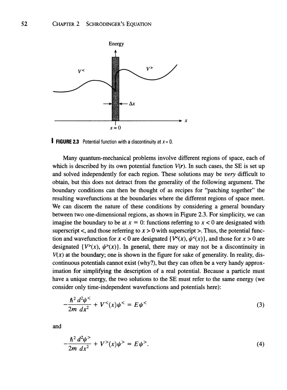
2.4 Interpretation of 1/1: Probabilities and Boundary
Conditions 49
Summary 56
Problems 56
Chapter 3 Solutions of Schrodinger's Equation in One Dimension 59
Part I: Potential Wells 60
3.1 Concept of a Potential Well 60
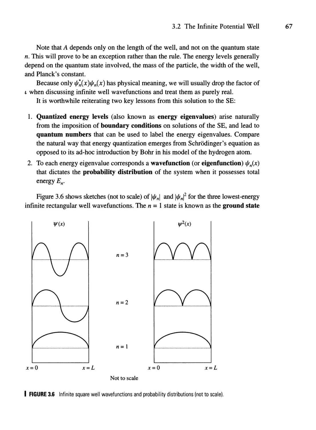
3.2 The Infinite Potential Well 62
3.3 The Finite Potential Well 70
3.4 Finite Rectangular Well-Even Solutions 79
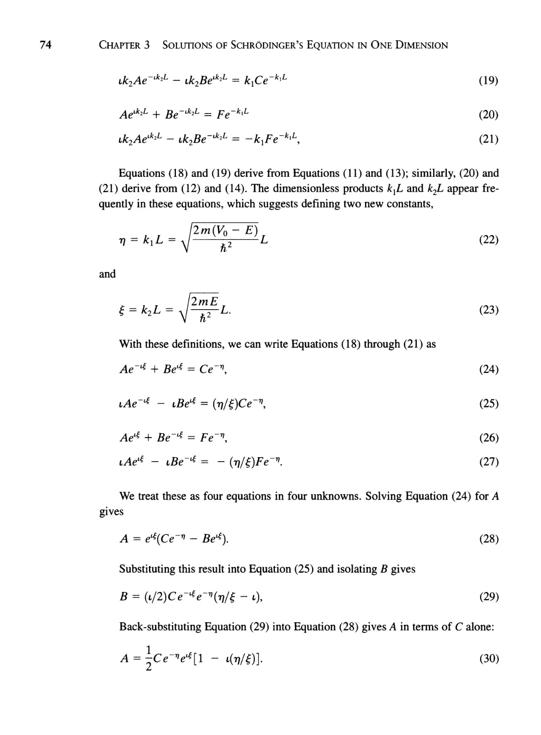
3.5 Number of Bound States in a Finite Potential Well 81
3.6 Sketching Wavefunctions 85
Part II: Potential Barriers and Scattering 88
3.7 Potential Barriers 88
3.8 Penetration of Arbitrarily Shaped Barriers 94
XI

Xll CONTENTS
3.9 Alpha-Decay as a Barrier Penetration Effect 97
3.10 Scattering by One-Dimensional Potential Wells 103
Summary 106
Problems 108
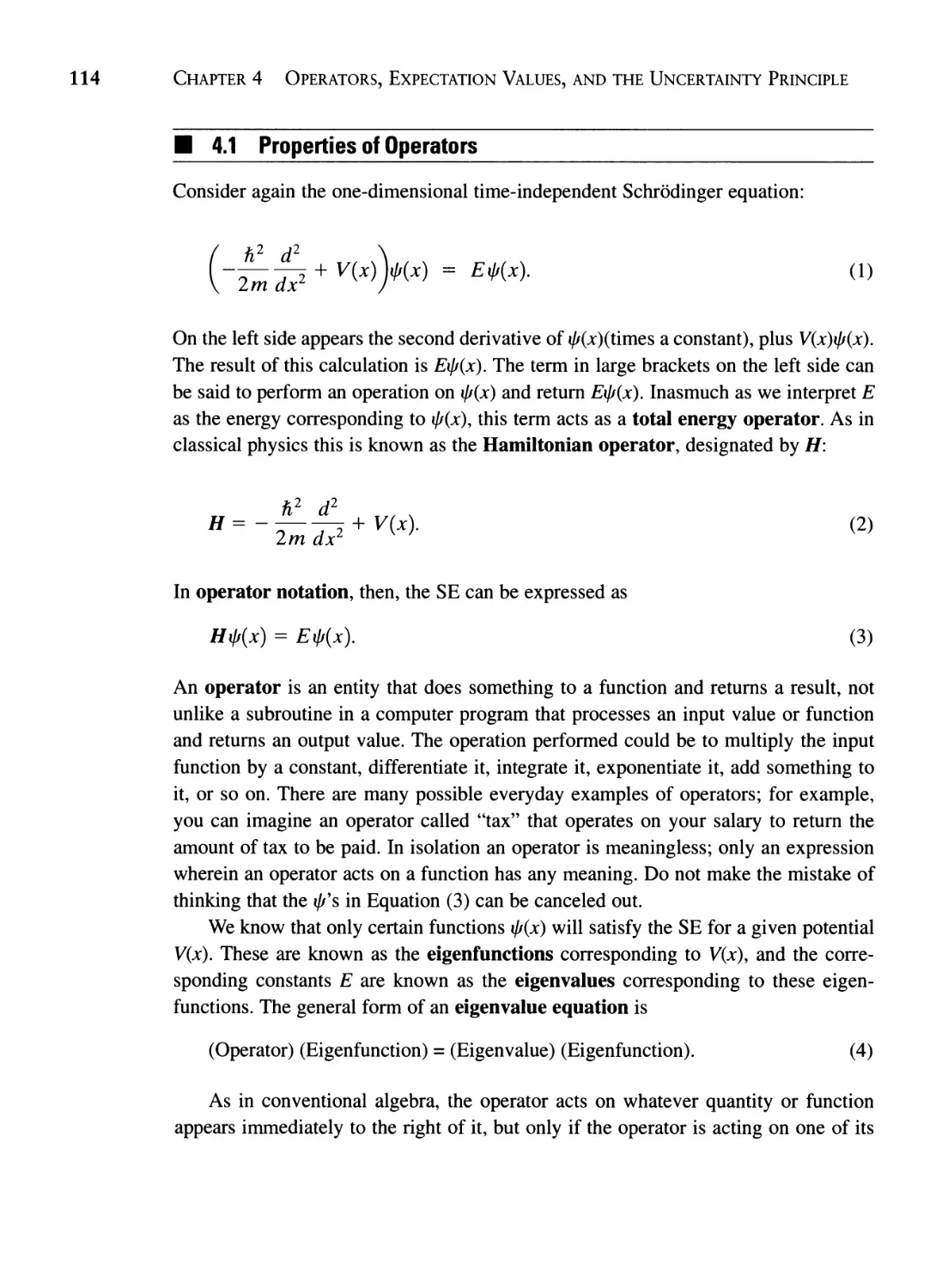
Chapter 4 Operators, Expectation Values, and the Uncertainty Principle 113
4.1 Properties of Operators 114
4.2 Expectation Values 118
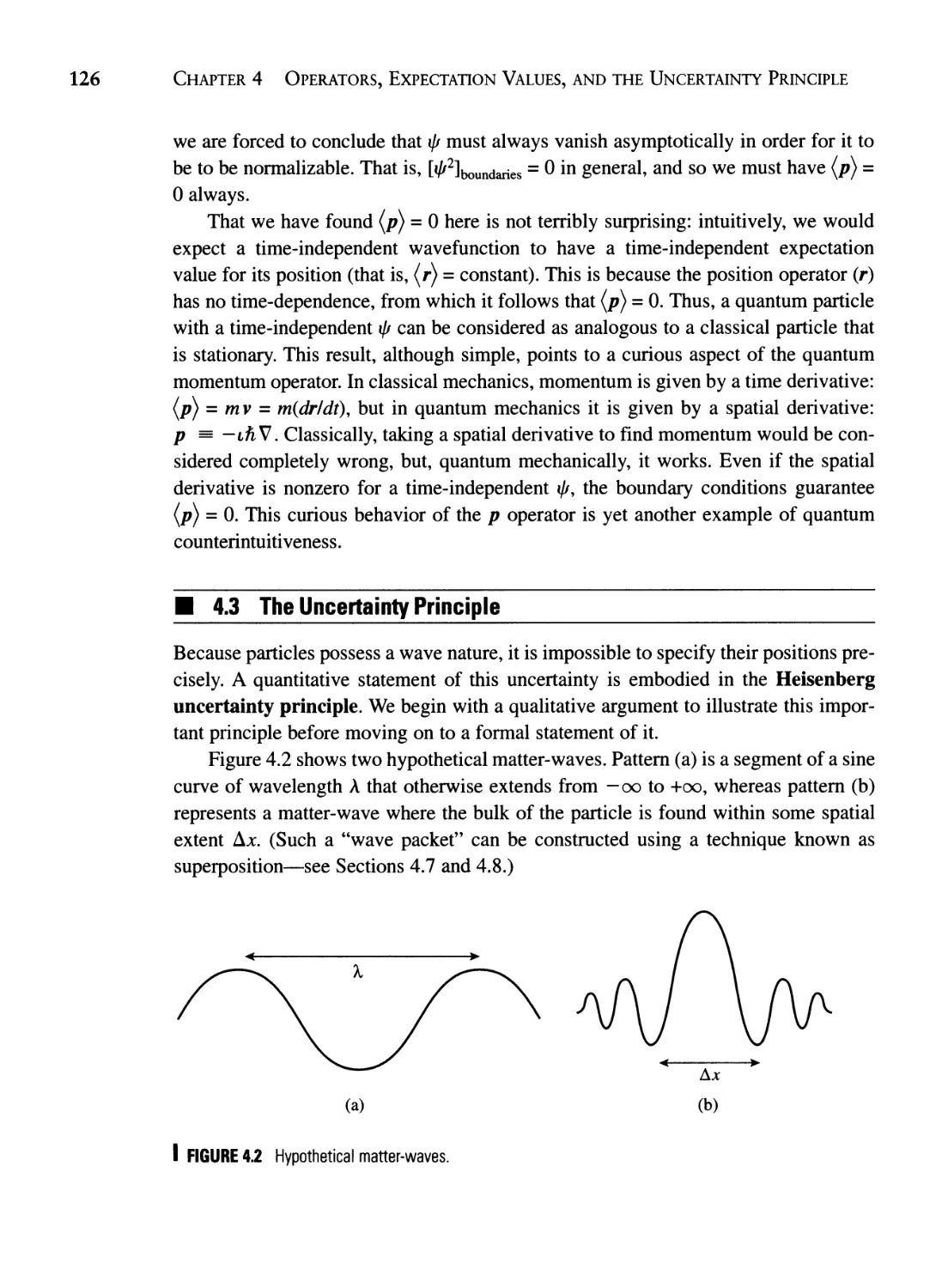
4.3 The Uncertainty Principle 126
4.4 Commutators and Uncertainty Relations 131
4.5 Ehrenfest's Theorem 134
4.6 The Orthogonality Theorem 137
4.7 The Superposition Theorem 139
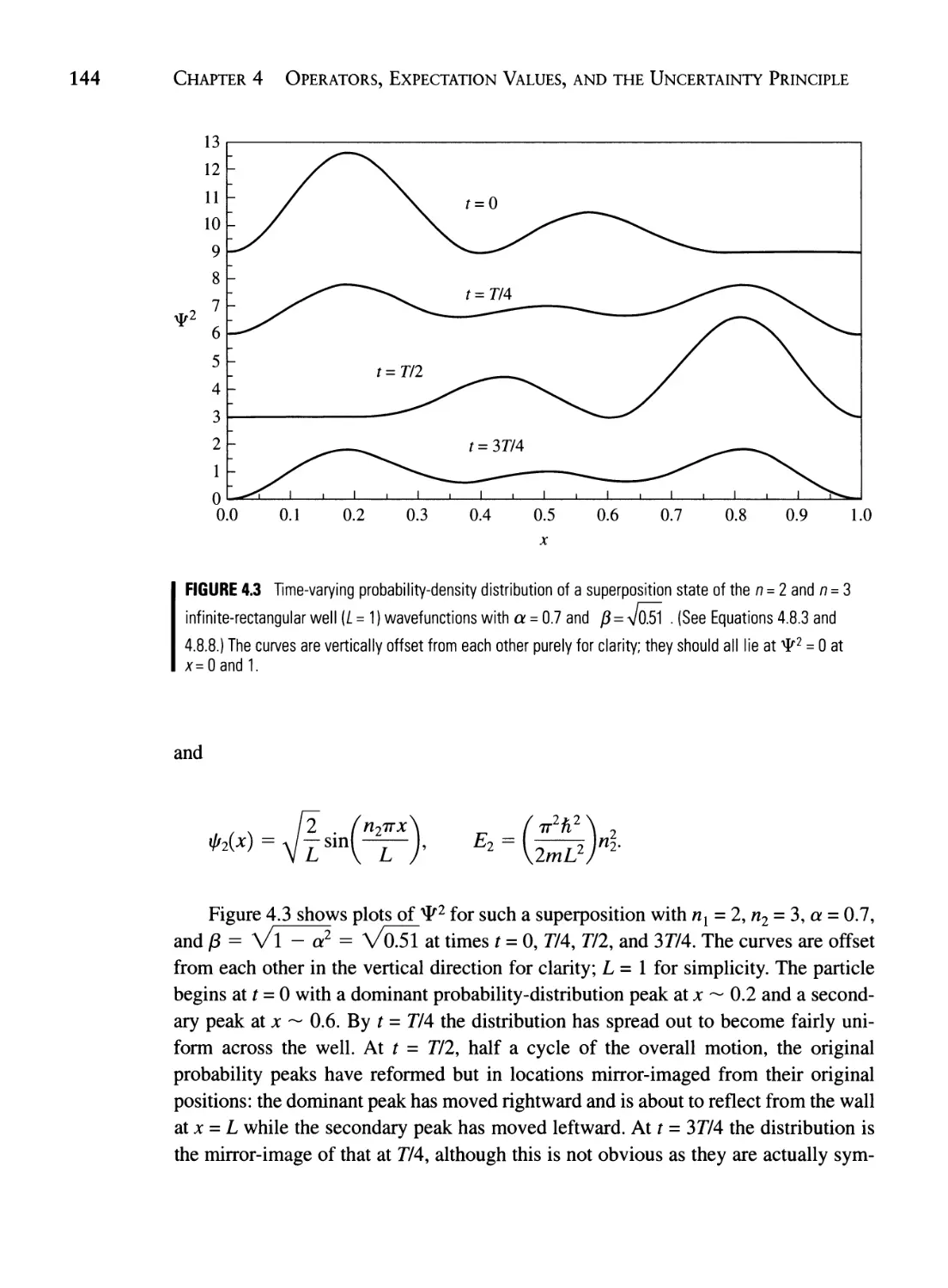
4.8 Constructing a Time-Dependent Wave Packet 141
4.9 The Virial Theorem 146
Summary 153
Problems 154
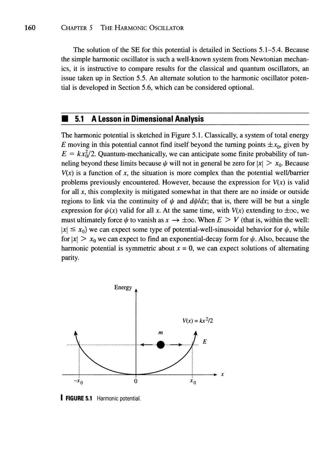
Chapter 5 The Harmonic Oscillator 159
5.1 A Lesson in Dimensional Analysis 160
5.2 The Asymptotic Solution 164
5.3 The Series Solution 165
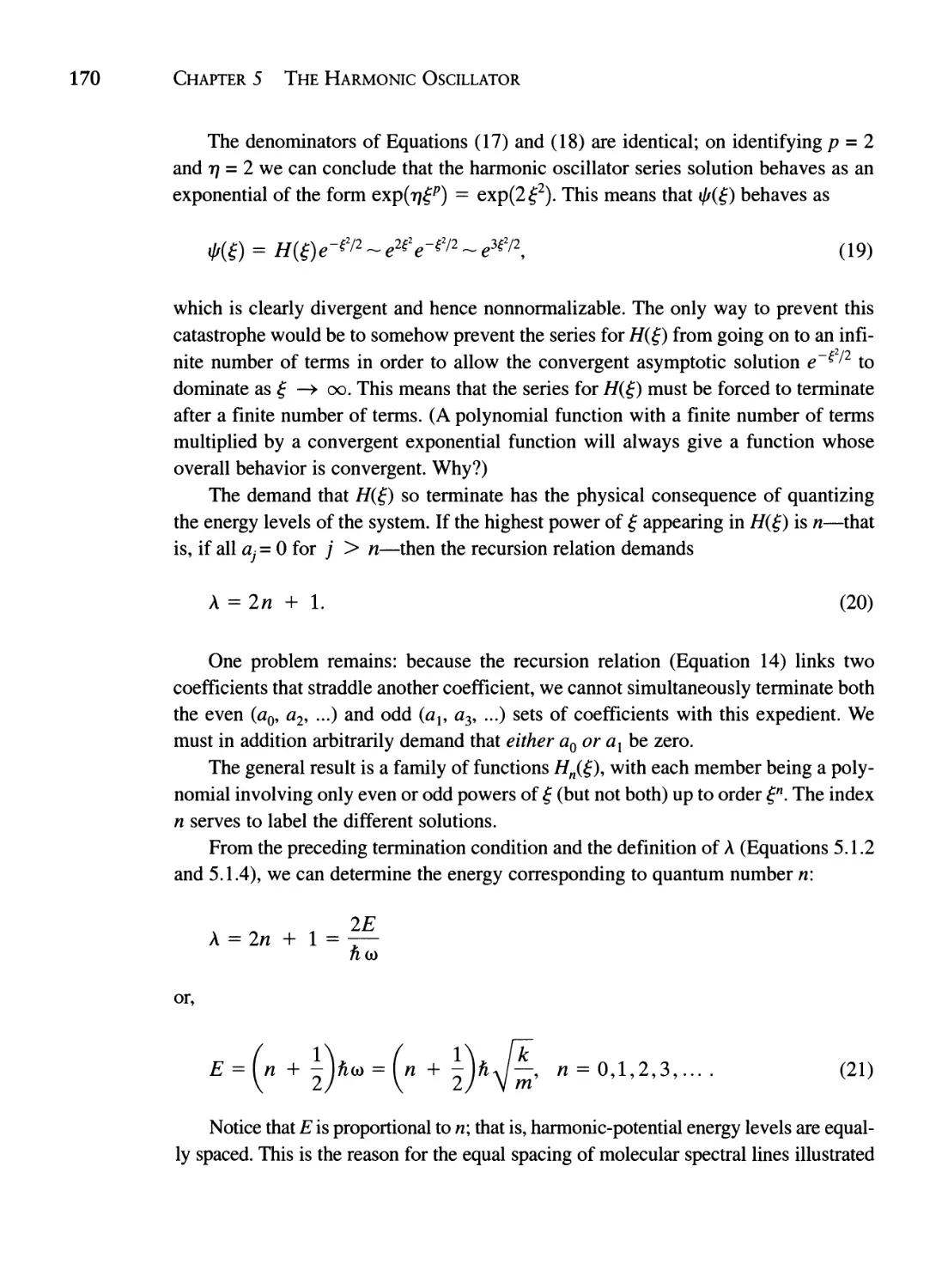
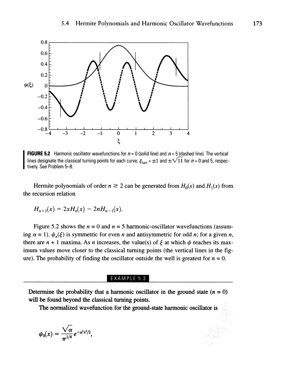
5.4 Hermite Polynomials and Harmonic Oscillator
Wavefunctions 172
5.5 Comparing the Classical and Quantum Simple Harmonic
Oscillators 176
5.6 Raising and Lowering Operators (Optional) 179
Summary 186
Problems 187
Chapter 6 SchrOdinger's Equation in Three Dimensions and an Introduction
to the Quantum Theory of Angular Momentum 191
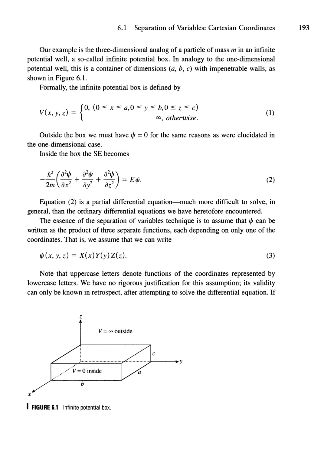
6.1 Separation of Variables: Cartesian Coordinates 192
6.2 Spherical Coordinates 201
6.3 Angular Momentum Operators 203
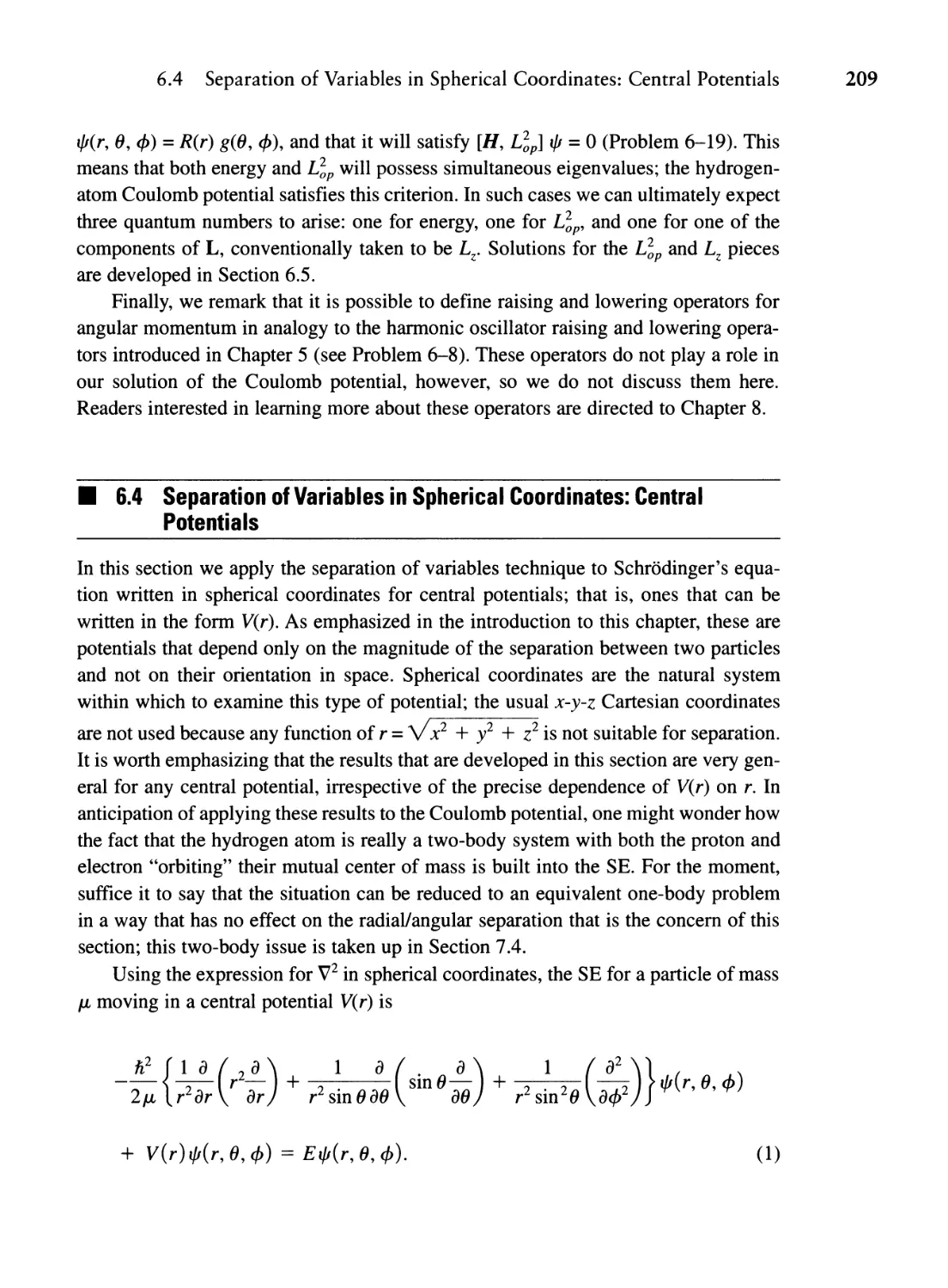
6.4 Separation of Variables in Spherical Coordinates: Central
Potentials 209
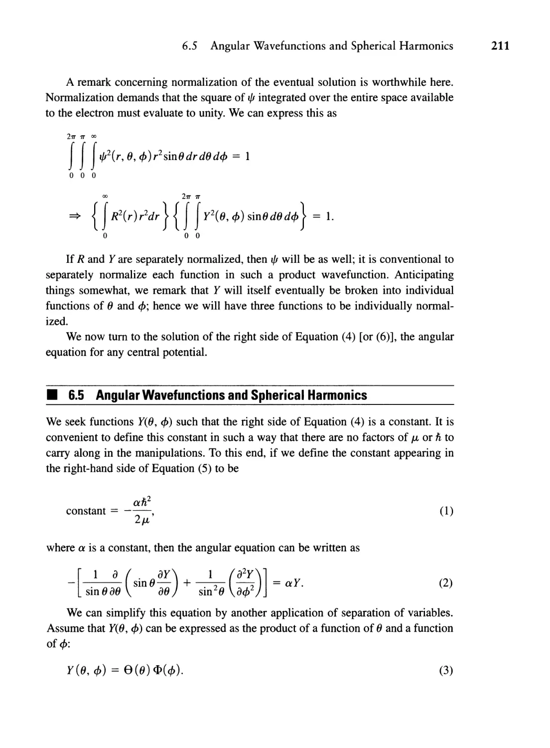
6.5 Angular Wavefunctions and Spherical Harmonics 211
6.5.1 Solution of the <I> Equation 212

CONTENTS Xlii
6.5.2 Solution of the e Equation 215
6.5.3 Spherical Harmonics 220
Summary 225
Problems 227
Chapter 7 Central Potentials 231
7.1 Introduction 231
7.2 The Infinite Spherical Well 234
7.3 The Finite Spherical Well 236
7.4 The Coulomb Potential 240
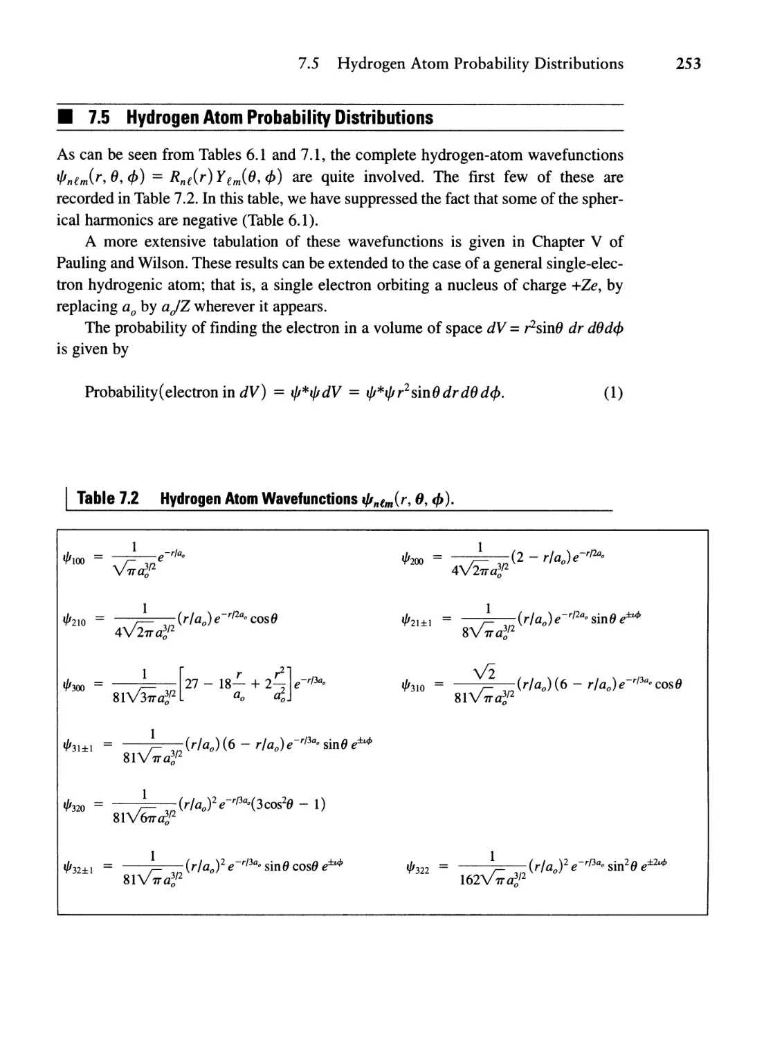
7.5 Hydrogen Atom Probability Distributions 253
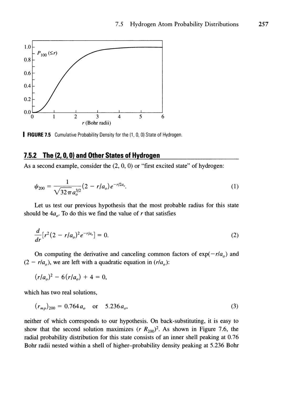
7.5.1 The (1, 0, 0) State of Hydrogen 254
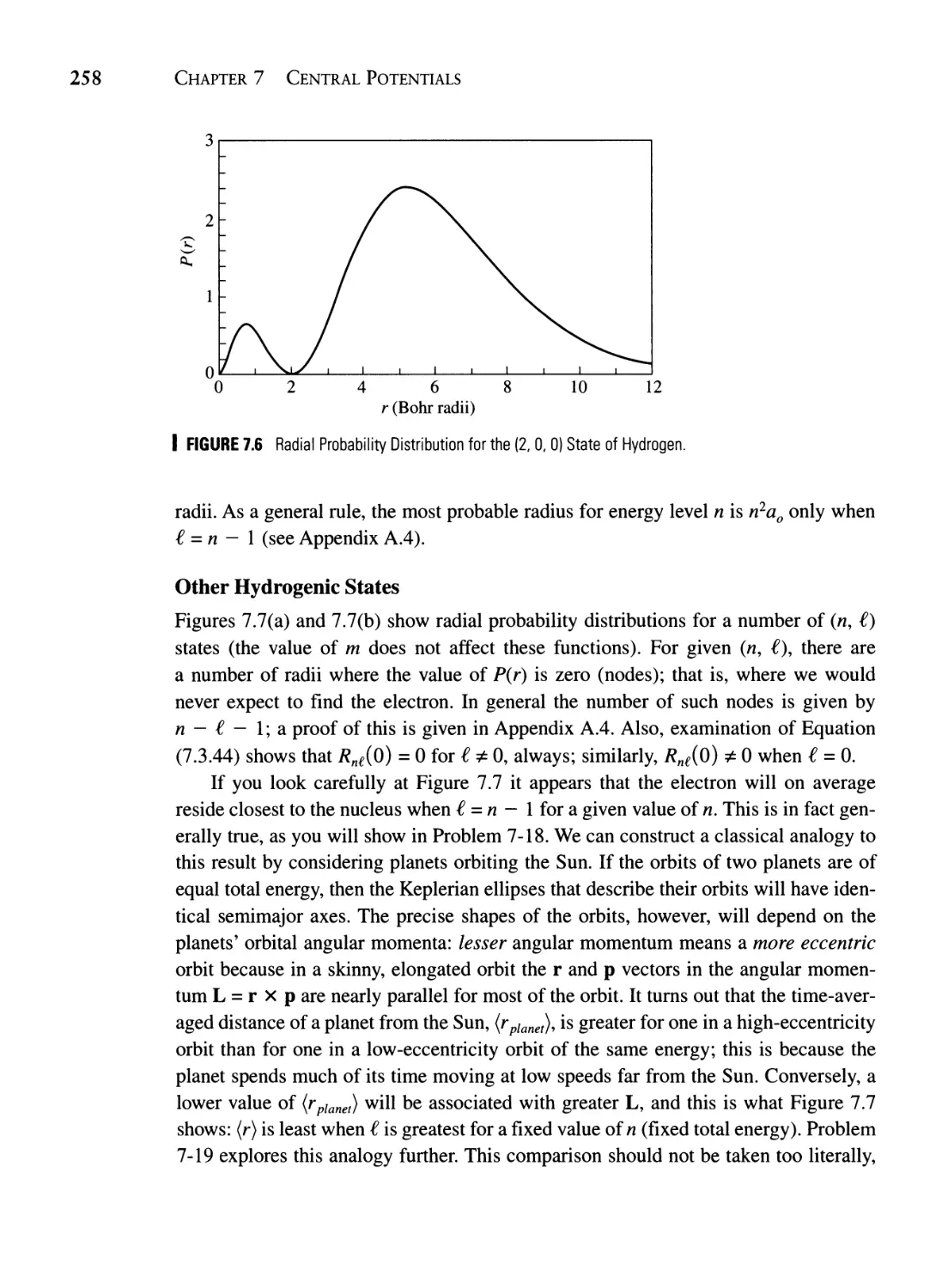
7.5.2 The (2, 0, 0) and Other States of Hydrogen 257
7.6 The Effective Potential 264
7.7 Some Philosophical Remarks 266
Summary 267
Problems 268
Chapter 8 Further Developments with Angular Momentum and
Multiparticle Systems 275
8.1 Angular Momentum Raising and Lowering Operators 275
Section 8.1 Problems 282
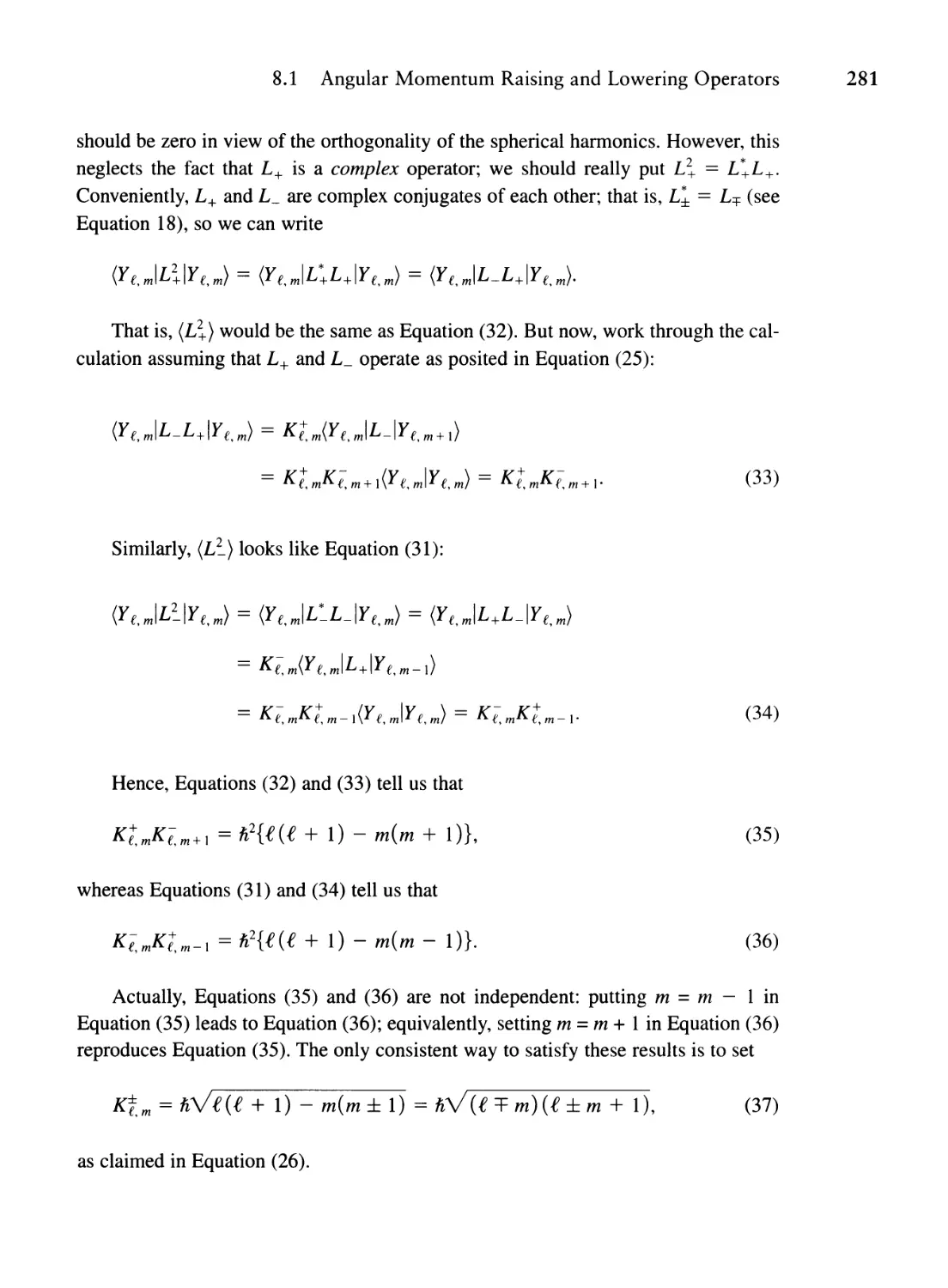
8.2 The Stern-Gerlach Experiment: Evidence for Quantized
Angular Momentum and Electron Spin 282
Section 8.2 Problems 287
8.3 Diatomic Molecules and Angular Momentum 287
Section 8.3 Problems 291
8.4 Identical Particles, Indistinguishability, and the
Pauli Exclusion Principle 291
Section 8.4 Problems 297
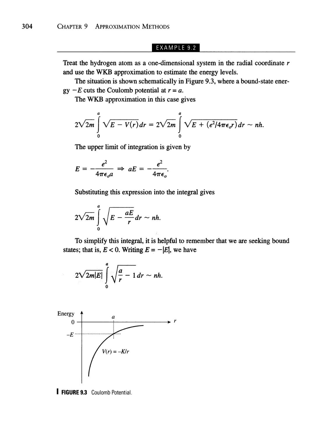
Chapter 9 Approximation Methods 299
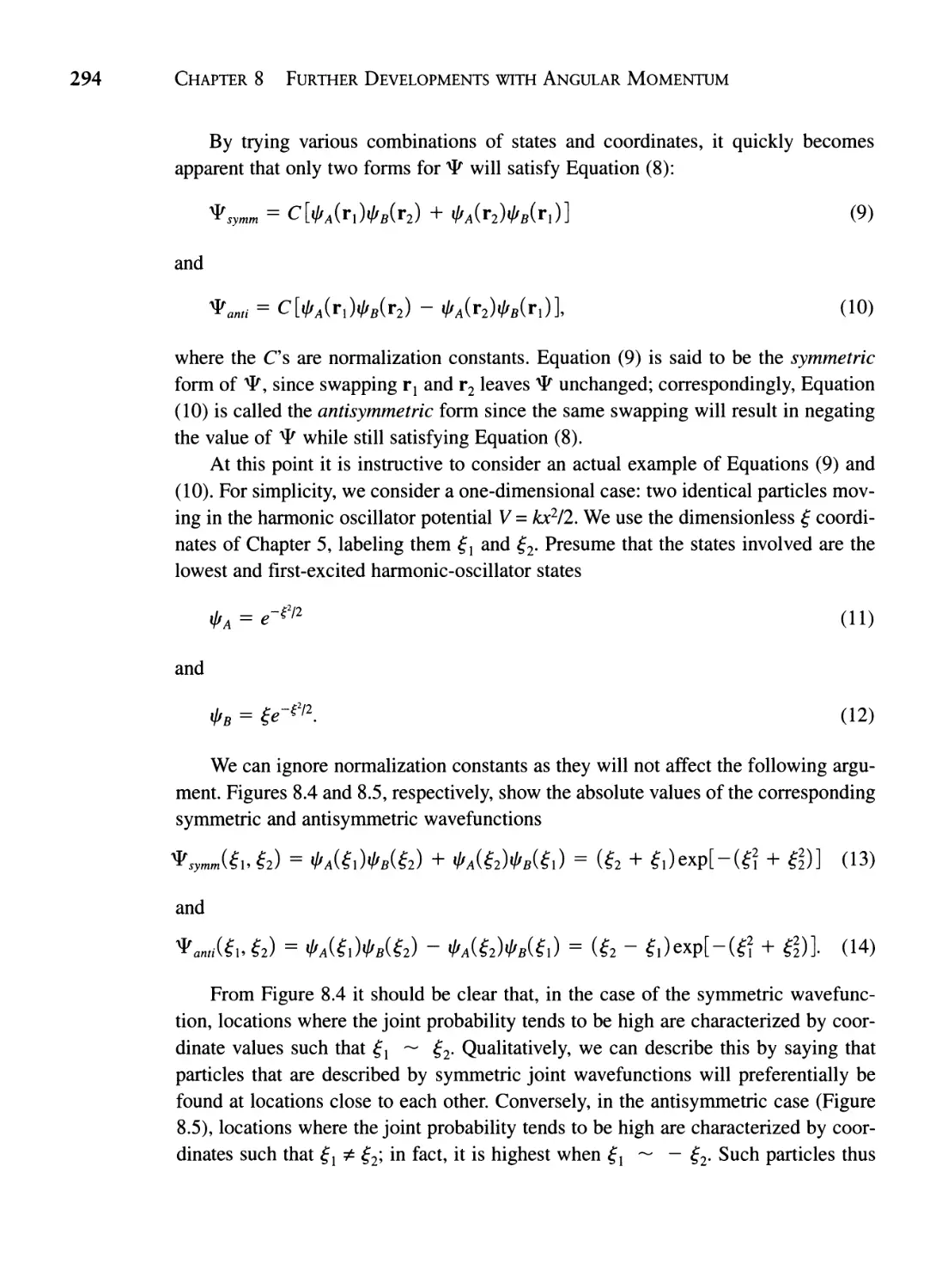
9.1 The WKB Method 299
9.2 The Superposition Theorem Revisited 305
9.3 Perturbation Theory 309
9.4 The Variational Method 327
9.5 Improving the Variational Method (Optional) 336
Summary 340
Problems 343

xiv CONTENTS
Chapter 10 Numerical Solution of Schrodinger's Equation 351
10.1 Atomic Units 352
10.2 A Straightforward Numerical Integration Method 353
Problems 365
Chapter 11 A Sampling of Results from Time-Dependent Quantum
Mechanics: Transition Rates and Probabilities 369
11.1 Transition Frequencies 369
11.2 Transition Rules 373
11.3 The Sudden Approximation 374
Summary 376
Problems 376
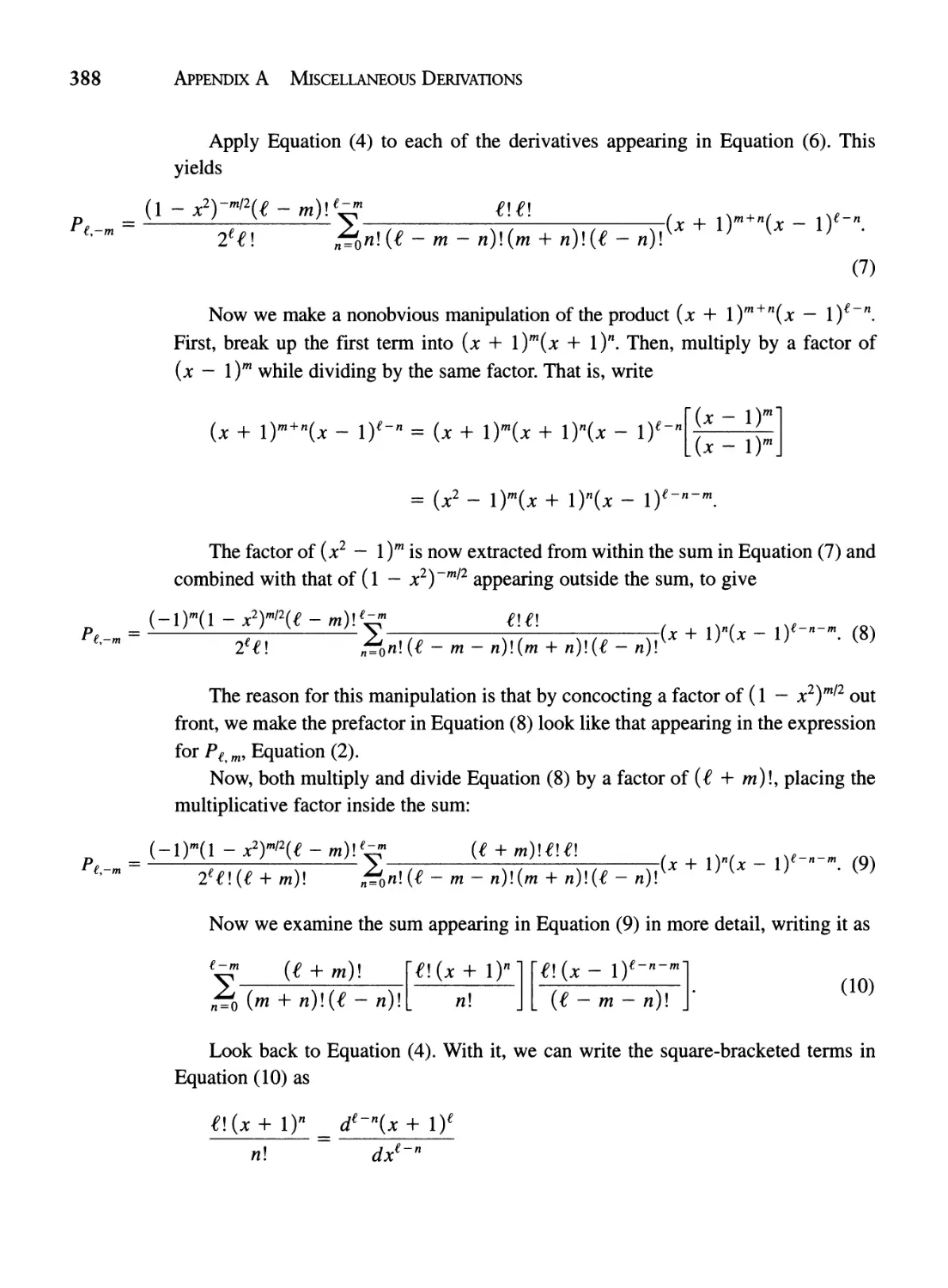
Appendix A Miscellaneous Derivations 379
A.l Heisenberg's Uncertainty Principle 379
A.2 Explicit Series Form for Associated Legendre Functions 384
A.3 Proof that ft, -m = (-1 )my;, m 386
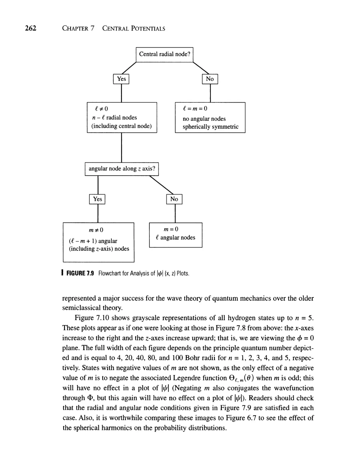
A.4 Radial Nodes in Hydrogen Wavefunctions 391
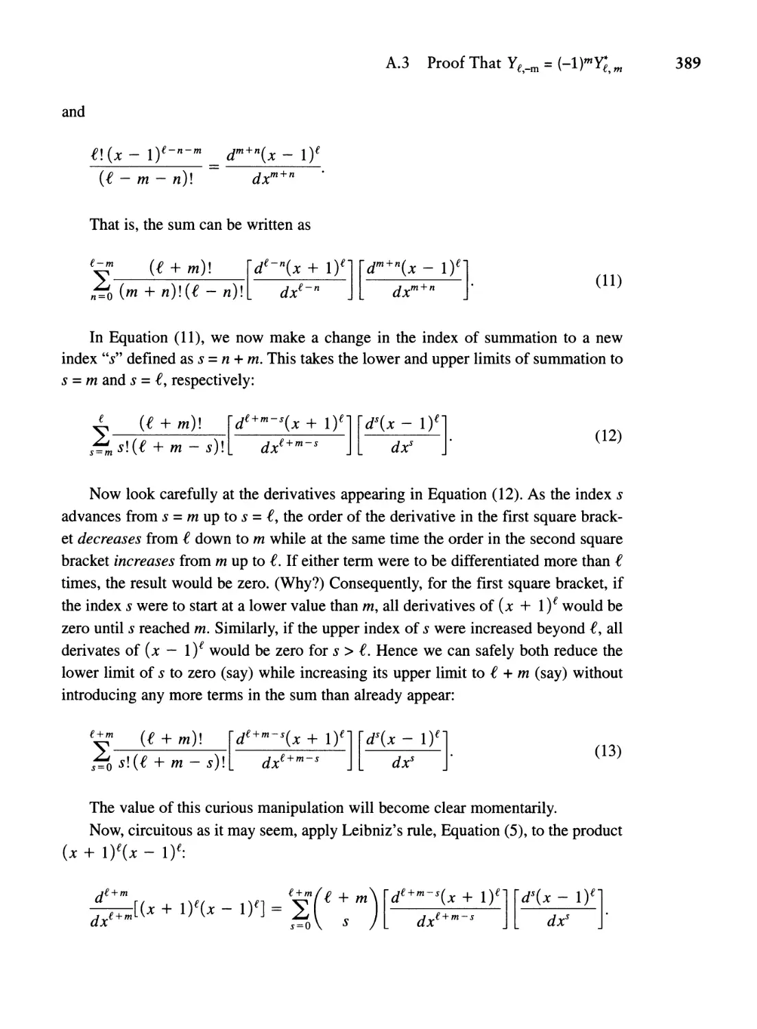
Appendix B Answers to Selected Problems 393
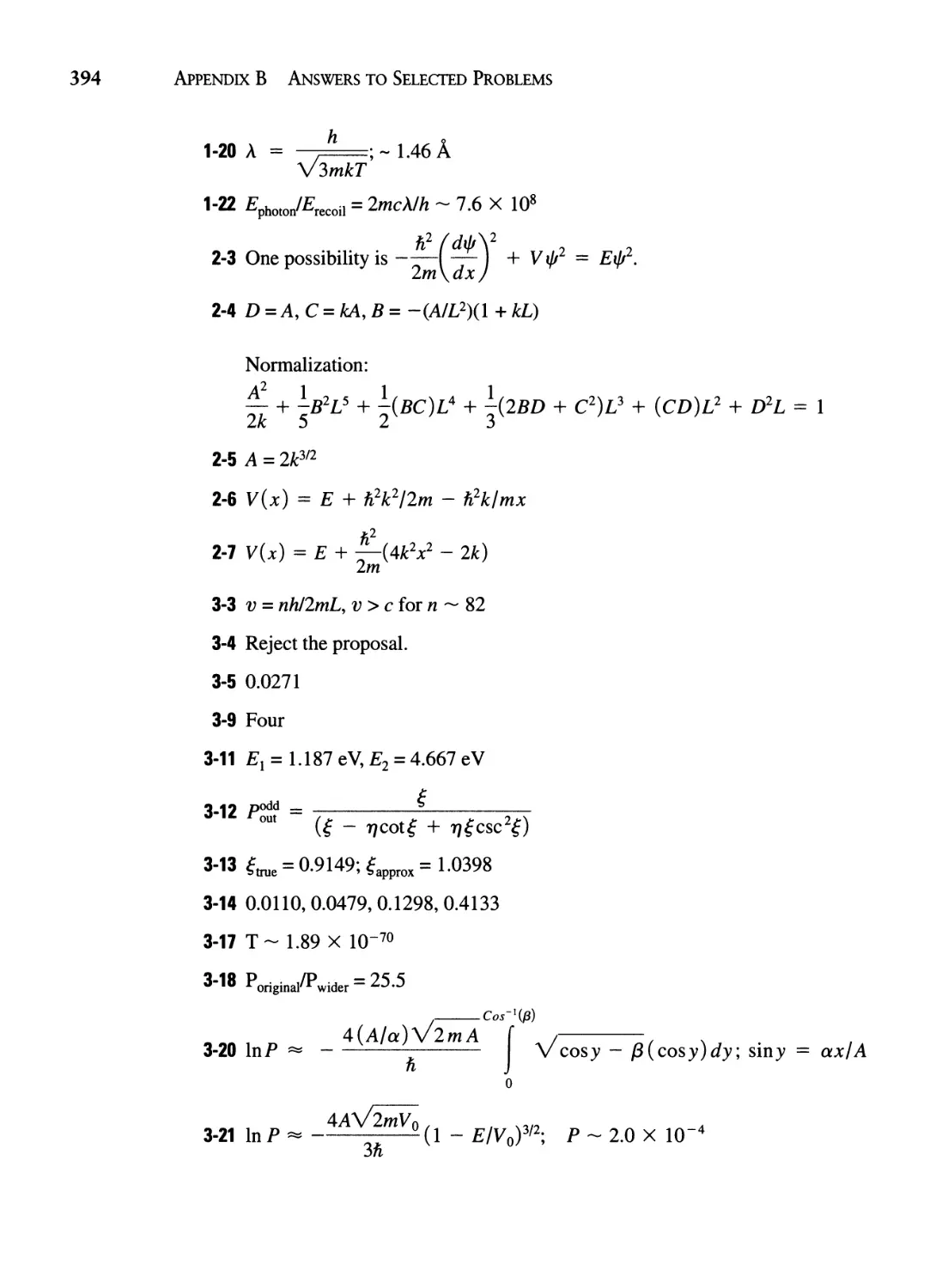
Appendix C Integrals and Trigonometric Identities 401
Appendix D Physical Constants 405
Notes and References 407
Index 411

Foundations
The tremendous success of Newton's laws of mechanics on scales from footballs to
clusters of galaxies is nothing less than staggering. These laws also possess a strong
intuitive appeal: the relative ease with which even beginning students can assimilate
and apply them is due in no small part to the fact that one can often literally see what
the mathematics is describing. Arcing footballs, spinning and colliding billiard balls,
rolling tires, flowing water, oscillating pendula, and to some extent even orbiting satel-
lites, are the stuff of everyday life and common experience: it's easy to formulate a
picture in the mind's eye around which an analysis can be developed. Conversely,
quantum mechanics deals with the nature of matter at the atomic level, far removed
from the domain of practical experience. Although it now constitutes the foundation
of our understanding of everything from the structure of atoms and molecules to the
life cycles of stars, it is also often counterintuitive. Its formulation, use, and interpre-
tation are so vastly different from Newtonian mechanics that questions regarding
familiar concepts such as position and velocity largely lose their meaning.
The counterintuitiveness of quantum mechanics renders it practically impossible to
develop the subject with the smoothness and logical flow of Newtonian mechanics. To
a great extent one must simply plunge in and trust that the customs of quantum culture
will become familiar as one's experience with it grows. Quantum mechanics is not, how-
ever, without its points of contact to classical physics, and these can be exploited to ease
the transition to a quantum mode of thinking. The danger in this is that familiar ideas and
unquestioned assumptions can be difficult to release; there is an art to sensing how far
analogies can be extended. Scientific theories, however revolutionary, do not arise in iso-
lation, and classical mechanics formed the background against which the architects of
quantum mechanics constructed their edifice. Qualitatively, quantum mechanics can be
viewed as a theory that correctly describes the behavior of microscopic material parti-
cles but incorporates the predictions of Newtonian mechanics on macroscopic scales.
The purpose of this chapter is to review some of the facts that led physicists in the
early part of the twentieth century to the realization that Newtonian mechanics is
invalid in the realm of atomic-scale phenomena. You may have encountered some of
the following material in an earlier course: the experiments of Michael Faraday and
1

2
CHAPTER 1 FOUNDATIONS
J.J. Thomson (Section 1.1), the nature of atomic spectra (Section 1.2), the Rutherford-
Bohr model of the atom (Section 1.3), and wave-particle duality (Section 1.4). The
intention here is not in-depth explanation, but rather the context of early twentieth-
century physics and the discrepancies between experiment and theory that forced the
development of a whole new area of physics.
II 1.1 Faraday, Thomson, and Electrons
The roots of modern scientific speculation on atomic structure trace their origins to the
early nineteenth century. From the chemical experiments of Antoine Lavoisier and
John Dalton, the concept of an atom as the smallest unit representative of a given ele-
ment was firmly established by about 1810. Michael Faraday's electrolysis experi-
ments of the early 1830s suggested that electrical current involved the transport of
"ions," which were what we now recognize as individual atoms or molecules bearing
net positive or negative electrical charges. Faraday thus perceived that nature quan-
tizes certain quantities: ions could apparently not possess any arbitrary amount of
electrical charge, but rather only integral multiples of a fundamental unit of charge. In
1881 Irish physicist George Stoney [1] first estimated the fundamental unit of nega-
tive charge to be about -10- 20 Coulomb. In 1891, he coined the term "electron" to
describe the carriers of the fundamental unit of negative charge.
Knowledge of Avogadro's number, N A' along with knowledge of the density and
atomic weight of an element, makes it possible to estimate the effective sizes of atoms
constituting that element. If one imagines a substance to be composed of tightly
packed spherical atoms of radius R, the distance between atomic centers will be 2R.
Each atom will effectively occupy a volume of space equivalent to a cube of side
length 2R, namely 8R3. If the atomic weight of the substance is A grams per mole, the
mass of an individual atom will be A/N A and the density will be p = Aj8N A R 3 , which
we can turn into an expression for the atomic radius:
= ( A ) 1/3
R 8N A P'
(1)
By applying Equation (1) to light and heavy elements, we can get an idea of the
range of atomic sizes. At one extreme is lithium, the lightest naturally solid element.
With A = 7 gram/mole (1.1 X 10- 26 kg/atom) and p = 0.534 gram/cm 3 , we find
R ---1.40 X 10- 10 meter, or 1.40 A (1 Angstrom = 10- 10 meter). At the other end of
the periodic table is uranium, the heaviest naturally occurring element, with A = 238
gram/mole (4 X 10- 25 kg/atom) and p---18.95 gram/cm 3 , which give R ---1.38 A.
Despite a factor of 80 difference in mass, uranium and lithium atoms effectively act as

1.1 Faraday, Thomson, and Electrons
3
if they are about the same size! This is a simplistic analysis, but it does demonstrate
the chemical wisdom that essentially all atoms act as if they are on the order of 1 A in
o
radius. The Angstrom is a convenient unit of length for atomic-scale problems and will
be used extensively throughout this text.
In 1897, J. J. Thomson [2] undertook his famous cathode-ray deflection exper-
iments ("cathode ray" was an early term for electron), from which he determined
the charge-to-mass ratio (e/m) of the electron. In modern units he arrived at a
value of about -2 X 1011 Coulombs/kg; in combination with Stoney's charge esti-
mate of --- -10- 20 Coulomb, it became clear at once that the mass of the electron
must be on the order of 10- 31 kg, some four orders of magnitude smaller than
atomic masses. Moreover, Thomson found the same result for a variety of differ-
ent cathode materials, demonstrating that electrons are universal constituents of all
atoms.
At the time of Thomson's elm experiments, Robert Millikan's oil drop exper-
iments to precisely determine the value of e lay well in the future (1909). However,
let us break with historical sequence to make a point about the size of the electron
itself. We begin with the modern values for the mass and charge of the electron:
me = 9.10954 X 10- 31 kg,
and
e = -1.60219 X 10- 19 C.
Now, a common demonstration in elementary texts on electricity and magnetism
is the derivation of an expression for the self-potential-energy V of a solid sphere of
radius r bearing an electrical charge e distributed uniformly throughout. The result
IS
3e 2
v=
207T€or
(2)
If we assume that this self-energy is equivalent to the sphere's Einsteinian rest
energy E = mc 2 (another break from historical sequence: Einstein did not develop his
special theory of relativity until 1905), we can solve for the radius of the sphere:
3e 2
r=
207T€omC 2 .
(3)

4
CHAPTER 1 FOUNDATIONS
For an electron the numbers give
re -
3( -1.602 X 10- 19 C)2
207T(8.85 x10- 12 C 2 /Nm 2 )(9.11 X 10- 31 kg)(2.998
= 1.69 X 10- 15 m --- 10- 5 atomic radii.
X 108m/s)2
Electrons are minute in comparison to their host atoms; essentially, they are point
masses. Actually, the current experimental evidence is that electrons are in fact point
masses, and that protons have radii of about 0.8 X 10- 15 m. l The preceding analysis pre-
dicts a radius of '"'-10- 18 m for the proton; we can interpret the discrepancy as indicating
that the origin of mass cannot purely be energy. (This is not to imply that E = mc 2 is
somehow in error, only that this approach cannot be an adequate model for the origin of
mass. Modern versions of quantum field theory hold that mass is built up of particles
known as quarks and gluons and fields that connect them. 2 )
Considerations along these lines stimulated development of models of atoms
wherein pointlike, negatively charged electrons were held in stable configurations by
their mutual repulsion within a larger positively charged cloud; Thomson himself was
one of the prime movers in this effort. (Atomic model-building had a venerable histo-
ry well before Thomson; an engaging account is given by Pais [3].) However, these
efforts met with little success, for they failed to explain atomic and molecular spectra.
In addition, Thomson's 1898 atomic model proved of no value in explaining the con-
tinuous spectrum of blackbody radiation. These phenomena played pivotal roles in the
development of quantum mechanics.
II 1.2 Spectra, Radiation, and Planck
In 1814, German scientist Joseph Fraunhofer passed sunlight through a prism and
examined the resulting continuous spectrum of colors with a magnifying glass. To his
surprise, he observed hundreds of dark lines crossing the spectrum at specific wave-
lengths. Later, in the 1850s, Gustav Kirchhoff observed the same effect on passing
light from artificial sources through samples of gas. Work along these lines culminat-
ed in Kirchhoff's three law of spectroscopy:
1. Light from a hot solid object, on passing through a prism, yields a continuous
spectrum with no lines.
IPhysics Today 1995; 48(11):9.
2physics Today 1999; 52( II): II and 2000; 53( I): 13.

1.2 Spectra, Radiation, and Planck
5
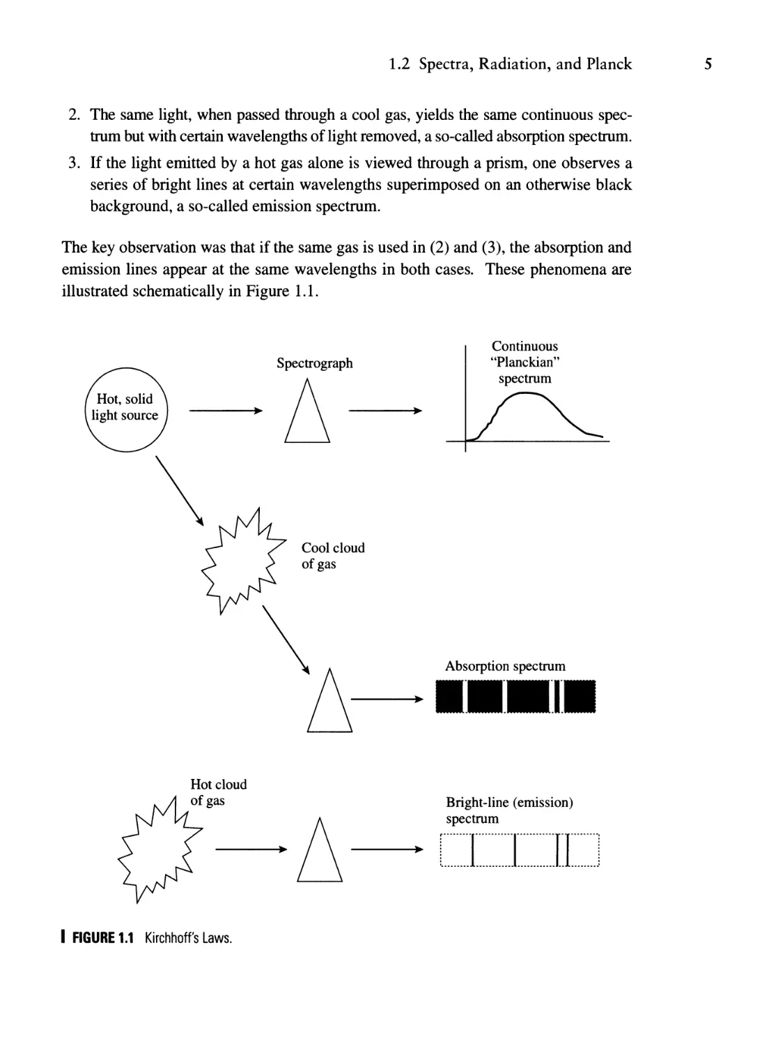
2. The same light, when passed through a cool gas, yields the same continuous spec-
trum but with certain wavelengths of light removed, a so-called absorption spectrum.
3. If the light emitted by a hot gas alone is viewed through a prism, one observes a
series of bright lines at certain wavelengths superimposed on an otherwise black
background, a so-called emission spectrum.
The key observation was that if the same gas is used in (2) and (3), the absorption and
emission lines appear at the same wavelengths in both cases. These phenomena are
illustrated schematically in Figure 1.1.
.
Continuous
"Planckian"
spectrum
Spectrograph
.
Cool cloud
of gas
Absorption spectrum
· ..:.1.
Hot cloud
of gas
.
Bright-line (emission)
spectrum
· :::::::1::::::::: r::::::::::[1::::::::
I FIGURE 1.1 Kirchhoff's Laws.

6
CHAPTER 1 FOUNDATIONS
It soon became clear that every chemical element or compound produces a char-
acteristic pattern of spectral lines; spectroscopy serves as a diagnostic test for the pres-
ence or absence of an element or compound in a given sample. Spectra of a few
substances are shown in Figure 1.2 (reproduced from [4]). Hydrogen displays the sim-
plest pattern of any element: a series of lines separated by ever-decreasing gaps until
a "continuum" of emission is reached at a wavelength of about 3646 A. Molecular
spectra are characterized by overlapping patterns of lines, but regularities are still
apparent.
Explaining line spectra posed a tremendous challenge to builders of atomic mod-
els. Because Maxwell's equations revealed that an accelerating electrical charge radi-
ates energy in the form of light, it was logical to suggest that spectral lines arise from
the motion of Thomson's "corpuscular" electrons in the vicinity of whatever consti-
tutes the massive, positively charged part of the atom. Thomson proposed an atomic
model consisting of pointlike electrons embedded within a much larger spherical
cloud of positive charge, the so-called "raisin bread" or "plum pudding" model. In
such an arrangement the electrons will oscillate back and forth through the cloud in
simple harmonic motion as would a billiard ball dropped into a frictionless hole bored
through the Earth. Although these oscillations lead to frequencies on the order of that
of visible light, Thomson's model suffers from two serious difficulties. The first is that
only one frequency results from an atom of a given size. How are we to account for
whole series of spectral lines ? The second difficulty is even more catastrophic. As the
electron radiates away energy the amplitude of its motion should steadily decrease
until it comes to rest in the center of the atom. In short, matter should collapse!
How, then, to explain discrete-line spectra at all? Thomson worked with immense
dedication over many years on a variety of models of this general sort, but with no real
success. Understanding the stability of atoms and the origin of line spectra had to
await the augmentation of classical models by new quantum postulates.
There was, however, one piece of evidence that gave early atomic theorists hope
that nature might yield her secrets to mathematical analysis. In 1885, Johann Balmer
discovered that the wavelengths of the spectral lines of hydrogen followed a simple
mathematical regularity [5], namely, that they could be computed from the formula
( n2 ) 0
An = 3646 2 A, n = 3, 4, 5, ... .
n - 4
(1)
Note that as n  00, An  3646 A, the wavelength at which the hydrogen spec-
trallines "pile up" into a continuum.
Balmer's formula was purely empirical, with no model of an underlying physical
mechanism. This does not diminish its value, though, for when a phenomenon can be

1.2 Spectra, Radiation, and Planck
7

00  lr) t-
N .....-4 0 .....-4
\0 \0  0
lr) 00  .....-4
\0   
I I I I
(a)
I I I I I
Ha Hfi Hy He} Hoo

  N
0\  .....-4
lr) lr) lr)
N N N
I I I
I ...111111111111. (b)
o<I::
\0 0\  0\
N N 0 
0 lr) 00 0\
 00 \0 lr)
 N N N
I I I
(c)
o<I::
t-
0\
\0
N
I
.111
lr)
o
\0
N
I
00
.....-4
lr)
N
I
.....-4
lr)

N
I
00
00

N
I
I I
I
. ]11
(d)
FIGURE 1.2 (a) Emission spectrum of hydrogen.
(b) Absorption spectrum of sodium.
(c) Emission spectrum of sodium.
(d) Spectrum of PN molecule.
Reproduced from G. Herzberg, Atomic spectra and atomic structure, Dover Publications, Inc.,
New York, 1944. Reprinted through the permission of the publisher.

8
CHAPTER 1 FOUNDATIONS
fitted into a simple arithmetic scheme one is justified in having hope that a deeper
understanding may not be far off. Indeed, Balmer's formula was a key clue for Niels
Bohr's development of the first really successful theory of atomic structure.
We remark in passing that spectroscopists often refer to spectral lines by their
reciprocal wavelengths. Balmer's formula can be rearranged to reflect this:
1 _ ( 1 1 ) 0 -1 _
An - R H 4 - n 2 A , n - 3, 4, 5, · .. ,
(2)
where R H is known as the Rydberg constant for hydrogen; its experimental value is
109,678 cm- l . With considerable success, Swedish physicist Johannes Rydberg sug-
gested that the spectral lines of any element could be described by a generalized ver-
sion of Equation (2):
1 ( 1 1 )
= K - - - (n > m),
A m 2 n 2
n, m
(3)
where K is a constant specific to the element involved. Different series of spectral lines
are given by various values of n for a fixed value of m. We will return to this modified
Balmer formula later in this chapter.
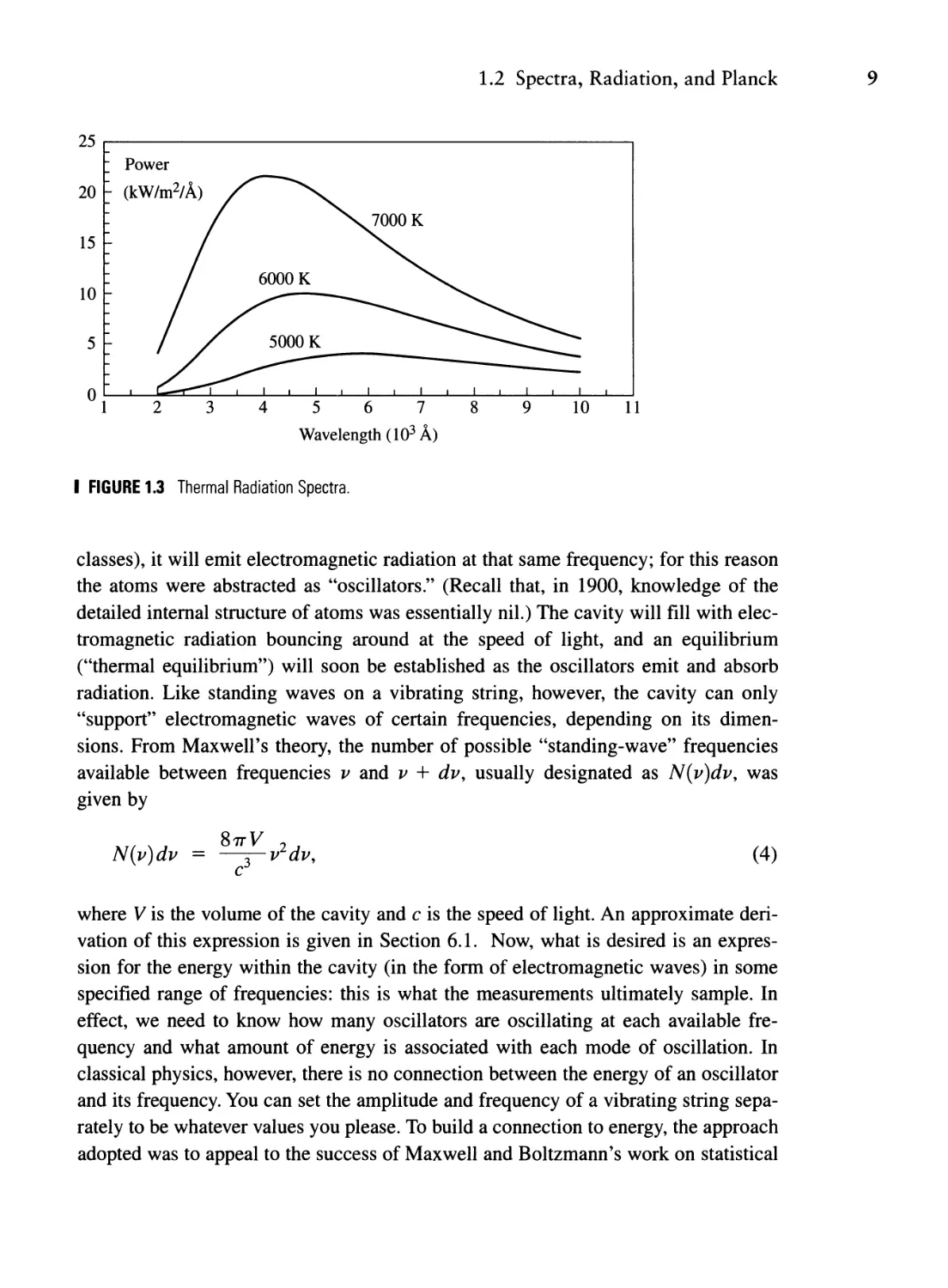
Continuous spectra also posed a challenge to classical physics. Experimentally,
any solid body at a temperature T above absolute zero emits a continuous spectrum of
electromagnetic radiation. By the end of the nineteenth century, experiment had also
established that the spectrum of "thermal radiation" emitted by a body is independent
of the nature of the body, depending only on T. These experiments were usually car-
ried out with so-called "blackbody" cavities. This can be thought of as a heated, inter-
nally hollow lump of metal with a hole in it from which some of the thermal radiation
can escape and so be sampled by a detector. Figure 1.3 shows spectra for the light
emitted by such cavities at temperatures of 5000, 6000, and 7000 K over the wave-
length range 2000-10,000 Angstroms; what is plotted is the power emitted per square
meter of surface area of the sampling hole per unit Angstrom wavelength interval as a
function of wavelength. (The range of human vision spans approximately 3500-7000
A). As T increases, the wavelength of peak emission shifts to shorter (bluer) wave-
lengths. If you are familiar with some stellar astronomy, you may know that blue stars
have hotter surfaces than yellow stars, which in turn are hotter than red-dwarf stars.
Attempts to find a mathematical description of thermal radiation based on clas-
sical models failed completely. The generally held concept was somewhat analogous
to Thomson's oscillating electrons: each atom of a material body would be in con-
stant motion, jostling about with its neighbors. When a charged particle oscillates at
frequency v (in, say, simple harmonic motion as studied in freshman-level physics

1.2 Spectra, Radiation, and Planck
9
25
Power
20 (kW/m 2 /A)
15
10
5
0 1
2
3
45678
Wavelength (10 3 A)
9
10
II
I FIGURE 1.3 Thermal Radiation Spectra.
classes), it will emit electromagnetic radiation at that same frequency; for this reason
the atoms were abstracted as "oscillators." (Recall that, in 1900, know ledge of the
detailed internal structure of atoms was essentially nil.) The cavity will fill with elec-
tromagnetic radiation bouncing around at the speed of light, and an equilibrium
("thermal equilibrium") will soon be established as the oscillators emit and absorb
radiation. Like standing waves on a vibrating string, however, the cavity can only
"support" electromagnetic waves of certain frequencies, depending on its dimen-
sions. From Maxwell's theory, the number of possible "standing-wave" frequencies
available between frequencies v and v + dv, usually designated as N(v)dv, was
given by
_ 87TV 2 d
N(v)dv - 3 v v,
c
(4)
where V is the volume of the cavity and c is the speed of light. An approximate deri-
vation of this expression is given in Section 6.1. Now, what is desired is an expres-
sion for the energy within the cavity (in the form of electromagnetic waves) in some
specified range of frequencies: this is what the measurements ultimately sample. In
effect, we need to know how many oscillators are oscillating at each available fre-
quency and what amount of energy is associated with each mode of oscillation. In
classical physics, however, there is no connection between the energy of an oscillator
and its frequency. You can set the amplitude and frequency of a vibrating string sepa-
rately to be whatever values you please. To build a connection to energy, the approach
adopted was to appeal to the success of Maxwell and Boltzmann's work on statistical

10 CHAPTER 1 FOUNDATIONS
mechanics. Their research showed that if a particle is in an environment at absolute
(Kelvin) temperature T, then the probability of it having energy between E and
E + dE is proportional to an exponential function of T:
p(E)dE = A e- E / kT dE
,
(5)
where A is a constant and k is Boltzmann's constant. To determine A we insist that if
we add up probabilities over all possible energies they must sum to unity. This is
equivalent to saying that the particle must have some energy between 0 and infinity.
That is, we demand
00
00
I p(E)dE = A I e- E / kT dE 1.
o 0
This integral evaluates to kT, giving A = l/kT. The average energy of a particle
in such a situation is then given by the integral of probability-weighted energy:
00
00
(E) = I Ep(E)dE = k I Ee- E / kT dE = kT.
o 0
(For a fuller elaboration of this averaging technique, see Section 4.2.) The assumption
is now made that the number of oscillators wiggling about with frequencies between
v and v + dv is given by Equation (4), and that the amount of radiant energy in the
cavity between these frequencies is consequently given by this number times the aver-
age energy of an oscillator at temperature T, kT:
(6)
87TV
E(v)dv = 3 kTv 2 dv.
c
(7)
Despite these various assumptions, this relationship actually proved to be in good
agreement with experimental data at low frequencies. At high frequencies, though, one
has a disaster: The amount of energy in the cavity becomes infinite, a situation known
as the ultraviolet catastrophe. Something was apparently wrong with either classical
electromagnetism or statistical mechanics, or perhaps even both. It is probably fair to
say that at the dawn of the twentieth century, thermal radiation was the outstanding
problem of theoretical physics.
A way around this difficulty was found by Max Planck of the University of Berlin
in late 1900, in a paper usually credited with marking the birth of quantum mechanics
proper [6]. However, his solution came at a substantial price: abandoning the classical
notion that the energy and frequency of an oscillator are independent. Planck proposed
that the energy of an oscillator is restricted to only certain multiples of its frequency,

1.2 Spectra, Radiation, and Planck 11
namely, En == nhv, where n is an integer-valued "quantum number" (n == 0, 1, 2, 3, ...)
and h is a constant of nature.
Maintaining the assumption of a Maxwellian exponential probability distribution,
the probability of an oscillator having energy E is now given by
p(E) == Ae-nhll/kT
,
(8)
where A is again a normalization constant. Note carefully that no "dE" appears in this
expression: the idea now is that an oscillator has some probability of having a partic-
ular energy, as opposed to any arbitrary energy between E and E + dE. Forcing the
probabilities to again add up to unity means that we must have
00
A  e-nhll/kT - 1,
n=O
or
00
A  (e-hll/kT)n - 1. (9)
n=O
We are summing over discrete energy states as opposed to integrating over ener-
gy as a continuous variable. The sum appearing in Equation (9) is of the form LX n ,
where x == e- hll / kT ; that is, we have a geometric series. Such a sum evaluates to
(1 - x)-l, hence
A == (1 - e- hll / kT )
,
(10)
and so the probability of an oscillator having energy E can be written as
p(E) == e-nhll/kT (1 - e- hll / kT ).
(11)
With this new probability recipe, the average energy of oscillators of frequency
v becomes
00 00 00
(E) == Ep(E) == (nhv)p(E) == hv(1 - e- hll / kT ) ne-nhll/kT
n=O n=O n=O
e- hv / kT
== hv ( 1 - e- hll / kT )
(1 - e- hv / kT )2
hv
( e hll / kT - 1 ) ·
(12)
In working Equation (12), we have used another result from series analysis, namely

12 CHAPTER 1 FOUNDATIONS
00 X
nxn == 2 (Ix I < 1),
n=O (1 - x)
where we again have x == e- hll / kT . Again assuming that the number of oscillators with
frequencies between v and v + dv is given by Equation (4), we find a new expression
for the energy in the cavity between frequencies v and v + dv:
87ThV v 3
E(v)dv == 3 h / kT ) dv.
c (e v-I
(13)
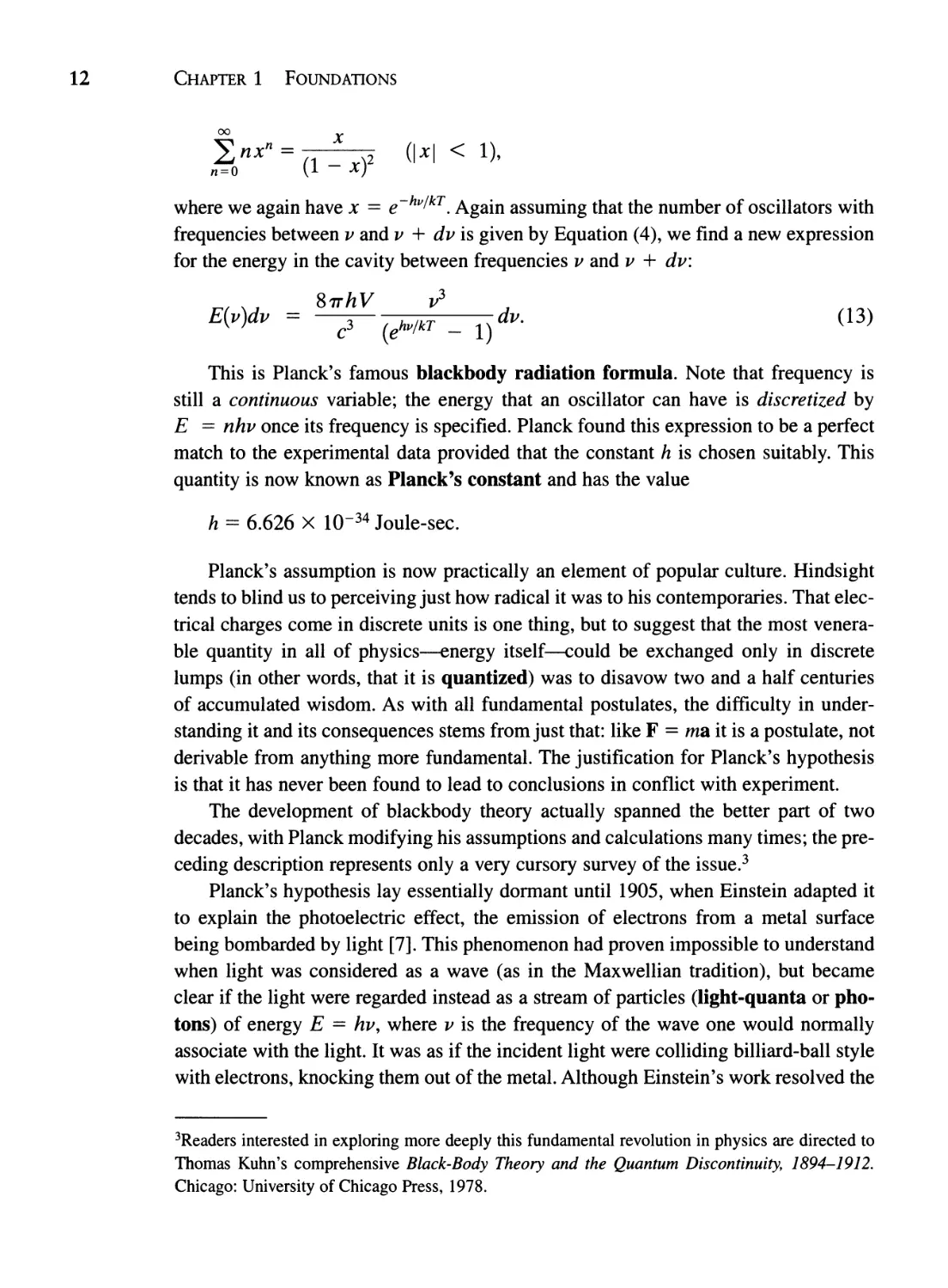
This is Planck's famous blackbody radiation formula. Note that frequency is
still a continuous variable; the energy that an oscillator can have is discretized by
E == nhv once its frequency is specified. Planck found this expression to be a perfect
match to the experimental data provided that the constant h is chosen suitably. This
quantity is now known as Planck's constant and has the value
h == 6.626 X 10- 34 Joule-sec.
Planck's assumption is now practically an element of popular culture. Hindsight
tends to blind us to perceiving just how radical it was to his contemporaries. That elec-
trical charges come in discrete units is one thing, but to suggest that the most venera-
ble quantity in all of physics-energy itself-could be exchanged only in discrete
lumps (in other words, that it is quantized) was to disavow two and a half centuries
of accumulated wisdom. As with all fundamental postulates, the difficulty in under-
standing it and its consequences stems from just that: like F == ma it is a postulate, not
derivable from anything more fundamental. The justification for Planck's hypothesis
is that it has never been found to lead to conclusions in conflict with experiment.
The development of blackbody theory actually spanned the better part of two
decades, with Planck modifying his assumptions and calculations many times; the pre-
ceding description represents only a very cursory survey of the issue. 3
Planck's hypothesis lay essentially dormant until 1905, when Einstein adapted it
to explain the photoelectric effect, the emission of electrons from a metal surface
being bombarded by light [7]. This phenomenon had proven impossible to understand
when light was considered as a wave (as in the Maxwellian tradition), but became
clear if the light were regarded instead as a stream of particles (light-quanta or pho-
tons) of energy E == hv, where v is the frequency of the wave one would normally
associate with the light. It was as if the incident light were colliding billiard-ball style
with electrons, knocking them out of the metal. Although Einstein's work resolved the
3Readers interested in exploring more deeply this fundamental revolution in physics are directed to
Thomas Kuhn's comprehensive Black-Body Theory and the Quantum Discontinuity, 1894-1912.
Chicago: University of Chicago Press, 1978.

1.2 Spectra, Radiation, and Planck 13
photoelectric effect, it thrust into the foreground an apparent paradox: Is light a wave
or a stream of particles? On one hand it behaves optically as any sensible wave: it is
refractable, diffractable, focusable, and so forth. On the other it can behave dynami-
cally, like billiard balls. Which picture do we adopt? The answer is, we have to live
with both. Although in some circumstances one can conveniently analyze an experi-
ment with an explicitly wave picture in mind (for example, double-slit diffraction in
classical optics), whereas in others a particle view provides for a convincing analysis
(the photoelectric effect), the inescapable fact is that photons possess both wave and
particle properties simultaneously (as do material particles such as electrons and entire
atoms and molecules-see Section 1.4). Indeed, it has been amply experimentally ver-
ified that photons interfere with themselves even as they pass, one by one, through an
optical system! 4 We shall have more to say about this wave-particle duality in coming
chapters.
The idea of light carrying momentum was not new. Indeed, Maxwell had pre-
dicted that electromagnetic radiation of energy E would possess momentum in the
amount p = E/c. (If you are familiar with special relativity, recall the Einstein ener-
gy-momentum-rest mass relation E2 = p 2 C 2 + m6c4, and set the rest mass mo to be
zero for a photon.) This can be expressed in terms of the frequency of the light as
p = E I A since c = Av. If light is also treated as consisting of particles character-
ized by the Planck relation E = hv, then p = hi A or
h
A = -.
P
(14)
Equation (14) applies only to photons even though it was derived from a mixture
of both classical and quantum concepts. Nevertheless, in the 1920s, Arthur H.
Compton verified that photons and electrons indeed interact billiard-ball style, pre-
cisely as the equation predicts. This deceptively simple equation will figure in subse-
quent discussions.
The substitutions leading to Equation (14) are simple. Yet, it seems remarkable
that the connection between Planck's quantized oscillator energies and the discrete
wavelengths (= discrete energies) of light constituting spectral lines was not made for
nearly another decade. This breakthrough had to await further experimental probing
of the internal structure of atoms.
_ 1.3 The Rutherford-Bohr Atom
4For readers interested in learning about the details of such experiments and many other aspects of
the fundamentals of quantum mechanics, George Greenstein and Arthur Zajonc's The Quantum
Challenge (Sudbury, MA: Jones & Bartlett, Second Edition, 2006) is highly recommended.

14 CHAPTER 1 FOUNDATIONS
In early 1911, Ernest Rutherford, in collaboration with Hans Geiger and Ernest
Marsden, proposed a model of atomic structure radically different from Thomson's
plum-pudding scenario [8]. Based on an analysis of the distribution of alpha-particles
(helium nuclei) scattered through thin metal foils, they put forth a nuclear model of
the atom wherein the positive charge (and with it most of the atomic mass) is concen-
trated in a tiny volume of space at the center of the atom, around which negative elec-
trons orbit like planets about the Sun. 5 Their experiments indicated a size on the order
of 10- 14 meters for the positively charged nucleus: it was larger than an electron, but
some four orders of magnitude smaller than the atom itself. Evidently, atoms are most-
ly empty space.
The stage was now set for a leap of logic of the sort alluded to at the end of Section
1.2. Planck had established that atoms constituting the source of thermal radiation
from material bodies could exist only in certain discrete energy states. If Rutherford's
planetary electrons were restricted to orbits of certain special energies, could electrons
"transiting" from orbits of higher energy (say, E 2 ) to orbits of lower energy (say, E 1 )
be the source of spectra and thermal radiation, with the energy difference appearing as
a photon of frequency V21 given by Planck's hypothesis written in the form
£2 - £1 = hV21? These were among the assumptions made by a young Danish
physicist, Niels Bohr, in a trilogy of papers published in the Philosophical Magazine
in 1913 that marked the first truly successful theory of the inner workings of atoms [9].
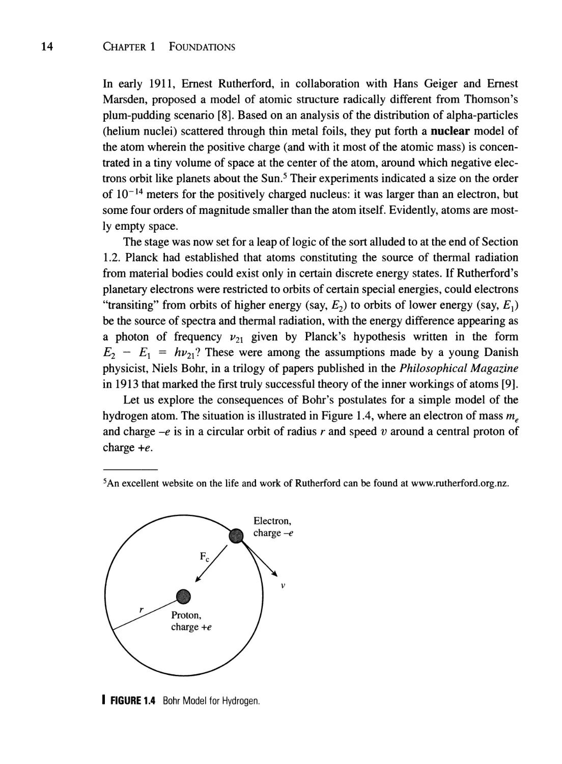
Let us explore the consequences of Bohr's postulates for a simple model of the
hydrogen atom. The situation is illustrated in Figure 1.4, where an electron of mass me
and charge -e is in a circular orbit of radius r and speed v around a central proton of
charge +e.
5 An excellent website on the life and work of Rutherford can be found at www.rutherford.org.nz.
Electron,
charge -e
v
I FIGURE 1.4 Bohr Model for Hydrogen.

1.3 The Rutherford-Bohr Atom 15
Bohr began by assuming that the energetics of the electron's orbit are dictated by
the Newtonian dynamics of circular orbits, namely that if the electron is in a circular
orbit, then it must experience a centripetal force of magnitude mev2/r toward the pro-
ton. Identifying as the source of this centripetal force the Coulomb attraction between
electron and proton gives
magnitude of Coulomb force -
m v 2
e
,
e 2
47T Eo,2'
(1)
A more refined version of this calculation accounts for the motion of the pro-
ton and the electron about their mutual center of mass. This can be effected by
substituting the reduced mass of the system, memp/(me + m p ) in place of the
electron mass me wherever it appears; mp is the mass of the proton. Also, the
theory can be extended to include hydrogen-like ions; that is, systems wherein a
single electron orbits a nucleus of charge + Ze by replacing e 2 by Ze 2 wherever it
appears.
Because the physically relevant quantities are wavelengths and energies, we start
out by deriving an expression for the total energy (kinetic + potential) of the electron
in its orbit. From Equation (1),
K . . 1 2
Inetlc energy = 2 me V
e 2
87TEo'.
(2)
The potential energy is just the electrostatic potential of an electron (charge - e)
and a proton (charge + e) separated by distance r:
e 2
47TEo"
Potential energy =
(3)
From Equations (2) and (3) we find the total energy Etotal:
Etotal = KE + PE =
e 2
87TEo"
(4)
The interpretation of the negative sign is that positive energy must be supplied
from some external source to dissociate the electron from the atom. We say that the
electron is in a bound energy state. Curiously, the total energy is equal to one-half of
the potential energy; this result is actually a specific case of a very general result
known as the vi rial theorem, which is treated in Section 4.9.
Imagine the electron "falling" from infinity [E = 0 with r = 00 in Equation (4)]
down to an orbit of radius r about the proton. In doing so it would lose energy,
which is assumed to appear as a photon of frequency v. At this point, Bohr made
two assumptions: (1) that this frequency is equal to one-half of the electron's final

16 CHAPTER 1 FOUNDATIONS
orbital frequency about the proton, and (2) consistent with Planck's hypothesis, the
energy of the photon is given by nhv where n is an integer and h is Planck's con-
stant. For an electron in a circular orbit of speed v and radius r, the time for one
orbit is 27Tr j v, hence the orbital frequency is v j2'TTr and Bohr's hypotheses give
nh ( V ) e2
Ephoton = I Etotall = nhv = _ 2 2 = 8 ·
'TTr 'TTEor
(5)
Solving the last two members of this expression for v gives
e 2
v= .
2Eonh
(6)
Now solving Equation (2) for the orbital radius and substituting this result for v gives
_ ( Eoh2 ) 2 _ 2 _
r n - 2 n - aon, (n - 1, 2, 3, ... ).
'TT mee
(7)
The interpretation of Equation (7) is that the electron is restricted to orbits of
radius a o n2, where ao' now known as the Bohr radius, represents the smallest per-
missible orbit (note that we cannot have n = 0, for this would imply E = -00 in
Equation 4); n is called the principal quantum number.
Using the following modern values for the constants
Eo = 8.8542 X 10- 12 C 2 /Nm 2 ,
h = 6.6261 X 10- 34 J-sec,
me = 9.1094 X 10- 31 kg,
e = 1.6022 X 10- 19 C,
one finds
a o = 5.2918 X 10- 11 m = 0.52918 A.
(8)

1.3 The Rutherford-Bohr Atom 17
This is a remarkable result, exactly of the order of atomic dimensions as deduced
in Section 1.1. Bohr's assumptions result in a theoretical explanation of the sizes of
atoms, an otherwise empirical detail.
The lone proton in a hydrogen atom has an effective radius of about 10- 15 m.
Suppose that the entire atom is magnified so that the proton has a radius of 1 rom,
about the size of a rather small pea. If the orbiting electron is in the n = 1 state in
Equation (7), what would be the radius of its magnified orbit?
As a multiple of the proton's effective radius, the distance of the n = 1
Bohr orbit is a o /l0- I5 m - (5.29 X 10- 11 m)/lO-I5 m - 52,900. If the proton
is expanded to a radius of 1 mm, then the electron will be orbiting at about
(1 mm)(52,900) - 52.9 meters. In other words, if the expanded proton is placed
at the center of a football field, the electron's orbit will reach to just beyond the
goal lines !
More importantly, Equation (7) leads to an expression for the wavelengths of pho-
ton emitted when electrons transit between possible orbits, and to a theoretically pre-
dicted value of the Rydberg constant. To arrive at the wavelength expression, imagine
that the electron falls from an initial orbital radius r i to some final orbital radius rf, with
r f < r i . According to Equation (4), Ef < E i (both Ef and E i are negative); if the energy
lost by the electron is presumed to appear as a photon in accordance with Planck's
hypothesis, then
Ephoton = E j - E f = 8 e 2 ( ! - ! ) = hVif'
7T € 0 ' f 'i
(9)
This would correspond to a photon of wavelength A = cjvor
Ajf = 87T::hC ( f - )
(10)

18 CHAPTER 1 FOUNDATIONS
Substituting Equation (7) for the orbital radii gives
1 me e 4 ( 1 1 )
An,-mr = 8Eh3c ni - nr
(nf < ni)'
(11)
Now recall the Balmer-Rydberg expression for the visible-region hydrogen-line
wavelengths, Equation (1.2.2):
= R( !- )
H 4 2 ·
An n
(12)
Equations (11) and (12) are remarkably similar in form; indeed, they correspond
precisely if we take nf = 2 and if the Rydberg constant is given by
m e 4
R H = 8 Ze h3 ·
Eo C
(13)
Substitution of the appropriate numerical values yields R H = 109,737 cm- 1 , in
close agreement with the experimental value of 109,678 cm- 1 . The slight discrepancy
(0.05%) can be accounted for by the motion of the electron and proton about their
mutual center of mass (Problem 1-11). With this agreement it is clear that Equation
(11) will produce the observed wavelengths of the Balmer lines when nf = 2.
According to the Bohr model, the Balmer series of hydrogen lines corresponds to
electrons transiting to the n = 2 orbit from "higher" orbits. 6
Equation (11) is quite general, and can be used to calculate the wavelengths of
whole series of spectral lines for hydrogen. Inverting it gives the wavelengths directly:
8 E h 3 C ( 1 1 ) -1 ( 1 1 ) -1 0
A ni -+ nf = 4 2" - 2" = 911.75 2" - 2" A,
mee nf ni nf ni
(14)
where the numerical value of 911.75 A accounts for electron/proton center-of-mass
motion.
6 A website giving the energy levels of hydrogen and deuterium for states n = I to 200 for all
allowed angular momentum states (see Chapter 6) is available through the National Institute of
Standards and Technology at http://physics.nist.gov/PhysRetData/HDEL.

1.3 The Rutherford-Bohr Atom 19
Compute the wavelength of the 7 -+ 4 transition for a hydrogen atom. What is the
energy of the photon emitted in such a transition, in e V?
From Equation (14),
( 1 1 ) -1 ( 1 1 ) -1 0
>"7-+2 = 911.75 4 2 - 7 2 A = 911.75 16 - 49 A
( 33 ) -1
= 911.75 784 A = 21,661 A.
With this wavelength, 2.166 X 10- 6 m, such a photon would lie in the infrared
part of the electromagnetic spectrum, far to the red of human visual response. The
energy IS
he (6.6261 X 10- 34 J · sec)(2.9979 X 10 8 mjs)
E = A - 2.1661 X 1O-6 m
= 9.171 X 10- 2o J.
With 1 eV = 1.602 X 10- 19 J, this corresponds to about 0.57 eVe
Table 1.1 lists hydrogen spectral wavelengths computed from this formula for a
number of (nj, nf) pairs. A group of lines corresponding to the same nf is known as a
series of lines. Each such series is characterized by a series limit corresponding to
I Table 1.1 Hydrogen Transition Wavelengths (A)
1 1215.7 1025.7 972.5 949.7 937.8 911.8 Lyman
2 6564.6 4862.7 4341.7 4102.9 3647.0 Balmer
3 18756.0 12821.5 10941.0 8205.8 Paschen
4 40522.2 26258.4 14588.2 Bracket
5 74597.7 22794.3 Pfu nd
6 32824.2 Humphreys

20 CHAPTER 1 FOUNDATIONS
nj = 00; the spacing of the lines decreases toward the series limits. As mentioned ear-
o
lier, the range of human vision runs from about 3500-7000 A; only the Balmer series
lies entirely within these limits. The series corresponding to nf = 3 lies in the infrared
region of the spectrum, and had been observed in 1908 by Freidrich Paschen [10] to
occur at exactly the wavelengths calculated by the Bohr formula. After publication of
Bohr's theory the series corresponding to nf = 1,4, and 5 were discovered by Lyman
(1914), Brackett (1922), and Pfund (1924) [11-13]. These discoveries lent immense
credibility to Bohr's theory.
The energy of an electron in quantum state n in the Bohr model is given by com-
bining Equations (4) and (7):
E =
n
m e 4
e
8 e 2 h 2 n 2
o
13.606
2 e V (n = 1, 2, 3, .. . ),
n
(15)
where the factor of 13.606 eV, known as the Rydberg energy, accounts for the elec-
tron/proton center-of-mass motion and the values of the various constants to five sig-
nificant figures. This is one of the most famous results of early quantum mechanics. It
tells us that to ionize a hydrogen atom from its ground state (n = 1) requires an
expenditure of 13.6 eV of energy, precisely the observed value.
Figure 1.5 shows an energy-level diagram for hydrogen based on the Bohr
model. Energy is plotted increasing upward on the vertical axis; the horizontal axis has
no physical meaning and serves only to improve the readability of the figure. The
arrows show a number of possible quantum jumps or transitions; their lengths are pro-
portional to the frequencies of the corresponding emitted photons because E = hv.
Electrons that are initially not bound to the atom (so-called free electrons with E> 0)
can become so by releasing just enough energy to bring them into one of the station-
ary states; thus, there is a continuum of energy levels with E > O.
An intriguing aspect of Bohr's model concems the orbital angular momentum of
the electron, usually designated L. Classically, a mass m in a circular orbit of radius r
and speed v has angular momentum L = mvr. If we apply this to the electron in the
Bohr model with the help of Equations (6) and (7),
L = mevr = m e ( 2E::h )( TrE::2 )n2 = ( 2: )n, (n = 1,2,3,... ).(16)
the physical interpretation of the result is that the orbital angular momentum of the
electron is quantized in units of h/27T. Planck's constant, which was originally intro-
duced to explain thermal radiation, now appears as a fundamental unit of angular
momentum. Many treatments of the Bohr model begin by assuming that angular

1.3 The Rutherford-Bohr Atom 21
o
5 -0.54
4 -0.85
Energy
(eV)
-I
3 -1.51
-2
-3
2 -3.40
-13
"TIlT'.
I -13.60
-14
n En (eV)
I FIGURE 1.5 Energy Level Diagram for Hydrogen.
momentum is quantized in this way. Whether one regards E or L as being the funda-
mentally quantized attribute is arbitrary; the relationship is symbiotic. The fundamen-
tal quantum of angular momentum, h/27T, is given its own symbol, Ii, read as "h-bar":
h
h = 27T = 1.05459 X 10- 34 Joule-sec.
(17)
We will see in Chapter 7 that angular momentum plays a central role in the wave
mechanics of the hydrogen atom.
At this point, it is useful to look back at the illustration of Kirchhoff's laws, (Figure
1.1), and relate it to Bohr's model. A cool gas will have most of its atoms in the lowest
energy (ground) state. When light is passed through such a gas only those photons with
energy equal to the various differences between the ground state and higher energy levels
of the gas atoms will be absorbed out, causing certain wavelengths to be removed from the
light beam. In the case of a hot gas, we will see photons emitted from de-excitations of the
gas atoms: the reverse of the cool-gas excitation process. The continuous spectrum of a hot
solid object (e.g., a lightbulb filament) is a manifestation of interactions between atoms.

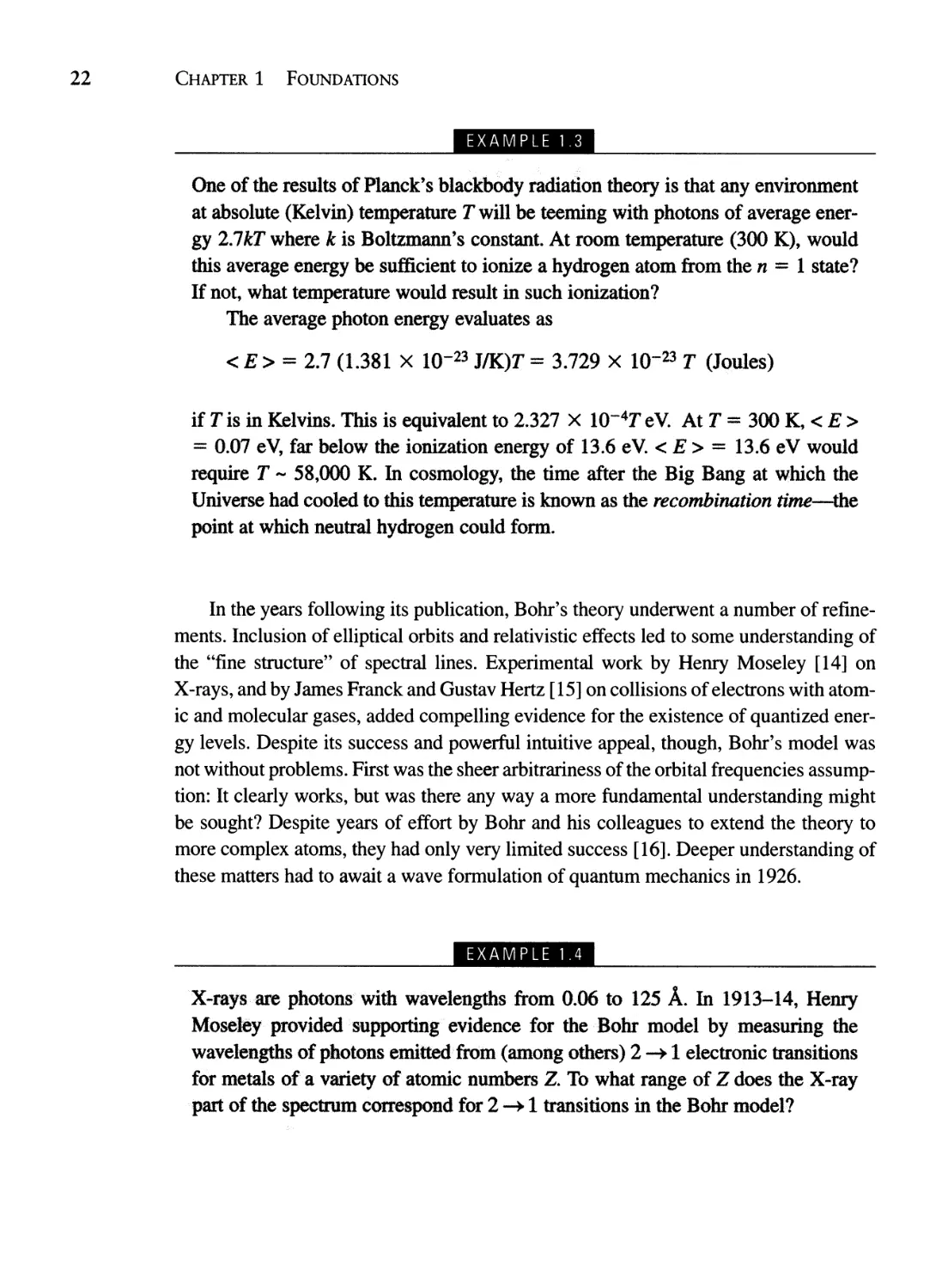
22 CHAPTER 1 FOUNDATIONS
One of the results of Planck's blackbOdy radiation theory is that any environment
at absolute (Kelvin) temperature T will be teeming with photons of average ener-
gy 2.7kT where k is Boltzmann's constant. At room temperature (300 K), would
this average energy be sufficient to. ionize a hydrogen atom from the n = 1 state?
If not, what temperature would result in such ionization?
The average photon energy evaluates as
< E> = 2.7 (1.381 X 10- 23 JIK)T = 3.729 X 10- 23 T (Joules)
if T is in Kelvins. This is equivalent to 2.327 X 10- 4 T e V. At T = 300 K, < E >
= 0.07 eV, far below the ionization energy of 13.6 eV. < E > = 13.6 eV would
require T - 58,000 K. In cosmology, the time after the Big Bang at which the
Universe had cooled to this temperature is known as the recombination time-the
point at which neutral hydrogen could fonn.
In the years following its publication, Bohr's theory underwent a number of refine-
ments. Inclusion of elliptical orbits and relativistic effects led to some understanding of
the "fine structure" of spectral lines. Experimental work by Henry Moseley [14] on
X-rays, and by James Franck and Gustav Hertz [15] on collisions of electrons with atom-
ic and molecular gases, added compelling evidence for the existence of quantized ener-
gy levels. Despite its success and powerful intuitive appeal, though, Bohr's model was
not without problems. First was the sheer arbitrariness of the orbital frequencies assump-
tion: It clearly works, but was there any way a more fundamental understanding might
be sought? Despite years of effort by Bohr and his colleagues to extend the theory to
more complex atoms, they had only very limited success [16]. Deeper understanding of
these matters had to await a wave formulation of quantum mechanics in 1926.
X-rays are photons with wavelengths from 0.06 to 125 A. In 1913-14, Henry
Moseley.. provided supporting... evidence for the Bohr model by measuring the
wavelengths of photons emitted from (among others) 2 -+ 1 electronic transitions
for metals ofa variety oiatomic numbers Z. To what range of Z does the X-ray
part of the spectrum correspond for 2 -+ 1 transitions in the Bohr model?

1.4 de Broglie Matter-Waves 23
From Equation (1.3.14) and the comment given regarding incorporating dif-
ferent Z values following Equation (1.3.1), we can write the Bohr transition wave-
lengths as
912 ( 1 1 ) -1
A1I;-+'" = Z2 n - nt A,
where we have rounded the Rydberg constant to the nearest Angstrom. For
(n i , nf) = (2, 1) this becomes (again to the nearest A)
1216
A21 = 2 A.
z
For A = 125 A we find Z - 3, and for ,.\ = 0.06 A, Z - 142. Thus, essentially
the whole of the periodic table was available to Moseley. Further details on
Moseley's work appear in Section 1-10 of French and Taylor.?
II 1.4 de Broglie Matter-Waves
In his 1924 Ph.D. thesis, French physicist Louis de Broglie (pronounced "de broy") pro-
posed that if photons could behave like particles and transport momentum according to
h
p = A '
(1)
then might material particles possessing momentum be accompanied by a matter-
wave of wavelength given by inverting the relation: A = hi p = hi mv?
The mathematical manipulation here is trivial, but the physical hypothesis seems
absurd: We do not observe matter to be wavy; it is solid and localized. But just because
we cannot see a particular phenomenon does not mean that it does not exist. The con-
trolling factor in Equation (1) is the minuteness of Planck's constant. A mass of 1 kg
moving at 1 meter/sec would have an associated de Broglie wavelength of -- 10- 34
meters, some 20 orders of magnitude smaller than an atomic nucleus. We could scarce-
ly hope to observe the "matter-wave" associated with such a macroscopic object. On the
other hand, if an extremely tiny mass is involved, such as that of an electron, then it turns
out that the associated wave can be comparable in size to its parent particle.
7 A. P. French and E. F. Taylor, An Introduction to Quantum Physics, Boca Raton, FL: CRC Press,
1978.

24 CHAPTER 1 FOUNDATIONS
I Table 1.2 de Broglie Wavelengths.
Situation A(A) Comment
Electron, energy 1 eV
Proton, energy 1 keV
800 kg car @ 20 m/sec
12.3
0.009
4.1 x 10- 28
Molecular size
Subatomic size
« Nuclear size
Table 1.2 shows a few de Broglie wavelengths computed via the relationship now
named after him [17]:
h h
A = mv = V2Km ' (v« c),
(2)
where K is the kinetic energy of the mass involved.
If particles really do possess associated waves, then it is clear that we can hope to
detect them only in atomic-scale phenomena. Leaving aside for the moment the ques-
tion of what they mean, let us ask how such matter-waves might manifest themselves.
Waves can be diffracted to produce constructive and destructive interference pat-
terns. According to de Broglie, then, electrons fired through a double-slit apparatus
should somehow interfere with each other (and themselves!). The problem is that the
slit separation must be on the order of the wavelength involved, far too small (at least
in de Broglie's day) to be physically manufactured. However, as de Broglie himself
pointed out, nature provides natural diffraction gratings with spacings on the order of
Angstroms: the regularly spaced rows of atoms in metallic crystals. Less than three
years after de Broglie advanced his hypothesis, experimental verification came inde-
pendently from American and British groups of researchers. Working at the Bell
Telephone Laboratories in the U.S., Clinton Davisson and Lester Germer observed, by
accident, interference effects with electrons scattering from crystals of nickel [18]. In
Britain, George P. Thomson (J.J.'s son) verified the effect by scattering electrons
through thin metallic foils [19]. In 1961, Claus Jonsson [20] demonstrated electron
diffraction with a true double-slit arrangement, utilizing an elaborate array of electro-
static lenses to magnify the image. More recently, the wave properties of Carbon-60
"buckyball" molecules have been observed by similarly passing them through a series
of slits, 8 as has the diffraction of electrons by a standing light wave. 9 All these exper-
iments and many others have demonstrated that electrons, atoms, and molecules
SPhysics Today 1992; 52( 12):9.
9Physics Today 2002; 55(1): 15.

1.4 de Broglie Matter-Waves 25
behave in full agreement with de Broglie's hypothesis. The wave nature of electrons
is put to stunning practical use in electron microscopy. The resolution of a microscope
(the smallest distance by which two objects can be separated and still viewed as dis-
tinct) is proportional to the wavelength of light used. Because electrons behave as
waves of wavelengths much shorter than that of visible light, much greater detail is
resolvable. Images of individual molecules and atoms can be obtained in this way.
The evidence for de Broglie's matter-waves is incontrovertible. But what does it
mean to say that a particle has a wave nature? How do we reconcile the classical point-
mass view of matter with wave properties? As a schematic model, consider Figure 1.6.
The victim in this game of wavy particles is the classical idea that the position of
the particle can be specified with an arbitrary degree of precision. In effect (but not in
reality) the electron acts as if it is smeared out into a so-called wave packet that per-
vades all space. The amplitude of this wave, however, is not constant: it proves to be
strongly peaked in the vicinity of the electron over a length scale x on the order of
the size of the electron, as the figure suggests. For practical purposes, we can no longer
specify with precision where the electron is; we can only speak meaningfully in terms
of the probability of finding the electron at some position. (We will explore these
"probability waves" further in subsequent chapters.) It is this wavy nature of matter
that lies at the heart of the Heisenberg uncertainty principle, which we will examine
in Chapter 4.
These considerations in no way invalidate the application of Newtonian
dynamics to objects such as golf balls or planets. The de Broglie waves accompa-
nying such masses are so infinitesimally small in comparison with their length-
scales that we cannot hope to detect them. Only when the size of the system under
study is comparable to A = hi mv will quantum effects become noticeable. As an
example, refer to Table 1.2. A 1 ke V proton incident on a hydrogen atom has a de
Broglie wavelength much less than the size of the atom; for practical purposes,
this will be a particle interaction. On the other hand, an electron of energy 1 e V
I .
m
.
.1
x
I FIGURE 1.6 A Particle and Its de Broglie Matter-Wave.

CHAPTER 1 FOUNDATIONS
has a de Broglie wavelength on the order of the size of that same hydrogen atom:
to an imaginary observer riding on the atom, the incoming electron would appear
amorphous.
The "wave-particle duality" is perhaps the most counterintuitive aspect of quan-
tum mechanics, and, not surprisingly, has inspired an extensive body of literature. An
excellent discussion on this topic appears in the first two chapters of the third volume
of Feynman's Lectures on Physics [21]. A very readable and humorous look at the sit-
uation appears in "Two lectures on wave-particle duality" by Mermin. 1o
What speed must an electron have if its de Broglie wavelength is 5000 A? A pho-
ton of this wavelength would be in the visible part of the electromagnetic spectrum.
Putting p = mv in Equation (1) and solving for V gives v = hi mA, hence
h
v -
mA
(6.626 x 10- 34 J · s)
= 1455 mise
(9.109 x 10- 31 kg)(5 X 10- 7 m)
See Problem 1-20. If this speed were due to the electron's random thermal
motion in an environment at absolute temperature T, the environment would be at
T - 0.04 K. Electrons of such speed are thus characterized as "cold."
---
de Broglie further hypothesized that the allowed orbits for an electron in a
hydrogen atom are given by the condition that an integral number "n" de
Broglie wavelengths fit around the circumference of the orbit. Show that this
condition leads to the Bohr quantization condition on angular momentum,
Equation (1.3.16).
Let the electron have speed v in an orbit of radius r. The circumference of the
orbit is then 27Tr. de Broglie's hypothesis is then that an integral number of wave-
lengths fit into this circumference:
27Tr
A
= n.
IOMermin ND, Physics Today 1993; 46(1):9-11.

1.4 de Broglie Matter-Waves 27
Setting A = h/mev gives
2Trm e vr
h
= n.
However, mevr is just the angular momentum of the electron in its orbit:
L = ( 2 )n = !tn,
precisely the Bohr quantization condition on L. If the condition on the electron's
speed that emerged from Bohr's orbital frequency assumption is used here
(Equation 1.3.6), the result is the same restriction on orbital radii and energies that
emerged from his approach.
Figure 1.7 shows a sketch of what de Broglie had in mind: an integral number of
wavelengths (in this case shown, n == 4) fitting around the circumference of an orbit
like a standing wave. It should be emphasized that the amplitude of the wave shown in
the sketch is purely arbitrary; de Broglie's relation gives no information on this.
I FIGURE 1.7 de Broglie's Quantization Condition.

28 CHAPTER 1 FOUNDATIONS
II Summary
The need to introduce the hypothesis that some physical quantities (such as energy and
angular momentum) are quantized grew out of the inability of classical physics to pro-
vide adequate understanding of phenomena such as thermal radiation, atomic spectra,
and atomic structure. The way was led by Max Planck, who in 1900 proposed that one
could model the mechanism of thermal radiation by assuming that the source of black-
body radiation lay in "oscillators" restricted to possessing energies given by
E = nhv,
where n is an integer (n = 1, 2, 3, ...), h is Planck's constant, and v is the frequency of
vibration. Later, Niels Bohr used this assumption in conjunction with a semiclassical
planetary electron model of the hydrogen atom. The essence of Bohr's model is that
the orbiting electron is restricted to certain "stationary" energy states wherein it does
not radiate. Atomic spectra are then presumed to be due to electrons executing transi-
tions between different stationary states the difference in energy L\E between the
states appearing as a photon of energy L\E = hv in accordance with Planck's hypoth-
esis. The energy level of a Bohr atom in quantum state n (n = 1, 2, 3, ...) is given by
E =
n
m Z 2 e 4
e
8 e 2 h 2 n 2
o
Z2
- -13.595"2 eV (n = 1,2,3,...)
n
where Z is the number of protons in the nucleus. The wavelength of the photon emit-
ted by an electron transiting from Bohr orbit n i to orbit n f (n i > n f ) is given by
911.75 ( 1 1 ) -1 0
A. ni -+ nr = Z 2 2 - 2 A.
nf ni
A corollary of the Bohr model is that the orbital angular momentum of the elec-
tron is quantized in units of h/27T.
A central concept of the quantum aspect of nature is that of matter-waves, due to
de Broglie. On the scale of atomic phenomena we are forced to abandon the notion of
point particles in favor of treating them as being smeared out over a characteristic de
Broglie wavelength given by
h
A=-.
mv

Problems 29
The idea of matter-waves proves to be intimately related to the probability distri-
bution interpretation of quantum mechanics.
II Problems
1-1(E) The table gIves densities and atomic weights for a number of common
elements.
Use Equation (1.1.1) to calculate approximate sizes for these species.
Density A
Element (g/cm 3 ) (g/mol)
AI 2.7 27
Fe 7.88 56
Cu 8.96 64
Pb 11.34 207
Pt 21.45 195
1-2(E) Consider a gas of "classical" Maxwell-Boltzmann atoms whose energies are
distributed in accordance with Equation (1.2.5). In an environment of T =
6000 K (the approximate temperature of the surface of the Sun), what is the
ratio of the number of atoms with energies between E + dE to those with
energies between 2E and 2E + dE, where E = 5 e V?
1-3(1) Equation (1.2.13) gives the amount of radiant energy E(v)dv between
frequencies v and v + dv within a blackbody cavity. According to Einstein,
the energy of an individual photon of frequency v is E = hv. If the radiant
energy is presumed to be comprised of individual photons, then the number of
photons with frequencies between v and v + dv in the cavity would be given
by n(v)dv = E(v)dv/hv. The total number of photons within the cavity will
then be given by the integral of this expression for v = 0 to 00. Given that
00
f x2dx
(eX - 1) - 2.404,
o
determine the density of photons in a blackbody cavity at T = 300 K, about
room temperature. Intergalactic space has a temperature of about 2.7 K;
what is the density of photons in that environment?

30 CHAPTER 1 FOUNDATIONS
1-4(E) To establish the relationship between Equation (1.2.13) and Figure 1.3
requires some knowledge of thermodynamics, which shows that the rate of
energy escape (power) between wavelengths A and A + dA through a hole
of area A in a blackbody cavity of temperature T is given by
{ 27Thc2 }
P(A)dA = A A5(e hc /AkT _ 1) dA.
Consider a blackbody at T = 7000 K. What is the power emitted through a
hole of area 1 m 2 between A = 4000 A and 4001 A? Does your result accord
with Figure 1.3?
1-5(E) Derive an expression for the speed of an electron in Bohr orbit n in terms of
the speed of light. Is it justifiable to neglect relativistic effects in the
development of the Bohr model?
1-6(E) Repeat the derivation of the Bohr model for a lone electron orbiting a
nucleus of Z protons. Use your results to compute ionization energies for a
single electron orbiting nuclei of (a) helium, (b) carbon, and (c) uranium.
1-7(E) Derive an expression for the centripetal force experienced by the electron in
Bohr orbit n as a function of n and physical constants. What is the value of
the force when n = I? Modern force-probe microscopes are capable of
measuring nano-Newton scale forces.
1-8(E) An electron transits between two energy levels separated by energy E,
emitting a photon of wavelength A in accordance with the PlanckIBohr
relation E = hc/ A.
(a) Show that if A is given in units of Angstroms, then E = 12,398/ A
electron- volts.
(b) As a consequence of some perturbing effect, the separation of the energy
levels is altered by an amount dE electron-volts. Show that the corre-
sponding change in the wavelength of the emitted photon is
dA = - A 2 dE/12,398 Angstroms. If a transition leading to a photon of
wavelength 4000 A is perturbed by dE = 0.01 e V, what is dA?
1-9(1) The purpose of this question is to derive an educated guess at the
classically expected "lifetime" of an electron in various Bohr orbits.
According to classical electrodynamics, an accelerated charge e radiates
energy at the rate P = e 2 a 2 /67T€oC 3 Joule/sec, where a is the acceleration
(v 2 /r for a circular orbit). Decay rate (DR; unit = sec- l ) can be defined to
be the power radiated divided by the energy emitted during the decay. Use

Problems 31
the Bohr model to derive an expression for DR for a decay from orbit n to
orbit n - 1; for simplicity, use the acceleration for orbit n in the
expression for P. The lifetime is given by the reciprocal of the decay rate;
evaluate this numerically for n = 2.
1-10(E) Both Newton's gravitational law and Coulomb's law are inverse-square
laws: The force of attraction between the Sun (S) and the Earth (E) has
magnitude GmSmE/r2 whereas the force of attraction between an electron
,
and a proton in a hydrogen atom is e 2 /47T€or 2 . Derive an expression for the
equivalent of the Bohr radius for the gravitational case. What is the value of
the quantum number of Earth's orbit? Would distance differences between
individual quantum states in the solar system be observable?
1-11(A) The text indicates how one can take into account the motions of the proton
and electron around their mutual center of mass in the Bohr model. Using
the condition that the center of mass of an isolated system must stay in the
same place, derive the correction specified in the footnote, and hence derive
the factor of 911.75 A in Equation (1.3.14). Hint: Do not forget the kinetic
energy of the proton about the electron/proton center of mass.
1-12(1) It is remarked in the text that the effect of the motions of the electron and
proton around their common center of mass in the Bohr model can be
accounted for by substituting the reduced mass of the system,
memp/(me + m p ) in place of the electron mass me wherever the latter
appears. An atom of deuterium consists of a lone electron orbiting a
nucleus consisting of a proton and a neutron fused together; such a
nucleus has mass close to 2mp. Show that the difference in wavelength
between the Balmer 3  2 transition for deuterium versus ordinary
hydrogen is given by
144 €h3C
(Ah - Ad)3--+2 -., _ 5 4 ·
mpe
Evaluate this result numerically. If you have available a spectrometer
capable of resolving spectral lines that are separated by no less than 2 A,
would you see the deuterium and hydrogen lines as separate?
1-13(E) Write a computer program to compute the wavelengths of photons emitted
by a single electron orbiting a hydrogen-like atom of nuclear charge +Ze as it
transits between any pair of states (n i , nf) (see Problem 1-6). Test your
program by comparing your results with Table 1.1 for Z = 1. What are the
wavelengths of the "Balmer series" for helium? For uranium?

32 CHAPTER 1 FOUNDATIONS
1-14(1) Derive expressions for the lowest- and highest-possible wavelength photons
emitted during transitions corresponding to a given series of spectral lines.
Show that as a result, only the Lyman and Balmer series in hydrogen are not
overlapped by lines from other series.
1-15(E) The Ritz combination principle was an empirical result that predated the Bohr
model. This principle states that the inverse of the wavelength of a spectral
line of some atomic species can often be predicted by computing the differ-
ence in the inverse wavelengths of two other spectral lines of the same
species. Show that in the context of the Bohr model, hydrogen p  m tran-
sitions can be predicted form the p  nand m  n transitions according as
1
1
1
Apm
Apn
Amn
Verify numerically by computing the 5  3 transition on the basis of the
values for the 5  1 and 3  1 wavelengths given in Table 1.1.
1-16(1) A diatomic molecule (such as H 2 ) can be modeled as two point particles,
each of mass m, joined by a rigid rod of length L. Assuming that the
molecule rotates about an axis perpendicular to the rod through its midpoint
and with angular momentum given by the Bohr condition (Equation 1.3.16),
derive an expression for the quantized values of the rotational energy.
1-17(1) As another model of an atom, consider a solid sphere of mass M and
radius R rotating about an axis through its center in accordance with the
Bohr quantization condition on angular momentum. Show that the
possible rotational energies are given by En = 5n 2 h 2 /167T 2 MR2, where n
is the quantum number. From this result derive an expression for the
wavelength of a photon emitted as this system undergoes a transition
from state n + 1 to state n. Evaluate your answer numerically for the
case of M equal to the mass of a proton (essentially the mass of a
hydrogen atom), R = 1 A, and n = 2. Approximately what value would n
have to be to give wavelengths in the optical region of the spectrum, A -
o
5000 A?
1-18(E) Compute the de Broglie wavelength for an electron of energy 1 keV. If this
electron were interacting with a hydrogen atom, would classical mechanics
suffice?
1-19(E) Particles in motion have associated de Broglie wavelengths. As a rule, if one
is within a few de Broglie wavelengths of a particle, then the particle loses

Problems 33
its identity as a particle and acts more like a wave. The result is that classical
mechanics no longer suffices to describe collisions. Rutherford investigated
the scattering of a-particles (helium nuclei) from stationary gold nuclei,
using classical mechanics to analyze the collisions. This question investi-
gates the issue from a wave-mechanics perspective.
(a) Determine the de Broglie wavelength of an a-particle of kinetic energy 6
million electron-volts.
(b) The electrical potential energy of charges QI and Q2 separated by
distance r is given by U = QIQ2/41T€or. By equating the initial kinetic
energy of the a-particle to the electrical potential energy, find the
distance of closest approach of the a-particle to the gold nucleus, and so
render a judgment as to how well-justified Rutherford was in his use of
classical mechanics.
1-20(E) In kinetic theory, atoms are modeled as point masses of mass m, and the
mean speed v of an atom in an environment at absolute temperature T is
given by mv 2 = 3kT, where k is Boltzmann's constant. Derive an
expression for the de Broglie wavelength for an atom of mass m at absolute
temperature T in terms of h, k, T, and m. At room temperature, hydrogen
atoms typically travel many thousands of Angstroms between collisions; is it
fair to treat them as effectively acting as point masses under such
circumstances?
1-21(E) In a paper published in the October 14, 1999 edition of Nature, 11 a group at
Universitat Wien in Austria reported experimental detection of the de
Broglie wave interference of Carbon-60 "buckyball" molecules. Such
molecules consist of 60 carbon atoms arranged in a roughly spherical shape
reminiscent of a soccer ball. In this experiment, the C-60 molecules had a
most probable velocity of 220 mls. Their data is well-fit by a de Broglie
wavelength of 2.5 picometers. Verify this wavelength from the information
gIven.
1-22(E) An atom of mass m is initially at rest with respect to an outside observer and
has an electron in an excited state. The electron transits to a lower energy
level, emitting a single photon of wavelength A in the process. The emitted
photon will have momentum p = hi A. To conserve momentum, the atom
must recoil with some speed v. Derive an expression giving the ratio of the
IINature 1999; 401:680--682.

34 CHAPTER 1 FOUNDATIONS
photon's energy to the kinetic energy of the recoiling atom in terms of A, m,
c, and h. A classical analysis will suffice for the recoiling atom. Evaluate the
ratio numerically for a hydrogen atom emitting a photon of wavelength
5000 A. Based on your result, do you think it was reasonable to neglect the
energy involved with the recoiling atom in the derivation of the Bohr model?
Along these lines, the momentum transferred to an atom upon its absorbing
a photon has actually been measured. 12
12Physics Today 2005; 58(7):9.

Schrodinger's Equation
From lines of evidence like those marshaled in Chapter 1, it became clear to physicists
in the early part of the twentieth century that the laws of classical mechanics do not
apply to physical systems on atomic scales. The problem then became how to modify
classical mechanics to produce a "quantum mechanics" consistent with the micro-
scopic characteristics of atoms and molecules that reverts to a form consistent with
Newtonian mechanics on macroscopic scales. As the essence of classical physics is
embodied in Newton's laws, the essence of quantum mechanics is embodied in
Schrodinger's equation (SE).
At this point we could simply state Schrodinger's equation and say, "Here it is-
let's see how to solve it in certain circumstances," just as you would use F = ma with
an applied force and some initial conditions to solve for the motion of a classical point
mass. This would be convenient, but not aesthetically satisfying. Postulated physical
laws, although derivable from nothing more fundamental, do not simply pop out of
thin air: They are products of thinking processes conditioned by past successes, empir-
ical facts, intuition, trial and error, and inspired guesses. In an effort to smooth the
transition, we introduce Schrodinger's equation by means of a plausibility argument.
This is a fancy way of saying that even though no rigorous derivation exists, it is pos-
sible to arrive at Schrodinger's equation by deftly combining some classical and quan-
tum concepts. Of course, any equation could be concocted in this way; whether or not
the result is useful is a matter for experiment.
We develop Schrodinger's equation in Sections 2.2 and 2.3 after first reviewing
the classical wave equation in Section 2.1. In Section 2.4, we discuss what general
constraints must be imposed upon solutions to Schrodinger's equation and how they
are interpreted. We follow this procedure because the interpretation, like the equation
itself, is fundamentally a postulate, and it seems sensible to gather postulates togeth-
er in one place, independent of any particular example. Examples of setting up and
solving Schrodinger's equation are reserved for subsequent chapters.
35

36 CHAPTER 2 SCHROOINGER'S EQUATION
II 2.1 The Classical Wave Equation
Any equation that purports to describe quantum physics must respect the incontrovert-
ible fact that particles possess a fundamentally wavy nature. To physicists of the early
twentieth century, this demand was familiar ground: waves in strings, water waves,
sound waves, electromagnetic waves, and so forth were pervasive phenomena in clas-
sical physics. As a starting point, then, let us consider the classical wave equation and
how one might modify it to accommodate the wave nature of individual particles.
As a classical model of a wave, consider a disturbance in a string. Figure 2.1(a)
shows a sketch of such a disturbance at some particular time t = O. Distance along the
string from the origin is measured by x, whereas y(x, t) measures the amplitude; that
is, the up or down displacement of the string from its undisturbed position as a func-
tion of position and time. The pattern may in fact be quite complex, but we can
describe it in principle by saying that at t = 0, Y = f(x).
The simplest wave pattern we can conceive is one that retains its shape as it prop-
agates down the string. The speed at which the pattern flows through the stris
determined by the tension T in the string and its mass per unit length JL: v = V T / JL.
In such a transverse wave, an individual point on the string oscillates up and down but
does not shift left to right as the wave passes by. Figure 2.1(b) shows the wave pattern
after time t has elapsed; the whole pattern has advanced a distance vt along the string.
The vertical offset between the two patterns is for clarity only.
Now imagine two observers, O} and O 2 , standing at fixed positions on the x-axis
as shown; O 2 is at distance vt to the right of Ole Distances measured by O} and O 2
along the x-axis are referred to as x and x', respectively. Assuming that the wave pat-
Amplitude
.-- vt
o} 02
Position (x or x')
I FIGURE 2.1 Traveling Wave at Two Different Times.

2.1 The Classical Wave Equation 37
tern retains its shape, each observer must describe the pattern with the same mathe-
matical function of his or her distance coordinate:
y = f(x) = f(x').
(1)
In addition, when x' = 0, x = vt. Thus x and x' are related as
x' = x - vt.
(2)
Substituting Equation (2) into Equation (1) gives
y = f(x) = f(x - vt).
(3)
The interpretation of this equation is that for the wave pattern to maintain its
shape, x, v, and t must always appear in the combination (x - vt). Examples of
acceptable wave patterns would be
y = sin(x - vt),
y = e(x - vtf/8
and
y = Tanh- 1 [(x - vt)-4/3].
On the other hand, a wave that would not maintain its shape is
y = cos [x 2 - (vt)2].
Although these considerations establish a constraint on x, v, and t if waves are to
maintain their shape, it is clear that we could write down an infinite variety of possi-
ble wave patterns y(x), which are called wave functions. Is there any way we can
express the constraint in more general terms without getting mixed up with an infinite
number of functions? Inevitably, such generalized expressions of physical laws take
the form of partial differential equations. Assuming that wave patterns must involve
functions of the formf(x - vt), it is possible to work out the general differential equa-
tion that any wave pattern must satisfy to be acceptable [1].
Now, we know that in general we can put
y(x, t) = f(x - vt) = f(z),
(4)
for which z = (x - vt). From this definition (the velocity is assumed to be constant),

38 CHAPTER 2 SCHRODINGER'S EQUATION
ay
aX
ayaZ
--
az ax
ay
az'
(5)
and
ay
at
ayaZ
--
az at
ay
= -v-.
az
(6)
From these results we can form an identity:
ay ay ay ay
+ v- = -v- + v- = o.
at ax az ax
(7)
Taking the partial derivative of Equation (7) with respect to time gives:
a ( a y ay )
at iit + v ax -
:t (0),
that is,
a 2 y
at 2
+ vi. ( a y ) - O.
at ax
or,
a 2 y a ( a y )
-+v-- =0
at 2 ax at '
(8)
where the last step resulted from exchanging the order of the partial derivatives. From
Equation (6) we can replace (ay/at) by -v(ay/az) = -v(ay/ax), hence
iiy + v ( - J-!- ) = 0
at 2 ax ax
or
a 2 y 2 a2y
at2 - v ax 2 '
(9)

2.1 The Classical Wave Equation 39
Equation (9) is the classical wave equation. If you are familiar with some
advanced mathematical physics, its solution in any particular case usually proceeds in
terms of Fourier or Laplace transforms, but this will not concern us. The essential point
for our purposes is that "classical wavefunctions" y(x, t) must satisfy this equation.
EXAMPLE 2.1
Show that the function y = e(x-v/)7/8 satisfies the classical wave equation. '
We have a function of the form eZ for w;trich z = (x - vt)7/8. It is helpful to
recall that for any variable q,
d
-[ ez(q)]
dq
_ z(q )dz
e dq.
Begin with the left side of the wave equation. Here we will have q = t, and
dz 7 _
dt - 8 (x - vt) 1/8( - v).
Hence
dy
dt
zdz
- e--
dt
7
- 8 (v)eZ(x - vtt l / 8 .
Remembering the chain rule of basic calculus, the second derivative goes as
d 2 y 7 d
- = --(v[eZ(x - vt)-1/8]
dt 2 8 dt
7 [ dz 1 ]
= --(v) ex - vt)-1/8 - -eZ(x - vt)-9/8( - v)
8 dt 8
7 [ 7 ) 1 / 4 1 9 / 8 ) ]
= --(v) - -(v)eZ(x - vt - - -eZ(x - vt)- (- v
8 ... 8 8
[ 49 7 ]
= (if) 64 (x - vtt l / 4 - 64 (x - vtt 9 / 8 ez.

40 CHAPTER 2 SCHRODINGER'S EQUATION
Now look at the right side of the wave equation. Here q - x, and we have
dz
dx
7
- g (x - vtrl/ 8 .
Hence
dy
dx
Zdz
- e--
dx
7
g e(x - vtr 1j8 .
The second derivative develops as
d 2 y 7 d [ -1 / 8 ]
- = -- eZ(x - vt)
dt 2 8 dt
7 [ dz 1 ]
= - eZ-(x - vt)-1/8 - -eZ(x - vt)-9/8
8 dx 8
7 [ 7 1 ]
= - -e z (x - vt)-1/4 - -e z (x - vt)-9/8
888
[ 49 7 ]
= -(x - vt)-1/4 - -(x - vt)-9/8 e Z
64 64 ·
Comparing the second derivatives shows that the wave equation is satisfied.
Why didn't we stop at Equation (6), (ay/at) = -v(ay/ax), and call it the classical
wave equation? The reason is that a wave equation should be space and time invari-
ant; that is, insensitive to changes in the definition of the positive directions of x and
t. Equation (9) has this property, whereas Equation (6) does not.
Aside from spatial (and temporal) invariance, Equation (9) has another important
property: that of linearity. This means that wherever the dependent variable y appears,
it does so only to the first power; there are no nonlinear terms such as e Y , sin (y), or
yl/2. The result of this property is that if one has a number of independent solutions Yl'
Y2' ..., Y n to the wave equation (all with the same speed v), then so, too, will be a func-
tion constructed by a linear sum of them; that is, a function of the form
Y = alYl + a2Y2 + ... + anYn,
(10)
where the coefficients aI' a2' ..., an are constants.

2.2 The Time-Independent Schrodinger Equation 41
This linearity property is of great value in the following sense: In discussions of
harmonic motion in elementary physics texts, one often encounters solutions of the
wave equation of the form
y = Asin(kx - oot),
(11)
where A is the amplitude of the wave, k is its wavenumber (k = 27T'/ A, where A is the
wavelength), and 00 its angular frequency (00 = 27T'v, where v is the frequency in cycles
per second, or Hertz). This expression corresponds to a wave pattern moving in the
direction of the + x-axis; for one moving in the - x direction, replace the - sign inside
the brackets with a + sign. Now, it might happen in some particular problem that the
solution to the wave equation is in fact more complicated than this. However, since
Fourier analysis will always let us represent any function as a linear sum of sines and
cosines, and because the wave equation is linear, we are guaranteed that such a sum
will also be a solution. That is, we can always express any solution of the wave equa-
tion as a sum of sinusoidal functions of the form of Equation (11). By using Equation
(11) as a prototype wave in our development of the Schrodinger equation, we can keep
the mathematical manipulations fairly simple while sacrificing no generality.
_ 2.2 The Time-Independent Schrodinger Equation
How can the classical wave equation be modified to accommodate the characteristics
of quantum matter-waves? This is by no means obvious. Strings exhibit wave phe-
nomena as a whole; y and v in Equation (2.1.9) refer to pattern amplitude and speed,
respectively. What we now desire is a wave equation applicable to individual particles.
With no idea of what a quantum wave equation can be expected to look like, how
should we proceed? It is at this point that our derivation becomes nonrigorous. What
follows might at best be called a plausibility argument. 1
Schrodinger was led by the assumption that the putative quantum wave equation
should possess two properties. Experience with classical waves argued strongly in
favor of a linear, second-order differential equation, and the success of the Bohr model
argued for retaining the concept of energy conservation. In classical notation, conser-
vation of mechanical energy is expressed as
p2
E = 2m + V(x),
(1)
1 Readers interested in a detailed account of the development of quantum ideas and fundamental rela-
tionships are urged to look at Max Jammer's masterful The Conceptual Development of Quantum
Mechanics (New York: McGraw-Hill, 1966).

42 CHAPTER 2 SCHRODINGER'S EQUATION
where p is the momentum of the particle, and where V(x) denotes the potential energy
of the particle as a function of position x: the so-called potential function. Momentum
will of course also be a function of position p(x). We will derive the Schr6dinger equa-
tion in one dimension and later generalize the result to three dimensions.
To make the connection from classical wave to quantum-mechanical matter-waves,
recall the de Broglie relation between the momentum of a particle to its wavelength:
h
A =
P
(2)
Substituting this into the prototype sinusoidal wavefunction introduced in the pre-
ceding section (Equation 2.1.11, along with k = 2'TT'/ A) yields
y = A sin ( : x - wt).
(3)
To impose the constraint of energy conservation without specifying any particu-
lar potential function V(x), let us extract an expression for the momentum from this
wavefunction. Differentiating Equation (3) twice with respect to x leads to
p2 = _ 1/,2 ( d 2y ) ,
Y dx 2
(4)
which, upon substitution into the law of conservation of energy (Equation 1), leads to
a differential equation:
fi2 d 2 y
--- + V(x)y
2 m dx 2
Ey.
(5)
Note how this derivation was carried out to yield a differential equation that bears
no explicit trace of the form of the wavefunction that was assumed at the start!
Equation (5) is the nonrelativistic, one-dimensional, time-independent Schrodinger
equation (also known as the Schrodinger Wave Equation) for a particle of mass m.
This equation and some of its fundamental applications were put forth by Erwin
Schrodinger in a series of papers in 1926 [2]. Much of what we shall take up in the
remainder of this book descends directly from these fundamental papers.
Mathematically, Equation (5) can be classified as a second-order linear differen-
tial equation with independent variable x and dependent variable y. As derived here,
this equation involves only one spatial dimension, x. This is fine for a pulse traveling

2.2 The Time-Independent Schr6dinger Equation 43
along a string, but atoms and molecules live in three dimensions. By intuition, let us
accept that Equation (5) can be expressed in a three-dimensional form by adding sec-
ond partial derivatives of the wave pattern with respect to y and z to the left side. This
leads to a minor crisis of notation: confusion between the function representing the
wave pattern and the coordinate y itself. Convention is to designate the time-inde-
pendent wave pattern by the lowercase Greek letter psi (f/J). In this notation
Schrodinger's equation becomes
_ h 2 ( a21fJ + a 2 1fJ + a 21fJ ) + V f/J
2m ax 2 ay2 az 2
Ef/J,
(6)
where we have written partial derivatives because f/J may be a function of some or all
of (x, y, z) and, in anticipation of the following section, of time. Be sure to understand
that both the potential function V and solution function f/J in this differential equation
will in general be functions of all three coordinates (x, y, z).
The astute reader will have noticed three curious aspects regarding the foregoing
derivation of the Schrodinger equation. The first is that the classical wave equation
was in fact never used-only a prototype wavefunction. The second is that nowhere
was the concept of quantization built into the development. Lastly, the total system
energy E appears explicitly in the resulting differential equation. From the point of
view of classical physics, this latter aspect is distinctly unusual. Newton's law F = mil
makes no mention of energy; that is something to be specified by supplying the initial
position and speed of the particle involved after solving the differential equation for a
particular force law, a process known as supplying "boundary conditions." We shall
see that quantization is actually predicted by Schrodinger's equation on solving it for
a given V(x, y, z) and set of boundary conditions. Indeed, Schrodinger's equation is of
a form known to mathematicians as an eigenvalue equation. Loosely interpreted, this
means that for a given V(x, y, z) and set of boundary conditions there exists a certain
restricted set of functions f/J(x, y, z) that satisfy the equation, and that to each of these
functions corresponds a particular value of E. This set of values of E comprises the
quantized energy states of the system.
Equation (6) is expressed in Cartesian coordinates. Coordinate systems are, how-
ever, a human construct; any true physical law should be expressible in a form that
makes no mention of any particular coordinate system. In the case of the SE, we can
satisfy this demand by writing it in the form
h 2
- 2m V 2 1fJ(r) + V(r)lfJ(r)
E f/J(r),
(7)

44 CHAPTER 2 SCHRODINGER'S EQUATION
where V 2 is the Laplacian operator and where r designates a general (x, y, z) dependence.
This coordinate-system independence is actually a rather profound point of funda-
mental physics. Coordinate systems are a human invention: physical laws must be inde-
pendent of the location and orientation of the origin and axes of the coordinate systems
we use for our descriptions of physical phenomena, and should transcend the choice of
any particular coordinate system. To be sure, the Laplacian operator has different forms
depending on the choice of coordinate system, but all of these forms express the same
concept: a summation of second derivatives. The results of physical calculations can-
not depend upon the coordinate system used to develop those calculations.
SUPpo$e that the function rfJ(x). = Ae- Jcx where £ = v'=1 , .andwnereA and k
..ar. constants, is known to be a solution to the time.independent one-dimensional
ScbrOdinger equation with energy E. What is the potential function. V(x)?
The time-independent SchrOdinger equation in one dimension appears as
Ii 2 d 2 t/J
- 2mdx 2 + V(x)f/I= Ef/I.
The second derivative of the. given function is d 2 t/J/dx 2 = (£k)2 Ae-"kx =
-k 2 1f,1.Hence we have
ft2
- 2m (-Je2f/1) + V(x)", £"'.
We can cancel.the cooofaetor of t/J to leave
> .... ..Ii, 21c'-" '
'r- . u . '(..¥ .. ..... .... . .. . ) . . .. " . ' . .. . . . F . . . . . , . .....< \2" .... ,
"................ '.m
dtatis;V(x) = constant This case corresponds.to.that()fa'so-caUedjree particle,
'one whose energy is in fact unrestricted. We...win'sQluti():ns .ofthis form in
Chapter 3. It is worth noting that the wavefunctiQnt(l(>= ...Be+'kxwould lead to
the same result for V(x). In general, V(x) iSJ1siQcred,.'obe given and t/J(x)
sought; for the case of V(x) = constaDt,.weWlllinCl1apter 3 that the k's in
both solutions will be the same. Hencetbe0st:goneralsolution to this potential
is y,(x) = Ae-"kx + Be+£kx. All secQndorderdiffelentia1 equations bave two
families of solutions.

2.3 The Time-Dependent Schrodinger Equation 45
_ 2.3 The Time-Dependent Schrodinger Equation
Any sensible wave equation should be both space- and time-dependent. In the pre-
ceding derivation, time dependence was overlooked by concerning ourselves only
with derivatives of y (or f/J) with respect to x. In doing so, any knowledge of the direc-
tion sense of the wave pattern was foregone. Because the vast majority of the prob-
lems that will be addressed in this book are time-independent, this represents no loss.
It is worthwhile presenting a brief pseudo-derivation of the time-dependent SE, how-
ever, for sake of completeness, in order to touch on some historical issues and to estab-
lish some results we will use in Chapter 3. Also, the time-dependent SE is necessary
for a complete proof of Heisenberg's famous Uncertainty Principle (Appendix A).
That we do not consider solutions of the time-dependent Schrodinger equation
should not be interpreted to mean that it is somehow of lesser importance than its
time-independent counterpart, which is referred to herein rather limitedly as the
Schrodinger equation. The time-independent Schrodinger equation can ultimately
only inform us of the permitted energy levels corresponding to a potential-what are
known as the "stationary states." Indeed, particles that are actually changing position
in time can only be modeled with solutions of the time-dependent SE, and an exam-
ple of constructing such a "moving wave packet" is treated briefly in Section 4.8.
Beyond this, one of the main applications of quantum mechanics is in calculating tran-
sition rates between stationary states, and for this one must also invoke the full
machinery of time-dependence. (The scope of the material presented here is restricted
to time-independent solutions, as the intention is an introductory treatment; develop-
ing and interpreting such solutions proves to be an area rich enough to fill several
chapters. Even then, we will only scratch the surface of known time-independent solu-
tions. )
Now, in deriving the SE, use was made of the concept of a particle as a wave
(A = hip). For the time-dependent part of the wave pattem, let us playa similar game.
Here the relationship that comes to mind is Planck's energy-frequency relation for
oscillators,
E = hv.
(1)
This, along with the definition of angular frequency w = 21TV, renders the proto-
type wave pattern as (in f/J notation)
'" = Asio [  (px - Et)].
(2)

46 CHAPTER 2 SCHRODINGER'S EQUATION
Proceeding as previously, we note that a factor of E appears in the energy-con-
servation expression (Equation 2.2.1); to express this in a differential form, we need
only take a single time-derivative of Equation (2):
af/J E [ 1 ]
- = --Acos -(px - Et) .
at Ii Ii
(3)
However, this leads to a problem: If our wave equation is to represent a physical
law it should be independent of the form of any of its particular solutions. That is, it
should involve f/J only, not any particular function for f/J. Because only a first deriva-
tive is necessary to extract a factor of E, we are left with a cosine function as opposed
to a sine function. One way to rectify this is to recall that the sum of a squared sine
and cosine of an argument is unity; that is,
A2sin2[  (px - Et)] + A2COS2[  (pX - Et)] = A 2 ,
(4)
Recognizing the first term in this expression as f/J2, and rearranging to isolate the
cosine term gives
ACOS[  (PX - Et)] = + V .k _1/12,
(5)
where the sign ambiguity arises on taking the square root. Substituting this into
Equation (3) and solving for the energy gives
=f Ii ( drfi )
E- -
- V A 2 -.y at '
(6)
which, upon substitution into the right side of the time-independent SE, renders it as
Ii 2 a 2 rfi =f Ii rfi ( drfi )
--- + V x t = -
2m ax2 ( ,)1/1 V .k -.y at '
(7)
Serious objections attend this result. The first is that the amplitude of the wave
should not appear in what is presumed to be a general physical law: Amplitude, like
energy, is presumably to be dictated by the boundary conditions relevant to a given
problem. Worse, because of the presence of the square root in the denominator of the
right side, this differential equation is not linear: A sum of independent solutions
would not itself be a solution. In addition, there is a sign ambiguity.

2.3 The Time-Dependent Schrodinger Equation 47
One might argue that the amplitude objection could be circumvented by taking a
second time derivative of the prototype waveform, which would return us to a sine
function; that is, to the original f/J. However, this would lead to an expression involv-
ing E 2 , with the result that the consequent differential equation would still be nonlin-
ear because E appears only to the first power in the energy-conservation expression,
necessitating taking a square root of a 2 f/Jlat 2 . We are forced to conclude that no con-
ventional prototype wave expression will lead to a sensible time-dependent wave
equation.
Faced with this situation, Schrodinger hit on the idea of modifying the wave
expression to the imaginary exponential form
If1(x,t) = Aexp [  (px - Et) l
(8)
where t = Y=1 . The beauty of this assumption is that it leaves the time-independ-
ent SE unchanged (that is, we still have Equation 2.2.5-try it!), but leads to a more
plausible time-dependent form. In this case, we find
E = _ ( af/J ) =  ( af/J )
t f/J at f/J at'
(9)
where we have used the fact that lIt = -to Upon substituting this result into the right
side of the time-independent SE, we find
h 2 a 2 f/J ( af/J )
--- + V(x)f/J = th -.
2m ax 2 at
(10)
Equation (10) is the time-dependent Schrodinger equation.
Despite our success in arriving at a linear time-dependent differential equation, one
final problem remains: We have played fast and loose with the form of the wavefunc-
tion in such a way that it now represents neither a wave to the right nor to the left.
Indeed, recalling Euler's identity for expressing a sine function in terms of exponentials,
1
sin () = - (e"O - e -"0),
2t
(11)
we see that a right-traveling "matter-wave" should be written as
If1(x, t) = A sin [  (px - Et)] =  [e'/h(Px-Et) - e-'/h(Px-Etl (12)

48 CHAPTER 2 SCHRODINGER'S EQUATION
Curiously, a purely right- (or left-) moving wave leads to an unacceptable time-
dependent wave equation. On the other hand, either of the individual exponential com-
ponents of which such a wave is composed does lead to a sensible differential
equation, albeit with a change of sign.
Clearly, we cannot have both a sensible-looking wave equation and a classical
left- or right-moving wave: something has to give. And yet, if we are to speak of par-
ticle-waves, there presumably must be some concept of direction of travel. To resolve
this impasse Schrodinger proposed adopting one of the exponential terms in Equation
(12) as arbitrarily representing a right-directed (that is, + x direction) matter-wave,
and the other to represent a left-moving matter-wave. By historical convention these
are taken to be the first and second terms, respectively:
o/right(X, t) = Ael,/fi(px-Et),
(13)
and
.1, ( X t ) = A e -L/fi(PX-Et)
'f'left , ,
(14)
where the factor of 1/2t has been absorbed into the amplitude. Experiment has shown
that one can consistently adopt these prescriptions.
Actually, the decision to adopt Equations (13) and (14) as representing right- and
left-moving waves is not wholly arbitrary, and can in fact be given some justification
via the following argument.
Consider Equation (10), the time-dependent Schrodinger equation. By comparing
it to the time-independent Schrodinger equation (2.2.5), it should be clear that the
solution can in general be written as
'If (x,t) = f/J(x) e-l,(J)t
where f/J(x) represents the solution to the time-independent SE and where w = E/ n.
Now consider a wavefunction whose spatial part is of the form of the supposed right-
moving wave, f/J(x) = Ael,kx. The complete solution is then
'If (x,t) = Ael,(kx-wt) = A [cos(kx - wt) + tsin(kx - wt)]. (15)
Panels (a) and (b) of Figure 2.2, respectively, illustrate the real (cosine) and imag-
inary (sine) parts of 'If at t = 0, and panels (c) and (d) illustrate them at a slightly later
time dt, presumed to be much less than the period of the wave. At the later time the
maximum of the cosine function in the real part of 'If is not reached until x = wtlk;
likewise for the zero of the sine function in the imaginary part. The pattern for qr

2.4 Interpretation of 1/1: Probabilities and Boundary Conditions 49
Real part of 'If
x
x
x
Imaginary part of 'If
I FIGURE 2.2 Real and imaginary parts of 'If(x, t) at t = a and t = t.
behaves as if it has advanced slightly to the right between t = 0 and t = dt. A similar
construction for f/J(x) = Ae-I,kx reveals a pattern whose "motion" is to the left.
Bear in mind that the preceding derivations are not rigorous. Although prototype
waveforms and the de Broglie and Planck relations were used to set up the SE, we will
find that its solutions will in general look nothing like simple sinusoidal or exponen-
tial functions.
II 2.4 Interpretation of If/: Probabilities and Boundary Conditions
For a wave on a string, the meaning of the wave pattern y(x, t) is clear: it represents
the vertical displacement of the string from its equilibrium position. How are we to
interpret a quantum-mechanical wavefunction f/J(x, y, z)? Does an electron orbiting a
nucleus actually "wave" in some way? Does it require some medium within which to
do so? An interpretation of f/J in terms of probabilities was hinted at in Section 1.4. The
precise recipe was postulated by German physicist Max Born in 1926 [3]. To state
Born's result quantitatively requires an understanding of the concept of the complex
conjugate of a quantity.
In general, the wavefunction f/J(r) that satisfies the SE for some potential function
V(r) may be explicitly complex; that is, of the form f/J = a + tb, where a and b are
real functions of (x, y, z). The complex conjugate of a function is formed by replacing
t by -t wherever it appears and consequently designating the result with an asterisk:
f/J* = a -tb. The product of a function and its complex conjugate is always a purely
real number:
f/J*f/J = (a + tb) (a - tb) = a 2 + tab - tab - t 2 b 2 = a 2 + b 2 ,

50 CHAPTER 2 SCHRODINGER'S EQUATION
because t,2 = -1. Thus, if f/J is complex (hence unphysical), we can construct a real
quantity from it by computing f/J*f/J. For brevity, f/J*f/J is often abbreviated as 1f/J1 2 , or
simply f/J2.
Born's interpretation of f/J can now be stated: The probability of finding the parti-
cle in a small volume of space dr located at position r is given by f/J*(r)f/J(r)dr. (The
dr notation is often used to designate an element of volume as opposed to the more
common dV in order to avoid confusion with the potential function V.) This interpre-
tation means that at any given time we cannot say exactly where the particle is; we are
restricted to specifying only that at some time the probability of finding the particle
between x and x + dx, y and y + dy, z and z + dz is given by W*(x, y, z, t) W(x, y,
z, t) dx dy dz. 2
This probabilistic interpretation of f/J is sometimes popularly misconstrued to
imply that a particle can be in two or more places simultaneously. This is not so; par-
ticles are not assumed to lose their identity as (essentially) point objects. To make a
macroscopic-scale analogy, suppose that a friend says, "There is a ten percent proba-
bility that I will be at home this afternoon, a sixty percent probability that I will be at
school, and a thirty percent probability that I will be at work." This does not mean that
your friend will be at all three places simultaneously, but rather that he or she is more
likely to be at school than at home or at work. 3 Until you do some experiments to find
out where your friend actually is at some time, your knowledge is limited to these
probabilities.
A probabilistic interpretation of f/J implies a clear break with the sort of quantities
one is familiar with computing in classical mechanics. Physicist and historian of sci-
ence Abraham Pais has remarked that the concept of probability as an inherent feature
of fundamental physical law may be the most dramatic scientific change of the twen-
tieth century. Instead of being able to specify explicit recipes for the position and
velocity of a particle, we can only predict the probability of finding the particle in
some region of space or of its having momentum within certain limits. This probabil-
ity will be greater in some places and less, perhaps even zero, in others. f/J itself has
no physical reality; it is simply a mathematical construct used to keep account of
2Bom is credited with coining the term "quantum mechanics"; see Physics Today 2001; 54(4):94 and
2001; 54(5):90.
3For a very readable treatment on other common quantum misconceptions, see "Common miscon-
ceptions regarding quantum mechanics," by Styer DF, American Journal of Physics 1996; 64:31.

2.4 Interpretation of f/!: Probabilities and Boundary Conditions 51
probabilities. Particles are not actually "undulating" in space; the apparent "waviness"
of matter is a consequence of its probability distribution.
Quantitatively, Born's interpretation can be expressed as
P(r) dV = f/J*(r) f/J(r) dV.
(1)
Probabilities are dimensionless pure numbers. Inasmuch as an element of volume
has units of (length)3, f/J*f/J must have units of (length)-3 to render dV dimensionless.
Thus, f/J*f/J is known as a probability density; literally, this is the probability per cubic
meter of space of finding the particle at a certain position (x, y, z). The position at
which the particle has the greatest probability of being found (that which maximizes
f/J*f/J) is known as the most probable position, r mp'
There is an important corollary to Born's interpretation. If one adds up the prob-
abilities of finding a particle over the entire space it could possibly occupy, the total
must be unity. That is, the probabilities must add up to a "whole particle."
Mathematically, we express this as
f 1/J*l/JdV = 1,
(2)
where, in practice, the limits of integration correspond to the limits of space to which
the particle is restricted. Because this is an integral over volume, it is in general a triple
integral. Any wavefunction for which this calculation can be performed is said to be
square-integrable. In practice, this constraint represents a condition imposed on f/J
that serves to pin down constants of integration that arise when solving the SE for a
given potential function V(r). Once those constants have been determined, a wave-
function is said to be normalized.
Schrodinger's equation is a second-order differential equation. Its solution for any
particular V(r) will in general lead to two constants of integration whose values
become specified upon supplying boundary conditions. Boundary conditions are
physical constraints applied to general mathematical solutions of differential equa-
tions; they are the means by which we specify the particular problem being solved. In
general, one needs to supply as many boundary conditions as there are constants of
integration: in our case, two. This is analogous to supplying the initial position and
velocity of a particle in a Newton's law problem. In quantum-mechanical problems,
however, these boundary conditions can be expressed very generally and independent
of any particular example. Although the description of them that follows will make
more sense in the context of solutions to the SE presented in subsequent chapters, this
discussion appears here in order to tie them in with Schrodinger's equation.

52 CHAPTER 2 SCHRODINGER'S EQUATION
Energy
x
x=o
I FIGURE 2.3 Potential function with a discontinuity at x = O.
Many quantum-mechanical problems involve different regions of space, each of
which is described by its own potential function V(r). In such cases, the SE is set up
and solved independently for each region. These solutions may be very difficult to
obtain, but this does not detract from the generality of the following argument. The
boundary conditions can then be thought of as recipes for "patching together" the
resulting wavefunctions at the boundaries where the different regions of space meet.
We can discern the nature of these conditions by considering a general boundary
between two one-dimensional regions, as shown in Figure 2.3. For simplicity, we can
imagine the boundary to be at x = 0: functions referring to x < 0 are designated with
superscript <, and those referring to x > 0 with superscript >. Thus, the potential func-
tion and wavefunction for x < 0 are designated {V«x), f/J«x)}, and those for x > 0 are
designated {V>(x), f/J>(x)}. In general, there mayor may not be a discontinuity in
V(x) at the boundary; one is shown in the figure for sake of generality. In reality, dis-
continuous potentials cannot exist (why?), but they can often be a very handy approx-
imation for simplifying the description of a real potential. Because a particle must
have a unique energy, the two solutions to the SE must refer to the same energy (we
consider only time-independent wavefunctions and potentials here):
Ii 2 d 2 f/J <
- + V«X)f/J< = Ef/J<
2m dx 2
(3)
and
Ii 2 d 2 f/J >
+ V>(X)f/J> = Ef/J>.
2m dx 2
(4)

2.4 Interpretation of f/!: Probabilities and Boundary Conditions 53
The first general boundary condition is that the probabilistic interpretation of f/I
can make sense only if each position in space has a unique probability associated with
it. Thus, f/I(x, y, z) must be a continuous function. In practice, this means forcing the
two solutions to agree at the boundary; that is,
f/I< (boundary) = f/I> (boundary).
(5)
The second condition is somewhat more involved. What follows will not be a
fully mathematically rigorous derivation, but rather one based on physical grounds.
We can rearrange the Schrodinger equation to read
d 2 f/1 ( 2m )
dx 2 = - fJ [E - V(x)]If1(x).
Now, imagine integrating this expression across the boundary:
I: (  )dX = _( 2:; ) I: lf1(x)dx + ( 2h ) I: V(x) lf1(x) dx,
(6)
where the limits of integration are to represent points within the {<, >} domains. In
general, the integral of the second derivative of f/I will be its first derivative. Suppose
that the limits of integration straddle the boundary with a narrow extent dx as shown
in the diagram; that is, we are integrating from x = - dx/2 to x = + dx/2 and will
eventually let dx  O. Because f/I must be continuous across the boundary [that is,
f/I«x)  f/I>(x)  f/l x = 0 as x  0], we have
( dr/1» _ ( dr/1< ) _ _ ( 2mE )( A )
- 2 r/1x-o ax
dx +x/2 dx -x/2 h -
x-+o x-+o
( 2m ) > < J( x )
+  [V (0) - V (0) If1x=OT.
(7)
Now, as dx  0, the first term on the right side of Equation (7) will always van-
ish if E and f/l x = 0 remain finite. For the second term, two circumstances are possible:
If the potential is continuous or at worst finitely discontinuous across the boundary
(that is, if V>(O) and V«O) are equal or at most differ by a finite amount), then the sec-
ond term will vanish as dx  O. On the other hand, if the potential is infinitely dis-
continuous (that is, if V>(O) and V«O) differ by an infinite amount), then the second

54 CHAPTER 2 SCHRODINGER'S EQUATION
term will be of the indeterminate form infinity times zero, in which case we can make
no conclusion regarding the continuity (or not) of df/J/dx. (Full disclosure: This state-
ment is not true in a very pathological case involving a mathematical model for the
potential known as a delta-function, but we will not encounter such a function in this
book.) It is crucial to appreciate that it is differences in potentials that are important,
not their absolute magnitudes: forces are given by F = -dV/dx and are unaffected if
the potential is changed by an additive constant.
To repeat: If V(x) is continuous or finitely discontinuous across a boundary, then
the first derivative of f/J must be made continuous across the boundary. If, however,
V(x) is infinitely discontinuous across the boundary, then no statement can be made
regarding the continuity of df/J/dx across the boundary. Potential discontinuities can-
not exist in reality as they would imply infinite forces, but such discontinuities are
often assumed in model problems to simplify the analysis.
In summary, the three conditions that must be imposed on solutions of
Schrodinger's equation are:
1. 1/1 must be square integrable: f 1/1*l/1dV = 1.
2. f/J must be continuous everywhere.
3. df/J/dx must be made continuous across a finite potential discontinuity, but cannot
be specified across an infinite potential discontinuity.
All of these conditions will be used in examples studied in Chapter 3.
In closing this chapter, a few quasiphilosophical remarks are appropriate.
Schrodinger's equation is not in itself terribly imposing: classical physics is full of
linear, second-order partial differential equations. It is the interpretation of the
solutions and the constraints imposed upon them that are unlike anything that is
familiar from Newtonian mechanics. The previously solid, deterministic Universe
dissolves into fuzzy, intangible clouds of probability where there is no yes or no,
but only might be. In the end, though, experiment arbitrates the correctness of
physical theories, and we shall see that application of Schrodinger's equation to
systems such as the hydrogen atom yields predictions entirely consistent with
experiment.

2.4 Interpretation of f/!: Probabilities and Boundary Conditions 55
Presume that the wavefunction f/I(x) = Ae- kx applies over the domain 0 S x :$
00 (assume that f/I = 0 outside this domain). What must be the value ofAin.tenns
of k if this function is to be properly normalized? What is the pro1?ility,"of fmd-
ing the particle between x = 0 and x = Ilk?
We must have f rfdx = 1. In the present case this demands
A Z r"e-ZkXdx = 1. Because f e-axdx = -  e-ax (see Appendix C), we
have (a = 2k)
00
A Z f e- 2kx dx -
o
1 => A2 [ _ 1-e- 2kx ] 00 _ 1,
2k 0
or
A Z [ 0 - ( - 2 )] = 1,
That is, A = Vii.
The probability of fmdingthe particle between x = 0 and x = Ilk is given by
the integral of 1/12 over these limits:
Ilk Ilk
P(O, l/k) = f I/ldx = k f e- 2kx dx
o 0
[ 1 ] llk
= 2(k) - 2k e- Zkx 0 = 1 - e- 2 - 0.865.
The chance that the particle will be found between these limits is about 86.5%.

56 CHAPTER 2 SCHRODINGER'S EQUATION
II Summary
Inasmuch as no derivation-from-first-principles of the Schrodinger wave equation
exists, there are almost an infinite number of ways of concocting it; the development
given in this chapter is a common one.
The central relationship in quantum physics is Schrodinger's equation, which in
one dimension appears as
h 2 d 2 f/J
--- + V(x)f/J = Ef/J.
2m dx 2
This linear, second-order differential equation is to quantum mechanics what
F = ma is to Newtonian mechanics. In general, one solves this equation for the wave-
functions f/J(x) and energy eigenvalues E for a system of mass m in an environment
where the potential energy is given by V(x); one need also apply the boundary condi-
tions that follow. In itself, f/J has no physical meaning, but f/J*f/J dV is the probability of
finding the system in a volume of space dV. More than anything else, it is this proba-
bility interpretation of quantum mechanics that implies a clear break with the sort of
directly tangible quantities one is used to in Newtonian physics.
The boundary conditions that must be imposed on solutions of Schrodinger's
equation are:
1. f/J must be square integrable.
2. f/J must be continuous everywhere.
3. df/J/dx must be made continuous across a finite potential discontinuity, but cannot
be specified across an infinite potential discontinuity.
II Problems
2-1(E) Verify that if one has a number of independent solutions Yl' Y2' ..., Y n of the
classical wave equation (all of pattern speed v), then a linear sum of them
(Equation 2.1.10) is also a solution.
2-2(E) Following Example 2.1, show that the wave pattern Y
Tanh-1[(x - vt)-4/3] satisfies the classical wave equation. Tanh-1(u)
designates the inverse hyperbolic tangent of argument u. Derivatives of this
function with respect to any variable q are given by
d ( 1 ) dU
- d {Tanh-l[u(q)]} = 2 - d .
q l-u q

Problems 57
2-3(1) Schrodinger's equation is not the only possible differential wave equation
consistent with the law of conservation of energy and the prototype
waveform (2.2.3). Derive one other.
2-4(1) Suppose that the solution to Schrodinger's equation for some potential gives
rise to three wavefunctions, f/1}(x), f/12(X), and f/13(X) of the forms and domains
0/1 (x)
0/2(X)
0/3(X)
Ae kx
BX2 + Cx + D
o
(-oo < x < O)
(0 < x < L)
(x > L).
What values must B, C, and D take in terms of A in order that these
solutions satisfy the continuity conditions discussed in Section 2.4? In
Chapter 3 we will see that a solution of the form f/13(X) = 0 requires the
presence of an infinitely discontinuous potential at x = L; consequently, you
do not need to apply the continuity condition on df/1/dx there. Derive also an
expression that A, B, C, D, k, and L must satisfy in order that the overall
(-00 < x < + (0) solution be normalized.
2-5(E) Given the wavefunction f/1(x) = Axe- kx (0 < x < 00; k > 0), what value
must A take in terms of k in order that f/1 be normalized? See Appendix C for
the relevant integral.
2-6(E) Suppose that the wavefunction in Problem 2-5 is known to be a solution of
Schrodinger's equation for some energy E. What is the corresponding
potential function V(x)?
2-7(E) The wavefunction f/1(x) = Ae- kx2 (-00 < x < + 00; k > 0) is known to
be a solution of Schrodinger's equation for some energy E. What is the
corresponding potential function V(x)? We will explore a potential like this
in Chapter 5.


Solutions of
Schrodinger's Equation
in One Dimension
The purpose of this chapter is to investigate solutions of Schrodinger's equation for a
variety of one-dimensional potential functions. Although such potentials have appli-
cations in areas such as modeling of real electronic devices such as CCD chips
(Example 3.3) and understanding phenomena such as alpha-decay (Section 3.9), our
reason for starting with them as opposed to two- or three-dimensional problems is that
they exhibit many uniquely quantum effects with a minimum of mathematical com-
plexity. Solving them will build a foundation for more involved problems in subse-
quent chapters.
This is a lengthy chapter, so an overview is given here to help orient the reader.
Part I of this chapter, comprising Sections 3.1-3.6, is devoted to examining potential
wells. Loosely defined, this means situations where a particle is trapped in some
region of space by force barriers that, classically, it does not possess sufficient energy
to "leap over" and escape from. Such situations lead to discrete bound-energy states
analogous to those appearing in the Bohr model. We will begin our study of potential
wells in Section 3.1 by reviewing certain characteristics of classical potential-energy
functions that make for valuable points of contact with quantum-mechanical prob-
lems. In Section 3.2 we will actually solve the SE for the frrst time, for the case of a
potential known as an infinite well. The solution of this highly idealized case illus-
trates how discrete wavefunctions and energies emerge upon application of the bound-
ary conditions derived in Chapter 2. In Sections 3.3-3.5 we will consider a similar
potential, the finite well. This case will help us to understand the phenomenon of
quantum tunneling. Although this phenomenon has a classical analog for massless
systems (penetration of electromagnetic waves through nonconducting media), we
will see that, wave-mechanically, tunneling can happen as well for particles with
mass. Section 3.6 discusses how the information gleaned from the infinite and finite-
well solutions can be used to create guidelines for sketching approximate wavefunc-
tions for any potential function. Part II, comprising Sections 3.7-3.10, is devoted to
an analysis of potential barriers. Again speaking loosely, we can regard a potential
barrier as a potential well that has been turned inside-out: instead of being trapped
within a well, an "incoming" particle encounters a barrier from the outside, which it
has some probability of penetrating through. Much of the mathematics involved in
59

60 CHAPTER 3 SOLUTIONS OF SCHRODINGER'S EQUATION IN ONE DIMENSION
studying wells and barriers is similar, but the motivations and results are different; this
is why these concepts are brought under the roof of one chapter but are housed, as it
were, in separate but adjacent (and communicating) apartments. Potential barriers are
of interest, for example, to nuclear physicists who probe the structure and energy lev-
els of nuclei by scattering accelerated subatomic particles from them. Results built up
in Sections 3.7 and 3.8 are applied in Section 3.9 to the phenomenon of alpha decay,
a quantum tunneling effect whose explanation was one of the first great successes of
quantum mechanics. Section 3.10 briefly discusses some further aspects of scattering
experiments; it could have been included with potential wells in Part I, but as the
emphasis is on scattering (a concept first studied in detail in Section 3.7) we put it with
Part II. Problems for all sections appear at the end of the chapter.
Part I: Potential Wells
II 3.1 Concept of a Potential Well
In Newtonian mechanics the "object of the exercise" is often to establish expressions
giving the position r and velocity v of a body of mass m as a function of time. To do
this one supplies the initial position and velocity and a description of the forces to
which the mass is subject. The forces can be expressed either directly or in the form
of a potential energy function V(r); the force on the body is given by the negative
gradient of V, F = - V V, and the motion follows from Newton's second law: F =
ma. In problems where quantum physics is applicable, the environment also enters
through V(r), but one solves for the wavefunctions and corresponding energy eigen-
values that satisfy Schrodinger' s equation.
Two constructs that we shall use extensively are energy-level diagrams and
potential wells. To introduce these concepts it is helpful to consider a simple
Newtonian example. Consider a car of mass m on a roller coaster track as shown in
Figure 3.1.
If the car starts from height h above the ground, its potential energy is given by
V = mgh. If the height of the track as a function of position is given by h(x), then we
can write V(x) = mgh(x). V(x) and h(x) are equivalent but for a factor of mg; the curve
in Figure 3.1 can be regarded either as a sideways view of the track or, more abstract-
ly, as a plot of the potential energy of the car as a function of position. We could label
the vertical axis interchangeably as "height in meters" or as "energy in Joules." If the
car is released from rest at position Xo as shown, its total energy would be E = mgh(x o )'
In the energy/position version of Figure 3.1, this value defines a horizontal line as
shown. In the absence of any friction or air resistance, E will remain constant at this

3.1 Concept of a Potential Well 61
m
Ground level
x
XO
Xl
I FIGURE 3.1 Car on a roller-coaster track.
level, which defines a "valley" or "well" between Xo and Xl' When the car is released
it will accelerate, reach a maximum speed at the bottom of the valley, and then climb
up the other side until it comes to rest momentarily at the same vertical height or ener-
gy level from which it was released. Destined to roll back and forth between Xo and Xl'
the car is constrained within a so-called potential well and is said to be in a bound
energy state. Technically, a bound state is one whose total energy is less than V(x) as
X  00. Points Xo and Xl are known as "classical turning points," positions at which
the particle stops momentarily and reverses its direction of motion. If the car were
released from Xo with some nonzero speed, the total energy line would not cut the
curve at Xo because of the contribution of the initial kinetic energy: E = mv o 2 /2 +
mgh(xo). In this event it would find itself in a new bound state, as illustrated in Figure
3.2.
Another possibility is that if the track to the right of the release point is always
lower than the vertical level of the release point, the car will eventually arrive at
X = +00. Figure 3.3 illustrates such an unbound energy state.
The preceding comments possess broad applicability. Figures 3.1-3.3 illustrate
what are known as potential diagrams. In these figures the x-axis always corresponds
to a position coordinate and the y-axis to energy; in general, the vertical axes in these
diagrams will not be equivalent to a vertical height. The potential energy function for
the system is typically plotted as a solid line in such diagrams.
Classically, the total energy of a system is in principle unrestricted; E does not
appear explicitly in Newton's second law. Quantum-mechanically, it does enter
Schrodinger's equation explicitly and solutions to that equation for a given potential

62 CHAPTER 3 SOLUTIONS OF SCHRODINGER'S EQUATION IN ONE DIMENSION
V(X)
E ............................ .......... .................................................................... -. - -....... -.... -......... ...
..
Car bound to this region
.
x
Xo
Xl
I FIGURE 3.2 Car in a bound energy state.
V(X)
Unbound travel
.
X
Release
point
I FIGURE 3.3 Car in an unbound energy state.
will involve E directly as a parameter. With these general ideas in mind, let us now set
up and solve the SE for some simple one-dimensional potentials.
II 3.2 The Infinite Potential Well
The simplest quantum environment imaginable for a particle is one in which it is
trapped between walls so energetically high that it would require an infinite amount
of energy to leap over them. The potential diagram for such a situation is shown in
Figure 3.4: a particle of mass m moves in an infinitely deep potential well between

3.2 The Infinite Potential Well 63
To infinity
To infinity
r:t I) '" .,.;.  . C (:I "" ,";:.
.  0 -:> o!,\,  -----. . ::::.. '{;>"(j """
:'. 0  ".ao. ",.....
Q} ': . j1 (  ,;  . Qq a'1< q V  :>
, " ' m .. ." ().  .
:10',,'?'..;. <70"",<:\"':"';
<:, r' '\, .  ...<. --...,
. . ' _  "'...." . ... ' 'QJ " . " :() -v ''''
 }..(:."
1"i -:;9 t>  (.) -JQ, (:. ;t:) '>
') ...... (> O. ;) '. ) ",:.g.()   ';
:; I) !).'",  v. ..; . q J ",".'\)
.:  -C.l J " :(\" ) .  "O,)'J;
   6  ': J .()  5  .
)  1: .... \1' (1 ot  .  q 'ot f (')   .J
./ C t\ '4 v: . (J 0 t.'... ":?'.;
" It  .f" 0 A'ft>: :> .  It";)" 0 '\> W
Q v  Q f) 6  't::.    ) .;;.,. 
J") VA t?- ("  . (;(;)-.......Oqt:J 0: r,.Q 
. (' t...,. v:"') f. ; q ":J"'." \-?;
:  .... J .06. ..... ",.. J ;
Q :;.  !) 6 <J ' v ': ..". ": \,,:" .... \,'? () ..) t\b 1,)"'( '" ,."r/ .  Q . 0 (.   t:.:  \' -: .. It :. Q
,  y -. ( o..'") 'q ;} .U Q 0 ..: .)',  (? ,41_  .:.    , . '" (Q Ct.: 0 f\..:"-' t),;.. A<J" ': 'V.. 0 ,,,
x=o
x=L
I FIGURE 3.4 Infinite square well.
x = 0 and x = L. Such a construct is known variously as an infinite potential well, infi-
nite rectangular well, or infinite square well.
In Figure 3.4 and subsequent similar diagrams, shading designates potential
"walls." Analytically, the infinite potential well is defined by
V(x) = { a,
00,
O < x < L
x < 0, x > L.
(1)
The walls need not (and in general will not) be physical barriers; Figure 3.5 shows
how one might construct an electronic potential well by trapping an electron between
strong electric fields in an evacuated chamber. 1
In reality, the electric fields cannot be made infinitely strong, but the idea should
be clear: As soon as the electron tries to penetrate to the left of x = 0 or to the right of
x = L, it will experience a strong opposing force that turns it back. We refer to the
regions defined by x < 0 and x > L as being "outside" the well and that defined by
o < x < L as being "inside." We seek bound-state solutions with E > O.
In the outside regions, the SE takes the form
n 2 d 2 f/J
- -- + (00)f/J = Ef/J, (x < 0, x > L ).
2m dx 2
(2)
IFigure 3.5 adapted from An Introduction to Quantum Physics by A. P. French and Edwin F. Taylor.
Copyright <9 1978 by the Massachusetts Institute of Technology. Used by permission of W. W.
Norton & Company, Inc.

64 CHAPTER 3 SOLUTIONS OF SCHRODINGER'S EQUATION IN ONE DIMENSION
B IA AI B
I 8 I
I I
I II( . I
I I
I I
x=o x=L
1 1 1 1 11 1 1
FIGURE 3.5 Schematic diagram of an electron trapped in a one-dimensional "box" made of electrodes and
grids in an evacuated tube. From An Introduction to Quantum Physics by A. P. French and Edwin F. Taylor.
Copyright @ 1978 by the Massachusetts Institute of Technology. Used by permission of W. W. Norton &
Company, Inc.
This equation can only be satisfied if f/J = 0 everywhere outside the well. This
is so because E must presumably be finite.
Inside the well the story is different. Here V(x) = 0, and
n 2 d 2 f/J
- -- 2 = Ef/J, (0 < x < L).
2mdx
(3)
Rearrange this equation to read
d 2 . 11
 = -k 2 . 11
dx 2 "',
(4)
where
k 2 = 2 mE
n 2 .
(5)
In general, the solution of Equation (4) is a sum of exponential functions with
imaginary arguments:
f/J(x) = Ae Lkx + Be- Lkx ,
(6)
where L = v=1 and where A and B are constants of integration.
We saw in Chapter 2 that three boundary conditions must be applied to solutions
of Schrodinger' s equation:
1. they must be normalizable by being square-integrable.
2. f/J must be continuous everywhere.
3. df/J/ dx must be made continuous across potential discontinuities unless the
discontinuity is infinite.

3.2 The Infinite Potential Well 65
It is generally easiest to consider the latter two conditions first. In the present case,
condition (3) cannot be used because we do in fact have infinite potential discontinu-
ities. Condition (2) demands
f/J(x) = 0 at x = 0
(7)
and
f/J(x) = 0 at x = L.
(8)
On substituting x = 0 into Equation (6) we find that it reduces to A + B = 0 or
B = -A. Thus the general solution can be cast as
f/J(x) = A(e tkx - e- tkx ) = (2LA) sin (kx).
(9)
At x = L, we must then have
(2LA)sin(kL) = o.
(10)
There are two possibilities: either A = 0 or sin (kL) = O. If A = 0, the wavefunction
vanishes entirely, an unphysical solution because we cannot normalize it. The second
possibility is much more interesting: sin(kL) will vanish if (and only if)
kL = n7T, where n is an integer. This restricts k to values such that k = n7T/ L; from
Equation (5) this sets a restriction on the permissible values for the total energy of the
particle:
( 7T2 n 2 )
En = 2mL 2 n 2 .
(11)
Strictly, n can be any nonzero integer and is known as the principal quantum
number of the system. Because E is proportional to n 2 , however, negative integers
give rise to no different energy eigenvalues than do their positive counterparts; for
practical purposes we can restrict ourselves to n = 1, 2, 3, ... . The ground-state ener-
gy corresponds to n = 1. (Note that n = 0 leads to a null solution. In this case E = k = 0,
and Equation (4) would imply f/J = ax + b. This solution can only be made to satis-
fy the boundary conditions if the constants a and b are set to zero.)
The important concept here is that application of the quantum-mechanical bound-
ary conditions has led to quantized energy levels. This is characteristic of all bound-
state solutions to the SEe It is customary to label the value of the energy corresponding

66 CHAPTER 3 SOLUTIONS OF SCHRODINGER'S EQUATION IN ONE DIMENSION
to its quantum number n as we have done in Equation (11). To each energy En corre-
sponds a wavefunction f/ln:
«Pix) = (2tA) Sin( n; x ).
(12)
where we have replaced k in Equation (9) with n7T / L. Note that negative quantum
numbers give rise to different wavefunctions than their positive counterparts:
f/ln(x) == -f/l-n(x). A given energy eigenvalue can therefore refer to two possible
wavefunctions; such a system is said to be doubly degenerate. In this case, however,
this feature has no observable consequence as only f/I * f/I has any connection to phys-
ical reality, and f/I(x) == +f/In(x). This degeneracy is really mathematical as opposed
to physical. In Chapters 6 and 7 we will explore potentials that give rise to true phys-
ical degeneracy.
What of the constant of integration A? There is one constraint we have not yet
imposed: that f/I must be normalized; that is, the probability distribution of the parti-
cle, when integrated over the well, must be unity. Thus, for every possible value of n,
L
I «P:(x) «Pn(x)dx = 1. (13)
o
In the present case, f/I(x)f/ln(X) == 4A 2 sin 2 (kx), so the normalization condition
proceeds as
L L
f "'(x)"'n(x)dx = 4A 2 f Sin 2 ( n; x )dX
o 0
= 4A 2 [ x _ S in(2n7Tx/L) ] L
2 4(n7T/ L) 0
= 4A2(  ) = 2A 2 L.
_ A2 { [ L _ sin (2n7T) ] _ [ 0 _ sin (0) ] }
2 4(n7T/ L) 4(n7T/ L)
Forcing this result to be equal to unity gives
A =  2 '
(14)
Combining Equations (12) and (14) gives the normalized infinite rectangular well
wavefunctions:
«Pix) = t  Sin( n; x). (0 -< x -< L), n = 1,2,3, ..,.
(15)

3.2 The Infinite Potential Well 67
Note that A depends only on the length of the well, and not on the quantum state
n. This will prove to be an exception rather than the rule. The energy levels generally
depend on the quantum state involved, the mass of the particle, the width of the well,
and Planck's constant.
Because only f/I{x)f/ln{x) has physical meaning, we will usually drop the factor of
L when discussing infinite well wavefunctions and treat them as purely real.
It is worthwhile reiterating two key lessons from this solution to the SE:
1. Quantized energy levels (also known as energy eigenvalues) arise naturally
from the imposition of boundary conditions on solutions of the SE, and lead to
quantum numbers that can be used to label the energy eigenvalues. Compare
the natural way that energy quantization emerges from Schrodinger's equation as
opposed to its ad-hoc introduction by Bohr in his model of the hydrogen atom.
2. To each energy eigenvalue corresponds a wavefunction (or eigenfunction) f/ln(x)
that dictates the probability distribution of the system when it possesses total
energy En'
Figure 3.6 shows sketches (not to scale) of I f/ln I and If/lnl 2 for the three lowest-energy
infinite rectangular well wavefunctions. The n = 1 state is known as the ground state
Vf(x)
Vf2(X)
n=3
n=2
n=1
x=o
x=L
x=o
x=L
Not to scale
I FIGURE 3.6 Infinite square well wavefunctions and probability distributions (not to scale).

68 CHAPTER 3 SOLUTIONS OF SCHRODINGER'S EQUATION IN ONE DIMENSION
or normal state of the system. In the plots of If/J n1 2 , the peaks correspond to positions
where there is a high probability of finding the particle. The valleys correspond to
positions of low probability. The number of extrema in the wavefunction is equal to n.
There are a number of positions-so-called nodes-where f/J = 0; that is, where we
would never expect to find the particle. Including the boundaries of the well, the num-
ber of nodes in state n is n + 1.
The wavefunctions sketched in Figure 3.6 are reminiscent of standing waves on
a string. In fact, the problems are mathematically identical in that an integral num-
ber of half-wavelengths fit between the boundaries in each case. For the string this
results in a constraint on the possible vibrational frequencies; for a particle in the
infinite well this translates to a constraint on possible energies via the de Broglie
relation.
If we accept the probability-distribution interpretation of quantum mechanics,
why, then, do we not detect a wavy nature for matter in everyday life? The answer lies
in the differing orders of magnitude of the quantum numbers involved in atomic-scale
and macroscopic-scale phenomena. To illustrate this we consider two cases. Case A is
the quantum case: an electron of energy 20 eV (= 3.20 X 10- 18 J) trapped in an atom-
ic-scale potential well of width L = 1 A (= 10- 10 m). Case B is a mass of 1 kilogram
and energy 1 Joule trapped in a potential well of width 1 meter. Then
8m A LiE A
nA = h 2
and
8mBLEB
nB = h 2
8(9.11 X 10- 31 kg)(10- 10 m)2(3.20 X 10- 18 J)
= 073
(6.626 X 10- 34 J sec)2 .
8(1 kg) (1 m)2(1 J) _ 33
34 2 - 4.3 X 10 .
(6.626 X 10- Jsec)
The n's should of course work out to be integers; the fact that n A did not means
that mutually incompatible values of m, L, and E were chosen. But the important point
is that in the atomic-scale problem f/J would have on the order of only one maximum
over the length-scale of the problem, whereas in the macroscopic case there would be
some 10 33 maxima in the space of one meter. The distance between probability maxi-
ma in the latter case would be about 10- 33 meters, some 20 orders of magnitude small-
er than a nucleus, and hence unresolvable from each other. This means that for
practical purposes, the 1 kg mass can be located anywhere in the I-meter box with
almost unlimited precision. On a macroscopic scale we do not notice the "bumpiness"
of the probability distribution.

3.2 The Infinite Potential Well 69
Pursuing this example further, consider the spacing between energy levels as a
function of energy. From Equation (11),
dEn = 2 ( 7T 2 h 2 ) n = 2En ,
dn 2mL 2 n
From this result we find that the spacing between the first and second levels in the
macroscopic and atomic cases are, respectively, about 3 X 10- 15 eV and 54.8 eVe In
macroscopic phenomena the spacing between energy levels is always much less than
the typical system energy and impossibly small to detect: energy will appear to be a
continuous quantity, as it is in Newtonian mechanics. In atomic-scale phenomena the
spacing can be on the same order as the system energy.
--
Determine the probability of fmding a particle of mass m between x = 0 and x =
LII0 if it is intbe n = 3 state of an infinite rectangular well.
We know that the probability of finding the particle in an infinitesimal region
of space dx at position x is given by Equation (2.4.1), (f/J*tfJ )dx. The answer to this
question is then given by integrating this probability over the desired range:
LI10 LllO
P(O. LI10) = I .p;(x).p3(x)dx =  I Sin 2 ( 3;: x )dX
o 0
= ! [ x _ SiD (611'X/L) ] L / lO = ! [  _ SiD(37T/5) ]
( / ) = 0.0496,
L 2 (1211'/ L) 0 L 20 1211' L
or about 5%.
It is important to remember that probabilities have meaning only in a statis-
tical sense. In practice, you would have to measure the positions of particles in a
number of identically prepared infinite wells and then somehow determine what
fraction of them were found between x = 0 and x = LItO.

70 CHAPTER 3 SOLUTIONS OF SCHRODINGER'S EQUATION IN ONE DIMENSION
In questions of the type of Example 3.1 a shortcut can often be used. We began
from the fact that the probability of finding the particle between x and x + dx when dx
is infinitesimally small is given by
P(x,x + dx) = f/J:(x) f/Jn(x) dx.
(16)
To compute the probability of finding the particle within some finite range x it
was necessary to integrate. However, if the desired range is small in comparison to the
length scale over which f/J changes appreciably, one can assume that f/J remains
approximately constant over x and write
P(x, x + x) '"- f/J:(x)f/Jn(x) x.
For the present example, we have x = L/10. Evaluating f/J at the midpoint of
the range, x = L/20, gives
2 . 2 ( 37T )( L )
P(O, L/10) '"- L SIn 20 10 '"- 0.041,
which compares favorably with the exact result obtained by integration.
II 3.3 The Finite Potential Well
We now consider a particle of mass m trapped in a potential well of finite depth. This
is a somewhat more realistic problem than that of the infinite well, corresponding, for
example, to an electron trapped near the surface of a metal in a photoelectric-effect
experiment and needing only a few electron-volts of energy to escape. The situation is
illustrated in Figure 3.7. This situation is commonly referred to as the finite rectangu-
lar well or finite square well.
We take the well to have a depth of V o Joules and width 2L, symmetric about
x = O. (This arrangement is different from that used in the infinite well, but ultimate-
ly makes the mathematics easier.) The well is described by
V(x) = {
(-L < x < L)
(Ix! > L).
(1)
We again divide space into inside (Ix! < L) and outside (Ix! > L) regions. Inside
the well, V(x) = 0, and the SE reduces to the same form as that inside the infinite rec-
tangular well:
h 2 d 2 f/Jin
- 2m dx 2 = E "'in'
(2)

3.3 The Finite Potential Well 71
Energy A
.J - V(x)
.....  0 -
0 "
,
c> ,"(
< -7
C "
'"
Region I c RegIon 2 ."( Region 3
.. .
 I
I
<' I (,f
 I
c> I ..
.. . m. . 
,
<' q
" I
 I :' (
I
I
.. I '" ....
< :.. (j  'Q'  ,," >c.;t , (J  : (,1 4.:""'b l.)'" 9:":,\ t ... \ .r ':;;') > 5 :; "f:I U t "   .",, ".,; Ai;} r
 " u .... "" (I . ":)  "" '..:... ." (. 1'>. i'" <: . ri {"" ,,\ "_ '! oJ ... IF <7 
\1,
x=-L
x=O
x=+L
I FIGURE 3.7 Finite rectangular well.
Outside the well, V(x) = V o , and
h 2 d 2 f/Jout
- 2m dx 2 = (E - V o )I/1out.
(3)
Equation (3) expresses the first difference from the infinite-well case: f/J outside
the well need not (and in general will not) be zero. To be precise, there are two out-
side regions, one with x <: - L and the other with x > + L. However, the SE is iden-
tical in both, and we can address this complication later. As a notational convenience,
label the regions as 1 through 3 from left to right, as shown in Figure 3.7. These region
numbers will be used as subscripts on the corresponding wavefunctions. (Note that
they do not designate energy levels!) Once again, we are seeking bound energy states;
that is, ones with E < V o .
We can write Equations (2) and (3) more compactly as
d 2 . 11
'I'm = _ k2 .11.
dx 2 2o/m
(4)
and
d 2 1/1out _ k 2
dx 2 - 1 f/Jout,
(5)
where
2 _ 2m
k 1 - -----z(V o - E)
h
(6)

72 CHAPTER 3 SOLUTIONS OF SCHRODINGER'S EQUATION IN ONE DIMENSION
and
k 2 _ 2mE
2 - h 2 '
(7)
Because the bottom of the well is at V = 0 and we are seeking bound states with
V o > E; both k l and k 2 are positive real. Note that the subscripts on the k's refer to
the regions to which they apply. Because the value of k in region 3 is equal to that in
region 1, we can put k3 = k l .
The solution to Equation (4) is of the same general form as that for the inside of
the infinite rectangular well:
f/1in( x) = A e tk2X + Be -tk 2 x.
(8)
The solution to Equation (5) is in general
f/1out(x) = C e k1X + De- k1X ,
(9)
where C and D are constants of integration.
As alluded to previously, Equation (9) actually applies to the two separate outside
regions; to be formally correct we should write down two versions of Equation (9),
each with its own constants of integration. Hence we put
{ f/11(X) = C e k1X + De- k1X
f/12(X) = Ae tk2X + Be- tk2X
f/13(X) = Ge k1X + F e- k1X
(x < - L)
(-L < x < L)
(x > L),
(10)
where we subscript the wavefunctions according to the regions to which they apply.
We do not use E as a constant of integration, as that symbol is used to represent
energy.
The problem now is to apply the general boundary conditions derived in Chapter
2. Here the potential discontinuities at x = - L and x = +L are not infinite, so we must
force continuity of both the wavefunctions and their derivatives at the boundaries.
That is, we must demand
f/11(X) = f/12(X) at x = - L,
(11)
f/12(X) = f/13(X) at x = + L,
df/11 df/12
- -
dx -L dx -L'
(12)
(13)

3.3 The Finite Potential Well 73
and
df/12
dx +L
df/13
dx +L'
(14)
Before applying these, we can simplify matters somewhat by considering the
nature of the third boundary condition: that f/1 be normalizable by being square inte-
grable. In practice, this means that f/1*f/1 must integrate to unity. This demands
-L L 00
f 1/1 1/11 dx + f 1/1; 1/12 dx + f I/1;I/13 dx = 1.
-00 -L L
Note that the square of each wavefunction is integrated only over the region with-
in which it applies.
This square integrability demand presents a problem. Consider the wavefunction
in region 1, f/1 l' the first of Equations (10). As x  - 00, f/1 1 (x) diverges due to the
De-kl x term, with the result that the integral of f/11*f/11 would never converge! A simi-
lar problem arises with the first term of f/13(X) as x  00. The only way to alleviate
this catastrophe is to insist that if the domain of a wavefunction includes ::f:oo, then we
must insist that f/1  0 asymptotically:
f/11(X)  0 as x  - 00
and
f/13(X)  0 as x  + 00.
(15)
(16)
These conditions require that D = G = 0 in Equations (10). This reduces the solu-
tion at once to
{ f/11(X) = Ce ktx (x < -L)
f/12( x) = A e tk2X + B e -tk 2 x ( - L <: x <: L)
f/13(X) = Fe- ktx (x > L).
All seems well: we have four constants to determine (A, B, C, F), and four con-
ditions to apply: Equations (11) through (14). But this is not the whole story: after
applying Equations (11) through (14), we still have to actually apply the square-inte-
grability condition, so we actually have an overdetermined system of five conditions
on four constants! The resolution of this apparent difficulty will become clear shortly,
when we address Equation (37).
Applying conditions (11) through (14) yields:
(17)
Ae- tk2L + Be tk2L = Ce- ktL
(18)

74 CHAPTER 3 SOLUTIONS OF SCHRODINGER'S EQUATION IN ONE DIMENSION
Lk2Ae-tk2L - Lk2Betk2L = k1Ce- ktL
(19)
Aetk2L + Be- tk2L = Fe- ktL
(20)
(21)
Lk2Aetk2L - Lk2Be-tk2L = -klFe- ktL ,
Equations (18) and (19) derive from Equations (11) and (13); similarly, (20) and
(21) derive from (12) and (14). The dimensionless products k}L and k 2 L appear fre-
quently in these equations, which suggests defining two new constants,
 2m(Vo - E)
'YJ = k 1 L = h 2 L
(22)
and
2mE
 = k 2 L = h 2 L.
(23)
With these definitions, we can write Equations (18) through (21) as
Ae-t + Bet = Ce- TJ ,
(24)
LAe -t - LBet = ('YJ/ )C e -TJ,
(25)
Aet + Be-t = Fe- TJ ,
(26)
(27)
LAet - LBe -t = - ('YJ/ )F e -TJ.
We treat these as four equations in four unknowns. Solving Equation (24) for A
gl ves
A = et( C e -TJ - Bet).
(28)
Substituting this result into Equation (25) and isolating B gives
B = (L/2)Ce-te-TJ('YJ/ - L),
(29)
Back-substituting Equation (29) into Equation (28) gives A in terms of C alone:
1
A = 2 C e-'" e' [1 - '(-11/)].
(30)

3.3 The Finite Potential Well 75
Eliminating A and B in Equations (26) and (27) via Equations (29) and (30) gives,
after some manipulation,
F = C [cos(2) + (17/ )sin(2) J,
(31)
and
F = -C[cos(2) - (/17)sin(2)J,
(32)
where we have used the Euler identities. Equating these two expressions gives a con-
dition on 17 and :
2cos(2) + (17/ - /17)sin(2) = O.
(33)
A, B, C, and F have disappeared. The meaning of Equation (33) can be elucidat-
ed by noting that  and 17 are not independent. From Equations (22) and (23), we have
2mV o L 2
e + 'TJ2 = h 2 = constant = K 2 ,
(34)
K is known as the strength parameter of the well. Expressing 17 as V K 2 - 2,
we can cast Equation (33) into the form of a constraint on  alone:
f(, K) = (K 2 - 22) sin (2) + 2 V K 2 - 2 cos (2) = O.
(35)
For a given value of K, only certain values of  will satisfy Equation (35); from
Equation (22) or (23), these will correspond to particular values of the energy of the
particle. The roots of Equation (35) correspond to the energy eigenvalues of the finite
potential well. If we label the roots of Equation (35) as  n' then the energy levels are
given by En = h2/2mL2. Now, if either of Equations (31) or (32) is squared and
Equation (35) is used to eliminate sin (2) or cos (2), the result is P = (!l, that is,
F = ::f:C. If F = +C, then Equations (24) and (26) reduce to A = B; in this case
f/12(X) = (2A)cos (k), and the overall wavefunction has even parity: f/1(x) = f/1( - x).
On the other hand, if F = - C, Equations (25) and (27) reduce to A = - B, and one finds
f/12(x) = (2tA)sin (k 2 x), that is, the overall wavefunction is of odd parity: f/1(x) =
- f/1( - x). Evidently, there exist two separate families of solutions to the finite rectan-
gular well problem. These are referred to as the even and odd solution sets:
B = A }
even solutions,
F=C
B = -A }
odd solutions.
F =-C
(36)
(37)

76 CHAPTER 3 SOLUTIONS OF SCHRODINGER'S EQUATION IN ONE DIMENSION
The value of making the well symmetric about x = 0 is that it causes the solution
to separate naturally into families of different parity. Equation (35) is valid for all of
the energy eigenvalues, however. Odd and even-parity solutions to the SE will always
be the case whenever a symmetric potential is involved; this is discussed further in
Section 3.6.
The presence of two solution-families resolves the dilemma alluded to in the para-
graph following Equation (17): not all of the boundary conditions can be satisfied
simultaneousl y.
An important aspect of the finite potential well is that there is some probability of
finding the particle beyond the walls of the well, where, classically, it cannot be found.
This behavior, known as tunneling or barrier penetration, is, like quantized ener-
gies, a purely quantum-mechanical phenomenon that arises due to the wave nature of
particles. Particles can penetrate into and through potential barriers that they cannot
surmount in classical physics. A characteristic tunneling length for a given energy
is given by the reciprocal of k l' An engaging account of the discovery of tunneling
appears in an article by Merzbacher, in which he wrote that "... among all the suc-
cesses of quantum mechanics as it evolved in the third decade of the 20 th century, none
was more impressive than the understanding of the tunnel effect-the penetration of
matter waves and the transmission of particles through a high potential barrier."2
Figure 3.8 shows sketches of the three lowest energy finite-well wavefunctions;
again, we normally plot If/JI, suppressing any explicitly complex nature of the wave-
function. Note the alternating parities and tunneling phenomena; the number of max-
ima in the wavefunctions again corresponds to n.
The finite well illustrates a number of concepts that apply generally for any poten-
tial well. Inside a well-that is, wherever E > V(x)-the wavefunction will always
have the oscillatory form of the second of Equations (3.3.10). In regions where E <
V(x), the solution will have the form of an exponential decay that corresponds to the
tunneling effect. The wavefunction and its first derivative must be continuous every-
where, and f/J must often be forced to vanish at the limits of its domain if those limits
go to + 00. The number of maxima in the wavefunction is equal to the quantum
number of the system, and can be used to label the various possible states.
Before closing this section, it is worthwhile to elaborate briefly on the energy-
eigenvalue condition, Equation (35). As it stands, this expression conotates no quan-
tum number "n" to number the bound states in the way Equation (3.2.11) does for the
infinite well. A quantum number for the finite well can be introduced through the fol-
lowing manipulation [1].
2Merzbacher E. The early history of quantum tunneling. Physics Today 2002; 55(8):44-49.

3.3 The Finite Potential Well 77
VJ(x)
x=-L
x=+L
Not to scale
I FIGURE 3.8 Finite rectangular well wavefunctions (not to scale).
First, extract a factor of K2 from both terms in Equation (35) to cast the eigen-
value condition as
[1 - 2(gj K)2] sin (2g) + 2(gj K) V I - (gj K)2 cas (2g) = O. (38)
Now, define the quantity <I> by
<I> = Sin -l(gj K).
(39)
From this definition, it follows that
cas 2 <1> = 1 - (gj K)2,
(40)
so that
cas (2<1» = cas 2<1> - sin 2<1> = 1 - 2(gj K)2
(41)
and
sin(2<1» = 2sin<l> cas <I> = 2(gjK) V l - (gjK)2.
(42)

78 CHAPTER 3 SOLUTIONS OF SCHRODINGER'S EQUATION IN ONE DIMENSION
Now consider the quantity
sin(2g + 2<1» = sin (2g)cos (2<1» + cos (2g) sin (2<1».
(43)
Substituting Equations (41) and (42) into Equation (43) gives
sin(2g + 2<1» = [1 - 2(gjK)2] sin (2g) + 2(gjK) Y 1 - (gjK)2cos(2g).
(44)
Compare Equations (38) and (44): they are identical. This means that we can write
the eigenvalue equation for the finite well as
sin (2g + 2<1» = O.
(45)
The sine of any angle will be zero only when that angle is equal to an integer
number of 7T radians; that is, we must have
2(g + <1» = n7T
,
or
 S . -1 ( g ) _ n7T
 + In K - 2'
(46)
Equation (46) is the recast eigenvalue condition for the finite well: in this consid-
erably simplified version, an integer quantum number appears explicitly.
Given an electron in a finite well of depth 100 eV and L = 1 A, find the bound energy states.
We have, from Equation (34),
K 2 _ 2mV o L 2 _ 2(9.1095 X 10- 31 kg)(1.6022 X 10- 17 J)(10- 10 m)2 _
- ",2 - (1.0546 X 10- 34 J - secf - 26.2462.
':::::' Figure 3.9 shows f(" K) [Equation (35)] vs.  for this value of K2; note that, from
:;;h'lIuatioDs (34) and (35), , cannot exceed K since both TJ and  must be positive real numbers.
':!'?}I¥'<'Q'\T:ing either Equation (35) or Equation (46), one finds that there are four bound states.
+!+! = 1.3118, 2.6076, 3.8593, and 4.9630, and correspond to energies of 6.56, 25.91,
"}'i/gi93.85 eV, respectively [Equation (23)].
;;-.:: <<i .

3.4 Finite Rectangular Well-Even Solutions 79
30
f(, k) 20
10
0
-10
-20
-30

I FIGURE 3.9 Example 3.2.
_ 3.4 Finite Rectangular Well-Even Solutions
Let us explore the even-parity solutions to the finite rectangular well in more detail.
With B = A and F = C, Equations (3.3.17) become
{ f/11(X) = C e ktX
f/12(X) = 2A cos(k 2 x)
f/13(X) = C e- ktX
(x < -L)
(-L < x < L)
(x > L).
(1)
Similarly, Equations (3.3.24) through (3.3.27) reduce to two conditions:
2Acosg = Ce- TJ (2)
and
2Asing = (rJ/g)Ce- TJ .
(3)
Normalization demands
-L L 00
f 1/11/11dx + f 1/1; 1/12 dx + f 1/1; 1/13 dx = 1.
-00 -L L
(4)
Again, note that each wavefunction is integrated only over the domain wherein it
applies. Because we are dealing with even-parity states, the first and third integrals are
equal and reduce to
-L 00 00
f 1/11/11dx = f 1/1; 1/13 dx = C 2 f e 2k ,xdx = C2T/ .
-00 L L
(5)

80 CHAPTER 3 SOLUTIONS OF SCHROOINGER'S EQUATION IN ONE DIMENSION
The middle integral evaluates as
L L
J * J [ X sin (2k 2 x) ] L
rfizrfizdx = 4A z cosZ(kzx)dx = 4A z 2 + 4k z -L
-L -L
2 [ sin (2) ]
= 4A 2k z + L ·
(6)
Hence we have
C 2 e -21] [ sin (2) ]
+ 4A 2 + L == 1.
k 1 2k 2
(7)
Eliminating C via either of Equations (2) or (3) gives
2 [ cos 2 sin (2) ]
4A + + L == 1,
k 1 2k 2
(8)
which, on substituting for  and 1] in favor of k 1 and k 2 , reduces to
4A z = 1Jg .
L[COS2 + 1]sincos + 1]J
(9)
Hence, from Equation (2),
1] e 2 1] cos 2 
C 2 ==
L[COs2 + 1]sincos + 1]J
1] e 2 T/
L [ + 1] tan  + 1]sec2  ] .
(10)
Equations (1), (9), and (10) specify the even-parity wavefunctions of the finite
rectangular well: once a given energy state n is specified, A and C can be computed.
Unlike the case of the infinite well, the normalization constants depend on the energy
eigenvalue involved.
The probability of finding the particle outside the well is given by
-L 00
J J * C 2 e- 2 1]
pn = rfi rfij dx + rfi3rfi3 dx = k j
-00 L

[g + 1Jtang + 1Jgsec Z gr (11)
Note that the probability is dimensionless and independent of A or C, depending
only on the energy eigenvalue.
One might think the idea of building atomic-scale finite potential wells to be a
fantasy. However, thanks to scanning tunneling microscopy, it is now possible to

3.5 Number of Bound States in a Finite Potential Well 81
manipulate atoms one at a time, and in doing so cause electrons to be confined with-
in corrals of atoms. The resulting probability distributions for the electrons are in
excellent agreement with what is predicted from solutions of Schrodinger's equation
(see the discussion of Figure 3.11).
_ 3.5 Number of Bound States in a Finite Potential Well
In Example 3.2 we saw that a finite rectangular well of strength K = 5.12 was capable
of binding four energy states, the most energetic of which was close to the top of the
well. From the form of the eigenvalue Equation (3.3.35) as exemplified in Figure 3.9,
one might infer (correctly as it turns out) that a well with a larger K would likely bind
more states. Is there any way to tell in advance how many states a well of a given K
can bind without having to solve the eigenvalue equation in detail? The answer is yes.
To see this, it is convenient to rearrange the eigenvalue equation into the equiva-
lent form
tan (2) =
2VK2 - 2
K 2 - 2e = g(,K).
(1)
This expression indicates another way one might solve for the eigenvalues: by
finding the intersections of the function g(, K) with branches of the function tan (2).
This is illustrated in Figure 3.10 for the case of K = 10.
A plot of tan (2) consists of a number of nearly vertical branches with zeros at
 = 0, 7T/2, 7T, 37T/2, ... . These branches approach positive infinity as  approaches
4 I
I
I
3 I
g(, k) I
.
I
.
2 I
,
I
.
.
.
I ,
,
I
0 /
-I
-2
-3
-4
0 I 2 3 4 5 6 7 8 9 10

I FIGURE 3.10 Tangent and eigenvalue functions for K = 10 finite well.

82 CHAPTER 3 SOLUTIONS OF SCHROOINGER'S EQUATION IN ONE DIMENSION
7T/4, 37T/4, 57T/4, ... , and increase toward zero from negative infinity when g is just
past 7T/4, 37T/4, 57T/4, ... . The function g(g, K) has two branches: initially, as g
increases from zero (recall that the range of g is 0 < g < K), g(g, K) decreases from
zero to negative infinity as g approaches K/V2, and then decreases from positive
infinity just past g = K/V2 down to zero at g = K. Although the figure shows six
intersections (eigenvalues!) between the branches of tan (2g) and the two branches of
g(g, K), there are actually seven: one lies below the plot at g - 7.07.
It should be clear that no matter what value of K one is dealing with, g(g, K) will
always be of the form shown in Figure 3.10: two descending branches separated by a
break at K/V2, one branch of negative values and one of positive, with g(g, K) 
0+ as g  K.
As you look at Figure 3.10, imagine decreasing K: the branches of g(g, K) will
shrink toward the left edge of the figure while the branches of tan (2g) remain
unchanged. No matter how small the value of K is, the second branch of the
g(g, K) function will always at least cut the first branch of the tan (2g) function, so we
can conclude that a finite rectangular well will always support at least one bound
state.
What can we say of the total number of bound states for a given value of K? The
branches of tan (2g) have zeroes at g = 0, 7T/2, 7T, 37T/2, ... . Imagine, now, increasing
K, so that the g(g, K) curve begins to stretch out to the right. If K is less than 7T/2, there
will be only one eigenvalue, the one corresponding to the positive-descending branch
of g(g, K) cutting the first branch of tan (2g) (the one that begins at g = 0). As soon as
K exceeds 7T/2, there will be a second eigenvalue, where the positive-descending
branch of g(g, K) cuts the second branch of tan (2g). The pattern is clear: as K increas-
es, and as it successively exceeds 27T/2, 37T/2, 47T/2, 57T/2, ..., we will have 3, 4, 5, 6,
. .. , eigenvalues. Study the figure carefully and convince yourself that because the
branches of tan (2g) go to :f::oo, we are guaranteed that g( g, K) is bound to cut all of
the ones that lie below the terminus of the g(g, K) curve and that extend into
tan (2g) > O.
We can summarize these conclusions by writing the number of eigenvalues N for
a given value of K as
N(K) = 1 + [ 2: ].
(2)
where [2K/7T] designates the largest integer less than or equal to 2K/7T. For K = 10, this
gives N = 7, as expected.
Finite potential wells find practical use in a number of everyday devices. Digital
cameras obtain their images with a two-dimensional grid of potential wells known as
a charge-coupled-device or "CCD chip." Made from light-sensitive materials, these

3.5 Number of Bound States in a Finite Potential Well 83
devices detect incident photons when they strike and liberate electrons from the mate-
rial. The electrons are trapped in electronic potential wells. Each well is known as a
picture element or "pixel." After the exposure is complete, the image is read out by
suitably lowering and raising the potential "walls" to march the electrons off of the
chip, thus clearing it for the next exposure. The now-ubiquitous "flash" drives used
for transferring information between computers work similarly.
A manufacturer of CCD cameras for amateur telescopes advertises that one of its
products uses a chip with "9-micron pixels" that have a ''full well" of 6O,oooelec-
trons. This means that each tiny potential well is 9 by 9 microns (1 micron =
1#£ = 10- 6 m) in size and that they can hold 60,000 electrons before becoming
full. (Each energy level can hold two electrons, one each of opposite spin; see
Chapter 8.) Suppose, for simplicity, that the pixels are one-dimensional fmite rec-
tangular wells. What must be their depth V o ?
WithN = 30,000, the factor of unity on the right side of Equation (2) can be
neglected:
K = N'TI'
2'
Combining this wiuation(.3.34) and solving for V o gives
(N 1Tft)2
V o = 8mL 2 '
'. "" ,':. ' ,-'.
where L is the half-width of1he:weU; d'tat is,Lf::4.5,microns..Puttingin..the numbers,
= [30,OOO1T(1;0$it),e)J2. = X -19
V o 8(9.109 X 10.,..31kg)("'tf.)2 · 6.70 10 Joules,
about 4.18 eVe Such adevicecanily;1ietiClttery-powered,a necessity for
astronomers at remote sites with .DoaCeess'toPo\\ier.
The probability distribution of electrons trapped in an atomic-scale two-dimension-
al potential well has actually been measured via scanning tunneling microscopy
(STM), a technique invented in 1981 by Gerd Binning and Heinrich Rohrer of ffiM's
Zurich Laboratory, and for which they shared the 1986 Nobel Prize for Physics. In this
technique, a very tiny metallic probe tip (ideally, only one atom wide at the tip) is posi-
tioned close (within a few atomic diameters) to a conducting surface. A small voltage

84 CHAPTER 3 SOLUTIONS OF SCHROOINGER'S EQUATION IN ONE DIMENSION
applied between the surface and the tip sets up a potential barrier through which elec-
trons can tunnel. (We shall have much more to say about tunneling in Sections 3.7-3.9.)
The resulting "tunneling current" is very sensitive to the barrier width (see Problem
3-18); consequently, by adjusting the tip/surface separation to maintain a constant current,
the surface can be mapped at the atomic level; a resolution of about 0.2 nanometers is
possible. A related technique, atomic force microscopy (AFM), makes it possible to
actually move individual atoms around on a substrate to create nano-scale structures.
Figure 3.11 shows a scanning-tunneling microscope "image" of a "quantum corral" con-
structed by atomic force microscopy. The image shows 48 iron atoms deposited on a
o
copper surface. The diameter of the corral is about 143 A; the wavelike ripples within
the corral reflect the probability distribution of surface-state electrons. As Crommie et
al. show, this electron distribution is dominated by the eigenstate density expected for an
electron trapped in a round two-dimensional box. This striking image is direct evidence
for the atomic-scale probability distributions predicted by quantum mechanics. 3
3 A good introduction to the physics of atomic force microscopy is the article "Atomic force
microscopy" by Rugar D and Hansma P, Physics Today 1990; 43( I 0):23-30; also recommended is
"Fifty years of seeing atoms" by Tsong TT, Physics Today 2006; 59(3):31-37 and "Exploring the
nanoworld with atomic force microscopy" by Giessibl FJ and Quate CF, Physics Today 2006;
59( 12):44-50. Tunneling also plays a central role in the design of devices such as transistors; a good
treatment of some of the engineering details can be found in Levi AFJ, Applied Quantum Mechanics,
Cambridge, UK: Cambridge University Press, 2003.
I FIGURE 3.11 Quantum corral of iron atoms on a copper surface. Reprinted with permission from
Confinement of Electrons to Quantum Corrals on a Metal Surface by M. F. Crommie, C. P. Lutz, and D. M.
Eigler, Science 262, 218-220 1993. Copyright 1993 AAAS.

3.6 Sketching Wavefunctions 85
_ 3.6 Sketching Wavefunctions
The finite potential well is a simple, symmetric potential, yet its solution possesses a
number of subtleties. It is easy to imagine that more complex potentials could involve
intractable or impossible algebra. Indeed, closed analytic solutions to the SE are
obtainable only for a very limited number of potentials; in many cases an appeal must
be made to brute-force series solutions, approximation methods, or numerical inte-
gration. It is, however, possible to make qualitative sketches of plausible wavefunc-
tions for complex potentials based on a few simple rules. This is instructive in its own
right, and can be helpful as a guide as to what form an analytic solution might take.
Figure 3.12 shows a hypothetical example. We wish to get an idea of the form of
the wavefunction corresponding to a particle of mass m and total energy E moving in
the potential shown. The points where the total-energy line cuts V(x) are known as the
classical turning points of the motion; these points serve to delimit the inside and
outside regions wherein the solutions will be of sinusoidal and exponential-decay
form, respectively.
At any position we can divide the total energy into potential and kinetic contribu-
tions as shown. At positions where the well is deep, the kinetic energy will be rela-
tively large. According to de Broglie's hypothesis, this will correspond to a smaller
wavelength because A = hIp. This is the first rule for sketching wavefunctions: deep-
er well  shorter A. Further, wavefunctions with more nodes (points where f/J(x) = 0)
exhibit shorter characteristic wavelengths, meaning higher energies. The ground state
wavefunction has no nodes, the frrst excited state one, the second excited state two,
and so on.
What of the amplitude of f/J as the well shallows or deepens? This question can
also be addressed from an energy argument. At a position where the kinetic energy is
large, the velocity of the particle will be high; hence it will spend less time in deeper
Energy
E
V(x)
Outside
Outside
E=O
x
III(

Classical extent of motion
I FIGURE 3.12 A hypothetical potential well.

86 CHAPTER 3 SOLUTIONS OF SCHR00INGER'S EQUATION IN ONE DIMENSION
parts of the well than in shallower regions. That is, there should be a lower chance of
finding it where the well is deep. Because the probability of finding the particle at
some position is proportional to f/J, the amplitude of f/J must decrease where the well
deepens. This is the second rule for sketching wavefunctions: deeper well  small-
er amplitude for f/J.
To get a deeper sense of the behavior of solutions to Schrodinger's equation in the
various regions, it is helpful to look at some of its purely mathematical aspects. The
discussion that follows is adapted from Eisberg and Resnick [2]. We can write
Schrodinger's equation as
d 2 f/J 2m
dx 2 =hT[V(x) - EJI/J(x).
Consider an outside region where [V(x) - E] > O. If f/J > 0 at some point, then
d 2 f/Jldx 2 must be > 0, whereas if f/J < 0 then d 2 f/Jldx 2 will be < O. For an inside
region, Jlf/Jldx 2 must be < 0 ( > 0) if f/J > O( < 0) because [V(x) - E] is < O.
From elementary calculus, we know that functions with Jlf/Jldx 2 > 0 must be con-
cave upward, whereas those with Jlf/Jldx 2 < 0 must be concave downward. Such
functions are sketched for the inside and outside regions in Figure 3.13.
Imagine that you are inside the well at the point where the inside and left-outside
regions meet, and that f/J > 0 with df/Jldx < 0 [or > 0] at this point. If you pro-
ceed leftward and enter the outside region, f/J must have the form typical of such
regions: a sum of positive and negative exponentials (Equation 3.3.9). f/J would ini-
tially decrease [or increase] in value, but will eventually begin to turn away from the
f/J = 0 line [or diverge even more rapidly from it] because Jlf/J/dx 2 > O. If the domain
V(x) - E> 0 V(x)-E<O V(x) - E > 0
Outside Inside Outside
d 2 V1/dx 2 > 0 d 2 V1/dx 2 > 0
'11>0
d 2 V1/dx 2 < 0
'11=0 x
d 2 V1/dx 2 > 0
'11<0
d 2 V1/dx 2 < 0
I FIGURE 3.13 Nature of f/I functions.

3.6 Sketching Wavefunctions 87
of the potential goes to x  00, the divergent part of f/J will have to be arbitrarily sup-
pressed to prevent an infinite divergence. Similar logic applies to the right-outside
region. If, on the other hand, you proceed rightward (toward the inside of the well), f/J
will always tend to turn toward the f/J = 0 line whether the initial values of f/J and its
first derivative be positive or negative. This behavior will always ensure the oscilla-
tory-form solutions characteristic of the infinite and finite wells.
Inasmuch as they derive from considerations of fundamental quantum relationships
and Schrodinger's equation, these comments regarding the wavelength and the number
of nodes and curvature of wavefunctions are quite general for any potential. Other fac-
tors to keep in mind are that that the number of extrema in the wavefunction is equal to
the quantum number of the state involved, and that if the well is symmetric the wave-
functions will alternate parity. Figure 3.14 illustrates an application of these rules.
When sketching such figures, it is conventional to superimpose the sketch of the
wavefunction over the sketch of the well at the vertical level of the energy of the
wavefunction.
Although the preceding argument for the amplitude of f/J based on potential and
kinetic energy sounds plausible, it can in fact lead to erroneous predictions regarding
what f/J should look like. An example is provided by the ground state of the parabolic-
shaped harmonic oscillator potential V(x) = kx 2 /2 discussed in Chapter 5, where f/J(x) in
fact has its greatest amplitude where the potential well is deepest (see Figures 5.1 and
5.2). This is because the above reasoning is based on classical concepts. The deeper well
 smaller amplitude reasoning is correct for high-n energy levels, where the corre-
spondence principle tells us that the results of classical and quantum computations must
agree, but fails completely for the lowest energy levels. "High," however, need not mean
"terribly high." As shown in Figure 5.2, the wavefunction for the fourth excited state of
the harmonic oscillator potential concurs with what the energy argument would indicate.
One must always be careful in applying classical concepts to quantum situations.
Energy
Increasing A and A
/ as well shallows  /...\ V(x)
Constant A and A : 
I ·
I ·
. .
....... ..... ...... . : ...
.-. .. ..,: .# ... ... ...: I I ..
*'. . . . . . .. -.
E ..:  :.:.. .........\............ .1..................... ........................ .:.................... .......................:....................... 4'.................... -1-............................ ...................
.. I' !. :  .: : :
...... : ....: ..., ... :  :
. ....... ..... . \ i
. I
V(x)
. I
. .
. .
..*
x
I FIGURE 3.14 Hypothetical n = 9 wavefunction.

88 CHAPTER 3 SOLUTIONS OF SCHROOINGER'S EQUATION IN ONE DIMENSION
Finally, it was remarked in Section 3.3 that a symmetric potential will always lead
to odd- and even-parity solutions to the SEe This can be understood on the basis of
some simple arguments. We can always define the coordinate system such that x = 0
is the symmetry axis of the potential; that is, such that the potential is described by
V(x) = V( - x). Because the two sides of the potential are indistinguishable, we can
expect that the particle should have no preference for being found on one side or the
other; that is, that the probability of finding the particle should also be symmetric
about x = 0: f/12(x) = f/12( -x). Taking the square root of this gives f/1( x) = f/1( - x); that
is, f/1(x) must be of either even or odd parity. If f/1 is of even parity, then it must have
either a local maximum or minimum at the symmetry point, with df/1/dx = 0 there. If
f/1 is of odd parity, then we must have f/1 = 0 at x = 0 and df/1/dx =t= 0 there. By sketch-
ing a few even and odd-parity functions, you should be able to convince yourself of
some further conclusions. One is that the lowest energy state for a symmetric poten-
tial must be of even parity. For an n = 1 state we expect one maximum; no odd-pari-
ty fu.nction can have only one maximum and still satisfy the usual boundary conditions
f/1  0 as x  oo, whereas a single-maximum even-parity function must always
behave in this way. Ground-state wavefunctions of symmetric potentials will thus
always have an appearance similar to that for the n = 1 state of a finite rectangular well
in Figure 3.8.
As to the higher energy states of symmetric potentials, consider fIrst those correspon-
ding to odd quantum numbers, n = 3, 5, 7 ... . To achieve both the desired symmetry and
have an odd number of maxima, f/1 must have an extremum at x = O. This can only be sat-
isfied by an even-parity function. (An odd-parity function must have df/1/dx =t= 0 at x = 0;
it is impossible to satisfy that requirement and the demands of symmetry and an odd num-
ber of maxima simultaneously.) For states with even quantum numbers n = 2, 4, 6, ... , one
can always easily sketch a suitable odd-parity solution, because a symmetric odd-parity
function satisfying f/1  0 as x  oo must have a total number of maxima that is even.
Even-parity functions are possible in this circumstance but only if they have a minimum
at x = O. This cannot be demanded, however, as this would be asking to impose a further
boundary condition on the solution. For these reasons, solutions to symmetric potentials
will alternate parity in the sequence even, odd, even, odd, and so forth. The harmonic-
oscillator potential discussed in Chapter 5 is another example of a symmetric potential.
Part II: Potential Barriers and Scattering
_ 3.7 Potential Barriers
We now turn our attention to what might be called inside-out potential wells, the so-
called potential barriers.
The general situation is depicted in Figure 3.15, where a matter-wave of energy E
propagating from the left encounters a rectangular potential barrier of height Va Joules

3.7 Potential Barriers 89
Energy
va
Transmitted wave
Absorbed wave
Incident + reflected wave
x
o
L
I FIGURE 3.15 Rectangular barrier penetration.
and thickness L. A simple classical analog is a ball rolling up a hill of height h: If the
energy of the ball is greater than mgh (that is, E > Va)' then the ball will scale the
hill and roll down the other side; if not, it will roll back toward the direction from
which it came. The presence of tunneling phenomena in potential-well problems,
however, hints that the quantum-mechanical situation could be quite different: there
may be some probability of the matter wave penetrating through the barrier, even if
E < Va.
As a result of such a reflection process, the region to the left of the barrier would
presumably contain a combination of incident and partially reflected waves and the
region to the right a transmitted or scattered wave; within the barrier itself would be
an absorbed component composed of exponential growth and decay terms of the form
of Equation (3.3.9). Intuitively, we might expect the amplitude of the transmitted wave
to depend on E, Va' L, and the amplitude of the incident wave.
Potential-barrier problems have considerable practical application. Essentially all
we know of atomic and nuclear structure derives from experiments wherein some inci-
dent probe matter-wave is fired at the atom or nucleus under study. From the intensi-
ty and spatial distribution of the scattered wave, much can be inferred as to the size
and structure of the target object. In reality these experiments are of course three-
dimensional, but many of the important features can be gleaned from a one-dimen-
sional analysis.
In principle, a number of situations are possible. One could have particles with
E > Va' or E < Va. The incident energy could be in the form of a spatially isolated
wave packet or a continuous, time-independent stream of monoenergetic particles.
The barrier could be thick or thin compared to the de Broglie wavelength of the inci-
dent particles. Because we will be analyzing the situation via time-independent wave-
functions like those used in our studies of potential wells, we are restricted to dealing

90 CHAPTER 3 SOLUTIONS OF SCHR0DINGER'S EQUATION IN ONE DIMENSION
with only a steady-state situation; that is, the case of a steady stream of particles of
energy E < V 0 incident on the barrier. (Intuitively appealing as they are, it is mis-
leading to invoke terms such as "incident," "reflected," and "transmitted," as these
imply that some particles are time-dependently burrowing their way through the bar-
rier to emerge on the other side. What we really have is a time-independent probabil-
ity distribution whose amplitude varies across the barrier.) We will first work out the
general situation for a barrier of arbitrary thickness, and then specialize our results to
a few particularly interesting cases.
The potential for the case depicted in Figure 3.15 is
V(x) = {o
(0 < x < L)
otherwise.
(1)
We divide space into three regions as shown in the figure. In the first region,
where V = 0, the solution to the SE will be of the same form as that inside an infinite
or finite rectangular well:
f/11 (x) = Aoe tktX + Ae- tktX ,
(2)
where
k 2 _ 2 mE
1 - h 2 '
(3)
and where Ao and A are constants of integration.
Equation (2) can be interpreted as the sum of two waves: an incident matter-wave
of amplitude Ao propagating to the right, and a reflected one of amplitude A propa-
gating to the left, corresponding to any partial reflection arising from the barrier at
x = O. Amplitude Ao would be set experimentally.
In region 2, where E < V o , the wavefunction will be of the form
f/12(X) = B e- k2X + C e k2X ,
(4)
where
2 _ 2 m (V o - E)
k 2 - h 2 .
(5)
Neither B nor C can be eliminated from Equation (4), as the barrier does not
extend to infinity; both terms must be retained for complete generality.

3.7 Potential Barriers 91
In region 3 we again have V = 0, but there is nothing for the transmitted wave to
reflect back from. In this region, then, we take the solution to be of the form of a mat-
ter-wave propagating to the right:
f/13(X) = Detk}x.
(6)
Note that the wave number k is the same in regions 1 and 3 as V is the same for
both regions. That fraction of the original incident wave that emerges from the barri-
er does so with the same energy that it entered with, but with a different, presumably
smaller, amplitude. (Radio signals generated by your favorite station do not differ in
frequency inside and outside of your house!)
Experimentally, one would measure the transmitted amplitude D as a function of
the amplitude of the incident wave, Ao, presumably over a range of incident energies
k l . To get D in terms of Ao it is necessary to apply the usual boundary conditions to
Equations (2) through (6), with the exception that we cannot force f/1  0 as x :f::oo
because the (incoming + reflected) and transmitted waves propagate to infinity in both
directions; the dimensions of a laboratory are likely to be large in comparison with the
size of a nucleus. Demanding the continuity of the wavefunctions and their derivatives
at x = 0 and x = L gives four conditions:
Ao + A = B + C
(7)
tktAo - tkt A = -k 2 B + k 2 C
(8)
Be- k2L + Cek2L = Detk}L
(9)
-k 2 Be- k2L + k 2 Ce k2L = tktDetk}L.
(10)
Taking Ao to be fixed, we can treat Equations (7) through (10) as four equations
in four unknowns: A, B, C, and D. Solving for D in terms of Ao is tedious but straight-
forward, and follows the same sort of logic as was applied in the study of the finite
rectangular well in Section 3.3. After eliminating A, B, and C, the result is
4tk k e-tk}L
D= t 2 A.
[(k 2 + tkt)2e-k2L - (k 2 - tkt)2ek2L] 0
(11)
DIAo is the amplitude of the scattered-wave probability density as a fraction of
that of the incident wave. The squared magnitude of this number, (DIA o ) (DIAo)*, is

92 CHAPTER 3 SOLUTIONS OF SCHRODINGER'S EQUATION IN ONE DIMENSION
then a measure of the fraction of matter waves that penetrate the barrier and emerge
on the other side. This is known as the transmission coefficient T:
T = D*D,
(12)
where we have taken Ao = 1 for simplicity. To expedite the algebra involved in com-
puting T, it is helpful to extract a factor of e k2L from the denominator of Equation (11):
4Lk k e- tklL e- k2L
D = 1 2
[(k 2 + Lk 1 )2 e- 2k2L - (k 2 - Lk1)2] .
Computing T is another exercise in algebra. One finds
16 k 2 k 2 e - 2k 2 L
T = 1 2
[(ki + k)2(1 + e- 4k2L ) - e- 2k2L (2kt - 12ki k + 2k)] .
(13)
Equation (13) is quite general for our E < V o rectangular barrier, but also rather
awkward. In the following subsections we consider two cases where simplifying
approximations can be made. If you are familiar with hyperbolic trigonometric func-
tions, Equation (13) can be expressed as
[ ( k2 + k 2 ) 2 ] -1
T = 1 + klk2 2 sinh 2 (k 2 L) ,
but Equation (13) as we have written it will suffice for our purposes.
(a) Thick Barrier A roximation
In cases where the width of the barrier IS large compared to the wavelength
A = 27T/k 2 , we can put k 2 L » 1, or
2mL 2 (V O - E)
2 » 1.
h
(14)
In this event, the e- 4k2L and e- 2k2L terms in Equation (13) approach zero; the sec-
ond term in the denominator drops away to give
16k 2 k2e-2k2L
T- '"- 1 2
THICK '"- (ki + k)2 '

3.7 Potential Barriers 93
or, on replacing k l and k 2 via Equations (3) and (5),
T.  16 ( E )( 1 - E ) e- 2::V 2m(Vo-E)
THICK V O V o .
(15)
Given Equation (14), the term being exponentiated will be large and negative,
which will make TTHICK exceedingly small. This is demonstrated in the following
example.
'I;lectrons of energy E = 1 eV are incident on a barrier of height V o = 50 eV andwidtbL = 10
A.What is the transmissi0tl coefficient?
First we verify that the thick barrier approximation is valid:
L V2 m("O - E) (10- 9 m) Y2 (9.11 X 10- 31 kg)(7.850 X 10- 18 J)
k 2 L = '" = 1.055 X 10- 34 J . see = 35.85,
: which we can regard as » 1 for the purpose of this example. Hence
T .... 16( ;0) ( ; )e-71.7 = 2.29 X 10- 32 .
The chance of an electron penetrating the barrier is remote. If 1 ()6 electrons are incident
per second, one would have to wait, on average, some 1.4 X 10 18 years for a penetration to
"occur. This is some eight orders of magnitude greater than the estimated age of the universe.
"',However, such calculations are not without practical value: if the electrons have higher ener-
"gy,. or if the barrier is thinner, tunneling is much more likely. An electronic device known as a
Josephson junction depends on quantum tunneling to control tiny currents very precisely by
raising,'and lowering potential differences appropriately.
A variant of the thick barrier scenario is the so-called semi-infinite potential step.
In this situation, the thickness of the barrier in Figure 3.15 is allowed to become infi-
nite: L  00. The transmission coefficient in this case goes identically to zero: a par-
ticle may penetrate into the barrier, but will eventually be turned back.
(b) Thin Barrier Al!)l roximation
In this case the thickness of the barrier is assumed to be small with respect to the
wavelength of the absorbed wave; that is, k 2 L « 1. This means that the incoming

94 CHAPTER 3 SOLUTIONS OF SCHRODINGER'S EQUATION IN ONE DIMENSION
wave will hardly notice the barrier at all; we can expect T1. Because
e- 2k2L  e- 4k2L  1, the denominator of Equation (13) reduces to 16(k 1 2 k 2 2 ), leaving
T ......... e - 2k2L
THIN ......... .
(16)
Inasmuch as k 2 L « 1, TTHIN will be only slightly less than 1. In itself, this result
is not particularly noteworthy. We put it to much more interesting use in the follow-
ing section.
_ 3.8 Penetration of Arbitrarily Shaped Barriers
Equation (16) gives the transmission coefficient for a matter-wave incident on a thin
rectangular barrier of height V o and thickness L. In reality, we are not likely to
encounter such a barrier; for example, the potential presented by a nucleus to an
incoming test particle is likely to have some more complex shape. However, it is pos-
sible to derive an expression for the penetration probability in the case of a particle
encountering an arbitrarily-shaped barrier by considering the barrier to be comprised
of a number of thin barriers placed back to back.
Figure 3.16 illustrates such a case. A particle of mass m and energy E is incident
on some potential barrier described by the function V(x).
We divide the barrier into a large number of back-to-back rectangular barriers,
each of width x. Because each thin barrier has a different height V(x), it will have a
different k in Equation (3.7.16):
_ ) 2m [V(x) - E]
k(x) - fi2 '
(1)
Energy
V(x)
m
............. E
x
a
L\x
b
I FIGURE 3.16 General barrier penetration.

3.8 Penetration of Arbitrarily Shaped Barriers 95
If the entire barrier is divided into n sub-barriers, the probability of traversing the
entire barrier is just the product of penetrating each sub-barrier in turn:
p --- (e -2k 1 dX) (e -2k 2 dX) . . . (e -2k n dX),
(2)
where the subscripts now refer to particular sub-barriers. Equation (2) can be
expressed more compactly as
n
-2) (x)Ax
-2(k +k +.. +k )Ax '
P - e I 2 n - e ,=( .
(3)
The k's are written as functions of x as a reminder to use Equation (1) for each sub-
barrier. In the limit of n  00, Equation (3) can be replaced by an integral over the
entire barrier:
P -2 f k(x)dx
PENETRATE - e ,
or, on using Equation (1),
_ 2& fb V(x)-E dx
P - e Ii a
PENETRATE .
(4)
The limits of integration in Equation (4) are taken to be the points at which E cuts
the V(x) curve (see Figure 3.16). In reality, an incoming particle would time-depend-
ently sense the barrier before striking it, so these limits are an approximation-a
complication we ignore.
The presence of the square root in Equation (4) limits the number of cases that can
be handled analytically; one often has to resort to numerical integration, as demon-
strated in the following example.
--
A electron of energy E=AI2 is incident on a potential barrier given by
V(x) =Ae';"(x1x2.
If A = 1 e V andxo "7 1A, what is the probability of it penetrating thebarrier1
(Figure 3.17)

96 CHAPTER 3 SOLUTIONS OF SCHRODINGER'S EQUATION IN ONE DIMENSION
Energy
A
V(x)
m
. . __ __ 0 0 0 __ __ 0 __ 00 0 oooooooo __ --0 --0 __ 0 00" 0 0 0 0 o. _. _0 0 .0_" 0.................. ................0...0...0..... A/2
x
x=O
I FIGURE 3.17 Example 3.5.
Equation (4) gives
InP - - 2& J  Ae-(Xlx.)' -E dx.
Ii
Substituting E = A/2 and extracting a common factor of A gives
In P - 2J2fA J  e -(xix.)' -112 dx.
For a reason that will become clear momentarily, it is helpful to define the change
of variable z = x/xo' giving
2x 2mA J  2
InP - 0 h e- z -112 dz.
The limits of integration correspond to the points at which E cuts the V(x) curve,
namely x =:f:x o VI;2, or z =::i:. Recognizing that the integral is sym-
metric about z = 0, we have
4x .J2mA M
InP - 0 J e -z' -1/2 dz.
Ii 0

3.9 Alpha-Decay as a Barrier Penetration Effect 97
The advantage of changing variables from x to z is now clear: The integral itself
has been rendered dimensionless, a significant convenience inasmuch as it can
only be solved numerically. The reader should verify that it evaluates to 0.4416,
gl vlng
Xo v;;;A
in P .-- -2.498 Ii ·
For A = 1 eV and Xo = 1 A, P-O.4047, a distinctly nonnegligible result.
Techniques of numerical integration are discussed in Chapter 4 of Press et al. 4
_ 3.9 Alpha-Decay as a Barrier Penetration Effect
Historically, one of the first great successes of quantum mechanics beyond reproduc-
ing the energy levels of the hydrogen atom (see Chapter 7) was the explanation of
alpha-decay as a barrier penetration process, work published independently by George
Gamow and the team of Ronald Gurney and Edward Condon in 1928 [3]. Alpha-decay
is a natural process wherein a nucleus spontaneously decays by emitting an alpha-
particle, a synonymous term for a helium nucleus. The resulting daughter nucleus,
having two fewer protons than the original nucleus, is thus an isotope of an element
two places lower in the periodic table than the parent nucleus. Half-lives for this
process vary from microseconds to billions of years, a range of over 20 orders of mag-
nitude. The emitted alpha-particles range in energy from about 4 to 9 Me V, with more
energetic decays being accompanied by shorter half-lives. A good example is provid-
ed by the decay of the common isotope of uranium, U-238, into thorium-234:
8U 4Th + iHe.
The half-life of this process is about 4.47 billion years; the a-particle emerges
with a kinetic energy of about 4.2 MeV. (It was this particular decay process that led
Henri Bequerel to the discovery of radioactivity in early 1896. Although we will refer
to this particular case in what follows for sake of specificity, our analysis will be quite
general and will ultimately be applied in detail to decay of thorium isotopes.) In papers
published in 1911 and 1912, Hans Geiger and John Nutall found a relation between
the logarithm of the half-life and the decay energy [4],
b
In (t 1 / 2 ) = a + " r;:;-'
YEa
(1)
4Numerical Recipes: The Art of Scientific Computing by William H. Press, Brian P. Flannery, Saul
A. Tuekolsky, and William T. Vetterling (Cambridge, UK: Cambridge University Press, 1986).

98 CHAPTER 3 SOLUTIONS OF SCHRODINGER'S EQUATION IN ONE DIMENSION
where the constants a and b depend on the element involved. Treating a-decay as a
barrier penetration process provided an understanding of this otherwise purely empir-
ical result.
The dilemma in trying to understand alpha-decay lay in what was known of
nuclear forces. To hold nuclei together against the tremendous repulsive Coulomb
forces between protons requires the existence of short-range ('"-10- 15 m) but very
strongly attractive nuclear forces that act between nucleons; the resulting potential can
be modeled as a very deep potential well with a spatial extent on the scale of the size
of the nucleus [5]. This is sketched in Figure 3.18, where the nuclear potential is rep-
resented by a rectangular well of width R; an alpha-particle of charge +2e is trapped
within this potential. (In reality, nuclei live in three dimensions. The x-axis in the
Figure 3.18 represents a radial coordinate measured from the center of the original
nucleus, so x is not defined for x < O. We represent the potential as an infinite wall
at x = 0, but this will not affect the argument that follows.)
The circles at the base of the figure represent the post-decay nucleus and emitted
alpha-particle; we take R to be defined by their center-to-center distance when they are
just in contact. Mter the alpha is emitted it will be strongly repelled by the inverse-square
Coulomb force of the daughter nucleus; this is represented by the decreasing curved part
of the potential function (the Coulomb potential behaves as l/r; see the upcoming
Energy
- 28 Me v..........................
Alpha
particle
I( .
Coulomb
potential
.................. ......................1 ........................... Ea (4 - 9 Me V)
...... ---.......... -----.................... .... -.-.......................... ----.. --------..-....- --.... --.. -----....-..
Nuclear
potential
Level of zero energy
-v
o
x
R b
o
(- 9 fm) (- 60fm)
/.\
Daughter Alpha
nucleus particle
I FIGURE 3.18 Alpha-decay.

3.9 Alpha-Decay as a Barrier Penetration Effect 99
Equation (2).) The difficulty in understanding alpha-decay was that nuclear potentials
were known to be some tens of Me V deep. How could an alpha-particle of an energy of
only a few MeV energy possibly jump out of such a well? Gamow, Gurney, and Condon
modeled alpha-decay as a penetration through the nuclear-plus-Coulomb barrier.
To get a sense of the distance scale involved, it is helpful to know that nuclei can
be modeled as spheres whose radii depend on their number of nucleons A: '---'OA1/3,
where ro is empirically known from scattering experiments to be --- 1.2 fm. (1 fm =
1 femtometer = 10- 15 m; a femtometer is also known as a Fermi, in honor of Enrico
Fermi.) For our thorium-alpha system, for example,
R --- 'o(A¥ + A:f3) --- (1.2 fm) (234 1/3 + 41/3) --- 9.3 fm.
The potential energy of this system when they are just in contact is given by the
Coulomb potential. If Z is the atomic number of the post-decay daughter nucleus, then
V(R) = QzQa = 22 e 2
47TEoR 47TEoR'
(2)
because the alpha-particle has a charge of Qa: = 2e. The combination of constants
e 2 /47TE o can be put into more convenient units as
e 2 (1.6022 X 10- 19 C)
f3 = = = 2.3071 X 10- 28 (J · m)
47TEo 47T(8.8542 X 10- 12 C 2 jNm 2 )
= 1.440(MeV · fm).
(3)
For our post-decay thorium-alpha system, the potential at contact is then
2f3Z
V(R) = R - 27.9 MeV,
where we have used Z = 90 for the thorium nucleus. The height of the (nuclear +
Coulomb) barrier at R is then about 28 MeV, as indicated in Figure 3.18. To reinforce
your appreciation of why alpha-decay could not be understood on the basis of classi-
cal energetics, imagine running the process in reverse: Fire an a-particle towards a
fixed thorium nucleus. If the alpha has only 4.2 Me V of kinetic energy, it would be
classically impossible for it to scale the 28-MeV high Coulomb barrier to the point
where it would be drawn into and fuse with the nucleus via the effects of nuclear
forces. Quantum-mechanically, however, there is a slight probability that the alpha
could penetrate through the Coulomb barrier. (An actual alpha-decay is the reverse of
this process, but this makes no difference to understanding the situation: Any funda-
mental physical process should be time-reversible; whether we imagine the a-particle
as incoming or escaping makes no difference to the calculation.)

100 CHAPTER 3 SOLUTIONS OF SCHRODINGER'S EQUATION IN ONE DIMENSION
Classically, in the fusion scenario, if the incoming alpha has kinetic energy Eo.,
then it should be able to approach no more closely to a target nucleus of charge Z than
distance b given by
2f3Z
b = E .
€X
(4)
For the thorium-alpha system with Eo. = 4.2 MeV, this evaluates (check it!) to
b ---- 62 fm, or b ---- 6.6R; this distance is sketched in Figure 3.18.
We are now ready to proceed with the penetration probability calculation. The
potential barrier is described by Equations (2) and (3). For algebraic convenience we
work with the natural logarithm of the penetration probability:
InP - 2,p;;;: J b 2f3Z E dx.
a Ii X a
R
(5)
Because R is fairly small compared to b, we invoke the approximation R ---- O.
Extracting a factor of Eo. from within the radical and defining the change of variable
y = x/b casts Equation (5) into the form
2 2m E b l 
In Pa - a a J --1 dy.
Ii 0 y
Substituting for b from Equation (4) and defining another change of variable to
y = sin 2 w gives
( 8f3Z,p;;;: ) 1C/2
In Pa - - nfE: a [cos 2 W dw.
This integral evaluates to 7T/4, giving
loP __ ( 2 f3 z.p;;;:n ) --
a n JE: JE:'
(6)
The constant K defined here is known as the Gamow factor for alpha-decay.

3.9 Alpha-Decay as a Barrier Penetration Effect 101
To connect this result to the Geiger-Nutalllaw, we make the following argument:
Imagine that the alpha-particle is trapped within the parent nucleus, making N escape
attempts per second. The number of successful escapes per second would then be NP a'
and the average time T between escapes would be the reciprocal of this, 1/(NP a)' or
T -., (1/N) e K / E !j2. If T is in some way identifiable with the half-life, we would predict
m tl/ 2 - m(  ) + k .
(7)
This expression has exactly the same energy dependence as the Geiger-Nutall
law! (Strictly, we should imagine a large number of nuclei, each containing an alpha
rattling around inside it that is attempting to escape; T would then represent an aver-
age time to escape.) Although reproducing the form of the Geiger-Nutall law is
impressive, we can also show that this calculation yields predicted values of K in
remarkably good accord with experiment [5].
Table 3.1 lists half-lives and decay energies for seven isotopes of thorium; this
element makes for a good test case in view of the tremendous range of half-lives
involved, from 10- 5 seconds to nearly 14 billion years. Thorium decays to radium,
which has Z = 88. These data are plotted in Figure 3.19.
The straight line in Figure 3.19 is a least-squares fit to the data (E a is taken to be
in MeV and t 1l2 in seconds):
323.87
In (1/2 = -119.84 + "r;:;-'
YEa
(8)
I Table 3.1 Thorium alpha-decays
Mass number Eu Half-life
A (MeV) (see)
220
222
224
226
228
230
232
8.95
8.13
7.31
6.45
5.52
4.77
4.08
10- 5
2.18 X 10 3
1.04
1854
6.0 x 10 7
2.5 X 10 12
4.4 X 10 17

102 CHAPTER 3 SOLUTIONS OF SCHRODINGER'S EQUATION IN ONE DIMENSION
50
40
,,-..,
V':J
"'0
c: 30
0
u
<I.)
V':J
c: 20
.-

.- 10
-

-

J: 0
'-'
c:

-10
-20
0.3 0.35 0.4 0.45 0.5
Inverse root of energy in Me V
I FIGURE 3.19 Observed and predicted thorium t 1 /2 vs. Ea relationship.
The units of K here are MeVl/2. We can get a predicted value of K from Equation
(6). To do this, it is helpful to write the mass of an a-particle as an energy equivalent,
ma. = ILa./ c2 where /La. = 3727.38 MeV. Hence
2f3Z 7T 2f3Z 7T
K = n = nc .
Now, nc = 3.1616 X 10- 26 J. m = 197.33 MeV. fm. With the value of f3 from
Equation (3) and Z = 88, we predict
_ 2(1.440)(88) V 2(3727.38)7T _ 1/2
K - 197.33 - 348.38 MeV ,
only about 7.5% high compared to the experimental value. On considering the
assumptions that went into this model (modeling a three-dimensional phenomenon
as one-dimensional, ignorance of the precise shape of nuclear potentials, and taking
R - 0), this is remarkably good agreement. The key point is that treating alpha-decay
as a barrier-penetration effect provides a natural explanation of the Geiger-Nutall
law. Few physical theories give results even qualitatively consistent with experiment
over so many orders of magnitude. The Gamow-Gumey-Condon analysis provided a
convincing example of the veracity of wave mechanics and showed at the same time
that it is valid within nuclei.

3.10 Scattering by One-Dimensional Potential Wells 103
_ 3.10 Scattering by One-Dimensional Potential Wells
The last phenomenon we consider in this chapter is the scattering of matter waves
from potential wells; that is, a situation wherein a matter-wave encounters a region of
lower potential. The situation is illustrated in Figure 3.20.
For convenience we put the top of the well at zero energy; if it is of depth Va' the
bottom of the well will be at V(x) = - Va. The well has width L, with one side located
at x = O. A matter-wave of energy E > 0 is incident from the left and experiences sud-
den changes of potential at x = 0 and x = L, leading to partial reflection and transmis-
sion at those positions. In regions 1 and 2 there will be waves propagating both right
and left, whereas only a transmitted rightward-propagating wave will presumably be
present in region 3. The analysis parallels that of Section 3.7. We can write the wave-
functions as
f/11(X) = Aoe tk1X + Ae- tk1X ,
(1)
f/1Z(x) = Be tk2X + Ce- tk2X ,
(2)
and
f/13(X) = De Lk1X ,
(3)
with
k Z _ 2 m E
1 - h Z
(4)
Incident plus . Partial transmission
reflected wave 1 and reflection
-.................. --r.............................................. .......................... Energy E
Transmitted wave
.J
--
"""
,
Region I
Region 2
Region 3
-va
x=o
x=L
I FIGURE 3.20 Scattering by a one-dimensional potential well.

104 CHAPTER 3 SOLUTIONS OF SCHRODINGER'S EQUATION IN ONE DIMENSION
and
2 _ 2m(E + V o )
k 2 - 2 .
h
(5)
The difference in sign between Equations (5) and (3.7.5) is due to the fact that the
top of the well is now at zero energy. Classically, the incoming particle has sufficient
energy to climb back out of the well once it has fallen in. Quantum-mechanically, we
will see that there is a nonzero probability of the particle becoming "trapped" inside
the well in that the transmission probability need not be unity.
Ao is again presumed to be experimentally set; the goal is to express D in terms of
Ao and then compute the transmission coefficient T = D*D. Applying the usual bound-
ary conditions on the continuity of f/J and its first derivative at x = 0 and x = L gives
four conditions:
Ao + A = B + C
(6)
Lk1 A O - Lk 1 A = Lk 2 B - Lk 2 C
(7)
Be"k 2 L + Ce-"k 2 L = De"ktL
(8)
Lk 2 B e Lk2L - Lk 2 C e- Lk2L = Lk 1 De"ktL.
(9)
Taking Ao = 1 and solving for D yields, after some algebra,
4k k e- LktL
D = 1 2
[(k 1 + k2)2e- Lk2L - (k 2 - k1)2e Lk2L J'
(10)
The transmission coefficient T = D*D is given by
16 k 2 k 2
T= 12
(k 1 + k 2 )4 - (k - ki)2( e2Lk2L + e-2Lk2L) + (k 2 - k 1 )4'
This result can be simplified as follows: The first and last terms in the denomina-
tor can be expanded and combined to give 2(k1 + 6kik + ki). The sum of the
exponential functions in the middle term can be expressed as 2 cos(2k 2 L) via Euler's
identity. Hence
16 k 2 k 2
T= 12
2(k1 + 6ki k + k) - 2(k - ki)2 cos (2k2L r

3.10 Scattering by One-Dimensional Potential Wells 105
On substituting cos (2k z L) = 2 cos z (kzL) -1, further simplification results, leav-
ing a fairly compact final result:
4 k Z k Z
T= 1 z
(ki + k)Z - (k - ki)Z cos Z(kzL) .
(11)
Three interesting cases follow.
(a) Low-Energy Scattering
Here the idea is that the incoming particle is of very low energy compared to the depth
of the well: E « Va; that is k 1 « k z . With E -., 0, we can regard k l as effectively
zero; k z will then have only a weak dependence on E. Setting k l -., 0 in the denomi-
nator of Equation (11) gives
4k z
T(E « Yo) - k 2 · 2( )"
zSln zL
(12)
The energy-dependence of this result resides primarily in k l . Because k 1 <X VE,
we can conclude that at low energies the transmission coefficient is proportional to the
energy of the incident wave. As E  0, the incoming particles are essentially captured
by the well.
(b) High-Energy Scattering
In the case of a high-energy incident wave, we have E » Va; that is, k l -., k z . In this
case, Equation (11) reduces to
T(E » Va) -., 1.
(13)
This is not surprising: high energy particles barely notice the well.
(c) Resonance Scattering
It would appear from the preceding approximations that perfect transmission (T = 1)
is never possible. In fact, this is not the case: There are certain energies for which
T = 1 exactly.
Consider a case where kzL = n7T, with n an integer. In this event, cos z (kzL) = 1,
and the denominator of Equation (11) reduces to exactly 4kik, giving
T(kzL = n7T) = 1.
(14)
This is known as a resonance condition. At certain energies, the well becomes
transparent to the incident matter-wave. The necessary condition is that the width of

106 CHAPTER 3 SOLUTIONS OF SCHRODINGER'S EQUATION IN ONE DIMENSION
the well correspond exactly to an integral number of half-wavelengths of the matter-
wave (recall that k = 27T/A). This effect, known as Ramsauer-Townsend scattering [6],
manifests itself in the form of a minimum in the scattering cross-section presented by
noble-gas atoms to incident electrons. Because noble-gas atoms consist of closed elec-
tron shells (Chapter 8), they present a fairly sharply defined force to a bombarding
particle.
Combining the condition k 2 L = n7T with the definition of k 2 gives an explicit
expression for the resonance-scattering energies:
1 ( n7Th ) 2
Eresonance = 2 m L - V o ,
(n = 1, 2, 3, ... ).
(15)
As an example, consider n = 1, m = me' L = 2 A, and Eres = 1 eVe These give
V o = 8.41 eV, a quite reasonable number on an atomic scale. The increase of T with E
predicted by Equation (11) is, however, so sharp that T remains very close to unity
after the first maximum is reached.
_ Summary
The energy levels of the infinite rectangular well are given by
( 7T2 h 2 )
En = 2 n 2 .
2mL
In general, in any region where V = constant and E > V, solutions of the SE take
the form
f/J(x) = Ae Lkx + Be- Lkx ,
where k is given by
k 2 = 2 m ( E - V )
h 2 .
When V = constant and E < V, then
f/J(x) = Ce kx + De- kx ,
with k 2 replaced by -k 2 . If V(x) is a symmetric function, there will be two families of
solutions whose energy levels interleave, one family each of even and odd parity.

Summary 107
The energy levels for a particle of mass m moving in a finite rectangular well of
width 2L and depth V o are given by solving
f(g, K) = (K 2 - 2g 2 ) sin (2g) + 2g V K 2 - g2 cas (2g) = 0,
where
K 2 = 2mV o L 2
li 2
is the strength parameter of the well and where
2mE
g = Ii 2 L.
The number of bound states that can be supported by such a well is given by
N(K) = 1 + [ 2: ].
Solutions to the SE when E < V give rise to the phenomenon of barrier penetra-
tion. The probability of finding the particle at a distance x within the barrier decreas-
es exponentially with a characteristic decay length given by
Ii
A 1 .-....
tunne mg V [ ( ) ] ·
2 2m V x - E
The probability of a particle of mass m and energy E penetrating through a rectangu-
lar barrier of height V and thickness L depends in a complicated way on all these
parameters. For a barrier of arbitrary shape defined by V(x), the penetration probabil-
ity P is given by
- 2& Jh V(x)-E dx
P -e Ii a
PENETRATE '
where the limits of integration are given by where E cuts the V(x) curve. The half-life
of various isotopes to alpha-decay may be understood as a barrier penetration effect.
For a particle of mass m incident on a rectangular potential well of width Land
depth V = - V o , 1000/0 transmission will occur at various resonance energies, which
are given by
1 ( n'TT'Ii ) 2
Eresonance = 2 m L
V o , (n = 1, 2, 3, ... ).

108 CHAPTER 3 SOLUTIONS OF SCHROOINGER'S EQUATION IN ONE DIMENSION
II Problems
3-1(E) A possible alternate version of Schrodinger's equation is.
-( 2h )(  J + vi = E0/2,
(Hint: See Problem 2-3.) Show that this equation admits no plausible solu-
tion for the case of the infinite potential well.
3-2(1) Write a computer program to calculate values for En' f/I n' and f/I for an elec-
o
tron in an infinite rectangular well with L = lOA. Plot separately, to scale,
f/ln and f/I for n = 1 to 6. What are the energies of these states?
3-3(E) Using classical arguments, derive an expression for the speed v of a particle
in a one-dimensional infinite potential well. Apply your result to the case of
o
an electron in a well with L = 1 A. For what value of n does v exceed the
speed of light? To what energy does this correspond?
3-4(1) An experimental physicist submits a proposal to a granting agency request-
ing support to construct an infinite potential well analogous to the one
shown in Figure 3.5. Specifically, the proposal is to build a well with
L = 1 mm, inject some electrons into it, and then measure the wavelengths
of photons emitted during low-n transitions via optical spectroscopy. As an
expert on quantum mechanics, you are asked to evaluate the proposal. What
is your recommendation?
3-5(E) A particle in some potential is described by the wavefunction f/I(x) = Axe- kx
(0 < x < 00; k > 0; see Problem 2-5). If k = 0.5 A -1, what is the proba-
bility of finding the particle between x = 2.0 and 2.1 A?
3-6(1) Verify the derivation of Equation (35) in Section 3.3, starting from the
wavefunctions given in Equation (3.3.17), and the appropriate boundary
conditions.
3-7(1) Verify the assertions leading to Equations (3.3.36) and (3.3.37).
3-8(1) By sketching a few even and odd-parity functions, convince yourself of the
assertions in Section 3.6 regarding the parity of solutions for symmetric
potentials.

Problems 109
3-9(E) A proton is moving within a nuclear potential of depth 25 Me V and full
width 2L = 10- 14 meters. If the potential can be modeled as a finite rectan-
gular well, how many energy states are available to the proton?
3-10(1) Write a computer program to calculate and plot tan (2g) and g(g, K) as a
function of x for various values of K, as shown in Figure 3.10. Verify by
comparing against Example 3.2. Run your program for a variety of combin-
ations of m, Va' and L. Can you discover any trends?
3-11(1) Consider a particle of mass m moving in the semi-infinite potential well
illustrated in the following figure. Set up and solve the SE for this system;
assume E < Va. Apply the appropriate boundary conditions at x = 0 and
x = L to derive an expression for the permissible energy eigenvalues. With
Va = 10 eV, L = 5 A and m = melectron' compute the values of the energy (in
eV) for the two lowest-energy bound states.
Energy
Va ............................ x
o L
I FIGURE P3.11 Problem 3-11.
3-12(1) Derive an expression analogous to Equation (3.4.11) for the odd-parity
states of the finite rectangular well.
3-13(1) (8) Show that the eigenvalue condition for the even-parity states of a finite
square well can be written as g2 tan 2g = K2(1 - e), where K is as
defined in Equation (3.3.34) and e = E/V a .
(b) For low-energy states, g will be very small. From your result in part (a),
derive an expression for the g-values of such states. Apply your result to
a case where K = 1.5 and compare your result with the exact value.
3-14(E) For the system discussed in Example 3.2, determine the probability of find-
ing the particle outside the well for each of the four possible bound states.

110 CHAPTER 3 SOLUTIONS OF SCHROOINGER'S EQUATION IN ONE DIMENSION
3-15(1) For the potential well illustrated in the following figure, sketch a plausible
form for a wavefunction corresponding to energy E.
00
00
E -.... -... . eo.. eo. eo eo eo eo eo eo... _. eo. eo eo. _ __ _ _ _ __. __ _ __ _ _ __ __ _ _ _ _ __ _ _ _ _ __ _ __ _ _ _. __ eo...... eo. eo. eo.. eo eo.. eo.. eo eo eo.. eo eo.. eo. eo. eo eo. . eo
 x
I FIGURE P3.15 Problem 3-15.
3-16(1) Verify the expressions given for D and T in the derivation of the rectangular
potential barrier, Equations (3.7.11) and (3.7.13).
3-17(E) Electrons of energy 10 e V are incident on a rectangular potential barrier of
o
height 20 e V and width 50 A. What is the transmission coefficient?
3-18(E) In quantum tunneling, the penetration probability is sensitive to slight changes
in the height and/or width of the barrier. Consider an electron with V(x) - E =
10 eV incident on a rectangular barrier of width 20 A. By what factor does the
penetration probability change if the width is increased to 21 A?
3-19(1) Write a computer program to numerically integrate the barrier-penetration
probability Equation (3.8.4) for any m, E, and V(x). Verify by comparing
with example 3.5. For this same problem, generate a plot of P vs. E for
E = O.IA, 0.2A, ... , 0.9A.
3-20(1) A potential barrier is defined by V(x) = V A 2 - a2x2,lxl < (A/a).
(8) Sketch V(x).
(b) A particle of mass m and energy E « A) is incident on this barrier.
Derive an integral expression for the probability of penetration in terms
of f3 = E/A and sin (y) = ax/A.
(c) Evaluate your expression in part (b) numerically for f3 = 0.1 to 1.0 in
steps of 0.1 for an electron striking such a barrier with A = 10 e V and a =
2 e V / A. Plot your result.
3-21(1) A potential barrier is defined by V(x) = Va (1 - x/A) for 0 < x < A;
V(x) = 0 otherwise. A particle of mass m and energy E « Va) is incident

Problems 111
on this barrier from the left. Derive an expression for the penetration proba-
bility. Evaluate your result numerically for an electron incident on such a
barrier with V o = 5 e V, E = 2 e V, and A = 12 A. Potentials of this form are
used to model the spontaneous escape of electrons from metal surfaces sub-
jected to electric fields, a process known as cold emission. The expression
for the transmission probability is known as the Fowler-Nordheim formula.
3-22(1) A potential barrier is defined as
V(x) = {Vo/ L2)X 2
O < x < L
x < 0; x > L.
A particle of mass m and energy V 012 is incident on this barrier from x < O.
Derive an expression for the penetration probability. Evaluate your expres-
o
sion numerically for an electron striking such a barrier with L = 10 A and
V o =5eV.
3-23(E) A sprinter of mass 70 kg running at 5 m1s does not have enough kinetic
energy to leap a wall of height 5 meters, even if all of that kinetic energy
could be directed into an upward leap. If the wall is 0.2 meters thick, esti-
mate the probability of the sprinter being able to "quantum tunnel" through
it rather than leaping over it.
3-24(E) From the information given in Section 3.9, compute the approximate num-
ber of escape attempts per second for an alpha particle trapped within a tho-
rium nucleus.
3-25(1) The following table gives a list of alpha-decay energies and half-lives for
various isotopes of radium, element 88. Does radium follows the Gamow
model for a-decay?
Mass number E({ Half-life
A (MeV)
214 7.136 2.46 see
220 7.46 0.019 see
221 6.608 29 see
222 6.656 38 sec
223 5.716 11 .435 days
224 5.686 3.66 days
226 4.784 1599 years
3-26(E) Some nuclei decay by beta-decay, the emission of an ordinary electron. By
examining the development of the Gamow factor, would you expect the

112 CHAPTER 3 SOLUTIONS OF SCHROOINGER'S EQUATION IN ONE DIMENSION
beta-decay probability for a given nucleus to be greater or less than that for
alpha decay, all other factors being equal?
3-27(1) Verify the expression for the transmission coefficient for scattering by a
potential well, Equation (3.10.11).
3-28(E) In an experiment involving electron scattering from a finite rectangular well
of depth 4 eV, it is found that electrons of energy 5 eV are completely trans-
mitted. What must be the width of the well? At what next higher energy can
one expect to again observe T = I?

Operators, Expectation
Values, and the
Uncertainty Principle
In this chapter we consider certain aspects of Schrodinger's equation and matter-
waves pertinent to the interpretation of quantum mechanics. The purpose here is not
to explore new solutions of the SE, but rather to broaden understanding of how solu-
tions are interpreted. As many of our points are postulates or require much more back-
ground to prove rigorously, we will sometimes resort to intuitive justifications.
We begin in Section 4.1 by considering the concept of a mathematical operator.
By showing how the SE can be expressed in operator notation, we gain insight as to
what is meant by an eigenvalue equation. This leads to a discussion of how mathe-
matical operators relate to physically observable quantities. In Section 4.2 we discuss
expectation values. The purpose of doing any calculation is, presumably, to compute
something that can be compared with experiment, and it is via expectation values that
quantum mechanics informs us of its predictions. In Sections 4.3 and 4.4 we give a
semi-intuitive justification of the famous Heisenberg uncertainty principle and elu-
cidate the recipe by which one can determine whether two quantities will be linked by
an uncertainty relation. Section 4.5 is devoted to Ehrenfest's theorem, which shows
how suitably defined average values of quantities in quantum mechanics agree with
the predictions of Newtonian mechanics. Section 4.6 develops the orthogonality
principle, which will prove to be of great value in the development of perturbation
theory in Chapter 9. In Section 4.7 we take up the superposition theorem, which will
also prove to be of value in developing the perturbation theory in Chapter 9. As an
example of an application of this theorem, we construct in Section 4.8 a representa-
tion of a moving particle trapped in an infinite rectangular potential well via a time-
dependent summation of two infinite-well states. Finally, in Section 4.9, we derive the
virial theorem, a relationship between the expectation values of kinetic and potential
energy for any potential.
113

114 CHAPTER 4 OPERATORS, EXPECTATION VALUES, AND THE UNCERTAINTY PRINCIPLE
II 4.1 Properties of Operators
Consider again the one-dimensional time-independent Schrodinger equation:
( h2 d 2 )
- 2m dx2 + V(x) «/J(x) = E«/J(x).
(1)
On the left side appears the second derivative of f/J(x)(times a constant), plus V(x)f/J(x).
The result of this calculation is Ef/J(x). The term in large brackets on the left side can
be said to perform an operation on f/J(x) and return Ef/J(x). Inasmuch as we interpret E
as the energy corresponding to f/J(x), this term acts as a total energy operator. As in
classical physics this is known as the Hamiltonian operator, designated by H:
h 2 d 2
H = - -- + V(x).
2m dx 2
(2)
In operator notation, then, the SE can be expressed as
H f/J(x) = E f/J(x).
(3)
An operator is an entity that does something to a function and returns a result, not
unlike a subroutine in a computer program that processes an input value or function
and returns an output value. The operation performed could be to multiply the input
function by a constant, differentiate it, integrate it, exponentiate it, add something to
it, or so on. There are many possible everyday examples of operators; for example,
you can imagine an operator called "tax" that operates on your salary to return the
amount of tax to be paid. In isolation an operator is meaningless; only an expression
wherein an operator acts on a function has any meaning. Do not make the mistake of
thinking that the f/J's in Equation (3) can be canceled out.
We know that only certain functions f/J(x) will satisfy the SE for a given potential
V(x). These are known as the eigenfunctions corresponding to V(x), and the corre-
sponding constants E are known as the eigenvalues corresponding to these eigen-
functions. The general form of an eigenvalue equation is
(Operator) (Eigenfunction) = (Eigenvalue) (Eigenfunction).
(4)
As in conventional algebra, the operator acts on whatever quantity or function
appears immediately to the right of it, but only if the operator is acting on one of its

4.1 Properties of Operators 115
eigensolutions will the form of Equation (4) be valid. Returning to Equation (1), we
can consider the total energy operator to be the sum of individual kinetic-energy and
potential-energy operators:
h 2 d 2
KEop = - 2m dx 2
(5)
PEop = V(x).
(6)
An example of operator algebra is provided by the infinite-well wavefunctions:
{2 . ( n'TT X )
«/1 n( x) = \j L sm L ·
In this case V(x) = 0, so
h 2 d 2 f/1 n( X )
H«/1n(x) = - 2m dX2
_ h 2 d 2 (Ji . ( n'TT X )) _ h 2 n 2 'TT2 (Ji . ( n'TT X ))
- -- - - SIn - - - sIn
2m dX2 L L 2m L 2 L L
= Enf/ln(x),
where we have used Equation (3.2.11).
Aside from energy, there are other dynamical variables whose values we may be
interested in computing-for example, position, momentum, or angular momentum.
What are the operators corresponding to these quantities? That there is an operator
corresponding to every observable quantity is a fundamental postulate of quantum
mechanics. In simple cases such as position (x), the operator is simply x itself (in three
dimensions r = xx + yy + zz where x, y, and z are the Cartesian-coordinate unit
vectors). The operator for linear momentum can be deduced by considering the
expression given in Chapter 2 for a right- or left-propagating matter-wave:
1JI( x, t) = A/*(PX-Et),

116 CHAPTER 4 OPERATORS, EXPECTATION VALUES, AND THE UNCERTAINTY PRINCIPLE
Extracting a factor of p by differentiating gives
 = + (  )p{ A/*(PX-B)} = + (  )PV1,
or
pf/J -
+ (  ) af/J = ( =f th ) f/J,
t ax ax
where we have used lit = -to The sign ambiguity can be resolved by arguing that, in
a wave to the right (or left) we choose the same sign (upper/lower) as is used in the
description of the wave. Hence we have
a
(Px)op = -th-.
ax
(7)
Similarly, for the y and z directions, we infer
a
(py)op = - t h-
ay
(8)
and
a
(pz)op = -th-.
az
(9)
Notice that we have switched to partial-derivative notation, as each of PX' PY' and
Pz differentiate with respect to only one coordinate. These results can be summarized
in a convenient vector form which makes no explicit mention of any particular coor-
dinate system:
Pop = -th V,
(10)
where V is the gradient operator. Some useful operators are summarized in Table 4.1.

4.1 Properties of Operators 117
I Table 4.1 Useful Operators
Physical Quantity Operator
Position x
Kinetic Energy
-thV
_ h 2 V 2
2m
V(x)
f(x)
Linear momentum
Potential Energy
Any function f(x) of x
Just as one can multiply together a string of numbers, it is possible to successive-
ly treat a function by the action of a number of operators. There is, however, an impor-
tant difference between ordinary algebra and operator algebra: in the latter, the order
of operations can make a difference to the final outcome; that is, operator algebra is
not necessarily commutative. An example utilizing the position, momentum, and
kinetic energy operators will illustrate this point. Consider some arbitrary functionf(x)
operated on first by the position operator and then by the momentum operator:
a
(Px)op[(x)opf(x)J = (Px)op[xf(x)J = -th-[xf(x)J
ax
= -th [f(X) + x  ].
(11 a)
On the other hand, if the order of the operators is reversed, we find
[ a ] df
(x)op[(pJopf(x)] = (x)op -th ax f(x) = -thx dx .
(lIb)
Only if f(x) = 0 will the operators for p and x commute, in which case we would
be left with a null wavefunction. In other instances, however, the overall result is
insensitive to the order of the operators:
[ h2 d 2f ] th3 d 3 f
(Px)op[(KE)opf(x)] = (Px)op - 2m dx 2 = 2m dx 3 '
( 12a)

118 CHAPTER 4 OPERATORS, EXPECTATION VALUES, AND THE UNCERTAINTY PRINCIPLE
and
(KE)op[(Px)opf(x)] = (KE)op [ -d  ]
Lh 3 d 3 f
--
2m dx 3 '
(12b)
At present, the fact that the order of operations mayor may not have an influence
on the result of a calculation is academic. Later we will see that this feature is close-
ly linked to Heisenberg's uncertainty principle.
Some comments on notation are appropriate here. Normally, bold type is reserved
to denote vectors or vector operators such as that for linear momentum. An exception
to this is to use H to designate the Hamiltonian operator, a scalar quantity (Equation
2). Also, we will henceforth often drop the superfluous "op" notation when there is lit-
tle possibility of confusion arising.
_ 4.2 Expectation Values
We have already seen that some questions in quantum contexts will yield exact
answers ("What is the energy of a particle in the n = 3 state of an infinite well?")
whereas others can only be answered in terms of a probability distribution ("What is
the position of the particle?"). In these latter cases, however, further information can
be gleaned by rephrasing the question. Although it may be meaningless to ask where
the particle is at any particular time, it is meaningful to ask what its average position
is. Experimentally, one might answer such a question by preparing a large number of
identical infinite wells containing electrons in the n = 3 state, somehow measure their
positions simultaneously, and then average the results. The theoretically predicted
value of this average is known as the expectation value of the position, designated by
(x). Our goal in this section is to devise a procedure for expressing the expectation
value of any function of x in terms of f/J(x).
To establish the relationship between expectation values and probability distribu-
tions, it is helpful to start with the familiar concept of an arithmetic average. Suppose
one takes a census of the heights of a number N individuals; if we designate the height
of individual i to be Xi' then the average height will be given by
1 N
(x) = N  Xi.
(1)
Now imagine binning the results; that is, counting up, histogram-style, the num-
ber of individuals in various height ranges. This is shown schematically in Figure 4.1.

4.2 Expectation Values 119
N
Height (m)
1.5
1.6
1.7
1.8
1.9
I FIGURE 4.1 A hypothetical distribution of heights.
Designate bins by index j; if x j designates the height corresponding to the middle
of the range of bin j, and n j the number of people falling in bin j, then the average
height can be expressed as
1
(x) = N  (height corresponding to bin j)(number of people in bin j)
bins j
or,
1 ( n j )
(x) = N 4 x jnj = 4. X j N ·
bms J bms J
(2)
Now, njlN is just the ratio of the number of people falling in binj to the total sam-
ple size. This is exactly the probability Pj of a randomly chosen individual falling in
bin j:
(x) = XjPj'
bins j
(3)
Summing over all possible bins is equivalent to summing over all possible
heights; Equation (3) can then be cast into a more suggestive form:
(x) =  x p(X).
all x
(4)

120 CHAPTER 4 OPERATORS, EXPECTATION VALUES, AND THE UNCERTAINTY PRINCIPLE
In words, the average of some quantity x is just the sum (over all possible values
of x) of x times the probability of a given member of the sample having as x its value
for the quantity under consideration.
A simple example with a discretely valued variable can be used to illustrate
Equation (4). Suppose that a census of a group of 30 students reveals 3 who are each
enrolled in 3 courses, 18 who are each enrolled in 4 courses, 8 who are each enrolled
in 5 courses, and 1 who is enrolled in 6 courses. The variable x is the number of cours-
es that a student is enrolled in, and the index of summationj runs from 3 to 6. (Why?)
The probability that a given student in the group is enrolled in {3, 4, 5, 6} courses is
given by {3/30, 18/30, 8/30, 1/30} = {0.1 00, 0.600, 0.267, 0.033}; these numbers are
the (nj/N) of Equation (2). Note that the probabilities add up to unity. The average
number of courses that any student is enrolled is then computed from Equation (4) as
3(0.100) + 4(0.600) +5(0.267) + 6(0.033) = 4.233. (This could also be computed from
the total number of student courses involved, 127, divided by the number of students.)
Note that no student is actually enrolled in the average number of courses! This last
feature is analogous to what happens in what are known as quantum mechanical
superposition states (see Sections 4.8 and 9.2): a measurement of the number of cours-
es that anyone student is enrolled in will yield a discrete "eigenvalue" of 3, 4, 5, or 6,
but the average is not (and in general will not be) one of the eigenvalues.
In the context of a quantum-mechanical average, we know that the probability of
finding a particle between x and x + dx is f/J*(x) f/J(x) dx. On realizing that position is
a continuous variable and not a discrete one, we can write the average or expectation
value of position as
(x) = f xl/J*(x)l/J(x)dx.
(5)
The limits of integration in any particular case correspond to the physical limits
of space that the particle could occupy. Sometimes these are written purely formally
as + 00.
What if one wishes to compute the expectation value of a quantity that is a func-
tion of position or involves derivatives of position-momentum or energy, for exam-
ple? The general rule for calculating expectation values is:
(observable) = f 1/J*(x)[(Operator)l/J(x)J dx,
(6)
where (Operator) denotes the operator corresponding to the observable of interest. The
order of computation is important here. First, [(Operator)f/J(x)] is computed. The result
of this is then multiplied by f/J*, and then the integral is carried out.

4.2 Expectation Values 121
A formal proof of Equation (6) is rather involved. For the moment, it is sufficient to
say that this form for computing expectation values is the only one consistent with the intu-
itive notion that the results of quantum calculations correspond to their Newtonian coun-
terparts when one averages over the system. We discuss this point further in Section 4.5.
It is worth emphasizing that eigenvalues (for example, the possible "stationary ener-
gy states" of a system) and expectation values are very different quantities. As explained
further in Section 4.8, a single measurement on a system will always yield one of the
possible eigenvalues, but not necessarily the expectation value. Only if the system is in
a time-independent stationary state will a measurement result in the expectation value.
A time-dependent phenomenon such as the motion of a particle can only be modeled via
what are known as superposition states (see Sections 4.7 and 4.8), in which case the
expectation value of some quantity is a sort of average of its possible eigenvalues.
Use Equation (6) to compute (x), (P), (E), (x 2 ), and (P2) for the infinite-well wave...
functions.
We have
(2 . ( n.'1Tx )
.pix) = 'J L StD. ir...'
According to Equation (6), and setting a = n1TIL,
L L
(x) = f .p:(X){X.pn(X)}dX i f!Sin (ax){x sin (ax)}dx
o 0
L
=  f xsin 2 (ax)dx =  [ :
o
x sin (2ax) _ cos (2aX) ] L
4a 8a 2 0
L
-
2-
This result means that the average of many measurements of the posit<I:of"
a particle in an inrmitwell would be x = U2. Notic.e that this result isjn4tr..
ent of the state number n. This is consistent with the fact that, becauseiS
symmetric, the particle should have no reason to prefer one sideto5,'o;tlierno
matter what state it is in.

122 CHAPTER 4 OPERATORS, EXPECTATION VALUES, AND THE UNCERTAINTY PRINCIPLE
When computing (P), care must be taken to respect the differential nature of
(Px)op:
L L
(P) = I t/I:(x) [ -" ft :x t/ln(X) ] dx = - 2ft f sin (ax) [ :x sin (ax) ] dx
o 0
L
- - 2,,ft f sin (ax) cos (ax)dx = - ": [sin2(ax)] = O.
o
This result is also not surprising: the symmetry of the well is such that the par-
ticle should have no preference for traveling one way or the other.
The expectation value of the energyproces similarly:
L L
(E) = f t/I:(x) [Ht/ln(x)]dx = J Sin(ax)[ - ::2 sin(ax) ]dX
o 0
L
_ 2 I sin 2 (ax)dx= ft:::2 [  _ SinX) ]:
o
fl, 2 Tr 2 n 2
- 2mt} .tJ'
TbeexPectationvalue of the energy for infinite well state n is just the energy
eigenvalue of that state.
For (x 2 ) we have.
L L
(x 2 ) ... f t/I:(x) [x 2 t/ln(x)] dx =  f x 2 sin 2 (ax) dx
o 0
- r -( ; - 3 )Sin(2aX)- xco;;aX) J: =  [ 3 - 4;n 2 ]
- 2 [1 - 2n2 ].

4.2 Expectation Values 123
Note that(x)2 is notequal to .(x 2 ); they are differentquantities having differ-
ent interpretations. (x'f is the square of the mean value of thtrposition, whereas
(x 2 ) is the ,mean value of (position squared). . ,
The Qperator for any power of the linear momentum can be drived by oper-
ating (P)op successively on itself. Workingin one dimension,
 = (Px)(Px) = ( - ,A iJ: )( - ,A iJ:) = -A2 iJ = 2m(KE).
Hence, for the infinite-wellwavefunctions,
(P2) = 2m <KE> -
1f2ft 2 n 2
£2 ·
Note that. (x 2 )anc.t.(p2)ihave... units of (length)2.. and (momentum)2, respective-
ly. These result$.'WiJ.fbeused later (in Example 4.3) to establish measures' of the
spreads of p andlb()gftheir mean values.
--
In Chapter 7 we swdy.thehY<JJ:(18p@Qrn, ..where we will often encounter wave-
functions of the form .j,(xl.A.e....lcxl2,O s x < 00, with k positive andn
being a positive . integer.Sucb.a.;QJlalways exhibits a mum at$ome
value of x followed by an infinite!y'!oDI..exponential tail.
(a) If this functionis to be normalized,\whtim1.1s1be the value of A?
, .'.c.',' ,"'.'.' .'C.' .'_'._',
(b) Atwhat value. of x does tf1.:.i;.'5Whatis<x), and Ilowdoes it
compare to the value ofx at wbich'tP  DeS;aJ)1aximum?
Normalizing demands
00
JX#XI!¥= 1.
o

124 CHAPTER 4 OPERATORS, EXPECTATION VALUES, AND THE UNCERTAINTY PRINCIPLE
This integral can be evaluated with the help of Appendix C, and emerges as
(2n) !/k 2n + 1 . Hence
k2n + 1
A 2 -
- (2n)!.
To find where t/J reaches its maximum value, set dt/Jldx = 0:
dt/1
- = A(nx n - 1 - kx n /2)e- kx /2 = 0
dx
2n
=? x max = T.
Now, the expectation value of x is given by
00
(x) = f I/JxI/Jdx =  f x2n+le- kx dx.
o
Appendix C is again useful, giviuS
(2n + 1)! k2n+l(2n + 1)! 2n + 1
(x) =  k2n+2 = (2n)! k2n+2 = k ·
For all n, the mean value of x exceeds the value of x at which f/J reaches its
maximum value:
(x) = 2n + 1
X max 2n'
Integrals of the general form of Equation (6) arise frequently in quantum-mechan-
ical calculations. To reduce the tedium of writing these out, it is convenient to adopt a
shorthand known as Dirac notation (also known as Dirac braket notation). In this
notation, the expectation value off(x) is written as (f/J*(x) If(x)If/J(x)):
(I/J*{x) If(x) II/J(x) = f I/J*(x){ Op [f(x) nI/J(x)dx,
(7)

4.2 Expectation Values 125
where If(x) I denotes Op[f(x)], the operator corresponding to f(x). A further simplifi-
cation is to drop the wavefunctions and simply write (f(x)). In this system of nota-
tion, there need not even be an operator involved. For example, the overlap integral
of two functions f/11(x) and f/12(x) (which are presumed to be valid over the same
domain of x) can be written in Dirac notation as
(1/11 1 1/12) = I 1/11(X) l/1ix)dx.
(8)
This is also known as the inner product of f/11(X) and f/12(x). These various forms
of Dirac notation will often be invoked throughout the remainder of this book in order
to simplify writing integrals.
Before closing this section, an interesting corollary can be made to the argument
above that (p) = 0 for the infinite-well wavefunctions is not surprising in view of the
symmetry of the situation. One can in fact show that (p) = 0 for any time-independent
wavefunction. In general, the momentum operator is given in three dimensions by
p = -"hV. Hence
(p) = -di II/1(VI/1)dV
v
where the integral extends over the volume domain of f/1; dV is an element of volume.
1
Because 1/1 (V 1/1) = 2 V (1/12), we can write this as
(p) = - t I V (1/1 2 )dV.
v
Now, the divergence theorem (also known as Gauss's theorem and Green's theo-
rem) from vector calculus tells us that the volume integral of the gradient of a func-
tion can be replaced with the integral of the function over the surface that bounds that
volume:
(p) = - t II/12 dS ,
s
(9)
where dS denotes an outwardly directed element of surface area bounding the volume
V. Because the limits of any potential extend, in principle, to the edge of the universe,

126 CHAPTER 4 OPERATORS, EXPECTATION VALUES, AND THE UNCERTAINTY PRINCIPLE
we are forced to conclude that f/1 must always vanish asymptotically in order for it to
be to be normalizable. That is, [f/12]boundaries = 0 in general, and so we must have \p) =
o always.
That we have found \p) = 0 here is not terribly surprising: intuitively, we would
expect a time-independent wavefunction to have a time-independent expectation
value for its position (that is, \ r) = constant). This is because the position operator (r)
has no time-dependence, from which it follows that \p) = O. Thus, a quantum particle
with a time-independent f/1 can be considered as analogous to a classical particle that
is stationary. This result, although simple, points to a curious aspect of the quantum
momentum operator. In classical mechanics, momentum is given by a time derivative:
\p) = mv = m(drldt), but in quantum mechanics it is given by a spatial derivative:
p = -tn V. Classically, taking a spatial derivative to find momentum would be con-
sidered completely wrong, but, quantum mechanically, it works. Even if the spatial
derivative is nonzero for a time-independent f/1, the boundary conditions guarantee
\p) = O. This curious behavior of the p operator is yet another example of quantum
counterintuitiveness.
_ 4.3 The Uncertainty Principle
Because particles possess a wave nature, it is impossible to specify their positions pre-
cisely. A quantitative statement of this uncertainty is embodied in the Heisenberg
uncertainty principle. We begin with a qualitative argument to illustrate this impor-
tant principle before moving on to a formal statement of it.
Figure 4.2 shows two hypothetical matter-waves. Pattern (a) is a segment of a sine
curve of wavelength A that otherwise extends from -00 to +00, whereas pattern (b)
represents a matter-wave where the bulk of the particle is found within some spatial
extent x. (Such a "wave packet" can be constructed using a technique known as
superposition-see Sections 4.7 and 4.8.)
c
.
c .
8x
(a)
(b)
I FIGURE 4.2 Hypothetical matter-waves.

4.3 The Uncertainty Principle 127
Pattern (a) can be described by a well-defined wavelength A. Via the de Broglie
wavelength we then have precise knowledge of the momentum of this matter-wave:
p = hI A. In case (b), however, the particle is essentially confined in a region of space
of extent dx. However, in localizing this wave packet we sacrifice precise knowledge
of its momentum because the pattern is described by no unique wavelength. If you are
familiar with Fourier analysis you will know that any wave pattern can be construct-
ed by addition of a number of waves of appropriate amplitudes and frequencies. If the
desired pattern is highly localized like pattern (b), then a great number of sine and
cosine terms must be summed; that is, there will be a large number of contributing
momenta. By adding more and more terms, dx can be made arbitrarily small, but at
the expense of the particle's momentum becoming less and less well-known. Nature
thus imposes limits on how precisely we can know position and momentum simulta-
neously.
A formal statement of the uncertainty principle is as follows. If we define the
uncertainty in x and p to be their variances
dx = V( x 2 ) - (X)2
(1)
and
dp = V( p2) - (p)2,
(2)
then the product dx dp must obey the restriction
dx dp > n12.
(3)
Use the results of Example 4.1 to calculate 4x p for a particle moving in an infi-
nite rectangular well.
From Example 4.1 we have
(x) = L12,
(P) = 0,
L 2 [ 3 ]
(x 2 ) = 3 1 - 2'11"2n2 '

128 CHAPTER 4 OPERATORS, EXPECTATION VALUES, AND THE UNCERTAINTY PRINCIPLE
and
'11'2 ft 2 n 2
(p2) = L 2 ·
These give
x = L ) :2 - 2 n2
and
A _ wAn
up - L ·
Therefore

xp == '\fu - 2 n .
The minimum value of (4x dp) obtains for n = 1, where
(XdP)n=l = 0.56811, ( O.5fi).
For large values of n, we find
nwft
(xP)n_oo = v12 = O.907nn.
12
Parenthetically, one might wonder if there is any potential having a wave-
function that realizes the minimum possible 4xp. There is: the ground-state of
the simple harmonic oscillator (SHO) potential; the wavefunction in this case has
a Gaussian fonn, t/1 '- e- kx2 . We will study this potential and its solutions in
,Chapter 5.

4.3 The Uncertainty Principle 129
An important practical aspect of the uncertainty principle lies in its use as a means
to estimate ground state energies for a particle moving in a given potential. Consider
again an infinite well of width L. Knowing that the particle must be confined within
the well gives dx :5 L . From symmetry we can argue that (p) = 0, hence
dp = V(Pi) = Y 2m(E). As a result we have
L Y 2m(E) > h12,
or
(E)
h 2
>
8mL 2 '
Comparing this result with the exact value, Equation (3.2.11), shows that we are
low by a factor of 47T 2 . Uncertainty-based arguments for ground state energies will not
in general yield exact results, but are useful for establishing approximate estimates and
for determining how the energy eigenvalues of a system depend on the parameters of
the system. The following example demonstrates this.
--
The harmonic oscillator:potentialisgiven by V(x) = kx 2 /2, -00 $ x S 00. Use
the uncertainty principle tGesti111atethe.ground-state'energy for a particle of mass
m moving in this potential
This potential is symmetricb<>l1t=;O".so we must have (x).= (P) -- O. We
can write the total energyoftf1estem
p2 p2 kx2
E= Zm +V(x)= Zm +2'
We caD write the average value of thetotlllen.ergyasthepsumof the
values ofthetinetic.andpotential energies:
(P2)k'
(E) = Zm + 2 (x2).

130 CHAPTER 4 OPERATORS, EXPECTATION VALUES, AND THE UNCERTAINTY PRINCIPLE
Hence
dx = V( X 2 ) - (X)2 = 
and
dp = V( p2) - (pf = V(P2).
Hence
< E > = {2 +  (X f
The uncertainty relation demands
h
p > 2(x)'
hence
h 2 k
(E) = 8m(x)2 + 2(X)2.
The minimum possible value of E is found by minimizing this result with
respect to 4x. Setting d(E)/d(4X) to zero gives
d(E)
d(dx)
= -
ft2
4m(x? + k(x) = 0,
or
h 2
(x):un = 4km '

4.4 Commutators and Uncertainty Relations 131
Substituting this result in the expression for (E) gives
(E). ..2:: ftfJ)/2.
where (a) is the classical angular frequency of the oscillator, .We\\li11see
in Chapter 5 that this ground-state energy is exactly what is predicted byafOpal
solution of SchrOdinger's equation for this potential
A proof of the uncertainty principle is somewhat lengthy, but worth looking at in
view of its historical importance. So as not to disturb the flow of the text, the proof
appears in Appendix AI. A website on Heisenberg's life and work prepared by the
American Institute of Physics can be found at http://www.aip.org/history/heisenberg/.
II 4.4 Commutators and Uncertainty Relations
How can one know a priori whether or not two observable quantities will obey an
uncertainty relation? Equivalently, one might ask under what circumstances is it pos-
sible to measure simultaneous eigenvalues for two operators? We can answer this in
terms of a generalized uncertainty relation. Consider any two operators A and B, and
their corresponding variances dA and dB, defined as in Equation (1) in the previous
section. It is possible to show [1] that these operators obey the general uncertainty
relation
(dA)(dB) >  V - [A,BF,
(1)
where [A, B] is itself an operator, known as the commutator of operators A and B,
defined as
[A, B] = AopBop - Boop'
(2)
If [A, B] is nonzero, then there will be an uncertainty relation linking A and B.
Pairs of physical variables that are linked by an uncertainty relation are known as con-
jugate or complementary variables. From the form of Equation (2), it is obvious that
if a wavefunction is an eigenfunction of both A and B, then the order of operations
does not matter and we will find [A, B] = 0; that is, the eigenvalues of A and B will be
measurable simultaneously.

132 CHAPTER 4 OPERATORS, EXPECTATION VALUES, AND THE UNCERTAINTY PRINCIPLE
We can verify the uncertainty principle in one dimension for (dx dpx) via these
general relations. Recall
X op = x,
(3)
and
d
(Px)op = - th dx '
(4)
Using a dummy wavefunction f/J to keep the order of differentiations straight, we
have (now dropping the "op" notation)
[x, PxJ f/J = (xp - px)f/J = {x(pf/J) - p(xf/J)}
{ ( df/J ) d } { df/J df/J }
= x -th- + th-(xf/J) = th -x- + x- + f/J
dx dx dx dx
= (th)f/J.
Hence,
[x,PxJ - th,
and
(dX)(dpJ > V -(th)2,
or,
h
(dX)(dPx) > 2'
precisely the uncertainty principle.
A considerable amount of very muddy philosophy has been written around the
uncertainty principle. Pais [2] summarizes the situation elegantly in the following
quotation:
I have oftenfelt that the expression uncertainty relation is unfortunate since it has all
too often invoked imagery in popular writings utterly different from what Heisenberg

4.4 Commutators and Uncertainty Relations 133
very clearly had in mind, to wit, that the issue is not: what don't I know? but rather:
what can't I know? In common language, "I am uncertain" does not exclude "I could
be certain. " It might therefore have been better had the term unknowability relations
been used. Of course one neither can nor should do anything about that now.
Before closing this section, we establish a property of commutators that will be use-
ful in Chapter 7. Suppose that we have three operators, A, B, and C, and that we wish
to evaluate the commutator [AB, C]f/J. Tempting as it might be to factor the operator A
outside of the square bracket and write A[B, C]f/J, this would not be a correct manipu-
lation as it would change the order of the operations. A form of factoring can be achieved,
however, by the following argument. The correct expansion of the commutator is
[AB,C]f/J == AB(Cf/J) - C(ABf/J).
Now, it is quite legal to add to the right side of this expression the quantity
AC(Bf/J) - AC(Bf/J), because the net effect of such an addition is to add nothing:
[AB,C]f/J == AB(Cf/J) - C(ABf/J) + AC(Bf/J) - AC(Bf/J).
Rearrange the right side of this expression to bring the first and fourth and second
and third terms together:
[AB,C]f/J == A(BC - CB)f/J + (AC - CA)(Bf/J).
Convince yourself that this is a legitimate rearrangement. The first bracketed term
on the right side is just the commutator of Band C, and the second is the commutator
of A and C:
[AB,C] f/J == A[ B,C] f/J + [A,C](Bf/J),
that is, we can factor the original commutator into the form
[AB,C] = A[B,C] + [A,C]B.
(5)
-
A wavefunction t/J has an energy eigenvalue E given by H.p = Ef/J, where H is the
Hamiltonian operator H = -E(tP/dx 2 ) + V(x), e=(A 2 j2m). Taking A == X,'
B = Px d C == H, evaluate [xPx' H] using Equation (5).
First compute A[B, C] .p:
A[B,C]t/J = x(pJl- Hpx)t/J = x{Px(E.p) - H( - tftt/J')},

134 CHAPTER 4 OPERATORS, EXPECTATION VALUES, AND THE UNCERTAINTY PRINCIPLE
where we use a prime to denote differentiation with respect to x. Applying the
Hamiltonian operator gives
A [B,C].p = x { ( -di )(E.p/) - ( -E ::2 + V )< -£ Ii .p') }
= X{( -t Ii )(EI/1') + (t Ii)( -el/1'" + V 1/1')}
= (t n){ xV f/J' - Ext/J' - exf/J"'}.
The other term on the right side of Equation (5) is
[A,C](B.p) = [x,H](Pxf/J) = (-th)(x,H]tjJ'
= (-t Ii,){ x(H.p') - H(xl/1')}
= (-£ Ii) { X( -E ::2 + V)(.p/) - (-E d2 + V )<X.p/) }
= (- t Ii) { -EXr/J"'+ XV.p' - (- 2E.p" - EXf/J'" + x V f/J')}
= (t It){ -2et/J"}.
Hence
(xpx,H] = (tn){xVt/J' - Ex.p' - EXI/1'" - 2e.p"}.
II 4.5 Ehrenfest's Theorem
As alluded to in Section 4.2, it is possible to show that quantum-mechanical expectation
values are in accord with the laws of classical physics if those expectation values are
computed according to Equation (4.2.6). We now prove this assertion, which is known
as Ehrenfest's theorem [3]. Our proof will be three-dimensional for sake of generality.

4.5 Ehrenfest's Theorem 135
Consider a system with some wavefunction '¥(x, t). (We use an uppercase sym-
bol for the wavefunction as a reminder that it is in general a function of position and
time.) The expectation value of the linear momentum p is given by
(p) = -di I'I'*V'I'dV,
(1)
where dV designates a three-dimensional volume element. Now, Newton's laws relate
force to the rate of change of momentum. However, a force can always be expressed
as the negative gradient of a potential:
F = dp = - V U,
dt
(2)
where we use U to denote the potential function to avoid confusion with the volume
element dV. If we can show that (dpjdt) = -(VU), then we can conclude that, on
average, a quantum system will behave in accord with classical mechanics. From
Equation (1) we have
a a I
) = -tn- '¥*V'¥dV
at at
I{ a'¥* a }
-tn V'¥ + '¥*-(V'¥) dV
at at
= -dL I { a* V 'I' + 'I'*v( aa )} dV
(3)
In the last step the order of differentiation in the second term within the integral
was exchanged. Equation (3) is an integral over the space coordinates, but derivatives
with respect to time appear. We can eliminate these via the time-dependent
Schrodinger equation from Chapter 2:
V 2 '1' _ EU'I' = 2m a'l'
tn at'
(4)
and its complex conjugate,
V 2 W* - eU'¥* =
2ma'¥*
tn at'
(5)

136 CHAPTER 4 OPERATORS, EXPECTATION VALUES, AND THE UNCERTAINTY PRINCIPLE
where we have defined B = 2m/h2. Solving Equations (4) and (5) for the time deriv-
atives gives
a'l' = th { V 2 '1' 'I' }
at 2m - E U ,
(6)
and
a'l'* = _ tfi {V 2 '1'* _ eU'I'*}.
at 2m
(7)
Substituting Equations (6) and (7) into Equation (3) gives
a < p > = -th f { - th {V 2 '1'* - eU'I'*}(V'I') + th 'I'*V {V 2 '1' - e u'I'} } dV. (8)
at 2m 2m
On expanding out the gradient operation in the second term within the integral,
some cancellations occur and one is left with
a < > h 2 f f
p = - {- (V 'I')(V 2 '1'*) + 'I'*(V 3 '1')}dV + '1'( - V U)'I'*dV. (9)
at 2m
Consider the second integral in this expression. It has the physical interpretation
f'l'(-VU)'I'*dV = (-Vu) = (Force).
(10)
If we can show that the first integral in Equation (9) vanishes, we will have
arrived at the desired result. To show this requires knowledge of a result from vector
calculus.
For convenience, define f = 'I' * and g = V '1'. Then we have
f { - (V 'I')(V 2 '1'*) + 'I'*(V 3 '1')}dV = f {f (V 2 g) - g (V 2 1) }dV. (11)

4.6 The Orthogonality Theorem 137
According to Green's second identity, this integral is equivalent to an integral over
the surface that bounds the volume V:
f {f(V 2 g) - g(V 2 f)}dV = f {f(Vg) - g(Vf)}. dS
= f {'¥* (V 2 ,¥) - (V '¥)(V '¥*)} · dS. (12)
If we make the physically reasonable assumptions that f/I and its gradient vanish-
es asymptotically, the first integral on the right side of Equation (9) vanishes, and what
remains proves Ehrenfest's theorem.
Ehrenfest's theorem shows that classical mechanics is the limiting case of quan-
tum mechanics for suitably large averages over time and space. In the words of Max
Born [4], "The motion of particles follows probability laws, but the probability itself
propagates according to the law of causality."
II 4.6 The Orthogonality Theorem
In this section we prove a theorem relating to solutions of Schrodinger's equation that
will be of value in the development of perturbation theory in Chapter 9: the orthogo-
nality theorem. Our proof will be one-dimensional; extension to three dimensions
should be obvious.
Consider two wavefunctions, f/ln(x) and f/lk(x), both of which satisfy Schrodinger's
equation for some potential V(x). If their energy eigenvalues are En and E k , respec-
tively, then the orthogonality theorem states that
f o/(x)o/n(x)dx = 0 (E k "* En),
(1)
where the integral is over the limits of the system.
The wavefunctions must satisfy
h 2 d 2 f/1n
2m dx 2 + V(x)o/n = Eno/n
(2)

138 CHAPTER 4 OPERATORS, EXPECTATION VALUES, AND THE UNCERTAINTY PRINCIPLE
and
Ii 2 d 2 f/1 k
- 2 2 + V(X)I/Ik = Ekl/lk'
mdx
(3)
Multiply Equation (2) and the complex conjugate of Equation (3) by f/lk* and f/ln'
respectively. Then subtract Equation (3) from Equation (2) to eliminate V(x). This
gIves
h 2 [ * d 2 f/1 n d 2 f/1 * ]
- 2m I/Ik dX2 - I/In dX 2k = (En - Ek)I/II/In'
(4)
Now integrate Equation (4) over the domain relevant to the problem:
h 2 I [ d2f/1 d 2 f/1 * ] I
- 2m I/I dx2n - I/In dx: dx = (En - E k ) I/II/Indx.
(5)
Consider the integral on the left side. The integrand can be expressed as
[ * d 2 f/1n _ d2f/1 ] _  [ * df/ln _ df/l ]
f/lk dx2 f/ln dx2 - dx f/lk dx f/ln dx .
With this, the left side of Equation (5) becomes
- I  [ I/I dl/ln -l/In dl/l ] dX = _ [ I/I dl/ln -I/In dl/l ] O.
2m dx dx dx 2m dx dx boundaries
The last step follows if we make the reasonable assumption that the wavefunc-
tions vanish asymptotically. Equation (5) then reduces to
(En - E k ) I I/II/Indx = o.
If Ek =1= En' then Equation (1) is proven.
Any set of functions f/lj(x) such that any two members of the set obey an integral
constraint of this form is said to constitute an orthogonal set of functions. If in addi-

4.7 The Superposition Theorem 139
tion each individual member of the set is normalized, then they are said to constitute
an orthonormal set of functions. In this case the mathematical expression of orthog-
onality can be written succinctly in Dirac notation as
f 1/1l/1ndx = (1/1ll/1n) = (j'k,
(6)
where <5 denotes the Kronecker delta, defined as
{ I (k = n)
n _
Uk -
o ( otherwise) .
(7)
II 4.7 The Superposition Theorem
In this section we examine the superposition theorem, whose mathematical underpin-
nings will be useful in the development of the perturbation and variational approxi-
mation methods taken up in Chapter 9. This theorem is in fact much more generally
useful than its application to just these areas; indeed, the entire mathematical devel-
opment of time-dependent wavefunctions to describe real particles is critically
dependent upon it, an issue we will touch upon briefly in the next section. If you go
on to more advanced study or research in quantum mechanics you will undoubtedly
frequently encounter this theorem.
Imagine that you have some potential V(x) for which Schrodinger's equation has
been solved, yielding a (potentially infinite) number of wavefunctions f/Ji(X) and their
corresponding eigenenergies E i . Now imagine constructing a sort of "super wave-
function" 'I' via a linear sum of the individual solutions:
'I'(X) =  aif/Ji(x),
(1)
where the a i are expansion coefficients. If we demand in addition 'I' be normalized
over the range over which the f/Ji(X) apply, this leads to a constraint on the a i :
f'l''I'*dX = 1 => f( ail/1)( ajl/1j)dX = 1.
(2)
You should be able to convince yourself that the order of integration and summa-
tion in this expression can be swapped without loss of generality. (If you are not sure,

140 CHAPTER 4 OPERATORS, EXPECTATION VALUES, AND THE UNCERTAINTY PRINCIPLE
try writing out a 'I' of a few terms and doing the algebra directly.) That is, we can
rewrite the normalization condition as
L Laia;(f/Ji1f/J;) = 1,
]
(3)
where we have invoked Dirac notation for the integral. From the orthogonality theo-
rem established in the preceding section, the integral must reduce to Sf. Consequently,
in the inner sum over j, only whenj = i will nonzero contributions arise. The normal-
ization condition thus reduces to
L aT = 1,
(4)
where we have written aia; = aT. If 'I' is to be normalized, the sum of the squares of
the expansion coefficients must be unity.
Now, suppose we wish to compute the expectation value of the energy of the super-
position state represented by '1'. From Section 4.2, we apply the Hamiltonian operator:
(E) = f W(HW*)dx = f (  a;if/;) { H  ajif/j } dx.
(5)
Taking the operator within the sum, and recalling that H(f/J;} = E i f/Ji' we have
(E) = f { (  a;if/;X  ajEjif/j)} dx =   a;ajE/if/;Iif1j).
(6)
Applying the orthogonality theorem (as in Equation 3) reduces this to
(E) = L L ai a ; EjS{ = L aT E i .
j i
(7)
The expectation value of the energy for the superposition state is a weighted sum
of the energies of the individual contributing states, with the weighting factors being
the squares of the expansion coefficients.
It is a fundamental postulate of quantum mechanics that if a system can be in any
one of the individual eigenstates f/Ji' then it can also be in a superposition state of the

4.8 Constructing a Time-Dependent Wave Packet 141
form of Equation (1); that is, the system need not be in an eigenstate. It is further pos-
tulated that when one proceeds to make a measurement to determine what state the
system is actually in, then the superposition state '\}1 "collapses" into one of the eigen-
states f/Ji' with the probability that one will find the system to be in state f/Ji given by
aT. These postulates constitute the superposition theorem. Measurements of the ener-
gy of a number of identically prepared superposition-state systems will yield, on aver-
age, that predicted by Equation (7).
The superposition theorem will be of considerable use to us in Chapter 9 for
exploring the idea of forming a function from a linear sum of eigenfunctions and
invoking the orthogonality theorem in order to simplify integrals such as those appear-
ing in Equations (3) and (6). In the following section, we illustrate an important appli-
cation of the superposition theorem: constructing representations of moving
probability distributions.
II 4.8 Constructing a Time-Dependent Wave Packet
An important application of the superposition theorem in more advanced work is the
construction of wavefunctions designed to represent particles that are time-depend-
ently moving in some potential, or even freely. Such wavefunctions are inevitably
developed via a superposition of stationary states for the potential at hand multiplied
by exponential functions that incorporate the time-dependence. Although the empha-
sis in this book is on time-independent solutions of the SE, we devote this section to
an example of how such a "wavepacket" can be constructed and interpreted. If you go
on to further study of quantum mechanics you will encounter many such time-depend-
ent superposition states.
Suppose that some wavefunction f/J(x) with corresponding eigenenergy E is one
of the solutions to the time-independent Schrodinger equation for some potential V(x).
From Equation (2.3.15), the corresponding solution '\}1(x, t) to the time-dependent
Schrodinger equation for this wavefunction and energy is given by
'\}1(x,t) = f/J(x)e-uJ)t = f/J(x)e-t(E/h)t.
(1)
Even though this prescription transforms f/J(x) into a time-dependent form '\}1(x, t),
no observable time-dependent consequence arises. This is because the physically
observable manifestation of '\}1 (x, t), its corresponding probability distribution, retains
no time-dependence:
'\}12 = '\}1*'\}1 = [f/J*(x)e+L(E/h)t] [f/J(x)e-t(E/h)t] = f/J*(x)f/J(x).
(2)

142 CHAPTER 4 OPERATORS, EXPECTATION VALUES, AND THE UNCERTAINTY PRINCIPLE
This means that the particle's probability distribution would never be observed to
alter in time. In other words, the particle would not move! Knowing full well that real
particles do move, how can we model movement in the context of quantum-mechan-
ical wavefunctions? The answer turns out to lie in formulating a superposition of
wavefunctions of the form of Equation (1).
We can illustrate such a superposition by using only two wavefunctions. To keep
the discussion general for the moment, imagine that f/11(X) and f/12(X) are two normal-
ized wavefunctions that satisfy the same potential V(x) with eigenenergies El and E 2 ,
respectively. For simplicity, we assume that both f/1 1 (x) and f/12(x) are real functions,
although this need not be the case in general. The subscripts should not be interpreted
to mean that we are using the n = 1 and n = 2 states specifically (although such might
be the case); they are intended to denote any two solutions of V(x) in general. Now
construct a time-dependent superposition state '\}1 of the form
'\}1 == af/11e-tWtt + f3f/12e-tWzt,
(3)
where a and f3 are real-valued constants (again, this need not be the case) and where
we drop the space-dependent-only nature of f/11(x) and f/12(x) for brevity. Now calcu-
late the (observable) probability density of this superposition state:
'\}12 == '\}1*'\}1 == [af/11 e+ tWtt + f3f/12e+tWzt] [af/11 e- tWtt + f3f/12e-tWzt]
== a 2 f/1i + f32f/1 + af3 ( f/1 1 f/1 1) [ e +t(WI - wz)t + e -t(WI - wz)t] .
(4)
Using the Euler identity e:3:t8 == cosO + t sinO, we can cast this result in terms
of purely real functions:
'\}12 == a 2 f/1i + f32f/1 + 2af3 ( f/1 1 f/12) cas [ (001 - 002) t].
(5)
'\}12 is a real-valued space-and-time dependent function; repeated observations of
the system would show a time-dependent probability distribution. The particle moves!
Because a function of the form cos (wt) reproduces itself over a time period T such
that wT = 21T, '\}12 will "oscillate" with a period that depends on the difference in ener-
gy of the two states involved:
T == 21T
(001 - 002)
21T
(l/h)(El - E 2 )
h
(E 1 - E 2 f
(6)
It is easy to show that even if '\}12 oscillates in time, its normalization is time-
independent. This follows from

4.8 Constructing a Time-Dependent Wave Packet 143
f ",2dx = 1 =} a? f I/1tdx + {32 f l/1dx + 2O'{3 COS[(Wl - W2)t] f 1/111/12 dx = 1. (7)
If El and Ez are different, then f/1 1 and f/1z must be orthogonal (Section 4.6). This
means that the last integral will vanish, eliminating any time dependence. Because
f/1 1 and f/1z can independently be normalized, Equation (7) reduces to
a Z + f3z = 1,
(8)
in analogy to Equation (4.7.4) for a time-independent summation state. Likewise, the
expectation value of the energy of such a superposition system looks like Equation
(4.7.7):
(E) = a Z E1 + f3 z E z .
(9)
It is worth emphasizing that these arguments will hold for any time-dependent
superposition of the form of Equation (3): no assumptions were made as to the spe-
cific potential V(x) that the f/1's satisfy. Equation (3) can be extended to a summation
of any number of terms; if so, Equations (8) and (9) will be found to emerge similar-
ly extended as well thanks to the orthogonality theorem.
We can calculate the time-dependence of the average position of a particle that
finds itself in such a superposition state by the usual recipe for computing expectation
values:
(Xl = f ("" X "')dx.
(10)
This integral proceeds much as Equation (7); the result emerges as
(Xl = 0'2 f (xl/1t)dx + {32 f (xl/1)dx + 2O'{3 cos [( Wl - W2)t] f (XI/111/12)dx. (11)
Note that even if f/1 1 and f/1z are orthogonal, the last integral in Equation (11) will
not necessarily vanish.
We now apply these results to a specific case, a superposition state constructed
from the sum of two infinite rectangular well wavefunctions:
(2 . ( n11TX )
1/11(X) = \j L SIll L '
( 1TZhZ )
E 1 = z ni,
2mL

144 CHAPTER 4 OPERATORS, EXPECTATION VALUES, AND THE UNCERTAINTY PRINCIPLE
13
12
II
10
9
8
7
'1'2
6
5
4
3
2
I
o
0.0
t= 0
t = T/2
t = 3T/4
0.1
0.2 0.3
0.4 0.5
0.6
0.7
0.8
0.9
1.0
x
FIGURE 4.3 Time-varying probability-density distribution of a superposition state of the n = 2 and n = 3
infinite-rectangular well (L = 1) wavefunctions with a = 0.7 and f3 = O.51 . (See Equations 4.8.3 and
4.8.8.) The curves are vertically offset from each other purely for clarity; they should all lie at '1'2 = 0 at
x = 0 and 1.
and
(2 . ( n21fx )
I/Jix)=\j L sm L '
( 1f 2 ft 2 )
£z = 2mL z n.
Figure 4 .3 sho ws plots of '\}12 for such a superposition with n 1 = 2, n2 = 3, a = 0.7,
and f3 = V I - a 2 =  at times t = 0, T/4, T/2, and 3T/4. The curves are offset
from each other in the vertical direction for clarity; L = 1 for simplicity. The particle
begins at t = 0 with a dominant probability-distribution peak at x --- 0.2 and a second-
ary peak at x --- 0.6. By t = T/4 the distribution has spread out to become fairly uni-
form across the well. At t = T/2, half a cycle of the overall motion, the original
probability peaks have reformed but in locations mirror-imaged from their original
positions: the dominant peak has moved rightward and is about to reflect from the wall
at x = L while the secondary peak has moved leftward. At t = 3T/4 the distribution is
the mirror-image of that at T/4, although this is not obvious as they are actually sym-

4.8 Constructing a Time-Dependent Wave Packet 145
metric about x = L/2. At t = T, the pattern at t = 0 is recovered. The distribution slosh-
es back and forth in the well every T seconds.
Equation (11) shows that (x) will oscillate with the same period as '\}12 if the last
integral in that equation does not vanish; if it does, then (x) will be independent of
time. In the case of the present example, the results of Example 4.1 indicate the first
two integrals in Equation (11) evaluate to L/2. The third integral is not particularly
neat; the overall result is
L ( L ) { [ ( -1 )n l - nz - 1 ] [ ( -1 )n l + nz - 1 ] }
(xl = 2 + 2a{3 7T'Z COS[(WI - wz)t] (nl - nzf - (nl + nz)Z '
where the normalization u 2 + f32 = 1 has been used. If n 1 and n2 are both even or both
odd then the time-dependent term in this result vanishes, a consequence of the sym-
metry of the superposition state about x = L/2. If they are of opposite parity (as in the
present example), then (x) oscillates with period T and an amplitude that depends on
u, f3, n 1 , and n 2 . For the values of the parameters chosen here, (x) oscillates between
0.3055 and 0.6945. For an electron in this particular superposition state moving in a
well with L = 1 A, the period of the motion is T - 2.2 X 10- 17 sec. The full back-and-
forth displacement of (x) over this time, 2(0.6945 - 0.3055) A = 0.778 A, then cor-
responds to a speed of about 3.5 X 10 6 mis, or about O.Olc, comfortably
nonrelativistic. A speed computed in this way is known as a "group velocity."
After all of our mathematics and calculations, what does it mean to think of a par-
ticle as somehow being in a combination of two energy states at once? It is a funda-
mental postulate of quantum mechanics that the experimental answer to this question is
that if one measured the energies of a large number of particles in such systems, any
individual measurement would give only either E 1 or E 2 but that the average of the
measurements would be as predicted by Equation (10). Wavefunctions predict only sta-
tistical results of the measurements of positions and energies of particles. It is now in
fact experimentally possible to prepare and make measurements on quantum systems in
superposition states. A brief article appearing in Physics Today 1997; 50(1):9 describes
how observation of a superposition state "collapsing" to a definite single state has been
achieved; see also Physics Today 1998;51(4):22,2000;53(9):9, and 2003;56(8):43-49.
A more practical question is: "I have a particle in an infinite well (or any other
potential) at some position "x" at t = O. How can I turn this analysis around to express
this condition as such a sum of wavefunctions for that potential? What does quantum
mechanics then predict for the subsequent motion of the particle?" To deal with this
you have to model the positional probability distribution of your particle at t = 0 as
some function, say, a tall but narrow rectangularly-shaped function cp(x) whose width
corresponds to the uncertainty in your knowledge of the particle's initial position.

146 CHAPTER 4 OPERATORS, EXPECTATION VALUES, AND THE UNCERTAINTY PRINCIPLE
Knowing the time-independent solutions f/Ji(X) of Schrodinger's equation for the
potential at hand, write cp(x) as an infinite-sum of the f/Ji(x) with various coefficients
a i : cp(x) = aif/J(x). Here, cp(x) is equivalent to W(x, t) at t = 0, and the coefficients a i
play the roles of u, f3, ... in Equation (3). The point now, however, is that rather than
being chosen arbitrarily, the a i need to be chosen to reproduce cp(x) from the f/Ji(X). An
explicit recipe for determining the coefficients is developed in Section 9.2, a technique
known as Fourier analysis. Once the coefficients have been determined, the fully time-
dependent superposition state as in Equation (3) is then constructed by tacking on the
time-dependent exponential factors to each of the f/Ji(X). From this you can make pre-
dictions of observable quantities such as (x) and (E). In the end, it is only by con-
structing superposition states in this way that moving probability distributions can be
obtained. This analysis can be extended as well to free particles; that is, ones not
bound within a potential well. Further details on this extension can be found in
Chapter 8 of French and Taylor, but one should first be familiar with the techniques of
Section 9.2 of this text.
Finally, we can make a qualitative connection here back to Planck's blackbody
radiation analysis in Chapter 1. Suppose that Figure 4.3 represents an electron oscil-
lating back and forth in a potential well; the oscillation frequency is determined by the
difference in energies of the superposition states. From electromagnetic theory we
know that charges oscillating at some frequency emit electromagnetic radiation at that
frequency. With quantized energy levels, it follows that the system will emit and
absorb radiation only at certain discrete frequencies, as Planck hypothesized.
II 4.9 The Virial Theorem
In this section we take up the virial theorem, an expression that relates the expectation
values of the kinetic and potential energy operators for any potential.
To set the stage for this, suppose that we have some operator A that is known to
be time-independent. Then operate the commutator of A and the Hamiltonian operator
H on some wavefunction f/J:
[A, H] f/J = A(Hf/J) - H(Af/J).
(1)
In general, it is assumed here that f/J may be both space- and time-dependent.
From Equation (2.3.10) we can write the Hamiltonian operator as
a
H - th-
at'
(2)

4.9 The Virial Theorem 147
so that Equation (1) becomes
[A,H]I/J = (di){ A( : ) - :/ AI/J)}.
(3)
Now, if A is independent of time (and only if it is so), it can be factored in the last
term within the curly brackets of Equation (3):
[A,H]I/J = (di){ A( : ) - A( : )} = 0,
(4)
that is, we must have [A, H] f/J = 0 whenever A is time-independent.
The virial theorem involves using this identity in the case where A is defined as
the vector dot product of the position and momentum operators:
A = Top. Pop = -(LIi)T. V,
(5)
where V is the usual gradient operator. Applying the commutator of A and H to some
wavefunction f/J that is a solution of Schrodinger's equation for some potential V gives:
[A,H]I/J = L( ; )[r. V(V 2 I/J) - V 2 (r. VI/J)] + (di)[V(r. VI/J) - r. V(VI/J)], (6)
where we have used the "spatial" form of the Hamiltonian in the usual Schrodinger
equation, H f/J = - ( Ii 2 12m) V 2f/J + V f/J.
Call the first square bracket appearing on the right side of Equation (6) "part 1"
and the second one "part 2." We analyze each of them individually.
Consider first the first term within part 1. The gradient operations can be written as
a a a
V(V 2 f/J) = -(V 2 f/J)x + -(V 2 f/J)y + -(V 2 f/J)z,
ax ay az
where x, y, and z denote the usual Cartesian unit vectors. The Laplacian operator
appears as
a 2 f/J a 2 f/J a 2 f/J
V 2 f/J = - + - + -.
ax 2 ay2 az 2

148 CHAPTER 4 OPERATORS, EXPECTATION VALUES, AND THE UNCERTAINTY PRINCIPLE
In expanding this term, it is helpful to write derivatives in the more compact nota-
tion
a 3 f/I
f/labc = aa ab ac '
Hence we find
V (V 2 f/1) = (f/I xxx + f/I xyy + f/I xzz)x + (f/I yxx + f/I yyy + f/I YZZ)y + (f/I zxx + f/I zyy + f/I zzz)Z,
From the usual procedure for taking a dot product, this gives the first term in part
1 as
r · V(V 2 f/1) = X(f/lxxx + f/lxyy + f/lxzz) + y(f/lyxx + f/lyyy + f/lyZZ) + Z(f/lzxx + f/lZyy + f/lzzz). (7)
Now look at the second term of part 1. In similar notation for the derivatives, it
eval uates to
V 2 (r · Vf/I) = 2(f/lxx + f/lyy + f/lzz)
+ x(f/lxxx + f/lyyx + f/lzzx) + y(f/lxxy + f/lyyy + f/lZZY) + z(f/lxxz + f/lyyZ + f/lzzz). (8)
In combining Equations (7) and (8) to formulate part 1, all of the third-derivative
terms cancel because the order of the derivatives is irrelevant. Also,
f/lxx + f/lyy + f/lzz = V 2 f/1, so part 1 reduces to
{ ; )[r · V(V 2 1/J) - V 2 (r · VI/J)] = 2di( - ; V 2 1/J ) = 2di(KE op l/J). (9)
Part 2 is much more straightforward. Recalling that we can write
V(Vf/I) = f/I(VV) + V(Vf/I), we have
V(r. Vf/I) - r. V(Vf/I) = V(r. Vf/I) - r. (f/lVV) - r. (VVf/I).
In the last term V is a purely scalar function, so it can be brought outside the
brackets; the first and last terms on the right side then cancel. In the middle term on

4.9 The Virial Theorem 149
the right side, the scalar function f/J can likewise be brought outside the brackets, leav-
Ing
(Ln)[V(r. Vf/J) - r. V(Vf/J)] = -Ln(r. VV)f/J.
(10)
Equations (6), (9), and (10) then give
[A, H] f/J = 2Ln(KE op f/J) - Ln (r · VV)f/J.
(11)
Multiplying through by f/J* and integrating over the domain of the wavefunction
gives, in terms of expectation values,
([A,H]) = Ln(2(KE) - (r. VV)).
(12)
However, because A = rop. Pop is a time independent operator, Equation (4)
tells us that ([ A, H]) = 0, so we can conclude that, for any potential V,
2(KE) = (r · V V).
(13)
Equation (13) is the virial theorem (VT).
One of the more interesting conclusions resulting from the VT concerns a purely
radial potential of the form
V(r) = kr n ,
(14)
where n is any power. In this case
vv = (  )r' = nkr n - 1 r',
where r' is the spherical-coordinate radial unit vector (see Section 6.2). Hence
r · VV = (rr') · (nkr n - 1 r') = nkr n = nV.
The VT then predicts
2(KE) = n(V).
(15)

150 CHAPTER 4 OPERATORS, EXPECTATION VALUES, AND THE UNCERTAINTY PRINCIPLE
The Coulomb potential is of this form, with n = - 1. This means that the VT
predicts that, on average, the potential energy of a hydrogen atom will be negative
twice its kinetic energy, a result consistent with the Bohr model. Because
(E) = (KE) + (V) in general, this result also means that, for the Coulomb potential,
(E) = -(KE), and hence that the expectation value of the momentum,
(p2) = 2m e (KE), can be expressed as (p2) = -2m e (E n ) = fi2/(an2).
The harmonic oscillator potential V(x) = kx 2 /2, -00 < x < 00 leads to a
ground-state wavefunction f/J(x) = Ae-a?-x 2 /2, where A is a normalization constant
and a = (mk/fi2)1/4 (this potential is analyzed in detail in Chapter 5). Verify that
the virial theorem is satisfied by this potential and wavefunction.
We need to show that 2(KE) = (r · V V). Deal with the left side fITst. The KE
operator is -(lt 2 /2m)o2/ox2, hence
2KEopf/i =
It 2 a 2 f/J
max 2
Afi 2
(-a2e-r/2 + a 4 x 2 e-a?-x 2 /2).
m
The expectation value is
00 00 00
(2KE op ) = f .p*(KEop.p)dx = - A2( -dl f e-, h2 dx + a 4 f x 2 e- olr dx ).
-00
-00
-00
The integrals are standard; the result is
(2KE op ) = A2h:Y; .
On the right side of the VT we have
r · VV = (xx) · (kxx) = kx 2 .

4.9 The Virial Theorem 151
Hence
oo f AZkY;
<r · VV) = A 2 k x 2 e-Q2x2 dx = 2 ·
-00
Invoking the identity a = (mk/ It 2)1/4 shows that the VT is satisfied:
2KE = A2fi 2 aY; = .tffi2Y; ( mk ) 1/4 = A2Y:;;fi3f2kl/4
< op) 2m 2m fi 2 2m 3 / 4
and
. ._.tfkY; _ .tfkY; ( ",2 ) 3/4 _ A Z Y:;;ft3/2k 1 / 4
<r VV)...., w - 2 mk - 2m 3 / 4 ·
Problem 5-18 in Chapter 5 investigates this question more fully.
Suppose thatyoU81pvn.theppential V(x) = fa!l/2, -00 < x S 00, with n
being a pO$itive,.evel1,..¥alud >.n.umber. Hypothesizing that a solution of
SchrOdinget:'s equCt,tiont6,tms,'Q.tialis tfJ(x) = Ae -rix2j2 for a particle of mass
m, how must a dependn.,m'oifi,rdk>$uch'that the virial theorem is satisfied?
Can this wavefunction infatbeJl\ade.qbe a..solution of SchrOdinger's equation
of this potential for.anyn'l.
This is the same wavefunctipnas,tb.atsedinExample 4.6, hence
 .,. . -.. -;: _: " :', "'" ;.;_. "
(2KEop) = A2fi: Y; .
Now,
( nk ) nk
r' VV = (XX), 2 x n-x = Txn.

152 CHAPTER 4 OPERATORS, EXPECTATION VALUES, AND THE UNCERTAINTY PRINCIPLE
The right side of the VT is then
00
I . V V) = A 2 nk J n - cX1x2 d = A 2 nk r ( n + 1 )
\r 2 x e x 2a n + 1 2.
-00
The gamma function r(x) is defined in Appendix C. Equating (2KE op ) to
(r · V V) and solving for a gives
a n + 2 = nmk r ( n + 1 ) .
v;.n 2 2
... We can check this result by setting 11, = 2. f(3/2) = v;./2, hence
;.";4 mk/n2, as claimed in Example 4.6.
,.,'" Although we can make this trial wavefunction satisfy the VT for this poten-
< .
,;tirdoes not in general satisfy Schrodinger's equation for this potential. To see
';/.s,'sRbstitute cf1(x) and V(x) into Schrodinger's equation; the result is
1i 2 cil
2m
1i 2 a 4 k
2m x 2 + "'2 xn = E.
For this to be meaningful, the two terms with x-dependences must cancel each
other; this demands n = 2anda 4 = mk/n2, as we found above. The remaining
'rms give E = fj, 2 ci2/2m, which is known to be the ground state energy for this
':,p:,tentialwben<n::::2. However, no solution is possible for n '* 2.
,,:Thi.sexatnpleappears to lead to a contradiction: we can apparently make a
iy:tilPotbetical'wavefunction satisfy the VT for some potentialjust by including an
'}J.djustable parameter (a) in the wavefunction. However, the wavefunction is not
'guaranteed to be a solution of SchrOdinger's equation for that potential. How can
. Uris be? The answer is that SchrOdinger's equation was never used in the derivation
of the VT. Our derivation of the VT depended on the definition of the Hamiltonian
operator H [see just after Equation (6)] and the fact that any time-independent oper-
ator A must satisfy [A, H] = 0, but it was never demanded that I/J satisfy Hf/J = Et/J.
For practical purposes, the VT is not particularly helpful for establishing or even
estimating solutions to SchrOdinger's equation. We have developed it, however, as
there is a corresponding theorem in classical dynamics, and it provides an interest-
;-ing generalization of the relationship between kinetic and potential energies in cen-
,\,tial potentials of which the Coulomb potential is a specific example"

Summary 153
II Summary
The expectation value (Op) of some observable whose operator is Op is given by
(Op) = f If/(x) {(Op)l{I(x) }dx.
It is important to compute {(Op) f/J(x)} first, then multiply by f/J*(x) before carry-
ing out the integral. Some useful physical operators are given in Table 4.1. A powerful
notational simplification can be had with Dirac notation:
(1{I*(x) If(x)ll{I(x)) = f 1{I*(x){Op[f(x)]}I{I(x)dx.
Heisenberg's uncertainty principle holds that the uncertainties dx and dp inher-
ent in simultaneous measurements of the position and momentum of a particle obey
the restriction
dx dp > fi/2,
with dx defined as
dx = V( x 2 ) - (X)2,
where the angle brackets denote expectation values as defined in the Dirac notation;
dp is defined analogously. This relationship is most useful for establishing approxi-
mate ground-state energies for a given potential; see Section 4.3.
The commutator operator of two operators Aop and Bop corresponding to two phys-
ical quantities A and B is defined as
[A, B] = AopBop - BopAop.
If [A, B] when operated on some wavefunction f/J yields a nonzero result, then
there will be an uncertainty relation linking A and B of the form
(LlA)(LlB) >  V - [A, BY
If [A, B] f/J = 0 then the eigenvalues of A and B can be measured simultaneously.

154 CHAPTER 4 OPERATORS, EXPECTATION VALUES, AND THE UNCERTAINTY PRINCIPLE
The orthogonality theorem states that for two wavefunctions f/J n(x) and f/J k(x)
which satisfy the SE for some potential,
(f/JIf/Jn) = S'k,
where S is the Kronecker delta symbol, equal to 1 if k = n and zero otherwise.
The superposition theorem states that if one forms a wavefunction from a linear
sum of eigenstates,
'I'(x) =  aif/Ji(x)
I
then the expectation value of the energy of such a superposition system is given by
(E) = aTEi'
i
The virial theorem states that the expectation values of kinetic energy and the
potential function V are related according as
2(KE) = (r · VV)
where r is the position vector.
II Problems
4-1(E) For the data of Figure 4.1, compute (height), (height)2, (height 2 ), and
d(height). The bins are 0.05 meters wide; take the effective height of each
to be its midpoint (e.g., there are three people of height 1.525 meters, seven
of height 1.575 meters, and so on).
4-2(1) Prove that for the infinite potential well wavefunctions,
(xp) = -(px) = Ln12.
4-3(1) A particle of mass m has the hypothetical wavefunction f/J(x) = Ae- ax ,
(0 < x < 00; f/J = 0, otherwise). Determine the normalization constant A in
terms of a. Determine (x) and (p)in terms of a and m.
4-4(E) The uncertainty principle tells us that dx dp > n12. Suppose that in some
experiment the position of a proton at some initial time is known to an accu-

Problems 155
racy of dx = 10- 15 meters. Using the classical definition of momentum,
determine the uncertainty in the speed of the proton. Given that distance =
vt, how much time must elapse before the uncertainty in the position of the
proton has grown to 1 meter?
4-5(E) A brief radio-wave pulse of photons is of duration T = 0.001 seconds. The
pulse must then have a length of TC = 3 X 10 5 meters, and, because an indi-
vidual photon might be anywhere in the pulse, the uncertainty in the position
of that photon will be dx = 3 X 10 5 meters. What is the corresponding
uncertainty in the momentum of the photon? If the momentum and frequen-
cy of a photon are related by p = hv/c, what is the uncertainty in the frequen-
cy of the photon?
4-6(1) The ground state wavefunction of the harmonic oscillator potential (see
Chapter 5) is given by
.1, ( ) -  -ohc'/2
0/0 X - 1/4 e ,
7T
where a is a constant. Verify that (dx dp) = fi/2 for this state.
4-7(1) Suppose that the hypothetical wavefunction f/J(x) = AI(a 2 + x 2 ),
(-00 < x < (0) is a solution of Schrodinger's equation for some poten-
tial V(x) with energy E.
(a) What must be the value of the normalization constant A in terms of a?
(b) What is the function V(x)?
(c) Evaluate dxdp for this function; is the uncertainty principle satisfied?
4-8(1) A hypothetical wavefunction is given by f/J(x) = Ax 2 e- ax , (0 < x < (0).
Normalize this wavefunction and compute dx dp for it.
4-9(A) Generalize your calculations in the previous problem to a wavefunction of
the form f/J(x) = Axn/2e(-xq/2), (0 < x < 00; n, q > 0).
Plot dx dp as a function of nand q. Can you discover any trends?
4-10(1) Use the uncertainty principle to estimate the ground state energy of a parti-
cle of mass m moving in the linear potential
V(x) = { oo
ax
(x < 0),
(x > 0).

156 CHAPTER 4 OPERATORS, EXPECTATION VALUES, AND THE UNCERTAINTY PRINCIPLE
Hint: Imagine some energy level E that cuts the potential at x = 0 and
x = Eta. Take x --- Llx and p --- Llp --- h /2( Llx).
4-11(E) Consider a nonrelativistic "free" particle (that is, one not subject to a poten-
tial) of mass m moving with speed v. The energy of this particle will be
mv 2 t2 = p 2 t2m where p = mv. Show that the uncertainty principle
LlxLlp > h/2 becomes LlELlt > h/2 in this case. According to Einstein,
this mass has an energy equivalent given by E = mc 2 ; show also that the
uncertainty principle can then be written in the form LlmLlt > h/2c 2 . A
free neutron (one not bound within a nucleus) has a half-life against beta-
decay of 10.25 minutes. Taking this time as an estimate of Llt, what is the
corresponding uncertainty in the mass of the neutron?
4-12(1) Show that (a) [x n , PxJ = Lhnx n - 1 and (b) [x, PJ = Lhnp-l. In the
latter case, it is helpful to know that the nth derivative of a product of two
functions u(x) and v(x) is given by
d n n ( n ) djv dn- ju
dx n (uv) =  j dx j dx n - j '
4-13(E) Show that for any function k(x), [k(x), PxJ
dk
- Lh dx '
4-14(E) Show that for four operators A, B, C, and D,
[(A + D), (B + C)] = [A, B] + [A, C] + [D, B] + [D, C]
where the square brackets denote commutators.
4-15(E) Verify that the infinite potential well wavefunctions form an orthonormal
set.
4-16(E) In Section 4.3 it was shown that if a particle of mass m is trapped within a
linear distance Llx --- L, then its energy must satisfy E > h 2 /8mL 2 . Early
in the history of nuclear physics (before the discovery of the neutron), it was
speculated that the neutral mass that was known must reside in nuclei might
be neutral particles composed of combinations of protons and electrons.
However, the discovery of the uncertainty principle refuted this theory. What
would be the minimum energy of an electron trapped in a nuclear potential
of L -., 10- 15 meter? Compare to the typical depth of nuclear wells for heavy
elements computed in Section 3.9.

Problems 157
4-17(E) Current versions of string theory hold that the most fundamental structures
in the Universe may be "strings" of length L  10- 35 m vibrating in various
energy s tates. The mass of these strings is taken to be the Planck mass,
mp = V he/G, where G is the Newtonian gravitational constant. Using the
argument presented at the end of Section 4.3, estimate the lowest possible
energy for a vibrating string. Express your answer in giga-electron-volts
(GeV = 10 9 eV). Do you think such energies are obtainable with current par-
ticle accelerators?
4-18(1) Consider a superposition wavefunction formed from the lowest three states
of an infinite potential well:
1 1 (5
'I' = v3 0/1 + V4 0/2 + \j 12 0/3 0
Verify that f/J is normalized. What is (E) for such a system? Put your answer
in terms of the energy El of the lowest infinite-well state.
4-19(E) Squares of wavefunctions must be normalized to unity. Express this in Dirac
notation.
4-20(1) In Chapter 5 we will explore the simple harmonic oscillator potential. The
wavefunctions for the two lowest energy states of this potential are of the
formf/Jo = Aoe- rx2 / 2 and f/Jl = A 1 xe-'i x2 / 2 (-00 -< x -< + oo),wh ereA o
and Al are no rmalization constants given by Ao = V'Y /V; and
A 1 = V2 l/V; and where 'Y is a constant that depends upon the mass
involved and the characteristics of the potential. (As explained in Chapter 5,
there are good reasons why the quantum numbering for the states of this
potential conventionally start at n = 0.) Construct a time-dependent superpo-
sition state from these two functions following the approach of Section 4.8.
Show that the amplitude of the oscillations in (x) for your superposition state
is given by (x) = af3V2/ y , where a and f3 are as in Equation (4.8.3). Do
the units of this result make sense?
4-21(1) Suppose it is claimed that the function f/J(x) = Axe-/3x/2 is a solution of
Schrodinger's equation for a particle of mass m moving in the linear poten-
tial V(x) = kx. (f3, k > 0; 0 -< x -< 00; V(x) = 00 and f/J = 0 otherwise.)
What is f3 in terms of k if the virial theorem is to be satisfied? Is this func-
tion actually a solution of Schrodinger's equation for this potential?

The Harmonic Oscillator
In this chapter we take up the solution of Schrodinger's equation for the harmonic
oscillator potential. This potential corresponds to any situation where a mass is sub-
ject to a linear restoring force:
F = -kx (-00 -< x -< (0).
The classical model for such a system is a mass m attached to a spring of force
constant k; if the spring is stretched (or compressed) a displacement x from its
equilibrium position, it will pull (or push) back with a force proportional to x, and
the result is a sinusoidal motion-a so-called simple harmonic motion-that
repeats with period T = 27T'v;;;;k seconds. Diatomic molecules behave to a
good approximation as two nuclei joined by a spring; by solving the SE for this
potential we will see how the equally spaced spectral lines in Figure 1.2( d) arise.
The potential corresponding to the linear restoring force is obtained by integrat-
ing the force equation:
Vex) = - f Fdx = f kxdx = kx 2 j2 + c,
where c is a constant of integration. This is the harmonic oscillator potential.
Normally, the constant c is dropped from further consideration as only differences in
potential energy are physically meaningful; the effect of a nonzero value for c would
be to raise or lower the permitted energy levels. The SE for the harmonic potential
then appears as
h 2 d 2 f/J(x) 1
- 2m dx 2 + 2 kx2rjJ (x) = ErjJ(x).
159

160 CHAPTER 5 THE HARMONIC OSCILLATOR
The solution of the SE for this potential is detailed in Sections 5.1-5.4. Because
the simple harmonic oscillator is such a well-known system from Newtonian mechan-
ics, it is instructive to compare results for the classical and quantum oscillators, an
issue taken up in Section 5.5. An alternate solution to the harmonic oscillator poten-
tial is developed in Section 5.6, which can be considered optional.
II 5.1 A Lesson in Dimensional Analysis
The harmonic potential is sketched in Figure 5.1. Classically, a system of total energy
E moving in this potential cannot find itself beyond the turning points :1:xo, given by
E = kX5/2. Quantum-mechanically, we can anticipate some finite probability of tun-
neling beyond these limits because f/J will not in general be zero for Ixl > xo. Because
V(x) is a function of x, the situation is more complex than the potential well/barrier
problems previously encountered. However, because the expression for V(x) is valid
for all x, this complexity is mitigated somewhat in that there are no inside or outside
regions to link via the continuity of f/J and df/J/dx; that is, there will be but a single
expression for f/J(x) valid for all x. At the same time, with V(x) extending to :1:00, we
must ultimately force f/J to vanish as x  :1:00. When E > V (that is, within the well:
Ixl -< xo) we can expect some type of potential-well-sinusoidal behavior for f/J, while
for Ixl > Xo we can expect to find an exponential-decay form for f/J. Also, because the
harmonic potential is symmetric about x = 0, we can expect solutions of alternating
parity.
Energy
V(x) = kx 2 /2
: . ; E
----.--. .....----............................... ........-.. ...--+-.........
m
x
-x o
o
Xo
I FIGURE 5.1 Harmonic potential.

5.1 A Lesson in Dimensional Analysis 161
Before plunging into the solution of Schrodinger's equation for the harmonic poten-
tial, we cast it into a dimensionless form (also along these lines, review Example 3.5).
This is a valuable lesson in its own right, and will make subsequent algebra easier.
Almost any incarnation of Schrodinger's equation can be made dimensionless by
finding two combinations of the mass of the particle involved (m), n, and any con-
stants that appear in the potential such that one combination has dimensions of recip-
rocallength and the other dimensions of reciprocal energy. Call these constants a and
€, respectively. Dimensionless variables  = ax and A. = €E are then defined, and x
and E in Schrodinger's equation are cast in terms of  and A.. The result is a dimen-
sionless differential equation that is free of constants, consequently easier to manipu-
late than the original version. In particular, dimensionless formulations are
particularly amenable to numerical computation because one is freed from concems
with units and quantities of exceptionally large or small magnitude. Once solutions to
the dimensionless differential equation have been established, they can be put back in
terms of the original variables by simple substitutions.
The harmonic oscillator potential involves only one constant, k. We begin by find-
ing a combination of m, n, and k that has units of reciprocal meters. This means that
we seek values of the powers a, b, and c such that makbn c has units of (meters)-l.
Recalling that mass has units of kg, k of Newton/meter (= kg/sec 2 ), and n of Joule-sec
(= kg meter 2 /sec), we have
( kg ) b ( k g meter2 ) C
meter- 1 = (kg)a - = kg a + b + c meter 2c sec-(2b+c).
sec 2 sec
To balance units, we must have c = -1/2. Further, because (2b + c) must equal
zero, then b = -c/2 = + 1/4. Finally, because (a + b + c) must also equal zero, a = + 1/4.
Hence we define
( mk ) 1/4
a = makbfic = m 1 / 4 k 1 / 4 fi-l/2 = 7 ·
(1)
Second, we desire a combination m a k b n C whose units are inverse Joules; that is,
sec 2
kg meter 2
_ k a (  ) b ( kg meter2 ) C _
(g) sec 2 see
kg a + b + c meter 2c sec-(2b+c).

162 CHAPTER 5 THE HARMONIC OSCILLATOR
Here we must have c = -1, b = -1/2, and a = +1/2, so
1  1
B = makbh c = ml/2k-l/2h-l = - - =-
h k h w'
where w = Vkj;;z is the angular frequency of a classical mass/spring system. For fur-
ther algebraic convenience, B is defined with an additional (dimensionless) factor of 2:
2
B= hw '
(2)
The reader should verify that a and B do have units of reciprocal length and
energy, respectively. The next step is to define dimensionless variables for position
and energy
 = ax
(3)
and
A = € E.
(4)
On substituting Equations (3) and (4) into Schrodinger's equation for the har-
monic oscillator, remember to make the substitution in the derivative as well; that is,
d 2 2 d 2
dx 2 - a d2 '
These substitutions reduce Schrodinger's equation to
d 2 f/J
de + (A - e) r/J = 0,
(5)
a considerably cleaner expression to work with than its ancestor (see Problem 1).
Had B not been defined with an additional factor of two as in Equation (2), such a
factor would remain in the A term in Equation (5). As A involves the energy of the
system, we can expect to see some boundary condition arise that restricts it to cer-
tain values.

5.1 A Lesson in Dimensional Analysis 163
-
In some cosmological theories, string theories, and grand-unified theories, the
Planck time plays the role of a "quantum of time"; that is, a smallest possible time
interval. This quantity is a combination of the constants G, c, and h that has units
of time. Use dimensional analysis to derive an expression for the Planck time.
What is its value?
We need to find powers (a, b, d) such that
Sl == c a hbG d .
Note that we use d as the power of G as opposed to c to avoid confusion with
the speed of light. Substituting the appropriate units (Appendix D) gives
( m ) a ( k g m 2 ) b ( m3 ) d
S1 == S S kg S2 == m a + 2b + 3d kg b - d s-a-b-2d.
Matching powers shows that we have three constraints:
a + 2b + 3d = 0
b-d=O
and
-a-b-2d=l.
The middle one of these shows that d = b. Substituting this into the flfSt con-
straint gives a = -5b. The last constraint then gives b = 1/2. Hence we have
b = d = 1/2 and a = -5/2. The Planck time is often abbreviated t p :
{hG
t p = C-5/2h1/2G1/2 = \/7'
Putting in the numbers gives
t p =
(6.626 X 10- 34 )(6.674 X 10- 11 ) _ -43
( 8 ) 5 - 1.351 X 10 s,
2.998 X 10
minute indeed.

164 CHAPTER 5 THE HARMONIC OSCILLATOR
II 5.2 The Asymptotic Solution
Our task is to solve Equation (5.1.5) for f/J(), then revert the result back to x-space via
the substitution  = ax. Because of the form of the potential, the usuallinear-equation-
with-constant-coefficient recipes cannot be applied. One might then surmise that a
brute-force series solution is called for, and indeed a series solution will figure promi-
nently in what follows. There is, however, a more elegant approach available that
exploits knowledge of the physics of the situation.
Recall the finite rectangular well (Sections 3.3-3.5). That situation, too, was char-
acterized by tuming points (the walls of the well) beyond which the wavefunction
behaved in an asymptotically exponential fashion. Given the similarity of that situa-
tion to the present problem, we might infer that f/J() approaches zero as  (or, equiv-
alently, x)  :1:00.
This inference proves to be correct, and leads to a technique of considerable
power and generality: that of first establishing the asymptotic form of f/J. The prob-
lem then reduces to finding a solution valid for "small" values of  to be grafted onto
the asymptotic solution in order to establish a solution valid for all . The goal of the
present section is to establish the asymptotic solution for the harmonic oscillator
potential. The detailed general solution is then developed in Section 5.3, and some
characteristics of the resulting wavefunctions are examined in Section 5.4.
To establish the asymptotic behavior of f/J, consider Equation (5.1.5) when  is
large. In this case the 2 term will dominate, rendering Schrodinger' s equation as
d 2 f/J
dt 2 - erjJ
( :1:(0).
(1)
Guided by the finite-well solution, we posit a trial solution to this asymptotic
behavior of the form
f/J()  A exp({3n),
( :1:(0),
(2)
where A, {3, and n are to be determined. Differentiating this trial solution gives
dt) = (n 2 f3 2 e n - 2 + n(n - 1)f3t n - 2 ] rjJ(t),
(3)
which, upon back-substitution into Equation (1), gives
n2{322n-2 + n(n - 1){3n-2  2,
(4)

5.3 The Series Solution 165
Equation (4) is meaningless unless the various powers of  can be brought into
accord. From the form of the trial solution, we can infer that n must be positive
(why?). For large , the first term will dominate the left side, leaving
n2f322n -2 ___ 2.
(5)
Equality will hold for the powers of  only if 2n - 2 = 2, or n = 2. For the multi-
plicative factors (n 2 f32 on the left; unity on the right) to agree, we must then have
413 2 = 1, or 13 = :1:1/2. Choosing 13 = + 1/2 would result in an asymptotic solution of the
form f/J() ex: exp( +2/2), which would be impossible to normalize. On the other
hand, choosing 13 = -1/2 would lead to a normalizable solution of the form
f/J() --- A exp(-2/2)
( :1:(0).
(6)
This result tells us that the postulate of an exponential form for the asymptotic solu-
tion is valid if we pick the particular form f/J() ex: exp( - 2 /2): n = 2 is the only possi-
bility if our postulated solution, Equation (2), is to satisfy Equation (1) as   00. At
this point there is nothing to be gained in attempting to establish the normalization
constant A as we have only a partial solution as yet; we can take care of normalization
later. The important thing is that we have established the general form of f/J for
large .
II 5.3 The Series Solution
What of the general solution of the SE for the harmonic potential? In the absence of
any recipe solution, we are reduced to a process of trial and error: postulate a trial
solution (usually a polynomial series in the independent variable) and tinker with it
until the differential equation is satisfied. This may seem a circuitous way of solving
a problem, but it is legitimate: a solution is, after all, a solution, and can always be
checked by back-substitution into the differential equation.
By whatever means we solve Schrodinger's equation for this problem, we wish to
explicitly build in knowledge of the exponential asymptotic behavior of f/J that was
established in the preceding section. One way to do this is by assuming that f/J can be
expressed as the product of two functions, one of which embodies the asymptotic
behavior of f/J and the other of which is an as-yet unknown function H(),
f/J() = H()e -2/2,
(1)
with H() to be determined.

166 CHAPTER 5 THE HARMONIC OSCILLATOR
How do we know if this is a valid assumption? The answer is that we don't, at
least not yet. As in any trial-and-error circumstance, this can be known only after the
fact by seeing if it can be made to work.
What of H()? From elementary calculus we know that any function of x (or )
can be represented as an infinite polynomial; that is, as a Taylor or MacLaurin series
expansion. We will assume that H() can be represented by such a series:
00
H() = ao + al + a22 +... = ann,
n=O
(2)
where the an are numerical coefficients (expansion coefficients) to be manipulated
until the series satisfies the differential equation at hand. Again, this is an assumption,
the validity of which can be established only if we can force it to satisfy the differen-
tial equation.
Now, our task is to solve Schrodinger's equation for the harmonic oscillator,
d 2 f/J
de + (A - t 2 )«fr = O.
(3)
The next step is to transform Schrodinger's equation into a differential equation
for H() by direct substitution of Equation (1). Differentiating Equation (1) twice
gIves
d 2 f/J _ _ ( d2H dH )
de de - 2t dt + (e - l)H e- f / 2 ,
(4)
where we have dropped the explicit dependence of H on  for sake of clarity.
Substituting this result and Equation (1) into Equation (3) and canceling the common
exponential factors gives the desired differential equation for H:
d 2 H
-
d2
2t dH + (A - l)H = O.
d
(5)
We now attempt a series solution for H of the form
00
H() =  ann.
n=O
(6)

5.3 The Series Solution 167
Note that the index of summation n begins at zero; we cannot admit negative pow-
ers of : because  = 0 is a legitimate point in the domain of the potential, negative
powers would lead to infinities. (Actually, infinities do not automatically disqualify a
f/J as being legitimate: so long as f/J is normalizable, it is fine. But the form of f/J being
dealt with here does not admit this possibility.) Differentiating Equation (6) gives
dH
d
00
 nann-l
n=O
(7)
and
d 2 H
d2
00
 n(n - 1)ann-2.
n=O
(8)
Substituting Equations (6), (7), and (8) into Equation (5) and gathering terms with
the same power of  gives
00 00
n(n - 1)ann-2 +  [A - 1 - 2nJann = O.
n=O n=O
(9)
As it stands, Equation (9) is awkward: expanding out the sums would give con-
tributions of the form  j from both terms for j :> 2. It would be convenient to have
all terms involving the same power in  collected together. We can do this with a trick
of notation. Consider the first sum in Equation (9). When n = 0 or 1, this sum makes
no contribution due to the factor of n(n - 1):
00 00
 n(n - 1)ann-2 = 0 + 0 +  n(n - 1)ann-2.
n=O n=2
(10)
Now, the index of summation n is known as a dummy index. This means that
because the sum runs over all possible integral values ( :> 0) up to infinity, it is irrel-
evant what label we assign the index of summation. This opens up the possibility of
performing a transformation of index in exactly the same way as one does a transfor-
mation of variable to simplify an integral. Consider, for example, defining a new index
j such thatj = n - 2. We can then write Equation (10) as
00 00 00
n(n - 1)ann-2 == n(n -1)ann-2 = (j + 2)(j + 1)aj+2j. (11)
n=O n=2 j=O

168 CHAPTER 5 THE HARMONIC OSCILLATOR
Note that in effecting this change of index, substitution is made everywhere the
original index appears. Because the lowest value of n that makes a nonzero contribu-
tion to the sum is n = 2, then the lowest value of j making a nonzero contribution is
j = 0 because j = n - 2.
Now, in Equation (11), both j and n are dummy indexes. We are at liberty to re-
label j as n (in effect, define a new index n = j), and write
00 00
 n(n - 1)ann-2 =  (n + 2)(n + 1)an+2n.
n=O n=O
(12)
If you have doubts as to the veracity of Equation (12), simply expand out the sums
on both sides: they are absolutely identical (Problem 2). The value of this manipula-
tion is that it transforms the n - 2 term in Equation (9) into one involving n, which is
exactly the form in which  appears in the other term. We can then combine the terms
in Equation (9) to give
00
 [(n + l)(n + 2)a n +2 + (A - 1 - 2n)anJn = O.
n=O
(13)
This transformation-of-index procedure is a useful artifice often employed in
series solutions of differential equations.
Examine Equation (13) carefully. The terms within the square brackets are pure
numbers; they have no dependence on . In general,  is not equal to zero (indeed,
-00 <:  <: (0), yet the sum evaluates to zero. The only way this can happen for all
possible values of  is if the quantity in square brackets vanishes in general. This
demands
(2n + 1 - A)
a n +2 = (n + l)(n + 2) an'
(14)
Equation (14) is a recursion relation: it specifies a given expansion coefficient
recursively in terms of a preceding coefficient in the series. To complete the solution
it is necessary to supply values for the first two coefficients, a o and a l . All subsequent
even-indexed coefficients can then be expressed in terms of a o and all subsequent odd-
indexed coefficients in terms of a l . The need to supply two coefficients can be under-
stood on the basis that second-order differential equations always yield two constants
of integration to be set by boundary conditions. In view of the fact that our recursion
relation links pairs of successive coefficients, we can imagine splitting the solution for
H() into a sum of two subseries:
H() '- (ao + a22 + a44 + ...) + (al + a33 + a55 + .. .),
(15)

5.3 The Series Solution 169
with the coefficients in both subseries related by Equation (14).
In the present case there is only one boundary condition to satisfy: that f/J(x)
remains finite as   :1:00 (that is, as x  :1:(0). Now, from Equation (1), f/J() is
the product of two functions, H() and exp( - 2/2). The latter of these is clearly con-
vergent; indeed, we deliberately chose the convergent case in Section 5.2. Thus, as
long as H() is convergent, or at worst if it diverges no more strongly than exp( +2/2),
then the overall solution will remain convergent. The issue is then the asymptotic
behavior of H(). Unfortunately, H() proves to behave asymptotically as exp(22). To
see this, consider a general series expansion of the exponential function exp( TJP):
TJ22p TJ33p
exp(1Je) = 1 + 1Je + 2! + 3! +
(16)
TJnnp TJn+ln+l)p TJn+2n+2)p
+ + + +...
n! (n + 1)! (n + 2)! ·
Now, our assumed series solution resulted in an expression, Equation (14), that
relates successive terms in even- and odd-indexed subseries, Equation (15). The ratio
of successive terms in either subseries goes as, from Equations (2) and (14),
[ Term (n + 1) ] = a n + 2 g2 = (2n + 1 - A) g2.
Term (n) subseries an (n + 1)(n + 2)
The ratio of successive terms in the exponential function of Equation (16) behaves
as
[ Term(n + 1) ]
Term (n) exp
TJP
(n + 1)'
Now compare these expressions as n  00:
[ Term(n + 1) ] 2 2
'- -
Term ( n ) subseries n
noo
(17)
and
[ Term(n + 1) ] TJ
'- -p.
Term(n) exp n
noo
(18)

170 CHAPTER 5 THE HARMONIC OSCILLATOR
The denominators of Equations (17) and (18) are identical; on identifying p = 2
and TJ = 2 we can conclude that the harmonic oscillator series solution behaves as an
exponential of the form exp( TJP) = exp(2 2). This means that f/J() behaves as
f/J() = H()e-e/2 --- e 2e e-e/ 2 --- e 3e / 2 ,
(19)
which is clearly divergent and hence nonnormalizable. The only way to prevent this
catastrophe would be to somehow prevent the series for H() from going on to an infi-
nite number of terms in order to allow the convergent asymptotic solution e-e/ 2 to
dominate as   00. This means that the series for H() must be forced to terminate
after a finite number of terms. (A polynomial function with a finite number of terms
multiplied by a convergent exponential function will always give a function whose
overall behavior is convergent. Why?)
The demand that H() so terminate has the physical consequence of quantizing
the energy levels of the system. If the highest power of  appearing in H() is n-that
is, if all a j = 0 for j > n-then the recursion relation demands
A = 2n + 1.
(20)
One problem remains: because the recursion relation (Equation 14) links two
coefficients that straddle another coefficient, we cannot simultaneously terminate both
the even (a o , a 2 , ...) and odd (aI' a 3 , ...) sets of coefficients with this expedient. We
must in addition arbitrarily demand that either a o or at be zero.
The general result is a family of functions Hn()' with each member being a poly-
nomial involving only even or odd powers of  (but not both) up to order n. The index
n serves to label the different solutions.
From the preceding termination condition and the definition of A (Equations 5.1.2
and 5.1.4), we can determine the energy corresponding to quantum number n:
A = 2n + 1 = 2£
nw
or,
E = (n +  )IiW = (n +  )li ffz , n = 0,1,2,3,....
(21)
Notice that E is proportional to n; that is, harmonic-potential energy levels are equal-
ly spaced. This is the reason for the equal spacing of molecular spectral lines illustrated

5.3 The Series Solution 171
in Chapter 1 in Figure 1.2(d). The zero-point energy of the harmonic oscillator is hw/2;
from Example 4.4 we can regard this as an aspect of Heisenberg's uncertainty principle.
These equally spaced energy levels are known as vibrational levels because the
harmonic potential mimics the attractive forces between molecules. In Problem 5-7,
it is shown that for real molecules the force constants involved are on the order of a
few hundred Newton/meter.
In reality, molecules are three-dimensional entities, so we cannot expect our one-
dimensional analysis to reveal the entire story. Indeed, it is clear from Figure 1.2( d)
that molecular spectra exhibit lines between the equally spaced vibrational transitions.
These so-called rotational levels are due to the quantization of the rotational angular
momentum of the molecule about its center of mass in accordance with the wave
mechanics of angular momentum, as discussed further in Chapters 6, 7, and 8; the
energetics of diatomic molecules is treated briefly in Chapter 8. The situation is
further complicated by the fact that diatomic-bond potentials are more complex than
V = kx 2 /2. In more advanced treatments, the Morse potential [1]
V(r) = D{l - exp[ -a(r - ro)J}2
is found to give a better fit to observed spectra. To a first order expansion, the Morse
and simple harmonic oscillator potentials are identical. The structure and spectra of
molecules is a vast, active area of research.
In Problem 5-7 you will show that diatomic molecules act like harmonic oscilla-
tors with force constants k--500 N 1m. Consider a hydrogen atom (m -... mproton =
1.673 X 10- 27 kg) subject to such a potential. What is the value of the zero-point
energy?
A force constant of 500 Nlm is surprisingly strong, corresponding to a spring
of strength --- 3.5 pounds per inch. Despite this very macroscopic strength, how-
ever, the zero-point energy (Ezp) energy is distinctly atomic in scale:
E _  k _ (1.055 X 10- 34 J see)
ZP - 2 m - 2
500N/m _ X -20
1.673 X 10- 27 kg - 2.88 10 J,
or about 0.18 eVe This is a tiny amount of energy; however, when one considers
how many atoms there would be in a lengthy molecular chain the sum. could be
appreciable. This energy is, however, inaccessible.

172 CHAPTER 5 THE HARMONIC OSCILLATOR
Parenthetically, the value of k --- 500 N 1m can be understood with a simple
estimate. If you compute the Coulomb force between two electrons separated by
lA, you will find a magnitude F --- 2.3 X 10-8 N. The force per unit distance is
then --- (2.3 X 10- 8 N)/(IO-lO m) --- 230 N/m, of the same order of magnitude
claimed here for k. The details will depend on the molecule at hand, but we can
expect atomic-scale situations to be characterized by charges and physical sizes
of these sorts of magnitudes.
II 5.4 Hermite Polynomials and Harmonic Oscillator Wavefunctions
The family of solutions Hn() to Equation (5.3.5) are known as Hermite polynomi-
als. Full details on their properties and normalization can be found in Chapter 13 of
Weber and Arfken. The first few Hermite polynomials are listed in Table 5.1. Note that
in each case the highest power of  appearing in the series for Hn() is n. To get the
polynomials in terms of real (x) space, substitute  = ax.
The normalized harmonic-oscillator wavefunctions are given by
f/ln(X) = AnHn()e-e/2 = An Hn(ax)e-a2x2/2,
(1)
where An is a normalization factor:
A =
n
a
v;,2 n n!'
(2)
and where
a = (mk/h 2 )1/4.
(3)
Table 5.1 Hermite Polynomials
Ho(g) = 1
H,(E) = 2E
H 2 (g) = 4g 2 - 2
H3() = 83 - 12
H 4 (g) = 16g 4 -48g 2 + 12
H5() = 32 -1603 + 120
H 6 (g) = 64g 6 - 480g 4 + 720g 2 -120
H 7 (E) = 1287 -1344(5 + 3360e -1680

5.4 Hermite Polynomials and Harmonic Oscillator Wavefunctions 173
0.8
0.6
0.4
0.2
\fJ() 0
-0.2
-0.4
A
. .
. .
. .
. .
. .
. . .
. . .
. . .
. . .
. . .
. . .
. . .
V V
-0.6
-0.8
-4
-3
-2
-I
o

I
2
3
4
I FIGURE 5.2 Harmonic oscillator wavefunctions for n = a (solid line) and n = 5 (dashed line). The vertical
lines designate the classical turning points for each curve; gturn = 1 and  Vli for n = a and 5, respec-
tively. See Problem 5-8.
Hermite polynomials of order n :> 2 can be generated from Ho(x) and H 1 (x) from
the recursion relation
Hn+l(X) = 2xHn(x) - 2nH n - 1 (x).
Figure 5.2 shows the n = 0 and n = 5 harmonic-oscillator wavefunctions (assum-
ing a = 1). f/Jn() is symmetric for even nand antisymmetric for odd n; for a given n,
there are n + 1 maxima. As n increases, the value(s) of  at which f/J reaches its max-
imum values move closer to the classical turning points (the vertical lines in the fig-
ure). The probability of finding the oscillator outside the well is greatest for n = O.
Determine the probability that a harmonic oscillator in the ground state (n = 0)
will be found beyond the classical turning points.
The normalized wavefunction for the ground-state hannonic oscillator is
./, ( x ) = V; e-ti-r/2
'1'0 1/4 '
7T

174 CHAPTER 5 THE HARMONIC OSCILLATOR
with
Eo = A 00/2.
The classically forbidden region corresponds to V(x) > Eo, or
kx 2 /2 > "'00/2,
that is,

Ix I > (3. where (3 = \j T'
It is easier to calculate the desired probability by determining the probability
that the oscillator will be found inside the well and subtracting the result from
unity:
P(outside) = 1 - P(inside}.
Hence
 13
P(inside) = 2 f 1/1l/1odx =  f e-t?-ildx.
o 0
The factorof2colBes from the symmetry of t/1*t/1 about x = o. Derming
 = ax gives
a{j
P(inside) =  f e-2dg.
o
This integral cannot be solved analytically; it has to be evaluated numerical-
ly. Integrals of this fonn turn up in a number of problems in mathematical physics
(in particular, statistics), and are known as error functions:
z
erf(z) =  f e-fdg.
o

5.4 Hermite Polynomials and Harmonic Oscillator Wavefunctions 175
Values of erf(z) are tabulated in a number of mathematical handbooks; some
of the asymptotic properties of this function are discussed in Section 5.10 of
Weber and Arfken, and methods for computing error functions are discussed in
Section 6.2 of Press et al. In the present case we have eif(l) because
= = ( mk ) 1/4 ( liw ) 1/2 = ( mw 2 ) 1/4 =
Z a{3 fi2 k k 1,
given that w 2 = klm. Since erf(l) = 0.843, we find P(outside) = 0.157, a distinct-
ly nonnegligible result. This is another manifestation of the phenomena of quan-
tum tunneling that we fIrst explored in Chapter 3.
Determine the root-mean-square position  for a ground-state harmonic
oscillator, and compare the result to the classical turning point.
Here we have
00 00 00
(x 2 ) = J t/Jx2t/Jodx = a J x2e-x2 dx = 2a J x2e-dlr dx
y; y;
-00 -00 0
 Y; ) 1 Ii
= 4 = 2ei- = 2v;;;k'
Because X turn = y' liw/ k,
(x 2)
2
X turn
Ii k
2 v;;;k Ii 00
k
200 v;;;k
k 1
- 2v;;;k = 2 '
Hence
=  ,
The RMS displacement of the oscillator from the origin is less that the turn-
ing-point position, an intuitively sensible result.

176 CHAPTER 5 THE HARMONIC OSCILLATOR
II 5.5 Comparing the Classical and Quantum Simple
Harmonic Oscillators
Our analysis of the quantum harmonic oscillator has resulted in wavefunctions which,
for a given quantum state n, are products of an nth order polynomial and an exponen-
tial function. These wavefunctions look nothing like what one sees as the time-
dependent functions used to describe a mass-spring system in Newtonian physics. In
the latter analysis, if a mass m is attached to a spring of force constant k, displaced
(stretched or compressed) a distance D from the spring's equilibrium position (x = 0)
and then released, the resulting motion is described by
x = D cos ( wt),
(1)
where the angular frequency w is identical to that appearing in the quantum analysis,
w =  (Section 5.1). The total energy of the classical oscillator is given by
E = kD2/2, an apparently continuous function of total displacement.
Because the simple harmonic oscillator is such a well-known Newtonian system,
it is instructive to compare the quantum and classical solutions for it and to try to rec-
oncile their apparently very different descriptions. Quantum-mechanical predictions
are invariably given as probabilities, so we effect our comparison via probabilistic
predictions. Quantum-mechanically, the probability of finding the oscillator between
x and x + dx is given by Pquant(x, X + dx) = If/lFdx; our task is to derive an analogous
expression for a classical oscillator and hence to compare expressions for quantized
and classical oscillators of the same energy. Equation (1) tells us where the classical
oscillator will be as a function of time. We can turn it into an expression for the veloc-
ity of the oscillator at any time by taking a derivative:
v =  = -wDsin(wt).
(2)
For a reason that will become clear momentarily, it is helpful to rewrite this expres-
sion so that the right si de is in terms of x( t). From the identity sin 2 lJ + cos 2 lJ = 1, we can
write D sin (wt) = Y D 2 - D 2 cos 2( wt), hence
v = -wDsin(wt) = - w Y D 2 - D 2 coS 2 (wt) = -w Y D 2 - x 2 . (3)
Now, imagine that you observe a classical mass-spring system by taking a large
number of superimposed stop-action photographs of it at random times over many
periods of the motion. As you examine the resulting image, you could tabulate a cen-

5.5 Comparing the Classical and Quantum Simple Harmonic Oscillators 177
sus of how many exposures out of the total number taken show the mass to be between
positions x and x + dx. Because all oscillations of the system are identical, this num-
ber would be given simply by the amount of time that the oscillator spends between
those limits over the course of each full oscillation divided by the period T = 27T'/oo for
one oscillation. For a small spatial slice of width dx, the passage time would be
dx/v(x), where v(x) is the velocity of the oscillator at position x; this is why we cast the
velocity of Equation (2) into the position-specific form of Equation (3). On recalling
that a full back-and-forth motion of the oscillator will bring it through the relevant
region of space twice during each cycle, we can write
[ d x / v( x ) J [ 2 ] [ 1 ]
Pclass(X, X + dx) = 2 T = y' dx = y' dx, (4)
Too D 2 - x 2 7T D 2 - x 2
where we have dropped the negative sign in Equation (3) because we are interested
only in the magnitude of the time that the oscillator spends in the relevant region.
For a meaningful comparison, we need to have our quantum and classical oscil-
lators to be of the same energy:
(n +  )hw =  kD2
=>
noo
D 2 = (2n + 1)To
(5)
It is convenient to cast Equation (4) into a form involving the dimensionless vari-
able  = ax that was introduced in Section 5.1 (Equations 5.1.1 and 5.1.3). Using
Equation (5) to eliminate D, the reader should verify that this transformation brings
Equation (4) to the form
Pclass('  + d) = [ y' 1 ] d.
1T 2n + 1 - 2
(6)
The square bracket is the classical probability density.
For the quantum oscillator we have
Pquant(x, X + dx) = f/12(x)dx = [AnHn(ax)e-£lx2/2J2dx,
where the normalization coefficients are given in Equation (5.4.2) and the Hn(ax) are
the Hermite polynomials. On converting to -space, this becomes
_ [ 1 2 -e ]
Pquant('  + d) -  / H n()e d.
V 1T2 n n!
(7)

178 CHAPTER 5 THE HARMONIC OSCILLATOR
For quantum state n, the turning points of the mo tion-t hat is, the classical limits
of the motion-are given by (Problem 5-8)  = ::!: Y 2n + 1. Note that P class diverges
at these points; this corresponds to the fact that the oscillator is momentarily at rest at
those points and hence has a high probability of being found at one or the other of
them in a series of short-exposure photographs of the system.
Equations (6) and (7) are difficult to compare analytically, so we content our-
selves with a numerical example. If we desired a macroscopic-scale energy we might
set m = 1 kg, k = 500 N/m, and D = 1 meter, in which case n -., 10 35 . Given the oscil-
latory nature of the Hermite polynomials, however, it would be impossible to plot
P quant and still resolve the individual probability peaks. We will have to settle for a
much smaller value of n.
Figure 5.3 shows the probability densities [square-bracketed quantities in
Equations (6) and (7)] for the case of n = 15. The wiggly line shows Pquant; the upward-
opening smooth curve is P class' Eyeball inspection of the graph shows that P class tracks
closely to the average run of P quant. Indeed, on considering that this energy would be
of distinctly microscopic scale, the agreement is striking (for our 1 kg oscillator with
k = 500 N/m and n = 15, Equation (5) gives D -., 10- 17 m; the energy would be about
10- 13 e V). If n is increased, the wiggles in the P quant curve would come closer and
closer together because the spatial density of peaks is  turn/ n ex: 1 y;; (Equation 5),
which grows as n increases. (P class always has the upward-opening form shown in the
figure.) For practical purposes, measurements of the position of the oscillator would
necessarily sample a finite range of distance incorporating many such wiggles; the
derived quantum probability distribution would then agree with the classical one to an
0.3
0.2
\fJ2
0.1
o
-6
--4
-2
o

2
4
6
I FIGURE 5.3 Probablilty densities for n = 15 classical (smooth upward-opening curve) and quantum (wiggly
curve) oscillators. The classical turning points of the motion are  -.. ::l::5.57.

5.6 Raising and Lowering Operators 179
incredible degree of accuracy. (If the agreement is good for n = 15, try to imagine what
it would be like for n = 10 35 !) It is in this way that we say that the predictions of quan-
tum mechanics merge into their classical counterparts when the quantum number of
the system is large. Real mass and spring systems have quantized energies, but the
energy levels and spatial probability distributions are, for all practical purposes, con-
tinuous.
_ 5.6 Raising and Lowering Operators (Optional)
In this section we explore an ingenious operator-based alternate solution to the har-
monic oscillator potential originally developed by Dirac. The advantage of this
approach is that it allows one to completely circumvent the lengthy solution of
Schrodinger's equation as laid out in Sections 5.1-5.3. Although this technique can be
extended to other potentials, the disadvantage is that is can be difficult to establish the
appropriate form for the relevant operators.
Dirac's approach is predicated on defining two operators:
A+ = t ( -  + oh )
 dx
(1)
and
-___L H ( d 2 )
A =  - dx - a x ,
(2)
where a is as defined in Equation (5.1.1),
== ( mk ) 1/4
a 2'
h
(5.1.1)
For reasons that will soon become clear, these operators are respectively known
as the raising and lowering operators.
In order to see how defining A + and A - lead to solutions for the harmonic-oscil-
lator potential, it is necessary to first establish some of their properties. Let f/J be some
wavefunction on which these operators can act. Although a here is defined as that for

180 CHAPTER 5 THE HARMONIC OSCILLATOR
the harmonic oscillator states, this dummy wavefunction can in fact be any wave-
function; it need not be one of the harmonic oscillator wavefunctions. First consider
what happens if A - is allowed to operate on the result of (A +f/J):
_ + t ( d 2 ) [ t ( df/J 2 )]
A (A f/J) = -- - a x - - + a xf/J
av2 dx av2 dx
t 2 ( d 2 f/J
---
2a 2 dx 2
df/J df/J )
a 2 f/J - a 2 x- + a 2 x- - a 4 x 2 f/J
dx dx
1 ( d 2 f/J 2 4 2 )
= -- - - a f/J - a x f/J .
2a 2 dx 2
(3)
Similarly,
A+{A-I/J) = _ ( d21/J + a 2 1/J - a4x21/J ) .
2a 2 dx 2
(4)
The commutator of A + and A - operating on f/J is then
[A-, A+] f/J = (A- A+ - A+ A-)f/J
1 ( d 2 1/J _ ifl/J _ a 4 x 2 1/J ) +  ( d 2 1/J + a 2 1/J - a 4 x 2 1/J )
- - 2a 2 dx 2 2a 2 dx 2
= f/J.
(5)
Equation (5) indicates that we can regard [A -, A +] as being a sort of "unity" oper-
ator:
[A-, A+] - (A- A+ - A+ A-) - 1.
(6)
This result is entirely independent of the particular wavefunction that [A +, A-]
should happen to be operating on. Now consider the result of operating (A - A + +
A+A-) on f/J:

5.6 Raising and Lowering Operators 181
(A- A+ + A+ A-)t/J = - ( d 2 t/J - lit/J - a 4 x 2 t/J ) _  ( d 2 t/J + a 2 t/J - a 4 x 2 t/J )
2a 2 dx 2 2a 2 dx 2
( 1 d 2 )
== + a 2 x 2 f/J.
a 2 dx 2
(7)
But for a multiplicative factor, the bracketed quantity on the right side of Equation
(7) is precisely the Hamiltonian operator for the harmonic-oscillator potential:
1 d 2 f/J 2 2 _ h d 2 f/J v;;;k 2
- 2 d 2 + a x f/J - - " r-; d 2 + J:.. x f/J
a x V mk x n
= 2 v;;jk ( It 2 d 2 + k 2 )
h 2mdx 2 2 x f/J.
(8)
Defining w == , Equations (7) and (8) give
hw
H = T(A- A+ + A+ A-).
(9)
Now, from Equation (6) we can write
(A- A+ - A+ A-) = 1 => A- A+ = 1 + A+ A-.
(10)
This result, when substituted into Equation (9) gives
H = hw(A+ A- + 1/2).
(11)
With this result, form the commutator of H and A + acting on f/J:
[H, A+Jf/J == (HA+ - A+H)f/J
== hw(A+ A- + 1/2)(A+ f/J) - hwA+(A+ A- + 1/2)f/J
== hw(A+ A- A+ - A+ A+ A-)f/J
== hwA+(A- A+
A+ A-)f/J
== (hwA+)f/J,
(12)

182 CHAPTER 5 THE HARMONIC OSCILLATOR
where Equation (6) was used to simplify (A- A+ - A+ A-) in the second-to-Iast line.
Equation (12) gives us the identity
[H, A+] = hwA+.
(13)
Similarly, it is easy to show that
[H, A-] = - hwA-.
(14)
Circular as it may seem, now redo the calculation of Equation (12), but using
Equation (13). This will reveal a remarkable conclusion.
(HA+ - A+ H)f/J == hw(A+ f/J)
=> H(A+f/J) - A+(Hf/J) == hw(A+ f/J).
Now, the action of H on f/J must be to return Ef/J where E is the energy corre-
sponding to I/J, that is, we must have
H(A+f/J) - A+(Ef/J) == hw(A+f/J),
or
H(A+I/J) = (E + hw)(A+ f/J).
(15)
Look at the structure of Equation (15): it is an eigenvalue equation. The remark-
able conclusion here is that when A + acts on f/J it gives rise to a new function, (A +f/J),
whose energy eigenvalue is just that of f/J, plus h w. By a similar approach, it is easy
to show that
H(A-f/J) == (E - hw)(A-f/J),
(16)
that is, when A - acts on f/J it gives rise to a new function, (A -f/J), whose energy eigen-
value is just that of I/J, less hw. It is worth reiterating that these results are quite inde-
pendent of the details of the wavefunctions that A + and A - are operating on; nowhere
in the derivation have we assumed that the f/J's are harmonic oscillator wavefunctions.
The reason why A + and A - are known as raising and lowering operators should
now be clear: when applied to any wavefunction they give rise to new wavefunctions
whose energies are raised (in the case of A +) or lowered (in the case of A -) from that
of the original ones by an amount hw. A + and A - are also sometimes known as lad-
der operators.

5.6 Raising and Lowering Operators 183
To establish the harmonic-oscillator wavefunctions and energies by this approach
requires an inference. The potential is
k
Vex) = 2x 2 .
(17)
Because V > 0 everywhere, we can infer that the energy eigenvalues must be
positively valued. Suppose, then, that f/J is some solution of this potential with energy
E > O. Successive applications of the lowering operator A - would yield functions
whose energies are decremented by hw at each application. If this process continued
indefinitely, we would arrive at negative energies, in contradiction to the conclusion
that all eigenenergies of this potential must be positive. We infer, then, that there must
exist some state of lowest positive energy, say (f/Jo, Eo)' which cannot be allowed to
generate a yet lower state when acted upon by A -; that is, f/J o must be such that
A- f/Jo == o.
(18)
f/Jo can be explicitly determined by demanding the veracity of Equation (18):
a ( - o - a 2 x%) = O.
The solution of this simple differential equation is f/Jo == K e -a 2 x 2 j2 where K is a
constant of integration; normalizing yields the ground-state harmonic-oscillator wave-
function. Eo can be determined by substituting f/J o back into Schrodinger's equation or
by applying Equation (11):
(19)
H% = Eo% =9- hw(A+ A- + 1/2)0/0 = (  hw ) % = Eo%,
(20)
where we have used the fact thatA- f/Jo == O.
Do not think that because A + and A - act to raise and lower the energy of a wave-
function that they operate on by ::!:hw that it follows that they must give rise exactly
to other harmonic oscillator wavefunctions. In fact, they act as
A+f/Jn == t Y n + If/Jn+l
(21)
and
A-f/Jn == -tv7zf/Jn-l'
(22)

184 CHAPTER 5 THE HARMONIC OSCILLATOR
To prove these, it is crucial to have on hand two recursion relationships satisfied
by Hermite polynomials (see Weber and Arfken, Section 13.1):
dHn
- dg + 2gH n = Hn+1
(23)
and
dHn
dg = 2nHnI'
(24)
Equation (21), for example, can be proven as follows: In terms of  = ax, A +
appears as
+ t ( d )
A = V2 - dg + g ·
Hence, from Equation (5.4.1),
+ t ( d ) -/:.2 / 2 tAn ( dHn ) -/:.2 / 2
A II, == - -- + /:. ( A H e  ) == - -- + 2/:. H e 
'l'n V2 d  n n V2 d  n .
(25)
From Equation (5.4.2), the normalization factors satisfy
An == Y 2(n + l)An+l'
(26)
Equations (23) and (26) in Equation (25) give
+ _ L Y2(n + l)An+1 -1;'/2 _ .. / -1;'/2 _ .. /
A I/In - V2 (Hn+l)e - Lvn + lAn+IHn+le - Lvn + 1I/ln+I' (27)
Equation (22) follows similarly, using Equation (24).
This operator approach to the harmonic potential has other advantages. Because
the momentum operator is Pop == -(tn )(d/dx), Equations (1) and (2) can be
rearranged to give
an ( + _ )
Pop = V2 A + A
(28)

5.6 Raising and Lowering Operators 185
and
x op =
t
(A+ - A-).
v2a
(29)
Suppose we wish to compute the expectation value of x 2 for any harmonic-oscil-
lator state, say f/ln' with En = (n + 1/2)hw. This demands calculating
(x 2 ) = I t/1n{xpt/1n)dx
t 2 I
=  f/ln[(A+ - A-)(A+f/ln - A-f/ln)Jdx
2a
= - 22 I t/1n{A+ A+t/1n - A+ A-t/1n - A- A+t/1n + A- A-t/1n)dx.
Look at the first term within the bracket in the integrand. A + A + f/I n will give rise
to f/ln +2, which will be orthogonal to f/ln (review the development of the orthogonality
theorem in Chapter 4); the integral of the product of this result and f/ln must conse-
quently be zero. A similar argument applies for the last term within the brackets. Only
the second and third terms will make any contribution to the integral:
(x 2 ) =  I f/ln(A+ A- + A- A+)f/ln dx .
2a
The bracketed term in the integrand is just the Hamiltonian operator of Equation
(9):
/ 2 ) - 1 2 I _I I
'x - 2a 2 hw t/1n{Ht/1n)dx - a 2 hw t/1n{Ent/1n)dx
En 1
2 = 2: (n + 1/2).
a hw a
(30)
(p2) follows similarly. Doing these calculations directly from the wavefunctions and
properties of Hermite polynomials is considerably more involved (see Problem 5-10).
The power of this operator approach derives from but is limited by the fact that
the harmonic-oscillator Hamiltonian has a sort of "sum of squares" form (Equation 8)

186 CHAPTER 5 THE HARMONIC OSCILLATOR
and can so be "factored" as in Equation (9). Although this sort of manipulation will
not in general be possible for any arbitrary potential, there are situations where defin-
ing similar raising and lowering operators can be valuable in more advanced work; we
will explore such a situation concerning angular momentum in Chapter 8.
_ Summary
The solution of the harmonic oscillator (HO) potential V(x) = kx 2 /2 is one of the clas-
sic triumphs of quantum mechanics, and can be found in virtually any text on the sub-
ject. Variants of this potential are central to our understanding of molecular spectra.
Almost as important as obtaining the wavefunctions and energies of the harmon-
ic-oscillator potential is that its solution illustrates three techniques of considerable
generality and power: (i) casting Schrodinger's equation into dimensionless form, (ii)
establishing and factoring out an asymptotic solution valid for extreme values of x,
and (iii) establishing a series solution to be grafted onto the asymptotic solution to
yield an overall solution valid for all x. Forcing the convergence of the series solution
leads to the energy eigenvalues of the system.
The normalized HO wavefunctions are given by
f/ln(X) = AnHn()e-e/2 = AnHn(ax)e-o:2x2/2,
where An is a normalization factor:
A =
n
a
-yl;2 n n! '
with
a = (mk/h 2 )1/4.
Hn(x) denotes a Hermite polynomial of order n, with n being the quantum number
(n = 0, 1,2,3, ...). Explicit expressions for the first few Hn(x) are given in Table 5.1;
expressions for any others can be produced from the recursion relation
Hn+l(X) = 2xHn(x) - 2nH n - 1 (x),
or, if you are ambitious, directly from the generating function
2 d n 2
Hn(x) = (-It eX dxn (e- X ).

Problems 187
The energy of a HO in state n is given by
E = (n +  )h JE , n = 0,1,2,3, ....
The raising and lowering operators are given by
A+ =u '_l - + a 2 x )
 dx
and
- _0 d 2 )
A =  - dx - a x ·
In terms of these, the harmonic oscillator Hamiltonian can be written as
H = liw(A+ A- + 1/2).
These operators act on the harmonic oscillator states according as
A+f/ln = " Y n + If/ln+l
and
A-f/ln = -t Y!;Zf/ln-l'
In terms of these operators, the position and momentum operators appear as
t + _
x op = - ...  (A - A )
v2a
and
ali ( + _ )
Pop = v2 A + A .
II Problems
5-1(1) Verify that Equation (5.1.5) results upon substitution of Equations (5.1.2),
(5.1.3), and (5.1.4) into Schrodinger's equation for the harmonic oscillator
potential.

188 CHAPTER 5 THE HARMONIC OSCILLATOR
5-2(E) Convince yourself that Equation (5.3.12) is valid by expanding out the first
few terms on both sides.
5-3(A) Working from Equations (5.3.1), (5.3.6), (5.3.14), and the normalization
condition, develop explicitly the expression for the n = 2 harmonic oscillator
wavefunction. Compare to Table 5.1.
5-4(1) From Table 5.1 and Equations (5.4.1), (5.4.2), and (5.4.3), write out an
explicit expression for the wavefunction for the third excited state (n = 3) of
the harmonic oscillator. Verify that it satisfies Schrodinger's equation for the
HO potential.
5-5(1) Verify by explicit calculation that the n = 0 and n = 2 harmonic oscillator
wavefunctions are orthonormal.
5-6(1) Consider a particle of mass m in the first excited state (n = 1) of a harmonic
oscillator potential. Compute the probability of finding the particle outside
the classically allowed region.
5-7(E) In the case of a diatomic molecule, the analysis of the harmonic potential
proceeds as above but with the mass m replaced by the reduced mass of the
molecule, m 1 m 2 /(m 1 + m 2 ), where ml and m 2 are the masses of the individual
atoms. In the case of molecular hydrogen, H 2 , the equal spacing between the
vibrational levels corresponds to a linear frequency v of 12.48 X 10 13 sec- 1 .
Determine the effective force constant k for H 2 .
5-8(E) Show that the classical turning po ints for a h armonic oscillator in energy
state n are given by turn = + Y 2(n + 1/2).
5-9(A) In Chapter 9 we will study the so-called linear potential
V(x) = { oo,
ax,
x < O
x > O.
Following the development in Sections 5.1 and 5.2, cast Schrodinger' s equa-
tion for this potential into a dimensionless form and derive an asymptotical-
ly valid solution to it. Then hypothesize a series solution and attempt to
establish a recursion relation. Is this potential soluble analytically?
5-10(A) Prove that dx dp = (n + 1/2) h for the harmonic oscillator wavefunc-
tions. HINTS:
(i) What can you say of \x) and \p)?

Problems 189
(ii) It is helpful to know that Hermite polynomials satisfy
00
I e H()e-ed = V:;;:2 n n! (n + 1/2).
-00
(iii) When computing (p2), Equation (5.1.5) may be helpful; convert from 
tox.
5-11(1) A form of the Morse potential is
V(x) =  {e- 2x / b - 2e- x / b },
where b is a constant. Show by appropriate expansions that for small values
of (x/b) this potential is equivalent to a harmonic-oscillator potential with
k = 2V o /b 2 , and which is offset by an additive energy -Vo' that is,
V(x) - - + (  )X2.
5-12(A) In Section 5.1, we rendered Schrodinger's equation for the harmonic oscilla-
tor dimensionless by establishing quantities a and e with units of inverse
meters and inverse Joules, respectively, and then replacing x and E with the
dimensionless proxies  and A. Consider a more general potential of the
form V(x) = A I x f. Generalize the expressions for a and e to be in terms of
the power p. Include with each quantity a purely numerical multiplicative
constant (Ka, Kg) and determine these as functions of p such that
Schrodinger's equation can be reduced to the form
(  ) + (A - Ino/ = o.
Check your results against the harmonic oscillator case. Are there any values
of p for which this scheme will not work?
5-13(1) As in Problem 5-12, consider a potential of the form V(x) = AxP
( - 00 < x < 00); presume that p is even so that no absolute values are
involved. Generalize the asymptotic solution of Section 5.2 to this case; put
f/J --- exp( -13n). How do nand 13 depend on p? Then generalize the series

190 CHAPTER 5 THE HARMONIC OSCILLATOR
solution of Section 5.3 to this case by setting f/J = F()exp( -13n). Show that
the differential equation for F() analogous to Equation (5.3.5) is
d 2 P _ 2e/ 2 dP + [A - (pj2)e/ 2 - 1 ]p = 0
dg 2 dg .
5-14(1) In setting up the series solution for H(), we assumed a summation of the
form H() = Lann. To accommodate the possibility that the solution might
not be a series in integral powers of , we should be more careful and
include an "indicial" power "c" in : H() = ann + c. Rework the solution
with this assumption, and show that we must have c = O.
5-15(E) Show that Equations (5.6.28) and (5.6.29) follow from Equations (5.6.1) and
(5.6.2).
5-16(E) Show that application of the lowering operator A - to the n = 3 harmonic-
oscillator wavefunction leads to the result predicted by Equation (5.6.22).
5-17(E) Following the approach that led to Equation (5.6.30), use the raising and
lowering operators to show that (p2) = a 2 n 2 (n + 1/2) for the nth harmonic-
oscillator state, and hence verify that dxdp is as given in Problem 5-10.
5-18(1) Show that the virial theorem holds for all harmonic-oscillator states. The
identity given in Problem 5-10 is helpful.
. 5-19(1) Use dimensional analysis to construct a quantity whose units are that of time
from the physical constants Eo, me' e, and c.

Schrodinger's Equation in
Three Dimensions and an
Introduction to the
Quantum Theory of
Angular Momentum
In Chapters 3 and 5 we examined solutions of Schrodinger's equation for various
examples of one-dimensional potentials. Those examples yielded a number of unique-
ly quantum-mechanical effects such as discrete energy states, altemating parity wave-
functions, barrier penetration, and resonance scattering. Although these examples are
instructive in that they make clear the differences between classical and quantum
mechanics, it is evident that if we seek to examine truly realistic problems it will be
necessary to consider fully three-dimensional solutions of the SEe This is the purpose
of both this chapter and Chapter 7.
Examining three-dimensional solutions to Schrodinger's equation even for rela-
tively simple potentials will prove to be an involved task. Culminating as it does with
a study of the hydrogen-atom Coulomb potential in Chapter 7, however, this work
very much comprises the heart of this book. The purpose of this introduction is to lay
out the plan of attack for these two chapters. Ultimately, we will see that the addition
of extra dimensions leads to two physical phenomena not present in purely one-
dimensional problems: energy degeneracy and quantization of angular momen-
tum.
The three-dimensional Schrodinger equation was given in Chapter 2:
fi2
- - \72 f/J ( r) + V ( r ) f/J ( r) = E f/J ( r ) ,
2m
where r denotes a three-dimensional vector position. In Section 6.1 we examine a
quite powerful method, known as separation of variables, for solving this equation in
multidimensional Cartesian coordinates. Application of this technique to a three-
dimensional analog of the infinite square well will allow us to develop an approximate
treatment of the number of photon states lying within a narrow band of frequencies
(Equation 1.2.4), one of the great problems in the history of quantum mechanics.
Since our ultimate goal is to study solutions of the SE for the Coulomb potential,
Section 6.2 is devoted to a review of some of the properties of spherical coordinates,
191

192 CHAPTER 6 SCHRODINGER'S EQUATION IN THREE DIMENSIONS
the coordinate system in which that potential proves most easily separable. An impor-
tant aspect of solutions of the SE for potentials such as the Coulomb potential is quan-
tization of angular momentum, so Section 6.3 is devoted to establishing some
properties of so-called angular momentum operators that will prove extremely useful
throughout the remainder of this chapter and in Chapter 7. The Coulomb potential is
an example of what is known as a central potential or radial potential, one that
depends only on the magnitude of the separation between two particles and not on
their orientation in space. Any central potential is thus normally symbolized in the
form V(r), as opposed to V(r). (In the case of the Coulomb potential, r is the elec-
tron/nucleus separation as in the treatment of the Bohr model in Chapter 1.) Section
6.4 is devoted to separating the SE for central potentials in spherical coordinates. We
will see that an important result of this separation is that the SE naturally breaks into
a "radial equation" and an "angular equation," with the potential V(r) being involved
only in the radial part. As a consequence, the solution to the angular part is quite gen-
eral for any central potential, and tums out to intimately involve the angular momen-
tum operators developed in Section 6.3. Section 6.5 is devoted to the general solution
of this angular part of the SE; this will lead to some rather complicated functions
known as spherical harmonics. Anticipating things somewhat, we might expect to
see no suggestion of energy levels in the angular solution inasmuch as the energy
eigenstates of a system depend exclusively on the potential and the boundary condi-
tions. This proves to be the case: for central potentials, energy levels are the purview
of only the radial equation. Chapter 7 opens with a general introduction to the radial
equation for central potentials (Section 7.1), and then takes up the solution of this radi-
al equation for three specific central potentials: the infinite and finite spherical poten-
tial wells (Sections 7.2 and 7.3; these are analogs of the one-dimensional wells of
Chapter 3), and then, in Sections 7.4 and 7.5, the all-important Coulomb potential.
Chapter 8, which is optional, explores some advanced aspects of the angular momen-
tum operators introduced in this chapter.
This is a lengthy, heavily mathematical, somewhat abstract chapter. The best advice
is to go through it step by step, convincing yourself of the manipulations and arguments
at each point, and then being sure (as always) to do the end-of-chapter problems.
II 6.1 Separation of Variables: Cartesian Coordinates
If the potential energy function V(r) is a function of all three coordinates, solving the
Schrodinger equation could be a daunting task. Fortunately, there is a technique avail-
able that often simplifies the job considerably. We illustrate this technique, known as
separation of variables, by example.

6.1 Separation of Variables: Cartesian Coordinates 193
Our example is the three-dimensional analog of a particle of mass m in an infinite
potential well, a so-called infinite potential box. In analogy to the one-dimensional
potential well, this is a container of dimensions (a, b, c) with impenetrable walls, as
shown in Figure 6.1.
Formally, the infinite potential box is defined by
( ) _ { O, (0 < x < a,O < y < b,O < Z < c)
V x, y, z - .
00, otherwlse.
(1)
Outside the box we must have f/J = 0 for the same reasons as were elucidated in
the one-dimensional case.
Inside the box the SE becomes
_ fi2 ( a 2 .p + a 2 .p + a 2 .p ) = Ef/J.
2m ax 2 ay2 az 2
(2)
Equation (2) is a partial differential equation-much more difficult to solve, in
general, than the ordinary differential equations we have heretofore encountered.
The essence of the separation of variables technique is to assume that f/J can be
written as the product of three separate functions, each depending on only one of the
coordinates. That is, we assume that we can write
f/J(x,y,z) = X(x)Y(y)Z(z).
(3)
Note that uppercase letters denote functions of the coordinates represented by
lowercase letters. We have no rigorous justification for this assumption; its validity
can only be known in retrospect, after attempting to solve the differential equation. If
z
v = 00 outside
................ V = 0 inside
b
c
y
x
I FIGURE 6.1 Infinite potential box.

194 CHAPTER 6 SCHRODINGER'S EQUATION IN THREE DIMENSIONS
it is a valid assumption, then we will be able to obtain a solution; if not, we will have
to try some other approach.
On substituting Equation (3) into Equation (2), two of the three functions X, Y,
and Z come through each of the partial derivatives as would constants because they do
not depend on the coordinate involved in the derivative:
h 2 ( a2x a 2 y a 2 Z )
-- YZ- + XZ- + XY- = E(XYZ).
2m ax 2 ay2 az 2
(4)
Since each partial derivative operates on a function of only one variable, they can
be replaced with ordinary derivatives:
h 2 ( d2X d 2 y d 2 Z )
-- YZ- + XZ- + XY- = E(XYZ).
2m dx 2 dy2 dz 2
(5)
Dividing through Equation (5) by (XYZ) gives
_ h 2 ( 1 d 2 X + 1 d 2 y + 1 d 2 Z ) = E.
2m X dx 2 Y dy2 Z dz 2
(6)
Study Equation (6) carefully. Each term within the brackets is a function of only
one coordinate. Inasmuch as the coordinates are independent, these terms can be var-
ied independently of one another. The right-hand side, however, is a constant. The
result of our assumption is that three independently variable functions add up to a con-
stant. This can only be so if each function is itself equal to a constant. Labeling these
constants Ex, Ey, and Ez, we can split Equation (6) into three simultaneous ordinary
differential equations:
_ ( 1 d 2 X ) = E
2m X dx 2 x'
(7)
h 2 ( 1 d 2 Y )
- 2m Y dl = EY'
(8)
_ ( 1 d 2 Z ) = E
2m Z dz 2 z,
(9)
with
E = Ex + Ey + Ez.
(10)

6.1 Separation of Variables: Cartesian Coordinates 195
Ex' Ey, and Ez are known as separation constants; in any successful application
of this method, one will always end up with as many separation constants as there are
dimensions.
The essential result here is that we have reduced the original partial differential
equation to three ordinary differential equations, one for each dimension. Equations
(7)-(9) are of exactly the same form as the SE for the one-dimensional infinite well.
From Chapter 3, we can now write the normalized solutions for X, Y, and Z as
(2 ( n x 11' X )
X ( x) = \j --;; sin a '
h 2 n 2
x
Ex = 2 '
8ma
(11)
Y(y) =  sin( ny:y ). Ey = ::2 '
(12)
 ( n 11'Z ) h2n2
Z ( z) = - sin Z , E z = z2 .
C c 8mc
(13)
Note that each dimension acquires its own quantum number and that the (x, y, z)
dimensions of the box appear in their corresponding wavefunctions. This is so because
Equations (7)-(9) must be solved independently of each other.
Recognizing that the volume of the box is given by V = abc, we can write the total
wavefunction as
(8 ( n x 11' X ) ( ny 11' Y ) ( nz 11' Z )
if/(x,y,z) = \j V sin a sin b sin c '
(14)
and the total energy as
h 2 ( n; n; n )
E = - _ 2 + _ 2 + _ 2 ' (n x ' n y ' n z ) = 1,2,3,....
8m a b c
(15)
The infinite potential box wavefunction can thus be regarded as the product of three
one-dimensional infinite-well wavefunctions, with a total energy equal to that given by
summing contributions from each dimension. Since each of X, Y, and Z are independent-
ly normalized, f/J will be normalized as well. That we have found a solution to the prob-
lem means that our initial assumption of separation of variables was valid.
To plot such three-dimensional wavefunctions on a two-dimensional piece of
paper is a challenge: Equation (14) associates a value (f/J) with each point in (x, y, z)

196 CHAPTER 6 SCHRODINGER'S EQUATION IN THREE DIMENSIONS
0.5
1
1jI
y
1
0.8
0.6
0.4
0.2 x
o
I FIGURE 6.2 Two-dimensional infinite-well wavefunction with (n x ' ny) = (5, 2).
space, and so we have the problem of trying to represent four numbers on a two-
dimensional surface. Wavefunctions for a two-dimensional infinite well are easier to
deal with. Figure 6.2 shows f/J(x, y) for the case (a, b) = (1, 1) and (n x ' ny) = (5, 2); in
creating the plot, the two-dimensional amplitude factor V4j;;b has been set equal to
unity for convenience. Notice that there are five and two maxima in the x and y direc-
tions, respectively. It is left as a mental exercise to the reader to extrapolate to a three-
dimensional situation.
An important facet of such multidimensional solutions of Schrodinger's equation
is energy degeneracy. For simplicity, consider an infinite potential box with sides all
of the same length L; that is, a = b = c = L. The possible energy states are then
h 2
E = 2 (n; + n; + n), (n x ' ny, n z ) = 1,2,3,... .
8mL
(16)
Since each of the quantum numbers can independently take on the values 1, 2,
3, ... , it follows that different combinations of (n x ' ny, n z ) can yield the same total ener-
gy. For example, E = 6h 2 /8mL2 can be realized in three different ways: (n x ' ny' n z ) =
(2, 1, 1) or (1, 2, 1) or (1, 1, 2). This energy level is said to be triply degenerate.

6.1 Separation of Variables: Cartesian Coordinates 197
Degeneracy means a condition in which different individual quantum states (n x ' ny' n z )
result in the same level of total energy E. Clearly, the degree of degeneracy of a
given energy level rises rapidly with the energy. But this does not mean that any
infinite potential box will exhibit degeneracy: from Equation (15) it can be seen
that only when the ratio of side lengths a:b:c is as a ratio of squares of integers will
degeneracy arise. The possibility of degeneracy is inherent in multidimensional
problems; its presence in any particular case depends on the boundary conditions.
The concept of degeneracy can be tricky to get hold of if it is new to you. A sim-
ple analogy might help. Consider rolling two regular dice. There is one, and only one,
way in which a total of 12 can appear: both dice must show 6. On the other hand, there
are four distinct ways ("states") in which a total of 5 can arise: (1, 4), (2, 3), (3, 2), and
(4, 1). We can say that the level wherein the total is 12 has a degeneracy of one, where-
as that in which the total is 5 has a degeneracy of 4.
How can one know, a priori, if the separation of variables technique will work in
any particular case? The answer to this depends on what coordinate system is being
used, and on the form of the potential function. Eisenhart has shown [ 1] that
Schrodinger's equation is separable in no less than 11 coordinate systems (including
the familiar Cartesian, cylindrical, and spherical systems), provided that the potential
is of the form
v = A Xl (Xl) + B X 2 (x2) + C X 3 (x 3 ),
where the uppercase letters Xi designate functions of the coordinates Xi.
To close this section we take up a problem with connections to the development
of Planck's theory of blackbody radiation discussed in Chapter 1: a derivation of the
number of individual quantum states available to a particle of mass m trapped within
an infinite three-dimensional potential box. This problem is analogous to the deriva-
tion in Section 3.5 of an expression for the number of energy states available to a par-
ticle of mass m moving in a finite one-dimensional rectangular well.
From Equation (15), the energy corresponding to quantum state (n x ' ny' n z ) is
given by
h 2 ( n 2 n2 n 2 )
E = - -1 + --% + -1 ' (n x ' ny, n z ) = 1, 2, 3,... .
8m a b c
(17)
The question of the number of available quantum states can be more precisely
phrased as, "How many individual quantum states with energies < E are available to
the particle?" A derivation of this is an interesting exercise in geometry.

198 CHAPTER 6 SCHRODINGER'S EQUATION IN THREE DIMENSIONS
First, rearrange Equation (17) by dividing through by E:
1 = ( : ) + ( ; ) + (  ).
(18)
where we have defined
{ } = { 8mEa2 8mEb2 8mEC2 }
ex, {3, 1 h2' h2' h 2 .
(19)
Consult a textbook on three-dimensional geometry: you will find that Equation
(18) describes the surface of a three-dimensional ellipsoid of semi-axes (ex, (3, 1)
along the (n x ' ny' n z ) axes. This is sketched in Figure 6.3, where only the positive octant
of the ellipsoid is shown. The volume of the entire ellipsoid (all eight octants) is
( 41T /3) ex {3 1.
In our case, the dimensionless axes (n x ' ny' n z ) do not correspond to continuous
variables, but rather to discrete integer quantum numbers. Imagine the space repre-
sented in Figure 6.3 to be divided up into a large number of tiny cubes of volume dn x
dn y dn z centered at integral values of (n x ' ny' n z ), each with dn x = dn y = dn z = 1. Each
such tiny volume (one is shown in Figure 6.3) would then correspond to a single quan-
tum state (n x ' ny, n z ). The total volume within the ellipsoid then represents the number
of individual quantum states lying below energy E, a quantity usually designated as
n z
y
EO f3
.. - --. - -. - -- -- --- ---.. ....... ... ... .-. -.- --- ---
ny
n x
I FIGURE 6.3 Positive octant of an ellipsoid of semi-axes (a, f3, y).

6.1 Separation of Variables: Cartesian Coordinates 199
N(E). This is given by the volume of only the positive octant of the ellipsoid since
(n x ' ny, n z ) are restricted to positive integers:
N ( ) = ! ( 41T ) a = 1T )8mEa 2 )8mEb 2 )8mEc 2
E 8 3 (31' 6 h 2 h 2 h 2 '
or
83/21T V m 3/2
N ( E ) = E3/2
6 h 3 '
(20)
where we have again put V = abc for the volume of the box.
Equation (20) represents the number of individual quantum states of energy < E
available to a particle of mass m trapped in a box of volume V with impenetrable
walls. It is true that if N(E) is small (that is, if E is small), then N(E) will not be accu-
rately predicted by Equation (20) because the ellipsoidal surface in Figure 6.3 will cut
through a relatively large number of the individual unit volumes and we will not get
an accurate count. But if E is large, the approximation made by representing the vol-
ume enclosed within the ellipsoid as little cubes will be quite accurate.
Another quantity of interest to Planck was the number of quantum states lying
between energies E and E + dE. We can get an expression for this by evaluating
Equation (20) at E + dE and taking the difference between N(E + dE) and N(E):
83/21T Vm 3/2 83/21T Vm 3/2
N ( E + dE ) = ( E + dE)3/2 = E3/2(1 + dE/E)3 / 2.
6 h 3 6 h 3
If dE « E, then we can perform a Taylor series expansion:
83/21T Vm 3/2 [ 3 dE ]
N(E + dE) --- 3 E3/2 1 + - - + ... .
6 h 2 E
Thus, the number of energy states lying between energies E and E + dE must be
83/21T Vm 3/2
N(E + dE) - N(E) --- 3 E 1 / 2 dE,
4 h
(21)
which is often designated as N(E)dE.

200 CHAPTER 6 SCHRODINGER'S EQUATION IN THREE DIMENSIONS
The connection between this result and Planck's radiation formula can now be
made as follows. First, for a reason that will become clear momentarily, we transform
Equation (21) to an equivalent momentum form N(p)dp by writing E = p2/2m and
dE = (plm)dp. This gives
( ) 41T V 2
N p dp'-"" 3 P dp.
h
(22)
Equation (22) gives the number of quantum states where a particle's momentum
would lie between p and p + dp. Now suppose that the particles are photons. In
Chapter 1 we saw how Einstein's energy-momentum-rest mass relationship
E 2 = p 2 C 2 + mc4 can be used to derive the wavelength-momentum relationship for
photons, A = hIp, by setting the rest mass mo to be zero. Setting A = clv we can put this
into the form p = h vlc, hence dp = (hlc)dv. In frequency form, then, Equation (22)
becomes
41TV
N (v )dv ,-..., 3 v 2 dv,
c
(23)
But for a factor of two, this is Planck's Equation (1.2.4) for the number of photon
"normal modes" in a chamber of volume V; note how Planck's constant cancelled out.
The reason for first transforming to a momentum distribution is that putting m = 0 in
Equation (21) directly would give a zero result. The missing factor of two can be
attributed to different photon polarizations. It is in fact somewhat surprising that this
derivation gives a result that even looks correct: Schrodinger's equation is not rela-
tivistic and was not designed to deal with massless particles! A rigorous derivation
involves computing the number of normal modes directly from Maxwell's equations
[2]. The present derivation should consequently not be regarded as rigorous; it is
included here only to give a sense of the situation.
11IIIIIIII
Estimate the volume of space necessary to support a single quantum state of ener-
gy E :=:; 1 e V to be occupied by an electron.
Rearranging Equation (20) to solve for the volume gives
v -
6Nh 3
8 3/2 7T m 312 E 3 / 2 '

6.2 Spherical Coordinates 201
Now, setting N = 1 and with E = 1 eV = 1.602 X 10- 19 Joule, we have, in
MKS units,
6Nh 3
v=
8 3 /2 1T m3/2 £3/2
(1.745 X 10- 99 )
83/21T (8.694 X 10- 46 ) (6.412 X 10- 29 )
= 4.403 X 10- 28 m 3 .
If this volume were in the shape of a sphere, the radius would be about 4.7 A:
atomic-scale.
II 6.2 Spherical Coordinates
Problems wherein the quantity of interest is a function only of the distance from some
point (the origin, say), and not of the direction are said to possess spherical symmetry.
For example, the magnitude of the electric field due to a point charge Q is given by
E= Q
41T€or 2 '
(1)
where r is the distance between the charge and the field point. As long as one remains
at distance r from the charge, the magnitude of E will not change, irrespective of how
you are oriented with respect to the charge. To describe such situations it is conven-
ient to develop a coordinate system wherein one of the coordinates is simply r itself.
Specifying r indicates only that you are somewhere on the surface of a sphere; to com-
pletely specify your location in space requires two other coordinates, analogous to
latitude and longitude. The spherical polar system, with coordinates designated by
(r, 0, cP), has been defined' with such situations in mind.
The relationship between spherical and Cartesian coordinates is illustrated in
Figure 6.4. Cartesian coordinates corresponding to a point P(r, 0, cP) are defined by
x = r sinO coscP
y = r sinO sincP ,
z = r cos 0
(2)

202 CHAPTER 6 SCHRODINGER'S EQUATION IN THREE DIMENSIONS
z
...............
......... P( r, e, l/J)
............ r sin e
.........
y
..............
.. .. .. .. .. .. .. .. .. .. .. .. .. .. .. .. .. .. .. .. .. .. .. .. .. .. .. .. .. .. .. .. .. .. .. .. .. .. .. .. .. .. .. .. .. :: ........ #'
x
I FIGURE 6.4 Spherical coordinates.
or equivalently by the inverse relations
r = V x 2 + y2 + Z2
o = COs -1 (z/r)
cP = tan -1 (y / x )
(3)
The volume of space enclosed between (r, 0, cP) and (r + dr, 0 + dO, cP + dcP) is
gi ven by
dV = r 2 sin 0 dr dO dcP.
(4)
The drawback of spherical coordinates is that the unit vectors are functions of the
coordinates themselves. This is due to the fact that the coordinates are defined in terms
of combinations of Cartesian coordinates (Equation 3). In terms of the usual Cartesian
units vectors (x,y, z), the spherical units vectors (r, 8, c/J) are given by
r = sin 0 cos cPx + sinO sincP y + cosO z
8 = cosO cos cPx + cosO sincP y - sinO z .
c/J = - sin cP x + cos <P y
Conversely, Cartesian unit vectors can be expressed in terms of the spherical unit
vectors as
(5)
x = sinO coscP r + cosO coscP 8 - sincP c/J
y = sinO sincP r + cosO sincP 8 + coscP c/J .
Z = cosO r - sinO 8
(6)

6.3 Angular Momentum Operators 203
In the following section, it will prove useful to have available derivatives of the
spherical unit vectors with respect to 0 and cjJ, in terms of themselves:
ar = 8
ao
a8
-= -r
ao
acp
-=0
ao
ar
ocjJ = sin 0 t/J
a8
ocjJ = cas 0 t/J
acp .
- = - SInOr - cosO 8
acjJ
(7)
These expressions were derived by differentiating Equations (5) (remembering
that (x, y, z) are constants), and then substituting Equations (6) into the results. It will
also prove helpful to have expressions for gradient and Laplacian operators in spher-
ical coordinates:
v a 8! cp 1 a
- r- + + r sinO acjJ' (8)
ar r ao
and
V 2 10(20) 1 0(_ a) 1 a 2
= - - r - + - sInO - + - (9)
r 2 ar ar r 2 sin 0 ao ao r 2 sin 20 acjJ2'
Complicated as these expressions are, we will find that they greatly facilitate
application of the SE to naturally spherical systems such as the hydrogen atom.
One can imagine an "infinite spherical potential" analogous to the infinite box
potential taken up in Section 6.1. Such a construct is considered to be a central poten-
tial and is examined in Chapter 7.
II 6.3 Angular Momentum Operators
The concept of angular momentum will prove central to the analysis of Schrodinger's
equation for the hydrogen atom. In classical mechanics, the angular momentum of a
particle is a vector quantity given by L = r x p, where rand p are, respectively, the
position and linear momentum of the particle and where x denotes a vector cross-
product. The purpose of this section is to develop general expressions for quantum-
mechanical operators for the components of angular momentum and for the square of
the magnitude of angular momentum. Our derivation of the latter follows that devel-
oped by P. T. Leung [3].
We saw in Chapter 4 that the operator for linear momentum is given by
Pop = -tn V,
(1)

204 CHAPTER 6 SCHRODINGER'S EQUATION IN THREE DIMENSIONS
where V is the gradient operator. The quantum-mechanical operator for L is then
defined as:
Lop = r op x Pop = -ih (r x V).
(2)
We reintroduce temporarily here the "op" notation of Chapter 4 to make clear
which quantities are operators.
In Cartesian coordinates, Lop appears as
Lop - r x Pop
- (xx + yy + zz) x ( - Lh) ( x + y + Z )
ax ay az
= -di [XZ : y - xy :z
a a a a ]
yz- + yx- + zy- - zx-
ax az ax ay
= -tn[x(y :z - z :y )+y(z :x
x :J + z(x :y - Y :x )].
where (x, y, z) again represent the usual Cartesian-coordinate units vectors. We can
then write operators for the components of L as
Lx = -tn(y :z - z :y ).
(3)
L = -Lh ( Z - x ) ,
y ax az
(4)
and
Lz = -Lh ( X - y ) .
ay ax
(5)
Notice the way in which the various coordinates enter these operators: no "x"
appears in the operator for Lx; similarly, no "y" appears in Ly, nor a "z" in Lz. In fact,
Ly and Lz can be derived from Lx by performing what is called a "cyclical permuta-
tion" of the coordinates: everywhere a "y" appears, replace it by "z"; similarly, replace
"z" with "x" (think of the order x  y  z  x  and so on). Lx and Lz can similar-
ly be derived from Ly, or Lx and Ly from Lz.

6.3 Angular Momentum Operators 205
Prove that [Lx, Ly]t/1 = (,ftL z )t/1.
The operators are
Lx == -t'{Y :z - Z:y ).
L == -"ft (z  - x )
y ax az '
and
Lz == - t'{ x :Y - Y :x ).
Apply [Lx, Ly] to some dummy wavefunction 1/1:
[Lx, Ly]t/1 = (LxLy - Ly L x)t/1
= - h2{ (Y :z - zt;)(z - x ) - (z :x - X:z )(Y  - z  )}.
a 2 t/1
For convenience, denote derivative by subscripts; for example, I/J xy = . Expanding
axay
out the commutator then gives
[Lx, Ly]1/J = -ft 2 {(yq,x + yz.pzx - xyq,zz - z2I/JyX + xzt/1yz)
- (Zyq, xz - rf/l xy - xyt/1, Z1. + xt/1 y + xzt/1 Zy) } .
On recalling the order of derivatives is irrelevant-that is, that t/1xy = t/1yx-a number of
terms cancel. What remains is
[Lx. Ly]lf1= -h 2 (ylf1x - xlf1y) = -h2(y iJ: -
= -h2(  )1f1 = (thLz)lf1.
x ) t/1
ay

206 CHAPTER 6 SCHRODINGER'S EQUATION IN THREE DIMENSIONS
Problem 6-10 elaborates on this example to show as well that [Ly, Lz] == (tli)L x and
[Lz, Lx] == (tlt)L y . The physical meaning of these results is that it is not possible to measure
simultaneous eigenvalues for the various components of L; they will be connected by uncer-
tainty relations.
Since our ultimate purpose is to apply Lop to the Coulomb (hydrogen) potential,
it is actually more convenient to have some of these results expressed purely in terms
of spherical coordinates. Working from the expression for the gradient in spherical
coordinates, Equation (8) in the previous section, we have, for Lop'
Lop = -di(r X V) = -di{rr X
{ a 1 a }
= - Lh cp- - 8 -
ao sin 0 acP '
( a la 1 a )}
r- + 8- - + cp -
ar r ao r sinO acP
(6)
where we used the identities r x r = 0, r X 8 = cp, and r x cp = -8.
A physically important quantity is the square of the magnitude of L. An operator
for computing this quantity, usually designated Lp or just L2, can be derived by oper-
ating Lop on itself. Since the vector equivalent of multiplication is to take a dot prod-
uct, we have
L . L = [ -Lh { t/J - 8 1  }] . [ -Lh { t/J - 8 1  }] . (7)
op op ao sin 0 acP ao sin 0 acP
In expanding out this expression, we must be careful to respect the order of dot
products and derivatives. Expanding from left to right gives
Lp = -n{ ( t/J :0 )- ( t/J :0 ) - (t/J dd O )- ( 8 SiO d )
- ( 8 Si 0 d )- ( t/J dd O ) + ( 8 Si 0 d )- ( 8 Si 0 d ) J.
(8)
When evaluating the four terms in this expression, care must be taken to first com-
pute the partial derivatives, including those of the unit vectors, and then to do the dot
products. The third term is worked through the following example:

6.3 Angular Momentum Operators 207
( 8 1  ) . ( f/J ) = 8 1 . { af/J  + f/J a 2 } = 1 8, ( at/J  )
sin 0 acp ao sin 0 acp ao acp ao sin 0 acp ao
1 a a
. 8' ( - sin 0 r - cos 0 8) - = - cot 0 - . ( 9 )
SIn 0 ao ao
In the first line of Equation (9), the second term inside the curly brackets vanished
because 8 . t/J = 0; in the second line, Equation (7) in the preceding section was used
to simplify at/J/acp, and we have written cosO/sinO = cotO. The other three terms in
Equation (8) similarly simplify, leaving
[ a2 a 1 a 2 ]
L 2 = -f/? - + cotO- +
op ao 2 ao sin 20 acp2
(10)
which, upon combining the first two terms, can be expressed more compactly as
[ 1 a ( a ) 1 a 2 ]
L 2 = -f/? sinO- + .
op sin 0 ao ao sin 20 acp2
(11)
This is our desired expression for the operator for the squared magnitude of angu-
lar momentum expressed in spherical coordinates. Now compare Equation (11) with
Equation (9) in the preceding section, which is the equation for the Laplacian opera-
tor in spherical coordinates. But for a factor of-f/?/r 2 , the angular parts are identical.
We can thus write the Laplacian in terms of Lp as
( ) L2
V2 =  r2 - 
r 2 ar ar f/?r 2 '
(12)
The Hamiltonian operator H = - (f/?/2m )V 2 + V(r, 0, cp) then appears in spher-
ical coordinates as
f/? a ( 2 a ) Lp
H = 2 2 r - + 2 2 + V(r, 0, cfJ),
mr ar ar mr
(13)
where V(r, 0, cp) is the potential function.
One further expression that will prove useful in the following section is an oper-
ator for the magnitude of the z-component of angular momentum, (Lz)op' The compo-
nent of any vector in any desired direction can always be found by taking the dot

208 CHAPTER 6 SCHRODINGER'S EQUATION IN THREE DIMENSIONS
product of the unit vector representing the desired direction with the vector at hand.
From Equation (6) in this section and Equation (6) in the preceding one, we have
(L) = z. L = (cosOr - sin(8) . { -th (  - 8 1  )}
z op op 'I' ao sinO acp ,
or
( L ) = -th { ( cosor ) . (  ) - ( cosOr ) · ( 0 ?  )
z op 'I' ao SIn 0 acp
-(sin08)' ( <fJ ) + (sin08)' ( 0 .1  )} .
ao SIn 0 acp
In this expression, the first three terms vanish because the dot product of orthog-
onal unit vectors always vanishes, no matter what coordinate system one is working
in. What remains from the last term is
a
(Lz)op = -di a</J '
(14)
This result can also be derived by substituting the expressions for the spherical-
coordinate unit vectors in terms of their Cartesian counterparts (Equation 5 in the pre-
ceding section) into Equation (6) and then taking the dot product with z.
A number of important points regarding angular momentum are worth emphasiz-
ing here. In Example 6.2, we concluded that since the operators for Lx, Ly, and Lz do
not commute with each other, any pair of them will be linked by an uncertainty rela-
tion; that is, a measurement of anyone component of L will introduce uncertainty into
our knowledge of the other two components. A measurement of Ly, for example, will
force a system into an eigenstate of Ly, which cannot simultaneously be an eigenstate
of Lx or Lz. In Problem 6-18 and in Chapter 8, however, we will see that [Lp, (Lx)op]f/J
= [Lp, (Ly)op]f/J = [Lp, (Lz)op]f/J = 0 for any wavefunction that is a product of separa-
ble functions of 0 and cpo This means that eigenvalues for L2 and any component of L
can be found. The overall result is that simultaneous eigenvalues for L2 and one of the
components of L can be found, but, once a measurement has been made, knowledge
of the other two components is irretrievably lost. The measured component is con-
ventionally taken to be Lz; the corresponding eigenfunctions of L2 and Lz are the spher-
ical harmonics developed in Section 6.5. Further, we will see in Section 6.4 that for a
potential that is a function of r only, the wavefunction can be separated into the form

6.4 Separation of Variables in Spherical Coordinates: Central Potentials 209
f/J(r, 0, cp) = R(r) g(O, cp), and that it will satisfy [H, Lp] f/J = 0 (Problem 6-19). This
means that both energy and Lp will possess simultaneous eigenvalues; the hydrogen-
atom Coulomb potential satisfies this criterion. In such cases we can ultimately expect
three quantum numbers to arise: one for energy, one for Lp, and one for one of the
components of L, conventionally taken to be Lz. Solutions for the Lp and Lz pieces
are developed in Section 6.5.
Finally, we remark that it is possible to define raising and lowering operators for
angular momentum in analogy to the harmonic oscillator raising and lowering opera-
tors introduced in Chapter 5 (see Problem 6-8). These operators do not playa role in
our solution of the Coulomb potential, however, so we do not discuss them here.
Readers interested in learning more about these operators are directed to Chapter 8.
II 6.4 Separation of Variables in Spherical Coordinates: Central
Potentials
In this section we apply the separation of variables technique to Schrodinger's equa-
tion written in spherical coordinates for central potentials; that is, ones that can be
written in the form V(r). As emphasized in the introduction to this chapter, these are
potentials that depend only on the magnitude of the separation between two particles
and not on their orientation in space. Spherical coordinates are the natural system
within which to examine this type of pote ntial; the usua l x-y-z Cartesian coordinates
are not used because any function of r = V x 2 + y2 + Z2 is not suitable for separation.
It is worth emphasizing that the results that are developed in this section are very gen-
eral for any central potential, irrespective of the precise dependence of V(r) on r. In
anticipation of applying these results to the Coulomb potential, one might wonder how
the fact that the hydrogen atom is really a two-body system with both the proton and
electron "orbiting" their mutual center of mass is built into the SEe For the moment,
suffice it to say that the situation can be reduced to an equivalent one-body problem
in a way that has no effect on the radial/angular separation that is the concem of this
section; this two-body issue is taken up in Section 7.4.
U sing the expression for V 2 in spherical coordinates, the SE for a particle of mass
IL moving in a central potential V(r) is
h? { I a ( 2 a ) 1 a ( . a ) 1 ( a2 ) }
-- - r - + slnO- + - f/J(r 0 cp)
2 J..L r 2 ar ar r 2 sin 0 ao ao r 2 sin 2 0 acp2 ' ,
+ V(r) f/J(r, 0, cp) = Ef/J(r, 0, cp).
(1)

210 CHAPTER 6 SCHRODINGER'S EQUATION IN THREE DIMENSIONS
We use J..L to designate mass here and in Chapter 7 because the symbol m will soon
be adopted to designate a quantity known as the magnetic quantum number. We now
attempt a separation of variables into radial and angular terms by assuming that f/J(r,
0, cp) can be expressed as the product of a "radial wavefunction" R(r) and an "angular
wavefunction" Y( 0, cp):
f/J(r, 0, cp) = R (r) Y (0, cp).
(2)
As in Section 6.1, uppercase letters represent functions of variables represented
by lowercase letters. For convenience we shall often refer to these functions simply as
Rand Y, dropping the implicitly understood arguments. Substituting Equation (2) into
Equation (1) gives
h? { Y d ( 2dR ) R [ 1 d ( dY )
-- - r - + - sin 0- +
2 J..L r 2 dr dr r 2 sin 0 dO dO
Si20 ( :; ) ]}
+ V(r) (RY) = E (RY).
(3)
Multiplying through by r2/RYand rearranging gives
- {  ( r2 dR )} + [V(r) - E]r 2
2J..L Rdr dr
h? [ 1 d ( dY ) 1 ( d 2 Y )]
= 2JL YsinOoO sinO 00 + Ysin 2 0 oqi ·
Equation (4) expresses the desired separation of variables: the left-hand side is a
function of r only [f(r), say], whereas the right-hand side is a function of 0 and cp [say,
g(O, cp)]. The equality can only hold if both sides are equal to some constant:
(4)
f(r) = g(O, cp) = constant.
(5)
Equation (5) can also be expressed in terms of the operator for squared total angu-
lar momentum derived in the preceding section:
-!{ {  ( r2 dR ) } + [V(r) - E]r 2 = - [L Y] = constant. (6)
2J..L R dr dr 2J..LY p
Equation (6) is quite general for any central potential.

6.5 Angular Wavefunctions and Spherical Harmonics 211
A remark conceming normalization of the eventual solution is worthwhile here.
Normalization demands that the square of f/J integrated over the entire space available
to the electron must evaluate to unity. We can express this as
21T 1T 00
f f f Ifi(r, 0, l/J)r 2 sinOdrdOdl/J = 1
000
00 21T 1T
 {f R2(r) r 2 dr } {f f y2(O, l/J) sinO dO dl/J} = 1.
000
If Rand Y are separately normalized, then f/J will be as well; it is conventional to
separately normalize each function in such a product wavefunction. Anticipating
things somewhat, we remark that Y will itself eventually be broken into individual
functions of 0 and cp; hence we will have three functions to be individually normal-
ized.
We now tum to the solution of the right side of Equation (4) [or (6)], the angular
equation for any central potential.
II 6.5 Angular Wavefunctions and Spherical Harmonics
We seek functions Y( 0, cp) such that the right side of Equation (4) is a constant. It is
convenient to define this constant in such a way that there are no factors of J..L or h to
carry along in the manipulations. To this end, if we define the constant appearing in
the right-hand side of Equation (5) to be
ah 2
constant = --,
2J..L
(1)
where a is a constant, then the angular equation can be written as
_ [ 1 d ( sin 0 dY ) + 1 ( d 2 Y )] = aYe
sin 0 dO dO sin 2 0 dcp2
We can simplify this equation by another application of separation of variables.
Assume that Y(O, cp) can be expressed as the product of a function of 0 and a function
of cp:
(2)
Y(O, cp) = e(o) <I>(cp).
(3)

212 CHAPTER 6 SCHRODINGER'S EQUATION IN THREE DIMENSIONS
With this assumption, Equation (2) becomes
<I> d ( d8 ) 8 ( d 2 <1»
- sinO- - - = a8<1>
sin 0 dO dO sin 20 dcp2 '
(4)
where partial derivatives have been converted to ordinary derivatives as they operate
on functions of only one variable. Multiplying through by sin 2 0/8<1> and rearranging
gIves
sin 0 d ( . d8 ) . 2 1 d 2 <1>
e dO SIn 0 dO - a SIn 0 = <I> dq/ '
(5)
A further separation of variables has been effected: the angular equation reduces
to a function of 0 equal to a function of cp, both of which must equal some constant.
6.5.1 Solution of the  Eq uation
We arbitrarily define the constant to which both sides of Equation (5) are equal to be
-m 2 . The m is known as the magnetic quantum number, a designation whose mean-
ing will be made clear later.
With this definition we have
d 2 <1> = _ m 2 <I>
dcp2 '
(1)
with m to be determined by appropriate boundary conditions. This differential equa-
tion is identical in form to that for the infinite potential well of Section 3.2. The solu-
tion is
<I> ( cp) = A etmc/> + B e - tmc/> .
(2)
To normalize <1>, we must demand
21T
f <I>*<I>dcfJ = 1.
o
Carrying out the integral results in a constraint involving A, B, and m:
A * B AB*
27T(A*A + B*B) - _(e- 4tm1T - 1) + _(e 4tm1T - 1) = 1.
2tfJn 2tfJn
(3)

6.5 Angular Wavefunctions and Spherical Harmonics 213
Now, <1>( cp) must satisfy one very important additional condition: cp is a cyclic
coordinate; that is, if the value of cp is changed by adding any integral multiple (pos-
itive, negative, or zero) of 27T radians, then it must describe the same direction in
space as it did initially. Mathematically, this can be expressed as
<I>(cp) = <I>(cp + 27T),
or,
<I> ( cp) = A etme/> + B e - tme/> = A etm (e/> + 21T) + B e - tm (e/> + 21T) .
(4)
We can rewrite this constraint as
A etme/> + Be -tme/> = A etme/> ( e 21Ttm ) + Be -tme/> ( e -21Ttm).
(5)
Equation (5) can only be satisfied if e21Ttm = 1; that is, if
cos (21Tm) :f: (, sin (21Tm) = 1,
which can only be satisfied if
m = 0, + 1, + 2, + 3, ....
(6)
Once again, imposition of a boundary condition has led to a quantization condi-
tion on a separation constant. On back-substituting this constraint into Equation (3),
we have
27T(A*A + B*B) = 1.
(7)
Having accounted for both the normalization of <I> and the cyclic nature of cp, we
are at this point at liberty to choose A and B as we please, provided that Equation (7)
is satisfied in the bargain. Tradition is to take B = 0, giving
A = 1/V2;,
(8)
and hence
1
<1>(4)) = V2; e,m4>, m = 0, ::f::l, ::f::2, ::f::3,....
27T
(9)
Another way of looking at this choice is that since m is allowed to be both posi-
tive and negative, either the A or B term in Equation (2) is redundant and can be

214 CHAPTER 6 SCHRODINGER'S EQUATION IN THREE DIMENSIONS
dropped. We choose to drop the B term. Note that 1 <I> 1 2 is independent of cp; this fea-
ture will be useful when we come to constructing and interpreting plots of hydrogen-
atom probability densities in Chapter 7.
The integral restriction on m implies that something physical is being quantized.
But what? To elucidate this, consider the operator for the z-component of angular
momentum, Equation (6.3.14):
a
L = -th-.
z acp
Applying Lz to <I>(cp) gives
a
L/J>(cf» = -tfL acf> (Ae,m"') = -t 2 mn(Ae,m"') = (mn) <J>(cf»,
(10)
an eigenvalue equation. This result indicates that for a particle moving in a central
potential, the z-component of its angular momentum is quantized in integral multiples
of h. In the case of the Coulomb potential, this angular momentum is that of the pro-
ton/electron system "orbiting" about their mutual center of mass.
The form of Equations (6.3.3)-(6.3.5) should convince you that none of the x, y, or
z components of L are any more "special" than either of the others. Consequently, as dis-
cussed following Equation (6.3.14), aU components of L are quantized in this way, not
just the z-component. The compact form of Equation (10) is a result of the way that the
angle cp is defined in spherical coordinates; it has become conventional (if misleading)
to consider the z-component as the "one" that is so quantized. Ultimately, L will be quan-
tized along a direction defined by an experimental arrangement; see Chapter 8. Also,
bear in mind that Equation (10) is a statement regarding eigenvalues, not expectation
values: a system might well find itself in a superposition of angular momentum states.
Equation (9) clearly satisfies Equation (1) at the beginning of this subsection.
However, if m = 0, the normalization condition, Equation (3), would appear to
involve infinities. Without invoking this form of normalization, show that
Equation (9) is valid for m = O.
With m = 0, Equation (1) becomes
d 2 c.t>
dcf>2 = 0,

6.5 Angular Wavefunctions and Spherical Harmonics 215
which has the solution <P = Acp + B. Normalization then demands
21T
f <J> 2d cP = 1 =>
o
Now, the cyclic nature of cp demands cI>(cp) = <P(cp + 21T), or
(21T )3
3 A 2 + (21T)2AB + (21T)B 2 = 1.
A(cp + 21T) + B = Acp + B.
This can only be satisfied if A = O. The normalization condition then gives
B = 1/y'2;, leading to an identical solution for <I> as Equation (9) when m = O.
As a further exercise, you should be able to show that Equation (3) does not in
fact diverge as m  O.
6.5.2 Solution of the e Eq uation
From Equation (6.5.5) in combination with the result for <I> derived in the preceding
subsection, we have
sin (J d ( . d8 )
e dO smO dO - lHin 2 0 = -m 2 ,
(1)
Recall that m is the magnetic quantum number, not a mass. Multiplying through
by -8/sin 2 (J casts this equation into a somewhat neater form:
1 d ( . d8 ) ( m2 )
. SIn (J- + a - 8 = O.
SIn (J d (J d (J sin 2(J
(2)
The presence of sin(J and sin 2 (J in this differential equation hint that the solution
likely involves a polynomial series in sines and cosines of (J. Because the algebra
involved in handling infinite series of trigonometric functions is awkward, it is con-
venient to introduce an independent variable that transforms the differential equation
into a linear form. Define
x = cos (J .
(3)
With this definition we have
dX = -sinOd(J = - V I - X 2 d(J

216 CHAPTER 6 SCHRODINGER'S EQUATION IN THREE DIMENSIONS
or
 = - V I - X2.
dO dX
(4)
Substituting Equations (3) and (4) into Equation (2) gives
d [ 2 d8 ] [ m 2 ]
- (1 - X)- + a - 8 = O.
dX dX (1 - X2)
(5)
where 8 is now regarded as a function of X.
At this point it would seem reasonable to attempt a series expansion of 8 in terms
of powers of X. Such an attempt leads to a problem, however: the recursion relation
involves more than two coefficients, making it impossible to terminate the series by
the sort of artifice employed in the solution of the harmonic oscillator. However, it is
possible to transform Equation (5) into a form wherein a series solution yields a more
tractable recursion relation. Define 8(X) in terms of another function G(X) according
as
8(X) = (1 - X 2 )l m l/2G(X).
(6)
With this definition [4], Equation (5) transforms into a differential equation for G:
d 2 G dG
(1 - X2) - 2x(lml + 1)- d + [a -lml(lml + 1)]G(X) = O. (7)
dX X
We now attempt a series solution of the form
00
G(X) = anxn.
n=O
(8)
Substituting this trial solution into Equation (7) gives
00
00
n(n - l)a n x n - 2 + [{3 - 2(lml + l)n - n(n - 1)]a n x n = 0, (9)
n=O n=O
where
{3 = [a - I m I ( I m I + 1)].
(10)

6.5 Angular Wavefunctions and Spherical Harmonics 217
The first term of Equation (9) vanishes for n = 0 and n = 1. Now
00
00
00
:L n (n - 1) a n x n - 2 = :Ln (n - 1) a n x n - 2 = :L (j + 1) (j + 2) a j +2x j ,
n=O n=2 j=O
where j = n - 2. Since j is a dummy index, we are at liberty to relabel it as n, just as
we did in the case of the harmonic oscillator. The result of this is to reduce Equation
(9) to the form
00
:L{[,8 - 2(lml + l)n - n(n - I)Ja n + (n + 1)(n + 2)a n +2}x n = O. (11)
n=O
Since X (= cosO) is not in general equal to zero, we are forced to establish the
recursion relation
a n +2 =
[,8 - 2 (I m I + 1) n - n (n - 1) ]
a
(n + 1) (n + 2) n'
(12)
or, on substituting for ,8,
a n +2 =
[(n + 1m I ) (n + 1m I + 1) - a]
(n + 1) (n + 2) an'
(13)
Again we have a recursion relation in which there are two arbitrary constants, a o
and aI' corresponding to even and odd series, respectively.
Now, refer back to Equation (6). Since X was defined as X = cosO and since
o < 0 < 11', then -1 < X < 1; that is, X itself can never diverge. Hence,
(1 - X2) will never diverge. What about the convergence of G(X)? We will not inves-
tigate this rigorously, but we will give an informal argument to show that G(X) does
diverge for certain values of X.
First we note that, for large n, the recursion relation gives
a n +2 -- an,
(14)
that is, in either the even or the odd series, all of the high-n coefficients are of the same
sign and approximately the same value. Hence, G(X) would appear to converge, since
X n diminishes rapidly for large n. A problem occurs, however, when X = + 1 (0 = 0 or
11'), for which the high-order terms in the series for G(X) behave as
+ constant (... + 1 + 1 + 1 + 1 .. .),

218 CHAPTER 6 SCHRODINGER'S EQUATION IN THREE DIMENSIONS
which is clearly divergent. [Strictly, as X  + 1, 8(X)  (0)(00), which is indetermi-
nate. But it is possible to show that 8(X) diverges as X  + 1: see Problem 6-15.] To
avoid this catastrophe, it is necessary to terminate the solution for G(X) at some max-
imum value of n; that is, it is necessary to demand that
an = 0, n > n max '
(15)
Since the recursion relation involves every second coefficient, either the even or
the odd series will also have to be suppressed by assuming in addition that either a o or
a l vanishes.
For Equation (15) to be satisfied, the recursion relation demands
a = [(n max + Iml) (n max + Iml + I)J.
(16)
The choice of n max is as yet arbitrary, except that it must be an integer > 0: as long
as the series for G(X) contains a finite (even if very large) number of terms, it can
never diverge. Since Iml = 0, 1, 2, ..., then (n max + Iml) = 0, 1, 2, .... Defining
f = (n max + Iml), we can write
a = f (f + 1), f = 0, 1, 2, ... .
(17)
f is known as the orbital angular momentum quantum number. To understand
its physical significance, recall Equation (6.4.6):
1
[LpYJ = constant.
2J.LY
(6.4.6)
Recalling the definition of the constant from Equation (6.5.1) casts this into the
form
LpY(O, cP) = li 2 aY(O, cP) = [li 2 f (f + 1) JY(O, cP).
(18)
Once again we have an eigenvalue equation. The interpretation of this result is
that the square of the magnitude of the angular momentum of the system (in the
Coulomb case, essentially the electron's orbital angular momentum) is quantized in
units of li 2 , or
L = V f (f + 1) Ii, f = 0, 1, 2, 3, ... .
(19)

6.5 Angular Wavefunctions and Spherical Harmonics 219
We can combine this result with our previous conclusion that Lz = mho Since we
must obviously have Lz  ILl, th e possible values that m can take are restricted once
f is chosen: m <: V f (f + 1). Since m and f are integers, this corresponds to
Iml <: f, hence
Lz = mh, (Iml <: f).
(20)
The essential physical conclusion here is that the lengths of both Land Lz are
quantized according as Equations (19) and (20).
As an example, consider the case of f = 2; that is, L = v'6h, for which Lz = mh,
-2 <: m <: 2. In the convention where the z-component of L is taken to be quan-
tized as mh, the L vector can lie on anyone of five cones concentric with the z-axis
consistent with its z-component being an integral multiple of h lying between -2 and
+2, inclusive. This is illustrated in Figures 6.5 and 6.6.
Quantization of angular momentum components is another purely quantum-
mechanical effect; there is no analog in classical mechanics. Experimental proof of
this effect is powerful evidence in support of Schrodinger's wave mechanics.
Ironically, the experimental verification, due to Stern and Gerlach, was in hand
before the arrival of Schrodinger's equation. (So as not to disturb the flow of the
present chapter, a discussion of this important experiment and its interpretation
appears in Chapter 8.) An excellent article on the history of the Stern-Gerlach
experiment is given in the article "Stern and Gerlach: How a bad cigar helped re-
orient atomic physics," by Freidrich, B., and Hershbach, D., Physics Today 2003;
56(12):53-59.
z
m= I
o
m=O
m=-I
I FIGURE 6.5 Possible orientations of L for f = 2, ILl = V6n.

220 CHAPTER 6 SCHRODINGER'S EQUATION IN THREE DIMENSIONS
z
211
y
x
I FIGURE 6.6 For f = 2, m = 2, L lies anywhere on the cone.
6.5.3 Spherical Harmonics
What of the detailed solutions for G(X)? The series solution gave
8 f , m( 0) = (1 - X2)l m I!2G(X) = (sin 0 )lmIG( cos 0),
(6.5.2.6)
where
f-Iml
G(cosO) =  an(cosO)n,
n=O
(6.5.2.8)
with coefficients an satisfying the recursion relation (Equation 6.5.2.13). The solution
for 8(0) now contains two indices, f and m, designating a particular (L, Lz) state;
the upper limit of the sum for G(X) in Equation (6.5.2.8) is consequently written as
n max = f - Iml.
With a view to the fact that we will eventually wish to compute probabilities, it is
useful to choose a o or a 1 (as applicable) for a given (f, m) to be such that 8 f, m ( 0) is
normalized; that is, such that
7T
f I 8 f ,m(O)lZ sinO dO = 1.
o
The details of this normalization are rather involved (see Appendix VI of Pauling
and Wilson); we omit them in favor of quoting the final results:
8 f ,m(0) =
2f + 1 (f - m)!
2 (.e + m)! P f, m ( COS 0 )
(Iml < f).
(1)

6.5 Angular Wavefunctions and Spherical Harmonics 221
P f, m( cos 0) is a function known as an associated Legendre function, given in
terms of a general argument x by
1 d f + m
P ( x ) - ( 1 - x 2 ) m/2 ( X2 - 1 ) f.
f,m - 2ff! dxf+m
(2)
In our case, x = cosO. Both Equations (1) and (2) are valid for m positive, nega-
tive, or zero; further details on the properties of these functions are given in Chapter
11 of Weber and Arfken.
For computational purposes, this form for the associated Legendre functions is
not convenient, as it involves computing the (f + m)th derivative of(x 2 - 1 )f. More
practical would be a form wherein 8(0) is expressed directly as a series in terms of,
say, sinO or cosO. This can be achieved via a binomial-expansion method. The details
of this manipulation are given in Appendix A2; the result is
[ Im ] k
e(o)=+ 2f+l(f+m)!(f-m)!(sin m O) L [ (-1) ( R )( 2R-2k ) (cosl-m-2kO) ] . (3)
2 £! 2 k = 0 k R + m
A few remarks on the nature of 8(0) that will be useful for when we come to inter-
pret plots of hydrogen atom wavefunctions can be made at this point. By studying
Equation (3), you should be able to convince yourself that the sum appearing therein
is a polynomial in cosO whose highest order (when k = 0) is always f - m, and whose
lowest order depends on the evenness or oddness of f - m. Neglecting numerical
coefficients,
f - m even ==> 8 f ,m(O) --- sinmO[cosf-mO + cOSf-m- 2 0 + ... + IJ, (4a)
f - m odd ==> 8 f ,m(O) --- sinmO[cosf-mO + cOSf-m- 2 0 + ... + cosOJ. (4b)
Consider first the factor of sinmO that appears in these expressions. If m =1= 0, this
term will force 8 f, m (0) = 0 along 0 = 0; that is, there will be an angular node along
the z-axis. Conversely, if m = 0, there will never be an angular node along the z-axis.
Now consider the square brackets in Equations (4a) and (4b). In each case the
polynomials in cosO will have (f - m) zeros; that is, there will be (f - m) angular
nodes. In the case of (f - m) even, 8 f ,m(O) will be nonzero along 0 = TT'/2. If, how-
ever, (f - m) is odd, the square bracket will lead to an angular node along 0 = TT'/2.
We can summarize these results as follows:

222 CHAPTER 6 SCHRODINGER'S EQUATION IN THREE DIMENSIONS
(i) If there is an angular node along the z-axis, then m =1= 0, and the total number
of angular nodes will be (f - m + 1), including the one along the z-axis. If
there is not an angular node along z-axis, then we must have m = 0 and the
total number of angular nodes will be (f - m), or simply f.
(ii) If there is an angular node along 0 = TT'/2, then (f - m) must be odd; if there is
not, then (f - m) must be even. This rule is independent of and in addition to
rule (i).
Finally, the complete solution to the angular part of Schrodinger's equation for a
central potential, Yf,m(O, cP) = 8 f ,m(O)cI>m(cP), is given by the product of Equations
(6.5.1.9) and (3). Traditionally, a further multiplicative factor of (-I)m is included in
this definition: Y f, m(O, cP) = ( - 1 )m8 f , m(O) cl>m( cP). This factor, known as the
Condon-Shortley phase, is a convention that serves to define spherical harmonics for
negative values of m (see Chapter 11 of Weber and Arfken). Hence we have
y ( e l/J ) = (-1 r
£, m' 2£ R!
[ lm ] k
U+1(l+m)!(l-m)!(sin m O) I [ (-1) ( R )( 2R-2k ) (cOSl-m-2kO) ] e. (5)
4n k=O k R+m
These functions are known as spherical harmonics. Since both 8 and <I> were
independently normalized, the Y f, m are as well. Spherical harmonics up to I = 3 are
listed in Table 6.1.
Show that for (f, m) = (3, 0), Equation (5) yields Y3'0 as given in Table 6.1.
With (.f, m)= (3, 0), the upper index of summation will be 1, so we have
Y3.0 =i -}; [(-lr( )( 6- 3 2k) JCOS 3 - 2k O)
=  [(  X  )cOS30-( )(: )COSO].

6.5 Angular Wavefunctions and Spherical Harmonics 223
I Table 6.1 Spherical Harmonics
Y 0, 0 ( 0, c/J ) = 1 Yl,o(O, c/J)  4 cosO
yI4; -
Y1,:iI(O, c/J) jl;. Y 2, 0 ( 0, c/J) ff e- cos 2 0 - !)
- =f -SInO e:ite/> -
81T 41T 2 2
Y 2, :i 1 ( 0, c/J)  Y 2, :i2 ( 0, c/J) Hf
- =f - sin 0 cosO e:he/> - -sin 2 0 e:i2te/>
81T 321T
Y 3, o( 0, c/J)  7 (Scos 3 0 - 3cosO) Y 3, :il (0, c/J ) Rf
- - =f -sinO (5cos 2 0 - 1) e:ite/>
161T 641T
Y 3, :i2 ( 0, c/J) J£ Y 3, :i3 ( 0, c/J ) Jlf.
- -sin 2 0cosO e:i2te/> - =f - sIn 3 0 e :i3te/>
321T 641T
Recalling that
( a ) a!
h - h! (a - h)!'
we have
Y3,O =  4: (20cos 3 8 - 1200s8).
Extract a factor of four from within. the bracket and combine it with the fac-
tors outside to give
y = J 7 ( 5cos 3 8 - 3cos8 ),
3, 0 161T
'in agreement with Table 6.1.

224 CHAPTER 6 SCHRODINGER'S EQUATION IN THREE DIMENSIONS
f=O
m=O
I
.
.

f=1
m = 0, I
f= 2
m = 0, I, 2
f=3
m = 0, I, 2, 3
I FIGURE 6.7 Polar diagrams of the absolute squares of spherical harmonics up to f = 3. Reproduced from
Siegmund Brandt and Hans Dieter Dahmen, The Picture Book of Quantum Mechanics, John
Wiley & Sons, Inc., New York, 1985, with the kind permission of the publisher.
Figure 6.7 shows pseudo-three-dimensional plots of lYe, ml 2 for various (f, m).
Study these figures carefully; recall that 0 is measured from the vertically upward
z-axis (north pole); since IfF is independent of c/J, they are rotationally symmetric
around the z-axis.
In Chapter 7 we will see that these functions manifest themselves in the prob-
ability distribution for finding the electron in an infinitesimal volume of space dV
at (r, 0, c/J) in a hydrogen atom:
P(r, 0, c/J)dV = f/J*f/JdV = IR(r) 1 2 IY e ,m(O, c/J) 1 2 r 2 sinO drdOdc/J.
(6)

Summary 225
The forms of the graphs in Figure 6.7 do not wholly dictate the probability distri-
bution of the electron, as we have yet to determine the solution of the radial function
R(r) for the Coulomb potential. However, it is clear that the probability distributions
will not be spherically symmetric; there will be regions of space wherein one is more
or less likely to find the electron, depending on its (f, m) state. Fundamentally, it is the
shape of these I Y)2 functions that dictate bonding orientations in molecules.
Finally, although it is not obvious from inspection of Equation (5), it can be shown
that Y e , -m = ( -1 )my;, m; a proof appears in Appendix A3.
II Summary
The key concepts introduced in this chapter are separation of variables in Cartesian
and spherical coordinates, degeneracy, angular momentum operators, and the solution
of the angular part of Schrodinger's equation for central potentials in terms of spher-
ical harmonics. Readers should be aware that definitions and notation for some of the
special mathematical functions involved here can vary; the definitions of the associ-
ated Legendre functions and spherical harmonics used here are identical to those in
Weber and Arfken.
Separation of variables is a standard technique used in the solution of ordinary
and partial differential equations, and is treated in any good text on differential equa-
tions. Solutions of the SE in more than one dimension prove to be characterized by the
presence of one quantum number for each dimension. Depending on the boundary
conditions, different choices for the quantum numbers can lead to the same energy, a
condition known as degeneracy.
The energy of a particle of mass m trapped in an infinite potential box of dimen-
sions (a, b, c) is given in terms of the (n x ' ny, n z ) quantum numbers by
h 2 ( n 2 n2 n 2 )
E = - -1 +  +  ' (n x ' ny, n z ) = 1,2,3,....
8m a b c
The number of individual energy states lying below energy E is
8 3 / 2 1T V m 3 / 2
N ( E ) = E 3 / 2
6 h 3 '
where V = abc is the volume of the box.
Angular momentum is a concept of central importance in quantum mechanics,
particularly in multibody systems where a careful accounting of the vector nature of

226 CHAPTER 6 SCHROOINGER'S EQUATION IN THREE DIMENSIONS
L is necessary. Operators for the x, y, and z components of angular momentum appear
in Cartesian and spherical coordinates as
Lx = -th ( Y - z ) = -th ( -SincP - cot(}COScP )
az ay ao ac/J '
L = -th ( Z - x ) = -th ( COScP - cot(} SincP )
Y ax az ao ac/J '
and
Lz = -d{X :Y - Y aa x ) = -th a '
(See Section 6.3 and Problem 6.7.)
The operator for the magnitude of the square of total angular momentum is
2 2 [ 1 a ( . a ) 1 a 2 ]
L = -h - sInO - + - .
sin 0 ao ao sin 20 ac/J2
With this result, the Hamiltonian (energy) operator for a system of mass J.L can be
written in spherical coordinates as
h 2 a ( 2 a ) Lp
H = 2 - r - + 2 + V(r, 0, c/J).
2J.Lr ar ar 2J.Lr
Schrodinger's equation in spherical coordinates for a particle of mass J.L moving
in a central potential V( r) appears as
h 2 { I a ( 2 a ) 1 a ( a ) 1 ( a2 ) }
- - - r - + - sin 0 - + - f/J(r 0 c/J)
2J.L r 2 ar ar r 2 sin 0 ao ao r 2 sin 20 ac/J2 ' ,
+ V(r) f/J(r, 0, c/J) = Ef/J(r, 0, c/J).
This equation is separable into a radial part R(r) and an angular part Y(O, c/J) on
assuffilng
f/J(r, 0, c/J) = R(r) Y(O, c/J).

Problems 227
The angular wavefunctions Yare given by
Y ( 8 cp ) = ( -1 r
f,m' 2 f f!
[ fm ] k
2£+ 1 (£ +m)!( £-m)!( sin m 6) I [ (-1) ( f )( 2f - 2k ) ( cosf-m- 2k 6) ] e ltmP .
4n k=O k f+m
The Y e , m are known as spherical harmonics. In these expressions, f is the orbital
angular momentum quantum number and m is the magnetic quantum number.
Respectively, these two integers quantize the total and (conventionally) z-components
of angular momentum of the system according as
L = V f( f + 1) h (f = 0, 1, 2, ... ),
and
Lz = mh (Iml < f).
II Problems
6-1(E) Consider an electron moving in an infinite potential box of dimensions
(1.0, 1.5, 1.9) A. Tabulate all possible energy levels (in eV) for (n x ' ny' n z ) = 1
to 3.
6-2(E) Consider an electron trapped in a box of volume 1 cubic centimeter. How
many quantum states are available to the electron below E = 10 eV? How
many states would lie between 10 eV and 10.01 eV?
6-3(E) For which of the following three-dimensional potentials would Schrodin-
ger's equation be separable?
(a) V(x, y, z) = x 2 y + sin (z)
(b) V(x, y, z) = x 2 + y + tan-l()
(c) V(x, y, z) = eX y7/2 Z2
(d) V(x, y, z) = ysin (x) + z cos (y) + Y tan (z)
(e) V(x, y, z) = y-4 + sin -l(e \1;) + tan (z)

228 CHAPTER 6 SCHRODINGER'S EQUATION IN THREE DIMENSIONS
(I) V(x, y, z) = eXY
(g) V(x, y, z) = e X + Y - 
6-4(E) In his development of blackbody theory, Planck assumed that photons in a
blackbody cavity were of a continuum of wavelengths as opposed to the dis-
crete wavelengths that the cavity could actually support on account of its
finite dimensions. Planck's expression for the number of photon states
between frequencies v and v + dv that a cavity of volume V could support
was
87TV
N(v)dv = 3 v 2 dv.
c
Transform this expression into an equivalent wavelength form. Now consid-
er a tiny volume, say 1 mm 3 . How many photon states are possible between
A = 5000 A and A = 5001 A, typical visible-light wavelengths? Was Planck
justified in his assumption of an essentially continuous distribution of fre-
quencies/wavelengths?
6-5(1) Verify the expressions given in the text for the derivatives of the spherical-
coordinate unit vectors, Equations (6.2.7).
6-6(1) Using the method demonstrated in Equation (6.3.9), evaluate the other three
terms in Equation (6.3.8), and hence verify Equations (6.3.10) and (6.3.11)
for Lop2.
6-7(1) Following the method that was used to derive the expression for (Lz)op in
Section 6.3, show that the operators for the x and y components of angular
momentum in spherical coordinates are given by
L = -tfi ( - sin cf>  - cot (J cos cf>  )
x ao a
and
L = -tn ( coscf> - cot(J sincf> ) .
y ao a
6-8(E) In Chapter 8 the angular momentum raising and lowering operators
L-x = Lx :i: tLy will be introduced. From your results in Problem 6-7, show
that in spherical coordinates these appear as
L = fie-:J:LCP { :f:  + t cot 0  } .
-:J: ao a

Problems 229
6-9(A) Following the procedures of Sections 6.2 and 6.3, derive expressions for the
Lp operator in (a) Cartesian and (b) cylindrical coordinates.
6-10(1) In Example 6.2 it was shown that [Lx, Ly] = (tn)Lz. Prove likewise that
[Ly, Lz] = (tli) Lx,
and
[Lz, Lx] = (tli )Ly.
6-11(1) Prove that [Lx, Px] = 0, [Lx, py] = (tn)pz, and [Lx, pz] = -(tn)py- Permut-
ing the coordinates leads also to the identities [Ly, PxJ = - (tn)pz,
[Ly, pyJ = 0, [Ly, pzJ = (tn) Px, [Lz, PxJ = (tn) Py, [Lz, pyJ = - (tn) Px' and
[Lz, pzJ = O.
6-12(1) Prove that [Lx,xJ = 0, [Lx,yJ = (tn)z, and [Lx,zJ = -(tn)y. Permuting
the coordinates leads also to the identities [Ly, x J = - (tn ) z, [Ly, y J = 0,
[Ly, zJ = (tn)x, [Lz, xJ = (tn)y, [Lz, yJ = -(tn)x, and [Lz, zJ = o.
6-13(E) Show that Equation (6.4.6) follows from Equation (6.4.4) and the discussion
in Section 6.3.
6-14(E) Prove that Equation (6.5.1.3) does not diverge for m  O.
6-15(1) In Section 6.5.2 it was remarked that the function 8(X) = (1 - X2)lm V2 G(X)
is indeterminate for X  + 1. Use L'Hopital's rule to prove this. Then try a
different factorization for 8(X), namely 8(X) = (1 - X 2 )-lmI/2U(X). Show
that the high-order terms in the resulting series solution for U(X) behave in
the same manner as do those for G(X), and hence that U(X) diverges for
X  + 1. From the uniqueness theorem for solutions of differential equations,
what can you conclude about the way G(X) was terminated in Section 6.5.2?
6-16(E) Verify the forms of the expressions for 8 f ,m(0) given in Equations
(6.5.3.4a) and (6.5.3.4b).
6-17(1) Working directly from Equation (6.5.3.5), verify the expression given for
Y3, 1 in Table 6.1.
6-18(1) Using spherical coordinates, show that [L 2 , LzJf/J = 0 if f/J is of the form f/J =
8( 0)4>( cP), that is, if f/J is a separable function of 0 and cPo If you are ambi-
tious, show as well that [L 2 , LxJf/J = 0 and [L 2 , LyJf/J = 0, but be warned
that the algebra is messy. An easier method is explored in Section 8.1.

230 CHAPTER 6 SCHRODINGER'S EQUATION IN THREE DIMENSIONS
6-19(1) Show that if the potential function is a function only of the radial coordinate
r [that is, V = V(r) only] and that the wavefunction can be separated as
f/J(r, 0, cP) = R(r) g(O, cP), then it follows that that [H, L2] f/J = O.
6-20(1) In more than one di mension, the "uncertainty packet" drdp is given by com-
puting drdp = Y ((r 2 ) - (r)2) ((p2) - (p)2), where the square of a vector
expectation value is given by a dot product as in (r)2 = (r) . (r). In three
dimensions it can be shown that the uncertainty principle appears as
dr dp > ('\/3/2)n (see [5]). For a centrally symmetric potential in three
dimensions we can put f/J(r, 0, cP) = R(r) Y fm(O, cP), where the Y fm are the
spherical harmonics of Section 6.5.3. Show that in such a case, (r) = 0 always.
[Hint: Note that the Y fm are explicitly complex. Use spherical coordinates;
write r = r r where r is the radial unit vector in spherical coordinates, Equation
(6.2.5)]. Since (p) = 0 for any time-dependent wavefunction (Section
4.2), the uncertainty packet for such wavefunctions reduces to
dr dp = Y (r 2 )(p2).
6-21(1) In ordinary vector algebra, the cross-product of a vector with itself is always
zero: A X A = O. When the vectors are operators, however, things can be
different. Using spherical coordinates, show that the angular momentum
operator behaves as L x L = (tn) L.

Central Potentials
II 7.1 Introduction
In the preceding chapter, it was shown how solutions to Schrodinger's equation in
spherical coordinates (r, 0, cP) for a mass J.L moving in a central potential V( r),
,,? { I d ( 2 d ) 1 d ( d ) 1 ( d2 ) }
-- - r - + sinO- + - f/J(r 0 cP)
2 J.L r 2 dr dr r 2 sin 0 dO dO r 2 sin 2 0 dcP 2 ' ,
+ V(r)f/J(r, 0, cP) = Ef/J(r, 0, cP),
(6.4.1 )
can be separated into radial and angular parts as f/J (r, 0, cP) = R (r ) Y ( 0, cP). In
terms of the operator for the squared angular momentum of the system, Lp [Eq.
(6.3.11)], this separation takes the form
_!{ {  ( r2 dR )} + [V(r) - E]r 2 = -(L Y).
2J.L R dr dr 2J.LY p
(6.4.6)
The solution of the angular function Y( 0, cP) was developed in Section 6.5 as the
spherical harmonic functions Y f, m ( 0, cP):
y ( 0 cp ) J -1 r
f.m' 2ff!
[ lm ] k _
2fI + 1 (f + m)!( f -m )!( sin m 0) L [ (-1) ( f J( 2f 2k J] ( cosl-m-2k 0) e
4n k=O k f+m
(6.5.3.5)
231

232 CHAPTER 7 CENTRAL POTENTIALS
where f and m are respectively the orbital angular momentum and magnetic quantum
numbers, with f = 0, 1, 2, . . . and I m I < f.
The eigenvalues of Lp are given in Equation (6.5.2.18):
Lp Y f, m (0, cP) = [fi2 f (f + 1) ] Y f, m (0, cP).
(6.5.2.18)
In developing solutions for the radial part of Equation (6.4.6) for central poten-
tials, it is conventional to put the equation in terms of f by substituting the result
(6.5.2.18) into the right side to yield
_ {  ( r2 dR )} + [V(r) - E]r 2 = _[h2f(f + l)]Y,
2p., R dr dr 2p.,Y
and then cancel the Y-functions and rearrange to the form
fi2 { I d ( 2dR ) ( ) } ( ) 2 2
-- - r - - f f + 1 + V r r = Er.
2p., R dr dr
(1)
This expression is known as the radial equation. The magnetic quantum number
m is "hidden" in the spherical harmonic Y f, m ( 0, cP) appropriate to the angular
momentum state f for which Equation (1) is to be solved. Clearly, if we can solve for
R(r) for some potential V(r), there will be a whole family of solutions available given
by choosing different combinations of the f and m quantum numbers.
Two other forms of the radial equation are commonly seen. The first casts the
derivative into a more compact form by noting that
1 d ( 2dR ) r d 2
-- r - = --(rR),
R dr dr R dr 2
(2)
hence rendering Equation (1) as
fi2 { r d 2 }
-- -z(rR) - f(f + 1) + V(r)r 2 = Er 2 .
2p., R dr
(3)
The other alternate form introduces the auxiliary function
U(r) = r R(r),
(4)

7.1 Introduction 233
in which case we have
d 2 U + 2 JL { E _ V(r) _ f(f + 1)1i 2 } u(r) = O.
dr 2 h 2 2/-Lr 2
(5)
In anticipation that the solution of Equations (1), (3), or (5) will lead to a quan-
tum number n that dictates energy levels, the overall wavefunction f/I will be of the
form
U n(r)
f/lnfm(r, 0, cp) = Rn(r) Y f m(O, cp) = Y f m(O, cp).
, r'
(6)
The purpose of this chapter is to take up solutions to these various versions of the
radial equation. We will begin by looking at two relatively simple cases, solutions for
the infinite and finite spherical potential wells (Sections 7.2 and 7.3) for the specific
case of f = O. These situations represent spherically symmetric analogs of the three-
dimensional rectangular box treated in Chapter 6. Solutions along these lines are of
interest in nuclear physics, where nuclei can be modeled as spherical potential wells
on the order of tens of MeV deep and '"- 10 -14 meters in radius. In Sections 7.4 and
7.5 we develop and examine a detailed solution for the hydrogenic Coulomb potential.
It is difficult to overstate the importance of this solution in the history and continuing
development of quantum physics; it truly is one of the crown jewels of quantum
mechanics. Bohr's treatment of the hydrogen spectrum marked the real beginnings of
quantum theory, and in his seminal paper on quantum mechanics, Schrodinger devel-
oped the solution of the wave equation for the Coulomb potential [1]. Being the only
realistic atomic potential for which the SE is exactly soluble analytically, solutions for
the Coulomb potential form the foundation on which our understanding of the physics
of more complex atomic and molecular systems rests. As solutions of Schrodinger's
equation are interpreted probabilistically, we can expect the resulting detailed work-
ings it predicts for hydrogen to be very different from those of the Bohr model. But
the Bohr and Schrodinger pictures must agree on at least one point: the permissible
energy levels of the electron/proton system, as revealed by spectroscopic analysis.

234 CHAPTER 7 CENTRAL POTENTIALS
II 7.2 The Infinite Spherical Well
The infinite spherical well is an analog of the three-dimensional box potential dis-
cussed in Section 6.1. The particle (mass /-L) is trapped in a spherical region of space
of radius a within an impenetrable barrier defined by
V(r) = { oo(r > a)
o (r < a).
(1)
This is illustrated in Figure 7.1.
The simplest case is a particle with zero angular momentum f = O. (Solving the
radial equation for f  0 involves functions known as spherical Bessel and Neumann
functions, exploration of which lies beyond the scope of this work.)
In this case, it proves most straightforward to work with version (5) of the radial
equation. A subscript 0 is appended to U as a reminder that the solution is valid only
for f = O. Inside the well we have
d 2 U 0 2 _
dr 2 + k U 0 - 0,
(2)
where
2 _ 2/-LE
k --Z'
n
(3)
z
y
x
I FIGURE 7.1 Infinite Spherical Well.

7.2 The Infinite Spherical Well 235
Equations (1) and (2) are formally identical to those describing a one-dimension-
al infinite potential well; this is why we chose version (5) of the radial equation. We
can immediately write the solution as
Uo(r) = Asin(kr) + Bcos(kr).
(4)
What boundary conditions apply in this case? It is important to bear in mind that
the solution to the radial equation is not given by U directly but by R = Ulr. To pre-
vent divergence as r  0, we must have U(r = 0) = 0, which forces B = 0 in Equation
(4). Furthermore, since the barrier is impenetrable, we must have U(r = a) = 0, or
ka = n7T. Hence
n 2 7T 2 ,,?
En(f=O)= 2 '
2/-La
(5)
(The argument given here regarding the vanishing of U(r) at r = 0 is too simplistic,
although adequate for our purposes. Deeper details are covered in Shankar [2].) The
energy levels for a particle with f = 0 in an infinite spherical well are identical to those
of a one-dimensional infinite rectangular well with the width of the rectangular well
replaced by the radius of the spherical well.
The total wavefunction in this case is
A ( n7Tr )
I/InOO(r, 0, 4» = Rn(r) Yo,o(O, 4» = \14; sin .
471' r a
Normalizing demands
a 11' 211'
:; f f f [ :z SinZ( n;r ) ]r Z SinOd4>dOdr = 1,
000
which gives A = . Hence we have
1 . ( n7Tr )
f/lnoo = ,, sIn .
V 27Tar a
(6)

236 CHAPTER 7 CENTRAL POTENTIALS
The expectation value of r for a particle in such a potential is given by
a 71' 271'
(r) = I I I [I/1noo r l/1noo]r 2 sinO de/> dO dr
000
a 71' 271'
= 2a {I rSin 2 (n7Tr/a)dr} { I sinO dO } { I de/> }
000
a
2 I .
= a rsm 2 (n7Tr/a)dr
o
= 2 [ r 2 _ rsin(n7Tr/a) _ c os(n7Tr/a) ] a = a
a 4 4(n7T/a) 8 (n7T/a)2 0 2'
(7)
(r) is independent of n: increasing the energy of the particle alters its probability dis-
tribution, but not its average position. If f  0, (r) would be a function of both n and f.
II 7.3 The Finite Spherical Well
The spherical analog of the one-dimensional finite well treated in Chapter 3 is defined
by
V(r) = { V o (r > a)
o (r < a).
(1)
Such a potential might describe a particle trapped inside a nucleus along the lines
of the alpha-decay problem treated in Chapter 3. We seek bound-state (E < V o ) solu-
tions of the radial equation for this potential; the solution for the energy levels of this
potential closely parallels that for the one-dimensional finite well studied in Sections
3.3-3.5.
Once again, we consider the f = 0 case. Inside the well (r < a), the radial equa-
tion is the same as that for the infinite spherical well, Equation (2) of the preceding
section. Applying the boundary condition that U(r = 0) = 0 leads to the solution
. A sin (k 1 r )
Rbn(r) = , ki = 2/-LE/f7? (r < a),
r
(2)
where J1 is again the mass of the particle trapped in the potential. Outside the well
(r > a), the radial equation becomes
d 2 u out ( r )
o = k 2 u out ( )
d r 2 2 0 r,
(3)

7.3 The Finite Spherical Well 237
where
2 _ 2m ( )
k 2 - 2 V 0 - E .
Ii
(4)
The general form of the solution is
ugut(r) = C e k2 ' + De- k2 ',
that is,
C e k2 ' De - k 2 ,
Rout(r ) = + .
o r r
(5)
Requiring U(r)  0 as r  00 demands C = 0, reducing the solution to
De - k 2 ,
Rgut(r) = .
r
(6)
Forcing the continuity of Rand dR/dr at r = a leads to two conditions:
A sin (k} a) = De- k2a ,
(7)
and
A [ak} cos (k} a) - sin (k} a)] = - De- k2a [ak 2 + 1].
(8)
Dividing Equation (8) by Equation (7) eliminates A and D and yields a transcen-
dental equation for the energy eigenvalues:
 cot = -11,
(9)
where we have defined
 = k}a
(10)
and
11 = k 2 a.
(11)

238 CHAPTER 7 CENTRAL POTENTIALS
From the definitions of k} and k 2 , we can form a strength parameter for the spher-
ical potential much like that for the one-dimensional finite potential of Chapter 3:
2J.LV oa 2
2 + 1]2 = a 2 (kT + k) = 2 = constant = R 2 .
Ii
(12)
Equation (12) is that of a circle of radius R in the (, 1]) plane: 2 + 1]2 = R2; this
is why the strength parameter is designated as R2. The permissible bound-state ener-
gies are given by finding the values of  and 1] that satisfy Equations (9) and (12)
simultaneously; that is, by finding the points of intersection of these equations in the
(, 1]) plane. From the definitions of k} and k 2 ,  and 1] must be positive, so our atten-
tion can be restricted to the first quadrant.
The situation is shown in Figure 7.2.
The quarter-circular like arcs correspond to wells of different depths, specifi-
cally, R = 1, 2, 4, and 6 in Equation (12). The points of intersection between the
circles and the almost vertical cotangent curves (1] = -cot) correspond to the
quantized energy levels. The R = 1 well possesses no bound states, while the other
wells all bind one state each. Since the zeros of the cotangent function occur at
(2n - 1)7T/2, n = 1, 2, 3, ..., it follows that for a spherical well to possess n bound
states it must have R > (2n - 1 )7T/2, or
(2n - 1)2h 2
V a 2 > ( f = 0 ) .
o 32 J.L
(13)
It is interesting to compare this example with the one-dimensional finite potential
well. In the present case there are no even and odd solutions to keep track of; that com-
6
5
4
17 3
2
I
0
0 I 2 3 4 5 6 7

I FIGURE 7.2 Illustration of the Solution for Energy Eigenvalues for a Finite Spherical Well.

7.3 The Finite Spherical Well 239
plication arises in one dimension because the boundary conditions have to be applied
at both sides of the one-dimensional well (x = + L), whereas r is not defined for r < O.
While a one-dimensional well will always have at least one bound state no matter how
shallow it is, this is not the case for a spherical well.
.....
How many energy states are available to an alpha-particle trapped in a finite
spherical well of depth 50 MeV and radius 10- 14 m? Assume -e = O.
From Equation (13),
( ) 2 32JLa2V 0
2n-l < 2 .
h
On substituting the appropriate numerical values we find
32 ( 6.646 X 10- 27 kg ) ( 10 -14 m ) 2 ( 8.010 X 10 -12 J)
( 2n - 1 ) 2 <
(6.626 X 10- 34 J - sec)2 '
or,
(2n - 1)2 < 388.
From this we find n < 10.4: the alpha-particle has only ten bound states of
-e = 0 available.
We can detennine the energy of the lowest-energy bound state for this system
as follows. From Equation (12) we have
2JLa 2 V o
g2 + 11 2 = 2 = 956.6.
n
Using this result to eliminate 11 in Equation (9) provides a constraint on :
cot + \1 956.6 - 2 = O.
The lowest-valued root of this equation is  = 3.04305, which gives, via
Equation (10) and the definition of k 1 in Equation (2),
2n2
E = 2 = 0.48 MeV.
2JLa

240 CHAPTER 7 CENTRAL POTENTIALS
II 7.4 The Coulomb Potential
As emphasized in the introduction to this chapter, the hydrogenic, or Coulomb, poten-
tial is perhaps the single most important potential for which an exact solution of
Schrodinger's equation can be obtained. Our model for the hydrogen atom consists of
a single electron of charge - e and a single proton of charge + e separated by distance
r. From electromagnetic theory we know that the potential energy of such an arrange-
ment is
V(r) =
e 2
41T Eor'
(1)
As indicated in Section 6.4, the importance of this potential demands that a full,
rigorous solution be presented. In the analysis of the Bohr atom in Chapter 1, it was
assumed that the proton's position could be considered as fixed in view of its much
greater mass than that of the "orbiting" electron. This is not strictly true, of course, and
leads to an analysis that cannot be generally applied to two-body systems. Hence, we
open this section with a proof that Schrodinger's equation for any two-body system
can be separated into a part that describes the motion of the center of mass (CM) of
the system as a whole and a part that describes the "internal" energy levels of the sys-
tem. The second part reduces the two-body problem to an equivalent one-body prob-
lem in a formulation that can be applied to any two body central-potential problem,
and thus becomes the primary center of interest for the rest of the chapter.
Consult Figure 7.3, which shows two masses, m A and mB' [We revert here to using
the symbol m to designate mass, as no confusion with the magnetic quantum number
z
m A
y
...:: t?
x
m B
I FIGURE 7.3 Reduction of Two-body System to Equivalent One-body System.

7.4 The Coulomb Potential 241
is likely to arise. J1 is reserved for the reduced mass of this two-body system, Equation
(4), which is shown below.] With respect to the coordinate origin shown, they lie at
vector positions r A and r B . RCM is the position of the center of mass of the two-mass
system, which we know must lie along the line joining the two masses. From classi-
cal mechanics, this is given by
mArA + mBrB
RCM = .
mA + mB
(2)
It will prove helpful to have a symbol to represent the sum of the masses,
M=m A +m B ,
(3)
and one to represent what is known as the reduced mass of the system:
mAmB
J..L = .
mA + mB
(4)
A crucial concept here is that of the relative coordinate of the two masses,
defined as
rrel = rA - rB'
(5)
By imagining a vector that goes from m B to m A , you should be able to convince
yourself that the separation between the two masses is given by the magnitude of the
vector r A - rB, or simply rrel' If the potential energy of the system is a function only
of the separation of the two particles, we can write it as V(r rei)'
Now, Schrodinger's equation for this system is
h 2 h 2
- _ 2 V f/J ( r A' r B) - _ 2 V f/J (r A, r B) + V ( r rei) f/J ( r A' r B) = E f/J (r A' r B) . ( 6)
mA mB
In writing this, note that V will take derivatives only with respect to the coordi-
nates of mass A; similarly for V and mass B. f/J(r A' rB) is a "joint probability" wave-
function that gives the probability of mass A being in a small volume of space at r A ,
while mass B is in some small volume of space at r B .
Given the success of the separation-of-variables approach of Chapter 6, one might
be tempted to try a separation of the form f/J ( r A' r B) = f/J A ( r A) f/J B ( r B)' However, you
would discover quickly that this would not work because the potential energy is a
function of the form V(rrel) = V(lr A - rBI), not separable into "A" and "B" coordinates.
If the derivatives were with respect to rrel' we might have some hope of separability.
Further, since there are two masses, rrel = rA - rB gives information only on their rel-
ative positions; we need some other piece of information to pin down their absolute
positions with respect to the origin. This second coordinate is taken to be R CM ' as

242 CHAPTER 7 CENTRAL POTENTIALS
defined in Equation (2). The point here is that we are going to transform Equation (6)
from (r A , r B ) coordinates to (rrel' R CM ) coordinates. In doing so we will find that
Schrodinger's equation naturally splits into separate rrel and RCM subequations.
The Laplacian operators in Equation (6) need to be transformed to the new coor-
dinates. We will illustrate this with the x-component of V; the other components and
those of V will then follow directly by inspection.
From multivariable calculus, this sort of transformation goes as
a ( aX CM ) a ( aXrel ) a ( m A ) a a
dXA = dXA (h CM + dXA dXrel = M dXCM + dXrel o
(7)
a/aXB follows similarly but with a change of sign due to the second term in the right
side of Equation (5):
( m B ) a
aXB = M aXCM
a
a
(8)
a x rei
On extending these to (y, z) components and then to second derivatives, the neg-
ative sign in Eq. (8) disappears due to a second application of VB, resulting in
V 2 - ( mA )V 2 V 2
A = M CM + rei
(9)
and
V 2 - ( m B ) V 2 V 2
B = M CM + rei'
(10)
Now assume separability of the form f/J (r A, r B) = f/J C M (Rc M ) f/J rei (r rei) and sub-
stitute Equations (9) and (10) into Equation (6). Remembering that derivatives with
respect to CM coordinates do not affect rel coordinates and vice-versa, we find
h 2 mA 2 h 2 mB 2
2 M 2 «Pre1 V CM«PCM - 2 M 2 «PreS CM«PCM
h 2 h 2
- _ 2 f/J C M V;el f/J rei - _ 2 f/J C M V;el f/J rei + V ( r rei) f/J C Mf/J rei = E f/J C Mf/J rei'
mA mB
( 11)

7.4 The Coulomb Potential 243
On dividing through by f/JCMf/Jreh Equation (11) becomes
[ -£VMtf1CM ] + [ -£V;eltf1rel + V(rrel) ] = E.
2M f/JCM 2J.L f/Jrel
In Equation (12), the term in the first square bracket deals with only CM coordi-
nates, whereas that in the second square bracket involves only relative coordinates: the
equation has been separated. Note that the reduced mass appears in the relative-coor-
dinates part of Equation (12). Writing E = ECM + Erel' we then have two independent
equations:
(12)
h 2
- 2M VMtf1CM = E CM tf1CM
(13)
and
h 2
- 211- V;eltf1rel + V(rrel)tf1rel = E re1 tf1rel o
(14)
Study Equations (13) and (14) carefully. Equation (13) is Schrodinger's equation
for a "free" particle; that is, one where V = O. This equation describes the "motion" of
the CM of our two-particle system and tells us that the kinetic energy of the CM is a
continuous variable. In fact, if the coordinate origin in Figure 7.3 had been put at the
CM, only Equation (14) would have emerged from the derivation.
Equation (14) is of the form of Schrodinger's equation for a single particle, but
with the mass of the particle being the reduced mass of the two-particle system. By
separating into CM and relative coordinates, we have reduced the two-mass system to
an equivalent single-particle system.
The advantage of this approach is powerful: it applies to any two-body central-
force potential. Because we have recovered Schrodinger's equation, the angular/
radial separation carried out in Chapter 6 and all that follows from it-in particular the
various forms of the radial equation given in Section 7.1-retain their validity: we
need only replace the single-particle mass with reduced mass of Equation (4). In prac-
tice, it is customary to drop the rel subscripts from Equation (14).
Section 8.4 deals with some further separation-of-variables issues in multiparticle
systems, particularly in regard to the role of distinguishable and indistinguishable par-
ticles. At present, our task is to solve the radial equation of the hydrogenic
electron/proton system. The reduced mass of this system is
memp me
J..L=
me + mp 1 + me/mp'
(15)

244 CHAPTER 7 CENTRAL POTENTIALS
which will be only very slightly less than the electron mass. For this reason, this
expression is often called the reduced electron mass, designated J.1 e , a notation we
adopt. As an example of the power of this two-body-reduction approach, consider a
hydrogen atom where the proton is replaced by a positive electron; that is, a positron.
Such a species is known as "positronium." The same radial wavefunctions and ener-
gies that we derive below for the hydro genic case will also be valid for positronium
upon substituting the appropriate reduced mass, which would be m e /2. We are, in
effect, about to solve many problems at once.
The form of the radial equation we will use here is that of Equation (5) in Section
7.1 :
n 2 { d2 f (f + I) }
-- 2 - 2 U(r) + V(r)U(r) = EU(r).
2/-Le dr r
(16)
We seek solutions for the particular case of the Coulomb potential, Equation (1)
in the present section:
{ n2 d 2 n 2 f (f + 1) _ e 2 } _
2 + 2 U(r) - EU(r).
2/-Ledr 2/-Ler 41T Eor
(17)
The various physical constants appearing in Equation (17) threaten to make sub-
sequent algebra awkward. In Chapter 5 we saw that the algebra attending solutions of
Schrodinger's equation can be simplified by casting it in a dimensionless form by find-
ing combinations of the constants involved in a problem that have dimensions of
length and energy. In the present case, such combinations are already in hand: the
Bohr radius and the Rydberg energy for hydrogen from Chapter 1 (Equations 1.3.7
and 1.3.15), now modified to have the reduced electron mass in place of the normal
electron mass. Labeling these as a o and E" respectively, we now define dimensionless
coordinates p and E according as
( 41T E on2 )
r = 2 P = aop,
/-Le e
(18)
and
( /-Lee4 )
E = 2 2 2 E = E,E.
321T Eon
(19)

7.4 The Coulomb Potential 245
Such dimensionless coordinates are also known as reduced variables, hence the
notation Er for the ground-state energy. With these definitions we have
d
dr
1 d
and
d 2
dr 2
1 d 2
--
a d p2 .
(20)
a o dp
On substituting for rand E in terms of p and E in Equation (17), we find that no
physical constants appear in the transformed equation:
d 2 U f (f + 1) 2
-- + U - -U = EU.
dp2 p2 P
(21)
This is a second-order linear differential equation with nonconstant coefficients;
evidently we will have to seek a series solution for U. However, as in the case of the
harmonic oscillator, we can simplify the ultimate form of the final result by establish-
ing asymptotic solutions for U. Here we have two cases: U(p) as p  00 and as p 
O. We examine these two extremes separately.
Case of p  0
As p  0, the second term in Equation (21) dominates by virtue of the factor of p-2,
leaving
d 2 U
-,.....,.,
dp2
f(f + 1)
2 U
P
(p  0).
(22)
Now, as p  0, we must have U  0 to keep the wavefunction finite. We might
therefore expect some power-law solution of the form U(p) = Apk. This would demand
k (k - 1) Apk - 2 = f (f + 1) Apk - 2,
or k(k - 1) = f (f + 1), which gives k = - f or f + 1. Since f is restricted to positive
integers or zero, the k = - f solution could lead to a negative value for k. This is not
physically acceptable, as it would cause U to diverge at the origin and hence be non-
normalizable. Consequently, we take
U(p)rxp€+l,
(p  0).
(23)
[Aside: The behavior of U(p) as p  0 is more subtle than this argument suggests.
The function that ultimately is to be normalized is R = Ulr, that is,

246 CHAPTER 7 CENTRAL POTENTIALS
f R 2 r 2 dr = f U 2 dr. It is possible for a function to have an infinite value at some point
but still have a finite integral over a domain that includes that point, for example,
U(p) = 1/(p - a) with a > O. But a simple inverse power of p such as p-e is not such
a function and so must be rejected. See [2] for more details. Further, the preceding
argument appears to fail for f = 0 since the p-2 term in Equation (21) would vanish,
leaving J2U/d p 2 --- -(2/p)U as the dominant behavior. No consistent solution of the
form U( p) = Apk can be found for this case; it is only because both factors of p in the
equation between Equations (22) and (23) are raised to the same power (and hence
cancel) that this derivation works. If f = 0, however, a series solution of the form
U --- "ipn is workable. The result is a series that can be folded into the general series
solution of Equations (26) and (31), so no separate derivation need be made for this
case.]
Case of p  00
In this case the second and third terms in Equation (21) vanish to leave
d 2 U
- --- EU (p  00).
dp2
(24)
This simple differential equation has two possible solutions: U(p) ex: e-:l=p.
Since we are seeking bound-state energies, E < 0; that is,  is positive real. The
solution corresponding to the positive sign in the exponential is unacceptable as it
would cause U to diverge as p  00, so we take
U(p) ex: e-P (p  00).
(25)
General Case
Combining Equations (23) and (25), we can infer that, in general,
U(p) == F(p)pe+le-P,
(26)
where F( p) is some polynomial in p.
Substituting Equation (26) into Equation (21) yields a differential equation for
F( p):
d 2 F + { 2D + 2'Y } dF + { 2 Y D + 2 } F(p) == 0,
dp2 P dp p p
(27)

7.4 The Coulomb Potential 247
where we have defined
I' = -  ,
(28)
and
D = f + 1.
(29)
Multiplying through Equation (27) by p renders it as
d 2 F dF
 + 2(D + yp)- + 2(yD + I)F = O.
dp dp
(30)
We now attempt a series solution for F(p) of the form
00
F(p) = Lbkpk.
k=O
(31)
Substituting this trial sum into Equation (30) yields, after the usual manipulations
to bring all of the terms in p to the same power,
[2Db l + 2b o (yD + 1) ]
00
+ L[bk+l(k + 1)(k + 2D) + 2b k (yk + I'D + I)Jpk = O.
k=1
(32)
Since p is not in general equal to zero, the quantities in square brackets must both
vanish. This gives
(I'D + 1)
b l = - b o ,
D
(33)
and
b k + I =
2 [I' (k + f + 1) + 1 ]
(k + l)[k + 2(f + 1 )]b k .
(34)
In writing Equation (34) we have used Equation (29) to eliminate D. Note that
Equation (33) is just Equation (34) for k = O. Equation (34) is our recursion relation.

248 CHAPTER 7 CENTRAL POTENTIALS
As always, the essential question is, "Does the series converge for all values of
p?" We explore this by examining the behavior of Equation (34) for large values of k:
b H1 = - ( 2; )b k .
(35)
The ratio of two successive terms in the series for F( p) then behaves as
[ Term(n + 1) ] = b H1 P _ _ ( 2 Y ) p.
Term (n ) series b k k
solution
(36)
Now, from Equation (5.3.16), the ratio of successive terms of the general expo-
nential series for exp( 11p P ) is, for large values of the expansion index n,
[ Term(n + 1) ] 11pP
Term ( n ) exponential  -;;-.
(37)
Comparing Equations (36) and (37) shows that we have p = 1 and 11 = -2y. This
means that, asypmtotically,
F(p)  e- 2yp .
(38)
Since y = -  we must have y < 0, which means that F( p) diverges.
However, the solution to the radial equation, U( p), is the product of F( p) and two other
functions (Equation 26), so the question of the overall convergence or divergence of
U( p) remains. Looking at the asymptotic behavior of all three terms together gives
U(p) = F(p)pf+le-P  e-2YPpf+leYP  e-yppf+l  pf+le+P,
which is clearly divergent. The only way to prevent this catastrophe is to assume that
the series for F( p) terminates at some finite n. Assuming b k = 0 for values of k greater
than some limiting value N, the recursion relation demands
yN + y( f + 1) + 1 = 0,
or,
y(N+f+l)=-I.
(39)

7.4 The Coulomb Potential 249
Inasmuch as f = 0, 1, 2, ..., (N + f + 1) = 1, 2, 3, ... . If we define
n = N + f + 1,
(40)
then the termination condition imposes a restriction on 1':
y = -  = _!,
n
or,
1
€ = -2'
n
(41)
Since the minimum value that N can take is 0, we can write
(f + 1) -< n,
(n > 1).
(42)
Recalling the definition of € in terms of the energy E, Equation (19), we find
Er
E = E € = -- =
n r 2
n
J.L e 4
32 2 e 21i? 2 (n > 1).
7T €o n
(43)
Equation (43) gives the hydrogen-atom bound-state energies predicted by
Schrodinger's equation: they are identical to those predicted by the Bohr model when
the reduced mass of the electron is used.
The solution for the radial part of the hydrogen-atom wavefunction can now be
expressed as
1 1 . 
R (r) = -U(r) = -F( p ) p f+l e -V-EP
nf r r
1
= - F(r/a o ) (r/ao)f+ 1 exp ( -r/na o )
r
1 n-f-l
= -(r/ao)f+ 1 exp (-r/na o ) L b k (r/ao)k.
r k=O
(44)
There is one arbitrary constant, bOo Selecting this constant such that R nf is nor-
malized for a given (n, f),
00
f Re(r) r 2 dr = 1,
o

250 CHAPTER 7 CENTRAL POTENTIALS
leads to the following results (Pauling & Wilson, Appendix VII):
R nf (r) = Anfe-r/nao (2r/na o )f L+f 1 (2r/na o )'
(45)
where A nf is given by
A nf =
4(n - f - I)!
an4(n + f)!'
(46)
and where L+f 1 (x) denotes an associated Laguerre polynomial in argument x:
L2f+1 (x)= " I(_I)k ( n+f ) £
n-f-l t n-f-l-k k!
= "fl ( -1 r ( n + R )! Xk
k=O (n-R-l-k)! (U+l+k)! k! ·
(47)
In our case, x = (2r/na o )' Readers are warned that definitions of the Laguerre polyno-
mials differ from text to text; that quoted here is consistent with the usages in Weber
and Arfken (Section 13.2) and in Pauling and Wilson. The first few radial wavefunc-
tions are given in Table 7.1. In these expressions, the radial coordinate r always
appears divided by the Bohr radius, a natural unit of length for hydrogenic systems.
Table 7.1 Hydrogen Radial Wavefunctions Rnt(r).
R 10 (r)
2
_ - e- r / ao
a 3 / 2
o
R 20 (r )
1
(2a o )3/2 (2 - rla o ) e- r / 2a ,
R 21 (r)
1
(r/a o ) e- r / 2ao
V3(2a o )3/2
R 30 (r )
2 [ 1 _ 2r + 2r 2 ] e-r/3ao
(3a o )3/2 3a o 27a
R 31 (r)
4\12 ( / ) [ r ] - r/3a ( )
9(3a o )3/2 r a o 1 - 6a o e 'R32 r
2\12
(r/ a )2 e -r/3a o
27V5(3a o )3/2 0

7.4 The Coulomb Potential 251
To summarize to this point, three quantum numbers, (n, f, m), are needed for a
complete description of the hydrogenic wavefunctions. Quantum number n (the
principal quantum number) dictates the energy level of the system. A given energy
level c an be rea lized by n states of total orbital angular momentum given by
L = V f (f + 1) h, 0 <: f <: (n - 1) as deduced in Chapter 6, and each of these
realizations can be obtained for a number of Lz states enumerated by - f < m < f, that
is, there are (2f + 1) possible values of m for each value of .e. To get the total number
of substates for a given energy level n we sum the values of (2f + 1) over all possible
values of f:
n-l n-l n-l
degeneracy of level En = L (2f + 1) = 2 Lf + L (1 )
f=O f=O f=O
= (n) (n - 1) + n = n 2 .
(48)
Upon accounting for electron spin (Chapter 8), this degeneracy actually proves to
be 2n 2 .
In writing the solution of Equation (30)
d 2 F dF
 + 2(D + 'YP)- d + 2(yD + l)F = 0
dp P
as a series of the form.
00
F(p) = Lbkpk,
k=O
we neglected to account for the possibility of any indicial term in the power of p, that is, for a
solution of the form
00
F(p) = Lbkpk+C.
k=O
Rework the solution of (30) with such an indicia! term.
Substituting this new expression for F into the differential equation gives
L(k + c)(k + c - 1 + 2D)b kp k+c-t + 2L[y(k + c + D) + l]b kp k+c = o.
k=O k=O

252 CHAPTER 7 CENTRAL POTENTIALS
Expanding out the first term by one step gives
c(c - 1 + 2D)b op c-1 + L(k + c)(k + c - 1 + 2D)b kp k+c-l
k=l
+ 2L[1'(k + c + D) + l]b kp k+c = o.
k=O
In the first summation, define a new indexj = k - 1 in the usual way. This gives
c(c - 1 + 2D)b op C-l + L(j + c + 1)(j + c + 2D)bj+l+c
j=O
+ 2L[1'(k + c + D) + l]b kp k+c = O.
k=O
The two summations can now be combined as
c(c - 1 + 2D)b op c-1 + {(k + c + l)(k + c + 2D)b k + 1 + 2[y(k + c + D) + l]bk}pk+c = O.
k=O
With D = ,f + 1, we have the indicial condition
c (c + 2( + 1 )b o = 0
and the recursion relation
b k + 1 =
2 [l'(k + c + f + 1) + 1]
(k + c + l)(k + c + 2f + 2)b k .
Note that this expression is identical to Equation (34) when c = O. Presuming that b o *' 0
(or else we would have a null solution), the recursion relation indicates that c = 0 or
c = -(2f + 1). c = 0 is the "standard" solution already derived; let us examine the consequences
of taking c = -(2,f + 1).
In this case, the recursion relation will appear as
b k + 1 =
2[1'(k - f) + 1]
(k - 2f)(k + l)b k .
While this recursion relation has the same asymptotic form. as that for c = 0,
b k + 1 .-- -(21'/k)b k , it has a serious problem: a factor of k - 2( appears in the denominator. If
k = 2(, then b k + 1 = 00, and the resulting series would be impossible to normalize. Consequently,
we are forced to discard c*,O as unphysical.

7.5 Hydrogen Atom Probability Distributions 253
II 7.5 Hydrogen Atom Probability Distributions
As can be seen from Tables 6.1 and 7.1, the complete hydrogen-atom wavefunctions
f/lnfm(r, 0, cP) = Rnf(r) Y fm( 0, cP) are quite involved. The first few of these are
recorded in Table 7.2. In this table, we have suppressed the fact that some of the spher-
ical harmonics are negative (Table 6.1).
A more extensive tabulation of these wavefunctions is given in Chapter V of
Pauling and Wilson. These results can be extended to the case of a general single-elec-
tron hydrogenic atom; that is, a single electron orbiting a nucleus of charge +Ze, by
replacing a o by ajZ wherever it appears.
The probability of finding the electron in a volume of space dV = r2sinO dr dOdcP
is given by
Probability(electron in dV) = f/I*f/ldV = f/I*f/lr 2 sinOdrdOdcP.
(1)
I Table 7.2 Hydrogen Atom Wavefunctions I/Inlm(r, 6, <p).
1/1100 -
I
e - r/a o
y; a/2
1/1200 -
I
(2 - r/a o ) e- r /2ao
4y!2;a 3 / 2
o
1/1210 -
I
(r/a o ) e- r / 2ao cosO
4 yI2; a 3 / 2
o
1/1211 -
I
(r/a o ) e -r/2a o sinO euP
8V; a 3 / 2
o
1/1300 -
I [ r ,2 ]
27 - 18- + 2- e- r / 3ao
81a3/2 a o 
o
1/1310 -
v2
(r/a o ) (6 - r/ao)e-r/3ao cosO
81V;a 3 / 2
o
1/1311 -
I
(r/a o ) (6 - r/a o ) e- r / 3ao sinO euP
81V;a 3 / 2
o
1/1320 -
I
(r/a o )2 e-r/3ao(3cos20 - I)
81 yI6; a2
1/132 1 -
I
(r/a o )2 e- r / 3ao sinO cosO euP
81V;a 3 / 2
o
1/1322 -
I
(r/a o )2 e- r / 3ao sin 2 0 e:f:2tc p
162V; a 3 / 2
o

254 CHAPTER 7 CENTRAL POTENTIALS
A central physical concept here is that of a probability density-literally, the
probability per unit volume of space of finding the electron at a given position. We use
the symbol P to designate probability density:
probability of finding electron in dV
P = = f/I*f/I.
dV
(2)
To visualize these probability density distributions in three dimensions requires an
imaginative ability bordering on clairvoyance. To illustrate some of the important
points, we consider the (1, 0, 0) and (2, 0, 0) states in particular.
7.5.1 The (1,0,0) State of Hy dro g en
The wavefunction for the (1,0,0) (= ground state) of hydrogen is given by
1
f/ll00 = e- r / ao
y; a 3 / 2 .
o
(1)
The probability density for this state is given by
P _ 1/,* II, _ 1 e -2r/ao
100 - '1'100'1' 100 -  ·
7Ta o
(2)
Note that PlOD is independent of 0; that is, the ground-state electron cloud is spher-
ically symmetric about the nucleus. The position of highest probability density for the
electron is at the nucleus itself. However, the most likely radius is not r = 0, as the fol-
lowing argument shows. Imagine surrounding the nucleus with concentric spherical
shells each of thickness Llr; the volume of each shell will be 47Tr 2 Llr. The probability
of finding the electron within the shell at radius r will be
P (electron in shell at radius r) = PlOD (volume of shell)
4
= 3( r2e-2r/ao) Llr.
a o
(3)
In what shell are we most likely to find the electron? This can be determined by
maximizing P with respect to r to find the most probable radius r mp:
( dP )
- =0
dr r=r .
mp
Therefore,
d
dr (r2e-2rfao) = 2re- 2rfa . - (2/a o ) r2e-2rfao = 0,

7.5 Hydrogen Atom Probability Distributions 255
or, on canceling a factor of [r e- 2r / ao ],
(r mp) 100 = ao'
The most probable radius for the electron in the ground state of hydrogen is exact-
ly one Bohr radius! This most probable radius, ao' is different from the position of
greatest probability density (r = 0) because there are more "points" near r = a o than
there are near r = 0, albeit with the former each individually less probable than the lat-
ter. From this result one might hypothesize (in analogy with the Bohr model) that
(r mp)nfm = n 2 ao, but we will see in the following subsection that this is in fact not the
case.
According to Equation (3), the probability of finding an electron in the ground
state at radius r is proportional to r2e- 2 r/a o . This function is shown graphically in
Figure 7.4, and is known as a radial probability distribution function. [Specifically,
P (r) = 4 'iT r 2 Rf (r ); the scale on the x-axis is in terms of Bohr radii. The units of
P(r) are m- I .]
EXAMPLE 7.3
The exponentialtail in Figure 7.4 indicates that the average radial position (expec-
tation value) of the electron will be beyond ao. Compute the average radial dis-
tance of the electron from the proton in the (1, 0, 0) state of hydrogen.
From the concepts developed in Chapter 4, this is given by
00 1T 217'
(rIOO) = ("';oolrl"'IOO) = f f f "';oor"';oo,-2sin6drd6d<f>
000
8
7
6
5
"C'
'-"4
Q...
3
2
I
o
o
234
r (Bohr radii)
I FIGURE 7.4 Radial Probability Distribution for the Ground State of Hydrogen.
I
5
6

256 CHAPTER 7 CENTRAL POTENTIALS
00  
= 1T ( f r3e-2rlaodr) ( f sinO dO )( f d )
000
1 ( 3a: )
= 1T0 8 (2)(21T) = 30 0 /2.
The interpretation of this result is that the average value of observations of the
radial positions of electrons in many ground-state hydrogen atoms would be 1.5a o
from the nucleus. You should be able to show that this result is consistent with the
result of Example 4.2.
---
What is the probability of finding the electron within distance r of the proton in
the (1, 0, 0) state of hydrogen?
The probability of finding the electron within any volume of space dV is
always given by t/1*t/1dV. To answer this question, we need to integrate this over all
volume out to radius r; thatis, overall values of (J and cp for r = 0 to r:
r 17' 217' r
P lOO ( < r) = f f f "';oo"';oo,-2sinOdrdOd = : (f r2e-2rlaodr)
000 0
= 1 - e-2r/ao[2(r/ao)2 + 2(r/a o ) + 1].
From this result we find the probability of finding the electron within one
Bohr radius (that is, r = ao) of the nucleus to be 0.323, and within two Bohr radii
to be 0.762. The probability of finding the electron beyond 10 Bohr radii is only
about 0.003. As r -7 00, P« r) -71. The ron of this cumulative probability for the
(1,0,0) state of hydrogen is shown in Figure 7.5.

7.5 Hydrogen Atom Probability Distributions 257
1.0
PlOO(r)
0.8
0.6
0.4
0.2
0.0
0 I 2 3 4 5 6
r (Bohr radii)
I FIGURE 7.5 Cumulative Probability Density for the (1, 0, 0) State of Hydrogen.
7.5.2 The (2,0,0) and Other States of Hy dro g en
As a second example, consider the (2, 0, 0) or "first excited state" of hydrogen:
1
f/J 200 = (2 - r / a 0) e - r /2a o .
\,132; a 3 / 2
o
(1)
Let us test our previous hypothesis that the most probable radius for this state
should be 4a o ' To do this we find the value of r that satisfies
d
-[r 2 (2 - r/a o )2e- r / ao J = O.
dr
(2)
On computing the derivative and canceling common factors of exp( - r/a o ) and
(2 - r/a o )' we are left with a quadratic equation in (r/a o ):
(r/a o )2 - 6 (r/a o ) + 4 = 0,
which has two real solutions,
(r mp )200 = 0.764a o or 5.236a o '
(3)
neither of which corresponds to our hypothesis. On back -substituting, it is easy to
show that the second solution maximizes (r R 200 )2. As shown in Figure 7.6, the
radial probability distribution for this state consists of an inner shell peaking at 0.76
Bohr radii nested within a shell of higher-probability density peaking at 5.236 Bohr

258 CHAPTER 7 CENTRAL POTENTIALS
3
I
2
--
'"
'-"
Q...
o
o
468
r (Bohr radii)
I FIGURE 7.6 Radial Probability Distribution for the (2, 0, 0) State of Hydrogen.
2
10
12
radii. As a general rule, the most probable radius for energy level n is n 2 a o only when
f = n - 1 (see Appendix A.4).
Other Hydrogenic States
Figures 7.7(a) and 7.7(b) show radial probability distributions for a number of (n, f)
states (the value of m does not affect these functions). For given (n, f), there are
a number of radii where the value of P(r) is zero (nodes); that is, where we would
never expect to find the electron. In general the number of such nodes is given by
n - f - 1; a proof of this is given in Appendix A.4. Also, examination of Equation
(7.3.44) shows that R nf ( 0) = 0 for f * 0, always; similarly, R nf ( 0) * 0 when f = O.
If you look carefully at Figure 7.7 it appears that the electron will on average
reside closest to the nucleus when f = n - 1 for a given value of n. This is in fact gen-
erally true, as you will show in Problem 7-18. We can construct a classical analogy to
this result by considering planets orbiting the Sun. If the orbits of two planets are of
equal total energy, then the Keplerian ellipses that describe their orbits will have iden-
tical semimajor axes. The precise shapes of the orbits, however, will depend on the
planets' orbital angular momenta: lesser angular momentum means a more eccentric
orbit because in a skinny, elongated orbit the rand p vectors in the angular momen-
tum L = r X p are nearly parallel for most of the orbit. It tums out that the time-aver-
aged distance of a planet from the Sun, (r planet)' is greater for one in a high-eccentricity
orbit than for one in a low-eccentricity orbit of the same energy; this is because the
planet spends much of its time moving at low speeds far from the Sun. Conversely, a
lower value of (r planet) will be associated with greater L, and this is what Figure 7.7
shows: (r) is least when f is greatest for a fixed value of n (fixed total energy). Problem
7 -19 explores this analogy further. This comparison should not be taken too literally,

7.5 Hydrogen Atom Probability Distributions 259
3
- (2,0, 0) -(2, I, 0)
I
(a)
2
,-.
'"
'-"
Q...
o
o
2
4 6 8
r (Bohr radii)
10
12
1.5
- (3, 0, 0) -(3, I, 0) ------ (3, 2, 0)
1.0
.-.-
..* -..
.
.
.
.
.
.
.
.
.
.
.
.
.
.
.
.
.
.
(b)
,-.
'"
'-"
Q...
0.5
0.0
o
10 15
r (Bohr radii)
I FIGURE 7.7 Hydrogen Radial Probability Distributions for (a) n = 2 and (b) n = 3.
5
20
25
however, as the three-dimensional electron probability distributions (Figure 7.10) look
nothing like classical orbits.
The radial probability distributions do not, however, tell the entire story. Because the
f/Jn, f, m have an angular dependence as well (through the spherical harmonics), the elec-
tron clouds are in general not spherically symmetric about the nucleus. Attempts to rep-
resent f/J n, f, m (r, (), cp) graphically are always plagued by the difficulty that one is
attempting to represent on a two-dimensional surface a function that associates an ampli-
tude with each point in three-dimensional space. One approach is to pseudo-three-dimen-
sionally plot the value of If/JI in a plane cutting through the nucleus; by convention, this is
usually taken to be the cp = 0 plane; that is, the xz-plane. (Actually, the choice of plane is
irrelevant as If/JI is rotationally symmetric about the z-axis, but choosing cp = 0 is compu-
tationally simplest.) Such plots are shown in Figure 7.8. To get an impression of the full
three-dimensional probability distribution, it is necessary to imagine rotating these figures
about the z-axis. In these figures, If/JI is plotted as opposed to the more physically mean-

260 CHAPTER 7 CENTRAL POTENTIALS
1.0
2.0
1.2
0.4
-0.4 
-1.2
10
x
10
(a)
(b)
30
(c) (d)
FIGURE 7.8 (a) ''''' Surface for (n, i, m) = (1, 0, 0).
(b) ''''' Surface for (n, i, m) = (2, 0, 0).
(c) ''''' Surface for (n, i, m) = (2, 1, 1).
(d) I"" Surface for (n, i, m) = (4, 1, 1).
(e) ''''I Surface for (n, f, m) = (5,3, 1).
10
-10
-30
r
(e)

7.5 Hydrogen Atom Probability Distributions 261
ingfullf/JF in order to render smaller-amplitude features more apparent. The scales along
the axes are in Bohr radii; note that the various figures are to different scales in the xz-
plane. For convenience of plotting, the vertical scales have been normalized to unity at
the maximum value of If/JI for each case; what is important are the shapes of the curves.
A number of features can be seen in these figures. The single peak in Figure 7.8(a),
(n, f, m) = (1, 0, 0), represents the purely radial exponential function characteristic of the
hydrogen ground state; when rotated about the z-axis, If/JI is spherically symmetric and has
its maximum value at the origin. The (n, f, m) = (2, 0, 0) state likewise has a central peak
and is spherically symmetric, but there is a radial node (a radius at which f/J = 0) located at
r = 2a o (see Table 7.2), followed by a second maximum at r = 4a o . On moving to (n, f, m)
= (2, 1, 1), no radial nodes are present, but there is an angular node at () = 0 (recall that ()
is measured from the positive z-axis). For (n, f, m) = (4, 1, 1) and (5, 3, 1), both radial and
angular nodes are present, with both having a central radial node; that is, f/J = 0 at r = O.
By following reasoning similar to that in the discussion of the radial probability
distributions P(r), it is possible to show that two cases obtain for the radial wavefunc-
tions Rnt(r). If f = 0, then there will be no central radial node and there will be a total
of (n - 1) radial nodes. On the other hand, if f =1= 0, then there will be a central radi-
al node, and the total number of radial nodes (including the central one, but not that at
r = 00) will be (n - f).
Given plots such as those in Figure 7.8, these rules, when combined with those
developed at the end of Section 6.5.3 for interpreting the associated Legendre func-
tions e t,m (() ), can be used to make inferences as to what values of (n, f, m) are
involved. Figure 7.9 summarizes these rules in flowchart form. In some cases one can
uniquely specify (n, f, m) from the If/JI plot alone. As an example of such a case, con-
sider (n, f, m) = (2, 0, 0). Here there is one (noncentral) radial node and no angular
nodes. The lack of a central radial node implies f = 0, which by default means m = O.
The presence of one radial node then demands n = 2. In contrast, (n, f, m) = (5, 3, 1)
is a case where the (n, f, m) values cannot be uniquely reconstructed from an exami-
nation of If/JI (x, z) alone. In this case we have two radial nodes (including a central
one) and three angular nodes, including one along the z-axis. The presence of a cen-
tral radial node indicates that f * 0 and n - f = 2. The presence of an angular node
along the z-axis indicates m * 0 and f - m = 2. Beyond these constraints, we cannot
further specify (n, f, m). As a rule of thumb, however, the radial extent of a wave-
function is largely confined to r < 2n 2 a o , so examination of the scales in the plots, if
they are provided, can be helpful in such otherwise non unique cases.
The shapes of the atomic orbitals one obtains on rotating such plots around the z-
axis dictate the orientations in which atoms will bind to form molecules. The suc-
cessful prediction of these bonding angles, which is beyond the scope of this book,

262 CHAPTER 7 CENTRAL POTENTIALS
Central radial node?
(*0
n - ( radial nodes
(including central node)
(=m=O
no angular nodes
spherically symmetric
angular node along z axis?
m*O
(f - m + I) angular
(including z-axis) nodes
m=O
f angular nodes
I FIGURE 7.9 Flowchart for Analysis of ''''' (x, z) Plots.
represented a major success for the wave theory of quantum mechanics over the older
semiclassical theory.
Figure 7.10 shows grayscale representations of all hydrogen states up to n = 5.
These plots appear as if one were looking at those in Figure 7.8 from above: the x-axes
increase to the right and the z-axes increase upward; that is, we are viewing the cp = 0
plane. The full width of each figure depends on the principle quantum number depict-
ed and is equal to 4, 20, 40, 80, and 100 Bohr radii for n = 1, 2, 3, 4, and 5, respec-
tively. States with negative values of m are not shown, as the only effect of a negative
value of m is to negate the associated Legendre function e f m ((}) when m is odd; this
,
will have no effect in a plot of If/JI (Negating m also conjugates the wavefunction
through <1>, but this again will have no effect on a plot of If/JI). Readers should check
that the radial and angular node conditions given in Figure 7.9 are satisfied in each
case. Also, it is worthwhile comparing these images to Figure 6.7 to see the effect of
the spherical harmonics on the probability distributions.

(1, 0, 0)
(3, 1, 0)
(4, 0, 0)
(4, 2, 2)
7.5 Hydrogen Atom Probability Distributions 263
(2, 0, 0)
(3, 1, 1)
(4,1,0)
(4,3,0)
(2, 1, 0)
(3, 2, 0)
(4, 1, 1)
(4, 3, 1)
(a)
(2, 1, 1)
(3, 2, 1)
(4, 2, 0)
(4, 3, 2)
(3, 0, 0)
(3, 2, 2)
(4, 2, 1)
(4, 3, 3)
I FIGURE 7.10 (a) Grayscale Representations of 1"'1 (x, z) for Hydrogen states to n = 4. (b) Grayscale Representations of I""
(x, z) for Hydrogen n = 5 states.

264 CHAPTER 7 CENTRAL POTENTIALS
(5, 0, 0)
(5, 2, 2)
(5, 4, 0)
FIGURE 7.10 (continued)
(5, 1, 0)
(5, 3, 0)
(5, 4, 1)
(5, 1, 1)
(5, 3, 1)
(5, 4, 2)
(b)
(5, 2, 0)
(5, 3, 2)
(5, 4, 3)
(5, 2, 1)
(5, 3, 3)
(5, 4, 4)
In a classic paper, H.E. White [3] described the construction of an ingenious set
of models of the xz-plane hydrogenic probability distributions, which, when set in
motion and photographed, produced figures analogous to those in Figure 7.10. His
paper is well worth reading.
II 7.6 The Effective Potential
In this section we briefly consider another way of thinking about the Coulomb poten-
tial that emphasizes some important qualitative points. This is done by casting the
radial equation into what is known as effective potential form.

7.6 The Effective Potential 265
Consider the dimensionless radial equation for the Coulomb potential, Equation
(7.4.21 ):
d 2 V f (f + 1) 2
-- + V - -V = eV.
dp2 p2 P
(7.4.21)
If we define the effective potential as
2 f(f + 1)
V ett = -- + 2 '
P P
(1)
then the radial equation has the form
d 2 V
- + VettV = eV.
dp
(2)
This form looks exactly like the regular one-dimensional Schrodinger equation.
Figure 7.11 shows plots of V eff vs. p for f = 0, 1, 2, and 3. The qualitative differ-
ence between the curve for f = 0 and those for f * 0 is striking: for the latter, the com-
bination of the two terms in Equation (1) leads to potential wells with infinite walls as
p  0; this is why there are central radial nodes (R = 0) in every panel of Figure 7.10
when f * O.
0.4
0.2
0
V eff -0.2 f=2
-0.4
-0.6
-0.8
o
2
4
6
8
10
12
14
p
I FIGURE 7.11 Effective Potential Curves for the Coulomb Potential.

266 CHAPTER 7 CENTRAL POTENTIALS
The f (f + 1) / p2 term in the effective potential is known as a "centrifugal" term
and contributes a repulsive potential that has the effect of driving the electron away
from the nucleus. The repulsion becomes stronger as f increases: each curve reaches
a minimum at p = f(f + 1) where V eff = -1/[f(f + 1)]. Thus as f increases we can
expect to find the electron residing further and further from the nucleus; this is con-
sistent with the statement in the preceding section that the most probable radius is n 2 a o
when f = n - 1. All of the curves approach V eff = 0 from below as p  00; the way in
which they merge together conveys a sense of why the Bohr energy levels get closer
and closer together as n  00.
II 7.7 Some Philosophical Remarks
In solving Schrodinger's equation for hydrogen we have been rewarded with results of
remarkable elegance and beauty. From a purely mathematical point of view we are for-
tunate that Schrodinger's equation for a two-body problem can be separated into cen-
ter-of-mass and relative-coordinate subequations, and that the latter can be further
separated into three independent one-dimensional equations. The solutions of these
equations required the imposition of various boundary conditions, requirements that
in each case led to the introduction of a quantum number restricted to certain integral
values. The purely radial Coulomb potential function makes its influence known only
in the radial equation and the subsequent quantization of energy levels. The quantiza-
tion of Land Lz will be a feature of any central potential, independent of the precise
form of the potential.
What has been lost in this solution is the intuitively powerful concept of Bohr
orbits. Instead of a planetary electron circling its nuclear Sun in some well-defined
orbit, our view of the atom has evolved into amorphous clouds of probability density
that peak here and there while extending to infinity.
Finally, beyond the evidence of spectra, how can we know whether or not this pic-
ture of probability distributions is fundamentally correct? Direct experimental evi-
dence for probability "orbitals" can be obtained via a technique known as electron
momentum spectroscopy. With this technique it is possible to measure the distribution
of electron orbitals in individual atoms as well as in molecules and solids [see Vos, M.
and McCarthy, I., "Measuring orbitals and bonding in atoms, molecules, and solids,"
American Journal of Physics 1997;65:544]. When this technique is applied to hydro-
gen atoms, the measured orbitals prove to be in excellent agreement with what is
deduced from solutions of Schrodinger's equation [Lohmann, B. and Weingold, E.,
"Direct Measurement of the Electron Momentum Probability Distribution in Atomic
Hydrogen," Physics Letters 1981 ;86A: 139]. Any debate as to the meaning or inter-

Summary 267
pretation of quantum mechanics pales before its success in yielding precise, verifiable,
correct predictions of measurable quantities in the atomic domain.
II Summary
The radial equation for a system of mass J1 moving in a central potential V(r) has the
equivalent forms
,,? { I a ( 2aR ) ( ) } ( ) 2 2
-- - r - - f f + 1 + v r r = Er,
2JL Rar ar
,,? { r a 2 }
-- -2(rR) - f(f + 1) + V(r)r 2 = Er 2 ,
2JL R ar
and
d 2 U 2JL { ( ) f (f + 1 )h 2 } ( )
-+- E-Vr - Ur =0
dr 2 h 2 2JLr 2
where U(r) = rR(r). The overall wavefunction f/I is of the form
U n(r)
f/lnfm(r, 0, 4» = Rn(r) Y f m(O, 4» = Y f m(O, 4».
, r'
For a zero angular momentum (f = 0) particle of mass J1 in an infinite spherical
well, the energy levels are analogous to those of an infinite rectangular well of width
L, with L replaced by the radius a of the spherical well:
n 2 7T 2 h 2
E(f = 0) = .
2 JL a 2
For a particle of mass J1 with f = 0 moving in a spherical potential of finite depth
V o and radius a, the condition that the well possess n bound states is given by
2 > (2n - 1)2 h 2 ( f) = )
Voa -  O.
32JL
The solution of Schrodinger's equation for the Coulomb potential,
V(r) =
e 2
,
47T€or

268 CHAPTER 7 CENTRAL POTENTIALS
forms the cornerstone of our understanding of atomic structure. The solution of the
radial part of the SE for this potential is
Rnf(r) = Anfe-r/nao(2r/nao)f L+f 1 (2r/na o )'
where a o is the Bohr radius and where A nf is a normalization constant given by
4 (n - f - I)!
an4(n + f)! .
L+f 1 denotes an associated Laguerre polynomial, which for general argument x is
given by
A nf =
L U + 1 (x)= nl(_I/ ( n+i ) x k
n-f-l t n-i-l-k k!
= nf' (-lr(n+R)! Xk.
k=O (n - R - 1- k)! (2R + 1 + k)! k!
In the hydrogenic case, x = 2r/na o ' The energy levels of the hydrogen atom are
given by
E =
n
JL e 4
2 e 2 2 2 (n > 1),
321T EOn n
where Ji e is the reduced mass of the electron/proton system. Note that f can take on
integer values from 0 to (n - 1). The degeneracy of energy level n is n 2 .
Although the Schrodinger and Bohr models of the hydrogen atom predict the
same energies, any strict comparison ends there. In the Schrodinger picture, the orbital
radius of the electron is not quantized. Instead, one has some probability (possibly
zero) of finding the electron in any given position; for most states, this probability is
a function of both rand (). For a given principal quantum number n there are preferred
regions where one is more likely (but not guaranteed) to find the electron.
II Problems
7-1(E) Show that for an alpha-particle moving in an infinite spherical well with
f = 0 and a = 10- 15 m, Ea = (51.6 n 2 ) MeV.
7-2(E) Derive an expression for (r 2 ) for a particle in the f = 0 state of the infinite
spherical well.

Problems 269
7-3(1) Normalize the wavefunction for the f = 0 finite spherical well. In terms of g
and TJ, derive an expression for the probability of finding the particle outside
the well. Evaluate your result numerically for the case discussed in Example
7.1.
7-4(1) Apply the results of Problem 6-20 to the infinite spherical well wavefunc-
tions (f = 0) of Section 7.2. It is helpful to recall that for a mass m,
(p2) == 2m(K E) where (K E) is the kinetic energy. Is the uncertainty principle
satisfied?
7-5(1) A particle trapped in a potential well of depth Va at energy level E is said to
possess a binding energy E B = Va - E; this is the amount of energy one
would have to supply to the particle to free it from the well. A deuteron is a
nucleus formed by the bonding of a neutron and a proton under the action of
nuclear forces. Assume that the corresponding potential can be modeled as a
finite spherical well of radius a = 2 X 10- 15 m and that the deuteron acts as
a single particle of mass equivalent to the reduced mass of the neutron/pro-
ton pair. Assume further that the deuteron is in an f = 0 ground state.
Experimentally, the deuteron has a binding energy of 2.23 MeV. What is the
depth of the potential well?
7-6(1) Consider a radial analog of the harmonic potential, V(r) = (k/2)r2 (0 < r < (0).
Show that if we define a, €, and A as in Section 5.1 and put p = ar, then the
radial equation for U(r) [Equation (7.1.5)] reduces to
d 2 U + { A- p 2- f(f+ l) } u==o.
dp2 p2
Now, from the development in Section 7.4 it should be clear that for any
central potential that does not diverge more strongly than 1/p2 as p  0,
then U(p) -., pf + 1 as p  O. This potential satisfies this requirement.
Further, as p  00, this differential equation has exactly the same form as
that for the one-dimensional harmonic oscillator (Equation 5.2.1 with p
in place of g), so we must have U -., e -p2/2 as p  00. As in Section 7.4,
then, we can posit that the overall solution must be of the form
U(p) == F(p)pf+ le- p2 / 2 . Show that F( p) must satisfy
d 2 F { (f + 1) } dF
 + 2 - p - + {A - (2f + 3)} F == O.
dp p dp
This result is known as the Kummer-Laplace equation; its solution usually
proceeds in terms of hypergeometric functions.

270 CHAPTER 7 CENTRAL POTENTIALS
7-7(E) An electron is trapped in a finite spherical potential of radius 10- 14 meters.
If it is in an f = 0 state, what must be the minimum depth of the potential (in
MeV) to bind the electron? Compare to the results of Problem 4-16.
7-8(A) Consider a linear central potential of the form V(r) = kr (0 < r < (0).
Show that if we define p = ar and A = €E with a = (kml"?) 1/3 and
€ = (ml k 2 ,,?) 1/3, then the radial equation can be expressed in the dimension-
less form
d 2 u f(f + 1)
- - U + 2(A - p)U = O.
dp2 p2
(See Problem 5-9; m = mass, not magnetic quantum number.) Now show
that as p  00, U must have the asymptotic form U(p) --- e-yp3/2 where
y = 2V2/3. From the logic of Problem 7-6 we can then propose a general
solution for this potential of the form U(p) = F(p) pi + 1 e-yp3/2. Hence show
that F( p) must satisfy
d 2 F " c. d F " c.
 + 2( f + 1 - V 2 p 3/2)- + [2Ap - V 2(2f + 5/2) pI/2JF = O.
dp dp
7-9(E) In Equation (7.4.18) we redefined the Bohr radius to involve the reduced
mass of the electron/proton system as opposed to just the electron mass, as
was used in Chapter 1. Consider a proton and an antiproton "orbiting" each
other under the force of their Coulomb attraction. What is the Bohr radius of
this system?
7-10(1) Working directly from Equations (7.4.34) and (7.4.44), determine the value
of the expansion coefficient ho such that R 3I (r) will be properly normalized.
Verify your result by consulting Table 7.1.
7-11(1) Determine (r) and (1Ir) for a hydrogen atom in the (2, 1, 0) state. Verify that
the most probable value of r for an electron in this state is 4a o ' What is the
probability of finding the electron between 3.9 and 4.1 Bohr radii from the
nucleus?
7-12(1) Working directly from the expressions given in Chapter 6 for the spherical
harmonics, verify by explicit calculation the expression given for f/13, 1, -1 in
Table 7.2. Use your result from Problem 7-10.

Problems 271
7-13(E) For a hydrogen atom in the (1, 0, 0) state, what value of r corresponds to a
cumulative probability of 50% of finding the electron within r?
7-14(E) Prove that the (1, 0, 0) and (2, 1, 0) states of hydrogen are orthogonal.
7-15(E) Verify the assertion made in Section 7.5.2 that the most probable radius for
the electron in the (2, 0, 0) state of hydrogen is 5.236 ao'
7-16(1) Apply the results of Problem 6-20 to the (1, 0, 0) state of hydrogen to com-
pute drdp for this state; see also the hint in Problem 7-4. Is your result con-
sistent with the uncertainty principle?
7-17(1) Write a computer program to generate the radial probability distribution
function for any (n, f) such as are shown in Figures 7.4, 7.6, and 7.7. Verify
your results against those shown in those figures.
7-18(A) To compare the results of wave-mechanical calculations with those in the
Bohr theory, it is useful to develop an expression for (r) for any hydrogenic
state. Given that the Laguerre polynomials defined in Equation (7.4.47) obey
the following relations,
00
I (N + K) !
e-XxKLK ( x ) LK ( x ) dx = 8 M
N M N! N,
o
and
xL(x) = (2N + K + I)L(x) - (N + K)L-l(X) - (N + I)L+l(X),
where 8 = 1 if M = N, (zero otherwise), show that
(r) = (a o I2) [3n 2 - f (f + 1)]. Show also that (1Ir) = n 2 a o . Hint: Do not
confuse Nand M with the quantum numbers nand m; the uppercase indices
used in the relations given here are general.
7-19(1) Because Coulombic and gravitational forces are both inverse-square, a num-
ber of interesting analogies can be made between them. In Newtonian gravi-
tational mechanics, the mean distance of a planet from the Sun is given by
(r planet) = a (1 + e 2 /2), where a is the semimajor axis and e is the eccentricity
of the orbit. Further, if the gravitational potential is written as V(r) = - Klr,
then a and e are given by
a = -K/2E

272 CHAPTER 7 CENTRAL POTENTIALS
and
2 _ 21EIL 2
e - 1 - 2 '
mK
where m is the mass of the planet, E is the total energy « 0) of the orbit, and
L is the planet's orbital angular momentum. Using the expression for K for
the Coulomb potential (watch your signs!), and those for the energies and
angular momenta of the various states of the hydrogen atom in terms of the
quantum numbers nand f, show that (r planet) reduces to that derived in the
previous problem for the mean distance of the electron from the proton.
7-20(E) For an electron orbiting a nucleus of Z protons, the hydrogen atom wave-
functions are as given in Table 7.2 with a o  ao/Z. Also, if the nucleus com-
prises a total of A nucleons, its radius is given approximately by r -., kA 1/3,
where k = 1.2 X 10- 15 m. Show that to a good approximation the probability
that an electron in the (1, 0, 0) state will be found within the nucleus is given
by P -., (4A/3)(kZ/a o )3. What is P for a hydrogen atom? For a lone electron
orbiting a uranium-238 nucleus? Nuclei can in this way occasionally "swal-
low" electrons, a process known as electron capture. The electron combines
with a nuclear proton to yield a neutron, thus lowering the atom by one
place in the periodic table.
7-21(1) Using the angular momentum operators developed in Chapter 6, verify that
(Lx) = 0 for the (2, 1, 1) state of hydrogen. Refer to the results of Problem
6-7.
7-22(1) Verify the assertions made following Figure 7.6 regarding the number of
nodes in the radial wavefunctions Rn f{r).
,
7-23(1) Using the rules developed in the text for interpreting plots of If/JI, how many
and what type of nodes would you expect to find in the case of (n, f, m) =
(6,2, I)? Check your conclusions against the accompanying figure.

Problems 273
7-24(A) Consider a particle of mass J1 trapped in an infinite cylindrical well of radius
a and height L defined by
V ( Z ) = { O,O < p < a, 0 < Z < L, 0 < cjJ < 27T
p,cjJ, > < 0 > L 0 <  < 2
00, p - a, Z - , Z - , - \fJ - 7T.
(a) Set up Schrodinger's equation for this potential. Use cylindrical coordi-
nates.
(b) Setting f/J(p, 4>, z) == R(p) <1>( 4» Z(z), show that the z-dependence can
be separated as in the one-dimensional infinite well; that is, if the separa-
tion constant is written as - k;, then the z-dependence solution is
fie
Z = " {i sm(kzZ), k z = nz'TT'/ L, n z = 1, 2, 3, ... .
(c) Show that the 4>-dependence then separates as in the hydrogen atom; that
is, if the separation constant is written as -m 2 , then the 4>-dependence
solution is
1
<I> = e Lmc/> m - 0 + 1 + 2 + 3
"';;::- , -,-,-,-, ....
V27T
(d) With your results from parts (b) and (c), show that Schrodinger's equa-
tion can be put in the form
d 2 R dR
p2_ +  + [k 2 p2 - m 2 JR = 0,
dp2 dp
where
k 2 == 2/-LE /f1? - k;.
This differential equation is known as Bessel's equation; its solution is treat-
ed in any good text on mathematical physics. The solutions to this equation
depend on the value of the azimuthal separation constant m and are known
as Bessel functions of argument kp and order m, usually designated Jm(kp).
In the present case of an infinite cylindrical well of radius a, the energy
eigenvalues are given by demanding that Jm(ka) = O. A Bessel function of
order m has an infinite number of zeros; they can be designated as Qpm' which
is read as "zero number p (p = 1, 2, 3, . ..) of order m." Hence, the eigenvalue
condition becomes ka = Qpm' For m = 0, the lowest zero is QI0 = 2.4048... .

274 CHAPTER 7 CENTRAL POTENTIALS
For an electron trapped in such a well with L = 50 A and a = 10 A, what is
the lowest energy state?
7-25(1) In Problem 6-19 it was shown that for a potential function of the form V =
V(r) and for wavefunctions of the separable form f/J(r, 0, 4» = R(r) g(O, 4»,
the Hamiltonian and L2 operators commute; that is, [H, L2] = O. It is also
true that the operators for Land L2 commute: [L2, L] = O. For central poten-
tials, L2 can be written as L 2 = g(r) - 2mr 2 H (Equation 6.3.13). Use this
expression in the identity [L2, L] = 0 to prove that [H, L] = 0; assume that f/J
is separable into the form f/J = R8<1>.
7-26(1) In the infancy of quantum mechanics there was considerable debate as to the
probabilistic interpretation of f/J. Suppose that a friend proposes that the
electron in a hydrogen atom in fact loses its identity as a particle, becoming
instead a smeared-out cloud of electric charge whose density is distributed
as f/J*f/J. How would you respond to this argument?

Further Developments
with Angular Momentum
and Multiparticle Systems
This chapter is a catchall in which we take up some more advanced aspects of angu-
lar momentum and multiparticle systems. This material should be considered option-
al; retuming to it later or skipping it entirely will have no effect on your understanding
of Chapters 9-11. As each section of this chapter is independent of all others, prob-
lems are placed at the end of their respective sections as opposed to the usual proce-
dure of placing them all at the end of the chapter. No summary is provided for this
chapter.
In Section 6.3 it was remarked that it is possible to define angular momentum rais-
ing and lowering operators. These operators are the subject of Section 8.1. Section 8.2
is devoted to a discussion of the famous Stem-Gerlach experiment. This experiment,
designed to test for quantization of angular momentum, revealed not only that such
quantization exists but that, in addition, electrons possess a previously unknown prop-
erty, which has come to be called spin angular momentum. Section 8.3 examines a
simple application of quantized angular momentum, that of understanding the rota-
tional states of diatomic molecules. Section 8.4 examines some consequences of the
separability of Schrodinger's equation similar to the center-of-mass and relative-coor-
dinates separation of Chapter 7.
II 8.1 Angular Momentum Raising and Lowering Operators
To begin, it is helpful to summarize various properties of the angular momentum oper-
ators that were introduced in Chapter 6. We drop the "op" notation for convenience.
The operators for the (x, y, z) components of L can be written in Cartesian coor-
dinates as
L = -Ln (y  - z )
x az ay'
L = -Ln ( z - x ) ,
Y ax az
(1)
(2)
275

276 CHAPTER 8 FURTHER DEVELOPMENTS WITH ANGULAR MOMENTUM
and
Lz = -Ln ( X - y ) .
ay ax
(3)
These operators satisfy the commutation relations (Problem 6-10)
[Lx, LyJ - (Ln )Lz,
[Ly, LzJ - (Ln )L x '
(4)
(5)
and
[ L z, Lx J = ( Ln ) Ly.
(6)
The operators for L2 and Lz satisfy (Problem 6-18)
[L2,LzJ = O.
(7)
Also, L2 and Lz generate eigenvalues according as (Equations 6.5.2.18 and 20)
L 2 Y f m = n 2 f(f + I)Y f m'
, ,
(8)
and
LzYf,m = mnYf,m'
(9)
We reiterate that "m" here is the magnetic quantum number, not a mass (indeed,
mass makes no appearance in this section).
Before defining new raising and lowering operators, it is helpful to look at the
commutator [L2, Lx]' Again we let the operators act on some dummy wavefunction to
help keep the order of things straight:
[L 2 , LxJf/J = L2(Lxf/J) - L x (L 2 f/J)
= (L; + L + L;)(Lxf/J) - Lx(L; + L + L;)f/J.

8.1 Angular Momentum Raising and Lowering Operators 277
Both terms in this expression will give rise to terms of the form L;f/J, which will
cancel each other. The remaining terms give
[L 2 , Lx J f/J = ( L; + L;) ( L xf/J) - Lx ( L; + L;) f/J
= (L;L x - Lx L ;) f/J + (L;L x - Lx L ;) f/J
= [L;, LxJf/J + [L;, LxJf/J,
(10)
where square brackets again denote commutators.
We can rewrite the commutators in Equation (10) with the help of Equation
( 4.4.5):
[L;, LxJ - Ly [Ly, Lx] + [Ly,Lx] Ly,
(11)
and
[L;, Lx] = Lz[Lz, Lx] + [Lz, Lx]Lz.
(12)
Substituting Equations (4)-(6) into Equations (11) and (12) gives
[L;, Lx] = - (th)LyLz - (th)LzLy
(13)
and
[L;, LxJ = + (th)LzLy + (th)LyLz.
(14)
Equations (13) and (14), when back-substituted into Equation (10), give
[L2,Lx] = O.
(15)
By an exactly analogous process, it can be shown that
[L 2 , Ly] = O.
(16)
(See also Problem 6-18.)
As an aside, Equations (7), (15), and (16) together indicate that the operators for
squared angular momentum and the total vector angular momentum itself commute:
[L 2 , L] = O.
(17)

278 CHAPTER 8 FURTHER DEVELOPMENTS WITH ANGULAR MOMENTUM
We are now in a position to introduce the angular momentum raising and lower-
ing operators
L+ = Lx + tLy
and
L_ = Lx - tLy,
which can be abbreviated as
L-x = Lx ::l: tLy.
(18)
To discover what these operators raise and lower, consider the commutator formed
by Lz and L-x:
[Lz, L-xJ = LzL-x - L-xLz
- Lz(Lx ::l: tLy) - (Lx ::l: tLy)Lz
- LzLx ::l: tLZLy - LxLz =F tLyLz.
The first and third, and second and fourth, terms in this expression can be reduced
to commutators:
[Lz, L-xJ = [Lz, LxJ ::l: t[Lz, Ly].
From Equations (5) and (6) this reduces to
[Lz, L-xJ = thLy =F t (thLx) = ::l: hL-x,
(19)
where you should verify the algebra for yourself. Now, circular as it may seem, expand
out the commutator on the left side of this result; this gives
LzL-x - L-xLz = ::l:hL-x,
or
LzL-x = L-x( Lz ::l: h).
(20)
Now apply Equation (20) to some spherical harmonic Y e , m:
Lz(L-xYe,m) = L-x{(Lz::l: h)Ye,m}'

8.1 Angular Momentum Raising and Lowering Operators 279
From Equation (9), LzY f, m = mh Y f, m' hence
Lz(L-xYe, m) = h(m  1) (L-x Y f, m)'
(21)
Study Equation (21) carefully. In words, it tells us that L-x operates on Y f, m so as
to yield a new function, L-xYe, m' whose z-component of angular momentum is, in units
of h, exactly one unit more (in the case of L+) or one unit less (in the case of L_) than
that possessed by Y e , m' That is, L+ and L_ respectively, act to raise or lower the state
of the z-component of the angular momentum of Y e m by one unit in terms of h.
,
You might wonder what effect the L-x operators have on the f-eigenvalue of Y f, m'
To see this, it is first helpful to compute the commutator of L 2 andL-x:
[L 2 , L-xJ = L2L-x - L-x L2
- L2(Lx  LLy) - (Lx  LL y )L 2
- L 2 L  LL 2 L - L L 2 =F LL L 2
x y x y
- [L 2 , LxJ  L[L 2 , LyJ = 0,
(22)
where the last step follows from Equations (15) and (16). Applying this result to some
spherical harmonic Y f, m tells us that
L 2 (L=1: Y e,m) = L-x(L 2 Y e ,m)'
(23)
However, from Equation (8) we know that L 2 Y e , m = h 2 f( f + 1) Y f, m' hence
L2(L-xYf,m) = h 2 f(f + 1) (L-xYf,m)'
(24)
Equation (24) indicates that when L2 operates on (L-xY f, m)' the result is
h 2 f( f + 1), just as it is when L2 operates on Y f, m alone. Hence, L+ and L_ have no
effect on the f-eigenvalue of Y e m'
,
In Chapter 5 we saw that the harmonic oscillator raising and lowering operators
do not return simply the next highest or lowest harmonic oscillator wavefunction. A
like situation holds with L+ and L_, that is, L=1: Y f, m =1= Y f, m-x l' In general,
L-x Y f, m = K mY f, m-xI,
(25)
where
Km = h Y f(f + 1) - m(m 1) = h Y (f=Fm)(fm + 1). (26)

280 CHAPTER 8 FURTHER DEVELOPMENTS WITH ANGULAR MOMENTUM
To prove this, it is helpful to first consider the operators L+L_ and L_L+. We do
L+L_ in detail:
L+L_ = (Lx + LLy)(Lx - LLy) = L; - LLxLy + LLyLx + L;
= L; + L; + L[Ly,Lxl
(27)
From Problem 6-10, [Ly,Lx] = -(Lh)L z ' hence
L+L_ = L; + L; + hLz.
(28)
If a factor of L had also appeared on the right side of this expression, we could
write L; + L; + L = L 2 . We can make this so by adding and subtracting factors of
L on the right side and writing
L+L_ = L 2 + hLz - L.
(29)
By a similar development you can show that
L_L+ = L 2 - hLz - L.
(30)
Equation (29) makes it easy to compute the expectation value of L+L_ as it acts
on some spherical harmonic Y f, m:
(Yf,mIL+L-IYf,m) = (Y f ,mI L2 + hLz - LIYf,m)'
RecallingthatL 2 Y f ,m = h 2 f(f + I)Y f ,m and LzYf,m = mhYf,m,thisevaluatesas
(Yf,mIL+L-IYf,m) = h 2 {f(f + 1) - m(m - 1)}(Yf,mIYf,m) = h 2 {f(f + 1) - m(m - I)}.
(31)
Similarly, Equation (30) gives
(Yf,mIL-L+IYf,m) = h 2 {f(f + 1) - m(m + 1)}(Y f ,mI Y f,m) = h 2 {f(f + 1) - m(m + I)}.
(32)
Now suppose that we desire to evaluate the expectation value of L as it acts on
some spherical harmonic Yf,m; that is, (Yf,mILIYf,m)' Since L+ acts to raise the
m-state of Y f, m to m + 1, this calculation, involving two successive applications of L+,
would appear to lead to (neglecting constants) a result of the form (Y f, ml Y f, m+2), which

8.1 Angular Momentum Raising and Lowering Operators 281
should be zero in view of the orthogonality of the spherical harmonics. However, this
neglects the fact that L+ is a complex operator; we should really put L = L:L+.
Conveniently, L+ and L_ are complex conjugates of each other; that is, L = L=f (see
Equation 18), so we can write
(Ye,mILIYe,m) = (Ye,mIL:L+IYe,m) = (Ye,mIL-L+IYe,m).
That is, (L) would be the same as Equation (32). But now, work through the cal-
culation assuming that L+ and L_ operate as posited in Equation (25):
(Ye,mIL-L+IYe,m) = Ktm(Y e ,mI L -IY e ,m+l)
= K;mKm+l(Ye,mIYe,m) = K;mKm+l'
(33)
Similarly, (L) looks like Equation (31):
(Ye,mILIYe,m) = (Ye,mILL-IYe,m) = (Ye,mIL+L-IYe,m)
= Km(Ye,mIL+IYe,m-l)
= KmKtm-l(Ye,mIYe,m) = KmKZm-l'
(34)
Hence, Equations (32) and (33) tell us that
K;mKm+l = h 2 {f(f + 1) - m(m + I)},
(35)
whereas Equations (31) and (34) tell us that
KmKtm-l = h 2 {f(f + 1) - m(m - I)}.
(36)
Actually, Equations (35) and (36) are not independent: putting m = m - 1 in
Equation (35) leads to Equation (36); equivalently, setting m = m + 1 in Equation (36)
reproduces Equation (35). The only consistent way to satisfy these results is to set
Km = h Y f(f + 1) - m(m 1) = h Y (f=fm)(fm + 1), (37)
as claimed in Equation (26).

282 CHAPTER 8 FURTHER DEVELOPMENTS WITH ANGULAR MOMENTUM
II Section 8.1 Problems
8-1(E) Show that the angular momentum raising and lowering operators, when
applied to the Y 2 ,1 spherical harmonic, give results in accordance with
Equation (8.1.26).
8-2(1) For a given spherical harmonic Y e , m' we must have Iml < f. Operating L+
on Y f, f or L_ on Y f, -f should thus yield zero.
( ) (- l)f (2f + 1) (2f)! ( . f ) fA.
(a) Show that Y [1 [1 0, 4> = [1 SIn 0 e L 0/.
1-, 1- 21- f ! 41T
(b) Show that L+Y f,e( 0,4» = o.
(c) Using the identity Y f, -m = (-1 )m(y;, m)' show that L_Y f, -f(O, 4» = o.
II 8.2 The Stern-Gerlach Experiment: Evidence for Quantized Angular
Momentum and Electron Spin
The solution of the angular part of Schrodinger's equation for a central potential in
Chapter 6 revealed that the z-component of the angular momentum of such systems is
quantized in units of n. To the extent of the development given in Chapters 6 and 7,
however, this result does not manifest itself in any way in the energy eigenvalues of
the system; energy quantization is solely the purview of the radial equation. Inasmuch
as this effect is a unique prediction of wave mechanics, experimental verification of
such effects would constitute a powerful argument in favor of Schrodinger's equation.
This verification was realized in 1921 as the Stern-Gerlach experiment, before the
development of wave mechanics [1].
Lying at the heart of the Stern-Gerlach experiment is the concept that atoms
behave like tiny magnets. By virtue of its "orbital" motion around the nucleus, an elec-
tron creates an electric current i which gives rise to a magnetic field (see Problem 8-5).
If such a circulating current encloses cross-sectional area A, then the atom acquires a
vector magnetic moment of magnitude J.L = iA.  is directed in the sense of the angu-
lar momentum L of the electron according as the right-hand rule. [Note that we now
use J.L to designate magnetic dipole moment as opposed to a mass, as was the case in
Chapters 6 and 7. In this section, masses will be represented by the symbol "m." No
confusion with magnetic quantum number should arise.] Since a magnetic dipole
immersed in an externally supplied magnetic field B will experience a torque given by
T =  X B, an atom placed in a B-field will experience a force. Since i can be
expressed in terms of L, the magnitude of this force consequently depends on the
f-state of the orbiting electron(s). Where there are forces there will be accelerations;

8.2 The Stern-Gerlach Experiment: Evidence for Quantized Angular Momentum 283
roughly speaking, a stream of atoms (a so-called atomic beam) passed through a suit-
able B-field can then be expected to split into a number of components depending on
the values of f present. As we shall see, Stern and Gerlach did observe this effect, but
in a way that revealed new information about electrons and their interactions.
A full wave-mechanical treatment of this effect lies well beyond the scope of this
text [2]; the intention here is to use a brief semiclassical argument to develop a basic
understanding of the Stern-Gerlach experiment and establish what orders of magni-
tude are involved. (More extensive details can be found in Chapter 10 of French and
Taylor.)
We first need an expression for the magnetic dipole moment created by an orbit-
ing electron. Consider an electron orbiting the nucleus in a circular orbit of speed v
and radius r as in the Bohr model. If the orbit is counterclockwise as shown in Figure
8.1, then (classically) L is vertically upward, as shown in the figure.
The orbital motion of the electron is equivalent to an electric current i:
. charge
z=
time
charge
orbital period
e
(27Tr/v)
ev
27Tr'
(1)
The area enclosed by the orbit is 7Tr2. The dipole moment of this arrangement is
then given by
. ( ev ) evr eL
J.L = zA = - (7Tr 2 ) = - = -,
27Tr 2 2me
(2)
where L = mevr is the classical orbital angular momentum of the electron (mass me)'
To be precise, both J.L and L are vector quantities; we should write
 = ( 2:J L.
(3)
v
I FIGURE 8.1 Electron Orbiting a Proton.

284 CHAPTER 8 FURTHER DEVELOPMENTS WITH ANGULAR MOMENTUM
Now, if the magnitude of L is in fact quantized as L = fL Y f (f + 1), we can write
the magnitude of IL as
IL = (  ) Y f (f + 1).
2me
(4)
On an intuitive level, IL can be thought of as quantifying the strength of a bar mag-
net, with  conventionally represented as a vector from the south to the north pole of
the magnet. The prefactor in Equation (4) is known as the Bohr magneton ILB' and it
serves as a natural unit of magnetic dipole moment for atomic systems:
ILB = (  ) = 9.2744 X 10- 24 amp - m 2 .
2me
(5)
[A note on units: 1 amp - m 2 is equivalent to 1 Jouleffesla. The Tesla is the MKS unit of
magnetic field (also known as magnetic flux density); 1 Tesla = 1 (Newton/amp - m) =
1 (kg/C-sec). A historical unit of magnetic field that is still in use is the Gauss;
1 Tesla = 10 4 Gauss. The magnetic field of the Earth at its surface is about 0.5 Gauss.
A good laboratory electromagnetic can create a field of a few Tesla.]
Now, it happens that if a stream of atoms possessing nonzero magnetic moments
is directed to pass through a nonuniform magnetic field, the magnetic forces involved
will split up the stream into a number of substreams, with one substream for each pos-
sible value of the z-component of IL (usually designated ILz)' Suppose for sake of sim-
plicity that the atoms are all in the same f state. If our interpretation of the angular part
of Schrodinger's equation is correct, then for a given f there can be (2f + 1) possible
values of the magnetic quantum number m (recall that -f < m < + f), hence (2f + 1)
possible values of ILz' Whatever the value of f, (2f + 1) must be odd, so we should
expect to see the beam split into an odd number of components on passing through the
magnetic field. This is the essence of the Stern-Gerlach experiment, which is sketched
in Figure 8.2. The essential setup is that atoms of mass m are emitted from an oven
with speed v (a function of the oven temperature) and directed through a region of
nonuniform magnetic field of linear extent x (the x-direction is to the right and the z-
direction is upward in the figure). The entire apparatus is enclosed in a vacuum cham-
ber to minimize collisions of the atoms with air molecules.
For atoms of mass m with z-components of IL given by ILz, it can be shown that
the vertical deflection W works out to
x ( dB )
W =  (R + x/2) IL z - ,
mv dz
(6)

8.2 The Stern-Gerlach Experiment: Evidence for Quantized Angular Momentum 285
Detector
Collimator
Magnet
v
Iw
Atomic
beam
Oven
R
---. x
I FIGURE 8.2 Schematic illustration of the Stern-Gerlach experiment. A stream of fast-moving atoms
travels through an inhomogeneous magnetic field, which splits them into various beams according to their
(-values.
where the field gradient (dBldz) is provided by machining suitably shaped magnet
pole-pieces.
The deflections predicted by Equation (6) are not large but are detectable; see
Problem 8-4. On performing this now-historic experiment with a beam of silver atoms,
Stern and Gerlach observed two components, in contradiction to the preceding pre-
diction. The same result was found a few years later for hydrogen [3]. These results
seemed to show that angular momentum is quantized, but not in the way predicted by
the preceding analysis.
Resolution of this evidence with the theoretical expectation was provided in the
form of a postulate by Uhlenbeck and Goudsmit [4]. They suggested that in addition
to their orbital angular momenta, electrons possess intrinsic spin angular momentum
S. In analogy with the orbital angular momentum quantum number f, Uhlenbeck and
Goudsmit proposed the existence of an electron spin quantum number "s" restricted to
magnitude 1/2 (in units of h), and, in analogy to the 2f + 1 possible z-projections of
L, that there can be only 2s + 1 = 2 possible z-projections of S. The magnitude of the
spin angular momentum is then
Is I = Y s(s + l)h = V3i4h
and the possible z-projections are
Sz = sh = ::l: h/2.
Uhlenbeck and Goudsmit's proposal was purely empirical: it worked. The classi-
cal analogy to electron spin is that of a planet spinning about its axis while orbiting

286 CHAPTER 8 FURTHER DEVELOPMENTS WITH ANGULAR MOMENTUM
the Sun. The word "spin" in the context of an electron is only a label, however: we
cannot really conceive of a point particle spinning. The overall effect is to add a fourth
quantum number s = + 1/2 to the already existing quantum numbers (n, f, m), there-
by doubling the number of possible electronic states. Possible states up to n = 3 are
enumerated in Table 8.1.
The situation demonstrated by Stern and Gerlach's experiment can now be rough-
ly elucidated. A neutral silver atom has 47 electrons-an odd number. If it is assumed
that electrons "pair off' with equal and opposite spin angular momenta as much as
possible, and that the remaining electron is in an f = 0 state, then the presence of two
beams in the experiment can be explained since the lone unpaired electron will have
Sz = + 1/2. A full understanding of this result and of how electrons fill up available
states requires an appreciation of Hund's Rule, the Pauli Exclusion Principle, and the
symmetry properties of multielectron atomic wavefunctions. Factors such as nuclear
spin effects, non-Coulombic effects due to nonspherical nuclei, and mutual electron
shielding complicate the situation further [5].
The existence of intrinsic electronic angular momentum was later found to be a natu-
ral consequence of reworking Schrodinger's equation to incorporate relativistic effects [6].
In some atoms, net nonzero orbital and spin angular momenta are present simultaneously,
and the corresponding magnetic moments interact in such a way as to cause a slight split-
ting of energy levels: the energy of the system is slightly higher when they are parallel and
slightly lower when antiparallel. This effect, known as spin-orbit coupling or L-S coupling,
involves defining a total vector angular momentum J as J = L + S, and is fundamental to
our understanding of the details of the structure and spectra of multielectron atoms.
The splitting of spectral lines of atoms in the presence of a magnetic field is now
known as the Zeeman effect, and a similar effect for electric fields is known as the
Stark effect; examples of these effects are discussed in Chapter 9. Quantitative
I Table 8.1 Electron States.
n 1 2 3
f 0 0 1 0 1 2
m 0 0 -1 0 1 0 -1 0 1 -2 -1 0 1 2
5 "7:.1/2 "7:.1/2 "7:.1/2 "7:.1/2 "7:.1/2 "7:.1/2
States 2 2 6 2 6 10
Subshell 15 25 2p 35 3p 3d
.
Shell K L M
Total states 2 8 18

8.3 Diatomic Molecules and Angular Momentum 287
measurement of line splittings can be used, for example, to determine the strength of
such fields in the Sun and other stars.
II Section 8.2 Problems
8-3(E) It was remarked that a magnetic dipole fJ immersed in an externally supplied
magnetic field B will experience a torque given by T = fJ x B. Use this to
show that the unit of magnetic field must be N/(amp - m).
8-4(1) Silver-l07 atoms have a mass of 106.905 mass units. You are setting up a
Stern-Gerlach experiment where the atoms leave an oven at 1000 mis, travel
through an inhomogeneous magnetic field of extent 1 centimeter, and then
travel 2 meters before being detected. For simplicity, take f = 1, and assume
J.Lz = J.L. If you want to achieve a deflection of W = 0.5 mm, what field gradi-
ent dB/dz will you need? If your magnet can provide a field of up to several
tens of Teslas, is this experiment possible?
8-5(1) A circular electric current i of radius r creates a magnetic field at its center
of magnitude B = (J.L o i/2r). Consider an electron in a hydrogen atom. By
using an argument like that at the start of this section, show that if the electron
is orbiting in Bohr state "n," then the magnetic field created by the electron at
the location of the proton is given by
II. m 2 e 7
B = ,..,.., 0 e
256 Tf'4 e 3 h 5 n 5 '
o
Evaluate this numerically for n = 1. In nuclear physics, the nuclear magneton
J.L K serves as a natural unit of magnetic field and is given by
J.LK = (en/2m p ), where mp is the mass of the proton. The magnetic moment
of the proton is 2.793 J.LK' A magnetic dipole moment J.L placed in a magnetic
field B acquires a potential energy of magnitude V = J.LB. What is the value
of this energy (in eV) for a proton in the field of an n = 1 electron and how
does it compare to the orbital energy for the n = 1 state?
II 8.3 Diatomic Molecules and Angular Momentum
One of the important applications of the theory of angular momentum is understanding the
rotational energy states of diatomic molecules as revealed by microwave spectroscopy. In
this section we develop a straightforward semiclassical analysis of such molecules.

288 CHAPTER 8 FURTHER DEVELOPMENTS WITH ANGULAR MOMENTUM
Atom A
I FIGURE 8.3 Diatomic Molecule.
Our model of a diatomic molecule is shown in Figure 8.3: two electrically neutral
atoms (so, to a good approximation, no Coulomb potential to deal with) of masses m A
and m B orbiting their common center of mass; r A is the orbital radius of atom A and r B
that of atom B. To keep the situation simple, imagine the atoms to be on the ends of a
massless, spinning, rigid rod. (The electrical forces in molecules are often modeled as
harmonic oscillator-type potentials such as were examined in Chapter 5; these lead to
the equally spaced vibrationa1 energy levels of that chapter. Our concern here is with
rotational energies.)
To keep the center of mass in a fixed location we must have
mA r A = mBrB'
(1)
a constraint we will make considerable use of shortly.
Imagine that the molecule is spinning about its center of mass with angular speed
w. Classically, the angular momentum of such an arrangement is L = Iw, where I is the
moment of inertia of the system as measured with respect to the rotational axis. If the
atoms are uncharged, then the only energy in the system is the rotational kinetic ener-
gy E = Iw 2 /2. Putting w = L/I gives
E = !/w 2 = L 2 = I?ece + 1)
2 2/ 2/
h 2 f (f + 1)
87T 2 I
(2)

8.3 Diatomic Molecules and Angular Momentum 289
where w e have as sumed that angular momentum is quantized in accordance with
L = /i Y f(f + 1).
Now consider such a system that undergoes a "rotational transition" f  f - 1.
The energy of the emitted photon will be
h 2
E = E f - E f - 1 = 2 (f).
47T [
(3)
We can get an idea of the order of magnitude of E via some simple approxima-
tions. Assume that the molecule consists of two equal-mass atoms, each of mass m and
separated by distance r. Then [= "2m(r/2)2 = mr 2 /2, and
h 2 h 2
47T 2 [ 27T 2 mr 2 '
For sake of explicitness, consider two hydrogen atoms (m = 1.67 X 10- 27 kg) sep-
arated by r = 1 A. Then
h 2
2 2 = 1.33 X 10- 21 J = 0.008 eVe
27T mr
For two heavier (and/or more separated) atoms we would find an even smaller
energy. We can infer that the energy spacings of the rotational levels in a spinning
molecule are much smaller than either those of the vibrational levels of the molecule
as a whole, or of the electronic levels within atoms themselves. Smaller energy spac-
ing will mean photons of much lesser frequency, hence much higher wavelength.
Analysis of the rotational characteristics of molecules is thus typically a matter of far-
infrared or microwave spectroscopy.
Most molecules involve atoms of unequal mass, though. We can modify Equation
(2) to accommodate this by looking in more detail at the moment of inertia of the sys-
tem. From Figure 8.3 this will be
[ _ 2 + 2
- mAr A mBrB'
(4)
Eliminating rAin this expression via Equation (1) leads to
_ 2 2 [ mA + m B ]
[ - mBrB .
mAmB
(5)

290 CHAPTER 8 FURTHER DEVELOPMENTS WITH ANGULAR MOMENTUM
Molecular spectroscopists prefer to speak in terms of the bond length r = r A + rB
of the system. Writing r B = r - r A and again invoking Equation (1) to eliminate r A gives
[ mA ]
rB = r .
mA + mB
(6)
Substituting Equation (6) into Equation (5) gives the moment of inertia in terms
of the bond length,
I = J.Lr 2 ,
(7)
where J.L is the reduced mass of the system, defined in the same way as in Chapter 7:
[ mAmB ]
J.L=
mA + mB
(8)
With this modification, the rotational energy levels are given by
h 2 f (f + 1)
E=
87T 2 J.Lr 2 .
(9)
In research practice, spectroscopists use measured photon frequencies for a given
species (hence known J.L) to infer bond lengths. The relevant information is often tab-
ulated in handbooks by listing what is known as the equilibrium rotation constant Be
of a given species. This is defined as
h
Be = 87T2J.Lr2"
(10)
Be has units of reciprocal seconds; values are often tabulated in units of MHz, and,
in testament to the precision achievable in such spectroscopy, are known to a remark-
able number of significant digits. Be values and bond lengths can be found in a num-
ber of reference books. For example, the 86th (2005-2006) edition of the CRC
Handbook of Chemistry and Physics (Boca Raton: Taylor and Francis) lists Be values
and bond lengths for dozens of diatomic species (pp. 9-82 through 9-85).

8.4 Identical Particles, Indistinguishability, and the Pauli Exclusion Principle 291
The CRC Handbook lists the value of Be for hydrogen chloride, HCI, as
3.175827 X 1011 MHz. Given that the isotopes involved are H and jCI, what is
the bond length of this molecule?
A table of isotopes gives the atomic weights of these species as 1.0078250 and
34.968853 mass units. These numbers give a reduced mass of 0.979593 mass units,
or 1.626652 X 10- 27 kg. The bond length then follows from Equation (10) as
r-h (6.62607 X 10- 34 J - sec)
r = \j = 81T2(1.626652 X 10- 27 kg) (3.175827 X 10 11 Hz)
= 1.275 X 10- 10 m = 1.275A,
about the size one would expect for a molecule.
II Section 8.3 Problems
8-6(E) Lithium fluoride (Li 9F) has an equilibrium rotation constant of 4.032983
X 10 10 MHz. What is the bond length of this species?
8-7(E) The CRC Handbook lists the rotation constant and bond length of lithium
oxide (Li60) as 3.63597 X 10 10 Hz and 1.688 A, respectively. What is the
reduced mass of this species as indicated by these values? How does your
result compare to the reduced mass calculated from the isotopic masses,
7.016004 and 15.994915 mass units?
II 8.4 Identical Particles, Indistinguishability, and the Pauli
Exclusion Principle
In this section we take up in a somewhat informal way a question similar to the cen-
ter-of-mass and relative-coordinates separation of variables technique discussed in
Chapter 7, but which has profound implications for the nature of particles and their
wavefunctions.
The issue here concerns solutions of Schrodinger's equation for a system of two
(or more) particles moving in the same potential, for example, two electrons in a heli-

292 CHAPTER 8 FURTHER DEVELOPMENTS WITH ANGULAR MOMENTUM
um atom. To keep the treatment simple, we shall assume that the electrons are non-
interacting; that is, that they exert no forces on each other, or at least that interelec-
tronic forces can be neglected in comparison with those that they experience from the
nucleus. Suppose that the particles have masses m I and m 2 , and respectively experi-
ence potentials VI(r I ) and V 2 (r 2 ) where r l and r 2 are their coordinates (see Figure 7.3).
The potentials that they experience may be different even if they are moving within
the same environment or even if r l = r 2 : they might, for example, carry opposite elec-
trical charges. The total Hamiltonian operator for the system will be the sum of the
kinetic and potential energies of each:
,,? h 2
H = -- 2 vi - _ 2 V + VI(rI) + V 2 (r2)'
mI m2
(1)
It is in writing the potential energy for each particle as afunction of only that par-
ticle's position and not as a function involving the position of the other particle that
we build in that the particles do not interact with each other.
Now presume that there is some solution 'I'(r I ,r 2 ) of the SE for this system with
some total energy E:
h 2 h 2
- _ 2 Vi'l' - -V'I' + VI(rI)'I' + V 2 (r2)'I' = E'I'.
m 1 2m2
(2)
If the particles do not interact, it would seem reasonable to assume that 'I' can be
written as a product of two functions, one for each particle: 'I' (r l' r 2) = f/I A (r 1) f/I B( r 2);
this is in analogy to the center-of-mass and relative-coordinates separation posited in
Section 7.4. The interpretation of 'I' is that '1'2 gives the "joint probability" that parti-
cle 1 will be found in state A within volume dT 1 of position r l' whereas particle num-
ber 2 is simultaneously to be found in state B within volume dT 2 of position r 2 . The
subscripts A and B serve as a reminder that the two independent particles will in gen-
eral be in different states. With this separability assumption the SE becomes
h 2 h 2
-- 2 vif/l Af/lB - _ 2 Vf/I Af/lB + V If/I Af/lB + V 2f/1 Af/lB = Ef/I Af/lB'
mI m2
(3)
where we have dropped the understood coordinate dependences of the potentials.
Now, the Laplacian operators vi and V operate on only one set of coordinates each:
r l = (xl' YI' 21) for the former and similarly for the latter. With this in mind, Equation
(3) can be factored into the form
{ - 21 vio/ A + V 10/ A }o/B + { - 2z Vo/B + V Zo/B }o/ A = Eo/ Ao/Bo (4)

8.4 Identical Particles, Indistinguishability, and the Pauli Exclusion Principle 293
The form of Equation (4) suggests that we write the total energy E as the sum of
energies for the individual-particle states: E = E A + E B . With this, as might be expect-
ed, Equation (4) separates neatly into two independent expressions:
h 2
-- 2 Vif/JA + V1f/JA = EAf/JA'
ml
(5)
and
h 2
--Vf/JB + V 2 f/JB = EBf/JB'
2m2
(6)
You should be able to convince yourself that this procedure can be extended to any
number of noninteracting particles. In a three-dimensional situation, Equations (5) and
(6) would each separate into three subequations if the potentials are of separable form.
We come now to an important point. Imagine that the preceding argument is
applied to two identical particles-perhaps two electrons in the vicinity of a nucleus.
We have been assuming that it is legitimate to imagine "labeling" the electrons as
numbers 1 and 2; that is, that we can imagine being able to distinguish them from each
other. However, it has been known since the early days of statistical mechanics that in
reality nature admits no such notion: identical particles are in principle indistinguish-
able: there is no way to tell them apart. (In classical mechanics, the notion of distin-
guishability can be gotten away with because the probability distributions of particles
do not appreciably overlap. But at the atomic level, probability distributions intermin-
gle, rendering it impossible to say that number 1 is here while number 2 is there.)
Indistinguishability is a fundamental physical fact and must be accounted for in our
calculations.
The fact of indistinguishability presents an awkward situation for our presumed
product wavefunction
'I'(r l' r 2) = f/J A (r 1) f/J B(r 2 ),
(7)
namely, that 'I' does not respect the fact of indistinguishability! If the particles were
"swapped," that is, if r 1 is replaced by r 2 and vice-versa, 'I' would be altered since the
states A and B will in general be different. Indistinguishability means that 'I' should
remain unchanged if we swap particle labels. Since it is probabilities that are the ulti-
mately measurable quantities, this means that we must demand that 'I' must satisfy
'l'2(rj, r2) = 'l'2(r2' rl)'
(8)

294 CHAPTER 8 FURTHER DEVELOPMENTS WITH ANGULAR MOMENTUM
By trying various combinations of states and coordinates, it quickly becomes
apparent that only two forms for 'I' will satisfy Equation (8):
'l'symm == C [ f/J A ( r 1 ) f/J B ( r 2) + f/J A ( r 2) f/J B ( r I ) ]
(9)
and
'I' anti == C [f/J A (r l )f/JB(r2) - f/J A (r2)f/JB(rl)],
(10)
where the C's are normalization constants. Equation (9) is said to be the symmetric
form of '1', since swapping r l and r 2 leaves 'I' unchanged; correspondingly, Equation
(10) is called the antisymmetric form since the same swapping will result in negating
the value of 'I' while still satisfying Equation (8).
At this point it is instructive to consider an actual example of Equations (9) and
(10). For simplicity, we consider a one-dimensional case: two identical particles mov-
ing in the harmonic oscillator potential V = kx 2 /2. We use the dimensionless  coordi-
nates of Chapter 5, labeling them l and 2' Presume that the states involved are the
lowest and first-excited harmonic-oscillator states
f/J A == e -g2/2
(11)
and
f/J B == e -g2/2.
(12)
We can ignore normalization constants as they will not affect the following argu-
ment. Figures 8.4 and 8.5, respectively, show the absolute values of the corresponding
symmetric and anti symmetric wavefunctions
'l'symm(h 2) = f/JA(I)f/JB(2) + f/JA(2)f/JB(I) = (2 + l)exp[ -(T + )] (13)
and
'l'anti(h 2) == f/JA(I)f/JB(2) - f/JA(2)f/JB(I) == (2 - l)exp[ -(T + )]. (14)
From Figure 8.4 it should be clear that, in the case of the symmetric wavefunc-
tion, locations where the joint probability tends to be high are characterized by coor-
dinate values such that l --- 2' Qualitatively, we can describe this by saying that
particles that are described by symmetric joint wavefunctions will preferentially be
found at locations close to each other. Conversely, in the antisymmetric case (Figure
8.5), locations where the joint probability tends to be high are characterized by coor-
dinates such that l * 2; in fact, it is highest when l --- - 2' Such particles thus

8.4 Identical Particles, Indistinguishability, and the Pauli Exclusion Principle 295
0.9
2.0
I FIGURE 8.4 1'1'1 for a Two-particle Symmetric Wavefunction for n = 0 and n = 1 Harmonic-oscillator States.
tend to avoid each other. (These conclusions can also be seen directly by looking at
the forms of Equations 13 and 14.) These "approach/avoidance" behaviors are gener-
al features of such two-particle joint wavefunctions.
It is important to emphasize that this behavior is not a consequence of any inter-
action between the particles involved; indeed, we have assumed all along that they do
not interact with each other. It is purely a consequence of the demand that 'I' must
respect the fact that the particles are indistinguishable. It is remarkable that such a
powerful conclusion can emerge from such a straightforward argument.
What dictates whether a given type of particle will be described by an overall
symmetric or antisymmetric wavefunction? This issue cannot be resolved with the
previous development. A full understanding of this question is quite involved, but we
can give a qualitative description of the essential points. In Section 8.2 we saw how
experiments conducted in the early 1920s revealed that particles possess intrinsic
angular momentum, an attribute now known as spin. These experiments further
revealed that all particles can be classed as one of two types: those whose spin is an
odd half-integer multiple of h ("spin-1/2" particles) and those whose spins are full-
integer (including zero) multiples of Ii ("spin-one" particles). The former are known
as fermions in honor of Enrico Fermi; the latter are known as bosons in honor of

296 CHAPTER 8 FURTHER DEVELOPMENTS WITH ANGULAR MOMENTUM
0.9
2.0
I FIGURE 8.5 1'1'1 for a Two-particle Antisymmetric Wavefunction for n = 0 and n = 1 Harmonic-oscillator
States.
Indian physicist Satyendra Bose. [An interesting biographical article on Bose's life
and work, "The man behind Bose statistics," by Wali, K., appears in Physics Today
2006; 59(10):46-52.] Fermions, which include electrons, protons, and neutrons, are
described by antisymmetric overall wavefunctions whereas bosons (which include
photons and other, more exotic particles) are of the symmetric kind. Hence, the pres-
ence of a boson in a particular state increases the probability that an identical particle
will be found in the same state. The presence of a fermion in a particular state decreas-
es the probability that an identical particle will be found in the same state. A compos-
ite structure, such as an entire atom, possesses the symmetry corresponding to the sum
of its constituent spins. For example, normal helium (iHe) is a boson in view of its
even number of spin-1/2 constituents (2 each of electrons, protons, and neutrons),
whereas helium-3 (He) is a fermion (2 protons, 1 neutron, 2 electrons). Bosons, being
characterized by symmetric wavefunctions, will presumably prefer to be found in the
proximity of each other. This prediction has been verified experimentally via creating
what is known as a Bose-Einstein condensate (BEC). A liquid-phase BEC was first
achieved in 1908 by cooling liquid He-4 to near absolute-zero temperature; in this

Section 8.4 Problems 297
circumstance the helium acts as a superfluid with no resistance to motion. A gas-phase
BEC was first achieved in 1988 with rubidium (Rb) atoms that had been cooled to a
temperature of about 200 billionths of a degree above absolute zero; this work is
described in "Gaseous Bose-Einstein condensate finally observed" by Collins, G.P.,
Physics Today 1998;51 (8):9. A summary of experimental work on gas-phase BEC's to
four years after their discovery appears in "Experimental studies of Bose-Einstein
condensation" by Ketterle, W., Physics Today 1999;52(12):30-35 [See also Physics
Today 1998;51(8):9, 1998;51(10):17-19, and 1999;52(8):9.] In such circumstances,
all of the atoms involved are in the same (lowest) quantum state and collectively act
as a single atom.
One important point remains. From Equation (10) it should be clear that, in the
antisymmetric (fermion) case, if the two particles should find themselves in the same
state (A = B), then '¥ = 0 everywhere. However, this would be inconsistent with the
presumed presence of the particles in the first place. Consequently, we are forced to
conclude that no two electrons in the same atom canfind themselves in the same quan-
tum state. This is the Pauli exclusion principle.
Ultimately, four quantum numbers are necessary to specify the state of an electron:
the principle quantum number n, the angular momentum quantum number.f, the mag-
netic quantum number m, and its spin-state quantum number, + 1/2. In view of the spin
quantum number, the total number of states for principle quantum number n is 2n 2 (see
Equation 7.4.48). For n = 1, 2, 3, . . ., this amounts to 2, 8, 18, . . ., states; these values
correspond to the noble gases helium, neon, argon, and so on, which are said to pos-
sess "closed" (completely filled) electron shells. Elements with 3, 9, 19, ..., electrons
will thus have their "last" electron being the lone occupant of n = 2, 3, 4, ..., states.
Such elements are those in the first column of the periodic table; as one might expect,
their lone electrons can be dissociated relatively easily, making these elements partic-
ularly reactive. A full treatment of the chemical nature of elements involves analysis of
the order in which energy states are filled in view of the interaction between electron
wavefunctions well as relativistic effects. Suffice it to say, the important concepts of
wavefunction symmetrylantisymmetry and exclusion survive these issues.
II Section 8.4 Problems
8-8(E) Classify the following neutral atoms in terms of whether they will be fermi-
b . 29 S ' 40 C 69 G 105 Pd 137 C 235 U
ons or osons. 14 1, 20 a, 31 a, 46 , 55 s, 92 .
8-9(E) In Problem 4-16 it was remarked that early in the history of nuclear physics
the electrically neutral mass of nuclei now attributed to neutrons was consid-
ered to arise from neutral particles composed of combinations of protons

298 CHAPTER 8 FURTHER DEVELOPMENTS WITH ANGULAR MOMENTUM
and electrons (as opposed to neutrons in their own right as fundamental par-
ticles). That problem explored the implications of the uncertainty principle
for that theory. Here we have a look at the spin statistics of the situation.
Consider a nitrogen-14 (j 4 N) nucleus. If the "protons + electrons" model
were correct, would you predict N-14 to be a spin-1/2 or spin-l system?
What about in the case of the "protons + neutrons" model? Spectroscopic
evidence indicates that N-14 is a spin-l system. Which model does this sup-
port?

Approximation Methods
In previous chapters we have explored solutions to Schrodinger's equation for a vari-
ety of potentials. In most cases these solutions were expressible in closed analytic
forms. As you might imagine, however, the number of potentials for which
Schrodinger's equation is soluble in closed form is very limited. For many poten-
tials-even some remarkably simple ones (e.g., the linear potential of Problem 4-
10)-it is impossible to develop closed-form analytic solutions.
How can we analyze such potentials within the framework of the knowledge of
solutions of Schrodinger's equation that we have built up? The purpose of this chap-
ter is to explore analytic methods of obtaining approximate solutions in such cases
(numerical methods are discussed in Chapter 10). We consider three methods in par-
ticular. In Section 9.1 we examine the Wentzel-Kramers-Brillouin or WKB method
[1], a scheme for determining approximate energy eigenvalues. In Sections 9.2 and 9.3
we develop perturbation theory, a powerful, quite general method for establishing
approximate wavefunctions and energies for potentials that can be expressed as vari-
ants of potentials for which the SE can be solved exactly. In Sections 9.4 and 9.5 we
examine how the variational method can be employed to generate approximate
ground-state energies based on an educated guess at the form of the ground-state
wavefunction. By applying these techniques to problems known to possess exact solu-
tions, it is possible to get a sense of how accurate they can be. As before, our empha-
sis here is on obtaining bound-state solutions.
II 9.1 The WKB Method
We have seen that for regions of space where the total energy of a particle exceeds the
local potential energy-that is, E > V(x)-the de Broglie wavelength characterizing a
particle of mass m is given by
h
A(x) = .
V 2m[E - V(x)]
(1)
299

300 CHAPTER 9 ApPROXIMATION METHODS
[We revert to the use of m to designate mass in this chapter. It will also sometimes be
used as a summation index, but no confusion with mass or magnetic quantum number
should arise.] In cases where V(x) is constant (such as inside a finite or infinite rec-
tangular potential well), A will be constant. In such a situation the wavefunctions are
mathematically identical in form to the standing-wave patterns of a vibrating string
clamped at both ends, as illustrated in Figure 9.1. From elementary mechanics you
may recall that such standing-wave patterns are defined by the requirement that an
integral number of half-wavelengths fit between the clamped ends. The essence of the
WKB method is to similarly assume that if f/J is characterized by a wavelength A, then
the particle's energy E must be such that an approximately half-integral number of de
Broglie wavelengths fit between the classical turning points of the motion. The
approximation in this method comes from neglecting the fact that, quantum mechan-
ically, the particle can penetrate into regions of space where E < V(x). In effect, this
method is predicated on the idea that if penetration of the wave into the potential bar-
rier is slight in comparison to the extent of the domain for which E > V(x), then f/J(x)
approximately goes to zero where E = V(x).
In general, however, V(x) will not be constant and A will be a function of position;
it is consequently not justifiable to simply equate n(A/2) to the distance between the
turning points. We can, however, build up an integral representation of Equation (1).
A short interval of distance dx over which the potential V(x) is effectively constant will
contain a number of wavelengths given by
dx
A
V 2m[E - V(x)]
dx.
h
(2)
The total number of wavelengths between the turning points is given by the inte-
gral of Equation (2) between those limits; if an integral number of half-wavelengths
are to approximately fit between the turning points, then
J dX -., n
A 2'
(3)
I FIGURE 9.1 Left: A string vibrating in the n = 3 mode.
Right: A quantum wavefunction with n = 4.

9.1 The WKB Method 301
or, on combining Equations (2) and (3),
2V2,;; f V E - V(x)dx - nh.
(4)
Equation (4) is the WKB approximation. A more sophisticated derivation (Pauling
and Wilson, Section 27b) renders the right side of Equation (4) as (n + 1/2)h, an
expression that gives better results for low-n states, but this is a refinement with which
we will not concern ourselves. With this result, one can estimate the energy corre-
sponding to quantum level n for a particle of mass m under the influence of any poten-
tial function V(x). In practice, the limits of integration are given by the positions at
which some general energy E cuts the V(x) curve; the result is an expression for E(n).
Before illustrating use of the WKB method with some examples, it is instructive
to look a little more closely at the conditions of its validity. The accuracy of Equation
(3) depends on the quantum wavelength A not varying too rapidly over short distances.
What we are really demanding here is that any change dA in A over distance dx be
small :
dA
- « 1.
dx
(5)
To compute actual numbers, it is more useful to express Equation (5) in terms of
the energy eigenvalues and potential function V(x). From the de Broglie relation the
quantum-mechanical wavelength is given in terms of momentum by A = hIp.
Classically, we can write momentum as
p(x) = V 2m[E - V(x)].
(6)
Taking the derivative gives
dA h dp mh ( dV )
dx = - p 2 dx = {2m[E - V(X)]}3 / 2 dx .
That is, Equation (5) is equivalent to
mh ( dV )
- «1
{2m [E - V(x) ]}3/2 dx .
(7)

302 CHAPTER 9 ApPROXIMATION METHODS
This is sometimes written with the absolute value of the gradient of the potential,
IdV/dxl, to accommodate the fact that A can either increase [or decrease] as V(x)
decreases [or increases.]
If dV/dx is small, the momentum is large, or both, Equation (7) is likely to be sat-
isfied. The phrase "momentum is large" has a macroscopic ring to it, so we shall refer
to Equation (7) as the classical approximation in this context. At locations where an
energy level E cuts the V(x) curve, or where E -., V(x)-that is, at or near the classical
turning points of the motion-Equation (7) will clearly not be satisfied. If such
regimes form a substantial part of the domain of the problem at hand, the WKB
approximation cannot be expected to be terribly accurate. An illustration of using
Equations (4) and (7) is given in the following example.
Use the WKB approximation to determine approximate energy eigenvalues for a particle of
mass m moving in the one-dimensional linear potential
{ OO,
V(x) =
ax,
x < O
o < x < 00.
Consider some general energy E as shown in Figure 9.2.
If energy E cuts the V(x) line at x = a, then E = aa. From Equation (4) we have
a
2y"2;; f V E - axdx - nh.
o
Energy
E --.............................
V(x)
x
o
a
I FIGURE 9.2 Linear Potential.

9.1 The WKB Method 303
Evaluating the integral gives
nh - 2\,1'2;;[ - 3 Y(E - ax)3 J: - 4 [(E - aa)312 - E 3 12].
With E = aa we find
( 3ah ) 2/3 ( 61Tah ) 2/3 ( an ) 2/3
En --- ... c- n --- ... c- n --- 2.811 ... c- n ·
4v2m 4v2m v2m
This result is consistent with that in Problem 4-10; for an electron in such a potential with
a = 1 eV/A, E 1 --- 4.39 eVe An analytic solution to this problem involves an infinite polyno-
mial known as an Airy function, the roots of which are related to the energy eigenvalues. The
exact ground-state energy is of the form derived here but with a numerical factor of 2.338 as
opposed to 2.811; that is, the WKB method overestimates the ground-state energy by about
20%. In Section 9.4 we will explore an alternate analytic method for estimating the ground-
state energy corresponding to this potential. A direct numerical solution of SchrOdinger's equa-
tion for this problem is detailed in Chapter 10.
To what extent is the classical approximation satisfied for this problem? To get a sense of
this we evaluate the left side of Equation (7) at an x-position equal to halfway between x = 0
and where a general energy level En cuts the potential line V(x). For convenience, write the pre-
vious result as En = {3n 2l3 , where (3 = C37Tah/2\,1'2;;)2/3. A given energy level En will cut the
potential line V(x) = ax at the turning point Xtum = {3n 2l3 /a. Evaluating the left side of Equation
(7) at xtum/2 gives
mh ( dV ) mha ha
{2m[E - V(X)]}312 dx = {2m [En - aX turn /2]}312 = yI;,{3 312 n -
4\12
3n ·
Equation (7) then demands
4\12
3
« n
==>
n » 1.886.
There is no hard-and-fast answer to the question, "For what values of n can this be con-
sidered to be satisfied?" It depends on your definition of "much greater than." In addition, the
numbers can be made to change by evaluating Equation (7) at a different value of X. But
"n < at least a few" is likely to be unsatisfactory by any reasonable definition. It is perhaps
somewhat surprising that the WKB method is in error by only 20% for the ground state.

304 CHAPTER 9 ApPROXIMATION METHODS
--
Treat the hydrogen atom as a one-dimensional system in the radial coordinate r
and use the WKB approximation to estimate the energy levels.
The situation is shown schematically in Figure 9.3, where a bound-state ener-
gy - E cuts the Coulomb potential at r = a.
The WKB approximation in this case gives
a a
2y!2; I YE - V(r)dr = 2y!2; I Y E + (e 2 / 41rE or}dr - nh.
o 0
The upper limit of integration is given by
E=
e 2 e 2
=> aE = - .
41TE o a 41TEo
Substituting this expression into the integral gives
a
2y!2; I  E a: dr - nh.
o
To simplify this integral, it is helpful to remember that we are seeking bound
states; that is, E < O. WritingE::: -lEI, we have
a
2 Y2mlEI I v: 1 dr - nh.
o
Energy
o
a
-E ..... ...................... : ....
r
I FIGURE 9.3 Coulomb Potential.

9.2 The Superposition Theorem Revisited 305
This integral is most easily solved by invoking the change of variable
r = a sin2 to yield
'Tr /2
4a Y 2mlEI I cos 2 13 dl3 - nh.
o
This integral evaluates to 1T/4. The energy levels are then
n 2 h 2
lEI - 2 2 2
m1T a
n 2 h 2 167r2EE2
2m7r 2 e 4
or, on canceling a common factor of E from both sides,
4
I WKB I me
En -.. 8 2h 2 2 '
Eo n
Remarkably, the WKB method yields exactly the energy levels as given by the
Bohr and SchrOdinger models.
II 9.2 The Superposition Theorem Revisited
In Chapter 4 we encountered the idea of constructing a superposition state by forming
a linear sum of solutions to Schrodinger's equation for some potential V(x). In this sec-
tion we examine a closely related mathematical technique that lies at the heart of both
the perturbation and variational methods developed later in this chapter.
An essential ingredient in developing the superposition theorem was the orthogo-
nality theorem: that the family of solutions f/ln(x) to the SE for a given potential satis-
fies the relationship
(f/I)f/I;) = a{,
(1)
where f/lj and f/l i are any of the f/ln and where at = 1 if i = j, zero otherwise. (Review
Section 4.2 for the angle-bracket notation and Section 4.6 for the a{ notation.) This
relationship will prove useful.
In developing the superposition theorem we had in mind the idea of a system in a
sort of indeterminate state composed of contributions from individual states f/ln with
the contribution of any particular state dictated by a corresponding "expansion coeffi-
cient" an' In the present development we reverse the sense of the argument to ask:

306 CHAPTER 9 ApPROXIMATION METHODS
Suppose that </J(x) is some continuous, but otherwise arbitrary function valid over the
same domain as the f/ln(x), What values must the expansion coefficients take if we
desire to write </J(x) as a linear sum of the f/ln(x); that is, if we wish to have
</J(x) = Lanf/ln(x)?
(2)
n
With both </J(x) and the f/ln(x) known, this seems a curious demand of no practical
value. As we shall see, however, this sort of construction proves valuable indeed.
To establish the an it is helpful to use the orthogonality properties of the f/I n(x). To
do this, begin by multiplying through Equation (2) by one of the f/I(x), say f/lj(x). This
gIves
f/lj(x)</J(x) = f/lj(x) Lanf/ln(x) = Lanf/lj(x)f/ln(x).
(3)
n
n
Integrating both sides of Equation (3) [in practice, over the domain of the f/I(x)] gives
(ljI)cjJ) = f { anljlj(X)ljIn(X) }dX.
Inasmuch as the an are constants they can be brought out of the integral provided
their positions within the sum are properly maintained:
(f/I)</J) = Lan(f/I)f/ln).
n
From the orthogonality condition expressed in Equation (1), the integral on the
right side reduces to D{. Hence
(f/I)</J) = LanD'}.
(4)
n
The sum in Equation (4) runs over all possible values of n. But since D'} = 0 when
n ;t j, the only surviving term is that for which n = j, namely aj' The result is a recipe
for the jth expansion coefficient in terms of </J(x) and f/lj(x):
aj = (f/I)</J).
(5)
The critical step in this derivation was simplifying the integral in the equation pre-
ceding Equation (4): had the f/ln(x) not obeyed the orthogonality relation, Equation (5)
would not have followed. It is worth emphasizing that </J(x) need not (and in general
will not) be a solution to the SEe

9.2 The Superposition Theorem Revisited 307
The resulting expression for <f>(x) will be valid only over the domain of the f/J(x).
If we desire in addition that <f>(x) be normalized over this range, a constraint arises on
the an' Normalization demands
{(I>*I<I» = f {( a:o/:(x) ) (amo/m(X) ) }dX = 1.
(6)
Note that two different dummy summation indices are used here to maintain gen-
erality. Equation (6) can be rearranged to read
 a:am(f/J:lf/Jm) = 1.
(7)
n m
The integral in Equation (7) reduces to 5 via Equation (1), leaving
 a:am5 = 1.
n m
(8)
Consider the inner sum in Equation (8): for some particular value of n, it runs over
all possible values of m. The index n is then incremented and all possible values of m
run through again. This process is continued until all of the possible values of n are
exhausted. In each case, however, 5 = 0 unless m = n. The result is that in each run
of the inner sum only one term, that for m = n, is nonzero:
 a:am5 = a:an = lanl2 = 1.
(9)
n m
n
n
The condition that <f>(x) be normalized means that the sum of the squares of the
absolute values of the expansion coefficients be unity. Conversely, if 4J(x) is initially
chosen such that it is normalized over the domain of the f/J(x), this will happen auto-
matically when the an are computed from Equation (5) as Equation (2) was assumed
to represent an exact expression for <f>(x).
-
Express the function cp(x) = x as a linear sum of infinite rectangular well wave-
functions.
The relevant wavefunctions are
{2 . ( n1T X )
o/n(X)=V L sm L ·

308 CHAPTER 9 ApPROXIMATION METHODS
From Equation (5) the expansion coefficients are given by
an = (I/1nlt/J) =  I xsin( n x )dX'
o
Defining c = nTrIL and evaluating the integral gives
(2 [ Ix ] L
an = V I; e 2 sin (cx) - cos (ex) 0
[ L2 ] Y2L3/2
= - --cos(nTr) = (_l)n+l
L nTr nTr '
where we used the fact that cos(nTr) = (-l)n. Note that the expansion coefficients
are functions of n; this is a regular occurrence. Hence our expression for <f>(x) is
2L (_I)n+l ( nTrx )
t/J(x) = x = anl/1n(x) = -  sin L ·
n Tr n n
Readers familiar with Fourier series will recognize the nature of this exam-
ple: that any function can be reproduced by adding together an infinite number of
sinusoidal functions. For computational purposes it is not practical to sum an infi-
nite number of terms; however, the "n" in the denominator of the sum ensures that
the high-n terms in the sum will make relatively little contribution. This is demon-
strated in Figure 9.4, where cp(x) is plotted for the case of L = 1.0. The two curves
1.2
1.0
- 5 terms
- 20 terms
0.8
If>(x) 0.6
0.4
0.2
0.0
o
0.2
0.4 0.6
x
0.8
I
I FIGURE 9.4 Approximating a Straight Line as a Sum of Rectangular-well Wavefunctions.

9.3 Perturbation Theory 309
correspond to including terms up to n = 5 and n = 20. Both curves collapse to zero
at x = 1.0 because the infmite-well wavefunctions vanish there; an infinite num-
ber of terms would need to be incorporated to reproduce a straight line up to
x = 1.
_ 9.3 Perturbation Theory
Sometimes we encounter problems that we have not solved per se but which bear a
strong resemblance to others that we have previously met. Almost intuitively, accu-
mulated wisdom of such past experience begins to suggest strategies for attacking the
new problem. Perturbation theory systematizes this strategy by specifying a recipe for
constructing an approximate solution to Schr6dinger's equation for a potential that
cannot be solved exactly in terms of the eigenfunctions and eigenvalues of a similar
problem that can. The "modification" required to cast the exactly soluble problem into
the desired one is known as a "perturbation."
Figure 9.5 shows an example: an infinite one-dimensional potential well with a
tilted floor described by V(x) = ax. The SE for this potential is not soluble in closed
form (see Problem 5-9); however, we know that if a = 0 the solution is trivial.
Hypothesizing a sort of continuity of nature, it would seem reasonable to presume that
if a is small (say, such that aL is small in comparison with the lowest energy level of
the unperturbed well), then the wavefunctions and energy levels of the perturbed well
will probably not be much different from their a = 0 counterparts. The essence of per-
turbation theory is to work out correction factors to be added to the unperturbed solu-
tions to approximate the solution of the perturbed problem.
00
00
V(x) = 00
V(x) = ax
V(x) = 00
x
x=O xL
I FIGURE 9.5 Perturbed Infinite Rectangular Well.

310 CHAPTER 9 ApPROXIMATION METHODS
Developing perturbation theory is a somewhat lengthy task that hinges on the
superposition theorem developed in the preceding section. While the physical concept
underlying it-that the solution to the SE for the perturbed potential can be expressed
as a sum over solutions to a closely similar "unperturbed" potential-is intuitively
appealing, the mathematics can be daunting at first glance, and so are worked out in
some detail.
As in the previous section, an important aspect of what follows is again the
orthogonality theorem of Chapter 4. Here, however, we invoke it in its full form: that
for two wavefunctions f/I k and f/I n that satisfy the same potential, the energies and
wavefunctions must satisfy
(En - E k ) (f/Ilf/ln) = O.
If f/lk and f/l n should happen to be degenerate, then En = Ek and no conclusion can
be made about the orthogonality of f/lk and f/l n : (f/Ilf/ln) might be zero, but this cannot
be assumed. In what follows, no assumptions are made regarding orthogonality (or
not) of wavefunctions unless it is clear that they refer to the different energies; as a
consequence, the derivation is equally valid for both nondegenerate and degenerate
systems. We do, however, restrict the discussion to bound-state, time-independent
problems.
In developing perturbation theory it is convenient to introduce some simplifying
notation. Suppose that we wish to solve the SE for the wavefunctions f/I(r) and ener-
gies E corresponding to some potential V(r); we put r-dependences for f/I and V as a
reminder that we may be dealing with a system of more than one dimension. We write
the SE in the usual form:
h?
Hf/I(r) = Ef/I(r), H = --V 2 + V(r)
2m
(1)
where H is the Hamiltonian operator. V(r) is presumed to be such that a closed analytic
solution to the SE is difficult or impossible to obtain. Suppose further that there is some
similar potential VO(r) for which we can solve the SE exactly. Designate the wavefunc-
tions and energies corresponding to this potential as f/I(r) and E. Superscript 0 refers
to the unperturbed problem. In this case the SE can be expressed as
h?
nof/l(r) = Ef/I(r), no = --V 2 + VO(r).
2m
(2)
These unperturbed states may be infinite in number. Irrespective of whether or not
some of them may be degenerate, the numbering scheme n = 1, 2, 3, . . ., can proceed

9.3 Perturbation Theory 311
arbitrarily; for practical computational purposes we will have to assume some upper
limit N on the index n. [There is an exception to this, as discussed at the end of the
subsection on first-order perturbation theory following Equation (15), but don't worry
about this for now.] The boundary conditions for the perturbed and unperturbed poten-
tials are assumed to be the same.
Comparing Equations (1) and (2) shows that we can write the perturbed Hamil-
tonian in terms of the unperturbed Hamiltonian as
H = HO + [V(r) - VO(r)] = HO + V'(r).
(3)
V' (r) is defined as the difference (in the sense perturbed minus unperturbed)
between the perturbed and unperturbed potentials. In the spirit of the superposition
process of Section 4.7, we assume that a solution for the perturbed potential can in
general be written as a linear sum over all of the solutions of the unperturbed poten-
tial:
f/I(r) = Cmf/l(r),
(4)
where the C's are dimensionless expansion coefficients and the index of summation
m = 1, 2, 3, .. . , N.
Now substitute Equations (3) and (4) into Schrodinger's equation for the per-
turbed problem, Equation (1). Dropping the understood dependences of the potential
and wavefunctions on r, this gives
(no + V') Cmf/l = ECmf/l.
On expanding out the left side of this equation, the unperturbed Hamiltonian can
be taken within the summation, yielding
CmEf/I + Cm (V'f/I) = E Cmf/l,
(5)
where we have used nof/l = Ef/I.
Now multiply through Equation (5) by one of the unperturbed wavefunctions, say
f/lJ (or, if f/lJ is complex, by its complex conjugate) and integrate over the range of the
potential. This gives
CmE(f/lJlf/I) + Cm(f/lJIV 'If/I) = E Cm(f/lJlf/I),
or
 C m {(E - E) (f/lJlf/I) + (f/lJIV 'If/I)} = o.
(6)

312 CHAPTER 9 ApPROXIMATION METHODS
We can cast Equation (6) into the more compact form
CmVjm=O
(7)
by defining matrix elements
V jm = {(E - E) (f/JJIf/J) + (f/JJIV'If/J)}.
(8)
If the summation in Equation (4) runs from m = 1 to N, then Equations (7) and (8)
can be expressed as
V ll
V 1k VIr V IN C 1
V kk V kr V kN C k
= O. (9)
V rk V rr V rN C r
V Nk V Nr V NN C N
V k1
V rl
V NI
The only way to satisfy Equation (9) is to require that the determinant of the large
square matrix, hereafter abbreviated [V], be zero. To determine the energy eigenval-
ues of the perturbed potential one must search, usually by trial and error, for those val-
ues of E that yield det[V] = O. Since we have an N-by-N matrix, there will be N
independent (although not necessarily different) solutions for E.
Once the perturbed energies have been established we can go back to solve for the
expansion coefficients C corresponding to each of them. It is important to bear in mind
that there will be a perturbed wavefunction f/J(E) corresponding to each value of E and
that each E must be treated separately. To do this, split up one of the elements of [V]
with the help of Equation (8), say the (r, k)th element (mnemonic: row, kolumn), and
then recast Equation (9) as
V ll
V 1k VIr V IN C I
V kk V kr V kN C k
(f/JIV' If/J) V rr V rN C r
V Nk V Nr V NN C N
o
V kl
C k (E - E) (f/JIf/J)
. (10)
V r1
o
V Nl
o

9.3 Perturbation Theory 313
In doing this rearrangement it is crucial to choose an element (r, k) such that
(E - E) (f/Jlv'If/J) is nonzero; otherwise, the large matrix of Equation (10) will not
be different from that of Equation (9) and the determinant would still be zero, render-
ing it impossible to proceed from this point.
A general expansion coefficient C i can be obtained by inverting Equation (10),
C; = C k {V;k (E - E) (f/JIf/J)}, (i = 1, N)
(11)
where V;k designates the (i, k)th element of the inverse of the square matrix in
Equation (10), not the complex conjugate of V ik . Coefficient C k itself is established by
demanding that the perturbed wavefunction be normalized:
(f/Jlf/J) = 1 => (Cnf/JI Cmf/J) = 1 =>  CnCm(f/JIf/J) = 1. (12)
n m
With Equation (11) this reduces to
C (E - E)2 (f/J1f/J)2   {(V: k ) (V: k ) (f/JIf/J)} = 1,
n m
or
C k =
(E - E) (f/JIf/J)   {(V: k ) (V: k ) (f/JIf/J)}
1
(13)
n m
Equation (13), in combination with Equation (11), gives, finally,
C. =
I
*
V ik
(14)
  {(V: k ) (V: k ) (f/J If/J)}
n m
If the unperturbed wavefunctions are nondegenerate, then (f/J If/J) = S, and only
m = n survives the innermost sum:
C. =
I )  (V: k )2
*
V ik
(nondegenerate only).
(15)

314 CHAPTER 9 ApPROXIMATION METHODS
Nondegenerate First-Order Perturbation Theory
The development just described indicates that the calculations involved in a perturba-
tion problem could rapidly escalate to a daunting degree. In the event that the unper-
turbed states are nondegenerate, however, considerable simplification can be had.
Consider the matrix elements of Equation (8):
V jm = {(E - E) (f/lJlf/I) + (f/lJlv'lf/I)}.
(8)
If the unperturbed states are nondegenerate, we must have (f/lJlf/I) = 57 from the
orthogonality theorem. That is, the first term within the curly brackets is zero unless
m = j. As to the remaining term, (f/lJlv' If/I), if the perturbing potential V' is small (a
condition that can be quantified only after the fact), then (f/lJIV' If/I) will likely be
small except perhaps when j = m. If we accept this approximation, then the only ele-
ments of V that would be significantly different from zero are the diagonal ones:
V mm  {(E - E) + (f/Ilv'lf/I)}.
(16)
In this case the determinant of V reduces to
det[V]  II {(E - E) + (f/IIV'lf/I)},
(17)
m
which means that the only way in which Equation (9) can be satisfied is if
E  E + (f/IIV'lf/I), (m = 1,2,3, ... .).
(18)
This result indicates that every state of the unperturbed system will give rise to a
perturbed state whose energy is just that of the unperturbed state plus the expectation
value of the perturbing potential acting on that unperturbed state. This result only
applies when the unperturbed states are nondegenerate.
To establish the expansion coefficients in this case, it is easiest to retum to
Equation (5):
CmEf/I + Cm(V'f/I) = ECmf/l.
(5)

9.3 Perturbation Theory 315
There will be a set of expansion coefficients corresponding to each possible per-
turbed energy of Equation (18). Let us find those corresponding to the perturbed state
that develops from some general unperturbed state, say the nth one:
E  E + (f/JIV' If/J).
(19)
Substitute Equation (19) into Equation (5), breaking out the m = n terms in the
sums explicitly. The result is, after some rearranging,
-Cnf/J(f/Jlv'If/J) + Cm{E - E - (f/JIV'If/J)}f/J
m=l=n
+  Cm(V'f/J) + Cn(V'f/J) = O.
m=l=n
(20)
Now multiply through Equation (20) by one of the unperturbed wavefunctions,
say f/J (k  n), and integrate over the domain of the potential, invoking the orthogo-
nality theorem where appropriate. The result is
C k {E - E - (f/JIV 'If/J)} +  C m (f/JIV 'If/J) + C n (f/JIV 'If/J) = O. (21)
m=l=n
Study Equation (21) carefully. If V' is small and the unperturbed wavefunctions
are orthogonal, all terms in the summation are likely to be negligible with the possi-
ble exception of m = k; that is, we can approximate Equation (21) as
Ck{E - E - (f/JIV'If/J) + (f/JIV'If/J2)} + Cn(f/JIV'If/J)  0,
or
c _ -Cn(l/Iglv'II/I)
k {E - E - (f/J I V ' I f/J) + (f/J I V ' I f/J)} .
(22)
In Equation (22), (f/JIV' If/J) and (f/Jlv' If/J) are likely to be small in comparison to
E and E. Further, since f/J can probably be expected to make the dominant contri-
bution to the perturbed wavefunction that arises from the unperturbed energy E, we
are likely safe in setting C n  1. Hence we have
C _ _ (I/Iglv' II/I)
k (E - E)
(k -:/= n),
(23)

316 CHAPTER 9 ApPROXIMATION METHODS
which, in combination with Equation (4), gives us an approximate expression for the
perturbed wavefunction:
II,  1/, 0 _  f/J(f/Jlv'If/J)
0/ n 0/ n .£..J ( 0 E o ) .
k=l=n Ek - n
(24)
The notation f/J n serves as a reminder that this result has evolved from a perturba-
tion to the unperturbed state f/J. In principle, the sum in Equation (24) runs over an
infinite number of states. However, only those values of E that are close to E will
yield significant contributions, so there is some hope that it will converge quickly.
Equations (19) and (24) constitute what is known as time-independent, nonde-
generate first-order perturbation theory; if one is dealing with a nondegenerate sys-
tem, and if the perturbations (f/JIV'If/J) caused by V to the unperturbed energies E are
small in comparison to E, this first-order approach is usually adequate. Otherwise,
the full matrix approach must be invoked. In dealing with the perturbed energy states
in first-order perturbation theory one can (in theory at least) handle an infinite num-
ber of states since only the mth-state eigenfunction and eigenvalue appears in the cor-
rection term for the mth energy state in Equation (18). The perturbed eigenfunction for
state m (Equation 24) still requires a summation over an infinite number of states in
principle, however.
To a frrst order approximation, what are the energy levels and wavefunctions for the perturbed
infinite rectangular well depicted in Figure 9.5?
This is a one-dimensional, nondegenerate problem, so we can use Equations (19) and (24).
The unperturbed energies and wavefunctions are given by
n 2 h 2
EO =
n 8mL 2 '
and
{2 . ( n1T X )
"'(x) = \j i sm L ·
The perturbing potential is V' = ax. We first compute the perturbed energy levels. From
Equation (19),

9.3 Perturbation Theory 317
L
2a f . ( n1TX )
(I/J2IV'II/J) = L xsm 2 L dx.
o
The integral is of the form
L
f · 2 ( )d [ X2 x sin (2ax) _ c os(2ax) ] L
x SIn ax x = - - 8 2 '
4 4a a 0
o
where a = (n1T/L). Substituting for the limits gives
(I/J2IV'II/J2) =  {[ 2 _ LSinn1T) _ COS:1T) ] _ [0 _ 0 _ CO:aO) ]}
2a { [ L 2 1 ] I } aL
= L 4 - 8a 2 + 8a 2 = T'
Therefore, to fIrst order, the energy levels of the perturbed well are
En --  + aL/2.
Each level is perturbed upward by the average value of the perturbing potential across the
well. Note that if a  0, the result reduces to the energy levels of the unperturbed well; this is
always a useful way of checking the validity of a perturbation calculation.
The perturbed wavefunction corresponding to any perturbed energy En is more involved.
From Equation (24) we have
L
2a f · ( k1T X ) . ( n1T X )
(I/JIV'II/J2) = L sm L xsm L dx.
o
Using the trigonometric identity
sin (ax) sin(bx) = (1/2) {cos [(a - b)x] - cos [(a + b)x]},
this integral can be simplified to
L
a {f [ (k - n)1Tx ]
(I/JIV'II/J2) = L x cos L dx
o
L
f [ (k + n)1Tx ] }
x cos L dx.
o

318 CHAPTER 9 ApPROXIMATION METHODS
Designate the fIrst integral as II and the second as 12. Both are of the form
I ( ) cos (ax) x sin ( ax )
x cos ax dx = 2 + ·
a a
Consider 11. Defining m = k - n, we have
[ cos (mTr xl L) xsin (mTr xl L) ] L
II = +
(mTrIL)2 (mTr/L) o'
Clearly, m must be an integer; since sin (mTr) = 0 for all m, the second term vanishes at
both limits. The remaining term yields
L 2
11 = 2 2 [ cos (m Tr) - 1].
mTr
Now, if m is even, cos (m7T) = 1 and 11 vanishes. If m is odd, cos (m'1T) = -1 and the term
in square brackets evaluates to -2. Therefore,
II =
2L 2
(k - n)2 Tr 2'
(k - n) even
(k - n) odd.
Similarly,
12 =
2L 2
(k + n) 2 '1T 2 '
(k + n)even
(k + n) odd.
Now, if (k - n) is even, (k + n) will be as well; similarly, (k - n) odd implies (k + n) odd.
Therefore,
( 0 1 ' 1 0 _ a ( ) _ 2aL [ 1 1 ]
"'k V "'n} - L 11 + 12 - 7T 2 (k + n)2 - (k _ n)2 ' (k - n) odd.

9.3 Perturbation Theory 319
This result indicates that in the sum over unperturbed states in Equation (24), only those
terms with (k - n) odd make a contribution. Bringing the preceding expression to a common
denominator gives
0 1 ' 1 ° - 8aL [ nk ]
(f/lk V f/ln} - - 7T 2 (k + n)2(k - n)2 '
(k - n) odd.
In the denominator of Equation (24) we have
22
E O k _  = 1r n ( k2 _ 2 )
n 2mL 2 n ,
hence,
[ (2 . ( k1CX )] 8aL nk
o V i sm L -7 (k+nf(k-nf
V' n ( x) - V' n ( X ) - L 2 1i 2
kM I (k 2 2 )
(k-n) odd 2 - n
2mL
or, after some simplification,
( ) O ( ) 16.fiamLS/2  nksin( knxl L)
1/1 x -1JI x + 24  3 ·
n n 1i 1r kn ( k2 _n2 )
(k-n) odd
Note again that if a  0, we recover the,unperturbed rectangular-well wavefunctions. This
result is plotted in Figure 9.6 for the case oian elecuon in the n = 1 state of an infmite well
with L = 1 A and a = 100 eV/A; terms up to k = 25 were included (f/1/1OS is plotted for con-
venience of scale). Notice how the perturbation "pushes" the particle preferentially to the left
side of the well, a result consistent with the precepts for sketching wavefunctions developed in
Section 3.6.

320 CHAPTER 9 ApPROXIMATION METHODS
1.6
1.4
1.2
I
0.8
0.6
0.4
0.2
o
o
Vf(x)
......---..
......
,
"
,
,
,
,
,
,
,
,
,
,
,
,
,
,
,
,
,
I
I
I
I
I
I
I
I
I
I
I
I
Unperturbed
-............ Perturbed
0.2 0.4 0.6
x(A)
0.8
I
I FIGURE 9.6 Perturbed and Unperturbed n = 1 States of an Infinite Rectangular Well.
Determine frrst-order expressions for the ground-state energy and wavefunction
of a particle of mass m moving in the perturbed harmonic-oscillator potential
V(x) = kx 2 /2 + f3x (f3 > 0, - 00 < x < 00).
Again we have a non degenerate problem; the perturbing potential is
V' (x) = f3x. As sketched in Figure 9.7, the effect of this perturbation is to lower
the potential well for x < 0 while raising it for x > O. This has the effect of destroy-
ing the symmetry of the well; we can expect as a consequence that the perturbed
wavefunction will be asymmetric.
Energy
V(x) = kx 2 /2 + f3x
V(x) = kx 2 /2
x
I FIGURE 9.7 Perturbed Harmonic Potential.

9.3 Perturbation Theory 321
The ground-state of a harmonic oscillator is
."g(x) = Aoexp( -x2/2),
where
Ao = v7x./ 1T .l/ 4
and
a 4 = mk/"?
The perturbed ground state energy is then
00
(",glv'l",g) = f3A f x exp( -£lx 2 )dx.
-00
Since the integrand is an antisymmetric function, this integral evaluates to
zero. To fITst order, a linear potential perturbing a harmonic oscillator causes no
change to the ground state energy. The same result will clearly hold for any odd-
powered perturbation. (Why?)
As to determining the perturbed ground-state wavefunction, we need to recall
from Chapter 5 the general expression for the harmonic-oscillator wavefunction
for any level k:
t/12(x) ='Ak Hk(ax)exp ( -x2/2), k = 0, 1,2, ...,
Ak = Va lV;2 k kL
Therefore,
00
("'lv'l",g) = {3A k Ao f xexp( -a 2 x2) Hk(ax) Ho(ax)dx,
-00
or, on defining g = ax,
00
("'IV'I",g) = {3Ao f texp( -t 2 ) Hk(t) Ho(t)dt.
-00

322 CHAPTER 9 ApPROXIMATION METHODS
Now, it is a property of Hermite polynomials (Weber and Arfken, Chapter 13)
that
00
f gexp( _g2) Hn(g) Hm(g)dg = V:;[2 n - 1 nl 5::,-1 + 2 n (n + 1)! 5::,+1]. (1)
-00
This property of the Hermite polynomials has an interesting consequence for
the perturbed ground-state wavefunction. We have, with n = k and m = 0 in
Equation (24),
o {3\1; Ao A k f//Z[2 k - 1 kI -1 + 2 k (k + I)! + 1]
1/10 - 1/10 - 2 :L (El - E') ·
a k,*O k 0
The sum in this expression runs over all values of k, excluding k = O. The flfSt
Kronecker delta,  - 1, is zero except when k - 1 = 0; that is, when k = 1. The sec-
ond will be zero except when k + 1 = 0; that is, k = -1. But the series runs from
k = 1 upward, so the second Kronecker delta makes no contribution at all to the
sum. The only surviving tenn is that for k = 1, which gives
o {3V:; AoA 1 f//?
1/10 - 1/10 - az (El- £8)'
On substituting explicit expressions for AI' f//?, El, and £8, we have
1/10 - Aoe -a2x2/2( 1 - :!w x ).
If {3 vanishes we recover the unperturbed ground-state solution. To a flfSt-
order approximation the perturbation causes no change to the ground-state ener-
gy level, but it does destroy the symmetry of the wavefunction. The forms of the
perturbed and unperturbed ground-state wavefunctions are sketched in Figure 9.8.
First-order perturbation theory predicts that, at x = 0, the perturbed and unper-
turbed wavefunctions will have the same value.
A closer look at the results of this example reveals a disturbing feature: the
perturbed wavefunction possesses two extrema. How can this be for a ground
state? The resolution of this question serves as a cautionary tale for users of per-
turbation theory.

9.3 Perturbation Theory 323
VI
o
VI 0 (x)
x
x = hro/f3 /
I FIGURE 9.8 Unperturbed and Approximate Perturbed Ground-state Harmonic-oscillator Wavefunctions.
It is possible to solve this example exactly and so glean some insight as to the
limits of perturbation theory. First, on completing the square, the perturbed poten-
tial can be written as
V(x) = (  x +  y
(32
2k'
On defining a new coordinate given by  = y(Ax + B) where
,,4 = 2m/!i 2 A 2 , A = ViJ2, and B = /3/v'2k, Schrodinger's equation for this
potential can be written in the form
d 2 «fJ
de + (A - e)t/1 = 0,
where A = y2(E + (32/2k). This is identical to the form of the SE for the unper-
turbed harmonic oscillator, Equation (5.1.5). The ground state energy corresponds
to A = 1 (see Equation (5.3.20) with n = 0),
exact It W {32
Eground = 2 - 2k '
where w = Vkj;, as usual. Contrary to the conclusion of first-order perturbation
theory, the exact solution shows that the ground state energy is less than for the

324 CHAPTER 9 ApPROXIMATION METHODS
unperturbed case. The essential behavior of the exact ground-state wavefunction
is then
.llexact __ e -€2/2 __ e -[,,(Ax + 8)2]
..,., ground
-- [e -a 2 x2/2J [e -/hw)xJ [e -13 2 / 2hwk J,
where a is as we defined in Chapter 5. As expected for a ground state, this solu-
tion has no nodes other than at x = 0 and x = 00. The fITst factor on the right side
is the normal harmonic oscillator ground state, whereas the third factor is a con-
stant. The middle factor on the right side is a new x-dependent term; if {3  0, we
recover the unperturbed case. The interesting thing about this new term is that if
one expands it to first order in x,
e -{f3ffaw)x "'" 1 - L x +
fun
. .. ,
we arrive at an expression identical to that given by first-order perturbation theo-
ry! The result yielded by first-order perturbation theory is thus but the fITst term
of an exponential function. For x > 0, the exact solution is asymmetric and has
only one extremum.
The point of this example should be clear: perturbation theory yields only an
approximation to a true solution, and one must be careful when interpreting the
results.
A collection of hydrogen atoms is subject to a uniform external electric field in the z-direction
of strength A Volt/meter. Determine the perturbations to the electronic energy levels.
The effect of an external electric field on the energy levels of an atom is known as the Stark
effect, after German physicist Johannes Stark (1874-1957). Stark won the 1919 Nobel prize for
Physics for its discovery. Here we must use the full machinery of degenerate perturbation
theory. The electrical potential corresponding to this field is V = - Az = - Ar cos () [recall
E = - VV]. An electron of charge - e will then experience a perturbing potential energy V' =
qE:
V' = ( -e) (-Ar cos(}) = +eAr cosO.

9.3 Perturbation Theory 325
To keep the calculations involved with the matrix of Equation (9.3.9) tractable, we limit
the number of states considered to those of the first two hydrogenic energy levels; that is, to
those of fundamental quantum numbers n = 1 and n = 2. In writing the matrix elements (9.3.8),
we label these states from 1 to 5, with states (1, 2, 3, 4, 5) corresponding to hydrogenic states
(n, .e, m) = (1, 0, 0), (2, 0, 0), (2, 1, 0), (2, 1, 1), and (2, 1, -1), respectively. Also, we shall
concern ourselves only with the perturbed energies as opposed to the expansion coefficients.
Table 7.2 gives the relevant unperturbed wavefunctions. Since some of these functions are
explicitly complex, it must be remembered to use the complex conjugates of the q,J in com-
puting the matrix elements.
Tedious, if straightforward, calculations (which the reader should verify) show that most
of the elements of the matrix in Equation (9.3.9) vanish. The matrix fmally appears as
(E} - E) 0 256 A a o e/243v2 0 0
0 (Et/4 - E) 3Aa o e 0 0
256 Aa o e/243v2 3Aa o e (E 1 /4 - E) 0 0
0 0 0 (E}/4 - E) 0
0 0 0 0 (E 1 /4 - E)
where a o is the Bohr radius and E} is the hydrogen ground-state energy. Mter further algebra,
the determinant of this matrix emerges as
B 2 (AB 2 - AIY - C 2 B) = 0,
where A = E} - E, B = El/4 - E, C = 256Aa o e/243v2, and D = 3Aa o e. Writing this out
explicitly gives
(E 1 /4 - E)2 {E 3 - (3E 1 /2)E 2 + (9Ei/16 - 1Y - C 2 )E
+ (EtD2 + E 1 C 2 f4'- Ej/16)} = O.
From the prefactor of (E 1 /4 - £)2 in the determinant, we can infer that there is a double
root of E = £1/4. This means that, to this levelof approximation, two of the four n = 2 states
remain unperturbed. The energies of the other threensolutions are obtained by solving the cubic
equation in E that resides within the curly brackets. Because this is algebraically messy, we
content ourselves with a numerical example.
To aid in examining this cubic equation it is helpful to cast it into a dimensionless form.
This can be accomplished by expressing the electric field strength A as a multiple (say, A *) of

326 CHAPTER 9 ApPROXIMATION METHODS
some field strength that could be regarded as natural for the problem at hand. To this end, we
use the strength of the electric field of the proton at a distance of one Bohr radius:
A ::::: A* ( e )
41TEoa ·
Hence
Aea o = A* ( e2 ) = A* ( e2 )( 1Tm e: 2 ) = -2A* EI'
41TE o a o 41TEo Eoh
With this result we can put
C = -'YEl'
" = A*(256/243\12)
and
D = -5E h
5 = 6A*.
With these, the cubic in E becomes
(E/E t )3 - (3/2)(£/£1)2 + (9/16 - 52 - y2)(E/E 1 ) + (52 + ,,2/4 - 1/16) = O.
Parenthetically, the strength of the proton's electric field at a o is about 5 X 1011 N/C; a
pulsed laser system can briefly create fields of about this strength.
Taking,A* = 0.01 as an example, three solutions emerge for (E/E 1 ): -., 0.1899, 0.3099, and
1.0002. The fIrst two of these represent not-quite-symmetrically perturbed n = 2 hydrogenic
states (normally at (E/E 1 ) = 0.25); the last represents a very slightly perturbed n = 1 state. This
example illustrates a situation where the original degeneracy is said to be partially lifted since
two degenerate states at energy E 1 /4 remain.
A word of warning is appropriate here: If A* is chosen too large (A* = 0.25, for example),
you will find that one of the roots for E/E 1 emerges as a negative number, which would have
to be interpreted as an unbound state. (Recall that all of the hydrogenic states have En < 0.)
This is because the perturbing potential energy that an n = 2 electron would experience in such
a situation, on the order of -2A*E}, is greater in magnitude than its initial energy £1/4. The
level of approximation used here would not be adequate in such circumstances; more unper-
turbed states would have to be allowed to contribute to the solution. Perturbation theory is
intended for use when the perturbing effect is small compared to the initial condition of what
is bg perturbed.

9.4 The Variational Method 327
_ 9.4 The Variational Method
The variational method is a technique for estimating ground-state energies of poten-
tials where one can make an educated guess at the mathematical form of the ground-
state wavefunction. The only requirement is a normalized trial wavefunction that
satisfies the boundary conditions of the problem; it need not satisfy the SEe We will
first show how an estimate on the ground-state energy can be obtained, then address
some strategies for establishing a trial wavefunction.
If 4>(x) is the trial ground-state wavefunction, then the predicted ground-state
energy E is
E = (4)*IHI4>),
(1)
where H is the Hamiltonian operator
h 2 d 2
H = --- + V(x)
2m dx 2 '
(2)
presuming that we are working in one dimension.
Now, the SE for the potential under consideration will in principle possess some
family of exact solutions; call these f/ln(x) and label their corresponding energies En' If
we knew the f/I n(x) we could expand 4> (x ) in terms of them along the lines of the devel-
opment of the superposition theorem of Section 9.2:
4>( x)
anf/ln(x),
(3)
n
where
a j = (f/l j l4».
(4)
In reality, the idea is that we do not know the f/ln(x): if we did there would be no
sense in trying to establish an approximate solution! The important point for the moment
is that if we did know them we could in principle expand out Equation (3) explicitly.
If 4>(x) is to be plausible as a trial wavefunction, it must satisfy two physical cri-
teria: (i) it must satisfy the boundary conditions of the problem at hand, and (ii) it must
be normalized. In practice, condition (i) is ensured by a judicious choice of 4>(x), as
will be discussed shortly. Condition (ii) was explored in Section 9.2, where we found
that the constraint
lanI2=1
(5)

328 CHAPTER 9 ApPROXIMATION METHODS
will ensure normalization of 4>(x). Although this result plays a central role in the devel-
opment that follows, we will see that in practice the an need not be explicitly comput-
ed.
Substitute Equation (3) into Equation (1). This gives
(</>*IHI</» = I( a:I/J:)H( aml/Jm) dx
L Laam I f/J(Hf/Jm)dX = L Laam I f/JEmf/JmdX
n m n m
L LaamEm I f/Jf/JmdX
n m
= L LaamEm8:.
n m
(6)
Because of the 8: the inner sum (over m) vanishes for all terms except when m =
n, leaving
E = LaanEn = Lla n l 2 En.
n n
(7)
Consider the right side of Equation (7). Designate the true ground state energy as
Eo; since all of the other states must have En > Eo, then
Lla n l 2 En >- Lla n l 2 Eo,
n n
or, since Eo is a constant,
Lla n l 2 En >- EOLla n 1 2 .
n n
The sum on the right side is just 1, however (Equation 5), so,
Lla n l 2 En >- Eo.
(8)
n

9.4 The Variational Method 329
Comparing Equations (7) and (8) shows that
E > Eo.
(9)
The essential result here is that if 4> (x ) is a normalized trial wavefunction for the
ground state of a system, (4)*IH 14» sets an upper limit to the ground-state energy. In
practical use, one starts with a trial wavefunction that obeys the relevant boundary
conditions, and which contains some parameter(s), and then varies the parameter(s) to
minimize (4)*IH I 4». In the next section we will examine how this scheme can be mod-
ified to give a lower limit on Eo as well.
How does one make a "judicious" choice for the trial wavefunction? A potential
that supports bound states can ultimately be conceived of as some sort of potential
well, in which case we know that f/J  0 as x  00. From prior experience (finite rec-
tangular well, harmonic oscillator, hydrogen atom) we also know that such states are
often characterized by exponential-decay functions. If the domain of the potential runs
over -00 < x < + 00, a function of the form 4>(x) = Ae-{3x 2 will both satisfy the bound-
ary conditions and be normalizable over the domain. Note that 4> contains two
constants, A and {3. A is a normalization constant; on computing I eji(x) dx it will
emerge in terms of /3. When the energy estimate E is computed from Equations (1) and
(2), it too will emerge in terms of /3; the resulting expression can then be differentiat-
ed with respect to {3 and minimized in order to yield the lowest possible estimate of E.
/3 is thus the variational parameter. [Parenthetically, if the domain is -00 < x < +00, any
even-powered exponential would do. (Why?) Similarly, if the domain is restricted to
o < x < +00 then an odd-powered exponential such as Ae-{3x or Ae-{3x 3 could be used.
(Why?)] If your potential contains an infinite wall at, say, x = 0 (but otherwise runs
over 0 < x < +00), such an exponential function will be fine as x  00 but unsatisfac-
tory at x = 0, as it does not respect the boundary condition there. In such a case we
could modify 4>(x) to, say, the form 4>(x) = Axe-{3x 2 . If you are ambitious you could
try a function of the form 4>(x) = Af(x)e-{3x 2 wheref(x) is a function containing yet
more variational parameters; you would then face a multiparameter minimization
problem. An approach for a two-parameter function might be 4>(x) = Ae-{3x n where
the power "n" in the exponential is considered a variational parameter along with /3.
This sort of extreme measure is usually not required for the level of problems intend-
ed here, however.
Although it has been emphasized that this method yields an upper limit on the
ground-state energy, there is no explicit requirement in the derivation that 4>(x) actu-
ally look anything like a ground-state wavefunction; indeed all states, ground and

330 CHAPTER 9 ApPROXIMATION METHODS
excited alike, have to satisfy the boundary conditions and be normalizable. The vari-
ational theorem tells you only that the energy corresponding to cP(x) must be greater
than or equal to that of the ground state. If you choose cP(x) = Af(x) e-{3x 2 withf(x)
as a polynomial, for example, you might actually be choosing a function that does a
better job of mimicking an excited state rather than the ground state, in which case the
resulting value of E will likely be a very poor estimate of the ground state energy.
Simplicity is a virtue when choosing trial wavefunctions.
Use the variational method to set an upper limit on the ground-state energy of the
linear potential
V(x) = { oo
ax
(x < 0)
(x > 0).
This problem was addressed with the uncertainty principle in Problem 4-10
and with the WKB method in Example 9.1; it will be interesting to compare the
merits of these approximation schemes.
First we need a plausible trial wavefunction 4>(x). From Chapter 3, we know
that the ground state wavefunction will have one maximum. We also know that it
must go to zero at x = 0 and decay exponentially at large x. These features are
sketched in Figure 9.9.
As suggested by the previous discussion, a simple function that satisfies these
requirements is
4>(x) = Axe- Px ,
Energy
E
t1f(x) = Axe - f3x
x
o
I FIGURE 9.9 Hypothetical Linear Potential Ground State.

9.4 The Variational Method 331
where A is the normalization co.nstant and (3 the variational parameter.
No.rmalization demands
00
A 2 f x?e-2{J x dx = 1,
o
that is, 2A 2/(2{3)3 = 1, or A 2 = 4{33.
It is always necessary to. compute tPq,/dx 2 in order to. compute Hef>:
d 2 lfJ
dx 2 = A(p 2 x - 2p)e-x,
hence
li 2 d 2 ef>
HlfJ = --- + V(x)lfJ = Ae- Px (2{3E - /32 EX + ax 2 ),
2m dx 2
where
E = ft 2 /2m.
The expectation value o.f the Hamiltonian is then
00 00 00
(</JIHI</J} = A 2 { 2Pe f x-2{Jxdx - p 2 e f x?e-2xdx + a f x 3 e-2{Jxdx }.
o 0 0
These integrals evaluate to 11(4!p2),1/(4f33), and 3/(8[34), respectively, and in
combination with the expressioIfforAgive
E = E{32 + (3a/2{3).
To set the strictest possible limit on Eo we need. to. minimize E with respect to
{3. Computing dE/d{3, setting the result to. zero., and solving for (3 gives
(3min = (3a/4E) 1/ 3 .
Back-substituting this result into the expression for E gives
E min = e(3a/4E)2/3 + (3a/2) (3a/4e)-1/3 = 2.476a 2/3 e 1 /3.

332 CHAPTER 9 ApPROXIMATION METHODS
Therefore, the ground state energy must satisfy Eo < 2.476a 2l3 E I13 . This is
consistent with the results yielded by the uncertainty principle and the WKB
method: EoI(a 2l3 E 1 / 3 ) > 1.191 and -2.811, respectively. The exact solution is
2.338a 2l3 E 1I3 . Our variational upper limit exceeds the correct result by only about
6%.
The power of the variational method is that any trial wavefunction will do as
long as it respects the boundary conditions of the problem. It need not (and in gen-
eral will not) satisfy the SE for the potential at hand. The closer one's guess for
the trial wavefunction is to the actual ground-state wavefunction, the more accu-
rate will be the result.
This example is somewhat abstract; you might want to come back to it after ftrSt
working a few of the end-of-chapter problems on the variational technique.
In this example we apply the variational theorem in spherical coordinates to
determine an upper limit for the ground-state energy for a particle of mass m mov-
ing in the attractive central potential (ACP)
V(r) = -KE 1 (  y .(0 Sr S 00),
(1)
whereK is a dimensionless strength parameter, a o is the Bohr radius, and E 1 is the
absolute valueoftbe ground-state energy of the hydrogen atom. Both K and n are
asSWnedi.toibe positive; bound states will have E < O.
As a trial wavefunctioll, we use a function of the form of the hydrogenic ground-
state:
cf> (r) = Aexp ( - f3r/2)
(0 S r <: (0),
where {3 is the variational parameter. Normalizing this function demands
00
41rA 2 f r 2 e-J3r dr = 1,
o

9.4 The Variational Method 333
where the factor of 41T arises from integrating over (J and cpo The integrals reduce
to 2/{33, so our trial wavefunction is
(jj3
cP(r) = V g; ex p ( -(3r/2)
(OSrS OO ).
(2)
The value of using this particular trial wavefunction is that when n = 1 and
K = 2 we should recover the exact ground-state energy for hydrogen, thus pro-
viding a check on our calculations.
Since both the potential and the trial wavefunction have only radial depend-
encies, we can write the Hamiltonian operator as
fi2 fi2 1 d ( d )
H = --V 2 + V(r) == - --- r 2 - + V(r).
2m 2m r 2 dr dr
(3)
The expectation value for the energy is
00
E = 41T f cP (HcP) r 2 dr,
o
(4)
where the factor of 417' comes from integrating over the volume element in spher-
ical coordinates (0 < (J < 1T; 0 < <P < 21T).
The Laplacian of the trial wavefunction is
V2cP =
/35/2 ( 2 _ /3 ) e -J3r/2
2y!8; r 2 '
leading to
00 00
n 2 fJ.4 f K Ea n fJ.3 f
E =  (2r - f3r 2 /2)e- fJr dr -  0 '" r 2 - n e- fJr dr.
8m
o 0
Evaluating the integrals gives, after some algebra,
fi2/32
E=-
8m
KEla/3nr(3 - n)
2 ' (n < 3)
(5)

334 CHAPTER 9 ApPROXIMATION METHODS
where r(x) denotes a gamma function (see Appendix C). The solution of the sec-
ond integral in the expression for E leads to a constraint on the value of n.
Minimizing E with respect to {3 gives
{ fl? } n2
/3 = (n < 3).
2mnK Elar(3 - n)
(6)
The reader should verify that for n = 1, K = 2, and m = me this expression
gives /3 = 2la o ' and that Equation (2) consequently reduces to exactly the hydro-
genic ground-state wavefunction. Back-substituting this result into the expression
above for E yields
E _ 1 { I }
(Ed JL) - 4 [(K JL) n [(3 - n) F/(n-2) -  '
(7)
where J.L is the ratio of the mass of the particle to that of the electron: J.L = (mIme)'
A key point here is that the variational method is predicated on minimizing E;
on computing the second derivative of E with respect to /3 from Equation (5), one
finds that it yields a minimum only for n < 2.
Clearly, the ground-state energies of ACPs depend on n and the combination
(KJ.L) of the dimensionless parameters K and J.L. Figure 9.10 illustrates ground-state
upper limits for ACPs of various (KJ.L) as a function of n; the quantity plotted on the
vertical axis is the dimensionless energy W = EI(E1/J.L). A number of conclusions
follow directly:
(i) Negative-energy bound states are possible for ACPs with 0 < n < 2.
(ii) The prediction of Equation (7) for the Coulomb potential, (K, n, J.L) = (2, 1, 1),
is W = -1, the exact value. This is to be expected on the basis that the trial
wavefunction is the exact solution of Schrodinger's equation in this case.
(iii) The most striking feature of Figure 9.10 is that for (KJ.L) > 0.5 (see below)
there exists a least-bound ground state of an ACP; as (KJ.L) increases, both
the value of n at which the maximum energy occurs and the energy of the
ground state both decrease; that is, the ground state becomes more tightly
bound. Interestingly, the ground state of the Coulomb potential is about as
unbound as it could possibly be. Numerical solutions of the radial
Schrodinger equation (Chapter 10) verify the presence of the maxima seen
in the figure. Equation (7) actually proves to yield fairly stringent upper

9.4 The Variational Method 335
o
-2
-I
W
-3
o
0.5
I
1.5
2
n
I FIGURE 9.10 Upper limits for ground-state energies of attractive central potentials. From top to bottom,
the curves correspond to KJ..L = 0.5, 0.75, 1, 1.5, 2, and 2.5.
limits: for (KIL) = 1, for example, it predicts - W = (0.435, 0.250, 0.260)
for n = (0.5, 1.0, 1.5), whereas the true solutions are - W -.. (0.438, 0.250,
0.292); the variational calculation overestimates the true energies by about
(0.7, 0, 11) percent.
How does the value Kp, = 0.5 come to be critical for determining whether or
not an ACP will exhibit a least-bound ground state? To answer this, it is instruc-
tive to study the behavior of E as n  2. In this limit, r(3 - n) approaches unity
from above, in which case Equation (7) reduces to
[ (EJL) L->2   (2KJL)"'(1 - 2/n).
(8)
Two fates are possible for E when 0 < n < 2: if (KIL) < 0.5, then E  0 from
below, whereas if (KIL) > 0.5, E  -00. An exact solution of Schrodinger's equa-
tion for this potential reveals that the critical value of (KIL) that discriminates
between these two behaviors is (KIL) = 1/4. That the present result for the critical
value of (KIL) differs from this is not surprising in view of the fact that we have
utilized a trial wavefunction that is approximate except when n = 1.

336 CHAPTER 9 ApPROXIMATION METHODS
_ 9.5 Improving the Variational Method (Optional)
The variational method is somewhat unsatisfying in that it gives no indication of how
far the true ground state energy Eo may be from the upper limit E that it provides. In
this section we take up a modification of the variational technique that gives both
upper and lower limits on Eo.
Again, let 4>(x) be a normalized trial ground-state wavefunction, and let E be
defined as before by
E = (4)*IH 14».
(1)
Now define a new quantity D given by
D = I (H<f>)* (H<f»dx.
(2)
D will have units of (energy)2. Expanding 4>(x) in terms of the exact solutions
f/ln(x) to the problem, we can write
D = I(Hann)*(H:amm)dX.
Recalling that Hf/lj = Ejf/lj' we have
D = I( Hann). (Hamm )dX =  {aamEnEm ImdX}
= L L {aamEnEm8} = LaanE,
n m n
or,
D = LlanI2E.
(3)
n
Now consider the quantity  defined as
 = Lla n l 2 (En - E)2,
(4)
n

9.5 Improving the Variational Method (Optional) 337
where E is defined in Equation (1). Expanding the binomial in this definition gives
 =  lanI2(E - 2EnE + E2)
n
= lanI2E - 2E( lanI2En) + E2lanI2.
The first term in this expression is D (Equation 3), the bracketed term is E
(Equation 9.4.7), and the sum in the last term is equal to 1 (Equation 9.4.5), hence
d = D - 2E(E) + £2 = D - £2.
(5)
Again, the ground-state energy Eo must be less than (or at most equal to) all of the
higher energy levels: Eo < En' Therefore
(Eo - E)2 < (En - E)2,
or,
lanI2(Eo-E)2 < lanI2(En - E)2.
n n
The right side of this last expression is just ; in the left side, (Eo - £)2 is a con-
stant and can be brought in front of the sum to give
(Eo - E)2lanI2 < .
n
But the sum of the I a n l 2 is just 1, so
 > (Eo - E)2,
(6)
or
 > :i: (Eo - E).
(7)

338 CHAPTER 9 ApPROXIMATION METHODS
Now, Equation (9.4.9) tells us that E > Eo, or (Eo - E) < O. Considering the lower-
sign case in Equation (7), we have
 > E - Eo,
or,
Eo > E - .
Recalling the Ll = D - E2 (Equation 5), we can combine this result with Equation
(9.4.9) to give a revised statement of the variational method that provides both upper
and lower limits on Eo:
E > Eo > E - V D - E 2 .
(8)
In practice, one sets up a trial function with variational parameters and varies
these parameters until D - E2 is minimized; this ensures the most stringent possible
limits on Eo consistent with how well the trial wavefunction matches the true ground-
state wavefunction. Selection of the upper sign in Equation (7) leads to a weaker upper
limit on Eo than is already available from Equation (9.4.9).
Rework Example 9.7 with the improved variational method.
From Example 9.7 we had
d 2 c/>
HcfJ = -e- + V(x)cfJ = Ae- 13x (2f3e - f3 2 ex + ax 2 ),
dx 2
where
A2 = 4{33,
and
E= E[32 + (3a/2{3).

9.5 Improving the Variational Method (Optional) 339
00
00
From Equation (2) and the result for (Hcp), we find
D = f(Hf/>)*(Hf/>)dX = 4A2{32e 2 f e- 2fjx dx - 4A2{33e 2 f xe- 2 {jxdx
o 0
00
00
+ (4A 2 {3ea + A 2 tre 2 ) f x 2 e- 2 {jxdx
o
2A2{32ea f x'3e- 2 {jxdx
o
00
+ A 2 a 2 f x 4 e- 2fjx dx.
o
These integrals are all standard; after some algebra one finds
D = 5tre 2 + {3ea + 3a:-/{32.
Combining this result with our previous result for E gives
(D - E2) = 4tre 2 - 2{3ea + 3a:-/4{32.
Minimizing (D - E2) with respect to {3 results in a quadratic equation in (33:
16e 2 ({33)2 - 2Ea(f33) - (3a 2 /2) = o.
Solving the quadratic gives
3 3a a
{3min = 8e or - 4e '
The second root implies an imaginary value for {3. This would lead to an imaginary esti-
mate for E, which we reject as un physical. Note thatthe remaining root, {3::mn = 3a/8e, is dif-
ferent from the result obtained in Example 9.7 (J3::mn = 3a/4e) when only E alone was
minimized. Back-substituting this root into the expression for (D - E2) results in
(D - E 2 )min = [4(3/8 )413] (a 4/3 e 2 /3),
or,
Y (D - E 2 )min = 1.040 (a2/3el/3).

340 CHAPTER 9 ApPROXIMATION METHODS
In the expression for E alone, this root gives
E min = [5 ( 3/8 ) 2/3 ] ( (12/3 e 1/3) = 2.600 ((12/3 € 1/3 ) ,
and hence
E - Y (D - E 2 )min = 1.560 (a2/3el/3).
Consistent with the remarks following Equation (8), this result for ElDin is slightly greater
than the one we obtained by minimizing E alone in Example 9.7. Combining the results from
both methods gives
2.476 2:: (E o /a 2/3 EI/3) > 1.560.
These limits bracket the exact value of 2.338.
An improved version of the trial wavefunction for this problem is
f//(x) = Ax exp( -l3x n ),
where n is taken to be a second variational parameter that is held constant through the varia-
tional calculation. The result is an expression for l3(n) that sets maximum and minimum limits
on the ground state energy according to Equation (8); n can then be varied until the most
restrictive limits are found, which can be shown to be 2.298 < (Eo/a 2l3 e 1l3 ) < 2.378 when
n = 1.773. These limits bracket the exact result to better than 2% [2].
II Summary
This chapter explores three methods of obtaining approximate energies and/or wave-
functions corresponding to potentials for which one cannot solve Schrodinger's equa-
tion exactly.
The WKB approximation says that the energy E corresponding to principal quan-
tum number n of a particle of mass m moving in a potential V(x) satisfies
2y!2; I Y E - V(x)dx - nh.

Summary 341
This approximation is valid where
mh ( dV )
- «1
{2m [E - V(x) ]}3/2 dx .
The development of perturbation theory hinges on the superposition theorem: that
any function 4> (x ) can be represented as a linear sum over all of the f/I n(x) that satisfy
the SE for some potential:
4>(x) = anf/ln(x),
n
where the expansion coefficients are in general given by
an = (f/lj(x)I4>(x)).
In notation where superscript 0 designates the energies and wavefunctions corre-
sponding to a potential for which one can solve the SE exactly, the energies and wave-
functions corresponding to a perturbation V' are given by those values of E that render
the determinant
V ll
V Ik
VIr
V IN
V kI
V kk
V kr
V kN
V rI
V rk
V rr
V rN
V NI
V Nk
V Nr
V NN
equal to zero, where the elements are given by
V jm = {(E - E) (f/lJlf/I) + (f/lJlv' If/I)}.
If a solution for the perturbed potential is written as a linear sum of N of the solu-
tions of the unperturbed potential,
N
f/I(r) =  Cmf/l(r),
m=l

342 CHAPTER 9 ApPROXIMATION METHODS
then the expansion coefficients are given by
c. =
I
*
V ik
, (i=I,N)
  {(V: k ) (v:k)(f/1If/1)}
n m
where V;k designates the (i, k)th element of the inverse of the square matrix
V ll
V rI
V Ik VIr
V kk V kr
(f/1lv' 1f/12) V rr
V Nk V Nr
V IN
V kI
V kN
V rN
V NI
V NN
not the complex conjugate of V ik . First-order expressions for the energies and wave-
functions corresponding to a perturbation V' are much easier to deal with, being given
by
E -- E + (f/1 I V ' I f/1)
and
1'1 __ 1,, 0 _  f/1/:(f/121 V' 1 f/1)
\f' n \f' n .£.J ( E o E O ) '
k=1=n k - n
The variational method is a powerful technique for estimating ground state ener-
gies when one can formulate a trial ground-state wavefunction. The trial function need
not satisfy the SE for the potential at hand, only the boundary conditions of the prob-
lem. In the simplest form of this method, if </>(x) is a normalized trial function, then
the ground-state energy Eo is constrained by
Eo <: (</>*IHI</»
where H is the Hamiltonian operator.

Problems 343
_ Problems
9-1(1) Expand the function <f>(x) = x 2 in terms of the infinite rectangular well wave-
functions. Take L = 1; plot your result for terms in the sum up to (a) n = 5,
and (b) n = 20.
9-2(1) Expand the function <f>(x) = e ax in terms of the infinite rectangular well
wavefunctions. Take L = 1 and a = 3; plot your result for terms in the sum
up to (a) n = 5, and (b) n = 20.
9-3(1) Using the WKB approximation, determine the energy eigenvalues for a par-
ticle of mass m moving in a potential given by V(x) = alxl, (-00 < x < (0).
9-4(1) In Example 9.2 it was shown that the WKB method predicts the energy lev-
els of the hydrogen atom exactly. Following the approach of Example 9.1,
investigate the application of the classical approximation to this system at
the point r tum /2 for a general energy level En'
9-5(1) Show that application of the WKB method to the harmonic-oscillator poten-
tial V(x) = kx 2 /2 leads to En --- nnw. Investigate the application of the classi-
cal approximation to this system at the point x tum /2 for a general energy level
En'
9-6(1) Set up the WKB expression for the energy levels of a potential given by
V(x) = Asio 2 (x/a)
o
00
x < O
o < (x/a) < 1T/2
otherwise.
If an electron were trapped in such a potential with A = 24 e V and a = 6 A at
an energy of 12 eV, approximately what quantum state would it be in?
7T/4
NOTE: f V I - 2 sin 2 y dy = 0.5991.
o
9-7(1) Set up the WKB integral for the potential
00
(x < 0)
(0 < x < ln2/a)
(x > lo2/a).
V(x) = Vo(e ax - 1)
V o

344 CHAPTER 9 ApPROXIMATION METHODS
If there is an energy level with n = 4 at E = 7 e V when V o = 28 e V, deter-
mine the value of a.
9-8(A) Consider the family of potential wells defined by
V(x) = alxl q ,
( - 00 < x -< 00); q > O.
(a) Show that the WKB integral for this potential can be put in the form
1
4y!2,;; F!q + 2)/2q f yl/q-I y 1 - y dy '"'-' nh,
qa l / q
o
where y = (alE)x'l.
(b) An integral of this form is related to a so-called Beta function, which can
be expressed in terms of Gamma functions:
1
f m-l (l - ) n-1 d = r(m)r(n)
x x x r(m + n)'
o
Two properties of the Gamma function, f(x + 1) = x! = xf(x) and
f( 1/2) = Y; are helpful here. Hence show that the energy levels are
given approximately by
En '"'-' { nhal/qr(3/2 + l/q) } 2q/(P+2).
2r(1 + l/q)
Check this result in the case of the harmonic oscillator: q = 2 and a = k12.
For further treatment of this problem, see Sukhatme, U.P., American
Journal of Physics 1973;41: 1015.
9-9(1) An infinite rectangular potential well is subject to a perturbing potential
V(x) = ax 2 , (0 < x < L). Determine a first order approximation for the energy
for any state f/ln(x).
9-10(A) An infinite rectangular potential well is subject to a perturbing potential
V(x) - VO(x) = - Yo, (0 < x < LI2); see the accompanying diagram.

Problems 345
Determine, to a first order approximation, the energy and wavefunction for
any state l/In(x).
00
00
"
o -.--.................
-v
°0
L/2
L
I FIGURE P9.10
9-11 (A) A particle of mass m with f = 0 is trapped in an infinite spherical well of
radius a (see Chapter 7). The well is subjected to a perturbing potential V(r)
= f3r-, (0 < r < a). Derive expressions for the first order corrections to the
energy and wavefunction for any state n.
9-12(1) As the previous problem but with V(r) = Ar 2 sin 0; derive an expression for
the first order correction to the energy for state n.
9-13(A) A ground-state (n = 0) harmonic oscillator is subject to a perturbing poten-
tial V' = {3x 4 .
(a) Determine the first-order perturbation to the ground-state energy.
(b) Derive an expression for the perturbed ground-state wavefunction. Note
that Hermite polynomials satisfy the identity
00
f l;'e-t; 2H n(l;) Hn+p(l;) dl; = {:(n + r)!V;,
(p > r)
(p = r).
-00
Hint: The parity properties of Hermite polynomials are useful in elimi-
nating some of the integrals not covered by this identity. Leave your
answer in terms of H2() and H4()'
9-14(A) As a consequence of some process within its nuclear proton, the electron in
a hydrogen atom finds itself subject to a perturbing potential V' = Ar. Using
Example 9.6 as a model, derive an expression for the determinant to be

346 CHAPTER 9 ApPROXIMATION METHODS
solved for the perturbed energies. Include contributions from the n = 1 and
n = 2 hydrogenic states. In computing the matrix elements, the following
identity for spherical harmonics is helpful:
ffYe,mle2m,SinOdOdcf> = DD.
Also, the result of Problem 7-18 for (r) may be helpful.
9-15(1) A hydrogen atom in the ground state is subject to the perturbing potential
V'(r) = f3r. Use non degenerate first-order perturbation theory to determine
the perturbation to the ground-state energy. If it is desired that the perturba-
tion amount be no more than E 1 /I0 (E 1 being the usual hydrogenic ground-
state energy), what is the maximum tolerable value of f3? Express your
o
results in units of e V and A.
9-16(E) In Chapter 8 it was shown that an electron orbiting a nucleus with orbital
angular momentum L gives rise to a (vector) magnetic dipole moment
IL = (e/2m e )L. A magnetic dipole moment placed in a magnetic field B
acquires a potential energy given by V = -IL' B. Consider hydrogen atoms
in general (n, f, m) states suddenly subjected to a magnetic field B = Bz
where z denotes the usual Cartesian-coordinate unit vector in the z-direction.
Use nondegenerate first-order perturbation theory to show that the hydro-
genic states will be perturbed by an amount dE = - JLBmB where JLB is the
Bohr magneton, JLB = (eh/2m e ). What does this result imply for the normal-
ly fourfold-degenerate n = 2 states? Within sunspots, magnetic fields can be
as strong as B = 0.3 T. In the unperturbed Bohr model, 3  2 transitions
usually give rise to photons of wavelength 6564 A. What alteration in the
photon wavelength would you expect to observe in the vicinity of such a
sunspot? The perturbation of atomic energy levels by an external magnetic
field is known as the Zeeman effect after Dutch physicist Pieter Zeeman
(1865-1943), who shared the 1902 Nobel prize for physics with Hendrik
Lorentz for its discovery. A fuller analysis of this effect takes into account
both the orbital and spin angular momenta of electrons; some details are
given in Chapter 14 of French and Taylor.
9-17(E) In Example 9.6, the term C = 256 Aa o e/243V2 actually plays a fairly small
role in the solution of the cubic equation for the perturbed energy levels. If it
is assumed that C  0, then the solution for the perturbed energies reduces
to AB 2 (B + D)(fJ - D) = 0 in the notation of that example. Hence, the result
is an unperturbed n = 1 level at energy El (the A term), two unperturbed

Problems 347
n = 2 levels at energy E}/4 (the B2 term), and two perturbed n = 2 levels at
E = £}/4 + 3Aa o e (the B + D terms). For a field of strength A* = 0.01, what
is the value of the perturbation term 3Aa o e expressed as a wavelength; that
is, what would be the wavelength of a photon arising from an electron tran-
siting from a perturbed n = 2 level to an unperturbed n = 2 level? Stark-
effect spectroscopy is usually carried out in the microwave region of the
electromagnetic spectrum.
9-18(A) A one-dimensional potential is given by
V(x) = { oo Av.;e-a
(x < 0)
(O < x < oo).
Analyze this potential by the variational method of Section 9.4 with the trial
wavefunction cP(x) = Bxe-{3x 2 , where B is a normalization constant and {3
is the variational parameter. Develop an expression for the value of {3 that
minimizes the system energy for a particle of mass m; you will not be able
to solve this expression analytically for {3. For the case of an electron mov-
ing in this potential with A = 100 eV A -1/2 and a = 1.75 A -2, solve for the
value of (3 that minimizes the energy, and so determine an upper-limit on the
ground-state energy.
9-19(A) Analyze the potential V(x) = - Ae- ax2 (-00 < x < 00) by the variational
method with the trial wavefunction cP(x) = Be-{3x 2 (-00 < x < 00), where
B is a normalization constant and {3 is the variational parameter. You will
not be able to solve the energy-minimization condition analytically for (3.
In the case of an electron moving in such a potential with A = 10 eV and
a = 5 A -2, what is the resulting upper-limit on the ground-state energy?
9-20(A) In the theory of nuclear forces a modification of the Coulomb potential
known as the Yukawa potential is sometimes utilized. This is a purely radial
potential given by
V(r) = -( ; ) e -(a/a)"
where a o is the Bohr radius, K = e 2 /47T'€o (as in the Coulomb potential), and
where a > O. Carry out a variational analysis for an electron moving in this
potential using as the trial wavefunction cP (r) = C e-({3/a o )', where C is a

348 CHAPTER 9 ApPROXIMATION METHODS
normalization constant and {3 is the variational parameter; show that the
ground-state energy satisfies
{ 2 8 {33 }
Eo -< -E 1 13 - (a + 213)2 '
where EI is the hydrogenic ground-state energy. For a = 0 the Yukawa
potential reduces to the standard hydrogen-atom potential. Since the trial
wavefunction is of the form of that for the hydro genic ground state, then for
a = 0 we should recover the exact solution for the hydrogen ground state;
verify that this is so. For a = 0.5, determine the value of (3 that minimizes
the expression for Eo and hence determine an upper limit on the ground state
energy in this case.
9-21(1) Consider the following potential, which is a one-dimensional analog of the
hydrogen atom:
K
V(x) ==
x'
x > O
00
,
x < 0.
Carry out a variational analysis for a particle of mass m moving in this
potential, taking as the trial wavefunction
4> (x) == Cxe-x (x > 0; 4>(x) = 0 otherwise),
where C is the normalization constant and {3 is the variational parameter. If
K = e 2 /47T'€o as in the Coulomb potential, how does your estimate of the
ground-state energy (for an electron) compare with that for the usual
Coulomb potential?
9-22(1) Use the variational method with the trial wavefunction cP(x) = A(A2 - x 2 ),
Ixl < A (cP = zero otherwise) to estimate the ground-state energy of the har-
monic-oscillator potential V(x) = kx 2 /2. A is a normalization constant; A is
the variational parameter. Compare your result to the true ground-state
energy.
9-23(A) Consider a potential well defined by
V(x) == { oo
ax n
x < O
o < x < 00.

Problems 349
Using as a trial wavefunction cP(x) = Axe-{3x, where A is a normalization
constant and f3 a variational parameter, use the variational method to derive
an expression for the ground-state energy for V(x). Check your result against
Example 9.7 for n = 1.
9-24(A) Use the trial wavefunction C exp( -f3r2) to estimate the ground-state energy
of the hydrogen atom. Compare your result to the true ground-state energy.
9-25(1) Consider two potentials VI(x) and V 2 (x), which run over the same domain.
For a mass m moving in each, you are given that their ground-state solutions
are (f/1I' £1) and (f/12' E 2 ). Now form a new potential by summing them:
V = VI + V 2 . By using the trial wavefunction f/1(x) = Af/1I(x)f/12(x), where A is
a normalization constant, show by using the variational theorem that the
ground state of the new potential must satisfy
A 2 h 2 f
E < E I + E 2 - --;;- o/Io/2(Vo/ I Vo/ 2 ) dx.
(The fact that the trial wavefunction has no variational parameter does not
render it invalid for use in the variational theorem: there is no requirement
that a trial function has to be a particularly good choice.) If VI = V 2 , what
does this result indicate for E in comparison to E I + £2? Can you make any
general statement about how E compares to E I + E 2 ?
9-26(E) In the analysis of the attractive central potential (ACP), it was remarked that
K = 2 and n = 1 would cause that example to reduce to the Coulomb poten-
tial. Verify this statement.

Numerical Solution of
Schrodinger's Equation
All of the solutions to Schrodinger's equation that we have considered so far, whether
exact or approximate, have been expressible analytically. In many cases, however, the
algebra attending these solutions was extremely tedious unless the potential was par-
ticularly simple. Based on this experience it is not hard to imagine that even a slight
change to an otherwise soluble potential could result in an intractable problem, and
that attempting to solve the SE exactly for many potentials will likely be difficult if
not impossible.
Through the use of computers, however, it is possible to solve Schrodinger's
equation even for complicated potentials via numerical integration. For most mod-
ern researchers this is the method of choice. Numerical solution not only shifts much
drudgery from human to computer, but has the additional advantage that once one has
constructed a working program, investigating a different potential becomes as easy as
changing a few statements in a subroutine or spreadsheet call. The drawback of a
numerical approach is that the eigenstates of a system have to be found specifically
one at a time, as opposed to an exact analytic solution where the full spectrum of solu-
tions is captured in one expression. But sometimes one has no choice in the matter.
Numerical solution of differential equations is an active, complex subdiscipline of
mathematics and computing science. In this chapter we discuss a straightforward
method for solving the one-dimensional Schrodinger equation numerically. It is suit-
able for use on any personal computer. The method we use is by no means the most
elegant or efficient, but it is straightforward and reasonably accurate. The point here
is not so much computational elegance as to explore how physical insight and com-
putational power can be used in tandem to explore problems effectively. As in most
other cases we have considered, the focus here is on solving for the eigenvalues of
bound states.
351

352 CHAPTER 10 NUMERICAL SOLUTION OF SCHRODINGER'S EQUATION
II 10.1 Atomic Units
Before plunging into details, some practical considerations need to be addressed. The
one-dimensional Schrodinger equation can be written as
d 2 f/J
-Z = -(3[E - V(x)]f/J(x),
dx
(1)
where
{3 = 2m/fj?
(2)
For an electron, {3 --- 1.6 X 10 38 in MKS units. Given that numerical integration
of a differential equation is likely to involve thousands of repetitive calculations-
each accompanied by possible overflows, underflows, and accumulating round-off
errors-numbers of such magnitude are inconvenient at best and catastrophic at worst.
In computer work it is best to keep all quantities of order unity to maintain maximum
accuracy.
There are two ways of circumventing the magnitude of {3: either (i) cast the SE
into a dimensionless form (as we have often done) and worry later about restoring
proper units and conversion factors into the results, or (ii) work from the outset in a
system of units appropriate to atomic-scale problems. To keep the physics of the situ-
ation in view, we choose the latter approach.
In setting up any system of units, one must adopt definitions for three fundamen-
tal quantities, usually chosen to be length, mass, and time. If you are dealing with
problems involving electromagnetism, a fourth fundamental quantity has to be added
to this list: electric charge. (The charge on the electron is a useful practical standard.)
Units for all other quantities can then be derived from the fundamental units-for exam-
ple [momentum] = [mass][length]/[time], or [energy] = [mass][length]2/[time]2- w here
square brackets denote "dimensions of." From previous experience we know that
o
atomic-scale problems are characterized by lengths on the order of Angstroms and
energies on the order of e V. Let us construct a system of units from these quantities
and the mass of the electron as the defined units:
o
[length] = 1 A = 1.0000 X 10- 10 meter.
[mass] = 1 me = 9.1094 X 10- 31 kg.
[energy] = 1 eV = 1.6022 X 10- 19 Joule.
(3)
(4)
(5)

10.2 A Straightforward Numerical Integration Method 353
While it is of no direct use here, the unit of time in this system is a derived quan-
ti ty:
[time] =
[mass] [length ]2 _ -16
[ ] - 2.3844 X 10 sec.
energy
Now,
h = 1.0546 X 10- 34 Joule - sec.
The units of !3 in Equation (2) are (Jm 2 ) -I. With the preceding definitions, we can
construct a conversion factor to atomic units:
1 (Jm 2 )-1 = 1.6022 X 10- 39 (eV A2)-I.
(6)
For an electron, then,
!3e = 2me/h2 = 1.6831 X 10 38 (Jm 2 )-1 = 0.26246 (eV A2)-I.
(7)
If we agree to specify mass (m) in terms of electron masses, lengths in A, and
energies in eV, we can then write Schrodinger's equation as
d 2 f/J
 = -0.26246m[E - v(x) Jf/J(x).
dx
(8)
This system of units is in no way special. One could, for example, choose the unit
of length to be the Bohr radius and the unit of energy to be the ionization energy of
hydrogen from the n = 1 orbit. In a problem involving nuclear physics one might
choose [length] = 10- 15 meter and [energy] = 1 MeV. The point is to build a system
such that any numerical factors appearing in Schrodinger's equation for the prob-
lem(s) you want to solve are of order unity.
We are now ready to look at an approach to numerically solving Equation (8).
II 10.2 A Straightforward Numerical Integration Method
In essence, all methods of numerically integrating differential equations boil down to
the following: the domain involved (x, in our case) is divided up into a number of
equally spaced discrete points separated by a stepsize Llx. Starting from a specified

354 CHAPTER 10 NUMERICAL SOLUTION OF SCHRODINGER'S EQUATION
value of the dependent variable y(x) [here, f/J(x)] at some initial point, say xo' one boot-
straps along increasing x by adding small increments to y(x) based on derivatives mul-
tiplied by stepsizes. As implied earlier, a vast technical literature exists in this area. We
will utilize a very straightforward approach. (For readers interested in exploring more
sophisticated techniques, Section 8.7 of Weber and Arfken is a good starting place and
contains a number of valuable references; see also Chapter 15 of Press et al.)
To motivate this approach, we need three expressions. The first is Schrodinger's
equation written in atomic units:
d 2 f/J
 = 0.26246 m [V(x) - EJf/J(x).
dx
(1)
The second expression we need is the definition of the second derivative of f/J at
some position, say Xo'
( d2 f/J ) = [()xoHX ()J
dx 2 dx
XI)
(Formally, we should define the second derivative as the limit of this expression
as Llx  0, but in actual practice Llx will be finite.) We rearrange this expression to the
form
( df/J ) ( d2f/J ) ( df/J )
- ==-dx+-
dx x + dx dx 2 x dx x'
o 0 0
(2)
Finally, we need the (truncated) expression for the Taylor-series expansion of
f/J(x):
( df/J ) ( d2f/J ) X2
I/J(x o + Llx) = I/J(x o ) + dx x Llx + dx 2 x 2 +
o 0
(3)
The procedure for numerically integrating f/J(x) can be summarized as follows.
(i) Specify Vex), the stepsize Llx, the initial position xo' and the values of f/J and
(df/J/dx) at xo'
(ii) Make a trial guess at the energy eigenvalue E.
(iii) A new integration "cycle" begins by using Equation (1) to compute
( d 2 f/J / d x 2 ) x .
o

10.2 A Straightforward Numerical Integration Method 355
(iv) From the values for f/J and (df/J/dx) at Xo and the result from step (iii), use
Equation (3) to compute f/J(x o + dx).
(v) From the value of (df/J/dx) at Xo and the result from step (iii), use Equation (2)
to compute (df/J / dx ) x + dx-
o
(vii) Now loop back to step (iii) and start a new cycle beginning with computing the
second derivative of f/J at (x o + Llx). Step (iv) will then give the value of f/J at
(x o + 2Llx), step (v) the value of (df/J/dx)x o +2dX' and so forth. Proceed until x
reaches some appropriate upper limit, plotting or printing out f/J as you go. A
correct eigenvalue will be one that makes f/J  0 as x  00. If this doesn't
happen, begin again at step (ii). A crucial qualification here is that even if you
are numerically analyzing a problem known to possess an exact analytic
solution you will actually never be able to make your solution behave as
f/J  0 as x  00 even if E is chosen to be one of the exactly known
eigenvalues. This is because all computers operate with finite numerical
accuracy; accumulation of small round-off errors is ultimately unavoidable,
with the result that the computed run of f/J will eventually diverge to + 00. As
we will see by example, the practical issue becomes one of isolating limits on
guesses for E between which f/J "wags" between positive and negative
divergences. Understandably, this method is sometimes known as a
"shooting" approach (as in shooting various values of E into Schrodinger's
equation in the hope of getting close to a correct eigenvalue) or a "wag the
tail" approach.
This procedure is ideally suited for a spreadsheet: successive rows of the spread-
sheet hold successive values of x while columns can be used to hold the values of V,
f/J, and deri vati ves of the latter. One advantage of using a spreadsheet is that you can
plot f/J(x) as the computation proceeds and so directly see the effect of changing your
estimate for E.
Some operational questions remain. Where do initial values for f/J and (df/J/dx)
come from? What is an appropriate stepsize? How far should the calculation be car-
ried? These questions require some physical judgment on the part of the operator. For
example, if V(x) possesses an infinite wall at x = 0, then we immediately know that
f/J = 0 there. If V(x) is symmetric about x = 0 and we seek an even-parity wavefunc-
tion, then set f/J(O) =1: 0 and (df/J/dx)o = O. If you already have an odd-parity solution for
a symmetric potential with (df/J / dx ) x < 0, then the next -higher-energy odd-parity solu-
o
tion must have (df/J / dx ) x > O. In the case of a potential possessing no symmetries, the
o
sign of the value you choose for (df/J/dx)x is irrelevant, as only 1f/J12 has any physical
o
meaning. As to the magnitude of Llx, some quick numerical estimates can serve as a

356 CHAPTER 10 NUMERICAL SOLUTION OF SCHRODINGER'S EQUATION
guide. If you are dealing with a potential-well type problem, for example, you can esti-
mate at what values of x your guess for E cuts the walls of the well and then divide
the range into a sensibly large number of intervals, say 1000. Carrying the calculation
out to a distance of three or four times the cut position should be sufficient to see if f/J
is "reasonably" approaching zero as x gets large. But beware: no computer represents
numbers exactly to an infinite number of decimal places, so even if your problem pos-
sesses exactly known eigenvalues your numerical solution will never truly go to zero
as x  00. It will always eventually diverge. If you have doubts as to the accuracy of
an energy eigenvalue, try di viding  by 2 and repeating the calculation: if the result
is the same or closely similar, then  was small enough. More accuracy can general-
ly be squeezed out of the solution by decreasing , but this will eventually run up
against issues of machine roundoff errors and simple practicability.
One physical point remains: what of the normalization of f/J, which has nowhere
been demanded in the integration scheme? This apparent oversight is actually an
advantage in that it allows some flexibility in specifying initial conditions. Consider a
potential well with an infinite wall at x = O. Suppose you set f/J = 0 and (df/J/dx) = 0.01
at x = 0, and experiment with different values of E until an eigenvalue, say E}, is
found. If you then take (df/J/dx) = 0.05, you will find that £} is still an eigenvalue;
indeed, it is possible to show that the choice of (df/J / dx) x affects only the amplitude
o
of f/J(x) but not its shape, leaving the energy eigenvalues unaltered (Problem 10-8).
Consequently, normalization can be taken care of later by multiplying the computed
wavefunction by a factor C defined such that
CIf/J(xj)12dX = 1.
Xl
For practical purposes, however, one is usually not interested in normalizing the
wavefunction: energy eigenvalues are the physically measurable quantities.
Use the numerical integration scheme just outlined to find the fIrst two energy eigenvalues for
an electron moving in the linear potential
V(x) = { (X)
ax
xsO
x> 0,
with a = 1 eV/A.

10.2 A Straightforward Numerical Integration Method 357
This problem was treated with the uncertainty principle in Problem 4-10, by the WKB
method in Example 9.1, and by the variational method in Examples 9.7 and 9.9. The energy
eigenvalue for quantum state n in this potential was found to be of the form En = l1n a213 E 1 / 3
where 1]n is a dimensionless numerical coefficient and where E = ft2/2m. Table 10.1 lists the
values of 1]1 yielded by these various methods. The exact value is taken from Abramowitz and
Stegun [1]. Parenthetically, you might wonder why we work this example as opposed to a case
where we know exact results in advance, such as an infinite square well or harmonic oscilla-
tor. The reason is that if we have only approximate estimates of the ground state energy on
hand-those in Table 10.1-then we are forced to use them as a guide to informing an initial
estimate for E, thus getting a taste of how the algorithm is actually applied in most cases. One
is often not even lucky enough to have an approximate starting estimate for the energy.
For the case specified here, a2/3 E 1/3 evaluates as
( ft2 ) 1/3 [ (1 0546 X 10- 34 J - sec )2 ] 1/3
a 2/3 E1/3 = (1 eV/A)2/3 - = (1.6022 X 10- 9 J/m)2/3 ·
2me 2 (9.1094 X 10- 31 kg)
= 2.5024 X 10- 19 J = 1.5619 eV,
that is, E,/1]n = 1.5619 eVe
Because V(O) = 00, we know that 1/1(0) = O. From the discussion in Section 3.6 we can infer
that the ground and first excited state wavefunctions must possess one and two maxima,
respectively, and asymptotically approach zero as x  00. Plausible forms for such functions
are sketched in Figure 10.1.
From the numbers given in Table 10.1 we might estimate 1] ---- 1.8 for the ground state,
equivalent to E ---- (1.8)(1.5619 eV) -- 2.8 eVe As a sensible fITst trial guess for E we can round
this off to 3 e V. This proposed energy level would cut the potential both at x = 0 A and x = 3A.
I Table 10.1 Linear potential ground-state numerical coefficient.
Method 11,
Uncertainty Principle
WKB Approximation
Variational
Improved Variational
Exact
> 1.191
2.811
< 2.476
1.560 - 2.476
2.338107

358 CHAPTER 10 NUMERICAL SOLUTION OF SCHRODINGER'S EQUATION
x
I FIGURE 10.1 Possible Linear Potential Wavefunctions..
Most of the action for f/J will lie between these limits; if we want, say, 1000 intervals between
these limits we then adopt  = 0.003 A. To be consistent with the infinite wall at
x = 0 we take 1/1 0 = O. (df/Jldx)o can be chosen arbitrarily; we take it to be 0.1.
Figure 10.2 shows a screenshot of the first few rows of a Microsoft Excel spreadsheet set
up to integrate this problem. The values of E (3 eV) and  (0.003 A) are defined in cells 01
and 02. Columns A through E, respectively, hold the values of x, V(x), f/J(x), df/J/dx, and
J2t/Jldx 2 . The values for x, V, f/J, and (dtfJldx) at x = 0 are entered manually (row 4). Subsequent
values for x and V(x) are based on fonnulaefor their respective columns, whereas all of the
other values for t/1 and its derivatives are computed through formulae based on the algorithm
ooe ExamplelO-l.xls
r "......- .... L . ...T........... f. .... ...",01)... D .. ................J.....=..T..." ___-::-c---.--r- "- Jr.. ..L - -=....... I.- ----:-.r--- -T
1 I X V(x) Y dy/dx d A 2y/dx A 2 E- 3
: Delta-X 0.003
0 0 0 0.1 0
---1
S 0.003 0.003 0.0003 0.1 -0.00023598
6 0.006 0.006 0.0006 0.099999 -0.00047148
7 0.009 0.009 0.0009 0.099998 -0.00070651
8 0.012 0.012 0.0012 0.099996 -0.00094 1 06 0.5
9 0.015 0.015 0.0015 0.099993 -0.001175 1 4 Y
10 0.018 0.018 0.0018 0.099989 -0.001 40873 0.4
11 1 0.021 0.021 0.0021 0.099985 -0.00164185
12'1 0.024 0.024 0.0024 0.09998 -0.00187448 0.3
1 0.027 0.027 0.0027 0.099975 -0.00210662
. "j 0.03 0.03 0.003 0.099968 -0.00233828
14 0.2
15 0.033 0.033 0.0033 0.099961 -0.00256946
16 I 0.036 0.036 0.0036 0.099954 -0.00280014 0.1
....1 0.039 0.039 0.0039 0.099945 -0.00303033
17 I
18 0.042 0.042 0.0042 0.099936 -0.00326003 0
19 ' 0.045 0.045 0.0045 0.099926 -0.00348923 0 2 4 6 8 10
......."..!
201 0.048 0.048 0.0048 0.099916 -0.00371794
----.1
21 i 0.051 0.051 0.005 1 0.099905 -0.00394615
.......!
J 0.054 0.054 0.0054 0.099893 -0.00417386
23: 0.057 0.057 0.0057 0.09988 -0.00440108
, -. -"...""........--.. - --.. ,....---.,."...
I FIGURE 10.2 Computed wavefunction for the linear potential V(x) = aX (a = 1 eV/A) for E = 3 eV. The
divergence of the wavefunction indicates that this energy cannot be an eigenvalue.

10.2 A Straightforward Numerical Integration Method 359
outlined previously. For example, (tf2t/J/dx 2 ) at x = 0 (cell E4) is defined as 0.26246 times (cell
B4-E) times cell C4; when this formula is copied and pasted into the subsequent rows of col-
umn E, Excel automatically updates the cell references for V(x) and t/J(x). Similarly, (dtfJ/dx) at
x = 0.oo3A (cell D5) is defined as cell D4 plus cell E4 times Ax, and cell C5, the value of tfJ at
x = 0.oo3A, as cell C4 + (cell D4)Ax + 0.5 (cell E4)Ax2 with like copy and paste operations for
both columns.
In what follows, the numbers for the fITst three cycles of the algorithm are worked through
in detail to four decimal places (your computer will keep more significant figures than this).
Work through these steps with your calculator, referring to Figure 10.2 as needed. For con-
venience, we denote derivatives with primes and use subscripts to designate x-values; for
example, t/J" 0.003 denotes the value of J2tfJ/dx 2 at x = 0.003 A.
Begin the fITst cycle. The values for steps (i) and (ii) were described earlier. For step (ill),
Equation (1) with m = 1 for an electron gives
tfJ"o.ooo = 0.26246 [V(x) - E]t/Jo.ooo = 0,
since t/J o . ooo = O. This result appears in cell E4. Proceeding to step (iv), we invoke Equation (3)
to compute the value of t/J at x = 0.003 A:
t/Jo.O()3 = t/Jo.ooo + t/J'o.ooodx + t/J"0.ooo(dx 2 /2)
= 0 + (0.1)(0.003) + (0)(0.003)2/2 = 3.0000 X 10- 4 ,
which appears in cell C5. Step (v) then provides the value of dtfJ/dx at x = 0.003 A:
t/J ' 0.003 = t/J" 0.000 dx + .p' 0.000
= 0(0.003) + 0.1 = 0.1000,
cell D5 in Figure 10.2. Step (vi) sends us back to step (iii) and the start of the second cycle.
Now commence the second cycle of the algorithm at step (iii). From Equation (1),
.p" 0.003 = 0.26246 [V( 0.003) - E ]t/JO.OO3
= 0.26246[0.003 - 3](3 X 10- 4 ) = -2.3598 X 10- 4 .
This result appears in cell E5; note that it depends upon the value of t/JO.OO3 computed in
step (iv) of cycle 1. Proceeding to step (iv) of this cycle gives
t/JO.OO6 = t/JO.003 + tfJ' 0.003 dx + t/J" 0.003 (dx 2 /2 )
= (3 X 10- 4 ) + (0.1)(0.003) + (-2.3598 X 10- 4 )(0.003)2/2
= 6.0000 X 10- 4 ,

360 CHAPTER 10 NUMERICAL SOLUTION OF SCHRODINGER'S EQUATION
where, to an accuracy of four decimal places, the Lil2 term makes no contribution. This result
appears in cell C6. Step (v) now gives
tfJ ' 0.006 = t/J" 0.003 x + tfJ' 0.003
= (-2.3598 X 10- 4 )(0.003) + 0.1 = 9.9999 X 10- 2 ,
cell D6. This brings us to the end of cycle 2. Note that df/J/dx has decreased slightly from its
value in cycle 1.
Cycle 3 proceeds likewise. Looping back to step (iii) fills in cell E6 as
f/J"0.006 = 0.26246[V(0.OO6) - E]tfJO.OO6
= 0.26246[0.006 - 3](6 X 10- 4 ) = -4.7148 X 10- 4 .
Step (iv) advances us to x = 0.009 A:
tfJO.009 = f/JO.OO6 + f/J' 0.006 x + f/J" 0.006 (X2 /2)
= (6 X 10- 4 ) + (9.9999 X 10- 2 )(0.003) + ( - 4.7148 X 10- 4 )(0.003)2/2 .
= 8.9999 X 10- 4 ,
cell C7. Step (v) of this cycle fills in cell D7:
tfJ ' 0.009 = tfJ" 0.006 x + tfJ' 0.006
= (-4.7148 X 10- 4 )(0.003) + 9.9999 X 10- 2 = 9.9998 X 10- 2 .
dtfJ/dx has again decreased slightly from its previous value. At this point we again loop back to
the fourth cycle at step (iii) again; you should find tfJ"O.OO9 = -7.0651 X 10- 4 (cell E7), and
so on.
The graph in Figure 10.2 shows that the computed run of f/J for E = 3 eV begins to strong-
ly diverge at x -., 6 A. Increasing the guess for E slightly (say, 3.1 eV ) pushes the divergence
to a slightly greater value of x. You should find that curve wags from a positive to a negative
divergence between E = 3.6 and 3.7 eVe Narrowing it down, the wag is found to occur between
3.6510 and 3.6511 eV, corresponding to 1] -., 3.6510/1.5619 = 2.3375, about 0.24% low in
comparison to the exact value of 2.3381. The sensitivity of the solution to a slight change in E
is stunning. Figure 10.3 shows the numerical solution for E = 3.6510 eVe Try experimenting
with a different initial value of (dtfJ/dx); does the eigenvalue change significantly?

000
_,L':::'::'A.:'o,
1 x
2 \
" '
" "',.....
5
_-J
?o.\
----1
"i
10 i
-----j
11 !
. ..........
,I? 1
1,,j
,...
,,.J
16,
'--1
17 !
18 ;
1
201
21)
.. ,-,j
22 i
..J
rO,:.,JC ._J_ "'COO,
VeX) y
3 '
? ,
o
0.003
0.006
0.009
0.012
0.015
0.018
0.021
0.024
0.027
0.03
0.033
0.036
0.039
0.042
0.045
0.048
0.051
0.054
() ()c:; 7
o
0.003
0.006
0.009
0.012
0.015
0.018
0.021
0.024
0.027
0.03
0.033
0.036
0.039
0.042
0.045
0.048
0.051
0.054
n nc:; 7
o
0.0003
0.0006
0.0009
0.0012
0.0015
0.00 1 8
0.0021
0.0024
0.0027
0.003
0.0033
0.0036
0.0039
0.0042
0.0045
0.0048
0.0051
0.0054
() ()()c:; 7
10.2 A Straightforward Numerical Integration Method 361
£xamp!e10 l.xls
,wwJtw__ _wwo' ...w.. ::w'..Io=::''o'.:J
dy/dx dJ\2y/dxJ\2 E -
Delta-X
0.1
0.1
0.099999
0.099997
0.099995
0.099991
0.099987
0.099982
0.099976
0.099969
0.099961
0.099953
0.099943
0.099933
0.099922
0.09991
0.099897
0.099884
0.099869
n ()qqc:; 4
o
-0.00028724
-0.000574
-0.00086029
-0.00114609
-0.00143142
-0.00171626
-0.00200062
-0.00228449
-0.00256787
-0.00285075
-0.00313314
-0.00341504
-0.00369643
-0.00397732
-0.0042577
-0.00453758
-0.00481695
-0.00509581
-0 ()()c:;  74 1 c:;
I FIGURE 10.3 Example 10.1 with E = 3.651 eV.
'O'G'O
w, ',-..,_.',"""'",,, _
3.651
0.003
"0"'0
Ie
0.5
0.4
0.3
0.2
0.1
o
-0.1
-0.2
y
10
On proceeding to E 2 we fmd that the divergence wags between 6.3841 and 6.3842 e V, cor-
responding to 112 - 4.0874. This is about 0.01 % low compared to exact value, which is known
to be 4.087949. The computed run of f/J for E = 6.3841 eV is shown in Figure 10.4. Note that
.p has two extrema, characteristic of an n = 2 wavefunction: it fITst passes through a positive-
valued maximum, turns over, goes through zero, reaches a minimum, and finally turns back to
the x-axis.
--
The Posch 1- Teller potential is given by
V(x) =
,,? A(A - 1)
2m cosh 2 ( ax)
(-00 < x < (0),
where a and A are parameters, both assumed positive. a has dimension (length)-l
while A is dimensionless. cosh(ax) denotes the hyperbolic cosine function of
argument ax; if you are unfamiliar with this function, it is defined by
1
cosh(g) = 2 (e€ + e-€).

362 CHAPTER 10 NUMERICAL SOLUTION OF SCHRODINGER'S EQUATION
o 0 e lxamp!elO-l.x!s
-<> L__ '"K'==- L'= ...'.:.:J. - - -- c- -. - - -- 'D -I:. ---:- _:'_ -_--_.:::.:r'-:...:..I......--..-
.._.; x Vex) y dy/dx d A 2y/dx A 2 E -
-J Delta- X
-3."..i
.. !
5
.......--"""'A":
6
71
8.
9
.<?_
.w;
1?!
13:
1,,!
1._
16 :
.,.w.o{
17 ;
.... ..{
.j
19
-,..-",,<
20
.!.j
22 1
o
0.003
0.006
0.009
0.012
0.015
0.018
0.021
0.024
0.027
0.03
0.033
0.036
0.039
0.042
0.045
0.048
0.051
0.054
a
0.003
0.006
0.009
0.012
0.015
0.018
0.021
0.024
0.027
0.03
0.033
0.036
0.039
0.042
0.045
0.048
0.051
0.054
o
0.0003
0.0006
0.0009
0.0012
0.0015
0.0018
0.002 1
0.0024
0.0027
0.003
0.0033
0.0036
0.0039
0.0042
0.0045
0.0048
0.005 1
0.0054
"'G'" , ......-.... - - H..... - -- - .. """r" -
6.384 1
0.003
"'- 'j'"
-- - .........je..- ,--
0.1 0
0.1 -0.00050244
0.099998 -0.00100439
0.099995 -0.00150587
0.099991 -0.00200685
0.099985 -0.00250734
Q099977 -Q00300732
0.099968 -0.00350678
0.099958 -0.00400572
0.099946 -0.00450414
0.099932 -0.00500202
0.099917 -0.00549935
0.099901 -0.00599614
0.099883 -0.00649237
0.099863 -0.00698803
0.099842 -0.00748311
0.09982 -0.00797762
0.099796 -0.00847154
0.099771 -0.00896487
0.2
y
0.1
o
12
-0.1
-0.2
I FIGURE 10.4 Example 10.1 with E = 6.3841 eV.
In this example we determine the fIrst two bound states for an electron mov-
ing in this potential with a = 0.3 A.-I and A = 5. Surprisingly, this potential can
be solved analytically; the bound states are given by [2]
:n 2 ci2
E = --(A - 1 - n)2
2m
(n < A-I; n = 0,1,2,....)
This problem differs from Example 10.1 in that we have to deal with the coor-
dinate "x" being both positive and negative. A good place to start is by casting the
potential into our system of atomic units and then plotting it. From the discussion
in Section 10.1, for a particle of mass "m" electron masses, (2m/fJ,z) = 0.26246m
(eV A2)-I. If a is specified in units of A-I, we then have
V(x) =
a 2 A(A - 1)
(0.26246m )cosh 2 ( ax)
(eV).
Figure 10.5 shows a plot of this function (m = 1, a = 0.3 A -I, A = 5). This
potential is symmetric about x = 0 (where V = -:n 2 a 2 A(A - 1)/2m = -6.858
eV) and approaches 0 from below as x  + 00 due to the behavior of the cosh
function. We can immediately conclude that any bound state must have -6.858 <
E < 0 eVe The plot also shows that by x = + 10 A, V(x) is very close to zero (about

10.2 A Straightforward Numerical Integration Method 363
-10
-5
o
x(A)
5
10
-8
I FIGURE 10.5 Poschl-Teller Potential for a = 0.3 A -1 and A = 5.
-0.07 eV); we take these extremes as our limits of numerical integration. But for
its large-x behavior, this potential is reminiscent of the harmonic-oscillator poten-
tial of Chapter 5: for the ground state we should expect to find a solution for f/J
with a single maximum at x = O.
The spreadsheet developed for Example 10.1 can be used for this example
upon changing the definition of V(x) and setting the initial value of x to be -10 A.
To determine the ground state it is easiest to work upward from E = -6.85 and
seek values of E between which divergent "wagging" occurs; the first such behav-
ior is found to occur in the vicinity of E  - 5.4 e V. Narrowing the estimate yields
E  -5.48655 eV, precisely what the exact solution predicts. Figure 10.6 shows
60 VI
-5
5
10
-10
I FIGURE 10.6 Computed Ground-state Wavefunction for Potential of Figure 10.5; E = - 5.48655 eV.

364 CHAPTER 10 NUMERICAL SOLUTION OF SCHRODINGER'S EQUATION
the computed ground-state wavefunction for this energy based on choosing t/J =
0.01 and dtfJldx = 0.001 at x = -10 A with  = 0.002. As expected, t/J is sym-
metric about x = 0 with one maximum there.
Proceeding to higher guesses for E, another wagging is observed to occur at
about E = -3.1 eV; refining it gives E = -3.0862 eV, again in excellent agree-
ment with the exact solution. The corresponding wavefunction is plotted in Figure
10.7. That this energy corresponds to the first excited state (n = 1) can be seen by
the presence of two maxima in the wavefunction; note that 1/1(0) = 0 as we would
expect for a symmetric potential.
The second excited state for this potential proves to lie at E  -1.373 e V.
A working numerical integration program gives one a powerful, flexible tool for
investigating a variety of problems. The method outlined here can be applied as well
to the general central-potential radial equation (7.1.1), as only one coordinate is
involved (see Problem 10-4).
Finally, a word of caution. As stated in the introduction to this chapter, numerical
solution of differential equations is an active, highly specialized area of mathematical
and computational research. The speed, accuracy, and stability of an algorithm can
depend on how it is coded and the operating characteristics of the machine on which
it is running. The algorithm developed here has been deliberately kept very straight-
forward in order to keep the physics of the situation as clear as possible. However, a
number of much more sophisticated techniques are available. (An excellent reference
x(A)
-2
I FIGURE 10.7 Computed first excited-state wavefunction for potential of Figure 10.5; E = - 3.0862 eV.
Note change in vertical scale from Figure 10.6.

Problems 365
for numerical computation issues in general is Press, W.H., Teukolsky, S.A.,
Vetterling, W.T., and Flannery, B.P., Numerical Recipes in C++: The Art of Scientific
Computing. New York: Cambridge University Press, 1992.)
II Problems
Note: Results of numerical integrations will vary slightly depending on the pro-
gram/spreadsheet and operating system used; do not be alarmed if your results differ
slightly from those given in Appendix B. All problems in this chapter should be con-
sidered to be of intermediate difficulty.
10-1 Write a program or set up a spreadsheet to numerically integrate the one-
dimensional Schrodinger equation. Test your program by reproducing the
results for the linear potential treated in Example 10-1. What is the energy of
an electron in the n = 3 state of this potential?
10-2 A potential is given by
V(x) == { oo, 3
ax
x < O
x> 0,
where a = 5 eV/A3. Determine the energy of the ground and first excited
states for an electron moving in this potential.
10-3 Consider a potential defined by
V(x) = { oo ' A -ax2
- xe
x < O
x> O.
(a) Show (analytically) that the position X o at which this potential reaches a
minimum corresponds to Xo == V 1/2a. Show in addition that
V(x o ) == - AxolVe.
(b) Consider an electron moving in a potential of this form with Xo = 1 A and
V(x o ) = -10 eVe Determine its ground state energy.
10-4 In atomic units the radial equation for a central potential can be written as
d 2 R R 2dR
- == f(f + 1)- - - - {3[E - V(r)]R,
dr 2 r 2 r dr
where f3 = (0.26246) m.

366 CHAPTER 10 NUMERICAL SOLUTION OF SCHRODINGER'S EQUATION
(a) Write a program or set up a spreadsheet to integrate the radial equation
numerically for any value of f.
(b) Show that in atomic units the potential function for the hydrogen atom is
given by V(r) = -14.3993/r.
(c) Test your program for a few f = 0 and 1 hydrogen atom states. Use the
form of the radial wavefunctions given in Table 7.1 to guide estimates for
initial values.
o
(d) Consider a potential given by V(r) = ar2, where a = 5 eV/Az. Use your
program to deduce the two lowest energy levels for an electron
moving in this potential for each of f = 0 and 1. Hint: Take R(O) = 1 and
R(O) = 0 for f = 0 and f * 0, respectively.
(e) This potential is the spherical analog of the one-dimensional harmonic
oscillator treated in Chapter 5. The radial equation can be solved analyti-
cally and yields energy eigenvalues given by

E = h\j-;;(2n + f + 3/2), n = 0,1,2, ... .
Compare the energies predicted by this formula to those determined numeri-
cally.
10-5 Apply the program developed in Problem 10-4 to the general attractive cen-
tral potential f = 0 discussed in Example 9.8. Check your program by apply-
ing it to the hydrogen atom, (K, m, n) = (2, 1, 1). Verify the exact values
claimed in the example for (KJL) = 1 for n = 0.5, 1.0, and 1.5. For what value
of the power n is the ground state energy a minimum when K = 2?
10-6 In Problem 9-18, the potential
V(x) = { (X) A-V:;e- ax '
(x < 0)
(0 <: X <: 00)
was investigated by the variational method, with the case of A =
100 eV A-I/Z and a = 1.75 A-z examined in detail. Solve this potential
numerically. How does your variational solution for the ground state com-
pare to the result of a numerical integration?
10-7 Set up a program to numerically integrate Schrodinger's equation for the
case of a finite rectangular well as treated in Section 3.3. Have your program

Problems 367
track the wavefunction to Ixl = 2L. How closely do your numerically deter-
mined energies match the results of Example 3.2?
10-8 It was remarked in Section 10.2 that the magnitude of the input value for
(df/J/dx)x affects only the amplitude of the resulting f/J but not its shape or
o
the energy eigenvalues. Prove this. Hint: Assume that your guess for
(df/J/dx)x is replaced by a different one, say k(df/J/dx)x where k is a pure
o 0
number.
10-9 Use your program from Problem 10-4 to investigate the linear radial poten-
tial V(r) = kr. Set k = 1 eV/A. How do the lowest three energy levels for
e = 0 compare with those of Example 10-1? See Problem 7-8 for a limited
analytic treatment of this potential.
10-10 Use your program from Problem 10-4 to investigate the exponential radial
potential V(r) = Ae kr . Set A = 5 eV and k = 0.2 A-I. What are the lowest
three energy levels for f = 0 and I?
10-11 Use your program from problem 10-4 to determine the lowest three energy
levels for f = 0 and 1 for the Wood-Saxon potential,
V(r) =
A
1 + e(r - b)/d'
Take A = 100 eV, b = 2 A, and d = 0.03 A.
10-12 In Problem 7-24 you explored the case of a mass J.L trapped in a cylindrical
potential well. Now suppose that you have a more general potential function
V( p), but with V = 00 for z < 0 and z > L as in that problem. Show that in this
case Schrodinger's equation for the radial function R(p) has the form (atom-
ic units)
d 2 R
dp2
IdR { n m 2 }
- -0.26246jL[E - V(p)] - 2 - 2 R (0 < Z < L)
p L p
where n z and m are the same quantum numbers that arose in Problem 7-24.
If V( p) = 0, then this is just Bessel's equation with "m" playing the role of
the order of the equation. Prepare a program or spreadsheet to numerically
integrate this equation for any desired V( p). Check your program for the
case of an electron trapped in the infinite cylindrical potential of height 50 A
and radius 10 A of Problem 7-24. Use your program to compute the energy

368 CHAPTER 10 NUMERICAL SOLUTION OF SCHRODINGER'S EQUATION
eigenvalues (in e V) for the three lowest states corresponding to m = 0, 1,
and 2 when n z = 1. How do your results compare with those determined
from the analytic solution of Problem 7-24? Hints: The results given in
Appendix B are based on an integration starting at p = 0.002 (to avoid diver-
gences) with d.p = 0.002 and (dR/dp)0.002 = 0.1. Bessel functions have
R(O) = 1 for m = 0 and R(O) = 0 for m > 1. For m = 0, 1, and 2 the three low-
est zeros of the Bessel functions are respectively (2.4048, 5.5201, 8.6537),
(3.8317,7.0156, 10.1735), and (5.1356, 8.4172, 11.6198). To incorporate
the boundary condition for the edge of the well you need only find energies
that yield R(10 A) = 0; your program may go beyond this limit in p but this
is of no concern. (Why?)
10-13 Use the program you developed in the preceding problem to determine the
energy states for m = 0, 1, and 2 (in eV) for an electron trapped in a (cylin-
drical) potential defined by V( p) = A p 2 (0 < P < 00) with V = 00 for z < 0 and
z > L. Take A = 0.5 eV/A2, L = 50 A, and n z = O. The results given in
Appendix B are based on an integration starting at p = 0.002 (to avoid diver-
gences) with d.p = 0.002 and (dR/dp )0.002 = 1.0. Note that since V( p) *- 0 the
solutions to this problem are not Bessel functions.
10-14 The Lennard-Jones 6-12 potential is a semiempirical potential used in the
study of intermolecular forces. This potential has the form
V(x) = A[ ( : yz _ 2( : )6]
(0 < x < 00),
with V(x) = 00 for x < O. Plot this potential for A = 100 eV and a = 2 A. For
an electron moving in this potential (with these values of A and a), how
many bound states does it support and what are their energies?

A Sampling of Results
from Time-Dependent
Quantum Mechanics:
Transition Rates and
Probabilities
It was remarked in Chapter 2 that while the primary emphasis in this book is on solu-
tions of the time-independent Schrodinger equation, understanding time-dependent
problems is important as it is via interactions between stationary states that the char-
acteristics of quantum systems are experimentally deduced. The purpose of this chap-
ter is to give readers a taste of some of the results of time-dependent quantum theory.
Specifically, we will look at three very practical, related issues: (i) how frequently we
can expect a system to transit between two given quantum states, (ii) whether or not
there are any restrictions on what transitions can in principle occur and, (iii) if a sys-
tem currently in state "m" undergoes a sudden change of some sort (sayan alpha decay
or the like), what is the probability of it ending up in state "n" of the altered system?
Deriving expressions for predicting such things requires a knowledge of time-depend-
ent solutions to Schrodinger's equation, time-dependent perturbation theory, and radi-
ation theory. Consequently, we will content ourselves with quoting some useful results
and illustrating their application with some simple examples. Readers interested in
more detailed treatments are urged to consult Section 40 of Pauling and Wilson and
Chapters 8 and 14 of French and Taylor.
In discussing transition phenomena, it is important to bear in mind that the results
have meaning only in a statistical sense. A conclusion to the effect that "the number
of transitions from state m to state n for atomic species Z is 1000 per second" means,
for practical purposes, that if we start with a large number of atoms of type Z all ini-
tially in state "m," then on average we will find 1 000 in state "n" one second later. A
given experiment might reveal 1027 or 945 atoms in state "n" after one second, but
the average over a great many experiments will be 1000. Quantum mechanics pro-
vides exact answers to some questions but probabilities to most.
II 11.1 Transition Frequencies
Suppose that you are given a large number of identical systems (electrons in infinite
rectangular wells, for example), all initially in the same quantum state m. How many
369

370 CHAPTER 11 A SAMPLING OF RESULTS FROM TIME-DEPENDENT QUANTUM MECHANICS
of these systems will, on average, have spontaneously "decayed" or "transited" to a
lower-energy state n (accompanied, presumably, by the emission of a photon) after
one second has elapsed? This quantity, known as the Einstein coefficient of sponta-
neous emission, is designated as Amn and is given approximately by
161T3q2 ( ) 3 1 * 1 1 1 2
Amn = 3 3 h 4 Em - En (o/n X o/m) ,
€oC
(m > n).
(1)
(Em' f/l m ) and (En' f/l n ) are the energies and wavefunctions corresponding to states m
and n, respectively, and q is the electrical charge of the system constituent (usually an
electron) undergoing the transition. This expression results from an analysis of the
effects of perturbing incident radiation on a system initially in state "m"; the charge
and position factors in Equation (1) arise from the response of the system's electric
dipole moment to the perturbing field (see Sections 39 and 40 of Pauling and Wilson).
The units of Equation (1) are reciprocal seconds; that is, transitions/sec. The recipro-
cal of Amn thus gives the lifetime of state m for transitions to state n. The "x" in the
Dirac bracket implies a one-dimensional problem; in three-dimensions, one sums the
absolute squares of three such integrals, one for each of x, y, and z, integrated over the
volume of space appropriate to the system's wavefunction (see Example 11.2). Analog-
ous equations concerning induced emission and absorption can also be derived; how-
ever, we will consider only spontaneous emission in this simple treatment.
--
A particle of mass equal to that of a hydrogen atom and possessing charge e
(= 1 electron charge) is moving in the harmonic potential V(x) = Ja2/2. Determine
the transition frequency between states n and n - 1.
The harmonic oscillator wavefunctions are given in Chapter 5. We have
00
(t/J:I x If/ln-l)
AnAn-1 f xe-a2x2Hn{ax) Hn-l{ax)dx
-00

11.1 Transition Frequencies 371
where An and An _ 1 are normalization constants given in Equation (5.4.2); do not
confuse them with the Einstein coefficient An n _ 1. On making the usual change
,
of variable  = ax with a = (mk/n 2 )1/4, we have
00
* I I _A n An - 1 f - 2 ( ) ( )
(I/In X I/In-l) - a 2 {e Hn { Hn-l { df
-00
This integral was discussed in Example 9.5. In general, Hermite polynomials
satisfy
00
f {e- E2 H n ({)H m ({)d{ = y';[2 n - 1 n! 5-1 + 2 n (n + 1)! 5+1].
-00
We have m = n - 1, so only the first Kronecker delta in this identity survives,
leaving
(:Ixln-l) -
2 n n!V;' An A n - 1
a 2
On substituting for the normalization factors and a, this reduces to
(:Ixln-l) = \/7,/(V2a). Then putting En - En-l = n Vk/m gives,
after some algebra,
e 2 k
An n - 1 = 3 2 n.
, 67TE o C m
From Problem 5-7, we can put k -.. 500 Nlm; setting n = 2 and using the mass
of a hydrogen atom gives
An, n -1 -.. 2.05 X 10 3 sec- 1 .
The number of transitions per second is small compared to the frequency of
the radiation emitted during a transition, about 10 15 Hz.

372 CHAPTER 11 A SAMPLING OF RESULTS FROM TIME-DEPENDENT QUANfUM MECHANICS
Determine the transition frequency from the (2, 1, 0) to the (1, 0, 0) state of hydrogen.
The wavefunctions are
1
f/1210 = - r e-r/ 2 aocos 8
4 V 211' a 5/2
o
and
1
II, - e -r1ao
0/ 100 - ... j- ·
V 11' a 3/2
o
To carry out this three-dimensional calculation we require the transformation equations
between Cartesian and spherical coordinates: (x, y, z) = r(sin8 cos</>, sinO sin</>, cosO).
For the x-contribution,
00 11' 211'
(1/12101 X 11/1 100) =  I I I re -3r/2a o cos 0 (r sin 0 cos </» r 2 sin 8 d</> dO dr
4 211' a:
000
00 11' 211'
= 41T a { I r4e-3r/2aodr } { I cos 0 sin 2 0 dO } { I cos tfJdtfJ }.
000
These integrals are of the sort encountered in Chapter 7. The integral over 4> vanishes, ren-
dering (f/12Iol x I f/11oo) = O. The y-contribution involves an integral of sin</> between zero and 211'
and is likewise zero.
For the z-contribution, we have
00 11' 211'
(1/12 10 1 Z 11/1100) = 41Ta {I r4e-3r/20odr} { I cos 2 0 sinO dO } {I d tfJ }
000
= 41Ta: ( 2:16 a)(  )(21T) = ( 24:5 )ao'
From the usual expression for the Bohr energy levels, E 210 - E 100 = 3mee4/32Eh2.
Inserting the expression for the Bohr radius gives
48 11'm e lO
A 2to ,too = 19683 E 5 c; h 6 ·
o

11.2 Transition Rules 373
Substituting the appropriate numerical values yields a transition rate of
6.27 X 10 8 per second. The experimental value of this quantity is somewhat less, 4.70 X 10 8
per second [1]. The difference is attributable to the fact that Equation (1) is an approximation;
transition rates are also influenced by spin, relativistic, and magnetic effects.
In practice, transition rates are deduced by measuring the energy associated with them:
knowing the stationary energy states for some system and hence En - Em (from solving the
time-independent Schrodinger equation), a measured rate of energy emission can be trans-
formed to a transition rate.
_ 11.2 Transition Rules
Depending on the properties of the wavefunctions involved, it is clear that the integral
in Equation (1) will vanish in some cases. In this event the corresponding transition is
said to be forbidden. For any quantum system it is possible to derive a set of transi-
tion rules or selection rules that indicate in what way the quantum number(s) of the
sytem must change during a transition in order that it not be forbidden.
A convenient example is provided by harmonic-oscillator transitions. The integral
appearing in Example 11.1 was of the form
00
J ge-t'Hn(g) Hm(g)dg = V 7T [2n-ln!5-1 + 2 n (n + 1)!5+]].
-00
Since this integral is nonzero only when m = n + 1, it follows that the quantum
harmonic-oscillator is restricted to transitions in which n increases or decreases by 1;
that is, the system can transit only to "immediately adjacent" states. The transition rule
for this case is then written as J).n = + 1. (If a "downward" transition is possible, so is
its "upward" counterpart.) In the case of the infinite one-dimensional well (treated in
Problem 11-2), the alternating parity of the wavefunctions restricts permissible transi-
tions to those that involve a change of parity. For the hydrogen atom, the properties of
the spherical harmonics are such that only transitions with J).f = + 1 and J).m = + 1 or
o are permissible; there is no restriction on any change (or not) of the principal quan-
tum number n. A change of value in f, incidentally, implies a change in the system's
angular momentum. If L is to be conserved, where, then, does angular momentum
come from or disappear to? The answer is that photons possess intrinsic angular
momentum of amount Ii: by absorbing or giving up a photon, an electron can make its
transition while conserving L.

374 CHAPTER 11 A SAMPLING OF RESULTS FROM TIME-DEPENDENT QUANTUM MECHANICS
The transition frequencies computed via Equation (1) of the preceding section
correspond to what are known as electric-dipole transitions. Other transition mech-
anisms (quadrupole, octopole, and so forth) between states are possible but are usual-
ly much less frequent than their dipole counterparts. However, it is possible for
transitions forbidden to dipole radiation to be permissible by other mechanisms.
Equation (1), when evaluated for different combinations of m and n, yields pre-
dictions of the relative intensities of spectral lines simply by taking appropriate ratios
of the results. In the case of multidimensional systems, predictions can also be made
as to the angular distribution and polarization of the emitted radiation. Predictions
along these lines are in accord with the observed characteristics of atomic and molec-
ular spectra. This success of wave mechanics represented a significant improvement
in our understanding of spectra that was not contained in the older Bohr theory.
_ 11.3 The Sudden Approximation
Imagine a quantum harmonic-oscillator in some state-say, f/ln' As a result of some
process (perhaps a chemical reaction), the force constant k of the system is suddenly
reduced to one-half of its original value. What is the probability of finding the "new"
system in the "corresponding" state f/I n or in some other state, f/I m? ("Corresponding"
here is meant in the sense of numbering the energy levels of both systems integrally,
increasing from lowest energy to highest.) Questions of this sort can be examined with
the so-called sudden approximation.
The mathematical statement of this approximation is that if the system was in
state n before the change, then the probability of finding it to be in state j after the
change is given by
p nj = f I/JrW(x) 1/Jld(X) dx 2.
(1)
The f/I's are presumed to be normalized and to apply over the same domain. In a
three-dimensional problem, dx is replaced by the volume element dV appropriate to
the coordinate system in use.
We can give a semi-intuitive justification of Equation (1). Short of performing
some sort of experiment, we have no idea in which of a number of possible states f/lj
the altered system will find itself after the change. However, we can imagine express-
ing the new wavefunction as a linear sum over all of the old system wavefunctions, as
was done in Section 9.2. Intuitively, the greater the coefficient multiplying any

11.3 The Sudden Approximation 375
"former" state f/J n' the greater will be the probability of finding the system in the "new"
nth state as well. By a development similar to that presented in Section 9.2, it is pos-
sible to show that the probability of the new system being in state j is given by the
square of the absolute value of the expansion coefficient a j in Equation (9.2.5). If the
f/J's are normalized, the sum over Equation (1) for all possible values of j is unity, in
analogy to Equation (9.2.9).
The force constant of a harmonic oscillator in the ground state suddenly decreases to one-half
of its original value. What is the probability of the system remaining in the ground (lowest
energy) state?
We have
J /l old ( ) = V a -o,2x'/2
0/ 0 X 1/4 e ,
7T
a 4 = mk/fl?
Halving the force constant causes a 4 to decrease by a factor of 2:
aew = a:ld/ 2 .
Setting a = aold' we have
( )  - a 2 x 2 /2 '" ;;: 2
1/J'Ot!w X = 1"/42'/8 e v/..
Equation (1) then gives
00
00
yip = f .pot!W{X) Ifr(/d{X) dx = 2'/8 f ex p [ -(  + 2 )a2x2]dX
-00
-00
00
2a f
= exp ( -a 2 x 2 ) dx,
v; 2 1 / 8
o
where
a 2 =
(1 + v2) 2
2v2 a.

376 CHAPTER 11 A SAMPLING OF RESULTS FROM TIME-DEPENDENT QUANTUM MECHANICS
This integral evaluates to V 7T /2a, hence
4a 2 7T
p=
7T 2 1 / 4 4a 2
a 2 2\12
2 1/4 (1 + \I2)a 2
2 5 / 4
,, = 0.985.
(1 + V 2)
The probability is overwhelming that the system will remain in the ground state. Note that
all of the physical constants canceled out in this calculation: the result must be a pure number.
_ Summary
The transition frequency Amn (transitions/sec) between states m and n for a transiting
particle of charge q is given by
_ 161T3q2 ( ) 3 1 * 1 I 1 2 ( )
Amn - 3 3 h 4 Em - En (I/In X I/Im), m > n ,
€oc
Transition is said to be forbidden between states nand m if Amn is zero.
The sudden approximation gives a means of computing the probability P (n  j)
that a system initially in state n will be in state j after a sudden change in the parame-
ters of the system:
p n-4j = f I/Ij'W(x) 1/Ild(X) dx 2,
_ Problems
11-1(E) Verify that the units of Equation (11.1.1) are reciprocal seconds.
11-2(1) Determine the transition frequency for a particle of mass m and charge q
between any two states nand j (n > j) of the infinite one-dimensional rec-
tangular potential well.
11-3(E) Verify by direct calculation that transition between the (3, 2, 0) and (1, 0, 0)
states of hydrogen is forbidden.
11-4(1) A hydrogen-like atom with a nuclear charge of +Ze is initially in the (1, 0, 0)
state. As a result of an inverse l3-decay, Z  Z - 1. Determine the probabili-
ty that the new species remains in the (1, 0, 0) state. Evaluate your answer
numerically for Z = 2.

Problems 377
11-5(1) A particle of mass m is in state f/ln(x) of an infinite rectangular well of width
L (0 < x < L). The right wall of the well suddenly expands to x = KL (K > 1;
the well now occupies 0 < x < KL). Determine the probability that the parti-
cle will be in any state f/I k after the expansion. (Take the original wavefunc-
tion to be zero between x = L and x = KL.) Following the expansion, what
state is the particle most likely to be in?

Miscellaneous Derivations
II A.1 Heisenberg's Uncertainty Principle
The proof of the uncertainty principle given here is adopted from Section 12 of
Leonard Schiff, Quantum Mechanics: 3rd edition, McGraw-Hill, New York, 1968.
This proof assumes one-dimensional wavefunctions, utilizes the time-dependent
Schrodinger equation of Chapter 2, assumes that wavefunctions vanish asymptotical-
ly (strictly, f/J  0 at the limits of its domain), and requires an integral identity from
functional analysis.
We begin by reiterating the definitions of  and p from Section 4.3:
x = Y (x 2 ) - (X)2
(1)
and
p = Y (p2) - (p)2 = V(il).
(2)
In writing p, we have made use of the proof in Section 4.2 that (p) - 0 for any
well-behaved wavefunction. Actually, it is easier to work with the squares of these
quantities,
X2 (x 2 ) - (X)2
and
p2 = (p2).
(3)
(4)
We begin with the  part of the uncertainty principle. It is helpful to introduce a
new operator a defined by
a = x - (x).
(5)
379

380 APPENDIX A MISCELLANEOUS DERIVATIONS
Now consider the integral
x = f(al/!)(a*I/!*)dx.
(6)
where an asterisk denotes complex conjugation and where the limits of integration are
those of the domain of f/J. Invoking the definition of a gives
x = f (xl/! - (x)I/! )(x*I/!* - (x)I/!*) dx
= f xx*I/!I/!*dx - (x) f xl/!I/!*dx - (x) f x*I/!I/!*dx + (x? f I/!I/!*dx.
Since x* = x, the first integral here is just (x 2 ) and the middle two integrals are
both equal to (x). If f/J is normalized, the last integral will be equal to unity. Hence
x = (x 2 ) - 2(X)2 + (X)2 = (x 2 ) - (X)2 = X2.
(7)
We will return to this result later.
Now we consider p2. In analogy to Equation (6), consider the quantity
p = f(PI/!)(P*I/!*)dX = f( - di )( + did* )dX = h 2 f(I/!) I (I/!*)'dx. (8)
where p is the momentum operator and a prime denotes differentiation with respect to
x. Now consider the second derivative
d 2
-(f/J*f/J) = 2{f/J'){f/J*)' + (f/J*) "(f/J) + (f/J*) (f/J").
dx 2
(9)
But for a factor of 2, the first term on the right side of Equation (9) is the inte-
grand appearing in Equation (8). Hence we can write Equation (8) as
h 2 f h2 f h2 f
P = - (f/J*f/J)" dx - - (f/J*) "(f/J) dx - - (f/J*) (f/J") dx
2 2 2 .
(10)
The first integral in Equation (10) vanishes as follows:
f (I/!* I/!) /I dx = f :A :) I/! * I/!) ] dx = f d [ :) I/! * I/!) ]
= [( f/J* ) , (f/J) + (f/J*) (f/J') ]limits = O.

A.1 Heisenberg's Uncertainty Principle 381
What remains of Equation (10) is then
h 2 f h2 f
P = -2 (1/1*)"(I/1)dx - 2 (1/1*)(I/1")dx.
(11)
Now, p2 is given by Equation (4) as
dp2 = f (1/1*) (p21/1) dx = -Ii? f (1/1*) (1/1") dx.
(12)
Compare Equations (11) and (12). The second integral in (11) is identical to (12)
but for a factor of 2. Also, the first integral in (11) is just the complex conjugate of the
second one. If we make the assumption (the proof follows) that conjugation leaves
Equation (12) unchanged; that is, that we can write
dp2 = -Ii? f (1/1* )" (1/1) dx,
(13)
then Equation (11) reduces to
p = f (pl/1 )(p*I/1*) dx = dp2.
(14)
From Equations (6), (7), and (14) we now have
dx 2 dp2 = xp = {f(al/1)(a*I/1*)dx} {f(PI/1)(P*I/1*)dX}.
(15)
The reason for going through this manipulation is that Equation (15) is of the form
of a theorem from functional analysis known as Schwarz's inequality. This theorem
states that for two functions fix) and g(x), both possibly complex and both running
over the same domain,
{ff*(x) f(X)dX} {fg*(x) g(X)dX} > {ff*(x) g(X)dX} 2, (16)
where the limits of integration are those of the domain of f(x) and g(x). (A proof of
this inequality can be found in any good text on mathematical physics.) Applying this
to Equation (15) gives
dx 2 dp2 > f(a*I/1*)(pl/1)dX 2.
(17)

382 APPENDIX A MISCELLANEOUS DERIVATIONS
Since a is a real operator, we can write a* = a. Evaluating the integral gives
I(a*I/1*)(pl/1)dX = I[(xl/1*) - (x)I/1*](pl/1)dx
= {II/1* x (pl/1) dx - (x) I 1/1* (pl/1) dx }
= {(xp) - (x)(p)}.
(18)
Since (p) = 0, the second term within the curly brackets vanishes.
Now consider the integral for (xp) in more detail:
(xp) = II/1* x (pl/1)dx = -d"II/1* X(  )dX = -d£II/1* xdl/1.
Integrating this by parts gives
(xp) = - d,,{ [1/1* x 1/1 Jlimits - II/1 d( 1/1* x) }.
If f/J vanishes at its limits, then the first term within the curly brackets will be zero.
Expanding out the integral gives
(xp) = d,,{II/1I/1*dX + II/1 Xd l/1*}.
(19)
The first integral on the right side of Equation (19) will be equal to unity if f/J
is normalized. In the second integral, convert df/J* back to a derivative: df/J* =
(df/J*/dx)dx, and then put the derivative in terms of the momentum operator:
df/J* = - (l/th) (pf/J*) dx. This gives
(xp) = d,,{ 1 - t I 1/1 x (pl/1*) dX} = th - (xp),
where we have invoked the assumption that the order of f/J and f/J* in an expectation-
value integral is irrelevant. Hence we have
th
(xp) = -.
2
(20)

A.1 Heisenberg's Uncertainty Principle 383
Equations (17), (18), and (20) consequently reduce to
fi
xp :> -,
2
the formal statement of the uncertainty principle.
One step remains to complete this proof: that it is indeed legitimate to write
(Equations 12 and 13)
f (I/J* )" (I/J) dx = f (I/J*) (I/J") dx.
(21)
A proof of this begins with the normalization condition, which we write in Dirac
notation:
(f/J*If/J) = 1.
(22)
Now, even if f/J should be time-dependent, this condition must always be satisfied;
that is, the time-derivative of Equation (22) must vanish:
(I/J*II/J) = j iJl/J* ll/J ) + j 1/J*l iJl/J ) = o.
at \ at \ at
(23)
To deal with the time derivatives, invoke the time-dependent Schrodinger equa-
tion and its complex conjugate (Equation 2.3.10)
( af/J ) 1 [ fi2 a 2 f/J ]
- - - --- + Vf/J
at - tfi 2m ax 2
(24)
and
( af/J* ) = _ [ _.!!...- iJ21/J* + V I/J* ] ,
at tfi 2m ax 2
(25)
where V is the potential function. Substituting these into Equation (23), canceling a
factor of (tfi), and expanding out the Dirac brackets gives
a fi2 fi2
iJt (I/J*II/J) = 2m ((I/J*)"II/J) - (VI/J*II/J) - 2m (I/J*II/J") + (I/J*IVI/J) = O. (26)

384 APPENDIX A MISCELLANEOUS DERIVATIONS
Since the potential V is purely multiplicative, the two terms involving V cancel
each other. What remains of Equation (26) then gives
((f/J*) "If/J) = (f/J*If/J"),
(27)
exactly as presumed in Equation (21).
II A.2 Explicit Series Form for Associated Legendre Functions
From Chapter 6, the azimuthal solutions for the angular part of Schrodinger's equa-
tion for a central potential are
8 f ,m(0) =
2f + 1 (f - m)! ( )
( ) P f m COS 0
2 f+m! '
(Iml < f),
(1)
where P f, m( cos 0) denotes an associated Legendre function,
1 d f + m
P ( x ) = ( 1 - x 2 ) m/2 ( X2 - l ) f.
f,m 2ff! dxf+m '
(2)
we have x = cosO. This expression is valid for m positive, negative, or zero.
For computational purposes it can be convenient to express 8(0) directly as a
series in terms of, say, cosO. This can be achieved as follows.
The binomial theorem states that the sum of any two quantities raised to a power
can be expressed as
(a + b)p = f ( P ) ap-kb k ,
k=O k
(3)
where the binomial coefficients () are given by
( p ) p!
k - k! (p - k)!'
(4)
Applying this to (x 2 - l)f gives
(x 2 - l)f = f (-I)k ( f ) (x 2f - 2k ).
k=O k
(5)

A.2 Explicit Series Form for Associated Legendre Functions 385
This expression is a polynomial in powers of x ranging from 0 to 2f in steps of
two, which, according to Equation (2), we need to differentiate (f + m) times with
respect to x. That is, we desire
d f + m f ( f ) df+m
(x 2 - l)f =  ( -1)k (x 2f - 2k ).
dxf+m  k dxf+m
(6)
Since m runs from -f to +f, the order of the derivative may be any integer from
o to 2f; consequently, any number of terms in the series-from all of them down to
only the highest-order one-may potentially survive the differentiation. Only those
whose power 2(f - k) exceeds the highest order of the derivative, (f + m), will
survi ve the differentiation. Hence, we need only differentiate so long as 2( f - k) >
(f + m); that is, as long as k < (f - m)/2. Since the derivative of a power can in gen-
eral be written as
dJ [ J-l ]
---:J(x N ) = II (N - i) x N - J ,
dx i=O
(7)
we find, with N = 2f - 2k and J = f + m,
dii++mJ x 2 -1 r = [ £ J [ ( -1 r ( f ) irf( 2f-2k-i) } e-m- 2k,
dx k=O k ;=0
(8)
where [ f  m ] designates the greatest integer less than or equal to (f - m)/2.
The term within the large square bracket can be simplified. The product is first
compacted by writing it in a binomial-coefficient form:
f+m-l
II (2f - 2k - i) = [2f - 2kJ [2f - 2k - 1 ] [2f - 2k - 2] ... [2f - 2k - (f + m - 1) ]
i=O
(2f - 2k) !
[2f - 2k - (f + m - 1) - I]!
(2f - 2k) !
[2f - 2k - (f + m) ] !.
(9)
Now, the definition of the binomial coefficients can be rearranged to give
() - k! (: k)! 
p! = k' ( p )
(p-k)! . k'
(10)

386 APPENDIX A MISCELLANEOUS DERIVATIONS
which, when applied to Equation (9), yields
f+m-} . (2f - 2k)! ( 2f - 2k )
JI(2f-2k-I)= [f_ -(f )], =(t'+m)! 0 ,(11)
I = 0 2 2k + m . 1- + m
leading to
l++: (X2 -1 r = [l (-1 r( )( f+m)! ( 2: + k )xt-m-2k J
(12)
Combining this result with the definition of 8(0) gives
8 f ,m(O) =
2f + 1 (f - m)! ( )
( ) P f m COS 0
2 f+m! '
1 (1 _ x 2 )m/2 2f + 1 (f - m)! d€+m (x2 _ 1)f
2 f f! 2 (f + m)! dxf+m
(13)
=  ( 1- x2 ) ml2 2f+ 1 (f -m)! [ f J [( _I ) k ( f )( f+m ) ! ( 2f - 2k ) x e -m - 2k ] ,
2 l f! 2 (f+m)!k=o k f+m
or, with x = cos 0,
1 2f+l ( ) [ t;m J [ k ( f )( 2f-2k )( )]
e(o)= (f+m)!(f-m)! sinmO r (-1) cOS l - m - 2k O ,(14)
2 f! 2 k = 0 k f + m
the desired explicit form of 8(0).
II A.3 ProofThatY l ._ m =(-1)mr;.m
This proof is adapted from the one given in M. E. Rose, Elementary Theory of Angular
Momentum: John Wiley & Sons, Inc., New York, 1957, Appendix III.
To prove this relationship, it is easiest to begin with the associated Legendre func-
tions P f, m of Section 6.5:
8 f ,m(O) =
2f + 1 (f - m)!
2 (f + m)!Pf,m(COSO)
(Iml < f),
(1)

A.3 Proof That Y f - m = (-l)my; m 387
, ,
where
1 d f + m
p (x) = (1 - x 2 ) m/2 (x 2 - 1) f.
f, m 2f.e! dxf+m
(2)
If we replace m by -m, Equation (2) becomes
1 d f - m
p _ = ( 1 - x 2 ) - m/2 ( X2 - 1 ) f
f, m 2 f .e! dx f - m '
(3)
where we have suppressed the x-dependence of P f, m for brevity.
Two results from calculus are central to this proof. The first is that the jth deriva-
tive of the nth power of x can be written as
d j [ j - 1 ] . n! .
j(x n ) = II(n - i) x n - J = _' , x n - J .
dx i=O (n J).
(4)
The second is a similar result, a way of writing the jth derivative of a product of
two functions of x, A(x), and B(x):
 AB = J ( j )( dJ-,nA )( dnB )
d / )  d r n d n '
X n=O n x x
(5)
where () denotes a binomial coefficient as in Appendix A.2. This result is known
as Leibniz' s rule for differentiating a product.
Now, write Equation (3) as
1 d f - m
p€,-m = 2€.e! (l - x 2 )-m / 2 dx€-m [ (x + l)€(x - l)€],
and apply Leibniz's rule, taking A = (x + l)f and B = (x - 1 )f. The result is
1 _ f - m (.e - m)! [ df - m - n (x + 1) f ] [ dn (x - 1) f ]
P €, -m = 2€.e , (I - x 2 ) m/2  '(.e _ _) , d € - m - n d n . (6)
. n=on. m n. x x

388 APPENDIX A MISCELLANEOUS DERIVATIONS
Apply Equation (4) to each of the derivatives appearing in Equation (6). This
yields
(1 - x 2 ) - m/2 (f - m)! f - m f! f!
p =  (x + l)m+n(x - l)f-n
f,-m 2 f f! n!(f-m-n)!(m+n)!(f-n)! .
(7)
Now we make a nonobvious manipulation of the product (x + l)m+n(x - l)f-n.
First, break up the first term into (x + 1 )m(x + 1 )n. Then, multiply by a factor of
(x - l)m while dividing by the same factor. That is, write
(x + 1 )m+n(x - 1 )f-n = (x + 1 )m(x + 1 )n(x _ 1 )f-n [ (x - 1 )m ]
(x - l)m
= (x 2 - 1 )m(x + 1 )n(x - 1 )f-n-m.
The factor of (x 2 - l)m is now extracted from within the sum in Equation (7) and
combined with that of (1 - x 2 ) -m12 appearing outside the sum, to give
p = (- I)m(1 - x2)m!2( f - mW  f! f! ( X + 1 ) n ( x _ 1 ) f-n-m ( 8 )
f, - m 2 f J) , £.J , ( J) _ _ ) , ( + ) , ( J) _ ) , .
'{, . n=on. '{, m n. m n. '{, n.
The reason for this manipulation is that by concocting a factor of (1 - x2)m/2 out
front, we make the prefactor in Equation (8) look like that appearing in the expression
for P f, m' Equation (2).
Now, both multiply and divide Equation (8) by a factor of (f + m)!, placing the
multiplicative factor inside the sum:
( - 1 ) m (1 - x 2 ) m/2 (l - m)! f - m (l + m)! l! f!
p =  ( X + 1 ) n ( X - 1 ) f - n - m ( 9 )
f, -m 2 f J) , ( J) + ) , £.J , ( J) _ _ ) , ( + ) , ( J) _ ) , .
'{,. '{, m. n=on. '{, m n. m n. '{, n.
Now we examine the sum appearing in Equation (9) in more detail, writing it as
f-m (f + m)! [ f! (x + l)n ] [ f! (x - 1 )f-n-m ]
 (m+n)!(f-n)! n! (f-m-n)! .
(10)
Look back to Equation (4). With it, we can write the square-bracketed terms in
Equation (10) as
f! (x + 1) n d f - n (x + 1) f
n! dx f - n

A.3 Proof That Y f - m = (-l)my; m 389
, ,
and
f! (x - 1 )f-n-m
(f-m-n)!
dm+n(x - l)f
dxm+n
That is, the sum can be written as
f-m (f + m)! [ df-n(x + 1 )f ] [ dm+n(x - 1 )f ]
 (m + n)!(t' - n)! dx f - n dxm+n '
(11)
In Equation (11), we now make a change in the index of summation to a new
index "s" defined as s = n + m. This takes the lower and upper limits of summation to
s = m and s = f, respectively:
f (f + m)! [ df + m - s (x + 1) f ] [ dS (x - 1) f ] .
s s! (f + m - s)! dxf+m-s dx s
(12)
Now look carefully at the derivatives appearing in Equation (12). As the index s
advances from s = m up to s = f, the order of the derivative in the first square brack-
et decreases from f down to m while at the same time the order in the second square
bracket increases from m up to f. If either term were to be differentiated more than f
times, the result would be zero. (Why?) Consequently, for the first square bracket, if
the index s were to start at a lower value than m, all derivatives of (x + l)f would be
zero until s reached m. Similarly, if the upper index of s were increased beyond f, all
derivates of (x - l)f would be zero for s > f. Hence we can safely both reduce the
lower limit of s to zero (say) while increasing its upper limit to f + m (say) without
introducing any more terms in the sum than already appear:
f + m (f + m)! [ df + m - S (x + 1) f ] [ dS (x - 1) f ] .
 s! (f + m - s)! dxf+m-s dx s
(13)
The value of this curious manipulation will become clear momentarily.
Now, circuitous as it may seem, apply Leibniz's rule, Equation (5), to the product
(x + l)f(x - l)f:
d f + m f+m ( f + m ) [ df+m-s(x + l)f ] [ dS(X - l)f ]
[( x + l ) f ( x - l ) f J = 
d f+m  d f+m-s d s .
x s=O S x x

390 APPENDIX A MISCELLANEOUS DERIVATIONS
The sum here is precisely that appearing in Equation (13); this is why the limits
on the index s were modified between Equations (12) and (13). Hence we can write
Equation (13) as
f + m (f + m)! [ df + m - s (x + 1) f ] [ dS (x - 1) f ] df + m
 = [( x + l ) f ( x - l ) f J
£.J , ( f) + - ) , d f+m-s d s d f+m .
s=O s. '{, m s. x x x
Back-substituting this result into Equation (9) and writing
(x + 1) f (x - 1) f = (x 2 - 1) f gives
( - 1 ) m (1 - x 2 ) m/2 (f - m)! d f + m (f - m)!
p = ( X2 - 1 ) f = ( -1 ) m P
f, -m 2f f ! (f + m)! dxf + m (f + m)! f, m'
(14)
From Equation (1), replacing m with -m,
8 f ,-m(0) =
2f + 1 (f + m)!
2 (f - m)! P t, -m'
or, with Equation (14),
8 2f + 1 (f + m)! ( (f - m)! )
( 0 ) = ( -I ) m p = ( -I ) m
f, -m 2 (f - m)! (f + m)! f, m
2f + 1 (f - m)!
2 (.e + m)! Pt,m'
Comparing this result to Equation (1) shows that we have
8 f ,-m(0) = (-I)m8 f ,m(0).
Now, the overall spherical harmonic is defined by
Y f, m(O, </» = 8 f , m(O) <l>m( </».
Since the azimuthal part of the solution satisfies (Section 6.5)
<I>-m(</» = <1>:(</»,
then
y f,-m - (-1 )mY;,m'
as claimed.

A.4 Radial Nodes in Hydrogen Wavefunctions 391
II A.4 Radial Nodes in Hydrogen Wavefunctions
From Equation (7.4.44), the radial hydrogen wavefunctions are
1 n - e - I ( n - e - I b )
Rne(r) = --;:(r1ao)f+ I exp ( -rlna o )  bk(rlao)k =  k++ I r kH exp( -rlna o )'
k=O k=O a o
When computing radial probability distributions P(r), we have
( n-e-l b ) 2
P(r) = 47Tr2Re(r) = 47Tr 2  k++l rk+e exp(-2r/na o )'
k=O a o
The factor of r2 outside the large bracket can be carried inside bracket if we write it
simply as r, since the large bracket is itself squared. Combining this factor of r with
the factor of r k + e within the sum gives
( n-f-I b ) 2
P(r) = 47T  k++l rk+e+1 exp(-2r/na o )'
k=O a o
(1)
Label the sum in Equation (1) as 9t(r); this represents a polynomial in r whose
lowest and highest orders are, respectively, (f + 1) (when k = 0) and n (when k = n -
f - 1). That is,
( n - f-1 b ) ( b b b b )
9\ ( r ) =  k r k + f + 1 = rf + 1 + 1 r f + 2 + -L r f + 3 + ... + n - f-1 r n .
£..J k+f+1 a f+1 a f+2 a f+3 n
k=O a a
o 0 0 0 0
or
( ) _ e+ I ( bo b l b 2 2 b n - e - I n-e-I )
9t r - r e+1 + e+2 r + e+3 r + ... + n r .
a o a o a o a o
Fundamentally, 9t(r) is a polynomial of order (n - f - 1). Since any polynomi-
al of order p has p zeros, we see that P(r) must have (n - f - 1) nodes, as asserted in
Chapter 7.
The proof that r mp = n 2 a o when f = n - 1 proceeds similarly. In this case the upper
limit of k in Equation (1) becomes zero, and we have
( 0 b ) 2 ( b ) 2
P(r) = 47T  k:n rk+n exp( -2r/na o ) = 47T -; r 2n exp( -2r/na o )'
k=O a o a o
Differentiating gives
d:r) = 47T( : Y {2nr 2n - 1 - n/ 2n }ex p ( -2rlna o )'
Setting the derivative to zero to maximize P(r) gives r mp = n 2 a o ' as claimed.

Answers to Selected
Problems
1-1 1.28 A, 1.14 A, 1.14 A, 1.56 A, 1.24 A
1-2 P(E)/P(2E) --- 15,800
1-3 T = 300: 5.48 x 10 14 m- 3 ; T = 2.7: 400 m- 3
1-4 21.59 kW
1-5 V n = e2/2Eohn = c/( 137 n). Relativistic effects negligible.
1-6 54.4 eV, 489 eV, 115 keV
1-7 Fe = (1Tm;e6/4Eh4n4) = (8.233 X 10- 8 /n 4 ) Newtons
1-8 dA = -12.9 A
_ 1Tm e e lO [ (n - 1)2 ] . -9
1-9 DR - 5 6 3 6 ( ) , 8.97 X 10 sec
12Eoh c n 2n - 1
1-10 a o = h2/41T2Gmsm = 2.32 X 10- 138 m; n Earth --- 2.54 X 1074;
undetectable
1-12 (A h - A d )3  2 --- 1.78 A
1-14 For transitions down to orbit n: Alowest = Ri/ (n 2 );
_ -I [ n2 (n + 1 )2 ]
Ahighest - R H 2n + 1
1-16 En = n 2 h 2 /41T 2 mL2, n = 1, 2, 3, ...
1-17 A n + l -+ n = 161T 2 cM R 2 /5h(2n + 1); A 3 -+ 2 --- 478,000 A; noptical --- 240
1-18 0.39 A. Use QM.
1-19 A --- 5.87 X 10- 15 m; closest approach --- 3.79 X 10- 14 m; marginally
justified
393

394 APPENDIX B ANSWERS TO SELECfED PROBLEMS
h
1-20 A = V ; - 1.46 A
3mkT
1-22 Ephotonl Erecoil = 2mc AI h --- 7.6 X 10 8
1£2 ( df/J ) 2
2-3 One possibility is -- - + Vf/J2 = Ef/J2.
2m dx
2-4 D=A, C=kA,B= -(AIL2)(1 +kL)
Normalization:
A 2 1 1 1
- + -B 2 L 5 + -(BC)L 4 + -(2BD + C 2 )L 3 + (CD)L 2 + D 2 L = 1
2k 5 2 3
2-5 A = 2k 3 / 2
2-6 V(x) = E + h 2 k 2 /2m - h 2 k/mx
ft2
2-7 V(x) = E + -(4k 2 x 2 - 2k)
2m
3-3 v = nhl2mL, v > c for n --- 82
3-4 Reject the proposal.
3-5 0.0271
3-9 Four
3-11 El = 1.187 eV, E 2 = 4.667 eV
3-12 podd = 
out ( - l1cot + 11CSC2)
3-13 true = 0.9149; approx = 1.0398
3-14 0.0110, 0.0479, 0.1298, 0.4133
3-17 T --- 1.89 X 10- 70
3-18 P original IP wider = 25.5
Cos- 1 ({3)
4(A/a)V2mA I ,,/
3-20 InP = - h V cosy - l3(cosy)dy; siny = ax/A
o
3-21 In P =
4AV2mV o ( 1 - E / V ) 3/2. p --- 2.0 X 10- 4
31£ 0 ,

APPENDIX B ANSWERS TO SELECfED PROBLEMS 395
L
3-22 In P --- -0.3768 h ; P --- 0.0473
3-23 T --- 10- 1036
3-24 1.11 X 10 52 per second.
3-25 Yes
3-26 Greater
3-28 L = 2.045 A, E 2 = 32 eV
4-1 1.678 m, 2.816 m 2 , 2.825 m 2 , 0.095 m
4-3 V 2a ,I/2a,too
4-4 3.17 X 10- 8 sec
4-5 p > 1.76 X 10- 40 kg(m/s); v = 80 sec- 1
2a 3 h 2 (x 2 - a 2 )
4-1 A 2 = -; V(x) = E + (2 2)2 ; f:..xf:..p - n
1T m a + x
4-8 xp = v'5h/2v3 - 0.645h
4-9
t1xt1p = [r- 3P ( n; 1 )  (I + nq _ q)r( n  l ){r( n; l )r( n; 3 ) _ r{ n; 2 )} ] 
If q > 0, the only restriction is n > 1.
4-10 E 1 > 1.191 a 2 / 3 (h 2 /2 m ) 1/3
4-11 m  9.54 X 10- 55 kg
4-16 E> 9534 MeV
4-17 E --- 4 X 10 18 GeV
4-18 <E> = (61/12) E 1
4-19 ( f/J * I f/J) = 1
4-21 f33 = 12mk/f1?; not valid
5-6 Pout --- 0.1116
5-7 k = 514 N/m

396 APPENDIX B ANSWERS TO SELECfED PROBLEMS
5-9 Defining  = ax and A = EE with a = (kmlh 2 )1/3 and E = (mlk 2 h 2 )1/3
reduces SchrOdinger' s equation to the dimensionless fonn - ( 1 12) (d 2 f/J 1 d 2) +
f/J = Af/J. The asymptotic solution is of the form f/J ex: exp ( - l3n) with
n = 3/2 and 13 = 2V2/3. No closed-from analytic solution is possible.
5-12 a = K a m I /(p+2)A 1 /(p+2)h- 2 /(p+2); E = KemP/(P+ 2)A- 2 /(p + 2)h- 2p /(p + 2). Fails
for p = -2. Taking Ka = 2 I /(p+2) and Ke = 2 P /(p+2) reduces Schrodinger's
equation to d2f/Jld2 + (A - I  IP)f/J = O.
5-19 e 2 1 Eomec3 '"- 1.18 X 10- 22 sec
6-1 Illustrative values: E ll1 = 64.7 eV; E 1l3 = 148.1 eV; E 323 = 499.1 eV
6-2 7.179 X 1022; 1.077 X 10 20
6-3 (b) and (e) are separable
6-4 About 40 million
{ a2 a 2 a 2
- ft2 (y2 + Z2)- + (x 2 + Z2)- + (x 2 + y2)_
ax 2 ay2 az 2
a a a a 2 a 2 a 2 }
-2x- - 2y- - 2z- - 2xy - 2zx - 2yz
ax ay az axay axaz ayaz
6-9 L 2 =
{ a2 a 2 (Z2 + p2) a 2 a (Z2 - p2) a a 2 }
L 2 = - 1£2 Z2- + p2_ + - 2z- + - 2pz
ap2 az 2 p2 a 4>2 az p ap azap
a 2 [ 3 ]
7-2 (r 2 ) = - 1 -
3 2 7T'2 n 2

7-3 Pout = ( 2 ) ; 0.1807
 - l1cot + l1CSC 
7-4 rp = 1. 670ft
7-5 V o = 36.6 Me V
7-7 V o > 940 MeV
7-9 5.764 X 10- 14 m
7-10 ho = Y 32/2187 a o
7-11 (r) = 5a o , (1Ir) = 1/4a o ' P(3.9a o ' 4.1a o ) = 0.039
7-13 r(50%) = 1.337a o

APPENDIX B ANSWERS TO SELECfED PROBLEMS 397
7-16 rp = V3n
7-20 Hydrogen --- 1.56 X 10- 14 ; uranium --- 2.88 X 10- 6
7-24 0.2354 e V
8-4 337.5 Tim
8-5 1.1 X 10- 6 eV
o
8-6 1.564 A
8-7 4.8768 mass units
8-8 F, B, B, F, B, F
( ) 2 2 L 2  oo [( - 1) n (n 2 1T2 - 2) + 2] . ( n 1T X )
9-1  x = x = - - SIn
 3 3 L
11' n=1 n
OO ( ) ( )
n . n1T x
9-2 4> ( x) = e ax = 21T  [1 - ( - 1) n e aL ] SIn
 a 2 L 2 + n 2 1T2 L
9-3 En  (3ahn/8)2/3
9-4 n» 21T
9-5 n» 2.42
9-6 n --- 2a(0.5991)/h n --- 2.03
In(I + /3)
2V2mV a I
9-7 a VI + /3 - e Y dy - nh; E = /3V 0 and
a
y = ax; a --- 0.01639 A-I
9-9 E _ n 2 h 2 + aL 2 ( ! _ 1 )
8mL 2 3 21T 2 n 2
n 2 h 2 Va
9-10 E --- - -
8mL 2 2
n 0 8y12mL3/2Vo. ( k1TX ) { sin[(k - n)1T/2] sin[(k + n)1T/2] }
f/J --- f/J + sIn - -
n 11'h 2 k*n L (k + n) (k - n)2 (k + n)2(k - n)

398 APPENDIX B ANSWERS TO SELECfED PROBLEMS
9-11 E --- EO + (3a2 ( ! _ 1 )
n 3 2Tr 2 n 2
O ( ) 64{3 ma 7 / 2  ( -1 )k-nnk sin (kTrr/a)
f/J --- f/J x - 
n V2Tr 5 / 2 h 2 k*n (k + n)3(k - n)3 r
Tr Aa 2 ( 1 1 )
9-12 E --- EO + - -
n 4 3 2n 2 Tr 2
9-13 E --- hw/2 + 3{3/4a 4
f/J --- Aoe-2/2 { 1 - t [ 'i H2 (t) + H4(t) ] }
a hw 8 64
9-14
(E 1 /4 - E + 5a o A)3[(E 1 - E + 3a o A/2)(E 1 /4 - E + 6a o A) - (64Aa o /81V2)2] == O.
9-15 {3 < Trm;e6/120eh4 == 1.713 eV/A
9-16 A --- 0.06 A.
9-17 A = 1.519 X 10- 6 m
_ _ _ [ 25/2 A r (7 /4) ] {33/2
9 18 E - 3e{3 y:;;. (0: + 2(3)1/4
{3---1.312A-2;E-- -18.32eV
A
9-19 E == e{3 - (e == f1?/2m)
y' a + 2{3
{3 --- 0.428542 A -2; E --- - 2.193 e V
9-20 For a = 0.5, {3 --- 0.87, E < 0.2930 E}
9-21 E < - m e e 4 /32Tr 2 eJt2 (the hydrogen ground-state energy)
9-22 Ain == 35f1?/2mk < E min > == V5i14hw
[ na(n + 2)! ] 1/(n+2)
9-23 a. ==
""'mID 2 n + 2 (h 2 /2m)
E <  ( :: ) n/(n + 2) (1 +  ) { 0: n (n + 2)! F/(n + 2)
8Trm 2 e 4 m e 4
e e
9-24 {3min == 2 4 ' E < - 3 2 2
ge o h 12Tr eon

APPENDIX B ANSWERS TO SELECfED PROBLEMS 399
10-1 E3 --- 8.6217 e V
10-2 E 1  14.654 eV; E 2  40.443 eV
10-3 E 1  -3.800 eV
10-4 .e = 0: E 1 --- 13.094, E 2  30.553 eV;.e = 1: E 1  21.823, E 2 --- 39.282 eV
W  -0.962 at n --- 0.85 for K = 2
10-6 E 1 --- -18.58 e V; only one solution
10-9 3.65, 6.38,8.62 eV for.e = 0; identical to the linear case
10-10 .e = 0: E  9.378, 13.635, 17.774 eV; .e = 1: E  11.646, 15.763, 19.881 eV
10-11 .e = 0: E  -79.041, -51.192, -25.488 eV; .e = 1: E  -65.991, -38.346,
-14.004 eV
10-12 m = 0: (0.2354,1.1760, 2.8683)analytic, (0.2354,1.1757, 2.8674)numerical
m = 1: (0.5744, 1.8903, 3.9585)analytic' (0.5744, 1.8899, 3.9577)numerical
m = 2: (1.0199,2.7145, 5. 1594)analytic, (1.0199, 2.7143, 5. 1588)numerical
10-13 m = (0, 1, 2): (2.7594, 5.5193, 8.2805)
10-14 Two bound states: -51.057 eV and -5.898 eV
( 2q2 h 2 ) (nj)2 .
11-2 Anj = 3 3 4 (" ) I . I ' (J - n) odd
31TE o C m L ] + n ] - n
64 [2 (2 - 1) J3
11-4 P = ( ) 6' P  0.7023 for 2 = 2
22 - 1
11-5
1 { sin[(j - n/K)TrJ _ sin[(j + n/K)TrJ } (n"* jK)
TrYK (j - n/K) (j + n/K)
Y P j -+ n =
 { ! _ KSin(2nTr/K) }
YK 2 4n7T
(n = jK).

Integrals and
Trigonometric Identities
The gamma function, r(n), appearing in (38), can be expressed in terms of the factori-
al function via r(n + 1) = n!, and can be extended to non integral values of the argu-
ment. Note that r( 1/2) = V;. Integral (29) is a generalization of (26H28); similarly
integrals (37) and (38) for (30H36).
J dx 1 ( x )
(1 ) 2 2 = - tan -1 -
a + x a a
(2) J dx = 1 [ x ( )J dx ]
( 2 2 ) 2 ( ) ( 2 2 ) 1 + 2n - 3 ( a2 + X2 ) n - 1
a + x n 2a n - 1 a + x n-
J x2dx 2 J dx
(3) (a 2 + .r) = x - a a 2 + x 2
J x2dx
(4) (a 2 + .r)n+ I =
x +  J dx
2n(a 2 + x2)n 2n (a 2 + x2)n
(5) J V a + bxdx =  V (a + bX)3
3b
(6) J V x 2 :i: a 2 dx =  [x V x 2 :i: a 2 :i: a 2 ln (x + V x 2 :i: a 2 )]
(7) J V a 2 - x 2 dx =  [x V a 2 - x 2 + a 2 Sin- 1 C:I )]
(8) J sin 2 (ax)dx = x - sin (2ax)
2 4a
401

402 APPENDIX C INTEGRALS AND TRIGONOMETRIC IDENTITIES
I xl.
(9) cos 2 (ax)dx = - + -sIn (2ax)
2 4a
(10)
I sin (mx) sin (nx)dx = sin [( m - n) x ] sin [( m + n) x ] (m 2 "* n 2 )
2(m - n) 2(m + n)
(11 )
Icos(mx) cos(nx)dx = sin [( m - n) x ] + sin [(m + n) x] (m 2 "* n 2 )
2(m - n) 2(m + n)
(12)
I sin (mx) cos (nx)dx = - cos [( m - n) x ] cos [( m + n) x] (m 2 "* n 2 )
2(m - n) 2(m + n)
(13) I sin (ax) cos (ax)dx = sin2(ax)
2a
(14) I sin (ax) cosm(ax)dx =
COS m + 1 ( ax )
(m + 1) a
I sin m + 1 ( ax )
(15) sinm(ax) cos (ax)dx = ( )
m + 1 a
(16) I x sin (ax) dx = sin (ax) - x cos (ax)
a a
I 1 x .
(17) x cos (ax) dx = zCos (ax) + -sIn (ax)
a a
I 2x a 2 x 2 - 2
(18) x 2 sin (ax) dx = sin (ax) - a 3 cos (ax)
I 2x cos (ax) a 2 x 2 - 2
(19) x 2 cos(ax)dx= 2 + 3 sin (ax)
a a
I X2 x sin (2ax)
(20) x sin 2 (ax) dx = - -
4 4a
cos(2ax)
8a 2
I x x sin (2ax) cos (2ax)
(21) x cos 2 (ax) dx = 4 2 + 4a + 8a 2

APPENDIX C INTEGRALS AND TRIGONOMETRIC IDENTITIES 403
(22) J X2 sin2(ax) dx = x 3 - ( x 2 -  ) sin (2ax)
6 4a 8a
x cos (2ax)
4a 2
J x ( xI ) x cos (2ax)
(23) x 2 cos 2 (ax) dx = 6 3 + -=- - - sin (2ax) +
4a 8a 3 4a 2
J eax
(24) xeaxdx = a 2 (ax - 1)
J xmeax m J
(25) xmeaxdx = a - -;; xm-1eaxdx
00
(26) I xe-aXdx = 
a 2
o
00
(27) I x2e-aXdx = 
a 3
o
00
(28) I x3e-aXdx = 
a 4
o
00
I r(n + 1)
(29) x n e -ax dx = n + 1 (a > 0; n > - 1)
a
o
00
(30) Ie-ax'dx = y:;,
2
0
00
(31) I ' 1
xe- ax dx = -
2a
0
00
(32) I2' y:;,
xe-axdx=
4a 3/2
0
00
(33) I x 3 e- ax 'dx = 
2a 2
0

404 APPENDIX C INTEGRALS AND TRIGONOMETRIC IDENTITIES
J oo 4 2 3Y!;
(34) x e- ax dx =
8a 5 / 2
o
00
(35) J x5e-ax2dx = 
a 3
o
00
(36) J 2 1 . 3 · 5 . · . . (2n - 1) 
x 2n e- ax dx = -
2 n + 1 an a
o
00
J 2 n!
(37) x2n+ 1 e- ax dx = (a> 0)
2 an + 1
o
00
J p r(k)
(38) xne-axdx= k [n>-I,p>O,a>O,k=(n+l)/p]
pa
o
(39) sin a sin /3 = 1. cos (a - /3) - 1. cos (a + /3)
2 2
1 1
(40) cos a cos {3 = - cos (a - (3) + - cos (a + (3)
2 2
(41) sin a cos/3 = 1. sin (a + /3) + 1. sin (a - /3)
2 2
(42) cos a sin/3 = 1. sin (a + /3) - 1. sin (a - /3)
2 2
(43) cos(n7T) = (-I)n
(44) sin(n7T) = 0
(45) sin(n7T/2) = 1, n = 1, 5, 9, ...
(46) sin(n7T/2) = -1, n = 3, 7, 11, ...
(47) cos(n7T/2) = 1, n = 0, 4, 8, . . .
(48) cos(n7T/2) = -1, n = 2, 6, 10, ...
(49) cos(n7T/2) = 0, n = 1, 3, 5, . . .

Physical Constants
The National Institute of Standards and Technology (NIST) maintains an extensive
listing of physical constants at physics.nist.gov/constants. The following values are
taken from that site, truncated to four decimal places.
Quantity Symbol Value Unit
Speed of light in vacuum c 2.9979 X 10 8 m S-l
Planck's constant h 6.6261 X 10- 34 J-s=kgm 2 s- 1
Planck's constant It 1.0546 X 10- 34 J-s=kgm 2 s- 1
Gravitational constant G 6.6742 X 10- 11 m 3 kg- I S-2
Elementary charge e 1.6022 X 10- 19 C
Electron mass me 9.1094 X 10- 31 kg
Proton mass mp 1.6726 X 10- 27 kg
Neutron mass m n 1.6749 X 10- 27 kg
Atomic mass unit AMU or u 1.6605 X 10- 27 kg
Bohr radius a o 5.2918 X 10- 11 m
Rydberg constant Roo 1.0974 X 10 7 -I
m
Avogadro's number N A 6.0221 X 10 23 mol- I
Boltzmann's constant k 1.3807 X 10- 23 JIK
Permeability constant /-Lo 417' X 10- 7 Tmlamp = kg mlCl
Permitivity constant Eo 8.8542 X 10- 12 Cl N-I m- 2 = C2 s2 kg- I m- 3
405

Notes and References
Chapter 1
1. Stoney GJ, Philosophical Magazine 1881; 11 :381.
2. Thomson JJ, Philosophical Magazine 1897;44:293.
3. Pais A, Inward Bound. New York: Oxford University Press, 1986.
4. Herzberg G. Atomic Spectra and Atomic Structure. New York: Dover Publica-
tions, 1945.
5. Balmer JJ, Annalen der Physik 1885;261:80.
6. Planck M, Annalen der Physik 1900;306:69.
7. Einstein A, Annalen der Physik 1905;322: 132.
8. Rutherford E, Philosophical Magazine 1911 ;21 :669.
9. Bohr N, Philosophical Magazine 1913;26:1,476, and 857.
10. Paschen F, Annalen der Physik 1908;332:537.
11. Lyman T, Physical Review 1914;3:504.
12. Brackett F, Nature 1922;109:209.
13. Pfund HA, Journal of the Optical Society of America 1924;9: 193.
14. Moseley H, Philosophical Magazine 1913;26: 1024 and 1914;27:703.
15. Hertz G, Zeitschreift fur Physik 1924;22: 18.
16. French AP and Kennedy PJ, Niels Bohr: A Centenary Volume. Cambridge:
Harvard University Press, 1985.
17. A relativistic treatment is given in Section 2-3 of French & Taylor.
18. Davisson C, Germer LH, Physical Review 1927;30:707.
19. Thomson GP, Proceedings of the Royal Society 1928;AI17:600.
20. Jonsson C, Zeitschreiftfur Physik 1961;161:454. A translation appears by Brandt
D and Hirschi S, American Journal of Physics 1974;42:5. See also Tonomura A,
et aI., American Journal of Physics 1989;57: 117.
407

408 NOTES AND REFERENCES
21. Feynman RP, Leighton RB, and Sands M, The Feynman Lectures on Physics.
Reading, MA: Addison-Wesley, 1963-1965.
Chapter 2
1. This derivation of the classical wave equation follows that given by Gauthier N,
American Journal of Physics 1987;55:477.
2. Schrodinger E, Annalen der Physik 1926;384:361, 1926:384:489, 1926;385 :437,
and 1926;386: 109.
3. Born M, Zeitschrift fur Physik 1926;37:863 and 1926;38:803.
Chapter 3
1. Aronstein DL, Stroud CL, American Journal of Physics 2000;68:943; Sprung
DWL, Wu H, and Martorell J, European Journal of Physics 1992;13:21.
2. Eisberg R, and Resnick R, Quantum Physics of Atoms, Molecules, Solids, Nuclei
and Particles. New York: John Wiley and Sons, 1974, Section 5-7.
3. Gamow G, Zeitschriftfur Physik 1928;51:204.
4. Geiger H, and Nutall JM, Philosophical Magazine 1911 ;22:613 and 1912;23:439.
5. See, for example, Heyde K., Basic Ideas and Concepts in Nuclear Physics, 3rd
ed. Bristol, UK: Institute of Physics Publishing, 2004, Figure 4.9.
6. Ramsauer CW, Annals of Physics 1921;64:513; Townsend JS, Philosophical
Magazine 1922;43:593.
Chapter 4
1. Gasiorowicz S, Quantum Physics. New York: John Wiley and Sons, 1974,
Appendix B.
2. Pais A, Inward Bound. New York: Oxford University Press, 1986, p. 262.
3. Ehrenfest P, Zeitschrift fur Physik 1927;45:455.
4. Pais, p. 258.
Chapter 5
1. Morse P, Physical Review 1929;34:57. See also Section 35d of Pauling and
Wilson.
Chapter 6
1. Eisenhart LP, Physical Review 1934;45:427.

NOTES AND REFERENCES 409
2. Beard DB, and Beard, GB, Quantum Mechanics with Applications. Boston: Allyn
and Bacon, 1970. See Chapter 1.
3. Leung PT, American Journal of Physics 1986;54: 1148.
4. Equation (6) is by no means an obvious substitution and deserves some comment.
Readers familiar with advanced techniques of solving differential equations will
recognize this substitution as one that renders the 8-equation in the form of a
hypergeometric equation, a standard form for a second-order differential equa-
tion.
5. Liboff RL, Introductory Quantum Mechanics, 2nd ed, Reading, MA: Addison-
Wesley, 1992, p. 147.
Chapter 7
1. Schrodinger E, Annalen der Physik 1926;384:361.
2. Shankar, R., Principles of Quantum Mechanics, 2nd ed, New York: Kluwer
AcademicIPlenum Publishers, 1994, Sections 12.6 and 13.1.
3. White HE, Physical Review 1931;37:1416.
Chapter 8
1. Stern W, Gerlach 0, Zeitschrift fur Physik 1921 ;8: 110. This historically important
experiment was undertaken at the suggestion of Niels Bohr and preceded the
development of wave mechanics.
2. See, for example, Landau LD, Lifshitz EM., Quantum Mechanics (Non-relativis-
tic Theory), Oxford: Pergamon Press, 1977, 3rd revised ed, p. 461.
3. Phipps TE, Taylor JB, Physical Review 1927;29:309.
4. Uhlenbeck GE, Goudsmit SA, Naturwissenschaften 1925;13:953 and Nature
1926; 117:264.
5. Very readable treatments can be found in Section 28 of Pauling and Wilson, and
Section 13.9 of French and Taylor.
6. Dirac, PAM, Proceedings of the Royal Society 1928;AI17:610.
Chapter 9
1. Wentzel G, Zeitschrift fur Physik 1926;38:518; also Kramers HA, Zeitschrift fur
Physik 1926;39:828 and Brillouin L, Journal de Physique et radium 1926;7:353.
This method is also sometimes known as the JWKB method in honor of Harold
Jeffreys, who established the basic mathematical approach in Proceedings of the
London Mathematical Society 1923;23:428.
2. Reed BC, American Journal of Physics 1990;58:407.

410 NOTES AND REFERENCES
Chapter 10
1. Abramowitz M, Stegun, lA, Handbook of Mathematical Functions. New York,
Dover Publications Inc., 1965, Table 10.13, p. 478.
2. Fliigge S, Practical Quantum Mechanics, Berlin, Springer-Verlag, 1974, pp.
94-100.
Chapter 11
1. A Physicist's Desk Reference: The Second Edition of Physics Vade Mecum. New
York: American Institute of Physics, Anderson, HL, ed. Table 5.07.B.l, p. 99.

Index
A
Absorption spectrum, 5, 5
ACPs. See Attractive central potentials
AFM. See Atomic force microscopy
Airy function, 303
Alpha decay, 98
as barrier penetration effect, 97-102
Gamow factor for, 100
Angstrom, 3
atomic-scale problems characterized by
lengths on order of, 352
Angular frequency, of a classical mass/spring
system, 162
Angular momentum, See also Quantization of
angular momentum
Bohr quantization condition on, 26
diatomic molecules and, 287-291
lesser, and more eccentric planetary orbits,
25,258
operator for magnitude of z-component of,
208
operators, 192, 203-209
quantization of, 27, 214, 218
raising and lowering operators and, 275-281
Angular momentum quantum number, state of
electrons specified by, 297
Angular nodes, 260, 261, 262t
Angular wavefunctions, 210
spherical harmonics and, 211-221
Antisymmetric form, of '1', 294-297
Approximation, sudden, 374-376
Approximation methods, 299-342
perturbation theory, 299, 309-316
nondegenerate first-order, 314-316
variational method, 299, 327-335
improved, 336-340
WKB method, 299-305
Arbitrarily shaped barriers, penetration of,
94-97
Arithmetic average, 118
Associated Laguerre polynomial, 250
Associated Legendre functions, 221, 261, 384
explicit series form for, 384-386
Asymptotic solution, 164
Atomic beam, 283
Atomic force microscopy, 84
Atomic mass unit, 405t
Atomic units, 352-353
Shrodinger's equation in, 354
Atoms
Bohr's theory of, 14-21
Attractive central potentials, 332-335
Averages, expectation values and, 118-121
Avogadro's number (N A ), 405t
B
Balmer, Johann, 6
Barrier penetration, 76
Be
values and bond lengths, 290
BEC. See Bose-Einstein condensate
Bell Telephone Laboratories, 24
Bequerel, Henri, 97
Bessel's equation, 273
Binding energy, 269
Binning, Gerd, 83
Binning, for hypothetical distribution of heights,
118-119, 119
Binomial theorem, 384
411

412 INDEX
"Blackbody" cavities, 8
Blackbody radiation formula, 12
Blackbody radiation theory, 4, 22, 146, 197
Bohr, Niels, 14-17
Bohr magneton, 284
Bohr model, 14-17
hydrogen-atom bound-state energies
predicted by Schrodinger's equation and,
249
Bohr radius, 16, 405t
Bold type, operation notation and, 118
Boltzmann's constant, 10, 405t
Bond length, 290, 291
Born,ax,49,50,51, 137
Bose, Satyendra, 296
Bose-Einstein condensate, 296-297
Bosons, 295, 296
Boundary conditions, 43
imposition of, on solutions of Schrodinger's
equation, 54, 67
interpretation of psi (I/J): probabilities and,
49-54
Bound energy state(s), 15, 61, 71
car in, 62
number of, in finite potential well, 81-83
Bright-line (emission) spectrum, 5
C
Car
on a roller-coaster track, 60-62
Carbon-60 "buckyball" molecules, observed
wave properties of, 24, 33
Cartesian coordinates
operators for x, y, and z components of
angular momentum in, 226
separation of variables in, 192-201
spherical coordinates and, 201-202
Cartesian unit vectors, expression of, in terms of
spherical unit vectors, 202
CCD chips, 59
finite potential wells and application to,
82-83
Center of mass (C), Schrodinger's equation
for any two-body system and, 240-243
Central potentials, 209-211, 231-267
Coulomb potential as example of, 192
Central radial node, 261, 262t
"Centrifugal" term, 266
Characteristic tunneling length, 76
Circular orbits, Newtonian dynamics of, 15
Classical approximation, 302, 303
Classical harmonic oscillator, quantum simple
harmonic oscillator vs., 176-179, 178
Classical mechanics
behavior of quantum system in accord with,
135
momentum given by time derivative in, 126
Classical probability density, 177
Classical turning points, 61, 85
Classical wave equation, 36-41
Coefficients, recursion relation and, 168
Collins, G. P., 297
Commutation relations, 276
Commutators, 276, 277
angular momentum raising and lowering
operators and, 278
uncertainty relations and, 131-134
Complementary variables, 131
Complex conjugate of a quantity, 49-50
Compton, Arthur H., 13
Condon, Edward, 97, 99, 102
Condon-Shortley phase, 222
Conjugate variables, 131
Continuous spectra, 8
Continuum of energy levels, 20
Coulomb potential, 240-251,304
dimensionless radial equation for, 245, 265
effective potential curves for, 265
CRC Handbook of Chemistry and Physics, 290
Crommie, . F., 84
Cyclical permutation of coordinates, 204
Cyclic coordinate, 213
D
Dalton, John, 2
Daughter nucleus, 97, 99
Davisson, Clinton, 24
de Broglie, Louis, 23, 24
de Broglie matter-wave, particle and, 25

de Broglie's hypothesis, sketching
wavefunctions and, 85
de Broglie's quantization condition, 27
de Broglie wavelengths, 23-27, 24, 28, 127
particle of mass m characterized by, 299
Degeneracy, 66
explanation of, 197
partially lifted, 326
Delta-function, 54
Deri vations, miscellaneous
explicit series form for associated Legendre
functions, 384-386
Heisenberg's uncertainty principle, 379-384
proof that f l , _m=(-I)mY;,m' 386-390
radial nodes in hydrogen wavefunctions, 391
Deuteron, 269
Diatomic-bond potentials, 171
Diatomic molecules
angular momentum and, 287-291
model of, 288
Differential equations
numerical solutions of, 351-356
cautionary note about, 364-365
partial, 193
series solution of, 166
Dimensional analysis
lesson in, 160-163
Planck time and, 163
Dirac, P. A. M., 179
Dirac notation (Dirac braket notation), 124, 125,
140,383
mathematical expression of orthogonality in,
139
Divergence theorem, 125
Dot product, of orthogonal unit vectors, 208
Doubly degenerate systems, 66
Dummy indexes, 167, 168
Dummy wavefunctions, 205, 276
Dynamical variables, 115
E
Effective potential, 264-266
Ehrenfest's theorem, 113, 134-137
proof of, 137
Eigenfunctions,67, 114
INDEX 413
Eigenstates of a system, numerical approach
and, 351
Eigenvalue equations, 43
general form of, 114
operator notation and, 113
Eigenvalue functions, for K = 10 finite well, 81
Eigenvalues, 114
expectation values and, 121
simultaneous, measuring for two operators,
131
Einstein, Albert, 200
photoelectric effect and, 12, 13
theory of relati vity, 3
Einstein coefficient of spontaneous emission,
370
Eisberg, R., 86
Eisenhart, L. P., 197
Electric-dipole transitions, 374
Electron capture, 272
Electron mass, 405t
Electron momentum spectroscopy, 266
Electrons, 4, 282, 283
coining of term for, 2
de Broglie wavelength and speed of, 26
fermions and, 296
modem values for mass and charge of, 3, 405
orbital angular momentum of, 20
orbital motion of, around proton, 283
quantum numbers specifying state of, 297
states of, 286t
trapped in one-dimensional "box" made of
electrodes and grids in evacuated tube,
64
wave nature of, 24-27
Electron spin, Stem-Gerlach experiment as
evidence for, 282-287
Electron spin quantum number, 285
Elementary charge, 405t
Ellipsoid, 198-199
Energy degeneracy, 191, 195
Energy eigenvalues, infinite rectangular well,
65-67
determining for perturbed potential, 312
for a finite spherical well, illustration of
solution for, 238

414 INDEX
finite rectangular well, 75, 78
finite spherical well, 237-238
harmonic oscillator, 170
hydrogen atom, 20, 249
infinite spherical well, 235
three-dimensional box, 195
WKB approximation for particle of mass m
moving in one-dimensional linear
potential, 302
WKB method and approximating of, 299-305
Energy-level diagrams, 20, 60
Energy-momentum-rest mass relation
(Einstein), 200
Equilibrium rotation constant Be' 290
Error functions, 174, 175
Even parity, 75, 76, 88
Even-parity solutions, finite rectangular well
and, 79-81
Expectation values, 113, 118-126
calculating, general rule for, 120-121
calculating time-dependence of average
position of particle and, 143
Ehrenfest's theorem and, 134-137
"Experimental studies of Bose-Einstein
condensation" (Ketterle), 297
F
Faraday, Michael, 1, 2
Fentometer, 99
FenTil, Enrico, 99, 295
FenTilons,295,296
Feynman, R. P., 26
Field gradient, 285
Finite depth, particle trapped in potential well
of, 70
Finite potential well, number of bound states in,
81-84
Finite rectangular well, 70-78
energy levels for a particle of mass m moving
in, 75
even-parity solutions and, 79-81
Finite spherical well, 236-239
First-order perturbation theory, time-
independent, nondegenerate, 314
Forbidden transitions, 373
Force, as negative gradient of a potential, 135
Fourier analysis, 127
Fourier series, 308
Fourier transforms, 39
Franck, James, 22
Fraunhofer, Joseph, 4
Freidrich, B., 219
Frequencies, number of photon states lying
within narrow band of, 197
Functions
any (f (x) of x), operator for, 117t
orthogonal set of, 138
orthonormal set of, 139
G
Gamma function, 401
Gamow, George, 97, 99, 102
Gamow factor, for alpha-decay, 100
"Gaseous Bose-Einstein condensate finally
observed" (Collins), 297
Gauss's theorem, 125
Gauss unit, 284
Geiger, Hans, 14, 97
Geiger-Nutalllaw,97, 101
alpha-decay as barrier penetration effect and
explanation of, 102
General barrier penetration, 94
Gerlach, 0., 219
Germer, Lester, 24
Goudsmit, S. A., 285
Gradient operators, 204
expressions for, in spherical coordinates, 203
Gravitational constant, 405t
Green's second identity, 137
Green's theorem, 125
Ground state, 20, 67
force constant of harmonic oscillator and
probability of system remaining in,
375-376
least-bound, of attractive central potentials,
334-335
Ground-state energy, 65
attractive central potentials and upper limits
for, 335
obtaining estimate of, 327

uncertainty-based arguments for, 129
Ground-state harmonic oscillator
determining root-mean-square position for,
and comparing to classical turning
point, 175
normalized wavefunction of, 173
Gurney, Ronald, 97, 99, 102
H
Half-life, alpha-decay, 97
Hamiltonian operator, 114, 118, 133, 134, 140,
146,147,152,185,226
perturbed/unperturbed, 311
in spherical coordinates, 207
variational method and, 327
Harmonic-oscillator potentials, 129, 150, 159,
288,363
asymptotic solution for, 164-165
Hamiltonian operator for, 181
operator-based alternate solution to, 179-186
Harmonic oscillator, 159-187, 216, 217, 245
classical vs. quantum simple, 176-179
ground-state, normalized wavefunction for,
173
probability of system remaining in ground
state and force constant of, 375-376
Schrodinger's equation solved for, 165-171
Harmonic oscillator raising and lowering
operators, 179-186, 279
Harmonic-oscillator transitions, 373
Harmonic-oscillator wavefunctions, 172
hermite polynomials and, 172-173
Harmonic potential, 160
Heights, hypothetical distribution of, 118-119
Heisenberg, Werner, 45, 132
website on life and work of, 131
Heisenberg's Uncertainty Principle. See
Uncertainty Principle (Heisenberg)
Helium
Bose-Einstein condensate and, 296, 297
"closed" electron shells possessed by, 297
nucleus, 97
Hermite polynomials, 172t, 177, 178, 371
harmonic oscillator wavefunctions and,
172-175
INDEX 415
perturbed ground-state wavefunctions and,
322
recursion relationships satisfied by, 184
Hershbach, D., 219
Hertz, Gustav, 22
High-energy scattering, 105
Hydrogen
Balmer's formula for wavelengths of spectral
lines for, 6
Bohr model for, 14-17
Bohr radius and Rydberg energy for, 244
cumulative probability density for (1,0,0)
state of, 257, 257
effective radius of lone proton in, 17
emission spectrum of, 7
energy level diagram for, 21
energy levels, 324-326
(1,0,0) state of, 254-256
other states of, 258-259, 261-262, 264
radial probability distribution for ground state
of, 255
radial probability distribution for (2,0,0) state
of, 257, 258
Rydberg constant for, 8, 18
solving Schrodinger's equation for,
240-252
transition frequency from (2,1,0) to (1,0,0)
state of, 372-373
(2,0,0) and other states of, 257-264
Hydrogen-atom bound-state energies,
Schrodinger's equation and prediction
of, 249
Hydrogen-atom wavefunctions, 253t
solution for radial part of, 244-250
Hydrogen chloride, value of Be for, 291
Hydrogenic electron/proton system, solving
radial equation of, 243
Hydrogenic potential, 240
Hydrogenic systems, Bohr radius and, 250
Hydrogen radial probabilities, for n = 2 and
n = 3, 258, 259
Hydrogen radial wavefunctions, 250t
Hydrogen states, grayscale representations of,
up to n = 5, 262, 263-264

416 INDEX
Hydrogen transition wavelengths, 19t
Hydrogen wavefunctions, radial nodes in, 391
I
Index of summation, series solution and, 167
Indistinguishability, 293
Induced emission and absorption, 370
Infiinte rectangular well wavefunctions,
normalized, 66
Infinite potential box, 193-195
Infinite potential well, 62-69
perturbed and unperturbed n = 1 states of,
316-320
Infinite rectangular well wavefunctions,
superposition state constructed from sum
of, 143-146
Infinite spherical well, 234-236
Infinite square well, 62-69
Infrared spectroscopy, rotational characteristics
of molecules analyzed with, 289
Inner product, 125
Integrals, 401-404
"Internal" energy levels, Schrodinger's equation
for any two-body system and, 240
Ions, 2
Iron atoms, quantum corral of, on a copper
surface, 84
J
Joint probability wavefunction, 241, 292
Jonsson, Claus, 24
K
Ketterle, W., 297
Kinetic-energy operator, 115, 117, 117 t
Kirchhoff, Gustav, 4
Kirchhoff's laws
Bohr's model and, 21
ofspecIToscopy,4-5,5
Kronecker delta, 139, 322, 371
symbol for, 139
Kummer-Laplace equation, 269
L
Ladder operators, 182
Laguerre polynomial, 250
Laplacian operator, 147, 242, 292
expressions for, in spherical coordinates, 203,
207
Lavoisier, Antoine, 2
Least-bound ground state, of attractive central
potentials, 334-335
Lectures on Physics (Feynman), 26
Left-propagating matter-wave, 48
Leibniz's rule for differentiating a product, 387,
389
Lennard-Jones 6-12 potential, 368
Lifetime, of state m for transitions to state n,
370
Light, speed of, in vacuum, 405t
Light-quanta, 12
Linearity, 40-41
Linear momentum operator, 116, 117 t, 118,
203-204
Linear potential, 302
computed wavefunction for, 358-361
ground-state energy of, variational method,
330
improved variational method, 338-340
numerical integration for electron moving in,
356-361
Linear restoring force, 159
Lorentz, Hendrik, 346
Low-energy scattering, 105
Lowering operators, 179-186
angular momentum, 209, 278-281
L-S coupling, 286
M
MacLaurin series, 166
Magnetic dipole moment for atomic systems,
Bohr magneton and, 284
Magnetic flux density, 284
Magnetic quantum numbers, 210, 212, 232, 240,
276
state of electrons specified by, 297
"Man behind Bose statistics, The" (Wali), 296
Marsden, Ernest, 14

Matter-waves (de Broglie), 23-27
Maxwell, J. C., 10
Maxwell's equations, 6, 200
Mermin, N. D., 26
Merzbacher, E., 76
Microwave spectroscopy
rotational characteristics of molecules
analyzed with, 289
Millikan, Robert, 3
Molecular spectra, harmonic oscillator potential
and understanding of, 170
Molecules
rotational characteristics of, 289
structure and spectra of, 171
Momentum operator, 117
Morse potential, 171
Moseley, Henry, 22
Moving probability distributions, superposition
theorem and, 141-146
Multidimensional problems, degeneracy and,
197
Multielectron atomic wavefunctions, symmetry
properties of, 286
Multiparticle systems, 291-297
separation-of-variables issues in, 240-243
N
National Institute of Standards and Technology,
physical constants listing by, 405t
Neon, "closed" electron shells possessed by, 297
Neutron mass, 405t
Neutrons as fermions, 296
NIST. See National Institute of Standards and
Technology
Noble-gas atoms, scattering and, 106
Nodes, 68
Nondegenerate first-order perturbation theory,
314-316
Normalization, 51
Normal state, 68
Nuclear model of atom, 14
Nuclei, as spherical potential wells, 233
Numerical integration, 353-365
Nutall, John, 97
INDEX 417
o
Odd-indexed coefficients, recursion relation
and, 168
Odd parity, 75, 76, 88
One-body system, reduction of two-body system
to, 240
One-dimensional finite well, spherical analog
of, 236
One-dimensional potential wells, scattering by,
103-106
Operator algebra, ordinary algebra VS., 117
Operator notation
Schrodinger's equation expressed in, 114
Operators, 113
angular momentum, 203-209
commutators of, 131
complex, 281
defined, 114
gradient, 203, 204
Hamiltonian, 114, 118, 133, 134, 140, 146,
147,152,181,185,207,310,311,327,
328,329,336
kinetic-energy, 115, 117, 117t, 146-152
ladder, 182
Laplacian, 147, 203, 242, 292
linear momentum, 115-117, 125, 126, 203,
204
lowering, 179-186,209,275-281
measuring simultaneous eigenvalues for, 131
order of, 117-118
position, 115, 117
potential-energy, 115, 117t, 146-152
properties of, 114-118
raising, 179-186, 209, 275-281
raising and lowering, angular momentum and,
275-281
total energy, 114, 115
useful, 117t
vector, 118
"Op" notation, 115, 118, 204, 275
Orbital angular momentum, 206-207
Orbital angular momentum quantum number,
218,232
Order of operations, commutators and, 133

418 INDEX
Orthogonality theorem, 137-141, 143, 154, 185,
305,314,315
perturbation theory and, 310
Orthogonal set of functions, 138
Orthogonal unit vectors, dot product of, 208
Orthonormal set of functions, 139
Oscillators, Planck's energy-frequency relation
for, 45
Overlap integral, 125
p
Pais, Abraham, 4, 50
Parent nucleus, 97, 101
Parity, alternating, 75, 87
Partial differential equations, 37, 193
reduction of, to ordinary differential
equations, 195
Partially lifted degeneracy, 326
Particles
constructing time-dependent wave packet
and, 141-146
identical and indistinguishable, 293
noninteracting, 292-293
spin of, 295
wave nature of, 24-27, 36
Paschen, Freidrich, 20
Pauli Exclusion Principle, 286, 297
Penetration probability, 95
Permeability constant, 405t
Permitivity constant, 405t
Perturbation theory, 137, 299, 309-316
intended use for, 326
interpreting results of, 324
nondegenerate first-order, 314-326
time-dependent, 369
Perturbed harmonic-oscillator potential,
320-324
Perturbed infinite rectangular well, 309,
316-320
Phi (<I» Equation, solution of, 212-215
Photoelectric effect, Einstein's work on, 12, 13
Photons, 12
Physical constants, 405
Pixels (CCD chip), 83
Planck,ax, 10-13, 16, 199
blackbody radiation formula, 12
energy-frequency relation for oscillators, 11
Planck mass, 157
Planck's constant, 12, 20, 200, 405t
Planck time, 163
"Plum pudding" model, 6, 14
PN molecule, spectrum of, 7
Polar diagrams, of absolute squares of spherical
harmonics, 224
Poschl- Teller potential, 361-365
Position, expectation value of, 120
Position operator, 115, 117t
Positronium, 244
Potential barriers, 88-94
thick barrier approximation, 92-93
thin barrier approximation, 93-94
Potential diagrams, 61
Potential energy function, 60
Potential-energy operator, 115, 117 t
Potential functions, 41-44, 52-54
Potential wells, See Wells, potential
Predictions
expectation values and, 113
Principal quantum number, 16, 65, 251
state of electrons specified by, 297
Probabilities, interpretation of psi (fjJ): boundary
conditions and, 49-55
Probability density, 51, 177, 254
Probability distributions, 51, 67, 68
finite square well wavefunctions, 77
hydrogen atom, 253-254
infinite square well wavefunctions, 67
time-dependent wave packet, 141-146
Proton mass, 405t
Protons, 4
fermions and, 296
orbital motion of electron around, 283
psi (fjJ)
asymptotic form of, 86, 245-246
probabilities and boundary conditions, 49-54
time-independent wave pattern designated by,
43

Q
Qualitative sketches of wavefunctions, 85-88
Quantization (early history), 2, 12
Quantization of angular momentum, 20, 191,
219
solutions of SE for potentials such as
Coulomb potential and, 192
Stem-Gerlach experiment and, 282-287
Quantum corral, 84
Quantum field theory, 4
Quantum mechanics
birth of, 10
birth of term, 50n2
counterintuitiveness of, 1
foundations of, 1-27
momentum given by spatial derivative, 126
wave-particle duality in, 23-26
Quantum Mechanics (Schiff), 379
Quantum numbers, 67
state of electrons specified by, 297
"Quantum of time," Planck time and, 163
Quantum simple harmonic oscillator, classical
harmonic oscillator VS., 176-179
Quantum states, number of, lying between given
energies, 199
Quantum tunneling, 59, 76, 88-93
Quarks, 4
R
Radial equation, 232, 233, 244
effective potential form, 264-265
finite spherical well, 236-239
of hydrogenic electron/proton system,
solving, 243-250
infinite spherical well, 234
Radial nodes, 260, 261, 262t
in hydrogen wavefunctions, 391
Radial potential, Coulomb potential as example
of, 192
Radial probability distribution
for ground state of hydrogen, 255
for (2,0,0) state of hydrogen, 257, 258
Radial wavefunction, 210
Radioactivity, 97
"Raisin bread" model, 6
INDEX 419
Raising operators (harmonic oscillator),
179-186
angular momentum, 275-281
Ramsauer- Townsend scattering, 106
Rectangular barrier penetration, 89
Rectangular-well wavefunctions, approximating
straight line as sum of, 308
Recursion relations, 168, 170,217,218,247,
248,252
hermite polynomials, 173
Reduced electron mass, 244
Reduced mass, 241, 290
Reduced variables, 245
Relative coordinate of two masses,
Schrodinger's equation for two-body
problem and, 241-243
Resnick, R., 86
Resonance condition, 105
Right-propagating matter-wave, 48
Ritz combination principle, 32
Rohrer, Heinrich, 83
Roller-coaster track, car on, 60-62
Rose, M. E., 386
Rotational energies, 171, 288-290
Rubidium, gas-phase Bose-Einstein condensate,
297
Rutherford, Ernest, 14
Rutherford-Bohr atom, 2, 14-23
Rydberg, Johannes, 8
Rydberg constant, 8, 17, 18, 405t
Rydberg energy, 20
S
Scanning tunneling microscopy, 83-84
Scattering
by one-dimensional potential wells, 103-106
high-energy, 105
low-energy, 105
resonance, 105-106
Schiff, Leonard, 379
Schrodinger, Erwin, 42
solution of wave equation for Coulomb
potential by, 233
Schrodinger's equation, 35-56, 63, 70, 86-88,
159,193,209,241-243,310

420 INDEX
angular momentum analysis of, for hydrogen
atom, 203
approximate solutions of, 299-340
asymptotic solutions of, 245-246
in atomic units, 353
boundary conditions imposed on solutions of,
49-54
for central potential
azimuthal solutions for angular part of,
215-222,384
Coulomb potential and obtaining exact
solution of, 240
in dimensionless form (harmonic oscillator),
161-162
energy degeneracy and multidimensional
solutions of, 196-197
expressed in operator notation, 114
hydrogen-atom bound-state energies
predicted by, 249
inside infinite potential box, 193
numerical solution of, 351-356
one-dimensional, 41-44
orthogonality theorem proof and, 137-139
perturbation theory and constructing
approximate solution to, 309-316
philosophical remarks pertaining to, 266-267
separability of, 192-197
series solution and, 165-170,216-218,
247-249
solutions of
angular part of, for central potentials,
211-222
for barriers, 88-95
for Coulomb potential, 240-251
for harmonic oscillator potential, 159-173
for one-dimensional wells, 62-83
for system of two (or more) particles
moving in the same potential, 291-297
for three-dimensional spherical wells,
234-239
supersposition state and forming linear sum
of solutions to, for some potential V( x),
305-307
in three dimensions, 192-200
time-dependent, 45-49
time-independent, 41-44
Schwarz's inequality, 381
SEe See Schrodinger's equation
Second-order linear differential equations, 42
with nonconstant coefficients, 245
Selection rules, 373
Semi-infinite potential step, 93
Separation constants, 195
Separation of variables, 192-197, 210, 212, 241
in spherical coordinates: central potentials,
209-211
Series limit, 19, 20
Series of lines, 19
Series solution, 165-170,216-218, 247-249
Shankar, R., 235
"Shooting" approach, 355
Sketching wavefunctions, 85-88
Sodium, absorption and emission spectra of, 7
Spatial derivative, for momentum, 126
Spectra, 4-13
continuous, 8
thermal radiation, 9
Spectral lines, "fine structure" of, 22
Spectrograph, 5
Spectroscopy, Kirchhoff's three laws of, 4-5, 5
Spherical Bessel and Neumann functions, 234
Spherical-coordinate radial unit vectors, 149,
202
Spherical coordinates, 201-203
Laplacian operator in, 207
operators for x, y, and z components of
momentum in, 204
separating the SE for central potentials in,
209-211
Spherical harmonics, 192, 220-225, 223t
polar diagrams of, 224
Spherical unit vectors, Cartesian unit vectors
expressed in terms of, 202
Spherical well
finite, 236-239
infinite, 234-236
Spin, 285, 295
"Spin-one" particles, 295
Spin-orbit coupling, 286
"Spin-l/2" particles, 295

Spin-state quantum number, state of electrons
specified by, 297
Spontaneous emission, 370
Spreadsheets, numerical integration method and,
355
Squared angular momentum, 206-207, 231,
232,276-277
Square integrability, 54
Stark, Johannes, 324
Stark effect, 286, 324
"Stem and Gerlach: How a bad cigar helped
reorient atomic physics" (Preidrich and
Hershbach), 219
Stem-Gerlach experiment, 282-285
schematic illustration of, 285
STM. See Scanning tunneling microscopy
Stoney, G. J., 2, 3
Strength parameter, 75
Strings, wave phenomena exhibited with, 36, 41
String theory(ies)
current versions of, 157
Planck time and, 163
Sub-barriers, 95
Sudden approximation, 374-376
"Sum of squares" form, harmonic-oscilllator
Hamiltonian and, 185
Superfluids, 297
Superposition, 126
Superposition states, 121
preparing/making measurements on quantum
systems in, 145
time-dependent, 141-146
Superposition theorem, 139-141, 305-309, 327
moving probability distributions and,
141-146
perturbation theory development and, 311
Symmetric form, of '1', 294-295
Symmetric potential, 88
T
Tangent functions, for K = 10 finite well, 81
Tesla, 284
Thermal equilibrium, 9
Thermal radiation spectra, 9
Theta (8) Equation, solution of, 215-219
INDEX 421
Thick barrier approximation, 92-93
Thin barrier approximation, 93-94
Thomson, George P., 24
Thomson, J. J., 2, 3, 4, 8, 14
Thorium alpha-decays, 101
Three-dimensional box potential, 192-196
Three-dimensional probability distribution plots
flowchart for analysis of, 262
for hydrogen, 260
Three-dimensional Schrodinger equation, 43,
191-201
Time-dependent quantum theory, sampling of
results from, 369-375
Time-dependent Schrodinger's equation, 45-49,
141
proof of Heisenberg's Uncertainty Principle
and, 379, 383
time derivatives eliminated via, 135-136
Time-dependent wave packet, constructing,
141-146
Time derivative, for momentum, 126
Time-independent, nondegenerate first-order
perturbation theory, 314-316
Time- independent Schrodinger' s equation,
41-44
Total angular momentum, operator for
magnitude of square of, 206-207
Total energy operator, 114, 115
Transition frequencies, 369-370
Transition rules, 373-374
Transmission coefficient T, 92
Trial wavefunctions, 329-330
Trigonometric identities, 404
Triply degenerate energy level, 196
Tunneling, 76, 88-92
Two-body system, reduction of, to equivalent
one-body system, 240-243
Two-dimensional infinite-well wavefunction,
196
"Two lectures on wave-particle duality"
(Mermin), 26
Two-particle wavefunctions, for n = 0 and n = 1
harmonic-oscillator states, 295, 296

422 INDEX
U
Uhlenbeck, G. E., 285
Ultraviolet catastrophe, 10
Unbound energy state, car in, 61, 62
Uncertainty Principle (Heisenberg), 25,
126-131,357,379-384
formal statement of, 127
order of operations and, 118
practical aspect of, 129
proof of, 379-384
writing about, 132-133
zero-point energy and, 171
Uncertainty relations
angular momentum and, 208
commutators and, 131-134
Uranium, decay of, into thorium-234, 97
finite spherical, 237
harmonic oscillator, 172
hydrogen, 253
infinite rectangular, 66
infinite spherical, 235
n = 9, hypothetical, 87
normalized, 51
raising and lowering operators and, 179-186
sketching, 85-88
square-integrable, 51
for two-dimensional infinite well, 196, 196
Wavefunction symmetry/antisymmetry,
chemical nature of elements and, 297
Wave-particle duality, 2, 23-27
Waves, traveling, 36, 49
Wells, potential
finite rectangular, 70-84
finite spherical, 236-239
harmonic, 160
infinite rectangular, 62-69
infinite spherical, 234-236
Wentzel-Kramers-Brillouin method. See WKB
method
WKB method, 299-305, 357
Wood-Saxon potential, 367
V
Variational method, 327-330
improving on, 336-338
Vector operators, 118
Vibrational energy levels, 171, 288, 289
Virial theorem, 15, 146-150
Vision, human, range of, 8, 20
VT. See Virial theorem
W
"Wag the tail", 355, 360, 363, 364
Wali, K., 296
Wave equations, space and time invariance in,
40,45
Wavefunctions, 37
finite rectangular, 77
Z
Zeeman, Pieter, 346
Zeeman effect, 286, 346
Zero point energy, 171