/


Автор: Auld B.A.
Теги: physics mathematical physics solid mechanics classical mechanics acoustic fields wave theory
ISBN: 0-471-03701-X
Год: 1973


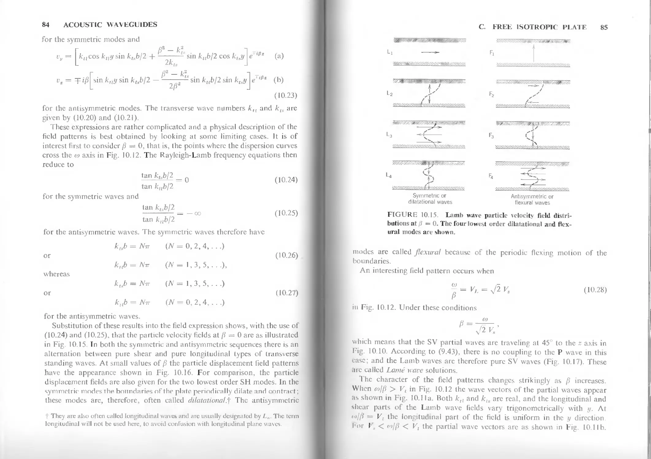
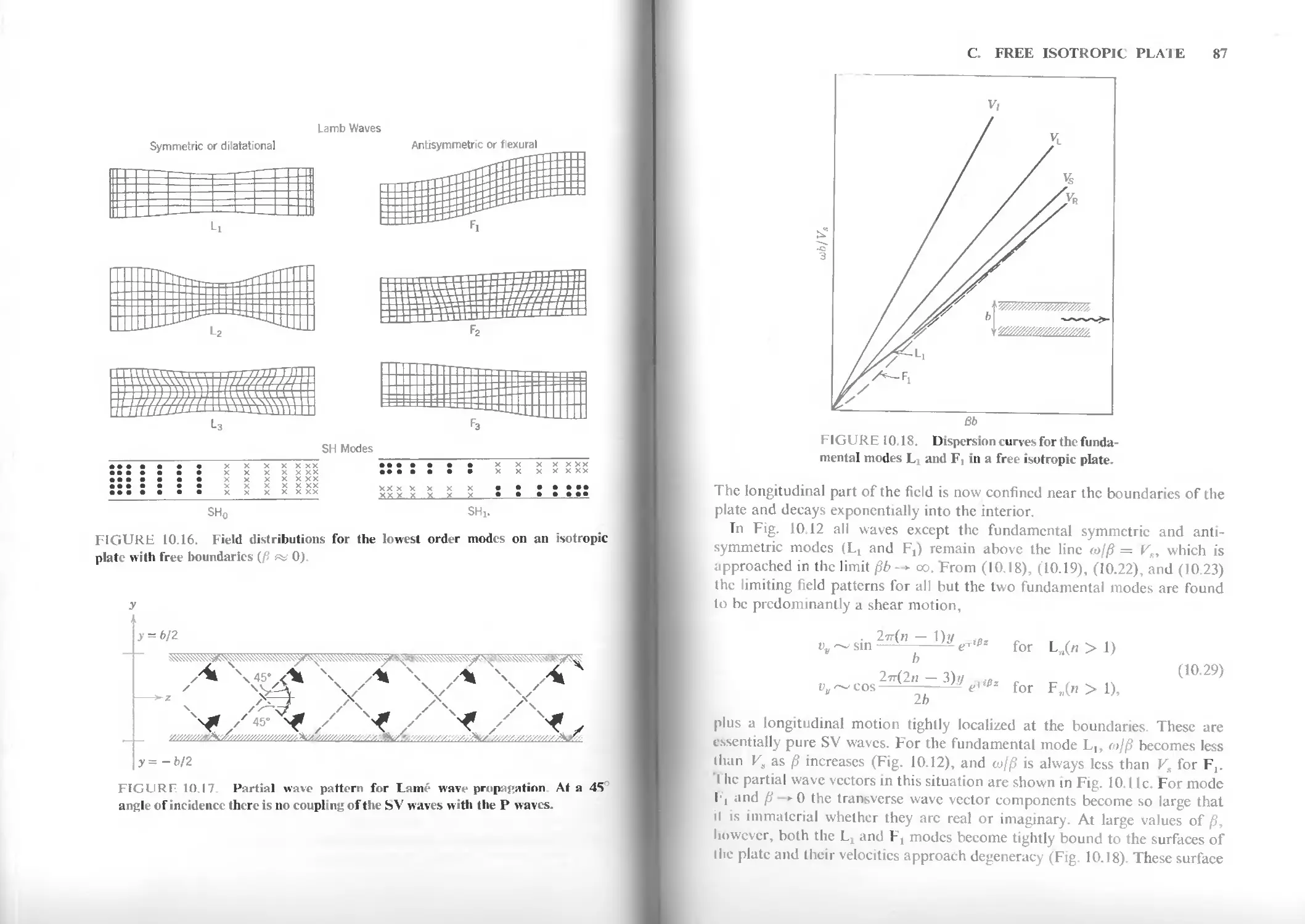
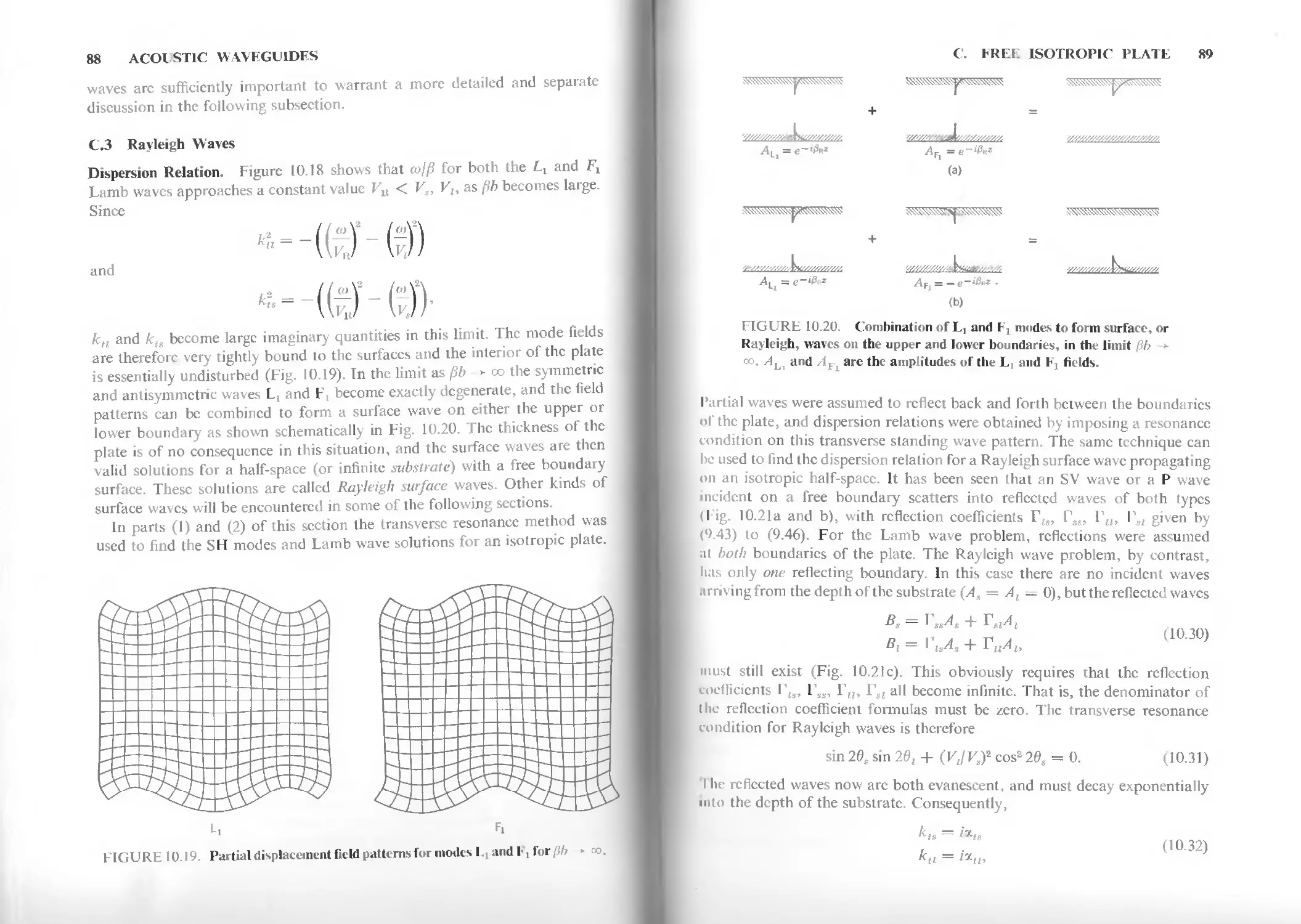
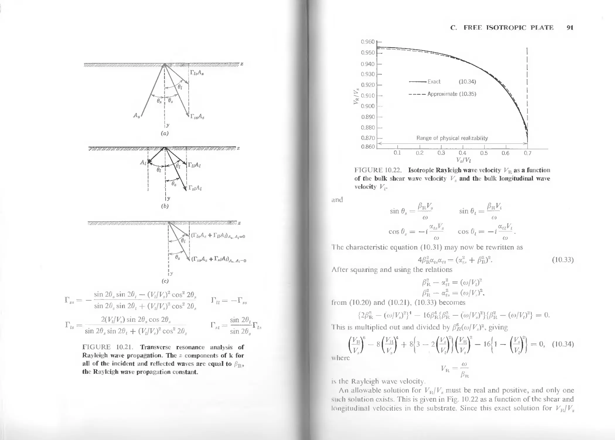
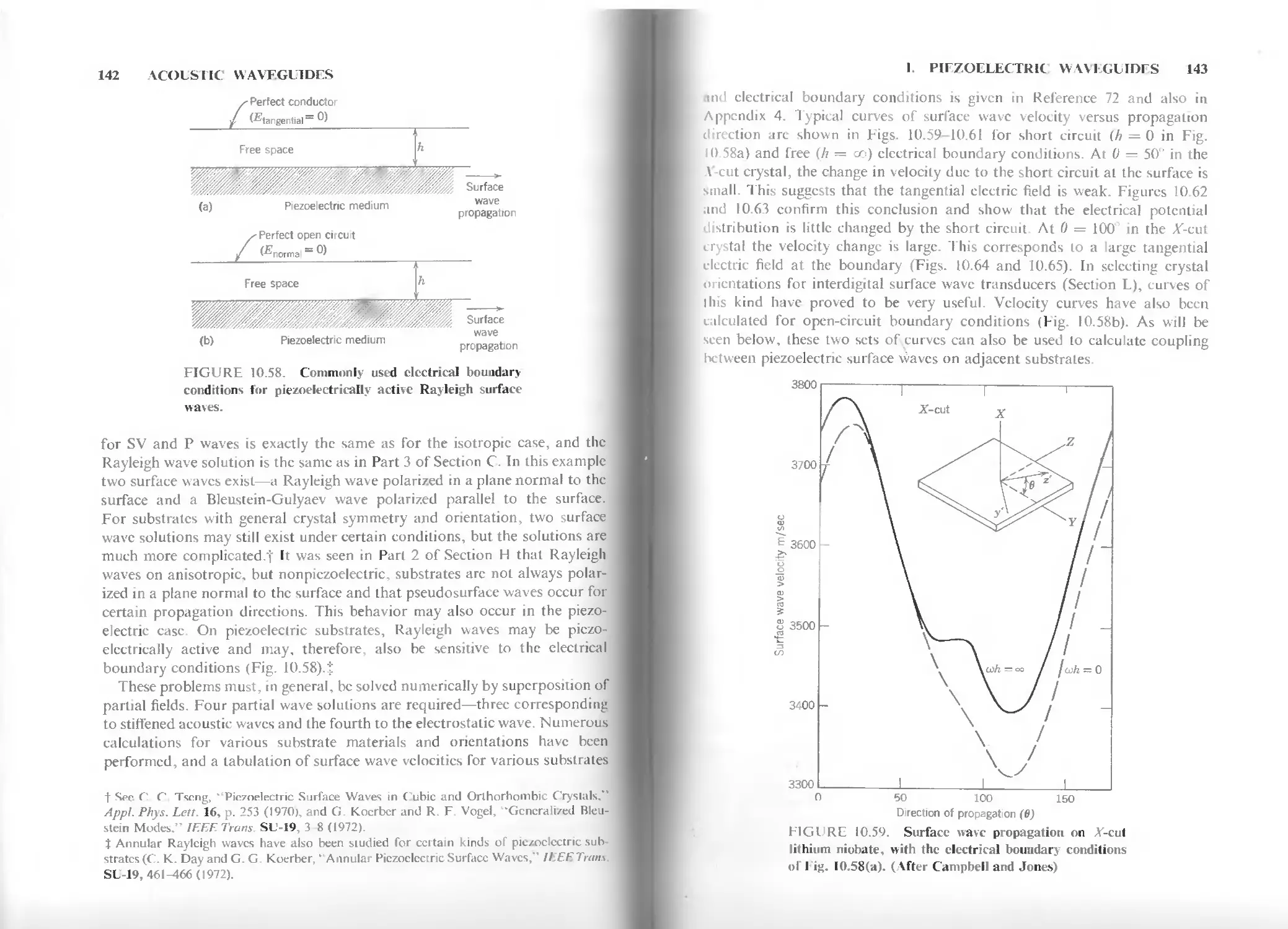
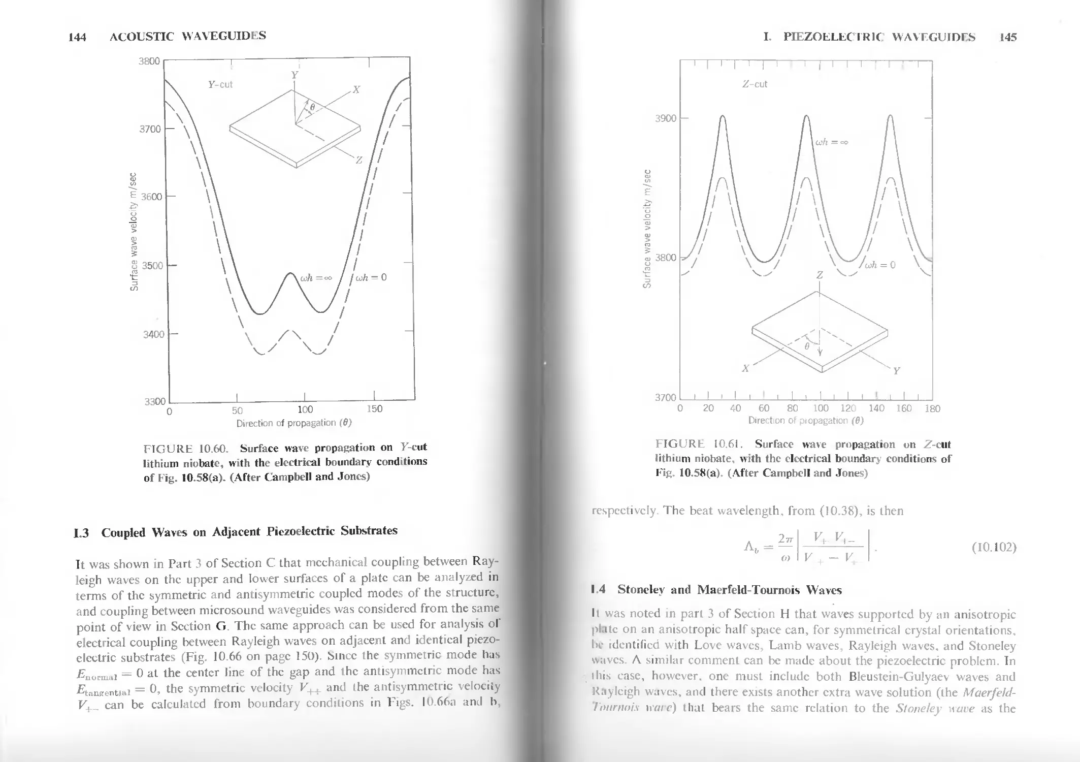
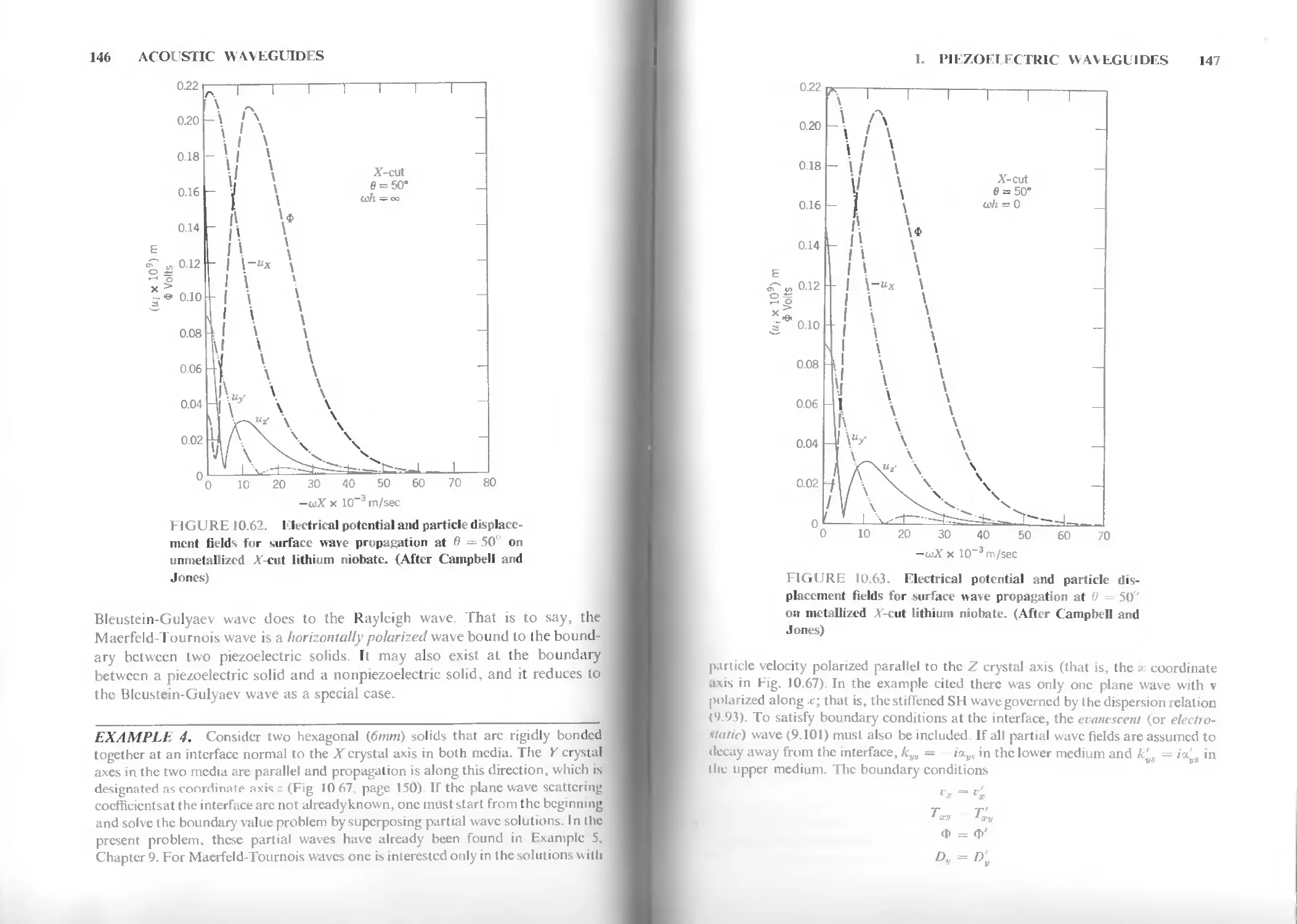
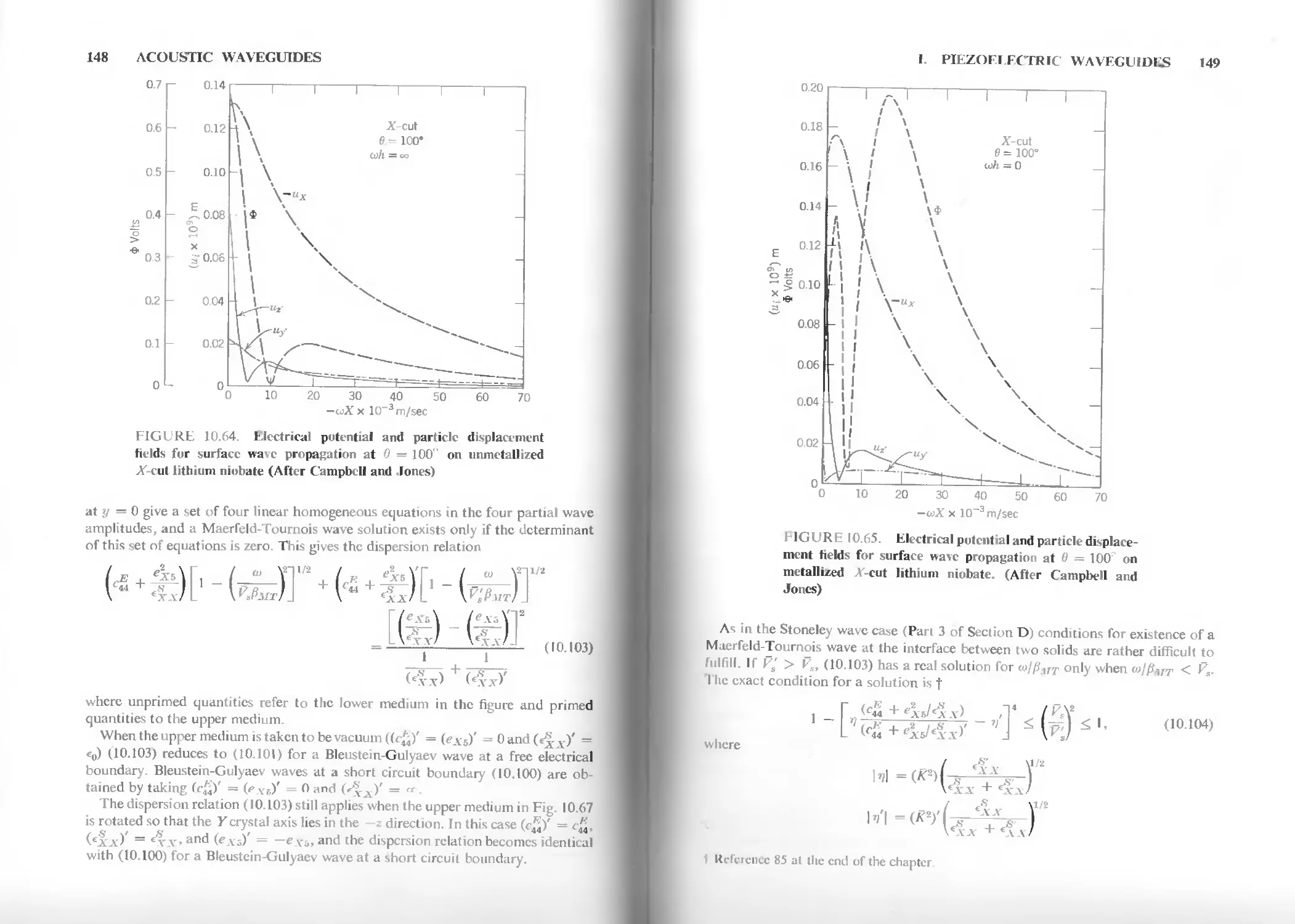
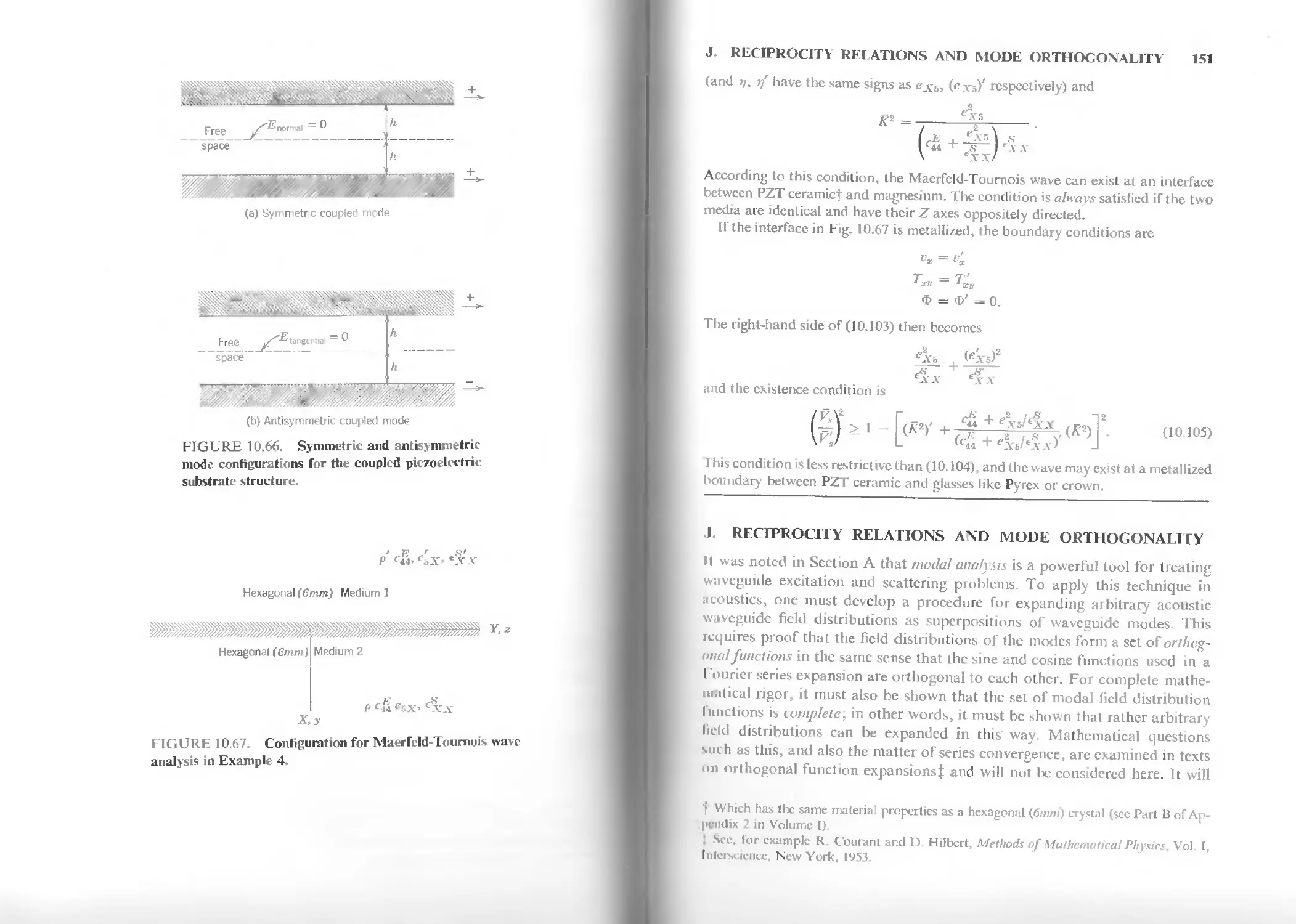
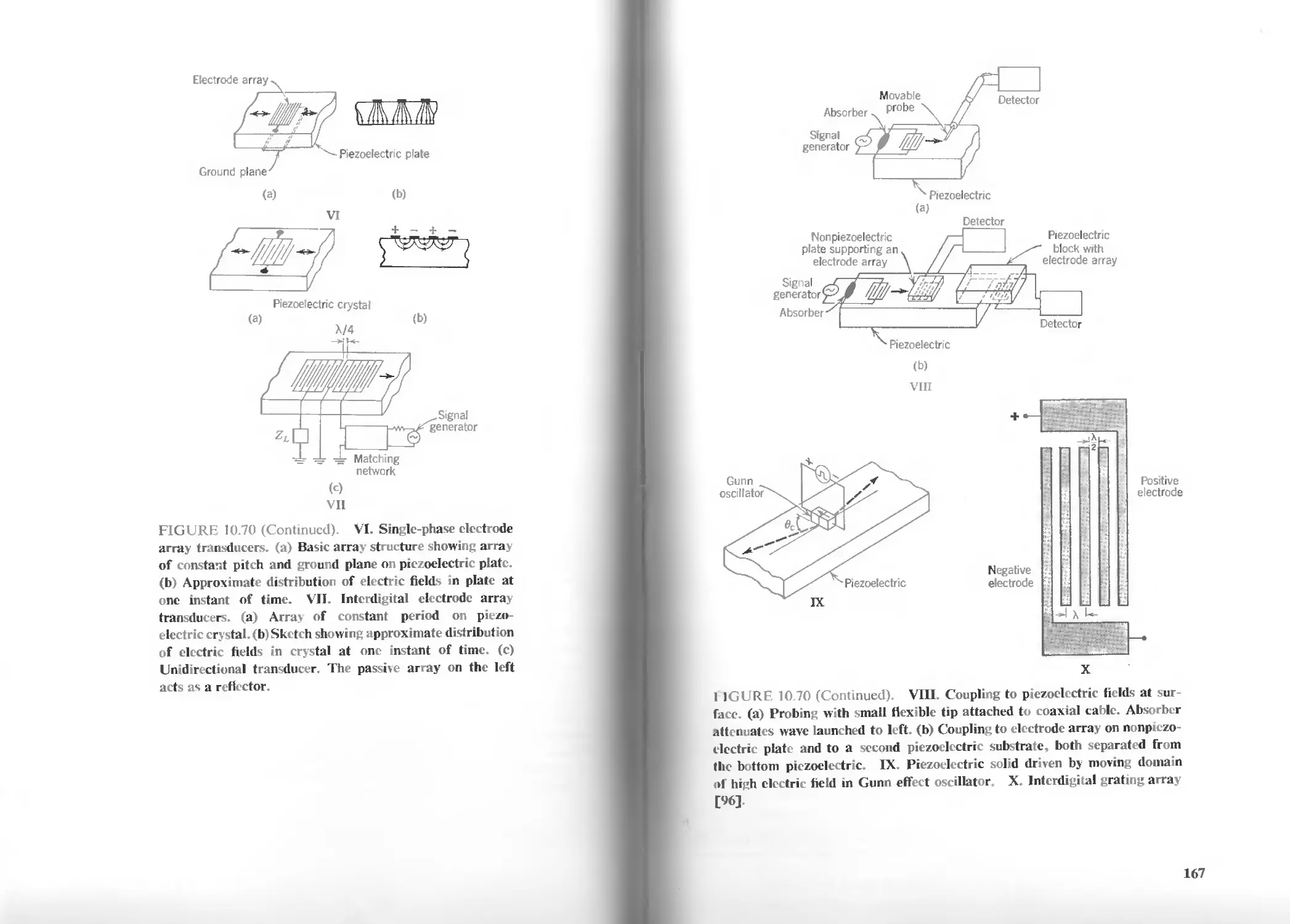
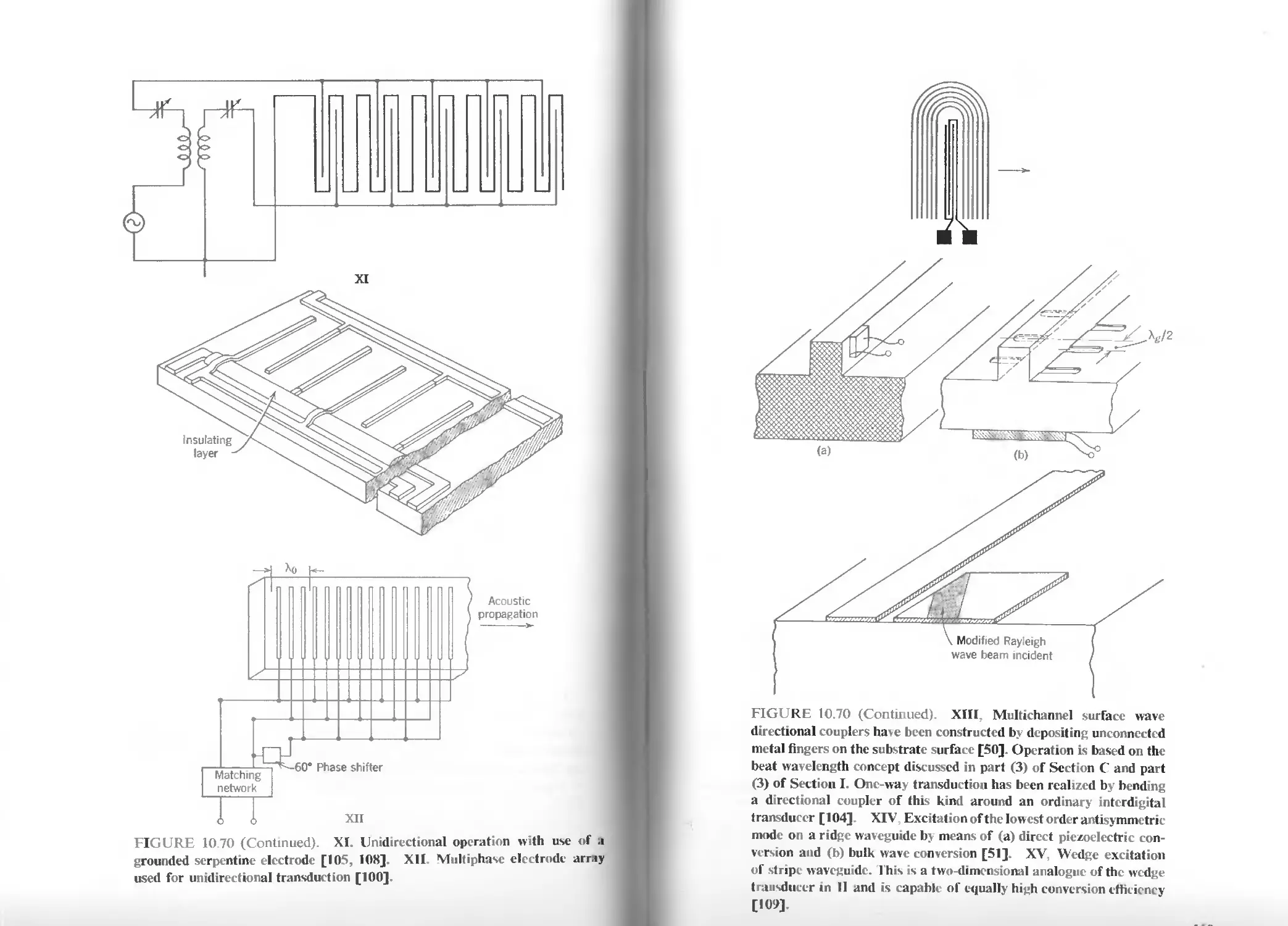
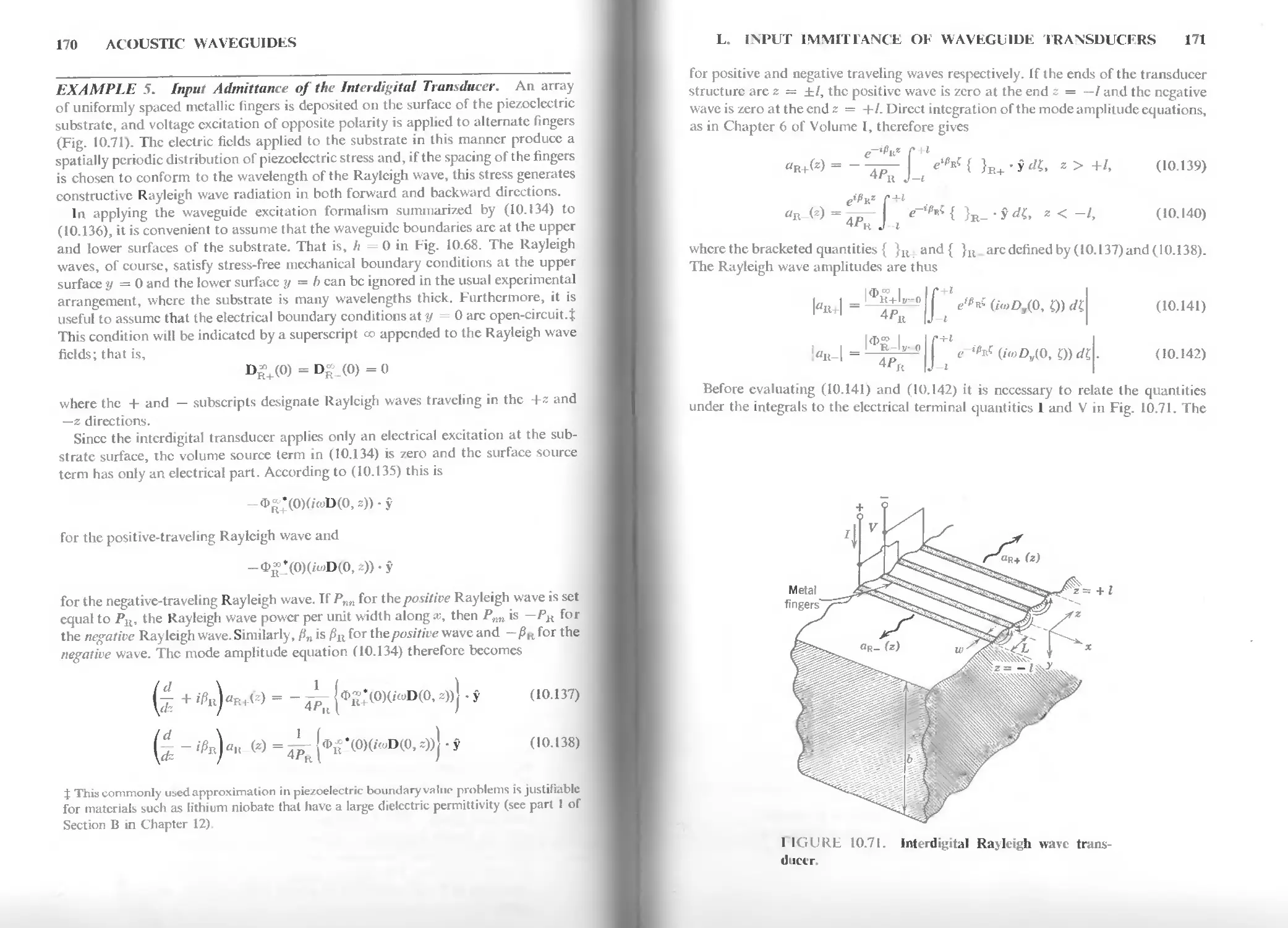
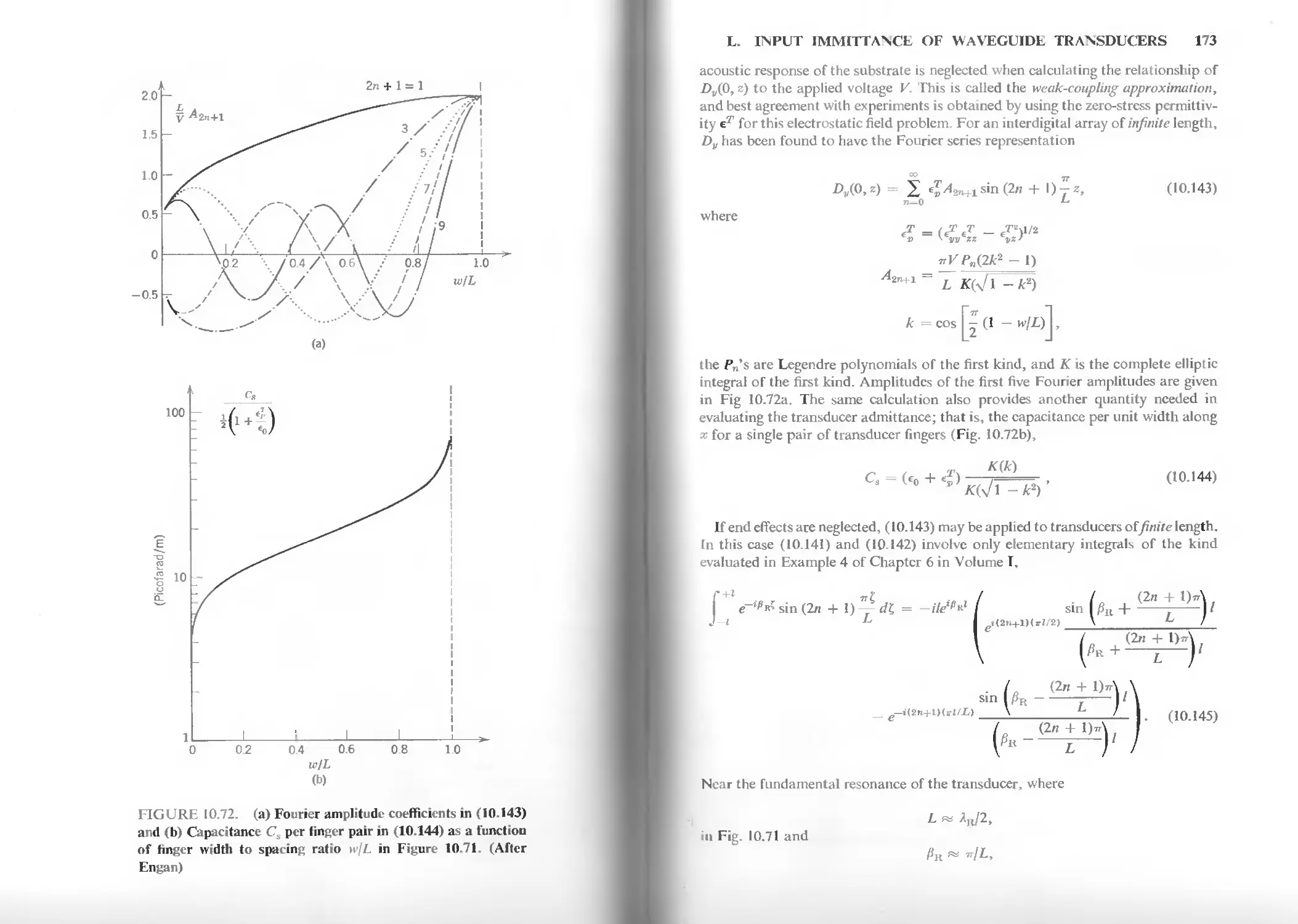
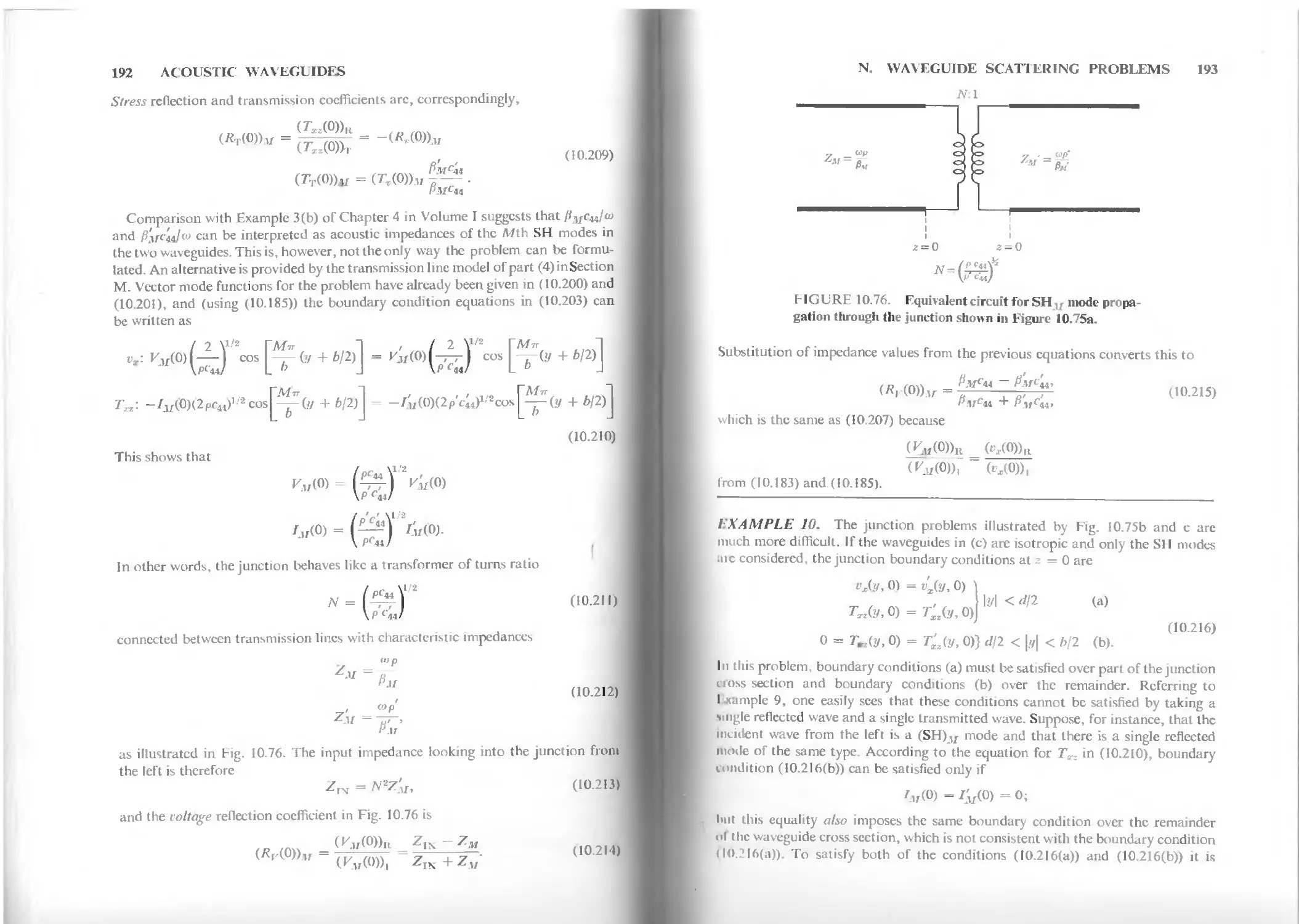
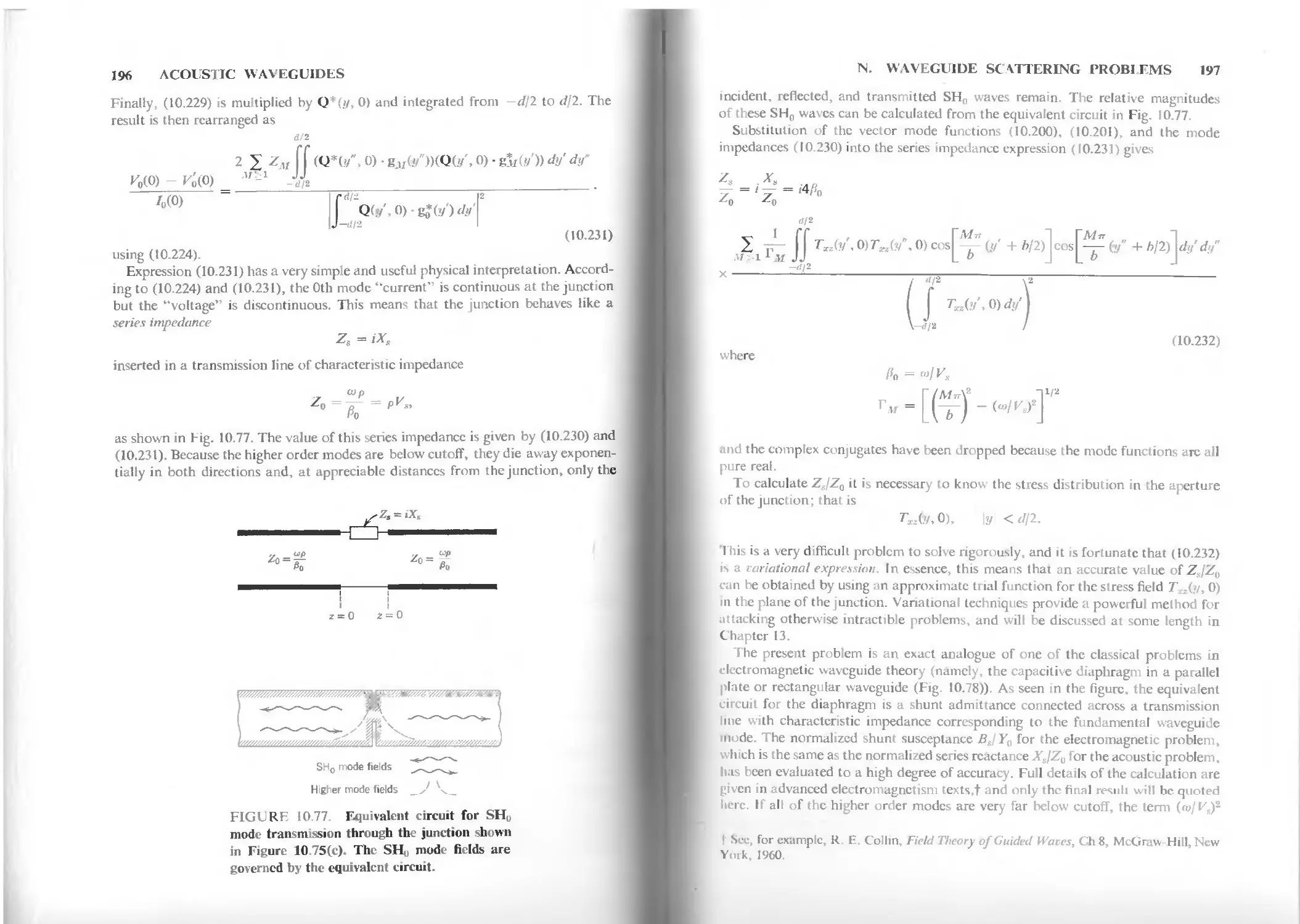
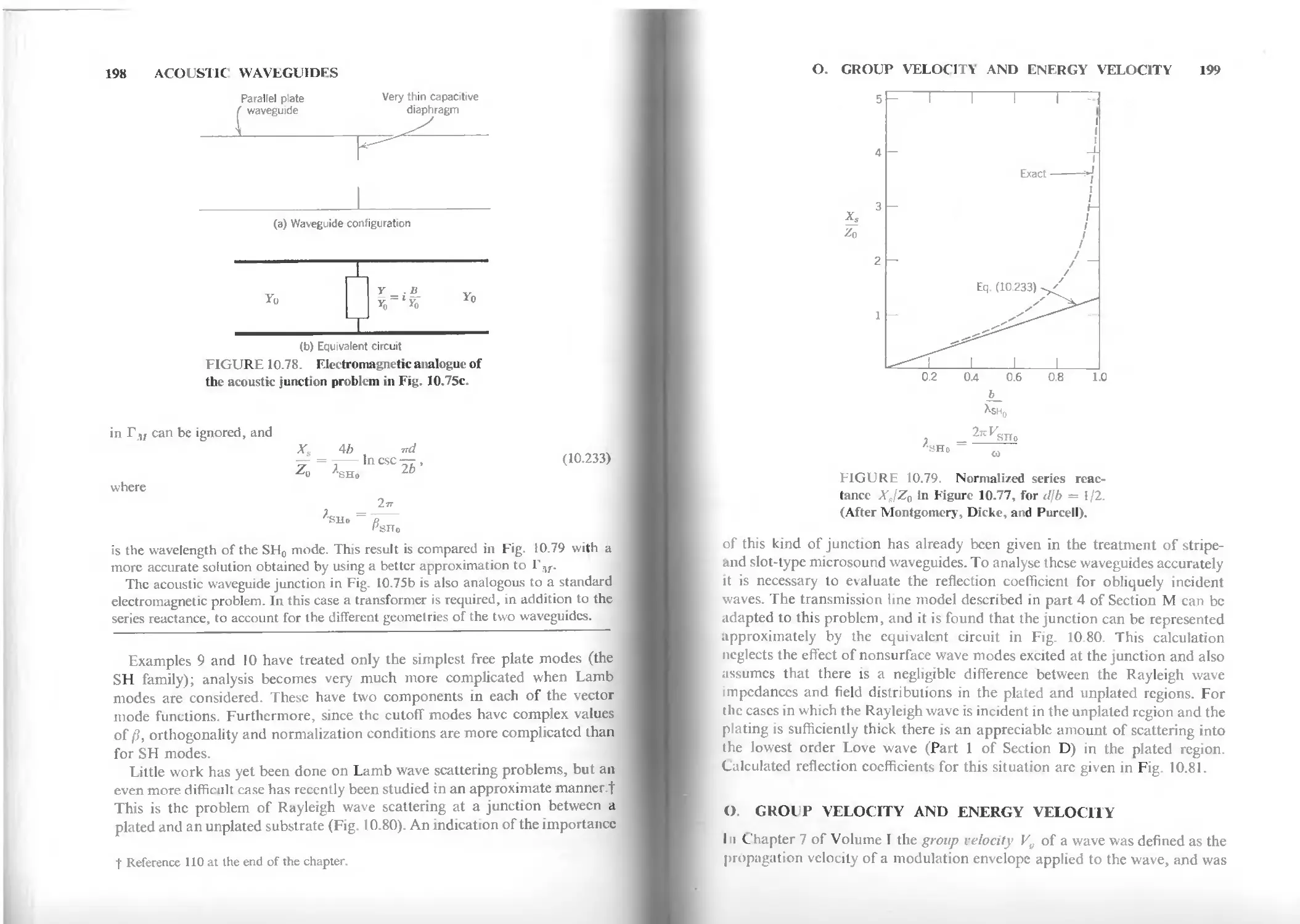
Текст
ACOUSTIC FIELDS
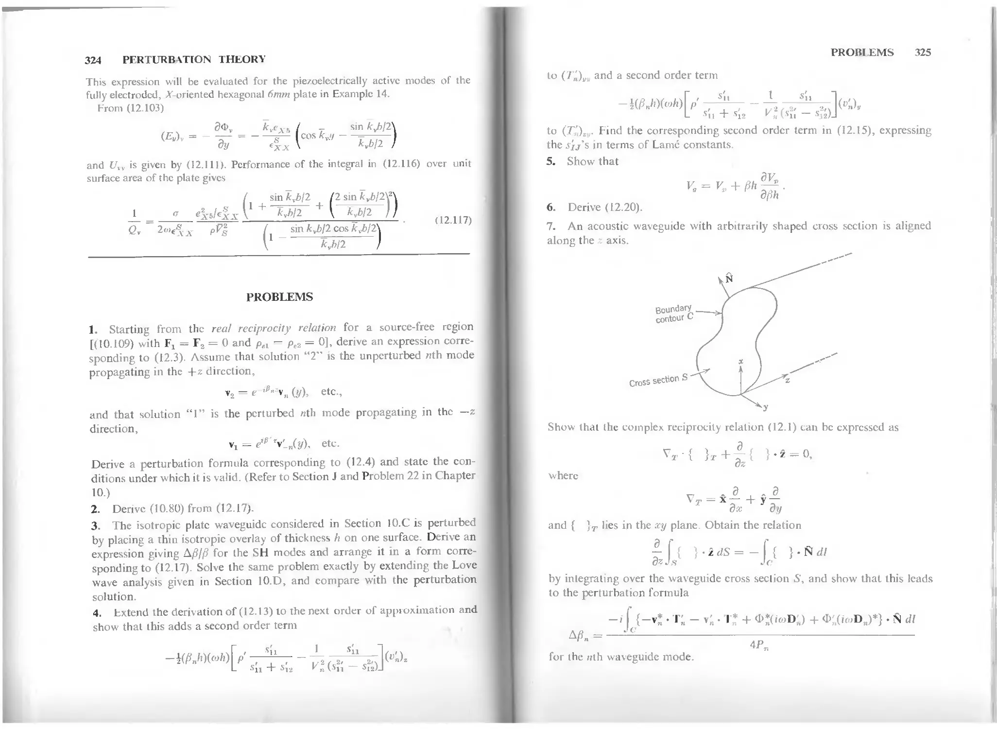
AND WAVES
IN SOLIDS
VOLUME II
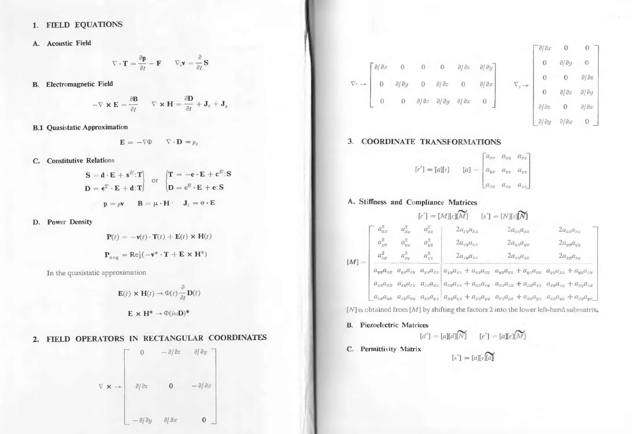
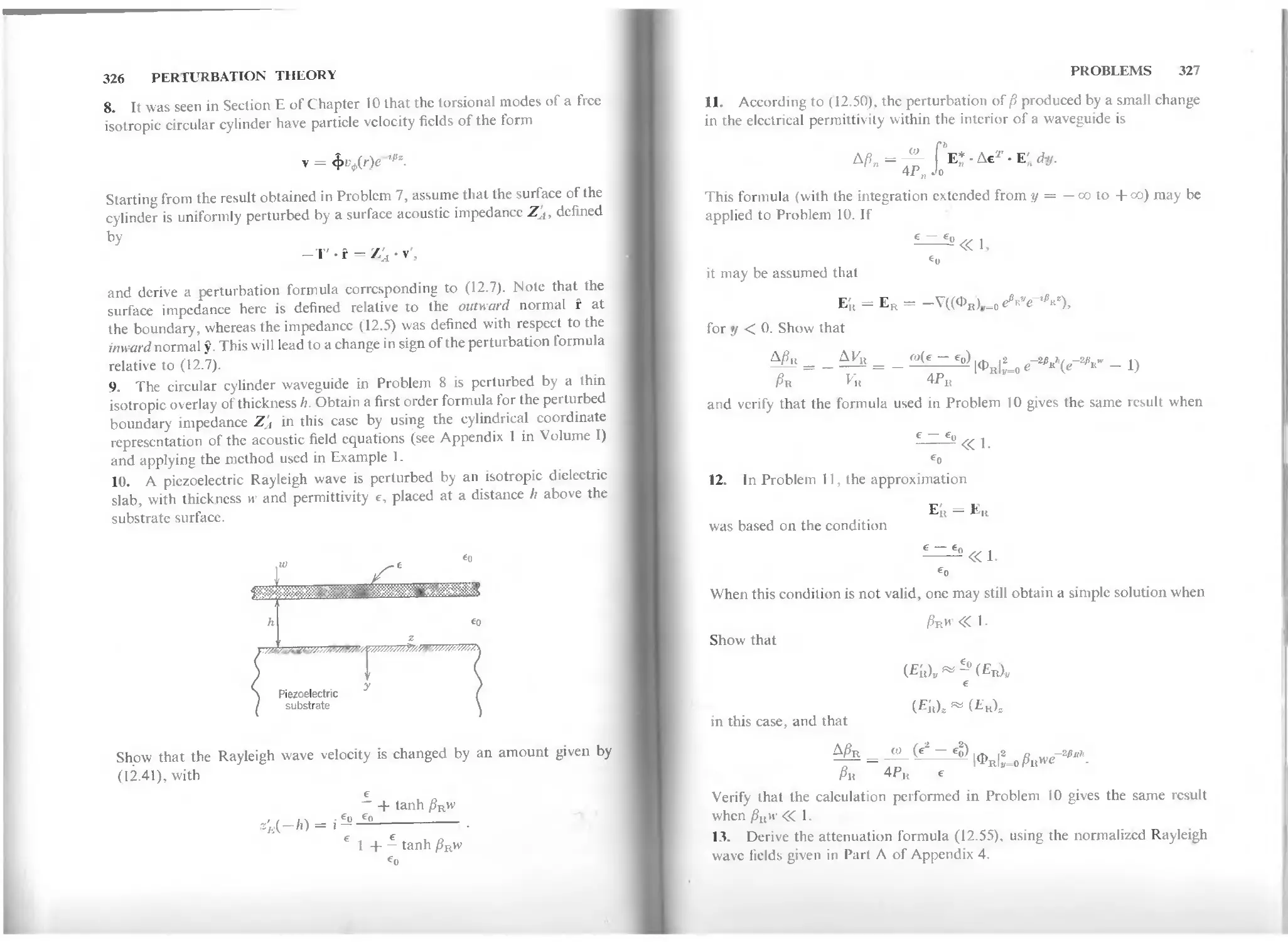
1. FIELD EQUATIONS
A. Acoustic Field
dp 3
VT=^-F Vsv=-S
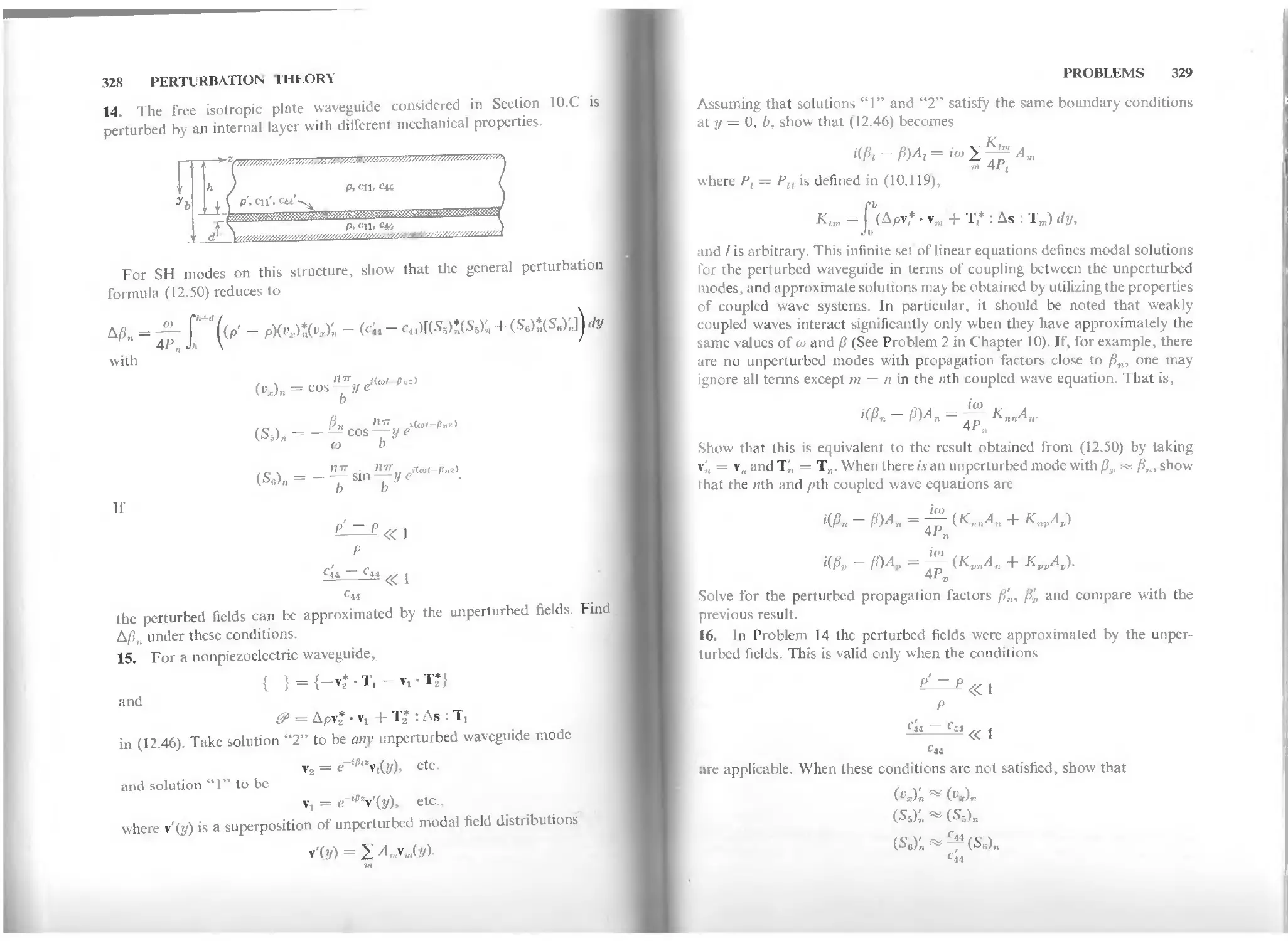
B. Electromagftetic Field
-V x E =
ЭВ 3D
If **H--+J. + J.
B.1 Quasistatic Approximation
E = -V0> V • D = ,
C. Constitutive Relations
S =d-E + sE:T
D = eT -E +d:T
or
T = -e-E + c^:S
D = • E + e.S
D. Power Densitj
p = pv B = jjl-H- Jc = a • E
P(,) = -v(/) • Ш + E(/) x H(/)
PaTK = ReK_v* • T + E x H*)
In the quasistatic approximation
E(/) x Н(/)^Ф(0-^О(г)
E x H* ^ Ф(/Ы))*
2. FIELD OPERATORS IN RECTANGULAR COORDINATES
0 -djdz d/dy
V X
d/dz
-djdy д/дх
■д/дх
djdx О 0 0 d/dz д/ду
О д/ду 0 djdz О д/Вх
О О д/dz djdy д/дх О
3. COORDINATE TRANSFORMATIONS
'д/дх
О
О
о
д/dz
д/ду д/дх О
[/] = [а][г]
[а] =
Jizx
azy azz_
A. Stiffness and С mplianc Matrices
[c] = [M]lcJM] [л'] =
Г a2
XX
a2
xz
"I
a2
vv
<
A.
Qyiflzy
avza
azx&xx
azyaxy
azza
_&хх@ух
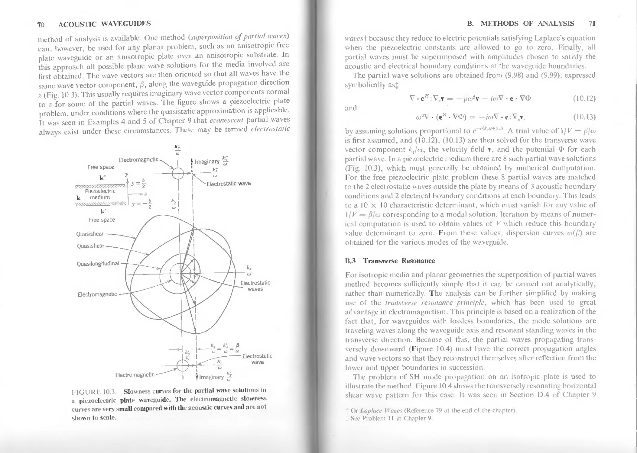
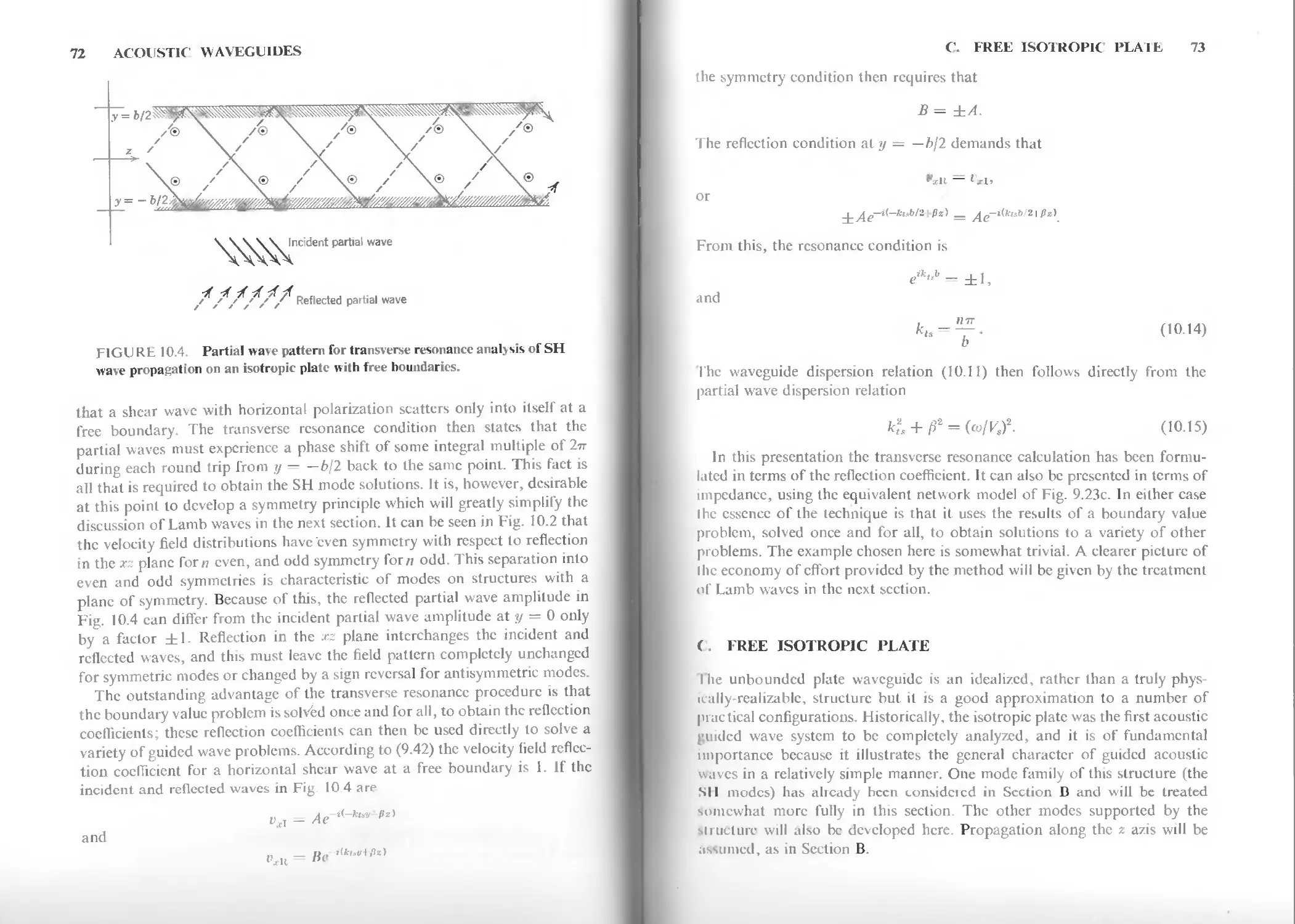
&ХУ&УУ
2aZydz
О О "
д/ду 0
О д/dz
д/dz 3/3//
О д/дх
&yy&zz "Т" &yz&zy uyx&zz "Т" Gyz&zx &y\№zx ^yx^zv
! Qxiflzz "Ь &XZ&ZV &xz@zx Q$vP-zy ^xiflzx
\ &xy&yz axzayy axzayx axx®yz &хх@уу axyayx_
f/V] is obtained from [M] by shifting the factors 2 into the lower left-hand submatnx.
U. Piezoelectric Matrices
C. Permittivity Matrix
ACOUSTIC FIELDS
AND WAVES
IN SOLIDS
VOLUME II
B. A. AULD
Senior Research Associate
in the W. W. Hansen Laboratories of Physics
and Lecturer in Applied Physics
Stanford University
Л WILEY INTERSCIENCE PUBLICATION
JOHN WILEY & SONS
New York London Sydney Toronto
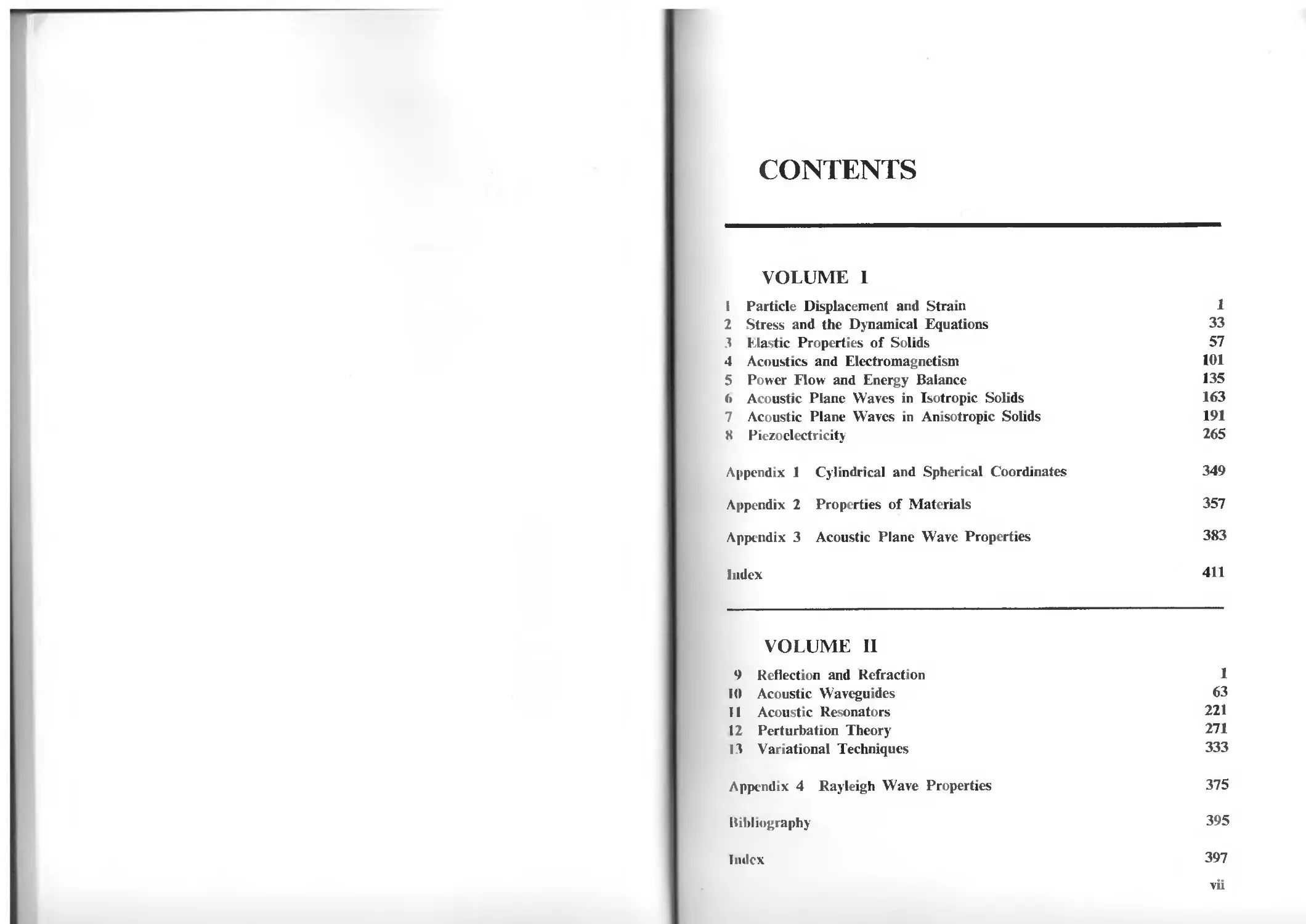
CONTENTS
VOLUME 1
1 Particle Displacement and Strain 1
2 Stress and the Dynamical Equations 33
3 Elastic Properties of Solids 57
4 Acoustics and Electromagnetism 101
5 Power Flow and Energy Balance 135
6 Acoustic Plane Waves in Isotropic Solids 163
7 Acoustic Plane Waves in Anisotropic Solids 191
Й Piezoelectricity 265
Appendix 1 Cylindrical and Spherical Coordinates 349
Appendix 2 Properties of Materials 357
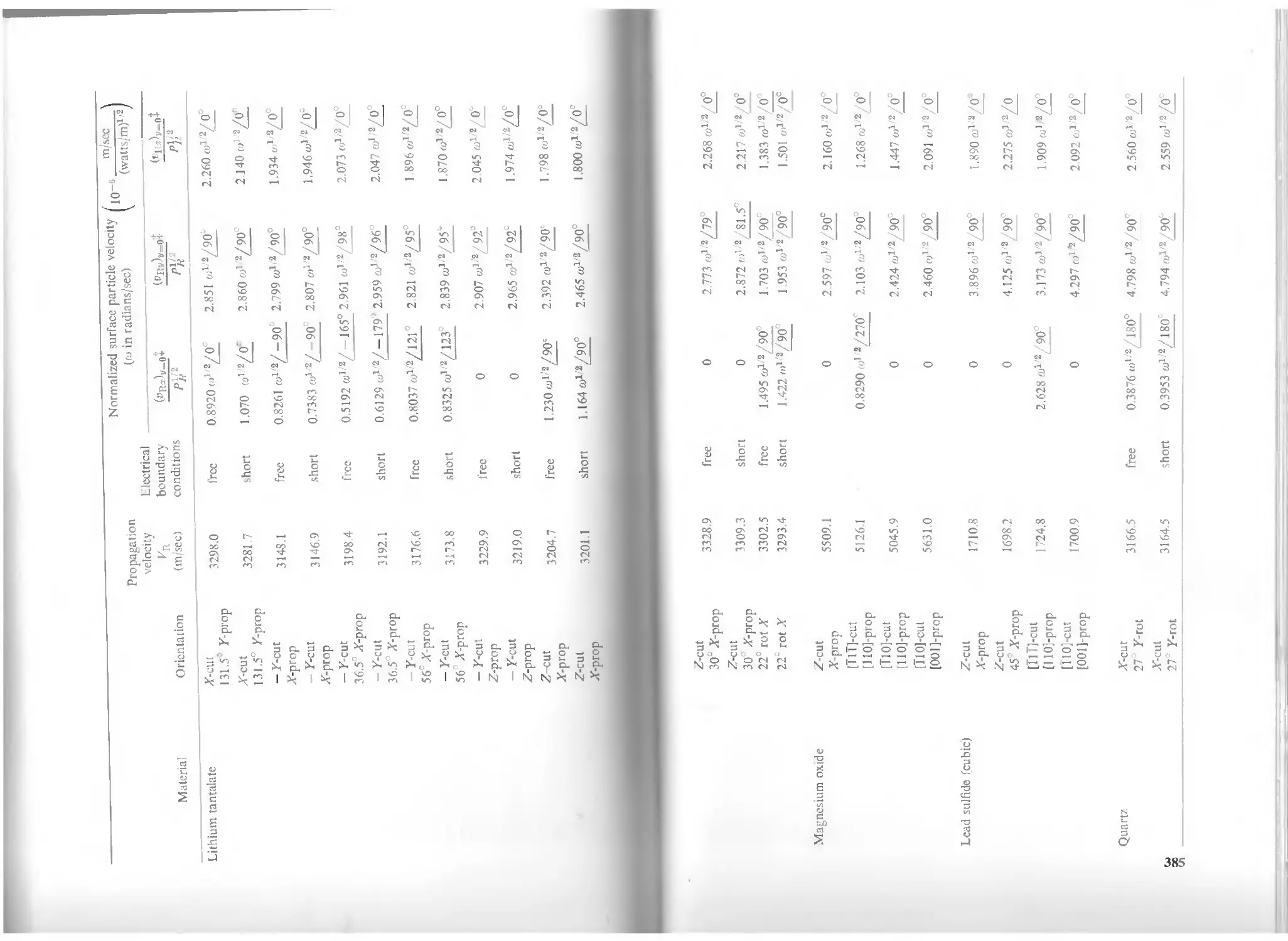
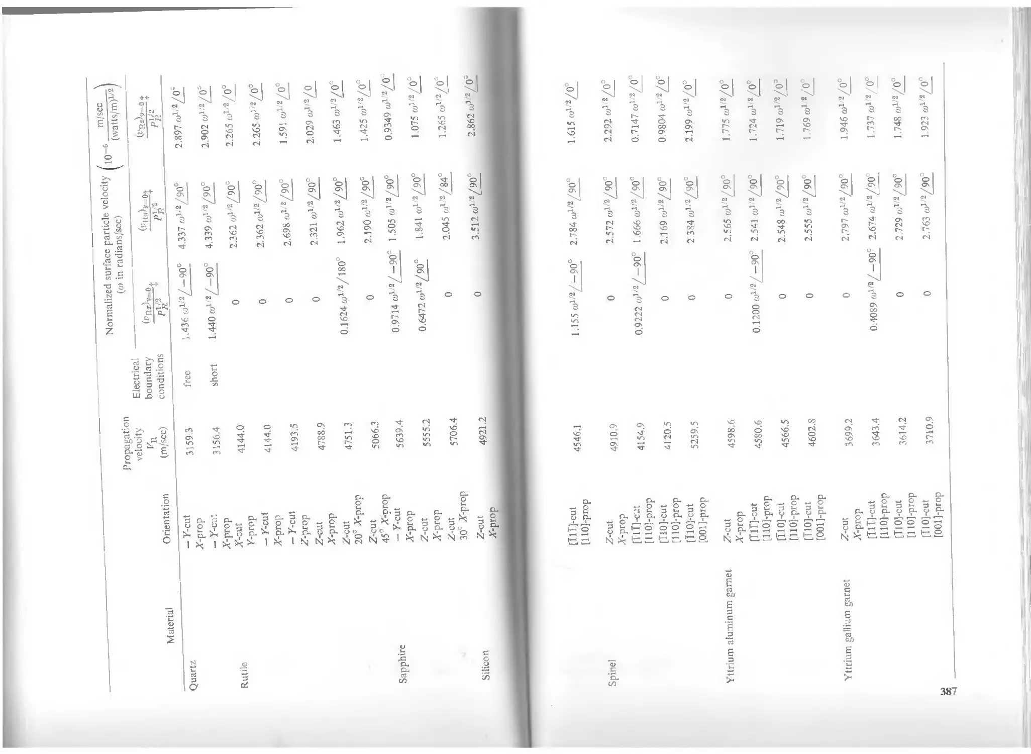
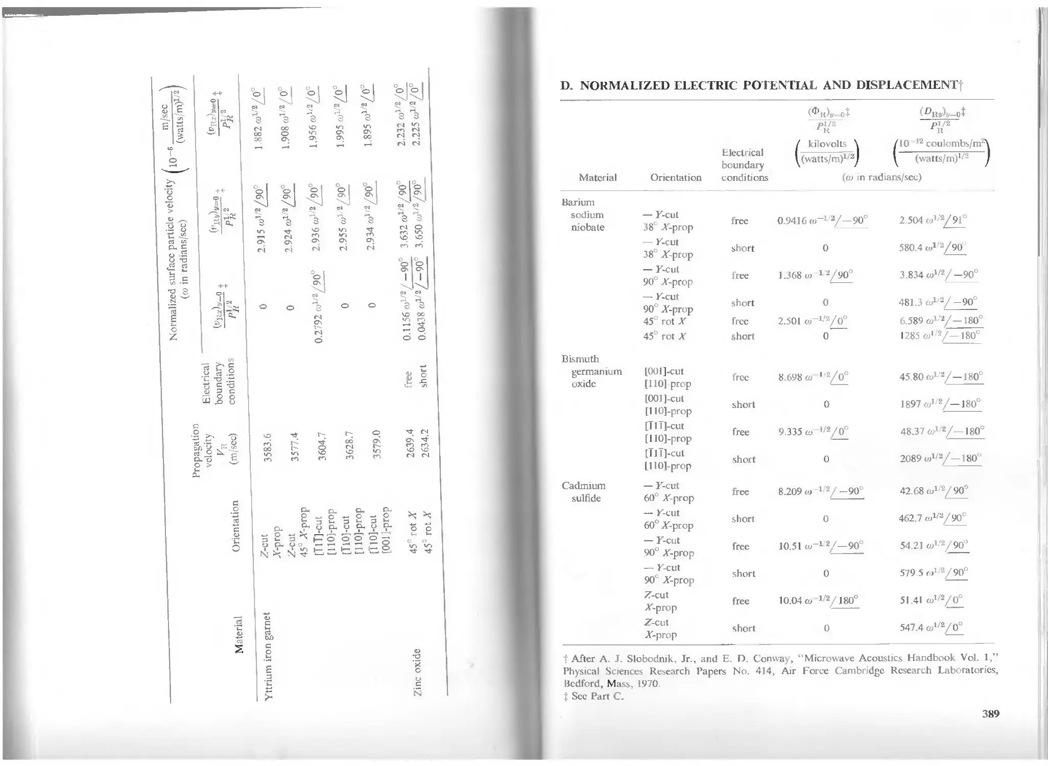
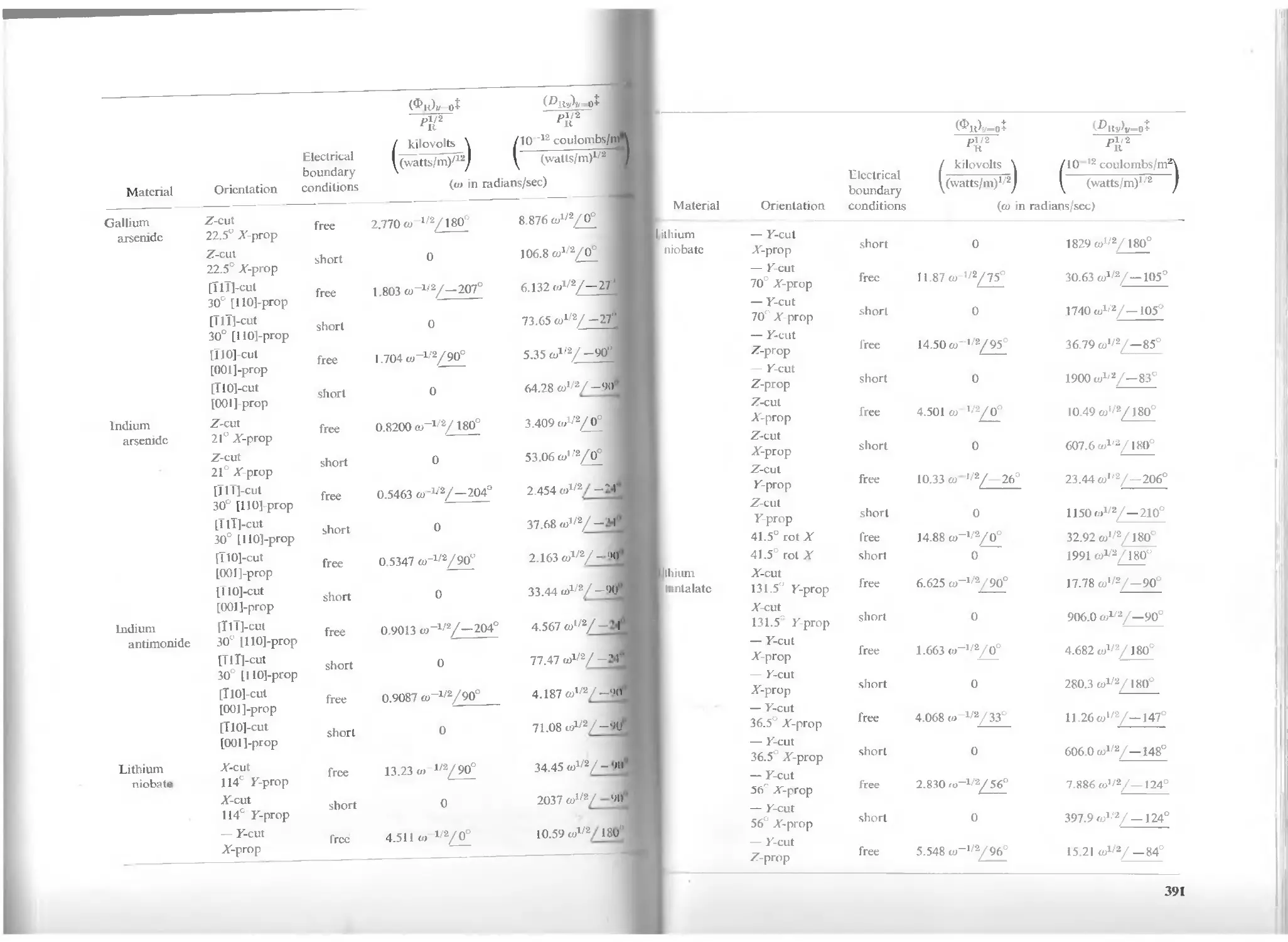
Appendix 3 Acoustic Plane Wave Properties 383
Index 411
VOLUME II
9 Reflection and Refraction 1
10 Acoustic Waveguides 63
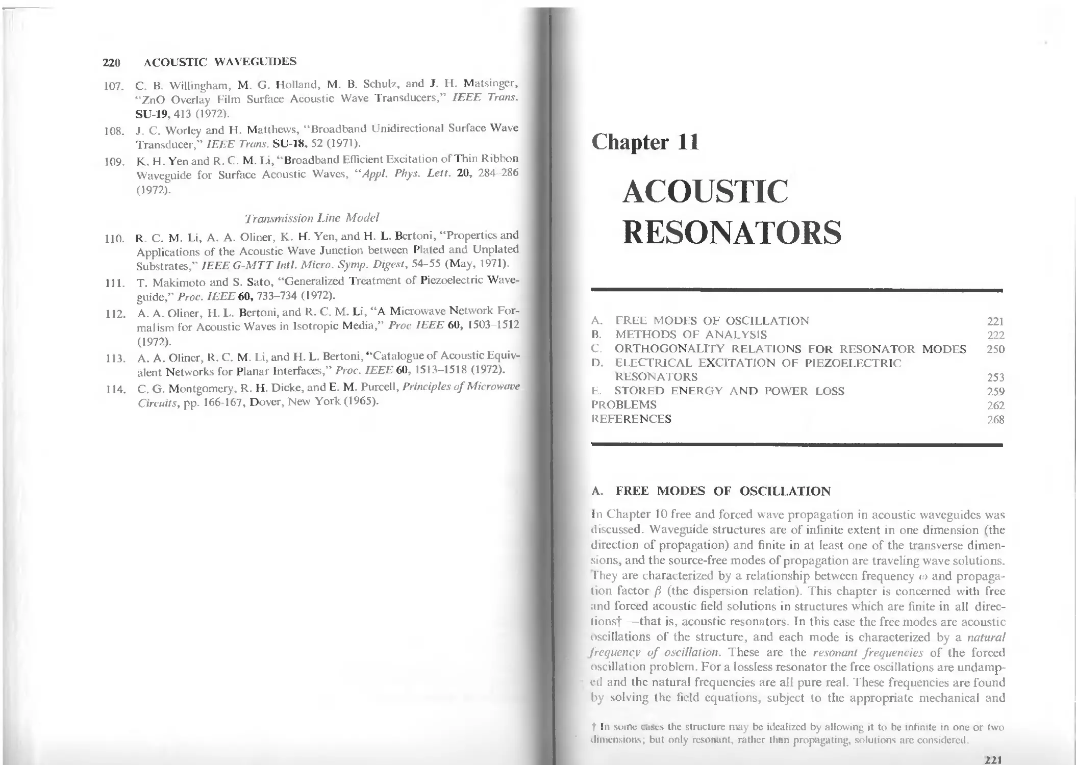
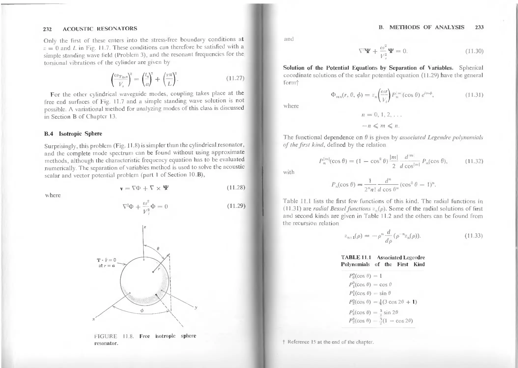
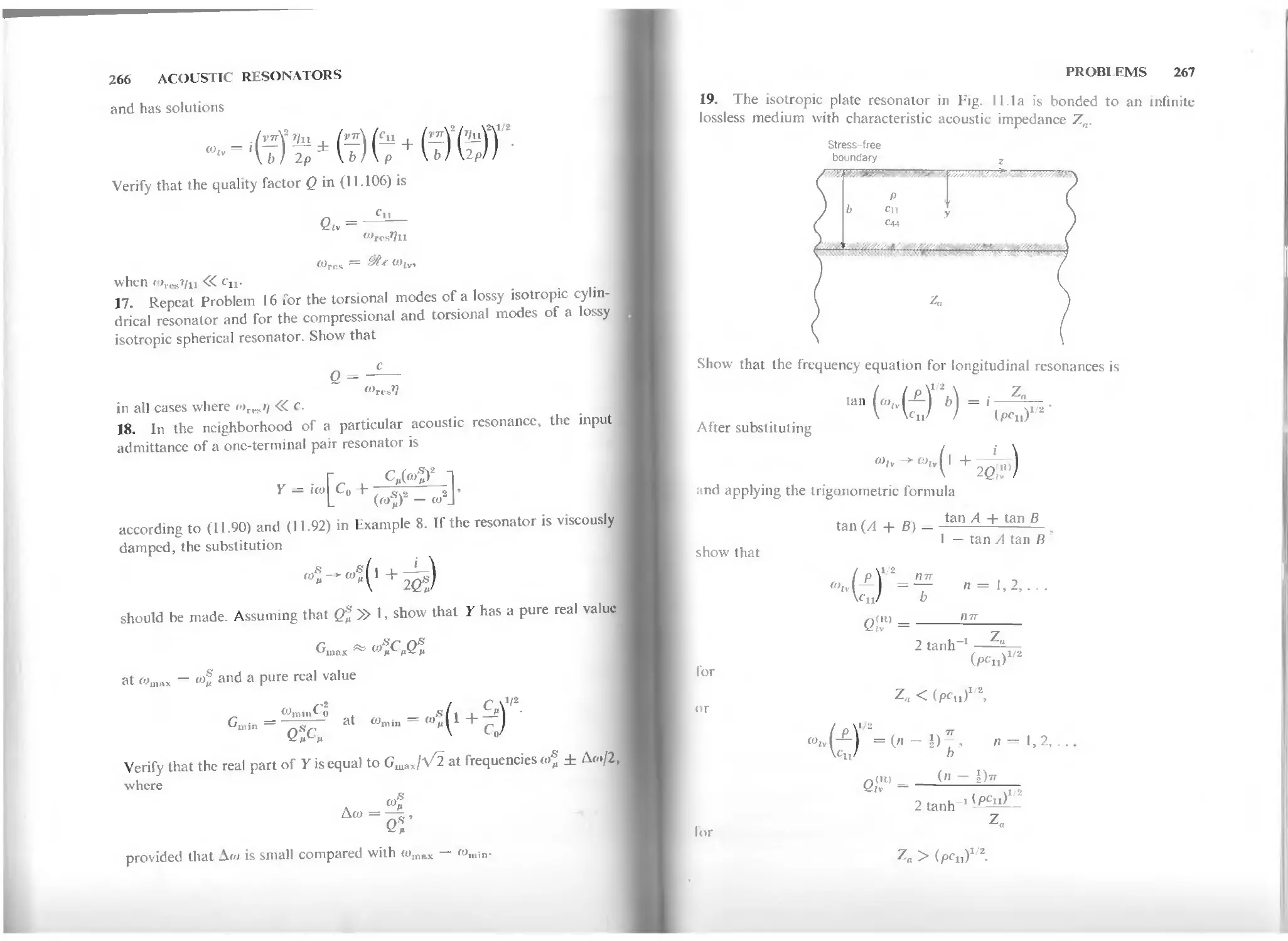
11 Acoustic Resonators 221
12 Perturbation Theory 271
13 Variational Techniques 333
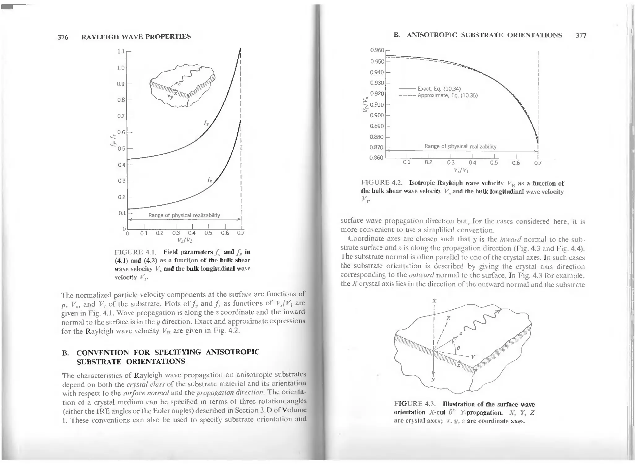
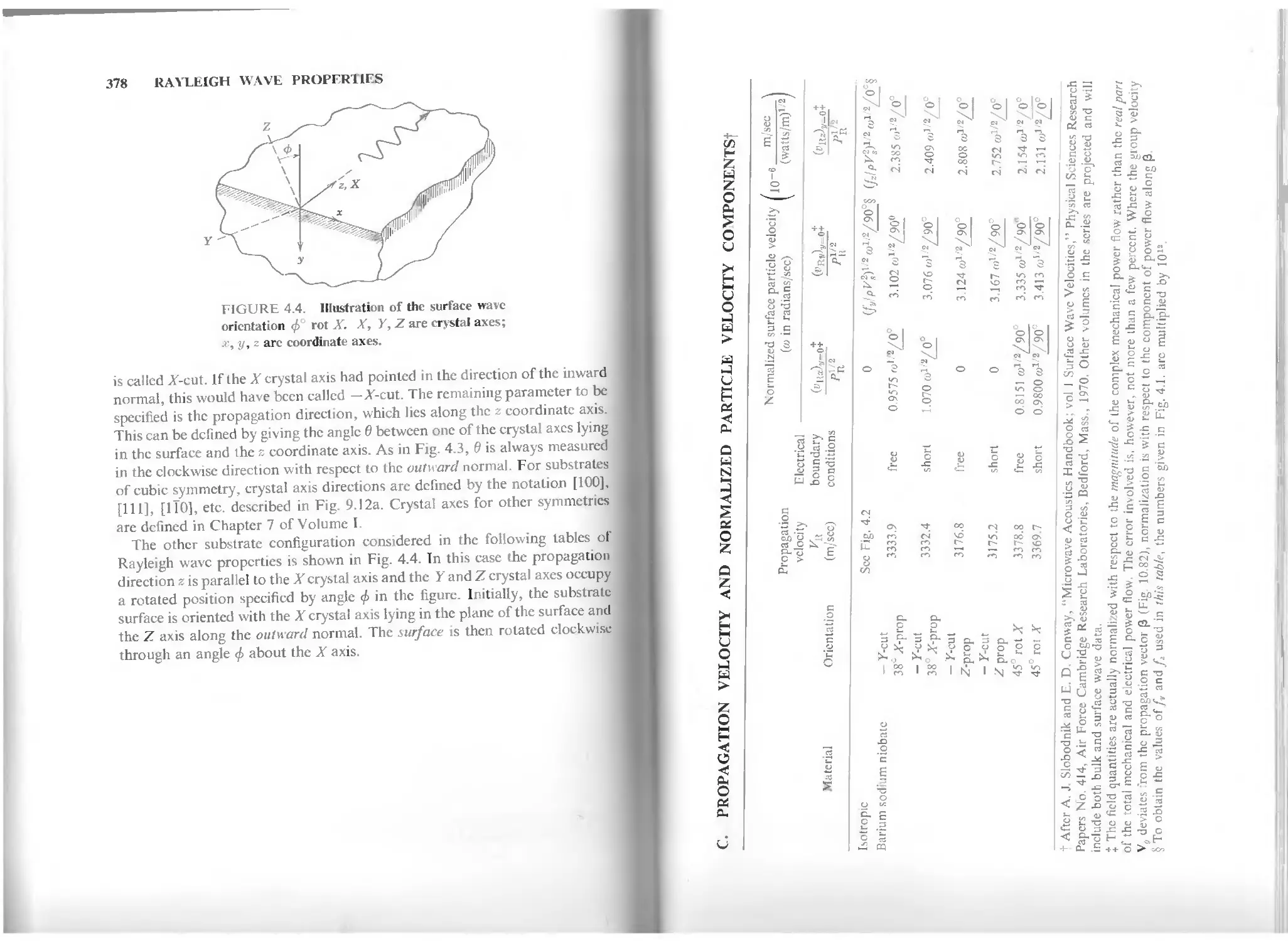
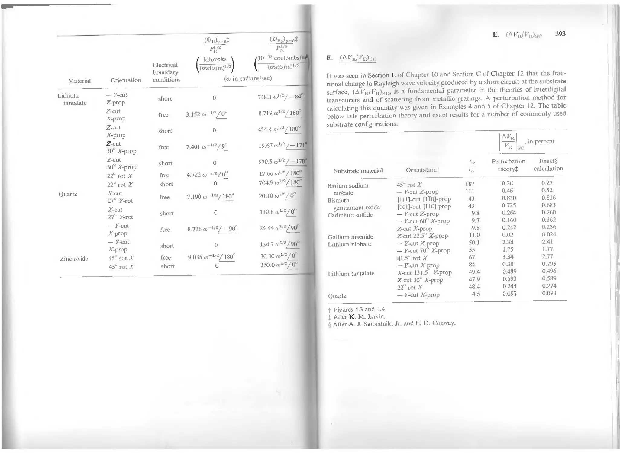
Appendix 4 Rayleigh Wave Properties 375
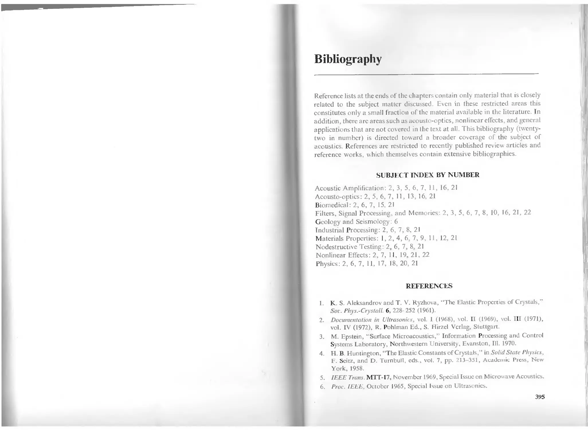
ItiMiography 395
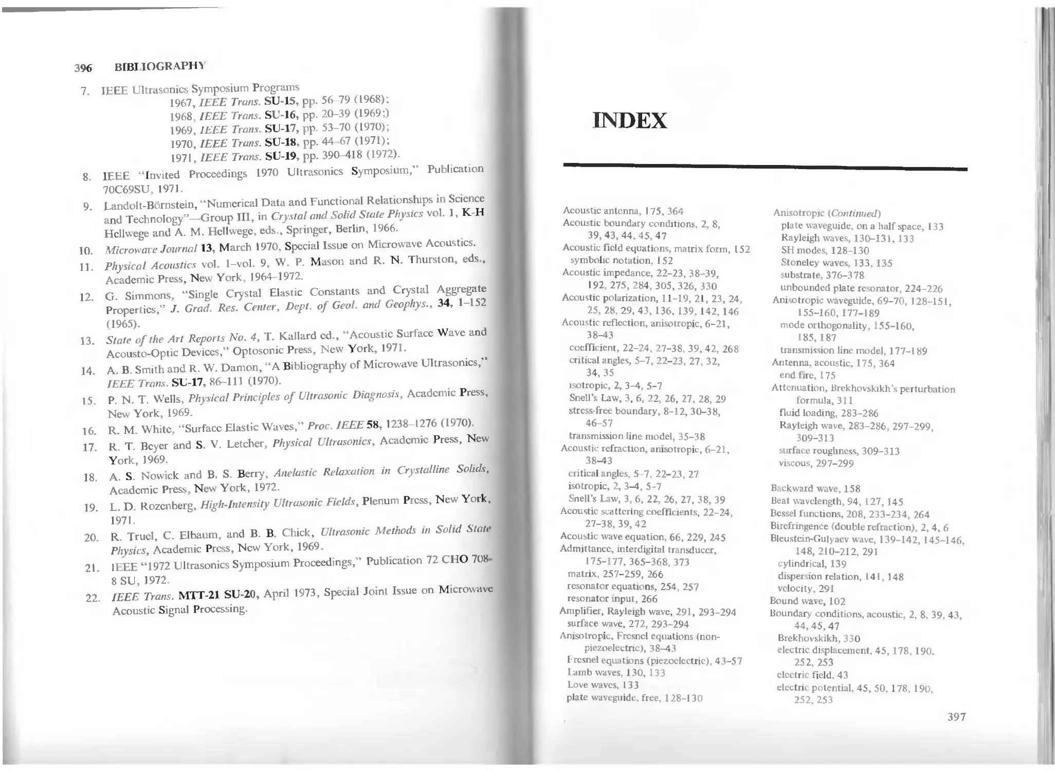
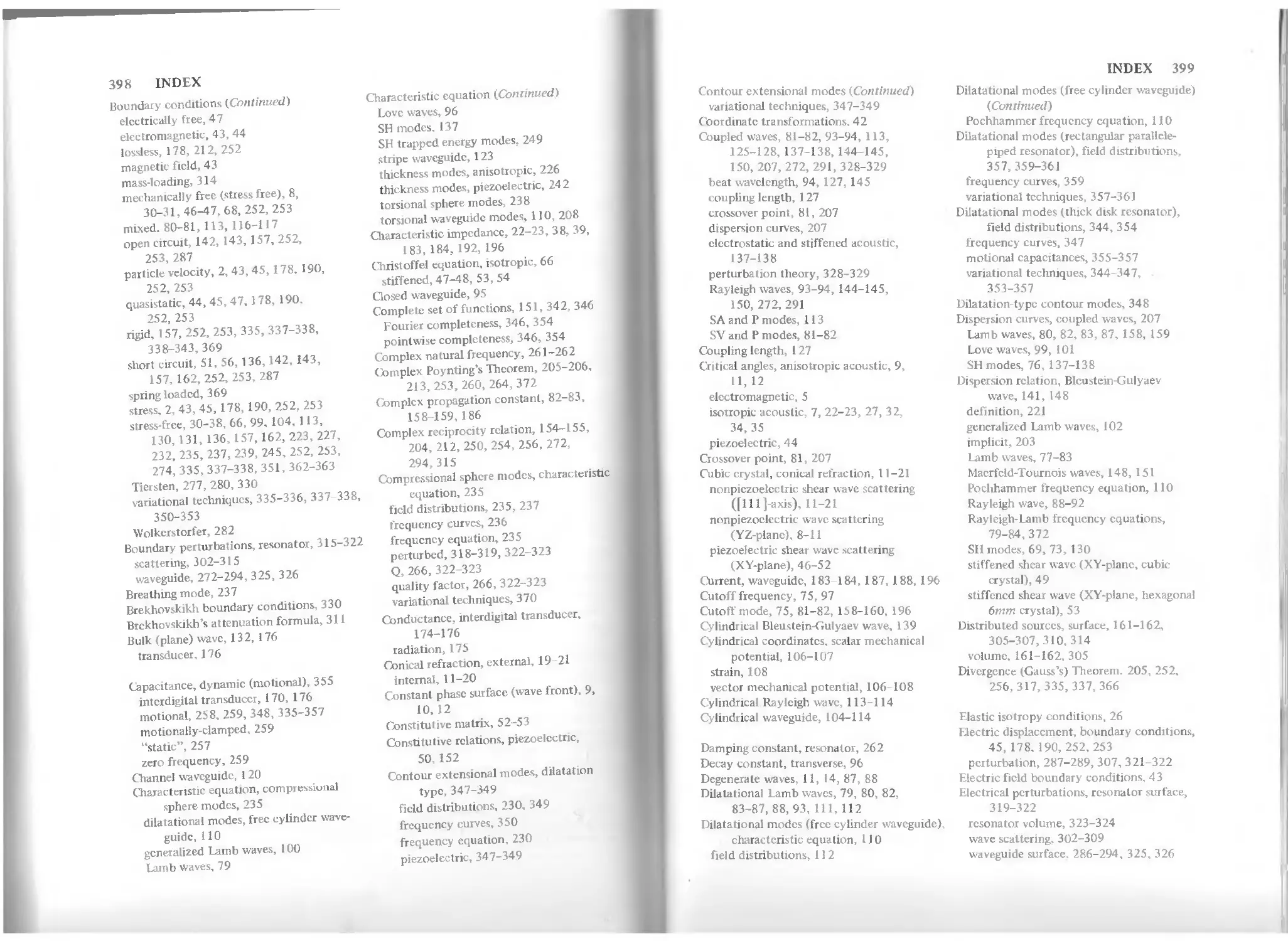
Index 397
Copyright © 1973, by John Wiley & Sons, Inc.
All rights reserved. Published simultaneously in Canada.
No part of this book may be reproduced by any means,
nor transmitted, nor translated into a machine language
without the written permission of the publisher.
Library of Congress Cataloging in Publication Data
Auld, Bertram Alexander, 1922-
Acoustic fields and waves in solids
"A Wiley-Interscience publication."
Bibliography: p.
1. Solids Acoustic properties 2. Sound-waves
Industrial applications 3. Elastic waves 4. Wave-
motion, Theory of. I. Title.
QC176.8 A3A84 534'.22 72 8926
ISBN 0-471-03701-х (V. 2)
ISBN 0-471 03702-8 (Set)
Printed in the United States of America
10 987654321
PREFACE
This book has developed from a lecture course on mechanical waves and
vibrations in solids, for first and second year graduate students. It is intended
to present, in a manner congenial to the disciplines of Applied Physics and
Tlectrical Engineering, a coherent treatment of the subject, starting from
fundamentals and proceeding to applications. In Volume I acoustic field
theory was developed step-by-step from the basic principles of mechanics
and electricity. The present volume applies this theory to a variety of
scattering, waveguide and resonator problems. As in the previous volume, the
material is organized along the lines used in graduate level electromagnetic
theory texts. This approach is of particular importance in connection with
acoustic waveguide theory, where recent advances in thin film technology
and waveguide transducer design have encouraged the application of
microwave electromagnetic concepts to problems in acoustics.
Generally speaking, acoustic field problems are significantly more difficult
than electromagnetic problems, and approximation methods must often be
used to obtain solutions. For this reason, chapters on two powerful
approximation procedures (perturbation theory and variational techniques have been
included). These chapters contain many examples chosen to demonstrate the
procedures and to present practical information for the applications engineer.
It has not been possible to treat the topics of diffraction, amplification and
nonlinear acoustics in this volume. However, some recent references on
these important and rapidly developing areas of acoustics theory are presented
in the bibliography. The examples and end-of-chapter problems are meant
lor classroom use and have been selected to illustrate both concepts and
problem solving methods in a progressive manner. Appendix 4 gi%es a
tabulation of the Rayleigh surface wave properties needed for the transducer
calculations described in Chapter 10 and the perturbation calculations in
t luptcr 12.
Stanford, California
B. A. Auld
Chapter 9
REFLECTION AND
REFRACTION
Л. WAVE SCATTERING AT BOUNDARIES 1
H. ISOTROPIC SOLIDS 2
C. ANISOTROPIC SOLIDS 6
IV ACOUSTIC FRESNEL EQUATIONS FOR ISOTROPIC SOLIDS 21
K. ACOUSTIC FRESNEL EQUATIONS FOR ANISOTROPIC 38
SOLIDS
PROBLEMS 57
К Г FERENCES 61
Л. WAVE SCATTERING AT BOUNDARIES
In Volume 1 the fundamentals of acoustic field theory were developed
*tep-by-step from the basic principles of mechanics and electricity. Volume II
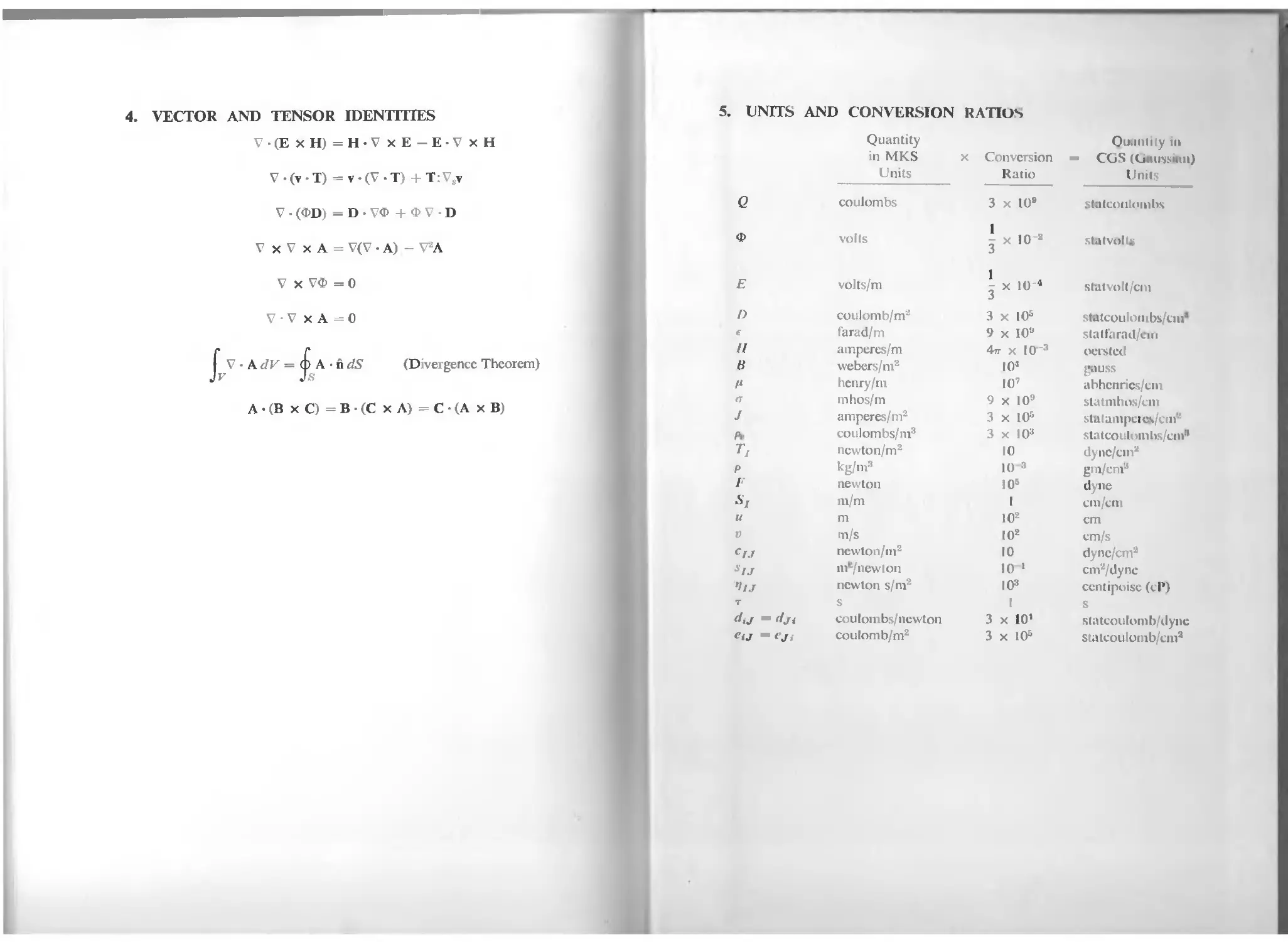
Starts from the field equations given in symbolic form on the front cover
papers, and applies the theory to a variety of acoustic boundary value
problems. The cover papers also list rectangular coordinate representations
of the field operators, transformation properties of the constitutive
parameters, and a number of useful identities. With this information on hand, the
experienced reader should be able to proceed without constantly referring
back to Volume T.
The simplest, and one of the most important, boundary value problems in
ttlectromagnetism and acoustics is the scattering of a uniform plane wave
incident upon a plane boundary between two different media. In the next
chapter it will be seen that many different waveguide configurations can be
analyzed by using solutions to this simple scattering problem. A brief
introduction to the subject was given in Chapter 4 of Volume I, which
considered the case of a wave incident normally on a plane boundary. This
chapter will deal with the more complicated case of oblique incidence.
2 REFLECTION AND REI RACTION
When a plane wave impinges on an interlace between two different media,
it is necessary that certain boundary conditions be satisfied at the interface.
Because these conditions cannot be satisfied by the incident wave alone, it is
necessary to include a certain number of reflected waves in the first medium
and transmitted waves in the second medium. If the incident wave travels
normal to the interface, the reflected and transmitted waves are also normal
to the interface; this was the case treated in Example 3 of Chapter 4. For an
obliquely incident wave the scattered waves travel in different directions. This
change in direction of the transmitted waves is called refraction The character
of the transmitted (or refracted) waves depends very strongly on the nature
of the second medium. When there is only one wave velocity for each
propagation direction (electromagnetic waves in an isotropic solid), there is only
one refracted wave direction. For electromagnetic waves in an anisotropic
solid and for acoustic waves in an isotropic solid, there may be two wave
velocities for each propagation direction and two refracted ware directions
may occur (birefringence). Acoustic waves in an anisotropic medium may
have three wave velocities for each propagation direction and three refracted
ware directions may occur (trirefringence).
In elcctromagnetism, propagation directions of the plane waves scattered
at a plane boundary are given by Snell's Law and the amplitudes of the
scattered waves are given by the Fresnel Equations. This chapter will develop
and examine corresponding relationships for acoustic wave scattering in
isotropic, anisotropic, and piezoelectric solids.
B. ISOTROPIC SOLIDS
B.l Snell's Law
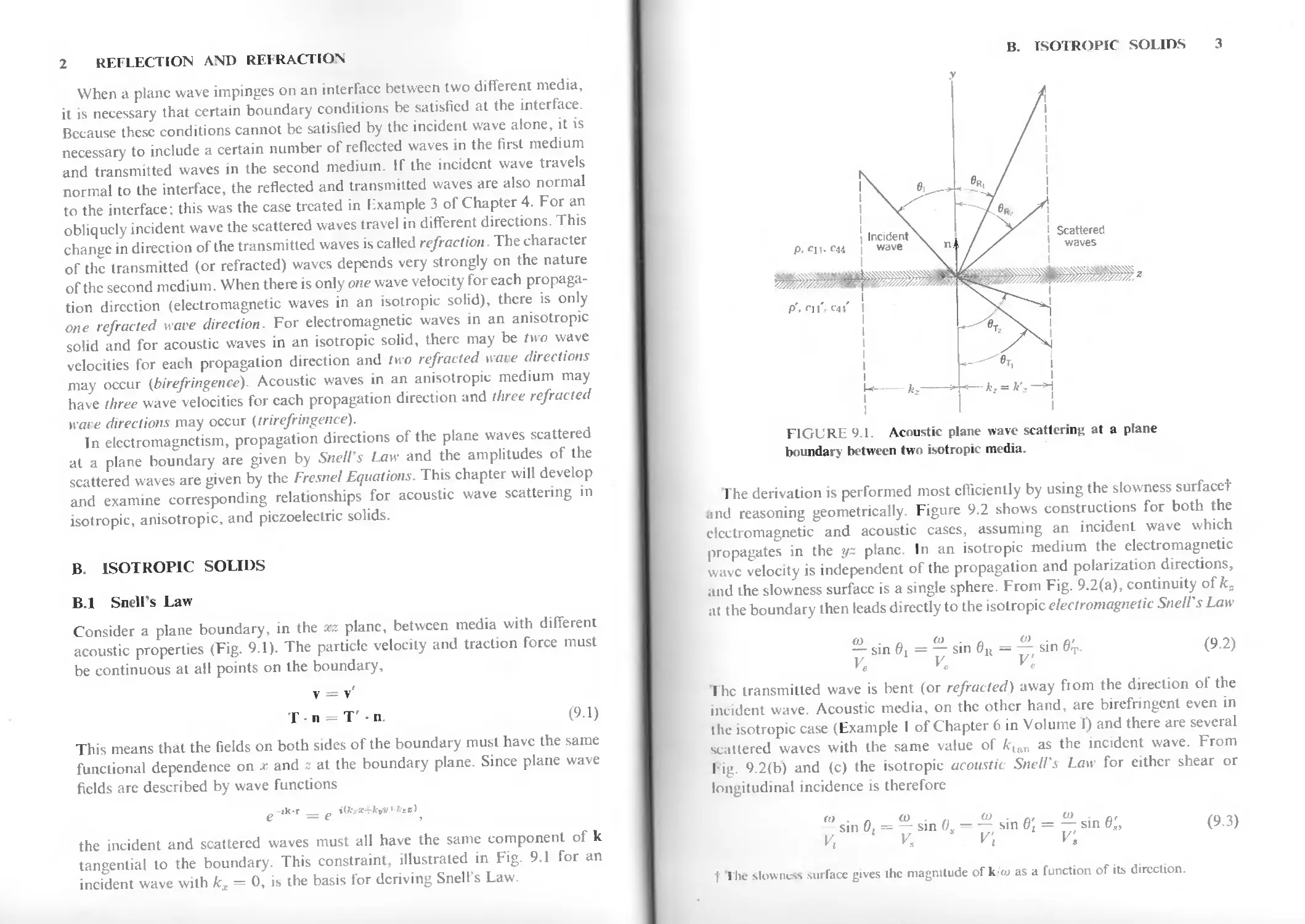
Consider a plane boundary, in the xz plane, between media with different
acoustic properties (Fig. 9.1). The particle velocity and traction force must
be continuous at all points on the boundary,
v = v'
T-n-T'-n. (9.1)
This means that the fields on both sides of the boundary must have the same
functional dependence on x and z at the boundary plane. Since plane wave
fields are described by wave functions
the incident and scattered waves must all have the same component of к
tangential to the boundary. This constraint, illustrated in Fig. 9.1 for an
incident wave with kx = 0, is the basis for deriving Snell's Law.
B. ISOTROPIC SOLIDS 3
FIGURE 9.1. Acoustic plane wave scattering at a plane
boundary between two isotropic media.
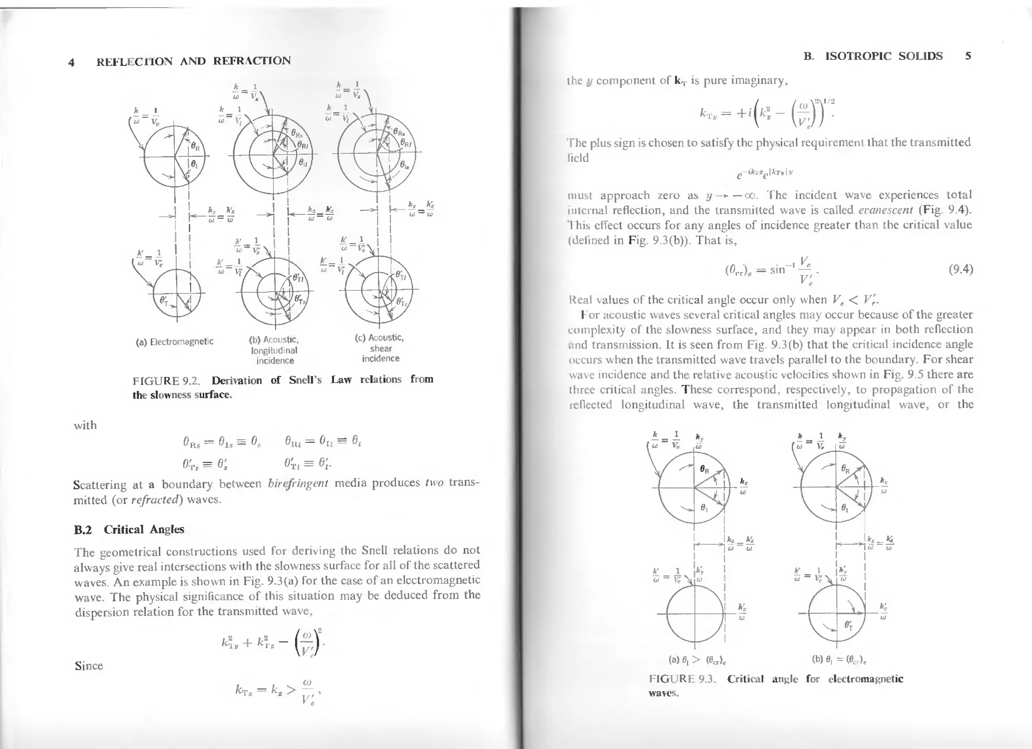
The derivation is performed most efficiently by using the slowness surfacet
and reasoning geometrically. Figure 9.2 shows constructions for both the
electromagnetic and acoustic cases, assuming an incident wave which
propagates in the yz plane. In an isotropic medium the electromagnetic
wave velocity is independent of the propagation and polarization directions,
and the slowness surface is a single sphere. From Fig. 9.2(a), continuity of k.
at the boundary then leads directly to the isotropic electromagnetic Snell's Law
ft) . fl CO . „ V) . c, ,,.
— sin 6, = — sin 6n = — sin GT. (9.2)
К v. Ve
The transmitted wave is bent (or refracted) away from the direction of the
incident wave. Acoustic media, on the other hand, are birefringent even in
the isotropic case (Example 1 of Chapter 6 in Volume I) and there are several
scattered waves with the same value of kUm as the incident wave. From
Fig. 9.2(b) and (c) the isotropic acoustic Snell's Law for either shear or
longitudinal incidence is therefore
sin 0, = — sin 0 — — sin 6, = — sin 6'„ (9.3)
t The slowness surface gives ihc magnitude of kw as a function of its direction.
(a) Electromagnetic <b) Acoustic, (с) Acoustic,
longitudinal shear
incidence incidence
FIGURE 9.2. Derivation of Snell's Law relations from
the slowness surface.
with
Or, = в1щ = os elu = on = et
o:es = e; o'Tl = e;.
Scattering at a boundary between birefringent media produces two
transmitted (or refracted) waves.
B.2 Critical Angles
The geometrical constructions used for deriving the Snell relations do not
always give real intersections with the slowness surface for all of the scattered
waves. An example is shown in Fig. 9.3(a) for the case of an electromagnetic
wave. The physical significance of this situation may be deduced from the
dispersion relation for the transmitted wave,
Since
fcrz = fc2 > 7^ .
B. ISOTROPIC SOLIDS 5
the у component of kT is pure imaginary,
The plus sign is chosen to satisfy the physical requirement that the transmitted
field
e—ikzze\kTv\v
must approach zero as у -> —со. The incident wave experiences total
internal reflection, and the transmitted wave is called evanescent (Fig. 9.4).
This effect occurs for any angles of incidence greater than the critical value
(defined in Fig. 9.3(b)). That is,
(0„). = sin-'^. (9.4)
Real values of the critical angle occur only when V, < V'f.
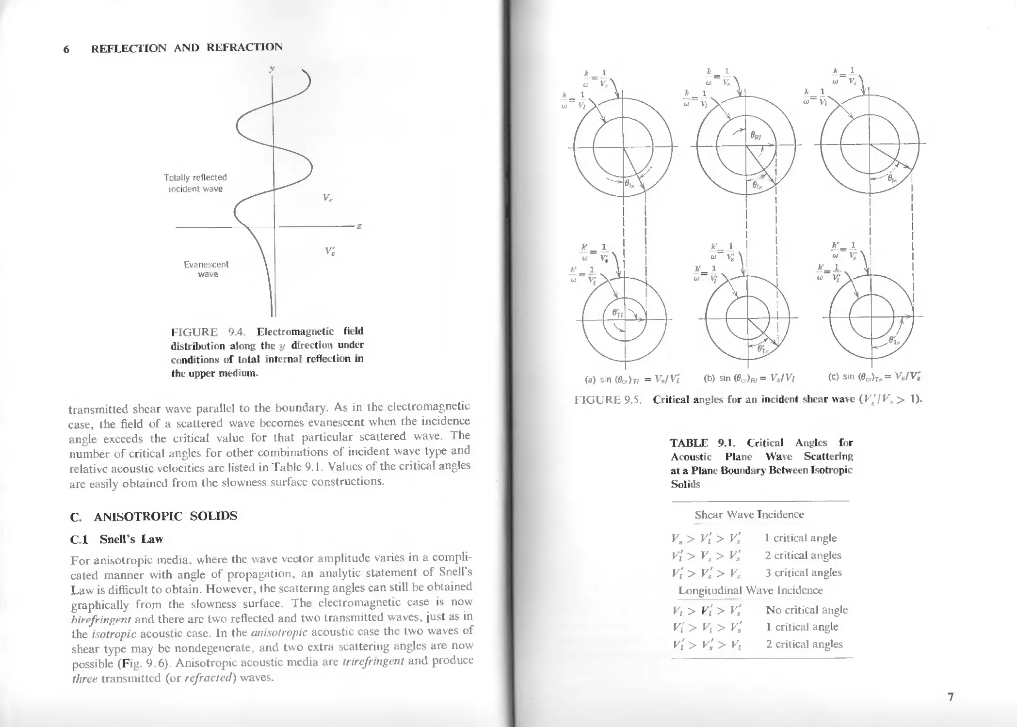
For acoustic waves several critical angles may occur because of the greater
complexity of the slowness surface, and they may appear in both reflection
and transmission. It is seen from Fig. 9.3(b) that the critical incidence angle
occurs when the transmitted wave travels parallel to the boundary. For shear
wave incidence and the relative acoustic velocities shown in Fig. 9.5 there are
three critical angles. These correspond, respectively, to propagation of the
reflected longitudinal wave, the transmitted longitudinal wave, or the
6 REFLECTION AND REFRACTION
у
Totally reflected
incident wave
vr
Evanescent \
wave \
FIGURE 9.4. Electromagnetic field
distribution along the у direction under
conditions of total internal reflection in
the upper medium.
transmitted shear wave parallel to the boundary. As in the electromagnetic
case, the field of a scattered wave becomes evanescent when the incidence
angle exceeds the critical value for that particular scattered wave. The
number of critical angles for other combinations of incident wave type and
relative acoustic velocities are listed in Table 9.1. Values of the critical angles
are easily obtained from the slowness surface constructions.
C. ANISOTROPIC SOLIDS
C.l Snell's Law
For anisotropic media, where the wave vector amplitude varies in a
complicated manner with angle of propagation, an analytic statement of Snell's
Law is difficult to obtain. However, the scattering angles can still be obtained
graphically from the slowness surface. The electromagnetic case is now
birefringpnt and there are two reflected and two transmitted waves, just as in
the isotropic acoustic case. In the anisotropic acoustic case the two waves of
shear type may be nondegenerate, and two extra scattering angles are now
possible (Fig. 9.6). Anisotropic acoustic media are trirefringent and produce
three transmitted (or refracted) waves.
(a) s n (ecr)T, = v„iVi (b) sin (ecr)R, = vsiv, (c) sm (e„)T„ = vs/v;
FIGURE 9.5. Critical angles for an incident shear wave (l^'/K, > 1).
TABLE 9.1. Critical Angles for
Acoustic Plane Wave Scattering
at a Plane Boundary Between Isotropic
Solids
Shear Wave Incidence
v» > v'i > v'a 1 critical angle
V'\ > К > К 2 critical angles
V[ > Vg > Vs 3 critical angles
Longitudinal Wave Incidence
V[ > V'i > Vg No critical angle
V{ > Vt> ys' 1 critical angle
V[ > Vs > Vj 2 critical angles
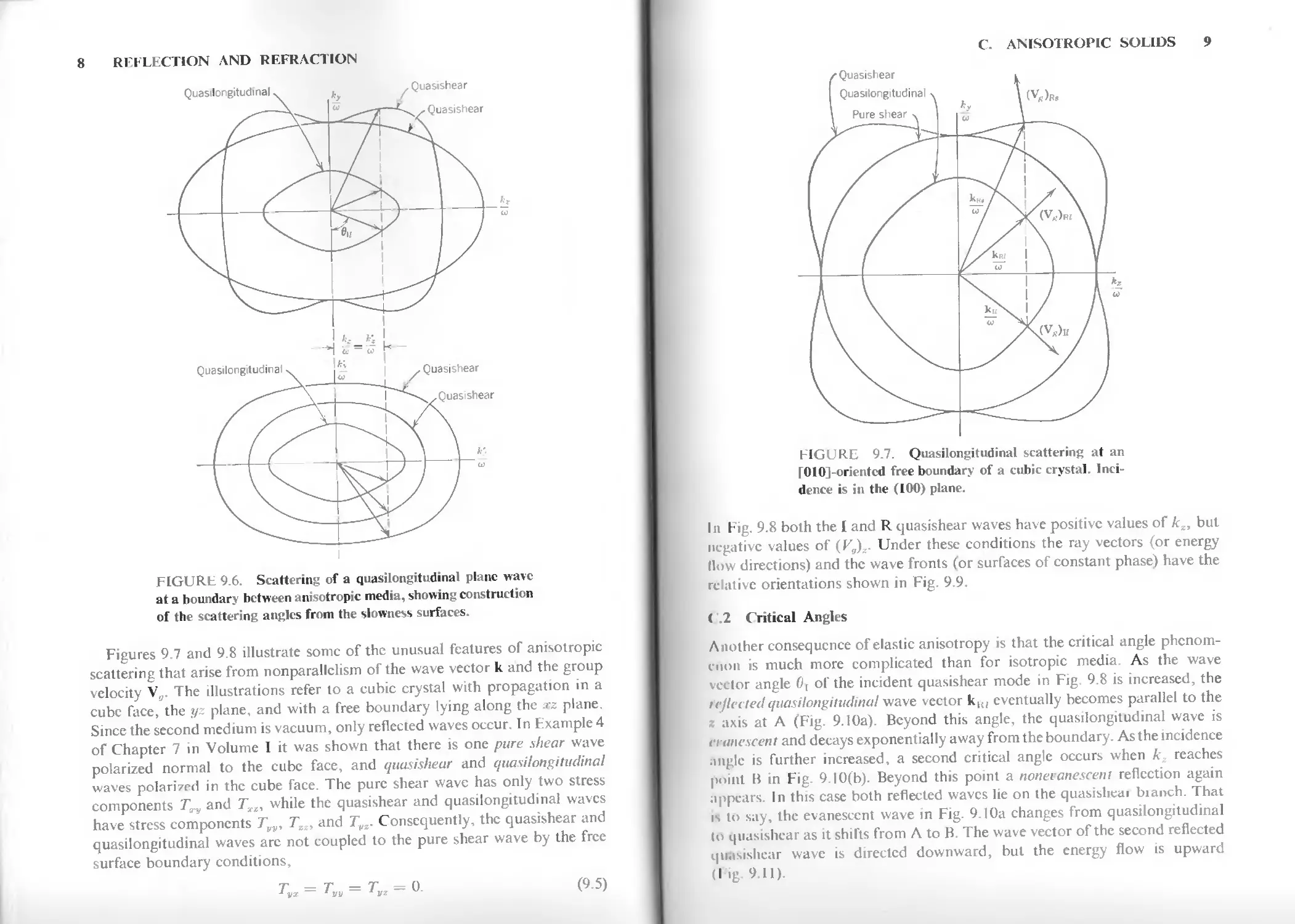
FIGURE 9.6. Scattering of a quasilongitudinal plane wave
at a boundary between anisotropic media, showing construction
of the scattering angles from the slowness surfaces.
Figures 9.7 and 9.8 illustrate some of the unusual features of anisotropic
scattering that arise from nonparallclism of the wave vector к and the group
velocity Vs. The illustrations refer to a cubic crystal with propagation in a
cube face, the yz plane, and with a free boundary lying along the rz plane.
Since the second medium is vacuum, only reflected waves occur. In Example 4
of Chapter 7 in Volume I it was shown that there is one pure shear wave
polarized normal to the cube face, and quasishear and quasilongitudinal
waves polarized in the cube face. The pure shear wave has only two stress
components TTy and Tx2, while the quasishear and quasilongitudinal waves
have stress components Tvv, Тгг, and Tvs. Consequently, the quasishear and
quasilongitudinal waves arc not coupled to the pure shear wave by the free
surface boundary conditions,
Tyx = Tvu = Туг = 0. (9.5)
С. ANISOTROPIC SOLIDS 9
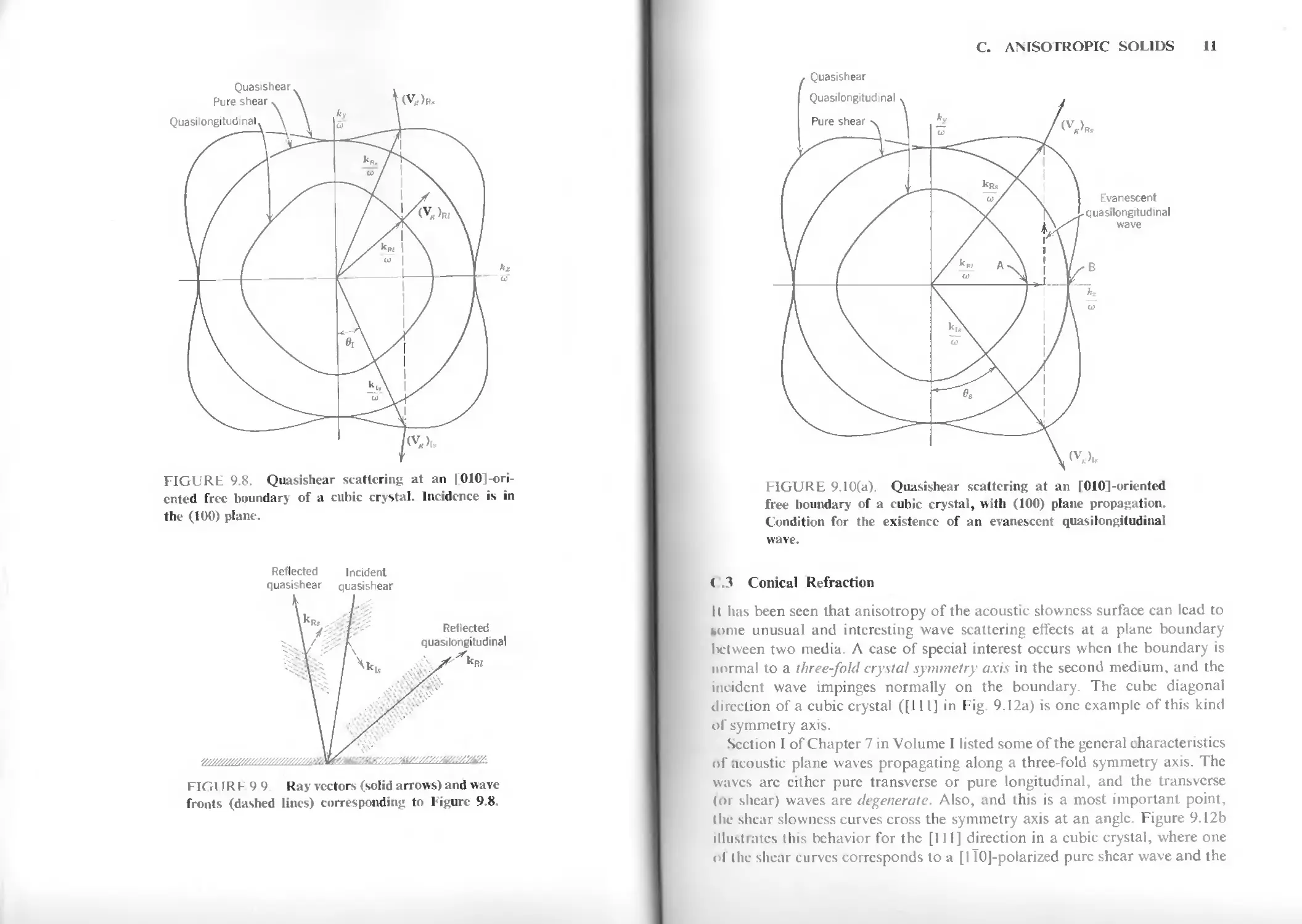
In Fig. 9.8 both the I and R quasishear waves have positive values of kx, but
negative values of (Vg),. Under these conditions the ray vectors (or energy
How directions) and the wave fronts (or surfaces of constant phase) have the
relative orientations shown in Fig. 9.9.
Г.2 Critical Angles
Another consequence of elastic anisotropy is that the critical angle
phenomenon is much more complicated than for isotropic media. As the wave
vector angle 0, of the incident quasishear mode in Fig 9.8 is increased, the
reflected quasilongitudinal wave vector kH, eventually becomes parallel to the
z axis at A (Fig. 9.10a). Beyond this angle, the quasilongitudinal wave is
vranescent and decays exponentially away from the boundary. As the incidence
angle is further increased, a second critical angle occurs when к reaches
point В in Fig. 9.10(b). Beyond this point a noneianescent reflection again
appears. In this case both reflected waves lie on the quasisheai bianch. That
is to say, the evanescent wave in Fig. 9.10a changes from quasilongitudinal
to quasishear as it shifts from A to B. The wave vector of the second reflected
quasishear wave is directed downward, but the energy flow is upward
(I l£ 9.11).
FIGURE 9.8. Quasishear scattering at an |010]-ori-
cnted free boundarj of a cubic crystal. Incidence is in
the (100) plane.
Reflected Incident
quasishear quasishear
FIG1Щ Ь 9 9 Ray vectors (solid arrows) and wave
fronts (dashed lines) corresponding to Figure 9.8.
C. ANISOTROPIC SOLIDS 11
FIGURE 9.10(a). Quasishear scattering at an Г010]-oriented
free boundary of a cubic crystal, with (100) plane propagation.
Condition for the existence of an evanescent quasilongitudinal
wave
( .3 Conical Refraction
К lias been seen that anisotropy of the acoustic slowness surface can lead to
some unusual and interesting wave scattering effects at a plane boundary
Ixrtween two media. Л case of special interest occurs when the boundary is
normal to a three-fold crystal symmetry axis in the second medium, and the
incident wave impinges normally on the boundary. The cube diagonal
direction of a cubic crystal ([111] in Fig. 9.12a) is one example of this kind
of symmetry axis.
Section I of Chapter 7 in Volume I listed some of the general characteristics
of acoustic plane waves propagating along a three-fold symmetry axis. The
waves arc cither pure transverse or pure longitudinal, and the transverse
(or shear) waves are degenerate. Also, and this is a most important point,
(lie shear slowness curves cross the symmetry axis at an angle. Figure 9.12b
illustrates this behavior for the [111] direction in a cubic crystal, where one
i>l llic shear curves corresponds to a [I T0]-polarized pure shear wave and the
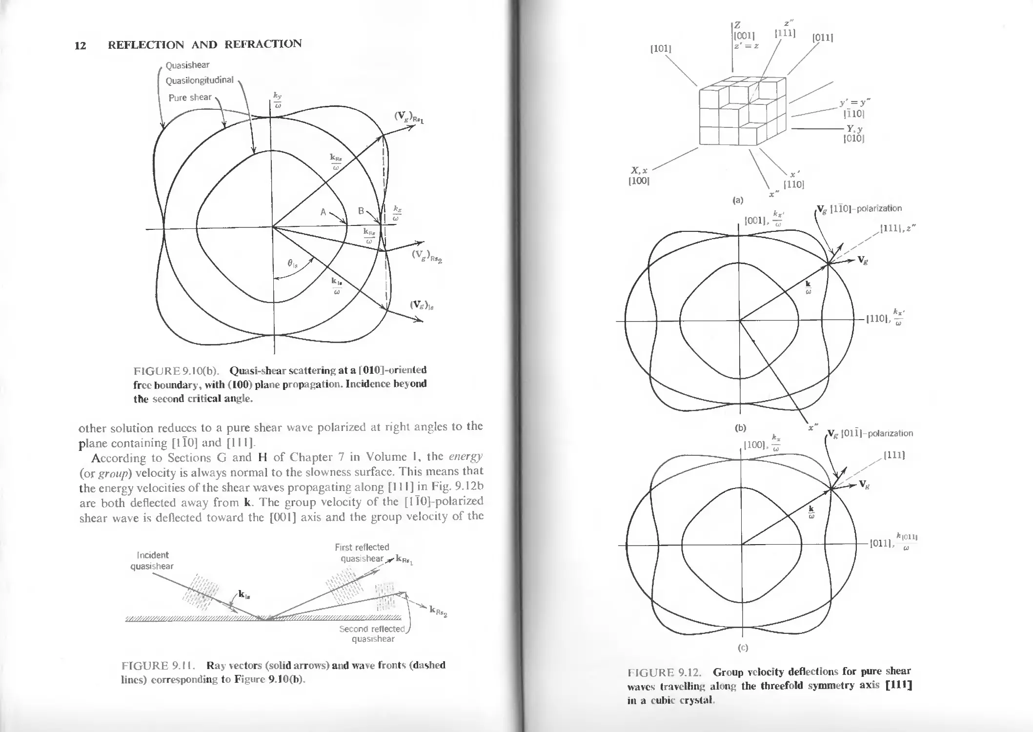
12 REFLECTION AND REFRACTION
FIGCJ R E 9.10(b). Quasi-shear scattering at a 1010]-oriented
free boundary, with (100) plane propagation. Incidence beyond
the second critical angle.
other solution reduces to a pure shear wave polarized at right angles to the
plane containing [HO] and [111].
According to Sections G and H of Chapter 7 in Volume I, the energy
(or group) velocity is always normal to the slowness surface. This means that
the energy velocities of the shear waves propagating along [111 ] in Fig. 9.12b
are both deflected away from k. The group velocity of the [lT0]-polarized
shear wave is deflected toward the [001] axis and the group velocity of the
First reflected
quasishear
FIGURE 9.11. Ray vectors (solid arrows) and wave fronts (dashed
lines) corresponding to Figure 9.10(b).
(c)
riGURH 9.12. Group velocity deflections for pure shear
waves travelling along the threefold symmetry axis [111]
in a cubic crystal
14
REFLECTION AND REFRACTION
other shear wave is deflected toward the [ПО] axis. There are, however,
still further complications. Figure 9.12b represents slowness curves for waves
propagating in the plane defined by the [110] and [0011 crystal directions,
but it is clear from the cubic symmetry of the crystal that identical curves
will be obtained for propagation in any plane that passes through a cube edge
and a cube face diagonal. Slowness curves for the plane passing through
[100] and [011] therefore appear as shown in Fig. 9.12c. The shear waves
propagating along [111] now have different polarizations than those given
in Fig. 9.12b. In itself, there is nothing unusual about this; degenerate shear
waves can always be combined to produce arbitrary polarization directions.
The unusual feature of the present situation is that the group velocity directions
are also different than they were in Fig. 9.12b. For the [Oil]-polarized pure
shear wave in Fig. 9.12c the group velocity is deflected toward [100] and the
other shear wave is deflected toward [011 ]. Slowness curves for the plane
passing through [010] and [101] also have the same shape as in Fig. 9.12b
and c, giving two additional polarization and energy velocity directions for
the pure shear waves traveling along [111]. This kind of behavior always
occurs when shear waves propagate along a three-fold crystal symmetry
axis. The detailed behavior of the waves is best illustrated by finding wave
solutions for a specific example and then calculating the power density
(or Poynting) vector P given by ID on the front cover papers.
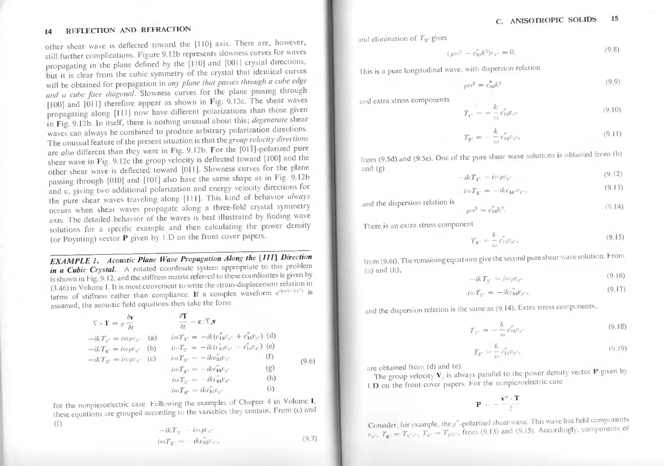
EXAMPLE 1. Acoustic Plane Wave Propagation Along the U1T] Direction
in a Cubic Crystal. A rotated coordinate system appropriate to this problem
is shown in Fig. 9.12, and the stiffness matrix referred to these coordinates is given by
(3.46) in Volume Г. It is most convenient to write the strain-displacement relation in
terms of stiffness rather than compliance. If a complex waveform e*<wt-'«"> is
assumed, the acoustic field equations then take the form
ev
T
V • г
— n
= с: Vsv
9 dt
dt
-;7сГ5.
= iwpiv
(a)
/га T"i-
= -ik{c"3vz.
+ c«tv) (d)
-'7c TV
= iWpVy.
(b)
1(0 7Л-
= —ik(c'[3vz.
- см»*») (e)
-,7c TT
= iwpvz~
(c)
|"«)Г3-
= —ikc33vz-
(f)
/ш Г4-
= —ikctiv.y~
сто
=
(h)
iwTB.
= ikc"svv~
(i)
(9.6)
for the nonpiezoelectric case. Following the examples of Chapter 4 in Volume I,
these equations are grouped according to the variables they contain. From (c) and
(f)
—ikT3~ io)pvt~
iioTr = ikc'3iv,~, (9.7)
C. ANISOTROPIC SOLIDS 15
and elimination of 7"3- gives
<pw* - c33k-)uz- = 0. (9.8)
This is a pure longitudinal wave, with dispersion relation
pc,,2 = c^fc2 (9.9)
and extra stress components
7> = - - fa, <9-10>
со
Гг = (9.11)
from (9.5d) and (9.5e). One of the pure shear wave solutions is obtained from (b)
and (g)
-ikTr = itopvr (9.12)
,7„Г4. = -ikcu-vr, (9.13)
and the dispersion relatio is
p<»2 = cl№. (9.H)
There is an extra stress component
7V = -r;5<y, (9.15)
to
from (9.6i). The remaining equations give the second pure shear wave solution. From
(a) and (h),
-ikTs- = /oiptv (9.16)
иоТъ. = -/ArrlW, (9.17)
and the dispersion relation is the same as (9.14). Extra stress components,
ю
to
are obtained from (d) and (e).
The group velocity Vs is always parallel to the power density vector P given by
I .D on the front cover papers. For the nonpiezoelectric case
v* - T
P
Consider, for example, the //"-polarized shear wave. This wave has field components
,v, Tt. = 7>.-, 7V = Tu.r., from (9.13) and (9.15). Accordingly, components of
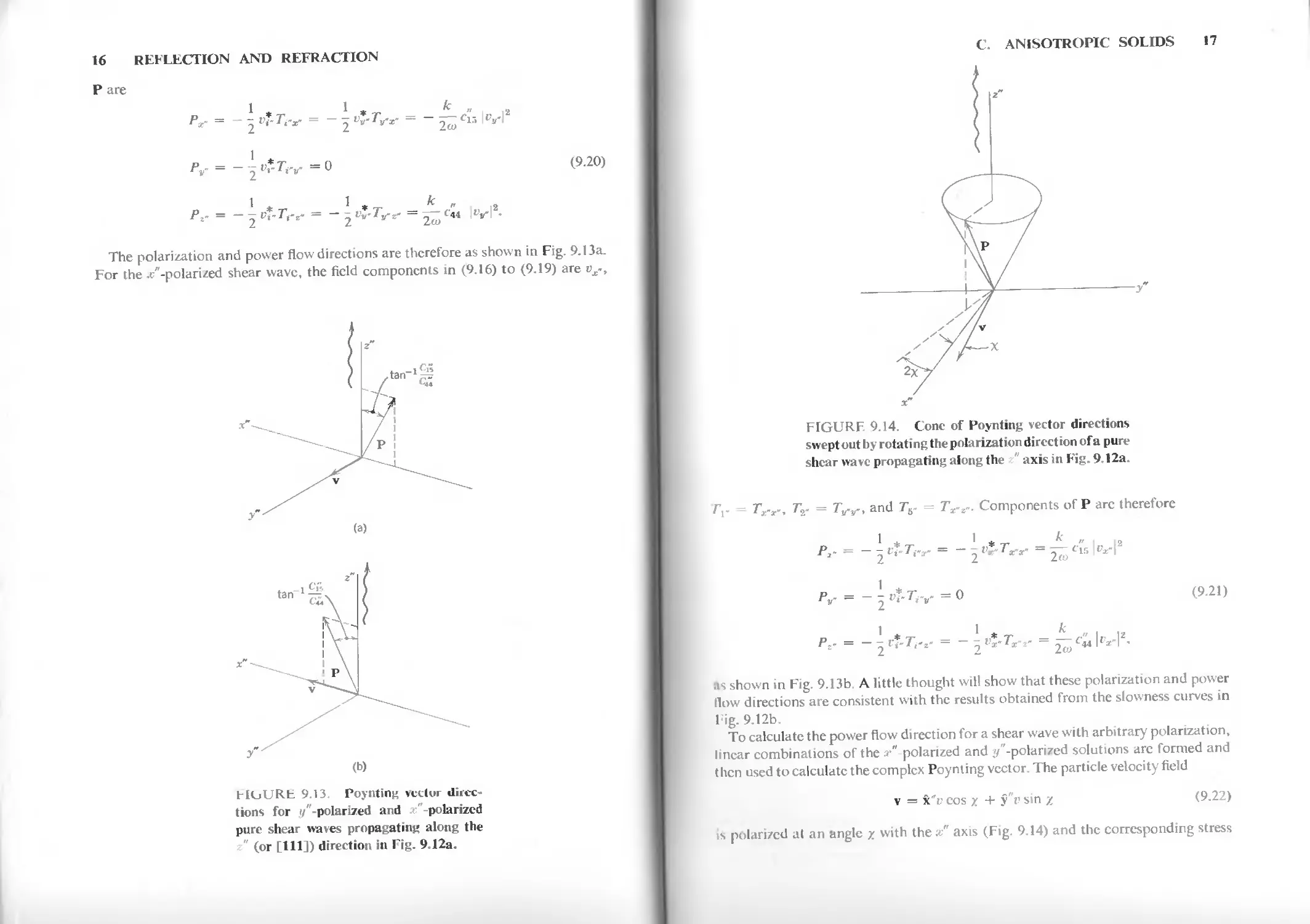
16 REFLECTION AND REFRACTION
(b)
HLiURt 9.13. Poynting vector
directions for (/"-polarized and "-polarized
pure shear waves propagating along the
" (or [111]) direction in Fig. 9.12a.
C. ANISOTROPIC SOLIDS 17
x"
FIGURE 9.14. Cone of Poynting vector directions
swept out by rotating the polarization direction of a pure
shear wave propagating along the " axis in Fig. 9.12a.
Tr = Tr-X., Г2. = Try, and Г5- = Tx.z-. Components оГР arc therefore
О ' * T ' * T ^ " 12
= — ~ Vi~l i~y — — - IV ' Х~У — Cl!i I I
Pv- = - \ vt-Trr = 0 (9.21)
1 1 к
as shown in Fig. 9.13b. A little thought will show that these polarization and power
llow directions are consistent with the results obtained from the slowness curves in
Fig. 9.12b.
To calculate the power flow direction for a shear wave with arbitrary polarization,
linear combinations of the .r" polarized and .'/"-polarized solutions arc formed and
then used to calculate the complex Poynting vector. The particle velocity field
v = x"v cos x + S"v sin x (9.22)
is polarized a( an angle x with the x" axis (Fig. 9.14) and the corresponding stress
Pare
/"»- =~2"*W=0 (9.20)
Pz- = — — Г?-Г,-г- = — - IV J"^г- = — C« |ty]2.
The polarization and power flow directions are therefore as shown in Fig. 9.13a.
For the ж"-polarized shear wave, the field components in (9.16) to (9.19) are vx~,
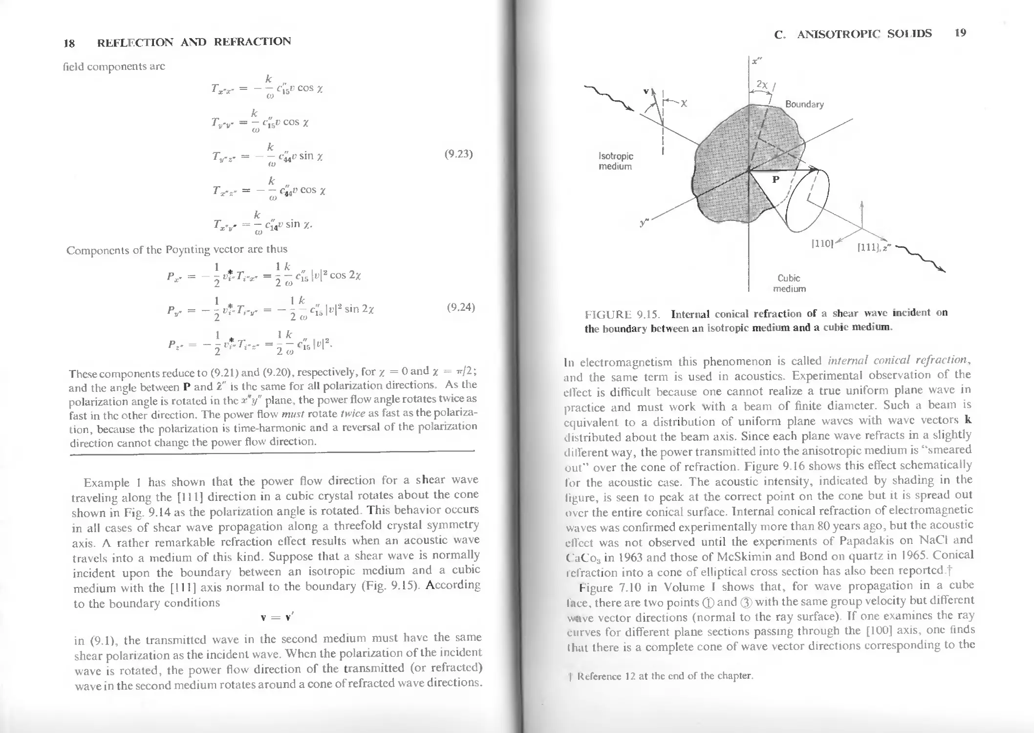
18 REFLECTION AND REFRACTION
field components arc
к
Tx-X- = - - cKv cos x
Ty-y = ^ c'^v cos x
к
Ту-г,- = t£p sin z (9-23)
A:
7VS- = - - c^e cos *
A:
7>„. = - c'^v sin z.
Components of the Poynting vector are thus
P*- = - \ uf~Ti-x- = j - c^, № cos 2*
*V- = - J «£■ *Vv = - i ~ c"& \tf sin 2* (9.24)
1 4 I At
L L Oi
These components reduce to (9.21) and (9.20), respectively, for z = 0andz = W2;
and the angle between P and i" is the same for all polarization directions As the
polarization angle is rotated in the ж y" plane, the power flow angle rotates twice as
fast in the other direction. The power flow must rotate twice as fast as the
polarization, because the polarization is time-harmonic and a reversal of the polarization
direction cannot change the power flow direction.
Example 1 has shown that the power flow direction for a shear wave
traveling along the [111] direction in a cubic crystal rotates about the cone
shown in Fig. 9.14 as the polarization angle is rotated. This behavior occurs
in all cases of shear wave propagation along a threefold crystal symmetry
axis. Л rather remarkable refraction effect results when an acoustic wave
travels into a medium of this kind. Suppose that a shear wave is normally
incident upon the boundary between an isotropic medium and a cubic
medium with the [111] axis normal to the boundary (Fig. 9.15). According
to the boundary conditions
r
\ — \
in (9.1), the transmitted wave in the second medium must have the same
shear polarization as the incident wave. When the polarization of the incident
wave is rotated, the power flow direction of the transmitted (or refracted)
wave in the second medium rotates around a cone of refracted wave direction .
C. ANISOTROPIC SOI IDS 19
Cubic
medium
FIGURE 9.15. Internal conical refraction of a shear wave incident on
the boundary between an isotropic medium and a cubic medium.
In electromagnetism this phenomenon is called internal conical refraction,
and the same term is used in acoustics. Experimental observation of the
effect is difficult because one cannot realize a true uniform plane wave in
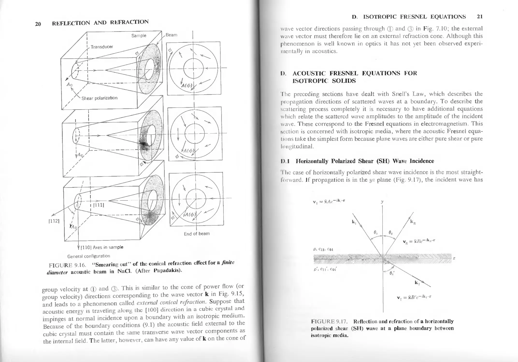
practice and must work with a beam of finite diameter. Such a beam is
equivalent to a distribution of uniform plane waves with wave vectors к
distributed about the beam axis. Since each plane wave refracts in a slightly
different way, the power transmitted into the anisotropic medium is "smeared
out" over the cone of refraction. Figure 9.16 shows this effect schematically
for the acoustic case. The acoustic intensity, indicated by shading in the
figure, is seen to peak at the correct point on the cone but it is spread out
over the entire conical surface. Internal conical refraction of electromagnetic
waves was confirmed experimentally more than 80 years ago, but the acoustic
effect was not observed until the experiments of Papadakis on NaCI and
CaCo3 in 1963 and those of McSkimin and Bond on quartz in 1965. Conical
refraction into a cone of elliptical cross section has also been reportcd.f
Figure 7.10 in Volume T shows that, for wave propagation in a cube
Bice, there are two points ф and ® with the same group velocity but different
wave vector directions (normal to the ray surface). Tf one examines the ray
curves for different plane sections passing through the [100] axis, one finds
that there is a complete cone of wave vector directions corresponding to the
I Reference 12 at the end of the chapter.
20 REFLECTION AND REFRACTION
"[110] Axes in sample
General configuration
FIGURE 9 16 "Smearing out" of the conical refraction effect for a finite
diameter acoustic beam in NaCl. (After Papadakis).
group velocity at ф and Q). This is similar to the cone of power flow (or
group velocity) directions corresponding to the wave vector к in Fig. 9.15,
and leads to a phenomenon called external conical refraction. Suppose that
acoustic energy is traveling along the [100] direction in a cubic crystal and
impinges at normal incidence upon a boundary with an isotropic medium.
Because of the boundary conditions (9.1) the acoustic field external to the
cubic crystal must contain the same transverse wave vector components as
the internal field. The latter, however, can have any value of к on the cone of
D. ISOTROPIC FRESNEL EQUATIONS 21
wave vector directions passing through ф and ® in Fig. 7.10; the external
wave vector must therefore lie on an external refraction cone. Although this
phenomenon is well known in optics it has not yet been observed
experimentally in acoustics.
D. ACOUSTIC FRESNEL EQUATIONS FOR
ISOTROPIC SOLIDS
The preceding sections have dealt with Snell's Law, which describes the
propagation directions of scattered waves at a boundary. To describe the
scattering process completely it is necessary to have additional equations
which relate the scattered wave amplitudes to the amplitude of the incident
wave. These correspond to the Fresnel equations in electromagnetism. This
bection is concerned with isotropic media, where the acoustic Fresnel
equations take the simplest form because plane waves are either pure shear or pure
longitudinal.
I) I Horizontally Polarized Shear (SH) Wave Incidence
The case of horizontally polarized shear wave incidence is the most
straightforward. If propagation is in the yz plane (Fig. 9.17), the incident wave has
v, = xAe ik "г у
vT =xB'e~ik>t
RGU RE 9.17. Reflection and refraction of a horizontally
polarized shear (SH) wave at a plane boundary between
isotropic media.
22 REFLECTION AND REFRACTION
acoustic field components
( )г = £44 = _ (Mi Си/4в-*х- (9.25)
,„ . _ c« 5(^)r _ (Ui --an
ко су (о
The boundary conditions (9.1) can therefore be satisfied by reflected and
transmitted waves of the same polarization; that is,
(9.26)
(9.27)
(».)„ = Be**'
(От = B-e^1.
According to Snelfs Law the scattering angles are such that
(A)i = (к,)и = (Kh = fc,;
and the boundary equations at у = 0 are therefore
A + B= B'
- ^4((AM - = ~ - W
o> «)
where the common exponential e lk*z has been dropped. These equations are
solved directly for the reflection coefficient Ts and the transmission coefficient
Г'
p __ * _ z»cos e» ~~ Z*cos e» (9 98)
s ~ a ~ zs cos os + z; cos 0;
p, _ 6^ _ 2Z,cos 0, (0 29)
* a zs cos es + z; cos 0;
where Zs = (pc«)"2 and Zs' = (p'cU)1* are the characteristic shear wave
impedances for the upper and lower media. The angle of incidence 6S and the
angle of transmission 6's must satisfy the condition
si" 0, = К (9 30)
sin 0's V'/
from bneirs Law.
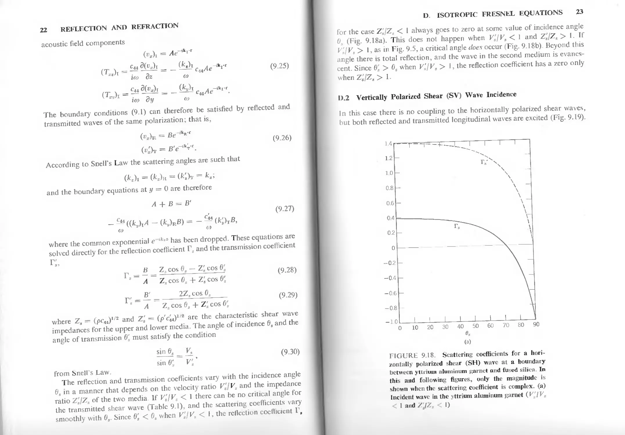
The reflection and transmission coefficients vary with the incidence angle
6S in a manner that depends on the velocity ratio V'JVS and the impedance
ratio Z'JZS of the two media. If Ks'/F6 < 1 there can be no critical angle for
the transmitted shear wave (Table 9.1), and the scattering coefficients vary
smoothly with 0S. Since B't < 0S when Ks'/Ks < I, the reflection coefficient Г,
D ISOTROPIC FRESNEL EQUATIONS 23
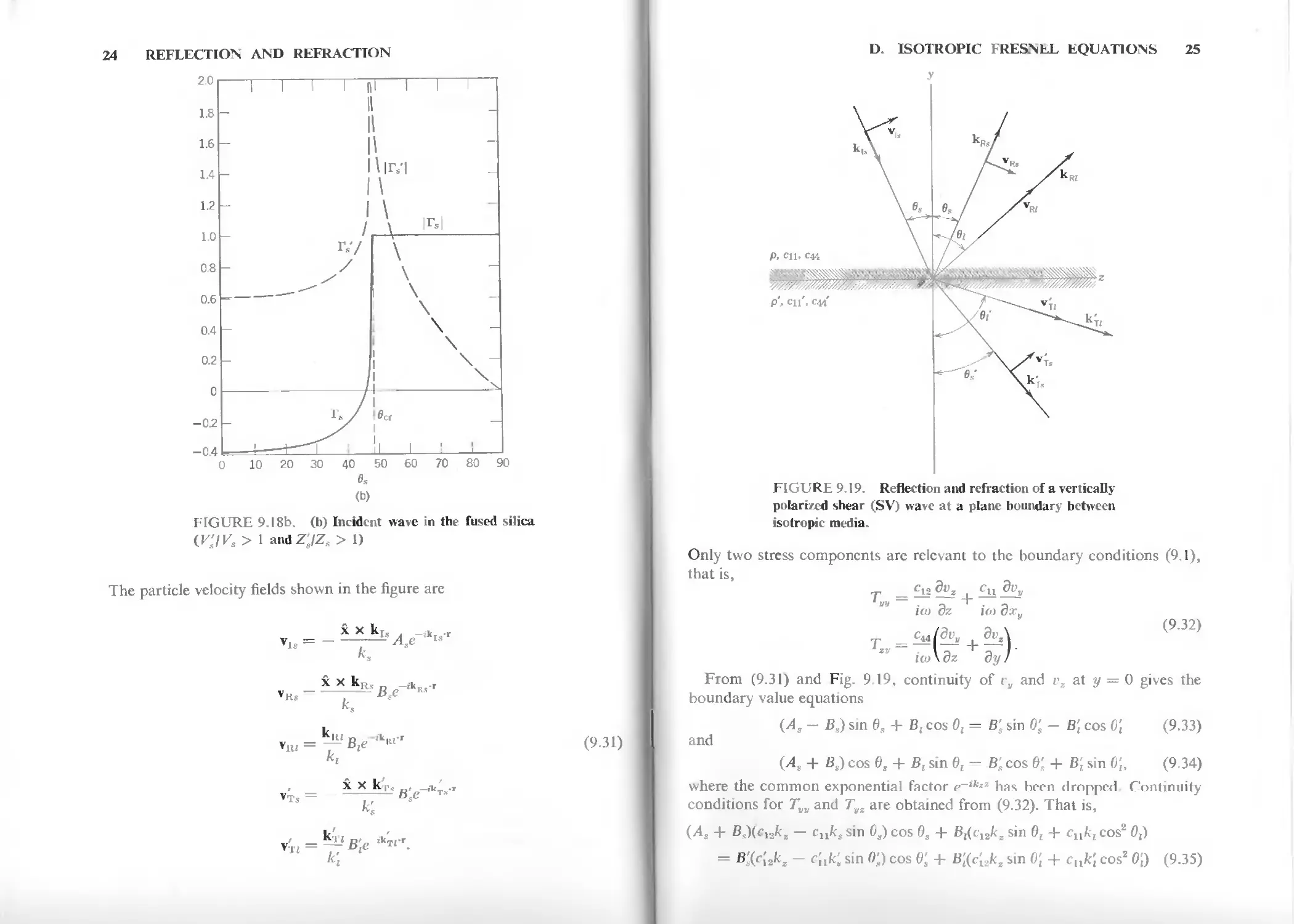
for the case Z'sjZa < 1 always goes to zero at some value of incidence angle
0S (Fig. 9.18a). This does not happen when V'JVS < 1 and Z'JZ, > I. Tf
V'JVS > 1, as in Fig. 9.5, a critical angle does occur (Fig. 9.18b). Beyond this
angle there is total reflection, and the wave in the second medium is
evanescent. Since 6's > 0S when V'sjVs > I, the reflection coefficient has a zero only
when z;/Zs > I.
D.2 Vertically Polarized Shear (SV) Wave Incidence
In this case there is no coupling to the horizontally polarized shear waves,
but both reflected and transmitted longitudinal waves are excited (Fig. 9.19).
0 10 20 30 40 50 60 70 80 90
es
(a)
FIGURE 9.18. Scattering coefficients for a
horizontally polarized shear (SH) wave at a boundary
between yttrium aluminum garnet and fused silica. In
this and following figures, only the magnitude is
shown when the scattering coefficient is complex, (a)
Incident wave in the yttrium aluminum garnet (F,'/Fs
< 1 and Z'JZ, < I)
24 REFLECTION AND REFRACTION
0 10 20 30 40 50 60 70 80 90
<b)
FIGURE 9.18b. (b) Incident wave in the fused silica
<V'JVS > 1 andZ'JZ, > 1)
The particle velocity fields shown in the figure arc
v,, = -
X X k'* л _-Лт«-г
vT5 = —— ese
(9.31)
D. ISOTROPIC FRESNEL EQUATIONS 25
(9.32)
FIGURE 9.19. Reflection and refraction of a vertically
polarized shear (SV) wave at a plane boundary between
isotropic media.
Only two stress components arc relevant to the boundary conditions (9.1),
that is,
_ c12 дюг cu dvv
UO OZ Ш cxv
iw\cz Су I
From (9.31) and Fig. 9.19, continuity of r„ and vz at у = 0 gives the
boundary value equations
(A - в,) sm e, + в, cos o, = e; sin о- - e; cos 0; (9.зз)
and
(/Is + Bs) cos 0, + Вг sin 0г - В.; cos 0; + В; sin 0;, (9.34)
where the common exponential factor p-'fc*z has boon dropped Continuity
conditions for ГЬК and Tv. are obtained from (9.32). That is,
(As + BsXcKks — clYks sin 0S) cos 6S + B,(c12/cz sin 0, + СцЛ^сов* 0,)
= В'£с[2кг - с;,k; sin 0.;) cos 0; + BKsfc, sin 0; + cnk't cos2 0;) (9.35)
у
26 REFLECTION AND REFRACTION
given in Section 6.B of Volume 1, and Snelfs Law,
k, = ks sin 0„ = k; sin 6's = fc, sin 0[ = kj sin 0;,
where
k, = — , etc.
It is also convenient to use the relation
Л + 2/j. cos2 0j = (Я + 2^) cos 20s,
derived from Snell's Law and
И = >* + 2И
These substitutions lead to the set of scattering equations
As sin 0S = -B, cos 0, - B/cos 0,' + S5 sin 0S + Bs' sin 0; (a)
/4S cos 0S -= —B, sin 0, + Bt' sin 0г' - fls cos 0S + B's cos 0^ (b)
T ■
-AgfjLk.sm 20, - -BIX + 2//>fctcos20s + ВЦЛ' + 2(j.')k\cos20^
+ B^ks sin 20s - B's(i'k's sin 20; (c)
-Astxkscos 20s = -B^k,sin 20t - B'^'k\ sin 20[
- Bsfiks cos 20s - B>% cos 20^. (d)
(9.37)
D. ISOTROPIC TRESNLL EQUATIONS 27
From (9.37) the reflection and transmission coefficients are
1 Is
A,
Д
1 Is
л
Д
r>
_
_ AJL*
Д
Г'
B's
~ A*
Д'
~ Д
(9.38)
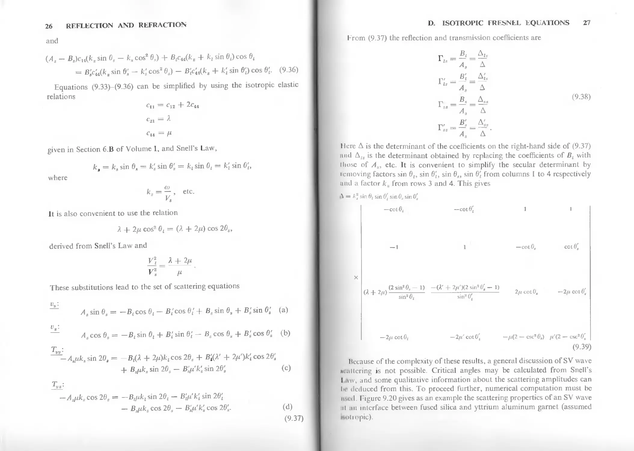
Here Д is the determinant of the coefficients on the right-hand side of (9.37)
iintl Д,8 is the determinant obtained by replacing the coefficients of BL with
those of As, etc. It is convenient to simplify the secular determinant by
iciiioving factors sin 0г, sin 0J, sin 0„ sin Q\ from columns I to 4 respectively
and a factor kz from rows 3 and 4. This gives
Л — к* sin 0, sin 0\ sin0S sin 0\
—col©( —cotfl] 1 1
—cotO, co\.6't
(2 sin2 0,-1) —(A' + 2/,')(2 sin2 (»; - I)
W + 2/() — -—j 2« Lot 0, -2ft col 6,
sin20, sinHlt
—2ft col 0, — 2fi cot 0'( —/j(2 — esc2 б,) fi'(2 — esc2 0\
(9.39)
Because of the complexity of these results, a general discussion of SV wave
maltering is not possible. Critical angles may be calculated from Snell's
Law, and some qualitative information about the scattering amplitudes can
hi4 deduced from this. To proceed further, numerical computation must be
пмч1. Figure 9.20 gives as an example the scattering properties of an SV wave
11I 1111 interface between fused silica and yttrium aluminum garnet (assumed
яи)1м)р1с)
and
(Л, - Bs)cH(kz sin 0e - fc, cos2 в,) + бгс44(кг + к, sin 0,) cos 0,
= Вуи(кя sin 6; - К cos2 0S) - B'lC'^kz + k\ sin 6\) cos 0|. (9.36)
Equations (9.33)-(9.36) can be simplified by using the isotropic elastic
relations
cn — c\2 + 2c41
с.,, = A
28 REFLECTION AND REFRACTION
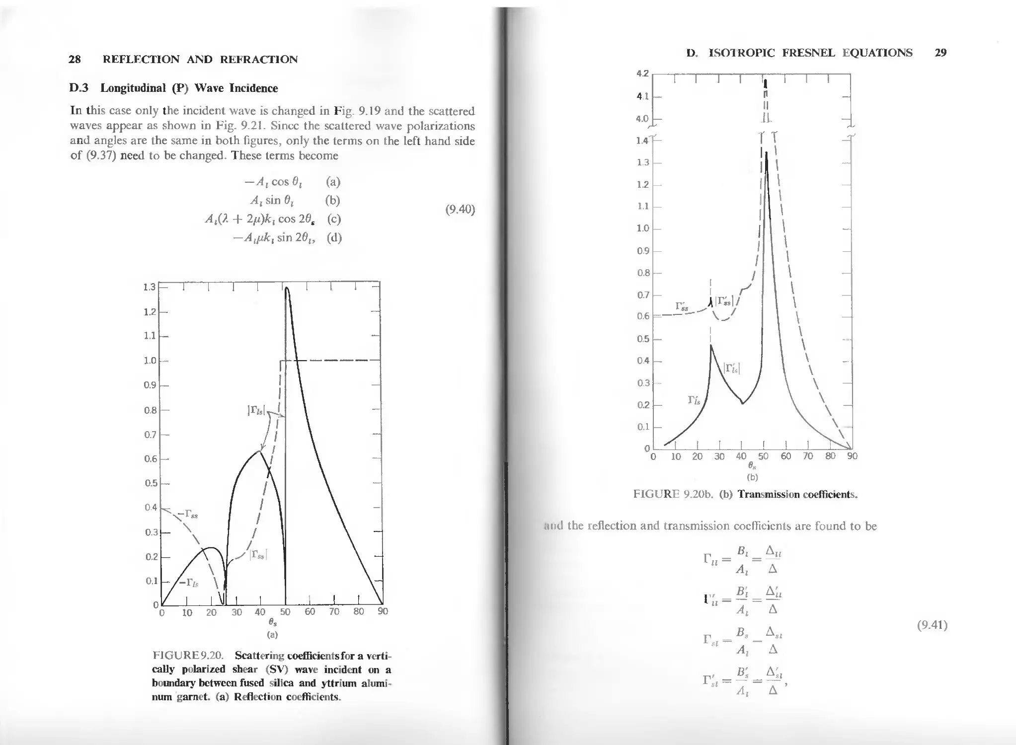
D.3 Longitudinal (P) Wave Incidence
In this case only the incident wave is changed in Fig. 9.19 and the scattered
waves appear as shown in Fig. 9.21. Since the scattered wave polarizations
and angles are the same in both figures, only the terms on the left hand side
of (9.37) need to be changed. These terms become
-AfCosdf (a)
A, sin 0, (b)
(9.40)
AS). + 2ц)к, cos 20, (c)
—Affik, sin 20{, (d)
(a)
Fl GU RE 9.20. Scattering coefficients for a
vertically polarized shear (SV) wave incident on a
boundary between fused silica and yttrium
aluminum garnet, (a) Reflection coefficients.
D. ISOTROPIC FRESNEL EQUATIONS 29
0 10 20 30 40 50 60 70 80 90
(b)
FIGURE 9.20b. (b) Transmission coefficients.
liud the reflection and transmission coefficients are found to be
A,
д
_Д[-
A
д
Bs
д..
Аг
д
E*
_Д1.
Аг
д
(9.41)
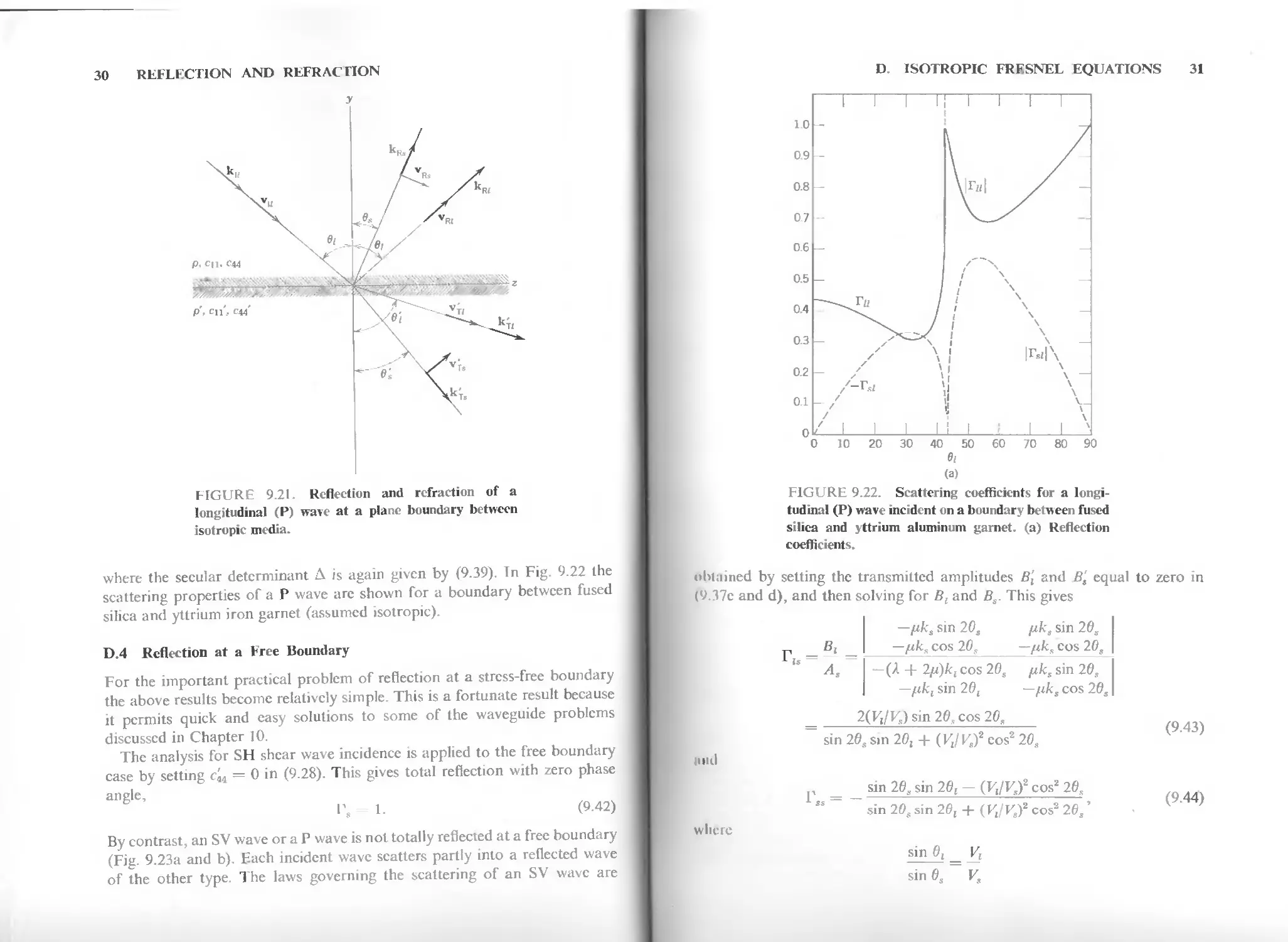
30 REFLECTION AND REFRACTION
у
FIGURE 9.21. Reflection and refraction of a
longitudinal (P) wave at a plane boundary between
isotropic media.
where the secular determinant Д is again given by (9.39). In Fig. 9.22 the
scattering properties of a P wave are shown for a boundary between fused
silica and yttrium iron garnet (assumed isotropic).
D.4 Reflection at a Free Boundary
For the important practical problem of reflection at a stress-free boundary
the above results become relatively simple. This is a fortunate result because
it permits quick and easy solutions to some of the waveguide problems
discussed in Chapter 10.
The analysis for SH shear wave incidence is applied to the free boundary
case by setting c'u = 0 in (9.28). This gives total reflection with zero phase
angle,
\\ 1. (9.42)
By contrast, an SV wave or a P wave is not totally reflected at a free boundary
(Fig. 9.23a and b). Each incident wave scatters partly into a reflected wave
of the other type. The laws governing the scattering of an SV wave are
D. ISOTROPIC FRESNEL EQUATIONS 31
10 20 30 40 50 60 70 80 90
в,
(a)
FIGURE 9.22. Scattering coefficients for a
longitudinal (P) wave incident on a boundary between fused
silica and yttrium aluminum garnet, (a) Reflection
coefficients.
obtained by setting the transmitted amplitudes B't and B's equal to zero in
(9.37c and d), and then solving for B{ and Bs. This gives
Г = ' -
'S A
—pks sin 20, [iks sin 20,
—/гк, cos 20, — /гк,. cos 20,
-(Л + 2[i)kl cos 20, [iks sin 20,
—fikt sin 20, — fiks cos 20,
i ml
where
2(VJVS) sin 20, cos 20,
sin 20, sin 20, + (VjVf cos2 20,
sin 20, sin 20, - (F,/F,)2 cos2 20,
Г.. = -
sin 20, sin 20, + (VJV,)* cos2 20,
sin 0, _ Vi
sin 0, ~ V,
(9.43)
(9.44)
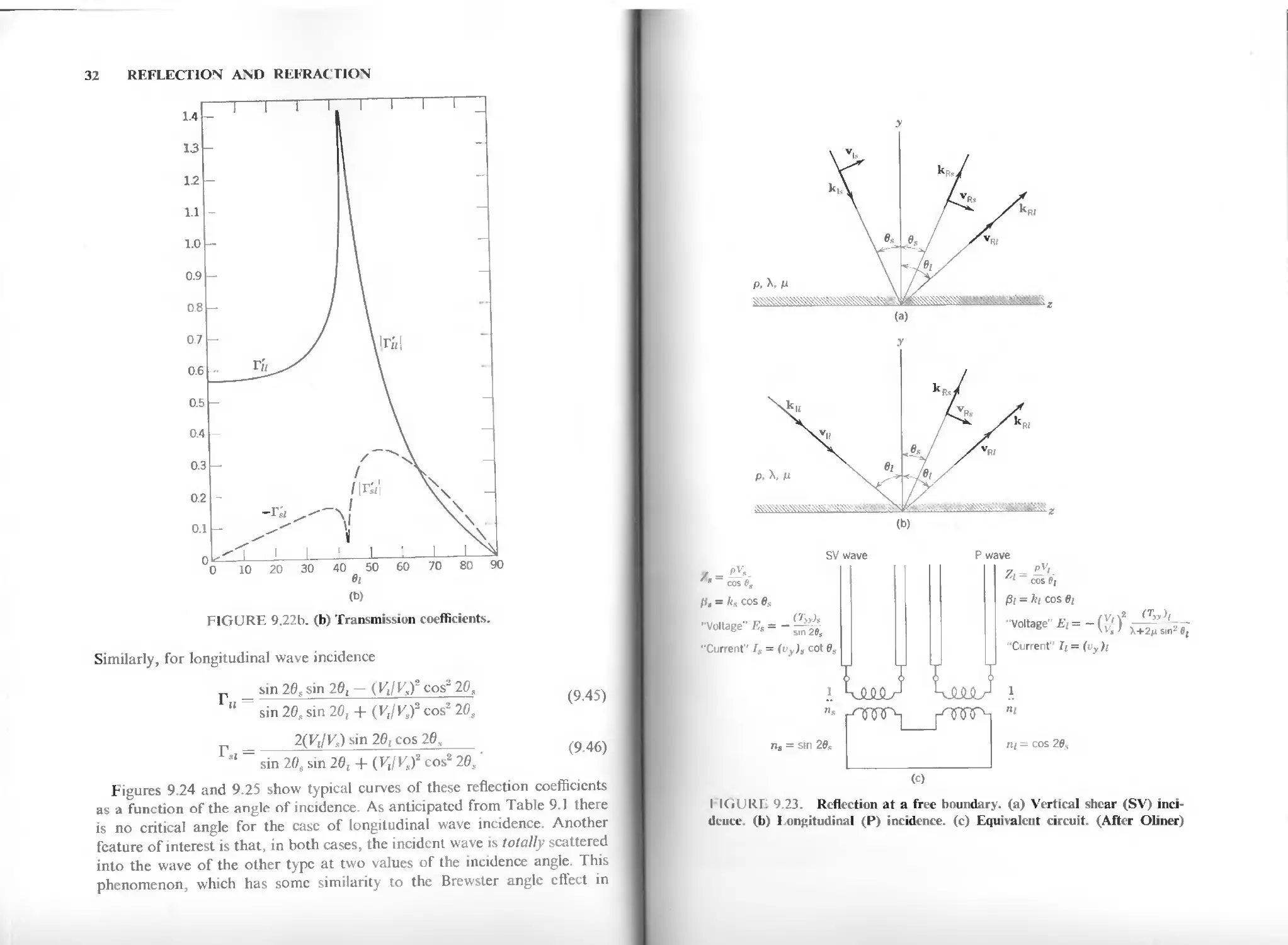
32 REFLECTION AND REFRACTION
61
(b)
FIGURE 9.22b. (b) Transmission coefficients.
Similarly, for longitudinal wave incidence
r _ sm 20, sin 20, - (VJV,? cos2 20,
" sin 26, sin 20, + (VtjVsf cos2 20,
2(Г,/К,) sin 20, cos 20,
sin 20, sin 20, + {VJVf cos2 20,
Figures 9.24 and 9.25 show typical curves of these reflection coefficients
as a function of the angle of incidence. As anticipated from Table 9.1 there
is no critical angle for the case of longitudinal wave incidence. Another
feature of interest is that, in both cases, the incident wave is totally scattered
into the wave of the other type at two values of the incidence angle. This
phenomenon, which has some similarity to the Brewster angle effect in
SV wave
P wave
cos 0,
I , = ks COS 0,
-Voltage" £,= -sm29s
"Current" /, = (vY)s cot 0,
(Та),
1 cos 0,
ft = hi cos в/
4/oltage"£,= -(M\-^\ -
"Current" /;= (vy)i
п, = sir 20,
щ = cos 20s
(c)
I IGURE 9.23. Reflection at a free boundary, (a) Vertical shear (SV)
incidence, (b) Longitudinal (P) incidence, (c) Equivalent circuit. (After Oliner)
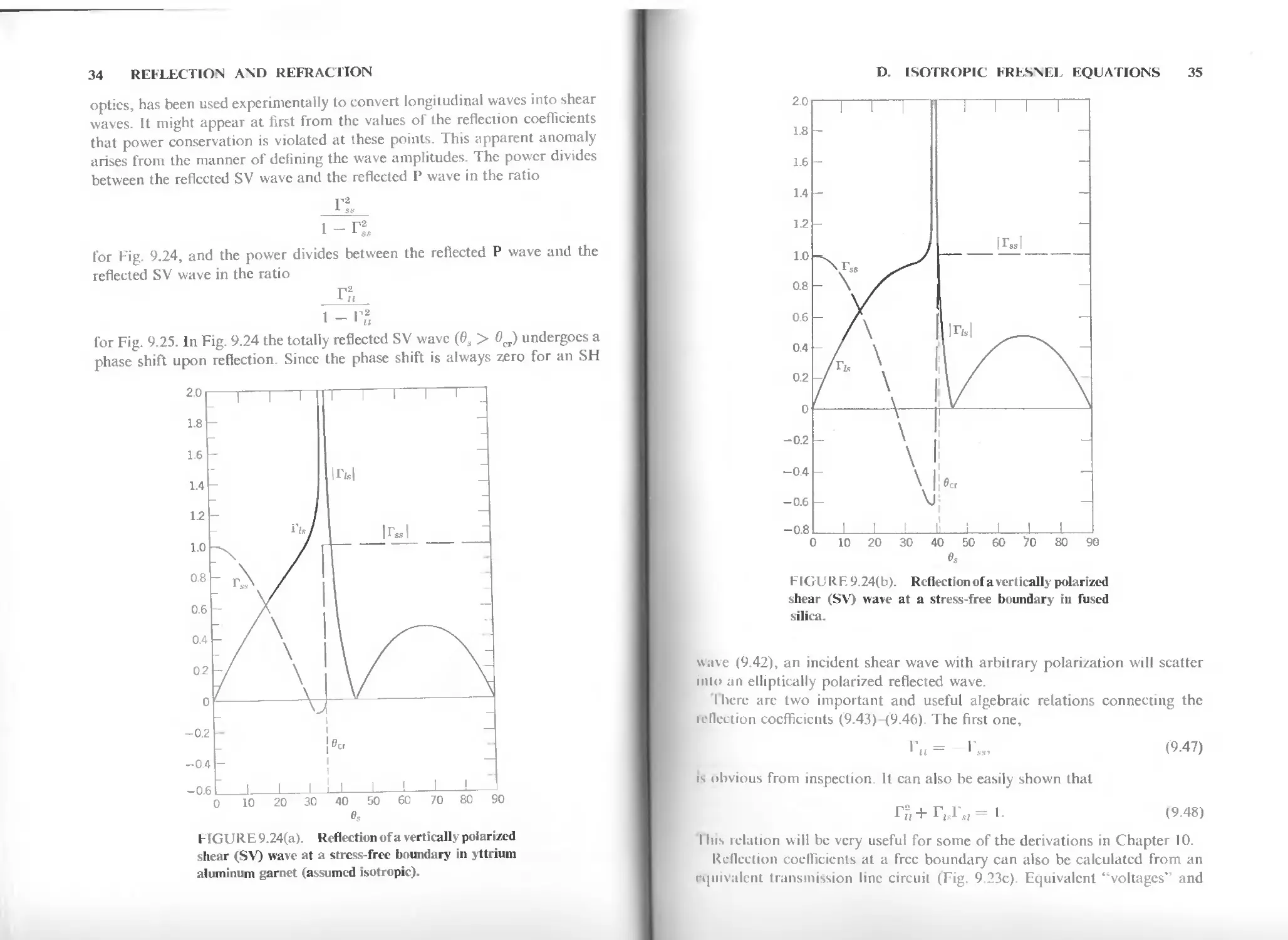
34 REFLECTION AND REFRACTION
-0.;
-0
0 10 20 30 40 50 60 70 80 90
FIGURE 9.24(a). Reflection of a vertically polarized
shear (SV) wave at a stress-free boundary in yttrium
aluminum garnet (assumed isotropic).
20
1.8
D. ISOTROPIC FRESNEL EQUATIONS 35
1.6 -
1.4 -
1.2 -
0 10 20 30 40 50 60 70 80 90
FIGURE 9.24(b). Reflection of a vertically polarized
shear (SV) wave at a stress-free boundary in fused
silica.
wave (9.42), an incident shear wave with arbitrary polarization will scatter
into an elliptically polarized reflected wave.
I here arc two important and useful algebraic relations connecting the
reflection coefficients (9.43)-(9.46) The first one,
Г„ = Г„, (9.47)
is obvious from inspection. It can also be easily shown that
rf,+rjsFs,= I. (9.48)
I his relation will be very useful for some of the derivations in Chapter 10.
Reflection coefficients at a free boundary can also be calculated from an
rrt|iiivalciit transmission line circuit (Fig. 9 23c) Equivalent "voltages' and
i—i—Г
optics, has been used experimentally to convert longitudinal waves into shear
waves. It might appear at first from the values of the reflection coefficients
that power conservation is violated at these points. This apparent anomaly
arises from the manner of defining the wave amplitudes. The power divides
between the reflected SV wave and the reflected P wave in the ratio
Г"
1 — Г2
for Fig. 9.24, and the power divides between the reflected P wave and the
reflected SV wave in the ratio
1 — Г2
for Fig. 9.25. In Fig. 9.24 the totally reflected SV wave (0S > 0cr) undergoes a
phase shift upon reflection. Since the phase shift is always zero for an SH
20
18
16
1.4
1.2
1.
08
06
0.1
02
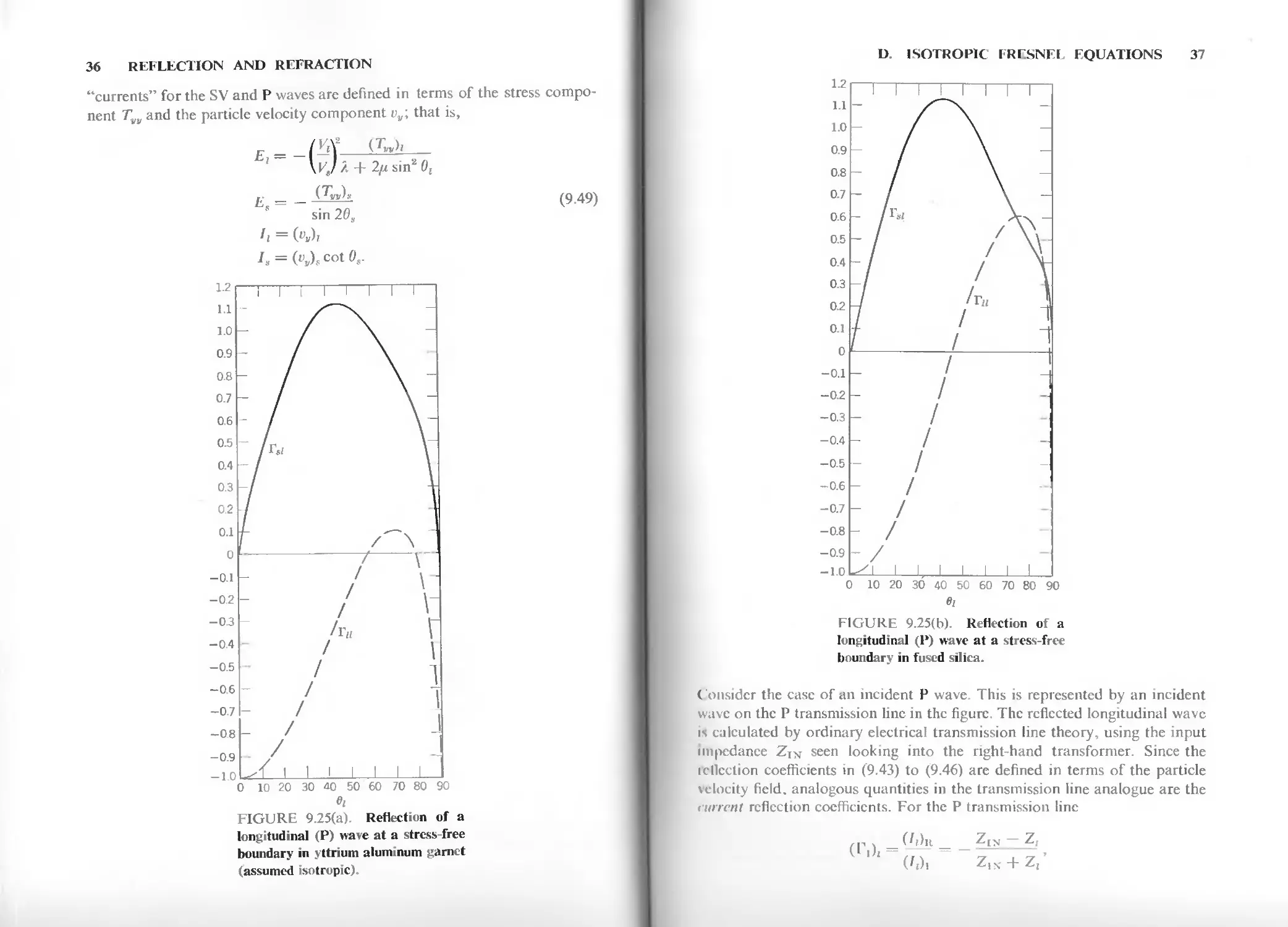
36 REFLECTION AND REFRACTION
£ C^yy)y
sin 26s
i, = ("Л
+ 2[i sin2 0,
(9.49)
10 20 30 <ЗД 50 60 70 80 90
FIGURE 9.25(a). Reflection of a
longitudinal (P) wave at a stress-free
boundary in yttrium aluminum garnet
(assumed isotropic).
D. ISOTROPIC FRESNEL EQUATIONS 37
1.2
1.1
1.0
0.9
0.8
0.7
0.6
0.5
0.4
0.3
0.2
0.1
0
-0.1
-0.2
-0.3
-0.4
-0.5
-0.6
-0.7
-0.8
-0.9
-1.0
0 10 20 30 40 50 60 70 80 90
ei
FIGURE 9.25(b). Reflection of a
longitudinal (P) wave at a stress-free
boundary in fused silica.
Consider the case of an incident P wave. This is represented by an incident
wave on the P transmission line in the figure. The reflected longitudinal wave
i* calculated by ordinary electrical transmission line theory, using the input
impedance ZIN seen looking into the right-hand transformer. Since the
reflection coefficients in (9.43) to (9.46) are defined in terms of the particle
velocity field, analogous quantities in the transmission line analogue are the
current reflection coefficients. For the P transmission line
I I I I I I 1 Г
/
/
/
/
/
/
- /
/
I I L
"currents" for the SV and P waves are defined in terms of the stress
component Tvy and the particle velocity component vy\ that is,
Vtf (Tvvh
40 REFLECTION AND REFRACTION
ky
CO
Pure
shear""""---
eJ
1 / **
\ 1 со
>
т
Pure
shear""""-4
к у
01
1 /Z axis
1 ) Ы
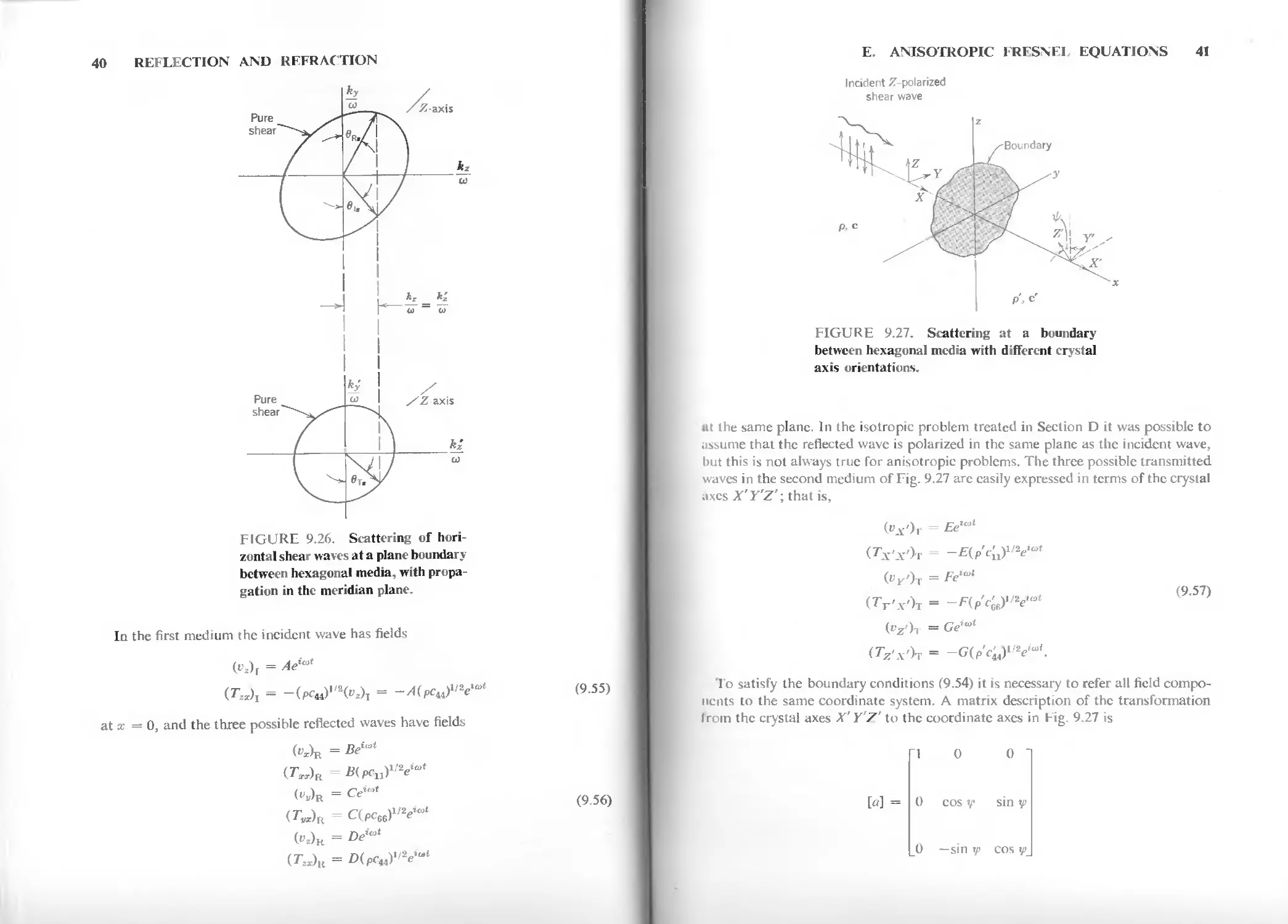
FIGURE 9.26. Scattering of
horizontal shear waves at a plane boundary
between hexagonal media, with
propagation in the meridian plane.
In the first medium the incident wave has fields
(t.V)r = Аеш
at x = 0, and the three possible reflected waves have fields
(M
= BeUoi
= Ce*"*
(7j/z)a
(Тгх)ц
= ЖрСм)"2/"'
(956)
E. ANISOTROPIC FRFSNFI EQUATIONS 41
Incident z*-polarized
shear wave
FIGURE 9.27. S after ng a b u dary
between hexagonal media with different crystal
axis orientations.
lit the same plane. In the isotropic problem treated in Section D it was possible to
assume that the reflected wave is polarized in the same plane as the incident wave,
but this is not always true for anisotropic problems. The three possible transmitted
waves in the second medium of Fig. 9.27 arc easily expressed in terms of the crystal
axes X'Y'Z'; that is,
(Tx'x'h
OvOt
(ТУ'х')т
("z'b
(TVa')t
Eetcot
-G(p'c'uy'*e"°1.
(9.57)
To satisfy the boundary conditions (9.54) it is necessary to refer all field
components to the same coordinate system. A matrix description of the transformation
Irom the crystal axes X' Y'Z' to the coordinate axes in Fig. 9.27 is
[«]
0 cos v sin у
0 —sin ip cos y>_
42 REFLECTION AND REFRACTION
and the transmitted fields therefore transform according to the relations+
= 'a'
■»
« vY>
cos у — "z' s'n У
"г
= Vy'
sin v + pz' cos v
т
f grx
= TX
x'
r
' yx
= rr
v' cos у Tz'x' s'n V
T
1 г
Y' sin у + Tz'x' cos у
(9.58)
The boundary condition equations at v = 0 are therefore
»я. В = E 00
к : С = ^cos у — G sin у (b)
„г: /1 + D = Fsin у + С cos у (с)
7W: «(Pr„)* -Е<№* <d>
Tw: C(Pce6)1/2 - -F(p'4)' 2 cos у f C^'c^'2 sin у (e)
Тгх:-А(рс44р2 + DOu)1'* = -F(p'c;6)1,2siny - GO't^cos у (0-
From (a) and (d) it follows that
В - E = 0,
and the remaining four equations can be solved for C, D, F, and G in terms of the
incident wave amplitude A. The reflection coefficients at a; = 0 are then found to be
(9.59)
С (ZZZ.' - ZvZ'y) sin 2y
А Д
(9.60)
p _ (z„ + z;xz, - z;) sin2 у + cz, + z;xzs - z;) cos2 у (Q61)
гг /1 A
where
Z, = (pr™)1'-
Zs = (pc«)-/2
^ = (
and
A=(ZV+ Z'z){Zz + Z'y) sin2 у + (Zs + z;XZ, + Z;) cos2 y, (9.62)
and the transmission coefficients are
_F 2Z,(Z;+Z,) sin у (9 63)
1 s /1 Д
= C=2Z,(Z; +Z„)cosy
*z А Д
t The three stress components ж, ?лц zx that appear in the boundary conditions (9.54) are
components of the traction force on the boundary. Since this is a vector quantity, it
transforms in exactly the same way as v. The stress transformation can thus be written down
directly in this case, where X — x.
E. ANISOTROPIC TRESNFL EQLATTONS 43
These results show that there is a scattering of the incident shear wave into
Kneeled and transmitted shear waves with orthogonal polarization. Since the two
shear polarizations travel with different phase velocities the polarizations of the
total reflected and transmitted fields vary with distance from the boundary. This
coupling into other polarizations at the boundary is somewhat analogous to the
coupling between SV and P waves at a boundary between isotropic solids (Figs. 9.19
and 9.21). An important distinction, however, is thai polarization coupling in the
isotropic case disappears when the waves are normally incident on the boundary,
'flic example treated here shows that this is not always true for anisotropic problems.
Reflection into the orthogonally polarized shear wave, described by (9.60), disap
pears only when у = 0 or л- 2 in Fig. 9.27. When у = -л 2 1 0 from (9.64) and
ihe transmitted wave is linearly polarised parallel to the incident polarization. The
fttnsmitted and incident polarizations are again parallel when у = 0.
K.2 Piezoelectric Media
In piezoelectric media, wave scattering analysis is further complicated by
coupling between the acoustic and electromagnetic field equations. The
acoustic field equations (LA on the front cover papers) have three uniform
plane wave solutions for each propagation direction, and the electromagnetic
held equations (LB on the front cover papers) have two solutions. These
solutions are coupled together through the piezoelectric constitutive relations,
j'iv ng five coupled wave solutions for each propagation direction. Because
ihese are hybrid waves, with both acoustic and electromagnetic field
components the boundary conditions
v = v'
T • ft - Г • ft
(9 65)
ft x E — ft x E'
n x H = й x II
must be satisfied at boundaries between piezoelectric solids or between a
piezoelectric solid and a nonpiezoclectnc solid
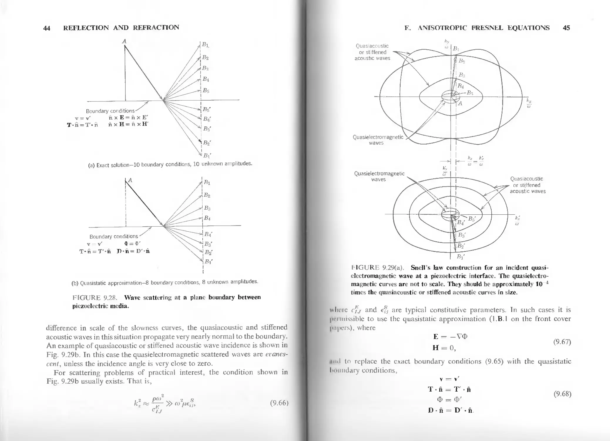
Since there are five different types of plane waves in piezoelectric media,
scattering problems may involve up to five reflected waves and five
transmitted waves (Fig. 9.28a). I here are therefore ten unknown wave amplitudes
p be determined from the ten linear equations obtained by expressing (9.65)
in component form. Snell's Law relations are obtained from the same kind
of slowness curve constructions that were used in Fig. 9.2. For an exact
analysis, slowness curves must be obtained from the coupled wave theory
picscntcd in Section F of Chapter 8 in Volume I: that is, slowness curves are
needed for the quasiclcctromagnctic, quasiacoustic and stiffened acoustic
wave types. "I he incident wave may be of any type Figure 9.29(a) illustrates
Hie case of a quasiclcctromagnetic incident wave Because of the large
44
REFLECTION AND REFRACTION
Boundary conditions
v = v' nxE = nxE'
T-ii = T'-ft AxH=ftxH
(a) Exact solution-10 boundary conditions, 10 unknown amplitudes.
Boundary conditions
v v' Ф = Ф'
T-fi = T'-ft T)-fi=D'-n
(b) Quasistatic approximation-8 bounda у conditions 8 unknown ampl tudes
FIGURE 9.28. Wave scattering at a plane boundary between
piezoelectric media.
difference in scale of the slowness curves, the quasiacoustic and stiffened
acoustic waves in this situation propagate very nearly normal to the boundary.
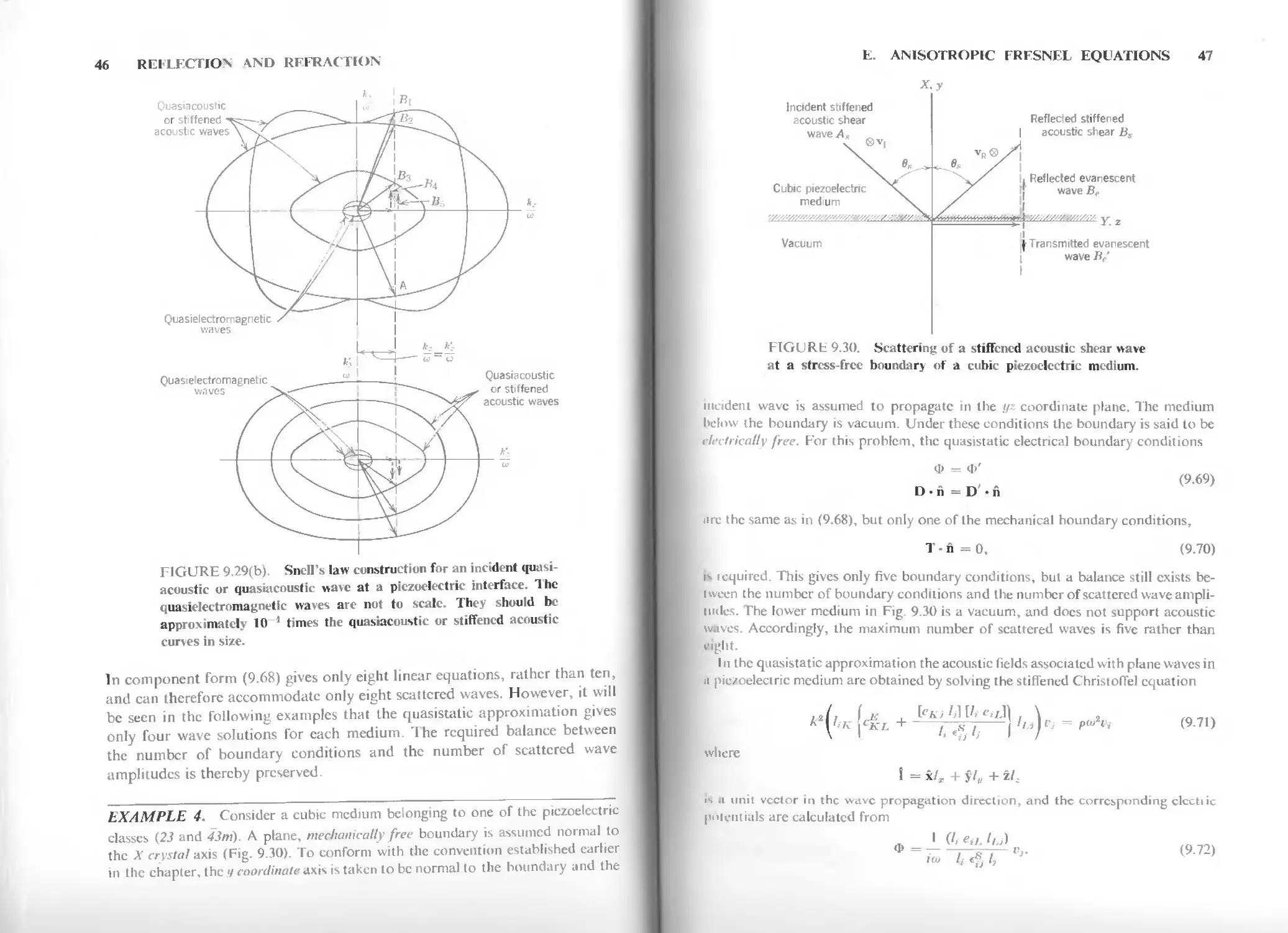
An example of quasiacoustic or stiffened acoustic wave incidence is shown in
Fig. 9.29b. In this case the quasielectromagnetic scattered waves are
evanescent, unless the incidence angle is very close to zero.
For scattering problems of practical interest, the condition shown in
Fig. 9.29b usually exists. That is,
2
К ** » ft>V.v. (9.66)
F. ANISOTROPIC FRESNEL EQUATIONS 45
Quas acoustic
or stiffened
acoustic waves
Quasielectromagnetic
waves
Quasielectromagnetic
waves
Quasiacoustic
or stiffened
acoustic waves
MGURE 9.29(a). Snell's law construction for an incident
quasielectromagnetic wave at a piezoelectric interface. The
quasielectromagnetic curves are not to scale. They should be approximately 10 4
times the quasiacoustic or stiffened acoustic curves in size.
where cfj and efs are typical constitutive parameters. In such cases it is
|u-imissiblc to use the quasistatic approximation (l.B.l on the front cover
papers), where
E - -V<D
н = о, (967)
(iuI to replace the exact boundary conditions (9.65) with the quasistatic
boundary conditions,
v = v'
T • n = T' • Й
Ф = Ф'
D-fi = D'-ii.
(9.68)
46
REFLFCTION AND REFRACTION
Quasiacoustic
or stiffened
acoustic waves
Quasielectromagnetic
waves
Quasielectromagnetic
waves
Quasiacoustic
or stiffened
ac stic waves
FIGURE 9.29(b). Snell's law construction for an incident
quasiacoustic or quasiacoustic wave at a piezoelectric interface. The
quasielectromagnetic waves are not to scale. They should be
approximately 10 1 times the quasiacoustic or stiffened acoustic
curves in size.
In component form (9.68) gives only eight linear equations, rather than ten,
and can therefore accommodate only eight scattered waves. However, it will
be seen in the following examples that the quasistatic approximation gives
only four wave solutions for each medium. The required balance between
the number of boundary conditions and the number of scattered wave
amplitudes is thereby preserved
bXAMPLE 4. Consider a cubic medium belonging to one of the piezoelectric
classes (23 and 43m). A plane, mechanically free boundary is assumed normal to
the X crystal axis (Fig. 9.30). To conform with the convention established earlier
in the chapter, the у coordinate axis is taken to be normal to the boundary and the
E. ANISOTROPIC FRESNEL EQUATIONS 47
X.y
Incident stiffened
acoustic shear
wave A*
Reflected stiffened
| acoustic shear iJ5
Cubic piezoelectric >L
medium N.
vR® Л
^ / 1
i Reflected evanescent
/ if wave Bf
/
v/s/////7s///s//e/s/ss//*'//,7///. :w Nt
^btimiiilumWHiiH j -V/.,/./-уу/,;/,;/, у
Vacuum
|| Transmitted evanescent
wave
1
FIGURb 9.30 Sc tteri ■ : tiff d u ti hear wave
at a stress-free boundary of a cubic piezoelectric medium.
incident wave is assumed to propagate in the yz coordinate plane. The medium
below the boundary is vacuum. Under these conditions the boundary is said to be
ulectrically free. For this problem, the quasistatic electrical boundary conditions
Ф = Ф'
(9.69)
ure the same as in (9.68), but only one of the mechanical houndary conditions,
T - n = 0, (9.70)
is required. This gives only five boundary conditions, but a balance still exists
between the number of boundary conditions and the number of scattered wave
amplitudes. The lower medium in Fig. 9.30 is a vacuum, and does not support acoustic
pves. Accordingly, the maximum number of scattered waves is five rather than
■glit.
In the quasistatic approximation the acoustic fields associated with plane waves in
E pie/oeleciric medium are obtained by solving the stiffened ChristofTel equation
*yiK \<-kl + т^гт; J '«J*J = P°>** (9-70
where
I = \lx + y/s + il.
is (i unit vector in the wave propagation direction, and the corresponding clcctiic
poicutials are calculated from
. I d.eaJ,,)
48 REFLECTION AND REFRACllON
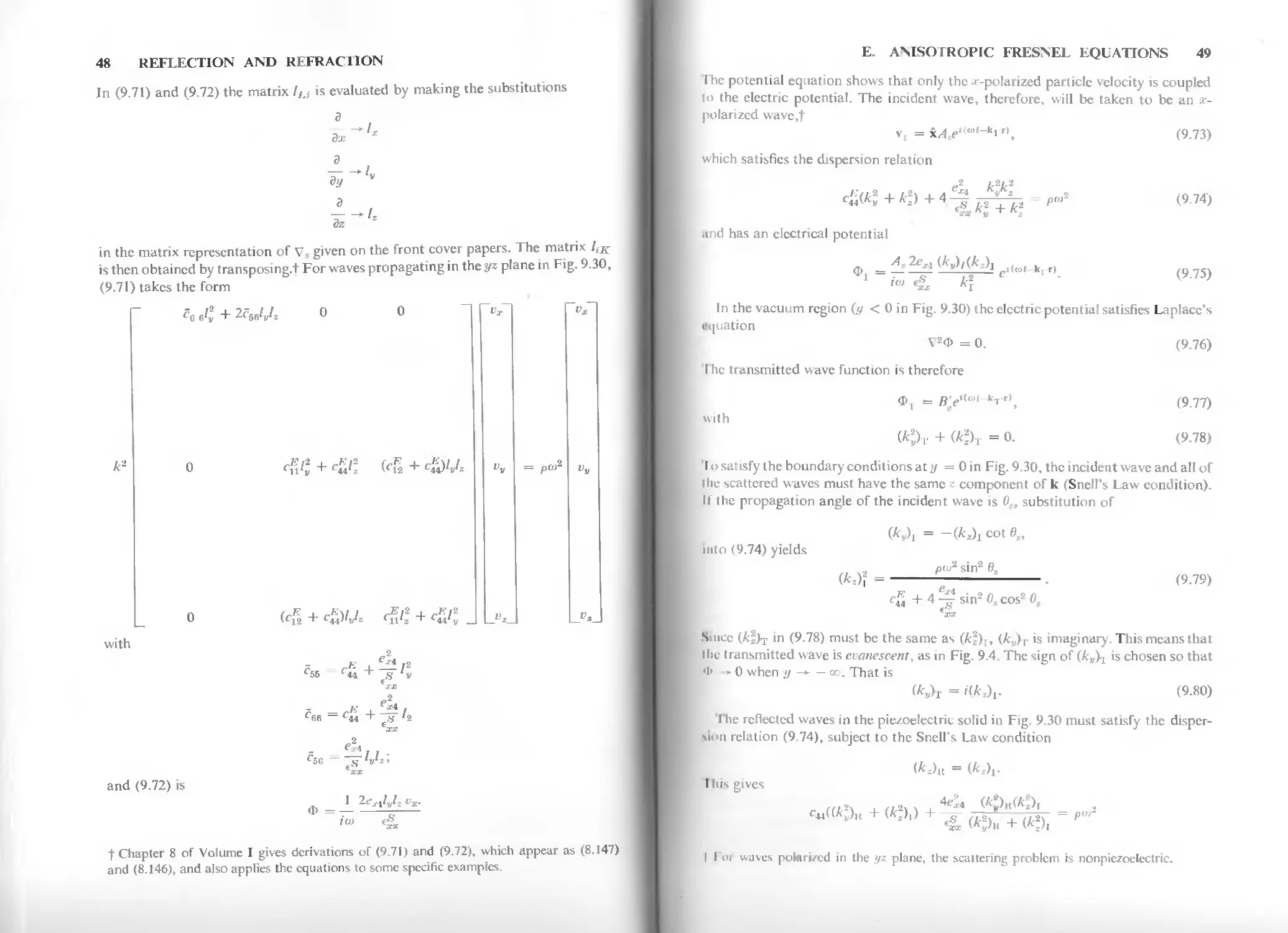
In (9.71) and (9.72) the matrix lu is evaluated by making the substitutions
a
г
dz
in the matrix representation of V$ given on the front cover papers. The matrix liK
is then obtained by transposing.t For waves propagating in the yz plane in Fig. 9.30,
(9.71) takes the form
ce e'v + 2с5В/Л 0 0
fc2
with
and (9.72) is
с{\1\ + c£j; (eg + c£)V,
l55
'14 T S V
.2
1 2eJfllyl. vx
Ф =
t Chapter 8 of Volume I gives derivations of (9.71) and (9.72), which appear as (8.147)
and (8.146), and also applies the equations to some specific examples.
E. ANISOTROPIC FRESNEL EQUATIONS 49
The potential equation shows that only the -r-polarized particle velocity is coupled
to the electric potential. The incident wave, therefore, will be taken to be an x-
polarized wave,t
v, =\Aseto"-^I\ (9.73)
which satisfies the dispersion relation
c£(kl + kl) + 4 ^ JfrP. P1"2 (9-7*J
and has an electrical potential
U» e« k\
In the vacuum region (у < 0 in Fig. 9.30) the electric potential satisfies Laplace's
equation
?2Ф = 0. (9.76)
The transmitted wave function is therefore
Ф, = В'се'ш kr'\ (9.77)
vvith
'I о satisfy the boundary conditions at у — 0 in Fig. 9.30, the incident wave and all of
the scattered waves must have the same г component of к (Snell's Law condition).
If the propagation angle of the incident wave is 0S, substitution of
(fr„)i = -(Wi cot es,
in I о (9.74) yields
pto2 sin2 8S
(kz)\ = - . (9.79)
cu + 4 ~7T sin2 °* cos'2 °s
XX
Since (fc2)T in (9.78) must be the same as (fcf )r, (ky)is imaginary. This means that
the transmitted wave is evanescent, as in Fig. 9.4. The sign of (ky\ is chosen so that
'I' ► 0 when .y —>- — со. That is
(Ars>r = iik^. (9.80)
The reflected waves in the piezoelectric solid in Fig. 9.30 must satisfy the
dispersion relation (9.74), subject to the Snell's Law condition
(kjt, = (кг\.
I his gives
. „A ч , (фн(к%
С«((*Л + ».),) + ^ ^ + ^ -
I I in waves poleri/cd in the >/z plane, the scaitering problem is nonpiezoelectric.
=cot26s (9.82)
50 REFLECTION AND REFRACTION
/ ЭФ.Д
E. ANISOTROPIC FRESNEL EQUATIONS 51
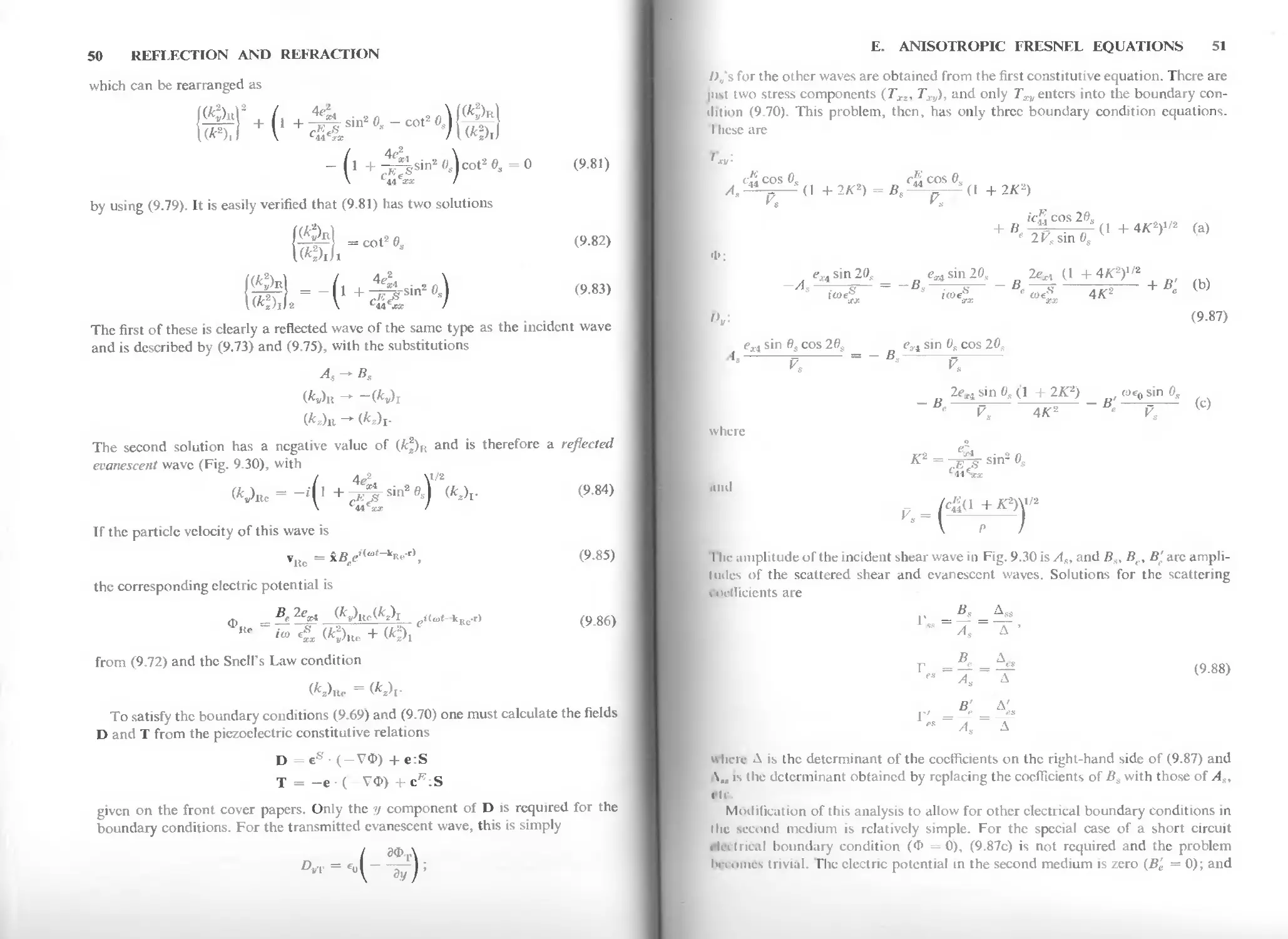
/Vs for the other waves are obtained from the first constitutive equation. There are
jiikt two stress components (Тхг, Txy), and only reenters into the boundary
condition (9.70). This problem, then, has only three boundary condition equations.
I liese arc
i ii cos 0S „ cE cos 0,
A.-^-p (I + 2**) = Bs - (I +2K2)
icJi cos 20,
Ф:
^ sin 20, g„sin20, 2^ (1 + 4Q'«
— p— - — Bs—;—^— — Я —5- —; h В (b)
«>„: (9.87)
exi sin 6S cos 2f?s exi sin 0S cos 20s
' ~ t ■ - -B- РГ
2eri sin 0S (1 + 2K2) <oe0 sin 0,
в< V. 4^ e ¥„ (c)
where
mid
The amplitude of the incident shear wave in Fig. 9.30 is As, and Яч, Bf, В' arc ampli-
Imles of the scattered shear and evanescent waves. Solutions for the scattering
Ouoilicients are
I-
" As ~ A '
в, д,
г« = л = "f (9-88)
Г' =В: = ^
" As A
wticrc Л is the determinant of the coefficients on the right-hand side of (9.87) and
Л., is the determinant obtained by replacing the coefficients of Bs with those of A„,
|tc
Modification of this analysis to allow for other clectiical boundary conditions in
I lie second medium is relatively simple. For the special case of a short circuit
PflttriCfil boundary condition (Ф — 0), (9.87c) is not required and the problem
Iw-i nines trivial. The electric potential in the second medium is zero (B'e = 0); and
which can be rearranged as
- (1 + ^.sin2 Л cot2 6>3 = 0 (9.81)
by using (9.79). It is easily verified that (9.81) has two solutions
®.--(,+3sH
The first of these is clearly a reflected wave of the same type as the incident wave
and is described by (9.73) and (9.75), with the substitutions
As —
(kv)K -► — (kv)I
(^z)ll ~** (^z)t-
The second solution has a negative value of (k2)H and is therefore a reflected
evanescent wave (Fig. 9.30), with
№Лс = -'(1 + ^sin2 4 V-)i- <9-84>
If the particle velocity of this wave is
vltc = kB/^Kf*, (9.85)
the corresponding electric potential is
ф = (*Лс(*Л . ,<„«- tRe.r) (9 86)
from (9.72) and the Snell's Law condition
To satisfy the boundary conditions (9.69) and (9.70) one must calculate the fields
D and T from the piezoelectric constitutive relations
D es-(-VO)+e:S
T = -e-( VO)+cB:S
given on the front cover papers. Only the у component of D is required for the
boundary conditions. For the transmitted evanescent wave, this is simply
52 REFLECTION AND REFRACTION
Incident stiffened
acoustic shear
wave As
Hexagonal (6mm)
medium
Vacuum
Reflected stiffened
acoustic shear
wave Bs
Л Reflected evanescent
JJ wave Br
mmmmY.z
ij Transmitted evanescent
wave B'„
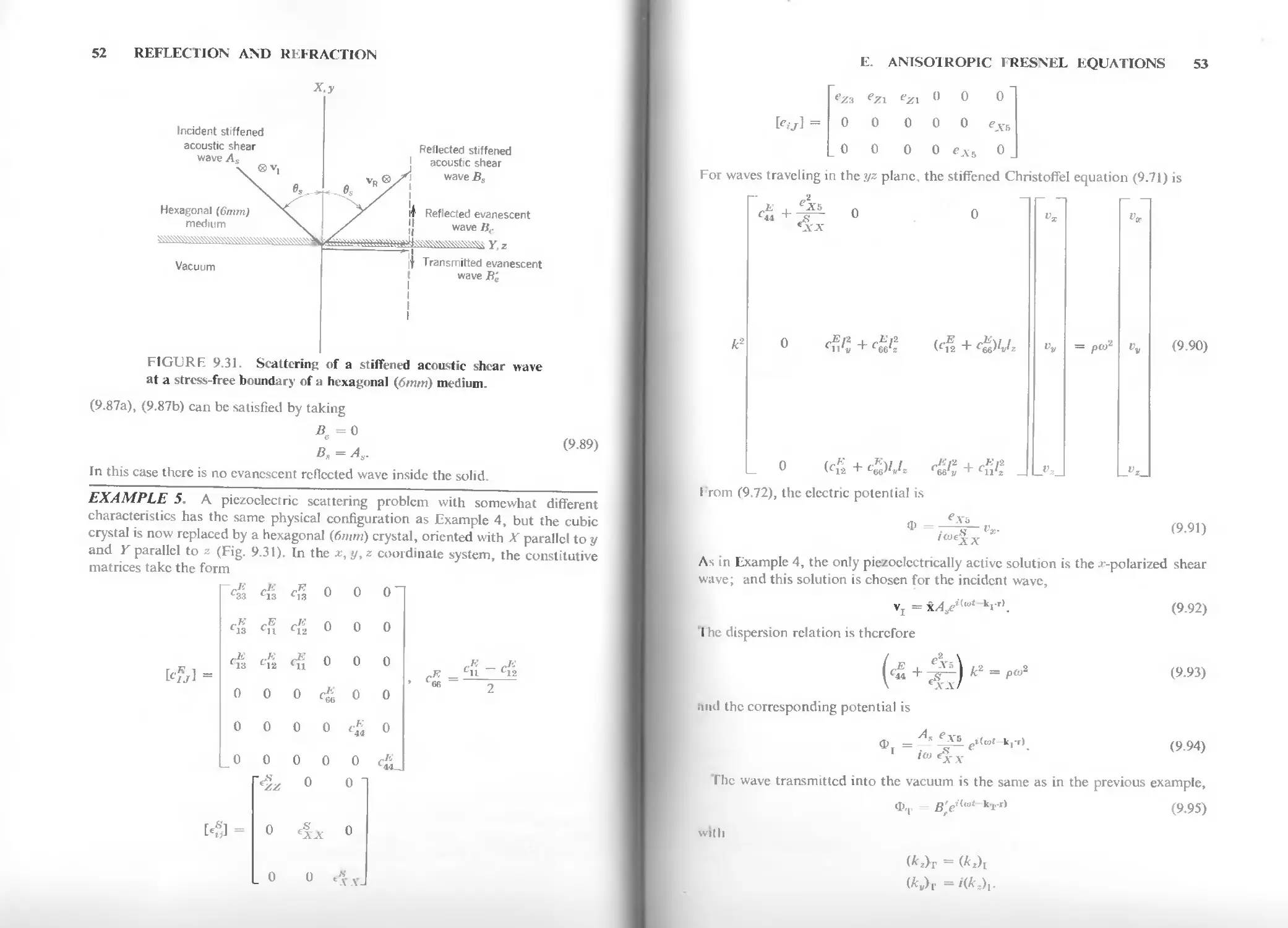
FIGURE 9.31. Scattering of a stiffened acoustic shear wave
at a stress-free boundary of a hexagonal (6mm) medium.
(9.87a), (9.87b) can be satisfied by taking
Bc=0
B„ = As.
In this case there is no evanescent reflected wave inside the solid.
EXAMPLE 5. A piezoelectric scattering problem with somewhat different
characteristics has the same physical configuration as Example 4, but the cubic
crystal is now replaced by a hexagonal (6mm) crystal, oriented with X parallel to у
and Г parallel to z (Fig. 9.31). In the x,y,z coordinate system, the constitutive
matrices take the form
(9.89)
l33
c13
C13
0
0
o-
ей
cK
CV1
0
0
0
«g
4
411
0
0
0
0
0
0
c&
0
0
0
0
0
0
0
0
0
0
0
0
CK
E. ANISOTROPIC FRESNEL EQUATIONS 53
ez3 ezi ezi 0 0 0
0 0 0 0 0 eXb
0 0 0 0 e.\s
0
For waves traveling in the yz plane, the stiffened Christoffel equation (9.71) is
0 0
k-
A'A"
En , E,2 , E , Aw i
0 (4 + O'J* egll + eftl
From (9.72), the electric potential is
fir.
Ф =
par
(9.90)
(9.91)
xx
As in Example 4, the only piezoclcctrically active solution is the ^--polarized shear
wave; and this solution is chosen for the incident wave,
Vj = х/и/'<и' -кгг). (9.92)
T he dispersion relation is therefore
tind the corresponding potential is
_ As exa ,t k].r)
(9.93)
Ф.
(9.94)
xx
The wave transmitted into the vacuum is the same as in the previous example,
Ф.( B'reHwt kJr) (9.95)
with
(kzh = №Л
(fc„)i' = /(*-_),•
54
REFLECTION AND REFRACTION
If the horizontally polarized shear wave (9.92) is incident at an angle 6S in Fig. 9.31
(&z)i = к sin 0K,
and
о
(k% = sin2 0„ (9.96)
E +е_хц_
from (9.93). Reflected waves inside the crystal must satisfy the dispersion relation
(9.93), subject to the Snell's Law condition
(^z)k = (^z)f
This gives
(*v)n = C*=)/ cot f?s. (9.97)
In this case the stiffened ChristofTel equation provides only one reflected wave
solution—a shear wave of the same type as the incident wave. There are, however,
three field components (7"ст, Ф, Dv) to be matched at the boundary; and a second
reflected wave is needed. This additional solution can be found by returning to the
quasistatic piezoelectric equations
ю»Л*(/^/,)Ф = -wkHl^JrJvj, (9.99)
from which the stiffened ChristofTel equation was derived/!" In the present problem
(9.98) and (9.99) reduce to
(«■Ж + k\) - Pco*K = -iWA.5(Aj + *|)Ф (a)
+ cgfcf - p^f, + (<:£ + c^kjev. = 0 (b) (9 ]oo)
(cf2 + C^)k,J<,Vv + (cgkt + cfikl - pW*)vz = 0 (c)
и?*хх<к* + к1)Ф * -1«*л-5(*; + *!)»«- (d)
The relevant equations are (a) and (d). If (d) is solved for Ф and the result is
substituted into (a), the dispersion relation (9.93) is obtained. It can be seen, however,
that another solution to (a) and (d) is*
kl+kl = 0
u, = 0 (9.101)
Ф^ 0.
This provides the reflected evanescent wave
Фцв B,,*>'<°"
Wiie = '№z)i
that is needed to satisfy the boundary conditions in Fig. 9.31.
(9.102)
t These equations appear as (8.142) and (8.143) in Chapter 8 of Volume I
% Although this solution has no particle motion, it does have a stress ticlu (Problem 8).
E. ANISOTROPIC FRESNEL EQUATIONS 55
Incident evanescent
wave Ac
Hexagonal (6mm) I
medium I
^\^\4444\W4\\\W444\W\\W^vl
Vacuum
0»
I Reflected stiffened
shear wave Bs
I
ij Reflected evanescent
wave Be
>ii)i))i)i)iiniw<t>M.\\^w^\^-> Y.z
T
it Transmitted evanescent
wave B'e
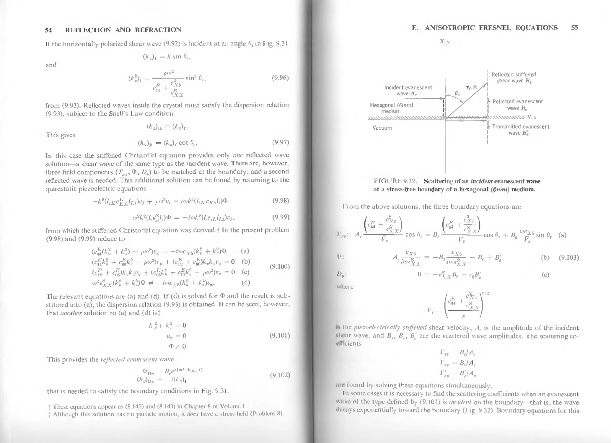
FIGURE 9.32. Scattering of an incident evanescent wave
at a stress-free boundary of a hexagonal (6mm) medium.
From the above solutions, the three boundary equations are
■ I lie piezoelectrically stiffened shear velocity, As is the amplitude of the incident
tlmiv wave, and flv, fie, B'e are the scattered wave amplitudes. The scattering
coefficients
Г„ = BJA„
1« = W
•n«" found by solving these equations simultaneously.
In some cases it is necessary to find the scattering coefficients when an evanescent
wiive of the type defined by (9.101) is incident on the boundary—that is, the wave
■Irc.iys exponentially toward the boundary (Fig. 9.32). Boundary equations for this
X.y
56 REFLECTION AND REFRACTION
problem arc obtained by making the substitutions
lue\s
cos 0. — A, —-" sin 0,
(9.104)
As : s ' A"
0 - -4x"«
in parts (a), (b), (c) of (9.103). The modified equations arc then solved for the
scattering coefficients
■1 ye = Bgf At,
vee = в,/л
Г' = B'JA,.
ее e' e
An important special case arises when a short-circuit electrical boundary
condition (Ф =0) is applied at у = 0 in Fig. 9.31. The boundary condition on Dv is no
longer required, and (9.103) reduces to
—-— cos в, = В
cje vb
cos0s + Д..--Г5 sin es (.a)
(9.10
B„ - В..
lb)
since B'e = 0. In this case
xx
Am
Д
Д
(9.106)
where
д _ _ \ <.v v ' УДГ-У
(9.107)
is the determinant of the right-hand side of (9.105) and Дет is the determinant
obtained by replacing the coefficients of B„ with those of A„ etc. 11 should be noted that
in this example, by contrast with Example 4, the reflected evanescent wave still
remains when the short-circuit electrical boundary condition is applied.
PROBLEMS 57
Ae —^ sin 0S = Bs~ лл cos 0, + BK —~ sine, (a)
(9.108)
A. = - тЦг~ В, - Br (b)
when an electrical short circuit is imposed at the boundary; and the scattering
coefficients are
л
.p _ ->s<?
A« - Д
(9.109)
Г —
д •
where the determinants A£e, Д„ arc obtained by replacing the coefficients of В and
B, in Л with those of Ac in (9.108).
PROBLEMS
1. Calculate complex Poynting vectors for plane waves propagating along
the Z-axis in sapphire (Problem 4, Chapter 3 of Volume 1). Compare with the
lingle between P and к calculated from Fig. 3.8 in Appendix 3 of Volume 1.
2. Find the complex Poynting vectors for plane waves propagating along
llie Z-axis in materials belonging to the trigonal crystal classes 3m and 32
(Problem 4, Chapter 8 of Volume I). Calculate the change in direction of P
due to the piezoelectric effect in lithium niobate and quartz.
X Using the relations derived in Section B.2, calculate the critical angles
relevant to Figs. 9.20 and 9.22. Locate these angles on the figures.
4. The formula (7.115) for [Z£] in Chapter 7 of Volume I applies to
isotropic, as well as anisotropic, materials. Derive the boundary condition
equations (9.27) and (9.37) by using the impedance concept.
5. Use the impedance concept to find reflection coefficients for the
configuration, shown at the top of page 58. Solve the problem for incident waves
Of both shear and compressional types.
<». I he two media in Problem 5 are separated by a slab of nonpiezoclectric
cubic material with axes oriented as shown in the figure. Use the
transformation law for impedance (Problem 25, Chapter 7 in Volume 1) to derive design
equations for shear and compressional wave quarter-wave matching trans-
loimcis (Problem 12 in Chapter 6).
Boundary equations for the incident evanescent wave problem become
58 REFLECTION AND REFRACTION
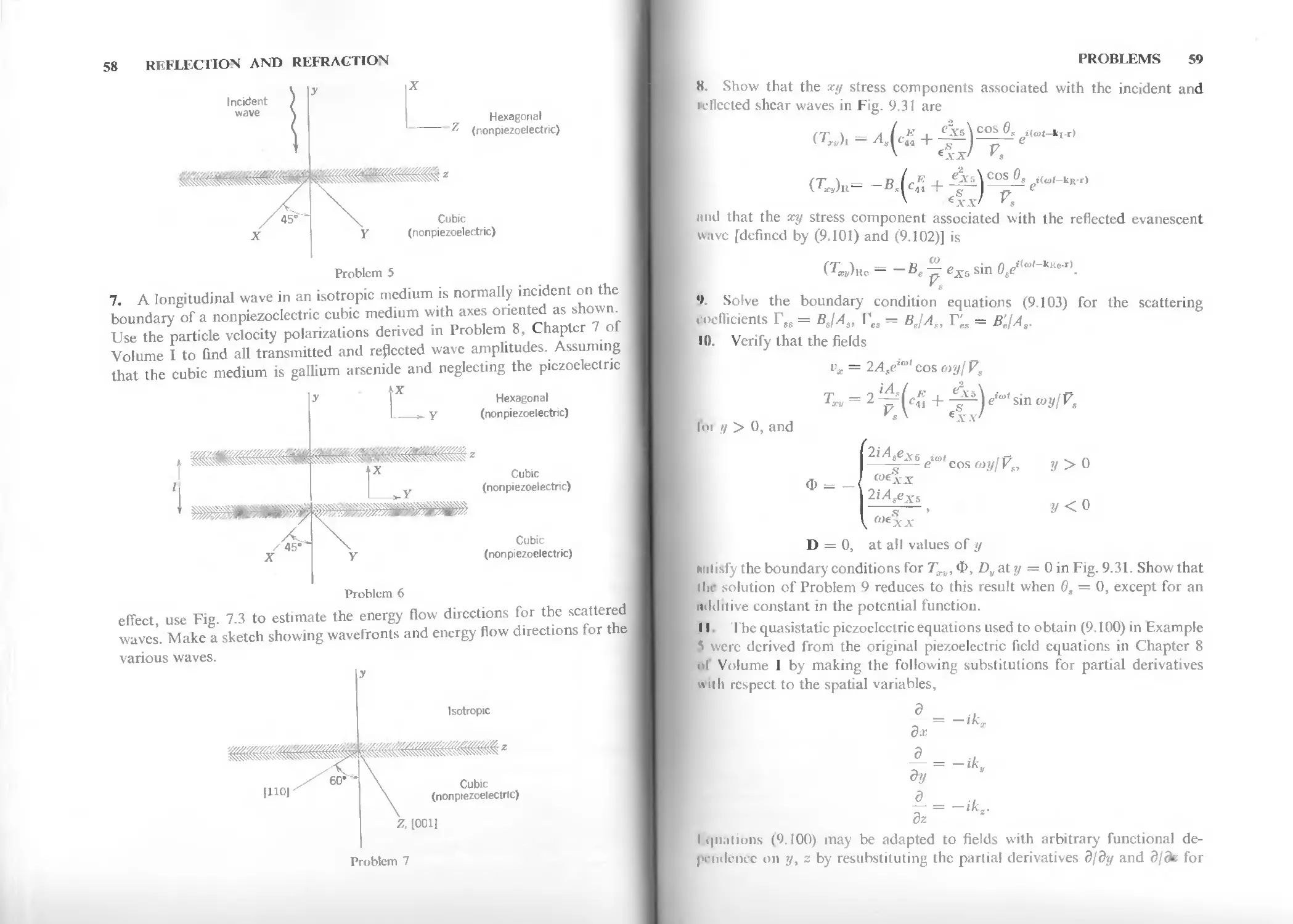
Incident
wave
Hexagonal
(non piezoelectric)
Cubic
(nonpiezoelectric)
Problem 5
7. A longitudinal wave in an isotropic medium is normally incident on the
boundary of a nonpiezoelectric cubic medium with axes oriented as shown.
Use the particle velocity polarizations derived in Problem 8, Chapter 7 of
Volume I to find all transmitted and reflected wave amplitudes. Assuming
that the cubic medium is gallium arsenide and neglecting the piezoelectric
Hexagonal
(nonpiezoelectric)
Cubic
(nonpiezoelectric)
Cubic
(nonpiezoelectric)
Problem 6
effect, use Fig. 7.3 to estimate the energy flow directions for the scattered
waves. Make a sketch showing wavefronts and energy flow directions for the
various waves.
1»
Isotropic
Cubic
(nonpiezoelectric)
Z, [0011
Problem 7
PROBLEMS 59
8. Show that the xy stress components associated with the incident and
Krlleeted shear waves in Fig. 9.31 are
and that the xy stress component associated with the reflected evanescent
wave [defined by (9.101) and (9.102)] is
(TOT)Kc=-Be^eX6sin 0/,"->.
4 Solve the boundary condition equations (9.103) for the scattering
coefficients Tgs = BJA„ Г„ = BJAS, V„ = B'JA,.
10. Verify that the fields
пх=2А^'cos o>y}Vs
T„ = 2 Mc* + e-' sin wyjVt
ioi у > 0, and
Ф -
2iA\ex& i№l r
-r—e cos a>yJ V„
MeA-J
2iAeeXa
У>0
У<0
D -
0, at all values of у
Hiilisfy the boundary conditions for Txv, Ф, Dy at у = 0 in Fig. 9.31. Show that
the solution of Problem 9 reduces to this result when 0, — 0, except for an
mldiiive constant in the potential function.
II. I he quasistatic piezoelectric equations used to obtain (9.100) in Example
5 were derived from the original piezoelectric field equations in Chapter 8
of Volume I by making the following substitutions for partial derivatives
h respect to the spatial variables,
d_
dy
3z
= -ifc,
= -iky
= — ik.
lunations (9.100) may be adapted to fields with arbitrary functional
dependence on y, z by resubstituting the partial derivatives djdy and djde for
CHAPTER 10
ACOUSTIC
WAVEGUIDES
A. GUIDED WAVES 63
II. METHODS OF ANALYSIS 66
C. FREE ISOTROPIC PLATE 73
I) ISOTROPIC PLATE ON AN ISOTROPIC HALF SPACE 94
I FREE ISOTROPIC CYLINDER 104
|. ISOTROPIC RECTANGULAR STRIP 114
ti. M1CROSOUND WAVEGUIDES 118
II ANISOTROPIC WAVEGUIDES 128
I PIEZOELECTRIC WAVEGUIDES 134
I. RECIPROCITY RELATIONS AND MODE ORTHOGONALITY 151
K. EXCITATION OF WAVEGUIDE MODES 161
I INPUT IMMITTANCE OF WAVEGUIDE TRANSDUCERS 163
M. TRANSMISSION LINE MODEL FOR ACOUSTIC
WAVEGUIDES 177
N WAVEGUIDE SCATTERING PROBLEMS 190
<> GROUP VELOCITY AND ENERGY VELOCITY 199
PROBLEMS 207
КI I ERENCES 214
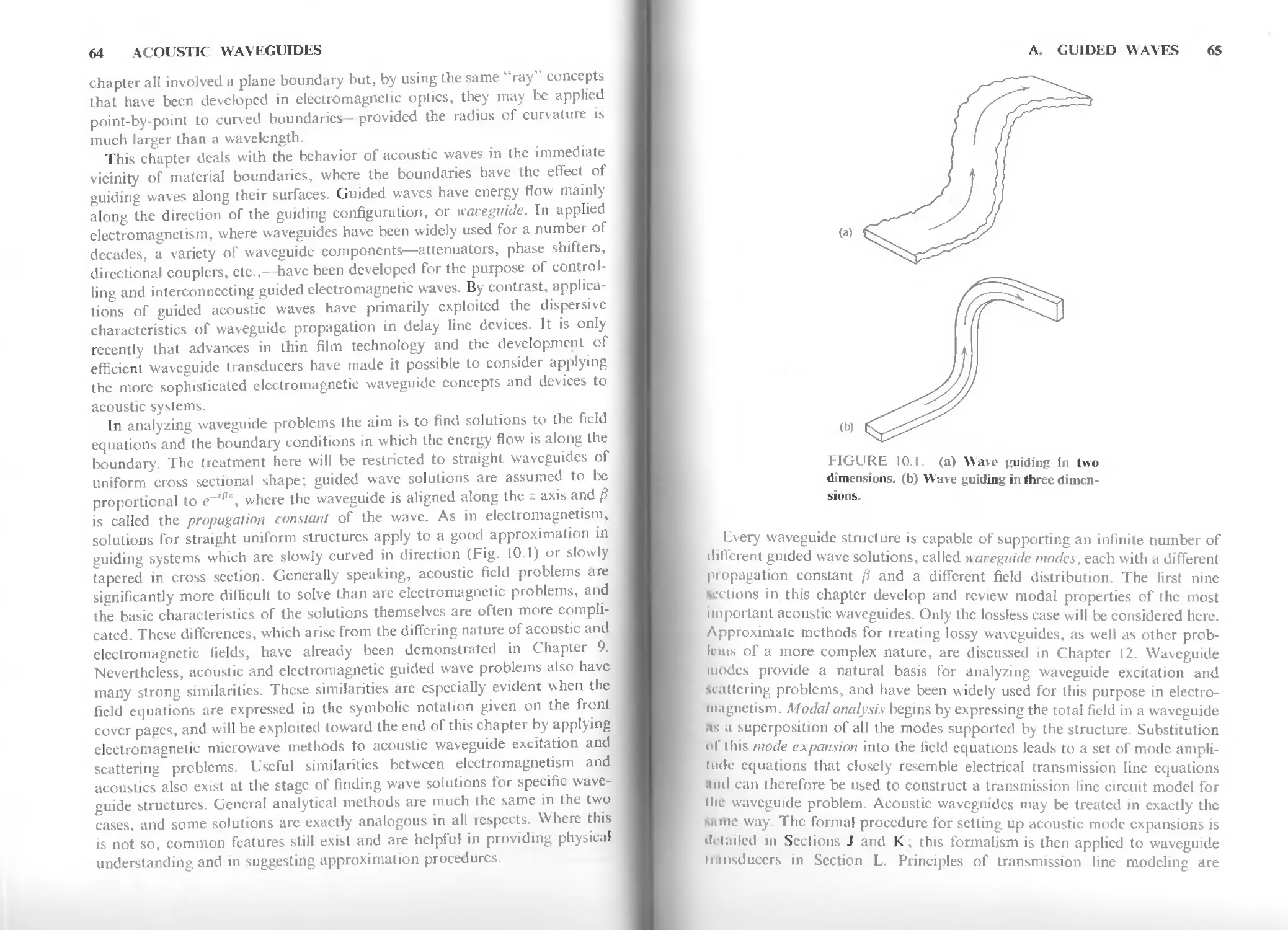
A. G1IDED WAVES
Chapter 9 was concerned with scattering of acoustic plane waves at a
boundary between different media. This interaction is of primary importance in
problems where the dimensions of a solid body are large compared with the
acoustic wavelength, and its volume is not completely occupied by the waves.
1'ioblcms of this kind are analogous to "optical" problems in electromagnet-
ism, where there is also only an occasional interaction of the waves with the
boundary of the medium. The scattering solutions presented in the previous
63
60 REFLECTION AND REFRACTION
— ik„ and —ik.. Prove that there arc then two general solutions to (9.100a)
and [9-I00d], one defined by
кое xx
and the other by
vx = 0
Use these differential equations to solve the scattering problem for an
a-polarizcd shear wave normally incident on the boundary in Fig. 9.31, and
show that the solution obtained is equivalent to the one given in Problem 10.
(Note that the electric field Ey must go to zero at у — — со, unless there is an
electrical charge layer at that point.)
12. A perfectly conducting plane with potential Ф = 0 is placed at у = —h
in Fig. 9.31. Use the differential equations in Problem 11 to solve the
scattering problem for an .^-polarized shear wave normally incident on the boundary
у = 0. Show (hat this reduces, when h = 0, to the solution determined by
(9.105).
13. Show that solutions of the form given in Problems 10 and 11 apply to
any case where a pure mode (v either parallel or perpendicular to k) is
normally incident on the boundary between a piezoelectric medium and an
unbounded vacuum.
14. Problem 13 is modified by replacing the unbounded vacuum with a
piezoelectric medium that supports a normally propagating pure mode with
the same polarization as the incident wave. Show how the solutions found in
Problem 13 arc modified in this case.
15. Consider an A"-oricnted interface between a cubic piezoelectric material
and vacuum (Fig. 9.30). Use the exact plane wave solutions given in Example
4, Chapter 8 of Volume I and the exact boundary conditions (9.65) to find the
scattered waves produced by normal incidence of a F-polarized quasi-
acoustic wave. Repeat for the Z-polarized quasiacoustic wave and the X-
polarized purely acoustic wave.
16. Consider a solid-to-vacuum interface oriented normal to the [110]
direction of a cubic piezoelectric medium. Using the exact plane wave
solutions obtained in Example 5, Chapter 8 of Volume 1, solve the normal-
incidence scattering problem for incident waves of purely acoustic, quasi-
acoustic, and stiffened acoustic types.
REFERENCES 61
REEI RENTES
SnelVs Law and the Fresnel Equations
1. L. M. Brekhovskikh, Waves in Layered Media, Academic Press, 1960.
2. W. M. Ewing, W. S. Jardetsky, and F. Press, Elastic Waves in Layered Media,
Ch. 2, 3, McGraw-Hill, New York, 1957.
3. E. G. H. Lean and H. J. Shaw, "Efficient Microwave Shear-Wave Generation
by Mode Conversion," Appl. Phys. Lett. 9, 372-374 (1966).
I. W. P. Mason, Physical Acoustics and the Properties of Solids, pp. 22 32, van
Nostrand, New York, 1958.
5. M. J. P. Musgrave, "The Propagation of Elastic Waves in Crystals and
Anisotropic Media," Reports on Progress in Ph . it 22, pp. 74-96 (1959).
ft. G. Nadeau, Introduction to Elasticity, pp. 241 258, Holt, Rinehart and
Winston, New York, 1964.
7. S. Ramo, J. R. Whinncry, and T. van Duzer, Fields and Waves in
Communication Electronics, pp. 342-365, Wiley, New York, 1965.
8. M. J. P. Musgrave, Crystal Acoustics, Ch 11, Holden-Day, San Francisco,
1970.
H.i. E. G. Henneke II, "Reflection-Refraction of a Stress Wave at a Plane
Boundary between Anisotropic Media", J. Acous. Soc. Am. 51, 210-217
(1972).
Conical Refraction
9. L. D. Landau and E. M. Lifshitz, Electrodynamics of Continuous Media, pp.
324-329. Pcrgamon, New York, 1960.
III. H. J. McSkimin and W. L. Bond, "Conical Refraction of Transverse
Ultrasonic Waves in Quartz," /. Acous. Soc. Amer. 39, 499 505 (1966).
II. E. P. Papadakis, "Ultrasonic Internal Conical Refraction in Rocksalt and
Calcite," /. Appl. Phys. 34, 2168 2171 (1963).
\1. K. S. Aleksandrov and Т. V. Ryzhova, "Internal Conical Refraction of
Elastic Waves in Ammonium Dihydrogen Phosphate," Soviet
Physics—Crystallography 9, 298-300 (1964).
ti. P. C. Waterman, "Orientation Dependence of Elastic Waves in Single
Crystals", Phys. Ree. 113, 1240-1253 (1959).
Lquii alent Netw ork Methods
I'I A. A. Oliner, "Microwave Network Methods for Guided Elastic Waves,"
IEEE Trans, on Microwave Theory and Techniques MTT-I7, 812-826 (1969).
Piezoelectric Media
H I Rurdati, G. Barzilai, and G. Gerosa, "Elastic Wave Excitation in
Piezoelectric Slabs," IEEE Trans, on Sonicsand Ultrasonics, SU-15, 193 202 (1968).
66 ACOUSTIC WAVEGUIDES
discussed in Section M, and application to the problem of waveguide
scattering is considered in Section N. The chapter concludes with a section on an
important relationship between the power flow, stored energy, and group
velocity of a guided wave.
B. METHODS OF ANAIYSIS
The simplest of all acoustic waveguide structures, an unbounded plate with
strcss-frcc surfaces will be used to illustrate the three most commonly
applied methods for waveguide analysis.
B.l Potential Theory
The most general method for solving isotropic waveguide problems makes use
of a representation of the particle velocity field in terms of a scalar and a
vector potential. For isotropic media, which are always nonpiezoelectric,
the left-hand side of the Christolfel equation (9.71) takes the form
4Уз- ^xlv
k'2\ cm + (cn - c4i)
^>Jx ^У^У ^V^Z
LL I J. LI
Matrix multiplication of the term on the right gives
~ljlxi'r + fa + 1л\У
Jz(Lrx + fa + lzl\)
Consequently, the Christoffel equation can be written as
r„A-2v + feu - c44)k(k • v) = orpy (10.1)
for an isotropic medium. This governs plane wave solutions with harmonic
time variation. To obtain the general equation for plane wave solutions, the
substitutions
V ^- -ik, 3/3/-*-iou,
are inverted. This gives
32v
r«VS + ('c,i-«,,)V(V.T)
dt2
(10.2)
or
cnvrV • v) - c44V x V x v = p — ,
at
(10.3)
B. METHODS OF ANALYSIS 67
where the vector identity
V x V x A = V(V • A) - V2A (10.4)
has been used to rearrange terms.
Solutions of (10.3) are obtained by expressing v in terms of a scalar
potential and a vector potentialf
v-v"(I> + Vx4' (10.5)
Substitution into (10.3) gives
v(cu¥4» - я|^ф) - V x (cAi\ xVx*+^T)=0, (10.6)
since
V-V x ¥ = 0
V x Yii> = 0.
For the second term, the quantity in brackets is set equal to the gradient of
an arbitrary function/. That is
c14Vx \ xW + P^ = Vf.
Application of the identity (10.4) converts this to
V(V .«Г -/) - V2Y + —2^,W = 0,
V f 3r
where VH - (c,ulp)1"2. Since/ is arbitrary, it can always be chosen to cancel
V • 41 in the first term on the left. The vector potential 4? can thus be taken as
a solution to the vector wave equation
This means that there are no necessary constraints on the divergence V • *F.
Problems treated in this chapter and the next will, however, use the zero
divergence condition (V • ¥ = 0). The first term in (10.6) is made zero by
simply requiring that the scalar potential Ф satisfy the scalar wave equation
oc,, 1 32Ф „
™ " Ц ^ - 0, (Ю.8)
where V\ = (cjpf*.
|- In piezoelectric problems the symbol Ф is also used to represent the scalar electrical
poleniial, Chapter 8 in Volume I. This docs not, however, lead to any ambiguities.
Mechanical potentials arc applied only to isotropic problems, and these are always nonpie/oelcctric.
64 ACOUSTIC WAVEGUIDES
chapter all involved a plane boundary but, by using the same "ray" concepts
that have been developed in electromagnetic optics, they may be applied
point-by-point to curved boundaries - provided the radius of curvature is
much larger than a wavelength.
This chapter deals with the behavior of acoustic waves in the immediate
vicinity of material boundaries, where the boundaries have the effect of
guiding waves along their surfaces. Guided waves have energy flow mainly
along the direction of the guiding configuration, or waveguide. In applied
electromagnetism, where waveguides have been widely used for a number of
decades, a variety of waveguide components—attenuators, phase shifters,
directional couplers, etc.,- have been developed for the purpose of
controlling and interconnecting guided electromagnetic waves. By contrast,
applications of guided acoustic waves have primarily exploited the dispersive
characteristics of waveguide propagation in delay line devices. It is only
recently that advances in thin film technology and the development of
efficient waveguide transducers have made it possible to consider applying
the more sophisticated electromagnetic waveguide concepts and devices to
acoustic systems.
In analyzing waveguide problems the aim is to find solutions to the field
equations and the boundary conditions in which the energy flow is along the
boundary. The treatment here will be restricted to straight waveguides of
uniform cross sectional shape; guided wave solutions are assumed to be
proportional to e~""\ where the waveguide is aligned along the 2 axis and ft
is called the propagation constant of the wave. As in electromagnetism,
solutions for straight uniform structures apply to a good approximation in
guiding systems which are slowly curved in direction (Fig. 10.1) or slowly
tapered in cross section. Generally speaking, acoustic field problems are
significantly more difficult to solve than are electromagnetic problems, and
the basic characteristics of the solutions themselves are often more
complicated. These differences, which arise from the differing nature of acoustic and
electromagnetic fields, have already been demonstrated in Chapter 9.
Nevertheless, acoustic and electromagnetic guided wave problems also have
many strong similarities. These similarities are especially evident when the
field equations are expressed in the symbolic notation given on the front
cover pages, and will be exploited toward the end of this chapter by applying
electromagnetic microwave methods to acoustic waveguide excitation and
scattering problems. Useful similarities between electromagnetism and
acoustics also exist at the stage of finding wave solutions for specific
waveguide structures. General analytical methods are much the same in the two
cases, and some solutions are exactly analogous in all respects. Where this
is not so, common features still exist and are helpful in providing physical
understanding and in suggesting approximation procedures.
A. GUIDED WAVES 65
(a)
(b)
FIGURE 10.1 (a) Wave guiding in two
dimensions, (b) Wave guiding in three
dimensions.
Every waveguide structure is capable of supporting an infinite number of
different guided wave solutions, called )\ areguide modes, each with a different
piopagation constant (i and a different field distribution. The first nine
tectums in this chapter develop and review modal properties of the most
important acoustic waveguides. Only the lossless case will be considered here.
Approximate methods for treating lossy waveguides, as well as other
problems of a more complex nature, are discussed in Chapter 12. Waveguide
modes provide a natural basis for analyzing waveguide excitation and
tcattcring problems, and have been widely used for this purpose in
electromagnetism. Modal analysis begins by expressing the total field in a waveguide
as a superposition of all the modes supported by the structure. Substitution
of this mode expansion into the field equations leads to a set of mode
amplitude equations that closely resemble electrical transmission line equations
• ml can therefore be used to construct a transmission line circuit model for
the waveguide problem. Acoustic waveguides may be treated 111 exactly the
same way The formal procedure for setting up acoustic mode expansions is
detailed 111 Sections J and K. this formalism is then applied to waveguide
li nisduccrs in Section L. Principles of transmission line modeling are
68 ACOUSTIC WAVEGUIDES
In the free isotropic plate waveguide shown in Fig. 10.2 propagation is
along the 2 direction and the fields are assumed to be uniform in the j-
direction. The strain component, S^, is therefore zero and the free boundary
conditions take the form
T3,v = c^Sj^ — 0
T„ = cuSyv + cl2Szz - 0 (10.9)
Tzv — c^.tSzv = 0
at у = ±6/2. These can be expressed in terms of the potentials by using
(10.5) and the definition of strain given by the second acoustic field equation
on the front cover papers. For simple geometries such as this, the wave
equations for the potentials are solved by separation of variables, assuming
harmonic time dependence; and the arbitrary constants in the solutions arc
specified by the boundary conditions (10.9).
As the general solutions for this geometry are more easily obtained by the
transverse resonance method, only one specific type of potential theory
solution will be considered. These arc solutions for which the scalar potential
Ф vanishes. For fields varying as <-'<"'' 'iz), (10.7) is
.y= +6/2
Free boundary
(y)
у//////////уЖ//лу///////////,
— 6/2 Vpree boundary
n «= 1 mode
«ж* ///////AY/'//,
У
/free boundary
у = + 6/2 /
-J. Ыу)
■= -6/2 \
^Free boundary
T ■
0
n'O mode
Txz(y)\
у//////////,у/.Ш/:'///////////. -//////////хул
V////'////////,y,
FIGURE 10 2. Particle velocity and stress fields for the tvto
lowest order SI I modes of a free isotropic plate waveguide.
B. METHODS Ob ANVLVSIS 69
dvr д ( д „ \
at у = ±b}2. This can be satisfied by taking either С = D = 0 in (10 10)
and
к1х=пф (n = 1,2, 3,...),
or
£= F= 0
in (10.10) and
kls = 0.
1 he dispersion relation is then
F = 0 (/; odd)
E = 0 (/; even)
and the particle velocity, strain, and stress fields have the transverse variations
shown in Fig. 10.2 These are called the SH (horizontal shear) modes of an
isotropic plate.
11.2 Superposition of Partial Waves
The potential theory method is limited in that it is not applicable to
anisotropic problems. These problems arc very difficult in general and no universal
and has general solutions
XVX = (A cos k,j/ + В sin ktsy)e iPz
Vv = (C cos ktsy + D sin ktsy)e~i0x (10.10)
xVt = (E cos klsy + F sin ktlty)e
with
kf, + f = af/Vi
The form of the boundary conditions (10.9) suggests that a simple solution
may exist when only the strain components SXj) and Szv are present. Since the
fields vary only with у and z, this requires vu = vz = 0. In terms of the
vector potential this means that
--ti = o
--тх = о,
by
which can be satisfied by taking 4'a. = (). The only nonvanishing strain
component in (10.9) is then Sxy, and
70 ACOUSTIC WAVEGUIDES
FIGU RE 10.3. Slowness curves for the partial wave solutions in
a piezoelectric plate waveguide. The electromagnetic slowness
curves are verj small compared with the acoustic curves and are not
shown to scale.
B. METHODS OF ANALYSIS 71
M-omvt because they reduce to electric potentials satisfying Laplace's equation
when the piezoelectric constants arc allowed to go to zero. Finally, all
partial waves must be superimposed with amplitudes chosen to satisfy the
acoustic and electrical boundary conditions at the waveguide boundaries.
The partial wave solutions are obtained from (9.98) and (9.99), expressed
symbolically asj
V • cK: Vsv = -pio2\ - iwV • e • УФ (10.12)
and
co2V • (c's - V<1)) = - V • с: V,v, (10.13)
by assuming solutions proportional to e •ikiv+>'iz\ д trial value of \\V = /?/«>
is first assumed, and (10.12), (10.13) are then solved for the transverse wave
vector component kjui, the velocity field v, and the potential Ф for each
partial wave. In a piezoelectric medium there arc 8 such partial wave solutions
(Fig. 10.3), which must generally be obtained by numerical computation.
For the free piezoelectric plate problem these 8 partial waves are matched
to the 2 electrostatic waves outside the plate by means of 3 acoustic boundary
conditions and 2 electrical boundary conditions at each boundary. This leads
to a 10 x 10 characteristic determinant, which must vanish for any value of
\\V = /3/cj corresponding to a modal solution. Iteration by means of
numerical computation is used to obtain values of V which reduce this boundary
value determinant to zero. From these values, dispersion curves w(P) are
obtained for the various modes of the waveguide.
B.3 Transverse Resonance
For isotropic media and planar geometries the superposition of partial waves
method becomes sufficiently simple that it can be carried out analytically,
rather than numerically. The analysis can be further simplified by making
use of the transverse resonance principle, which has been used to great
advantage in electromagnctism. This principle is based on a realization of the
fact that, for waveguides with lossless boundaries, the mode solutions are
traveling waves along the waveguide axis and resonant standing waves in the
transverse direction. Because of this, the partial waves propagating
transversely downward (Figure 10.4) must have the correct propagation angles
and wave vectors so that they reconstruct themselves after reflection from the
lower and upper boundaries in succession.
The problem of SH mode propagation on an isotropic plate is used to
illustrate the method. Figure 10 4 shows the Iransversely resonating horizontal
shear wave pattern for this case. It was seen in Section D.4 of Chapter 9
I Or l.aplace Wanes (Reference 79 at the end of the chapter).
\ Sec Problem 11 in Chapler 9.
method of analysis is available. One method (superposition of partial waves)
can, however, be used for any planar problem, such as an anisotropic free
plate waveguide or an anisotropic plate over an anisotropic substrate. In
this approach all possible plane wave solutions for the media involved are
first obtained. The wave vectors are then oriented so that all waves have the
same wave vector component, p\ along the waveguide propagation direction
z (Fig. 10.3). This usually requires imaginary wave vector components normal
to 2 for some of the partial waves. The figure shows a piezoelectric plate
problem, under conditions where the quasistatic approximation is applicable.
It was seen in Examples 4 and 5 of Chapter 9 lhat evanescent partial waves
always exist under these circumstances. These may be termed electrostatic
72 acoustic; waveguides
F1GU RE 10.4. Partial wave pattern for transverse resonance analysis of SH
wave propagation on an isotropic plate with free boundaries.
that a shear wave with horizontal polarization scatters only into itself at a
free boundary. The transverse resonance condition then states that the
partial waves must experience a phase shift of some integral multiple of 2тт
during each round trip from у — —b\2 back to the same point. This fact is
all that is required to obtain the SH mode solutions. It is, however, desirable
at this point to develop a symmetry principle which will greatly simplify the
discussion of Lamb waves in the next section. It can be seen in Fig. 10.2 that
the velocity field distributions have even symmetry with respect to reflection
in the xz plane for и even, and odd symmetry forn odd. This separation into
even and odd symmetries is characteristic of modes on structures with a
plane of symmetry. Because of this, the reflected partial wave amplitude in
Fig. 10.4 can differ from the incident partial wave amplitude at у = 0 only
by a factor ±1. Reflection in the xz plane interchanges the incident and
reflected waves, and this must leave the field pattern completely unchanged
for symmetric modes or changed by a sign reversal for antisymmetric modes.
The outstanding advantage of the transverse resonance procedure is that
the boundary value problem is solved once and for all, to obtain the reflection
coefficients; these reflection coefficients can then be used directly to solve a
variety of guided wave problems. According to (9.42) the velocity field
reflection coefficient for a horizontal shear wave at a free boundary is 1. If the
incident and reflected waves in Fig 10 4 are
vx\ - Ae l{-k"y "z)
and
С. FREE ISOTROPIC PLAIE 73
the symmetry condition then requires that
В = ±A.
The reflection condition at у = —h\2 demands that
*x\\ — 1 j-l>
or
±A\e~i<~k"b/2"lz) = /4e~'<s's6 2|/,г)
From this, the resonance condition is
eik"b - ±1,
and
fc^-T1. (Ю.14)
The waveguide dispersion relation (10.11) then follows directly from the
partial wave dispersion relation
k'L + /32 = (w/Vsf. (10.15)
In this presentation the transverse resonance calculation has been
formulated in terms of the reflection coefficient. It can also be presented in terms of
impedance, using the equivalent network model of Fig. 9.23c. In either case
I he essence of the technique is that it uses the results of a boundary value
problem, solved once and for all, to obtain solutions to a variety of other
problems. The example chosen here is somewhat trivial. A clearer picture of
I he economy of effort provided by the method will be given by the treatment
of Lamb waves in the next section.
(. FREE ISOTROPIC PLATE
fhe unbounded plate waveguide is an idealized, rather than a truly
physically-realizable, structure but it is a good approximation to a number of
practical configurations. Historically, the isotropic plate was the first acoustic
guided wave system to be completely analyzed, and it is of fundamental
importance because it illustrates the general character of guided acoustic
waves in a relatively simple manner. One mode family of this structure (the
SH modes) has alicady been considcicd in Section В and will be treated
somewhat more fully in this seclion. The other modes supported by the
structure will also be developed here. Propagation along the z az.is will be
assumed, as in Section B.
74 ACOUSTIC WAVEGUIDES
C.l SH Modes
Тл the previous section the dispersion relation for these waves was obtained
by both potential theory and transverse resonance methods. The physical
meaning of this relation, (10.11), is easily pictured by using the graphical
construction of Fig. 10.5. The two arrows on the diagram represent the
incident and reflected partial waves in Fig. 10.4. Tl was seen in the transverse
resonance analysis that each of these partial waves has
K = P-
For the incident partial wave the ;;/, or transverse component, of the wave
vector is —Onrjb) and for the reflected wave it is +(mrjb). By plotting these
wave vector components on the slowness curve for the isotropic medium,
which is simply a circle, one can easily visualize their behavior as the
frequency is varied. If the frequency is increased, the angle of partial wave
incidence в steadily increases, and at very high frequencies the partial waves
propagate essentially along z. Under these conditions
Pico « IIV,.
For decreasing frequencies, the incidence angle 0 decreases and becomes
w V
FIGURE 10.5. Slowness diagram for SH
modes on an isotropic plate of thickness b.
C. FREE ISOTROPIC PL ME 75
>-
Non propagating mode
FIGURE 10.6. Wave functions for
propagating and nonpropagating SH waveguide
modes
•его when
П7Г 1
ho ~ V, '
At this point
b
and, since the partial waves are reflecting back and forth directly across the
guide, there is no variation of the waveguide field along z. For m < ojck the
partial waves no longer lie on the slowness curve. Since k,s is always
determined by (10.14) it follows from (10.15) tha: /9 must be imaginary. This
means that the waveguide fields, which are proportional to the propagating
wave function e for w > v>cn, are proportional to the exponential (or
nonpropagating) wave function e '**z for ш < шсп. In the second case the
guided wave decreases exponentially with distance from the source that
excites it (Fig. 10.6). Under these conditions the waveguide mode does not
transport energy along the plate. The frequency wCM at which the mode
changes from propagating to nonpropagating is called the cutoff frequency.
Dispersion curves showing this behavior are given in Fig. 10.7.
Field distributions for the SH modes were obtained in part 1 of Section В
by using potential theory. They may also be calculated from the transverse
lcsonance method, by combining the partial wave fields. For waves traveling
in the positive and negative z directions,
(
with
and
O,, = cos + fc/2)]e^»*
(Тхг)п = T ^ cos Г"77 (» + Ь/2)1<г*" (Ю.16)
<u L fc J
(Te).--^«n[^(» + b/2)V-.
Л„ = [(«/ K,)2 - W)2]1/2 (" = 0, 1,2, 3,. . .)
"i - (тЩГ
\ bm / J
where Zs = c„/K, is the plane shear wave impedance.
(10.17)
C.2 Lamb Waves
From the transverse resonance analysis of SH waves it might seem plausible
that other modes of the plate structure could be constructed by taking
C. FREE ISOTROPIC PLATE 77
у
F1GURL 10.8. Partial wave pattern for transverse resonance analysis of
uncoupled SV wave propagation on an isotropic plate with mixed boundary
conditions, Tm — 0, т„ = 0 at у = ±bj2.
vertically polarized shear partial waves or longitudinal partial waves in the
transverse resonance patterns of Figs. 10.8 and 10.9. For a plate with free
boundaries such SV (vertical shear) and P (pressure) waves do not exist
individually, but are coupled. This is seen very simply from the reflection
coefficients (9.43) to (9.46), which show that vertically polarized shear and
longitudinal waves are coupled at a free boundary. A partial wave pattern
for these polarizations must therefore appear as in Fig. 10.10. The wave
vectors of the shear and longitudinal partial waves must all have the same
component ft along the z axis, and the shear and longitudinal partial waves
consequently propagate at different angles to the z axis for these modes,
which arc called Lamb wave (Fig 10 J 1
Dispersion Relations. In this problem the transverse resonance condition
requires that the incident shear and longitudinal partial waves (traveling
downward in Fig. 10.10) must reconstruct themselves after successive
reflection from the lower and upper faces of the plate. This condition can be
у
FIG URE 10.9. Partial wave pattern for transverse resonance analysis
of uncoupled P wave propagation on an isotropic plate with mixed
boundary conditions, Tyy = 0, iv = 0 at у = ±bj2.
78 ACOUSTIC WAVEGUIDES
.v
Incident and reflected longitudinal partial waves
Incident and reflected vertically polarized shear partial waves
HGURE 10.10. Partial wave pattern for transverse resonance analysis
of Lamb wave propagation on an isotropic plate with free boundaries.
established analytically, without solving the boundary value problem, by
using the reflection coefficients (9.43) to (9.46). Analysis is greatly simplified
by using the symmetry principle established in part 3 of Section B. The
modes are either symmetric or antisymmetric with respect to reflection in the
xz plane, and the reflected partial wave amplitudes at у — 0 differ from
the incident wave amplitudes at the same point only by a factor ±1.
If particle velocity fields of the incident partial waves are proportional to
A,e-lktVT, A,e
and those of the reflection partial waves arc proportional to >
FIGURE 10.11. Wave vector diagrams for lamb waves on an isotropic
plate of thickness b. Imaginary transverse wave vector components are shown
by dashed lines.
C. FREE ISOTROPIC PLATE 79
the symmetry condition requires that
Bt = ±Л,
В, = ±AS.
The reflection coefficients at the lower boundary {y = — A/2) in Fig. 10.10
impose the further condition
-А^к„Ы2.-
' A le-,kM'2r
-Г.1
_Ase-ik^\
±r„ =
where kt, and ku are the magnitudes of the transverse wave vector
components for the longitudinal and shear partial waves. For modal solutions
the characteristic determinant of this equation must vanish. With use of the
reflection coefficient relation (9 48), the characteristic equation becomes
sin (ktl + kts)bj2
sin (kn - ku)bj2
The right-hand side is expanded and multiplied top and bottom by
cos knbj2 cos ktshj2, giving
tan klsbj2 _ 1 + Г„
tan fc„6/2 ~ 1 - Ги
for the symmetric solutions and
tan fct,,ft/2 _ 1 - Г„
tan kHb/2 ~~ 1 + Г„
for the antisymmetric solutions. Finally, by expressing the partial wave
incidence and reflection angles in terms of ktl, kts, and fj these are reduced to
the Rayleigh-Lamh frequency equations
tan klsbj2
tan knbj2
for the symmetric solutions and
tan ktsbl2
(fcj.-/*■)-
(10.18)
(10.19)
tan knbj2
for the antisymmetric solutions.
In (10.18) and (10.19) the transverse wave vector components are related
to w and the propagation factor ft by
(.10.20)
80
ACOUSTIC WAVEGUIDES
and
fi\
(10.21)
Dispersion relations for the symmetric and antisymmetric solutions can then
be obtained by solving (10.18)—(10.21) for <o as a function of f>. The dispersion
curves (Fig. 10.12) are complicated, and it is fortunate that they can be
interpreted in a rather simple physical way.
Tt was noted, in connection with Figs. 10.8 and 10.9, that simple SV and
P-type guided waves do not exist on a plate with free boundaries. Such waves
do, however, occur for the mixed boundary conditions Tm - - 0, t, = 0
shown in the li urcs Tin is casil confirmed by ferring to (9.3 ) and (9.40),
with the transmitted wave amplitudes li\ and B's equal to zero. For shear
wave incidence the mixed boundary conditions staled here require only that
(9.37b) and (9.37c) be satisfied. It is obvious by inspection that these
conditions are met when
7tvs
FIGURE 10.12. Lamb wave dispersion curves for the
lower order modes of an isotropic free plate with VJ Vs =
1.9056.
C. FREE ISOTROPIC PLATE 81
and
B«
Г.. = — = — I
That is, there is no coupling of an incident vertical shear wave to a
longitudinal reflected wave and it is totally reflected with a velocity reflection
coefficient of —1. Similarly from (9.40) an incident longitudinal wave is found to
be totally reflected into a longitudinal wave, again with a velocity reflection
coefficient of —1.
Because of these simple reflection conditions, SV and P guided waves
(Figs. 10.8 and 10.9) do exist for these mixed boundary conditions (or their
duals, Tyr = 0, and vy = 0). They have simple solutions and dispersion
relations of the kind obtained for the SH waves (Fig. 10.7). With free
boundary conditions, the vertical shear and longitudinal particle motions are
coupled at the boundaries, and the Lamb waves (Fig. 10.10) therefore have
the nature of coupled SV and P waves. The phenomenon of wave coupling
is important in many branches of engineering and physics, and it is well
known that the dispersion curves for the uncoupled waves are split at their
crossover points when coupling is introduced.t Far from crossover the
coupled wave dispersion curves nearly coincide with those of the uncoupled
waves. This behavior is illustrated in Fig. 10.13 where dispersion curves for
the uncoupled modes are shown by dashed and solid lines, and the symmetric
mode dispersion curves from Fig. 10.12 are superimposed. Because the
coupling is very strong, the coupled waves exhibit large departures from the
uncoupled curves. One of the clearest examples of coupled mode behavior is
the lowest order symmetric Lamb wave, which begins on the m=0 P mode
curve and then shifts over to the n = \ SV mode at the first crossover point.
Owing to the strength of the coupling, this particular mode does not remain
on then — I SV curve and is eventually depressed below the /;=0 SV curve.
All of the other symmetric modes approach SV curves asymptotically as fib
becomes very large. Similar behavior is displayed by the antisymmetric
Lamb waves; all except the lowest order mode approach SV curves when fib
becomes large. The special nature of the two lowest order modes has an
important physical consequence that will be explored fully in the next
subsection.
The concept of waveguide mode cutoff was introduced in the subsection on
SH modes, where it was shown that these modes have a real value of fi
above the cutoff frequency and an imaginary value of fi below the cutoff
frequency. This was illustrated by the dispersion curves shown in Fig. 10.7.
t Sec Problem 2 ai ihe end of the chapter.
82 ACOUSTIC WAVEGUIDES
4 6 8 10 12
fib
FIGURE 10.13. A comparison of the symmetric I amb
waves with uncoupled SV and P modes for an isotropic
plate.
Lamb waves exhibit much more complicated behavior than the SH modes.
The propagation constant ft is always real for propagating modes but is
usually complex for nonpropagating modes. To show the complete dispersion
curves one must therefore use a three-dimensional plot, as in Fig. 10.14.
In the regions where ft is real the curves will be recognized as the first three
symmetric Lamb modes in Figs. 10.12 and 10.13. The method of mode
indexing is related to the mode orthogonality relations developed in Section J
and will be explained at that point. Examination of these curves shows that
there are four cutoff points (А, А', В, B') where ft changes from real to
imaginary or complex. At Л and A' cutoff occurs for ft = 0, as in the case
of SH modes. Points В and B', on the other hand, have finite values of ft.
С FREE ISOTROPIC PLATE 83
0b Imaginary
FIGURE 10.14. Dispersion curves for the three
lowest order symmetric Lamb waves on a free isotropic
plate. (After Mindlin). Each continuous solid curve
(such as L3—JL3) corresponds to a wave earning
power or decreasing exponentially in the + direction,
while each continuous dashed curve (such as L 3-L 3)
corresponds to a wave carrying power or decreasing
exponcntialK th d eti Th th d f h
ing mode indices is explained in Part 3 of Section J.
I'icld Distributions. As in the case of SH modes, field distributions can be
obtained by combining the partial wave fields. Only the particle velocity
field components are given here. These are
Д2 _ b2
vv = ~kn sm кцу cos kubj2 - -———^cos клЪ}2 sin kuy
2kts
= ТФ\ cos kny cos klsbj2 - P *«'cos Ac„6/2 cos kuy
L 2ft2
(a)
(b)
(10.22)
84
ACOUSTIC WAVEGUIDES
for the symmetric modes and
ft2 — ^7*
A:,,cos kny sin ktllbj2 + —— sin k^b/l cos kisy
vz = Tip
sin kny sin klsbj2
2*„
? ~ kj
2ff
ipz
sin /ct(fc/2 sin kuy
, iPz
(a)
(b)
(10.23)
for the antisymmetric modes. The transverse wave numbers ktl and fc,s are
given by (10.20) and (10.21).
These expressions are rather complicated and a physical description of the
field patterns is best obtained by looking at some limiting cases. It is of
interest first to consider /3 = 0, that is, the points where the dispersion curves
cross the w axis in Fig. 10.12. The Rayleigh-Lamb frequency equations then
reduce to
tan kubj2
tan fc„b/2
- 0
for the symmetric waves and
tan klsbj2
■ oo
tan k„bj2
for the antisymmetric waves. The symmetric waves therefore have
or
whereas
or
k,Jb =
Ntt
(N =
0,2,4,.
-■)
knb =
Л'тг
(N =
1,3,5,.
■•),
KJb =
Ntt
(Л' =
1,3,5,.
-)
M =
Ntt
(N =
0, 2,4, .
•■)
(10.24)
(10.25)
(10.26)
(10.27)
for the antisymmetric waves.
Substitution of these results into the field expression shows, with the use of
(10.24) and (10.25), that the particle velocity fields at fi = 0 are as illustrated
in Fig. 10.15. In both the symmetric and antisymmetric sequences there is an
alternation between pure shear and pure longitudinal types of transverse
standing waves. At small values of /3 the particle displacement field patterns
have the appearance shown in Fig. 10.16. For comparison, the particle
displacement fields are also given for the two lowest order SH modes. In the
symmetric modes the boundaries nf the plate periodically dilate and contract;
these modes arc, therefore, often called dilatational.]' The antisymmetric
t They are also often called longitudinal wave* and arc usually designated by L„. The term
longitudinal will not be used here, to avoid confusion with longitudinal plane waves.
C. FREE ISOTROPIC PLATE 85
WWW У/ащШУ УУУУУУУ
ws//y///y/y//*wy//r*wi'/«,yMv.
'УЯУ"У>ЧЯ"—wr—y -
I /
4
',,,^У/Ууу/МШУУУУШУ#УУУМ'/У/у,
ш/уууш-уу&щ-'мьу-тж
тшуу>у,уум\фхш/,>у>,ш.
p
Symmetric or
dilatational waves
ry9±.:y>v>-yyy-
ШУУУУУУУУУУУуУ/У/УУуу^УУУ/УУУУУУУУШ
^w^\\\\\\\\\\\<\\n\\\\4N\4^^^
Antisymmetric or
flexural waves
FIGURE 10.15. Lamb wave particle velocity field
distributions at (I = 0. The four lowest order dilatational and
flexural modes arc shown.
modes are called flexural because of the periodic flexing motion of the
boundaries.
An interesting field pattern occurs when
со
Ум. = v72 К (10.28)
in Fig. 10.12. Under these conditions
^ = ~72~?'
v * y*
which means that the SV partial waves are traveling at 45° to the z axis in
Fig. 10.10. According to (9.43), there is no coupling to the P wave in this
Case; and the Lamb waves arc therefore pure SV waves (Fig. 10.17). These
arc called Lame ware solutions.
The character of the field patterns changes strikingly as fi increases.
When o>lfi > Vt in Fig. 10.12 the wave vectors of the partial waves appear
as shown in Fig. 10.11 a. Both ktl and kls are real, and the longitudinal and
shear parts of the Lamb wave (ields vary trigonometrically with y. At
(„//У = vl the longitudinal part of the field is uniform in the у direction
lor \\ < vijfi < Vx the partial wave vectors are as shown in Fig. 10.1 lb.
Lamb Waves
FIGURE 10.16. Field distributions for the lowest order modes on an isotropic
plate with free boundaries (/? f=a 0).
у
У = 6/2
у = - b/2
FIGURF. 10.17 Partial wave pattern for Lame wave propagation At a 45
angle of incidence there is no coupling of the SV waves with the P waves.
C. FREE ISOTROPIC PLATE 87
FIGURE 10.18. Dispersion curves for the
fundamental modes Lx and F| in a free isotropic plate.
The longitudinal part of the field is now confined near the boundaries of the
plate and decays exponentially into the interior.
Tn Fig. 10.12 all waves except the fundamental symmetric and
antisymmetric modes and Fi) remain above the line «>//? = F"K, which is
approached in the limit fjb — со. From (10.18), (10.19), (10.22), and (10.23)
the limiting field patterns for all but the two fundamental modes are found
to be predominantly a shear motion,
tV~sinM" ~ 1)V-*-- for L„(«>1)
h
2тг(2и — 3)?/ .щ, r r- i ^ i\
Uj,~cos—1 — e|!PZ for F„(n > 1),
lb
(10.29)
plus a longitudinal motion tightly localized at the boundaries. These are
essentially pure SV waves. For the fundamental mode L,, mjfj becomes less
than Vs as /3 increases (Fig. 10.12), and cojfj is always less than Vs for F,.
The partial wave vectors in this situation are shown in Fig. 10.1 Ic. For mode
F, and fJ-^O the transverse wave vector components become so large that
il is immaterial whether they arc real or imaginary. At large values of fj,
however, both the Lx and F, modes become tightly bound to the surfaces of
the plate and their velocities approach degeneracy (Fig. 10.18). These surface
88 АООТ. STIC WVVFGUIDFS
waves arc sufficiently important to warrant a more detailed and separate
discussion in the following subsection.
C.3 Rayleigh Waves
Dispersion Relation. Figure 10.18 shows that со IЯ for both the Ц and FY
Lamb waves approaches a constant value Vu < Vs, Vt, as ffh becomes large.
Since
«•-т-т
and
kn and kis become large imaginary quantities in this limit. The mode fields
are therefore very tightly bound to the surfaces and the interior of the plate
is essentially undisturbed (Fig. 10.19). In the limit as /5Л > со the symmetric
and antisymmetric waves Li and F, become exactly degenerate, and the field
patterns can be combined to form a surface wave on either the upper or
lower boundary as shown schematically in Fig. 10.20. The thickness of the
plate is of no consequence in this situation, and the surface waves are then
valid solutions for a half-space (or infinite substrate) with a free boundary
surface. These solutions are called Rayleigh surface waves. Other kinds of
surface waves will be encountered in some of the following sections.
In parts (1) and (2) of this section the transverse resonance method was
used to find the SH modes and Lamb wave solutions for an isotropic plate.
FIGURE 10.19. Partial displacement field patterns for modes L] and E, for (Ih * со.
C. FREE ISOTROPIC PLATE 89
■v///////////*tt«///////////.
ALl = e-'/M
= e"
(a)
A. = с-'/Звг
''/////'//'/Лжи*,*;',
AFl = — е-'Вчг .
(b)
FIGURE 10.20. Combination of L, and h\ modes to form surface, or
Rayleigh, waves on the upper and lower boundaries, in the limit fib >-
со. ALi and AFl are the amplitudes of the L, and bx fields.
Partial waves were assumed to reflect back and forth between the boundaries
Of the plate, and dispersion relations were obtained by imposing a resonance
condition on this transverse standing wave pattern. The same technique can
he used to find the dispersion relation for a Rayleigh surface wave propagating
on an isotropic half-space. It has been seen that an SV wave or a P wave
incident on a free boundary scatters into reflected waves of both types
(Fig. 10.21a and b), with reflection coefficients Г,„ Tss, I1,,, Vsl given by
(9.43) to (9.46). For the Lamb wave problem, reflections were assumed
at both boundaries of the plate. The Rayleigh wave problem, by contrast,
has only one reflecting boundary. In this case there are no incident waves
arriving from the depth of the substrate (A, — At = 0), but the reflected waves
Bs = VSSAS + VflAt
B, = VlsAs + VHAt,
(10.30)
must still exist (Fig. 10.21c). This obviously requires that the reflection
coefficients l\s, l\s, Y,„ Г , all become infinite. That is, the denominator of
I lie reflection coefficient formulas must be zero. The transverse resonance
condition for Rayleigh waves is therefore
sin 26s sin 20, + (VtjV,f cos2 26„ = 0.
(10.31)
'1 he reflected waves now arc both evanescent, and must decay exponentially
into the depth of the substrate. Consequently,
0 3 )
(с)
sin 20s sin 20, - (У,/!/)2 cos2 20,
~ sin 20, sin 20, + (V,}Vsf cos2 20,
2(F,/FS) sin 20, cos 20,
' sin 20, sin 20, + (F,/!/)2 cos2 20s
FIGURE 10.2E Transverse resonance analysis of
Rayleigh wave propagation. The z components of к for
all of the incident and reflected waves arc equal to />Е,
the Rayleigh wave propagation constant.
F\i — F„
sin 20v
C. FREE ISOTROPIC PEATE 91
FIGURE 10.22. Isotropic Rayleigh wave velocity KR as a function
of the bulk shear wave velocity Vs and the bulk longitudinal wave
velocity V,.
and
sin fj, =
ft)
sin 0, =
ft. К
ft)
eos 0. — — i
cos 0, = —i
The characteristic equation (10.31) may now be rewritten as
fc = (4 + ^)2- (Ю.ЗЗ)
After squaring and using the relations
fa - 4 = (colV,f
fa - «2, = («,/!/)*.
from (10.20) and (10.21), (10.33) becomes
{2pt - (to/I/)2}' " 16ft№ - WVf}{Bl - (co/Vf) = 0.
This is multiplied out and divided by /5tj(oj/F,)2, giving
where
ft.
is the Rayleigh wave velocity.
An allowable solution for FR/F, must be real and positive, and only one
such solution exists. This is given in Fig. 10.22 as a function of the shear and
longitudinal velocities in the substrate. Since this exact solution for VnjVs
92 ACOUSTIC WAVEGUIDES
Propagation
0
о
i)
Propagation
(b)
FIGURE 10.23. (a) Particle velocity and
(b) particle displacement field distributions
for a Rayleigh surface wave traveling to the
right on an isotropic substrate. Ла = 2я7/7ц.
t A range — 1 to + 1/2 is theoretically possible (Problem 4 in Chapter 6 of Volume 1)
but is not found experimentally.
C. FREE ISOTROPIC PLA'lE 93
illustrates the resulting field patternf
v = ± i/Sufe-"* - 2a"K" е-и*)в^« (10.36)
vz = аАё-*иу - 2PR , e-'Atr*'*', (10.37)
Pii + *ts
for the case of a wave traveling to the right. As in the Lamb wave solutions,
the particle motion is elliptically polarized in the yz plane. In the figure
it can be seen the the Rayleigh wave motion is retrograde near the surface and
reverses its sense at depths greater than approximately one-fifth of a
wavelength. The major axes of the ellipses are normal to the surface and the
aspect ratio varies with depth.
Coupled Surface Waves. In an infinitely thick plate the surface waves on the
upper and lower boundaries do not interact. For a plate with finite, but
large, thickness the field pattern of a surface wave on the upper boundary
has a small residual amplitude at the lower boundary and vice versa. These
small residual amplitudes cause a continuous coupling between the two
surface waves, which can no longer be treated separately. The proper wave
solutions for the coupled surface wave problem are the fundamental
symmetric and antisymmetric Lamb waves L, and Fx (Fig. 10.19). It was noted
in the section on Lamb wave dispersion relations that, in general, coupling
between two waves induces a separation or splitting of their dispersion curves.
Increased coupling of the surface waves on the upper and lower faces of the
plate is therefore the cause of the increased separation of the Lx and Fj
dispersion curves with decreasing fib in Fig. 10.18.
In the infinitely thick plate the Lt and F, modes have the same phase
velocity,
ft t = ArE = fin,
and the field patterns in Fig. 10.20a and b propagate without change. For a
plate of finite thickness, L, and Fj have different phase velocities
If a surface wave disturbance is excited on the upper boundary at z = 0
the Lamb wave amplitudes and AF must be equal and in phase at that
point, just as in Fig. 10.20a. The fields excited are therefore described by
ALl = A exp (-ifiLz)
ЛК] = A cxp {-ifiFz).
I Other forms appear in the references, but they are easily converted by using (10.33).
is not easy to calculate, an approximate solution is often used instead,
namely,
Vu 0.87 + 1.12«t
— = , (10 35)
К i + cr
where
1 - 2(VsIV,f
2(1 - [VJVtf)'
called Poisson's ratio, ranges from 0 to J for actual materials.! The figure
shows that the approximate expression is accurate to better than 0.5 %.
Field Distribution. The particle velocity field for a Rayleigh wave is found
by combining fields of the longitudinal and shear partial waves. Figure 10.23
94 4COUSTIC \\A\EGUIDES
By contrast with the infinite plate case, however, the field pattern cannot
persist as it propagates. Because fjbi and /?F( arc unequal, A,^ and vlFj
continually shift in relative phase as the waves travel. After a propagation
distance /, such that
AF will be in phase opposition to Abt, and the pattern will correspond to a
surface wave on the lower boundary (Fig. 10.20b). Propagation through a
distance 21 will again return Alt and /1F] to an in-phasc condition and the
surface wave energy will all reappear at the upper boundary. Because of this
"beating" between the two nondegenerate waveguide modes, energy will
continue to transfer periodically back and forth between the upper and lower
faces of the plate. This behavior, which is characteristic of coupled wave
systems, will be encountered again in part 3 of Section T. The length of one
spatial period of the energy transfer process, called the beat wavelength, is
A6 = 2w . (10.38)
PFl ~ Ры
Energy is completely transferred from one face to the other in one-half beat
wavelength. As the coupling is increased by reducing the plate thickness b,
the difference between /3Fi and /3Lj becomes larger and the energy transfers
from the top of the plate to the bottom in a shorter distance.t
D. ISOTROPIC PLA1E ON AN ISOTROPIC HALF SPACE
Historically, the first investigations of guided wave propagation in elastic
media were stimulated by the problem of seismic shock propagation in the
earth's crust. Because the radius of the earth is much larger than the
wavelength of seismic disturbances, this problem can be simplified by considering
the earth's surface to be the top of an infinite half space. It was on the basis
of this model that Rayleigh waves were first predicted and then observed
experimentally. The structure of the earth is, however, more complicated
than this, and other types of seismic waves can also exist. At the simplest
level, one must allow for the fact that the earth's crust has different clastic
properties than does the underlying material. In the planar model this
situation is represented by an isotropic plate rigidly bonded to an isotropic
half space (or substrate) having different material properties. Additional
complications, in the form of multiple layers of different materials, are often
required for models of scismological problems. Only the case of a single
layer will be treated here, however. Problems of this kind, originally of
interest only to seismologists, have in recent years taken on new importance
■j For furlher details see Reference 10 in Chapter 6, Volume 1.
D. ISOTROPIC PLATE ON AN ISOTROPIC HALF SPACF 95
Reflected partial wave
^^.^^-^ Transmitted partial wave
^^S^S^S^S^S^ Incident partial wave
FIGURE, 10.24. Partial wave pattern for transverse resonance analysis of
Love wave propagation on an isotropic plate over an isotropic half space.
with regard to high frequency acoustic surface wave devices for electronic
signal processing.
Wave propagation on an infinite half space differs in a very fundamental
way from propagation on a plate of finite thickness. In both cases the problem
is two-dimensional; that is, the fields in Figs. 10.4 and 10.24, for example,
are uniform with respect to the x direction. The free plate, however, is
closed on both sides by totally reflecting boundaries normal to the у axis,
while the plate on an infinite half-space is open on one side. In the second
case there is a possibility of radiation or energy leakage out of the wave into
the half space, and it will be seen below that such leaky wave solutions do,
in fact, exist. It has already been seen in Section С tha't leaky waves do not
occur in the free plate problem. In seismology and electronics, unbounded
structures do not, of course, actually occur in practice; nevertheless, the
open structure is often the most convenient and suitable analytical model to
use for many problems.
11.1 Love Waves
The simplest solutions to the problem of a plate on a half space are Love
waves. These arc shear waves polarized parallel to the plate boundaries and
reduced to the SH waves of part 1 Section С when the mass density or stiffness
96 ACOUSTIC WAVEGUIDES
Vr
B'e ik'"b!i
Zs cos 6, + Z; cos 0; £ *«*
By rearranging terms and evaluating cos 0f and cos 0^ in terms of wave
vector components, this can be expressed as
V'7'к'
i tan A- fa — .
When k'ts is a real number the transmitted wave in Fig. 10.24 carries energy
away from the plate and the solution is a leaky wave. Since solutions which
trap and guide the energy are of greater interest the substitution
к Is
where a.',, is the transverse decay constant of the acoustic field in the half
space, is made. The transverse resonance condition is then
tan ktJb = • (10.42)
D. ISOTROPIC PLVTE ON AN ISOTROPIC HALF SPACE 97
This is to be solved simultaneously with
kjs = (a>IVsf — ft* (10.43)
a|; = p'2 - UojV'tf. (10.44)
Equation (10.44) shows that trapping can occur only when V\ > Vs. The
reason for this is pictured graphically in Fig. 10.25, which shows slowness
diagrams for the partial waves in trapped and leaky Love wave regions.
Problems of this kind are often encountered in electromagnetism and
graphical methods developed for their solution are also useful here. Equations
(10.43) and (10.44) are first combined by eliminating /3,
(10 45)
Graphical plots are then made of (10.42) and (10.45) versus coordinates
a'tl, k'fs, and simultaneous solutions are obtained from the intersection points
(Fig. 10.26). For a given parameter ratio V'S7.'JVSZS (10.42) can be calculated
once and for all, and (10.45) is a simple straight line which shifts along the
aj2 axis with increasing frequency at a rate determined by the shear velocities
in the two media.
In Fig. 10.26 each branch of (10.42) corresponds to a separate Love mode.
At m = 0 there is an intersection at к}2 = 0 for/; = 0 only. All other modes
tire therefore leaky waves. As frequency is increased, each mode in succession
makes a transition at a)2 = 0 into a trapped wave. These transitions occur at
о.Гп = (пп)2 . (10.46)
and
Bl = {птт? *J . (10.47)
For in-* cc the transverse wave numbers in the plate approach лтг/2, and
MJfi approaches Vs. The dispersion curves (Fig. 10.27) are obtained by using
(111.43) to evaluate В(ы) from the solutions k„(w) of Fig. 10.26. At high
frequencies these curves all approach <u//3 = F, in the same manner as the
SI I waves. There are no cutoff frequencies. Below a certain transition
iicquency each mode become leaky.
D.2 Generalized Lamb Waves
These solutions are polarized in the vertical plane and bear the same relation
lo I amb waves as Love waves do to SH waves. They are, however, much
more complicated in their behavior.
of the underlying half space goes to zero. The partial wave pattern for this
type of wave is shown in Fig. 10.24.
Following the transverse resonance procedure used for SH waves in part 3
of Section В the particle velocity fields of the incident, reflected, and
transmitted waves are taken to be
cm - Be-M"'J+Pz)
From (9.42) the horizontal shear reflection coefficient at the free boundary
у — b\2 is Г, = 1. Since в,, is the reflected wave at the upper boundary,
у = Ы. = *1 = i (10.39)
vrR he
At the interface у = — b\2 the scattering coefficients are, from (9.28) and
(9.29),
z,< cos o, — z; cos о; _ = ^ щ
Zs cos 6S + Z'f cos 6's vrl
and
2Z.cose, _ .v, (Ю.41)
z, cos o„ + z; cos
Transverse resonance requires that the two reflection conditions (10.39)
and (10.40) be satisfied simultaneously. That is,
zs cos o, - z; cos e; e-1*"*
cd
с
О
о
со
О
о
Э1-»
+ I
+
с'
I
cd"
с
Г-н
I
О
cd
cd
о
о
cd ^ „
.л СО
° с
cd
Гч1
о
+
cd
о
cd
О
cd
с
+
cd
О)
Г-Г
cd
с
cd
О
О
I
cd
О
О
J3
FIGURE 10.27. Love wave dispersion curves.
у
Longitudinal partial waves
Shear partial waves
HGURE 10.28. Partial wave pattern for generalized Lamb waves on an
isotropic plate over an isotropic half space.
10
Plate
kz _ k-2 _ §
S bstr te
Plate
—
1 K
H OJ ~~ w
к
(Jj
1
1
1
У "
Substrate
(b)
TIGURC 10.25. Slowness diagrams
for partial waves, in the (a) trapped
and (h) leaky wave regions. Part (b)
does not strictly represent a wave
solution because leaky waves arc
attenuated and must therefore have complex
values of ft.
D. ISOTROPIC PLATE ON AN ISOTROPIC H\LF SPACE 99
10 20 30 40 50
riGURE 10.26. Graphical construction of Love wave
dispersion curves (V'^Z'JVSZS = 1, h — 1). Note that
branches with klx tan klls negative are excluded, since x'ts
in (10.42) must always be positive.
The partial wave pattern is as shown in Fig. 10.28. Scattering relations at
Hie interface у = —bj2 are very complicated (Sections D.2 and 3 in Chapter
9), and it does not seem advantageous to use them directly for calculating
dispersion relations. Instead, the analysis may be performed by returning
lo the scattering equations (9.37) and (9.40). The partial wave amplitudes
in the plate (At, Л„ Bt, Д) must satisfy stress-free surface boundary
conditions at у — bjl. Since A, and As are amplitudes of the reflected waves at this
surface, the condition is
TV
~B,elk,lb"r
Д giktshf'2
В il-|S&/2
_ ;
Using this equation As and A, can be eliminated from (9.37) and (9.40).
II can then be shown from (9.47) and (9.48) that (9.37) and (9.40) both lead
to the same set of four linear equations for B,, 7J„ B[. Bs. The determinant of
this set of equations gives the characteristic equation for generalized Lamb
waves.
102
ACOUSTIC WAVrGUIDLS
Dispersion relations are obtained by solving (10.49) simultaneously with the
auxiliary conditions
(10.50)
«;2 = [3- - {oiivf
<; = f - Wf.
To carry the problem beyond this point requires numerical computation.
The details, which are thoroughly covered in references at the end of this
chapter, will not be discussed here. As in the case of Love waves, the
characteristics of generalized Lamb waves depend strongly on the ratio of the shear
velocity V',. in the substrate to the shear velocity Vs in the plate. If the two
velocities are appreciably different and Кя » V's there is only one generalized
Lamb wave solution. This reduces to a Rayleigh wave on the substrate
when fib -> 0 and exists only over a range of fib for which
e>IP < V,.
When V„« V's there is an infinite number of solutions which fall into two
families of modes, often called the M, series and the M2 series. These reduce
to the symmetric and antisymmetric Lamb waves, respectively, when the
density or stiffness of the half space goes to zero. The fundamental modes of
the two series (Mn, M2I) have especially interesting properties. For plate
thicknesses approaching zero (fib -*■ 0) the Mu mode approaches a Rayleigh
type surface wave on the substrate (Fig. 10.29a), while the higher order Tvl,
modes and all the M2 modes are leaky waves. As the plate thickness is
increased, the first additional mode to become trapped is the M2, mode,
which is called the Sezawa wave in this region (Fig. 10.29b). For very high
frequencies or thick plates (fJb > oc) the Mu mode approaches a Rayleigh
t pe surface wave on the upper boundary of the plate l 0 9c). All
higher modes (M,„ M2i, /' > 1) degenerate into essentially vertically
polarized shear waves in the plate when^A-^ со. That is, they behave like the
Lamb waves of a free thick plate. The behavior of mode M2i depends
critically on the relative material parameters of the plate and the substrate.
If V's and Vs are appreciably different this mode also approaches a shear wave
in the plate when fib—>*oo; but for certain special combinations of material
parameters with V's Ve it becomes a bound, or surface-type, wave at the
plate-substrate interface. Waves of this type may also exist when Vs «a V,
and Ks > V's. In this case the Rayleigh wave solution for the uuplated
substrate (fib — 0) becomes a bound wave at the interface (with toffJ < V'j
in the limit as fib -*■ со. General conditions for the existence of these interface
waves arc discussed in the following subsection.
D. ISOTROPIC PI.ATE ON AN ISOTROPIC HALF SPACE 103
MH Mode
(a) /36-
(b) /36 ss 0
;;.,»*...v'.».., —j—
-llfel-1-
»*- —mm
1L
Shear plate wave
(VS«V')
(с) /36-Э-оо
Stonely wave
(Vs ~ V-)
FIGURE 10.29. Schematic velocity field distributions for the dominant
modes Mu and M2, of an isotropic plate of thickness /> over an isotropic half
space. The shear velocity in the plate Ks less than the shear velocity in the
substrate V'.
D.3 Stoneley Waves
For certain specific combinations of material parameters, mode M21 becomes
n surface wave tightly bound to the plate-substrate interface when fib ->- do.
These waves arc called Stoneley waves. The field distribution is entirely
composed of two partial waves decaying away from the surface in each
medium (Fig. 10.30). Numerical computation is required for evaluation of
the propagation velocity Vb and the field distributions; but some general
slatements can be made about the allowed range of velocities and also about
the ranges of material parameters within which Stoneley waves can exist.
It has been shown that the Stoneley velocit) must lie between the velocity
of Rayleigh waves and shear waves in the denser medium, that is,
V'K < Fs < V't,
(10 51)
104
ACOUSTIC WAVEGUIDES
Stonely wavelength
Tungsten
Pa ic e velocity
normal to the
interface
\ Particle velocity
^ parallel to the
interface
У у
FIGURE 10.30. Particle velocity field components
for a Stonelcy wave at an interface between polycrys-
tallinc (isotropic) aluminum and tungsten media (after
Farnell and \dlcr)
where p > p. Limits on the values of c41/c« and pip' for which Stoneley
waves can exist are given in Fig. 10.31. The figure shows plots of these curves
for two acoustic velocity ratios which bracket the typical range for real
materials (V,]VS^ 2). The solutions are very sensitive to the ratio VJVS
in the more dense of the two media but are only slightly influenced by VjV,
in the less dense medium. Table 10.1 shows pairs of isotropic (that is, poly-
crystaline) metallic solids which support Stoneley waves."!" The figures
tabulated give the ratio of the Stoneley velocity to the lower of the two shear
velocities.
E. FREE ISOTROPIC CYLINDER
Up to this point, only planar structures have been considered and the
guiding effect is confined to one dimension, as in Fig. 10.1a. For guidance in
two dimensions (Fig. 10.1b) it is necessary to use a three-dimensional
structure such as the cylindrical isotropic rod waveguide with stress-free boundaries
t It should be noted that Table 10.1 does not include the case shown in Fig. 10.30. This
discrepancy is due to the use of slightly different values of material constant by the ai thors,
and it serves as a vivid illustration of the sensitivity of Stoneley wave solutions to the values
of these parameters.
а в
> S
D IV0 P3)S
Э KO'O P3)s
UlUinfEJllQ
oojUfV
uais§unj.
PJPIN
lunisaugrji^
joddo^j
«">00|--OOOOOl/->M>00№
со о On -sr r— r 1 Гч1 о со — cs m
— —' OO — ON О Г- О О CO Г] О
m (4 гч гч r-i r*i r-1 r*-i rs п m
rl
ON
ON
d
NO
CO
ON
NO
ON
О
rl
on
on
о
r-
CO
no
on
on
on
on
on
on
d
d
d
d
О ON
Г- On
ON On
Г
On
On
rl i-~ r-
CO ^ On
On On On
odd
"Л 1Л in oo rl
ON NO CO —< r-
ГП О Г- .—■
*N m n r*i о
ON
On
d
On
On
On
On
on
d
On
On
О
I -
ON
Aiouiuuy
NO
ON
ON
d
ON
On
On
On
О
lunujiuniy
С
3 ■—)
'■5
ON
on
d
с
E
Г-]
CO
r—
CO
NO
On
On
ON
On
On
On
d
d
О
О
a — 5 .э .3
•S « с u с -о «J
— с о о £ ■- га .с 5 -
to
с
с
1
о _
о га д
U U
со со
О т
О О
J06 ACOUSTIC WAVEGUIDES
p
(b)
FIGURE 10.3F Range of existence of Stoneley
waves. Solutions exist any where within the shaded
regions (after Scholte). (a) VJ V„ = V[\ V[ = V3.
(b) vjy, = viiv; = cc.
(Fig. 10.32). In this case it is most convenient to apply the potential theory
method (part 1, Section B). For time-harmonic fields with frequency w]
(10.8) and (10.7) have cylindrical coordinate representations
11(гЭФ)+1^ + ^=_-!ф Oo.52)
дЛ Ьг1 г2 дф~ dz2 V,
and
(10.53)
E. bRIT ISOTROPIC CYI [NDER 107
EIG URE 10.32. Free circular rod waveguide.
where
rdr\ dr) f дф2 dz2
For waveguide problems, the appropriate solutions are of the form
Ф(г, ф)е'ш'рх) 4f(r, ф)е'ш~рг).
The standard separated variable solution to the scalar potential equation
(10.52) is then
РФ\
cos рф\
Ф = ARri(k„r)\
Icos рф)
(10.54)
4 +
where A is an arbitrary constant and Rv is a Bessel function. In Fig. 10.32
the potential must remain finite at r — 0, and Bessel functions of the first
kind arc used; that is, „ .,. . . ,.
ЯДА„г) = /ДА',/).
It is easily checked by direct substitution (Problem 7) that the rector potential
equation (10.53) has two independent divergenceless solutions
and
M = V x zY
V.
N = — V x M
w
where x¥ satisfies the scalar potential equation
It follows that has the same form as (10.54), but with
Rp(kur) = JAktj)
kl + * = W.
(10.55)
(10.56)
108 ACOUSTIC WAVEGUIDES
A general solution for the vector potential is then
4? - BM + CN
fcos рф
рф
— cos рф
. sin рф
M = I —r
\ kisr { cos рф .
sin рф.
iPz
sin рф
cos рф.
(10.57)
f—cos рф\\
v Sin рф ) I
рф
where primes indicate a derivative with respect to the argument.
Substitution of (10.54) and (10.57) into
v - V<D + V x 4/
gives the general particle velocity field in cylindrical coordinates. That is,
Aktlj'v{knr) + №KiKr) + - C./„(fc,sr)l(COS P%~ipz
r J (sin p<^> J
- AJP(kar) + y£ BJv(klsr) + ktsCJ^(ktM~Sin РФ
.r ktssr J{ cos рф ,
(10.58)
v, - l-ipAJJLkur) - k,MJ.klsr)]
cos рф
sin рф
According to Appendix 1 in Volume T the strain field in cylindrical
coordinates has components
1 dv_r
но dr
Sz<t> ~
io> \r г оф I
io> dz
2u»\dz гдф)
1 idvr dv\
2im\dz dr)
1 /1 dvT di-ф _ сф\
2ico\r дф dr rl
(10.59)
and these are converted to abbreviated subscript notation by the relations
Si
= s
s4 =
2SZ^
s2
— Зфф
s5 =
2STZ
(10.60)
s3
= szz
Se =
2Sr0.
E. FRFF ISOIROPIC GYL1NDI R 109
Stress components are calculated from (10.59), using (10.60) and
T = c:S.
For the free cylinder, the boundary conditions
T„ = 7\ = 0
Trz =TS = 0 (10.61)
ттф = ть = о
must be applied at r = a. In the case of an isotropic medium the stiffness
matrix has the same form in cylindrical coordinates as it does in rectangular
coordinates (Appendix 1 Volume I) and the boundary equations (10.61)
take the form
1
ко
Tr
1
ко
1
дф.
(10.62)
дф
Substitution of the particle velocity field (10.58) leads to the three equations
in А, В, С
\ J ********* ( —.'**>)
ЪГ,кпф„а) K-lP)j'v(ktla)
iBp
(10.63)
110 ACOUSTIC W4VEGUIDFS
The characteristic equation is obtained by setting the determinant of these
equations equal to zero. Solving this problem in the general case is a
formidable task, but it has been thoroughly analyzed in the references at the end of
the chapter and the general propagation characteristics arc well understood.
These characteristics are most easily summarized by considering first the
azimuthally symmetric modes (p = 0).
E.l Azimuthally Symmetric Modes
For p = 0, С is decoupled from A and В in (10.63), and the characteristic
equation is
2cH\8ktJl{ktsa)
-c,«(k-tl + B-)J0(kHci)
+2сык*,31(кпа)
Тфкптаа) (kl - ДУЙМ)
0 (10.64)
In (10.63) the constant С can have a nonvanishing value only when
kfMkt.a) + — Jo(ktsa) = 0. (10.65)
a
Since A and В can be set independently equal to zero, this gives (from (10.58)),
a set of solutions
vr - vz = 0
еф = Ck.Xik^e^
= -CktJ^k^e (10.66)
In these modes, the torsional modes, the particle velocity is entirely azimuthal
(Fig. 10.33). It vanishes al r — 0 and alternates in sign with increasing r.
The designation T(llj has been proposed for these modes, where 0 is the value
of p, and q designates the solutions of (10.65) in order of increasing kls. A
solution q = 0 exists, in which kts — 0 and гф r. For this mode, each cross
section of the rod rotates rigidly about the axis (Problem 9). Propagation
is at the bulk shear velocity Vs — (c.,„/p)1/2 and extends down to zero
frequency, where the motion is a rigid rotation of the entire rod. The torsional
modes are therefore very similar to the SH modes of the free plate (part 1
of Section C) both in the simplicity of the solutions and in the mode
characteristics themselves.
Two other families of azimuthally symmetric modes are obtained by
constructing a two-by-two determinant from the upper left-hand corner of
(10.63) and equating to zero. This gives the Pochhanimerfrequency equation.
F1GURF 10.33. Particle velocity distributions for the
three lowest order members of the torsional mode familv
w
The constant С must now be zero; but, in general, both A and В are non-
vanishing. For the special case /3 — 0, however, the determinant becomes
diagonal and solutions arc simply
A - С = 0; Jy(kud) = 0, (10.67)
which gives pr = = 0 from (10.58); and
В = С = 0; -c]2J0(fc„«) + 2см.П(кии) = 0, (10.68)
which gives юф, гг — 0. In the solutions (10.67) the particle motion is entirely
axial and in (10.68) it is entirely radial (Fig. 10.34).
When /1^0 these two motions are coupled, but С is still zero. T he
particles therefore move in radial planes. These modes arc usually referred to as
longitudinal or dilatational, the philosophy of this terminology being the
same as for the symmetric Lamb modes of the free plate (Fig. 10.15). That is,
the particle velocity fields have a radial component which does not vary
112 ACOUSTIC WAVEGUIDES
1-02 "o2
FIGURE 10.34. Schematic particle
displacement patterns for the lowest order dilatational
modes of a circular rod at P = 0.
azimuthally, and the free boundary alternately dilates and contracts. It has
been proposed that this set of modes should be subclassified, according to
their axial and radial motions at /3 = 0, and designated as L^ and
(Fig. 10.34). This would correspond to a subclassification of the symmetric
Lamb waves in Fig. 10.15 as either axial or transverse types.
Numerically calculated dispersion curves for the L^ and Rtv modes have
the same general appearance as curves for the symmetric Lamb modes,
where it was seen that the behavior could be interpreted in terms of coupling
between guided wave solutions to a mixed boundary value problem. This
approach is also instructive in the circular rod problem and will be discussed
below. The lowest order mode propagates down to zero frequency and
approaches the Rayleigh velocity VH (part 3 of Section C) as pa -> oo.
E.2 Azimuthally Varying Modes
Modes with p = I are usually termed Jlexural modes, the reason being that
radial motions at opposite points on the circumference move in phase
opposition and the boundaries consequently execute a flexing motion, as in
antisymmetric Lamb waves (Fig. 10.16). Modes with p > 2 are often called
higher order flexural modes. Just as in the p = 0 case discussed above, the
matrix in (10.63) becomes diagonal when /8 = 0 and the modes can be
classified as T , LM, and Rm according to their behavior at p = 0.
E. FREE ISOTROPIC CYLINDER 113
In general, the azimuthally varying modes have particle velocity fields with
r, фу and z components. Dispersion curves have the same general appearance
as the azimuthally symmetric modes. For p = 1 the lowest order mode
propagates down to zero frequency and approaches the Rayleigh velocity Vn
as pa -»- со. The Rayleigh velocity limit still applies to the lowest order modes
with p > 1, but these do not propagate down to zero frequency.
E.3 Uncoupled P and SA Modes
It was seen in part 2 of Section С that the characteristics of Lamb waves
could be usefully interpreted in terms of uncoupled SV and P waves (Figs.
10.8 and 10.9). These are simple wave types which are solutions to the plate
problem with mixed boundary conditions. Introduction of complete stress-
free boundary conditions leads to coupling of these modes and explains the
characteristic coupled wave appearance of the Lamb wave dispersion curves.
This suggests that the same approach might be usefully applied to the circular
rod waveguide. For the aximuthally symmetric case (p = 0), the uncoupled
modes are easily obtained for the mixed boundary conditions
tV = 0
(10.69)
at r = a. The torsional modes T0o, discussed above, already satisfy these
boundary conditions. From (10.58) two other classes of solution are easily
found to be
oT ktlJ,(ktlr)e *•
vz = ipJ0(kllr)e-"!!! (10.70)
4k,fi) = o,
and
vr=-ipUklsr)e*»*
». = -ktMkt^e-1"* (10.71)
Jt(fctsc) = 0.
At (I = 0 the particle velocities become purely radial and purely axial, that is,
radial standing waves of pressure (P) and axially polarized shear (SA) types,
respectively. By analogy with the Lamb wave problem, the uncoupled waves
for the cylindrical rod may therefore be designated as P waves (in (10.70))
and SA waves (in (10.71)).
E.4 Cylindrical Rayleigh Waves
Another cylindrical coordinate problem of considerable interest is that of
wave propagation along ф. Solutions corresponding to (10.58), but with
114 ACOUSTIC WAVEGU1DFS
direction
FIGURE 10.35. Configuration for
cylindrical Rayleigh wave propagation.
е'"ф angle functions rather than sines and cosines and with /3 = 0, arc matched
to stress-free boundary conditions at r — а. A wedge geometry (Fig. 10.35)
is selected, to allow nonintegral values of the azimuthal wave number. One
solution of the characteristic equation has the property that it reduces to the
Rayleigh surface wave solution (part 3 of Section C) when a-+ <x>. For
finite radius this solution, called a cylindrical Rayleigh ware, travels at a
slightly higher velocity than the Rayleigh wave on a plane boundary (Fig.
10.36).
F. ISOTROPIC RECTANGULAR STRIP
In rectangular Cartesian coordinates, general separated variable solutions
to the potential equations (10.7) and (10.8) are easily obtained. Since the
FIGURE 10.36 Propagation velocity for cylindrical
Rayleigh waves. A is the azimuthal wavelength. (After \ iktorov)
cii 2c,14
2(сц + P44)
I he wave becomes leaky at the point where the curve stops at
the left.
F. ISOTROPIC RECTANGULAR STRIP 115
ox
p- +ilF
dy
where general solutions for4;v and V, arc
T, = (A cos kxx + В sin кгх){С cos kyy + D sin kyy)e~i0z
= (t cos krx + F sin kxx)(G cos kyy + И sin kyy)e~ipz,
with
(10.72)
(10.73)
kl+k
The scalar potential solution is simply
Ф = (J cos kx% + К sin kxx)(L cos kyy + M sin kyy)e~
with
(10.74)
k* + k\ + ft
1.1 Free Strip
In view of the simplicity of these results it seems paradoxical that an analytical
solution has not yet been found for the free rectangular strip (Fig. 10.37),
while a solution does exist for the cylindrical problem (Fig. 10.32). The
boundary conditions shown in the figure cannot, in fact, be satisfied with the
potential functions (10.72) and (10.74), and the problem has been attacked
TxX — TXy ~
гхг = о
TIGURE 10.37. Tree rectangular
isotropic strip waveguide.
divergence of the vector potential W ts arbitrary, it may be taken as zero
For a potential of the form 4?(x, у)е^\ the z component of the potential
can then be calculated from the other two components; that is,
116 ACOUSTIC WAVFGUIDFS
by approximation methods suitable for the thiii strip case (b « a). These
make use of approximate boundary conditions on some of the surfaces.!
Usually, exact boundary conditions are applied on the broad faces of the
waveguide
Tvv = Г„„ = T„ = 0 at у = 0, b
and approximate boundary conditions
Txx = 0 at x = 0, a
are applied to the narrow faces. It can be shown that the neglected stress
components (Txv and Tx.) on the narrow faces go to zero as the thickness b
goes to zero. There arc also some exact solutions known for special
conditions. At the Lame velocity (part 2 of Section C), the Lamb wave solutions
reduce to pure SV waves (Fig. 10.17) which satisfy stress-free boundary
conditions at all surfaces of a rectangular strip. Exact solutions have also
been obtained at special frequencies and for special width-to-thickness
ratios.
F.2 Uncoupled Modes
In view of the difficulty in obtaining exact solutions to the rectangular strip
waveguide it appears desirable to apply to this problem the coupled wave
formulation which proved to be so useful in the Lamb wave problem. As
in the plate and cylindrical rod waveguides the uncoupled modes are generated
by applying mixed boundary conditions. In the rectangular strip it is
convenient to choose these to be vanishing normal particle velocity and tangential
traction force (Fig. 10.38).
It is easy to show that these boundary conditions are satisfied by (10.74)
with A! — M = 0 and kx = nmja, kv = nnjb, where m and « are integers.
The particle velocity field is then
ТПП .
mnx
Птту
— sin
cos —-
a
a
b
тттх
. птту
— cos
sin
b
a
0
(10.75)
тттх птту _tpz
vz - —ip cos cos e
a b
and the dispersion relation is
f = ИК,)* - (^J - (^J. (10.76)
f Reference 41 at the end of the chapter.
F. ISOTROPIC RECTANGULAR STRIP 117
vx = 0
Txy = T„ = 0
vx = 0
Txy=Txz = Q
FIGURE 10.38. Mixed boundary' conditions
defining uncoupled modes for the rectangular
isotropic strip waveguide
Two other classes of solutions are obtained from the vector potential
given by (10.72) and (10.73). These are
(v)(f)
тттх птту ..„„
sin cos —- e~tfiz
a b
p2 + (nnrjaf mnx . птту
i\ -" cos sin —- e p"
'P ah
птт mnx nny itt,
vz = cos cos —- e p\
b a b
obtained by taking В = С = 0 and lF, = 0 in (10.73), and
p2 + (nnjbf . mnx nny
Vx= : sin cos —- e p
ip a b
(?)(t)
iP
mnx . птту ,ft.
cos sm —- e fz
mn mnx nny ,„„
vz= cos cos — e'Pz.
(10.77)
(10.78)
oFlained by taking lF, = 0 and F _ H = 0 in (10.73). Both of these classes
of modes have the dispersion relation
P2 = HKf
(10.79)
118
ACOUSTIC WAVEGUIDES
For m = 0 and [i — 0 these modes become very simple Equation (10.75)
reduces to a pure P wave reflecting between the upper and lower boundaries,
(10.77) reduces to a pure SV wave, and (10.78) becomes identically zero.
With n = 0 and /7=0 (10.75) and (10.78) become, respectively, P and SV
waves reflecting between the side boundaries, and (10.77) vanishes.
F.3 Rectangular Strip on a Substrate
In most waveguide applications it is important that there should be only a
single propagating mode in the frequency band of interest; all other modes
should be cut off. Otherwise, mode interference effects and multiple delay
times will cause distortion of the transmitted signal. This poses a practical
problem in the case of strip waveguides. The analysis of SH modes in Section
В showed that the number of propagating modes increases as the signal
frequency is increased and decreases as the transverse dimension of the
waveguide is decreased. This means that the transverse dimension must be
decreased when the signal band is shifted to higher frequencies, in order to
preserve single mode operation. All types of waveguides share this property.
Consequently, single-mode strip waveguides for operation at very high
frequencies are too thin to be self-supporting and must be mounted on a
substrate (Fig. 10 39a). Thi practical consideration further complicates the
already difficult free strip problem. Approximate numerical methods have,
however, been applied to the problem,+ and Fig. I0.39b shows typical phase
velocity versus frequency curves for the four lowest order modes. The terms
symmetric and antisymmetric refer to the field distribution in a horizontal
plane. Modes described as Love-type become the Love waves of Section D.l
when fl->cc, and the Rayleigh-typc modes become the generalized Lamb
waves of Section D.2 under the same conditions. It should be noted that only
the 1st Symmetric Raylcigh-type mode propagates for atb{V't < 0.9.
G. MICROSOLND WAVEGUIDES
The waveguide in Fig. 10.39 is one of a general class of waveguides that may
be used to guide acoustic energy along a curved path on the surface of a solid
body Cither planar or curved surfaces may be considered; the only constraint
on the shape of the surface and the path of the guide along the surface is that
the radius of curvature should be much larger than the wavelength (Л — 2тт}р)
of the guided wave—typically, at least 10 times as large. Because these are
open waveguides, too sharp a curvature causes the acoustic energy to radiate,
t С. С Tu and G. W. Farnell, "On the Hcxural Mode of Ridge Guides for Elastic
Surface Waves," Electronics Letters 8, pp. 68 70 (1972).
G. MICROSOLND WAV FGLIIDES 119
p, 41, c4a
Substrate shear velocity = v,'
(a)
0.2 0.4
0)6
V/
FIGURE 10.39. Rectangular strip waveguide on a substrate,
(a) Ba-sic configuration, (b) Typical velocity versus frequency
curves for the lowest order modes. (After lu and farnell)
or leak, from the guided wave*. Many waveguide structures in this class
[inicrosound waveguides) have been investigated (Fig. 10.40). One of the
earliest studies dealt with the ridge guide% shown in (a), which is closely
related to Fig. 10.39, but differs in having a substrate of the same material
t—Птс same effect was noted in Fig. 10.36.
I Finite-clement computations have recently been reported for this structure. See R.
IJuriiclge and F. J. Sabma, "Theoretical Computations on Ridge Acoustic Surface Waves
Using the Finile-elcmcnt Method," Lleclromcs Letters!, pp. 720-722 (1971); P. R. l.agassc,
"Analysis of a nispersionfrcc Guide for Elastic Waves," electronics LettersS, pp. 372-373*
i |tl"7*)l * '
120 ACOUSTIC WAVEGUIDES
(a) (W
(c) №
(e) «
(E)
FIGURE 10.40. Microsouud waveguides,
(a) Ridge Guide [48, 52, 55]. (b) Channel
Guide [48]. (c) Topographic guiding with a
low ridge; arrows on and near the ridge
indicate a greater freedom from constraint,
and therefore a lower phase velocity, in the
ridge [48]. (d) "Slow-on-fast" stripe guide.
Stripe may be a mass-loading film on the
s t te r it ma b a low densit Iec-
trical conductor on a piezoelectric substrate
[46,47,49, 53]. (e) "Fast-on-slow" stripe
guide, (f) Guide with diffused- or growii-in
material that has a low surface wave
velocity, (g) Sandwich guide with a low-velocity
center section [48]. (After R. M. White)
as the strip. An advantage of this arrangement is that fabrication is simpler;
however, use of two different materials provides tighter confinement of the
acoustic field within the waveguide. The channel guide in (b) is an obvious
structural modification of the ridge guide. Ridge and channel structures are
examples of topographic guides. The guiding action arises from a geometrical
deformation of the substrate surface, without use of a second material.
G. MICROSOl ND WAVEGUIDES 121
Another type of microsound waveguide is based on the concept of reducing
the Rayleigh wave velocity underneath the guiding structure. It has already
been shown in the analysis of Love waves (part I of Section D) that waves
can be trapped within a region with a lower phase velocity than its
surroundings. Outside this region the fields decay exponentially to zero. This is a
general principle of wave propagation and can be applied to both surface
and volume waves. Parts c, d, e, f, and g of Fig. 10.40 show several kinds of
microsound waveguide based on this principle. These may be categorized as
structures which change the Rayleigh wave velocity by perturbing the surface
boundary conditions (c, d, e) and structures which alter the elastic properties
of the substrate. Of these waveguide types, the stripe guide and the slot
guide have been subject to the most thorough study and only these two will
be considered further. Superficially, the stripe guide in Fig. 10.40 and the
strip-on-substrate guide in Fig. 10.39 appear to be identical; and,
geometrically, they are. The distinction lies in the fact that the plating is only a small
perturbation in the case of a stripe guide and the acoustic energy therefore
resides almost entirely in the substrate; the guide in Fig. 10.39, on the other
hand, has most of its stored energy in the rectangular strip, which must
therefore be much thicker than for the stripe guide.
In stripe and slot waveguides the guiding structure is defined by a pattern
of thin film plating on the surface of the substrate. The purpose of this
plating is to perturb the velocity of the Rayleigh wave propagating
underneath it. For energy trapping within the guide it is necessary that the Rayleigh
velocity be lower under the stripe in Fig. 10.40d and the slot in Fig. 10.40e
than it is elsewhere. This means that the stripe plating must slow down the
Rayleigh wave, while the slot plating must speed it up. Because of the
complexity of the exact characteristic equation (10.49) for the plate-on-a-
snbstrate problem it is desirable to use an approximate solution for the thin
plating situation. A detailed treatment оГ the approximation will be given
in Section B.l of Chapter 12 and only the end result will be given here. The
effect of plating on the Rayleigh wave velocity can be predicted from the
»ign of the quantity!
I/ /1 _ (V'IV',f\,/2
L = — — ( yvj 'M , (10.80)
where primes refer to the substrate medium. When L > 0 the Rayleigh wave
velocity is increased by the plating, and when L < 0 it is decreased.
It docs not appear possible to obtain an exact solution of the stripe and
tlot waveguide problems. One method of analyzing the problem is to obtain
I (Inference 20 at the end of ihe chapter.
122 ACOUSTIC YVAYTGUIDES
field solutions in Regions I, II, and III in Fig. 10.41, using the
approximations described above for the plated regions, and then to satisfy boundary
conditions for one or more acoustic potential components along the lines
у = 0, x = ±«/2- In Regions I, II, and III the acoustic fields must all vary
with z according to the same factor e'fi. This condition is satisfied by
superposing partial waves, as in the Lamb wave and Love wave analysis (part 2
of Section С and part 1 of Section D). In this case, however, the partial
waves are Rayleigh surface waves (Fig. 10.42) rather than plane waves.
Unperturbed Rayleigh waves are used in the unplated regions and perturbed
solutions in the plated regions. Slowness diagrams corresponding to Fig.
10.25 are shown in Fig. 10.43. For field confinement near the slot or stripe
it is clear that the partial wave velocity in Regions II and III must be greater
than in Region 1. This wave trapping condition, which is the same as for
1 Region Ш
(b)
FIGURE 10 41. Stripe waveguide, (a) "Slow-
on-fast" configuration, (b) "Fast-on-slow"
configuration.
G. MICROSOUND WAVEGUIDES
123
FIGURE 10.42. Pattern of partial
Rayleigh waves for the analysis of stripe
waveguide. Imaginary wave vector components
are designated by dashed lines.
Ixive waves, requires that the quantity L in (10.80) be less than zero for the
stripe configuration (a) and greater than zero for the slot configuration (b).
Since the variation of the field quantities with у will be different for the
perturbed and unperturbed Rayleigh waves, it is not possible to match
boundary conditions everywhere on the interfaces 1, II and I, III by using
only these partial wave solutions. This is the reason the boundary conditions
arc matched only on the lines у = 0, x — ±«/2 in Fig. 10.41. Boundary
conditions for the plated region are ignored completely, on the grounds that
the plating is very thin.
In this way, approximate characteristic equations arc found to be of the
form
tan kaa\2 = ± (—L1 . (10.81)
Here, the transverse wave number in the central region, ka, and the
transverse decay constant in the outer regions, <x(TT must satisfy relations
3*+ k-fi = HVnl)2 (10.82)
ft2 ~ «m - HVnnf- (Ю.83)
7.\ and Zxl are effective impedances for Rayleigh waves in the inner and outer
regions.
Because of the similarity of (10.81) to the characteristic equation (10.42)
foLLove waves, the same graphical procedure can be used for calculating the
piopagation characteristics. An infinite set of modes exists, each one being a
tupped mode above a certain transition frequency and a leaky mode below
that frequency. As in the Love wave case, the dominant mode propagates
down to zero frequency. Calculated velocity curves and experimental results
(b) "Fast on-slow" configuration
FIGURE 10.43. Surface wave slowness diagrams for
trapped microsound waves.
G. MICROSOUND WAVEGUIDES 125
0 0.1 0.2 0.3 0.4
FIGURE 10.44. Propagation velocity Vof the lowesl
order symmetric mode for (he stripe configuration
(gold on fused silica). V's is the substrate shear velocity.
(After Ticrsten)
for the two lowest order modes are shown in Figs. 10.44 to 10.47. These
show that the slot configuration has the advantage of being less dispersive
than the stripe configuration. Furthermore, in this configuration the energy
!s concentrated primarily in an unplatcd region and the attenuation would
therefore be expected to be less than for the stripe guide if the plating material
Is lossy, as it always is experimentally.
Г wo other formulations of the stripe and slot waveguide problems are
given in references 46 and 110 at the end of the chapter. In the Adkins and
Hughes treatment, an exact numerical solution for the Rayleigh wave
velocity in the plated region is fitted to a power scries expansion in tobjV
tnid somewhat different boundary conditions are used at ц = 0, a = ±« 2.
The second method, due to Olincr el al., uses waveguide mode theory to
(Hkulale the Rayleigh wave reflection coefficient at the edge of the plating
(Section N). All three calculations agree quite well with each other and with
experimental results.
VV hen two stripe or slot guides are run close to each other, they interact
through the exponentially decaying fields in Regions If and III of Fig. 10.41.
The situation is analogous to coupling between Rayleigh waves on the upper
О 01 0.2 0.3 0.4
соб/V
FIGURE 10.45. Propagation velocity V of the lowest
order antisymmetric mode for the stripe configuration
(gold on fused silica). V's is the substrate shear velocity.
(\fter Tiersten)
о o.i о.г и j 0 4 o,5
ubIV
FIGURE 10 46 Propagation velocity V of the lowest order
symmetric mode for the slot configuration (aluminum on T 40
glass). V's is the substrate shear velocity (After Tiersten)
G. MtCROSOLIND WAVFGUIDLS 127
1.000
i 0.950
0.914
0.900
1 Г
A um num-
T-40 Glass
0.1
0.2 0.3
oib/V
0.4
0.5
E1GURE 10.47. Propagation velocity V of the lowest order
antisymmetric mode for the slot configuration (aluminum on
T-40 glass). V's is the substrate shear velocity. (After Tiersten)
and lower faces of a plate (part 3 of Section C). If" the guides are not too close
logclher, coupling is weak and the modes on the individual guides are
essentially unperturbed. Гп this situation, the two lowest order coupled wave
solutions for the double guide system have field distributions that are closely
described by even and odd excitation, respectively, of unperturbed modes
on the two guides. Excitation of just one of the two guides is then described
by an appropriate superposition of the even and odd coupled waves, as in
'Fig. 10.20. Since these coupled waves have slightly different propagation
l.iclors (/3+ and p ), the initially excited fic d pattern cannot pers'st as it
propagates. Energy transfers back and forth between the two guides with a
spatial period defined by the heat wavelength
(10.84)
IP- - P-\
The coupling length, or distance required for complete transfer of energy from
one guide to the other, is equal to one-half beat wave length. This coupling
pi maple has been used as the basis for a number of electromagnetic waveguide
devices (directional couplers, power dividers, etc.) and it also allows similar
devices to be realized acoustically. In the weak coupl nc lim t comp cte
energy transfer from one guide to the other is possible, but the coupling
Iciiglh is excessively large. Increasing the coupling induces a larger difference
between /?. and (i in (10.84), thereby reducing the coupling length, but it also
128 ACOUSTIC WAVEGUIDES
means that the modes of the individual waveguides are no longer unperturbed
(L. R. Adkins and A. J. Hughes, "Investigations of Surface Wave Directional
Couplers," IEEE Trans. SU-19, 45 58 (1972)).
H. ANISOTROPIC WAVEGUIDE
Up to this point, only isotropic structures have been considered. These are
adequate for some purposes, but high frequency waveguides require the use
of single crystal materials in order to reduce attenuation. Because of the
anisotropy that is introduced in this way, the simple potential equations
(10.7) and (10.8) no longer apply and cither superposition of partial wares
or the transverse resonance method must be used to analyze single crystal
waveguides. The problems that can be treated are therefore, almost without
exception, restricted to planar geometries. Since anisotropic plane wave
solutions arc themselves usually obtained only by numerical computation,
these problems are necessarily more complicated than isotropic problems.
Solutions for some cases can be found analytically: but, more commonly,
numerical computation must be used to find the partial waves and also to
satisfy the boundary conditions. Both kinds of problem will be discussed in
this section, which considers only nonpiczoelectric waveguides. Piezoelectric
structures are treated in Section 1.
H.l Free Anisotropic Plate
Analysis of the free isotropic plate waveguide in Section С showed that the
modal (iclds are polarized either parallel to the faces of the plate (SH modes)
or normal to the faces of the plate (Lamb waves). In the anisotropic case this
occurs only for certain crystal symmetries and plate orientations.
EXAMPLE i. Consider a nonpiezoelectric hexagonal plate (crystal classes
6jm, 6lmmm) with the Z axis oriented at an angle у with the plate (Fig. 10.48).
According to Appendix 3 in Volume I there exist pure shear partial waves which arc
polarized normal to the YZ crystal plane and satisfy the dispersion relation
(<W'4 + <~м*4 - p"j2) = 0.
Transformation into wave vector components along the coordinate axes у and z
gives
к у = к у cos у — kz sin у
к% — kv sin if + kz cos у
and
kl(ceccas2 у + e„ sin2 y) + &f(coe sin2 у + (ц cos2 у)
kjtzipt* - f44) sin 2y - p,o- = 0. (10.85)
у
II. ANISOTROPIC WAVEGUIDES 129
у = 6/2
FIGURE 10.48. SH wave propagation on a nonpiczoelectric
hexagonal plate with free boundaries.
The slowness diagram for this problem (Fig. 10.49) shows that the incident partial
wave and the reflected partial wave have different values of ka. Superposition of
these waves gives a particle velocity field
vx = (Ae + В ,км*)е ,Рг. (10.86)
lo obtain the stress held relevant to the boundary conditions it is useful to transform
the strain components
10.87)
ITGURE 10.49. Slowness diagram corresponding
to Figure 10.48.
130 ACOUSTIC WAVEGUIDES
into the crystal axis system Y, 7.. This gives
Sxy = Sxycos у — .S.j.sin v1
Szx = i'j.ysin у + S,x cos v,
and the resulting stresses are
T.xr = ceK(S„cos v - 52a.sin y)
Tzx = c^tS^sin у + -S^cos y).
Transformation back to the coordinate axes then gives
(c • — с )
= (cee cos2 v- + сц sin2 vVbj, 1,6 44 sin 2y Л'-j.. (.10.88)
The stress-free boundary conditions require
Txy =0 at I/ = ±/>/2. (10.89)
This leads, in general, to a complicated transcendental equation which must be
solved simultaneously with (10.85), after setting k, = ft. The problem is simple only
when у = 0 or ttJ2. For у = 0
A'lu = —klx
and (10.89) requires that
S„ = -ik^{Ae"<i," + ft>"V) = 0
at.'/ = ±bj2. These conditions are satisfied if
A = —B
and
From (10.85), the dispersion relation is
+ См/З* - p«>a = 0: (10.901
and the dispersion curves have the same general form as for the isotropic plate
(Fig. 10.7). I
Л characteristic equation for Lamb wave solutions on the crystal plate
shown in Fig. 10.48 can also be derived analytically. For crystal axes oil
arbitrary orientation numerical methods are required. This is more typical I
of anisotropic plate problems.
112 Ravleigh and Pseudosurface Waves on an Anisotropic Half Space
The anisotropic waveguide problem which has received the most attention is
Rayleigh wave propagation on an anisotropic substrate. For the isotropic^
H ANISOTROPIC WAVEGUIDES 131
problem, it was seen in part 3 of Section С that the Rayleigh surface waves
are made up of two partial waves, both having real decay constants into the
substrate. On anisotropic substrates these simple solutions occur only for
certain special orientations and propagation directions. Generally, three
partial waves are required, the decay constants arc complex, and the particle
motion no longer lies in a plane normal to the surface. Solutions of this kind
are sometimes called generalized Rayleigh wares.
Another feature of anisotropic surface wave propagation is that a "leaky"
surface wave sometimes exists for certain ranges of propagation directions.
This wave contains a bulk type of partial wave, which radiates or leaks
energy into the substrate. The velocity is greater than that of the slowest
quasishear bulk wave traveling in the same direction. At certain critical
propagation directions the leaky surface wave becomes totally trapped at
the surface and is called a pseudosurface wave; at this point the Rayleigh wave
reduces to a pure bulk shear wave which travels along the boundary and
itself satisfies slrcss-frce boundary conditions.
Pseudosurface wave solutions require both numerical computation of the
partial waves and numerical solution of the boundary value equations.
Figures 10.50 10.52 show some typical examples for cubic crystals. Figure
10.50 applies to the (001) plane of germanium. This is a crystal with anisotropy
factor A < 1; that is, the fast shear wave S2 propagating in a cube face
(Part B.2 of Appendix 3 in Volume I) is a pure mode with polarization normal
to the face. Along the [100] and [110] directions the slow shear wave Si is a
pure mode polariaed in the plane of the cube face. It therefore satisfies the
stress-free boundary condition at points in the figure. The ordinary surface
wave approaches the Sx wave as the [110] axis is approached and becomes
identical with it when the axis is reached. At the same point the pseudo-
surface wave becomes nonradiating, with two partial wave components and
an elliptical particle motion at the surface. The same type of field distribution
occurs at the point 0 = 0 for the ordinary surface wave (marked x in the
figure).
Figure 10.51 shows surface wave velocity characteristics for a free surface
*long the (TTO) plane of KCI, which also has an anisotropy factor A < 1.
In this case the pure shear wave S, has the fastest velocity along the [110]
direction. Along this direction the pseudosurface wave reduces to a non-
radiating solution with two partial wave components and elliptical particle
motion at the surface (marked x in the figure). At points marked the
slow shear wave Sx itself satisfies stress-free boundary conditions on the free
surface.
In Fig. 10.52 the free surface is along the (111) plane for silicon. This has
ни anisotropy factor A > 1 but the shape of the curves docs not depend upon
Ihis parameter. At an angle (J = 30= with the [П0] axis a different type of
132 ACOUSTIC WAVEGUIDES
3600
3500
3200
_ 3100
3000
2900
2800
2700
1 (001] I
[0101
Propagation
Fast bulk
/Dure shear wave
1100)
Slow bulk
quasishear wave
Pseudosurface
wave
50"
I1O0I
1110]
FIGURE 10-50. Pseudosurface wave propagation in
the (001) plane of germanium. (After Lim and Farnell)
pseudosurface wave behavior occurs. The normal surface wave retains its
character and, in fact, reduces to a solution with only two partial wave
components (marked x). The pseudosurface wave, on the other hand,
becomes a bulk wave which satisfies the free boundary conditions. This wave
has its group velocity directed along the boundary but its propagation vector
tilted into the substrate. The phase velocity marked by the triangle is
computed along the free surface. That is, it is greater than the bulk wave to which it
corresponds. This particular bulk wave velocity does not appear on the
figure because it corresponds to a wave vector к at an angle to the surface,
while the angle в refers to bulk waves with к lying in the free surface.
H. ANISOTROPIC WAVEGUIDES 133
11.3 Anisotropic Plate on an Anisotropic Half Space
Tor certain crystal symmetries and orientations the guided modes for this
geometry separate into horizontally and vertically polarized families just
its in the isotropic case, and the solutions can be described as Love waves,
Utmb waves, Rayleigh wanes, and Stoneley waves. Under these conditions the
Love wave solutions can be obtained analytically, but the other wave types
nrc very complicated and generally require numerical analysis. Some
problems of this kind arc treated in the references at the end of this chapter.
Figure 10.53 shows the range of parameters for which Stoneley waves can
exist at an interface between two cubic media. The curves are of the same
general shape as for the isotropic case but, because of the anisotropy, they
now depend upon the propagation angle 0.
[Hoi1 '
134 ACOUSTIC WAVEGUIDES
I. PIEZOELECTRIC WAVEGUIDES
The addition of piezoelectricity complicates still further the already-difficult
anisotropic waveguide problem. Numerical computation is usually required;
but simple examples do exist where the solutions can be obtained analytically
by applying cither the superposition of partial wares or the transverse resonance
methods. Illustrations of both methods will be given.
1.1 Free Piezoelectric Plate
As in the nonpiezoelectric case, the piezoelectric plate problem can be treated
analytically only for plate symmetries and orientations where the mode*
separate into horizontally and vertically polarized families.
0.0 1.0 2.0 3.0 4.0 0.0 1.0 2 0 3.0 4.0
40
3.0 -
1.0
1 0
Unprimcd Piimcd
(Cv,
0.595
0.595
0.0
1.0
0.595
0.0
1.0
0.0
0.489
0.0
0.489
0.489
0.516
0.516
0.0
1.0
0516
0.0
1.0
0.0
0.295
0.0
0.295
0.295
1 1
e = 45'
1
i
1
3.0
I К it) КI 10.53. Range of existence of Stonclcy waves at an interface between
cubic media. Stoneley waves exist in the shaded regions Both media have the
Mm* crystal axis directions, with the Z (or [001]) axis normal to the interface.
Wave propagation is at an angle 0 with respect to the X (or [100]) axis. Stiffness
i onslaiit ratio
c\i = 0»/<-ц. С[г = сУс'ц, etc.
in с maintained loiislaul. Values used for calculating the curves are given in the (able.
136 ACOLSTIC WAVEGUIDES
EXAMPLE 2. The hexagonal plate geometry shown in Fig. 10.54 will be used to
demonstrate some general properties of piezoelectric plate waves. In contrast with
Example I, the plate now belongs о the iezoelectr с crystal cla s 6mm and e Z
crystal axis is oriented normal to the page. Electrical short-circuit boundary
conditions are applied at the surfaces of the plate, which are assumed to be mechanically
free, and the thickness of the plate is sufficiently small that the quasistatic
approximation can be used.
Partial wave solutions appropriate to this problem were obtained in Example 5 of
Chapter 9. It was seen there that the problem is isotropic in the yz plane and that
the partial fields polarized in the yz plane have no interaction with the electric field.
Vertically polarized modes of this structure are therefore identical with the Lamb
waves treated in part 2 о Section C. Horizontal particle motions on the other hand,
do interact with the electric field, and two kinds of piezoclcctrically active partial]
waves exist. One of these (with dispersion relation (9.93)) is simply a piezoelectrically
stiffened shear wave. The other, which has no particle motion but does have
horizontally polarized shear stresses 7"a.„and Txz, follows the dispersion relation (9.101)
and has an evanescent (or exponential) field variation in the у direction. In part 2
of Section В this second kind of wave was called an electrostatic wave because it
reduces to an electric potential satisfying Laplace's equation when the piezoelectric
coupling goes to zero.
For these horizontally polarized waves, the scattering coefficients at a stress-free
shor -circuit boundary have been calculated in xa pie 5, Chapter 9. I i g these
coefficients, the transverse resonance method is formulated just as it was for the
Lamb wave problem (part 2 of Section C), and the solutions obtained are found to
have striking similarities with Lamb waves. If the particle velocities of the incident
(downward traveling) and reflected (upward traveling) stiffened acoustic waves arc
proportional to
/V-''k*T-f, Sse-'k»E'r (10.91)
and the electric potentials of the electrostatic waves are proportional to
Aee "<«'"r, В,,е-'кл-', (10.92)
FIGURE 10 54 SIi wa>e propagation on a
hexagonal (6mm) piezoelectric plate with short circuit
electrical boundary conditions.
I PIEZOELECTRIC WAVEGUIDES 137
symmetry requires that
Вг = ±AS
Й, = ±A„.
The reflection coefficients at the lower boundary of the plate impose the further
condition
гг T ~
Аге1к,Л-
1" Г
Using (9.106) and (9.109) and taking kte
nd to be
tan к ,
tanh Щ2 =
for the symmetric solutions, and
tan кф\2
tanh Щ2 ~
i/5, the characteristic equations are
P
^44 e А" X kfs
4-s T
for the antisymmetric solutions.
Dispersion curves are obtained by solving these simultaneously with
+ k% = (<»lf'f
where
V1/2
(10.93)
(10.94)
(10.95)
If44 +
A A
is the stiffened shear wave velocity. As suggested by the similarity of (10.93) and
(10.94) with the Rayleigh-Lamb frequency relations (10.18) and (10.19) the curves
have a coupled wave form (Figs. 10.55 and 10.56). In this case, however, the
coupling is between stiffened acoustic waves and electrostatic waves. Strong inter-
nclions therefore occur only when p is imaginary.
Field distributions for the plate wave solutions governed by the dispersion
Nations (10.93) and (10.94) in Example 2 have a stiffened shear wave part
described by partial waves (10.91) and an electrostatic wave part described
by partial waves (10.92). The electrostatic field always has an imaginary trans-
veise wave vector component and is therefore bound to the surfaces, decaying
exponentially into the center of the plate. The horizontal shear wave field, on the
oilier hand, usually has a trigonometric transverse variation as in the isotropic
case (part I, Section C). For large values of jib, however, Figs. 10.55 and 10.56
tihow that tuff} for the fundamental symmetric and antisymmetric solutions
hppioaohes n value less than IAccording to (10.95) ktf then becomes
imaginary and the horizontal shear wave part of the field is also bound to the
Imaginary Rea
FIGURE 10.55. Dispersion curves for the symmetric SH modes on an X-cut
hexagonal (6mm) plate, with propagation normal to the Z axis. (The dotted curves
on the left-hand side of the figure represent uncoupled acoustic and electrostatic
waves.) (After Blcnstcin)
J vT' asymptote
tor modes 3, 5, 7 etc.
Z~i
1 _~
10
9~
1.—-'''
5
3
M Л л -;
/ i / ! Л A; J./
M ' i t i t '■ f\\ i
i i i i i
asymptote for
mode 1
fib
10 98765432 10123456789 10
Imaginary Real
FIGURE 10.56. Dispersion curves for the antisymmetric Sll modes on an
Jf-cut hexagonal (6mm) plate, with propagation normal to theZ axis. (The dotted
curves on the left-hand side of the figure represent uncoupled acoustic and
electrostatic waves.) (After Bleustein).
I. PIEZOELECTRIC WAVEGUIDES 139
/ X AMPLE 3. A hexagonal (6mm) substrate has its surface oriented normal to
ihe X crystal axis. Wave propagation along Y is assumed (Fig. 10.57). Surface
scattering coefficients for horizontally polarized waves were calculated in Example 5
of Chapter 9 and, for the special case of an electrical short circuit at the boundary,
have already been used in Example 2 of this chapter. If the incident shear and clcclro-
siatic waves have amplitudes A and A,,, respectively, the scattered amplitudes arc
B^ I ssA, -Ь E,F/tt,
Be ~ i\,As + TeeAc (10.96)
в', - r'PSAs + V'fcAr.
I Wave solutions of the same general type arc found in nonpiczoclcctnc media when the
Reformation potential is included in the analysis. Yu. V. Oulyaev, Appl. Phys. l-ett. 20, pp
2IS 217 (1972).
I Cylindrical Oleuslein Culvacv waves are discussed in Reference H6 at the end of this
I iMpicr.
plate surfaces. This situation, where the two dominant modes become
tightly bound to the surfaces and approach phase velocity degeneracy with
each other, is trongly eminiscent of the behavior of Lamb waves on an
isotropic plate; and the same argument can be used to show that these
surface waves are valid solutions for the half space or infinite substrate
problem. The following subsection will discuss these horizontally polarized
surface waves in detail and compare them with Rayleigh waves.
1.2 Rayleigh and Bleustein-Guljaev Waves on a Piezoelectric Substrate
In the isotropic case it was seen that there is an intimate relationship between
the dominant Lamb wave solutions on a thick plate and Rayleigh waves on
an infinite isotropic substrate (Part 3, Section C). The preceding subsection
r s just shown that an almost identical situation occurs in the case of SH
modes on a piezoelectric plate. Here the dominant SH mode solutions are
ielated to a horizontally polarized surface wave (the Bleustein-Gulyaev wave)
on an infinite piezoelectric substrate.! This relationship can be used to define
lhe Bleustcin-Gulyacv wave as a limiting case of plate waves; but, just as in
(he Rayleigh wave case, it is much simpler to apply the transverse resonance
method directly to the finite substrate geometry. In the Rayleigh problem it
was noted that SV and P waves incident on a free surface scatter into reflected
waves of both types. At the surface of an infinite substrate there can be no
incident waves but the reflected waves arc still present (Fig. 10.21c); this
means that the scattering coefficients must go to infinity. In the Bleustein-
Gulyaev case one is concerned with scattering of horizontally polarized
waves at the surface of a piezoelectric substrate; and the existence of the
wave again demands that the relevant scattering coefficients become inlin te
'I he analysis will be illustrated by a specific example. J
140 ACOUSTIC WAVEGUIDES
Vacuum
Hexagonal
(6mm)
medium
(b)
Va u
Hexagonal
(6mm)
medium
(c)
||{ГяА5 + ГиАе)Л1А=0
(rtsAs + 1 seAe)A л _q
FFGURE 10.57. Transverse resonance analysis of Bleustcin-
Gulyaev wave propagation. The z components of к for all of the
incident and scattered waves are equal to /JjG, the Bleustein-
Gulyaev wave propagation constant.
Transverse resonance requires that these remain finite when As = Ae = 0 (Eig.
10.57c). Therefore, Г„, Vse, Г,„ 1» must all go to infinity. In other words the
denominator Д in the reflection coefficient formulas must be zero.
Consider the simplest case, in which an electrical short-circuit boundary condition
is applied at у — 0. From (9.107)
whcie
(10.97)
I. PIEZOELECTRIC WAVEGUIDES 141
cos 0, + i-^- sin 0S = 0. (10.98)
Both reflected waves must now be evanescent, and
Ic vy_v / 0C f....
It follows, then, that
sm 0,. =
cos 0„ =
in (10.98), which becomes
Bug. (10.99)
After squaring and using the relation
one obtains the dispersion relation
(1/Ю2
(5bo = -f 71 <»2 (10.100)
I -I
Uleustein-Gulyaev wave propagation is very sensitive to electrical boundary
conditions at the substrate surface. This can be demonstrated by applying free, rather
than short circuit, electrical boundary conditions to the surface. In this case the
relleetion coefficients are found by solving the boundary equation (9.103) in Ex-
aii pie 5, Chapter 9. The denominator of the reflection coefficient formulas is equal
id the determinant of the right-hand side of (9.103) Setting this equal to zero gives
the dispersion relation
aiv,r
Phe 7 j ^7 \2Ш (10 101)
rather than (10.100).
For the hexagonal (6mm) substrate considered in Example 3, SV and P
w.ives arc not piezoelectrically active and, furthermore, the problem is
i iiinplclcly isotropic in the yz plane. Consequently, the scattering problem
is the stiffened shear wave velocity. The transverse resonance condition is therefore
142
ACOUSTIC WAVEGUIDES
'Perfect conductor
^tangential= °)
' Perfect open circuit
(^normal = °)
Free space
(b)
Piezoelectric medium
щ Surface
wave
propagation
FIGURE 10.58. Commonly used electrical boundary
conditions for piezoelectncally active Rayleigh surface
waves.
for SV and P waves is exactly the same as for the isotropic case, and the
Rayleigh wave solution is the same as in Part 3 of Section C. In this example
two surface waves exist—a Rayleigh wave polarized in a plane normal to thm
surface and a Bleustein-Gulyaev wave polarized parallel to the surfacel
For substrates with general crystal symmetry and orientation, two surface
wave solutions may still exist under certain conditions, but the solutions are
much more complicated.")" It was seen in Part 2 of Section H that Rayleigll
waves on anisotropic, but nonpiezoelectric, substrates arc not always
polarized in a plane normal to the surface and that pseudosurface waves occur for
certain propagation directions. This behavior may also occur in the piezol
electric case. On piezoelectric substrates, Rayleigh waves may be piczol
electrically active and may, therefore, also be sensitive to the electrical
boundary conditions (Fig. 10.58).*
These problems must, in general, be solved numerically by superposition of
partial fields. Four partial wave solutions are required—three correspondinl
to stiffened acoustic waves and the fourth to the electrostatic wave. Numerous
calculations for various substrate materials and orientations have Ьсеи
performed, and a tabulation of surface wave velocities for various substratel
t See. С С Tseng, "Piezoelectric Surface Waves in Cubic and Orlhorhombic Crystals."*
Appl. Phys. Letr.\6, p. 253 (1970), and G. Kocrbcr and R. F. Vogel, "Generalised Bleul
stein Modes." IEEE Trans. SU-19, 3 8 (1972).
J Annular Rayleigh waves have also been siudied for certain kinds of piezoelectric sub-l
stratcs (С. K. Day and G. G. Koerber, "Annular Piezoelectric Surface Waves," lEEETrtm.s.
SU-19, 461^66 (1972).
I. PirZOELECTRIC W WKGUIDrS 143
*nd electrical boundary conditions is given in Reference 72 and also in
Appendix 4. Typical curves of surface wave velocity versus propagation
direction arc shown in Figs. 10.59-10.61 for short circuit (h = 0 in Fig.
10.58a) and free (h = со) electrical boundary conditions. At V = 50° in the
Л'-cut crystal, the change in velocity due to the short circuit at the surface is
small. This suggests that the tangential electric field is weak. Figures 10.62
[and 10.63 confirm this conclusion and show that the electrical potential
distribution is little changed by the short circuit. At 0 — 100" in the Л'-cut
crystal the velocity change is large. This corresponds to a large tangential
electric field at the boundary (Figs. 10.64 and 10.65). In selecting crystal
orientations for interdigital surface wave transducers (Section L), curves of
lhis kind have proved to be very useful. Velocity curves have also been
calculated for open-circuit boundary conditions (Fig. 10.58b). As will be
seen below, these two sets of curves can also be used to calculate coupling
between piezoelectric surface vvaves on adjacent substrates.
38001 1 ■—I 1 1
33001. I I I
0 50 100 150
Direction of propagation (в)
FIGURE 10.59. Surface wave propagation on Л'-cut
lithium niobate, with the electrical boundary conditions
of Fig. 10.58(a). (After Campbell and Jones)
144 ACOUSTIC WAVEGUIDES
3800
S 3500
3300
50 100
Direction of propagation (в)
50
FIGURE 10.60. Surface wave propagation on У-cut
lithium niobate, with the electrical boundary conditions
of Fig. 10.58(a). (After Campbell and Jones)
1.3 Coupled Waves on Adjacent Piezoelectric Substrates
It was shown in Part 3 of Section С that mechanical coupling between
Rayleigh waves on the upper and lower surfaces of a plate can be analyzed in
terms of the symmetric and antisymmetric coupled modes of the structure,
and coupling between microsound waveguides was considered from the same
point of view in Section G The same appro ch an b u cd for analysis of
electrical coupling between Rayleigh waves on adjacent and identical
piezoelectric substrates (Fig. 10.66 on page 150). Since the symmetric mode has
£ШГ1Ш] = 0 at the center line of the gap and the antisymmetric mode has
^t:m«entmi = 0, the symmetric velocity V++ and the antisymmetric velocity
Vj__ can be calculated from boundary conditions in Figs. 10.66a and b,
I PIEZOELECIRK WA\ TGUIOFS 145
'МММ
Z cut
37001 1—1 !_J l M 1 i 1 i I i i i I i
0 20 40 60 80 100 120 140 160 180
Direct on of piopagation (в)
FIGURE 10.61. Surface wave propagation on Z-cut
lithium niobate, with the electrical boundary' conditions of
Fig. 10.58(a). (After Campbell and Jones)
respectively. The beat wavelength, from (10.38), is then
(10.102)
1.4 Stoneley and Maerfeld-Tournois Waves
It was noted in part 3 of Section H that waves supported by an anisotropic
pbtc on an anisotropic half space can, for symmetrical crystal orientations,
be identified with Love waves, Lamb waves, Rayleigh waves, and Stoneley
waves. A similar comment can be made about the piezoelectric problem. In
ihis case, however, one must include both Bleustein-Gulyaev waves and
Rayleigh waves, and there exists another extra wave solution (the Maerfeld-
Tournois ware) thai bears the same relation to the Stoneley wave as the
146
ACOUSTIC WAV EGLTD S
-01X x 10"3 m/sec
FIGURE 10.62. Electrical potential and particle
displacement fields for surface wave propagation at в = 50° on
unmetal ized Jf-cut lithium niobatc. (After Campbell and
Jones)
Bleustein-Gulyaev wave does to the Rayleigh wave. That is to say, the
Maerfeld-Tournois wave is a horizontally polarized wave bound to the boundl
ary between two piezoelectric solids. It may also exist at the boundarj
between a piezoelectric solid and a nonpiezoelectric solid, and it reduces to
the Bleustein-Gulyaev wave as a special case.
EXAMPLE 4. Consider two hexagonal (6mm) solids that arc rigidly bondcJ
together at an interface normal to the Л'crystal axis in both media. The Y crystal
axes in the two media are parallel and propagation is along this direction, which is
designated as coordinate avis % (Fig 10 67, page 150) If the plane wave scattcringl
coefficicntsat the interface arc not alreadyknown, one must start from the beginning!
and solve the boundary value problem by superposing partial wave solutions. In thd
present problem, these partial waves have already been found in Example 5,j
Chapter 9. For Maerfeld-Tournois waves one is interested only in the solutions withl
I. PIEZOEf FCTR1C WAVEGUIDES 147
0.22
0.20 -
0.18
0.16 -
0.14 -
oT^ 0.12 --
0.10 - -
0.08
0.06
0.04
0.02
-wXx 10~Jm/sec
FIGURE 10.63. Electrical potential and particle
displacement fields for surface wave propagation at 0 50°
on metallized Л'-cut lithium niobate. (After Campbell and
Jones)
particle velocity polarized parallel to the Z crystal axis (that is, the x coordinate
axis in Fig. 10.67). In the example cited there was only one plane wave with v
polarized along x; that is, the stiffened SH wave governed by the dispersion relation
(4.93). To satisfy boundary conditions at the interface, the evanescent (or electio-
itatic) wave (9.101) must also be included. If all partial wave fields are assumed to
decay away from the interface, kys — ia,JS in the lower medium and k'vs = /Vs in
the upper medium. The boundary conditions
1 * = li
T T'
ф = Ф'
A, = К
148 ACOUSTIC WAVEGUIDES
FIGURE 10.64. Electrical potential and particle displacement
fields for surface wave propagation at 0 = 100" on unmetallized
X-cul lithium niobate (After Campbell and Jones)
at у = 0 give a set of four linear homogeneous equations in the four partial wave
amplitudes, and a Maerfeld-Tournois wave solution exists only if the determinant
of this set of equations is zero. This gives the dispersion relation
i i
(10.103)
where unprimed quantities refer to the lower medium in the figure and primed
quantities to the upper medium.
When the upper medium is taken to be vacuum (lcf$ = (^-5)' = 0 and (e^- Y)' =
«о) (10.103) reduces to (10.101) for a Bleustein-Gulyaev wave at a free electrical
boundary. Bleustein-Gulyaev waves at a short circuit boundary (10.100) are
obtained by taking (c£)' = (e Y6)' = 0 and (<|-^)' = «\
The dispersion relation (10.103) still applies when the upper medium in Fij_ 10 67
is rotated so that the У crystal axis lies in the —z direction. In this case (сД)' = c„,
{е'ххУ = €xx< an^ (eXbY = —e vs, and the dispersion relation becomes identical
with (10.100) for a Bleustein-Gulyaev wave at a short circuit boundary.
I. PIEZOEIFCTRIC WAVEGUIDES 149
70
-oiX x 10_Jm/sec
FIGURE 10.65. Electrical potential and particle
displacement fields for surface wave propagation at 0 = 100 on
metallized X-cut lithium niobate. (After Campbell and
Jones)
As in the Stoneley wave case (Part 3 of Section D) conditions for existence of a
Maerfeld-Tournois wave at the interface between two solids are rather difficult to
fulfill. If V's > Vs, (10.103) has a real solution for cu/A.ut °nly when < K-
The exact condition for a solution is t
1-Ы+ЫЫ-ч\ * W (ШЛ04)
where
a V *
*xx + «Д-А/
таг)
1 Reference 85 at the end of the chapter
Free _y^Enormal - 0
h
space
h
(a) Symmetric coupled mode
152 ACOUSTIC WAVEGUIDES
be assumed that the set of acoustic waveguide mode functions is complete
for all practical purposes. Proof of orthogonality is, however, essential. This
requires, first of all, a derivation of two general acoustic field theorems—the
real reciprocity relation and the complex reciprocity relation.
J.l Real Reciprocity Relation
Both this and the complex reciprocity relation apply to the general
piezoelectric case, governed by the electromagnetic and acoustic field equations
listed on the front cover papers
ав
— V x E = —
dt
3D
V x II = — + Js
at
dp
V-T = V--F
dt
and the constitutive relations
D = er • E + d : T
S = d • E + sB : T.
These equations may be written completely and conveniently in "matrix"
form as
0 V
0
0
0 0
0 0 0 -Vx
0 0 Vx
0
H
E_
a
dt
0 0
0
.E
0 s:
0 0 u.- 0
0 d : 0
H
+
—F
0
0
L J,
(10.106)
To derive the real reciprocity relation, one takes the fields to be time-i
harmonic (v -•- v(.r, y, z)eiat, etc.); that is,
d\dt /о
in (10.106). As in all the previous discussion, the constitutive parameter^
p, sK, etc. are time-independent. Two field solutions are assumed: v,, T,,
E1; H, driven by sources J„, and h\, and v2, T2, E2, 112 driven by sources
Js2 and F2. Solution "1" is written into (10.106) and the "matrix" scalar
J. RECIPROCITY RELATIONS AND MODE ORTHOGONALITY
153
T
H,
_0 -d: 0 .e-T Et_
+ yt-F1 + Et-3a. (10.107)
Subscripts 1 and 2 are then interchanged and the result is subtracted from
(10.107). After invoking the identities
V-(ExH) = HVxE-E-VxH
V.(t.T) = ».(V-T) + T:V>
from the back cover papers and noting that the matrix array of constitutive
parameters in (10.107) is symmetric, one obtains the real reciprocity relation
V" • Oi • T2 - v2 • Tf + Ex x H2 - E2 x H,)
= v2 • F, - vt • F2 + E2 - Jsl - Et • Jrt. (10.108)
hi the nonpiezoelectric case this separates into Lorentz's reciprocity relation!
lor electromagnetic fields and Lamb's reciprocity relation* for acoustic fields.
1 Since the quasistatic approximation is applicable to most problems of
practical interest, it is convenient to re-cxpress the cross-product terms of
110.108) in this form by using the identities
V • (-V<1> x H) = H ■ V x ( — УФ) + \7Ф • V x H = ¥Ф • V х Н
and
V . ФО = ФУ • D + УФ • D.
« ombining these terms with the electrical source terms then gives
V • К • T2 - v, - T, + O/icoDJ - Os(/wD,)]
= v2 • F, Vl • F2 + Ф^/юр.и) - 0,(iftj/t>„) (10.109)
1 II. A. Lorcntz, Amst. Akad. van Wetensch. 4, p. 176 (1895-96).
(Ill amb, Proc. London Math. Soc. 19, p. 144 (1889).
product is taken with the "row vector"
[-v2 T, -H, E,],
giving
-t.-(V7-T1) + Ts:V.v1 + H,-V xEi + E.-V xH,
[v2 T2 H2 Е2]Г-0 0 0 0
1S4
ACOUSTIC WAVEGUIDES
where the electrical sources are now charges rather than currents. An integral
version of this quasistatic reciprocity relation was first stated by Lewis.f
J.2 Complex Reciprocity Relation
In this case the solutions are allowed to be nonperiodic functions of time.
That is,
v,(*, ij, z, t) = 2 vi»0, У. s)e""''etc.
where the frequency components <яр arc completely arbitrary. As a matter of
notational convenience the derivative djdt will be retained, rather than
introducing a factor ioiv for each term in the summation. Solution "1" is
written into (10.106) and the "matrix" scalar product is taken with the
complex conjugate of solution "2," giving
v? • (V • Tj) + T* : V,vt — H* • V x E, + Ef - V x H\
'№ T* H* Ef]
0
0 : s
0 0
— v* • Ft + E* • J,,. (10.110)
A second equation, obtained by complex conjugation and interchanging
subscripts, is added to this; and the identities from the back cover papers are
again applied, as in deriving (10.108). Tn this case the sum can be reduced to
V • {-v? • Tj - V! • T* + Ef x EE + E x H?
0
0
\
0
:d-
d
dt
T,
0
Hi
0
• e -T_
-Et_
'[v? Tf H* Ef]
dt
0
0 :s
0
0 :d
0 0 -p.
0 -d: 0
I,
-Et_
+ (v| • Ft + v, • F.f) - (E2* • J5l + E, • J*) (10.111)
t Reference 30 in Chapter 11.
I RECIPROCITY RELATIONS AND MODF ORTHOGONALITY 155
when the constitutive matrices are real and symmetric, so that
- d*
e„
= €*
Pu
*
= Ри-
(10.112)
In a medium with elastic and dielectric losses, the constitutive matrices are
bymmclric but no longer pure real, and the complex reciprocity relation does
not apply.f In the quasistatic approximation (10.111) becomes
[v2* T* -УФ.*]
p о
0 : s :E
0 ■ d :
0
d
T
+ (v2* • Fa + Vl • F*) + Ф* % + Ф, ^
dt dt
(10.113)
.1.3 Waveguide Mode Orthogonalitj
To derive orthogonality relations for waveguide modes, all field quantities
are assumed to vary as e"°', and djdt therefore becomes /<•>. The source terms
in the quasistatic reciprocity relations (10.109) or (10 113) arc set equal to
xero,
F1 = F2 = 0
Рл = Pc2 = 0-
t Note, however, that the real reciprocity relation is still valid for lossy media, Por fields
varying as euot, lossless media that exhibit rotary activity or Faraday rotation have complex
constitutive matrices that satisfy relations (10.112). In such cases the complex reciprocity
■ elation is still applicable, but the real reciprocity relation is not. (See, for example,
A. Ci.Gurevich, Ferritesat Microwave Frequencies, pp. 128 132, Consultants Bureau, New
York, 1963. Also Problem 21 at the end of this chapter.) It can also be shown that
ilic reciprocity relations are not applicable to systems that contain both piezoelectric and
pir/oniagneiic (or biased magnetostrictive) coupling media (see E. M. McMillan, "Violation
ftf ilic Reciprocity Theorem in Linear Passive Electromechanical Systems," J. Acous. Soc.
timer. 18, 344 347 (1946)).
156 ACOUSTIC WAVEGUIDES
Solutions "1" and "2" are then taken to be free modes with propagation
factors @m and /9И respectively,
(10.114)
Vl = e iPmZvJx, y), etc,
v, = e~ip"*vn(x, y), etc.
Different orthogonality relations, applicable to different kinds of problems,
can be obtained from the two different reciprocity relations. However, only
those obtained from the complex reciprocity relation (10.113) will be
considered here. They apply, therefore, only to lossless waveguides.
Orthogonality derivations may be carried out for waveguide structures of
arbitrary shape (Problem 25), but it has been seen in the preceding sections
that waveguides of practical interest arc usually geometrically simple. For
this reason, and to display the analytical details in the simplest and clearest
manner, proof of mode orthogonality will be given only for layered waveguide
structures (Fig. 10.68), where the material media may have arbitrary aniso-
tropy and inhomogeneity, provided the properties do not vary along the
Electrical
boundary
Me amcal
boundaries
Electrical
boundary
FIGURE 10.68. General layered waveguide
structure. The waveguide cross section is infinite in the a
direction and the fields are uniform along .i.
.1. RECIPROCITY RELATIONS AND MODE ORTHOGONALITY 157
cross
sccfri on
(10.119)
In (10.119) the integral is performed over the entire waveguide cross section,
from i/ = —Л to у — b + h, but the acoustic terms contribute only over the
range у — 0, b.
If the acoustic boundary conditions in (10.118) arc cither stress-free or
iij'iil,
T • у = 0 or v = 0, at у - 0,b,
iiiul I lie electrical boundary conditions are either short-circuit or open
i in.nit,
Ф = 0 or D • у = 0 at у = —A, h + h,
* coordinate. For such structures the modal field distributions are independent
of ж, and (10.114) is
т, = «*ЧМ etc. <,0-,,5)
Under these conditions the complex reciprocity relation (10.113) reduces to
V{ }=f-{ + }-y = 0, (10.116)
oz ay
with
{ } = {-v* • T, - v, • TJ + ФЯнвОО + Ф^/шЦ,)*}.
After substitution of (10.115). this becomes
<</',„ - P*n){~< • t,„ - vm • t* + 4>t(i<ol>m) + Ф„(1о>В„)*} -
= I" {-▼: ■ t„ - v,„ - t* + OK'«DJ + QJiitoDJ*} ■ ye рп*,г,
ду
(10.117)
winch is then integrated with respect to у across the waveguide. The term on
I he right-hand side leaves simply the values of { } at the transverse
boundaries of the waveguide; and, since the acoustic medium in Fig. 10.68 occupies
only part of the waveguide cross section, (10.117) is converted to
hp* - nwmn = {-< • тт - v„,. t:j . я-*
+ + Фт(шВ„)*} . у] -ь~," (10.118)
where
К* = l~ j {-< ■ Tm - vm • t* + <K(io,DJ + Фт(иоОп)*} - z dy.
156 ACOUSTIC WAVEGUIDES
Solutions "1" and "2 are then taken to be free modes with propagation
factors /?„, and Д„ respectively,
(10.114)
Vl = e iPmZvJx, y), etc.
v2 = е**~*чн(х, y), etc.
Different orthogonality relations, applicable to different kinds of problems,
can be obtained from the two different reciprocity relations. However, only
those obtained from the complex reciprocity relation (10.113) will be
considered here. They apply, therefore, only to lossless waveguides.
Orthogonality derivations may be carried out for waveguide structures of
arbitrary shape (Problem 25), but it has been seen in the preceding sections
that waveguides of practical interest arc usually geometrically simple. For
this reason, and to display the analytical details in the simplest and clearest
manner, proof of mode orthogonality will be given only for layered waveguide
structures (Fig. 10.68), where the material media may have arbitrary aniso-
tropy and inhomogeneity, provided the properties do not vary along the
Electrical
boundary
Me arucal
boundaries
Electrical
boundary"
FIGURE 10.68. General layered waveguide
structure. The waveguide cross section is infinite in the a
direction and the fields are uniform along i.
.1. RECIPROCITY RELATIONS AND MODE ORTHOGONALITY 157
cross
(10.119)
lii (10.119) the integral is performed over the entire waveguide cross section,
from у = —h to у = b + h, but the acoustic terms contribute only over the
Oinge у = 0, h.
If the acoustic boundary conditions in (10.118) arc cither stress-free or
11| (I,
T • у = 0 or v = 0, at у - 0, b,
ninl (he electrical boundary conditions are either short-circuit or open
< limit,
Ф = 0 or D • у = 0 at у = —A, h + h,
.r coordinate. For such structures the modal field distributions are independent
оГ л:, and (10.114) is
v, = e->p-\n(y), etc.
v2 = e-f»"*vn(y), etc- (,°-,15)
Under these conditions the complex reciprocity relation (10.113) reduces to
V'{ }=f-{ + }-y = 0, (10.116)
os ay
with
{ } = {-v* • Tj — vt • T* + ФК/coD,) + Ф^йоВД*}.
Alter substitution of (10.115). this becomes
V.tL - P*n){~< • T,„ - vm - T* + Ф*п(шВт) + Фт(коОа)*} • te-^"'"
ду
(10.117)
which is then integrated with respect to у across the waveguide. The term on
I lie right-hand side leaves simply the values of { } at the transverse
boundaries of the waveguide; and, since the acoustic medium in Fig. 10.68 occupies
only part of the waveguide cross section, (10.117) is converted to
HP* ~ №ПРтя = {-v* • Tm - v,„ • T*} • y]-J
+ {Ф*п(шВт) + Фт(|«.Би)*} • y]Z%" (10.118)
where
f'mn = l~ j {-< ■ Tm - vm • T* + Ф*п0о,От) + Фт(шОУ} - z dy.
158
ACOUSTIC WAV ECUIDES
the right-hand side of (10.118) is zcro.t Consequently,
>W,„ ~ />t)P«,„ = 0:
and an orthogonality relation for the waveguide modes is
Pm„ = 0 pm * p*r (10.120)
In the first part of this chapter it was seen that waves on isotropic
waveguides always occur in pairs having equal and opposite propagation factors [I.
Figure 10.14 illustrated this property for some of the symmetric Lamb
modes. It will be seen in Section M that this kind of mode pairing also occurs
in the most general piezoelectric waveguides. Mode labeling is arranged so
that one member of each mode pair carries energy or decays exponentially
in the +z direction, while the other carries energy or decays in the opposite
direction. This is indicated by allowing the mode subscripts m and n to
assume positive and negative values. That is,
m=±M (10.121)
n — ±Л',
where M, N arc positive integers and
P 1/ = -Pm (10.122)
Р л = ~Py
Positive subscripts (M and Л) refer to waves carrying energy or decaying in
the +: direction, while negative subscripts (— M and —N) refer to energy
How or field decay in the opposite direction. The mode indexing used in
Fig. 10.14 can now be explained. Note that the curve from A' to В is labeled
with a different index than the curve to the right of B. At any given frequency
©j it is seen that p_3 ^ p* in these two regions. The corresponding
waves arc therefore orthogonal, according to (10.120), and must be indexed
differently. Although p and the phase velocity K„ = «>//? arc positive in region
A'B, the group velocity Vg = doldp (Section O) is negative. This is called a
backward wave mode and, following the convention of assigning the sign of
the subscript on the basis of power How direction, is labeled with a negative
subscript. For the nonpropagating regions (complex or imaginary p) the
subscript sign is determined by the direction of energy decay. In this way one
arrives at a set of continuous curves, each labeled with a single mode index
as shown in Fig. 10.14.
For propagating modes, p„, and p„ are real. It follows, then, from (10.120)
that
F„„, - 0, /71 Ф и (pm, p„ real). (10.123)
t "this is irtie, in general, for any kind of loss-less boundary conditions (Problem 20).
I RECIPROCITY RELATIONS AND MODE ORTHOGONALITY 159
! -v*m • I „ - т. ■ T* + Ф1 m(m,Om) + ФИ(|ИВ „,)*} • z dy
(10 128)
Nonpropagating (or cutoff) modes have pTs that are either pure imaginary or
complex, and a distinction must be made between the two cases. When
P,n, Pn are pure imaginary
Pm = — Pm = P m
Pt " ~Pn = P-n>
from (10.122), and the orthogonality relation becomes
P„,„ =0 m Ф —n (/?„„ pn pure imaginary). (10.124)
I f pm and pn are complex
Pm = #,„■. m' ^ ±m
P* = p„; П' ф ±П
and the orthogonality relation (10.120) becomes
Pmn = 0 m ^ n' (pm, pn complex) (10.125)
where n is neither +m nor —m. All three cases can be illustrated by the L3
dispersion curve in Fig. 10.14. Above A, and from A' to B', p3 is pure real
and (10.123) applies. Between A' and A, p{, is pure imaginary and
P* — —p-i = Р-ъ
о (10.124) applies. Below B'
Pt = P-*
and (10.125) apphes.
It is seen from the remarks above that there is always some value of л
for which Pmn is nonzero. This has an important physical interpretation. For
propagating modes
P„„„ - \ J {-v* • T,„ + Фш0о>Ом)*} -idy (10.126)
crnss
section
is nonzero (from (10.123)) and I.D on the front cover papers identifies this
as the average power (low in the +z direction, per unit waveguide width
nlong .v. According to this identification and the convention for positive and
negative mode subscripts,
p *t. м = Flfu (propagating modes). (10.127)
I or nonpropagating modes the interpretation is simplest when pm is pure
imaginary. In this case
160 ACOUSTIC WAVEGUIDES
is nonzero (from (10.124)) and
P-m.m = P*, m (Sm pure imaginary). (10.129)
By definition, a nonpropagating (or cutoff) mode cannot by itself transport
energy along a waveguide (Fig. 10.69a). If, however, a lossy load is placed on
the waveguide at a finite distance from a source exciting the cutoff mode
(Fig. 10.69b) the average power absorbed by the termination must be
transmitted in some manner from the source to the load. For cutoff modes with
imaginary B's this average power flow is carried by the cross-product terms
between the fields of the positive-decaying mode M and the reflected mode
— M. The average power flow is calculated by substituting
v = Ал1уЛ1{у)е-*»> + A_rf M{y)e-if-MZ
and corresponding expressions for T, Ф, D into the real part of the complex
power formula. Using (10.124) and (10.128), this is then reduced to
(Payg) z = 2<%* (АмА1ыРм_ m\ (10.130)
which gives a physical interpretation of the integral in (10.128). Power
transfer by cutoff waveguide modes is seen from (10.130) to be critically
dependent on the relative phase angle of the reflected wave. Accordingly, the
existence of a reflected wave does not always imply an average power flow.l
For nonpropagating modes with complex values of/9, the integrals
P В —в*
have a similar interpretation. In this case power is transported by pairs of
modes with the indices m and n' in (10.125).
Source
Source
Load
(b)
FIGURE 10.69. Mechanism of power transfer in a cutoff
waveguide, (a) Infinite waveguide;—no power transfer, (b)
Waveguide terminated with an absorbing load—power
transferred through interaction of the incident and reflected waves.
K. EXCITATION OF WAVEGUIDE MODES 161
K. EXCITATION OF WAVEGUIDE MODES
One of the most important applications of modal analysis is for analyzing
waveguide excitation by sources placed either on the surface of an acoustic
waveguide or within its volume. The principles of these calculations will be
developed in this section and then used in the following section to evaluate
the input electrical immittance of a waveguide transducer.
The starting point of the derivation is, again, the complex reciprocity
relation (10.113). As in the orthogonality derivation, all field quantities
are assumed to vary as еш' and only layered geometries (Fig. 10.68) are
considered. In this case, however, it is necessary to retain the source terms F1; F2
and prl, pe2, and (10.116) is replaced by
T{ }-* + ^{ }-y = v*'l'\ + »i-FJ+**('«>P,i'l+*i('«'Prt)*.
oz oy
(10.131)
where { } is defined as before and the right-hand side of the equation is a
function of у and z only.
The waveguide may be excited by volume sources on the right-hand side
of (10.131), by traction force sources T • у and velocity sources v at the
acoustic boundaries in Fig. 10.68, and by potential sources Ф and surface
charge sources D ■ у at the electrical boundaries. It is assumed that the
excited field in the waveguide can be represented by the mode expansion
v{y, z) = 2 ajz)vm(y)
■m
T(.y, г) • z = J fi„,(2)Tm(!/) • 2
Ф(.У, г) - 2 ат(г)Фт(у)
m
m
These arc the only field components appearing in the orthogonality relation
(10.120). All other components can be evaluated from these, since
Vsv
S = —
Uo
E = -УФ,
mid the stress and electric displacement fields are given by
162 ACOUSTIC WAVFGLIDES
L. INPU'l 1MMITTANCF Ob WAVEGUIDE TRANSDUCERS 163
L. INPUT IMMITTANCL OF WAVEGUIDE TRANSDUCERS
Section К gave a method for finding the waveguide fields excited by arbitrary
distributions of mechanical and electrical sources. This theory provides the
basis for dealing with a wide variety of waveguide transducer problems.
Analysis of the thin disk piezoelectric transducer in Chapter 7 of Volume I
showed that it is not sufficient to calculate the amplitude of the radiated
acoustic wave in terms of the electric current (or voltage) applied at the input
terminals of a transducer. The reason is that the acoustic fields react back on
the electrical source and, in this way, affect the level of excitation. This
back reaction always occurs when the electrical source has a finite electrical
immittance. The degree of back reaction on, or loading of, the source depends
on the relationship between the source immittance and the input immittance
of the transducer. Calculation of the input immittance is therefore of crucial
importance in transducer analysis. These considerations applied equally well
to piezoelectric waveguide transducers and also, with mechanical immittance
substituted for electrical immittance, to mechanical waveguide transducers.
Most experimental investigations of waveguide transducers have been
concerned with Raylcigh surface waves, and an enormous variety of different
excitation techniques have been explored. Successfully operated Rayleigh and
inicrosound waveguide transducers of different kinds are shown in Fig. 10.70.
At the present time, the interdigital electrode array (Part VII in the figure) is
the most widely used transducer and is chosen in the following example as an
illustration of modal analysis.!
motion
i
FIGURE 10.70. Types of Rayleigh wave and microsound waveguide
transducers that have been successfully operated experimentally. (I-IX
After Reference 94, X After Reference 96, XI After Reference 105,
XII After Reference 100, XIII After Reference 104, XIV After Reference 51,
XV After Reference 109.) I. Transduction by dm en point or line on surface.
Pickup or drive transducer used in exploratory studies. Alternatively metal
stylus might contact bare surface and have transducing crystal at its upper end.
\ kaylcigli wave excitation problems are also analyzed by means of radiation theory in an
minute half space. see, for example. reference 15 at the end of the chapter.
To evaluate the mode amplitudes am(z) in (10.132), solutions "1" and "2"
in (10.131) are taken to be
П = v(?/, z), etc.,
from (10.132), and
v2 = e^"zyn(y), etc.,
with F2 = 0, pe2 = 0. Integration across the waveguide then gives
f" 1 4am{z)Pmne*»* + {-v„* . T - v . T*K*S* • y|-0l
oz m
+ (OfibD) + Ф(/»В.)*}е«««.
гь гч-ь+h
= чу"* • F{y, z)dy+\ <bt<**\w>p.{y, г)) dy, (10.133)
jo -й
wherePmn has been defined in (10.119) and F(y, z), pe(y, s) are the prescribed
acoustic and electric volume source distributions. According to the
orthogonality relation (10.120) the summation on the left-hand side of (10.133)
has only a single nonzero term. If я is a propagating mode (/9„ real), one has
4РИП (J; + a J?) - fJLz) + fvn(z), (10.134)
where
.Ш = К(У) ■ Ш z) + y(y, z). T*(?/)} • y|U
- {0*(j,)(JcoD(y,s)) + 0(y,g)(io>Dn)*} - у|ГТ (10-135)
is the forcing function due to surface sources and
гь [y=b+h
f,M = <{У) • Ш *) + Ф*„(у)(коРе(У, z)) dy (10.136)
jo jv—h
is the forcing function due to volume sources. Tf the waveguide modes have
stress-free (Tn • у = 0) and short-circuit boundary conditions (Ф„ = 0), the
surface excitation function (10.135) shows that excitation is completely
prescribed by the applied traction forces and potentials at the surface. When
the modal boundary conditions are changed, corresponding changes must be
made in the surface excitation specifications. The mode amplitude equations
(10.134) are seen to be exactly analogous to the normal mode equations
introduced in Chapter 6 of Volume T and can he solved hy using the techniques
illustrated by Examples 3 and 4 in Chapter 6 and Examples 12 and 13 in
Chapter 8. In the next section these methods will be applied to waveguide
transducer problems.
Compressional wave
transducer
Shear wave
transducer
\ Nonpiezoelectric
substrate
Thin piezoelectric film
Piezoelectric block
Thin liquid film
\^Nonpiezoelectric
substrate
Array of
-interdigital
electrodes
Nonpiezoelectric \ Array of
substrate N» interdigital
electrodes
(c)
Bulk wave transducer
III
Comb structure
FIG U RE 10.70 (Continued). П Piezoelcctricallу driven surface-wavetrans-
ducers. (a) Bulk wave transducer crystals driving surface, (b) Thin
piezoelectric film on surface. Interdigital electrode array beneath or on top of
piezoelectric film, or single-phase electrode array and ground plane on
opposite side of film may be used [101, 102, 107]. (c) Separate piezoelectric
block set on electrode array deposited on substrate with thin liquid film.
III. Wedge (left) and comb (right) transducers. Angle of wedge is set so
wavelength of bulk wave measured along contact surface is approximately equal
to surface wavelength A. Absorber attenuates reflected bulk waves. Wedge
transducers can be designed to have high conversion efficiency [97, 98].
Suface of liquid
^Transmitting
transducer
(a)
Incident bulk wave
(a)
Specimen
>~ Support
Transm tting
transducer
Receiving
transducer
IV
Guiding
stripe
Receiving transducer
Solid
Liquid
Asymmetrical
grooves
Waveguide
««4
Conducting stripes
Incident
bulk wave
Surface
wave
Piezoelectric
l«0
FIGURE 10.70 (Continued}. IV. Transduction at liquid-solid boundary,
(a) Scheme used to measure surface wave velocity. Pressure wave from drive
transducer is less strongly reflected at some angle of incidence 0, given by
I) = sin 1 (^liquid/t'amfscf) at which the incident pressure wave is converted to
a surface wave, (b) Scheme used to measure attenuation of surface waves
along a guiding stripe. Point of measurement varies as depth of immersion of
solid changes. V. Transduction by bulk-surface mode conversion, (a)
Conversion from incident bulk wave to surface waves at symmetrical grooves cut
into surface. Groove period equals surface wavelength and wavelength of bulk
wave projected onto surface plane, (b) Conversion at asymmetrical grooves
from incident surface wave to downward propagating bulk wave and then to
surface wave propagating on lower surface of plate. The asymmetrical cut
causes waves to emerge in preferred directions shown, (c) Conversion from bulk
longitudinal to surface wave on surface waveguide, (d) Mode conversion at
conducting stripe1, on piezoelectric substrate.
165
Electrode array
i~J>' Piezoelectric plate
n la e
Piezoelectric crystal
(a) (b)
X/4
Signal
generator
-i -i Matching
network
w
VII
FIGURE 10.70 (Continued). VI. Single-phase electrode
array transducers, (a) Basic array structure showing array
of constant pitch and ground plane on piezoelectric plate,
(b) Approximate distribution of electric fields in plate at
one instant of time. VII. Intcrdigital electrode array
transducers, (a) Arrav of constant period on
piezoelectric crystal, (b) Sketch showing approximate distribution
of electric fields in crystal at one instant of time, (c)
Unidirectional transducer. The passive array on the left
acts as a reflector.
Movable
Absorber v Probe
Signal
generator
Piezoelectric
Detector
Nonpiezoelectric
plate supporting an. / Г _
electrode array \ //
I—— \ / i A
Signal
generator
Absorber
Pi I
block with
electrode array
Detector
Piezoelectric
(b)
VIII
Piezoelectric
Negative
electrode
г -i
Positive
e ectrode
FIGURE 10.70 (Continued). VIII. Coupling to piezoelectric fields at
surface, (a) Probing with small flexible tip attached to coaxial cable. Absorber
attenuates wave launched to left, (b) Coupling to electrode array on
nonpiezoelectric plate and to a second piezoelectric substrate, both separated from
Ihe bottom piezoelectric. IX. Piezoelectric solid driven by moving domain
of high electric field in Gunn effect oscillator. X. Intcrdigital grating array
[96].
167
Acoustic
propagation
Matching
network
-60° Phase shifter
XII
FIGURE 10.70 (Continued). XI. Unidirectional operation with use of a
grounded serpentine electrode [105, 108]. XII. Multiphase electrode array
used for unidirectional transduction [100].
FIGURE 10.70 (Continued). XIII Multichannel surface wave
directional couplers have been constructed by depositing unconnected
metal fingers on the substrate surface [50]. Operation is based on the
beat wavelength concept discussed in part (3) of Section С and part
(3) of Section I. One-way transduction has been realized by bending
a directional coupler of this kind around an ordinary intcrdigital
transducer [104]. XIV Excitation of the lowest order antisymmetric
mode on a ridge waveguide by means of (a) direct piezoelectric
conversion and (b) bulk wave conversion [51]. XV, Wedge excitation
of stripe waveguide, l'his is a two-dimensional analogue of the wedge
transducer in II and is capable of equally high conversion efficiency
[109].
1 о
ACOUSTIC WAVEGUIDES
EXAMPLE 5. Input Admittance of the Interdigital Transducer. An array
of uniformly spaced metallic fingers is deposited on the surface of the piezoelectric
substrate, and voltage excitation of opposite polarity is applied to alternate fingers
(Fig. 10.71). The electric fields applied to the substrate in this manner produce a
spatially periodic distribution of piezoelectric stress and, if the spacing of the fingers
is chosen to conform to the wavelength of the Rayleigh wave, this stress generates
constructive Rayleigh wave radiation in both forward and backward directions.
In applying the waveguide excitation formalism summarized by (10.134) to
(10.136), it is convenient to assume that the waveguide boundaries are at the upper
and lower surfaces of the substrate. That is, h = 0 in Fig. 10.68. The Rayleigh
waves, of course, satisfy stress-free mechanical boundary conditions at the upper
surface у = 0 and the lower surface у = h can be ignored in the usual experimental
arrangement, where the substrate is many wavelengths thick. Furthermore, it is
useful to assume that the electrical boundary conditions at у = 0 arc open-circuit.t
This condition will be indicated by a superscript <x> appended to the Rayleigh wave
fields; that is,
D»+(0)=D^(0)=0
where the + and — subscripts designate Rayleigh waves traveling in the +z and
—z directions.
Since the interdigital transducer applies only an electrical excitation at the
substrate surface, the volume source term in (10.134) is zero and the surface source
term has only an electrical part. According to (10.135) this is
-0&<P)C'»D(P,s))-?
for the positive-traveling Rayleigh wave and
-Ф£!<Р)(й!Д><0, '))•*
for the negative-traveling Rayleigh wave. If Pnn for the positive Rayleigh wave is set
equal to Pu, the Rayleigh wave power per unit width along x, then Pnn is —PK for
the negative Rayleigh wave. Similarly, /i„ is PR for the positive wave and — £H for the
negative wave. The mode amplitude equation (10.134) therefore becomes
{ct + /ftl)"Rl-(Z) = ~ 47^ (Фй+(°)0'ю1>(0, z))\ . у (10.137)
«,< (*) = ~ {«>if (0)(/wD(0, *))} • У (Ю.138)
Is"*)
ф This commonly used approximation in piezoelectric boundary value problems is justifiable
for materials such as lithium niobate that have a large dielectric permittivity (see part 1 of
Section В in Chapter 12).
L. INPUT 1MMIT1ANCE OF WAVEGUIDE TRANSDUCERS 171
for positive and negative traveling waves respectively. If the ends of the transducer
structure are z = ±/, the positive wave is zero at the end z = —I and the negative
wave is zero at the end z = +/. Direct integration of the mode amplitude equations,
as in Chapter 6 of Volume I, therefore gives
«R+(z) =
e-iptlz г l
{ }E+ • у dC, z> +/,
(10.139)
(10.140)
where the bracketed quantities { }n and{ }n arcdefinedby(10.137)and(10.138).
The Rayleigh wave amplitudes are thus
1Ф,°° I I C+l
Ы = 4^fjJ , e'H" V'oDJO, Q) dt
4Г,х J
е-*^ (iwDJO, Q)di
(10.141)
(10.142)
Before evaluating (10.141) and (10.142) it is necessary to relate the quantities
under the integrals to the electrical terminal quantities I and V in Fig. 10.71. The
I 1С. U RE 10.71. Interdigital Rayleigh wave
transducer.
О 0.2 0.4 0.6 0.8 1.0
w/L
(b)
FIGURE 10.72. (a) Fourier amplitude coefficients in (10.143)
and (b) Capacitance Cs per ringer pair in (10.144) as a function
of finger width to spacing ratio w\L in Figure 10.71. (After
Engan)
L. INPUT IMMITTANCE OF WAVEGUIDE TRANSDUCERS 173
acoustic response of the substrate is neglected when calculating the relationship of
A/(0» z) to the applied voltage V. This is called the weak-coupling approximation,
and best agreement with experiments is obta ned by using the zero-stress permittiv-
lt eT for this electrostatic field problem For an interdigital array of infante length,
Dy has been found to have the Fourier series representation
Dy(0,z) = J e^/l^sinO + I)-г, (10.143)
71—0 ^
where
irVPn(2k* - 1)
A; cos
(1 - н./£)],
the P„'s are Legendre polynomials of the first kind, and К is the complete elliptic
integral of the first kind. Amplitudes of the first five Fourier amplitudes are given
in Fig 10.72a. The same calculation also provides another quantity needed in
evaluating the transducer admittance; that is, the capacitance per unit width along
x for a single pair of transducer fingers (Fig. 10.72b),
K(k)
c' = <- + '-,^ra- (,0J441
If end effects are neglected, (10.143) may be applied to transducers offinite length.
In this case (10.141) and (10.142) involve only elementary integrals of the kind
valuated in Example 4 of Chapter 6 in Volun e I,
ё~г^ sin (In + 1) -f dl = -ite'V*1 I sin I /SR + y-^-V
- e-i(2«+i>(rj/i) \ i !_ I. (Ю.145)
Near the fundamental resonance of the transducer, where
L яа Au/2,
ill Fig. 10.71 and
1 4
ACOUSTIC WAVEGUIDES
only the second term in (10.145), with n =0, makes a significant contribution.
The positive-wave amplitude (10.141) is therefore
K+| = \AX\ h»4
sin 2; -
(10.146)
where
Л =7
V
' L K(s 1 - k2) '
from (10.143).
If /V is the number of finger pairs in the transducer,
/ ЛХ.
Also
«r( to - (on)
plxL — тт = ■ ,
<"o
where <o„ is the fundamental resonant frequency. When these substitutions are made
in (10.146)
/W(cu — <o0)
sin ——
ш0
*K,-l*-0
K(yJ\ - k2)
Nir((v — «)„)
to0
4Pn
(10.147)
Since |Ф£_|„ о in (10.142) is always equal to |Ф£,|„.-0,Т the negative-traveling
wave amplitude is
l«n-l = l«n+l-
A simple power balance calculation may now be used to find the input
conductance of the transducer. The average power supplied by the source in Fig. 10.71 is
*ау=К7«1И'. (,0J48)
where Ga is the input conductance of the transducer per unit width along x. Since the
transducer itself is lossless, this must equal the radiated acoustic power per unit
width,
PAV = ( l«R+l2 + l«R-IVn = 2 |eR. \2PR- (10 149)
If (10.148) and (10.149) are equated and the mode amplitudes are substituted from
the preceding paragraph, the input conductance per unit width along x is found,
finally, to be
Nir(m — wn)
Ca = Go(«'0)
sin
Nir'tn — o>0)
(10.150)
t See Part 1 of Section M.
L. INPUT IMM1TTANCE OF WAVEGUIDE TRANSDUCERS 175
with
n I \ IK) 2У>/ эт \1^)K+1«0
4A.
This is the "radiation" conductance of the transducer and represents the radiated
power for unit applied voltage. Its form is characteristic of end-fire antenna
performance, with a mid band conductance proportional to /V2 and a frequency
bandwidth proportional to 1//V (Fig. 10.73a). The measured input conductance for
an actual transducer is shown for comparison in Fig. 10.73b.
In the weak-coupling approximation, the potential | Ф,™ |„ 0 in (10.147) can be
related to the free boundary potential Фк \y 0 used in the perturbation
calculations of part 1 in Section 12.B. From (12.36)
T
o=f4^4<j>R.,u).
FIGURE 10.73. Frequency response of the input admittance for
an intcrdigital Rayleigh wave transducer. (Vfter W. R. Smith,
ct. al.)
176 ACOUSTIC WAVEGUIDES
If this is substituted into (10.150). the midband conductance is
/ * \2\Ayn
(10.151)
where
№1
(from the Ingebrigtsen perturbation formula (12.38)) is a commonly accepted
measure of piezoelectric surface wave coupling. Usually, the midband conductance is
expressed in terms of the total static capacitance of the transducer,
Cr = NCS, (»0.152)
where Cs is given by (10.144). In this case,
К(к)К(\/ I - A:2)
(10.153)
For a transducer with equal finger widths and spacings A: = I/л/2, from (10.143),
and
K(k)=K(\ll — кг) = 1.854
in (10.153). The midband conductance is then
G„(4) = 2.87(onGrV —
(10.154)
For comparison, a quasiempirical treatment of the same problem, in which the
surface wave transducer is modeled by a series of bulk wave transducers,! gives
C>;n) = 2.55F4CT/V
(10.155)
where Fis an empirically determined factor. Experimentally, F has been found to
be in the range I ± 0.2 for lithium niobate substrates of various orientations.
When ш ^ w0, the transducer input admittance contains a radiation
susccptancc term Bjco) in addition to the radiation conductance Ga(o>)
and the static susceplance wCT. This additional term cannot be evaluated
easily by the method described here but the frequency dependence of Ba(o>)
may, however, be obtained from Smith's bulk wave model, and it is found to
agree closely with the experimental results (Fig 10 73h) An alternative
approach is to use Kino's variational formula% for transducer admittance
t Reference 103 at the end of the chapter.
X Reference 95 at the end of the chapter.
M. TRANSMISSION LINE MODEL 177
(Section D of Chapter 13),
ico f Ф(0, z)D(0, z)-ydz
Y = -±i . (10.156)
This method, which is not limited to the weak-coupling approximation,
reproduces (10.153) and also gives an explicit formula for Ва(м).
A practical disadvantage of the intcrdigital transducer analyzed in Example
5 is that it radiates equally in both directions. This means that 50% of the
acoustic power is ost (see part Vll(a) of Fig. 10.70). Not all Rayleigh wave
transducers have this disadvantage. The wedge transducer, for example, in
part 111 of Fig. 10.70 radiates only to the right and the grating in part V(b)
also has some directivity. Parts VII (с), XI, XII, and XIII of the figure show
modified interdigital structures that radiate acoustic waves only to the right.
The transducers shown in VII(c) and XI significantly reduce the transducer
bandwidth, and require either additional electrical components or increased
precision in the fabrication techniques. In XII the bandwidth is not reduced,
but additional fabrication techniques are required. The structure shown in
XIII, by contrast, neither reduces the bandwidth nor requires special
techniques and extra components.
M. TRANSMISSION LINE MODEL FOR ACOUSTIC
WAVEGUIDES
The strong similarity of the mode amplitude equations (10.134) to the normal
mode formulation of electrical transmission line equations has already been
noted at the end of Section K. Using this analogy, it is possible to define
equivalent transmission line currents and impedances for the waveguide
modes. This is not a particularly advantageous procedure for waveguide
excitation problems, where the mode amplitude formulation is easier to use,
but it will be seen in the next section that transmission line equivalent circuits
arc especially useful for scattering problems.
M.I Positive- and Negative-Traveling Guided Waves
In Chapter 6 of Volume I it was seen that there is an intimate relationship
between the positive- and negative-traveling wave amplitudes (or normal
modes) and the voltage and current in an electrical transmission line. This
lclationship provides the basis for transmission line modeling of acoustic
waveguides. In general, a transmission line model can be constructed only
when waveguide modes can be grouped in pairs (labeled M and M, or N
mid —N, in (10.121)) with equal and opposite propagation factors It will
178 ACOUSTIC WAVEGUIDES
be shown, first of all, that this grouping occurs in all straight, uniform
piezoelectric waveguides.!
General Piezoelectric Waveguides. Modal solutions for the waveguide in
Fig. 10.74 must satisfy the quasistatic equations
V-T=r
V.v = sE:— + d- д (-V<P) (10.157)
dt dt
V • D — V • (-eT • V<1> + d : T) = 0,
obtained from LA, LB. I, and l.C on the front cover papers. These equations
are subject to appropriate mechanical and electrical boundary conditions on
the boundary C. To be specific it will be assumed that these boundary
conditions are
TN =0
or
v = 0
Ф = 0
or
D.JN-0, (10.158)
although more general lossless boundary conditions might also be used.
For steady state time-harmonic fields,
v(r, 0 - v„(r)e"0', etc.;
Boundary
contour С
HGURC 10.74. General piezoelectric
waveguide with a common mechanical and
electrical boundary C.
f Nonrcciprocal systems, such as ferromagnetic or semiconducting waveguides in a do
magnetic field, are specifically excluded from this discussion.
M. TRANSMISSION LINE MODEL 179
the field equations (10.157) become
v • Тш = Uopvt0
Vsv„, = "<>(rs' : T„, - d • VOJ (10.159)
V.D(O = V.(-er^w + d:Tw) = 0,
and a general positive-traveling mode solution to these equations takes the
form
vM = ?.„(*, я)«Г"а"
тш = TjK*, i/)e
Dw = D4(.r,!j)e
If the frequency transformation
to —*■ — со
is applied to (10.159), it is found by direct substitution that the corresponding
transformation of (10.160) is
v —*• v = —v
to T —to to
1 > T — г
фю - ф_., = фт
О» > D _„ = D„. (10.161)
When the transformed time factor tr1"' is included, the transformed solution,
I = Tu(*, У)е~'ш
Ф = фф>1/)е (10.162)
D = D„(.<:, y)e-iilaU^\
also satisfies the original time-dependent field equations (10.157). For a
propagating mode (fiM real), complex conjugation of (10.162) gives
-Vjr(.r, ууш+^г)
*S,t>, уУ1"**-'"1 (Ю.163)
D_w(ar, y)eti,ot^z).
Since the equations (10.157) arc pure real, this is also a valid solution and
represents a negative-traveling mode with time dependence e""' and a propaga-
lioii factor — (5Л1.
Piezoelectric waveguide modes, therefore, always occur in pairs (M and
MYf with propagation constants ±fiif; and, for propagating modes, the
I 1 he proof given here is applicable onlv to propagating modes (рл real), but the statement
i»n be generalized by analytically continuing the solutions as functions of frequency from
piop.igaling regions to nonpropagating regions.
180 ACOUSTIC WAVEGUIDES
fields of these mode pairs satisfy relations
*-м(х> y) = -v*n(a;, У)
т_ис*,) = П(*,*)
EXAMPLE 6. In С and D of Appendix 4. fields of a +Z-propagating Rayleigh
wave at the surface of a - У-cut electrically free lithium niobate substrate are given
as
pi/2
pi/2 "
(ФвЬ-с
pi/2
R
= 2.625 x 10-* w1;2/90'
X=a - 1.777 x 10 *iov*/V
= 14.50 o> 1/2 /95°
(Дк^Г° = 36.79 x 10-la «гЛ/-85°.
pjv. Z. .
According to (10.164), the surface fields for a —Z-propagating Rayleigh wave are
(P"^° = -2.625 x 10 6 с»"2/-90°
"it
= -1.777 x 10-fi <Wo°
^f? = 14.50,0 m /-95°
(г>к,^Г" = 36.79 x 10-la оЛ« /85°.
£^
Reflection-Symmetric Waveguides. If the waveguide in Fig. 10.74 is
isotropic, or if the material medium has a crystal symmetry plane normal to the
propagation direction, the problem is invariant with respect to a reflection in
the xy plane
z^-z (10.165)1
In this case, proof of the mode-pairing property is much simpler, and the
relations between positive- and negative-traveling wave fields are mordj
stringent.
When a waveguide structure is symmetric with respect to the transformation I
(10.165), any modal solution transformed according to z—>- —z still satisfies!
all the field equations and boundary conditions of the problem. Consequently J
M. TRANSMISSION LINT MODEL 181
1
0
0"
[«] =
0
1
0
.0
0
-1.
and the field quantities in (10.160) transform according to the following
matrix equations
iV] = WW
[Г] = [M][T]
ф' = Ф
[/)'] = [a][D].
The transform of solution (10.160) is therefore
' My
— v.
D
-D
Vs.
! mxj-
Myy
Mzz
My г
-Г
Mxz
мху
(10.166)
В hese fields represent a negative-traveling mode with propagation factor
\—P.\r, and should therefore be labeled — M. This shows that modes in
fcflection-symmetric waveguides occur in pairs with equal and opposite
propagation factors and have field components satisfying the relations
v~Mx — vMx<
T — T
* Mxx 1 Mxx>
T-Mvz T
Myz*
v~My = v3fu>
Т-итуу — TpIt
T-Mxz = —T,
mz
— V
Mz
T-Mzz — ^Mzz
Mxz*
Т-мху = TM.x, (10.167)
D
Ф-.1/ = Фд*
D-nf,= -Dliz-
-my — "my
Uy contrast with the general case, (10.167) applies to both propagating and
nonpropagating modes.
Since (10.164) applies to both general and reflection-symmetric systems,
additional constraints on the field components of a reflection-symmetric
the transformed field is a modal solution traveling in the opposite direction.
For the transformation (10.165) the matrix [a] given on the front cover papers
is
182 ACOUSTIC WAVEGUIDES
EXAMPLE 7. Lithium niobate belongs to the trigonal crystal class 3m, and the
plane normal to the Z crystal axis is not a reflection symmetry plane. The Rayleigh
wave surface components in Example 6 do not, therefore, satisfy the conditions in
(10.167).
On a — K-cut lithium niobate substrate, the X-axis direction is normal to a
crystal symmetry plane; an A'-propagating Rayleigh wave should therefore exhibit
all he reflection symmetry properties listed in (10.167). From part С of Appendix
4, the particle velocity field for a +X-propagating Rayleigh wave is
0.7298 x 10"° «>1'* /-90°
3.150 x 10-° ro1'2 /90°
2.219 x 10⁻⁶wl/2 /0'.
Surface fields for a negative-traveling wave can always be calculated from (10.164).
The —X-propagating Rayleigh wave therefore has a particle velocity field
0.7298 x 10-fi ш1/2 /90°
3.150 x 10"° cu1 2 /-90°
2.219 x 10 0 <о1/г /о°,
in accord with (10.167). Similarly, the potential and the electrical
displacement are consistent with both (10.164) and (10.167).
(cU*)g-0
pi, 2
' JR.
('"lly)i/ f)
pi 2
(vTlz)y-0
pi'2
' К
(p Hy)yi 0
p1 ,2
' 11
(vU-)y О
' II
M. TRANSMISSION LINE MODEL 183
M.2 Waveguide "Voltage," "Current," and "Impedance"
From (10.121) and (10.132) the waveguide fields v, T • z, Ф, Dz can be written
in terms of normal mode amplitudes as
У, z) = 2,(a+„(z)vM(x, y) + a v(z)y v(x, y))
TO, y, z) • г = 2 (a, M(2)T m(x, y). £ + a_.v(2)T_JU(ir, //). 2)
Ф(*. ?y, г) = J (я+;И(г)Ф 1f(r, ?/) + «_„(г)Ф л1(х, у)) О0168)
г/, z) = 2(«кгг(2)Оиг(Ж, ?/) + a_u(z)D_M.(x, у)),
м
In (10.168) the normal mode amplitudes a v and a_w satisfy differential
equations (10.134), which have the same general form as the normal mode
transmission line equations introduced in Chapter 6 of Volume I. Therefore,
waveguide "voltages" V4(z) and "currents" fu{z) defined by the relations '
r:^+;i« со..»)
а-ы — ум — AvAv
will automatically satisfy the voltage-current "transmission line" equations
dVM if( 7 т . w
= -»AjtZu/A/ + Vsst
dz Zu
These "voltages" and "currents" are not physical quantities, but simply
provide a useful means for describing the z variation of the waveguide fields.
Substitution of (10.169) into (10.168) gives
v = |(КдК*)»3?Се, У) + Tу))
Т " 2 = 2 {Vu{*№\*. И) ■ * + /«(гУГЭДж, .V) ■ 2)
Ф = ЦУ„(г)Ф%>(х, у) + 1л[(г)Ф^(х, у))
(10.171)
\\ here
D* = I (VK(z)D%i(x, у) + I3l(z)D%{x, у))
= vjj + v u, etc. (10.172)
me the parts of the fields associated with "voltage" and
v'/r = Zu(vM - y_.„), etc. (10.173)
guide may be obtained by combining (10.164) with (10.167). For example,
(10.164) requires that
v-mjc — V-Mu — v Mz — ~v*lz> Ф-м = Ф*/-
This is consistent with (10.167) only if
v4x, vMv are pure imaginary
vMz, Фз/ are pure real.
Accordingly, the particle velocity field in a reflection-symmetric waveguide is
always elliptically polarized with a major or minor axis along the z direction,
and the sense of polarization rotation reverses with the propagation direction.
A similar conclusion applies to the electric displacement field.
184
ACOUSTIC WAVEGUIDFS
are the parts of the fields associated with "current." Because of the non-
physical nature of V3T and /jU the equivalent transmission line "impedance"
Zu in these equations can be specified rather arbitrarily and may therefore
be chosen in different ways to suit particular problems.
For general waveguide structures the positive- and negative-traveling J
fields are related by (10.164), and the "voltage" and "current" parts of the
field,
vV = (v* ~ v|r)
T5,-2 = (TJZ + Tjr).4, etc.
v<7)
Tjj • 1 - Z3tCT„ - T*f) • 2, etc.,
(10.174J
usually contain all field components. Reflection-symmetric waveguides, on
the other hand, are much simpler. Since
V-Mx —
Mx
-Mv
u3Iy
Mz
Mz
in (10.167), the "voltage" part of the particle velocity field (10.172) has onbJ
x and?/ components, while the "current" part (10.173) has only as component!
For reflection-symmetric waveguides the mode functions appearing in (10.17Ш
are therefore
1 if
2vMx
. 0 .
0
0
®W = 2Ф.И-.
in
= Z
м
г =
M
« = Z
0
0
IT.
Mxz
IT
Myz
0
(10.1751
ф((; = о
Z 2D
Mz-
M.3 Waveguide Power Flow
According to Chapter 5 in volume I the complex power flow in an electricae
transmission line is given by
W-^Vl*. (10 176)
A true and complete representation of a piezoelectric waveguide by a set or
transmission lines should therefore describe complex power flow in the
M. TRANSMISSION LINE MODEL 185
I waveguide by a sum of terms like (10.176); that is,
W = ZiVufc. (10.177)
at
This requirement is, in fact, not often satisfied. However, the usefulness of
the transmission line model is not seriously impaired by this limitation. A
I more important requirement is that
Pavg - &cW = »c 2' I VMI%. (10.178)
м
This also is not satisfied in general, but it does apply to many problems of
practical interest.
I For simplicity, the question of waveguide power flow will be discussed
Only for reflection-symmetric waveguides. In this case the field relationships
(10.167) lead to an important simplification of the mode orthogonality
relations. For two positive-traveling modes (in = W and n = Л') the
orthogonality relation'!' is
) {-"Ufa - vZ-Ju,. ~ ^JMzz + ®„0«>DXz)*
l ггпкч
■ Ul'l Ion
- vMxT%xz - vMyT%z - vMJl-„ + Ф*(иоВЛГг)} dS = 0,
Pu*P%\ (10.179)
unci for one positive- and one negative-traveling mode (m = M and и = —N)
ill is
I J" {-«&Лг« - + v^T„Zz ~ Фл,(1"«мОл-,)*
m-f I Ion
+ + v3IvT*yz - v3TsT%zz + Ф^(к*Ол/г)} dS = 0,
(10-180)
When these equations are added, one obtains
( {-v***Tv„ ~ ckTUyz - vSIzT*zz + Ф,*(Ы).Ш)} dS = 0,
*'
14 nMrl
■ Ktl)
Рлг*(Р£)\ (Ю.181)
which is a general orthogonality relation for reflection-symmetric wave-
indcs. According to l.D on the front cover papers the average power flow
I Ik-ic ilie orthogonality relation (10.120) has been generalised to include waveguides of
in I'ilfluy cross sectional shape (Problem 25).
186
ACOUSTIC WAVEGUIDES
along z is
cross
st'ction
If this is rewritten as
Pavo = St' J К~"Л: - vv T* - vtTzz + Ф (i«.DJ*) rfS,
(ТОНН
section
substitution of (10.171) and (10.175) leads to the expression
Payg = 2 4ZA.(JK3//£) (-i>Mv„ - »ЬЛ*.
М.Л" J
- »*.TSr„ + <S>b(iu>DMJ)*dS (10.182)
for average power flow in a reflection-symmetric waveguide. When /?jlf, /?lV
are pure real or pure imaginary, the integral in (10.182) is zero unless M = N\
(from (10.181)). This means that the condition (10.178) is satisfied for &Щ
modes with pure real or pure imaginary propagation factors, provided the
field distributions are suitably normalized. For modes with complex propaga-j
tion factors, on the other hand, the integral in (10.182) takes on nonzero
values only for certain combinations M ^ N. This means that power is
transported only by pairs of modes having different subscripts, as wal
anticipated in the last paragraph of Section J.
M.4 Mode Functions for Nonpiezoelectric Waveguides with
Reflection Symmetry
For reflection symmetric waveguides the fields in (10.175) split into сопи
plctely independent "voltage" and "current" parts. The notation can thus nu
simplified by introducing new symbols for the "voltage" part of the ficlJ
and the "current" part of the field.f For nonpiezoelectric waveguidesj till
"voltage" part of the field for the A/lh mode is described by the column
vector
G u(z, .V, z)
»2lAx> &z)
If' Z)
(10.1 Щ
t References 112 and 113 at the end of the chapter.
I Piezoelectric reflection-symmetric waveguides are discussed in Reference 111.
M. TRANSMISSION LINE MODEL 187
Qu('. y,z) =
(10.184)
and the "current" part of the field by
Tv„(x, y, z)
TMvz(x, У у z)
Bach of these fields is regarded as the product of the "voltage" or "current"
amplitude with an appropriately defined rector mode function. That is,
gm = Km(z)Em(x, y)
where the vector mode functions are defined as
(10.185)
gjtfs
Члгх
(10.186)
The "voltage" VM in (10.185) is chosen to have units of stress and the
current IM has units of velocity. The impedance ZM in (10.169), which is
ni|ual to VMjIM, must have units of stress/velocity. For consistency with
< 10.183) to (10.185) gЛ1г and qMz must therefore be dimensionless quantities.
Components gMx and gMv have the dimensions of 1/ZW, while qMx and qMv
have the dimensions o(Z3I.
In this notation the orthogonality relation (10.181) may be stated succinctly
us
I
(10.187)
section
where the dot indicates a matrix scalar product. The "impedance" ZM is an
nrbitrary parameter; but it is often convenient to choose
cup
Tt
(10.188)
1 his gives a real impedance for propagating modes (jiM real) and an imagin-
iny (or complex) impedance for cutoff modes. Average power flow will be
■Ven by (10.178) if all modes present in the summation have cither real or
imaginary fTs and the modal field distributions are normalized so that the
188 ACOUSTIC WAVEGUIDES
nonzero integrals in (10.182) are equal to unity. This condition is satisfied by
applying the normalization
J 4M'Z$fdS=-\ (10.189)
croes
section
to the vector mode functions (10.186). For each specific problem, the vector
mode functions are obtained by substituting field solutions for positive-
traveling waves into (10.183) and (10.184), choosing a value for the
"impedance" ZM, and imposing the normalization condition (10.189). This
procedure is best illustrated with a specific example.
EXAMPLE 8. According to part 1 of Section C, the SH modes of a free
isotropic plate have just three field components vx, Txz, and Txy. Only the first two of
these enter into the vector mode functions. For a positive-traveling wave
('*).!/ = cos
ГМет
It
(T«)„ = -cos
(3 + A/2)
Mi
(у + m
hi = [(ш/ E"s)2 - (МфП>\
and the equations in (10.185) are
Mtt
cos —r- (v + hl2)e~,pMz
b
Г
~g\1x(>/)~
0
= Fm(z)
0
_0_
0
cos — 0/ + bWe-Px*
b
CO
0
0
Ямх(У)
0
. 0 .
The "voltage" must therefore have the form
(10.190)
(10.191)
(10.192)
where V0yr is the "voltage" amplitude corresponding to the fields (10.190), and the*
"current" is
If the "impedance" is chosen to be
top
Рм
(10.193)
(10.194)
M. TRANSMISSION LINF MODEL 189
it follows from (10.191) that
M-rt
cos
Рись
cos
Accordingly,
(У + A/2)
(У + A/2)
ЧмхКуУ
1 Мп
рС.ц Mir
= - i^cos— [(// + Л/2)],
(10.195)
(10.196)
where K0;W is to be evaluated by imposing the normalization condition (10.189).
That is.
Г +6/2 л -6/2
Чм ■ g*f dy = <jMxgMx dy
J-6/2 J—b/2
Substitution from (10.195) and (10.196) gives
"« Г "/2 о ГАГ"
-r cos2 — (у + 6/2)
iJfl J -6/2 L b
= -I.
Pcit
(10.197)
dy
-2, M=0
2 *Wf
which requires
\l/2
|EWl
(10.198)
(10.199)
I he phase of УоЛ1 in (10.199) is arbitrary. If it is taken to be 0°, the normalized
vector mode functions for the SH modes of a free isotropic plate are
Ъм = (cos p^fr +A/2)JJ<
\ LA JM(2Pc44)I«, M^0|
г
0
/
_0
Since
(10.200)
(10.201)
I c°s \-J-(y + A/2) cos — (j/ + Л/2) U/ = 0 (10.202)
lot Л/ rV, these obviously satisfy the orthogonality condition (10.187).
190 ACOUSTIC WAVEGUIDES
VMM.
P. с
(a)
П
\////,V/A
(b)
Very thin slots
p,c T&-~*
ГД' V 1*' V У'"'" wit.
61 P, с
(0
FIGURE 10.75. Examples of collinear,
isotropic acoustic waveguide junctions.
N. WAVEGUIDE SCATTERING PROBLEMS
The analysis of scattering in acoustic waveguides is a difficult and relatively
unexplored subject, and only a brief introduction can be given here. The
simplest problems of this kind arc junctions of two collinear waveguides
(Fig. 10.75), where the guides may have different material properties,
different geometrical shapes, or may be separated by a planar discontinuity.
An incident waveguide mode is directed toward the junction from one side,
and one seeks to find the amplitudes of all the reflected and transmitted
waves. As in the plane wave scattering problems of Chapter 9, the scattered
wave amplitudes are calculated by applying boundary conditions
T"„z L"z (io2o3>
ф = ф
D ■ z = D' ■ £
at the interface between the two guides. A sufficient number of reflected
waves in the first guide and transmitted waves in the second must be assumed
to permit solution of these equations. Two simple examples of nonpiezo-
electric problems will serve to demonstrate how these calculations are
performed and to illustrate some general features of the scattering process.
EXAMPLE 9. Consider first a junction of two isotropic plate waveguides wilh the
same thickness b but different material properties (Fig. 10.75a) The Mih SH mode
N. WAVEGUIDE SCATTERING PROBLFMS 191
in the left-hand waveguide is assumed to be incident on the junction. That is
(vx) = Av cos
-у (У + b/2)
ГМтт
It
cos — (y + hj2)
(10.204)
e "м
Рм = [(«V F,)2 - (МфП^.
At the plane of the junction it is necessary that vx and Txz be continuous. These
boundary conditions can be satisfied by assuming a reflected SHj,f mode in the left-
hand guide
'M-n
Юн = Влг cos
(у + 6/2) с*'*8
(Jxzhi = вм cos
OJ
and a transmitted SH.lf mode in the right-hand guide,
~M;
((A*)T = BM cos
b
— 0/ +/3/2)
;uide,
(y + bjl)\e-ifl'^
(10.205)
,_' , „, Рмсц [М-
\l xzh — —Им cos
~(y +bl2)\e-^s
(10.206)
At z = 0 the boundary condition equations (10.203) then give
vx: AM+BM=B'M
(AM - BM)
P'mc'u ,
'I hese equations are solved for the particle velocity reflection coefficient
("x(°))i AM
or
Рмсм РмСц
PmQ** fhrcu Рмсм + P'mc'u '
(10.207)
nml the transmission coefficient
Рмс'ла РмСц
со со
(10.208)
192 ACOUSTIC Vv'AVEGUTDF.S
Stress reflection and transmission coefficients arc, correspondingly,
1 lA',T , (10.209) -
(Тт(0))ц = (Г,(0))л, ^ •
Comparison with Example 3(b) of Chapter 4 in Volume I suggests that PMc4Jw
and Р'лгс'м1<о can be interpreted as acoustic impedances of the Mth SH modes in
the two waveguides. This is, however, not the only way the problem can be
formulated. An alternative is provided by the transmission line model of part (4) inSection
M. Vector mode functions for the problem have already been given in (10.200) and
(10.201), and (using (10.185)) the boundary condition equations in (10.203) can
be written as
/ 2 \1/2 ГЛЬ- 1 I 2 \1/2 ГМтт 1 I
v Kj'(0)UJcos br{y+H= Кл/(0)Ыcos It*+bm\ I
Г„: -/дг(и)(2рс4;)"гсо5^0/ + A/2)] = -/u(0)(2PV;4)1'2cos^0/ + A/2)]
(10.210)]
This shows that
™o> = (^J4<o>
'"<0) - Ш"7^0'
'.i
In other words, the junction behaves like a transformer of turns ratio
connected between transmission lines with characteristic impedances
to p
1
40 p
£|7
as illustrated in Fig. 10.76. The input impedance looking into the junction from
the left is therefore
= Wit, (Ю.213)
and the voltage reflection coefficient in Fig. 10.76 is
JJ^^-z*. ,10.2M)
(KF(v>hr (Kw(0))i ZIK+ZV
N. WAVEGUIDE SCATTERING PROBLEMS 193
7 ' _ W
Air —
I
I
2 = 0
г = 0
FIGURE 10.76. Equivalent circuit for SHJf mode
propagation through the junction shown in Figure 10.75a.
Substitution of impedance values from the previous equations converts this to
<*iW.v
(10.215)
which is the same as (10.207) because
(^»(Q))it _ fe(Q)V
(Ku(0)h ОлДО)),
from (10.183) and (10.185).
P.XAMPLE 10. The junction problems illustrated by Fig. 10.75b and с arc
much more difficult. If the waveguides in (c) are isotropic and only the SFI modes
.ue considered, the junction boundary conditions at z = 0 are
(a)
vjll, 0) = vjy, 0)
T„(y, 0) = T'jg, 0)
T*(y, 0) = T'xz(y, 0)} d\2 < \y\ < A/2 (b).
(10.216)
hu this problem, boundary conditions (a) must be satisfied over part of the junction
cross section and boundary conditions (b) over the remainder. Referring to
I sample 9, one easily sees that these conditions cannot be satisfied by taking a
.single reflected wave and a single transmitted wave. Suppose, for instance, that the
incident wave from the left is a (SH)U mode and that there is a single reflected
mode of the same type. According to the equation for Г„ in (10.210), boundary
condition (10.216(b)) can be satisfied only if
Ли(0) - /v(0) = 0;
but this equality also imposes the same boundary condition over the remainder
til the waveguide cross section, which is not consistent with the boundary condition
(10.216(a)). To satisfy both of the conditions (10.216(a)) and (10.216(b)) it is
JV:1
194 ACOUSTIC WAVEGUIDES
necessary to assume an infinite series of reflected and transmitted modes. That is to
say, the junction acts as a waveguide mode converter. Similar remarks apply to the
junction illustrated in Fig. 10.75(b).
In Fig. 10.75(c) the waveguides on both sides of the junction arc identical. It
will be assumed that only the fundamental (M = 0) SH mode is propagating, all
other SH modes are below cutoff. That is
M > I
(10.217)
If the (SH)0 wave is incident on the junction from the left, the total field in the
left-hand waveguide may be written as
QU, *) =
vx(y, z)'
0
0
0
0
Fo(z)800y) + £ K„(*)ev<!,) (10.218)
Л/>1
««ОЧоМ + 2Мг)Ч^); (Ю.219)
and the total field in the right-hand guide is
G'd/, )
Q'(2/,*)
0
0
0
0
W 1
/o(^o0/) + 2 'Ji0*b/C") (Ю.221)
ЛГ 1
because the left-hand and right-hand waveguides, being identical, have the same
vector mode functions gJf, qM. These are given in explicit form by (10.200) and
(10.201), but it will be more convenient to retain the general formulation until the
end of the calculation.
According to the two parts of (10.216), the boundary condition
TMfe/,0) = tUv,o)
applies over the entire waveguide cross section. This is equivalent to
Q(y, 0) Q'(?/, 0) (10 222)
in (10.219) and (10.221); and one can therefore write
Q(y,0) /u(0)qovy) + 2 W0)qtf(y) = f'o(0)qo(l/) + £ /jf (0)<Ц,0/). (10.223)
M XT 1
N. WAVEGUIDE SCATTERING PROBLEMS 195
where use has been made of the fact that trz(y, 0), and therefore Q0/, 0), is zero for
\y\ > d\1 (boundary condition (10.216(b))).
Another relation may be obtained from the particle velocity boundary condition
in (10.216(a)). The applies only for \y\ < d/2 and is equivalent to
G(y, 0) = G'(y, 0)
Ы < d/2
in (10.218) and (10.220). That is,
F0(0)gu0/) + У Vv(0)Zm(!/) <(0Ш'/) + 2 У'мШмМ- (Ю-226)
л/Ti м i
Because the reflected modes with M ^ 1 in the left-hand guide all travel in the
—z direction
F„(0) = -rv(0)ZM; (10.227)
but
Fu(0) = Im(0)Zm (10.228)
for the transmitted waves. Using (10.225), (10.227) and (10 228), one can rearrange
(10.226) in the form
rd 2
(Fu(0) - У«(0)ЫУ) ="2 2 Zlfg w(y) gw0/) ■ QU , 0) dy', (10 229)
M 1 J -d/2
where the "impedances" of the higher order modes are
Wp (lip
Zn = = i -ртгг-^ in , M * 0 (10.230)
Pi
The "currents" in (10.223) may now be calculated in terms of the aperture field
Q(y, 0) by using the orthogonality relation (10.187). To do this, (10.223) is
multiplied by g*(i/) and integrated over the waveguide cross section. That is
g;Vfe/) • QO/'. 0) dy Ш g* ■ Чо dy + 2 s% ■ 4w dy'
J-b/2 J-b/2 If .1 J-b 2
J l! M -1 J-1/2
where a dummy integration variable у has been introduced. From the orthogonality
condition (10.187) satisfied by the vector mode functions gv and qM, there is only
one nonzero "current" term for each choice of N. According to (10.189), this gives
rdii
7„(0) = f'0(0) = - g*(y') • Q(?/', 0) dy' (10.224)
J—it 2
and
4,(0) = /лг(0) = - P "g*, (У) • Qfy', 0) dy', (10.225)
196 ACOUSTIC WAVEGUIDES
Finally, (10.229) is multiplied by Q*(>i, 0) and integrated from -d\2 to d]2. The
result is then rearranged as
d/2
^o(O) - Fu(0)
2 %ZM jj (0*(y", 0) • gu(</"»(Q0/, 0) ■ gW)) <*/ «ЙГ*
|j%(./,0)-g*(?/)^/'
(10.231)
using (10.224).
Expression (10.231) has a very simple and useful physical interpretation.
According to (10.224) and (10.231), the 0th mode "current" is continuous at the junction
but the "voltage" is discontinuous. This means that the junction behaves like a
series impedance
Zs = iXs
inserted in a transmission line of characteristic impedance
cop
Zq = ~7T~ = pVs,
Pa
as shown in Fig. 10.77. The value of this series impedance is given by (10.230) and
(10.231). Because the higher order modes are below cutoff, they die away
exponentially in both directions and, at appreciable distances from the junction, only the
ft,
Z0 =
ft,
4
y////////////////////////////rf////////%\ fy///*/////////.--У////// ''V////A '' 1
SH0 mode fields
Higher mode fields v._
FIGURE 10.77. Equivalent circuit for SH0
mode transmission through the junction shown
in Figure 10.75(c). The SHy mode fields are
governed by the equivalent circuit.
N. WAVEGUIDE SCATTERING PROBLEMS 197
incident, reflected, and transmitted SH„ waves remain. The relative magnitudes
of these SHn waves can be calculated from the equivalent circuit in Fig. 10.77.
Substitution of the vector mode functions (10.200), (10.201), and the mode
impedances (10.230) into the series impedance expression (10.231) gives
Zs .X„
— = ,— = Afi0
rf/2
vr?i"i я Ш"(У°- 0) c°s[t" 0/' + fc/2>]cos[^ + hl2)\dy'df
where
(10.232)
Pa = ЧК
and the complex conjugates have been dropped because the mode functions are all
pure real.
To calculate ZJZ0 it is necessary to know the stress distribution in the aperture
of the junction; that is
T^(:v,0), \y <dj2.
This is a very difficult problem to solve rigorously, and it is fortunate that (10.232)
is a variational expression. In essence, this means that an accurate value of ZJZ0
can be obtained by using an approximate trial function for the stress field Txz(y, 0)
in the plane of the junction. Variational techniques provide a powerful method for
attacking otherwise intractible problems, and will be discussed at some length in
Chapter 13.
The present problem is an exact analogue of one of the classical problems in
electromagnetic waveguide theory (namely, the capacitive diaphragm in a parallel
plate or rectangular waveguide (Fig. 10.78)). As seen in the figure, the equivalent
circuit for the diaphragm is a shunt admittance connected across a transmission
line with characteristic impedance corresponding to the fundamental waveguide
tnode. The normalized shunt susceptance BJY0 for the electromagnetic problem,
which is the same as the normalized series reactance XJZ0 for the acoustic problem,
has been evaluated to a high degree of accuracy. Full details of the calculation are
given in advanced electromagnetism texts,t and only the final resuli will be quoted
here. If all of the higher order modes are very far below cutoff, the term (ro/Fs)2
I See, for example, R. E. Collin, Field Theory of Guided Waves, Gh8, McGraw-Hill, New
York. 1960.
198
ACOUSTIC WAVEGUIDFS
Parallel plate
f waveguide
Very thin capacitive
diaphragm
F
(a) Waveguide configuration
. В
1ъ
Yd
(b) Equivalent circuit
FIGURE 10.78. Electromagnetic analogue of
the acoustic junction problem in Fig. 10.75c.
in Гл/ can be ignored, and
— = i In esc — , (10.233)
where
я,
SUn p
is the wavelength of the SH0 mode. This result is compared in Fig. 10.79 with a
more accurate solution obtained by using a better approximation to Глт.
The acoustic waveguide junction in Fig. 10.75b is also analogous to a standardj
electromagnetic problem. In this case a transformer is required, in addition to the
series reactance, to account for the different geometries of the two waveguides.
Examples 9 and 10 have treated only the simplest free plate modes (the!
SH family); analysis becomes very much more complicated when LamlJ
modes are considered. These have two components in each of the vectol
mode functions. Furthermore, since the cutoff modes have complex valuesJ
off}, orthogonality and normalization conditions are more complicated than!
for SH modes.
Little work has yet been done on Lamb wave scattering problems, but an
even more difficult case has recently been studied in an approximate manner.!
This is the problem of Rayleigh wave scattering at a junction between a
plated and an unplated substrate (Fig. 10.80). An indication of the importance
t Reference 110 at the end of the chapter.
O. CROUP VELOCITY AND ENERGY VELOCITY 199
5
4
3
2
-
1 1 1 -.,
1
1
1
1
_L
1
Exact *j
1
-
/
f-
f
i
1
1
1
1
/ —
/
Eq. (10.233) - /
l l l
0.2 0.4 0.6 0.8 1.0
b_
Xsh0
FIGURE 10.79. Normalized series
reactance XJZ0 in Figure 10.77, for d\b = 1/2.
(After Montgomery, Dicke, and Purcell).
of this kind of junction has already been given in the treatment of stripe-
and slot-type microsound waveguides. To analyse these waveguides accurately
it is necessary to evaluate the reflection coefficient for obliquely incident
waves. The transmission line model described in part 4 of Section M can be
adapted to this problem, and it is found that the junction can be represented
approximately by the equivalent circuit in Fig. 10.80. This calculation
neglects the effect of nonsurface wave modes excited at the junction and also
assumes that there is a negligible difference between the Rayleigh wave
impedances and field distributions in the plated and unplated regions. For
the cases in which the Rayleigh wave is incident in the unplated region and the
plating is sufficiently thick there is an appreciable amount of scattering into
the lowest order Love wave (Part 1 of Section D) in the plated region.
Calculated reflection coefficients for this situation arc given in Fig. 10.81.
O. GROUP VELOCITY AND ENERGY VELOCITY
I l Chapter 7 of Volume I the group velocity Ve of a wave was defined as the
propagation velocity of a modulation envelope applied to the wave, and was
Free surface
Gold
Plating/^'
Fused quartz
Modified Rayleigh wave
nL :1
Love wave
Love
30.0 60.0
Incidence angle, в
30.0 60.0
Incidence angle, в
FIGURE 10 80 Equivalent circuit representation of Rayleigh wave scattering at
the boundary between plated and unplated substrate regions. (After Ol.ner, Berto...
and Li).
и
a
"a.
с
з
•x3
с
a
a
"a.
♦J
a
•o
с
3
о
a
ё 3
с
a a
S S
с о
- и
a
■t С
ш
л с
ос —
>• I-
и с
"я --^
О N
5 з
I- о-
3 2
с
■ о
о "о
— ,ьп
ей "
о $
201
202 ACOUSTIC WAVEGUIDES
calculated for the case of a uniform plane wave. If the modulation envelope is
one-dimensional,
V. = ; (Ю.234)
ok
in the more general case of a three-dimensional modulation envelope,
„ dm . dw do) nn1K\
Vv = x—- + y- !-£-—. (10.235)
dkx ok,j dkz
Expressions for the group velocity of a guided wave arc calculated in
exactly the same way. If the wave is guided in three dimensions (Fig. 10. lb),
only a one-dimensional modulation can be applied—the field variation across
the waveguide cross section is completely specified for each type of guided
wave. The group velocity is then
К = . (Ю.236)
dp
Dispersion relations for uniform plane waves have a linear relationship
between to and k, and the group velocity in (10.234) and (10.235) is therefore
independent of frequency. This is not usually true for guided waves. The
dispersion relations obtained in this chapter generally express m as a
nonlinear function of p. An illustration of this is given by the dispersion curves
for the SH modes of an isotropic plate (Fig. 10.7). Only the curve for the
fundamental mode (я = 0) is a straight line. For all other modes Va = dtojdp
differs from the phase velocity Vs = vo\p, and both velocities are functions of
frequency. This property (called frequency dispersion) is of great importance
in most practical applications. If the signals to be transmitted cover a band of
frequencies, signal distortion resu ts when the propagation velocity i
frequency-dependent. In communications applications, where accurate
reproduction of a signal is essential, frequency dispersion is to be avoided.
Other applications, such as radar and sonar systems, require transformation
(or processing) of the signals, and in such cases an appropriate form of
frequency dispersion is often deliberately introduced into the system. Guided
acoustic waves are sometimes used for this purpose.
EXAMPLE 11. Because guided wave dispersion relations are generally presented
in the implicit form
fi(w. P) = 0, (10.23
the group velocity is most easily calculated by using implicit differentiation; that is,
O. GROLP VELOCITY AND ENERGY VELOCITY 203
from part I of Section C, one may use
«(/», « = - ^ - Pi (Ю.239)
for the nth SH mode. Accordingly,
V„ = --
ZmfV, mjVs
At the cutoff frequency («и = (птт/Ь)Ух)
Уе=0,
as is readily apparent from the slope of the dispersion curves (Fig. 10.7).
(.10.240)
For many types of guided waves, dispersion curves can be obtained only
by numerical computation. In these cases the general characteristic equation
of the system may be used for (10.237); the value of p corresponding to a
particular mode is substituted into (10.238) after the differentiation. In the
case of Lamb waves, functions Q(w, p) for the symmetric and antisymmetric
solutions are obtained by substituting (10.20) and (10.21) into (10.18) and
(10.19). The derivatives diljdp and 3Q/3co in (10.238) can be taken
analytically and may then be evaluated numerically for particular modes of interest.
When a wave is guided in only two dimensions (Fig. 10.1a) the modulation
envelope may be two-dimensional. If the phase propagation is allowed to
Itcive an arbitrary direction in the xz plane.f the method followed in Chapter 7
of Volume I may be used to obtain an expression
„ dm _ do
v* = x^ + z^r (1024l)
°Px OP г
for the group velocity. With a dispersion relation presented in the implicit
fonn
I2(w, px, pt) = 0 (10.242)
Ihis is most conveniently evaluated by implicit differentiation; that is,
V*=-^4r- (Ю.243)
Ал in the plane wave case, (10.242) defines a slowness curve for the waves;
v^ii in (10.243) and therefore the group velocity Vg are always normal to
litis slowness curve (Fig. 10.82). The direction of the group velocity can thus
I 11 in 1 is, the guided wave fields vary as e
204 ACOUSTIC WAVEG IDES
FIGURE 10.82. Relationships between the group velocity
Vg, the propagation vector (J and the slowness curve.
The magnitude of p/co is 1IV„(0).
be easily deduced by inspecting the curve. Guided wave propagation
characteristics are usually presented in the form of numerical plots of рЬаЯ
velocity V„ — w//3 as a function of the phase propagation direction 0 (seM
for example, Figs. 10.59 to 10.61). If
в = tan-' pjp„
the normal to the slowness curve (defined by 1/^,(0)) makes an angle
— tan
-i dVJdO
(10.24
with the z axis (Fig. 10.82). This is the group velocity direction.
The orthogonality relations derived in part 3 of Section J were obtained
choosing solutions "1" and "2" in the complex reciprocity relation (10.113)
to be the fields of different waveguide modes at the same frequency ы. An
important relation between group velocity, power flow, and stored energy is
derived by choosing solutions "1" and "2" in the complex reciprocity relation
to be fields of the same waveguide mode at different frequencies ы and o> + fifiM
That is,
vi = ^eO-yJx, y), etc.
Ma+SaH„-i(Pm'. tfim)zt
у,. — e
Ьт(х, У) + 8vn,(x, y)), etc.
(10.245)
O. GROUP VELOCITY AND ENERGY VELOCITY 205
Here, dfim and dvm, etc., are changes due to the frequency shift 8co, and /3m
is assumed to be real (propagating mode). Substitution of (10.245) into the
left-hand side of (10.113) gives
'" ^«{-т? ■ Тц - v, • Tf + ФГОЪВО + Ф,(/(й) + 6fl))D,)*} - г
+ {-v* . Т, - тц • Т* + OJCiwDO + U\(i(w + 3w)D2)*}, (10.246)
where
da- dy
This is integrated over the cross section of the waveguide in Fig. 10.74,
and Gauss's theorem is used to convert the second term in (10.246) into a line
integral around the waveguide boundary C. For any set of lossless boundary
conditions (Problem 20), this line integral is zero. The integral of (10.246) over
the waveguide cross section then reduces to
i&Rmute j 2{-y*-TM + <bJivJDJ*}-tdxdyt (10.247)
cross
section
when second-order terms in <5 are ignored. Similarly, substitution of (10.245)
into the right-hand side of (10.113) and integration over the cross section
gives
I da j (pv,* • ym + T •(: s* : Tm - : d • УФт)
cross
section
- УФ * (■ d : Tm - • er • W>J) d* dy
= dw j (pv* • vm + T * : Sm - УФ* • Dm) Лс dy. (10.248)
cross
Section
Wince (10.248) is equal to (10.247), and is therefore a real quantity, the group
Velocity is
2Ste Г {-v* • T„, + Фв(/а>Б J*} • z d* dy
'^-"(sT-) = r • (10249)
vam j J>m • v* + T,„ : S * - \Фт ■ D*) dz dy
According to the complex Poynting Theorem of Section 8.G in Volume T,
the numerator in (10.249) is 4 times the average power flow PAV, and the
denominator is 4 times the average stored energy UAV per unit length of the
waveguide. The waveguide group velocity V„ and the waveguide energy
206
ACOUSTIC WAVEGUIDES
velocity Vt are therefore equal,
Кй = Ve = —. 0°-25°)
U^AV
just as they were for uniform plane waves.
Relation (10.249) can be further simplified by applying the complex
Poynting Theorem to a length dz of the waveguide and substituting fields of
the mth waveguide mode. The surface integral in Poynting's Theorem is
independent of 2 (for a propagating mode) and goes to zero at the waveguide
boundaries; the integral over the closed surface is therefore zero. For a
freely propagating mode there are no sources (F = pe = 0), and therefore
where
This means that the average stored energy per unit length of waveguide
in (10.250) is given by
UAV = 2f Zym*yZdxdy, (10.251)
Js 4
which avoids laborious calculations of the stress field and the electric
potential. Using (10.250), it is then possible to calculate the average waveguide
power flow from the particle velocity field alone; that is,
Рлу= V.\ Eym-<dxdy, (10.252)
Js 2
This result can also be applied to structures which guide in only two
dimensions (Fig .10.1a), provided the group velocity is collinear with the phase
velocity.
EXAMPLE 13. For one-dimensional waveguides (such as the isotropic plate)
power flow and stored energy should be evaluated for unit length in a direction
normal to the propagation direction. For the SH plate modes of Part 1 Section С
and
UAV = J j cos* \j (?/ + */2)J d,j = , (10.254)
PROBLEMS 207
from (10.16). According to (10.250) the group velocity is then
This agrees with (10.240), which was obtained directly from the dispersion re -a on.
PROBLEMS
1. Derive the Rayleigh-Lamb frequency equations (10.18) and (10.19), and
verify the field distributions (10.22) and (10.23).
2. Find solutions of the form
vt = А1ехШ-*х)
for the coupled differential equations
\rjr or! dz"
giving a dispersion relation
m = fik)
and a particle displacement ratio
»i _ A{k)
v, B(k)
for each solution. Show that the coupled dispersion curves "split" at points
where the uncoupled (K = 0) curves cross each other, and verify that the
coupled solutions differ appreciably from the uncoupled solutions only in the
neighborhood of a crossover point.
According to (9.43), an SV wave incident at 45° to a free boundary
scatters only into a reflected SV wave. When the SV components of a Lamb
wave satisfy this condition, the wave is called a Lame wave [see (10.28)].
Show that the first terms within the brackets in (10.22) and (10.23) go to zero
under these conditions.
4. When to//3 — У1л/2, Lamb wave solutions contain only longitudinal
partial waves. Prove this statement, using the free-surface scattering constants
derived in Chapter 9, and verify that the second terms in the field distribution
equations (10.22) and (10.23) go to zero under these conditions.
208 ACOUSTIC WAVEGUIDbS
5. Derive the v field distribution equations (10.36) and (10.37) for Rayleigh
waves, and show that these correspond to Fig. 10.23. Find the associated T
field equations.
6. Use Fig. 10.26 to show that Love mode fields arc tightly confined to the
plate at high frequencies, even when V'a -=ss V„.
7. Show by direct substitution that
M = V x zip
N = (F>))V x M
have zero divergence and are solutions to the vector wave equation
V2*= -fej*
when
Derive the potential functions given in (10.57).
8. Derive (10.58) and the boundary condition equations (10.62).
9. Use the standard Bessel function identities
1 d_ JJy) = JVM
ydy у" ~ y"n
and
y-j-Wy)] = -PJ„(y) + yJv-&)
dy
to demonstrate that (10.65) is equivalent to
J2(kua) = 0,
which has roots
re = kua - 0, 5.136, 8.418, etc.; and
show that the dispersion relations for torsional modes are therefore
«=(fJ-(l5- I
For tv = 0,
but the corresponding v field in (10.66) is zero. Verify that the solution
ru = Ore «""V»
PROBLrMS 209
corresponding to tq = 0 is obtained by substituting the vector potential
into (10.53).
10. Starting from (10.58), derive the characteristic equation for waveguide
modes in a circular cylinder with rigid boundaries. Find the torsional mode
field distributions and dispersion relations for this structure.
11. Prove that the Lame waves considered in (10.28) and in Problem 3
have Txx — Tyx — T,x = 0, where z is the propagation direction and a: is
parallel to the surfaces of the plate, and verify that they satisfy all the
boundary conditions for a free rectangular strip waveguide (Fig. 10.37) with
arbitrary width a. Show that these strip waveguide solutions are valid only at the
discrete frequencies given by
n = 1,2, 3
Do the P-type plate waves considered in Problem 4 also provide exact
solutions for the rectangular strip waveguide?
12. Only г-propagating SH and Lamb modes were considered in Section С
but these modes may, of course, also propagate along any direction in the
plate. For waves propagating in directions other than z, the SH mode
dispersion relation (10.15) and the Lamb wave dispersion relations (10.18)
(10.21) are modified by making the simple substitution
Fxact solutions to the free rectangular strip waveguide problem in Fig. 10.37
can then be obtained (for special frequencies and special ratios a/b) by
treating the SH and Lamb modes as partial waves and reflecting them back
and forth between the waveguide sides r = 0 and a. Boundary conditions
may be satisfied by suitably combining
(1) Four SH modes, defined by
kt.i = ~T~ . kx = ± — , fc2 = 6'
b a
and
kts = ~r~ > kx -j- — , kz = 8
b a
(2) Two Lamb modes, defined by
. Ш77 1177 PTT i о i
Ktl — . > kx — ± » Яг — P •
b b a
210
ACOUSTIC WAVEGUIDES
Verify that this is possible when
m, n, p, q are positive integers
q - ff
The calculation is carried out most conveniently by transforming the
previously given SH and Lamb mode field distributions.
13. Rigid boundary conditions (v = 0) are applied at the surfaces of the
rotated hexagonal plate in Fig. 10.48. Show that the SH mode solutions in
this case arc
sin
b
n = 2, 4, 6,
птту ., -
cos , n = \, 5,3, .
h
with
Wcor у + sin>)g ^ + (Cg6 cos, v + ^ sin, V)M2 _ ^ = o.
(ceG cos2 y> + cu sin у) \ b /
14. Derive (10.93) and (10.94).
15. Noting that ce6 = K<n - <1г)- show that the solutions to [9.100(b)]
and [9.100(c)] area pure longitudinal wave, with a dispersion relation
and a pure shear wave, with a dispersion relation
Verify that this result allows (10.34) to be used for Rayleigh waves
propagating along the F-axis of an X-oriented hexagonal (6mm) substrate.
16. Find plane wave solutions for propagation in the XY plane of hexagonal
crystals belonging to classes 6, 622, 6 and Ът2. Since all hexagonal crystals
have uniaxial symmetry about the Z axis (sec Example 2 in Chapter 4 and
Example 7 in Chapter 8 of Volume I), the analysis may be simplified by
assuming propagation along X. The solutions obtained are then converted
to an arbitrary propagation dir tion by transforming t v nd Ф fi d with
a coordinate rotation about the Z axis. Using these solutions as partial waves,
show that F-propagating surface waves on an A'-oriented substrate (with
an electrical short circuit boundary condition) have the following properties
PROBLEMS 211
Crystal Class Bleustein-Gulyaev Wave Rayleigh Wa*c
6 Yes
622 No
6 No
6m 2 No
Inactive piezoelectrically
Inactive piezoelectrically
Active piezoelectrically
Active piezoelectrically
The incident wave amplitudes may be set equal to zero directly in the
boundary condition equations, instead of calculating the scattering coefficients and
proceeding as in Example 3. The latter approach is advantageous only when
the scattering coefficients are already available.
17. There are two general methods for analyzing surface wave problems:
(a) by finding singularities of the scattering coefficients (as in Example 3),
or (b) by matching boundary conditions with a set of outgoing partial waves
(as in Problem 16). In some special cases the method of singularities does not
seem to provide all possible solutions, but a closer examination of the
equations shows that this is not so. Consider, for example, the problem of an
[010]-propagating Bleustein-Gulyaev wave on a [100]-oricnted cubic
substrate with short circuit electrical boundary conditions. The relevant
boundary condition equations and scattering coefficients were given at the end of
Example 4 in Chapter 9. In particular, (9.89) stated that the reflection
coefficient for a horizontally polarized shear wave is equal to unity. From method
(a), one would then conclude that there is no Bleustein-Gulyaev solution.
Using method (b), show that the solution is a horizontally polarized uniform
plane shear wave propagating parallel to the boundary, and that this
corresponds to the scattering equation (9.89) with 0S = тг/2. In this case the
Bleustein-Gulyaev wave has degenerated into a nonpiezoelectric solution
with infinite penetration depth in the substrate.
18. Equations (9.100)(a) and (d) in Example (5) of Chapter 9 take the form
lor fields with arbitrary functional dependence on y, z (Problem 11 Chapter 9).
Show that the substitution
Ф = у +
ч 1
212 ACOUSTIC WAVEGUIDES
reduces these equations to
where _
Compare these reduced differential equations (Reference 73 at the end of the
chapter) with those given in Problem 11, Chapter 9. Use one or the other set
of equations to solve for K-propagating Bleustein-Gulyaev waves on an
A'-oriented Hexagonal (6mm) substrate with short circuit electrical boundary
conditions.
19. Derive (10.103), (10.104), and (10.105).
20. Suppose that the boundary conditions in Fig. 10.68 are
T • у = Ъл • v
Ъл symmetric and pure imaginary
at у — 0, b and
Ф = ZK(iwD - y)
ZE pure imaginary
at у — —Л, b + h. Show that the orthogonality relation (10.120) still applies.
21. Show that the real reciprocity relation (10.108) is valid, but the complex
relation (10.111) is not, when acoustic losses (cu -*ctJ + itorjij) and
dielectric losses (e,7 -*- ei3 + a Jim) are present. Verify that the complex
relation applies to fields varying as e'wl in lossless ferrite and semiconductor
media with a dc magnetic field (fitj = //*, etj = «*), but the real relation
docs not.
22. Starting from the real reciprocity relation (10.109), derive an
orthogonality relation that applies to lossy waveguides with lossy boundary
conditions (that is, Z , and ZE in Problem 20 are pure real).
23. Derive expressions for the Rayleigh wave amplitudes excited by the
following time harmonic distributions of surface forces,
(/■', N</
(a) T - у =
(b) T$ =
(c) Т-у=(/
О, |г| > *
F sin Kz, \z\ < I
0, \z\ > I
Z F, \z\ < I
10, |z| > /
PROBLEMS 213
24. Two thin-wire electrodes, arranged in the configuration shown, are used
to excite Rayleigh waves on a piezoelectric substrate. Assuming that the
diameter of the electrodes is much smaller than the Rayleigh wavelength,
derive expressions for the Rayleigh wave amplitudes excited by a charge
Qe™* per unit length on one wire and —Qe110* on the other.
j ^Piezoelectric \
Thin wire
electrodes
1/
25. Prove that the orthogonality relation (10.120) is generalized to guides of
arbitrary cross sectional shape by performing the integral Pmfl over the entire
cross section.
26. Extend the formalism of Section M,4 to piezoelectric waveguides with
reflection symmetry. Include Ф in the "voltage" field and ia>Dz in the
"current" field.
27. Show that the SFI mode dispersion relation (10.15) becomes
(/?-ia)2+ L-
mrY pax2
when viscous damping is included.
28. The wth mode of a nonpiezoelectric lossy waveguide with stress-free
side boundary conditions is
vm(a\ y)e ^'e'iPnZ
T,„ • z(.r, y)e-"mze iPnZ.
Apply the complex Poynting Theorem to an elemental length dz of the guide
mid, after substituting the wth mode fields, show that
where
S* dS
2
(P,/)av = w js ~
is the average power loss per unit length and
-v*.T,n.zdS
is 2
JS
is (he average power flow. For low-loss waveguides, this formula may be used
Hi lind am by substituting lossless modal solutions into (P^av and i\v-
Apply this method to the lossy SH modes in Problem 27. Show that the same
214 ACOUSTIC \\ AVFGUIDES
approach can be used for piezoelectric waveguides with the general side
boundary conditions given in Problem 20.
REFERENCES
Methods of Analysis
1. T. R. Meeker and A. H. Meitzler, "Guided Wave Propagation in Elongated
Cylinders and Plates/' pp. 112 119, 130-134, Physical Acoustics 1A, W. P.
Mason, Ed., Academic Press, New York, 1964.
2. M. Redwood, Mechanical Waveguides, Pergamon, New York, 1960.
3. 1. Tolstoy and E. Usdin, "Dispersive Properties of Stratified Elastic and
Liquid Media: A Ray Theory," Geophysics 18, 844-870 (1953).
4. A. A. Oliner, "Microwave Network Methods for Guided Elastic Waves,"
IEEE Trans. МТГ-17, 812 826 (1969).
Free Isotropic Plate
5. W. M. Ewing, W. S. Jardetzky, and F. Press, Elastic Waves in Layered
Media, pp. 281 288, McGraw-Hill, New York, 1957.
6. Reference 1, pp. 119-129.
7. A. H. Meitzler, "Backward-Wave Transmission of Stress Pulses in Elastic
Cylinders and Plates," /. Acous. Soc. Amer. 38, 835-842 (1965).
8. R. D. Mindlin, "Waves and Vibrations in Isotropic, Elastic Plates," pp.
199-232, Structural Mechanics, Pergamon, New York, 1960.
9. Reference 3, pp. 845 853.
10. I. A. Viktorov, Rayleigh and Lamb Waves, Ch. II, Plenum, New York, 1967.
Isotropic Rayleigh Waves
11. Reference 5, Ch. 2.
12. L. D. Landau and E. M. Lifshilz, Theory of Elasticity, pp. 105 109,
Pergamon Press, New York, 1959.
13. G. Nadeau, Introduction to Elasticity, pp. 233 236, Holt, Rinehart, andj
Winston, New York, 1964.
14. Reference 4, pp. 822-823.
15. Reference 10, Ch. 1.
Isotropic Plate on an Isotropic Half Space
16. J. D. Achenbach and S. P. Keshava, "Free Waves in a Plate Supported by a
Semi-infinite Continuum," /. Appl. Mech. 34, 397^104 (1967).
REFERENCES 215
17. J. D. Achenbach and II. 1. Epstein, "Dynamic Interaction of a Layer and a
Half-space," J. of the Engineering Mechanics Division, Proc. ASCE 93,
pp. 27-42 (1967).'
18. L. M. Brekhovskikh, Waves in Layered Media, Academic Press, New York,
I960.
19. Reference 5, Ch. 4.
20. G. W. Farncll and E. L. Adler, "Elastic Wave Propagation in Thin Layers,"
Chapter 2 in Physical Acoustics 9, W. P. Mason and R. N. Thurston ed.
Academic Press, New York, 1972.
21. C. Lardat, C. Maerfcld. and P. Tournois, "Theory and Performance of
Acoustical Dispersive Surface Wave Delay Lines," Pioc. IEEE 59, 355 368
(1971).
22. Reference 13, pp. 237-241.
23. Reference 4, p. 824.
24. K. Sezawa, "Dispersion of Elastic Waves Propagated on the Surface of
Stratified Bodies and on Curved Surfaces," Bull. Earthquake Res. Inst. 3,
1-18 (1927).
25. K. Sezawa and K. Kanai, "Discontinuity in the Dispersion Curves of
Rayleigh Waves," Tokyo Bull. Earthquake Res. Inst. 13, 237 244 (1935).
26. H. F. Tiersten, "Elastic Surface Waves Guided by Thin Films," J. Appl.
Phys. 40, 770-789 (1969).
27 Reference 3, pp. 857-861.
Isotropic Stoneley Waves
28. Reference 5, pp. 107-113.
Ю Reference 20.
30. Т. E. Owen, "Surface Wa\e Phenomena in Ultrasonics," Prog. In Appl.
Mat. Res. 6, 69 87 (1964).
31 J. G. Scholte, "The Range of Existence of Rayleigh and Stoneley Waves,"
Roy. Atsron. Soc. London, Monthly Notices Geophys. Suppl. 5,120-126 (1947).
32 K. Sezawa and K. Kanai, "The Range of Possible Existence of Stoneley
Waves and Some Related Problems," Tokyo Bull. Earthquake Res. Inst. 17,
1-8 (1939).
33- R. Stoneley, "Elastic Waves at the Surface of Separation of Two Solids,"
Roy. Soc. Proc. London, Series A 106, 416-428 (1924).
Free Isotropic Cylinder
fl. Reference 1, pp. 130 141.
15 Reference 2.
J6. R. A. Waldron, "Some Problems in the Theory of Guided Microsound
Waves,' IEEE Trans. MTT-I7, 893 904 (1969).
216
ACOUSTIC WAVEGUIDES
Rayleigh Waves on Curved Surfaces
37. L. M. Brckhovskikh, "Surface Waves Confined to the Curvature of the
Boundary in Solids," Soc. Phys.- -Acoust. 13, 462-472 (1968).
38. B. Uulf, "Rayleigh Waves on Curved Surfaces," J. Aeons. Soc. Amer. 45,
493 499 (1969).
39. Reference 10, pp. 29 41.
Isotropic Rectangular Strip
40. M. A. Medick, "One Dimensional Theories of Wave Propagation and
Vibration in Elastic Bars of Rectangular Cross section," J. Appl. Mech. Series
E 33, 489 495 (1966).
41. R. D. Mindlin and M. A. Medick, "bxtcnsional Vibrations of Elastic Plates,"
J. Appl. Mech. Scries E 26, 561-569 (1959).
42. Reference I, pp. 142-145.
43. N. .1. Nigro, "Steady-State Wave Propagation in Infinite Bars of Noncircular
Cross Section,"/. Acous. Soc. Amer. 40, 1501 1508 (1966).
44. С. C. Til and G. W. Farnell, "Thickness Effects in Overlay Elastic
Waveguides," IEEE Trans: SU-19, p. 394 (1972).
45. R. A. Waldron, "Mode Spectrum of a Microsound Waveguide Consisting
of an Isotropic Rectangular Overlay on a Perfectly Rigid Substrate," IEEE
Trans. SU-I8, 8 16 (1971).
Microsound and Related Waveguide Structures
46. L. R. Adkins and A. J. Hughes, "Elastic Surface Waves Guided by Thin
Films: Gold on Fused Quartz," IEEE Trans. MTT-17, 904 911 (1969).
47. A. .1- Hughes, "Flastic Surface Wave Guidance by ДЕ/К Effect Guidance
Structures," /. Appl. Phys. 43, 2569-2586 (1972).
48. E. A. Ash, R. M. De La Rue, and R. F. Humphryes, "Microsound Surface
Waveguides," IEEE Trans. MTT-17, 882 892 (1969).
49. H. Engan, "Experiments with Elastic Surface Waves in Piezoelectric
Ceramics," FLAB Report T-I28, The Royal Norwegian Institute of Technology,
Trondheim, 1969.
50. F. G. Marshall and E. G. S. Paige, "Novel Acoustic Surface Wave
Directional Coupler with Diverse Applications, * Electron Lett 7,460-462 (1971).
51. I. M. Mason, R. D. DeLa Rue, R .V. Schmidt, E.A. Ash, and P E. Lagasse,
"Ridge Cinides for Acoustic Surface Waves," Electron Lett. 7, 395 397
(1971).
52. J. D. Ross, S. J. Kapuscienski, and К.. B. Daniels, "Variable Delay Line
Using Ultrasonic Surface Waves," IRE Nat. Cone. Rec. pi. 2, 118 120 (1958).
53. Reference 26, pp. 776 785.
REFERENCES 217
54. Reference 44.
55. R. A. Waldron, "Some Problems in the Theory of Guided Microsome
Waves" IEEE Trans M1T-I7, 893 904 (1969).
56. R. M. White, "Surface Elastic Waves,*' Proc. IEEE 58, 1238 1276 (1970).
Anisotropic Waveguides
57. N. G. Einspruch and R. Truel, "Propagation of Traveling Waves in a
Circular Cylinder Having Hexagonal Elastic Symmetry," J. Acous. Soc.
Amer. 31, 691-693 (1959).
58. G. W. Farnell, "Properties of Elastic Surface Waves," Ch. 3 in Physical
Acoustics 6, W. P. Mason and R. N. Thurston, ed., Academic Press, New
York, 1970.
59. Reference 20.
hO. D. C. Gazis and R. F. Wallis, "Exlensional Waves in Cubic Crystal Plates,"
Proc. 4th U.S. National Congress of Applied Mechanics, vol. 1, pp. 161-168
(1962).
61. W. W. Johnson, "The Propagation of Stoneley and Rayleigh Waves in
Anisotropic Elastic Media," Bull. Seis, Soc. Amer. 60, 1105 1122 (1970).
62. Reference 21.
63. Т. C. Lim and G. W. Farnell, "A Search for Forbidden Directions of Elastic
Surface Wave Propagation in Anisotropic Crystals," J. Appl. Phys. 39,
4319^325 (1968).
64. Т. C. Lim and G. W. Farnell, "Character of Pseudo Surface Waves on
Anisotropic Crystals." J. Acous. Soc. Amer. 45, 845-851 (1969).
65. T С Lim and M. J. P. Musgiave, "Stoneley Waves in Anisotropic Media,"
Mature 225, 372 (1970).
66. D. S. Loftus, "Elastic Surface Waves on Layered Anisotropic Crystals,"
Appl. Phys. Letters 13, 323-326 (1968).
67. M. J. P. Musgrave, Crystal Acoustics, Ch. 12, Holden-Day, San Francisco,
1970.
68. N. J. Nigro, "Wave Propagation in Anisotropic Bars of Rectangular Cross
Section Part I. Longitudinal Wave Propagation," J. Acous. Soc. Amer. 43,
958 965 (1968).
64. N. J. Nigro and R. Andrews, "Wave Propagation in Anisotropic Bars of
Rectangular Cross Section II. Flexural Wave Propagation," J. Acous. Soc.
Amer. 46, 639 642 (1969).
70 F R Rollins, Jr., Т. C. Lim, and G. W. Farnell, "Ultrasonic Reflectivity
and Surface Wave Phenomena on Surfaces of Copper Single Crystals."
Appl. Phys. Letters 12, 236 238 (1968).
71 A. Ronnckleiv. "Propagation of Elastic Waves Along Cylindrical Rods
and Holes in Hexagonal and Isotropic Media," ELAB Report TE-I4I,
The Norwegian Institute of Technology, Trondheim, 1970.
218
ACOUSTIC WAVEGUIDES
72. A. J. Slobodnik, Jr. and E. D. Conway, "Microwave Acoustics Handbook,
vol. 1 Surface Wave Velocities," Physical Sciences Research Paper No. 414,
Air Force Cambridge Research Laboratories, Bedford, Mass (1970).
Piezoelectric Waveguides
73. J. L. BIcustein, "A New Surface Wave in Piezoelectric Materials," Appl.
Phys. Letters 13, 412-413 (1968).
74. .1. L. Bleustcin, "Some Simple Modes of Wave Propagation in an Infinite
Piezoelectric Plate," /. Aeons. Soc. Amer. 45, 614-620 (1969).
75. J. J. Campbell and W. R. Jones, "A Method for Estimating Optimal Crystal
Cuts and Propagation Directions for Excitation of Piezoelectric Surface
Waves," IEEE Trans. SU-15, 209-217 (1968).
76. H. Deresiewicz and R. D. Mindlin, "Waves on the Surface of a Crystal,"
J. Appl. Phys. 28, 669-671 (1957).
77. H. Engan, K. A. Ingebrigtsen, and A. Tonning, "Elastic Surface Waves
in a-Quartz: Observation of Leaky Surface Waves," Appl. Phys. Letters lb,
311-313 (1967).
78. Reference 57.
79. C. A. A. J. Greebe, P. A. van Dalen, T. J. B. S. Swanenburg, J. Wolter,
"Electric Coupling Properties of Acoustic and Electric Surface Waves,"
Phys. Lett. 1С, 235-268 (1971).
80. Yu. V. Gulyaev, "Elcctroacoustic Surface Waves in Solids," JETP Letters
9, 37 38 (1969).
81. K. A. Ingebrigtsen and A. Tonning, "Numerical Data for Acoustic Surface
Waves in a- Quartz and Cadmium Sulfide," Appl. Phys. Letters 9, 16 18
(1966).
82. K. A. Ingebrigtsen, "Surface Waves in Piezoelectrics," J. Appl. Phys. 40,
2681-2686 (1969).
83. G. Kocrber, "Uncoupled Piezoelectric Surface-Wave Modes," IEEE Trans.
SU-18, 73 78 (1971).
84. Reference 21.
85. C. Maerfeld and P. Tournois, "Pure Shear Elastic Surface Wave Guided by
the Interface of Two Semi-Infinite Media," Appl. Phys. Lett. 19, 117-118
(1971).
86. R- C. Rosenfeld, "Bleustein Waves on Cylindrical Surface," IEEE Trans.
SU-18, p. 48 (1971).
87. R. V. Schmidt and F. W. Voltmer, "Piezoelectric Elastic Surface Waves in
Anisotropic Г ayered Media." Trans. IEEEMTT-П, pp. 920 926 (1969).
88. Reference 72.
89. H. F. Tiersten, Linear Piezoelectric Plate Vibrations, Ch. 10, Plenum,
New York, 1969.
REFERENCES 219
90. С. C. Tseng and R. M. White. "Propagation of Piezoelectric and Elastic
Surface Waves on the Basal Plane of Hexagonal Piezoelectric Crystals,"
J. Appl. Phys. 38, 4274-4280 (1967).
91. С. C. Tseng, "Elastic Surface Waves on Free Surface and Metallized Surface
of CdS, ZnO, and PZT-4," /. Appl. Phys. 38, 4281-4284 (1967).
92. L. V. Verevkina, L. G. Merkulov, and D. A. Ttirsunov, "Surface Waves in a
Quartz Crystal," Son. Phys. Acoustics 12, 254-258 (1967).
93. F. W. Voltmer, E. P. Ippcn, R. M. White, Т. C. Lim, and G. W. Famell,
"Measured and Calculated Surface Wave Velocities," Proc. IEEE 56,
1634-1635 (1968).
94. R. M. White, "Surface Elastic-wave Propagation and Amplification,"
IEEE Trans. ED-14, 181 189 (1967).
Transducers
95. B. A. Auld and G. S. Kino, "Normal Mode Theory for Acoustic Waves and
its Application to the Interdigital Transducer," IEEE Trans. ED-18, 898 -908
(1971).
96. A. J. Bahr, R. E. Lee, A. F. Podell, "The Grating Array; A New Surface
Acoustic Wave Transducer," Proc IEEE 60, 443 -444 (1972).
97. H. L. Bertoni and T. Tamir, "High Efficiency Wedge Transducers," IEEE
Trans. SU-19, 413 (1972).
98. G. A. Coquin and R. E. Dean, "Low Loss Excitation of Surface Waves with
Wedge-Type Mode Converters," IEEE Trans. SU-18, 52 (1971).
99. H. Engan, "Excitation of Elastic Surface Waves by Spatial Harmonics of
Interdigital Transducers," IEEE Trans. ED-16, 1014-1017 (1969).
100. C. S. Hartmann, W. S. Jones, and H. Vollers, "Wideband Unidirectional
Interdigital Surface Wave Transducers," IEEE Trans SU-19, 378 381 (1972).
101. F. S. Htckernell, "Piezoelectric Film Surface Wave Transducers," IEEE
Trans. SU-19, 413 (1972).
102. G. S. Kino and R. Wagers, "interdigital Transducers on Nonpiezoelectric
Substrates," IEEE Tians. SU-19, p. 413 (1972).
103. W. R. Smith, H. M. Gerard, J. H. Collins, Т. M. Rccdcr, and H. J. Shaw,
"Analysis of Interdigital Surface Wave Transducers by Use of an Equivalent
Circuit Model," IEEE Trans. MTT-17, 856-864 (1969).
104. F. G. Marshall, E. G. S. Paige, and A. S. Young, "New Unidirectional
Transducer and Broadband Reflector of Acoustic Surface Waves," Electron
Lett. 7, 638-640 (1971).
105. R. A. Waldron, "Principles of Wideband Unidirectional Piezoelectric
Transducers," MIT Lincoln Laboratory, Technical Note 1969-54, 1969.
106. R. M. White, "Surface Elastic Waves," Proc. IEEE 58, 1238-1276 (1970).
220 ACOUSTIC WAVEGUIDES
Chapter 11
ACOUSTIC
RESONATORS
A. FREE MODFS OF OSCILLATION 221
B. METHODS OF ANALYSIS 222
С ORTHOGONALITY RELATIONS FOR RESONATOR MODES 250
D. ELECTRICAL EXCITATION OF PIEZOELECTRIC
RESONATORS 253
E. STORED ENERGY AND POWER LOSS 259
PROBLEMS 262
REFERENCES 268
A. FREE MODES OF OSCILLATION
In Chapter 10 free and forced wave propagation in acoustic waveguides was
discussed. Waveguide structures are of infinite extent in one dimension (the
direction of propagation) and finite in at least one of the transverse
dimensions, and the source-free modes of propagation are traveling wave solutions.
I'hey are characterized by a relationship between frequency < > and
propagation factor ft (the dispersion relation). This chapter is concerned with free
and forced acoustic field solutions in structures which are finite in all direc-
tionst —that is, acoustic resonators. In this case the free modes are acoustic
oscillations of the structure, and each mode is characterized by a natural
frequency of oscillation. These are the resonant frequencies of the forced
oscillation problem. For a lossless resonator the free oscillations are
undamped and the natural frequencies are all pure real. These frequencies are found
by solving the field equations, subject to the appropriate mechanical and
t In some cases the structure may be idealized by allowing it to be inbnite in one or two
dimensions; but only resonant, rather than propagating, solutions are considered
221
107. С. В. Willingham, M. G. Holland, M. B. Schub-, and J. H. Matsinger,
"ZnO Overlay Film Surface Acoustic Wave Transducers," IEEE Trans.
SU-I9,413 (1972).
108. J. C. Worley and H. Matthews, "Broadband Unidirectional Surface Wave
Transducer," IEEE Trans. SU-18, 52 (1971).
109. К. H. Yen and R. С. M. Li, "Broadband Efficient Excitation of Thin Ribbon
Waveguide for Surface Acoustic Waves, "Appl. Phys. Lett. 20, 284 286
(1972).
Transmission Line Model
110. R С. M. Li, A. A. Oliner, К. H. Yen, and H. L. Bcrtoni, "Properties and
Applications of the Acoustic Wave Junction between Plated and Unplated
Substrates," IEEE G-MTT Intl. Micro. Symp. Digest, 54-55 (May, 1971).
111. T. Makimoto and S. Sato, "Generalized Treatment of Piezoelectric
Waveguide," Proc. IEEE 60, 733-734 (1972).
112. A. A. Oliner, H. L. Bertoni, and R. С. M. Li, "A Microwave Network
Formalism for Acoustic Waves in Isotropic Media," Proc IEEE 60, 1503 1512
(1972).
113. A. A. Oliner, R. С. M. Li, and H. L. Bertoni, "Catalogue of Acoustic
Equivalent Networks for Planar Interfaces," Proc. IEEE 60, 1513-1518 (1972).
114. C. G. Montgomery, R. H. Dicke, and E. M. Purcell, Principles of Microwave
Circuits, pp. 166-167, Dover, New York (1965).
222 ACOUSTIC RESONATORS
electrical boundary conditions at the resonator boundaries. The quasistatic
field equations (10.12) and (10.13) can usually be used. That is,
V • (cK: V» = -p (,/y - iroV • e - У7Ф
«rV . (€'s • УФ) = -iwV ■ e : Vsv.
The free mode problem is more difficult to solve in resonators than it is in
waveguides. As a result there are even fewer exact solutions available.
Although some of the analytical techniques used in solving the waveguide
problem (Section 10.B) are applicable to some of the simpler problems and
will be discussed in this chapter, it is generally necessary to use sophisticated
approximation techniques. Perturbation and variational methods of attacking
these problems will be treated in Chapters 12 and 13.
B. METHODS O* ANALYSIS
B.l Unbounded Nonpiezoelectric Plate
The simplest and most direct method of resonator analysis is to set up
standing waves which match the required boundary conditions at the
resonator surface. This technique can be carried through to an analytic
solution in closed form only for a very few cases, and the unbounded
isotropic plate resonator (Fig. 11.1a) is the only problem in which simple
analytic solutions can be obtained for the complete mode spectrum. In this
case the analysis is just a specialization of the transverse resonance method
for isotropic plate waveguides (part 3 of Section 10.B).
у у = + 6/2
— H
**-T'y = 0
^ v = - 6/2
(a)
У ^
> z 6 <
*Vr- y = 0
(b)
FIGURE 11.1. Isotropic and aniso-
tropic unbounded free plate
resonators.
B. METHODS OF ANALYSIS 223
EXAMPLE 1. Thickness Resonances in an Unbounded Isotropic Plate.
These resonances are found by setting up standing longitudinal and shear waves
across the plate. The stress fields may be written as
tyy = Ateiki" + b*rikt» (11.2)
for the longitudinal standing wave, and
тух = /V**** + bje-***
tvz = As.eilc-v + Ве.е~ш'у (' ''^
for the two shear standing waves. For a free plate resonator, the stress-free boundary
conditions
tvy = ту, = tVZ=0 (11.4)
at у = ±/j/2 can be satisfied independently for each of these standing waves.
The symmetry argument of part 3 Section 10.B is first used to show that
В = ±A (11.5)
in each case. It is then sufficient to consider boundary conditions at only one surface
of the plate.
Taking the longitudinal case first, the boundary condition at у = b/2 is
At(cik'm ± e <kffZ) = 0
from (11.2) and (11.4). This requires that
e4.lb = ±i
and
where v = 1, 2, 3,..., is a mode index labeling the resonant frequencies. The
stress field patterns are then
tm ~ sin — 0/ + b/2) (11.7)
h
from (11.2), (11.5), and (11.6). Similarly, the properties of the shear modes are
(Os„ vtt
and
vtt
sin— (?/+-) (11.9)
('4
't(» + 2)-
or
v-n i h\
(11.10)
Each of the three families of modes separates into an even symmetry class and an
odd symmetry class (Fig. 11.2).
224 ACOLSTIC RESONATORS
v = 3
• = 2
„ = 4
Longitudinal Modes
z-Polarized Shear Modes
v = 4
3 Ш
. = 3
v = 2
%-Polanzed Shear Modes
■ ^
Symmetric Anbsymmetric
FIGURE 11.2. Particle velocity field distributions
cos ■— (v + W2), p„
b
cos — (v + fc/2), в.
ft
c0S Z (.. + /,/2)] for the resonator shown in figure
b '
11.1a.
EXAMPLE 2. Thickness Resonances in an Unbounded Anisotropic Plate.
The standing wave method can also be applied to anisotropic plate resonators. Here
the problem is much more difficult and it is not usually convenient to seek an
.analytical solution in closed form. The most common technique is to derive Л'
cnaracteristic equation for the resonant frequencies and then to solve this
numerically.
In the nonpiezoelectric cubic plate resonator of Fig. I l.lb, plane wave solution*
for propagation along </ are obtained from Section D of Chapter 7 in Volume I.
These solutions consist of one pure shear wave polarized along .», and quiKishoB
B. METHODS ОГ ANALYSIS 225
and quasilongitudinal waves polari/ed in the yz plane. Standing waves are
constructed by superposing waves traveling in the positive and negative у directions.
v.*,, = y.(A^Heik^" + flsll<--,'*sHi')
v« = (''„>' + i'sA){A0lfiik°*" + £,se-'A"-»)
v„i = (v„S + vltmA,lte,k-"« + В,ле-^у).
The total velocity field is then taken to be a superposition of these three standing
waves,
l'J: = Аяце1"*** + B<ne ""sn"
iv = ^(/V"'"" + В„е-''*«-«) + vly(AtJleu«» + BQie (11.11)
r* = VsM^*"'1 + Ва?-'***) + elz(Avleik'0' Role *»«■*)
and the stresses required for the boundary conditions (11.4) arc obtained from the
consliiulive relations, using the transformation laws on the front cover papers to
find the stiffness constants in the rotated coordinate system. This gives
I 3r,
T = —
141
c™ dy
i fa,
v22 dy
+ C'2i By j
( dv,
where the subscripts on the stiffness constants are referred to the coordinate axes
•г, y, z in Eig. I l.lb rather than the crystal axes X, E, Z.
Since the stress component Tyx involves only the wave amplitudes Лнп and fi8H
in (11.11), this part of the problem can be treated separately. It follow* the isotropic
analysis given above, and the result is thai the SH modes have resonant frequencies
vt7
FSH h '
where K?„ = CgJp.
For the remaining two stress components there are four boundary conditions
T, = 0, у = ±b\2
(11.12)
Tzy = 0, у = ±ft/2
involving the four unknown amplitudes,
A,,i.< liJsy
in (11.11), and these cannot, in general, be simplified by means of symmetry
krgumenls. Because of the wave coupling imposed by the boundary condition
equations (11.12) the resonant modes have both quasishear and quasilongitudinal
field component*. The characteristic equation for the resonant frequencies is
226 ACOUSTIC RESONATORS
obtained by setting the determinant of the four linear equations (11.12) equal to
zero and substituting
where i/os and Kol are obtained from Example 4 of Chapter 7 in Volume I.
In this example the resonant frequencies may be found analytically in closed
form. More generally, however, all three types of standing waves are coupled by the
boundary conditions, and numerical solution of the characteristic equation is
required.
B.2 Bounded Nonpiezoelectric Plates
The unbounded plate structure is an idealization suitable for analyzing
thickness vibrations in plate resonators with dimensions / and w that are
very much larger than the plate thickness / (Fig. 11.3). Analysis of the other
vibration modes in thin plates and of the general problem for thick plates
is very difficult and approximation methods are usually required. Because of
the great practical importance of the bounded plate resonator structure a
great deal of effort has been devoted to its analysis and there is a large
literature on the subject. General references are given at the end of this
chapter, and application of the variational method is discussed in some
detail in Chapter 13. Only two of the direct analytical methods will be
illustrated here.
EXAMPLE 3. Resonances in an Isotropic Plate Bounded in One Transverse
Direction. In this case / — да in Fig. 11.3 and simple solutions may be obtained
for some special cases by considering the structure as a section of plate waveguide
of length w, with stress-free boundary conditions at the ends (Fig. 11.4). As in
the example above, the problem is analyzed by setting up standing waves, where
the waves arc now waveguide modes of the plate structure rather than plane
waves. For the nth SH mode (part 1 of Section 10C) the stress field of the
FIGURE 11.3. Bounded plate resonator.
B. METHODS OF ANALYSIS 227
FIGURE 11.4. Standing SH plate wave.
standing wave is
where
T„ = - ^ c« cos ^ (у + A/2)J (Ae - Be*"*')
У w f" S'n \~b (2/ + Ь/2) +
Stress-free boundary conditions at z = ±w/2 demand that
T„ =0
in (11.13). That is
/te-'""" 2 Ве^,г1г = 0
Ae*** 2 - Be-fl>«w/s = 0
which requires
The solution is
Pn = m-njw and В = Ae m = 0, 1,2,
Combining (11.14) and (11.15) then gives the resonance condition
(11.13)
(11.14)
(11.15)
(11.16)
mid the field distribution is found by substitution (11.15) into (11.13).f
I orthe Lamb modes of a plate waveguide (part 2 of Section 10.C) simple standing
wuve resonance solutions cannot be set up by using incident and reflected waves
of the same mode type. The stress-free boundary condition at the end of a semi-
iiifmiic plate waveguide cannot be satisfied by such a simple reflection, because a
t 'I hese arc called iliickness-iwisi modes of the plate (Reference 6).
228 ACOUSTIC RESONAIORS
particular Lamb mode incident upon a free boundary reflects into an infinite
number of other modes. In this case approximation techniques, such as the
variational method (Chapter 13) m st be used.
EXAMPLE 4. Contour txtensional Modes in Thin Plates. An especially
important family of modes for the bounded thin plate resonator (Hg. 11.5a) is the
set of contow-extensional modes. In these vibrations the mid-plane of the plate
remains fixed and, throughout the plate, the particle motion is primarily in the
xz plane (Fig. 11.5b). The stress components
are zero at the upper and lower surfaces of the plate and, if the plate is very thin,
these stresses are very nearly zero throughout the plate. In the thin plate
approximation Tvv, Tvz, and Tyx are assumed to be exactly zero at all points. The elastic
properties of the plate can then be described by a "planar" Ffooke's Law,
A-
'hi
л13
s3
=
s13
■S33
*1S
A_
JlS
S1S
Л.
(a)
FIGURE 11.5. (a) Bounded thin-plate
resonator, (b) Plan view of (a) showing one of the
resonant modes of contour-cxtensional type.
B. METHODS OF ANALYSIS 229
To obtain a "planar" wave equation for this problem it is most convenient to
invert (11.17), giving
(11.18)
The planar stiffness matrix in (11.18) is the inverse of the truncated compliance
matrix in (11.17) and the planar stiffness constants ctJ differ from the bulk stiffness
constants Cjj, which arc obtained from the inverse of the complete compliance
matrix. In the isotropic case the "planar" stiffness constants are
"'"11
C|3
A~
r3
=
S3
Jl5
'~55_
A-
сзз —
ct,
С12
cnCia ~ C12
Си
(11 19)
ru = 0
A "planar" wave equation is derived by substituting the "planar" stiffness relation
TT = crjSj
into the source-free acoustic field equations^
a
'dtVi
with
1, J =x,z
LJ = I, 3,5.
elimination of the strain from these equations gives
v>7 ?u ^Ji'b = <'>2pVi
I, J = I, 3,5 (11.20)
for fields with ei,at time dependence. At the edges of the plate in Fig. 11.5, stress-
free boundary conditions require that
T - np =0
where ft" is the normal to the plate edge.
(11.21)
See I .Л on the front cover papers.
230 ACOUSTIC RESONATORS
FIGURE 11.6. Isotropic thin-strip resonator,
AH boundaries arc stress free.
As an illustration consider the isotropic resonator in Fig. (11.6), where the
particle velocity field is entirely along z and is independent of the x coordinate. In
this case (11.20) reduces to
eh - c?2 Э2
Cii Oz
subject to the boundary condition
_ 1 & - ff2 dvt
- 0, 2 = 0, w
* zz -~v
ICO Сц 02
from (11.21). A general solution to (11.22) is
vz = A sin kz + В cos kz.
where
">Vii
2 2 '
I'll Cfj.
p =i 1,2,3,
(11.22)
(11.23)
The boundary conditions (11.23) require
Л =0
= ,i=l,2,3,...
w
and the resonant frequencies are given by
For plates of more general shape it is not usually possible to obtain a closed form
solution such as this, and the variational methods of Chapter 13 must be used.
(П.24)
B. METHODS OF ANALYSIS 231
B.3 Isotropic Cylinder of Finite Length
1 his problem (Fig. 11.7) is another case where some of the resonances may be
analyzed as standing waveguide modes. The simplest waveguide modes for a
free circular rod waveguide are the torsional modes T0g (part I of Section
10.E). These have a velocity field
Wt^-J-I^V (П.25)
a \ a I
with
■w = 0t <7= 1,2,3-•■
and
There is also a mode (q = 0) with
= «~*г"" (П-26)
and
PToo — у •
Since the isotropic stiffness matrix has the same form in cylindrical and
rectangular coordinates (Part D оГ Appendix 1 in Volume I) it follows from
(10.59) that the stress field corresponding to (11.25) and (11.26) has two
components
Тгф and Тгф.
T- 5 = 0
at z = 0, IX
T • f = 0_
at r = о
FIGU R E 11.7. Free isotropic cylinder resonator.
I Sec Problem 10.9
232
ACOUSTIC RESONATORS
Only the first of these enters into the stress-free boundary conditions at
z = 0 and L in Fig. 11.7. These conditions can therefore be satisfied with a
simple standing wave field (Problem 3), and the resonant frequencies for the
torsional vibrations of the cylinder are given by
For the other cylindrical waveguide modes, coupling takes place at the
free end surfaces of Fig. 11.7 and a simple standing wave solution is not
possible. A variational method for analyzing modes of this class is discussed
in Section В of Chapter 13.
B.4 Isotropic Sphere
Surprisingly, this problem (Fig. 11.8) is simpler than the cylindrical resonator,
and the complete mode spectrum can be found without using approximate
methods, although the characteristic frequency equation has to be evaluated
numerically. The separation of variables method is used to solve the acoustic
scalar and vector potential problem (part 1 of Section 10.B),
v = VO + V x W (11.28)
where
У2ф + = () (Ц.29)
t-f = 0
at r = о
x
HGURE П.8. Free isotropic sphere
resonator.
B. METHODS OF ANALYSIS 233
and
V'W + -\ 4> = 0. (11.30)
Solution of the Potential Equations by Separation of Variables. Spherical
coordinate solutions of the scalar potential equation (11.29) have the general
formf
0, ф) = zn P,[" (cos 0) е""ф, (11.31)
where
и = 0, 1, 2, . . .
— n < m < n.
The functional dependence on 0 is given by associated Legendre polynomials
of the first kind, defined by the relation
with
1ш1 d m
PlTkcos 0) = (1 - cos2 6) l—± - — Pjcos 0), (11.32)
2 d cos1™"
r„(cos 0) = — (cos- в - 1)».
2"я1 dcos В"
Table 11.1 lists the first few functions of this kind. The radial functions in
(11.31) are radial Bessel functions zri(p). Some of the radial solutions of first
and second kinds are given in Table 11.2 and the others can be found from
the recursion relation
d
dp
n+i(/») = -Pn — (/> %(/»))■ (11.33)
TABLE 11.1 Associated Legendre
Polynomials of the First Kind
Pj(cos 6) = I
Pj(cos в) = COS 0
P{(cos в) = sin 0
Pg(cos 0) =4(3 cos 20 + 1)
P-](cos в) = i sin 26
Pi(cose) .](! - cos 26)
t reference 15 at the end of llie chapter.
234 ACOUSTIC RESONATORS
First kind, zn(p) = j„(p) Second kind, zn(p) = nn(p)
sin p cos p
n = 0
n = 1
n = 2
P
p я
sin p cos p _ sin p _ cos p
"7" ~~ ~~P~ v P2
if— - л sin p - ^-cos p - ^sin p - -(-2- IJ cos p
p\p2 / p2 p Л? /
In deriving (11.30) in Section 10.B.1, it was found that V-4? may be
chosen arbitrarily. Here it is convenient to use the condition
Y-Y - 0.
Solutions for the vector potential can then be constructed in a simple manner
from the scalar functions (11.31), with Vl replaced by Vs\ that is
^mn(r, в, ф) = Z„(y)plm,(cos 0) e"* (11.34)
It is easily checked by direct substitution into (11.30) that
М=УхгТ_ (11.35)
and
NM = -'VxM„ (H.36)
where4rmn is defined by (11.34), are vector potential solutions with V • 4! = 0
(Problem 4). When V • 4? = 0, (11.30) is equivalent to
-VxVx»F+^ = 0; (U-37)
У s
and it follows from this and (11.36) that Mm„ and Nmn are also related by the
equation
MM = -'VxNm (11.38)
со
Pure Compressional (S0I) Modes. For a solid spherical resonator, the field
must remain finite at r = 0 and only the spherical Bessel functions of the
B. METHODS OF ANALYSIS 235
first kind in Table 11.2 can be used. In this case the scalar potential (11.31) is
Ф,т„(г, 0, ф) = jB ^ Pj^cos 0) e""* (11.39)
These solutions take a particularly simple form when m = n = 0, namely,
(eor\ , д . f(or\
Voo = V^-)=r-7o(_J (11.40)
According to Appendix 1 in Volume I the strain field corresponding to
(11.40) has only three components
с ±?Ei
^rr — . _
II!) ог
s
ко r
с J_£r
ьфф — .
1(0 r
and the traction force on the spherical surface is therefore!
T -r = T„ — cuSrr + c^CSm, + S^).
Consequently, the stress-free boundary condition is
C,1cV
at r = a; and substitution of
(cor\ _ sin (cor/F;)
Vj- corjV,
from Tabic 11.2 gives the characteristic frequency equation
/сосЛ (oalV,
tan ы = ~^2- (И-41)
4c„\ VJ
If the roots of (11.41) are designated as s00l, where the first two subscripts
indicate m = n = 0 in (11.39), the natural frequencies of this family of
modes are
, -Z'c
""(JO! — S00!-
a
t The isotropic stiffness matrix in spherical coordinates has the same form as in rectangular
coordinates.
(0)r\ , 2c12 д . /тг\
TABLE 11.2. Spherical Bcssel Functions of Tirst and Second Kinds
236 ACOUSTIC RESONATORS
According to common convention these modes are labeled S0l on the mode
chart of Fig. 11.9. The particle motion is entirely radial. In the lowest order
mode Sm the entire sphere expands and contracts radially (Fig. 11.10).
For the higher order modes there are spherical shells of oppositely directed
motion.
Pure Shear (Tn ,_j) Modes. The spherical shear waves defined by (11.36).
▼m« = V x Nmn,
are also fairly simple in nature. From (11.36) and (11.37)
vm„ = (-', V x V x Mmn = f Mmn. (11.42)
Vol V„
Poisson s Rat о, о —
Z(cn - cu
FIGURE 11.9. Mode chart for an isotropic spherical resonator of radius a,
with stress-free boundary conditions. The first mode subscript n refers to the 0
variation (Figure 11.8), and for each value of л there exist 2л 4- 1 degenerate
modes with ф indices |m| < |n|. (After Eraser and I.eCraw).
В MFTHODS OF ANALYSIS 237
FIGURE 11.10. Lowest frequency spherical
resonator mode of the compressional family (Sol),
often called the "breathing" mode.
Since
Мгая = V x rV
(11 35)
the particle motion is always normal to the radial coordinate, and
sin в дф
ЭУ„Я (11.43)
V*~~ дв
from (11.34). The spherical Bcssel function of the first kind is again chosen
in (11.34) because the field must remain finite at r = 0.
According to Appendix 1 in Volume I the strain field corresponding to
(11.43) has components
Soo > Sre< Sr4>>
and the traction force on the spherical surface is therefore
ito \dr r) ioj \dr r /
(11.44)
Substitution of the velocity field (11.43) and imposition of the stress-free
boundary condition T-f = 0atr = a gives a characteristic equation in the
variable v»a\Vs. If the roots of this equation are designated as /,„ the resonant
frequencies of this family of modes are
a
These frequencies are shown as a function of c„ and c44 in Fig. 11.9, where the
conventional mode designation Tn , г has been used. Because the frequency
«'тт does not depend upon m, there are 2n + 1 degenerate modal solutions
(—n ^ m ^ n) for each root /„,.
238 ACOLSTIC RESONATORS
FIGURE 1 Ell. Lowest order pure shear (or
torsional) mode of an isotropic spherical
resonator (7\ x). Figure 11.9 shows that this does
not have the lowest resonant frequency of the
Tn pure shear family.
This family of modes is called torsional because there is no radial motion.
The torsional motion is illustrated in an especially simple manner by the case
m = 0,n= 1. From (11.35) and (11.42) the particle velocity field ist
v24l = 4>-|TM=-d>cosO./1(^) (И-45)
and the frequency relation reduces to
tan—= WalK ... (П46)
V
_ l/amY-
3\fJ
The motion in this case is a rigid rotation of spherical shells about the 2-axis,
with adjacent shells moving in opposite directions (Fig. 11.11). From the
spherical symmetry of the problem it is obvious that similar motions about
the x and у axes have the same natural frequencies. These correspond to
linear combinations of the degenerate mode solutions, with m = ± 1 rather
than m — 0.
Mixed (5„ м,л?« 0) Modes. It is not possible to match the stress-free
boundary conditions at the sphere surface by using just the spherical
shear wave solutions obtained from the vector potential M,„„ in (11.35),
v -VxM = — N (11-47)
To solve this problem it is necessary to combine (11.47) with the
congressional solution obtained from (11.39),
v = A V0> + SNmm.
t When n = 1 the second mode subscript is chosen to be / rather than / — 1.
B. METHODS OF ANALYSIS 239
FIGUR E 11.12. Lowest frequency
spherical resonator mode of the
mixed family (S20). This is often
called the oblate-prolate mode.
Imposition of the stress-free boundary conditions at r = a then leads to a
complicated frequency relation, which must be solved numerically for
specific cases. Figure 11.9 gives the resonant frequencies for some of the
lower order modes of this family, designated S„ (n Ф 0); and Fig. 11.12
illustrates the field pattern for the lowest frequency mixed mode (S^).
B.5 Unbounded Piezoelectric Plate
Addition of piezoelectricity makes the resonator problem very much more
difficult to solve, but it is still possible to obtain a closed-form frequency
equation for the unbounded plate by setting up standing waves. Both ine-
han cal and electrical boundary cond t ons must now be satisfied at the
surfaces of the plate. As in piezoelectric waveguide problems, this generally
requires use of all three of the acoustic wave solutions, as well as an
electrostatic wave solution (part 2 of Section 10.B), and for most problems the
frequency equation must be solved numerically.
EXAMPLE 5. Thickness Resonances of an Unbounded Piezoelectric
(Hexagonal 6mm) Plate. Equations appropriate to this problem (Fig. 11.13)
have already been discussed at some length in Example 5 of Chapter 9. All three
of the acoustic wave solutions are obtained by taking kz 0 in (9.100). From
(l>.100b) and (9.100c) a pure longitudinal acoustic wave
v, - ye
кг = <o(plcnrn
240 ACOUSTIC RESONATORS
Perfectly
conducting-
electrode
Stress-free^
boundaries"
Perfectly
conducting''
electrode
X,y\~~
Hexogonal
(6mm) plate
7///^v//m///////w////////.v/////////////m -..■////// ■
x
Г G U undcd ul h xa na ) p ate
resonator.
and a pure shear acoustic wave
ksv = fotp/сдд)1'2
are obtained. Since these do not interact with the electric potential, they generate
nonpieroelectric resonances, as in Examples 1 and 2, and will not be considered
further. Elimination оГ Ф from (9.100a) and (9.100d) gives the stiffened acoustic
shear wave solution
v*n
<Psii
s
(11.48
with
aii1 = к , i I -s- ) •
\c.w + <?ЫЕл'л/
In Example 5 of Chapter 9 the evanescent (or electrostatic) solution was given by
(9.101). This would seem to indicate that
k., = 0
when k, = 0; but this is not, in fact, correct. The reason becomes clear if one
returns to (9.100) and recalls that this equation was obtained by making tlto
substitutions
djdy * —ikv
djdz ► —ik.,
B. METHODS OF ANALYSIS 241
— Ф = -Л? ,
ду* io, ду2'
(11.49)
when the fields are independent of the r and z coordinates. This shows that the
solution corresponding to kz =0 in (9.101) must be
u, - 0
— =0 Ф = А,у + В
<V cJ e (11.50)
ЭФ
T^ = eX6^.
To satisfy the boundary value problem in Fig. 11.13, the fields within the plate
are described by a standing SH wave
(7^)SH =kjf(c?x + pjr-)(V*«"» - Bj **•)
*sn = (A**** + (M-51)
constructed from (11.48), or by taking 0S =0 in (9.103), and the electrostatic
solution
Фв = Acy + B,
(£>„)„ = -e%xA,
x* (11.52)
(T„)e exs~dy =ехьЛ"
hum (11.50). Outside the plate, the electrical potential satisfies Laplace's equation
V^I> = 0,
and the solutions arc
b b
- h <y < - -
2 2
Ф «= /Ц. [y + ^ + hj,
/ b \
(11.53)
I lie boundary conditions to be satisfied arc
T =0
Ф, continuous
Dy, continuous
for exponential wave solutions, in the original field equations. For general non-
c.\poncntial solutions, the equations are
242 ACOUSTIC RESONATORS
\ <xx/
= ("-54)
and
cj
вде^ у 2
- 4л-4« = -VU (П.55)
respectively. These equations are most easily solved by considering separately the
odd-symmetry modes (Bs = —As, Be = 0) and the even-symmetry modes (B„ =
As, Ac = 0). If the SH subscript on k is dropped, the frequency relations can be
written as
s
к b \ e0 b} к b
tan^_=-i ?— '— (11.56)
2 *A'5 2
js
II
for the odd modes and
kvb = 2>чг
»' = 1, 2, 3,
for the even modes. In both cases
(П.57)
The spectrum of the odd modes is most easily visualized by means of a graphical
solution to the transcendental equation (11.56). In Fig. 11.14 the left and right-hand
sides of (11.56) are graphed separately as functions of A„A/2, and the intersections
give the odd natural frequencies of the resonator. As the piezoelectric coupling
constant ел'ь goes to zero, the roots of (11.56) approach the poles of the tangent
function. That is
b
fcv-=0 + .)-,
or
kvb = О + 1)тг
(11.58)
»■ =0,1,2,3, ...
where kv is calculated from the unstiffened constant c'^.
B. METHODS OF ANALYSIS 243
kyb/Z
7Г/2 Зтг/2 5тг/2
FIGURE 11.14. Graphical solution of (11-56)
for the odd mode frequencies of the resonator
shown in rigure 11.13.
tan kyb/2
It this is combined with (11.57) the complete mode spectrum Tor the nonpiezoelectric
ease may be given as
(11.59)
»' = 1, 2, 3,
As would be expected, this is the same as the result obtained in Example 1.
In (11.56), removing the electrodes to infinity (A ->■ ш) has the same effect as
letting еХъ — 0. Гог electrodes at a finite distance from the plate the odd-symmetry
mode frequencies arc shifted, the amount of frequency shift being different for each
at у = ±Ь/2 (Fig. П. 13). That is,
248 ACOUSTIC RESONATORS
у
(Ь)
FIGURE 11.19. Energy trapping in the SH mode
plate resonator of Figure 11.4. (a) Thickened region
on a nonpiezoelectric plate, (b) Elcctrodcd region on a
piezoelectric plate.
(-w'j2 < z < w'12) the stress field is
P,
from (11.13), and the corresponding particle velocity field is
t, = cos[^//F^](^ «««+&*.•>,
r---'S'«cM[?(*+^]°*H
with
Forz < w'\2
vr = cos
(11.65)
(11.66)
(11.67)
B. METHODS OF ANALYSIS 249
with
and for z > w'/2
■ (;)' со
I?, = cos ^ ^ + ^ Jxte-»»".
TIZ = I - C„ CO!
CO
(11.68)
Boundary conditions at the planes z = — w'/2 and w'/2 require continuity of
Txz and iv Because of the discontinuity in the upper and lower surfaces of the
plate, the fields (11.65) to (11.68) cannot satisfy these boundary conditions exactly
and other higher order modes must be added to obtain a rigorous solution.
Variational methods are available for solving problems of this kind. However, if b' » b
it is permissible in the lowest approximation to assume b' = h for the field
expressions, but not for the waveguide dispersion relations. The boundary conditions at
z = ±w'j2 then state that
Pi
Ae-ifi*w'l- - Be*"*™'1* = — — De-'"u,'lt
ft
Solution of the problem is simplified by considering separately the even symmetry
modes (B = A, D = C) and the odd symmetry modes (B = — A, D = — C).
It is then sufficient to consider boundary conditions at only one edge of the
thickened region, and the frequency relations are
P\w y\
tan-i- = -J (11.69)
2 Pi
for the even symmetry modes and
cot^- = - 1 (11.70)
2 px
for the odd symmetry modes, with
As anticipated, the mode spacing is determined by w' rather than w.
In a piezoelectric resonator, plate thickening can also be used to achieve
energy trapping but another, more convenient, technique is also available.
250 ACOUSTIC RESONATORS
Electroded
' regions
Input
Output
FIGURE 11.20. Trapped energy monolithic filter on a
piezoelectric plate.
According to Example 2 in Chapter 10, conducting electrodes on the surfaces
of a hexagonal (6mm) plate waveguide lower the cutoff frequencies for the
SH modes. The trapped energy region in Fig. 11.19b can therefore be defined
by means electrodes on the plate surfaces, and the frequency relation is
derived by following the same field-matching procedure used in obtaining
(11.69) and (11.70), (Problem 9).
Another important feature of the energy trapping principle is its
application to the design of monolithic multimodc filters. These are constructed by
placing several trapped energy resonators in close proximity to each other on a,
single piezoelectric plate (Fig. 11.20). The individual resonators are coupled
to each other through their evanescent fields and, in this way, a coupled
resonator chain is realized.f
C. ORTHOGONALITY RELATIONS FOR RESONATOR MODES
Orthogonality relations for resonator modes can be derived from the reei-,
procity relations (Section J of Chapter 10) in a manner which parallels very
closely the waveguide derivation. The existence of these orthogonality
relations allows the forced oscillation problem for a resonator to be solveij
by expanding the fields in a series of modes. As in the waveguide problem, this
transforms the partial differential field equations into ordinary difTerentinl
equations for the mode amplitudes and leads to an equivalent circuit reproJ
sentation of the acoustic resonator. The practical usefulness of this approacli
has been very convincingly demonstrated in microwave electromagneti
theory. Only the complex reciprocity relation (10.113) will be used to deriv
resonator orthogonality relations. A different set of relations can be obtaintr
from the real reciprocity relation (10.109).
Except for notational details, the approach used here will be the same .
that developed by Lewis and Lloyd.J The resonator configuration, show
t For a survey of multiple resonator filter applications see W. J. Spencer, "Monolilli
Crystal Filters," Ch. 4 in Physical Acoustics 9, W. P. Mason and R. N. Thurston, euV.
Academic Press, New York, 1972.
J References 30 and 31 at the end of the chapter.
C. ORTHOGONALITY RELATIONS FOR MODES
251
SurfacesS0 ■■•«д. If
are underneath ° 1
the electrodes Ф
FIGURE 11.21. Iree piezoelectric resonator.
i\Tfh- П'2г' 1S, a" arbitrari,y shaPed> l^sless piezoelectric body with N
o7ut on" ?2 ?durg; mTss e,ectrodcs dep°sited °» ^
solutions 1 and 2 m the complex reciprocity relation,
v. (-y*. tl _ vl. t*+ф* ^+ф] m\
V " ' dt 1 dt)
P о о
0 :s:R :d-
.0 • d : - e
+ v* • F, + vx • F* + ф* ^ + ф,д-&
dt 1 dt
(1171)
are taken to be free oscillation modes. That is, the volume sources are zero,
F, - F2 = 0
Pel = Pel = 0,
and the fields are assumed to have the form
V] = еи°»\н(х> y> Z), etc.
v2 = ^'vv(.r, y, z), etc. (.4.72)
Since the resonator is lossless, the free oscillations are undamped and the
ural requcncies to „,v arc real. After these substitutions have been made
'» (П.71), an mtcgrahon ,s perlormed over the volume V of the resonator
252 ACOUSTIC RESONATORS
Use of the divergence theorem converts the result into
j{-v* - T, - ■ Tv* + ф,*(.7-)„В„) + 0„(/£ovDv)*} • & dS
= — i(« — <u J
'[v* T* -у"ф*]
0
C2J
-V<&j
</F
(11.73)
where the boundary surface 5 is assumed to pass under the electrodes in
Fig. 11.21.
The boundary 5 in Fig. 11.21 can be divided into N electroded regions 5в
and an unelectroded region Sv. Because the electrodes are perfect conductors,
the potential function ф must be a constant on each electroded boundary
region Sp. The mass of the electrodes is ignored, and mechanical boundary
conditions are assumed to be either free or rigid. For a lossless resonator, the
electrical boundary conditions on the electrodes must be chosen so that
there is no average power flow out of the terminals. This permits connection
of an arbitrary reactive circuit to each terminal. However, only the simplest
terminations, short-circuit (фк = 0) and open-circuit (/„ = 0), will be
considered here. Boundary conditions at the electrodes are summarized in
Table 11.3.
On the unelectroded boundary region Su any set of lossless boundary
conditions, including capacitance loading, may be used; but only the
boundary conditions in Table 11.4 will be considered here. These boundary
conditions may have discrete or continuous variations with position on Su.
Substitution of the boundary conditions from Tables 11.3 and 11.4 into
(11.73) gives
'[v* T* -ЪФЩр о
/(-/>„ — to,,)
0
0 :s
L0
-
V
T,
.-^ф„.
dV
(11.74)
With short-circuit or open-circuit terminations on the electrodes, the right-
hand side of (11.74) is zero, and
i(to„ — cov)4UMy = 0,
D. ELECTRICAL EXCITATION OF RESONATORS 253
where
Mechanical
Free T - ft = 0
Electrical
Фв = constant
Rigid v = 0 \ 8 D • n dS = - - л = _/
'К т* — дф*]
P о 0
0 : s :B : d ■
.0 -d:
Jf \ L0 -d: .€.TJL-V^
An orthogonality relation for resonator modes is therefore
\dV. (11.75)
^, = 0, юц9£ыг. (11.76)
From the complex Poynting's Theorem for piezoelectric media (Section G
of Chapter 8 in Volume 1) Uyy is equal to the stored energy of the *>th mode.
( alculation of this quantity will be discussed in Section E.
1). ELECTRICAL EXCITATION Ob PIEZOELECTRIC
RESONATORS
The primary device applications of acoustic resonators are as transducers
and filters. For simple geometries, such as the thin disk transducer, it is
possible to analyze the resonator excitation problem and find an equivalent
circuit representation without using resonator mode theory. Modal analysis,
mi the other hand, provides a circuit representation without restriction to
any specific resonator geometry.
TABLE 11.4. Boundary Conditions for the
Unelectroded Region Su
Mechanical Electrical
Free T • n = 0 Short-circuit Ф = 0
Rigid v = 0 Open-circuit D ■ n = 0
TABLE 11.3. Boundary Conditions for the Electroded
Regions Sp
254 ACOLSTIC RESONATORS
фу **
FIGURE 11.22. Driven piezoelectric resonator.
The theory of forced oscillations can be developed from the complex
reciprocity relation (11.71). For simplicity the analysis is restricted to the
case of purely electrical excitation, and Fig. 11.22 is taken as a typical
geometry with N electrical terminal pairs, or circuit ports. The theory pre-i
sentcd here is therefore applicable only to electrical filtering, but it may be
generalized without difficulty to both transducer and mechanical filter
problems
D.l Mode Amplitude Equations
Viewed from its electrical terminals, the resonator of Fig. 11.22 is simply an
electrical circuit with N terminals; and the excitation may be specified by
giving either the terminal voltages
<v'3', p = 1,2, ... N
or the terminal currents
Ive™\ p = 1,2,... N,
but not both. In the first case the response of the system to the excitation is
described by the terminal currents, which are related to the excitation voltage^
by the admittance equations
/s = iv, p,q=\,2,...N. (1i.77j
For current excitation, the voltage response is described by the impedan-
equations
Ф, = 1ад. P,q=l,2,--.N.
Only the first case will be considered here.
(11.79)
D. ELECTRICAL EXCITATION OF RESONATORS 255
The analysis begins by expressing the forced oscillation field as a
superposition of the modal field distributions discussed in the preceding section;
that is,
v(x, y, - ^ a^x, y, z)j eUat
T(.r, у, «у»' = a^x, y,
Ф(х, у, zy«" = (J а„ФД*. У> *)) e'""
Щх, у, z)euat - (2 а^х, у, г)) etc.
In electromagnetic resonator theory it is well-knownt that such a normal
mode expansion does not always completely describe the forced oscillation
Held, and it is often necessary to include a "static" field solution. This
requirement also occurs in piezoelectric resonator problems, where the
"static" field term is a solution
У, 2) = 0
Ts(*,«/, z) 7* О (Ц.80)
Ф,(аг, у, z) j£ 0
Ds(x, y, z) Ф 0
to the static (to >-0) boundary value problem with the same boundary
conditions as the forced solution. In particular,
Ф = Ф„ p=l,2, .../V
on the electrodes. The complete forced oscillation fields at frequency a> are
therefore given by
j(x, y, z)eiai = а^(х, y, z))e'»«
T(.r, y, z)eu°l = fax, y, z) + 2 aj^x, у, z))<T'
Ф(х, у, z)eito1 = (фг{х, у, fc) + 2 aflJL*, у, zjj eitoi
Щх, у, г)е*°>' - у, z) + £ fl„D„(*, у, *)j сГ1. etc.,
rather than (11.79).
(11.81)
Reference 25 at the end of the chapter.
256 ACOUSTIC RESONATORS
The next step is to substitute (11.81) for solution "1" in the reciprocity
relation, with no volume sources, and to let solution "2" be one of the free
normal modes
v2 = vv(x, //, z)e'"", etc.
of the resonator. An integration is then performed over the resonator volume
and the divergence theorem is applied, as in deriving (11.73). The forced
oscillation field "1" and the free mode field "2" satisfy the same electrical
boundary conditions on the unelectroded part of the resonator boundary
(Su in Figs. 11.21 and 11.22) and the same mechanical boundary conditions
at all parts of the boundary. Consequently the surface integral over S\
reduces to
2 f {ф* (i«iD) + <!>,,(k»vDv)£} • n dS.
where Ф,7, is the rth normal mode potential on the pth electrode. The result
of performing the integration on (11.71) is therefore
- i(o, - ю,)\ли„ + i 4a„uJ = i f {<1>*,(.V„D) + ф„(ia,vDv)*} • ft dS
L * j » ij.s\,
(11.82)
where Usy is given by (11.75) with v„ ■> v„, T„ - Ts, ф,, - ф, from (11.80).
In a voltage-excited resonator problem, the first term in the integral on the
right-hand side of (11.82) cannot be evaluated directly from the applied
voltages фг„ and it must therefore be eliminated. Since the electrical boundary
conditions for the normal modes have not yet been specified on the electrodes,
this is easily accomplished by imposing short-circuit boundary conditions at
the electrodes for all of the modal fields; that is
фу„ = 0, /> = 1,2 N.
This reduces (11.82) to
i(w — cof)
41/* + 2 4e,l/*l = 2фво? qf)i, (11-83)
f j » 1
where the superscript S indicates a short-circuit resonator mode and
(Qf)B= - f Df-rWS
is the rth resonator mode charge on the pth electrode.
According to the orthogonality relation (11.76) only the term p = j
contributes to the summation on the left-hand side of (11.83). Furthermore,
4£/* = 2ф„(с??)*
D. FLECTRICAL EXCITATION OF RESONATORS 257
according to Problem 12. The amplitude of the ?lh resonator mode is
therefore given in terms of the applied voltages by
i4U%(co — co%)
D.2 Admittance Matrix for a General Л' Terminal Pair Resonator
The current responses at the electrodes, given by
/„ = -но D-fidS,
are calculated by substituting the mode amplitudes (11.84) into the expression
for electric displacement in (11.81),
This gives
where
Df>, y, z) = Ds(.r, y, 2) + J a^D„(:r, y, z).
1>-1 ц iW^Uo — со")
= - j D,-n dS,
the "static" contribution to the charge on the qth electrode, is related to the
applied voltages фр by the "static" capacitances Cav
ея = 2сл (П.86)
These "static" capacitances are defined under the same mechanical boundary
conditions as those applied to the resonator problem. The frequency со in the
numerator of (11.84) has been approximated by «»f, because the vth mode
amplitude is significant only near resonance.
For each modal solution
v — v„(.r, у, 2)е'ш"', etc.,
another mode solution can always be obtained by taking the complex
conjugate. That is, the modes always occur in complex pairs, with frequencies
<•!„ and «>_ц = —(Op. Furthermore, the normal mode fields can always be
chosen so that all the electrode charges (Q%, (Qf)„ in (11.85) are pure real.
The terms in the summation (11.85) can then be combined in pairs, giving
/, = 2 '»>Cqv + но X гт-^-т-^ ; (11-87)
258 ACOUSTIC RESON4TORS
Elements of the admittance matrix in (11.77) are therefore
If
L к 21/л (со*)
(11.88)
D.3 Resonator Equivalent Circuits
In computing equivalent circuit elements from (11.88) it is usual to normalize
the resonant mode fields so that
s\2
2uf.
- 1.
The admittance matrix elements are then
where
(6g),(6*)
7(e»*)2-*-
(11.89)
(ej?)«
is the free charge on the <yth electrode for the /ith short-circuit mode.
EXAMPLE 8. One Terminal-pair Resonator. In this case (11.88) reduces tol
у ■ \r 4- V 1
(11.90)
This is equivalent to the circuit shown in Fig. 11.23, where the shunt capacitam
C„ contributes the first term in (11.90). Each of the series resonant branches in thejj
figure contributes an admittance
C„(LUC„)
Y» U" (Lucu)
which corresponds to the /<th term in the summation of (11.90) if the resonan
frequency is chosen according to
(L,CJrin = rf (ii.9i;
and the equivalent capacitance is defined by
(f-
(11.92)
This is called the motional capacitance of the //th resonator mode. If a mode « has a
large motional capacitance C„ the input admittance will be large in the vicinity t(f
the resonant frequency «у That is, a strong resonance will be observed. Tin
E. STORED ENERGY AND POWER LOSS 259
FIGURE 11.23. Equivalent circuit for a one terminal-pair
piezoelectric resonator.
motional capacitance of a mode is therefore a measure of its piezoelectric coupling
strength. A more useful measure is the normalized motional capacitance
с„х = г^г. (11.93)
From the circuit diagram in Eig. 11.23 the normalization factor in the denominator
of (11.93) is easily seen to be the difference between the zero frequency capacitance
ct and the motionally-clampcd capacitance C„.
FXAMPLE 9. Two Terminal-pair Resonator. In this case
^=4^+?(^b] (i,-94)
and the general circuit representation is very complicated. However, if all resonant
terms except one can be ignored, the circuit of Fig. 11.24 is applicable. Because
there arc only three independent motional parameters, "
one of the circuit elements must be specified arbitrarily. In this case the motional
capacitance Сц has been taken to be unity.
E. STORED ENERGY AND POWER LOSS
In order to calculate the stored energy in the ilh resonator mode,
f/w = IJ (pv,. • v* 4- T* : (sB : Tv - d • VФV)
- VO* ■ (d : Tv e7' • V4>v)) dV,
= I Г (/°vv • v* + 1 * : Sv - \"Ф* • Dv) dV, (11.95)
260 ACOUSTIC RESONATORS
Сц — с,, + Cl2
Co2 = C22 + Cl2
jv,, = e„i/4
N„2 = {?„»/«>„
FIGURE 11.24. Equivalent circuit for a two terminal-pair
piezoelectric resonator near one of its resonant frequencies
(after Holland and Eer Nisse).
it is necessary to know the particle velocity, the stress, and the potential
fields. This calculation can be greatly simplified by using the complex
Poynting's Theorem (8.194), in Section G of Chapter 8 in Volume T. For any
combination of the boundary conditions in Tables 11.3 and 11.4 the Poynting
vector is zero at all points on S, and the surface integral on the left-hand side
of (8.194) is zero. Since Jf = о • E = 0 for a lossless resonator and F =
pt = 0 for a modal solution, one has
J dv _ J (LIS _ ™v py*) dK (, i.96)
where pv = pvv. Using the complex conjugate of (11.96) it is possible to
rewrite (11.95) as
U„=ljp»r-»r^; (11.97)
that is, the stored energy can be calculated from the v field alone. The
integrals in (11.96) represent peak stored energies in the velocity, strain, and
electrostatic fields. Since the instantaneous modal fields are periodic functions
of time with frequency cov, the instantaneous stored energy terms are periodic
F. STORED ENERGY AND POWER LOSS 261
functions of time with frequency 2o>v. In a lossless resonator the total stored
energy is, however, constant. One must conclude from (11.96), therefore,
that the instantaneous kinetic stored energy is 90° out of phase with the
sum of the instantaneous strain and electrostatic stored energies. That is to
say, the strain and electrostatic stored energies are zero when the kinetic
stored energy is at its peak. The stored energy in the resonator can thus be
calculated when it is all in kinetic form. This is the meaning of (11.97).
Up to this point only lossless resonators have been considered, although
it has been noted that all acoustic materials have internal energy losses. In a
lossless resonator a free oscillation, once initiated, will persist indefinitely
and the resonant modes therefore have purely real natural frequencies. On the
other hand, if the resonator is lossy there is continuous dissipation of the
energy stored in the oscillating field and it eventually dies away to zero. This
behavior can be illustrated by the simple mechanical system in Fig. 11.25,
which is governed by the equation of motion
K'~ + K = 0. (11.98)
or at
Assuming an exponential solution
х=Аеи°', (11.99)
one finds that the characteristic equation for the oscillation frequency is
m(u»f + io,K' + К = 0, (11.100)
which has solutions
'« = - — ± ,(— -—)) . (11.101)
2M \m \2mJJ
This displacement of the mass in Fig. 11.25 is found by taking the real part
of (11.99). If A is pure real, this gives an exponentially damped cosine
function
*■> £-(з#Г'- <1U02)
м
Si
K ^
FIGURE 11.25. Damped mechanical resonator.
262 \COUSriC RESONATORS
which dies away in the manner described. As the viscosity K' is reduced to
zero the oscillation persists for a longer and longer time. In Chapter 12,
approximate methods will be given for analyzing acoustic resonators with
small losses and it will be found that all resonant modes exhibit the same
exponentially damped behavior.
Tf the rate of loss of energy by an acoustic resonator mode is small
compared with its stored energy, it is permissible to assume that the rate of
decrease of stored energy is equal to the power loss averaged over several
cycles; that is
_4Ш = (Р) (Ц.103)
dt
Assuming that the fields are damped exponentially as e-m and noting that
stored energy is a quadratic function of field strength, one can express the
peak stored energy in (I I 103) as
(t/vv(0) = «ио»-*"-
Therefore,
0P„.)av - 2oc(lUO))
and the damping constant (which is equal to the imaginary part of the natural
frequency, as in (11.101)) is given by
(Р*,)а\' (11.104)
2(UVV(0))
This is usually expressed in terms of the quality factor or Q of the mode,
defined as
_ «>0(Stored energy) (11.105jj
Average power loss
where mB is the real part of the natural frequency Accordingly
a = ^. (11.106)
2Q
Examples illustrating calculations of these quantities will be given in Chapter
12.
PROBLEMS
1. Under certain special conditions, the Lamb wave solutions of Section
10.C reduce to SV waves reflecting back and forth at 45° to the plate surfaces.
These are the Lame waves discussed in Problems 3 and II of Chapter M.
PROBLEMS 263
Using (9.43), verify that an incident Lame wave at a free boundary reflects
into a reflected wave of the same type. If w/b in Fig. 11.4 is equal to p\q,
wherep and q are any integers, show that standing Lame wave resonances can
be constructed by reflecting Lame waves back and forth between the
boundaries z = ±u/2, and prove that the resonance condition is
where a is arbitrary
2. Starting from Problem 4, Chapter 10, construct P-type standing wave
resonances for Fig. 11.4 when wjb = pjq (p,q any integers). Are these
solutions valid for the completely bounded plate resonator in Problem 1 ?
3. Derive the v field distribution for the torsional modes of a finite circular
cylinder and verify the resonance condition (11.27).
4. Verify by direct substitution that
M = V x гЧ'
and
N - V V x M
aj
264 ACOUSTIC RESONATORS
PROBLEMS 265
then use the resulting expressions to show that
pv? • v„ dV = 0,
T* : s : T„ dV = 0, % ^ «,„
12. Prove that
4<л? = 1Флад
in (11.83). (Use short-circuit electrode conditions for the vth mode in (11.73)
and replace the /nth mode with the static solution (11.80), noting that co^ is
replaced by со >-0.)
13. Verify that the orthogonality relation
|*pv* • v„ dV = 0, со„ Ф V)y
derived in Problem 11 applies to the torsional modes of a finite circular
cylinder (Problem 3) and to the pure compressional modes of a sphere
(11.40).
14. By using open-circuit resonator modes in (11.82), derive impedance
matrix equations corresponding to (11.88).
15. Assume that the electrodes in Fig. 11.13 are ungrounded and that h — 0.
Use the modal solutions obtained in Problem 8 and the impedance equations
in Problem 14 to find the electrical input impedance between the electrodes.
Compare with the input impedance obtained by imposing stress-free acoustic
boundary conditions in (8.247). The series expansions
. a 1 , ^ 20
cot 0 = +2,
e »-i в- - (птг)2
1 * (-1Г20
esc 0 — - 4- У
e £i в2 - (птг)2
will be found useful in this connection.
16. The unbounded isotropic plate resonator in Fig. 11.1(a) is viscously
dampled by elastic losses. That is,
c,., c44 + icorju.
Show that the frequency equation (11.6) is now
are dieergenceless solutions to (11.30), provided that
*t+(?)v-0-
Show also that
M = K V x N.
со
5. Show that the spherical Bessel functions of the first kind in Table 11.2
remain finite at p = 0.
6. Starting from (11.40), derive the characteristic frequency equation
(11.41) for the purely comprcssional modes of a sphere. Derive the torsional
mode frequency equation (11.46) from (11.45).
7. Derive the modal field distributions (11.60) and (11.61) in Example 5.
8. Assume that the electrodes in Fig. 11.13 are ungrounded; that is, the
electrical boundary conditions are open-circuit. Find the resonant modes of
the structure and their resonant frequencies. Show that the frequency
differences between the odd-symmetry short-circidt modes (Example 5) and
the odd-symmetry open-circuit modes are measures of the piezoelectric
coupling.
9. Assume that the piezoelectric plate in Fig. 11.19(b) is Hexagonal (6mm)
with the Z axis parallel to x. Find the trapped mode resonances corresponding
to the fundamental SH0 plate waveguide mode (Example 2 in Chapter 10).
Boundary conditions at z = ±vv'/2 should be approximated as in Example 7
of this chapter.
10. Verify that the resonator modes in Examples 1 and 5 satisfy the
orthogonality relation (11.76).
11. For a nonpiezoelcctric resonator, the orthogonality relation (11.76)
reduces to
J\pvv* • v„ + T* : s : T„) dV - 0, (o„ * <or
Apply the complex Poynting's Theorem (Section F.2 of Chapter 5 in Volum
I) to the field distributions
(vteto*' + v/'"«')
(TveiMv-f 4- 1>MV)
and
(т/и>' + iv/'V)
(TvetoV + ,T(lC"V);
266 ACOUSTIC RESONATORS
in all cases where ">res// <5C c.
18. In the neighborhood of a particular acoustic resonance, the input
admittance of a one-terminal pair resonator is
Y = i to C0 + s.., —; ,
L u<v" — J
according to (11.90) and (11.92) in Example 8. If the resonator is viscously
damped, the substitution
should be made. Assuming that Q* » I, show that Y has a pure real value
at rumnx — aif and a pure real value
Gu,in = —5— at "tab. = ("H 1 + 77)
Verify that the real part of У is equal to G^/VS at frequencies о>® ± Дт/2,
where
S
provided that S.<» is small compared with <отах — f'Jmin-
PR OBI EMS 267
Stress-free
boundary
Show that the frequency equation for longitudinal resonances is
tan Lj-^'b) = i-^s—.
After substituting V W 7 ^
—4,+2fJr)
and applying the trigonometric formula
show that
1ап(Л + В)- tan/t + tang
I — tan Л tan В
V —I =— n = J,
«и/ £>
GiJ° = -
;i7r
lor
2 tanh-1 "
Z„ < (pc,,)1
(n - lb
2 tanh 1
(pen)1
lor
^Xpci,)lrt.
and has solutions
^тмт)(1+ш" I
Verify that the quality factor Q in (11.106) is
ft.--5"-
"'resell
«rr.s = ^ «>iv>
when furmr/u « cu.
17. Repeat Problem 16 for the torsional modes of a lossy isotropic
cylindrical resonator and for the compressional and torsional modes of a lossy
isotropic spherical resonator. Show that
19. The isotropic plate resonator in Fig. 11.1a is bonded to an infinite
lossless medium with characteristic acoustic impedance Zn.
268 ACOUSTIC RESONATORS
2c2,(:" 20™
kt —
1 1 (t-j — t-j,v)
2GJV1) + 2Q™ + 1
Note that there is no reflection at w = «>„ when the radiation Q equals the]
unloaded Q.
REFERENCES
Free Resonators
1. J. S. Arnold and J. G. Manner, "Description of the Resonances of Short
Solid Barium Titatiate Cylinders," Jour. Acous. Soc. Amer. 31, 217 226 (1959
2. J. L. Bleustein and H. F. Tiersten, "Forced Thickness Shear Vibrations 1
Discontinuously Plated Piezoelectric Plates," J. Acous. Soc. Amer. 43, 131 I-J
1318 (1968).
3. R. J. Byrne, P. Lloyd, and W. J. Spencer, "Thickness-Shear Vibration ml
Rectangular AT-Cut Quartz Plates with Partial Electrodes," J. Acous. Soc.
Amer. 43, 232-238 (1968).
4. II. Ekstein, "Free Vibrations of Anisotropic Bodies," Phys. Rev. 66, 108 1 IK
(1944).
5. D. B. Fraser and R. C. LeCraw, "Novel Method of Measuring Elastic and
Anclastic Properties of Solids," Rev. Sci. Inst. 35, 1113-1115 (1964).
6. R. Holland and E. P. EerNisse, "Design of Resonant Piezoelectric Devices,
Chapter 2-5, Research Monograph No. 56. MIT Press, Boston (1969).
REFLRENCES 269
7. R. Holland, "Piezoelectric Effects in Ferroelectric Ceramics," IEEE Spectrum
7, 67-77 (April 1970).
8. W. H. Horton and R. C. Smythe, "The Work of Mortley and the Energy-
trapping Theory for Thickness-Shear Piezoelectric Vibrators," Proc. IEEE
(Letters) 55, p. 222 (1967).
9. P. Lloyd and M. Redwood, "Finite Difference Method for the Investigation
of the Vibrations of Solids and the Evaluation of the Equivalent-Circuit
Characteristics of Piezoelectric Resonators," Parts I, II, J. Acous. Soc. Amer.
39, pp. 346-361 (1966), Part III, J. Acous. Soc. Amer. 40, 82-85 (1966).
10. G. W. McMahon, "Experimental Study of the Vibrations of Solid, Isotropic,
Elastic Cylinders," Jour. Acous. Soc. Amer. 36, 85 92 (1964).
11. R. D. Mindlin, "Waves and Vibrations in Isotropic Elastic Plates," pp.
220-230, Structural Mechanics, Pergamon, New York, 1960.
12. P. M. Morse and H. Fcshbach, Methods of Theoretical Physics, pp.1872-1874,
McGraw-Hill, New York, 1953.
13. G. Nadeau, Introduction to Elasticity, Ch. 10, Holt, Rinehart and Winston,
New York, 1964.
14. Y. Sato and T. Usami, "Basic Study on the Oscillation of a Homogeneous
Elastic Sphere," Ceophys. Mag. 31, 15-62 (1962).
15. J. A. Stratton, Electromagnetic Theory, pp. 399-406and pp. 414-416, McGraw-
Hill, New York, 1941.
16. M. Onoe and H. Jumonji, "Analysis of Piezoelectric Resonators Vibrating in
Trapped Energy Modes," Electronics and Communications in Japan 48,
84-93 (September 1965).
17. W. Shockley, D. R. Curran, and D. J. Koneval, "Energy Trapping and Related
Studies of Multiple Electrode Filter Crystals," Proc. J7th Ann. Symp.
Frequency Control, pp. 88 126 (1963).
18. E. A. G. Shaw, "On the Resonant Vibrations of Thick Barium Titanate Disks,"
Jour. Acous. Soc. Amer. 28, 38 50 (1956).
19. K. Shibayawa and Y. Kikuchi, "Studies on Vibration of Short Columns
Part I Theoretical Consideration for Longitudinal Modes and their
Electromechanical Constants," Sci. Rep. RITU (Tohoku University), B-(Elect.
Comm.) 8, 133 -150(1956).
20 K. Shibayawa and Y. Kikuchi, "Studies on Vibration of Short Columns
Part II Experimental Consideration of Longitudinal Modes and their
Electro-mechanical Constants," Sci. Rep. RITU (Tohoku University), B-(Elect.
Comm.) 9, 113-122 (1957).
21. K. Shibayawa and Y. Kikuchi, "Studies on Vibration of Short Columns
Part III—On the Longitudinal Mode with Nodal Circles and the Related
Thickness Modes," Sci. Rep. RITU (Tohoku University), B-(Elect. Comm.) 11,
203 217 (I960).
The quality factor g"0, which relates to radiation loss from the resonator,
is called the radiation Q and should be distinguished from the unloaded Q
(or Q\l') which was calculated in Problem 16.
20. Assume that the resonator considered in Problem 19 is viscously
damped; that is
c~n -* cn + 'e)4n-
If
« сц
(f*.i)"" » zn
show that the acoustic input impedance looking into the resonator at у — h
is
and that the stress reflection coefficient at the same point is
1 1 (t» — o),v)
+ i— —
270
ACOUSTIC RESONATORS
22. Т. R. Sliker and D. A. Roberts, "A Thin-Film CdS Quartz Composite
Resonator," J. Appl. Phys. 38, 2350 2358 (1967).
23. Ft. F. Tiersten, Linear Piezoelectric Plate Vibrations, Chapter 9 16, Plenum,
New York, 1969.
Forced Resonators
24. D. A. Berlincourt, D. R. Curran, and H. Jaffee, "Piezoelectric and Piezo-
niagnetic Materials and their Function in Transducers," Ch. 3, Physical
Acoustics I-A, W. P. Mason Ed., Academic Press, New York, 1964.
25. R. N. Ghose, Microwave Circuit Theory and Analysis, Ch. 8, McGraw-Hill,
New York, 1963.
26. K. Haruta. P. Lloyd, and J. L. Hokanson, "Monolithic Crystal Filter II—
Normal Mode Frequencies and Displacements," IEEE Trans. SL-16, p. 21
(1969).
27. Reference 6, Ch. 2, and pp. 129 145, 167-179, 237-244.
28. С. C. Johnson, Field and Wave Electrodynamics, Ch. 6. McGraw-Hill,
New York, 1965.
29. Y. Kikuchi, Ultrasonic Transducers, Tohoku University Electronics Series II,
Corona, Tokyo (1969).
30. J. A. Lewis, "The Effect of Driving Electrode Shape on the Electrical
Properties of Piezoelectric Crystals," B.V77 40, 1259-1280 (1961).
31. P. Lloyd, "Equations Governing the Electrical Behavior of an Arbitrary
Piezoelectric Resonator having N Electrodes," BSTJ 46, 1881-1900 (1967).
32. P. Lloyd and K. Haruta, "Monolithic Crystal Filter (I) -Theoretical Model,"
Trans. SU-16. p. 21 (1969).
33. W. P. Mason, "Use of Piezoelectric Crystals and Mechanical Resonators in
Filters and Oscillators," Ch. 5 in Physical Acoustics I A, W. P. Mason, ed..
Academic Press, New York, 1964.
34. J. W. May, Jr., "Guided Wave Ultrasonic Delay Lines," Ch. 6 in Physical
Acoustics I A, W. P. Mason, ed., Academic Press, New York, 1964.
35. M. Опое, II. Jumonji, and N. Kobori, "High Frequency Crystal Filters
Employing Multiple Mode Resonators Vibrating in Trapped Energy Modes."
Proc. 20th Annual Syrnp. Trequency Control, pp. 266-287, 1966.
36. R. C. Smythe, "Communications Systems Benefit from Monolithic Crystal
Filters," Electronics, 48-51 (Jan. 31, 1972).
37. R. A. Sykes and W. D. Beaver, "High Frequency Monolithic Crystal Filters
with Po<*ihlc Application to Single Frequency and Single Side Band Use.*
Proc. 20th Annual Symp. Frequency Control, pp. 288 308 (1966).
38. R. A. Sykes, W. L. Smith, and W. J. Spencer, "Monolithic Crystal Filters,"
1967 IEEE International Conv. Record 15, Pt. II, 78 93.
39. Reference 22, pp. 132-136.
chapter 12
PERTURBATION
THEORY
A. INTRODUCTION 271
B. WAVEGUIDE PROBLEMS 272
C. WAVE SCATTERING PROBLEMS 302
D. RESONATOR PROBLEMS 315
PROBLEMS 324
REFERENCES 331
A. INTRODUCTION
Chapters 10 and 11 have shown that the number of waveguide and resonator
problems with exact analytical solutions is not large, especially for anisotropic
and piezoelectric media. This difficulty can be overcome to a large degree by
using electronic computers to obtain numerical solutions of the field equations.
However, such computations do have certain disadvantages. They do not
show clearly the effects of changing physical parameters in the problem and
also they are not easily applicable to problems with complicated boundaries.!
For instance, numerical computation is easily applied to the surface wave and
layered media waveguides in Chapter 10, but not to the general piezoelectric
resonator geometries in Sections С and D of Chapter 11. There is therefore a
real need for analytical approximation techniques, to provide physical
guidelines for numerical computation and to solve prohlems that are not
readily attacked by direct computation. The two most powerful
approximation techniques of applied mathematics are perturbation theory and the
variational method. In electromagnetism these methods have been applied
10 a wide variety of waveguide and resonator problems, and this work is
almost directly transferable to the acoustic problems of interest here. In
i Sec, however, the second foolnole at the beginning of Section I0.G.
271
272 PERTURBATION THEORY
this chapter the basic principles of perturbation theory are presented and
applied to a number of problems. The variational method is treated in
similar fashion in Chapter 13.
Perturbation theory is concerned with small changes in a solution, caused
by small changes in the physical parameters of the problem. In the context
of acoustic wave problems the theory is particularly useful for calculating the
effects of small parameter changes on a numerically computed solution. It
might, for example, be used to find the attenuation of a surface wave solution
that has been solved numerically for the lossless case. Another application
would be to evaluate the temperature coefficient of the propagation velocity
for a numerically computed surface wave solution. Perturbation theory can
also serve as a guideline for computation. Examination of various
perturbations of a numerical solution shows trends which are useful in selecting other
cases to be carried through a full scale computation.
B. WAVEGUIDE PROBLEMS
The complex reciprocity relation (10.113) is a useful starting point for the
derivation of perturbation formulas. Application of these formulas will, of
course, be limited to conditions under which the reciprocity relation is valid.
This means that the unperturbed material parameters must be lossless, but
ferrite and semiconducting media in a dc magnetic field are permitted It will
be seen that these restrictions do not apply to the perturbed system. That is,
the formulas can be applied to lossy perturbations. An alternative set oil
perturbation formulas may be derived from the real reciprocity relation
(10.109). These formulas (Problem 1) are subject to a different set of
restrictions; the unperturbed material parameters may be lossy but ferrite and
semiconducting media in a dc magnetic field are excluded.
B.l Boundary Perturbations
This first class of problems deals with perturbations at or outside the
transverse boundaries of a waveguide; material parameters within the waveguide,
interior are assumed to be unchanged. Perturbations of this kind are relevand
to the microsound waveguide problem (Section G of Chapter 10) and to
coupled piezoelectric waveguides (Section 1.3 of Chapter 10). They are also of
central importance in the theory of the surface wave electroacoustic amplifier.
In the complex reciprocity relation (10.113), it is assumed that no sources
are present and that solutions "1" and "2" both vary with time as eiml\
This gives
V • {—v* • Tj — vx • T* + otfrtadx) + <I\(<«'D2)*} =0. (12.1)|
From this simple relation, boundary perturbation formulas can be derived1
B. WAVEGUIDE PR OBI EMS 273
FIGURE 12.1. General layered waveguide structure.
The waveguide cross section is infinite in the direction
and the fields are uniform along с.
for waveguides of arbitrary structure. However, as in Sections J, K, and L of
Chapter 10 a restriction will be made to layered structures such as Fig. 12.1,
which have fields that are independent of the x coordinate. In such cases
the divergence operation of (12.1) contains only у and z derivatives, and
integration from у = 0 toy = b in Fig. 12.1 gives
(12.2)
{ } = {-▼? ■ t, - v, • t2* + фд/тВ.) + o.owd,)*}.
Solution "2" in (12.2) is taken to be some unperturbed waveguide mode of
the structure!
v., = e-,p"*vrt(y), etc.
The exponential time factor assumed in deriving (10.113) has now been dropped.
274 PERTURBATION THEORY
Jo
4P„ - 2 ?Ae \\-vl ■ t„ + ф,/>>в,Л - i dy
Jo
where Pn is the average unperturbed power flow per unit width along x.
Unfortunately, the same simple approximation cannot be made in the
numerator of (12.3), because this would simply give Д/5,, = 0. A more
accurate approximation must therefore be found. Various approximation
techniques will be demonstrated in the following examples. Once the
perturbed fields have been found by use of these methods, an approximate
value of A/?„ can be calculated from the general boundary perturbation
formula
_ -j{-< ■ t; - yn ■ т; + ф;(шр;,) + ф:,(.о>рд)*} • пи (124)
Mechanical Surface Perturbations. Since small perturbation effects are
directly additive, it is convenient to treat mechanical and electrical
perturbations separately. For mechanical problems, the unperturbed waveguide is
assumed to have stress-free boundary conditions at the upper and lower
surfaces у — 0, h in Fig 12.1 and the electrical boundary conditions art-
assumed to be unperturbed. Under these conditions the second term in (12.41
is zero and the third and fourth terms are omitted. If only the upper surface
% Note that this does not violate any of the restrictions on the derivation of (12.2).
B. WAVEGUIDE PROBLEMS 275
0 is perturbed, the change in the propagation factor is
'■({-v;-t;}.& о
Д/5„ =
4p„
The change in sign on the right-hand side arises from the fact that у = 0 is the
lower limit in (12.4).
To evaluate Д/5и it is necessary to relate the perturbed surface traction
force — T'„ • у to the unperturbed fields. By analogy with the acoustic
impedance defined in Section К of Chapter 7 in Volume I, an acoustic surface
impedance Z'A for the perturbed case is defined by the relation
-t;-y = Z^-v;. (12.5)
This can be used to evaluate the perturbed surface traction force if the
particle velocity field at the surface is assumed to be unchanged by the
perturbation; that is,
Ю„-о = (v„U- (12.6)
The perturbation formula is then
where Д/Зи reduces correctly to zero for the (unperturbed) stress-free
boundary condition
Z'A - ъА - 0.
The remaining step in the calculation is to evaluate the mechanical surface
impedance for the perturbed problem. In the most common practical
problem, a thin film overlay on the surface, this is a relatively simple matter.
Several illustrations will be given.
LXAMPLE /. Mechanical Surface Perturbation by a Thin, Lossless
Isotropic Overlay.^ In this problem (Fig. 12.2) the overlay is characterized by a
mass density p', Lame constants '/.' = c'V2 and /(' = c'^, and a thickness A. The
boundary conditions at the upper surface of the overlay are, of course, stress-free.
Within the overlay the perturbed fields satisfy the acoustic field equations on the
rront cover paper, with F = 0. For fields that arc independent of a; and vary with z
t If the unperturbed waveguide is piezoelectric, a thin film overlay will perturb both the
mechanical and electrical boundary conditions. Because of the additive property of small
perturbations, the electrical perturbation can, however, usually be ignored in evaluating the
mechanical perturbation and vice versa. An exception is the short circuit electrical boundary
condition on a strong coupling piezoelectric, which has a strong influence on the particle
velocity field v at the surface and must therefore be taken into account for an accurate
evaluation of the mechanical perturbation due to a conducting overlay.
This is assumed to be a lossless, propagating wave; that is /Sn is pure real.
Solution "1" is the corresponding perturbed wave
vT = е-<гу„(у), etc.,
where /S« will be complex if the perturbation is lossy.! Substitution into
(12.2) then gives
Д/?п = fi'n - fin
-i{-< - t; - v; • т; + ф^шад + ф;,('о>р„)*} • ?к j
{-< • т„ - v; • т* + ФГХ^Ю + Щ™ъп)*} ■ z dy
о
This is an exact expression; but the perturbed fields v.;„ T'n, etc., must be
known in order to use it. If an exact calculation of the perturbed problem is
available, the perturbation calculation is unnecessary. It is therefore necessary
to seek an approximate solution for the perturbed fields. This is always the
central problem in applying perturbation theory.
Since the perturbation in (12.3) is assumed to be small, the perturbed
fields in the denominator may be replaced by the unperturbed fields, giving
276 PERTURBATION THEORY
FIGURE 12.2. Perturbation of the upper
mechanical surface (y = 0) in Fig. 12.1 by a thin
film isotropic overlay.
as e~ip'z, the first field equation takes the form
э ,
dy vx
- w't'zx
= nop vx
д ,
дуТт
- iP'T^
t 1
= КО p Vy
г,,J-
- ip'TL
(12.8),
Since S\ = {\luo)(dv'xjdx) = 0 because the fields are independent of x, the seco^
field equation can be reduced to
. /■sii-^i2„, siic*u — s12) л
— = no I ; lvy + ; lzz\
ду \ s,i su )
. (s'vzis'n - s[.z) , (s'd - Sis) , \
— Vz = 1(0 I ; Iyv h 7 lzz]
\ Sn Su /
— IP Vy = 1(1)544/ .
dy
dv'x
dy
(12.'
by eliminating the stress component Txx.
B. WAVEGUIDE PROBLEMS 277
1 yz
- iP'T™
— ;<„„'.> to)
- J(Op vx
r<i>
1 yy
= icljp't'j,0'
(12.11)
t<1)
* zv
- Ф'т™
= »v40),
and the only equations in (12.9) that involve zero order velocity components arc
■sll
-ifl'v™ = ias'uT™. (12.12)
This shows that, in the zero order approximation, v is uniform throughout the
film. The sets of equations (12.11) and (12.12) are now solved for T(1) • f as a
function of v(0). For the nth waveguide mode this gives
(«•■«)*
( T<n)xy
= ifohyp' —
= uohp'(v^)y
cK)Zy
= io)h\ p' —
kv1+twjj(^' (1213)
where the approximation
P'„ = Pn = «>IVr, (12.14)
has been used and the compliances s'a are expressed in terms of the Lame constants
in Fig. 12.2. These equations, the Tiersten boundary conditions^ for a very thin
isotropic film overlay, define the acoustic surface impedance Z'A in (12.5). From
(12.7) and (12.13) the perturbation formula for a very thin isotropic overlay is
(12.15)
This result is often expressed as a perturbation of the phase velocity Vn rather than
the propagation factor /?„; from (12.14)
да д К
Pn Vn
t Reference 23 at the end of the chapter.
For a thin overlay, an approximate solution to these equations is found by
expanding the fields as power scries in the variable (»/ + A),
v'(,/) = v«» + >d)(,y + A) + v'2>('/ + A)2 + • • •
(12.10)
T'fr) = T'°> + Т<»(у + A) + T<2>(?/ + A)2 + • • •
Because of the stress-free boundary conditions at у = —A in Fig. 12.2,
t(0) . у = 0
in (12.10). The zero order terms in (12.8) are therefore
278
PERTURBATION THEORY
Formula (12.15) has been applied most frequently to Rayleigh surface wave
problems (n = R), and it can be used for substrate materials with arbitrary aniso-
tropy. An important special case is that of an isotropic substrate, where \vllx\ = 0
from (10.36) and (10.37), and
ApR Д1/к VHh\ , I, V X + //\ "I
In this case the normalized particle velocity components at the surface,
(l'l\y\=0 (vhz\ о
рш ' pi/2
*r r
can be evaluated analytically in terms of the mechanical properties of the substrate.
Expressions for these quantities are given in Part A of Appendix 4. Using these
results, the perturbation Д/Зи//?к can be evaluated for any combination of arj
isotropic substrate and an isotropic overlay. Figure 12.3, for example, compares
perturbation and exact velocity-curves for a polycrystalline gold overlay on fusa"
quartz. The quantity (10.80) which determines whether an isotropic overlay i.
"fast" or "slow" can be derived by substituting the particle velocity components al
у = 0, from part A of Appendix 4, and expressing the right-hand side of (12.171
in terms of wave velocities.
For Rayleigh waves on anisotropic substrates the normalized particle velocily]
components at the substrate surface arc not usually obtainable in analytic form
and must be computed numerically. In part С of Appendix 4 these quantities ard]
listed for a number of substrate materials and propagation directions. These can bJ
used in (12.15) to calculate ЪРа1ри. for a thin isotropic overlay on an anisotropic
FIGURE 12.3. Comparison of perturbation theory
with an exact calculation of Ravkigh wave propagation.
Fused silica substrate with a gold overlay (after Skcie).
FIGURE 12.4. The phase velocity as a function of
finh for fused silica on YAG, with propagation along Z.
Both first and second order perturbation solutions are
shown (after Wolkerstorfer) The computer solution is
by Solie.
substrate. Comparisons of perturbation curves with computer solutions are given
in Figs. 12.4, 12.5, and 12.6 for a fused quartz overlay on YAG, YIG, and lithium
niobate substrates. In these cases it is seen that the first order perturbation theory,
defined by the impedance relation (12.13), fits the computer solution only over a
small range of the parameter PHh. To obtain a better approximation, second order
terms in h may be retained in the impedance relation (12.13) and this gives a second
order term in (12.15) (Problem 4). Calculations based on this theory, shown as
dashed curves in Figs. 12.4, 12.5, and 12.6, arc seen to agree much more closely
with the computer results.
In applications of Rayleigh wave propagation on a substrate covered with a film
overlay, it is often necessary to distinguish between the group velocity Vg = d<»ldp
and the phase velocity У„ = w/p (Section О of Chapter 10). For a Rayleigh wave on
tin unplated surface, pn is linearly proportional to o>; Vg and Vv are therefore both
the same and are independent of cj. The phase velocity curves in Figs. 12.3-12.6
show that this is no longer true when a film overlay is deposited on the surface. In
this case the phase velocity Vv is given as a function of ph by the perturbation
280
PERTURBATION THEORY
3600
3550
3500
t
Second order /
/
i
/
Fused silica on YAG
(Z propagation)
Computer solution
0.0
0.2
0.4
0.6
0.8
1.0
1.2
FIGURE 12.5. The phase velocity as a function of
fSKli for fused silica on YIG with propagation along Z.
Both first and second order perturbation solutions are
shown (after VVoIkerstorfer). The computer solution is
by Solic.
formulas (12.15) or (12.17), and the group velocity can be calculated from
V,, + ph
dph
(Problem 5). A comparison of perturbation and computed curves for Vv and V„
is given in Fig. 12.7.
EXAMPLE 2. Mechanical Surface Perturbation by a Thin, Lossless
Anisotropic Overlay. In this problem the perturbed acoustic surface impedance
is no longer given by the Tiersten boundary conditions (12 13), but impedance
boundary conditions for the anisotropic case can be derived in the same general w-лЩ
For fields that arc independent of x and vary with s as e.-ip"'z, the first acouste
field equation takes the form
a
7"
by B
д
a/2
iPin
H»pv'x
i°>f*>v
(I2.IH
B. WAVEGUIDE PROBLEMS 281
Fused silica on YZ lithium n obate
5200 -
■£ 4600 -
E
- 4400 -
FIGURE 12.6. The phase velocity as a function of pKh
for fused silica on YZ LiNb03. The upper curves (a)
are for no shorting plane at the interface, while the lower
curves (b) do have an electrical shorting plane at the
interface (after VVoIkerstorfer). The computer solution is
by Solie.
f>ince S, = (\\w)0v'Jcw) = 0. T1 can always be expressed in terms of the other
itress components by using the first component of the elastic constitutive relation.
In this way, 7\ is eliminated and the second field equation becomes
<4
ду
= iioTjS?
IPX
= "°TjS9
= i"T'js{
IP'n<
= i«>Tjsi
dy
3650
282 PERTURBATION THEORY
where summation over J is, of course, implied and
/ s'iis'ij ~~ susn
s'i = ; •
%
Fields in the overlay are then expanded as a power series in the variable (y + it)
and the zero order set of equations are solved, as in Example 1, for T(1) ■ у as a
function of v(fl). This gives the Wolkerstorfer boundary conditions^ for a thin
anisotropic film overlay. For the nth waveguide mode these are
t Reference 26 at tlie end of the chapter.
B. WAVEGUIDE PR OBI EMS 283
5700
1 1 1 1
\ Y7 lithium niobate on
\^ ZY sapphire
5500
— \\
VP in meters/second
Ul
s
\ n. Computer so ution
5100
— First order \ _
perturbation \
theory \
4900
0.0 0.25 0.50 0 75 100
FIGURE 12.8. The phase vclocit) as a function of pafi
for an overlay of YZ lithium niobate on a substrate of
Z У sapphire. The first order approximate theory is
compared with the computer curve (after W olkerstorfer).
The computer solution is by Vх agers. Both overlay and
substrate arc anisotropic.
where
d = 44 - 44.
These define the acoustic surface impedance Z'A in (12.5), and substitution into
(12.7) gives the perturbation formula for a thin anisotropic overlay
(12.21)
Comparisons of perturbation and computer curves are given in Figs. 12.8 and 12.9.
Ii\AMPLE 3. Rayleigh Surface Wave Attenuation due to Surface Loading
by a Nonviscous Gas or Liquid. In this example the Rayleigh wave is perturbed
by a semi-infinite nonviscous fluid above the substrate surface (Fig. 12.10). Power
is radiated from the substrate surface into the fluid and the Rayleigh wave is
.iltcnualed by virtue of the power lost in this way.
284 PrRTURBATION THEORY
5700
5500
5300
5100
4900
zx zinc oxide on
zy sapphire
First order
perturbation
theory
1.2
HGURE 12.9. The phase velocity as a function of flnh
for ZX ZnO on Z Y sapphire. The first order approximate
theory is compared with the computer curve (after Wolkcr-
storfer). The computer curve is by W agers. Both overlay
and substrate are anisotropic.
To apply (12.7) in this problem it is necessary to find an approximate value for
the perturbed acoustic surface impedance Z'A. As in the previous examples, this
requires an approximate solution to the perturbed field problem. A nonviscous
fluid supports only waves of compressional (or pressure) type. For this problem,
the compressional field in the fluid medium is assumed to be a plane wave with a
particle velocity field
v' = fcexp(-i(fc>/Fc')fc-r)
and a pressure field (12-22)
p = p Fc' exp (-/(«>/Ррк ■ r),
where p is the mass density and V'e the compressional propagation velocity in the
fluid, radiating at an angle
6' =sin-1 V'lV^.
B. WAVEGUIDE PROBLEMS 285
Radiated
„ ._,,.,,„ compress onal
^=sin Vc/Vjfj-^ waves
Fluid
Solid
substrate
Rayleigh wave
FIGURE 12.10. Fluid loading of a Rayleigh
wave.
This angle is determined by the boundary conditionst
(12.23)
at the substrate surface, which require that the Rayleigh and compressional wave
fields are both proportional to <hv*. If the attenuation is small, it is permissible to
assume that
From (12.22) and (12.23) the surface mechanical impedance is
7' — L
i — . —
and
cos С y/V*-{Vp
д0в = -i
ЛР« № - (КУ-
from (12.7). The perturbation is imaginary (or attenuative), and the attenuation
constant is
= (20 ,og e) ^ dB/m. (12.24)
For air at standard temperature and pressure (20°C and one atmosphere)
p = 1.21 kg/m3
V'c = 343 m/sec.
Figure 12.11 shows a comparison of perturbation, computer, and experimental
attenuation curves for air loading of a Rayleigh wave on K-oriented Z-propagating
t Only the normal components of particle velocity and traction force are continuous at a
l'riclionless interface.
286 PERTURBATION THEORY
T
x _
1000 1500 2000 2500
Frequency (MHz)
FIGURE 12.11. A comparison of perturbation,
exact computer and experimental attenuation curves for
air loading of Ravleigh wave propagation on ) -oriented
Z-propagating lithium niobate.
lithium niobate.t The variation of attenuation with frequency arises from the
frequency dependence of
given in part С of Appendix 4. Discrepancy between the theoretical and
experimental results may be due to the neglect of collision damping in air.
Electrical Surface Perturbations. In these problems the mechanical
boundary conditions (T„ • у = 0 at у = 0, b in Fig. 12.1) are unperturbed/)-
The first two terms in (12.4) are therefore zero. If the electrical boundary
conditions are perturbed only at the upper surface у = 0, the perturbation
t More recent information is available in A. J. Slobodnik, Jr., "Attenuation of Microwave
Acoustic Waves due to Gas Loading," J. Appl. Phys. 43, 2565-2568 (1972).
t If an overlay is actually placed on the surface of a piezoelectric waveguide, neglect of ihc
mechanical boundary perturbation is justified by the additive property of small
perturbations. The electrical and mechanical perturbations can thus be evaluated independently.
B. WAVEGUIDE PROBLEMS 287
v • eT • w = 0
(12.29)
formula is then
^Pn — ' — - (12.2Э)
As in the mechanical examples, the central problem is to find an
approximate relationship between the perturbed and unperturbed fields. For
mechanical problems with a stress-free unperturbed boundary, the
assumption
was made. In the electrical case, the corresponding procedure would be to
require that either (Ф„)„_0 or (D„ • y)y _0 be unchanged by the perturbation.
The difficulty is that the unperturbed electrical boundary conditions are not
usually either short-circuit [(Ф„Х,=0 = 0] or open-circuit [(Dn • y)„__0 = 0],
and it is not clear whether the potential or the electrical displacement should
be approximated by its unperturbed value. Tt has been found that neither of
these choices is, in fact, optimum. Best agreement between perturbation
theory and exact numerical calculations is obtained by using the so-called
weak coupling approximation in which the stress field T is assumed to be
unchanged by the perturbation.
From
D = eT - E + d : T
and the condition
v . D = 0,
for a region with no free charge density p„, the relation between electrical
potential and mechanical stress is
V ' eT ■ У7Ф = v • d : T (12.26)
for the unperturbed problem and
v- ет-\7Ф' = v -d :T (12.27)
for the perturbed problem. If the difference between the perturbed and
unperturbed potential distributions is
«F = ф' _ ф (12.28)
and the weak coupling approximation
i' = j
is made, it follows from (12.26)-(12.28) that
288 PERTURBATION THEORY
l -j
The perturbed fields in (12.25) are now related to the unperturbed fields by
writing
Ф' = Ф 4-
1 + (12.31)
D' = D - eT • VF
and using the arbitrary constants in (12.30) to satisfy the perturbed electrical
boundary conditions. This procedure is a slight variant of the derivation
given in Reference 14.
To illustrate the method, a perturbation formula will be derived for the
important practical case of a piezoelectric Rayleigh wave (Fig. 12.12). In
doing this it is most convenient to express the electrical boundary conditions
in terms of the electrical surface impedance
Like Z'A in (12.5), this is an impedance per unit area.
It will be assumed, in general, that the unperturbed problem has free
electrical boundary conditions at the substrate surface. That is, the region
above the substrate (// < 0 in Fig. 12.12) is vacuum and extends to у = —со.
For this region (12.26) reduces to Laplace's equation
V20 - 0. (12.33)
The unperturbed potential function is therefore
Ф = Фн(у)е^Ркг = e"*ve *a"', у < 0
and the normal component of e ectrical displacement is
Dv = -Pn^e '"KV, у < 0.
В. WAVEGUIDE PROBLEMS 289
FIGURE 12.12. Perturbation of a piezoelectric Rayleigh wave by a
change in electrical surface impedance.
Consequently, the unperturbed surface impedance is
z,;(0) = - —j— . (12.34)
The perturbed boundary conditions will be specified in terms of the
normalized surface impedance
For a surface wave problem, the potential must go to zero as у -»■ со
(lig. 12.12); therefore В = 0 in (12.30). From (12.31)
where
(Ф Vo = (Ф)„ „ + A
A general solution to (12.29) of the form
has
W(y) = Ле r* + Bev+* (12.30)
where /4, are arbitrary constants and
290 PERTURBATION THEORY
<*V. = ~'4(0) г кч +:iml(%o. (12.36)
УО---*™^^ (12-37)
fa + eft
l>„ - i^(0)]
From (12.35) the perturbed electrical displacement is then
Substitution of the perturbed fields (12.36) and (12.37) into (12.25) and use
of the impedance relation (12.34) then gives
AAi._AK.__ (Щ £o 1 + ЬЦО) , (12.38)
where the unperturbed boundary condition is electrically free,
ei = vv;s - («£),
and
/afr\
\ fk /вс
-w(eo + ei>)
4PR
is the perturbation due to an electrical short circuit on the boundary. This is
the Ingebrigtsen formulae for electrical surface perturbations of piezo-
electrical Rayleigh waves. It is also applicable to other types of piezoelectric
surface waves when the appropriate normalized surface wave potential is
used in (af/f)sc. Since the unperturbed wave satisfies free electrical
boundary conditions, a/5R -»■ 0 in (12.38) when
zM) = —— —>-1
!Zk(0)|
EXAMPLE 4. Perturbation of a Piezoelectric Rayleigh Wave by an
Electrical Short Circuit Boundary at the Substrate Surface. The simplest
application of (12.38) is acalculation of the short circuit perturbation (Д У-sJVxdsc- It was
seen in Section L of Chapter 10 that this useful parameter provides a figure of merit
for the coupling of a Rayleigh wave to an interdigital transducer.
To evaluate this perturbation it is necessary to know only the normalized
electrical potential at the substrate surface (Part D of Appendix 4) and the effective
permittivity e^T, which can be calculated from constants given in Part C.2 of
f Reference 10 at the end of the chapter.
B. WAVEGUIDE PROBLEMS 291
Appendix 2 in Volume I. A comparison of perturbation and exact numerical
calculations of (^fr/flt)sc is given in Part E of Appendix 4. For all but a few
cases, the agreement is very good. These exceptional cases are characterized by the
existence of a Bleustein-Gulyaev surface wave under free electrical boundary
conditions. The propagation velocities of Rayleigh and Bleustein-Gulyaev waves
differ by only a few percent. Under these circumstances a perturbation of the
system introduces appreciable coupling between the Rayleigh wave and the
Bleustein-Gulyaev wave, and the perturbed fields cannot be approximated by assuming
that T remains constant. This is a difficulty that must always be watched for in
performing perturbation calculations (Problem 15).
EXAMPLE 5. Perturbation of a Piezoelectric Rayleigh Wave by an
Arbitrary Impedance Boundary Close to the Substrate Surface. Figure 12.12 shows
a typical illustration of this problem, which is relevant to calculation of the beat
wavelength in the piezoelectric surface wave coupling described in Section 1.3 of
Chapter 10 and also to the Rayleigh wave amplifier in the following example. To
apply (12.38) to this problem, the impedance at у = —h is transformed into an
equivalent impedance at the substrate surface= 0.
The transformation law, which corresponds to the impedance transformation
along an electrical transmission line, is derived by writing general expressions for
Ф' and D'v in the region 0 > у > —к. Since Ф' satisfies Laplace's equation, these
are
ф' = (Ае"к* + Be-ify-'pr'-
дФ'
л; = -«о--£- = -Ръ^АеРв? - Ве-»к*)е-^
where the perturbed propagation constant P'K has been approximated by pK.
From (12.35) the normalized impedance at arbitrary у is therefore
'I \ I
It* е-»Н* i
A
The constant BjA is evaluated by setting у = — h in (12.39), and this gives the
mpedancc transformation aw
i tanh pRh + z'( h)
^-.-^(%«JThM- (12-40)
After substitution of (12.40) into (12.38), one has
lАУЛ lАУЛ J I -tanhfaA \ / 1 +iz'E(-h) \
\ Ун /V< u \ "и Лзс (" Vo + 4 tanh pKh) u - i$z'K(-K)J' 11 л '
where
T _ «f + <r0 tanh PKh
C'' ~ e0 + tanh pKh "
and the approximation р'н = pR has been made. The electrical displacements
D„ and D'v are expressed in terms of potentials by means of (12.34) and
(12.35), and elimination of A gives
292 PERTURBATION THEORY
fib Radians
FIGURE 12.13. Comparison of perturbation theory
with an exact numerical calculation for YZ lithium
niobate and z^(-A) = 0. (After Kino and Reeder)
Figure 12.13 shows a comparison of perturbation theory and numerical
computation for YZ lithium niobate and zjj(—Л) = 0.
To calculate the beat wavelength for coupled piezoelectric Rayleigh waves it is
necessary only to evaluate (12.41) forz^(^A) = 0 and z^(-A) = со (Fig. 12.14).
The even and odd velocities required in (10.102) are then simply
F++ = (F„Xa'(-m=oo = V\i + (A Vv)zE-i-b\ со (12 42)
..4 = 0
f
h
v 2
(Ь)
FIGURE 12.14. Perturbed Rayleigh
wave configurations used to
calculate piezoelectric wave coupling (a)
4(-A) =0,(Ь)4(-Л) = со.
B. WAVEGUIDE PROBLEMS 293
EXAMPLE 6. Rayleigh Wave Amplifier. Electronic amplification of a
piezoelectric Rayleigh wave can be achieved by placing a semiconducting material
carrying a dc current in the vicinity of the substrate surface. A typical arrangement is
shown in Fig. 12.15. Analysis of this device has been one of the most important
applications of Ingcbngtscn's perturbation formula (12.38).
A detailed treatment of current carrier dynamics! in the semiconductor film of
Fig. 12.15 gives an expression for the normalized admittance y'v(—h) = ~—-—
гК(-Л)
at the semiconductor surface. For a film of arbitrary thickness
, . 1 Pn(0c€s tanh pRd
»it-A) = TT—= fo«rfB JL-L^ (12-43)
**<-*> (V{V n , . /<■», tanh M
where K„ is the drift velocity,
is the diffusion frequency,
<°c = "J и
is the dielectric relaxation frequency of the semiconductor, and
'a = Уц1\!соссоп
is the Debye length. After substitution of (12.43) into (12.38), the gain per unit
length ol0 is calculated from
aff = (20 log е)(У»мАРъ) dB/m. (12.44)
Figures 12.16 and 12.17 compare perturbation calculations with experimental
results.
; D electric, td '■
d >■ V0 Semiconductor film, ts, <rs, <£
Air gap. eo
Raylegh
wave ■
Piezoelectric tp .
r
FIGURE 12.15. Rayleigh wave amplifier
structure. (After Kino and Reeder)
[ Reference 12 at the end of the chapter.
294 PERTURBATION THEORY
-Я 60
20
1— i 1 1 1 ii 11
° experiment
1 1 1 i ш1
— theory
^л = 560а
о >v _
/ о
s °
1 1 1 1 \ 1 1 11
h = 1580 a
i i i f i i i i
frequency in ghz
FIGURE 12.16. Comparison of theoretical and
experimental acoustic gain versus frequency for a silicon-lithium
niobate Rayleigh wave amplifier. (After Lakin and Shaw)
b.2 interior perturbations
In this class of problems the perturbations are entirely inside the boundaries
у = 0, b in Fig. 12.1 and the boundary conditions are assumed to be lossless.
To derive perturbation formulas for this case the complex reciprocity
relation (10.113) must be slightly modified. The fields v2, T2 etc., now
represent a solution corresponding to lossless material parameters p2, s^,
etc., and the fields vb т1э etc., correspond to a different set of material
0 40 80 120 lbu 200 240 280 320 360 400
frequency (mhz)
FIGURE 12.17. Comparison of theory and experiment for
a Rayleigh wave amplifier using a silicon-on-sapphirc
semiconductor and a lithium niobate substrate. (After Kino and
Reedcr)
B. WAVEGUIDE PROBLEMS 295
v • {-v* • t, - y, • t* + tdfo-todj + ф^ъб*)*}
t[vf t* -уф*][др о 0 "
0 :As:E :ad-
where
_0 -ad: .Де.гл_-?Ф,
ДР = pi — Pi, etc.
(12.45)
This is the starting point for derivations of interior perturbation formulas.
In the special case of waves on a layered structure (Fig. 12.1), with fields
independent of x, only the у and z derivatives appear in the divergence
operation and integration of (12.45) from у = 0 to у = b in Fig. 12.1 gives
jo3^ )'idy= ~{ } ' yj - ioj & dy, (12.46)
tth
and
{ } = {-v? ■ t, - v, • t* + ©ftiodo + Ф^а.Т),)*}
^ = Apv% ■ v, + T* : (AsE: 1\ - ad - уф,)
+ vф* • (AeT • уф1 - ad : tj.
Solution "2" in (12.46) is taken to be a lossless unperturbed waveguide
mode
v2 = e-{li"z\n{y), etc.,
and solution "1" is the perturbed wave
v, = е-*""'х(2), etc.
since the boundary conditions are unperturbed the boundary terms in
parameters Pl, sf\ etc., which may be lossy. There are no sources present and
solutions "1" and "2" both vary as e'«". Under these assumptions, a repetition
of the steps leading to (10.113) now gives
296 PERTURBATION THEORY
(12.46) are zero when these fields are substituted, and one is left withf
со P(APv* • v;, + T* : (As" : T'„ + Ad ■ EJ,)
Jo
A/S„=-
+ е;-(А6у-е; +Ad:T;))^y
f {-v* • t; - v; ■ т* + Ф*п(иоЮ + Фп(1юъ„)*} ■ z dy
Jo
(12.47)
where
Ap = p' - p
A_s* = se- _ sk etc.
Just as in (12.3), the denominator of (12.47) can be approximated by AP„.
Methods of approximating the perturbed fields in the numerator will be
considered in the examples below; but, before doing this, it will be convenient
to express the second and third terms of the numerator in terms of v rather
than T. This is easily accomplished in the following way.
In (12.47) the second and third terms of the numerator can be rearranged
as
T: : (sE': T; + d' • e;) - T; : (e* : T„ + d • en)*
+ e* ■ (£t' • e;, + d' : T;) - e; • (eT • e„ + d : tj* (12 48)
if all of the lossless constitutive parameters sK, eT, and d for the unperturbed
waveguide arc pure real.t The piezoelectric relations on the front cover
papers can then be used to convert (12.48) to
т*: s; - t; : s* + e* • d; - e; - d*
= s; : T: - S: : T'n + e* • - e; . D* (12.49)
Substitution of the piezoelectric constitutive relations for T*, T^, and D*, D'„
in terms of the strain and rearrangement of terms then gives the volume
perturbation formula
AS. = P(Apv* - v; - S* : Ac* : S'n + E* ■ AeT - e;
4f„ Jo
+ e:-Ae:S; + S*:Ae.e;)^ (12.50)
Ар = p — p, etc.,
Vsv
S = —
ico
where
and
t As in Section M of Chapter 10, functions bearing mode subscripts are independent of
Incoordinate 2. For this reason, the electric field should be expressed as E„(y), rather than
—V0>„(y). The modal potential function Фп(у) gives only а у component of the electric
field when the gradient operation is taken.
J This excludes ferrite and semiconducting media in a dc magnetic field.
B. WAVEGUIDE PROBLEMS 297
Mechanical Volume Perturbations. In these problems the electrical and
piezoelectric properties of the waveguide are unperturbed. The third, fourth,
and fifth terms under the integral in (12.50) are therefore zero.
EXAMPLE 7. Temperature Dependence of the Rayleigh Velocity. In
surface wave delay line applications, minimizing the changes of delay with temperature
,9~ is often an important practical consideration. To do this it is necessary to
evaluate the temperature coefficient of the surface wave velocity for various substrate
materials and orientations. A direct computation of the velocity temperature
variation from temperature coefficients for the substrate material parameters requires
very high precision, because small differences of large quantities are involved.
Perturbation theory provides a useful means for avoiding this difficulty.
Although piezoelectric substrates are of primary interest in this problem, the
simpler nonpiezoelectric case will be used to illustrate the method. For a Rayleigh
wave on a nonpiezoelectric substrate (12.50) reduces to
Д£
"ft
where
hi Vn f™
- = - -ГГ = 7# • v t - «г* *>J:Ac: V^rf,. ('2-51)
dp _
dc
The upper limit of integration may be taken to be infinity, as the thickness of the
substrate in most instances is very much larger than the Rayleigh wave penetration
depth. For very small changes Д/> and Дс the approximation
vn = VR
can be made, and (12.51) then gives
bW = -4^J0 [W W 02.52)
This is the Rayleigh velocity temperature coefficient for an anisotropic, but
nonpiezoelectric, substrate.
In the isotropic case (12.52) can be evaluated analytically, using (10.36) and
(10.37). For anisotropic substrates the field distribution must be obtained by
numerical computation.
EXAMPLE 8. Rayleigh Wave Attenuation Owing to Viscous Damping
in the Substrate. Another important problem is the calculation of Rayleigh
vsmve attenuation due to a lossy substrate material. In this example the substrate is
allowed to be piezoelectric.
If viscous damping is assumed
Дсл = ;Ът)Л,
298 PERTURBATION THEORY
where r\E is the viscosity tensor defined in Section E of Chapter 3 in Volume I,
and (12.51) then becomes
-/ f m
when the approximation SR = SK is made. According to Section F.2 of Chapter 5
in Volume I the integral is twice the average power loss (Pd)KV per unit surface area.
Therefore
aR = (20 log e)
(_^IdB/m
(12.53)
with
г со
Jo V>ft:4B:
in watts/m2 and Pn in watts/m. This is the King-Sheard surface wave attenuation
formula.^ It can also be stated in terms of an effective viscosity coefficient; that is,
where
2/>P| '
(12.54)
is a function of the particle velocity field vR and the viscosity matrix componentsj
For an isotropic medium there are two independent viscosity coefficients, the
compressional viscosity rju and the shear viscosity »j44- The attenuation constant
for a Rayleigh wave on an isotropic surface can thus be evaluated analytically]
and is found to be
8.686co2
with
4<£(1 -4)2
" = T 2
я-о -<)[44 - a +«?/]
/ = 4«(2, + [4^(1 - «2г)/(1 - <)] (1 + </,
where ats = a-tjfai and an = *ti!Pn (see Section C.3 of Chapter 10). For most
isotropic insulators С « Я, and Rayleigh wave attenuation is therefore dominated
by the shear viscosity »;44.
In anisotropic materials the number of independent viscosity coefficients is equal
to the number of independent stiffness constants. For quartz there are 6 independent
t Reference 11 at the end of the chapter.
B. WAVEGUIDE PROBLEMS 299
TABLE 12.1. Viscous Damping of Ravleigh Surface Waves on
Quartz Substrates (After King and Shcard)
Substrate
Orientation*
Attenuation at 1 GHz (dB/cm)
n**
''elf
Perturbation Theory
Experiment***
YX
0.33
7.0
8.6
ZX
0.33
6.3
—
XY
0.36
6.9
—
ZY
0.39
5.2
■—
XZ
0.33
4.1
—
YZ
0.34
4.1
—
* The first letter gives the surface normal, and the second the propagation
direction.
** In centipoises (units conversion ratios on back endpaper).
*** E. Salzmann, T. Plieninger, and K. Dransfeld, appl. Phys. Lett. 13,
14-15 (T968).
coefficients, with values
'in E37 !?la=0.73
4» = 0-97 vis = 0.72
?jM = 0.36 nu = 0.01
in centipoises. Table 12.1 lists attenuations calculated from these viscosity
coefficients and numerically computed Rayleigh wave fields. It should be noted that the
I \BLE 12.2. Room Temperature Propagation losses in LiNb03 at 1 GHz (After
Slobodnik et al.)
Surface Waves, У-Cut, Z-Propagating
Volume Waves, Z-Propagation*
'1 emperature-
dependent
attenuation
0.7 dB/microsecond
(Shear 0.9 dB/microsecond
Temperature-
|Compressional 0.3 dB/microsecond
independent
attenuation
(Best sample)
0.2
Air loading
0.2
Total
1.1 dB/microsecond
• Л. B. Smith, M. Kcstigian, R. W. Kedzie, and M. I. Grace, j. appl. Phys. 38, 4928^1929
(1467).
300 PERTURBATION THEORY
effective viscosity coefficient docs not differ widely from the shear viscosity
just as in the isotropic case. (Measurements of Rayleigh wave attenuation on a
lithium niobate substrate (Table 12.2) indicate the same behavior.) Table 12.1 also
gives a comparison of perturbation theory with experiment for the VX orientation.
The discrepancy may be due to the surface defects and to polishing damage to a
depth of several Rayleigh wavelengths into the substrate. In Table 12.2 the
temperature-independent part of the attenuation is attributed to surface mechanisms of this
kind.
Electrical Volume Perturbations. Tn this case just the electrical properties
of the waveguide are perturbed. All but the third term in (12.50) is equal to
zero.
EXAMPLE 9. Perturbation of a Piezoelectric Rayleigh Wave by a Perfectly
Conducting Layer within the Substrate. In Example 4 the perturbation of a
Rayleigh wave by a perfectly conducting layer at the substrate surface was seen to
provide a figure of merit for operation of an intcrdigital transducer on a
piezoelectric substrate surface. For some applications one would like to use an inter-
digital transducer to excite Rayleigh waves on a nonpiezoelectric substrate.^ One way
of doing this is to place the interdigital array directly on the substrate and then
cover it with a piezoelectric overlay. Tn this case, the relevant figure of merit is given
by the perturbation of the Rayleigh wave velocity by a perfectly conducting layer
at the interface between substrate and overlay (Fig. 12.18).
The problem may be approached by assuming that
in the thin perturbing layer of thickness d, and then letting a' — со. From (12.50)
■ eh+d
&fi*=7ir\ En-Jn^ 02.56)
where
is the conduction current density in the perturbing layer.
Before taking the limit of infinite conductivity, the integrand in (12.56) must be
rearranged. Let
У (if, *) = jb&V~*»' <12-57>
and
Ф(У, г) = Фк(«/)«г г"кг (12.58)
t Sec, for example, Reference 24 at the end of the chapter.
B. WAVEGUIDE PROBLEMS 301
thin
conducting
layer
FIGURE 12.18. Surface wave perturbation by a thin
conductive layer in the interior of a Rarteigh waveguide In the
example treated, the electrical boundary condition at the plane
у = 0 is assumed to be short circuit.
be the current density and the unperturbed potential in the perturbing layer. Because
V ■ J' =0 within the layer,
V ■ (ф*Л') = r£*V • J' + УФ* . J' = ?ф* . J'.
Use of (12.57) and (12.58) converts this relation to
V ■ (*,*fc)jr(S/V-<-V*) = -E*M • jR(j/)e-<-V*, (12.59)
where
-Vfcfjf.*) =Et,(y)e-il>^.
In the zero order approximation (P'R = pR), (12.59) becomes
and substitution into (12.56) gives
= ~ л „ ~ (фКЛ J- (12-60)
For a layer of high, but finite, conductivity the boundary conditions at у = A,
A + d require that
302 PERTURBATION THEORY
C. WAVE SCATTERING PROBLEMS
Perturbation theory can also be used for wave scattering problems. Although
problems of a very general nature may be treated in this way, only two-
dimensional examples will be considered here. Figure 12.19 illustrates •
typical situation. The waves arc uniform along the x coordinate but, by
contrast with the problems of Section B, the perturbation now varies along
the direction of wave propagation. A different approach to the analysis will
therefore be required.
In Fig. 12.19, the unperturbed waveguide is uniform along the z direction
and supports pure traveling wave solutions
v = e^"vM(y), etc.
C. WAVE SCATTERING PROBLEMS 303
These modal solutions are governed by the quasistatic field equations
v • T = icopv
v> = ia>sE : T — ioA • v<$ (12.63)
V.(-€T-VO + d:T) = 0,
with unperturbed boundary conditions at у = 0 [defined in terms of surface
impedances (12.5) and (12.32)] assumed to be stress-free,
ZA = 0
and electrically free (12.34),
'-e . q
For the perturbed structure, the field equations arc
V • T = io>(p + f, Ao)v'
vy = ko(se + e usb): I" - iw(d + в Ad) • vg>' (12.64)
V . (-(eT + £ AeT) • УФ' + (d + e Ad) : T') = 0,
and the boundary conditions are
Z'A = e AZA
Z'E — + f.l\ZK.
l«/5„e0
Here e is a perturbation parameter, introduced to separate the various orders
of approximation. After serving this purpose it is set equal to unity.
If the layer is very thin, Фд is the same at both boundaries; (12.60) then becomes
/;n K n 4iK
and this result remains unchanged when the conductivity is allowed to become
infinite.
In (12.61) the perturbed electric displacement field D'M cannot be approximated
by the unperturbed field, which is continuous through the perturbing layer. To
find D[, the weak coupling approximation ((12.28) (12.31)) is again used. For
Region 1 in Fig. 12.18
smh (Me i\ )h
is the solution to (12.29), subject to short circuit boundary conditions applied to
ф; = фг + Tj
at у = 0 and h. The solution in Region II is
Tu = (Фи), A^«V^.
According to (12.31) the perturbed electrical displacements on either side of the
perturbation are therefore
U>iiJ*-ft = (OuAmi + (OiAw^iWk /?) coth y+A)
and
and (12.61) gives
vvhere
304 PERTURBATION THEORY
(12.65)
terminal 2
z = I
perfectly conducting
strip perturbation
p', X, j"'
terminal 1
z = 0
transmitted
rayleigh wave
FIGURE 12.20. Rayleigh wave scattering from a thin,
isotropic strip overlay. (A' = c'lit P = £44).
t The perturbation parameter e has now been set equal to unity.
C. WAVE SCATTERING PROBLEMS 305
These define the scattered wave fields, which are driven by distributed
volume source" and "surface source" terms calculated from the zero-order
or incident wave) fields. As will be illustrated in the following examples,
these forced wave equations can be solved by the normal mode method of
Section К in Chapter 10.
EXAMPLE 10. Scattering of a Piezoelectric Rayleigh Wave at a Very
Thin Isotropic Strip Overlay. In this problem there is no volume perturbation
and the surface impedances are perturbed just at the upper boundary у = 0 (Fig.
12.20). Only the scattering into reflected and transmitted Rayleigh waves will be
calculated, but the method can also be used to find the scattering into Lamb waves.
Underneath the perturbing strip the mechanical surface impedance at # = 0 is
p'-fi'lV^ 0 0
-icoh
0 '-1%\ттг?)_
from (12.5) and (12.13). If the strip is perfectly conducting, the electrical surface
impedance perturbation is
д-^е = — C^a')free bound пгт = ~7, -
The source terms in the first order boundary conditions of (12.66) are therefore
[/- мфк»*, n
в '"it
(12.67)
eopit
Solutions to (12.64) are constructed by superposing modal solutions for
the unperturbed waveguide. The problem is solved by expanding the total
fields in terms of the perturbation parameter e,
v' = v'01 + f?v(1) + e2v(2> + - •
T' = T"» + eT1' + e4m + •
ф' = ф<п> + еФ*11 + *2Ф(2) +
D' = D(n> + eD(1> + k2D<2> +
These fields are then substituted into (12.64) and equal powers of rj are
equated. In the zero-order equations, which are
solution is taken to be an incident wave,
vIU) = е-*"ти(У)> etc.,
The equations of first order in e arc thent
V • T'1' = uoPv(1> + ito Apv""
V/1' = i<osK : Тш - hod • ТФ'1' + iw AsK : T(0) - iv> Ad - УФ'0) (12.66)
V*. (-eT • W + d : T(1)) = -V • (-Ae7' - VФ(0) + Ad : T""),
subject to the first order boundary conditions
_ т(1) • у = AZ,, • v(w
ф'" = (Г,, - bZK)io>Oa> • у + AZKm>D(01 • y.
306 PERTURBATION THEORY
r( •Т"'w + «&-<toD<" <*» + Ф<1ч*)(/™Юк+)*^ o • У
Лк+0)=<
/ - a
l + a
2 <Z< 2
0, elsewhere
(12.68)
and
(^-#u)^k-M = <
' —( -v* -Т'1»^) + Ф* (i»D«4*» + Фичз)(|0>О,^*j
4"r( 1* 0
/ - a
i + a
2 <Z< 2
0, elsewhere
(12.6ЧЦ
where eip^\i^_(i/), etc., are the fields of a negative-traveling Rayleigh wave with
unit amplitude. From (12.65) the perturbed electric potential and displacement are
Ф' = oR + фш
D' = DR + D<"
in the first order approximation.* Substitution into (12.68) and (12.69), and use of
the boundary conditions
1
(12.70)
1
k0e0/3k
Ф' = 0
(kudlt -y)
converts the driving terms to
_l(
v*+-T»>(z) + Ф
in (12.68) and
*(imD'(z))} у
A- ( • т<1>(г> + *r-('»>D'(e))] • У
4/r ( j«-0
(12.71)
(12.72)
in (12.69), where d' is the pcrluibed electrical displacement in (12.70).
In (12.71) and (12.72), T(1) • у is related to the unperturbed field by the boundary
condition (12.67), but the perturbed electrical displacement D' • у is as yet unknown
t After the perturbation parameter с has been set equal to unity.
Г. V< AVE SCATTERING PROBLEMS 307
where the zero-order field has been taken as a positive-traveling Rayleigh wave with
unit amplitude, v(0) = <r!/,r*vH+(,'/), etc.
According to (10.134), the forward- and backward-scattered Rayleigh wave
amplitudes are calculated from the differential equations
It seems reasonable at this point to follow the weak-coupling approximation used
in deriving Ingebrigtsen's perturbation formula (12.38). That is, the stress field is
assumed to be unchanged by the electrical perturbation. The perturbed electrical
displacement is then
(D' • y),J=Q = -pE(eo + ^W*. (12.73)
since z'K(0) = 0 in (12.37).
According to (10.164) the potential and the particle velocity for the negative-
traveling Rayleigh wave arc given by
(ФкЛо = (Ф*ло (12.74)
(vK-.)*=o = -(v,^)*_0.
After substitution of (12.67), (12.73), and (12.74), the driving terms (12.71) and
(12.72) become
/e~1pr" = 47н к " ■ v»+ _ + Я |фн+11_0 c"'pr* (,275)
for (12.68) and
f c ~ 4^ { ~v,l+ " ^ ' vl1^ ~ 'ft>/ir(e° + е?)(фк )2} _0е"!ркг п2л6)
for (12.69). Integration of the differential equations (12.68) and (12.69) by the
methods used in Section L of Chapter 10 gives the scattered wave amplitudes
(Ml+oJ/2
d* = afe-*^
_ u-n)/2
for z > (/ + a)/2, and (12.77)
fu+n)/2 sin Я n
Jfl-a)f* Pil
for z < (/ - a)j2.
Solutions (12.77) can now be used to find the scattering coefficients in Fig. 12.20.
'ITie reflection coefficient at г = 0 is
sin fi.>a „ ,
Su = Лк-(0) = p^f_e
pit
and the transmission coefficient from z = 0 to z = / is
S21 = е-1"*1 + All+(l) = (1 + afy »•».
Го evaluate the scattering of a negative-traveling incident wave, it is necessary
only to substitute R_ for R in (12.67) and (12.73), and to make appropriate
xign changes in the exponents.
More useful formulas for the scattering coefficients are obtained by expressing
the driving amplitudes fv and f in terms of simple physical paiainctcis. From
(12.38) the second terms in/+ and/_ arc
308 PERTURBATION THEORY
and
... /(Фк+П /ДРк\
respectively. The first term in/^. is
I
ДРц
lc3.3
from (12.15), and the first term in f_ is
-ip.
Д Kf
APi:
Stiffness/
where /C^ is defined below. Scattering coefficients at z = 0 and z = / in Fig. 12.20
are therefore
5„ - -/sin /?Ra A e '"r1
522 = -«sin^BflA*r-*«l
5]2 = S21 = (1 -1р>Д>
(12.78)
Here
<4 =
л = -л:
^R
Д^т
R
+ A",
|ДРр
+ КГ
sc
ДР,
11 |stiffiicss
R
SO
with
**~\ l»nja JU
/(У + 2fi){vK+x? + 4(л' + /Q(tW2\
+ 2//)|rw+J2 + 4(Л' + ^OIpjbhI1
Pr |Мазя
PB*
4Pu
p' Ipr+IiI-o
Stiftuess
and
v hi /so
is given by (12.38).
If there is no crystal symmetry plane normal to the z axis, KM and KE are generally
complex. This means that Д is also complex; and 5U, S22 have different phase
angles. According to Example 6 of Chapter 10, the phase angle of the third teniij
C. WAVE SCATTERING PROBLEMS 309
in Д is 190° for Z propagation on a — У cut lithium niobate substrate. For a thin
aluminum strip perturbation the first two terms in Д_ arc negligible compared with
the third term; and the reflection coefficients Sxl and 522 for positive- and negative-
traveling Rayleigh waves differ, therefore, by a phase angle of 20°. When a
symmetry plane does exist, Pr^ and vRJI y are pure imaginary and v Ф11ч_ arc pure
real (Part 1 of Section 10.M). In this case KM, KE, and Kc are all real and,
as required by the symmetry,
Su = S'i2.
The surface wave reflection and transmission coefficients at the strip now have
the same form as for a bulk acoustic wave scattering at a layer with a slightly
different impedance and velocity. (Compare Sxl with the bulk wave reflection
coefficient obtained by following the method described by Problems 8-10
of Chapter 6 in Volume 1). This physical interpretation of surface wave
scattering at a strip has been used to analyze the effects of scattering in
interdigital transducer structures (W. R. Smith, H. M. Gerard, and W. R
Jones, "Analysis and Design of Dispersive Interdigital Surface Wave
Transducers," IEEE Trans. MTT-20, 458-471 (1972); W. S. Jones, С S. Hartmann,
and T. D. Sturdivant, "Second Order Effects in Surface Waves Devices," IEEE
Trans. SU-19, 368 377 (1972) Reflection at arrays of strips and grooves has also
been used to realize surface acoustic wave filters (R. C. Williamson and H. I.
Smith, "Large-Time-Bandwidth-Product Surface-Wave Pulse Compressor
Employing Reflective Gratings," Electronics Letters 8, 401-402 (1972). A review
article on these reflection filters appears in Reference 22 in the bibliography.
EXAMPLE 11. Rayleigh Wave Attenuation Owing to Surface Roughness.
Example 10 dealt with scattering of a Rayleigh wave by a localized perturbation on
the substrate surface. In this example the substrate is assumed to be semi-infinite
and isotropic, and the perturbation is a roughening of the entire surface (Fig. 12.21).
A calculation will be made of the energy scattered from a Rayleigh wave into
longitudinal and transverse plane waves propagating into the substrate. The problem
is approached by first finding the perturbed boundary condition at the substrate
surface, and then using (12.66) to evaluate the longitudinal and shear wave radiation
fields.
Unperturbed
surface \
Perturbed
FIGURE 12.21. Characterization of a roughened
substrate surface by the roughening function fr(z).
с is a perturbation parameter.
310 PERTURBATION THEORY
dfrW
ftO) = yn„(z) + z,h(z) ъ у - if -±—.
(12.8
Since the roughened surface is stress-free, the exact boundary condition for the!
perturbed field is
T'(.'/, *) • fi(z) - Т'(?У, *) - f - e T%, z) ■ i = О. у yT(z), (12.81)
from (12.80). As in (12.65), the field is expanded in powers of c,
T'O/, z) = Т'°Чу/, z) + <Т(1)0/, z) + ■ ■ • .
The boundary condition (12.81) then becomes
T' • fi(V) = T'°> ■ у + f ^T(1» - у - T<°> ij + - ■ - = 0 (12.
82
at у = yT(z). Each term in this perturbation series is now expanded as a powe
series in y; for example,
x*.or.«>-» - or« - л- + as-l.+ ■
The final expression for the boundary condition at у = yT(z) is then
(t'-aw = a™ -y%=o + {/,(^r^)yo+ ст(1'-у)^ - §(т<°> .«^1
= 0, (12.8.
where only the first order term in и is shown.
From the unperturbed boundary condition
7,A =0, у = 0,
the zero order term in (12.83) is zero; and the first order boundary condition '
therefore
(T<»-a=o = -г.
/ат'°> • y\
(12.8-
The exact boundary condition on the perturbed field at у = yr(z) has thus hern
converted to an approximate boundary condition at the substrate surface, у =■ 0.
Setting the perturbation parameter в equal to unity, the radiated field is calculate!
by using (12.84) as a boundary source term in (12.66).
C. WAVE SCATTERING PROBLEMS 311
Once the radiation field has been obtained, the power loss can be calculated.
If this is small and is averaged over many corrugations of the perturbed surface,
the average power loss (Pd)AT per unit surface area can be treated as a uniformly
distributed viscous loss, and the attenuation is calculated from
aR = (20 log e) dB/m, (12.53)
where (Ра)±у = average radiation loss per unit surface area and PK = average
Rayleigh wave power per unit width normal to the propagation direction.
To evaluate the attenuation factor aR, the roughening function is expanded in a
bourier series,
fT(.z) 1/ги/(2""г/Ч (12.85)
m— со
where >.T is the fundamental corrugation period of the surface. Attenuation factors
for the individual Fourier components are then weighted according to f*m and
added, giving
CO
l»=—co
Tor the case of an isotropic substrate the with Fourier component of the roughening
function gives an attenuation
4** (s - l)Vs(s - q) {vq - ? IZ-12 + VT - v* I Г|2}
aRm = ~, :; "—, dB/m, (12.87)
K, 4s2 - 3qs - 3s + Zq - His - 1) V(s - q)(s - i)
where
* = (Я5/ЛЕ)3
ч = (W
к к
v = — + m —,
/R f.r
А,, А,, Лк are the longitudinal, shear, and Rayleigh wavelengths,
/„„ГС - 2>f)(2s - 1) f(l+4™-4i) ЪпК \\
l -2 u 4.vttt_+2""1" "1 д ~ " " 41
f _ ^r,fa - r^? + _ m + % - 4.) _ 2^ j-!
v^l 2sv's - 1 i 2v'5 *r j j
Д = -(2j;2 - If - 4j?2V(9 - if)(l - rf)
mid A,, is the fundamental period of the surface roughness. This is Brekhovskikh's
attenuation formula^ for a roughened isotropic substrate.
In Fig. 12.22 the calculated attenuation for a sinusoidal surface is shown as a
function of the corrugation period Ar. The normalized attenuation a}lAs is a function
t The expressions for L and T incorporate corrections in the sign of terms containing m
(Reference 18).
An analytic description of the perturbed surface in the figure is given by the
roughening function
уЛ*)=&тЮ> fl2-79>
where f is the perturbation parameter and it is assumed that: (a) yr is much le
than the Rayleigh wavelength AR, and (b) the slope of the perturbed surface is smallJ
(dfTjdz) « i. The normal to the perturbed surface is therefore
312 PERTURBATION THEORY
10.0 r-
FIGURE 12.22. Theoretical Rayleigh wave attenuation due
to sinusoidal roughening of an isotropic substrate. (After Sabine)
only of the Poisson ratio of the substrate
1 -2(VjV.f
"га-WW (12-88)
and is shown for two values of this parameter. The curves exhibit two maxima,
which are high and narrow for small values of a but broaden out as с becomes
larger. These peaks occur when the scattered longitudinal wave propagates parallel
to the surface, in the same direction as the Rayleigh wave for the left-hand peak anil
in the opposite direction for the right-hand peak. This behavior is fully discussed
in Reference 17.
Figure 12.23 shows attenuation calculations for a sawtooth profile on an alunii
num substrate, including only the first and third harmonic components in (12.86).
Experimental results from Reference 17 are also shown for comparison. Agreement
is better for the smaller amplitude sawtooth, as would be expected from the
assumptions of the theory. Large discrepancies occur at the above mention-
attenuation peaks, where the assumption of weak scattering breaks down, and f
points where the fundamental period of the sawtooth is some integral multiple |
AR/2. In the latter case there is constructive scattering of the Rayleigh wave from th
periodic perturbation (Problem 18). This accounts for the large experiment-
attenuation at <IJK) = 1-07 in Fig. 12.23a and at (2s//r) = 2.14 in Fig. 12.23b.
/3= 10*
<r = 0 33
Theoretical results
x x Rischbieter s exeiimental results
0 0.5 10 1.5
К/к
(a)
0 05 10 1.5 2.0 2.5
(t>)
FIGURE 12.23. Comparison of theoretical and
experimental Rayleigh wave attenuation due to a sawtooth
roughening function. (After Sabine)
314 PERTURBATION THEORY
EXAMPLE 12. Rayleigh Wave Excitation by Plane Wave Scattering at a
Substrate Surface with Periodic Mass Loading. In this example a plane wave
is normally incident on the periodically loaded surfacct (Fig. 12.24). A perturbation
formulation of the problem is established by using (12.63) (12.66), where the zero
order equations describe scattering of the plane wave at the unperturbed boundary.
Solution of the latter problem gives the unperturbed velocity field at the boundary,
(v(0'w
Mechanical boundary conditions for the first-order equations (12.66) arc then
-<T«>to • y),_o - AZ^ • (v<°vo> (1289>
where
AZ.( = — iwhp'<z)
ir only mass loading is considered. It will be assumed that there is no electrical
perturbation.
The radiated Rayleigh waves are calculated by applying (12.68) and (12.69), with
appropriately modified driving terms. With the purely mechanical perturbation
assumed here,
AR (*) = - {-<_ • T(,)<s) • *L 0 (12.91)
For a single mass-loading strip (Fig. 12.25)
i о .
p'w =
— < 2 < -
2 2
> dl2\
7/////////У//У/'//
Radiated
Rayleigh
wave
Incident
plane
wave
Thin str p array
Reflected
plane
wave
FIGURE 12.24. Scattering of a normally
incident plane wave into Rayleigh waves by an
array of thin isotropic strips on the surface.
f Reference 2 at the end of the chapter.
Mass density p".
Rayleigh wave
amplitude AR_
D. RESONATOR PROBLEMS
315
Rayleigh wave
amplitude Да+
Incident
plane
wave
Reflected
plane
wave
FIGURE 12.25. Plane wave scattering into
Rayleigh waves at a single strip.
and, from (12.89) to (12.91),
iwhp
'K+V
itohp rd/2 .
o-(v(0vo^z е'Ы
dt.
itohp' ^ , sin B,, dl2
= - -йГ КЛо • (v""Vo 7 ' e~^ (12.92)
ioihp' „ sin 6„ dl2
AR& = (v*a=„ • (v<°% „ 7 ' (12.93)
The wave amplitudes (12.92) and (12.93) can be evaluated from the normalized
Rayleigh wave particle velocities in part С of Appendix 4 and the power density Рг
of the incident longitudinal wave. If the incident wave is pure longitudinal
(2P, V1-
~pTj ' (12-94>
and the power radiated into the Rayleigh waves,
Р+ = ик_:1гл,
P_ =
/vi'''ills proportional to Pt. Since the perturbation calculation is based on a
weak-scattering assumption, scattering by an array of strips is calculated by combining
amplitudes (12.92) and (12.93) for all of the strips.
1). RESONATOR PROBI EMS
To obtain perturbation formulas for resonator problems, it is necessary to
further modify the complex reciprocity relation (10.113). In deriving (12.45),
solutions "I" and "2" were both assumed to vary as eiat. If they are now
allowed to have different frequencies ro, and co2, a repetition of the steps
d
316 PERTURBATION THEORY
= [у* Tf -*Ф*] ш>2[ ]3-ift>i[ Ь
т
(12.95)
where
[ ] =
О О
О : s :й : d
_0 • d : • е •:
A simple rearrangement of the right-hand side of (12.95) leads to
V ■ {-v* ■ Ti — vx • T* + ФЮсоЕЧ) + Ф,(и»1Ч>*}
'[у* T* -VOJ]
= —i Aw
where
and
0 0
0 : s :л : d
_0 • d : • e
T
.-toJ
(12.96)
& = APv„* • V! + T* : (AsE : T, — Ad • TOE) + УФ} • (Дег • TOX - Ad : Т,).
with Др = pi - рг, etc., as in (12.47).
Solution "2" in (12.96) is now taken to be a lossless unperturbed resonator
mode
v, — eiw»*vv(a:, y, s), etc.,
and solution "1" is the perturbed mode
v, = е*°»У.(.т, ?/, z), etc.
D. RESONATOR PROBLEMS 317
/Ас
.к
1
dV
-то;_
= ~j{ }-*dS - ic.,'vj-&dV
where 0s is defined above and
{ } = {-▼«• Ъ - v, • T* + *Jf>D,) + ФДкоЦ,)*}.
When the perturbed fields under the volume integral on the left are
approximated by unperturbed fields, this term becomes
/4Г7 Aok
where Urr is the stored energy of the unperturbed mode (Section e of
Chapter 11). Since the unperturbed mode is lossless, can be expressed
entirely in terms of v, following the derivation of (12.50); and the final result
is
Aft>v = 4lT l'~v*'T: ~v;" T*+ ф*(^в,У + *№^DV)*} ■ ft dS
- ~j- JW: ■ v; - sv*: Ac75: s; + e* . дег. e;
+ E*.Ae:S; + S:-Ae.e;)dE (12.97)
where to'v has been approximated by to„ in the second term on the right-hand
side, and
Др = p — p, etc.,
S — VjV/iVj).
D.l Boundary Perturbations
If perturbations occur only on or outside the resonator boundary, (12.97)
i educes to
A«v = 77Г f {-v* ■ Ti - v; ■ T* + 0*(i«D()' + OtfwD,)*}. ft dS.
4t/vs Js
(12.98)
which led to (12.45) now gives
After integration over the volume of the resonator and conversion of the
divergence term into a surface integral, one obtains
К т* -УФ2*]ГР о о
318 PERTURBATION THEORY
Mechanical Surface Perturbations. As in the waveguide case (Section В. 1)
mechanical and electrical surface perturbations may be treated independently.
Mechanical perturbations are governed by the first two terms under the
integral in (12.98).
EXAMPLE 13. Resonant Frequency Perturbation by Mass Loading.
If the resonator is nonpiezoelectric or if there is no electrical surface perturbation,
the electrical terms do not appear in (12.98). With stress-free boundary conditions
on the unperturbed resonator,
Tv • n = 0 on S,
and
The perturbed stress at the boundary is evaluated by assuming that
vv = vv on 5
and expressing T, • n in terms of \'v, as in Problems (8) and (9). If the perturbation
is a thin overlay of thickness ft and mass density p deposited on the surface of
the resonator (Fig. 12.26) and only the mass loading effect is significant,
T^ • n = —hoyp'h \[
and
FIGURE 12.26. Perturbation of anisotropic
spherical resonator by mass loading.
D. RESONATOR PROBLEMS 319
urn-
1
ill l^t
from (11.41). The stored energy in (12.99) is therefore, according to (11.97),
given by
and the velocity field under the integral is obtained by setting r = a in (12.100)
Electrical Surface Perturbations. In this case (12.98) is
Ae»v = - J- Г {<P*(/wvDv)' + Ф;('соД>у)*} • ft dS. (12.102)
4UYVJx
As in the waveguide surface perturbation formula (12.25), the central
problem here is to approximate the perturbed fields under the integral. For
the waveguide analysis good agreement between perturbation theory and
numerical calculations was obtained by assuming that the stress field T is
unchanged by the perturbation. In the resonator problem, by contrast, it
is best to assume that the strain field S is unchanged. The validity of this
choice will be demonstrated by an example.
EXAMPLE 14. Frequency Perturbation due to a Change in Electrical
Boundary Conditions. The fully electroded unbounded plate resonator (Part 5
of Section 11 .B), one of the few piezoelectric resonator problems with an exact
solution, will be used as an illustration. For the unperturbed resonator the electrodes
are chosen to be in direct contact with the plate (Fig. 12.27a). In this case the
unperturbed fields for the piezoelectrically active (odd symmetry) modes of an X-
oriented hexagonal (6mm) plate arc given by Example 5, Chapter 11. That is,
(ux)v = ho sin kvy
(JxV)v = + pf^j (cos kvy - cos kvb/2)
m e**(- Z y ■ ТыЛ (l2103>
Фу = \sm kvy - — sin kvb!2j
2exs —
(Dv\ = —г— sin kvbl2.
d
For the Sol modes of an isotropic sphere with radius a and stress-free boundary
conditions (Part 4 of Section ll.B), the particle velocity field is entirely radial,
. д fejr\ „ <a /a>r\
•*"-r ~гуАу) (12л00)
where
ша am] Vt
320 PERTURBATION THEORY
electrodes
electrodes
Г
-Y,z
hexagonal (6mm)
"piezoelectric plate
(a) unperturbed resonator
П
Х,У
v,\v////////////// ////////////////
1 1
_ hexagonal (6mm)
piezoelectric plate
(b) perturbed resonator
FIGURE 12.27. Frequency perturbation of an unbounded
piezoelectric plate resonator by a change in electrical boundary
conditions.
where
[ей +
exr>
4у
and the unperturbed frequency relation is
tan
kyb
2
П 2.1041
For the perturbed resonator (Fig. 12.27b), the electrodes arc separated from the
plate surfaces by a small distance A. The boundury condition perturbation at Л
can be defined in terms of the electrical surface impedance (12.32) used for the
waveguide problem; namely,
= ) •
ZF
D. RESONATOR PROBLEMS 321
In this case the unperturbed impedance atу = ±bjl is
and the perturbed impedance
h
= ~ 7 (12.105)
»»„€„
is obtained from the potential solution for the region between plate and resonator.
From
D = es E + e:S
and
V • D =0
the relation between electrical potential and mechanical strain is
V.e's'. ?Ф = V-e:S (12.106)
for the unperturbed case, and
V.e*. V0>' = V-c:S' (12.107)
for the perturbed case. The difference between the perturbed and unperturbed
potentials is expressed as
lF = Ф' - Ф. (12.108)
If the strain field is assumed to be unperturbed in the lowest order approximation,
S' = S.
it follows from (12.106) (12.108) that
V-es'.V4=0. (12.109)
In the present example, where the fields depend only on the у coordinate, the
general solution to (12.109) is
г = Ay + B.
This function must satisfy the same odd symmetry requirements as the unperturbed
potential, and therefore
П = 0.
Consequently, the perturbed electrical potential and displacement are
фу = ^;(sin kv'J ~ Щ sin M>/2^ + Ay
(D»)f = 7~ sin kv Ы2 - 4A-/1.
b
Imposition of the perturbed boundary condition (12.105) at у = ±6/2 gives
(2\ 2h exi sin kvbj2
b b
322 PERTURBATION THEORY
/sin кф!!^
Am, Abl'o \ m/2 ) 2Л
to, pVf I sin /с„/>/2 cos kvb/2\ h,
(12.112)
m/2 /
where an approximation
has been nride in the denomina or Tl i agrees w th the pe ttirbation о taincd by
differentiating the exact frequency relation (11.56) with respect to Л and assuming
h ъ 0.
D.2 Interior Perturbations
If perturbations occur only within the volume of the resonator, (12.97)
reduces to
—v = - f (APv? ■ v-;. - s* : Ac*: £ + e* ■ Де*'. E'v
+ e* • Де : s;, + s* • Де • e^rfF (12.113)
Mechanical V olume Perturbations. If only the mechanical properties of the
resonator are perturbed the third, fourth, and fifth terms under the integral
in (12.113) are zero.
EXAMPLE 15. Q-Factor of a Viscously Damped Resonator. In this
problem
Ac = iwr\.
From (12.113) and (11.106),
дй, i /tu. f
— = 4rT = IiT^ v.*?'-4: rfF, (12.114)
wv 2(2v 4Lrvv(yv |r
where the perturbed fields have been approximated by the unperturbed fields.
D. RESONATOR PROBLEMS 323
As an illustration, (12.114) will be evaluated for the SDl modes used in Example 13.
The viscosity matrix for an isotropic medium is
where
'hi Viz
Vl2
0
0
0 ~~
4iz Vn
0
0
0
Vl2 Vl2
Vu
0
0
0
0 0
0
'lii
0
0
0 0
0
0
Пи
0
0 0
0
0
0
wr]u =
Qi
"»Ht =
c.
COth2 =
-
2'i«)
and (2,, Gs are the longitudinal and shear wave Q's. These matrix components arc
directly applicable in spherical coordinates (Appendix I in Volume I), and
substitution of the velocity field (12.100) into the perturbation formula gives
/Д"Л Ы Г" I I dv,
+ 2(>hl + »)12) - \)r*dr (12.1
15)
where U?Ql and t> arc given in Example 13.
Electrical Volume Perturbations. In this case, the perturbation is Де7, and
only the third term in (12.113) is nonzero.
EXAMPLE 16. Q-Factor of a Piezoelectric Resonator with Finite
Conductivity. The unperturbed resonator is assumed to be lossless and electrically
isotropic.
From (12.113) and (11.106) the £>-factor is given by
and the perturbed potential is therefore
From (12.103), (12.105), and (12.110) the integrand in the numerator of (12.102)
is evaluated at ?/ = ±h/2 and the stored energy in the denominator is, from
(11.97),
t/w = iP"'l \jrsin1 *v'J dV. (12.111)
The integrals arc taken over a unit surface area of the plate and, since the surface
integral of S includes both upper and lower faces,
. 2
324 PERTURBATION THEORY
This expression will be evaluated for the piezoelectrically active modes of the
fully electroded, -V-oriented hexagonal 6mm plate in Example 14.
From (12.103)
ЭФ, куехл J - sin k~№\
(E„)v = - — = — cos kv!, - )
ду 4A V Kbll }
and r/vv is given by (12.111). Performance of the integral in (12.116) over unit
surface area of the plate gives
/ sinM/2 /2 sin *vr3/2\2\
Q, 2"'exx Pvs ( sin fcvi/2 cos At
V ~" \h\2
PROBLEMS
1. Starting from the real reciprocity relation for a source-free region
[(10.109) with Fj = F2 = 0 and pel = pe2 = 0], derive an expression
corresponding to (12.3). Assume that solution "2" is the unperturbed nth mode
propagating in the -f-z direction,
v, = e iP"z\„ (y), etc.,
and that solution "1" is the perturbed wth mode propagating in the —z
direction,
v, _ e'rV_„(y), etc.
Derive a perturbation formula corresponding to (12.4) and state the
conditions under which it is valid. (Refer to Section J and Problem 22 in Chapter
10.)
2. Derive (10.80) from (12.17).
3. The isotropic plate waveguide considered in Section Ю.С is perturbed
by placing a thin isotropic overlay of thickness h on one surface. Derive an
expression giving Д/9//3 for the SH modes and arrange it in a form
corresponding to (12.17). Solve the same problem exactly by extending the Love
wave analysis given in Section 10.D, and compare with the perturbation
solution.
4. Extend the derivation of (12.13) to the next order of approximation and
show that this adds a second order term
PROBLEMS 325
lo and a second order term
-№Mv>h)\P' ± _«L_l(ia
L S|j + s« V-(sj, - SjJ)J
to (TrXy Find, the corresponding second order term in (12.15), expressing
the i/j's in terms of Lame constants.
5. Show that
dV
dp Л
6. Derive (12.20).
7. An acoustic waveguide with arbitrarily shaped cross section is aligned
along the z axis.
Boundary
contour С
Cross section S
Show that the complex reciprocity relation (12.1) can be expressed as
where
oz
dx dy
Rdl
and { }T lies in the xy plane. Obtain the relation
Bz
by iniegrating over the waveguide cross seclion S, and show that this leads
lo the perturbation formula
f { }-idS=- \ { }
J я Jo
f {-v: • t; -»; • т; + ф*о«о;) + ф'Лшъх} • n
di
for the tith waveguide mode.
4p„
326 PERTURBATION THEORY
8. It was seen in Section E of Chapter 10 that the torsional modes of a free
isotropic circular cylinder have particle velocity fields of the form
v = &ф(г)е
Starting from the result obtained in Problem 7, assume that the surface of the
cylinder is uniformly perturbed by a surface acoustic impedance Z'A, defined
by
-Ti -7s'A-\',
and derive a perturbation formula corresponding to (12.7). Note that the
surface impedance here is defined relative to the outward normal f at
the boundary, whereas the impedance (12.5) was defined with respect to the
inward normal y. This will lead to a change in sign of the perturbation formula
relative to (12.7).
9. The circular cylinder waveguide in Problem 8 is perturbed by a thin
isotropic overlay of thickness h. Obtain a first order formula for the perturbed
boundary impedance Z'A in this case by using the cylindrical coordinate
representation of the acoustic field equations (see Appendix 1 in Volume I)
and applying the method used in Example 1.
10. A piezoelectric Rayleigh wave is perturbed by an isotropic dielectric
slab, with thickness и and permittivity e, placed at a distance h above the
substrate surface.
Show that the Rayleigh wave velocity is changed by an amount given by
(12.41), with
€
+ tanh /?Rw
z,,{-h) = i —
€ 1 + — tanh /?Rw
PROBLEMS 327
11. According to (12.50), the perturbation of /9 produced by a small change
in the electrical permittivity within the interior of a waveguide is
4P„ Jo
Aft
This formula (with the integration extended from у = — со to + со) may be
applied to Problem 10. If
—u«l,
it may be assumed that
e;: = er- -У((Фй),_0Л*е *v>,
for »/ < 0. Show that
f1-- — -- \**&+ e-^\e-^ - 1)
Pr Pn 4PX
and verify that the formula used in Problem 10 gives the same result when
й«1.
12. In Problem 11, the approximation
Er — KK
was based on the condition
^ « 1.
When this condition is not valid, one may still obtain a simple solution when
P> « I.
Show that
In
€
(Ej,)2 ~ (ErL.
in this case, and that
ApR _ to (e~ - <;g)
А» 4PH e
Verify that the calculation performed in Problem 10 gives the same result
when Rltw « 1.
13. Derive the attenuation formula (12.55), using the normalized Rayleigh
wave fields given in Part A of Appendix 4.
328 PERTURBATION THEORY
14. The free isotropic plate waveguide considered in Section 10.C is
perturbed by an internal layer with different mechanical properties.
ft cll, c44
For SH modes on this structure, show that the general perturbation
formula (12.50) reduces to
Д9я = -2- Г+7(р' - Р)(»ХЫ» - - cn)[(s5)*(s5); + (s6)*n<sj„])<iy
4P„ Jit \
with
(0«
/177
= cos у e
b
(ы! fttiZ)
(S5)«
Pr.
= — — cos
(o
—у e
b '
(Se)„
п77 .
- - — sin
h
If
p - p
«)
c44 ~ Cli « 1
the perturbed fields can be approximated by the unperturbed fields. Find
A/?n under these conditions.
15. For a nonpiezoelectric waveguide,
{ } = {-y*-T, -v.-tf}
and
&> = Apvt ■ v, + t* : As : t,
in (12.46). Take solution "2" to be any unperturbed waveguide mode
v2 = e^y,(y), etc.
and solution "1" to be
Vl = e "V(y), etc.,
where v'(«/) is a superposition of unperturbed modal field distributions
v'(y) = 2/1mv»«C*)-
PROBLEMS 329
Assuming that solutions "1" and "2" satisfy the same boundary conditions
at у = 0, b, show that (12.46) becomes
m 4Pt
where P, = Pn is defined in (10.119),
Klm = f• v,„ + t* : As : t J dy,
Jo
and / is arbitrary. This infinite set of linear equations defines modal solutions
for the perturbed waveguide in terms of coupling between the unperturbed
modes, and approximate solutions may be obtained by utilizing the properties
of coupled wave systems. In particular, it should be noted that weakly
coupled waves interact significantly only when they have approximately the
same values of со and p" (See Problem 2 in Chapter 10). If, for example, there
are no unperturbed modes with propagation factors close to /?„, one may
ignore all terms except m = n in the nth coupled wave equation. That is,
'(Pn ~ P)An = j~ K„„A„.
Show that this is equivalent to the result obtained from (12.50) by taking
v» = у„ and t^, — t„. When there is an unperturbed mode with ftp /?„, show
that the nth and pth coupled wave equations are
i(a - (i)An = ~ (K„nAn + K.npA„)
KP» - P)A„ = ~ (KvnAn + K„AJ.
Solve for the perturbed propagation factors f>'n, p"v and compare with the
previous result.
16. In Problem 14 the perturbed fields were approximated by the
unperturbed fields. This is valid only when the conditions
P
С'ы ~ C" « 1
are applicable. When these conditions arc not satisfied, show that
332 PERTURBATION THEORY
Chapter 13
VARIATIONAL
TECHNIQUES
A. INTRODUCTION 333
B. RESONATOR PROBLEMS 334
C. WAVEGUIDE PROBLEMS 361
D. TRANSDUCER PROBLEMS 364
PROBLEMS 36g
REFERENCES 373
A. INTRODUCTION
For calculating small changes (5 or 10 percent) in physical quantities such as
propagation velocity or resonant frequency, the perturbation theory of
Chapter 12 is completely satisfactory. If larger changes are required, or if no
exact solution is available as a starting point for the perturbation, a
variational analysis is called for.| This is basically a technique for calculating a
desired physical quantity from an estimated (or trial) solution to the problem,
w here the mechanism of the method provides that a relatively large error in the
trial solution will give only a small error in the calculated quantity. A
substantial advantage of this technique is that the trial solution does not have
to satisfy the exact boundary conditions of the problem. However, a
significant amount of numerical computation is usually required; and the
variational method does not, therefore, provide physical insights as readily as
perturbation theory does.
t Oiher approximation methods for problems of this kind are discussed in References 10
niul 11 at ihe end of the chapter.
333
9. К. A. Ingebrigtsen, "Surface Waves in Piezoelectrics," J. Appl. Phys. 40,
2681 2686 (1969).
10. K. A. Ingebrigtsen, "Linear and Nonlinear Attenuation of Acoustic Surface
Waves in a Piezoelectric Coated with a Semiconducting Film," J. Appl. Phys.
41, 454-459 (1970).
11. P. J. King and P. W. Sheard, "Viscosity Tensor Approach to the Damping of
Rayleigh Waves," /. Appl. Phys. 40, 5189-5190 (1969).
12. G. S. Kino and Т. M. Reeder, "A Normal Mode Theory for the Rayleigh
Wave Amplifier," IEEE Trans. ED-18, 909 920 (1971).
13. К. M. Lakin and H. J. Shaw, "Surface Wave Delay Line Amplifiers," IEEE
Trans. МТГ-17, 912-920 (1969).
14. К. M. Lakin, "Perturbation Theory for Electromagnetic Coupling to Elastic
Surface Waves on Piezoelectric Substrates," J. Appl. Phys. 42, 899-906 (1971).
15. M. F. Lewis, G. Bell, and E. Patterson, "Temperature Dependence of Surface
Elastic Wave Delay Lines," /. Appl. Phys. 42, 476-477 (1971).
16. F. Press and J. Hcaly, "Absorption of Rayleigh Waves in Low-Loss Media,"
J. Appl. Phys. 28, 1323-1325 (1957).
17. F. Rischbicter, "Messungen an Oberflachenwellen in festen Korpern,"
Acoustica 16, 75-83 (1965).
18. P. V. H. Sabine, "Rayleigh-Wave Propagation on a Periodically Roughened
Surface," Electronics Letters 6, 149-151 (1970).
19. M. B. Schulz, B. J. Matsinger, and M. G. Holland, "Temperature Dependence
of Surface Acoustic Wave Velocity on a Quartz," J. Appl. Phys. 41, 2755 2765
(1970).
20. H. Skeie, "Electrical and Mechanical Loading of a Piezoelectric Surface
Supporting Surface Waves," J. Acous. Soc. Am., 48, 1098-1109 (1970).
21. A. J. Slobodnik, Jr., P. H. Carr, and A. J. Budrcau, "Microwave Frequency
Acoustic Surface-Wave Loss Mechanisms on LiNb03," J. Appl. Phys. 41,
4380-4387 (1970).
22. L. P. Solie, "Piezoelectric Effects in Layered Structures," to be published i
Appl. Phys., 44 (1973).
23. H. F. Tiersten, "Elastic Surface Waves Guided by Thin Films," Appl
Phys. 40, 770-789 (1969).
24. G. S. Kino and R. S. Wagers, "The Theory of Interdigital Couplers oA
Nonpiezoelectric Substrates," to be published in J. Applied Phys., 44 (1973).]
25. R. A. Waldron, "Perturbation Formulas for Elastic Resonators and WavcJ
guides," IEEE Trans. SU-18, 16 20 (1971).
26. D. C. Wolkerstorfer, "Methods for Measuring the Acoustic and Optica
Properties of Organic Crystals," PhD Thesis, Dept. of Applied Physics,,
Stanford University, August 1971.
336 VARIATIONAL TECHNIQUES
(13.4)
pv ■ v d V
It will now be shown that this is a variational expression.
Suppose that vv is some exact solution to (13.1) with a resonant frequency
cjv. An approximate (or trial) solution
v — vv + <5v = vv + ef
is assumed. Here e is a measure of the error in the trial solution, this error]
being described by function f Substitution into (13.4) gives o>2 as a function]
Of e,
(Ae) - «>v + K«2)(U + tW)(2) + • " •
J V,vv : с : Vsvv dV + 2ejvj: с : Vsvv dV + Л )
j pvv • vv dV + 2e f pi • vv dV + e-'( )
(13.5
In order for w2 to be stationary, the first order coefficient (ro2)a> in (13.5
must be zero. When evaluating this coefficient, the r2 terms may be ignoredj
since only first order terms are significant; and use of the Binomial Theorem
gives
^) = Jr , +
, с : V,vv dV
P\,-y\.dV pv,-vvdV
J у Jr
J V,v,: с : Vevv dV
f:c:V,vvdF-
pf-v.dV,
dV
From (13.5) and (13.6) it follows that
V,vv :c :X\vv dV
2 J г
"К - —y~—
I pvv • v„ dV
+ A ) +
(13.(
B. RESONATORS 337
v
' = vv + sf
c:Vsvvn 1
= 0 (Rigid Boundary Conditions)
= 0 (Stress-Free Boundary Conditions)
at every point on the resonator boundary 5, the surface integral in (13.7) is
zero. Therefore
and
Vv :c : V.vdF
= f - (13.8)
1
pv • v
is a variational expression for the resonant frequency of any resonator lhat
has an arbitrary distribution of rigid and stress-free boundary conditions
on its surface. This has been shown to be true only if the trial solution satisfies
precisely the same boundary conditions as the exact solution. In a resonator
ol complicated shape this is a limitation which makes it difficult to perform
exact and approximate solutions satisfy the same conditions. Since
c:Vsv = iroT,
the surface integral in (13.3) is zero under these conditions; and
V,v : с : Vs\ dV
.2 Jr
and
2 Г (V,f :c:V5v, - a»2Pf.vv) </F
/ 2.(1) Jr
(w ) =
p\y-vvdV
Jv
The expression for (<w2)(1) can be transformed to a more useful form by
applying the identity
V • (f - [c:V>]) = f • (V • [c:V,v]) + [c:V,v]:VJ
to the first term in the numerator, and
V • с : Vsvv — — i:o2pvv
(from (13.1)) to the second term. Use of the divergence theorem then gives
the final result
2 Г f.[c:\>,J-*dS
("v" = • (13-7)
pv,, • v,
Jr
Under the assumptions that
338 VARIATIONAL TECHNIQUES
the variational calculation. Fortunately, boundary condition restrictions
on the trial solution can be removed by adding a suitably chosen surface
integral to the numerator of (13.3). For example, the right-hand side of
(13.4) is obtained from the right-hand side of (13.3) by adding an identical
surface integral to the numerator. One may then show, by substituting a
trial solution, that this is a variational expression for a>2 when the surface
integral on the right-hand side of (13.7) is zero. This condition is satisfied
for any resonator with completely stress-free boundaries. Notice that there
are now no boundary condition restrictions on the trial solution. To apply
(13.8) to a resonator with stress-free boundaries one may use trial solutions
with arbitrary boundary conditions. In a similar way, variational expressions
with unrestricted trial functions may be found for other classes of boundary
conditions (Problem 4). Removal of boundary condition restrictions on the
trial solution greatly simplifies the task of choosing trial functions. However,
this advantage is gained at the cost of slower convergence of the
approximation process.
To illustrate the use of (13.8) it is best to consider some specific examples.
EXAMPLE L Unbounded Isotropic Plates. In mathematical physics texts
the standard example of a variational calculation is the vibrating string problem.
The analogue in acoustic field theory is an unbounded isotropic plate with rigid
boundary conditions (Fig. 13.2). The exact solution is trivial; but the problem
serves, nevertheless, as a useful vehicle for illustrating the basic features of the
variational method.
To reduce the problem to its essentials, only the compressional wave resonances
are considered. Exact solutions, obtained by the method used in Section B.l of
Chapter 11, are
vv = у sin
Virjf
b* p
(13.9
where »> = 1, 2. 3 The exact boundary conditions are rigid, and the same
boundary conditions must therefore be applied lo the trial solution if (13.8) is to
used.
Rigid boundary
77-
Rigid boundary-
FIGURE 13.2. Unbounded isotropic plate resonator
with rigid boundary conditions.
B. RFSONATORS 339
As a first approximation, choose the parabolic trial function
v = y(b - ?/)»/.
The integrand in the numerator of (13.8) is then
Vsv:c:V> = cn{b - 2yf.
Since the fields are independent of * and z, (13.8) becomes
f Ф - 2,/)- ,
Jo
Jo (Ь" ~ 1Л
Comparison with (13.9) shows that this differs by less than 2 percent from the exact
value for the fundamental resonance
г ь
">i = -г—
b P
V = fi»)v(l) + fiU)v<2, = £ в,1)у{я)
(13.10)
The first term is taken to be the function already used above,
v(1> = y(b - y)y,
and the second is
v«) = уф - y)hf.
Both functions satisfy the required rig d boundary conditions at у =0,/>; and
substitution into (13.8) gives
j В™В^Р(*,Р)
2 B(x)B(p>H{a,fi)
where
(13.12)
tf(a, ft) = pv"" • V(/" dV
Jf
arc matrix elements related, respectively, to the strain and kinetic energies of the
lesonator.
340 VARIATIONAL TECHNIQUES
The stationary condition is imposed on (13.11) by requiring that
^_1_*£.-0 (13-13)
This step is most easily carried out by rearranging (13.11) as
й(«)Л^)(Р(а. /Г) - ш2Жа, p)) = 0.
а-/) 1
Differentiation with respect to B(1> and B(2>, and use of (13.13), then gives*
6 = 1.2.
This is a matrix equation
[P о;2Я][В] = [0],
with the explicit representation
-P(l, 1) - o>*H0, D P(L 2) - w4f(\,2)
_P(2, 1) «>2tf(2, 1) P(2, 2) - «>2tf(2, 2)J
(13.14)
= 0.
Solution of (13.14) gives the values of Bn) and B('-> required for an extremum of
(13.11). For a nontrivial solution the determination of the matrix must vanish;
that is'
|P — m*ff| = b, (13-15)
which gives two solutions. The significance of this fact will be considered below.
For the trial functions assumed above, the matrix elements in (13.14) are
P(l, 1) = c„*V3; P(1, 2) = P(2, 1) = <_*•/!5; «2, 2) = 2Cll67/l05;
Я(1, 1) = pfc5/30; H(\, 2) = Я(2, 1) p/>7/140; tf(2, 2) = /А'/бЗО.
The dcterminantal equation (13.15) is therefore
cn/>s/3 - <>rplfftQ c,,ft*/IS - ^2р67/140
rufc5/l5 - to2 РЛ7/140 2c„AT/105 - w*pb»l630
0,
or
(V -тЫ+|С"-0:
and this has two roots,
and
, (56 - 2 v 532) cn _ 9.86974 c„
^= ^-7"~^7
(56+2V532)cu 102 rn
= м 7^^T-
f Mote that P(cc, 0) = />(& a) and //(a, jS) = //(ft =0 >n (13.12).
B. RESONATORS 341
From (13.9) the frequency of the fundamental resonance (v = 1) is given by
2 = ^ cn _ 9.8696044 c„
tUj ~ 7 Ь* я '
With the two-term trial function, this has been approximated to the order of one
part in 100,000 by the root mj. The meaning of the second root m*t next comes into
question. A check against (13.9) shows that this is a fair approximation to the
frequency of the second overtone resonance (»■ = 3), given by
2 (3«)*<_ 89 cn
fO„ = .
3 h* p b2 p
At this point it is natural to ask what happened to the first overtone resonance
(v = 2). A clue is obtained by examining the symmetry of the solutions in (13.9).
This shows that the fundamental and all the even-order overtones (r odd) have even
symmetry, while all the odd-order overtones (v even) have odd symmetry (Fig.
13.3). On the other hand, the trial functions used in calculating w\ and to,2, both have
even symmetry. It is, therefore, at least plausible that the use of these trial functions
will lead only to approximations for mode solutions with the same symmetry. These
results also suggest that approximations to more and more of the even-order
I ) \
Fundamental (v = 1)
\ < I
2nd Overtone (v = 3)
4th Overtone (v = 5)
6th Overtone (v = 7)
Even Symmetry
Vy = sin -j- у
v = 1, 2, 3,
1st Overtone (v = 2)
3rd Overtone {v = 4)
5th Overtone (i» = 6)
[
7th Overtone (v = 8)
Odd Symmetry
]
FIGURE 13.3. Particle velocity field distributions for the
compressional resonant modes of an unbounded isotropic
plate with rigid boundary conditions (Figure 13.2).
344
VARIATIONAL TECHNIQUES
that was derived in Problem 11.11. The approximate solutions obtained from
the Rayleigh-Ritz method can also be normalized with respect to (13.16).
Solution of (13.14) gives only the ratios of the weighting coefficients B(a) in
(13.10), and a common multiplying factor can always be used to achieve this
normalization (Problem 8).
EXAMPLE 2. Thick Anisotropic Disks. Example I was an academic
exercise chosen to illustrate the principle of the variational method. It is necessary
now to consider some practical examples; that is, problems for which there are no
analytic solutions. In such problems it is not always easy to pick trial functions, and
convergence of the Rayleigh-Ritz method is not generally as rapid as in the above
example. However, the availability of electronic computers makes it possible to use
a large number of suitably chosen trial functions in the trial solution, thereby
assuring accurate results. At the same time, calculations using many trial functions
give the resonant frequencies for many modes.
In this example the variational method will be applied to the thick anisotropic
disk resonator with stress free boundary conditions (Fig. 13.5). The elastic proper-
tics are assumed to correspond to a ferroelectric ceramic poledf along the г-axis in
the figure,
с =
012
<13
0
0
0^
c,.
cn
0
0
0
C13
f33
0
0
0
0
0
0
C44
0
0
0
0
0
0
0
0
0
0
0
0
However, the piezoelectric effect will be neglected for the purpose of the example.
This calculation is therefore a first approximation to the thick piezoelectric disk
treated below in Example 4.
It was noted in Example 1 that the choice of trial functions hinges to some extent
on the symmetry of the resonator modes that are to be approximated. In this
example attention will be directed to modes having the following symmetry
properties
iV: independent of ф and described by an even
function of z
1>ф = 0
r-: independent of Ф and described hy an odd
function of z.
These are called the angularly symmetric dilatational modes of the disk.
t This material has the same properties as a hexagonal (6mm) crystal, with the poled
direction corresponding to the Z axis.
FIGURE 13.5. Nonpiezoelectric thick-
disk resonator.
The approximation calculation follows exactly the procedure outlined in Example
1. A trial solution is assumed to have the form of (13.10), with a now summed up
to some upper limit,Sf m. The coefficients required to minimize «>2 are then
determined by (13.14), where the matrix elements (13.12) have indices a and p running
up to <f„■.
An initial choice of trial functions which satisfies the symmetry requirements is t
v(ra) = wmsin [(2mx - lWi-]]
4«>=o j
„..>=0 * = 1,2,...^ (,3.17)
i>'a) = J0(kxrla) cos [(2nx - 1)^/t]
* =sr1 + 1, &1+г,...уп
where
ma, n„ = 1,2,3,...
m0(a) = (I - Си/cuvica.)
JB(ka) = 0.
These trial functions were chosen for ease in computing the matrices P(a, p) and
H(a. p) in (13.12). They do not closely resemble the exact solutions nor do they
satisfy stress-free boundary conditions. From the discussion following (13.8) it is
t Only a brief summary of this calculation is given here. Full details are given in Reference
7. where the problem is formulated in terms of the displacement field u rather than the
velocity field v. These fields differ only by the scalar factor 1Y0 and are therefore equivalent.
346 VARIATIONAL TECHNIQUES
nol necessary that they should do so; but, if they do not, it is necessary to pay
close attention to convergence of the approximation.
One necessary condition for good convergence is that the set of trial functions be
complete. The question is discussed in Reference 7 in full detail. Here it will bd
simply stated that the set of trial functions (13.17) is complete in the Fourier sense
but is notpointwise complete. The latter condition, which requires that not all of the
trial functions be zero at the same point, is essential to convergence of the
approximation, ft is difficult to find simple trial functions which satisfy this condition, anil
a way out of the difficulty is to add correction terms which make the set of functions
over-complete in the Fourier sense but give the desired pointwise completeness.
The selection of correction terms cannot in general be made on the basis of a
simple recipe. For the present case the following set of over-complete trial function^
was found to work well.
p<«' =y,(V/«)sin [(2ma - lW-r])
i-i" = 0 j
a = 1,2,...^
•{.«> =Л(Ы"))
t<->=0 j
a=^ + I, £/\ +2,...У2
(13.181
.•<*»= 0 \
rj" = A,^'W«)cos [(2иа - 1W-])
a = if, + 1.^ + 2,...-^,
r<*> = 0 \
4a) = cos K2nx - l)^/r]j
a = ,У3 + \,<?3 + 2,...£Гт
where mx, иа, ha, kx are as given in (13.17). In (13.18) the correction terms vlra) j
Jr1(A,r/e) and г'"' = cos [(2^ - 1)-яг/т] are functions of only a single variable.
This has been found to be a satisfactory arrangement in most cases.
Complete numerical calculations have been carried out for Clevitc Ceramic A|
(BaTi03) disks. This material has the following material parameters (MKS units)
с& = 1.5 x 10" eg = 0.44 x 10¹¹
eft = 0.66 x 10" ей = 0.43 x 10"
ей = 0.66 x 10¹¹ p = 5.7 x 10³.
eg = 1.46 x 10¹¹
A total of 30 trial functions were used. These are, referring to (13.18),
У\ = 12, with (Д,, ma) (hlt 1), (A5, 1), V's, О, ("*, 0
(Aj, 2), (Л2, 2), (ft3, 2), (Л4, 2)
(A„ 3), (A2, 3), (A3, 3), (A4, 3)
.9".. - .S^ = 6, with A« = Alf А», A3, A4, A5, A. (13.1«/)
Уз - У» = 8, with (&,,«*) = (fci, I), (*г, 1), (*з. О. (A-4. 1)
№l5 2), (fr2, 2), (a3, 2), (A4, 2)
-Г,,, - У3 = 4, with ла = 1, 2, 3, 4.
В. RESONATORS 347
Figure 13.6 compares the calculated resonant frequencies with experimental
results and with a variational calculation including piezoelectricity, to be treated
in Example 4. The agreement with experiment is very good, even with
piezoelectricity neglected, and is found to be excellent when the piezoelectric coupling
is included. Results are expressed in terms of normalized dimensions and arc
therefore applicable to any disk of this material.
EXAMPLE 3. Rectangular Contour-extensionul Thin-plate Resonators
The problem of contour-extensional modes in thin plates is of such great practical
importance that a special thin plate formalism has been developed to deal with it.
Field equations for nonpiezoelectric cases are given by (11.20) and (11.21). For thin
piezoelectric plates that arc completely covered with short-circuited electrodes, the
electric field is approximately zero; and (11.20). (11.21) arc modified by simply
348 VARIATIONAL TECHNIQUES
appending a subscript E to the stiffness constants. For most problems of this kind
the plate equations cannot be solved exactly, and the variational method must be
used. Since the plate approximation reduces the resonator problem to two
dimensions, the integrals in (13.8) are performed over the surface area of the plate. Except
for this, the procedure is exactly the same as in the previous example.
The particular problem illustrated here is a rectangular ferroelectric ceramic
plate, with the polarization axis normal to the platef (Fig. 13.7). In this case the
medium is planarly isotropic, with only two independent "planar" stiffness
constants,
This problem differs from Example 2 in that the piezoelectric effect is not ignored.
After an approximate solution has been obtained by the variational method, the
motional capacitances (Section D.3 in Chapter 11) can be calculated directly from
(11.62), (11.83), and (11.92). A calculation of this kind will be illustrated for the
thick disk resonator structure in Example 4.
First, the symmetry of the desired resonant modes must be decided upon. One
particular class of modes is characterized by
vx: odd with respect to x and even with respect to у
i;„: even with respect to x and odd with respect to y.
These are dilation-type contour modes. In this case use of an over-complete trial
function scries is found to be desirable (even through a pointwise-complete series
is easily found), since convergence is greatly improved by the addition of correction
FIGURE 13.7. Thin-plate fully electroded
piezoelectric resonator (тг <^ тж, т„). In
Example 3 resonant frequencies are calculated
for the short-circuited case shown here.
t Poled ceramics have the same properties as a hexagonal (6mm) crystal, with the polari/a-
tion axis corresponding ю z
B. RESONATORS
349
Mode 1
Mode 2
FIGURE 13.8. The Ave lowest-order short-circuit contonr-
dilatational modes of a square thin-plate resonator (тх = Ty in
Figure 13.7) with fully electroded surfaces (a = c{\lc[\ = 0.30).
(After Holland and Eer Nisse)
terms.f In Example 2, by contrast, the addition of correction terms was essential.
Otherwise, convergence would not have been obtained.
Calculations were carried out using a total of 40 trial functions. Figure 13.8
shows the contour deformation patterns obtained for the first 5 modes of a square
plate, assuming a "planar" Poisson's ratio
c12 sVi
Figure 13.9 shows the normalized resonant frequencies of the lowest order modes as
a function of length-to-width ratio of the plate.
B.2 Piezoelectric Case
In the quasistatic approximation, the free oscillation modes of a
piezoelectric resonator are governed by the quasistatic field equations J
V • (cE : V» = -pco2u — V . e • У"Ф
V.£s-VO = V.(e:V,u)
plus the mechanical and electrical boundary conditions at the surface S of
the resonator. The method used in deriving a variational expression from
(13.1) for the nonpiezoclcctric case cannot be used here and it is necessary to
lollow the more fundamental Lagrangian approach.
t Reference 7 at the end of the chapter.
* 11 is somewhat more convenient to formulate piezoelectric variational calculations in
lerms of ihc displacement field u rather than the velocity field v = ittm used in (I I.]).
350 VARIATIONAL TECHNIQUES
Tjc/7jp
FIGURE 13.9. Contour-dilatational mode
spectrum for the resonator shown in Figure
13.7 (h = efg/cf, = 0.3). (After Holland
and Eer Nissc)
It has been shownj- that a Lagrangian density function appropriate
Equations (13.20) is
jsf = —kinetic energy density \p
— dielectric potential energy density \D • E
+ clastic potential energy density : T.
The Lagrangian L Гиг a piezoelectric resonator is obtained by integral in J
& over the volume V of the resonator and adding surface integrals over S
to take care of boundary conditions. This is a stationary quantity, in thd
f References 7 and 17 at the end of the chapter.
B. RESONATORS 351
Boundary surface S
FIGURE 13.10. General piezoelectric resonator
with short-circuited electrodes. The outward normal
to the boundary surface is given by the unit vector n.
sense defined above, for the exact solution defined by (13.20) and the
boundary conditions.
Thorough discussions of Lagrangian theory for piezoelectric problems,
and derivations of Lagrangian functions Li for a variety of boundary
conditions are given in References 7 and 17. Here, only the short-circuit resonator
modes used in Section D of Chapter 11 will be considered. The boundary
conditions for this case are shown in Fig. 13.10. Volume V is defined as the
total volume of the resonator, including the electrodes, while V' is the volume
of the piezoelectric medium. Tn this case, by contrast with the treatment of
Section D in Chapter 11, the enclosing surface Spasses outside the electrodes.
This allows for inclusion of mass loading by the electrodes. Stress-free
boundary conditions T • n = 0 are applied at all points on the surface 5. As is
common in piezoelectric resonator analysis, electric fields outside the
resonator arc neglected. That is, open-circuit electrical boundary conditions
D • ft = 0 are applied everywhere on S. This is not an unreasonable
assumption since many of the piezoelectric materials, notably the ferroelectric
ceramics, have very high dielectric constants. For this general configuration
the Lagrangian function is
L=j i(Y> : c7- : Vsu - Pw2u*) dV
+ f (2Vcf>.c:Vsu V<f> • es ■ \Ф) dVf <I>D.firfS, (13.21)
t This is distinguished from the lagrangian density function by the fact that it involves
volume and surface inlegrals. (See (13.21) below).
352 VARIATIONAL TECHNIQUES
where the surfaces Sj, between the electrodes and the piezoelectric medium
are identical with the surfaces Sp in Fig. 11.21 and
D = e • Vsu — cs • W>. (13.22)
Derivations of (13.21) and proof of its stationary property are given in the
references cited.
The procedure for using the variational expression (13.21) is exactly the
same as for (13.8). Trial solutions for the particle displacement and electrical
potential fields are taken to be linear combinations of trial functions,
7] (13.23)
ф =2c(/,w'.
As before, the trial functions must be pointwisc complete but do not have to
satisfy the exact boundary conditions of the problem. However, it is
advantageous if the trial functions do satisfy some of the boundary conditions.
For example, if the trial functions ф"" satisfy the correct boundary condition
ф = 0
on all of the electrode interfaces in Fig. 13.10, the surface integrals in
(13.21) are all zero. Convergence of the approximation is improved by
satisfying as many boundary conditions as possible.
The stationary property of L requires that
dB{x)
dL
ec"1
= 0 a - 1,2, . . .У„
and, as before, this leads to sets of linear equations which must be satisfied
by the weighting coefficients BU) and C(/" in (13.23). In this case these are
expressed as the matrix equations
[P-w*H][B] = -[K][C]
[E][C] = [K][B],
(13.24)
B. RLSON \TORS 353
(13.27)
The potential weighting coefficients Cj" are then obtained from (13.26)
and the modal electric potential distributions are
(13.28)
EXAMPLE 4. Thick Piezoelectric Disks, (a) Resonant frequencies. This is
a generalization of the thick disk problem of Example 2 above. The same material
(Clevite Ceramic A), with
e =
0 0 0 0
0 0 0 em
ers 0
0 0
<?,i e~ 0 0 0
where the P (clastic), /7 (kinetic), E (electric), and A' (piezoelectric)
interaction matrices are
P(«, p) =]ЧУа) : cK : Vsu(/,> dV
Я(а,/3) -|р"Ы ' u<p)dV
£(a, Я) = j" V^P**' • сл' ■ уф"" dV
- £ I (фый • cs • уф«" + ф^'п • es - уфы) dS
v=l JSv
X(a, /3) = Г уф"" • с : V,uM dV - £ Г ф(/1)й • e : у5иы dS
The simplification achieved by requiring фы = ф"" = 0 on all Sp becomes
obvious at this point.
It is convenient to rearrange the equations (13.24) by eliminating [С].
This gives
[P + KE'K - oj2H] [В] = 0 (13.25)
and
[С] - [E-*K][B]. (13.26)
In the absence of a piezoelectric term ([KE^K] = 0) this is simply an
alternative derivation of (13.14), which was previously obtained from (13.8).
Solution of (13.25) gives the resonant frequencies and the particle
displacement field distributions for a number of modes equal to .Ут, the number
of trial functions used to approximate u. That is,
354 VARIATIONAL TECHNIQUES
FIGURE 13.11. Symmetric piezoelectric
thick-disk resonator with three electrodes.
(After Holland and Eer Nisse)
and
4
XX
о 0
ezzJ
(13.29)
is assumed. Figure 13.11 shows the electrode configuration, where the gap between
electrode 1 and electrode 2 is assumed to be negligible. Symmetry of the modal
solutions is taken to be the same as in Example 2 (angularly symmetric dilatatwnal
modes).
This problem has been solved for the short-circuit resonanccst by using the trial
functions (13.18) for the particle displacement field and the electric potential trial
functions
Ф<"> = ЛЛУ/fl) sin Pj,W^I P = 1> 2, 3,.. -У5
Ф"» = sin Раряг/т] p=<fi + \, 2>b + 2, ... Sft
with
qf = 1,2, 3,...
and
W = o.
These electrical trial functions are complete in both the Fourier and pointwise
sense, and no correction terms arc needed. They also satisfy the correct short-
circuit boundary conditions.
Ф</» = 0
on the electrodes. This eliminates the surface integrals in E(a, P) and K(x, p)
in (13.24), and also provides improved convergence.
f Reference 7 at the end of the chapter.
B. RESONATORS 355
An accuracy of approximately 3 percent for the short-circuit resonant frequencies
of the first 10 modes was achieved by using the 30 trial functions of (13.19) for u
and the 22 trial functions, referring to (13.29),
У& = 16, with (lf, qf) = (Л, 1), (l2,1), (/3,1), (/4, I)
(A, 2), (4,2),(.3,2),(/4,2)
(4,3), (4, 3),(/3, 3),(/4,3)
(/,,4), (4,4), (/3,4),(/4,4)
Ус - = 6- with ^ = 1, 2, 3,4, 5, 6
for Ф. In Fig. 13.6 the results are compared with experiment and with the nonpiezo-
electric calculation. Piezoelectric and dielectric parameters used are
ezl -- -4.35
ez3 = 17.5
= 11-4
4-U15«o
4 = 12«ч
in MKS units.
(A) Motional Capacitances. In Part 3 of Section D in Chapter 11 it was shown
that the equivalent circuit of a tw o-clcctrode piezoelectric resonator is characterized
by its resonant frequencies and its motional capacitances. The structure considered
here (Fig. 13.11) falls into this two-electrode category if electrodes 1 and 2 are
connected together. The resonant frequencies have already been obtained in (a)
above and only the dynamic capacitances
Cv=-^f- (11.92)
remain to be calculated.
The free charge on electrodes 1 and 2 connected together is given by
2ir a
-IS
(Dv-z)z Trdrd$ (13.30)
и и
where
However, convergence difficulties may arise if Qv is calculated by directly
substituting the series (13.27) and (13.28) into (13.30). A better procedure is to note,
from
V ■ D = 0
and the boundary condition
D • n = 0
on the sides of the disk, that (13.30) is independent of the г coordinate. Averaging
over г therefore gives
6„ = \ J D • idV,
О г
Electrode 1
Electrode 2
356 VARIATIONAL TECHNIQUES
and this extra integration eliminates the convergence difficulties. Figure 13.12 gives
the normalized motional capacitances (11.93) for the first seven angularly
symmetric dilatational modes of the resonator.
In the more difficult case of a three-electrode resonator the equivalent circuit
representation is given by Fig. 11.24. The important parameters are now tov and
NVJI = , with p = 1, 2. It is possible to evaluate as
However, the convergence difficulties mentioned in the preceding paragraph may
again occur. This can be avoided by generalizing the previous technique.
Consider the closed surface defined by z = -r, -/ and r = a (Fig. 13.13). Since the
divergence of D is zero, the flux of D through the upper surface z = т is equal to
the inward flux over the remainder of the surface. Because this inward flux is
Diameter-to-thickness ratio
га/т
FIGURE 13.12. Normalized motional capacitances
for the first seven angularly symmetric dilatational
modes of the resonator shown in Figure 13.11. (After
Holland and Eer Nisse)
B. RESONATORS 357
Electrode 2,
S2
v Electrode 1,\
1
T
1
r'
!
Electrode 0
FIGURE 13.13. Method of averaging used to
calculate values of Qvi for the resonator shown in
Figure 13.11.
therefore independent of т — r it can be averaged over 0 < / < т. The averaged
value of
■i.dS
is then
Gvi = ~t jo -J 2na'tD ■ r)T_a dz + j 2Mli ■ -l)z_T. dr
dr.
As in the previous example, this additional integration eliminates convergence
difficulties. The corresponding value of £>v2 can be obtained by subtracting Qvl
from the result for the fully electroded resonator calculated above. That is,
Qv2 = (GJ.
Fully electroded
These quantities can then be used to calculate the normalized transformer ratios
of Fig. 11.24, which are given in Fig. 13.14 for the second azimuthally symmetric
dilatational mode of a Clevitc Ceramic A disk.
EXAMPLE 5. Rectangular Piezoelectric Parallelepipeds. In this problem
the thin plate problem of Example 3 is generalized by allowing the thickness to be
arbitrary. The upper and lower faces arc fully electroded (Fig. 13.15). Dilatational
modes having the following symmetry
Kx:odd in x, even in у and z
uv:odd in y, even in x and z
n2:oddinz, even in x and у
are assumed.
A detailed evaluation of this problemt has been given for PZT-5A material.
t Reference 7 at the end of the chapter.
z
а'/а
FIGURE 13.14 Normalized transformer ratios for the v = 2 angularly
symmetric dilatational mode of the resonator shown in Figure 13.11. See
Figure 11.24 for the equivalent circuit diagram. C. - C0 is equal to the
denominator of (11.93) for the single electrode case. (After Holland and
Ecr Nisse)
z,Z
FIGU R E 13.15. Fully electroded piezoelectric
parallelepiped resonator. As in Figure 13.7 the
material is a piezoelectric ceramic poled along
the coordinate axis.
B. RESONATORS
1.00 0.90 0.80 0 70 0.60 0.50 0 40 0.30 0.20 0.10 0
ft
FIGURE 13 1 Dilatational mode spectr m for th resonator shown n Figure
13.15, with material PZT-5A and rx = T„ = w. Even symmetry (subscript e) and
odd symmetry (subscript o) arc defined with respect to the diagonal x = y. (After
Holland)
An accuracy of about 3 percent for the first 30 modes was obtained by using 33
trial functions for each component of the panicle displacement and 33 trial functions
for the electrical potential. Resonant frequencies for structures with square cross
section in the xy plane are shown in Fig. 13.16. The even modes have the symmetry
"svO, </>z) = Uyv(y, x, z)
Uzv(x, У, z) = MzvO/, x, z)
and the odd modes have
uxv(x, y, z) = -UyV(y, x, z)
"zvO. ?/, z) = -u„(y, x, z)
In Fig. 13.17 are shown level (or contour) curves for the particle displacement
component щ in the plane z = 0. The first odd mode and the first four even modes
arc shown. For comparison, the results for an isotropic cube arc also given.
Isotropic cube , . PZT-5 cube
1st odd symmetry mode
C. WAVEGUIDES 361
Isotropic cube ^ PZT 5 cube
3rd even symmetry mode
Isotropic cube , PZT-5 cube
(e)
4th even symmetry mode
FIGURE 13.17. Contour curves of the particle displacement
component и, at plane z 0 in isotropic (cu/Cm = 3.5) and PZT-5
cube shaped resonators, тх = ry = rz in Figure 13.15. (After
Holland and Eer Nisse.)
C. WAVEGUIDE PROBLEMS
By contrast with the acoustic resonator problems just considered, acoustic
waveguide problems have not often been treated by the variational method.
As shown in Chapter 10, most waveguides of current interest are layered
structures. In this kind of geometry, problems which cannot be solved
exactly or by perturbation theory are easily attacked by direct numerical
computation. This approach has the disadvantage, already noted, of not
providing the physical insights available from exact analytical and
perturbation solutions. However, variational analysis is not much more helpful in
this respect. The examples of resonator variational analysis given above
show that a computer is usually required Consequently, direct numerical
362 VARIATIONAL TECHNIQUES
This is applied to waveguide problems by assuming a standing wave
resonance of the waveguide mode in Fig. 13.18. Because of mode conversion effects
(Section N of Chapter 10), such a standing wave pattern cannot be established
by simple physical boundary conditions at the ends of the resonant section.
However, this point is of no importance here, where it is necessary only to
assume that a standing wave pattern is somehow established and has the form
Ъ = vh(*, y)e^ + vjx, y)j»', (13.31)
for the particle velocity field.
■f Sec, for example, References 9, 10, 14, J 8, and 19 at the end of the chapter.
C. WAVEGUIDES 363
FIGURE 13.18. Resonant length of
a nonpiezoelectric waveguide with
stress-free boundaries.
The volume V in (13.3) is defined by a length L along the waveguide,
such that
flL = 2ir. (13.32)
From this condition, the surface integrals on the end-faces in Fig. 13.18
will cancel. Under these conditions, these surface integrals will also cancel
for a traveling wave solution. One can therefore simplify the calculation by
using only the first term in (13.31). The surface integral over the sides of
the waveguide also vanishes because of the assumed stress-free conditions,
and (13.3) therefore becomes
Vsvp : с : V,vp dV
wp = . (13.33
j^pVp - y„ dV
The arguments of Section B.l can again be used to show that this is a
variational expression, even when the trial function does not satisfy stress-free
boundary conditions on the sides of the waveguide.
For some simple types of acoustic waveguide modes, such as the SH
waves in Section C.l of Chapter 10, the complete dispersion relation is
determined by the cutoff frequency, where ft = 0. In such cases, a calculation
of the cutoff frequency from (13.33) gives the complete dispersion relation.
The transverse resonance approach to waveguide analysis used in Section В. 3
of Chapter 10 shows that an SH mode at cutoff is simply a plane standing
wave resonance across the plate, and the waveguide problem at cutoff
therefore becomes identical with the infinite plate problem of Example 1 in
this chapter. A variational calculation of the cutoff frequencies for the SH
modes of a transversely uniform plate then follows exactly the steps of
Example 1. This is, of course, a trivial problem, but the same approach can be
applied to the nontrivial problem of SH wave propagation on a transversely
analysis is usually the most efficient procedure in geometries where it is
easily performed. For more complicated geometries (such as the rectangular
strip and microsound waveguides in Chapter 10) direct numerical
computations are, however, difficult. In such cases variational methods prove to be
useful.!
In resonator problems, each free oscillation mode is characterized by a
resonant frequency and a modal field distribution. For waveguides the
situation is more complicated. The propagation characteristics of a waveguide
mode cannot, in general, be specified by a single number. It is necessary,
instead, to give a functional relationship between the propagation factor /?
and the frequency w. Each waveguide mode is therefore characterized by a
dispersion relation and a modal field distribution in the plane transverse to
the propagation direction.
In applying the variational method to a waveguide problem the preferred
procedure would be to find a variational expression for the propagation
constant fi at a specified frequency w, in terms of the transverse modal field
distribution. Waveguide variational expressions of this kind are frequently
used in electromagnetism. However, compared with resonator variational
expressions, they require more involved derivations and are of more
complicated form. An alternative, and simpler, procedure is to regard the
propagation characteristic /s as an independent variable and to use a resonator-type
variational expression to find the corresponding frequency «> and transverse
modal field distribution. This second approach will be followed here.
A nonpiezoelectric waveguide with stress-free boundaries (Fig. 13.18)
is taken as an example. The starting point for the derivation of
nonpiezoelectric variational expressions has been shown to be
vjv : с : V„v — v - (c : Vsv) • fl dS
Js . (13.3)
364 VARIATIONAL TECHNIQUES
nonuniform plate, which is solved in the same way as the nonuniform plate
resonator (Problem 11). A variational analysis of dilatational wave
propagation in a thin isotropic plate is considered in Problem 12.
Piezoelectric waveguide problems may also be analyzed by specifying 8
as an independent variable and solving for w. Tn this way they are converted
to resonator problems, which can be treated by the Lagrangian methods of
Section B.2.
D. TRANSDUCER PROBLEMS
Variational methods play a very important part in the theory of
electromagnetic antennas and the approach used there is directly applicable to
acoustic transducers, which may be quite properly regarded as acoustic antennas.
Certain very simple transducer problems can be analyzed exactly; more
complicated structures, on the other hand, usually require approximations
such as the weak coupling approximation used in analyzing the interdigital
transducer (Section L of Chapter 10). In problems of this kind the variational
method provides a powerful tool for obtaining solutions having the required
degree of accuracy, without using simplifying physical assumptions.
Application of the variational method to transducer problems is best
illustrated by a specific case, the interdigital transducer. It is first assumed
that the transducer and the source driving it are enclosed by a surface S0
(Fig. 13.19a), and the system is taken to be perfectly lossless. From the real
form of Poynting's theorem
VI = i ExH-udS + — , (13.34)
Jso dt
where dUjdt is the rate of change of electromagnetic stored energy within S0
If the surface S0 is shrunk closely around (but does not touch) the surface.
(a)
D. TRANSDUCERS 365
(b)
FIGURE 13.19. Derivation of a variational expression
for the electrical input admittance of an interdigital
transducer.
of the transducer lingers and leads in Fig. 13.19b, the stored energy U
becomes negligible. The input admittance of the transducer is then given by
I
E x H - fl dS
Y~v = • <13-35>
where E, H, V, and / all vary as eUot. This is the same as the standard
variational expression for the input admittance of an electromagnetic
antenna. Similarly, the input impedance can be written as|
i
Exti-ndS
Z = -^-J, • (13-36)
Since the entire transducer structure in Fig. 13.19 is much smaller than an
electromagnetic wavelength, it is permissible to use the quasistatic
approximation
E = -УФ.
In this case the integrands in (13.35) and (13.36) may be replaced by,
ф(/шБ) • ii
according to the quasistatic approximation. If the fringing fields are ignored,
the only significant contributions to the integrals come from the part of the
surface (ST) under the transducer, and the input admittance and impedance
These expressions are often derived by using the reaction concept (Reference 6), which,
is also applicable lo acoustic problems
366 V ART A HON AT TECHNIQUES
D. TRANSDUCERS 367
since there are no stress forces on the surface. When (13.40) is substituted
for the electric displacement fields, (13.42) becomes
jj Ф1(г)^(г, г')Ф2(г') dS dS' = JJ Ф2(т)Щг, г'Ж(г') dS dS'.
Since this is true for arbitrary Ф, and Ф2 and the integral on the right-hand
side is equivalent to
jj Фг(г')%', г)Фх(г) dS ds;
sT+ss
it follows that
Щг', г) = &(r, r'). (13.43)
It can now be demonstrated that (13.41) is a variational form. The proof
follows the method of Section B.l. A trial solution
Ф = Ф„ + ef
is first assumed. Substitution into (13.41) gives
Y = Г° + \Ыi0J jj Чг; г')(Фо(г)/(г') + Ф0(г')/(г)) dS dS'
- 2Y0V0Vf)j + e\ ) + -•■ (1345)
where
«» jj ^(г,г')Ф0(г)Ф0(г'.) dSdS'
Y0~
is the exact input admittance. Because of the condition (13.43), the coefficient
of e in (13.45) can be rearranged as
K\ Я Г')/(г)Фо(Г,) dS dS' - (13.46)
From (13.40), this is the same as
_2
V.
are given by
у =— f ФО -ft dS (13.37)
V- Jsr
Z = — Г ФБ • fi dS. (13.38)
/2 Js,
Proof that these are variational expressions will be given only for the
admittance case. The impedance case follows completely parallel lines.
The piezoelectric fringing field at small distances from the substrate is
negligibly small, and the electric potential Ф and displacement D can
therefore be assumed to be zero on the surface 5^ in Fig. 13.19b. Integration in
(13.36) may thus be extended over both 5T and Ss, giving
У = — J ФВ-hdS. (13.39)
Since no sources are enclosed, the acoustic and electric fields in the volume
enclosed are completely specified by the distribution of Ф on ST + Sgi
(Problem 13). In particular, the normal component of electric displacement
can be expressed formally as
n • D(r) - j Щг; г')Ф(г') dS, (13.40)
where rS(t, r') is called the Greerts function of the problem. Substitution of
(13.40) into (13.39) then gives
У = -p jj ФШ(т; г')Ф(г') dS dS'. (13.41)
&r+Sg
To prove the variational character of (13.41) it is necessary only to show
that ^ is a symmetric function, that is
SF(r; r') - Щг'; r).
By using the real reciprocity relation (10.109), this can be done without
requiring an explicit formulation of 3?(r;r'). For a source-free region
(10.109) becomes
V • (yl • T2 - v2 - T, + Ф1(/шВ4) - Ф2(/соБ0) = 0.
Integration over the volume enclosed by S-, + Ss in Fig. 13.19b and use of the
divergence theorem gives
Г Ф^ - n dS = I Ф2В, • f. dS (13.42)
368 VARIATIONAL TECHNIQUES
In deriving (13.39) it was assumed that the fringing field outside the
substrate in Fig. 13.19b is completely negligible. According to this assumption,
the only contribution to the integral in (13.47) comes from the parts of the
surface under the fingers; D-й is zero at all other points. The integral is
therefore
ho j* ar)D(r) • ft dS = ^ j iwD(r) ■ ft dS - |" iwD(r) • ft dS,
Fingers Positive Negative
Fingers Fingers
since each finger is an equipotential. Each of the integral terms is equal in
magnitude to the total current /n flowing into the transducer, and it follows
that
\o> f (./(r)D(r) • n) dS = ^ (/„) - ^ (-/„) = Y0V0Vf.
JsT+ss 2 2
The coefficient of e in (13.45) is thus equal to zero and (13.41) is.
consequently, a variational expression.
To evaluate the transducer admittance from (13.41) the integration is
performed only over S,, since the contribution of Ss is negligible. If the
fields are uniform along the fingers the result is Kino\ variational formula
(13.48)
where 21 is the length of the transducer array. This gives the input admittance
for fingers of unit length (as in (10.156) of Chapter 10).|
problems
1. Starting by taking the scalar product of (13.1) with v*, derive the
expression
f y>* :c : VjrdV
o> = —— .
pv*-vde
j г
Show that the variational proof (13.5) (13.8) breaks down in this case,
unless v is pure real.
2. Expression (13 8) applies to the modal particle velocity field
\(т, у, г)еш
t Another variational analysis of the interdigital transducer is given in Reference 13 lit
the end of the chapter
PROBLEMS 369
that was assumed in (13.1). According to parts 1-4 of Section ii.B, v(x, y, z)
is pure real. Prove that (13.8) is therefore equivalent to
where
fer^g fs(0:c:s(0
Jv 2 Jv 2
u(t) = &lc (j- «*"")
and the bar denotes a time average. Show that this result is consistent with
the statements made in the first paragraph of Section 1 I.E.
3. Substitute into (13.3) a trial function
v = vv + ef
and show that (13.7) now becomes
(о/)'" -
j(f • [(c : vsvv) • ft] - vv ■ [(c : Vsf) ■ ft]) dS
j^pvv ■ vv dV
Prove from this that the trial solution and the exact solution must both
satisfy the same spring-loaded boundary conditions t • n = jfvu.
4. Starting from the calculation in Problem 3 find a variational expression
for rigid-boundary resonators, allowing arbitrary trial solution boundary
conditions.
5. A nonpiezoelectric resonator has either rigid (v = 0) or stress free
(t' • ft — 0) boundary conditions at every point on its boundary S Assume
a trial function
v = 2 "a'
where vm are correct modal functions for the problem, and show that
с»* -" ;r
li Jv
The identity
V" • (v„ • tv) - v„ - (t • t.) + tv : vjv^,
where
ico tv = с : vsvv,
and the orthogonality relation of Problem 11 Chapter 11 will be found
useful in this connection. Note that v,, can be taken as pure real.
170
Л ARIA ТЮХА L TECHNIQUES
6. Assume that the trial solution v in Problem 5 is very close to the Ath
modal solution (that is, aja?, = ru « I, fi Ф A). Normalize the integrals in
Problem 5, and derive the expression
(l)2 _ wi + 2 u% — °A.)rl + ■•■ ■
Prove from this that the stationary value in the neighborhood of the lowest-
frequency mode is an absolute minimum.
7. Show that solutions
^TT
and
L«TT J
to the generul two-by-two matrix equation (13.14) are orthogonal in the
sense that
e<2>]
на, о h(i,2)
'в\[г
_
g(2)
= 0
and prove from this that the approximate modal solutions
+ b'2V2'
satisfy the orthogonality relation
Pvi • yn dV = 0.
Generalize to the case of an n-term trial solution in (13.10).
8. Find the multiplicative factors required to normalize the solutions in
Problem 7 so that
Pi?vdV = 1,
9. Assume a trial function
v = I, II.
у = f (Aa2r - Br3)
for the lowest-frequency compressional mode Sm of an isotropic sphere withJ
radius a and material constants p, cu, c44 Use (13.14) to find the ratio A\B,
and show that the trial solution docs not satisfy stress-free boundary
conditions at the resonator surface. Note that с has the same form in spherical
coordinates as in rectangular coordinates. Evaluate
Vl/2
aa /c44V2
— = tool — I
and compare with the curve S0l in Fig. 11.9 for a = 0.1, 0.2, 0.3, 0.4.
PROBLEMS 371
10. Assume a trial function
v - ф(Ло2г - Br3)
for the v = 0 modes of the circular cylinder resonator in Fig. 11.7 and use
(13.14) to calculate the two lowest resonant frequencies. Compare with the
exact solutions given by (11.27), where
tu = 0, 5.136,8.418, etc,
from Problem 9 in Chapter 10. Repeat the calculation using a trial function
v — &(Aa~r — Brs) cos
L
for the v = 1 modes.
11. Figure 13.2 is modified by making the lower boundary (y = b) stress-
free rather than rigid, and the material constants are assumed to vary with
У as
Cu(y) -
ct0
- У b)
c*i(y) -
<?.(!
У\Ь)
p(y) =
Po(I
- У lb)
For compressional vibrations, show that (13.1) reduces to
Id2 1 д юлрЛ „
f = h - y.
Verify that solutions matching the boundary conditions are
with w/j(p0/c,)1/2 equal to one of the zeros of Jn,
/„(«) = о
a = 2.4048, 5.5201, 8.6537,
Use (13.8) and a trial solution
у sin —=-
2b
solution31' Ше frCqUCnCy °f the lowest modc> and compare with the exact
_ 2.4048/сД1 2
CO
Repeat the calculation for shear vibrations.
372 VARIATIONAL TECHNIQUES
12. In Fig. 10.12 there exists only one propagating symmetric wave and
one propagating antisymmetric wave when
>b cob
« 1.
Show that the symmetric Rayleigh-Lamb frequency relation (10.18) reduces
under these conditions, and use the auxiliary conditions (10.20) and (10.21)
to show that
2 . c44 (с» — c41) 2
со = 4 — - - P ■
Assuming a trial solution
v = (A + Bij) cos fiz
in (13 33), solve for the ratio A\B by using (13.14), and give the lowesj
frequency solution. Compare the dispersion relation with the exact lovl
frequency relation given above.
13. Show that Poynting's Theorem for a source-pee piezoelectric mediul
reduces to
cE :s s* :е-(-уф)
+
- (-уф) • cs • (-уф)* - (-vo) • e : s*| dV
)
Jr
when the lossy constitutive relations
t = —e • (-^ф) + (c*: + hovf) : s
D = ^cs + -—^ • (-уф) + e : s
are used. Assume that \u Tlt s„ Dj and v2, T2, s2, D2 are two solutions to
the piezoelectric field equations, and substitute
v = yt — v2, etc.,
into Poynting's Theorem. Verify that solutions "1" and "2" are identica
throughout the volume V when yt — v2 (or tx • fi = t2 • ft) and фа = фш
REFERENCES 373
(or Dx • ft = D2 - n) on S. This statement specifies the boundary conditions
needed to uniquely specify the piezoelectric field in a lossy, source-free region.
14. Derive a variational expression for the input admittance of the
transducer.
у ' /' / ' / '' . /л
Piezoelectric
plate
Assume that the electrodes are massless and the electroded plate is semi-
infinite.
15. Show that the input admittance and impedance in Fig. 13.19 can also
be expressed as
ico
VV* J a*
•
ф*0 -ft
.sv.
dS
ico С
~ II* j»
Prove that these are not variational expressions
Z = - — i ФО* ■ ft dS.
st
REFERENCES
1. B. A. Auld and G. S. Kino, "Normal Mode Theory for Acoustic Waves and
Its Application to the Interdigital Transducer," IEEE Trans. ED-18,898-908
(1971).
2. M. Becker, "The Principles and Applications of Variational Methods,"
Research Monograph No. 27, MIT Press, 1964.
3. M. Ben-Amoz, "Variational Principles in Anisotropic and Nonhomogeneous
Elastokinetics," Quart. Appl. Math. 24, 82-86 (1966).
4. A. D. Berk, "Variational Principles for Electromagnetic Resonators and
Waveguides," IRE Trans. AP-4, 104-111 (1956).
5. LL. G. Chambers, "An Approximate Method for the Calculation of
Propagation Constants for Inhomogeneously Filled Waveguides," Quart. J. of Mech.
and Applied Math. 7, 299-316 (1954).
6. R. F. Harrington, Time-Harmonic Electromagnetic Fields, pp. 331-365,
McGraw-Hill, New York, 1961.
7. R. Holland and E. P. EerNisse, "Design of Resonant Piezoelectric Devices,"
Ch. 3 and 4, Research Monograph No. 56, MIT Press, 1969.
8. R. Holland, "Piezoelectric Effects in Ferroelectric Ceramics," IEEE Spectrum
7,67-77 (April, 1970).
374 VARIATIONAL TECHNIQUES
9. G. J. Kynch, "The Fundamental Modes of Vibration of Uniform Beams for
Medium Wavelengths," Brit. J. Appl. Phys. 8, pp. 64-73 (1957).
10 P E. Lagasse, "A Higher-Order Finite Element Analysis of Topographic
Guides Supporting Elastic Surface Waves," to be published in /. Acous. Soc.
Amer. S3 (1973).
11 L Meirovitch, Analytical Methods in Vibrations, Macmillan, New York,
1967.
12. S. G. Mikhlin, Variational Methods in Mathematical Physics, Pergamon,
New York, 1964.
13. R. F Milsom and M. Redwood, "The Piezoelectric Generation of Surface
Waves by an Interdigital Array: A Variational Method of Analysis," Proc.
IEE 118, 831-840 (1971).
14 N. J. Nigro, "Steady State Wave Propagation in Infinite Bars of Noncircular
Cross Section," J. Acoust. Soc. Amer. 40, 1501-1508 (1966).
15. С. H. Page, Physical Mathematics, pp. 65 76, van Nostrand, New York, 1955.
16. M. P. Stallybrass, "A Variational Approach to a Class of Mixed Boundary-I
value Problems in the Forced Oscillations of an Elastic Medium," Proc.
4th U.S. Nat. tongr. Appl. Mech. 1, pp. 391-400 (1962).
17. H. F. Tiersten, Linear Piezoelectric Plate Vibrations, Ch. 6 and pp. 137 139,
Plenum, New York, 1969.
18. G. O. Stone, "Coupling Matrices for High-Order Finite-Element Analysis
of Acoustic-Wave Propagation," Electronics Letters 8, 466-468 (1972).
19. R. Burridge and E. J. Sabina, "The Propagation of Elastic Surface Waves
Guided by Ridges," Proc. Roy. Soc. London, Л.330, 417^141 (1972).
Appendix 4
RAYLEIGH WAVE PROPERTIES
A. ISOTROPIC SUBSTRATES 375
B. CONVENTION FOR SPECIFYING ANISOTROPIC
SUBSTRATE ORIENTATIONS 376
С PROPAGATION VELOCITY AND NORMALIZED PARTICLE
VELOCITY COMPONENTS 379
D. NORMALIZED ELECTRIC POTENTIAL AND DISPLACEMENT 389
E- (AFJFhXsc 393
To calculate the performance of surface wave transducers (Section L of
Chapter 10) or the effects of a thin plating on the substrate surface (Sections
В and С of Chapter 12), it is necessary to know the wave field components
at the substrate surface in terms of the power flow. In this appendix, field
components (normalized with respect to power flow) are given for Rayleigh
surface waves propagating on a variety of different substrates.
A. ISOTROPIC SUBSTRATES
In this case analytic expressions for the normalized particle velocity
components at the substrate surface can be derived from (10.36) and (10.37);
that is, for a wave traveling in the +z direction
(£тф_0 = (A;V ™"2 /o° (4-2)
where
P,( = power flow per unit width along x
ЫУ-HlVsf - i
щ
375
376 RAYLEIGH WAVE PROPER! IES
VJVi
FIGURE 4.1. Field parameters fv and fz in
(4.1) and (4.2) as a function of the bulk shear
wave velocity V and the bulk longitudinal wave
velocity V,.
The normalized particle velocity components at the surface are functions oil
p, Vs, and V, of the substrate. Plots offy and fz as functions of VJV, атЩ
given in Fig. 4.1. W'ave propagation is along the z coordinate and the inware
normal to the surface is in the у direction. Exact and approximate expression J
for the Rayleigh wave velocity fu are given in Fig. 4.2.
В CONVENTION FOR SPECIFYING ANISOTROPIC
SUBSTRATE ORIENTATIONS
The characteristics of Rayleigh wave propagation on anisotropic substrates!
depend on both the crystal class of the substrate material and its orientatioJ
with respect to the surface normal and the propagation direction. The
orientation of a crystal medium can be specified in terms of three rotation anglcsj
(either the IRE angles or the Euler angles) described in Section 3.D of Voluniu]
I. These conventions can also be used to specify substrate orientation unfl
В. ANISOTROPIC SUBSTRATE ORIENTATIONS 377
0.960
0.950
0.940
0.930
0.920
Э
; 0.910
0.900
0.890
0.880
0.870
0.860
■ Exact, Eq. (10.34)
■ Approximate, Eq. (10.35)
Range of physical realizability
_L
0.1
0.2
0.3 0.4
VJVi
0.5
0.6
0.7
FIGURE 4.2. Isotropic Rayleigh wave velocity KH as a function of
the bulk shear wave velocity Vs and the bulk longitudinal wa\e velocity
surface wave propagation direction but, for the cases considered here, it is
more convenient to use a simplified convention.
Coordinate axes arc chosen such that у is the inward normal to the
substrate surface and z is along the propagation direction (Fig. 4.3 and Fig. 4.4).
The substrate normal is often parallel to one of the crystal axes. In such cases
the substrate orientation is described by giving the crystal axis direction
corresponding to the outward normal to the surface. In Fig. 4.3 for example,
the X crystal axis lies in the direction of the outward normal and the substrate
A'
FIGURE 4.3. Illustration of the surface wave
orientation X-ctit 0° F-propagation. X, Y, Z
are crystal axes; x, y, z are coordinate axes.
378 RAYLEIGH WAVE PROPERTIES
FIGURE 4.4. Illustration of the surface wave
orientation ф° rot X. X, Y, Z are crystal axes;
x, y, z arc coordinate axes.
is called ЛГ-cut. If the X crystal axis had pointed in the direction of the inward
normal, this would have been called — A"-cut. The remaining parameter to be
specified is the propagation direction, which lies along the г coordinate axis.
This can be defined by giving the angle в between one of the crystal axes lying
in the surface and the z coordinate axis. As in Fig. 4.3, в is always measured
in the clockwise direction with respect to the outward normal. For substrates
of cubic symmetry, crystal axis directions are defined by the notation [100],
[111], [ПО], etc. described in Fig. 9.12a. Crystal axes for other symmetries
are defined in Chapter 7 of Volume I.
The other substrate configuration considered in the following tables of
Rayleigh wave properties is shown in Fig. 4.4. Tn this case the propagation
direction z is parallel to the X crystal axis and the У and Z crystal axes occupy
a rotated position specified by angle ф in the figure. Initially, the substrate
surface is oriented with the X crystal axis lying in the plane of the surface and
the Z axis along the outward normal. The surface is then rotated clockwise-
through an angle ф about the X axis.
И
Z
О
On
о
и
и
о
>
а
U
Р
<
Он
О
ы
N
-1
<
а
О
Й
а
z.
<
Н
D
о
Ы
>
о
Б
-<
о
I
си
I
о
_о
4>
я Й
<2 Е
3 с
(/} ■—
•о 3
4J -—-
N
О
. ^ 'Л
и i 8
о
° I
^1
о.
ш
(Г
ел
о 1
О
о
О
1 *
1 о |о
О О
?Г
>
3
1 \
Ъ
1
а "з
С.
О
Ч;
ос
о
со
гч
гч
гч'
гч' 14
с
о
о\
>
О О
>ы
з
"з
i а
г-
о
1 -
ГГ> —<
ГО ^
го
со
ГО гп
о
г-
о
3^3
I Й I
с
в
а,
о
Б.
о
О
о
OS
ч.
>
\
о
"з
1-«
3
,8151
0086
о
о
у §•
у о
^ о.
I N
«о ГО
Р 5
и С
_ Он
с 5
51
И i х о
я
О
_ о
—* (/,
О я
jo s
•о .
с та
I <£
Is
О <L>
о "С
< В
it
-с о
|*- £ *.
С с S
и *— О. Л
1) s- U.
о I* ^: с
-А -с £ „
с
с
■— р
s 5
? с
- 1Л
jj 01 а:
С 1) л
О ел-о
Й д <ч -5:
£ Ь » -5
х: -°S
? О зд^
■а . ii —
= # ca. "
■с « £ a « ^
■IS*-
ц и и = "
я „
м °
я
с -а
о
с-
5. S
-5 ц,
с -а
■а Ь R
S < га '■
и С и
С J=
55 3
Я -г; j-
S -
СЗ О
. ■£ ^™ ■ ■ с
< Z -о о В Г -
ь- а> - -3 -о
" ^ "С о и ^ ^
+- cl .£ ++ о > vc-,
J; >
о В-
5 о
-С £ сд
— "5 с
ь. с
О о —
■£ Й я
га л S
о о.<« —
•5 Й § л
J3 5 &£■
о х: с: —
с - ° Э
Ё 1) " Р
m sec
Material
Germanium
Indium Arsenide
Indium arsenide
Indium antimonide
Orientation
Propagation
velocity
[110]-cut
[I10]-prop
LTlO]-cut
[001]-prop
Z-cut
21° AT-prop
Z-cut
21° AT-prop
[TlT]-cut
30° [110]-prop
[TlTj-cut
30 [110] prop
[Tl0]-cut
[001]-prop
[TW]-cut
[001]-prop
[TH]-cut
30° [110]-prop
[TiT]-cut
30°[110>prop
[TlORut
[001]-prop
Normalized surface particle velocity /ш_б
(су in radians/sec) ^ (watts/m):
Electrical
boundary
conditions
(°ItrV
pl/2
Ml
2648.4
0
3.602 cy1/2/90°
2.050 ^'VO0
3013.7
0
3.705 ft.1'2/90"
3.172 (у1 уг/
2116.8
free
0.7428 O)112/CP
4.685 о)1,3/90с
3.454 иА'УР"
2116.7
short
0.7434 ш1/а/00
4.685 mui/9(f
3.454 щ'''2/0°
1986.7
free
0
4.245 v1'2/104'
2.428 шь'2/0°
1986.6
short
0
4.245 си1'2/104°
2.428 су1'2/£
2192.0
free
0
4.622 а>"У90°
4.021 «Л'УО0
2192.0
short
0
4.622 a?i2/9(f
4.021 су1,г/0°
1751 2
free
0
4.824 cu1'2/103°
2,766 су"2/0°
1751.1
short
0
4.824 су"2/103°
2.766 су^/О0
1923.8
free
0
5.252 су"8/90°
4.472 й^уг/
Lithium niobate
<5
[Tl0]-cut
[001]-prop
1923.7
short
0
5.252 at'*/90°
4.471 со'/уо0
AT-cut
114° У-ргор
3397,4
free
0.4502 оЯ'уо"
2.572 су1''у 90°
1.774ю1Й/0с
A'-cut
114° У-ргор
3318.8
short
0.2553 ft>1/2/0°
2.996 су''2/90с
1.597 су]'У0°
- У-cut
A'-prop
3769.0
free
0.7298 to1'2/ -90°
3.150 си1 у 90°
2.219 w1'2/0°
- У-cut
AT-prop
3739.5
short
0 4420 со1/2/900
3.152 су1'2/90°
2.311 t^'yo0
- У-cut
70° AT-prop
3428.3
free
0.9484 су1/2/-134'
2.614 су1'2/88°
1.831 су1/2/0°
- У-cut
70° AT-prop
3367.4
short
0.9072 to1'2/-126е
2.909 ш1 у 83°
1.655 оЛ'*/0с
- У-cut
Z-prop
3487.7
free
0
2.625 су1 2/90с
1.777 оЛ'*/0й
- У-cut
Z-prop
3403.7
short
0
3.056 а>'Л/89°
1.638 со^/О0
Z-cut
AT-prop
3797.6
free
0.8554 ео'/уэО"
2.866 (о1/а/90°
2.302 су1 у 0°
Z-cut
AT-prop
3787.8
short
0.6265 са^уэО0
2.982 су1'У 90°
2.261 tuVa/o°
Z-cut
У-ргор
3902.2
free
0
3.041 су,/2/97.2°
2.480 су1 'у 0°
Z-cut
У-ргор
41.5° rot AT
3858.5
short
0
3.170 ш1 у 90.8°
2.377 со12/ 0°
3999.5
free
0.2996 су1'2/-90°
3.122 («''УЭО0
2.802 су1/2/0°
41.5° rot AT
3888.6
short
0.2446 тЧ*/90°
3.432 а>У*/90°
2.571 су»'2/0°
Vr
(m/scc)
material
orientation
propagation
velocity
normalized surface particle velocity
(«> in radians/sec)
electrical
boundary
conditions
ity ,|0~6 m-sec \
[ (watts.'m)1'2,
pl/2
nl/2
1 li
bismuth germanium oxide
cadmium sulfide
diamond
[001]-cut
[110]-prop
[001]-cut
[110]-prop
[tlt]-cut
[1101-prop
[tlt]-cut
[]10]-prop
- у-cut
60° лг-ргор
-у-cut
60° a"-prop
- у-cut
z-prop
- у-eul
z-prop
z-cut
.v-prop
z-cut
a"-prop
z-cut
a*-prop
1680.7
1669.2
1707.9
1693.9
1702.2
j 699.5
1715.7
1711.2
1728.9
1724.8
10971
free
short
free
short
free
short
free
short
free
short
4.163 со1'2/90c
4.265 ш1/2/90с
2.468 о;1/г/90° 3.680 со1'у90е
2.726 <а*''8/90° 3.578 ю*л/90°
0.4304 wi/y-180° 5.582 т1/2/90с
0.3006 -180е 5.162 со1'2/90°
0 5.083 си1/2/90°
5.095 со1/2/90°
5.324 соу2/90с
5.297 №1/2/90°
1.405 w]/V 90е
2.535 с^'Уо"
2.540 ft^Vjf
2.409 (ц1;г/0°
2.388 w12/0c
3.163 w1 у 0°
3.155 со1/8/0°
2.600 о)] у 0°
2.636 цлг/0°
2.861 ал'2/0°
2.868 м1/г/0°
1.143 ш^/о0
europium iron garnet
gallium arscnids
germanium
Z-cut
45° jt-prop
[tlt]-cut
[moj-prop
[tl0]-cut
[110]-prop
[tl0]-cut
[00lj-prop
[tl0]-cut
[110]-prop
[tl0]-cut
[0011-prop
z-cut
22.5е л"-ргор
z-cut
22.5° *-prop
[tlt]-cut
30° [110]-prop
[IlTJ-cut
30° [110]-prop
[tl0]-cut
[001]-prop
[tl0]-cut
[001]-prop
z-cut
x-prop
[tlt]-cut
[110]-prop
11120
10756
10602
11063
3158.7
3207.4
2763.4
2762.8
2605.2
2605.0
2822.0
2821.8
2934.3
2687.2
free
short
free
short
0 1.398 a^y 90°
0.2414 ая/у-90° 1.322 w1/2/90a
0 1.381 со]/а/90°
0
о
о
1.363 0^/90"
2.994 cu^yjxf
3.018 щ]/г/90°
free 0.4978 ю1/2/0° 3.853 wl<*/90°
short 0.5033 ш1'2^ 3.852 сош/90°
3.627 со'/3/102°
3.626 to1 'а/102°
3.849 wlfi/90c
3.849 ш^/эо0
1.080 ш^/оЦ
9.599 ая^/о0
9.816 a>1/2/0°
1.123 ш"у0°
1.928 t»'/yoc
2.039 со^ур0
2.883 со'^/0с
2.881 а>'''уо°
2.201 со1'у 0"
2.202 сцууо0
3.318 wiyo0
3.317 со]'у0о
0 3.925 со1'2/90° 3.285 «л'*/о°
1.323 а^у-90с 3.050 а^2/90° 1.741 a^'/p0
(m/sec)
9~
I
О
1 в
о тз
£ 2
3 -S
■о 3
£
о
°
о
\|
м
а.
"з
as
г<1
О
С х> —
» 3 с
Гп S °
о
"о
вя
rt
CL.
О
(Л
jO
о
/ш
О
>
—
U
о
с
о
£- D. CL, ft
О _ о — о — о
о. г4 у у 9
0.0^ ^ ~ч — О
^ .j ч1, «л I— — |" " t а
~2
с
N
D. NORMALIZED ELECTRIC POTENTIAL AND DISPLACEMENT!
Material
Barium
sodium
niobate
Bismuth
germanium
oxide
Cadmium
sulfide
el/2
I kilovolts \ /
Pi/2
10 12 coulombs/m2'
boundary \(wa«s/m^ \ (watts/m)"*
Orientation conditions (to in radians/sec)
— Г-cut
38" X-prop
— K-cut
38° X-prop
— F-cut
90° X-prop
— K-cut
90° X-prop
45° rot x
45u rot x
I001]-cut
[110] prop
[001]-cut
[1IO]-prop
[TlT]-cut
[110]-prop
[TlT]-cut
Lll0]-prop
— K-cut
60° X-prop
— K-cut
60° X-prop
— F-cut
90° X-prop
— K-cut
90е X-prop
Z-cut
X-prop
Z-cut
X-prop
free
short
free
short
free
short
free
short
free
short
free
short
free
short
free
short
0.9416 w-1'2/—90°
0
1.368 to 1 у 90°
0
2.501 w-l'2/0°
0
8.698 o; ''2/0°
0
9.335 (a "2/0°
0
8.209 oi 1 y-90°
0
10.51 щ-1 У—90°
0
10.04 о *«/180°
0
2 504 си1'У91°
580.4 ш1,8/90
3.834 ш1/2/-90°
481.3 оЛ'У-90°
6.589 си1'2/—180°
1285 о1-'2/—180°
45.80 шУ/—180°
1897 со1 У—180°
48.37 о1/2/—180°
2089 р)г/У—180°
42.68 со1 у 90°
462.7 «1^/90°
54.21 о1''2/90'
579 5 г)1 У90°
51.41 о'Я/О"
547.4 cu1/2/0°
t After A. J. Slobodnik, Jr., and E. D. Conway, "Microwave Acoustics Handbook Vol. 1,"
Physical Sciences Research Papers No. 414, Air Force Cambridge Research Laboratories,
Bedford, Mass, 1970.
% Sec Part C.
389
Material
Quartz
Rutile
Sapphire
Silicon
orientation
- V-cut
A'-prop
- У-cut
A'-prop
дг-cut
У-ргор
- У-cut
A'-prop
- У-cut
Z-prop
Z-cut
A-prop
Z-cut
20° A'-prop
Z-cut
45° A-prop
- У-cut
A-prop
Z-cut
AT-prop
Z-cut
30° A'-prop
Z-cut
A'-prop
Propagation
velocity
Fr '
(m/sec)
Electrical —
boundary
conditions
3159.3
free
3156.4
short
4144.0
4144.0
4193.5
4788.9
4751.3
5066.3
5639.4
5555.2
5706.4
4921.2
Normalized surface particle velocity
(со in radians/sec)
fV» m/scc \
\ (watts/m)1'2/
(vrt)v o.
-У1/2 +
(vhy)y 0
1 e
1.436 fu^V-90° 4.337 ы^У90°
1.440 uA'*/-90° 4.339 w1 '8/90°
0 2.362 w1,2/9Q-
0 2.362 co]/2/90"
0 2.698 tu1'У 90°
0 2.321 wU*/90°
0.1624 a)*/*/180" 1.962(^^/90°
0 2.190 cu1'2/90°
0.9714 ю^»/-90° 1.505 to1 ■''/ 90°
0.6472 0)^/90° 1.841 wLy_90°
0 2.045 аЛу84°
0 3.512 ft)1 'У 90"
-Й7Г-*
2.897 f^yo-
2.902 w^'yO0
2.265 ta^/P0
2.265 cu'VO0
1.591 au/0°
2.029 cu^/P
1.463 Ц)1'У0°
1.425 co''2/0°
0.9349 w1 У0
1.075 юш/0°
1.265 aW/V
2.862 ц)]/2/0°
spinel
Yttrium aluminum garnet
yttrium gallium garnet
[Tl !]-cut
[lioj-prop
Z-cut
A'-prop
[TlT]-cut
[!10]-prop
[TlOJ-cut
[110]-prop
[TlOJ-cut
[001]-prop
Z-cut
A'-prop
[TlT]-cut
[110]-prop
[Tl0]-cut
[110]-prop
[Tl0]-cui
[001]-prop
Z-cut
A'-prop
[TlT]-cut
[110]-prop
[TlOJ-cut
[110]-prop
[Tl0]-cut
[OOlj-prop
4546.1
4910.9
4154.9
4120.5
5259.5
4598.6
4580.6
4566.5
4602.8
3699.2
3643.4
3614.2
3710.9
1.155 cu'/y-90° 2.784 0^/90° 1.615 ш'-'уо0
0 2.572 at^/W0
0.9222 (о"У-90° 1.666fti1/a/90°
0 2.169 ю''У90°
0 2 384 to1'У 90°
0 2.565 to1'У 90°
0.1200 <о1/г/-90° 2.541 со1 ''/90°
0 2.548 at>*/90°
0 2.555 ш1/а/90°
0 2,797 а^у90°
0.4089 ^/-90° 2.674 to1'2/90
0 2 729 шт/90°
0 2,763 «Р'У90°
2.292 со1 2/0э
0.7147 tu^yp'
0.9804 м"уо°
2.199 аА'ь/О0
1.775 си^ур0
1.724 щ^уо0
1.719 со1 у 0°
1 769 со1 yjf
1.946 со1 уо°
1.737 су1 2/0°
1.748 гд^уо"
1.923 со1 у 0°
Material
Indium
arsenide
Indium
antimonide
Lithium
b
Ml
pl/2
Ml
Orientation
Electrical
boundary
conditions
(kilovolts \ /10 12 coulombs
(watts/my12j \^ (walts/m)"2'
(cu in radians/sec)
Z-cut
22.5° X prop
Z-cut
22.5° A'-prop
[TlT]-cut
30" [H0]-prop
[TlT]-cut
30° [110]-prop
[DO] cut
[OOtj-prop
[Tt0]-cut
[001] prop
Z-cut
21" A'-prop
Z-cut
21 AT prop
[ilt]-cul
30° [110] prop
lTlT]-cut
30° [U0]-prop
[Tl0]-cut
[001]-prop
I110]-cut
[001]-prop
[TlT]-cut
30' [П0]-ргор
[TlTj-cut
30 1110]-prop
[Tl0]-cul
[001]-prop
[Tl0]-cut
[00l]-prop
AT-cut
114е K-prop
X-cut
114° У-ргор
У-cut
AT-prop
free 2.770 cu I2/180
short 0
free 1.803 to-1'2/—207°
short 0
free 1.704 to-1'a/90°
short 0
free 0.8200 cu~"2/180°
short 0
free 0.5463 огш/—204°
short 0
free 0.5347 т-1,й/9й"
short 0
free 0.9013 к)-1'2/— 204°
short 0
free 0.9087 tt)-1/2/90°
short 0
free 13.23 at "2/90°
short 0
free 4.511 со 1 2/0°
8.876 to"2/0°
106.8 со"2/0°
6.132 to"2
73.65 со"2/
— 2
5.35 со1'2/ -90
64.28 co"2^
3.409 со"2/0°
53.06 ^"уо0
2 454<»"2>
37.68 ш"2/
2.163 co"2^
33.44 о)1 y_-jj
4.567 col/2/
77.47 co"2£-
4.187 со"2
71.08 со1'2
34.45 to"2/-.
2037 со"2/ -9j
10.59 to"2/180"
Omiw
At,),
pi 2
Mi
Material
lithium
niobate
Ilium
tenia late
Orientation
— K-cul
AT-prop
— K-cut
70° AT-prop
— K-cut
70' X prop
— У-cut
Z-prop
— K-cut
Z-prop
Z-cut
A'-prop
Z-cut
A'-prop
Z-cut
K-prop
Z-cut
У-ргор
41.5° rot AT
41.5° rot AT
AT-cut
131.5° r-prop
A^cut
131.5 К prop
— K-cut
AT prop
K-cut
A'-prop
— K-cut
36.5° A'-prop
— K-cut
36.5 AT-prop
— У-cut
5ff A"-prop
— K-cut
56' A'-prop
— K-cut
Z-prop
Electrical
boundary
conditions
/ kilovolts \ /10 12 coulombs/m^X
^(watts/m)"^ ^ (watts/m)1'2 J
(со in radians/sec)
short
free
short
free
short
free
short
free
short
free
short
free
short
free
short
free
short
free
short
free
11.87 со "2/75°
0
14.50 to-,/s/95a
0
4.501 со- '-yo"
0
10.33 со-"2/—26°
0
14.88 co-i/yo°
0
6.625 eo-1/g/90°
0
1.663 w-"2/0°
0
4.068w "2/33°
0
2.830 г0-1Л2/56°
0
5.548 cu-'y96°
1829 to'-'8/180°
30.63 cu"2/—105°
1740 со1-2/—Ю5°
36.79 со"2/—85°
1900 to1'2/—83^'
10.49 o>'/yi80°
607.6 со1'3/180°
23.44 со1'2/—206°
1150 to"2/—210°
32.92 to"2/180°
1991 со"2/180"
17.78 со"2/—90°
906.0 со1'2/—90°
4.682 to"2/180°
280.3 со"2/!80°
11.26 со"2/—147°
606.0 со"2/—148°
7.886 п>"у_ 124°
397.9 to1'2/ — 124°
15.21 со"2/—84°
391
Gallium
arsenide
(^Ktr)y-ot
Material
Quartz
Zinc oxide
Orientation
— У-cut
Z-prop
Z-cut
X-prop
Z-cut
X-prop
Z-cut
30° X-prop
Z-cut
30° X-prop
22° rot X
22° rot X
X-cut
27° У-rot
X-cut
27° K-rot
— У-cut
X-prop
— У-cut
X-prop
45" rot X
45е rot X
short
free
short
free
short
free
short
free
short
free
short
free
short
t>l/2
Mt
pin
1 к
Electrical
boundary
conditions
(kilovolts \ /
(watts/m)1'^ \
10 12 coulombs/
(watts/m)1')
(со in radians/sec)
0
3.152 eo-^/O0
0
7.401 с»-'/2/9°
0
4.722 со 1/2/<f
0
7.190 в)-1Д/180°
0
8.726 со 1/2/ —90°
0
9.035 oj-^y 180°
0
748.1 со"2/—84
8.719 arVyi80°
454.4 со1'2/180°
19.67 со1'2/—I7i
970.5 со1'2/—1?
12.66 со1''2/180"
704.9 со1-"2/]80"
20.10 со^ур"
110.8 co^yo"
24.44 со1/2/9(/
134.7 о№/Щ?
зо.зо о"уо"
330.0 m1;2/0°
Е. (AFR/Kn)Hf. 393
Е. (AFk/^r)s,-
It was seen in Section L of Chapter 10 and Section С of Chapter 12 that the
fractional change in Rayleigh wave velocity produced by a short circuit at the substrate
surface, (A^'r/E'iOsc' ls a fundamental parameter in the theories of interdigital
transducers and of scattering from metallic gratings. A perturbation method for
calculating this quantity was given in Examples 4 and 5 of Chapter 12. The table
below lists perturbation theory and exact results for a number of commonly used
substrate configurations.
У*
, in percent
sc
€v Perturbation Exact§
Substrate material
Oriental ionf
e0 theoryj calculation
Barium sodium
45° rot X
187
0.26
0.27
niobate
— У-cut Z-prop
lit
0.46
0.52
Bismuth
[Ul]-cut [Н0]-ргор
43
0.830
0.816
germanium oxide
[001]-cut [I10]-prop
43
0.725
0.683
Cadmium sulfide
— У-cut Z-prop
— E-cut 60° X-prop
98
0.264
0.260
9.7
0.160
0.162
Z-cut X-prop
Z-cut 22.5° X-prop
9.8
0.242
0.236
Gallium arsenide
11.0
0.02
0.024
Lithium niobate
— T-cut Z-prop
— У-cut 70° X-prop
50.1
2.38
2.41
55
1.75
1.77
41.5° rot X
67
3.34
2.77
— T-cut X prop
Л'-cut 131.5° T-prop
84
0.38
0.795
Lithium tantalate
49.4
0.489
0.496
Z-cut 30° X-prop
47.9
0.593
0.589
22° rot X
48.4
0.244
0.274
Quartz
— У-cut X-prop
4.5
0.091
0.093
t Figures 4.3 and 4.4
X After К. M. Lakin.
§ Alter A. J. Slobodnik, Jr. and E. D. Conway.
Lithiufn
tantalate
Bibliography
Reference lists at the ends of the chapters contain only material that is closely
related to the subject matter discussed. Even in these restricted areas this
constitutes only a small fraction of the material available in the literature. In
addition, there arc areas such as aoousto-optics, nonlinear effects, and general
applications that are not covered in the text at all. This bibliography (twenty-
two in number) is directed toward a broader coverage of the subject of
acoustics. References arc restricted to recently published review articles and
reference works, which themselves contain extensive bibliographies.
SUBJECT INDEX BY NUMBER
Acoustic Amplification: 2, 3, 5, 6, 7, 11, 16, 21
Acousto-optics: 2, 5, 6, 7, 11, 13, 16, 21
Biomedical: 2, 6, 7, 15, 21
Filters, Signal Processing, and Memories: 2, 3, 5, 6, 7, 8, 10, 16, 21, 22
Geology and Seismology: 6
Industrial Processing: 2, 6, 7, 8, 21
Materials Properties: 1, 2, 4, 6, 7, 9, 11, 12, 21
Nodestructive Testing: 2, 6, 7, 8, 21
Nonlinear Effects: 2, 7, II, 19, 21, 22
Physics: 2, 6, 7, 11, 17, 18, 20, 21
REFERENCES
1. K. S. Aleksandrov and Т. V. Ryzhova, "The Elastic Properties of Crystals,"
Sov. Phys.-Crystall. 6, 228-252 (1961).
2. Documentation in Ultrasonics, vol. 1 (1968), vol. II (1969), vol. Ill (1971),
vol. IV (1972), R. Pohlman Ed., S. Hirzel Vcrlag, Stuttgart.
3. M. Epstein, "Surface Microacoustics," Information Processing and Control
Systems Laboratory, Northwestern University, Evanslon, 111. 1970.
4. H. B. Huntington, "The Elastic Constants of Crystals," in Solid State Physics,
F. Scitz, and D. Turnbull, eds., vol. 7, pp. 213-351, Academic Press, New
York, 1958.
5. IEEE Trans. MTT-17, November 1969, Special Issue on Microwave Acoustics.
6. Proc. IEEE, October 1965, Special Issue on Ultrasonics.
395
396 BIBIIOGRAPEH
INDEX
Acoustic antenna, 175, 364
Acoustic boundary conditions, 2, 8,
39,43, 44,45,47
Acoustic field equations, matrix form, 152
symbolic notation, 152
Acoustic impedance, 22-23, 38-39,
192, 275, 284, 305, 326, 330
Acoustic polarization, 11-19, 21, 23, 24,
25, 28, 29, 43, 136, 139, 142, 146
Acoustic reflection, anisotropic, 6-21,
38-43
coefficient, 22-24, 27-38, 39, 42, 268
critical angles, 5-7, 22-23, 27, 32,
34, 35
isotropic, 2, 3-4, 5-7
Snell's Law, 3, 6, 22, 26, 27, 28, 29
stress-free boundary, 8-12, 30-38,
46-57
transmission line model, 35-38
Acoustic refraction, anisotropic, 6-21,
38-43
critical angles, 5-7, 22-23, 27
isotropic, 2, 3-4, 5-7
Snell's Law, 3, 6, 22, 26, 27, 38, 39
Acoustic scattering coefficients, 22-24,
27-38, 39,42
Acoustic wave equation, 66, 229, 245
Admittance, interdigital transducer,
175-177, 365-368, 373
matrix, 257-259, 266
resonator equations, 254, 257
resonator input, 266
Amplifier, Rayleigh wave, 291, 293-294
surface wave, 272, 293-294
Anisotropic, Frcsncl equations
(nonpiezoelectric), 38-43
Ircsnel equations (piezoelectric), 43-57
lamb waves, 130, 133
Love waves, 133
plate waveguide, free, 128-130
Anisotropic (Continued)
plate waveguide, on a half space, 133
Rayleigh waves, 130-131, 133
SH modes, 128-130
Stoneley waves, 133, 135
substrate, 376-378
unbounded plate resonator, 224-226
Anisotropic waveguide, 69-70, 128-151,
155-160,177-189
mode orthogonality, 155-160,
185, 187
transmission line model, 177-189
Antenna, acoustic, 175, 364
end fire, 175
Attenuation, Brekhovskikh's perturbation
formula, 311
fluid loading, 283-286
Rayleigh wave, 283-286, 297-299,
309-313
surface roughness, 309-313
viscous, 297-299
Backward wave, 158
Beat wavelength, 94, 127, 145
Bcssel functions, 208, 233-234, 264
Birefringence (double refraction), 2, 4, 6
Bleustcin-dulyaev wave, 139-142, 145-146,
148, 210-212, 291
cylindrical, 139
dispersion relation, 141, 148
velocity, 291
Bound wave, 102
Boundary conditions, acoustic, 2, 8, 39, 43,
44,45,47
Brekhovskikh, 330
electric displacement, 45, 178, 190.
252, 253
electric field, 43
electric potential, 45, 50, 178, 190,
252, 253
397
7. IEEE Ultrasonics Symposium Programs
1967, IEEE Trans. SU-15, pp. 56 79 П 968);
1968, IEEE Trans. SU-16, pp. 20-39 (1969;)
1969, IEEE Trans. SU-17, pp. 53-70 (1970);
1970, IEEE Trans. SU-18, pp. 44 67 (1971);
1971, IEEE Trans. SU-19, pp. 390 418 (1972).
8. IEEE "Invited Proceedings 1970 Ultrasonics Symposium," Publication
70C69SU, 1971.
9. Landolt-Bornstein, "Numerical Data and Functional Relationships in Science
and Technology"—Group III, in Crystal and Solid State Physics vol. 1, K-H
Hcllwege and A. M. Hcllwege, eds.. Springer, Berlin, 1966.
10. Microwave Journal 13, March 1970, Special Issue on Microwave Acoustics.
11. Physical Acoustics vol. 1-vol. 9, W. P. Mason and R. N. Thurston, eds.,
Academic Press, New York, 1964-1972.
12. G. Simmons, "Single Crystal Elastic Constants and Crystal Aggregate
Properties," /. Crad. Res. Center, Dept. of Geol. and Geophys., 34, 1-152
(1965).
13. State of the Art Reports No. 4, T. Kallard cd., "Acoustic Surface Wave and
Acousto-Optic Devices," Optosonic Press, New York, 1971.
14. A. B. Smith and R. W. Damon, "A Bibliography of Microwave Ultrasonics,"
IEEE Trans. SU-17, 86-111 (1970).
15. P. N. T. Wells, Physical Principles of Ultrasonic Diagnosis, Academic Press,
New York, 1969.
16. R. M. White, "Surface Elastic Waves," Proc. IEEE 58, 1238-1276 (1970).
17. R. T. Beyer and S. V. Letcher, Physical Ultrasonics, Academic Press, New
York, 1969.
18. A. S. Nowick and B. S. Berry, Anelastic Relaxation in Crystalline Solids,
Academic Press, New York, 1972.
19. L. D. Rozcnberg, High-Intensity Ultrasonic Fields, Plenum Press, New York.
1971.
20. R. Trucl, C. Elbaum, and В. B. Chick, Ultrasonic Methods in Solid State
Physics, Academic Press, New York, 1969.
21. IEEE "1972 Ultrasonics Symposium Proceedings," Publication 72 CHO 708-
8 SU, 1972.
22. IEEE Trans. MTT-21 SU-20, April 1973, Special Joint Issue on Microwave
Acoustic Signal Processing.
398 INDEX
Boundary conditions (Continued)
electrically free, 47
electromagnetic, 43, 44
lossless, 178, 212, 252
magnetic field, 43
mass-loading, 314
mechanically free (stress free), 8,
30-31,46-47,68, 252, 253
mixed. 80-81, 113, 116-117
open encuit, 142, 143, 157, 252,
253, 2R7
particle velocity, 2, 43, 45,178. 190,
252, 253
quasistatic, 44, 45, 47, 178, 190.
252, 253
rigid, 157, 252, 253, 335, 337-338,
338-343, 369
short circuit, 51, 56, 136,142, 143,
157, 162, 252, 253, 287
spring loaded, 369
stress. 2, 43, 45, 178, 190, 252, 253
stress-free, 30-38, 66, 99, 104, 113,
130, 131, 136, 157, 162, 223, 227,
232, 235, 237, 239, 245, 252, 253,
274, 335, 337-338, 351, 362-363
Tiersten, 277, 280, 330
variational techniques, 335-336, 337 338,
350-353
Wolkerstorfer, 282
Boundary perturbations, resonator, 315-322
scattering, 302-315
waveguide, 272-294, 325, 326
Breathing mode, 237
Brekhovskikh boundary conditions, 330
Brekhovskikh's attenuation formula, 311
Bulk (plane) wave, 132, 176
transducer, 176
Capacitance, dynamic (motional), 355
intcrdigital transducer, 170, 176
motional, 258, 259, 348, 335-357
motionally-clamped, 259
"static", 257
zero frequency, 259
Channel waveguide, I 20
Characteristic equation, compressional
sphere modes, 235
dilatational modes, free cylinder
waveguide, 110
generalized Lamb waves, 100
Lamb waves, 79
Characteristic equation (Continued)
Love waves, 96
SH modes. 137
SH trapped energy modes, 249
stripe waveguide, 123
thickness modes, anisotropic, 226
thickness modes, piezoelectric, 242
torsional sphere modes, 238
torsional waveguide modes, 110, 208
Characteristic impedance, 22-23, 38, 39,
183, 184, 192, 196
Christoffel equation, isotropic, 66
stiffened, 47-48, 53, 54
Closed waveguide, 95
Complete set of functions, 151, 342, 346
Fourier completeness, 346, 354
pointwise completeness, 346, 354
Complex natural frequency, 261-262
Cvomplex Poynting's Theorem, 205-206,
213, 253, 260, 264, 372
Complex propagation constant, 82-83,
158 159, 186
Complex reciprocity relation, 154-155,
204, 212, 250, 254 , 256 , 27 2,
294,315
Compressional sphere modes, characteristic
equation, 235
field distributions, 235, 237
frequency curves, 236
frequency equation, 235
perturbed, 318-319, 322-323
Q, 266, 322-323
quality factor, 266, 322-323
variational techniques, 370
Conductance, interdigital transducer,
174-176
radiation, 175
Conical refraction, external, 19-21
internal, 11-20
Constant phase surface (wave front), 9,
10, 12
Constitutive matrix, 52-53
Constitutive relations, piezoelectric,
50, 152
Contour extensional modes, dilatation
type, 347-349
field distributions, 230, 349
frequency curves, 350
frequency equation, 230
piezoelectric, 347-349
INDEX 399
Contour extensional modes (Continued)
variational techniques, 347-349
Coordinate transformations. 42
Coupled waves, 81-82, 93-94, 113,
125-128, 137-138, 144-145,
150, 207, 272, 291, 328-329
beat wavelength, 94, 127, 145
coupling length, 127
crossover point, 81, 207
dispersion curves, 207
electrostatic and stiffened acoustic,
137-138
perturbation theory, 328-329
Rayleigh waves, 93-94, 144-145,
150, 272, 291
SA and P modes, 113
SVand P modes, 81-82
Coupling length, 127
Critical angles, anisotropic acoustic, 9,
11, 12
electromagnetic, 5
isotropic acoustic, 7, 22-23, 27, 32,
34, 35
piezoelectric, 44
Crossover point, 81, 207
Cubic crystal, conical refraction, 11 -21
nonpiezoelcctric shear wave scattering
(fl Ill-axis), 11-21
nonpiezoelcctric wave scattering
(YZ-plane), 8-11
piezoelectric shear wave scattering
(XY-pIane), 46-52
Current, waveguide, 183 1 84,187, 188,196
Cutoff frequency, 75, 97
Cutoff mode, 75, 81-82, 158-160, 196
Cylindrical Bleustein-Gulyaev wave, 139
Cylindrical coordinates, scalar mechanical
potential, 106-107
strain, 108
vector mechanical potential, 106 108
Cylindrical Rayleigh wave, 113-114
Cylindrical waveguide, 104-114
Damping constant, resonator, 262
Decay constant, transverse, 96
Degenerate waves, 11, 14, 87, 88
Dilatational Lamb waves, 79, 80, 82,
83-87, 88, 93, 111, 112
Dilatational modes (free cylinder waveguide),
characteristic equation, IJ 0
field distributions, 11 2
Dilatational modes (free cylinder waveguide)
(Continued)
Pochhammer frequency equation, 110
Dilatational modes (rectangular
parallelepiped resonator), field distributions,
357, 359-361
frequency curves, 359
variational techniques, 357-361
Dilatational modes (thick disk resonator),
field distributions, 344, 354
frequency curves, 347
motional capacitances, 355-357
variational techniques, 344-347,
353-357
Dilatation type contour modes, 348
Dispersion curves, coupled waves, 207
Lamb waves, 80, 82, 83, 87, 158, 159
Love waves, 99, 101
SH modes, 76, 137-138
Dispersion relation, Bleustein-Gulyaev
wave, 141, 148
definition, 221
generalized Lamb waves, 102
implicit, 203
Lamb waves, 77-83
Macrfcld-Tournois waves, 148, 151
Pochhammer frequency equation, 110
Rayleigh wave, 88-92
Rayleigh-Lamb frequency equations,
79-84,372
SH modes, 69, 73, 130
stiffened shear wave (XY-planc, cubic
crystal), 49
stiffened shear wave (XY-plane, hexagonal
6mm crystal), 53
Distributed sources, surface, 161-162,
305-307, 310, 314
volume, 161-162, 305
Divergence (Gauss's) Theorem. 205, 252.
256, 317,335, 337, 366
Elastic isotropy conditions, 26
Electric displacement, boundary conditions,
45, 178. 190, 252, 253
perturbation, 287-289, 307, 321-322
Electric field boundary conditions, 43
Electrical perturbations, resonator surface,
319-322
resonator volume, 323-324
wave scattering, 302-309
waveguide surface. 286-294, 325. 326
400 INDEX
Electrical perturbations (Continued)
waveguide volume, 300-302
Electrical potential, boundary conditions,
45, 50, 178, 190, 252, 253
definition, 45
perturbation, 287-289, 321-322
piezoelectric plane wave, 47-48,
53,136
quasistatic equations, 54, 71
Electrical sources, 161-162, 163
Electrically free boundary,
46-57,288
definition, 47
reflection at, 46-57
Electromagnetic boundary conditions,
43,44
Electromagnetic field equations, matrix
form, 152
symbolic notation, 152
Electromagnetic reflection, critical
angle, 5
Snell's Law, 3, 6
Electromagnetic refraction, critical angle, 5
Snell's Law, 3, 6
Electrostatic stored energy, 260-261
Electrostatic wave, 70-71, 136, 137-138,
139-141, 147, 239, 240, 241
definition, 70-71
Elliptic integral, 173
End fire antenna, 175
Energy density, kinetic, 350
potential, 350
Energy flow direction (ray vector), 9,
10, 12
Energy velocity, 12, 199-207
group velocity, 205-206
SH modes, 206-207
waveguide, 205-206
Equivalent circuit, free boundary scattering,
33, 35-38
one terminal-pair resonator, 258-259
two terminal pair resonator, 259.
356-358
waveguide junction, 193, 196,198, 200
Evanescent wave, 5, 6, 9, 11, 23, 44, 47,
49, 50, 51, 52, 55, 5G, 57, 59, 70,
136, 147, 240
definition, 5
incident, 55, 57
reflected, 9, 11, 44, 47. 50, 52, 54, 56, 59
transmitted, 5, 6, 23, 44, 47, 49, 50, 52
Even symmetry modes, 242-245, 341-342
Faraday rotation, 155
Filter, general, 253-259
monolithic, 250
multimodc, 250
surface wave reflection, 309
First order perturbation theory, 304.
310, 314
Flcxural Lamb waves, 79, 80, 84-87,
88,93, 102
1 lexural modes (free cylinder waveguide),
field distributions, 112-113
Forced oscillation, 221, 250, 254, 255, 256
Forced wave, 161-177, 221
Fourier series expansion. 151
Free mode, 156, 221-222, 251, 334,
349, 362
Free oscillation, 221, 251, 256, 261-262,
334, 349, 362
Free wave, 211
Frequency, natural, 221, 251, 261-262, 334
resonant, 221, 334
Frequency curves, compressional sphere
modes, 236
contour extensional modes, 350
dilatational modes, rectangular
parallelepiped, 359
dilatational modes, thick disk, 347
mixed sphere modes, 236
torsional sphere modes, 236
Frequency dispersion, 202
Frequency equation, compressional sphere
modes, 235
contour extensional modes, 230
SH modes, bounded plate, 227
SH trapped energy modes, 249
thickness modes, anisotropic, 225-226
thickness modes, isotropic, 223, 265,
267,338
thickness modes, piezoelectric,
242-243, 320
thickness-twist modes, 227, 246-247
torsional cylinder resonator, 232
torsional sphere modes, 238
Fresnel equations, anisotropic
nonpiezoelectric, 38^13
anisotropic piezoelectric, 43-57
definition, 2
isotropic, 21-38
Fundamental resonance, 173, 174, 341, 343
INDEX 401
Fundamental resonance (Continued)
interdigital transducer, 170, 174
Gauss's (Divergence) Theorem, 205, 252,
256, 317, 335, 337, 366
Generalized Lamb waves, characteristic
equation, 100
dispersion relation, 102
field distributions, 102-103
Generalized Rayleigh waves, 131
Green's function, 366-367
Group velocity, 8, 12, 14, 158, 199-207,
279, 280
energy velocity, 205-206
SH modes, 202-203
waveguide, 158, 202, 205-206, 279, 280
Hexagonal crystal, nonpiezoelectric shear
wave scattering (X-axis), 39-43
nonpiezoelectric shear wave scattering
(YZ-plane), 39
piezoelectric shear wave scattering
(XY-planc, 6mm crystal), 52-57
Hooke's Law, planar, 229
Hybrid wave, 43
Imaginary propagation constant, 74,
81-82, 158-159, 186
Immittance, transducer, 163
Impedance, acoustic, 22-23, 38-39,
192, 268, 275, 284, 305, 326, 330
characteristic, 22-23, 38, 39, 183,
184, 192, 196
equivalent transmission line, 33, 37-38
interdigital transducer, 365, 366, 373
matrix, 38-39, 57
Rayleigh wave, 123
relation to reflection coefficient, 22,
37, 39, 192-193
relation to transmission coefficient,
22, 39
resonator equations, 254
resonator input, 268
shear wave, 22-23, 76, 192
surface, acoustic, 275, 284, 305,
326. 330
surface, electrical, 288, 289, 291,
305, 320-321
surface, mechanical, 275, 284, 305,
326, 330
transformation, 57
Impedance (Continued)
transverse resonance analysis, 73
waveguide, 184, 187, 188, 192, 195
Implicit dispersion relation, 203
Index (subscript), resonator modes,
235-237
waveguide modes, 82-83, 158
lngebrigtscn perturbation formula, 176,
290, 293
Instantaneous stored energy, 260-261
Interaction matrix, 353
Interdigital transducer, 163-177, 290,
309, 364-368, 375, 393
admittance, 175-177, 365-368, 373
capacitance, 173, 176
conductance, 174-176
fundamental resonance, 173, 174
impedance, 365, 366, 373
susccptance, 175, 176
variational techniques, 176-177,
364-368
Interface wave, 102
Interior perturbations, resonator, 315-317,
322-324
scattering, 302-305
waveguide, 294-302
Isotropic, bounded plate resonator, 226-230
Christoffel equation, 66
cylinder resonator, 231-232
cylinder waveguide, free, 104-114
Fresnel equations, 21-38
plate waveguide, free, 66-94
plate waveguide, on a half space,
94-104
sphere resonator, 232-239
strip waveguide, free, 115-118, 209
strip waveguide, on a substrate, 1 I 8,
119, 121
substrate, 375-376
unbounded plate resonator, free,
222-224
unbounded plate resonator, rigid,
338-343
Isotropic waveguide, 66-128
mode orthogonality, 155-160, 185, 187
transmission line model, 180-189
lsotropy, elastic, 26
Junction, waveguide, 190, 193. 196,
198, 200, 201
402 INDEX
Kinetic energy density, 350
Kinetic stored energy, 260-261
Kino's variational formula, 176-177, 368
Lagrangian, density function, 350, 351
function, 350, 351
methods, 349-353, 364
Lamb reciprocity relation, 153
Lamb waves, 76-88, 130, 133, 136, 139,
145, 158, 198, 203, 207, 227-228,
262, 305, 372
anisotropic, 130, 133
antisymmetric (flexural), 79, 80,
84-87, 88, 93, 102, 372
characteristic equation, 79
dilatational (symmetric), 79, 80, 82,
83-87, 88, 93, 111, 112
dispersion curves, 80, 82, 83, 87,
158, 159
dispersion relation, 77-83
field distributions, 83-88
flexural (antisymmetric), 79, 80,
84-87, 88, 93, 102
Rayleigh-Lamb frequency equations,
79, 84, 372
scattering, 198, 305
slowness curves, 78
symmetric (dilatational), 79, 80,
82, 83-87, 88, 93, 111, 112, 372
variational techniques, 372
Lame, constants, 275, 277
velocity, 85, 116
wave, 85, 86, 207, 209, 262, 263
Laplace wave, definition, 71
Laplace's equation, 49, 71, 241, 288, 291
Layered waveguide, 156
Leaky wave, 95, 96-97, 98, 102, 114,
119, 123, 131
Legendrc polynomials, 173, 233
Lewis reciprocity relation, 154
Longitudinal wave, 7, 28-32, 223-224
Lorentz reciprocity relation, 153
Lossless boundary conditions, 178,
212, 252
Lossy media, 155, 212, 213, 261-262,
264, 266
resonators, 261-262, 264, 266
waveguides, 212, 213
Love waves, 95-98, 99, 101, 133,
145, 201, 208
anisotropic, 133
Love waves (Continued)
characteristic equation, 96
dispersion curves, 99, 101
scattering, 201
slowness curves, 98
Love-type mode, velocity dispersion
curves, 119
Maerfeld-Tournois wave, 145-151
conditions for existence, 149, 151
dispersion relation, 148, 151
Magnetic field boundary conditions, 43
Magnctostrictive coupling, biased, 155
Mass loading, 314, 318
boundary conditions, 314
Matrix, acoustic field equations, 152
constitutive, 52-53
electromagnetic field equations, 152
impedance, 38-39, 57
interaction, 353
planar stiffness matrix, 229, 245
resonator admittance, 257-259
scalar product. 152
stress boundary condition, 39
Mechanically free (stress-free) boundary,
8-12, 30-38,46-57,68
definition, 8
reflection at, 8-12, 30-38, 46-57
Mechanical perturbations, resonator
surface, 318-319
resonator volume, 322-323
wave scattering, 302-315
waveguide surface, 274-286, 325, 326
waveguide volume, 297-300
Mechanical potential, cylindrical coordinates,
106-108
definition, 67
scalar, 67-68, 107
spherical coordinates, 233-234
vector, 67-69, 108
Mechanical sources, 161-162, 163
Microsound waveguides, 118-128, 272
Mixed boundary conditions, 80-81,
113,116-117
Mixed sphere modes, field distributions,
238, 239
frequency curves, 236
Modal analysis, complete set of
functions, 151
orthogonal functions, 151, 250-253
resonator, 250, 253-259
waveguide, 65, 151. 163
INDEX 403
Modal field distributions, compressional
sphere modes, 235, 237
contour extensional modes, 230, 349
dilatational modes, free cylinder
waveguide, 112
dilatational modes, rectangular
parallelepiped, 357, 359-361
dilatational modes, thick disk, 344, 354
flexural modes, free cylinder waveguide,
112-113
generalized Lamb waves, 102-103
Lamb waves, 83-88
Maerfeld-Tournois waves, 147
mixed sphere modes, 238, 239
Rayleigh wave, 88, 92-93, 146, 147,
148, 149, 180, 182, 278, 375-392
SH modes, bounded plate, 227
SH trapped energy modes, 248-249
SH waveguide modes, 76, 137-139
Stoneley waves, 104
thickness modes, anisotropic, 225
thickness modes, isotropic, 223-224,
338, 339, 343
thickness modes, piezoelectric, 244
thickness-twist modes, 227
torsional cylinder resonator, 231-232
torsional sphere modes, 238
torsional waveguide modes, 111
Mode, angularly symmetric dilatational
(thick disk), 344-347, 353-357
antisymmetric, 72, 79, 137, 144, 150,
223, 224, 242-245
backward wave, 158
Bleustein-Gulyaev wave, 139-142,
145-146, 148, 210-212, 291
breathing mode, sphere, 237
compressional sphere, 234-236, 266,
318-319,322-323, 370
contour extensional, 228-230, 245-246,
347-349
cutoff, 75, 81-82, 158-160, 196
dilatational, free cylinder waveguide,
110-112
dilatational, free plate waveguide, 79,
80, 82, 83-87, 88, 93
dilatational, rectangular
parallelepiped, 357-361
dilatational, thick disk resonator, 344-347,
353-357
even symmetry, 242-245, 341-342
excitation, 161 162
Mode (Continued)
flexural, free cylinder waveguide, 112-113
flexural, free plate waveguide, 79, 80,
84-87, 88, 93
free, 156, 221-222, 251, 334, 349, 362
function, 184,187, 188-189
generalized Lamb waves, 97-103
generalized Rayleigh waves. 131
index (subscript), 82-83, 158, 235-237
Lamb waves, 76-88. 130, 133, 136, 139,
145, 158, 198, 203, 207, 227-228,
262, 305, 372
Love waves, 95-98, 99, 101, 133, 145,
201, 208
Love-type, strip waveguide, 118, 119
Maerfeld-Tournois wave, 145-151
mixed modes, sphere, 236, 238-239
nonpropagating, 75, 158-160, 179, 186
normalization, 188, 189
oblate-prolate mode, sphere, 239
odd symmetry, 242-245, 264, 341-342
open circuit, 264, 265
orthogonality, resonator, 250-253,
264-265, 343, 370
orthogonality, waveguide, 155-160,
185, 187
P.77, 80-81, 82,113
perturbed, 274
propagating, 75, 158-160, 179, 186
pseudosurface waves, 131-134, 135, 142
Rayleigh wave, 88-94, 130-131, 139,
141-144. 145, 163-177, 198-199,
200, 201, 210-211, 278-294,
305-315, 326, 375-393
Rayleigh-type, strip waveguide, 118, 119
resonator, 222
SA, 113
SH, bounded plate, 226-227
SH, free plate waveguide, 68-69,
71-73, 136 139
shear modes, sphere, 236-238
short-circuit, 239-246, 256, 258, 264,
347, 351,354, 357-361
Stoneley waves, 103-104, 105, 106,
133, 135, 145
subscript (index), 82-83, 158, 235-237
SV, 77, 80-81,82,113
symmetric, 72, 79, 137, 144, 150, 223,
224. 242-245
thickness, nonpiezoelectric, 222-224,
224-226, 265, 267, 268, 338-343
404 INDEX
Mode (Continued)
thickness, piezoelectric, 239-245,
319-322, 323-324
thickness-twist, 226-227 , 246
torsional, cylinder resonator, 231-232,
266, 371
torsional, sphere, 236-238, 266
torsional waveguide modes, 110-111
trapped energy, 246-250
unperturbed, 273
waveguide. 65, 222
Mode amplitude, resonator, 250, 254-257
waveguide, 161-162, 183
Mode amplitude equations, resonator,
254-257
waveguide, 162, 170
Mode expansion, resonator, 250,
254-258
waveguide, 65, 161
Monolithic filter, 250
Motional capacitance. 258, 259, 348,
355-357
normalized, 259, 356
Motionally clamped capacitance, 259
Natural frequency, 221, 251, 261-262, 334
complex, 261-262
real, 221, 251
Nonpropagatingmode, 75, 82, 158-160,
179, 186
power flow, 159-160, 186
Normal mode, amplitudes, 183, 255-258
equations, 183, 255-258, 305
Normalized motional capacitance, 259, 356
Normalization of waveguide modes,
188, 189
Oblate-prolate mode, 239
Odd symmetry modes, 242 245. 264,
341-342
Open circuit boundary conditions,
142, 143, 157, 252. 253, 287
Open-circuit mode, resonator, 264, 265
Open waveguide, 95, 118
Orthogonal functions, 151, 250-253
Orthogonality, nonpropagating modes, 159
propagating modes, 158
resonator modes, 250-253, 264-265,
343, 370
waveguide modes, 155-160, 185, 187
Oscillation, angularly symmetric dila-
tational (thick disk), 344-347, 353-357
breathing mode, 237
Oscillation (Continued)
contour extensional, 228-230, 245-246,
347-349
dilatational, rectangular parallelepiped,
357-361
forced. 221, 250, 254, 255, 256
free, 221, 251, 256, 261-262, 334,
349, 362
mixed, isotropic sphere, 236, 238-239
oblate-prolate mode, 239
pure compressional, isotropic sphere,
234-236, 266, 318-319, 322-323, 370
pure shear, isotropic sphere, 236-238
SH, bounded plate, 226-227
thickness, unbounded anisotropic plate,
224-226
thickness, unbounded free isotropic
plate, 222-224. 265, 267, 268
thickness, unbounded piezoelectric
plate, 239-245, 319-322, 323-324
thickness, unbounded rigid isotropic
plate, 338-343
thickness-twist, 226-227, 246
torsional, isotropic cylinder, 231-232,
266, 371
torsional, isotropic sphere, 236-238, 266
trapped energy, 246-250
Overlay, anisotropic, 280-283
isotropic, 274-280, 326
Overtone resonance, 341-343
Pmodes, 77, 80-81, 82,113
Pwave, 28, 30, 31,32
Partial wave, 69-71, 71-72, 74-75,
77-78, 86, 89-90, 95-96, 99,
101, 122-123, 128-130, 136, 142,
146-148
definition, 70
electrostatic, 70-71, 136, 139-141, 147
evanescent, 70, 136, 147
longitudinal, 77
quasilongltudinal 70
quasishear, 70
Rayleigh, 122-123
shear, 72, 77
superposition, 128-130, 131, 142,
146-148
transverse resonance, 71-72, 77-78.
89-90, 96,99, 101, 136-137,
139-141
INDEX 405
Particle velocity, boundary conditions,
2,43,45, 178, 190, 252, 253
coordinate transformation, 41-42
polarization, 11-19, 21, 23, 24, 25,
28, 29, 43
polarization conversion at a boundary,
27-32, 34-35, 36, 37, 43
reflection coefficient, 22-24, 27-38, 39,
42, 191
transmission coefficient, 22-24, 27-38,
39, 42
Peak stored energy, 260, 262
Perturbation theory, 176, 271-324
acoustic (mechanical) surface impedance
perturbation, 275, 277, 283, 284-285,
305, 314, 326, 330
anisotropic lossless overlay, 280-283
boundary perturbation formula,
resonator, 317
boundary perturbation formula,
waveguide, 274, 275, 287, 325, 326
Brekhovskikh's attenuation formula, 311
conductive piezoelectric plate resonator,
323-324
coupled waves, 328-329
electrical surface impedance perturbation,
290-293, 305,321
electrical surface perturbations,
resonator, 319-322
electrical surface perturbations,
waveguide, 286-294, 325, 326
electrical volume perturbations,
resonator, 323-324
electrical volume perturbations,
waveguide, 300-302
first order, 304,310,314
fluid loading, 283-286
Ingebrigtsen formula, 176, 290, 293
interior perturbation formula, resonator,
317, 322
interior perturbation formula,
waveguide, 296
internal layer perturbation, 300-302,
326-328
isotropic lossless overlay, 274-280, 326
mass loading, 114,318
mass-loaded isotropic sphere resonator,
318-319
mechanical surface perturbations,
resonator, 318-319
Perturbation theory (Continued)
mechanical surface perturbations,
waveguide, 274-286, 325, 326
mechanical volume perturbations,
resonator, 322-323
mechanical volume perturbations,
waveguide, 297-300
perturbation parameter, 303, 310
Rayleigh wave attenuation, 283-286,
297-299, 309-313
resonator boundary perturbations,
315-322
resonator interior perturbations,
315-317, 322-324
thickness modes, piezoelectric, 319-322,
323-324
viscously damped isotropic sphere
resonator, 322-323
wave scattering, 302-315
waveguide boundary perturbations,
272-294, 325,326
waveguide interior perturbations,
294-302
Phase velocity, waveguide, 158, 202,
204, 277, 299
Piezoelectric constitutive relations, 50,
152, 245
planar, 245
Piezoelectric coupling, 155
Piezoelectric media, conditions for unique
field solution, 372-373
Fresnel equations, 43-57
plane waves, 43-57, 136-137
Poynting vector, 57
quasistatic equations, 54, 59, 71, 178,
222, 303, 349
scattering, 43-57
Snell's Law, 45-46, 49, 50, 54
Piezoelectric reflection, critical angles, 44
cubic crystal, 46-52
hexagonal (6mm) crystal, 52-57
Snell's Law, 45, 46, 49, 50, 54
Piezoelectric refraction, critical angles. 44
Snell's Law, 45, 46
Piezoelectric resonator, equivalent
circuit, 258-259,356-358
general, 250-253
open-circuit mode, 264, 265
rectangular parellelepiped, 357-361
406 INDEX
Piezoelectric resonator (Continued)
short-circuit mode, 239-246, 256,
258, 264, 347, 351, 354, 357-361
"static" solution, 255-257, 265
thick disk, 353-357
thin plate, 245-246, 347 349
trapped energy, 249-250
unbounded plate, 239-245, 319-322,
323-324
Piezoelectric scattering coefficients, 51,
55, 56, 57
Piezoelectric waveguide, 70-71, 134-151,
155-160
free plate, 134-139
general, 178-180
mode orthogonality, 155-160, 185
Rayleigh wave, 139, 141-144, 145, 146,
147, 148, 149, 210-211, 272,
288-294, 379-393
SH modes, 136-139
transmission line model, 177-186
Piezoelectrically stiffened velocity, 55
Ficzomagnetic coupling, 155
Planar, constitutive relations, 245
Hooke's Law, 229
Poisson's ratio, 349
stiffness matrix, 229, 245
wave equation, 229, 245
Plane wave, nonpiezoelcctric media, 1-43
piezoelectric media, 43-57, 136-1 37
scattering, 1-57
scattering into Rayleigh waves, 314-315
transducer, 176
See also, Bulk wave
Plate waveguide, 66 104
Pochhammer frcquen у equation 110
Poisson's ratio, 92, 236, 312, 349
numerical values, 92
planar, 349
Polarization, acoustic, 11-19, 21, 23, 24,
25, 28, 29, 43, 136, 139, 142, 146
particle velocity, 11-19, 21, 23, 24, 25,
28, 29, 43
particle velocity conversion at a boundary,
27-32, 34-35, 36,37, 43
Potential, cylindrical coordinates. 106-108
electric, 45, 47-48, 50, 53, 67, 71, 136
scalar mechanical, 67-68, 107
scalar wave equation, 67, 106-107
spherical coordinates, 233-234
vector mechanical, 67-69, 108
Potential (Continued)
vector wave equation, 67, 106-107
Potential energy density, 350
Potential theory, free isotropic cylinder,
104-110
free isotropic strip, 115-118
isotropic sphere, 232-234
SH modes, free plate, 68-69
Power density vector, 14
Power flow, nonpropagating modes,
159-160, 186
propagating modes, 159, 186
Rayleigh wave, 170
reflection-symmetric waveguide, 185-186
transmission line model, 184-185
waveguide, 184-186, 274
Poynting vector, nonpiezoelectric, 14-18
piezoelectric, 57, 260
Poynting's Theorem, complex, 205-206,
213. 253, 260, 264, 372
real, 364
Propagating mode, 75, 82, 158-160,
179, 186
power flow, 159, 186
Propagation constant, complex, 82-83,
158-159, 186
definition, 64, 158, 159
imaginary, 74, 81-82, 158-159, 186
real, 74, 81 82, 158, 186
Pseudosurface waves, 131-134, 135, 142
definition, 131
Pure mode, 39, 60
Pure shear wave, 8,11-18, 39-43
Q, compressional modes (sphere), 266.
322-323
definition, 262
radiation, 268
thickness modes, piezoelectric, 323-324
torsional modes, cylinder, 266
torsional modes, sphere, 266
unbounded isotropic plate, 265-266
unloaded, 268
Quality factor, compressional modes (splicirl.
266, 322-323
definition, 262
thickness modes, piezoelectric, 323-324
torsional modes, cylinder, 266
torsional modes, sphere, 266
unbounded isotropic plate, 265 266
Quasiacoustic wave, 43-46
Quasielectromagnctic wave, 43-46
Quasilongitudinal wave, 8. 70, 225
Quasishear wave, 8, 70, 224-225
Quasistatic, approximation, 45-46, 47,
59-60, 70, 136, 349, 365
boundary conditions, 44, 45, 47, 178,
190, 252, 253
equations, 54, 59, 71, 178, 222, 303, 349
reciprocity relations, 153-154, 155
Quaitcr-wavc matching transformer, 57
Radial Bessel functions, 233-234
Radiation conductance, 175
Radiation Q, 268
Ray vector (energy flow direction), 9,
10, 12
Rayleigh wave, 88-94, 130-131, 133, 139,
141-144, 145, 163-177, 198-199,
200, 201, 210-211, 278-294,
305-315, 326, 3 75-393
amplifier, 291, 293-294
anisotropic, 130-131, 133
attenuation, 283-286, 297-299,
309-313
coupling, 93-94, 144-145, 150, 272, 291
cylindrical, 113-114
dispersion relation, 88-92
excitation by plane wave scattering,
314-315
field distribution, 88, 92-93, 146, 147,
148, 149, 180, 182, 278, 375-392
impedance, 123
perturbed, 278-286, 288-294, 393
piezoelectric, 139, 141-144, 145, 146,
147, 148, 149, 210-211, 272,
288-294, 379-393
power flow 172
reflection coefficient, 307-309
scattering, 198-199, 200, 201,
305-315,330,393
lowness curves, 1 22-124
Smith's transducer model, 176
temperature dependence, 297
transducer, 163-177, 290, 309,
364-368, 375, 393
transmission coefficient, 307-309
velocity, 91-92, 112, 113, 121, 143,
144, 145, 291, 377, 379-388, 393
Rayleigh-Lamb frequency equations, 79,
84, 372
Raylcigh-Ritz method, 339-344
INDEX 407
Rayleigh-type mode, velocity dispersion
curves, 119
Real Poynting's Theorem, 364
Real propagation constant, 74, 81-82,
158, 186
Real reciprocity relation, 152-154, 212,
250, 272, 324, 366
Reciprocity relation, complex, 154-155,
204, 212, 250, 254, 256, 272,
294, 315
Lamb, 153
Lewis, 154
Lorentz, 153
quasistatic, 153-154, 155
real, 152-154, 212, 250, 272, 324, 366
Rectangular parallelepiped resonator,
357-361
Reflection, anisotropic acoustic, 6-21,
38-43
electromagnetic, 2, 3, 4-6
isotropic acoustic, 2, 3-4, 5-7
piezoelectric, 43-57
total internal, 5, 23
Reflection coefficient, equivalent current,
37-38
particle velocity, 22-24, 27-38, 39,
42, 191
plane wave, normal incidence, 42
plane wave, oblique incidence, 22-24,
27-38, 39,46-57
Rayleigh wave, 307-309
relation to impedance, 22, 37, 39,
192-193
stress, 192, 268
transverse resonance analysis, 72-73
waveguide, 191-193
Reflection-symmetric waveguide, 180-189
mode orthogonality, 155-160, 185, 187
power flow, 185-186
Refraction, anisotropic acoustic, 6-21,
38-43
birefringence, 2, 4, 6
electromagnetic, 2, 3,4-6
external conical, 19-21
internal conical, 11 -20
isotropic acoustic, 2, 3-4, 5-7
piezoelectric, 43-46
birefringence, 2,6
Resonance, fundamental, 173, 174, 341, 343
overtone. 341-343
Resonant frequency, 221, 334
408 INDEX
Resonator, acoustic input impedance, 268
admittance equations, 254, 257
admittance matrix, 257-259, 266
angularly symmetric dilatational modes,
thick disk. 344-347, 353-357
boundary perturbation formula, 317
boundary perturbations, 315-322
bounded isotropic plate, 226-230
breathing mode, sphere, 237
compressional modes, sphere, 234-236,
266, 318-319, 322-323, 370
contour extensional modes, 228-230,
245-246, 347-349
damping constant, 262
dilatational modes, rectangular
parallelepiped, 357-361
electrical input admittance, 266
equivalent circuit, 258-259, 356-358
impedance equations, 254
interior perturbation formula, 317, 322
interior perturbations, 315-317,
322-324
isotropic cylinder, 231-232
isotropic sphere, 232-239, 318-319,
322-323, 370
lossy, 261-262, 264, 266
mixed modes, sphere, 236, 238-239
modal analysis, 250, 253-259
mode, 222
mode amplitude, 250, 254-257
mode amplitude equations, 254-257
mode expansion, 250, 254-258
mode orthogonality, 250-253,
264-265, 343, 370
oblate-piolate mode, sphere, 239
open-circuit mode, 264, 265
perturbation theory, 315-324
potential theory, 232-239
Q, 262, 264, 266
quality factor, 262, 264, 266
rectangular parallelepiped, 357-361
rigid boundary, 338-344, 369
SH modes, bounded plate, 226-227
shear modes, sphere, 236-238
short-circuit mode, 239-246, 256,
258, 264, 3-17, 3S1, 354, 357-361
stored energy, 253, 259-262, 319, 322
thick anisotropic disk, 344-347, 353-357
thickness modes, anisotropic, 224-226
thickness modes, isotropic, 222-224,
265, 267, 268, 338-343
Resonator (Continued)
thickness modes, piezoelectric,
239-245, 319-322, 323-324
thickness-twist modes, 226-227, 246
thin plate, 228-230, 245, 347-349
torsional modes, cylinder, 23 1-232,
266, 371
torsional modes, sphere, 236-238, 266
trapped energy, 246-250
unbounded anisotropic plate, 224-226
unbounded isotropic plate, free, 222-224,
265, 267, 268
unbounded isotropic plate, rigid, 338-343
unbounded piezoelectric plate, 239-245,
319-322, 323-324
variational techniques, 334-361
Ridge waveguide, 119-120
Rigid boundary conditions, 157, 252, 253,
335, 337-338, 338-343,369
Rotary activity, 155
Sandwich waveguide, 120
Scalar product, matrix, 152
Scattering, acoustic plane waves, 1-43, 49
coefficients, acoustic, 22-24, 27-38,
39, 43
coefficients, piezoelectric, 51, 55, 56, 57
electrical, 43-57, 302-309
equivalent circuit, 33, 35-38, 193,
196, 198, 200
Lamb waves, 198, 305
longitudinal to shear, 28-30, 32, 36, 37
Love waves, 201
mechanical, 1-57, 190-201, 302-315
perturbation theory, 302-315
piezoelectric plane waves, 43-57
plane wave into Rayleigh waves, 314-315
plane waves, 1-57
Rayleigh wave, 198-199, 200, 201,
305-315,330,393
SH (horizontal shear) modes, 190-198
shear to longitudinal, 27-29, 30-31,
34-35
waveguide, 190-201
weak-scattering assumption, 315
Sezawa wave. 102-103
SH (horizontal shear) modes, 68-69.
71-73, 73-76, 128-130, 136-139,
190-198, 202-203
anisotropic, 128-130
antisymmetric, 72, 137-138
INDEX 409
SH (horizontal shear) modes (Continued)
bounded plate resonator (thickness-twist
modes), 226-227
characteristic equation, 137
dispersion curves, 76, 137-138
dispersion relation, 69, 73, 130
energy velocity, 206-207
field distributions, 76, 137-139
group velocity, 202-203
piezoelectric, 136-139
scattering, 190-198
slowness curves, 74
symmetric, 72, 137-138
trapped energy resonator, 246-250
SH trapped energy modes, characteristic
equation, 249
field distributions, 248-249
frequency equation, 249
SH wave, 21, 23, 24
Shear sphere modes, 236-238
See also. Torsional sphere modes
Shear wave, 7, 21-29, 30-31, 49-52,
53-57, 223-224
horizontally polarized (SH). 21, 23, 24
vertically polarized (SV), 23, 25, 28, 29
Short circuit boundary conditions, 51, 56,
136, 142, 143, 157, 162, 252,
253, 287
Short-circuit mode, resonator, 239-246,
256, 258, 264, 347, 351, 354,
357-361
Slot waveguide ("fast-on-slow" stripe
waveguide), 121-127,199
coupled, 125-128
velocity dispersion curves, 126-127
Slowness curves, I,amb waves, 78
Love waves, 98
purely acoustic, 8-13, 70
purely electromagnetic, 4, 5, 70
quasiacoustic, 45, 46
quasielectromagnetic, 45, 46
Rayleigh waves, 122-124
SH modes, 74
stiffened acoustic, 45, 46, 70
surface waves, 122-124
two-dimensional waveguides, 203-204
Slowness surface, 3, 6, 8
Smith's Rayleigh wave transducer
model, 176
Snell's Law, acoustic, 3, 6, 22, 26, 27,
38. 39
Snell's Law (Continued)
definition, 2
electromagnetic, 3, 6
piezoelectric, 45, 46, 49, 50, 54
slowness surface, 3, 6, 8, 45, 46
Sources, distributed, 161-162, 305-307.
310,314
electrical, 161-162, 163
mechanical, 161-162, 163
surface, 161 162
volume, 161-162
Spherical Bessel functions, 233-234, 264
Spherical coordinates, scalar mechanical
potential, 233
strain, 235
vector mechanical potential, 234
Spring-loaded boundary conditions, 369
Standing wave, 222, 223, 225-226,
227, 239, 241, 362
"Static" capacitance, 257
"Static" resonator solution, 255-257, 265
Stationary property, 334, 335, 340,
350-351
Stiffened acoustic wave, 43-46, 47,
52, 136, 137, 147
coupling, 137-138
Stiffened Christoffel equation, 47-48,
53, 54
Stiffness matrix, planar, 229, 245
Stoneley waves, 103-104. 105, 106, 133,
135, 145
anisotropic, 133, 135
conditions for existence, 106, 135
field distributions, 104
velocity, 103-104, 105
Stored energy, electrostatic, 260-261
instantaneous, 260-261
kinetic, 260-261
peak, 260-262
resonator mode, 253, 259-26 2,
319,322
strain, 260-261
waveguide mode, 205-206
Strain, cylindrical coordinates, 108
spherical coordinates, 235
stored energy, 260-261
Stress, boundary conditions, 2, 43, 45,
178, 190, 252, 253
coordinate transformation, 41-42
reflection coefficient, 192
transmission coefficient, 192
410 INDEX
Stress-free boundary, 30-38, 66, 99, 104,
113 130, 131, 136, 157, 162, 223,
227, 232, 235, 237, 239, 245, 252,
253, 274, 335, 337-338
See also. Mechanically free boundary
Strip waveguide. 114-118. 128-151, 209
Stripe waveguide, characteristic
equation, 123
coupled, 125-128
"fast-on-slow" (slot), 120-127, 199
"slow-on-fast", 120-127, 199
velocity dispersion curves, 125-126
Subscript (index), resonator modes.
235-237
waveguide modes, 82-83, 158
Substrate, anisotropic, 376-378
definition, 94
isotropic, 375-376
orientation convention, 376-378
velocity, 102-103
Superposition of partial waves, Maerfeld-
Tournois waves, 146-148
piezoelectric surface waves, 142. 146-148
SH modes, 128-130, 131
Surface impedance, acoustic, 275, 284,
305, 326, 330
electrical, 288, 289, 291, 305,
320-321
mechanical, 275, 284, 305, 326, 330
perturbation, 275-294, 305, 314, 321,
326, 330
transformation, 291
Surface sources, 161-162
Surface waves, 87, 88-94, 94-97, 97-103,
103-104, 118-128, 130-134, 135,
139-144, 145-151, 163-177, 200,
201, 210-211, 272-315, 375-393
Surface wave, amplifier, 272, 293-294
coupled, 93-94, 125-128, 144-145, 150
slowness curves, 122-124
Smith's transducer model, 176
transducer, 163-177, 290, 309,
364-368, 375, 393
Susceptance, interdigital transducer,
175,176
SV modes, 77, 80-81, 82, 113
SV wave, 23, 25, 28, 29
Symbolic notation, acoustic field
equations, 152
electromagnetic field equations, 152
Symmetry, arguments, 72, 79, 137, 242-245
Symmetry (Continued)
even, 242-245, 341-342, 348, 357,
359-361
odd, 242-245, 264, 341-342, 348,
357, 359-361
Temperature dependence, Rayleigh wave
velocity, 297
Thick disk resonator, 344-347, 353-357
Thickness modes (anisotropic), characteristic
equation, 226
field distributions, 225
frequency equations, 225-226
Thickness modes (isotropic), field
distributions, 223-224, 338,
339, 343
frequency equations, 223, 265, 267, 338
0, 265-266
quality factor, 265-266
variational techniques, 338-343
Thickness modes (piezoelectric),
characteristic equation, 242
field distributions, 244
frequency equation, 242-243, 320
perturbed, 319-322, 323-324
Q, 323-324
quality factor, 323-324
Thickness-twist modes, field
distributions, 227
frequency equation, 227, 246-247
Thin bounded plate resonator, 228-230,
245-246, 347-349
Thin plate resonator, 228-230, 245,
347-349
Tierstcn boundary conditions, 277, 280 33(1
Topographic waveguide, 120
Torsional cylinder resonator modes, field
distributions, 231-232
frequency equation, 232
Q, 266
quality factor, 266
variational techniques, 371
Torsional sphere modes, characteristic
equation, 238
field distributions, 238
frequency curves, 236
frequency equation, 238
Q, 266
quality factor, 266
Torsional waveguide modes, Uiaracterislii:
equation. 110, 208
Transducer, general, 253-254
immittance, 163
interdigital, 163-177, 290, 309,
364-368, 375, 393
Kino's variational formuM, 176-177, 368
Rayleigh wave, 163-177, 290, 309.
364-368, 375, 393
surface wave, 163-177, 290, 309,
364-368, 375, 393
unidirectional, 177
variational techniques, 364-368
waveguide, 163-177
wedge, 177
Transformation, coordinate, 42
impedance, 57
surface impedance, 291
Transformer, matching, 57
Transmission coefficient, particle velocity,
22-24, 27-38, 39,42, 191
plane wave, normal incidence, 42
plane wave, oblique incidence, 22-24,
27-38, 39, 191
Rayleigh wave, 307-309
relation to impedance, 22, 39
stress, 192, 268
waveguide, 191, 192
Transmission line, characteristic impedance,
183, 184, 192, 196
model for reflection at a free boundary,
35-38
model, general piezoelectric waveguide.
177 180
model, reflection-symmetric
piezoelectric waveguide, 180-182
normal mode amplitudes, 183
normal mode equations, 183
power flow, 184-185
voltage-current (VI) equations, 183
Transverse decay constant, 96
Transverse resonance, Bleustein-Gulyaev
wave, 139-141
definition, 71
generalized Lamb waves, 102-103
impedance. 73
Lamb waves, 78-79
Love waves, 96
partial waves, 71-72, 77-78, 89-90
96, 99, 101, 136-137, 139-141
Rayleigh wave, 88, 89-90
reflection coefficient, 72-73
Sll modes, 71-73, 136-137
INDEX 411
Trapped energy resonator, 246-250
Trapped wave, 96-97, 98. 102, 121,
123, 131
Traveling wave, 221, 363
Trial function, 339, 344-346, 348, 352,
353, 354, 359, 363
Trial solution, 333, 334, 336-338,
339, 352, 367
boundary conditions, 335-336,
337-338
Trircfringence (triple refraction), 2, 6
Unidirectional transducer, 177
Uniqueness theorem, 372-373
Unloaded Q, 268
Variational expression, 334, 336-338
Variational techniques, 176-1 77, 197,
333-368
boundary conditions, 335-336,
350-353
compressional sphere modes, 370
contour extensional modes, 347-349
convergence, 338, 342, 346, 348-349,
352, 354, 355-357
dilatational modes, rectangular
parallelepiped, 357-361
dilatational modes, thick disk. 344-347,
353-357
interdigital transducer, 176-177,
364-368
Kino's variational formula, 176-177, 368
Lagrangian density function, 350, 351
Lagrangian function, 350, 351
Lagrangian methods, 349-353, 364
Lamb waves, 372
lower bound, 342
nonpiezoelectric resonator, 334-349
nonpiezoelectric waveguides, 362-364
piezoelectric resonator, 349-361
piezoelectric waveguide, 364
Rayleigh-Ritz method, 339-344
resonator, 334-361
rigid-boundary resonator, 369
stationary property, 334, 335, 340,
350-351
thickness modes, isotropic, 338-343
torsional cylinder resonator modes, 371
transducer, 364-368
trial function, 339, 344-346, 348, 352,
353,354, 359, 363
412 INDEX
Variational techniques (Continued)
trial solution, 333. 334. 336-338,
339, 352, 367
upper bound, 342
variational expression, 197, 334,
336-338
waveguide, 361-364
Vector mode function, 184, 187, 188-189
Velocity, Bleustein-Gulyaev, 291
energy, 12,199-207
group, 8, 12, 14, 158, 199-207,
279, 280
Lame, 85, 116
phase, 158, 202, 204, 277, 299
piezoelectricaUy stiffened, 55
Rayleigh wave, 91-92, 112, 113, 121,
143, 144, 145, 291, 377,
379-388, 393
stiffened acoustic, 55
Stoneley, 103-104, 105
Velocity dispersion, 202
Velocity dispersion curves, Love-type mode
on strip waveguide, 119
Rayleigh-type mode on strip
waveguide, 119
stripe waveguide, 125-126
slot waveguide, 126-127
Voltage, waveguide, 183-184,187, 188,196
Volume sources, 161-162
Wave, backward, 158
Bleustein-Gulyaev, 139-142, 145-146,
148, 210-212, 291
bound, 102
bulk (plane), 132, 176
coupling, 81, 93-94, 113, 125-128,
137-138, 144-145,150, 207, 272,
291, 328-329
degenerate, 11, 14, 87, 88
electrostatic, 70-71, 136, 139-141,
147, 239, 240, 241
evanescent, 5, 6, 9, 11, 23, 44, 47,49,
50.51,52, 55, 56, 57, 59, 70,
136, 147, 240
excitation by distributed sources,
161-162. 305-307, 310, 314
forced, 161-177, 221
free, 221
front, 9, 10, 12
generalized Lamb, 97-103
generalized Rayleigh, 131
Wave (Continued)
guided, 64
horizontally polarized shear (SH), 21,
23, 24
hybrid, 43
interface, 102
Lamb, 76-88, 130, 133, 136,139, 145,
158,198, 203, 207, 227-228,
262, 305, 372
Lame, 85, 86, 207, 209, 262, 263
Laplace, 71
leaky, 95, 96-97, 98, 102, 114,
119,123, 131
longitudinal, 7, 28-32, 223-224
Love, 95-98,99, 101, 133, 145,
201, 208
Maerfeld-Tournois, 145-151
P, 28, 30, 31, 32
partial, 69-71, 71-72, 74-75, 77-78, 86,
89-90, 95-96, 99, 101,122-123,
128-130, 136, 142, 146-148
plane (bulk), 132, 176
plane waves in nonpiezoelcctric media,
1-43
plane waves in piezoelectric media, 43-57,
136-137
pseudosurface, 131-134, 135, 142
pure shear, 8, 11-18, 39-43
quasiacoustic, 43-46
quasielectromagnetic, 43-46
quasilongitudinal, 8, 70, 225
quasishear, 8, 70, 224-225
Rayleigh, 88-94,130-131, 139,
141-144, 145, 163-177, 198-199,
200, 201, 210-211, 278-294,
305-315,326,375-393
reflected, 2
refracted, 2
scattering, 1-57, 190-201
scattering perturbation theory, 302-315
Sezawa, 102-103
SH, 21,23, 24
shear, 7, 21-29, 30-31,49-52,
53-57, 223-224
spherical shear, 238
standing, 222, 223, 225-226, 227, 239,
241, 362
stiffened acoustic, 43-46, 47, 52,
136, 137, 147
Stoneley, 103-104,105, 106, 133.
135. 145
INDEX 413
Wave (Continued)
surface, 87, 88-94, 94-97, 97-103,
103-104, 118-128, 130-134, 135,
139-144, 145-151, 163-177,200,
201, 210-211, 272-315, 375-393
SV, 23, 25, 28, 29
transmitted, 2
trapped, 96-97, 98, 102, 121, 123,131
traveling, 221, 363
vector, 8, 19-21, 70
vertically polarized shear (SV), 23,
25, 28, 29
Wave equation, acoustic, 66, 229, 245
planar, 229, 245
scalar potential, 67, 106-107
vector potential, 67, 106-107
Wave vector, 3, 5, 8, 19-21, 49, 53, 54. 70
boundary conditions, 3, 20
imaginary component, 5, 49, 53, 54,
75, 78, 88
Snell's Law condition, 3, 49
Waveguide, anisotropic, 69-70,
128-151
anisotropic plate on a half space, 133
backward wave, 158
Bleustein-Gulyaev wave, 139-142,
145-146, 148, 210-212, 291
boundary perturbation formula, 274,
275, 287, 325, 326
boundary perturbations, 272-294,
325, 326
channel, 120
closed, 95
components, 64
current, 183-184, 187, 188, 196
definition, 64
dilatational modes, free cylinder, 110-112
dilatational modes, free plate, 79, 80,
82, 83-87, 88, 93
energy velocity, 205-206
excitation, 161-162
flcxural modes, free cylinder, 112-113
flexural modes, free plate, 79, 80,
84-87, 88, 93
free anisotropic plate, 128-130
free isotropic cylinder, 104-114
free isotropic plate, 66-94
free isotropic strip, 115-118, 209
free piezoelectric plate, 134-139
frequency dispersion, 202
generalized Lamb waves, 97-103
Waveguide (Continued)
generalized Rayleigh waves, 131
group velocity, 158, 202, 205-206,
279, 280
impedance, 184, 187, 188, 192, 195
interior perturbation formula, 296
interior perturbations, 294-302
isotropic, 66-128
isotropic plate on a half space, 94-104
isotropic strip on a substrate, 118,
119,121
junctions, 190, 193, 196, 198, 200, 201
Lamb waves, 76-88, 130, 133, 136, 139,
145, 158, 198, 203, 207, 227-228,
262, 305, 372
Lame wave, 85, 86, 207, 209, 262, 263
layered, 156
lossy, 212, 213
Love waves, 95-98, 99, 101, 133, 145,
201, 208
Love-type mode, strip waveguide,
118. 119
Maerfeld-Tournois wave, 145-151
microsound, 118-128, 272
modal analysis, 65, 151, 163
mode, 65
mode amplitude, 162, 183
mode amplitude equations, 162. 170
mode expansion, 65, 161
mode orthogonality, 155-160, 185. 187
open, 95, 118
P modes, 77, 80-81, 82, 113
perturbation theory, 272-302,
325, 326
phase velocity, 158, 202, 204, 277, 279
piezoelectric, 70-71,134-151,
155-160
potential theory, 66-69
power flow, 184-186, 274
pseudosurface waves, 131-134,
135, 142
Rayleigh wave, 88-94, 130-131, 139,
141-144, 145,163-177, 198-199,
200, 201, 210-211, 278-294,
305-315,326,375-393
Rayleigh-typc mode, strip waveguide,
118. 119
reflection coefficient, 191-193
reflection-symmetric, 180-189
ridge, 119-120
SA modes, 113
414 INDEX
Waveguide (Continued)
sandwich, J 20
scattering, 190-201
SI I modes, 68-69, 71-73, 136-139
slot ("fast-on-slow stripe"), 121-127,190
Stoneley waves, 103-104, 105, 106,
133, 135, 145
stored energy, 205-206
stripe, 120-127,199
superposition of partial waves,
69-71, 128, 134
surface sources, 161-162
SV modes, 77, 80-81, 82, 113
symmetry analysis, 72, 79, 137
three-dimensional guiding, 65
topographic, 120
torsional modes, 110-111
transducer, 163-177
Waveguide (Continued)
transmission coefficient, 192
transmission line model, 177-189, 192
transverse resonance, 71-73, 128, 134,
139, 222
two-dimensional guiding, 65, 203-204
variational techniques, 361-364
velocity dispersion. 202
voltage, 183-184, 187, 188, 196
volume sources, 161-162
Waveguide junction, equivalent circuit,
193, 196, 198, 200
Weak coupling approximation, 173. 175,
177, 287,302, 307, 319,364
Wedge transducer, 177
Wolkerstorfer boundary conditions, 282
Zero frequency capacitance, 259