/


Автор: Fung Y. C.
Теги: physics mechanics mathematical physics solid mechanics foundation of solid mechanics
Год: 1965


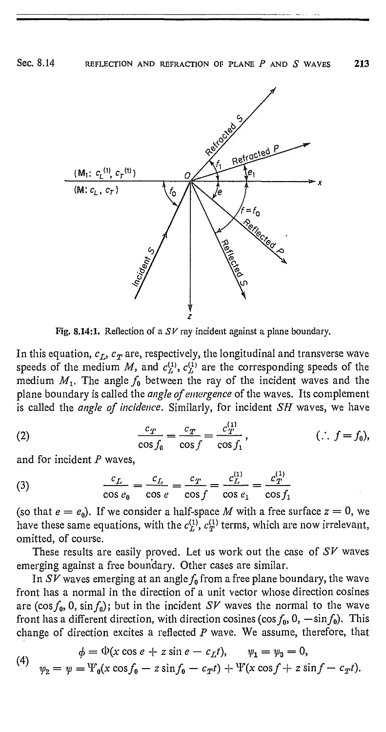
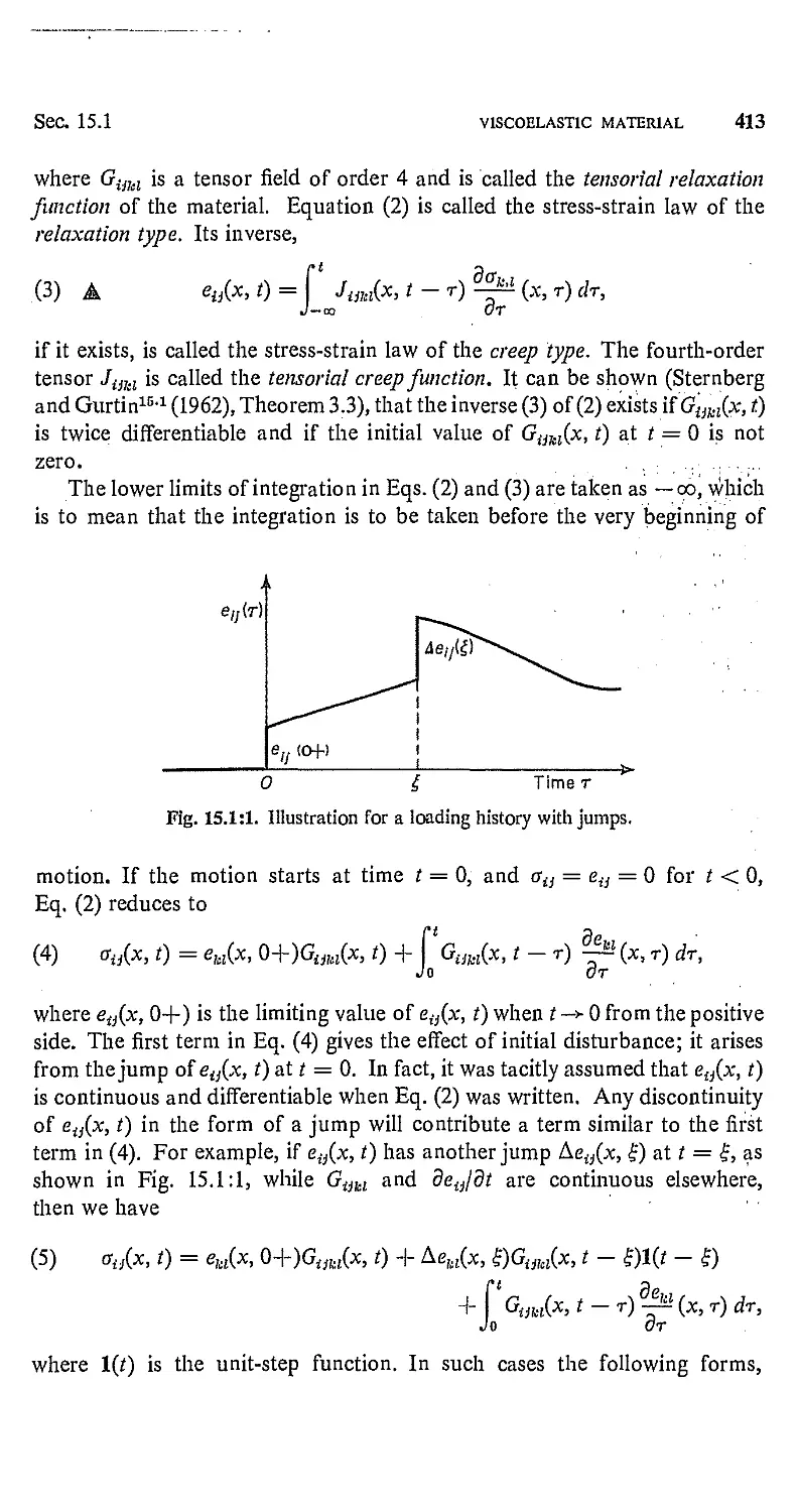
Текст
FOUNDATIONS OF
SOLID MECHANICS
Prentice-Hall International Series in Dynamics
Y. C. Fung, Editor
PRENTICE-HALL, INC.
ENTICE-HALL INTERNATIONAL, INC., UNITED KINGDOM AND EIRE
PRENTICE-HALL OF CANADA, LTD., CANADA
Foundations of Solid Mechanics by Y. C. Fung
Principles of Dynamics by Donald T. Greenwood
FOUNDATIONS OF
OLID MECHANIC
Y. C. FUNG
Professor, California Institute of Technology
PRENTICE-HALL, INC.
Englewood Cliffs, New Jersey
PRENTICE-HALL INTERNATIONAL, INC., London
PRENTICE-HALL OF AUSTRALIA, PTY., LTD., Sydney
PRENTICE-HALL OF CANADA, LTD., Toronto
PRENTICE-HALL OF INDIA (PRIVATE) LTD., New Delhi
PRENTICE-HALL OF JAPAN, INC., Tokyo
© 1965 by Prentice-Hall, Inc., Englewood Cliffs, N.J.
All rights reserved. No part of this book may be
reproduced in any form, by mimeograph or any other means,
without permission in writing from the publisher. Library
of Congress Catalog Card Number 65-18496.
Current printing (last digit):
11 10 9 8 7 6 5 4
Printed in the United States of America
32991—C
To
My Mother
'i^^^33s^&^^^^s^^^3^^^'
PREFACE
Solid mechanics deals with the deformation and motion of "solids." The
displacement that connects the instantaneous position of a particle to its
position in an "original" state is of general interest. The preoccupation about
particle displacements distinguishes solid mechanics from that of fluids.
This book is written for engineers and scientists who have had some
exposure to the theory of strength of materials and elasticity. It deals with
the mechanics of continuous media. The bulk of the text is concerned with
the classical theory of elasticity, but the discussion also includes
thermodynamics of solids, thermoelasticity, viscoelasticity, plasticity, and finite
deformation theory. Fluid mechanics is excluded. Both dynamics and statics
are treated; the concepts of wave propagations are introduced at an early
stage. Variational calculus is emphasized, since it provides a unified point
of view and is useful in formulating approximate theories.
Since the book is of an introductory nature, an introduction to the tensor
analysis and the calculus of variations is included. The general tensor theory
is presented here for those readers who are interested in advanced literature.
However, to reach a wider circle of readers, I have used only Cartesian
tensors in developing the theory (see footnote on p. 37). I believe that those
who will take the time to study the general tensor analysis will find ample
reward: the simplicity in conception and the efficiency of the notations gives
the subject a great beauty.
The text was developed from my notes for a course offered to graduate
students at the California Institute of Technology. Since the beginning of
1959, it was decided to modify the traditional elasticity course to one that
gave greater emphasis to general methodology. This shift in emphasis was
prompted by the broadening of engineering fields in recent years. It has been
my experience in long association with the aerospace industry that young
engineers are often asked to deal with subjects which were not taught in
school. In view of the constantly changing problems in engineering, I believe
that a broad course m solid mechanics is useful.
Of course, no one path can embrace the broad field of mechanics. As in
mountain climbing, some routes are safe to travel, others more perilous; some
may lead to the summit, others to different vistas of interest; some have
popular claims, others are less traveled. In choosing a particular path for
a tour through the field, one is influenced by the curricula, the trends in
vii
viii PREFACE
literature, the interest in engineering and science. Here, a particular way has
been chosen to view some of the most beautiful vistas in classical mechanics.
In making this choice I have aimed at straightforwardness and interest, and
practical usefulness in the long run.
Holding the book to reasonable length did not permit inclusion of many
numerical examples, which have to be supplemented through problems and
references. Fortunately, there are many excellent references to meet this
demand; a fairly comprehensive bibliography is included.
I am indebted to many authors whose writings are classics in this field.
To Love, Lamb, Timoshenko, Southwell, von Karman, Prager, Synge, Biot,
Green, Truesdell and many others, I am especially indebted. The study of
classical mechanics is a profound experience. The deeper one delves into it,
the more he appreciates the contributions of great masters.
It remains for me to record my gratitude to many of my teachers,
colleagues, friends, and students. My appreciation of mechanics as a living
subject was enhanced through many years of association with Prof. Ernest
E. Sechler and Dr. Millard V. Barton. Their deep insight of many facets of
engineering and broad knowledge about practical matters of design and
construction inspires people around them always to seek a better or simpler
solution. To the late Dr. Aristotle D. Michal, professor of mathematics at
the California Institute of Technology, I am grateful for his gentle
encouragement and guidance in earlier years. To Drs. Hans Krumhaar and Max L.
Williams, who shared with me the teaching of the course from which this
book was developed, I owe a special note of thanks. Sections 10.1-6 are
based on Dr. Krumhaar's notes. Dr. John A. Morgan, professor of engineering
at UCLA, read the entire manuscript and gave me many valuable suggestions
for improvements. Dr. Benjamin Cummings checked part of the manuscript.
Drs. Charles Babcock, jr., Wolfgang G. Knaus, Wei-Hsuin Yang, Gilbert A.
Hegemier, Jerold L. Swedlow, and Messrs. Pin Tong, Jen-Shih Lee, and
Jay-Chimg Chen read the proofs and made many useful suggestions. I also
wish to thank many of my students, not named here individually, without
whose discussions the book would not have taken this form. The Prentice-
Hall staff has been very cooperative. In particular, Mr. Nicholas Romanelli
offered his competent knowledge and gave unstinted effort in editing this
book. The preparation of the manuscript was helped by Helen Burrus, Joan
Christensen, Jeanette Siefke, and Sandra Mann, who typed and retyped as
the words were weighed and revised, without showing a hint of annoyance.
To all of them I am truly thankful.
Y.C.F.
CONTENTS
1 PROTOTYPES OF THE THEORY OF ELASTICITY AND
VISCOELASTICITY
1.1. Hoolce's Law and Its Consequences
1.2. Positive Definiteness of the Strain Energy and the
Uniqueness of Solution
1.3. Minimum Complementary Energy Theorem
1.4. The Minimum Potential Energy Theorem
1.5. Some Important Remarks
■ 1.6. Linear Solids with Memory: Models of Viscoelasticity
..- 1.7. Sinusoidal Oscillations in a Viscoelastic Material
1.8. Structural Problems of Viscoelastic Materials
2 TENSOR ANALYSIS
2.1. Notation and Summation Convention
2.2. Coordinate Transformation
2.3. Euclidean Metric Tensor
2.4. Scalars, Contravariant Vectors, Covariant Vectors
2.5. Tensor Fields of Higher Rank
2.6. Some Important Special Tensors
2.7. The Significance of Tensor Characteristics
2.8. Cartesian Tensors
2.9. Contraction
2.10. Quotient Rule
2.11. Partial Derivatives in Cartesian Coordinates
2.12. Covariant Differentiation of Vector Fields
2.13. Tensor Equations
2.14. Geometric Interpretation of Tensor Components
2.15. Geometric Interpretation of Covariant Derivatives
2.16. Physical Components of a Vector
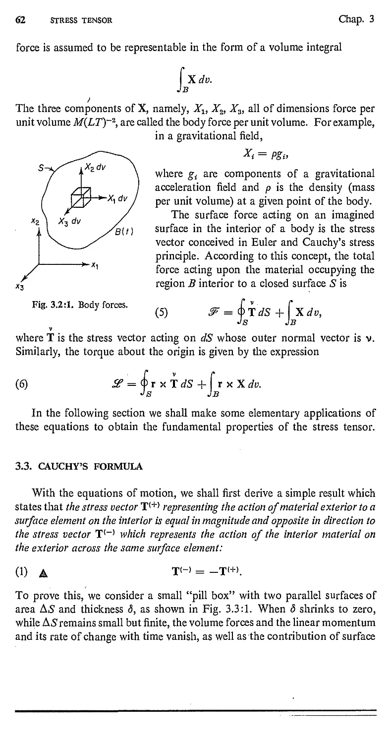
3 STRESS TENSOR
3.1. Stresses
3.2. Laws of Motion
3.3. Cauchy's Formula
ix
X CONTENTS
3.4. Equations of Equilibrium 65
3.5. Transformation of Coordinates 69
3.6. Plane State of Stress 70
3.7. Principal Stresses 72
3.8. Lame Stress Ellipsoid 75
3.9. Cauchy's Stress Quadric 76
3.10. Shearing Stresses 78
3.11. Mohr's Circles 79
3.12. Stress Deviations 80
3.13. Octahedral Shearing Stress 81
3.14. Stress Tensor in General Coordinates 82
3.15. Physical Components of a Stress Tensor in General
Coordinates 86
3.16. Equation of Equilibrium in Curvilinear Coordinates 87
4 ANALYSIS OF STRAIN 89
4.1. Deformation 89
4.2. Strain Tensors in Rectangular Cartesian Coordinates 92
4.3. Geometric Interpretation of Infinitesimal Strain
Components 94
4.4. Rotation 96
4.5. Finite Strain Components 97
4.6. Compatibility of Strain Components 99
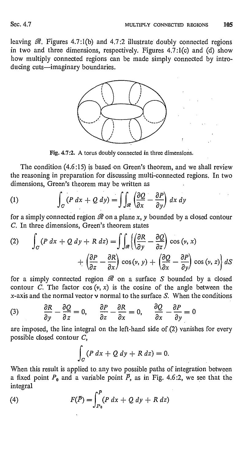
4.7. Multiply Connected Regions 104
4.8. Multivalued Displacements 107
4.9. Properties of the Strain Tensor 108
4.10. Physical Components 111
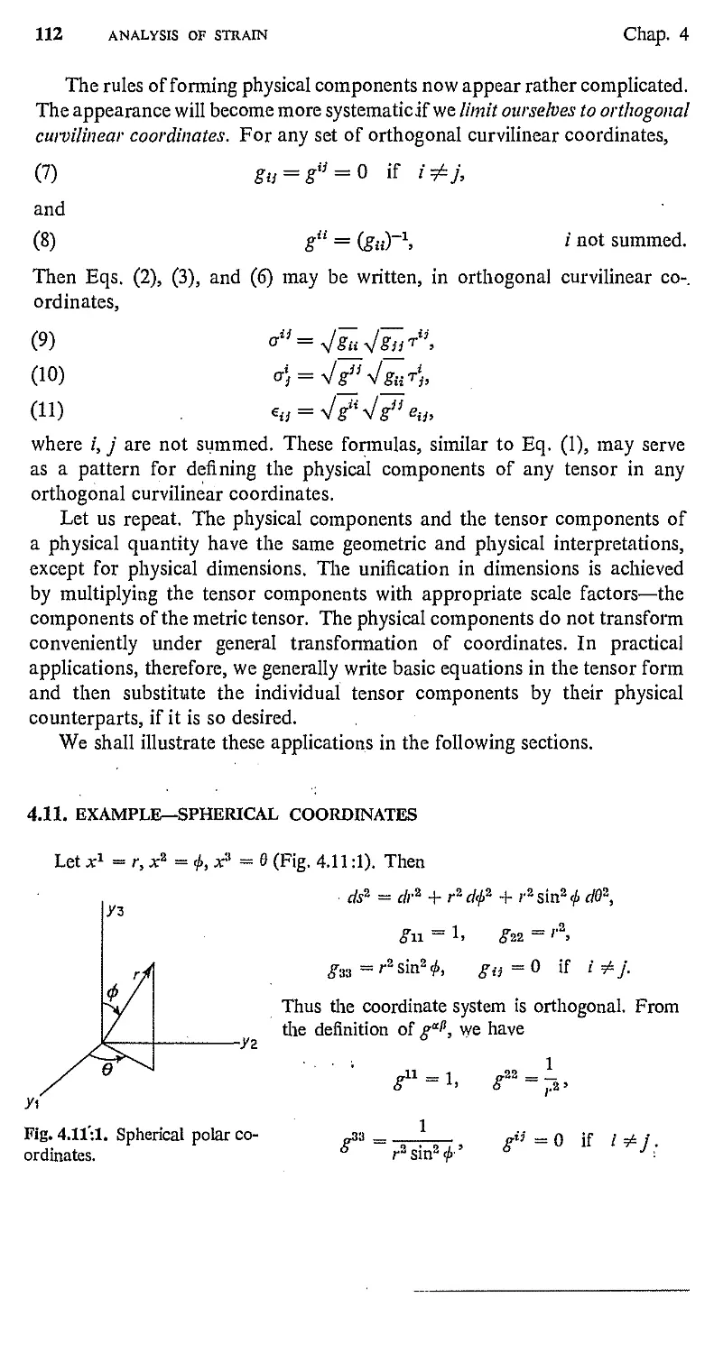
4.11. Example—Spherical Coordinates 112
4.12. Example—Cylindrical Polar Coordinates 114
5 CONSERVATION LAWS 116
5.1. Gauss' Theorem 116
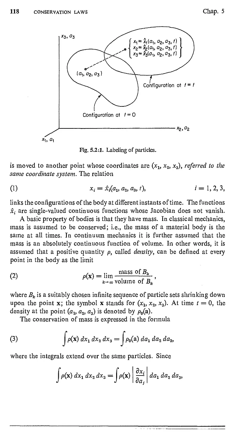
5.2. Material and Spatial Description of Changing Configurations 117
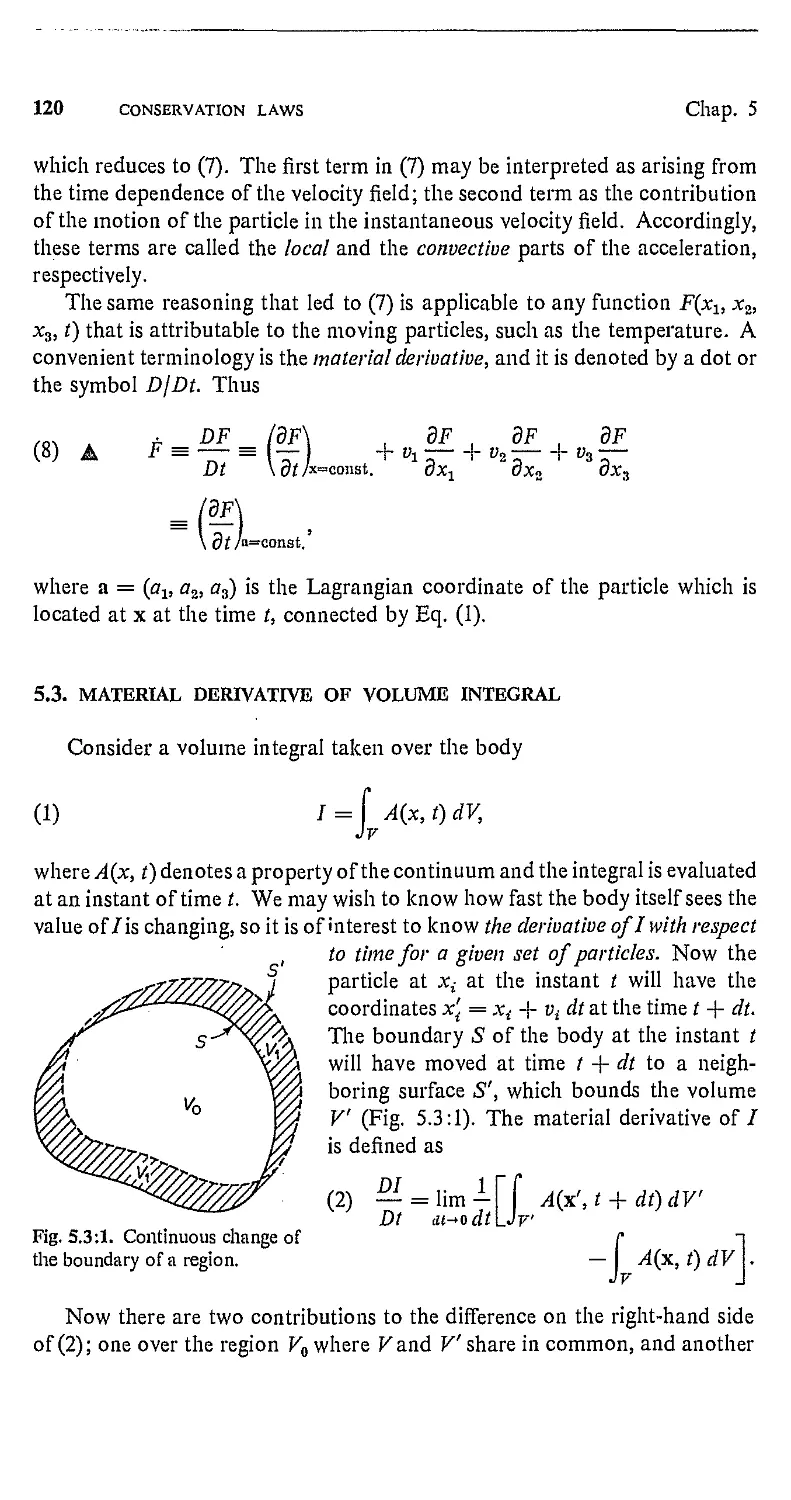
5.3. Material Derivative of Volume Integral 120
5.4. The Equation of Continuity 121
5.5. The Equations of Motion 122
5.6. Moment of Momentum 123
5.7. Other Field Equations 124
6 ELASTIC AND PLASTIC BEHAVIOR OF MATERIALS 127
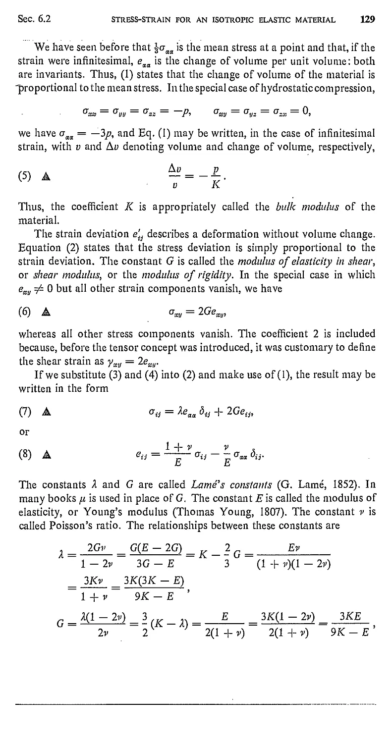
6.1. Generalized Hooke's Law 127
6.2. Stress-Strain Relationship for an Isotropic Elastic Material 128
6.3. Ideal Plastic Solids 131
6.4. Some Experimental Information 134
CONTENTS XI
6.5. A Basic Assumption of the Mathematical Theory of
Plasticity 137
6.6. Loading and Unloading Criteria 140
6.7. Isotropic Stress Theories 141
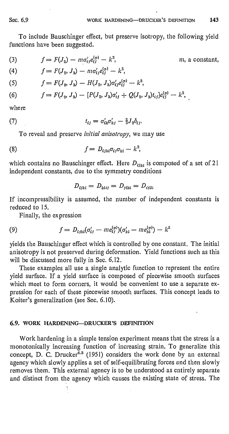
6.8. Further Examples of Yield Functions 142
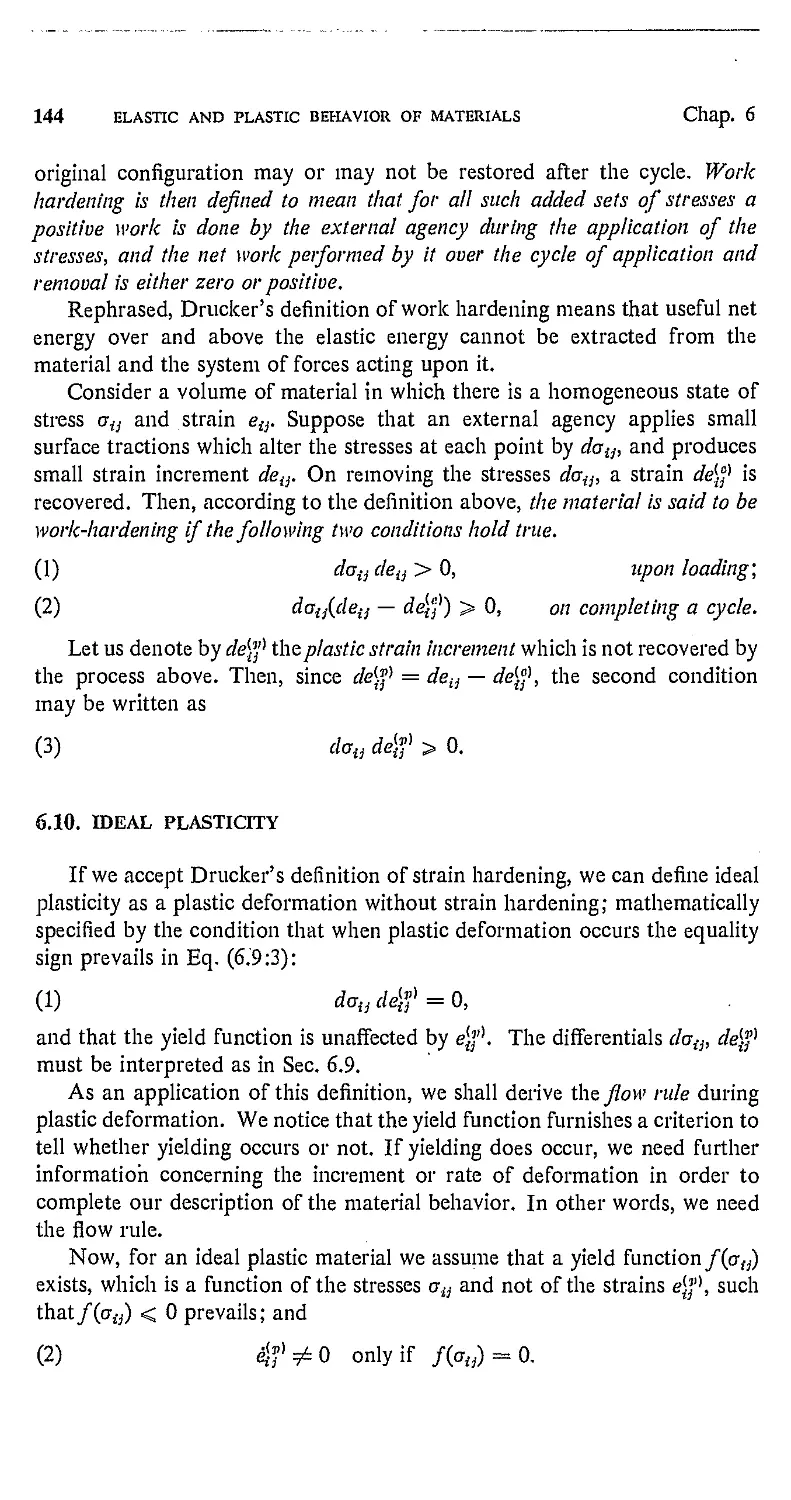
6.9. Work Hardening—Druclcer's Definition 143
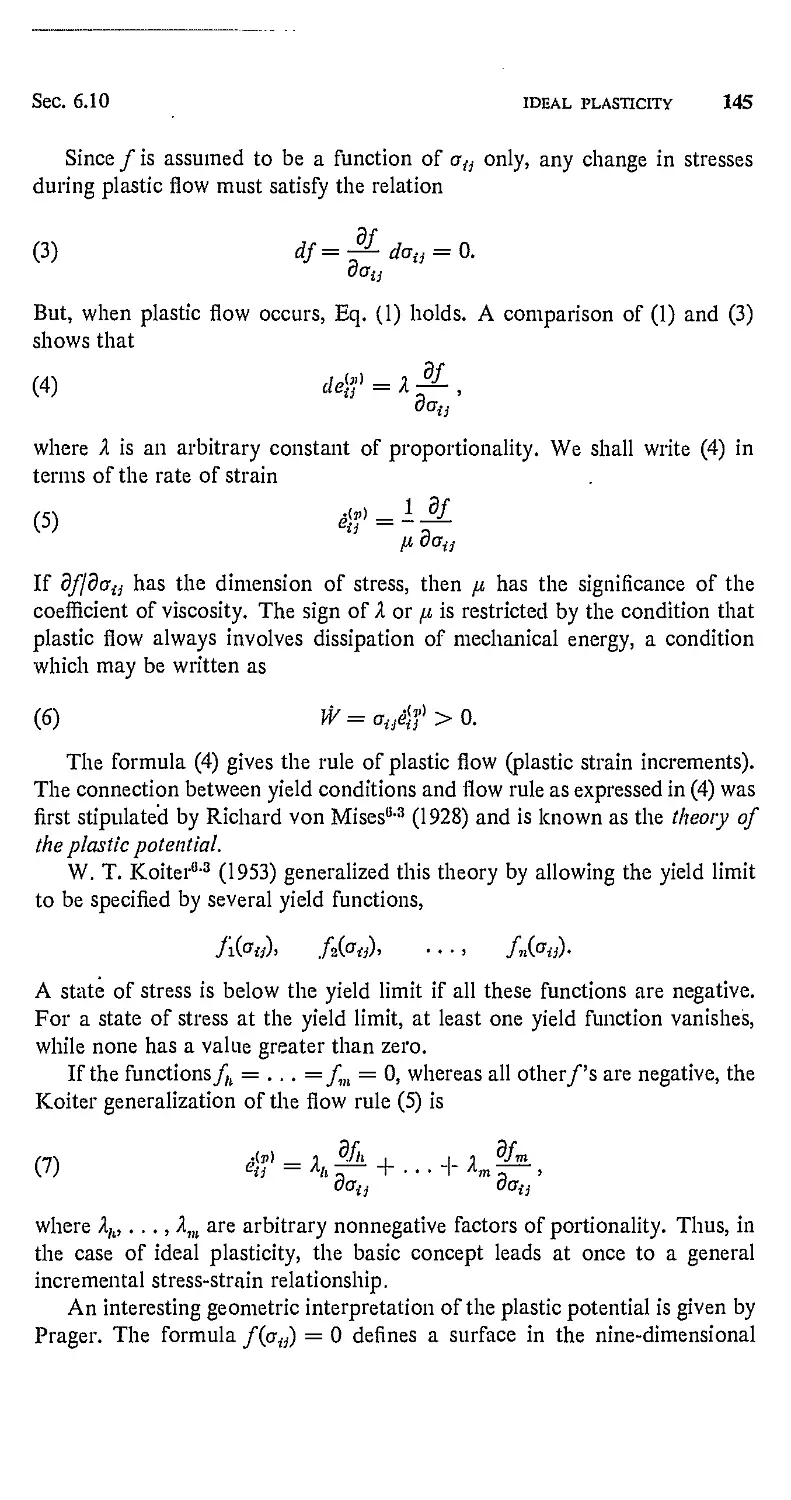
6.10. Ideal Plasticity 144
6.11. Flow Rule for Work-Hardening Materials 147
6.12. Subsequent Loading Surfaces—Hardening Rules 150
7 LINEAR ELASTICITY 154
7.1. Basic Equations of Elasticity for Homogeneous Isotropic •
Bodies 154
7.2. Equilibrium of an Elastic Body Under Zero Body Force 156
7.3. Boundary Value Problems 157
7.4. The Problem of Equilibrium and the Uniqueness of
Solutions in Elasticity 160
7.5. Saint Venant's Theory of Torsion 162
7.6. Soap Film Analogy 170
7.7. Bending of Beams 172
7.8. Plane Elastic Waves 176
. 7,9. Rayleigh Surface Waves 178
7.10. Love Waves 182
8 SOLUTION OF PROBLEMS IN ELASTICITY BY
POTENTIALS 184
8.1. The Scalar and Vector Potentials for the Displacement
Vector Fields 184
8.2. Equations of Motion in Terms of Displacement Potentials 186
8.3. Strain Potential 189
8.4. Galerkin Vector 191
8.5. Equivalent Galerkin Vectors 194
8.6. Example—Vertical Load on the Horizontal Surface of a
Semi-Infinite Solid 195
8.7. Love's Strain Function 197
8.8. Kelvin's Problem—A Single Force Acting in the Interior
of an Infinite Solid 198
8.9. Perturbation of Elasticity Solutions by a Change of Poisson's
Ratio 202
8.10. Boussinesq's Problem 205
8.11. On Biharmonic Functions 206
8.12. Neuber-Papkovich Representation 210
8.13. Other Methods of Solution of Elastostatic Problems 211
8.14. Reflection and Refraction of Plane P and S Waves 212
8.15. Lamb's Problem—Line Load Suddenly Applied on Elastic
Half-Space 214
xii CONTENTS
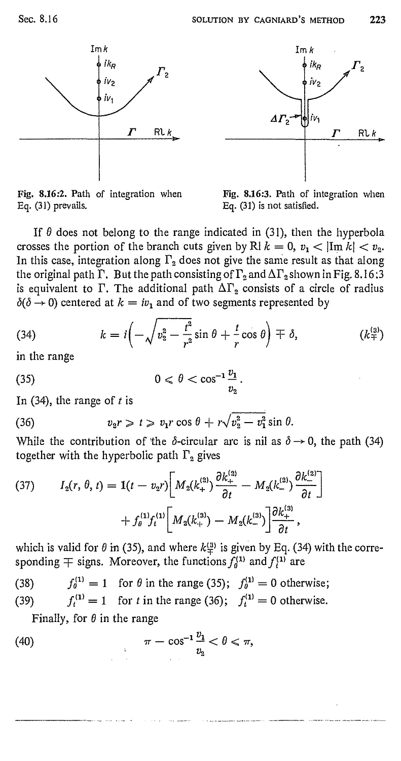
8.16. Solution by Cagniard's Method 218
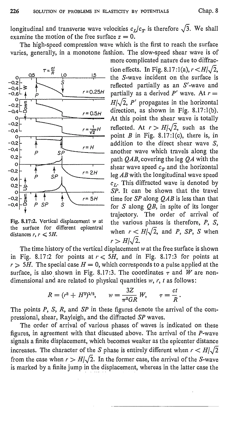
8.17. Motion of the Surface Due to a Buried Pulse 225
8.18. Galerkin Vector and Neuber-Papkovich Functions in
Dynamics 228
9 TWO-DIMENSIONAL PROBLEMS IN ELASTICITY 233
9.1. Plane State of Stress or Strain 233
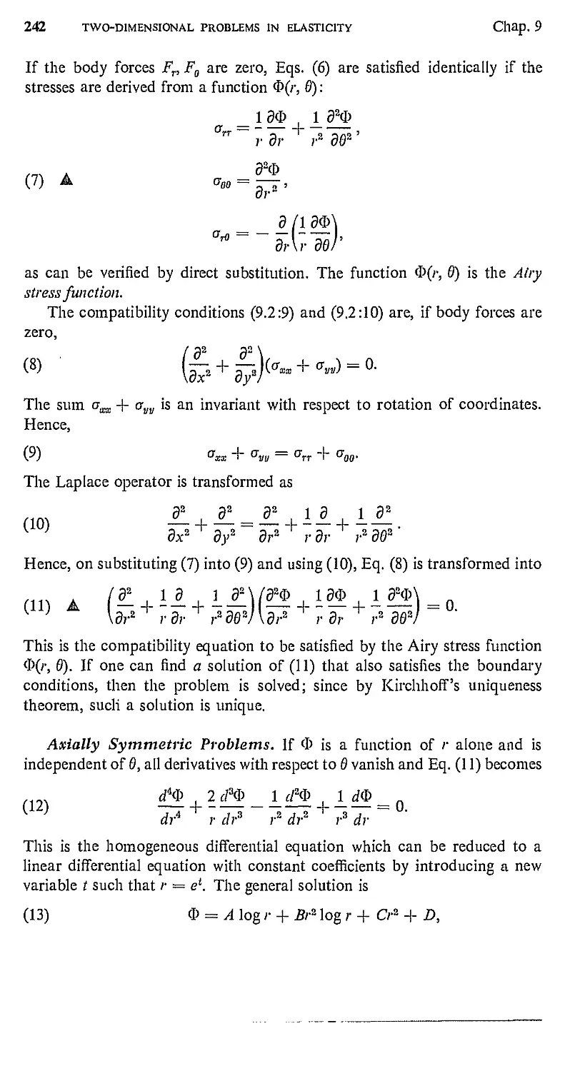
9.2. Airy Stress Functions for Two-Dimensional Problems 235
9.3. Airy Stress Function in Polar Coordinates 241
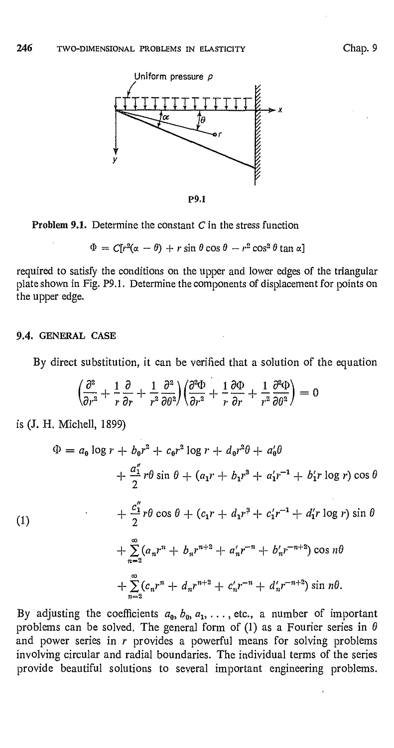
9.4. General Case 246
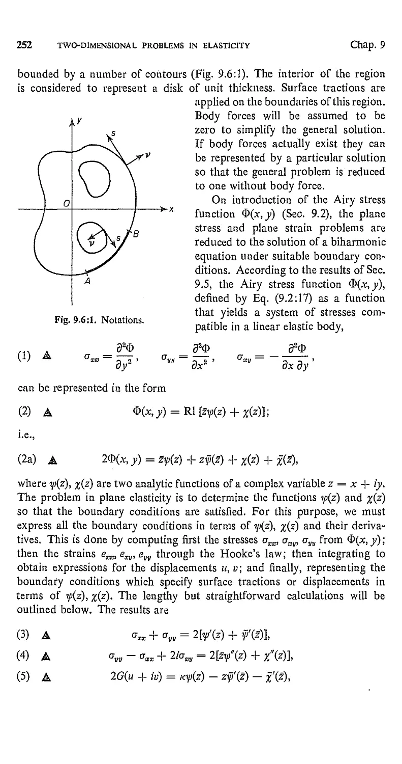
9.5. Representation of Two-Dimensional Biharmo'nic Functions
by Analytic Functions of a Complex Variable 250
9.6. Kolosoff-Muskhelishvili Method 251
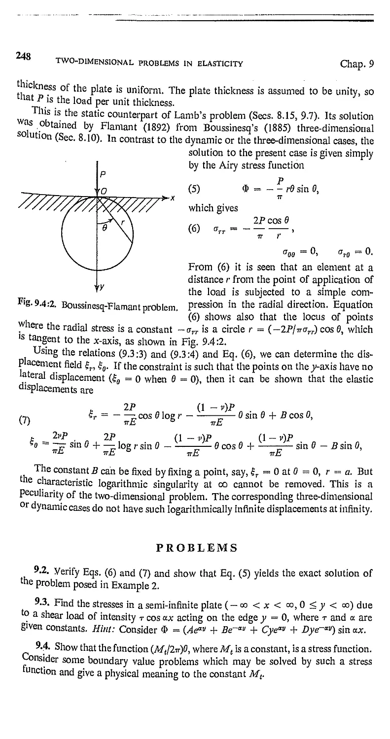
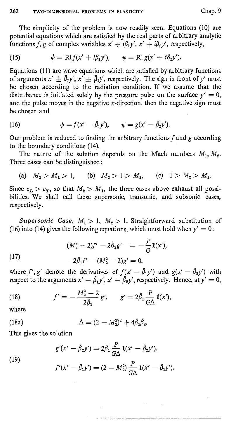
9.7. Steady-State Response to Moving Loads 259
9.8. Alternate Method of Solution 266
10 VARIATIONAL CALCULUS, ENERGY THEOREMS,
SAINT-VENANT'S PRINCIPLE 270
10.1. Minimization of Functional 270
10.2. Functional Involving Higher Derivatives of the Dependent
Variable 275
10.3. Several Unknown Functions 276
10.4. Several Independent Variables 278
10.5. Subsidiary Conditions—Lagrangian Multipliers 280
10.6. Natural Boundary Conditions 283
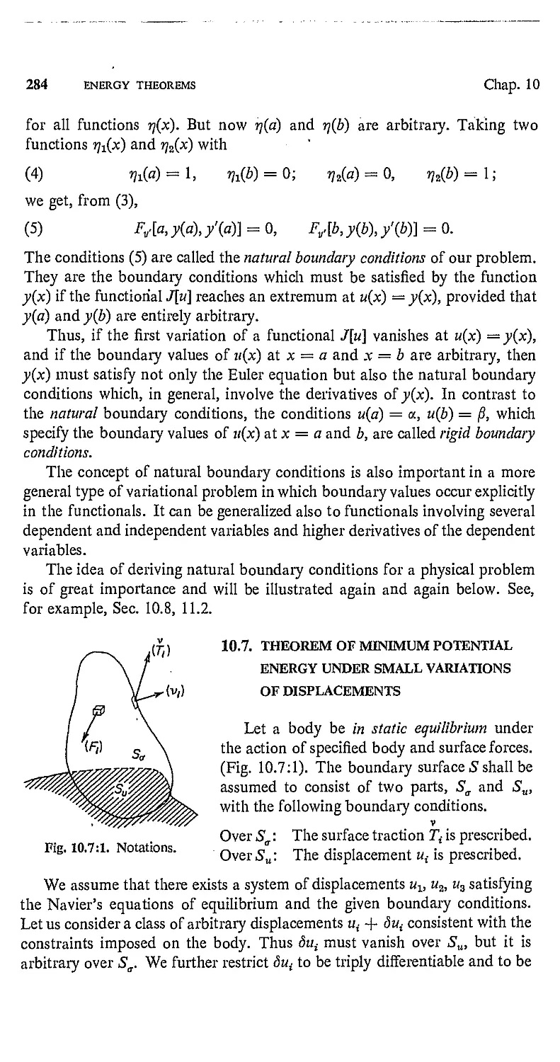
10.7. Theorem of Minimum Potential Energy Under Small
Variations of Displacements 284
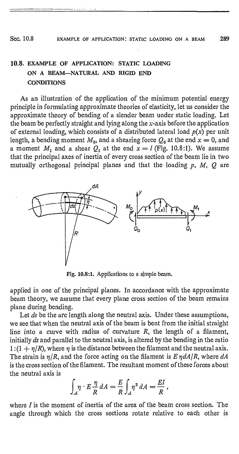
10.8. Example of Application: Static Loading on a Beam—
Natural and Rigid End Conditions 289
10.9. The Complementary Energy Theorem Under Small
Variations of Stresses 292
10.10. Reissner's Principle 299
10.11. Saint-Venant's Principle 300
10.12. Saint-Venant's Principle—Boussinesq~Von Mises-Sternberg
Formulation 304
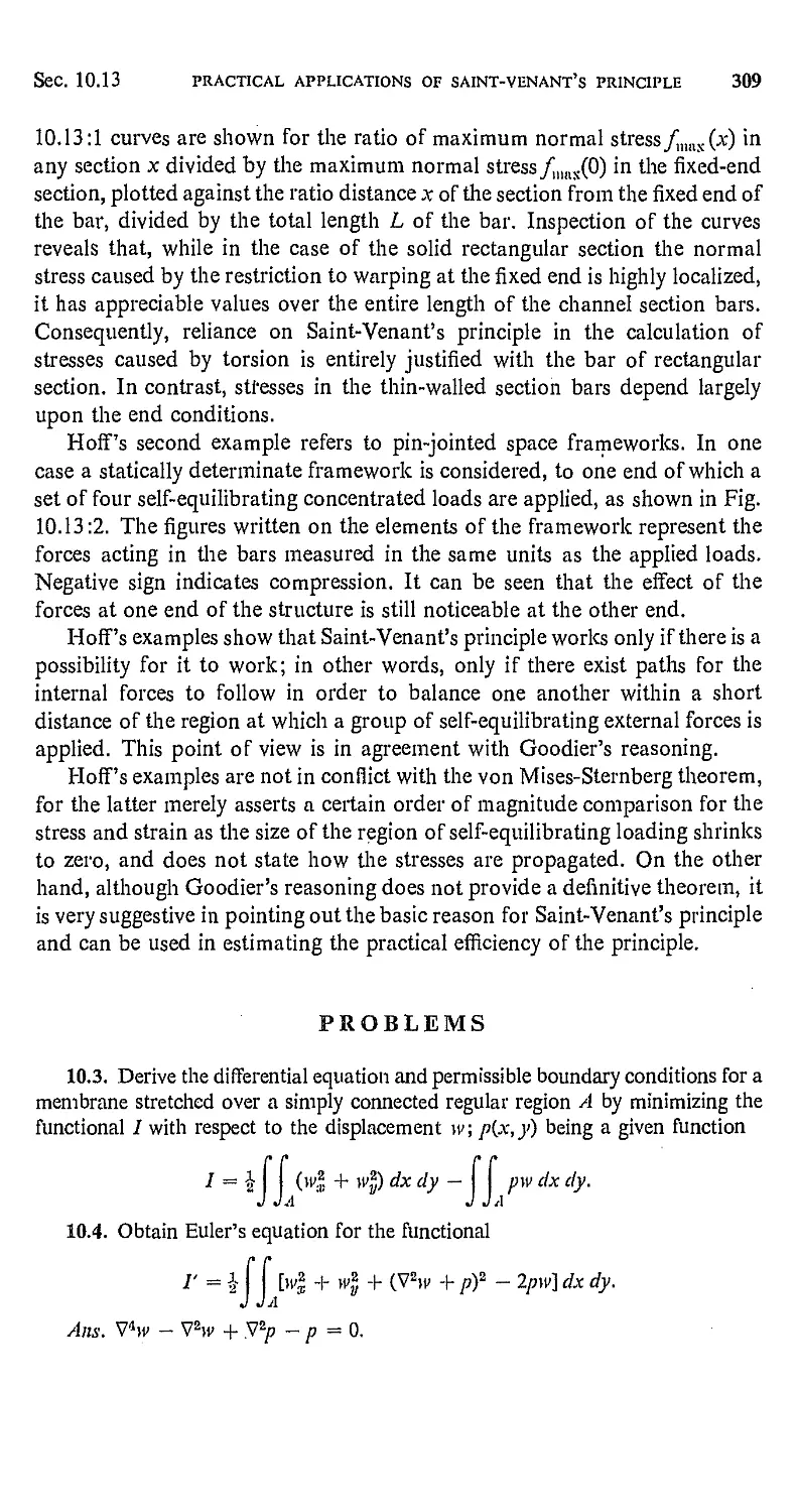
10.13. Practical Applications of Saint-Venant's Principle 306
11 HAMILTON'S PRINCIPLE, WAVE PROPAGATION,
APPLICATIONS OF GENERALIZED COORDINATES 315
11.1. Hamilton's Principle 315
11.2. Example of Application—Equation of Vibration of a Beam 319
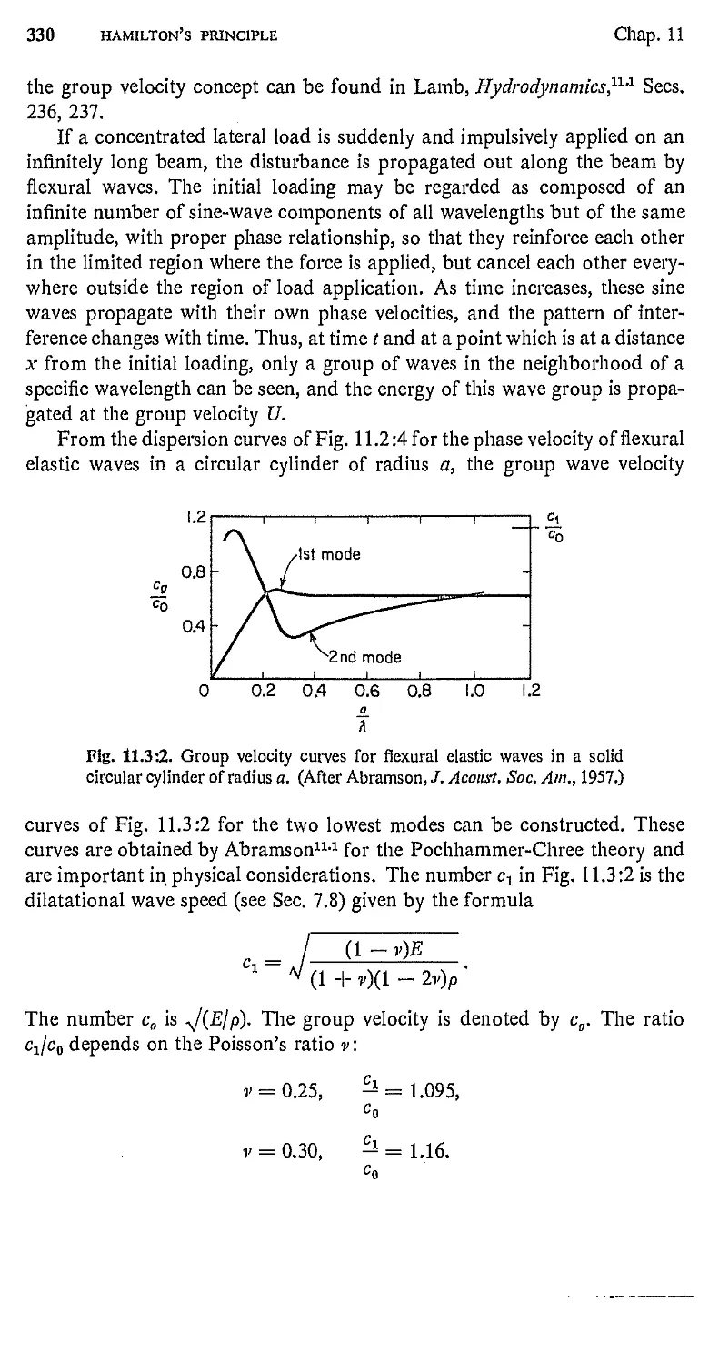
11.3. Group Velocity 328
11.4. Hopkinson's Experiments 331
11.5. Generalized Coordinates
11.6. Approximate Representation of Functions
11.7, Approximate Solution of Differential Equations
11.8, Direct Methods of Variational Calculus
12 ELASTICITY AND THERMODYNAMICS
12.1. The Laws of Thermodynamics
12.2. The Energy Equation
12.3. The Strain Energy Function
12.4. The Conditions of Thermodynamic Equilibrium
12.5. The Positive Definiteness of the Strain Energy Function
12.6. Thermodynamic Restrictions on the Stress-Strain Law of an
Isotropic Elastic Material
12.7. Generalized Hooke's Law, Including the Effect of Thermal
Expansion
12.8. Thermodynamic Functions for Isotropic Hoolcean Materials
12.9. Equations Connecting Thermal and Mechanical Properties
of a Solid
13 IRREVERSIBLE THERMODYNAMICS AND
VISCOELASTTCITY
13.1. Basic Assumptions
13.2. One-Dimensional Heat Conduction
13.3. Phenomenological Relations—Onsager Principle
13.4. Basic Equations of Thermomechanics
13.5. Equations of Evolution for a Linear Hereditary Material
13.6. Relaxation Modes
13.7. Normal Coordinates
13.8. Hidden Variables and the Force-Displacement Relationship
13.9. Anisotropic Linear Viscoelastic Materials
14 THERMOELASTICITY
14.1. Basic Equations
14.2. Thermal Effects Due to a Change of Strain; Kelvin's
Formula
14.3. Ratio of Adiabatic to Isothermal Elastic Moduli
14.4. Uncoupled, Quasi-Static Thermoelastic Theory
14.5. Temperature Distribution
14.6. Thermal Stresses
14.7. Particular Integral: Goodier's Method
14.8. Plane Strain
14.9. An Example—Stresses in a Turbine Disk
14.10. Variational Principle for Uncoupled Thermoelasticity
14.11. Variational Principle for Heat Conduction
XIV CONTENTS
14.12. Coupled Thermoelasticity
14.13. Lagrangian Equations for Heat Conduction and
Thermoelasticity
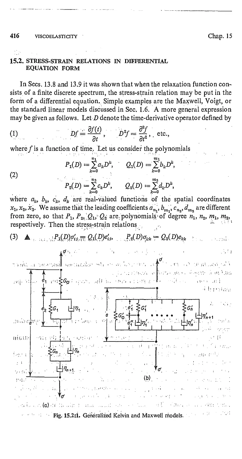
15 VISCOELASTICITY
15.1. Viscoelastic Material
15.2. Stress-Strain Relations in Differential Equation Form
15.3. Boundary-Value Problems and Integral Transformations
15.4. Waves in an Infinite Medium
15.5. Quasi-Static Problems
15.6. Reciprocity Relations
16 FINITE DEFORMATION
16.1. Strain Tensors
16.2. Lagrange's and KirchhofTs Stress Tensors
16.3. Equation of Motion in Lagrangian Description
16.4. Rate of Deformation
16.5. Viscous Fluid
16.6. Elasticity, Hyperelasticity, and Hypoelasticity
16.7. The Strain Energy Function and Variational Principles
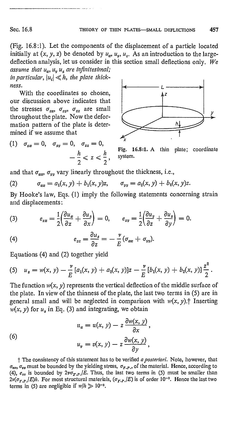
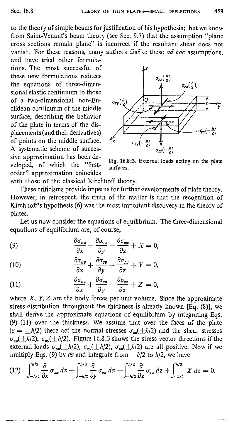
16.8. Theory of Thin Plates—Small Deflections
16.9. Large Deflections of Plates
EPILOGUE
NOTES
BIBLIOGRAPHY
INDEX
PROTOTYPES OF THE THEORY OF
ELASTICITY AND VISCOELASTICITY
Historically, the notion of elasticity was first announced in 1676 by Robert
Hooke (1635-1703) in the form of an anagram, ceiiinosssttuv. He explained
it in 1678 as
Ut tertsio sic vis,
or "the power of any springy body is in the same proportion with the
extension."! The mathematical theory developed and extended to other
materials since that time is associated with the names of practically all great
mathematical physicists of the last three centuries and forms one of the
most important parts of classical physics. The line of inquiry has never
been broken, and in recent times we witness the most vigorous developments. $
Hooke's law is the constitutive law for a Hoolceaii, or linear elastic, material.
As stated in the original form, its meaning is not very clear. Our first task is,
therefore, to give it a precise expression. This we shall do in two different
ways. The first way is to make use of the common notion of "springs," and
consider the load-deflection relationship. The second way is to state it as a
tensor equation connecting the stress and strain. Although the second way
is the proper way to start a general theory, the first, simpler and more
restrictive, is not without interest. In this chapter we develop the first
alternative.
1.1. HOOKE'S LAW AND ITS CONSEQUENCES
Let us consider the static equilibrium state of a solid body under the
action of external forces (Fig. 1.1:1). Let the body be supported in some
manner so that at least three points are fixed in a space which is described
with respect to a rectangular Cartesian frame of reference. We shall make
three basic hypotheses regarding the properties of the body under
consideration.
f Edme Mariotte enunciated the same law independently in J680.
t Some historical remarks are given in Notes 1.1, p. 473.
1
2 PROTOTYPES OF THEORY OF ELASTICITY AND VIS CO ELASTICITY Chap. 1
(HI) The body is continuous and remains continuous under the action of
externalforces.
Under this hypothesis the atomistic structure of the body is ignored and
the body is idealized into a geometrical copy in Euclidean space whose points
are identified with the material particles
of the body. The continuity is defined
in the mathematical sense with respect to
this idealized continuum. Neighboring
points remain as neighbors under any
loading condition. No cracks or holes
may open up in the interior of the body
under the action of external load.
A material satisfying this hypothesis
Fig. 1.1:1. Static equilibrium of a body is said to be a continuum. The study of
under external forces. the deformation or motion of a continuum
is called the continuum mechanics.
To introduce the second hypothesis, let us consider the action of a set of
forces on the body. Let every force be fixed in direction and in point of
application, and let the magnitude of all the forces be increased or decreased
together: always bearing the same ratio to each other. Let the forces be
denoted by Pl3 P2,.. ., Pn and their magnitude by PXi P2,..., Pn. Then
the ratios Px : P2 :. .. : Pn remain fixed. When such a set of forces is applied
on the body, the body deforms. Let the displacement at an arbitrary point
in an arbitrary direction be measured with respect to a rectangular Cartesian
frame of reference fixed with the supports. Let this displacement be denoted
by u. Then our second hypothesis is
(H2) Hooke's law,
(1).
u = axPx + a2P2 + ... + anPni
where aXia2i ..., an are constants independent of the magnitude ofPltPZi...,
Pn. The constants aXi a2i..., an depend, of course, on the location of the
point at which the displacement component is measured and on the directions
and points of application of the individual forces of the loading.
Hooke's law in the form (H2) is one that can be subjected readily to
direct experimental examination.
To complete the formulation of the theory of elasticity, we need a third
hypothesis:
(H3) There exists a unique unstressed state of the body, to which the body
returns whenever ail the external forces are removed.
A body satisfying these three hypotheses is called a linear elastic solid.
Sec. 1,1
hooke's law and its consequences 3
A number of deductions can be drawn from these assumptions. We
shall list a few important ones.
(A) The principle of superposition for loads at the same point
Let Fx and P^ be forces in the same direction acting through the same
point. Then the resultant displacement n is equal to the sum of the
displacements produced by Px and P^ acting individually, regardless of the
order of application of Px and P{. This is evident from (H2) when "applied to
one load alone.
(B) Principle of superposition
By a combination of (H2) and (H3), we can show that Eq. (1) is valid not
only for systems of loads for which the ratios PX:P» :. .. :Pn remain fixed
as originally assumed, but also for an arbitrary set of loads Pl3 P2,..., Pw.
In other words, Eq. (1) holds regardless of the order in which the loads are
applied. The constant ax is independent of the loads P2, P3,. . ., Pw. The
constant a2 is independent of the loads Px, P3,..., Pw; etc. This is the
principle of superposition of the load-and-deflection relationship.
Proof If a proof of the statement above can be established for an
arbitrary pair of loads, then the general theorem can be proved by mathematical
induction.
Let Fx and P2 (with magnitudes Px and P^) be a pair of arbitrary loads
acting at points 1 and 2, respectively. Let the deflection in a specific direction
be measured at a point 3 (see Fig. 1.1:1). According to (H2), if Px is applied
alone, then at the point 3 a deflection «3 = ciXPx is produced. If P2 is applied
alone, a deflection */3 = c^zPz is produced. If Px and P2 are applied together,
with the ratio PX:P2 fixed, then according to (H2) the deflection can be
written as
(a) lh = di\P\ + ^32^2-
The question arises whether c!n = c31, c32 = c32. The answer is affirmative,
as can be shown as follows. After Fx and P2 are applied, we take away Fx.
This produces a change in deflection, —clxPXi and the total deflection becomes
(b) «s = c'uPx + c'^P* - clxPx.
Now only P2 acts on the body. Hence, upon unloading Pa we shall have
(c) l/3 = ^31^1 "T C32* 2 ^-31^ 1 ^32* 2*
Now all the loads are removed, and u3 must vanish according to (H3).
Rearranging terms, we have
(d) (c31 - clx)Px = (c32 - c32)P2.
4 PROTOTYPES OF THEORY OF ELASTICITY AND V1SCOELASTIC1TY Chap. 1
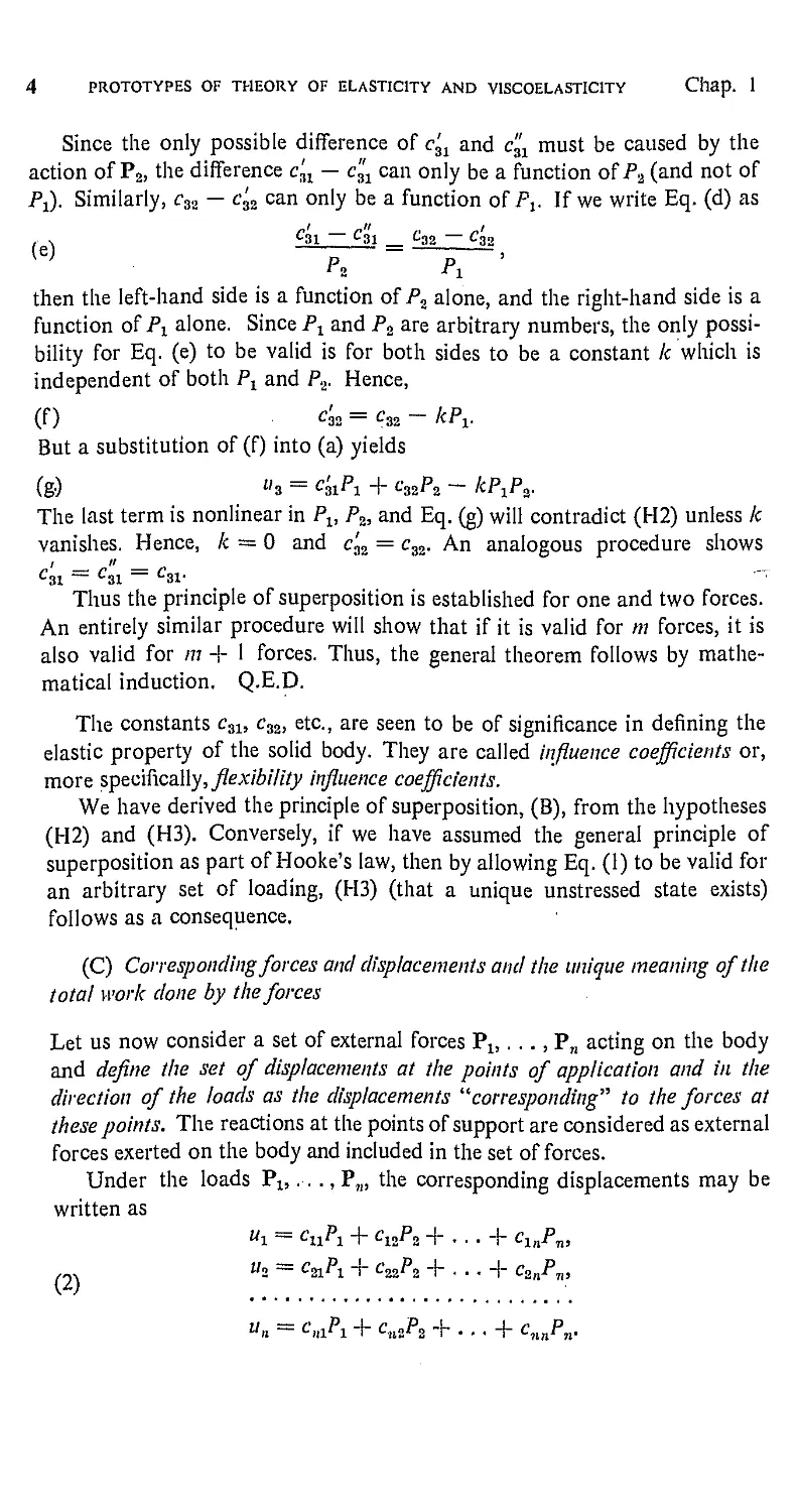
Since the only possible difference of c^ and c3i must be caused by the
action of P2, the difference c'nx — c31 can only be a function of Pa (and not of
Px). Similarly, c32 — c32 can only be a function of Pv If we write Eq. (d) as
/ \ g31 g3l ^32 — C32
(e) ________
then the left-hand side is a function of P2 alone, and the right-hand side is a
function of Px alone. Since Px and P2 are arbitrary numbers, the only
possibility for Eq. (e) to be valid is for both sides to be a constant /c which is
independent of both Px and P2. Hence,
(f) <4 = c32 - kPx.
But a substitution of (f) into (a) yields
(g) »3 = ^31^1 + ^32^2 - kPlP*
The last term is nonlinear in Px, Pz, and Eq. (g) will contradict (H2) unless /c
vanishes. Hence, /c = 0 and c^ = c32. An analogous procedure shows
i »
C31 — C31 — C31' "
Thus the principle of superposition is established for one and two forces.
An entirely similar procedure will show that if it is valid for m forces, it is
also valid for m + 1 forces. Thus, the general theorem follows by
mathematical induction. Q.E.D.
The constants c3l5 c32, etc., are seen to be of significance in defining the
elastic property of the solid body. They are called influence coefficients or,
more specifically, flexibility influence coefficients.
We have derived the principle of superposition, (B), from the hypotheses
(H2) and (H3). Conversely, if we have assumed the general principle of
superposition as part of Hooke's law, then by allowing Eq. (1) to be valid for
an arbitrary set of loading, (H3) (that a unique unstressed state exists)
follows as a consequence.
(C) Corresponding forces and displacements and the unique meaning of t lie
total work done by the forces
Let us now consider a set of external forces Px,. . ., Pn acting on the body
and define the set of displacements at the points of application and in the
direction of the loads as the displacements "corresponding" to the forces at
these points. The reactions at the points of support are considered as external
forces exerted on the body and included in the set of forces.
Under the loads Pl5..., Pw, the corresponding displacements may be
written as
"i = cnPx + cl2P% +..- + cXnPn)
,~ »2 = ^21^1 + ^22^2 +-.. + C2nPn3
»» = c>api + cuiP2 + ... + cnnPn.
Sec. 1.1
hooke's law and its consequences 5
If we multiply the first equation by Px, the second by P2i etc., and add, we
obtain
(3) Pxitx + P2u2 + ... + Pnun = cnP\ + cx2PxP2 + . . .
-i- clHPxPn + czxPxP2 + c22Pi + ...+...+ cltnPl
The quantity above is independent of the order in which the loads are
applied. Hence, it has a definite meaning for each set of loads Pls..., Pn.
Now, in a special case, the meaning of the quantity on the left-hand side
of Eq. (3) is clear. This is the case in which the ratios Px : P% : P3 : . .. : Pn
are kept constant and the loading increases very slowly from zero to the
final value. In this case, the corresponding displacements also increase
proportionally and slowly. It is then obvious that the work.done by the force
Px is exactly \Pxuu that by P2 is £P2w2, etc- Hence, we conclude from (3) that
the total work done by the set of forces is independent of the order in which the
forces are applied.
(D) Maxwell's reciprocal relation
An important property of the influence coefficients of corresponding
displacements follows immediately.
The influence coefficients for corresponding forces and displacements are
symmetric,
(4) ctJ - c$i.
In other words, the displacement at a point i due to a unit load at another point
j is equal to the displacement at j due to a unit load at /", provided that the
displacements and forces "correspond" i.e., that they are measured in the
same direction at each point.
The proof is simple. Consider two forces Fx and P2 (Fig. 1.1:1). When
the forces are applied in the order Pl5 P2) the work done by the forces is easily
seen to be
W = KCllPl + ^22^2) + ^12^2.
When the order of application of the forces is interchanged, the work done is
Wl = XcnPZ+0^) + 0^^.
But according to (C) above, W — W for arbitrary Pu P2. Hence, c13 = c.n,
and the theorem is proved.
The reciprocal relation may be put into a different form, sometimes
more convenient in applications, as follows.
(E) Betti-Rayleigh reciprocal theorem.
Let a set of loads Px, P2,.. . ,'P7( produce a set of corresponding
displacements uXi u2j ..., un. Let a second set of loads P{, Fl,. .. , P,', acting in the
6 PROTOTYPES OF THEORY OF ELASTICITY AND VISCOELASTICITY Chap. 1
same directions and having the same points of application as those of the
first, produce the corresponding displacements u'Xi w£,. . ., u'n. Then
(5) Pxu[ + P%u'% + ...+ Pyn = P[ih + ...+ p>».
In other words, in a linear elastic solid, the work done by a set of forces acting
through the corresponding displacements produced by a second set of forces is
equal to the work done by the second set of forces acting through the
corresponding displacements produced by the first set of forces.
A straightforward proof is furnished by writing out the ut and ui in terms
of P{ and Pi, (/= 1,2,...,/7), with appropriate influence coefficients,
comparing the results on both sides of the equation, and utilizing the symmetry
of the influence coefficients.
In the form of Eq. (5), the reciprocal theorem can be generalized to include
moments and rotations as the corresponding generalized forces and generalized
displacements. An illustration is given in Fig. 1.1:2. These theorems are very
useful in practical applications.
For the same beam, c2^ = c^z.
(a) Forces and corresponding displacements.
(b) Generalized force (moment) and the
corresponding generalized displacement
(moment ~ rotation of angle).
Fig. 1.1:2. Illustration of the reciprocal theorem,
(F) Strain energy
Further insight can be gained from the first law of thermodynamics. When a
body is thermally isolated and thermal expansions are neglected the first
law states that the work done on the body by the external forces in a certain
time interval is equal to the increase in the kinetic energy and internal energy
in the same interval. If the process is so slow that the kinetic energy can be
ignored, the work done is seen to be equal to the change in internal energy.
Sec. 1.1
hooke's law and its consequences 7
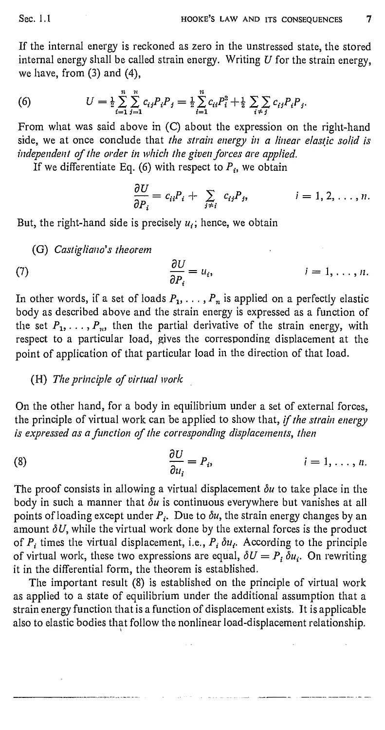
If the internal energy is reckoned as zero in the unstressed state, the stored
internal energy shall be called strain energy. Writing U for the strain energy,
we have, from (3) and (4),
(6) u=iii c^p,=i | Ciip\+i 11 Ctiptp,.
From what was said above in (C) about the expression on the right-hand
side, we at once conclude that the strain energy in a linear elastic solid is
independent of the order in which the given forces are applied.
If we differentiate Eq. (6) with respect to Pi9 we obtain
— = cHP{ + 2 ciSPj9 1=1,2,,,,, n,
OPi j*i
But, the right-hand side is precisely ut\ hence, we obtain
(G) Castigiiands theorem
(7) 5^ = M<' /=-1,...,/2.
dP{
In other words, if a set of loads Pl3.. . ,Pn is applied on a perfectly elastic
body as described above and the strain energy is expressed as a function of
the set -Pi,. . . , Pn3 then the partial derivative of the strain energy, with
respect to a particular load, gives the corresponding displacement at the
point of application of that particular load in the direction of that load.
(H) The principle of virtual work
On the other hand, for a body in equilibrium under a set of external forces,
the principle of virtual work can be applied to show that, if the strain energy
is expressed as a function of the corresponding displacements, then
(8) t- = p» ; = i,...,«.
The proof consists in allowing a virtual displacement du to take place in the
body in such a manner that du is continuous everywhere but vanishes at all
points of loading except under P{. Due to du, the strain energy changes by an
amount 3U, while the virtual work done by the external forces is the product
of P( times the virtual displacement, i.e., P{ du^. According to the principle
of virtual work, these two expressions are equal, 6U = P-t du^ On rewriting
it in the differential form, the theorem is established.
The important result (8) is established on the principle of virtual work
as applied to a state of equilibrium under the additional assumption that a
strain energy function that is a function of displacement exists. It is applicable
also to elastic bodies that follow the nonlinear load-displacement relationship.
8 PROTOTYPES OF THEORY OF ELASTICITY AND V1SCOELASTIC1TY Chap. I
1.2. POSITIVE DEFINITENESS OF THE STRAIN ENERGY
AND THE UNIQUENESS OF SOLUTION
The theorems established in the previous section [except (1.1:8)f which
is more general] are based on the hypotheses (HI), (H2), and (H3). Of
course, the theory can be modified by starting from some other hypothesis
which implies (H2) or (H3) as consequences. For example, we have
remarked that if we start from the assumption of principle of superposition,
then (H2) and (H3) follow as consequences. But this is a rather trivial change.
A much more significant alternative is to start with the assumption that a
strain energy function U exists which is expressible as a function of the
displacements. If such a strain energy function exists, we could use Eq.
(1.1 ;8), which is based on the principle of virtual work, and deduce the load-
displacement relationship for the elastic body. Obviously, the load-deflection
relation depends on the form of U, If U is a homogeneous quadratic function
ofux, Uo,.. . un {called a quadratic form), then Pt will be a linear function of
ux,.. . , un; and the load-displacement relationship is linear, as assumed by
Hooke's law. However, a nonlinear load-displacement relationship can be
formulated if an appropriate U other than a quadratic form in displacements
is assumed. This second approach was first taken by the self-taught
Nottingham genius, George Green (1793-1841), in 1837.
There is a theorem in thermodynamics which states that for a solid body
to have a stable natural state (such as the unstressed state of a linear elastic
solid) the strain energy function must be positive definite; i.e., it must be
nonnegative, and it is zero only in the natural state. We shall discuss this
further in Chap. 12. For the moment, let us assume the existence and the
positive deiiniteness of the strain energy function, and see what are the
consequences.
The positive deiiniteness of the strain energy function implies certain
relationships between the influence coefficients. For example, if Eq. (1.1:6)
which defines U in terms of Pl3. . ., Pti,
V
(1) ^ = 12^/+^2%¾
i=l i*J
is positive definite, i.e., U > 0, and the equality sign holds when and only
when all P's vanish, then the sum of the coefficients cH and the determinant
\cti\ are both positive. The necessary and sufficient conditions for the
positive deiiniteness of a quadratic form are well known. (See pp. 29, 30.)
These conditions restrict the elastic constants of a material, as we shall see
later.
Based on the assumption of the positive deiiniteness of the strain energy
function U as a function of the displacements, it is easy to establish the
t Equation (8) of Sec. 1.1. This notation will be used hereafter.
SeC. 1.2 POSITIVE DEFIN1TENESS Or THE STRAIN ENERGY 9
uniqueness theorem, (Kirchhoff, 1859). The theorem states that for a linear
elastic solid as defined in Sec. 1.1 and having a positive definite strain energy
function, there exists a one-to-one correspondence between the elastic
deformation and the forces acting on the body. A proof runs as follows. Let Eqs.
(1.1:2) define the displacements as functions of the corresponding forces so
that the strain energy function is expressible as (1). Let us assume that two
different sets of forces Px, Pz,. .., Fn and F{,.. ., P'n acting at points 1, 2,
...,« of a body correspond to a single state of deformation of the body. Let
us now first apply the loads Px,. .., P}) to deform the body; then let us apply
the loads — P[,..., —P'n to annul the displacements. The final configuration
is completely unstrained; hence, U = 0. However, there are the forces
Px — P[, P2 — P^, etc., acting on the body. This is impossible, because of the
assumed positive definiteness of U, unless Px = P{, Pz = Pi,, etc. Thus, a
contradiction is obtained. The assumption that two different sets of forces
correspond to the same displacements is untenable, and the uniqueness of
solution of the Eqs. (1.1:2) is proved.
Thus, Eqs. (1.1:2) can be solved uniquely. This implies, first, that the
determinant of the coefficients does not vanish.
(2)
11
^12
lit
C „o
»11
#0,
n.
■tfl UW2
and, second, that a unique solution
P\ = kuux + /c12tfs +•■• + kiHuu
(3) ■ - -
exists. Since c^ = cu, we can show that
(4) kis = kitt /J= 1,.
A substitution of (3) into (1) yields the strain energy expression
(5) U = i f kHiq + i J 2 klsihus,
which could, of course, be derived directly by multiplying the individual
forces Px,, .., Fn given by Eqs. (3) by one-lialf of the corresponding
displacements ux, iu, ..., un and summing. From (5), we again obtain, by
differentiation,
dU
dui
The constants kti are called stiffness influence coefficients or, simply,
spring constants.
(6)
— = Pi,
/= 1,. ..,77.
10 PROTOTYPES OF THEORY OF ELASTICITY AND V1SCOELAST1C1TY Chap. 1
1.3. MINIMUM COMPLEMENTARY ENERGY THEOREM
Consider the following problem. A beam rests on five rigid posts as
shown in Fig. 1.3:1. A set of lateral loads PRj. .., PQj parallel to each other,
is applied. Find the reactions at the posts.
The problem can be solved as follows. We remove the posts at points 1,2,
and 3, and apply the reactions Pu P2, Pa as external loads. This results in a
statically determinate problem from which the reactions PA and P5 can be
expressed as a function of Pl3 P2, P3, and P6 to PQ, From the known influence
function of the beam deflection, we can write down the deflection uu w2, «3 at
the center posts in terms of the loads Px,..,, Pd. But the conditions at the
^ ^ 4 ^ %
4 12 3 5
(a)
Fig. 1.3:1. A beam with redundant supports.
posts are ux = uz = w3 — 0. Hence, three equations are obtained from which
the three unknowns Pl3 P2, Pa can be determined.
The method just described is called the method of consistent deformation.
It is used very often. However, we shall now take a new point of view and
formulate a different method of solution.
We begin by saying that the problem presented in Fig. 1.3:1 is to find the
forces and deflections in the beam under the forces specified at points 6 to 9
and the deflections specified at points 1 to 5. Our attention shall be limited to
the set of points 1, 2,.. ., 9 on the beam, the set of forces Px,.. ., PQ acting
at these points, and the "corresponding" displacements ul3. . . ,ud m the
direction of these forces. Because of the problem specification, we separate
the set of points 1, 2,.. ., 9 into two subsets.
Su: points 1, 2, 3, 4, 5, at which the deflections are specified;
SQ,: points 6, 7, 8, 9, at which forces are specified.
We shall speak of the specified conditions as boundary conditions. Thus, the
boundary conditions on forces are prescribed on Sv9 those on displacements
are prescribed on Sn.
Let us now consider the equations of equilibrium,
Sec. 1.3
MINIMUM COMPLEMENTARY ENERGY THEOREM 11
where x{ is the moment arm of P?: about a point in the plane of the beam.
Since PG to PD are known, we have two Eqs. (1) for the five unknowns Px to P5.
It is apparent that these equations can be satisiied by an arbitrary set of
forces Pl5 P2, P3. In other words, if we consider the equations of equilibrium
alone, we have a triply infinite number of solutions. Now, among these
solutions there is exactly one that will also satisfy the condition of consistent
deformation (i.e., the specified support deflection). How can we characterize
this one particular solution to separate it from the infinite number of possible
solutions?
The answer is given by the minimum complementary energy theorem. We
shall state this theorem for a set of/7 points,-which are separated into subsets
Su and Sy according to whether deflection or forces are specified at the point.
The theorem states that among all sets of forces (P,) that satisfy the equations
of equilibrium and the boundary conditions where forces are prescribed, the
"actual" one that keeps a linear elastic solid continuous and compatible with all
prescribed surface displacements is distinguished by the minimum value of the
complementary energy:
(2) V* = U - 2 «,P„
where U is the strain energy in the body expressed in terms of the loads Pz>.
When the flexibility influence coefficients cis(= cJt) are used, we have
(3) V = \11 c^Pf,.
i i
The second term in Eq. (2) represents the potential energy of the loads. The
sum 2 lh^i needs to include only those points where the displacements ut are
prescribed; a fact indicated by the notation 2- In the example illustrated in
iS'„
Fig. 1.3:1, ut — 0 on Su and the complementary energy is equal to the strain
energy.
Proof. We first show that if the set of forces P{ satisfies the equations of
equilibrium and minimizes V*, the solution will be compatible with the
specified displacements over Sn. Let Pi be the actual solution. All other
solutions that satisfy the conditions of equilibrium can be written as P{ +
a dPi9 where a is a numerical factor, and dPi is a set of arbitrary loads
satisfying the conditions of equilibrium and the boundary conditions. The set
6P{ must vanish on the set of points St„ where the loads are prescribed. Such
a set '6Pi is said to be admissible. The value of the complementary energy for
Pt + a. 6P{ is
(4) V*(Pt + adP{) = 12 2 cttft + « Witfi + « ^) - 2 utft + « ^)-
Now, when V* is minimized with respect to arbitrary (a <5P,-), it is also
minimized with respect to the numerical factor a for any specific set (<5P^).
12 PROTOTYPES OF THEORY OF ELASTICITY AND V1SCOELASTIC1TY Chap. 1
But F* in (4) is a quadratic function in the variable a; it can be exhibited as
V%a). The condition for F*(a) to be a minimum at a = 0 is that its first
derivative vanishes at a = 0. Carrying out this differentiation, we have
m flea) -iw,-.,)«.,-a
\ Oa /a=Q /=1 \i=l /
If dPf were independently arbitrary, every coefficient of dP{ in the equation
above must vanish and we would obtain the desired result at once. However,
dP{ are subjected to the conditions of admissibility
n n
(6) 2 dF< = °> 2 *< AP< = 0, and AP, = 0 over SP.
Since both (5) and (6) must be satisfied by dPi9 it is necessary that
n
(7) JtCaPj — ii{ + A + /*xf = 0,
*«i
where A and ^ are two constants (Lagrangian multipliers). It is clear that a
displacement field represented by A + pXi is a rigid-body motion. Since
Pi = 0 implies U{ = 0 in our problem, we must have A = \x = 0. Equation
(7) then becomes exactly the equation for consistent deformation at the
points where displacements are specified. Hence, the minimal principle leads
to the correct solution.
Conversely, we shall show that if (/¾ satisfies all conditions of equilibrium
and is compatible with the specified displacements over Sn, then V* is a
minimum. We begin by considering the "complementary" virtual work
n
2 ut dP{ done by a set of small admissible variations (dP{). We obtain at once
t~i
by Hooke's law that
(8) 2M^=iiMVA.
*«a t=ii=i
Let us give the last term a different expression. Consider the strain energy
U(?i) given by Eq. (3) and the difference
{;& + dp{) - u(pt) = 22 c^p, ^ + 122 cu dp{ »p,.
i i i i
The last term is a small quantity of the second order if 6P{ are infinitesimal,
and can be neglected in comparison with the first. When the last term is
neglected, we shall write the difference above as dU. Similarly, since dP{ = 0
over Sp, we write
I i'i &Pt = 2 i'i(Pi + &Pt) - 2 "A = ill, uA.
Hence, Eq. (8) may be written as
shuA = w
Sec. 1.4
THE MINIMUM POTENTIAL THEOREM 13
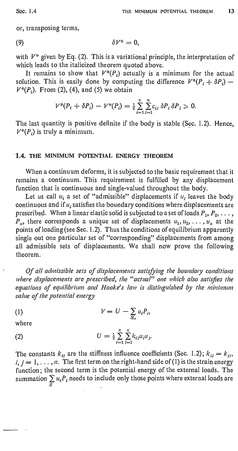
or, transposing terms,
(9) bV* = 0,
with F!ii given by Eq. (2). This is a variational principle, the interpretation of
which leads to the italicized theorem quoted above.
It remains to show that K*(Pf) actually is a minimum for the actual
solution. This is easily done by computing the difference V*{Pt -f- <5Pt) —
F*(/\). From (2), (4), and (5) we obtain
v*(p{ + dp.;) - v%pt) = i i 2¾ dp.; dPj > o.
The last quantity is positive definite if the body is stable (Sec. 1.2). Hence,
V*(P{) is truly a minimum.
1.4. THE MINIMUM POTENTIAL ENERGY THEOREM
When a continuum deforms, it is subjected to the basic requirement that it
remains a continuum. This requirement is fulfilled by any displacement
function that is continuous and single-valued throughout the body.
Let us call u{ a set of "admissible" displacements if ut leaves the body
continuous and if ut satisfies the boundary conditions where displacements are
prescribed. When alinearelasticsolidissubjectedtoasetofloads.P1;P2,...,
P]l9 there corresponds a unique set of displacements ul9u2,..., ua at the
points of loading (see Sec. 1.2). Thus the conditions of equilibrium apparently
single out one particular set of "corresponding" displacements from among
all admissible sets of displacements. We shall now prove the following
theorem.
Of all admissible sets of displacements satisfying the boundary conditions
where displacements are prescribed, the "actual" one which also satisfies the
equations of equilibrium and Hooke's law is distinguished by the minimum
value of the potential energy
(1) V=U-ZuiPh
where
(2) V = ithwi"*>
The constants /c# are the stiffness influence coefficients (Sec. 1.2); lcu = ic.Jh
i,j= l,...,n. The first term on the right-hand side of (1) is the strain energy
function; the second term is the potential energy of the external loads. The
summation ]£ uiPi needs to include only those points where external loads are
s
14 PROTOTYPES OF THEORY or ELASTICITY AND VISCOELASTICITY Chap. 1
prescribed (a fact indicated by the notation ]T). The set of points Sv rep-
resents the points where external loads are prescribed.
Proof. To prove this theorem, we denote by (u,) the actual displacements
corresponding to the set of forces (Pt). We shall compare (»,-) with other
admissible displacements, which may be written as {ut 4- dut). Since (w£ +
du() satisfy the boundary conditions on displacements, (du{) must vanish
n
wherever (ut) are prescribed. Now consider the "virtual" work ^P,-dii{.
From Eq. (1.2:3) we have '=1
(3) | Pi «5«, = if kuuj dut = sU i iktiutuj) = 6U.
-/=1 *«i*»l \ /=u^i J
After rearranging terms, this can be written as
(4) dV = 0.
Thus, the actual solution satisfies this variational equation, and V is an
extremum for ut.
That Kis indeed a minimum is easily verified by showing that, on account
of (4),
Vfa + dut) - V(t$ = * 2 J,kti dut diij > 0.
The last inequality follows from the positive definiteness of the strain energy
function.
The minimum principles are very important in the theory of elasticity,
because they lead to practical approximate methods of solution of
complicated problems.
1.5. SOME IMPORTANT REMARKS
Three important remarks should be added concerning the use of the
theorems derived above.
First, the "force" in Hooke's law may be generalized to mean torque,
couple, etc. The "corresponding" deformation can be so defined that the
work done upon the body when the deformation changes by a small amount
is equal to the force times the increment of the deformation. Thus, if P is the
generalized force and At/ is the change of the corresponding generalized
displacement, then
A work — P* Aw.
Thus, for a force, torque, or couple, a refers to displacement, angle of twist,
and angle of bending, respectively.
Sec. 1.5
SOME IMPORTANT REMARKS 15
When generalized forces are considered, it is very important to notice the
word "corresponding" in the statement of the reciprocal relations. A
generalized force corresponds to a generalized displacement if their product
gives exactly the work done. Thus, for a beam, the change of slope
corresponds to a moment, the deflection corresponds to a force, and the twisting
angle corresponds to a torque. Although Maxwell's reciprocal relation
asserts that the deflection at point 1 due to a unit couple at point 2 is equal
to the rotation at point 2 due to a unit force at point 1, it is completely wrong
to assert that the rotation at point 1 due to a unit force at point 2 must be
equal to the rotation at point 2 due to a unit force at point 1. In the latter
case the force and rotation do not correspond to each other.
The second remark is a truism: one may prove a theorem one way, but
use it another way. We proved the reciprocal theorem, Castigliano's theorem,
the minimum potential energy theorem, and the minimum complementary
energy theorem with the influence coefficients cu or /clV, but we do not have to
know these influence coefficients to apply these theorems. In fact, as long as
we can write an expression for the strain energy, we caii use these theorems.
Indeed, this is why these energy theorems can form a basis for approximate
theories in elasticity. For example, in the theory of simple beams we have the
time-honored approximation that plane cross sections remain plane in bending
and the Bernoulli-Euler approximation that the local curvature of the beam
axis is proportional to the local moment in the' beam. We can use these
assumptions to derive an appropriate expression for strain energy. When we
wish to apply the complementary energy theorem, the strain energy must be
expressed in terms of forces and moments. When we wish to apply the
minimum potential energy theorem, the strain energy must be expressed in
terms of displacements. In particular, when the strain energy expressions are
known in terms of forces, we can use Castigliano's theorem to derive
deflections, (In practice, that is the usual way the flexibility influence coefficients
are computed.)
In other words, the %'s are the vehicle through which the general principles
are established, but usually we do not know them. In applications, we try to
obtain an expression for the strain energy with trustworthy accuracy and
deduce the c{/s as well as other solutions from them. Establishing effective,
simplifying assumptions which yield accurate strain energy expressions is
indeed one of the most important objectives of engineering research.
Finally, we must comment on the sets of points S]t and Stt in Sees. 1.3 and
1.4. Although in the example in Sec. 1.3 the sum Stt + S„ is equal to the
total set of points engrossing our attention, such a limitation need not be
imposed. Thus, the total set may be greater than Sv + Su; the difference
consists of internal points, whereas S,„ + SH constitutes boundary points.
These remarks will be useful in solving the problems at the end of this
section.
The theory presented in the foregoing sections forms the basis of the
16 PROTOTYPES OF THEORY OF ELASTICITY AND V1SCOELASTIC1TY Chap. I
engineering theory of framed structures. Many ingenious applications of
this theory have been made to the analysis of machines, trusses, rigid frames,
reinforced concrete structures, aircraft structures, etc. In particular, the
Maxwell or Betti-Rayleigh reciprocal relations and the first theorem of
Castigliano are very useful in finding displacements in a structure when the
stresses in it can be determined from statics. Limitation of space prevents us
from going into any discussions of these applications. The reader is urged
to study some of the standard references listed in Bibliography 1-3 at the end
of the book in order to appreciate the many uses that can be made of this
rudimentary theory.
But the elementary formulation has neither reduced the theory to its
simplest form, nor given it sufficient generality to deal with more difficult
problems. For example, to describe the elastic properties of a body by the
method described above, we will need a complete set of influence coefficients
(or influence functions) instead of a few elastic moduli of the material. The
elementary theory cannot give a detailed picture of stress distribution in a
body in response to external loads. Most problems in stress concentration,
contact pressure, propagation and refraction of elastic waves, transient or
steady oscillations, lie beyond the scope of the elementary theory.
Furthermore, HooIce's law expressed in terms of the linearity in load-
displacement relationship is unnecessarily restrictive. There exist many cases
in which the material remains elastic everywhere but the load-displacement
relationship is nonlinear. Examples are a beam under simultaneous action of
lateral and end loads, a large deflection of an elastic arch, and a large
deflection of a thin plate or a thin shell.
Finally, practical engineering materials do not always obey Hooke's law.
They may be elastic, but the stress-strain relationship may be nonlinear;
or they may be viscoelastic or plastic. How shall we formulate the physical
laws of nonlinear elasticity, of flow and motion? How can such laws be
tested in the laboratory ? What guidance can we obtain from such theoretical
considerations as tensor analysis?
To answer these questions, a more general theory of continuum mechanics
is developed, the presentation of which will occupy later chapters of this book.
PROBLEMS
1.1, Prove that it is possible to generalize Hooke's law to deal with moments
and angles of rotations by considering a concentrated couple as the limiting case of
two equal and opposite forces approaching each other but maintaining a constant
moment.
1.2. A pin-jointed truss is shown in Fig. PI.2. Every member of the truss is
made of the same steel and has the same cross-sectional area. Find the tension or
compression in every member when a load P is applied at the point shown in the
Chap. 1
PROBLEMS
17
figure. M?/e: Ajoint is said to be a. pin joint It no moment can be transmitted across
it. This problem is statically determinate. - ■ ■ ■
1.3. Find the vertical deflections at a, b, c of the truss in Fig. PI .2 due to a load
P at point b. Assume that P is sufficiently small so that the truss remains linear
elastic. Use the fact that for a single uniform bar in tension the total change in
length of this bar is -given by PL/AE, where P is the load in the bar, L is the bar
length, A is the cross-sectional area, and E is the Young's modulus of the material.
For structural steels E is about 3 x 10⁷ Ib/sq in. Hint: Use Castigliano's theorem.
1.4. A "rigid" frame of structural steel shown in Fig. PI.4 is acted on by a
horizontal force-P. Find the reactions at the points of support a, and d. The cross-
sectional area A and the bending rigidity constant EI of the various members are
shown in the figure.
w%
mm
PJ.4
Ha
~n)
,Ma
4fH"
By a "rigid" frame is meant a frame whose joints are rigid; e.g., welded. Thus,
when we say that corner b is a rigid joint, we mean that the two members meeting
at b will retain the same angle at that corner under any loading. The frame under
loading will deform. It is useful to sketch the deflection line of the frame. Try to
locate the points of inflection on the members. The points of inflection are points
where the bending moments vanish.
*° PP PBS C . .ORY w vuASTIcm AND VISCOELASTIC1TV Chap. 1
The reactions to be found are the vertical force V, the horizontal force H, and
the bending moment M, at each support.
Use engineering beam theory for this problem. Irt this theory, the change of
curvature of the beam is MjEI, where Mis the local bending moment and EI is the
local bending rigidity. The strain energy per unit length due to bending is, therefore,
MZI2EI. The strain energy per unit length due to a tensile force P is P2j2EA. The
strain energy due to transverse shear is negligible in comparison with that due to
bending.
1.5. A circular ring of uniform linear elastic material and uniform cross section
is loaded by a pair of equal and opposite forces at the ends of a diameter (Fig. PI .5).
Find the change of diameters aa and bb. Note: This is a statically indeterminate
problem. You have to determine the bending moment distribution in the ring.
P1.5 P1.6
1.6. Compare the changes In diameters aa, bb, and cc when a circular ring of
uniform linear elastic material and uniform cross section is subjected to a pair of
bending moments at the ends of a diameter (Fig. PI.6).
1.7. Begg*s Deformeter: G. E. Beggs used an experimental model to determine
the reactions of a statically indeterminate structure. For example, to determine the
horizontal reaction H at the right-hand support b of an elastic arch under the load-P,
he imposes at b a small displacement d in the horizontal direction and measures at P
the deflection d' in the direction corresponding with P, while preventing the vertical
P1.7
PI.8
Chap. 1 PROBLEMS 19
displacement and rotation of the end bt Fig. PI.7. Show that H = —Pd'td. (Use
the reciprocal theorem.) [G. E. Beggs, J. Franklin Institute, 203 (1927), pp. 375-386.]
1.8. A simply supported, thin elastic beam of variable cross section with bending
rigidity EI(x) rests on an elastic foundation with spring constant k and is loaded
by a distributed lateral load of intensity p(x) per unit length (Fig. PI.8). Find an
approximate expression for the deflection curve by assuming that it can be
represented with sufficient accuracy by the expression
t ^ v ■ mx
Note: This expression satisfies the end conditions for arbitrary coefficients an.
Use the minimum potential energy theorem.
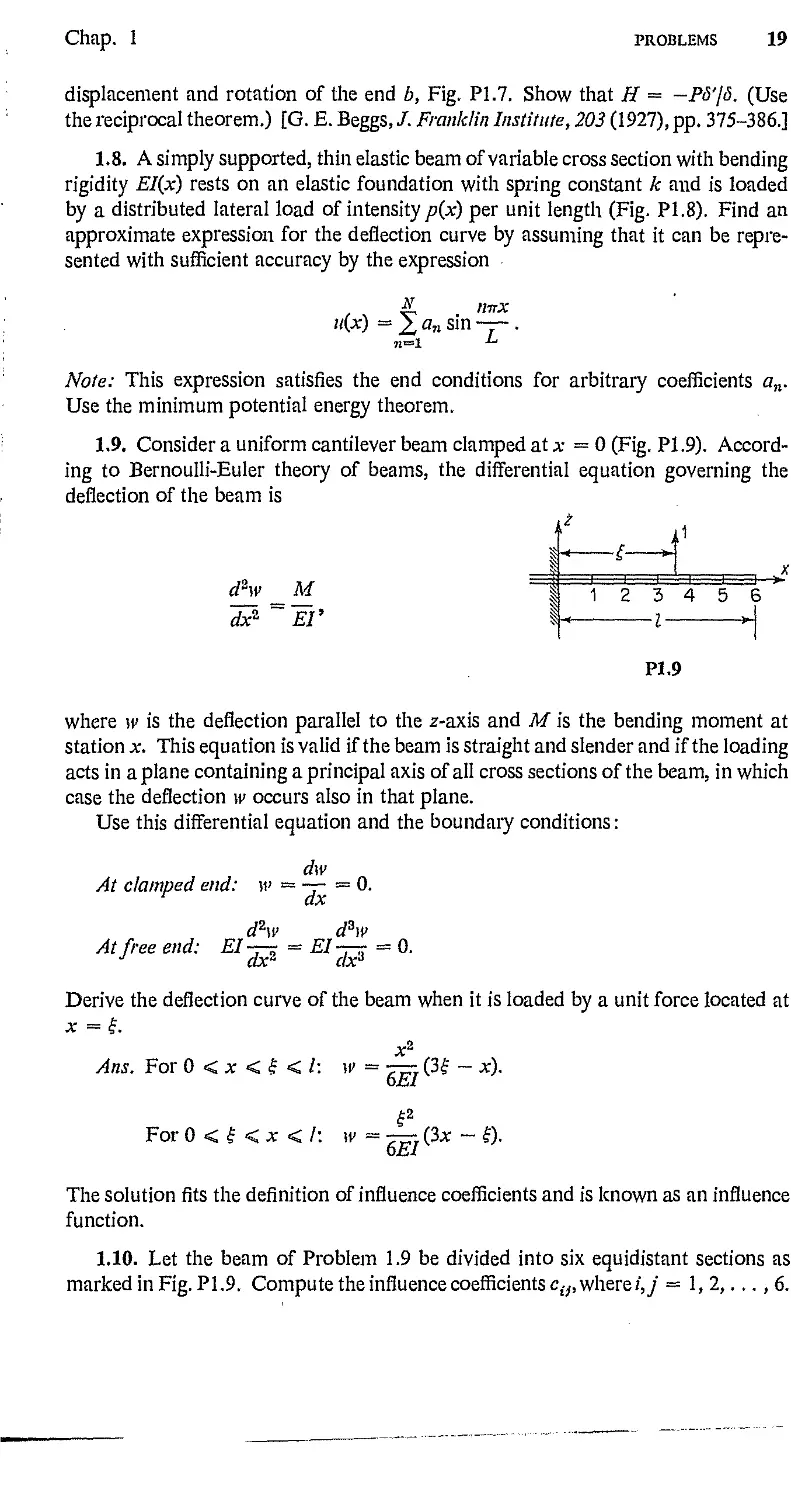
1.9. Consider a uniform cantilever beam clamped at a: = 0 (Fig. PI .9).
According to Bernoulli-Euler theory of beams, the differential equation governing the
deflection of the beam is
t
dhv M
dx2 ^EI9
•£-
I 12 3 4 5 6
PI .9
where w is the deflection parallel to the 2-axis and M is the bending moment at
station x. This equation is valid if the beam is straight and slender and if the loading
acts in a plane containing a principal axis of all cross sections of the beam, in which
case the deflection w occurs also in that plane.
Use this differential equation and the boundary conditions:
dw
At clamped end: w = — — 0.
dhv cPw
At free end: EI—% = EI
dx*
0.
Derive the deflection curve of the beam when it is loaded by a unit force located at
Ans. For 0 < x < $ < I: w =
For 0 < f < x < /: w =
X*
i2
-*)•
-«•
The solution fits the definition of influence coefficients and is known as an influence
function.
1.10. Let the beam of Problem 1.9 be divided into six equidistant sections as
marked in Fig. P1.9. Compute the influence coefficients cip where/,/ — 1, 2,..., 6.
20 PROTOTYPES OF THEORY OF ELASTICITY AND VISCOELASTICITY Chap. 1
1.11. Invert the cu matrix of Prob. 1.10 to obtain the stiffness influence
coefficients kti. Note: If you work this problem out, you will find that the inversion of the
flexibility influence coefficients matrix (c{j) is very difficult. The difficulty increases
rapidly as the range of the indices i,j increases. It arises from the fact that the (c#)
matrix is nearly singular; i.e., neighboring columns of the matrix (cH) are nearly in
linear proportion to each other. On the other hand, inversion of the stiffness
influence coefficients matrix (/ciV), in general, will have no difficulty.
1.12. A cantilever wing of an airplane is subjected to a concentrated load P at
the wing tip (Fig. PI.12). By moving P along the tip chord, a point C, called the
center of flexure, can be found which has the property that if P acts at C the wing tip
P1.12
section has no rotation (assuming the wing ribs to be rigid). On the other hand, if a
couple Mis applied at the wing tip, the wing twists; but there will be one point in
the tip section, say C", which remains undisturbed and is called the center of twist.
Show that the center of flexure and the center of twist coincide; i.e., C and C" are the
same point.
1.6. LINEAR SOLIDS WITH MEMORY: MODELS OF
VISCOELASTICrrY
Most structural metals are nearly linear elastic under small strain, as
measurements of load-displacement relationship reveal. The existence of
normal modes of free vibrations which are simple harmonic in time, is often
quoted as an indication (although not as a proof) of the linear elastic
character of the material. However, when one realizes that the vibration of
metal instruments does not last forever, even in a vacuum, it becomes clear
that metals deviate somewhat from Hooke's Jaw. Thus, other constitutive
laws must be considered. The need for such an extension becomes particularly
evident when organic polymers are considered.
In this section we shall consider a simple class of materials which retains
linearity between load and deflection, but the linear relationship depends on a
third parameter, time. For this class of material, the present state of
deformation cannot be determined completely unless the entire history of
loading is known.
Sec. 1.6
LINEAR SOLIDS WITH MEMORY 21
A linear elastic solid may be said to have a simple memory; it remembers
only one configuration; namely, the unstrained natural state of the body.
Many materials do not behave this way: they remember the past. Among
such materials with memory there is one class that is relatively simple
in behavior. This is the class of materials named above, for which the cause
and effect are linearly related.
To discuss the foregoing in concrete terms, let us consider a simple bar
fixed at one end and subjected to a force in the direction of the axis at the
other end. Let the force at time t be F(t) and the total elongation of the bar
be u(t). The elongation u(t) is caused by the total history of the loading up to
the time t. If the function F(t) is continuous and differentiate, then in a small
time interval dr at time r the increment of loading is (dFjdt) dr. This
increment remains acting on the bar and contributes an element du(t) to the
elongation at the time t, with a proportionality constant c depending on the
time interval t — r. Hence, we may writef
dF
du(t) = c(t — r) — (r) dr.
Let the origin of time be taken at the beginning of motion and loading. Then,
on summing over the entire history, we have J
(1) «(*) = fc(* - t) ^(t) dr.
Jo dt
A similar argument, with the role of F and u interchanged, gives
(2) F(t) = Pk(t - r) ^ (r) dr.
Jo dt
These laws are linear, since a doubling of the load doubles the elongation,
and vice versa.
Equations (1) and (2) are Boltzmann's formulation (Ludwig Boltzmann,
1844-1906) of the constitutive equation, in the case of a simple bar, for a
material which has a linear load-deflection relationship. We may call such a
material a Boltzmann solid. Vito Volterra (1860-1940), however, has
introduced the more dramatic term hereditary law for any functional relation of
the type exemplified in Eq. (1). To emphasize the linearity assumption, we
shall call a material that follows such a law a linear hereditary material.
There are, however, a host of other terms in common use, e.g, viscoelasticity,
creep, internal friction or damping, anelasticity, elastic after-effect, stress
relaxation, etc., each emphasizing a particular aspect or a particular model.
t The notation (dFldt)(r) means the value of dFjdt, which is a function of time,
evaluated at the instant of time t = r. It is, of course, equal to the derivative dFtyjdr, if the
argument t of F{t) is replaced first by t.
| A simple modification of the formula is necessary if a finite load is applied suddenly
at time t = 0, or if FQ) is discontinuous in some other way. See Sec. 15.1, p. 413.
22 PROTOTYPES OF THEORY OF ELASTICITY AND VISCOELASTIC1TY Chap. 1
The function k(t) is called the relaxation function. The function c(t) is
called the creep function. They are characteristic functions of the material.
Physically, c(t) is the elongation produced by a sudden application at
t = 0 of a constant force of magnitude unity; i.e., a unit-step forcing function
which is zero when t < 0 and unity when t > 0. Similarly, k(t) is the force
that must be applied in order to produce an elongation which changes at
/ = 0 from zero to unity and remains unity thereafter.
It is generally accepted that the deformation at the present time t is due to
forces that act in the past, and not in the future. This concept is expressed by
the requirement that
(3) c(t) = 0, for t < 0.
It is often referred to as the axiom ofnonretroactivity. Similarly, by the same
axiom,
(4) k(t) = 0, for t < 0.
Of course, this nonretroactivity is implied already when we write t for the
upper limits of the integrals in Eqs. (1) and (2),
V $
*F
I [J—ww—^f %
I |—vwv-
(a) (b) (c)
| V\AAr~
-*-F
Fig. 1.6:1. Models of linear viscoelasticity: (a) Maxwell, (b) Voigt, (c)
standard linear solid.
Before further discussions let us consider some simple examples. In Fig.
1.6:1 are shown three mechanical models of material behavior, namely, the
Maxwell model, the Voigt model, and the "standard linear" model, all of
which are composed of combinations of linear springs with spring constant
[x and dashpots with coefficient of viscosity rj. A linear spring is supposed to
produce instantaneously a deformation proportional to the load. A dashpot
is supposed to produce a velocity proportional to the load at any instant. The
load-deflection relationship for these models are
(5) Maxwell model: u = ~+~, u(0) = ^1 s
fX 7] fX
(6) Voigt model: F = \xu + rju, u(0) = 0,
(7) Standard linear model:
F + ref = ER(u + T,tf), r£F(0) = ERrau(0),
where r£, ra are two constants. When these equations are to be integrated,
the initial conditions at t = 0 must be prescribed as indicated above.
Sec. 1.6
LINEAR SOLIDS WITH MEMORY 23
The creep functions can be easily derived by solving Eqs. (5)-(7) for a(t)
when F(t) is a unit-step function 1(/). They are
(8) Maxwell solid:
c(t)=(~+~t)l(t),
Voigt solid: c(t) = -(1- e~{fllnH)l(t),
(9)
(10)
Standard linear solid:
1
c(t) =
E
R
1_ h_l£ \e-tlr.
1(0.
where the unit-step function 1(/) is defined as
f\ when / > 0,
(11) 1(/)= I when /=--0,
0 when / < 0,
A body which obeys a load-deflection relation like that given by Maxwell's
model is said to be a Maxwell solid, etc. Since a dashpot behaves as a piston
moving in a viscous fluid, the above-named models are called models of
viscoelasticity.
Interchanging the roles of F and u, we obtain the relaxation function as a
response F(t) = k(t) corresponding to an elongation u(t) = 1(/).
(12) Maxwell solid:
k(t) = txe~Wil(t\
(13) Voigt solid:
/c(0 = rj 8(/) + ^1(/),
(14) Standard linear solid:
/c(/) = EB
l- i-^W-tfr<
1(0.
Here we have used the symbol 8(/) to indicate the unit-impulse function, or
Dirac-delia function, which is defined as a function with a singularity at the
origin:
8(0 = 0 for t < 0, and t > 0,
(15)
/(0 8(0 d< =/(0),
c> 0,
where/(/) is an arbitrary function continuous at / = 0. These functions, c(t)
and k(t), are illustrated in Figs. 1.6:2 and 1.6:3, respectively, for which we
add the following comments.
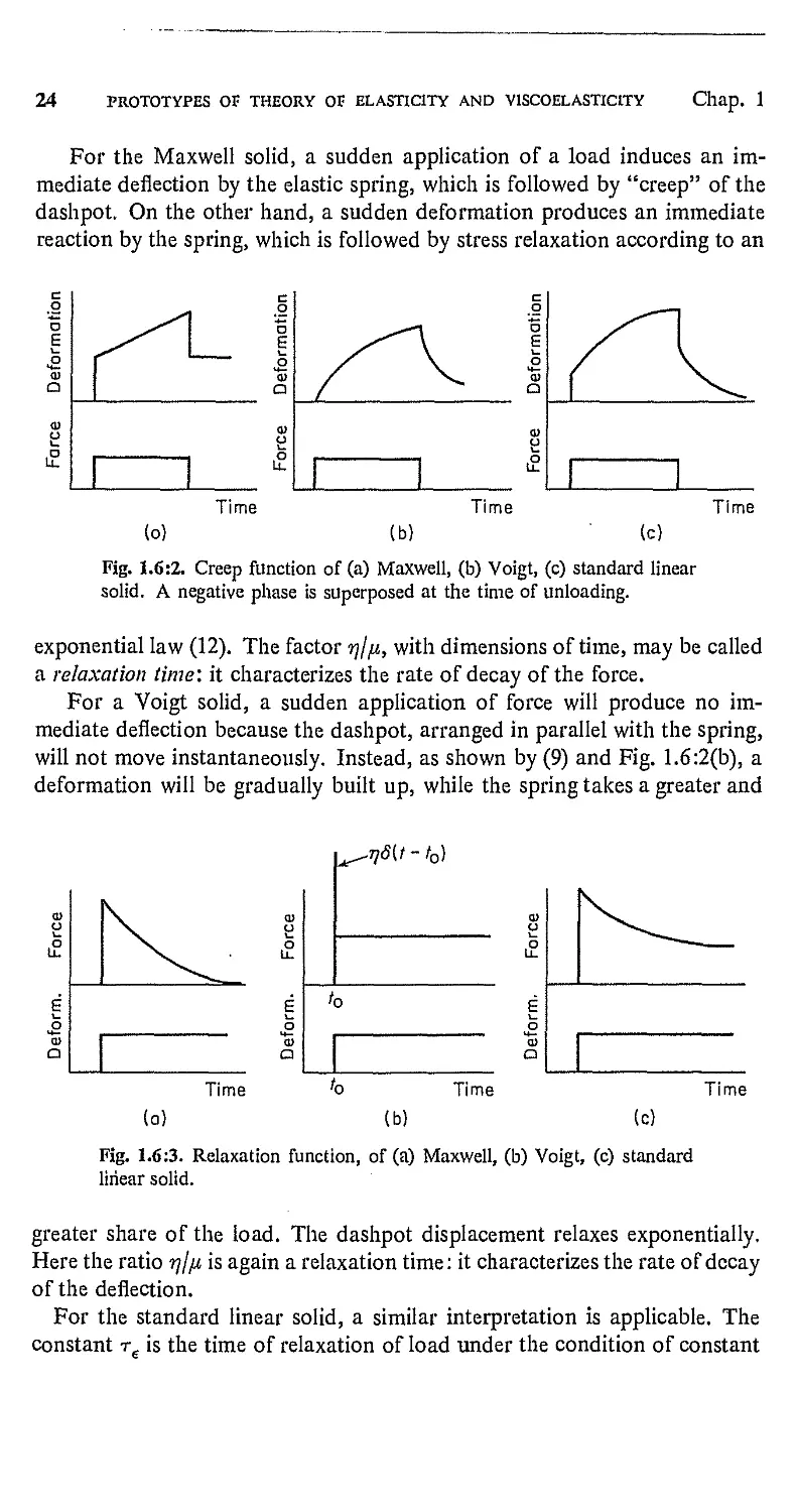
24 PROTOTYPES OV THEORY OV ELASTICITY AND V1SCOELASTICITY Chap. 1
For the Maxwell solid, a sudden application of a load induces an
immediate deflection by the elastic spring, which is followed by "creep" of the
dashpot. On the other hand, a sudden deformation produces an immediate
reaction by the spring, which is followed by stress relaxation according to an
Time
Time
Time
(o)
(b)
(c)
Fig. 1.6:2. Creep function of (a) Maxwell, (b) Voigt, (c) standard linear
solid. A negative phase is superposed at the time of unloading.
exponential law (12). The factor ??//*, with dimensions of time, may be called
a relaxation time: it characterizes the rate of decay of the force.
For a Voigt solid, a sudden application of force will produce no
immediate deflection because the dashpot, arranged in parallel with the spring,
will not move instantaneously. Instead, as shown by (9) and Fig. 1.6:2(b), a
deformation will be gradually built up, while the spring takes a greater and
£
o
M—
a
0>
o
u.
i
0>
a
t
j^ifitt-to)
0
Time
Time
Time
(a)
(b)
(c)
Fig. 1.6:3. Relaxation function, of (a) Maxwell, (b) Voigt, (c) standard
linear solid.
greater share of the load. The dashpot displacement relaxes exponentially.
Here the ratio rjl/x is again a relaxation time: it characterizes the rate of decay
of the deflection.
For the standard linear solid, a similar interpretation is applicable. The
constant r€ is the time of relaxation of load under the condition of constant
Sec. 1.7 SINUSOIDAL OSCILLATIONS IN A VISCOELASTIC MATERIAL 25
deflection [see Eq. (14)], whereas the .constant ra is the time of relaxation of
deflection under the condition of constant load [see Eq. (10)1. As t —>- co,
the dashpot is completely relaxed, and the load-deflection relation becomes
that of the springs, as is characterized by the constant En in Eqs. (10) and
(14). Therefore, ER is called the relaxed elastic modulus.
Load-deflection relations such as (5)-(7) were proposed to extend the
classical theory of elasticity to include anelastic phenomena. Lord Kelvin
(Sir William Thomson, 1824-1907), on measuring the variation of the rate of
dissipation of energy with frequency of oscillation in various materials,
showed the inadequacy of the Maxwell and Voigt equations. A more
successful generalization using mechanical models was first made by John
H. Poynting (1852-1914) and Joseph John Thomson ("J.J.," 1856-1940) in
their book Properties of Matter (London: C. Griffin and Co., 1902). The
model shown in Fig. 1.6:1(c) identified with Eq. (7) is called the standard
linear model because it is the most general relationship to include the load,
the deflection, and their first derivatives (often known as linear derivatives!).
It is, of course, a special case of Boltzmann's general linear relation, (1) or (2).
Problem 1.13. Derive Eqs. (8), (9), and (10), first by elementary methods of
integration and then by Laplace transformation.
Problem 1.14. Consider Eqs. (1) and (2) of Sec. 1.6. Let c(t) be a continuous
function for t > 0, and c(t) = 0 for t < 0. Show that the condition for the
existence of a continuous kernel k(t)3 so that (2) is the inverse of (1), is that c(0) ^ 0.
Note: In a Voigt solid c(0) = 0 and k{t) contains a delta function, which is
discontinuous.
1.7. SINUSOIDAL OSCILLATIONS IN A VISCOELASTIC
MATERIAL
It is interesting to obtain the relationship between load and deflection
when the body is forced to perform simple harmonic oscillations. We are
interested in the steady-state response. Hence, we assume that a sinusoidal
forcing function has been acting on the body for an indefinitely long time and
that all initial transient disturbances have died out. Under this circumstance,
it is convenient to put the beginning of motion at time — co. Hence, we shall
replace the lower limits of Eqs. (1.6:1) and (1.6:2) by —co. Using complex
representation for sinusoidal oscillations, we put F(t) = F^eiloi into these
equations. It will be more convenient to make a change of variable t — r = £
first. This gives
(1) «(0 = f%(*)^0-*)#.
Jo at
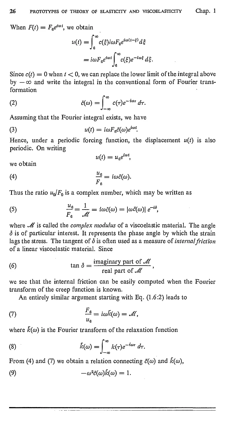
26 PROTOTYPES Or THEORY Or ELASTICITY AND VISCOELASTICITY Chap. 1
When F(t) = F^a\ we obtain
ii(0 = f"c(0foJVto(M)d£
Jo
Jo
Since c(t) = 0 when t < 0, we can replace the lower limit of the integral above
by -co and write the integral in the conventional form of Fourier
transformation
(2) cO») = P° c(r)<r*w dr.
J —CO
Assuming that the Fourier integral exists, we have
(3) i/(0 = /a)J?0c(a))eto*.
Hence, under a periodic forcing function, the displacement u(t) is also
periodic. On writing
u(t) = uReil0t,
we obtain
(4) ^ = icoc(co).
Thus the ratio uJFq is a complex number, which may be written as
(5) £• = -L = ta^o,) = |w£(w)| c-»
where ^f is called the complex modulus of a viscoelastic material. The angle
b is of particular interest. It represents the phase angle by which the strain
lags the stress. The tangent of b is often used as a measure of internal friction
of a linear viscoelastic material. Since
,-. , „ imaginary part of Ji
(6) tan o = -^- ,
real part of Ji
we see that the internal friction can be easily computed when the Fourier
transform of the creep function is known.
An entirely similar argument starting with Eq. (1.6:2) leads to
^o
(7) -$ = icok(a)) = J/,
uR
where £(eo) is the Fourier transform of the relaxation function
(8) k(a>) = | /c(r>-lW dr.
J —CO
From (4) and (7) we obtain a relation connecting c(co) and k(co)3
(9) -co2c(co)lc(a)) = 1.
Sec. 1.7
SINUSOIDAL OSCILLATIONS IN A VISCOELASTIC MATERIAL 27
Internal friction
tan 6
100
w^__
Fig. 1.7:1, Frequency dependence of internal friction and elastic modulus.
As an example, let us consider the standard linear solid. On putting
u = u0e
(10)
(11)
iiot
, F = FQeif0t into Eq. (1.6:7), we obtain
jfj _ _ .—^ERi
/1 + C02T2\l/2
tan d =
1 + icor€ ,-,--,
<To ~ re) (ra - rc) ^^
When 1^1 and tan d in (10) and (11) are plotted against the logarithm of co,
curves as shown in Fig. 1.7:1 are obtained. Experiments with torsional
oscillations of metal wires at various temperatures, reduced to room
temperature according to certain thermodynamic formula, yield a typical
"relaxation spectrum" as shown in Fig. 1.7:2. Many peaks are seen in the
10
■12
10
10
I0~6 I0"4 I0"2
Frequency
1 I02 I04
Fig. 1.7:2. A typical relaxation spectrum. (After C. M. Zener, Elasticity
and Anelasticity of Metals^ The University of Chicago Press, 1948.)
28 PROTOTYPES OF THEORY OP ELASTICITY AND VISCOELASTICITY Chap. 1
internal-friction-versus-frequency curve. It has been suggested that each
peak should be regarded as representing an elementary process as described
above, with a particular set of relaxation times ra, r£. Each set of relaxation
times r0, r£ can be attributed to some process in the atomic or microscopic
level. A detailed study of such a relaxation spectrum tells a great deal about
the structures of metals; and the internal friction has been a very effective key
to metal physics. Zener's fascinating book1,4 is recommended to those
interested in this subject.
A number of materials follow a linear viscoelastic stress-strain law very
well when the strain is small. Among such materials are many high polymers.
The damping characteristics of many metals can also be explained by such a
model. The creep of metals at higher stresses, however, usually follows a
nonlinear law. See Bibliography 6.4 and 14.8.
1.8. STRUCTURAL PROBLEMS OF VISCOELASTIC
MATERIALS
Several steps of generalization are necessary before the simple models
discussed in Sees. 1.6 and 1.7 can be used in structural analysis. The simplest
point of view is to idealize a solid body into a set of mass particles
interconnected by simple bars, for each of which a hereditary stress-strain law is
specified. (For many structures and machines, this is actually not a very bad
description!) The equations of motion of these mass particles and massless
linkages can be written down and analyzed.
A second point of view is to generalize the Hooke's load-displacement law,
Eq. (1.1:1), by a hereditary law. Thus, if a set of external forces Flt F2s..., Fn
act on a body at points 1, 2,..., n and produce the "corresponding"
displacements ult u2i..., un at these points, then, for a properly supported
viscoelastic body, we may assume
n Ct d
«<=2 QiC _ r) TF^ dr> i = l,...,n.
i«i Jo ar
In this specification of the constitutive property of the body we shall need
the full set of creep functions C#(0« These creep functions and the
convolution integrals assume the role of the influence coefficients in linear
elasticity. Physically, Ci}(t) means the deflection 1/,(/) produced by a unit-step
function F} = 1(/) acting at the point/. In reality, we cannot demand that all
these functions Ci} be determined experimentally. To do that would be too
tedious. In general, we have to compute them from the basic equations of
viscoelasticity.
Therefore, it is fundamental to express the concept of viscoelasticity in a
stress-strain-history law. Such a generalization is given .in Chap. 13 and 15.
With proper interpretation, the theory of viscoelasticity parallels the theory
Chap. 1
PROBLEMS
29
of elasticity in every respect. However, the basic equations of viscoelasticity
are more difficult to solve, and behavior of a body of viscoelastic material can
be very complex.
PROBLEMS!
1.15. Consider the quadratic form of two real variables,
f(x> y) = «*2 + bxy + cy2.
Show thatf(x,y) is positive definite if and only if a > 0, Aac — b2 > 0.
1.16. Show that the necessary and sufficient condition for the quadratic form
(X, ICX) = 2 *«***»
where K is real symmetric and X is real, to be positive definite is that all the
eigenvalues of the eigenvalue problem KX = AX are real and positive. Here K is a
n x n square matrix and X is a 1 x n column matrix,
li
k
12
'In
K
X
k
nl
-n2
»nn>
(X, KX) is the scalar product of the vectors X and ICX. Similarly, (X, KX) is negative
definite if all the eigenvalues are negative. (Note: Since
n n
2 kijXiXj = J 2 (*tf + kji)xix3>
2,1=1 i,i*l
no generality is lost by considering K as a symmetric matrix.)
1.17. Consider the determinantal equation
axl ~X a12 ... aln
«21 «22 ~ ^ • • • a<
'271
a
nl
a
nl
a.
mi
0,
where an = an are real numbers. Let the n roots of this equation be denoted by
^i, ^23 • • • 3 K> These roots can be identified with the eigenvalues of the eigenvalue
problem AX == AX, where
«11 «12
flirt
X
Mnl anZ
a.
nn,
f These problems are not directly related to the previous sections. They form an
appendix concerning the positive definiteness of quadratic forms, which are very important
in continuum mechanics.
30 PROTOTYPES OF THEORY OF ELASTICITY AND VISCOELASTICITY Chap. 1
Let this determinantal equation be written as
F(A) = (¾ - A)(Aa - X)... (Xn - A)
= Oq - ttlA + a2A2 + ...+ (-1)VV + • • • + (-!)**" = 0.
The coefficients are symmetric functions of the roots Av:
"o = hh • • • *n = F(0) = det |^v|
av == V*2 . .. Xn_v + ...+ *v+i*v+a .. . An, v = 0, 1,.. ., n — 1.
' w ' » v '
Prove the following statements:
1. All eigenvalues Av are positive if and only if all av are positive.
2. All eigenvalues Av are negative if and only if all (—l)n~vav are positive.
3. There exist exactly r eigenvalues equal to zero while the other n — r
eigenvalues are positive if and only if
a0 = «! == ... = ar_1 == 0, av > 0, v - r,..., n.
Hint: Apply Descartes' rule of signs.
4. There exist exactly r eigenvalues equal to zero while the other n — r
eigenvalues are negative if and only if
5. If we strike out v rows and v columns of the same indices from the
determinant IfyJ, the determinant of the remaining elements is called a. principal
minor of order n — v. Show that av = sum of all principal minors of order
n — v of k/IV|.
6. State the conditions for the positive or negative derlniteness of a quadratic
form in terms of the principal minors of the symmetric matrix of coefficients.
2
TENSOR ANALYSIS
In attempting to make a generalization of the theory outlined in the previous
chapter, we shall first learn to use the powerful tool of tensor calculus. At
first sight, the mathematical analysis may seem involved, but a little study
will soon reveal its simplicity.
2.1. NOTATION AND SUMMATION CONVENTION
Let us begin with the matter of notation. In tensor analysis one makes
extensive use of indices. A set of n variables xlt x2,. .., xn is usually denoted
as Xy, /=1, ...,/2. A set of n variables y\y2,...,yn is denoted by
y, i = 1, ..., n. We emphasize that y\y\ ... ,yn are n independent
variables and not the first n powers of the variable y.
Consider an equation describing a plane in a three-dimensional space
vl v2 V"
(1) a-ix1 + azx2 + fl3x3 = /;,
where at and p are constants. This equation can be written as
(2) 2 ap* = p.
However, we shall introduce the summation convention and write the
equation above in the simple form
(3) a^ = p.
The convention is as follows: The repetition of an index (whether superscript
or subscript) in a term will denote a summation with respect to that index
over its range. The range of an index i is the set of n integer values 1 to n.
A lower index z, as in au is called a subscript, and upper index i, as in x\ is
called a superscript. An index that is summed over is called a dummy index;
one that is not summed out is called a. free index.
Since a dummy index just indicates summation, it is immaterial which
symbol is used. Thus, tyx* may be replaced by a^, etc. This is analogous
to the dummy variable in an integral
"/(x) dx = \hf(y) dy.
31
32
TENSOR ANALYSIS
Chap. 2
The use of index and summation convention may be illustrated by other
examples. Consider a unit vector v in a three-dimensional Euclidean space
with rectangular Cartesian coordinates x, y, and z. Let the direction cosines
a.{ be defined as
ai = cos (v, x), a2 = cos (v, y), a3 = cos (v, z),
where (v, x) denotes the angle between v and the x-axis, etc. The set of
numbers <x,{ (/= 1, 2, 3) represents the projections of the unit vector on the
coordinate axes. The fact that the length of the vector is unity is expressed
by the equation
(<*i)* + (a2)2 + (a3)2 = 1,
or simply
(4)
a^= 1.
As a further illustration, consider a line element (dx, dy, dz) in a three-
dimensional Euclidean space with rectangular Cartesian coordinates x, y, z.
The square of the length of the line element is
(5)
If we define
(6)
and
(7) A
ds* = dx2 + dy2 + dz\
dx1 = dx, dx2 = dy, dx3 = dz
<5u = ^22 = ^33 = 1»
<5ia = ^2i = <5i3 = <531 = dw = <532 = 0.
Then (5) may be written as
(8)
ds2 = dtj dx1 dxj,
with the understanding that the range of the indices / and j is 1 to 3, Note
that there are two summations in the expression above, one over i and one
over/ The symbol du as defined in (7) is called the Kroneclcer delta.
The following determinant illustrates another application
#11 #12 ^13
#21 #22 ^23
#31 #32 ^33
= #11^22#33 + #21^32#13 + ^31#12^23
— axla^a^ — a12a2ia33 — tf13a22a31.
If we denote the general term in the determinant by a{j and write the
determinant as \atj\, then the equation above can be written as
(9) l#«l = erst#rl#S2#t3>
Sec. 2.2
COORDINATE TRANSFORMATION 33
where erst, the permutation symbol, is defined by the equations
^111 = ^222 = ^333 = ^112 = ^113 = ^221 = ^223 = ^331 = ^332 = 0,
(10) A <?123 = ^231 = ^312 = h
^213 =1 ^221 =1 ^132 =1 1-
In other words, em vanishes whenever the values of any two indices coincide;
em = 1 when the subscripts permute like 1, 2, 3; and em = — 1 otherwise.
The Kronecker delta and the permutation symbol are very important
quantities which will appear again and again in tills book. They are connected
by the identity
(11) A etstfut = diAt — <5*A*-
This e-d identity is used sufficiently frequently to warrant special attention
here. It can be verified by actual trial.
Finally, we shall extend the summation convention to differentiation
formulas. Let f(x\ x2,..., xn) be a function of n numerical variables
M. Then its differential shall be written
(12) df=Bdxi'
PROBLEMS
2.1. Show that, when i,j, k range Over 1,2, 3,
(a) $u $a = 3 (c) emAtAu - 0
(b) ewfitei - 6 (d) d{j djk - dik
2.2. The vector product of two vectors x =* (¾ x2, x3) and y = (ylt y2t ya) is the
vector z = x x y whose three components are
Z1 — X2y><i ~~ ^3^2» Z2 ~ X^yi ~* ^ljV Z3 ~ Xl)'z ~* X2jl-
This can be shortened by writing
Zi = etii(X}yTt'
Verify the following identity connecting three arbitrary vectors by means of the
e-d identity.
A X (B x C) - (A ■ QB - (A ■ B)C.
Note: The last equation is well known in vector analysis. After identifying the
quantities involved as Cartesian tensors, this verification may be construed as a
proof of the e-d identity.
2.2. COORDINATE TRANSFORMATION
The central point of view of tensor analysis is to study the change of the
components of a quantity such as a vector with respect to coordinate
transformations.
34
TENSOR ANALYSIS
Chap. 2
A set of independent variables xl9 xZi x3 may be thought of as specifying
the coordinates of a point in a frame of reference. A transformation from
xl9 x2, x3 to a set of new variables xlt x2i x3 through the equations
(1) Xi = ji\X\> x2, X3), * = 1, 2, 3,
specifies a transformation of coordinates. The inverse transformation
(2) x{ = gt(xlt x2t x3) / = 1, 2, 3,
proceeds in the reverse direction. In order to insure that such a
transformation is reversible and in one-to-one correspondence in a certain region
R of the variables (¾ x2, x3), i.e., in order that each set of numbers (¾ x2, x3)
defines a unique set of numbers (xl9 x2, x3), for (xlt x2, x3) in the region R,
and vice versa, it is sufficient that
(a) The functions f are single-valued, continuous, and possess
continuous first partial derivatives in the region R, and
(b) The Jacobian determinant J = \dxjdxj] does not vanish at any point
of the region R.
dxx dxx dxx
dx1' 3x2' 3x3
(3)
J =
dxi
dxj
dx2 dx2 dx2
dxx dx2 ' 3x3
#0
ini?.
3¾ 5¾ 5¾
dxx dx2 ' 3x3
Coordinate transformations with the properties (a), (b) named above
are called admissible transformations. If the Jacobian is positive everywhere,
then a right-hand set of coordinates is transformed into another right-hand
set, and the transformation is said to be proper. If the Jacobian is negative
everywhere, a right-hand set of coordinates is transformed into a left-hand
one, and the transformation is said to be improper. In this book, we shall
tacitly assume that our transformations are admissible and proper.
2.3. EUCLIDEAN' METRIC TENSOR
The first thing we must know about any coordinate system is how to
measure length in that reference system. This information is given by the
metric tensor.
Consider a three-dimensional Euclidean space, with the range of all
indices 1, 2, 3. Let
(i)
"i — "l\xl9 X2> X'a)
be an admissible transformation of coordinates from the rectangular
Cartesian (in honor of Cartesius, i.e., Descartes) coordinates xl9 x2i x3 to some
Sec. 2.3
EUCLIDEAN METRIC TENSOR 35
general coordinates 0l9 02, 03. The inverse transformation
(2) Xi = x/fl1( 02, 03)
is assumed to exist, and the points (¾ x2, jcg) and (0l9 0a, 03) are in one-to-
one correspondence.
Consider a line element with three components given by the differentials
dx1, dx\ dx'A. Since the coordinates jc^ x2, x3 are assumed to be rectangular
Cartesian, the length of the element ds is determined by Pythagoras' rule:
(3) A ds* = dx{ dx1 = 6ti dx1 dx3'. >
When a coordinate transformation (1) is effected, we obtain from Eq. (2),
according to ordinary rules of differentiation,
dr.
(4) dxi = —td6k.
90*
Substituting into (3), we have
£ dxt dx{ Jtik
i-iSft.Sfl.
If we define the functions gkm(Q\, 02, &s) by
3 fly-, 3v.
(5) A fo,(M*« = 2^sf .
i~ioukoum
then the square of the line element in the general dl3 02, 03 coordinates
takes the form
(6) A ds* = g7cmdO?<dOm.
This, of course, stands for
(7) ds" = gll(d8J* + gu dO, d6, + gia d6, dOa
+ £* dQx d02 + g22(d02Y + g23 d02 dO,
+ f si Mi M* + g,z d02 dO, + f ss(^a)a.
It is apparent from (5) that
(8) A gkm = gmJc for each Ic and m,
so the functions g?em are symmetric in ic and m. The functions gl6m are called
the components of the Euclidean metric tensor in the coordinate system
01,02,%-
Let 0l9 02, 03 be another general coordinate system. Let
(9) fl< = 0,(0i, 02, 03)
be the transformation of coordinates from 0l9 02, 03 to 0l9 02, 03. Now
36
TENSOR ANALYSIS
Chap. 2
Hence, from (6),
(id
If we define
(12)
Then (11) assumes a form which is the same as (3) or (6):
(13) ds* = glndQldQn.
Accordingly, we call gln the components of the Euclidean metric tensor in
the coordinate system 0l9 02, 03.
The quadratic differential forms (3), (6), or (13) are of fundamental
importance since they define the length of any line elementjn general
coordinate systems. We conclude that if 6l9 02, 03 and 6l9 0a, 03 are two sets
of general coordinates, then Euclidean metric tensors gkm(0i, 0%, 03) and
ikm$i9 ®te ^3) are related by means of the characteristic law of transformation
(12).
The law of transformation of the components of a quantity with respect
to coordinate transformation is an important property of that quantity.
In the following section, we shall see that a quantity shall be called a tensor
if and only if it follows certain specific laws of transformation.
All the results above apply as well to the plane (a two-dimensional
Euclidean space), as can be easily verified by changing the range of all
indices to 1, 2.
PROBLEMS
2.3. Find the components of the Euclidean metric tensor in plane polar
coordinates (¾ = r, 02 — 0; see Fig. P2.3) and the corresponding expression for the
length of a line element.
Arts. Let xl9 xz be a set of rectangular Cartesian coordinates.
Then
xx = 0! cos Q29 61 - V(Xl)2 + (x2)2,
X,
01 sin 6.
2j
On = sin"1
^ii=cos202 + sin202 = l,
g12 = (cos ^)(-¾ sin 02) + (sin 0,,)(¾ cos 02) - 0 =^21,
g2Z - (-¾ sin 02f + (¾ cos Q2f - (¾)2.
The line element is
ds2 - W2 + (¾)2 w.
P2.3
SeC. 2.4 SCALARS, CONTRAVARIANT VECTORS, COVARIANT VECTORS 37
2.4. Let *!, x2, x3 be rectangular Cartesian coordinates and 0^ 02,03 be spherical
polar coordinates! (See Fig. P2.4.) Then
h = V(Xl)2 + (Xa)2 + Gv3f,
COS"
0„ - tan"1
x.
^Cx^ + Cx^H-Cxg)2'
x2
and the inverse transformation is
xx = Q-l sin 02 cos 03>
x2 = 0J sin 02 sin 03,
x3 = 02 cos 02.
P2.4
Show that the components of the Euclidean metric tensor in the spherical polar
coordinates are
^ii-l, ^22 -(¾)2. ^33 = (Wsin 02)2
and all other ^-w = 0. The square of the line element is, therefore,
els* - W2 + (¾)2½)2 + (Wn Q2ndQ,f.
2.5. Show that the length of the line element (dd\ 0, 0) is Vg~ \dQl\; that of the
line element (0, dB\ 0) is v£~ |</02|,
2.6. Let the angle between the line elements (d0\ 0,0) and (0, ciQ2,0) be denoted
by a12. Show that
cos a12 = .
^11^22
H/w/; Find the components of the line elements with respect to a system of
rectangular Cartesian coordinates in which we know how to compute the angle between
two vectors.
2.4. SCALARS, CONTRAVARIANT VECTORS, COVARIANT
VECTORSf
In nonrelativistic physics there are quantities like mass and length which
are independent of reference coordinates, and there are quantities like
displacement and velocity whose components do depend on reference
coordinates. The former are the scalars; the latter, vectors. Mathematically,
we define them according to the way their components change under
admissible transformations. In the following discussions we consider a system
whose components are defined in the general set of variables 6{ and are
t One may pass over the rest of this chapter and proceed directly to Chap, 3 on first
reading.
38 TENSOR analysis Chap. 2
functions of 6\ 02, 0a. If the variables 0{ can be changed to 0{ by an
admissible and proper transformation, then we can define new components
of the system in the new variables d{. The system will be given various
names according to the way in which the new and the old components are
related.
A system is called a scalar if it has only a single component </> in the
variables 0i and a single component $ in the variables 0\ and if </> and $ are
numerically equal at the corresponding points,
(1) <j>(6\ Q\ 03) = $(0\ 5\ 03).
A system is called a contravariant vector field or a contravariant tensor
field of rank one, if it has three components f ** in the variables Q* and three
components I1' in the variables $*, and if the components are related by the
characteristic law
(2) a iKQ\o\Q*) = m,o\P)^
90*
A contravariant vector is indicated by a superscript, called a contravariant
index,
A differential d6{ is a prototype of a contravariant vector:
riW-
(3) d0{ = —, d0\
Hence, a vector is contravariant if it transforms like a differential.')*
A system is called a covan'ant vector field, or a covariant tensor field of
rank one, if it has three components ??4 in the variables 01, 62, 03 and three
components rjt in the variables 01, 02, 03, and if the components in these two
coordinate systems are related by the characteristic law
dti*
(4) A U0\0\ 0*) = ri7£0\6\0»)%.
A covariant vector is indicated by a subscript, called a covariant index.
A gradient of a scalar potential </> transforms like (4),
Hence, a vector is covariant if it transforms like a gradient of a scalar
potential.
f The variables Ql and Ql, in general, are not so related [see Eq. (2,3:9)]. Thus, although
the differential dOi is a contravariant vector, the set of variables 0* itself does not
transform like a vector. Hence, in this instance, the position of the index of 0* must be regarded
as without significance.
Sec. 2,5
TENSOR FIELDS OF HIGHER RANK 39
2.5. TENSOR FIELDS OF HIGHER RANK
A system such as the three-dimensional Euclidean metric tensor gtj has
nine components when / and/ range over 1, 2, 3. Such quantities are given
special names when their components in any two coordinate systems are
related by specific transformation laws.
Covariant tensor field of rank two, ttj;
91. 02. 0^ _ _
30* 90'
(1) 1^, o\ 0-3)=tmn(o\ q\ 03) d-£ g;.
Contravariant tensor field of rank two, tij:
(2) t%Q\ 02, 03) = tm\e\ 02, 03) — — .
w v J v Jd6mddn
Mixed tensor field of rank two, /*:
(3) 'Re1, e2, 03) = C(0\ e2, e3) ^ §" ■
Generalization to tensor fields of higher ranks is immediate. Thus, we call
a quantity t^\\\y> a tensor field of rank r =p -\- q, contravariant of rank p
and covariant of rank q, if the components in any two coordinate systems
are related by
(a\ f«i...«j. = £SL £H_.oa oa M...*»
K) *■••* 90**'" 90*» dQ11* '" dQp° mi-**m°"
Thus, the location of an index is important in telling whether it is
contravariant or covariant. Again, if only rectangular Cartesian coordinates are
considered, the distinction disappears.
These definitions can be generalized in an obvious manner if the range
of the indices are 1, 2,..., n.
PROBLEMS
2.7. Show that, if all components of a tensor vanish in one coordinate system, then
they vanish in all other coordinate systems which are in one-to-one correspondence
with the given system.
This is perhaps the most important property of tensor fields.
2.8. Prove the theorem: The sum or difference of two tensors of the same type
and rank (with the same number of covariant and the same number of contravariant
indices) is again a tensor of the same type and rank.
Thus, any linear combination of tensors of the same type and rank is again a
tensor of the same type and rank.
40
TENSOR ANALYSIS
Chap. 2
2.9. Theorem. Let A^;^, B^i;;^ be tensors. The equation
4l::; £(*. *,..., o») = <\-;: ip\ e»,..., 0")
& « /e/wwr equation; i.e., /////& equation is true in some coordinate system, then it is
true in all coordinate systems which are in one-to-one correspondence with each other.
Hint: Use the results of the previous problems.
2.6. SOME IMPORTANT SPECIAL TENSORS
If we define the Kroneclcer delta and the permutation symbols introduced
in Sec. 2.1 as components of covariant, contravariant, and mixed tensors of
rank 2 and 3 in rectangular Cartesian coordinates xlt x2, x3j
= 0 when i ^j\
(1)
(2)
6^ = 6^ = 6) = 6} ,....,
,= 1 when i = j, j not summed,
= 0 when any two indices are equal,
em = em { = 1 when /, j, Ic permute like 1, 2, 3,
= —1 when /, y, Ic permute like 1, 3, 2,
what will be their components in general coordinates 0*? The answer is
provided immediately by the tensor transformation laws. Thus,
(3)
(4)
(5)
(6)
(7)
dxmdxn , dxmdxm
gtj = —- — <L.„ =
*" =
d0i dQl m»
£mn _
*s =
dxm dx*
i^9*V =
dxm d6j n dxm B6i
d6{ B6i '
do* dei
dxm dxm'
BO* dxm
= dx^ch£chS =
d6{ dOi dOk 6rBt ~ 6
Hih
m
dx
m
em =
dxr dxs dx1
erst = em
d6m
dxn
Jik
f*'
where g is the value of the determinant \gu\ and is positive for any proper
coordinate system.
(8)
g = If «1 > 0-
We see that the proper generalizations of the Kroneclcer delta are the
Euclidean metric tensors, and those of the permutation symbol are em and
e"ft, which are called permutation tensors or alternators.. (See, however, Notes
2.2, p. 475.)
Sec. 2.7 THE SIGNIFICANCE OF TENSOR CHARACTERISTICS 41
Note that the mixed tensor g) is identical with d) and is constant in all
coordinate systems. From (3) and (4) we see that
(9) gimgml = &l
Hence, the determinant
1611116 I 16«! 16 I \ui\ — -*-■
Using (3) and (4), we can write
S = l&jl =
(10)
8
d6i
Since g is positive, Eq. (9) may be solved to give
(ID 6^=-,
8
where Dij is the cofactor of the term gtj in the determinant g. The tensor gu
is called the associated metric tensor. It is as important as the metric tensor
itself in the further development of tensor analysis.
Problem 2.10. Prove Eqs. (6), (7), and (10). Write down explicitly Dij in Eq. (11)
in terms of ^,^2,...,^33-
2.7. THE SIGNIFICANCE OF TENSOR CHARACTERISTICS
Tlie importance of tensor analysis may be summarized in the following
statement. The form of an equation can have general validity with respect
to any frame of reference only if every term in the equation has the same
tensor characteristics. If this condition is not satisfied, a simple change of
the system of reference will destroy the form of the relationship. This form
is, therefore, only fortuitous and accidental.
Thus, tensor analysis is as important as dimensional analysis in any
formulation of physical relations. Dimensional analysis considers how a
physical quantity changes with the particular choice of fundamental units.
Two physical quantities cannot be equal unless they have the same dimensions;
any physical equation cannot be correct unless it is invariant with respect
to change of fundamental units.
Whether a physical quantity should be a tensor or not is a decision for
the physicist to make. Why is a force a vector, a stress tensor a tensor?
Because we say so! It is our judgement that endowing tensorial character to
these quantities is in harmony with the world.
42 TENSOR ANALYSIS
Chap. 2
Once we decided upon the tensorial character of a physical quantity, we
may take as the components of a tensor field in a given frame of reference
any set of functions of the requisite number. A tensor field thus assigned
in a given frame of reference then transforms according to the tensor
transformation law when admissible transformations are considered. In other
words, once the values of the components of a tensor are assigned in oiXQ
particular coordinate system, the values of the components in any general
coordinate system are fixed.
Why are the tensor transformation laws in harmony with physics?
Because tensor analysis is designed so. For example, a tensor of rank one
is defined in accordance with the physical idea of a vector. The only point
new to the student is perhaps the distinction between contravariance and
covariance. In elementary physics, natural laws are studied usually only in
rectangular Cartesian coordinates of reference, in which the distinction
between the contravariance and covariance disappears. When curvilinear
coordinates are used in elementary physics, the vectorial components must
be defined specifically in each particular case, and mathematical expressions
of physical laws must be derived anew for each particular coordinate system.
These derivations are usually quite tedious. Now, what is achieved by the
definition of a tensor is a unified treatment, good for any curvilinear
coordinates, orthogonal or nonorthogonal. This simplicity is obtained,
however, at the expense of recognizing the distinction between contravariance
and covariance.
In Sec. 2.14 we discuss the geometric interpretation of the tensor
components of a vector in curvilinear coordinates. It will become clear that each
physical vector has two tensor images: one contravariant and one covariant,
depending on how the components are resolved.
2.8. CARTESIAN TENSORS
We have seen that it is necessary to distinguish the contravariant and
covariant tensor transformation laws. However, if only transformations
between rectangular Cartesian coordinate systems are considered, the distinction
between contravariance and covariance disappears. To show this, let xl3 x2, x3
and x-i, xz> x3 be two sets of rectangular Cartesian coordinates of reference.
The transformation law must be simply
(1) xt = PijXj + ai9
where ax, a%, a3 are constants and p{j are the direction cosines of the angles
between unit vectors along the coordinate axes x{ and x}. Thus,
(2) Pn = COS (¾ JTj),
etc. The inverse transform is
(3) xt = PHXj + h.
Sec. 2.9
CONTRACTION 43
Hence,
W ^r = ft* = r->
and the distinction between the characteristic transformation laws (2,4:2)
and (2.4:4) disappears.
When only rectangular Cartesian coordinates are considered, we shall
write all indices as subscripts. This convenient practice will be followed
throughout this book.
2.9. CONTRACTION
We shall now consider some operations on tensors that generate new
tensors.
Let A*m be a mixed tensor so that, in a transformation from the
coordinates xa to xa (a = 1, 2, ..., n), we obtain
If we equate the indices i and k and sum, we obtain the set of quantities
Ti ,_N dxidxpdxydx5 .„ , .
A mix) = —.—M^Ax)
nlK J dxa dxj dxJ dxl m
dxP dx5 „y.a , ,
= Yx^blA^
dx^dx5
Let us write Aapa5 as Bfi5. Then the equation above shows that
Hence, Bp5 satisfies the tensor transformation law and is therefore a tensor.
The process of equating and summing a covariant and a contravariant
index of a mixed tensor is called a contraction. It is easy to see that the
example above can be generalized to mixed tensors of other ranks. The result
of a contraction is another tensor. If, as a result of contraction, there is no
free index left, the resulting quantity is a scalar.
The following problem shows that, in general, equating and summing
two covariant indices or two contravariant indices does not yield a tensor
of lower order and is not a proper contraction. However, when only Cartesian
coordinates are considered, we write all indices as subscripts and we contract
by equating two subscripts and summing.
44 tensor analysis Chap. 2
Problem 2.11. If A\ is a mixed tensor of rank two, show that A\ is a scalar.
If Aij is a contravariant tensor of rank two show that in general Au is not an
invariant. Similarly, if Ati is a covanant tensor of rank two, An is not, in general,
an invariant.
2.10. QUOTIENT RULE \
Consider a set of /r1 functions .4(111), ^4(112), ,4(123), etc., or ,4(/,/,/t)
for short, with the indices /, /, Ic each ranging over 1, 2,..., tu Although
the set of functions A(i, /, Ic) has the right number of components, we do
not know whether it is a tensor or not. Now, suppose that we know
something about the nature of the product of ,4(/,/, Ic) with an arbitrary tensor.
Then there is a theorem which enables us to establish whether A(i, /, Ic) is a
tensor without going to the trouble of determining the law of transformation
directly.
For example, let fa(jc) be an arbitrary tensor of rank 1 (a vector). Let
us suppose that the product A(a.,j, lc)i-a (summation convention used over
a) is known to yield a tensor of the type Ajc(x),
A(*,],k)? = A[.
Then we can prove that ,4(/, /, Ic) is a tensor of the type A\k(x).
The proof is very simple. Since A(<x,j, k)i-a is of type A*k, it is transformed
into x-coordinates as
_ dxj dxl
dxj dxs
A(„.,,,k)? = At = --A;
But £0 = (dx1*/dx*)!-*\ Inserting this in the right-hand side of the equation
above and transposing all terms to one side of the equation, we obtain
dx* dxs dx^
A(<x,j, k) — A(B, r, s)
. J dxrdxkdxa v' .
§a = 0.
Now |a is an arbitrary vector. Hence, the bracket must vanish and we have
3rJ dx3 dxp
Afr, j, k) = -z-—j.z-a A(P, r, s),
dxr dxk dxa
which is precisely the law of transformation of the tensor of the type A\k.
The pattern of the example above can be generalized to prove the theorem
that, if [A(il9 /2,..., /r)] is a set of functions of the variables x\ and if the
product A(k, /2,..., /r)fa with an arbitrary vector fa be a tensor of the type
Aj£\\-t**(x), then the set A(il3 /2, ... ir) represents a tensor of the type
Ajv'•'-** (x)
See. 2.11 PARTIAL DERIVATIVES IN CARTESIAN COORDINATES 45
Similarly, if the product of a set of' n% functions A(<x,j) with an arbitrary
tensor £ali (and summed over a) is a covariant tensor of rank 2, then A(i,j)
represents a tensor of the type A\.
These and similar theorems that can be derived are called quotient rules.
Numerous applications of these rules follow. See, for example, pp. 64, 85,91.
2.11. PARTIAL DERIVATIVES IN CARTESIAN
COORDINATES
The generation of a tensor of rank one from a tensor of rank zero by
differentiation, such as the gradient of a scalar potential, indicates a way of
generating tensors of higher rank. But, in general, the set of partial
derivatives of a tensor does not behave like a tensor field. However, if only Cartesian
coordinates are considered, then the partial derivatives of any tensor field
behave like the components of a tensor field under a transformation from
Cartesian coordinates tot Cartesian coordinates. To show this, let us consider
two Cartesian coordinates (¾ x2, x3) and (xl3 x2, Jc3) related by
(1) xt = atjx.j + b{,
where ati and bt are constants. From (1), we have
(2) — = aH,
oxi
(3) /§- = 0.
dx.j dxk
Now, if f*(*!, x2, x3) is a contravariant tensor, so that
dx
(4) i\xx, x2, x3) = ^{xx, x2j xg) —*.
oxa
Then, on differentiating both sides of the equation, one obtains
dx* \dxp dxjdxa \dxa dxjdxj
When xt and x{ are Cartesian coordinates, the last term vanishes according
to (3). Hence,
d^=d?dxldxi
dxj dx(l dxj dxa
Thus, the set of partial derivatives di-ajdxp follows the transformation law
for a mixed tensor of rank two under a transformation from Cartesian
coordinates to Cartesian coordinates. However, the presence of the second
derivative terms in (5) which does not vanish in curvilinear coordinates
46 tensor analysis Chap. 2
shows that d^ajdxfi are not really the components of a tensor field in general
coordinates. A similar situation holds obviously also for tensor fields of
higher ranks.
In the following text, we shall often employ Cartesian coordinates to
derive general results. We shall use a comma to denote partial differentiation.
Thus,
t — % , _ d(j> dan
oxj dxi dxk
When we restrict ourselves to Cartesian coordinates, <j>ti, fM , aiJik are
tensors of rank one, two, three, respectively, provided that </>, ^ , atj are
tensors.
2.12. COVARIANT DIFFERENTIATION OF VECTOR FIELDS
The generalization of the concept of partial derivatives to the concept
of covariant derivative, so that the covariant derivative of a tensor field is
another tensor field, is the most important milestone in the development of
tensor calculus. It is natural to search for such an extension in the form of a
correction term that depends on the vector itself. Thus, if f * is a vector, we
might expect the combination
|l + lX/j,«)f
to be a tensor. Here the suggested correction is linear function of f, and
r(/,y, a) is some function with three indices. The success of this scheme
hinges on the Euclidean Christoffel symbols, which are certain linear
combinations of the derivatives of the metric tensor gti. This subject is beautiful,
and the results are powerful in handling curvilinear coordinates. However,
since the topic is not absolutely necessary for the development of solid
mechanics, we shall not discuss it in detail, but merely outline below some
of the salient results.
We discussed in Sec. 2.3 the metric tensor gti in a set of general
coordinates (x\ x2, x3), and in Sec. 2.6 the associated metric tensor gij. By
means of these metric tensors, the Euclidean Christoffel symbols T^A'1, xz, x3)
are defined as follows:
(1) rux\ x\ x3) = \giap^ + % - ^y
W aftK J ^ \dxa dxp dxa!
The T{ap is not a tensor. It transforms under a coordinate transformation
x* =f\x\ x\ x3) as follows (see Prob. 2.24, p. 55)
— 3y^ 3yv 3v* r)Kk P5vi
(2, W t. *•, = r;,(,., ,*, „ | £ * + ^ * .
SeC. 2.12 COVARIANT DIFFERENTIATION OF VECTOR FIELDS 47
This equation can be solved for dzxx/dx* dxp by multiplying (2) with dxmldx{
and sum over i to obtain
(z) -i^L - f (x)^ - r* (X)9-^ ^-v
(3) dx"dx«~ ali)dx< ^^dx-dxf
Interchanging the roles of xt and xt and with suitable changes in indices, we
can substitute (3) into Eq. (2.11:5) to obtain
d? d^dx^dx1 , hXdxfl
dx* «, ,^d5?"dxn'
dx« dx* 3JE- dx" + ^ dAn(l(X) dxa TimM dx" dx>\'
which can be reduced to
But this states that the functions dp/dx*1 + T^fia are the components of a
mixed tensor of rank two. Hence, the functions
(5) A f 1 - ^¾ **' X3) + I^(x\.x2, x*)r(*\ x\ x3)
are //*e components of a mixed tensor field of ranlc two, called the covariant
derivative of the contravariant vector f\ We shall use the notation f'|a for
the covariant derivative of%{.
By a slight variation in the derivation, it can be shown that the functions
(6) A fi = f^-%
are the components of a covariant tensor field of rank two whenever ^ are
the components of a covariant vector field. This is called the covariant
derivative ofiji, and is denoted by £{\a.
More generally, a long but quite straightforward calculation analogous
to the above can be made to establish the covariant derivative of a tensor
Tpnip" of rankp + q, contravariant of rank/?, covariant of rank q:
"I" 1 tryr/>!.../V-i/*0 L PiyxoH .,.pQ • • • L pQyx Pi...PQ-io
This derivative is contravariant of rank p, and covariant of rank q + I.
Since the components of the metric tensor gti are constant in Cartesian
coordinates, we see from Eq. (1) that the Euclidean Christoffel symbols are
zero in Cartesian coordinates. The covariant derivative of a tensor field
reduces to partial derivatives of the tensor field when the tensor field and
the operations are evaluated in Cartesian coordinates.
48 tensor analysis Chap. 2
2.13. TENSOR EQUATIONS
The theorems included in the problems at the end of Section 2.5 contain
perhaps the most important property of tensor fields: if all the components
of a tensor field vanish in one coordinate system, they vanish likewise in all
coordinate systems which can be obtained by admissible transformations. Since
the sum and difference of tensor fields of a given type are tensors of the same
type, we deduce that if a tensor equation can be established in one coordinate
system, then it must hold for all coordinate systems obtained by admissible
transformations.
The last statement affords a powerful method for establishing equations
in mathematical physics. For example, if a certain tensor relationship can
be shown to be true in rectangular Cartesian coordinates, then it is also
true in general curvilinear coordinates in Euclidean space. Thus, once an
equation is established in rectangular Cartesian coordinates, the
corresponding equation (stating a physical fact, such as a condition of equilibrium,
of conservation of energy, etc.) in any specific curvilinear coordinates in
Euclidean space can be obtained by a straightforward "translation" in the
language of tensors.
As an example of the application of these remarks, let us consider the
successive covariani derivatives of a tensor field. Since the covariant
derivative of a tensor field is a tensor field, we can form the covariant derivative
of the latter, which is called the second covariant derivative of the original
tensor field. If 7¾ denotes the original tensor field, we can consider the
second covariant derivative T$\y5. Now, if the space is Euclidean, then it
can be described by a rectangular Cartesian coordinate system. In Cartesian
coordinates, the Euclidean Christoffel symbols are all zero and the covariant
derivatives of a tensor field reduce to partial derivatives of the tensor field.
But partial derivatives are commutative if they are continuous. Hence, we
see that the following equation is true in Cartesian coordinates if every
component is continuous,
and, therefore, it is true in all coordinates that can be obtained by admissible
transformations from a Cartesian system.
We must remark that the commutativeness of the covariant differentiation
operation is established above only in Euclidean space. A coordinate
system in a more general Riemannian space may not be transformed into
Cartesian coordinates and the method of proof used above cannot be applied.
In fact, the theorem expressed in Eq. (1) is, in general, untrue in Riemannian
space: successive covariant derivatives are, in general, not commutative in
the Riemannian space. (See Prob. 2.31 below.)
SeC. 2.14 GEOMETRIC INTERPRETATION OF TENSOR COMPONENTS 49
As a second application we can prove the following theorem; the co-
variant derivatives of the Euclidean metric tensor gti and the associated
contravariant tensor g{* are zero:
(2) gu\u = 0, g% = 0.
Since giS\h andg*J|ft are tensors, the truth of the theorem can be established
if we can demonstrate Eq. (2) in one particular coordinate system. But this
is exactly the case in Cartesian coordinates, in which g{j and gif are constants
and, hence, their derivatives vanish. Thus, the proof is completed. In
contrast to Eq. (1), however, it can be proved that Eqs. (2) remain true in
Riemannian space.
Further examples are furnished in Probs. 2.17 to 2.23. See also Notes 2.3,
p. 475.
2.14. GEOMETRIC INTERPRETATION OF TENSOR
COMPONENTS
Before we conclude this chapter we shall consider briefly the geometric
interpretation of tensor components. For this purpose we must use the
concept of base vectors. We know that in a three-dimensional Euclidean
space any three linearly independent vectors form a basis with which any
other vectors can be expanded as a
linear combination of these three
vectors. When a rectangular Cartesian
frame of reference is chosen, we can
choose as base vectors the unit vectors
il9 i2, i3 parallel to the coordinate axes:
Thus, if a vector A has three
components (Al9 AZy A^), we can write
A = A& + Azi2 + 43i3.
In a curvilinear coordinate system in a
Euclidean space, we shall introduce
the base vectors from the following Fig. 2.14:1. Base vectors.
consideration.
Let dR denote an infinitesimal vector PQ joining a point P = (xl9 x29 x3)
to a point Q = (x2 + dxx, x2 + dx«, x3 + f/x3) where xl9 xZ9 x3 are referred
to a rectangular Cartesian frame of reference. (See Figure 2.14:1.) Then,
obviously,
(1) dR = dxr ir = dxr F,
where il9 i2, i3, or i1, i2, i3 denote the base vectors along coordinate axes.
Here, since a rectangular Cartesian coordinate system is used, we can assign
dO' =
de,*
dx'
dx* ,
= —■ dx{,
de1 "
dx* =
dxt =
de1
dx% i
50 tensor analysis Chap. 2
arbitrarily an index as contravariant or covariant. In the assignment chosen
above, dxr and dxT are, respectively, contravariant and covariant differentials.
Now let us consider a transformation from the rectangular Cartesian
coordinates xl to general coordinates 0*.
(2) 0* = e%xl3 x2, ^¾).
According to the tensor transformation law, when dxr and dxT are regarded
as tensors of order one, their components in the general coordinates become
(3)
(4)
Now in (3), d$ can be identified as the usual differential of the variable
6j, as specified in Eq. (2); hence, the superscript is justified. But in Eq. (4),
dOj is not to be identified with the usual differential; dds is a covariant
differential that will have a different geometric meaning as will be seen later.
By (3) and (4), we may write Eq. (1) as
(5) A dR = gTdOr = grdOT,
where
(6) *-5^ '-a?1'
Since gr and gr are linear combinations of unit vectors, they are themselves
vectors; they are known as the covariant and contravariant base vectors,
respectively, or as the base vectors and reciprocal base vectors. Equation (5)
shows that
9R
0) A gt = —{
Hence g{ characterizes the change of the position vector R as 0* varies. In
other words, gt is directed tangentially along the coordinate curve 0\ These
vectors are illustrated in Fig. 2.14:2.
It is easily verified that
(8) A gr' gs = gT8> gT' £ = gT\
(9) A gr • gs = gl = <3;
(10) A gT = gT%, gr = ^r3gsJ
where gT3 is the Euclidean metric tensor of the coordinates system, and gTS
is the associated, or conjugate metric tensor. From (9) it is clear that the
contravariant base vectors g1, g2, g3 are, respectively, perpendicular to the
planes ofgz g3, g3 gx, gx g2. (See also Prob. 2.28.)
Sec. 2.14 GEOMETRIC INTERPRETATION OF TENSOR COMPONENTS 51
We can now deal with the contravariant and covariant components of a
vector. Consider the expression vrgr, where vr is a contravariant tensor of
rank one, and gr are the covariant base vectors at a generic point. This
expression remains invariant under coordinate transformations, and, since it
Right angles
ng1 ^-*i
Fig. 2.14:2. Contravariant and covariant components of a vector v in two
dimensions.
is a linear combination of the base vectors gr, it is a vector, which may be
designated v:
(11) v = tfgr.
By Eq. (10), replacing gr by graga, we also have
(12) A v = vrgr = vBg\
where
(13) A
s ors »
V = gr\
According to Eq. (12), if we represent v by a directed line, then the
contravariant components vr are the components of v in the direction of the co-
variant base vectors, while the covariant components vr are the components
of v in the'direction of the contravariant base vectors. A two-dimensional
illustration is shown in Fig. 2.14:2.
Equation (12) justifies naming vT the contravariant components of the
vector v, and vr the covariant components of v. Thus, in our Euclidean
space, the tensors vT and vT are two different representations of the same
vector v. Equations (13) establish the process of raising and lowering of
indices.
52 TENSOR ANALYSIS
Chap. 2
2.15. GEOMETRIC INTERPRETATION OF COVARIANT
DERIVATIVES
Consider now a vector field v defined at every point of space in a region
R. Let the vector at the point P(6\ 02, 03) be
(1) T(P) = *'(P)&(P).
At a neighboring point P'ifi1 + d6\ 02 + ddz, 03 + d&% the vector becomes
y(pf) = y(p) -|- d\(P)
= lv%P) + dvWVgtf) + dgiiP)}-
On passing to the limit d0{ ->■ 0, we obtain the principal part of the difference
(2) dy = (p* + *0(& + dgx) - v% = gtdv* + vldgi
and the derivative
(3) A w>-giw + wv-
Thus the derivative of the vector v is resolved into two parts: one arising
from the variation of the components v* as the coordinates 01, 02, 03 are
changed, the other arising from the change of the base vector g{ as the position
of the point di is changed. It can be shown (see Notes 2.1, p. 474) that, in a
Euclidean space,
(4) a S = r?&.
Hence
(5) A
90'
3v _ dva
= ^ + ^-^
Thus, the covar'tant derivative va\j represents the components ofdyjdQ* referred
to the base vectors ga.
2.16. PHYSICAL COMPONENTS OF A VECTOR
The base vectors gr and gr are in general not unit vectors. In fact, their
lengths are
Igrl = VgW» lgrl = VgrP, r not summed.
Let us write Eq. (2.14:12) as
Sec. 2.16
PHYSICAL COMPONENTS OF A VECTOR 53
Then, since gr/v£rr and gr/v £rr are unit vectors, all components vrs grr and
*vVgrr (r not summed) will have the same physical dimensions. It is seen that
vvgrr are the components of v resolved in the direction of unit vectors
gjy/grr which are tangent to the coordinate lines; and that vr\/grr are the
components of v resolved in the direction of unit vectors gr/v grr which are
perpendicular to the coordinate planes. The components
vrvgrr> vr^grry r not summed,
are called the physical components of the vector v. They do not transform
according to the tensor transformation law and are not components of
tensors.
We should remember that the tensor components of a physical quantity
which is referred to a particular curvilinear coordinate system may or may
not have the same physical dimensions. This difficulty (and it is also a great
convenience!) arises because we would like to keep our freedom in choosing
arbitrary curvilinear coordinates. Thus, in spherical polar coordinates for a
Euclidean space, the position of a point is expressed by a length and two
angles. In a four-dimensional space a point may be expressed in three
lengths and a time. For this reason, we must distinguish the tensor
components from the "physical components," which must have uniform physical
dimensions.
PROBLEMS
2.12. Show that in an orthogonal //-dimensional coordinates system, we have
for each component i =y, gli = 1/^.
2.13. If a{j is a tensor, and the components ati = a5h then the tensor a.a is
called a symmetric tensor. If the components ati = — ait, then the tensor a{i is said
to be skew-symmetric, or antisymmetric. Show that the symmetry of a tensor with
respect to two indices at the same level is conserved under coordinate transformations.
Since ati = $(a{j 4- aj{) + \{ati — ait), any covariant (or contravariant) second-
order tensor can be written as the sum of a symmetric and a skew-symmetric tensor.
2.14. Show that the scalar product of a symmetric tensor Sij and a skew-
symmetric tensor Wi5 vanishes ^identically.
2.15. Show that the tensor mik = eiiuni is skew^symmetric, where iij is a vector.
2.16. Show that if Aik is a skew-symmetric Cartesian tensor, then the unique
solution of the equation a){ = %etikAjh is Amn = emnio)(.
2.17. Let V be the operator
9
V — pT
54 tensor analysis Chap. 2
Show that
d<f>
grad<£ = V<f> *=UrQQr,
div F = V - F = F<
r»
curl A = V x A = era^a|rg(.
Show that these functions are invariant under coordinate transformations.
2.18. Let gaP be the associated contravariant Euclidean metric tensor and
wix1, x2, x3) be a scalar field. Show that
(a) gapy>\ap is a scalar field.
(b) In rectangular Cartesian coordinates gap =* 5apy the scalar gapw\ap reduces to the
form (writing x1 = x, xz = y, x3 = z)
dzy} d2y> dzy>
(c) Hence, the Laplace equation in curvilinear coordinates with the scalar field
y*(x\ xz, Xs) as unknown is given by
f*{x\ x\ x3) \y>ap(x\ x\ x3) = 0.
2.19. Let y1,yz,yi (or x,y,z) be rectangular Cartesian coordinates and
x1, x2, x3 (or /*, <f>, 0) be the spherical polar coordinates. Show that the Laplace
equation in spherical polar coordinates, when the unknown function is a scalar
field y;(r, <f>, G), is
dztp 1 dhp 1 dzys 2 dtp cOt<£ dip
Up- +72a^2 +r2sin2^ W +7"ar +~ a£ ^0,
2.20. Let kl{y\ y\ /) be the components of an unknown vector in rectangular
Cartesian coordinates. Let each component satisfy Laplace's equation in
rectangular coordinates,
d& a2? aV
(W + (W + (W = a
Show that a generalization of this equation is that ^(x1, x2, x3) in curvilinear
coordinates x1, x2, x3 will satisfy the system of three differential equations
where ^\aP is the second covariant derivative of &(x\ x2, x3).
2.21. Prove that
Chap. 2 problems 55
Hint: Since g = giaGia {i not summed), Gij is the cofactor of the element g{i in
g =\gt$\, show that
3x* ^ 3^
and that
Hence,
|=w,
r* =^iogvj.
"< dx'
2.22. Prove that the Laplacian of Prob. 2.18 can be written
1 3[V^(3y/axQ]
ifw// Use the results of Prob. 2.21.
2.23. Show that the covariant differentiation of sums and products follows the
usual rules for partial differentiation. Thus,
(vrvr)\t = (vTvr),{ = vr\iVr + vrvr\i
(A{jB™% = Aii\rBmn 4- AuBm%
where a comma indicates partial differentiation. Remember that the covariant
derivatives of a scalar are the same as partial derivatives.
2.24. Derive the transformation law for the Euclidean Christoffel symbols
Tiap(x1) xz, xz). Ans. Under a transformation of coordinates from x* to x\ the
Euclidean metric tensor transforms as
dx? dxv
iap(x\ x2, x3) = g^x\ x\ x*) — —p .
Differentiating both sides of the equation with respect to xa, considering the xa as
the independent variable, we obtain
dgap _ /dgflv dxP\ dxf dxv 3V dxv dxfi 3V
JJF ~ \5xP ~dx~«) IF ~dW + ^v dx? dxa !¥' ^v 9iF dxP dxa "
On first interchanging a and cr in this formula and then interchanging /5 and a, two
similar expressions for dga(ij dx? and dgaJ dxP are obtained. Adding and subtracting,
with several further interchange of dummy indices, and recalling gVfl = gftv, we
obtain
2\dxa dxP dx?J 2\ dx*1 dxv dx?) dxa dx? dxa
dx* d*xv
+ g/tv ^ d$p dxa •
Now,
, dx1 dxa
pia — p-Aoi
6 dXX dx0" '
56 tensor analysis Chap. 2
A multiplication of the corresponding sides of the last two equations leads to the
desired result.
2.25. All the results obtained above can be applied to two-dimensional spaces
by assigning the range of indices to be 1 to 2 instead of 1 to 3. Compute the
Euclidean Christoffel symbols for the plane polar coordinates (x1 = r, x2 = 0)
Ans. 1¾ = ~x\ T\z - r|2 = l/.v\ all other components = 0.
2.26. Show that Trmn is symmetric in m and «; i.e., VTmn - r;.
nrn'
2.27. Show that the necessary and sufficient condition that a given curvilinear
coordinate system be orthogonal is that £-^ = 0, if / #J, throughout the domain.
2.28. Prove that gr x g3 « ersig*, gr x g3 = €T3%, where ef3i, €rai are the
permutation tensor of Sec. 2.6. Hence, if we denote the scalar product of the
vectors gi and g2 x g3 by [gig2g3] or fe, g2 x g3), we have
[gig2g3] = fei> g* * 83) - Vl feW] = (g\ g2 x ga) = IIV}.
2.29. The element of area of a parallelogram with two adjacent edges dsz =
gzdO* and </s3 *=uadO* is
dSx = |rfsa x <fc3| = |g2 x g3| </02 <&.
Show that ¢/^ = ^(gg11) $% $*• In general, the element of area dSt of a
parallelogram formed by the elements gidQi and %kddk on the 0rsurface is
dSi = ^(ggu) dQi dQk (' not summed, / # J # A:).
2.30. With reference to Prob. 2.28, show that the volume element
dV - dSl ■ </s2 x </s3 = [glg2g3] dP dP dd* = V} dQ1 dP. dd'\
2.31. If the space is non-Euclidean, we cannot find a coordinate system in
which the metric tensor g{j has constant components everywhere throughout the
space. (In a Euclidean space there do exist just such coordinate systems, namely,
Cartesian coordinate systems.) In this case, we must compute the successive
derivatives frL and £r|i3 according to the covariant differentiation rules. Show
that
where
api api
r>i _ W _ g* 1 pr pi _ pr pi
^si "~ g^i a^s tlJ»Ar* x3Jixrs*
Show that i?'5i is a tensor of rank 4, which is the famous Riemcinn-Christoffel
curvature tensor. It is not a zero tensor in a general Riemannian space. Hence, in
8pnffa1' *l **l
in a Riemannian space.
Note: The results obtained above hold true also for two-dimensional spaces,
provided all indices range over 1 and 2 only. A curved shell in a three-dimensional
Chap. 2
PROBLEMS 57
Euclidean space appears, in general, to be a two-dimensional non-Euclidean space
to a "two-dimensional" animal who has to measure distances right on the shell
surface and is never allowed to leave the shell surface to view the third dimension.
For a spherical surface, the nonvanishing components of the two-dimensional
Riemann-Christoffel curvature tensor are all equal to a constant, which may be
written as 1. For a flat plate, they are all zero. For certain hyperboloidal surface
all the nonvanishing components of curvature may talce on the value — 1. Since the
spirit of the theory of thin elastic shells is to reduce all the properties of the shells
into differential equations describing the middle surface of the shell, an engineer
deals with non-Euclidean geometry rather frequently.
STRESS TENSOR
The definitions of stress vector and stress components will be given and the
equations of equilibrium will be derived. We shall then show how the stress
components change when the frames of reference are changed from one
rectangular Cartesian frame of reference to another, and in this way we will
prove from physical standpoint that the stress components transform
according to the tensor transformation rules. The symmetry of the stress
tensor will then be discussed, and the consequences of the symmetry property
will be derived. The principal stresses, the Mohr, Lame, and Cauchy
geometric representations, the stress deviations, the octahedral stresses, and
finally, the stress tensor in general curvilinear coordinates, form the material
for the remainder of the chapter.
Except for Sec. 3.14 et seq., we shall use only rectangular Cartesian
frames of reference, whose coordinate axes will be denoted by xlt xz, xz and
are rectilinear and orthogonal to each
/""""TpX other. We shall use subscripts for all
f \ ^\ components unless stated otherwise.
x2
3.1. STRESSES
\ J Consider a configuration occupied
\ gy > by a body B at some time (Fig. 3.1:1).
^-- -^ Imagine a closed surface S within B. We
would like to know the interaction
Fig. 3.1:1. Stress principle. between the material exterior to this
surface and that in the interior. In this
consideration, there arises the basic defining concept of continuum mechanics
—the stress principle of Euler and Cauchy.
Consider a small surface element of area AS on our imagined surface S.
Let us draw a unit vector v normal to AS, with its direction outward from
the interior of S. Then we can distinguish the two sides of AS according to
the direction of v. Consider the part of material lying on the positive side
of the normal. This part exerts a force AF on the other part, which is situated
on the negative side of the normal. The force AF is a function of the area
and the orientation of the surface. We introduce the assumption that as AS
58
Sec. 3.1
STRESSES 59
tends to zero, the ratio AF/AS tends to a definite limit dF/dS and that the
moment of the forces acting on the surface LS about any point within the area
vanishes in the limit. The limiting vector will be written as
(i)
dS'
where a superscript v is introduced to denote the direction of the normal v
V
of the surface A& The limiting vector T is called the stress vector, or traction,
and represents the force per unit area acting on the surface.
The assertion that there is defined upon any imagined closed surface S in
the interior of a continuum a stress vector field whose action on the material
occupying the space interior to S is
equipollent to the action of the
exterior material upon it, is the
stress principle of Euler and Cauchy.
Consider now a special case in
which the surface ASk is parallel to
one of the coordinate planes. Let
the normal of ASk be in the positive
direction of the xfc-axis. Let the
stress vector acting on &Sk be de-
*3
noted by Ts with three components
fc fc ft
Tlt Ts, T3 along the direction of the
coordinate axes xl9 xz, xz, respec-
■>-x-
*i
Fig. 3.1:2. Notations of stress components.
tively, the index i of f{ denoting the
components of the force, and the symbol /c indicating the surface on which
the force acts. In this special case, we introduce a new set of symbols for the
stress components,
(2)
h h fc
If we arrange the components of tractions acting on the surfaces /c
/c = 2, k = 3 in a square matrix, we obtain
= 1,
Components of Stresses
12 3
Surface normal to xx
Surface normal to xz
Surface normal to xz
Til
T21
-¾
T12
T22
T32
Tl3
T23
T33
This is illustrated in Fig. 3.1:2. The components rll9r^r^ are called
normal stresses, and the remaining components r12, r13, etc., are called
60 STRESS TENSOR
Chap. 3
shearing stresses. Each of these components has the dimension of force per
unit area, or M\LT%.
A great diversity in notations for stress components exist in the literature.
The most widely used notations in American literature are, in reference to a
system of rectangular Cartesian coordinates x,y, z,
(3)
°Q3 Tan/ ^¢:
^~Vx ®V ^V*
Tzv Tzv °z
T22-*
^T22
Love writes Xm Ya for a^ and rau, and Todhunter and Pearson use xx, xy.
In this book we shall use both rw and a{j. We use rtj to denote stress temors
in general, and we use a^ to denote the physical components of stress tensors
in curvilinear coordinates (see p. 86). In rectangular Cartesian coordinates
the tensor components and the
physical components coincide. Hence, we
use 0^ for Cartesian stress tensors.
Although the lack of uniformity may
seem awkward, little confusion will
arise, and in many instances different
notations actually result in clarity.
It is important to emphasize again
that a stress will always be understood
to be the force (per unit area) which
the part lying on the positive side of
a surface element (the side on the
positive side of the outer normal)
exerts on the part lying on the
negative side. Thus, if the outer normal
of a surface element points in the
positive direction of the x^axis and
rn is positive, the vector representing
the component of normal stress acting on the surface element will point
in the positive .^-direction. But if rn is positive while the outer normal points
in the negative x^axis direction, then the stress vector acting on the element
also points to the negative Xi-axis direction (see Fig. 3.1:3).
Similarly, positive values 'of r12) r13 will imply shearing stress vectors
pointing to positive x2, x3-axes if the outer normal agrees in sense with xx-
axis, whereas they point to the negative jc2, x3-direction if the outer normal
disagrees in sense with the Xi-axis, as illustrated in Fig. 3.1:3. A careful study
of the figure is essential. Naturally, these rules agree with the usual notions
of tension, compression, and shear.
Fig. 3.1:3. Senses of positive stresses.
Sec. 3.2
LAWS OF MOTION 61
3.2. LAWS OF MOTION
The fundamental laws of mechanics for bodies of all kinds are Euler's
equations, which extend Newton's laws of motion for particles. Let the
coordinate system xlt xz, x3 be an inertial frame of reference. Let the space
occupied by a material body at any time t be denoted by B(t). Let r be the
position vector of a particle with respect to the origin of the coordinate
system. Let V be the velocity vector of a particle at the point xl9 x2, x3. Let
(1) .^ = f Ypdv
JBU)
be called the linear momentum of the body in the configuration B(t), and let
(2) 3tf=[ vxYpdv
JBU)
be called the moment of momentum. In these formulas p is the density of the
material and the integration is over the volume B(t). Newton's laws, as stated
by Eider for a continuum, assert that the rate of change of linear momentum is
equal to the total applied force <F acting on the body,
(3) P = S?9
and that the rate of change of moment of momentum is equal to the total applied
torque J?',
(4) 2tf =se.
The torque X is taken with respect to the same point as the origin of the
position vector r. It is easy to verify that if (3) holds, then if (4) holds for one
choice of origin, it holds for all choices of origin.f
It is assumed that force and torque are quantities about which we have
a priori information in certain frames of reference.
On material bodies considered in mechanics of continuous media, two
types of external forces act:
1. Body forces, acting on elements of volume of the body.
2. Surface forces, or stresses, acting on surface elements.
Examples of body forces are gravitational forces and electromagnetic
forces. Examples of surface forces are aerodynamic pressure acting on a
body and pressure due to mechanical contact of two bodies.
To specify a body force, we consider a volume bounded by an arbitrary
surface S (Fig. 3.2:1). The resultant force vector contributed by the body
t The derivatives &* and & are material derivatives; i.e., the time rate of change of
#> and #e of a iixed set of particles (Cf. Sees. 5.2 and 5.3).
62 STRESS TENSOR
Chap. 3
force is assumed to be representable in the form of a volume integral
Xdv.
The three components of X, namely, Xl9 X2, JJf3, all of dimensions force per
unit volume M(LT)~Z, are called the body force per unit volume. For example,
in a gravitational field,
%i = Pgu
where gi are components of a gravitational
acceleration field and p is the density (mass
per unit volume) at a given point of the body.
The surface force acting on an imagined
surface in the interior of a body is the stress
vector conceived in Euler and Cauchy's stress
principle. According to this concept, the total
force acting upon the material occupying the
region B interior to a closed surface S is
*-X,
*3
Fig. 3.2:1. Body forces.
(5)
V .
& = (pTdS + iXdv,
JS JB
where T is the stress vector acting on dS whose outer normal vector is v.
Similarly, the torque about the origin is given by the expression
(6)
S,= <btxTdS + \TxXdv.
JS JB
In the following section we shall make some elementary applications of
these equations to obtain the fundamental properties of the stress tensor.
3.3. CAUCHY'S FORMULA
With the equations of motion, we shall first derive a simple result which
states that the stress vector T(+> representing the action of material exterior to a
surface element on the interior is equal in magnitude and opposite in direction to
the stress vector T*_) which represents the action of the interior material on
the exterior across the same surface element:
(1) A
j(-) = — x<+>.
To prove this, we consider a small "pill box" with two parallel surfaces of
area AS and thickness d, as shown in Fig. 3.3:1. When d shrinks to zero,
while AS remains small but finite, the volume forces and the linear momentum
and its rate of change with time vanish, as well as the contribution of surface
Sec. 3.3 cauchy's formula 63
forces on the sides of the pill box. The equation of motion (3.2:3) implies,
therefore, for small AS,
T<+> AS + T<-> AS = 0.
Equation (1) then follows.
Another way of stating this result is that the stress vector is a function of
the normal vector to a surface. When the sense of direction of the normal
vector reverses, the stress vector reverses also.
Now we shall show that knowing the
components rii9 we can write down at once the stress
vector acting on any surface with unit outer
normal vector v whose components are vl9 vZ9 v3.
V
This stress vector is denoted by T, with com-
V V V
ponents Tl9 Tz, T3 given by Cauch/s formula
V
(2) A Tt = VjTH,
Fig. 3.3:1. Equilibrium of a "pill
which can be derived in several ways. We box" across a surface S.
shall give first an elementary derivation.
Let us consider an infinitesimal tetrahedron formed by three surfaces
parallel to the coordinate planes and one normal to the unit vector v (see
Fig. 3.3:2). Let the area of the surface normal to v be dS. Then the area of
the other three surfaces are
dSx = dS cos (v, xj
= v1 dS = area of surface || to the x2x3-plane,
dSz = vz dS = area of surface || to the XgX^plane,
dS3 = v3dS = area of surface || to the x^-plane,
and the volume of the tetrahedron is
dv = \h dS,
where h is the height of the vertex P from the base dS. The forces in the
positive direction of x1 acting on the three coordinate surfaces can be written
as
(-Tii + *i) dSl9 (-r2i + 63) dSS9 (-731 + e3) dS3y
where rll9 r21, t31 are the stresses at the point P. The negative sign is obtained
because the outer normals to the three surfaces are opposite in sense with
respect to the coordinate axes, and the e's are inserted because the tractions
act at points slightly different from P. If we assume that the stress field is
continuous, then e1; e2, e3 are infinitesimal quantities. On the other hand, the
V
force acting on the triangle normal to v has a component (7\ + e) dS in the
x^axis direction, the body force has an Xi-component equal to {Xx + e') dv,
64 STRESS TENSOR
Chap. 3
Fig. 3.3:2. Surface tractions on a tetrahedron.
and the rate of change of linear momentum has a component pVx dv. Here
V
rx and X-i refer to the point P and e, e' are again infinitesimal. The first
equation of motion is thus
(-Tii + ei>i dS + (—r21 + e>2 dS + (—t31 + e3>3 rfS
Dividing through by dS and taking the limit h -> 0, one obtains
V
(3) Ti = tuV! + r21*2 + r31*3)
wliich is the first component of Eq. (2). Other components follow similarly.
Cauch/s formula assures us that the nine components of stresses r{j are
necessary and sufficient to define the traction across any surface element in a
body. Hence the stress state in a body is characterized completely by the set of
V
quantities rl7. Since Ti is a vector and Eq. (2) is valid for an arbitrary vector
vjy it follows from the quotient rule (Sec. 2.10) that rl7 is a tensor. Henceforth
Ttf will be called a stress tensor.
We note again that in the theoretical development up to this point we have
assumed, first, that stress can be defined everywhere in a body, and, second,
that the stress field is continuous. The same assumption will be made later
with respect to strain. These are characteristic assumptions of continuum
Sec. 3.4
EQUATIONS OF EQUILIBRIUM 65
mechanics. Without these assumptions we can do very little indeed.
However, in the further development of the theory, certain mathematical
discontinuities will be permitted—often they are very useful tools—but one
should always view these discontinuities with great care against the general
basic assumptions of continuity of the stress and strain fields.
3.4. EQUATIONS OF EQUILIBRIUM
We shall now transform the equations of motion (3.2:3), (3.2:4) into
differential equations. This can be done elegantly by means of Gauss'
*2
9^22
r22 + gjf dx2
dr,z
^S1^
3T\2 .
\ Sri3 .,
*3.
-*-*-
Fig. 3.4:1. Equilibrating stress components on an infinitesimal
parallelepiped.
theorem and Cauchy's formula. But we shall pursue here an elementary
course to assure physical clarity.
Consider the static equilibrium state of an infinitesimal parallelepiped
with surfaces parallel to the coordinate planes. The stresses acting on the
various surfaces are shown in Fig. 3.4:1. The force ru dxz dx,A acts on the
left-hand side, the force I ru + -^~r ^i) ^2 ^xa acts on ^le right-hand side,
etc. These expressions are based on the assumption of continuity of the
stresses. The body force is X{ dxx dxz dx^. \
Now, the equilibrium of the body demands that the resultant forces
vanish. Consider the forces in the Xx-direction. As shown in Fig/3v4:2, we
66
STRESS TENSOR
Chap. 3
>~ 7-,,+
Fig. 3.4:2. Components of tractions in xx direction.
have six components of surface forces and one component of body force. The
sum is
(Tn + ™^ dxxJ dx2 dx^ — Tudxzdx,A + (r21 + -½1 dxA dx,Adxx — r21 dx<A dxx
+ I Tai H ~ dx31 dx1 dx% — t31 dx1 dxn + Xx dx^ dxz dx3 = 0.
\ 3x3 /
Dividing by dxx dx% dx,A, we obtain
3th , 9r2i , 3t31
(1)
+ r^1 + P* + *i = 0.
dxx dx
dx>
A cyclic permulation of symbols leads to similar equations of equilibrium
of forces in x2, x3-directions. The whole set, written concisely, is
(2) A
djji
dxj
+ X{ = 0.
This is an important result. A shorter derivation will be given later in Sec. 5.5.
The equilibrium of an element requires also that the resultant moment
vanish. If there do not exist external moments proportional to a volume, the
consideration of moments will lead to the important conclusion that the
stress tensor is symmetric,
(3) A T# = rH.
This is demonstrated as follows. Referring to Fig. 3.4:3 and considering the
moment of all the forces about the axis Ox3, we see that those components of
forces parallel to Ox3 or lying in planes containing Ox3 do not contribute any
Sec. 3.4
EQUATIONS OF EQUILIBRIUM 67
rM + 2S2. dxz
TZZ + !llldXz
*3
r„+il!i^,
5*1
^*1
0x,
Fig. 3.4:3. Components of tractions that contribute moment about
0x3-axis.
moment. The components that do contribute a moment about the 0x3-
axis are shown in Fig. 3.4:3. Therefore, properly taking care of the moment
arm, we have
+
+
+
3rn
dx<>-
dx,
Tn H dxx I dxz dx,^ - —- + Tn dxz dx
dx1 1 2 2
t18 + r^-2 dxx) dx2 dx3 • d*! — (t2i + »^ dx2) dx2 dxa • dx,
ox1 J \ oxz I
dx1
T~
t3S + -r^2 dxa) dx1 dxz'-^— t32 dxx dxz • -^1
ox^/2 2
t31 + r^-1 dx,A) dXi dxz • -^ + t31 dx! rfx2 • -^
9x3 / 2 2
-^22 + r^2 ^2) dx1 dxa • ~~ - t32 dxx dx,
ox« I 2
dx
dxx
— Xi dx1 dxz dx>i + Xz dxx dxz dx% ~ = 0.
On dividing through by dx1 dx% dxa and passing to the limit dxx -* 0, dxz ~y 0,
dx$ -> 0, we obtain
(4) t12 = T2i-
Similar considerations of resultant moments about Ox2, Ox3 lead to the
general result given by Eq. (3). Again a shorter derivation will be given later
in Sec. 5.5.
68 STRESS TENSOR
Chap. 3
It should be noted that if an external moment proportional to the volume
does exist, then the symmetry condition does not hold. For example, if there
is a moment c3 dx1 dxz dx^ about the axis Ox>M then we obtain in place of
Eq. (4) the result
(5) r12 - r21 + c3 = 0.
Maxwell pointed out that nonvanishing body moments exist in a magnet
in a magnetic field and in a dielectric material in an electric field with different
planes of polarization. If the electromagnetic field is so intense and the
stress level is so low that r12 and cz are of the same order of magnitude, then,
according to (5), r12 cannot be equated to r21. In this case, we have to admit
the stress tensor ru as asymmetric. If c3 is very much smaller in comparison
with r12, then we can omit c3 in (5) and consider (4) as valid approximately.
In developing a physical theory, particularly for the purpose of engineering,
one of the most important objectives is to obtain the simplest formulation
consistent with the desired degree of accuracy. A decision of whether or not
we shall treat the stress tensor as symmetric must be based on the purpose of
the theory. Since electromagnetic fields pervade the universe, the stress
tensor is in general unsymmetric. But, if the theory is formulated for the
purpose of a structural or mechanical engineer who studies the stress
distribution in a structure or a machine with a view towards assessing its strength,
stability, or rigidity, then a stress is important when it is of the order of the
yielding stress of the material. Even for a structure which is designed
primarily on the basis of stability, such as a column, an arch, or a thin-walled
shell, a good design should produce a critical stress of the order of the yielding
stress under the critical conditions, for otherwise the material is not
economically used. When ru is comparable to the yielding stress in magnitude
(of order 10,000 to 100,000 lb/sq in. for a steel, or 50 to 5,000 lb/sq in. for a
concrete), there are few circumstances in which the assumption of symmetry
in stress tensor should cause concern.
However, if one wants to study the influence of a strong electromagnetic
field on the propagation of elastic waves, or such influence on some high-
frequency phenomenon in the material, then the stress level may be very low
and the body moment may be significant. In such problems the stress tensor
may not be assumed symmetric.
In the rest of this book the stress tensor will be assumed to be symmetric
unless stated otherwise.
Notes on Couple-stresses
If, following Voigt, we assume that across any infinitesimal surface element in
a solid the action of the exterior material upon the interior is equipollent to a
force and a couple, (in contrast to the assumption made in Sec. 3.1) then in addition
V v
to the traction T that act on the surface we must have also a couple-stress vector M.
Sec. 3.5
TRANSFORMATION OF COORDINATES 69
These two vectors T and M, together, are now equipollent to the action of the
exterior upon the interior. Similarly, one might have body couples as pointed
out by Maxwell, i.e., couple per unit mass, c, with components ci9 (/ = 1, 2, 3).
If we accept these possibilities, then we must define a couple-stress tensor, J£^ in
addition to the stress tensor rijt The tensor M{j is related to the couple-stress
vector by a linear transformation like Eq. (3.3:2):
V
Mi
"MjiVj
An analysis of the angular momentum then leads to the equation
dJt
H
dx<
+ pCi == emrjk,
i.e.,
dJlt
XX
+
dJt.
xy
+
3^-,-
xz
+ PCQ
yz
T„
zyy
etc.
dx dy dz
Thus, the antisymmetric part of the stress tensor is determined by the body couples
and the divergence of the couple-stress tensor. When couples of both kinds are
absent, the stress tensor must be symmetric.
Couple-stresses and body couples are useful concepts in dealing with materials
whose molecules have internal structure and in the dislocation theory of metals.
3.5. TRANSFORMATION OF COORDINATES
In the previous section, the components of stress rti are defined with
respect to a rectangular Cartesian system xl9 x2, x3. Let us now take a second
set of rectangular Cartesian coordinates x^, x£, Xy with the same origin but
oriented differently, and consider the stress components in the new reference
system (Fig. 3.5:1). Let these coordinates be connected by the linear relations
(1) xk = pkix{, k = 1, 2, 3.
where pki are the direction cosines of the x^-axis with respect to the xraxis.
,
/s
,
i
< '
Gi
yen s
*3
tr33
►_,
S
resse
,
_J22
\2
s
i*3
f
i 4
/ / ^V\
V^W /-^-
\* \/ /
VH
y —— ^
Desired stresses
*i "' \4
Fig. 3.5:1. Transformation of stress components under rotation of
coordinates system.
70
STRESS TENSOR
Chap 3.
Since r{j is a tensor (Sec. 3.3) we can write down the transformation law at
once. However, in order to emphasize the importance of the result we shall
insert an elementary derivation based on Cauchy's formula derived in
Sec. 3.3, which states that if dS is a surface element whose unit outer normal
vector v has components v{, then the force per unit area acting on dS is a
V
vector T with components
V
If the normal v is chosen to be parallel to the axis x'k, so that
then
^1 = Pkl> H = ft2) ^3 = ft3,
Ti — THpkj.
The component of the vector T( in the direction of the axis xm is given by the
product of T( and f$mi. Hence, the stress component
T*m = 2Pr°J- 0f Ti0T1Xm
i.e.,
(3) A
= -TllPmlPkl + r2lPmlPh2 + •
rhm = rHPkjPmi>
If we compare Eq. (3) with Eq. (2.5:2) we see that the stress components
transform like a Cartesian tensor of rank two. Thus, the physical concept of
stress which is described by r{j agrees
with the mathematical definition of a
tensor of rank two in a Euclidean space.
3.6. PLANE STATE OF STRESS
A state of stress in which
*-x
(i)
^33 — r31 — r32 _ 0
Fig. 3.6:1. Change of coordinates in
plane state of stress.
is called a plane state of stress in the
XiXa-plane. In this case, the direction cosines between two systems of
rectangular Cartesian coordinates can be expressed in terms of a single angle 6,
as shown in Fig. 3.6:1. Writing x,y and xr9/ in place of xl9 x2 and x'l9 x'2; am
Sec. 3.6
PLANE STATE OF STRESS 71
Since
for rn; rm for r12, etc. we have
°"i = Ga cos2 6 + oy sin2 0 -f 2rxy sin 6 cos 0,
K = aa sin2 6 + oy cos2 6 — 2rm sin 6 cos 0,
rii/ = (—ffffi + cry) sin 0 cos 0 + r^cos2 0 — sin2 0).
sin2 d = |(1 - cos 20), cos2 0 = 4(1 + cos 20),
we may also write
o/ = ^±£» + £-LZ£»cos 20 + Tw sin 20,
(3) ff; = £^±5i _ £^¾ COs 26 - T(Wsin 20,
2 2 *"
/ '-'m
o*m — a
• mil
m Olll *~\S 1 I Qjy
^sin20+TajI/cos20.
Note that
(4) ff1. + oj = (r„ + a,
v>
(5) ^2 = 2^,
dd
(6) t^ = 0 when tan 20 =
2t,
aji/
ff* _ ffy
The directions given by the particular values of 0 given by (6) are called
the principal directions; the corresponding normal stresses are called the
principal stresses (see Sec. 3.7). Following (5) and (6), the principal stresses
are extreme values of the normal stresses,
(7)
ffmax) _ ffg, + ffy _j_ //ffs — gffY , a
amJ- 2 ^1 2 rr
Differentiating r'm with respect to 0 and setting the derivative to zero, we can
find the angle d at which r attends its extreme value. This angle is easily
seen to be ±45° from the principal directions given by (6), and the maximum
value of tL is
coy
f«\ ^ — ffmax — ffmln _ / (cfa — Gy\ . 2
W ^max — —J H~ rai/-
72
STRESS TENSOR
Chap. 3
{<rx,rjy}
Fig. 3.6:2. Mohr's circle in plane state of stress.
Figure 3.6:2 is a geometric representation of the relations above. It is the
well-known Mohr's circle.
Problem 3.1. Find the transformation law for the moments of inertia and
products of inertia of an area about a set of rectangular Cartesian coordinates in a
plane,
lcoai
y*dA,
lXV
xy dA,
lvv
xzdA,
with respect to rotation of the coordinate axes about the origin. Mohr's circle was
invented in 1887 for the transformation of the inertia tensor.
Problem 3.2. Let vh i = 1, 2,3, be the velocity vector field of a continuum, and
let ViVj be the average value of the product vtVj over a period of time. Show that
the correlation function o^, with components h2, uu, uw, vz, etc. in unabridged
notations, is a symmetric tensor of the second order.
Problem 3.3. Show that the mass moment of inertia of a set of particles,
hi = eimeihn *»** dm>
/,/-1,2,3,
is a tensor, where dm is an element of mass and the integration is extended over the
entire set of particles. Write out the matrix of the inertia tensor lti. Show that la
(i not summed) is the moment of inertia about the Xi axis, whereas /# (i ¥=j) is
equal to the negative of the product of inertia about the axes xt and x$. Show that
for a rigid body rotating at an angular velocity co^, the angular momentum vector
of the body is lti coj.
3.7. PRINCIPAL STRESSES
Let us now generalize some of the results obtained in the previous
section, which was restricted to the plane state of stress.
In a general state of stress, the stress vector acting on a surface with outer
Sec. 3.7
PRINCIPAL STRESSES 73
normal v depends on the direction of v. Let us ask in what direction v the
stress vector becomes normal to the surface, on which the shearing stress
vanishes. Such a surface shall be called a. principal plane, its normal a. principal
axis, and the value of normal stress acting on the principal plane shall be
called a principal stress.
Let v define a principal axis and let a be the corresponding principal
stress. Then the stress vector acting on the surface normal to v has
components Gvt. On the other hand, this same vector is given by the expression
rHVj. Hence, writing vt = d^vp we have, on equating these two expressions
and transposing to the same side,
(1)
(rH - adH)Vj = 0.
The three equations, i = 1, 2, 3, are to be solved for vl9'v29 v& Since v is a
unit vector, we must find a set of nontrivial solutions for which v\-\- v\-\-
v\ = 1. Thus, Eq. (1) poses an eigenvalue problem. Since ru as a matrix is
real and symmetric, we need only to recall a result in the theory of matrices to
assert that there exist three real-valued principal stresses and a set of orthonormal
principal axes. Whether the principal stresses are all positive, all negative, or
3
mixed depends on whether the quadratic form 2 raxix3 & positive definite,
negative definite, or uncertain, respectively. Because of the importance of these
results, we shall give the details of the reasoning below.
Equation (1) has a set of nonvanishing solutions vl9 v2, v% if and only if the
determinant of the coefficients vanishes, i.e.,
(2)
« — ad J = 0.
a
m
Equation (2) is a cubic equation in a; its roots are the principal stresses.
For each value of the principal stress, a unit normal vector v can be determined.
On expanding Eq. (2), we have
(3)
rll — a r12 r13
Wa - my =
where
r21 r22 — a r23
r31 r32 T33 — °"
h = rll "I" r22 + T33)
= -(^ + /^-/^ + /3 = 0,
(4)
h =
r22 r23
^32 T33
+
^11
T31
T13
Tas
+
Til
-7*21
Tl2
r22
/3 =
^11
T21
T31
Tl2
r22
r32
Tl3
r23
r33
74 STRESS TENSOR
Chap. 3
On the other hand, if al9 aZi a3 are the roots of Eq. (3), which can be
written as
(a - aj(a - a^)(o - o3) = 0,
it can be seen that the following relations between the roots and the
coefficients must hold:
A = °i + 0½ + °3>
(5) /2 = (JiCTg + Cr2<T3 + (Tgff!,
h = axGzGz-
Since the principal stresses characterize the physical state of stress at a
point, they are independent of any coordinates of reference. Hence, Eq. (3)
and the coefficients Il9I^h are invariant with respect to the coordinate
transformation; Il9IZ9I$ are the invariants of the stress tensor. The
importance of invariants will become evident when physical laws are formulated
(see, for example, Chap. 6).
We shall show now that for a symmetric stress tensor the three principal
stresses are all real and that the three principal planes are mutually
orthogonal. These important properties can be established when the stress tensor
is symmetric,
(6) ry = 7>
12 3
The proof is as follows. Let v, v, v be unit vectors in the direction of the
12 3
principal axes, with components vi9 vi9 V{ (i = 1, 2, 3) which are the solutions
of Eq. (1) corresponding to the roots al9 oz, a^, respectively;
0) (rtj - cr2 dH)vi = 0,
(t# — ff3 <5<j)vj = 0.
2 1
Multiplying the first equation by vi9 the second by vi9 summing over i and
subtracting the resulting equations, we obtain
1 2
(8) (cr2 — G^M = 0,
on account of the symmetry condition (6), which implies that
12 12 2 1
(9) TiPjVt = TflVjVt = TijVjVi,
the last equality being obtained by interchanging the dummy indices i and j.
Now, if we assume tentatively that Eq. (3) has a complex root, then, since
the coefficients in Eq. (3) are real-valued, a complex conjugate root must also
exist and the set of roots may be written as
ax = a + //?, cr2 = a — //?, a
3)
Sec. 3.8
lam£ stress ellipsoid 75
where a, /?, o3 are real numbers and i stands for the imaginary number
• ^ 1 2
V — 1. In this case, Eqs. (7) show that v$ and v$ are complex conjugate to each
other and can be written as
Vj = fy -f ibj, Vi = ai — ibj.
Therefore,
VM = (fli + i»i)(fli - ibi)
= al + 4 + al + b\ + b\ + bl^0.
It follows from (8) that o^ — cr2 = 2//9 = 0 or /9 = 0. This contradicts the
original assumption that the roots are complex. Thus, the assumption of the
existence of complex roots is untenable, and the roots al9 az, a3 are all real.
When gx^z a^^z <t3, Eq. (8) implies
12 2 3 3 1
(10) v{Vi = 0, ViVi = 0, v{Vi = 0;
i.e., the principal vectors are mutually orthogonal to each other. If ax =
1 2
c2 # o"a, we can determine an infinite number of pairs of vectors v{ and yf and
3 12
define vt as a vector orthogonal to vt and vt* If ox = a%= a3, then any set of
orthogonal axes may be taken as the principal axes.
If the reference axes xl3 x2, x3 are chosen to coincide with the principal
axes, then the matrix of stress components becomes
(oi 0 0 \
0 crs 0 J.
0 0 gJ
3.8. LAMfi STRESS ELLIPSOID
On any surface element with a unit outer normal vector v, (^), there acts
V V
a traction vector T, (2^), with components given by
V
Let the coordinate axes a^j -^2> 3
be chosen as the principal axes of the
stress tensor, and let the principal stresses be written as al9 aZi a3. Then,
tw = 0 if /#;',
and
V V V
Since vt is a unit vector, we have
M2 + W2 + W2 = I-
16
STRESS TENSOR
Chap. 3
Hence, the components of T{ satisfy the equation
(i)
+ ^ + ^ = 1,
which is the equation of an ellipsoid with reference to a system of rectangular
V V V
Cartesian coordinates with axes labeled 7\, T2, T3. This ellipsoid is the
V
locus of the end points of vectors T{
issuing from a common center (Fig.
3.8:1). Its existence was noted by
Cauchy and by Lame during the
period of founding of the theory of
elasticity (1820-1830).
When negative values of the
principal radii al9 oz, o3 of the Lame
ellipsoid of stress are admitted as a
possibility, the three stress invariants
Il9 /2, /3 in Eqs. (3.7:4) and (3.7:5)
have the following geometric
meaning: Ix is the sum of the three principal
radii of the ellipsoid, /2 is
proportional to the sum of the three principal
diametral areas, and /3 is proportional
to the volume of the ellipsoid.
Fig. 3.8:1. Stress ellipsoid as the locus of
the end of the vector T as v varies.
3.9. CAUCHY'S STRESS QUADRIC
We have seen that on an element
of surface with a unit outer normal v,
V V
(Vi), there acts a traction T, (Tt =
V
rHVj). The component of T in the direction of v is the normal stress
acting on the surface element. Let this normal stress be denoted by o(n).
Since the component of a vector in the direction of another vector is given
by the scalar product of the two vectors, we obtain
(1) . o-(») = TW>
Let a point P be chosen along the outer normal (Fig. 3.9:1). If we multiply
Vi by the length OP, a vector
(2) Xi = \OP\v{
is obtained. Multiplying Eq. (1) by \OP\\ we obtain
(3) a{n) \OP\* = rtfctx^
Sec. 3.9
cauchy's stress quadric 77
Cauchy considers the quadratic surface
(4) f(xi, xz, x3) = r^x^ =F *o = °> K = constant,
where the ambiguous sign is to be chosen so that (4) represents a real surface.
A radius vector drawn from the origin to the quadratic surface will have a
length | OP |,
(5)
\OP\* =
±]4
If a radius vector drawn from the origin to the quadratic surface in the
direction of v{ intersects the surface at a point P, then the normal stress acting
P(x{)
Tangent plane
Cauchy quadric
Fig. 3.9:1. Notations.
Fig. 3.9:2. Cauchy's stress quadric.
on the surface perpendicular to vt is given by
(6)
Vtn) =
\OP[
Furthermore, since the direction cosines of a normal to a surface
(7) '/(*i»*»»*a)=0
are proportional to the partial derivatives dfjdxXi dfldxz, 3//3x3, we can see
that the components of the normal to the stress quadric (4) are
9
(8)
dXr
(rijXiXi) — TkjXj + riliXi'
V
This is equal to 2Tk \OP\, if rw = rH. Hence, for a symmetric stress tensor, the
V
outer normal to the stress quadric agrees in direction with the traction T
acting on a surface with normal v (Fig. 3.9:2).
From the geometry of quadratic surfaces, it is known that a set of
coordinate axes can be determined so that the cross-product terms in (4)
vanish. The proof for this statement is formally identical with what we did in
Sec. 3.7, although we now speak in the language of geometry. The axes so
78
STRESS TENSOR
Chap. 3
determined are the principal axes of the quadratic surface. With respect to the
principal axes, the Cauchy quadric assumes the form
(9) afctf + alxtf + <t3(x3)2 = ±fcj.
The coefficients al9 az, <t3 are the principal stresses. Let the axes be so
numbered that
(10) Oi > gz > <r3.
Then (9) represents
(a) an ellipsoid if
oi >cr2 > <r3 > 0, (+fcj); 0>a1 >cr2>cr3, (-/<$;
(b) an ellipsoid of revolution if cr's are all of the same sign and either
o-i = £r2, or cr2 = cr3, or oz = oy,
(c) a sphere if
°i = °"2 = °3;
(d) a hyperboloid of one sheet if
°1 > °2 > 0> 0-3 < 0,
(e) a hyperboloid of two sheets if
o"i > 03 > 0> 0-3 < 0>
+/4;
/4
where ±^0 indicates the right-hand side term in Eq. (9).
The last two cases show that the ambiguous sign in Eq. (9) must be chosen
as positive when the normal stress is in tension, negative when the normal
stress is in compression. As shown in Fig. 3.9:3,
it takes both sets of the hyperboloids to describe
the stress state at a point P in the last cases.
The case at > 0, 0 > oz > o5 is similar to the
last named case.
If the stress tensor is asymmetric because
body moments must be considered, then the
normal to quadric (9) does not coincide with
the surface traction T, in which case the principal
axes of the Cauchy quadric are not the princi- ^,
pal axes for the stress.
*~<fi
3.10. SHEARING STRESSES
Fig. 3.9:3. Hyperboloidal stress
quadric.
The magnitude of the resultant shearing stress on a section having the
normal v{ is given by the equation
(i)
r2 = IT/ - o?n)
Sec. 3.11
mohr's circles 79
(see Fig. 3.9:1). Let the principal axes be chosen as the coordinate axes, and
let al9 az, <r3 be the principal stresses. Then
1^ = (^^ + (^^ + (¾^
and, from Eq. (3.9:1),
4» = KM3 + <72("2)2 + a3(v3?f-
On substituting into (1) and noting that
w2 - w = w2[i - w2i = wiw + (v3n
we see that
(2) r* = MW^i - aj* + W2«V2 - asy + (^WVb ~ <?i)2.
For example, if v1 = vz= 1/V2 and v3 = 0, then r = ±Kffi — ^2)-
Problem 3.4. Show that TmftX == Kffmax ~ ffmin) and tnat tne plane on which
rmax acts makes an angle of 45° with the direction of the largest and the smallest
principal stresses.
3.11. MOHR'S CIRCLES
Let crl9 <t2> °3 be the principal stresses at a point. The stress components
acting on any other sections can be obtained by the tensor transformation
r
, .Shear
stress ^¾¾¾^¾¾^
I ^§P^% Normal
f Y } stress
Fig. 3.11:1. Mohr's circles.
law, Eq. (3.5:3). Otto Mohr, in papers published in 1882 and 1900, has
shown the interesting result that if the normal stress oin) and the shearing
stress r acting on any section be plotted on a plane, with a and r as
coordinates as shown in Fig. 3.11:1, the locus necessarily falls in a closed
domain represented by the shaded area bounded by the three semicircles
with centers on the cr-axis. A detailed proof can be found in Westergaard,1,2
Elasticity and Plasticity, pp. 61-64; or Sokolnikoff,1,2 Elasticity, p. 52. The
80 stress tensor Chap. 3
practical problem of graphical construction of Mohr's circle from strain-gage
data is discussed in Biezeno and Grammel,1,2 Engineering Dynamics, Vol. 1,
p. 245; Pearson,1,4 TiteoreticalElasticity, p. 64. See Bibliography on pp. 481-
485.
3.12. STRESS DEVIATIONS
The tensor
(1) A r'{i = ru — <J0 d„
is called the stress deviation tensor, where d{j is the Kronecker delta and o0 is
the mean stress
(2) °b = M°i + °2 + 0¾) = Kni + r22 + ^33) = 4A»
where Ix is the first invariant of Sec. 3.7 and *r# specifies the deviation of the
state of stress from the mean stress.
The first invariant of the stress deviation tensor always vanishes:
(3) I'x = Tn + Tg2 + T33 = 0.
To determine the principal stress deviations, the procedure of Sec. 3.7 may
be followed. The determinental equation
(4) k, - cf <y = 0
may be expanded in the form
(5) <j'3 - J$' - J3 = 0.
It is easy to verify the following equations relating J2, J3 to the invariants
/2, /3 defined in Sec. 3.7,
(6) Jo = 3<To — h>
(7) J3 = /3 — Izg0 + 2<rj| = I3 -f- J2o0 — a0,
and the alternative expressions below on account of Eq. (3),
(8) J a = — TuTo2 — ^2Sr33 ~ ^33ril + (¾) + (¾) + fol)"
= M(rn)2 + (r22)2 + M3)2] + (r12)2 + (r23)3 + (r31)2
= «t„ - r22)2 + (tm- t33)2 + (r33 - ru)2] + (r12)= + (r23)2 + (r31)2
■ jlj*
The r0 in the last equation is the octahedral stress, which will be defined in
the next section.
We note also the simple expressions
(9) A Jz = faifti*
(10) A J3 = hif'ik^H-
Sec. 3.13
OCTAHEDRAL SHEARING STRESS 81
Problem 3.5. Show that the principal stresses as given by the three roots of
Eq. (5) can be written as
a[ =T0V2cosa, 0-3 =t0V2cos (a + — L
where cos 3a = /3 V2/i* and /2 = 3tJ/2.
3.13. OCTAHEDRAL SHEARING STRESS
The octahedral shearing stress r0 is the resultant shearing stress on a plane
that makes the same angle with the three principal directions. Such a plane
is called an octahedral plane; eight such planes can form an octahedron.
See Fig. 3.13:1. The direction cosines v{ of a normal to the octahedral plane
relative to the principal axes are
such that &
W2 = to* = W2 = h
Hence, Eq. (3.10:2) gives
H = (¾ - atf + (<j2 - (J3)2
+ (0-3 - Oi)2>
which is proportional to the sum of
the areas of Mohr's three
semicircles. It can be easily verified that
the octahedral stress can be
expressed in terms of the two
invariants Ix and /2 of Sec. 3.7,
9r2 = 2I\ - 6/2.
02 -<
*~(T?
Fig. 3.13:1. Octahedral planes.
The square of the octahedral stress happens to be proportional to the
second invariant J2 of the stress deviation, Eqs. (3.12:6) and (3.12:8). In
1913, Richard von Mises proposed the hypothesis that yielding of some of the
most important materials occurs at a constant value of the quantity J2.
Nadai then introduced the interpretation of J2 as proportional to the
octahedral shearing stress. In this way, /2 or r0 enters into the basic equations of
plasticity.
Problem 3.6. If a1 > az > o-3 and al9 ct3 are given, at what values of az does t0
attain its extreme values ?
Problem 3.7. Let ax ~ —5c, av = c, az « c, rxy — — c, rvs — rzx — 0, where
c = 1,000 ib/sq in. Determine the principal stresses, the principal stress deviations,
the direction cosines of the principal directions, the greatest shearing stress, and the
octahedral stress.
82
STRESS TENSOR
Chap. 3
Problem 3.8. Consider a horizontal beam as shown in Fig. P3.8. According to
the usual elementary theory of bending, the "fiber stress" is am — —\2Myjbhz,
where M is the bending moment which is a function of x. Assume this value of
axstt and assume further that azz = azx = azv = 0, that the body force is absent,
J.UI
*-X
P3.8
that amv = 0 at the top and bottom of the beam (y » +///2), and that avv = 0 at
the bottom. Derive am and avy from the equations of equilibrium. Compare the
results with those derived in elementary mechanics of materials.
3.14. STRESS TENSOR IN GENERAL COORDINATES
So far we have discussed the stress tensor in rectangular Cartesian
coordinates, in which there is no necessity to distinguish the contravariant and
covariant transformations. The necessary distinction arises in curvilinear
coordinates.
Just as a vector in three-dimensional Euclidean space may assume
either a contravariant or a covariant form, a stress tensor can be either
contravariant, rI-i, or mixed, rj, or covariant, *rw. The tensors rI-i, rj, and ru
are related to each other by raising or lowering of the indices by forming
inner products with the metric tensors g{j and g**;
(i)
The correctness of these tensor relations are again seen by specializing them
into rectangular Cartesian coordinates. We have seen that rti is symmetric
in rectangular Cartesian coordinates. It is easy to see from the tensor
transformation law that the symmetry property remains invariant in coordinate
transformation. Hence, rti = rit in all admissible coordinates^, and we are
f Similarly, the contravariant stress tensor rij is symmetric, rij = t". It does not make
sense, however, to say that the mixed tensor r) is symmetric, since an equation like t| = r\,
with the indices switching roles on the two sides of the equation, is not a tensor equation.
Sec. 3.14
STRESS TENSOR IN GENERAL COORDINATES 83
allowed to write the mixed tensor as rj and not r^ or r/. But what is the
physical meaning of each of these components?
To clarify the meaning of the stress components in an arbitrary curvilinear
coordinates system, let us first consider a geometric relationship. Let us
form an infinitesimal tetrahedron whose edges are formed by the coordinate
Fig. 3.14:1. Geometric relationship.
curves PPl9 PP2, PP3 and the curves PXP^ iy3, /y^, as shown in Fig. 3.14:1.
Let us write, vectorially,
PPi = tlt PP2 = r2, PP, = r3.
Then
•*1-* 2 = r2 *1» •* 1-* 3 = ^3 *1? •* 2-* 3 = **3 r2>
and we have
(2) 1\PZ X FJ^ = (r2 - rO x (r3 - rj = -¾ x r3 - r2 x r2 + r2 x r3
= TZXT3 + T3XT1 + T1X r2.
Now the vector product A x B of any two vectors A and B is a vector
perpendicular to A and B, whose positive sense is determined by the right-
hand screw rule from A to B, and whose length is equal to the area of a
parallelogram formed by A, B as two sides. Hence, if we denote by v, vl9 v2,
v3 the unit vectors normal to the surfaces iy2.P3, PPJ*$,9 PP$Pi> -^Va*
respectively, and by dS9 dSl3 dSZi dS3 their respective areas, Eq. (2) may be
written as
(3) vdS = v1 dSi + v2 dS% + v3 dS3.
84 stress tensor Chap. 3
Now let us recall that in Sec. 2.14 we defined the reciprocal base vectors
g\ g2> g3 which are perpendicular to the coordinate planes and are of length
Vg11, Vg22, Vg"33, respectively. We see that the unit vectors v]s v2s v3 are
exactly gVvJf11, gVVjf22, gVvif33, respectively. Hence,
(4) vdS=2^Lg\
If the unit normal vector v is resolved into its covariant components with
respect to the reciprocal base vectors, then
(5) v = v&K
We see from the last two equations that
(6) A VisffF* dS = dSit i not summed.
This is the desired result.
Let us now consider the forces acting on the surfaces of the infinitesimal
tetrahedron. We assume that the limiting value of the stress acting on any
surface exists as the area of the surface tends to zero. Let the stress vector
v i
acting on dS be denoted by T, and let those acting on dSt be denoted by —T.
The equation of motion of this infinitesimal tetrahedron is, in the limit,
(7) T dS = f dSt.
Volume forces and inertia(mass • acceleration) forces acting on the tetrahedron
do not enter into this equation, because they are of higher order of smallness
than the surface forces. On substituting (6) into (7) and canceling the non-
vanishing factor dS, we have
(8) T = i TnV?.
If the coordinates x* are changed to a new set x* while the surface iW^
V
and the unit outer normal v remain unchanged, the stress vector T is in-
i
variant, but the vectors T will change because they will be associated with the
new coordinate surfaces. (See Fig. 3.14.2, in which only one pair of vectors
2 2
T, T' are-shown.) The covariant components vt will change also. Inasmuch
v i ,—
as T is invariant and v{ is a covariant tensor, Eq. (8) shows that Ty/glt
transforms according to a contravariant type of transformation. Resolving the
vectors Ty/gu into their components with respect to the base vectors gt and the
reciprocal base vectors g\ we have
(9) A Vg"'T = r% = tV» i not summed.
Sec. 3.14
STRESS TENSOR IN GENERAL COORDINATES 85
On the other hand, the components of T may be written as
(10) T = 7¾ = Tig'.
Substitution of (9) and (10) into (8) shows that
(11) A 7^ = ^, 7,=7¾¾.
The tensorial character of rw and rj are demonstrated both by (9) and by (11)
according to the quotient rule.
Fig. 3.14:2. Tractions referred to two different elementary tetrahedron
with a common surface.
Let us recapitulate the important points. We consider an infinitesimal
tetrahedron P—PtPiP^ as shown in Fig. 3.14:1, where the surfaces PP2P&
PP^Pi> PP1P2 are coordinate surfaces. The outer normal to the triangle
V
P-lPzPz is v. Let the vector T represent the stress (force per unit area)
1 2
acting on the face PxP2P^ of the tetrahedron. Then the vectors —T, — T,
—T represent the stress vectors acting on the coordinate surfaces PP2P&
i
PPaPn PPiP& respectively. We cannot say much about the vectors —T,
but we learn that when a scale factor is added the vectors T\/gii (/= 1, 2, 3,
not summed) transform according to the contravariant rule. When the
86 stress tensor Chap. 3
vectors Tvg"" are resolved into components along the base vectors gp the
tensor components rij are obtained. When the resolution is made with
respect to the reciprocal base vectors g\ then the mixed tensor r) is obtained.
V
On the other hand, if the stress vector T (acting on the triangle PiiV^ with
V
outer normal v) is resolved into the contravariant components T3 along the
V
base vectors gj and the covariant components T$ along the reciprocal base
vectors g\ then
The contravariant stress tensor *rw and the mixed stress tensor r\ are related
i
to the stress vectors T by the Eq. (9). The covariant stress tensor *rw defined
i
in Eq. (1) cannot be so simply related to the vectors T and are therefore of less
importance.
3.15. PHYSICAL COMPONENTS OF A STRESS TENSOR IN
GENERAL COORDINATES
If we write Eq. (3.14:9) as
.
(1) T = 2 /&* tw 4k = JT ali -pk , i not summed.
Then, since gj\fg^ (j not summed) are unit vectors along the coordinate
curves, the components oij are uniform in physical dimensions and represent
i
the physical components of the stress vector T in the direction of the unit
vectors gj\lgii9
(2) a*' = / 2ii rl% i,; not summed.
But oij is not a tensor.
On the other hand, if we use the mixed tensor rj in (3.14:1), we have
(3) T = ri -|= = rl, ./ ^ ■ -2— , i not summed.
Thus
(4) cr^ = J^-r.r), U j not summed
are the physical components of the tensor rj, of uniform physical dimensions,
representing the components of the stress vector T resolved in the directions
of the reciprocal base vectors.
Sec. 3.16 EQUATIONS OF EQUILIBRIUM IN CURVILINEAR COORDINATES 87
When curvilinear coordinates are used, we like to retain the liberty of
choosing coordinates without regard to dimensions. Thus, in cylindrical
polar coordinates (/", 6, z), r and z have the dimensions of length and 0 is an
angle. The corresponding tensor components of a vector referred to polar
coordinates will have different dimensions. For physical understanding it is
desirable to employ the physical components, but for the convenience of
analysis it is far more expedient to use the tensor components.
3.16. EQUATIONS OF EQUILIBRIUM IN CURVILINEAR
COORDINATES
In Sec. 3.4 we discussed the equations of equilibrium in terms of Cartesian
tensors in rectangular Cartesian coordinates. To obtain these equations in
any curvilinear coordinates, it is only necessary to observe that the
equilibrium conditions must be expressed in a tensor equation. Thus the equations
of equilibrium must be
(1) r% + X* = 0, in volume,
(2) r% = f\ on surface.
The truth is at once proved by observing that these are truly tensor equations
and that they hold in the special case of rectangular Cartesian coordinates.
Hence, they hold in any coordinates that can be derived from the Cartesian
coordinates through admissible transformations.
The practical application of tensor analysis in the derivation of the
equations of equilibrium in particular curvilinear coordinates will be illustrated
in Sees. 4.11 and 4.12. It will be seen that these lengthy equations can be
obtained in a routine manner without too much effort. Because the
manipulation is routine, chances of error are minimized. This practical application
may be regarded as the first dividend to be paid for the long process of
learning the tensor analysis.
Problem 3.9. Let us recast the principal results obtained above into tensor
equations in general coordinates of reference. In rectangular Cartesian coordinates,
there is no difference in contravariant and covariant transformations. Hence, the
Cartesian stress tensor may be written as riit or t^, or rj. In general frames of
reference, rii9 rfi, rj are different. Their components may have different values.
They are different versions of the same physical entity. Now prove the following
results in general coordinates.
(a) The tensors tw, rtj are symmetric if there is no body moment apting on the
medium; i.e.,
88 STRESS TENSOR
Chap, 3
V
(b) Principal planes are planes on which the stress vector T is parallel to the normal
vector v. If we use contravariant components, we have, on a principal plane,
V
p = ov*, where a is a constant. If we use covariant components, we have,
V
correspondingly T$ = ovj. Show that a must satisfy the characteristic deter-
minantal equation
\Tj - adj\ = 0 or its equivalent |i# - ag#| = 0,
(c) The first invariant of the stress tensor is t|, or i^gij. However, t« and 7ii are in
general not invariants.
(d) The stress deviation tensor jJ is defined as
4 = tJ - H&
The first invariant of sj is zero. The second invariant has the convenient form
(e) The octahedral shearing stress has the same value in any coordinates system.
ANALYSIS OF STRAIN
In this chapter we shall consider the deformation of a body as a "mapping"
of the body from the original state to the deformed state. Strain tensors
which are useful for finite strains as well as infinitesimal strains are then
defined.
4.1. DEFORMATION
In the formulation of continuum mechanics the configuration of a solid
body is described by a continuous mathematical model whose geometrical
points are identified with the place of the material particles of the body.
When such a continuous body changes its configuration under some physical
action, we impose the assumption that the change is continuous; i.e.,
neighborhoods are changed into neighborhoods. Any introduction of new
boundary surfaces, such as caused by tearing of a membrane or fracture of
a test specimen, must be regarded as an extraordinary circumstance requiring
special attention and explanation.
Let a system of coordinates al9 a2, a% be chosen so that a point P of a
body at a certain instant of time is described by the coordinates at(i =1,2,3).
At a later instant of time, the body is moved (deformed) to a new
configuration ; the point P is moved to Q with coordinates xJSj. = 1, 2, 3) with respect
to a new coordinate system xl9 x2, „r3. The coordinate systems al9 a2, a$ and
*i» xS9 x3 may be curvilinear and need not be the same (Fig. 4.1:1), but, of
course, they both describe a Euclidean space.
The change of configuration of the body will be assumed to be continuous,
and the point transformation (mapping) from P to Q is assumed to be one-
to-one. The equation of transformation can be written as
(1) xt = xi(al9a29a^9
which has a unique inverse
(2) at = ai(xl3 x2, x3)
for every point in the body. The functions x£al9 a2, a3) and at(xl9 x2, Xg) are
assumed to be continuous and differentiable.
89
90 ANALYSIS OF STRAIN
Chap. 4
We shall be concerned with the description of the strain of the body, i.e.,
with the stretching and distortion of the body. If P, P'9 P" are three
neighboring points forming a triangle in the original configuration, and if they
are transformed to points Q9 Q\ Q" in the deformed configuration, the
change in area and angles of the triangle is completely determined if we know
Fig. 4.1:1. Deformation of a body.
the change in length of the sides. But the "location" of the triangle is
undetermined by the change of the sides. Similarly, if the change of length
between any two arbitrary points of the body is known, the new configuration
of the body will be completely defined except for the location of the body
in space. In the following discussions our attention will be focused on the
strain of the body, because it is the strain that is related to the stress. The
description of the change in distance between any two points of the body
is the key to the analysis of deformation.
Consider an infinitesimal line element connecting the point P(al9 a2, a^)
to a neighboring point P'(ai + da\ a% + da\ as + da3)^ The square of the
length dsQ ofPP' in the original configuration is given by
(3) ds\ = aadaidai9
where ai}9 evaluated at the point P, is the Euclidean metric tensor for the
coordinate system a{. When P, P' is deformed to the points Q(xl9 x2, x3) and
Q'(xi + dx\ x2 + dx\ x3 + dx*)9 respectively, the square of the length ds of
the new element QQ is
(4) ds* = gti dxi dx\
where gtj is the Euclidean metric tensor for the coordinate system xt.
t As remarked before in a footnote on p. 38, the point transformation between a{ and
X{ does not follow tensor transformation law and the position of the indices has no
significance. But the differentials dax and dxi do transform according to the contravariant
tensor law and are contravariant vectors.
Sec. 4.1
DEFORMATION 91
By Eqs. (1) and (2), we may also write
(5) ds0 = au — — dx dx ,
OXi oxm
(6) ^ = ^^1^^^-
The difference between the squares of the length elements may be written,
after several changes in the symbols for dummy indices, either as ■
(7) dst-ds^^J^-a^da'da',
or as
(8) df - dsl = L, - aa(l ^ dM dx' dxK
dx{ dxj>
We define the strain tensors
(9) A E{1= Hg^-a±
1/ dxa dxt
'iV* da, da,
so that
(11) A ds* - dsl = 2¾ da1 da\
(12) A ds2 - dsz0 = leu dx1 dx5.
The strain tensor 2¾ was introduced by Green and St. Venant, and is
called Green's strain tensor. The strain tensor eti was introduced by Cauchy
for infinitesimal strains and by Almansi and Hamel for finite strains, and is
known as Almansi's strain tensor. In analogy with a terminology in
hydrodynamics, 2¾ is often referred to as a strain tensor in Lagrangian coordinates
and ew as a strain tensor in Eulerian coordinates.
That Ey and eiS thus defined are tensors in the coordinate systems a{
and xi9 respectively, follows from the quotient rule when it is applied to Eqs.
(11) and (12). The tensorial character of 2¾ and e{i can also be verified
directly from their definitions (9), (10) by considering further coordinates
transformations in either the original configuration (from al9 a29 a3 to
dlt aZi a3), or the deformed configuration (from xl9 x2, x3 to x\, x2, x3). The
details are left to the reader. The tensors Eti and eti are obviously symmetric,
i.e., \
(13) A EiS = Eii9 eu = e
if
92 ANALYSIS OF STRAIN
Chap. 4
An immediate consequence of Eqs. (11) and (12) is the fundamental
result that a necessary and sufficient condition that a deformation of a body be
a rigid-body motion (consists merely of translation and rotation without changing
distances between particles) is that all the components of the strain tensor
Eti or eiS be zero throughout the body.
In the discussion above we have used two sets of curvilinear coordinates
to describe the position of each particle. One, al9 a2i tf3, is used in the original
configuration, the other, xl9 x2, x3, is used in the deformed configuration.
Now there are two particularly favored choices of coordinates:
I. We use the same rectangular Cartesian coordinates for both the original
and the deformed configurations of the body. In this case, the metric tensors
are extremely simple:
04) ga = an = <V
II. We distort the frame of reference in the deformed configuration in such
a way that the coordinates xly x2, x3, of a particle have the same numerical
values alt a2, a% as in the original configuration. In this case, xi = aiy dxjdat =
3ai> $aJdxi = $ai> anc* ^- (¾ and GO) are reduced to
G5) Eij = eij = \(gij-aij).
Thus all the information about strain is contained in the change of the metric
tensor as the frame of reference is distorted from the original configuration to
the deformed configuration. In many ways this is the most convenient choice
in the study of large deformations. The coordinates so chosen are called
convected or intrinsic coordinates.
In the following sections we wish to discuss the meaning of the individual
components of the strain tensor. For this purpose the choice (I) above is
the most appropriate.
4.2. STRAIN TENSORS IN RECTANGULAR CARTESIAN
COORDINATES
If we use the same rectangular Cartesian (rectilinear and orthogonal)
coordinate system to describe both the original and the deformed
configurations of the body, then
fl if/=y,
G) - &* = «« = <»« = L ._. t .
[0 ui^j.
Furthermore, if we introduce the displacement vector u with components
(2) Ui = xi-aii /=1,2,3,
(see Fig. 4.2:1) then
SeC. 4.2 STRAIN TENSORS IN RECTANGULAR CARTESIAN COORDINATES 93
^2, *2
*1.*1
Fig. 4.2:1. Displacement vector,
and the strain tensors reduce to the simple form
(3) A
= 1
2
2
" dxadxfi '
/3k.
vl 9«..
and
(4) A
-da{ daj dai da^
7*i
-¾
-ii
«*
V
3^,3^
3xf 3x
du
r
du,
4»-M-3T + 4- -£ + '
3xf
_3x; 3xi 3xf 3x^
3¾
W
In unabridged notations (x, y, z for xls x2, x3; a, b, c for al9a2,a3; and
w, t?, w for «!, «2, w3), we have the typical terms •
E ^ + l-
$+ (H+ (I) J'
^xa
(5)
JCjnJ.
du
dx
1
21
fdu\2 (dvt (dw
l\dx! \dx! + \dx/j
Jab
emv
'du , dv . (du du dv dv dw dws
Idb da \da db dadb da dbl¥
He _j_ ^2 (^H, ^H _i_ — ^2 _j_ ^. ^
jdy dx \dxdy dxdy dx dyl_
94
ANALYSIS OF STRAIN
Chap. 4
Note that u, v, w are considered as functions of a, b, c, the position of points
in the body in unstrained configuration, when the Lagrangian strain tensor
is evaluated; thereas they are considered as functions of x, y, z, the position
of points in the strained configuration, when the Eulerian strain tensor is
evaluated.
If the components of displacement ut are such that their first derivatives
are so small that the squares and products of the partial derivatives of u{
are negligible, then eu reduces to Cauchy's infinitesimal strain tensor,
(6) A
In unabridged notation,
1
_dxi dxj.
(7)
&cea
evv
e„* =
du
dx
dv
By
dw
'®V
'COZ
= 1/9« ,dv\
~ 2\dy dx)
~ 2\dz dx*
= e
i/oj>
= e
ZCO)
1/3
V
'vz ~2\dz+
dw'
By/
= e
zy
In the infinitesimal displacement case, the distinction between the Lagrangian
and Eulerian strain tensor disappears, since then it is immaterial whether the
derivatives of the displacements are calculated at the position of a point
before or after deformation.
4.3. GEOMETRIC INTERPRETATION OF INFINITESIMAL
STRAIN COMPONENTS
Let x, y, z be a set of rectangular Cartesian coordinates. Consider a
line element of length dx parallel to the x-axis (dy = dz = 0). The change
of the square of the length of this element due to deformation is
Hence,
rfs2 - dsl = 2emm(dxy
ds — dsn =
2em(dxf
ds + ds0
But ds = dx in this case, and ds0 differs from ds only by a small quantity
of the second order, if we assume the displacements u, v, w and the strain
components eu to be infinitesimal. Hence,
ds — ds{
ds
= e
coco>
Sec, 4.3
INFINITESIMAL STRAIN COMPONENTS 95
and it is seen that eax represents the extension, or change of length per unit
length of a vector parallel to the x-axis. An application of the above
discussion to a volume element is illustrated in Fig. 4.3:1, case 1.
To see the meaning of the component emyy let us consider a small rectangle
in the body with edges dx, dy. It is evident from Fig, 4,3:1, cases 2, 3, and 4
C
u + §->
^
dx
Case 1:J7>0, v = Q
~>~x
y
/
„+£>
X
dx
5
Case1:|^<0, v = 0
&u
y j Slope ta vertical = -
■*-x
Slope = Tx Case 3. Fy>0% Tx~Tx=0
\JL
Case2:|>0,^>0
■+-*
dx
Cose4:§[<0,§*>0
Fig. 4.3:1. Deformation gradients and interpretation of infinitesimal
strain components.
that the sum dujdy + dvjdx represents the change of angle xOy which was
originally a right angle. Thus,
e*v = 2\f + ^)= ^change of angle x0y^
In engineering usage, the strain components eu (i ^ j) doubled, i.e., 2e{i>
are called the shearing strains, or detrusions. The name is perhaps particularly
suggestive in Case 3 of Fig. 4.3:1, which is called the case of simple shear.
96 ANALYSIS OF STRAIN Chap. 4
The quantity
a)8 = -l
l(dv _du\
2\dx dy)
is called the infinitesimal rotation of the element dx dy. This terminology is
suggested by Case 4 in Fig. 4.3:1, If
dv _ du
dx dy'
then exv = 0 and a)s is indeed the angle through which the rectangular
element is rotated as a rigid body.
4.4. ROTATION
Consider an infinitesimal displacement field Ui(xl9 x2, x3). From ui9 form
the Cartesian tensor
(1) a) = l/^_—A
iXdxi dxj*
which is antisymmetric, i.e.,
(2) 0¾ = -o)H.
In three dimensions, from an antisymmetric tensor we can always build a
dual vector,
(3) cok = -}ekijcoij} i.e., a> = J curl u,
where ekij is the permutation tensor (Sees. 2.1, 2.6). On the other hand,
from (3) and the e-d identity [Eq. 2.1:11] it follows that eijkcok = l(coH —
cOji). Hence, if <ww is antisymmetric, the relation (3) has a unique inverse,
(4) «w = eiikcok.
Thus, co£j may be called the dual (antisymmetric) tensor of a vector cok. We
shall call a)k and a)ii} repsectively, the rotation vector and rotation tensor of
the displacement field u{.
We shall consider the physical meaning of these quantities below.
At t\\Q end of sec. 4.3 we saw that a)z represents the (infinitesimal) rotation
of the element as a rigid body if e^ vanishes. Now we have the general
theorem that the vanishing of the symmetric strain tensor E{i or etj is the
necessary and sufficient condition for a neighborhood of a particle to be moved
like a rigid body. This follows at once from the definitions of strain tensors,
Eqs. (4.1:11) and (4.1:12). For, if a neighborhood of a particle P moves
like a rigid body, the length of any element in the neighborhood will not
change, so that ds = ds0; it follows that Eu = eu = 0, Conversely, if Eu or
Sec. 4.5
FINITE STRAIN COMPONENTS 97
e{i vanishes at F, the length of line elements joining any two points in a
neighbourhood of F will not change and the neighborhood moves like a
rigid body.
When the strain tensor vanishes at P> it can be shown that for an infinitesimal
displacement field the infinitesimal rotation (angular displacement) of the
rigid-body motion of a neighborhood ofP is given by the vector a)it To show
this, consider a point P' in the neighborhood of P. Let the coordinates of
P and P' be xt and xi + dxi3 respectively. The relative displacement of P*
with respect to P is
(5) diii = —s dXj,
dxj
This can be written as
iXdxt
diij
dxt
The first quantity in parentheses is the infinitesimal strain tensor, which is
zero by assumption. The second quantity in parentheses may be identified
with Eq. (1). Hence,
dut = —cox dXj = coH dxi
(6) = -eiiha)1t dxi9 by Eq. (4),
= u> x dx, by definition.
Thus the relative displacement is the vector product of u> and dx. This is
exactly what would have been produced by an infinitesimal rotation |io|
about an axis through P in the direction of u>.
It should be noted that we have restricted ourselves to infinitesimal
angular displacements. Angular measures for finite displacements are related
to a>ij in a more complicated way.
4.5. FINITE STRAIN COMPONENTS
When the strain components are not small, it is no longer possible to
give simple geometric interpretations of the components of the strain tensors.
Consider a set of rectangular Cartesian coordinates with respect to which
the strain components are defined as in Sec. 4.1. Let a line element before
deformation be da1 = ds0, da2 = 0, ddA = 0. Let the extension 2¼ of this
element be defined by
_ds- dsQ
Ei-— ,
ds0
or
(1) ds = (1 + EJ ds0.
98 ANALYSIS OF STRAIN Chap. 4
From Eq. (4.1:11), we have
(2) ds* - dsl = 2¾ da1 da5 = lE^da1)2.
Combining (1) and (2), we obtain
(1 + Elf - 1 = 2En>
or
(3) E1 = j\+2E11-L
This reduces to
(4) E, = EUi
when En is small.
To get the physical significance of the component 2s12, let us consider
two line elements ds0 and ds0 which are at a right angle in the original state:
ds0: da1 = ds0) daz = 0, ddA = 0;
(5)
ds0: da1 = 0, da2 = ds0> da* = 0.
After deformation these line elements become ds, (dx1) and ds, (dxl). Forming
the scalar product of the deformed elements, we obtain
ds ds cos 6 = dxh dt = —* da1 ^ da5
da{ dai
— « Z ° °*
oa1 oaz
Therefore, from the definition (4.1:9), on specializing to rectangular Cartesian
coordinates we have
(6) ds ds cos 0 = 2E1Z ds0 ds0.
But, from (1) and (3), we have
ds = V1 + 2En ds0) ds = VI + 2¾ ds0.
Hence, (6) yields
(7) cos 6 =
2£12
Vl+2£nVl+2£22'
The angle 6 is the angle between the line elements ds and ds after deformation.
The change of angle between the two line elements, which in the original state
ds0 and ds0 are orthogonal, is aI2 = tt/2 — d. From (7) we therefore obtain
Sec. 4.6
COMPATIBILITY OF STRAIN COMPONENTS 99
This reduces, in the case of infinitesimal strain, to
(9) a12 = 2Elz.
A completely analogous interpretation can be made for the Eulerian
strain components. Defining the extension ex per unit deformed length as
(10) ei = ^>,
as
we find
(11) e1 = 1 - Vl - 2eu.
Furthermore, if the deviation from a right angle between two elements in
the original state which after deformation become orthogonal be denoted
by f$ls, we have
(12) sin p
2e
12
12
These again reduce to the familiar results
*1 — ell> &2 ~ 2el2>
in the case of infinitesimal strain,
4.6 COMPATIBILITY OF STRAIN COMPONENTS
The question of how to determine the displacements u{ when the
components of strain tensor are given naturally arises. In other words, how do
we integrate the differential equations (in rectangular Cartesian coordinates)
'diij diif dua du,
(1) *u = -
2L3XJ- dxj dxtdxj-
to determine ut ?
Inasmuch as there are six equations for three unknown functions uu
the system of Eqs, (1) will not have a single-valued solution in general, if the
functions e{i were arbitrarily assigned. One must expect that a solution
may exist only if the functions eu satisfy certain conditions.
Since strain components only determine the relative positions of points in
the body, and since any rigid-body motion corresponds to zero strain, we
expect that the solution ut can be determined only up to an arbitrary rigid-body
motion. But, if e{i were specified arbitrarily, we may expect that something
like the cases shown in Fig, 4,6:1 may happen. Here a continuous triangle
(portion of material in a body) is given. If we deform it by following
an arbitrarily specified strain field starting from the point A, we might end
at the point C and D either with a gap between them or with overlapping
100 ANALYSIS OF STRAIN
Chap. 4
of material. For a single-valued continuous solution to exist (up to a rigid-
body motion), the ends C and D must meet perfectly in the strained
configuration. This cannot be guaranteed unless the specified strain field along
the edges of the triangle obeys certain conditions.
Unstrained Strained Strained
Fig. 4.6:1. Illustrations for the requirement of compatibility.
The conditions of integrability of Eqs. (1) are called the compatibility
conditions. They are conditions to be satisfied by the strain components etj
and can be obtained by eliminating u{ from Eqs. (1).
The nonlinear differential Eqs. (1) are difficult to handle, so first let us
consider the linear infinitesimal strain case
2 \0Xj ox/
By differentiation of (2), we have
Gij,hl = l(ui,m + ui,ikl)>
where an index / following a comma indicates partial differentiation with
respect to x{. Interchanging subscripts, we have
ekl,ii = \(Uk,lH + Ul,Hi)>
ejl,ik = i(ui,lik + ul,jik)>
,-.: ^ik,il = \(ui,kil + uk,iid'
From these we verify at once that
(3) A eUM +. ekltii — eiktil — eHttle = 0.
This is the equation of compatibility of St. Venant, first obtained by him in
1860.
Of the 81 equations represented by (3), only six are essential. The
rest are either identities or repetitions on account of the symmetry of eti
Sec. 4.6
COMPATIBILITY OF STRAIN COMPONENTS 101
and of ekl. The six equations written in unabridged notation are
3 emM d
'tax
dy dz dx
d\v __ 9
dz dx dy
d\z __ d
dx dy dz
(4) A 2 d\y _ d\m d\y
dx dy dy* dx
2
d%z _ d\v d\z
dy dz dz% dy2
dzdx dx* + dz2 '
These conditions are derived for infinitesimal strains referred to
rectangular Cartesian coordinates. If the general curvilinear coordinates are used,
we define the infinitesimal strain by
(5) e{i = i(«<|i + lh\i)>
where a^ is the covariant derivative of uit etc. The corresponding
compatibility condition is then
(6) *«|*i + e*i|« — en\n — en\ik = 0.
If, however, the strain is finite so that e{i is given by Eq. (1) in rectangular
Cartesian coordinates, or by
0) fy = ihkh + ^i\i - "J<«aW
in general coordinates, then it is necessary to use a new method of derivation.
A successful method uses the basic concept that the compatibility conditions
say that our body initially situated in a three-dimensional Euclidean space,
must remain in the Euclidean space after deformation. A mathematical
statement to this effect, expressed in terms of the strain components, gives
the compatibility conditions. (See Probs. 2.31 and 4.9. Full expressions can
be found in Green and Zerna,1,2 Theoretical Elasticity, p. 62.)
Let us now return to the question posed at the beginning of this section
and inquire whether conditions (3) or (4) are sufficient to assure the existence
of a single-valued continuous solution of the differential Eqs. (2) up to a
rigid-body motion. The answer is affirmative. Various proofs are available,
the simplest having been given by E. Cesaro4,1 in 1906. (See notes in Bib. 4.1.)
The proof may proceed as follows.
102 analysis or strain Chap. 4
Let -P0(*i» x% x§ be a point at which the displacements u°. and the
components of rotation co^ are specified. The displacement u{ at an arbitrary
point F is obtained by a line integral along a continuous rectiiiable curve C
joining P0 andP,
J*P pP g
diti = u? + ~ dxk.
Pq JPq oxk
But
(9) fa = l
oxk 2
fduj du^\ Idut _ (V
_ \dxk dxj \dxk dxj _
= etk — °>ito
according to the definitions of the infinitesimal strain and rotation tensors,
eu and coii} respectively, as given by Eqs. (4.2:6) and (4.4:1). Hence, (8)
becomes
(10) uKxk xZ) xg) = u? + etk dxh - coik dx\
J Pa JPq
We must eliminate coik in terms of eik. To achieve this, the last integral is
integrated by parts to yield
(11) f coikdxk = { coik(x)(dxk-dxM)
JPq JPq
= (¾ - 4)< + f (¾ - **) ^ (*)dx',
JPq OXt
where co?& is the value of coik at P0. In (8) we have replaced dxk by dxh — dx!\
to have eo°7. appear outside the integral instead of a)tk at A This is permissible,
since P is fixed with respect to the integration so that dxk = 0. Now,
(12) _^ik- llJtHL. _ JSl-\
dxt 2\dxtdxk dxtdx{'
1/9¾ 3^ \ 1 / 3¾. | 32Wj
2 \9x& 3x^ 3xfc 3^/ 2 \dxt dxt dx{ dxh*
3xfc2\3x( dxj dxilxdxi dxj
= Seit dekl
dxk ' dxi
Substitution of (11) and (12) into (10) yields
(13) 1^(¾. xZ) Xg) = «J - (xk - x§(4k + Uit dx\
JPq
where f
(14) 'u^e. + ^-xJp-^).
xdxu dxi I
Sec. 4.6
COMPATIBILITY OF STRAIN COMPONENTS 103
Now, if u{(xl3 xZi x3) is to be single-valued and continuous, the last
integral in (13) must depend only on the end points P0i P and must not be
dependent on the path of integration C. Therefore, the
integrand must be an exact differential. (See Sec. 4.7
below.) The necessary condition that Utldxl be an exact
differential is
(15) — & = 0.
dxm dxt
This condition also suffices in assuring the sinele-valuedness „. , „ „ „■
f+t, • + i -p+t, • --1 +j tt Fig. 4.6:2. Paths
of the integral if the region is simply connected. However, of jnteprati0n
for a multiply connected region, some additional
conditions must be imposed; they will be discussed in the next section.
Now we obtain, from (14) and (15),
den . (deti 3cg\ ,,- , d tdeu
0X„ \0Xr, OXi I OXm\OXk
Xoxu ox, I oxAoxi,
The factors not multiplied by xk — xk cancel each other, and the factors
multiplied by xk — xk form exactly the compatibility condition given by (3).
Hence, Eq. (15) is satisfied if the compatibility conditions (3) are satisfied.
Thus, we have proved that the satisfaction of the compatibility conditions (3)
is necessary and sufficient for the displacement to be single-valued in a
simply connected region. For a multiply connected region, Eq. (3) is
necessary, but no longer sufficient. To guarantee single-valuedness of displacement
for an assumed strain field, some additional conditions as described in
Sec. 4.7 must be imposed.
Problem 4.1. Consider the two-dimensional case in unabridged notations,
du dv du dv
Prove that in order to guarantee the solutions u(x, y), v(x, y) to be single-valued in a
simply connected domain /)(^,^), the functions em(x9y% Cyjx^y), exy(x,y) must
satisfy the compatibility condition
dyz dxz dx dy'
Prove the sufficiency of this condition in unabridged notations.
104 ANALYSIS OF STRAIN Chap. 4
4.7. MULTIPLY CONNECTED REGIONS
As necessary conditions, the compatibility equations derived in Sec. 4.6
apply to any continuum- But the sufficiency proof at the end of the preceding
section requires that the region be simply connected- For a multiply connected
continuum, additional conditions must be imposed.
Fig. 4.7:1. Two-dimensional examples of simply and multiply connected
regions. In (a), region ^ is simply connected; in (b), ^ is doubly connected
A region is simply connected if any simple closed contour drawn in the
region can be shrunk continuously to a point without leaving the region;
otherwise the region is said to be multiply connected.
Figure 4.7:1(a) illustrates a simply connected region 0t in which an
arbitrary closed curve C can be shrunk continuously to a point without
Sec. 4.7
MULTIPLY CONNECTED REGIONS 105
leaving M, Figures 4.7:1(b) and 4.7:2 illustrate doubly connected regions
in two and three dimensions, respectively. Figures 4.7:1(c) and (d) show
how multiply connected regions can be made simply connected by
introducing cuts—imaginary boundaries.
Fig. 4.7:2. A torus doubly connected in three dimensions.
The condition (4.6:15) is based on Green's theorem, and we shall review
the reasoning in preparation for discussing multi-connected regions. In two
dimensions, Green's theorem may be written as
for a simply connected region M on a plane x} y bounded by a closed contour
C. In three dimensions, Green's theorem states
(2) l(Pdx + Qdy + Rdz)=$ll(^-f)cos(V,X)
, IdP dR\ ,,, tdQ dP\ , .1 ,_
for a simply connected region ^ on a surface S bounded by a closed
contour C. The factor cos (v, x) is the cosine of the angle between the
x-axis and the normal vector v normal to the surface S. When the conditions
(3) ^_9_2 = 0> ^-^ = 0, ^-^ = 0
By d z dz dx dx By
are imposed, the line integral on the left-hand side of .(2) vanishes for every
possible closed contour C,
I (Pdx + Qdy + R dz) = 0.
When this result is applied to. any two possible paths of integration between
a fixed point P0 and a variable point P, as in Fig. 4.6:2, we see that the
integral
(4) F(P) = [ (Pdx + Qdy + Rdz)
J Pa
106 ANALYSIS OF STRAIN Chap. 4
must be a single-valued function of the point P, independent of the path of
integration; for in Fig. 4.6:2 the curve P0CPLP0 forms a simple contour.
Hence,
f +f =o=f -f
J PQCP JPLPo JPbCP Jpqlp
Thus, the last two integrals are equal. This is the result used in Sec. 4.6 to
conclude that the compatibility conditions as posed are sufficient for
uniqueness of displacements in a simply connected region.
Let us now consider a doubly connected region on a plane as shown in
Fig. 4.7:1(b). After a cut is made as in Fig, 4.7:1(c), the region 0t is simply
connected. Let the two sides of the cut be denoted by (+) and (—) and let
the points A+ and A" be directly opposite to each other on the two sides of
the cut. The line integrals
F(A~) = \ (Pdx + Q dy\ F(A+) = f* (P dx + Q dy\
JPo JPq
integrated from a fixed point P0 along paths in the cut region, are both
single-valued. But, since A+ and A" are on the opposite sides of the cut, the
values of the integrals need not be the same. Let the chain-dot path PqA+
in Fig. 4.7:l(c) be deformed into PQA~~ plus a line 3? connecting A~ to A+,
encircling the inner boundary. Then
JPo
Hence,
(5) F(A+) - F(A') =jjP dx + Q dy).
Similar consideration for another pair of arbitrary points B+ and B~ across
the boundary leads to the same result,
(6) F(B+) - F(Br-) =jjp dx + Q dy).
The right-hand sides of (5) and (6) are the same if P and Q are single-valued
in the region ^, because a line ££' connecting B~ to B+% encircling the inner
boundary, may be deformed into one that goes from Br to A~ along the cut,
then follows 3? from A" to A+, and finally moves from A+ to B+ along the
+ side of the cut. If P and Q were single-valued, the integral from B~~ to
A" cancels exactly the one from A+ to B+.
From these considerations, it is clear that function F(P) defined by the
line integral (4) will be single-valued in a doubly connected region if the
supplementary condition
0) jjPdx + Qdy) = 0
Sec. 4.8
MULTIVALUED DISPLACEMENTS 107
is imposed, where 3? is a closed contour that goes from one side of a cut to
the other, without leaving the region.
The same consideration can be applied generally to multiply connected
regions in two or three dimensions. An (m-f- l)-ply connected region can
be made simply connected by m cuts. In the cut, simply-connected region,
m independent simple contours JSf1( oSf2,..., 3?m can be drawn. Each JS^
starts from one side of a cut, and ends on the other side of the same cut. All
cuts are thus embraced by the o5f's. Then the single-valuedness of the
function F(P) defined by the line integral (4) can be assured by'imposing,
in addition to the conditions (3), m supplementary conditions
(8) f (P dx + Q dy -h R dz) = f ( ) = ••• = [( ) = 0.
When these results are applied to the compatibility problem of Sec. 4.6
we see that if the body is (m + l)-ply connected, the single-valuedness of
the displacement function u/x^ x2, x3) given by Eq. (4.6:13) requires m X 3
supplementary conditions:
(9) A \ Undxl=--- = \ Vitdxl=09 1=1,2,3,
where
(10) A U« = «'+ (** _ *^|? + |f)
and J2?ls,.., JSf ,n are m contours in M as described above.
4.8. MULTIVALUED DISPLACEMENTS
Some problems of thermal stress, initial strain, rigid inclusions, etc., can
be formulated in terms of multivalued displacements. For example, if the
horseshoe in Fig. 4,8:1(a) is strained so that the faces Sx and S% come into
contact and are then welded together, the result is the doubly connected
body shown in Fig. 4.8:1(b). If the strain of the body (b) is known, we can
use the procedure described in Sec. 4.6 to compute displacements and
generally we will obtain the configuration of Fig. 4.8:l(a). In this case a
single point P on the welded surface S will open up into two points Px and
P2 on the two open ends. Thus the displacement at P is double-valued.
In the example posed here, the strain components and their derivatives
may be discontinuous on the two sides of the interface S of Fig. 4.8:l(b).
Hence, the value of a line integral around a contour in the body that crosses
the interface S will depend on where the crossing point is. In other words,
(1) u{(P2) - «XA) = f Vn dx1
108 ANALYSIS OF STRAIN
Chap. 4
depends on the location of P} where ^(P) is a contour passing through the
point P as indicated in the figure and Un is given in Eq. (4.6:14).
On the other hand, if we have a ring as in Fig. 4.8:l(b) and apply some
load on it and ask what is the con'esponding deformation, we must first
decide whether some crack is allowed to be opened or not. If the ring is to
(a) (b)
Fig. 4.8:1. Possibility and use of multivalued displacements.
remain integral, the deformation must be such that the displacement field
is single-valued. In this case the strain due to the load must be such that
(2) f Undxl=0
for a contour ^f(P) as shown in Fig, 4.8:1(b). Of course, Eq. (2) in
conjunction with the compatibility conditions (4.6:4) assures that the line integral
J Un dxl will vanish on any contour in the ring. Thus the point P in Eq. (2)
is arbitrary.
These examples show that both single-valued displacement fields and
multi-valued displacement fields have proper use in answering appropriate
questions.
4.9. PROPERTIES OF THE STRAIN TENSOR
The Symmetric strain tensor e{j has many properties in common with
the stress tensor. Thus, the existence of real-valued principal strains and
principal planes, the representation of the Lame" strain ellipsoid, the Cauchy
strain quadric, the Mohr circle for strain, the octahedral strain, strain
deviations, and the strain invariants need no further discussion.
The first strain invariant,
(1) e = exl + eZ2 + e33 = sum of principal strains,
Sec. 4.9
PROPERTIES OF THE STRAIN TENSOR 109
has a simple geometrical meaning in the case of infinitesimal strain. Let a
volume element consist of a rectangular parallelepiped with edges parallel
to the principal directions of strain. Let the length of the edges be /l5 /2, /3
in the unstrained state. Let ellt e22, eaa ^e the principal strains. In the strained
configuration, the edges become of lengths /^1 + en), /2(1 + e22), /3(1 + e33)
and remain orthogonal to each other. Hence, for small strain the change of
volume is
AF= 1,1,1,(1 + eu)(l + e22)(l + e33) - /,¼
Therefore,
(2) e = eH = &VlV.
Thus, in the infinitesimal strain theory the first invariant represents the expansion
in volume per unit volume. For this reason, e is called the dilatation.
If two-dimensional strain state (plane strain) is considered it, or w = 0.
the first invariant exl + e22 represents the change of area per unit area of
the surface under strain.
For finite strain, the sum of principal strains does not have such a simple
interpretation.
PROBLEMS
4.2. A state of deformation in which all the strain components are constant
throughout the body is called a homogeneous deformation. What is the equation, of
the type/(jt, y% z) — 0, of a surface which becomes a sphere xz 4- y2, 4- zz = r2 after
a homogeneous deformation? What kind of surface is it? (*,;>, z are rectangular
Cartesian coordinates.)
4.3. Show that a strain state described in rectangular Cartesian coordinates
exx = h(x% + /), evv = fc(yz 4- z% exv = h'xyz,
p_ -^=. p r= p r= 0
ca:s ^vz ^zz "j
where /c, k* are small constants, is not a possible state of strain for a continuum.
4.4. A solid is heated nonunifornily to a temperature 7(jt, y, z). If it is supposed
that each element has unrestrained thermal expansion, the strain components will be
^xflj ** eyy = eZ3 = a7",
exy = evs «* ezx = 0,
where xs y} z, are rectangular Cartesian coordinates and a is the thermal expansion
coefficient (a constant). Prove that this can only occur when 7* is a linear function
of jc, y, z; i.e., T = cxx 4- c$y 4- c$z 4- c^ where clf. .., r4 are constants.
4.5. A soap-film like membrane stretched over a ring is deformed by uniform
pressure into a hemisphere of the same radius (Fig. P4.5). In so doing, a point P on
the flat surface over the ring is deformed into a point Q on the sphere. Determine
a mathematical transformation from P to Q. Note: A "soap-film like" membrane
110
ANALYSIS OF STRAIN
Chap. 4
shall be defined as a membrane in which the tension is a constant, isotropic, and
independent of the stretching of the membrane.
Let P be referred to plane polar coordinates (/*, Q) and Q be referred to spherical
polar coordinates (Rs 0, <f) with the same origin. We assume that R = a, 0 = 0.
The problem is to determine the angle ^ as a function of /*.
If the thickness of the film is uniform originally, it will not remain so after being
blown into spherical shape. It will be interesting to determine the thickness
distribution in the final configuration under the assumption of material incompressibility.
P(r, 0)
/69
V'""~n
<?(/?, o, ¢)
-^/
1/r
. u
« 2o
\ 0
^\"s
>»
P4.5
P4.6
4.6. Consider a two-dimensional inflatable structure which consists of an
infinitely long tube. When folded flat, the cross section of the tube appears like a
line segment AB of length 2 in Fig. P4.6. When blown up with an internal gas
pressure/?, the tube assumes the form of an ellipse with major axis a and minor
axis p.
Questions:
(a) Devise (arbitrarily, but specifically) a law of transformation which transforms
the folded tube into the elliptic cylinder.
(b) Compute the components of membrane strain in the midsurface of the tube
referred to the original folded tube (components of Green's strain tensor).
(c) Compute the corresponding components of strain referred to the blown up tube
(components of Almansi's strain tensor).
(d) For equilibrium, what must be the distribution of membrane tension force Tin
the blown-up tube? (The internal pressure is uniform.)
(e) Assume that T = khel9 where T is the membrane tension, ex is the strain
component of Almansi on the midsurface of the tube wall, h is the wall thickness
of the blown up tube, and k is a constant. Determine h,
(f) If the tube material is incompressible (like natural rubber), what would have to
be the initial thickness distribution. ?
Sec. 4.10
PHYSICAL COMPONENTS 111
4.10. PHYSICAL COMPONENTS
In Sec. 2.16 we defined the physical components of a vector v as the
components of v resolved in the directions of a set of unit vectors which are
parallel either to the set of base vectors or to the set of reciprocal base
vectors. Thus,
r
rr
Tensor components: vr v,
(1) Physical components; *>rv£Vr vrVg
Reference base vectors; gr gr
All the physical components have uniform physical dimensions; but they do
not transform conveniently under coordinate transformations.
In Sec. 3.15 we defined the physical components of the stress tensors rij
i
as the components of the stress vector T resolved in the directions of unit
vectors parallel to the base vectors. If the physical components of rli are
denoted by aij, we have
(2) ' a*' = /¾ tw, z, j not summed.
i
Correspondingly, when T is resolved with respect to the reciprocal base
vectors, the physical components are
(3) G) = J^r)> z,; not summed.
/V git
All components oij, a) have uniform physical dimensions.
Now consider the strain tensor eii3 which is covariant in the most natural
form of definition (Sec. 4.1). If ds is the length of an element (d6\ dOz, d&A)
at a point (6\ Q\ 03), and ds0 is the length of the same element before the
deformation takes place, then
(4) ds* - dsl = 2eu d0{ dB*.
The differential element (d0{) is a vector, whose physical components are
ygu dQ*, (i not summed). We may rewrite (4) as
(5) ds* - dst = i i Gii J (vs £»%/£; d¥).
i=li=l y/gii^/gjj
Since all the components sgu d6ii V£# dQi have the dimension of length,
we may define the physical strain components
(6) €W = — — eii3 ij not summed,
ylSiiylSii
which are all dimensionless.
112
ANALYSIS OF STRAIN
Chap. 4
The rules of forming physical components now appear rather complicated.
The appearance will become more systematic if we limit ourselves to orthogonal
curvilinear coordinates. For any set of orthogonal curvilinear coordinates,
(7)
and
(8)
Su = ^ = 0
if i^j,
g" = (g»)~\
i not summed.
Then Eqs. (2), (3), and (6) may be written, in orthogonal curvilinear co-.
ordinates,
(9) ^w^y^.
(10) <n = vw&^
(ii) % = v^v^%,
where /, j are not summed. These formulas, similar to Eq. (1), may serve
as a pattern for defining the physical components of any tensor in any
orthogonal curvilinear coordinates.
Let us repeat. The physical components and the tensor components of
a physical quantity have the same geometric and physical interpretations,
except for physical dimensions. The unification in dimensions is achieved
by multiplying the tensor components with appropriate scale factors—the
components of the metric tensor. The physical components do not transform
conveniently under general transformation of coordinates. In practical
applications, therefore, we generally write basic equations in the tensor form
and then substitute the individual tensor components by their physical
counterparts, if it is so desired.
We shall illustrate these applications in the following sections.
4.11. EXAMPLE—SPHERICAL COORDINATES
Let x1 == r, x* = <£, x3 = 0 (Fig. 4.11:1). Then
els2 = clr* 4- r2^2 -h r2 sin2 ^ dQ\
gm =r2 sin2 <£, gu =0 if i*j.
Thus the coordinate system is orthogonal. From
the definition of gap, we have
g11 = i. g
22
,.2'
Fig. 4.11:1. Spherical polar
coordinates.
^3
1
r2 sin2 ft'
<T=0 ^ I*];
Sec. 4.11
EXAMPLE—SPHERICAL COORDINATES 113
The Euclidean Christoffel symbols are
r22 = ->■> raa= -rsin*#,
r?2 - r2i = ~> 1¾ = "Sin * cos c6,
ri33 ^ r33l - J • rL » r32 = COt ¢,
all other 1¾. = 0.
Let ^ be the covariant components of the displacement vector. We have the
infinitesimal strain tensor components
1 , r N 1/3«* 9//A
since 1¾ = 1¾. Hence,
er)
9//;!
9/- '
9//2
<?22 = "gT + "'ll
9//.j
eaa = -^- "i- r sin2 c6 /fl 4- sin2 c6 cos2 <£ //2,
1/9//! 9//2\ 1
u 2\ 9c6 9/-/ /• -'
1 / 9//2 9//3\
e2a==2^+"^/~COt^/a'
1/9//3 9//A 1
2\"97 + loj ™ r
%i =oKf +-^ -:%
The //2- and ew are tensor components. Let the corresponding physical
components of the displacement vector be written as £„ £^, £0 and that of the strain
tensor be written as eiit Then, since the spherical coordinates are orthogonal,
Sr = V1 lh = ,,„ ^ = Vj» «, = i*
"a
f0 = V3»3=^. ««-V^y««.
114 ANALYSIS OF STRAIN Chap. 4
Therefore,
c
11
=22
dr '
rd<j> r '
1 3¾ 1 cotd
33 rsin^ 90 ^,- r T r k*'
1/ 1 3^ 13¾ cot* \
623 2\rsin<6 30 r 3* 2r f"/'
1/1 Sg 3¾ SA
%1 2\rsin<6 36 3;- ;•/'
The equations of equilibrium now become, with F„ F0, F, denoting the physical
components of the body force vector,
13 13 13 1
-Fr~-Jr (r\r) + J^ go (Sin 6 *r0) + ^ - (^) - - (¾ + ^),
Id \d Id cot<£
-F# " 73 5? (rV + JIS^(sin * '*> + rlfo* a5 ^ ~~ "T "»•
4.12. EXAMPLE—CYLINDRICAL POLAR COORDINATES
rr,
Letting £r, £0, £s be the physical components of displacement and crr, cr0,..., a,
o"r0,..., etc., be the physical components of the strain and stress, respectively, we
obtain the following results.
Hence,
x1-
ds*--
gVL *
gn~~
r1 =
x22
= r9
= dr*l
-1,
= 1,
= -r9
crr ;
xz - 0, *
-r^ + dz2,
<?22 = ^3S
F22 =__
o ;.2 »
•T2 _ p2
x12 x21
.3 __
#» ;
^33
1
r
*,
= 1, all other gti = 0,
- 1, allother ^=0,
, all other V)1c * 0.
1 9¾ £r 9^S
Sec. 4.12
EXAMPLE—CYLINDRICAL POLAR COORDINATES 115
The equations of equilibrium are
13 13 3 a00
*r =~%.0'°rr) + 7¾¾ + ^ *« ™
-^-^^:^^ + 735^ + ¾¾
13 13 3
PROBLEMS
4.7. Give proper definitions of strain tensors ey, e} in general frames of reference
in terms of eu. Show that eih eij are symmetric tensors. Show that the principal
strains els e2s e3 are the roots of the characteristic equation
and that the first invariant is ei.
\ei - edi\ = 0
4.8, The generalization of the expressions of strain tensors in terms of the
displacement vector field u, which represents the displacement of any particle as the
body deforms as explained in Sec. 4.2, can be done as follows. The displacement
vector u can be resolved into covariant and contravariant components iii and «%
respectively, along base vectors and reciprocal base vectors defined in the original
coordinates aXi a2, «3. Then Green's strain tensor is
where a^ is the covariant derivative of U{ with respect to ty.
The displacement vector u can be resolved also into covariant and contravariant
components ut and u{ along base vectors and reciprocal base vectors defined in the
Eulerian coordinates xXi xZ) x,. Then the Almansi strain tensor is
■a
;Wli + lii\\i - «*ll*«*lljl
where a double bar is used to indicate that u^ uj and the covariant derivatives are
referred to the coordinates xit
Prove these statements.
4.9. The condition of compatibility for finite strain can be derived easily if
convected coordinates are used [see Eq. (4.1:15)]. By the fact that the space of the
deformed body is Euclidean, derive the compatibility conditions. Hint: See
comments on p. 101 and Prob. 2.31. Note: however, the properties g*% ~ 0}g{i\k = 0
are valid in Riemannian space as well as Euclidean space. The feature that
distinguishes a Euclidean space is the vanishing of the Riemann-Christoffel curvature
tensor Rlmt of Prob. 2.31. Expressing J^s< = 0 in terms of the metric tensors before
and after deformation leads to the compatibility conditions.
CONSERVATION LAWS
We shall discuss in this chapter the basic laws of conservation of mass and
momentum. A rectangular Cartesian frame of reference will be used
throughout. All tensors are Cartesian tensors.
5.1. GAUSS' THEOREM
Consider a convex region V bounded by a surface S that consists of a
finite number of parts whose outer normals form a continuous vector field
(Fig. 5.1:1). Let a function A(xl3 x2, x,) be defined and diiferentiable in the
region F+ S. Then, by the usual process of integration, we obtain
(1)
— dxx dxz dxa = (A* — A**) dx% dx,^
v ox1 J Ja
Fig. 5.1:1.
where A* and ^4** are the values of A
on the surface S at the right and left
ends of a line parallel to the ^-axis,
respectively. The factors ±dxz dx,A in
the surface integral in (1) are the
projections of the x2) x3-plane of the
areas dS* and rAS** at the ends of a
line parallel to the xraxis. Let v =
(^1) vz> va) be the unit vector along the
outer normal of S. Then dx% dx% =
vf dS* at the right end and dxz dx% =
-?** dS** at the left end.
Therefore, the surface integral in Eq. (1) can be written as
I (A v* dS* + A**vT dS**) = J Avx dS.
Js Js
Thus, Eq. (1) may be written as
f dAdv=[ AvxdS,
Jv OX-l Js
116
Sec. 5.2
DESCRIPTION OF CHANGING CONFIGURATIONS 117
where clV and dS denote the elements of V and S, respectively. A similar
argument applies to the volume integral of dAjdx^ or dAjdx^. In summary,
we obtain Gauss' theorem
(2) \¥dV=\ Av'dS-
This formula holds for any convex regular region or for any region that
can be decomposed into a finite number of convex regular regions, as can be
seen by slimming (2) over these component regions.
Now let us consider a tensor field AiJiUi. Let the region V with boundary
surface S be within the region of definition of Am_. Let every component
of Ajkltit be continuously differentiable. Then Eq. (2) is applicable to every
component of the tensor, and we may write
(3) A \ l-Am...dV=\ v{Am
Jv oxi JS
This is Gauss' theorem in a general form.
dS.
Problem 5.1. Show that
U.dV lipids or grad<£rfK« v^/S,
u._. civ = lliVi dS or div u dV == v . u dS,
eU*Pk.i dV = eHk «*.i dV ~ em ukvi dS = ¢^/¾^ dS9
or
curIutfK== vxurfiS,
where eiih is the permutation tensor. Verify that these formulas are also valid in
two dimensions, in which case the range of indices is 1,2 and the volume and surface
integrals are replaced by surface and line integrals, respectively.
5.2. MATERIAL AND SPATIAL DESCRIPTION OF
CHANGING CONFIGURATIONS
We shall speak ol&particle in the sense of a material particle as we know it
in Newtonian particle mechanics. The instantaneous geometric location of a
particle will be spoken of as a point. A body is composed of particles. To
label the particles of a body we choose a Cartesian frame of reference and
identify the coordinates of the particles at a time t = 0. Let (al9 a2i a3) be
the coordinates of a particle at t = 0 (Fig. 5.2:1). At a later time the particle
118
CONSERVATION LAWS
Chap. 5
*3,°3
Configuration at t-0
x2,o2
*1, °1
Fig. 5.2:1. Labeling of particles-
is moved to another point whose coordinates are (xls x2, x3), referred to the
same coordinate system. The relation
(1)
*t = #*(«!» «2» a3, 0»
/=1,2,3,
links the configurations of the body at different instants of time. The functions
xt are single-valued continuous functions whose Jacobian does not vanish.
A basic property of bodies is that they have mass. In classical mechanics,
mass is assumed to be conserved; i.e., the mass of a material body is the
same at all times. In continuum mechanics it is further assumed that the
mass is an absolutely continuous function of volume. In other words, it is
assumed that a positive quantity p, called density, can be defined at every
point in the body as the limit
mass of Bh
(2)
p(x) = lim
volume of Bk
where Bk is a suitably chosen infinite sequence of paiticle sets shrinking down
upon the point x; the symbol x stands for (x1} x2, x3). At time t = 0, the
density at the point (al3 a2, a3) is denoted by p0(a)*
The conservation of mass is expressed in the formula
(3)
p(x) dxx dxz dx,A = />o(a) da-i daz da3)
where the integrals extend over the same particles. Since
/>(x) dxx dx% dxa = p(x)
dx{
dai
dax daz da:
3»
Sec. 5.2
DESCRIPTION OF CHANGING CONFIGURATIONS 119
and since this relation must hold for all bodies, we have
dx,-
/>0(a) = />(x)
(4) A
da j
da;
dxj
where \dajdxjl denotes the determinant of the matrix {dajdxj}. These
equations relate the density in different configurations of the body to the
transformation that leads from one configuration to the other.
For the particle (al9 a29 <73) whose trajectory is given by (1), the velocity is
(5) A t^M) =—**(«, 0
and the acceleration is
•32 a
(6) A ^(a, t) = — ^(a, *)=-- uf(a, t)9
ot ot
where a stands for (al9 a2> tf3) and is held constant.
A description of mechanical evolution which uses (al9 a%9 <73) and t as
independent variables is called a material description. In hydrodynamics,
traditionally, a different description, called the spatial description, is used. In
the spatial description, the location (xl9 xZs x3) and time t are taken as
independent variables. This is convenient because measurements in many
kinds of materials are more directly interpreted in terms of what happens at a
certain place, rather than following the particles. These two methods of
description are commonly designated as the Lagrangian and the Eulerian
descriptions, respectively, although both are due to Euler. The variables
als aZ) a$} t are usually called the Lagrangian variables, whereas xl3 x2, x3, t are
called the Eulerian variables; they are related by Eq. (I). For a given particle,
it is convenient to speak of (al9 aZ} a$) as the Lagrangian coordinates of the
particle at (xl9 xZs x3).
In a spatial description, the instantaneous motion of the body is described
by the velocity vector field v{(xl9 x2, x3) t) associated with the instantaneous
location of each particle. The acceleration of the particle is given by the
formula
(7) A *(x, 0 = ^ (x, 0 + »i I5" (*> 0.
Ot OXj
where x again stands for the variables xl9 xZ9 x3, and every quantity in this
formula is evaluated at (x, t). The proof follows the fact that a particle located
at (xl5 x&9 x3) at time t is moved to a point with coordinates x{ + v{ dt at the
time t + dt; and that, according to Taylor's theorem,
i)f(x, t) dt = v^Xj + Vj dt, t + dt) — Vi{x91)
= v{ + —ldt + -p-; vj dt - vi9
Ot OXj
120
CONSERVATION LAWS
Chap. 5
which reduces to (7). The first term in (7) may be interpreted as arising from
the time dependence of the velocity field; the second term as the contribution
of the motion of the particle in the instantaneous velocity field. Accordingly,
these terms are called the local and the convective parts of the acceleration,
respectively.
The same reasoning that led to (7) is applicable to any function F(xl9 x2)
x3, t) that is attributable to the moving particles, such as the temperature- A
convenient terminology is the material derivative, and it is denoted by a dot or
the symbol DjDt. Thus
(8) A
fdF\ , dF , dF , dF
\ dt /x«conat. 3xx 3x2 dxz
dt /n^const.
where a = (al9 aZ} a$) is the Lagrangian coordinate of the particle which is
located at x at the time ts connected by Eq. (1).
5.3. MATERIAL DERIVATIVE OF VOLUME INTEGRAL
Consider a volume integral taken over the body
(1)
1 = ( A(x31) dV,
Jv
where A(x, t) denotes a property of the continuum and the integral is evaluated
at an instant of time t. We may wish to know how fast the body itself sees the
value of/is changing, so it is of interest to know the derivative of I with respect
to time for a given set of particles. Now the
particle at x{ at the instant t will have the
coordinates x^ = x{ + vt dt at the time t + dt.
The boundary S of the body at the instant t
will have moved at time t -\- dt to a
neighboring surface S\ which bounds the volume
V (Fig. 5.3:1). The material derivative of/
is defined as
(2)
Fig. 5.3:1. Continuous change of
the boundary of a region.
DI ,. 1
— = hm —
Dt dt->odt
A(x.\t + dt)dV'
- A(x,t)dV
Jv
Now there are two contributions to the difference on the right-hand side
of (2); one over the region V0 where Fand V share in common, and another
Sec. 5.4
THE EQUATION OF CONTINUITY 121
over the region Vx where V and V differ. The former contribution to DIjDt
is evidently
. Ku dt
Tlie latter contribution comes from the value of A on the boundary
multiplied by the volume swept by the particles on the boundary in the time interval
dt. If vi is the unit vector along the exterior normal of 5*, then, since the
displacement of a particle on the boundary is vt dt, the volume swept by
particles occupying an element of area dS on the boundary SisdV = vividS •
dt. The contribution of this element to DIjDt is Av-}ih dS. The total
contribution is obtained by an integration over S. Therefore,
(3) A — f AdV={ ^dV+f Av^^S.
Dt Jv Jv dt Js
Transforming the last integral by Gauss' theorem and using Eq. (5.2:8), we
have
(4) A -£ f AdV=\ ^dV+{ j-(AVj)dV
Dt Jv Jv dt Jvoxj
f (dA , dA L a dD*\ /T/
JV\Ot OXj OXj/
Jv\Dt dx3!
This important formula will be used over and over again below. It should be
noted that the operation of forming the material derivative and that of spatial
integration is nonconwiutatme in general.
5.4. THE EQUATION OF CONTINUITY
The law of conservation of mass has been discussed in Sec. 5.2. With the
results of Sec. 5.3, we can now give some alternative forms.
The mass contained in a region V at a time t is
(1) m = \ pdV,
Jv
where p = p(x, t) is the density field of the continuum. Conservation of mass
requires that DmjDt = 0. The derivative DmjDt is given by Eqs. (5.3:3)
and (5.3:4), when A is replaced by p. Since the result must hold for arbitrary
122 conservation laws Chap. 5
V9 the integrand must vanish. Hence, we obtain the following alternative
forms of the law of conservation of mass.
(2) A f ^dV+{ PvjvjdS = 0.
JV ot Js
(3) A — + — = 0.
Ot OXj
(4) A ^ + ^ = °-
Dt 0Xj
These are called the equations of continuity. The integral form (2) is useful
when the differentiability of pvi cannot be assumed.
In problems of statics, these equations are identically satisfied. Then the
conservation of mass must be expressed by Eq. (5.2:3), or (5-.2:4).
5.5. THE EQUATIONS OF MOTION
Newton's laws of motion state that, in an inertial frame of reference, the
material rate of change of the linear momentum of a body is equal to the
resultant of applied forces and that the material rate of change of the moment
of momentum with respect to the coordinate origin is equal to the resultant
moment of applied forces about the same origin.
At an instant of time t9 a regular region V of space contains the linear
momentum
(1) 0>i = \ Pv{dV.
Jv
v
If the body is subjected to surface tractions T{ and body force per unit
volume Xu the resultant force is
i*
(2) JF.= T{dS + \ X{dV.
Js Jv
According to the stress principle of Euler and Cauchy (Sees. 3.2 and 3.3),
V
T{ = aHvj9 where ou is the stress field and vi is the unit vector along the
exterior normal to the boundary surface S of the region V. Substituting into
(2) and transforming into a volume integral by Gauss' theorem, we have
Newton's law states that
(4) ^ SP{ = ^.
Sec. 5.6
MOMENT OF MOMENTUM 123
Hence, according to Eq. (5.3:4), with A identified with pvt, we have
(5)
'dpv{ d . '
vL dt dxj
dv=\ \?B! + x)dV.
,v\dxi
Since this equation must hold for an arbitrary region F, the integrand on the
two sides must be equal. Thus
dpVi d , . dan
(6) -if + T{pViVj) = ^ + Xi-
dt 0Xj 0Xj
The left-hand side of (6) is equal to
*(M?Mf'+°'|)-
The first parentheses vanish by the equation of continuity (5.4:3), while the
second is the acceleration DvJDt. Hence,
n\ a « Dv* 9cr« _l_ v
(7) A P — = 1-¾.
Dt 0Xj
This is the Eiderian equation of motion of a continuum. The equation of
equilibrium discussed in Sec. 3.4 is obtained by setting all velocity components
vi equal to zero.
If differentiability of the stress field or the momentum field cannot be
assumed, we may use Eq. (5.3:3) to compute D&jDt. Then Eqs. (2) and (4)
give Eider's equation in the integral form,
(8) f ^p dV= \ (au - pwfa dS + f X{ dV.
Jv dt Js jv
The corresponding equations of static equilibrium are obtained, of
course, by setting all velocity components to zero.
5.6. MOMENT OF MOMENTUM
An application of the law of balance of angular momentum to the
particular case of static equilibrium leads to the conclusion that stress tensors
are symmetric tensors (see Sec. 3.4). We shall now show that no additional
restriction to the motion of a continuum is introduced in dynamics by the
angular momentum postulate.
At an instant of time t, a body occupying a regular region V of space with
boundary S has the moment of momentum [Eq. (3.2:2)]
(1) &i = \ eijkxjPvkdV}
Jv
124 conservation laws Chap. 5
V
with respect to the origin. If the body is subjected to surface traction Tt and
body force per unit volume Xit the resultant moment about the origin is
(2) - J2?i = f eijkXjXk dV + f e^f* dS.
Jv Js
v
Introducing Cauchy's formula Tk = alkvl into the last integral and
transforming the result into a volume integral by Gauss' theorem, we obtain
(3) Si = f eijkXjXk dV + f (fl^crifcXi dV.
Jv Jv
Euler's law.states that for any region V
(4) -£ 2/e{ = se,.
Evaluating the material derivative of ^ according to (5.3:4), and using (3),
we obtain
(5) em*! r- (/>«») + — fe^p w) = eWfcx,Zfc + ^(^¾)^.
ot oxt
The second term in (5) can be written as
oxt oxt
The last term in (5) can be written as emojk + eijkXjGik t. Hence, Eq. (5)
becomes
(6) eijkx
- P»u + r- (p«fc«t) - Xu - °IM
Jot oxt
- ewPm = 0.
The sum in the square brackets vanishes by the equation of motion (5.5:6).
Hence, Eq. (6) is reduced to
(?) ewflik = 0;
i.e., ojk = okj. Thus, if the stress tensor is symmetric, the law of balance of
moment of momentum is identically satisfied.
5.7. OTHER FIELD EQUATIONS
The 'motion of a continuum must be governed further by the law of
conservation of energy. If mechanical energy is the only form of energy
of interest in a problem, then the energy equation is merely the first integral of
the equation of motion. If the interaction of thermal process and mechanical
process is significant, then the equation of energy contains a thermal energy
term and is an independent equation to be satisfied. We shall discuss the
energy equation in Sec. 12.2.
Sec. 5.7
OTHER FIELD EQUATIONS 125
The equations of continuity and motion constitute four equations for ten
unknown functions of time and position; namely, the density p, the three
velocity components vt (or displacements u^) and the six independent stress
components (¾. Further restrictions would have to be introduced before the
motion of a continuum can be determined. One group of such additional
restrictions comes from a statement about the mechanical property of the
medium, in the form of a specification of stress-strain relationship. These
specifications are called constitutive equations.
One of the most ambitious programs of research in mathematical physics
is to derive the relationship between stress, strain, and other physical
characteristics of a material from the properties of the constituent elementary
particles. The field of endeavor in this respect is statistical mechanics; in
particular, the newer statistical mechanics of transport phenomena that
deals with nonequilibrium states. At present, however, this program is still
in its initial stages of development.
A different approach is to determine the physical relations experimentally.
From the experimental results, certain general laws characterizing a material
are abstracted. Once such a set of laws is formulated, new problems can be
proposed and solved mathematically, new experiments can be suggested and
performed to check the accuracy of the basic laws, and, if it is satisfactory, to
be used in solving technical problems of engineering importance.
Since experimental observation as a human endeavor is always limited in
scope, the abstraction of observed facts into a mathematical law can only be
a mental process guided by logic and consistency with the general principles
of physics as a whole. This abstraction and deduction is an important
function of continuum mechanics.
In the next chapter we shall discuss the simplest constitutive equation for
solids—that of linear elastic body. In the theory of linear elasticity, the
stress-strain relationship provides six additional equations relating the
variables named above, making the motion of the continuum deterministic.
In later chapters we shall discuss the cases in which the constitutive equations,
involve new variables so that additional equations from thermodynamics or
other physical principles must be considered.
PROBLEMS
5.2. Express the following statements in tensor equations. Define your symbols.
(a) The force of gravitational attraction between two particles of inertial masses
m-i and /hB( respectively, and separated by a distance /*, is equal to Gni^iuji'2
and is directed toward each other.
(b) The components of stress is a linear function of the components of strain.
(c) A normal vector of a surface is perpendicular to any two line elements tangent
to the surface (in particular, to tangents of the parametric curves).
126 CONSERVATION LAWS
Chap. 5
5.3. If the stress-strain law in rectangular Cartesian coordinates is
Ttf - M Stj + 2Geijs 0 - eaa,
what is the proper form of tensor relation between rij and e^ in general coordinates
of reference ?
5.4. Discuss the appropriateness, from the tensorial point of view, of the
following proposals for the constitutive equations in Cartesian tensors for certain
nonlinear, isotropic, elastic materials.
(a) Tw = P(emn)eij9 where P(emn) « aen 4- be^ (a, b constants).
(b) ru = P(emJ)eij, where P(emn) « a + b jej2 («, Z? constants), and el9 e2, e3 are
the three principal strains satisfying the relation e1> ez> e3.
(c) ru = Q(Ilt /2, /3)cjv, where Ilt Iz> /3 are the first, second, and third invariants
of gtf, respectively.
(d) tw = «c5lV + /?ew + )¾¾¾ + Ae^,.,^,,, where a, ft y, A are constants.
(e) If in (d), a, ft y, A are permitted to depend on the stress components, what kind
of combinations of the stress components would be allowed for a, ft y, I to be
functionally dependent upon ?
ELASTIC AND PLASTIC BEHAVIOR
OF MATERIALS
In this chapter, some simple constitutive laws are considered. These laws
correspond to material behavior which is isothermal, in the range of relatively
small strains, with slow rates of flow. Thus, the plasticity considered here is
appropriate to most problems in structural engineering, in which excessive
plastic flow is generally undesirable; but it does not meet the needs of solving
problems in metal forming, wire drawing, rolling, etc.
We shall use Cartesian tensors in the text. In rectangular Cartesian
coordinates the physical components of a stress tensor are the same as the
tensor components, so stresses will be denoted by o^. The reader should try
to put all of the equations in this chapter into general tensor equations in
curvilinear coordinates.
6.1. GENERALIZED HOOKE'S LAW
With the introduction of the concepts of stress and strain, Cauchy
generalized Hooke's law into the statement that the components of stress are
linearly related to the components of strain. As a tensor equation, the
generalized Hooke's law may be written in the form
(1) A J* = CmehU
where ai3 is the stress tensor, ekl is the strain tensor,*)* and Cijkl is the tensor of
the elastic constants, or moduli, of the material. Inasmuch as oij = oji) we
must have
Furthermore, since ekl = em, and in Eq. (1) the indices /c and / are dummys, we
can always symmetrize Cml with respect to k and / without altering the sum.
Hence, without loss of generality, we may assume that
According to these symmetry properties, the maximum number of the
independent elastic constants is 36.
t If the displacement is infinitesimal, ew = l(u{5 + uM)t Ifw, is finite, ei} is theAlmansi
strain tensor of Sea 4.1. See also Sec. 16.6, 16.7.
127
128 ELASTIC AND PLASTIC BEHAVIOR OF MATERIALS Chap. 6
If there exists a strain energy function W,
(4) W = \Cmetje1iU
with the property
(5) A • ¥- = *.
then we can always suppose that the quadratic form (4) is symmetric, and it
follows that
(6) Cim - CkW.
Under the symmetry condition (6), the number of independent elastic
constants is reduced further to 21.
The question of existence of strain energy function will be discussed later
in Chap. 12. It is now generally accepted that the number of independent
elastic constants in the generalized Hooke's law is 21 in the most general form
of anisotropy.
If a material possesses further symmetry in its elastic property in certain
directions, the number of independent elastic constants will be reduced
further. For example, if the material exhibits symmetry with respect to a
plane, the number of independent elastic constants becomes 13. If there is
symmetry with respect to three mutually perpendicular planes, the number
becomes 9. However, if the material is elastically isotropic, i.e., if its elastic
properties are identical in all directions, then the number of independent
elastic constants reduces to 2.
The study of crystal symmetry is a very interesting subject. Many
excellent references exist. See Love,1-2 Green and Adkins,1-2 SokoInikorT.1*2
In the following discussion, we shall limit our attention to isotropic
materials.
6.2. STRESS-STRAIN RELATIONSHIP FOR AN ISOTROPIC
ELASTIC MATERIAL
For an isotropic elastic material in which there is no change of temperature,
Hooke's law referred to a set of rectangular Cartesian coordinates may be
stated in the form
'aai
(1) A' <r„ = 3J&,
(2) A a'u = 2Ge'ij,
where K and G are constants and g'u and e'u are the stress deviation and
strain deviation, respectively; i.e.,
(3) A da = ati - \<Jaa <5H,
(4) A e'u = eti - haa <5„.
Sec. 6.2
STRESS-STRAIN FOR AN ISOTROPIC ELASTIC MATERIAL 129
We have seen before that §aaa is the mean stress at a point and that, if the
strain were infinitesimal, eaa is the change of volume per unit volume: both
are invariants. Thus, (1) states that the change of volume of the material is
"proportional to the mean stress. In the special case of hydrostatic compression,
we have aaa = —3/?, and Eq. (I) may be written, in the case of infinitesimal
strain, with v and Au denoting volume and change of volume, respectively,
(5) A ^= -f.
u K
Thus, the coefficient K is appropriately called the bulk modulus of the
material.
The strain deviation e'tj describes a deformation without volume change.
Equation (2) states that the stress deviation is simply proportional to the
strain deviation. The constant G is called the modulus of elasticity in shear,
or shear modulus, or the modulus of rigidity. In the special case in which
e^ ^/- 0 but all other strain components vanish, we have
a:y*
(6) A crm = 2Ge
whereas all other stress components vanish. The coefficient 2 is included
because, before the tensor concept was introduced, it was customary to define
the shear strain as yxrt = 2em.
If we substitute (3) and (4) into (2) and make use of (1), the result may be
written in the form
0) A (½ = %eaa dtj + 2Geij}
or
1 -}- v v
(8) A % = "IT" Gii — ~ Gaa <5tj-
E E
The constants 1 and G are called Lame's constants (G. Lame, 1852). In
many books p is used in place of G. The constant E is called the modulus of
elasticity, or Young's modulus (Thomas Young, 1807). The constant v is
called Poisson's ratio. The relationships between these constants are
x = 2Gv = G(E ~ 2G) = K _ 1 Q = Ev
\-2v 3G - E 3 (1 + ?>)0 - 2v)
_ 3Kv _ 3K(3K - E)
~ i _|_ v ~ 9K- E '
G = HI - 2v) = l(K-n= E = 3K(1 ~ 2y) = 3KE
2v 2 2(1 + v) 2(1 + v) 9K-E3
130 ELASTIC AND PLASTIC BEHAVIOR OF MATERIALS Chap, 6
v ~ 2{X + G) ~ (3K - ?,) ~ 2G ~ 2(3K + G) 6K '
= G(3Jt + 2G) = Jt(l + y)(l - 2v) = 9K(K - X)
~ X+G ~ v 3K- I
= 2G(1 + v) = 9KG = 3X(1 - 2v\
3K + G
K-.\ 1 2 G = X{X + V) - 2G(1 + V)-
GE E
3 3v 3(1 - 2v) 3(3G - E) 3(1 - 2?>)
To these we may add the following combinations that appear frequently,
_£_ = 1-2,, ^_ = _z_.
X + G X+2G 1-v
In unabridged notation, Eq. (8) reads
exx = ~ Kx - v(?vv + °zz)l
E
E
(10)
E
_l + v _J_
exy — _ Gxy -^, Gxyi
1 + V 1
E 2G
evs „ ®vz ns~, °Vz»
1 + V 1
a — ! (j _ , re
czx usx -„uzx-
E 2G
Table 6.2:1 gives the average values of E, G, and v at tooni temperature for
several engineering materials which are approximately isotropic.
In 1829, Poisson advanced arguments, later found untenable, that the
value of v should be J. The special value of Poisson's ratio v = J makes
(11) X = G
and simplifies the equations of elasticity considerably. Consequently, this
assumption is often used, particularly in geophysics, in the study of
Sec. 6.3
IDEAL PLASTIC SOLIDS 131
Metals:
Steels
Aluminum alloys
Magnesium alloys
Copper (hot rolled)
Plastics:
Cellulose acetate
Vinylchloride acetate
Phenolic laminates
Table 6.2:1
10Glb/sqin.
30
10
6.5
15.0
0.22
0.46
1.23
10fl lb/sq in.
11.5
2.4
2.4
5.6
V
0.29
0.31
0.35
0.33
0.25
Speed of Sound
(Dilatational Wave),
10a ft per sec
16.3
16.5
16.6
3.6
5.1
8.2
Glass 8 3.2 0.25
Concrete 4 0.2
complicated wave-propagation problems. The special value v = \ implies
that
(12) G = -E9 - = 0,
K J 3 JC
and
(13) ^- = ^ = 0.
V
Inasmuch as experience shows that hydrostatic compression induces reduction
of volume, v = \ is an upper limit of the Poisson's ratio (cf. Sec. 12.5).
6.3. IDEAL PLASTIC SOLIDS
Metals obey Hooke's law only in a certain range of small strain. When a
metal is strained beyond an elastic limit, Hooke's law no longer applies. The
behavior of metals beyond their elastic limit is rather complicated. We shall
give a very brief outline of some experimental facts in the next section, and
we will discuss the formulation of the constitutive relations in the plastic
regime later. However, before engaging in such a long and involved
discussion, let us present a set of laws which defines the simplest of plastic
materials—an ideal plastic solid obeying von Mises3 yielding criterion. That
such a set of laws is a reasonable abstraction of the behavior of certain real
materials will be discussed later. At the moment, we shall just exhibit the
minimum ingredients that constitute a theory of plasticity.
132 ELASTIC AND PLASTIC BEHAVIOR OF MATERIALS Chap. 6
In Sees. 3.12 and 3.13 we defined the stress deviation afip which has a
second invariant J*
(1) J% = Ww
In a similar way, the strain deviation effj is defined by subtracting the
mean strain from the strain tensor eij}
(2) A eij = eii — iemdij.
If the material is isotropic and obeys Hooke's law, then
(3) «,=£«,.
When the elastic limit is reached, erfj is no longer given by Hooke's law. In
this case we define the plastic strain deviation as the actual strain deviation
minus the strain deviation that would be computed if Hooke's law still
applied. Let the plastic strain deviation be denoted by e™,
(4) ^ = 4,-^,.
2.KJ
Then the total strain deviation may be written as
(5) A 4t = W + ±-&it.
2.KJ
If at each instant of time the rate of plastic deformation is ef$\ then the
increment of plastic strain in the time interval dt is e\f dt, and the total plastic
strain deviation after successive stages of yielding will be the algebraic sum
of the deformations that occur at all stages:
(6) e\f = 4? (0) + j^fit) dt
where e^ (0) is the initial value of effl at time t = 0. A theory of plasticity is
formulated by specifying how e\f can be computed.
For an ideal plastic solid obeying von Mises' yielding criterion and flow rule
our specifications are as follows.
(a) Hooke's law holds for the mean stress and the mean strain at all
times.
aaa = 3Keaa.
Hence, the plastic strain is incompressible (e[f = 0) and the plastic strain
deviation tensor is the same as the plastic strain tensor. This justifies the
notation effi in places where normally we would write ef^\ to indicate a
strain deviation.
Sec. 6.3
IDEAL PLASTIC SOLIDS 133
(b) The material is elastic and obeys Hooke's law as long as the second
invariant /2 is less than a constant /c2. In other words, no change in plastic
strain can occur as long as J2 < /c2.
e\f = 0 when J, < /c2.
(c) Yielding can occur (elastic limit is reached) when and only when
Jo = /c2, When the yielding condition J2 — /c2 = 0 prevails, the rate of
change of the plastic strain is proportional to the stress deviation.
4? = - oii9 ft > o
where p, is a positive factor of proportionality which has the dimensions of
the coefficient of viscosity of a fluid.
(d) Any stress state corresponding to /2 > ^2 cannot be realized in the
material.
The set of laws above contains two essential parts: the criterion for
yielding, and the stress-strain relation in the elastic and plastic regimes. In
the specifications above, the yielding condition is based on the second
invariant of the stress deviation tensor. Such a yielding criterion was first
proposed by von Mises. The constant k can be identified with the yield
stress in simple shear.
We notice that only the rate of plastic strain is specified by our laws.
Under a varying loading program, successive plastic strain increments must be
added together algebraically according to Eq. (6). Such a theory is called an
incremental theory. Since the material behaves like a viscous fluid when it is
in the plastic state, it is called an ideal viscoplastfc material.
In many applications of the theory of plasticity the rate at which plastic
flow occurs is of little interest. Sometimes an engineer is concerned only with
the total amount of plastic flow. In these applications we often replace Eq.
(c) by the incremental law
Ae^ = XafiP X > 0,
where X is an arbitrary factor of proportionality and not a characteristic
constant of the material. The sign of X is determined by the fact that plastic
flow involves dissipation of energy. Under a given set of loading conditions
the value of X, and hence the total plastic flow, is determined by the total
work done by the external load.
Although the bulk of the mathematical theory of plasticity deals with ideal
plastic materials as specified above, actual materials may exhibit much more
complicated plastic behavior. For this reason, other yielding conditions and
other plastic flow rules have been proposed. As a preparatory measure for
the study of these formulations, we shall review briefly below some basic
experimental facts.
134
ELASTIC AND PLASTIC BEHAVIOR OF MATERIALS
Chap. 6
6A. SOME EXPERIMENTAL INFORMATION
Simple Tension Tests. If a rod of a ductile metal is pulled in a testing
machine at room temperature, the load applied on the test specimen may be
plotted against the elongation,
l-h
e =
/r
where /0 is original length of the rod and / is the length under load. Numerous
experiments show typical load-elongation relationships, as indicated in the
Upper yield
point
(Elastic response
exaggerated)
X)
D
o
Elongation
Elongation Elongation
(b) (c)
Fig. 6.4:1. Typical load-elongation curves in simple tension tests.
diagrams of Fig. 6.4:1. The initial region appears as a straight line. This is the
region in which the law of linear elasticity is expected to hold. Mild steel
shows an upper yield point and a flat yield region which is caused by many
microscopic discontinuous small steps of slip along slip planes of the crystals
[Fig. 6.4:1 (a)]. Most other metals do not have such a flat yield region [Fig.
6.4:l(b)].
Upon unloading at any stage in the deformation, the strain is reduced
along ah elastic unloading line, and reloading retraces the unloading curve
with relatively minor deviation and then produces further plastic deformation
Sec. 6.4
SOME EXPERIMENTAL INFORMATION 135
when approximately the previous maximum stress is exceeded. The test
specimen may "neck" at a certain strain, so that its cross-sectional area is
reduced in a small region. When necking occurs under continued elongation,
the load reaches a maximum and then drops down, although the actual average
stress in the neck region (load divided by the true area of the neck) continues
to increase. The maximum Mis the ultimate load. Beyond the ultimate load
the metal flows. At the point C in the curves of Fig. 6.4:1 the specimen breaks.
Materials like cast iron, titanium carbide, beryllium, or any rock material
which allow very little plastic deformation before reaching the breaking
Fig. 6.4:2. Bauschinger effect in a simple tension-compression test.
point, are called brittle materials. The load-strain curve for a brittle material
will appear as Fig. 6.4:1 (c). The point C is the breaking point.
A fact of great importance for geology is that brittle materials such as
rocks tend to become ductile when subjected to large hydrostatic pressure
(large negative mean stress). This was demonstrated by Theodore von
Karman (1911) in his classical experiments on marbles.
Tests of specimens subjected to simple compression or simple shear lead
to load-strain diagrams similar to those of Fig. 6.4:1.
Bauschinger Effect. When a metal specimen is subjected to repeated
tension-compression tests, the load-deflection curve sometimes appears as in
Fig. 6.4:2. The tension stroke and the compression stroke are dissimilar.
This is referred to as Bauschinger effect, after J. Bauschinger's basic paper on
strain hardening published in 1886.
Anisotropy. Plastic deformation is physically anisotropic. The process
of slip on a crystal plane is clearly directional. As a consequence, any initial
isotropy which may have been present is usually destroyed by plastic
deformation. From the point of view of the dislocation theory, slip is an
irreversible process; every slip produces a new material. These changes are
136
ELASTIC AND PLASTIC BEHAVIOR OF MATERIALS
Chap. 6
32
revealed in the Bauschingei* effect and in the anisotropy of materials after
plastic deformation.
Time and Temperature Effects. The results described above are
typical of those which would be obtained by slow application of the load in a
testing machine. Under rapid loading, the hereditary nature of the material
usually reveals itself. If the hereditary stress-strain law is linear, it is often
described as anelasticity or viscoelasticity (see Chaps. 1 and 15). If the
strain is large, the hereditary
stress-strain laws for metals are
generally nonlinear. The time-
dependent plastic flow is often
described as creep.
A simple tension specimen of
lead wire under a constant
tension load shows a creep curve
as illustrated in Fig. 6.4:3.
Following an initial extension,
the rate of strain first decreases
gradually, then remains nearly
constant for a while, and finally
accelerates until the specimen
breaks. The three stages of creep
are called, respectively, the
primary, the secondary, and the
22
Constant stress
0
100
200 300
Time (mfn)
400 500
Fig. 6.4:3. Creep test of a lead wire in tension.
The initial lengths and initial loads were the same
in both tests. (After Andrade, 1910; courtesy of tertiary creep,
the Royal Society, London.) Andrade has pointed out,
however, that if a creep test is
performed at constant stress, the final stage of accelerated elongation
generally does not appear. As shown in Fig. 6.4:3, the creep curve at
constant load differs considerably from that at constant stress.
The creep rate and the length of the primary and secondary stages are
dependent on the temperature and the stress level. At high temperature and
high stress levels the secondary creep stage may not be appreciable.
The phenomenon of creep is important in geophysics and in those
engineering problems in which accurate dimensions must be maintained over a long
period of time. It is a controlling factor for the design of machinery that
operates at high temperature, On the other hand, plastic deformation
generates heat, and a very rapid' application of load is usually associated with a
large temperature gradient, localized plastic flow and anisotropic effects.
Continuous metal cutting is a good example of large localized plastic deformation.
Size Effect and Stress Inhomogeneity. Since practically all materials
have a nonhomogeneous microscopic structure, plastic properties of a small
Sec. 6.5 assumption or the mathematical theory of plasticity 137
region may be different from those of a larger region. This consideration
becomes important in the question of stress concentration in a notched
specimen.
Combined Stress. One of the most important tasks of mathematical
theory is to extend and generalize the experiences of simple experiments and
to suggest crucial tests to verify the basic assumptions of the theory. In
plasticity, this function of mathematics is particularly evident, because here
one must consider the stress and strain tensors; yet no direct observation of
all components of these tensors is possible.
A relatively simple combined-stress experiment employs a thin-walled
circular cylinder. With the combination of an axial tension, a twisting
moment about the cylinder axis, and an internal or external pressure, a good
approximation to a biaxial state of stress (involving allt a12, (¾ with o31 =
°32 = ^33 = 0) can be produced. Much information has been gathered from
such experiments. Among other things, it is found that the shear stress is by
far the major cause of yielding.
P. W. Bridgman's renowned experiments on the influence of hydrostatic
pressure on yielding and other mechanical and metallographical
characteristics on metals have shown that hydrostatic pressures of the order of the
yield stress have practically no influence on yielding of metals, If a tensile
test or shear test is run at atmospheric pressure in the standard manner,
with load and deformation recorded, immersion of the whole setup in a
chamber under high hydrostatic pressure will hardly alter the stress-strain
curves in the small strain range, The major effect is to increase greatly the
ductility of the material and thus permit much larger deformation prior to
fracture,
Conversely, very small changes in material density are found when a metal
is subjected to repeated plastic deformation, indicating that the plastic volume
change is small.
6.5. A BASIC ASSUMPTION OF THE MATHEMATICAL
THEORY OF PLASTICITY
If the laws of linear elasticity and ideal plasticity, as described in Sees.
6.1,6.2, and 6.3, are compared with the typical experimental features described
in 6.4, we can determine the applicability and limitations of the mathematical
formulations. We see that near the origin of the stress-strain diagrams of
Fig. 6.4:1 the linear relationship is good in nearly all cases. For the case of
mild steel represented by Fig. 6.4:1 (a), the large, flat, yielding region A~B
has the features of the ideal plasticity. The slightly unstable region of the
yield curve at the peak A* in Fig, 6.4:l(a) is, of course, ignored by the ideal
plasticity law. The rise beyond the point B in Fig. 6.4:1 (a), as well as the
138 ELASTIC AND PLASTIC BEHAVIOR OF MATERIALS Chap. 6
curved portion of the curves in Fig. 6.4:1(b) and (c), obviously can be
represented neither by the linear elasticity law nor by the ideal plasticity law.
The features of these curved portions of stress-strain curves are said to be
features of strain hardening.^ It is evident that the stress-strain laws of strain-
hardening will be basically different from those of ideal plasticity.
It is the objective of the theory of plasticity to offer a mathematical
description of the mechanical behavior of materials in the plastic range.
Since the foundation of the theory of plasticity is not yet firmly
established, we shall present below only an outline of some of the best known
theories.
For the purpose of describing the state of stress at any point in the
material, it is convenient to represent each state of stress by a point in a
nine-dimensional stress space, with axes o{j (/, j = 1, 2,3). Similarly, a
state of strain may be spoken of as a point in a nine-dimensional strain
space, with components eH. In particular, a state of plastic strain e\f may
be so represented. A program of loading may be regarded as a path in
the stress space and the corresponding deformation history as a path in the
strain space.
A basic assumption is made that there exists a scalar function, called a
yield function or loading function, and denoted by f{aip e\f, /c), which
depends on the state of stress and strain and the history of loading, and which
characterizes the yielding of the material as follows. The equation/=0
represents a closed surface in the stress space. No change in plastic
deformation occurs as long as f < 0. Change in plastic deformation occurs
when/ = 0. No meaning is associated with/> 0. The parameter /c is
called a work-hardening parameter, which is assumed to depend on the plastic
deformation history of the material.
Work hardening will be considered later. Here let us consider two simple
examples to see the plausibility of the yielding assumption.
Example 1. Yielding Condition of von Mises
The yielding condition of von Mises is defined by the yield function
(0 ' fan) - h ~ k\
t The material that is most qualified to be called elastic is probably natural rubber.
But if the stress-strain relationship of natural rubber is plotted in the manner of Fig. 6.4:1,
the resulting curve will not be a straight line. In some rubbers this can be corrected by
plotting the stress components versus the (finite) Eulerian (Almansi) strains orsequivalentlyj
by plotting the Kirchhoff stress components versus Green's strain components. In such
cases the material is said to be linearly elastic with respect to finite strain. In other cases
the nonlinearity in the stress-strain relationship remains, although the material returns to
its original state along the same stress-strain curve when all the loads are removed. In this
case the material is said to be nonllneavly elastic. In this chapter we discuss the strain
hardening only under the assumption of small strain. Finite deformation is discussed in
Chap. 16.
Sec. 6.5 ASSUMPTION OF THE MATHEMATICAL THEORY OF PLASTICITY 139
where /2 is the second invariant of the stress deviation,
(2) ' h = KaV
For an ideal plastic material obeying von Mises' condition, k is a constant
independent of strain history. The stress state is characterized by the condition /2< k\
with plastic flow possible only when Jz = kz, whereas the condition Jz > k% can
never be realized. These are the conditions specified in Sec. 6.3. For a work-
hardening material, k will be allowed to change with strain history.
If a material obeying von Mises'yield condition is subjected to a simple shear a12
while all other stress components vanish (a state of stress realizable in torsion of a
thin-walled tube), then /2 = o-22, anc* yielding should occur when
ff12 -= k. ■
Hence the number k means the yield stress in simple shear.
Example 2. Yielding Condition of Tresca
Tresca first advanced the idea of yielding criterion. Through his work on metal
forming in an armory, he concluded that the decisive factor for yielding is the
maximum shear stress in the material. Tresca's criterion stipulates that the
maximum shear stress must have the constant value k during plastic flow.
To express Tresca's idea analytically, it is the simplest to use the principal
stresses a1} o-2, ct3. If it is known that
(3) ff! > cr2 > ff3l
then Tresca's yielding condition is
(4) /^-^-2/^0.
However,/in this form is not analytic; it violates the rule that the manner in which
the principal axes are labeled 1,2, 3 should not affect the form of the yield function.
To obey this rule, we observe that Tresca's condition states that during plastic flow
one of the differences \ax ~ az\, \az — o-3|, |o-3 — a^ has the value 2k. Hence we
may write
(5) / » [(¾ - ^)2 - 4/c2][(cr2 - cr3)2 - 4/c2][(cr3 - axf - 4/c2] - 0.
This equation is now symmetrical with respect to the principal stresses, and it can
be put into an invariant form which is due to Reuss:
(6) 4J$ - 27J3a ~ 36kZjz + 96/c4/2 ~ 64/c° = °>
where /2, /3 are the second and third invariant of the stress deviation tensor.
In certain problems, the direction of the principal axes and the relative
magnitudes of the principal stresses are known by symmetry considerations or by intuition.
Then it is possible to use the simple form (4) for Tresca's criterion. In general,
however, we cannot tell a priori the relative magnitude of the principal stresses, and
we would be obliged to use the general form (6).
140 ELASTIC AND PLASTIC BEHAVIOR OF MATERIALS Chap. 6
Problem 6.1. Apply the yielding criteria of von Mises and Tresca to simple
tension and to simple shear. Show that, although they give the same yielding stress
in simple shear, the tensile yielding stress predicted by von Mises' criterion is
smaller than that predicted by Tresca's criterion by a factor V3/2.
Problem 6.2. Show that in no other type of stress is the discrepancy between the
predictions of the yielding stresses by von Mises' and by Tresca's criteria as large as
it is in simple tension (von Mises,6-3 1913).
6.6. LOADING AND UNLOADING CRITERIA
Let us first clarify what is meant by loading and unloading in a plastic
state. Consider a plastic state at which the yield function vanishes,
(i) SiPu, 4f, «) = 0.
If we consider the time rate of/, i.e.,
(2) /_^V% 3«
then, obviously, f= 0 and/< 0 at a time t would imply /< 0 the next
instant of time. Such a change leads to an elastic state and is a natural
attribute to the term unloading. However, we also require that in an unloading
process no plastic strain occurs, e[f = 0, and that by its very nature, the rate
of change of the strain-hardening parameter, /c, must also vanish. Hence, by
Eq. (2) we stipulate that the criterion for unloading from a plastic state is
(3) -^- ai} < 0, /= 0, during unloading.
Otherwise it is said to be loading or neutral loading. Thus,
(4) —^- ai} = 0, /= 0, during neutral loading;
(5) -*- au > 0, / = 0, during loading.
dotj
The function/is called a loading function because of its prominence in these
loading criteria.
A simple geometric interpretation of these criteria exists. Since the
yield surface, i.e., the loading surface, is assumed to be a closed surface, we
can speak of its inside and outside. Then, for a state of stress on the loading
surface, loading, unloading, or neutral loading takes place, according to
whether the stress increment vector is directed outward, inward, or along the
tangent to the loading surface, respectively. Because of this geometric
Sec. 6.7
ISOTROPIC STRESS THEORIES
\41
interpretation (also for reasons to be discussed in Sec. 6.9), it is important to
obey the sign convention in writing Eq. (1) so that dfjda^ be directed along
the outer normal to the surface/= 0.
6.7. ISOTROPIC STRESS THEORIES
A material is said to be isotropic if there is no orientation effect in the
material. If the yield function/depends only on the invariants (with respect
to rotation of coordinates) of stress, strain, and strain history, then the
plastic characteristics of the material is isotropic. If the yield function/is an
isotropic function of the stress alone, then the theory of plasticity is called an
isotropic stress theory. In such theories,
(1)
f=f(h,h,h\
where Ilt I2, /3 are the three invariants of the stress tensor GiP Equivalently,
we may write (1) in terms of principal stresses,
(2)
/=/(0-1^2,0-^).
Axis is the line
<A=crz
If the principal stresses al9 <r2> °3 ai*e taken as the coordinate axes, the
surface/(oi, oZ} 0¾) = 0 can be plotted in a three-dimensional stress space.
For example, if we take/=/3 — A:2, the surface/= 0 will appear as a
circular cylinder whose axis is equally
inclined to the coordinate axes, as
shown in Fig. 6.7:1.
According to P. W. Bridgman0,3
(1923), the plastic deformation of
metals essentially is independent of
hydrostatic pressure; Crossland6*3
(1954) and many others have
verified this result. If this conclusion is
accepted, the yield function will be
independent of Ix = Oi + <t2 + 03, Then
it is advantageous to introduce the
stress deviations du = a{j — \akh diS.
Let J2, /3 be the second and third
invariants of the stress deviation 0
ir
Fig. 6.7:1. A yield surface in the principal
stress space.
Then/ =/(J2, /3). von Mises took the
simplest of such functions, assuming
further that J3 does not appear, and in this way obtained his famous criterion
/= Ja — const. The surface/(Jo) = 0> when plotted in the space of principal
stresses, will be a cylinder perpendicular to the plane
(3)
h = °1 + °2 + °3 = 0-
142
ELASTIC AND PLASTIC BEHAVIOR OF MATERIALS
Chap. 6
Its axis is equally inclined to the coordinate axes ov oZ) o^, but its cross section
is no longer circular if/3 participates in/.
When/depends on J2, J3 alone, it can be written in the form/(^ — o3}
gz — 0-3). Then a two-dimensional plot of the surface/= 0 is possible, with
o"i — 0-35 0-2 — ^3 as coordinate axes (see Fig. 6.7:2).
Another way of representing a yield surface when it is unaffected by
hydrostatic pressure is to project the yield surface on the so-called it-plane,
von Mises', Jz = const.
1 von Mises
Tresca
0T03 --^=-^
Tresca,
maximum shear = const.
Fig. 6.7:2. Yield surface plotted on the
plane of (0^ — 0-3), (az — ff3).
Fig. 6.7:3. Projection of yield
surfaces on the 7r-plaiie.
o"i + 0-3 + 0-3 = 0. For example, von Mises' criterion would appear as a
circle on this plane, and Tresca's criterion would appear as a regular hexagon,
as shown in Fig. 6.7:3. The 7r-plane projection will be used extensively below
in discussing the flow and the hardening rules in plasticity.
6.8. FURTHER EXAMPLES OF YIELD FUNCTIONS
Let G^ stand for the stress deviation and /2, /3 for the second and third
invariants of o'iP respectively. Von Mises' and Tresca's yield function
discussed in Sec. 6.5 imply initial isotropy, and equality of tensile and
compressive yield stresses at all stages of the deformation. The more general
expression
(1) f=F(J2iJ3)-k*
still contains no Bauschinger effect. A simple example is
(2)
F = Jl
cJt
A good correlation with Osgood's experimental data6'3 (1947) is obtained by
talcing c = 2.25.
SeC. 6.9 WORK HARDENING—DRUCICER'S DEFINITION 143
To include Bauschinger effect, but preserve isotropy, the following yield
functions have been suggested.
(3) / = F(JZ) — ino^elf — /c2, m, a constant,
(4) f=F{J»JJ-mald?-k\
(5) / = F(J2, J3) - H(J* JzWiA? " **>
(6) / = F(J2, J3) " FC* W, + GC* ^)¾]^ - **, .
where
(7) *«, = (1½ - !M,
To reveal and preserve initial anisotropy, we may use
(8) /=Ai«ff«<rw-fc*
which contains no Bauschinger effect. Here Z>?:ifcl is composed of a set of 21
independent constants, due to the symmetry conditions
If incompressibility is assumed, the number of independent constants is
reduced to 15.
Finally, the expression
(9) f = Dtmtfu - «#V„ - me$) - /c8
yields the Bauschinger effect which is controlled by one constant, The initial
anisotropy is not preserved during deformation. Yield functions such as this
will be discussed more fully in Sec, 6.12,
These examples all use a single analytic function to represent the entire
yield surface, If a yield surface is composed of piecewise smooth surfaces
which meet to form corners, it would be convenient to use a separate
expression for each of these piecewise smooth surfaces, This concept leads to
Koiter's generalization (see Sec. 6,10).
6.9. WORK HARDENING—DRUCKER'S DEFINITION
Work hardening in a simple tension experiment means that the stress is a
monotonically increasing function of increasing strain. To generalize this
concept, D. C. Drucker6,3 (1951) considers the work done by an external
agency which slowly applies a set of self-equilibrating forces and then slowly
removes them. This external agency is to be understood as entirely separate
and distinct from the agency which causes the existing state of stress. The
144 ELASTIC AND PLASTIC BEHAVIOR OF MATERIALS Chap. 6
original configuration may or may not be restored after the cycle. Work
hardening is then defined to mean that for all such added sets of stresses a
positive work is done by the external agency during the application of the
stresses, and the net work performed by it over the cycle of application and
removal is either zero or positive.
Rephrased, Drucker's definition of work hardening means that useful net
energy over and above the elastic energy cannot be extracted from the
material and the system of forces acting upon it.
Consider a volume of material in which there is a homogeneous state of
stress a^ and strain ew. Suppose that an external agency applies small
surface tractions which alter the stresses at each point by da{p and produces
small strain increment de{j. On removing the stresses doijy a strain de\f is
recovered. Then, according to the definition above, the material is said to be
work-hardening if the following two conditions hold true.
(1) do{j de{j > 0, upon loading;
(2) doij(dei} — de\f) > 0, on completing a cycle.
Let us denote by de\f the plastic strain increment which is not recovered by
the process above. Then, since deW = deu — de\f, the second condition
may be written as
(3) dau de\f > 0.
6.10. IDEAL PLASTICITY
If we accept Drucker's definition of strain hardening, we can define ideal
plasticity as a plastic deformation without strain hardening; mathematically
specified by the condition that when plastic deformation occurs the equality
sign prevails in Eq, (6.9:3):
(1) dau de\f = 0,
and that the yield function is unaffected by e^f. The differentials daip de\f
must be interpreted as in Sec. 6.9.
As an application of this definition, we shall derive the flow rule during
plastic deformation. We notice that the yield function furnishes a criterion to
tell whether yielding occurs or not. If yielding does occur, we need further
information concerning the increment or rate of deformation in order to
complete our description of the material behavior. In other words, we need
the flow rule.
Now, for an ideal plastic material we assume that a yield function /(<%)
exists, which is a function of the stresses a.gj and not of the strains e\f, such
that f(a{j) < 0 prevails; and
(2) 4? ^0 only if f{au) - 0,
Sec. 6.10
IDEAL PLASTICITY 145
Since f is assumed to be a function of afj only, any change in stresses
during plastic flow must satisfy the relation
(3) df=^da{j = 0.
But, when plastic flow occurs, Eq. (1) holds. A comparison of (1) and (3)
shows that
(4) del? = A ^-,
where X is an arbitrary constant of proportionality. We shall write (4) in
terms of the rate of strain
(5) ^ = 1^
If 3//3(¾ has the dimension of stress, then \i has the significance of the
coefficient of viscosity. The sign of X or f.t is restricted by the condition that
plastic flow always involves dissipation of mechanical energy, a condition
which may be written as
(6) W = atdf > 0.
The formula (4) gives the rule of plastic flow (plastic strain increments).
The connection between yield conditions and flow rule as expressed in (4) was
first stipulated by Richard von Mises6,3 (1928) and is known as the theory of
the plastic potential.
W. T. Koiter6,3 (1953) generalized this theory by allowing the yield limit
to be specified by several yield functions,
A state of stress is below the yield limit if all these functions are negative.
For a state of stress at the yield limit, at least one yield function vanishes,
while none has a value greater than zero.
If the functions fh = ... =fm = 0, whereas all other/'s are negative, the
Koiter generalization of the flow rule (5) is
(T\ /v) — 2 §fk J- I 2 ^-
\') eij ~ Ah Z T- • • • ~r Am a '
dau oo{j
where Xh,..., Xm are arbitrary nonnegative factors of portionality. Thus, in
the case of ideal plasticity, the basic concept leads at once to a general
incremental stress-strain relationship.
An interesting geometric interpretation of the plastic potential is given by
Prager. The formula /0½) = 0 defines a surface in the nine-dimensional
146 ELASTIC AND PLASTIC BEHAVIOR OF MATERIALS Chap. 6
stress space with Gi5{i^j — 1, 2, 3) as coordinates. The normal vector to this
surface has the components dflda{J. Equation (5) states thus that the vector
of plastic deformation rate e\f is normal to the surface/= 0 in the stress
space.
Example 1
Under the yielding condition of von Mises, Eq. (6.5:1), and assuming that the
constant k is independent of plastic deformation, we derive the flow rule according
to Eq. (5)
(8) ti$ - Hp
which is the rule presented in Sec, 6.3,
Example 2
Tresca's yielding condition can be expressed in terms of Koiter's generalized
plastic potential by defining the functions
A = ff2 - ffa ~ 2k> fa ** ff3 ~ ai - 2#> /3 = ai - a2 - 2/c,
(9) fa = -(¾ ~ '8> - 2*> /5 « -(¾ - *i) - 2A,
/0 = ~(ffi -¾) -2/c.
where o-j, ff2» °3are the principal stresses. A state of stress is below the yield limit if
/1» • ■ • >/g are a11 negative. Yielding occurs when one or more of these/'s are equal
to zero. None of the/'s can have a positive value. When yielding occurs, the flow
rule is given by Eq. (7). For example, if/i = 0, while all the other/'s are negative,
then
(10) 4* - ?ih 4*> - -Al5 e& - 0,
where ^ > 0, and els e2, e3 are the principal strains corresponding to ah aZi o-a.
The principal axes of the strain tensor coincide with those of the stress tensor under
Tresca's condition.
Remark: Formal application of our method of derivation to a simple
load-deflection experiment may appear difficult. If we twist a tube of ideal
plastic material in torsion, the yield condition according to von Mises'
criterion is reached when the shearing stress r = /c, the yielding stress,
Plastic flow will continue with no possibility of increasing r beyond /c.
Hence, if we limit ourselves to torsion and apply Eqs. (1) or (2) we would have
obtained dr — 0, which yields no useful information. To deduce anything
significant we would have to consider adding other loads, for example,
tension or internal pressure in the tube. These additional varieties of loads
will alter the plastic flow, thus providing nontrivial changes datj and de\f, to
which the derivation above applies.
Sec 6.11 FLOW RULE FOR WORK-HARDENING MATERIALS 147
6.11. FLOW RULE FOR WORK-HARDENING MATERIALS
Under Drucker's hypothesis, as incorporated in his definition of work-
hardening materials, the following consequences will be proved,
A. The yield surface and all subsequent loading surfaces must be convex.
B. The plastic strain increment vector must be normal to the loading
surface at a regular point, and it must lie between adjacent normals
to the loading surface at a corner of the surface.
C. The rate of change of plastic strain must be a linear function of the
rate of change of the stress.
To facilitate the proof,f let us think of an increment of stress doi5 as a
vector dS in the nine-dimensional stress space, and the corresponding plastic
strains deffi as the components of a vector dE in the same (stress) space.
Then, by Eq, (6.9:3), we have
(1) dS • dE = |rfS| \dE\ cos y> > 0,
This implies that
(2) --< V<-,
which means that the angle between dS and dE is acute.
Now let P be a regular (smooth) point on the yield surface. Let dE be a
plastic strain vector ati3. According to Eqs. (1) and (2), all stress increments
dS that will produce dE, i.e., vectors that
represent loading in the stress space and
end at P, and corresponding to dE, must
form an acute angle with dE, If we
represent a hyperplane normal to dE by AB in
Fig. 6.11:1, then the vectors dS(~ do{j)
must all originate in one side of the
hyperplane AB. The initial points of the
dS vectors, represented by stress states
inside or on the yield surface, must thus
all lie on one side on the hyperplane AB. „. r„ - ~ .,,,. ,
Jr r Fig. 6.11:1. Possible stress increments
However, dS are loading vectors (since dE corresponding to a plastic strain incre-
exists); they are outward vectors whose menidE.
directions are bounded by the tangent
plane of the yield surface (see Sec. 6.6). Hence, the hyperplane AB must be
tangent to the loading surface. Since dE is normal to the hyperplane, it is also
normal to the yield surface at the point of tangency. Furthermore, since the
yield surface lies on one side of the tangent plane, the yield surface is convex
fThe following explanation follows that of P. M. NaghdiG-3 (I960).
148 ELASTIC AND PLASTIC BEHAVIOR OF MATERIALS Chap. 6
at P. Finally, since P is an arbitrary point on the yield surface, the convexity
of the entire yield surface is established.
Since at a regular point on a surface there is a unique tangent plane, the
hyperplane AB is unique at a regular point of the yield surface. Thus, the
direction of dE normal to the hyperplane is also unique. In other words,
at a smooth point of the yield surface the direction of c/E (i.e., de\f) is
independent of the direction of da{j.
At a corner on the yield surface, there may have been more than one
limiting tangent plane; convexity must still hold, but the direction of strain
increment de\f may depend on.the direction of the loading vector dou.
Now the normality of the plastic strain rate vector at a smooth point of
the loading surface requires that
(3) A ejf=A-^,
where A is a function which may depend on stress, stress rate, strain, and
strain history. Since the work done by an external agency during loading
must be positive, it is easy to show that A must be nonnegative. Equation (3)
here is similar to Eq. (6.10:4); thus, the loading function/plays the role of a
plastic potential.
Since subsequent loading surfaces pass through the loading point, we
must have
(4) f(aii9 4?, k) = 0.
This equation is called the consistency condition by Prager. It means that
loading from a plastic state must lead to another plastic state. Assuming/c
to be a function of e\f, then during loading we must have
(5) J-doJiJ + deWCiJ +d«deWeiJ -°'
" ^ + 3^+3^
Substituting (3) in (5) and solving for A, we obtain
df
(6) A = -
9<%
'3L + 3L*l\M.'
\deff d,< del? J dot,
Combining (6) with (3), we have
(7) A -^ = GP-P-6W
where
(8) G =
9<% dau
1
3e^n d,< de\$Jdamn
Sec. 6.11
FLOW RULE FOR WORK-HARDENING MATERIALS
149
These results were first given by Prager0,3 (1948) and Drucker6-3 (1959).
Equation (7) proves the linearity statement (C) given above.
For a loading surface that has corners, Koiter's generalization can be
used. Such a surface is composed of a number of individual smooth loading
surfaces/,, which meet to form corners. Koiter0-3 (1953) has shown that if the
loading surfaces described by fp = 0 act independently, the total plastic
deformation can be written as a sum of contributions from certain of the
/„*s, as follows.
where
(10)
C, = 0 if fv < 0, or (dfjdauytu < 0, '
Cv = 1 if fv = 0, and (dfjdai5)au > 0,
and /2 *s are positive functions of stress, strain, and strain history. Equations
(10) specify, of course, the condition of yielding and loading.
It should be remarked that the properties deduced above, namely, the
convexity, normality, and linearity, followed Drucker's hypothesis—which
is often interpreted as a statement that the material is stable. Hence, these
properties may hold only for the class of stable materials. Unstable materials
do exist. Mild steel at its upper yield point (see the point A* in Fig. 6.4:1) is a
well-known example. However, no general stress-strain relations have been
proposed as yet for unstable materials.
Example
If we choose/ — /2 — k, where Jz is the second invariant of the stress deviation,
and k is a hardening parameter which depends on plastic deformation then the flow
rule at yielding condition is
A df df Jdf dj«\(dj2 do'A
ij teuton m VhKlXKi dt
— G a{i Jz, Xj ^ "•
If we set/ — F(JZ,J^) — k, and assuming ^/¾¾ =£ 0 for some w, n, then the flow
rule is
c>[v) « G
'BF BF
F, F>0,
where /w — ff*fcffjy — §«Aj^«*
Note that the yield-function of a work-hardening material depends on the plastic
strain e\f in some significant manner, in contrast to an ideal plastic material the
yield function of which is independent of the plastic strain.
150
ELASTIC AND PLASTIC BEHAVIOR OF MATERIALS
Chap. 6
6.12. SUBSEQUENT LOADING SURFACES—HARDENING
RULES
We have discussed the yield surface and the flow rule. Now we must
consider the third aspect: the determination of subsequent loading surfaces
as plastic flow proceeds. In other words, we must now consider how the
plastic deformation effl enters into the loading surface
(1) /(<%, $, k) = 0.
Laws governing this aspect are called hardening rules. Researches in this
area are much discussed in the current literature, but a firm experimental
foundation is still lacking.
If we assume that plastic deformation is independent of hydrostatic
pressure, then the loading surfaces in the principal stress space are cylinders
of infinite length perpendicular to the 7r-plane (Xi + 0¾ + ff3 = 0- Hence,
they can be represented by their cross sections on this plane (see Sec. 6.7).
We know that these cross-sectional curves are closed, convex, and piecewise
smooth; but they change in size and shape during plastic deformation.
We shall illustrate several proposed hardening rules in Fig. 6.12:1. In
Fig. 6.12:1 (a) is shown Tresca's initial yield surface, a regular hexagon on
la)
(e)
Fig. 6.12:1. Several hardening rules, (a)
Initial yield condition (Tresca), (b)
isotropic hardening, (c) kinematic
hardening (Prager), (d) kinematic hardening
(Ziegler's modification), (e)
independently acting plane loading surfaces,
(f) interdependent plane loading surfaces.
(From Naghdi,0-3 i960.)
Fig. 6.12:2. A mechanical model used in
explaining the kinematic hardening rule.
SeC. 6.12 SUBSEQUENT LOADING SURFACES—HARDENING RULES 151
the 7r-plane Oi-f-cr2-f-cr3 = 0. In Fig. 6.12:l(b) is shown the so-called
isotropic hardening, which assumes a uniform expansion of the initial yield
surface. The subsequent yield surfaces may be written as
(2) f=f*V*JJ-* = 0,
where i< depends on the plastic strain history. Isotropic hardening, though
widely used in analysis, has little experimental support.
Figure 6.12:1 (c) illustrates Prager's kinematic hardening. The initial
yield surface translates in the 7r-plane without rotation and without change in
size. To explain this rule, Prager6,3 (1954) used a mechanical model which may
be represented as in Fig. 6.12:2. The initial yield surface is regarded as a
planar rigid frame lying on the 7r-plane. The loading point on the 7r-plane is
represented by a small, frictionless pin. If the pin engages the frame, it may
push the frame about. Under the assumption of fnctionlessness, any motion
that can be imparted by the pin to the frame must be normal to the edge in
contact. However, when a corner of the frame is caught by the pin, the pin may
carry the frame if the direction of motion lies within'a certain angle.
Rotation of the frame is supposed to be prevented by some mechanism. If the
pin disengages and moves away from the frame, the frame stays put, and the
change represents an unloading. It is obvious that none of the flow rules
deduced from Drucker's hypothesis is violated, and no theoretical objection
can be raised against interpreting the motion of the rigid frame as a hardening
rule. In fact, the Bauschinger effect is represented very simply, and the
development of anistropy due to plastic deformation appears most naturally.
With some variation in the model, Prager0,3 (1954) was able to represent
various models of plasticity; rigid, perfectly plastic, rigid work-hardening
elastic, etc. Almost simultaneously, a similar concept was introduced
independently by Ishlinski0*3 (1954) in the Soviet Union. Further developments
were made by Prager,0-3 Boyce,0,3 Hodge,0,3 Novozhilov,0-3 Kadasevich,0,3
and others. Hodge0,3 (1956) points out that the concept of kinematic
hardening must be applied in nine-dimensional stress space.
An example of Prager's kinematic hardening is given in Eq. (6.8:9). In
general, Prager's loading surface may be expressed as
(3) /(*«, - og = o,
where vHj represents the translation of the center of the initial yield surface.
If linear hardening is assumed, we have
(4) du = ceff,
where c is a constant (Shield and Zielger,6,3 1958). From (3) and (4), we
obtain easily, according to Eq. (6.11:6),
(5\ a _ l (dfldat*)*u
c(dfjdakl)(dfldakiy
152
ELASTIC AND PLASTIC BEHAVIOR OF MATERIALS
Chap. 6
Ziegler'1,3 (1959) modified Prager's rule by suggesting that Eq. (4) be
replaced by the relation
(6)
*« = fan — «&)>
where ft > 0. Geometrically, this means that the direction of motion of the
center of the initial yield surface agrees with the radius vector that joins the
instantaneous center a{j with the load point au.
Ziegler's modified kinematic hardening is illustrated in Fig. 6.12:1 (d).
Figures 6.12 :l(e) and (f) show two other hardening rules. In Fig. 6.12:1 (e)
the plastic deformation causes a linear segment to move. In Fig. 6.12:1(f) the
plane loading surfaces changes with plastic loading in some interdependent
manner.
More complicated hardening rules have been proposed from time to time.
For example, Hodge0,3 (1957) has extended the kinematic hardening to
include an expansion of the yield surface simultaneously with its translation.
A significant, new line of thinking was introduced independently by
Budiansky0,3 and Kliushnikov6-3 in 1959. They considered the possibility
of creating corners in subsequent yield surfaces at the point of loading, and
both achieved a compromise with the Hencky-Nadai "deformation" theory
or the "total strain" theory. For an account of these theories the reader is
referred to Notes 6.1, p. 476. See Hill,0,2 Nadai,6,2 and papers by Budiansky,
Kliushnikov, Naghdi, Sanders, Phillips, etc., in Bibliography 6.2, and
6.4-6.6.
PROBLEMS
6.3. A simple torsion test of certain material, using a hollow cylinder specimen
as shown in Fig. P6.3(a), shows that the load-deflection curve is linear for a shearing
stress below 25,000 lb/sq in. and that
at the stress 25,000 lb/sq in. yielding f t 11
occurs. If the criterion of yielding for
this material is von Mises' J2 = k2, -j-^^^qq^,-n,
what is the expected value of the tensile
stress at which yielding would occur in
a tension test specimen as shown in Fig.
P6.3(b). 3in. 2 in.
6.4. Consider an isotropic,
incompressible, but nonlinearly elastic material.
Let e'ip o'.j be the strain deviation and
stress deviation, respectively. If the
material were elastic,
■ij
2G %j
•t in,-
(a)
?M
/
/
(b)
P6.3
Chap. 6
PROBLEMS 153
This can be written, of course, as a matrix equation,
<1
<1
Ux
<2
C22
i
C32
<
c23
C33J
1
"ii
"u
k
«i,
<4
"»
"is"
"i.
d
or, in short,
1
To generalize such a relation to a nonlinear elastic material, we assume that the
matrix e' can be represented as a power series in a',
e' - Qa' + Qa'2 + Qa'3 +
Prove, by an application of the Cayley-Hamilton theorem, that the most general
nonlinear elasticity law of this type can be reduced to the form
e' - Pa' + Qa'2. (Prager)
6.5. In soil mechanics, Coulomb's yield condition is widely used. Consider a
two-dimensional problem. If ax and o-2 are the principal stresses in the plane of the
problem, Coulomb's condition is specified by the yield functions
/i = CTi(l + sin j>) — ffa(l — sin ¢) ~~ 2c cos <£,
/a = —ffj.(l — sin<£) -|- ff2(l + sin<£) — 2c cos ^,
where c = cohesion and <£ — angle of internal friction. The soil is elastic if both
/i and/2 are negative, and it is plastic when/i, or/2, or both, vanish.
(a) Show that the flow rule derived from this condition by means of Koiter's
theory of generalized plastic potential requires that the rate of the planar
dilatation e[v) 4- e2J,) and the maximum shear rate \e[v) — e{2v)\ have the constant
ratio sin <£ for all states of stress at the yield limit, except the state ffx = <r2 =
c cot <£.
(b) Generalize the results above to obtain the generalized plastic potentials for
three-dimensional problems.
(c) According to your generalization (b), is there any general relationship between
the three-dimensional dilatation and the maximum shear rate for stress states
at the yield limit ?
Ref. W. Prager, "On the Kinematics of Soils. Memoires des Sciences 28 (1954),
Ac. Roy. Belgique, pp. 3-8.
LINEAR ELASTICITY
In the following chapter we shall discuss the classical theory of elasticity—a
generalization of the method of Chap. 1 to a continuum. We shall discuss
the general structure of the theory and illustrate the applications of the
theory by a few examples.
Rectangular Cartesian coordinates of reference will be used throughout.
The coordinates will be denoted by xl7 x2, x, or x, yy z unless stated otherwise.
7.1. BASIC EQUATIONS OF ELASTICITY FOR
HOMOGENEOUS ISOTROPIC BODIES
An elastic body has a unique natural state, to which the body returns
when all external loads are removed. All stresses, strains, and particle
displacements are measured from this natural state: their values are counted
as zero in that state.
There are two ways to describe a deformed body: the material and the
spatial (see Sec. 5.2). Consider the spatial description. Tlie motion of a
continuum is described by the instantaneous velocity field v{(xlt xZ) x3, t).
To describe the strain in the body, a displacement field U{(xl9 x2, x,, t) is
specified which describes the displacement of a particle located at xxxzxz at
time t from its position in the natural state. Various strain measures can be
defined for the displacement field. The Almansi strain tensor is expressed in
terms of Ui(xXi x2, x3, t) according to Eq. (4.2:4),
(i) ■ « = \
_dxt dXj dxt dxj.
The particle displacements ut are functions of time and position. The particle
velocity is given by the material derivative of the displacement,
(2) vt = -J■ + vj — .
ox dxj
Tlie particle acceleration is given by the material derivative of the velocity
(5.2:7),
(3) ai=Ji+v^
154
SeC. 7.1 EQUATIONS OF ELASTICITY—HOMOGENEOUS ISOTROPIC BODIES 155
The motion of the body must obey the equation of continuity (5.4:3)
(4) |£ + fe) = o
and the equation of motion (5.5:7)
(5) ^. = ^ + ^,
In addition to the field Eqs. (4) and (5), the theory of linear elasticity is
based on Hooke's law. For a homogeneous isotropic material, this'is (6.2:7).
(6) crlV = Xekkdi5 + 2Ge{j,
where X and G are constants independent of the spatial coordinates.f
The famous nonlinear terms in (1), (2), and (3) are sources of major
difficulty in the theory of elasticity. To make some progress, we are forced
to linearize by considering small displacements and small velocities, i.e., by
restricting ourselves to values of uti v{ so small that the nonlinear terms in
(1)-(3) may be neglected. In such a linearized theory, we have
(?) eu = Wu + ";,z)>
(8) * = ->, 0, = ^.
Unless stated otherwise^ all that is discussed below is subjected to this restriction
of linearization. Fortunately, many useful results can be obtained from this
linearized theory.
Equations (1)-(6) or (4)-(8) together are 22 equations for the 22
unknowns p, u{, v., eih o{i. In the infinitesimal displacement theory we may
eliminate a{i by substituting Eq. (6) into (5) and using (7) to obtain the
well-known Naviefs equation,
(9) A Guitjj + (X + G)uitH + X{=P~^.
This can be written in the form
(10) A GV\ + (X + G)e4 + Xi = Pj^,
where
(11) e=uu
(12) V% = (ut),,j.
f The corresponding equations based on the material description are the following:
velocity and acceleration, Eqs. (5.2:5), (5.2:6); strain measure, the Green's strain tensor,
Eq. (4.2:5); the equation of continuity, Eq. (5.2:1); stress tensors, Sec. 16.2; the equations
of motion, Eqs. (16.3:6)-(16.3:9); the stress-strain laws, see Sec. 16.6, 16.7; in particular,
Eqs. (16.7:1) and (16.7:2). It can be seen that the kinematical relations appear simpler in
the material description, but the equations of motion appear more complicated.
156 LINEAR ELASTICITY Chap. 7
The quantity e is the divergence of the displacement vector ut. V2 is the
Laplace operator. If we write x, yy z instead of xXi xz, x3, we have
(13) e = T + T + T '
ox oy oz
02 32 02
(14) v'=h+b+h-
Love1,2 writes Eq. (10) in the form,
111
3x dy dzl ' dt
which is a shorthand for three equations of the type
(15) GV\u,v9 w) + (X + G){~ ,^ ,^)e + (X, Y,Z) = />£;(«, », w),
(16) A GV*u+(X + G)Jr + X = p
This can also be written as
If we introduce the rotation vector
(18) (o)tt3 coVi a)s) = | curl (u, w, w)
— l/^ „ ^it—^ ii — ^il\
2\dy dz* dz dx' dx dy/
and use the identity
(19) V2(«, v,w)=[—9 — 9 — )e-2 curl (a>tt, cov, coa),
\ox oy oz/
then (10) may be written as
(20)
7.2. EQUILIBRIUM OF AN ELASTIC BODY UNDER
ZERO BODY FORCE
Consider the conditions of static equilibrium of an elastic body. If the
body force vanishes, Xt = 0, then by taking divergence of Eq. (7.1:9), we
have
Guum + (A + G)ujMi = 0,
or
(1) (uu),u = <>•
Sec. 7.3
BOUNDARY VALUE PROBLEMS 157
In unabridged notations for rectangular Cartesian coordinates, this is
(2) \i-; + i-; + i-9)e = o> or v2e = o.
3x2 dy2 dz2
Equation (2) is a Laplace equation. A function satisfying Eq. (2) is called a
harmonic function. Thus, the dilation e is a harmonic function when the body
force vanishes.
But
(3A + 2G)e = cr^. + avv + azz = 3cr,
where g is the mean stress. Hence, the mean stress is also a harmonic function:
(3) V2o- = 0.
If we put X= 0, d2ujdt2 = 0, and operate on Eq. (7.1:16) with the
Laplacian V2, we have
(X+G)~Vze + GVzVhi = 0.
ox
With Eq. (2), this implies that
(4) VHi = 0,
where, in rectangular Cartesian coordinates,
94 94 94 94 94 a4
(5) v4 = — + — + — +2—— + 2 —— + 2
dxl ' 9/ dz" dxzdy*> dy*dz2 dz2dx%'
Equation (4) is called a biharmonic equation, and its solution is called a
biharmonic function. Hence, the displacement component u is biharmonic.
Similarly, the components v, w are biharmonic. It follows that when the body
force is zero, each of the strain components and each of the stress components,
being linear combination of the first derivatives of u, v, w, are all biharmonic
functions;
(6) V%l7 = 0,
(7) V4% = 0.
7.3. BOUNDARY VALUE PROBLEMS
Navier's equation (7.1:9), combines Hooke's law and the equation of
motion. It is to be solved for appropriate boundary and initial conditions.
The boundary conditions that occur are usually one of two kinds:
A. Specified displacements. The components of displacement u{ are
prescribed on the boundary. v
B. Specified surface tractions. The components of surface traction Tt
are assigned on the boundary.
In most problems of elasticity, the boundary conditions are such that over
part of the boundary displacements are specified, whereas over another part
158 LINEAR ELASTICITY
Chap. 7
the surface tractions are specified. Let the region occupied by an elastic
body be denoted by V. Let the boundary surface of V be denoted by S. We
separate S into two parts: Su, where displacements are specified; and Sai
where surface tractions are specified. Therefore, on Sa,
V
Tt = aiivi = a prescribed function,
where Vj is a unit vector along the outer normal to the surface Sa. By Hooke's
law, this may be written as
[XUftjfiy -f- 0(u{i -f- Ui,ii\vi = prescribed function.
Hence, over the entire surface, the boundary conditions are that either
nu or a combination of the first derivatives of uti are prescribed.
In dynamic problems, a set of initial conditions on itt or ati must be
specified in the region V and on the boundary S.
The question arises whether a boundary-value problem posed in this
way has a solution, and whether the solution is unique or not. The question
has two parts. First, do we expect a unique solution on physical grounds?
Second, does the specific mathematical problem have a unique solution?
In continuum mechanics, there are many occasions in which we do not
expect a unique solution to exist. For example, when a thin-walled spherical
shell is subjected to a uniform external pressure, the phenomenon of buckling
may occur when the pressure exceeds certain specific value. At the buckling
load, the shell may assume several different forms of deformation, some
stable, some unstable. On the other hand, our everyday experience about the
physical world tells us that the vast majority of mechanical cause-and-effect
relationships are unique. Theoretically, the physical question is partly
answered by thermodynamics. But the mathematical question must be
answered by the theory of partial differential equations. A satisfactory theory
must bring harmony between the mathematical formulation and the physical
world. In the next section we shall present a restricted proof of uniqueness
due to Kirchhoff. Further remarks are given in Notes 7.1, p. 478.
In the preceding discussions we have taken the displacements ut as the
basic unknown variables. In problems of static equilibrium, however, it is
customary to use an alternate procedure. The equations of equilibrium are
first solved for the stresses a{i. We then use Hooke's law to obtain the
strain e{j. This solution will not be unique. In fact, an infinite set of solutions
will be found. The correct one is then singled out by the conditions of
compatibility. Only the one solution that satisfies both the equation of
equilibrium and the equations of compatibility corresponds to a continuous
displacement field. This procedure becomes very attractive when stress
functions are introduced, which yield general solutions of the equations of
equilibrium, (see Sec. 9.2).
By means of Hooke's law, the compatibility equation
(1) eUM + eki,a - <?»,« - en,ih = 0
Sec. 7.3
BOUNDARY VALUE PROBLEMS 159
can be expressed directly in terms of stress components. On substituting
eu = —r- Gu - - Ooii9 6 = (¾
b b
into (1), we obtain
(2) Gijjsi + &H,i3 ~ °ik,il ~ ail,ik
V
1 -(- V
Since only six of the 81 equations represented by (1) are linearly independent,
the same must be true for (2). If we combine Eqs. (2) linearly by setting
/c = / and summing, we obtain
(3) Giikk + Gkk,ij ~ Gik,ik — Gik,ik
V
= —— (Pifijtk + Skifi,ij — Sik®,jk — <5j*0 fit)*
1 + v
which is a set of nine equations of which six are independent because of the
symmetry in /' and j. Hence, the number of independent equations is not
reduced, and (2) and (3) are equivalent. Since ohk = 0 and aiiikk = ^¢^ if
we use the equation of equilibrium to replace, say, oikikj by — XUi we can
write (3) as
(4) v*ati + -f- e,,, - -a- 6ti v2e = -(Xit) + X,J,
1 + V 1 -f V
where Xt is the body force per unit volume. In dynamic problems the inertia
force should be included in Xt. With a contraction i=j, Eq. (4) furnishes a
relation between V20 and Xu. If this is used to transform the third term in
(4), we obtain
(5) A V\r„ + -^- Otii =---^- ^Xkth - (Xiti + Xiti).
1 + v 1 — v
Written out in extenso, these are
1 + v dxz 1 — v\dx dy dz I dx
V72 ,13¾ v IdX . dY , dZ\ -97
1 + v dv 1 — v\dx dv dz/ dv
(6)
+ v dyz 1 — v\dx By dz/ dy
v^ + _J-^ = ^A + SY + dz\_2dz
1 + v dz% 1 — v\dx dy dz/ dz
1 9¾ _(dY d£
1 + v dy dz \dz dy,
1 + v dz dx \dx dz)
1 + v dx dy \dy dx,
160 LINEAR ELASTICITY Chap. 7
These equations were obtained by Michell in 1900, and, for the case in which
body forces are absent, by Beltrami in 1892. They are known as the Beltrami-
Michell compatibility equations.
For a simply connected region, satisfaction of the Beltrami-Michell
equations implies that the stress system ati is derivable from a continuous
displacement field. If the region concerned is multiply connected, additional
conditions in the form of certain line integrals must be satisfied (see Sec.
4.7).
7.4. THE PROBLEM OF EQUILIBRIUM AND THE
UNIQUENESS OF SOLUTIONS IN ELASTICITY
Consider the problem of determining the state of stress and strain in a
body of a given shape which is held strained by body forces Xt and surface
V
tractions T{. Let us assume that a function W(e1Xi e12,..., e33), called the
strain energy function of the elastic material, exists and has the property
(1) r~ = ?«•
deu
For example, if the material obeys Hooke's law [Eq. (6.1:1)], then
(2) W = \Cimeuehl.
The existence and the positive definiteness of the strain energy function
for an elastic body are discussed in Chap. 12. In Sec. 12.4 it is shown that
W is positive definite in the neighborhood of the natural state. A natural
state of a material is a stable state in which the material can exist by itself
in thermodynamic equilibrium. Limiting ourselves to consider materials
which have a unique natural state in the theory of elasticity, we are assured
of a positive definite strain energy function in the neighborhood of the
natural state.
The equations of equilibrium aiUi -\- X{ = Q may be written in terms of
W as
'dW\
The boundary conditions over the boundary surface Su + Sa are:
(4a) Over Sui the values of ut are given,
(3) br1 +xt = o.
dW
(4b) Over S 9 the tractions Tt = -5— Vj are specified
detj
(see Sec. 7.3). If Sa constitutes the entire surface of the body, it is obvious
that equilibrium would be impossible unless the system of body forces and
Sec. 7.4
THE PROBLEM OF EQUILIBRIUM 161
surface tractions satisfy the conditions of static equilibrium for the body as
a whole. In the same case, the displacement will be indeterminate to the
extent of a possible rigid-body motion.
We shall prove the following theorem due to Kirchhoff. If either the
surface displacements or the surface tractions are given, the solution of the
problem of equilibrium of an elastic body as specified by Eqs. (1)-(4) is unique
in the sense that the state of stress (and strain) is determinate without ambiguity,
provided that the magnitude of the stress (and strain) is so small that the strain
energy function exists and remains positive definite.
Proof Since a strained state must be either unique or nonunique, a
proof can be constructed by showing that an assumption of nonuniqueness
leads to absurdity. Assume that there exist two systems of displacements u,
and u". which define two states of strain, both satisfying Eq. (3) and the
boundary conditions (4a) and (4b). Then the difference u{ = it — u satisfies
the equation
and the boundary conditions that
and
deu
dW
(6) ux = 0 on Sn and -— v} = 0 on Sa.
From (5) we have
Ha---*
which, on integrating by parts, becomes
f dW C dW
The first surface integral vanishes because of the boundary conditions (6).
The second volume integral may be written as
Now, when Wis a homogeneous quadratic function of e{i [Eq. (2)], the integral
above is equal to J2PF dV. Since W is assumed to be positive definite, the
integral J WdV cannot vanish unless PF vanishes, which in turn implies that
e{j = 0 everywhere. Hence, ut = u[ — u" corresponds to the natural,
unstrained state of the body. Therefore, the states of strain (and stress) defined
by u[ and u'l are the same, contrary to the assumption. Hence, the state of
strain (and stress) is unique. Q.E.D.
162 LINEAR ELASTICITY Chap. 7
We must note that the uniqueness theorem is proved only in the
neighborhood of the natural state. In fact when the strain energy function fails
to remain positive definite, a multi-valued solution or several solutions may
be possible. See further remarks in Notes 7.1, p. 478.
Problem 7.1. Prove Neumann's theorem that the solution u£x, /), for x in
V •¥ Su •¥ Sa and t > 0, of the following system of equations, is unique.
3 (dW\ dhi{
(8) _^_J+r,_p_ = 0; tor»mF,/>0.
(9) m =/*(*, t), for x on Sw t > 0,
dW
(11) tt{ = h^x), iii = ki(x), when t = 0, x in V 4- S,
(12) en = Kitij -h «*,*),
where A*, /i, £v, /iz-, £* are preassigned functions and ^0¾) is a positive definite
(10) r-v^ W*» 0, for x on £0, / > 0,
oe.u
quadratic form. Hint; Multiply Eq. (8) by durfdt and integrate over V and (0, /).
Note that the kinetic energy is positive definite, (Ref., Love, Elasticity,1-2 p. 176.)
7.5. SAINT VENANT'S THEORY OF TORSION
To illustrate the applications of the theory of elasticity, we shall
consider the problem of torsion of a cylindrical body. A cylindrical shaft, with
an axis z, is acted on at its ends by a distribution of shearing stresses whose
resultant force is zero but whose resultant moment is a torque T. The lateral
surface of the shaft is stress free (see Fig. 7.5:1).
If the shaft is a circular cylinder, it is very easy to show that all plane
cross sections normal to the z-axis remain plane, and the deformation
consists of relative rotation 0 of the cross sections. The rate of rotation per
unit axial length dQjdz is proportional to the torque T, with a proportionality
constant equal to the product of the shear modulus G of the shaft material,
and the polar moment of inertia J of the shaft cross-sectional area:
(1) GJ—=T.
dz
The only nonvanishing component of stress is the shear in cross sections
perpendicular to z, whose magnitude is
m Tr
(2) t = —,
where /• is the radius vector from the central axis z.
4 .-a
a
a
4-1
o
0>
V]
VI
V]
D
i-H
O
<U
l-l
a
VI
■a
4-1
a,
a
<u
D
V]
i-i
D
c
.2
*vS
l-l
D
H
163
164 LINEAR ELASTICITY Chap. 7
If the cross section of the shaft is not circular, a plane cross section does
not remain plane; it warps, as is shown in Fig. 7.5:1. The problem is to
calculate the stress distribution and the deformation of the shaft.
This is an important problem in engineering; for shafts are used to
transmit torques and they are seen everywhere. The celebrated solution to
the problem is due to Barre de Saint-Venant (1855), who used the so-called
semi-inverse method, i.e., a method in which one guesses at part of the
solution, tries to determine the rest rationally so that all the differential
equations and boundary conditions are satisfied. The torsion problem is
not simple. Saint-Venant, guided by the solution of the circular shaft, made
a brilliant guess and showed that an exact solution to a well-defined problem
can be obtained.
We shall consider, then, a cylindrical shaft with an axis z, with the ends
at z = 0 and z = L. A set of rectangular Cartesian coordinates x, y, z will
be used, with the x,j>-plane perpendicular to the axis of the shaft. The
displacement components in the x, y, z-direction will be written as it, v, w,
respectively. Saint-Venant assumed that as the shaft twists the plane cross
sections are warped but the projections on the x, j>-plane rotate as a rigid
body; i.e.,
(3) u = — <xzy, v = vlzx, w = a.<p(x, y),
where <p(x,y) is some function of x and y, called the warping function, and a
is the angle of twist per unit length of the bar and is assumed to be very
small «1). We rely on the function <p(x, y) to satisfy the differential
equations of equilibrium (without body force)
9^0, , ^ , d<*mz _ q
dx dy dz
(4) ' ^ + ^-1-^ = 0
ox dy dz
faza _|_ fozv _|_ d<?zz _ 0
dx By dz
the boundaiy conditions on the lateral surface of the cylinder
(5) ' 0-^+0^ = 0,
<W« + <*zvvv = 0»
and the boundary conditions at the ends z = 0 and z = L:
(6)
azw azv equipollent to a torque T.
Sec. 7.5
SAINT VENANT'S THEORY OF TORSION 165
The constants vw vv are the direction cosines of the exterior normal to the
lateral surface (vz = 0).
From (3) we obtain the stresses according to Hooke's law.
a.
vz
(7)
<*mv = <*«* = avv = azz = 0-
A substitution of these values into
Eqs. (4) shows tliat the equilibrium
equations will be satisfied if<p(x, y)
satisfies the equation
(8) ^ ' ^
+
= 0
3x2 ■' dy*
throughout the cross section of the
cylinder. To satisfy the boundary
conditions (5), we must have
(9) (¾ "') ^8 & *)
+ (|£ + xj cos (v, y) = 0,
on C,
where C is the boundary of the cross section R (Fig. 7.5:2). But
d<p t . , dtp , . dtp
-^ cos (x, v) + -1- cos (j/, ^) = —•;
9x 3}> 3^
hence, the boundary condition (9) can be written as
dcp
Fig. 1.5\1. Notations.
(10)
dv
= y cos (x, v) — x cos (y, v) on C.
The boundary conditions (6) are satisfied if
(11)
(12)
IR
<ysgs dx dy = 0,
IR
azv dx dy = 0,
j (x<xsv - yam) dx dy = T.
*• x
We can show that Eqs. (11) are readily satisfied if <p satisfies (8) and (10);
because
azm dx dy = aG M- - yJ dx dy
= aG
'i?i3x
_ \dx
+
dy
>&+*
dx dy,
ds,
166 LINEAR ELASTICITY Chap. 7
since 93 satisfies (8). On applying Gauss' theorem to the last integral, it
becomes a line integral on the boundary C of the region R:
olG] x — — y cos (x, v) + x cos (y, v)
JC LOV
which vanishes on account of (10). Similarly, the second of Eqs. (11) is
satisfied. Finally, the last condition (12) requires that
as) r=«cJJa(x- + f + *f-y$***y-
Writing J for the integral
we have
(15) T=aGJ.
This merely shows that the torque T is proportional to the angle of twist
per unit length a, with a proportionality constant GJ, which is usually
called the torsional rigidity of the shaft. The J represents the polar moment
of inertia of the section when the cross section is circular. However, it is
conventional to retain the notation GJ for torsional rigidity, even for non-
circular cylinders.
Thus, we see that the problem of torsion is reduced to the solution of
Eqs. (8) and (10). The solution will yield a stress system azm azy. If the end
sections of the shaft are free to warp, and if the stresses prescribed on the
end sections are exactly the same as those given by the solution, then an
exact solution is obtained, and the solution is unique (see Sec. 7.4). If the
distribution of stresses acting on the end sections, while equipollent to a
torque T, does not agree exactly with that given by Eq. (7), then only an
approximate solution is obtained. According to a principle proposed by
Saint-Venant, the error in the approximation is significant only in the
neighborhood of the end section (see Sees. 10.11-10.13).
Equation (8) is & potential equation; its solutions are called harmonic
functions. The same equation appears in hydrodynamics. The boundary
condition (10) is similar to that for the velocity potential in hydrodynamics
with prescribed velocity efflux over the boundary. In the hydrodynamics
problem, the condition for the existence of a solution 93 is that the total flux
of fluid across the boundary must vanish. Translated to our problem, the
condition for the existence of a solution 93 is that the integral of the normal
derivative of the function 93, calculated over the entire boundary C, must
vanish. This follows from the identity
(16) f ?£ ds = J J div (grad 93) dx dy = [\ V*<p dx dy
JCOV JJR J JR
Sec. 7.5
SAINT VENANT'S THEORY OF TORSION 167
and from the fact that Y2<p = 0. This condition is satisfied in our case by
(10), as can be easily shown. Tlierefore, our problem is reduced to. the
solution of a potential problem (called Neumann's problem) subjected to
the boundary condition (10).
An alternate approach was proposed by Prandtl, who takes the stress
components as the principal unknowns. If we assume that only <yaz, ayz
differ from zero, then all the equations of equilibrium (4) are satisfied if
(17) 22« + ?£» = o.
dx dy
Prandtl observes that this equation is identically satisfied if axz and avz are
derived from a stress function y)(x, y) so that
(18) <?xz = -f, ays=--f .
oy ox
This corresponds to the stream function in hydrodynamics, if aaz and ayz
were identified with velocity components. Although ip can be arbitrary as far
as equilibrium conditions are concerned, the stress system (18) must satisfy
the boundary conditions (5) and (6), and the compatibility conditions. From
Eq. (7.3:6), we see that compatibility requires that (in the absence of body
force),
V*ayz = 0; Y2o*M = 0,
where V2 denotes
(19)
It follows that
(20)
L-* + a/)-Hence'
lv> = o, fvy=
ox oy
V2t/j = const.
= 0.
Of the boundary conditions (5), only the last equation is not identically
satisfied. If we note from Fig. 7.5:2, that
(21) vx = cos (v, x) = -^-, vy= cos (v, y) = - -~ ,
as as
we can write the last of Eq. (5) as
(22) dfdy+d1dx = d1 = Q> QnC
dy ds dx ds ds
Hence ip must be a constant along the boundary curve C. For a simply
connected region, no loss of generality is involved in setting
(23) y) = 0, on C.
168 LINEAR ELASTICITY Cliap. 7
If the cross section occupies a region R that is multi-connected, additional
conditions of compatibility must be imposed (see Sec. 4.7).
It remains to examine the boundary conditions (6). The first, azz = 0,
follows the starting assumption. The other conditions are stated in Eqs.
(11) and (12). Now,
, <7zxdxdy = \\ -^- dx dy.
lR J jr oy
By Gauss' theorem, this is tpvv ds, and it vanishes on account of (23).
Jc
Similarly,, the resultant force in the j>-direction vanishes. Thus, Eqs. (II)
are satisfied. Finally, Eq. (12) requires that
which can be transformed by Gauss' theorem as follows:
(24) T = - f f (f (xW) + f (yW) - 2 J dx dy
J JRWX oy *
= — {xip cos (v, x) + yip cos (v, y)} ds + 2y dx dy.
JC J JR
If R is a simply connected region, the line integral vanishes by the boundary
condition (23). Hence,
(24a) T=2\ J ipdxdy.
Thus, all differential equations and boundary conditions concerning
stresses are satisfied if ip obeys Eqs. (20), (23), and (24). But there remains
an indeterminate constant in Eq. (20). This constant has to be determined
by boundary conditions on displacements. We have, from Eqs. (3) and (7),
no dw azx dw <Jzy
(25) — = ~f + ay, — = -f - ax.
ox G oy G
Differentiating with respect to y and x, respectively, and subtracting, we
get
™ ■ T& -%)--*■
Hence, a substitution from (18) gives
In this way, the problem of torsion is reduced to the solution of the Poisson
Eq. (27) with boundary condition (23).
Sec. 7.5 saint venant's theory of torsion 169
With either of the two approaches outlined above, the problem of torsion
is reduced to standard problems in the theory of potentials in two dimensions.
Such potential problems occur also in the theory of hydrodynamics,
gravitation, static electricity, steady flow of heat, etc. A great deal is known about
these potential problems; many special solutions have been worked out in
detail and general methods of solution are available. The most powerful
tool for potential theory in two dimensions comes from the theory of
functions of a complex variable. Since this branch of applied mathematics is
probably well-known to the reader in his study of other branches of physics,
we shall not elaborate further. In any case, a detailed account of this
beautiful field will require a book in its own name, and indeed many
excellent books exist (see, for example, Courant,5,1 Courant and Hilbert,10,1
Kellogg,5,1 etc.) The complex variable method and the associated singular
integral equations approach are developed in the monumental works of
Muskhelishvilli;1,2 a shorter account is given by Sokolnikoff.1,2 Other
methods of solution and detailed examples can be found in the classical
books1,2 of Love, Sokolnikoff, Southwell, Timoshenko and Goodier, Treffitz,
Sechler, Green and Zerna. Goodier's article in Fliigge's1,4 Handbook of
Engineering Mechanics contains results for various cross sections commonly
used in engineering.
Example. Bars with Elliptical Cross Section
Let the boundary of the cross section (Fig. 7.5:3) be given by the equation
x2 y2
a2 b2
Then Eqs. (27) and (23) are satisfied by
tf&Ga (x2 y2 \
Equation (24) gives the relation between the torque and the rate of twist a = dd/dz.
irdW dQ
T== (a2 + b2)GTz'
The stresses are given by Eq. (18). Note that the curves y>(x,y) = const, have an
interesting meaning. The slope dyjdx of the tangent to such a curve is determined
by the formula
dw dip dy
--1--^-=0.
Bx dy dx
Hence, according to Eq. (18), we have
170
LINEAR ELASTICITY
Chap. 7
Fig. 7.5:3. Lines of constant warping, according to St. Venant.
Thus, at each point of the curve y>(;e, y) — const.) the stress vector (asm azy) is
directed along the tangent to the curve. The curve w(x3y) = const, are called the
lines of shearing stress. The magnitude of the tangential stress is
(29)
3VA2 /3yA2
Tx) + \Ty)'
Hence, t is proportional to the absolute value of the gradient of the surface
z = y>(x,y). The maximum stress occurs where the gradient is the largest.
In the present example, the lines of shearing stress are concentric ellipses. It is
easy to see that the spacing of the y — const, lines are closest at the end of the minor
axis. The maximum shearing stress occurs there and is given by Eq. (29) to be
Tnmx
2Ga
cPb
fls + 62'
A general theorem can be proved that the points at which the maximum shearing
stress occurs lie on the boundary curve of the cross section.
The warping function <p(x, y) is easily shown to be
9 « -
* + »**'
Contour lines of constant displacement along the z-axis, w = a<p(jc, y) = const.j are
hyperbolas as shown in Figs. 7.5:3, which were taken from St. Venant's original
publication. The solid lines in the figure indicate where w is positivej the dotted
lines where w is negative.
7.6. SOAP FILM ANALOGY
As remarked before, Eqs. (7.5:8) and (7.5:27) occur in many other
physical theories entirely unrelated to the torsion problem. For example) if
we consider a thin film of liquid, such as that of a soap bubble4 we see that
the predominant force acting in the film is the surface tension, which may
Sec. 7.6
SOAP FILM ANALOGY 171
be considered to be constant. The equation of equilibrium of an element
of soap film is
T , T
where Rl3 Rz are the principal radii of curvature and/? is the pressure per unit
area normal to the film. The derivation of this equation is simple and can
be understood from elementary considerations as illustrated in Fig. 7.6:1.
Now if we take a tube whose cross-sectional shape is the same as that of the
shaft whose torsional property is questioned, cut a plane section spread a
7*
7*
i \
I \ R
T
I \
I
lR:
I
I/
I/
\ p I
\ Ir
w
V
7*
Fig. 7.6:1. Equilibrium of a soap film.
soap film over it under a small pressure/;. If the film deflection is sufficiently
small, the mean curvature of the film is given by the sum of the second
derivatives of the deflection surface. Thus,
T/9Sv 9V
\9x2 dyh
= P>
w = 0 on boundary,
where w denotes the deflection of the film measured from the plane of
the cross section and x, y are a set of rectangular coordinates. These
equations are identical with Eqs. (7.5:23) and (7.5:27). Thus, we obtain
Prandtl's soap film analogy. The gradient of the soap film is proportional
to the shear stress in torsion. The volume under the film and above the
cross section is proportional to the total torque.
The value of an analogy lies in
its power of suggestion. Most people
can visualize the shape of a soap film,
perhaps because of their long
experience with it. Thus, with the soap film
analogy it is very easy to explain the
stress concentration at an re-entrant
corner in a cross section, such as the Fig. 7.6.-2. Re-entrant corners suggest stress
points marked by P in Fig. 7.6:2. concentration.
172 LINEAR ELASTICITY Chap. 7
Economical and efficient use of materials to transmit forces is an
important objective in engineering; and the problem of avoiding the weakest
links—points where stress concentrations occur—is obviously of great
interest.
7.7. BENDING OF BEAMS
When a shaft is used to transmit bending moments and transverse shear,
it is called a beam. Since beams are used in every engineering structure, the
theory of beams is of great importance. The long history of the development
of man's understanding of the action of the
beam is a fascinating subject well-recorded
in Timoshenko's book.1,1 Modern investi-
"*~z gation began with Galileo, but it is again
to the credit of Saint-Venant that the
problem is solved within the general theory
of elasticity.
^ n „ . Consider first the pure bending of a
Fig. 7.7:1. Pure bending of a pns- . r G
maticbeam. prismatic beam (Fig. 7.7:1). Let the beam
be subjected to two equal and opposite
couples M acting in one of its principal planes.f Let the origin of the
coordinates be taken at the centroid of a cross section, and let the x, z-plane
be the principal plane of bending. The usual elementary theory of bending
assumes that the stress components are
Ex
(1) azz = — * <*«« = avu = aM = a*z = avz *** 0>
in which R is the radius of curvature of the beam after bending. It is easily
verified that the stress system (1) satisfies all the equations of equilibrium
(7.5:4) and compatibility (7.3:6). The boundary conditions on the lateral
surface of the beam are also satisfied. If the normal stress at the ends of the
beam is linearly distributed as in Eq. (1), and if the bending moment is
(2) M =\ \o3Zx dx cly = J J - Ex2 dxdy = —,
where I is the moment of inertia of the cross section of the beam with respect
to the neutral axis parallel to the j>-axis, then every condition is satisfied,
and Eq. (1) gives an exact solution.
Consider next the same prismatic beam loaded by a lateral force P at
the end z = 0, and clamped at the end z = L (Fig. 7.7:2). For a beam so
f A principal plane is one that contains the principal axes of the moment of area of the
cross sections of the beam.
Sec. 7.7
BENDING OF BEAMS 173
1
L
L-z
Fig. 7.7:2. Cantilever beam loaded at one end.
loaded, the resultant shear P has to be resisted by the shearing stresses
ozgs, ozy. Hence, the stress system (1) will not suffice.
Let the force P be parallel to one of the principal axes of the cross section
of the beam. (An arbitrary force can be resolved into components parallel
to the principal axes, and the action of each component may be considered
separately.) Let P be parallel to the x-axis and let the x, z-plane be a principal
plane. Saint-Venant, using his semi-inverse method, assumes that
rns P(L — Z)X
(3) Gzz = > °W- = <*vy = Gmy = 0,
leaving ozgs, osv undetermined. The first term is given by the elementary
theory, P(L — z) being the bending moment at section z. Now we must see
how the equilibrium, compatibility, and boundary conditions can be satisfied.
In the absence of body force, the equilibrium equations (7.5:4) require that
(4)
(5)
dz '
da
-*! = <>,
oz
3ff« + !?k + £ = o.
dx dy I
The Beltrami-Michell compatibility conditions (7.3:6) require that
1 P
(6)
Y2^ = 0, Y2^ +
= 0,
l + vl
where Y2 = 32/3x2 + 32/3j>2. The stress-free boundary condition on the
lateral surface requires that [Eq. (7.5:5)]
(7) <Jzm cos (y, x) + gzv cos (v,y) = 0, on C.
The end condition at z = L requires that
(8)
0-,, = 0,
a,v Ax dy = 0,
(9)
ozgs dx dy = P.
174 LINEAR ELASTICITY Chap. 7
The end condition at z = 0 is concerned with the conditions of clamping,
and it is usually stated in the form
(10) u= — = 0 at x = y = z = 0.
dz
The method of solving Eqs. (4) through (9) is similar to that of Sec. 7.5.
Equations (4) imply that both am and ovz are independent of z. Equation (5)
may be written as
where f(y) is a function of y only. Equation (11) can be satisfied identically
if the stresses amz, ovz are derived from a stress function tp(x, y) such that
(12)
Equations (6)
(13)
Hence,
(14)
dy
imply that
1(V» =
OX
9>
9x2 +
Px_2
21
o,
9>
"+/00.
1(V» =
dy
v Py
1 +v I
Gvz= ~
V P
l + vl
-7 +
dy
dtp
dx
d2f
d/
c.
The integration constant c has a very simple physical meaning. Consider
the rotation co of an element of area in the plane of a cross section.
(15) w -ilaT^-
The rate of change of this rotation in the z-axis direction is
da) _ 1 d_(dv du\
dz 2dz\dx dy/
(16) = I A (h + ^\ _ I jLl<!l | dw\ = devz demz
2 dx\dz dy/ 2dy\dz dx/ dx dy
= J_fe _ <K,\ _ J_/9> 9> df\
2G\dx dy! 2gW dy* dy/
In deriving the last line, Hooke's law and Eq. (12) are used. Hence, Eq. (14)
leads to
(17) _2G^--^-2+c.
J dz 1 + v I
This shows that c represents a constant rate of rotation, i.e., it corresponds
to a rigid-body rotation of a cross section (the same kind as in the torsion
problem). It can be shown that by a proper shifting of the load P parallel
Sec. 7.7
BENDING OF BEAMS 175
to itself in the plane z = L, the torsional deformation can be eliminated so
that c = 0. (This leads to the concept of shear center, the point through
which P must act so that c = 0.) In the following discussion we shall assume
that P acts through the shear center. The more general problem can be
solved obviously by a linear superposition of the solutions of bending and
of torsion.
On setting c = 0, Eq. (14) becomes
v Py tf
\dy'
(18)
dztp dztp
dx* df 1 + v I
The boundary condition (7) now requires that [see Fig. 7.5:2 and Eqs.
(7.5:21)]
(19)
dtp dy dtp dx dtp
By ds dx ds ds
'Px^
.21
-/GO
dy
Jds
From these equations, the value of tp can be determined up to an integration
constant which does not contribute anything to the stress system. The
function/^) is arbitrary; it was introduced by Timoshenko to simplify the
solution in case the boundary curve of the cross section can be written in the
form
(20) C: ££-/00 = 0.
21
This would be the case, for example, if C is a circle or an ellipse. In such a
case, we choose/00 according to Eq. (20). Then the boundary condition
may be written as
(21) y) = 0 on C.
It remains to show that the load at the end z = L is equipollent to a
shear P, i.e. that Eqs. (8) and (9) are satisfied. This is easily done. For
example, using Eqs. (5) and (7), we have
aaz dx dy =
21
a,
coz
\dx dy! I J
dx dy
= P + ] *K2 cos (v, x) + g cos (v, y)] ds = P,
Jc
avs dx dy =
>+'(!r+1)+ ^
dx dy
= J J yfaxz c°s (v, x) + Gvz cos (v, y)] ds = 0,
since §§xy dx dy vanishes because the x-axis is assumed to be a principal axis.
Thus, all the equations are satisfied if a solution tp(x, y) is found from
Eqs. (18) and (19) or (21). This reduces the beam problem to a standard
problem in two-dimensional potential theory.
176 LINEAR ELASTICITY
Chap. 7
If a solution is obtained and the moment of the shearing stresses is
computed and set equal to Pe
(22) J J (xGys - yam) dx dy = Pe,
the constant e will give the location of the shear center. The applied load
must have an eccentricity e in order to obtain a bending without twisting
(see discussion about the constant c above).
Example. Beam of Circular Cross Section of Radius r
The boundary curve C is given by the equation
Hence, we take
Equation (18) becomes
/00 - | (<-2-/).
dzip dhp 1 + 2vPy
dx* By* 1 + v I '
It is easily verified that the solution that satisfies the boundary condition (21) is
(1 +2v)P
V
-— T (x* + y2 - r*)y.
-h v) I
8(1
The stress components are
(3 + 2»)P/, 1 -2v '
"z 8(1 +v)/\ 3 +2V7 .
ffw
(1 + 2v) Pxy
4(1 -i- v) /
A large number of examples can be found in the books1,2 of Love, Sokolnikoff,
Timoshenko, etc. An extensive discussion of the shear center can be found in
Sechler's and SokolnikofFs books.1,2 There are several possible definitions of shear
center and center of twist [Trefftz (1935), Goodier (1944) and Weinstein (1947)];
an outline and comparison of various definitions can be found in Fung's Aero-
elasticity10-5 (1957) pp. 471-475. See Bibliography 7.2, p. 491.
7.8. PLANE ELASTIC WAVES
As'a further illustration of the theory of elasticity, let us consider
some simple types of waves in an elastic medium. The displacement
components «!, Ur», w3 (or in unabridged notations, u, u, w) will be assumed to be
infinitesimal so that all equations are linearized. The basic field equation,
in the absence of body force, is Navier's Eq. (7.1:9)
(1) p?^ = Guit„ + (A + G)ujJ{.
Sec. 7,8
PLANE ELASTIC WAVES 177
We shall first verify that the motion
lit
(2) u = A sin — (x ± ct), v = w = 0,
where A, I, c are constants, is possible if c assumes the special value cL,
(3) A eL ^ p V(l + i0(l-2i0/
This can be verified at once by substituting Eqs. (2) into (1). Tlie pattern of
motion expressed by Eqs. (2) is unchanged when x ± cLt remains constant.
Hence, if the negative sign were taken, the pattern would move to the right
with a velocity cL as the time t increases. Tlie constant cL is called the phase
velocity of the wave motion. In Eqs. (2), I is the wave length, as can be seen
from the sinusoidal pattern of u as a function of x, at any instant of time.
The particle velocity represented by Eqs. (2) is in the same direction as that
of the wave propagation (namely, the x-axis). Such a motion is said to
constitute a train of longitudinal waves. Since at any instant of time the
wave crests lie in parallel planes, the motion represented by (2) is called a
train of plane waves.
Next, let us consider the motion
lit
(4) u=0, v = A sin — (x ± ct), w = 0,
which represents a train of plane waves of wave length / propagating in the
x-axis direction with a phase velocity c. When Eqs. (4) are substituted into
Eqs. (1), it is seen that c must assume the value cT,
(5) a CT = Jy
The particle velocity (in the ^-direction) represented by Eqs. (4) is
perpendicular to the direction of wave propagation (x-direction). Hence, it is
said to be a transverse wave. The speeds cL and cT are called the characteristic
longitudinal wave speed and transverse wave speed, respectively. They depend
on the elastic constants and the density of the material. Tlie ratio cTjcL
depends on Poisson's ratio,
(6) A e* = eLJ*T=7y
lfv = 0.25, then cL = *J3 cT.
Similar to Eqs. (4), the following example represents a transverse wave
in which the particles move in the z-axis direction.
2?r
(7) u = 0, v = 0, w = A sin — (x-± cTt).
178 LINEAR ELASTICITY
Chap. 7
The plane parallel to which the particles move [such as the x, j>-plane in Eqs.
(4), or the x, z-plane in Eqs. (7)], is called the plane of polarization.
Table 6.2:1, p. 131, gives a brief list of the longitudinal wave velocities
of some common media. It is very interesting to see that most metals and
alloys have approximately the same wave velocities.
Plane waves as described above may exist only in an unbounded elastic
continuum. In a finite body, a plane wave will be reflected when it hits a
boundary. If there is another elastic medium beyond the boundary,
refracted waves occur in the second medium. The features of reflection and
refraction are similar to those in acoustics and optics; the main difference is
that, in general, an incident longitudinal wave will be reflected and refracted
in a combination of longitudinal and transverse waves, and an incident
transverse wave will also be reflected in a combination of both types of
waves. The details can be worked out by a proper combination of these
waves so that the boundary conditions are satisfied. See Sec. 8.14.
7.9. RAYLEIGH SURFACE WAVES
In an elastic body, it is possible to have another type of wave, which is
propagated over the surface and which penetrates only a little into the
interior of the body. These waves are similar to waves produced on a smooth
surface of water when a stone is thrown into it. They are called surface
waves. The simplest is the Rayleigh wave that occurs on the free surface of a
homogeneous, isotropic, semi-infinite solid. It is an important type of wave
because the largest disturbances caused by an earthquake recorded on a
distant seismogram are usually those of Rayleigh waves.
The criterion for surface waves is that the amplitude of the displacement
in the medium diminishes exponentially with increasing distance from the
boundary.
Let us demonstrate the existence of Rayleigh waves in the simple two-
dimensional case. Consider an elastic half-space y > 0. The surface y = 0
is stress-free. Let us consider displacements represented by the real part of
the following expressions:
u = A e-hv exp [ik(x — ct%
(1) v = B e-hv exp [ik(x - ct)],
w = 0,
where i is the imaginary unit V—1 and A and B are complex constants.
The coefficient b is supposed to be real and positive so that the amplitude
of the waves decreases exponentially with increasing y, and tends to zero as
y —y oo.
We would first see if the displacements given by (1) can satisfy the
Sec. 7.9
RAYLEIGH SURFACE WAVES 179
equations of motion, which, in view of the definitions of cL and cT by Eqs.
(7.8:3) and (7.8:5), can be written as
(2) ~~ = c%uit„ + (c% - c%)uJtH.
Substituting (1) into (2), cancelling the common exponential factor and
rearranging terms, we obtain the equations
[c%bz + (c2 - ci)kz]A - i(czL - c\)bkB = 0,
(3) -i(c% - 4)bkA + [cib* + (c2 - c%)k*]B = 0.
The condition for the existence of a nontrivial solution is the vanishing of
the determinant of the coefficients, which may be written in the form
(4) & - (4 - c2)/c2][4£2 - (4 - ^/c2] = o.
This gives the following roots for b.
I c2\1/2 / c2\1/2
(5, M'-d)- M'-i)'
The assumption that b is real requires that c < cT < cL. Corresponding to
b' and b", respectively, the ratio BjA can be solved from Eq. (3).
Hence, a general solution of the type (1), satisfying the equations of motion,
may be written as
u = A!e*'vexp [z/c(x - ct)] + A"e~h"vexp [ik(x - c/)],
(7) v=-~ A'e-h'v exp [z7c(x - ct)] + - A"e"h"v exp [ik(x - ct)],
ik b"
w = 0.
Now, we would like to show that the constants A\ A", /c, and c can be
so chosen that the boundary conditions on the free surface j> = 0 can be
satisfied:
(8) V = gvv = gvs = 0, on y = 0.
By Hooke's law, and in view of (7), conditions (8) are equivalent to
— + — = 0, on y = 0,
oy ox
(9) i(duj„dv\Mirdv n n n
\T T) T> ony = 0.
On substituting Eqs. (7) into (9), setting y — 0, omitting the common factor
exp [ik(x — ct)], and writing
G = />4, X = P(cl - 24),
180 LINEAR ELASTICITY Chap. 7
we obtain the results
-2b'A' - lb" + ^\a" = 0,
(10) , .,«
\A ~ 24) - c\ b~y- - 2c%A" = 0.
This can be written more symmetrically, by Eqs. (5), as
(11) / ,
c\i b"
\2-^-\a' + 2bu— = 0.
\ c%) b"
For a nontrivial solution, the determinant of the coefficients of A\ A" must
vanish, yielding the characteristic equation for c
The quantity c2/c|, can be factored out after rationalization, and Eq.
(12), called the Rayleigh equation, takes the form
,2
(13)
.0 A I^A -\c\ I „2\-l
'4_,£ + J«_!fl_161_4
.Crn Crn ^21 ^1/ ^L ~
= 0.
If c = 0, Eqs. (7) are independent of time, and from (11) we have A" = —A'
and u — v = 0. Hence, this solution is of no interest. The second factor in
(13) is negative for c = 0, cT < cL, and is positive for c = cT. There is
always a root c of Eq. (13) in the range (0, cT). Hence, surface waves can
exist with a speed less than cT.
For an incompressible solid cL —> oo, Eq. (13) becomes
c° „ c4 . _ c2
(14) 8+24^-16 = 0.
_0 4 ' _2
L. rn L. m L. rn
This cubic equation in c2 has a real root at c2 = 0.91275c|r, corresponding
to surface waves with speed 0=^0,95538021. The other two roots for this
case are complex and do not represent surface waves.
If the Poisson ratio is -J, so that 1 = G and cL = V3 cT, Eq. (13) becomes
(15) ' 4_84 + L64_32 = 0.
Cm Cm J Crn J
This equation has three real roots: ca/c|i = 4, 2 + 2/V3, 2 — 2/V3. The last
root alone can satisfy the condition that b' and b" be real for surface waves.
The other two roots correspond to complex b' and b" and do not represent
surface waves. In fact, these extraneous roots do not satisfy Eq. (12); they
Sec. 7.9
RAYLEIGH SURFACE WAVES 181
Instantaneous wave surface
-£jfc»-
Instantaneous particle velocity
Direction of wave propagation
Particle oath
Displacement vectors
Fig. 7.9:1. Schematic drawing far Rayleigh surface waves.
arise from the rationalization process of squaring. The last root corresponds
to the velocity
(16) ^ = 0.9194^,
which corresponds, in turn, to the displacements
(17)
u = 4'(e-o.84?6*i/ _ 0.5773 e-«-'m'ikv) cos /c(x - cRt),
v = /f(-0.8475 e-o.8475fc./ +. 1.4679 e-o-aoaa**) sin /c(x _ c^
where A' is taken to be a real number, which may depend on /c. From (17)
it is seen the particle motion for Rayleigh waves is elliptical retrograde in
contrast to the elliptical direct orbit for surface waves on water (see Fig.
7.9:1). The vertical displacement is about 1.5 times the horizontal
displacement at the surface. Horizontal motion vanishes at a depth of 0.192 of a
wavelength and reverses sign below this.
Figure 7.9:2 shows KnopofFs calculated results for the ratios cRjcT}
crIcl f°r Rayleigh waves as functions of Poisson's ratio v.
0.8
0.6
0.4
0.2
^s
^L
^
^~**
\
N
\
\
0.94
0.92
0.90
J
/
/
/
~y
/
/
/
r
/
/
0
0.1 0.2 0.3 0.4 0.5 0 0.1 0.2 0.3 0.4 0.5
Paissan's ratio v Paissan's ratio v
Fig. 7.9:2. Ratios cRjcL, CjJcTi and cTjcL, where cn == Rayleigh wave
speed, ch = the longitudinal wave speed, cT ~ the transverse wave speed.
182
LINEAR ELASTICITY
Chap. 7
7.10. LOVE WAVES
In the Rayleigh waves examined in the previous section the material
particles move in the plane of propagation. Thus, in Rayleigh waves over
the half-space j> > 0 along the surface y = 0, propagating in the x-direction,
the z-component of displacement w vanishes. It may be shown that surface
waves with displacements
perpendicular to the direction of propagation
(the so-called SH waves) is impossible
in a homogeneous half-space.
However, SH surface waves are observed
as prominently on the Earth's surface
as other surface waves. Love showed
that a theory sufficient to include SH
surface waves can be constructed by
having a homogeneous layer of a
medium Mx of uniform thickness H1}
overlying a homogeneous half-space
of another medium M.
*-x
Fig. 7.10:1. A layered half-space.
Using axes as in Fig. 7.10:1, we take u = v = 0, and
(i)
in M, and
w = A exp
exp [lk(x — ct)]
(2) w = ^exp
w>-(t>)\
+ Ai exp
'^-m
x exp [ik(x — ct)]
in Mv It is easily verified that these equations satisfy the Navier's equations.
If c < cTj then w -»• 0 as y -> oo, as desired.
The boundary conditions are that w and ozy must be continuous across
the surface y =. 0, and azy zero at y = —Hv On applying these conditions
to (1) and (2), we obtain
(3) A = A1 + A[,
(4) GA[1 - (c/cT)*F* = GX(AX - 4)[1 - (c/c£>)2f2,
(5) Ax exp {fcffjl - (clcfff) = A!x exp {-fcffjl - (c/4>)2]1/2}.
Eliminating A from (3) and (4), and then using (5) to eliminate Ax and A'v
we have
G[l ~ (cIctT]1'* _ A - A[
G1[l - (c/4>)2f2 A, + A',
i tan {Ifcffjl - (c/4>)2]1/2}.
Sec. 7.10
LOVE WAVES 183
Hence, we have
(6) G[l - (c/cT)2]1/2 - ^[(c/cg1)2 - If* tan {/cff^c/cg')2 - if2} = 0
as the equation to give the SH surface wave velocity c in the present
conditions.
If c$ < cT, Eq. (6) yields a real value of c which lies in the range
c$ <c < cT and depends on /c and Hx (as well as on G, Gl9 cT9 and c^J),
because for c in this range the values of the left-hand-side terms in (6) are
real and opposite in sign. Thus, SH surface waves can occur under the
stated boundary conditions, provided the shear velocity cip in the upper layer
is less than that in the medium M. These waves are called Love waves.
Love waves of general shape may be derived by superposing harmonic
Love waves of the type (2) with different /c. The dependence of the wave
speed c on the wave number k introduces a dispersion phenomenon which
will be considered later.
PROBLEMS
7.2. Derive Navier's equation in spherical polar coordinates.
7.3. From data given in various handbooks, determine the longitudinal and
shear wave speeds in the following materials:
(a) Gases: air at sea level, and at 100,000 ft altitude.
(b) Metals: iron, a carbon steel, a stainless steel, copper, bronze, brass, nickle,
aluminium, an aluminium alloy, titanium, titanium carbide, berylium, berylium
oxide.
(c) Rocks and soils: a granite, a sandy loam.
(d) Wood: spruce, mahogany, balsa.
(e) Plastics: lucite, a foam rubber.
7.4. Sketch the instantaneous wave surface, particle velocities, and particle
paths of a Love wave.
7.5. Investigate plane wave propagations in an anisotropic elastic material.
Apply the results to a cubic crystal. Note;
"IF - c«*l£k> "< = ^^
where k^, /c2J /½) is the wave vector normal to the wave front.
7.6. Determine the stress field in a rotating, gravitating sphere of uniform
density.
SOLUTION OF PROBLEMS IN ELASTICITY
BY POTENTIALS
In this chapter we shall consider the use of the method of potentials in
treating static and dynamic problems of an isotropic elastic body subjected
to forces acting on the boundary surface of the body, the forces being
independent of the deformation of the body. The main problem is determining
the stresses and displacements at every point in the body under appropriate
boundary conditions. The displacements will be assumed to be infinitesimal
and Hooke's law is assumed to hold, so that the basic equations are those
listed in Sec. 7.1.
In both static and dynamic problems, we may start with Navier's
equation and try to determine a continuous and twice differentiable solution
Ui under appropriate boundary conditions. In the case of static equilibrium,
we may also start with a general solution of the equation of equilibrium and
use the compatibility and boundary conditions to determine the unique
answer.
To simplify the solution, a number of potentials have been introduced.
The most powerful ones are presented below. Potentials related to
displacements are the scalar and vector potentials, the Galerkin vectors, and
the Papkovich-Neuber functions. These will be discussed in this chapter.
Potentials that generate systems of equilibrating stresses are the Airy
stress-functions, the Maxwell-Morera stress functions, etc. (see Chap. 9).
Some applications will be illustrated in this and subsequent chapters.
8.1. THE SCALAR AND VECTOR POTENTIALS FOR THE
DISPLACEMENT VECTOR FIELDS
It is well-known (sometimes referred to as Helmholtz1 theorem) that any
analytic vector field u(ult tin, w3) can be expressed in the form
(0 "A tti = <j>,i + emfJcJ
i.e.,
(2a) A u = grad <j> -f curl 4*
184
Sec. 8.1
POTENTIALS FOR THE DISPLACEMENT VECTOR FIELDS
185
involving three equations of the type
(2b) Ul=d±+^_^>
dxx 9x2 3.½
where </> is a scalar function and tj> is a vector field with three components
^i> tyz* tyz> The requirement (1) leaves % indeterminate to the extent that its
divergence is arbitrary. For deflniteness, we may impose the condition
(3) Wu = 0.
Then </> is called the scalar potential and 4* the vector potential of the vector
field u. We shall prove this theorem presently by showing that the functions
(j> and iplr y)Zj ?/>3 so proposed can be found.
Applying Eq. (1) to the elastic displacement vector ui9 we shall see that the
dilatation e can be derived from the scalar potential <f> and that the rotation
can be derived from the vector potential <|k Note first that if (1) is effected,
then
(4) ui%i = <f>tii + emfktH.
The last term vanishes when summed in pairs since ipkiH = fkii, but eiik =
—em. Hence,
(5) e = uiti = (j>iH.
Furthermore,
(6) eimuk,i = em$M + emehimWmtn
= ehUeiamWm.ii [by symmetry of <j>Jci]
= ($iAn ~ ^infiii^mM tby the e~d identity,
Eq. (2.1:11)]
= -Wi%a, [by virtue of Eq. (3)].
The curl of «,-, given by the left-hand side of (6), is twice the rotation vector
a),-:
Hence, we may write
(7) y>Ui = -2a>i.
This shows that each component of the vector ip{ is related to a component
of the rotation vector field.
Now, particular solutions of (5) and (7) are known in the theory of
Newtonian potentials. They are
(8) #¢1, ** *a) = - :r f f f<XlJ ** ***dx* dx*dx'-
(9) %•(*!> x2j xj = f f f f °*X* *'* A) dx[ dx'z dx'.
186 SOLUTION OF PROBLEMS IN ELASTICITY BY POTENTIALS Chap. 8
where
r* = (x, - x[f + (x% - xQ* + (x3 - x3)3
and the integration extends over the entire body. But fy given in (9) does not
always satisfy Eq. (3). To overcome this difficulty, we note that the curl of the
gradient of a scalar function vanishes, and a general vector potential is
(10) Wi = ijh + 0,
«
where 0 is a scalar function. The added term 0ti contributes nothing to «,-.
However, d can be determined in such a manner that
(11) G,u=-fi,i
by an integral analogous to (8). With 6 so determined, the function y){ given
by (10) will satisfy the requirement (3).
The general solution of Eq. (5) is the sum of (8) and an arbitrary
harmonic function </>*. The general solution of Eq. (7) is the sum of (10) and a
set of harmonic functions ipi. Thus, the equation (1), considered as a set of
partial differential equations for the unknown functions <f> and tp, can be
solved. Q.E.D.
Love shows (Mathematical Theory of Elasticity,1,2 p. 48), through
integration by parts of (8) and (9), that the following resolution meets all the
potentials requirements:
(12) <j> = - ^ \\^i(xv 4> *i) £"(*) dx[ dx>2 dxl
(13) tpi = — J J J emult(x\, x2) x3) —I-1 dxi dx'% dx^
Pendse8,1 (1948) pointed out, however, that the use of scalar and vector
potentials is not always free from ambiguity.
8.2. EQUATIONS OF MOTION IN TERMS OF
DISPLACEMENT POTENTIALS
Let the displacement vector field ult uz, u3 be represented by a scalar
potential <j>(xlf x2, xa, t) and a triple of vector potentials ^(¾ x2, x3, /),
i = 1, 2, 3, so that
OX{ OXj
We shall assume that the body force is zero. [If this is not the case, the body
force term can be removed by a particular integral such as Kelvin's, see Eq.
Sec. 8.2
EQUATIONS OF MOTION 187
(8.8:9). See also Sec. 8.18.] We can write the Navier's equation of linear
elasticity for a homogeneouss isotropic body,
(2a) P^=Guitii + (X + G)uiiH,
in the form
3x^\ 3/2,
= (1 + 0)½ V% + G AVV + Oem-f V>„
0Xi oxi dxi
where V2 is the Laplacian operator
02 -32 02
V2 = iL + iL _|_ iL ,
3x2 3x1 9^3
The fact that ipiti = 0, [Eq. (8.1:3)], is used here. Furthermore, since the
displacements are assumed to be infinitesimal, any change in the density p is an
infinitesimal of the first order, as can be seen easily from the equation of the
continuity [Eq. (5.4:4)]. Since in Eq. (2a) p is multiplied by small quantities of
the first order, uif it can be treated as a constant. Now, it is easy to see that
Eq. (2) will be satisfied if the functions <f> and ipi are solutions of the equations
(3) a ^* = i7r ^"'=,'
where
1¾ ^^1¾
c\ 3/2 ' % c% 3/2
(4) cl-4 '
These are wave equations. They indicate that two types of disturbances
with velocities cL and cT may be propagated through an elastic solid. A
comparison with Eqs. (7.8:3) and (7.8:5) shows that cL and cT are the speeds
of plane longitudinal and transverse waves, respectively. These waves are
also referred to as dilatational and dfstorsional waves. The latter are also
known as shear, equivohimmal, or rotational waves. If we write e for the
dilatation uiti and (*>(%, coz, co3) for the rotation, then, by Eqs. (8.1:5) and
(8.1:7), we have, from (3),
c\ 3/2' ' 4 3/2
(5) ^ = 4¾ w-^
Thus, by introducing the potentials </> and tpx, tpz, tpz, we have reduced the
problems of linear elasticity to that of solving the wave equations.
188 SOLUTION OF PROBLEMS IN ELASTICITY BY POTENTIALS Chap. 8
If static equilibrium is considered, then all derivatives with respect to
time vanish, and we see that Eq. (2) is satisfied if
(6) Y2</> = const., Vhpi = const.
In the following sections we shall consider some applications to statics based
on Eqs. (6).
Of course, all solutions of Eq. (2) are not given by (3) and (6). We shall
now consider a more general solution. Such a generalization often becomes
important when we wish to examine the limiting case of a dynamic problem
as the loading tends to a steady state. For example, if we consider a load
suddenly applied at t = 0 on a body and then kept constant afterwards, we
may question whether the steady-state solution is given by Eqs. (3) with 3</>/3/,
dtpjdt terms set to zero. A quick comparison with Eq. (6) shows that this
may not be the case if the constants in Eq. (6) do not vanish.
Let us differentiate Eq. (2) with respect to xm.
(7) d^pw) + ^j^yiF)
= (A + G) -^- V* + G —^- W + Gem -^- Y>„
ox{ dxm ox{ dxm axm dxj
A contraction of m with i yields
<8) v°Kii)=°-
A multiplication of (7) with eiml, summing over m and summing over z,
and using Eq. (8,1:3), yields, on the other hand,
(9) VjV*--^ =0.
J_9V
4 d?
Hence,
(10) A VV-T7T=(I)> V2<I> = 0,
Ld3
(11) A V!fj-i^=%, V2Y,= 0,
Cy or
where ¢/1^,¾^¾^ are harmonic functions. The <J> andT's are not entirely
independent, but are connected through Eq. (2).
(12) a 4ir + «*r- T> = °-
CT OXi OXj
Sec. 8.3
STRAIN POTENTIAL 189
Equations (10)-(12) give the general solution of (2). Equations (3) are
obtained by setting <D = xYk = 0; Eqs. (6), by taking <I> andxFfc to be constants
and by letting time derivatives vanish.
8.3. STRAIN POTENTIAL
In this section we shall consider the static equilibrium of elastic bodies in
the restricted case in which the components of displacement can be derived
from a scalar function <f>(xx, x2, x3) so that
(1) 2d, = !*.
ox{
The function <f> is called Lame's strain potential. With Eq. (1), the dilatation
e, the strain tensor eij3 and the stress tensor g^ are
(2) 2Ge = 2Guiti = <j>tii,
(3) % = - ("W + ui.d = — hi*
(4) Gti = lbtie + 2Geu = Xd^e + <j>tii.
In the absence of body force, the function <f> must satisfy Eqs. (8.2:6). Since
our objective is to obtain some solution, not necessarily general, the constant
in (8.2:6) will be chosen as zero. Then </> satisfies the Laplace equation
(6) Y2<£ = 0.
Hence, it is a harmonic function by definition. Under this choice, we have
00 °W = hi-
In unabridged notations with respect to rectangular Cartesian coordinates
x, y, z, Eqs. (2)-(7) are
(8) 2Gu^, 2Gu = &, 2Gw = ^,
dx dy dz
132 32 92 \
(10) ffM=^. Gxu = T"T-> etc.
ox ox oy
CoiTesponding formulas for curvilinear coordinates can be obtained by
converting Eqs. (1)-(7) into general tensor equations and then specializing.
The results for cylindrical coordinates r, 0} z are as follows, where (£r, £0, £,.)
190 SOLUTION OF PROBLEMS IN ELASTICITY BY POTENTIALS Chap. 8
and (prr, gtQ, etc.) denote the physical components of displacement and stresses,
respectively.
(11) 20^ = ¾ 2G& = i|jL 2Gf. = ^.
or r oO dz
„,. 9¾ 1 d<j> , 1 92<£ 3V
dr r dr r 96" dz"
(15) cr0„ = £- , crzr = —^-.
r 30 3z 3z 9r
Harmonic functions are well-known. For example, it can be easily
verified that the functions
(16) A(xz - f) + 2Bxy,
(17) Crn cos nO, ra = x2 + /,
(18) C log (r/a), r2 = x2+/,
(19) Cfl, 0 = tail-1 (y/x),
(20) |, K2 = x2 + f + z\
(21) Clog(K + z),
(^ ° l0g I ~* \ K\ = r2 + (z + c)2,
are harmonic functions, and combinations of them may solve some important
practical problems in elasticity. In (16)-(19) the coordinate z does not appear.
Hence, the component of displacement in the z-direction, dfydz, vanishes,
and any combination of these functions can only correspond to a plane
strain condition. It is obvious that the solutions (17)-(19) may be useful for
cylindrical bodies, (20) may be useful for spheres, and (21) and (22) may be
useful for bodies of revolution about the z-axis.
To the stress systems derived from these potentials, we may add the
uniform stress distributions given by
(23) <j>^Cr* = C(x2 + /)
(24) <£ = CR* = C(x2 + f + z%
which are special solutions of Eq. (8.2:6). With (23) or (24), Eqs, (9)-(10)
and (12)-(15) must be modified because e •=£■ 0.
Sec. 8.4
GALERK1N VECTOR 191
Example. Ho/low Spheres Subjected to Internal and External Pressure
Let a hollow sphere of inner radius a and outer radius b be subjected to an
internal pressure p and an external pressure*/. Because of the spherical symmetiy
of the problem, it will be advantageous to use spherical coordinates R} 0,95. But it is
also possible to use rectangular coordinates and note that at a point (x, 0,0) on the
x-axis the radial stress aRR can be identified with the normal stress avact and the
tangential stresses aQQ can be identified with avv. All shearing stresses oRo, a Qi etc.,
vanish on account of symmetry.
The solution is furnished by the strain potential (20) and (24),
Q
~ 4 f 4 z\
* =
from which
= J + DR>,
32<£ 3Cx2 C 92<£ 3Cj/a
dxz R* R* ' 9/ R*
Hence, at the point (R, 0, 0),
aoo = a™ ^
2C
c
- ^3 + 2D.
Rz - jc2
C
- ^ + 2D.
The constants C and D are easily determined from the boundary conditions,
aim = ~~P when R — a9 ojm = ~a when R = b.
The results are
(b/Rf - 1 _ 1 - (alRf
01111 "" _/? (6/fl)3 - 1 * 1 - (fl/Z>)3 '
a
00
p (b/Rf 4 2 q (alRf -|- 2
2 (Z>/«)3 - 1 2 1 - (0/¾3
Problem 8.1. Find the solution for a solid sphere subjected to a uniform external
pressure*/.
Problem 8.2. Let the inner wall of the hollow spherical shell, at R == a, be rigid
(a condition realized by filling the hole with some incompressible material). When
the outer surface R = b is subjected to a uniform pressure q, what are the stresses
at the inner wall?
Problem 8.3. Show that the function </> ^ CO solves the problem of a circular
disk subjected to uniformly distributed tangential shear on the circumference.
8.4. GALERKIN VECTOR
We have shown in Sec. 8.2 that when the displacement field ui is expressed
in terms of scalar and vector potentials, </> and t/^, ipZi ip.^ respectively,
(1) 2G"i = <k.i + emfiu> V^i = 0
192 SOLUTION OF PROBLEMS IN ELASTICITY BY POTENTIALS Chap. 8
the basic equations of static equilibrium for a homogeneous isotropic linear
elastic medium are satisfied if
(2) V2</> = const., V2%. = const.
Thus, a broad class of problems in elastic equilibrium is solved by determining
the four functions </>, ipl3 ipZj ?/j3. However, this may not be the general
solution. The general solution (8.2:10)-(8.2:12) is more complex.
In searching for other solutions of equal generality, Galerkin introduced,
in papers published in 1930, displacement potential functions which satisfy
biharmonic equations. Papkovich noted in 1932 that Galerkin's functions
are components of a vector. It is perhaps simpler to introduce the Galerkin
vector by considering the vector potential ?/>ft itself as being generated by
another vector field Fi3
(3) y>k= -eklmcFmtU
where c is a constant. Then Eq. (1) becomes
(4) 2Gu{ = <j>ti - emeUmcFmM.
This can be simplified by means of the e-d identity [Eq. 2.1:11)] into
(5) 2Gu{ = <j>ti - (dndim - dimdn)cF1Utli
But cFiti is a scalar function, and can be specified arbitrarily without
disturbing the definition (3). This suggests the representation!
(6) 2G«< = cFUi - FhH.
The hope now arises that, by a judicious choice of the constant c, the Navier
Eq. (7.1:9), namely,
(* "I" G)«*.i* + GuJCM + Xk = 0,
where Xh represents the body force per unit volume, can be simplified.
Indeed, on substituting Eq. (6) into the Navier equation, and remembering
that X + G = G/(l — 2v), we obtain
[cFijji — Fj,Hilk + « [C^kjl ~ FjJliXmm + Xk = 0.
2(1 _ 2*)L l'3n ''""•* ' 2
With a proper change of dummy indices, this is
c-1 1
r i.Hik ~\~ 7 Fk.iiii + Xk = 0.
L2(t-2,-) 2J '-«* T 2 ' *'""
The coefficient of the first term vanishes if
c = 2(1 - v).
f In order that (5) and (6) both represent the same displacement field, we may choose
Ft = Ft 4- Ht, where Ht are arbitrary harmonic functions (Huj ~ 0) and demand that
FM = (* + HjMc - 1).
Sec. 8.4
GALERKIN VECTOR 193
Therefore, we conclude that the basic equation of elasticity is satisfied when
(7) A 2Gut = 2(1 - v)FiM - Fuu
if Fi satisfies the equation
X-
(8) A Fijjmm = — " ~ •
1 — V
The vector F{ so defined is called the Galerkin vector. If X{ = 0, Eq. (8) is
said to be biharmonic and its solutions are called biharmonic functions.
Thus, to solve a problem in static equilibrium is to determine the three
functions Flf Fz, F3.
From (7) we can derive expressions for the stresses in terms of F{. In
unabridged notation, we have, with
02 02 OS
V2 = — + — + —
dxz dyz 9z2'
the following results.
(9) V4F! = -
ijy %1
1 - v
,8_ d ldFx dFz dF3
(10) 2Gux = 2(1 - v) V^ - xH^ + ~»2 + ^,
OX1\OX1 C7X2 OX3/
'3«! , duz . du,\ M . ,r72(dF1 , 9Fa , 9F3N
(11) 2Gl^+f-- + «S|-(l-2v)V-^ + ^ +
NO^i C7X2 9X3/ \9Xi OX2 OX3/
(12) „n = 2(1 - ,) f V*Fl + (, V - £) (f& + f + f),
\C7x2 oXi / oXiOXaXoXi 9x2 9x3/
(14) (a„ + a2a + a33) = (1 + v) V2(^ + %* + %*). '
XoXi ox 2 9x3/
Other components w2, t*3, cr22, 0-33, etc., are obtained by cyclic permutation of
the subscripts 1, 2, 3.
Problem 8.4. Determine the body forces, stresses, and displacements defined
by the following Galerkin vectors in rectangular Cartesian coordinates:
(a) Fi-Fa-O, Fs - *•
(b) Fx-yR\ Fz~~xR\ Fs - 0,
(c) i?1=F2=0, Fs-**,
where Rz = xa + /2 4- 22.
Problem 8.5. Show that the Lame strain potential </> can be identified with the
divergence — Fitii if the body force vanishes and if F* is harmonic.
194
SOLUTION OF PROBLEMS IN ELASTICITY BY POTENTIALS
Chap. 8
8.5. EQUIVALENT GALERKIN VECTORS
If two Galerkin vectors F{ and Ft define the same displacements, they
are equivalent. Let p. and Ft be two equivalent Galerkin vectors. Then their
difference
(1) Ft = F{ - F,
is a biharmonic vector and corresponds to zero displacement, wf = 0. A
general form of Fi can be obtained if we set, as in Sec. 8.4,
(2) Ft = cfiM + /,.„
and determine c such that ut = 0, where
2Gu{ = 2(1 - v)FUi - FUi.
The result is
(3)
provided that
(4)
Fi = (\ -2v)fitiJ+fiiHi
fi.jttk — 0-
As an application, let us consider a Galerkin vector the third component
of which does not vanish,
(5)
Flt /",. Ft*0.
It will be shown that all equivalent Ft with F3 = 0 can be formed if the body
force X{ = 0. A particular solution is obtained by taking a special vector ft
(6) /i=/, /,=/. = 0.
Then, from (3) and (5),
(?)
(8)
(9)
F1=F1-F1 =
F, = F,-F» =
(1 - 2v) V2 +
)2-1
9x11
/.
a2/ t
dx By'
F„ = i?a - F3 = ft =
J2/.,
dx dz'
F, = 0.
Now, since ^ = 0 implies that F% is biharmonic, it will be possible to
determine a biharmonic function f that satisfies Eq. (9). When/is so
determined, we could compute Fx and F2 according to Eqs. (7) and (8). Thus, when
the body forces are zero, any Galerkin vector has an equivalent Galerkin
vector with a zero component in the direction of z.
Sec. 8.6 VERTICAL LOAD ON SURFACE OF A SEMI-INFINITE SOLID 195
8.6. EXAMPLE—VERTICAL LOAD ON THE HORIZONTAL
SURFACE OF A SEMI-INFINITE SOLID
Consider a semi-infinite homogeneous, isotropic, linear elastic solid which
occupies the space z > 0 as shown in Fig. 8.6:1, and subjected to a sinusoidally
distributed veitical load on the boundary surface z = 0, so that the boundary
conditions are
(1)
0:
rrX try
(a) azz = s# cos — cos —,
(b) azx - a
SV
0.
The boundary condition at z = co shall be assumed to be the vanishing of all stress
components.
Fig. 8.6:1. Sinusoidally distributed load acting on a semi-infinite solid.
The problem can be solved by taking a Galerkin vector with one nonvanishing
component,
(2) Fi-Fa-0, Fa=Z.
The function Z must be biharmonic. It can be easily verified that, if y> is a harmonic
function, then the following function is biharmonic (cf. Sec. 8.11);
(3) Z = (A+ Bcz)y>.
The form of the boundary condition (\a) suggests that we should try
irX iry
y> = COS — COS -~f(z).
(4) r -.,.-^
On substituting (4) into the Laplace equation V2i/> = 0, one finds that
fiz) = e
where
(5)
,,—02
Tf ♦ (z)'■
Tlie other solution ecz must be rejected by the boundary condition at infinity.
196 SOLUTION OF PROBLEMS IN ELASTICITY BY POTENTIALS Chap. 8
The stresses corresponding to the Galerkln vector above can be easily derived.
Note that
V^Z ^2Bc~ - -25cfy,
dz '
dZ
(6) — = — cAw 4- Bc(i ~ cz)y>}
az
[J? + Bf)Z =^ ^A + BCZ)CXjK
Hence, by Eq. (8.4:13),
(7) azx = - [2vBc* ~ (A + Bcz)c*]f.
ox
The boundary conditions (lb), that asx and azv vanish at the surface z = 0, are
satisfied if
(8) A - 2vB.
Then, Eq. (8.4:12) yields
(?) azs - Bc\\ -h cz)y = Bc*(\ + cz) cos ^ cos ~ e~cs.
A comparison with the boundary condition (la) shows that all boundary conditions
are satisfied by taking
& 2vsJ
(10) B=-, „„.
The resulting displacements and stresses are as follows, where we write, for
convenience,
IT IT
(11) a=7> /?=Z,
"* = op-! (—^ + ^v "'" cz) s*n a-v cos Py e~cz->
nv ~ 2T~2 ^ ~~ * + 2" + CZ^ C0S a-V Si*n ^ e °"'
»z === ^7T P(l — v) + cz] cos ax cos /?v e~cz,
IxjC
axx = "2 (-a2 - 2i>/?2 + accz) y/,
ff„ « -j/(l -|. cz) ft
o'xy = —jr 0 ~ 2v — cz) sin ax sin /3j/ e-*13,
o-yz = —stffiz cos ax sin fly e~cz}
azx = ~s/<xz sin ax cos /3y e~w.
(12)
Sec. 8.7
love's strain function 197
Thus, stresses are attenuated, exponent! ally ..as the depth z Is increased; the rate of
attenuation c depends on the wave lengths / and L.
Solutions of this form may be superposed together to produce further solutions.
The method of Fourier series may be used to obtain periodic loadings on the surface
z=0, and the method of Fourier integral may be used to obtain more general
loadings.
8.7. LOVE'S STRAIN FUNCTION
A Galerkin vector that has only one nonvanishing component is, is called
Love's strain function and shall be denoted by
F,=Z.
In many applications it may be desired to express Z both in rectangular
coordinates x, y, z and in cylindrical coordinates /■, 0, z. In both cases,
where
V4Z=-
92
1 - V
19.191
V 9x2 + 9/ + 9z2 drz + r dr + r* 902 + dz'
and Xa is the body force per unit volume in the ^-direction—the only non-
vanishing component that can be treated by such a strain function.
On putting F1 = Fz = 0 and /¾ = Z in Eqs. (8.4:10)-(8.4:14) we obtain
the following expressions for the physical components of displacements and
stresses:
In rectangular coordinates:
a2z »„ a2z
2Gux = — . . ,
ox dz
2Guy = - ,
oy dz
2Giu =
*■-'>*-£]
z,
G
0 = Vxx + GVV + <*zz = (i+v)
dz\ dxV
9V3Z
dz
XX
"■>-&'*-$*•
azz
°s*
azv
d
dz
d
~dy
_d_
dx
12 1
921
z,
93Z
<*<u> = —
dx dy dz'
= f (l-,)V2-^-2 Z.
198
SOLUTION OF PROBLEMS IN ELASTICITY BY POTENTIALS
Chap.-8
In cylindrical coordinates:
92Z
2GL = -
drdz
2G£0 = --
1 92Z
rdOdz'
2GL =
121
2(1 -*)V2-;p
oz■ _
Z,
0 = crrr + 1½ + azz = (1 + v)
9V2Z
9z
d I vz Id 1S\.
3z\ rdr rdOv
Gzs = —
9
9z
°Vo = —
32-1
(2-,,) V2-f2
oz .
93 /Z\
Z,
drdOdzXrl'
1 9
* r 90
(l-")V2-f-2
92
9z2J
2,
ffzr = —
9
9r
(1 -,0 V- £
z.
Love introduced, in 1906, the strain function Z as a function of r and z
only in treating solids of revolution under axi-symmetric loading.
8.8. KELVIN'S PROBLEM—A SINGLE FORCE ACTING
IN THE INTERIOR OF AN INFINITE SOLID
Let a force 2P be applied at the origin in the direction of z (Fig. 8.8:1).
This concentrated force may be regarded as the limit of a system of loads
applied on the surface of a small cavity at the origin. The boundary
conditions of the problem are: (1) At infinity, all stresses vanish. (2) At
the origin, the stress singularity is equivalent to
a concentrated force of magnitude 2P in the
z~direction.
The symmetry of the problem suggests the
use of cylindrical coordinates, and Love's strain
function Z(r, z) suggests itself. Since body force
is absent, Z must be a biharmonic function
whose third partial derivatives should define
stresses that vanish at infinity, but have a
singularity at the origin. One such function is
Fig. 8.8:1. Kelvin's problem. (1)
Z = BR = B(z* + r2)1/^
Sec. 8.8
kelvin's problem 199
(the function — is harmonic, hence R = R2 — is biharmonic see Theorem 2,
R
p. 208), for which
dZ
dr
dZ
dz
Bi
R
Bz
R
R
dr* \R R3J R3'
dz2 \R RV J?3'
Therefore,
2GL =
Brz
R*
V2Z =
IB
R
2G& = 0, 2GL = B
"2d ~2>) ,1,^
. R R R*J
arr=B
rr
(Jnn =
2_1
(1 - 2v)z 3/-¾
'00
R*
(1 - 2v)Bz
Rl
Gzz = ~B
*« = -b
'(1 - 2v)z 3zf
. R* R'J
"(1 - 2v)r 3rzn
R*
Rl
0>0 = Grn = 0.
These stresses are singular at the origin and vanish at infinity, and they have
the correct symmetry. Therefore, the stress singularity can only be equivalent
to a vertical force. Thus, (1) is indeed the desired solution if this force can be
made equal to IP by a proper choice of the constant B. To determine B, we
consider a cylinder with a cavity at its center at the origin and with bases at
z = ±a (Fig. 8.8:2). Since this cylinder is in equilibrium, the resultant of
surface tractions on the outer surface must balance
the load 2P acting on the surface of the cavity at the J^A
origin. Therefore, we must have, when the radius of
this cylinder tends to infinity,
1
CO
2P=\ 2irrdr(-azz)z=a
Mtttti
/*CO
+ 2irv dr (pzz)Za_a -f lim | 2ttt dz (o^).
r->co J— a
Fig. 8.8:2. Boundary
used in evaluating the
integration constant.
200
SOLUTION OF PROBLEMS IN ELASTICITY BY POTENTIALS
Chap. 8
The values of the first and the second integrals are seen to be the same, and the
third integral vanishes in the limit. Noting that v civ = R dR, we have
f CO
2P = 2 277^^(-0-,)^
Jo
= 4irB
(1 - 2v)a
'CO
RdR
CO
+ 3al
RdR'
R5 J
Hence,
(4)
= 8tt(1 - v)B.
B =
4-77-(1 — V)
and the solution is completed.
An especially simple situation results when the Poisson's ratio is \, Then
the factor (1 — 2v) vanishes, and the stresses become
(5)
°Vr= —
<*« = -
3Pr*z
2ttR5
3Pz3
<?00 = 0) °Vo = Gz0 = 0)
°V* = -
3Przl
2ttR5 tz 27rRfi
Tliese results appear even simpler if the stresses are resolved in directions
of spherical coordinates. In any meridional plane (see Fig. 8.8:3), at a
point whose coordinates are (/*, z) in
| cylindrical and (R, cp) in spherical
coordinates, we find
(6) grr = gtt sin8 93 + <jzz cos2 cp
9\
V"
^4,
R
+ 2arz sin (p cos <p = Grr
+ ¾
h rzR*=~
Rz
3Pz
2ttR*
Rz
Similarly, we have
(?) °W = GR<p = °oo = 0»
and, by symmetry,
Fig. 8.8:3. Simple interpretation of the /g) G _ G _ q
solution to Kelvin's problem when the
Poisson's ratio is 1/2. Hence, gRRj aip{p) a00 are principal
stresses, and the only nonvanishing
component is aRnt If the solid were divided into many cones extending
from a common vertex at the origin, each of these cones would transmit
its own radial force without reaction from the adjacent cones.
In the special case of Poisson's ratio v = i, it is evident that the solution
of the Kelvin problem also furnishes the solution to Boussinesq's problem of
a normal force and Cerruti's problem of a tangential force acting on the
Sec. 8.8
KELVIN'S PROBLEM 201
boundary of a semi-infinite solid (see Fig. 8.8:4). When v = §, Eqs. (5)-(8)
hold for Boussinesq's problem when the solid occupies the space z > 0, and
for Cerruti's problem when the solid occupies the space x > 0.
The observation that the solutions of Boussinesq's and Cerruti's problems
take on such simple form when Poisson's ratio is £ led Westergaard to
consider a method of solution for these problems by perturbation of Poisson's
ratio, a method to be described in the next section.
Fig. 8.8:4. Boussinesq and Cerruti's problems.
Originally, Lord Kelvin, Boussinesq, and Cerruti obtained solutions to the
problems which now are adorned by their names (in 1848, 1878, 1882,
respectively) by an extension of the method of singularities in the theory of
Newtonian potentials. Lord Kelvin (1848) discovered that a particular
solution of Navier's Eq. (7.1:9) is
(9) Ui(x) = A
where
r ox,- \ rj
tffi dfa d%&
r = K*i - «2 + (*a - f2)2 + (½ - f3)2]1/2,
A =
A+ G
B =
A+ 3G
8ttG(A + 2G) X + G
In this formula x stands for (xlt x2) x3), and f for (f1; f 2, £3). The quantity r
is the distance between the field point x to the variable point f. The functions
Xi(£) are the components of the body force Xt expressed in terms of the
variables of integration ^. If an idealized case is considered in which a small
sphere is isolated in the body, in which the body force concentrates, the
limiting case will provide a solution of the Kelvin problem named above. A
combination of such a solution with some other singular solutions of
Navier's equation yields solutions to the Boussinesq and Cerruti problems.
A general theory for this adaptation was given by Betti (1872), who showed
how to express the dilatation and rotation at every point in a solid body by
surface integrals containing explicitly the surface tractions and surface
displacements. A lucid exposition of this approach can be found in Love,
Elasticity^ Chapter X.
202 SOLUTION OF PROBLEMS IN ELASTICITY BY POTENTIALS Chap. 8
The corresponding problems of specific normal and tangential
displacements at the origin on a semi-infinite solid were also solved by Boussinesq
(1888). There are numerous ways of arriving at these results. For references,
see Love,1,3 p. 243.
Problem 8.6. Investigate the system of stresses corresponding to
(a) Strain potential <j> = log (R 4- z), R2 = x2 4- / + z2.
(b) Love's strain functions Z = log (R 4- z),
(c) Z-xlogCtf +z).
Find a strain potential that is equivalent to (b).
8.9. PERTURBATION OF ELASTICITY SOLUTIONS
BY A CHANGE OF POISSON'S RATIO
In many problems of elasticity, the effect of Poisson's ratio is relatively
unimportant. In two-dimensional problems without body force, Poisson's
ratio has no effect on the stress distribution at all. In fact, this is the basic
justification of most photoelasticity studies, in which the selection of materials
for the models can be made regardless of elastic constants.
In three-dimensional problems, the effect of Poisson's ratio generally
cannot be disregarded, but the examples of Boussinesq's and Cerruti's
problems in Sec. 8.8 show that particularly simple solutions can be obtained
when Poisson's ratio assumes a certain particular value. This leads one to
consider the effect of Poisson's ratio. Westergaard proposes to obtain a
solution by first solving a problem for a specific value of Poisson's ratio m,
and then determining the necessary corrections when the actual value of v is
used. The value of the shear modulus G is considered fixed.
Consider a body bounded by a surface S. Let ut be the solution of a
certain problem, i.e., it satisfies the Navier equation (in rectangular Cartesian
coordinates).
1 X-
(1) — eA + uittta + -r = 0, e = uatClt
1 — 2v G
V
and assumes on the boundary S surface traction Tt and surface
displacement n^
Let af be. a solution of another problem, satisfying, for a different value
of Poisson's ratio m, but the same value of G, the equation
(2) -^- e* + «*„ + 7f = 0, e* = a.*,.,
1 — 2m G
V
Tf, uf onS.
Sec. 8.9
PERTURBATION OF ELASTICITY SOLUTIONS 203
This problem shall be assumed to have been solved, and is the starting point
for further investigation on the effect of variation of Poisson's ratio.
Subtracting (2) from (1), and writing
(3) uf* = u, - ut,
etc., we obtain
(i) ( 1 1
V"' \l-2v I-2m,
and
(5) r,** =h-
P** — P — P* y** — y _ y*
eij — eij ei3* A* ~~ Ai. Ai »
| * _, 1 ** , ** | x\ n
]s< 1 ^^K,- 1 "*,* 1 G -0
V
77, w/ = u{ - ii- on S.
Equations (4) and (5) define another problem in the linear theory of elastic
equilibrium. Any solution of (4) and (5), added to (2), which corresponds to
Poisson's ratio m, will yield a solution of (1) with the value of Poisson's ratio
equal to v.
To make this concept useful, let us consider a class of problems such as
Boussinesq's, in which the boundary conditions take the form of specified
surface tractions; e.g.,
(6) cr^g, ovji, O32 are specified on S: x3 = const.
Then it is expedient to consider a problem (4) with
(7) cr33 = cr3i = <t32 = 0 on S: x3 = const.
When such a particular solution is found, it can be added to the solution of
(2) to form a solution of (1) with the same specified boundary values of
0*3» °3i> °32 as in (6).
Westergaard shows how to construct a general solution in which 0$,*, a**,
and a** vanish identically throughout the elastic body. The method is based
on the assumption that the components of displacement are derived from a
scalar function cp according to the rule
(8) 2Gu** = <ptl, 2G»J* = 95,2, 2Gh** = -93,3.
Westergaard calls this a "twinned gradient," the third component —cp:i
being regarded as the "twin" of the ordinary gradient 933. Now
(9)
Hence,
2v
<?ij = " — Geaabu + 2Geu,
1-2^
2 m
5 1 - 2m
Geldu + IGef,.
(10) a** = au-a*
— 2G(y — m) * - 2Gv **. orj<*
(1 — 270(1 — 2m) 1 — 2t
204 SOLUTION OF PROBLEMS IN ELASTICITY BY POTENTIALS Chap. 8
From (8), we have
(11) en = 0, e31 =0.
Hence,
(12) cr23 = 0, a^ = 0.
Furthermore,
(13) 2Ge*a* = 9?(11 + 9?)22 — 93,33 = V2<p — 293,33,
and, from (10),
(14) ^33 = -—rrz—-z—, *« + -—- (V 9? - 2<p^) - 93,33.
(1 — 2^)(1 — 2m) 1 — 2v
Hence, if we choose to have
(15) 4*=o>
then 93 must satisfy the equation
, „ na 2G(v — m) *
(16) vW^-^=-^-^ el.
With 93 so chosen, Eq. (4) will yield the required value of the body force Zf *
in order to keep the body in equilibrium. However, it is simpler to proceed
as follows. Compute first the stress of/',
(17) ffu = On — 0-33 = 2G(en — ew ) = <piU + <pt&.
Tlien the only nonvanishing components of stress are
(18) (J^ = V293 - 93i22, gzz = V 93 - 9?tll, , ffja = 9?tl2.
Tlie equations of equilibrium expressed in stresses show at once that the
components of the required body force are
(19) -^r=(vv).i, -*2* = (vv>,2.
The solution is established if a function 93 can be found that satisfies (16) and
(19) simultaneously. ■
In a majority of significant problems, both the original and the final body
forces are zero; i.e.,
(20) X, = xf = xt* = 0.
Then (16) and (19) can be satisfied if
(21) V> = 0 and 93,33 = —^——f esaa = — a*a.
(1 — 2m) 1 + m
But e%tt is 'd harmonic function. Hence, these two equations can be satisfied
simultaneously, and the method is established.
Tlie formulas given above are valid as long as v and m are not exactly
equal to \. In case m—>-i, the dilatation e* tends to zero, but the bulk
modulus tends to infinity. The sum of normal stresses
m\ a" - 2G(1 + m) e*
(22) % "(I- 2m) B"
Sec. 8.10
BOUSSINESQ'S PROBLEM 205
remains finite as m —> \. It is easy to show that all the formulas in this section
remain valid when m = \, provided that the e£ term is replaced by the a*
term according to (22), as in the last equation of (21).
8.10. BOUSSINESQ'S PROBLEM
A load P acts at the origin of coordinates and perpendicular to the plane
surface of a semi-infinite solid occupying the space z > 0, (Fig. 8.8:4).
When Poisson's ratio is'-J, the problem has the simple solution as stated in
Eqs. (8.8:5) which gives
(1) 0* = a11 + a22 + a33=-^, R* = z2 + r2 = x* + f + z2.
7/ttK
If Poisson's ratio is ?>, Westergaard's Eq. (8.9:21) becomes, in this case,
9*9? (1 - 2v)P z
(2) V> = 0,
Integrating, we have
df = _ (1 - 2v)P
} dz lirR
dr
<p =
2tt R3
(1 - 2v)P
2tt
log (R + z).
It can be shown that <p is harmonic; therefore the problem is solved.
On substituting (3) into Eqs. (8.9:8)-(8.9:14), and adding to the solution
for m = I, we obtain the final results, in which the only nonvanishing
components are
(4)
(5)
(6)
(?)
(8)
(9)
(10)
4ttGR
P
4ttGR
6 = a„ + a00
rz
R*
2(1-
(l-
R
-v)-
■ 2v)f
-\- z _
z2"
~r*.'
= _0+v) z_
R?
7T
a„ =
3r2z , (1 - 2v)R
27rRzL Rl
+
G00 =
(1 - 2v)P
(T-„ = —
Grz= -
2ttR2
3Pz*
2ttR&!
3Prz*
2ttR*
R + z _
R
iR R + zl
where r2 = xz + y\ Rz = ra -f z2 = xz + f- + z2.
206 SOLUTION OF PROBLEMS IN ELASTICITY BY POTENTIALS Chap. 8
Problem 8.7. Solve the Boussinesq problem by a combination of a Galerkin
vector
Fx « 2¾ = 0, F3 ~BR, R~ (r2 + z2)1'2
and a Lame strain potential <D = clog(7? + 2). Show that c = -(1 — 2v)B,
B = P/2tt.
Problem 8.8. Solve Cerruti's problem by the method of "twinned gradient"
(Ref, Westergaard,1,2 p. 142).
8.11. ON BIHARMONIC FUNCTIONS
We have seen that many problems in elasticity are reduced to the solution
of biharmonic equations with appropriate boundary conditions. It will be
useful to consider the mathematical problem in some detail.
We shall consider the equation
(1) V2 Vhi = 0,
where the operator V2 is, in rectangular Cartesian coordinates (x, y} z),
32 32 32
(2) V2"3x"2 + 372 + 372'
in cylindrical polar coordinates (r, 6, z),
x = r cos 0, y=r sin 6} z = z,
(3)
9r2 /• drr2 902dz2
and, in spherical polar coordinates (R, 93, 6),
x = R sin (p cos 0, y = R sin 93 sin 0, z = R cos 93,
,2_1 9/,2 d\ ■ 3
V,Sf.nKn +
9 / . 9 \ , 1 92
— sin m — -\
dv\ dJ R* sin2 03 9(52
(4) 7?29/?\ dRl /?2 sin 93993V 9^/ 7?2 sin2 93
92 , 2 9 , 1 92 , cot 93 9 , 1 92
"r—-r—+ —; —; i -T- h
9/?2 7? dR R*dq? R* dcp 7?2 sin2 93 9(52
The V4 operator is obtained by repeated operation of the above. Thus,
W \9*2 + 9/ + 3zV W2 + 9/ + 9z2/
3x4 9/ 3z4 3x23/ 3x23z2 ~3j/23z2
A regular solution of Eq. (1) in a region S$. is one that is four times
continuously differentiable in M. A regular solution of (1) is called a
Sec. 8.11
ON BIHARMONIC FUNCTIONS 207
biharmonic function. Since Eq. (1) is obtained by repeated operation of the
Laplace operator (2), and the regular solution of the equation V2w = 0 is
called a harmonic function, it is expected that biharmonic functions are
closely connected with harmonic functions. In fact, we have the following
theorems due to Almansi.8,1
Theorem 1. Ifuls tu are two functions, harmonic in a region Sl(xtyt z),
then
(6) u = xux + u%
is biharmonic in £%. Conversely, if it is a given biharmonic function in a region 0%,
and if every Mne parallel to the x-axis intersects the boundary of $ in at most
two points, then there exist two harmonic functions ux andu2 in £%} so that u can
be represented in the form of Eq. (6).
Proof The first part of the theorem can be verified directly according to
the identity
(7) *(*) = * V> + V V*+ llg* + |^ +¾¾).
\ox ox oy oy oz oz I
To prove the converse theorem, we note that the theorem is established if we
can show that there exist a function ux such that
(8) (a) VaW! = 0, (b) V2(jcw2 - u) = 0.
By virtue of (8a), the second equation can be written as
(9) V*u = V\xuJ = 2^,
ox
which has a particular solution
(10) ufa j>, z) = f\ V2i/(f, y} z) rff,
>XQ
where x0 is an arbitrary point in the region &. This particular solution does
not necessarily satisfy Eq. (8a). However, since u is biharmonic, we have
(11) 3-V% = V*—l = iVu=0.
dx dx 2
Hence V2i73 is a function u(j>} z) of the variables;', z only. Now let us determine
a function ufy, z) so that
for example, by
(13) Th(y} z)=-\ f(log r) • ofo, Q dtj d£,
208
SOLUTION OF PROBLEMS IN ELASTICITY BY POTENTIALS
Chap. 8
where r2 = (y — rff + (z — £)2 and the integral extends through the region
01. Then the function u1 = u± + ux satisfies both conditions (9) and (8a) and
the theorem is proved.
By a slight change in the proof it can be shown that Theorem 1 holds as
well in the two-dimensional case.
Similarly, we have the following
Theorem 2. If ux, u2 are two harmonic functions in a three-dimensional
region M, then
(14) u = (R*-RHu1 + uSi
is biharmonic in M> where Rz = xz + yz + zz and R0 is an arbitrary constant.
Conversely, ifti is a given biharmonic function in a region ffl> and if M is such
that, with an origin inside M, each radius vector intersects the boundary of M
in at most one point, then two harmonic functions ul9 uz can be determined so
that (14) holds.
Proof The proof of the first part again follows by direct calculation.
Since itv u2 are harmonic, an application of the identity (7) yields
V*u = Ul W + 4(3 + A1 + * ^) = 6ih + 4/^,
n . \ dx dy . dzl oR
To prove the converse theorem, we note that the theorem is established if
we can determine a function u± with the properties
(16) (a) VaUl = 0, (b) V*[u - (R* - K&uJ = 0.
Equation (16b) can be simplified, by virtue of (16a), into
(17) Vhi = 611, +4R^.
dR
An integral of this differential equation is
(18) Ul = R~^r^p^Vhldp.
It will now be shown that this integral indeed satisfies the condition (16a)
and, hence, is the desired function. The demonstration will be simpler if the
spherical coordinates are used. From (18),
(19) V-«! = \—n— \R —
\R-dR\ BR/
+
1 9 / . 9 \ , I 92
— sin <p— +
_R" sin cp dcp \ dtp! R~ sin2 <p dO"J J Jo 4
R-^T-p^Vhidp.
Sec. 8.11
ON B1HARMON1C FUNCTIONS 209
The operator in the square bracket can be taken under the sign of integration.
But, since u is biharmonic V2 Vhi = 0, we have
1 9/. 9\ , 1 92"jr.> d I ,d\r«
_sm cp ocp\ o<p/ sur cp oO"J dp\ dpi
Therefore, (19) may be written as
v2Ul = -,^- (ie ^) r-3/* r - p1'2 vh, dP
R*dR\ dRI Jo 4^ H
JR1
-R-1/*\ -^-[p*
Jo 4 dp \ dp
V2u dp.
On carrying out the indicated differentiation in the first term and integrating
the second term twice by parts, we obtain finally
V2Ul = —, — (- - R-1'2 f V* V2u dp + - V2o
1 R* BR I 8 Jo H ^4
4/? 9« 8
R ,,, 9_Vtj
9P
»/a
dp
1{H
7?M8 2
J«*
-3/2
U
1/2 _o . 3 _a , 1 „o , 7? 3 V2w
^ ^8 4 4 97?
1 1 3VBw . 1 1
4 7? 97?
8 7?2 8 2 Jo ^ '
= 0.
Hence, u± given by (18) satisfies all the requirements, and the theorem is
proved.
Theorem 2 holds also in the two-dimensional case when 7?2 is replaced by
/-2 = x2 + yz. The proof is analogous to the above. It is also evident that the
choice of A' in Theorem I is incidental. The theorem holds when x is replaced
by y or z.
Special representation of biharmonic functions in two-dimensions by
means of analytic functions of a complex variable will be discussed in Sec. 9.5.
Problem 8.9. Ytlfs solution of multiple Bes's'ei ¢(/nations. Harmonic functions in
cylindrical polar coordinates may assume the Form Z{r)etaX c'l10, where Z(/*) is a
Bessel function. Now consider the hyper-Bessel equation:
/<r/2 1 (I /r V'
(JP ~'~ 7~dr " 72 "!" H f " °* "* P°SitlVe illtegCr*
With the help of AlmansPs theorems dfscussed above, show that if/? (taken to be
positive for convenience) is not an integer, the solutions are r'"J,L{V.b,„}(!<r)} in which
m = 0, 1, 2,.. ., ii — 1; otherwise they are rmJv.Vm(kr) and rmNv+m{kr\ with m
210 SOLUTION OF PROBLEMS IN ELASTICITY BY POTENTIALS Chap. 8
ranging over the same integers. The symbols J and TV stand for the Bessel function
and the Neumann function, respectively. (Chia Shun Yin, Quart. AppL Math., 13,
4,462-463, 1956,)
Problem 8.10. Generation of' biharmonic functions in cylindrical coordinates. If
it-^z, x) is a harmonic function in a space &(x} y} z), then
2
1 f 2ir
u^z, r cos 6) d0}
,TT
obtained by turning the space around the z-axis, is also harmonic. By selecting
u(z, x) as the real part of (z 4- ix)n} in which n is a positive integer, show that the
following functions are harmonic in cylindrical coordinates (/•, 0, z), where
/.2 = x2 4- f-.
i/i2 = zz - \r\
7/;3 = Z3 - 1^/-2,
V4 = z* - 3z2/-2 4- |r*,
V>5 = 25 - 5z3/*2 4- \-z/-4,
Vo = z° - *W 4- 4Vr4 - xV°.
Show that zytn and (z2 4- /,2)yn are biliarmonic (n = 2, 3,. . .,). Note:Ifu(z, x) is a
biharmonic function, then the process indicated above generates a biharmonic
function v(z, /•).
8.12. NEUBER-PAPKOVICH REPRESENTATION
In Sec. 8.4, the displacement field ut is represented by the Galerkin vector
(Flt Fz, F^), in the form
(1) IGut = 2(1 - v) V*Ft - FUi i = 1, 2, 3.
If we set
(2) V*F,= —^-** FJtj = W,
2(1 - v)
Eq. (1) becomes
(3) 2Gut = <I\- - xFj.
Consider first the case in which the body force is absent. Since in the absence
of body force the Galerkin vector must satisfy the biharmonic equation, we
see that <bt and x¥ satisfy the equations
(4) V2<I\ = 0, WY = 0.
Hence the <I>'s are harmonic and theT is biharmonic. They are related through
(2) by the equation
(5) V*Y=^-^-
2(1 - v)
SeC. 8.13 OTHER METHODS OF SOLUTION OF ELASTOSTATIC PROBLEMS 211
On noting that V2(x^?d) = 20^, we see that a particular solution of this
equation is — x/I^. Hence, the general solution can be written as
4(1 — v)
(6) Y = —*— x/I>, + <j>0,
4(1 — v)
where <f>0 is an arbitrary harmonic function. On substituting into Eq. (3), we
obtain
0) 2Gut = ^=^- ¢, - -i— xt<bt.t - </>«,.
4(1 — v) 4(1 — v)
If we define
(8) A = *<
4(1 - v)
(9) /c = 3 - 4v,
we get
(10) 2Gu{ = icfa - Xjfaj - <j>0ti.
This formula expresses ii{ in terms of four harmonic functions </>09 </>l9 </>2, </>3.
It was given independently by P. F. Papkovich (1932) and H. Neuber (1934)
by different methods. The connection with the Galerkin vector was pointed
out by Mindlin (1936). The special importance of the Neuber-Papkovich
solution lies in its strict similarity to a general solution in two dimensions
(Sec. 9.6), in which case a well-known procedure exists for the determination
of the harmonic functions involved from specified boundary conditions.
The question of whether all four of the harmonic functions are
independent, or whether one of them may be eliminated so that the general
solution of the three-dimensional Navier's equation involves only three
independent harmonic functions, has been a subject of much discussion. See
Sokolnikoff, Elasticity™ 2nd ed. (1956), p. 331, and Naghdi8-1 (1960).
If the body force does not vanish, a general solution of Navier's equation
can be obtained by adding a particular integral to the Neuber-Papkovich
solution [see Eq. (8.8:9)].
8.13. OTHER METHODS OF SOLUTION OF
ELASTOSTATIC PROBLEMS
Two other classical methods of solving Navier's equations for elastostatic
problems must be mentioned. The first is Betti's method, which was referred
to in Sec. 8.8. The second is the method of integral transformation (Fourier,
Laplace, Hankel, Mellm, Stieltjes, etc.). For the former, see Love,
Mathematical Theory,1-2, Chap. 10, and for the latter, Sneddon, Fourier Transforms^2,
(1951), Chap. 10, andFlugge, Encyclopedia ofPhysicss1A Vol. 6 (1962).
t
212 SOLUTION OF PROBLEMS IN ELASTICITY BY POTENTIALS Chap. 8
8.14. REFLECTION AND REFRACTION OF PLANE P AND
S WAVES
So far we have considered only static problems. We shall now consider
some dynamic problems in order to illustrate the use of displacement
potentials in dynamics.
According to Sec. 8.2, when the displacements are represented by a scalar
potential </> and vector potentials fls tpZs % through the expression
u - ?± . e dJb
lli — « T" Gift « >
OXt OXj
a broad class of solution is obtained if </> and tpk satisfy the wave equations
9¾ 9V 9V = J_9V
dx* dyz dz* " c% df '
Syk dyk d\Ph _ 1 dSpk ^
dx* By" dzz c% df
The functions </> and ipl9 ipz, ip$ define dilatational and distorsional waves,
which are called, in seismology, the primary, orP (or "push"), waves, and the
secondary, or S (or "shake"), waves. If we consider plane waves, as in Sec.
7.8, we see that the S waves are polarized. If an S-wave train propagates along
the x-axis in the x, z-plane, (z "vertical," x "horizontal"), and the material
particles move in the z-direction (vertical), then we speak of SV waves. If the
S waves propagate along x in the x, z-plane but the particles move in the
^-direction ("horizontal"), then we speak of SH waves.
Consider a homogeneous isotropic elastic medium occupying a half-space
z > 0. Since an elastic medium has two characteristic wave speeds, plane P
waves hitting the free boundary z = 0 are reflected into plane P waves and
plane S waves. Similarly, incident SV waves are reflected as both P and SV
waves. If two elastic media are in contact with a "welded" interface, then
incident P waves will be reflected in the first medium into P and S waves, and
also refracted in the second medium in P and S waves. A similar statement
holds for incident SV waves. The SH waves behave simpler. A train of
incident SH waves will not generate P waves at the interface, so it is reflected
and refracted in SH waves.
We*shall show that the laws of reflection and refraction are the same
Snell's law as in optics. Thus, if we have two homogeneous isotropic elastic
media M and Ml9 of infinite extent and in "welded" contact at the plane
z = 0, as shown in Fig. 8.14:1, and if the directions of advance of the waves
are all parallel to the x, z-plane as illustrated by rays in the figure, then for
incident SV waves,
(i) -^ = ^=^ = .^ = -^, (.-./=/„).
cosj0 cos/ cose cosji cos ex
Sec. 8.14 REFLECTION AND REFRACTION OF PLANE P AND S WAVES 213
imcL, cT)
*-x
Fig. 8.14:1. Reflection of a SV ray incident against a plane boundary.
In this equation, cIj} cT are, respectively, the longitudinal and transverse wave
speeds of the medium M} and c$9 c^J are the corresponding speeds of the
medium M±. The angle /0 between the ray of the incident waves and the
plane boundary is called the angle of emergence of the waves. Its complement
is called the angle of incidence. Similarly, for incident SH waves, we have
(2)
and for incident P waves,
(3)
T
,.(11
cos/0 cos/ cos/i
(.-. /=/.),
■L
cos e
CL
r(1)
2*
cos e0 cos e cos/ cos e± cosfx
(so that e = e0). If we consider a half-space M with a free surface z = 0, we
have these same equations, with the c{l\ c$} terms, which are now irrelevant,
omitted, of course.
These results are easily proved. Let us work out the case of SV waves
emerging against a free boundary. Other cases are similar.
In SV waves emerging at an angle/0 from a free plane boundary, the wave
front has a normal in the direction of a unit vector whose direction cosines
are (cos/0, 0, sin/0); but in the incident SV waves the normal to the wave
front has a different direction, with direction cosines (cos/0, 0, —sin/0). This
change of direction excites a reflected P wave. We assume, therefore, that
(f) = d)(x cos e + z sin e — cLt\ ipx = ipz = 0,
' y2 = ip = W0(x cos/o — z sin/o — cTt) + xY(pc cos/+ z sin/— cTt).
214 SOLUTION OF PROBLEMS IN ELASTICITY BY POTENTIALS Chap. 8
The displacements are
/c. d<j> dip d<j> dip
ox oz oz ox
and the stresses are given by
(6)
3x3z 3x2 3z2/
Tlie boundary conditions are
(7) at z = 0, osz = azx = 0.
On substituting (4) and (6) into (7), we have
(8) (A + 2G sin2 e)0"(x cos e - cLt)
- 2G[cos/0sin/01F^(xcos/o - cTt) - cosfsinfW"(xcosf- cTt)] = 0}
(9) cos e sin eO"(x cos e — cLt) + (cos2/0 — sin2/0WO cos/0 — cTt)
+ (cos2/- sin7)Y"(xcos/- cTt) = 0.
These equations can be satisfied for all values of x and t only if the arguments
of the various <D and Y functions are in a constant ratio. Hence,
(10) ~^L_ = -^^.^, Q.E.D.
cos/o cos e cos/
When Eqs. (10) are satisfied, the functional relationships between To, T,
and <I> are given by Eqs. (8) and (9). A detailed study of such functional
relationships yields information about the partitioning of energy among the
various components of reflected and refracted waves—an important subject
whose details can be found in Ewing, Jardetzky, and Press.7*4
8.15. LAMB'S PROBLEM—LINE LOAD SUDDENLY
APPLIED ON ELASTIC HALF-SPACE
Lamb,7*4 in a classic paper published in 1904, considered the disturbance
generated in a semi-infinite medium by an impulsive force applied along a line
or at a point on the surface or inside the medium. Lamb's solution, as well as
the extensions thereof, has been studied by Nakano, Lapwood, Pekeris,
Cagniard, Garvin, Chao, and others. In this section we shall consider only the
problem of a line load suddenly applied on the surface. (Fig. 8.15:1.)
Consider a semi-infinite body of homogeneous isotropic linear elastic
material occupying the space z > 0. For time t < 0, the medium is stationary.
Sec. 8.15
lamb's problem 215
Fig. 8.15:1. A suddenly applied line load on an elastic half-space.
At t = 0, a concentrated load is suddenly applied normal to the free surface
z = 0, along a line coincident with the j>-axis. Tlie boundary conditions are
therefore two-dimensional. We may assume the deformation state to be
plane strain. The displacement v vanishes, and u and w are independent of y.
Under this assumption, only one component of the vector potential is
required. According to Sec. 8.2, the displacements are represented by
(1)
d<j>
dip
dx dz
Navier's equations of motion are satisfied if <j> and tp satisfy the wave equations
_ d<j> dip
dz dx
(2)
3V , 3V
+
dx2 ' dzz
The stress components are
J_9V
c\ dt>
d\ d\
dx* dz*
1¾
4 d?
(3)
avz = am = °>
a.
(4)
a„ = Ae + 2G — = X\
dz
ay 9>
dx dz dx2
ay
9z2/
am = Xe + 2G — = A!
dx
Kdx* dz\
\dzz dx dz.
+ 2G|
'3V 9>
3x2 3x 3z>
3x2 3z2/
The boundary conditions on the surface z = 0 are
(5) (0,=0 = (o-o = o> (o^o = - e*(*)i(o»
where 1(/) is the unit-step function
(6) 1(/) = 0 for / < 0, 1(0 = 1 for t > 0,
while <5(x) is the Dirac delta function, i.e., one whose value is zero everywhere
except in the neighborhood of x = 0 where it becomes infinitely large in such
216 SOLUTION OF PROBLEMS IN ELASTICITY BY POTENTIALS Chap. 8
a way that d(x) clx = 1. It is seen that the surface stress given by (6) is
equivalent to a concentrated load Q per unit length suddenly applied on the
line x = 0, z = 0 and maintained constant afterwards.
For the conditions at infinity, it is reasonable to demand that (a) all
displacements and stresses remain finite at infinity, and (b) at large distances
from the point of application of the load the disturbance consists of outgoing
waves. These are called the finiteness and radiation conditions, respectively.
In the present problem, the disturbance is propagated outward at a finite
velocity, so conditions (a) and (b) are equivalent to the statement that there
exists an outgoing wave front, beyond which the medium is undisturbed.
The question arises whether the boundary conditions (5) and the finiteness and
radiation conditions, in the absence of any other disturbances in the medium,
will determine a unique solution of our problem. For a point load, the answer
is obviously affirmative, because for a suddenly applied point load, the wave
front will be at a finite distance from the point of application of the load at
any finite time. Hence, if we take a volume sufficiently large so that it includes
the wave front in its interior, we have a finite body over whose entire surface
the surface tractions are specified. Neumann's uniqueness theorem (Prob.
7.1, p. 162) then guarantees a unique solution. For a line load, we do not have
such a simple and general proof. In fact, difficulty may arise in two-
dimensional problems. (For example, in the corresponding static problem—
a static line load acting on the surface—the displacement at infinity is
logarithmically divergent. See Sec. 9.4, Example 2.) However, for the present
problem, a unique solution can be determined if we assume the deformation
to be truly two-dimensional.
(The significance of the last assumption is made clear by the following
remarks. Note that a cylindrical body subjected to surface forces uniform
along the generators may have an internal stress state that is not uniform
along the axis. For example, transient axial waves may be superposed
without disturbing the lateral boundary conditions. In other words, a
seemingly two-dimensional problem may actually be three-dimensional. Such
an occasion also occurs in fluid mechanics. A nontrivial example in
hydrodynamics is the flow around a circular cylinder, with a velocity field uniform
at infinity and normal to the cylinder axis. At supercritical Reynolds numbers,
the three-dimensionality of the flow in the wake, i.e., variation along the
cylinder axis, is very pronounced and becomes a predominant feature.)
The boundary conditions (5) can be written in a different form. The unit-
step function l(t) has no Fourier transform. But if we consider it to be the
limiting case of the function e~IH 1(f), which has a Fourier transform, then the
Fourier integral theorem
(7) f (x) = i- T e*« dk ^ m e** d£,
27T J—co J—co
Sec. 8.15
lamb's problem 217
which is valid for an arbitrary function/(x) that is square-integrable in the
Lebesgue sense, yields the representation
(8) 1(0 = ± lim -^- do.
2ir /(-+o J-co p + icd
Equation (8) is obtained on substituting e~M 1(f) for fig) in Eq. (7) and
changing /c to co. Similarly, d(x) has no Fourier transform. But, considering
the delta function as the limit of a square wave
1 *+3"" - L
as e -> 0, we can use (7) to obtain the representation
(9) d(x) = lim— r?^eik*dlc.
c-+o lire J-co /c
Therefore, the second condition in (5) may be written
(10) [*„]_ = =¾ lim f" f" ^ t-^t- «"-"*' ^ <**■
W a-+0 J-co J-co /C£ p + ICO
/(-+0 '
From this, we see that if we can obtain an elementary solution of Eqs. (2)
satisfying the boundary conditions
(11) [ajz==0 = 0, [azs]^0 = ZtP»***\
then by the principle of superposition the solution to the original problem
with boundary conditions (5) can be obtained by setting
(12) Z(/c, co)=~^
Att^ Ice p + ho
integrating with respect to k and co both from — oo to oo, and then passing
to the 'limit /3 -> 0, e->0.
The solution of the elementary problem is obtained by assuming
(13) (/> = Ae~vz+ikaHria\ y) = Be-v'z~H1cx+im\
which satisfy the wave Eqs, (2) if
(14) v* = /c2 - /c2, ,'* = /c2 - /c2, K = (-, kfi = ~.
cL cT
On substituting (13) into (4) and (11), we obtain
-lAivk - (2/c2 - k})B = 0,
(15) t
(2/c2 - k*)A - IBikv' = - Z(/c, co).
G
218 SOLUTION OF PROBLEMS IN ELASTICITY BY POTENTIALS Chap. 8
Solving these equations for A and B, we obtain
(1$) a = 2k* ~ kPZ(k> ^) p = —2ikvZ(k9a>)
F(k) G ' F(k) G '
where
(17) F(k) = (2/c2 - ktf - 4/c
V
is Rayleigh's function (see Sec. 7.9).
A formal solution of our problem is obtained by substituting (16) and (12)
into (13) and integrating with respect to co and /c from — oo to oo as indicated
before. In so doing, an appropriate branch of the multi-valued functions v
and v' must be chosen so that the conditions at infinity are satisfied.
The evaluation of these integrals is a formidable task. Direct integration
or numerical integration are exceedingly difficult. Lamb uses the method of
contour integration. The variables of integration /c and co are replaced by
complex variables, and the contours of integration are deformed in such a
way that some explicit results are obtained. However, we shall not pursue
this method here. Details can be found in Lamb's paper, or in Ewing,
Jardetzky, and Press, Elastic Waves in Layered Media™ pp. 44-64. In the
following section, we shall explain a very elegant exact solution given by
Cagniard's method.
8.16. SOLUTION BY CAGNIARD'S METHOD
Let Eqs. (8.15:2) and (8.15:5) be transformed by Laplace transformation
with respect to time. Let the Laplace transforms of </> and tp be written as
(1) $ = e~si(j>(x, z; t) dt, W=\ e~sty}(x, z; t) dt9 Rl s > p,
Jo Jo
where p is the abscissa of convergence. Since the initial conditions are
(j> = tp = 0 for t < 0, Eqs. (8.15:2) are transformed into
(2) w + J? = 7j> w + J? = VK
The boundary conditions (8.15:5), together with (8.15:4), are now expressed
as
2ii+a_a atz=0>
ax oz oxu or"
Sec. 8.16 solution by cagniard's method 219
An elementary solution of $ from Eq. (2) may be posed in the form ei7cm-V8S,
provided that v = + c£2. Henceforth, we shall write, for simplicity,
(5) vx = — , vz = — .
CL CT
Then the elementary solutions of Eqs. (2) may be written as
1 _ gilcsm— Vks+vts sz sz _ ifrso—Vfc2-j-u23 sz
By the principle of superposition, we see that a general solution of Eqs. (2) can
be written as
(6) f=( P^/c) e-8iVv^7c" z~im die.
(7) ip = [ P2(/c) e-s^v^k* z~im dk,
where P^/c) and P2(/e) are two arbitrary functions and Y is chosen to be a
path of integration in the positive direction along the axis of real /c. To insure
the existence of Laplace transforms, the real part of s must be greater than the
abscissa of convergence p. It is sufficient to consider s real and positive and
>p. The quantities \jv\ + &2 and Vv\ + /c2 are given positive real parts
along the path of integration so that <j> and f tend to zero as z -> oo. On
substituting (6) and (7) into (3) and (4), we obtainf
(8) [-2ifeV»J + /c2Pi(/c) - (2/c2 + vt)P2(k)]s* eik8(0dk = 0,
(9) f [(2/c2 + vDP^k) - 2ikjvt + IcP2(k)]Gsz ei7c8Xdk = - ^^ .
Jr s
Equation (8) is satisfied by
(10) P^/c) = (2/c2 + vt)R(k), P2(/c) = -2i/cA2 + /c2P(/c),
where P(/c) is a new unknown. Substituting (10) into (9) and using the Fourier
representation of d(pc)9 Eq. (8.15:9), we obtain
(id
f [(2/c2 + «D2 - 4/cV(«! + k\v\ + /c2)]7?(/c)G/ etlcmdk = - £ f eamdk,
which is satisfied by
(12) R(k) =--^-4 [(2/<2 + $2 - 4/c2V(/c2 + »2)(/c2 + 1¾]-1.
t Note that from Eqs. (5) and (8.2:4) we have (A + 1G)v\ = G»*.
220 SOLUTION OF PROBLEMS IN ELASTICITY BY POTENTIALS Chap. 8
Recalling Eqs. (6), (7), and (10), we see that
(13) $=--^\ U/C + V2) e , die,
IttGs2 J? (2/c2 + vtf - 4/cV(/c2 + ^(/c2 + 1¾
(14) ^ = -^- W"1 + /C e, die.
■nGs2 Jr (2fe2 + v*f - 4fcV(/c2 + «?)(/c2 + «2)
The Laplace transforms of the stresses can be expressed, according to
Eq. (8.15:4), as
(15)
2tt Jr A
+ 2Q r feVfrj + /cg)(^ + /c2) ..
tt Jr A
(16) ff, = fii f (^ + ^^ + ^fc
7T Jr A
gf cakt + v^vi + k*^^
ir Jr A
(17) ffm=_8f^-^-fX^ + ^)e^/c
27T Jr A
_2Q f /c2V(i;2 + /cg)(t;| + /c2) ., ^
tt Jr A
where
(18) A = [(2/c2 + »2)2 - 4/c2V(/c2 + «2)(/ca + ^)J,
(19) I = —sV^2. + /c2z + isfoc, rj = —s-Jv\ + kz z + islcx.
To find the inverse of these transforms, we use a method originally due to
Cagniard7'4(1935) and later modified by De Hoop7-4 (1958). The details of our
solution are very similar to those given by Ang9*2 (1960) in his analysis of
suddenly started moving line loads. The method consists in considering /c
as a complex number and so deforming the path of integration V that the
integrals in Eqs. (13) and (14) can be recognized as the Laplace transforms
of certain explicit functions of time, thus allowing us to write down the
inverse transforms by inspection. This is done, for example, for the integral in
Eq. (13), by introducing a transformation of variable from /c to t in such a
way that
(20) *Jv\ + /c2z - ikx = t
and deforming Y into another curve I\ in such a way that the corresponding
Sec. 8.16
SOLUTION BY CAGNIARD'S METHOD 221
path of integration on the /-plane is the positive real axis from 0 to oo, so that
the integral assumes the form
Jo
If this scheme is successful, then the inverse of that integral is exactly/(x, z, t).
Since the entire complex /c-plane will be considered, we shall make the
functions V'v\ + /c2 and V v\ + /c2 single-valued and having their real parts
positive throughout the /c-plane. This is
achieved by introducing branch cuts along
the imaginary axis from the branch points
±ivx to ±/oo and from ±ivz to ±/oo
(see Fig. 8.16:1). Note that vx < v29 since
cL > cT. The integrands in (13)-(17) have
singular points where the denominator A
vanishes. Now, if we write /c = ijc, we see
readily that the denominator A is exactly
the Rayleigh function which has two real
roots at c = ±cB9 where cR is the Rayleigh
surface wave speed [see Eq. (7.9:12) etseq.].
Hence, the integrand has two poles at
the points ±ikR> on the imaginary axis, Fig> 816:1 ftth of ,ntegration and
where kR = \jcR. Since cR < cT < cLi the location of branch points.
relative position of the poles and the branch
points are as shown in Fig. 8.16:1. This exhausts all singularities. The
integrands of (13)-(17) are analytic on the entire Argand plane of/c cut in this
manner.
To illustrate the details, let us consider the integral
(21)
J — \ (2fc + 1½) g-alVmV^Mi) fife
Jr A
Introducing the transformation (20) and solving for /c, we obtain
(22)
where
(23)
/ r it
k = ± J— — v\ sin 0 + - cos 0
r = Vx2 + z\ 6 = tan"1 - ,
o< e
7T.
Let t be real and positive. As t varies from vxr to oo, /c traces on the Argand
plane a hyperbola whose asymptotes make an angle 0 with the imaginary-
/c axis. This is shown as curve I\ in Fig. 8.16:1. Hence, our scheme will
work if the original path of integration V can be deformed into the path I\
on the /c-plane. Now, we have seen before that all the singularities of the
integrand lie on the imaginary axis, and all have moduli >vv Hence, for
222
SOLUTION OF PROBLEMS IN ELASTICITY BY POTENTIALS
Chap, 8
0 < 6 < 7r there is no singularity between F and r\. Furthermore, the
integrand —»-0 exponentially as /c -> oo, so that an integral along the circular
arcs connecting the ends of F and F2 gives no contribution as |/c| -> oo.
Hence, the paths F and F2 are equivalent, Therefore, we can write Ix as
(24)
where
/i =
CO
\v\r
at at .
e-stdt,
(25) Mx(/c) = (2/c2 + «l)2[(2/c2 + vtf - 4/c2V(/c2 + »2)(/c2 + i*)]"1,
(26)
/41' = ±J~Z - v\ sin (5 + i - cos 0,
Hence, the inverse transform of I is
0 < 6 < ir.
(27)
/(r, 0, 0 = 10 - iy)
M^/c"1')
a/c- _ Mi(/cil)) a/c-
dt
dt J
where /^(/-, 0, t) are given by (26), and 1(f) is the unit-step function.
Consider next the integral /2,
(28) /2 = f fcVfa2 + fc2)0>2 + /c2) e-8[V^p 2_.ta;i ^
Here we let
(29)
so that
(30)
t = -Jv\ + /c2z — f/cx,
f*
/c = ±J-^ - vl sin 0 + - cos 0,
(2h
(*!£')
with /■, 0 given by (23). For t real and varying from ty to oo, the curve F2 on
the /c-plane is again a hyperbola with asymptotes making an angle 0 with the
imaginary axis. Now, depending on 0, the intercept of the hyperbola on the
imaginary axis, namely, n>2 cos 0, may or may not be above the point ivx.
If 0 lies in the range
(31)
cos — < 0 < 7r — cos — ,
«2 *>2
the situation of Fig. 8.16:2 prevails, and F and F2 are equivalent. Hence, in
this range of 0 we have
(32)
/a0% 0> 0 = i(< - *v)
.(2),
9/ci2)
(2),
iW) -^ - M2(/0
9/cl_2)"
3t " 3t J
where ^(|)(/", 0,0 are given by (30) with corresponding + signs, with 0
limited by (31), and
(33)
M2(/c) = /c2V(»2 + k")(vt + /c2)[(2/c2 + vt)" - 4/c2V(t>2 + /c2)(t>l + /c2)]"1.
Sec. 8.16
SOLUTION BY CAGNIARD'S METHOD 223
Im/f
Fig. 8.16:2. Path of integration when
Eq. (31) prevails.
Fig. 8.16:3. Path of integration when
Eq. (31) is not satisfied.
If 0 does not belong to the range indicated in (31), then the hyperbola
crosses the portion of the branch cuts given by Rl /c = 0, vx < |Im /c| < t>2.
In this case, integration along F2 does not give the same result as that along
the original path F. But the path consisting of r2 and AF2 shown in Fig. 8.16:3
is equivalent to F. The additional path AF2 consists of a circle of radius
(5((5 -*■ 0) centered at /c = ivx and of two segments represented by
/c = i(— 7^-— sin 0 + -cosflj =F (5,
v-.
0 < 6 < cos"1 — .
*>2
(34)
in the range
(35)
In (34), the range of t is
(36) v2r > t > vxr cos 6 -f r\jv\ — v\ sin 0.
While the contribution of the ^-circular arc is nil as d -
together with the hyperbolic path F2 gives
(*'=?')
0, the path (34)
(37) J2(r, 0, t) = 10 - iv)
~r Jo Jt
m 9/ci2) »i dkm
dt
MJ$t) - M2(/ci_3i)
dt J
9/cf
J dt
which is valid for 0 m (35), and where /c^1 is given by Eq. (34) with the
corresponding ^F signs. Moreover, the functions/0(1) and/e(1) are
(38) fil) = 1 for 6 in the range (35); /J1* = 0 otherwise;
(39) fta) = 1 for t in the range (36); /,(1) = 0 otherwise.
Finally, for 6 in the range
(40)
,-i vi
7T — COS 2 — < 0 < 7T,
*>2
224
SOLUTION OF PROBLEMS IN ELASTICITY BY POTENTIALS
Chap. 8
we have results similar to (37) except that/0(1),/t(1), and k{3) must be replaced
by/0(2),/f >, /cw).
(41)
(42)
/f' = 1 for 0 in (40); f^ = 0 otherwise;
flz) = 1 for «2?- > t > v°,r |cos 0\ + rsjvt — v\ sin 0;
= 0 otherwise.
(43) kf = ±d + iUv\ - -z sin 6 + - cos d).
To summarize, the stress aZ!S is given by
(44) a„ = - £ l(t - iy)
lit
+ ^ l(t - v2r)
7T
Mi(/C<i>) !££! _ ^(/,(1)) M-
Bt
dt J
M2(/^>) ^±! _ M2(/c!r')dk-
Bt
dt J
+ ^T
7T
+ ^¾21
7T
M2(/43)) - M2(/cL3i)
M2(k{f) - M2(/cL4))
9^!
J dt
J 9*
0 < 6 < 7T.
Other stress components can be obtained in a similar manner. This gives the
exact solution in a closed form.
Let us examine the wave pattern of the stress response oZB as revealed by
Eq. (44). At a time t after the application of the force Q at the origin, the
first term in (44) is nonvanishing only for /■ < t/vx = cLt, whereas the second
term.is nonvanishing for /• < tjvz = cTt. These are the zones disturbed by the
dilatational and the distorsional waves, respectively, as regions I and II in
Fig. 8.16:4. The third and the fourth terms are nonvanishing in the shaded
Fig. 8.16:4, Different regions of stress waves.
SeC. 8.17 MOTION OF THE SURFACE DUE TO A BURIED PULSE 225
curvilinear triangle regions III and IV, respectively, as marked in Fig. 8.16:4.
Waves in III and IV are called head waves or von Schmidt waves. The existence
of the head waves can be understood from Huygens' principle simply by
noting that as the wave front of the longitudinal waves intersects the free
surface, the point of intersection may be regarded as a new source of
disturbance which causes both dilatational and distorsional waves. The former is
included in the first term in Eq. (44); the latter in the third or the fourth term.
Such successive wave fronts and their envelope are sketched in Fig. 8.16:4.
A careful examination of the terms M-^k^), M^ik^), etc., will reveal
also the Rayleigh surface waves, corresponding to the poles of the integrands
in Eqs. (13)-(17), i.e., the roots of A(/c) in Eq. (18). These poles are marked
as ±ikR in Figs. 8.16:1, 8.16:2, and 8.16:3.
8.17. MOTION OF THE SURFACE DUE TO A BURIED
PULSE
The methods illustrated in the preceding sections can be used to solve
Lamb's problems of the more general kind—such as a line load applied
internally or a point load applied on the surface or internally. They can be
extended also to layered media. Because of its importance to geophysics and
seismology, a very extensive literature exists on this subject [see, for example,
the bibliography in Ewing, Jardetzlcy, and Press74 (1957)].
The problem of a concentrated vertical point load applied internally to a
homogeneous elastic half-space at a distance H below the horizontal free
surface is solved by Pekeris7'4 (1955), whose analytical results were evaluated
by Pekeris and Lifson7"4 (1957). Because of their general interest, we shall
present here, without going into detail, some of Pekeris' numerical results.
Since a point load is considered, it is appropriate to use a system of
cylindrical polar coordinates (z, r, 0). The load is applied at the point
z = H9 r = Q. The solution is independent of 6. The surface z = 0 is free,
on which gzz = Gzr = 0. The load is of magnitude Z, pointing downward,
and is a step function of time. The elastic constants A and G are assumed
to be equal, corresponding to Poisson's ratio v = 0.25. The ratio of the
H H H
(a) (b) (c)
Fig. 8.17:1. Ray diagram of the reflection of a SKwave at a free surface.
(Courtesy Pekeris and Lifson.)
226
SOLUTION OF PROBLEMS IN ELASTICITY BY POTENTIALS
Chap. 8
longitudinal and transverse wave velocities cLjcT is therefore ->/3. We shall
examine the motion of the free surface z = 0.
The high-speed compression wave which is the first to reach the surface
varies, generally, in a monotone fashion. The slow-speed shear wave is of
more complicated nature due to
diffraction effects. InFig.8.17:l(a),/-<#/72,
the 5-wave incident on the surface is
reflected partially as an S'-wave and
partially as a derived P' wave. At /• =
Hjyjl, P' propagates in the horizontal
direction, as shown in Fig. 8,17:l(b),
At this point the shear wave is totally
reflected. At /• > H/^/2, such as the
point B in Fig. 8.17:l(c), there is, in
addition to the direct shear wave 5,
another wave which travels along the
path QAB, covering the leg QA with the
shear wave speed cT and the horizontal
leg AB with the longitudinal wave speed
cL, This diffracted wave is denoted by
SP. It can be shown that the travel
time for SP along QAB is less than that
for S along QB, in spite of its longer
trajectory. The order of arrival of
Fig, 8.17:2. Vertical displacement w at tiie various phases is therefore, P3 5,
the surface for different epicentral , „,. ,~r ,„„„„,
distances r, r < SH. when r < HN2> and F> SF> S when
r > HlJl
The time history of the vertical displacement w at the free surface is shown
in Fig. 8.17:2 for points at/• < 5H, and in Fig. 8.17:3 for points at
r > 5H. The special case H = 0, which corresponds to a pulse applied at the
surface, is also shown in Fig. 8.17:3. The coordinates r and W are non-
dimensional and are related to physical quantities w, i\ t as follows:
R = (/-2 _|_ #2)l/2) w =
3Z
7T2G7?
W,
ct
The points P, 5, R, and SP in these figures denote the arrival of the com-
pressional, shear, Rayleigh, and the diffracted SP waves.
The order of arrival of various phases of waves is indicated on these
figures, in agreement with that discussed above. The arrival of the P-wave
signals a finite displacement, which becomes weaker as the epicenter distance
increases. The character of the S phase is entirely different when /• < Hj^jl
from the case when /* > Hj^Jl. In the former case, the arrival of the 5-wave
is marked by a finite jump in the displacement, whereas in the latter case the
Sec. 8.17
MOTION OF THE SURFACE DUE TO A BURIED PULSE 227
0.5 0.6 0.7 0,8 0,9 1.0 I.I 1.2 1.3 1.4
l 1 r i 1 ; 1 1 r~ 1
0,5L
^
ot-2
oC—2?
-0.5L ,
SP
.Or
0
SP
2.0
rs
tap
I.OhilP
o-
SP
7.0
6.0
5,0
4,0
3.0-
2.0 ;$p
g-IO
^=20
ff = 40
£=100
£ = 1000
0.5 0.6 0.7 0.8 0.9 1,0 1,1 1.2 1,3 1.4
ct
T =
R
Fig. 8,17:3. Vertical displacement w at the surface for different epicentral
distances r, r > 5H, (Courtesy Pelceris and Lifson.)
5-phase is marked by a logarithmic infinity in the displacement directed
opposite to the former. The SP-phase is rather weak, its strength increases as
/• increases. The displacement following the arrival of 5-P-phase is upward and
outward.
Referring to Fig. 8.17:2, we see that there is no sign of a surface wave for
ranges /• < Hj^Jl. At /• = 5H, the Rayleigh wave begins to emerge. At
large epicentral distances, the Rayleigh surface wave is obviously the most
important phase.
The time history of the horizontal (radial) displacement q at the free
surface is shown in Figs. 8.17:4 and 8.17:5. As before the points P, S, R, and
SP denote the arrival of the compressional, shear, Rayleigh, and the
228
SOLUTION OF PROBLEMS IN ELASTICITY BY POTENTIALS
Chap. 8
diffracted SP waves, respectively. The dimensionless displacement Q is
related to the physical quantity q by the equation
3Z
9 =
7T2G7?
G'.
The Rayleigh waves are more clearly discernible in the horizontal
displacement when /• lies between 5H to lOH,
The coordinates used in Figs. 8.17:2-8.17:4 are dimensionless quantities.
The amplitude of the Rayleigh
0,5 " i,o 1,5 waves in these figures increases
with increasing range because an
r= 0.25H extra factor of R is applied for the
ordinate, whereas the surface waves
decrease only like l/s/R.
8.18. GALERKIN VECTOR AND
NEUBER-PAPKOVICH
FUNCTIONS IN DYNAMICS
lacovache,8,1 and Sternberg and
Eubanks8-1 extended the Galerkin
and Neuber-Papkovich
representation of statics to wave equations.
We have shown in Sec. 8.2 that if
the elastic displacements u{ are
represented by
(1) 2Gut = <j>A + emykJ
Wt.i = 0, /= 1, 2, 3,
then Navier's Eqs. (7.1:9) are satisfied
r = 5tf
Fig. 8,17:4. Horizontal displacement q at
the surface for different eptcentral
distances r (r < SH).
by arbitrary functions </> and ipu which satisfy the equations
(2)
(3)
(4)
where
(5)
(6)
U4 = (I)> Um = *'*
/c= 1,2,3
A<& =-2^XiA,
c\
AXFfc ™ —2ekmlXm,l>
^¢,+ ^,,,+ 2^ = 0,
•T
92 92 92
a-A-4^.
c\dt
a
A-■*■£.
4 9/2
Sec. 8.18 GALERK1N VECTOR AND NEUBER-PAPK.OVICH FUNCTIONS 229
_ et
R
0.5 0.6 0.7 0.8 0.9 1.0 I.I 1,2 1.3 1.4
i i 1 j ! 1 1 r
f rr-5
0.5 0.6 0.7 0.8 0.9 1.0 1.1 1.2 1.3 1.4
-=£
Fig. 8.17:5. Horizontal displacement q at the surface for different epicentral
distances r(r > 5H). (Courtesy Pekeris and Lifson.)
In Eq. (4), we have retained the body force term Xi9 which was omitted in Sec.
8.2. We have also added the constant factor 2G in Eq. (1) so that the final
result may be directly compared with those of Sees. 8.4 and 8.12,
Now let us define
0) Ft = —±—fe <!>:<+emf;J,
2(1 — v)\c~T I
where
(8) cw = ¢, nlV'k = %.
Then by (8), (2), and (4),
(9)
atv, =
1
2(1 - v)
xt
230 SOLUTION OF PROBLEMS IN ELASTICITY BY POTENTIALS Chap, 8
Furthermore, from (7), we have
(10) Fi.i = TTT1—, ¥ #1
2(1 -v)cyM
and
(11) 0^= l
rc2
.Cm
2(1 - v)
Solving (11) for emipkti and substituting into (1), we obtain
2Gut = <j>ti + 2(1 - v)DiF, - 4 Di#,.
C/p
Expressing $ by $ by (8), so that
2Gu. = (l - p{)A#< + 2(1 - lOQiJv
Using (10), and remembering that
Cm 1 — 2V
c\ 2(1 - v)'
we obtain finally
(12) A 2Gu< = -Fut + 2(1 - rJDi^.
This is a general representation for w£ which satisfies the Navier's equation if
Fi satisfies Eq, (9),
(9) A DiM=-
Xi
1-v
Equation (12) may be compared with Eq, (8.4:8), It is seen that the operator
Di has replaced A, and that Ft satisfies Eq. (9) rather than the condition of
biharmonicity. If the body force term is removed, the reader may prove the
interesting fact that when cL -=/=. cT, any quantity Ft satisfying Eq, (9) can
be written as a sum F[ + F", where Di^' = 0, OzF'! = 0.
To extend the Neuber-Papkovich representation (Sec, 8.12), we define
(13) 1¾ « 2(1 - *)□!*<■
(14) m=-F +—L-Xin
4(1 — v)
Then Eq, (12) gives
(15) 2G"i = ~ — : (*#*).* +Vi+ °>,i-
4(1 — v)
Sec, 8,18 GALERION VECTOR AND NEUBER-PAPK.OVICH FUNCTIONS 231
Applying the operators Q2 and Qi on Eqs, (13) and (14), respectively, we see
that rji and co must obey the following equations instead of being harmonic:
(16) n.i?«« -2¾
(17) n^ = —l— x.n^i.
4(1 — v)
PROBLEMS
8.11. Derive potentials to solve the following equations:
Example:
Bit Bv dtf) dtji
r- = ° *1S solved by taking u = —, v = —,
9y &c J ° dx By
Bu Bv
(b) Plane stress:
—3 + ^^ « 0, -J2 + _* = o.
9jt 9); 9jc By
(c) In the theory of membrane stresses in a flat plate:
^ + ^ _ o dNxv \ dNv - 0
dx By ' dx By
(d) In theory of bending of plates:
17 H" IjT ~ °' 17 "h If ~ Q®' "17" + "^T " G»-
8.12. A train of plane wave of wave length L and phase velocity c can be
represented as
t~r{vxx -\-v2y -)-v3z ± ct)
$ = A exp
L
where A is a constant and vlt d2, *3 are the* direction cosines of a vector normal to the
wave front, Consider suitable superposition of these waves, derive expressions for
trains of
(a) Cylindrical waves,
(b) Spherical waves, such as those generated by a point source.
Ans. (a) BJ&kr) e~vM eini, v% - /c2 - k\ , r2 = jca + y
(b) C - exp [ ±i(kaR " «">]. *» = *»+/ + z\
Here .5, C are constants, ka = co/c, and k is a parameter. The analysis may be
simplified by means of contour integrations, regarding some vai'iable of integration
as complex numbers. ,
.2
232
SOLUTION OF PROBLEMS IN ELASTICITY BY POTENTIALS
Chap, 8
8.13. High pressure vessels of steel will be designed on the basis of von Mises1
yield criterion, Consider spherical and cylindrical tanks of outer radius b and inner
radius a. Compare the maximum internal pressure p at which yielding occurs.
Ans. J% — /c2 — 0, k — yield stress in simple shear.
Sphere: pyMd - V3 I-
Cylinder:/3yiQid -= (1 — y% J k, (far away from the ends).
If bja = 1.1, /^yieid = 0.523/c for sphere, == 0.222/c for cylinder.
8.14. Consider a sphencal fluid gyroscope which consists of a hollow metallic
sphere filled with a dense fluid. This sphere is rotated at an angular velocity to
about its polar axis. In a steady-state rotation, (to = constant), what are the stresses
and displacements in the shell due to the fluid pressure and the centrifugal forces
acting on the shell ?
8.15. Determine the frequencies of radial vibrations for a hollow sphere whose
inner wall is rigid and the outer wall is free.
8.16. An infinitely long circular cylindrical hole of radius a is drilled in an
infinite elastic medium, A pressure load is suddenly applied in the hole and starts
to travel at a constant speed, so that the boundary conditions on the surface of the
hole are, at /* = a,
/ w\
The medium is initially quiescent, Determine the response of the medium,
8.17. Shock tubes are common tools used in aerodynamic research, A shock
tube consists of a long cylindrical shell, closed at both ends, Near one end a thin
diaphragm is inserted normal to the tube axis, On one side of the diaphragm the air
is evacuated; on the other side, gas at high pressure is stored, In operation, the
diaphragm is suddenly split, the onrushing gas from the high pressure side creates a
shock front that travels down the evacuated tube.
Elastic waves are generated in the tube wall by the bursting of the diaphragm and
by the moving shock wave, These elastic waves have some effect on the
instrumentation and measurements, Discuss the transient elastic response of the shock
tube wall,
8.18. An infinite elastic medium contains a spherical hole of radius a, A
sinusoidally fluctuating pressure acts on the surface of the hole. Determine the
displacement field in the medium,
TWO-DIMENSIONAL PROBLEMS
IN ELASTICITY
The application of the Airy stress function reduces elastostatic problems in
plane stress and plane strain to boundary-value problems of a biharmonic
equation, A general method of solution using the theory of functions of a
complex variable is available. We shall discuss this method briefly and
illustrate its utility in solving a few important problems.
In the latter part of this chapter we shall return to dynamics. The problem
of a load moving at constant speed over an elastic half-space will be
discussed.
Throughout this chapter x,y, z represent a set of rectangular Cartesian
coordinates, with respect to which the displacement components are written
as u, v, w, the strain components are exx, eau9 etc., and the stress components
are oxx> axy, etc. We recall the factor £ in our definition of the strain
components ;
iV^ + ^A
2\dx.j dxj
^ = ^1-l +
When curvilinear coordinates are used, we retain the notations of Chapter 4,
in which ii{ and ei} denote the tensor components of the displacement and
the strain, respectively; whereas £,-, ew denote the physical components of
these tensors. See Sees. 4.10-4.12.
9.1. PLANE STATE OF STRESS OR STRAIN
If the stress components aza, ozx, azy vanish everywhere,
(0 " <*zz = Gzx = °W = °>
the state of stress is said to be plane stress parallel to the x, j>-plane. In this
case,
exx = ~ (<?xx — Wvv)* evv = ~ (°vv — ^°W)>
(2) _ > _JL
ezz _ \Gxx "T Guv)> exv -^, ^ojyj Gxz Qvz ">
233
234 TWO-DIMENSIONAL PROBLEMS IN ELASTICITY Chap, 9
(3)
E , E_,
1 — 1' 1 — V
E
1 + V
®xx
®xv , , emn
E
(4) <*m + Gvv = (Gxx + evv),
1 — V
(5) exx + evv = — +
du dv
dx dy
Substituting (3) into the equation of equilibrium (7.1:5), we obtain the basic
equations for plane stress,
(6)
Jdh, dh,\ ,.1 + rS (du ,Sv\,y 9s"
Jdh dh\ 1+,8 (du ,dv\,Y d*v
If the z-component of displacement w vanishes everywhere, and if the
displacements j/, v are functions of x,y only, and not of z, the body is said to
be in plane strain state parallel to the x, j>-plane. In plane strain we must have,
(7) T = T = w = ' a °zz = v(a** + aw> 'smce e« = °^*
The basic equation (7,1:9) becomes, in plane strain,
(8)
\dx2 dyV 1 - 2v dx\dx dy
\3x2 3// 1-2* 3/3x dy
Ifr is replaced by v/(I + v) in Eq. (8), then it assumes the form (6). Hence,
any problem of a plane state of strain may be solved as a problem of a plane
state of stress after replacing the true value of v by the "apparent value"
v/(l + v).f Conversely, any plane stress problem may be solved as a problem
of plane strain by replacing the true value of v by an apparent value v/(I — v).f
The strain state in a long cylindrical body acted on by loads that are
normal to the axis of the cylinder and uniform in the axial direction often
can be approximated by a plane strain state. A constant axial strain esz may
be imposed on a plane strain state without any change in stresses in the
x, j>-plane. Hence a minor extension of the definition of plane strain can be
t This substitution refers only to the field equations (6) and (8). The boundary
conditions, the stress-strain relationship, and the shear modulus G are not to be changed.
Sec. 9,2 AIRY STRESS FUNCTIONS FOR TWO-DIMENSIONAL PROBLEMS 235
formulated by requiring that esz be a constant, that u and v be functions of
x, y only, and that w be a linear function of z only.
The state of stress in a thin flat plate acted on by forces parallel to the
midplane of the plate is approximately plane stress. However, since in
general ezz does not vanish, the displacements u, vt w are functions of z, and
the problem is not truly two-dimensional. In fact, it can be shown that the
general state of plane stress, satisfying Eqs. (1) and the equations of
equilibrium and the Bel tram i-Michell compatibility conditions (7.3:6), is one in
which the stresses o^, oyu, oxy are parabolically distributed throughout the
thickness of the plate, i.e., of the form f(x,y) + g(x,y)z2. (See Timoshenko
and Goodier,1'2 p. 241.) However, the part proportional to zz can be made
as small as we please compared with the first term, by restricting ourselves
to plates which are sufficiently thin (with the ratio h\L ~> 0, where h is the
plate thickness and L is a characteristic dimension of the plate).
9.2. AIRY STRESS FUNCTIONS FOR TWO-
DIMENSIONAL PROBLEMS
For plane stress or plane strain problems, we may try to find general
stress systems that satisfy the equations of equilibrium and compatibility and
then determine the solution to a particular problem by the boundary
conditions.
Let x, y be a set of rectangular Cartesian coordinates. For plane stress
and plane strain problems in the x,j>-plane, the equations of equilibrium
(3.4:2) are specialized into
y q^ v[lfm\
(1)
dx dy
dy ' dx
with the boundary conditions
(3) 1<JXX + mam = p, moyy + hxy = q9
l = cosa
m = s'ma
Fig. 9.2:1. Notations.
where /, m ane the direction cosines of the outer normal to the boundary
curve and where/?, q are surface tractions acting on the boundary surface.
The strain components are,
(a) In the plane stress case;
(4)
Caw = - (°xx — vayy), eyy = - (oyy — va^),
E E
ecov
2G
°W =
(l + y)
E
a,
coy?
236 TWO-DIMENSIONAL PROBLEMS IN ELASTICITY
Chap. 9
(b) In the plane strain case:
CM = ~ [(1 - V*)0XX - Kl + V)Gyyl
E
(5) ew = - [(1 - vz)GVy - v(l + i>)gxx],
E
e*v ="(! + ^Kr
E
In view of what was discussed in the preceding section, for very thin
plates we may assume gxx> Gyy> gxv to be independent of z. Then the plane
stress problem becomes truly two-dimensional, as well as the plane strain
problem.
The compatibility conditions are as follows (see Sec. 4.6):
d8gflM , &evv = 2 d2gflW d2gaa s _9_/_ 3¾¾ , 9£g2 , 9fxv\
3j>2 3x2 3x3j>' 3j>3z dx\ dx dy dz J3
dz2 dy2, dy dz' 3x dz 9y\ 3x 3}> dzl
32gg2 , 32gaig, _ 2 32gq,z 32gga = 3 fdeyz 3¾ _ 3gffi]/\
3x2 3z2 3z 3x' 3x dy dz\ dx dy dz J
On substituting (4) into the first equation of (6), we obtain, in the plane
stress case,
32, a2, 32
T:
XV
Differentiating (1) with respect to x and (2) with respect to y and adding,
we obtain
(8) ¥Zss _|_ ^Ejh _|_ M _|_ <!L « _2 ^
3x2 3/ 3x 3j> 3x 3j>'
Eliminating r^ between (7) and (8), we obtain
« (£^--+^+^)-
Similarly," in the plane strain case, we have
nm (P,P\f , ^ 1 (dX , dY\
(10) te+d?h*+^=~ (T37)fc+^) •
Equations (1), (2), (3), and (9) or (10) define the plane problems in terms
of the stress components gxx, gvv, gxu. If the boundary conditions of a
problem are such that surface tractions are all known, then the problem can be
solved in terms of stresses, with no need to mention displacements unless
Sec. 9.2 AIRY STRESS FUNCTIONS FOR TWO-DIMmSIONAL PROBLEMS 237
they are desired. Even in a mixed boundary-value problem in which part
of the boundary has prescribed displacements, it still may be advantageous
to solve for the stress state first. These practical considerations lead to the
method of Airy stress function.f
Airy's method is based on the observation that the left hand side of Eqs.
(1) and (2) appears as the divergence of a vector. In hydrodynamics we
are familiar with the fact that the conservation of mass, expressed in the
equation of continuity
(ID f-H + ^ = o,
ox oy
where n, v are components of the velocity vector, can be derived from an
arbitrary stream function ip(x,y);
(12) u=%. ,--¾.
oy ox
In other words, if w, v are derived from an arbitrary i/;(x, y) according to
(12), then Eq. (11) is satisfied identically.
Let us use the same technique for Eqs. (1) and (2). These equations can
be put into the form of (11) if we assume that the body forces can be derived
from a potential V, so that
(.3, x- * r—»
ox oy
A substitution of (13) into (1) and (2) results in
(14) r- (<rax —V) + — = 0, —- + ■— (avv - V) = 0.
ox oy ox oy
Now, as in (11), these equations are identically satisfied if we introduce two
stream functions XY and % in such a way that
dxV ffp
(15)
oy ox
uxy « > uyy " « •
oy OX
In other words, a substitution of (15) into (14) reduces (14) into an identity
inlF and %, Now, Eqs. (15) can be combined if we let
(16) r = - ^ = -'
1 ' X dx% dy'
i.e.,
9¾) 92<I> 92<D
(17) A 0-^- V=—-, ^^-r-r*' Gvv~y=-rz-
oy ox oy ox
t For problems in which displacements are prescribed over the entire boundary, the
displacement potential or other devices of the preceding chapter should be tried first.
238 TWO-DIMENSIONAL PROBLEMS IN ELASTICITY Chap. 9
It is readily verified that if oXXi oxyi oyy are derived from an arbitrary
function 0(x, y) according to (17), then Eqs. (14) are identically satisfied.
The function <&(xsy) is called the Airy stress function, in deference to its
inventor, the famous astronomer.
An arbitrary function 0(x, y) generates stresses that satisfy the equations
of equilibrium, but <I> is not entirely arbitrary: it is required to generate
only those stress fields that satisfy the conditions of compatibility. Since
the compatibility condition is given by (9) or (10), a substitution gives the
requirement that, in the plane stress case,
94<I> 94$ 940
(18) A w + 2wv+v"(,-»
and that, in the plane strain case,
(19) A ^+2^+^--^2^
K } 9x4^ dx'dy2 9/ (i_r)\9x2
If the body forces vanish, then, in both plane stress and plane strain, 0 is
governed by the equation
940 - 94^ 94¾)
(20) A — + 2 4-- = 0.
^ ; 9x4 9x2 9/ ^ 9/
A regular solution of Eq. (20) is called a biharmonic function. Solution
of plane elasticity problems by biharmonic functions will be discussed in the
following sections.
How about the other five compatibility conditions in Eqs. (6) left alone
so far? In the case of plane strain it is clear that they are identically satisfied.
In the case of plane stress, however, they cannot be satisfied in general if
we assume o^ oyy3 o^ to be independent of z. For, under such an assumption
these compatibility conditions imply that
,*<k dzezs 9V.2 92e~.
(21) —5£ — —& _ tl — o.
9x2 9j>2 dx By
Hence, eZZi and 'hence a^ + oyys must be a linear function of x and y
[ezz = — v(ffa» + Gvv)IE\> which is the exception rather than the rule in the
solution of plane stress problems. Hence, in general, the assumption that
plane stress state is two-dimensional, so that o^, oyyi gxv are functions of
x,y only, cannot be true; and the solutions obtained under this assumption
cannot be exact. However, as we have discussed previously (Sec. 9.1), they
are close approximations for thin plates.
The stress-function method can be extended to three dimensions. The
crucial observation is simply that the equation of equilibrium represents a
vector divergence of the stress tensor. We are familiar with the stream
function in hydrodynamics. In three-dimensions we need a triple of stream
functions. Similarly, a generalization of Airy's procedure to equations of
Sec. 9.2 AIRY STRESS FUNCTIONS FOR TWO-DIMENSIONAL PROBLEMS 239
equilibrium m three dimensions requires a tensor of stress functions. Finzi8*1
(1934) showed that a general solution to the equations
(22) aiu = 0, ats = g
H
IS
,7/m>
(23) <*ii = eimre3nB<l>rB.:
where <f>rs stands for the components of a symmetric second-order tensor of
stress functions, while eimr is the usual alternator (Sec. 2.1). Specialization
by taking </>rs = 0 (r -=/=. s), yields Maxwell's stress functions, while taking
</>rr = 0(no sum), yields Morera's stress function, see Sec. 10.9, Eqs. (10.9:19),
et seq. If all elements </>rS9 except </>33, are assumed to vanish, then (23)
degenerates into Airy's solution of the two-dimensional equilibrium equations.
An elegant proof of Finzi's result that is applicable to n-dimensional
Euclidean space was given by Dorn and Schild.8,1
Finzi (1934) obtained further a beautiful extension to the equations of
motion of a continuum, with an arbitrary density field, by introducing a
fourth dimension. Finzi's arbitrary tensor yields by differentiation a motion
and a stress field that satisfy the equation of motion.
For a curved space (nonEuclidean), Truesdell16*1 obtained related results
by methods of calculus of variations. The curved space problem arises
naturally in the intrinsic theory of thin shells or membranes, for the two-
dimensional surface is, to a two-dimensional observer who is not allowed to
leave that surface, a nonEuclidean space (imbedded, of course, in a three-
dimensional Euclidean space).
Example 1
The following polynomials of second and third degree are obviously biharmonic.
#2 = «2x2 H- b2xy H- c2y\
#3 = «2x3 + b&*y 4- <W2 + <V-
By adjusting the constants «3) (73, etc., many problems in which the stresses are
linearly distributed on rectangular boundaries can be solved. Examples of such
problems are shown in Fig. 9.2:2.
i t
1 4
♦ t I
-777777777777
Fig. 9.2:2. Examples of problems solvable by simple polynomials.
240
TWO-DIMENSIONAL PROBLEMS IN ELASTICITY
Chap. 9
Example 2
Consider a rectangular beam (Fig. 9.2:3) supported at the ends and subjected
to the surface tractions
on y
on y
—c
xy
xy
o,
Hi
Vy
'vy
Fig. 9.2:3. A beam subjected to a sinusoi-
dally distributed loading.
—B sin ax,
—A sin ax.
Other edge conditions are unspecified
at the beginning, and the body forces
are absent.
Solution. Let
<P = sin axf{y\
where f[y) is a function of y only.
A substitution into Eq. (20) yields
a*f(y)-2aY"(y)+f*(y)^0.
The general solution is
f(y) = Cx cosh ay -\- C2 sinh ay -\~ C^y cosh ay -\- C4y sinh ay.
Hence,
a
a
sin ax (Q cosh ay 4- C2 sinh ay 4- Cyj> cosh ay -\- Q)> sinh ay)
sin ax [Qa2 cosh ay 4- C2a3 sinh aj; -f- C3(j>a2 cosh ay
4- 2a sinh aj;) 4- C4(^a2 sinh aj; 4- 2a cosh ay)]
—a2 sin ax [Cx cosh ay 4- Ca sinh aj; 4- .. .],
a cos ax [Cxa sinh aj; 4- C2a cosh ay 4- C3(cosh aj;
4- y& sinh a)») 4- C4(sinh ay -h J>a cosh aj;)].
On application of the boundary conditions axy = 0 on y = ±c, we can express
C3 and C4 in terms of Q and C2. The other boundary conditions then yield the
constants
(A 4- B) sinh ac 4- ac cosh ac
1/1/
xy
c3
a'
sinh 2ac H- 2ac
(/1 — B) cosh ac 4- ac sinh ac
a2 sinh 2ac — 2ac
— B a cosh ac
a
2 sinh 2ac — 2ac
(A 4- B) a sinh ac.
a
2 sinh 2ac 4- 2ac '
The details can be found in Timoshenko and Goodier,1,2 p. 48.
Sec. 9.3 AIRY STRESS FUNCTION IN POLAR COORDINATES 241
9.3. AIRY STRESS FUNCTION IN POLAR COORDINATES
For two-dimensional problems with circular boundaries, polar coordinates
can be used to advantage. Let £r, £0, £2 denote physical components of the
displacement, and let £„., cr0i..., orr, ar0,..., etc., be the physical
components of the strain and stress, respectively. The general equations in
cylindrical polar coordinates are given in Sec, 4.12. For plane stress problems,
we assume that
For plane strain problems, we assume that
(2) L = 0,
and that all derivatives with respect to z vanish. In both cases, the strain
components are defined as follows:
(3)
€r0 2\rdB dr r/
Furthermore, in plane stress,
(4) err = 7 (°Vr — ?<XOT), c00 = - iPoo — VCFrr\ gt0 = "—I- ar0,
E E E
and in plane strain,
err = " K1 - v2)arr - Kl + v)°ool
(5) e00 = i[(l-^>00-r(l + ^rr],
E
1 +v
Gr0 — _ °r0>
E
and the equations of equilibrium become
1 d(rorr) 1 dar0 g00
r
9r + r 90 r ^ r '
(6) 1 3(rV0r) 1 da00 _
"a ~a ' ao + ^° 0l
242 TWO-DIMENSIONAL PROBLEMS IN ELASTICITY Chap. 9
If the body forces Fr, F0 are zero, Eqs. (6) are satisfied identically if the
stresses are derived from a function <!>(/•, 6):
(7) A
a„
<*oo
0Vo
_19$
rdr
92<D
dr"'
d
dr
1 9¾
r2 902'
/1 9$\
17- del'
(8) (—2 + ji(o-M +<r„) = 0.
as can be verified by direct substitution. The function <I>(/-3 6) is the Airy
stress function.
The compatibility conditions (9.2:9) and (9.2:10) are, if body forces are
zero,
3xz dy
The sum gxx -f- oyy is an invariant with respect to rotation of coordinates.
Hence,
(9) GXX + °VU = °TT + %•
The Laplace operator is transformed as
K J dxz 9/ dr* r dr rz 902
Hence, on substituting (7) into (9) and using (10), Eq. (8) is transformed into
K } W rdi- rzdOV\dr2 rdr r2 dOV
This is the compatibility equation to be satisfied by the Airy stress function
¢(/-, 6). If one can find a solution of (11) that also satisfies the boundary
conditions, then the problem is solved; since by Kirchhoff's uniqueness
theorem, sucli a solution is unique.
Axially Symmetric Problems. If <I> is a function of /' alone and is
independent of 0, all derivatives with respect to d vanish and Eq. (11) becomes
K } dr" r dr" r2 dr2 + r3 dr
This is the homogeneous differential equation which can be reduced to a
linear differential equation with constant coefficients by introducing a new
variable t such that /• = eK The general solution is
(13) d> = A log /• + Br* log r + Cr* + D,
Sec. 9.3 AIRY STRESS FUNCTION IN POLAR COORDINATES 243
which corresponds to
a„ = ^ + B(l+21ogr) + 2C,
(14)
a
A
oo
-- + 5(3 + 2 log r) + 2C,
r"
or0 = 0.
The solutions of all problems of symmetrical stress distribution and no body
forces can be obtained from this.
The displacement components corresponding to stresses given by (14)
may be obtained as follows. Consider the plane stress case. Substituting
(14) into the first of the Eqs. (4) and (3), we obtain
dr
1
E
(1 +/)A + 2(1 - v)B log r + (1 - 3v)B + 2(1 - v)C
from which, by integration,
(15) f,
E_
(1 + v)A
+ 2(1 - v)Br log r - B(l + v)r
+ 2C(1 - v)r
+ W\
where/(0) is an arbitrary function of 6 only. From (14) and the second of
the Eqs. (4) and (3), we obtain
dS0 4B;«
dO
E
m.
Hence, by integration,
(16)
So = ~- f/(0) de + m,
E Jo
where/2(r) is a function of /* only. Finally, from the last of Eqs. (14), (4) and
(3), we find, since ar0 = cr0 = 0,
r dO dr r Jo r
Multiplying throughout by /*, we find that the first and the third term are
functions of 6 only and the other two terms are functions of r only. Hence,
the only possibility for the last equation to be satisfied is
dO Jo dr
where a is an arbitrary constant. The solutions are
f(0) = a sin 6 + y cos 6, far) = fir + a,
244 TWO-DIMENSIONAL PROBLEMS IN ELASTICITY
Chap. 9
where a, /?, y are arbitrary constants. Substituting back into (15) and (16),
we obtain, for the plane stress case,
£ =
(1 + v)A
+ 2(1 - v)Br log r - £(1 + r)r + 2C(1 - r)r
(17)
ft = —— + a cos 0 — y sin 0 + /9;-.
+ a sin d -f- y cos 0,
The arbitrary constants A, B, C, a, /9, y are to be determined from the
boundary conditions of each special problem. The corresponding expressions
for the plane strain case are
£ =
(1 + v)A
- B(l + v)r + 2B(1 - v - 2v> log ;•
(18)
+ 2C(1 - v - 2*>
+ a sin 0 .+ y cos 0,
4i?r0
£o = —— (1 — v2) + a cos 0 — y sin 0 + /?r.
Example 1. Uniform Pressure Acting on a Solid Cylinder
The boundary conditions are, at /• = a,
arr = a00 = -/?0, ar0 = 0.
There should be no singularity in the solid. A glance at Eq. (14) shows that the
problem can be solved by taking
A ^B - 0, c = — ^ •
Example 2. Circular- Cylindrical, Tube Subjected to Uniform Internal and External
Pressure
For this problem (Fig. 9.3:1) the boundary
conditions are
(19)
rr
rr
-p at r = a,
-q at /* = b.
The form of arr in Eq. (14) suggests that the boundary
conditions can be satisfied by fixing two of the
constants, say A and C. From (19) alone, however, there
is no reason to reject the term involving B; but
inspection of the displacements given by Eq. (18)
shows that if B ¥* 0 the circumferential displacement
£0 will have a nonvanishing term
4Br6,
(20) S0 - -~
Fig 9.3:1. Circular tube.
Sec. 9,3
AIRY STRESS FUNCTION IN POlAR COORDINATES 245
which is zero when 0=0 but becomes £0 = SirBr/E when one traces a circuit
around the axis of symmetry and returns to the same point after turning around an
angle 2ir. Thus the displacement given by (20) is not single-valued. Such a
multivalued expression for a displacement is physically impossible in a full cylindrical
tube. Hence, 5=0.
It is simple to derive the constants A and C in the expression
'rr
-5 + 2C
such that (19) is satisfied. Thus we obtain Lame's formulas for the stresses,
(21)
rr
'00
~P(bz/az)
1
1 - (a2//-2)
P
1 q\ - (a2//?2) '
(62/r2) + 1 _ 1 + (a2/;-8)
(62/«2) - 1 q 1 - (aW)'
It is interesting to note that arr + a00 is constant throughout the cylinder. If
^=0 and p > 0, arr is always a compressive stress and a00 is always a tensile
stress, the maximum value of which occurs at the inner radius and is always
numerically greater than the internal pressure /?.
Example 3. Pure Bending of a Curved Bar
The coefficients A, B, C may be chosen to ^\
satisfy the conditions arr ~ 0 for /* = a and r = /?, M\j
and ^
a00 dr = 0,
a00r dr
-Mt and a,
TO
0
at the boundary 0 = const, (see Fig. 9.3:2). See
Timoshenko and Goodier,1-2 p. 61; Sechler,1*2 pig. 9,3.-2. Pure bending of
p. 143. a curved bar.
Example 4. Initial Stress in a Welded Ring
If the ends of an opening in a ring, as shown in
Fig. 9.3:3, are joined together and welded, the
initial stresses can be obtained from the expressions
in Eq. (14) by taking
(22)
cE
B = —
8tt
Fig. 9.3:3. Welding of a
ring.
See Eq. (17) for circumferential displacements.
The constants a, /?, y are all zero.
246
TWO-DIMENSIONAL PROBLEMS IN ELASTICITY
Chap. 9
Uniform pressure p
TTTTTTTTTTrr
P9.1
Problem 9.1. Determine the constant C in the stress function
$ = C[r\a - Q) + r sin Q cos Q - r2 cos2 Q tan a]
required to satisfy the conditions on the upper and lower edges of the triangular
plate shown in Fig. P9.1. Determine the components of displacement for points on
the upper edge.
9.4. GENERAL CASE
By direct substitution, it can be verified that a solution of the equation
(JL _l il _i_ iilU— + i— 4- -— \ = 0
\3r» r dr r* 90s/ \3r* r dr r8 902 /
is (J. H. Michell, 1899)
<P = a0 log r + b0rz + cQrz log r + dorz0 + a'o0
+ 2l ,.0 Sin 0 _(_ (fl ,. + vr3 _|_ flj,-i _|_ ^r Jog r) cos 0
2
(1)
+ £ rfl cos 6 + for + d^ + cir'1 + d{r log r) sin 0
2
+ 2 («„>•" + V"** + a'nrn + b'nr-«**) cos n6
n=2
+ t(c»r» + 4rn+2 + <'-" + 4>-n+2) sin «»•
71=2
By adjusting the coefficients a0i bQi ax,,.., etc., a number of important
problems can be solved. The general form of (1) as a Fourier series in d
and power series in r provides a powerful means for solving problems
involving circular and radial boundaries. The individual terms of the series
provide beautiful solutions to several important engineering problems.
Sec. 9.4
GENERAL CASE 247
Many examples are given in Timoshenko and Goodier1*2, pp. 73-130 and
Sechler1*2, pp. 149-171.
Example L Bending of a Curved Bar By a Force at the End
Consider a bar of a narrow rectangular cross section and with a circular axis,
as shown in Fig. 9.4:1, loaded by a force P in the radial direction. The bending
moment at any cross section is proportional to sin 0. Since
the elementary beam theory suggests that the normal stress p
Oqo is proportional to the bending moment, it is reasonable
to try a solution for which a00i and hence ¢, is proportional
to sin 0. Such a solution can be obtained from the term
involving sin 0 in Eq. (1). It can be verified that the solution is
(2)
with
#
<V3 + ^i + ^rlogrj sin0,
P
Pa2b*
IN
di
|(«2 + 62),
Fig. 9.4:1. Bending
of a curved bar.
where TV = a2 - b% -f (a2 4- bz) log(Z?/«). The stresses are
(3)
•tt
'oo
Wo
ft+
azbz «2 + 62N
,.3
a2/?2 «2 4- 62>
r
aW
sin0,
sin 0,
.3
«2 + bz\ .
I cos 0.
If the boundary stress distribution were exactly as prescribed by the equations
above, namely,
0 for r — a and /* = b,
(4)
'IT
'00
'r0
Wo
o,
o,
Wo
Gnn =
Tl /* +
'00
P
N
P
N
3r
#& 1
r> /
- (a2 + 62)
for 0-0,
^¾2 , . o 1"
TT
for 9 —
then an exact solution is obtained.
A detailed examination of the exact solution shows that a commonly used
engineering approximation in the elementary beam theory, that plane cross sections
of a beam remain plane during bending, gives very satisfactory results.
Example 2. Concentrated Force at a Point on the Edge of a Semi-Infinite Plate
Consider a concentrated vertical load P acting on a horizontal straight boundary
AB of an infinitely large plate (Fig. 9.4:2). The distribution of the load along the
248
TWO-DIMENSIONAL PROBLEMS IN ELASTICITY
Chap. 9
ickness of the plate is uniform. The plate thickness is assumed to be unity, so
lat p is the load per unit thickness.
This is the static counterpart of Lamb's problem (Sees. 8.15, 9.7). Its solution
J& .obtained by Flamant (1892) from Boussinesq's (1885) three-dimensional
ution (Sec. 8.10), In contrast to the dynamic or the three-dimensional cases, the
solution to the present case is given simply
by the Airy stress function
+-x
(5)
which gives
(6)
#
P
- rO sin 0,
IP cos Q
rr
IT
'00
0> ar0 = 0.
From (6) it is seen that an element at a
distance r from the point of application of
the load is subjected to a simple
compression in the radial direction. Equation
(6) shows also that the locus of points
is a circle r = (—2Plrrarr) cos 0, which
1I8- 9.4:2. Boussinesq-Flamant problem.
where the radial stress is a constant
Is tangent to the x-axis, as shown in Fig. 9.4:2.
Using the relations (9.3:3) and (9.3:4) and Eq. (6), we can determine the dis-
P acenient field £r, |0, If the constraint is such that the points on the j-axis have no
lateral displacement (¾ - 0 when 0 - 0), then it can be shown that the elastic
displacements are
(?)
L
IP
— cos 0 log r
(1 -v)P
rr
E
rr
E
2vP
IP
~sinO + -log i-sin 0
(1
rr.
E
v)P (1
0 cos 0 4- -
0 sin 0 4- B cos 0
v)P
rr.
E
sin 0 — B sin 0,
The constant B can be fixed by fixing a point, say, f r « 0 at 0 = 0, r « a. But
he characteristic logarithmic singularity at oo cannot be removed. This is a
peculiarity of the two-dimensional problem. The corresponding three-dimensional
or dynamic cases do not have such logarithmically infinite displacements at infinity.
PROBLEMS
9.2. Verify Eqs. (6) and (?) and show that Eq. (5) yields the exact solution of
the problem posed in Example 2.
9.3. Find the stresses in a semi-infinite plate (-oo<#<co,0<j><co) due
o a shear load of intensity t cos ax acting on the edge y = 0, where t and a are
given constants. Hint: Consider <I> = {Ae™ 4- Be~av 4- Cye™ 4- Dye**") sin a*.
9.4. Show that the function (Mjl^d, where Mt is a constant, is a stress function.
v-onsider some boundary value problems which may be solved by such a stress
Unction and give a physical meaning to the constant Mt.
Chap. 9
PROBLEMS
249
9.5. Consider a two-dimensional wedge of perfectly elastic material as shown
in Fig. P9.5. If one side of the wedge (0 — 0) is loaded by a normal pressure
distributionp(r) = P/'m, whereP and m are constants, while the other side (0 — a) is
stress-free, show that the problem can be solved by an Airy stress function <I>(r, 0)
expressed in the following form. If m i=Q{m may be >0 or <0),
(1) <I> - v™+\a cos (m 4- 2)0
4- b sin (m 4-2)0 4- c cos mO + d sin mO].
If m = 0,
(2) <I> =iCr2[-tanacos20
4- i sin 20 4- a - 0].
Determine the constants «, 6, c, */, A".
Discuss the boundedness (i.e., whether they
are zero, finite, or infinite) of the stresses
°Vn aoo> aro'-> tne sIoPe dvldr> ^d the second P9.5
derivative 92y/9/-2, in the neighborhood of
the tip of the wedge, (r -»- 0). The symbol v denotes the component of
displacement in the direction of increasing 0.
When the wedge angle a is small, v is approximately equal to the vertical
displacement. This problem is of interest to the question of curling up of the
sharp leading edge of a supersonic wing.
Ref. Fung, J. Aeronautical Sciences, 20, 9 (1953).
9.6. A semi-infinite plate (— co < x < co, 0 < y < qo) is subjected to the edge
conditions
a -22
w ~ 2
4*
7T
irX
1
3ttJC 1
5ttJC
2 *C0ST H~PC0ST~ H'5aC0ST" +
ff^ = 0,
on the edge y = 0 (Fig. P9.6). Find the Airy stress function that solves the problem.
P9.6
Obtain expression for axx and avy. Sketch ayy as a function of x on the line j> = d,
where d > L.
250 TWO-DIMENSIONAL PROBLEMS IN ELASTICITY Chap. 9
9.5. REPRESENTATION OF TWO-DIMENSIONAL
BIHARMONIC FUNCTIONS BY ANALYTIC
FUNCTIONS OF A COMPLEX VARIABLE
It is well-known that the real and imaginary part of any analytic function
of a complex variable z = x -\- iy is harmonic, where i = \j —\. Thus, if
f{z) is an analytic function of z, and ux and vx are the real and imaginary parts
of/(z), we have
(1) f{z) = ux + ivl3
(2) M. = &±± + i^h = _i§l!i + ^ii
dz dx dx dy dy
dux _ dvi diti _ dvi
dx dy ' dy dx
(3)
ox oy oy ox
(4) V2Wl = 0, V\ = 0, where V2 = |^ + f~2.
dx2 dy*
Let (£(x, y) be a biharmonic function
V2(VV) = 0.
Then V2^ is a harmonic function; let it be denoted by P(x, y),
(5) ^=P{x,y).
By means of the Cauchy-Riemann differential Eqs. (3), a conjugate harmonic
function Q(x, y) can be determined so that P -f- iQ is an analytic function
of z. Its integral is again analytic; let its real and imaginary parts be denoted
by R and I, respectively,
(6) y(z) = i f \p + i® dz = R + il.
JZq
We shall verify that
(7) V*[j> - (xR + yl)] = 0.
This is readily seen from (5), and the relations
2,„^_„V72» , ^_0P1^_£
(8) V\xR) = xV2R + 2^ = 2R\^ =
dx dz 2
^.n_o3/_01J1^_P
(9) V\yl) = 2f = 2Rl^ =
oy dz 2
Hence,
(10) </> = xR+yI+u1,
Sec. 9.6
K0L0S0FF-MUSKHEL1SHV1U METHOD 251
where ux is a harmonic function. The last formula can be written as the real
part of an analytic function in the form
(11) <l> = -Bl[2tp(z) + x(z)l
where z = x — iy is the complex conjugate of z, and %(£) is an analytic
function whose real part is uv
The formula (11) is due to the French mathematician Goursat. It forms
the starting point of a very powerful method of solution for two-dimensional
elasticity problems.
Problem 9.7.
(a) Show that x — iy is not an analytic function of z =- x 4- iy.
(b) Determine the real functions of x and y which are real and imaginary parts of
the complex functions z11 and tanh z.
(c) Determine the real functions of r and 0 which are the real and imaginary parts
of the complex function z log z.
(d) z — x 4- iy, z » x — iy, a — a + //?, a =- a — //?, where xt y, a, p are real
numbers- Express the real and imaginary parts of the following functions
explicitly in terms of x, y, a, p to get acquainted with the notations/(2), f(z),
1. f(z) = az, f(z) - o2, f(z) - az.
2. f(z) - eiaz, /(z) = e-«« f(z) - eiai.
3. f(z) - <a», /(z) - o2», /(z) - flz".
Show that the complex conjugate off(z) is f(z) in these examples.
CO
(e) Show that the complex conjugate of f(z) — 2flnz" is
(f) Show that the derivative of f(z) with respect to z is equal to the complex
conjugate of df(z)/dz.
(g) Find a function v(x, y) of two real variables x, yt such that log (x2 + yz) +
w(jc, j>) is an analytic function of a complex variable x + (y. Use the Cauchy-
Riemann differential equations.
9.6. KOLOSOFF-MUSKHEUSHVIU METHOD
The representation of biharmonic functions by analytic functions leads
to a general method of solving problems in plane stress and plane strain.
We consider a region—simply or multiply connected—on the x,j>-plane
252 TWO-DIMENSIONAL PROBLEMS IN ELASTICITY Chap. 9
bounded by a number of contours (Fig. 9.6:1). The interior of the region
is considered to represent a disk of unit thickness. Surface tractions are
applied on the boundaries of this region.
Body forces will be assumed to be
zero to simplify the general solution.
If body forces actually exist they can
be represented by a particular solution
so that the general problem is reduced
to one without body force.
On introduction of the Airy stress
function (D(x,j>) (Sec. 9.2), the plane
stress and plane strain problems are
reduced to the solution of a biharrnonic
equation under suitable boundary
conditions. According to the results of Sec.
9.5, the Airy stress function $>(xty)t
defined by Eq. (9.2:17) as a function
that yields a system of stresses
compatible in a linear elastic body,
9¾ _ 82<I>
ox" ox oy
can be represented in the form
(2) A ®(x,y) = R\ [zip(z) + X(z)];
i.e.,
(2a) A 2<D(x, y) = zip(z) + zf(z) + %{z) -f %(z),
where ^(z), %{z) are two analytic functions of a complex variable z = x -f- y>.
The problem in plane elasticity is to determine the functions ip(z) and %{z)
so that the boundary conditions are satisfied. For this purpose, we must
express all the boundary conditions in terms of tp{z), %{z) and their
derivatives. This is done by computing first the stresses axxi axv, oyy from <&(x, y);
then the strains exx,exyievv through the Hooke's law; then integrating to
obtain expressions for the displacements w, u; and finally, representing the
boundary conditions which specify surface tractions or displacements in
terms of ip{z), %{z). The lengthy but straightforward calculations will be
outlined below. The results are
(3) A ^x+(yvy = 2bp'(z) + fm,
(4) A <yvv - cr^ + 2iam = 2[zip\z) + %\z)l
(5) A 2G{u + iv) = tap(z) — ztf(z) — £'(*)»
Fig. 9-6:1. Notations.
(1) A
Gw =
Sec, 9.6
KOLOSOFr-MUSKHELISHVlLI METHOD 253
(9) A M-Rl
where a prime denotes differentiation with respect to z, thus tp'(z) = dipjdz,
and
(6) /c = 3 — 4v for plane strain,
(7) /c = for plane stress;
1 + v
v is Poisson's ratio. In addition, we have the following expressions for the
resultant forces Fm Fv and the moment M about the origin of the surface
tractions acting on an arc AB of the boundary from a point A to a point B:
(8) A Fm + iFv =j (t + it) ds = -i ip(z) + zfp!(z) + f (z) *
-|2?
%(z) - z%{z) - zzf{z) ■
The physical quantities o^ ayyi oxv, u, vt etc., are of course real-valued.
If the complex-valued functions on the right-hand side of Eqs. (3)-(8) are
known, a separation into real and imaginary parts determines all the stresses
and displacements.
The derivation of these formulas is as follows. From (l), we have
, . _ 92$ . 92<I> . 9 /9<I> . 9<I>\
dy2 dx dy dyXdx dy/'
92<I> , , 92<I> 9 /9<D , . 9<D\
dx dxdy dx\dx dy/
From (2a) it is easily verified that, since
9#_9#9f L^i}l! d®_d®dz 9£> dz
dx dz dx dz dx' dy dz dy dS dy
we have
(11) ~ + i^ = V(z) + zfp'(z) + x\z).
ox dy
A further differentiation and recombination and taking complex conjugates
gives Eqs. (3) and (4).
To derive (5), we have to consider plane stress and plane strain separately.
Consider the plane stress case. Hooke's law states
9^\
,9/ 9x2/'
(12)
(13)
(14)
Q
Qvv
"xy
du 1 , . 1/9¾)
do 1 , , 1/9¾) d*<#
\ldu , dv\ 1 1 92d>
2\dy dx) 2G xv 2Gdxdy
254 TWO-DIMENSIONAL PROBLEMS IN ELASTICITY
Chap. 9
But, from Eqs. (1) and (3), we have V24> = o^ + a-,,, = 4 Rl ip'. Hence,
920/9j;2 = 4 Rl tp' - 920/3x2. A substitution into (12) gives
dx E
2/tsi
4RIV'-(1 + V)^J
3x _
An integration with respect to x gives
(15)
u =
I
E
90
4R\ip -(1 + *) —
dx.
+/O0,
where/(j^) is an arbitrary function of y. Similarly, from (13), we obtain
(16)
v =
E
30
4 Im ip — (1 + v) —
dyj
+ g(*\
where g(x) is an arbitrary function of x. Substituting (15), (16) into (14), and
noticing that 3(R1 ip)/dy = — 3(Im ^)/3x, and EjG = 2(1 + v), we obtain
/00 + g'(x) = o.
Hence, f(y) = a.y -\- p, g(x) = —ax + y, where a, /?, y are constants. The
forms of/and g indicate that they represent a rigid displacement and can
O
O
Fig. 9.6:2. Notations.
thus be disregarded in the analysis of deformation. If we set f= g = 0 in
(15), (16), using Eq. (11), and combine properly, we obtain Eqs. (5) and (7).
The plane strain case is similar, and (6) can be obtained without further
analysis by applying a rule derived in Sec. 9.1, namely, replacing v in (7) by
an apparent value vj{\ — v).
It remains to prove formulas (8) and (9). Refer to Fig. 9.6:2. Let AB
be a continuous arc, s be the arc length, ds be a vector tangent to the arc, v be
Sec. 9.6
KOLOSOFF-MUSKHELISHVIU METHOD 255
the unit normal vector, and Tm Tv be the surface tractions acting on a surface
perpendicular to v. We note that
(17)
dy
cos a = — ,
ds
dx
sin a = ,
ds
(18) Tm = axx cos a + oxv sin a, Tv = ayy sin a + aav cos a.
Hence by Eq. (1),
(19)
V
T =
3j>2 ds 3x dy ds dsXdy/'
V
ly
ds\dx/
Therefore, the resultant of forces acting on the arc AB has the following
components:
(20)
ja dy
, Fv = \ Tyds=-0^-
A JA OX
B
A
The moment about the origin 0 of the forces acting on the arc AB is:
M = xfx ds - yfvds= -\
*€)-€,
(21)
J \3x ds dy ds/ \ dx dy/
= d>
a \ dx dy,
A simple substitution of (20), (21), (11), and (2) into (8) and (9) verifies
the desired results.
Equations (8) and (9), applied to a closed contour, show that if ip{z) and
%{z) are single-valued, the resultant forces and moment of the surface traction
acting on the contour vanish, since the functions in brackets return to their
initial values when the circuit is completed. If the resultant of tractions
acting on a closed boundary does not vanish, the value of the functions in
brackets must not return to their initial value when the circuit is completed.
The function log z = log r + i6 does not return to its original value on
completing a circuit around the origin, since 6 increases by lit. Thus, if
tp(z) = Clogz, or %{z) = Dzlogz, where C and D are complex constants,
Eq. (8) will yield a nonzero value of Fx + iFy. Similarly, %{z) = D log z will
yield a nonzero value of M according to Eq. (9) if D is imaginary, but a
zero value of M if D is real.
The examples below will show that a number of problems in plane stress
and plane strain can be solved by simple stress functions. By reducing the
256 TWO-DIMENSIONAL PROBLEMS IN ELASTICITY Chap, 9
problem into the determination of two analytic functions of a complex
variable, Muskhelishvili and his school have succeeded in devising several general
methods of approach. The principal tools for these general approaches
are the conformal transformation and Cauchy integral equations. The
details are well recorded in Muskhelishvili^ books which an interested
reader must consult.
PROBLEMS
1/ 1\
9.8. Discuss the conformal mapping specified by £ = -I z + -I. Obtain the
inverse transformation. This transformation is the basis of airplane wing theory.
9.9. Consider a multiply connected region in the x3 j;-plane. Express the
condition for the single-valuedness of displacements in terms of the stress components.
9.10. If 9#/9jc + /9<&/9j/ = y>(z) + zf'(z) ~h %'{z) is to be single-valued, how
arbitrary are the functions y(z\ %(z)1
9.11. Consider a doubly connected region R bounded by two concentric circles.
If the stress is single-valued in R, how arbitrary are the functions y(z), %(z) in the
Airy stress function? If both stresses and displacements are single-valued in R, how
arbitrary are y(z), x(z)? [Muskhelishvili,1-2 p. 116-128]
9.12. Show that, if all stress and displacement components o^ and u.t vanish on
an arc AB, then the stresses and displacements vanish identically in the entire
region R containing the arc AB. [Muskhelishvili,1*3 p. 132]
9.13. Show that the transformation z = e^ defines a transformation from
rectangular coordinates to polar coordinates.
9.14. A ring (a < r < b) is subjected to uniformly distributed shearing stress in
the circumferential direction on the inner and outer surfaces as in Fig. P9.14. The
couple of the shearing forces over the circumference is of magnitude M. Determine
P9.14. Twisting of a disk. P9.15. Pure bending of a curved bar.
Chap. 9
PROBLEMS 257
the stress and displacement components by means of complex potentials of the form
y(z) = 0, %(z) - A log z3
where A is a constant which can be complex-valued.
9.15. A curved bar is subjected to a bending moment M at each end. The bar is
defined by circular arcs of radius a and b and radial lines with an opening angle
a, (a< 2w), as in Fig. P9.15. Show that the problem can be solved by complex
potentials of the form
f(z) = Az log z -|- Bz,
x(z) - Clogz.
Determine the constants A, B, and C.
9.16. Consider a rectangular plate of sides 2/ and 2L, and small thickness 2//.
Various loads are applied on the edges, Fig. P9.16. There is no body force.
Determine the stresses and displacements in the plate with the suggested stress functions
V>(z) and %{z). Express the constants a, b in terms of the external loads.
(a) All-round tension, Fig, P9.16(a):
y(z) = az, %{z) - 0.
Uniaxial tension at an angle a to the ;e-axis, Fig. P9.16(b):
(b)
(c)
(d)
y)(z) = az,
Pure bending, Fig. P9,16(c):
f(z) — alz2
Bending with shear, Fig. P9.16(d):
yt(z) — 2aiz''\
Note: In comparison with the bending of a beam in the three-dimensional case
discussed in Sec. 7.7, the example in (d) shows how much simpler is the two-
dimensional problem.
xXz) =
*(*)■
'(*) =
~2aze~"ix.
- -Jfl/Z3.
-2ai(z* -1- 6zb%
r
tttttmtiti
mimiiiiii
r
(a)
•j
z
0
///////////
r
7s\
(b)
^* -
v*—
^:—*.
* w
I
I
ZL
—py
-—i.
(c)
i
ZL
(d)
P9.16
258
TWO-DIMENSIONAL PROBLEMS IN ELASTICITY
Chap. 9
(b)
ma)zr
(a)
(c)
r^~
(d)
>.
■>-
■>-
r
->
■>■
>.
(e)
P9.17
9.17. Consider plane-stress or plane-strain states, parallel to the x, j-plane,
of elastic bodies occupying regions bounded by circles.' Determine the stresses
and displacements for the following physical problems with the suggested stress
functions (Fig. P9.17):
(a) Cylinder under internal pressure px and external pressure p2 [Fig. P9.17(a)]
t;<z) - Az, %'{z)
B
z
(b) A disk of radius a rotating about its axis at a constant angular speed to [Fig.
P9.17(b)]: The centrifugal force constitutes a body force per unit mass = o>V,
which has a potential V = —|co2/-2. Find a particular integral to Eq. (9.2:18)
and (9.2:19).
(c) Rotating hollow disk [Fig. P9.17(c)]. Solve by combining (a) and (b).
Sec. 9.7
STEADY-STATE RESPONSE TO MOVING LOADS 259
(d) Large plate under tension and containing an unstressed circular hole [Fig.
P9.17(d)]:
1 A
y>(z) = - Tz + -,
*'<?)
1
B C
■-Tz+ -+ -=.
2 z z"
Show that A - \a\ B - -|7a2, C - ^TaK
(e) Large plate containing a circular hole under uniform pressure [Fig. P9.17(e)]:
A
f(z) - 0, %'(z) = - .
U
Moving load
Pd(x + Ut)
*-x
9.7. STEADY-STATE RESPONSE TO MOVING LOADS
We shall now again turn our attention to dynamics. Limiting ourselves
to plane stress or plane strain, we shall deal with two-dimensional wave
equations. The general equations of Sec. 9.1 are applicable; but the Airy
stress function is no longer useful
because the inertia forces now occupy the
center of the stage.
Let us consider the following
problem. A line load moves with a
constant speed U over an elastic half-space
as illustrated in Fig. 9.7:1. We shall
assume that & plane strain state prevails.
At the beginning of applying the load,
elastic waves are generated as discussed
in Sees. 8.15 and 8.16. However, we
shall assume that the load has been
applied and moving for an infinitely
long time so that a steady state prevails in the neighborhood of the loading,
as seen by an observer moving with the load. We shall determine this steady-
state response and shall not be concerned any further with the propagation
of the initial disturbances.
Let x,y,z be rectangular Cartesian coordinates fixed in the medium
which occupies the half-space y > 0. The medium is assumed to be
homogeneous, isotropic, and obeying Hooke's law. In a state of plane strain the
elastic displacements it, v, (w = 0) are derivable from the displacement
potentials <f>(x, y) and ip(x, y) so that
Fig. 9.7:1. A moving load over an
elastic half-space.
(i)
di dw d& , dtp
dx dy dy ox
260 TWO-DIMENSIONAL PROBLEMS IN ELASTICITY Chap. 9
A solution of Navier's Eq. (9.1:8) is obtained if <£ and ip satisfy the wave
equations
(2) ^4.^ = 1¾ ^4.^=1¾
dx2 By2 c\ dt* ' dx2 By2 c\ df '
where
_ /X + 2G _ G
are the dilatational and shear wave speeds, respectively (see Sec. 8.2). The
stress components are, in plane strain,
ox oy oy ox
\dy dx/
Now, in the problem stated above, the load moves in the negative x-axis
direction at a constant speed U. An observer moving with the load at the
same speed would see the load as stationary. Thus, if we introduce a Galilean
transformation
(4) x' = x+ Ut, y'=y, t' = t,
then the boundary conditions would be independent of t\ In other words,
x and t enter the boundary conditions only in the combination x + UU
For a concentrated load the boundary conditions are, in the moving
coordinates,
(5) ' avv = -Pd(x'\ am = 0, at / = 0,
where d(x) is the Dirac-delta function, which is zero everywhere except at
f* CO
xr = 0 where it tends to infinity in such a way that d(xf) dx' = 1.
J —CO
Now, if the response in the elastic half-space is in a steady-state, </> and f
also shall be independent of t' as seen by an observer moving with the load.
In other words, x and t enter <j> and ip only in the combination x + Ut*
Under this assumption, Eqs. (2) are simplified into
( } ' dx'2 dy'* ~ c\ dx'z' dx'2 By'2 c\ dx'2'
On introducing the Mach numbers
(7) Mi = -, M2 = -
CL CT
and the parameters
(8) h = Vl - Ml h = Vl - M2, if Mx < 1, M2 < 1,
Sec. 9.7
STEADY-STATE RESPONSE TO MOVING LOADS 261
and
(9) & = y/Ml - 1, jff. = VMS - 1, if Mx > 1, Afa > 1,
we obtain the elliptic equations
/^ + ^ = 0, ifM^l,
ox ay
(10) .2 '
^.-^=°.
and the hyperbolic equations
/5^-^ = 0, ' ifM^l,
ox ay
Expressions of the stress components may be reduced, by means of (3),
(6), and (7), into
^-^-^ + ^-^-
(12) ^-2)^ + 2^,
G dx'd/ K - dx'2
The boundary conditions (5) become, at y' = 0,
(1^,-2)^ + 2^=--8(,),
^ 2-^L_(M°-2)-^L = 0,
3x'3/ " 3x'3/
which can be integrated once to give, at y' = 0,
dx' dy' G
(14) pj< a
The solution of our problem is given by the functions <£ and tp, which satisfy
the differential eqs. (10) or (11), the boundary conditions on the free surface
(14), and the appropriate radiation and finiteness conditions at infinity
(Sec. 8.15).
262 TWO-DIMENSIONAL PROBLEMS IN ELASTICITY Chap, 9
The simplicity of the problem is now readily seen. Equations (10) are
potential equations which are satisfied by the real parts of arbitrary analytic
functions/g of complex variables x' + /ft/, x' + /ft/, respectively,
(15) <f> = R\f(xf + /ft/), y> = R\g(xf + /ft/).
Equations (11) are wave equations which are satisfied by arbitrary functions
of arguments x' ± ft/, x' ± ^/, respectively, The sign in front of / must
be chosen according to the radiation condition. If we assume that the
disturbance is initiated solely by the pressure pulse on the surface / = 0,
and the pulse moves in the negative x-direction, then the negative sign must
be chosen and
(16) <f> =/(*' " fo'\ V = g& ~ &/)•
Our problem is reduced to finding the arbitrary functions/and g according
to the boundary conditions (14).
The nature of the solution depends on the Mach numbers Ml3 Mz,
Three cases can be distinguished:
(a) M»>M1> 1, (b) M2 > 1 > Mlt (c) 1 > M2 > Mv
Since cL > cT, so that M2 > Ml3 the three cases above exhaust all
possibilities. We shall call these supersonic, transonic, and subsonic cases,
respectively.
Supersonic Case, Mx>\, M2 > 1. Straightforward substitution of
(16) into (14) gives the following equations, which must hold when/ = 0:
(Ml - 2)f - 2ft*' =-£l(*'),
Cr
(1?) -2ft/' - (Ml - 2)gf = 0,
where f\g' denote the derivatives of f(x' — ft/) and g(x' — ft/) with
respect to the arguments x' — ft/, x' — /5^'s respectively. Hence, at y' = 0,
(18) /' = - ^¾^ S', g' = 2& -¾ !(*')>
Zp1 CrA
where
(18a) A = (2 - Ml? + 4/½.
This gives the solution
(19)
g'(x' - to') = 2& -£- i(x' - to'),
CrA
* p
fix' - to') = (2 - Ml) j- l(x' - ^)-
CrA
Sec. 9.7
STEADY-STATE RESPONSE TO MOVING LOADS
263
Hence, from Eqs. (16), (1), and (12), we have
u =~rl(2- Mt)l(xf - fo) + 2ftftl(x' - ft/)L
CrA
v = £- \-fa2 - Ml)l(x' - /V) + 2^1(^ - &/)],
GA
(20)
(2 - MS) (2 + I MjJ8(x' - ft/) + tfjt6(x'- &/)
= I [(2 - Ml) (¾¾ + -Q M?) 8(x' - ft/) - 4ftft8(x' - /J2/)
Cm = ll
yy
aCT = -12ft(2 - Ml)[8(x' - ft/) - 8(x' - ft/)].
These equations show that the dis- y
turbances are marked by two Mach '<—
waves
(21) x'-ft/ = 0, x'-ft/ = 0.
The medium is undisturbed in front of
these Mach waves, as shown in Fig.
9.7:2.
Fig. 9.7:2. Wave fronts induced by a
Subsonic Case, Mx < 1, M2 < 1. load traveling at supersonic speed.
In this case <f> and y> are given by (15),
which, on substituting into (14), reduces the boundary conditions at/ = 0
into
(22a)
(2 - Ml) Rl/' + 2ft Im g'= r- l(x%
G
(22b) -2/¾ Im/' + (2 - M|) Rl ff' = 0,
where/', g' denote the derivatives off(x' + /ft/), g(xf + /ft/*/) with respect
to the complex variables x' + /ft/ and x' + /ft/, respectively. These
boundary conditions can be used to characterize the singularities of the
analytic functions/and g. Equation (22b) can be satisfied by
2ft
(23)
g = ~l
2-M\
Then Eq. (22a) shows that Rl/' has a jump across the load as the argument of
x' + /ft/ goes from tt to zero. This implies a logarithmic singularity in/'
and g', and the solution can be found to be
KJP
(24)
f'(x' + (ft/) =
g'(x' + ift/) =
G
K2P
G
log (x' + ift/) + 1
log (x' + ift/) - i
264 TWO-DIMENSIONAL PROBLEMS IN ELASTICITY Chap. 9
where
(25) *!= ;-/* , K.~ ^
(2 - M\f - W2' -(2- Mlf ~ W, ^
From this solution the displacements and stresses are found to be
u =
(26)
P
v = — (K2 log r2 - ft/Ci log rj,
0r7T
where
(27) (*' + ipj) = n A (x' + '&/) = ra eiQ\ 0 < fllf 02 < tt.
and
-ttct^ = KXP{2 - M22) 5«Lii _ 2K2hP ^2 ,
(28) -7rcrffll/ = 2K&P
cos 0! cos 0S
r2 -B.2 , ..sinflx , .r. „ Dsin02
-ttct^ = -^(M* - 2M? + 2) ^-1 + 2/C2i92P
Note that there is a singularity under the point of application of the load,
where the vertical displacement is logarithmically singular. This is caused
by the idealized concept of concentrated load. For any loads distributed
over an area, this singularity is integrable. However, the vertical
displacement also tends to infinity logarithmically as r± ->■ co, r2 ->■ co. This
unbounded displacement at infinity is not caused by load concentration. It
is a general feature of the steady-state solutions of two-dimensional problems
in an unbounded region. We have encountered it in the two-dimensional
Boussinesq problem—a static line load over an elastic half-space (Sec. 9.3).
It can be shown generally (cf. Muskhelishvili,1,2 Sec. 36) that in two
dimensions if static loads with a nonvanishing resultant act on a semi-infinite
elastic body, the displacement at infinity is logarithmically divergent. On
the other hand, the solution of the three-dimensional Boussinesq problem—a
static point load over an elastic half-space (Sec. 8.9)—does not present such
a difficulty; nor is the solution of the dynamic line load problem singular at
infinity (Sees. 8.16, 8.17). Therefore, the feature of an unbounded
displacement at infinity must be regarded as a mathematical consequence of idealizing
a real physical problem into a static two-dimensional problem.
The horizontal displacement given by (26) is not antisymmetric with
respect to x = 0. This again serves to emphasize that the displacements are
not uniquely determined in this problem and that a constant displacement
could be added to (26) to adjust the symmetry. However, the stresses are
uniquely determined.
Sec, 9.7
STEADY-STATE RESPONSE TO MOVING LOADS 265
A boundary condition at infinity for this case states that the integrated
stresses should balance the load; this is automatically satisfied.
The denominator of Kx and K2 in Eq. (25) vanishes when
(29) (2 - M%f - 4/¾¾ = 0.
If the definitions (7), (8) are substituted into this equation, we see that it is
satisfied if the load moves at exactly the speed of Rayleigh surface waves.
Hence if the load moves steadily at the Rayleigh wave speed, the responses
will be infinitely large.
Transonic Case, Mx < \,M2> 1. In this case the load is moving at a
speed slower than the longitudinal wave speed but faster than the shear
wave speed, According to Eqs. (15) and (16), the solution may be taken in
the form
(30) $ = Ri/(*' + /ft/), y = g(x' - hy'l
Then boundary conditions at the surface y' = 0, Eqs. (14) become
(31) (2 - Ml) Rl/'(x') + 2p3g'(x') = 11(*'),
-2& Im/'(*') + (2 - Ml)g'(x') = 0,
where/', g' denote derivatives of/and g with respect to their respective
arguments. On eliminating g' from Eqs. (31), we obtain
(32) (2 - Ml)2 Rl/' + 4ftjffa Im/' = J (2 - M\)l{x').
G
Hence, there is a jump in both Rl/' and Im/' on crossing the load at the
surface. This again implies a logarithmic singularity. The solution is
(33) /'(*' + /ft/) = (JCa +[IQP [log (x' + tfj/') - In],
7TUr
where
4PM2 - Ml) (2 - Ml)3
(2 - Ml? + 16/¾¾ ' " (2 - Ml? + 16/¾¾
(34) K3 =-^^-^, K<
From (29) and (31) we obtain
(35) g'(x' - /?V) - ~*Pl* [K, log \x' - hy'\ + Kftl(x' - /?>')]■
tt(2 - p»)G
It is evident now that the solution becomes singular both under the load and
along the characteristics x — /3^' — 0.
The problem discussed above was first proposed by Lamb7,4 (1904), see
Sec. 8.15. The solution given above is due to Cole and Huth0,2 (1956).
Sneddon0,2 (1951) gave the solution for the subsonic case, and also extended
the problem to include a moving load tangential to the free surface. In his
book Fourier Transforms (1951), Sneddon9*2 also considered moving point
266 TWO-DIMENSIONAL PROBLEMS IN ELASTICITY Chap. 9
loads by the method of integi'al transforms. The problem has attracted
much attention because of its engineering significance in the question of
ground motion under pressure waves generated by nuclear explosions.
9.8. ALTERNATE METHOD OF SOLUTION
The Lamb's problem discussed in the previous section can be solved by
other methods. We shall discuss here an approach which is useful in solving
many problems in mathematical physics.
Let us consider first the supersonic case Mx> I, M% > 1. In this case,
we must solve Eqs. (9.7:11), which admit the elementary solutions
<£(*', y') = A eaa' *""**',
y(jc', j/') = B eM e~iX^v\
where A, A9 B are arbitrary constants. These solutions satisfy the radiation
condition at infinity—only backward running waves are admitted. The other
possible solutions, of the form exp [iX(x' + ftj)], are rejected on the basis
of the radiation condition because they represent disturbances which originate
at infinity and converge toward the load.
Since A is arbitrary and the system is linear, we may let the constants
A and B depend on A and integrate over A. Hence, we assume a general
solution in the form
(1) #jc\j/')=— f°° A{X) e~iXW eM dX,
-co
'CO
(2) y)(xr, y') =—[ B(X) e^a^v'eiXx'dX.
2tt J-co
The boundary conditions (9.7:14) then give
(3) (M| - 2)iXA(X) - 2B(X)iXpz = 0>(X),
(4) -2iXp1A(X) - (Ml - 2)\XB(X) = 0S
1 Cx'
where ^(A) is the Fourier transform of p(x') dx't and p(x') =
G Jo
p(x + Ut) is the pressure distribution over the surface y = 0. Hence,
2px k i A
(6) «»--»?.
KM
where
(7) , = ¾^^.
Sec. 9.8
ALTERNATE METHOD OF SOLUTION 267
Substituting back into (1), we obtain
Hence,
(9)
_ , &{X)eiM~^')dX
dx' 477*0!« J-co
(8) #*', y') = ^k^- ^ ^) e*M-W dX,
4nPiK J~-co iX
d</> _ Ml - 2
J-CO
2 - Ml 1 f ^-^
{M\ -2)2 + 4ftftGJo
In particular, if the load p(x') is a concentrated force P, then
dx' {Ml — 2)2 + 4/¾¾ G
Similarly,
(id ^ = ,.„ Z\ „« -„w -ft*1)-
dip = 2ft P
9x' (Jtf| - 2)2 +. 4ftft G
These results are in agreement with those derived in the previous section.
Next, let us consider the subsonic case, Mx < 1, M2 < 1. In this case the
differential eq. (9.7:10) admits the formal solution
(12) </>=— r A{X) e""' e-W dX,
2.7T J-co
(13) f = — f " B(X) eUx' e-WW dX.
2.7T J-co
The boundary conditions (9.7:14) become
(14) iX{M\ - 2)A{X) - 2ft ]A| B{X) = 0>{X\
(15) -2ft |A] A{X) - {Ml - 2)iXB{X) = 0.
Hence,
(16) A(X)=- ^-^--^)
(17)
(M| - 2)2 - 4ftft X '
m=—&- *®.
(MS - 2)2 - 4ftft \X\
If the loading is a concentrated line load, &(X) is the Fourier transform
of a step-function
(18) --1(jc')= -i--Liim ——elX* dX.
G G2tt c=o J-co e + iX
Hence
(19) ' ^ = - ! £ M ~ 2> lim f" -J- e»«' ^Ul dL
3jc' 2tt G (M| - 2)2 - 4ftft ,=o J-oo € + iX
268 TWO-DIMENSIONAL PROBLEMS IN ELASTICITY Chap. 9
The last integral is
2 fm «1**: e-^ dX=n-2 tan"1 ^ = 2 tan"1
X
(20) -.- , ----- ,
Jo /i X ' ft/
[See Sneddon, Fourier Transform,0'* p. 272, or Erdelyi, Ta&to of Integral
Transforms, McGraw-Hill, Vol. 1, p. 72, 2.4(2).] Hence,
dj _ 1 (Ml-2) /1 ltan-i/?i/\
dx' G (Ml - If - 4ftft\2 tt x' /*
(21)
Similarly,
(22) J&--1 , 2y (i_itan-M).
v d/ G (Mj - 2)2 - 4ftft,\2 7T x' /
Hence,
which differs from Huth and Cole's solution, Eq. (9.7:24), only in a constant,
which reveals the nonunique character of the solution with respect to
displacement.
Finally, consider the transonic case, Mx < 1, M% > 1. In this case the
solution to the applicable differential equations may be posed in the form
(24) <f> = ~ ^ A(X) eM <r"lU'ul dX,
2.7T J—co
(25) y> = — f " B(X) e~u^' e ""* dX.
lit J~co
The boundary conditions can now be written as
(26) (Af S - 2)A - 2ft£ = $%&,
iX
(27) -2ft |A] A-(Ml- 2)iXB = 0.
Hence,
(28) A = _iM\-2)iX
2ft |A|
(29) B=-^
■ {Mt-2f.X
2ft |A|J
iX
which again lead to the desired solution.
PROBLEMS
9.18. A unit concentrated load acts normal to the free edge of a semi-infinite
elastic plate, and moves at constant speed U over the free edge. Assuming a plane
stress state, find the steady-state responses in the plate.
Chap. 9
PROBLEMS
269
p(x+W
Tt*X
p
P9.19
*-x
9.19. Generalize the solutions obtained above to the case in which the traveling
load is a distributed loading/K* + Ut), as in Fig. P9.19.
9.20. For engineering purposes it is of interest to know the acceleration
imparted to the elastic medium due to the traveling pressure loading. Derive
expressions for the vertical and horizontal accelerations for the problems considered in
Sees. 9.7 and 9.8.
9.21. Consider a half-space composed of a homogeneous layer of fluid on top
of an elastic mediumof infinite extent (Fig. P9.21). Let a pressure pulse p{x + Ut)
travel to the left at constant speed U. Find the response in the fluid and solid media.
9.22. Let the top layer in Prob. 9.21 be a linear elastic solid as well as the medium
below. Let the two media be "welded" together at the interface. Let cc^ p± be the
longitudinal and shear wave speeds of the medium in the top layer, and let a2, /¾ be
the corresponding speeds in the medium below. Now we have five characteristic
speeds: U, al9 a2> Pv Aj> with which four Mach numbers can be defined; namely,
«i
I- ^
/½
The nature of the response of the layered medium to the traveling pressure pulse
will differ according to whether the Ws are greater than 1 or not. We have to
distinguish the following cases.
Mjja> > M^ > 1.
iW/<2> > 1 > Mi*K
1 > M<2> > MizK
(a) super-super: M^ > M^ > 1,
(b) super-tran: M2{1) > M[X) > 1,
(c) super-sub: Mp > M{1) > 1,
And similarly, tran-super, tran-tran, tran-sub, sub-super,
sub-tran, and sub-sub (altogether 9 cases). The case (a)
is the simplest to solve. Obtain the solution for the
displacements and stresses in the elastic media for a
traveling line load.
9.23. Consider a cylinder of radius a rotating at a
constant speed m about its axis and subjected to a
concentrated line load P located at a fixed position in space,
Fig. P9.23. Therefore the load P travels at a constant
speed relative to the cylinder surface. Assume a plane
strain state. Discuss qualitatively the nature of the
stresses and displacements in the cylinder.
P9.23
10
VARIATIONAL CALCULUS,
ENERGY THEOREMS,
SAINT-VENANT'S PRINCIPLE
There are at least three important reasons for taking up the calculus of
variations in the study of continuum mechanics.
1. Because basic minimum principles exist, which are among the most
beautiful of theoretical physics.
2. The field equations (ordinary or partial differential equations) and the
associated boundary conditions of many problems can be derived from
variational principles. In formulating an approximate theory, the
shortest and clearest derivation is usually obtained through variational
calculus.
3. The "direct" method of solution of variational problems is one of the
most powerful tools for obtaining numerical results in practical
problems of engineering importance.
In this chapter we shall discuss several variational principles and their
applications.
A brief introduction to the calculus of variations is furnished below.
Those readers who are familiar with the mathematical techniques of the
calculus of variations may skip over the first six sections.
10.1. MINIMIZATION OF FUNCTIONALS
The calculus of variations is concerned with the minimization of functionals.
If u(x) is a function of x, defined for x in the interval (a, b), and if I is a
quantity defined by the integral
I = \\u(x)f dx,
Ja
then the value of/depends on the function u(x) as a whole. We may indicate
this dependence by writing I[u(x)]. Such a quantity / is said to be afunctional
of u(x). Physical examples of functionals are the total kinetic energy of a
flow field and the strain energy of an elastic body.
270
Sec. 10.1
MINIMIZATION OF FUNCTIONALS 271
The basic problem of the calculus of variations may be illustrated by the
following example. Let us consider a functional J[u] defined by the integral
(i)
^[»] = F(x, u, u') dx.
We shall give our attention to all functions u{x) which are continuous and
differentiable, with continuous derivatives u'{x) and u"{x) in the interval
a < x < b, and satisfying the boundary conditions
(2) u(a) = w0, u(b) = wl9
where w0 and ux are given numbers. We assume that the function F(x, u, u')
in Eq. (1) is continuous and differentiable with respect to x, and all such i/,
and u'', up to all second-order partial derivatives, which are themselves
continuous.
Among all functions u{x) satisfying these continuity conditions and
boundary values, we try to find a special one u(x) = y(x), with the property
that J[u] attains a minimum when u(x) = y(x), with respect to a sufficiently
small neighborhood of y(x). The neighborhood (/z) of y(x) is defined as
follows. If h is a positive quantity, a function u(x) is said to lie in the
neighborhood (h) ofy(x) if the inequality
(3) \y(x) - u(x)\ < h
holds for all x in (a, b). The situation is illustrated in Fig. 10.1:1.
uix)
Fig. 10.1:1. Functions u(x) and ;<*).
Let us assume that the problem posed above has a solution, which will be
designated by y(x); i.e., there exists a functiony(x) such that the inequality
(4)
J[y] < J[u]
holds for all functions u(x) in a sufficiently small neighborhood (h) of y(x).
Let us exploit the necessary consequences of this assumption.
Let 7](x) be an arbitrary function with the properties that i](x) and its
derivatives rj'(x), if(x) are continuous in the interval a < x < b, and that
(5)
7](a) = rj(b) = 0.
272 ENERGY THEOREMS Chap. 10
Then the function
(6) u(x) = y(x) + et](x)
satisfies all the continuity conditions and boundary values specified at the
beginning of this section. In fact, any function u(x) satisfying these conditions
can be represented with some function rj(x) in this manner. For a sufficiently
small ¢5 > 0, this function u(x) belongs, for all e with )e) < ¢5, to a prescribed
neighborhood (h) of;>(*)• Now we introduce the function
(7) #0 = J[y + erj] = f V[x, y(x) + erj(x), y'(x) + «j'(x)] dx.
Ja
Since y(x) is assumed to be known, <£(e) is a function of e for any specific
i](x). According to (4), the inequality
(8) #0) < #e)
must hold for all e with )e] < ¢5. In other words, </>(e) attains a minimum at
e = 0. The function </>(e) is differentiable with respect to e. Therefore, the
necessary condition for ¢(e) to attain a minimum at e = 0 must follow,
(9) f (0) = 0,
where a prime indicates a differentiation with respect to e. Now, a
differentiation under the sign of integration yields
(10)
f («) = f IFJx, y + «?, y' + eV')V(x) + Fn.(x, y + aj, y' + er,')r,'(x)] dx.
Ja
where Fn, Fn* indicates dF/du, dF/du', respectively. Integrating the last
integral by parts, we obtain
(id
m =
'br
Fn(x, y +'erj, y' + &I1) - — Fu.(x9 y + erj, y' + erjr)
dx
rj(x) dx
+ F1t,(x9 y + erj, y' + erj')rj(x)
The last term vanishes according to (5). </>'(e) must vanish at e = 0, at which
u equals j. Hence, we obtain the equation
(12) 0 = f (0) =
'br
d
■Ft/(*» y> y') - — M*> y, y')
dx
yj{x) dx,
which must be valid for an arbitrary function ??(a').
Equation (12) leads immediately to Euler's differential equation, by
virtue of the following "fundamental lemma of the calculus of variations:"
Lemma. Let tp(x) be a continuous function in a < x < b. If the relation
(13) I ip(x)rj(x) dx = 0
Sec. 10.1
MINIMIZATION OF FUNCTIONALS 273
holds for all functions rj(x) which vanish at x = a and b and are continuous
together with their first In derivatives, where n is a positive integer, then ip{x) = 0.
Proof This lemma is easily proved indirectly. We shall show first that
tp(x) = 0 in the open interval a <x <b. Let us suppose that this statement
is not true, that ip(x) is different from zero, say positive, at x = f, where f
lies in the open interval. Then, according to the continuity of tp(x), there
must exist an interval f — ¢5 < x < f + ¢5 (with a < ij — 6, ij + d <b,d >
0), in which tp(x) is positive. Now we take the function
'(jc - f + dy*(x - £ - dy» in f - 6 < x < f + ¢5,
0 elsewhere,
(14) rj(x) =
where n is a positive integer. (See Fig. 10.1:2.) This function rj(x) satisfies the
continuity and boundary conditions
specified above. But the choice of kt)
rj(x) as defined by (14) will make
f(x)v(x) d* > ^, *n contradiction j ■ ^>[\..j
-<J i +d b
-*~x
to the hypothesis. Thus, the
hypothesis is untenable, and ip(x) = 0 in Fig. 10.1:2. The function ??(*)•
a <x <b. According to the
continuity of tp(x), we get ip(x) = 0 also in a < x < b. Q.E.D. We remark that
the lemma can be extended to hold equally well for multiple integrals.
From Eq. (12), it follows immediately from the lemma that the factor in
front of rj(x) must vanish:
(15a) A Fv(x, y, y') - — Fv.(x, y, y') = 0, a < x < b.
ax
This is a differential equation that y(x) must satisfy and is known as Euler's
equation. Written out in extenso, we have
n*u\ a #y d%F / * , dy_d*Fr .
(15b) A d?W^^y9y) + ^B7Ty^y)
+ TTT (*» ^ J7) ~ T" (*» J7' J7) = °*
Should the problem be changed to finding the necessary condition for
J[u] to attain a maximum with respect to a sufficiently small neighborhood
(h) ofy(x), the same result would be obtained. Hence, the result: The validity
of Euler's differential Eq. (15) is a necessary condition for a function y(x) to
furnish an extremum of the functional J[u] with respect to a sufficiently small
neighborhood (h) ofy(x).
The satisfaction of Euler's equation is a necessary condition for J[u] to
attain an extremum; but it is not a sufficient condition. The question of
274 ENERGY THEOREMS Chap. 10
sufficiency is rather involved; an interested reader must refer to treatises on
calculus of variations such as those listed in Bib. 10.1, on p. 494.f
Now a point of notation. It is customary to call erj(x) the variation of
u(x) and write
(16) a](x) = 8u(x).
It is also customary to define the first variation of the functional J[u] as
(17) 6J = € f 00.
On multiplying both sides of Eq. (11) by e, it is evident that it can be written as
(18) 6J =
'br
d
Fn(x9 u, u') — — Fu,(x9 u, «')
ax
du(x) dx
+ Fn>(x, u9 a') du(x)
This is analogous to the notation of the differential calculus, in which the
expression df= ef'fa) for an arbitrary small parameter e is called the
"differential of the function/(*)." It is obvious that dJ depends on the function
u(x) and its variation du(x). Thus, a necessary condition for J[u] to attain an
extremum when u(x) = y(x) is the vanishing of the first variation dJ for all
variations du with du(a) = du(b) = 0.
Example L
1[U] =, (l-i- «'2) dx = min, u(a) = 0, u(b) = 1.
J a
The Euler equation is
d d
Hencey(x) is a straight line passing through the points (a, 0) and (b, 1).
Example 2.
Which curve minimizes the following functional?
fir/2
M - K«')2 - «2] dx, «(o) - o, i/(i,r) - l.
Jo
Ans. y — sin ^.
f Any consideration of the sufficient conditions requires the concept of the second
variations and the examination of its positive or negative definiteness. Several conditions
are known; they are similar to, but more complex than, the corresponding conditions for
maxima or minima of ordinary functions. It is useful to remember that many subtleties
exist in the calculus of variations. A physicist or an engineer rarely worries about the
mathematical details. His minimum principles are established on physical grounds and the
existence of a solution is usually taken for granted. Mathematically, however, many
examples can be constructed to show that a functional may not have a maximum or a
minimum, or that a solution of the Euler equation may not minimize the functional. An
engineer should be aware of these possibilities.
Sec. 10.2
FUNCTIONAL INVOLVING HIGHER DERIVATIVES 275
Example 3. Minimum surface of revolution
Find j>(x) that minimizes the functional
■6
l[u] = 2tt it Vl + m'S dx9 u(a) = A, u(b) = B.
J'a
Ans, The Euler equation can be integrated to give
.'2
Let j' = sinh /, then j> == cx cosh t and
«[y cx sinh t dt
Hence, the minimum surface is obtained by revolving a curve with the following
parametric equations about the x-axis,
x = c-J -h c2, y ~ c± cosh /, or y = q cosh
x C2
which is a family of catenaries. The constants cl9 c2 can be determined from the
end points.
10.2. FUNCTIONAL INVOLVING HIGHER DERIVATIVES
OF THE DEPENDENT VARIABLE
In an analogous manner one can treat the variational problem connected
with the functional
(1) J[u] = f V(x, u, u(1)s..., u(n)) dx
<Ja
involving u(x) and its successive derivatives w(1)(;c)s u{z)(x),..., w(n)(;c)s for
a < x <b. To state the problem concisely we denote by D the set of all real
functions u{x) with the following properties:
(2a) u(x)3. .., i/(2n)(x) continuous in a < x < b,
(2b) w(a) = a0, u{v\a) = avs v = 1, . . ., n — 1,
(2c) u(6) = ft, uM(b) = p„ v = 1,..., n - 1,
where a03 ft, a„ and /5,, are given numbers. A function u(x) which possesses
these continuity properties and boundary values is said to be in the set D.
We assume that the function F(x, u3 w(1),... 3 u{n)) has continuous partial
derivatives up to the order n + 1 with respect to the n + 2 arguments
x, u, ua),..., u{n) for u in the set D. We seek a function u{x) = y(x) in D
so thatJfw] is a minimum (or a maximum) for u{x) = y(x), with respect to a
sufficiently small neighborhood (h) of y(x).
276
ENERGY THEOREMS
Chap. 10
(3)
Let rj(x) be an arbitrary function with the properties
*7(*)» *7a>M» • • • > ifzn)(x) continuous in a < x < b,
rj(a) = ...= V""1^) = i?(6) = ...= 17(,I-X>(6) = 0.
Then the function u(x) = y(x) + &](x) belongs to the set D for all e. For
sufficiently small e's this function belongs to a prescribed neighborhood (h)
of y(x). Once again, we introduce the function
(4) #€) = J[y + *i] = f V(x, y + er}, ya) + ^(1), ..., y{n) + ^(n)) dx.
Ja
The assumption that j(jc) minimizes J[u] leads to the necessary condition
(£'(0) = 0. So we obtain by differentiating under the sign of integration,
integrating by parts, and using Eqs. (3), the result
(5)
0=^(0) = Til
Ja \w=>0
in)-
3y
,(v)
F(x, y, ya\ ..., y(n))
,(v)
rj{v)(x))dx
=ni(-.)i
la lve=>0
XnY
3y
» F(x, y, ya\ ..., y{n))
\rj(x) dx,
which holds for an arbitrary function rj(x) satisfying (3). According to the
lemma proved in Sec. 10.1, we obtain the Euler equation
(6) A
2(-1)1
v=0
dxy
inY
3y
(v)
F(x, y, ya\ ..., y{n))
= 0,
which is a necessary condition for the minimizing (or maximizing) function
y(x).
The notations du, dJ9 etc., introduced in Sec. 10.1, can be extended to this
case by obvious changes.
Example
Find the extremal of J\u
(1 -j- z/"2) dx satisfying the boundary conditions
//(0) = 0, //'(0) = 1, //(1) = 1, tt'(l) = 1.
Ans. y = x.
10.3. SEVERAL UNKNOWN FUNCTIONS
The method used in the previous sections can be extended to more
complicated functionals. For example, let
(1)
J[wx, i/o,..., um] = F(x9 ul9..., um; u[9 ...9u'„ddx
Sec. 10.3
SEVERAL UNKNOWN FUNCTIONS 277
be a functional depending on m functions ux{x\ ..., um{x). We assume that
the functions F(x9 ul9... 9 u^)9 u-^x),..., um(x) are twice differentiable,
and that the boundary values of ul9..., um are given at x — a and b. We
seek a special set of functions uft(x) — yft(x)3 fi = 1,..., m9 in order that
J[ul9.,., um] attains a minimum (or a maximum) when uj^x) — yfl(x)9 with
respect to a sufficiently small neighborhood of the y^x); i.e., for all uft(x)
satisfying the relation
\yM(x) - u^x)] < hft9 hft > 0, p = 1, 2,..,, m.
Again it is easy to obtain the necessary conditions. Let the set of functions
yi(x)9,.., ym(x)be a solution of the variational problem. Let ??i(x),..., rjm(x)
be an arbitrary set of functions with the properties
*7/iM» *7/»M> ^IW continuous in a < x < b9
%(a) = %(b) = 0, j« = 1,. , ., m.
Then consider the function
(3) <K^ ..., ej = Jbi + eiiyi, -.., ym + €mym]
= F(x9 yx + e^i,. . ,, ym + €mrjm\ y[ + etf{, ,. ., y'm + €m7}'J <fac.
Since j/^jc),... >yjx) minimize (or maximize) J{yx + e% ..., ym + emr)m],
the following inequality must hold for sufficiently small €lt..., em:
(4) ^¾ ...,€„)> #0,..., 0), [or #^..., O < #0,..., 0)].
The corresponding necessary conditions are
(5) (r^j = 03 for €l = e2 = . . . = em = 0, jtt = 1,. .., m9
which lead to
(6) 0 = 1 [F (jc, yl9. .., j/m, j/{,... , y'JrjJx)
'a
+ jFV^jc, a, ..., ym3 y'l9..., KXX*)] <**>
/f = 1,... 3 m.
Using integration by parts and the conditions (2), we obtain
(7) 0 =ja [FvJixt yl9..., yw y[,..., y'J
- — jFV (x, j/i,..., yWi yi ..., y'JJn^x) dx
ax **
b
+ Fv>(x9 yl9..., ym9 j>i, . . . , y'Jyft(x) ,
' a
p = 1,. ,.,/n.
278 ENERGY THEOREMS Chap. 10
Equation (7) must hold for any set of functions 7](x) satisfying (2). By the
lemma of Sec. 10.1 we have the following Euler equations which must be
satisfied by jfi(x),..., ym(x) minimizing (or maximizing) the functional (1):
(8) A FVft(x, yl3. . ., y1tl; y[, ..., y'm)
- — Fv'^t(x, ylt..., ym; ^..., y£) = 0, p = 1,. .., m.
As a generalization of the variational notations given in Sec. 10.1 the
expression
(12) 8j=l4¥)
is called the "first variation of the functional."
Variational problems for functionals involving higher derivatives of
ult..., um can be treated in the same way.
Example
Find the extremals of the functional
fir/2
•%*]= (y'"-hz'" + 2yz)dxi
Jo
J(0) = 0, yfy = 1, z(0) = 0, rfc) - -1.
The Euler equations are
y" - z - 0, z" - y = 0.
Eliminating z, we have ylv — y = 0. Hence,
y = c^e® -f c2e~a -|- c3 cos x + c4 sin x,
z = y = Cle* -|- Cg^-ai _ c3 cos x „ Ci sin x.
From the boundary conditions we obtain the solution
j = sin x, z — —sin x.
10.4. SEVERAL INDEPENDENT VARIABLES
Consider the functional
(1) J[u] = J F(x, y, u, vai uv) dx dy,
where G is a finite, closed domain of the x, j-plane with a boundary curve C
which has a piecewise continuously turning tangent. The function F(x, ys u,
um uv) is assumed to be twice continuously differentiable with respect to its
Sec. 10.4
SEVERAL INDEPENDENT VARIABLES 279
five arguments. Let D be the set of all functions u{x, y) with the following
properties:
((a) u{x,y\ ujx,y), uv(x,y\ um{x,y),
(2) D:
uaJLxi y\ uw(x> y) continuous in G,
(b) u(x, y) prescribed on C.
We now seek a special function u(x, y) = v(x, y) in the set D, which minimizes
(or maximizes) the functional J[u\.
Let v(x, y) be a solution of this variational problem. Let rj(x,y) denote an
arbitrary function with the properties
1(a) rj(x, y) has continuous derivatives up to the
second order in G,
(b) rj(x,y) = 0 for (x, y) on the boundary C.
A consideration of the function
(4) #e) = J[v + erj],
which attains an extremum when e = 0, again leads to the necessary condition
(5) ^(0) = 0,
i.e., explicitly,
(6) 0 = JJ {Fv(x, y, v, va, vv)rj + FVx(x, y, v, vaJ vv)rja
+ FVv(x, j/, v, va, vv)rjv} dx dy.
The last two terms can be simplified by Gauss' theorem after rewriting (6) asf
An application of Gauss' theorem to the sum of the second and fourth terms
in the integrand gives
(7) HJ^-^-i^
rj(x, y) dx dy
+ f {FVa • Wl(s) + FVv • nz(s)}rj ds
Jc
Here n^s) and n<>(s) are the components of the unit outer-normal vector
nCO of C.
t The symbol (djdx)Fv means that Fv should be considered as a function of x and j,
e.g.,
A/r « —^ dFv* dV 1 BFva dVa 1 dFv* BVy
dx Vx dx Vx Bv dx dv- dx dvv dx
280 ENERGY THEOREMS Chap. 10
The line integral in (7) vanishes according to (3). The function rj(x,y) in
the surface integral is arbitrary. The generalized lemma of Sec. 10,1 then
leads to the Euler equations
F ——-F —-F = 0'
v dx * dy Vv
i.e.,
(9) A
dF dzF dzF dzF dv dzF dv
dv dva dx dvy dy dva dv dx dvv dv dy
_ d*F ffh) _ dzF dh _<PF<Po = Q
dvl dxz dvx dvv dx dy dvl dy2
Equation (9) is a necessary condition for a function v(x,y) in the set D
minimizing (or maximizing) the functional (1).
In the same way one may treat variational problems connected with
functionals which involve more than two independent variables, higher
derivatives, and several unknown functions.
Example 1
m-lUul + ifydxcly,
with a boundary condition that u is equal to an assigned function f{x, y) on the
boundary C of the domain D, The Euler equation is the Laplace equation
Vxx + »w = 0.
Example 2
JM " ]\d"*x + "*v + 2"Xv)2 dX dy " min'
Then v must satisfy the biharmonic equation
dx1 * BxzBy* dy* U'
10.5. SUBSIDIARY CONDITIONS—LAGRANGIAN
MULTIPLIERS
In many problems, we are interested in the extremum of a function or
functional under certain subsidiary conditions. As an elementary example,
let us consider a function/(x, y) defined for all (x, y) in a certain domain (7.
Suppose that we are interested in the extremum off(x, y), not for all points in
G, but only for those points in G which satisfy the relation
(1) </>(xsy) = 0.
Thus, if the domain G and the curve ${xsy) = 0 are as shown in Fig. 10.5:1,
then we are interested in finding the extremum of/(*, y) among all points
Sec. 10.5
SUBSIDIARY CONDITIONS—LAGRANGIAN MULTIPLIERS 281
0(x,y) = O
*-x
Fig. 10.5:1. Illustrating a subsidiary condition.
that lie on the segment of the curve AB. For conciseness of expression, we
shall call such a subdomain—the segment AB—(?..
Let us find the necessary conditions ?orf(x,y) to attain an extreme value
at a point (x, y) in G^ with respect to all points of a sufficiently small
neighborhood of (x, y) belonging to G^
Let us assume that the function </>(;c, y) has continuous partial derivatives
with respect to x and y, and that at the point (x, y) not both derivatives are
zero; say,
(2) u*> y) # o.
Then, according to a fundamental theorem on implicit functions, there exists
a neighborhood of x, say x — d < x < x + ¢5 (¢5 > 0), where the equation
^{x, y) = 0 can be solved uniquely in the form
(3) y = g(x).
The function g(x) so defined is single-valued and differentiable, and
</>[x, g(x)] = 0 is an identity in x. Hence
dg(x)
(4)
0 = </>x[x, g(*)] + <&/!>> £"(*)]
dx
Now, let us consider the problem of the extremum value of f(x, y) in G^.
According to (3), in a sufficiently small neighborhood of (x, y), y is an
implicit function of x3 and f(x,y) becomes
(5) ^(x)^f[x,g(x)].
If ^"(x) attains an extreme value at x3 then the first derivative of *F{x)
vanishes at x: i.e.,
(6)
0 = ?f (x) =fx(x, y) +fv(x, y) & (x).
dx dx
But the derivative dgjdx can be eliminated between (6) and (4). The result,
together with (1), constitutes the necessary condition for an extremum of
f(x9y)'mG+...
282
ENERGY THEOREMS
Chap. 10
The formalism will be more elegant by introducing a number A, called
Lagrange's multiplier, denned by
(7) A =_£&£.
A combination of (4), (6), and (7) gives
(8) fj& y) + X<f>x(x, y) = 0,
while (7) may be written as
(9) fv(x, y) + Xfafr y) = 0.
Equations (1), (8), and (9) are necessary conditions for the function/(x, y) to
attain an extreme at a point (x3 y), where </>£ + $ > 0. These conditions
constitute three equations for the three "unknowns" x, y, and A.
These results can be summarized in the following manner. We introduce
a new function
(10) F{x,y\ A) =f(x,y) + tyx,y).
If the function jf(x,jiO has an extreme value at the point (xt y) with respect to
G+> and if
(11) ite*> JOl8 + lM*>y)? > ®>
then there exists a certain number 1 so that the three partial derivatives of
F(x3 y; A) with respect to xt y, and A are zero at (xt j>, A):
dF
dx
dF
dy
dF
BX
If there exist points (*',/) in G with </>(;c',/) = 0 and <j>Jx\y') =
^{x^y') = 0, additional considerations are necessary.
In the formulation (10) and (12),
the theorem can be generalized to the
case of n variables xlt ...,xB and
several subsidiary conditions 0 = ^x(xl3
..,, jO = ... = ^w(jci, ..., xn), m < n.
The application of the Lagrange
multiplier method to the minimization of
functionals follows a similar reasoning.
As an example, let us consider the
classical problem of geodesies: to find
the line of minimal length lying on a
given surface (f>(x3y, z) = 0 and joining
(12)
(xs ys A) =/„(*, y) + fyjx, y) = 0,
(x, ys A) =/„(*; y) + fy„(x, y) = 0,
(x, j;, I) = ¢()0, y) = 0,
a
Fig. 10.5:2. A problem of geodesies.
Sec. 10.6
NATURAL BOUNDARY CONDITIONS 283
two given points on this surface (Fig. 10.5:2). Here we must minimize
the functional
(13) I - f "Vl + /8 + z" dx,
with y(x% z(x) satisfying the condition </>(x, y3 z) = 0. This problem was
solved in 1697 by Johann Bernoulli, but a general method of solution was
given by L. Euler and J. Lagrange.
We consider a new functional
(14) J*[y, z, A] - f Vl + /* + z'2 + Kx)#x. y, z)] dx
J XQ
and use the method of Sec. 10.3 to determine the functions y{x), z(x)} and
X(x) that minimizes I*. The necessary conditions are
(15) aM„a y ^o,
dy dxjl + y,z + z,z
(16) A^~^ , *' =:0,
dz dxVl + /* + z,a
(17) ^(x,j3z)-0.
This system of equations determines the functions y(x), z{x\ and A(x).
10.6. NATURAL BOUNDARY CONDITIONS
In previous sections we considered variational problems in which the
admissible functions have prescribed values on the boundary. We shall now
consider problems in which no boundary values are prescribed for the
admissible functions. Such problems lead to the natural'boundary conditions.
Consider again the functional (10.1:1) but now omit the boundary
condition (10.1:2). Following the arguments of Sec. 10.1, we obtain the
necessary condition (10.1:11),
(1) 0 = f "[fv - j- Fv)V(x) dx + Fv. ■ r,{x)
Ja\ dx )
This equation must hold for all arbitrary functions rj(x) and, in particular, for
arbitrary functions rj(x) with rj(a) = rj(b) = 0. This leads at once to the
Euler equation (10.1:15)
(2) Fv(x, y, y') - ~- Fv,(x3 y, y') « 0, in a < x < b.
dx
In contrast to Sec. 10.1, however, the last term Fv, • rj(x) |£, does not vanish
by prescription. Hence, by Eqs. (1) and (2), we must have
(3) , (Fv> • rj)ac=b - (iy • yf)x==a == 0
284 ENERGY THEOREMS
Chap. 10
for all functions ?}(x). But now 7j(a) and rj(b) are arbitrary. Taking two
functions rj^x) and rjz(x) with
(4) rj^a) - 1, rj^b) = 0; rj2(a) - 0, rj2(b) - 1;
we get, from (3),
(5) ivfo y{a\ /(a)] « 0, Fv,[b, y{b\ /(6)] - 0.
The conditions (5) are called the natural boundary conditions of our problem.
They are the boundary conditions which must be satisfied by the function
y(x) if the functional J[u] reaches an extremum at u(x) — y{x), provided that
y(a) and y(b) are entirely arbitrary.
Thus, if the first variation of a functional J[u] vanishes at u{x) =y{x),
and if the boundary values of u{x) at x = a and x = b are arbitrary, then
y(x) must satisfy not only the Euler equation but also the natural boundary
conditions which, in general, involve the derivatives of y(x). In contrast to
the natural boundary conditions, the conditions u(a) = a, u(b) = /3, which
specify the boundary values of u(x) at x = a and b, are called rigid boundary
conditions.
The concept of natural boundary conditions is also important in a more
general type of variational problem in which boundary values occur explicitly
in the functional. It can be generalized also to functional involving several
dependent and independent variables and higher derivatives of the dependent
variables.
The idea of deriving natural boundary conditions for a physical problem
is of great importance and will be illustrated again and again below. See,
for example, Sec. 10.8, 11.2.
10.7. THEOREM OF MINIMUM POTENTIAL
ENERGY UNDER SMALL VARIATIONS
OF DISPLACEMENTS
Let a body be in static equilibrium under
the action of specified body and surface forces.
(Fig. 10.7:1). The boundary surface S shall be
assumed to consist of two parts, Sa and Su}
with the following boundary conditions.
V
Over Sa: The surface traction T{ is prescribed.
OverSu: The displacement ut is prescribed.
We assume that there exists a system of displacements u1} w2, «s satisfying
the Navier's equations of equilibrium and the given boundary conditions.
Let us consider a class of arbitrary displacements u{ + du{ consistent with the
constraints imposed on the body. Thus ¢5^ must vanish over SU} but it is
arbitrary over Sa. We further restrict du{ to be triply differentiable and to be
Fig. 10.7:1. Notations.
Sec, 10.7
THEOREM OF MINIMUM POTENTIAL ENERGY 285
of such an order of magnitude that the material remains elastic. Such
arbitrary displacements «3«^ are called virtual displacements.
Let us assume that static equilibrium prevails and compute the "virtual
work" done by the body force Ft per unit volume and the surface force Tf
per unit area:
\ Fiditidv + l TfditidS.
Jv Js
v
On substituting Tf = aiivi and transforming according to Gauss' theorem,
we have
(1) I Tf dUi dS = \ au duiVj dS
Js Js
Jv
■» ft
= <yij,jdaidv+ auduitidv.
Jv Jv
According to the equation of equilibrium the first integral on the right-hand
side is equal to —J /%• du{ dv. On account of the symmetry of aip the second
integral may be written as
0iMdui*i + dui>i)] dv = au deu clv-
Jv Jv
Therefore, (1) becomes
(2) A fjF^du + f T? diit dS = { <?„ de{j dv,
Jv Jsa Jv
This equation expresses theprinciple of virtual work. The surface integral needs
only be integrated over Sat since du{ vanishes over the surface Su where
boundary displacements are given.
If the strain-energy function W(e11} e12,...) exists, so that a{j = dW\deii7
(Sec. 6.1), then it can be introduced into the right-hand side of Eq. (2).
Since
(3) I au de^ dv = | f^ deu dv = d | Wdv,
Jv Jv oe{j Jv
the principle of virtual work can be stated as
(4) A d\ Wdv-\ Ftdutdv-] TfdiudS^Q.
Jv Jv JSa
Further simplification is possible if the body force F{ and the surface
tractions T* are conservative so that
(5) ft— — — , li — — — •
OH; OU,
286 ENERGY THEOREMS Chap. 10
The functions G(ul7 u%, uz) and g(ux, u2, uz) are called the potential of Ft and
V
Tf, respectively. In this case,
(6) - I Ft 8ut dv-\ Tf diti dS = 6 | G dv + 6 | g dS.
Jv Jsc Jv Js
Then Eq. (4) may be written as
(1) A 8rr = 0,
where
(8) A i^ = \{W+G)dv + \gdS
Jv Js
The function 7^ Is called the potential energy of the system. This equation
states that the potential energy has a stationary value in a class of admissible
variations du{ of the displacements u{ in the equilibrium state. Formulated in
another way, it states that, of all displacements satisfying the given boundary
conditions, those which satisfy the equations of equilibrium are distinguished by
a stationary (extreme) value of the potential energy. For a rigid-body, W
vanishes and the familiar form is recognized. We emphasize that the linearity
of the stress-strain relationship has not been invoked in the above derivation,
so that this principle is valid for nonlinear, as well as linear, stress-strain law,
as long as the body remains elastic.
That this stationary value is a miminum in the neighborhood of the
natural, unstrained state follows the assumption that the strain energy
function is positive definite in such a neighborhood (see Sees. 12.4,12.5). This
can be shown by comparing the potential energy *V of the actual
displacements u{ with the energy f^' of another system of displacements u{ ~\~ du{
satisfying the condition ¢5^- = 0 over Su. We have
(9) ir> - r=j[W(en + d6ll,...,)- W(en,..,,)] dv
- \Ft &ut dv - \T? ditt dS.
Expanding W(en + den,...,) into a power series, we have
dW
(10) W(exl + dell7.. .,) = W(en, .. .,) + r1- Ks
deu
+ - ™—— <fe« &ekl +
2 de{j dekl
A substitution into (9) yields, up to the second order in deip
(11) r' - ir = I |^ 6eH dv - I F{ du{ dv-\ T? du{ dS
Jv oei:S Jv Js
Jv l oe{i oekl
Sec. 10.7
THEOREM OF MINIMUM POTENTIAL ENERGY 287
The sum of the terms in the first line on the right-hand side vanishes on
account of (4). The sum in the second line is positive for sufficiently small
values of strain de{j and can be seen as follows. Let us set e{j = 0 in Eq. (10).
The constant term is immaterial. The linear term must vanish because
dW/de^ = a{J, which must vanish as eti —>- 0. Hence, up to the second order,
(12) ±-pf~deiJdekl=W(deiJ).
2 deu dekl
Therefore, (11) becomes
(13) T' - r = j Wide^) dv.
If W{de{^ is positive definite, then the last line in (11) is positive, and
(14) r' -T> 0
and that ir is a minimum is proved. Accordingly, our principle is called the
principle of minimum potential energy. The equality sign holds only if all
detj vanish, i.e., if the virtual displacements consist of a virtual rigid-body
motion. If there were three or more points of the body fixed in space, such
a rigid-body motion would be excluded, and *f is a strong minimum;
otherwise it is a weak minimum.
To recapitulate, we remark again that the variational principle (2) is
generally valid; (4) is established whenever the strain energy function
W(en, e12,...,) exists; and (7) is established when the potential energy "T
can be meaningfully defined, but the fact that *f is a minimum for "actual"
displacements is established only in the neighborhood of the stable natural
state, where Wis positive definite.
Conversely, we may show that the variational principle gives the equations
of elasticity. In fact, starting from Eq. (7) and varying ui7 we have
(15) W = f ^ ieii dv-[ Ft du{ dv - f T? du, dS = 0.
Jv oeti Jv Js
But
J r— ^j dv = - j a^du^ + 6uu) dv =- j aihi dut dv + J aijVj du{dSt
Hence,
(16) f (%, + FJ dut dv + f (a^ - T?) du{ dS = 0,
Jv Js
which can be satisfied for arbitrary dut if
(17) aiiti + Ft = Q inF
and either
(18) du{ = 0 on Su (rigid boundary condition),
288 ENERGY THEOREMS
Chap. 10
or
v *
(19) T{ = Cf'/ifj on Sff (natural boundary condition).
The one-to-one correspondence between the differential equations of
equilibrium and the variational equation is thus demonstrated; for we have
first derived (7) from the equation of equilibrium and then have shown that,
conversely, Eqs. (17)-(19) necessarily follow (7).
The commonly encountered external force systems in elasticity are
V
conservative systems in which the body force F{ and surface tractions Tt
are independent of the elastic deformation of the body. In this case, i^ is
more commonly written as
(20) ir = \Wdv-\ Ftu{ dv-\ T*ut dS.
Jv Jv Jsa
A branch of mechanics in which the external forces are in general non-
conservative is the theory of aeroelasticity. In aeroelasticity one is
concerned with the interaction of aerodynamic forces and elastic deformation.
The aerodynamic forces depend on the flow and the deformation of the entire
body, not just the local deformation; thus in general it cannot be derived from
a potential function. The principle of virtual work, in the form of Eq. (4), is
still applicable to aeroelasticity.
Problem 10.1. The minimum potential energy principle states that elastic
equilibrium is equivalent to the condition J «= min, where
(a) J = [W{e,j) + Fiiii] dV + | 7¾ dSs (varying «<);
■ JV JStr
(b) eu « 4(«ij + Hj,i)-
By the method of Lagrange multipliers, the subsidiary condition (b) can be
incorporated into the functional J, and we are led to consider the variational equation
(c) 6J' «= 0, (varying eij} u{ independently),
where
(d) • J' - J + J x^ - i(mtj + «,,«)] dV.
Since the quantity in [ ] is symmetric in /,y, we may restrict the Lagrange
multipliers %ij to be symmetric, Aw «= XHi so that only six independent multipliers are
needed. Derive the Euler equations for (c) and show that Aw should be interpreted
as the stress tensor.
Note; Once Lagrange's multipliers are employed, the phrase "minimum
conditions" used in the principle of minimum potential energy has to be replaced by
"stationary conditions."
Sec. 10,8 EXAMPLE OF APPLICATION: STATIC LOADING ON A BEAM 289
10.8. EXAMPLE OF APPLICATION: STATIC LOADING
ON A BEAM—NATURAL AND RIGID END
CONDITIONS
As an illustration of the application of the minimum potential energy
principle in formulating approximate theories of elasticity, let us consider the
approximate theory of bending of a slender beam under static loading. Let
the beam be perfectly straight and lying along the x-axis before the application
of external loading, which consists of a distributed lateral load p(x) per unit
length, a bending moment M0, and a shearing force Q0 at the end x = 0, and
a moment Mx and a shear Qx at the end x = I (Fig. 10.8:1). We assume
that the principal axes of inertia of every cross section of the beam lie in two
mutually orthogonal principal planes and that the loading /?, M, Q are
iy
Mr
('
'p(x)
Mi
Or
}
0,
Fig. 10.8:1. Applications to a simple beam.
applied in one of the principal planes. In accordance with the approximate
beam theory, we assume that every plane cross section of the beam remains
plane during bending.
Let ds be the arc length along the neutral axis. Under these assumptions,
we see that when the neutral axis of the beam is bent from the initial straight
line into a curve with radius of curvature R, the length of a filament,
initially ds and parallel to the neutral axis, is altered by the bending in the ratio
1: (1 + rj/R), where r\ is the distance between the filament and the neutral axis.
The strain is rj/R, and the force acting on the filament is ErjdA/R, where dA
is the cross section of the filament. The resultant moment of these forces about
the neutral axis is
L-EVdA = *L*dA=¥}
J a R RJa R
where I is the moment of inertia of the area of the beam cross section. The
angle through which the cross sections rotate relative to each other is
290
ENERGY THEOREMS
Chap. 10
ds/R. Hence, the work to bend a segment ds of the beam to a curvature
l/Ris
2 Rz
where tlie factor \ is added since the mean work is half the value of the
product of the final moment and angle of rotation. Hence, integrating
throughout the beam, we have the strain energy
(i)
2 Jo Rz
If we now assume that the deflection of tlie beam is infinitesimal so that
if y denotes tlie lateral deflection, the curvature \\R is approximated by
dzy/dx\ and ds is approximated by dx, then
The potential energy of the external loading is, with the sign convention
specified in Fig. 10.8:1 and with y0, ylt (dyldx)0,(dyldx)l denoting the value
of y and dyjdx at x = 0, /, respectively,
(2) -jp(x)y(x) dx + M0(£)o - M,(£) - g0J'o + Qi)h-
Hence, the total potential energy is
(3)
-HJ>(SM>- <,
(dy
~Ml\dx)i~Q*y* + Qiyi'
At equilibrium, the variation of "T with respect to tlie virtual displacement dy
must vanish. Hence,
"--/>£'(£) *-J>*
+ M0 8\^j - Mt8^j - g0 6y0 + Qt 8yt = 0.
Integrating the first term by parts twice and collecting terms, we obtain
(4)
srr =
l r .;2
Ax*
EI
+
dxV
dy dx
OF ~Ml
dxVi \
72.
EI
dx \dxVi ■ \
4dJ)-
\dxli
sldJ
.dx \dxVo °J
= 0
SeC. 10.8 EXAMPLE OF APPLICATION: STATIC LOADING ON A BEAM 291
Since dy is arbitrary in the interval (0, /), we obtain the differential equation of
the beam
In order that the remaining terms in (4) may vanish, it is sufficient to have the
end conditions
'^)-M, = 0 or 6&
dxvi \dx,
(6a) Either EI\=^)-Ml = 0 or <5|^)=0.
(6b) Either Eli^-A -M0 = Q or d(^)=0.
\dxVo \dxk
(6c) Either MeI 7¾ -Qt = Q or 8yt = 0.
dx\ dxyi
(6dJ Either A(EI^l\_Qo or dy0 = Q'.
dx\ dxyo
If the deflection j0 is prescribed at the end x = 0, then 6y0 = 0. If the slope
(dy/dx)0 is prescribed at the end x = 0, then d(dy/dx)0 = 0. These are called
"rigid" boundary conditions. On the other hand, if the value of y0 is
unspecified and perfectly free, then dy0 is arbitrary and we must have
as an end condition for a free end; otherwise 6^ cannot vanish for arbitrary
variations dy0. Equation (7) is called a "natural" boundary condition.
Similarly, all the left-hand equations in (6a)~-(6d) are natural boundary
conditions, and all the right-hand equations are rigid boundary conditions.
The distinction between natural and rigid boundary conditions assumes
great importance in the application of the direct methods of solution of
variational problems; the assumed functions in the direct methods must
satisfy the rigid boundary conditions. See Sec. 11.8.
It is worthwhile to consider the following question. The reader must be
familiar with the fact that in the engineering beam theory, the end conditions
often considered are:
(8a) Clamped end: . j/ = 0, — = 0,
dx
(8b) Free end: EI ^¾ = 0, MeI j1) = 0,
dx* dx\ dx*i
(8c) Simply supported end: y = 0, EI —^ = 0,
, dx"
292 ENERGY THEOREMS Chap. 10
where y{x) is the deflection function of the beam. May we ask why are the
other two combinations, namely
C9a) y = 0, -f \EI~*z =0,
(9b) J = 0, Ei:r* = 0>
dx ax
never considered?
An acceptable answer is perhaps that the boundary conditions (9a) and
(9b) cannot be realized easily in the laboratory. But a more satisfying answer
is that they arenot proper sets ofboundary conditions. If the conditions (9a)
or (9b) were imposed, then, according to (4), it can not at all be assured that
the equation b'V = 0 will be satisfied. Thus, a basic physical law might be
violated. These boundary conditions are, therefore, inadmissible.
From the point of view of the differential Eq. (5), one may feel that the end
conditions (9a) or (9b) are legitimate. Nevertheless, they are ruled out by the
minimum potential energy principle on physical grounds. In fact, in the
theory of differential equations the Eq. (5) and the end conditions (8) are
known to form a so-called self-adjoint differential system, whereas (5) and (9)
would form a nonself-adjoint differential system. Very great difference in
mathematical character exists between these two catagories. For example, a
free vibration problem, of a nonself-adjoint system may not have an
eigenvector, or it may have complex eigenvalues or complex eigenvectors.
There are other conceivable admissible boundary conditions, such as to
require
dx dx \ dx'
Such an end, with zero slope and zero shear, cannot be easily established in
the laboratory. Similarly, it is conceivable that one may require that at the
end x = 0 the following ratios hold:
¢5(-1: dy = c, a constant,
(11) ™/
(10) 2Jf = 0, JL[EI±I =Q, at* = 0.
M-a
dzv
= c, the same constant.
This pair pf conditions are also admissible, but are unlikely to be encountered
in practice.
10.9. THE COMPLEMENTARY ENERGY THEOREM
UNDER SMALL VARIATIONS OF STRESSES
In contrast to the previous sections let us now consider the variation
of stresses in order to investigate whether the "actual" stresses satisfy a
Sec. 10.9
THE COMPLEMENTARY ENERGY THEOREM
293
minimum principle. We pose the problem as in Sec. 10.7 with a body held in
equilibrium under the body force per unit volume F{ and surface tractions per
V
unit area T* over the boundary Sff, whereas over the boundary Su the
displacements are prescribed. Let au be the "actual" stress field which satisfies
the equations of equilibrium and boundary conditions
nj %,i + ^i = 0 inF,
ai5v5 = T* on Sa.
Let us now consider a system of variations of stresses which also satisfy the
equations of equilibrium and the stress boundary conditions
(8a^ti+8Ft = 0 inF;
(2) (<5%>, = 8Tt on Sa,
da{j are arbitrary on Su.
In contrast to the previous sections, we shall now consider the complementary
virtual work,
{ iiidFidv + liiidTidS,
Jv Js
which, by virtue of (2) and through integration by parts,
= - KAP<tii\idv + \ Uiida^VjdS
Jv Js
Jv Js Js
Jv
= eu&audv.
Jv
Hence,
(3) A \ eijdai5dv = \iiidFidv + \ui5TidS.
Jv Jv Js
This equation may be called the principle of virtual complementary work.
Now, if we introduce the complementary strain energy W0$ which is a
function of the stress components <7U, <712)..., and which has the property
that,
(4) t-2 = *u
dai5
fThe Gibbs' thermodynamic potential (Sec. 12.3) per unit volume, p<D, is equal to
the negative of the complementary strain energy function. If the stress-strain law were
linear, then W0{aa) and W(eu) are equal: — pO — W0— W (linear stress-strain law).
294 ENERGY THEOREMS Chap, 10
then the complementary virtual work may be written as
(5) f u, 6Ft dv + f Ui 6Tt dS = f ^ dau dv = 6 f Wc dv.
Jv Js Jvoai5 Jv
Since the volume is fixed and u{ are not varied, the result above can be
written as
(6) a tn- = 0,
V
where ir*, as a function of the stresses <7U) <712,..., the surface traction Tt
and the body force per unit volume J1^, is defined as the complementary energy
(7) A r*(a^ .. ., F4) ss f Wc dv - f WfF, <fe - f t/,7; rfS.
Jv Jv Js
In practice, we would like to compare stress fields which all satisfy the
equations of equilibrium, but not necessarily the conditions of compatibility.
V
In other words, we would have 6Fj = 0 in Fand 6Tt = 0 on Sff. In this case
V
da^ and, hence, 6Ti are arbitrary only on that portion of the boundary where
displacements are prescribed, Su. Therefore, only a surface integral over
Sv is left in the left-hand side of (5) and we have
(8) A "/^Vii, ..., tr33) = [wcdv-[ uA dS.
Jv Js„
Therefore, we have the
Theorem. Of all stress tensor fields au that satisfy the equation of
equilibrium and boundary conditions where stresses are prescribed, the "actual" one
is distinguished by a stationary (extreme) value of the complementary energy
^(on, • . . , Oga) as given by (8).
In this formulation, the linearity of the stress-strain relationship is not
required, only the existence of the complementary strain energy function is
assumed. However, if the stress-strain law were linear, and the material is
isotropic and obeying Hooke's law, then
(9) W0(<ru,..., c23) =-^- (*„)« + i±J %%.
We must remark that the variational Eqs. (10.7:2) and Eq. (3) of the
present section are applicable even if the body is not elastic, for which the
energy functional cannot be defined. These variational equations are used in
the analysis of inelastic bodies.
Sec. 10.9
THE COMPLEMENTARY ENERGY THEOREM 295
Before we proceed further, it may be well worthwhile to consider the
concept of complementary work and complementary strain energy. Consider
a simple, perfectly elastic bar subjected to a tensile load. Let the relationship
between the loadP and the elongation of the bar u be given by a unique curve
as shown in Fig. 10.9:1. Then the work W is the area between the
displacement axis and the curve, while the complementary work Wc is that included
between the force axis and the curve. Thus, the two areas complement each
other in the rectangular area (force) • (displacement), which would be the
work if the force were acting with its full intensity from the beginning of the
(a) (b)
Fig. 10.9:1. Complementary work and strain energy.
displacement. Naturally, Wand WG are equal if the material follows Hooke's
law.
The principle of minimum potential energy was formulated by Willard
Gibbs; and many beautiful applications were shown by Lord Rayleigh. The
complementary energy concept was introduced by F. Z. Engesser; its
applications were developed by H. M. Westergaard. In the hands of Kirchhoff, the
minimum potential energy theorem becomes the foundation of the
approximate theories of plates and shells. Recently, Argyris has made the
complementary energy theorem the starting point for practical methods of analysis
of complex elastic structures using modern digital computers. See
Bibliography 10.2, p. 494.
Let us now return to the complementary energy theorem. We shall show
that in the neighborhood of the natural state, the extreme value of the
complementary energy "ir is actually a minimum. By a natural state is meant a state
of stable thermodynamic existence (see Sec. 12.4). In the neighborhood of a
natural state, the thermodynamic potential per unit, volume p$ can be
approximated by a homogeneous quadratic form of the stresses. For an
isotropic material, —p<D is given by Eq. (9), in which Wc is positive
definite.
The proof that ir'*' is a minimum is analogous to that in the previous
296
ENERGY THEOREMS
Chap, 10
section, and it can be sketched as follows. Comparing nfr%{aii + dau) with
^*(°'ij)» we have
(10) ^(<ru + 8an,...,) - r\a^ ...,)
Wc(a11 + dan,...,)~ WG{axl,...,)
dv
's«
[7¾¾ + d^u,... ,) - TXcrn, .. .,)]«, dS
±±1 ai5 -1 0 6^ da{j + W0(a<ru,...,)
dv
where
(11)
's«
Hi
(^«)W ^
ftT* + J WJ8ant da12,...,) do,
^oO^in • • •») is positive definite for infinitesimal variations ¢5¾. Hence,
when <3*3T* = 0,
(12)
^*(*n + ^n,. .. ,) - ^(cru,.. . ,) > 0,
and that ^*(o*u,...,) is a minimum is proved.
The converse theorem reads:
Let "K* be the complementary energy defined by Eq. (8). If the stress
tensor field atJ is such that d^* = Qfor all variations of stresses dai3 which
satisfy the equations of equilibrium in the body and on the boundary where
surface tractions are prescribed, then ai5 also satisfies the equations of
compatibility.1 In other words, the conditions of compatibility are the Euler
equation for the variational equation tf* = 0.
The proof was given by Richard V. Southwell1,2 (1936) through the
application of Maxwell and Morera stress functions. We begin with the variational
equation
(13)
d-T* = ei5 5ai3 dv - «, 6^ dS = 0.
Jv JSu
Sec. 10.9
THE COMPLEMENTARY ENERGY THEOREM 297
The variations datJ are subjected to the restrictions
(14) (^),, = 0 inF;
(15) (&r<>, = 0 on5ff.
To accommodate the restrictions (14) into (13), we make use of the celebrated
result that the equations of equilibrium (14) are satisfied formally, as can be
easily verified, by taking
^°ll = 922,33 + $33,22 ^$23,23»
0°22 = 933,11 + $11,33 2$3ij3i,
--- "°33 = $11,22 + ?22,11 — 2<pi2ji2>
(30-23 = 931,12 + 912,13 — 911,23 — 923,11»
^1½. = 912,23 "T 923,21 922,31 931,22»
0°12 = 923,31 ~T 931,32 933,12 $12,33*
where $^ = $i£ are arbitrary stress functions. On setting $i2 = $23 = $31 =
0, we obtain the solutions proposed by James Clerk Maxwell. On taking
(£u = ^22 = ^33 = 0, we obtain the solutions proposed by G. Morera.
Let us use the Maxwell system of arbitrary stress functions for the
variations day. Equation (13) may be written as
(17) drT* = [^11(^22,33 + $33,22) + ^22(^33,11 + $11,33)
Jv
+ ^33($ll,22 + $22,ll) — 2e23$ll,23 — 2e31 $22,31 — 2el2$3'3,12] dV
-f UidTidS
= 0.
Integrating by parts twice, we obtain
(18) (57^* = [(e22,33 + ^33,22 — 2e23|23)$ll + (^33,11 + ^11,33 — 2e31,3l)$22
J V
+ («11,22 + e22,n — 2ei2ii2)$33] dv + a. surface integral
= 0.
Inasmuch as the stress functions $u, $22, $33 are arbitrary in the volume V,
the Euler's equations are
(19) ^22,33 ~T «33,22 ^23,23 = «»
etc., which are Saint-Venant's compatibility equations (see Sec. 4.6). The
treatment of the surface integral is cumbersome, but it says only that over
298 ENERGY THEOREMS Chap. 10
Su the values of nt are prescribed and the stresses are arbitrary; the derivation
concerns a certain relationship between <j>ti and their derivatives to be
satisfied on the boundary.
Similarly, the use of Morera system of arbitrary stress functions leads to
the other set of Saint-Venant's compatibility equations
(20) ell,23 = ^23,11 ~T e31,21 + el2,31>
etc. [Eq. (4.6:4)].
If we start with bir* in the form
(21) df* = 0 = f (^±1 a _ 1 a^iau dv + f «, 6T, dS
Jv\ E E I JSu
and introduce the stress functions, the Beltrami-Michell compatibility
equations
(22) V% + -L-dHi + -2— 8.jF]!]c + Fij + F ^0 in V
1 + v 1 — V
can be obtained directly.
In concluding this section, we remark once more that when we consider
the variation of the stress field of a body in equilibrium, the principle of
virtual complementary work has broad applicability. The introduction of the
complementary energy functional ir*, however, limits the principle to
elastic bodies. That ir% actually is a minimum with respect to all admissible
variations of stress field is established only if the complementary strain
energy function is positive definite.
There are many fascinating applications of the minimum complementary
energy principle. In Sec. 10.11 below we shall consider its application in
proving Saint-Venant's principle in Zanaboni's formulation.
Problem 10.2. The principle of virtual complementary, work states that
(23) eifiou dv - itfdTi dS - 0
Jv Jsu
under the restrictions that
(24) daujr0 inF,
(25) 6auvt = 0 on Sa.
(26) iii = itf prescribed on Su, but <$r£ =. Sa^Vj arbitrary on Su,
Using Lagrange multipliers, we may restate this principle as
(27) e^u dv - itfdTi dS + Xfiau jdv-i t-H$Wj dS = 0
JV JSU JV ' JSa
Sec. 10.10
reissner's principle 299
The six equations (24), (25), / =* 1, 2, 3, require six Lagrange multipliers A<s/^
which are functions of (xlt x2i x3). Show that the Euler equations for (27) yield the
physical interpretation
(28) Xt = itu ^ = iii.
10.10. REISSNER'S PRINCIPLE
Consider the functional J(eij3 uk, a^), where ai5 = a5i:
(1) J = \ [W{ei3) - FiUi] dv - f au[ei3 - \{uiti + uj%)] dv
Jv Jv
. -f TMdS-\ wfa-^dS, (S = Sff + Su).
vSff J Su
Let us seek the necessary conditions for J to be stationary. On setting the
first variation of J to zero, permitting the fifteen functions eij9 uh and <rij3
(/ = 1, 2, 3) to vary over the domain V, and u{ to vary over Sff, and ai5 to vary
V
over Su, while Fis Tf, and uf are prescribed, we obtain
(2) 0 = 6J = f [|^ ieu - F, im - dvdev " K«w + ";„•)]
- Visldeu - i(8uiti + 8uiti)]\ dv
- f 71* iut dS-\ [datffa - uf) + aijVj 8ut] dS.
J Sff JSU
Integrating by parts those terms involving du{ jt we obtain the Euler equations:
(3) 5~=0« InF'
(4) %,i + ^ = 0 inK,
(5) ei5 = \{uitj + MJ#i) in V,
(6) %*;=t* onS*ff,
(7) «* = «?. &*< = <> onSu.
Clearly these are the basic equations of linear elasticity (Section 7.1).
TheEq. (2), 6J= 0, where/is defined in (1), is a statement of Reissner's
principle as applied to linear elasticity.
The motivation for J is clear. The functional
h = f W^) - JW <*» - f tm ds
'Jv JSff
300 ENERGY THEOREMS Chap. 10
represents the sum of the strain energy and the potential energy of the
external loads. Now if we wish to find a stationary value of Jx by varying e±i
and iii, subjected to the subsidiary conditions (5), (6), and (7), we may do so
by introducing Lagrange multipliers. Obviously ai5 plays the role of the
Lagrangian multiplier in (1).
Eric Reissner.10,2 announced this principle in 1950 and extended it to
finite elastic deformations in 1953. In Reissner's original paper, the
complementary energy functional was used instead of the potential energy. In the
infinitesimal displacement theory, the complementary energy is defined as
(8) W^) = ai5ei5 - PF(%).
W0{ai5) is a function of the stress components if ei;S on the right-hand side are
expressed in terms of akl by means of Hooke's law. W^o^) has the property
that
(9) !»=«„.
On substituting W = a^e^ — Wc from Eq. (8) into Eq. (1), we have Reissner's
functional JR:
(10) JR =j {-We(ati) - F& + \au{uiti + «,,<)} dv
- f TM dS - f c^iiii - ut) dS
and Reissner's principle that the elastic equilibrium is distinguished by
SJR = 0, when au and u{ (/, j = 1, 2, 3) are varied independently, provided
that the tensor ai5 is symmetric.
If we vary JR with respect to au only, (diit = 0), keeping the stress
conditions (4) and (6) satisfied, then the complementary energy theorem is
obtained.
10.11. SAINT-VENANT'S PRINCIPLE
In 1855, Barre de Saint-Venant enunciated the "principle of the elastic
equivalence of statically equipollent systems of loads." According to this
principle, the strains that are produced in a body by the application, to a
small part of its surface, of a system of forces statically equivalent to zero
force and zero couple, are of negligible magnitude at distances which are
large compared with the linear dimensions of the part. When this principle is
applied to the problem of torsion of a long shaft due to a couple applied at its
ends, it states that the shear stress distribution in the shaft at a distance from
the ends large compared with the cross-sectional dimension of the shaft will
be practically independent of the exact distribution of the surface tractions of
Sec. 10.11
saint-venant's principle 301
which the couple is the resultant. Such a principle is nearly always applied,
consciously or unconsciously, when we try to simplify or idealize a problem in
mathematical physics. It is used, for example, in devising a simple tension
test for a material, when we clamp the ends of a test specimen in the jaws of a
testing machine and assume that the action on the central part of the bar is
nearly the same as if the forces were uniformly applied at the ends.
The justification of the principle is largely empirical and, as such, its
interpretation is not entirely clear.
One possible way to formulate Saint-Venant's principle with mathematical
precision is to state the principle in certain sense of average as follows
(Zanaboni,10-3 1937, Locatelli,10-3 1940, 1941), Consider a body as shown
in Fig. 10.11:1. A system of forces P in static equilibrium (with zero
resultant force and zero resultant couple) is applied to a region of the body
enclosed in a small sphere B. Otherwise the body is free. Let S' and S" be
/?'
Fig. 10.11:1 Fig. 10.11:2
two arbitrary nonintersecting cross sections, both outside of B, with S" farther
away from B than S'. Due to the system of loads P, stresses are induced in the
body. If we know these stresses, we can calculate the tractions acting on the
surfaces S' and Sff. Let the body be considered as severed into two parts at S\
and let the system of surface tractions acting on the surface S' be denoted by
i?' which is surely a system of forces in equilibrium (see Fig. 10,11:2). Then a
convenient measure of the magnitude of the tractions R' is the total strain
energy that would be induced in the two parts should they be loaded by R? alone.
Let this strain energy be denoted by UR>. We have,
Jv
where Wis the strain energy density function, and the stresses affl correspond
to the loading system R\ Similarly, let the magnitude of the stresses at the
section S" be measured by the strain energy UR», which would have been
induced by the tractions R" acting on the surface S" over the two parts of
the body severed at S". Both UR> and UR~ are positive quantities and they
vanish only if R\ R" vanish identically. Now we shall formulate Saint-
Venant's principle in the following form (Zanaboni,10,3 1937).
302 ENERGY THEOREMS Chap. 10
Let S' and S" be two nonintersecting sections both outside a sphere B. If
the section S" lies at a greater distance than the section S' from the sphere B in
which a system of self equilibrating forces P acts on the body, then
(1) UR, < va.
In this form, the diminishing influence of the self-equilibrating system of
loading P as the distance from B increases is expressed by the functional UR,
which is a special measure of the stresses induced at any section outside B.
The reason for the choice of Uli as a measure is its positive definiteness
character and the simplicity with which the theorem can be proved. Further
sharpening of the. principle will be discussed later.
In order to prove the theorem (1), we first derive an auxiliary principle.
Let a self-equilibrating system of forces P be applied to a limited region B at
the surface of an otherwise free elastic body Cls (Fig. 10.11:3). Let E^ be the
strain energy produced by P in Q. Let us now consider an enlarged body
Q + C2 by affixing to Q an additional body C2 across a surface S which does
not intersect the region B. When P is applied to the enlarged body Cx + C2,
the strain energy induced is denoted by U1+2> Then
the lemma states that
<b (2) U1+Z<UX.
Proof of the Lemma. To compute U1+z, we
imagine that the stresses in the enlarged body
Q + C2 are built up by the following steps (see
Fig. 10.11:3). First the load P is applied to Cv
The face ■S1 of d is deformed. Next a system of
C^ (t^f 13^1 surface tractions R is applied to Q and C2 on
^¾ ^*-"S the surfaces of separation, ^ and S2. R will be
*/? so chosen that the deformed surfaces Sx and S2
fit each other exactly, so that displacements of
material points in Cx and C2 are continuous as
Y-'B well as the stresses. Now Q and C2 can be brought
together and welded, and S becomes merely an
Fig. 10.11:3 interface. The result is the same if Cx and C2
were joined in the unloaded state and the
combined body Q + C2 is loaded by P.
The strain energy C/1+2 is the sum of the work done by the forces in the
above stages. In the first stage, the work done by P is Uv In the second
stage, the work done by R on C2 is Ufi2; the work done by R on Cx consists of
two parts, 11%! if Q were free, and U}It, the work done by the system of
loads P due to the deformation caused by R. Hence,
(3) Uw =U,+ U& + U *2 + Up'n.
Sec, 10.11
saint-venant's principle 303
Now the system of forces R represents the internal normal and shear stresses
acting on the interface S of the body Q + C2, It is therefore determined by
the minimum complementary energy theorem. Consider a special variation of
stresses in which all the actual forces R are varied in the ratio 1:(1 + <0>
where e may be positive or negative. The work 1¾ will be changed to
(1 + e)2t/|15 because the load and deformation will both be changed by a
factor (1 + e). Similarly, t/|2 is changed to (1 + e)2t/|2- But Upn is only
changed to (1 + e)U$Ri because the load P is fixed, while the deformation
is varied by a factor (1 + e). Hence, C/1+2 is changed to
(4) U'w =U1 + {\+ e)*U*R1 + (1+ <02t4 + (1+ €)UpR.
The difference between (4) and (3) is
At/1+2 = 6(2t4 + 2t/*2 + U£R) + e\U^ + UR2).
For C/1+2 to be a minimum, AC/1+2 ^ust be positive regardless of the sign of
e. This is satisfied if
(5) 2U*X + 2U*2 + U*R = 0.
On substituting (5) into (3), we obtain
(6) u1+z =U,- (U*, + u£>.
Since 1¾ and t/|2 are positive definite, we see that lemma (2) is proved.
Now we shall prove Saint-Venant's principle embodied in Eq. (1).
Consider an elastic body consisting of three parts Q + C2 + C3 loaded by
P in B, as shown in Fig. 10.11:1, Let this body be regarded first as a result of
adjoining C2 + C3 to Q with an interface force system R', and then as a
result of adjoining Ca to Cx + C2 with an interface force R", We have, by
repeated use of (6),
^1+(2+3) = ^1 — (Ur'1 + ^'(2+3))'
^(1+2)+3 = ^1-1-2 _ (^i£"<H-2) + Urh3)
= Ux — (UR1 + UR^ — (UR>.il+2) + UR.>x).
Equating these expressions, we obtain
Uji'i + ^'(2+3) = Um + Um + Ur"(i~\-%) + Ur"z>
or, since UR1 and [/|2 are essentially positive quantities,
(7) UR.X + t/ij'{2+3) > UR«iw) + C/jk-3.
This is Eq. (1), on writing t/^/for [/¾^ + tfjr<2+3)» e^c. Hence, the principle is
proved.
304 ENERGY THEOREMS
Chap. 10
10.12. SAINT-VENANT'S PRINCIPLE—BOUSSENESQ-
VON MISES-STERNBERG FORMULATION
The Saint-Venant principle, as enunciated in terms of the strain energy
functional, does not yield any detailed information about individual stress
components at any specific point in an elastic body. However, such
information is clearly desired. To sharpen the principle, it may be stated as
follows (von Mises, 1945). "If the forces acting upon a body are restriced to
several small parts of the surface, each included in a sphere of radius e, then
the strains and stresses produced in the interior of the body at a finite distance
from all those parts are smaller in order of magnitude when the forces for
each single part are in equilibrium than when they are not."
The classical demonstration of this principle is due to Boussinesq (1885),
who considered an infinite body filling the half-space z > 0 and subjected-to
several concentrated forces, each of magnitude F, normal to the boundary
z = 0. If these normal forces are applied to points in a small circle B with
diameter e, Boussinesq proved that the largest stress component at a point P
which lies at a distance R from B is
(1) of order F/R2 if the resultant of the forces is of order Ft
(2) of order (e/i?)(F/i?2) if the resultant of the forces is zero,
(3) of order (e/i?)2(F/i?2) if both the resultant force and the resultant
moment vanish.
(Cf. Sees. 8.8, 8.10.)
These relative orders of magnitude were believed to have general validity
until von Mises (1945) showed that a modification is necessary.
Consider the half-space z > 0 again. Let forces of magnitude F tangent
to the boundary z — 0 be applied to points in a small circle B of diameter e.
Making use of the well-known Cerruti solution (Sec. 8.8), von Mises obtained
(o) (b) (c) (d)
Fig. 10.12:1. von Mises* examples in which forces tangential to the surface
pf an elastic half-space are applied in a small area.
the following results for the four cases illustrated in Fig. 10.12:1. The order
of magnitude of the largest stress component at a point P which lies at a
distance R from B is
(1) of order a0 = F/R2 in case (a),
(2) of order (€JR)a0 in case (b),
(3) of order (e/i?)o"0 in case (c),
(4) of order (e/i?)a(r0 in case (d).
Sec. 10.12
BOUSSINESQ-VON M1SES-STERNBERG FORMULATION 305
The noteworthy case is (c), which is drastically different from what one
would expect from an indiscriminating generalization of Boussinesq's
result, for in this case the forces are in static equilibrium, with zero moment
about any axes, but all one could expect is a stress magnitude of order no
greater than (elR)a0, not (e/R)2<j0. von Mises found that in this case the
order of magnitude of the largest stress component is reduced to (€JR)2a0 if
and only if the external forces acting upon a small part of the surface are such
as to remain in equilibrium when all the forces are turned through an arbitrary
angle. (Such a case is called astatic equilibrium.)
von Mises examined next the stresses in a finite circular disk due to loads
acting on the circumference, and a similar conclusion was reached. (See Fig.
10.12:2.)
These examples show that Saint-Venant's principle, as stated in the
traditional form at the beginning of this section, does not hold true.
Fig. 10.12:2. von Mises' examples of a circular disk subjected to loads on
the circumference.
Accordingly, von Mises10,3 proposed, and later Sternberg10,3 proved (1954),
the following mathematical statement of the Saint-Venant principle:
Let a body be acted on by surface tractions which are finite and are
distributed over a number of regions all no greater than a sphere of diameter
e. Consider an interior point x whose distance to any of these loading areas
in no less than a characteristic length which will be taken as unity, e is
nondimensionalized with respect to this characteristic length. Then, as e —>- 0,
the order of magnitude of the strain components at x is as follows:
e(Xi e) = 0(^)
where
(a) If the tractions have nonvanishing vector sums in at least one area, then
306 ENERGY THEOREMS
Chap. 10
in general, p > 2. (Note that the surface traction is assumed to be finite,
so the resultant force —>- 0 as e2, since the area on which the surface
tractions act —>- 0 as e2.)
(b) If the resultant of the surface tractions in every loading area vanishes,
then p > 3.
(c) If, in addition, the resultant moment of the surface tractions in every
loading area also vanishes, then still we can be assured only of p > 3.
(d) p > 4 in case of astatic equilibrium in every loading area, which may be
described by the 12 scalar conditions
f Tt*dS = 09 f Ti*xidS = 0s (/,/=1,2,3)
JS(c) J Sic)
for each loading area S(e), where Tf represents the specified surface
traction over S(e).
If the tractions applied to S(e) are parallel to each other and not
tangential to the surface, then if they are in equilibrium they are also in astatic
equilibrium, and the condition p > 4 prevails.
If, instead of prescribing finite surface traction, we consider finite forces
being applied which remain finite as e-> 0, then the exponent p should be
replaced by 0, 1, 2 in the cases named above, as was illustrated in Figs. 10.12:1
and 10.12:2.
The theorem enunciated above does not preclude the validity of a stronger
Saint-Venant principle for special classes of bodies, such as thin plates or
shells or long rods. With respect to perturbations that occur at the edges of a
thin plate or thin shell, a significant result was obtained by K. O. Friedrichs10,3
(1950) in the form of a so-called boundary-layer theory. With respect to
lateral loads on shells, Naghdi10-3 (1960) obtained results similar to von Mises-
Sternberg's.
10.13. PRACTICAL APPLICATIONS OF SAINT-VENANT'S
PRINCIPLE
It is well-known that Saint-Venant's principle has its analogy in
hydrodynamics and that these features are associated with the elliptic nature of the
partial differential equations. If the differential equations were hyperbolic and
two-dimensional, local disturbances may be propagated far along the
characteristics without attenuation. Then the concept of the Saint-Venant's
principle will not apply. For example, in the problem of the response of an
elastic half-space to a line load traveling at supersonic speeds over the free
surface, as discussed in Sec. 9.7, the governing equations (9.7:11) are
hyperbolic, and we know that any fine structure of the surface pressure distribution
is propagated all the way to infinity.
On the other hand, one feels intuitively that the validity of Saint-Venant's
Sec. 10.13 PRACTICAL APPLICATIONS OF SAlNT-VENANT's PRINCIPLE 307
principle is not limited to linear elastic solid or infinitesimal displacements.
One expects it to apply in the case of rubber for finite strain or to steel even
when yielding occurs. Although no precise proof is available, Goodier10,3
(1937) has argued on the basis of energy as follows:
Let a solid body be loaded in a small area whose linear dimensions are of
order e, with tractions which combine to give zero resultant force and couple.
Such a system of tractions imparts energy to the solid through the relative
displacements of the points in the small loaded area, because no work is done
by the tractions in any translation or rotation of the area as a rigid body.
Let the tactions be of order/?. Let the slope of the stress strain curve of the
material be of order E. (The stress-strain relationship does not have to be
linear.) Let one element of the loaded area be regarded as fixed in position
and orientation. Then since the strain must be of order p/E9 the displacements
of points within the area are of order (pe/E). The work done by the traction
acting on an element dS is of order (pep ■ dSjE). The order of magnitude of
total work is, therefore, pzes/E. Since a stress of order p implies a strain
energy of order p2/Eper unit volume, the region in which the stress is of order
p must have a volume comparable with e3. Hence, the influence of tractions
cannot be appreciable at a distance from the loaded area which are large
compared with e.
Goodier's argument can be extended to bodies subjected to limited
plastic deformation. In fact, the argument provides an insight to practical
judgement of how local self-equilibrating tractions should influence the
strain and stress in the interior of a body.
An engineer needs to know not only the order of magnitude comparison
such as stated in von Mises-Sternberg theorem; he needs to know also how
numerically trustworthy Saint-Venant's principle is to his particular problem.
Hoff10-3 (1945) has considered several interesting examples, two of which are
given in Figs. 10.13:1 and 10.13:2 and will be explained below.
In the first example, the torsion of beams with different cross sections is
considered. One end of the beam is clamped, where cross sectional warping
is prevented. The other end is free, where a torque is applied by means of
shear stresses distributed according to the requirements of the theory of pure
torsion. The difference between the prescribed end conditions at the clamped
end from those assumed in Saint-Venant's torsion theory (Sec. 7.5) may be
stated in terms of a system of self-equilibrating tractions that act at the
clamped end. Timoshenko has given approximate solutions to these problems.
Hoff's example refers to beams with dimensions as shown in the figure and
subjected to a torque of 10 in. lb. Due to the restrictions of warping,
normal stresses are introduced in the bar in addition to the shearing stresses of
Saint-Venant's torsion. For the rectangular beam, the maximum normal
stress at the fixed end is equal to 157 lb/sq in. For the other two thin-walled
channel sections, the maximum normal stresses at the fixed end are 1230 and
10,900 lb/sq in., respectively, for the thicker and thinner sections. In Fig.
308 ENERGY THEOREMS
Chap. 10
0 0.2 0.4 0.6 0.8 1.0
x/L
Fig. 10.13:1. Hoff's illustration of St-Venant's principle.
Fig. 10.13:2. Hoff's example illustrating the slow decay of self-equilibrating
forces in a space framework.
Sec. 10.13 PRACTICAL APPLICATIONS OF SAINT-VENANT's PRINCIPLE 309
10.13:1 curves are shown for the ratio of maximum normal stress/mix(x) in
any section x divided by the maximum normal stress/mis(0) in the fixed-end
section, plotted against the ratio distance x of the section from the fixed end of
the bar, divided by the total length L of the bar. Inspection of the curves
reveals that, while in the case of the solid rectangular section the normal
stress caused by the restriction to warping at the fixed end is highly localized,
it has appreciable values over the entire length of the channel section bars.
Consequently, reliance on Saint-Venant's principle in the calculation of
stresses caused by torsion is entirely justified with the bar of rectangular
section. In contrast, stresses in the thin-walled section bars depend largely
upon the end conditions.
Hoff's second example refers to pin-jointed space frameworks. In one
case a statically determinate framework is considered, to one end of which a
set of four self-equilibrating concentrated loads are applied, as shown in Fig.
10.13:2. The figures written on the elements of the framework represent the
forces acting in the bars measured in the same units as the applied loads.
Negative sign indicates compression. It can be seen that the effect of the
forces at one end of the structure is still noticeable at the other end.
Hoff's examples show that Saint-Venant's principle works only if there is a
possibility for it to work; in other words, only if there exist paths for the
internal forces to follow in order to balance one another within a short
distance of the region at which a group of self-equilibrating external forces is
applied. This point of view is in agreement with Goodier's reasoning.
Hoff's examples are not in conflict with the von M ises-Sternberg theorem,
for the latter merely asserts a certain order of magnitude comparison for the
stress and strain as the size of the region of self-equilibrating loading shrinks
to zero, and does not state how the stresses are propagated. On the other
hand, although Goodier's reasoning does not provide a definitive theorem, it
is very suggestive in pointing out the basic reason for Saint-Venant's principle
and can be used in estimating the practical efficiency of the principle.
PROBLEMS
10.3. Derive the differential equation and permissible boundary conditions for a
membrane stretched over a simply connected regular region A by minimizing the
functional I with respect to the displacement w; p(xty) being a given function
^ i (wj + wj) dx dy -\\ pw dx dy.
10.4. Obtain Euler's equation for the functional
I' = \ \ J b4 + wj + (v^ + Pf - 2H dx dy.
Ans. V4w - V2w + V2/? - p = 0.
310 ENERGY THEOREMS
Chap. 10
Note: Compare /' with I of Prob. 10.3. Since Vau> + p = 0 for a membrane,
the solution of Prob. 10.3 also satisfies the present problem. But the integrand of/'
contains higher derivatives of w and the equation 81' = 0 is a sharper condition
than the equation SI » 0. These examples illustrate Courant's method of
sharpening a variational problem and accelerating the convergence of an approximating
sequence in the direct method of solution of variational problems.
10.5. Bateman's principle in fluid mechanics states that in a flow of an ideal,
nonviscous fluid (compressible or incompressible) in the absence of external body
forces, the "pressure integral"
rrr
p dx dy dz,
which is the integral of pressure over the entire fluid domain, is an extremum.
Consider the special case of a steady, irrotational flow of an incompressible fluid,
for which the Bernoulli's equation gives
PK2 p
const. —- == const. — -
'9«A2 /W
where <£ is the velocity potential. Derive the field equation governing <j> and the
corresponding natural boundary conditions according to Bateman's principle.
[H. Bateman, Proc. Roy. Soc. London, A, 125 (1929) 598-618.]
10.6. Let
and
n
L = T - U,
where qfl(t) - dqjdt, and qfl(t0) - afh q^) = bfh (^ = 1,...,;«); flft bM are given
numbers. Derive the Euler differential equations for the variational problem
connected with the functional
Prove that
d(T -f U)
di
to
0,
if dUjdt = 0, dP^Jdt - 0, fi, v - 1,..., m. Hint: Use the Euler's relation for
homogeneous functions.
10.7. Find the curves in the x, j-plane such that
'b
V2E-nYds, ds2~dx2 + df
is stationary, where E and n are constants and the integral is taken between fixed
end points.
Chap. 10 PROBLEMS 311
10.8. Let D be the set of all functions u(x) with the following properties:
'(1) u(x) — «! sin ttx 4- a2 sin 2ttx%
D:
(2) alt «2 are real, arbitrary numbers,
{0) a\ + fl| > 0.
Consider the functional
[u\x)fdx
[o
[«(x)]2</x
/0
for all functions tt(x) in D.
(a) Give necessary conditions for a function u*(x) in I> so that «*(#) furnishes an
extremum of the functional X
(b) Show that there exist exactly two functions
u^x) = au sin nx + «12 sin 2ttx,
uz(x) — «21 sin nx + «22 sin 2ttx,
notwithstanding a constant factor, which satisfy these necessary conditions
mentioned in (a).
(c) Show that for one of the functions mentioned in (b), say, u^x), the inequality
JItf J < JI«]
holds for all functions u(x) in D. Then show that for the other solution, w2(#)»
the inequality
J[u] < /M
holds for all functions u(x) in D.
(d) Does there exist any relation between J[u^ J[tt2] and the eigenvalues of the
eigenvalue problem
—it"(x) = foi(x), 0 < x < 1,
with
«(0) » w(l) = 0.
10.9. Gapeyron's theorem states that, if a linear elastic body is in equilibrium
under a given system of body forces Ft and surface forces Th then the strain energy
of deformation is equal to one-half the work that would be done by the external
forces (of the equilibrium state) acting through the displacements ut from the
unstressed state to the state of equilibrium; i.e.,
FtUidv + TitttdS = 2 Wdv.
Jv Js Jv
Demonstrate Clapeyron's Theorem for:
(a) A simply supported beam under its own weight [Fig. PI 0.9(a)].
312
ENERGY THEOREMS
Chap. 10
(b) A rod under its own weight [Fig. PI0.9(b)],
L
\g
(a)
(b)
P10.9.
(c)
(c) A strip of membrane of infinite length and width b [Fig. PI 0.9(c)], under a
constant pressure y?0, for which
w
10.10. The "pokev chip" problem
(Max Williams). To obtain a nearly
triaxial tension test environment for
polymer materials, a "poker chip" test
specimen (a short circular cylinder) is
glued between two circular cylinders
(Fig. P10.10). When the cylinder is
subjected to simple tension, the center of
the poker chip is subjected to a triaxial
tension stress field. Let the elastic
constants of the media be Ev Gls vx and £2,
G2, v2i as indicated in Fig. P10.10, with
E1 <^E*, vx a; 0.5. Assume cylindrical
symmetry, and obtain approximate
expressions of the stress field by the
following methods.
(a) Use the complementary energy
theorem and a stress field satisfying
stress boundary conditions and the
equations of equilibrium.
'3(1 -*2)/V><
64 Eh*
tttjJttttt
£z, G2,VZ
^(h^^mmmm
12/)
-£
EZGZ vz-
•2o-
ttttIyyttt
P10.10 Poker chip specimen.
(b) Use the potential energy theorem and assumed displacements satisfying
displacement boundary conditions.
(c) Experimental results suggest that the following displacement field is reasonable:
w
w.
-// < z < A,
u
A*
*00,
whereg(v) is as yet an unknown function of r. Obtain the governing equation
for £■(;') and its appropriate solution for this problem by attempting to satisfy
Chap. 10
PROBLEMS
313
the following equilibrium equations in some average sense with respect to the
z-direction:
dr dz r
a
00
0,
*°rz
9/* dz v
I
10.11. Consider a pin-ended column of length L and
bending stiffness El subjected to an end thrust P, A spring
is attached at the middle of the column as shown in Fig. P10.1L
When the column is straight the spring tension is zero. If the
column deflects by an amount A, the spring exerts a force R on
the column:
R =* K& - aA3, (K > 0, a > 0).
Derive the equation of equilibrium Of the system. It is
permissible to use the Euler-BernOulli approximation for a beam,
for which the strain energy per unit length is
\EI - (curvature)2
an bending moment — EI • (curvature).
10.12. For the column of Prob. 10.11 under the axial load P, is the solution
unique? Under what situation is the solution nonunique? What are the possible
solutions when the uniqueness is lost?
10.13. A linear elastic beam of bending stiffness El is supported at four
equidistant points ABCD, Fig. P10.13. The supports at A and D are pin-ended. At B
and C, the beam rests On two identical nonlinear pillars. The characteristic of the
pillars may be described as "hardening" and is expressed by the equation
K& ^R~- PR? (K > 0, P > 0),
where R is the reaction of the pillar, A is the downward deflection of the beam at the
point of attachment of the beam to the pillar, K and p are constants.
A load P is applied to the beam at the mid-span point. Find the reactions at the
supports B and C. One of the two minimum principles (of potential energy and of
complementary energy) is easier to apply to this problem. Solve the problem by a
variational method with the appropriate minimum principle.
A
W77?
B
I
L vMjwm l w$*
¾
H ■=■■
D
$m
P10.13
P10.14
314
ENERGY THEOREMS
Chap. 10
10.14. Consider a square plate loaded in the manner shown in Fig. P10.14.
Derive Euler's equation and the natural boundary conditions for Kto be a minimum
when w(xt y) is varied.
U = — [(¾ + wvvf - 2(1 - vXWflaWjrt/ - wjpl dx dy,
A
m f1/ 9"'
qwdxdy - \MX —
o jo Jo \ ox,
dy + (Q«.w)
¢=0 Jo
m=l
dy
a=l
1/=1
11 / 9u>v
+ (&w)
1/==0
'o °y
w=i
dx
1/=0
1/=.1
dx.
1/=0
11
HAMILTON'S PRINCIPLE,
WAVE PROPAGATION,
APPLICATIONS OF GENERALIZED
COORDINATES
In dynamics, the counterpart of the minimum potential energy theorem is
Hamilton's principle. In this chapter we shall discuss this important principle
and its applications to vibrations and wave propagations in beams.
Toward the end of the chapter a brief discussion of the so-called direct
methods of solving variational problems is given. The basic idea is to apply
the concept of generalized coordinates to obtain approximate solutions for
a continuous system by reducing it to one with a finite number of degrees
of freedom. Several important methods—those of Euler, Rayleigh-Ritz-
Galerkin, and Kantrovich—will be outlined. The question of convergence,
however, must be referred to mathematical treatises. See Bibliography 11.3
on p. 498.
11.1. HAMILTON'S PRINCIPLE
For an oscillating body, with displacements «.- so small that the
acceleration is given by d^ujdt2 in Eulerian coordinates (Sec. 5.2) the equation of
small motion is
(1) <*<*, + F<=PJf>
where p is the density of the material and F{ is the body force per unit volume.
Let us again consider virtual displacements dut as speciiied in Sec. 10.7, but
instead of a body in static equilibrium we now consider a vibrating body.
The variations dut must vanish over the boundary surface Sut where values of
displacements are prescribed; but are arbitrary, triply differentiable over the
domain V\ and are arbitrary also over the rest of the boundary surface Sffi
where surface tractions are prescribed.
315
316 Hamilton's principle Chap. 11
The virtual work done by the body and surface forces is, as before,
Fi5uidv + \ TtdUidS.
Jv Js
v
The last integral can be transformed on introducing T{ = aijvi and using
Gauss' theorem, as in Sec. 10.7;
f i dut dS = f <rijVj du{ dS = f (<rw SiQtj dv
Js Js Jv
= a^duidv + i a{jduttjdv
Jv Jv
By Eq. (1), and by the symmetry of aiP the right hand side is equal to
P^j—Fi) dut dv + J au deu dv.
'f V IF 7 l ' Jv
Therefore, we obtain the variational equation of motion
(2) A J au de„ dv =£ \F{ - P ^) dut dv + j Tt dut dS
As before, this general equation can be stated more concisely if we
introduce various levels of restrictions. Thus, if the body is perfectly elastic
and a strain energy function W exists, then the variational equation of
motion can be written as
]v J v\ l ' dtz/ " ' ' Js
(3) A d\ Wdv = \ \Fi-p^)dutdv + \ TtdutdS.
The variations 6u{ are assumed to vanish over the part of the boundary
Su where surface displacements are prescribed. Hence, the limit for the
surface integral can be replaced by Sff. If the variations <5wf were identified
with the actual displacements (dujdfydt, then the result above states that,
in an arbitrary time interval, the sum of the energy of deformation and the
kinetic energy increases by an amount that is equal to the work done by the
external forces during the same time interval.
If the virtual displacements du{ are regarded as functions of time and
space, not to be identified with the actual displacements, and the variational
equation of motion (3) is integrated with respect to time between two
arbitrary instants t0 and tlt an important variational principle for the moving
body can be derived. We have
(4) j * I dWdv dt = \dt I Ft du{ dv + \dt \ T{ dih dS
J to Jv J tQ Jv J tQ J Sff
- ["dt f P ^ d* dv.
JiQ Jv dr
Sec. 11.1
HAMILTON'S PRINCIPLE 317
Calling the last term J, inverting the order of integration, and integrating
by parts, we obtain
(5) J = \ P^idutdo
Jv at
J*. dtV dt dt 7
The dpjdt term can be ignored because dpjdt = —p(dui/dxi) according to
the equation of continuity, and thus the term dufipjdt is an order of
magnitude smaller than other terms in this equation. Let us now impose the
restriction that at the time t0 and tl9 the variations 6u{ are zero at all points
of the body; i.e.,
(6)
Then
(7)
duM = duftj = °
in V.
J=r>\ p^i^dvdt
JtoJv dt dt
V l„*L<aw
\'l{ p*h8d-*dvdt=-
hQ Jv dt dt JtQ Jv2 dt dt
where
(8)
= - dK dt,
JtQ
_, if diii diti ,
K = - p —• —- do
ir dt dt
is the kinetic energy of the moving body. Therefore, under the assumption
(6), Eq. (4) becomes,
•«i r«i r Hi r v
d(U-K)dt = \ Fidu.dvdt + l T^^dSdU
(9) A
where [/represents the total strain energy of the body,
U = \ Wdv.
Jv
If the external forces acting on the body are such that the sum of the
integrals on the right-hand side of (9) represents the variation of a single
function—the potential energy of the loading, —A,
(10)
then (9) can be written as
(11) A
Ft dUi dv + \ ^ du, dS = -5A,
v Jsa
d\ (U -K + A)dt = 0.
JtQ
318 Hamilton's principle Chap. 11
The term
(12) L= U-K + A
(or sometimes — L) is called the Lagrangian function and the equation (11)
represents Hamilton's principle, which states that:
The time integral of the Lagrangian function over a time interval t0 to tx
is an extremum for the "actual" motion with respect to all admissable virtual
displacements which vanish, first, at instants of time t0 and tx at all points of
the body, and, second, over SUi where the displacements are prescribed,
throughout the entire time interval.
To formulate this principle in another way, let us call u{{xx, x2i xs;t) a
dynamic path. Then Hamilton's principle states that among all dynamic
paths that satisfy the boundary conditions over Su at all times and that start
and end with the actual values at two arbitrary instants of time t0 and tx at
every point of the body, the "actual" dynamic path is distinguished by making
the Lagrangian function an extremum.
In rigid body dynamics the term U drops out, and we obtain Hamilton's
principle in the familiar form. The symbol A replaces the usual symbol V
in books on dynamics because we have used V for something else.
Note that the potential energy —A of the external loads exists and is a
linear function of the displacements if the loads are independent of the elastic
displacements, as is commonly the case. In aeroelastic problems, however,
the aerodynamic loading is sensitive to the small surface displacements u{\
moreover, it depends on the time history of the displacements and cannot
be derived from a potential. Hence, in aeroelasticity we are generally forced
to use the variational form (9) of Hamilton's principle.
In some applications of the direct method of calculation, it is even
desirable to liberalize the variations du{ at the instants t0 and tx and use
Hamilton's principle in the variational form (4) which cannot be expressed
elegantly as the minimum of a well-defined functional. On the other hand,
such a formulation will be accessible to the direct methods of solution. On
introducing (5), (7), and (10), we may rewrite Eq. (4) in the following form:
dut
(13) i\u-K + A)dt
J to
= \1 Ft dUi dvdt + \\ f{ dut dS - | P^ du{ dv
JtQJV JtaJs Jv Ot
Here U is the total strain energy, K is the total kinetic energy, A is the
V
potential energy for the conservative external forces, Ft and Tt are,
respectively, those external body and surface forces that are not included in A,
and du{ are the virtual displacements.
Sea 11.2
EQUATION Or VIBRATION OF A BEAM 319
Problem 11.1. Prove the converse theorem that, for a conservative system, the
variational Eq. (11) leads to the equation of motion
3¾ 9 dW
„ p ^ —
dp Bxj
demand the boundary conditions
dW
either &/, = 0 or -— v* = 7V.
deu
11.2. EXAMPLE OF APPLICATION—EQUATION OF
VIBRATION OF A BEAM
As an example of the application of Hamilton's principle in the
formulation of approximate theories in elasticity, let us consider the free, lateral
vibration of a straight simple beam. We assume that the beam possesses
principal planes and that the vibration takes place in one of the principal
planes, and let y denote the small deflection of the neutral axis of the beam
from its initial, straight configuration. In Sec. 10.8 it is shown that the
strain energy of the beam is, for small deflections,
where E is the Young's modulus of the beam material, I is the cross-sectional
moment of interia, and / is the length of the beam.
The kinetic energy of the beam is derived partly from the translation,
parallel to y, of the elements composing it, and partly from the rotation of
the same elements about an axis perpendicular to the neutral axis and the
plane of vibration. The former part is
where m is the mass per unit length of the beam. The latter part is, for each
element dx9 the product of moment of inertia times one-half of the square
of the angular velocity. Let Ip denote the mass moment of inertia about the
neutral axis per unit length of the beam. The angular velocity being dzy/dt dx,
the kinetic energy of the beam is
KJ 2 Jo la// 2 Jo P\dxdt!
If the beam is loaded by a distributed lateral load of intensity p{x71) per unit
length and moment and shear M and <2, respectively, at the ends as shown
in Fig. 11.2:1, then the potential energy of the external loading is
(3) A=- Prfx, t)y{x) dx - Mt(&)+ M0(&) + Ql}h - Q0y0.
Jo ' \ox/} \oxL
320
Hamilton's principle
Chap. 11
*-x
Fig. 11.2:1. Applications to a beam.
The equation of motion is given by Hamilton's principle:
(4)
i.e.,
(5)
'ir
Uq Wo
d I \U -K + A) dt = 0;
1 ,r/W 1 (dyV 1 , l dzy \2
dx
- Mt(~A+ M0(|-) + Qtyt - fio^oj dt =o;
Following the usual procedure of the calculus of variations, noting that the
virtual displacement must be so specified that dy = 0 at t0 and tl9 and,
hence, d{dy)jdx = d{dyjdx) = 0 at /0 and tl9 we obtain
dzy d2dy
Id a^2 a^2 a/ a/ "dxdtdxdt
-pdy
dx
-Mj ^0+M° HE)+fij ^ - Q° dy°
dt = 0.
Integrating by parts, we obtain
p r -
JtQ Jo ldxz\ dxV ' dt
(6)
ra2/craM , a23> a2 /_ d2y\ , '
" aav
. dx*
BxdtV'dxdt,
n
<3_y c/x £"//
4¾
A
'l(EIs!y\_l(r liA-n
ldx\ dx2/ dt\"dxdtl ~
dj;
d/=0.
Hence, the Euler equation of motion is
(7)
dx2\ dx2/ dt2 dxdt\ dxdtl
and a proper set of boundary conditions at each end is
(8a)
either EI^n = M or d\^\=0
dx"
,dx,
Sec. 11.2
EQUATION OF VIBRATION OF A BEAM
321
and
These are equations governing the motion of a beam including the effect
of the rotary inertia, due to Lord RayJeigh, and known as Rayleigh's equations.
If the rotary inertia is neglected and if the beam were uniform, then the
governing equation is simplified into:
9/2 + C° dx< ~ EI
where
(9) H + «*A'"d-^*
2 _ £ r>2 J
(10) cj = =, *' =
P A
The constant c0 has the dimension of speed and can be identified as the phase
velocity of longitudinal waves in a uniform bar.f R is the radius of gyration
of the cross section. A is the cross-sectional area, so that m = pA.
In the special case of a uniform beam of infinite length free from lateral
loading,/? = 0, Eq. (9) becomes
(11) ^ + ^^ = 0.
dil ° ax4
It admits a solution in the form
lit
(12) y = a sin — (x — ct\
A
which represents a progressive wave of phase velocity c and wave length A.
On substituting (12) into (11), we obtain the relation
(13) c = ±fib*T'
A
which states that the phase velocity depends on the wave length and that it
tends to infinity for very short wave lengths. Somewhat disconcerting is the
fact that, according to Eq. (13), the group velocity (see Sec. 11.3) also tends
to infinity as the wave length tends to zero. Since group velocity is the velocity
at which energy is transmitted, this result is physically unreasonable. If
Eq. (13) were correct, then the effect of a suddenly applied concentrated
load will be felt at once everywhere in the beam, as the Fourier representation
for a concentrated load contains harmonic components with infinitesimal
wave length, and hence infinite wave speed. Thus, Eq. (11) cannot be very
accurate in describing the effect of impact loads on a beam.
t SeeProb. 11.2, p. 325.
322
Hamilton's principle
Chap. 11
This difficulty of infinite wave speed is removed by the inclusion of the
rotary inertia. However, the speed versus wave length relationship obtained
from Rayleigh's Eq. (7) for a uniform beam of circular cross section with
radius a, as is shown in Fig. 11.2:2, still deviates appreciably from Pochham-
merand Chree's results, which were derived from the exact three-dimensional
linear elasticity theory. A much better approximation is obtained by
including the shear deflection of the beam, as was first shown by Timoshenlco.
To incorporate the shear deformation, we note that the slope of the
deflection curve depends not only on the rotation of cross sections of the
1,0
c_
Co
Elementary
theory
Roylelgh
theory
0
Fig. 11.2:2. Phase velocity curves for
flexural elastic waves in a circular
cylinder of radius a.
Fig. 11.2:3. A Timoshenlco
beam element.
beam but also on the shear. Let ip denote the slope of the deflection curve
when the shearing force is neglected and /3 the angle of shear at the neutral
axis in the same cross section. Then the total slope is
(14)
OX
The strain energy due to bending, Eq. (1), must be replaced by
(15)
2 Jo \dx/
because the internal bending moment does no work when shear deformation
takes place (see Fig. 11,2:3). The strain energy due to shearing strain /3
must be a quadratic function of ft if linear elasticity is assumed. We shall
write
(16) \[kf-dx =
I Jo 2 Jo \ox
dx
Sec. 11.2
EQUATION OF VIBRATION OF A BEAM 323
for the strain energy for shear. The kinetic energy is
1 %\2
(17)
2 Jo \ dt! 2 Jo
>\Bt r*
because the translational velocity is dyjdt, but the angular velocity is dip/dt.
Hence, Hamilton's principle states that
(18)
6
1
hQ Jo 2
2L \dx/ \dx 7 19//
-'$.
2-|
dx dt+ dA = 0,
where A is given by (3) except that dyjdx at the ends is to be replaced by y>.
The virtual displacements now consist of dy and Sip, which must vanish at
h and h aBd also where displacements are prescribed. On carrying out the
calculations, the following two Euler equations are obtained:
(19a)
(19b)
dx \ dx/
d2y
+t(fH-''£-*
df
9
dx
'€ - >:
-P = Q.
The appropriate boundary conditions are, at each end of the beam,
(20a) Either EI
J = M or dip = 0,
dx
and
(20b)
either /cl — — yn = Q or 6y = 0,
These are the differential equation and boundary conditions of the so-called
Thnoshenko beam theory.
For a uniform beam, EI, /c, m, etc., are constants, and the function ip
can be eliminated from the equations above to obtain the well-known
Thnoshenko equation for lateral vibration of prismatic beams,
(21)
3V
dx'1
9J7
dt2
EIm\ d"y , _ md*y
EI- + m-V> + —fiM + I>kBfi
/c dtz Jc dxz
So far we have not discussed the constants m, I, and /c. For a beam of
uniform material, m = pA, I = pARz, where p is the mass density of the
beam material, A is the cross-sectional area, and R is the radius of gyration
324 Hamilton's principle .Chap. 11
of the cross section about an axis perpendicular to the plane of motion and
through the neutral axis. But /c depends on the distribution of shearing
stress in the beam cross section. Timoshenko writes
(22) /c = k'AG,
where G is the shear modulus of elasticity and k' is a numerical factor
depending on the shape of the cross section, and ascertains that according
to the elementary beam theory, k' = f for a rectangular cross section. The
use of such a value of /c is, however, a subject of controversy in the literature.
Mindlin11,1 suggests that the value of /c can be so selected that the solution
of Eq. (21) be made to agree with certain solution of the exact
three-dimensional equations of Pochhammer (1876) and Chree (1889) (see Love,1*2
Elasticity, 4th ed., pp. 287-92). Indeed, Ip, which arises in the assumption
of plane sections remain plane in bending, may also be regarded, when such
an assumption is relaxed, as an empirical factor to be determined by
comparison with exact solutions.
For a uniform beam free from lateral loadings, Eq. (21) can be written
as
( } dx* \c\ c%) dx* 9/2 c0a4 dt* ^ c%R2 9/2
where
n&\ rz — ~ r2 — — R* = —
p p A
If the beam is of infinite length, a solution of the form (12) may be
substituted into (23), and we see that the wave speed c must satisfy the equation
<-> '-(H)+«-^)°=o'
The solution of this equation for c/c0 versus X yields two branches,
corresponding to two "modes" of motion (two different shear-to-bending
deflection ratios for the same wavelength). They are plotted in Fig. 11.2:4
for the special case of a beam of circular cross section with radius a. The
results of the exact solution of Pochhammer and Chree for Poisson's ratio
v = 0.29'are also plotted there for comparison. It is seen that the Timoshenko
theory agrees reasonably well with the exact theory in the first mode, but
wide discrepancy occurs in the second mode. The approximate theory
gives no information about higher modes: an infinite number of which
exist in the exact theory.
The equations derived above are, of course, appropriate for the
determination of the free-vibration modes and frequencies of a beam. The
effects of rotary inertia and shear are unimportant if the wavelength of the
SeC. 11.2 EQUATION OF VIBRATION OF A BEAM 325
vibration mode is large compared with the cross-sectional dimensions of
the beam; but these effects become more and more important with a decrease
of wavelength, i.e., with an increase in the frequency of vibration. In the
example of a uniform beam with rectangular cross section and simply
supported at both ends, with E = §G and /c' = §, we find that the shear
deflection and rotary inertia reduce the natural frequencies. If the wavelength
2.8
2.4
2.0
1.6
1.2
0.8
0.4
0 0.2 0.4 0.6 0.8 1.0 1.2
a_
A
Fig. 11.2:4. Phase velocity curves for flexural elastic waves in a solid
circular cylinder of radius a. (From Abramson,u>1 J. Acottst. Soc.
Am., 1957.)
is ten times larger than the depth of the beam, the correction on the frequency
due to rotary inertia alone is about 0.4 per cent, and the correction due to
rotary inertia and shear together will be about 2 per cent.
The Timoshenko beam theory has attracted much attention in recent
years. For a survey of literature, see Abramson, Plass, and Ripperger.11,1
PROBLEMS
11.2. Consider the free longitudinal vibration of a rod of uniform cross section
and length L, as shown in Fig. PI 1.2. Let us assume that plane cross sections
remain plane, that only axial stresses are present, being uniformly distributed over
the cross section, and that radial displacements are negligible (i.e., the
displacements consist of only one nonvaiiishing component u in the x-direction). Derive
Timoshenko theory
Exact theory
Elementory theory
326
HAMILTON'S PRINCIPLE
Chap. 11
—>\dx\*—
-¾
&+d&
L
(26)
PH.2. Longitudinal vibration of a rod.
expressions for the potential and kinetic energy and show that the equation of
motion is
dht 1 dht _ 2 _ E
"aJ2~^~aT2==0' C^"P'
Show that the general solution is of the form
(27) a = f(x - c0t) + F(x-\-c0t),
where/and Fare two arbitrary functions.
11.3. Consider the same problem as above, but now incorporate approximately
the transverse inertia associated with the lateral expansion or contraction connected
with axial compression and extension, respectively. Let the (Love's) assumption be
made that the displacement in the radial direction v is proportional to the radial
coordinate /•, measured from a centroidal axis, and to the axial strain Bu/Bx; i.e.,
du
(28) v =
•vr
dx'
where v is Poisson's ratio. Derive expressions of the kinetic and potential energy
and obtain the equation of motion according to Hamilton's principle,
(29)
(vR)'
&u
dxz a/2
E
o,
Elementory theory
Exact theory (first
two modes,v = 0.29),
Love theory
Mindlin-Herrmann -
theory
0
A
radius of bor
wave length
P11.3. Phase velocity curves for longitudinal elastic waves in a solid
circular cylinder of radius a. (After Abramson et al., Adv. Applied Meek,
5,1958.)
Sec. 11.2
EQUATION OF VIBRATION OF A BEAM 327
where R is the polar radius of gyration of the cross section. The natural boundary
condition at the end x — 0, if that end is subject to a stress a0(t), is
(30) Pv*R* —^ -I- E ~ = *„(/) at x = 0.
Note. It is important to note that, according to the last equation, the familiar
proportionality between axial stress a and axial strain dujdx does not exist in this
theory.
Comparison of the dispersion curves obtained from the elementary theory
(Prob. 11.2), the Love theory, the Pochhammer-Chree "exact" theory, and another
approximate theory due to Mindlin and Herrmann,11-1 are shown in Fig. PI 1.3
The last-mentioned theory accounts for the strain energy associated with the
transverse displacement vt of which the most important contribution comes from the
shearing strain caused by the lateral expansion of the cross section near a wave front.
11.4. The method of derivation of the various forms of equations of motion of
beams as presented above has the advantage of being straightforward, but it does
not convey the physical concepts as clearly as in an elementary derivation. Hence,
rederive the basic equations by considering the forces that act on an element of
length dx, as shown in Fig. P11.2 and Fig. PI 1.4. Obtain the following equations,
and then derive the wave equations by proper reductions.
Longitudinal waves, elementary theory (Fig. PI 1.2);
(31)
(32)
(33)
dGax
dx
dht
dx dt
axx =
dhl
= p-r2 (equation of motion),
- _J2 (equation of strain),
= Ee^x (equation of material behavior),
where aaa = axial stress, exx — axial strain, dujdt = axial particle velocity, x
axial coordinate, t = time, E = modulus of elasticity, and P = mass density.
Flexwal waves, Timoshenko theory (Fig. PI 1.4, p. 328);
dM _ dco
(rotational) |
(equations of motion),
(34)
(35)
(36)
(37)
(38)
(39)
dx
3Q
dx '
BK
17 =
dp
dt'
M =
Q =
-Q^PI-
dv
^ATt
dco
^~dx
dv
dx r
-~EIK
■A8P ■
(rotations
(transvei's
(bending)
(shear)
(bending)'
(shear)
(equations of material behavior),
328
HAMILTON'S PRINCIPLE
Chap. 11
<?+(/<?
PU.4. Element of a beam in bending.
where M = moment, Q = shear force, K ~ axial rate of change of section angle =
— dipjdx, p = shear strain = dyftx — y>, ct) == angular velocity of section =»
— dyjdt, v = transverse velocity ~ By/9/, / = section moment of inertia,
A *= section area, and /13 = area parameter defined by H y(z) dA =» f}A3 where y(z)
is the shear strain at a point z in the cross section.
11.3. GROUP VELOCITY
Since we have been concerned in the preceding sections about wave
propagations in beams, it seems appropriate to make a digression to explain
the concept of group velocity as distinguished from the phase velocity. We
have seen that for certain equations a solution of the following form exists:
(i)
u = a sin (fix — vt).
If x is increased by 2^, or t by lirjv, the sine takes the same value as
before, so that A = 2ir\\i is the wavelength and T = lir/v is the period of
oscillation. If fix — vt = constant, i.e. x = const. + vt/fi, the argument of
the sine function remains constant in time; which means that the whole
waveform is displaced towards the right with a velocity c = v/fx. The quantity
c is called the phase velocity, in terms of which Eq. (1) may be exhibited as
(2)
. 2-rr , .
u = a sin — (x — ct),
A
If the phase velocity c depends on the wavelength X, the wave is said to
exhibit dispersion. Our examples in the previous section show that dispersion
exists in both longitudinal and fkxural waves in rods and beams.
What happens when two sine waves of the same amplitude but slightly
different wavelengths and frequencies are superposed? Let these two waves
be characterized by two sets of slightly different values ft, v and ft\ v'. The
resultant of the superposed waves is
u + u' = A[sin (fix — vt) + sin (ft'x — vt)].
Sec. 11.3
GROUP VELOCITY 329
Using the well-known formula
sin a + sin p = 2 sin £(a + p) cos -|(a — /?),
we have
(3)
u + u' = 2A sin [%(p + ^')x — -£(? + ?')/] cos BO" — ^0* — 10' — V'M-
This expression represents the well-known phenomenon of "beats." The
sine factor represents a wave whose wave number and frequency are equal to
the mean of p9 \i and v9 v\ respectively. The cosine factor, which varies very
slowly when p — p\ v — v' are small, may be regarded as a varying amplitude,
A wove group
Fig. 11.3:1. An illustration of a wave group.
as shown in Fig. 11.3:1. The "wave group" ends wherever the cosine becomes
zero. The velocity of advance of these points is called the group velocity;
its value U is equal to (v — v')j(p — ft'). For long groups (or slow beats),
the group velocity may be written with sufficient accuracy as
(4) U = £.
dp
In terms of the wavelength A (= 2^), we have
(5) v = diEl = c-X^,
dp. dX
where c is the phase velocity.
From the fact that no energy can travel past the nodes, one can infer
that the rate of transfer of energy is identical with the group velocity. This
fact is capable of rigorous proof for single trains of waves.
The most familiar examples of propagation of wave groups are perhaps
the water waves. It has often been noticed that when an isolated group of
waves, of sensibly the same length, advancing over relatively deep water,
the velocity of the group as a whole is less than that of the individual waves
composing it. If attention is fixed on a particular wave, it is seen to advance
through the group, gradually dying out as it approaches the front, while its
former place in the group is occupied in succession by other waves which
have come forward from the rear. Another familiar example is the wave
train set up by ships. The explanation as presented above seems to have
been first given by Stokes (1876). Other derivations and interpretations of
330 HAMILTON'S PRINCIPLE Chap. 11
the group velocity concept can be found in Lamb, Hydrodynamics,11'1 Sees.
236, 237.
If a concentrated lateral load is suddenly and impulsively applied on an
infinitely long beam, the disturbance is propagated out along the beam by
flexural waves. The initial loading may be regarded as composed of an
infinite number of sine-wave components of all wavelengths but of the same
amplitude, with proper phase relationship, so that they reinforce each other
in the limited region where the force is applied, but cancel each other
everywhere outside the region of load application. As time increases, these sine
waves propagate with their own phase velocities, and the pattern of
interference changes with time. Thus, at time t and at a point which is at a distance
x from the initial loading, only a group of waves in the neighborhood of a
specific wavelength can be seen, and the energy of this wave group is
propagated at the group velocity U.
From the dispersion curves of Fig. 11.2:4 for the phase velocity of flexural
elastic waves in a circular cylinder of radius a, the group wave velocity
1.2
0.8
Cg
CO
0.4
0 0.2 0.4 0.6 0.8 1.0 1.2
a_
A
Fig. 11.3:2. Group velocity curves for flexural elastic waves in a solid
circular cylinder of radius a. (After Abramson, J. Acoust. Soc. Am., 1957.)
curves of Fig. 11.3:2 for the two lowest modes can be constructed. These
curves are obtained by Abramson11-1 for the Pochhammer-Chree theory and
are important in physical considerations. The number cx in Fig. 11.3:2 is the
dilatational wave speed (see Sec. 7.8) given by the formula
c = I (1 - W
1 * (1 + *)(1 - 2v)p '
The number c0 is ^/(£/p). The group velocity is denoted by cff. The ratio
cjc0 depends on the Poisson's ratio v:
v = 0.25, -= 1.095,
c0
v = 0.30, ^ = 1.16.
c0
co
Sec. 11.4
hopicinson's experiments 331
Note that the phase velocities in the higher branches exceed the dilatational
wave velcoity (at long wavelengths), but the group velocities do not. Similar
group velocity curves can be constructed for longitudinal waves from Fig.
PI 1.3. Note that the greatest possible velocity of energy transmission is the
dilatational velocity, for both flexural and longitudinal waves.
From Fig. 11.3:2 for a circular cylinder of radius «, it can be seen that
for the first branch the group velocity reaches a maximum when a/X is between
0.25 and 0.30, where A is the wavelength. Hence, when a pulse is propagated
along a beam in accordance with the first branch, Fourier components of
wavelengths about 0.25 or 0.30 times the radius will be found at the head of
the pulse. A detailed study of the transmission of a pulse along the beam
can be found in R. M. Davies' paper.11,2
We must remark that elastic substances are not inherently dispersive,
but the dispersion effect appears in waves traveling through rods and beams
because of wave reflections from the boundaries. Therefore, the dispersion
in the case of an elastic medium is simply an interface phenomenon and not
a physical property of the material. The phenomenon is analogous to that
obtained in electrical wave guides and can be discussed in similar terms. In
this light, we can answer the question of the existence of phase velocities
greater than the dilatational velocity, although no disturbance can be
propagated with a velocity greater than that. The point is that energy is
propagated at the group velocity and that group velocities greater than the
dilatational velocity will not occur. The phase velocities are merely velocities
of propagation in the axial direction of the loci of constant phase in specific
mode patterns and their values are thus not limited by physical considerations.
11.4. HOPKINSON'S EXPERIMENTS
John Hoplcinson published in 1872 an account of an interesting
experiment, the explanation of which will help us understand the nature of elastic
wave propagation and its significance in engineering.
Hoplcinson measured the strength of steel wires when wtffftfff^w/m
they were suddenly stretched by a falling weight. A
ball-shaped weight pierced by a hole was threaded on
the wire and was dropped from a known height so that i
it struck a clamp attached to the bottom of the wire
(Fig. 11.4:1). For a given weight we expect the existence
of a critical height beyond which the falling weight
would break the wire. Using different weights dropped
from different heights, however, Hoplcinson obtained xzmmr*-
the remarkable result that the minimum height from — -- 4,- A sketch
which a weight had to be dropped to break the wire 0f Hopkinson's ex-
was nearly independent of the size of the weight 1 periment.
332 HAMILTON'S PRINCIPLE Chap. 11
Now, when different weights are dropped from a given height, the velocity
reached at the end is independent of the size of the weight. Hopkinson's
result suggests that in breaking the wire it is the velocity of the loading end
that counts. Following this lead, Hopkinson explains his result on the basis
of elastic wave propagation (ignoring the effects of plasticity). Assuming
that the stress state in the wire is approximately one-dimensional, we see
from Eqs. (11.2:27), or (11.2:31)-(11.2:33), that the stress in the wire is
proportional to the particle velocity:
/-, x 9"
(1) axx = />C0 "T '
where c0 = \/#/p is the speed of sound of longitudinal waves in the wire.
For steel, c0 is about 16,000 ft/sec. The largest particle velocity in the wire,
however, is not reached at the instant of blow, but is reached at the top after
the elastic waves propagate up and down the wire several times. When this
largest particle velocity induces a stress equal to the ultimate stress of the
wire, the wire breaks.
When the weight hits the clamp in Hopkinson's test, the end of the wire
acquires a particle velocity V0 equal to that of the weight and clamp. A
steep-fronted tension wave is generated and propagated up the wire. In the
meantime, the weight and the clamp are slowed down exponentially by
the tensile load imposed by the wire:
dV
(2) M — = Aaa„ = Apc0V,
at
where M is the mass of the weight and clamp, Fis its velocity, and A is the
cross-sectional area of the wire. The elastic wave, on reaching the fixed
end at the top, is reflected as a tension wave of twice the intensity of the
incident wave. The reflected wave, going through the tail of the incident
pulse, is reflected again at the lower end as a compression wave, and so on.
If the stress at the first reflection (equal to 2pc0y0), is sufficient to break the
wire, then fracture will be expected to take place near the top. In a systematic
test of gradually increasing the height of drop h (i.e., gradually increasing V0),
this breaking at the first reflection does not happen. In J. Hopkinson's
experiments, the head of the stress waves was able to travel the length of
wire several times before the weight M was decelerated sufficiently, and the
stress wave pattern in the wire was very complicated. Bertram Hopkinson
(1905), in repeating his father's experiment, used smaller weights so that the
rate of decay was rapid. Nevertheless, as shown by G. I. Taylor11*2 (1946),
the maximum tensile stress in B. Hopkinson's experiment did not occur at
the first reflection, when the stress was 2pc0V0i but at the third reflection, i.e.,
the second reflection at the top of the wire, when the tensile stress reached
2A5Pc0V0.
Sec. 11.5
GENERALIZED COORDINATES 333
To work out the details, we have to determine the function f(x — c0t)
and F(x + c0t) of Eq. (11.2:27) to satisfy the initial conditions u = du/dt = 0
at t = 0, and the boundary conditions u = 0 at the top; du/dt = V, the
velocity of the weight and clamp, at the bottom. The velocity Fis determined
by Eq. (2). The full solution is given in Taylor's paper.11*2
Incidentally, Hopkinson found that the tensile strength of steel wires
under rapid loading is much greater than that under a static load.
11.5. GENERALIZED COORDINATES
We shall now turn our attention to the actual construction of the
minimizing sequence in solving a variational problem. Our aim is to obtain
efficient approximate solutions. For this purpose, we shall discuss first the
idea of generalized coordinates and the definitions of the "best
approximations."
Let us consider a function u(x) of a real variable x, defined over an interval
(a, b). If u{x) can be represented by a power series
(1) u{x) = a0 + axx + azx* +... + anxn + .. .
or by a Fourier series
(2) it(x) = 2 bn sin nx
or, more generally, by a series of the form
00
(3) "(*)=2cn&.(*)»
?i=l
where {(/>n(x)} is a given set of functions, then u(x) can be specified by the
sets of coefficients {an}, {bn}, or {c,J. These coefficients may be regarded as
the generalized coordinates of u(x) referred to the bases {xn}, {sin nx}, {</>„},
respectively. In (3), each term (f>n(x) represents a degree-of-freedom, and
the coefficient cn specifies the extent to which </>n(x) participates in the
function u(x). For example, if u(x) represents a disturbed state of an elastic
string which is anchored at the points x = 0 and x = it, then Eq. (3) states
that u(x) can be obtained by a superposition of successive normal modes
</>n = sin nx, and that the nth mode participates with an amplitude cn.
This terminology is conventional when cn is a function of time t. For
example, in the dynamics of a vibrating string the displacement u(x, t) may
be written as
00
(4) u(xt 0 = 2 4«(0sin nx*
Ttr=l
The quantity qn(t) is .known as the generalized coordinate with respect to
334 HAMILTON'S PRINCIPLE Chap. 11
the mode sin nx. The possibility of generalizing this terminology to cases in
which x and u represent vectors in vector spaces of dimensions m and k,
respectively, is obvious.
The fundamental idea of approximate methods of solution is to reduce a
continuum problem (with infinite number of degrees-of-freedom) into one of
a finite number of degrees-of-freedom. The reduced problem is solved by
usual methods. Then a limiting process is used to extend the restricted
solution to the solution of the original problem. In the following discussion
we shall describe the ideas about the first step—reducing a given problem
to one of finite degrees-of-freedom. The second step—the proof of the
validity of the limiting process—is the main mathematical problem.
Examples of the mathematical theories which deal with the second step are the
theories of Taylor's series, Fourier series, eigenfunction expansions, etc.
The theories are beyond the scope of our discussion, and the reader is
referred to the Bibliography 11.3,
11.6. APPROXIMATE REPRESENTATION OF FUNCTIONS
Let a function f(xl9 x2,.,., xn) of n variables xlt..., xn be defined in
a domain St (xux29. • •, x.n); or, in brief notation, f(x5) in 0t (x5). To
represent f{x5) "as well as possible" by a linear combination of given
functions </>n(x5)9 n = 1, 2, ..., Nt say, QN(x5)9 where
N
(1) Gjvto) = 2 *«&»(**)>
n=l
the question arises as to the meaning of the term "as well as possible." As
soon as the "best approximation" is defined, a definite procedure for
calculating an can be devised.
The usual definitions of the "best approximation" may be classified in
two classes.f In the first class the concept of norm is introduced. For any
function g(xj) in,the domain 3i{x^9 a real positive number, called the norm
ofg(xj)t and denoted by ||gfo)||, is defined, with the stipulation that ||gfo)|| =
0 only for gfa) ^0 in^ (x,). Then the best approximation is taken to
mean that
(2) ll/W-|fl»^«WII=min.
In the second class, a set of linear homogeneous expressions Lk, k =
1,2 JV, defined for functions in the domain dlfa), is selected, and the
best approximation is taken to mean that
(3) Afov) = 0, /c =1,2,..., tf,
t We follow Collatz11-8 (1955) in the subsequent exposition.
Sec. 11.6
APPROXIMATE REPRESENTATION OF FUNCTIONS 335
where sN is the "error"
(4)
N
SN 3= fijv(jC,) = /(*,) - 2 an<f>n(Xj).
n<=l
Examples of the first class are
(A) Absolute error method: In this method the norm for any function
g(xj) in ^(xj) is defined to be the maximum absolute value of g(x3) in 0t(x^\
(5)
||£(jc,)|| =max|g(^)|.
Hence, the best approximation is defined by requiring that
(6) ||6^|| = max |eA,(*,)| = min.
This method was used in the early nineteenth century, but is not in favor
now because it is difficult to apply.
(B) Least squares method: In this method we take *a positive integrable
function W{x^) and define the norm
(7)
llffto)ll = V Wfdv,
where W(xj) is called the weighting function. The volume integral, which
may be defined in Riemann or Lebesgue sense, is assumed to exist, dv being
a volume element. In this method, the constants an are to be determined
from the equations
1 d Kyi]2 r
2 dak
(8)
= eNW<f>kdv = 0,
J0£
/c = 1, 2, . . ., N.
Examples of the second class are
(Q Collocation method: We take N points P]e in the domain 0£ (xj) and
let
(9) Llc(eN) = ^,(¾.
Hence Eq. (3) implies that the constants an are so chosen that/(.¾) is
represented exactly at Appoints. A substituting leads to the equations
(10) 2 ^(¾ =/(¾ * = 1,2,..., N.
If the determinant A of coefficients of an does not vanish,
A
^v(A) ... tM
the constants an can be uniquely determined.
#0,
336 HAMILTON'S PRINCIPLE Chap. 11
(D) Orthogonality method: We choose a set of N linearly independent
functions g^xj) and let
(11) Lk(eN) = J c#gk do, /c = 1, 2, . , , , N.
If we choose gk = W(j>h, then we get the conditions
(1¾ f ^W<f>kdv=Q
identical with the least squares method.
(E) Subregion method: As a generalization of the collocation method,
we subdivide the region M{x5) into N subregions Mx, .%, ...,^ and
define
(13) Lk(e) = { edv, /c = 1, . . . , N.
then follow the steps of the collocation method.
li.7. APPROXIMATE SOLUTION OF DIFFERENTIAL
EQUATIONS
If we try to approximate the solution ufa) of a differential equation
defined over a domain &(xl9...., xN) with certain boundary conditions by
an expression
(1) Qdx,) = I ante**)*
71=1
we may take one of the following approaches: (A) each fafa) satisfies the
boundary conditions, (B) each </>,v(*j satisfies the differential equation. In
either case an error function can be defined, and it is required to be "as
small as possible."
For example, consider the case (A). Let the differential equation be
(2) «S?{m(^)} = 0.
A substitution of (1) into (2) gives the error
which must be minimized. The definition of the "best approximation" can
be varied, but all methods of the previous section can be used here.
A possible generalization of (1) to the form
Qdxj) = m<*i» • • •> xnI ai> • • •>%)>
which depends on the N parameters ani seems evident, although a
mathematical theory of such a generalization is by no means simple.
Sec. 11.8
DIRECT METHODS OF VARIATIONAL CALCULUS 337
11.8. DIRECT METHODS OF VARIATIONAL CALCULUS
Ideas similar to those presented in the preceding sections can be applied
to variational problems. Let Si be the class of admissible functions u(xj) of
ft variables Xi, x%,...» xn, or Xj for short, defined over a domain 0£(x^ and
satisfying all the "rigid" boundary conditions (cf. Sec. 10.8). Let yfa),
belonging to 3>t minimize the functional I[u], The following approximate
representations of y(xj) are suggested:
Method of Finite Differences. We choose a set of points Pkt k =
1,2,..., N, inland let
(1) y(PJ = Jfc Pfc in 9t> k = 1, 2,..., N.
The derivatives of y(xj) are then replaced by expressions involving successive
finite differences of 71,72» • • • >yN> according to the calculus of finite
differences, and the integrations are replaced by a finite summation. Then the
functional I[y] becomes a function xF0>i,72> • • •>yx)- We choose the values
yu • - • >yx so thatT^) has an extrernum; i.e.,
(2) f1 = 0, /c = 1,..., N.
This method was used by Euler.
Rayleigh-Ritz Method. We set
(3) y#(Xj) = 2 an<t>n(*s\
N
I
where <j>Jxj) are known functions which are so chosen that yN(xj) are
admissible, i.e., they belong to the class @. When (3) is substituted into
I[u]9 the latter becomes a function Y(alt a>, .. ,, aN) of the coefficients a,.
These coefficients al9..., aN are then so chosen thatVfo) has an extrernum;
i.e.,
(4) T1 = 0, j = 1, 2, ..., N.
oai
Kantrovich's Method. We choose a set of coordinate functions
<j>l(Xi, X2, • • • , XjJ9 <p2\xlt x2> • • • > xn)> • • • j YN\Xl9 *2» • ■ • » xn)
and try an approximate solution in the form
(5) yN =2^1)^(¾ x*> • • •> *«)»
where the coefficients aft(#i) are no longer constants, but are unknown
functions of one of the independent variables. The functional I[u] is reduced
338
Hamilton's principle
Chap. 11
to a new functional ^[#1(^1), a2(x1)f..., flvfai)]* which depends on N
functions of one independent variable,
(6) ax(xi), 02(^),..., ^(¾).
The functions (6) must be chosen to minimize the functional XF (Sec. 14.3).
It should be recognized that Kantrovich's method is a generalization of
a method commonly used in the classical treatment of small oscillations of
an elastic body, in which the displacements are represented in the form
N
(7) ^,0=2^0^00,
7,.=1
where <f>k(x), depending solely on the spatial coordinates, are the bases of
the generalized coordinates. The Euler equations of the energy integral,
according to Hamilton's principle, are the Lagrangian equations of motion.
Galerkin's Method. Galerkin's idea of minimization of errors by
orthogonalizing with respect to a set of given functions is best illustrated by
an example. Consider the simple beam discussed in Sec. 10.8. The
minimization of the functional F, Eq. (10.8:3), leads to the variational equation
J2.
(8)
Q = 5V =
'o
dA dx*>
-V
+
'ei^-m
. dx*
dy dx
(di
\dxJ
dx \ dxV
dy
Here EI, and/? are known functions of x; M, Q are unspecified if an end is
"rigid" [where dy = d{dyjdx) = 0]; or are given numbers if an end is
"natural" [where dy and d(dy/dx) are arbitrary].
Let us consider a clarnped-clamped beam (both ends "rigid"). If we
assume
(9) J>jv=5>fc&(*)>
where
fc=i
(10)
fa = ~h = o at x = 0 and x = I,
dx
/c = 1,.. ., N5
then, in general, Eq. (8) cannot be satisfied. The quantity
(ii)
£"£-'-«"«
may be called an error. Now we demand that the coefficients ah be so chosen
that Eq. (8) be satisfied when dy is identified with any of the functions
<f>x(x\ <f>2(x),.. .,<f>N(x):
(12) r«jv(*)&(*) dx = 0, /c = 1,..., N.
In other words, we demand that the error be orthogonal to </>k(x).
Sec. 11.8
DIRECT METHODS OF VARIATIONAL CALCULUS 339
If some of the end conditions are "natural," we still represent the
approximate solution in the form (9) and require yN(x) to satisfy only the
"rigid" boundary conditions wherever they apply. In this case, Eq. (8) leads
to the following in place of (12).
(13) %(*)&.(* dx +
~ei£m_m
. dx*
-Wr%)-i
dx
fc
= 0, /c = 1, 2,. .., N,
Equations (12) or (13) are sets of N linear-equations to solve for the N
unknowns constants a
aN.
Trefftz1 Method. Consider again Eq. (8). In the Trefftz method, the
approximate solution (9) is so chosen that </>k(x) satisfies the Euler equation
dx'\E1 dx*
p = Q
but not necessarily the boundary conditions. We now select the coefficients
a]e in such a way that (8) is satisfied if the variations by were limited to the
set of functions </>k:
'ei^-m
, dx2
!("%)-*
h
= 0.
PROBLEMS
11.5. St. Venant's problem of torsion of a shaft with a cross section occupying a
region R on the x, y plane bounded by a curve (or curves) C, is discussed in Section
7.5. Show that the St. Venant's theory is equivalent to finding a function y>(x, y)
(Prandtl's stress function, p. 167) which minimizes the functional
I =
dx,
-h
— 4Gai/>
dx dy,
under the boundary condition that dytjds = 0 on C, If the region R is simply
connected, we may take y> = 0 on C, If R is multiply connected, we take y> equal to
a different constant on each boundary. The torque is then given by Eq, (7.5:24).
Consider a shaft of rectangular cross section. Obtain approximate solutions to
the torsion problem by two different direct methods outlined in Section 11.8.
Compare the values of the torsional rigidity of the shaft obtained in each method.
(Ref., SokolnikofT1-2, 2nd ed., Ch. 7, pp. 400, 416, 423, 430, 437, 442.)
11.6. Consider the pin-ended column described in Prob. 10,11, p, 313. Assume
that the column and the spring are massless but that a lumped mass M is situated on
the column at the point A. At the instant of time t = 0, the column is plucked so
340 Hamilton's principle Chap. 11
that the deflection at A is A0 # 0. By Hamilton's principle, or otherwise, find the
equation of motion of the mass. Integrate the equation of motion to determine the
motion of the mass in the case in which the lateral spring is not there (K = 0, a = 0),
11.7. Let the load P of Probs. 10.11 and 11.6 be an oscillatory load,
P = P0 + Px cos cot.
Could the column become unstable (i.e., with the amplitude of motion unbounded as
t -»■ co)? In particular, if P0 = Pcr, the buckling load, is there a chance that by
properly selecting Px and co, the column remains stable? Discuss the case of no
lateral spring (K = 0, a = 0) in greater detail.
11.8. Consider longitudinal wave propagation in a slender rod which in various
segments is made of different materials. It is desired to transmit the wave through
the rod with as little distortion as possible. How should the material constants be
matched? (This is a practical problem which often occurs in instrumentation, such
as piezoelectric sensing, etc.) Hint: Consider transmission of harmonic waves
without reflection at the interfaces between segments. If quantities pertaining to the
«th segment are indicated by a subscript n, show that we must have pncn = const,
for all n or, in another form, EnPll = const.
11.9. Consider a beam on an elastic foundation. A traveling load moves at a
constant speed over the beam. Determine the steady-state elastic responses of the
beam.
11.10. Consider the longitudinal vibrations of a slender elastic rod of variable
cross-sectional area A(x). Determine the speed of propagation of longitudinal waves,
assuming that the rod is so slender that the variation of the elastic displacement over
the cross section is negligible. If one end of the beam is subjected to a harmonic
longitudinal oscillation with the boundary condition 00¾-o «= aeimt, whereas the
other end is free, determine the beam response for the following cases:
(1) A(x) — const.,
(2) A(x) - A0x\ (0 < a < x < b),
(3) A(x) = A0e^L, (0 < x < L).
ELASTICITY
AND THERMODYNAMICS
In this chapter we shall consider what restrictions classical-thermodynamics
imposes on the theory of solids and what information concerning solid
continua can be deduced from thermodynamics. We shall discuss also the
question of existence and positive definiteness of the strain energy function
which is of central importance in the theory of elasticity.
12.1. THE LAWS OF THERMODYNAMICS
A brief summary of the basic structure of the classical theory of
thermodynamics is given in this section. We call a particular collection of matter
which is being studied a system. Only closed systems, i.e., systems which
do not exchange matter with their surroundings, are considered here.
Occasionally, a further restriction is made that no interactions between the
system and its surroundings occur; the system is then said to be isolated.
Consider a given system. When all the information required for a
complete characterization of the system for a purpose at hand is available, it will
be said that the state of the system is known. For example, for a certain
homogeneous elastic body at rest, a complete description of its
thermodynamic state requires a specification of its material content, i.e., the quantity
of each chemical substance contained; its geometry in the natural or unstrained
state; its deviation from the natural state, or strain field; its stress field; and,
if some physical properties depend on whether the body is hot or cold, one
extra independent quantity which fixes the degree of hotness or coldness.
These quantities are called state variables. If a certain state variable can be
expressed as a single-valued function of a set of other state variables, then the
functional relationship is said to be an equation of state, and the variable so
described is called a state function. The selection of a particular set of
independent state variables is important in each problem, but the choice is to
a certain extent arbitrary.
If, for a given system, the values of the state variables are independent of
time, the system is said to be in thermodynamic equilibrium. If the state
variables vary with time, then the system is said to undergo a process. The
341
342 ELASTICITY AND THERMODYNAMICS
Chap. 12
number of state variables required to describe a process may be larger than
that required to describe the system at thermodynamic equilibrium. For
example, in describing the flow of a fluid we may need to know the viscosity.
The boundary or wall separating two systems is said to be insulating if it
has the following property: If any system in complete internal equilibrium is
completely surrounded by an insulating wall, then no change can be produced
in the system by an external agency except by movement of the wall or by
long-range forces such as gravitation. A system surrounded by an insulating
wall is said to be thermally insulated, and any process taking place in the
system is called adiabatic.
A system is said to be homogeneous if the state variables does not depend
on space coordinates. The classical thermodynamics is concerned with the
conditions of equilibrium within a homogeneous system or in a heterogeneous
system which is composed of homogeneous parts ("phases"). A generalization
to nonhomogeneous systems requires certain additional hypotheses which will
be considered in Sec. 13.1. In this chapter we shall restrict our attention
to homogeneous systems.
The first step in the formulation of thermodynamics is to introduce the
concept of temperature. It is postulated that if two systems are each in thermal
equilibrium with a third system, they are in thermal equilibrium with each
other. From this it can be shown to follow that the condition of thermal
equilibrium between several systems is the equality of a certain single-valued
function of the thermodynamic states of the systems, which may be called
the temperature IF: any one of the systems being used as a "thermometer"
reading the temperature 5" on a suitable scale. The temperature whose
existence is thus postulated is measured on a scale which is determined by the
arbitrary choice of the thermometer and is called the empirical temperature.
The first law of thermodynamics can be formulated as follows. If a thermally
insidated system can be taken from a state I to a state II by alternative paths,
the work done on the system has the same value for every such {adiabatic) path.
From this we can deduce that there exists a single-valued function of the
state of a system, called its energy, such that for any adiabatic process the
increase of the energy is equal to the work done on the system. Thus,
(1) A energy = work done (adiabatic process).
It is to be noticed that for this definition ofenergy it is necessary and sufficient
that it be possible by an adiabatic process to change the system either from
state I to state II or from state II to state I.
We now define the heat Q absorbed by a system as the increase in energy
of the system, less the work done on the system. Thus,
(2) Q = A energy — work done (all processes),
or
(3)
A energy = Q + work done.
Sec. 12.1
THE LAWS OF THERMODYNAMICS 343
If this is regarded as a statement of the conservation of energy and is
compared with (1), we observe that the energy of a system can be increased either
by work done on it or by absorption of heat.
It is customary to identify several types of energy which make up the
total: the kinetic energy K, the gravitational energy G, and the internal
energy E. Thus, the equation
(4) energy = K + G + E
may be regarded as the definition of the internal energy.
We now formulate the second law of thermodynamics for a homogeneous
system as follows.
There exist two single-valued functions of state, T, called the absolute
temperature, and S, called the entropy, with the following properties:
I. T is a positive number which is a function of the empirical temperature
T only.
II. The entropy of a system is equal to the sum of entropies of its parts.
III. The entropy of a system can change in two distinct ways, namely, by
interaction with the surroundings and by changes taking place inside the
system. Symbolically, we may write
(5) dS = d0S + dtS5
where dS denotes the increase of entropy of the system, d0S denotes the
part of this increase due to interaction with the surroundings, and d{S
denotes the part of this increase due to changes taking place inside the
system. Then, if dQ denotes the heat absorbed by the system from its
surroundings, we have
(6) d0S = f.
The change d{S is never negative. IfdtS is zero the process is said to be
reversible. If dtS is positive the process is said to be irreversible:
(7)
dtS > 0 (irreversible process),
dtS = 0 (reversible processes).
The remaining case, d{S < Qs never occurs in nature.
The absolute temperature T and the entropy S are two fundamental
quantities. We will not attempt to define them in terms of other quantities
regarded as simpler. They are defined merely by their properties expressed in
the second law. Lord Kelvin has shown how it is possible to calibrate any
thermometer into absolute temperature scale. (See Prob. 12.3.) The scale of
the absolute temperature is fixed by defining the temperature at equilibrium
between liquid water and ice at a pressure of 1 atm at 273.16°K, i.e., 273.16
degrees on Kelvin's scale.
344 ELASTICITY AND THERMODYNAMICS Chap. 12
These postulates form the basis of the classical thermodynamics. The
justification of these postulates is the empirical fact that all conclusions
derived from these assumptions are without exception in agreement with the
experimentally observed behavior of systems in nature at the macroscopic
scale. The form in which these principles are enunciated above is essentially
that used by Max Born12-1 (1921) and I. Prigogine13,1 (1947).
It is important to familiarize ourselves with the concept that entropy is an
attribute to a material body, just as its mass or its electric charges are. A
pound of oxygen has a definite amount of entropy, which can be changed by
changing the temperature and specific volume of the gas. A pound of steel at
a given temperature and in a given state of strain has a definite amount of
entropy. It is instructive to consider Problems 12.5 and 12.6 to obtain some
intuitive feeling about entropy.
PROBLEMS
12.1. Calculate the work performed by 10 g of hydrogen expanding isothermally
at 20°C from 1 to 0.5 atni of pressure. Note: The equation of state for a system
composed of m grams of a gas whose molecular weight is M is given approximately
by pv = (mlM)RT, where R is a universal constant (same for all gases); R =
8.314 x 10⁷ ergs/degree, or 1.986 cal/degrees.)
12.2. Calculate the energy variation of a system which performs 8 x 10⁸ ergs
of work and absorbs 60 cal of heat. (Note; 1 cal = 4.185 x 10⁷ ergs.)
12.3. To calibrate an empirical temperature scale against the absolute
temperature scale, let us consider a heat engine. A working substance is assumed which
undergoes a cycle of operations involving changes of temperature, volume, and
pressure and which is eventually brought back to its original condition. In a Carnot
cycle, an ideal gas is first brought to contact with a large heat source which is
maintained at a constant empirical temperature 3"v The gas at the equilibrium
temperature ^"i is allowed to expand (isothermally) and absorbs an amount of heat Qi from
the heat source. Then it is removed and insulated from the heat source and is
allowed to expand adiabatically to perform work, lowering its empirical
temperature to a value f2. Next it is put in contact with a heat sink of temperature f2 and
is compressed isothermally to release an amount of heat Q2- Finally, it is recom-
pressed adiabatically back to its original state. If every process in the Carnot cycle is
reversibtej the engine is said to be reversible, otherwise it is irreversible.
From the second law of thermodynamics prove that:
(a) When the temperatures of the source and sink are given, a reversible engine is
the most efficient type of engine, i.e., it yields the maximum amount of
mechanical work for a given abstraction of heat from the source. Note: Efficiency =
(Qi - QdlQi-
(b) The efficiency of a reversible engine is independent of the construction or
material of the engine and depends only on the temperatures of the source and
sink.
Sec. 12.2
THE ENERGY EQUATION
345
(c) In a reversible Carnot engine, we must have
Wl
where/^,^) is a universal function of the two temperatures ^ and f2.
Show that the function/^, ^"2) has the property
where &"0, ^\, and ^2 are three arbitrary temperatures. If ^"0 is kept constant,
we may consider f(&~0t &~) as being a function of the temperature &~ only.
Hence, we may write
where TsT is a constant. Thus,
Qi e2
^i) 0(^2)'
Lord Kelvin perceived (1848) that the numbers 0(^~i), 0(^"2), mav be taken to
define an absolute temperature scale. Identify this with the T introduced above.
(d) It is suggested that the reader review the theory of the Joule-Thomson
experiment, which is used in practice to calibrate a gas thermometer to absolute
temperature scale.
12.4. By considering an ideal gas as the working fluid of a Carnot cycle, show
that the gas thermometer reads exactly the absolute temperature.
12.5. Derive the following formula for the entropy of one mole of an ideal gas.
&> = Qlogr+ R\ogV-ba,
where Cv is the specific heat at constant volume, R is the universal gas constant, and
a is a constant of Integration.
12.6. Prove the following analogy. The work that one can derive from a
waterfall is proportional to the product of the height of the waterfall and the quantity of
the water flow. The work that can be derived from a heat engine performing a
Carnot cycle is proportional to the product of the temperature difference between
the heat source and the heat sink, and the quantity of entropy flow.
12.2. THE ENERGY EQUATION
We shall now express the equation of balance of energy, (12.1:3) and
(12.1:4), in a form more convenient for continuum mechanics. As an
exception in the present chapter, this section is not limited to homogeneous
systems.
346 ELASTICITY AND THERMODYNAMICS
Chap. 12
For a body of particles in a configuration occupying a region abounded
by a surface S, the kinetic energy is
(1) K = Ipvfo do,
Jv
where v{ are the components of the velocity vector of a particle occupying an
element of volume dv, and p is the density of the material. The internal
energy is written in the form
(2)
E = \ pi dv,
Jv
where $ is the internal energy per unit mass:]' The heat input into the body
must be imparted through the boundary. A new vector, the heat flux h, with
components hl3 hz, h& is defined as follows. Let dS be a surface element in the
body, with unit outer normal vt. Then the rate at which heat is transmitted
across the surface dS in the direction of vi is assumed to be representable as
hpi dS. To be specific, we insist on defining the heat flux in the case of a
moving medium that the surface element dS be composed of the same
particles. The rate of heat input is therefore
(3) ^ = -j V* dS = -J hiti dv
The rate at which work is done on the body by the body force per unit volume
Ft in Fand surface traction Ti in S is th& power
(4) P=^Fividv-v[rTividS
= Ffit dv + a^Pi dS
= J Fm dv + J (¾^ dv.
The first law states that
(5) j£ + £=6 + p,
where the dot denotes the material derivative D/Dt.
Formula for computing the material derivative of an integral has been
given in Eq. (5.3:4). A little calculation yields
,- 1 Dv* v*DP v*. , D£ t -Dp t - A.
(6) - p \- £- + — p div v + p \- 0 —*- + ®p div v
J 2 Dt 2Dt 2 Di Di
= ~hu + Fivi + 0a,Pi + Ww
f It is interesting to Verify that if one chooses to use the internal energy per unit volume
<?« instead of S per unit mass, so that E = J &v dv then the energy equation, corresponding
to Eq. (7) infra, will be somewhat more complicated.
Sec. 12.3
THE STRAIN ENERGY FUNCTION 347
On substituting the equation of continuity and the equations of motion
-~£ + p div v = 0, P — = F< + 0-,,,,,
respectively, into Eq. (6), we obtain
rrs a DS> dhi , t/
where
is the symmetric part of the tensor viij} called the rate of deformation tensor.
The antisymmetric part of vitj contributes nothing to the sum <ytjvi%i since au
is symmetric.
In classical thermodynamics we are concerned with the small
neighborhood of thermodynamic equilibrium. It suffices in the present chapter to
consider infinitesimal strain, which is imposed very slowly. In this case we
may write Eq. (7) in a form commonly used in thermodynamics books:
(9) pdi = dQ + au de{j
Our Eq. (7) gives precise meaning to this Eq. (9). If there is no internal
entropy production in the process, so that d%SP = 0, then the second law
gives dQ = Tp dS?} where Sf denotes the specific entropy, or the entropy
per unit mass. Hence,
(10) A d£ = TdSP + -aii deu
P
Problem 12.7. In the case of a fluid under hydrostatic pressure, so that
oru = <r22 = o-33 = -p9 tr12 -= o-23 *= or31 = 0,
show that
(11) dS z=Tdy -pdir,
where ir «= 1/p is the specific volume, i.e., the volume per unit mass of the fluid.
12.3. THE STRAIN ENERGY FUNCTION
In the theory of elasticity, it is often desired to define a function W{elly
e12,...) of the strain components eij} with the property thatf
dW
(1) ^- = ^ (f,J = 1,2,3).
f We limit our attention to infinitesimal deformations in this chapter. Then eit is the
infinitesimal strain tensor. For finite deformations, see Chap. 16, especially Sees. 16.6
and 16.7.
348 ELASTICITY AND THERMODYNAMICS Chap. 12
Such a function W is called the strain energy function. We shall now identify
FPwith the internal energy in an isentropic process and the free energy in an
isothermal process.
By definition, the state of stress in an elastic body is a unique function of
the strain, and vice versa. Hence, it is sufficient to choose one of these two
tensors, etj and <rij3 as an independent state variable. Now, Eq. (12.2:10),
(2a) dS'=~aijdeij+Td^s
P
shows that g is a state function, £(eij3 S?\ of the strain eu and the entropy
per unit mass Sf. By ordinary rules of differentiation, we have
On comparing (2a) and (2b), we see that
(3) Cl=^ (il=T-
Since in infinitesimal deformations the density p remains constant, Eq. (3)
states that in a reversible adiabatic process there exists a scalar function pS
whose partial derivative with respect to a strain component gives the
corresponding stress component!
On the other hand, if the process is isothermal (T = const), we introduce
the Helmholtz5 free energy function per unit mass (also called Gibbs3 work
function) &:
(4) & = £-TS?
Then, from Eqs. (4) and (2a), we obtain
(5) d&= SPdT+-audeii,
P
whence
Hence,'in an isothermal process there also exists a scalar function, p^s whose
partiul derivative with respect to a strain component gives the corresponding
stress component in an elastic body.
Comparing Eq. (1) with (3) or (6), we see that W can be identified with
p£ or p^s depending on whether an isentropic or an isothermal condition is
being considered.
f In the corresponding equation (16.7:1) for finite deformation, the density Po is the
uniform density at the natural state of the material.
Sec. 12.4
THE CONDITIONS OF THERMODYNAMIC EQUILIBRIUM 349
A counterpart to Eq. (6), namely,
is obtained from the Gibbs thermodynamic potential ¢, which is defined as
(8) d> = S - T#> - i auati =&-± aueu.
P P
For, on differentiating (8) and using (5), we have
(9) d<$>=-&>dT-±eiidaii>
P
from which (7) follows. Thus, — /><£ may be identified with the
complementary energy function WB3 which has the property that
do, a=.,,
We have identified the strain energy function for two well-known
thermodynamic processes—adiabatic and isothermal. For these two processes, no
explicit display of temperature in the function W is necessary. In other
words, the stress-strain relation can be written without reference to
temperature. In other thermomechanical processes the situation is not so
simple; explicit display of temperature is required. In general, Wis a function
of e{j and T. A simple example is discussed in Sec. 12.7.
12.4. THE CONDITIONS OF THERMODYNAMIC
EQUILIBRIUM
The second law of thermodynamics connects the theory with nature in the
statement that the case dyS? < 0 never occurs in nature. It states a direction
of motion of events in the world. According to the proverb, "Time is an
arrow;" the second law endows the arrow to time.
Thus, the second law indicates a trend in nature. What is the end point of
this trend? It is thermodynamic equilibrium. In Sec. 12.1 we have defined
thermodynamic equilibrium as a situation in which no state variable varies
with time. For a system to be in thermodynamic equilibrium no change in
boundary conditions is permissible and no spontaneous process which is
consistent with the boundary conditions will occur in it.
To derive the necessary and sufficient conditions for thermodynamic
equilibrium, we compare the system in equilibrium with those neighboring
systems whose state variables are slightly different from those of the
equilibrium state, but all subjected to the same boundary conditions. This
comparison is to be made in the sense of variational calculus. We shall write
350 ELASTICITY AND THERMODYNAMICS
Chap. 12
6T, 5^, etc., to denote the first-order infinitesimals, and AT", A^, etc., to
denote the variations including the first-, second-, and higher-order
infinitesimal terms. Thus, if we consider a homogeneous system A and a neighboring
state B} we have the following variables:
System A System B
In equilibrium Neighboring to A
£, ew aw #>}T £ + A*?, eti + Ae„, <r„ + Act,,
^ + a^, r+Ar
We shall require that the first law be satisfied so that all variations must be
subjected to the restriction
(1) M = Afi + i (<rw + Act,,) Ae„, b€ = dQ + ± a^ detj.
P P
Let us consider the following particular case. We require the system B to
have the same energy as A and that the boundaries are rigid so that no work
can be done; thus k£ = 0, Aetf = 0. It follows from (1) that Ag = 0 too.
Now system B has the entropy S? + A^. If any spontaneous changes can
occur in B at all, it would occur in the direction of increasing entropy.
Therefore, if A^ < 0, we must say that the second law would permit system
B to change itself into the state of A. If A^ > 0, no such change is
permitted. The second law does not say that if A^ < 0 the change must occur.
But if we make an additional assumption—as an addition to the second
law—that which is permitted by the second law will actually occur in nature,
then A^ < 0 necessarily implies that B will change itself into A. On the
other hand, if A^ < 0 the second law prohibits A from changing into B.
Therefore, if energy variation is prohibited the necessary and sufficient condition
for the system A to be in the state of thermodynamic equilibrium is
(2) A (A^<0.
In other words, the entropy S? of the system A is the maximum with respect
to all the neighboring states which have the same energy. Hence, the
variational equation
(3) A S? = max. ($ = const., e{j = const.)
for thermodynamic equilibrium. If we restrict ourselves to the first-order
infinitesimals, the condition for thermodynamic equilibrium may be written
(4) A (<5<?% < 0.
This is the celebrated condition of equilibrium of Willard Gibbs. Gibbs
gave an alternative statement, which is more directly applicable to continuum
Sec. 12.5 POSITIVE DEFIN1TENESS OF STRAIN ENERGY FUNCTION 351
mechanics: For the equilibrium of any isolated system it is necessary and
sufficient thai in all possible variations in the state of the system which do not
alter its entropy, the variation of its energy shall either vanish or be positive:
(5) A (A<£V>0, (<5«£V >0.
In other words, the internal energy shall be a minimum with respect to all
neighboring states which have the same entropy.
Gibbs proves the equivalence of conditions (2) and (5) from the
consideration that it is always possible to increase both the energy and the
entropy of a system, or to decrease both together, viz., by imparting heat to
any part of the system or by taking it away. Now, if the condition (2) is not
satisfied, there must be some neighboring systems for which
A^ > 0 and Ac? = 0.
Then, by diminishing both the energy and the entropy of the system in this
varied state, we shall obtain a state for which
A^ = 0 and M < 0;
therefore, (5) is not satisfied. Conversely, if condition (5) is not satisfied,
there must be a variation in the state of the system for which
M < 0 and A^ = 0.
Hence, there must also be one for which
M = 0 and A^ > 0.
Therefore, condition (2) is not satisfied. Taken together, the equivalence of
(2) and (5) is established.
The derivation of Gibbs' conditions for thermodynamic equilibrium
requires a little more than the first and second laws of thermodynamics. The
conditions also guarantee more than equilibrium in the ordinary sense
they guarantee stable equilibrium, stable in the sense that a neighboring
disturbed state will actually tend to return to the equilibrium state.
12.5. THE POSITIVE DEFINTTENESS OF THE
STRAIN ENERGY FUNCTION
A piece of steel can exist for a long time without any spontaneous changes
taking place in it. Thus, it is in a stable thermodynamic equilibrium condition,
or said to be in a natural state. When we strain a piece of steel with an
application of forces, the strained body is in a state disturbed from the
natural one. If the metal remains elastic, the strained body will return to its
352
ELASTICITY AND THERMODYNAMICS Chap. 12
natural state upon removal of the applied forces. This tendency to return to
le natural state endows a property to a strain energy function which we
shall now investigate.
bince the natural state of a solid body is a stable equilibrium state, it
ollows from Eq. (12.4:5) that at constant entropy the strain energy must be a
minium. Consider now a strained solid. Let the internal energy of a strained
oody be g and that of an unstrained body be g0. According to Gibbs'
theorem, therefore, the stability of the unstrained state implies that the
inerence kg = g — g0 is positive, and it vanishes only in the trivial case of
le natural state itself. Therefore, in isentropic processes
(1)
kg = g - g. > 0
hi the neighborhood of the natural state; the equality sign holds only in the
natural state. In other words, g - g0 is positive definite.
In the case of an isothermal process, it can be deduced from the Helm-
holtz free energy function that & attains its minimum S^0 at thermodynamic
equilibrium. A similar consideration as above shows that b^ = & — ^0
^ positive definite in the neighborhood of the natural state in the isothermal
condition.
In either the adiabatic or the isothermal condition, the strain energy
function W can be identified as p(g - g0) or p{& - J%) respectively,
therefore, since p > 0, the strain energy function Wis positive definite in the
neighborhood of the natural state.
From the positive definiteness of the strain energy function, the following
important theorems are deduced.
1. The uniqueness of the solution in elastostatics and dynamics. (Sec. 7.4.)
2. The minimum potential energy theorem. (Sec. 10.7.)
3. The minimum complementary energy theorem. (Sec. 10.9.)
4. Saint-Venanfs principle (in a certain sense). (Sec. 10.11.)
12.6. THERMODYNAMIC RESTRICTIONS ON THE
STRESS-STRAIN LAW OF AN ISOTROPIC
ELASTIC MATERIAL
We shall consider those restrictions imposed by thermodynamics on the
stress-strain law proposed.in Sec. 6.2, which is supposed to hold in isentropic
or isothermal conditions.
By definition of the strain energy function, dW = atj deijr If we substitute
the stress-strain law Eq. (6.2:7) into this equation, we have
m dW = (Xe 5{j ■+■ 2Ge{j) de{j
\l) e = e_
= Xe de + 2Geu deijy
aa
Sec. 12.6
THERMODYNAMIC RESTRICTIONS ON THE STRESS-STRAIN LAW
353
The elastic constants A and G differ slightly in adiabatic and isothermal
conditions (Sec. 14.3), but this difference is of no concern here. On integrating
Eq. (1) from the natural to the strained state, we have
(2) W=\ Ae de + | ' 2Geu deu\
Jo Jo
i.e.,
(3) W=^+Geijeu,
This function is required to be positive definite from thermodynamic
considerations. Since all terms appear as squares, an obvious set of sufficient
conditions are
(4) A>0, G>0.
But this condition is not necessary because the term elV% is not independent
of e. Therefore, let us introduce the strain deviation e'u = e{i — \e dijt whose
first invariant vanishes, and rewrite (3) in the form
(5) W = i(X + §G)e* + G(% - ie 3tt)(ew - \e iti\
On recognizing that A + §G is the bulk modulus K and \{ei} — \e dH)z is the
second invariant of the strain deviation e'w
(6) J2 = MA*
we see that Eq. (5) may be written as
(7) W = \K& + 2GJ2.
The two groups of square terms are now independent of each other. Hence,
the necessary and sufficient condition for W to be positive definite is
(8) K = A + §G >03 G>0.
Since K and G are related to Young's modulus E and Poisson's ratio v by
(9) K = ^ , G= E
3(1 - 2v)3 2(1 + v)3
an equivalent set of conditions are
(10) E>03 -1 <v<i.
In reality, materials with negative values of v are unknown. Common steels
have v about 0.25, and aluminum alloys have v about 0.32; but the value of v
for beryllium is near zero (0.01-0.06) and for lead is near 0.45.
354 ELASTICITY AND THERMODYNAMICS
Chap. 12
12.7. GENERALIZED HOOKE'S LAW, INCLUDING THE
EFFECT OF THERMAL EXPANSION
We shall now consider the stress-strain law in a general thermal
environment, not limited to isothermal or isentropic conditions. Let us assume that
the strain energy function W can be expanded in a power series
(1) 2W = C0 + Qfy + Cla&fyt + ...,
where the coefficients C0, Cij3 etc., are functions of the entropy S? and the
temperature T. Since W = 0 when eu = 0 by definition, the constant C0
must vanish. As to Cijs we note that since
OGij 2
C{j means twice the value of the stress component au at zero strain. Such
stresses at zero strain can be brought about by a linear expansion if there are
temperature changes from a standard state. The simplest assumption is to let
Cij be linearly proportional to the temperature change:
Q = —iPijfT— r0),
where /?w are numerical constants. Hence, we have, when etj are small and
terms higher than the second order are neglected,
(2) A W= -pt£T - T0)e{j + iC/^,%.
The stress components are, therefore,
(3) au = |£ = \(Cim + Cklij)ekl - A,(T- T0).
deu 2
This is the general Duhamel-Neumcmn form of Hooke's law. If the quadratic
form in Eq. (2) is symmetrized in advance, we can write (3) in the form
(4) A <r„ = Cimehl - ^{T - T0)}
where
is a tensor of rank 4. Since eu and a{j are symmetric tensors, we also have
Thus, for an anisotropic medium there are 21 independent elastic constants
Cim and six independent constants /¾. This number is reduced to two C3s
Sec. 12.7
GENERALIZED HOOlCE's LAW 355
and one /3 if the medium is isotropic. The relationship for an isotropic
material is
(7) A
or
(8) A
where
(9)
(10)
<ra = Xe <5„ + 2Geu - /»(r - T0) da,
au = - I s 5it + ^±1 „ti + a(T _ To) 8iji
£/ £/
e = en + e22 + e33, J = cu + ^22 + <%,
X =
Ev
(1 + *)(1 - 2v)
The corresponding strain energy function is
(11) A W = G^fy, + ^e* - 0(T - TJe
P =
Ev.
1 -2v
= G
£ifia +
v 0 2(1 + v)
AG
1 -2v
v
e —
Gifiii —
1 + V
1 -2v
+ a(T - T0)s.
<T - T0)e
Here a is the linear coefficient of thermal expansion, T0 the temperature of a
reference state of the body, T — T0 the rise of temperature above the reference
state.
The strain energy function must be a relative minimum at the natural
state (see Sec. 12.4), which implies that, when T= T0, the quadratic form
(12) W=\Cimw)a
must be positive definite.
PROBLEMS
12.8. State the^conditions which must be satisfied by the constants Cijhl in order
that the quadratic form (12) be positive definite.
12.9. Let T *= r0, and derive Clapeyron's formula for a linear elastic material:
12.10. In a conventional structural analysis, honeycomb sandwich material is
often treated as a homogeneous orthotropic material, provided that the dimensions
of the structure are much larger than the dimensions of the individual honeycomb
cell. Suggest a stress-strain law for an orthotropic material. Determine explicitly
the limitations imposed on the elastic constants that appear in the stress-strain law
by the first and second laws of thermodynamics.
36 ELASTICITY AND THERMODYNAMICS Chap. 12
l2-8. THERMODYNAMIC FUNCTIONS FOR ISOTROPIC
HOOKEAN MATERIALS
, It will be interesting to record the thermodynamic functions for an
isotropic elastic material. Restricted to infinitesimal strains, the derivation of
ne formulas is quite simple. Consider a perfectly elastic, isotropic body which
obeys the Duhamel-Neumann generalization of Hooke's law, Eq. (12.7:7).
n a reversible, infinitesimal deformation, we have
(1) d^r=-^dT+-aijdeip
P
where T, cf, ^3 and & = $ — TS? are, respectively, the absolute temperature,
mternal energy, entropy, and Helmholtz free energy per unit mass. If we
substitute au from Eq. (12.7:7) into (1), we obtain
£ ^CfCfJ
(2) p d& = -pSf dT +Xede- p{T - T0) de -f 2Ge{j deij3
which can be integrated with respect to the strain to yield
(3) P* = Y - P(T - T0)e + Geueu + C^T),
where C^T) is a function of T. To evaluate Cx, we first note that Eq. (1)
^plies that {dSF\dT)Hj = -ST, [see Eq. (12.3:6)]. Hence, from (3),
(4) D.9>=-<Ld±_0.0.ZG^ 3 r«,<r_™_<£l
^ow, the function d can be expressed in terms of the heat capacity per unit
^ass at constant strain Cv. For, on the one hand, since £f is a function of T
an<* eii9 we have that, if deu = 0,
(5) dQ = Tpd^ = TP(~) dT.
°n the other hand, we have, by definition, that at zero strain
(6) dQ = PCV dT.
Hence
C"-(I1;
Which relates C„ with Cx when tf is substituted from (4). Simple
relationships are obtained if C„ is evaluated at zero strain. Then
(8)
(C) -T{d-^\ - ^^
Sec. 12.9
THERMAL AND MECHANICAL PROPERTIES OF A SOLID
357
or, if we assume that &* and J5" vanish for zero strain at T = T0}
(9) cx = -\Tdr\r Z-iCX^dT.
Now, the internal energy S per unit volume can be obtained. By Eqs.
(3), (4) and (12.6:3)-(12.6:9), we have
(10)
pi = p{& + TSf)
2
+ e
~K - T^
dT.
+ 2JJG-T
9Gf
dT,
iST0 + T{T- T0)
M
dT.
+ C1-T
dT
If X, G, /J, and C„ are independent of temperature, Eqs. (9) and (10) are
simplified to
(11)
c^-c4li°4a-T0+ih
(12) Pi = \Ke* + 2GJ2 + pT0e + (CV)^(T - 3¾.
where J2 is the second strain invariant:
(13) Jt = i(e« - \edv){eti - ^¾).
Problem 12.11. Starting with the equation
1
■STdT-- elt daitt
p
(14) d®
where 'I' is Gibbs' thermodynamic potential per unit volume, show that
(15)
P* = ^/- - -^- otfi„ - <T - T0)5 + c2(r),
(16) Q=pf dT\ (CJ^-dT,
where s = a a and Cv is the heat capacity per unit volume at constant stresses.
12.9. EQUATIONS CONNECTING THERMAL AND
MECHANICAL PROPERTIES OF A SOLID
It is possible to derive relations which connect the specific heats, the
moduli of elasticity, the latent heats of change of strain or stress at constant
temperature, etc. These results were given by Lord Kelvin and by Gibbs.
(3) '«, = T™, CV=T
358 ELASTICITY AND THERMODYNAMICS Chap. 12
The specific heat at constant strain and the various latent heats of change
of strain are defined by the following equation.
(1) dQ = CvdT+t0ijdeij}
where dQ is the heat required to change the temperature of a unit mass by dT
and the strain by deij} Cv is the specific heat per unit mass measured in the
state of constant strain, and €a are the six latent heats per unit mass due to a
change in a component of strain (in each case the temperature and the
remaining five strain components are unchanged). Now, under reversible
conditions, the change of entropy is
(2) d^ = ^=£ldT + ^de
T T T
Hence,
£^ r -r^
de{j' v " dT '
But from Eq. (12.3:6) we have, by further differentiations,
deu BTde{j p dT ' Be^dT p dTz '
It follows that
(4\ / =_I^ ac, = T d%i
K) Bii p dT3 Betj p BTZ'
In a similar manner we may choose the temperature and the six components
of stress as thermodynamic variables and define the specific heat per unit
mass at constant stress and the latent heats per unit mass due to change of
stress by an equation analogous to (2),
(5) dSr=£*dT+±L.udeti
The specific heat CV(T9 o) is more practically obtainable under usual
conditions of measurement where the external forces on the solid are
unchanged. The latent heats L , etc., are defined each at a constant temperature
and with five of the stress-components unchanged.
A similar analysis with Gibbs' potential (D leads to the results
(fa t — T ^M. ^£* — I d2g"
W "" P dT ' dau ~ pdT*'
The difference between the two specific heats can be expressed as follows.
Let an infinitesimal change take place at constant stress. The change of
entropy can be expressed in two ways. By Eq. (2) it is
Sec. 12.9
THERMAL AND MECHANICAL PROPERTIES OF A SOUD 359
by Eq. (5) it is
dse = £> dr.
T
Equating these two expressions, we obtain
(7) C, = C9 + tJj!*.
By Eq. (4), this becomes
(8) c,-C=—— —
Problem 12.12. Prove the following reciprocal relations.
"«*
*«
dL.«
dau
deu '
tt-«
*« '
daH
deki
d*u
data
daui
deu
deki
dau
13
IRREVERSIBLE THERMODYNAMICS
AND VISCOELASTICITY
Problems involving heat conduction, viscosity, and plasticity belong to the
realm of irreversible thermodynamics. In this chapter we shall outline the
methods of irreversible thermodynamics, limiting ourselves to linear
processes. Biot's treatment of relaxation modes and hidden variables will be
presented and applied to the stress-strain relationship of viscoelastic materials.
13.1. BASIC ASSUMPTIONS
The classical thermodynamics of Chap. 12 deals essentially with
equilibrium conditions of a uniform system (or a heterogeneous system with
uniform phases). As far as irreversible processes are concerned, it contains
little more than a statement about the trend toward thermodynamic
equilibrium. To bring the irreversibility to a sharper focus, we would like to be
able to write down definite "equations of evolution" (or equations of
"motion"), which describe in precise terms the way an irreversible process
evolves. To make the theory useful to continuum mechanics, we must
extend the formulation to include nonuniform systems. These two items
are the main objectives of the theory of irreversible thermodynamics. Since
these objectives are beyond the scope of classical thermodynamics, some new
hypotheses must be introduced, whose justification can only be sought by
comparing any theoretical deductions with experiments.
The first assumption is that the entropy is a function of state in
irreversible processes as well as in reversible processes. In Chap. 12 we considered
reversible processes and showed that the value of the entropy of a system
can be computed when the values of the state variables are known (except
for an integration constant which is, in general, of no importance.) (Near
zero absolute temperature, the additive constant of entropy does become
important, but in that case its value can be fixed according to Nerst's
theorem—the third law of thermodynamics.) We now assume that this same
function of state defines entropy even if the system is not in equilibrium.
The motivation for this assumption is analogous to our attitude toward the
mass distribution of any mechanical system: once the mass of a particle in
360
Sec. 13.1
BASIC ASSUMPTIONS 361
a continuum is determined, we assume that it remains the same no matter
how fast the particle moves.
Just as the constancy of mass must be subjected to relativistic restrictions,
the validity of the assumption of entropy as a state function must be restricted
to relatively mild processes. Prigogine has investigated this question by
comparing our assumption with results of statistical mechanics for some
particular models, such as the Chapman-Enskog theory of nonuniform gases.
He shows that the domain of validity of this assumption extends throughout
the domain of validity of linear phenomenological laws (Fourier's law of
heat conduction, Fick's law of mass diffusion, etc.). In the case of chemical
reactions, he shows that the reaction rates must be sufficiently slow so as not
to perturb Maxwell-Boltzmann equilibrium distribution of velocities of
each component to an appreciable extent. This means, for example, that
the temperature changes over the length of one mean free path must be much
smaller than the absolute temperature itself; and the like for other properties.
The second assumption consists of an extension of the second law of
thermodynamics locally to every portion of a continuum, whether it is
uniform or nonuniform, and may be explained as follows. We notice first
that entropy is an extensive quantity, so it must be subjected to a conservation
law: for a given set of particles occupying a domain V the total change of
entropy must be equal to the total amount of entropy transferred to these
particles through the boundary, plus the entropy produced inside this domain.
Let the boundary of this domain be denoted by B. Then we may write
(1) -£ \P<?dV=-\ cjw/A +-£ [P{^)dV,
Dt Jv Jb Dt Jv
where S? is the specific entropy per unit mass, {tSf) is the entropy source
(internal entropy production per unit mass), <£ is the entropy flow vector on
the boundary, dA is a surface element whose vector direction coincides with
the outer normal, so thatc|>. dA is a scalar product representing the outflow,
which is equal to the normal component of <\> times the area dA. The material
derivative D\Dt is taken with respect to a given set of particles. On
transforming the second term into a volume integral and using Eq. (5.3:4) to
reduce the material derivative of an integral, and realizing that the domain
V is arbitrary, we obtain
where v is the particle velocity vector of the flow field. The sum in the
parentheses vanishes by the equation of continuity, Eq. (5.4:4). Hence, we
have
(2) A P^=-div<i> + p^-.
362 IRREVERSIBLE THERMODYNAMICS AND VISCOELASTICITY Chap, 13
We can now state the second hypothesis (an extension of the second law of
thermodynamics) as follows.
(3) A 4> = —, h = heat flux vector,
D £f
(4) A —— = 0, reversible processes,
(5) A —-— > 03 irreversible processes,
(6) —— < 0, never occurs in nature.
J Dt
In Eq. (3) h is the heat flux vector representing the heat flow per unit area
and Tis the local absolute temperature. In a moving medium, h is defined
convectively, i.e., with respect to elements of surfaces that are composed
always of the same sets of particles.
When Eqs. (3)-(5) are compared with Eqs. (12.1:6) and (12.1:7), we see
that the entropy production is now required to be nonnegative everywhere in
the system. Such a formulation may be called a local formulation of the
second Jaw in contrast to the global formulation of the classical
thermodynamics.
Corresponding to <j> we have a vector field <\> which is the entropy
displacement field introduced by Biot13,1 (1956). If we require that
(7) $ = 0 at t = t
0)
then the points of the body at time t > t0 are assigned an entropy
displacement vector 4», just as they are assigned a material displacement vector u.
The two vector fields u and 4» connect the state of the body at time t > t0
with the natural state at t0. The material displacement field defines the
reversible change of mass distribution by — div (pu); the entropy
displacement field <\> defines a reversible change of entropy by — div<|>. The material
displacement field can be analyzed through the displacement gradient
tensor uiti\ the entropy displacement field can be analyzed through the
second order tensor <f>iti.
If we introduce a notation analogous to that of Eq. (12.1:5), we may
write the rate of reversible change of entropy as
(8) p^- = — div 4».
Dt
Further development of irreversible thermodynamics requires a detailed
description of the entropy production D^jDt. To this end we shall first
consider a simple example in the following section.
Sec. 13.2
ONE-DIMENSIONAL HEAT CONDUCTION 363
13.2. ONE-DIMENSIONAL HEAT CONDUCTION
Consider the heat transfer in a slender solid bar with continuous
temperature gradient in the direction of the lengthwise axis of the bar, x; Fig.
13.2:1. The temperature is assumed to be uniform in each cross section of the
bar, and the walls (except the ends) are thermally insulated. It will be assumed
that the heat flow takes place in the
direction of the temperature gradient,
so that the problem is mathematically
one-diinensional. Furthermore, we as- 1 ^ '*' I ^x
sume that the bar is free of stresses and Fig nvt Heat conductioni
that the cross section is of unit area.
Let T{x), $(x), S?{x) denote, respectively, the temperature, the energy
per unit mass, and the entropy per unit mass of the solid. Let h denote the
heat flux per unit area per unit time in the x-direction; i.e., if Q represents
the heat transported to the right across a unit cross-sectional area, then
-I-
Now consider the changes occurring in a small element of length dx in a
small time interval dt. The net increment of heat in this element is evidently
dQ = hdt- (h + ^dx)dt=-^- dx dt
\ ox I ox
The increase in energy in this element is (/> D$\Dt dt) dx. The stresses being
zero, the first law states that the quantities above must be equal. Cancelling
the factor dx dt we obtain
Di dh
The change of entropy in this element is caused by the addition of heat
dQ alone. Hence,
(y\ p dxdt = — = — dx dt.
w H Dt T Tdx
Hence,
(4)
This equation is of the form of Eq. (13.1:2). The entropy flow <\> may be
identified with h\ T. The entropy production per unit time per unit volume is
(5) P
D^ h dT
Dt Ta dx
364 IRREVERSIBLE THERMODYNAMICS AND VISCOELAST1C1TY Chap. 13
The postulate that D^jDt must be positive implies that h has an oppositive
sign to that of dTjdx; i.e., the heat flows in a direction against the temperature
gradient.
Problem 13.1. Generalize the results above to the three-dimensional case:
The entropy production per unit volume is
D^ /ha dT hv BT lu BT\ h grad T
(6) A p—= ~|^+^ + -2i7j --r'-?"'
where ha, hv, hz are the three components of the heat flux vector h, i.e., /ia is the heat
flux per unit area across a surface element normal to the x-axis, etc.
13.3. PHENOMENOLOGICAL RELATIONS—ONSAGER
PRINCIPLE
In the preceding section it was shown that in heat conduction the
entropy production can be written as the product of a "generalized force"
—(grad T)/T and the corresponding flux h/T. This is true also for other types
of irreversible processes such as diffusion, chemical reactions. In chemical
reactions the "forces" and "fluxes" are often termed affinities and reaction
rates. In general, then, we may write, for an irreversible process,
(i) ^7 = 2J**fc>o,
Dt k
where Jk denotes the kth flux and Xh the corresponding generalized force.
For example, in heat conduction
m r -& x - --— fc = i 2 3
(2) Jk-T, X,- Td^ fc 1,2,3.
At thermodynamic equilibrium all processes stop and we have
simultaneously for all irreversible processes
(3) , Jk = 0, Xjz — 0, at equilibrium.
It is quite natural to assume, at least in the neighborhood of an equilibrium
condition, that the relations between generalized forces and generalized
fluxes are linear. Fourier's law for heat conduction is such an example.
Linear laws of this kind are called phenomenological relations. For such
phenomenological relations, an important symmetry is known among the
coefficients that appear in these relations. This symmetry is embodied in
the so-called Onsager principle.
Sec. 13.3 PHEN0MEN0L0G1CAL RELATIONS— ONSAGER PRINCIPLE 365
Let us consider heat conduction again. It has been known for a long
time that in anisotropic crystals a symmetry exists in the heat conduction
coefficient matrix, which could not be explained by crystallographic symmetry
properties. It was found that when we write
/ _ r dJL , r d_T . T dT
ox oy oz
W 'lV — -^21 ~, ~T -^22 ~ ~T -^23 ~ s
ox o_y oz
/ - r 21 j_ r aT . r 9T
n% — -^31 ~ ~T -^32 - ~T -^33 T~~ 5
ox oy oz
the matrix Lkl is always symmetric:
(5) Lkl = Llk, /, /c = 1,2,3,
for arbitrary orientations of the coordinate axes, irrespective of the
crystallographic axes. Considerable effort has been spent on accurate experiments
to detect any deviation from relation (5). The most ingenious experiments
are those of Soret13*1 and Voigt.13,1 The symmetry relation is always verified
with great accuracy.
A similar symmetry property occurs in other p hen omen ological relations
describing interferences between several simultaneous irreversible processes.
For example, consider the case of one-dimensional thermodiffusion for
which two phenomenological relations may be written as
Jx = £»11-Ai + J->12Xq,
(6)
^2 = -^21-^1 ~T -^22-^25
where Jx represents heat flux, J3 represents the mass flux of a particular
component in a mixture, Xx represents the temperature gradient, and X%
represents the concentration gradient of that particular component. Then
Ln is the heat conductivity, L22 is the diffusion coefficient, and L12 and L21
are coefficients describing the interference of the two irreversible processes
of heat conduction and diffusion. The coefficient L21 is connected with the
appearance of a concentration gradient when a temperature gradient is
imposed, called the Soret effect. The coefficient L12 is connected with the
inverse phenomenon, the Dufour effect, which describes the appearance of
temperature difference when a concentration gradient exists. The first
equation in (6) is a modification of Fourier's law of heat conduction to include
the Dufour effect. The second equation in (6) is a modification of the Fick's
law of diffusion to include the Soret effect. In this case also, we have
£12 = -^21-
366 IRREVERSIBLE THERMODYNAMICS AND VISCOELASTIC1TY Chap. 13
Other linear phenomenological laws verified by experiments include
Ohm's law between electrical current and potential gradient, Newton's
law between shearing force and velocity gradient, the chemical reaction
law between reaction rate and chemical potentials, etc. The reciprocal
phenomena of thermoelectricity arising from the interference of heat
conduction and electrical conduction include the Peltier effect (discovered in 1834),
which refers to the evolution or absorption of heat at junctions of different
metals resulting from the flow of an electric current, the Seebeck effect
(discovered in 1822), which relates to the electromotive force developed in a
circuit made up of different conducting elements, when not all of the
junctions are at the same temperature, and the Thomson effect (discovered by
Lord Kelvin in 1856), which refers to the reversible heat absorption which
occurs when an electric current flows in a homogeneous conductor in which
there is a temperature gradient.
The simultaneous action of several irreversible processes may cause
interferences as typified by the examples named above. As a general form
of phenomenological laws, let Jk(k = 1, 2,..., m) represent the generalized
fluxes (heat flow, electric current, chemical reaction rate, etc.), and let
Xk(k = 1, 2,. .. , m) represent the generalized forces (temperature gradient,
electric potential gradient, chemical affinity, etc.). Then a linear
phenomenological law is
m
(7) Jk = 2 Lkixi> /c = 1, 2, .. ., m.
To this general form, Onsager principle now states a symmetry property
of the coefficients LJU as follows.
When a proper choice of the fluxes Jk and the forces Xx is made, so that
the entropy production per unit time may be written as
D S* m
(8) -T7 =24¾
Dt Jeml
and if the flux and forces are related by linear phenomenological relations,
m
^h ~ Z, LkiXu
fe«i
then the matrix of the coefficients Lkl is symmetric; i.e.,
(9) Lkl = Llk, k, I = 1, 2, ..., w.
The identities (9) are called the Onsager reciprocal relations.
On substituting (9) into (8), we obtain a quadratic form
r\ CP mm
do) ^=22VA>o.
Dt ?;=1I«1
Sec. 13.4
BASIC EQUATIONS OF THERMOMECHANICS 367
This quadratic form has to be positive for all positive or negative values of
the variables Xk except when Xx = X2 = . .. = 0, in which case the entropy
production vanishes. The necessary and sufficient conditions which must be
satisfied by the coefficients Lkl in order that the quadratic form (10) be
positive definite are well known (cf. Probs. 1.16, 1.17).
Onsager derived (1931) this principle from statistical mechanics
considerations under the assumption of microscopic reversibility; i.e., the
symmetry of all mechanical equations of motion of individual'particles
with respect to time. It furnishes an explanation of the observed relation
(5) of the heat conduction for anisotropic crystals. The statistical derivation
may be found in Onsager's papers, or in Prigogine13,1 and De Groot's13,1
books.
Some further remarks on the coupling of irreversible processes are given
in Notes 13.1, p. 479.
13.4. BASIC EQUATIONS OF THERMOMECHANICS
Thermomechanical systems are subjected to the same general conservation
laws with regard to mass and momentum as were discussed in Chap. 5.
However, the law of conservation of energy contains both mechanical and
thermal energy. The change of thermal energy is related to the change of
entropy. Thus, a complete description of the evolution of a system requires
a knowledge of the entropy production. Phenomenological relations, together
with the Onsager principle, provide sufficient details about the entropy
production. These laws, taken together, determine the evolution of the
system.
To demonstrate the procedure let us consider a solid body occupying a
regular domain V with boundary B. A set of rectangular Cartesian
coordinates will be used for reference; the instantaneous position of a particle
will be denoted by (xl9 xz, xz). Equations will be written with respect to
the instantaneous configuration of the body, i.e., in Eulerian coordinates.
The conservation of mass is expressed by the equation of continuity
(5.4:3)
<» I+1 - °-
The conservation of momentum is expressed by the Eulerian equation of
motion (5.5:7), and Cauchy's formula (3.3:2)
(2) P ^ = *iu + P?i in V,
(2a) Tt = aijvj on B,
(2b) <yij = <yji in V+ B.
368 IRREVERSIBLE THERMODYNAMICS AND VISCOELASTIC1TY Chap. 13
The conservation of energy is given by Eq. (12.2:7)
(3) p — = WW ~
Kiln these equations, p is the mass density, (uls v2t 1½) is the velocity vector of a
particle, DjDt is the material derivative
(4) 3=1+,,2.,
K } Dt dt 'dx,
V
F{ is the body force per unit mass, T{ is the surface traction per unit area,
S is the internal energy per unit mass, au is the stress tensor, hi is the heat
flux vector, and a comma followed by i indicates partial differentiation with
respect to x{. The indices /, j range over 1, 2, 3; and the summation
convention is used.
Next we need the entropy balance equation. According to the first
assumption named in Sec. 13.1, we shall assume, for a solid body, that the
specific entropy S? per unit mass is a function of the internal energy S and
the strain tensor e.ti>
(5) Se = Sf{$, e{j).
This is also expressed by the fact that, in equilibrium, the total differential
of & is given by Gibbs' relation (12.2:10)
(6) pTdSf = pd£ -a{jdeir
Since our hypothesis asserts that Sf is related to S and eH in the same way
even if the system-is not in equilibrium, it follows that along the path of
motion
(7) >»T—'^-^
where Vti = i(vu + vjA) is the symmetric part of vifP called the rate of
deformation tensor. On substituting Eq. (3) into (7), we obtain
(8) ' PT — = -hiA,
or
(9) p— = -y--\tI hir-
The first term on the right-hand side is the divergence of the entropy flow,
the second term is the entropy production which must be positive. This
result is in agreement with what was discussed in Sec. 13.2.
Sec. 13.4
BASIC EQUATIONS OF THERMODYNAMICS 369
The entropy production —htTjT2 is a product of the flux hjT, and the
"force," —TjT. A phenomenological law relates the flux to the force in
the form
(10) h{ = -k^Tt
where
(11) ku = kH.
This is all we can get from the general considerations of mass, momentum,
energy, and entropy. Equations (1) through (11), taken together, still do
not define the strain field uniquely. To complete the formulation, a
constitutive law must be added, which relates the stress tensor a{j to the strain
tensor eijr It can be verified that with the addition of such a constitutive
law, a sufficient number of differential equations are obtained for which
boundary value problems can be formulated.
As another illustration let us consider a body of fluid instead of a solid.
A fluid is distinguished from a solid by the fact that it cannot sustain shear
stress without motion. In an equilibrium condition, the internal energy must
depend only on the volumetric change. Hence, instead of (5), we now make
the assumption
(12) $? = Sf{fi%e\
where
(13) e = eu = uu
is the first invariant of the strain tensor. Correspondingly, the stress tensor
is separated into a pressure and a stress deviator:
(14) ^ = -pda + <s'i-h
(15) -,-».
The Gibbs' relation in thermostatics (12.2:11) is now generalized to read,
according to Eq. (12) and our basic assumptions listed in Sec. 13.1,
(16) oT = p p — .
V J H Dt Dt Dt
A substitution of Eq. (3) yields
(17) pT -^- = -hiti + &uvi%i - poUi + pviti.
Hence,
(18)
370 IRREVERSIBLE THERMODYNAMICS AND V1SCOELASTIC1TY Chap. 13
The first term on the right-hand side of (18) is the divergence of the entropy
flow. The last two terms have the significance of entropy production,
(19) ,^=-^+0^.,.
Now viti can be split into a symmetric part Vu and an antisymmetric part
coy, called the rate of deformation tensor and the vorticity tensor respectively,
(20) viti = Vu + a>ijt
(21) Vy = Vii% COy = —0)H,
(22) Vti = \{viti + vjti), a){j = \{viti - vitt)
The contraction of the symmetric stress tensor a'u with the antisymmetric
tensor co{j vanishes. Hence, ¢#$^ = o'^V^ and (19) becomes
D*SP 1 dT
(23) ,-L-=_,,,-_ + «,„,,,
The linear phenomenological laws assume the form
T T oXj
(25) ^ = C^i^+44X,
TBxk
where, according to Onsager's principle, the symmetry relation
(26) C<g = Cg
prevails. Equation (25) is a law for viscous flow. The coupling terms
involving Cj$( (¾¾ express the possible interference between viscous flow
and heat conduction/)'
In the case of a fluid, the Eqs. (1)-(3) and (12)-(26) provide the right
number of field equations for the determination of the flow field.
13.5. EQUATIONS OF EVOLUTION FOR A LINEAR
HEREDITARY MATERIAL
The remainder of this chapter will be devoted to the question of stress-
strain law for a linear hereditary material, following a treatment first given
by Maurice A. Biot13,1 (1954). We have in mind such materials as
f It follows further from Curie's principle that C$ = C\$ = 0. See p. 480.
SeC. 13.5 EQUATIONS FOR A LINEAR HEREDITARY MATERIAL 371
polycrystalline metals, high polymers, etc. When such a material is subjected
to a variable strain, many things happen inside, which, however, are not
explicitly observed in formulating the stress-strain law. For example, when
a polycrystalline metal is uniformly strained in a macroscopic sense, the
individual anisotropic crystals are strained differently, and thermal currents
that circulate among the crystals are generated. The interstitial atoms
move in the crystals or among the crystals. These processes can be accounted
for explicitly. However, often we are not interested in them. Our interest
may be limited to the extent of their interference with the deformation.
They are the "hidden variables" in the stress-strain relationship.
We follow Biot to formulate a problem as follows. Consider a system I
with n degrees of freedom defined by n state variables qls q^ ..., qn. These
q's may represent strain components, local temperature, piezoelectric
charges, concentrations such as induced by chemical or solubility processes,
etc. It is assumed that the system is under the action of generalized external
forces denoted by Qj3 the units and senses of which are such that for each
j = 1, 2,... ns Qj dq} (j not summed) represents the energy furnished to the
system when qj is changed by an amount dqjt These forces may be externally
applied, forces, electromotive forces, or may result from deviations of the
Gibbs and chemical potential from the equilibrium state. Inertia forces, if
any, are considered as external forces according to D'Alembert's principle.
Let the system I be adjoined to a system II which is a large reservoir at
constant temperature T0, and let the total system I + II be insulated. The
variables qi will be defined as the departure from the state of thermodynamic
equilibrium; i.e., ^ == 0 at the condition of equilibrium at which the
temperature is uniform and equal to T0.
Let the system I be given an initial disturbance from equilibrium. The
forces Qj as functions of time are given. If all coordinates qt{t) are determined
for t > 0, we say that the evolution of the system is known. The time history
of qfo) is said to be a trajectory. The differential equations that describe
the evolution of qd(t) from their initial values are called the equations of
evolution.
A little reflection will show that if we consider the body represented by
the system I to be macroscopically homogeneous and subjected to macro-
scopically homogeneous stresses, we may let ql9 q2i .. ., qG represent the six
independent strain components ell9 e12 = e21,..., e33, and Qt the
corresponding stress components. The relations between gl5. .., Qa and
al9. .., qa are influenced by the other <fs and <2's. However, if all other <2's
vanish and if we can eliminate all q*s other than the first six, then the stress-
strain relationship of the material is obtained. It will be seen that the
influence of the hidden variables is revealed in the hereditary character of the
material. In the present section we shall derive the equations of evolution.
The solution of free evolution following an initial disturbance will be
discussed in Sec. 13.6, and the forced motion and the elimination of hidden
372 IRREVERSIBLE THERMODYNAMICS AND V1SCOELASTIC1TY Chap. 13
variables will be treated in Sees. 13.7-13.8. Biot's results about viscoelastic
material will be presented in Sec. 13.9.
We shall now consider what happens in a small time interval. Let the
change of the coordinate^ in a time interval dt be denoted by dqjt According
to the first law of thermodynamics, the heat, J(I), required by the system I to
bring about a change of state dqj is the difference between the change in
internal energy ix and the work done. Without loss of generality, we shall
write the following equations under the assumption that the system I is of
unit mass.
(1) rfj2(I) = ^1-2 2^-
3=1
Since the total system I + II is insulated, we have
*2«> + d£ai) = 0,
where dl{11) denotes the heat received by system II. According to our basic
assumption stated in Sec. 13.1, Gibbs' relation for change of entropy holds.
Hence, the change of entropy of system II is
The change of entropy of the isolated total system I + II is
(2) dtyl+11 = d^ + dsru = ^-^+2^ dii-
This is the entropy production in the time interval'A. Since SPt and St are
functions of state, the total differentials of dSPx and dSx are
Hence,
dy1 = 1d-fidqjt ^ = 2^-1^.
According to the second law of thermodynamics, ^^i+n is nonnegative.
If we write dqjdt for the generalized flux Ji of the previous section, we have
the following general expression for the entropy production:
n
(4) A ^Vn=2AV^>
i=i
where Xj are the generalized force conjugate to 5¾ in the entropy production.
To distinguish Xj from the "generalized external forces" ft, we shall call
Xi the generalized entropy-production forces. We remark that Xj may be
identically zero for some index j. Hence, the number of significant terms
in the sum on the right-hand side of Eq. (3) may be less than n.
SeC. 13.5 EQUATIONS FOR A LINEAR HEREDITARY MATERIAL 373
Identifying the general expression (4) with (3), we see that in our problem
<5' A '--s;('»-s'-) + v
Now, if the phenomenological laws connecting Xi and cjj are linear so that
(6) A Xi=±2brf»
then Eq. (5) becomes
(7) A Ibjkqk-£-(Toyi-£1) = Qji j = 1, 2, . . . , n%
which is the equation of evolution.
Onsager's principle assures that the coefficients btj in Eq. (6) are
symmetric :
(8) A ba = bH.
Let us introduce the quadratic form
(9) a s = .-2M^
Then Eq. (6) may be written as
(10) A ^ = t57-
The quadratic form @t is nonnegative because it is proportional to the entropy
production, d^i^ujdt, and because T0 is positive by definition, as can be
seen from the following equation:
(11) A ^.^.jlS**,.
at i i T^dqi T0
In addition, let us define
(12) a -r = ex-T*srv
Then the equation of evolution (7) can be written in the familiar Lagrangian
form.
d® dnr
(13) A ££ + ££ = ft.
dq{ dq{
It is easy to see that in the neighborhood of an equilibrium state On
which qt = 0, qt = 0, Qi = 0, Xi = 0), ir is a quadratic form in q{. For, on
expanding "K into a power series in qi9 the constant term has no significance
and can be removed, whereas the linear terms must all vanish, because
otherwise Eq. (13) cannot be satisfied at the equilibrium condition. Hence,
374 IRREVERSIBLE THERMODYNAMICS AND VISCOELAST1CITY Chap. 13
if sufficiently small values of qt are considered, a quadratic form is obtained
if higher powers of qt are neglected:
(14) A ^ = i S>«ft«,.
Since only the sum is of interest, we may assume, without loss of generality,
that this quadratic form is symmetric,
(15) A *« = *«•
Hence, Eq. (7) can be put in the form
(16) A 2M* + 2%^ = 2;-
Equation (16) assumes a form which occurs frequently in the theory
of vibration of discrete masses. Evidently, "T plays the role of a potential
energy and S that of the dissipation function which occur in the usual
vibration theory.
13.6. RELAXATION MODES
Let us now consider the solutions of the equation of evolution
n n
(1) 2 Qifti + 2 hiAi = Qi> i = 1, 2, ..., n9
where the coefficients ai5 and btj are real-valued and symmetric,
an = oH9 by = bH.
We shall ignore the inertia forces for the moment, so that Q{ do not involve
the acceleration q{. The nature of the solution depends very much on the
nature of the quadratic form
(2) ^=iihi^,
which has been shown above to be proportional to the entropy production
^1+11/^ and is thus nonnegative. However, 2 can be identically zero if
the process is reversible. In any case, a coefficient b{j (i^j) will be zero if
there is no interference between the processes qt and qd. For a certain i,
the diagonal coefficient bu will be zero if qt do not participate in the
irreversible entropy production (i.e., if qt is a reversible variable), in which
case all coefficients ba,..., bin vanish. Hence, in general, the quadratic
form 2 is not positive definite. However, it can be reduced into a reduced
positive definite form if all the reversible variables are eliminated (unless
2 = 0, in which case there is no problem). Let us assume that this reduction
has been done, so that the variables qx, qz,. .., qm (m < n) really participate
Sec. 13.6
RELAXATION MODES 375
in the irreversible entropy production. Then we can assert that the quadratic
form
(3) Si = i 12 hM,
is positive definite in the m variables qt (/=1,..., jji).
Equations (1) can then be separated into a group of m equations involving
ql3. .., qm, and another group of {n — m) equations which does not contain
time derivatives. The latter group of equations can be solved for qm+1,..., qn,
which can be substituted in turn into the first m equations. In this way we
obtain a sharper restatement of the equations of evolution:
m in
(4) 5>/^ +ZMj = G* i = 1, 2, .. . , m,
where the matrix [b{j] is real-valued, symmetric, and positive definite. It is
easy to see that the new coefficients a'tj are again real arid symmetric.
Let us now consider the solutions of Eqs. (4) in the homogeneous case in
which Q'. = 0. The equations
m in
(5) 2«w^ + 2>«fr = °> i = 1,..., m,
admit a solution of the form
(6) qj = yi^, j = 1, 2,.. ., /72,
where ?/;,, are constants. On substituting (6) into (5), we have
(7) 2(ff« - M>u)Vj = °> i = 1, ... , m.
To find a set of nontrivial solutions ipj poses an eigenvalue problem. The
eigenvalues satisfy the determinantal equation
(8) det \ati - Xbu\ = 0.
Since the square matrices [a'i:S], [bu] are real, symmetric, and [/¾] is positive
definite, all eigenvalues Al3. .., Xm are real-valued. Whether they are all
positive or not depends on the nature of the quadratic form
m m
(9) ^ = 42 2«««^-
The irreversible process is considered as a disturbed motion about an
equilibrium state. If the equilibrium state is stable, then nr is positive definite and
all roots A1(..., Xm are positive. In that case, every disturbance tends to
zero with increasing time [see Eq. (6)]. If the equilibrium is unstable, then ^
is indefinite and some of the roots X will be negative. In that case, the disturbed
motion will increase exponentially with time. If the equilibrium is neutrally
376 IRREVERSIBLE THERMODYNAMICS AND V1SCOELAST1C1TY Chap. 13
stable with respect to some coordinates, then *T is positive semi-definite;
some of the roots X may be zero, while the others are positive.
It is known that corresponding to the m eigenvalues X1,..., Xm (some of
them may be zero or may be multiple roots), there exist m eigenvectors
{y/°},. • •» W"'} wh^h are linearly independent and orthonormal;
■m m
22kMkVP =
i=i 4=1
m 77i
(10)
i=l ^=1
0 if k =£ I,
U if /c = I,
0 ifk=£.I9
U* if/c = /.
The general solution of Eqs. (5) is
m
(11) q, =2^6-^, j = 1,2,..., m.
fe=l
Each solution corresponding to a Xk (k = 1,.. ., m),
(12) qf = f{Jc) e~Xk\ j = 1, 2, . . ., m,
is called a relaxation mode.
Thus, for an irreversible process with m fluxes ql9..., qm participating,
there exist m linearly independent orthonormal relaxation modes.
13.7. NORMAL COORDINATES
Now we shall consider the nonhomogeneous case, so that we may find the
evolution of an irreversible process under a given set of forcing functions.
As in the theory of mechanical vibrations, an introduction of the relaxation
modes as the basis of generalized coordinates will decouple the equations of
motion and thus lead to simple solutions.
We introduce the linear transformation from the state variables {q{} to the
normal coordinates {f J by the equations
(l) qt=2v?)^, i = 1,..., m,
&=1
where {ip^} is the modal column of the /cth relaxation mode. Let the
relaxation modes be normalized as in Eq. (13.6:10). Then the potential and
dissipation functions assume the form
m
r = \2 Ul,
(2)
® = \2ll
fc«l
;wirm t' s s*;m,'TOs;*»&s5»»ew%i ?/* £^ (wEn^-ii
Sec. 13,7 NORMAL COORDINATES 377
The Lagrangian equations of motion, Eq. (13.6:4), now become decoupled,
(3) — + rj = a*,
where Sfe is the generalized force corresponding to f
k*
711
(4) sfc=2v?'fij.
From (2) and (3) we have
(5) .4 + ^/, = ¾ * =1,2,...,111.
The Laplace transform of (5) is, for zero initial condition (ffc = 0 when t = 0),
(6) (s + XJC)£k = Ek, k =1,2,..., w,
where
'CO
(7) f* =Jo «-"4(0 dt, Ek =Jo 3,.(0 e-' dt.
The solution of (6) as algebraic equations in s is
(8) ^="rV' fc = l, 2,..., m.
Substituting back into Eq. (1), we obtain the Laplace transform of q^t),
(9) ?,= ^^0A = 2#-^V
_y y Wi y}j \Li
Equation (9) provides the solution to the response problem in Laplace
transformation language. On transforming back to the physical plane, the
time history of the evolution of an irreversible process in response to external
forcing functions is obtained:
mm ft
(10) A £(0=2 2vW e-^Qft - r) dr,
i«l fc=l Jo
or
mm ft
(10a) qt{t) =2 I^fV/0 e~^Q.'lr) dr.
This gives the complete solution if m = n. The case m < /z [cf. discussion in
Sec. 13.6 following Eq. (13.6:2)] is treated in the exercise below (Prob. 13.2).
378 IRREVERSIBLE THERMODYNAMICS AND VlSCOELASTICITY
Chap. 13
It is seen from Eq. (17) below, that, in general, if some coordinates are
reversible, qt are related to Qi by equations of the form
(id
n I m j tic) \
«0=2 2-4^ + 4, &(*),
4=1 \fc=i 5 + Xk
rt
(12) A ^0=2
where
(13) A
m
J^IM c-W«-r>G (r) dT + A{Mt)
j^i u=i J o
A&) — AM A — A
Problem 13.2. Write Eq. (13.6:1) in the form of partitioned matrices
(14)
where
B
H
"A
C
B"
H_
-qur
_q(2)_
+
"F
_0
0"
0_
-q(D-
_ 0 _
=
-Q(D-
-Q(2L
q
a)
ft
»(D
q
(2)
3m-
'fil
Hn J
, Q(2)
.Cm.
Gm+1
2» J
flll fl12
F
fll,m-f-l • • • flin
&11 b-i* , . .
'11 "12
flml * * • amv.
, c
. 6,
?n-{-ltl • ■ • am-\-ltvi
fllM-l-1 i • ■ . CI
fl„i ... a
L "nl
nm .
flm+l,m+l ■ ■ ■ am+ltn
L fln,m+l
. . . a
nn _
BT,
Sec. 13.8
THE FORCE-DISPLACEMENT RELATIONSHIP 379
Assume that det |H| # 0 so that H"1 exists and that at i = 0, qa) = 0, q(2) = 0.
Show that if Eq. (13.6:4) is written as
(15) A'-qa> +F-q(1> = Q',
then
A' = A - BH^C,
Q' = Qtt) _ BH^Q^.
(16)
Let ¥ be a square matrix formed by the columns of relaxation modes/ ^T be the
transpose of ^, and A be a diagonal matrix of the relaxation spectrum:
A 0 ... 0
4»a) 4»(2) ... 4»( "
¥
A
0 h
0
0 0
l«U
Then the Laplace transforms of q(1), q(2), Q(1), Q{2) are related by
qd)(j) = ip(A + sir^XQM - BH^Q*21),
(17)
where
q(2>(f) = H^Q^ - H^CTJA + 1vI)-1^2'(Qa) " BH^Q^),
(a + sir1
i
s -V A1
0
0
0 ... 0
s -h Am
13.8. HIDDEN VARIABLES AND THE FORCE-
DISPLACEMENT RELATIONSHIP
In many physical problems a great many variables are "hidden/' that is,
we do not observe them. For example, we may have a system with n variables
in which only k internal forces Qls..., Qks corresponding to the
displacements q19. .., qki are examined, while the remaining coordinates constitute
an "internal system." An example of this occurs in the stress-strain
relationship of a polycrystalline metal with stresses <2i = o"lls Qz = <rlz = an,...,
2c = ^33» strains qx = en, qz = e12 = ezl1. .., q& = e33; whereas the inter-
crystalline thermal currents, movement of interstitial atoms, twining, etc., are
represented by q7, qB,, , ., qn, for which no corresponding external forces are
applied. We wish to know the influence of these hidden variables on the
stress-strain relationship.
In the general case, some of the hidden variables qk+u qk.bZ, .. ., qn may
380
IRREVERSIBLE THERMODYNAMICS AND VISCOELAST1 CITY
Chap. 13
not participate in the entropy production: they may be reversible. These
reversible hidden variables are related to the other variables by linear
algebraic equations, and can be eliminated easily. To simplify our
expressions we shall assume that this elimination has been done so that every
flux qJt+1, qJt+z,..., qn participates in the entropy production.
We now divide all the variables into two groups;
(i)
q« =
¢2
_S*J
q<2> =
Sffc+i
Qlc+2
in-
where q(1) is the vector to be observed, the elements of which correspond to
the generalized forces Qx,..., QK written as a vector
(2)
Q:
_&.
We may now write the equations of evolution in the form of partitioned
matrices:
(3)
^11
l_A12
12
L22J
q
(i)"
Lq<2)J
+
B
li
B
12
7>2'
B,
q
(i)"
■(21
Q
o
L-^12 ! -"22-
where a superscript T indicates the transpose of the matrix. The submatrices
Aii» A22, Bu, B22 are symmetric. The matrix 322 is positive definite because
we have assumed that every element of q{2) participates in the entropy
production.
Our problem is to eliminate q(2) and relate Q to q(1) directly. Let us first
consider the subsystem
(4) A22q(2) + B22q(2) = 0.
Since B22 is a positive definite square matrix of order n — k, there exists
n — k linearly independent orthonormal relaxation modes 4*a)> 4*<2,> * • • >
^(n-fcj^ corresponding to the real-valued eigenvalues /^, A2,..., AnHfc. Let
\F be a square matrix composed of the columns of relaxation modes,
(5)
*¥ =
Sec. 13.8
THE FORCE-DISPLACEMENT RELATIONSHIP 381
and let the relaxation modes be so normalized that
(6) WTB21¥ = I, ¥rAjF = A,
where I is a unit matrix and A is diagonal:
(7)
1 =
'1 ... 0"
LO
1J
A =
\ ... 0
LO
hl—kr
By introducing the normal coordinates % denned by the relation
(8)
q<2) = V%
we are ready to simplify Eq. (3). Let us introduce Laplace transformation
with respect to time for the q's and Q's:
(9)
ft =
e~%{t) c\U
etc., and write qa) for the column matrix whose elements are ql9 <72, . . . , %,
etc. For our purpose it is sufficient to consider zero initial condition, qa) = 0,
q*2) _ o, when t = 0. Then, since the Laplace transformation of qt is equal
to sqi9 we can reduce the differential Eq. (3) into the algebraic equation
(10)
An A12
A2" A
+ s
J*ll B12
-"12 "22-
' f q(1)l
, lq,aj
(Q'
lo,
Finally, let us define an n X n matrix <&
I 0
(11)
<£ =
0 *¥
Then it is easy to verify, on account of Eqs. (6) and {1), that
(12)
(13)
(14)
^Bio B22
Premultiply (10) by <i>T, substituting (12), and using (13), (14), we obtain
(15)
An + sBu A12¥ + sBi2¥'
L^Ag + s*¥TB& A + si
q
CD"
§J
Q
L0J
382
IRREVERSIBLE THERMODYNAMICS AND VlSCOELASTlClTY
Chap. 13
Expanding by rows, we see that tills is equivalent to two equations:
(16) (Au + sBu)q(1) + (A12 + sB12)¥f = Q.
(17) ¥r(A£ + sBgfiP + (A + sift = 0.
From (17), we have
(18) I = -(A + sIJ-^AS + sBS)q(1).
A substitution back into (16) then gives the final result;
(19) Q = [Au+ sBn - (A12+ sB12)¥(A + sir*¥T(A& + sBfJlq™.
It is clear that the matrix in the brackets is symmetric. The inverse matrix
(A + si)"1 is simply
1
(20)
,-i
(A + sir1 = 1
0
0
1
s+A«
0
0
0
0
1
5 + K-k
The general term in (19) may be written in the form
_ k / n-k Ja) \
ft=2 k + ^ + 2 —r^
*«1 V o«l 5 + /ia/
(21) A
where
(22) A c« = c«» c«=c«. w* -Wi
By taking the inverse transform, we obtain the general form of the generalized
force-generalized displacement relationship,
rM_r(a)
(23) Ae^)=ir
o«l JO
g/r) dr
Fig. 13.8:1. Model suggested by Eq. (13.8:23).
Sec. 13.9
ANISOTROPIC LINEAR VISCOELASTIC MATERIALS 383
If this equation is interpreted in terms of mechanical models, we see that
any relaxation phenomena may be represented by a spring, a dashpot, and a
sum of a great many elements made up of a Maxwell type material (Fig.
13.8:1).
13.9, ANISOTROPIC LINEAR VISCOELASTIC MATERIALS
Let the six independent components of the stress tensor au play the role
of the generalized forces Ql9.. . , <2c, and let the six independent components
of the strain tensor e{j play the role of the generalized coordinates ql9..., qG.
According to the results of Sec. 13.8, the effect of relaxation modes renders
the stress-strain relationship into the form (with summation convention used)
(1) A oW = C^(s)%,
with
(2) A Cg(0 =2-^7+A"?+ sl>#
The restrictions imposed by thermodynamics are
sn\ A jnkl r^hl r^llt r^ltl P^ii
Strictly speaking, the last two Laplace transform terms in (2) have no
inverse in the time domain. But the inverse of Cfjls* exists. Hence, if s2ekl
has a Laplace transform, the inverse of &{j given by Eq. (1) can still be defined.
However, as the delta function and higher order delta functions are often
used in mathematical physics as generalized functions, we can formally write
(4) CfXO = I Bf^e~^l{i) + Al 8(0 + D$%(t)s
a
where l(t), B(t), h^t) are, respectively, the unit-step function, the delta
function, and the first-order delta function. The inverse of (1) then gives,
formally,
(5) A a{j(t) = I fV-^Dg'-Wr) dr + D?jekl(t) + D??^ .
a JO Ot
A further generalization is possible if the hidden variables are so numerous
so that the summation over a is replaced by an integration over Aa. See
M. A. Biot13-^^).
On the other hand, in analogy to the Neumann-Duhamel generalization
of Hooke's law in thermoelasticity, we may wish to include the deviation of
local temperature from the uniform reference temperature, T — T0, as an
observable variable in the stress-strain relationship. This can be done by
adding another coordinate q7 to be the local temperature deviation, while
the corresponding force Q7 is taken to mean the local value of entropy per-
unit volume above that at the reference state.
384 IRREVERSIBLE THERMODYNAMICS AND V1SCOELASTIC1TY Chap. 13
PROBLEMS
13.3. Specialize the results of Sec. 13.9 to the case of an isotropic material.
(See M. A. Biot,13-1 1954.)
13.4. From Eq. (13.7:9) or (13.7:11), derive the form of the coefficients j4$ that
relates strain to stress:
hi = Af^s)dn,
13.5. If, for purely mathematical generality, we write the most general linear
relation between the Laplace transforms of stress and strain as
where s is the Laplace transformation variable, and
etc., enumerate the ways that this general expression may not satisfy
thermodynamic requirements. (See Biot,13*11958.)
THERMOELASTICITY
Basic equations of thermoelasticity will be discussed in this chapter, and their
applications will be illustrated in some typical problems.
14.1. BASIC EQUATIONS
We shall consider a solid body subjected to external forces and heating.
We assume that the material is linear elastic, and that it is stress-free at a
uniform temperature T0 when all external forces are removed. The stress-
free state will be referred to as the reference state, and the temperature T0 as
the reference temperature. A system of rectangular Cartesian coordinates
x{ will be chosen. The displacement u{ of every particle in the instantaneous
state from its position in the reference state will be assumed to be small, so
that the infinitesimal strain components are
(1) % = i(uu + tijj, Uj = 1, 2, 3.
The instantaneous absolute temperature will be denoted by T3 and the
difference T— T0by 0:
(2) 0 = T-To.
Under these conditions the basic equations of thermoelasticity are
The Constitutive Equation. Duhamel-Neumann law. (12.7:4.)
(3) ai3 = Cmlekl-^{T-T,).
Conservation of Mass. Continuity equation.
Conservation of Momentum. Newton's law.
(5) pv^pi+X,
OXj
Conservation of Energy. (12.2:7).
385
386 THERM0ELAST1C1TY Chap. 14
Rate of Change of Entropy. (13.1:2) and (13.2:6).
(7) ,^=-1^=-A(*A_£3I.
Tdx{ dxt\T/ T2dxt
Heat Conduction. Fourier's law. (13.3:4),(13.4:10).
(8) h{ = -k„ |I.
Definition of Specific Heat. If e{j = 0 (/, j =1,2, 3), then
(9) -^ = PCJ.
ox{
In these equations, all the indices range over 1, 2, 3; p is the mass density,
au are components of the stress tensor, Cml are the elastic moduli; ptj are the
thermal moduli; vt are components of the velocity vector; Xt are components
of the body force per unit, volume; S is the internal energy per unit mass; $P
is the entropy per unit mass; h{ are the components of the heat flux vector;
ku are the heat conduction coefficients; and Cv the heat capacity per unit mass
at constant volume of the solid. A dot above a variable denotes the material
derivative of that variable:
. DLJ = aL) aU^
v J Dt dt i dXj
which, under the approximation of small velocities, is the same as the partial
derivative with respect to time. In the following, we assume
V } dt
A comma indicates partial differentiation, thus 0ti means dQ\dxt.
Summation convention for repeated indices is used. Equation (3) is discussed in
Sec. 12,7; Eqs. (4) and (5) are discussed in Sec. 5.4; Eq. (6) is discussed in
Sec. 12.2; Eq. (7) is discussed in Sees. 13.1 and 13.2, where h^T is identified
as the rate of change of entropy displacement and —{hijT7) dT\dxz as the
entropy production. We have assumed in Eq. (7) that there is no heat
source in the material; otherwise, to the right-hand side of Eq. (7) we should
add a term representing the strength of the heat source (heat generation per
unit time per unit volume). Equation (8) is discussed in Sec. 13.3. The
coefficients Cmi, pii9 and kti have the following symmetry properties as
discussed in Sees. 12.7 and 13.3.
(H) Pa = Pa*
(12) !cH = kH.
Sec. 14.1
BASIC EQUATIONS 387
The energy equation may be put in a more convenient form as follows.
On introducing the free energy $F
& = g - T¥%
we obtain, according to Eq. (12.3:6),
With (13), Eq. (7) can be written as
/1^ 1 dhi ti> d¥ . x d¥ +
(14) -ri = ^ = V + 'wr
A multiplication by T and comparison with (9) when iti = 0 yields
(15) C»=-TS-
Also, from (13) and (3), it is seen that
(16) PJ^¥= 3?-"^
Equation (14) therefore takes the form
(17) A -^=PCVT+Tf}iieu.
OX;
(18) A £^1) = ^1+^
Finally, on substituting Eq. (8) into (17), we obtain
dt '
If the material is isotropic, these equations are simplified as follows.
(19) ati = Xeim dti + 2Geu - 0 5U0,
(20) ft, = 0 8i3> 0 = -^- = (3A + 2G)«,
1 — Zv
(21) k{j = k 8i}.
The constant a is the thermal coefficient of linear expansion and /c is the heat
conductivity.
A problem in thermoelasticity is formulated when appropriate boundary
conditions and initial conditions are specified. Several simple examples will
be discussed below. A proof for the existence and uniqueness of solution
under suitable continuity conditions can be constructed in a way analogous to
that discussed in Sec. 7.4; an explicit proof in the case of isotropic materials
can be found in Boley and Werner14'1, pp. 38-40.
388 THERM0ELASTIC1TY Chap. 14
14.2. THERMAL EFFECTS DUE TO A CHANGE OF
STRAIN; KELVIN'S FORMULA
It is a familiar fact that an adiabatic expansion of a gas is accompanied by
a drop in its temperature. Similarly, a solid body changes its temperature
when the state of strain of the body is altered adiabatically. For a material like
steel, there will be a fall of temperature when the body is strained to expand
adiabatically.
Equation (14.1:18) gives the relationship between the rate of change of the
temperature and the strain with the heat conduction:
dx{
If heat conduction is prevented, the left-hand side should vanish, and we
obtain at once
■ BT'
OXj.
BT TR Be{i
(1) ¥=-;f/"17'
which is Kelvin's formula for the change of temperature of an insulated body
due to a uniform strain.
14.3. RATIO OF ADIABATIC TO ISOTHERMAL
ELASTIC MODULI
If an elastic modulus is measured on a sample that is completely insulated,
or if the change in strain takes place so rapidly that the heat does not have
time to escape, the measured value may be called the adiabatic modulus. On
the other hand, it is called the isothermal modulus if it is measured in such a
way that the temperature is kept uniform and constant throughout the process.
The coefficients Cmi in the Duhamel-Neumann law (14.1:3) is the
isothermal modulus of elasticity at 0 = 0:
(1) ^=Cimekl-^0, Q = T-T0.
If a deformation is adiabatic, and no heat conduction takes place, then Eq.
(14.1:17) gives
(2) ' pC^ + roiVw = 0,
or
(3) PCV0 + T0pueu = const.
The constant of integration is zero if eH = 0 when 0 = 0. On solving (3) for
0 and substituting into (1), we obtain in an adiabatic process
(4) <rw = (cim + ^ AAiW = <Ww
\ pCv I
Sec. 14.4 UNCOUPLED, QUASI-STATIC THERMOELAST1C THEORY 389
Thus, the adiabatic modulus of elasticity C'im is related to the isothermal
modulus Cim by the equation
(5) Cim = Ciiu H 7T PuPu
PROBLEMS
14.1. Derive the relationship of the temperature and the elastic constant
(BpjdV)rp for an ideal gas, and compare qualitatively the temperature change in an
adiabatic expansion of a gas with the temperature change of a similar process in a
solid.
14.2. Show that the Young's modulus of steel determined by an adiabatic
process such as the propagation of elastic waves or the longitudinal vibration of a
rod is higher than that determined by a slow static test in which the strains are
maintained constant for a sufficiently long time for the temperature to become
uniform.
14.3. For steel at T = 274.7° K, or nearly 1.6° C, p = 7.0, a - 1.23 x 10~6,
Cv == 0.102 gm-cal/(gm) (°C), show that dT - -0.125° C if a wire is subjected
adiabatically to a sudden increment of tensile stress of 1.09 x 10° dyne/sq cm.
Over a century ago, Joule [Phil. Trans. Roy. Soc. London, 149 (1859), p. 91] gave an
observed value dT = —0.1620° C for the above case by experiments on cylindrical
bars.
14.4. Consider simple tension and derive the following relationship between the
adiabatic and isothermal Young's modulus, E' and E, respectively:
1 = I a'r°
E' e jcy
which shows that the adiabatic modulus E' is always greater than the isothermal
modulus E. In the equation above a is the linear coefficient of expansion, T0 is the
equilibrium temperature, J is the mechanical equivalent of heat, Cv is the specific
heat per unit mass at constant strain, p is the density of the material.
14.5. Show that the theoretical value of the ratio E'jE is of order 1.003 for steel
and copper at room temperature.
14.4. UNCOUPLED, QUASI-STATIC THERMOELASTIC THEORY
The basic equations given in Sec. 14.1 combine the theory of elasticity
with heat conduction under transient conditions. Boundary-value problems
involving these equations are rather difficult to solve. Fortunately, in most
engineering applications it is possible to omit the mechanical coupling term
in the energy equation (14.1:6) or (14.1:18) and the inertia term in the
equation of motion (14.1:5) without significant error. When these simplifying
390 THERMOELASTICITY Chap. 14
assumptions are introduced, the theory is referred to as an uncoupled, quasi-
static theory, it degenerates into heat conduction and thennoelasticity as two
separate problems.
A plausible argument for the smallness of the thermoelastic coupling is as
follows. We have seen in Sec, 14.2 that the change of temperature of an
elastic body due to adiabatic straining is, in general, very small. If this
interaction between strain and temperature is ignored, then the only effects of
elasticity on the temperature distribution are effects of change in dimensions
of the body under investigation. The change in dimension of a body is of the
order of the product of the linear dimension of the body L, the temperature
rise T, and the coefficient of thermal expansion a. If L = 1 in., 0 = 1000° F,
a = 10~~6 per °F, the change in dimension is 10~*2in., which is negligible in
problems of heat conduction.
Again, if the temperature rise from 0 to 1000° F were achieved in a time
interval of 0.1 sec, then the acceleration is of the order 10~~2 -r (0.1)2 = 1 in./
sec2. The change of stress due to this acceleration may be estimated from the
equation of equilibrium
Aff^^Axp — .
If the specific gravity of the material is ten and the material is 1 in. thick,
we have
ha = — x 10 X 62.4 X — X — X —^0.001 lb/sq in.
12 32.2 12 144 ™
This stress is negligible in most structural problems in which the
magnitude of the stresses concerned are of the order of the yielding stress or
ultimate stress of the material.
Some examples of the coupled theory are presented in Chap. 2 of Boley
and Weiner's book.14,1 It is pointed out that the thermomechanical coupling is
important in the problem of internal friction of metals.
14.5. TEMPERATURE DISTRIBUTION
We shall denote the temperature above a reference temperature by 0, the
space coordinates by (x, y, z), and time by t. In an uncoupled theory for an
isotropic material, Eq. (14 1:18) becomes
In the following discussion we shall assume /c and C„ to be constants.
Then,
(2) k
rF0 9¾ 9¾-1
.dx* 3/ dz2
r d0
Sec. 14.5
TEMPERATURE DISTRIBUTION 391
In cylindrical coordinates (x, r, y))t we have
(3) k
dx2 dr2 r dr r2 dip2
r dd
In spherical polar coordinates (r, y), 93), we have
(4) k
1 d I . 9(T
__ gln yj
r sin ipdipx dip/
+
1 a2r
rz sin2 y) dq>\
= PCV
dt
For the special case of steady heat flow, dO/dt vanishes, then
(5) V20 = 0.
Numerous examples of solution of these equations can be found in books
on the conduction of heat in solids, such as Carslaw and Jaeger, McAdams,
etc. (See Bibliographies 14.1, 14.2.)
Example. Steady Temperature Distribution in a Disk Cooled by Air
If there is a heat source in the material, of Q Btu per unit volume per unit time,
the equation of heat conduction is modified into
(6)
kV*0-\- Q-PCV
BO
Tt
Hot gos
Cooling ■*"
air
---*■
An atomic reactor with a radiation source may
present problems of this kind. A turbine disk may also
be described approximately by an equation of this type.
Consider a circular disk as shown in Fig. 14.5:1. The
heat flux from the rim represents the heat from the
turbine blades operating in hot combustion gas. The heat
loss on the disk surface represents the effect of cooling
air. Let 0(r) be the average temperature (above the
cooling air) across the disk at any radius r. The heat
loss per unit area on each face is ~i$. The total heat loss
per unit volume is Q «= -~2i$jb. Hence, for the axially symmetric temperature
distribution, the heat conduction equation at the steady state is
1
■Heot flu
T
R
Fig.
disk.
tc0
14.5:1. A turbine
(7)
d*0 \d0
dr~* +.rdi-
lie
kb
0-0.
This is the differential equation for the modified Bessel functions. The
appropriate solution is
(8)
where I0(z) is the modified Bessel function of the first kind and zeroth order.
The constant A is determined by the boundary condition at the rim r ==5 Rt where
a heat flux h enters the disk from the hot gas:
dO
(9) k-r ^h at r = R.
dr
392 THERM0ELASTEC1TY Chap. 14
Therefore,
where I'0 is the derivative of I0 and is equal to Iv Thus, finally,
(11) 0 ov '
^luk\bIxi^2u\kbK)'
14.6. THERMAL STRESSES
In the uncoupled, quasi-static theory, the stress and strain fields are
computed for each instantaneous temperature distribution 0(xXj x2i x3)
according to Eqs. (14.1:1) to (14.1:5), with appropriate boundary conditions.
For an isotropic material, we have
(1) ai3 = Xemi5i3+2Geu-p5uQi
(2) aiU + Xt = 0.
The strain field
(3) ett = i(uu + uitd
must satisfy the compatibility conditions
(4) eWiW + eklM - eikM - eiltik = 0.
As a conjugate to (1), we have
(5) ew = —— au - ~ attfl 8U + *0 dUs p =
E " E nfl " ' " ' 1 - 2v
Let us first observe that if au = 0, then
(6) eti = afl du
and Eq. (4) is reduced to
(7) 0M 3{j + Qtij du - 8M di7c - 0ti7c 5n = 0,
which is satisfied if
(8) 0.1, = 0, /,7=1,2,3.
The solution is
(9) 0 = a0 + a1x1 + #2*2 + #3*3*
with arbitrary coefficients a^ Hence, if 0 is a linear function of spatial
coordinates xlt x2, x3, and if the displacements on. the boundary are
unrestrained, then it is possible to satisfy the compatibility condition without
Sec. 14.6
THERMAL STRESSES 393
calling stresses into play. Generally, for an arbitrary temperature field, the
strain field corresponding to thermal expansion alone, Eq. (6), will not be
compatible, in which case thermal stresses must be called into action.
If we substitute (1) and (3) into (2), we obtain the generalized Navier's
equation
(10) <?«,.„ + (A + cou^ +x{- peti = o.
This is particularly convenient to use if the boundary condition is specified
in terms of displacements:
(11) itt = f{(xl9 xZj x3) on the boundary.
On the other hand, if tractions are specified on the boundary, i.e., if
V
(12) Tt = aiivi = gi(x1} xi9 x3) on the boundary,
where vi is the outer normal vector to the boundary surface, and g/s are
specified, we must have
(13) Vjfati.fi $ij + Gui.s + Gus,i ~ P &ifl] = Si on tne boundary.
By comparing Eqs. (10)-(13) with the corresponding equations in linear
elasticity (Sees. 7.1 and 7.3), we see that the effect of the temperature change
0 is equivalent to replacing the body force Xt in Navier's equations by X{ —
pOti and to substituting for the surface tractions g{ by gt + pv{0. Thus the
displacements ul9 u2i u3 produced by a temperature change 0 are the same as
those produced by the body forces —pOti and the normal tractions @Q acting
on the surface of a body of the same shape but throughout which the
temperature is uniform. These facts can be stated in a theorem.f
Theorem: Duhamel-Neumann Analogy. Consider two bodies of exactly
the same shape but with conditions prescribed as shown in Fig. 14.6:1. Then
1½ (xl9 x2, x%9 t) = t/x- yxl9 x%9 x^i t),
Body I:
?»*0
£™=4<»+ j80%
Body E:
Fig. 14.6:1. Duhamel-Neumann analogy,
f The Duhamel-Neumann theorem was stated in this form by A. J. A. Morgan.
394 THERMO ELASTICITY Chap. 14
Problem 14.6. Thermal Stresses in Plates with Clamped Edges. Consider a flat
plate of arbitrary shape clamped at all edges. Let the midplane of the plate in the
unloaded position be the xt )>-plane and let the temperature be uniform in the plane
of the plate but variable throughout the thickness, i.e., 0 = 6(z). Show that under
these conditions the plate will remain flat, i.e., no bending will be introduced
except possibly near the edges. Determine the thermal stresses in the plate. This
example shows the extreme importance of the edge constraints on the thermal
stress problem.
14.7. PARTICULAR INTEGRAL. GOODIER'S METHOD
By introducing suitable particular integrals, the problem of thermal
stresses can be reduced to the solution of the homogeneous Navier's equations.
Let us assume a solution of Eq. (14.6:10) in the form
(!) *-f*
where (^ is a displacement potential Let us assume also that the body forces
are conservative so that
(2) *,--»
then the generalized Navier's Eq. (14.6:10) may be written as
(3) (A +20)^, = P.i+P0ti.
An integration yields
(4) K* = T~~ OP + ^)-
1_
A + 2G
The constant of integration may be absorbed in the potential P. Since Eq. (4)
is linear its solution may be written
(5) . j> = fi» + fi'\
where <f>{p) is a particular integral satisfying Eq. (4), and rj>{c) is the
complementary solution satisfying the equation
(6) Vyc) = 0.
A particular integral can be taken in the form of the gravitational potential
due to a distribution of matter of density (P + j?0)/(A + 2G), i.e.,
1 f f f 1
(7) j>W(xd = ——T-— M [P(x$ + P0(xff\ dx[ dx'2 dx't
4tt(A +2G)JJJ r
where
(8) r = [(x, - xtf + (xz - xtf + (x, - xtff\
'3*
Sec. 14.8
PLANE STRAIN 395
Once </>(3)) is determined, the boundary conditions for the complementary
function <f>{c) can be derived.
There are problems which cannot be solved by the method of scalar
potential. However, the particular solution ^(3)) can still be used. From </>(3)),
the displacements u\v] are computed according to Eq. (1). Then we put
(9) if, = «iB> + «<*>.
The equations governing u\c) are the homogeneous equations
(10) {X+G)^ + GV2t/]c) = 0, . e{a} - u{a% i = 1, 2, 3.
oxi
The boundary conditions for u\c) must be derived, of course, from the original
boundary conditions by subtracting the contributions of the particular
integral on the boundary.
Problem 14.7. Consider the special case in which X{ = 0. Show that, in view
of the heat conduction equation
dO
kV*0-PC9-t
a particular solution <£C3)) of Eq. (4) is
(11) +W(pclt *„ *3; t) = —:; : G(*i, *2, *8; «) *,
P*"V i ~v Jt
provided that 0 -»- 0 as t -»- oo.
14.8. PLANE STRAIN
A long cylindrical body is said to be in the state of plane strain parallel to
the x,j-plane if the displacement component w vanishes and the
components w and v are functions of x, y, but not of z. The temperature
distribution must be independent of z also. Let the body occupy a domain V(x, y)
with boundary B in the x, _}>-plane (Fig. 14.8:1). Then, in V + B,
(1) u = u(Xiy)i v = v{x,y\
w = 0, Q = d(x,y).
It is easily verified that
(2) eaz = evz = ezz = 0,
(3) ow = <tw = 0,
(4) azz = X{e^ + ej - $0
= v(azx + O — a£$- Fig- 14.8:1. Notations.
396 THERMOELASTICITY Chap. 14
We may derive Duhamel's analogy explicitly in this two-dimensional case.
For a body in V + B, subjected to a temperature rise 0{x,y), but with zero
body force and zero surface traction over Bffi and assigned displacements
ut on Bu, where B = Ba + Bu, the stress field is the same as that given by a
superposition of a hydrostatic pressure
(5) 0"«» = <sm = -P09 a^ = 0,
with that given by another problem in wliich the same body in V + B is
kept at the uniform reference temperature, but subjected to a body force
X = -PidOjdx); Y = -ft(dQ\dy)% and a tension /30 over Ba.
Let us see how the last-mentioned problem can be solved. The equation of
equilibrium is
dx By dx ' dx dy By
and the compatibility condition is
By2 Bxz Bx By'
which can be reduced to
(8) VVM + a„) = -i- V20.
1 — V
This equation can be obtained by substituting — {$ BO/Bx and —j? BO/By for
X and 7 in Eq. (9.2:10). If we introduce the Airy stress function <& so that
5¾) , on B2® , on w>
dy2 for 3x dy
then (6) is identically satisfied and (7) becomes
(10) v*$ = --££- v20, v««il + il
v 1 — v 3xa dy2
where a = (1 — 2v)P/E is the linear coefficient of expansion. But
(11) /cV20 = PC„^.
Hence, finally,
4a oc£pQ 30
(12) V40 = -
V ' . /c(l-v)d*
The details are left to the reader.
Example
If a long cylinder with axis z is subjected to steady heat flow with resulting
temperature distribution Q(x,y) independent of /, then V20 = 0 and (12) implies
that
(13) V4$ = 0.
Sec. 14.8
PLANE STRAIN 397
Let the boundary surface of the cylinder be unrestrained. According to Duhamel
analogy, the boundary condition is a tensile traction ftO. Hence, according to Eq.
(9), the boundary conditions can be satisfied by taking
(14)
a2#
If
o,
a2#
1j?
0,
a2<i>
dx dy
0 on the boundary.
A solution is evidently <1> ss 0. For this solution, a superposition of (5) and (9)
yields
(15)
whereas, from Eq. (4),
(16)
aasx =* avv = am =* 0,
zz
■olEO.
If the region V(xt y) occupied by the cylinder is simply connected, and if plane
strain condition can be assumed, we can quote the uniqueness theorem to say that
this is the solution. Hence, we conclude that if a cylinder is simply connected and
unrestrained on the surface, then under steady two-dimensional heat flow and plane
strain condition, there will be no thermal stress in any surface element parallel to the
cylinder axis.
PROBLEMS
14.8. Plane Stress. A body is said to be in a state of plane stress parallel to the
xx, ;e2-plane if
'13
so that
^33
<723 = <733 = 0
V dm 1 + V
+
a.0, eia - e23 = 0,
1 — v dxi 1 — v
where i = 1, 2. Prove the following Duhamel analogy (Fig. 14.8:2):
Problem I: Heating Problem II: Nonheating
7-T^e'Hv,
Fig. 14.8:2. Duhamel analogy in the case of plane stress.
Then
4?>
ff(l) « ff(ll) - — a
a
a
1
V
a-
398 THERMOELASTICITY Chap. 14
It is seen that the role of the parameter ft = a£/(l — 2v) is now played by the
parameter a£/(l — v). If Prob. II in plane stress is posed in terms of stresses and
Airy stress functions so that
then
dzQ olEO 92<I> olEO 92<P
dx'l I —v ** dx\ I —v dxi dx%
92 92
V%^ -a£V20, V2 =—+ _.
14.9. Consider a thin plate parallel to the x3 j-plane subjected to a temperature
distribution T(x, y) which is independent of z. The Duhamel analogy can be applied
either in the three-dimensional form or in the plane stress form with the vanishing
of azz, aza, azv introduced explicitly at the outset. Demonstrate the similarity and
differences of these two analogies.
14.9. AN EXAMPLE—STRESSES IN A TURBINE DISK
Let the cooled turbine disk which is treated in Sea 14.5 (see Fig. 14.5:1) be
rotating at an angular velocity co. The body force per unit volume is then radial and
equal to co2pr3 where p is the density of the disk material. If the thickness of the disk
is small compared with its radius JR., the axial stress is negligible. The disk is then in
a state of plane stress.
On account of the fact that all stresses are considered to be functions of r only
and the boundary condition rrz = 0 at r *= R, the shearing stress rrz vanishes and
only the tension strains erri e00 and tension stress arr, a00 are to be determined. The
elastic displacement has only the radial component u, which is a function of r.
Then
du u
(1) err — ~fo > eoo " ~ s
du 1
(2) ^=^K ~~vaoo) + a0,
u 1
(3) . - = ]j(ff00 ~~varr) + a0-
The equation for the equilibrium of stresses and body forces is
(4) —r- H 1- o)-Pr = 0.
dr r
To solve for stresses directly, we eliminate u from Eqs. (2) and (3). Thus,
. * ldaM darr\ arr ~ a00 *E d0
{) 1 + v\dr V dr ) r 1 + v dr
An elimination of (arr — a00)jr from (4) and (5) yields
darr dann dO
(6) -~ + ~ + olE- + (1 + v)Pco*r - 0.
dr dr dr
Sec. 14.9
AN EXAMPLE—STRESSES IN A TURBINE DISK 399
But (4) gives
(7)
a00 =JfMarr) +0>V.
Therefore, from (6) and (7), the equation for arr is
(8)
1 d ( n daj\ d6
On integrating twice, we obtain
1 Cx
(9)
ffrra
2 /
.2
+ C2 - a£ — dvj
Jo 1?
f" </0(f) "
3+t
8
1 o
The integral involving 0 may be simplified by interchanging the order of integration.
Thus
H/^*' ^-l«"
i
</f \2f* 2/-2
■tff
0(0) l r
J + - I f 0(f)</f.
,.2
Hence, (9) may be written
(10)
'rr
1 cx
2? + * + 2
a£0(O) olE r
m)«
3+t
8
^.
The boundary conditions are that arr = 0 at r = R and <rrr remain finite at r = 0.
Hence,
3 + v
(ID
arr — a.E
R2Jo
Equation (7) then gives
(12) agg = *.E
1 f* 1 f
8
co*P(R* - r2).
1 r*
1
#
f 0(f)« "I" ~i f0(f)« - 0(r)
+ co2p
(3 + v)R2 - (1 + 3*)r2
8
It is interesting to note that the first integral in (11) is one-half the average
temperature throughout the whole disk. The second integral is one-half the average
temperature in the inner portion of the disk (between 0 and r). Therefore, the
thermal stress in the radial direction, i.e., the part of arr caused by 0(r), is
proportional to the difference between the average temperature throughout the whole
disk and the average temperature for the inside portion between 0 and r. The
circumferential thermal stress differs from that in the radial direction by
.2,,,2
(13)
'oo
rr
a.E{0
nvg (0 to r)
00')] +
(1 — v)pf2co
400 THERMOELASTIC1TY Chap. 14
For the particular problem of the turbine disk treated in Sec. 14.5, the
temperature is given by Eq. (14.5:11). Since
zl0(z) dz = zl^z),
Jo
we have
1 f h bL{^2Kkbr)
>*2Jo ^ ri^VZtjkbR)
and
1 CR h b
With these relations, the thermal stresses can be easily calculated.
14.10. VARIATIONAL PRINCIPLE FOR UNCOUPLED
THERMOELASTICITY
In uncoupled thermoelasticity theory, the temperature field is determined
by heat conduction and the influence of the latent heat due to change of
strain is ignored. Variational principles analogous to those of Chap. 10 can
be derived. In fact, the only difference between the linear elasticity of Chaps.
7-9, which is valid in isothermal or isentropic conditions, and the
thermoelasticity of the present chapter lies in a difference in the stress-strain law.
Furthermore, in linear thermoelasticity concerning infinitesimal displacement,
even this difference in stress-strain is hidden in the following expressions
which apply to both elasticity and thermoelasticity:
dW dWc
(1) T~ = <*u, ~ = %$-
deu dati
Here W(ew T) and W0(aip T) are the strain energy function and the
complementary strain energy function, respectively. W{eii7 T) is expressed in strain
components; Wjia^ T) is expressed in stress components; in linear theory
they are equal; W = Wc. For isothermal or isentropic elasticity (Chap. 7)
Wis given by Eq. (12.6:3). For general thermoelasticity (Chap. 14), Wis
given by Eq. (12.7:2) or (12.7:11).
With these remarks we may derive the following theorems.
Let ^/ be the total strain energy of a body which occupies a region V
with boundary B,
(2) # = f W(eUi T) dv,
Jv
where W(e^ T) is given by Eq. (12.7:2).
Let the body be subjected to a body force X{ per unit volume in V, and
V V
surface tractions T{ on Ba (Ba in B). Both Xt and T{ are assumed to be
SeC. 14.10 VARIATIONAL PRINCIPLE FOR UNCOUPLED THERMOELASTIC1TY 401
functions of time and space not influenced by the small elastic displacements.
Let <yT be the kinetic energy of the body and stf be the potential of the external
loading;
(4) jaf = - f X^ dv-\ 2¾ dS.
Then the Hamilton's principle states that of all displacements ut that satisfy the
boundary condition that
(5) u4 = &(xls x2, *3) over BU = B- Bff,
the one that also satisfies the equations of motion minimizes the integral
(6) \<% — 3f + j#)dt = minimum,
where t03 tx are two arbitrary instants, and where the admissible variations du{
are triply differentiable and satisfy the conditions
(7) dut = 0 on Bu in t0 < t < fls
(8) du{ = 0 at t = t0 and t = t1'mV + B,
If we consider static equilibrium, then the principle of minimum potential
energy for thermoelasticity states that of all displacements that are
continuous and triply differentiable in a body V H- B3 and satisfying the specified
boundary displacements ut over the surface Bw the one that also satisfies the
condition of equilibrium minimizes the potential
(9) W(e{.j, T)dv-\ XM dv - 7¾ dS = minimum.
Similarly, on varying the stresses o^, the complementary energy theorem
in thermoelasticity states that the stress system a^ that satisfies the equations
of elasticity minimizes the complementary energy with respect to variations of
(10) W0(aii3T)dv-iXiiiidv-i 7¾ dS = minimum.
Wc = —/><[) is given by Eq. (12.8:15). The variations datj are subjected
to the conditions (da.^)j = 0 in V and da^Vj = 0 over Bff, where surface
tractions are specified.
Problem 14.10. Derive Euler equations for the functionals in Eqs. (6), (9), and
(10) and compare the results with the basic equations of Sec. 14.1.
402 THERMOELASTIC1TY Chap. 14
14.11. VARIATIONAL PRINCIPLE FOR HEAT
CONDUCTION
The basic equations for heat conduction, Eqs. (14.1:8) and (14.1:9), are
(1) /,.= -/^, 1=1,2,3,
(2) - r- = pCv — ,
oxi at
where Cv is the specific heat per unit mass at constant volume, p is the density,
ley are the coefficients of heat conduction, 0 = T — T0 is the difference of
local temperature T from a uniform reference temperature T0, and h =
(hl9 h23 A3) is the heat flux vector per unit area. A problem in heat conduction
for a body occupying a volume Fwith boundary B is to find a continuously
differentiable function Q(x lX,%, x$ ; t) which satisfies Eqs. (1) and (2), the
boundary conditions
(3) 6 -= 0o(x, t) on Bl3
(4) hn = k(x9 t)[0o(x, t) - 0(x, t)] on B - Bx,
and the initial condition at t — 0
(5) 0 = 0o(x3Q) in V and B,
where hn is the component of the heat flux vector h in the direction of the
outer normal to the boundary, i.e., hn = hivi and 00 is an assigned temperature.
Equation (4) represents Newton's law of surface heat transfer; 00(x, t) is the
temperature just outside the boundary layer, and /c is the heat transfer
coefficient which usually depends on the space coordinate x.
We shall now prove Biot's variational principle which states that ifCv is a
constant, then Eqs. (1)-(4) are the necessary conditions for the following
variational equation to hold for an arbitrary variation of the vector iJz-
(6) d f £^- dv + f Xi$8$ 6H, dv + [ 00 dH^ dS = 0,
Jv 2 Jy JBi
under the stipulations that
(7) PCvd = -Hu
and that dHi = 0 over the boundary B — Bls where heat flux is so specified
that dHjdt = ht satisfies Eq. (4). The matrix (A*/), called the thermal resistivity
matrix, is the inverse of the conductivity matrix (fcw):
(8) &,) = {kid'1-
Sea 14.11
VARIATIONAL PRINCIPLE FOR HEAT CONDUCTION 403
Proof. First, we have
f 0a f 1
6 pCv — dv = d\ H{ jHj} dv (by substitution)
Jv 2 Jv2pCv
= — Hi idHu dv (/, j being dummy indices)
ly
— Hiti8H) -(-1-H^dH,
dv
tpCv Li \pCv ' /.$
= f -L Hiti 6H& dS - f (-L H J <5H, <fc;
(by Gauss' theorem)
= - f 0 <3ff ,v, dS + f 0 , <3Hi dv.
JB JV
Hence, Eq. (6) is
0 = f (0 , + AWJ},) (5Ht. du - | (0 - fl0) <8ff,v< dS - f 0 ¢5/¾ dS.
JV ' JBi JB-Bi}
To satisfy this equation by arbitrary dHi in V and on Bl3 the necessary
conditions are
0,, + ^ = ¾ or ^i = -M.y inT/>
0 = 0O on ifl9
AH>, = 0 onB- Bv
The first equation, together with (7), is exactly Eq. (1). The second equation
is the same as (3), the last equation is in accordance with the stipulation
stated. Q.E.D.
Applications of this variational principle will be shown later in Sees. 14.13.
A few remarks will be made here. First, the vector Ht is related to the heat
flux h{:
(9) ht = St.
If we impose the condition that
(10) //, = 0 when 0=0,
then Eqs. (2) and (7) are consistent since Cv is a constant. Comparing (9)
with Eq. (13.1:3) it is seen that H{ is proportional to the entropy
displacement introduced by Biot.
Second, the special way in which the second term in Eq. (6) is posed
should be noted. Biot denotes this term by 6D and calls it the variation of a
dissipation function. The justification of this terminology becomes clear when
404 THERMOELASTIC1TY Chap.. 14
generalized coordinates are introduced. Let ql9.. ., qn be the generalized
coordinates so that
(11) Ht = Hfa, ft, . . ., qnl *i> *2, ^)-
Then
Hence,
(12)
Therefore,
'dSr=dHi
3¾ Hu
f XiiaidEidv = f V?, ^idq7i dv
Jv Jv oqk
= 6qJ XuSMdv
Jv dqh
= dqlt^7\\xiiBiSidv.
oqkJv2
It is then clear that if we define a dissipation function .
■« >.
(13) D = i Xififii dv,
Jv
then
(14) f kA dHt dv = ~ dqk.
JV dqk
The application of generalized coordinates will be illustrated in Sec. 14.13.
It may appear unnatural to introduce the vector field H{ rather than vary
the temperature 0 directly. A little reflection will show, however, that the
thermal evolution is determined by the heat flow. The three components of
the heat flow vector are capable of independent variations. Hence, as a
proper choice of variables, we use the components of the heat flow vector.
Equivalently, the three components of the temperature gradient may be used
also, but then the analysis will be purely formal; the functionals do not have as
simple an interpretation as those encountered above.
14.12. COUPLED THERMOEIASTICITY
A variational equation corresponding to the basic equations of Sec 14.1 is
given by Biot under the assumptions that the elastic-constants Q^,'--the
thermal stress constants pi$i the specific heat per unit mass-at constant strain
Cv, and the heat conductivity matrix (/c^) or its inverse (*„}-= (/fa)"1;: are
independent of the temperature and time, and that the temperature change
Sec. 14.12
COUPLED THERMOELASTIC1TY 405
0 is small compared with T0, the absolute temperature of the reference state.
Under these assumptions, Eq. (14.1:17) can be integrated to give
(1)
where
-Hui = Pc»e + r0iv,7,
dH{ .
—- ex. h •
dt - l'
Hi = 0 when 0 = e.u = 0.
The vector H{ so defined is proportional to the entropy displacement. Biot's
principle now states that the thermoelastic equations are necessary conditions
for the following variational equation to hold for arbitrary du{ and 6Hb except
that «3«$ = 0 over the portion of the boundary where the displacement u- is
prescribed, and 6H{ = 0 where the heat flow is prescribed:
(2) &T + dS = f (J, - Put) iut dv + f (f, du€ + 0o ^ vt) dS3
Jv Jb \ T0 I
where
(3, "--£(1«-*+^*.
(4) &9 = f ± kA ^ dv,
JvT0
0o is the boundary value of 6, v.t are the direction cosines of the outward
normal to the surface B (see Sec. 14.11), and "T is the thermoelastic potential
of Biot. On solving (1) for 0, substituting 0 and eu = \{uu + ititi) into (3),
and varying it{ and Hi3 the statement above can be verified readily. We may
also use the method of Lagrangian multipliers as in Sec. 14.10. The details
are left to the reader.
Note that if Eq. (2) is integrated with respect to time between an
arbitrary interval (t0, /J, under the stipulation that du{ = 0 at t = t0i tlt
the term involving the inertia force — pu{ can be expressed as — &2f, where
<yT is the kinetic energy. Then a formula similar to the Hamilton's principle,
now including a dissipation function, is obtained.
Biot1'1*5 derived the expressions above for "K and 2 from a reasoning
which has been discussed in Sec. 13.5. For small deviations from equilibrium,
the equation of evolution (13.5:13) is a necessary condition for the variational
equation
(5) — + — -& M& = 0
\dq{ dq{ I
to hold for arbitrary variations dq{. It was shown in Sec. 13.5 that 'f is the
sum of $ — T0S? over the entire system, and 29/T0 is equal to the rate of
406 THERMOELAST1C1TY Chap. 14
entropy production. Although no heat input on the boundary was considered
in Sec. 13.5, the generalization of Q{ to include heat conduction on the
boundary is justified by the theorem just proved above.
Let us now evaluate ir = J p(<f — T&?) dv when a temperature
increment 0(xlt x2y *3; t) is imposed on the body without changing any other
state variables, The absolute temperature distribution is T0 + 0. To change
the temperature by dO at a particular point requires an amount of heat
pCv dO per unit mass, where Cv is the specific heat per unit mass at constant
strain. Hence, the change of internal energy per unit volume, <f, is pCv dO, and
the change of entropy per unit volume is pCvdO/(T0 + 0). Thus, the
imposition of a temperature increment 0 changes ir by
JvuuJo :
If 0 < r0, then
(7)
The total value of ir is obtained by adding to Afr0 the value of "T at the
constant temperature T0. The latter is the classical Helmholtz free energy at
T0. The term irc is familiar to power engineering: it represents the heat that
may be transformed into useful work. Indeed, ir0 is an integral of the heat
pCvdO multiplied by the Carnot efficiency Q/(T0+6)=± 6/T0, integrated
first with respect to 0 from 0 to 0, then over the region V,
The special treatment of the dissipation function S in the variational
equations should be noted. The variational invariant d@ was defined directly.
When the equations of motion are written in the Lagrangian form, Eq. (5),
S can be identified as a functional which is equal to T0j2 times the rate of
entropy production of the entire system [see Eq. (13.5:11), assuming 0 <ro].
From Eq. (13.2:6), the entropy production per unit volume is —hjTjT\,
where h} is the heat flux and Tj is the temperature gradient. On introducing
Fourier's law of heat conduction in the form Tti= — XHhj, the rate of
entropy production per unit volume is i>jihjhJT%. Hence,
(8) ® = ±lWld,
In Sec. 14.11, for the boundary condition over B — JBl9 where the wall
temperature is unspecified, it is required that the heat flow be specified
exactly. For a variational approach, this boundary condition can be relaxed
by including in the dissipation function a term corresponding to entropy
production at the boundary. Let there be a heat flux per unit area hivi leaving
Sec. 14.13
LAGRANGIAN EQUATIONS FOR HEAT CONDUCTION 407
the body at a boundary, where v} is the direction cosine of the outer normal
to the surface. Let Ta be the temperature outside the heat transfer layer at the
wall and T be that of the body inside. (For example, Ta represents the
adiabatic wall temperature in. the boundary-layer flow in aerodynamic
heating.) If Ta ^ T, the entropy production per unit wall area is —h^v^T"1 —
T"1). A phenomenological law may be posed as
« *.-»*--*(£-£).
Therefore, the contribution of heat transfer at the boundary to the dissipation
function is
(10) 9B = -° f k(- - -)*dS = ^ f - h2n dS.
2 Jb \T TJ 2 Jb K
If @)B is added to 9 from (8), we have
(11) 9 = ±- \ XHhA dv + |» f 1 hi dS,
2 T0 Jv 2 jb K
which must be used if the heat flow at the wall is to be considered as a
natural boundary condition. When the expression (11) is used, the variation
6Hi can be regarded as arbitrary over the entire boundary.
14.13. LAGRANGIAN EQUATIONS FOR HEAT
CONDUCTION AND THERMOELASTICITY
When n generalized coordinates qly q2i... , qn are introduced to represent
the displacement vector and heat flow vector by expressions
Ui = ui(<li> ft* • • *»<ln\ *i> *a> *a)> f = 1, 2, 3,
Hi = HJfli* ft> • * •»?«; *i> *2» *3X i = 1, 2, 3.
The variational principles of the preceding section may be written as
(2) %- + %7 = Qfi 7 = 1,2,...,«,
dqj dq$
where ir and & are given by Eqs. (14.12:3), (14.12:8) respectively, and
(3) Q, = f (X, - ,*) df dv + f ft df + £ fA dS.
Jv oq^ Jb\ oqi T0oq^/
The applications of these Lagrangian equations are well-known for the stress
problems (Chaps. 10, 11). In what follows we shall give illustration to heat
conduction problems.
408
THERMOELASTICITY
Chap, 14
Example 1. Prescribed Wall Temperature
Consider a semi-infinite homogeneous, isotropic solid, with constant parameters
k and Cv, initially at a uniform temperature 0=0 (Fig. 14.13:1). The boundary at
x - 0 is heated to a variable temperature 00(t).
On ignoring the inertia force and thermo-
elastic coupling, it is desired to find the
temperature distribution in the half-space.
We propose to solve this problem
approximately, Following Biot14-5 (1957), we assume
the temperature distribution to be parabolic
and represented by
(4) <**o-w[i -¾¾]1. x<1v
Q(x, 0=0, x > ft.
The function qx(t) can be interpreted physi-
Fig. 14.13:1. Penetration of heat in cally as a "penetration depth," and will be
one-dimensional flow. taken as our generalized coordinate (see Fig.
14.13:1).
The heat flow vector ft is defined by Eqs. (14.11:7), (14,11:9), and (14.11:10).
(5) : ft~V ~'ftw-PQ0.■-.. ■ .-,,.; •■ -::,
In the one-dimensional problem posed here, we may assume'that only one
component ft is different from zero and that ft is a function of x alone, Hence,
from (5),
(6) , —~~PCV0., ...
For x > £l, thermal equilibrium is undisturbed so that ft = .0, Hence, Eqs. (6)
and (4) can be integrated to give.
(7)
f«i<*> /ffx x2
ftOc, o = pCJ 0(1, o dS = pcMf - * + £
39!/'
To evaluate ir and ^, it is sufficient to consider a semi-infinite cylinder of unit cross
section with axis parallel to x. Hence,,, .! >
(8)
(9) ®
which, from (7),
r
P£v f*1
2T>
0*dx
1 C^/dHj}
dt
2kT,
o Jo
dx3
lQTn
ft>
0 JO
P2Q
«1
2kZ
o Jo
dM-x +
x<
x
?i m
53 + °*h
x2 2x3,i
dx
P2Qa /13
1
^315^ + 21^^ + 5^
Sec. 14.13
LAGRANGIAN EQUATIONS FOR HEAT CONDUCTION 409
The generalized force Qx is, according to Eq. (3),
Hence, the Lagrangian equation for heat conduction (2) is
ml &A ,_ P2Cf 126 1 \ PQ0|
(11) Iw7 +2feF0?43~B^0 + 2T?Mj = 1t7-
Let
(12) z = #.
Then Eq. (11) reduces to
nn . 15 d0 147 /c
(13) z + no;z = TipQ-
This is a standard differential equation with an integration factor
eJ(15/13)(()0/00)£i£ = [0^/)]15/13.
i.e.
Hence, on noting the initial condition ft = z = 0 when / = 0, we obtain the
solution
147 k Cl
(14) z = ——[o0(orl5/l3 tw»/« ^-.
If it is assumed that the wall temperature follows a power law,
(15) BJJ) - a/«, n > 0,
we find
147 k t
(16) q\ - z
13 pC^ttn + r
This shows that the penetration depth ft varies with V/. It is independent of a and
depends on the exponent n only through a constant factor [Jfn + l]"1/2. The case
where 00 = const, corresponds to n = 0 and yields the result
11a
(17) ft =3.36 /— .
A/ pC;
Comparison of this simple solution, with only one generalized coordinate, with
the exact solution of the problem was made by Biot14*5 (1957) who shows that the
approximation (4) is valid if the temperature increases or decreases monotonically.
Biot also points out that if this is not the case, one may split up the time interval
into segments for which 00 varies monotonically, and then apply (13) to each
segment using the principle of superposition. Use can also be made of the power
law solution (16) by dividing the time history of the temperature into segments,
each of which may be approximated by a power law, or by an additive combination
of such terms, including the constant value.
410
THERMOELASTICITY
Chap. 14
Example 2. Prescribed Heat Flux
The semi-infinite solid described in Example 1 is heated at the wall x = 0 with a
uniform, constant heat flux /^.-Fat the wall (see Fig, 14.13:2) (Lardner,14*6 1963).
The problem is assumed to be one-
dimensional with only one nonvanishing
component of the vector H; namely, Hv
which will be written as H, Then
(18)
dH
5T = -res
Again, we assume a parabolic temperature
distribution
[~ x I2
Fig. 14.13:2. Heating of a half-space (19) 0(jc9 0 = A(t) 1
with prescribed heat flux. *-
with qx representing a "penetration depth."
The function A(f) must be so chosen to satisfy the boundary condition at x — 0.
An integration of (18) gives
fc(0J
(20)
whence
(21) hz
H
ApC$
x
Mi --
3 I' qr
l PCv
X
H'A'-f^-^+TpC^(i-1j +
x V xApCvq-i
ft
At x = 0, the boundary condition htt = F requires that
(Aqx + qxA)
F,
or
(22)
3F/
pQfr
On substituting this expression for A into (19) and (20) and then computing the
thermal potential 7^ and dissipation function 9 according to Eqs. (14.12:3) and
(14.12:11), we obtain
Iqi " " \0PCvql
t2'
dB
^(3J£ .,1
(-
dqx k \35q1 42/'
9
The governing differential equation (2) becomes
k
(23)
^ftW + 5?!
10
t.
Sec. 14.13
LAGRANGIAN EQUATIONS FOR HEAT CONDUCTION 411
The solution for the penetration depth is
/ k \i/a
*-Z81U' •
(24)
The surface temperature is
(25) 0
W F/ kt Wa
o --TT— " 1.065- — .
pQ?1 /c\Pcy
The exact solution is known to be
(26) 60 =
F/ /c/ y/a
1.128- —-I .
/c \Pcy
PROBLEMS
14.11. Consider a slab of thickness b, heated on the surface x = 0. Initial
condition at t = 0 is 0 = 0 throughout the plate. The boundary condition at the
surface x = 0 is 0 = 0O(/) for / > 0 (same as in Example 1), and that at x » b is
/^ = 90/9x = 0. At certain time /0, the penetration depth q1 will be equal to b.
For time t > /0, the temperature profile will be as shown in Fig. P14.ll. Obtain an
approximate solution by takings as the generalized coordinate.
P14.ll
P14.12
14.12. Consider the same problem as in Prob. 14.11 except with the boundary
conditions shown in Fig. P14.12: x = 0, is hx = F, a const, (same as in Example 2).
14.13. A long, circular, cylindrical, solid-fuel rocket, upon curing, releases its
heat of polymerization throughout its mass at a steady rate, say, Q0. The external
surfaces may be assumed held at constant temperature T0. Assuming that the
cylinder is so long that over the body of the cylinder the heat flow is essentially
two-dimensional, determine approximately the temperature distribution in the
cross section of the cylinder.
Consider other cylindrical rockets whose cross-sectional shapes are (1) an
isosceles right triangle, (2) an equilateral triangle, (3) a square. Let all of these
rockets be made of the same material and have the same cross-sectional area.
Compare the steady-state temperatures at the centroids of these rockets.
VISCOELASTICITY
In this chapter we shall generalize the ideas discussed in Sec. 1.6 to deal with a
three-dimensional continuum. It is popular to call a material that obeys a
linear hereditary law viscoelastic, although the logic of this terminology is by
no means certain. The origin of the term lies in the simple models such as
those of Maxwell, Voigt, or the standard linear solid, wliich are built of
springs and dashpots'; The springs"are elastic, the dashpots are viscous; lience
the name/'Such an etymqlogyis'entirelydife
hyperelasticity, hypqelasticity, elastic-ideally plastic materials, etc. However,
the terminology of-identifying a material obeying a linear hereditary law as
viscoelastic is popular, and well-accepted. .
15.1. VISCOELASTIC MATEIUAL
In Sec. 1.6 we described the load-deflection relationship of a linear
viscoelastic bar by means'of a convolution integral. A generalization of such
a relationship into : one applicable to a three-dimensional continuum is
desired. We have had a.similar occasion before:, in extending the Hooke's
law (1.1:1) into the stress-strain relationship of Chap. 6. We see that a proper
generalization consists in replacing the load-deflection relation by a tensorial
stress-strain relation! From this remark, we proceed as follows.
Let a rectangular Cartesian frame of reference be chosen, and let the
position vector of a point be denoted by (¾ xZi x3). A function of position
f(xlf x2, x3) will be written asf(x) for short. Let <xu and etj be the stress and
strain tensors defined, at every point x of a body and in the time interval
(—-oo; <:. t < co). The strain.field e^x, t) and the displacement.field a^x, t\
as well as the velocity field yf(x, t), will be assumed to be infinitesimal, and
(0- ^'";,:jy'l.. ,,;...' 'U/-.e^ife :, . ■ :-. ■; ■...-■
where a^ comma indicates a partial differentiation, Under.the assumption
of infinitesimal strainand velocity, the partial derivative with respect to time
de^/dt is equal tb'the"material derivative etj within the first order; Now'we
define a linear viscoelastic material to be one for which a^x^t) is related to
eij{Xyt) by a convolution'integral as follows. '' ■• '" ; ■ i,,; f"j'' l|:
412
Sec. 15.1
V1SC0ELAST1C MATERIAL 413
where Gim is a tensor field of order 4 and is called the tensorial relaxation
function of the material. Equation (2) is called the stress-strain law of the
relaxation type. Its inverse,
(3) A eu(x9t) = \ Jim(x,t-r)d-^(x3T)dr3
J-oo or
if it exists, is called the stress-strain law of the creep type. The fourth-order
tensor Jim is called the tensorial creep function. It can be shown (Sternberg
and Gurtin16*1 (1962), Theorem 3.3), that the inverse (3) of (2) exists if'Gim(xt t)
is twice differentiable and if the initial value of Gmi(x, t) at t = 0 is not
zero.
The lower limits of integration in Eqs. (2) and (3) are taken as —oo, which
is to mean that the integration is to be taken before the very beginning of
0 £ Time r
Fig. 15.1:1. Illustration for a loading history with jumps,
motion. If the motion starts at time t = 0, and ati = e{j = 0 for t < 0,
Eq. (2) reduces to
(4) *„(*, 0 = cM(x, Q+)Gim(x31) + \Gim(x, t-r)^ (x, r) dr,
Jo or
where e^(jc, 0+) is the limiting value of ey(x, t) when t ~> 0 from the positive
side. The first term in Eq. (4) gives the effect of initial disturbance; it arises
from the jump of eti(xt t) at t = 0. In fact, it was tacitly assumed that ew(jc, t)
is continuous and differentiable when Eq. (2) was written. Any discontinuity
of etj(x, t) in the form of a jump will contribute a term similar to the first
term in (4). For example, if ea(jc9 0 has another jump Aew(x9 £) at t = £, as
shown in Fig. 15.1:1, while Gim and dejdt are continuous elsewhere,
then we have
(5) ffife, t) = eM(x, 0+)Gim(x, t) + AeM(x, t)Gmi(*> * - g)l(t - £)
ft
4- I G^Jx. t — r)
dr
+J*G««(*^-r)?^(x,r)dr,
where \{t) is the unit-step function. In such cases the following forms,
414 viscoelasticity Chap. 15
which are equivalent to (4) when dejdt, dGimjdt exist and are continuous in
0 < t < oo, may be used to advantage:
(6) au(x, 0 = G„w(x, 0)eM(x, 0 + Pe^x, t - r) ^ (x, r) dr
Jo or
= r- cw(x, t - r)Gim(x, r) dr.
at Jo
These constitutive equations are appropriate for isothermal conditions.
For the influence of temperature, see references listed in Bib. 15.2, p. 505.
A viscoelastic material is defined by a specific relaxation function or
creep function. In the following discussions we shall regard Gim or Jmi as
experimentally determined functions. Restrictions imposed on these functions
by thermodynamics, as well as their origin in hidden coordinates, are
discussed in Chap. 13.
In the treatment-of viscoelasticity, we would have to write many
convolution integrals. A shorthand is therefore desired. We shall introduce the
notation of composition products commonly used in abstract algebra. Let <f>
and ip be functions defined on the intervals 0 < t < oo and — oo < t < oo,
respectively, and let the integral
(7) I{t) = J* <f>{t - r) ^ (r) dr + Ht)V(0)
exist for all t in (0, oo). Then the function I(t) is called the convolution of
<f> and ip and is denoted by a 'composition' product
(8) /(0 = <j> * dip.
The integral in (7) may be understood in Riemannian or Stieltjes5 sense, the
latter being more general and better suited to our purpose. Sternberg and
Gurtin16,1 developed the theory of viscoelasticity on the basis of Stieltjes5
convolution.
The following properties of the convolution of <£ with y> and 0 (also defined
over — oo < t < oo) can be verified.
(9) (j> * dtp = ip * d(f> (commutativity),
(10) (j> * d(y> * dO) = (</> * dip) * dO = </> * dip* dO (associativity),
(11) (j> * d(ip + 0) = <f> * dip + <f> * dO (distributivity),
(12) <j> * dy> £s 0 implies ^ = 0 or ip ss 0 (Titchmarsh theorem).
With these notations, Eqs. (2) and (3) may be written as
(2a) A (fa = Gim * dekl = eu * dGijhli
(3a) A e{j = Jmi * dakl = <rkl * d/aw.
Sec. 15.1
VISCOELASTIC MATERIAL 415
The symmetry of the stress and strain tensors either requires or permits
that
(13) Gmi = GHU = Gijlk3
(14) Jim = Jjua = Jaw
Furthermore, it is natural to require that the action of a loading at a
time /0 will produce a response only for t > t0. Hence, we must have
(15) Gim = 0, Jmi = 0, for -co < t < 0.
This requirement is sometimes called the axiom of nonretroactivity.
If Gim is invariant with respect to rotation of Cartesian coordinates,
the material is said to be isotropic. It can be shown that a material is isotropic
if and only if Gim is an isotropic tensor. A fourth-order isotropic tensor with
the symmetry properties (13) can be written as
(16) Gim = Sl^ d{j dkl + | (5ik 5n + &u dju),
where Gl3 G2 are scalar functions satisfying (15). If (16) is substituted
into (2a), we obtain the stress-strain law which can be put in the form
a'u = e'ti * dGi = Gi * de'w
°k = ehh * dG* = Gz * de,cv
where a'tj and e'u are the components of the stress and strain deviators:
(18) cf'u = On ~ HAfc, e'{i = e{i ~ 4¾¾.
The functions Gx and Gz are referred to as the relaxation functions in shear
and in isotropic compression, respectively.
The corresponding stress-strain laws of the creep type for an isotropic
material is
(19) A " %s ,! ! /'
where Jlt J2 are called the creep functions in shear and in isotropic compression,
respectively.
If GijUi Jim or Gl3 GZ3 Jl3 Jz are step functions in time, then the stress-strain
laws (2), (3), (17), and (19) reduce to those of linear elastic solids.
Although Eqs. (2), (3), (17), and (19) are tensorial equations, for fixed
indices i and j they are of the same form as those discussed in Sec. 1.6.
Therefore, what was deduced in Sees. 1.6 and 1.7 applies equally well here.
In particular, we see that the Fourier transforms of G and J can be
interpreted as the responses to appropriate harmonic forcing functions. Within a
certain range of frequencies, measurements of harmonic responses of many
materials are feasible. The bulk of our information about the viscoelastic
behavior of high polymers is presented in the form of frequency responses.
416
VISCOELASTICITY
Chap. 15
15.2. STRESS-STRAIN RELATIONS IN DIFFERENTIAL
EQUATION FORM
In Sees. 13.8 and 13.9 it was shown that when the relaxation function
consists of a finite discrete spectrum, the stress-strain relation may be put in the
form of a differential equation.. Simple examples are the Maxwell, Voigt, or
the standard linear models discussed in Sec. 1.6. A more general expression
may be given as follows. Let D denote the time-derivative operator defined by
a)
m=m
D*f
92/
,, etc.,
dt ' -' ■ dv
where/is a function of time, Let us consider the polynomials
■m
m%
Pi(I»=5>*D*, &0D) =5>*D*.
fe>0
7»a
(2)
where aki bki ck, dk are real-valued functions of the spatial coordinates
"i» x2i xz. We assume that the leading coefficients an%, bmi, c„2, dm^ are different
from zero, so that Pl9 P^\Qi,"Qi are.polynomials1 of degree nl9 n2s ml9 m»,
respectively. Then the stress-strain relations , ,. ;u
(3) A, ^.Mm^Q^ii' .:..^7 2.(% ■::.. -•.:,,;.
* m'
it
J
I
""■ '6
! n (.;;i."•
%
i p ■ ■ .1:)
., (, J,,j:..-
* -.«; ZGl
-Gi
« * a • a
■ ■■• .f..
l±M+-
:cn>
%
V
S».ti.
V
(b)
■■(a)-:.' ::. -- : -- :: - ■• -■
'- Fig. 15.2:1. Generalized Kelvin and Maxwell models.
Sec. 15.2 STRESS-STRAIN RELATIONS IN DIFFERENTIAL EQUATION'FORM 417
specify an isotropic linear viscoelastic material. Here a{ji eijs a^p e^'[see Eq.
(15.1:17)] shall be understood to be functions of xl9 x2, x3 and./. In Eq;(3)
et seq., the dependence on x is not explicitly shown, but shall be understood.
If we consider the load-deflection relationship of a network, of. springs
and dashpots such as those pictured in Fig. 15.2:1, it can beshown that the
load a and the deflection e are related by an equation of the form of (3)
(see Prob. 15.1). For this reason, a viscoelastic body is often represented'by
a mechanical model. Naturally, not all conceivable polynomials (2). may
represent physically realizable systems. Some restrictions are imposed by
thermodynamic considerations, as discussed in Sec. 13.9 and Prob. 13.5.
If the stress-strain law for a given material can be expressed in,both the
integral form and the differential form, then the relationship between the
relaxation (or creep) function and the differential operators can be
determined. The result is particularly simple if we assume that
(4)
aJt) = eJt) = 0
for t < 0,
and that the Laplace transformation (with respect to time) of all the functions
concerned exist. Let the Laplace transformation of a function f(t) be
indicated by a bar, thus '•:-...■■■
CO
/(J)=!e mdu
Rl s > s0s
where s0 is the abscissa of convergence of the Laplace integral.
The Laplace transformations of Eqs. (15.1:17) and (15.1:19) are
(5) oils) = sG^e'vis), &kk(s) = sGz(s)ekk(s%
(6) e'u(s) = sJ-^d'uis), ekk(s) = sJz(s)akk(s).
The Laplace transformations of Eqs. (3) are -,.-■.
«i
(7a) P^K^-Za,
7c=l
/-^(0)+/-^(0) + ..
Ot
■h
d"-1-'
,fc-l„' /n\ i Jc-2ucii
/-^(0) + /-^(0) +
ot
d.tk
..+
^(0)
dtk
Vis,
^(0)
«2
(7b) P2(*)5„(s)-2>,.
7:=1 I_
/-^(0) + ...+-^^(0)
hi a
= Q^)eji{s)-J^dk
^(0) + ...+^(0)
where
(8)
«1 m\
7c=0 7;=0
418 viscoelasticity Chap. 15
and 0^(0), (30^/3/)(0), etc., are the initial values of a'w da'i5jdt9 etc., i.e., the
value of a'^x, t) and its time derivatives as t —► 0 from the positive side.
Whether Eqs. (7) should be identified with the relaxation law (5) or with
the creep law (6) depends on whether nx > ml9 n% > mz or not. If nx > ml9
then (7a) may be written as *
(9) A ^) = 1^(4
provided that the following initial condition holds:
«i
(10) la
fc«l
/-VX0)+ ...+^(0)
/-^0) + ...+^(0)
= 0.
3*
In this case we may identify (9) with the relaxation law (5), with
(11) A ^)=%¾.
The initial condition (10) is an identity as a polynomial in s\ every coefficient
of the polynomial must vanish. Thus, if mx = nl9
ctnAM = b^M
(12) A ,
««1^ (°) + *«■* 1^ (0) + --- + «^(0)
= ^^^(0) + .-. + ^(0).
If m1 < nl9 then those coefficients bh in Eqs. (12) with subscript k > mx must
be replaced by zero.
In the alternative case nx < ml9 Eq. (7a) may be written as *
(13) e'i5{s) = %& Us),
provided that the initial condition (10) holds. We may identify Eq. (13) with
the creep law (6), with
(14) Us) = -¾¾ .
If «! = ml9 then the material may be represented by stress-strain laws of
both the relaxation and the creep type.
An analogous situation exists for the laws governing the mean stress and
mean strain, akh and ehk.
*Note that a polynomial of s has no continuous inverse function. The inverse of s is
d(t); those of j-% s3 are higher order singularities.
Sec. 15.2 STRESS-STRAIN RELATIONS IN DIFFERENTIAL EQUATION FORM 419
The initial conditions (12) are interesting and important. They represent
the proper initial conditions that must be imposed when Eqs. (3) are regarded
as differential equations to solve for a'w with e'tj regarded as given forcing
functions; or vice versa.
What is the physical significance of the initial conditions (12)? We
recognized their necessity through an identification of Eq. (15.1:17), which
is valid for t in (— oo, oo), with Eq. (3), which applies for t in (05 oo). For
the purpose of identification we have assumed e^ = <^ = 0 for fin (-oof0).
If
(15)
then Eqs. (12) imply
(16)
, _^_
*« =
dt
dot
= 0
, j _ _
ij dt
9wl"Vtf
= 0
at t = 0,
at* = 0.
e'tjit)
Time t
Thus the ti'ansition is smooth, as expected. The surprising aspect of Eqs. (12)
arises only when e'^t) is continuous in (0, oo) but the limiting values
*«(<>+). (3e'Jdt)(Q+)f etc., are
nonzero as t—>0 from the positive side.
In this case there is a jump in the
value of e'tj or its derivatives in the
neighborhood of t = 0. The initial
conditions (12) must stem from the
fact that the differential operator in
Eq. (3) is expected to hold, in a
certain sense, during the jump.
To see that this is indeed the case,
let us smooth off the jump in an
interval (—e, e) (see Fig. 15.2:2).
Let e'i}{u ^) be a smooth function
(bounded, continuous, and nx times
differentiable) in the range (—e, e),
which has the property that e'tj(t, e)
and its derivatives vanish at the left
end, t = — e; whereas assume the
values ^(0+), (de'J 30(0+), etc.,
at the right end, t= +e. Such a
function serves to describe the jump
if we let e ~>0. Let o^(/, e) be the corresponding smoothing function
describing the jump in the stress deviation. We now assume that e^(f, e) and
aij(t> €) are connected by the viscoelasticity law (3); i.e.,
J
~e(~*«|e
O
Time t
(b)
Fig. 15.2:2. Smoothing of a jump.
(17)
2,a,—^r--2A dtk .
7£=0
420 VISCOELASTIC1TY
Chap. 15
where N is equal to the larger of m1 and nl9 with some of the coefficients
afc) bk set equal to zero to eliminate any terms which may be absent from (3).
An integration of (17) with respect to t gives
(18)
fc-i or J~e fc«i .or .J-c,.
Now let / = e, and take the limit <■—> 0. Since o^(f, e), e^t, e) are bounded
in (—e, e), the integrals in (18) are of order e and vanish as e—► 0. Therefore,
at / = e and in the limit e —► 0, we obtain the necessary initial condition
2^^(0+)=2^-^(0+).
fc=i ot fc-i dr
which is one of the equations in (12). Integrating (18) again from —e to e
and repeating the arguments as above, we obtain the second initial condition
All- Eqs. (12) can be obtained in this way by repeated applications of the
same process.
Problem 15.1. Let a denote loads and e denote displacements. Show that, for
the generalized Kelvin model shown in Fig. 15.2;l(a),
G0ex = a, G^o + n^De^ = a, ..., £ = ^ + ^4-...4- em
so that
/11 1 1 \
For the generalized Maxwell model shown in Fig. 15.2; 1(b), we have
Oft = alt ^[Del - alt
,-4 + ^-(^ + -^,
..^ + ^ + ... + ^.^ + -^ + ...+..--- + ^..
Reduce these relations to the form of Eq. (3).
Problem 15.2. Let a special case of Eq, (3) be specified by
P^ = 05(¾ + a^ + a0ffW)
where a dot denotes a differentiation with respect to time. Deduce proper initial
conditions. Interpret the usual statement that "the initial response of a viscoelastic
body is purely elastic."
Sec. 15.3 BOUNDARY-VALUE PROBLEMS AND INTEGRAL TRANSFORMATIONS 421
15.3. BOUNDARY-VALUE PROBLEMS AND INTEGRAL
TRANSFORMATIONS
The motion of a viscoelastic body is governed by the laws of conservation
of mass and momentum, the stress-strain relations, and the boundary
conditions and initial conditions. Let ufi eip a{ji and X{ denote the Cartesian
components of the displacement, strain, stress, and body force per unit
volume, respectively, and p the mass density. Let us restrict our consideration
to homogeneous and isotropic viscoelastic solids, and infinitesimal
displacements. Under these limitations the field equations are;
(1) Definition of strain:
(2) Equation of continuity:
^ + ^(,^) =0,
dt dxX dt/
(3) Equations of motion:
Shu
dt
auti +. Xi = p —*,., ... au = aH.
The stress-strain relation may assume any of the following forms (see Sec.
15.2): :;;
(4a) Relaxation law:
a'tj = e'u * dGlt akJc = e^ * dG2,
(4b) Creep law:
e'tj = a'u * dh> em = akh * M*
(4c) Differential operator law:
i\(DK = 2i(% U*»°* = fi.(D)e»,
where e'iP a'u are the stress and strain deviators defined by
(5) cfii = au — 4¾^ e'u = eii~ Idi&cio
Gl3 G2 are the relaxation functions, Jl3 J2 are the creep functions, and Pl9 Pz,
<2i> Qz are polynomials of the time-derivative operator D as discussed in
Sec. 15.2. In view of the assumed homogeneity of the material, these functions
and operators are independent of position.
If the body is originally undisturbed, then the initial conditions are
(6) uf = etj = aij = Q for — co < t < 0.
422 viscoelasticity Chap. 15
If the differential operator law (4c) is used and there is a jump condition at
t — 0, then the initial conditions may assume the form of specific assigned
de' dne' da'
values of <,(0+), ^f (0+), -..,-^ (0+), and of ^,(0+), -^ (0+),...,
-r~ (0+), which must be connected by the necessary conditions [Eq.
(15.2:12)]:
(7) 2>&~^(0+) = Zbkd—^(0+), r=l,2,...,n.
h=r Ot fc=r Ot
where n is the larger of the degrees of PX{D) and Qx(D). Similar statements
hold for initial values of mean stress and mean strain.
The boundary conditions may take the form of either assigned traction
over a surface Sa with an outward-pointing unit normal vector vi9
(8) T{ =aijVj =f{ over 5^
or of assigned displacement over a surface SU9
(9) Ut = gi over Su9
where fi9 gi are prescribed functions of position and time, and Sa + Su = S9
the total surface of the body.
The problems in the theory of linear viscoelasticity usually consist of
determining ui9 eij9 and ai} for prescribed Xis f{i gi and initial conditions.
Except for the stress-strain law, these same equations occur in the theory of
linear elasticity.
In the theory of linear elasticity we have applied the Laplace
transformation to solve dynamic problems. The transformation translates an original
problem involving derivatives and convolution integrals with respect to the
time t into an algebraic problem with respect to a parameter s. After the
algebraic problem is solved, the solution is translated back to the time
domain. The last step, of course, may not be easy.
It appears natural to apply the Laplace transformation also to problems
in linear viscoelasticity. In fact, the transformed problem, involving the
parameter s, can be put into the same form as that in the theory of linear
elasticity. If the latter problem can be solved, the viscoelasticity solution can
be obtained by an inverse transformation from s back to the time domain.
The last step, again, may not be easy.
The Fourier transform may be used in place of the Laplace transform.
The selection of the appropriate transform depends on the nature of the
functions involved. A function which has a Laplace transform may not
necessarily have a Fourier transform, and vice versa. For example, the
unit-step function 1(0, or a power tn, has no Fourier transform in the
interval (0, oo).
Sec. 15.4
WAVES IN AN INFINITE MEDIUM 423
The identification of a problem in linear elasticity with one in visco-
elasticity in the transformed plane, is called the correspondence principle.
Applications of the correspondence principle will become apparent by
examining some examples in Sees. 15.4 and 15.5.
Problem 15.3. Assuming that the functions uh Gl5 G2 are continuous and can be
differentiated as many times as may be desired, show that the equation of motion
may be written (in the form of Navier's equation) as
(ft)* * dG± + (wi(i)t< * dK + 2Xt = 0, /- 1, 2, 3,
where 3JST = Gx + 2G2.
(Gurtin and Sternberg (1962)1^1)
Problem 15.4. From the strain equations of compatibility
the stress-strain relations
and the equation of equilibrium
deduce the stress equations of compatibility
(<%).«* * dJx + ffi*f« * dK - 0,.,-,
where
3 A - 2^ H- /2,
9fl «Ji * rf(/a - jy * d{j1 -i- 2^)-1.
(Gurtin and Sternberg (1962)15-1)
Problem 15.5. Let u(//t-), 6(^), cf(<tiV) satisfy the equations of viscoelasticity, and
Gx =£ 0, 2G1 -b G2 =^ 0. Show that, when the body force X{ is absent,
V2(V • u) - 0, V2(V x u) = 0, V2efc7c - 0, V*olilc - 0,
V*u - 0, V4e = 0, V*a - 0.
(Gurtin and Sternberg (1962)15-1)
15.4. WAVES IN AN INFINITE MEDIUM
Let us consider a viscoelastic medium of infinite extent and look for
solutions of Eqs. (15.3:1)-(15.3:6), in which all dependent variables, including
body forces, vary sinusoidally with time. We shall use the complex
representation for sinusoidal oscillations. Since cos cot is equal to the real part of
eioii, a real-valued function/(jc, t) that varies like cos cot at every point x
may be represented as Rl [F(x) eio3i], where F(x) is real. A real-valued
424 viscoelasticity Chap. 15
function /(x, 0 that varies like cos (cot + (/>) may be represented as
Rl [F(x) e*'(»*+*>] or as Rl [F(x) eioitl where F(x) now stands for a complex
number F(x) elttl. It is elementary to show that
Rl F(x) = F(x) cos (j), Im F(x) = F(x) sin <j>,
Rl [F(x) eiat] = Rl F Rl e™1 - Im ^Im ei(at
= Fcos <j) cos cot — Fsin <j) sin cot
= F cos (cot + (/»).
Thus it is clear that the real part of F(x) is in phase with cos cot and that the
imaginary part of F(x) leads cos cot by a phase angle <j> = 7r/2. In general,
^ is a function of x. In this way a sinusoidal oscillation of a solid medium
whose amplitude and phase angle vary from point to point may be
represented by a complex function F(x). A multiplication of F(x) by the imaginary
number / means an advance of phase angle by ttJ2; a multiplication by — i
means a lag by tt/2.
With these interpretations of complex representation we let
(1) eu = Rl (¾ e^l ati = Rl (a{jeita% etc.,
where eijt d{ji etc., are complex-valued functions of the spatial coordinates
only. The basic Eqs. (15.3:1)-(15.3:4) now read
(2) % = l(uuj + wit<),
(3) aiu + X{ + pco% = 0,
(4) c'{j = icoG^co)^ <% = icoG2(co)ekki
where Gx(co% G2(co) are the deviatoric and the dilatational complex moduli,
and are the Fourier transforms of the relaxation functions Gx(t) and G2(0>
respectively. If we write
(5) l(co) = iico[G2(co) - G^co)], G(co) = iicoG^col
and call l(co) and G(co) the complex Lame constants for a viscoelastic
material, we see that Eqs. (2)-(5) are identical with those governing linear
elasticity theory (Sec. 7.1), except that the Lame constants are replaced by
complex moduli. Hence, without much ado, we can write down the Navier
equation [cf. Eq. (7.1:9)]
(6) G(co)ilitjj + [I((o) + G(co)]ujtH + X{ + pco% = 0
and the solutions, in case X{ = 0,
(7) Uj = RlU^exp
ih = Rl I
and
(8) uj= RlJQexp
\ ^ 3X(co) + 2G(co) t
ico\^t ± J-^ nkxk
P
G(co)
where A is a complex constant, n} is an arbitrary vector, and C} are
components of a vector perpendicular to nj9 i.e., Cffi = 0.
Sec. 15.4
WAVES IN AN INFINITE MEDIUM
425
Equation (7) represents a plane dilatational wave. Equation (8) represents
a plane shear wave. The exponential factors in (7) and (8) are complex. A
little reflection shows that the real parts of the factors in front of nhxh are
the inverse of wave velocities, vD, vR\ whereas the imaginary parts are
attenuation factors Oq, ocr.
(9) Dilatational waves:
vD= Rl
old = -co Im
3%(co) + 2(?(a>)/_
(10) Rotational waves:
3l(co) + 2G(co)J _T .
^= Rl
'R
G(<o)I\\ '
a
R
= — co Im
G(co)I J
If the material is elastic, I(a>), G(co) become real numbers, independent of co,
in which case the attenuation factors old and a^ vanish and the wave speeds
vD, vR are independent of frequency.
Any formal solution of Navier's equation in the classical theory of linear
elasticity, of the form f— Rl [f(xlt x2i x3) eiai], offers a corresponding
solution for a linear viscoelastic body, if the elastic moduli that-occur in
/(*i> *2» *a) are replaced by the corresponding complex moduli of the
material. If the boundary conditions for the elastic and viscoelastic problems
are identical, then a solution in viscoelasticity can be obtained by this
correspondence principle. Note, however, that the operation of separating
a complex modulus into its real and imaginary parts is one that has no
counterpart in the theory of linear elasticity. Hence, such an operation is
excluded from the correspondence principle. For example, if we wish to
find the maximum of |/| with respect to co, we must separate the real and
imaginary parts, and no direct analogy will be available.
Problem 15.6. Work out the details of the derivation of Eqs. (7) and (8) by
reference to Sec. 7.8.
Problem 15.7. Find the speed and attenuation factor for Rayleigh surface
waves propagating over a viscoelastic half-space (see Sec; 7.9). Ref. Bland, Linear
Viscpelasticity15-1 pp. 73-5.
Problem 15.8. Consider a uniform cantilever beam the clamped end of which is
forced to oscillate at a constant amplitude w0 (the clamping wall moves, while the
Other end is free). Fig. PI5.8.
426
V1SC0ELASTIC1TY
Chap. 15
#-*■
L
>
wQ cos cot
P15.8
For an elastic beam, the equation of motion of the beam is
where w is the beam deflection, m is the mass per unit length, E is the Young's
modulus, and / the moment of inertia of the cross section. The boundary conditions
are at x — 0:
dw
atx^L:
W = H'0 COS COt,
dhv 33h>
dx* dx*
dx
0.
0;
Determine a solution w(x, t) in the form w(pc) eio}i.
If the beam material is viscoelastic, determine (a) the corresponding complex
bending rigidity EI(co) from the stress-strain relationship of the material and (b)
the solution w(pc, t).
The amplitude ratio and phase lag of the oscillations at the free and the clamped
ends can be used for experimental determination of the complex modulus. Ref.
Bland and Lee, J. Appl. Phys.t 26 (1955), p. 1497.
15.5. QUASI-STATIC PROBLEMS
If all functions of concern vanish for t < 0 and have Laplace
transformations, tlie'transforms of the basic Eqs. (15.3:1)-(15.3:9) assume exactly
the same form as in the theory of linear elasticity. In quasi-static problems,
the loading is assumed to be so slow that inertia forces may be neglected.
In this case, the corresponding elastic problems are static.
Let the Laplace transform of a variable be denoted by a bar over it.
The basic equations for quasi-static problems of a viscoelastic body occupying
a region V with boundary B = Ba + Bu are
(1)
(2)
(3a)
au =
hi = Wu + ui.d
aiu + X{ = 0
in K,
in V,
inK
Sec. 15.5
QUASI-STATIC PROBLEMS 427
or
(3b)
or
(3c)
(4)
(5)
in = sUs)dii> ekk = sJ2(s)&
fcfe
PlisWiJ = filter, PjsWfffcfc = ^2(5)¾
0«^ =fi
«< = ft
in F,
in F,
on 5.
»»
on B„.
The boundary surface enclosing V is 5 = Bn + i?tt. The initial Conditions
(15.3:6) and (15.3:7) are assumed to be satisfied both in V and on B. The
material properties G^s), <j2(j); or Us), J2(s); or Pi(j),'P2(j), gi(*X G2W;
are given. The problem is to determine wf, eijt 5ti for assigned forcing
functions X{ in K and fi3 g{ on the boundary. If the bars were removed,
these would be the same equations that govern the static equilibrium of an
elastic body of the same geometry. If the solution of the latter were known,
the transformed solution would be obtained, and the solution of the original
problem could be obtained by an inversion.
The counterpart of Young's modulus E, the shear modulus G, the bulk
modulus K, Poisson's ratio v, and one of Lame constants A (the other Lame
constant is \i = G) can be derived from Eqs. (3a), (3b), and (3c), and are
(6) E(s) =
3fii(s)fi^)
_ 3^(/^)(/2(^)
<2i(s)P2(s) + 2P1(s)Q2(s) 2(¾) + Gx(s) silUs) + Jz(s)]'
(7) G{s) = lQM = lsGl(s) = l-±-.i
W W 2 P^s) 2 W 2 sUs)
(8) ^) = i2^) = i5(,(5) = iJL
3 P2(s) 3 3 s J2(s)
(9) $(s) = PMQJJs) - Qi(s)P2(s) = G2(s) - G1(s) = Us) - Us)
<2i(s)P2(s) + 2Pi(s)Q&) 2(¾) + G^s) 2Us) + Us)'
(10) l(s) = R(s) - iG(s) = MG2(s) - G^s)].
Example 1. Boussinesq Problem
Consider the problem of a concentrated load Zona half-space (Fig. 15.5:1).
The elastic solution is given in Sec. 8.10. For example, the stress component arr
is given by Eq. (8.10:7) as
(11) fffrfr, z) = - (1 ~2v)
,.2 ,.2 (,.2 _j_ z2)l/2^
3r2z
1
(,.2 _j_ z2)5/2j-
On applying the correspondence principle, the solution of arr is
2(s) {
(12) ^0-,2-,^)=-^11-2^)]
"1
1
,.2 r2 (,.2 _}_ .,2)1/2
3r2z
1
(,.2 + z?)5/2 •
428
VISCOELASTICITY.
Chap. 15
11;,
Fig. 15.5:1. Boussinesq problemover a viscoelastic material. ^.-
wfcere(^)isgivenby:Eqv(9). An inverse■U^'t^p^tion^y^&er^ore,
(13) <7rr0,z; 0
2tt
"1 z "■ 1
f r2(r2+>2)i/2
'. ■*■': -;J<• ',"■.
J JO
Z{t - r) <D(r) dr
-3r2zr
VI. ■ '.; \\- i'- -lit,
where
";< i!
(r2 + z2)5/
1--2(0,
(14)
pc-|-ioo
.' $~2v(s)]e»tdsy-
EJ—JOT
is the inverse Laplace transformation of i - 2^, the constant c being any number
greater than the abscissa of convergence.
• \ -, !'
Problem 15.9. A concentrated load Z(t) =Z01W(Z0 a constant, 1(/) a unit-step
function) acts normal to the free surface of a half-space of Vpigt material, for which
'■:'•■ '■'■•■■■ ^-4=(2^ + 20)^^^ = 3^,^.-
Showthat- !!.',,."^ v)^'---' ■■ ;-•■'■■-■
' '" 3(^-|-G)";
, j.■
1 - 2v(s)
and
.f'.:r.M ?*■{...3..,
<7.
.*V.:'2W 3i£ +G
G'-f3&exp -—i^t
3-K + ^.rh-Gr: -..-,-,.-..---..
; I. .^i... -,1.,,,
'',•">.
y ■■■-''rf(^.+:2?)l/a
■'» , i
3/¾
: 15
1(0-
Problem 15.101 Consider a long, tliick-walle'd circular cylinder subjected1 to' a
uniform internal presgure^^and.uniform^ternal.pressure/^. Fig. P15.10.
Regarding this as a plane strain problem, show that the stress distribution in tlie cylinder
is the same whether the cylinder material! js linear elastic or linear viscoelastic.
Derive the history of deformation ut(t) if trie cylinder is viscoelastic, ; " '
Sec. 15.6
RECIPROCITY RELATIONS 429
'0
P15.10
Note\ In the theory of elasticity, the biharmdriic1 equation governing the Airy
stress function in plane stress or plane strain problems is independent of the elastic
constants if the body force vanishes. Note, however, that if the boundary conditions
of a two-dimensional problem involve1 displacements, theti the associated elas.tic
problem will involve elastic moduli and the correspondence principle applies.
15.6;;REGIPROClTYiRELATIONS'S.l .;■.,..I ■.; -;/,;; -:.v. (:-,0 r,- !,.,:, --^,.-
:'.'.'; ■"!',;; ■■: :•■"]•' ;'.:■!••; -.--:..- -^: v^f'"' '"--iKjqn '.:]'!:" • ::vf ;■ ;,!1M:..|f'',}-,| * ---,-; '■ vi.j:'.'■*;'/ v/oH
, r>; In the beginning -of Sec; 1.1 we/derived .the ^Maxwell arid B.etti-Rayleigh
reciprocity, relations. ,These relations i!can be-:gerteralized do ati;.elastic oii
viscoelastic continuum and, with proper interpretations, they are valid:-not
only for statics but also for dynamics.
. Themost general'reciprocal theorem in dynamics wa's^a'sserted'by'Morac'e'
Lamb15'3 to.-be derivable from a remarkable fo'rmula established by Lagrange,
in the Mecanique Analytique (1809) by way of,a prelude to Lagrange's theory
of the variation'of arbitrary constants. Lamb'-showed how the''reciprocal'
theorems of yon .HelmhoiJ;z, inj-the-|tliepry;Of least actiQii; in acoustics; ;and
optics, and of Lord Rayleigh, in acoustics, can-jt>ej..deriv]ed fr.orn.Lagiiange's
formula. Rayleigh15-3 extended the reciprocal theorem to include the action of
dissip^tive forcesjand Lamb*?-3 shpwedithe complete, reciprocity .-relationships
in a moving fluid with reversed-fiow conditions. ■;!■ ' ■ t'-.
In the theory of elasticity, a generalization of the reciprocity theorem.to
dynamic problems was given by Graffi,1*'3. and certain applications of
GraftTs results to the problem of elastic wave'propagation were pointed out
by Di Maggio and Bleich.18'3
We shall derive the dynamic reciprocity relationship for a viscoelastic
solid, which includes the linear elastic solid as a special case. We assume
the stress-strain law, to be. given; by one of the equations (15.3:4). The
equations of motion and boundary conditions are given by Eqs, (15.3:3) and
(15.3:8.) or (15.3:9), respectively. Let us consider the problems in which the
body force-1.¾¾ x2, jc31; 0>'the specified surface tractions/^^, x2i x3; t) and
430 viscoelasticity Chap. 15
the specified displacements g{(xl9 x2, jc3; 0 are given functions of space and
time, which starts its action at t > 0, under the initial conditions
UJ h. = — = .. , = —-1 = 0 when t < 0,
"* dt '" dtN
where TV is either unity or equal to the highest derivative that occurs in the
stress-strain law (4c). We apply Laplace transformation with respect to the
time t to every dependent variable, assuming that the transforms exist. Let
the Laplace transform of u be written as w,
(2) u = | Vrtu(0 du
We have, due to the initial conditions indicated above,
dtj = l(s)uktk bu + Gis)(uu + uitd,
(3) s2put = X{ + aiu in V,
^i=fi onSn
ut = gt on Su
where X(y) and G(s) are given by Eqs. (15.5:10) and (15.5:7), respectively.
Now consider two problems where the applied body force and the surface
tractions and displacements are specified differently. Let the variables
involved in these two problems be distinguished bysuperscripts in parentheses.
Then,
(4a) In V: s*pu?} = X™ + *<» (4b) ^¾°° = %* + 3¾
(5a) On So: *<}>,, = /*> (5b) ogV, = jf«
(6a) OnSu: u™ = g™ (6b) uf=gf
Multiplying Eq. (4a) by u\2) and (4b) by mJ1', subtracting, and integrating
over the region K, we obtain
(7) f XV'u^dv+l $]$*dv=[ Xj^dv + l aSffidv
Jy Jy ' Jy Jy '
Now
(8) f 5««fi<« dv = f [(¾ 3M).^«« + (G5<V + GfiJM*] <fo
Jf Jy
Js Jy
+ \ GffloPv, ds + \ Gu?}a™VidS
Js Js
- f 5¾¾¾¾1 dt; - f Gu%m dv.
Jy Jy
Sec. 15.6
RECIPROCITY RELATIONS 431
A similar expression is obtained for the integral
(9) f 5™u™dv.
Jv
When these expressions are substituted into Eq. (7), we see that a number of
volume integrals cancel each other. The surface integrals contributed by the
integrals (8) and (9) to (7) are
(10) f lu^ufv, dS + f Gu^u^ dS + f 68%$% dS
Js Js Js
= f «r<»fl<«„ dS - f ff'J'flJ1'^ dS.
Js Js
Recall that Sn is the part of S over which surface tractions are specified, Su
is that part of S over which displacements are specified, S = Sa + Su.
Now, substituting (8), (9), (10) and the boundary conditions (5a), (5b), (6a),
(6b) into Eq. (7)j we obtain finally:
(11) f xPul* dv + f //"«{» <tf + f *<»£<«,, ^
Jf Jsn Jsn
= f *?«fl{» <b + f /w^' ^ + f *<«*<»,, dS.
JV Jsn JSH
This is the general reciprocal relation in the Laplace transformation form.
If we remove the bars and consider the variables to be in the real-time
domain, then it becomes Betti's reciprocal relation in elastostatics.
Since the inverse transform of the product of two functions is the
convolution of the inverses, we obtain:
(12) f \x\
JvJa
dVv * _A,.<2>
X\1}(x, t - t)uF(x, t) dr dv
+ f f ft1}(x, t - r)i,<2,(x, t) dr dS + { f al)\xs t - T)ffj«(x, r>, dr dS
JsnJo JsuJo
= f f X{«(x, t - r)uV(xs r) drdv+{ f//«(*, / - r)^1J(x, r) dr dS
JvJo JsnJo
+ f f£o-if(x, / - t)^1j(x, t>, dr dS
J Sn Jo
This is the general reciprocal relation for elasto-kinetics. Whether the material
is viscoelastic or purely elastic makes no difference in the final result. Note
that this result holds for variable density p(xlt x2, x3) and nonhomogeneous
material properties. *
432 viscoelasticity - -/:--1 Chap. 15
Generalization to Infinite Region. A'generalization of the above result
to an infinite or semi-infinite region is possible. Since with a finite wave speed
there always exists a finite boundary surface, at any finite t > 0, which is
yet uninfluenced by the loading initiated at t = 0. Let Su be such a surface.
Thenj^ = 0 on Su,. and the remainder of the equation holds without question.
■-■ .! :. : ■ :■/ ,. .■ '! ;■.:-■..■-■;; :: ^V,./- .; ■. ■ /•;-/ :''w: iv- -• " :- ■ ■
Examples of Applications --.(./v*:, . '■■■■,-;
(a) Space-time-separable ■ body forces, surface^ /factions and displacements. If
xp = z?Kx)Kt), x\v ~zW(x)Kt\
;-.;v...-, ^;,f^^p^^hm:--: \ /<^pj*>(i)^),'[ ■
then Eq;'(ll) can be written,'.on cancelling h(s) from every term, as
'""' Zfifadv + I PjaJfiJi) dSi-\ WpaffvjdS.
V JSa JStl
The inverse transformation gives
f ZMu\*Kx, t)dv + \ pMn\V(x, t) dS + [ W^a\f(x, t)v, dS = If,
or -'• ■- ■' .! ": ' ' ■'" .■
■..JfJDfc t)uf\(x, t) do.. +; :-./41.)(¾. /)«$*>(*,■/) ^ + ^, %S2,(*, t)vj dS - 32
"12
where \ indicates the same expression, as ."on .the left-hand side except that the
superscripts (l.)<and (2) are interchanged. Graft's.,well-known formula results if
(b) Forces applied at different times. If
XV = ZW(x)h(t - 7\),: V^W^'EW^W-Ty
/(i) = PfKxW -TO, /?> = 1?>(*W - 7»,
-•.-■.■■ , i- ."^'=0, ,//j j ; .-.^=0/,^
where h(t) = 0 for t < 0, then Eq. (12) becomes, on cancelling h(s), ■,
V JSa
The inverse transform gives ' ./,, . .
-^3^)(^)14^^/-^^0+1 "'^"'(i^'Ci X —' ra)""^-
= I z?>{x)ii?>(x, t - yytfi; +
'5a
Sec, 15.6
RECIPROCITY RELATIONS 433
(c) Concentrated forces. If the loading consists of concentrated loads F\x) and
Fj2) acting at points /^, y?2 respectively, we may consider St- or Pt of the cases
(a), (b) above as suitable delta functions and obtain at once
mpMz)Qh, t - tx) = 'ppwupip* t - r2),
or, if 7\ = r2,
FfKpiWKpi, t) - F}*KpMl)(pz, t).
This is the extension of the conventional elastostatic Betti-Rayleigh reciprocal
relation to kinetics.
(d) Impulsive and traveling concentrated forces. Let an impulsive concentrated
force act at a point plt
... .. :■- . .:.,.::..■ -X^l^ F^ 6^6(/)^ h,^ -- -,,A !:..'..,■■■..»
where ¢5(0 is a unit-impulse or delta function, arid let a 'concentrated 'force F^ :be
applied at the origin at /=== 0,fand thereafter moved along ;trie';q: axis at uniform
speed' U: '"■'-"■ ■•■'■■ .-'-j ■■■■.■ /r;ii.:,■. ;'r;r-1 - £p;v:.:- :-.i <-.v -i '.>-'; j i.; :. •.■;*.•,■:'
No other surface loading or 'displacement is :imppsea.'!Then Eq. (12)'gives ' '
and therefore, . ,,. , ..;,:, -:>-..:.. i.t,t ■ .: .:
-,^,,,:,,.,,,. „.,,. ;,. ;/ ,,....,
FVUM(pvt)=:FW[- <uAxv 0,0, t'^\dXi' '■■■■
If //j1) (xl, 0, 0, / — jfi/jy) is known, then //^(/^, /) can be found from the above:
equation.
(e) Suddenly started line load over an elastic half-space. Ang0,2 considered the
problem of suddenly started line load acting on the surface :Of a half-space. Now,-,
according to the reciprocal theorem Ang's problem can be solved by one integration
of the solution of Lamb's problem: the impulsive loading at one point (not traveling)
inside a two-dimensional half-space. Only the surface displacement due to the
point loading needs to be known. ' ■
Problem 15.11. The'Equation of transverse'motion1 of a string'stretched b:etweem
tWO points is '-' "* "; ■'.,-.'■'>, ;". :--: M. .'.•.;. '.,■". :\ •'...".,vy. >:■■ ,., \<'w
c
:idXZ ■ dt2
Let F{1)(x, t) be a dynamic loading corresponding to a solution w{1\x\'t): F{2)(x,t)'
be a dynamic loading corresponding to a solution ^(2J(x,' r). Generalize tlie dynamic
reciprocity relationship to the present 'problem'"by1 ■ integrating 6ver the:-length'
0 <#<"'£ as-welPas over the time (0, *).;,:'v.r:-' ";'-; ;;i Or* »''-u.^,: . >.! ui/ ..lir.-!
Next consider'the specific casein which \F{$(x,t)is'&n> impulsive concentrated
load acting at x: F(2)(x, t) = S(x) 8(t); and F{1)(x, t) is a traveling load F{1)(x, t) =*
c5(x — K/), where Kis a constant..Show that w{1)(xjt) can be derived by the
reciprocity relation from the solution w{2)(x, t) corresponding to F{z)(x, t).
1
FINITE DEFORMATION
In Chap. 4 we considered the analysis of deformation without being restricted
to infinitesimal displacements, and we defined and distinguished Almansi's
and Green's strain tensors. In subsequent chapters, however, we restricted
ourselves to problems involving small displacements only. Now we shall
remove this restriction and consider some basic questions involving finite
displacements.
The generalization from the infinitesimal strain theory to finite
deformation opens up a tremendous field. The nonlinear field theory is difficult and
extensive. In this chapter we shall discuss only some of the most important
concepts. Our objective is to include the material needed for a precise
treatment of the theory of plates and shells, which is of great importance in
modern technology. The application of the general concepts to the derivation
of the fundamental large-deflection equations in the theory of plates will be
illustrated.
16.1. STRAIN TENSORS
Consider the transformation
(1) xt = a{ + ui9
which maps the location of a particle P at a point {a{} in a three-dimensional
space into a point {xt} in the same space. We shall assume that both {xj
and {cti} are referred to the same set of rectangular Cartesian coordinates.
The vector {u{} is the displacement of the particle, the coordinates {a{}
describe the location of the particle in the original position, and {xt}9 its
displaced position.
Now let us consider another particle Q with coordinates {a{ + da.t} in a
neighborhood of the point P whose coordinates are {a{}. The vector {da{}
defines the line segment PQ in the original configuration. After deformation,
{da{} becomes {dxt}, which, according to Eq. (1), has components
(2) d* = ^da>=(8*> + te)da>'
434
Sec. 16.1
STRAIN TENSORS 435
When the displacement {wj is regarded as a function of alf az, a3, we define
(3)
eu =
(4)
1 Iditi du A
2Wj la)
diti
^ = --^-
2\dai da J
When {z/J is regarded as function of xx, x2, x3, we define
(5)
(6)
H5
2 \dxj
l(du{ ditj
«« =
_ 1(¾
2\&c<
With these symbols, we may write
diti)
dxj
(7)
dxi
dx{ = —* A?, = (3W + ew — (¾) A*,,
da{ = —{dxj = (5{j - e„ + cow) dxj3
OXj
(8)
or
(9) du{ = dxt - dat = (ew - a>w) A?, = (¾ - cow) Ac,.
The Green and Almansi strain tensors E{j and ew, respectively, arise from
the relations (see Sec. 4.2)
(10) dsz — dsl = dx{ dx{ — da{ da{ = 2E{j da{ dai = 2eti dxt dXj
and are defined by
~dxk dxk
(11) A
Eu =
Hi
(12) A
% =
-b
a
.dci{ da$
'diti . ditj dukduk
1 j
3a j da{ da{ da^
(Green),
»u-
'ii
dak dah
dx{ dx^
duj , duj ditjt duji
.dXj dx{ dx{ dx^
(Almansi).
A substitution of (5) yields
(13) A Eu = i{j + |(efci - a>ki)(ifd - a)w),
(14) A eu = €{j - |(% - <%)(% - cokj).
In the case of infinitesimal displacements, we know the geometric
meaning of Eqs. (3)-(6): ew, €tj are strains and coijf w^ are rotations. For
infinitesimal displacements there is no need of distinguishing ew> ew, Eii9 and
436 FINITE DEFORMATION
Chap. 16
eu\ they are the same. In finite displacements, however, they are all different.
We see that the strain components Etj depend on both ew and <5W; and eu
depend on both €{j and a>w. In finite displacements, the vanishing of Eti or
eti characterizes the absence of strain, whereas ew, ew no longer enjoy such
good roles.
The geometric meaning of various components of E{j and e{j has been
discussed in Chap. 4. In particular, we see that since E{j is symmetric, there
exists at least one set of principal axes with respect to which the matrix E{j is
diagonal. Therefore, there exists a triple of material directions atP that are
orthogonal both in the initial and the displaced state.
The necessity of specifying whether the stresses and strains are measured
with respect to the original configuration (Lagrangian description) or with
respect to the deformed configuration (Eulerian description) is characteristic
of a finite strain analysis. When the original state is a natural state such as
the homogeneous, stress-free state of an elastic body, the kinematic equations
are simple, but the dynamic equations are complicated in the Lagrangian
description; whereas the reverse is true for Eulerian description; the dynamic
equations are simple but the kinematic equations are complicated. These
remarks will become evident in the following sections,
16.2. LAGRANGE'S AND ICIRCHHOFF'S STRESS
TENSORS
When we defined stresses in Chap, 3, we considered a continuum in a
strained state. The resulting equation of equilibrium is simply expressed in
terms of a symmetric stress tensor a^
A stress tensor referred to the strained state is a natural physical concept.
However, in the course of analysis we must relate stresses to strains. Hence,
if strains were referred to the original position of particles in a continuum,
it would be convenient to define stresses similarly with respect to the original
configuration.
Consider an element of a strained solid as shown on the right-hand side
of Fig.-16.2:1. Assume that in the original (undeformed) state this element
has the configuration as shown on the left side of Fig. 16,2:1. A force vector
dT acts on the surface PQRS. A corresponding force vector dT0 acts on the
surface P0Q0Ro^o- If we assign a rule of correspondence between dT and
dT0 for every corresponding pair of surfaces, and define stress vectors in
each case as the limiting ratios dT/dS, dT0/dS0, where dS and dS0 are the
areas of PQRS, P0O0R0S0, respectively, then by the method of Chap. 3 we
can define stress tensors in both configurations. The assignment of a
Sec, 16.2
LAGRANGE'S AND KIRCHHOFF'S STRESS TENSORS 437
AOz,Xz
o4lx4
*3.*3
Fig. 16.2:1. The corresponding tractions in the original and deformed state
of a body,
correspondence rule between clT and dT0 is arbitrary, but must be
mathematically consistent.
The following alternative rules are known as Lagrangian and Kirchhoff
rules, respectively (see Fig, 16,2:2):
(1) A dTW = dTt (dT^ = dT),
(2) A dP0jp = ^dTA i.e., dT&> and dT are related by the same rule as
the transformation da{ = —l dx* I.
0Xj 7
> >oz, x2
tfT
dX^dl
Ol.^l
(b)
n °Z i *2
^---^
,7 /
/ 'y
F7
/td
r >i
—»»-
■tfT
Of. *1
Fig. 16.2:2. The correspondence of force vectors in defining (a) Lagrange's
and (b) Kirchhoff's stresses, illustrated in a two-dimensional case.
438
FINITE DEFORMATION
Chap, 16
The vector dT, with components dTit denotes the force acting on a
surface element of area dS with a unit outer normal v; whereas dT0 denotes
the corresponding force assigned to the corresponding original area dS0,
with the corresponding unit outer normal v0. If o*w is the stress tensor
referred to the strained state, we have Cauchy's relation
(3) dTt = a^ dS.
We now define stress components referred to the original state by a law
similar to (3). If (1) is used, we write
(4) A dT™ = THv0j dS0 = dT{ (Lagrange).
If (2) is used, we write
(5) A
dT^=SHv0jdS0 = ^dTa
oxa
(Kirchhoff).
<sw 7^, Sy will be called the Eulerian, the Lagrangian, and the Kirchhoff9s
stress tensors, respectively.
In order to find the relationship between ai5, 7^, and S{j, we must find
the relation between Vj dS and v0 dS0, Consider two material line elements
dx(dxx, dxZi c/x3), and <5x(<5xi, Sxz, dx3), in the strained state, which
correspond to dn(dat) and dn(da^) in the original state. The area dS of a
parallelogram with dx and dx as sides is given by the magnitude of the vector
product dx x dx, which may be written with the help of the permutation
tensor eijk as
v. dS = em dxj dxk.
The unit vector normal to the plane of dx and <5x has the components vt.
Similarly, in the original state, the area dS0 and the normal v0 of the
parallelogram formed by the vectors dat and dat is given by the product
v0i dS0 = em daj dak.
Therefore, by (16.1:8),
da j daje 7 5
dxa dxp.
*o, dS0 = e.
ijk
dx„dx
p
We now multiply both sides of this equation by dajdxv and simplify the
result by making use of the definition of the determinant
(6)
i,e,,
det
dxm
= e
ijk
daj daj dah
dx-i dxz dx3
-ijk
dot daj dag _
dxy dxa dxp
and the law of conservation of mass
(7) £- = det
eyap det
da}
dai
dx
m
dx
m
Sec. 16,2
lagrange's and kirchhoff's stress tensors 439
where p is the density of the material in the deformed configuration, and
p0, that in the original configuration. We obtain
(8)
dat
*o, dS0 = -£■ enp dxa dxp = —vy dS,
OXv On pQ
__P
y Po
Hence, from (4), (3), and (8),
(9)
i.e.,
_ Po da*
_ P
THv0j dS0 = aHv5 dS = ami & f^ v0j dS
p dx
o>
m
(10) A
1H — —
dx
«w
Similarly, from (5), (3), and (8),
nn a 9 _ po dat daj
p dxa oxp
The Eulerian stress tensor au is symmetric. From (10), we see that, in
general, the Lagrangian stress tensor TH is not symmetric. From (11), we
see that the KirchhorFs stress tensor SH is symmetric. The Lagrangian
tensor will be inconvenient to use in a stress-strain law in which the strain
tensor is always symmetric. The KirchhorT stress tensor is more suitable
for this purpose.
From (11), we have
(12) A
Hence, from the identities
_ dat ^
^ ji — Z J JZ'
ox„
« _ dat dxv j. _ dxt daP
dXy ocij dciy 0Xj
we find at once the relations
(13) A
(14) A
_ pdxi _ p dXidxj
dXj
Pofai
Po daa dap
Xw = S..
Hj
tv
da.
Expressed in terms of the displacement components ul9 uz, w3, [Eq.
(16.1:1)], Eqs, (11) and (13) may be written as
(15) A
(16)
5, = ^-°
}H
0* =
__P
Po
_ (a this j. a Oil* _ *!Hi i^A
, l I dxa a dxp dxa dxp/ a_
<7 4- (* dlli J- Z —* 4- —* dllj\ <7
440
FINITE DEFORMATION
Chap, 16
16.3. EQUATION OF MOTION IN LAGRANGIAN
DESCRIPTION
. ,02' *2
Consider a body of a continuum occupying a region V with a boundary
surface S in the deformed state, which correspond to a region V0 with a
boundary surface S0 in the original
(natural) state (Fig. 16.3:1). The body
is subjected to external loads. In
Eulerian description the external loads
consist of a body force F (with
components jFi, Fn, F3) per unit mass, and
V
a surface traction Tt per unit area
acting on a surface element dS whose
unit outer normal vector is vt. In
Lagrangian description, we shall write
the body force per unit mass as F0
(with components F0, F^f F0^) which
will be associated with the location at
of a particle of mass p0 dv0. The original density p0 corresponds to the
density p in the deformed state. We shall specify that
Fig. 16.3:1, Notations.
(1)
pdv = Po dv0, F0i = F^
We shall consider the static equilibrium of the body under the body force
and the surface traction. If the body is in motion, we shall consider the
product of the mass and the negative of the acceleration as the inertia force
and apply D'Alembert's principle to reduce an equation of motion to an
equation of equilibrium. Hence Ft and F0 include the inertia force. The
notations described above are shown in the accompanying table (see p. 441).
Now the resultant body force acting on the region V(V0) is
FiP dv = F0iPo dv0
Jy JVn
(2)
\y JVq
The resultant of the surface tractions acting on S(S0) is
(3)
Tt dS = aHv.} dS
}s Js
According to Eq. (16,2:4) this is equal to Tjtv0 dS0t which can be
transformed by Gauss' theorem into
(4)
ZdS =
vQ dai
Sec. 16.3
EQUATION OF MOTION IN LAGRANGIAN DESCRIPTION
441
Region
Boundary surface
Volume element
Surface element
Unit outer normal
Particle coordinates
Body force per unit mass
Surface traction
Density
Stresses
In Deformed
Configuration
V
S
dv ~ dx-i dxz dx%
dS
V> (¾ v2> "3)
V V V V
t, (T19 r2, r3)
ati (Eulerian)
In Natural
Configuration
Vo
So
dv0 ~ dax daz da%
dS0
vo> (V \> vo3)
al9 «2) «3
F* (F9l* % Fo3)
V V V V
To (7^, 7^, T0J
Po
Sti (Kirchhoff)
Tti (Lagrangian)
The condition of equilibrium is obtained when the sum of the body forces
and surface tractions vanishes. Hence, by (2) and (4), we have, at equilibrium,
(5)
m + t)*' = °-
Since this equation must be valid for an arbitrary region V0, the integrand
must vanish. Hence the equation of equilibrium
(6) A
da.
+ PoF0i = 0.
On substituting Eq. (16.2:14), we obtain the equation of equilibrium
expressed in terms of the Kirchhoff stress tensor:
(7) A
i.e.,
(8) A
£(*.£) W., = »,
d_
Sjdik +
dctvj
+ PoFGi = 0.
If we introduce displacements «* and tensors ey and mu as in Eq. (16.1:1),
(16.1:3), and (16.1:4), we have
(9) A
r- [Sd$ik + €& — <%)] + PoF0i = 0.
OCtj
This equation exhibits the geometric effect of finite deformation through the
"strains" iik and "rotations" coik.
442 FINITE DEFORMATION Chap. 16
16.4. RATE OF DEFORMATION
We shall discuss some of the applications of the concepts developed
in previous sections, and we shall consider several classes of materials with
particular constitutive equations. In some of these definitions the rate of
deformation appears prominent. Hence, we shall digress into this topic.
In Sec. 5.2, we have discussed the velocity field of a continuum in both
the material (Lagrangian) and the spatial (Eulerian) methods of description.
In this section, we shall consider the relationship of velocities at neighboring
points. Since we are concerned with the instantaneous motion, we choose
the spatial description and write v/xl9 x%9 x3) for the velocity components of
a typical particle P as functions of the instantaneous position xl9 x2, xa of
this particle.
Consider two neighboring particles P and P' with instantaneous
coordinates xt and xt + dxi9 respectively. The difference in velocities at these
two points is
(1) dVi = & dxjt
OXj
where the partial derivatives dvjdxj are evaluated at the particle P. Now
Bxj ixdxj dxj ixdXi dxj
Let us define the rate-of-deformation tensor Vti and the spin tensor Q.ti as
It is evident that V{j is symmetric and £iy is antisymmetric; i.e.,
(5) Vu = Viit Qt, = -£V
Hence, there exists a dual vector of Q.ii9
(6) ^fe = KfA^ }.e-» S2 = £curlV,
which is called the vortktty vector. With these definitions, Eqs. (2) and (1)
may be written.
(7) p-' = Vu - QH,
OXj
(8) dv{ = (Vu - QJ dx,.
Equations (3), (4), and (8) are similar in form to Eqs. (16.1:5), (16.1:6), and
(16.1:9), respectively. Their interpretations are similar too. Indeed, if we
multiply v{ by an infinitesimal interval of time dt9 the result is a small
displacement u{ = v{ dt. On multiplying all the Eqs. (1)-(6) above by dt, we
Sec. 16.5
viscous fluid 443
can interpret them as relating to an infinitesimal displacement field. Thus,
from Eqs. (3), (4), and (6),
*■*-!1(1;-¾)^
Q,kdt = e^con = cok,
where eii9 cow cok are, respectively, the strain tensor, the rotation tensor, and
the rotation vector of an infinitesimal displacement field. With the well-
known interpretations of e#, coij3 and cok (see Sec. 4.3 and 4.4), it is seen that
Vip £2W, and Q.k are, respectively, the rate of change with respect to time of
the infinitesimal strain and rotations. Thus, the names assigned above,
namely, the rate of deformation, the spin, and the vorticity, are justified.
16.5. VISCOUS FLUID
Before defining various kinds of elastic materials, let us consider the
related topic of viscous fluids.
The mechanics of viscous fluids is as old as that of the linear elasticity.
A viscous fluid is specified by the following constitutive equation:
(1) A ff«=-A + ^M
where ati is the stress tensor, Vkl is the rate-of-deformation tensor, and @im
is a tensor of rank 4 defining the fluid, all referred to a rectangular Cartesian
frame of reference in the Eulerian description, and p is called the static
pressure. The term —pd{j represents the state of stress possible in a fluid at
rest (when Vkl = 0). The static pressure p is assumed to depend on the
density and temperature of the fluid according to an equation of state. For
Newtonian fluids, we assume that the tensor 3tim may depend on the
temperature, but not on the stress or the rate of deformation. By an argument
analogous to that of Sec. 6.1, we can discuss the various symmetry properties
of ®iiki and count the number of independent constants that characterize
®im. In particular, if the fluid is isotropic, i.e., if the tensor ®im has the
same array of components in any right-handed system of rectangular
Cartesian coordinates, then @mi can be expressed in terms of two independent
constants;
(2) ®iM = AV» + tiWii + <^<U
and
(3) A ati = —pdti + XVjJiu + IpV^.
A contraction of (3) gives
(4) akk =-3p + (3X + 2/,)Vu,
444 finite deformation Chap. 16
If it is assumed that the mean normal stress -¾¾ is independent of the rate of
dilatation Vkk, then we must set
(5) 3A + 2/i = 0;
thus the constitutive equation becomes
(6) A ^=-M, + 2^-§^A-
This formulation is due to George G. Stokes, Trans. Cambridge Phil. Soc,
8 (1844-49), p. 287. A fluid that obeys (6) is called a Stokes fluid. The only
characteristic constant p is called the coefficient of viscosity.
If {.i = 0, we obtain the constitutive equation of the perfect fluid;
(7) 00 = ~Pdv
The presence of the static pressure term/? marks a fundamental difference
between fluid mechanics and elasticity. To accommodate this new variable,
it is often assumed that an equation of state exists which relates the pressure
p, the density p, and the absolute temperature T,
(8) f(p, P,T) = 0.
For example, for an ideal gas, we have
(9) £ = RT,
. , P
where R is the gas constant.
Fluids obeying Eq. (1) or (3), whose viscosity effects are represented by
terms that are linear in the components of the rate of deformation, are called
Newtonian fluids. Fluids that behave otherwise are said to be non-Newtonian.
For example, a fluid whose coefficient of viscosity depends on the basic
invariants of Vtj is non-Newtonian.
16.6. ELASTICITY, HYPERELASTICITY, AND
HYPOELASTICITY
If one leaves the linear world of Hookean solids and Newtonian fluids,
one encounters a world of much greater variety.
In the small-strain linear elasticity in isothermal or adiabatic conditions,
the stress-strain relationship may be stated in three equivalent ways:
(i)
(2)
(3)
°ii — Cmie!:li
dW
feu
d dehl
Cijn = constants;
W= zCmieuehl\
Sec. 16.6
ELASTICITY, HYPER ELASTICITY, AND HYPOELASTICITY 445
The constants Cmi may depend on temperature, but are independent of the
stress or strain. In mathematically generalizing these statements into less
restrictive ones that still retain the concept of "elasticity," one arrives at
constitutive equations that are no longer equivalent. In fact, three different
orders of generality are obtained, which are named by Truesdell the elasticity,
the hyperelasticity, and the hypoelasticity. The definitions are as follows
and will be explained in the sequel.
Definition 1. A material is said to be elastic, if it possesses a
homogeneous stress-free natural state, and if in an appropriately defined finite
neighborhood of this state there exists a one-to-one correspondence between
the Eulerian stress tensor aH and the Almansi strain tensor e{j:
(4) A ^,=^(^).
Definition 2. A material is said to be hyperelastic, if it possesses a strain
energy function per unit mass, ^, which is an analytic function of the strain
tensor formed with respect to the homogeneous stress-free natural state,
such that the rate of change of the strain energy per unit massf is equal to
the rate of doing work by the stresses. Thus, in Eulerian variables
(5a) A £^ = -%P«,
Dt p
whereas in Lagrangian variables
(5b) A 1. i/r = L sDEtj = 1 s3E{jj
Dt p0 Dt Po ot
where Vu is the rate of deformation [see Eq. (16.4:3)], au is the Eulerian
stress tensor, Eu is the Green strain tensor, and S{j is the Kirchhoff's stress
tensor; p0 and p are the density in the original and deformed states
respectively.
Definition 3. A material is said to be hypoeiastic if the components of
the stress rate are homogeneous linear function of the components of the
rate of deformation, i.e., if
(6) A ^ = ¾.
where
(7) A og = — atj - ^0^ - t>v A*-
Vkl and £iw are defined in Eqs. (16.4:3) and (16.4:4), respectively. The
tensor r$im may depend on the stress tensor.
t For finite deformation it is natural to consider internal energy per unit mass. If we
base our discussion on energy per unit volume, the resulting formulas will be more
complicated.
446 FINITE DEFORMATION
Chap. 16
The first definition is based on Cauchy's approach. It is understood that
the natural state is a state of thermodynamic equilibrium, at which all
components of stress and strain are zero throughout the body. This definition
incorporates the idea that the stress and the strain are uniquely related and
that the body returns to the natural state when all loads are removed.
Since the Eulerian stress tensor axi and the Almansi strain tensor e{j are
related uniquely to the Kirchhoff stress tensor Su and the Green's strain
tensor Eijt respectively, an elastic material may be described in Lagrangian
variables as
(8) A Sy = ^(¾) (elastic material),
where ^ is a single-valued function.
The simplest of such relations is the linear isotropic law
(9) au = XeJu + 2Geijt
(10) Sti = X'B^u + 2G'E^
where A, G, A', G' are constants, and ew, Eu are no longer limited to be
infinitesimal. In finite elasticity there exists a beautiful theory that determines
and classifies the functions ^"(%), ^(¾) axiomatically on the basis of
various invariant principles. The most important contributors to this theory
are Rivlin, Reiner, Noll, Truesdell, etc. See Bibliography 16.1.
The second definition that defines hyperelasticity is based on Green's
method. If we compare Eq. (5a) with Eq. (12.2:7), which describes the first
law of thermodynamics, we see that in adiabatic conditions (Af = 0), iir can
be interpreted as the internal energy per unit mass. Following the reasoning
of Sec. 12.3 we see that in an isothermal condition i/r can be identified with
the free energy per unit mass. In these cases the temperature T does not
have to appear explicitly in if. On the other hand, a reference to Sec. 12.7
shows that ilr may exist in other thermal conditions, but then it would be
necessary to exhibit the temperature T in iir. Of course, when T is variable
it is necessary to define a reference state that is at a uniform temperature
T0 and is stress-free. The strain components are formed with respect to this
reference state. The function iir is assumed to be an analytic function of T
and the strain components.
The use of the strain energy function in variational principles will be
discussed in Sec. 16.7. At present we shall consider only the definitions.
To show that the statement of hyperelasticity is consistent, we must prove
that the statements (5a) and (5b) are equivalent. To prove this equivalence
we need a relationship between Vti and DE^/Dt, which can be derived as
follows. Consider Eq. (16.1:10). Taking the material derivative gives
(11) — (ds2 - dsl) = — (dxJxA, - da, dafa) = l(^\ da, dai
Sec. 16.6 ELASTICITY, HYPERELASTICITY, AND HYPOELASTrCITY 447
Now,
D D . , dv{j
Dt Dt axl
Dt Dt l
Hence the left-hand side of (11) is
dvi dx^ + dxx dVjdij = —l- dxt dx{ -| i dXj dxt
dxt dxt
= 2Vn dx{ dxx
dxt dxt
= 2Vu——dahdam.
dah da
m
A substitution back into (11), with several changes in the dummy indices,
yields the desired relation:
(12) A ^Eij=vJ^.
Dt m daidai
Equation (12) shows that a rigid-body motion, Vti = 0, implies DEjDt = 0.
We now have, according to Eq, (16.2:13) and Eq. (12) above,
1 T/ _ 1 dx{ dxj _ 1 „ D
- a^V^ — — — — bfiaVij — Ofia — ii/Ja-
P PoWaVGp P0 Dt
Thus the equivalence of (5a) and (5b) is demonstrated.
The simplest examples of strain energy functions are provided by those
of linear elasticity, Eqs. (12.6:5) and (12.7:2). In finite deformation theory,
certain restrictions on the form of the function iir can be determined
according to the type of crystal symmetry and various invariance axioms. See
Green and Adkins,1'" and Noll and Truesdell.1*2
The third definition embodies the simplest rate theory, which was named
hypoelasticity by Truesdell (1955). A crucial point in the third definition
lies in the concept of stress rate. Now, the rate-of-deformation tensor Vy is
a well-defined quantity; it vanishes when the body performs a rigid-body
motion. But, for a stressed body performing rigid-body rotation, neither
the time derivative datjjdt nor the material derivative Dau\Dt vanishes
identically. As an example, consider a bar subjected to simple tension and
rotating about the z-axis. At one instant the bar is parallel to the x-axis so
that axx # 0, am/ = 0. At another instant, when the bar becomes parallel to
the j-axis, we have a^ = 0, avv # 0. Thus a rigid-body rotation changes
the stress tensor, even though the state of stress in the bar remains unchanged.
Thus neither da^jdt nor Da^jDt can serve as an appropriate stress rate
measure to be related simply with the deformation rate Vu. This is why a
new rate derivative such as 0¾ is introduced. The need for such a new
derivative was emphasized in recent years by Oldroyd (1950), Truesdell
448 riNiTE deformation Chap. 16
(1953), and others, while Prager has pointed out that Jaumann (1911) defined
a stress rate 0¾ as given by Eq. (7), which serves our purpose. The desired
stress rate derivative must be invariant with respect to rigid-body rotations;
but this requirement demands no unique answer. Truesdell (1953), Green
(1956), Cotter and Rivlin (1955), and Naghdi (1961) introduced somewhat
different definitions, while Oldroyd pointed out that the differences among
the various definitions of stress rate are not essential as far as constitutive
laws of the type Eq. (6) are concerned.
To see the meaning of Jaumann's definition, let us consider a field of
flow with velocity components vt with respect to a rectangular Cartesian
frame of reference xl3 x», x3. For convenience of discussion we may take the
origin of the coordinate system at a generic point P in the flow field. Let
x'19 x'z, jcj be another rectangular Cartesian frame of reference which rotates
with the medium, with the same origin at P, at an angular velocity SI, with
components Of:
(13) 0l = 1(^-^A 0^1(3¾..^). o3 = i(^_^)
2V&3 dxj 2\dxx 3x3/ 2\dx» dxj
Let x't coincide with xt at the instant of time t, when the stress tensor at P is
aij(f) = o*«(0- At a later instant of time t + dt let the stress at the particle
P be denoted by a'^t + dt) referred to the rotating axes xv Then Jaumann
defines the stress rate as
(14) al = Lim ± [a'^t + dt) - o^Ol
(W-k) at
Now, the coordinates x\ and x{ are related by
(15) xl = Xi + eii/:Q, dtx}1 = (¾. + eii&Q, dt)xk
whereas the stress tensor at the particle P at the instant t + dt referred to the
fixed coordinates Xj is
(16) %(0 + ^i dt
Transforming the stress tensor (16) under the coordinate transformation (15)
to the x'j axes, we obtain
(17) a^t -I- dt) = (8ip + eimfim dt){djQ + ejm£ln dt) aJt) + ^ dt
Hence, according to (14), we obtain
(18) °S = ~ + <wA»°W + ehA^
This reduces to (7) when we recall the definition of vorticity;
Sec 16.7 STRAIN ENERGY TUNCTION AND VARIATIONAL PRINCIPLES 449
Hypoelasticity, elasticity, and hyperelasticity are not equivalent
However, Noll10*1 has shown that the definition of elastic materials characterizes
a special case of hypoelastic behavior, and that an isotropic hyperelastic
material is a particular elastic and hence hypoelastic material. If we restrict
our attention to the neighborhood of the stress-free state, and linearize the
constitutive equation (6), we obtain the linear elasticity law of Chap. 6.
See Noll and Truesdell1*3 for a complete summary of the literature.
Only experiments can indicate in which way a real material behaves—
which constitutive equation describes it best. At present, a number of
rubbers are identified as hyperelastic, but much research remains to be done.
16,7. THE STRAIN ENERGY FUNCTION AND
VARIATIONAL PRINCIPLES
In this section we shall describe some salient properties of the strain
energy function iff that characterizes a hyperelastic solid. We shall assume
that iff as a function of the nine components of a symmetric strain tensor is
written in a form which is symmetric in symmetric components (2¾ and IS^),
and that in forming the derivative of iff with respect to a typical tensor
component (-£"#), symmetric components will be formally treated as
independent variables. With this convention, we shall prove that the Kirchhoff's
stress tensor can be expressed as
dEu
where p0 is the uniform mass density at the natural state, and E{j are the
components of Green's strain tensor. On the other hand, if iff is considered
as a function of the components of the deformation gradient tensor dxjdaj =
dy + dujdaj [see Eqs. (16.1:1), (16.1:2)],f then we shall show that the
Lagrange's stress tensor can be expressed as
(2) A Tji = Ik^l = MP^l,
With these relations we shall establish several variational principles: that of
the potential energy, the complementary energy, and the Reissner principle,
in analogy to those discussed in Chaps. 10 and 11, but extended to finite
deformation.
t We use Xi to describe the position of a particle in the deformed configuration of the
body, and a{ for that in the* original, undeformed configuration. xt is also used as the
geometric variable in Eulerian description of the deformed body, and at for that in Lagran-
gian description of the undeformed body. u{ is the displacement vector. x{, ai} iit are referred
to the same rectangular Cartesian frame of reference.
450 FINITE DEFORMATION
Chap. 16
(3)
To prove Eq. (1), we note that by the convention stated above we have
dE{j BEH
and
(4) Rir = ^L2hi
Dt dEu Dt
A comparison of (4) with Eq. (16.6:5b) shows that
(5) (is.H_fq^=0.
Vo dEj Dt
Both factors of this equation are symmetric with respect to i9j. Since Eq. (5)
is valid for arbitrary values of the rate of strain DE^jDt^ we must have
(6) iSij-^ = 0
which is Eq. (1).
If all the components of rate-of-strain tensor DEjDt are not allowed to
vary independently, we cannot claim the validity of (6) on the basis of (5).
For example, if we insist that the material is incompressible^ then it follows
from Eq. (5.4:4) that the divergence of velocity field vanishes: dvjdxi^
yu = o. This can be expressed in terms of DE^Dt as follows. Multiply
Eq. (16.6:12) by {daJdxX^il^ and note that
dxp dcti _ „ dx^ doj
dat dxr dctj dxB
we have
, . _ DEU dcii da3
Dt axr oxs
Hence the condition of incompressibility implies that
{9) £Eui£t?£i = Q
*• Dt dxT dxr
Writing
(10) r- r- = Bu>
oxr oxr
we have
DF..
(li) B»m=0-
Bw is called Finger's strain tensor. Since DE^jDt are restricted by Eq. (11),
we cannot say that the first factor in Eq. (5) must vanish, but only that it
must be proportional to Bijt Therefore, for an incompressible hyperelastic
material we must have
(12) A Su = &&--pBu,
dE{j
where p is an arbitrary scalar which can be identified with pressure.
Sec. 16.7 STRAIN ENERGY FUNCTION AND VARIATIONAL PRINCIPLES 451
To derive Eq. (2), we return to the general compressible material and
regard iV as a function of the nine components of the tensor dxjdcij. Let us
write xiti for dxjdajt Then
(13) dPoir = dPoir dEu
dxu dEkl dxitj
From Eq. (16.1:11) we have
(14)
Hence
dEu= Ud*id +iBgy
dxui 2Idaj c dak >
(15) Mil = 1(^¾ + <k£!L Ob
dxz, 21 dEn da, dEM da±
il uul ux^hi
_ dPoir dxi _ dxi _
dEjU dak dak
The last equality is obtained in accordance with Eq. (16.2:14). Thus Eq. (2)
is verified.
If one likes to consider ifr as a function of the derivatives of the
displacements uiti = dujdaj9 we note that uiti = xiyi — dij9 where <3y is the Kronecker
delta. From Eq. (16.1:11) we obtain the following equation, which is
equivalent to Eq. (14):
(14a) f& = \LAi + 6Aj + p 6kj + ^ 8X
ouitJ 2\ dal oak I
Hence, according to Eq. (13) we obtain
9"i,i BEjk \ lk da J
dxj
3ak
which is again Eq. (15) or (2).
With these results we shall now consider the variational principles.
Consider the functional
(16) A ^=1 PotTdvo-] RoF^dVo
JVo JVo
-| ("f - "A rfS0 - I utT&dS9
JSqu J Soff
for a body occupying a region V bounded by a surface S = Su + Sff
in the deformed state, which corresponds to a region V0 within a surface
S0 — S0u + S0ff in the natural (undeformed) state. The body is subjected to a
V
body-force per unit mass F0i, a surface traction 7*0* over the portion of
452
riNITE DEFORMATION
Chap. 16
boundary surface S0a, and specified displacements uf over the portion of the
boundary surface S0u. The body force F0ip0 dv0 is defined for the natural
state as one associated with the position of the particle of mass p0 dv0 in the
undeformed configuration, and in value identical with that acting on the
particle (of mass p dv — p0 dv0) in the deformed position. The surface
V
traction ro* is defined in the position of the surface in the natural state; its
magnitude is referred to the original area of the boundary dS0, and acts in
the same direction as the surface traction that acts on the surface element dS
in the deformed configuration. Thus
(17)
F0iPo dv0 = FiP dv, T0l dS0 = Tt dS
These are illustrated in Fig. 16.7:1.
,,02**2
V
V T*
\
\
/su
—-.»».-.,- — "■*
Deformed configuration V
Original configuration V0
>•
°3.*3
Fig. 16.7:1. Correspondence between original and deformed states.
As before, we describe the position of a particle before and after
deformation by a{ and x{ respectively. In the functional (16), all quantities in the
integrand are regarded as functions of av a& a3, and the integrations are
referred to-the undeformed configuration of the body.
Consider small variations of uit which are single-valued, continuous, and
satisfy the boundary conditions over S0u, so that du{ = 0 on 50n. Let #" be
regarded as a symmetric function of the nine derivatives uiti = dujda^
The variation of"/'* with respect to the variation of t/f is
(18)
8r = f ML 8Uij dVo _ f poFoM dUo_{ x 0i
Ttdu4 dS0
SeC. 16.7 STRAIN ENERGY FUNCTION AND VARIATIONAL PRINCIPLES 453
The first integral on the right-hand side can be transformed by Gauss
theorem:
(19)
>Vo dltitj JVa\ duitj
\i
(dp»ir
J St duitj Jvq\ duiti l,i
diti dv0.
Substituting into (13), we see that if d'f = 0 for arbitrary du{ in F0 and over
S0ff, then the following Euler equation and boundary conditions must be
satisfied:
(20)
(21)
_9_
-dPoin
+ Po^Oi = 0
f* - ML v
5(t'u)
in V0,
over S0ff.
By Eq. (2), we may write the results as
(22)
(23)
+ PoFot = 0
in V,
o>
v .„
t&, = n
on S0ff.
These are precisely the equations of equilibrium and stress boundary
conditions, Eqs. (16.3:1) and (16.2:4), respectively. Thus we conclude that the
equation of equilibrium is obtained as the Euler equation of the variational
equation &V = 0.
If if is regarded as a symmetric function of Eii3 we have
(24) af PoinEij)dvQ = \ i^p*-dUitid0o
JVa JVo OEkl 0(14 ij)
2 Jvo
+ — Oy
dak J
= \Sndu+Sn
Jva \ oaxi
duu dv0
3hK
= s
dxj ddiij
n
dv0
by Eq. (14a),
dv0 since S{J = SH,
by Eq. (16.1:2),
iditidvQ + i Sjf^dUiVjdSQ
JSq dal
by Gauss' theorem.
454 HNTTE DEFORMATION Chap. 16
Hence, on replacing the first term in (18) with the above, we see that since the
variations dtii are arbitrary but vanish over S0m, the Euler equation and the
boundary conditions are
(25) ±(SjM+p,F,t = 0 inF0,
dai \ da
(26) "Air5 = ft, overSo^
dat
These are again precisely in agreement with Eqs. (16.3:2) and (16.2:5).
Therefore the vanishing of dir for arbitrary small variation in ui3 which
satisfies the specified boundary condition on displacements, implies the
complete set of relations governing the finite deformation of a hyperelastic
solid, and conversely the equations of finite elasticity imply d"/r = 0. This is
the potential energy principle extended to finite deformation of elastic bodies.
If the constitutive equation
(TO %-^
can be inverted; i.e., if E{j can be expressed as £#(£^, Slz,...), then there
exists a function "//rc(Sn, Sl2,...) of the stress components, such that
(28) ir^SvEn-pjr
and
(29) EH =
2¾
In Eq. (28), Etj and ifr{E{^ are considered as functions of stresses after Eu
is replaced by E^S^x, SX2, S22, •. .)• Equation (28) defines the complementary
strain energy density i/rc by a Legendre (contact) transformation on i/r. In
this case we can substitute if from (28) into (16), and we are lead to consider
Reissner's functional
(30) A J*=| {SklEkl - ir0(Sij) - RoFo^i) dv0
We shall consider the variation of JR when both S{j and u{ are permitted to be
varied. However, we assume that u{ always satisfies the boundary conditions
on displacements, and Sti always satisfy the boundary conditions on S0(T.
These restrictions can be stated as
(31) ¢5^- = 0 on S0lt, ¢55,-^ = 0 on S
Oct-
Sec. 16.7 STRAIN ENERGY FUNCTION AND VARIATIONAL PRINCIPLES 455
Now
(32) 6JR =
]Vq
dui%i
¢5¾ - PoFoM
So,
dutfl dS0 +
Squ
dv,
9¾
dUif0i + (h* - t/,.)(3f0i
dS„.
The first term on the right-hand side can be reduced in the same way as in
Eq. (24). The result is
(33) f S,d^-lduitidv0=-\ ±(S^k>0+f SilpduivjdSa
JVa OUitJ JVaOCtjX ddtf J SQ OCll
On substituting back into Eq. (32) and reducing, we see that if 6JR = 0 for
arbitrary ¢5¾ and du{, subjected only to the restrictions (31), then the Euler
equations are precisely Eqs. (25), (26), (29), and u{ = uf on S0 . These are
the basic equations of elasticity under finite strain. Thus the vanishing of
6JR for arbitrary dut and dSij} subjected only to the restrictions (31), implies
the field equations of finite elasticity. Conversely, Eqs. (25), (26), (29), and
\i. = uf imply dJR = 0. This is known as Reissner's theorem.
To generalize the complementary energy theorem of Sec. 10.9, consider
variations of stresses which satisfy the equilibrium conditions (25), (26).
Then, by expressing Eu according to (16.1:11), using Gauss' theorem and
Eqs. (25), (26), we can reduce Reissner's functional JR to
(34) A
.u V
Jc=-\ Wcdv0 + \ ufToidSo
JVo J So..
(35) a wc = lSuuhtiu1u + irc{su)
It can be shown (by differentiating Wc with respect to t/1(W while holding T{i
fixed) that Wc is a function of the Lagrangian stresses Tti only. Thus Jc[T{j]
is a functional of T{j. The complementary energy theorem of finite
deformation states that <3/c[7#] = 0 for variations of Tu that satisfy the equations
of equilibrium.
Finally, the reader may verify that an extension of the general equations
(10.10:1) to (10.10:7) is
(36) ¢5/-0
under arbitrary simultaneous variations of Eij} ui3 and Sip where
(37) A J = f {p.TfW + sJiga + p + p p) - E.
'it
V ,u
-PoF0iUi} rf«0 - utlZ dS» - (ut - uf)T0i dS»
*Sq& "Sou
(38)
Si A OjJ
Hi
a
456 FINITE DEFORMATION Chap. 16
v
and where T$ and uf are prescribed over S0 and S0 respectively. This may
be regarded as the fundamental variational principle of finite elasticity because
of its great generality. The practical applications of these principles are also
similar to those discussed in Chaps. 10 and 11, and will not be discussed
further. For the special case of incompressible material, see Levinson and
Blatz.10'2
16.8. THEORY OF THIN PLATES—SMALL
DEFLECTIONS
In the following three sections we shall consider the basic equations in
the theory of plates. Section 16.8 serves as an introduction. Section 16.9
treats the main subject of large deflection of plates. From the standpoint
of engineering applications, the theory of plates is currently one of the
most important and one of the most interesting topics in the theory of
elasticity.
A plate is a body bounded by two surfaces of small curvature, the distance
between these surfaces, called the thickness, being small in comparison with
the dimensions of the surface. The thickness of the plate will be denoted by h.
A surface equidistant to the bounding surfaces is called the middle surface.
When h is constant, the plate is said to be of uniform thickness; when the
middle surface is a plane in the underformed configuration, the plate is said to
be flat. We shall consider only flat plates of uniform thickness and of
homogeneous linear elastic material. Our purpose is to illustrate the application
of the concepts developed in Sees. 16.1 to 16.3 to the derivation of basic
equations for the theory of plates.
We shall develop .the theory of plates in the light of their applications in
engineering. A principal feature in straining a plate or a shell is the relative
smallness of the tractions acting on surfaces parallel to the middle surface as
compared with the maximum bending or stretching stresses in the body.
For example, the aerodynamic pressure acting on the wings of an airplane in
flight is of the order of 1 to 10 pounds per square inch, whereas the bending
stress in the wing skin is likely to range from 10,000 to 200,000 pounds per
square inch. In many other applications, plates and shells are used to transmit
forces and moments acting on their edges, and no load acts on the faces at all.
This practical situation is important in simplifying the theory.
When a plate is very thin, the smallness of tractions on the external faces
implies the smallness of tractions on any surface parallel to the middle
surface.
Let us consider a flat plate and choose a fixed right-handed rectangular
Cartesian frame of reference with the x,y plane coinciding with the middle
surface of a plate in its initial, unloaded state, and the z-axis normal to it
Sec. 16.8 THEORY OF THIN PLATES—SMALL DEFLECTIONS 457
(Fig. 16.8:1). Let the components of the displacement of a particle located
initially at (x, y, z) be denoted by ua1 uy, uz. As an introduction to the large-
deflection analysis, let us consider in this section small deflections only. We
assume that ux1 uv uz are infinitesimal;
in particular, \iii\<^h, the plate
thickness.
With the coordinates so chosen,
our discussion above indicates that
the stresses o-™ a„.„ <7„„ are small
throughout the plate. Now the
deformation pattern of the plate is
determined if we assume that
(1) aza = 0, azv = 0, azz = 0,
h h
— - < z < -,
2 2
Fig. 16.8:1. A
system.
thin plate; coordinate
and that a^, avv vary linearly throughout the thickness, i.e.,
(2) o-^ = ax(x, y) + bx(x, y)z, avv = a2(x, y) + b2(x, y)z.
By Hooke's law, Eqs. (1) imply the following statements concerning strain
and displacements:
(3)
(4)
'ZX
2\dz dx!
e„
2\dz
duz
By
= 0.
e„„ = —? = (a
oz E
wx
Vyy)-
Equations (4) and (2) together yield
(5) uz = w(x, y)-~~ [ax(x, y) + a2(x, y)]z - ~ [b^x, y) + b2(x, y)] -
E
E
The function w(x, y) represents the vertical deflection of the middle surface of
the plate. In view of the thinness of the plate, the last two terms in (5) are in
general small and will be neglected in comparison with w(x, y).]' Inserting
w(x, y) for uz in Eq. (3) and integrating, we obtain
u.
= u(x9 y) — z
(6)
uv = v(x, y)-z
dw(x, y)
dx
dw(x, y)
By
f The consistency of this statement has to be verified a posteriori. Note, however, that
3ez, °W must he bounded by the yielding stress, ar,P., of the material. Hence, according to
(4), esz is bounded by 2var.PjE. Thus, the last two terms in (5) must be smaller than
2v(pYtPJE)h. For most structural materials, (cr.PJE) is of order 10"*3. Hence the last two
terms in (5) are negligible if w/h ^> 10"3.
458
FINITE DEFORMATION
Chap.16
*-x
Fig. 16.8:2. Notations for components of displacement.
where u(x,y), v(x,y) are the tangential displacements of points lying on the
middle surface (Fig. 16.8:2). From (6) we deduce the strain components:
"aa —
du
d2w
<hijc = z
dx dx dx*'
(7)
evv —
Buy _ dv _ dSv
e™ = -'■
dy By " dy*'
dlty
3*w
2\dy dxl dxdy
1/3"» |
2\dy dx
By means of Hooke's law for a homogeneous isotropic material, we find the
stresses
0*0» —
(8)
avv =
1-v'
E
1 -
(Cyy + VeflJ =
% , dv (BSv ,9V"
i-*!
'dv du_ (&w, 2Y"1
\Jy + Vdx *W**d*lA
<fau'=2Ge(SO = 2G
ml(3u,do\ z dzw
2\dy dxl Zdxdy}
In this way, the stress and deformation patterns in the plate are determined
on the basis of the assumptions (1) and (2).
The approximate results embodied in Eqs. (6) are called Kirchhoff's
hypothesis: it states that every straight line in the plate that was originally
perpendicular to the plate middle surface remains straight after the strain and
perpendicular to the deflected middle surface.
In most cases the ad hoc assumptions (1) and (2) can only be satisfied
approximately. In general, they are not even consistent. Kirchhoff alluded
Sec. 16.8
THEORY OF THIN PLATES—SMALL DEFLECTIONS 459
to the theory of simple beams for justification of his hypothesis; but we know
from Saint-Venant's beam theory (see Sec. 9.7) that the assumption "plane
cross sections remain plane" is incorrect if the resultant shear does not
vanish. For these reasons, many authors dislike these ad hoc assumptions,
and have tried other
formulations. The most successful of
these new formulations reduces
the equations of
three-dimensional elastic continuum to those
of a two-dimensional
non-Euclidean continuum of the middle
surface, describing the behavior
of the plate in terms of the
displacements (and their derivatives)
of points on the middle surface.
A systematic scheme of
successive approximation has been de- p.g ^^ ^^ loads Qn ^ plate
veloped, of which the first- surfaceSj
order" approximation coincides
with those of the classical Kirchhoff theory.
These criticisms provide impetus for further developments of plate theory.
However, in retrospect, the truth of the matter is that the recognition of
Kirchhoff's hypothesis (6) was the most important discovery in the theory of
plates.
Let us now consider the equations of equilibrium. The three-dimensional
equations of equilibrium are, of course,
<%*K)
(9)
(10)
(11)
da
XX
dx
da
XV
dx
+
+
da.,„ da.
'yx
dy
dffvi
dy
da„~ da.
dx
+
vz
+
+
+
dz
da
zy
dz
da~~
dy dz
+ X = 0,
+ Y = 0,
+ z=o,
where X, Y,Z are the body forces per unit volume. Since the approximate
stress distribution throughout the thickness is already known [Eq. (8)], we
shall derive the approximate equations of equilibrium by integrating Eqs.
(9)-(11) over the thickness. We assume that over the faces of the plate
(z = ±hjl) there act the normal stresses azz(±hl2) and the shear stresses
(TgJi±hl2\ azv(±hj2). Figure 16.8:3 shows the stress vector directions if the
external loads azx{±hj2\ azv(±hl2), aza{±hj2) are all positive. Now if we
multiply Eqs. (9) by dz and integrate from -///2 to /i/2, we have
run a run 3 run 3 rm
(12) -aaxdz+\ —awdz + \ ~-azxdz + \
J-h/2 dx J-h/2 dy J-h/2 oz J-ft/2
X dz = 0.
460 FINITE DEFORMATION
Chap. 16
The order of integration and differentiation can be interchanged in the first
two terms. The third term contributes
C/i/2
-h/Z
d<yza = <?zx
h/Z
-/i/2
.2,
= <*ztA-) — <?zx\ — 7 •
Hence, defining the stress resultants (forces per unit length) Na, Nv, N^,
rn/2 rn/2 /V1/2
(13) Nx = <raa dx, Nav = aav dz = Nva, Nv = avv dz,
J-h/Z J-h/Z J-h/Z
and the external loading tangential to the plate (forces per unit area):
(14)
'■-'-©-'-(-iJ+O*
we can. write (12) as
(15)
«. + *»+, _„.
dx By
Similarly, Eq. (10) can be integrated to
(16)
dNav , dNv
+ -^+/« = 0.
dx dy
Now if we multiply Eq. (9) by zdz and integrate from -/)/2 to /)/2, we
shall obtain the results
(17)
ox dy
dx dy
where
p/2 r/1/2 rn/z
(18) Ma = a^z dz, M^ = amz dz = Mvx, Mv = avvz dz,
J -/i/2 J-h/Z J-h/2
(19)
rn/z p/2
Qx = <yaz dz> Qv = <rvs dz>
J-h/Z J-h/Z
m« =~
(20)
azJz) +^zx\-~
n/z
+ zX dz,
2/J ^J-,
h
^i- +^(-^
■h/Z
n/z
+ zYdz,
2/J J-h/Z
Sec. 16.8
THEORY OF THIN PLATES—SMALL DEFLECTIONS
461
*-x
The quantities Mx, Mv, Mxy, of physical dimensions of moment per unit
length, are called the stress moments in the plate. Specifically, Mx, My are
called the bending moments and Mxv the twisting moments, Qa, Qv, of the
dimensions force per unit length, are called the transverse shear; m^, mv, of
physical dimensions of moments per
unit area, are the resultant external
moment per unit area about the middle
surface. Clearly, the moment arm is hjl
for shear on the faces and z in the
plate. These stress resultants and stress ^
moments are illustrated in Figs. 16.8:4 A/* /ffi
and 16.8:5.
If Eq. (11) is multiplied by dz and
integrated from — hjl to hjl, we obtain y a/,
(21) ^ + ^ + .=0
K J dx By ' Fig. 16.8 ;4. Stress resultants.
where q is the external load per unit area normal to the middle surface,
(22)
Q = aszyzj — °W
2/ J-ft/2
Eliminating Qa, Qv from (19) and (21), we have the equation of
equilibrium in moments, I I
(23)
BzMa 2d*Mav B*MV
Bx2 ~
dx By By
Bmk Bmy
Bx By
q-
To complete the formulation, we substitute cr^, avy, axv from (8) into (13)
and (18), to obtain
Eh (Bit , Bv
W = rl i- V
(24)
1 — v2\Bx By/'
N„ =
Eh (Bv , Bu
■i f- v
1 — vz\By dx/9
N
XV
nl(Bu , Bv\ 1-v Eh (Bu , Bv\
(25)
., n(d*w . 32w\
Ma = —D\ \- v—-,
\Bx* 3//
Mv = —D —- + v —
\dy Bxz/
Mxv = Mva = -(l-v)D
where the quantity
(26) D =
V J 12(1 - /)
is called the bending rigidity of the plate.
d*w
dx dy'
Ehz
462
FINITE DEFORMATION
Chap. 16
+-x
a)
+•*
(b)
Fig. 16.8:5. Stress moments.
Equations (23) and (25), involving the deflection w(x, y\ define the so-
called bending problem. Equations (15), (16), and (24), involving the
displacements «, v in the midplane of the plate, define the so-called stretching problem.
An examination of these equations shows that in the linear theory of plates,
under the assumption of infinitesimal displacements, the bending and the
stretching of the plate are independent of each other. There is no coupling
between these two responses. It will be seen later that for large deflections,
the bending and stretching become coupled and introduce a nonlinearity
which is the principal difficulty in the theory of plates.
A substitution of (25) into (23) yields the fundamental equation of the
linear theory of bending of a plate of uniform thickness.
(27)
dx* dxzdyz
, 34w 1/ , dm
d/ D\ dx
Sec. 16.9
LARGE DEFLECTIONS OF PLATES 463
On the other hand, a substitution of Eqs. (24) into Eqs. (15) and (16) gives the
basic equations for stretching of a plate of uniform thickness;
3¾ 1 - v dhi 1+v dh l-v*
dxz ■ 2 dy* 2 dx By Eh Jm ~ '
(28)
dy* 2 dxz 2 dxdy Eh Jv
Equation (27) shows that the problem of bending is reduced to the
solution of biharmonic equations with appropriate boundary conditions. The
mathematical problem is, therefore, the same as that of the Airy stress
functions in plane elasticity. The mathematical problem of plate stretching is
identical with the plane stress problem, and Airy stress functions can be
introduced.
16.9. LARGE DEFLECTIONS OF PLATES
The theory of small deflections of plates was derived in the previous
section under the assumption of infinitesimal displacements. Unfortunately,
the results are valid literally only for very small displacements. When the
deflections are as large as the thickness of the plate, the results become quite
inaccurate. This is in sharp contrast with the theory of beams, for which the
linear equation is valid as long as the slope of the deflection curve is
everywhere small in comparison to unity.
A well-known theory of large deflections of plates is due to von Karman.
In this theory the following assumptions are made.
(HI) The plate is thin. The thickness h is much smaller than the typical
plate dimension L, i.e. h<^ L.
(H2) The magnitude of the deflection w is of the same order as the thickness
of the plate, h, but small compared with the typical plate dimension L, i.e.,
\w\ = 0(h), |vi'K L.
(H3) The slope is everywhere small, \dw/dx | << 1, \dwjdy\ < 1.
(H4) The tangential displacements, u, v are infinitesimal. In the strain-
displacement relations only those nonlinear terms which depend on dw/dx,
dw/dy are to be retained. All other nonlinear terms are to be neglected.
(H5) All strain components are small. Hooke's Jaw holds.
(H6) Kirchhoffs hypotheses hold; i.e., tractions on surfaces parallel to the
middle surface are negligible, and strains vary linearly within the plate thickness.
464 FINITE DEFORMATION Chap. 16
Thus von Rinnan's theory differs from the linear theory only in retaining
certain powers of the derivatives dw/dx, dw/dy in the strain-displacement
relationship.
We now have a basic small parameter h. The elastic displacement w is
assumed to be of the same order of magnitude as h. The term large deflection
refers to the fact that w is no longer small compared with h. Thus, as shown
in Fig. 16.9:1, the deformed configuration differs considerably from the
original one. We cannot imitate the procedure of Sec. 16.8 without further
care. For example, if we retain the rectangular coordinates, with the z plane
fixed as the original middle plane of the plate in the undeformed position,
Z = /7/2
Fig. 16.9:1. Corresponding stresses in the initial and deformed
configurations of a plate.
then the limits of integration across the plate thickness for a loaded plate can
no longer be from —/j/2 to /j/2. In fact in a deformed plate the z coordinates
of the plate surfaces are now variable. On the other hand, if we wish to retain
the convenience of fixed coordinates for the surfaces, we have two alternative
courses. The first is to introduce "convective" coordinates which become
curvilinear in the deformed state, i.e., a set of curvilinear coordinates
imbedded in the plate so that the middle surface is always the surface z = 0, and
the faces of the plate z = ±/f/2. This method is reasonable but complicated.
The other is to adopt the Lagrangian description for the plate. In Lagrangian
coordinates the plate surfaces are always designated as z = rt/i/2. The
second alternative is by far the simplest approach, and will be pursued below.
In the following we shall choose the Lagrangian description. Let a fixed
right-handed rectangular Cartesian frame of reference be used, with the x>y
plane coinciding with the middle surface of the plate in its initial, unloaded
state, and the z-axis normal to it. Let the components of the displacement of a
particle located initially at (x, y> z) be denoted by tttt> uy> uz. In the Lagrangian
description, the Green's strain tensor, referred to the initial configuration, is
Sec. 16.9
LARGE DEFLECTIONS OF PLATES 465
used, whose components are [see Eq. (16.1:11), identifying al9 a2, a3 with
r 3uB 1
" Sjc 2
(1)
9j> 2
JVV
W+ (D,+(D!
2n
F =
1
'du
„ . 9uv . duxdux , 9t/y9t/y , 9«a3«,
ox
2\_dy ' dx ' dx dy ' dx dy dx dy.
Now, according to the ad hoc assumptions (H6), we have
(2) ua = u(x, y) — z
dw
dx
t \ dw t \
uv = v(x, j/) — z —, uz = w(jc, y%
dy
as was demonstrated in the previous section [Eqs. (16.8:5) and (16.8:6)].
Furthermore, according to (H4) the higher powers of the derivatives of u and v
are negligible in comparison with their first powers, and since \z\ < h << L,
it can be argued that the only nonlinear terms to be retained in the strain-
displacement relations (1) are the squares and products of dwjdx, dw/dy.
Hence,
dx dx2 2\dx/'
'XX
(3)
'"" dy Z dy2 2\dy)'
'1/1/
1
F =-
av 2
'du dv
1 2z
.dy dx dx dy dx dy
dhv dw dw
Corresponding to Green's strain tensor, we have KirchhofTs stress tensor
Sip which can be used in the Lagrangian description. (See Sec. 16.2.) We
assume, according to (H5), that Sti is related to Ey through Hooke's law.
Hence, for an isotropic material,
(4) Su = XEjJu + 2GEiy
Identifying individual components, we obtain, from Eqs. (3) and (4),
o„m
E
XX
(5)
e _
E
1-/
E
(EXX + VEyy)
.dx dy~ Z\dx* V 9// 2\dx) 2\dy,
&n
't/i/
Om„
'XV
1 2
1 — V
G
'dv , du
fd2w
dyL
.dy Vdx Z\9/ V dxV 2\dy) 2\dx).
'du , dv . dSv , dw dw'
.9_y 9x 9x 9_y 9x 9j;.
466
FINITE DEFORMATION
Chap. 16
We now define the stress resultants
(6)
NL =
XX
dz, N'n = Say dz, N'v = \ Sw dz,
J-ft/2 J-h/Z
and the stress moments
(7)
ML =
wx
z dz,
M' =
Sxyz dz,
m; =
Svvz dz.
A prime is used over the TV's and Af s to indicate that they are based on
Kirchhoff stresses and are referred to the initial, unloaded configuration of
the plate. A substitution of (5) into (6) and (7) gives the following stress-
deflection relations.
K =
Eh
1-/
iyV * .2
^ + 3 + 1/^+-(- f
N' =
1 -V
1-v Eh
"32 + 3 + i^T+-(—
.ay dx 2\dy/ 2\dx,
,2n
2 1 - vs
du I dv , dw dw
.By dx dx dyj
(8)
.., n/92w , 92hA
(dzw dzw\
M' =-(1- v)D
dzw
dx dy
£C'
The stress tensor Sii9 the resultants Na, Ny, N'ay, and the moments Ma
My, M'ay are defined with respect to the original, unloaded configuration of
the plate. However, since all derivatives du/dx, du/dy, dv/dx, dv/dy, dw/dx,
dw/dy are small in comparison with unity, the values of Sti) N& N^, Nxy, and
Mx, My, M'm are, in the first order approximation, equal, respectively, to the
Eulerian stress tensor a^, the stress resultants Na, Ny, N^, and the stress
moments Ma, Mv, May defined in the deformed configuration of the plate.
See Eq. (16.2:15), which relates the Eulerian stress tensor axi with the
Kirchhoff stress tensor S{j.
Let us now consider the equations of equilibrium. In Lagrangian
description, the condition of equilibrium is given by Eq. (16.3:8):
dci)
Sjdih +
duX
da J.
+ xt = o.
Sec. 16.9
LARGE DEFLECTIONS OF PLATES 467
where Xt are the components of the body force per unit volume referred to the
original volume. Identifying al3 az, a3 with x, y, z, and identifying xl3 x2, x3
with x + ux, y + uv, z + uz, we obtain, on substituting (2) and retaining only
the first-order terms, the equations
(9)
A? 4-Is 4-1
dx oy oz
dx " + 9j> "" h 9z
- Sra + - SOT + - SOT + X = 0,
5w + -s«« + r-s»+ f=0,
(i°) —I Sew — + SOT — + Sjs, I + —I sm — + Sm — + Su,.
9x\ 9x 9j< ' oy\ ox ay i
+ ^[sm^ + Sm^ + sJ+2-0.
dz V dx 3j/
The rest of the development of the large deflection theory parallels closely
that of the classical linear theory. Hence, our presentation will be brief, and
we refer to the preceding section for many details. Equations (9) and (10)
correspond to Eqs. (16.8:9), (16.8:10) and (16.8:11). If equations (9) are
multiplied successively by dz and zdz and integrated from —h/2 to A/2, we
get, with the definitions (6) and (7),
dx oy ox oy
3M'a dM'av , BM'm BM'V ,
(12) — + — 2,, + ma = 0, — 1-- Qv + my = 0.
dx oy ox oy
These correspond with Eqs. (16.8:15)-(16.8:17):/;/;, Q'a, Q'v, <, and m'y
are given by the same formulas as in Sec. 16.8, with ati replaced by S{j.
The primes are used to indicate that these forces and moments are referred
to the undeformed plate.
Finally, an integration of Eq. (10) with respect to z from —h/2 to h/2 gives
(13)
where q' is the lateral load per unit area (of the undeformed middle plane)
acting on the plate,
(14) q'=(s„ + Sm% + Sm&
\ ox oyt
h/2 /Vt/2
+ Zdz.
-ft/2 J-ft/2
The first and the last terms on the right-hand side of (14) are the familiar
vertical load. The second and third terms represent contributions to the
468
FINITE DEFORMATION
Chap. 16
lateral load due to shear acting on the surfaces that are rotated in the deformed
position. Equation (13) is substantially different from the corresponding
Eq. (16.8:21) of the small-deflection theory. By means of (11), Eq. (13) can
be written as
(15)
dx dy
, 3"w
dzw
+ ^ + ql+K^+2Nln—— + Nly—m-fi—-fi— = Q.
dx* dxdy
rJav
., dw
dx
., dw
dy
We can now eliminate Q'a, Q'v between (12) and (15) to obtain
(16)
9¾
dx2
+ 2
d2ML . d2M'„
XV
+
dm' dm'
dx dy dy
Z=-q> -^l*-^l-N
-2NL
ay
dx
dzw
dx dy
dy
,d2w
9o
dx2
, dw
., dw
vdy^3adx^3v dy
Finally, a substitution of Eqs. (8) into the above gives, for a plate of
uniform thickness,
(17) ^ + 2-I!e-
UJ dxi+ dx2dy2
dy* D
dx dy dx2
+ 2N' -^IL + N'^-f'^-f'-
ox oy oy ox oy.
The Eq. (11) governing the membrane stresses Na, N^y, Ny are identical
with Eqs. (16.8:15) and (16.8:16) of the linear theory. A substitution of (8)
into (11) yields immediately the basic equations
dx
(18)
dy
sri
.dx dy 2\dx) 2\dy/
.dy dx 2\dv) 2\dx).
dy,
1-v d
2 dy
1-v d
2 dx
^u ^v dwdw
.dy dx dx dy.
'^u d*J dwdw
.dy dx dx 9j>_
+/« = 0,
+/:=0.
Alternatively, a stress function F(x,y) can be introduced from which Na,
N'v are derived that satisfy Eqs. (11) identically.
dzF
v dx* 2'
dzF
ox ay
dzF
(19) N'a = °-^ - Pl5
dy"
where Pls P2 are the potentials of the tangential forces given by the indefinite
integrals
i\ = jf&, y) dx, P2 = J/i(x, y) dy.
Sec. 16.9
LARGE DEFLECTIONS OF PLATES 469
The compatibility condition can be derived by eliminating w, v from Eqs. (8),
and using (19). We obtain, for a plate of uniform thickness,
d*F d*F
(20) £Jl + 2-?-i-
K J 9x4 dx* By2
B*F
+ — = Eh
By"
B2w B2wn
Bx2 By2
dx2
Equations (17) and (20) are the famous von Kdrmdn equations for large
deflection of plates.
In most problems the external loads /J, fv\ m'a, m'yi Pls P3 are zero. We
then have the well-known pair of equationsf
(21)
(22)
W =
D
' , d2Fd2w .
d2F d2w
V*F = Eh
d*w
dx By Bx By
B2w 3 V
Bx2 By\
kBx By/ Bx2 By\
where V'1 is the two-dimensional biharmonic operator.
The most important features of Eqs. (21) and (22) are that they are
coupled and nonlinear. The nonlinear terms are fairly easy to interpret.
Equation (15) shows that the membrane stresses N'ai N'yi N'ay multiplied by
the corresponding curvatures and twist, Bzw/Bxz3 Bzw/Byz3 B^w/Bx By,
respectively, are equivalent to a lateral force. The nonlinear terms in Eq.
(17) or (21) represent such feedback of induced membrane stress on bending.
On the other hand, the reader may recall from differential geometry that if
a surface is represented by the equation z = w(x, y), the total, or Gaussian,
curvature of the surface is given by the quantity
B2w B2w
Bx2 By2
f B2w '
kBx By,
The Gaussian curvature of a surface is equal to the product of the principal
curvatures at a point. The Gaussian curvature vanishes if the surface is
developable. Hence, the right-hand side of (22) vanishes if the deflection
surface is developable. If a flat plate is deformed into a nondevelopable
surface, its middle surface will be stretched in some way and the right-hand
side of Eq. (22) does not vanish. Thus, the nonlinear term on the right-hand
side of (22) arises from the stretching of the middle surface of a flat plate
due to bending into a nondevelopable surface.
When the nonlinear terms in Eqs. (18)-(22) are neglected, these equations
reduce to the corresponding equations of the small-deflection theory.
t These equations were given without proof by von Kirm£n10'3 in 1910. Most books
give derivations of these equations without a clear indication as to whether Lagrangian or
Euierian descriptions were used. The explicit use of Lagrangian description introduces
a degree of clarity not hitherto achieved.
470 FINITE DEFORMATION Chap. 16
There are a large number of papers on the theory of plates. Some are
devoted to justifying the ad hoc assumptions (H1)-(H6), or to their removal
or generalization; others are concerned with the solution of boundary-value
problems. See Bibliographies 16.2-16.4. But we shall conclude our discussion,
here, merely pointing out that the mathematical structure of the theory of
small deflection of plates is the same as the mathematical structure of the
plane problems of linear elasticity, whereas the large-deflection equations are
essentially nonlinear. The theory of large deflection of plates includes many
interesting problems on the stability, responses, vibrations, subharmonic
resonances, edge layers, etc., most of which are not yet entirely resolved, and
are still subjected to intensive theoretical and experimental studies. The
explicit introduction of both Eulerian and Lagrangian descriptions of stress
and strain clarifies the foundation of the large-deflection theory of plates. It
would be worthwhile to do the same for the theory of shells to clarify that
subject too.
EPILOGUE
On reaching this point in our study, the reader must have a feeling that the
panorama of solid mechanics is somehow unreal. The examples selected and
discussed in the book are idealized problems. When we think of any practical
situation in the real world, we realize that none of the solutions is directly
applicable. Much more complex situations would have to be tackled. The
real material behaves in a complicated way. The real object has an irregular
geometric shape. Nonhomogeneity and anisotropy prevail, nonlinearity
reveals itself almost everywhere. We might ask: if the examples are too
simple, are the underlying methods sufficiently general to deal with all
practical situations?
"Unfortunately, no sweeping answer can be given. It is true that with the
application of modern computing machines, the power of some analytic
methods can be extended beyond the dreams of their inventors. But many
fundamental problems still are unsolved; and, beyond linearization, not
only is our capability in analysis very limited, but in many instances we do
not know even how to ask questions.
I do not wish to leave the impression that engineering problems can be
solved by arbitrary idealizations. But by proper interpretation of idealized
results we can often obtain adequate solutions to important problems. One
may reflect on the fact that for generations bridges and buildings were
designed on the basis of simple truss and beam theory. Products of our
civilization, airplanes, ocean liners, even space ships, were designed mainly
on the basis of the theory of elasticity. It seems that by a proper use of the
known knowledge, amazing things can be achieved.
Central questions constantly asked by an engineer are: how can a problem
be idealized so that it can be handled? and how can an idealization be
evaluated as to its adequacy with respect to the real situation ? There are
no quick answers to these questions. By accumulating experiences, by
refining analysis, by creating more general and more rigorous theories, we
gradually learn to understand the real world. In a book like the present one,
whose main aim is a survey of the principal methods in solid mechanics,
much is left to the thoughtful contemplation of the reader.
Solid mechanics is going through a period of intensive development.
On the one hand, the movement of rational mechanics has produced
remarkable results. On the other hand, rapid developments in all kinds of engineering
have created a tremendous literature in technical mechanics. To furnish a
471
472 EPILOGUE
guide to literature in both of these fields, we give in the following (pp. 481-
507) a selected list of references. The bases of selection are:
1. If an adequate review article is available from which a comprehensive
bibliography can be found, the review article is quoted and most of
the bibliography will be omitted.
2. In rational mechanics emphasis is laid on methods and ideas.
3. In technical mechanics emphasis is laid on quantitative information,
both experimental and theoretical.
NOTES
CHAPTER 1
1.1. HISTORICAL REMARKS
The best-known constitutive equation for a solid is the Hooke's law of linear
elasticity, which was discovered by Robert Hooke in 1660. This law furnishes the
foundation for the mathematical theory of elasticity. By 1821, Louis M. H. Navier
(1785-1836) had succeeded in formulating the general equations of the three-
dimensional theory of elasticity. All questions of the small strain of elastic bodies
were thus reduced to a matter of mathematical calculation. In the same year, 1821,
Fresnel (1788--1827) announced his wave theory of light. The concept of transverse
oscillations through an elastic medium attracted the attention of Cauchy and
Poisson. Augustin L. Cauchy (1789-1857) developed the concept of stress and
strain, find formulated the linear stress-strain relationship that is now called Hooke's
law. Simeon D. Poisson (1781--1840) developed a molecular theory of elasticity and
arrived at the same equation as Navier's. Both Navier and Poisson based their
analysis on Newtonian conception of the constitution of bodies, and assumed
certain laws of intermolecular forces. Cauchy's general reasoning, however, made
no use of the hypothesis of material particles. In the ensuing years, with the
contributions of George Green (1793-1841), George Stokes (1819-1903), Lord Kelvin
(William Thomson, 1824-1907), and others, the mathematical theory was
established. The fundamental questions of continuum mechanics have received renewed
attention in recent years. Through the eflforst of C. Truesdell, R. S. Rivlin, W. Noll,
J. L. Erikson, A. E. Green, and others, theories of finite strain and nonlinear
constitutive equations have been developed. New developments in continuum
mechanics since late 1940's have been truly remarkable.
The great impact of solid mechanics on civilization, however, is felt through its
application to technology. In this respect a fine tradition was established by early
masters. Galileo Galilei (1564-1642) considered the question of strength of beams
and columns. James (or Jacques) Bernoulli (1654-1705) introduced the simple beam
theory. Leonhard Euler (1707--1783) gave the column formula. Charles Augustin
Coulomb (1736-1806) considered the failure criterion. Joseph Louis Lagrange
(1736--1813) gave the equation that governs the bending and vibration of plates.
Navier and Poisson gave numerous applications of their general theory to special
problems. Tlie best example was set by Barre de Saint-Venant (1797-1886), whose
general solution of the problems of torsion and bending of prismatical bars is of
great importance in engineering. With characteristic consideration for those who
would use his results he solved these problems with a completeness that included
many numerical coefficients and graphical presentations.
It will not be possible to outline the history of our subject in a few pages. The
reader is referred to the many excellent references listed in Bibliography 1.1, p. 481.
473
474 NOTES
CHAPTER 2
2.1. DERIVATION OF Eq. (2.15 -A)
To establish Eq. (2.15:4), we differentiate the equation^ = g* • g3- to obtain
On permuting the indices /, /, /c, we can obtain the derivatives 9^/90', 9^/90*.
Furthermore, since gf = 9R/90% we have
90' dQi\BQi) d&\d&) 90*'
Hence, by substitution, it is easy to show that
2\90* 90* 90*/ 90' *"
On multiplying the two sides of the equation by ga,e and summing over /c, the left-
hand side becomes V^ according to the definition of Christoffel symbols. We
then multiply the scalar quantity on both sides of the equation by the vectors ga
and sum over a to obtain
«9 r?, g„ = (¾ • &) r'£g*
= (S-g'=)g&-
The right-hand side, the sum of the vectors glt multiplied by the scalar quantities
/9¾ \
I —g • g/. J is exactly equal to the vector 9gi/90' itself. To see this, we note that since
the set of vectors g1, g2, g3 are linearly independent and form a basis of the vector
space, 9gt./90' can be expressed as a linear combination
(7) § = hs1 "I- ^3 + *3g3,
where Al9 A2, A3 are scalars. If we multiply this equation by gl5 we obtain
(8) >i-S-«i-
Similarly, A2, A3 can be evaluated. A comparison of (6), (8), and (7) thus shows the
truth of Eq, (2.15:4):
9gf
T* g = -=? Q.E.D.
NOTES 475
2.2. ON THE DEFINITION OF PERMUTATION TENSORS
As defined in Sec. 2.6, the components of our permutation tensors eiik, tiJli do
not have values 1, — 1 or 0 in general coordinates. In some books, symbols e^te
em are defined for general coordinates to have the same values 1, — 1, or 0 as in
rectangular coordinates. As is shown by Eqs. (2.6:6) and (2.6:7), it is clear that
eUh is a relative tensor of weight —I, and em is a relative tensor of weight +1.
2.3. REMARKS ON TENSOR EQUATIONS. RELATIVE TENSORS
To apply the powerful procedure discussed in Sec. 2.13, one must make sure
that all quantities involved are tensors. In particular, we must ascertain that all
scalars are "absolute" constants. This remark is very important because in physics
we also use quantities that transform like relative tensors. A relative tensor of weight
w is an object with components whose transformation law differs from the tensor
transformation law by the appearance of the Jacobian to the wtli power as a factor.
Thus,
9*y
(1)
(2)
m
m
BO.
Bx<
B0_
<K*\
to
Fix)
dQi
are the transformation laws for a relative scalar field of weight w and a relative
contravariant vector field of weight w, respectively. If w = 0, we have the previous
notion of a tensor field. Whether an object is a tensor or a relative tensor is often
a matter of definition.
As an examples consider the total mass enclosed in a volume expressed in terms
of density. Let xt be rectangular coordinates which are transformed into curvilinear
coordinates %. We have
(3)
Po(*i» x& -½) "*i» dxz qxk
10(x)]
dXi
Bxa
d61dQ2d6ri
/¾¾.¾.¾)^¾^¾^
If p(0) in the last term is defined as the density distribution in the 0-coordinates,
then it is a relative scalar of weight one. On the other hand, pQ[0(x)] = Po(x) is an
absolute scalar which defines the (physical) density of the medium.
As another example, consider the determinant g of the Euclidean metric tensor
gn whose transformation law is
dxi dxj
(4) M°>-^)55-55-
476 NOTES
Let g ~ \gap\, the determinant of gafj. By a double use of the formula for the product
of two determinants when applied to (4), it is easy to prove that
(5)
m
3xi
30.
g(x)
which shows thatg is a relative scalar of weight two. It follows that Vg is a relative
scalar of weight one. We note that if xt are rectangular coordinates, g = 1. Hence
Eq. (5) shows that ^g(B) = |9*i/9fy|, the Jacobian of the transformation. Thus the
volume enclosed by a closed surface can be written as
(6)
dxx dxz 'dx%
dx,
BO.
d61dOzdd:i
Vg(d)d01dOzd6^
The last integral shows the importance of Vg in mechanics.
The method of tensor equations does not apply to relative tensors. Therefore
it is important to properly define all quantities involved in an equation to be tensors.
CHAPTER 6
6.1. DEFORMATION THEORIES OF PLASTICITY
In contrast to the incremental theories of plasticity discussed in Chap. 6, there
is another group called the deformation theories of plasticity. The difference lies in
the flow rule. Boundary-value problems in deformation theories are simpler than
those in the incremental theories; hence the great popularity of the deformation
theory among mathematicians.
A typical deformation theory is specified as follows (with the same notations as
in Sec. 6.3 and 6.5):
(1) The mean stress and mean strain are linearly related:
3Ke
act'
K = bulk modulus.
(2) -The total strain deviates are composed of an elastic part and a plastic part,
where
eu
1
e£
'<■«> = — a'
a -2C«'
(3) Yielding is specified by a function f(p'iP e^, k). The material remains
elastic, i.e. e\p == 0, when / < 0. When f = 0, and when the loading process
NOTES 477
continues, the plastic strain e\f is a unique function of the stress deviation a'{r A
relation given in Prager's form is
6jJ> = to'u + Qt„,
where
Ui ~ a'ika'hi " Wii
is the deviation of the square of the stress deviation. For an isotropic material P
and Q are functions of the invariants J2 and /3 of the stress tensor. With the help
of the Cayley-Hamilton theorem in the theory of matrices, it can be shown that
Prager's form is the most general form under the assumption that the plastic strain
can be expressed in powers of a'ir
(4) If unloading occurs at any stage of plastic deformation, the material becomes
elastic at once. In other words, as soon as/(^, e\fi\ k) < 0, no change in e$ is
possible.
(5) On reloading, the material remains elastic until the yield condition is reached,
i.e., until/(<*#, e*g\ k) = 0; then the plastic strain follows the same rule (3).
Different choices of the yielding function/(ff^, elf) *)» the functions P and Q,
and the hardening parameter k lead to different theories of plasticity. But the
characterizing feature of the deformation theory is the unique relationship between
the plastic strain and the stresses in the plastic state. This uniqueness is what the
incremental theory avoids.
The following comparison of the flow rules shows the differences:
Deformation theory:
e\f = Pa'.. -I- Qtij.
Incremental theory, ideal plastic material:
i$ =ll / -/(^), X indefinite.
a
Incremental theory, work-hardening material:
^ = 0¾¾¾ /=/(¾. 4?'.«).
Deformation theories were developed by Hencky and Nadai and their followers.
Handelman, Lin, and Prager0*3 discussed some conceptual difficulties of the
deformation theory. See Hill8*3, pp. 45-48.
In certain class of problems a deformation theory yields the same answer as the
corresponding incremental theory. Such is the case if in a loading process the ratio
of the stresss components
ffu : ff22 : ff33 : ff12 : ff23 : ff31
is held constant at all times. Many practical problems are concerned with such a
loading. For these problems the incremental flow rule can be integrated to yield the
deformation rule. More recently, Budiansky8*3 and Kliushnikoff8*3 have shown
independently that the deformation rule can be derived from the incremental rule
for a much wider class of loadings, provided that "corners" develop in the loading
surface as plastic deformation proceeds.
478 NOTES
CHAPTER 7
7.1. ON UNIQUENESS OF SOLUTION AND STABILITY
OF ELASTIC SYSTEMS
The uniqueness theorems of Kirchhoff and Neumann (Sec. 7,4) are the
foundation for the method of potentials (Chaps. 8, 9). For, when uniqueness of solution
is established, one needs to find only a solution of a given boundary-value problem:
that solution is the solution.
But it is essential for our theory to be able to violate the uniqueness of solution
in one way or another. We know that elastic columns can buckle, thin shells may
collapse, airplane wings can flutter, machinery can become unstable in one sense or
other. The word "stability" has naany meanings; to define a stability problem we
must define the sense of the word stability. But a large class of practical stability
problems is connected with the loss of uniqueness of solution. Under certain
circumstances two or more solutions may become possible; some of these may be
dangerous from engineering point of view or undesirable for the function of the
machinery; and the circumstances are said to cause instability.
The uniqueness theorem can be violated by violating any one of its assumptions.
Referring to Kirchhoff and Neumann's theorem, we have two possibilities:
(a) Loss of positive-definiteness of the strain energy function, W(e^).
(b) Basic changes in the equations of equilibrium (or of motion).
The first possibility arises when the material becomes unstable, as yielding or
flow occurs (cf. Sec, 12.5). It is relevant to the plastic buckling of columns, plates,
and shells.
The second possibility may arise in a variety of forms, The most important are
those due to
(1) finite deformation,
(2) noncoiiservative forces, and
(3) forces that are functional of the deformation or history of deformation.
Most buckling problems can be understood only if we realize the basic changes in
the equation of equilibrium introduced by finite deformation. For finite
deformations the equation of equilibrium (or of motion) is given by Eq. (16,3:7) or (16.3:8).
These equations are basically nonlinear because the strains and rotations depend
on the stresses. The corresponding equations of equilibrium or motion for a plate
are given in Sec. 16.9, e.g., Eqs. (16.9:21) and (16.9:22). The situation with a
column is similar. The linearized versions of these equations retain the basic
features of these large-deflection equations, so that these problems generally become
eigenvalue problems or bifurcation problems.
Nonconservative forces generally depend on the deformation of the structure
in a certain specific manner. For example, consider an axial load applied to the
end of a cantilever column. If this load is fixed in direction, it is conservative. If
this load is not fixed in direction, but may rotate in the process of buckling, then it
NOTES 479
is nonconservative. The case (3) listed above is a special but broad class of non-
conservative forces. It occurs commonly if a solid body is placed in a flowing fluid.
The aerodynamic or hydrodynanaic pressure acting on the body depends on the
deformation, or on the local velocity and acceleration of the body as a whole. If
the wake and vorticity are important, the aerodynamic pressure will depend also
on the history of deformation. This is commonly the case of an aircraft lifting
V
surface. Under these loadings the terms X{ and T{ in Eqs. (7.4:3), (7.4:4), and
(7.4:8), (7.4:10) are functions or functionals of ufa^x^ *3, t).
In any of the cases mentioned above the basic equations differ from those
assumed in the Kirchhoff and Neumann theorems. Loss of uniqueness does not
necessarily follow, but it becomes a possibility and must be investigated.
CHAPTER 13
13.1. FURTHER REMARKS ON THE COUPLING OF
IRREVERSIBLE PROCESSES
Casimir [Philips Res. Repts., 1 (1945), p. 185; Reus. Mod. Phys.t 17 (1945),
p. 343] and Tellegen [Philips Res. Repts., 3 (1948), pp. 81, 321; 4 (1949), pp. 31,
366] classify the irreversible processes into two classes according to whether
(1) Jj.(t) = Jk(—t) Jk an even function of time,
(2) Jk(t) = —J}£(—t) Jk an odd function of time.
Heat flow, mass flow, and so on, defined by expressions such as (50(5/, are odd
functions of time. From the point of view of the kinetic theory of matter, J is even
or odd according to whether J does or does not change sign as particle velocity is
reversed. So far, we have considered cases in which generalized flows are so chosen
that they are all odd. In the more general case, Onsager's principle should be
generalized to state: If the irreversible processes i and k are both even or both odd,
then
Liu — Lin
If one is even and the other is odd, then
Lib = ~^*w
A further modification is necessary if there exist forces depending explicitly on the
velocity, such as Lorentz forces, Coriolis forces, and so on. For example, in the
presence of a magnetic field, H, two odd or two even processes are related by:
Lik(H) ~ Lki(-H)
The generalized theorem is sometimes called the Onsager-Casimir theorem.
For simultaneous action of several irreversible processes a general phenomeno-
logical law may be written in the form discussed in Sec. 13.3. The Onsager-Casimir
theorem simplifies these laws. A further simplification exists in the form of certain
480 NOTES
symmetry requirements which may dictate whether certain interference coefficients
should vanish or not. This is Curie's symmetry principle [P. Curie, Oeiwres (Paris:
Societe Francais de Physique 1908)], which states that macroscopic causes always
have fewer elements of symmetry than the effects they produce. An interference of
the irreversible processes is possible only if this general principle is satisfied. For
example, chemical affinity (a scalar) cannot produce a directed heat flow (a vector)
and the interference coefficient between the heat flow and chemical affinity must
vanish.
BIBLIOGRAPHY
1.1. References for historical remarks.
Todhunter, I. and K. Pearson. A History of the Tlieory of Elasticity and of the Strength
of Materials. Cambridge; University Press, Vol. 1,1886; Vol. 2,1893. Reprinted New
York: Dover Publications, 1960. This monumental work demonstrates the amazing
vigor with which the theory of elasticity was developed until the time of Lord Kelvin.
Originated by the mathematician Todhunter (1820-1884, St. John's College, Cambridge),
the book was completed after Todhunter's death by Karl Pearson (1857-1936). Pearson,
who later became a famous statistician and biologist, writes in the preface: "The use of
a work of this kind is twofold. It forms on the one hand the history of a peculiar phase
of intellectual development, worth studying for the many sidelights it throws on general
human progress. On the other hand it serves as a guide to the investigator in what has
been done, and what ought to be done. In this latter respect the individualism of modern
science has not infrequently led to a great waste of power; the same bit of work has been
repeated in different countries at different times, owing to the absence of such histories
as Dr. Todhunter set himself to write.,.. As it is, the would-be-researcher either wastes
time in learning the history of his subject, or else works away regardless of earlier
investigators. The latter course has been singularly prevalent with even some first class
British and French mathematicians" (vol. 1, p. xi).
Love, A. E. H. The Mathematical Theory of Elasticity. Cambridge: University Press,
1st ed., 1892, 1893; 4 th ed., 1927. Reprinted New York: Dover Publications, 1944.
Note especially the "Historical Introduction," 1-31.
Encylclopadie der mathematischen Wissenschaften. Leipzig: Teubner. Vol. 4, sub. vol. 4,
1907-1914, "Elastizitats-und Festigkeitslehre," 1-770.
Lorenz, H. Techniche Elastizitatslehre. Munich and Berlin; Oldenbourg, 1913. The last
chapter, 644-83, is on the history.
Auerbach, F. and W. Hort (eds.). Handbuch der physikalischen und technischen Mechanik.
Leipzig: Barth, Vol. 3,1927, Vol. 4, sub. vols. 1 and 2,1931.
Westergaard, H. M. Theory of Elasticity and Plasticity. Cambridge, Mass.; Harvard
University Press, 1952. Chapter 2, "Historical Notes," contains a very interesting outline of
developments until 1940.
Timoshenko, S. P. History of Strength of Materials. New York: McGraw-Hill, 1953
This book is beautifully written and illustrated.
1.2. Basic references, frequently referred to within the text, follow. The
reader will benefit greatly by parallel reading of these references, which
are classics in the field. Most of them contain extensive bibliography.
Biezeno, C. B. and R. Grammel. Engineering Dynamics. Vols. 1 and 2. (Transl. by
M. L. Meyer from the 2nd German edition. Glasgow: Blackie, 1955, 1956.
Biot, M. A. Mechanics of Incremental Deformations (Theory .of Elasticity and Visco-
elasticity of Initially Stressed Solids and Fluids, Including Thermodynamic Foundations
and Applications to Finite Strain). New Yorlc: Wiley, 1965.
481
482 BIBLIOGRAPHY
Eringen, A, C. Nonlinear Theory of Continuous Media. New York: McGraw-Hill, 1962.
Green, A. E. and W, Zerna, Theoretical Elasticity. London: Oxford University Press,
1954. General tensor notations and convective coordinates are used. The first part
concerns finite deformation; the second part is small perturbation about finite
deformation; the third part is infinitesimal theory.
Green, A. E. and J. E. Adkins. Large Elastic Deformations and Nonlinear Continuum
Mechanics. London: Oxford University Press, 1960, This is an advanced treatise,
with many explicit solutions.
Love, A. E. H. A Treatise on the Mathematical Theory of Elasticity. Cambridge;
University Press, 1st ed, 1892, 4th ed., 1927. Reprinted New York: Dover Publications,
1963. There is a great wealth of information presented in this classical treatise.
Muskhelishvili, N. I. Some Basic Problems of the Theory of Elasticity. (Translation of
third Russian edition by J. R. M. Radok.) Groningen, Netherlands: Noordhoff,
1953.
Noll, W. and C. A. Truesdell. The Non-linear Field Theories of Mechanics. Vol. 3,
part 3, of Encyclopedia of Physics, edited by FlUgge. Berlin; Springer, 1964, This
treatise presents the most advanced picture of continuum mechanics known today.
Prager, W. Introduction to Mechanics of Continua. Boston: Ginn and Co., 1961. An
excellent book which treats both solids and fluids.
Rayleigh, J. W. S., baron, 1842-1919. The Theory of Sound, 1st ed. 1877, 2nd ed. revised.
New York: Dover Publications, 1945.
Sechler, E. E. Elasticity in Engineering, New York: Wiley, 1952. An effective introduction
to elasticity with many examples worked out in detail.
Sokolnikoff, I, S. Mathematical Theory of Elasticity, 2nd ed. New York: McGraw-Hill,
1956. Contains a thorough treatment of the theory of bending and torsion of beams,
complex variable technique in two dimensional problems, and variational principles.
Southwell, R. V. Theory of Elasticity, Oxford: The Clarendon Press, 1936,1941.
Timoshenko, S, and N. Goodier. Theory of Elasticity. New York: McGraw-Hill, 1st ed.
1934, 2nd ed. 1951,
Timoshenko, S and J. M, Gere, Theory of Elastic Stability. New York: McGraw-Hill,
lsted. 1936, 2nd ed. 1961.
Timoshenko, S. and S. Woinowsky-Krieger. Theory of Plates and Shells. New York:
McGraw-Hill, 1st ed. 1940,2nd ed. 1959.
Timoshenko, S. Vibration Problems in Engineering, 2nd ed. New York*. D. Van
Nostrand, 1937.
Truesdell, C. A. and R. A. Toupin. The Classical Field Theories. Vol. 3, part 1, of
Encyclopedia of Physics, edited by Flugge. Berlin: Springer, 1954. This book explains
the development of basic field concepts through exhaustive historic and scientific
detail.
von Karman, Theodore and M. A. Biot. Mathematical Methods in Engineering. New
York: McGraw-Hill, 1940.
Westergaard, H. M. Theory of Elasticity and Plasticity. Cambridge Mass.: Harvard
University Press, 1952.
BIBLIOGRAPHY 483
1.3. The following introductory texts contain applications of the principles
and methods discussed in Chapter 1. See also Sechler (Bib. 1.2),
Southwell (Bib. 1.2).
Barton, M.V. Fundamentals of Aircraft Structures. Englewood Cliffs, N.J.: Prentice-Hall,
Inc., 1948.
Cross, Hardy, and N. D. Morgan. Continuous Frames of Reinforced Concrete. New
York: Wiley, 1954.
Hoff, N. J, The Analysis of Structures. New York: Wiley, 1956,
Niles, A. S. and J. S. Newell. Airplane Structures (2 vol.), 3rd ed. New York: Wiley,
1955.
Sutherland, H., and H. L. Bowman, Structural Theory, 4th ed. New York: Wiley, 1958.
Timoshenko, S. Strength of Materials, 3rd ed. New York: Van Nostrand, 1955.
Williams, D. An Introduction to the Theory of Aircraft Structures. London: Edward
Arnold Publishers, 1960.
1.4. Additional references.
Argyris, J. H. and P. C. Dunne. Structural Principles and Data. New York: Pitman, 1952.
Azaroff, L. V. Introduction to Solids. New York: McGraw-Hill, 1960.
Coker, E. G. and L. N. G. Filon. Photoelasticity. Cambridge: University Press, 1931.
A classic which presents mathematical solutions as well as experimental results.
Cosserat, E. and F. Cosserat. Theorie des corps deformables. Paris: Hermann, 1909.
A remarkable general treatise containing full discussion of curvature and torque stresses.
Cox, H. L. The Buckling of Plates and Shells. New York: Pergamon Press, 1963.
Durelli, A. J,, E. A. Phillips, and C. H. Tsao. Introduction to the Theoretical and
Experimental Analysis of Stress and Strain. New York: McGraw-Hill, 1958.
Fliigge, S. (ed). Handbuch der Physilc, Vol. VI, Elasticity and Plasticity. Berlin: Springer,
1958. Contains the following chapters: Sneddon, I. N. and D. S. Berry: The classical
theory of elasticity. Jessop, H. T.: Photoelasticity. Freudenthal, A. M. and H. Geiringer:
The mathematical theories of the inelastic continuum. Reiner, M.: Rheology. Irwin,
G. R.: Fracture, Freudenthal, A. M.: Fatigue. This comprehensive handbook will be
an invaluable source of reference.
Fliigge, W, (ed.). Handbook of Engineering Mechanics. New York: McGraw-Hill, 1962.
F6ppl, L. Drang und Zwang, Vol. 3. Munich: Leibniz Verlag, 1947.
Fredrickson, A. G. Principles and Applications of Rheology. Englewood Cliffs, N.J.:
Prentice-Hall, Inc., 1964.
Frocht, M, M. Photoelasticity (2 vol.). New York: Wiley, 1941,1948.
Girkmann, K.: Fl'achentragwerke, 5th ed. Vienna: Springer, 1959.
484 BIBLIOGRAPHY
Godfrey, D. E. R. Theoretical Elasticity and Plasticity for Engineers. London: Thames
and Hudson, 1959.
Goodier, J. N. and N. J. Hoff (eds.). Structural Mechanics, Proc. 1st Sym. on Naval
Structural Mechanics. New York: Pergamon Press, 1960.
Grioli, G. Mathematical Theory of Elastic Equilibrium (Recent Results). New York:
Academic Press, 1962.
Hetenyi, M. Handbook of Experimental Stress Analysis. New York: Wiley, 1950.
Hodge, P. G. Plastic Analysis of Structures. New York: McGraw-Hill, 1959.
Jaeger, J. C. Elasticity, Fracture and Flow, with Engineering and Geological Applications.
New York: Wiley, 1956.
Kauderer, H. Nichtlineare Mechanik. Berlin: Springer, 1958. Part I about elasticity,
Part II on vibration.
Landau, L, D. and E. M. Lifshitz. Theory of Elasticity (translated from Russian by
J. B. Sykes and W. H. Reid). London: Pergamon, 1959.
Langhaar, H. L. Energy Methods in Applied Mechanics. New York: Wiley, 1962.
Lekhnitskii, S. G. Theory of Elasticity of an Aniostropic Elastic Body. San Francisco:
Holden-Day, 1963.
Lubahn, J. D. and R. P. Felgar. Plasticity and Creep of Metals. New York: Wiley, 1961.
Milne-Thomson, L. M. Antiplane Elastic Systems. New York*. Academic Press, 1962.
Presents author's method of solving static problems by complex variables.
Morse, P. M. Vibration and Sound, 2nd ed. New York: McGraw-Hill, 1948.
Murnaghan, Francis D. Finite Deformation of an Elastic Solid. New York: Wiley, 1951.
Nadai, A. Theory of Flow and Fracture of Solids (2 vol). New York: McGraw-Hill, 1963.
Novozhilov, V. V. Theory of Elasticity (translated from Russian by J. K. Lusher). New
York: Pergamon Press, 1961. The first half deals with finite strain, the second half with
infinitesimal theory. It does not make use of the tensor notation.
Novozhilov, V. V. Foundations of the Nonlinear Theory of Elasticity (English translation
by F. Bagemihl, H. Komm, and W. Seidel). Rochester, New York: Graylock Press,
1953.
Olszak, W. (ed.). Non-Homogeneity in Elasticity and Plasticity. New York: Pergamon
Press, 1959.
Pearson, C. E. Theoretical Elasticity. Cambridge: Harvard University Press, 1959. A
brief outline of theoretical elasticity.
Pestel, E. C. and F. A. Leclcie. Matrix Methods in Elasto Mechanics. New York: McGraw-
Hill, 1961.
Prescott, J. Applied Elasticity. New York*. Dover Publications, 1946.
Roark, R. J. Formulas for Stress and Strain, 3rd ed., pp. 174-179. New York: McGraw-
Hill, 1954.
Shames, I. H. Mechanics of Deformable Solids. Englewood Cliffs, N.J.: Prentice-Hall,
Inc., 1964.
BIBLIOGRAPHY 485
Simmons, J, A., F, Hauser, and J, E. Dorn. Mathematical Theories of Plastic Deformation
Under Impulsive Loading, Berkeley: Univ, of Calif, Press, 1962.
Sneddon, I. N. and R. Hill (eds.). Progress in Solid Mechanics, Vol. I, I960, Vol. 2,1961,
Vol. 3,1963, Vol. 4,1963. Amsterdam: North-Holland Pub. Co., 1960.
Southwell, R, V. Relaxation Methods in Theoretical Physics, Vol. 2. New York: Oxford
Univ, Press, 1956,
Theimer, O. F, Hilfstafeln zur Berechnung wandartiger Stahlbetontrager. Berlin: Ernst,
1956.
Thomas, T. Plastic Flow and Fracture in Solids. New York: Academic Press, 1961.
TreiTtz, E. Mechanik der elastischen Kbrper, in H. Geiger, K, Scheel (eds,), Handbuch der
Physik, Vol. 6. Berlin: Springer, 1928.
Volterra, Vito and Enrico. Sur les distorsions des corps e'lestiques. Paris: Gauthier-
Villars, 1960.
Wang, C. T. Applied Elasticity. New York: McGraw-Hill, 1953.
Weber, C. and Giinther, W. Torsionstheorie. Braunschweig: Verlag Friedr. Vieweg and
Sohn, 1958.
Zener, C. Elasticity and Anelasticity of Metals. Chicago: Univ, of Chicago Press, 1948.
2.1. Tensor analysis has its historical origin in the works on differential
geometry by Gauss, Riemann, Beltrami, Christoffel, and others. As a
formal system it was first developed and published by Ricci and Levi-
Civita.2-1 A brief historical introduction can be found in Wills.2-1 An
exhaustive presentation is given by Coleman in an appendix to Truesdell
and Toupin (Bib. 1.2).
Aris, R. Vectors, Tensors, and the Basic Equations of Fluid Mechanics. Englewood Cliffs,
N.J.: Prentice-Hall, Inc., 1962.
Borg, S. F, Matrix-Tensor Methods in Continuum Mechanics. Princeton, N.J.: D. Van
Nostrand Co., 1963.
Brillouin, L, Les Tenseurs en mecanique et en eMasticite" (Paris, 1938). New York: Dover
Publications, 1946.
Jeffreys, H. Cartesian Tensors. Cambridge: University Press, 1931.
Landau, L. and E. Lifshitz. The Classical Theory of Fields (Translated from Russian by
H. Hammermesh). Reading, Mass.: Addison-Wesley Press, 1951. Covers tensor analysis
in enough detail and with exceptional physical judgement.
Levi-Civita, T. The Absolute Differential Calculus (translated from Italian by M. Long).
London: Blaclcie, 1927.
Lichnerowicz, A. filaments de Calcul tensoriel. Paris: Lib. Armand Colin,, 1958.
McConnell, A. J. Applications of the Absolute Differential Calculus. London: Blaclcie
1946.
Michal, A. D. Matrix and Tensor Calculus, with Applications to Mechanics, Elasticity
and Aeronautics. New York: Wiley, 1947.
486 BIBLIOGRAPHY
Ricci, G. and T. Levi-Civita: MSthodes du calcul diffeientiel absolu et leurs applications.
Math. Ann., 54 (1901) 125-201.
Sokolnikoff, I. S. Tensor Analysis, Theory and Applications. New York: Wiley, 1951,
1958.
Synge, J. L. and A. Schild. Tensor Calculus. Toronto: Univ. Press, 1949.
Wills, A. P. Vector Analysis with an Introduction to Tensor Analysis. Englewood Cliffs
N.J.: Prentice-Hall, Inc., 1938.
3.1. Couple-stress. E. and F. Cosserat (Bib. 1.4) presents a thorough
formulation of the couple-stress theory. Hellinger (Bib. 10.2) gives the
variational principles including couple-stress.
Koiter, W. T. Couple-Stresses in the Theory of Elasticity. Kon. Nederl. Akad. v. Weten-
schappen-Amsterdam, Proc. Ser. B, 67, No. 1 (1964).
Krbner, E. On the physical reality of torque stress in continuum mechanics. Int. J. Eng.
Sci., 1 (1963) 261-78.
Mindlin, R, D. and H. F. Tiersten. Effects of Couple-Stresses in Linear Elasticity. Arch.
Rational Mech. and Analysis. 11 (1962) 415-48.
Sadowsky, M. A., Y. C, Hsu, and M. A. Hussain. Boundary layers in couple-stress elasticity
and stiffening of thin layers in shear. Watervliet Arsenal, New York, Report RR-6320,
1963.
Voigt, W. Theoretische Studien uber die Elasticitatsverhaltnisse der Krystalle. Abh. Ges,
Wiss. Gottingen, 34 (1887),
4.1. Our presentation of the compatibility conditions follows Sokolnikoff,
(Bib. 1.2), p. 25. The original reference is
Cesaro, E. Sulle formole del Volterra, fondamentali nella teoria delle distorsioni elastiche.
Rendiconto dell' Accademia della Scienze Fisiche e Matematiche (Societa Reale di
Napoli), (1906)311-21.
5.1. More rigorous treatment of Gauss' theorem can be found in
Courant, R. Differential and Integral Calculus (transl. by E. J. McShane), New York:
Interscience.
Kellogg, O. D. Foundations of Potential Theory. Berlin: J. Springer, 1929.
6.1. The determination of elastic constants is discussed in the following
books.
Born, M. and K. Huang, Dynamical Theory of Crystal Lattices. Oxford: Clarendon
Press, 1954.
r
BIBLIOGRAPHY 487
Duffy, J. and R. D. Mindlin. Stress-Strain Relations of a Granular Medium. Jour. Appl.
Mech., 24 (1957) 585-93.
Huntington, H. B. The Elastic Constants of Crystals. New York: Academic Press, 1958.
Koehler, J. S. Imperfections in Nearly Perfect Crystals. (See p. 197 for influence on elastic
constants.) New York: Wiley, 1952.
Walsh, J. M. and R. H. Christian. Equation of state of metals from shock wave
measurements. Phy. Rev., 97(1955)1544-56.
6.2. Books on mathematical theory of plasticity.
Freudenthal, A. M. and H. Geiringer. The Mathematical Theories of the Inelastic
Continuum. Vol. VI of Encyclopedia of Physics, S. Flugge (ed.). Berlin: Springer-Verlag,
1958.
Goodier, J. N. and P. G. Hodge, Jr. Elasticity and Plasticity. New York: Wiley, 1958.
Hill, R. The Mathematical Theory of Plasticity. Oxford: Clarendon Press, 1950.
Hodge, P. G.*. Plastic Analysis of Structures. New York: McGraw-Hill, 1959.
Hodge, P. G., Jr. Limit Analysis of Rotationally Symmetric Plates and Shells. Englewood
Cliffs, N.J.*. Prentice-Hall, Inc., 1963.
Hoffman, O. and G. Sachs. Introduction to the Theory of Plasticity for Engineers. New
York: McGraw-Hill, 1953.
Lee, E. H. and P. S. Symonds (eds.). Plasticity*. Proceedings of the Second Symposium on
Naval Structural Mechanics. New York*. Pergamon Press, 1960.
Nadai, A. Theory of Flow and Fracture of Solids. 2 vols. New York: McGraw-Hill, Vol. 1,
1950; Vol.2,1963.
Neal, B. G. The Plastic Method of Structural Analysis. New York: Wiley, 1956.
Phillips, A. Introduction to Plasticity. New York: Ronald, 1956.
Prager, W. and P. G. Hodge, Jr. Theory of Perfectly Plastic Solids. New York; Wiley,
1951.
Prager, W. An Introduction to Plasticity. Reading, Mass.: Addison-Wesley, 1959.
Sokolovskij, V. V. Theorie der Plastizitat (German translation of Russian 2nd ed.). Berlin:
Verlag Technik, 1955.
van Iterson. Plasticity in Engineering. New York: Hafner Publishing Co.
6.3. Plasticity—constitutive equations.
Besseling, J. F. A theory of elastic, plastic, and creep deformations of an initially isotropic
material. Stanford University, SUDAER No. 78, April 1958.
Boyce, W. E. The bending of a work-hardening circular plate by a uniform transverse
load. Quart. Appl. Math., 14 (1957) 277-88.
Bridgman, P. W. The compressibility of thirty metals as a function of pressure and
temperature. Proc. Am. Acad. Art. Sci., 58 (1923) 163-242.
488 BIBLIOGRAPHY
Bridgman, P. W, The thermodynamics of plastic deformation and generalized entropy.
Rev. Mod, Phys., 22 (1950) 56-63.
Budiansky, B, A reassessment of deformation theories of plasticity, J. Appl, Mech., 26
(1959)259-64.
Crossland, B. The effect of fluid pressure on the shear properties of metals, Proc. Inst.
Mech. Engr., 169 (1954) 935-44.
Drucker, D, C. Stress-strain relations in the plastic range—A survey of theory and
experiment. Report to Office of Naval Research, under contract N7-onr-358, Div. Appl, Math.
Brown University, December 1950.
Drucker, D, C, A more fundamental approach to plastic stress strain relations. Proc.
1st. U.S. Natl. Congress Appl. Mech. (Chicago, 1951), 487-91.
Drucker, D. C. Stress-strain relations in the plastic range of metals-experiments and basic
concepts. Rheology, 1 (1956) 97-119.
Drucker, D. C. A definition of stable inelastic material. J. Appl. Mech,, 26 (1959) 101-6.
Handelman, G. H,, C. C. Lin and W. Prager. On the mechanical behavior of metals in
the strain-hardening range. Quart. Appl. Math., 4 (1947) 397-407.
Hencky, H. Zur Theorie plastischer Deformationen und die hierdurch im Material
hervorgerufenen Nach-Spannungen, Z. ang. Math. Mech, 4 (1924) 323-34.
Hill, R. The mechanics of quasi-static plastic deformation in metals, Article in Surveys
in Mechanics, G, K. Batchelor and R. M. Davies (eds.). Cambridge: University Press,
1956.
Hodge, P, G., Jr. Piecewise linear plasticity. Proc. 9th Intern. Congress Appl. Mech,
(Brussels, 1956). Vol. 8 (1957) 65-72.
Ishlinskii, I, U, General theory of plasticity with linear strain hardening. In Russian,
Ukr. Mat. Zh., 6 (1954) 314-24.
Kadashevich, I,, and V. V. Novozhilov. The theory of plasticity which takes into account
residual microstresses. J, Appl. Math, Mech. (Translation of Prikl. Mat. i. Mekh.), 22
(1959) 104-118.
Kliushnikov, V, D. On plasticity laws for work hardening materials. J. Appl. Math. Mech.
(Translation of Prikl. Mat. i. Mekh.), 22 (1958) 129-60.
Kliusnikov, V. D. New concepts in plasticity and deformation theory. J. Appl. Math.
Mech. (Translation of Prikl, Mat. i. Mekh.), 23 (1959) 1030-42.
Koiter, W. T. Stress-strain relations, uniqueness and variational theorems for elastic-
plastic materials with a singular yield surface. Quart. Appl. Math., 11 (1953) 350-54.
Levy, M. Memoire sur les equations generates des mouvements interieurs des corps
solides ductiles au dela des limites ou l'elasticite pourrait les ramener a leur premier etat.
C.R. Acad. Sci (Paris), 70 (1870) 1323-25.
Lode, W. Versuche uber den Einfluss der mittleren Hauptspannung auf das Fliessen der
Metalle Eisen, Kupfer, und Nickel. Z. Physik, 36 (1926) 913-39.
McComb, H. G. Some experiments concerning subsequent yield surfaces in plasticity.
NASA TN D-396, June 1960.
Naghdi, P. M., F. Essenburg, and W. Koff. An experimental study of initial and subsequent
yield surfaces in plasticity. J. Appl. Mech., 25 (1958) 201-9.
Naghdi, P. M. Stress-strain relations in plasticity and thermoplasticity. Article in Lee
and Symonds (eds.), Plasticity (Bib. 6.2) 121-69.
BIBLIOGRAPHY 489
Osgood, W. R. Combined-stress tests on 24 ST aluminum alloy tubes. J. Appl. Mech,
14, Trans. ASME, 69 (1947) 147-53.
Prager, W. The stress-strain laws of the mathematical theory of plastidty—A survey of
recent progress. J. Appl. Mech., 15 (1948) 226-33. Discussions on 16 (1949) 215-18.
Prager, W. The theory of plasticity: A survey of recent achievements (James Clayton
Lecture). Proc. Instn. Mech. Engrs., 169 (1955) 41-57.
Prager, W. A new method of analyzing stress and strains in work-hardening plastic solids.
J. Appl. Mech., 23 (1956) 493-6. Discussions by Budiansky, and Hodge, 24 (1957)
481-82, 482-84.
Prager, W. Non-isothermal plastic deformation. Nederl, K. Ak. Wetensch., Proc. 61 (1958)
176-92.
Prandtl, L. Ein Gedankenmodell zur kinetischen Theorie der festen Korper. Z. angew
Math. Mech., 8 (1928) 85-106.
Ramberg, W. and W. R. Osgood. Description of stress-strain curves by three parameters.
NACATN 902 (1943).
de Saint Venant, B..* Memoire sur I'Stablissement des equations differentielles des mouve-
ments interieurs opdres daus Ies corps solides ductiles au dela des limites ou Pelasticite"
pourrait Ies ramener a Ieur premier etat. C.R. Acad. Sci. (Paris), 70 (1870), 473-80.
Shield, R. T. and H, Ziegler. On Prager's hardening rule. Z. ang. Math, und Phys.
(1958)260-76.
Taylor, G. I. and H. Quinney. The plastic distortion of metals. Phil. Trans. Roy. Soc.
(London) A, 230 (1931) 323-6Z
Tresca, H. Memoire sur Tecoulement des corps solides, M6m. pres. par div. Savants 18
(1868) 733-99.
von Mises, R. Mechanik der plastischen Formanderung von Kristallen. Z. angew. Math.
Mech. «5(1928)161-85.
von Mises, R. Mechanik der festen Korper im plastisch deformablen Zustand. Gottinger
Nachrichten, math.-phys. Kl. 1913 (1913) 582-92.
Ziegler, H. A modification of Prager's hardening rule. Quart. Appl. Math., 17 (1959)
55-65.
6.4. Creep. See also Bib. 14.8, on p. 503.
Andrade, E. N. da C. On the viscous flow in metals and allied phenomena. Proc. Roy. Soc.
(London), 84 (1910)1.
Andrade, E. N. da C. The flow of metals under large constant stress. Proc. Roy. Soc.
(London), 90(1914)329.
Andrade, E. N. da C. Creep of metals and recrystallization. Nature, 162 (1948) 410.
Andrade, E. N. da C. The flow of metals. J. Iron Steel Inst., 171 (1952) 217-28.
Finnie, t. and W. R. Heller. Creep of Engineering Materials. New York: McGraw-Hill,
1959.
Hoff, N. J. A survey of the theories of creep buckling. Stanford Univ., SUDAER No.
501958.
490 BIBLIOGRAPHY
6.5. Plasticity under rapid loading. See also Simmons1*4.
Bodner, S. R. and P. S. Symonds. Plastic deformations in impact and impulsive loading of
beams. Brown Univ. Div. Appl. Math. TR 61, I960.
Fowler, R. G. and J. D. Hood. Very fast dynamical wave phenomenon. Phys. Review,
128, 3 (Nov. 1962) 991-92.
Green, D. J, The effect of acceleration time on plastic deformation of beams under
transverse impact loading. Brown Univ. Rept. A 11-112, ONR N7-onr-35801 (1956).
Perzyna, P. The constitutive equations for rate sensitive plastic materials, Quart. Appl.
Math., 20(1963)321-32,
Reiner, M, and D. Abir, Research on the dependence of the strength of metals on the
rate of strain. Israeli Technion Research and Development Foundation, TN I (Jan. 1961).
Rinehart, J. S. and J. Pearson. Behavior of metals under impulsive loads. Cleveland:
American Soc. of Metals (1954).
Shewmon, P. G. and V. F. Zackay (eds.). Response of Metals to High Velocity
Deformation. New York: Interscience Publishers, 1961.
Thomas, T. Y. On the velocity of formation of Luders bands. J. Math. Mech., 7, 2 (1958)
141-48.
von Karman, T. and P. Duwez. The propagation of plastic deformation in solids. J. Appl.
Physics., 21 (1950) 987-94.
6.6. Some selected papers on plasticity. See Lee and Symonds (Bib. 6.2) for
a recent symposium in which many authors contributed.
Drucker, D. C. Plasticity. Art. in Goodier and HofT (eds.), Structural Mechanics (Bib. 1.4)
(1960),407-55.
Hill, R. A variational principle of maximum plastic work in classical plasticity. Quart.
J. Mech. Appl. Math., 1 (1948) 18-28.
Koiter, W. T. General theorems for elastic-plastic solids. Progress in Solid Mechanics,
Vol. 1 (Sneddon and Hill, eds.), Ch. 4. Amsterdam: North Holland Pub. Co., 1960.
Murch, S. A. An extension of DuhamePs analogy to plasticity. J. Appl. Mech. 28 (1961)
421-6.
Prager, W. Stress analysis in the plastic range. Brown Univ., Div. of Appl. Math., TR 51,
1959.
71. Linear theory of elasticity. Basic references are listed on pp. 481-485.
See especially Sternberg's article in Goodier and HofT, Structural
Mechanics (Bib. 1.4).
BIBLIOGRAPHY 491
7.2. Torsion and bending. See Basic references, Bib. 1.2; especially, Biezeno
and Grammel, Love, Sechler, Sokolnikoff, Timoshenko, Weber. See
Goodier's article in Fliigge, Handbook of Engineering Mechanics,
Bib. 1.4. For the important subject of shear center, see the author's
book, An Introduction to the Theory of Aeroelasticity (Bib. 10.5),
p. 471-75, where references to work of Goodier, Trefftz, Weinstein, etc.
are given.
7-3. Stress concentration due to notches or holes. See also Durelli,1*4
Sternberg.8-2
Durelli, A. J., J. W. Dally, and W. F. Riley. Stress concentration factors under dynamic
loading conditions. Illinois Institute of Technology, Dec. 1958.
Hardrath, H. F. and L. Ohman. A study of elastic and plastic stress concentration factors
due to notches and fillets. NACA TR 1117,1953.
Holgate, S. The effect of a hole on certain stress distribution in aeolotropic and isotropic
plates- Proc. Cambridge Phil. Soc, 40 (1944) 172-88.
Isida, Makoto. On some plane problems of an infinite plate containing an infinite row of
circular holes. Japan Soc. Mech. Eng. Bull., May 1960,259-65.
ICoiter, W. T. An infinite row of collinear cracks in an infinite elastic sheet. Ingenieur-
Archiv, 28 (1959), 168-72.
Ling, Chih-Bing. Collected papers. Institute of Mathematics, Academia Sinica, Taipei,
Taiwan, China, 1963. Contains many articles on notches and holes.
Neuber, H. Kerbspannungslehre, 1st ed. Berlin: Springer, 1937. (Translated as Theory of
Notch Stresses. Ann Arbor: Edwards, 1946); 2nd ed., 1958.
Okubo, H. Stress concentration factors for a circumferential notch in a cylindrical shaft.
Mem. Fac. Eng., Univ. Nagoya, 6 (1954) 23-29.
Peterson, R. E. Stress Concentration Design Factors. New York: Wiley, 1953.
Shea, R. Dynamic stress concentration factors. Watertown Arsenal Lab.,TR 811.611 (1963).
Williams, M. L. Stress singularities resulting from various boundary conditions in angular
corners of plates in extension. J. Appl. Mech., 19 (1952) 526-28.
7.4. Elastic waves. Kolsky7-4 gives a lucid and attractive introduction.
Ewing, Jardetzky, and Press7'4 is comprehensive and contains a large
bibliography. Davies,7*4 and Miklowitz7*4 also give extensive
bibliography. See also Bib. 9.2, 11.1, 11.2.
Brekhovskikh, L. M. Waves in Layered Media. New York: Academic Press, 1960.
Cagniard, L. Reflexion et Refraction des Ondes Seismiques Progressives. Paris:
Gauthiers-Villars, 1935.
492 BIBLIOGRAPHY
Davies, R. M. Stress waves in solids, in "Surveys in Mechanics" (Batchelor and Davies,
eds.). Cambridge: University Press, 1956, 64-138.
De Hoop, A. T. Representation Theorems for the Displacement in an Elastic Solid and
Their Application to Elastodynamic Diffraction Theory. Thesis. Technische Hogeschool
Te Delft. 1958.
Ewing, W. M., W. S. Jardetzky, and F. Press. Elastic Waves in Layered Media. New York:
McGraw-Hill, 1957.
Garvin, W. W. Exact transient solution of the buried line source problem. Proc. Roy
Soc. (London), 234 (1956) 528-41.
Hayes, M. and R. S. Rivlin. Surface waves in deformed elastic materials. Archive Rat'I
Mech. and Analysis, 8 (1961) 358-80.
Knopoff, L. On Rayleigh wave velocities. Bull. Seism. Soc. America, 42 (1952) 307-8.
Kolsky, H. Stress Waves in Solids. Oxford: University Press, 1953.
Lamb, H. On the propagation of tremors over the surface of an elastic solid. Phil. Trans.
Roy. Soc. (London). Ser. A, 203 (1904) 1-42.
Lamb, H. On waves due to a travelling disturbance, with an application to waves in
superposed fluids. Phil. Mag. Ser. 6,13 (1916) 386-99.
Maue, A. W. Die Entspannungswells bei plotzlichem Einschnitt eines gespannten
elastischen Korpers. Z. f. angew. Math. Mech., 34 (1954) 1-12.
Miklowitz, J. Recent developments in elastic wave propagation. Appl. Mech. Rev., 13
(1960) 865-78.
Pekeris, C. C. The seismic surface pulse. Proc. Nat. Acad. Sci., 41 (1955) 469-80.
Pekeris, C. C. and H. Lifson. Motion of the surface of a uniform elastic half-space produced
by a buried pulse. J. Acoustical Soc. America, 29 (1957) 1233-38.
8.1. Basic references to Chapters 8 and 9 are those of Bib. 1.2. Original
references to Lame, Galerldn, Popkovich, Neuber, Cerrute, Lord Kelvin, and
Mindlin can be found in Westergaard1*2. References to recent works by
lacovache, Eubanks, Naghdi etc. can be found in Sternberg8*1 (1960).
See also extensive bibliography in Truesdell and Toupin.1,2
Almansi, E. SuirintegrazionedeU'equazionedifferenziale, Aa"« = 0. Annali di matimatica
(III), 2 1899. (See Frank and von Mises. Die Differential- und Integralgleichungen der
Mechanik und Physik, Vol. 1, 845-62. New York*. Dover Publications.
Boussingesq. J. Applications des potentiels a I'etude de 1'equilibre et du mouvement des
solides elastique. Paris*. Gauthier-Villars, 1885.
Biot, M, A. General solutions of the equations of elasticity and consolidation for a porous
material. J. Appl. Mech., 23 (1956) 91-96,
Cosserat, E. and F. Cosserat. Sur la theorie de I'elasticite, Annales de la Faculte des
Sciences de rUniversite de Toulouse, 10, 1896.
Dom, W. S. and A. Schild. A converse to the virtual work theorem for deformable solids.
Quart. Appl. Math., 14 (1956) 209-13.
BIBLIOGRAPHY 493
Finzi, B. Integrazione deile equazioni indefinite della meccanica dei sistemi continui.
Rend. Lincei (6) 19 (1934) 578-84, 620-23.
Gurtin, M. E, On Helmholtz's theorem and the completeness of the Papkovich-Neuber
stress functions for infinite domains. Archive Rational Mech. and Analysis, 9 (1962),
225-33.
Marguerre, K, Ansatze zur LSsung der Grundgleichungen der Elastizitatstheorie, Z.
angew. Math, Mech., 35 (1955) 242-63,
Massonnett, C. General solution of the stress problem of the three-dimensional elasticity
(in French), Brussels: Proc. 9th Intern, Congr, Appl. Mech., Vol. 5, 168-80, 1956.
Pendse, C. G. On the analysis of a small arbitrary disturbance in a homogeneous isotropic
elastic solid. Phil. Mag. Ser. 7, 39 (1948) 862-67,
Sternberg, E. On some recent developments in the linear theory of elasticity, in Goodier
and Hoft*(eds.). Structural Mechanics, New York: Pergamon Press, 1960.
Sternberg, E. and R. A. Eubanks, On stress functions for elastokinetics and the
integration of the repeated wave equation. Quart. Appl. Math., 15 (1957) 149-53.
Truesdell, C, Invariant and complete stress functions for general continua. Archive Rat'I
Mech. & Analysis, 4 (1959/60), 1-29.
Weber, C. Spannungstunktionen des dreidimensionalen IContinuums. Z, angew. Math u.
Mech., 28 (1948) 193, Rediscovered Finzi's result.
8.2. Bodies of revolution. See Yu8*2 and Sternberg's reviews.8-2
Mindlin, R. D. Force at a point in the interior of a semi-infinite solid. Physics, 7 (1936),
195-202; Urbana, III.: Proc. 1st Midwestern Conf. Solid Mech., 56-59, 1953.
Papkovitch, P. F. Solution generate des equations dirTerendelles fondamentales d'elasticite,
exprimee par trois fonctions harmoniques. Compt. Rend. Acad. Sci. Paris, 195 (1932)
513-15, 754-56.
Sternberg, E. Three-dimensional stress concentrations in the theory of elasticity. Appl.
Mech. Rev., 77(1958)1.
Yu, Y. Y. Bodies of revolution, ch. 41 of Handbook of Engineering Mechanics, W.
FItigge (ed,). New York: McGraw-Hill, 1962.
9.1. Complex variable technique. See list of Basic References, Bib. 1.2,
especially Muskhelishvili, Green and Zerna, SokolnikoJT, Timoshenko,
and Goodier,
Lekhnitsky, S. G. Theory of Elasticity of an AnisotropicBody (in Russian). Moscow, 1950.
Muskhelishvili, N. Investigation of biharmonic boundary value problems and
two-dimensional elasticity equations. Math. Ann., 707 (1932) 282-312.
Savin, G. N. Concentration of Stresses around Openings (in Russian). Moscow, 1951.
Shtaerman, I. Y. The Contact Problem of Elasticity Theory (in Russian). Moscow, 1949.
494 BIBLIOGRAPPIY
9.2. Ground shock induced by moving pressure pulse. See also Bib. 7.4.
Ang.D. D. Transient motion of a line load on the surface of an elastic half-space. Quart.
Appl. Math., 18 (1960) 251-56.
Chao, C. C. Dynamical response of an elastic half-space to tangential surface loadings.
J. Appl. Mech., 27 (1960) 559-67,
Cole, J. and J. Huth. Stresses produced in a half-plane by moving loads. J. Appl. Mech.,
25(1958)433-36.
Eringen, A. C. and J. C. Samuels. Impact and moving loads on a slightly curved elastic
half-space. J. Appl. Mech., 26 (1959) 491-98.
Morley, L. S. D. Stresses produced in an infinite elastic plate by the application of loads
travelling with uniform velocity along the bounding surfaces. British Aero. Research
Comm. R and M 3266,1962.
Sneddon, I. N. Fourier Transforms. New York; McGraw-Hill, 1951, 445-49.
10.1. There are many books on the calculus of variations, Bliss' introductory
book is highly recommended for beginners,
Bliss, G. A. Calculus of Variations. Mathematical Association of America, 1925;
reprinted, 1944.
Courant, R. and D. Hilbert. Methods of Mathematical Physics, Vol. I. New York*.
Interscience Publishers, 1953.
Gelfand, I. M. and S. V. Fomin. Calculus of Variations. Englewood Cliffs, N.J.: Prentice-
HaII,Inc, 1963.
Gould, S. H. Variational Methods for Eigenvalue Problems; an Introduction to the
Methods of Rayleigh, Ritz, Weinstein, and Aronszajn. Toronto*. University Press, 1957.
Lanczos, C. The Variational Principles of Mechanics. Toronto: University Press, 1949.
Pars, L, An Introduction to the Calculus of Variations. New York*. Wiley, 1962.
10.2. Variational principles in elasticity were known to Lagrange, and have
been developed steadily. We give some more recent references. In
examples of application, Lord Rayleigh's Theory of Sound (Bib. 1.2)
is perhaps the most remarkable contribution. D. Williams' paper10-2
illustrates the many ways a variational principle may be interpreted
and stated.
Argyris, J. H. and S. Kelsey. Energy Theorems and Structural Analysis. London:
Butterworth, 1960.
Gurtin, M. E. A note on the principle of minimum potential energy for linear anisotropic
elastic solids. Quart. Appl. Math., 20 (1963) 379-82.
BIBLIOGRAPHY 495
Hellinger, E. Die allegemeinen Ansatze der Mechanik der Kontinua. Art. 30, in F. Klein,
C. Muller (eds.). Encyklopadie Mathematischen Wissenschaften, mit Einschluss ihrer
Anwendungen, Vol. IV/4, Mechanik, 601-94. Teubner: Leipzig, 1914. Hellinger
discusses oriented bodies (Cosserat), relativistic thermodynamics, electrodynamics,
internal frictions, elastic after-effect, and finite deformation.
Langhaar, H. L. The principles of complementary energy in non-linear elasticity theory,
J. Franklin Inst., 256 (1953) 255.
Levinson, M. and P. J. Blatz. Variational principles for the finite deformation of a perfectly
elastic solid. GALCIT Report SM-5. Also, Levinson, Ph. D. Dissertation, California
Institute of Technology, 1964.
Prager, W. The general variational principle of the theory of structural stability. Q. Appl.
Math., 4 (1947) 378-84.
Reissner, E. On a variational theorem in elasticity. J. Math, and Physics, 29 (1950) 90-95.
Reissner, E. On a variational theorem for finite elastic deformations. J. Math, and
Physics, 32 (1953) 129-35.
Reissner, E. On variational principles in elasticity. Symp. Calculus of Variations and
Applications, Amer. Math. Soc, Apr. 1956, 1-7.
Reissner, E. Variational considerations for elastic beams and shells. J. Eng. Mech.,
ASCE, No. EM 1 (1962) 23-57.
Washizu, K. On the variational principles of elasticity and plasticity. Aeroelastic Research
Lab., MIT, Tech. Rept. 25-18 (1955).
Washizu, K. Variational principles in continuum mechanics. University of Washington,
Dept. of Aeronautical Engineering, Rept. 62-2 (1962).
Williams, D. The relations between the energy theorems applicable in structural theory.
Phil. Mag. and J. of Sci., 7th Ser. 26 (1938) 617-35.
10.3. Saint Venant's principle.
Boley, B. A. Some observations on Saint-Venant's principle. Providence, R.I.: Proc. 3rd
U.S. Nat. Congress Appl. Mech., 1958, 259-64.
Boley, B. A. On a dynamical Saint Venant principle. ASME Trans., Ser. E-AM (1960)
74-78.
Friedrichs, K. O. The edge effect in the bending of plates. Reissner Anniversary Volume
Ann Arbor: J. W. Edwards, 1949.
Frocht, M. M. and P. D. Flynn. On Saint Venant's principle under dynamic conditions.
Illinois Inst, of Tech., Tech. Rept. 8 (1959).
Goodier, J. N. A general proof of Saint-Venant's principle. Phil. Mag. Ser. 7, 23 (1937)
607. Supplementary note 24 (1937), 325.
Hoflf, N. J. The applicability of Saint-Venant's principle to airplane structures. J.
Aeronautical Sci., 12 (1945) 455-60.
Horvay, G. Some aspects of Saint Venant's principle. J. Mech. and Phys. Solids, 5 (1957)
77.
496 BIBLIOGRAPHY
Lichtenstein, L. Ueber die erste Randwertaufgabe der Elastizitatstheorie. Math. Zeitsch-
rift, 20 (1924) 21-8.
Locatelli, P. Estensione del principio di St. Venant a corpi non perfettamente elastici.
Atti. Accad. Sci. Torino, 75 (1940) 502, and 76 (1941) 125.
Naghdi, P. M. On Saint Venant's principle: elastic shells and plates. Univ. of Calif.,
Inst, of Eng. Research, TR 1 (1959).
de Saint-Venant, B. Memoire sur la Torsion des Primes. Mem. des Savants Strangers,
Paris, 1855.
Southwell, R. On Castighano's theorem of least work and the principle of Saint Venant.
Phil. Mag. Ser. 6, 45 (1923) 193.
Supino, G. Sopra alcune Iimitazioni per la sollecitazione elastica e sopra la dimostrazione
del principio del de Saint-Venant. Annali di mathematica pura ed applicata (1931) 91.
Ser. IV, Tome 9.
Sternberg, E. On Saint-Venant's principle. Quart. Appl. Math., 11 (1954) 393-402.
Timoshenko, S. On the torsion of a prism, one of the cross sections of which remains plane.
Proc. London Math. Soc. (2), 20 (1921) 389.
von Mises, R. On Saint-Venant's principle. Bull. Amer. Math. Soc., 51 (1945) 555.
Zanaboni, O. Dimostrazione generale del principio del de Saint-Venant. Atti. Accad.
Lined, Roma, 25 (1937) 117.
Zanaboni, O. Valutazione dell errore massimo cui da luogo I'applicazione de principio
del de Saint-Venant in un solids isotropo. Atti. Accad. Lincei, Roma, 25 (1937) 595.
10.4. Variational principles for plasticity, viscoelasticity, and heat conduction
bear close resemblance to those for elasticity.
Biot, M. A. Variational and Lagrangian methods in viscoelasticity. Deformation and
Flow of Solids, Colloquium Madrid, Sept. 26-30, 1955, Grammel (ed.). Berlin:
Springer-Verlag.
Biot, M. A. Variational principles for acoustic-gravity waves. Physics of Fluids, 6 (1963)
772-80.
Gurtin, M. E. Variational principles in the linear theory of viscoelasticity. Archive Rat.
Mech. and Analysis, 13 (1963) 179-91.
Herrmann, G. On variational principles in thermoelasticity and heat conduction. Quart.
Appl. Matb., 21 (1963) 151-55.
Hodge, P. A new interpretation of the plastic minimum principles. Quart. Appl. Math.,
79(1962)143-44.
ICachanov, L. M. Variational Methods of Solution of Plasticity Problems (Prikl. Mat. i
Mekh., May-June 1959, 616). PMM—J. Appl. Math. Mech., 3 (1959) 880-83.
Onat, E. T. On a variational principle in linear viscoelasticity. Brown Univ. TR-74 (1962).
Pian, T. H. H. On the variational theorem for creep. J. Aero. Sci., 24 (1957) 846-47.
BIBLIOGRAPHY 497
Pian, T. H. H. Creep buckling of curved beams under lateral loading. Proc. 3rd U.S.
Nat. Cong. Appl. Mech. (1958) 649-54.
Sanders, J. L., Jr., H. G. McComb, Jr., and F. R. Schlechte. A variational theorem for
creep with applications to plates and columns. NACA Report 1342 (1958).
10.5. Variational principles applied to nonconservative systems are discussed
in the following references.
Bolotin, V. V. Nonconservative Problems of the Theory of Elastic Stability. New York:
Pergamon Press, 1963.
Bisplinghoff, R. L., H. Ashley, and R. L. Halfman. Aeroelasticity. Cambridge, Mass.:
Addison-Wesley, 1955.
Bisplinghoff, R. L. and H. Ashley. Principles of Aeroelasticity. New York: Wiley, 1962.
Fung, Y. C. An Introduction to the Theory of Aeroelasticity. New York: Wiley, 1956.
Fung, Y. C. Flutter. Chap. 63, Handbook of Engineering Mechanics, W. FlOgge (ed.).
New York; McGraw-Hill, 1962.
10.6. An unconventional application of variational principle.
Pian, T. H. H. and T. F. O'Brien. Transient responses of continuous structures using
assumed time functions. Ninth Int. Cong, of Appl. Mech., Brussels, 1956. Also MIT
Aeroelastic and Str..Res. Lab. TR 25-21 (1956).
11.1. Waves in beams and plates. See Abramson, Plass, and Ripperger's
review.11-1
Abramson, H. N. Flexural waves in elastic beams of circular cross section. J. Acoustical
Soc. of Am., 29 (1957) 42-46.
Abramson, H. N., H. J. Plass, and E. A. Ripperger. Stress propagation in rods and beams.
Advances in Appl. Mech., 5 (1958) 111-94. New York: Academic Press.
Lamb, H. Hydrodynamics. New York: Dover Publications, 1879.
Mindlin, R. D. Influence of rotatory inertia and shear on flexural motions of isotropic,
elastic plates. J. Appl. Mech., 18 (1951) 31-38.
Mindlin, R. D. and G. Herrmann. A one-dimensional theory of compressional waves in
an elastic rod. Proc. 1st. U.S. Nat. Congress Appl. Mech., Chicago. (1951) 187-91.
Robinson, A. Shock transmission in beams. British Aeronautical Research Committee,
R and M 2265 (Oct. 1945).
Timoshenko, S. P. On the correction for shear of the differential equation for transverse
vibrations of prismatic bars. Phil. Mag. Ser. 6, 41 (1921) 744-46.
Timoshenko, S. P. On the transverse vibrations of bars of uniform cross-section. Phil.
Mag. Ser. 6, 43 (1922) 125-31.
498 BIBLIOGRAPHY
11.2. The theory of the Hopkinson's experiments, and the problem of
spallation—i.e., a complete or partial separation of a material resulting
from tension waves. See also Davies.7-4
Butcher, B. M., L. M. Barker, D. E. Munson, and C. D. Lundergan. Influence of stress
history on time-dependent spall in metals. AIAA Journal, 2 (1964) 977-90.
Davies, R. M. A critical study of the Hopkinson pressure bar. Phil. Trans. Roy. Soc.
(London), 240 (1946-1948) 375-457.
Hopkinson, B. A method of measuring the pressure produced in the detonation of high
explosives or by the impact of bullets. Proc. Roy. Soc. (London), A, 213 (1914) 437-56.
Taylor, G. I. The testing of materials at high rates of loading. (James Forrest Lecture.)
J. Institution of Civil Engineers. 26 (1946) 486-519.
11.3. On generalized coordinates and direct method of solution of variational
problems, the following references are recommended.
CoIIatz, L. Eigenwertaufgaben mit technischen Anwendungen. Leipzig; Akad. Verlag,
1949,
CoIIatz, L. The Numerical Treatment of Differential Equations, 3rd ed. Berlin; Springer,
1959.
CoIIatz, L. Numerische und graphische Methodea, Vol. 11, 349-470, Encyclopedia of
Physics, S. Flu'gge (ed.). Berlin: Springer, 1955.
Duncan, W. J. Galerkin's method in mechanics and differential equations. British Aero.
Res. Comm. R and M 1798 (1937).
Duncan, W. J. The principles of the Galerkln method. British Aero. Res. Comm. R and
M 1848(1938).
Kantorovich, L. V. and V. I. Krylov. Approximate Methods of Higher Analysis (transl.
from Russian by C. D. Benster). New York: Interscience Pub., 1958.
Ritz, W. Ober eine neue Methode zur LSsung gewisser Variationsprobleme der mathemat-
ischen Physik. Z. reine u. angew. Math., 135 (1909) 1-61.
Sneddon, I. N. Functional Analysis. Encyclopedia of Physics, S. Flugge (ed.). Vol. 2.
Berlin: Springer, 1955.
Temple, G. and W. G. Bickley. Rayleigh's Principle and Its Applications to Engineering.
New York: Dover Publications, 1956,
Temple, G. The accuracy of Rayleigh's method of calculating the natural frequencies of
vibrating systems, Proc. Roy. Soc. (London), A, 211 (1952), 204-24.
Trefftz, E. Em Gegenstuck zum Ritzschen Verfahren. Zurich: Proc. 2d Intern. Cong.
Appl. Mech., 131-37, 1926.
BIBLIOGRAPHY 499
12.1. Classical thermodynamics, with special reference to the mechanical
properties of solids. There is much written on this subject; we list
only a few references.
Born, M. ICritische Betrachtungen zur traditionellen Darstellung der Thermodynamik.
Physik. Zeitschr., 22 (1921) 218-24, 249-54, 282-86.
Caratheodory, C, Untersuchungen uber die Grundlagen der Thermodynamik. Math. Ann.,
(57(1909)355-86.
Epstein, P. S. Textbook of Thermodynamics. New York: Wiley, 1937.
Gibbs, J. W. On the equilibrium of heterogeneous systems. Trans. Connecticut Acad., 3t
108-248 (1875), 343-524 (1877); The Collected Works of J. Willard Gibbs, Vol. 1,
55-371. New Haven: Yale University Press, 1906 (reprinted 1948).
Poynting, J. H. and J. J. Thomson. A Text-Book of Physics (Properties of Matter), 4th
ed. Ch. 13, Reversible thermal effects accompanying alteration in strains. London*.
Ch. Griffin, 1907.
Thomson, Sir William (Lord Kelvin). Mathematical and Physical Papers. Cambridge:
University Press, Vol. 1,1882.
13.1. Thermodynamics of irreversible processes.
Biot, M. A. Theory of stress-strain relations in anisotropic viscoelasticity and relaxation
phenomena, J. Appl. Phys., 25,11 (1954) 1385-91.
Biot, M. A. Variational principles in irreversible thermodynamics with application to
viscoelasticity. Phys. Rev., 97, 6 (1955) 1463-69.
Biot, M. A. Dynamics of viscoelastic anisotropic media. Proc. 2nd Midwest. Conf. on
Solid Mechanics, Res. Ser. No. 129, Eng. Exp. Stn., Purdue Univ. (1955) 94-108.
Biot, M. A. Thermoelastidty and irreversible thermodynamics. Appl. Phys., 27, 3 (1956)
240-53.
Biot, M. A. Linear thermodynamics and the mechanics of solids. Third U.S. Natl.
Congress of Appl. Mech. (1958) 1-18.
Biot, M. A. New thermomechanical reciprocity relations with application to thermal stress
analysis. J. Aero/Space Sciences, 26, 7 (1959) 401-8.
Casimir, H. B. G. On Onsager's principle of microscopic reversibility. Rev. Mod. Phys.,
77(1945)343-50.
Chandrasekhar, S. Stochastic problems in physics and astronomy. Rev. Mod. Phy., 15
(1943) 1-89, in particular 54-56.
Curie, P. Oeuvres de Pierre Curie. Paris: Gautheir-Villars, 1908.
De Groot, S. R. Thermodynamics of Irreversible Processes. Amsterdam: North-Holland
Pub. Co., 1951.
500 BIBLIOGRAPHY
De Groot, S. R. and P, Mazur. Non-Equilibrium Thermodynamics. Amsterdam; North
Holland Pub. Co., 1962.
Meixner, J. Die thermodynamische Theorie der Relaxationsercheinumgen und ihr Zusam-
menhang mit der Nachwirkungstheorie. KoIIoid Zeit., 134, 1 (1953) 2-16,
Onsager, L, Reciprocal relations in irreversible processes, I, Phys, Rev,, 37, 4 (1931)
405-26, II. Phys. Rev., 38,12 (1931) 2265-79.
Onsager, L. and S. Machlup. Fluctuations and irreversible processes. Phys. Rev., 9/, 6
(1953) 1505-12, Part II, 1512-15.
Prigogine, I. Etude Thermodynamique des Phenomenes Irreversibles. Paris: Dunod.,
Liege: Ed. Desoer, 1947.
Prigogine, I. Le domaine de validite de la thermodynamique des phenomenes irreversibles.
Physica, 15 (1949) 272-89 (Netherlands).
Prigogine, I. Non-linear Problems in Thermodynamics of Irreversible Processes. Stanford
University: 1956. Heat Transfer and Fluid Mechanics Institute.
Prigogine, I. Introduction to Thermodynamics of Irreversible Processes, 2nd ed. New
York: Interscience Pub., Wiley, 1961.
Prigogine, I, Non-Equilibrium Statistical Mechanics. New York: Interscience Pub.,
Wiley, 1962. Extensive use of Feynman diagram.
Voigt, W. Fragen der Krystallphysik. I. !)ber die rotatorischen Constanten der
Warmeleitung von Apatit und Dolomit. G5tt. Nach. (1903) 87.
Ziegler, H. Thermodynamik und rheologische Problems. Ing. Arch., 25 (1957) 58.
Ziegler, H. An attempt to generalize Onsager's principle, and its significance for rheological
problems. Zeit. f. ang. Math. u. Phys., 9 (1958) 748-63.
14.1. Thermoelasticity—basic reference books.
Boley, Bruno A. and J. H. Werner. Theory of Thermal Stresses. New York: Wiley, 1960.
Carslaw, H. S. and J. C. Jaeger. Conduction of Heat in Solids, 2nd ed. London: Oxford
Univ. Press, 1959.
Gatewood, B. E. Thermal Stresses. New York: McGraw-Hill, 1957.
Hoff, N. J. (ed.). High Temperature Effects in Aircraft Structures. London: Pergamon,
1958.
Melan, E. and H. Parkus. Warmespannungen. Vienna: Springer, 1953,
Nowacki, W. Thermoelasticity. Reading, Mass: Addison-Wesley, 1962.
Parkus, H. Instationare Warmespannungen. Vienna: Springer, 1959.
Parkus, H. Thermal Stresses, Ch. 43 (20 pp) of Handbook of Engineering Mechanics,
W. Flugge (ed.), New York: McGraw-Hill, 1962.
Schuh, H. Heat Transfer in Structures. New York: Pergamon Press, 1964.
Timoshenko, S. and J. N. Goodier. Theory of Elasticity, 2nd ed. New York: McGraw-
Hill, 1951.
BIBLIOGRAPHY 501
142. Bibliography on Thermoelasticity.
Brahtz, J. F. and A. Dean. An Account of Research Information Pertaining to
Aerodynamic Heating of Airframe. U.S. Air Force WADC TR 55-99 (1955), which includes
a five-volume Part II on Bibliography.
14.3. Additional references. Goodier's papers14*3 are recommended for
readers who wish to obtain an intuitive physical feeling about thermal
stress distributions in common problems.
Boley, B. A. Thermal Stresses, Chapter in Goodier and Hoff (eds.) Structural Mechanics.
New York; Pergamon Press, 1960.
Goodier, J. N. On the integration of the thermo-elastic equations. Phil. Mag. Ser. 7,
25(1937)1017.
Goodier, J. N. Thermal stresses and deformations. J. Appl. Mech., 24 (1957) 467-74.
Hemp, W. S. Fundamental principles and methods of thermo-elasticity. Aircraft
Engineering, 26, 302 (April 1954) 126-7.
Jaeger, J. C. Conduction of heat in a solid with a power law of heat transfer at its surface.
Proc. Camb. Phil. Soc., 46(1950) 634-41.
Morgan, A. J. A. A proof of Duhamel's analogy for thermal stresses. J. Aero. Sci., 25
(1958)466-67.
14.4. Aerodynamic heating is a subject of great concern to aerospace
engineers, See Hoff (Bib. 14.1) and the following,
BisplinghofT, R. L. Some structural and aeroelastic considerations of high-speed flight
(19th Wright Brothers Lecture). J. Aerospace Sci., 23 (1956) 289-329.
Budianslcy, B. and J. Mayers. Influence of aerodynamic heating on the effective torsional
stiffness of thin wings. J. Aero. Sci., 23 (1956) 1081-93.
Eckert, E. R. G. Survey on heat transfer at high speeds. U.S. Air Force WADC TR
54-70 (1954). Very extensive bibliography.
Griffith, G. E. and G. H. Miltonberger. Some effects of joint conductivity on the
temperatures and thermal stresses in aerodynamically heated skin-stiffner combinations. NACA
TN 3699 (1956).
Hoff, N. J., M. Bloom, F. V. Pohle, et al. Theory and experiment in the solution of
structural problems of supersonic aircraft. U.S. Air Force WADC TR 55-291 (1955).
Mansfield, E. H. The influence of aerodynamic heating on the flexural rigidity of a thin
wing. British, Royal Aeronautical Establishment, Report Struc. 229 (1957).
Stainback, P. C. A visual technique for determining qualitative aerodynamic heating rates
on complex configurations. NASA TN D-385 (1960). A temperature sensitive paint was
used.
502 BIBLIOGRAPHY
Thomann, G. E. A, and R. B. Erb. Some effects of internal heat sources on the design of
flight structures. AGARD Report 208 (1958).
Yoshikawa, K. K. and B. H. Wick. Radiative heat transfer during atmosphere entry at
parabolic velocity, NASA TN D-1074 (1961).
14.5. Biot's Lagrangian approach to thermomechanical analysis, and other
approximate methods of analysis,
Biotj M, A. Variational and Lagrangian methods in viscoelasticity. Deformation and
Flow of Solids, R, Grammel (ed,), IUTAM Colloquium, Madrid, 1955,251-63. Berlin:
Springer, 1956,
Biot, M, A, New methods in heat flow analysis with application to flight structures,
J. Aero. Sci., 24 (1957) 857-73.
Biot, M. A. Variational and Lagrangian thermodynamics of thermal convection-
fundamental shortcomings of the heat-transfer coefficient. J. Aero. Sci., 29, 1 (1962)
105-6.
Biot, M. A. Lagrangian thermodynamics of heat transfer in systems including fluid motion.
J. Aero. Sci., 29, 5 (1962) 568-77.
Citron, Stephen J. A note on the relation of Biot's method in heat conduction to a least
square procedure. J. Aero. Sci., 27, 4 (1960) 317-8.
Goodman, T. R. The heat balance integral and its application to problems involving a
. change of phase. Trans. ASME, 50, 2 (1958) 335-42.
Goodman, T, R. The heating of slabs with arbitrary heat inputs. J. Aero. Sci., 26, 3
(1959) 187-88.
Goodman, T, R, and J. J. Shea. The melting of finite slabs. J. Appl. Mech., 27 (1960) 16-24.
Lardner, T. J. Biot's variational principle in heat conduction. AIAA Journal, 1,1 (1963)
196-206.
Washizu, IC. Application of the variational method to transient heat conduction problems.
MIT Aeroelastic Lab. Rept. No. 25-17 (1955).
14.6. Physical properties of materials vary with temperature. See various
standard handbooks, and the following references.
Barzelay, M. E., K. N. Tong, and G. F. HoIIoway. Effect of pressure on thermal
conductance of contact joints. NACA TN 3295 (1955).
Dorn, J. E. (ed.). Mechanical Behavior of Materials at Elevated Temperatures. New
York: McGraw-Hill, 1961.
Goldsmigh, A., T. E. Waterman, and H. J. Hirschhorn. Handbook of Thermophysical
Properties of Solid Materials. Vol. I, Elements. New York: Pergamon Press, 1961.
(Reprint of WADC TR 58-476 (1959).)
Hoyt, S. L. Metal Data. New York: Reinhold, 1952.
BIBLIOGRAPHY 503
The Reactor Handbook, Vol. I, Physics, Vol. II, Engineering. Washington, D. C: United
States Atomic Energy Commission, AECD-3646, U.S. Government Printing Office,
May, 1955.
Tietz, T. E. Refractory metal alloys in sheet form: availability, properties, and fabrication.
J. of Spacecraft and Rockets, 1 (May 1964) 225-33.
14.7. Thermal stress analysis of bodies with temperature dependent elastic
constants usually require extensive calculations.
Hilton, H. H. Thermal stresses in bodies exhibiting temperature dependent properties.
J. Appl. Mech., 74 (1952) 350.
Nowinski, J. Thermoelastic problem of an isotropic sphere with temperature dependent
properties. Z. ang. Math. Phy., 10 (1959) 565-75.
Sokolowski, M. Thermal stresses in a spherical and cylindrical shell in the case of material
properties depending on the temperature, Rozprawy Inzynierski, 169, 5,4 (1960) 641-67.
USAF translation, MCL-1104/1 + 2, 1961 :(Ad 267704).
Trostel, R. Warmespannungen an Hohlzylindern mit temperaturabhangigen Stoffwerten,
Ing. Archiv., 26 (1958) 134-42. Also, Ing. Arch,, 26 (1958) 416-34.
14.8. Thermal stresses at higher temperature and higher stresses usually
involve creep problems.
Bailey, R. W. The utilization of creep test data in engineering design. Proc. Inst. Mech.
Engrs. (1935) 131-349.
Hoff, N. J. Approximate analysis of structures in the presence of moderately large creep
deformations. Quart. Appl. Math., 12 (1954) 49-55,
Hoff, N J. Buckling and stability. 41st Wright Mem. Lecture, J. Roy. Aero. Soc, 55, 1
(1954) 1-52.
Johnson, A. E. The creep of a nominally isotropic aluminium alloy under combined stress
systems at elevated temperature. Metallurgie, 40 (1949) 125-139. Article on Magnesium
alloy, 42 (1951) 249-262. See also Inst. Mech. Engrs. Proc, 164, 4 (1951) 432-47.
Kempner, J. Creep bending and buckling of non-linear viscoelastic columns. NACA TN
3137(1954).
Marin, J. A survey of recent research on creep of engineering materials. Appl. Mech.
Rev. 4, 12(1951)633-34.
Mordfin, L. and A. C. Legate. Creep behavior of structural joints of aircraft materials
under constant loads and temperatures. NACA TN 3842 (1957).
Odqvist, F. K. G. Influence of Primary Creep on Stresses in Structural Parts. Acta
Polytechnica 125 (1953) Mech. Eng. Ser., 2, 9 (also Kungl. Tekniska Hogskolans
Handlingar Nr 66) 18 pp.
Wah, T. and R. K. Gregory. Creep collapse of long cylindrical shells under high
temperature and external pressure. U.S. Air Force WADD TR 60-230 (1960).
504 BIBLIOGRAPHY
A recent compendium is the following.
Hoff, N. J. (ed.). Colloquium on Creep in Structures, Stanford, Calif,, 1960. New York:
Academic Press, 1962.
15.1. Viscoelasticity. Sternberg's papers15*2 and Gurtin and Sternberg16-1 are
particularly recommended.
Alfrey, T. Mechanical Behavior of High Polymers. New York: Interscience Publishers,
1948.
Bergen, J, T. (ed.). Viscoelasticity; Phenomenological Aspects. A Symposium. New York:
Academic Press, 1960.
Biot, M. A. Stability problems of inhomogeneous viscoelastic media. Non-Homogeneity
in Elasticity and Plasticity, proceedings of IUTAM. New York: Pergamon Press 1959.
Biot, M. A. and H. Ode. On the folding ofa viscoelastic medium with adhering layer under
compressive initial stress. Q. Appl. Math., 19 (1962) 351-55.
Bland, D, R. The Theory of Linear Viscoelasticity. New York: Pergamon Press, 1960.
Bodner, S. R. On anomalies in the measurement of the complex modulus. Trans, of Soc. of
Rheology, 4 (1960), 141-57.
Chu, B. T. Deformation and thermal behavior of linear visco-elastic materials. Brown
Univ. Div. Appl. Math. Tech. Rept, 1 and 2 (1958).
Coleman, B, D, and W, Noll. On the foundation of linear viscoelasticity, Mellon Inst.
AFOSR TN 60-1367 (1960),
Ferry, J. D. Viscoelastic Properties of Polymers, New York: Wiley, 1961.
FItigge, W, (ed.). Plasticity and Viscoelasticity, Part 5, Chap, 46-54, Handbook of
Engineering Mechanics, New York: McGraw-Hill, 1962. Articles by D, C. Drucker,
A, Phillips, W, F. Freiberger, P, S. Symonds, A, P, Green, P, G. Hodge, Jr., J, E.
Duberg, E. H, Lee, and J. iCempner.
Gross, B, Mathematical Structures of the Theories of Viscoelasticity. Paris: Hermann,
1953,
Gurtin, M, E. and E. Sternberg, On the linear theory of viscoelasticity. Archive Rat.
Mech, Analysis, 11 (1962) 291-356.
Hsu, C. T., C, W, Chu, and C, C, Chang, Effect of Viscoelastic foundation on forced
vibration of loaded rectangular plates. U.S. Air Force WADD TR 60-360 (1960).
Kolsky, H, and S, S, Lee, The propagation and reflection of stress pulses in linear
viscoelastic media. Brown Univ. TR-5 (1962).
Lee, E, H, Viscoelastic stress analysis. Structural Mechanics, Goodier and Hoff (eds.)
456-82. New York: Pergamon Press, 1960,
Lianis, G, Constitutive equations of viscoelastic solids under finite deformation, Purdue
Univ. Aero, and Engr. Sci. 63-11 (Dec, 1963),
Naghdi, P. M, and W. C, Orthwein, Response of shallow viscoelastic spherical shells to
time-dependent axisymmetric loads, Q. Appl, Math, (1960) 107-21.
BIBLIOGRAPHY 505
Naghdi, P, M, and S, A, Murch, On the mechanical behavior of viscoelastic-plastic solids.
J. Appl. Mech., 30 (1963) 321-28.
Onafc, E. T. and S. Breuer. On uniqueness in linear viscoelasticity. Brown Univ. Div. Appl.
Math. TR—84 (1962).
Perzyna, P. The study of the dynamic behavior of rate sensitive plastic materials. Brown
Univ. Div. Appl. Math. TR—77 (1962).
Prager, W. Linearization in visco-plasticity. Brown Univ., Div. Appl. Math. TR—64
(1960). Osterreich. Ing. Archiv, 15 (1961) 152-57.
Prager, W. On higher rates of stress and deformation. J. Mech. Phys. Solids, 10 (1962)
133-38.
Schapery, R. A. Approximate methods of transform inversion for viscoelastic stress
analysis. Proc. 4th. U.S. Nat. Congress Appl. Mech., 1962.
Williams, M. L. and R. A. Schapery. Studies of viscoelastic media. USAF Aero. Res. Lab.,
Dayton, Ohio ARL 62-366 (1962). Also, GALCIT SM 62-11, Calif. Institute of Tech.
15.2. Influence of temperature variations on viscoelasticity.
Hilton, H. H. An introduction to viscoelastic analysis. Tech. Rept. AAE 62-1, Aero.
Dept., Univ. Illinois (1962).
Koh, S. L. and A. C. Eringen. On the foundations of nonlinear thermo-viscoelasticity.
Int. J. Eng. Sci„ 1 (1963) 199-229.
Landau, G. H., J. H. Weiner, and E. E. Zwicky, Jr. Thermal stress in a viscoelastic-plastic
plate with temperature-dependent yield stress. J. Appl. Mech., 27 (1960) 297-302.
Morland, L. W. and E. H. Lee. Stress analysis for linear viscoelastic materials with
temperature variation. Trans. Soc. Rheology, 4(1960) 233-63.
Muki, R. and E. Sternberg. On transient thermal stresses in viscoelastic materials with
temperature-dependent properties. J. Appl. Mech., 28 (1961) 193-207.
Prager, W. Thermal stresses in viscoelastic structure. Z, ang. Math. Phy. 7(1956)230-238.
Sternberg, E. On the analysis of thermal stresses in viscoelastic solids. Brown Univ.
Div. Appl. Math. TR—19 (1963).
15.3, Reciprocal theorems and their applications.
DiMaggio, F, L. and H. H, Bleich. An application of a dynamic reciprocal theorem.
J. Appl. Mech., 26 (1959) 678-79.
Graffi, D. Sul Teoremi di Reciprocity nei Fenomeni Dipendenti dal Temp, Ann. d
Mathematica, 4,18 (1939) 173-200.
Graffi, D. Sul Teoremi di Reciprocity nella Dinamica dei Corpi Elastici, Memoria della
Academia della Scienze, Bologna, Series 10, 4 (1946-47) 103-111.
Goodier, J. N. Applications of a Reciprocal Theorem of Linear Thermoelasticity, Stanford
Univ. Div. Appl. Mech. TR—128 (AD 260476) June 1961,
506 BIBLIOGRAPHY
Greif, R, A, Dynamic Reciprocal Theorem for Thin Shells. AVCO, Res, and Adv. Dev,
Div, RAD TM 63-80 (AD 426 712) Dec, 1963,
Knopoff, L. and A. F, Gangi, Seismic Reciprocity, Geophysics, 24(1959) 681-91,
Lamb, H, On reciprocal theorems in dynamics, Proc, London Math, Soc,, 19 (1888)
144-51,
Strutt, J. W. (Lord Rayleigh). Some general theorems relating to vibrations, Proc,
London Math. Soc, 4 (1873) 357-68,
16.1. Finite deformations. See Eringen, Green and Zerna, Green and
Adkins, Noll and Truesdell, Prager, and Truesdell and Toupin, in the
Basic Reference list, Bib, 1,2, p, 482, See also Michal (Bib. 2,1) and
Murnaghan (Bib, 1.4).
Doyle, T, C, and J. L. Erickson, Nonlinear elasticity. Advances in Applied Mechanics,
4(1956)53-115,
Kappus, R, Zur Elastizitat Theorie endlicher Verschiebungen. Z, f, ang. Math, u, Mech.,
19 (Oct. and Dec, 1939), 271-85, 344-61.
Kirchhoff, G, Ober die Gleichungen des Gleichgewichtes cines elastischen ICorpers bei
nicht unendlich kleinen Verschiebungen seiner Theile, Sitzungsberichte der mathe-
matischnaturwissenschaftlichen Klasse der Akademie der Wissenschaften, Vienna, 9
(1852) 762-73.
Noll, W, On the continuity of the solid and fluid states, 3, Rat. Mech. Analysis, 4 (1955)
3-81,
Rivlin, R, S, Some topics in finite elasticity, in Structural Mechanics (Goodier and HofT,
eds,), pp. 169-198, New York: Pergamon Press, 1960,
Rivlin, R. S, Mathematics and rheology, the 1958 Bingham medal address. Physics
Today, 72, 5(1959)32-36,
Truesdell, C. The mechanical foundations of elasticity and fluid dynamics. J, Rat, Mech,
and Analysis, 1 (1952) 125-300, and 2 (1953) 593-616,
Truesdell, C, The Principles of Continuum Mechanics, Field Research Laboratory,
Socony Mobil Oil Company, Inc. (Dallas, Texas), Colloquium Lectures in Pure and
Applied Science, No, 5, i960. These pungent and informal lecture notes are recommended
for beginners and for those who want a taste of the lectures of this gifted speaker,
16.2. Theory of plates. See Timoshenko, Green and Zerna, Sechler, and
Love in Bib. 1,2, p, 482,
Mansfield, E, H, The Bending and Stretching of Plates, New York: Pergamon Press, 1964,
16.3. The famous Karman equation is given in this reference,
von Karmdn, T, Festigkeitsprobleme im Maschinenbau, Encyklopiidie der mathe-
matischen Wissenschaften, Vol. IV, 4 (1910), Chap, 27, p, 349,
BIBLIOGRAPHY 507
16.4. The theory of plates and shells has an extensive literature. One of
the most important problems of plates and shells is stability or buckling.
The following references contain extensive modern bibliography on
this subject.
Flugge, W. Stresses in Shells. Berlin: Springer, 1960.
Fung, Y. C. and E. E. Sechler. Instability of thin elastic shells. Structural Mechanics,
Goodier and Hoff (eds.). New York: Pergamon Press (1960) 115-68.
Koiter, W. T. (ed.). The Theory of Thin Elastic Shells. Symp, 1UTAM, Delft, 1959.
Amsterdam: North-Holland Pub. Co., 1960.
Mushtari, K. M. and K. Z, Galimov: Non-linear Theory of Thin Elastic Shells (transl.
from Russian by J. Morgenstern, J. J. Schorr-ICon.) Washington, D.C.: U.S. Dept.
of Commerce, 1961.
Novoshilov, V. V. The Theory of Thin Shells. Holland: Noordhoff, 1959.
von K&rm&n, T. The engineer grapples with nonlinear problems. Bull. Am. Math.
Soc. 46 (1940) 615-83. Collected works of Theodore von iOirman, Vol. IV. London:
Butterworths Sci. Publications, 1956.
Ziegler, H. On the concepts of elastic stability. Advances in Applied Mechanics, Vol.
IV, 351-403. New York: Academic Press, 1956.
AUTHOR INDEX
A
Abir, D„ 490
Abramson, N„ 325, 326, 330, 497
Adkins,J, E„ 128,447,482
Airy, G, B„ 184, 238
Alfrey, T., 504
Almansi, E„ 91, 207, 435, 492
Andrade, E, N, da C„ 136, 489
Ang, D, D., 220, 433, 494
Argyris, J, H„ 483, 494
Aris, R„ 485
Ashley, H„ 497
Auerbach, F„ 481
Azaroff, L. V„ 483
B
Bailey, R, W., 503
Barker, L, M„ 498
Barton, M. V„ 483
Barzelay, M. E., 502
Bateman, H„ 310
Bauschinger, J,, 135
Beggs, G, E„ 18
Beltrami, E„ 160
Bergen, J, T„ 504
Bernoulli, J„ 473
Berry, D, S., 483
Besseling, J, F., 487
Betti, E., 201, 211
Bickley, W, G„ 498
Biezeno, C, B„ 80,481
Biot, M, A„ 360, 370, 383, 384, 402, 403,
404, 405, 408, 409, 481, 482, 492,
496, 499, 502, 504
Blisplinghoff, R, L„ 497, 501
Bland, D, R„ 425, 426, 504
Blatz, P. J„ 456, 495
Bletch, H. H„ 429, 505
Bliss, G. A„ 494
Bloom, M„ 501
Bodner, S, R., 490, 504
Boley, B. A„ 387, 495, 500, 501
Bolotin, V, V., 497
Boltzmann, L„ 21
Borg, S, F„ 485
Born, M„ 344, 486, 499
Boussinesq, J., 200, 201, 202, 248, 492
Bowman, H. L„ 483
Boyce, W, E,, 151, 487
Brahtz,J. F., 501
Brekhovskikh, L, M., 491
Breuer, S„ 505
Bridgman, P, W., 137, 141, 487, 488
Brillouin, L., 485
Budiansky, B., 152, 477, 488, 501
Butcher, B, M„ 498
C
Cagniard, L., 214, 218, 220, 491
Caratheodory, C, 499
Carslaw, H. S„ 391, 500
Casimir, H, B, G., 479, 499
Cauchy, A, L., 58, 76, 91, 127, 473
Cerruti, VM 200, 201
Cesaro, E„ 101,486
Chandrasekhar, S„ 499
Chang, C. C, 504
Chao, C, C„ 214, 494
Chree, C, 322, 324, 327
Christian, R. H., 487
Christoffel, E. B., 46, 115
Chu, B. T., 504
Chu, C, W., 504
Citron, S, J., 502
Clapeyron, B, P, E„ 311, 355
Coker, E, G., 483
Cole, J., 265, 494
Coleman, B, D., 504
CoIIatz, L„ 334, 498
Cosserat, E. and F„ 483, 492
Cotter, B. A„ 448
510 AUTHOR INDEX
Coulomb, C. A„ 473
Courant, R„ 169, 310, 486, 494
Cox, H. L,, 483
Cross, H., 483
Crossland, B„ 141, 488
Curie, P., 480, 499
D
Davies, R. M„ 331, 488, 492, 498
Dean, A., 501
DeGroot, S, R„ 367, 499, 500
DeHoop, A. T„ 220, 492
Descartes, R„ (Cartesus), 34
DiMaggio, F. L„ 429, 505
Dorn, J. E„ 485, 502
Dorn, W. S., 239, 492
Doyle, T, C„ 506
Drucker, D. C, 143, 147, 149, 151, 488,
490
Duffy, J„ 487
Dufour,L„365
Duhamel, J. M, C„ 354
Duncan, W, J., 498
Dunne, P. C„ 483
DureIH,A. J„ 483, 491
Duwez, P., 490
E
Eckert, E. R. G„ 501
Epstein, P. S„ 499
Erb, R,B„502
Erdelyi, A., 268
Erickson, J. L., 473, 506
Eringen, A. C, 482, 494, 505, 506
Essenburg, F., 488
Eubanks, R. A., 228, 492, 493
Euler, L., 58, 61, 473
Ewing, W. M., 214, 218, 225, 492
F
Felgar, R. P., 484
Ferry, J. D., 504
Filon, L. N. G„ 483
Finnie, I., 489
Finzi,B.,239,493
Flamant, M„ 248
FlUgge, S., 211, 481, 482, 483, 487
FlOgge, W., 169, 483, 504, 507
Flynn, P. D, 495
Fomin, S, V„ 494
FoppIe.L., 483
Fowler, R, G„ 490
Fredrickson, A, G„ 483
Fresnel, A„ 473
Freudenthal, A, M., 483, 487
Friedrichs, K, O,, 306, 495
Frocht, M. M., 483
Fung, Y, C, 176, 249, 497, 507
G
Galerkin, B., 184, 191, 192, 338
Galileo, G., 172, 473
Galimov, K.Z., 507
Gangi,A, F.,506
Garvin, W. W., 214,492
Gatewood, B. E., 500
Gauss, F„ 116
Geiringer, H„ 483, 487
Gelfand, I, M., 494
Gere, J, M., 482
Gibbs, J, W., 349, 351, 357, 499
Girkmann, IC, 483
Godfrey, D. E. R., 484
Goldsmigh, A., 502
Goodier, J. N„ 169, 176, 235, 240, 247,
307, 394, 482, 484, 487, 495, 501,
505
Goodman, T. R„ 502
Gould, S. H., 494
Goursat, E., 251
Graffi, D„ 429, 432, 505
Grammel, R., 80, 481
Green, A, E., 101, 128, 447, 448, 473,
482
Green, D. J„ 490
Green, G„ 8, 91, 435, 473
Gregory, R, K„ 503
Greif, R. A„ 506
Griffith, G,E„ 501
Grioli, G., 484
Gross, B., 504
Gunther,W„485
Gurtin, M. E., 413, 423, 493, 494, 496,
504
H
Halfman, R. L., 497
Hamel, G„ 91
Hammermesh, H., 485
Handelman, G, H., 477, 488
Hardrath, H, F., 491
Hauser, F., 485
Hayes, M„ 492
Heller, W, R., 489
Hellinger, E„ 495
Helmholtz, H., 184, 348, 429
Hemp,W. S., 501
Hencky,H., 152,477,488
Herrmann, G., 327, 496, 497
Hetenyi, M„ 484
HiIbert,D„169,494
Hill, R, A., 152, 477, 485, 487, 488, 490
Hilton, H, H., 503, 505
HLrschhorn, H, J., 502
Hodge, P. G., 151, 152, 484, 487, 488,
496
Hoff, N, J., 307, 308, 309, 483, 484, 489,
495, 500, 501, 503, 504
Hoffman, O., 487
Holgate, S„491
HoIIoway, G. F., 502
Hood, J. D„ 490
Hooke, R., 1, 473
Hopkinson, B., 332, 498
Hopkinson, J., 331
Hort, W., 481
Horvay, G., 495
Hoyt, S, L., 502
Hsu, C, T„ 504
Hsu, Y. C„ 486
Huang, K„ 486
Huntington, H, B„ 487
Hussain, M, A,, 486
Huth, J., 265, 494
I
Iacovache, M., 228, 492, 493
Irwin, G, R„ 483
Ishlinskii, I, U„ 151,488
Isida, M., 491
3
Jaeger, J. C, 391, 484, 500, 501
Jardctzky, W, S., 214, ?,18, 225, 492
Jaumann, G., 448
Jeffreys, H., 485
Jessop, H. T., 483
Johnson, A, E., 503
Joule, J. P., 389
AUTHOR INDEX 511
K
ICachanov, L. M., 496
Kadasevich, I„ 151, 488
Kantrovich, L. V,, 337, 498
Kappus, R,, 506
Karman, T. von, 135, 463, 469, 482, 490,
506,507
Kauderer, H„ 484
Kellogg, O.D., 169,486
Kelsey, S„ 494
Kelvin, Lord (W, Thomson), 25, 186,
198, 201, 343, 345, 357, 388, 473,
499
Kempner, J., 503
Kirchhoff, G„ 9, 158, 161, 438, 478, 506
KHushmkov, V, D., 152, 477, 488
Knopoff,L., 181,492,506
Koehler, J, S., 487 ■
Koff, W„ 488
Koh, S, L., 505
Koiter, W. T\, 143, 145, 149, 486, 488,
490, 491, 507
Kolosoff, G.V., 251
Kolsky, H., 492, 504
Komm, H„ 484
Kronecker, L., 32
Kroner, E., 486
Krylov, V, I„ 498
L
Lagrange, J. L„ 429, 438, 473
Lamb, H„ 214, 218, 265, 330, 429, 492,
497, 506
Lame, G„ 58, 75, 189
Lanczos, C, 494
Landau, G. H„ 505
Landau, L, D„ 484, 485
Langhaar, H, L., 484, 495
Lapwood, E. R., 214
Lardner, T, J„ 410, 502
Leckie, F. A., 484
Lee, E. H., 426, 487, 488, 504, 505
Lee, S. SM 504
Legate, A, C, 503
Lekhnitskii, S. G„ 484, 493
Levi-Qvita, T„ 485, 486
Levinson, M., 456, 495
Levy, M., 488
Lianis, G., 504
Lichnerowicz, A., 485
512 AUTHOR INDEX
Lichtenstein, LM 496
Lifshitz, E. M., 484, 485
Lifson, H., 225, 227, 229
Lin, C. C, 477, 488
Ling, Chih-Bing, 491
Locatelli, P„ 301, 496
Lode, W„ 488
Long, M, 485
Lorenz, H., 481
Love, A. E, H., 128, 162, 169, 176, 186,
201,202,211,326,481,482
Lubahn, J, D., 484
Lundergan, C, D„ 498
Lusher, J, K„ 484
M
Machlup, S., 500
Mansfield, E.H., 501, 506
Marguerre, K., 493
Marin, J, A„ 503
Mariotte, E., 1
Massonnett, C„ 493
Maue, A, W„ 492
Maxwell, J. C„ 5, 22, 23, 184, 239
Mayers, J,, 501
McAdams,W.H.,391
McComb, H. G„ 488, 497
McConnel, A, J„ 485
McShane, E. J„ 486
Meixner, J., 500
Melan, E., 500
Meyer, M. L„ 481
Michal, A, D„ 485
Michell, J, H., 160
Miklowitz, J., 492
Milne-Thomson, L, M., 484
MiItonberger,G.H„501
Mindlin, R. D„ 211, 324, 327, 486, 487,
493, 497
Mises, R. von, 81, 132, 138, 140, 141,
145, 304, 305, 496
Mohr, 0,,58,71, 72, 79
Mordfin,L., 503
Morera,G„184, 239
Morgan, A, J. A., 393, 501
Morgan, N, D„ 483
Morland, L. W., 505
Morley, L, S, D„ 494
Morse, P. M., 484
Muki, R„ 505
Munson, D. E„ 498
Murch, S. A„ 490, 505
Murnaghan, F, D,, 484
Mushtari, K. M., 507
MuslchelishviU, N, I„ 169, 251, 256, 264,
482, 493
N
Nadai, A„ 152, 477, 484, 487
Naghdi, P, M., 147, 150, 152, 211, 306,
448, 488, 496, 504, 505
Nakano, H., 214
Navier, L. M, H., 473
Neal, B.G„487
Neuber, H„ 184, 211, 491
Neumann, F„ 354, 478
Newell, J, S., 483
Newton, I„ 61
Niles, A .S„ 483
Noll, W., 447, 449, 473, 482, 504, 506
Novozhilov, V. V„ 151, 484, 488, 507
Nowacki, W., 500
Nowinski, J„ 503
O
O'Brien, T, F., 497
Ode, H„ 504
Odqvist, F. K. G„ 503
Ohmaa, L., 491
Okubo, H„ 491
Oldroyd, J. G., 447
Olszak, W„ 484
Onat, E, T„ 496, 505
Onsager, L., 364, 366, 367, 500
Orthwein, W. C„ 504
Osgood, W, R., 142,489
?
Papkovich, P, F., 184, 192, 210, 211, 493
Parkus, H., 500
Pars, L., 494
Pearson, C, E„ 80, 484
Pearson, J., 490
Pearson, IC, 481
Pekeris, C, C, 214, 225-229,492
Pendse, C, G., 186,493
Perzyna, P., 490, 505
Pestel, C. E„ 484
Peterson, R, E., 491
Phillips, A„ 152, 483, 487
Pian, T. H. H., 496, 497
Plass, H. J., 325, 497
Pochhammer, L„ 322, 324, 327
Poisson, S. D„ 130,473
Poynting, J, H., 25, 499
Prager, W., 148-153, 448, 477, 482, 487-
490, 495, 505
PrandtI,L„ 167, 171,489
Prescott,J., 484
Press, F., 214, 218, 225, 492
Prigogine, I„ 344, 361, 367, 500
R
Radok, J, R.M., 482
Ramberg, W„ 489
Rayleigh, Lord (J. W. Strutt), 178, 321,
337, 429, 482, 506
Reid, W, H„ 484
Reiner, M„ 483, 490
Reissner, E„ 299, 300, 454, 455, 495
Reuss, E„ 139
Ricci, G„ 486
Riemann, G, F, B„ 115
Rinehart, J. S., 490
Ripperger, E, A., 325, 495
Ritz,W,, 337, 498
Rivlin, R, S„ 448, 473, 492, 506
Roark, R, J., 484
Robinson, A„ 497
S
Sachs, G„ 487
Sadowsky, M, A„ 486
Saint Venant, B, de, 91, 100, 162, 163,
164, 166, 170, 172, 300, 473, 489,
496
Samuels, J, C„ 494
Sanders, J, L„ Jr., 497, 152
Savin, G, N., 493
Schapery, R. H„ 505
Schild, A„ 239, 486, 492
Schlechte, F, R„ 497
Schmidt, O, von, 225
Schuh, H„ 500
Sechler, E, E„ 247, 482, 507
Seidel, W„ 484
Shames, I, H„ 484
Shea, J, J„ 502
Shea, R,, 491
Shewman, P, G., 490
Shield, R, T„ 151, 489
Shtaerman, I. Y„ 493
Simmons, J, A,, 485
AUTHOR INDEX 513
Sneddon, I, N„ 211, 265, 268, 483, 485,
494, 498
Solcolnikoff, I. S., 79, 128, 169, 176, 211,
482, 486
Sokolovskij, V, V.,.487
Sokolowski, M., 503
Soret, C„ 365
Southwell, R. V„ 169, 296, 482, 485, 496
Stainback, P, C„ 501
Sternberg, E„ 228, 305, 413, 423, 493,
496, 504, 505
Stokes, G„ 329, 444, 473
Supino, G„ 496
Sutherland, H„ 483
Sykes, J, B., 484
Symonds, P, S., 487, 488, 490
Synge, J.L„486
T
Taylor, G, I., 332, 333, 498
Tellegen, B, D, H„ 479
Temple, G„ 498
Tlieimer, O, F„ 485
Thomann, G, E, A„ 502
Thomas, T, Y., 485, 490
Thomson, J, J„ 25, 499
Tiersten, H, F., 486
Tietz, T. E„ 503
Timoshenko, S, P., 169, 172, 176, 235,
240, 247, 322, 324, 481, 482, 483,
496, 497, 500
Todhunter, 1,,481
Tong, K, N„ 502
Toupin, R., 481, 482
Trefftz, E„ 176, 339, 485, 498
Tresca, H„ 139, 150
Trostel, R., 503
Truesdell, C, A„ 239, 447, 448, 449, 473,
481,482,493,506
Tsao, C, H„ 483
V
van Iterson, F, K„ 487
Voigt, W„ 22, 23, 365, 486, 500
Volterra, V, and E„ 21, 485
W
Wah, T., 503
Walsh, J, M., 487
514 AUTHOR INDEX
Wang, C. T„ 485
Washizu, K., 495, 502
Waterman, T, E., 502
Weber, C„ 485, 493
Weiner,J. H„ 387, 500, 505
Weinstein, A,, 176
Westergaard, H, M„ 79, 202, 205,
481,482
Wick, B.H., 502
Williams, D., 483, 495
Williams, M, L., 312, 491, 505
Wills, A, P., 486
Woinowsky-Krieger, S„ 482
Y
Yih, C. S„ 209
Yoshikawa, K, K„ 502
Young, T., 129
Yu, Y, Y„ 493
206, Z
Zackay, V, K, 490
Zanaboni, O,, 298, 301, 496
Zener, C„ 27, 28, 485
Zerna, W., 101,482
Ziegler, H„ 150, 151, 152, 489, 500, 507
Zwicky, E, EM Jr., 505
SUBJECT INDEX
A
Acceleration:
convective part, 120
Lagrangian description, 119
spatial description, 119
Adiabatic process, 342
Admissible displacements, 13
Admissible transformation, 34
After effect, elastic, 21
Airy stress functions, 235, 237, 238
applications, 239-259
axially symmetric problems, 242-244
complex variable representation, 251-
256
ICoIosoff-Muskhelishvili
representation, 251-256
Michell's form, 246
polar coordinates, 241» 242
AlmansPs strain tensor, 91, 435
general coordinates, 115 (Prob, 4,8)
Alternators (permutation tensor), 40
Anelasticity, 21, 136
Angle of emergence and incidence, 213
Anxsotropy in plasticity, 135
Apparent value, Poisson's ratio, 234, 254
Area, curvilinear coordinates, 56
Associated metric tensor, 41, 50
Astatic equilibrium, 305
Asymmetry of stress tensor, 68
Axiom of nonretroactivity, 22, 415
B
Base vectors, 49, 50
contravariant, 50
covariant, 50
derivative of, 52, 474
reciprocal, 50
Bateman's principle, 310
Bauschinger effect, 135, 151
Beams;
bending, torsion (see St, Venant's
theory)
group velocity, 330
large deflection, 16
longitudinal waves, 325, 326 (Probs.
11,2, 11,3)
Love's equation, 326
natural boundary conditions, 289-292
Pochhammer-Chree theory, 322
Rayleigh's equations, 321
simple theory, 15 (Probs, 1,4, 1,9)
sinusoidal loading, 240
Timoshenko's theory, 322-324
vibration equation, 319
vibration modes, 324, 325
waves in, 321, 324, 325
Beggs'deformeter, 18
Beltrami-Michell compatibility condition,
160
Bending of beams, 172-176
Bending rigidity of plates, 461
Bernoulli-Euler approximation for beams,
15
Betti-Rayleigh reciprocal theorem, 5, 18
(Prob, 1,7)
Biharmonic equations, 157
Biharmonic functions, 157
Airy stress functions, 238
Almansi's theorems, 207, 208
general representations, 206-211
representation by analytic functions,
250-251
Body forces, 61, 62
Boltzmann's formulation of constitutive
law, 21, 25
Boltzmann, solid, 21, 25
Boundary conditions:
in elasticity, 157-158
natural, 283
rigid, 284
516 SUBJECT INDEX
Boundary value problem:
inelasticity, 157-160
uniqueness of solution, 158, 160-162,
478
Boussiaeq's problem, 200, 201, 205-206
relation to moving load, 264
two-dimensions (Flamant), 247-248
viscoelastic medium, 427
Buckling, 478
Bulk modulus, 129
Buried pulse, 225-228
C
Cagniard's method, 218-225
Calculus of variations {see Variational
calculus)
Carnot cycle, 344 (Prob, 12.3)
Cartesian tensors, 42
special notations, 43
Castigliano's theorems, 7, 17
Cauchy's formula (balance of
momentum), 62, 63
Cauchy's integral equations, 256
Cauchy's stress (strain) quadric, 76, 77,
78, 108
Center of flexture, 20
Center of twist, 20
Cerruti's problem, 200, 201, 206
Christoffel symbols, 46, 474
cylindrical polar coordinates, 114
plane polar coordinates, 56
spherical polar coordinates, 113
transformation law, 46, 55
Clapeyron theorem, 311 (Prob, 10.9)
Collocation method, 335
Compatibility:
Beltrami-Michell form, 159-160
Cesaro's derivation, 101, 486
curvilinear coordinates, 101, 115
equation of, 100, 101, 158
finite strains, 101, 115
general coordinates, 115 (Prob. 4.9)
multiply.connected regions, 104-107
necessary conditions, 100
plane strain state, 103 (Prob, 4,1)
St, Venant's condition, 100
strain components, 99
stresses, 159-160
sufficiency proof, 102-103
Complementary energy, 11, 293, 349
finite deformation, 454
Complementary virtual work, 293
Composition products, 414
Conformal transformation, 256
Conjugate (associated) metric tensor, 41,
50
Conservation laws, 116-126
of energy, 124, 342-343, 345-347
of mass, 118, 119, 121,122
of moment of momentum, 123
of momentum, 122
Consistent deformation method, 10
Constitutive laws, 125
elasticity, 127-131,445
hyperelasticity, 445
hypoelasticity, 445
incompressible hyperelasticity, 450
irreversible thermodynamics, 379
isotropic elastic material, 128
plasticity, 131-152
viscoelasticity, 20-25, 383-384, 412»
420
viscous fluid, 443-444
Continuity, equation of, 121
Continuum mechanics, defined, 2
Contraction, 43, 44
Contravariant, index, 38
tensor, 38, 39
vector field, 38
Convective acceleration, 120
Convective coordinates, 92
Convention, summation, 31
Convolution integrals, 414
Coordinate transformation, 33
Correspondence principle, 423, 424, 427
Corresponding displacements and forces,
4,15
Coulomb yield condition (of soils), 153
Couple-stresses, 68, 486
Covariant:
index, 38
tensor, 38, 39
vector, 38
Covariant differentiation:
in Cartesian coordinates, 47
of contravariant vector, 46
of covariant vector, 47
of Euclidean metric tensor, 49
of general tensors, 47
geometric interpretation, 52
successive derivatives, 48
Creep, 21, 28, 136
Creep function, 22, 413, 415
Maxwell solid, 23, 24
standard linear solid, 23, 24
SUBJECT INDEX 517
Creep function (cont.) :
Voigt solid, 23, 24
Curie's symmetry principle, 370, 480
Curved bars, 245, 247, 256
Curvilinear coordinates:
cylindrical coordinates, 114
equation of equilibrium, 87
principal stresses, 88
spherical coordinates, 112
stresses in, 82
Cylindrical polar coordinates;
equation of equilibrium, 115
strain components, 114
D
E
e-5 identity, 33
Eigenvalues, 29, 30
Elastic after-effect, 21
Elastic constants, 127
adiabatic, 388-389
bulk modulus, 129
isotropic, 128
Lame constants, 129
modulus of elasticity, 129
modulus in shear, 129
modulus of rigidity, 129
relaxed, 25
shear modulus, 129
symmetry of, 127, 128
table of, 131
thermodynamic restrictions, 352-353
Young's modulus, 129
Elasticity defined, 1, 127, 354, 444
finite deformation, 444, 445
prototype, 1
Elastic limit, 131
Energy, defined, 342
complementary, 11, 294
equation of, 345, 347
free (Helmholtz), 348
internal, 343, 351
potential, 13,286
strain (see Strain energy)
Energy theorems, 284-340
minimum complementary energy, 10,
292-298
minimum potential energy, 13, 284-
288
Entropy, 343, 345 (Probs. 12,5, 12,6)
balance, 361
displacement, 362
flow, 361
Hookean material, 356
maximum, 350
source, 361
specific, 347
Entropy production, 362
fluids, 370
forces of, 372
heat conduction, 363, 364
solids, 368
Equation of:
continuity, 121
energy, 345, 347
entropy, 361
equilibrium, 65, 66, 87
Cartesian coordinates, 65, 66
curvilinear coordinates, 87
finite deformation, 440, 441
zero body force, 156
evolution, 360, 373, 374
Damping, 21, 28
Delta function, 23
Delta, Kronecker, 32
Deformation, 89 (see also Strain)
absence of, 92
Deformation gradient tensor, 449
Deformation theory of plasticity, 152, 476
Deformeter (Beggs'), 18
Density, 118
Derivatives, material, 61
Detrusion (see Shearing strain)
Deviations of stress, strain (see Stress,
Strain)
Dilatation, 109
Dilatational waves, 187, 425
Dirac delta function, 23, 215-217, 260
Dispersion, 183, 328
Displacement:
multivalued, 107
potential, 186-189
single-valued, compatibility, 100
vector, 92
Dissipation function, 403
Distorsional waves (syn: shear waves,
see Waves)
Divergence (tensor form), 54, 55
Drucker's definition (work hardening),
143
Duhamel-Neumann analogy, 393, 396,
397
Dummy index, 31
518 SUBJECT INDEX
Equation of (cont,):
evolution (cont,):
linear hereditary material, 370-374
normal coordinates, 376
relaxation modes, 374
solutions, 377, 378, 382
moment of momentum, 61
momentum, 61
motion, 61, 122, 123
Equilibrium (see Equation of
equilibrium)
Euclidean-Christoffel symbols (see Chris-
toffel symbols)
Euclidean space, 32, 34, 56, 57
Eulerian description, variables, 119
Eulerian strain tensor (see Cauchy's and
Almansi's strain tensors)
Euler's equation (calculus of variations),
273, 276, 278, 280
Euler's equation of motion, 61, 123
Evolution (see Equation of evolution)
Extension, 95
F
Field (tensor), 38, 39
Finger's strain tensor, 450
Finite deformation, 434-470
constitutive laws, 444-449
equation of motion in Lagrangian
description, 440, 441
strain tensors, 91, 93, 434, 435
stress rate derivative, 447, 448
stress tensors, 436-439
variational principles, 451-456
complementary energy theorem, 455
potential energy theorem, 454
Reissner's theorem, 455
Finite differences, 337
Finite strain tensors, 91, 93, 434, 435
compatibility conditions, 101, 115
geometric interpretation of components,
97, 98, 99
Finiteness condition at infinity, 216
Finzi's stress functions, 239
Flexure, center of, 20
Flow rule in plasticity, 132
ideal plastic material, 145
work-hardening material, 147, 148, 149
Fluid;
Newtonian, 444
non-Newtonian, 444
perfect, 444
Fluid (cont,):
Stokes, 444
viscous, 443
Forces, body and surface, 61
Fourier's law of heat conduction, 364,
365
Free energy, 348
of Hookean material, 356
Free index, 31
Frequency dependence of:
elastic modulus, 27
internal friction, 27
Frequency response of:
standard linear solid, 27
viscoelastic solid, 27
Functional, defined, 270
minimization of, 270-283
G
Galerkin's method, 338
Galerkin vector, 191-194
applications, 195-206
in dynamics, 228-231
Galilean transformation, 260
Gauss' theorem, 116
Generalized coordinates, 333
'approximate representation, 334
solution of differential equations, 336
Generalized displacements and forces, 6,
14, 15 (Prob, 1.8)
Geodesies, 282
Geometric interpretation of:
covariant derivatives, 52
physical components of stress, 86
strain components (see Strain)
tensor components of stress, 84
tensor components of vectors, 49, 50,
51
Gibbs' condition of thermodynamic
equilibrium, 350, 351
Gi'bbs* thermodynamic potential, 349
of Hookean material, 357
Green's strain tensor, 91, 115, 435
general coordinates, 115 (Prob, 4.8)
Green's theorem, 105
Group velocity, 328, 329
in circular cylinder, 330
H
Hamel's strain tensor, 91
Hamilton's principle, 315-319, 401
SUBJECT INDEX 519
Hardening rules (plasticity), 150-152
kinematic, 151
Harmonic functions, 157
Head waves (von Schmidt), 225
Heat, defined, 342
Heat transfer:
examples, 408, 410
Fourier's law, 365
Lagrangian equations, 407
temperature distribution, 390-392
variational principles, 402
Helmholtz* theorem, 184
Hencky-Nadai deformation theory, 152
Hereditary material, 21
stress-strain law, 383
thermodynamics of, 370-374, 379-383
Hidden variables, 371, 379-383
Historical remarks, 473
Homogeneous deformation, 109 (Prob,
4,2)
Hookean material, 1
Hooke's anagram, 1
Hooke's law, 1, 2
Cauchy's form, 127
Duhamel-Neumann form, 354, 355
generalized, 28, 127
thermal expansion, 354
Hopkinson's experiments, 331-333
Hyperelasticity, 445, 446
incompressible, 450
Hypoelasticity, 445, 447
I
Ideal plastic solids, 131-133, 144-146
flow rule, 144, 145
von Mises' yielding criterion, 131, 133
Improper transformation, 34
Incremental theory of plasticity, 133
Index:
contravariant, covariant, 38
dummy, 31
free, 31
Infinitesimal strain tensor, 94
Influence coefficients, 4
flexibility, 4
inversion of, 19, 20
stiffness, 9
symmetry of, 5, 9
Influence function, 19
Integral transformation methods, 211
Internal energy, 343
Internal energy (cont,);
Hookean material, 357
minimum, theorem of, 351
Internal friction (damping), 21
dependence on frequency, 27
Interpretations of:
convariant derivatives, 52
finite strain components, 97-99
infinitesimal strain components, 94
tensor components of stresses, 82-86
tensor components of vectors, 49-52
Intrinsic coordinates, 92
Invariance of:
tensor equations, 51, 54
transformation, 51
Invariants of:
strains, 108
stress deviations, 80
stresses, 73, 74, 88
Irreversible thermodynamics, 360-384
basic assumptions, 360-362
entropy production, 362, 364
the second law, 362
Irreversibility, plastic deformation, 135
Isotropic elastic material, 128
/«, second invariant of stress deviations,
80,81
Jacobian determinant, 34
K
Kantrovich's method, 337
Kelvin's formula, 388
Kelvin's problem, 198-202
Kinematic hardening (Prager) 151
Kirchhoff s stress tensor, 436-439
Kirchhoffs theory of plates, 458, 459
KirchhorTs uniqueness theorem, 9, 161
Kolosoff-Muskhelishvili method, 251-256
Kronecker delta, 32, 33
connection with eiju, 33
generalization to curvilinear
coordinates, 40
relation to metric tensor, 40
L
Lagrangian:
coordinates, 119
520 SUBJECT INDEX
Lagrangian (cont.);
description, 119
multipliers, 280-282
strain tensor, 91, 115, 435
stress tensor, 436-439
variables, 119
Lamb's problem, 214-228
two-dimensions, 259-269
viscoelastic media, 433
Lame constants, 129
Lam6 stress ellipsoid, 75
Laplace equation (tensor form), 54
Latent heat, 357-359
Least squares method, 335
Length element, 32
Linear elasticity, 1, 2, 154-359
basic equations, 154-156
Linear solid, standard, 22, 23
Lines of shearing stress, 170
Loading criterion, 140-141
Loading function, 138 (see also Yield
function)
Loading surface (see Yield surface)
Longitudinal waves (syn: compression
waves, dilatational waves), 177
in beams, 325, 326
Love's strain function, 197-198
applications, 198-202
Love waves, 182-183
M
Material derivative, 61, 120
of an integral, 120, 121
Material description, 117, 119
acceleration, 119
Maxwell's reciprocal theorem, 5, 15
Maxwell's stress function, 239, 296-297
Memory of materials, 20
Metric tensor, defined, 34, 40
deformed bodies, 90
Euclidean, 35
interpretation of components, 37
relation to Kronecker delta, 40
plane polar coordinates, 36
spherical polar coordinates, 37
symmetry of, 35
transformation law, 36
Minimum complementary energy
theorem, 10, 294-296
Minimum potential energy theorem, 13
284-288,401
Minors, of determinants, matrices, 30
Mixed tensors, 39
Modulus of elasticity (see Elastic
constants)
Mohr's circle, 71, 72, 79
Morera's stress functions, 239, 296-297
Moving loads, 259-269
Multiply connected regions, 104
compatibility In, 107
Multivalued displacements, 107, 108
N
Natural boundary conditions, defined,
283
beams, simple, 289-292
direct variations method, 338-339
Timoshenko beam theory, 323
Natural state, 8, 351, 445
Navier's equation, 155, 156
Necking of tension specimen, 135
Neuber-Papkovich representation, 210-
211
in dynamics, 228-231
Neumann's uniqueness theorem in elasto-
dynamics, 162 (Prob. 7.1)
Neutral loading, 140
Newton's laws of motion, 61
Newton's law of surface heat transfer,
402
Nonconservative forces, 478-479
Non-Euclidean geometry and shell theory,
57
Nonretroactivity, axiom, 22, 415
Nonsymmetry of stress tensor, 68, 69
Normal modes (relaxation), 376
O
Octahedral planes, shearing stress, 81
Onsager-Casimlr theorem, 479
Onsager principle, 366
reciprocal relations, 366
Orthogonal curvilinear coordinates, 112
Orthogonality;
method of approximation, 336
of principal directions of strain, 108
of principal directions of stress, 74
V
P-waves (syn: dilatational waves), 212
Partial derivatives, 45
Cartesian tensors, 45
SUBJECT INDEX 521
Partial derivatives (cont.) :
comma notations, 46
general tensor, 45
Particle, 117
labeling of, 118
Permutation symbol, 33
connection with §a, 33
generalization to curvilinear
coordinates, 40
Permutation tensors, 40, 475
Perturbation by varying Poisson's ratio,
202
Phase velocity:
dilatational waves, 177
flexural waves in beams, 322, 325
longitudinal waves in beams, 326
Love waves, 183
Rayleigh waves, 181
shear waves, 177
Phenomenological relations, 364
heat conduction, 365
thermodiffusion, 365
thermoelectricity, 366
viscous .fluid flow, 370
Physical components:
cylindrical coordinates,H4
orthogonal curvilinear coordinates,
111
relation to tensor components, 87
spherical coordinates, 115
strain tensor, 111-112
stress tensor, 86
vector, 52
Plane elastic waves, 176-178
Plane of polarization, 178
Plane state of stress and strain, 70, 233-
269
strain, 234
stress, 233, 235, 238
Plastic deformation:
anisotropy, 135
Bauschinger effect, 135
combined stresses, 137
creep, 136
experimental results, 134-137
flow rules, 133, 145, 147-149
hardening rules, 150-152
irreversibility, 135
necking, 135
slip, 135
temperature effect, 136
time effect, 136
viscoplasticity, 136
Plastic potential, 145
ideal plastic materials, 145
work-hardening materials, 148
Plastic solid:
ideal, 131-133, 144-146
viscoplastic, 133
work-hardening, 147-152
Plastic strain deviation, 132
Plasticity:
deformation theories, 152, 476
incremental theories, 133
isotropic stress theories, 141
Plates:
large deflection theory, 463-470
basic assumptions," 463
basic equations, 468, 469
equations of equilibrium, 466-467
Lagrangian description, 466
stress function, 468
stress moments, 466
stress resultants, 446
von Karman equation, 469
Small deflection theory, 456-463
bending problem, 462
equations of equilibrium, 460
iCirchhoffs hypothesis, 458
ICirchhoff's theory, 459
stretching problem, 462
Poisson's ratio, 129
table of, 131
Polymers, 28
Positive definiteness, 8, 29, 30
conditions of, 29, 30
quadratic form, 8, 30
strain energy, 8
Potential energy, 13, 286
Potentials:
Airy stress functions, 235, 237-238
displacement, 186-189
Finzi's stress functions, 239
Galerkin, 191-194, 228-231
Love's strain function, 197-198
Maxwell stress functions, 239
Morera stress functions, 239
Neuber, 210, 228-231
Popkovich, 210, 228-231
scalar, 184-186
strain, 189-191
vector, 184-1-86
Principal:
directions, 71, 74
minors (determinants, matrices) 30
522 SUBJECT INDEX
Principal (cont.):
planes, 71, 74, 88
stresses, 71, 72
Principle of stress (Caiichy, Euler), 58-59,
(Voigt), 68
superposition, 3
virtual complementary work, 293
virtual work, 7, 285
Proper transformation, 34
Q
Quadratic form, 8
Quotient rule, 44
applications, 64, 85, 91
R
Radiation condition at infinity, 216
Rank of tensor, 38
Rate of deformation, 442
Rayleigh-Ritz method, 337
Rayleigh's rotary inertia effect, 321
Rayleigh surface waves, 178-181, 225,
226, 227, 228, 265
in viscoelastic medium, 425
Reciprocity theorems, relations of:
Betti-Rayleigh, 5, 6, 433
dynamic, 429-433
Graffi, 429
infinite region, 432
Lamb, 429
Maxwell, 5
viscoelastic media, 429-433
Reflection of elastic waves, 212-214
Refraction of elastic waves, 212-214
Reissner's functional, 300, 455
Reissner's principle, 299-300, 455
Relative tensors, 475
Relaxation function of:
irreversible process, 413, 415
Maxwell solid, 23, 24
standard linear solid, 23, 24
Voigt solid, 23, 24
Relaxation modes, 374, 376
Relaxation spectrum, 27, 28
Relaxation time, 24
Relaxed elastic modulus, 25
Riemann-Christoffel curvature tensor, 56,
115
relation to compatibility conditions,
115
Riemannian geometry, 56, 57
shell theory relation, 57
Rigid boundary conditions, 284
in direct variation, 338
Rotation, 96, 97, 435
Rotational waves (see Waves, shear)
S
S-waves (syn: shear waves), 212
SH, SV waves, 212
Saint-Venant's principle, 300-309
Boussinesq's formulation, 304, 305
Goodier's estimates, 307
Hoffs examples, 307-309
plates and shells, 306
Saint-Venant's formulation, 300
Sternberg's proof, 305
von Mises' formulation, 305-306
Zanaboni formulation, 301-303
Saint-Venant's strain tensor, 91
Saint-Venant's theory:
of bending, 172-176
of torsion, 162-172
Semi-infinite solid:
concentrated load, 200, 201, 205, 206,
247, 248
moving load, 259-268
sinusoidal load, 195-197
suddenly applied load, 214-228, 433
viscoelastic solid, 427
Semi-inverse method, 164, 173
Shear center (torsion), 175
Shearing strains, 95
Shearing stresses, 78
maximum, 79
octahedral, 81
Shear modulus, 129
table of, 131
Shear waves, 177, 212, 425
Simply connected regions, 104
compatibility in, 100, 103
Single-valuedness conditions, 106
in multiply connected regions, 106, 107
Skew-symmetric tensor, 53 (Prob. 2.12)
Snell's law, 212-214
Soap film analogy, 170
Solid:
Boltzmann, 21, 25
Maxwell, 22, 23
standard linear, 22, 23
Voigt, 22, 23
Spatial description (see Lagi'angian) 117,
119
SUBJECT INDEX 523
Specific heat, 358-359, 386
Spectrum, relaxation, 27, 374
Speed of sound, table of, 131
Spherical polar coordinates, 112, 113,
114
Spheres, under pressure, 191
Spin tensor, 442
Springs, elastic, 1
constants, 9
in viscoelasticity model, 22
Stability of elastic systems, 478
Standard linear solid, 22, 23, 24
State functions, variables, 341
Step function, 215, 216, 217
Strain, 89-115
Strain deviation, 132
Strain ellipsoid (Lame), 108
Strain energy, 6, 15
positive definiteness, 8
relation to stability, 8
relation to uniqueness, 160-162
Strain energy function, 128»_347r348 .
finite deformation, 449
isentropic, 348x
isothermal, 348
positive definiteness, 351-352
Strain hardening, 138, 150-152
Strain potential, 189-191
Strain quadric (Cauchy), 108
Strain space, 138
Strain tensor, 91, 93
Almansi's, 91, 93
Cauchy's, 91
Cartesian coordinates, 92, 93
compatibility of, 100, 101, 103
continuity assumption, 64
convective coordinates, 92
curvilinear coordinates, 91, 115 (Probs.
4.7-4.9)
cylindrical coordinates, 114
ellipsoid of Lame, 108
Finger's, 450
finite, 91, 115
Green's, 91, 93
Hamel's, 91
physical components, 111, 112
quadric of Cauchy, 108
Saint Venant, 91,93
spherical coordinates, 113, 114
symmetry of, 91
Stress:
compression, 60
deviations, 80
Stress (cont.):
ellipsoid (Lame), 75
invariants, 73, 80
maximum shear, 79
normal, 59
octahedral, 81
physical components, 60, 86, 111-112
plane state, 233,235,238
positive senses, 60
principal, 72
quadric (Cauchy), 76, 77, 78.
shear, 60, 78
tension, 60
tensor (see stress tensor)
tensor components, 60
Stress concentration, 171
Stress functions, 158, 167
Stress moments (plates), 460-461, 466
Stress principle (Euler, Cauchy), 58, 59
Stress rate, 447, 448
Stress relaxation, 21
Stress resultants (plates), 460, 466
Stress space, 138
Stress-strain law (see Constitutive laws)
Stress tensor, 58, 63, 64
Cartesian, 58, 60
continuity condition, 64
general (curvilinear) coordinates, 82-
84, 87-88
physical components, 60, 86, 111-112
symmetry of, 66, 82, 124
transformation of coordinates, 69
Stress vector (syn: traction), 59
Subsequent loading surface, 148, 150-152
Prager's condition of consistency, 148
Subsonic moving load, 263, 267
Successive differentiation of tensors, 48,
56 (Prob. 2,31)
Suddenly applied load:
bars (see Hopkinson's experiments)
elastic half-space (see Lamb's problem)
Summation convention, 31
Superposition principle, 3
Supersonic moving load, 262, 266
Surface waves (Rayleigh) 178-181
Symbols:
Euclidean-Christoffel, 46
permulation, 33, 40
Symmetric tensor, 53 (Prob. 2.12)
Symmetry of:
influence coefficients, 5
nonsymmetry, 68, 69
stress tensor, 66, 67
524 SUBJECT INDEX
T.
Temperature distribution, 390-391
Tensor:
analysis, 31-57
associated metric, 41
contraction, 43
contravariant, 38
covariant, 38
covariant differentiation, 46
curvature, 56
differentiation, 45
dual vector, 96
equations, 39-42, 48, 475-476
geometric interpretation, 49, 50, 51
mixed, 39
notations, 31
partial derivatives, 45
permutation, 40
physical components, 52, 86, 111
quotient rule, 44, 64, 85, 91
rank of, 38, 39
rate of deformation, 347
relative, 475
Riemann-Christoffel curvature, 56
skew-symmetry, 53 (Prob. 2.12)
strain, 89-115
stress, 58-88
symmetry, 53 (Prob. 2.12)
Tensor equations:
applications, 48, 475-476
Laplace equation, 54
Poisson's equation, 54
significance of, 41, 48
Thermodiffusion, 365
Thermodynamic equilibrium, 349-351
conditions of, 350, 351
Thermodynamics, 341-384
equilibrium, 341, 349-351
first law, 342,346
limitation on elastic constants, 353
irreversible {see Irreversible
thermodynamics)
second law, 343, 362
Thermoelasticity, 385-411
absence of stresses, 392-393, 396-
397
adiabatic cooling, 388
example-turbine disk, 398-400
Goodier's method, 394
Lagrangian equations, 407
particular integral, 394, 395 (Prob.
14.7)
Thermoelasticity (cont.);
plane strain, 395
stress-strain law, 354-355
temperature-strain relation, 388
thermal stresses, 392-400
uncoupled, quasi-static theory, 389-
390
variational principles:
coupled theory, 404
heat conduction, 402, 408, 410
uncoupled theory, 400
Thermomechan'ics, 367-369
Timoshenko beam theory, 322-324
Torsion, Saint-Venant theory, 162-172
soap film analogy, 170
variational formulation, 339
Torsional rigidity, 166
Traction, 59, 85
Transformation of coordinates, 33
admissible, 34
proper, 34
Transonic moving load, 265, 268
Transverse shear, 461
Transverse waves (syn: shear waves),
177,212,425
Traveling loads, 433
Trefftz method, 339
Tresca yield condition, 139, 142
in Koiter's f orm, 146
Turbine disk, thermal stresses, 398-400
Twinned gradient method (Westergaard),
203-204
applications, 205-206
Twist, .center of, 20
U
Uniqueness of solution, 8, 478
elasticity, 160-162
KirchhofFs theorem, 9, 161
stability, relation to, 478
thermoelasticity, 387
Unit-impulse function, 23
Unit-step function, 23, 215, 216, 217
Unloading criterion, 140
V
Variational calculus, 270-283
Courant's sharpening, 310
direct methods of solutions, 337-339
equation of motion, 316
Euler equations, 273
SUBJECT INDEX 525
Variational calculus (cont.);
functionals involving higher derivatives,
275
fundamental lemma, 272
Lagrangian multipliers, 282
several dependent variables, 278
several unknown functions, 276
subsidiary conditions, 280
Variational principle:
elasticity, linear (see Energy theorems)
finite deformation, 451-456
thermoelasticity (see Thermoelasticity)
Vector, defined, 38
contravariant, 38
covariant, 38
geometric interpretation of tensor
components, 49, 51
Velocity field, 119
Virtual work, 7, 14
principle of, 285
Viscoelasticity, 20, 21, 136, 412-433
boundary value problems, 421-429
basic equations, 421
Fourier transformation, 422, 423-
425
initial and boundary conditions, 421-
422
Laplace transformation, 422,426-429
constitutive laws, 412-420
composition products form, 414-415
creep type, 413, 415
differential form, 416-420
influence of temperature, 505
initial conditions, 418-420
integral form, 412-414
isothermal, 414
isotropy, 415
Laplace transformation of, 417
relaxation type, 413, 415
correspondence principle, 423
quasi-static problems, 426-429
sinusoidal oscillations, 25
stress-strain law, 383
structural problems, 28
thermodynamic restrictions, 383
thermodynamics of, 379-383
wave motion, 423-425
Viscoplastic material, 133
Viscosity:
coefficient of, 444
Viscosity (cont.):
in rheolog'ical model, 22
Viscous fluid, 443-444
Volgt model (viscoelasticity), 22, 25
Volume, curvilinear coordinates, 56
von Karman plate equations, 469
von Mises* yielding criterion, 131
von Schmidt waves, 225
W
Warping function (in torsion), 164
Wave:
equation, 187
length, 177
longitudinal (dilata'tlonal, push, P),
177, 325
Love, 182-183
Rayleigh, 178-481, 225, 265, 425
shear (shake, rotational, transverse, S),
177, 212, 425
speeds:
group velocity, 328
phase velocity (see Phase velocity)
viscoelastic media, 423-425
Weight of relative tensors, 475
Work hardening, 143
flow rules, 147-149
hardening rules, 150-152
Koiter*s generalization, 149
parameter, 138
subsequent loading surface, 150-152
Y
Yield function, defined, 138
with Bausch'mger effect, 143
hardening rules, 150-152
initial anisotropy, 143
Kolter's generalization, 143, 145, 146
strain-hardening parameter, 143 (Eq.
9)
ofTresca, 139, 142, 146
of vonMises, 138, 142
Yielding criterion in plasticity (see Yield
function), 132
Yield surface:
convexity, 147
projection on it-plane, 142
subsequent, 148