/


Автор: Sakurai J. J.
Теги: physics mathematical physics quantum mechanics theoretical physics advanced quantum mechanics
Год: 1967


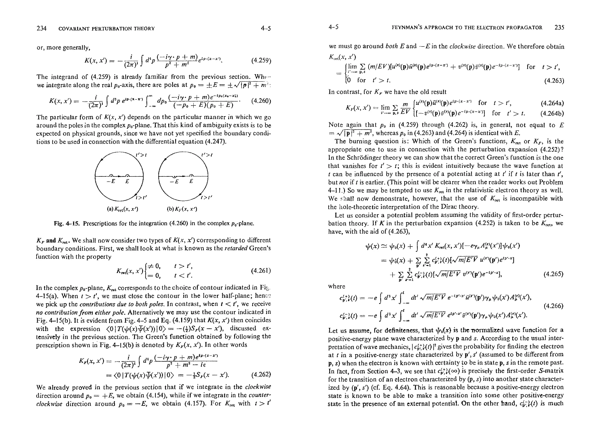
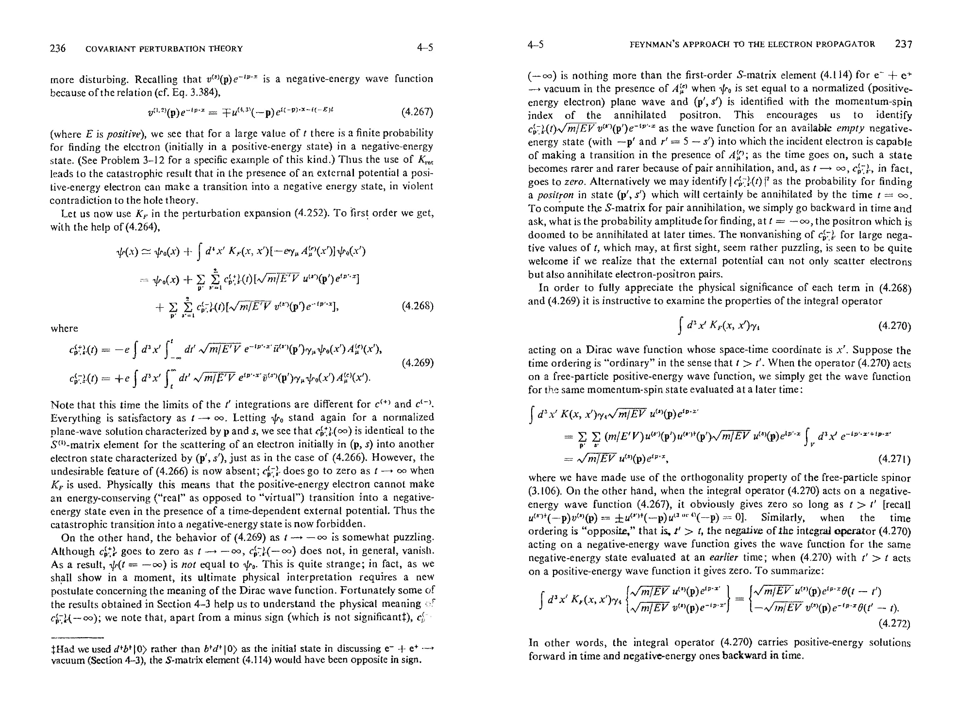
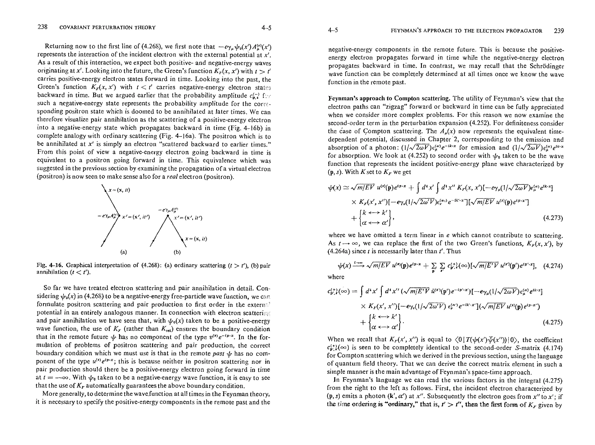
Текст
AO . ,1
Quantum Mechanics
PREFACE
The purpose of this book is to present the major.advances in the fundamentals of
quantum physics from 1927 to the present in a manner that cannot be made any
simpler. In selecting the materials covered in this book I have omitted those topics
which are discussed in conventional textbooks on nonrelativistic quantum
cha.ics, group-theoretic methods, atomic and molecular structure, solid-state
physics, low-energy nuclear physics, and elementary particle physics. With some
regret I have also omitted the formal theory of collision processes; fortunately a
careful and detailed treatment of this subject can be found in a companion Addison-
Wesley volume, Advanced Quantum Theory, by P. Roman. Thus the emphasis
is primarily on the quantum theory of radiation, the Dirac theory of leptons, and
covariant quantum electrodynamics. No familiarity with relativistic quantum
mechanics or quantum field theory is presupposed, but the reader is assumed to
be familiar with nonrelativistic quantum mechanics (as covered in Dicke and
Wittke or in Merzbacher), classical electrodynamics (as covered in Panofsky and
Phillips or in Jackson), and classical mechanics (as covered in Goldstein).
The book has its origin in lecture notes I prepared for the third part of a three-
quarter sequence of courses in quantum mechanics required of a//Ph.D, candidates
in physics at the University of Chicago. Twenty years ago such a short course
in "advanced quantum mechanics" might have covered the materials discussed
in the last three chapters of Schiff. We must realize, however, that forty years have
passed since P. A. M. Dirac wrote down the relativistic wave equation for the
electron; it was nearly twenty years ago that R. P. Feynman invented the famous
graphical techniques that have had profound influences, not only on quantum
electrodynamics and high-energy nuclear physics, but also on such remotely
related topics as statistical mechanic, superconductivity, and naclear many-body
problems. It is evident that, as the frontier of physics advances, the sort of curric-
ulum adequate for graduate students twenty years ago is no longer satisfactory
today.
Chapter I of this book is concerned with a very brief introduction to classical
field theory needed for the latter parts of the book. The subject matter of Chapter
2 is the quantum theory of radiation. First, the transverse electromagnetic field
is quantized in analogy with quantum-mechanical harmonic oscillators. The
subsequent parts of the chapter deal with standard topics such as the emission,
absorption, and scatlering of light by atoms, and thus pro-tide rigorously correct
iii
iv PREFACE
(as opposed to superficial) explanations of a number of atomic pheoomena (e. g.,
spontaneous emission, Planck's radiation law, and the photoelectric effect) with
which the students are already familiar from their earlier courses. In addition,
we discuss more advanced topics including radiation damping, resonance fluores-
cence, the Kramers-Kronig (dispersion) relations, the idea of mass renormalization,
and Bethe's treatment of the Lamb shift.
It is deplorable that fewer and fewer students nowadays study Heitler's classical
treatise on the quantum theory of radiation. As a result, we see a number ,!"
sophisticated, yet uneducated, theoreticians who are conversant in the LSZ
formalism of the Heisenberg field operators, but do not know why an excited atom
radiates, or are ignorant of the quantum-theoretic derivation of Rayleigh's law
'that accounts for the blueness of the sky. It is hoped that Chapter 2 of this book
will fill the missing gap in the education of physicists in the mid-twentieth century.
The wave equation of Dirac is introduced in Chapter 3 by linearizing the rela-
tivistic second-order ,equation involving Pauli matrices, as originally done by
B. L. van der Waerden. In addition to presenting standard topics such as the
plane-wave solutions, an approximate and the exact treatment of the hydrogen
atom, and the physical interpretations of Zitterbewegung, we make special attempts
to familiarize the reader with the physical meanings of the various gamma matrices.
The inadequacy of the single-particle interpretation of the Dirac theory is pointed
out, and towards the end of the chapter we quantize the Dirac field using the
Jordan-Wigner method. Although a rigorous proof of the spin-staiistics connec-
tion is not given, we demonstrate that it is difficult to construct a sensible field
theory in which the electron does not obey the Pauli exclusion principle. The
chapter ends with applications to weak interactions, including short discussions
on the two-component neutrino and parity nonconservation in nuclear beta
decay, hyperon decay, and pion decay.
Symmetry considerations are emphasized throughout Chapter 3. We not
only discuss the formal transformation properties of the Dirac wave function and
the quantized Dirac field under Lorentz transfornatlons, parity, and charge
conjugation, but also show how the various symmetry operators can actually be
used in specific problems (e. g., in constructing momentum and heliclty eigen-
functions or in proving that the intrinsic parity of the positron is opposite to that
of the electron). In Sections 9 and 10 w attempt to clarify the basic differen<
between charge conjugation in the unquantized Dirac theory and charge con jug:-
lion in the quantized Dirac theory, which is often a source of confusion in the
iiterature.
Covarlant perturbation theory is covered in Chapter 4. A distinct feature of
this chapter is that we present covariant quantum electrodynamics not as a "new
theory" but rather as a natural and almost immediate consequence of relativistic
quantum mechanics and elementary quantum field theory, whose foundations
had been laid down by 1932. In the usual derivation of the Feynman rules from
quantum field theory, one first defines five different kinds of invariant functions,
three different kinds of ordered products, etc., and during that time the novice
has no idea why these concepts are introduced. Instead of deriving the Feynman
PREFACE
rules in the most general case from field theory using the Dyson-Wick formalism,
we demonstrate how, in a concrete physical example, the vacuum expectation
value of the time-ordered product (0IT (¢'(x') ff (x))10) emerges in a natural
manner. It is then poini.ed out how this vacuum expectation value can be inter-
preted pictorially in terms of the propagation of an electron going forward or
backward in time t la Feynman. The simplicity and elegance of the postwar
calculational techniques are explicitly exhibited as we demonstrate how two non-
covariant expressions add up to a single covariant expression. The Feynman
rules are also discussed from the point of view of the unit source solution (the
Green's function) of the wave eqnafion, and Feynman's intuitive space-time
approach is compared to the field-theoretic approach. Some electromagnetic
processes (e. g., Mort scattering, two-photon annihilation of electron-positron
pairs, M¢ller scattering) are worked out in detail. The last section of Chapter 4
comists of brief discussions of higher-order processes, the mass and charge re-
nor, aalization, and difficulties with the present field theory. In addition to dis-
cussing standard topics such as the electron self-energy and the vertex correction,
we demonstrate how the principles of unitarity and causality can be utilized to
obtain a sum rule that relates the charge renormalization constant to the prob-
ability of pair creation in an external field. The method for evaluating integrals
appearing in covariani perturbation theory is discussed in Appendix E; as examples,
the self-energy and the anomalous magnetic moment of the electron are calculated
in detail.
We present the covariant calculational techniques in such a nmnner that the
reader is least likely to make mistakes with factors of 2r, i, -- l, etc. For this
reason we employ, throughout the book, the normalization convention according
to which there is one particle in a box of volume V; this is more convenient in
practice because we know that the various V's must cancel at the very end, whereas
the same cannot be said about (2r)'s. A good amount of space is devoted to
showing how observable quantities like differential cross sections and decay
rates are simply related to the covriant d'/-matrices, which we can immediately
write down just by looking at the "graphs."
Throughout this book the emphasis is on physics with a capital P. Complicated
mathematical concepts and formalisms that have little relation to physical reality
are eliminated as much as possible. For instance, the starting point of the quan-
tization of the Dirac field is the anticommutation relations among the creation and
annihilation operators rather than the anticommut.afio -lation between two
Dime fields; this is because the Dirac field itself is not measurable, whereas the
anticommutation relation between two creation operators has a simple and direct
physical meaning in terms of physically permissible states consistent with the
Pauli exclusion principle. In this sense our approach is closer to the "particle"
point of view than to the "field" point of view, even though we talk extensively
about the quantized Dirac field in the last third of the book.
Whenever there are several alternative methods for deriving the same result,
we do oot necessarily choose the most elegant, but rather present the one that
makes thephysics of the problen most transparenl at each.stage of the derivation.
vi PREFACE
For example, in discussing the ,Moiler interaction between two electrons we start
with the radiation (Coulomb) gauge formalism of E. Fermi and show how this
noncovariant but.simple method can be used to derive, in an almost miraculous
manner, a manifestly covariant matrix element which can be visualized as arising
from the exchange of four types of "covariant photons." We prefer this approach
to the one based on the Bleuler-Gupta method because the latter introduces
artificial concepts, such as the indefinite metric and negative probabilities, which
are not very enlightening from the point of view of the beginner's physical under-
standing of quantum electrodynamics.
Wlerever possible, we show how the concepts introduced in this book are
related to concepts familiar from nonrelativistic quantum mechanics or classical
electrodynamics. For example, as we discuss classical electrodynamics in Chapter
1 we review the role of the vector potential in nonrelativistic quantum mechanics
and, in particular, consider the Aharonov-Bohm effect and flux quantization.
In Chapter 2 the scatte.ring of light by atoms in the quantum theory is compared to
its classical analog. In discussing the polarization correlation of the two-photon
system resulting from the annihilation of an electron-positron pair, we illustrate
some peculiar features of the quantum theory of measurement which have disturbed
such great minds as A. Einstein. In Chapter 4 a fair amount of attention is paid to
the connection between the calculational methods of the old-fashioned pe.rturba-
tion theory (based on energy denominators) and those of covariant perturbation
theory (based on relativistically invariant denominators). In discussing the
Moiler interaction and the nucleon-nucleon interaction, we try to indicate how
the potential concept one learns about in nonrelativistic quantum mechanics is
related to the field-theoretic description based on the exchange of quanta.
Although numerous examples from meson theory and nuclear physics arc
treated throughout the book, it is not our intention to present systematic accounts
of nuclear or high-energy phenomena. Nonelectromagnetic processes are dis-
cussed solely to illustrate how the ideas and techniques which we acquire in
working out electromagnetic problems can readily be applied to other areas of
physics.
The forty-seven problems scattered throughout comprise a vital part of the
book. The reader who has read the book but cannot work out the problems has
learned nothing. Even though some of the problems are more difficult and chal-
lenging than others, none are excessively difficult or time-consuming. Nearly
every one of them has been worked out by students at the University of Chicago;
some, in the final examination of the course on which the book is based.
In recent years several excellent textbooks have appeared on the calculational
techniques in relativistic quantum mechanics..The distinct feature of this book
is not just to teach the bag of tricks useful only to high-energy physicists or to
show how to compute the trace of the product of Dirac matrices, but to make the
reader aware of the progress we have made since 1927 in our understanding of
fundamental physical processes in the quantum domain. From this point of view
we believe it is just as important for the student to know how the quantum descrip-
tion of the radiation field reduces to the familiar classical description in the limit
PREFACE vii
of a large number of quata, or why the spin-- particle "must" obey the exclusion
principle, as it is to master the rules that enable us to calculate the magnetic
moment of the electron to eight decimals.
To summarize our philosophy: Relativistic quantum mechanics and field
theory should be viewed as part of the heroic intellectual endeavor of a large
number of twentietl-century theoretical physicists in the finest tradition of M.
Planck, A. Einstein, and N. Bohr. It would be catastrophic for the future develop-
ment of physics if the terminal course in theoretical physics for most Ph.D. level
students in physics were nonrelativistic quantum mechanics, the fundamentals of
which had essenti;illy been perfected by 1926. For this reason I believe that the
topics covered in this book should be studied seriously by every Ph.D. candidate
in physics, just as nonrelativistic quantum mechanics has become recognized as
a subject matter to be digested by every student of physics and chemistry.
I am grateful to the Alfred P. Sloan Foundation for a fellowship which enabled
me to write the last chapter of the book in tle congenial atmosphere of CERN
(Eur,pean Organization for Nuclear Research). I wish to thank Drs. J. S. Bell,
S. t',nster, and A. Maksymowicz, and Mr. D. F. Greenberg for reading various
parts of the book and making many vahmble suggestions. Particular thanks are
due to Mr. L Kimel for the painstaking task of filling in the equations.
May 1967 J. J. S.
Chicago, llliaois
CONTENTS
Chapter 1
I-I
1-2
1-3
I-4
1-5
Chapter 2
2-1
2-2
2-3
2-4
2-5
2-6
2-7
2-8
Chapter 3
3-1
3-2
3-3
3-4
3-5
3-6
3-7
3-8
3-9
3-10
3-11
Chapter 4
4-1
4-2
Classical Fields
Particles and fields ...............
Discrete and continuous mechanical systems ....... 3
Classical scalar fields .............. 5
Classical Maxwell fields ............. 12
Vector potentials in quantum mechanics ........ 15
The Quantum Theory of Radiation
Classical radiation field ............. 20
Creation, annihilation, and number operators ....... 23
Quantized radiation field ............. 29
Emission and absorption of photons by atoms ....... 36
Rayleigh scattering, Thomson scattering, and the Raman effect . 47
Radiation damping and resonance fluorescence ...... 53
Dispersion relations and causality .......... 57
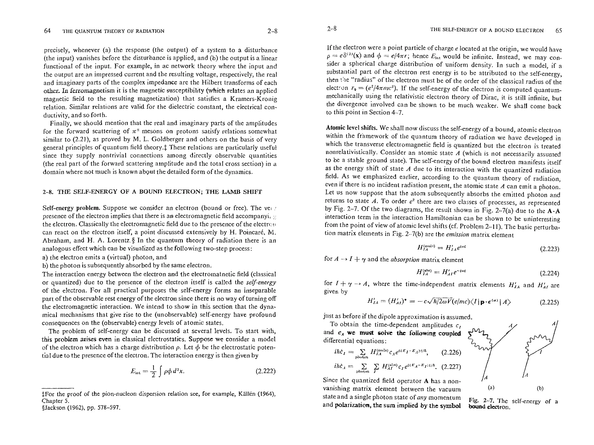
The self-energy of a bound electron ; the Lamb shift ..... 64
Relativistic Quantum Mechanics of Spin- Particles
Probability conservation in relativistic quantum mechanics 75
The D[raC equation .............. 78
Simple solutions; nonrelativisfic approximations; plane waves 85
Relativistic covariance .............. 95
Bilinear covariants ............... 104
Dirac operators in the Heisenberg representation ...... 112
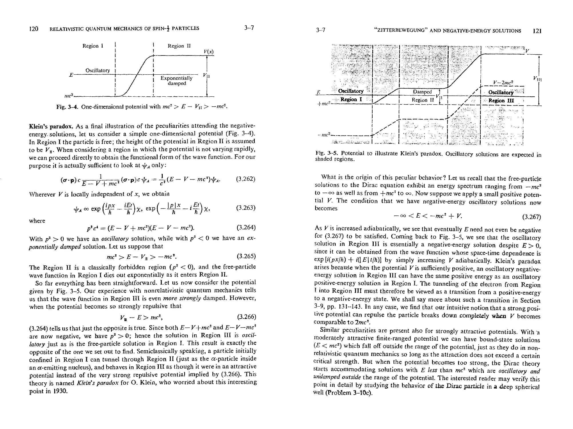
Zitterbe,vegungamd negalive--energy solutions ....... 117
Central force problems; the hydrogen atom ....... 122
Hole theory and charge conjugation .......... 131
Quantization of the Dirac field ........... 143
Weak interactions and parity nonconservation; the two-component
neutrino .................. 156
Covariant Perturbation Theory
Natural units and dimensions ........... . 179
S-matrix expansion in the interaction m3rresentatitTn ..... 181
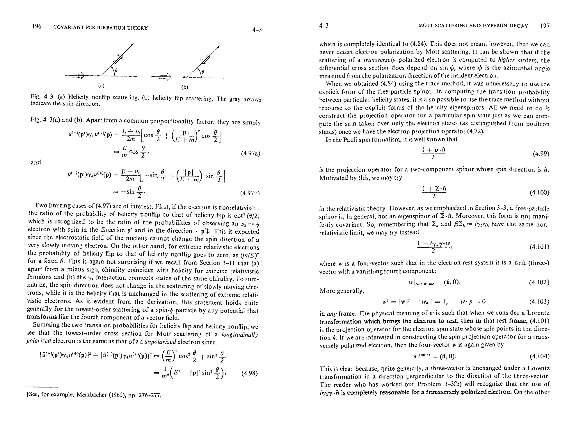
First-order processes; Mott scattering and hypcron decay 188
xii CONTENTS
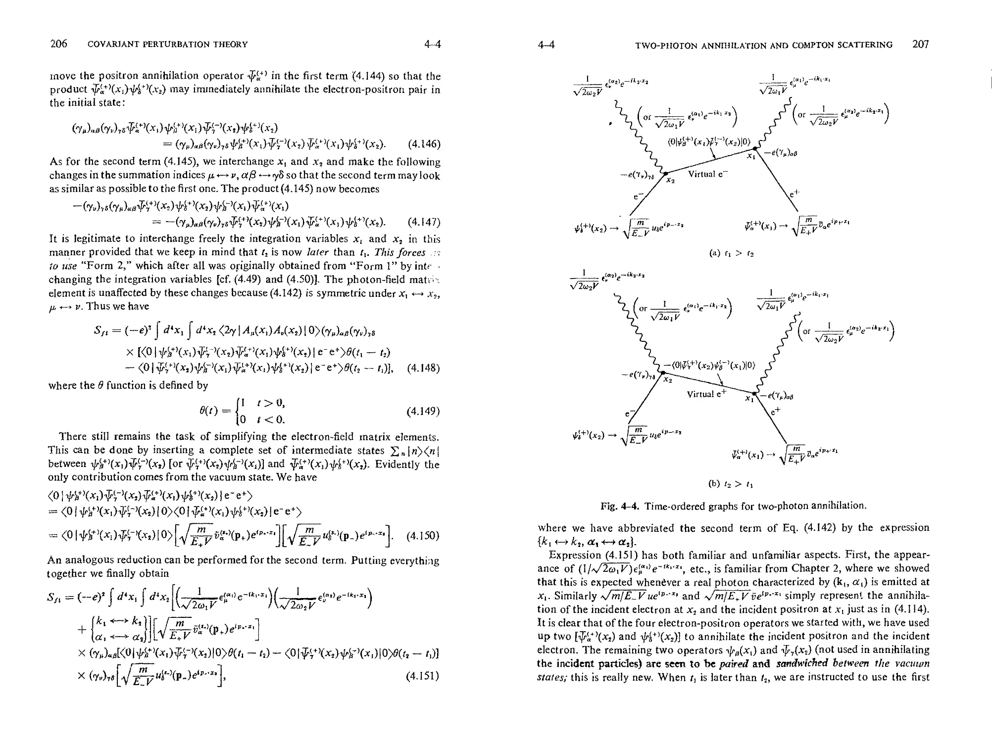
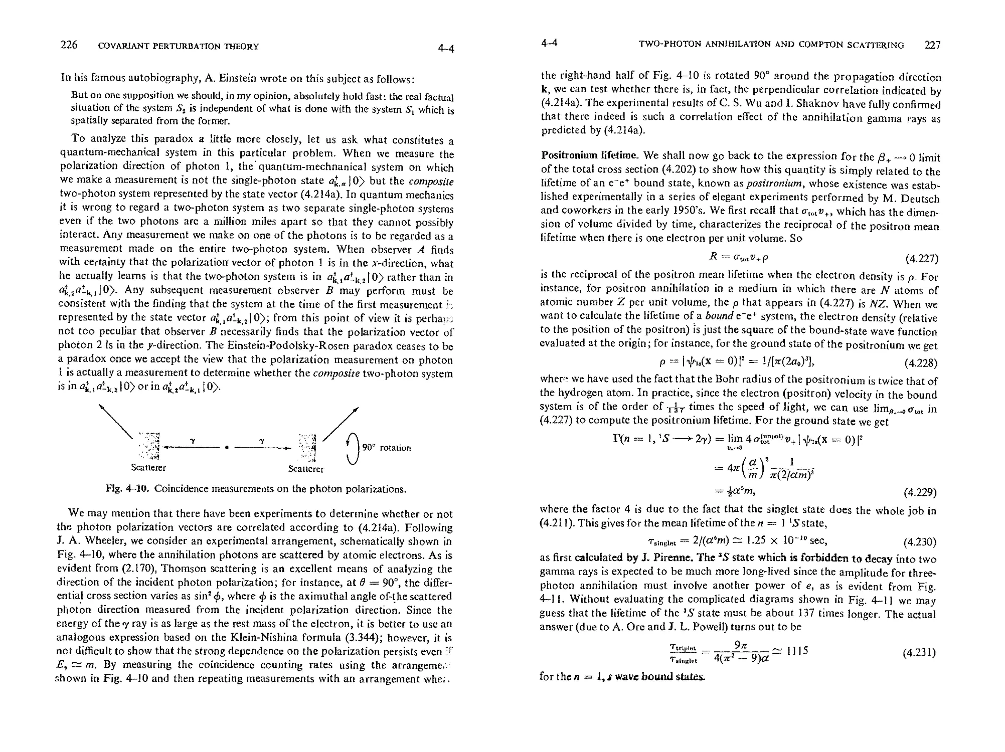
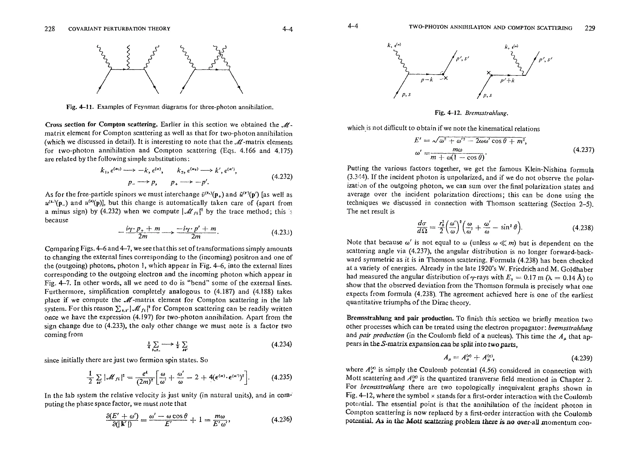
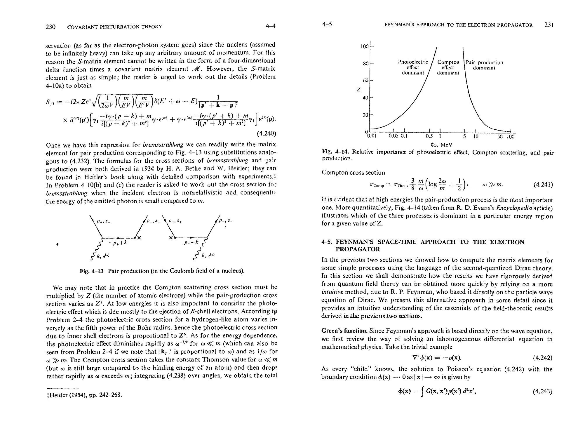
4-4 Two-photon annihilation and Compton scattering; the electron
propagator .................
4-5 Feynman's space-time approach to the electron propagator .
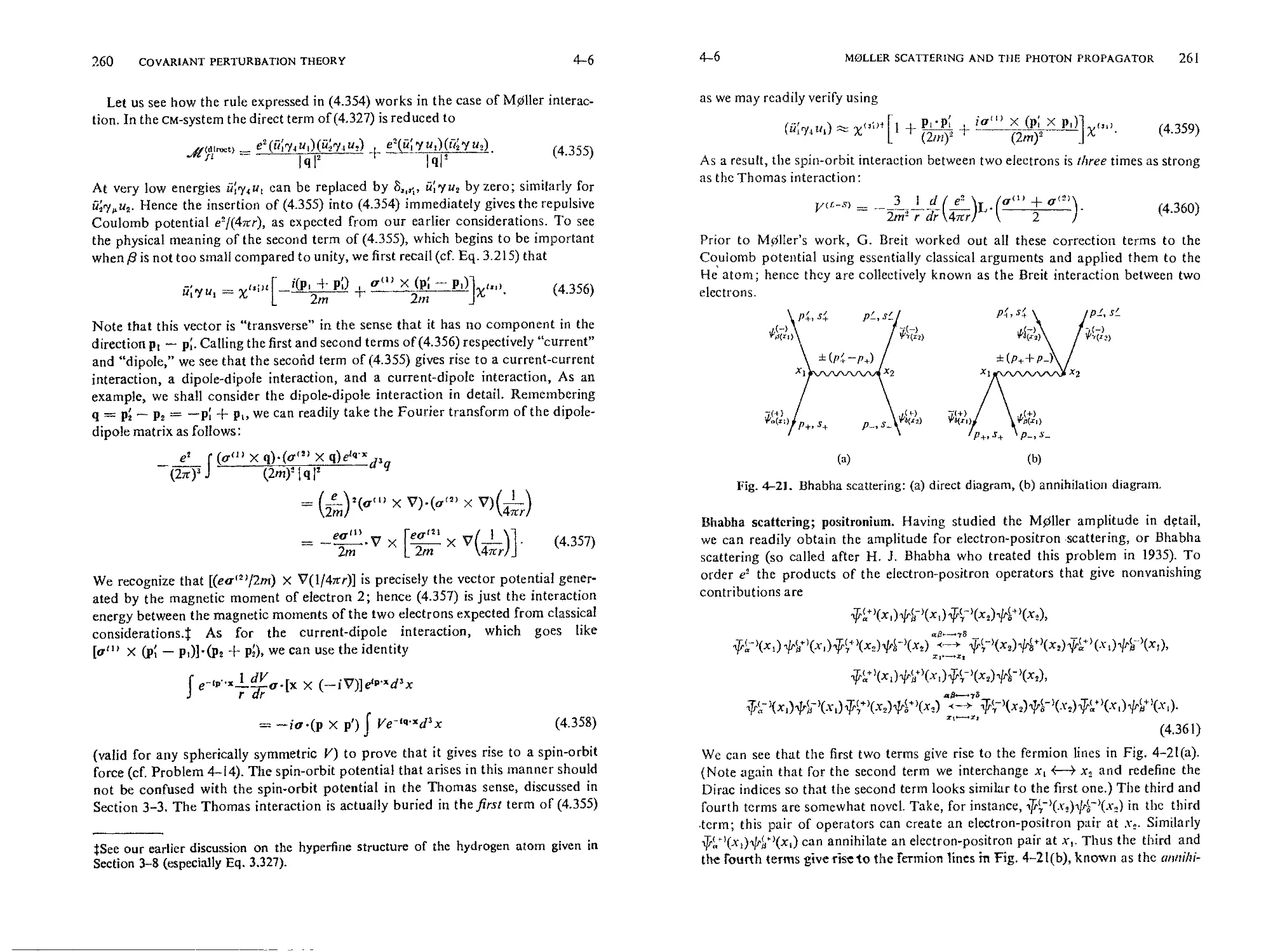
4-6 Moiler scattering and the photon propagator; one-meson exchange
interactions .................
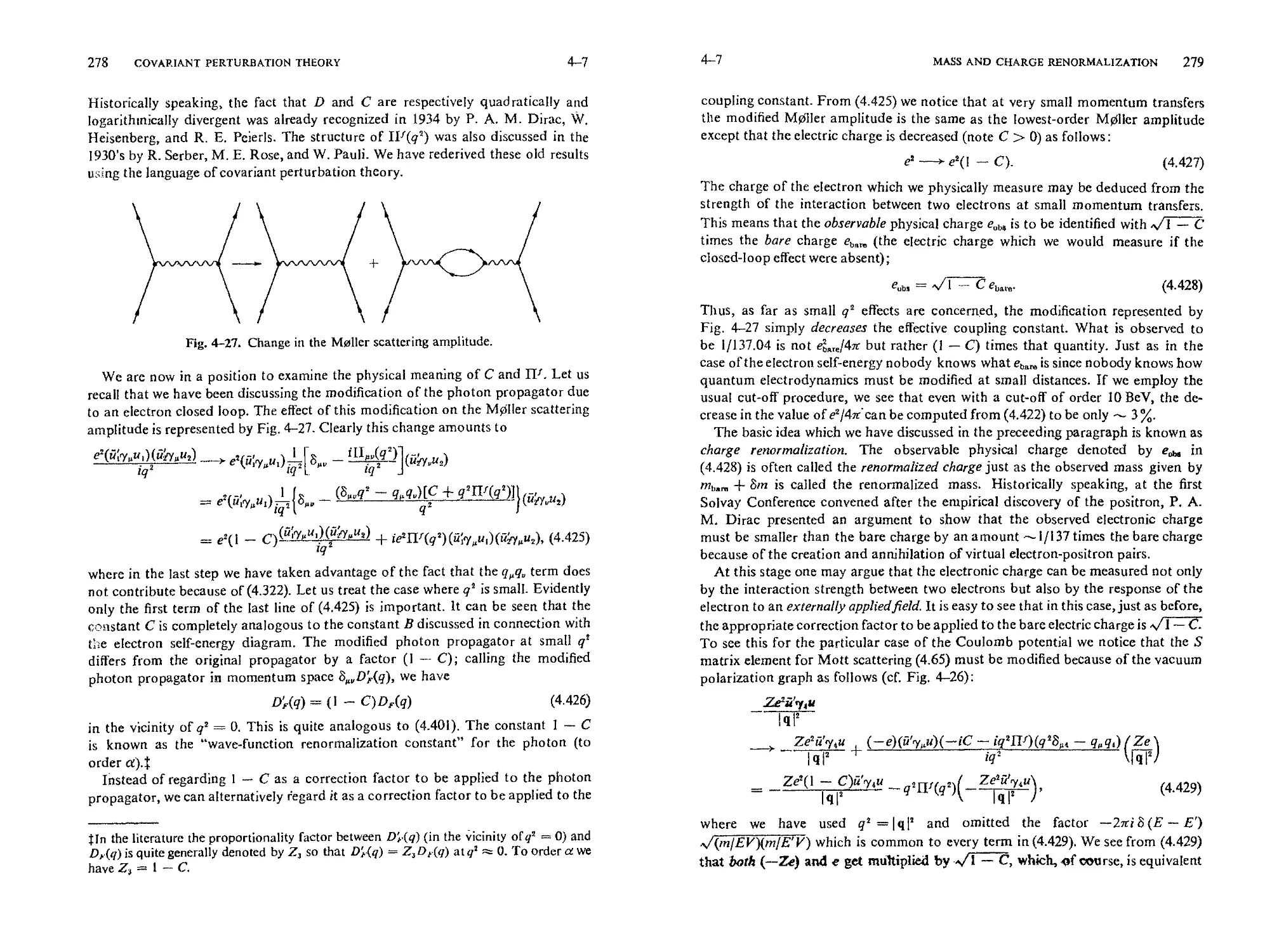
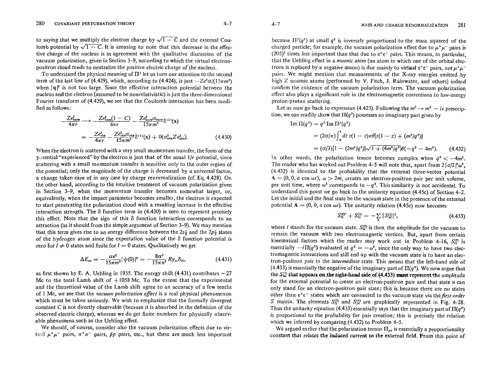
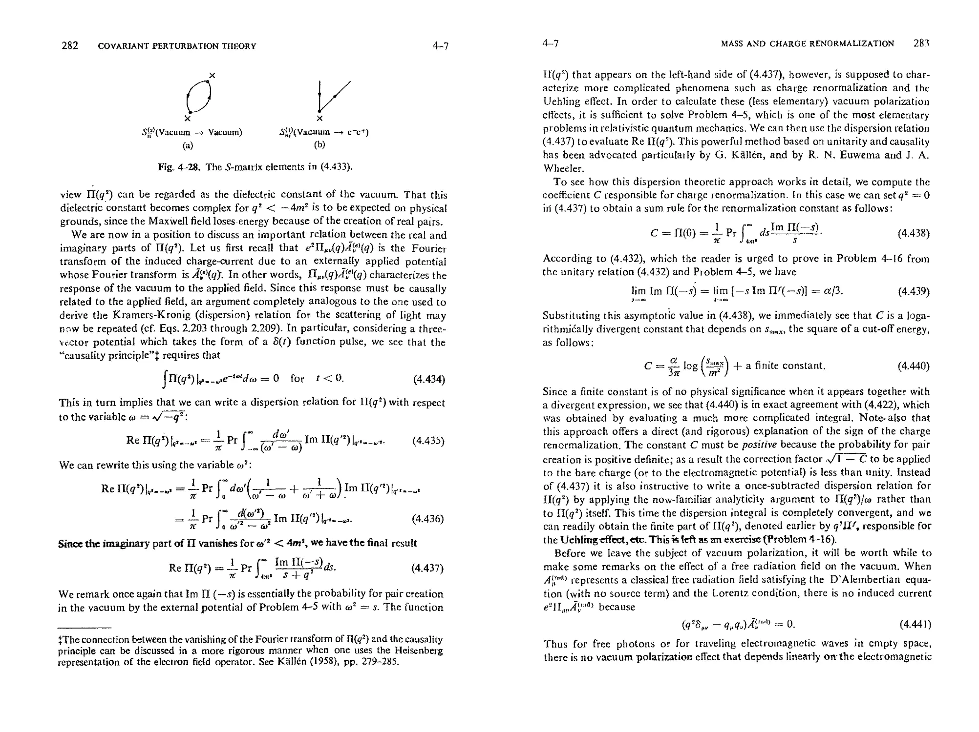
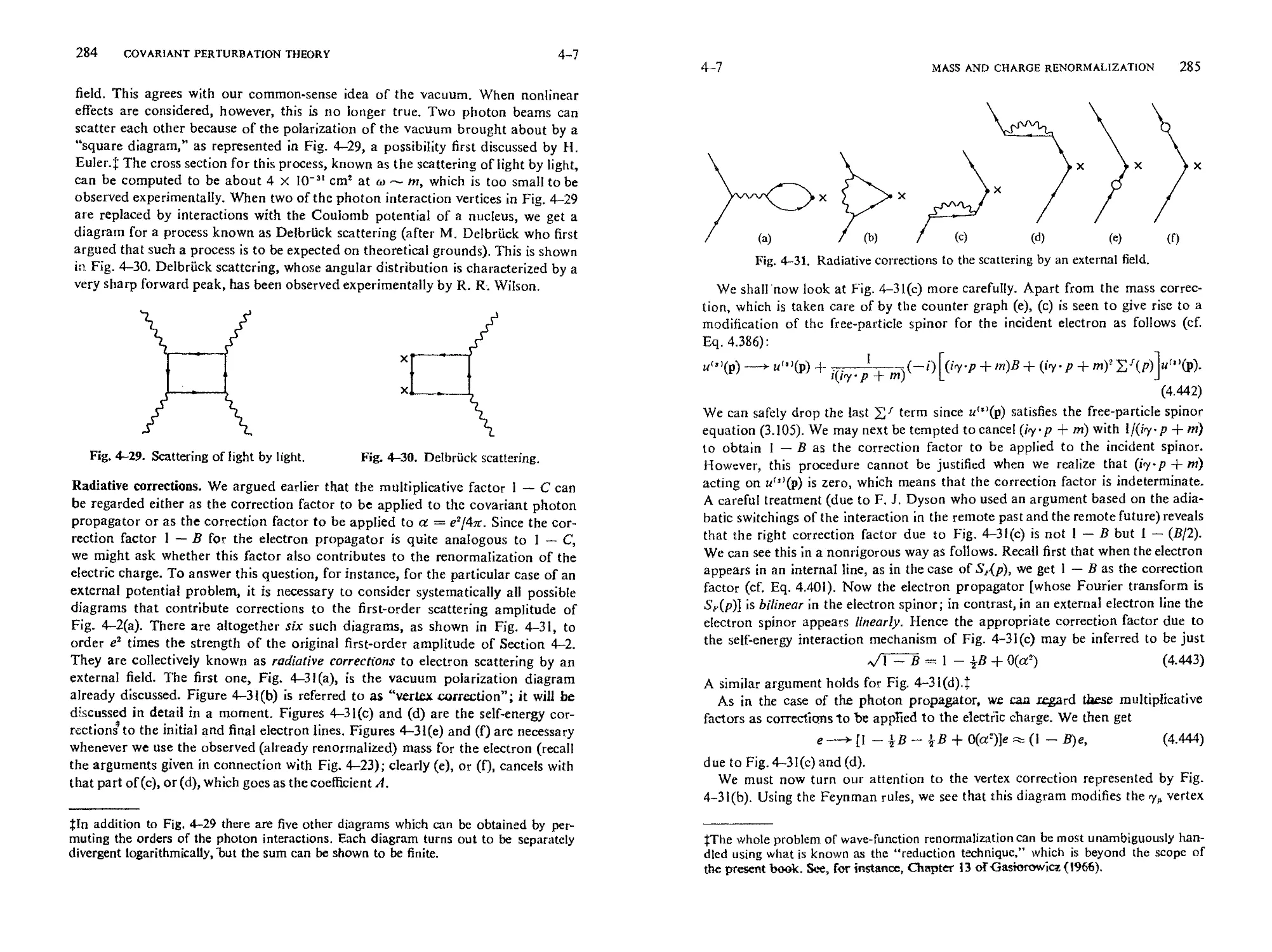
4-7 Mass and charge renormalization; radiative corrections ....
Appendix A
Appendix B
Appendix C
Appendix D
Appendix E
Bibliography
Electrodynamics in the radiation (Coulomb) gauge .....
Gamma matrices ...............
Pauli's fundamental theorem ............
Formulas and rules in covariant perturbation theory .....
Feynman integrals; the computations of the self-energy and the
anomalous magnetic moment of the electron .......
Index .......................
204
231
242
267
301
305
308
315
323
327
CH PTER 1
CLASSICAL FIELDS
I-.1. PARTICLES AND FIELDS
Nonrelativistic quantum mechanics, developed in the years from 1923 to 1926,
provides a unified and logically consistent picture of numerous phenomena in the
atomic and molecular domain. Following P.A.M. Dirac, we might be tempted
to assert: "The underlying physical laws necessary for the mathematical theory
Of a large part of physics and the whole of chemistry are completely known."
There 9.re, however, basically two reasons for believing that the description
of physical phenomena based on non,relativistic quantum mechanics is incomplete.
First, since nonrelativistic quantum mechanics is formulated in such a way as to
yield the nonrelativistic energy-momentum relation in the classical limit, it is
incapable of accounting for the fine structure of a hydrogen-like atom. (This
problem was treated earlier by A. Sommerfeld, who used a relativistic generaliza-
tion of N. Bohr's atomic model.) In general, nonrelatlvistic quantum mechanics
makes no prediction about the dynamical behavior of particles moving at rela-
tivi;tic velocities. This defect was amended by tile relativistic theory of electrons
devel.oped by Dirac in 1928, which will be discussed in Chapter 3. Second, and
what ; more serious, nonrelativistic quantum mechanics is essentially a single-
particle theory in which the probability density for finding a given particle inte-
grated over all space is unity at all times. Thus it is not constructed to describe
phenomena such as nuclear beta decay in which an electron and an antineutrino
are created as the neutron becomes a proton or to describe even a simpler process
in which an excited atom returns to its ground state by "spontaneously" emitting
a single photon in the absence of any external field. Indeed, it is no accident that
many of the most creative theoretical physicists in the past forty years have spent
their main efforts on attempts to understand physical phenomena in which various
particles are created or annitated. The major part of this book is devoted to the
progress physicists have made along these lines since the historic 1927 paper of
Dirac entitled "The Quantum Theory of the Emission and Absorption of
Radiation" opened up a new subject called the quantum theory offields.
The concept of a field was originally introduced in classical physics to account
for the interaction between two bodies separated by a finite distance. In classical
plysics the electric field E(x, t), for instance, is a three-component function defined
at each space-time point, and the interaction between two charged bodies, 1 and
2, is to be viewed as the interaction of body 2 with the electric field created by
body I. In "the quantum theory, however, the fied concept acquires a new dimen-
2 CLASSICAL FIELDS 1-1 1-2 DISCRETE AND CONTINUOUS MECHANICAL SYSTEMS 3
sion. As originally formulated in the late 1920's and the early 1930's, the basic
idea of quantum field theory is that we associate particles with fields such as the
electromagnetic field. To put it more precisely, quantum-mechanical excitations
of a field appear as particles of definite mass and spin, a notion we shall illustrate
in Section 2-2, where the connection between the transverse electromagnetic fieJ
and photons is discussed in detail.
Even before the advent of postwar calculational techniques which enabled us
to compute quantities such as the 2s-2p 2 separation of the hydrogen atom to
an accuracy of one part in 10 , there had been a number of brilliant successes
of the quantum theory of fields. First, as we shall discuss in Chapter 2, the quantum
theory of radiation developed by Dirac and others provides quantitative under-
standings of a wide class of phenomena in which real photons are.emitted or
absorbed. Second, the requirements imposed by quantum field theory, when
combined with other_general principles such as Lorentz invariance and the
probabilistic interpretation of state vectors, severely restrict the class of particles
that are permitted to exist in nature.-In particular, we may cite the following two
rules derivable from relativistic quantum field theory:
a) For every charged particle there must exist an antiparti.cle with opposite charge
and with the same mass and lifetime.
b) The particles that occur in nature must obey the spin-statistics theorem (first
proved by W. Pauli in 1940) which states that half-integer spin particles
(e.g., electron, proton, A-hyperon) must obey Fermi-Dirac statistics, whereas
integer spin particles (e.g., photon, -meson, K-meson) must obey Bose-
Einstein statistics
Empirically there is no known exception to these rules. Third, the existence of
a nonelectromagnetic interaction between two nucleons at short but finite distances
prompts us to infer that a field is responsible for nuclear forces; this, in turn,
implies the existence of massive particles associated with the field, a point first
emphasized by H. Yukawa in 1935. As is well known, the desired particles, now
known as rt-mesons or pions, were found experimentally twelve years after the
theoretical prediction of their existence.
These considerations appear to indicate that the idea of associating particle:;
with fields and, conversely, fields with particles is not entirely wrong. There are,
however, difficulties with the present form of quantum field theory which must
be overcome in the future. First, as we shall show in the last section of Chapter
4, despite the striking success of postwar quantum electrodyaamics in calculating
various observable effects, the "unobservable" modifications in the mass and charge
of the electron due to the emission and reabsorption of a virtual photon turn out
to diverge logarithmically with the frequency of the virtual photon. Second, the
idea of associating a field with each "particle" observed in nature becomes ridic-
ulous and distasteful when we consider the realm of strong interactions where
many different kinds of "particles" are known to interact with one another; we
know from experiment that nearly 100 "particles" or "resonances" participate
in the physics of strong interactions. This difficulty became particularly acute
in 1961-1964 when a successful classification scheme of strongly interacting
particles was formulated which groups, together into a single "'family" highly un-
stable "particles'" (lifetimes 10 --a sec, often called strong interaction resonances)
and moderately metastable particles (lifetimes 10 -° sec). Yet, despite these difficul-
ties, it is almost certain that there are many elements in present-day quantum
field theory which are likely to survive, say, one hundred years from now.
Before we study qm.ntized fields, we will study classical fields. In part this deci-
sion is motivated by the historical fact that prior to the development of quantum
electrodynamics there was the classical electrodynamics of Maxwell which, among
other things, successfully predicted the existence of Hertzian electromagnetic
waves. This chapter is primarily concerned with the elements of classicalfield
theory needed for the understanding of quantized fields. As a preliminary to the
study of quantization we are particularly interested in the dynamical properties
of classical fields. For this reason we will follow an approach analogous to Hamil-
ton's formulation of l_.agrangian mechanics.
1-2. DISCRETE AND CONTINUOUS MECHANICAL SYSTEMS
The dynamical behavior of a single particle, or more precisely, a mass point in
classical mechanics, can be inferred from Lagrange's equation of motion
.t -- -, = O, (1.1)
whici is derivable from Hamilton's variational principle
;i L(q,, O)dt = O. (1.2)
The Lagrangian L (assumed here not to depend explicitly on time) is given by the
difference of the kinetic energy T and the potential energy V,
and the variation in (1.2) is to be taken over an arbitrary path q(t) such that q
vanishes at t and t. The Hamiltonian of the system is
H = ,O,- L, (1.4)
where the momentum p, canonical conjugate to q, is given by
OL
p, = - (.5
.]:ln fact the one-to-one correspondence betweea a "'field" and a "'particle" appears to be
lost in a more modern formulmion of the field theory of strong interactions as many (if
not all) of the so-called "'elementary" particles may well be regarded as bound (or
resonant) states of each olhcr. The distinction between fundamental particles and com-
posite states, however, is much more clear-cut in the realm of the electromagnetic inter-
actions among electrons, muns, and photons. As an example, in Section 4-4 we shall
calculate the lifetim of the ground slate of tor, itronium withou1 introducing a field
COrresponding to the positronium.
4 CLASSICAL FIELDS 1-2 1-3 CLASSICAL SCALAR FIELDS 5
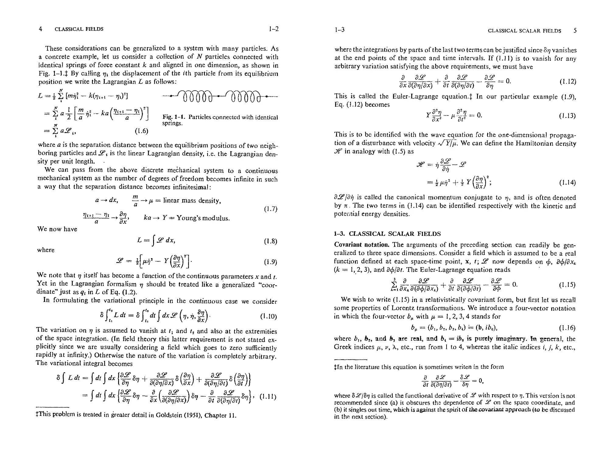
These considerations can be generalized to a system with many particles. As
a concrete example, let us consider a collection of N particles connected with
identical springs of force constant k and aligned in one dimension, as shown in
Fig. I-1.5 By calling r h the displacement of the ith particle from its equilibrium
position we write the Lagrangian L as follows:
r
: 1 [m . ()]
= a- -- ka
--- r/ Fig: 1-1. Particles connected with identical
, springs.
= a..,, (1.6)
where a is the separation distance between the equilibrium positions of two neigh-
boring particles and .La is the linear Lagrangian density, i.e. the Lagrangian den-
sity per unit length.
We can pass from the above discrete mechanical system to a continuous
mechanical system as the number of degrees of freedom becomes infinite in such
a way that the separation distance becomes infinitesimal:
a--* dx, m
"-h- --/ = linear mass density,
0:7)
+ -ff, ka -- Y = Young's modulus.
We now have
where
L = J dx,
(l
.. = ½[#f - Y(l.
(1.9)
\axl _1
We note that r/itself has become a function of the continuous parameters x and r
Yet in the Lagrangian formalism r/ should be treated like a generalized "coor-
dinate" just as q in L of Eq. (1.2).
In formulating the variational principle in the continuous case we consider
, /. 0.]0)
The variation on r 1 is assumed to vanish at t and t and also at the extremities
of the space integration. (In field theory this latter requirement is not stated ex-
plicitly since we are usually considering a field which goes to zero sufficiently
rapidly at infinity.) Otherwise the nature of the variation is completely arbitrary.
The variational integral becomes
is problem is treated in reater detail in Goldstein (1951), Chapter 11.
where the integrations by parts of the last two terms can be justified since 8r/vanishes
at the end points of the space and time intervals. If (1.11) is to vanish for any
arbitrary variation satisfying the above requirements, we must have
a a a a a=0. (1.12)
axa(n/ax) + at a(anlat) an
This is called the Euler-Lagrange equation.t In our particular example (1.9),
Eq, (1.12) becomes
Y -- = 0. 0.]3)
This is to be identified with the wave equation for the one-dimensional propaga-
tion of a disturbance with velocity #--]. We can define the Hamiltonian density
Y in analogy with (1.5) as
. Oc. ca
= 0 + r(]" (1.14)
kOx} '
0]00 is called the canonical momentum conjugate to , and is often denoted
by . The two terms in (1.14) can be identified respectively with the kinetic and
potetial energy densities.
I-3. CLASSICAL SCALAR FIELDS
CovarJant notation. The arguments of the preceding section can readily be gen-
eralized to three space dimensions. Consider a field which is assumed to be a real
function defined at each space-time point, x, t; .. now depends on b, O/Ox
(k = 1,.2, 3), and O/Ot. The Euler-Lagrange equation reads
_a a o a a
,axa(a4/axO + at a(a4/at) = 0. (1.15)
We wish to write (1.15) in a relativistically covariant form, but first let us recall
some properties of Lorentz transformations. We introduce a four-vector notation
in which the four-vector b with = 1,2, 3, 4 stands for
O = (b,, b,, b, b,) (b, ibo), (1.16)
where b, b, and b are real, and b = ibo is purely afm. gal, the
Greek indices , u, k, etc., run from 1 to 4, whereas the italic indices i, L k, etc.,
.]:In the literature this equation is sometimes writen in the form
at o(alOt) - = O,
where 8.LalSr/is called the functional derivative of with respect to . This version is not
recommended since (a) it obures the dependence of on the space coordinate, and
(b) it singles out time, which isait the spi6t ofv approach (to be discussed
in th next section).
6 CLASSICAL FIELDS 1-3 1-3 CLASSICAL SCALAR FIELDS 7
run from 1 to 3. The coordinate vector x,is given by
x = (x, x2, xa,
= (x, ict). (I.I 7)
The symbols x, y, and z may also be used in place of xl, x, and xa. Under a Lor.entz
transformation, we have
x', = a,x, (1.18)
where the a, satisfy
Hence
a,,a,x = ,, (a-% = a,. (I.19)
x = (a-'),,,x', = a,x' (I.20)
when x' and x are related by (I.18). The matrix elements al, a, are purely real,
whereas a and a are purely imaginary. A four-vector, by definition, transforms
in the same way as x, under Lorentz transformations. Because of (I.20) we have
0 Ox 0 0 (1.21)
-- a -- ;
ax' Ox' Ox ax
so the four-gradient O/Ox is a four-vector. The scalar product b.c is defined by
b.c = b,G = bc + b,c
= b-c -- boco. (1.22)
It is unchanged under Lorentz transformations, since
b'.c' = Gba, c = x bc
= b.c. (1.23)
A tensor of second rank, t, transforms as
t = Gxa¢tx,. (1.24)
Generalizations to tensors of higher rank are straightfoard. Note that we make
no distinction between a covariant and a contravafiant vector, nor do we define
the metric tensor g. These complications are absolutely unnecessary in the special
theory of relativity. (It is regrettable that many textbook writers do not emphasize
this elementa point.)
Equation (1.15) can now be written as
It is seen that the field equation derivable from the Lagrangian'density is covari-
ant (ke., the equation "looks the same" in all Lorentz frames) if the Lagrangian
density f is chosen to be a relativistically scalar density. This is an important
point because the relativistic invariance of is so restrictive that it can be used
as a guiding principle for "deriving" a covariant wave equation.
Neutral scalar field. As an illustration let if(x) be a scalar field which, by definition,
trafisforms like
'(x') = (x),
under a Lorentz transformation, where q5' is the functional form of the field in the
prim:d system. Now the dependence of .e on space-time coordinates is only
throgh the field and its first derivatives, and x, cannot appear explicitly in..'..
This means that O/Ox, is the only four-vector at our disposal; when it appears
in c.L° it must be contracted with itself. Moreover, if we are interested in obtainig
a linear wave equation, .. must be a quadratic hnction of and O/Ox. A pos-
sible candidate for consistent with the above requirements is
2 kOx, q- )" (I.27)
From the Euler-Lagrange equation (1.25) we obtain
I 0 (2)+'0, (1.28)
2
or
- = o, 0.9)
where
= V 1 0
e Ot (1.30)
e wave equation (I.29) is called the Klein-Gordon equation. It was considered
in the middle 1920's by E. Schr6dinger, as well as by O. Klein and W. Gordon,
as a candidate for the relativistic analog of the nonrelativistic Schr6dlnger wave
equation for a free particle. The similarity of (I.29) to the relativistic energy
momentum relation for a free particle of mass m,
E -- [p['c' : mc ', (1.31)
becomes apparent a5 we consider heuristic substitutions:
Eih, ,--ih. (1.32)
The parameter in (I.29) has the dimension of inverse length, and, using (I.32),
we may make the identification
= mc/h. (1.33)
Numerically 1/ is 1.41 X 10 - cm for a particle of mass 140 MeV/c (corre-
sponding to the mass othe charged pion).
Yukawa potential. So far we have been concerned with a field in the absence of any
source. Such a field is often called a free field. The interaction of with a source
can easily be incorporated into the Lagranglan formalism by adding
to (1.27), where is the source density, which is, in general, a function of space-
time coordinates. The field equation now becomes
CLASSICAL FIELDS 1-3 1-3 CLASSICAL SCALAR FIELDS 9
Let us consider a static (i.e., time-independent) solution to (1.35) where the
source is assumed to be a point source at the origin, independent of time. We have
(V --/z)q5 = G5°)(x), (1.36)
where G, the numerical constant that characterizes the strength of the coupling
of the field to the source, is analogous to the constant e in electrodynamlcs.
Although the solution to (1.36) can be guessed immediately, for pedagogical
reasons we solve this equation using the Fourier transform method. First, we
define ((k) as follows:
4,(x) =
1 J rdxe_,k.,+(x) ' (1.37)
wher k and , respectively, stand or volume elements in the three-dimensional
k-spac and the coordinat space, ffw¢ multiply both sides o(1.35) by e-*k'/(2 /
and integrate with , w obtain, ater ntegrating by parts twice(assuming that
and V go to zro suciently rapidly at infinity),
(--Iki -- )(k) =
Thus the differential equation (1.3 has been converted nto an algebraic equation
which can easily be solved:
5(k) e • ( .3)
(]kl + "
x) = () dklk, +
where r = [ x[ and 0 = L, x). The integration can be performed to give
G e -
(x)= r (]')
Yukawa proposed that a nucleon is the source of a force field, called the meson
field, in the same way as an electrically charged object is the source of an
trostatic field. Suppose that the static meson field ounda aaron loted at
origin satisfies (1.36). The strength of the meson field at point x due to the presence
of a nucleon at point x is given by
Since the interaction Lagrangian density (1.34) does not involve the time derivative
o$, the interaction Hamiltonian density (cf. Eq. LI4), is given by st
Hence the total interaction Hamiltonan is
The interaction energy between two nucleons, one located at point x"-, the other
at point x, is
l. -- 4c tx"- -- xi[ (1.44)
Unlike the Coulomb case, this interaction is attractive$ and short-ranged; it
goes to zero very rapidly for
Ix.. - x, I>> l//. (1.45)
We have seen that by postulating the existence of a field obeying (1.36), we can
qualitatively understand the short-ranged force between two nucleons. The mass
of a quantum associated with the field was originally estimated by Yukawa to be
about 200 times the electron mass. This estimate is not too far from the mass
of the observed plon (about 270 times the electron mass) discovered by C. F. Powell
and ]is coworkers in 1947. To represent the interaction of the pion field with the
nucleon in a more realistic way, we must make a few more modifications. First,
we must take into account the spin of the nucleon and the intrinsic odd parity
of the pion, both of which will be discussed in Sections 3-10 and 3-11. Second, we
must note that the pions obseed in nature have three charge states (+, 0, -).
These considerations naturally lead us to a discussion of a complex field.
Complex scalar field. Suppose we consider two real fields of identical masses.
We can always construct complex fields and * byff
=, * -- ; (1.46)
¢ *
6, = , , = - - (z.7)
The free-field Lagrangian density can be written either in terms of the real fields
and or in terms of the complex fields and * :
__ -(a¢* a¢ + '¢*¢)-
(1.48)
The field equations for ff and +* can be obtained from the variational principle
by treating and * as two independent
x (¢/x.) o +* - = o,
:The reason for the Coulomb repulsion and the Yukawa attraction will be treated in
Section 4--6. The difference stems from the fact that the Coulomb field transforms like
the fourth component of a vector, whereas our field is a scalar field.
rth-'oghout this book the superscript '* slands for complex conjztgation. The super-
script 1 will be used for Hermitian conjugation.
I0 CLASSICAL FIELDS I--3 I-3 CLASSICAL SCALAR FIELDS I I
What is the physical interpretation of a complex field ? It is not difficult to show
that if qb is a solution to the Klein-Gordon equation in the presence of A with
charge e, then qb* is a solution to the Klein-Gordon equation in the presence of
the same A but with charge --e. This demonstration is left as an exercise
(Problem 1-3).
To see further the connection between the complexity of a scalar field and
an internal attribute such as electric charge associated with it, we consider the
following unitary (actually orthogonal) transformation on qb and
qb' = cos -- qb sin , qb; = sin + cos , (1.50)
where is a real constant independent of space-time points. Since the masses
associated with t and are assumed to be strictly the same in (1.48), the free-
field Lagrangian (1.48) is clearly invariant under (1.50). In terms of ff and *,
the transformation (1.50) amounts to
Let us consider (1.51) with X taken to be infinitesimally small. We then have
3 = iX, * = --iX*, (1.52)
for the changes in ff and *. Meanwhile, the variation in induced by (1.52) is
( a (
+
_ .. O la*,
where we have used the Euler-Lagrange equation. Since the Lagrangian density
is known to be unchanged from our earlier argument, must be zero. Thus
we have the important result
= 0,
where
kax,
This means that there exists a conseed four-vtor current [i.e., a four-vector
density that satisfies the continuity equation (1.54)] associated with a complex
field .
Under the substitution *, s, changes its sign. This suggests that
to be interpreted as the charge-current density up to a constant, and that
a field corresponding to a particle with charge e, then * is a field correspondirg
to a particle with charge --e, in agreement with the interpretation suggested
Problem 1-3. It is a remarkable feature of relativistic field theory that it can readily
accommodate a pair of particles with the same mass but opposite charges. In the
formalism, however, there is nothing that compels us to relate s;, to the charge-
current density that appears in electrodynamics. In fact, our formalism can ac-
commodate any conserved internal attribute associated with a complex field.
Let us get back to pions. In order to describe the three charge states observed
in nature, we ignore the mass difference between the r ± and the 7r ° (about 5 MeV
out of 140 MeV) and start with
where the orthogonal linear combinations of and = given by (1.46) correspond
to the charged pions, and +a corresponds to the neutral pion. This suggests that
we may consider a class of unitary transformations wider than (1.50) in which
not only + and but also all three = are mixed with one another. This is essen-
tially the starting point of isospin formalism, a subject which we shall not discuss
in this book.
To sum up, the strict mass degeneracy of and }= implies the invariance of
under (1.50) and (1.51) which in turn gives the conservation law of electric charge,
or some similar iuternal attribute, associated with the complex fields and *.
The connection between invariance under a certain transformation and an
sociated conservation law is well known in both classical and quantum mhanics,
e.g., the connection between rotational invariance (isotropy of space) and angular
momentum conservation. But here we see that the conseation law of a non-
geometrical attribute such as electric charge can also be formulated in terms of '
invariance under a transformation (1.51) which is called, aRer W. Pauli, the gauge
transfirmat&n f the first kind.
Perhaps the real significance of what we have accomplished can be appreciated
only by considering an example in which the conservation of an internal attribute
is approximate. In field theory neutral K mesons created in high-energy collisions
must be described by complex fields even though they are electrically neutral.
This is because K ° and its antiparticle carry internal attributes called hyper-
charge, denoted by Y; Y +1 for K with which we may associate a complex
field , and Y = --1 for with which we may associate if*. Hypercharge con-
servation (which is equivalent to the conservation of strangeness, introduced
by M. Gell-Mann and K. Nishijima in 1953) is a very 1 conservation law,
b it is ok a class o iaions abo 10 times weaker than the
kind of interactions responsible for the production of K ° and 0 with definite
hypercharges. As a result, the particle states known as K and K which essentially
correspond to our ff and ff turn out to have a very small but measurable mass
difference (I0 -n MeV/c). Thanks to the nonconservatlon of hypercharge
we have a realistic example that illustrates the connection between the noncon-
servation of an internal attribute and a removal of the mass degeneracy.
For an elementary discussion of hypercharge conservation see, for example, Segr+
(1964), Chapter 15. For a more complete discussion consult Iqishijima (1964), Chapter 6,
and :3akurai (1964), Chapter" 10.
12 CISSICAL FIELDS
1-4. CLASSICAL MAXWELL FIELDS
]Basic equations. We shall now discuss electromagnetic fields within the framework
of classical electrodynamics. In this chapter and the next we shall use Heaviside-
Lorentz (rationalized) units in which the Maxwell equations read:
V.E = p,
V×B I ,gE_ j. (1.57)
c gt c'
V-B =0,
1 0B (1.58)
V x E -[- ---- =- O.
According to our units the fine-structure constant is given by
e:
T-. ' (1.59)
which is equal to e/hc in Gaussian (egs) Units and e/(4rhceo) in inks rationalized
units. The fields and potentials in our units are related to the corresponding fields
and potentials in Gaussian units by 1]-; for example, (I/2)(]EI + IB[ ) in
our units should read (l/Sz) (] El'- + ]B] 2) in Gaussian units. Note, however, that
expressions such as p -- eA/c are the same in both units since
(4-e) (X//-) = cA.
The Maxwell equations can be written more concisely if we introduce the field
tensor F., antisymmetric in / and v, and the charge-current four-vector Jr as
follows:
L = (i, ic0).
Equation 0.57) now becomes
v__ .
o B,
iE iE
(1.60)
(1.61)
. (1.62)
The simplicity of the covariant form of the Maxwell equations should be noted.
in fact, what is now known as Lorentz invariance was first noted by H. Poincar6
as he examined the transformation properties of the Maxwell equations.
By virtue of the antisymmetry of F,, we have the continuity equation for the
charge-current density. To show this we just take the four-divergence of both sides
of (1.62). We have
(1.63)
1-4
CLASSICAL MAXWELL FIELDS
O j, _ O. (1.64)
In other words, the Maxwell theory is constructed in such a way that the charge-
current conservation is guaranteed automatically once F, is introduced. His-
torically, the conservation of electric charge played a crucial role in the formula-
tion of classical electrodynamics. C. Maxwell introduced the notion of displacement
current, the OE[Ot term in (1.57), so that the charge would be conserved even in
nonsteady-state problems.
The vector potential A, is introduced by
A 0 _ . (1.65)
The second pair of the Maxwell equations (1.58) can be written as
tx.. + t,,.x + tx.. = 0. (1.66)
where a third-rank tensor tx,.. is defined by
t OFx, O (OA, OAx] (1.67)
We see that once the vector potential is introduced by (1.65), the second pair of
the Maxwell equations are automatically satisfied. Conversely, if there were
magnetic monopoles analogous to electric charges so that
then the description of E and B in terms ofA, ahme would be untenable.
Lagr agian an Hamiltonian. The only true scalar density that can be constructed
form the field tensor
F,F, = 2(I B l -- I E l). (1.69)
We may try the Lagrangian density,
-- -F... + (j.A.)/c. (1.70)
By regarding each component of A. as an independent field, we obtain
- fl- F. 0.70
An alternative form, (i/8)%xFuFx = B.E (where eu,x is zero unless , u, k, g are all
different, is I for even permugon of 1, 3, 4, is --I for odd permutation of
I, 2, 3, 4), is not considered here cause it is not invariant under space inversion (parity).
14 CLASSICAL FIELDS 1-4 1-5 VECTOR POTENTIALS IN QUANTUM MECHANICS 15
and
O__ = j._.. (1.72)
OA c
So the Euler-Lagrange equation for each component of A gives the Maxwell
equations (1.62).
The Hamiltonian density 2'0,,, for the free Maxwell field can be evaluated from
-- follows:
.... O(OA,/x,) Ox,
=--F,(F,, +)+(IBI'--[E[ )
= (IBi + IEI') -- iE-VA,.
In the free-field case the last ter of (1.73) has no effect when integrated by parts,
since V.E = p = 0, and E as well as A vanish sufficiently rapidly at infinity.
In this way we get the familiar expression
= (IBI' + IEl')d'x (1.74)
in the free-field case.
Gauge transfoalions. Let us now go back to the covariant form of the Maxwell
equations (1.62) which can be written as
, -- (" = -- &" 0-75)
Ox k Ox,I c
Suppose that
Ox O. (1.76)
We may redefine A. without changing F. as follows:
OX (1.77)
where
-- 0.78)
Then
+ z = o.
x Ox
(1.7)
:[:Strictly speaking, the Lagrangian density (1.70) is not suitable for the Hamiltonian
formulation of the Maxwell theory. This is because the canonical momentum conjugate
to A4 vanishes identically due to the fact that the Lagrangian density does not contain
We take the point of view that the F, are the only quantities of physical signifi-
cance; the potential A t is introduced merely to simplify computations. So we
may as well work with the simpler equation:
A = --L/c, (1.80)
where A satisfies
A./ax = 0. 0.80
Equation (1.81) is known as the Lorentz condition.
Even if we work within the framework of (1.81), the potential A. is still not
nnique. We are free to make a further chaqge:
, aa (I .82)
,,t, -- A = A. + Ox---'
where A now satisfies the homogeneous D'Alembertian equation [in conhst
to the inhomogeneous equation (1.78)]:
A = O. 0.83)
The transformation (1.82) is known as a gauge transfirmation of the second kind.
1-5o VECTOR POTENTIALS IN QUANTUM MECHANICS
Charged particles in the Schriidinger theory. We know from classical mechanics
that the Hamilton/an of a nonrelativistic mass point of an electronic charget
e = --{el is given by§
A = (A, iAo),
when it is subject to a Lorentz force
F = e[E -t- (1/c)(: × B)].
(1.84)
(1.86)
It is important to note that p is the momentum conjugate to x and is not equal
to rn2. Rather
m: = p -- eA/c. (1.87)
When A : 0, the classical velocity one measures is not p/m but the : which occurs
in (1.86). A gauge transformation on A must be accompanied by a corresponding
change in 1 so .hat n is unchanged. To see explicitly how comes about,
let us recall that the Lorentz force (1.86) can be obtained from
L = T -- eAo q- (e/c) A., (1.88)
and that p is equal to OL/Ok.
In nonrelativistic quantum mechanics, if the interaction of the spin magnetic
moment is ignored, one starts with a Hamiltonian operator of the same form as
(1.84) with p replaced by the operator p. In the coordinate representation this
Throughout this book the constaut e is taken to be aegativc.
§See Goldstein (1951), p. 222.
16 CLASSICAL FIELDS
1-5
operator is given by --ihV. The time-independent Schr/Sdinger equation reads
where V = eAo, and both A and V are assumed to be time independent.
We now show that in a magnetic-field free region (B = 0) the solution + when
A(x) :/: 0 can be written in the form
where +°)(x) satisfies the Schr6dinger wave equation with the same V but witL
A set equal to zero. The line integral can be taken along any path so long as
end point s(x) is the point x itself, and the curl of A vanishes. To prove this
first note that
= exp ( -- ih V o)). ( 1.91 )
Similarly,
Thus x) satisfies the Schr6dinger equation with A 0 so long as °)(x) satisfies
the 8chr6dinger equation with the same V but with A = 0.
As an application, let us first consider the gauge transformation
A A' = A + VA(x). (1.93)
Since for time-independent fields the noncovariant form of (1.65) reads
B = V X A, E = --VA,, (1.94)
neither B nor E is changed. Equati6n (1.90) tells us that we must change (first
emphasized by F. London):
iAcx)],
apart from an irrelevant space-time independent phase factor. We thus see that
the form of the nonrelativistic wave function depends on the particular gauge
we happen to use.
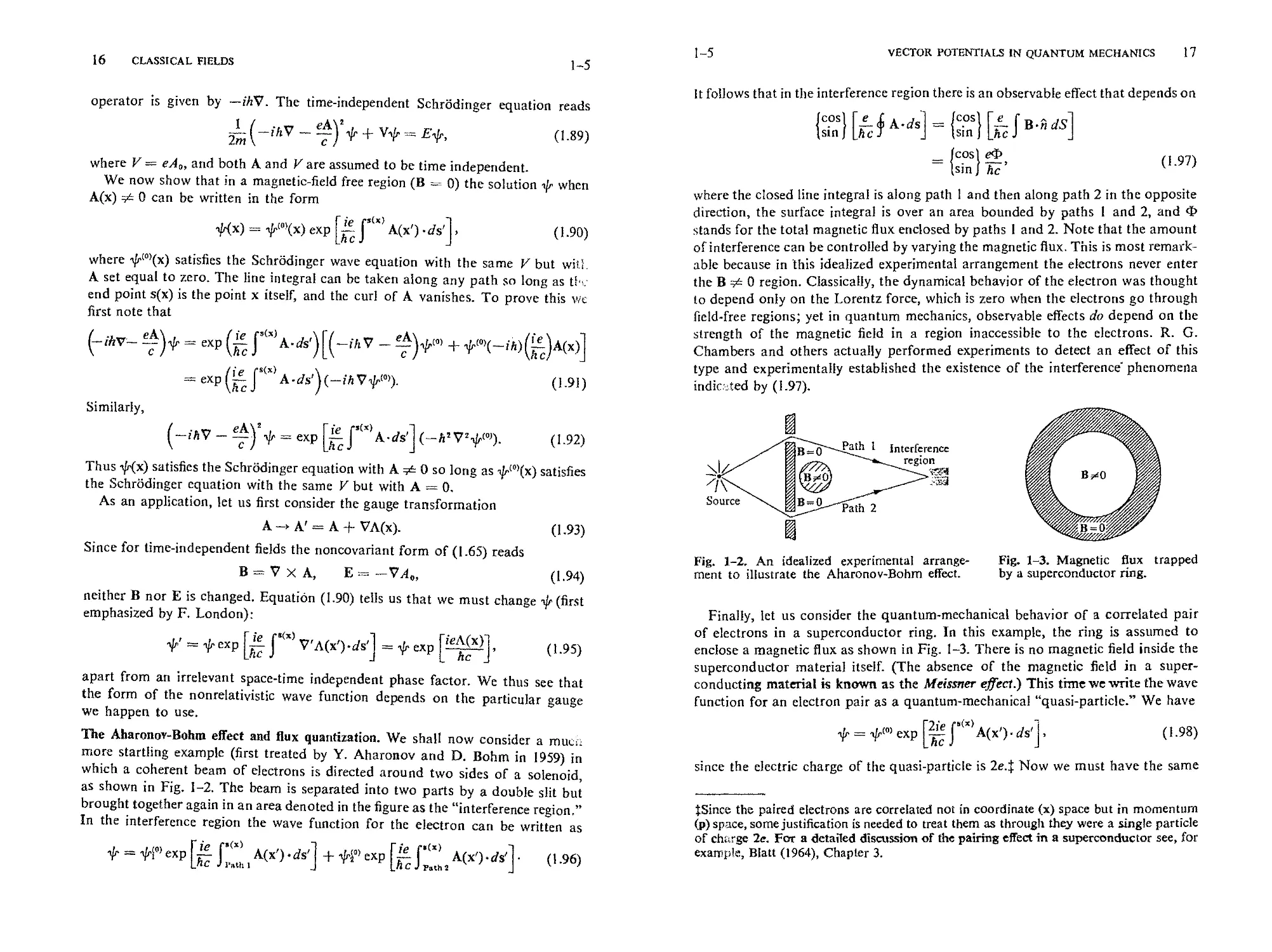
e Aharonov-Bohm effect and flux quantization. We shall now consider a mucz
more startling emple (first treated by Y. Aharonov and D. Bohm in 1959) in
which a coherent beam of electrons is directed around two sides of a solenoid,
as shown in Fig. 1-2. The beam is separated into two parts by a double slit but
brought together again in an area denoted in the figure as the "interference region,"
In the interference region the wave function for the electron can be written as
VECTOR POTENTIALS IN QUANTUM MECHANICS 17
It follows that in the interference region there is an observable effect that depends on
= e
tsm J hc
where the closed line integral is along path 1 and then along path 2 in the opposite
direion, the surface integral is over an area bounded by paths 1 and 2, and
stands for the total magnetic flux enclosed by paths 1 and 2. Note that the amount
of interference can be controlled by varying the magnetic flux. This is most remark-
able because in this idealized experimental arrangement the electrons never enter
the B 0 region. Classically, the dynamical behavior of the electron was thought
to depend only on the Lorentz force, which is zero when the electrons go through
field-free regions; yet in quantum mechanics, observable effects do depend on the
strength of the magnetic field in a region inaccessible to the electrons. R. G.
Chambers and others actually performed experiments to detect an effect of this
type and experimentally established the existence of the interference" phenomena
indic,:ted by (1.97).
Fig. 1-, An idealized experimental aange- Fg. 1-3. Maetic flux trapped
merit to illustrate the Aharonov-Bohm efft, by a superconductor g.
Finally, let us consider the quantum-mechanical behavior of a correlated pair
of electrons in a superconductor ring. In this example, the ring is assumed to
enclose a magnetic flux as shown in Fig. 1-3. There is no magnetic field inside the
superconductor material itself. (The absence of the magnetic field in a super°
conducting material is known as the Meissner effect.) This time we write the wave
function for an electron pair as a quantum-mechanical "quasi-particle." We have
b = /°' exp [2ie ('{*}A(x') ds'] (1.98)
LT " J'
since the electric charge of the quasi-particle is 2e.: Now we must have the same
.Since the paired electrons are correlated not in coordinate (x) space but in momentam
(i) space, some justification is needed to treat them as through they were a single particle
of charge 2e. For a detaed discussion of the pairing effect in a superconductor see, for
example, Blatt (1964), Chapter 3.
18 CLASSICAL FIELDS
wave function , whether or not the path of integration encloses the flux; otherwise,
the wave function would be multivalued. This imposes a severe restriction on the
flux euclosed by the ring. A line integral enclosing the flux once must satisfy
A-ds = 2nzr, (1.99)
(2e/hc)
or
= zcnhc/e, n = 0, El, 2 .... (1.100)
Thus we arrive at the far-reaching conclusion that the magnetic flux trapped by
the superconductor ring must exhibit a step behavior in units of
zrhc ch
- = - = 2.07 × 10 - gauss-cm , (1.101)
as first discussed by F. London and L. Onsager (apart from the factor 2). The
expected behavior was verified experimentally in 1961 by B. S. Deaver and W. M.
Fairbank and by R. Doll and M. NS.bauer. This experiment also illustrates in
a direct and striking manner th6 existence of pairing effects in superconductors,
which forms the basis for currently accepted theories of superconductivity.
We emphasize that throughout this chapter the electromagnetic field has been
regarded as classical In partict, lar, the "quan.tlzation" of magnetic flux we have
just discussed has nothing to do with the quantization of the electromagnetic field
to be discussed in the next chapter.
PROBLEMS
1-I. (a) Show that the energy-momentum tensor density defined by
satisfies the continuity equation
when the Euler-grge equation for is assumed.
(b) Show that ch component of the four-vtor
Pu(t) = --if ,dx
is constant in time if 4 vanishes suciently rapidly at infinity. (The integration is
over three-dimensional space at a given instant t.)
(c) Obtain the Hamiltoniaa density = --** for the real slar field.
1-2. Let (x, t) a solution to the free-field Klein-Gordon equation. Write
(x, t) = (x, t)e -'t/n.
Under what condition will satisfy the nonrelativistic Schrfdinger equation?
Interpret your condition physilly when is given by a plane-wave solution.
PROBLEMS 19
1-3. Using the prescription
-i -L-+-i.; _e__A
OX C "
write the field equation for the charged scalar field interacting with A,. Show that if
is a solution with A = (0, 0, 0, iA0), then * is a soluti th Ao replaced by --A0.
I. The Lagrangian density for a assive vector field interacting with a four-vector
density j is given by
Obtain the field equation. Show that the continuity equation forj. is not guaranteed
by the field equation, as it is in the Maxwell case. Show also that the subsidiary
condition
necessarily holds if the source is conserved (that is, iff satisfies the continuity equa-
tion). Note: A massive vector field was first considered by A. Pra.
I-5. Consider a Klein-Gordon particle subject to the four-vector potential A, sumed
to be dependent on both x and t. Write a relativistic generalization of Eq. (1.91).
State explicitly what.kind of path i four-dimensional (Minkowski) space is con-
sidered.
2-1 CLASSICAL RADIATION FIELD 21
CHAPTER 2
THE QUANTUM THEORY OF RADIATION
2-1. CLASSICAL RADIATION FIELD
Transversality condition. In order to study radiation phenomena in the quantum
domain we shall first discuss in detail the properties of the vector potential satis-
fying
V.A = 0 (2.1)
within the framework of classical electrodynamics. Equation (2.1) is known as the
transversality condition; it should not be confused with the Lorentz condition (1.81).
The electric or magnetic fields derivable from vector lotentials satisfying (2.1) are
called transverse fields or radiatian fields. Often the term "transverse field" or
"radiation field" is used to refer to a vector potential itself satisfying (2.1).
The transversality condition (2.1) is of interest under a variety of circumstances.
First, supposej, = 0. We can then consider a gauge transformation that eliminates
the fourth component of A and makes A obey (2.1). Consider
such that
AA'=A+ VA,
(2.2)
I OA
c 0t A0- (2.3)
Since the fourth component of A, has been eliminated in the new gauge, the
Lorentz condition (1.81) reduces to the transversality condition (2.1).
Let us consider a situation in whichj :¢ 0, as in the case of mutually interacting
electrons. We may first dcompose A so that
A = Ax + A,, V-Aa. = 0,
(2
V × A, = 0.
This can always be done.; Here Aa. and All are called respectively the transverse
and the longitudinal component of A. In 1930 E. Fermi was able to show that
and Ao together give rise to the instantaneous static Coulomb interactions between
.,tSee, for example, Morse and Feshbach (1953), pp. 52-54.
the charged particles, whereas A. accounts for the electromagnetic radiation of
moving charged particles. The total Hamiltonian of the charged particles (treated
nonrelativistically) and the electromagnetic fields generated by them can be written
(apart from the magnetic moment interaction) as:
H = [_l 4 Ix"' x" + tI, (2.5)
where Ha (which we shall discuss later in detail) is the free field Hamiltonian of
A z only. Equation (2.5) is derived in Appendix A. Note that nowhere in (2.5)
do A0 and A, appear explicitly.
Fermi's formalism bed on (2.5) is called the radiation (or Coulomb) gauge
method. Since the decomposition (2.5) is not relativistically covariant, nor is the
transversality condition itself, the whole %rmalism appears noncovariant; each
time we perform a Lorentz transformation, we must simultaueously make a gauge
transformation to obtain a new set of A and A0. Yet it is possible to develop mani-
festly eovariant calculational techniques starting with the relativistic analog of the
Hamiltonian (2.5), as will be shown in Chapter 4 when we discuss MNler (electron-
electron) scattering. It is also possible to construct a formalism which preserves
relativistic covariance at eve stage.
In any case, it is worth studying a theory of transverse electromagnetic fields
before we learn about more sophisticated formalisms. When the theory is quan-
tized, it provides simple and physically transparent descriptions of a variety of
processes in which real photons are emitted, absorbed, or scattered. The three
basic equations we work with for the free-field case are
B=V x A, E 1 0A (2,6)
c Ot'
10A
WA ? =0, (2.7)
where A satisfies the transversality condition (2. l).
Fourier decomposition and radiation oscillators. At a given instant, say t = 0, we
expand A in Fourier series. We assume the periodic bounda conditions for A
enclosed in a box taken to be a cube of side L = (V) /n. Remembering the reality of
A, we have
,-o = -,,,Z (c..(0)u,.(x) + c.(0)u..(x)), (2.8)
where
Uk.,(X ) : ff,a)elk.x (2.9)
and , called a (linear)polarization vector, is a real unit vector whose direction
depends on the propagation direction k (even though we will not write it in this text
as 6"(k) as is done in many books). Given k, we choose and e in such a
way that (e", , k/[k) form a right-handed set of mutually orthogonal unit
vectors. Note that ¢" and ¢ : are, in general, not along the x- and the y- axes since
2"2 THE QUANTUM THEORY OF RADIATION 2-- i 2-2 CREAT1ON ANNIHILATIONs. AND NUMBER OPERATORS 23
k is, in general, not along the z-axis. Since is perpendicular to k, the trans-
versality condition is guaranteed. The Fourier component nk. satisfies
where
/uu.,'uu..,J '
(2.10)
k, k, k.. =- 2mr[L, n -- +_ 1, + 2 .... (2. I I )
because of the periodic boundary conditions.
To obtain A (x, t) for t 0, we simply replace Ck.o(0) and c.,(0) by
cu.(t) = cu. (O)e " , c(t). c*u.,rOXet , (2.12)
where
o.= Ikl c. (2.13)
With this replacement both the wave equation (2.7) and the reality condition on A
are satisfied. So
1
= 7 (cK"(O)e''e' + c.,(O) e`'e-') (2.14)
with
k.x -- k.x -- ot = k-x -- Iklct.
The Hamiltonan of the field is
H = ½ f (IBI' + IEI)dx
½ J" [I V x A I' + l (l/c) (gA/at)l q d * x.
A typical term we must evaluate for the IBI integration is
(2.15)
(2.16)
(2.8)
(2.17)
where we have used the periodic boundary conditions and the identity
V × (V × ) = V(V. ) -- V -. Similarly, for the .IEI integration it is useful
to evaluate first
['I+(Ck,,,k.a]. rl° * ,¢,,)]dX , , . *.
Using these relations, we obtain
H = 2(o/c)ccu., (2.19)
k a
where ct. is a time-dependent Fourier coefficient satisfying
?k, a : --" 03 Ck. a (2.20)
(cf. Eq. 2.12). This reminds us of an expression for the energy in a collection of
independent and uncoupled harmonic oscillators. To make the analogy more
vivid, we define
, i ,
Qk., = (Ck.a + Ck.a), Pk.a = (Cu,. -- Ck. ). (2.21)
Then
= (. + ... (.)
k
The Pk, and Qu., are now seen to be canonical variables:
H _.,, H
aPk. = + 0u.. (2.23)
Thus the radiation field can be regarded as a collection of independent harmonic
oscillators each of which is characterized by k, a and whose dynamical variables
are orthogonal linear combinations of the Fourier coefficients.
2--2. CREATION, ANNIHILATION, AND NUMBER OPERATORS
Quantization of radiation oscillators. At the end of the nineteenth century it was
recognized that the space-time development of the radiation field satisfying the
wave equation (2.7) resembles the dynamical behavior of a collection of harmonic
oscillators. By assigning an average energy kT to each radiation oscillator, Lord
Rayleigh and J. H. Jeans wrote an expressioon for the energy distribution of the
radiation field as a function of o in an ideal situation where the radiation field is
enclosed by peffectty absorbing walls. The expression they obtained was in satis-
factory agreement with observation for low values of o at sufficiently high tem-
peratures, but in marked disagreement for high values of c0. This difficulty led M.
Planck to take one of the most revolutionary steps ever taken in the history of
science. He proposed that:
The energy of each radiation oscillator is not an arbitrary quantity but must be
an integral multiple ofhco, where h ig a new fundamental constant in nature.
This he did in 1901. Four years later, in order to explain the photoelectric effect,
A. FSnstein proposed that an electromagnetic wave of wavelength L = 2zrc/o
be regarded as a collection f massless particles each of which has energy hco.
24 THE QUANTUM THEORY OF RADIATION
2-2
We can now do better than did Planck and Einstein, but only because we kno'.
nonrelativistic quantum mechanics. Indeed, no sooner was nonrelativistic quantum
mechanics fully developed than P.A.M. Dirac proposed that the canonical
dynamical variables of a radiation oscillator be treated as noncommutable oper-
ators, just as x and p of a one-dimensional harmonic oscillator are treated in
nonrelativistic quantum mechanics.
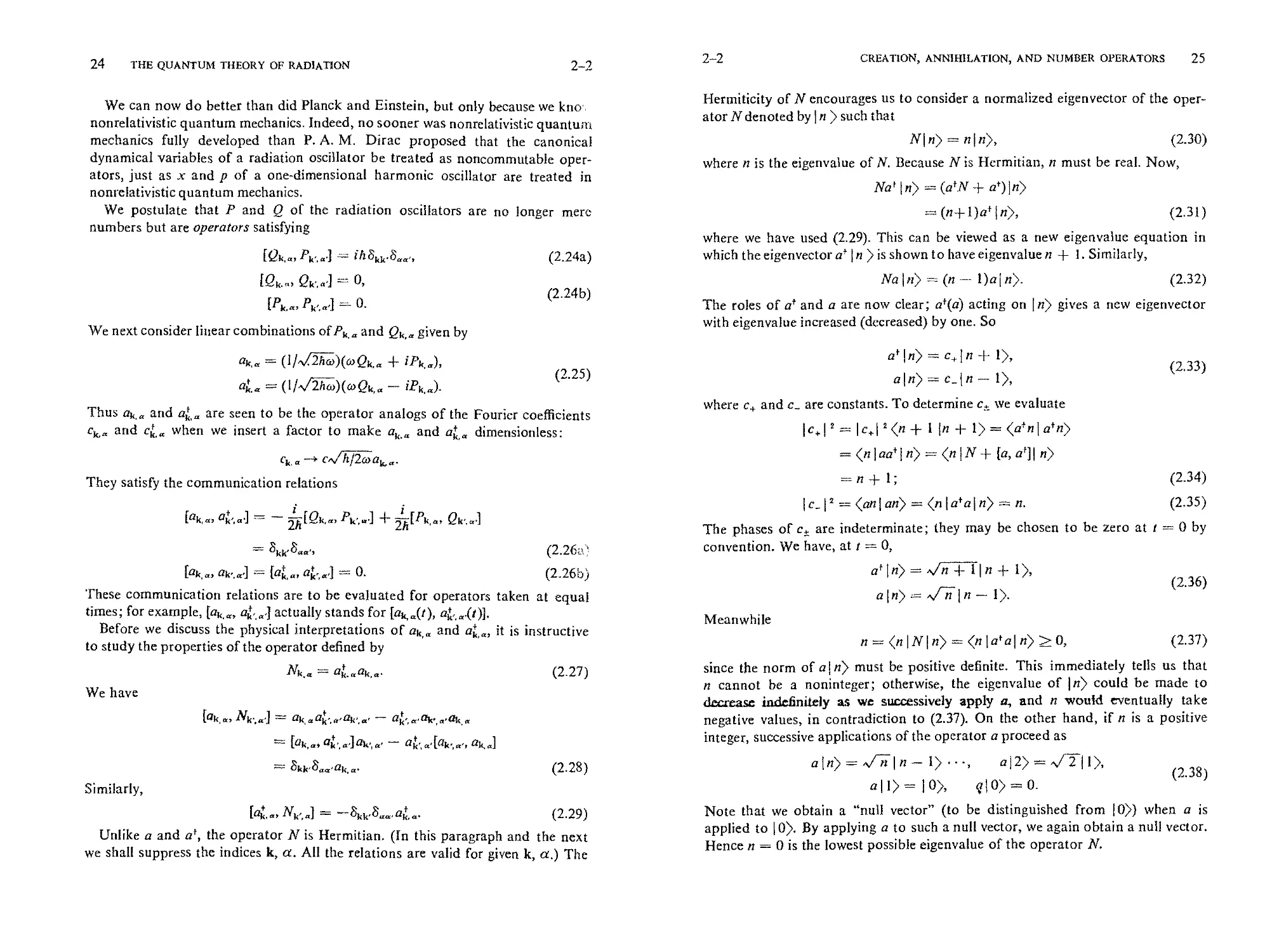
We postulate that P and Q of the radiation oscillators are no longer mere
numbers but are operators satisfying
[Qk.,, Pk,..] ih8.8,, (2.24a)
[Qu., Qu,.,,] = 0,
(2.24b)
We next consider linear combinations of P,., and Q<, given by
(2.25)
a],.. = (l/ 2'-)(wQ,,. - iP,,.).
Thus a,.. and a,,. are seen to be the operator analogs of the Fourier coefficients
c,,. and %t ,, when we insert a factor to make %,, and a,,. dimensionless:
c. --+ c,-h/2wa.
They satisfy the communication relations
i "
= gu,S,,,, (2.26;£?
[ak.=, ak,.a'] : ÷
[%,, a,,., 1 = 0. (2.26b)
These communication relations are to be evaluated for operators taken at equal
times; for example, [au.=, a,.,,] actually stands for [a,(t),
Before we discuss the physical interpretations of au,, and a,,, it is instructive
to study the properties of the operator defined by
Nu., = a.,a<,. (2.27)
We have
Similarly,
(2.28)
[a.,, Nk,,,] = --8uwS,,,a, .. (2.29)
Unlike a and a t, the operator N is Hermitian. (In this paragraph and the next
we shall suppress the indices k, a. All the relations are valid for given k, a.) The
2-2 CREATION, ANNIHILATION, AND NUMBER OPERATORS 25
Hermiticity of N encourages us to consider a normalized eigenvector of the oper
ator N denoted by ] n ) such that
NI n) = n ln ), (2.30)
where n is the eigenvalue of N. Because N is Hermitian, n must be real. Now,
Na t In) = (atN + a')ln)
= (n+l)atln), (2.31)
where we have used (2.29). This can be viewed as a new eigenvalue equation in
which the eigenvector a ÷ [n ) is shown to have eigenvalue n ÷ I. Similarly,
Na In) = (n -- 1)a[ n). (2.32)
The roles of a * and a are now clear; at(a) acting on In) gives a new eigenvector
with eigenvalue increased (decreased) by one. So
aln) = c+ln ÷ 1),
(2.33)
aln)=_ln-- 1),
where c+ and c_ are constants. To determine c_+ we evaluate
= (n I aa'l n) = (n)N ÷ In, aql n)
=n÷ 1; (2.34)
[c_[ = (an[an) = (n[a*a[n) = n. (2.35)
The phases of c are indeterminate; they may be chosen to be zero at t = 0 by
convention. We have, at t = 0,
a'ln) = V'+ lln+ l),
(2.36)
aln) = ,1 n -- 1).
Meanwhile
n =- (nlNln) = (nla*a I n) >_ O, (2.37)
since the norm of a[ n) must be positive definite. This immediately tells us that
n cannot be a noninteger; otherwise, the eigenvalue of In) could be made to
dgaareas indetinitely as we sttccessively apply a, and n would eventually take
negative values, in contradiction to (2.37). On the other hand, if n is a positive
integer, successive applications of the operator a proceed as
aln)=,,/-ZIn-- 1).--, a12) = ,,/--I 1 ),
(2.38)
all>= 10), ql0) = 0-
Note that we obtain a "null vector" (to be distinguished from 10)) when a is
applied to [0). By applying a to such a null vector, we again obtain a null vector.
Hence n = 0 is the lowest possible eigenvalue of the operator N.
26 THE QUANTUM THEORY OF RADIATION 2-2
2-2 CREATION, ANNIHILATION, AND NUMBER OPERATORS 27
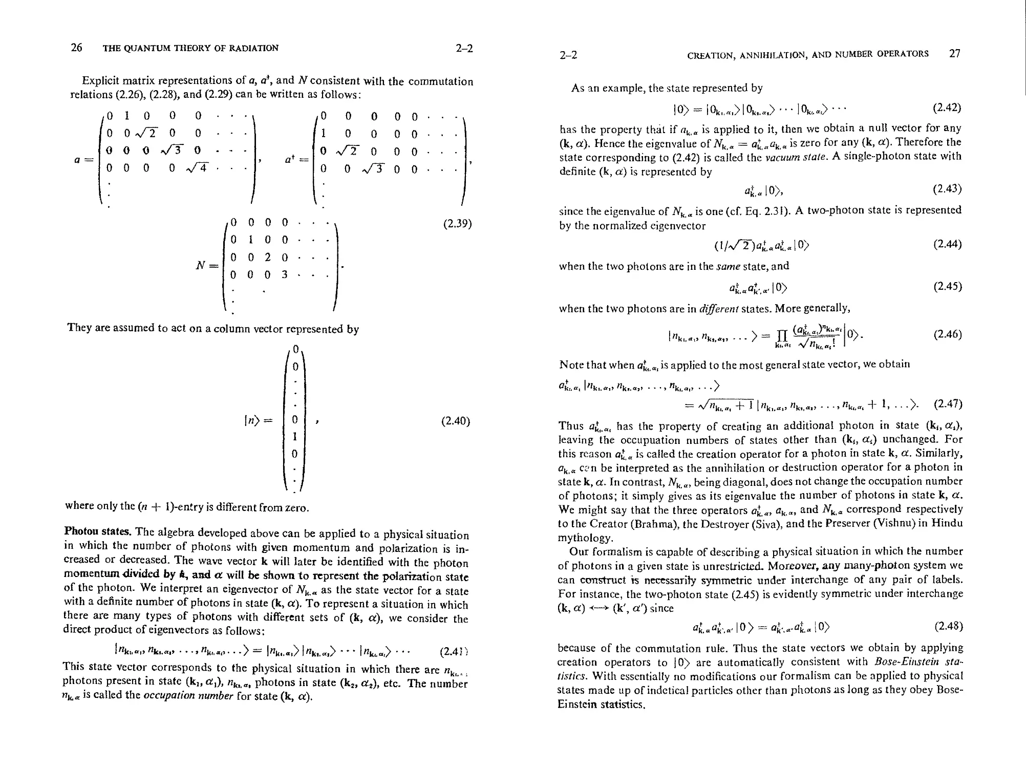
Explicit matrix representations of a, a t, and N consistent with the commutation
relations (2.26), (2.28), and (2.29) can be written as follows :
(! 0M'- 0 0 0 0 0 0
0 0 ,V" 0 , at = r- 0 0 0
a= 0 0 0 M-T 0 M-3- 0 0 '
N= 020
0 0 3
They are assumed to act on a column vector represented by
In) = 0 I ' (2.40)
1
where only the (n + l)-entry is differeat from zero.
Photou states. The algebra developed above can be applied to a physical situation
in which the number of photons with given momentum and polarization is in-
creased or decreased. The wave vector k will later be identified with the photon
momentum divided Iy/t, and tt will be shown to represent the polarization state
of the photon. We interpret an eigenvector of Na. as the state vector for a state
with a definite number of photons in state (k, ct). To represent a situation in which
there are many types of photons with different sets of (k, ct), we consider the
direct product of eigenvectors as follows:
Ink ..... nk ......... nl ........ ) = Inl,.,,,)tnk,.,,)"'" ]nk,.,,) " . • (2.4!3
This state vector corresponds to the physical situation in which there are n k ....
photons present in state (k, cq), nk .... photons in state (k2, c2), etc. The number
nk.,, is called the occupation number for state (k,
As an example, the state represented by
10) = [Ok,.,,)[0k,.,,) "" 10k,.,) " " " (2.42)
has the property that if ak., is applied to it, then we obtain a null vector for any
(k, o:). Hence the eigenvalue of Nk, : ak.,ak.+ is zero for any (k, o:). Therefore the
state corresponding to (2.42) is called the vacuum state. A single-photon state with
definite (k, a) is represented by
\ (2.43)
a.o 10/,
since the eigenvalue of Nk. is one (cf. Eq. 2.31). A two-photon state is represented
by the normalized cigenvector
( I/e-) a.. a. 1 o) (2.44)
when the two photons are in the same state, and
a., a.. ,, 10) (2.45)
when the two photons are in different states. More generally,
Yl (a- , ,)k" ' 10"> (2.46)
Ink ..... nk ........ ) = ,-
1 .... ./nk,., . I
Note that when a,,., is applied to the most general state vector, we obtain
aLo, lnk ..... n ......... n ........
= lnk ..... n k ......... nk,,, + 1 .... ). (2.47)
Thus a .... has the property of creating an additional photon in state (k.
leaving the occupuation numbers of states other than (k, a) unchanged. For
this reason a. is called the creation operator for a photon in state k, a. Similarly,
ak,. cz'n be interpreted as the annihilation or destruction operator for a photon in
state k, a. In contrast, Nk,., being diagonal, does not change the occupation number
of photons; it simply gives as its eigenvalue the number of photons in state k,
We might say that the three operators a,=, ak.., and Nk, correspond respectively
to the Creator (Brahma), the Destroyer (Siva), and the Preserver (Vishnu) in Hindu
mythology.
Our formalism is capable of describing a physical situation in which the number
of photons in a given state is unrestricted. Moreover, any many-photon system we
can cemslruct is necessnriby symmetric under interchange of any pair of labels.
For instance, the two-photon state (2.45) is evidently symmetric under interchange
(k, a) -- (k', a') since
ak., ak..=, I 0 )
ak...ak. 10 (2.48)
because of the commutation rule. Thus the state vectors we obtain by applying
creation operators to ]0) are automatically consistent with Bose-Eit,stein sta-
tistics. With esscntially no modifications our formalism can be applied to physical
states made up of indetical particles other than photons as long as they obey Bose-
Einstein stiics.
28 THE QUANTUM THEORY OF RADIATION
2-2
Fermion operators. There exist, in nature, particles that do not obey Bose-Einstein
statistics but rather obey Fermi-Dirac statistics--electron, muons, protons, etc.
For such particles the formalism we have developed is obviously inadequate.
We must somehow incorporate the Pauli exclusion principle. This can be done. In
1928 P. Jordan and E. P. Wigner proposed a formalism in which we again con-
sider the operators b and bT, but they now satisfy the the "anticommutatic,:':
relations"
[bT, b+.} = 6rT,, {b, br.} = {b, b.} = 0, (2.49)
where the term in braces is defined by
{A, } = A + . (.0)
The operators b and b are again interpreted as the creation and annihilation oper-
ators, and the index r provides a collective description of the momentum state, the
spin state, and according to the Dirac hole theory (to be discussed in Sections
3-9 and 3-10), the sign of the energy as well. A single-particle state can be con-
structedjust as before:
but, since
bb 10> = {b, b} 10> = 0 (2.52)
according to (2.49), we cannot put two particles in the same state. This is just
what is needed if the electrons are to satisfy the Pauli exclusion principle. However,
if r r', then we can construct a two-particle state
bb, ]0) = --b.b 10). (2.53)
Note that it is necessarily antisymmetric under interchange r r', in conformity
with Fermi-Dirac statistics. We define a Hermitian operator N by
Nr = bbr (2.54)
just as before. When b and b are interpreted as the creation and annihilation
operators, it is natural to regard N as the occupation number operator:
NI0) = bblO) = 0;
N,b¢ 10) = b( -- bCb,)10) = be 0).
Jn general, N has the property
N = bbrbb = b(--bb + l)b = N. (Z56)
Hence
N(N -- ) = 0, (2.57)
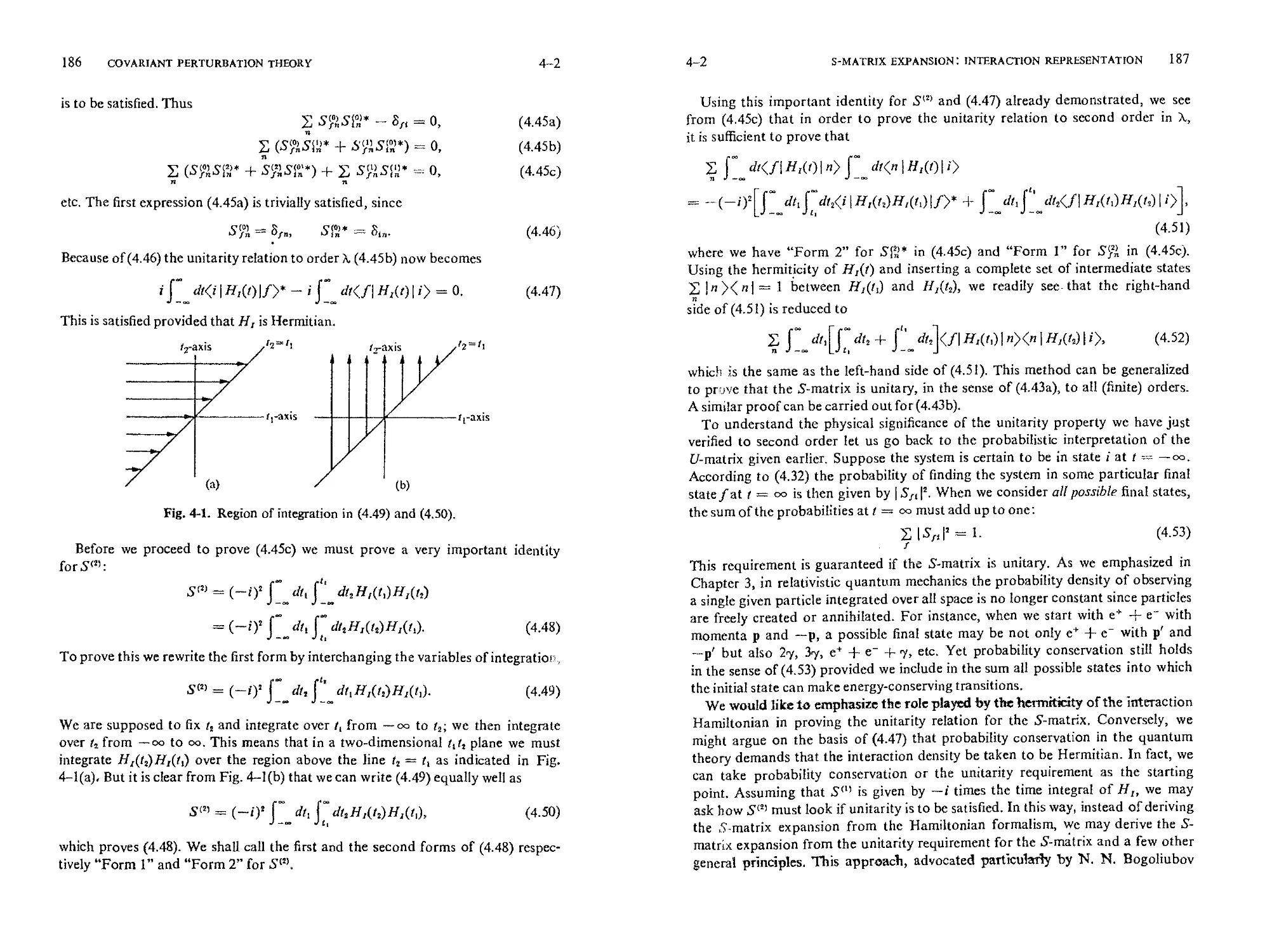
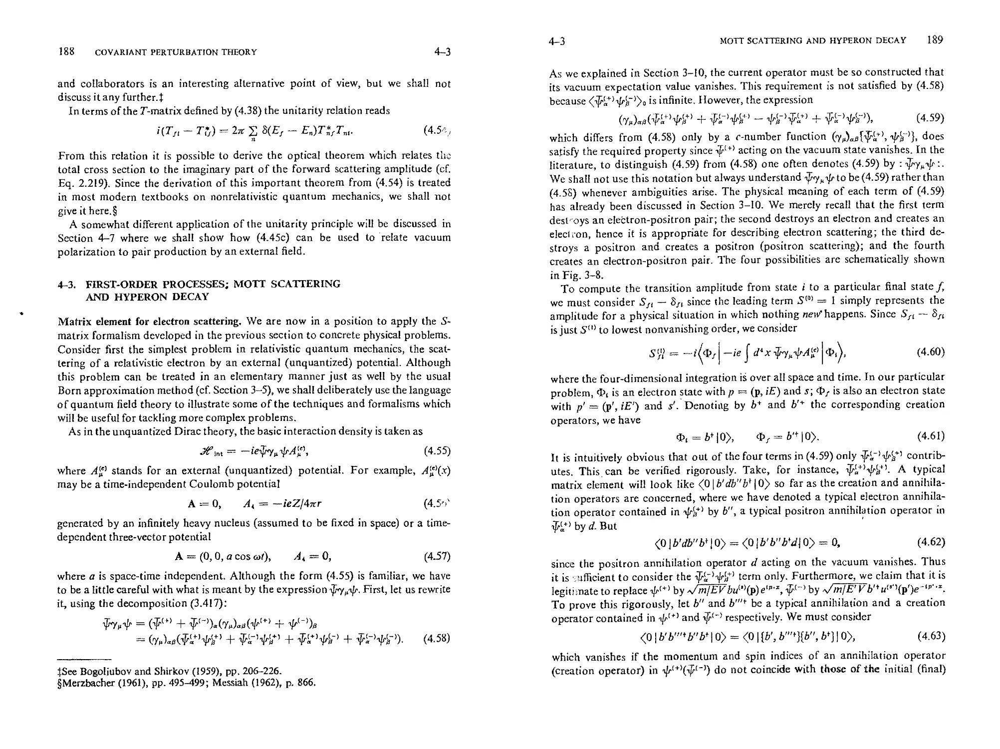
which means that the eigenvalue of N is either zero or one. Physically speaking,
state r is either unoccupied or occupied by just one electron. Explicit matrix
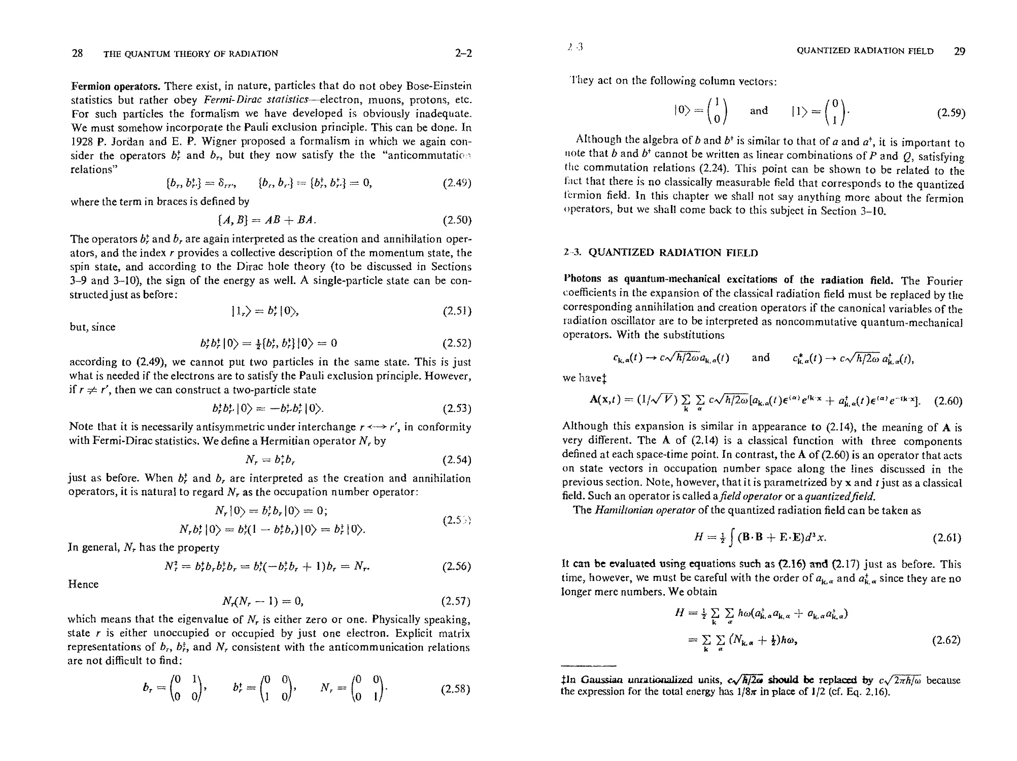
representations of b, b, and N consistent with the anticommunication relations
are not difficult to find:
2-3
QUANTIZED RADIATION FIELD 29
They act on the following column vectors:
Although the algebra of b and b* is similar to that of a and a ÷, it is important to
note that b and b* cannot be written as linear combinations of P and Q, satisfying
tlc commutation relations (2.24). %his point can be shown to be related to the
lhct that there is no classically measurable eld that coresponds to the quantized
lrmion field. In this chapter we shall not say anything more about the fermion
operators, but we shall come back to this subject in Section 3-10.
2-3. QUANTIZED RADIATION FIELD
Photons as quantum-mechanical excitations of the radiation field. The Fourier
coefficients in the expansion of the classical radiation field must be replaced by the
corresponding annihilation and creation operators if the canonical variables of the
radiation oscillator are to be interpreted as noncommutative quantum-mechanical
operators. With the substitutions
c.(t ) -- c/-h/2oTa.(t) and c,(t ) -- c.v/-/2o a.(t),
we lave:
A(x,t) = (1/,v/-) Z Z c'v/2[ak.,(t)e'"'e ''x + a.,(t)e'"'e-n"x]. (2.60)
k
Although this expansion is similar in appearance to (2.14), the meaning of A is
very different. The A of (2.14) is a classical function with three components
defined at each space-time point. In contrast, the A of (2.60) is an operator that acts
on state vectors in occupation number space along the lines discussed in the
previous section. Note, however, that it is parametrized by x and t just as a classical
field. Such an operator is called afieM operator or a quantizedfield.
The Hamiltonian operator of the quantized radiation field can be taken as
½ f (B.B + E.E)dax. (2.61)
H
It can be evaluated asig equations such as (2.16) and (2.17) just as before. This
time, however, we must be careful with the order of ak., and a,.= since they are no
longer mere numbers. We obtain
k a
= X X (N., + ½)ho, (2.62)
*In Gaussian unrationalized units, c - aould be replac by c2v//o because
the expression for the total energy has 1/8r in place of 1/2 (cf. Eq. 2.16).
30 THE QUANTUM THEORY OF RADIATION 2-3 ' QUANTIZED RADIATION FIELD 31
with o = lk I c. Since the absolute energy scale is arbitrary, we may use the energy
scale in which the energy of the vacuum state is zero,
HI0) = 0. (2.63)
This amounts to subtracting ] ho/2 from (2.62), so that (2.62) is replaced by
n = hoNk. . (2.64)
The Hamiltonian operator H acting on a many-photon state gives
H Ink ..... n ........ = Z n,.,,h, ] nu ..... n ........ ). (2.65)
The total momentum of the radiation field is given in classical electrodynamics :,
the space integral of the Poynting vector (E B)/c.* Using an operator exprcssioa
identical in appearance to the total momentum of the field in classical electro-
dynamics, we obtain the momentum operator as follows:
f -hk(a.a. + a.,a.)
= X hk(Nk, + ), (2.66)
where we have used relations such as
ch ,
2,c ) k.] k'.' X (k' X
h
= au.au,kS,,,. (2.67)
(Note: ¢) (k X ¢2') = 0, e" x;(k X e") = k, etc.) The . that appears
in (2.66) can be dropped because whe we sum over the allowed k, hk cancels with
--hk. Hence
P = X, hkN,,,. (2.68)
Let us consider the effect of H and P on a single-photon state:
. 10> = ., 10>, P4., 10> : hka.10). (2.69)
We see that h = h lk I c and hk are respectively the energy and the momentum
of the photon. The mass of the photon is given by
(mass) = (I/c')( E -- IPl
= [(h) - (h Ikl c) ]
= 0. (2.7)
The photon state is characterized not just by its momentum but also by the
polarization vector e . Since e" transforms like a vector, the general theory of
angular momentum encourages us to associate with it one unit of angular momen-
um. This is what is meant by the statement that the photon has one unit of spin
_This expression can also be obtained by evaluating the 4-k component of the energy
momentum tensor of the transverse electromagnetic field (cf. Problem 1-1).
,m?:ular momentum. To find spin components we first consider
'*-' = (l//)('" +_ i"), (2.7)
wtich are called circular polarization vectors. Under an infinitesimal rotation
.tiound the propagation direction k by an amount , the circular polarization
vctors are changed by
: i . (2.72)
Ihmc we associate wit e the spiu component m = I where the quantization
.xis has been chosen in the propagation direction. If e were along k, we would
:sociate = 0 (since k is unchanged under an infinitesimal rotation about k);
however, the m = 0 state is missing in the expansion of A because of the trans-
vt-rsality condition k-e " = 0. In other words, the photon spin is either parallel
,r antiparallel to the propagation direction. We note that the absence of the m = 0
late has an invariant meaning only for a particle whose mass is strictly zero. If the
photon mass is different from zero, we can perform a Lorentz transformation such
that in the new frame the photon is at rest; in such a frame the photon spin is
"'parallel to nothing."
Te description of the polarization state with as the base vectors is called
Ihc circular polarization representation in contrast to the linear polarization
tcpresentation based on e" and e . The orthogoaality relations for are
(2.73a)
k-e = 0. (2.73b)
We could have started with an expansion of A with e in place ore " and e ='.
A single-photon state with definite circular polarization can be constructed by
applying the creation operator
. = +(,, i, 0
to the vacuum state. Conversely, a. 0) with = I, 2 and k in the z-direction can
be regarded as a 50/50 mixture of the m = I and m = -- 1 state.
To sum up, the quantum postulate applied to the canonical variables of the
radiztoa oil y ds to Mea tt the quantum-mechical excita-
tions of the radiation field can be regarded as particles of mass zero and spin one.
It is a general feature of the quantum theory of fields that with every fieM we
associate a partic& of definite mass and spin. The arguments we have presented
can be repeated for the quantization of other fields with essentially no modifications.
For a further discussion of this point, see Problem 2-2. The spin angular momentum
of the radiation field can also discussed from the point of view of the total angular-
momentum operator (I/c)[x x (E x B)]dx which can be decomposed into the orbital
and e pM L I# W (lgk g. 123 and Mi (1962), pp. 1022-
I4, . 10-1034.
32 THE QUANTUM THEORY OF RADIATION 2-3 2--3 QUANTIZED RADIATION FIELD 33
To study the time development of the quantized radiation field, let us first note
that ak., and a,. are time-dependent operators satisfying the Heisenberg equation of
motion :
= - ioa,. ; (2.7.5)
iiu., = (i/h)[H, .] = (i/h)[H,
= --'ak.. (2.76)
These are dentical in appearance with the differential equations satisfied by the
Fourr coecients ck., (t) of the classical radiation field. Similarly,
From (2.76) and (2.77) it is evident that the quanted field A satisfies the same
wave equation (2.7) as does the classical field, lnteating (2.75) we obtain the
explicit time dependence for the annihilation and the creation operator:
a. = ak.,(0)e -', a. == a.(0)e"'. (2.78)
Finally, we have
A(x, t) ---- 1 E c[a'"(O)e'"%''-*z + a'"(0)e"e-U'+']" (2.79)
Note that the quantized field operator A is Hermitian while the cassical field
A is real. It is important to note that the and ¢ that appear n the quantized
field A(, t) are not quantum-mechanical variables but just parameters on which the
field operator depends. In particular, and t should not be regarded as the space-
time coordinates of the photon.
Fluctuations and the uncertainty relations. We are now in a position to discuss
some of the peculiarities arising from the quantum nature of the radiation fieTd
First, let us note that neither the individual occupation number operator N, .
nor the total number operator defined by
commutes with , E, and B because of (2.28) and (2.29). As is well known, in
quantum mechanics the observables corresponding to noncommutable operators
cannot be simultaneously determined to arbitrary degrees of accuracy. In the
present case, if the number of photons is approximately fixed, there must neces-
sarily be uncertainties in the field strengths.:l: Such a fluctuation behavior is ex-
pected even for the vacuum state. To check this explicitly let us take the
In general, by "uncertainty" we mean the square, root of the deviation of the expectation
value of the square of the operator in question from the square of the expectation value of
the operator, that is, Aq = /q) --
electric field operator E = --(I/c)OA/Ot. Although the vacuum expectation value
of the electric field (01El0) vanishes (because au.,10)= 0) as expected from
symmetry considerations, the mean square fluctuation of the electric field can be
readily shown to be infinite:
<01E.EI0> --[<01EI0>I = = <0[E-EI0> = . (2.81)
This llustrates our assertion that if the occupation number is fixed (zero Jn this
case), then the field strength is completely uncertain. On the other hand, since
what we measure by a test body is the field strength averaged over some region in
space, it may be more realistic to consider the average field operator about some
point, for example the origin, defined by
1 = (I/AV) f,v Edx' (2.82)
whev A V is a small volume containing the point in question. We can then prove
<0 { 1. 1[ 0> hc/(Al) , (2.83)
where AI is the linear dimension of the volume AV. Equation (2.83) characterizes
the fluctuation in the electric field when no photons are present. In general, if the
set of occupation numbers is approximately fixed, then the electric or magnetic
field has no precise value but exhibits fluctuations about a certain average value.
Another peculiar feature of the quantized radiation field is that the components
ore and B do not necessarily commute. For instance, we have§
[E,(x, t), B(x', t)] = icho8(x -- x'). (2.84)
It follows that we cannot simultaneously determine E and B Ut the same point in
space to arbitrary'degrees of accuracy. However, it is possible to show that
[E:(x, t), Bu(x', t')] = 0 for (x -- x') z -- (1]c)(t -- t') =: O. (2.85)
Thus there is no interference between measurements of field strengths performed
at two space-time points separated by a distance that cannot be connected by a
light signal. This is in comformity with the principle of causality in the special
theory of relativity. The commutation relations (2.84), (2.85), and other similar
relations were first obtained by P. Jordan, W. Heisenberg, and W. Pauli.
Using the commutation relation (2.84) we can write an uncertainty relation
that iavolue.s AE and AB. Howeter, before we interpret such a-rda'dtn physically
we must first define what is meant in the quantum theory by the measurement of
field strength. This would require a rather careful discussion based on a 1933
paper by N. Bohr and L. Rosenfeld. Consequently we shall not discuss this subject
any further. An excellent treatment of it can be found in Heitler's book.]l
:We shall not prove (2.83) since in Problem 2-3 the reader is asked to prove a similar
relation for the scalar field.
§Again we shall not prove this relation because Problem 2-3 is concerned with a similar
relation for the scalar field.
{[Heitler (1954), pp. 76-86.
34 THE QUANTUM THEORY OF RADIATION 2-3 )-3 QUANTIZED RADIATION FIELD 35
We know from classical optics that a localized or converging light beam can be
constructed by superposing various plane waves with definite phase relations.
For this reason we wish to consider the phase operator Sk., associated with given
k, o such that the observable corresponding to it is the phase of the plane wave in
question in the sense of classical optics, This we can do by setting
(2.86)
4,.° =
where the operator /k., satisfies the property (,/,,)-" = N.. The quantized
radiation field can be written in such a way that the only operators appearing are
and ..:
-- ) -- + k.-)])' (2.87)
+ ,.e exp [--.i(k-x
which is of a form convenient for use in discussing the connection with the classical
description. The commutation relation for a and a (for given k, ) can now be
written as
e* Ne -* N = I,
(2.87
eN _ Ne* : e ,
where we have suppressed the subscripts k, . It is easy to prove by expandin
each exponential that the commutation relation (2.88) Js satisfied whenever
N$ -- SN-- i. This leads to a new uncertainty relation for the corresponding
observables:
N$ . (Z89)
For example, if the phase difference of two plane-wave components is given pre-
cisely, then we canuot tell the occupation numbe associated with each of the wave
components.
The above uncertainty relation can be used to derive a more familia-Iooking
uncertainty relation for the light beam. Since the momentum operator is written
as the sum of the number operators weighted by hk (cf. Eq. 2.68) the momentum
of the light beam is uncertain whenever there are definite phase relations among
individual plane-wave components. Meanwhile a localized wave train can be
constructed by superposing plane-wave components with definite phase relations.
It theu follows that we cannot associate a definite momentum to a well localized
beam. For simplicity let us consider a one-dimensional wave train confined to a
region whose characteristic dimension is -. Ax. Although the actual mathematical
description of such a Iocafizcd wave train is somewhat involved, we expect that the
phase of a typical plane wave component must be known qualitatively to an
accuracy of k Ax if the localization is to be possible. The uncertainty relation
(2.89) then implies
Apx Ax h, (2.99)
,ince the momentum nncertainty is of the order of ANhk. This relation is formally
identical to Heisenberg's uncertainty relation for a "particle." However, because
of (2.89), a single photon cannot be localized in the same sense that a particle
in nonrelativistic quantum mechanics can be localized. For this reason, it is better
to regard (2.90) as a relation imposed on the light beam, as we have done.
It i:; amusing to note that Helsenberg's uncertainty principle for a material
particle, for example, an electron, can be formulated only when the light beam
also satisfies the uncertainty relation (2.90). If there were no restriction on Ax
and Ap for the light beam, we would be able to determine the position of the
electron to an infiaite degree of accuracy by a very well-localized beam without
transferring an appreciable momentum uncertaiuty to the electron in an uncon-
trollable way. Two successive measurements of this kind would determine accu-
rately both the momentum and the position of the electron, in contradiction with
I leisenberg's relation,
Validity of the classical description. All these peculiarities of the quantized radiation
lield could be rather disturbing, especially if we recall that many of the con-
veniences of our civilization rely upon the validity of classical electrodynamics
which, as we have seen, must be modified. For instance, having learned about the
quantum fluctuations of' the radiation field, how can we listen in peace to an FM
broadcast of symphonic music? In nonrelativistic qnantum mechanics the classical
description is trustworthy whenever the noncommutativity of dynamical variables
is unimportant. Likewise, in the quanturn theory of radiation, if we could ignore
the right-hand side of [a, a ] : I, then we would return to the classical description.
Since the nonvanlshing matrix elements of a and a are of the order of (cf.
Eq. 2.36), the occupation number must be large if the classical description is to
be valid.
To be more specific, let us compare the vacuum fluctuation of" a squared-field
operator and the square of the field strength for a classical .electromagnetic wave of
wavelength 2zcX. When there are no photons of any kind, the square of the average
electric field operator has the following expectation value (cf. Eq. 2.83):
(0 IE.E t 0 ) he/V, (2.91)
where the average is taken over a volume X . Meanwhile, according to classical
electrodynamics, the time average ofE can be equated with the energy density of
the electromagnetic wave. So we set
E
( ):,.,,.,,o = hh(c/X), (2.92)
where ,5 stands for the number of photons per unit volume. For the validity of the
classical description, purely quantum effects such as (2.9l) must be completely
negligible in comparison to (2.92). For this we must have
>> I/. (2.93)
In other words, the description of physical phenomena based on classical electro-
dynamics is reliable when the number of photons per volume La is much greater than
or.e. As an example, for a Chicago FM station (WFMT), which broadcasts at
36 THE QUANTUM THEORY OF RADIATION 2-4 2--4 EMISSION AND ABSORPTION OF PHOTONS BY ATOMS 37
98.7 Mc (, 48 cm) with a power of 135,000 watts, the number of photons per
volume at a distance five miles from the antenna is about 10 Iv. Thus the classical
approximation is an extremely good one.
The historical development of quantum mechanics was guided by an analogy
between the electron and the photon both of which were recognized to exhibit the
famous wave-particle duality. As Heitler correctly emphasized in his treatise, this
sirliilafity can be somewhat misleading. The classical limit of the quantum theory
of radiation is achieved when the number of photons becomes so large that the
occupation number may as well be regarded as a continuous variable. The
space-time development of the classical electromagnetic wave approximates the
dynamical behavior of trillions of photons. In contrast, the classical limit of
Schrfdinger's wave mechanics is the mechanics of a single mass point obeying
Newton's equation of motion. Thus it was no coincidence that in the very begin-
ning only the wave nature of light and the particle nature of the electron were
apparent.
2-4. EMISSION AND ABSORPTION OF PHOTONS BY ATOMS
Basle matrix elements for emission and absorption. We now have the necessary
machinery to deal with the emission and absorption of photons by nonrelativis ..
atomic electrons. The interaction Flamiltonian between the atomic electrons a
the radiation field is assumed to be obtainable from the standard prescription
p --* p -- eA/c, where A now stands for the quantized radiation field. We have
H,t: [--(p,-A.(x,, t)+ A(x,, t).p)+ A(x,,t).A(x,,t)], (2.94)
where the summation is over the various atomic electrons that participate in the
interaction. The expression A(x, t) is now a field operator assumed to act on a
photon state or a many-pho[on state at xT, where x, refers to the coordinate of the
ith electron. The operator in ocA is a differential operator that acts on every-
thing that stands to the right; however, because of the transversality coudit/o
V. A = 0, it is legitimate to replace p- A by A. . Since the spin magnetic momelt
is knowu to interact with the magnetic field, there is an additional interaction of
the form
As we saw in the previous stion, A(x, t) is a linear combination of the creation
and annihilation operators for photons. The question of which particular creation
or annihilation operator gives rise to a nonvanishing matrix element depends
entirely on the nture of the initial and final aates in question.
From the time-dependent perturbation theory (which we will review shortly),
it is well known that the transition matrix element for AB (where A and B
may, for example, be atomic states) can be computed to first order in the inter-
action Hamiltonian H t by simply taking the matrix element of H2 between A ar6
B. The H, that appears in (2.94) and (2.95), however, acts not only on atomic
states but also on photon states. In a typical process appearing in the quantum
theory of radiation the state vector for the initial (or final) state is the direct product
of the state vector for an atomic state (denoted by A, B, etc.) and the state vector
for a single- or a multi-photon state (characterized by n.). With this point in
mind we can still evaluate the transition matrix element to lowest order by taking
the atrix element of (2.94) or (2.95) between the initial and final states.
Let us first consider the absorption of a light quantum characterized by k, o.
An atom which i initially in state A makes a radiative transition to state B. For
simplicity we shall assume that there are only photons of the kind (k, o0 present.
If there ae n.,.photons in the initial state, then there are n. -- l photons in the
final state. Although A contains both a.= and a.,, only a., gives rise to a non-
vanishing matrix element so long as we are computing the absorption process to
lowest order. The quadratic term A.A makes no contribution to this process in
Iowest order since t changes the total number of photons by either 0 or :2. So,
ignoring the spin magnetic moment interaction, we have
---- --(B,e • nu,. -- 1 I cau..(O)e a''-'"'.,, e'"'[ A;
e.
-- (Ble'a',p,.'"'lA)e-'"', (2.96)
where we have used (2.36) and (2.79). Note that the annihilation operator for a
photon with momentum and polarization different from hk and e gives a zero
matrix element.
It is instructive to compare this expression with the expression we obtain using
the semiclassical theory of radiation in which the vector potential A is treated
classically. Within the framework of the semiclassical theory we may define an
equivalent classical vector potential denoted by A ¢'" such that when it is used for
an absorption process we obtain a matrix element identical to (2.96). Evidently
A '' = ")e ux- (2.97)
will c¢o, where
A `''' = c, e'"'. (2,98)
2or
According to the semiclassical theory the absorption probability is proportional
to the intensity [A0[ ; in the quantum theory it is proportional to n.,. We expect
on general grounds that the semiclassical theory approximates reality for large
values of n.=, but since the matrix element (2.96) is linear in , the semiclas-
steal theory gives the correct answer even for small values of n., or for weak
radiation.
The above happy accident no longer takes place for emission processes which
we will now discuss. This time it is the creation op a., that gives rise to
a nonnishing contribution since fle photon occupation number is increased by
38 THE QUANTUM THEORY OF RADIATION 2-4 2-4 EMISSION AND ABSORPTION OF PHOTONS BY ATOMS 39
one. We have (c£ Eqs. 2.36 and 2.79):
(2.99)
If nk. is very large, the semiclassical treatment based on the complex conjugate
of the equivalent potential, (2.97) and (2.98), is adequate since, in practice, there is
no difference between ,,,/u. -4- 1 and /-.++ Therefore, for very intense radiation,
the problem can again be treated using tile se,niclassical theory. On the other hand,
for small values of nk., the correspondence with the semiclassical description
fails completely. In particular, the transition matrix element tbr emission need
not be zero when there are no photons at all present initially (nk. : 0). This
accounts for the emission of a photon by an isolated excited atom when there are
no electromagnetic waves incident on it, a phenomenon known as "spontaneous
emission." In contrast, the emission of a photon in the case where nk., v 0 is known
as "induced (or stimulated) emission." Note that in the quantum field-theoretic
treatment spontaneous emission and induced emission are discussed on the same
footing. The single expression (2.99) suffices for both.
The fact that we can account for spontaneous emission in such a natural way is
one of the triumphs of the quanturn theory of radiation as opposed to the semi-
classical theory of radiation. So long as the electromagnetic field is described by "
classical potential, the transition matrix element for emission is zero when the;,
is no electromagnetic wave incident on the atom ; A. p :: 0 when A : 0, and that
is that. In the quantum theory of radiation this is not the case because the matrix
element of the field operator A(x, t) taken between the vacuum state and the one-
photon state does not vanish.
In general, in the classical theory, A is an externally applied potential that
influences the charged particles but is not influenced by them; A itself does not
change as an atom makes a radiative transition. This description is satisfactory,
even within the framework of quantum theory, whenever the occupation number
is so large that the radiation field can be regarded as an inexhaustible source and
sink of photons. It should be clear that, for intense radiation, taking one photon
away from the radiation field or adding one photon to it does not make much
practical difference. On the other hand, for weak or no incident radiation the
classical description runs into difficulty because the change in the radiation field
brought about by the emission and absorption of a photon by an atom is quite
noticeable.
With tile above limitations in mind, we may still define an equivalent classical
potential appropriate for emissioh processes as follows :
A '''ls) : A'"i'e -k'x+'t, (2.100)
:We recall that the total time-dependent potential that appears in nonrelativistic qt, anlum
mechanics must be Hermitian. In our particular case, the classical vector potential A
must be real anyway.
with
Ag ""'1) := c/-(n,,,, ÷ 1)h/2coVe "'. (2.101)
By treating (2.100) as the time-dependent vector potential that appears in the
SchrSdinger equation we can obtain the correct matrix elements (2.99) for emission
processes (including spontaneous emission). The fact that A '' is no longer
linear h and is not quite the complex conjugate of A ¢' given by (2.97)
and (2.98), reflects the failure of the classical concepts.
To sum up, starting with the quantum theory of radiation, we have rigorously
derived the following very useful rule.
The emission or absorption of a light quantum by a charged particle is com-
pletely equivalent to an interactiou of the charged particle with the equivalent
unquantized vector potential given below:
absorption : c
(2.102)
emission : - ,
where nu. is the photon occupation number in the initial state.
This simple rule is one of the most important results of this book.
Timependent perturbation lheory. Before we start computing the transition
probabilities for various processes let us briefly review the time-dependent per-
turbtion theory developed by Dirac. An atomic wave function + can be expanded
as
= Z c(t)u(x) e-''u, (2103)
where u(x) is the energy eigenfunction with energy E satisfying
in the absence of a time-dependent perturbation. The time-dependent Schr6dinger
equation in the presence of a time-dependent potential H(t) is
= ih (ue -''u' -- i(Lflh)cue-a: (2.105)
In our case, in addition to the kinetic energies of the electrons the unperturbed
Hamiltonian H, contains the Coulomb interactions between the electrons and the
nucleus, whereas Ht(t) accounts for the interaction of the atomic electrons with
the equivalent vector potential (2.102). Using (2.104), we have
}We again emphasize that in Gaussian nratioraliztxt )anitx :/it[2o is to be replaced
40 TIlE QUANTU/vI THEORY OF RADIATION 2-4 2-4 EMISSION AND ABSORPTION OF PHOTONS BY ATOMS 41
Multiplying u*e :/ and integrating over the space coordinates, we obtain the
differential equation
G, = (I/ih)(m]H(t)lk)e ":'-z'''/G(t). (2.107)
Suppose only state l is populated when the time-dependent perturbation is turned
on at t = 0;then
c(0) = G. (2. 0)
We may then approximate c, by
fo dt (m 1H,(t ') I . (2.
If c,P vanishe for some reason or if a better approximation is called for, we use
c c + c , (2.110)
where
1 ' tn)e .... -.,v./cn(t,, )
.... 1 ' dt" 0 ] H,(t ")1
(ih) fo V'dt'(m n)e .... -'"':(nlH,(t')ll)e ''''''''v,
(.)
and so on.
When we are dealing with the emission and absorption of a photon by an atom,
we may work with just c2 . The time-dependent potential H can be written as
/ab°ti°n (2.112)
H(t) = He for remission
where H is a time-independent operator. Hence
c' : (mlHl l) f dt''--,'v/C (2.113)
We can readily perform the time integration and obtain
lc,(t)l=(2r/)l(mlH ll)lt3(-- E h), (2.114)
where we have used
. I sin a x
m = (x). (2.11
Note that the transition probability per unit time is ]c(t)[/t, which
ndependent oft.
Let us now apply our formalism to emission processes. The photon states allowed
by the periodic boundary conditions form a continuous energy spectrum as the
normalization volume becomes infiuite (cf. Eq. 2.11). For a photon emitted into a
solid angle element dO, the number of allowed states in an energy interval [h,
h(o + dw)] can be written as pn,and(h), where
Vlkl'dlkld_ V dz (2.116)
So for the transition probability per unit time into a solid angle element d.-Q we
obtain the famous GoMen Rule
"n = J" (I cd'l/t) p .... n d(h6)
= (2r/h) [Qn{ tt' l l)lp .... ,, (2. I17)
where hco must satisfy
E,, -- E, + ho O. (2.118)
Spontaneous emission in the dipole approximation. In the case of spontaneous
emis:don, an atomic state A makes a radiative transition to a state B in the absence
of any incident electromagnetic wave. The matrix element (B tH I A) in this
case is just (2.99) with e. * omitted and n. set equal to zero. Hence for wan we
obtain
eZh [ e_k.x,r.p x Vr d
wan h 2ma,V (BI / , (2.119)
where satisfies the energy conservation E. = E, + h. The normalization
volume Vcancels out as it should.
In a typical atomic transition in the optical region the wavelength of the emitted
photon is much greater than the linear dimension of the atom:
,, ..... : 1/k I >> r. ...... (2.120)
since X,,oto. is typically of the order of several thousand angstrom units whereas
the atomic radius is of the order of one angstrom unit. This means that we can
replace
e -'k'*, = l -- ik.x, -- (k-x,)/2 q .... (2.121)
by its leading term I. It turns out that the spin-magnetic-moment interaction is
also negligible. To see this, just note that the matrix element of (e/mc)¢=.p, is
larger than that of (eh/2mc)a,.(k X e"), again by Xoto./r.,,, since the matrix
element of p, is of the order of h/r..,,,,. An approximation in which only the
term is kept is called the electric dipole (E I) approximation.
To further simplify the problem let us assume that only one of the atomic elec-
trons participates in spontaneous emission, as in the case of a hydrogen-like atom
(an atom whh te ly one vale etr). ing e sum over i
we : ve
e z
w,,, = I(BI p I A). e '' I ' da. (2.122)
Meanwhile, using the commutation relation between p and x,
[! , x] = --2ihp, (2.123)
;Many of the results we derive for one-etimO:on atoms.caa readily be generalized to
many-electron atoms.
42 THE QUANTUM TIIEORY OF RADIATION 2--4
we can rewrite the matrix element (B [Pi A) as follows:
A> = Wo, xj I A>
h
:= imox.,. (2.124)
This matrix element [s precisely what we would directly compute if the interaction
HamiltoMan were replaced as follows:
eA._ e x 0A
-- -m "7 .... ex.g, (2.125)
provided that we again kept only the leading term fin the plane-wave expansion
orE. The origin of the term "electric dpole transition" is now evident.
The angular momentum selection rule for El is
I3--Ja[=-I,0; no 0-0. (2.126)
To derive this we first note that the components ofx can be rearranged as follows:
(a.7)
Y.
Then the Wigner-gckart theorem gives
where (lmq[Jmn) is a Clebsch-Gordan coefficient. The condition that t
Clebsch-Gocdan coefficient shall not vanish leads immediately to the angula
momentum selection rule (2.126). Physically this selection rule is a consequence
of the fact that one unit of angular momentum is carded away by the spin of the
emkted photon in an El transition.
We also must cohsider the parity selection rule: parity change "yes." To prove
this merely note that
<Olxl/> = --<OlI-'xIII A>
= --II,,H<alxl A>, (2 129)
where H and Ha. stand for the parity opecator and its eigenvalue.
Equation (2.122) can also be written as
wn = 1 x., l cos: " d, (2.130)
where we have defined the angle by
cos "' = [ x,,.,. '" [/I x,,.., [. (. 131 )
Those who are unfamiliar with the Wigner-Eckart theorem and C]ebsch-Gordan
coefficients may consult Merzbacher (1961), Chapter 22; Messiah (1962), Chapter 13.
EMISSION AND ABSORPTION OF PHOTONS BY ATOMS 43
Note that
= 1_,,.,___)-'+ x,,._,y,,., '+ Iz.,(. (2.,32)
So far we have been concerned with a radiative transition in which a photou with
definite k, o is emitted. We must now sum over two independent polarization
states for given k and integrate over all propagation directions. From Fig. 2-1 it is
evident that
cosO'"=sinOcosqo, cosO '' = sin 0sin @ (2.133)
The sum over the two polarization states just gives sin-"0. Integrating over all
possible propagation directions with
the direction of x2_l fixed in space, we
obtain
2rr sin s Od (cos 0) = 8r/3.
(2.134)
Finallyl for the integrated transition
probability for spontaneous emission
we have
( e ]4co
= \/,--5- Ix.,IL (2.35)
k
Fig. 2-1. The orientation of xta.
with (e2/4xhc) 1/137. Note that the dimension of w is (time) - as expected.
This expression was obtained prior to the advent of quantum field theory by W.
Heisenberg, who used the correspondence principle.
In order to compute the mean lifetime "r of state A we must sum the transition
probabilities into all possible final states allowed by the selection rule and
energy conservation :
I/'ra = w.,.,,,. (2.136)
In particular, it is important to sum over the magnetic quantum number of the
final statr_
At: a concrete example, we may mention that the mean lifetime of a radiative
El transition from the state having the quantum numbers (n, l, m) to the state
having (n', 1', m') where m' = m, m -_k 1, is given by the reciprocal of
.'[(nhn)(n'l'm')]
-- em (`+ 1,/(2`+1)} f:R,,,,,(r,R,,(r,rdr for 1'= {',@ '
(2.[37)
$See Merzbacher (1961), p. 481. for a detailed deriwltion of this formula.
44 THE QUANTUM THEORY OF RADIATION 2-4 2--4 EMISSION AND ABSORPTION OF PHOTONS BY ATOMS 45
where R,(r) is the normalized radial wave function of a hydrogen-like arm.
characterized by n and l. Note that he lifetime is independent of m. This result,
which can be proved using the orthogonality properties of the Clebsch-Gordan
coefficients (cf. Eq. 2.128), is reasonable in view of rotational invariance; the life-
time of an excited state in the absence of an external field should not depend on
its orientation in space. In general, because the lifetime of an isolated state is in-
dependent of its m value, in computing the lifetime we can either sum over first
thefinal magnetic quantum numbers for a fixed initial magnetic quantum number
or sum over both the initial and thefinal magnetic quantum numbers and divide
by the multiplicity of the initial state. For instance, in (2.137) we are free to make
the replacement
_ 1
where J (ill this case, just l) is the angular momentum of the decaying state.
As an application of (2.137) we oay cmnpute the lifetime of the 2p state of the
hydrogen atom which decays into the ground (Is) state. The radial wave functions
are
2
_ 1 r e.r/, , and R,. e -r/',
R,, -- -- (2.139)
where a is the Nohr radius. We obtain
(2p-- ls) = 1.6 10 - see. (2.140)
The mean fifetimes of other excRed sates of the hydrogen atom are tabulated in
the literature.$ In general, the lifetime of an excited hydrogen-like atom goes up
with increasing n, roughly as n for a fixed vMne of/, and as
for the average over L
Occasionally the symmetry of atomic states may be such that the electric dipole
emission of a photon is forbidden. Th;s occurs when xe = 0 for every state B with
an energy lower than A. It is then necessa to go back to the plane-wave
expansion (2.121) and take seriously the tern k-x hich we previously ignored.
The matrix element we must evaluate can be decomposed as follows:
< I(k- x)( "'- )l > = <B I (k-x)( ' • ) + (k- )(e'"'. x) l A>
+ < l(k.x)(e,-,-) - (k.)('"'-x)l z>.
The first term can be rew6tten using
[(k.x)(e'.) + (k-)(er"'.x)] = Ik-(x + ,x)-e "', (2.143)
where x + x is a symmetric dyadic. The radiat;ve transition due to this term is
known as an electricquadrupole (E2) transition since
x + x = (hn/h)[H,, xx], (2.t44)
SBcthe and Salpeter (1957), p. 266.
and
--<Blxp + pxlA>-e '"' = --ik.<BlxxlA>.#"L (2.145)
Because of the transversality condition k-e " = 0, it is legitimate to replace xx
by its traceless part whose individual components are
T u = x,x -- (o/3)Ix I"- (2.146)
Note that it has five independent components which can be written as linear
combinations of Y.f'. It then follows from the Wigner-Eckhart theorem that the
angular nomentum selection rule for an E2 transition is
(2.4D
qie second term in (2.142) can be written as follows:
(k.x)(e'"'-p) -- (k-p)(¢'"'-x) = (k x ¢")-(x × p). (2.148)
Now k × e ' is the leading term in the plane-wave expansion of the magnetic
field B while x × p is just the orbital angular momentum operator of the atomic
electron which gives the orbital magnetic mo,nent operator when combined with
e/(2mc). Hence the radiative transition due to this term is called a magnetic" dipole
(Ml) transition. Together with this term we should consider the leading term from
the spin magnetic moment interaction (2.95) (eh/2mc) a-(k × e"), which is of the
same order. The angular momentum selection rule for an MI transition is
--Ja] _<.1, no 0 - 0, just as in the El case. In contrast to an El transition, the
parity of the atomic states changes neither in an MI nor in an E2 transition.
We can treat higher multipole transitions by considering the higher powers of k. x
in (2.121). However, it is better to use a formalism that employs vector spherieal
harmonics, a more powerful technique based on an expansion of #"e ''x in terms
of the elgenfunctions of the angular momentum operator of the radiation field. We
shall not discuss this method; it is treated in standard textbooks on nuclear physics.{:
The atomic states for which electric dipole transitions are forbidden have long
lifetimes. In contrast to the lifetime of order 10 -n sec characteristic of a typical El
transition, the lifetimes of typical Ml or E2 transitions are of the order of 10 -a sec,
roughly ([r,,,,,,,)" times the typical E1 lifetime, as expected. As an example in which
El, MI, E2, etc., are all forbidden for ,practical ptrrposes, we may mention the
radiative transition between the metastable 2s state and the ground (Is) state of
the hydrogen.atom. For this transition El is forbidden by parity, the MI matrix
eter,,*:nt vanishes whenthe nonrelativistic wave functions are used, and E2 and all
oth.::r higher multipole transitions are forbidden by angular momentum conserva-
tion. Its decay mode turns out to be the simultaneous emission of two photons
which can be calculated to be sec (cf. Problem 2-6). Note that this lifetime is
extremely long compared to the lifetime ofthe 2p state, 1.6 × 10 -a sec.
$Consult, for example, Blatt and Weisskopf (1952), Chapter 12.
46 THE QUANTUM THEORY OF RADIATION
2-4
Planck's radiation law. We wish to conclude this section with a derivation of
Planck's radiation law from the point of view of quantum field theory. Suppose
we have atoms and a radiation field which can freely exchange energy by the
reversible process
A .:2 V + B (2.149)
in such a way that thermal equilibrium is established. If the populations of the
upper and lower atomic levels are denoted by N(A) and N(B) respectively, we have
the equilibrium condition
N(B))r,, = N(A) w+,,t+, (2.150)
N(B) __ e-%/r = en,,,+r (2.15)
N() '
where w,,,,, and wo,,, are respectively the transition probabilities for B + V --,
and A B + % According to (2.96), (2.99) and (2. 114) we have
(., )I E<)-''''" IA>
w.,,a - , (2.152)
w, .... , I Ale''' .... ,IBI
But
B)*.
(2.153)
Hence
N(B) _ w,,,,,, __ nk. "F 1
N(A) w: nk.
Using (2.151) and (2.154) we obtain
1
(2.154)
(2.155)
All this is for photon states which satisfy ao = , -- E. Suppose the radiation
field is enclosed by "black" walls wfiich are made up of various kinds of atoms
and are capable of absorbing and re-emitting photons of any energy. The energy
of the radiation field, per volume, in the angular frequency interval @, w + d)
is given by (cf. Eq. 2.116)
U(o)dw I ( hco 2( L
The energy distribution per frequency per volume s
8lw s 1 (2.157)
U() = U(¢o) c e '''- 1
This is Planck's famous law which opened up the twentieth-century physics of the
quantum domain.
2-5
RAYLEIGH AND THOMSON SCATTERING; RAMAN EFFECT 47
It is instructive to compare our derivation of Planck's law with Einstein's 1917
derivation.: They are both based on thermal equilibrium between the atoms and
the radiation field. In Einstein's derivation the principle of detailed balance is
explicitly invoked; by contrast, in our derivation the physics of detailed balance is
contained in (2.153) which is an antomatic consequence of the hermitlcity of the
Hamiltonian used in the quantum theory of radiation. Note also that in our deriva-
tion we do not distinguish between the contributions from spontaneous emission
and induced emission.
Although our attention has been focused in this section on the radiative transi-
tions between two atomic states, the techniques we have acquired can readily be
applied to a host of other phenomena. For instance, the reader may calculate the
cross section for the photoelectric effect (Problem 2-4) or the lifetime of the E0
hyperon (Problem 2-5):
°-A+ V.
2-5. RAYLEIGH SCATTERING, THOMSON SCATTERING, AND THE
RAMAN EFFECT
Kramers-Heisenberg formula. Let us now examine the field-theoretic treatment of
the scattering of photons by atomic electrons. Before the scattering, the atom is
in state A, and the incident photon is characterized by (k, etch). After the scattering,
the atom is left in state B, and the outgoing photon is characterized by (k',
For implicity let us again consider a one-electron atom and neglect the spin-
magnetic-moment interaction.
The: interaction Hamiltonian (2.94) is made up of a linear (A-p) term and a
quadratic (A. A) term. Since A changes the number of photons by one, A-p makes
no contribution in first order to a scattering process in which there is no net change
in the number of photons. On the other hand, the A-A term contains aa , a*a,
an, and a+a +, the first two of which do give nonvanishing contributions provided
that a * and a, respectively, represent the creation operator for (k', ¢z') and the
annihilation operator for (k, ct), e.g., (k', ct'l a,., a,,,+ I k, c 0 = 1. Hence
(B;k',':" I H,,I A ; k, ',)
:= ( B; k', '" ]c.A(x, t ).A(x, t ) l d ; K e'"' >
X exp [i(k -- k'),x -- i(co -- ')t]l A; k,
= 2--_,z . exp [--/(o -- ')t](B IA), (2.158)
for example., Kittel (1958), pp. 175-176.
4-8 THE QUANTUM THEORY OF RADIATION 2.-5 2-5 RAYLE1GH AND TttOMSON SCATTERING; RAMAN EFFECT 49
where we have replaced e k'x and e ,u'.x by 1, since in the long-wave approximation
the atomic electron may be, assumed to be situated at the origin. For the first-
order transition amplitude cm(t) we have
dh,
(Z
with = ]k] c and 6/= I k'l c as usual.
Although the A.p term makes no contribution in first order, the A-p
taken twice is of the same order as the A-A term, so far as powers of e are
corned. Therefore we must treat a double A- p interaction and a single A. A interac-
tion sultaneously. TheA. p interaction acting at t, can either annihilate the incident
photon (k, ) or create the outgoing photon (k', '). When the A.p interaction
acts again at a time t which is later than t, it must necessarily create the outgoing
photon (k', ') if the outgoing photon has not yet been created. Otherwise we
would end up with a zero matrix element. On the other hand, if the outgoing
photon has already been created but the incoming photon has not yet been annihb
lated, the A.p interaction acting at t > t, must annihilate the incoming photon
(k, ). Between h and t the atom is in state I which is, in general, different from
A and B. To summarize, two types of intermediate states are possible. In the first
type the atom is in state I and no photons are present. In the second type the atom
is in state I and both the incident and the outgoing photon are present.
(a) (b) (c)
Fig. 2-2. Space-time diagram for scattering of light.
All -this can best be visualized if we draw a space-time diagram (Feynman di
gram) in which a solid line represents the atom, and a wavy line represents a photon.
Time is assumed to run upward (Fig. 2-2). For a type 1 process, represented by
Fig. 2-2(a), the atomic state A first absorbs the incident photon at t and becomes
state I; subsequently at t the atomic state /emits the outgoing photon and changes
Strictly speaking, we should also consider the case where 1 stands for a continuum
state. The relevant matrix element then corresponds to a photo-effect matrix element
(cf. Problem 2-4). In practice snch "distant" intermediate states are not important be-
cause the energy denominators become large (cf. Eq. 2.160 below).
into state B. For a type 2 process, represented by Fig. 2-2(b), state A first emits
the outgoing photon at t and changes into state I; subse.quently at t state/absorbs
the incident photon (which has not yet been annihiltted) and becomes state B.
In contrast, the lowest-order A.A interaction, discussed earlier, is represented by
Fig. 2-2(c) ("seagull graph").
As emphasized in the previous section, the emission and absorption of a photon
by an atomic electron are equivalent to interactions of the atomic electron with the
time-dependent potentials (2.102). Using this rule, we can readily write down the
second-order transition amplitude c(t) as follows:
X (11 .e'"' ] A) exp [i(E t -- E, --
+ (B I p.e'" [ I) exp [i(En -- Ez -- h)t/h]
X G I P'e'""l A) exp It(E, -- Ea + h')t,/h]
X fodGexp[i(En -- Ea +
hm'
h)t/h],
(2.160)
where we have made the dipole approximation and ignored a term that depends
on the artificial sudden turning of the perturbation (which is negligible if the
energy conseation, En -- t + ho' -- h = 0, is nearly satisfied). Combining
c(t) and c(t), we have the transition probability
f
Wan = j(Ic m + )P,an u&
{ ch { e ' v
....
To obtain tke differential cross section we must divide tkis transition probability
by the flux sity w isj ciV, sin it e om he nor-
realization box of volume P. Finally, we have for tke differential cross section
da = r()lS,,,e<""e'"" -- k
.
+ (''<')'(''`:>)',d t , (z162)
where ro stands for the classical radius of the eltron, and
e I h
rt ..... x& X lO-I. (2.163)
4x 137mc
50 Tt-tE QUANTUM TttEORY OF RADIATION 2-5 2-5 RAYLEIGH AND THOMSON SCA'VrERING; RAMAN EFFECT 51
A formula equivalent to (2.162) was first obtained by H. A. Kralners and W.
]{eisenberg using the correspondence principle in 1925; hence it is called the
Kramers-Heisenberg formula.
Rayleigh scattering. There are certain special cases of (2.162) worth examining in
detail. Let us first discuss the case in which A = B, ho = hco'. This situation
corresponds to elastic scattering of light. It is also called Rayleigh scattering
because this problem was treated classically by Lord Rayleigh. To simplify (2.162)
we rewrite e {"}.'', using the commutation relation between x and p, the com-
pleteness of the intermediate states I, and (2.124)::
= 7g Z, [(x'"').,,(p'e'""),.., -- (P'e'').,,(x.'"),.,]
1 1
--m [(P' )A0" ) + (°'')'('d"%A (.6)
where a = (Et -- Ea)/h. We now see that the three terms in (2.162) combine
so that
Using the expansion I/( ) [I (/o))]/, valid for small values of
, and
= m' Z [(x'e''),,(x'e'"'),., - (x''"'),(x'e'""),]
= m([x-e ''', x-e"]),
= 0, (2.166)
we obtain the Rayleigh cross section for
[ Tom 4 2
(2.1
Thuz we see that the scattering cross section at lottg wavelengths varies as the inverse
fourth power of'the wavelength (Rayleigh's law). For atoms in ordiary colorless
gases the lght wave corresponding to a typical t. is in the ultraviolet region.
The intermediate states I form a complete set only when we include the continuum
states as well a the discrete (bound) states.
Hence the approximation w << w;. is good for in the visible optical region.
This theory explains why the sky is blue and the sunset isred.
Thomson scattering. Let us now consider the oppositc case in which the incident
photon energy is much larger than the atomic binding energy. It is then legitimate
to ignore the second and third term of (2.162), since ho(-- ho') is much larger than
(poe').(p.e")t./m, so the scattering is dne solely to the matrix element corre-
sponding to the "seagull graph" (Fig. 2-2c). Now the 3.ue .e "' term is insensi-
tive to the nature of the binding of the atotnic electron. The cross section we
compute in this case coincides with the cross section for the scattering of light by
a free (unbound) electron, first obtained classically by J. J. Thomson:
do-
d -- r le '' -e'"" [-. (2.168)
Note that this expression is independent ofo.
Fig. 2-3. Polarization in Thomson scattering.
To study the polarization dependence of Thomson scattering we consider a
coordinate system in which e " and k are taken along the x-and the z-axes respec-
tively, as shown in Fig. 2-3. The orientation of k' is characterized by the spherical
coordinate angles 0 and q. The final polarizafioa vector ' may be Iaken to be
aorma! to the shaded plane (the plane determined by k and k') for c' = 1 ;
with x' = 2 must then lie in the shaded plane. The Cartesian components of e
are given by
e. _/(sin,--cos,0) for o'= 1, (2.169)
[(cos 0 cos qS, cos 0 sin qS, --sin 0) for c( = 2.
Hence
do" _ [ sinb for a' = 1, (2.170)
riD, r/cos 0 cos: + for a' == 2.
52 THE QUANTUM THEORY OF RADIATION 2-5 2-6 RADIATION DAMPING AND RESONANCE FLUORESCENCE
For initially unpolarized photons we may either integrate (2.170) over the angle
+ and divide by 2r or evaluate
do-
The two procedures are completely equivalent. Note that even if the initial polariza-
tion vector is randomly oriented, the final photon emitted with cos0 1 is
polarized, since the differential cross section is rg/2 for e "' normal to the plane
determined by k and k' and (r/2) cos 0 for e' lying in the plane. It is remarkable
that the polarization of the scattered photon is complete for 0 = z/2. We find,
then, that a completely unpolarized light beam, when scattered through 90 °, results
in a I00 linearly polarized beam whose polarization vector is normal to the
plane determined by k and k'.
If the initial photon is polarized but the final photon polarization is not observed,
we must sum over the two possible states of polarization. We have
d .. = rl(sin + cos 0 cos ). (2.172)
If the initial photon is not polarized and the final photon polarization is
measured, we have
,,.,,,,,.o, = + cos0). (2.1737
The total cross section ibr Thomson scattering is
rg
t,,t= = 6.65 x 10-cm . (2.174)
As we emphasized earlier, this expression for the cross section is valid at photon
energies much greater than the atomic binding energy. Hower, the foregoing
derivation breaks down if the photon energy is so high that it actually becomes
comparable to the rest energy of the electron. We must then take into account
he relatMstic nature of the electron, as we shall do in Section , discussing
Compton scattering.
The quantum-theoretic treatment of Rayleigh and Thomson scattering can be
compared to the classical counterpart. The scattering of an electromagnetic wave
can be visualized in classical mechanics by the tbllowng two-step process:
a) A bound electron oscillates when it is exposed to a time-dependent electric field.
b) The oscillating charge in turn radiates an eltromagnetic ve.
For a model of the electron bound by a force obeying Hooke's law, the displace-
ment x of the electron in the presence of an applied electric field E,e -* satisfies
the differential equation
+ x = (e/m)Eo e-%
where is the characteristic angular frequency o the oscillator. Knowing that
the acceleration of the electron is given by
Et, = Etd,,u/--
(a) (b)
Fig. 2-4. (a) Stokes' line, (b) anti-Stokes" line.
we can readily compute the total scattering cross section in a straightforward
manner;l: We obtain
o-t,,t =: 3 (I -- )" (2.177)
For << o we have the w dependence of (2.167), whereas for w >> 0 we recover
the fquency independent cross section (2.174).
The Raman effecL The Kramers-Heisenberg formula (2.162) can also be applied
to inelastic scattering of light in which w ' and A B. In atomic physics
this phenomenon is called the Raman effect after C. V. Raman who observed a
shift in the frequency of radiation scattered in liquid solutions, an effect predicted
earlier by A. Smekal. If the initial atomic state A is the ground state, then the energy
of the final photon hw' cannot be greater than the incident photon energy h
because h + Ea = h' + E, (Fig. 2a). This accounts for the presence of a
Stokes' line in atomic spectra, a spectral line more reddish than that of incident
radiation. On the other hand, if the atom is in an excited state, ' can be larger
than (Fig. 2b). This leads to an anti-Stokes' line which is more violet than
the spectral line of the incident radiation.
2 6. RADIATION DAMPING AND RESONANCE FLUORESCENCE
The Kramers-Heisenberg formula we derived in the previous section is clearly
inadequate if ho becomes equal to Ez -- Ea for some state J. The cross section
according to (2.162) is then infinile, a phenomenon no't observable in nature, of
course. It is nevertheless true that the scattering cross section becomes very large
and goes through a very sharp maximum in the neighborhood of E, -- Ea
This is a phenomenon known as resonance scattering of light or resonance
fluorescence.
Where did our theory go wrong? When we use the second-order time-dependent
perturbation theory, we assumed that the intermediate state I is a stationary state
with an infinitely long lifetime. In other words, we did not take into account the
**Panorsky and Phillips (1955), p. 326; Jackson (1962), pp. 602-604.
54 THE QUANTUM THEORY OF RADIATION 2__. 2-6 RADIATION DAMPING AND RESONANCE FLUORESCENCE 55
instability of state I due to spontaneous emission. In this connection, it is amusing
to note that the classical expression for tile Rayleigh scattering cross section (2.177)
also blows up for o o0. This catastrophe can be avoided by introducing a damp-
ing force in the differential equation (2.175) as follows:
+ 74x + ox = (e/m)Eoe -`°t. (2.178)
The scattering cross section is then given by
o = ( _ ) + 7/4, (2.179)
which is large but finite at = . As we shall see in a moment, in the quantum-
theoretic treatment the depletion of state I due to spontaneous enission plays a
role analogous to the damping force in the classical treatment; hence it is known
as radiation damping. The quantum theory of unstable states was first developed
by V. F. Weisskopf and E. P. Wigner precisely in this connection.
To simplify, let us assume that the initial atomic sate A is a stable (ground)
state. As the light beam hits the ato, the coecient c,(t) builds up because state
A makes a transition to state I as it absorbs the incident photon. Mathematically
he differential equation for cz(t) due to this absorption process is (cf. Eq. 2.107)
where HLi " (0 is the time-dependent matrix elemen characteristic of the phot¢
absorption. But this is no the whole story. The amplitude cj( 0 changes with tin.
because of spontaneous emission even if state I is left alone in the absence of
iucident radiation. The probability of finding the excited state I decreases wkh
time as e -'z, where t = /, being the nean life of state I given by (2.135)
and (2.136). Since the amplitude for state I must va as e -'' in the absence of
any incident radiation, we can take into account the depletion of state I by adding
to the right-hand side of the differential equation (2.180) a new term as follows:
, = HI?(t)cae '''-a'' P' (2.181)
The first term of(2.181) characterizes the growth of state I due to the absorption
of light, while the second term describes the depletion of state I due to spontaneous
emission. Admittedly our approach is somewhat phenomenological; a more rigor-
ousjustification of the second term will be given in Section 2-8 when we discuss the
second-order level shift due to the emission and absorption of a virtual photon.
We solve the differential equation (2.181) subject to the initial condition c(0)
= 0, caO) = 1. By direct substitution we find that the solution to this differential
equation satisfying the above initial condition is
c)"(t) -- HI., (exp [-- P,tl2h] [i(E, -- E., -- h)/]}, (2.182)
where H} is the time-independent matrix element given by
• HI:'(t) = Hte -'"t = --(e]mc)(Ilc/2a, VO.#"'lA)e-'% (2.183)
The lowest-order probability for finding state I is just I c" (t)[ 2. Note that, unlike
(2.1 ] 4) of Section 2-4, it is not proportional to t times $(E -- Ea -- hw) as t
Wh,:her (2.182) or (2.113) is the more realistic expression for describing a given
absorption process depends on whether the lifetime of state I is short or long
compared to the observation time. From (2.182) we obtain
Ic7'(c)12 - (e, - , - no) + p/4
State I is found copiously in abundance when the resonance condition Et -- Ea
h is satisfied. If (2.184) is regarded as a function of the incident photon energy
hw, it has the familiar Lorentz shape whose full width at half maximum is given
by I'r h/wz. When the atom is irradiated by a continuous spectrum of radiation,
we expect an absorption line whose wdth corresponds in the energy scale to
often called the natural width. Using a similar argument, we can show that the
frequency dependence of an emission lne for an excited state I returning to the
ground state A is also given by the same form, as we would expect from considera-
tions based on equilibrium (Kirchhoff's law).
Let us now return to the scattering problem. To compute the scattering cross
section for + A + B, where h Et , for some I, we must re-evaluate
c using our modified c' in the general formula (cf. Eq. 2.11 l).
c'(t) = -L X f dt"(B[ H'(t')] l) e"ra *'v'/ac"(t") "in , (2.185)
For a suciently large value of t we can omit the transient term e -r,t/za in (2.182).
Denoting by R those intermediate states I for which the resonance condition
h E r t is satisfied, we obtain the second-order amplitude c as follows:
ci.(t) = 1 ( e <nlcw,..,l<lc.,.,im
X f' dt" exp [i(En , + h' -- hw)t"/h] + nonresonant terms,
(z 86)
where the "nonresonant terms" stand for (2.160) except that in the sum over I
for the type' 1 intermediate states those states (R) which sy the resonance
condition a missing. We sthe ty age nessary is the substitution
Et Et -- i(rt/2) (2.187)
*The foregoing discussion of line width ignores the broadenings of spectral lines due
to the Doppler effect and atomic collisions which, in many instances, are more important
than the broadening due to spontaneous emission. However, our phenomenological
treatment can easily be generalized to the case where the depletion of state 1 is due to
inelastic collisions. Compare our treatment with the discussion on absorption of radia-
tion found in Dicke and Wittke (1960), pp. 273-275, where the maia de4letion is assumed
to be due atomic collisions rather than spontaneous emission.
THE QUANTUM TtIEORY OF RADIATION
2--6
for the type 1 intermediate states satisfying the resonance condition. Hence fi'
any arbitrary co we have the modified Kramers-Heisenberg forlnula
CO t
dt)
In practice Pz can be ignored except when Er -- Ea ho.
In general, the resonant amplitude is much larger than the sum of the non-
resonant amplitudes. This is because the magnitude of the resonant amplitude is
of the order of = c/o (cf. Problem 2-8) while the magnitude of the nonresonant
amplitude is of the order of r0. Ignoring the nonresonant amplitudes, we can obtai
a single-level resonance formula applicable to the scattering of light in the vicinity
of a nondegenerate resonance state:
_.{ X/ I XI(P'" )I I(P " ).,I (2.189)
It is amusing to note that this expression is identical with the probabilty of finding
state R formed by the absorption of photon (k, if), multiplied by the spontaneous
emission probability per solid angle for R B with the emission of photon (k', if),
and divided by the flux density. To prove this statement we merely note that from
(2.184) and (2.119) we obtain
(absRrption.probability) X (emission probability per solid angle)
flux density
_ 2m' V L(E. -- + {"/4] L h 2m ' P '< '="' _1
(2.19;..
which is identical to (2.189). Thus resonance scattering can be visualized as the
formation of the resonance state R due to the absorption of the incident photon
followed by the spontaneous emission of the outgoing photon.
The above simple interpretation of resonance fluorescence as the formation of
resonance followed by its decay is subject to the usual peculiarities of quantum
mechanics. First of all, if the nonresonant amplitudes are appreciable, (2.188)
tells us that they can interfere with the resonant amplitude. Interference between
the nonresonant amplitudes and the re p g freqnfly observed
in nudlear resonance fluorescence. Further, if the resonant state has spin or, more
generally, if there are several resonant states of the same or approximately
the same energy, it is important to sum over the amplitudes corresponding to the
various resonant states as indicated in (2.186) before squaring the amplitude.
This point will be.illustrated in Problem 2-8.
These considerations naturally ead to the following question: How can we
decide whether a particular physical phenomenon is best descried as a single
quantum-mechanical process of resonance scattering or as two independent quan-
tum-mechanical processes of absorption followed by emission? The answer to this
2-7
DISPERSION RELATIONS AND CAUSALITY 57
question depends critically on how the lifetime of the metastable state compares
with the collision time, that is, the time interval during which the atom is exposed
to the incident beam. To illustrate this point, let us first consider an experimental
arrangement in which the temporal duration of the incident photon beam is short
compared to the lifetime of the resonance. The energy resolution of such a photon
beam is nccessarily ill-defined, A(hCO) >> IR, because of the uncertainty principle.
It is then possible to select the excited resonant state by observing the exponential
decay of the resonance long after the irradiation of the atom has stopped. In such
a case, it is legitimate to regard the formation of the metastable state and its sub-
sequent decay as two independent quantum-mechanical processes.
On the other hand, the situation is very different with scattering of a photon
beam of a very well-defined energy. If the energy resolution of the incident beam is
so good (or if the lifetime of the resonant state is so short) that the relation
A(hco) << 1'1 is satisfied, it is not possible to select the excited resonant state by
a delayed lifetime measurement or any other measurement without disturbing the
system. This is because the uncertainty principle demands that such a monochro-
matic photon beam must last for a time interval retuch longer than the lifetime of
the resonance. We can still determine the lifetime of the resonance by measuring
the decay width Pn through the variation of the scattering cross section as a func-
tion of CO, using monochromatic beams of variable energies. Under such a cir-
cumstance the interference effect between the nonresonant amplitudes and the
resoant amplitude discussed earlier can become important. In such a case, it is
meamgless to ask whether or not a particular photon has come from the resonance
state. If we are considering an everlasting, monochromatic, incident beam, re-
sonance fluorescence must be regarded as a single quantum-mechanical process
so long as the atom is undisturbed, or so long as no attempt is made to determine
the nature of the intermediate states.
In nuclear physics it is sometimes possible to obtain a sufficiently monochro-
matic photon beam so that we can study the Lorentzian energy dependence of the
cross section in the vicinity of a resonance whose lifetime is 10 -1 sec. For a
resonance with lifetime 10 -1° sec, the mean life may be more readily determined
by observing the exponential decay. For a nuclear level with lifetime 10 -'° sec
(corresponding to a decay width of about I0 - eV) we can determine the lifetime
both by a delayed lifetime measurement and by a study of the energy dependence of
the cross section. Whenever both procedures are available, the agreement between
the lifetimes determhaed "oy the entirely differera methods is quite satisfactory.
2-7. DISPERSION RELATIONS AND CAUSALITY
Real and imaginary parts of the forward scattering amplitude. In this section we shall
discuss the analytic properties of the amplitude for the elastic scattering of
photons by atoms in the forward direction, with no change in polarization. We
defined the coherent forward scattering amplitudef(a 0 by
(do'idU)o=. g,,,,t,e = ] f(CO)l:- (2.191 )
58 THE QUANTUM THEORY OF RADiATiON 2
The sign off(o) is taken to be opposite to that of the amplitude inside the absoiuv.
value sign of (2.188). This is because the amplitude computed in Born approxima-
tion is positive if the interaction is attractive and negative if it is repulsive.:
The explicit form off(o) can be obtained directly from (2.188) if the scatterer is
assumed to be the ground state of a single-electron atom:
We now evaluate the real and imaginary parts off(). Iu atomic physics the level
width P, is of the order of 10 -; eV, while the level spacing is of the order of 1 eV.
Hence in computing the real part we may as well ignore the presence of P,. This
approximation breaks down only in very narrow intervals near hw = E, -- ,.
Using the trick already employed in obtaining (2.165), we have
where aa = E, .- &t. In computihg the imaginary part we can make a narrow-
width approximation in which the very sharp peak at ho E, Ea is replaced
by a 8-function. Thus
Im[f()] = (E
where we have used
We note thatf(o) acquires an imaginary part only when there is an intermedia,:
state into which the initial system + A can make a transition without violating
energy conservation.
Because of (2.193) and (2.194) the real and imaginaw parts off(w) satisfy the
relation
Re[(f(w)] = 7 Jo ( " (2.196)
This relation is known as the dispersion relation for scattering of light. It is equiva-
lent to a similar relation for the complex index of refraction (to be discussed later)
written by H. A. Kramers and R. Kronig in 1926d927; hce it is sometimes
referred to as the Kramers-Kron& relation. The relation (2.196) can be shown
to be a direct consequence of a very general principle, loosely referred to as the
causality principle which we shall discuss presently. Its validity is independent of
the various approximations we have made, such as the narrow width approxima-
tion for states L te dipole approximation for the emission and absorption matrix
elements, and the perturbation-theoretic expansion.
SMerzbacher (1960, pp. 491493.
The histow of the Krame-Kronig relation w traced back by M. L. Goldrger
to an 1871 paper by Sellmeier.
2-7
DISPERSION RELATIONS AND CAUSALITY 59
Causz.lity and analyticity. What do we mean by the causality principle? In the
classical wave theory it simply means that no signal can travel with a velocity faster
than that of light. When applied to a scattering problem, it amounts to the require-
ment tlmt no outgoing disturbance shall start until the incoming disturbance hits
the scatterer. In quantum field theory "causality" is often equated with the vanish-
ing of the commutator of two field operators taken at two space-time points sepa-
rated by a spacelike distance (cf. Eq. 2.85). As mentioned in Section 2-3, this
requirement, technically referred to as local commutativity, is directly related
to the notion that two measnrements caunot influence each other if they are made
at a spacelike separation. Historically, the connection between the classical cau-
sality peinciple and the Kramers-Kronig relation was discussed by R. Kronig,
N. G. van Kampen, and J. S. Toil. In 1953 M. Gell-Mann, M. L. Goldberger, and
W. Thirring proved the dispersion relation for the scattering of light within the
framework of quantum field theory.
The derivation of the dispersion relation from the requirement of local
commutativity in quantum field theory is beyond the scope of this book. Instead,
we shall now demonstrate how the dispersion relation can be obtained from the
causality principle in the classical wave theory.
In studying the properties of the coherent forward amplitude for scattering of
light, we find that the photon spin is an inessential complcation. So we shall
consider a scattering problem within the framework of the classical field theory of
a scalar zero-mass field . Let us suppose that there is an incident monochromatic
wave whose propagation vector k is oriented along the z-axis. The asymptotic form
of the wave at large r is
e '-t +J'(; O)e'k-/r = e />u +.f(w;O)e/-"/r, (2.197)
wher f(; 0) is the scattering amplitude. We also use the notation f() for the
forward scattering amplitude as in (2.191),
f(o) = f(; O) [e.0. (2.198)
If we are to take advantage of the causal connection between the outgoing
wave and the incident wave, it s not so convenient to use a plane wave for the
incident disturbance. This is because the plane wave is everlasting both in space
and time. It is much better to use an ncident wave train with a very sharp front.
For this reason we consider a 8-function p moving n osRive z-direction
with the y *he diuance nishes everywhere except at z ct.
Because of the well-known relation
f_ e "/°-" d, (2.199)
the -function pulse contains negative as well as positive frequency components.
To obtain the scattering amplitude for negative values of we exploit the reality
of the wave equation which tells us that, if is a solution to the scattering problem,
then * is also a solution with the same scatterer. Clearly, the form (2.197) is
wesed if we s
f(--; 0) =f*(; ). (2.200)
60 THE QUANTUM TttEORY OF RADIATION 2-7 2-7 DISPERSION RELATIONS AND CAUSALITY
Scattered\ I
wave \ \ I
Scatterer Scatterer / / ]1 s
-function -function
disturbance disturbance
(a)
Fig. 2-5. Causal relation between the scattered wave and the incident pulse: (a) before
scattering, (b) after scattering.
Using the superposition principle, we can write an asymptotic solution to the
scattering problem when the incident wave is given by a 3-function pulse instead
of a plane wave. All we have to do is integrate (2. 197) with respect to a,. Denoting
by F(x, t) the outgoing wave at x (characterized by r, O, and qb), we have the asymp-
totic form
(2.201)
Initially, we have only the first term, the incident 8-function pulse whose "trajec-
tory" is given by z et. The scattered wave or the outgoing disturbance should
not start until the incident pulse hits the scatterer; otherwise the causality p6nciple
would be violated (Fig. 2-5). Ths requirement takes a particularly simple form v
the strictly forward direction r = z, cos 0 = 1. We have
F(x, t)[ .... ) ...... t,=0 for z>ct, (2.202)
which because of (2.201) implies the following very stringent requirement for the
Fourier transform of the forward scattering amplitude:
jS.,f()-,-, a = 0 fo < 0. (2.03)
Assuming that f(r) is square integrable, we can invert the Fourier transform as
follows:
In other words, f() is the Fourier transform of a function which vanishes for
<0.
So ar f() is defined only for real values o . To study its analytic properties
we now definef() in the entire upper haft o a complex -plane by (2.204), that is,
f
or -- < < +'
(2.205)
where or and a, are the real and imaginary parts, respectively, of the complex
angular frequency co. Clearly, f(a,) with cot > 0 is better behaved than f(co) with
a, purely real because of the exponential damping factor e -'* with 'r > 0. Thts
f(a,) is a function analytic in the entire upper half of the co-plane.
We now consider a line integral
f (co') da,',
(2.206)
whose coutour is shown in Fig. 2-6. The
point co is an arbitrary point on the real
axis, an.d the line integral along the real
axis is to be understood as the principal
value integral
Fig. 2-6. Contour of the line integral
(2.206).
There is no contribution from the semicircular path if If(a,) I -- 0 at infinity faster
than l/I co [. Using the Cauchy relation we obtainS:
f(
(2.208)
This leads to a pair of relations
1 [" Im._[fg(a,')laa,' '
(2.209)
I [ Re(')]
Imp(m)]
where, although we have dropped subscripts r, the frequencies w and w' are to be
understood as real. Whenever a functionf(w) satisfies (2.209), the real and imagi-
nary parts off() are sad to be the Hilbert transforms of each other.
In the realistic case of the scattering of light by atoms the coherent forward
scattering amplitudef(w) does not vanish at infinity. But we can repeat the fore-
going analyticity argument for the function f(w)/w. Provided thatf(O) = 0 [which
is fisd for t Jng of lt by a boundeon; . yigh's law (2.167)]
we have
Re(<,,)] - ('-- )
In (2.208), I[i rather than ll2i appears because the point r lies right on the contour;
see orse and Fhbach (1953), p. 368.
lTitchmarsh (1937), p. 119-128, gives a mathematically rigorous discussion of the
connection among (a) the vanishing of the Fourier transform for < 0, (b) the analytical
nsi of fusion f a 1 rb io lhe ti.u half Nane, and (c) the
Hilberi transform relation.
62 THE QUANTUM THEORY OF RADIATION 2-7 2--7 DISPERSION RELATIONS AND CAUSALITY 63
Because of the reality condition (2.200) this can be rewritten as
2 " Imf(') d',
= T J. = (2.211)
which is identical to (2.197).}
Index of refradion; lhe oplieal lheorem. The above reladon for the scattering amplb
tude can be converted nto an equivalent reladon for the complex index of refraction.
To demonstrate this, we first derive a relation between the forward scatteri ..:
amplitude and the index of refraction. Let us consider a plane wave e normm :,
incident on a slab of an infinitesimal thickness . (We are omttlng the time de-
pendence e - throughout,) The slab, assumed to be in the xy-plane, is made up
of N scatterers per unit volume. It is not dicult to show that the transmitted
wave at z = I is gNen by
2uic
for sulciently large 1 >> cir. The first term, of course, is due to the original inci-
dent wave. To prove that the waves scattered in the various parts of the slab
actually add up to the second term, we simply note that the expression
N8 J= f(, O)2pdp (2.213)
[where p" = x + y2, = tan - (P/0] can be integrated by parts to give the second
term of (2.212) plus a term that varies as (c/1), which is negligible for large 1.}
Consider now a slab of finite thickness D. The phase change of the transmitted
wave can be computed by compounding the infinitesimal phase change given by
(2.212). We have
This should be compared to e '"">I, where n() is recognized to be the complex
index of refraction. In this manner, we obtain an equation that relates the micro-
scopic quantity, the forward scattering amplitude, to the macroscopically measur-
able quantity, the complex index of refraction:
n() = I + :(c&)'wf() (.2. )
(first derived by H. A. Lorentz).
$1ff(o) does not vanish at o = 0, simply replace Re[f(0)] by Re[f(o) --f(O)]. In this
connection we mention that f(0) for the scattering of light by any free particle of mass
M and electric charge q can rigorously be shown to be given by the Thomson amplitude
{}Strictly speaking, the integral (2.213) is ill defined because the integrand oscillates with
a finite amplitude even for large values of p. Such an integ'al can be made convergent
by setting ro o + ie, where e is an infinitesimal real positive parameter.
It is now evident that we can write an integral representation for n(ro) analogous
to (2.211):
2 f; o' Im [n(co')] d.l'_l _pc f; cffai)d' (2.216)
Re [n()] = 1 + ' -- 7 ' -- '
where if(o) is the absorption coeNcient defined by
if(m) = (2w/c) Im [n()]. (2.217)
The relation (2.216) is precisely the original dispersion relation derived by Kramers
and Kronig.
As another useful application of (2.215) we can show that the imaginary part
off(w) is related to the total cross section et. First let us note that the intensity
of the transmitted wave attenuates as
e -<°<''= = le""l<'P = e -l'''"'. (2.218)
It then follows from (2.215) that
Im g()] = (t/4:)(o/),().
If we write it as
t,t() -- 4 Ik()], (2.220)
we see that it is identical in form to the optical theorem (the Bohr-.Peierls-Placzek
relation) in wave mechanics which can be derived from the requirement of the
conservation law of probability. Because of this theorem we can rewrite the
dispersion relation as
" ,,(d) din' (2.221)
Re(o)]=j0 ' "
To avoid any possible misunderstanding we emphasize that the optical theorem
(2.219) is exact, whereas the expression for the imaginaw part given by (2.194),
being based on perturbation theory, is approximate. According to (2.194) the
imaginary part off() vanishes when :a; yet (2.188) tells us that there must
be a finite amount of scattering even when :a. There is no inconsistency
here. The nonresonant cross section obtained by squaring the perturbation ampli-
tude is of the order of#; hence within the framework of an approximation in which
only terms of order e are kept, u,, or equivalently, .Ira )]. does vanish ex-
cept .,. In this connei may recall that when we originally inferred
the validity of the disrsion relation using (2.193) and (2.194), we were merely
equating terms of order e , ignoring the e contributions. In any event, the approxi-
mation implied in (2A94) is a very good one, since the cross section at resonance
is greater, by many orders of magnitude, than the nonresonant cross section.
The utility of relations such as (2.209) and (2.211) is not limited to the scattering
of light. Similar relations can be writtcn for a widc class of problems in physics
whenever there is a causal connectibn between the input and the output, or, more
SMerzbacher (1961), p. 499.
64 THE QUANTUM THEORY OF RADIAl'ION 2-8 2-8 THE SELF-ENERGY OF A BOUND ELECTRON 65
precisely, whenever (a) the response (the output) of a system to a disturbance
(the input) vanishes before the disturbance is applied, and (b) the output is a linear
functlonal of the input. For example, in ac network theory where the input and
the output are an impressed current and the resulting voltage, respectively, the real
and imaginary parts of the complex impedance are the Hilbert transforms of each
other. In ferromagnetism it is the magnetic susceptibility (which relates an applied
magnetic field to the resulting magnetization) that satisfies a Kramers-Kronig
relation. Similar relations are valid for the dielectric constant, the electrical con-
ductivity, and so forth.
Finally, we should mention that the real and imaginary parts of the amplitudes
for tile forward scattering of zc +- mesons on protons satisfy relations somewhat
similar to (2.21), as proved by M. L. Goldberger and others on the basis of very
general principles of quantum field theory..]: These relations are particularly useful
since they supply nontrivial connections among directly observable quantities
(the real part of the forward scattering anplitude and the total cross section) in a
domain where not much is known abgut the detailed form of the dynamics.
2-8. TIlE SELF-ENERGY OF A BOUND ELECTRON; THE LAMB SHI*E
Self-energy problem. Suppose we consider an electron (bound or flee). The ve.,
presence of the electron implies that there is an electromagnetic field accompanyi, :;
the electron. Classically the electromagnetic field due to the presence of the electrc
can react on the eIectron itself, a point discussed extensively by H. Poincar6, M.
Abraham, and H. A. Lorentz.§ In the quantum theory of radiation there is an
analogous effect which can be visualized as the following two-step process:
a) the electron emits a (vlrtual) photon, and
b) the photon is subsequently absorbed by the same electron.
The interaction energy between the electron and the electromatnetic field (classical
or quantized) due to the presence of the electron itself is calIed the self-energy
of" the electron. For all practical purposes the self-energy forms an inseparable
part of the observable rest energy of the electron since there is no way of turning off
the electromagnetic interaction. We intend to show in this section that the dyna-
mical mechanisms that give rise to the (unobservabIe) self-energy have profound
consequences on the (observable) energy levels of atomic states.
The problem of self-energy can be discussed at several levels. To start with,
this problem arises even in classical electrostatics. Suppose we consider a model
of the electron which has a charge distribution p. Let ,/5 be the electrostatic poten-
tial due to the presence of the electron. The interaction energy is then given by
.E,, = - f pdx. (2.222)
;For the proof of the pion-nucleon dispersion relation see, for example, Klldn (1964),
Chapter 5.
§Jackson (1962), pp. 578-597.
If the electron were a point particle of charge e located at the origin, we would have
O = eSSaY(x) and r/ e/47cr; hence E], would be infinite. Instead, we may con-
sider a spherical charge distribution of uniform density. In such a model, if a
substantial part of the electron rest energy is to be attributed to the self-energy,
then :ae "radius" of the electron must be of the order of the classical radius of the
electron r, = (e'/47cmc). If the self.energy of the electron is computed quantum-
mechanically using the relativistic electron theory of Dirac, it is still infinite, but
the divergence involved can be shown to be much weaker. We shall come back
to this point in Section 4--7.
Atomic level shifts. We shall now discuss the self-energy of a bound, atomic electron
within the frhmework of the quantum theory of radiation we have developed in
which the transverse electromagnetic field is quantized but the electron is treated
nourelativistlcally. Consider an atomic state A (which is not necessarily assumed
to be a stable ground state). The self-energy of the bound electron manifests itself
as the energy shift of state A due to its interaction with the quantized radiation
field. As we emphasized earlier, according to the quantum theory of radiation,
even if there is no incident radiation present, the atomic state A can emit a photon.
Let us now suppose that the atom subsequently absorbs the emitted photon and
returns to state A. To order e there are two classes of processes, as represented
by Fig. 2-7. Of the two diagrams, the result shown in Fig. 2-7(a) due to the A-A
interaction term in the interaction ttamiltonian can be shown to be uninteresting
from the point of view of atomic level shifts (cf. Problem 2-1 I). The basic perturba-
tion matrix elelnents in Fig. 2-7(b) are the emission matrix element
tIT ") = H'+, e`t (2.223)
for A --, I + ,,/and the absorption matrix dement
H("") :tI]r e-+ (2.224)
for I -I- 7 --' A, where the time-independent matrix elements H.;.t and Hit are
given by
tl't, = (HI,)* = --c,,/-h/2o V(e/mc)<li. e"'l A> (2.225)
just as before if the dipole approximation is assumed.
and c we mu ,olve the following coupled
differential equations:
ihd = y, tt°f)cte"r-<o/a ' (2.226)
Since the quantized field operator A has a non-
vanishing matrix element between the vacuum (a)
state and a single photon state of any momentum Fig. 2-7. The
and polarization, the sum implied by the symbol Ixnd electron.
(b)
self-energy of a
66 THE QUANTUM THEORY OF RADIATION
2-8
E,.,oto,, is over all possible momenta and polarizations, even those for which the
photon energy is not equal to E --
We are interested in obtaining an expression for the energy shift of state A
For this reason we propose to solve (2.226) and (2.227) by making the ansatz
ca = exp [--idxE,t/h]. (2.228)
With this ansatz the complete wave function varies as
+ ua(x) exp [--i(E. + &E.dt/h], (2.229)
so that the time dependence of the wave function is precisely what we expect from
a quantum-mechanical state of energy E a + &Ea. Inserting (2.228) into (2.226)
and integrating, we have
f
E)t' .,
= .u,,E Ha(exp [i(Et£,] +--AEaE --_,E -- + hh)t[h] -- _1). (2.230]
To obtain the energy shift for sate A we substitute (2.228) and (2.230) into (2.227]
and divide by exp [iAEat/h]:
AEa = E E I H.,I(I -- exp [i(Ea + E. -- E, h)t]h]) (2.231)
o. z E + AE a -- E t h
Since we are computing At to second order in e, it is legitimate to drop
on the right-hand side of (2.3 I). Hence
aEa = X X L;tV(I - e_ xp [1(, - E, -- h)t/h]) (2.232)
The time inteal during which the perturbation acts may now be made to go to
infinity. The expression as it stands, however, indicates oscillation as t . This
is not surprising since we obtained (2.232) from an integral of the form (c£ Eq.
Z30)
Ito e',v dt', (2.233)
which s obviously ill defined as t . HoweveG such an integral can be made
convergent by adding a small positive imagina part to x. In this way we obtain
a very useful set of relations:
lim 1 -- e = --lim i ( eU*t')Vdt
= lira
,o. x + ie
="m[ x
= Z -- i(x). (2.234)
x
These are directly applicable to (2.233) with -- .
2-8
THE SELF-ENERGY OF A BOUND ELECTRON 67
The energy shift AE, is now seen to have both a real and an imaginary part :
I It;A I:(2.235)
Im (AG) = -= X X 1tI;.,I3(G - E, -- t,o). (2.236)
The photon sum in (2.235) is over photons of all possible momenta and polariza-
tions, and the atomic level sum G in (2.235) is also unrestricted in the sense that
E < E. need not be satisfied (in coutrast with a "real" emission process). This
means that the emission and absorption of the photons in (2.235) do not in general
satisfy energy conservation, hence they are not like the emission and absorption
processes observed for actual photons (discussed in Section 2-4). Such photons
are said to be "virtual." We may imagine that the physical atom is part of the
time in a dissociated state "atom + virtual photon." It is the interaction energy
associated with the energy-nonconserving emission and absorption of virtual
photons of all possible momenta and polarizations that gives rise to the real part
of the energy shift.
In sharp contrast with the photon sum in (2.235), the photon sum in (2.236)
is over only those photons which satisfy energy conservation = E, + hw.
In other words the phptons that appear in (2.236) are "real" as opposed to "virtual."
The energy shift AEa acquires an imaginary part only when it is possible for state
A to decay into state I via spontaneous emission without violating energy conserva-
tion. More quantitatively, we note that
But the right-hand side of this expression is precisely the expression for the transi-
tion probability for spontaneous emission computed according to the Golden
Rule with all the energetically allowed final states summed over (cf. Eqs. 2.114
through 2.117). Hence it is equal to the reciprocal of the mean lifetime of state A.
Thus we have the very important result
z
1 ., (2.238)
--h Im [ae,,] -
The physical significance of Im [AK.,] is now clear. Going back to (2.229) we see
that the complete wave function is given by
.--.(x)exp[ i(E., + Re[&E.,])th t]. (2.239)
From this follows the familiar conclusion: the probability of finding the unstable
state A decreases as
[+ I e-., '". (2.240)
To sum up, the real part of the energy shiR A, (arising from the emission and
absorption of virtual photons) is what we normally call the level shift, whereas the
imaginary part of AK. (arising from the emission and absorption of real photons)
characterizes the decay width, or the reciprocal lifetime, of the unstable state in
68 THE QUANTUM THEORY OF RADIATION 2-8 2-8 THE SELF-ENERGY OF A BOUND ELECTRON 69
question. We also note that our earlier phenomenological treatment of radiation
damping, given in Section 2-6, is now justified since the second terin in the differ-
ential equation (2.18 I) can be viewed as arising from the imaginary part of AE..
From now on we shall concentrate on only the real part of A/,. (In the following
the expression AE. shall mean its real part.) Inserting the explicit form (2.225)
into (2.235), we have
AE, c'-h( e_]" dkV I I(-e':'),., 1
= V tmc/ (2.24])
The polarization sum and the angular integration are identical with tkose encount-
ered in our earlier discussion of spontaneous eiss[on (of. [qs, 2.130 through
2.132),
aa } I(.e<:,),., f , = (813) 1 (),., I .
(.4)
We are thus left with just the energy integration
3rt4rhci(mc) - E,
vkere f = h = h lUll. This enrgy integration is over all possible values
E,, from zero to infinity. ut the integral clearly diverges linearly. We may arg-,
that we cannot take too seriously the contribtlons fr-om virtual photons of
high energies since the aonrelativistic approximation for the electron must break
down for the emission or a photon of f rod. So we replace
where E '''' is known as the cut-off energy. Unfortunately, the energy shift
computed in this way is very sensitive to the arbitrary parameter E ''''x) which
we introduced.
Ms renormaliza/ion. At this stage it will be advantageous to discuss the self-
energy of a free electron of a fixed momentum p due to the process shown in Fig.
2-7(b). This time the wave functions for states A and I are represented by
and e"in/ respectively. The time-independent perturbation matrix elemelt
JiJ. in (2.235) is given by
' -c e f .e,.,)e.id:x
- - ; .e ,,.,_,,.
The energy denominator is
KI -- Er -- hm = P:12m -- (p -- hk):/2m --- h -- hm (2.246)
in the energy regloas where the electron can be treated nonrelativistically. The
remaining steps are the same as before. We obtain for the self-energy of the free
electron
=-( e " 2p :
AE .... \4:,rhc]3zr(mc) Jo " dEr - CP'
(2.247)
where
FCmax)
C = - 3 (me)' (2.48)
Note that (2.247) is also linearly divergent as E '''' .
We see that Fig. 2-7(b) for the free electron simply gives rise to an energy
proportional to p. To the extent that we can never switch off the eectromagnetic
interaction, this additional energy cannot be separated from the usual kinetic
energy term p/2m. In fact, the observable kinetic energy is the sum of the kinetic
energy in a hypothetical world in which there is nointeraction ofthe type represented
by Fig. 2-7(b) and the Cp we computed. Meanwhile, if the electron is regarded as
a nonrelativistic particle, the electron mass is given by the energy momentum
relation
OE/Op = I/2m, (2.249)
where E is the energy of a free particle. The observed mass mo, of the electron is
then related to C by
pZ/2m,,, = p/2m .... + Cp' p/[2m,,,(I -- 2m,,C)], (2.250)
where m,o stands for the electron mass we would measure in the absence of the
interaction represented by Fig. 2-7(b). To summarize, the net effect of Fig. 2-7(b)
is only to change the definition of the electron mass:
The mass we observe in our laboratory is not m,:, but m,,,, sometimes known
as the renormalized mass. Note that E m" in (2.247) is negative while Am
m,,, -- mu is positive. From (2.251) we see that for a cut-off E ''' of order
rod, about 0.3 of the obseed electron mass is attributed to the self-energy.
We cannot, however, attach much significance to this kind of calculation since we
obtain a very different expression for the electron self-energy if Dirac's relativistic
electron theory is used.
No 1 as t to th= d ifts of ic ates. When we solve the Schrd-
inger equation to compute the energy levels of an atom, the kinetic energy we use
is ]2m,,, which already includes the correction term Cp . In estimating the
observable energy shifts, we must make sure to subtract that part of the energy
which is already accounted for, since we used p/2m,,,, instead of p/2m .... in
computing the unperturbed energy levels. This is the idea of mass renormalization
:l:The reader who is familiar with solid-state physics may recognize that the notion of the
observed or renormalized mass in the quantum theory of r.adia.ion is somewhat like that
of the effective mass of an electron in interaction with lattice vibrations of solids.
70 THE QUANTUM THEORY OF RADIATION 2-8 2-8 THE SELF-ENERGY OF A BOUND ELECTRON 71
proposed by I-I. A. Kramers. Quantitatively, the observable energy shift AE.."""
is given by
In other words, what is observable is the difference of the bound-electron self-
energy and the free-electron self-energy.
Bethe's lreatment of the Lamb shift. Stimulated by precise level-shift measurcments
made possible by the wartime development in microwave techniques, H. A. Bethe
applied Kramer's idea of mass renormalization in computing the energy shifts
of the hydrogen atom due to the interaction shown in Fig. 2--7(b). From (2.243)
and (2.247) we obtain
e 2
E,
where we have used
(P=).L, = ()*.,[ (2.254)
and assumed that E '''' is much greater than E -- E,- Note that A"' now
depends much less sensitively on E '''. Our expression still diverges as E ''''*-, ,::
but the divergence is logarithmic rather than linear.
Summing over I is facilitated by the observation that
l(p),a[( -- E) = --h = f I [ ev Vdx, (2.255)
which can be proved by means of the following three steps. First, note that for an
unperturbed Hamiltonian of the form (p/2m) + V(x), we have
p& -- tfo p = ih V V. (2.256)
Second, take the matrix element of (2.256) between I and A:
Third, multiply p from the left, sum over I, and note that the resulting expression
must be real:
= -(ih/)[, v v] ....
which yields (2.255). For the hydrogen atom we have
V V -- e=8 TM (x). (2.259)
Let us also recall that the atomic wave function vanishes at the origin except for
s states. The integral that appears in (2.255) is
{/rna) for s states,
f I+,,I =v= Vdx = e= I+.,(0) 1 = = (2.260)
otherwise,
where
(/mc)
a0 = (2.261)
is the Bohr radius of the hydrogen atom. The observable energy level shift now
becomes
zXE,,) = 3( e"- \a{ e: \ I . [ E '''':') \
- I,-) k8----aa0} -- log k) (2.262)
for s states, where we may recall that (e3/Szcao) is the ionization energy for the ground
state of the hydrogen atom (sometimes denoted by Ry, the Rydberg energy). For
states with I 0, no observable level shifts are expected.
It is well known that in the Schrtidinger theory the energy levels of the hydrogen
atom depend only on the principal quantum number n. As we shall see in Chapter
3, if we solve the hydrogen atom problem using the Dirac equation, the above
degeneracy is partially removed by the spin-orbit force, but states with the same
n andj are still degenerate. In particular, the 2s½ and 2p½ states are exactly de-
generate according to the Dirac theory. Although the possible existence of an
energy difference between the 2s½ and 2p½ states was speculated upon by S. Paster-
nack and others even before the 1940's, no precise measurement was made of this
energy difference until the development of microwave techniques during the war.
In 1%.:7 W. E. Lamb and R. C. Retherford showed that the radio frequency corre-
spon,.ilng to the 2s-2p½ separation is about 1060 Mc, the 2s state being the higher
of the two.: Bethe derived the formula (2.262) to account for the observation of
Lamb and Retherford, usually referred to as the Lamb shift. The average excitation
energy (E, -- E,) .... was estimated numerically for the 2s state to be 17.8
times the Rydberg energy, and when E (''"x was set to be mc (to allow for the
breakdown of the whole approach in the relativistic domain), the calculated upward
shift for the 2s state turrmd out to be 1040 Mc, in remarkable agreement with
observation.
Subsequent relativistic calculations, which will be discussed in Section 4-7,
have led to a completely convergent result for this separation.§ The theoretical
To appreciate the order of magnitude of the Lamb shift note that the reciprocal wave-
length corresponding to 1060 Mc is 0.035 cm -, compared with 27,000 cm - correspond-
mg to the ionization energy of the ground state.
§This is because the self-energy of the free or bound electron is only logarithmically
divergent in the relativistic treatment, as first shown by V. F. Weisskopf. Crudely speaking,
the difference between the two logarithmically divergent expressions that appear in the
relativistic approach turns out to be finite just as the difference between the two linearly
divergent expressions in (2.253) is only Iogarithmitlly divergent.
72 THE QUANTUM THEORY OF RADIATION PROBLEMS 73
value 1057.7-_4:0.2 Mc is to be compared with the experimental value 1057.8
0.1 Mc. In any case, the semiquantitative success of Bethe's treatment indicates
that the Lamb shift is basically a nonrelativistic low-frequency effect. What is
more important, this treatment illustrates how we can extract sensible numbers
that can be compared with observation despite the divergence difficulties inherent in
the present form of field theory. The idea oFmass renormalization which is so basic
to the success of Bethe's calculation turns out to play a role just as essential in tte
more sophisticated relativistic treatment of the Lamb shift.
PROBLEMS
The annihilation and creation operators of the electron denoted by bk and
are expected to satisfy the anticommutation relation
[bk,, bk.,.] =0, {b,,, b,.,.] =
where .1 characterizes the spin state up ( [ ) or down ( ). In the Bardeen-Coor-
Schrieffer theo of superconductivity, the anhilation and creation operators
for a correlated pair of eltrom are defined by
Show that [, .] =0, [c, c.] = O. Evaluate [, c.].
Show that the three indendent nonvanishing components of antisyetric
dyadic
Sk : --ih(¢° 0 )
satisfy the anlar momentum commutation relation
St.S -- S.St = ihS,
where (ijk) are cyclic permutations of(l, 2, 3), and ¢ is defined by k/]k[. Show
also that
S.uk = huk , (S.St)u =
2-2.
where
2-3. When quantized, the neutral scalar field can be expanded as follows :
cole = + (mc/h), ak(t) ak(O)e -',
See, however, the first lbotnote on p. 294.
a) Prove the equal-time commutation relation
bb(x, t), (x', t)] = i(x - x'),
where
r(x, t) = (l]c)(6]t).
b) Suppose we define the average fiehl operator in the neighborhood of the
origin by
= [l/(2rbZ) /] daxe-r'/'$( x, O.
Show that apart from a numerical factor the vacuum expectation value of
is given by ch/b , provided b << h/mc.
2M. Consider the photoelectric efft of the ground state of the hydrogen atom.
a) Usi the quantum theory of radiation (as opposed to the semiclsical argu-
ments found in many texts), write the transition matrix element in lowest order.
b) Show that the differential cross section is
if the energy of the incident photon is so large that the final-state wave function
of the ejected electron can approximated by a plane wave. The spheril coor-
dinate variables 8 and 6 are defined in such a way that the incident photon momen-
tum and polarition are along the z- and x-axes respectively, and ao stands for
the Bohr radius.
2-5. The phenomenological intection Hamiltonian responsible for e dey of the
E ° hyperon 0 _, A + ) located at x = 0 n taken
where ra is an operator that converts X ° into A, leaving the spin state unchanged,
and is a dimemionless comtant assumed to be of the order of unity.
a) Show that the alar distribution of the decay is isotropic even when the
parent E0 is polarized.
b) Find the mean lifetime (in sonds) for = l (m : 1115 MeV/c , mz = I192
MeWc).
2-6. e mettable state of the hydrogen atom turns into the ground state by emit-
ting two photons. The Golden Rule in this case takes the form
for the emission of photons characterized by , ) and (k, z)- Write out the
expression for Tyt. State explicitly what kind of intermediate states characterized
by (n, l, m) give rise to nonvanishing contributions. Simplify your expression as
far you n.
2-7. Prove that the sttering amplitude of a neutral scalar meson on an infinitely hvy
nucleon which h no discrete excited states is zero up to orderg when the inter-
aion density is given by
g(x, t)3(x -- x'), x' = position of the nucleon.
74 TtIE QUANTUM THEORY OF RADIATION
2-8. A stable, spinless nucleus A of even parity has a pin-on¢, odd-parity excited state
R whose only significant decay mode is R -¢- A + %
a) Assuming that excitations to intermediate states other than R are unimportant
and ignoring the nuclear Thomson temx (due to A.A), show that the differential
and total scattering cross sections of a -ray by the ground state A are given by
l 4
where X = c/o. (The second formula can be generalized to resonance scattering
involving any multipole tramition if we replace 3/2 by (u + )2(.t + 1)].)
b) Verify that the above expression for the total cross secti6n is equal to
4(c/) I mf().
c) The nucleus C whose ground state is known to be a 0 + state has an excited
1- state (denoted by C *) 6.1 MeV above the ground state. The only decy mode
of C * is known to be C + % Compute the total cross section at exact resonance
and compare it with the cross section for nuclear Thomson scattering due to the
C nucleus a whole.
2-9. Assuming that f(w) for the scattering of a high-energy photon by the hydrogen
atom is given by the Thomson amplitude, derive the sum rule
Show that within the frzmework of the approximations made in this chapter, the
above sum le is equivalent to the well-known Thomas-Reiche-Kuhn sum rule:
2mta
xa[ =3.
2-10 Assuming the vM[dity of perturbation theory, use the fixed-source neutral scalar
" theo of Problem 2-7 to obtain an expression for the probability of finding One
vrtual meson of energy <h610ntx) ound the nucleon.
2-1 I. Why is it legitimate to igno Fig. 2-7(a) in estimating the Lamb shift?
;[Merzbacher (1961) po 446.
CHAPTER 3
RELATIVISTIC QUANTUM MECHANICS
OF SPIN-½ PARTICLES
3-1. "ROBABILITY CONSERVAflON IN RELATIVISTIC
QUANTUM MECHANICS
It is almost trz/ditional to start an exposition of the Dirac theory of spin-½ par-
ticles by discussing some of the "difficulties" of the Klein-Gordon theory. As we
shall see later, there is actually nothing wrong in the Klein-Gordon equation if
it is properly interpreted. We shall sketch, however, the usual arguments against
the Klein-Gordon equation since they played an important historic role in the
formulation of relativistic qnantum mechanics.
In Schr/Sdinger's wave mechanics we associate a complex-valued wave function
with a single particle, such that l@ldx gives the probability of finding the
particle in a volume element dx. This interpretation is possible because the proba-
bility density P and the flux density S given by
,o = I+1 > 0 (3.1)
and
S = --(ih/2m)(+* V+ -- @V+*) (3.2)
satisfy the continuity equation
OP/t + V.S = 0 (3.3)
by virtue of the SchrSdinger equation. Using Gauss' theorem, we also see that the
integral over all space .[ Pdx is a constant of the motion which can be set to unity
by appropriately normalizing @.
If one is to construct a relativistic quantum mechanics in analogy with non-
relativistic quantum mechanics, it may appear natural to impose the following
requirements on the theory. First, with the relativistic wave function we must be
able to construct bilinear forms which can be interpreted as the probability density
and the flux density satisfying a continuity equation of type (3.3). The probability
density we form must, of course, be positive definite:In addition, the special theory
of relativity requires that P must be the fourth component of a four-vector density.
To see this last point, we recall that dx----, dx,v/i- (v/c) " under a Lorentz
transformation because of the well-known Lorentz contraction of the volume
element; if Pdx is to remain invarlant, it is essential that P transforms like the
fourth component of a four-vector P --, P/,v/"f -- (v]c)L The continuity equation
(3.3) takes the following covariant form,
(O/O.r)s --= O, (3,4)
where
s. = (S, icP). (3.5)
76 RELATIVISTIC QUANTUM MECHANICS OF SPIN-J 2 PARTICLES
3-1
Let us now see whether the relativistic quantum mechanics based on the Klei,'
Gordon equation satisfies the above requirements. Consider a four-vector densi
given by
s = A (q* - 04*d'O.v ']' (3.6)
where q5 is a solution to the free particle Klein-Gordon equation, and A is a mul-
tiplicative constant. The four-divergence of (3.6) vanishes,
0s_ = a [ 04* 0
Ox, LaX, Ox, -- (*) -- * -- := 0, (3.7)
Ox Ox
by virtue of the Klein-Gordon equation. For a Klein-Gordon particle moving
at nonvelativistic velocities (E mc),
. +-'""L O.s)
where + is the corresponding Sch?dinger solution (of. Problem I-2). The com-
ponents ors, are then given by
so = -is, Oiml)a I+IL s = a[+" V+ -- (V+*)+]. (3.9)
If we set A = --ih]2m, then s and so are precisely the flux density and c times
the probability density in the Schvdinger theory. Thus we obtain a four-vector
current density from a solution of the Klein-Gordon equation with the following
properties: (i) the current density satisfies the continuity equation, and (ii) the
components of the current density coincide with the flux density and c times the
probability density in the nonrelativistic limit.
So far everything appears satisfactory. There is, however, a difficulty in inter-
preting
ih I .
as the probability density. In the Schr6dinger theory, in which the time derivative
appears only linearly in the wave equation, the sign of the frequency is determinefl
by the elgenvalue of the Hamiltonlan operator. In contrast, because the Klein-
Gordon equation is of second order in the time derivative, both u(x)e -*rt/ and
u*(x)e +trt/n are equally good solutions Nr a given physical situation (cf. Problem
1-3). This means that P given by (3.10) can be positive or negative. We may arbi-
trarily omit all solutions of the Nrm u(x)e -*rt[ with E < 0. But this would be
unjustified because solutions of the form u(x)e -ttm with E > 0 alone do not
form a complete set. It appears that we must either abandon the interpgetatlon
of (3.10) as the probability density or abandon the Klein-Gordon equation al-
together.
ket us analyze the origin of this dicnlty a little more closely. From the deriva-
tion of the continuity equation (3.7) we may infer that the appearance of the linear
time derivative in so is unavoidable so long as the wave function satisfies a partial
differential equation quadratic in the time derivative. Perhaps we could avoid
this diculty if we wrote a relativistic wave equation linear in the time derivative.
3-1
PROBABILITY CONSERVATION 77
In 1928, in what is undoubtedly one of the most significant papers in the physics
of the twentieth century, P.A.M. Dirac succeeded in devising a relativistic wave
equation starting with the requirement that the wave equation be linear in O]Ot.
Using his equation, known to us as the Dirac equation, he was able to construct
a conserved four-vector density whose zeroth component is positive-definite. For
this reason, from 1928 until 1934 the Dirac equation was considered to be the
only correct wave equation in relativistic quantum mechanics.
In 1934 the Klein-Gordon equation was revived by W. Pauli and V. F. Weiss-
kopf. Thcir proposal was that, up to a proportionality factor, s given by (3.6)
be interprete.d as the charge-current density rather than as the probability-current
density. As we saw iu Section 1-3, an interpretation of this kind is reasonable
in the classical field theory of a complex scalar field. The fact that the sign of so
changes when u*(x)e -rt/n is substituted for u(x)e r-'/a makes good sense if the
negative-energy solution is interpreted as the wave function for a particle with
opposite electric charge (cf. Problem 1-3).
The interpretation of s as the charge-current density is even more satisfactory
for a theory in which a solution to the Klein-Gordon equation is to be interpreted
as a quantized field operator. In analogy with what we did for the complex scalar
field in classical field theory we form a non-Hermitian field operator qS( 4*)
such that
where 4 and q5 are Hermitian operators whose properties are given in Problem
2-3. Consider now a four-current operator
It is easy to show (Problem 3-1) that the fourth component ofj, has the property
(./c)d. = e X (U*' -- N-', (3.13)
where
with
N ± = a,+_a,a, (3.14)
ia).
(3.
15)
Physically, N + and N - are the number operators for the Klein-Gordon particle
of charge e and for its antiparticle with charge --e. So the eigenvalue of the opera*
tot expression (3.13) is the total charge of the field. Usually the four-vectorj, is
regarded as the charge-current density operator.
As emphasized in Chapter 2, quantum field theory accommodates physical
situations in which particles are created or annihilated. When there are processes
like 7 + - which take place in the Coulomb field ofa leus, what is
cons is not the wobaNtiW of finding a given particle integrated over all
space but rather the total charge of the field given by the eigenvalue of (3.13).
78 RELATIVISTIC QUANTUM MECHANICS OF SPIN-½ PARTICLES
3-2
Coming back to the original argument against the Klein-Gordon equation, we see
that if we are to reject the Klein-Gordon equation on the ground that we cannot
form a positlve-definite probability density, we might as well give up the Maxwell
theory which, as the reader may verify, cannot accommodate any conserved
four-vector density bilinear in the electromagnetic field.
3-2. THE DIRAC EQUATION
Derivation of the Dirac equation. Even though the Klein-Gordon equation is
quite satisfactory when properly interpreted, there is reason for rejecting it for
the description of an electron. The Klein-Gordon equation cannot accommodate
the spin-½ nature of the electron as naturally as the Dirac equation can. In this
connection, let us first study how to incorporate the electron spin in nonrelativistic
q:antum mechanics.
In nonrelativistic quantum mechanics, in order to account for the interaction
of the electron spin magnetic moment with the magnetic field, it is customary to
add a term
H'P" = -- (eh/2mc) a- B (3.16)
to the usual Hamiltonian, as done originally by W. Pauli. This procedure appears
somewhat artificial, especially if we subscribe to the philosophy that the only
"fundamental" electromagnetic interactions are those which can be generated
by the substitution p ---p -- edu/c. There is, however, a slightly less ad hoe
way of introducing the spin magnetic moment interaction. In the usual wave-
mechanical treatment of the electron, the kinetic energy operator in the absence
of the vector potential is taken to be
H 0' : p/2m. (3.17)
However, for a spin-½ particle we may just as well start with the expression
H cg) = (tr- p)(a- p)/2m. (3.18)
This alternative form is indistinguishable from (3.17) for all practical purposes I
when there is no vector potential. There is, however, a difference when we make
the substitution p -- p --eA/e. The expression (3.18) then becomes
2N "
i
(339)
2re\c/
2rnc '
w.zre we have used
p × A---- --ih(V × A)- A × p. (3.20)
(The operator p is assumed to act on everything that stands to the right; in contrast,
:We recall that the formula ('.A)('.B) = A.B + i'-(A × B) holds even if A and B
are operators.
3-2 THE DIRAC EQUATION 79
the V operator in (3.20) acts only on A.) Note that the spin magnetic moment
generated in this way has the correct gyromagnetie ratio g = 2.
Our object is to derive a relativistic wave equation for a spin--} particle.
Just as we incorporated the electron spin into the nonrelativisti¢ theory by using
the kinetic energy operator (3.18), we can incorporate the electron spin into the
general framework of relativistic quantum mechanics by taking the operator analog
of the classical expression
(E-/c °') -- p"- -- (mc)" (3.21)
to be
+ =
where
E °"' : ih -- := ihc , (3.23)
and = --ihV as before. This enables us to write a second-order equation (due
to B. L. van der Waerden),
rt.ihV) = (mc), (3.24)
+
1br a free electron, where is now a two-component wave function.
We are interested in obtaining a wave equation of first order in the time deriv-
ative. Relativistic covariance suggests that the wave equation linear in BlOt must
be linear in V also. An analogy with the Maxwell theory may now be helpful.
The free-field D'Alembertian equation A = 0 is a second-order equation,
while the free-field Maxwell equation (O/Ox,) F, = 0 is a first-order equation.
Note that F obtained by differentiating A, has more components than A,. This
increase in the number of components is the price we have to pay when we work
with the first-order equation.
Motivated by this analogy, we can define two two-component wave functions
$m and
- = f. (3.25)
The total number of components has now been increased to four. The superscripts
R and L come from the fact that as m 0, n) and (z), respectively, describe
a right-handed (spin parallel to the momentum direction) d a t-ded (spin
antiparallelto the moment diion) state of the spin- particle, as we shall
see later. The second-order equation (3.24) is now equivalent to two first-order
equations
(3.26)
i-fan. V -
Historically, all this was first obtained by working out the nonrelativistic limit of the
Dirac theory, as we shall show in the next section. For this reason, most textbooks state
that the g = 2 relation is a consequence of the Dirac tlmory. We have seen, howeveL
that the g = 2 relation follows just as naturally from the nonrelativistic Schr6dinger-
Pauli theory if we start with the kinetic energy operator (3.18). This point was emphasized
particularly by R P Feynman.
80 RELATIVISTIC QUANTUM MECHANICS OF SPIN-½ PARTICLES 3-2 3-2 THE D1RAC EQUATION 81
Note that unless the particle is massless, these first-order equations couple
and Sm just as the Maxwell equations, also first-order equations, couple E and B.
Equation (3.26) is equivalent to the celebrated wave equation of Dirac (cf.
Problem 3-5). To bring it to the form originally written by Dirac, we take the
sum and the difference of (3.26). We then have
(3.27)
i(a.V)( + ') + ia(O/Ox.)(" - ) = -mc( -
cr, denoting the sum and the difference of rm and ) by +a and +, we have
iha. V ih(O/Oxo)/ kq'a/
Defining a four-component wave function + by
we can Nwrite (3.28) more concisely as
or
where u with = 1, 2, 3, 4 are 4 X 4 matrices given by
which really mean
"/3 = 0 0 ' % =
--i 0
Equation (3.31) is the famous Dirac equation.§
:We use the standard form of the 2 x 2 Pauli matrices
The symbol I stands for the 2 x 2 identity matrix
§In deriving the Dirac equation we have not followed the path originally taken by Dirac.
The first published account of the derivation given here is found in B. L. van der Waerden's
1932 book on group theory. The original approach of Dirac can be found in many books,
for example, Rose (1960, pp. 39--44; Bierken and Drell (1964), pp. 6-8.
We wish to emphasize that (3.31) is actually four differential equations that
couple the four components of+ represented by a single-column matrix
'= + (3.34)
A four-component object of this kind is known as a bispinor or, more commonly,
as a Dirac spbor. If there is any confusion as to the real meaning of (3.31), lhe
reader may write the matrix indices explicitly as follows:
The fact that has four components has nothing to do with the four-dimensional
nature of space-time; a does not transform like a four-vector under a Eorentz
transformation, as we shall see in Section
The 4 x 4 matrices , we introduced are called the gamma matrices or the
D#ac matrices. They satisfy the following anticommutation relations as we may
readily verify:
{%,, %} = %% + %% = 2,,. (3.36a)
For instance,
+
Moreover, each u is seen to be Hermitian,
% = %, (3.37)
and traceless.,
Multiplying (3.30) by 7, we see that the Dirac equation can also be written
in the Hamiltonian form
H+ = ih(O+/3tX (3.38)
where
H = --icha.V + [3mc , (3.39)
with
:ln the literature some people define gamma matrices that do not quite satisfy (3.35)
and (3.37). This is deplorable. Our notation agrees with that of Dirac's original paper
and Pauli's 11andbuch article. The alternative notation sometimes found in the literature
is summarized in Appendix B.
8,. RELATIVISTIC QUANTUM MECHANICS OF SPIN-½ PARTICLES 3-2 3-2 THE DIRAC EQUATION 83
The matrices x and/3 satisfy*
{o,., t} = 0, B - = l, {a, m} = ,., (.4)
In Section 3, we shall make extensive use of the Hamiltonian formalism based
on (3.39).
Cnrv eenL We shall now derive the differential law of current conservation.
First let us define
= +'y,, (3.42)
where is cMled the adjoint spinor, as distinguished from the Hermitian conjugate
spinor +¢. Explicitly as well as +¢ can be represented by single-row matrices,
that is, if
, = , (3.43)
then
(.44)
To obtain the wave equation for we start with the Hermitian conjugate of the
Dirac equation,
Multiplying (3.45) by from the right, we obtain the adjoint equation
where we have used
0 0 0 (3.47)
a = = -'
and % = --%%. We now multiply the original Dirac equation (3.31) from the
left by , the adjoint equation (3.46) from the right by +, and subtract. Then
(la,)(.+) = 0. .4)
Thus we see that
*In addition to ,'/, o, and/, one also finds in the literature
0'). ood _0,).
We shall, however, not use the rho matrices in this book.
satisfies the continuity equation., Using Green's theorem we see that
f a)7,*dax = f *'+dax= const, (3.50)
which may be set to unity by appropriately normalizing 4" Now, unlike (3.9),
is necessarily positive-definite. So we may be tempted to identify % = +
with the probability density as we did in the Schr6diuger theory. With this in-
terpretation,
s identified with the flux density. For the covariance of the continuity equation,
we must, of course, prove rigorously that s indeed transforms like a four-vector;
thi wilt be done in Section 3.
For the time being, we assume that a solution + to the Dirac equation is a single-
particle wave function ubject to the above interpretation of+*+ as the probability
density. Toward the end of this chapter, however, we shall point out some of the
ditficulties associated with this interpretation. For a more satisfactory interpretation
of the Dirac theory, it is necessary to quantize the Dirac field. This we shall do in
Section 3-10.
Representation iudependence. In concluding this section we shall mention briefly
the notion of the representation independence of the Dirac equation. Suppose
somebody writes
.t,. 0 mc\--,
+ 'h-) 0, (3.53)
where the only defining property of/ is that -/ with/ 1 ... 4 forms a set of
4 × 4 matrices satisfying
{-/,, ,,/} --.= 23,. (3.54)
Our assertion is that this equation is equivalent to the Dirac equation (3.31) where
the matrices % are explicitly given by (3.32). Note that we do not assert that for
a given physical situation and 4' are the same. Different sets of 4 X 4 matrices
satisfying (3.54) are referred to as sets of the gamma matrices in different repre-
sentations.
We ranprove th representation independence of'the Dirac equation by appeal-
ing to what is known as Pauli's fundamental theorem: Given two sets of 4 × 4
matrices satisfying
{%, %} = 28.. and {/'.,
{All this can be readily proved even in the presence of the electromagnetic interaction
geuerated by the substitution
--ih O@ --)---i
in (3.31).
84 RELATIVISTIC QUANTUM MECHANICS OF SPIN-½ PARTICLES 3-2 3-3 NONRELATIVISTIC APPROXIMATIONS; PLANE WAVES 85
with F, v = 1... 4, there exists a nonsingular 4 × 4 matrix S such that
S,S-' = A- (3.55)
.oreover, S is unique up to a multiplicative constant. The proof of the theorem
can be found in Appendix C. Assuming the validity of Pauli's theorem, we rewrite
(3.53) as
(S/,S-'o+m--hc-)ss-t+'=O, (3.56)
where S is the matrix that relates the set {} and the set {%} via a relation of the
form (3.55). Multiplying by S -t from the left, we obtain
, mc_ ,,
. + ) v = 0. (3.7)
This is the same as the original Dirac equation with S- ' as solution. In other
words, (3.53) is equivalent to the Dirac equation, (3.31), and the wave functions
' and + are related by
+' = S+. (.S)
Let us consider the case where the are also Hermitian. By taking the Hermitian
conjugate o£(3.35) we see that Scan be chosen to be unitary S* = S -. With a
unitary S we see that expressions like the probability density and the flux density
are the same:
= .+. (3.59)
Evidently all the physical consequences at* the same regardless of whether we use
(3.31) or (3.33). Note, however, that the wave functions for the same physical
si:uation look different when different representations are used.
n practice three representations o£ the gamma matrices are found in the
literature:
a) The standard (Dirac-Pauli) representation given explicitly by (3.32).
b)The Weyl representation in which not only , but also are off-diagonal
(cf. Problem 3-5).
:[:Actually we are already familiar with an analogous situation in the Pauli two-component
theory. In nonrelativistic quantum mechanics it is customary to use the standard repre-
sentation of the r matrices in which '3 is diagonal. From the point of view of the conl-
mutation relations, however, one may as well work with what we may call "a noncon-
formist's representation,"
The spin-up spinor (the spin in the positive z-direction) is then given by
c) The Majorana representation in which the , are purely real and ,. is purely
imaginary, hence /,(a/Ox,) is purely real.
In this book, whenever explicit forms of% or a. are called for, only the standard
(Dirac-Pauli) representation is used.
3-3. SIMPLE SOLUTIONS; NONRELATIVISTIC APPROXIMATIONS;
PLANE WAVES
Large and small components. Before we study the behavior of Dirac's wave func-
tion [ under Lorentz transformations, let ns examine the kind of physics buried
in the harmless-looking equation (3.31).
In the presence of eIectromagnetic coupIings, the Dirac equation reads
- = O, (3.60)
where the usual replacement - i(/x) .... ih(/x,)- ed,/c is assumed to
be valid. Assuming that d, is tme independent, we let the time dependence of
be given by
= (x, t),oe -':', (3.61)
(which, of course, means that a is an egenfunction of ih /t with eigcnvalue E).
We can then write the coupled equations for the upper and lower two components,
. and a[r, as follows (Eq. 3.28) :
1 (E -- edo -- mc).,
where A = (A, iA,) as before. Using the second equation, we can readily elimi-
nate a in the first equation to obtain
Up to now we have made no approximatidns. We now assume that
E mc , leA. 1 << nzL (3.64)
Defining the energy measured from me: by
E u = E -- me , (3.65)
we can make the following expansion:
c' _ l (2,nc, 2,,,c' = l [1 E ''''- eAo
E -- eAo -. mc 2m _ 7 j _ + "" "j"
(3.66)
Ths can be regarded as an expansion in powers of (v/c): since E x" -- eAo is
roughly [p- (eA[c)]m mv/2. Keeping only the.Ieading term in (3.66), we
86 RELATIVISTIC QUANTUM MECHANICS OF SPIN-½ PARTICLES
3-3
obtain
eA eA
---a'(P -- --)a'(, --'-d-)ala = (E'a' -- eAo)., , (3.67)
which, as we have already seen (cf. Eq. 3.19), becomes
Thus to zeroth order in (v/c) , +.t is nothing more than the Schr6dinger-Pauli
two-component wave function in nonrelativistic quantum mechanics multiplied
by e -*'/n. Using the second expression of (3.62), we see that + is "smaller'"
than +a by a factor of roughly tP -- e(A]c)/2mc v/2c, provided that (3.64) is
valid. For this reason with E mc z, +a and are respectively known as the
large and small components of the Dirac wave function
Approximate Hamiltonian for an elecostatic problem. We shall now study the
consequences of keeping the second term in (3.66). For simplicity, let us treat
the case A = 0. The equation we must work with is
H]a)a = E(xa)a, (3.69)
where
-/(a-p) + e&. (3.70)
At first sight it might appear that we can regard (3.69) as the time-independent
Schrdinger equation for .t. There are, however, three diculties with this
interpretation. First, if we are working to order (v/c) , a no longer satisfies the
normalization requirement because the probabilistic interpretation of the Dirac
theory requires that
( + )x =
where is already of the order of v/c. Second, by expanding (3.70) it is easy to
see that H x contains a non-Hermitian term ihE.p. Third, (3.69) is not an
eigenvalue equation for the energy since
,. contains E <)itself.
To overcome these diculties, let us first note that the normalization require-
ment (3.71) can be written as
to order (v/c) since, according to the second expression of (3.62),
.,. (3.73)
This suggests that we should work with a new two-compohent wave function
defined by
W = a, (3.74)
where
= 1 + (p/8mc). (3.75)
3--3
NONRELATIVISTIC APPROXIMATIONS ; PLANE WAVES 87
With this choice, [t is normalized to order (v/c) since
f lId3. " f [1 + (p/4mc')].dLr, (3.76)
wliere we have used (3.71). Multiplying (3.69) from the left by
1 - (/Sm d), we obtain
-' '-' = E(m-F' (3.77)
Explicitly, to order (v/c) we have
[,; eA -- {g, ( + eA0)} (a'P){E'X"'-- eA°''a
--E''°(I- )*; (3.78)
or, writing E " as -{E (m, }, we have
= E(W. (3.79)
In general, for any pair of operators A and B, we have
{, " -- 2, = [, [, ,]. (3.80)
This very useful formula can be employed to simplify (3.79) where we set a- p = A
and E eAo = B. Using
[a. p, (E <xa) -- eA)] -- feb a- E, (3.81)
and
[a. p, --ieha. El = ehV. E -- 2eha. (E X p), (3.82)
both of which are valid since VAo = --E and V x E = 0, we finally obtain
[ p' eha.(E X p) eh' V.E], = E,,. (3.83)
-[ eMo -- c .... 4nlc 8mc
This equation is free of the difficulties mentioned earlier and can therefore be
regarded as the Schrgdinger equation for the two-component wave function.
The physical significance of each term in (3.83) will now be given. The first two
need no explanation. The third term is due to the relativistic correction to the
kinetic energy as seen from the expansion
+ Iplc = -md = Ipl/2m - (IplVSmc) + .... (3.84)
The fourth term represents the spin interaction of the moving electron with the
electric field. Crudely speaking, we say this arises because the moving electron
"sees" an apparent magnetic field given by E x (v/c). Naively, we expect in this
way --(eh/2nw) o. [E N (v/e)], which is just twice the fourth term of (3.83). That
bis argument is incomplete was shown within 'he framework of classical electro-
dynamics two years before the advent of the Dirac theory by L. H. Thomas, who
argued that a more careful treatment which would take into account the energy
assoated with the precession of the electron spin would result in reduction by
88 RELATIVISTIC QUANTUM MECHANICS OF SPIN-½ PARTICLES 3-3 3-3 NONRELATIVISTIC APPROXIMATIONS; PLANE WAVES 89
a factor of two, in agreement with the fourth term of (3.83).* Hence the fourth
term of (3.83) is called the Thomas term. For a central potential
eAo = V(r), (3.85)
we obtain
h 1 a-(x × p)-
eh ---4 2m'c dr
with S : hal2. Thus the well-known spin-orbit force in atomic physics, repre-
sented by (3.86), is an automatic consequence of the Dirac theory.
As for the last term of (3.83) we note that V-E is just the charge density. For
the hydrogen atom where V-E : --eS(x), it gives rise to an energy shift
f eh <(x)[l:dx = e-n" hr (3.87)
8m c
which is nonvanishing only for the s states [in contrast to (3.86) which affects
all but the s states]. The last term of (3.86) was first studied in detail by C. G.
Darwin; hence it is called the Darwin term. We shall postpone the physical hter-
pretations of the Dain term until Section 3-7.
Using the third, fourth, and fifth terms of(3.83) as the perturbation Hamiltonian
and the wave functions for the hydrogen atom in nonrelativistic quantttm me-
chanics as the unperturbed wave functions, we can compute the lowest-order
relativistic correction to the energy levels of the hydrogen atom. Since this cal-
culation based on first-order time-independent perturbation theory is straight-
forward, we present only the results:
which is to be added to the unperturbed energy levels
E ° = (eVSaon'). (3.89)
Ts sum E ' + E correctly describes the fine structure of the hydrogen atom
to order ()* times the Rydberg energy (e/Sao). Note that states with the
same n but diffent j (for example, 2pa -- 2p/) are now split. On the other
hand, states with te same n and the samej (for example; 2s, a 2p) are still
degenerate. This degeneracy persists even in the exact treatment of the Coulomb
potential problem, as we shall see in Section 3-8.11
:tFor the derivation of the Thomas factor in classical eleclrodynamics consult Jackson
(1962), pp. 364-368.
§See, for example, Bethe and Salpeter (1957), pp. 59-61.
Illn practice it is of little interest to work out an expansion more accurate tha (3.88)
using only the Dirac equation with V = --e°'/(4rr), because other effects such as the
Lamb shift (discussed in the last chapter) and the hyperfine structure (to be discussed
in Section 3-8) become more significant.
Free particles at rest. Let us now turu our attention to problems where exact
solutions to the Dirac equation are possible. The simplest solvable problem deals
with a free particle. We will first demonstrate that each component of the four-
component wave function satisfies the Klein-Gordon equation if the particle is
free. Although the validity of this statement is rather obvious if we go back to
f/' arid q5 <°, we prove it by starting with the Dirac equation (3.31). Multiplying
(3.31) from the left by 7 (O/x), we have
0.
Addiug to (3.90) the same equation written in a form in which the summation
indices and v are interchanged, we obtain
( + ) - 2 () 0, (3.91)
& x
which reduces to
- (c/ ) , = 0 (3.9)
by virtue of the anticommutation relation of the gamma matrices (3.35). Note
that (3.92) is to be understood as four separate uttcottp[ed equations for each
component of ,@. Because of (3.92), the Dirac equation admits a free-particle
olution of the type
* u(p) exo [i(p./) -- i(t/h)] (3.93)
with
= pl + mc ', (3.94)
where it(p) is a four-component spinor independent of x and t. Note that (3.93)
is a simultaneous eigenfunction of --ihV and ih (O/3t) with eigenvalues p and E,
respectively.
For a particle at rest (p 0), the equation we must solve is
3 mc
,* :: -T,. (3.95)
In accordance with (393) and (3.94), we first try the time-dependence e
Equation (3.95) then becomes
which is satisfied only if the lower two-component spinor u(0) vanishes. But,
using a similar argument, we see that (3.95) can be satisfied equally well by the
time-dependence e *'/ provided that the upper two-component spinor
vanishes. As in the Pauli theory, the nonvanishing two-component spinors can be
taken as
90 RELATIVISTIC QUANTUM MECHANICS OF SPIN-½ PARTICLES 3-3 3-3 NONRELATIVISTIC APPROXIMATIONS; PLANE WAVES 91
So there are four independent solutions to (3.95):
0)
0
0
0)
0
!
(3.97)
If we insist on the interpretation that ih(O/St) is the ttamittonian operator, the
first two are "positive-energy" solutions while the last two are "negative-energy"
solutions. Note that the eigenvalues of the ttamiltonian operator are :mc',
depending on whether the eigenvalues of , = are E1 ; this also fotlows directly
from the expression for the Hamiltonian (3.39). In Section 3-9 we shall show that
the existence of negative-energy solutions is intimately related to the fact that
tt-,e Dirac theory can accommodate a positron.
Earlier in this section we showed that in the nonretativistic limit E mc -,
the upper two-component spinor +a coincides with the Schr6dinger wave function
apart from e -Iwn. Therefore the first solution in (3.97) is the Dirac wave func-
tion for a particle at rest with spin up, since the eigenvalue ofr is +1 when applied
(I) Thisleadsustodefiuea4×4matrix
to 0 '
whose eigenvalue is to be interpreted as the spin component in the positive z-
direction in units of hi2. This interpretation wilt be justified in later parts of this
chapter where we shall show that
a) the operator E[2 is the infinitesimal generator of a rotation about the z-axis
acting on the space-time independent part of the Dirac wave function; and that
b) for a central force problem the sum of x × I and hTE/2 is indeed a constant of
the motion, to be identified with the total angular momentum, where 7/,x is
defined as it was in (3.98), that is,
Z" = ""---"% = (; ' 0 )2i cry. (ijk) cyclic.,- (3.99)
Evidently the solutions (3.97) are eigenfunctions of E with eigenvalues +1 for
the first and third and --I for the second and fourth. Thus for each sign of the
energy there are two independent solutions corresponding to two spin states,
as expected from the spin nature of the particle described by the Dirac equation.
notation "(qk) cyclic" stands for (i,.h k) = (1, 2, 3), (2, 3, 1), or (3, I, 2).
It has sometilnes been stated that we need a 2 × 2 = 4 component wave func-
tion in the relativistic electron theory to take into account the two energy states
and the two spin states of the electron for given p. This argument is incomplete
(if not incorrect). To see this we recall that although the wave function in the
Klein-Gordon theory is a single-component wave function, it can accommodate
the two energy states of a spin-zero particle. Furthermore, the two-component
second-order equation (3.24) of Waerden, which we started with, is a perfectly
valid equation for the electron; it can accommodate the two energy and the two
spin states of the electron just as the Dirac equation can.: In this connection
we note an important difference between a differential equation linear in O/Ot,
such as the diffusion (heat) equation or the SchrSdinger equation, and a differential
equation quadrfitic in the time derivative, such as the wave equation (for a vibrating
string) or the Klein-Gordon equation. When we solve the problem of the tem-
perature distribution of a potato placed in boiling water, it is sufficient to specify
initially only the temperature of the inside region of the potato; we do not need
to know how fast the potato is warming up. On the other hand, if we want to
predict the time development of a vibrating string for t > 0, it is not sufficient
to know only the displacement of the string at t ----- 0; we must also know how
fast the various parts of the string are moving at t = 0. In general, then, when
solving a partial differential equation quadratic in the time derivative, we must
specif) as initial conditions both the function and its time derivative. However,
when solving a partial differential equation linear in the time derivative, we need
specify only the function itself. Thus in the Dirac theory if we know + at t = 0,
we can predict the time development of for t > 0. By contrast, the two-com-
ponent equation (3.24) of Waerden is second order in the time derivative; so we
must know both and Oqb/,3t at t = 0 to predict the future development of $.
For an energy eigenstate, specifying go}lOt (in addition to $) amounts to specifying
the sign of the energy. The number of independent components we must specify
is four whether we use the four-component Dirac equation or the two-component
Waerden equation.
Plane-wave solutions. Now let us return to the free-particle problem, this time
with p O. Substituting
into (3.62) with A0 = A = 0, we obtain
u,(p) -- E- (a-p)u(p), u,(p) = (a.p)u.,(p). (3.101)
E÷
+One of the reasons that the two-component formalism based on (3.24) is not used so
extensively as the Dirac theory is that a solution to (3.24) with the electromagnetic
teraction added has a rather complicated transformation property under parity (cf.
Problem 3-5). Nevertheless, the two-component equation can be used for solving prac-
tical problerr in quanttrm electrodyruamics just a the Dirae equmion can, as shown by
R. P. Feynman and L. M. Brown.
92 RELATIVISTIC QUANTUM MECHANICS OF SPIN-½ PARTICLES 3-..3 3-3 NONRELATIVISTIC APPROXIMATIONS; PLANE WAVES 93
For E = p[c z + m 2c4 > 0 we may try, apart from a normalization constant,
for u.(p). We can easily find the lower t''o-component spinor un(p) by using the
second equation of (3.101) if we recall that
( p p, ip. (3.102)
o-p=
p + ip p /
In this way we get two independent solmions for E > 0,
p c/(EIO+ mc 2) ]
(p, + ip2)c[(E + me2)]
and
where the normalization constant N is
.(2)(p)
N
(Pt -- ip2)c/(E + mc)|
- p3 c/(E + rod')
(3.103)
to be determined later. For E =
--./Ipl2c = + mZc < 0, we may start with the lower two-component spinor u,,
set to
(10) and (01)
so that in the case where p = 0, + reduces to the third and fourth solutions of
(3.97). Using the first of (3.101) to obtain the upper spinor u, we have
_pc/(iE[Wmc,) , [--(p--ip)c/(lE]+mc)
u)(p) -- N --(p,+ip,)!(lEl+mc') and u,,(p)= NI p3e/(lE!+mct) J.
(3.104)
Since
satisfies the free-field Dirac equation, it is evident that each free-particle spinor
u * with r = I,..., 4 satisfies
(i"/. p + mc)u'(p) = 0 (3.105)
with ,'/.p ----- "t'P, P = (P, iE/c) regardless of whether E > 0 or E < 0. This can,
of course, be checked by direct substitution.
As shown earlier, the four independent free-particle solutions with p = 0 written
in the form (3.97) are eigenspinors of tlae 4 × 4 matrix . This is not true for the
free-particle solutions we have written for the case where p : 0, as we can directly
verify by applying , to (3.103) and (3.104). But suppose we choose the z-axis
in the direction of momentum p so that Pt --= P = 0. We then see that #') with
r = 1 .... ,4 are eigenspinors of E with eigenvalues of +I, --1, +1, --1, respec-
tively. In general, although free-particle plane-wave solutions can always be chosen
so that they are eigenfunctions of X- (where = P/IP[), it is not possible to
choose solutions in such a way that they are eigenfunctions orE. with an arbitrary
unit vector i.* As we shall see in Section 3-5, this peculiarity of the plane-wave
solution in the Dirac theory stems from the fact that the operator X-fi does not
commute with the free-particle Hamiltonian unless fi = dz or p = 0. The operator
E- wlaich can be diagonalizcd simultaneously with the free-particle Hamiltonian
is called the helicity operator. The eigenstates of helicity with eigenvalues +1
and --1 are referred to, respectively, as the right-handed state (spin parallel to
motion) and the left-handed state (spin opposite to motion).
It is easy to see that for a given fixed p, the free-particle spinors u(rg(p) given
by (3.103) and (3.104) with r 1,..., 4 are orthogonal to each other;
u(!(p)uW)(p) = 0 for r :# r'.
For the normalization of u (), two conventions are found in the literature:
(a) u)(p)*u)(p)-- I,
which implies
[I + (c[pl-O)/(1El + md')']N" = 1,
hence
which means
ll(r)(p)ll(r)(p) = IEl/md -,
(3.106)
(3.107)
(3.108)
(3.109)
(3.110)
N + mc)/2mc "-'. (3.111)
The second normalization convention which says that uu transforms like the
zeroth component of a four-vector appears somewhat artificial at this stage. How-
ever, we shall see in the next section that this convention is quite natural from the
relativistic point of view. Throughout this book we shall use the normalization
condition given by the second form (3.110).
To summarize, the normalized plane-wave solutions for given p are:
a/,-= u .... (p) exp [ip.---.Et],
t Tj (3.112)
for E -- plc z + mc > 0, and
(3.113)
:This situation is in sharp contrast to the nonrclativistic Pauli theory in which at(v space-
.i,'.nc independent two-component spinor can be regarded as an eigenspinor oftr-h, where
n s a unit vector in some direction, that is,
Assuming that the spinor is normalized, all we have to do is set a = cos (00/2)e
and b = sin (00/2)e ÷"0/, where 00 and 'b0 characterize the orientation of the unit vector
along which the spin componcm is sharp.
94 RELATIVISTIC QUANTUM MECHANICS OF SPIN-½ PARTICLES 3-3 34 RELATIVISTIC COVARIANCE 95
for E = --/[pl2c + m2c < 0, where
0
ut or ,)(p) = ,q/E +mc')/2mc' p, c/(E + mc"-)
or (pt_ip)c](E+mc)
--pc](E +mc
for E > 0, and
u""() = (IE I + mc,)/2mc --(Pt + ip,) (IEI
or , (3.115)
for E < 0. The square root factors in (3.112) and (3.113) merely compensate for
I El'lmc in (3.110), so that
As V , the allowed values of E form a continuous spectrum. For positive-
energy free-particle solutions, mc E < , whereas for negative-energy solu-
tions, --< E --me , as shown in Fig. 3-1.
Allowed E>0
EO. Forbidden
Allowed
Fg. 1. The allowed values of E for fr particles.
When the particles are not free, problems for which the Dirac equation can be
solved exactly are rather scarce. In Section 3-8 we shall treat the classical problem
of the electron in the Coulomb'potential for which exact solutions can be found.
Aaother problem that can be solved exactly is that of an electroa in a uniform
magnetic field, which is left as an exercise (Problem 3-2).
3-4. RELATIVISTIC COVARIANCE
Lorentz transformations and rotations. Before we establish the relativistic covariance
of the Dirac equation, we shall review briefly the properties of Lorentz transfor-
mations. Since a Lorentz transformation is essentially a rotation in Minkowski
space, let us first examine ordinary rotations in the usual three-dimensional space.
Consider a rotation through an angle o, of the coordinate system in the 1-2
plane about the third axis. The sense of rotation is that of a right-handed screw
advancing in the positive x-direction if :> 0. A point described by (x, x, x3) in
the old coordinate system is described in the new (primed) coordinate system by
(xl, x, x) where
x'=xcos+xsino, x = --x sin + xcos . (3.117)
Meanwhile, when we perform a Lorentz transformation along the x-direction
zuch that the primed system moves with velocity v = fie, (x, ixo) and (x', ix) are
related by
, x xo x xo
xt _ , x;=-- +, (3.118)
x't = x cosh X + ix sinh X, x = --ix sinh X + x cosh X, (3.119)
where we have set
tanh X = . (3.120)
Since the cosine and sine of an imaginary angle ix are cosh X and i sinh X, the above
Lorentz transformation may be viewed as a rotation in Minkowski space by an
angle i X "in" the 1 plane, just as the transformation (3.117) represents a rotation
in the I-2 plane by a realangle . For both three-dimensional rotations and Lorent
transformations we have
aaa = x, (3.121)
where a, is defined by
x = ax. (3.122)
From now on, the term Lorentz transformation will be used both for a three-
dimensional rotation of the form (3.117) and for a "pure" Loren transformation
of the form (3.119). At this stage we shall consider only those coordinate trans-
formations which can be obtained by successive applications ofa transformation
that differs infinitesimally from the identity transformation. For example, (3.117)
be obtai by sesl compodiag an inmal rotation
x't = x + 8x, x = --mx + x, (3.123)
where is the infinitesimal angle of rotation. This means that we restrict our
considerations to the cases where
det (a) = 1, a, > 0. (3.124)
Covariance of the Dirac equation. What is meant by the covariance of the Dirac
equation under Lorentz transformations? First of all, if someone, working with the
pfim stem, w to formulate a relatis eteon theory, his first-order
wave equation would look like the Dirac equation. Second, there exists an explicit
96 RELATIVISTIC QUANTUM MECHANICS OF SPIN-{ PART1CLFS
3--4
prescription that relates +(x) and .'(x'), where +(x) and +'(x') are the wave
functions corresponding to a given physical situation viewed in the unprimed
and the primed system, respectively. Third, using the foregoing prescription, we
must be able to show that the "Dirac-like" equation in the primed system not
only.Jooks like the Dirac equation in the unprimed system but actually is equivalent
to it.
We take the point of view that the gamma matrices are introduced merely as
useful short-hand devices that enable us to keep track of how the various com-
ponents of + are coupled to each other. Hence the explicit forms of the gamma
matrices are assumed to be unchanged under Lorentz transformations.c Note,
in particular, that the gamma matrices ttlemselves are not to be regarded as com-
ponents of a four-vector even though, as we shall show in a moment, %,+ does
transform like a four-vector. On the other hand, we expect that for a given physical
situation the wave functions in different Lorentz frames are no longer the same.
With this point of view, if the Dirac equation is to look the same in the primed
sy.',tem, we must have
0 '"r') mc4/'')
",',O-W't. q---T- =0. (3.125)
Note that the gamma matrices themselves are not primed. The question we lnust
now ask is: How are + and +' related? An analogy with electrodynamics may be
helpful here. When we perform a Lorentz transformation without a simultaneous
change in the gauge, the components of Au(x) and A(x') are related by
A'.(x ) = aA(x), (3.126)
where a,. given by (3.122) depends only on the nature of the transformation and
is independent of the space-time coordinates. Similarly, we may assume that the
prescription that relates +(x) and +'(x') is a linear one that can be written as
+'(x')-= Sa(x), (3.127)
vhere S is a 4 × 4 matrix which depends only on the nature of the Lorentz trans-
formation and is completely independent of x and t. We rewrite (3.125), using
O/Ox' = a(O]Ox,) [which was proved in Chapter 1 (cf. Eq. 1.21)] as follows:
0 -S+ = 0 (3.128)
or, multiplying S - from the left, we have
S-',),,Sa,,o---- + -+ = 0. (3.129)
We now ask: Is (3.129) equivalent to the Dirac equation ? The answer to this ques-
tion is affirmative provided that we can find an S that satisfies
S-%S au,, - % (3.130)
:l:This means that we are considering a Lorentz transformation not accompanied by
a simultaneous change in the representation of the gamma matrices.
3-4
RELATIVISTIC COVARIANCE 97
or, multiplying by ax, and summing over r, we obtain
S-/ S = %a, (3.131)
where we have used (3.121).; The problem of demonstrating the relativistic covari-
ancc of the Dirac equation is now reduced to that of finding an S that satisfies
(3.131).
We shall first treat the case of an ordinary rotation in three dimensions which
we refer to as a "pure rotation." In lookiug for an S appropriate for the transfor-
mation (3.117), we recall that for a particle at rest the upper two-component
spinor tt.t is identical with the corresponding two-component spinor in the non-
relativistic Pauli theory. So in this particular case we know from nonrelativistic
quantnm mechanics how u., transforms under three-dimensional rotations: if
u., is the Pauli spinor in the unprimed system, then
times u. is the Pauli spinor corresponding to the same physical situation seen Jn
the primed system defined by (3.117).§ Since the form of S is independent of
whether it acts on the "at-rest" spinor or a more general wave function, it is natural
to try for S the 4 × 4 analog of (3.132) given by
S,, = cos -- -t- i ] sin" -2-°
o (3.133)
= cos -- + %, sin o
which is now assumed to act on a four-component wave function. Since
(% 7) - -- %3'-3',"/ = --'3' --= --1, SLt is given by
Sg, = cos -- . o (3.134)
% %0 sin --.
:Note that the matrices axv rearrange the coordinates x and x, whereas the gamma
matrices and the 4 x 4 matrix S rearrange the components of .. Although a,, and ,/,
are both 4 × 4 matrices, they are in entirely different spaces. The relation (3.131), for
instance, really means
E (S-')o('/),(S), = Z a,()..
ee, example, Dicke and Wittke (1960), p. 755. As an example, let us consider aa
electron whose spin is in the positive x-direction. Its wave function is represented- by
1 1
which is evidently an eigenspinor of a with eigenvalue + 1. In a primed system obtained
by a rotation of 90 about the x-axis, the electron spin is in the negative x-direction.
Accordingly, tim wave function in the primed system is
. . 1 /1 {1+i
This is indeed seen to be an eigenspin0r of e with eigenvalue --1.
98 RELATIVISTIC QUANTUM MECHANICS OF SP1N- PARTICLES
3-4
:;o the relation to be checked is (cf. Eq. 3.131)
For £ = 3, 4 we have aa = (x,; hence (3.135) is trivially satisfied by virtue of
%%%. = %.%3' and %%%.4')'')' = --,. For X 1,
=%cos'-+sin o o _ -
cos ,sm-
= % cos .+ sin . (3.136)
But according to (3.117) cos = a., sin - a. So (3.135) is indeed satisfied
for L = 1 ; similarly for k = 2. Thus we have proved that the Sot that satisfies
(3.131) is given correctly by (3.133)..
According to (3.119) a "pure" Lorentz transformation is nothing more than
a rotation in the 1-4 plane by an imaginary angle i X. Hence for S corresponding
to (3.119) we try a matrix analogous to (3.133) with
S, = cosh (X/2) + i,% sinh (X/2). (3.137)
The relation we must check this time is
Using similar techniques, we can verify this. For instance,
= cosh X + (--isinh X)
= a + %at. (3.139)
Since we have found S that satisfy (3.131) for the transformation (3.117) and
(3.119), we have established the covariance of the Dirac equation under (3.117)
and (3.119). In genera/, the S that relates + and +' via (3.127) is given by
(3.140)
S,, = cos ff + ia o sin
for a rotation about the kth-axis (ijk cycfic) by an angle , and
S, = cosh - -- ,, sinh - (3.141)
for a Lorentz transformation along the kth-axis with = tan X, where we ave
introduced new 4 x 4 matrices
, = (1/2i)[, %] = --i,%, v. (3.142)
3-4
RELATIVISTIC COVARIANCE 99
More explicitly,
O'kt --0". Cgg - (0
It is easily verified lhat
0), (ijk) cyclic,
O" k
(3. t43)
== cosff.- io" U sm- : S ..... (3.144)
but
Thus, unlike &,,t, S,, is not unitary. This is not catastrophic, however; S should
not be unitary if is to transform like the fonrth component of a four-vector
under Lorentz transformations. It is very important to note that for both pure
rolations and pure Loremz transformations we have
S = %S%, S :: %S-%, (3.146)
since 7, commutes with o but anticommutes with e.v We shall make extensive
use of (3.146) in the next section.
Space inversion. So far we have considered only those transformfitions which
can be obtained by compounding transformations that differ infinitesimally from
b.e identity transformation. Under such transformations the right-handed coor-
dlnate system remains right-handed. In contrast, space inversion (often called
the parity operation) represented by
x' = --x, t' = t (3.147)
changes a right-handed coordinate system into a left-handed one; hence it is outside
the class of transformations considered so far. We shall now demonstrate that
the Dirac theory is covariant under space inversion even in the presence of A u.
According to the Maxwell theory the four-vector potential transforms under
space inversion as}
A'(x', ') = --A(x, 1), A;(x',') = A,(x, t). (3.148)
:To prove this we first note that if the equation for the Lorentz force
d f v
m_ = e[E +(v/c) x B]
ia to take the same form in the space-inverted system, the electromagnetic fields must
transform as E' = --E, B' = B since v' = --v. Meanwhile, E and B are related to A and
Ao = iA. by
E =--VA B= xA.
c
Hence we must have (3.148).
100 RELATIVISTIC QUANTUM MECHANICS OF SPIN-½ PARTICLES 3--4 3-4 RELATIVISTIC COVARIANCE 101
If the Dirac equation is to look similar in the space-inverted system, we have
0 ie A, + mc , =0, (3.149)
or, equivalently,
ie ie , mc
We try as before
+'(x', t') = S,.+(x, t), (3.151)
where S is a 4 x 4 matrix independent of the space-time coordinates. Multiplying
(3.150) by S from the left, we see that (3.149) is equivalent to the Dirac equation
if there exists S, with the property
SfJS .... , SS == %. (3.152)
Since , commutes with but anticommutes with ,
will do the job, where is some multiplicative constant. The invariance of the
probability density Nrther requires I1 = 1, or = e * with real. It is
customary to set this phase factor equal to 1 even though no experiment in the
world can uniquely deteine what this phase factor is. We shall take
S, (3. 154)
for an electron wave function.
Closely related to the parity operation is an operation known as mirror reflecdon,
for example,
(xl, x;, x) = (x, x,, -x3, x; = x;. 0.155)
Since (3.155) is nothing more than the parity operation followed by a 180 rotation
about the third axis, the covarlance of the Dirac equation under mirror reflection
has already been demonstrated inplicitly. Similar statements hold for more general
transformations with
det (a,,) = -- 1, a > 0, (3.156)
which are called improper orthochronous Lorenex transformations in contrast to
proper ohochronous Lorentz transformations that satisfy
det (a) = 1, a > 0. (3.157)
Simple example. To appreciate the real physical significance of S, S,,, St, it is
instructive to work out some examples at this stage. As a first example, let us con-
sider an infinitesimal form of (3.117) in which cos and sin are set, reswctively,
to 1 and . The wave functions in the two systems are related by
+'(x') = [l + i Z, (842)]aAx), (3.158)
.Some authors argue that one can narrow down the choice for r/to 1, i by requiring
that four successive inversion operations return the wave function to itself. However,
there does not appear to be any deep physical significance attached to such a requirement.
where x' := x q- 8x with
3x = (xz o,, --'X16, 0). (3.159)
But
. 9' . a' (3.160)
Consequently,
(3.161)
We see that the change in the mctional form of+ induce by the infinitesimal
rotation consists of two parts: the space-time independent operator i3/2 acting
on the "interual" part of a](x) and the familiar iL8/h operator affecting just
the spatiu[ part of the wave function. The sum
(l/h)[(h /2) + L] (3.162)
is to be identified with the third component of the total angular-momentum opera-
tor i units ofh since it geuerates an infinitesimal rotation around the third axis.$
l c p3c
Fig. 3 2. A positive-helicity electron moving with momentura p along the x-axis. The
etectrola is at rest in the primed system. The gray arrow indicates the spin direction.
As a second example, let us consider a free positive-energy electron of helicity
+ 1 and momentum p along the positive xa-direction. We choose a primed system
in such a way that it will coincide with the rest system of 12aee.le.ctroa {Fig. 3-2). In
the primed system the electron wave function can be written
1 0 e -'''. (3.163)
tUsually an operator that rotates the physical system around the third axis by an angle
8w is t --- io(Ja/h). But in our case we are rotating the coordinate system-rather than the
physical system. This explains why we have I + iSwJ/fi instead of the above operator.
102 RELATIVISTIC QUANTUM MECHANICS OF SPIN-½ PARTICLES
3-4
The question is: What is the wave function for the same physical situation in the
unprimed system ? According to (3.141) and (3.137)
+(x) = S?2,.+'(x'), (3.164)
where
SL, = cosh (Z/2) -- i%% sinh (Z/2), (3.165)
with Z given by
cosh X, = E/mc, sinh X = p/mc. (3.166)
Since
cosh (X/2) = (l + cosh )/2 = -- mce)/2mcL
(3.167)
sinh (Z/2) = h (z/Z) -- 1 = pac/c(E + mc),
we obtain
p l/°
2mc(E + mc ) N 1 0
This result is in complete agreement with u"(), with p p =-0 obtained
earlier by solving directly the Dirac equation (cf. q. 3.114). It is amusing that
the normalization constant which we pick up automatically is precisely the one
that appears when u() is normalized according to (3.110), which says that uu is
the fourth component of a four-vector. As for the space-time dependence of the
wave function, we merely note that
' = t cosh -- (x]c) sinh
= (E/mc')t -- (p/mc)x. (3.169)
So we find that
.) = s',,+'(x')
mc (') (3.170)
: u (p)exp[i x it],
where we have used V = (mc[E)V ' that follows from the Lorentz contraction
of the normalization volume along the direction of motion. Thus we see that
once we know the form of the wave function for a particle at rest, the correct
wave function for a moving particle of definite momentum can be constructed
just by applying S£2. This operation is sometimes known as the Lorentz boost.
RELATIVISTIC COvARIANCE 103
To work out an example that involves S., let us look at a Dirac wave function
with a definite parity:
FI +(x, t) = -_k+(x, t). (3.171)
According to (3.151) and (3.154) the fimctional form of the wave function in the
space-inverted system is
+'(x, t) %+(--x, t), (3.172)
which is to be identified with iT+(x, t). Thus
lf, in addition, +a and + can be assumed to be eigenstates of orbital angular
momentum, then
+.,(--x, 0 = (--l)"+.,(x, t) -- %,(x, t),
(3.174)
where t and l are the orbital angular momenta of the two-component wave
fnctions. Thus
(= 1)" --(-- 1)". (3.175)
At first sight this appears to be a peculiar result, since it implies that if +a is a
two-component wave function with an even (odd) orbital angular momentum,
then a is a two-component wave function with an odd (even) orbital angular
momentum. Actually, this is not too surprising in view of the second part of (3.62),
which, for a central force problem with A = 0, takes the form
C
+ -- E -- V(r) + mc ('p)+,t. (3.176)
Let us suppose that +,t is an s/ state wave function with spin up so that
,,R(r)(lo)e -''/). (3.177)
Then we find that
E-- V+mcl 0 . 0 0 ]k 0 ]
E-- V + mc x + ix --x I k O
-- E-- V+ mc -- Y 0 + Y e-('/) (3.178)
which is recognized as a wave function whose angular part is that of a P,a wave
fuuction with l = k. Thus +. and akz have opposite parities in agreement with
(3.175). We could have guessed that this would be so, since operator that
multiplies +t in (3.176) is a pseudoscalar operator which does not change j and
104 RELATIVISTIC QUANTUM MECHANICS OF SPIN-- PARTICLES
3.-.5
J3 but does change the parity. We shall make use of this property in Section 3--8
when we discuss central-force problems in detail.
• An even more striking consequence of Sv = % may now be discussed. Consider
a positive-energy free-particle wave function and a negative-energy free-particle
wave function both with p = 0:
) e -"° '" and #mr,t/h,
0
where Z v' may stand for
(3.179)
Since they are cigenstates of% with eigenvalucs +1 and --1, respectively, we
have the following far-reaching result: a positive energy electron at rest and a
negative energy electron at rest have opposite parities. This will be shown to imply
that an electron and a positron have opposite "intrinsic" parities when a negative
energy state is properly interpreted in Section 3-9. For instance, the parity of an
e+e--system in a relative s state must be odd desgite its even orbital parity. This
remarkable prediction of the Dirac theory has been checked experimentally in
the decay of a positronium and will be discussed in Chapter 4.
3-5. BILINEAR COVARIANTS
Transformafinn properties of bilinear densities. We are in a position to discuss
bilinear densities of the form I?, where 7P is a product of gamma matrices°
Such densities are called bilinear covariants since they have definite transforma-
tion properties under Lorentz transformations, as will be shown in a moment.
Let us first note that because of (3146) the relation '(x') = S (x) implies that
whether S stands for &o or S. Clearly this relation holds also for Sv. Using
(3.180) we immediately see that f, is invariant:
ff'(') +'(x') = (x) q() (3.
under pure rotations, pure Lorentz transformations, and space inversion; hence
(not +*+) is a scalar density. To investigate the transformation properties
of %, it is sufficient to recall (3.131). We have
under pure rotations and pure Lorentz transformations. For the behavior under
space inversion, we obtain
Hence is a four-vector density whose space components ctmnge under
parity. Consequently the flux density and the probability density defined earlier
(cf. Eq. 3.49) do indeed form a four-vector. Using similar techniques we find
3-5
BILINEAR COVARIANTS
Table 3-1
BEHAVIOR OF BILINEAR COVARIANTS UNDER LORENTZ
TRANSFORMATIONS
105
Scalar
Vector
Tensor (antisyrnmetric
second rank)
Axial vector
(pseudovector)
Pseudoscatar
Proper orthochronous
Lorentz transformations
Space
inversion
that o,+ = --i'%%+ with/, : u (which is necessarily antisymmetric in/, and
v) is a second-rank tensor density. At this point it is advantageous to define a
Hermitian 4 4 matrix
% :: % % % %. (3.184)
This % matrix has the remarkable property that it anticommutes with every one
of% with # : 1 .... ,4,
{. d - 0, 5, (3.185)
as seen, for instance, from %%%%% = ( l)aT=a, where we have used
the fact that 7 commutes with % but anticommutes with %, %, %. Note also that
= 1 (3.186)
just as % with = 1,..., 4. As for its explicit form it is easy to show that
in the standard (Dirac-Pauli) representation. Using (3.185), we see that
$72,S, = %, Sa, ie&o, = %, (3.188)
since % commutes with ,o, but
$7,'s,, = -, (3A 89)
since % anticommutes with 7,. Hence %+ transforms exactly like the scalar
density under proper orthochronous Lorcn transformations but changes
its sign uuder space inversion. This transformation is characteristic of a pseudo-
scalar density. Finally, using similar arguments, we can easily see that
transforms in the same way as a% under proper orthochronous Lorentz trans-
formations but in exactly the opposite way under space inversion. This is expected
of an axial vector (pseudovecto o density. Table 3-1 summarizes the results.
The question naturally arises: Have we listed 1 ssib bne covariants
of the form U+? To answer this question let us start multiplying the %,. If we
106 RELATIVISTIC QUANTUM MECHANICS OF SPIN-{ PARTICLES 3--5 3-5 BILINEAR COVARIANTS 107
multiply any pair of gamma matrices, we get either 73 = 1 when the two matrices
are the same or %% = --3',"/,, = io% when the two matrices are different. When
we multiply three gamma matrices, we get back only one of the ,,/, up to sign unless
all three are different (for example, 71"/2"/i -=: --"A772 = --72); when the three
matrices are different, we do get a new matrix "/'/p'/x. But %,yp,yx with/ ,
can always be written in the form 's'/ up to sign, where r ¢:/, , X (for example,
9'"/"/74"/ = 'Yn%). Finally, when we multiply four gamma matrices, we get
only one new matrix, % = ,,/i,,,/a,,/ (which is, of course, equal to
"/"/,"/"/2, etc.). Needless to say, when we multiply five or more gamma matrices,
we obtain nothiltg new. So
P = 1, ,,/, o' : --i,,/,,,,/ (/ =/= v), i7%, and 7 (3.190)
represents all we can get. This means that there are in all sixteen independent
4 × 4 matrices (as we might have guessed): the identity matrix, the four % matrices,
the six o', matrices (antisymmetric in / and ), the four i,9,, matrices, and
the % matrix. The factors =J=i in (3;190) are inserted so that
r, = , (3.191)
for A = 1,..., 16. The I?a are all traceless with the obvious exception of the
identity matrix, as the reader may easily verify by using the explicit forms of
in the standard (Dirac-Pauli) representation (cf. Appendix B). Moreover, they
are all linearly independent. Consequently any 4 × 4 matrix can be written as
a unique linear combination of the sixteen Pa. We can find the coefficient in the
expansion of an arbitrary 4 × 4 matrix A
A = XaP., (3.192)
by simply evaluating
Tr(AP) = Tr( XI',P) = 4X.,, (3.193)
where we have used the fact that l%Pa is traceless when B A and is equal to the
identity matrix when A = B. The algebra generated by P is called Clifford algebra
after W. K. Clifford, who studied generalized quaternions half a century before
the advent of the Dirac theory.
Let us return now to our discussion of the bilinear covariants. It is worth keep-
ing in mind that Table 3-1 exhausts all possible bilinear covariants of the form
(.iP4/', as first shown by J. yon Neumann in 1928. For instance, note that we have
n way to write a symmetric second-rank tensor of the form P. This does not
mean, however, that we cannot form a symmetric second-rank tensor in the Dirac
.]:To prove this without appealing to any particular representation, first verify that for
every I'a there exists at least one F (different from F)such that I',l'n = --F',FA. Then
--Tr(l-'a) : Tr(F'z'') = Tr(FF'a) : Tr(F')
which would be impossible unless l-'a were traceless.
theory, ff we start introducing derivatives of and @, we can develop an expres-
sion like
a: "A " ) + (,%%), (3.194)
which can be shown to be the energy-momentum tensor of the Dirac wave func-
tion.
For not too relativistic electrons of positive energies some bilinear covariants
are "large" while others are "small." To see this we first recall that if E mc
and V<< rod, then +a is of order (v/c) compared to +.. We can see then that
aff and a+ given by
are both "large" and in fact equal if tes of order (vie) or higher are ignored.
Similarly, since
iTy : (: _y,.), u : = (aS 0), (3.196,
it follows that iff%7 + and ff (Ok cyclic) are "large" and indistinguishable
up to order v/c:
i%} + ++.,. (3.197)
t u l
ltl contrast to l, 7, i%7, and , which connect with +, the matrices
i%%, a., and 7 connect () with ,(). Hence the corresponding bilinear
covariants are "small" or, more precisely, of order v#. For instance,
0 /
= -+;+,, + +,+.,. (3.98)
Gordon decomposition of the vector currenL The remaining part of this section is
devoted o a detailed discussion of the vector covariant ,+, which occurs most
frequently. We argued earlier that within the framework of the single-particle
Dirac theory, so = icau@ is to be regarded as the four-vector probability current.
We therefore define
j = es, = ieca7,, (3.199)
which is to be interpreted as the charge-current density. Using steps analogous
to (3.45) through (3.48) we can show thatj, satisfies the continuity equation even
in the presence of the electromagnetic interaction. With (3.199) as the charge-
current density, the Hamiltonian density for the electromagnetic interaction of the
charged Dirac particle is given by
= -e,Ha+.a + e++Ao. (3.200)
RELATIVISTIC QUANTUM MECHANICS OF SPIN-½ PARTICLES 3-5 3-5 B1L1NEAR COVARIANTS 109
This relationship can also be inferred from the Hamiltonian form of the Dirac
equation (cf. Eqs. 3.38 and 3.39):
ih(a/Ot)+ = [(- ichV -- eA)-a + Brnc'- + eAo]ar. (3.201)
To appreciate the physical significance ofj, we rewrite (3.199) as
ieh f _ ie ie
where we have used (3.60) and its analog for the adjoint wave function . This
encourages us to split j into two parts:
J = J2' + J', (3.203)
according to dependency on whether or not the summation index in (3.202)
coincides or does not coincide with . We have
jn ieh (0 . , eZ A, (3.204)
&nd
ie ie A -
eh 0 , ., (3.205)
This decomposition is known as the Gordon decomposDion, named for W. Gordon.
Let us look at each component of (3.2) and (3.205) a little more closely. The
four-vector (3.204) does not contain any gamma matrix. In fact jt would be
formally identical to the expression for the three-vector current density in the
SchrSdinger theory if we could replace the Dirac wave function by the Schrdinger
wave function. This is rather gratifying since we know that in the nonrelativistic
limit, (/ax), etc., can be legitimately replaced by (/ax., etc. As for
j]t) we can easily show that
ieE _ ie
ji, = .. 0 (3.06)
whe the tJe dependence e -tein is assumed. This reduces to ic times the charge
current density e++. in the Schr6dinger theory, provided E mc and ] eAo <<
mc . As for (3.205) we.recall that in the nonrelativistic limit
can be ignored while %+ can be interpreted as the spin density t. (jkl
cyclic). In other words, the kth component of (3.205) is --eh/2m times
( ;,) -- (N J), (jkl) cyclic, (3.207)
which is just the kth component of the curl of the spin density.: Thus for slowly
moving electrons thc Gbrdon decomposition ofj can be regarded as the separation
ofj- into the convection current due to the moving charge and the current associated
with the intrin:dc magnetization (magnetic dipole density) of the electron.
When .j) interacts with A, via (3.200), we have the interactioa Harniltonlan
density
_ _7L.(..¢ ) + l
eh
where we have dropped (O]Ox)(,+A) which is irrelevant when the interaction
density is integrated. Noting that
kF,,+ : B-(+,+,) (3.209)
in the nonreativistlc limit, we see that (3.208) can indeed accoant for the spin
magnetic moment interaction with the gyromagaetlc ratio g = 2, in agreement
with our earlier dlscassion based on (3.67).
Experimentally, as first shown by P. Kusch in 1947, the observed gyromaetic
ratio of the electron is not exactly 2 but rather
( ) . .],
g=2[l+k}+ .
(3.210)
which holds also for the muon. The origin of the extra magnetic moment was
satisfactorily explaiaed in 1947 by J. Schwinger who took into account the fact
that the physical electron can emit or absorb a virtaal photon, as we noted in
Section 2-8. (We shall come back to this point in Chapter 4.) When the magnetic
moment is not correctly given by g = 2 we may add a phenomenological term to
the interaction Hamiltonian of the form
called an anomalous moment aal] moment) interaetfon. The total magnetic
Sin this connection recall that according to classical etectrodynamics a magnetic dipole
density ,//[ gives rise to an effective current density
See Panofsky and Phillips (1955), p. 120; Jackson (1962), p. 152.
§The interaction (3.211) is to be interpreted as an effective Hamiltonian density. To the
extent that Schwinger's correction is computable on the basis of the interaction (3.200),
there is no need to postulate an additional "fundaanentat" interaction of the type (3.211),
at least for the electron and the muon.
110 RELATIVISTIC QUANTUM MECHANICS OF SPIN-½ PARTICLES 3-5 3-5 BILINEAR COVARIANTS 1 11
moment computed from the sum of (3.208) and (3.211) is
t = (eh/2mc)(l + c). (3.212)
For the proton, replacing e and m in (3.208) and (3.21 I) by lel and the proton
mass m,, we have
#,, = (1 e]h/2m, c)(1 + ,,), (3.213)
where experimentally G, = 1.79, as O. Stern first determined. We thus see that
roughly 60 of the observed proton magnetic moment is "anomalous." According
to (3.208), spin-{ particles should have zero magnetic moments as e - 0, yet
experimentally neutralparticles, such as the neutron and the A-hyperon, are
known to possess sizable nagnetic moments. They can again be represented
phenomenologically by interactions of the type (3.211). In contrast to the anom-
alous moments of the electron and the ruuon, the anomalons moments of the
proton, the neutron, the A-hyperon, and so forth, cannot be accounted for by
Schwinger's mechanism. Therefore their existence appears to indicate a failure
of the simple prescription p, --, p qA/c. However, if we consider that these
particles are complicated objects surrounded by virtual meson clouds, the failure
of the simple prescription does not seem surprising. Spin-} particles whose
electromagnetic properties can be understood on the basis of (3.2) alone are
sometimes referred to as pure Dirac particles.
Vector covariant for free particle. To investigate further the physical meaning
of the gamma matrices, let us consider this time +,, where and +y are
E > 0 plane-wave solutions:
(3.214)
This is of some practical interest in connection with the scattering of a Dirac
particle by an external vector potential A, since the transition matrix element
which we compute in the Born approximation is essentially --ie
Assuming for simplicity that the vector potential is time independent so that
E = E' (elastic scattering), we can evaluate i7 taken between "(p) and u(p)
as follows:
ifi')(p')u(p) = u'*(p')u)(p)
L +
where e,) ad (") are the initial a fial Paoli two-component spinors. Yhe first
term, of course, corresponds to tM oonveotion current j) of (3.201). To see the
meaning of the secon term, we note that it appears in the transition matrix
element as
(3216)
which is recognized as the perturbation matrix element expected from the spin
matnetio moment interaction.
Finally, let s consider the case + = +i- Using (3.215) with p = p', we have
(?if) 2p, V p,. (3.217)
" = E
Bnt this is nothing more than the classical particle velocity divided by c. It is
interesting to recall in this connection that the analog of --ie,+A. dx in the
classical electrodynamics of a point particle is
H¢. = (--ev.A/c) + eAo. (3.218)
Since plane-wave solutions 6f the form (3.214) are orthonormal, the result
(3.2t7) can be generalized to any wave function that can be expressed as a super-
position of E > 0 free-particle plane-wave solutions:
where e. is a Fourier coeciet whose modulus squared directly gives the pro-
ability for lidi l the electro ia state (p, r). With the help of (3.215), we obtain
= Z Z Ic,..p(p<cl£)=(p<clEY. (3.220)
where + stands for positive energy. Using similar techniques with negative energy
spinors, we can readily obtain
for a wave function made up exclusively of negative-energy plane-wave solutions.
We shall come back later to these ve important relations.
Although we have treated only iaa = ; in detail, the reader may
work out the analogs of (3.216) for other matrices %, i%%,, , 7, and so forth.
For instance, the interpretation of ¢.@ is of interest in connection with electron-
neutron scattering (Problem 3-6).
*Note that. although we have used the two-component language, we have not made
a single nonrelativistic approximation in obtaining (3.215) and (3.217).
112 RELATIVISTIC QUANTUM MECHANICS OF SPIN-½ PARTICLES
3-6
3-6. DIRAC OPERATORS IN THE HEISENBERG REPRESENTATION
Heisenberg equation of motion. Up to now we have regarded the Dirac matrices
as short-hand devices that rearrange the various components of . In discussing
the time development of a matrix element such as J''÷(x, t)o(x, t)d3x, we shall
find it sometimes more convenient to introduce a time-dependent operator o":(t)
(where H stands for Heisenberg) with the property
'÷(x, t)zta,.(x, t) d3x - '(x, 0)zm(t)3tr(x, 0) dax. (3.222)
The time delopment of 't(x, t)(x, t)dx can then be inferred directly
from the differential equation that governs the behavior of the operator m. All
is amounts to working in the Heisenberg representation, where the state vector
is time independent and the dynamical operator is time dependent. For this reason
let us briefly review the connection between the Heisenberg representation and the
Schringer representation.
By virtue of the Schr6dinger equation [or the Dirac equation written in the
Hamiltonian form (3.38) and (3.39)], a Schr6dinger (or Dirac) wave function, which
is not necessarily assumed to be an energy eigenfunction, can be written as
x, t) = e-m/nx, 0), (3.223)
where H is the Hamiltonian operator that acts on the wave function. Associated
with a time-independent operator ts where S stands for Schr6dinger, the cor-
responding operator in the Heisenberg representation can be defined as
(n)(t) = e/ (s) e -m/n. (3.224)
Clearly, at t = 0, (rr) coincides with s:
u(0) = (s.
With (3.223) and (3.224), the matrix elements of a given operator in the two re-
presentations taken between any initial and final state are seen to be the same
provided that in evaluating the matrix element in the Heisenberg representation
we use the wave function at t = 0, that is,
By considering an infinitesimal displacement in time, we are able to readily deduce
the Heisenberg equation of motion:
d ut i [H, ("] + 0" (3.226)
t =w
where the last term is nonvanlshing only when depends explicitly on time.
Note that this equation is equivalent to
A_
dx
=@ f "(x,t)[H,,'s']x, tld'x + f +"(x, tXO,I's'[Otlx, tldax. (3.227)
3-6
D1RAC OPERATORS 1N THE HEISENBERG REPRESENTATION 113
With a Dirac matrix, ok(/3) we may associate a Heisenberg dynamical operator
c,(Y)(/ (¢) with the property that its explicit matrix representation at t = 0 is
cZ.(/3). Since the operator e -m,' that connects a ") with o, /3 u) with /3, and
so forth, is unitary, the anticommutation relations among o and/3 hold also for
the corresponding dynamical operators. In this section only, we shall omit the
superscript (H) so that o will stand for the dynamical operator that corresponds
to the matrix ok discussed in the previous sections. Similarly, the symbols
I, and L will stand for the velocity operator, the momentum operator, and the
orbital angular momentum operator in the Heisenberg representation.
Constants of the motion. With the aid of the Heisenberg equation of motion we
can immediately determine whether or not a given observable is a constant of the
motion. For instance, for a free particle whose Hamiltonian is
H cop + Cme"- (3.228)
we have the Heisenberg equation for the momentum
dp J- [II, px] = 0, (3.229)
dt '- h
since p commutes with both c%p and/3mcL Equation (3.229) tells us that we
can find a solution to the Dirac equation which is a simultaneous eigenfunction
of the Hamiltonian and the momentum. But we know this already, since the plane
wave solutions obtained in Section 3-3 are simultaneous e, igenfunctions of H
and p,
As a less trivial example, let us consider L for a free particle. For the x-com-
ponent of L we have
[H, L d = [cop, (x..p -- xp..)] = --ihc(o.p -- oGp..) , (3.230)
and similarly for L.. and L. So
dL/dt = c(a × 1). (3.231)
This means that for a free Dirac particle, L is not a constant of the motion, in
sharp contrast with the corresponding operator in the SchrSdinger theory.
Next let us consider "!, First it is useful to note that
tz = --27 = --7., (3.232)
which is obvious from the explicit forms of o., %, and EL.§ Therefore
[fir, E,] = [co.p,, E,] =" -c[,.:p, Ed
= 2ic(a.p -- ap..), (3.233)
*Since it is customary to use z and ,8 to write H, we shall, in this section, make exclusive
use of z and/3 rather than o- and %.
§To prove this without recourse to any paxtiuaa, rcprentat/on, no/e, for instance,
z = --f%% = ,/.,/%,%% = _3%, where we have used (%%,)-" = --1.
114 RELATIVISTIC QUANTUM MECHANICS OF SPIN--- PARTICLES 3-6 3--6 DIRAC OPERATORS 1N THE HEISENBERG REPRESENTATION 115
where we have used ,ysE.E --i%E = icq, and so forth. Consequently,
dE 2c (ct × p). (3.234)
d-?- = -X
Thus the spin angular momentum of a free electron is trot a constant of the motion,
either. But taking the dot product of (2.234) and p and remembering (3.229), we
oiain
d(E.)/dt = 0, (3.235)
which means that the helicity E'p/Ipl is a constant of the motion, as shown in
Section 3-3.
Let us now consider
J = L + hE/2. (3.236)
Because of (3.231) and (3.234) we have
dJ/dt = O. (3.237)
Thus, although L and hE/2 taken sc,arately are not constants of the motion, the
sum (3.236) which, according to (3.161), should be identified with the total angular
momentum is a constant of the motion. As is well known, the constancy of J is
a consequence of invarlance under rotation. Hence we may argue that J must be
a constant of the motion even if we add to the free-particle Hamiltonian a central
(spherically symmetric) potential I/(r). Indeed, the relation (3.237) still holds in
the presence of I/(r) since both L and E commute with I/(r).
Next we shall consider the time derivative of the mechanical momentum
r = p -- eAlc (3.238)
(as opposed to the canonical momentum p) of an electron in the presence of A n.
Using the Hamiltonian
H = ca.r + eAo + mc ,
we obtain
--[H, zr.] e OA " a[zr, zr,] + ie rA
c Ot n Tt o,
Bt we know that
(3.239)
(3.240)
and
ieh OA, ieh OA __ieh B, etc. (3.241)
[r,,rd c Oxi c Ox.. c
Hence
zi" = e(E + a x B). (3.242)
Since @t)÷ has been shown to correspond to the classical particle velocity in
units of c (cf. Eq. 3.220), we may be tempted to identify (3.242) with the operator
equation for the Lorentz force. However, as we shall see later, we have to be
somewhat careful in regarding cot as the operator that corresponds to the particle
velocity in the usual sense,
It is also of interest to study the time dependence of E-r for an electron in the
electromagnetic field. Assuming that A, is time-independent, we obtain
d(E-zr) i ie A
dt =-[(--c%E'a:+tgmc"-+eAo),E'a:]=--t 0, E.a']=eE.E, (3.243)
since both % and/9 commute with E-zg. Let us suppose that there is no electric
field. We know that the magritude of the Inechanical momentum of a charged
particle is unchanged in a time-independent magnetic field. The constancy of
E.a" then amounts to the constancy of the helicity. It follows that a longitudinally
polarized electron (one whose helicity is q-I or --1) entering a region with a mag-
netic field will remain longitudinally polarized no matter how complicated B may
be. When an electron is injected into a region with a uniform magnetic field B
whose direction is perpendicular to tke initial electron velocity, the electron follows
a circular path with an angular frequency, known as the cyclotron frequency:
c "-" (teB lime) -- ¢?-. (3.244)
In this particularly simple case, the constancy of helicity implies that the electron
spin precesses in such a way that its precession angular frequency cos is equal to
, as pictorially represented in Fig. 3-3.
Fig. 3-3. Spin precession of a moving electron in a uniform magnetic field. The gray
arrows indicate the spin direction.
In deriving the equality of o. and cos we implicitly assumed that the gyromagnetic
ratio of the electron is strictly two. In reality, because of the anomalous moment
of the electron, ¢oz and ¢o. s are not quite equal. It can be shown that the correct
relation is given by
" = l + ( g - A
cot. \ 2 ] I.,/'i-2 " (3.245}
This means that as the initially longitudinally polarized electron makes one orbital
turn, its spin direction departs from the direction of motion by a very small amount,
1/137 tad if the electron is nonrelativistic (cf. Eq. 3.210). This principle has been
used experimentally to make precise measurements on the anomalous moments
of the electron and the muon.
"Velocity" in the Dirac theory. Let us now return to the free-particle case. Consider
.¢ = (i/h)[H', x] == (ic/h)[op, x] = co&, (3.246)
which says that a is the velocity in units of c. (Actually this relation holds even
116 RELATIVISTIC QUANTUM MECHANICS OF SPIN-{ PARTICLES 3-6 3-7 "Z1TTERBEWEGUNG" AND NEGATIVE-ENERGY SOLUTIONS 117
in the presence of A.) At first sight this appears quite reasonable in view of (3.220),
which says that (xx)÷ is the same as the expectation value ofp.cH-k Note, how-
ever, that the eigenvalue of o is + 1 or -- 1. Hence the eigenvalue of the velocity
operator is c, as first pointed out by G. Breit in 1928. This is a truly remarkable
result, since for a particle of finite mass the classical velocity cannot be equal to
:t:c. We may also note that because o and o do not commute when k /, a
measurement of the x-component of the velocity is incompatible with a measure-
ment of the y-component of tle velocity; this may appear strange since we know
that p and p commute.
n spite of these peculiarities, there is actually no contradiction with the results
d:rived earlier. The plane-wave solutions (3.114) and (3.1t5) which are eige-
functions of are not eigenfunctions of x (unless the particle is massless), as
the reader may verify by directly applying . In fact, since fails to commute
with the ttamiltonian (see Eq. 3.248), no energy eigenfunctions are expected to be
simultaneous eigenfunctlons of .
Let us now look at the time drivative of :
= (iI)[, ,]
= (i/h)(--2,H + 2cp), (3.247)
where we have used the fact that anticommutes with every term in H except
the term that involves itself. This equation can also be written as
& = -- (X X p) 2imc (3.248)
We see that the velocity operator 2 = cff is not a constant of the motion despite
the fact that the particle is free. Contrast this with Eq. (3.229), which says that
the momentum of a free particle is a constant of the motion.
The relation (3.247) can be regarded as a differential equation for ff(t).
Keeping in mind thatp and Hare constants of the motion, we easily see by direct
substitution that the solution of this differential equation is
(t) = cp H-' + ((0) -- cp H- ') e -m/. (3.249)
The first term of (3.249) is reasonable since, for an eigenstate of momentum and
energy, it gives cpdE in agreement with (3.220) and (3.221). But what is the physical
si;nificance of the second term? Taken literally, it seems to say that the velocity
of the electron has an additional term that fluctuates rapidly about its average
value even in the absence of any potential.
As for the coordinate operator, the relation (3.249) can be easily integrated
to yield
x(t) = x(O) + cZpH-t + (ich[2)(t(O) -- cpH-')H-' e -"''/n. (3.250)
The first and the second terms are understandable because their expectation values
are seen to give the trajectory of the wave packet according to the classical law:
x"t-'(t) = x"u(0) + t(p,c/E) °''', (3.251)
just as they do in nonrelativistic quantum mechanics. The presence of the third
term in (3.250) (which, of course, is a consequence of the second term in Eq. 3.249)
appears to imply that the free electron executes very rapid oscillations in addition
to the uniform rectilinear motion (3.251). This oscillatory motion, first discussed
by E. SchrSdinger in t930, is called Zitterben,egmg (literally "quivering motion").
We shall say more about this in the next section.
3-7. ZITTERBEVEGUNG AND NEGATIVE-ENERGY SOLUTIONS
Expectation values of cx and x. The algebraic techniques extensively employed in
the previous section are quite powerful when we want to obtain the constants
of the motion or establish a correspondence with the classical theory. However, in
order to analyze the peculiarities we encountered at the end of the previous section,
it is instructive to go back to the Schr6dinger representation and reinterpret the
operator relations (3.249) and (3.250), using specific wave functions.
Since the positive- and negative-energy plane-wave solutions (3. l l4) and (3.115)
with all possible p form a complete orthonormal set, the most general free-particle
wave function can be written as.
+ ,.,;d %.u' '(p) exp ( + t), (3.252,
where c. is to be determined from the Fourier expansion of+ at t = 0. By ap-
proprlately choosing co. , we can write the wave function for an arbitrarily localized
free-particle wave packet in the Nrm (3.252). Let us now evaluate (ff). A
straiglt%rward calculation using (3.220) and (3.221) gives
r=t,2 r'.i I I
+.'." te'" e " (3.253)
The first (second} te which is time inddem represents the oup velocity
of the way6 packet made up exclusively of positive- (negative-) energy plane-wave
components. The last two terms which are time dependent are more interesting.
First note that taken between u''(p) and u°.2(p) is "large" when I p I< < me,
in sharp contrast with ff taken between uo.'(p) and u.(p) which is of order
v/c. Specifically,
u ..... "(p)u" '' (p) = X'-eX "' + 0([I p [/mc]), (3.254)
where " and X, °- are the two-component Pauli spinors corresponding to
u ° '' and u " . Therefore the last two terms of (33) reprent a superposl-
tion of violent and rapid oscillations, each with an angular frequency 2md/h
= 1.5 x 10 sec -I and an amplitude [c°.2'c.t I.
118 RELATIVISTIC QUANTUM MECHANICS OF SPIN- PARTICLES 3-7 3-7 "ZITTERBEWEGUNG" AND NEGATIVE-ENERGY SOLUTIONS 119
As for (x) we first observe that the operator relation (3.246) implies
We can therefore obtain (x) by integratig c times (3.253) with respect to time:
-- %.cgu')(p).uW)(p )
(3.56)
Thus on top of the rectilinear motion of the wave packet we again have a super-
position of violent oscillations, each with an angular frequency 2mc/h. If both
% and c, ,, are appreciable, the fluctuation of the electron coordinate due
to these oscillations is of the order of'h[mc = 3.9 X 10 - cm. It is very important
to note that the peculiar oscillatory behavior, Zitterbewegung, of both () and
(x) is due solely to an interference between the positive- and negative-energy
components in the wave packet. The Zitterbewegung is completely absent for
a wave packet made up exclusively of positive- (negative.-) energy plane-wave
solutions.
Presence of negative-energy components. At this stage we may naturally ask why
we cannot simply forget all about the trouble-making negative-energy componenta
in constructing a wave packet. This can certainly be done for a free-particle wave
packet since in a potential-free region a wave packet made up exclusively of posi-
tive-energy plane waves at a given time does not develop negative-energy com-
ponents at later times. On the other hand, we can show that the wave function
for a well-localized particle contains, in general, plane-wave components of nega-
tive energies. As an illustration, let us consider a harmless-looking four.-component
wave function at t ----- 0,
/(x, 0) = / ! ) , (3.257)
where ]+(x)] is assumed to be appreciable only in a region whose linear dimension
is x. From our earlier discussion in Section 3-3, we see that corresponds
to the four-component'wave function for a nonrelativistic particle with spin-up
localized to x. We now propose to expand this wave function in various
plane-wave components so that (x, 0) takes the form (3.252), evaluated at t = 0.
e appropriate Fourier coefficients can be readily found by multiplying (3.257)
from the left by um(p)e -'/ and integrating over the space coordinates.
Although the coefficients themselves depend on the detailed form of (x), we
easily see tbat
q,.a pc q,. (p, -- ip)c. (3.258)
%, IEl+mc -'' q,.'- iEl+mc----r
This means that a negative-energy component is comparable in importance to
the corresponding positive-energy component whenever qb has a Fourier com-
ponent with momentum comparable to me. On the other hand, we know that
the Fourier transform of qb is appreciable in a region in momentum-space whose
linear dimension is
zX p t,/Ax.. (3.259)
Suppose the state in question is localized to Ax <. h/mc. The uncertainty relation
(3.259) tells us that we need plane-wave components of momenta I PI me.
From (3.258), we then infer that there must be appreciable amounts of negative-
energy components.
We have seen that a well-localized state contains, in general, plane-wave com-
ponents of negative energies. Conversely, we may ask how well localized a state
will be which we can form using only plane-wave components of positive energies.
A rather careful analysis by T. D. Newton and E. P. Wigner indicates that the
best-localized state we can construct in this way is one in which the characteristic
linear dimension of the wave packet is h/mc but no smaller. This statement can be
shown to be valid also for a Klein-Gordon particle.
It is interesting to note that a positive-energy bound-state wave function when
expanded in free-particle plane waves usually contains some negative-energy com-
ponents. For instance, let us take the case of the ground-state wave function of the
hydrogen atom whose energy is evidently positive, E = md -- (e/8ra) >. 0. When
this bound-state wave function (whose explicit form will be given in the next
section) is expanded in free-particle plane waves, we do obtain nonvanishlng
coefficients for negative-energy plane waves. An immediate consequence of this
is that the electron in the hydrogen atom exhibits Zitterbewegung. As a result,
the effective potential that the electron at x feels is no longer just g(x) but rather
V(x-k 8x), where 8x characterizes the fluctuation of the electron coordinate.
Note now that V(x -k 8x) can be expanded as follows:
1 Og
g(x -t- x) = g(x) + 8x.g V + T x, dx + ". (3.260)
Assuming that x fluctuates with magnitude ]8x[ h/mc without any preferred
direction, we obtain for the time average of the difference between
V(x + ;x) -V(x):
"""""Y-T\--) - v- Z-(i) 3' (x). (3.261)
Apart from a numerical factor ( instead of ), this is just the effective potential
needed to explain the Darwin term discussed earlier in connection with the ap-
proximate treatment of the hydrogen atom (el. Eqs. 3.83 and 3.87).
120 RELATIVISTIC QUANTUM MECHANICS OF SPIN-½ PARTICLES
3-7
Region i 1 I Region II
l V(x)
.E Oscillat
I I Exponentially - Vii
Fig. 3-4. One-dimensional potential with m& > E -- I,'xr > --m&.
Klein's paradox. As a final illustration of the peculiarities attending the negative-
energy-solutions, let us consider a simple one-dimensional potential (Fig. 3-4).
In Region I the particle is free; the height of the potential in Region II is assumed
to be I/n. When considering a region in which the potential is not varying rapidly,
we can proceed directly to obtain the functional form of the wave function. For our
purpose it is actually sufficient to look at +a only:
1 1 -
(a'l)CE-- V+ mc (a-p)ca = -(E- V-- mcOa. (3.262)
Wherever V is locally independent of x, we obtain
a oz exp (ipx iEt / [pl x .Et
\ h -- -h-] 9d, exp -- ---- --, --) 9d, (3.263)
where
p'c' = (E -- V + m&)(E -- V -- mc). (3.264)
With p >- 0 we have an oscillatory solution, while with p: < 0 we have an ex-
ponentially damped solution. Let us suppose that
m& > E- Vn > --me . (3.265)
The Region II is a classically forbidden region (p < 0), and the free-particle
wave function in Region I dies out exponentially as it enters Region II.
So far everything has been straightforward. Let us now consider the potential
given by Fig. 3-5. Our experience with nonrelativistic quantum mechanics tells
us that the wave function in Region III is even more strongly damped. However
when the potential becomes so strongly repulsive that
V -- E > mc t, 0-266)
(3.264) tells us that just the opposite is true. Since both E-- V+m& and E-- V--me
are now negative, we have pa>. 0; hence the solution in Region III is oscil-
latory just as is the free-particle solution in Region I. This result is exactly the
opposite of the one we set out to find. Semiclassically speaking, a particle initially
confined in Region I can tunnel through Region II (just as the c-particle inside
an o-emitting nucleus), and behaves in Region III as though it were in an attractive
potential instead of the very strong repulsive potential implied by (3.266). This
theory is named Klein's paradox for O. Klein, who worried about this interesting
point in 1930.
3-7
"ZITTERBEWEGUNG" AND NEGATIVE-ENERGY SOLUTIONS 121
V- 2mc 2
"kmc ..3:Region I '1./" I Region II
........ ?-.-/_.
Fg. 5. Yotential to illustrate KIein's paradox. OsciIIato solutions are exited in
shaded regions.
What is the origin of this peculiar behavior? Let us recall that the free-particle
solutions to the Dirac equation exhibit an energy spectrum ranging from --m&
to --co as well as from +m& to o. Now suppose we apply a small positive poten-
tial V. The condition that we have negative-energy oscillatory solutions now
becomes
--oo < E< --mc + V. (3.267)
As V is increased adiabatically, we see that eventually E need not even be negative
for (3.267) to be satisfied. Coming back to Fig. 3-5, we see that the oscillatory
solution in Region IlI is essentially a negative-energy solution despite E > 0,
since it can be obtained from the wave function whose space-time dependence is
exp [i(px[h) + i(I El t[h)] by simply increasing V adiabatically. Klein's paradox
arises beeauge when the potential V is sufficiently positive, an oscillatory negative-
energy solution in Region III can have the same positive energy as an oscillatory
positive-energy solution in Region I. The tunneling of the electron from Region
I into Region III must therefore be viewed as a transition from a positive-energy
to a negative-energy state. We shall say more about such a transition in Section
3-9, pp. 131-143. In any ease, we find that our intuitive notion that a strong posi-
tive potential can repulse the particle breaks down completely wlwm V becomes
comparable o 2m&.
Smilar peculiarities are present also for strongly attractive potentials. With a
moderately attractive finite-ranged potential we can have bound-state solutions
(E < m&) which fall off outside the range of the potential, just as they do in non-
relativistic quantum mechanics so long as the attraction does not exceed a certain
critical strength. But when the potential becomes too strong, the Dirae theory
starts accommodating solutions with E less than m& which are oscillatory and
undamped outside the range of the potential. The interested reader may verify this
point in detail by studying the behavior of thg DJxac particle in a deep spherical
well (Problem 3-10c).
122 RELATIVISTIC QUANTUM MECHANICS OF SPIN*½ PARTICLES 3-8 3--8 CENTRAL FORCE PROBLEMS; THE HYDROGEN ATOM 123
3-8. CENTRAL FORCE PROBLEMS; THE HYDROGEN ATOM
General considerations. In this section we shall first study some general properties
of the wave function for an electron in a spherically symmetric potential. As we
have already seen in Section 3-6, the total angular momentum operator J is a
constant of the motion whenever the Hamiltonian is given by
H = coop -+/gmc 2 + V(r). (3.268)
Let us now look for other constants of the motion. Intuitively, we expect that we
must be able to specify whether the electron spin is parallel or antiparallel to the
total angular momentum. In nonrclativistic quantum mechanics these two pos-
sibilities are distinguished by the eigenvalues of
o,-d = o,.(L + ho,[2) = (l/h)(J .... L + -h-). (3.269)
Alternatively, we may specify I, which can be eitherj + ½ orj -- ½. For a relativistic
electron we might try the 4 × 4 ge0eralization of (3.269), namely X-J. However,
the commutator of tI with X.J turns out to be rather involved, as the reader may
verify. Instead, then, let us try ,QE-J which has the same nonrclativistic lirnit
as X-J:
[H,/9 .'2 "al = [tt,/9] X.J q- ,8[H, X] .J
--2c/9(x- p)(X- J) + 2ic/9(a × p)-J, (3.270)
iere we have used (3.233), and
[H,/91 = ca.p/9 -
= --2c/9a. p. (3.271 )
If we take advantage of
(a-A)(X.B) - --vdX-A)(X -B)
= --%A.B + hx.(A × B), (3.272)
we can simplify expression (3.270):
[H,/9 X-J] =
-= 2c/9%1.(L + hE/2)
.... chBa. = (h/2)[lt, /9], (3.273)
where we have used
p.L " --ihV.[x × (--ihV)] = 0 (3.274)
and (3.271). Therefore an operator K defined by
=/gX.J --/9hl2 =/3(X-L + h) (3.275)
does commute with H:
[H, K] = 0. (3.276)
Furthermore, using the fact that J commutes with/9 and Y,,- L, we readily see that
[J, K] =- 0 (3.277)
as well, Thus, for an electron in a central potential, we can construct a simultaneous
eigenfunction of H, K, 32, and d. The corresponding eigenvalues are denoted
by E, --h,j(j + l)h , andj, h.
We shall now derive an important relation between ,c andj. First let us consider
K = B(X.L + h)/9(X.L + h)
= (E-L +
= L - q.. iE-(L × L) -1- 2hX-L + h -
=L " +hX-L+h -.
At the same time, since
we obtain
J" =: L +. hX-L + 3h'/4,
(3.278)
(3.279)
(3.280)
(3.281)
K' = J' + {-h ,
which means that the eigenvalucs of,F- and K are related to each other by
K'h' =j(j + I)h - k ¼h = (j + ½)-h =-
So we must have
c = ±(j + ½). (3.282)
Thus c is a nonzero integer which can be positive or negative. Pictorially speaking,
the sign of c determines whether the spin is antiparallel Qc > 0) or parallel (x < 0)
to the total angular momentum in the nonrclativistic limit.
Explicitly, the operator K is given by
K = - (3.283)
0 --r.L -- h
Thus, if the four-component wave function (assumed to be an energy eigen-
function) is a simultaneous cigenfunction of K, d, and J, then
(o'-L + h)alr., = --xh.,, (o'-L + h). = xh+,,, (3.284)
and
(3.285)
The operator L = is equal to .1 - -- ho,-L -- ¼h - when it acts on the two-component
wave functions +., and +,,. This means that any two-component eigenfunction of
a.L + h and J= is automatically an eigenfunction of LL Thus, although the four-
component wave function a is not an eigenfunction ofL = (since H does not com-
mute with L=), a. and an separately are eigenfunctions of L-" whose eigenvalues
are denoted by l.,(l a + l)h'- and 1(I,, + l)h . From f3.284) and {3.285) we then
obtain
--=j(jq-l)--l.,(/.,+ 1)+.}, x=j(j+ I)--I,,(1,,+ I)+¼. (3.286)
Using (3.282) and (3,386), we can determine l.t and 1, for a given :. The results
are summarized in Table 3-2.
For a given j, 1, can assume two possible values corresponding to the two possible
values of x. This fact is already familiar from our study of nonrelativistic quantum
mechanics. For example, forj = ½, G can be either 0 or 1 (s½ or p½), depending
on whether x is negative or positive. What is new is that for a fixed c the orbital
124
RELATIVISTIC QUANTUM MECHANICS OF SPIN-½ PARTICLES
Table 3-2
RELATIONS AMONG x, j, /j, AND /a
3-8
,= -() + ½) j-½
parities of a. and + are necessarily opposite. As we showed in Section 3-4,
this result can also be derived from the requirement that the four-componel,.t
wave function have a definite parity (cf. Eqs. 3.172 through 3.175).
We can now write a as
where ,aYJl stands for a normalized spin-angular function (an r-independent
eigenfunction of J, Ja, L , and, of course, S ) formed by the combination of the
Pauli spinor with the spherical harmonics of order I. Explicitly,
f*,'j = l + k, and
=----J+}Y'-v()+/+J+{Y'"(OI)2I+ 1 21+ 1 (3.289)
forj = I -- {. The dial functions f and g depend, of course, on x. The tctor
i multiplyingfhas been inserted to makefand g real for bound-state (or standing-
wave) solutions.
Before we substitute (3.287) in the Dirac equation written in the form
c(a.),#. = (- v(O - me')+.,, c(a-)+, = (- v(r) + mc)+., (3290)
let us note that
--(;x)(--ihr + i-L). (3.291)
Moreover, the pseudoscalar operator (-x)/r acting on Jl, must give an eigen-
function of 3 , Y, and L with the same j and j but of opposite orbital parity. There-
fore [(-x)/r] q/l, is equal to J}, itself up to a multiplicative phase factor. [Note."
(-x)/r = 1.] It is not difficult to show that this phase factor is minus one if we
See, for example, Merzbacher (1961), p. 402. Throughout this book we shall follow
the phase convention used in Condon and Shortley ( 1951 ), P, ose (1957, 1961 ), Merzbacher
(1960, and Messiah (1962). The phase convention used by Bethe and Salpeter (1957) is
slightly different due to an unconventional definition of Yp.
3--8
CENTRAL FORCE PROBLEMS; THE HYDROGEN ATOM 125
conform to the phase convention used in writing (3.288) and (3.289). In fact,
we have already verified this for the special casej =j, = ½, l, = 0, as seen from
c/, gives JL apart from a minus sign.
(3.178). Similarly [(o,-x)/r] acting on ,
Thus
Similarly
(3.292)
(a.p)+a = ih dTg--lJ ÷ i(l + c)hg?2/jL" (3,293)
ar " r
We now observe that the spin-angular functions completely drop out when we
rewrite (3.290), using (3.292) and (3.293):
_ch df (I -- )bj.= (E- V --
dr r (3.294)
dg (1 + ¢)hc
char + -r g= (E -- V + mcOf .
Introducing
F(r) = rf(r), G(r) = rg(r) (3.295)
as in nonrelativistic quantum mechanics, we finally get radial equations:
he( dF
\-r -- -- F) .... (E -- V -- mc)G,
(3.296)
e(- +-- G)= (E-- V+ me').
Hydrogen atom. On the basis of the coupled equations (3.296) a variety of problems
can be attacked. We shall consider only one problem along this line; the remaining
part of this section will be devoted to a discussion Of an electron bound to the
atomic nimleaas by a Coulomb ]potential Th/s classical problem (first treated by
C. G. Darwin and W. Gordon in 1928) can be solved exactly. The reader who is
interested in other central-force problems--the anomalous Zeeman effect, free
spherical waves, exact solutions (as opposed to Born approximation solutions
to be discussed in Chapter 4) to the Coulomb scattering problem, etc.--may
consult Rose's book.$
In order to simplify (3.296) when V is given by
V - --(Ze'[4rcr), (3.297)
SRose (1961), Chapter 5.
126 RELATIVISTIC QUANTUM MECHANICS OF SP1N-- PARTICLES
3-L8
we introduce
= (md + E)/c, = (me - E)/c,
/== (Ze/4rhc) = Za Z/137, p = .,,/-, r. (3.298)
Note that h -- EVe is just the magnitude of the imaginary mo-
mentum of an electron of energy E. The coupled equations we must solve are
d's in the nonrelativistic treatment of the hydrogen atom, we seek solutions to
(3.299) of the form
F = e-°p" N a,,o", G = e-p" N bp - (3.300)
Substituting (3.300) in (3.299), and equating the coefficients of e-p'p - , we obtain
the recursion relations
(s + q + )b, -- b,_, -- Ua, -- 2 a_, : 0.
For q = 0, we have
(s -- )a + Ub = 0, (s + )b, -- Ua. = 0.
Since a, and b0 are not zero, the secular determinant of (3.302) must vanish; hence
s = :k- C-
We must require that I dx be finite. This requirement amounts to
flfl"dp < , lat'dp < . (3.304)
Thus F and G must behave better than p-/ at the origin, which means s > --..
Since
-- U' rain (') -- U 1 -- (Z/137) , (3.305)
the above requirement cannot be satisfied if we take the negative root of (3.303).
So we are led to take the positive root.
tt is not difficult to show that F and G would increase exponentialIy as p
('aat is, F, G e "° at infinity) if the power series (3.300) did not terminate.
Assuming that the two series terminate with the same power, there must exist
n' with the property
a,,. = b,c+ = 0, a,, 0, b,, 0. (3.306)
.'[:For Il = 1, f= F]r and g = G/r diverge at the origin (since s < 1); yet (3.304) is
satisfied.
§The e o behavior for F and G at infinity is allowed if E > mc , which means a purely
imaginary p. Indeed the oscillatory behavior of the radial functions at infinity is charac-
teristic of scattering-state solutions which exhibit a continuous energy spectrum.
3-8
CENTRAL FORCE PROBLEMS; THE ttYDROGEN ATOM 127
Setting q -= n' + I in (3.301) we obtain
a,,, = --,,,/-d/'ce, b,. (3.307)
from both parts of (3.301) (which incidentally justifies our assumption that the
two series tcrminate with the same power). To write an equation that involves
only a,, and b,, whosc ratio is now known, we multiply the first of (3.301) by
cq, the second by , set q = n' this time, and subtract:
[cq(s q n'--- x) + ,v/o ,]a,,- [ a,,,," (s + n'+ x)--oq,]b,, = 0; (3.308)
hence
2/,a (s + n') = V(a -- ce), (3.309)
or
,,(mC) " -- E (s -[- n') = E% (3.310)
Thus we obtain the energy eigenvalues:
E = mcZ = mc
+ ---4- +
Note that E depends only on n' and j + ½ = [ ¢ 1.
J[n order to compare (3.31 t) with the corresponding expression obtained in the
Schrfdinger theory, we define
n = n' -F (1" + ½) n' -F Ix[- (3.312)
Since the minimum value of n' is zero, we have
n >j + ½ = [cl, (3.313)
which is at least unity. Expanding (3.311) we get
[ 1 (Za)' 1 (Zo:)'( 1 3) -]- (3.314)
E = mc 1 2 n 2 n j + ½ -- ""
Since§
½ x"mc" = e/(8zra,,,,), (3.315)
we see that n is indeed identical with the familiar principal quantum number in
nonrelativistic quantum mechanics. Note also that the leading correction to the
Balmer formula is precisely the fine-structure splitting (3.88) which tells us that,
for a given n, higher j-states are at higher levels.
In the Dirac theory each state of a hydrrgen atom can be completely charac-
terized by n', x, and j. We can translate this classification scheme into the more
tiamiliar one based on spectroscopic notation. This is done in Table 3-3 which
can be obtained with the help of Table 3-2 and Eqso (3.312) and (3.313). Note that
although L" is-not "good" in the relativistic theory, it is customary to use the
*Formula (3.311) was first obtained by A. Sommerfeld, using a relativistic version of
N. Bohr's old quantum theory.
§In this section we shall use a,,,, rather than a0 for the Bohr radius to avoid a possible
confusion with the coefficient a, in (3.300).
128 RELATIVISTIC QUANTUM MECHANICS OF SPIN-- PARTICLES 3--8 3-8 CENTRAL FORCE PROBLEMs; THE HYDROGEN ATOM 129
Table 3-3
RELATIVISTIC QUANTUM NUMBERS AND SPECTROSCOPIC
NOTATION
A pair of states which have the same energy according to,
n n'=n--]lO = -.(j+½) Notation
--1
--1
+1
--2
--1
+l
--2
+2
--3
3.311) are denoted by "'deg. ""
Is½
2p /
2p-
3s½ / deg
3p½J
3d1
3d
Botation P3a, etc., which actually means 1,t = 1 with j = , etc. in other words the
orbital angular momentum of the upper two-component wave function (which
becomes the wave function of the Schr6dinger-Pauli theory in the nonrelativistic
limit) determines the orbital angular momentum in the spectrgscopic language.
The reader may wonder why we have omitted in Table 3-2 the x > 0 states when-
ever n' = 0. The reason for this omission is evident if we go back to the second
expression of (3.302) and (3.307) which together imply
(s + )/ = --f-[, n' = 0 only. (3.316)
Ts can be satisfied only if x is. negative because s is a positive number smaller
tkan Ixl (of. Eq. 3.303). The absence of the > 0 states for n' = 0 corresponds
to the familiar rule in nonrelativistic quantum mechanics: The maximum value
ofllsn-- l, notn.
For the ground state (n' = 0, x = --1), the relation (3.311) simplifies to
E, = rnc',cql --(Za) -. (3.317)
So
/-ot, = Zomc/hc = Z/apohr , (3.318)
and
b0 Z (1 - ,q'l -- (Z)). (3.319)
Up to an overall multiplicative constant denoted by N we can readily write the
ground-state wave function
where ' is the Pauli spinor
depending on whether ] ½ or --½. A straightforward calculation shows that
the normalization requirement for gives
N = 2 '/zzT- - /-q---- (Zff) (3.321)
dPO+ 2 _ (Z))'
where
(3.3)
U(m) = (m -- 1) for m = positive integer.
Note that N approaches 1 as Z 0. Furthermore
(.Zr]a,,O - is essentially unity except at distances of order
137h
r e . (3.323)
As r , 0, + exhibits a mild si6gularity. This, however, is of academic interest
only, snce the wave function at short distances must be modified because of the
finite charge distribution of the nucleus. Thus we see that for the ground states of
hydrogen-like atoms with low Z, the upper two-component wave function is
essentially identical to the Schr6dinger wave function multiplied by a Pauli spinor.
As for the lower two-component wave function, we merely remark that, apart
from i(a.x)/r, the ratio of the lower to the upper components is given by (cf.
Eq. 3.307)
where v is the "velocity" of the electron in Bohr's circular orbit theory. This result
s in agreement with our earlier discussion in Section 3-3 on the ratio of +n to
in 1947 W. E. Lamb and R. . Retherford observed a splitting between the
2s- and 2pk-states of the hydrogen atom not given by (3.311). As already dis-
cussed in Section 2-8, the man part of this "Lamb shiW' can be satisfactorily
accounted for wh we eoir the interaction of elec .wi qntized
radiation field.
Another important effect not contained in (3.311) arises from the interaction
between the magnetic moment of the nucleus and the magnetic moment of the
electron. In the case of the hydrogen atom, for instauce, when we compound the
electron spin with the proton spn, the net result is F= 1 (triplet) or F = 0 (sin-
glet), where F is the quantum number corresponding to the total spin. Since the
magnetic interaction is dependent on the relative orientation of the two magnetic
dipole moments, each level of the hydrogen atom characterized by n, j, l(= l) is
split fn into two ublevel oepon to t two sib values of F
130 RELATIVISTIC QUANTUM MECHANICS OF SPIN-2 PARTICLES 3-8 3-9 HOLE THEORY AND CHARGE CONJUGATION 131
even in the absence of any external magnetic field. This is known as a hyperfine
splitting. Let us estimate it for the s-states using nonrelativistic quantum mechanics.
Classically the magnetic field created by the proton magnetic moment M
B=V×(Mt'"'×V47r )- (3.325)
Quantum-mechanically we replace M t'' by the magnetic moment operator
M = [elh(l + x) (3.326)
2m. "
where #,, is the Pauli matrix for the proton spin and 2(1 + x) is tbe g-factor of the
proton. (We assume that the magnetic moment distribution of the proton is point-
like.) Within the framework of the Schrdinger-Pauli theory we obtain the in-
teractlon Hamiltonian operator
H'" = --..V x (M x V).
= (,-M)V ()--[(,-V,(M.V,- ,-MV; , (3.327)
where = (eh/2mc)a,. The quantity in the brackets transforms like a traceless
tensor of rank two; so when it is integrated with a function of x,Jx), it gives
a nonvanishing contribution only if the expansion off(x) in spherical harmonics
contains Y. For the spherically symmetric s states, only the first term of (3.327)
i relevant. Using the nonrelativistic wave function ., we obtain the energy shift
AE= = -- g. M f °(x)lr,,(x )
d
X
l-( + )h l
(m, m,c' { l, F= l, (3.328)
+)k..-d --, F=0,
as first shown by E. Fermi in 1930. Note that the order of magnitude of this split-
ting is the fine-structure splitting multiplied by (m,/m,). For the l@state, the
above energy difference corresponds to a radio microwave of 1420 Mc or 21 cm;
the radiative transition between these two hyperfine levels is of fundamental
importance in radio astronomy. We may parenthetically mention that this energy
difference is one of the most accurately measured quantities in modern physics;
S. B. Crampon, D. Kleppner, and N. F. Ramsey have determined that the corre-
sponding radioffequency is (1420.405751800 0.028) Me.
There are other corrections to formula (3.31 l). First, we mzst take into account
the motion of the nucleus since the mass of the nucleus is not infinite; a major
,Panofsky and Phillips (1955), p. 120; Jackson (1962) p. 146.
part of this correction can be taken care of if" we use everywhere the reduced mass
m,m,/(m,, + r G) in place of m,,. Second, there are other contributions to the Lamb
shift not discussed in Chapter 2; especially important is the vacuum polarization
effect to be discussed later. Third, the finite size of the nucleus also modifies for-
mula (3.311) especially for the s states which are sensitive to small deviations from
Coulomb's law at close distances; in the interesting case of the 2s state of the
hydrogen atom, however, we can estimate the energy shift due to this effect to be
only 0.1 Me, using the observed proton charge radius 0.7 × 10 -t3 cm.
The utility of the Dirac theory in atomic physics is not limited to light hydrogen-
like atoms. For heavy atoms where (Zt) - is not very small compared with unity
(0,45 for uranium);_ the relativistic effects must be taken into account even for
understanding the qualitative features of the energy levels. Although we cannot,
in practice, study one-electron ions of heavy atoms, it is actually possible to check
the quantitative predictions of the Dirac theory by looking at the energy levels
of the innermost (K-shell and L-shell) electrons of high Z atoms which can be
inferred experimentally from X-ray spectra. Similar studies have been carried
out with muonic atoms (atoms in which one of the electrons is replaced by a nega-
tive muon).
Although we shall not discuss the.emission and absorption of radiation using
the Dirac theory, the results of Section 2-4 are applicable mutatis mutandis.
All we need to do is make the following replacements:*
1 eh tr.B-----a.A
-- --(p.A + A-p) -- 2mc
,t(SchrOdinger-Pattli) (Ditac)
a shdi"-eil+ --- rOil (not rtoio). (3.329)
3-9. HOLE THEORY AND CHARGE CONJUGATION
Holes and positrons. Although we have shown that the Dirac theory accommodates
negative-energy solutions whose existence should not be ignored altogether,
we have as yet not examined their physical significance. This section is devoted
to the physical interpretation of the negative-energy states within the framework
of a theory in which the electron field is not quantized.
As a simple example to illustrate some of the difficulties with the original Dirac
theory of 1928, let us consider an atomic electron. According to Ltm quantum
theory of radiation developed in the previous chapter, an exalted atomic state
can lose its energy by spontaneously emitting a photon even in the absence of
any external field. This is why all atomic states, with the exception of the ground
states, have finite lifetimes. In the Dirac theory, however, the so-called ground
state of an atom is not really the lowest state since there exists a continuum of
negative-energy states from --me " to --oo for any potential that vanishes at
We have to be a little more careful when we treat a process in which the quadratic A
term in the nortrelmivistle "Hztmiltonian Ls important. This point will be discussed in the
next section with reference to Thomson scattering.
132 RELATIVISTIC QUANTUM MECHANICS OF SPIN- PAR:fICLES
3-9
hlfinity. We know that an excited atomic state makes a radiative transition to the
ground state; similarly, we expect that the atomic electron in the ground state
with energy mc"- --[Et. I can emit spontaneously a photon of energy . 2me "
and fall into a negative-energy state. Furthermore, once it reaches a negative-
energy state, it will keep on lowering its energy indefinitely by emitting photons
since there is no lower bound to the negative-energy spectrum. Since we know
that the ground state of an atom is stable, we must somehow prevent such cata.
strophic transitions.
Faced with this difficulty, Dirac proposed, in 1930, that all the negati,e-energy
states are completely filled under normal conditions. The catastrophic transitions
mentioned above are then prevented because of the Pauli exclusion principle.
What we usually call the vacuum is actually an infinite sea of negative-energy
eectrons. Occasionally one of the negative-energy electrons in the Dirac sea can
ai;sorb a photon of energy ho 2rnc and become an E > 0 state. As a result,
a "hole" is created in the Dirac sea. The observable energy of the Dirac sea is
now the energy of the vacuum rniius the negative energy of the vacated state°
hence a positive quantity. In this way we expect that the absence of a negative-
energy electron appears as the presence of positive-.energy particle. Similarly,
when a hole is created in the Dirac sea, the total charge of the Dirac sea becomes
Q=Q .......... -e=Q ........... -(-[el) = Q ............. +tel; (3.330)
hence the observable charge of the hole is
Q,,,,, = a - O ........... = lel. (3.33i)
This means that a hole in the sea of negative-energy states looks like a positive-
energy particle of charge l el- Thus once we accept (a) that the negative-energy
states are completely filled under normal conditions and (b) that a negative-energy
electron can absorb a photon of energy > 2mc (just as a positive-energy electron
can) to become a positive-energy electron, we are unambiguously led to predict
the existence of a particle of charge I el with a positive energy•
When Dirac proposed this 'hole theory," there was no good candidate for the
predicted positively charged particle. In the beginning Dirac even thought that
the hole in the negative-energy state should be identified with the proton. How-
ever, it was quickly pointed out by J. R. Oppenheimer that if this interpretation
were correct, the hydrogen atom would undergo a self-annihilation into two
photons with a lifetime 10 -'° sec.$ Moreover, H. Weyl, who looked at the
symmetry properties of the Dirac equation, proved that the mass of the particle
associated with the hole must be the same as the electron mass. Prior to 1932,
because of the experimental absence of the conjectured particle, Dirac's hole
theory was not taken seriously. To recapture the prevailing atmosphere of the
tiae, we'quote from W. PauIi's Handbuch article.§
:.[:This number assumes that the energy released is 2m,,cL tf we take the energy released
to be m,,c + m,,c -, the lifetime is even shorter.
§The translation from the original German text is the work of J. Alexander, G. F. Chew,
W. Sclove, and C. N. Yang.
3-9
HOLE THEORY AND CHARGE CONJUGATION 133
Recently Dirac attempted the explanation, already discussed by Oppenheimer, of
identifying the holes with antielectrons, particles of charge -I- [el and the electron mass.
Likewise, in addition to protons, there must be antiprotons. The experimental absence
of such particles is then traced back to a special initial state in which only one of the
two kinds of particles is present. We see that this already appears to be unsatisfactory
because the laws of nature in this theory with respect to electrons and antielectrons
are exactly symmetrical. Thus "/-ray photons (at least two in order to satisfy the laws
of conservation of energy and momentum) must be able to transform, by themselves,
into an electron and an antielectron. We do not believe, therefore, that this explana-
tion can be seriously considered.
When the article appeared in print, however, C. D. Anderson had already de-
monstrated the existence of a positron. Many years later Pauli made the following
famous remark on Dh'ac:
•.. with his fine instinct for physical realities he started his argument without knowing
the end of it.
We shall now examine a little more closely the absorption of a photon by one
of the negative-energy electrons in the Dirac sea. As stated earlier, if the photon
energy is sufficiently large, an electron in a negative-energy state may be "esca-
lated" to a positive-energy state
e;:< + q --- e;3>0. (3.332)
According to the hole-theoretic interpretation, this appears as
' ---0- e>0 + e>0, (3.333)
since the vacated negative--energy state is observable as a positron state. Although
a photon cannot produce an e-e + pair in free space without violating energy and
momentum conservation, the process (3.333) can take place in the Coulomb field
of a nucleus. As is well known, the production of an electron-positron pair is
a very frequent phenomenon when high-energy,y-rays go through matter. We may
also consider a closely related process,
e>0 eT_.< + 2% (3.334)
Since all the negative-energy states are supposed to be filled under normal con-
ditions, (3.334) is forbidden except when there is a hole in the normally filled
negative-energy states. This means that whenever (3.334) is allowed, we can inter-
pret it a
e0 + e:>o÷ 2q,. (3.335)
This process has also been observed frequently as positrons slow down in solids.
We shall present a quantitative treatment of this electron-positron annihilation
process in Chapter 4.
At this stage we emphasize again that the electron must obey the Pauli exclusion
principle if the hole theory is to make sense. Otherwise we cannot attach much
meaning to the notion that the negative-energy states are completely filled. If it
were not for the exclusion principle, we could keep on, for milliont of years, piling
up electrons in the same negative-energy state. Even though the energy spectrum
134 RELATIVISTIC QUANTUM MECHANICS OF SPIN-½ PARTICLES 3-9 3-9 HOLE THEORY AND CHARGE CONJUGATION 135
Table 3-4
DYNAMICAL QUANTITIES IN THE HOLE THEORY
Charge Ener omentum _11 "'Velocity"
E<O
of free Klein-Gordon particles is identical to that of free Dirac particles, it is not
possible to construct a sensible hole theory out of Klein-Gordon partlcles which
obey Bose-Einstein statistics.
Let us study the connection between the various dynamical quantities of the
positron and those of the negative-energy electron whose absence appear as the
presence of the positron in question, We have already seen that both the charge
and the energy of the physical positron must be positive. What is the momentum
of the positron? Just as in the case of energy, the absence of momentmn p in the
Dirac sea appears as the presence of momentum p. Hence the momentum of the
physical (E > 0) positron state is opposite to that of the corresponding negative-
energy eltron state. Similarly the absence of a spin-up E < 0 electron is to be
intereted as the presence of a spin-down E > 0 positron. Thus we can construct
Table 3 for a free particle. (We have listed (E) rather than the eigenvaluc of
E since, in general, the plane-wave solutions are not eigenstates of
The entry "velocity" in Table 3 requires some explanation. Suppose we con-
sider a wave packet made up of negative-energy solutions whose momenta center
around a certain mean value. We can then associate a certain group-velocity
with the wave packet. The absence of this E < 0 wave packet must appear
a wave packet made up of E > 0 positron states moving in the same directiorL
that is, the velocity of the positron wave packet must be the same as that of the
corresponding E < 0 electron wave packet. It is not hard to see that this is pos-
sible only if the "velocity" of the negative-energy electron is opposite in direction
to its momentum. This appears somewhat strange but is completely consistent
wth (3.221), which says that the expectation value of the velocity operator
i: he negative of the expectation value of pc[]El. The reader who is still not
convind may amuse himself by working out steps analogous to (3.163) through
(3.170) for a negative-energy plane wave. If we apply SE, to the wave function
. for an E < 0 electron at rest in the primed system, we obtain the wave
function ' which corresponds to the negative-energy electron whose momen-
tum (defined as the eigenvalue of --ihV) in the unprimed system is opposite to
the direction of motion of the primed system.
omson scaering in the Dirac theory. As a simple calculation that dramatically
illustrates the importance of the negative-energy states in an unexpected domain,
we shall now compute the cross section for Thomson scattering, that is, the sca-
tering of a low-energy photon (ho << mc ) by a free electron. As in Section 2-5
(ef. Eqs. 2.158 and 2.168) we expect that the differential cross section is given by
rl ''<' 12, wlfich is also the same as the classical result. In the Dirac theory
there is no analog of the seagull graph Fig. 2-2 (c); we must compute the analogs
of Fig. 2-2 (a) and (b) for the free electron. We characterize the initial, final, and
intermediate states of the electron by (p, r), (p', r'), and (p", r") respectively. We
then obtain for the transition matrix dement,
e2c2h x" E (
2. .....
-} (P'r'['ee'R'*[P"r")(P"r"['e' e-'k"=Pr) )E" -- E + h' , (3.336)
where we have used the rule stated in (3.329). Since all the negative-energy states
are supposed to be filled, the summation is over positive-energy states only
(r" = 1, 2). The electron is initially at rest. 8% as p0, k0, a typical matrix
element in (3.336) becomes
(p" r"a.e¢">JOr) : (1/V)VE f e-"'x/nu<e'*(P")(a'e{=>)um(O) dax
since the matrix element of taken between two at-rest E> 0 spinors vanishes.
Because the final electron is also at rest for the scattering of a very soft photon,
we easily see that (3.336) is identically zero. This means that the Thomson scat-
tering cross section should vanish, in contradiction to both obseation and non-
relativistic quantum mechanics.
What went wrong? In the hole theory we must take into account an additional
process which has no analog in nonrelativistic quantum mechanics. Consider
a negative-energy electron in the Dirac sea. It can absorb the incident photon
(say, at t t0 and become a positive-energy electron. Even though this virtual
transition does not consee energy (unless hw > 2mc), there is a finite matrix
element for it. At a subsequent time (t = t=) the initial eItvon can fill up the
vacated negative-energy state by emitting the outgoing photon. Meanwhile the
escalated electron goes on as the positive-energy final-state electron. All this
may be visualized physically as follows. The incident photon creates an electron-
positron pair at t = &; subsequently at t = t= the positron is annihilated by the
initial elron, eng the ougng phil, as sh M Fig. 3a). Similarly
it is possible for the outgoing photon to be emitted first as one of the E < 0 elec-
trons in the Dirac sea is escalated; subsequently the initi electron fills up the
vacated negative-energy state by absorbing the incident photon. This is illustrated
in Fig. 3-6(b), which physically represents the creation of an electron-positron
pair plus the outgoing photon followed by the annihilation of the positron with
the initial electron and the incident photon.
We shall now calculate the matrix elements for the two diagrams. According to
the hole theory, for electrons, the initial state is made up of the incident electron
and the Dira= sea. Fig. 3-a), o of the ne- dons denoted
136 RELATIVISTIC QUANTUM MECHANICS OF SPIN-½ PARTICLES
3-9
Absence of (P/, rO/
(b)
Fig. 3-6. Thomsor scattering in the Dirac theory.
by (p",r") makes a transition to a positive-energy state (p', r') by absorbing the
photon (k, a). The relevant matrix element is --ec/h/2 Va)(p'r'la. (")#k. I p"r"}-
Since the absorption takes place first, the energy denominator according to the
rules of Chapter 2 is Ei--Ea--lio, where EI=Ev,c--(--IE"I)+E+E'
and Ea = E,,o + E. For the transition at tt we have the matrix element
--ec{p"r"la.e("')e-'lpr ). Working out Fig. 3-6(b) in a similar way,
we obtain for the transition matrix element for both diagrams combined:
As before, we set E = E' = rnc , p = p' = 0 as k --* 0. Furthermore, because
of the space integration thit appears in the evaluation of each matrix elemenL
p" = 0; hence I E"I = mc*. It is now simple to evaluate each of the four matrix
elements. For example,
A, O' • ()
= X'")a.e)% ('). (3.339)
As , ' << rod, the two terms in (3.338) combine. Taking into account the two
s!-,[n states of the negative-energy electron at rest, we obtain
X [@r"'a'e'=')lOr)<Or'l='(")lOr"> +<Or"l='')lOr><Or'l'¢("')lOr"> ]
= X(,')[(a.(*))(a."')) + (a.('))(a.("))]X (')
= 2().('),,,, (3.340)
3-9
HOLE THEORY AND CHARGE CONJUGATION 137
where we have used (3.339) and the closure property of the Pauli spinors
Z x('")x'" = (I O) + (0 1)
,"-. 0 1
Thus (3.338) is
(3.341)
e c h I
2 V,f mcZ o,,, cos ®, (3.342)
where ® is the angle between e " and e ("'. Apart from the minus sign ir front
this is exactly the tlme-independent part of (2.158), which has been shown to be
responsible for Thomson scattering., It is amusing to note that the seagull graph
(Fig. 2-2c) which is the sole contributor to Thomson scattering in the nonrelati-
vistic theory is replaced in the relativistic theory by the two diagrams of Fig. 3--6
in which the photons are emitted and absorbed one at a time.
The moral we can draw from this calculation is twofold. First, it illustrates
(perhaps more vividly than any other example can) that it is absolutely necessary
to take into account transitions involving negative-energy states if we are to obtain
the correct nonrelativistic results, It is truly remarkable that only by invoking the
concept of a negative-energy state (or a positron state), which is completely foreign
to nonrelativistic quantum mechanics, can we arrive at the correct Thomson
amplitude." Second, comparing (3.336) with (3.338) and noting that because of
energy conservation, the energy denominators in (3.338) can be written as
E' + IE"I -- ho = --(E" -- E +
(3.343)
E' + I E"I + ho' = --(E" -- E -- ho),
we observe that the negative of (3.338) is formally identical with (3.336) as we
replace r" = 3,4 with r" = 1, 2 despite the reversal in the time orderings of the
matrix elements.§ This kind of observation provides a natural justification of
R.P. Feynman's point of view according to which a negative-energy electron go-
ing " backward in time " is to be regarded as a positron going "forward in time."
We shall say more about this in the next chapter.
We might add that we can evaluate expressions (3.336) and (3.338) without
making the approximation ho << md, E'= mcL We then obtain the famous
elf (3,336) is finite (as in the case of the scattering of a high-energy photon), the relative
sign of (3.336) and (3.338) is important. Actually the correct amplitude turns out to be
the difference of (3.336) and (3.338). This is because for Fig. 3-6 we must take into account
the minus sign arising from the fact that the initial E > 0 electron is "exchanged" with
one of the E < 0 electrons in the Dirac sea. The reader need not worry about such subtle
sign changes; we shall show in the next chapter that the covariant prescription based
on the quantized Dirac theory automatically gives the correct signs for these matrix
elements. (See Problem 4-12.)
§In writing (3.336) and (3.338) we have used the usual convention in which the matrix
element standing to the right represents the perturbation acting earlier.
138 RELATIVISTIC QUANTUM MECHANICS OF SPIN-{ PARTICLES 3-9 3-9 HOLE THEORY AND CHARGE CONJUGATION 139
\ /
-.---+ --k+ + + +
+
1 \
Fig. 3-7. Pictorial representation of vacuum polarization.
formula for Compton scattering
= -g 0\-] ,- + -- 2 + 4cos O (3.344)
de.rived by O. Klein and Y. Nishina in 1929.
Virtual elecon-positron pai. As another example illustrating the importatce
of electron-positron pairs we mention a phenomenon known as vacuum polariza-
tion. According to the hole theory, the completely filled sea of negative-energy
electrons has no observable effects; in particular, what we normally call the vacuum
is homogeneous and has no preferred direction. Let us, however, consider a nu-
cleus of charge Q = Zlel placed in the Dirac sea. There is now a departure from
complete homogeneity because the charge distribution of the negative-etergy
eltrons is different from that of the free-field case. in terms of the electron-
positron language this is due to the fact that a virtual electron-positron pair created
in the Coulomb field behaves in such a way that the electron tends to be attracted
to the nucleus while the positron tends to escape from the nucleus. This is pictori-
ally represented in Fig. 3-7. Note that the "induced" negative charges in the
vicinity of the nucleus are compensated for by positive charges that "escape to
infinity." As a result, the net charge observed at large but finite distances is smaller
than the bare charge of the nucleus. In fact what is usually caIled the observed
charge of the nucleus is the original bare charge of the nucleus partially canceled
by the charges of the virtual electrons surrounding the nucleus. This situation is
rather analogous to that of a charge placed in a dielectric material; the effective
charge in a polarized medinm is the original charge divided by e, where e is the
dielectric constant. In other words, because of virtual electron-positron pairs the
vacuum behaves like a polarizable medium.
On the other hand, at very close distances to the nucleus the "bare charge"
itself may be explored; the electron in a hydrogen-like atom should feel at very
short distances a stronger attraction than the attraction determined by the Cou-
lomb potential due to the usual observed charge. Since the s state electrons have
a greater probability of penetrating the nucleus, we expect that the energy levels
of the s states should be displaced to lower levels. Although the argument pre-
sented here is rather qualitative, the 2s½ -- 2p½ splitting of the hydrogen atom due
to this vacuum polarization effect turns out to be calculable. In 1935, E. A. Uehling
predicted that the 2s½-state should lie lower by 27 Mc than the 2p½-state_:l: The
experimentally observed Lamb shift, as we have seen in Section 2-8, has the oppo-
site sign and is aboit 40 times larger in magnitude. Although the mior part of
the Lamb shift is not due to this Uehling effect, for a precise comparison of the
experimental value with tle theoretical value of the Lamb shift (measured to an
accuracy of 0.2 Mc) it has been proved essential to take vacuum polarization
seriously. The effect of vacuum polarization is also observable in zt mesic and
muor, ic atoms.
The notion that the negative-energy states are completely filled becomes rather
treacherous when applied to a particle subject to an external potential. The results
of Section 3-7 show that even the (positive-energy) wave function of the hydrogen
atom when expanded in plane waves contains small negative-energy components.
At first we may be tempted to simply drop the negative-energy components by
saying that these states are completely filled. But this cannot be right because,
if we do so, we do not even obtain the correct energy levels; in fact, we may recall
that tile Darwin term (needed for the 2s,--2p½ degeneracy) can be qualitatively
explained by invoking Zitterbewegung, which arises from interference of the posi-
tive- and negative-energy plane-wave components of the bound-state wave func-
tion.
A crude physical argument for the Zitterbewegung of an atomic electron within
the framework of the hole theory goes as follows. We note that in the Coulomb
field of the nucleus a negative-energy electron can make a virtual transition to
a positive-energy state (which is equivalent to saying that the Coulomb field can
create a virtual electron-positron pair). Now the fact that the wave function in
the hydrogen atom contains negative-energy components implies that the atomic
electron in the orbit can fill up the hole in the negative-energy state (which means
that the atomic electron can aihi/at.e with the poion of.the "¢irtua/ pair).
The escalated electron which is left over can now go around the nucleus as the
atomic electron. In short, the atomic electron and one of the E < 0 electrons in
the Dirac sea are visualized as undergoing "exchange scattering." What is the order
ot magnitude of the distance over which this effect takes place ? From the uncer-
taiaty principle we expect that the energy violation by an amount 2me °- involved
il the escalation of the negative energy electron is allowed only for a time interval
zXt h/2mc . (Note incidentally that this is of the order of the reciprocal of the
,Formula (3.344) can be obtained more readily using covariant perturbation theory :Using covariant perturbation theory, we shall briefly outline the calculation of the
(of. Section 4-4). Uehling effect in Chapter 5.
] 40 RELATIVISTIC QUANTUM MECHANICS OF SPIN-½ PARTICLES 3-9 3-9 IIOLE THEORY AND CHARGE CO NJUGATION 141
Zitterbewegung frequency.) At the time the original atomic electron fills up the
vacated negative-energy state, the escalated electron is at most c(At) h/2mc
away from the original electron. This distance is precisely the order of magnitude
of the fluctuation of the electron coordinate due to the Zitterbewegung.
Charge-conjugate wave function. It is not entirely obvious from the form of the
Dirac equation that the space-time development of an electron state ia a given
potential A is identical to that of the corresponding positron state in the potential
--A t. For this reason let us cast the Dirac theory into a form which makes the
symmetry between the electron and the positron self-evident. This can be best
done using a method originally exploited by H. A. Kramers, E. Majorana, and
W. Pauli.
We first ask whether the theory based on the Dirac equation with the sigu of
ear, reversed,
is equivalent to the one based on the original Dirac equation (3.60). We assume
as usual that there is a definite prescription that relates c (called the charge-
conjugate wave function) and which are respectively solutions to (3.345) and
(3.60). Motivated by our experience with the Klein-Gordon theory (cf. Problem
I-3), we tryst
c== So+*, (3.346)
where Sc is a 4 X 4 matrix. We must now show that
is as good as the original Dirac equation (3.60). Taking the complex conjugate
of (3.347) we have
ie ie A,)q*] S,] + mc.,_
Multiplying (3.348) by (S'.) -I from the left and comparing the result with the
original Dirac equation, we see that the equivalence of (3.346) and (3.60) can be
established if there exists Se such that
(Sg.)-'rtS. =
(3.349)
(s.)-,Tt sg. = -,,.
In the standard (Dirac-Pauli) representation, q, and % are purely real while qq
and % are purely imaginary• It is easy to see that in this rpresentation,
Se = ' = Sg. = (Sg.) - (3.350)
:Note that +e is to be represented by a single column matrix, since * (complex con-
jugate) rather than + (Hermitian conjugate) enters.
will do:
t(-%)J % (3.351)
Since we have demonstrated the existence of an S. that satisfies (3.349), ;ve have
proved the equivalence of (3.345) and (3.60).
It is very important to note that 5',. = %. is true only in the standard (Dirac-
Pauli) representation. In fact the particular forms of S, depend on the particular
represcntatioas we happen to use. For instance, in the Majorana representation
in which % is purely imaginary and Va is purely real, ' .is simply * itself,as
can readily be seen by complex-conjugating (3.60).§ This situation should be
contrasted with the parity case where Se = % (tip to a phase factor) holds in any
representation.
What does (3.346) mean for some of the familiar wave functions we have obtained
in the previous sections? Take, for instance, the first of the E > 0 plane-wave
solutions (3.114). We have
,r-/i II¢'l(p) exp (i x
pc/(E +mc ) exp (_ ip-x _ it)
0 (p, + ip)c/(E + mc)]
= .__--;b| p:cl(ltrl-k, mc ) .
" - t -- ) exp (- - + t-)
- - ,-) -) (3.352)
ote that the eigenvalues of --ih7 and ih(iO are-n ad -IEI respectively,
(3.353)
More generally we have Sc = "r/,z. where r/ is an undetermined phase factor; however,
this phase factor can be set to 1 by convention.
§In a more advanced lreatment of the subject the relations (3.346) and (3.349) are often
wrillen as ,': = Cffr r, C-,},,C = _,},r,, where Tstands for "lranspose." In the standard
representation C = %% up to a phase factor since e =,,¢,h(+%), =,qttr, = ,.,.
142 RELATIVISTIC QUANTUM MECHANICS OF SPIN-JLr_ PARTICLES 3-9 3-10 QUANTIZATION OF THE DIRAC FIELD 14
Tiros the charge-conjngate wave function c obtained from the positive-energy
plane-wave solution by means of (3.346) is the wave function for a negative-
energy plane wave whose magnitude of the energy is the same and whose momen-
tum is opposite. Moreover, the spin direction (or if p is not along the z-axis, the
expectation value of E) is also reversed since the index 4(3) goes with the indc
I(2). If we now invoke the hole theory, we see that the charge-conjugate wave
function describes the dynamical behavior of the negative-energy state whose
absence appears as the E > 0 positron of the same p and same (E) (cf. Table 3-4).
Likewise, when + represents a negative-energy electron state whose absence
appears as the positron state ofp and (E), then +c represents the positive-encrg
electron state of p and
As another example, let us compare the probability distribution +/ with the
corresponding e+c where for the sake of definiteness, + naay be taken to be
the wave function for the ground state of the hydrogen atom. In general, we have
(3,354)
For the electron in the hydrogen atom, the Ao(= --iA) that appears in (3.60)
isle [/4zrr; e, according to (3.345), is a solution to the Coulomb energy problem
in the negative electrostatic potential --[el/4xr. Evidently the energy eigenvalne
ofa,b ,c is the negative of that of because of the complex conjugation that appears
in (3.346). Thus the relation (3.354) implies that the negative-energy electron going
around the negative electrostatic potential has the same probability distribution
as the corresponding positive-energy electron going around the positive electro-
static potential. This means that in an electrostatic potential that appears repulsive
to the positive-energy el.cotton (for example, in the Coulomb field of the amipro-
toga), the negative-energy electron behaves dynamically as though it were in an
attractive force field. Invoking now the hole-theoretic interpretation, we see that
an antiatom in which a positron is bound to the center by A0 = --[e[[47rr looks
like the usual atom in which an electron is bound to the center by A = [ e I/4rr.
We define the charge-conjugation operation such that its application on the
electron (positron) state of momentum p and the spin-expectation valae h()/2
results in the positron (electron) state of momentum p and the spin-expectation
value h('Y)/2. The equivalence of (3.345) and (3.60) implies that if ..(x, t) charac-
terizes the space-time behavior of an E > 0 electron state in a potential A,, then
its charge-conjugate wave function +e(x, t) characterizes the space-time behavior
of the negative-energy electron state whose absence appears as the charge-conjugate
(positron) state in the potential --A u.
When we start computing the expectation values of the various dynamical
variables.using +", we obtain results which may appear somewhat confusing at
first sight. For example, if we naively evaluate the expectation value of with
respect to + and +, we obtain the result: () is opposite to ().., as can be seen
directly from (3.352) and (3.353) for the free-particle ease, and simihrly for (E).
But we know that the momentum and the spin direction are unchanged under
charge conjugation which transforms the electron state of momentum p and
(I;) into the positron state of momentum p and (E) (not --p and --('Y'.)). Thi,,
peculiarity is due to the fact that iu the unquantized Dirac theory the so--called
charge-conjugatc wave function a,b ,¢' is not the wave function of the charge con
jugate state but rather that of the state (subject to the potential whose si1;, i,,
opposite to the original one) whose absence appears as the charge-co:inp.;m-
state.
What is even more strikig, the space integral of the charge density
Q
which is the total charge, cannot possibly change its sign when we replace le by
its charge-conjugate wave function a] e, in sharp contrast to the Klein-Go,&m
case where the substitution (,b :-: 4" results in the reversal of the charge-currem
density (cf. Eqs. 1.55 and 3.127).:1: Actually this is expected because when a is
a positive-energy wave function, +e is the wave function for an E < 0 negatively
charged particle even though it "behaves dynamically" like a positively charged
particle in an external electromagnetic field. For a more satisfactory formulation
of charge conjugation, it is essential to quantize the electron field according to
Fermi-Dirac statistics.
3--10. QUANTIZATION OF THE DIRAC FIELD
Difficulties of the unq.antized Dirac theory. One of the great triumphs of rela-
tivistic quantum theory is that it has succeeded in providing a theoretical frame-
work within which we can discuss quantitatively a variety of physical phenomena
iwolving the creation and annihilation of various particles. We learned in the
last chapter that the "natural language" used to describe the creation and an-
nihilation of photons is that of quantum field theory. In the previous section
we did discuss phenomena such as pair creation and pair annihilation. The lan-
guage used there, however, is very different fi'om that of quantum field theory;
instead of saying that the number of electrons is not conserved in pair production,
we have argued that the number of electrons actually is conserved and that all that
hppens is just the escalation of a uegative-energy electron. In other words, we
have tried to describe phenomena such as pair production without abandoning
the single-particle interpretation of the Dirae wave function according to which
the space integral of ap,* is a constant of the motion even in the "presence of the
electromagnetic interaction. In doing so, however, we were forced to depart very
radically from the single-particle theory itself; in fact, we had to introduce a sea
of an itnite number of negative-energy particles.
There are essentially two reasons why the hole-theoretic description works.
First, as we have already mentioned, crucial to the success of the hole theory is
the assumption that the electron obeys the Pauli exclusion principle. Second,
fact /t cannot have its sign changed under any transformation that preserves its
positive-definite form.
144 RELATIVISTIC QUANTUM MECHANICS OF SPIN-- PARTICLES 3-10 3--10 QUANTIZATION OF TIlE DIRAC FIELD 145
although electrons and positrons can be created or annihilated, the basic interac-
tion in electrodynamics is such that the difference between the number of (positive-
energy) electrons and the number of (positive-energy) positrons,
N = V(e-) --- U(e+), (3.356;
is conserved. In the hole-theoretic description what we do is just set
N(e>0) = N(e-), (3.357)
N(e<0) = --N(e +) + constant background,
so that the newly defined electron number, given by the suet
N' = N(e2>o) + N(eT:<0), (3.358
is necessarily conserved whenever (3.356) is conserved.
In the "real world" there are nonelectromagnetic phenomena which do
conserve (3.356). Take, for instance, a beta. (plus) decay
p --," n + e + + v. (3.359.]
Although the free proton cannot undergo this disintegration process because
of energy conservation, a proton bound in a nucleus can emit a positron and
neutrino and turns itself into a neutron. In the hole-theoretic interpretation we
may try to attribute the presence of the e ÷ in the final state to the absence of a
negative-energy electron in the Dirac sea. But where is the electron which used
to occupy the now vacated negative-energy state'?. It is apparent that the proba-
bility of finding the electron is no longer conserved.*
Second qnantlzation. Our beta-decay example reveals that it is actually much
m.we sensible to construct a formalism in which we allow electrons and positrons
te be destroyed or created more freely. Guided by the success of the quantum
theory of radiation, we are tempted to follow, as much as possible, the quantiza-
tion procedure we used in the photon case. We shalt first construct a "classical"
theory of the Dirac field using the standard Lagrangian formalism of Chapter 1
and then quantize the dynamical excitations of the Dirac field by replacing the
Fourier coefficients by creation and annihilation operators. At this stage it is |lot
completely clear whether this method is a legitimate one. As we emphasized in
Section 2-3, the classical field theory is a limit of the quantum field theory where
the occupation number goes to infinity, but we know that the occupation number
of a particular electron state is at most one. However, let us go ahead with the
Lagrangian formulation of the classical Dirae field.§
.We might argue that in this + process a negative-energy electron gives up its charge
to the proton and gets escalated to a (positive-energy) neutrino state. But note that the
electron and the neutrino are different particles which must be described by different
wave equations.
§The reader who is unhappy with our procedure may study an alternative, more axio-
matic, approach based on J. Schwinger's action principle, discussed, for instance, in
Chapter 1 of Jauch and Rohriich (1955). In Schwinger's formalism tle field variables
are treated as operators from the very beginning.
The basic free-field Lagrangian density from which the field equation may be
derived is taken to be
-- --ch,(%,),,(O/Ox,)lr -- mc 3,+,, (3.360)
which is a Lorentz invariant scalar density. In the Lagrangian formulation each
of the four components of and is to be regarded as an independent field
variable. Varying ,, [which actually stands for (++)(7)r-] we obtain four Euter-
Lagrange equations of the form 0/0, = 0 which can be summarized as the
single Dirac equation (3.31). To obtain the field equation for @, we first make
the replacement.
which is justified since the difference is just a four-divergence. Vaing + we
then get the adjoint equation (3.46). The "canonical momentum" conjugate
to +
3(O+n/Ot ) ih -(%)-e = ih+. (3.362)
The Hamiltonian density is then obtainable by the standard prescription (1.4):
' Ox0
= +'(--ihca.V + Bmc')+. (3.363)
Thus the total Hamiltonian of the fe Dirac field is
f +¢(--ihca.V + mc2)+dx. (3.364)
H
Since the plane-wave solutions (3.114) and (3.115) taken at t = 0 form com-
plete orthonormal set, an arbitrary four-component field at t = 0 can be expanded
in free-partMe plane waves. The Dirac field + becomes quantized field if we
replace the Fourier coefficients in the plane-wave expansion by operators of the
type considered at the end of Section 2-2. We have
+(x, t) 4N b'(t)um(p)e '.''", (3.365)
where + is now an operator assumed to act on state vectors in occupation number
space. We interpret b ) and b ) as respectively the annihilation and the creation
operators for state (p, r). A single electron state characterized by (p, ;) is represented
by b (0)[0). As we have already seen in Chapter 2, the Pauli exclusion prin-
As we have written the Lagrangian density, the canonical momentum conjugate to
vanishes.
146 RELATIVISTIC QUANTUM MECHANICS OF SPIN-z PARTICLE.S 3--]0 3-I0 QUANTIZATION OF THE DIRAC FIELD 147
ciple is guaranteed if we use the Jordan-Wigner anticommutation relations (cf.
Eq. 2.49)
{b", b<, ",} = 0, (3.366)
fl'om which it follows that the eigenvalue of the number operator defined by
N; = "b () (3.367)
is zero or one.
We assume that the Hamiltonian operator of the quantized Dirac field has the
same form as the classical epressiou (3.363). We then have
mcE (r}(r}flr ffntl rg/n t)
because of the orthogonalfly and normalization relations (3.106) and (3.110),
and the energy momentum relation
E' = lp'lc + mc for / = 3, 4.
Recall that by our definition, the creation and annihilation operators b m and
b are time-dependent operators. Their time dependence can be inferred from the
Heisenberg equation of motion,
=--[H,bl]= T-'br[E[ for r= 3,4,
i i {I, 2,
bgr'=T[H,b"]=±Tbg'lE j for r= 3,4,
where we have taken advantage of the very useful relation
[A.S, C] = {, C} -- {A, C}.
Thus we have
: l 1'2,
b'(t) = b'(O)e lt/ for r 1.3, 4,
(3_370)
(3.371)
(3.372)
Previously we used the symbol H for the Hamiltonian operator (--ihcot.V + tgmc
acting on the Dirac wave function. In this Section, H stands for the total Hamiltonian
operator of the free Dirac field acting on state vectors in occupation-number space.
and a similar relatiou for b'(t). Th expansion (3.365) now becomes
+ ,.,Z b'(O)u'(p)exp +
The quantized free field is now seen to satisfy the same field equation (viz. the
Dirac equation) as the one derived from the classical variational principle. Note
that lais is not a priori self-evident; recall, in particular, that b and b can no
longer bc written as linear combinations of P and Q satisfying [Q, P] : ih. What is
even more stalking, the form of the eld equatiou obtainable from the Heisenberg
equadon of moion is the same whether the creation and annihilalion operators
satisfy anticommutation relations of commutation relations, as the reader may
readily verify. Mathematically this remarkable feature i a consequence of the
fact that the commutator lAB, C] that appears in (3.371) can also be written as
lAB, C] A[B, C] + [A, C]B. (3.374)
From the fact that we can get the sae field equation whether the electron atisfies
Fermi-Dirac statistic or Bose-Einstein statistics, we may be tempted to infer that
quantum field theory does not "know" which statistics the electron is supposed
to satiffy. This inference, however, is not correct, as we shall see shortly.
At this point it turns out to be mole convenient to redefine the b and b so that
they now become time-independem operators. We do this because we would like
to exhibit the time dependence of the field operator more explicitly. We set
b.,,,. __ b,o(O),
{, , 0.75)
b'°'"(0 = b"e :w for r = 3, 4.
The form of the anticommutation relations is unchanged under this replacement.
h tle previous sections the symbol stood for a single-particle wave function
while iu the present section the sam symbol is used to denote the quantized
Dirac field which is an operator that can act on state vectors in occupation-number
spacc. To distinguish between the two possibilities the wave function is oRen
called a c-number field; the field operator , a q-number field. We naturally ask:
what is the comection between the c-oumber and q-ner For a single-
particle pane-wave ate te desired connection is easily established:
+ .......... (01< ...... "'l b TM @o), (3.376)
where a]/ ....... ' s given by (3.373) wih bb ) replac ng b(0). To see this, just note
( '<* O) -- ,.pp.. (3.377)
:Note that (3.368) would still be valid even if the electron satisfied Bose-Einstein
statistics.
148 RELATIVISTIC QUANTUM MECHANICS OF SPIN-½ PARTICL' 3-10 3-10 QUANTIZATION OF THE DIRAC FIELD 149
Therefore, for r = 1, 2, we have
which is indeed the wave function for a positive-energy plane wave characterized
by , r). The transition from + ........ o to * ...... o is sometimes called second
quantization.* Although in the above example we considered just a single-particle
state, it is important to keep in mind that, in general, a.,,,,o can actually
operate on the state vector for an assembly of electrons (and positrons). The Dirac
equation in the quantized theo should be regarded as a differential equatiou
t,t determines the dynamical behavior of the entire'aggregate of electrons (and
psitrons).
Let us now go back to the expression for the Hamiltonian operator (3.368),
which is unchanged under the replacement (3.375). This expression for the total
Hamiltonian makes good sense since we showed in Chapter 2 that ¢" h (whose
eigenvalue is zero or one) is to be interpreted as the number operator. The energy
of a one-eltron state characteri by , r) is just I E t or --fEl depending on
whether r = 1, 2 or r = 3, 4. The total energy of an ensemble ofE > 0 electrons
is just the sum of the energies of the individual electrons.
We n also compute the total charge operator. Following steps analogous to
(1.51) through (1.54), we n readily show that i+ satisfies the continuity
equation. Assuming that the charge density operator is given by @+ even in
the q-number theo, we get for the total charge operator,
= e ,t,t, . (3.379)
This is again expected. As for the total momentum of the Dirac field we may
start with (cf. Problem 1-1)
dx,
where
then obtain
p r
(3.380)
(3.381)
(3.382)
tBy first quantization one simply means p¢i,,i=t __, --ihV, etc., for the dynamical
variables of a single particle.
§Recall that the negative-energy electron has electric charge e = -lej even though it
"behaves dynamically" like a positively charged particle.
Positron operators and positron spinors. Although (3.368), (3.379), and (3.382)
are satisfactory from the hole-theoretic point of view, the persistent appearance
of vegative energies seems somewhat distasteful. It is much better to have a for-
realism in which the free-particle energy is always positive while the total charge
is positive or negative (depending on whether there are more positrons or electrons).
With this aim in mind let us define bO, '4'>, ,,,'ru,, and v'(p) with s = 1, 2 such
that
b =b ), (r=s) forr= 1,2,
d, , =/, /s = I for r = 4, (3.383)
='- (s=2 for r:3;
and
#')(P) = u>(p), (r = s) for r -- 1, 2,
s = I for r : 4, (3.384)
v'(p) = Tu(--p) s = 2 for r = 3.
The basic motivation for all this stems from the fact that the annihilation of a
negative-energy electron of momentum --p and spin-down appears as the creation
of a positron with momentum + and spin-up. We later see that d * (d) can ndeed
be interpreted as the creation (annihilation) operator of .a positron. We have
rcshued the order of the r- and s-indices and inserted minus signs in such a way
that
Scv(,).(p ) = Vv(,,(p) = u(,@) ' (3.385)
with the same s (= 1, 2 (cf. 3.352). Note that the d and d* satisfy the same anticom-
mutation relations as the b and the b:
(3.386)
We also have
{b '>, d: "} = {b *>, dg "} -- f/,¢'>* A¢*'*I
=: [b"*, d"}. = 0. (3.387)
For later purposes it turns out to be useful to collect formulas for u and v. First,
(3.105) now eomes
(iT" p + mc)M'(p) : O,
(3.388)
(--i. p + mc)v'(p) = O,
where p = (p, iE/c) with Epositive, even in the equation fo F v¢'>(p). The orthogo-
nality and normalization relations (3.106) and (3.110) become
u'+(p)u'(p) = 3,,,(E/mc), v*'*(p)#'(p) = ,,.(E/mc),
(3.389)
150 RELATIVISTIC QUANTUM MECIIANICS OF SPIN-½ PARTICLES 3-10 3-10 QUANTIZATION OF THE DIRAC FIELD 151
where E is again understood to be positive. In terms of fi')(p) and V')(p) we obtain
from the Hermitian conjugate of (3.388),
t'(p)(i,,/-p + me) = O,
(3.390)
fi')(p)(--i,'/-p + me) = O,
where we have used (3zfT"p + mc)* = 7(i7"p + me). It is also straight-
forward to prove with the aid of (3.389)
(3.391)
"(p)¢'(p) : "(p)u'(p) = 0,
for example, by multiplying the first expression of(3.388) from the left by ¢")(p)%,
multiplying the first expression of (3.390) (with s replaced by s') from the right by
7,u<'O), and adding the two. The expansions for + and now take the lrm
"
(3.392)
where from now on it is understood that E shall always stand for the positive square
root /lp*ld + m*c '. Note that in obtaining (3.392)from (3.373) we used the
fact that the sum over p runs over all directions (--p as well as
Going back to the Hamiltonian operator and the total charge operator, we
can now rewrite (3.368) and (3.379) as follows:
= E E r:,*, dgd, 1), (3.393)
and
= e Z :('*' -- d'+d " + 1). (3.394)
We rall that the anticommutation relations for the d and d are completely
identical in from with those of the b and bL This means, among other things, that
the eienvalue ,r a¢,a is one or zero. From (3.393) and (3.394) we see that
if we interpret d('+d ' as the number operator for a positive-energy positron,
then we have the following satisfactory result: A state with an extra positron has
the expected extra positive energy and positive (--e = ]el) charge. Thus we take
N,'., *., N,'., = 3'z' (3.395)
to be the occupation-number operators for the electron and the positron state
characterized by (p, s). In hole-theory language, where r runs from 1 to 4, the ap-
plication of an E < 0 electron creation operator b3.) * to the "physical vacuum"
must result in a null state since all the negative-energy states are already filled.
In our new notation this means that the application of d TM to the vacuum must
result in a null state. This ' " ' ) "
s reasonable fd. s to be understood as the annihila-
tion operator for a positron with (p, s); in the vacuum there is no positron to be
annihilated. So for the vacuum state we require
b'[0) = 0, d"[0) = 0. (3.396)
From the anticommutation relation between N ','), d'), and d;", it follows
that the eigenvalue of (°'.') is zero for the vacuum state and one for a single
positron state d")*[0) (cf. Eqs. 2.55 through 2.57). In other words, d')* is the
creation operator for a positron.
The expressions (3.393) and (3.394) are still not completely satisfactory. It is
trite that according to (3.393) the vacuum is the state with the lowest possible
energy; however, if we apply H to the vacuum state, we get --2E,E which is
Physically this means that the infinite negative energy of the Dirac sea has not
yet been properly subtracted. We can redefine the energy scale so that H applied
to [0) gives a zero eigenvalue. We then have
H = Z Z E(N °-m + N 0'')) (3.397)
whose eigenvalue is necessarily positive semidefinite. Similarly subtracting the
infinite negative charge of the Dirac sea, we obtain
This subtraction procedure amounts to starting with the charge density
p - eg+ -- e(+'+)o. (3.399)
Note that, unlike the total charge in the c-number theory (3.355) which is neces-
sarily negative, the eigenvalue of (3.398) can be negative or positive. Now at last
we can forget completely about negative energy electrons, the picturesque Dirac
sea, the negative charged particles with E < 0 that behave like potivelycharged
particles, the absence ofp appearing as the presence of--p, and all that. From now
On we can work with electrons and positrons of positive energies only.
We have seen that once we define both the energy and the charge of the vacuum
state to be zero, then the total energy of the Dirac field is necessarily positive
:The expression (3.399) can be shown to be equal to
which is not zero i the q-numlmr theory. Tiak method o£ e£imJnating the undesirable
vacuum expectation value is due to W. Heisenberg.
152 RELATIVISTIC QUANTUM MECHANICS OF SPIN-.½ PARTICLES
semidefinite, while the total charge can be negative or positive. We emphasize
that in obtaining this satisfactory result the anticommutation relations for the
creation and annihilation operators have played a crucial role. Had we used com-
mutation relations instead, we would have ended up with an expression for the
Hamiltonian operator whose eigenvalue has no lower bound [since p,T*/,ro with
r = 3, 4 in (3.368) can take on an arbitrarily large positive number]. Thus the
Dirac field must be quantized according to Fermi-Dirac statistics if we demand
that there be a state with the lowest energy. We have actually illustrated a special
case of a very general theorem which states that half-integral spin fields must be
quantized according to Fermi-Dirac statistics while integer spin fields must be
quantized according to Bose-Einstein statistics. This spin-statistics theorem
first proved by W. Pauli in 1940, is one of the crowning achievements of relativistic
q.antum theory.
Let us now look at the total momentum operator (3.382). We get
(since oP : 0). This justifies our earlier assertion that the physical momentum
of the positron state dm[0) is p, not --p (cf. Eq. 3.384).
In order to convince ourselves that b"10) and d"[0) with the ame
(p, s) really are an electron and a positron state with the same spin direction, it is
instructive to work out the efft of applying the spin operator to these states.
Taking the spin density to be (a/2'+ we obtain
(3.401)
for the z-component of the spin operator. For an electron,
S, bg" I0) = [&,
2
_ h mc uO)(p)uo)(p)b,[O). (3.402)
2 E
Within the framework of the Lagrangian formalism the ultimate justification for inter-
t.' eting (hi2)@ + as the spin density rests on the fact that the constancy of
is guaranteed by the invariance of the Lagrangian density under an infinitesimal rotation
around the z-axis [see, for example, Bjorken and Drell (1965), pp. 17-19, 55]. Note that
no additive constant is needed because, with S given by (3.401), S{0) = 0 is attto-
matically satisfied by rotational invariance,
3-10
QUANTIZATION OF THE DIRAC FIELD 153
contrast,
Sdg"*lO) : [&, dgm]! O)
= ---E --v (P)v*'(P)dml0). (3.403)
ff the free-particle spinor corresponding to an electron state has an eigenvalue
= +I, then (3.402) tells us that S = hi2, as expected. On the other hand,
if we want to describe a positron with spin-up, (3.403) demands that we use a free-
particle spinor v for which the eigenvalue of E is minus one. As an example, take
the electron at rest with spin-up. The corresponding free particle spinor is urn(0)
with X = + I. For the positron state at test with the me spin direction we are
supposed to use vO)(0)= --uO(0) which indeed has = --1. This, of course,
is expected on the basis of the hole theol.
Under the charge conjugation operation defined in the previous section, a single
electron state b ') 10) goes into the corresponding positron state d')*10 ) with
the same (p, s). Thus
b ' d '), bg d ' (3.404)
under charge conjugation. We see that the total charge operator (3.398) indeed
changes its sign under charge conjugation in contrast to its c-number analog (3.355),
which always has the same sign. The Hamilton[an operator (3.397) does remain
invariant under charge conjugation, as it should.
In the previous section we also examined the invariance property of the Dirac
equation under eA --cA,. In the quantized theory the steps (3.345) through
(3.351) go through just as before if we replace +* by +w (where the transpose
operation brings the free-particle spinor back to the column matrix form without
affecting the creation and annihilation operators); +, given by
+ = ,+', (3.405)
is now called the charge-conjugate held (rather than the charge-conjugate wave
function). Using (3.385), we find that + in the free-field case is given by
(3.406)
Comparing this with (3.392), we see'tha 'the ransforma'tion
+ ----- +: (3.407)
is achieved if we make the substitution (3.404) which is precisely the charge con-
jugation operation; +c annihilates positrons and creates electrons just as an-
nihilates electrons and creates positrons.
We shall now briefly mention the anticommutation relations among +, +*,
and . First, it is evident that
+.(x), +(x')] = {k'.(x), ;(x')} = {.(x), (x')} = o, (3.408)
154 RELATIVISTIC QUANTUM MECHANICS OF SPIN-{ PARTICLES
3-10
where x now stands for the four-vector (x, ict). For +(x) and ++(x'), we have the
equal-time anticommutation relation first written by W. Heisenberg and W. Pauli:
[+,(x, t), a(x', t')},=t, = ,na)(x "- x'), (3.409)
the proof of which is left as an exercise (Problem 3-13). This also implies
{,(x, t), (x', t')}t.,. = (7,),,°)(x -- x'). (3.410)
As for the anticommutation relation between + and at different times, for our
purpose it suffices to remark that {+,(x), (x')} is a function of the four-vector
x -- x' such that it vanishes when x and x' are separated by a space-like distance::
{+,(x), (x') = 0
if (3.411)
(x - x'y = (x - x'y - c(t - tT > o.
Because of the anticommutation relation, it is clear that +(x) and (x') do not
commute when x -- x' is space!ike. This is not disturbing sinci a and , having
no classical analog, are not "measurable" in the same sense as E and B are measur-
able. On the other hand, for the charge-current density
L(x) -- ie+ -- ie(0l¢,10), (3.412)
w!fich is "measurable," we obtain.from (3.408) and (3.410),
[L(x),L(x')] = 0 if (x -- x')' > 0, (3.413)
where we have used
[AB, CD]=--AC{D,B}+ A{C,B}D--C{D,A}B+{C,A}DB. (3.414)
Thus measurements of charge-current densities performed at two different points
separated by a spacetike distance cannot influence each other, in agreement with
the causality principle.
Electromagnetic and Yukawa couplings. Let us now talk about the interaction of
electrons and positrons with the electromagnetic field. The Hamiltonian density
for the basic interaction is taken to be
,, = --ie,,+A, (3.415)
where b, is now the quanfized electron field; A, can be either classical or quan-
tized. Thisinteraction can be derived from the Lagrangian density
.W,, = ie,,A, (3.416)
since -.. is just the negative of.La, whenever.W, does not contain time deriva-
tives of field operators. Strictly speaking, ieu , should be replaced by (3.412),
btt in practice the form (3.415) is sufficient since a constant (c-number) interaction
cannot cause a transition between different states.
:The explicit tbrm of {+,(x), a(x')} known as --iS(x -- x') may be found in more ad-
vanced textbooks, for example, Mahdi (1959), pp. 30-35, pp. 54--55; Schweber (1961),
pp. 180-182, pp. 225-227.
3-10
QUANTIZATION OF THE DIRAC HELD 155
e,/ e e-
Fig. 3-8. Four possibilities realized by the interaction (3.415).
In lowest-ordcr perturbation theory (and also in covariant perturbation based
on the interaction representation to be discussed in the next chapter), we may
regard b, in (3:415) as the free field b, given by (3.392) and look at the effect of
.,,, on a given initial state. It is convenient to decompose each of + and into
two parts as follows:
(3.417)
where
(3.418)
Note that ++) (which is called the positive frequency part of +) is linear in the
electron annihilation operators; it can therefore annihilate electrons but cannot
do anything else. Likewise -), +), and -) respectively create positrons,
annihilate positrons, and create electrons. So we see that the interaction (3.415)
caa do four different types of things, as shown in Fig. 3-8 where the symbol × may
stand for an interaction with. an external classical potential, the emission of a
photon, or the absorption of a photon. The question of which of the four pos-
sibilities given in Fig. 3-8 is actually realized in.a parlieutar-physical process
depends entirely on what kind of initial and final state are present. For instance,
if initially there is only a positron, the action of (3.415) may result in the scattering
of the positron, represented by Fig. 3-8(b). On the other hand, if initially there is
an electron-positron pair, and if we also know that there is neither an electron nor
a positron in the final state, the matrix element ofd/dt,,t is that of a pair annihilation
process represented by Fig. 3-8(c). Note that in all cases the difference between the
number of electrons and the number of positrons (3.356) is conserved. In Chapter
4 we shall work out a number of problems in quantum electrodynamics based on
(3.415).
156 RELATIVISTIC QUANTUM MECHANICS OF SPIN-½ PARTICLES 3-11 3-11 WEAK INTERACTIONS AND PARITY NONCONSERVATION 157
The meson-nucleon interaction proposed by H. Yukawa in 1935 is patterned
eqer (3.415).C We have
,ZC'n = Gab, (3.419)
where and q are now the nucleon and a neutral spin-zero meson field. Note
that can annihilate nucleons and create antinucleons while @ can create nu-
cleons and annihilate antinucleons. The constant, G, characterizes the strength
of the coupling of the meson field to the nucleon. Alternatively we may have§
,o°,t = iG% a]Mp. (3.420)
Both (3.419) and (3,420) are invafiant under proper orthochronous Lorentz trans-
formations, as is evident from Table 3-I. The form of the interaction (3.419)
can be made invariant under space inversion if b in the space-hwerted system
is given by
b'(x') = qb(x), x' - (--x,/ct). (3.421)
On the other hand (3.420) can also be made invariant under space inversion if q5
in the space-inverted system is give by
qb'(x') = --qb(x), x' = (--x, ict), (3.422)
since 4,,5 changes its sign. If we require that parity be conserved, we may have
either (3.419) only or (3.420) oniy but not both simultaneously. In the next section
we shall point out that a Yukawa interaction of the type (3.419) leads to an s.-wave
emission (absorption) of a meson by the nucleon while an interaction of the type
(3.420) leads to a p-wave emission (absorption). The meson fields that transform
like (3.421) and (3.422) under space inversion are called respectively a scalar
and a pseudoscalar field; the couplings (3.419) and (3.420) are respectively called
a scalar coupling and a pseudoscalar (pseudoscalar) coupling.II The meson fields
c: 'responding to the observed neutral spin-zero mesons, r" and /, turn out to be
beth pseudoscalar. We shall say more about the meson-nucleon interaction when
we discuss the one-pion exchange potential in the next chapter.
3--11. WEAK INTERACTIONS AND PARITY NONCONSERVATION;
THE, TWO-COMPONENT NEUTRINO
Classification of iteractions. To illustrate the power of the field-theoretic formalism
we have developed in the last section, we shall discuss in this section some simple
examples taken from the physics of so-called "weak interactions." As is well
/We emphasize that the field-theoretic description of the meson-nucleon interaction
is not as firmly founded as that of the electromagnetic interaction of electrons and posi-
trons. Quantum field theory does, however, provide a convenient language to describe
some phenomena involving mesons and nucleons.
§The factor i is necessary to make the interaction density Hermitian. Note (@%ak)
IlSo called to distinguish it from a pseudoscalar (pseudovector) coupling of the type
known, the basic interactions of elementary particles can be classified into three
categories:
a) strong interactions, for example, n+p--,n-l-p, r-+pA-l-K ,
p° - zr+ +r-;
b) electromagnetic interactions, for example, e + q- e- -- 2% q, -1- p --, p -1- zr °,
E ° - A +
c) veak interactions, for example, n -- p + e- -t- , ' + p /+ + A,
K + - r+ + 7c °.
To this list we should add a fourth (and the oldest) class of interactions, the grav-
itational interactions. But gravity turns out to be of little interest in our present-
day understanding of elementary particles. What is remarkable is that all four
classes of interactions are characterized by dirnensionless coupling constants that
differ by many orders of magnitude; the dimensionless coupling constant that
characterizes electromagnetic interaction is (e[4rtw)= a aft. As we shall
show in Section 4-6, for the analogous coupling constant in pion-nucleon physics,
defined as ia (3.420), we have (G[4rhc) 14, which is a typical strong-interaction
coupling constant. In contrast, the constant that characterizes the strength of a
typical weak-interaction process, when defined in a similar manner, turns out to
be as small as 10 -" to 10-; this will be illustrated in a moment when we discuss
A decay and pion decay. Gravitational interactions are even weaker; at the same
separation distance the gravitational attraction between two protons is about
10 - times weaker than the electrostatic repulsion between them.
Another striking feature of the elementary particle interactions is that some
conservation laws which are obeyed to high degrees of accuracy by the strong
and electromagnetic interactions are known to be violated by the weak interac-
tions. In particular, weak-interaction processes in general do not conserve parity.
In this section we shall illustrate this point using the language of quantum field
theory.
Parity. One learns in nonrelativistic quantum mechanics that a state with mo-
mentum p goes into a state with momentum --p under parity, as is evident from
the operator form of morrtentum, p = --ihVo For instance, in the Schrtidinger
theory the plane-wave solution (x, t) = exp(ip.x/h -- iEt]h) goes into +(--x, t)
exp [i(--p).x[h -- iEt/h], which we recognize as the plane-wave solution with
momentum opposite to the original one. The orbital angular mamentum L is
unchanged under parity since it is given by x × p. Furthermore, we argue
that the spin angular momentum is also even under parity since space inversion
commutes with an infinitesimal rotation. As a result the magnetic moment inter-
action--(eh[2rnc)a.B, for instance, is invariant under parity since B does not
change under parity either. From these considerations we expect that in field
theory an electron state b'IO) goes into b÷}0) (with the same s), etc.
We shall see, in a moment, that this is essentially the case except that we
have to be careful with the relative transformation properties of the electron and
positron state
158 RELATIVISTIC QUANTUM MECHANICS OF SPIN-- PARTICLES 3-1 ] 3-11 WEAK INTERACTIONS AND PARITY NONCONSERVATION 159
In Section 3-4 we proved that the Dirac wave function in the space-inverted
system x' = --x, t" = t is related to the wave function in the original system by
'(x', t) = a/t(x, t) (up to a phase factor). The proof given there goes through
just as well even if stands for the quantized Dirac field. If we now consider the
space inversion operation (commonly called the parity operation) that transforms
x into --x, we see that the functional form of the field operator changes as
(x, t) '(x, t) = /,a/t(--x, t), (3.423)
si.,,ce what used to be called x' = --x is now x. What does this mean? Going back
to the plane-wave expansion of the filed operator, we have
m/c[-b,,, u,,,,,,ex, ( ip.x it)
+ a,,+,v,,,) exp ( + )]. (3.424)
But it is easy to show (cf. Problem 3:4) that
,u,O) = u,(--p), ,v'O) = --v'(--p). (3.425)
Note the nus sign preceding the positron spinor, v'(--p); a special case of this
has already been worked out in Section 3M, where we learned that a positive-
energy at-rest spinor and a negative-energy at-rest spinor behave oppositely under
parity. Thds
--ip-x . iEtXq
-- dg'*¢"(p) exp ( + W J J" (3.426)
Comparing this with (3.392) we deduce that the transfoation (3.423) is accom-
plished if the creation and annihilation operators change in the following manner:
b') b, dg') --d,
(3.427)
bg) b , d
A.n immediate consequence of this is that a single-particle state with (p, ) goes
i¢o a state with (--p, s), as expected from nonrelativist¢ quantum mechanics,
e:cept that a positron state acquires a minus sign,
b)¢ 10 > b"* t0> =
(3.428)
where U is the parity operator that acts on state vectors.
We shgll now discuss the physical significance of the minus sign in the second
part of (3.428). Consider, for simplicity, an eltron-positron system in which the
eltron and the positron are both at rest, hence are in a relative s-state. According
:fUsing the operator II, we can write (3.427) as IIb ') II -1 = b2, etc. We assurnc that
the vacuum state is even by convention: III0> =
to (3.428), such a system transforms as
bp=o d=o 10> ----+ --'' 0 -'n'÷o 10) (3.429)
under parity. This means that the parity of an s-state e-e ÷ system is odd. Actually
we could have anticipated this from the hole theory. According to the hole-theoretic
interpretation, what is physically observable is the relative parity between the
completely filled Dirac sea and the Dirac sea with one negative-energy electron
missing. Retnembering that parity is a multiplicative concept in the sense that the
parity ofa cotnposite system is the product of the parities of the constituent systems,
we infer that the observable parity of the positron is the same as that of the missing
negative-energy e.lectron. But, according to our earlier discussion following (3.179),
the parity of a negative-energy electron at rest is odd (when the phase factor r/is
so chosen that the parity of a positive-energy electron at rest is even). Hence the
parity of a positron at rest is odd (relative to that of an electron at rest).
If we follow steps similar to (3.423) through (3.429) with a non-Hermitian
(charged) field b,,(x, t) which transforms as
,,(x, t) :k,(--x, t) (3.430)
under parity, it is not difficult to show that a r- state and a r + state transform
in the same way under parity and that a r+zc - system in a relative s-state is even
(in sharp contrast to the e+e - case). Quite generally, the "intrinsic parity" of the
"antiparticle" is opposite to that of the corresponding "particle" inthe fermion
case and is the same in the boson case. This is one of the most important results
of relativistic quantum theory. In Section 44, we shall present experimental
evidence in favor of the odd parity of an s-state e÷e - system.
Hyperon decay. So much for the transformation properties of the free-particle
states. Let us now examine how we may describe parity-nonconserving decay
processes using the language of quantum field theory. As a particularly simpte
example, we shall consider the decay of a free A hyperon (known to be a spin-½
particle):
A -- p -k zc-. (3.431)
A simple interaction density (operator) that can account for this process is
Z,,, ----- qb.,,(g + g')a -F He, (3.432)
where ^ can annihilate A hyperons and create anti-& hyperons,§ -,c.an annihi-
late antiprotons and create protons, and qS can create zc- and annihilate r +.
We have added Hc which stands for the "Hermitian conjugate" because, without
:The skeptical reader may demonstrate that this conclusion (which can be verified ex-
perimentally) is independent of our choice r/
{}The anti-A hyperon is to be distinguished from the A hyperon. First, even though they
have the same charge (namely, zero), the same mass, and the same lifetime, their magnetic
moments are opposite. Second, annihilations of a p system into mesons, for example,
+ p --, K* + r ÷ + r-, have been observed, whereas reactions of the Iype A + p ----"
mesons are strictly forbidden.
160 RELATIVISTIC QUANTUM MECHANICS OF SPIN-½ PARTICLES 3-11 3-11 WEAK II'UfEKACTIONS AND PARITY NONCONSERVATION 161
it, the interaction density would not be Hermitian.: Explicitly stated,
= ^(g* -- g'*,),)+p,. (3.433)
We see that the Hc can give rise to processes like
p + r +, (3.434)
w*ere and stand for an ami-A hyperon and an antiproton. It is a characteristic
L.ture of the quantum-field-theoretic description that if (3.431) takes place,
then (3.434) must also take place. At the end of this section, we shall show that
this feature is a consequence of what is known as CPT invariance. Experimentally
the decay process (3.434) has indeed been obseed to be as follows:
p + O - A +
[--- + * (3.435)
p + -.
We do not actually believe that the Hamiltonian density (3.432) is a
mental" interaction in nature in the same way as we believe that
is "fundamental." So many new particles and new decay processes are observed
nowadays in high-energy nuclear physics that if we were to introduce a new funda-
mental interaction eve time a new decay process was discovered, a complete
list of the fundamental interactions would become ridiculously long. Anybody
in his right nd would then say that most (or perhaps all) of the interactious in
the llst could not possibly be "fundamental." Unfortunately, as yet we do not
know what the basic interaction mhanisms are which give rise to a phenomeno-
logil interaction of the kind deribed by (3.432). In any case, for computational
puoses, let us go along with (3.432).
We shall now investigate the transformation properties of (3.432). First, we can
easily see that (3.432) is invariant under a proper orthochronous Lorentz trans-
foation,
since the form of S(S) is independent of the type of spin- field. Next, we
shall show that the interaction (3.432) is not invariant under parity unless g = 0
or g' = 0. Since , ,, and transform under parity as
(3.437)
,The use of a Hermitian Hamiltonian density is required since the fexpectation value o
the Hamiltonian operator must be real. Furthermore, in Section 4-2 we shall show that
the use of a non-Hermitian Harrfiltonian violates probability conservation.
the interaction density (3.432) changes under the parity operation as follows:
Yn(x, t) --> r/, r/* r/A6 (--X, t)t,(--X, t)(g --g'V)@A(--X, t) + Hc. (3.438)
Suppose g' = 0; then "fltnt transforms like a scalar density,
'n(x, t) --> )',t(--x, t), (3.439)
provided we choose the phase factors in (3.437) in such a way that r/ p* r/ ,* r/ a ---
Similarly for g = 0, again transforms like a scalar density provided we set
z/*z/*z/ = -- I. However, if both g and g' are nonvanishing, then cannot be
made to transform like a scalar density no matter how we choose r/,,, r/,, and
This is what we mean by saying that the interaction fs not invariant under parity.
All this appears somewhat formal. We now wish to exhibit some of the physical
manifestations of the parity-nonconserving interactior (3.432). For this purpose
let us obtain the transition matrix element for this process. First, recall that the
state vectors we have been using are time independent, while the interaction
Hamiltonian density is made up of time-dependent field operators. In the language
of time-dependent perturbation theory, discussed in Section 2-4, a state vector
in our occupation-number space corresponds to a time-independent wave func-
tion u(x) rather than to a timg-dependent one un(x)e :'¢n. Recalling the connec-
tion between the operators in the Heisenberg and the Schrfdinger representations,
we see that the matrix element of ot't,tdx taken between the initial A state and
the final -p state corresponds, in the language of Chapter 2, to the matrix ele-
ment of e"°UHre -"r°t/n taken between u(x) and u(x); the only new point is
that our Hamiltonian can now change the nature of the particles. Using this fact
and recalling the expression for c *x given by (2.109) we see that cU(t) in our
case is given by
where the perturbation is assumed to be turned on at t = 0..
In the language of quantum field theory the initial and final states in A decay
are given hy
l i) = t,"'"' I0), (3.440
If) = a'(p,)/C.'"'10),
where b ^'':, b .'''*, and a÷(p,) are the creation operators for the A hyperon,
the proton, and the r- meson. It is legitimate to re, place+, ly iti lmitive frequency
part+ + since the negative frequency part of acting on the initial state would
result in a (A + .) state which, because of orthogonality, gives zero when mul-
tiplied by (f]$,, from the left. Furthermore, the only part of ++ which
contributes is just (l/,ffff) b^'"u)(p) exp (ip-x/h -- iEt/h),slnce b¢:")b '''* 10) 0,
unless p" p, s" = s. All this amounts to saying that it is all right to replace the
:We shall present a more formal discussion of the connection between the transition
matrix and the interaction Hamiltonian in Section 4-2, when we shall discuss the S-matrix
expansion, in the irrteraction represratatiom
162 RELATIVISTIC QUANTUM MECHANICS OF SPIN-{ PARTICLES
3-11
f, eld operator , by the wave function of tile initial A particle multiplied by the
corresponding annihilation operator. Likewise it is easy to see that c'p canbe
re:placed by just
a(p)c//2co Vexp (--ip. x/h + icot)
(with hco = /[plc + mc), and ., can be replaced by
¢/,,c 2/ E V b? ."'' ft,v(p ') exp (- ip'. x/h + i E, t/h).
The result of all this gives
= (fla*) bg')'"'* bg' I i)(c@ () a'"(p') (g + g') u"(0)
(3.442)
where we have assumed that the initial A particle is at rest. Using
b" g")nx = (1 -- ba'mb")lO, etc.,
it is not difficult to see that (fa+)b.")+bJ i) can eventually be reduced to
(0[0) = 1. The exponential time dependence in (3.442) is precisely the kind that
appears in the derivation of the Golden Rule in time-dependent perturbation theory
(cf. Eq. 2A13); if we assume that the perturbation is switched on at t = 0 and
acts for a long time, the modulus squared of exp (it + iEvt'/h -- bn.ct'/h)dt
leads to 2ght times the usual function that expresses energy eonseation.
Note also that the space integral in (3.442) simply telts us that the transition matrix
eement is zero unless momentum is conseed.
To sum up, the time-dependent matrix element that appears in the Gold¢n
Iute can be obtained immediately from the Hamittonian operator
just by replacing the quantized field operators in . by the appropriate initial
and final wave functions with their time dependence omitted. In other words,
we get the correct rults by pretending that the q-number density (3.432) made
up of the field operators is a c-number density made up of the initial- and final-state
wave functions.
Let us now simplify the spinor product in (3.442). We have
= ./..(g g, _____
N k + E + m,c'}g • (3.443)
:l:In fact this kind of replacement is implicit in the discussions of beta decay that appear
in most textbooks on nuclear physics, for example, Segr (1964), Chapter 9, and Preston
(1964), Chapter 15. We now understand why beta decay can be discussed at an elementary
level without using the language of quantum field theory.
3-11
WEAK INTERACTIONS AND PARITY NONCONSERVATION 163
Assuming that the initial A is polarized with spin along the positive z-axis, we
obtain
a.p'c " ,(,) a cos O) ( 1
where
and he angles 0 and characterize the orientation of relative to the A spin
direcdon. The physical meaning ofg and g' can now be seen as follows. Ifg 0,
g' = 0, the nat state proton can be described by an s., j = wave function
(g). On the other hand, if g = 0, g' 0, the final proton is in a pure p, j =
state described by cos 0()+ sin 0 e*(). In other words, the scalar coupling
(the .-term) gives rise to an s -p system, whereas he pseudoscalar ()coupling
(the g'-term) gives rise to a p -p system. If g and g re both nonvamshmg, both
s and p are allowed; in other words, the same initial state can go into final states
of opposite parities. Recalling that for g 0, g' 0 the interaction density (3.432)
is not invariant under parity, we see that an t that does not transform like
(3.439) under parity indeed gives rise to final states of opposite parities.
We shall digress here and examine the pseudoscatar (pseudoscalar) coupling
of the pion to the nucleon (3.420) which gives rise to processes likep p @ .
We may argue that when the proton dissociates itself into a a' and a proton,
the final p system must be in p state. Unfortunately, such dissociation processes
are forbidden by energy momentum conservation if all the particles are free.
However, taking advantage of a reaction in which the nucleon is bound (specifi-
cally * + d p + p) it has been proved possible to show that the is pseu-
doscatar (with the convention that he proton and the neutron are both even),
that is, (x, t) --(--x, t). Note that if there is just a type coupling, parity
is conseed; the "intrinsic" odd parity of the pion is compensated for by the
odd orbital parity.
Coming back to A decay, we can now compute the decay-angular distribution.
The relative probabilities of obseing the proton with spin-up and spin-down
can be obtained immediately from (3.4):
spin-up: In, + a.cos0lL
(3.446)
spin-down: ]al sin z 0,
which results in the dy-angutar distribution of the proton
1 -- cos 0, (3.447)
where
Re.
[a, lZ + la]Z (3.448)
An alternative way of understanding what is mnt by the intrimie odd parity of the
pion is to visualize the pion a very tightly bound state of a nucln (intrinsilly even)
and an antinueln (intrinsilly odd) in a relative s-state.
he minus sign in (3.7) arises from the fact that the experimentalists usually talk
about the dy-auhr ibution e pion to t A spin: 1 + a cos 0 ")
whe cos 0 ) = s 0.
164 RELATIVISTIC QUANTUM MECHANICS OF SPIN-{ PARTICLES 3-11 3-1 l WEAK INTERACTIONS AND PARITY NONCONSERVATION 165
Recalling that 0 is measured from the A spin direction, we see that the angular
distribution (3.447) implies that whenever Re(a,a') #:0 or equivalently
Re (gg'*) 0, there exists an observable effect that depends on (a^).p', a pseudo-
scalar quantity that changes its sign under parity.
To really understand the meaning of parity nonconservation in this decay
process, it is instructive to work out the special decay configuration 0.= 0. This
is shown in Fig. 3-9(a). The transition probability for this process is, according
to (3.446), l a, + a[ apart from kinematical factors. If we apply the parity
tion to the decay configuration shown in Fig. 3-9(a), we obtain the decay configura-
tion shown in Fig. 3-9(b) since, under parity, momentum changes but spin does
not. However, according to (3.446), the transition probability for the physical
situation described by Fig. 3-9(b) is ]a, -- a[ since 0 = zc. Thus the transition
probability for ]i)--,]f) is not the same as that for Illi)--- II[f) unless
Re(a,a) = 0. Since the configuration in Fig. 3-9(b) is the mirror image of the
configuration in Fig. 3-9(a) apart from a t80 ° rotation about an axis perpendic-
ular to p', we conclude that the mirror image of our world looks different from
our world if Re(gg'*) O.
Probability
[a.+ a,[ 2 IA Probability
(a) (b)
Fig. 3-9. A decay. Parity Conservation would require that the two decay configurations
(which go into each other under space inversion) be physically realizable with the stove
transition probability. The gray arrows indicate the spin direction.
Although we cannot prepare a polarized sample of A hyperons using a magnet,
it turns out that the A hyperons produced in
r- + p---* A + K ° (3.449)
are strongly polarized in the direction p,,o,,t × P^. Parity nonconservation
in A decay was unambiguously established, in 1957, by a Berkeley group and by
a Columbia-Michigan-Pisa-Botogna collaboration group who showed that there
are more decay pions emitted with (ptlneld,nt ×p.0.p,,a.r>0 than with
(P, ,,.tao, t × p)'la ar < 0. Now, at last, it is possible to communicate even to
intelligent beings in outer space that the incident pion direction, the A direction,
and the preferential direction of the decay pion, taken in that order, form the
three axes of what we mean by a right-handed system.
Prior to 1956 practically everybody tacitly assumed that it was "illegal" to
write parity-nonconserving interactions like (3.432). There was a good reason for
this; the success of the parity selection rules in atomic and nuclear physics shows
that the principle of parity conservation holds to a high degree of accuracy in both
electromagnetic and strong interactions. In the years from 1954 to 1956, as various
experimental groups studied the properties of "strange" mesons called q-+ and 0 +
which decay via weak interactions as
,r ÷ ---* 2r + + zr-, 0 + --+ r ÷ + r °, (3.450)
it soon became evident that "r + and 0 ÷ have the same mass and the same lifetime;
it therefore appeared natural to assume that a -r-like decay event and a 0-like
decay event simply represent different decay modes of the same parent particle
(now called K÷). However, using an ingenious argument based only on parity
and angular momentum conse.rvation, R. H. Dalitz was able to show that the
experimental energy and angular distributions of the pions from r-decay strongly
suggest that the -r and the 0 could not possibly have the same spin parity. Since,
at that time, people believed in parity conservation, this led to the famous -r-0
puzzle.. Faced with this dilemma, in the spring of 1956 T. D. Lee and C. N. Yang
systematically investigated the validity of parity conservation in elementary particle
interactions. Their conclusion was that in the reahn of weak interactions parity
conservation (which holds extremely well for the strong and electromagnetic
interactions) was "'only an extrapolated hypothesis unsupported by experimental
evidence." Furthermore, they suggested a number of experiments that are really
sensitive to the question of whether or not parity is conserved. (Their list of sug-
gested experiments included, the decay angular distribution of a polarized A
hyperon which we have been discussing.) As is well known, subsequent experi-
ments (beginning with the historic Co ° experiment of C. S. Wu and coworkers
and the 7-/,-e experiments of J. I. Friedman and V. L. Telegdi and of R. L. Garwin,
L. M. Lederman, and M. Weinrich) have unequivocally supported the idea that
weak interactions in general do not conserve parity.
Coming back to A decay, let us work out the decay rate using the Golden Rule
and (3.442) through (3.446). The cos 0 term drops out as we integrate over all
angles. For the reciprocal of the partial lifetime, we get
1 _ I(A ---* pzc-)
2rct, m__,c_([ Ig'llPlC' 47rV IP'l"-d[p' I
=-ff 2o,EV 2m,,c \ gl +-+-mpV(2ch)d(E,, + E)
(Igl' leT (E - mf)'llp'l(E,, + m,c), (3.451)
= \4hc + 4h--" (E, + m,c)] hm^c
:l:For detailed discussions of tim --0 puzzle for. exampt¢ Nishijin-m (1964), pp.
315-323; Sakurai (1964), pp. 47-51.
166 RELATIVISTIC QUANTUM MECHANICS OF SPIN-½ PARTICLES 3--11 3-11 WEAK INTERACTIONS AND PARITY NONCONSERVATION 167
where we have used
d[p'[
d(E, + E,) = [(IP'ld/E,,) + (Ip'lc2/E,)]dlP'l
ha,,E__. (3.452)
If we insert the experimentally measured mean life of the A particle (2.6 × 10
see) and the branching ratio into the r- p decay mode (known to be about ].),
we obtain
[g[ +03 [g'[2 10 -' (3.453)
4hc " 4hc "
Thus the dimensionless coupling constants
I g I'/(4hc) and l g'
for A decay are seen to be small compared to e[(4hc) by many orders of
magnitude. The interaction responsible for A decay is indeed "weak."
Fermi eo of beta decay, Historically the theory of weak interactions started
when E. Fermi wrote, in t932, a Hamiltonian density that involves the proton,
neutron, electron, and neutrino fields to account for nuclear beta decay:
n p + e- + . (3.454)
Fermi assumed for simplicity that the derivatives of the field operators do not
appear. With this hypothesis the most general interaction density invariant under
proper orthhronous Lorentz transformations has the form
where
P = t, x, ax,, ix, . (3.4563
We have subscribed to the usual convention according to which the light neutral
particle emitted together with the e- in 0.454) is an "antineutrino" (9), not a
"neutrino" (u), and the field operator annihilates neutrinos and creates antineu-
trinos. Evidently the explicitly written part of 0.455) can account for the neutrino
induced reaction
u + n e -+ p (3.457)
as well as for- decay (3.454). The He in (3.455) can describe + decay, K (electron)
capture, etc.:
0.458)
e-+pn+u,
since, when explicitly written, it contains the annihilation operators for protons
and electrons and the creation operators for neutrons, positrons, and neutrinos.
The constants C and C characterize the strength of the interactions of type i
(scalar, vector, tensor, axial vector, and pseudoscalar); they have the dimension
of energy times volume. From our earlier discussion on A decay, it is evident that
parity conservation requires either
C = 0 for all i 0) ,,* % r/ . : 1),
or (3.459)
C = 0 for all i (%*)o0*7. = --1).
If neither of the two possibilities is satisfied, then the interaction density (3.455)
is not invariant under parity.
As it stands, (3.455) contains 10 arbitrary constants (which need not be purely
real). About a quarter-century after the appearance of Fermi's paper, it finally
became evident that the correct Hamiltonian density that phenomenologically
described nuclear beta decay was
o = C,.(,,,,)[o(l + )+1 + C(i%)[;.,i( + o/1 + Ic
(3.460)
with
C v = 6.2 × 10 -`4 MeV cm --' (10-/' -) m,c(h/m,c) s,
(3.461)
C,/Cv "- -- 1.2.
The interaction (3.460) with Cr --Ca is known as the V-- A interaction; it was
written, on aesthetic grounds, by E. C. G. Sudarshan and R. E. Marshak, by R. P.
Feynman and M. GelI-Mann, and by J. J. Sakurai in advance of the confirming
experiments. Since the nucleon can be assumed to be nonrelativistic, only the time
component of the vector covariant and the space components of the axial vector
covariant contribute (, and i,/ are "small") unless the symmetry of the initial
and final nuclear states is such that the expectation values of 1 (the nonrelativistic
limit of @,'4,) and o- (the nonrelativistic limit of b,i,%b,,)are both zero.
The vector interaction gives the Fermi selection rule AJ = 0, no parity change,
while the axial-vector interaction gives the Gamow-Teller selection rule A J--__ 0,
zkl, no parity change, for the nuclear states.
W0 shall not discuss in detail the various aspects of nucleir beta decay: the
electron spectrum, the ft-values, forbidden transitions, the eleCtron-neutrino
angular correlation, the axgul distributions of electrons from lolarizt nuclei,
etc. They are treated in standard textbooks on nuclear physics. We concentrate
on just one aspect of (3.460), namely the physical meaning of (1 + ,),.
Two-component neutrino. The neutrino field , can be expanded just as in (3.392).
The only difference is that its mass is consistent with zero, rn, < 200 eV[d ex-
perimentally. The positive frequency part of is linear in the free-particle spinor
fo: an annihilated neutrino. So let us investigate the effect of (1 + %) on u')(p).
/We avoid the indices/ and , to prevent possible confusions with muon and neutrino. ;See, for example, Preston (1962), Chapter 15; Ki116n (196), Chalrter 13.
168 RELATIVISTIC QUANTUM MECHANICS OF SPIN-½ PARTICLES
3--11
As mr ---* 0, we have
= _ (,,.
\ x "> /"
Meanwhile
(3.462)
---_ _ [o" .Z"' 1 (3.463)
\ X ' /"
This means that as m ---* 0, the % operator (sometimes called the chirality oper-
ator:) and the negative of the helicity operator have the same effect on a free-
particle splnor u')(p). In particular, eigenspinors of X- arealso eigenspinors of
with opposite eigenvatues, and ( + %) acting on the free-particle spinor for
a right-handed particle gives zero as m 0. It then follows that (1 + )+
annihilates only left-handed (helicity = --1) neutrinos, denoted by vz. Likewi
it is easy to see that
(1 + - creates n,
+(1--) annihilates
-(1 --" q) creates v,
where n stands for a right-handed antineutrino. Now the Hc in (3.4) contains
,(1 -- %) since
where the upper signs are for the space components, the }ower for the time com-
ponents. An immediate consequence of this is that the heficity of the neutrino
emitted in K (e}ectron) capture [the second of (3A58)] is --1. This haz indeed
been shown to be the caze by a beautiful experiment of M. Gotdhaber, L. Grodzins,
and A. W. Sunyar. e positive (negative) helicity of the antineut6no (neutrino)
etted in - +) day has also been ierred from the electron (posion)
potarition and the e-(e*) angular correlation (cf. Problem 3-14). Parity con-
servation wouM require that i a physically reafible process the emissio prob-
ability for a right-handed particle be the same as that for a left-handed particle
since the helicity changes sign uder parity. It is therefore evident that the interac-
tion (3.460) which produces only (n) in * -) decay is incompatible with the
pciple of parity co,sedation.
SThis expression is derived from the Greek word Xe, p meaning "hand." The term
lity" was first used by Lord Kelvin in a somewhat different context.
3-11
WEAK INTERACTIONS AND PARITY NONCONSERVATION 169
There is another (simpler) way to see the connection bei:ween heticity and chira-
lity for a massless particle. Let us go back to (3.26) which was obtained by }ineariz-
ing the Waerden equation. When the frmion mass is zero, the two equations are
completely decoupled,J
( ia'V-i-'-'P'z'=O'xo} (--ia'V--iZ)?P<":'O" (3.465)
Let us now postulate that only the first of (3.465) has to do with physical reality.
Evidently a free-particle solution of the qb () equation in the c-number (wave-
function) language satisfies
a.p = --E/c, (3.466)
where E can be positive or negative. This means that the helicity of a positive-
energy neutrino is negative, while the helicity of a negative-energy neutrino is
positive. Using the hole theory, we infer that the heticity of a (positive-energy)
antineutrino is also positive (cf. Table 3-4). We should emphasize that the asser-
tion that the neutrino (antineutrino) is always left-handed (right-handed) makes
sense only if the mass is stdctly zero. Otherwise we can easily perform a Lorentz
transformation that changes a left-handed particle into a right-handed one.
Meanwhile, according to Problem 3-5, in the Weyt representation of the Dirac
equation we have
[4'"' I
= \4,,1, (3.467)
and
It is then evident that (1 + ,)q, selects just qb ), that is, only the lower two of
the four components of in the Weyl representation :
(0)
(1 + %)+ = 2 b , . (3.469)
:It is amusing that the Maxwell equations applying to empty space can also be written in
a form similar to (3.465). The reader may show that (1.57) and (1.58) with p = 0, j = 0
can be combined to give
where
S=i 0 - , S=i 0 , S=i 0 ;
1 -- 0 0
and
170 RELATIVISTIC QUANTUM MECHANICS OF SPIN-½ PARTICLES 3-11 3-11 WEAK INTERACTIONS AND PARITY NONCONSERVATION 171
Suppose we demand that only
(1 + %), and (l -- %) = [(1 + %),]÷,
appear in the beta-decay interaction. Because of (3.469) this requirement amounts
to saying that only tz) and b ')+ appear, hence the neutrinos (antineutrinos)
emitted in/9 + (/9-) decay are necessarily left- (right-) handed. We may argue that
the appearance of only b r') is due to either (a) an intrinsic property of the J?ee
neutrino itself, or (b) a property of the parity-nonconserving beta-decay interaction
that just happens to select b r') (and also of other interactions in which the neutrino
participates). If the neutrino mass is strictly zero, the two points of view are,
in practice, completely indistinguishable.$ A theory of neutrinos based on
b z) : 0, b w) --0 (or vice versa) is called the two-component theory of the
neutrino.
Historically, the idea that the neutrino is described by r.) only (or b m only)
was advanced by H. Weyl in 1929; it was rejected by W. Pauli in his Handbuch
article on the grounds that the wave equation for (t) only (called the Weyl equa-
tion) is not manifestly covariant under space inversion (cf. Problem 3-5). With the
advent of parity noneonservation in 1957 the Weyl equation was revived by A.
Salam, by L. D. Landau, and by T. D. Lee and C. N. Yang.
Muon capture,
/- + p n -b v', (3.470)
can also be described by an interaction of the form (3.455); . and are now
replaced by , and ,.. The particle v' whose mass is also consistent with zerc,
turns out again to be left-handed (its antiparticle if' is right-handed). For some
years it was generally believed that v and v' were identical; however, motivated
by the experimental absence of/+ ---* e* + , (which can be best understood if
v v'), B. Pontecorvo and others proposed an experiment to test the assumption
that v is the same as v'. Noting that v' also appears in
r + p+ + v' (3.471)
(because r* can virtually disintegrate into a proton and an antineutron), we can
settle the question of the identity or the nonidentity of v and v' by examining
whether or not the neutral particle from pion decay (3.471) can induce a high-
energy neutrino reaction, that is,
v' 4- n ---+ e- 4- p- (3.472)
In 1962 M. Schwartz and collaborators established experimentally that (3.472)
is forbidden, while
v' 4- n --"/- 4- p (3.473)
is fully allowed for v' from pion decay; these experimental facts are in agreement
with the idea that v and v' are different.
:ln general, you may introduce as many fields as you like without changing the physical
content, so long as the fields introduced are coupled to nothing.
Pion decay and the CPT theorem. As a final example, let us make a comparison
between
zr- ---+/- + " (3.474)
and
r- --- e- + . (3.475)
It is appealing to assume that the interactions responsible for (3.474) and (3.475)
are the same in form as well as in strength, that is, the interactions are invariant
under
e -+ <--> , v +- v', '. (3.476)
lu addition it is reasonable to postulate that in (3.475) the field operators
and + enter in the same combiuation as in nuclr decay viz..in the com-
bination i(I + , [which is also equal to --iqx(l 4- ]. With
these two hypotheses, the interaction densities may ken as
.i, = if [%t(1 + "),l + Hc, (3.477)
for (3.475) and
, =/f+[,(l + ]),] + He,
(3.478)
for (3.474). The constantfis assumed to be univer, that is, the same for both
(3.474) and (3.475); we have inserted the factor h/m,cjt to make (f=/4hc) dimen-
sionless. Using the same argument a in A day, we obin the following for the
-e process:
h mvc 2 mc .-
h OI C
(3.479)
where we have suppressed the momentum and spin indices for the free-particle
spinors. The four-gradient acting on the pion plane wave just brings down ip)/h;
bemuse of energy-momentum conservation we get
mcO,(l + )v, (3.480)
where we have used (3.388) and (3.390) with m, 0. Let us now work in the rest
system of the decaying pion with the z-axis along the antineutrino momentum
denoted by p. Using the explicit forms of free-panicle spinors (cO Eqs. 3.115 and
3.384), we can easily verify that for p along the quanttion axis,
as m, . 0, which supports our earlier asseion that (1 + .- creates right-
handec: antineutros only. e alitude for the production of a right-handed
172 RELATIVISTIC QUANTUM MECHANICS OF SPIN-½ PARTICLES 3-t 1 3-t I WEAK INTERAC'rIONS AND PARITY NONCONSERVATION 173
(spin-down) electron with momentum p. = --p is proportional to
+ +
= --2 ---- 1, O,
U 2E ¢ 2Eo
as m ---, 0, where we have used
(m
u
(3.48)
+ Iptc = m,,c'. (3.483)
Note that the use of the normalization convention (3.389) does not cause any
xouble in the m, 0 limit. For the other (left-handed) spin state of the electron
we can readily show that
.n(--p)(1 + 7)v"(p) = 0, (3.484)
which we could actually have guessed from angular momentum conservation.
(The pion is spintess and the orbital angular momentum cannot have a nonvanish-
ing component along p.) The only other thing we must evaluate is the phase-space
factor
= -- = -- " (3.485)
d(E q- E.) m,c 4mc
Collecting all the factors and using the Golden Rule, we finally get
1 f'
rn' ( m
-- ----- --, - (3.486)
Similarly
I -- (4-"c)m(m -- m.)c
(3.487)
,r- ---+ - + ') - hrn .......
What is more significant, the ratio of (3.475) to (3.474) is
P(- e- + ) = [m, ( -- m)' 1.3 X 10-L (3.488)
Nolo tha th muonc decay mode {s much moc fcqucnt despite
-vauc avalaMc; it s had to bca the factor (ffm)' 2.3 x I0 -.
Actua}}y the fact tha h transition pobabfity computed Rh (3.77) {s po-
pofiona] to m s not sup{sn. To see ths we tst note that, ff = 0, thou
would create only left-handed electrons. But the simultaneous creation of a left-
handed electron and a right-handed i in pion decay is strictly forbidden by angular
momentum conservation. It is therefore expected that the amplitude for (3.473) is,
proportional to mo.
Although the result (3.488) was first obtained by M. Ruderman and R. Fink-
elstein as early as 1949, only two years after the discovery of the pion, for a
very long time the experimentalists failed to find the electronic decay mode; the
quoted upper limit was an order of magnitude lower than (3.488). When it became
evident that the electron and neutrino enter in the combination "'07(1
in beta decay and also in muon decay, the idea of describing p/on decay by (3.477)
and (3.478) became so attractive that some theoreticians even said, "The experi-
ments must be wrong." Truly enough, a number of experiments performed since
1958 at CERN and other places brilliantly confirmed the predicted ratio (3.488).
We mention this example just to emphasize that the power of relativistic quantum
mechanics in making quantitative predictions is not limited to the domain of
electromagnetic interactions.
As a by-product of our calculation we obtain
(ff/4zrhc)--1.8 × 10 -'s, (3.489)
when the observed pion lifetime is inserted in (3.487). So this is again an example
of "weak" interactions. We may also mention that a similar calculation with Hc
in (3.478) gives the following result:
I'(zr + --+/+ + ) = l'(zr- --+/- + ,) 0,
(3.490)
P(+ --/+ + ) = P(zr- --/,- + D = 0.
This means that charge conjugation invariance [which demands P(zr ÷ /+ + v,.)
:-- P(zr- ---,/- + :), etc.] is violated as well as invariance under parity.
It is very important to note that the equality of the zr + and the r- lifetime holds
despite the breakdown of charge conjugation invariance.
Following E. P. Wigner, we shall define the time-reversal operation which
reverses both momentum and spin. This definition of time reversal agrees with
our intuitive notion of the "reversal of motion."{} Consider now the product
The original calculation of Ruderman and Finkelstein was based on the parity conserv-
ing interaction ff(h/medp[xx)r%"l. The numerical result for the ratio of the
two decay modes is unchanged since
and the calculation for lhe emission of a right-handed , proceeds in the same way as
that for the emission of a left-handed .
If the final state is not described by a plane wave, a much more careful discuion o["
time reversal is nded. This is because time reversal interchaages the roles of an incmning
and an outgoing state. For a detailed discuion of time reversal in both nonrelativistic
and rvc q (tgk p 4.
174 RELATIVISTIC QUANTUM MECHANICS OF SPIN-½ PARTICLES 3-] ' PROBLEMS 175
Fig. 3-10. CPT operation applied to pion decay. The gray arrows indicate the spin
direction.
Table 3-5
TRANSFORMATION PROPERTIES UNDER CHARGE CONJUGATION,
PARITY, TIME REVERSAL, AND CPT
Q p 3 Helicity
Charge conjugation -- + + +
Parity + -- + --
Time reversal + -- -- +
CPT -- + -- --
/By charge conjugation we mean "particle-antiparticle conjugation."
of charge conjugation, parity, and time reversal, denoted by CPT. The relations
(3.490) are completely consistent with invariance under CPT; the decay configura-
tiot obtained by applying CPT is seen to be a physically realizable configuration
with the same transition probability (Fig. 3-10 and Table 3-5).
In the formalism-developed in this chapter, the invariance under CPT can be
regarded as a consequence of the use of a Hermitian Hamiltonian. (Actually the
pion decay interaction we have written turns out also to be invarlant under CP,
the product of charge conjugation and parity, but it is easy to write down a Her-
mltian Hamiltonian that violates CP invarlance; for example, the electric-dipole-
moment interaction of Problem 3-16.) In a more axiomatic formulation of quantum
field theory it can be shown that it is impossible to violate CPT invariance without
drastically altering the structure of the theory. The fact that a wide class of quan-
tum field theories is invariant under CPT was first demonstrated by G. LiJders
and W. Pauli; its physical implications have been extensively discussed by T. D.
Lee, R. Oehme, and C. N. Yang.§
§For a more complete discussion of CPT invariance see Nishijima (1964), pp. 329-339;
Sakurai (1964), Chapter 6; Streater and Wightman (1963), pp. 142-146.
PROBLEMS
3-I. Prove Eq. 3.13.
3-2. Consider an electron in a uniform and constant magnetic field B along the z-axis.
Obtain the most general four-component positive-energy eigenfunctions. Show that
the energy eigenvalues are given by
E= + 2nehc[BI
with n = 0, 1, 2 .... List all the constants of the motion.
3-3. (a) Construct the normalized wave flmctions for E > 0 plane waves which are
eigenstates of the helicity operator. (The momentum p is not necessarily assumed
to be in the z-direction.) Evaluate the expectation values of -} and
= ,-, that is, .1" +''d x = I i%,. d3x and ai%,.+ d3x =
I X' dx.
(b) Construct the normalized wave function for an E > 0 transversely polarized
plane wave whose propagation and spin ((X)) directions are along the positive
z- and the positive x-axes resptively. Evaluate the exptatioa values of and
3-4. Let (x, t) the wave function for an E > 0 plane wave.
(a) Show that 7,(-x, t) is indeed the wave function for the E > 0 plane wave
with momentum reversed and the spin direction unchanged.
(b) Show that iX*(x, --t) is the wave function for the "time-reversed state"
in the sense that the momentum and spin directions are both reversed while the
sign of the energy is unchanged.
3-5. Consider the coupled two-component equations (cf. Eq. 3.26)
-i * = - c
(a) Write the above wave equations in the form
where
+, = (*"%
Obta the explicit fsoand ' = ' ' ' ' '
z t%Ta% and check [7, 7 = 2Buy for
#, v = 1 .... ,5. Find a unitary S that relates the new (Weyl) set [7} and the standard
(Dirac-Pauli) set {7] via 7 = sv.s-,.
(b) Without using the inriance properties of the Dirac theory, discussed in
Section 34, establish directly the relativistic covariance of the coupled two-com-
ponent equations. In particular, find 2 x 2 matrices S {u and S *,} such that
,b v*'*''(x9 = S ' ' $"' ' (x),
whcre x and .,' are related by a Lorentz transformation along the xt-axis. Discuss
176 RELATIVISTIC QUANTUM MECHANICS OF SPIN-½ PARTICLES PROBLEMS 177
also the covariance of the coupled wave equations under parity; 4(R,z)'(x ') = ?,
where x = (-x, tat).
3-6. (a) Reduce
to the form ')') where u)(p) and ue(p ') are positive-energy free particle
spinors and ') and ") are the rresponding two-component PauIi spinors.
Assume [p[ = [ p'[.
(b) The interaction of a neutron with the eltromaelic field can be represented
at low energies by the phenomenological Hamillonian density
, = -(lel/2mc)[F,,+], : -1.91.
Using the expression obtained in (a), compule the differential cross section for
scattering of a slow neutron by an electroslalic field in Born approximalio:,
Interpret your results physically. Show, in particular, that even a ve slow neutron
can have an attractive short-ranged (8(x)-like) interaction (own as the Foldy
interaction) with an electron. Show also that if this interaction is represented by
an equivalent spherical potential 11 of radius ro : (ei]4moc), then the depth
of the potential is 4.08 keV.
3-7. Using the uncertainty principle, N. Bohr argued that it is impossible to prepare
a bm of free electrons with all spins pointing in the same direction by mea
of a Slern-Gerlach type experiment or, mo generally, by a sellion mechanism
that takes advantage of the classical concept of a particle trajecto. Justify Bohr's
thesis from the point of view of the Dirac theo of the electron. Would this still
be te even if the electron had a large anomalous magnetic moment ?
8. Coider the unitary operator
U-- +
-- #2[E[(mc +[El)
where [E[ is Io be underslood a "square root orator," c + mc, which
just gives [c + mc ¢ as its eigenvalue when il ac on the wave function for
a free-particle plane wave.
(a) Show that lhe applicallon of U Io the ve function for a posilive- (negative-)
ener plane wave resulls in a wave funclion whose lower (upper) lwo components
are missing.
(b) The above lransformation (firsl consided in 1948 by M. H. Pcel[) can
regarded as a change in the representation of the Dirac matrices. Show that the
operator in the usual represenlatlon that corresponds Io x in lhe new presenla-
lion is
(The orator X is sometimes cled the mean position operator.)
:[:Although the Foldy interaction is much weaker than the nuclear interaction, it can be
detected experimentally as thermal neutrons are scattered coherently by high-Z atoms.
§The original argument of Bohr can be found in Molt and Massey (1949), p. 61,
[[This transformation is a special case of a class of transformations considered extensively
by L. L. Foldy and S. A. Wouthuysen, and by S. Tani.
(c) Prove
R = :t:c,/IEI.
(Note that the expression for is free from Zitterbewegung, but the nonlocality
of X is the price we must pay.)
3-9. At some instant of time (say, t : 0) the normalized wave func./n for an electron
is known to be
+(x, o)
where a, b,'c, and d are independent of lhe space-time coordinates and satisfy
lal + [b[ + [cl + Idl = 1. Find lhe probabilities of observing lhe electron
with (i) E > 0 spin-up, (it) E > 0 spin-down, (iii) E < 0 spln-up, and (iv) E < 0
spin-down.
3-10. Consider a Dirac particle subject Io a (three-dimensional) spherical well potential
V(r)=--Vo<O for r<r0,
V(r)=O for r>
(a) Obtain the exact four-component energy eigenfunctions for j = ½ ("even")
bound states, where "even" means even orbital parity for the upper two components.
(b) Set up an equation that determines the energy eigenvalues.
(c) What happens if the strength of the potential is increased so that V becomes
comparable to or larger than 2me ?
3-11. Discuss how the numbers of nodes of the radial functions G(r) and F(r) of the
hydrogen atom are related to the quantum numbers n, j, and l.
3-12. Consider a positive-energy electron at rest with spin-up. Suppose at t = 0 we
apply an external (classical vector potential) represented by
A = aa cos t
(where a is space-time independent, and a stands for a unit vector in the positive
z-direction). Show that for t > 0 there is a finite probability of finding the electron
in a negative-energy state if the negative-energy states are assumed to be initially
empty. In particular work out quantitatively lhe following two cases: ho << 2mc =
and hco . 2mc .
3-13. (a) Prove
= B, (} E[/mc).
(b) Using the above relation, prove lhe equal-time anticommutalion relation
between +,(x) and +(x) (3.409).
3-14. Consider an allowed pure Fermi ,8 ÷ decay. Only the vector imeraction contributes,
and it is legitimate Io replace %, by %. Wilhout using the lrace techniques Io be
introduced in the nexl chapter show that lhe positron-neulrino angular correlation
is given by
1 + (#c). cos O,
178 RELATIVISTIC QIJANTUM MECHANICS OF SPIN-½ PARTICLES
where 0 is the augle between the momenta ofe + and v.* Compute also the expecta-
tion value of the positron helicity, and interpret your result, using angular momen-
tum conservation.
3-15. We showed in Section 2-3 that in atomic physics, favored radiative transitions
take place between states of opposite parities, that is, parity must change. Mean-
while, we know that the fundamental electrmnagnetic interaction consemes parity.
Resolve this paradox.
3-16. (a) Suppose the electron had a static electric dipole moment analogous to the
magnetic moment. Write a Hamiltonian density that represents the interaction
of the electric dipole moment with the electromagnetic field and prove that it is
not invariant under parity.
(b) Show that the electric dipole moment interaction would lead to a mixing
(in the quantum-mechanical sense) between the 2s½ and 2p states of the
hydrogen atom. From the fact that the observed and the calculated Lamb shift
agree within 0.5 Mc, obtain an upper limit on the magnitude of the electric dipo,
moment of the electron. (Caution: the relevant matrix element vanishes if t!,.
nonrelativistic wave functions for 2s, and 2p½ are used.)
Because "/4u(p) = u(--p), it is easy to see that the angnalar coefficient would be just op-
posite in sign if the interaction were scalar. Historically the vector nature of Fermi transi-
tions was first established by J. S. Allen and collaborators, who showed that the positron
and the neutrino tend to be emitted in the same direction in the/* decay of A 35 (almost
pure Fermi).
CHAPTER4
COVARIANT PERTURBATION THEORY
4-1. NATURAL UNITS AND DIMENSIONS
In relativistic quantum theory it is most convenient to use units in which action
(energy times time) is measured in h, and length divided by time is measured in c.
This system of units is referred to as natural units. When we work in natural units
(as we shall for the remaining part of this book) the symbol mo may mean not only
the electron mass but also any one of the following:
a) reciprocal length
m { 1 _ 1
"\: ] 3.86 × 10 -'cm' (4.1)
b) reciprocal time
c) energy
d) momentum
( 1) 1
rno = -- 1.29× 10 -21se6'
rno(= rn, c ) = 0.511 MeV,
(4.2)
(4.3)
(4.4)
(4.5)
too(= mec ) = 0.511 MeV/c.
In natural units the fine-structure constant is simply
e 2
ix = 4-- 137.0----"
In the."pure" electrodynamics of electrons and photons, apart from mo there
is no other constant that has the dimension of mass or reciprocal length. So, from
purely dimensional considerations, we may argue that the cross section for any
electrodynamic process which is of order e in the amplitude must be of the order of
m-, = \T/] m.. = r, (4.6)
ro being the classical radius of the electron. Indeed, apart from the numerical
factor 8zc/3, (4.6) is "precisely the Thomson cross section computed in Chapter 2.
Working with x and m,, we can form other constants which are familiar from
atomic physics. For instance, the Bohr radius is given by
ao = l/ixm, (4.7)
so that
1
1
no: ,,:r0 137: 1: 17" (4.8)
The Rydberg energy is simply
Ry. "= o m./'2 = 13.6 eV. (4.9)
180 COVARIANT PERTURBATION THEORY 4-1 4-2 S-MATRIX EXPANSION: INTERACTION REPRESENTATION ]81
In high-energy physics a typical energy scale is set by the rest energy of the pion,
139.6 MeV for zc -+
mr= 135.0MeV forrr °.
(4.10)
A typical length is then given by
1/m × 10 -' cm, (4.11)
which is accurate to 0.07 o if the charged pion mass is used. Since the dimen-
sionless constant analogous to is of the order of unity in strong-interaction
physics, a typical cross section in collisions of strong-interacting particles is ex-
pected to be
1/m ----- 2 × 10 -2 cm 2 = 20 rob, (4.12)
which is, in fact, roughly equal to the total cross section for zc-*-p collisions at higI-
energies. Suppose thet:e is a short-lived state that decays via strong interactions.
The decay width of such a short-lived state must be of the order of the pion rest
energy. As an example, we may mention that the decay width of the 750-MeV
p meson is about 100 MeV.:]: A decaying state whose decay width is 100 MeV has
a mean lifetime of 6.58 × 10 -a sec, which is a typical time scale of strong inter-
actions. As we mentioned in Section 3-11, the square of a weakqnteraction coupling
constant is smaller than that of a strong-interaction coupling constant by a
factor of about 10 t. As a result, the time scale characteristic of weak interac-
tioBs is about 10 ' × 6.6 × 10 - sec. Indeed the mean lifetimes of particles like
K mesons and A hyperons are in the vicinity of 10 - to l0 -1° sec.
In any practical calculation we can work with h = 1, c = 1 throughout. At
the very end of the calculation we may insert, if we wish, the numerical values for
h and c in the appropriate places to make the dimension right. In going from
natural units to the usual units all we need to remember are :
h = 6.58 × l0 - MeV-sec, (4.13)
and
hc = 1.973 × 10 -n MeV-cm. (4.14)
For instance, take the example of E" decay (X, ° A + q0, which the reader may
have worked out in Problem 2-5. The mean lifetime in the system of units used in
Chapter 2 turns out to be
" = ,r(m^ + m)'c .
e,hk (4.15)
*More quantitatively, if the p decay interaction (00 __. zc÷ + zc-) is represented by
where Sv, $, and $n are the field operators for 0 , -, and +, then we can show
(m
which gives (g]4z) 2 when = 1 MeV.
If we compute the same quantity using natural units, we, of course, get
r = ,r(m + m_0 =
e=ka (4.16)
Now k may mean the wave number of the photon E/hc, the photon energy Ev,
the photon momentum E,/c or the photon angular frequency co = E,/h; likewise
rn may mean rn,,c , (h/m,c) - or (h/m.,c2) -. But we need not worry about all this.
All '',e should note is that when m, rn, and k in the formula (4.16) are expressed
in MeV, we must multiply the right-hand side of(4.16) by h = 6.58 × I0 -- MeV-
sec to make the expression dimensionally correct. Noting that (rn, + rm_)c - = 2307
MeV, and E = 74.5 MeV, we obtain
137(2307 MeV 6.58 × 10 - MeV-sec 2.9 × 10 -' sec. (4.17)
r 4 \ 74.5 --] 74.5 MeV --
It is a complete waste of time to keep track of all the h and c at each stage of the
calculation, to convert the value of the hyperon mass in grams, or to express e in
terms of (gram)'a(cm)a/(sec)-, etc. It is so easy to get numbers if we just work in
natural units.
To conclude this section we shall make a few remarks on the dimensions of the
field operators. The Hamiltonian density or the Lagrangian density .go must
have the dimension of energy divided by volume:
[.go] ___ energy/(length)a "....... ,,ou.(mass),. (4.18)
In the free-field Lagrangian density the boson field q (or A) appears in the form
(aqa/Ox,)"-, (mc/h) q', [(1/c)OA/Ot] =, etc. This means that
[] = y/length ...... , ,u - mass. (4.19)
Note that c,v/2c.oV which appears in the plane-wave expansion (2.60) indeed
has the dimension of egy/length which is expected since the creation and
annihilation operators defined in Chapter 2 are dimensionless. According to
(3.360) the Dirac field appears in the Lagrangian density as hxr/u(O/Oxu) and
rnc. Hence
[] = (mass) . (4.20)
Note again that ,,,/-m-d/EV which appears in the plane-wave expansion (3.392)
is dimensionally correct since the creation and annihilation operators as well as
the free-particle spiaor uS>(p) are dimensionless. In constrnctiag interaction
densities it is worth remembering that expressions le ia,,,,A, and + automati-
cally have the dimension of the Hamiltonian density in natural units, while an
expression like ¢] must be multiplied by a constant that has the dimension of mass.
4-2. S-MATRIX EXPANSION IN THE INTERACTION REPRESENTATION
Interaction representation. In this chapter we wish to discuss a variety of physical
processes assuming the validity of perturbation theory. The usual time-dependent
perturbation theory used in Chapter 2 is not too convenient for treating processes
182 COVARIANT PERTURBATION THEORY
4-2
involving relativistic particles because neither the space-time coordinates nor the
energy-momentum variables appear in a covariant manner. It turns out that within
the framework of the Hamiltonian formalism manifestly covariant expressions for
transition matrices can be most readily obtained if we use a representation known
as the interaction representation. The utility of this representation in quantum field
theory was first recognized by S. Tomonaga and by J. Schwinger in 1947.
In the usual Schriidinger representation the time development of a state vector
(I)¢s)(t) is given by the SchrSdinger equation
i(OdO(s)[t) H() s), (4.2)
where the supecrpt (S) stands for SchrSdinger. We can split H (s into two parts,
HS) = H s) + H, (4.22)
where H6 ) is the Hamiltonian in the absence of perturbation, and H ) stands for
the perturbation Hamiltonian. In field theo H ) is taken to bc the free-field
Hamiltonian while H ) is the space integral of the interaction Hamiltonian density.
Consider now the transformation
( t) = e' U)t s,
O( t ) : e' "h OS e- nt, (4.23)
where O is an operator in the Schrdinger representation. The above transfor-
mation can be regarded as a change in the representationfrom the Schr6dinger
representation to what is known as the interaction representation. The symbols
and O which have no superscripts stand for the state vector and the operator
in the interaction representation which correspond respectively to t and O
in the Schrdinger representation. The time development of(t) is given by
t'O = i[iHe,)t(s) + eUs) t (s]Ot 3
= H, (4.24)
where H is the perturbation Hamiltonian in the interaction representation. Mean-
while, noting that O (s and O coincide at t = 0, wc have
o(t) = e"q )' o(o)e-'"6 )', 0.25)
rom which follows the equation of motlon for O,
since H6 s) and H0 are identical. It s amusing to note that (4.24) would give
constant state vector just as n the Heisenbcrg representation if H were zero
and that 0-25) resembles the Heisenbcrg equation whh H0 replacing the total
Hamiltonian. We could have anticipated all this, since the traafformatioa 0.23)
would be identical with the familiar transfortion that relates the SchrSdiager
representation to the Heisenberg representation if H ) were replaced by H
4-2
S-MATRIX EXPANSION; INTERACTION REPRESENTATION 183
The differences among the three representations are summarized more sys-
tematically as follows:
a) In the Heisenberg representation the state vector is completely time independent,
whereas the operator which is time dependent satisfies the Heisenberg equation.
b) In the Schr6dinger representation it is the state vector that carries the entire
time dependence.
c) In the interaction representation the time dependence is split into two parts: the
time dependence of the noninteracting systems is carried by the operators, while
the remaining part of the time dependence due to the interaction is taken up by
the state vector. For this reason the interaction representation is sometimes
referred to as t.he intermediate representation.
In quantum field theory the field operator in the iqteraction representation
satisfies the equation of motion (4.26) which involves H0 only. This means that the
field operator satisfies the free-field equation even in the presence of the interaction
provided that we use the interaction representation. This is indeed gratifying since
from the previous chapters we already know a great deal about the explicit forms
of the free-field operators. We can, for instance, use the plane-wave expansion
(3.392) for the electron field.
As for the interaction Hamilt6nian, Ht differs from H ) in that the field oper-
ators occurring in Ht are time-dependent free-field opetors.
U-matrix and S-matrix. We now propose to obtain a formal solution to the dffer-
ential equation (4.24). First, let us define an operator U(t, to) by
(t) = U(,, ,o)'P(to), (4.27)
where (D(to) is the state vector that characterizes the system at some fixed time t.
Clearly we have
U(t, to) = I. (4.28)
Equation (4.24) is equivalent to
i(O/gt) U(t, to) = Hz(t)U(t, to). (4.29)
But the differential equation (4.29) and the boundary condition (4.28) can be
combined to give a siugle integral equation
Eet us solve tSis 5y lh e- iti ecedre. We hve
+
They physical meaning of U is as follows. Suppose the system is known to be
in state im t. proMt of fin.th, fat me ter time t
184 COVARIANT PERTURBATION THEORY
4-2
is given by
[(cpe[ U(t, t0)cP,)t= = I U,(t, to)I =. (4.32)
The average transition probability per unit time for i --,fis
1
w = t _--Z-t01 U,(t, to) -- 3;, ]", (4.33)
since the "1" in (4.31) would be present even ift he interaction were absent. Although
this ratio has a rather complicated time dependence when the time interval t -- ta
is small, it approaches a definite limit as to .... and t +, as we shall see
explicitly in working out actual physical problems in the next section. This moti-
vates us to define what is known as the S-matrix by
S = U(,--). (4.34)
From (4.27) we see that the S-matrix connects () and (--) according to
() = S(--). (4.35)
The explicit fo of the S-matgx an easily be read from (4.3l):
S = S ° + S ' + S + S + ---
Whether or not the expansion (4.36) is useful depends on the strength of the
interaction. Ia quantum electrodynamics the S-matrix expansion turns out to
converge rapidly so that we can obtain results that agree extremely well with
obseation just by considering the first few tes; this, of course, is because the
dimensionless constant is small compared to unity. In the realm of strong-
interaction physics, however, the situation is not so fortunate bause the relevant
expansion parameter is of the order of unity.
At this stage it is perhaps of some interest to discuss the connection between the
formalism developed here and Dirac's time-dependent perturbation theo ex-
tensively used in Chapter 2. First, let us look at the formula (2.107), which deribes
the time development of the coefficient c(t). We may imagine that the c form a
column matrix that corresponds to the state vector in the language of this sec-
tion; the differential equation (2.107) is then seen to correspond precisely to (4.24).
The coefficient c(t) is nothing more than the matrix element of the expansion
(4.31) taken between the nitial (k) and the final (j) state; c = corresponds to
the leading term, 1, of(4.31); c(t) given by (2.109) is readily seen to correspond
to the second term in the expansion (4.31) with to = 0 if we recall that
(jlH(t)[k) = (jle'U"HSe-'Ual k)
= (j]HS I k)e '¢'-'u. (4.37)
A similar remark holds for higher-order terms. From this point of view the basic
idea of interaction representation is as old as Dirac's time-dependent peRurbation
theol.
4-2
S-MATRIX EXPANSION: INTERACTION REPRESENTATION 185
There is, however, an important difference between the perturbation method
we learn in nonrelativistic quantum mechanics and the perturbation method we
shall develop in this chapter. In the nonrelativistic theory, using (4.37), we first
integrate over t, t, etc. in (4.36) to obtain a transition matrix T that goes as
follows:
S, = 3s, -- 2ri3(E r -- E,)Tr, , (4.38)
q- -.- (4.39)
T, = tr1' + __ e. + i
(where we have assumed for simplicity that H s) is time independent) and sub-
sequently perfgrm a space integration of the type
Hq : (l/V) f e-P"HS)e+" dx, (4.40)
etc. This is not how we shall proceed in this chapter. Instead, we propose to per-
form the space and time integrations simuRaneously in a covariant manner. As a
result, it becomes possible to obtain a manifestly covariant expression for the
transition matrix even though neither the basic equation (4.24) nor the expression
for the interaction Hamiltonian
H = , d x
(4.4l)
is covariant. We shall see how this method works in the following sections.
Utari. We shall finish this section by discussing the unitarity property of the
S-matrix:
or equivalently
SS = 1, (4.42a)
SS = 1, (4.42b)
. SrSf' ----- 3,, (4.43a)
Z S*rS,, = Jr,. (4.43b)
Although there are several ways of proving this important property, we present
here a straightforward proof (to second order) based on the explicit form of
the S-matrix expansion (4.36). We assume that Ht is linear in some coupling
parameter X; for instance, in the case of
the parameter is just e itself. The expansion (4.36) can then be regarded as a
power series in L; S ) varies as L ° = 1, S 0' as L, S as L , etc. Meanwhile the
unitarity equation (4.43a) can be written as
;'.rc°) + S + ...') ---t- ..-)(S[* + St )* + S[ * + ...) = .,. (4.44)
This must hold as art identity relation for any value of ?,. So the coefficient of
each power of l, on the left-hand side of (4.44) mast vanish ff the nnitarity relation
186 COVARIANT PERTURBATION THEORY 4-2 4-2 S-MATRIX EXPANSION: INTERACTION RE.PRESENTATION 187
is to be satisfied. Thus
] ,cco q* _ 3s = 0,
(o) (I), '(n (o,- O,
etc. The first expression (4.45a) is trivially satisfied, since
Because of(4.46) the unitarity relation to order (4.45b) now becomes
This is satisfied provided that H is Hermitian.
I / tl'axls
(a)
(b)
Fig. 4-1. Region of integration in (4.49) and (4.50).
(4.45a)
(4.45b)
(4.45c)
(4.46)
(4.47)
Before we proceed to prove (4.45c) we must prove a very important identity
for S(:
= (_,)5 i_-.
= (--i)' I.dt, I2 dhH,(h)H,(',). (4.48)
TO prove this we rewrite the first form by interchanging the variables of integratior
We are supposed to fix h and integrate over t, from -- to h; we then integrate
over tn from -- to . This means that in a two-dimensional hh plane we must
integrate Hx(tn)H(tO over the region above the line tz = h as indicated in Fig.
l(a), But it is clear from Fig. 1 (b) that we can write (4.49) equally well as
which proves (4.48). We shall call the fit and the second forms of (4.48) respec-
tively "Form 1" and "Form 2" for S .
Using this important identity for S and (4.47) already demonstrated, we see
from (4.45c) that in order to prove the unitarity relation to second order in
it is sufficient to prove that
(4,$1)
where we have "Form 2" for SI* in (4.45c) and "Form 1" for s,e(2) in (4.45c).
Using the hermit.icity of H(t) and inserting a complete set of intermediate states
Z ]n)(nl = 1 between H(h) and H(t), we readily see that the right-hand
n
side of (4.51) is reduced to
whict s the same as the left-hand side of (4,$1), This method can be generalized
to prove that the S-matrix is unitary, in the sense of (4.43a), to all (finite) orders.
A similar proof can be carried out for (4.43b).
To understand the physical significance of the unitarity property we have just
verified to second order let us go back to the probabilistic interpretation of the
U-matrix given earlier. Suppose the system is certain to be in state i at t
According to (4.32) the probability of finding the system in some particular final
state fat t ----- oo is then given by I Ss[ . When we consider allpossible final states,
the sum of the probabilities at t = oo must add up to one:
Z IS,l ' = 1. (4.53)
This requirement is guaranteed if the S-matrix is unitary. As we emphasized in
Chapter 3, in relativistic quantum mechanics the probability density of observing
a single given particle integrated over all space is no longer constant since particles
are freely created or annihilated. For instance, when we start with e + -f- e- with
momenta p and --p, a possible final state may be not only e + -t- e- with p' and
--p' but also 2<7, 3<7, e + -t- e- + % etc. Yet probability conservation still holds
in the sense of (4.53) provided we include in the sum all possible states into which
the initial state can make energy-conserving transitions.
We would like Io emphasize the role played by the hermitieity of the interaction
Hamiltonian in proving the unitarity relation for the S-matrix. Conversely, we
might argue on the basis of (4.47) that probability conservation in the quantum
theory demands that the interaction density be taken to be Hermitian. In fact, we
can take probability conservation or the unitarity requirement as the starting
point. Assuming that S m is given by --i times the time integral of Hz, we may
ask how S must look if unitarity is to be satisfied. In this way, instead of deriving
the S-matrix expansion from the Hamiltonian formalism, we may derive the S-
matrix expansion from the unitarity requirement for the S-m.trix and a few other
general principles. This approach, advocated particularly by "N. N. Bogoliubov
188 COVARIANT PERTURBATION THEORY
4-3
and collaborators is an interesting alternative point of view, but we shall not
discuss it any furtherAt
In terms of the T-matrix defined by (4.38) the unitarity relation reads
From this relation it is possible to derive the optical theorem which relates th
total cross section to the imaginary part of the forward scattering amplitude (cf.
Eq. 2.219). Since the derivation of this important theorem from (4.54) is treated
in most modern textbooks on nonrelativistic quantum mechanics, we shall not
give it here.§
A somewhat different application of the unitarity principle will be discussed in
Section 4-7 where we shall show how (4.45c) can be used to relate vacuum
polarization to pair production by an external field.
4-3. FIRS'I-ORDER PROCESSES; MOTT SCA'VI'ERING
AND HYPERON DECAY
Matrix element for electron scattering. We are now in a position to apply the S-
matrix formalism developed in the previous section to concrete physical problems.
Consider first the simplest problem in relativistic quantum mechanics, the scat-
tering of a relativistic electron by an external (unquantized) potential. Although
this problem can be treated in an elementary manner just as well by the usual
Born approximation method (cf. Section 3-.5), we shall deliberately use the language
of quantum field theory to illustrate some of the techniques and formalisms which
will be useful for tackling more complex problems.
As in the unquantized Dirac theory, the basic interaction density is taken as
.¢¢', : --iet'/ A ", (4.55)
where A " stands for an external (unquantized) potential. For example, A"(x)
may be a time-independent Coulomb potential
A = O, A = --ieZ/4rcr (4.5'?
generated by an infinitely heavy nucleus (assumed to be fixed in space) or a time-
dependent three-vector potential
A = (0, 0, a cos cot), A, = 0, (4.57)
where a is space-time independent. Although the form (4.55) is familiar, we have
to be a little careful with what is meant by the expression ,.,,/+. First, let us rewrite
it, using the decomposition (3.417):
:See Bogoliubov and Shirkov (1959), pp. 206-226.
§Merzbacher (1961), pp. 495-499; Messiah (1962), p. 866.
4-3
MOa'I" SCATTERING AND HYPERON DECAY 189
As we explained in Section 3-10, the current operator must be so constructed that
its vacuum expectation value vanishes. This requirement is not satisfied by (4.58)
because (¢,+)-))0 is infinite, ttowever, the expression
(/),,(.+)+) + -) ) -)+) + -)-)), (4.59)
which differs from (4.58) only by a c-number function (),+),-)}, does
satisfy the required property since +> acting on the vacuum state vanishes. In the
literature, to distinguish (4.59) from (4.58) one oRen denotes (4.59) by : ua :.
We shall not use this notation but always understand u to be (4.59) rather than
(4.58) whenever ambiguities arise. The physical meaning of each term of (4.59)
has already been discussed in Section 3-10. We merely recall that the first term
dest."oys an eleCtron-positron pair; the second destroys an electron and creates an
electron, hence it is appropriate for describing electron scattering; the third de-
stroys a positron and creates a positron (positron scattering); and the fourth
creates an electron-positron pair. The four possibilities are schematically shown
in Fig. 3-8.
To compute the transition amplitude from state i to a particular final statef
we must consider S -- 3 since the leading term S °> : 1 simply represents the
amplitude for a physical situation in which nothing ne¢happens. Since S
is just S > to lowest nonvanishing order, we consider
where the four-dimensional integration i over all space and time. In our particular
problem, is an electron state with p = (p, iE) and s; is also an electron state
with p' = (p', iE ) and s'.Denotig by b* and b '+ the corresponding creation
operators, we have
(b, = b 10), = b '+ 10). (4.61)
h is intuitively obvious that out of the four terms in (4.59)only -++ contrib-
utes. This.can be verified rigorously. Take, for instance, ++*. A typical
matrix element will look like (0 [b'db"b]O) so far as the creation and annflaila-
tion operators are concerned, where we have denoted a typical electron annihila-
tion opetor contained in + by b", a typical positron annihilation operator in
+ by d. But
<O lb'db'b*lO) = <O lb'b"b'd O> = O, (4.62)
since the positron annihilation operator d acting on the vacuum vanishes. Thus
it is. uffcient to consider the -++ term only. Furthermore, we claim that it is
legitimate to replace +'* by bu'(p) e '', ff-' by b'*u'"(p')e
To prove this rigorously, let b" and b'"* be a typical annihilation and a creation
operator contained in +* and - respectively. We must consider
<0 I b'b"'*b"b'lO) = <0 I{b', b""J{b", b*]l 0), (4.63)
which vanishes if the momentum and spin indices of an annihilation operator
(creation operato0 in +*(q-) do not coincide with those of the initial (final)
190 COVARIANT PERTURBATION THEORY 4--, 4--3 MOTT SCATTERING AND HYPERON DECAY
electron. Thus, in the language of quantum field theory, the lowest-order scattering
is viewed as the simultaneous annihilation of the incident electron and creation of
the final outgoing electron at the same space-time point at which the potential
A is operative. This is shown schematically in Fig. 4--2(a). In contrast the second-
order amplitude, which we shall not consider here, is represented by Fig. 4--2(b).
The anticommutator {b", M} in (4.63) is unity
when the momentum and spin indices of b" x N
coincide with those of bL The case is similar
for {b', b"'}. So we finally get x
X %' [Em---- u')(P)e''* ] A)(a " ) . (4.64) (a)
Specializing now to the Coulomb pote0,tiaI
case (4.56) and abbreviating ")(p') and
urn(p) by fi' and u, we obtain
m Ze = -,
where we have used
== --2zc/8(E -- E')(Ze/I p -- p'
X
X
(b)
Fig. 4-2. Scattering of an electron
by an external potential.
(4.65)
(4.66)
The results (4.64) and (4.66) are precisely what we expect when we solve the prob-
lem in an elementary manner using the Born approximation method (cf. Sect/o.
3-5).
The transition probability is I S. ] divided by the time interval t -- to that ap-
pears in (4.33). If we naively square (4.65), we get the square of the &function that
expresses energy conservation. The meaning of this can be understood if we set
t = T/2, to ---- --T/2, and let T----* c. By the 8-function in (4.65) we actually mean
(E' -- E) = lira (l/2zc) e '-')t' dt. (4.67)
But this evaluated at E' -- E = 0 is just T/2rc. We therefore setJ;
] 2zr3(E' -- E)[= = 2zcTS(E' -- E). (4.68)
tA more "rigorous" way of proving (4.68) is given below:
IS(E' --
r-I (E' -- E)
= (TI2)(E' --
where we have uz (2.1
Because of this, [ S.n [/T is seen to be independent of T. To get the differential
cross-section element into dO, we must multiply ]S.&[°']T by the phase space
factor and divide by the incident flux density which, in this case, is just [p[]EV.
Thus
I[ VdP']rEV
d°=-T L(J \])
Z=e' m= L''uI=8E '- E)dap'
= 4z = EIpl IP- P'I' "
Z2e*m= ]h'7u[z d, (4.69)
where we have used
= l pl E d, (4.70)
with [p']
Spin Slim and projection operator. The problem is now reduced to that of evaluating
lW% u IL For a transition from a particular momentum-spin state to some other
mome:ntum-spin state we may use the expllclt forms of the free-particle spinors,
just as we did in discussing weak interaction phenomena (cE Section 3-11). Quite
often, however, we are not interested in the transition probability into a paicular
spin state, since what is readily observable is the angular distribution of scattered
electrons without any regard to their spin orientations. We must then sum over
the final spin states. This spin sum can most readily be perfoed using a trick
originally introduced by H. Casimir. First, recall that] a'% u 1 really means
= (,),, 4 a;(v,)e=,. (4.7 )
So we must evaluate the spin sum ,. u"(p')*'(p'). To do this we take ad-
vantage of the following matrix relation:
u(p)'(p) = [(--iT.p + m)/2m]e. (4.72)
The proof of this relation goes as follows. First, for the flee-particle spinors that
represent the electron at rest, we have
z u'(0)'>(0)= (1 0 0
0)+ (0 I 0 O)
% + 1 m% + m (4.73)
-- ---y- -- 7
192 COVARIANT PERTURBATION THEORY
4-3
Now consider the "inverse" Lorentz transformation of Section 34 (cf. Eq. 3.165)
which "boosts" the electron at rest.
u')(0) - u(p) = S 2u'(0),
(4.7)
Multiplying (4.73) by S from the left and by Sr, from the right, we readily
obtain (4.72) with the aid of
S,Sr : cosh iy. sinh
= --i 7 • pfin (4.75)
(cf. Eq. 3.139). The matrix (4.72) can be regarded as the projection operator for the
electron spinor u(')(p) in the sense that when it acts on u°)), w6 merely obtain
u'(p) itself, whereas when it acts on the positron spinor v*(p), it gives zero.
This is evident from (3.391). It is not difficult to show that the analog of (4.71) for
the positron spinor is
(iT"P % m] , (4.76)
where p is the momentum-energy four-vector of the physical positron state (not
that of the negative-energy electron state whose absence appears as the positron
state). Note that
[u)(p)i"(p) - v')(p)l°(p)] = ... (4.77)
(Contrast this with Problem 3-13.)
Cross section for Mo scaerg. Let us go back to electron scattering. We may
further suppose that the incident electron beam is unpolarized. We can then sum
over the initial spin states using Casimir's trick once again and divide by two.
So we are led to consider
_ 1Tr [ [--iT.p'+m),(--ip.+
= (l[8m)Tr[(--i • p" + m--ir.p + re)I, (4.78)
whe the symbol Tr stands for the "trace" (the sum of the diagonal elements)
and p" is defined by
P' = --P, P7 = P. (4.79)
To evaluate a trace of this kind it is usetl to note that for any pair of four-vectors
a and b, we have
Tr[(- a. b)] = Tr[(. b- a)] = 4a- b. (4.80)
4-3
MOTT SCATI'ERING AND HYPERON DECAY 193
This can easily be proved since
%,a,yb + ,y, bo'a, = 2ab, = 2a.b, (4.81)
and
Tr(1) = 4. (4.82)
Recall also that the ,-matrices are traceless so that a term like Tr(,,/.p) vanishes.
Quite generally the trace of the product of an odd number of q-matrices vanishes
as we can prove most elegantly, using , which anticommutes with eve ( =
1,2,3,4):
Tr(7 "'" ¢7) = Tr(%7 "'" %%)
odd number
= Tr(%% ..-
= --Tr(%, -.. 7). (4.83)
Thus
Ifi'u] ' = (p -p + 4m )
= (4p.p' + 4E + 4m )
Collecting everything we obtain the differential cross section for the scattering of
unpolarized electrons:
d = l(z) E
-- Ip 1, s(0/2)(1- fl sin' ), (4.85)
d
where we have used
[p -- p'[z = 4[p[ sin (0/2), = IPl/E. (4.86)
It is seen that, as v 0, Eq. (4.85) is reduced to the famous Rutherford cross
section
(d) I (Z,)' (4.87)
= 4 mv sin (0/2)
It is also interesting to note that for the scattering of the charged Klein-Gordon
particle we simply have (4.85), with the sin (0/2) term omitted, as the reader
may easily verify.
The problem we have been treating was discussed, in 1929, wi rourse to
perturbation theory by N. F. Mott using an E > m Coulomb wave function
(involving hypergeometric functions) obtained earlier by W. Gordon and C. G.
Dain. For this reason the scattering of a relativistic electron by a Coulomb
field is referred to as Mott scattering. Our perturbative treatment is expected to
be valid at sufficiently high energies with relatively low values of Z, or more quanti-
tatively for Z/(137) << 1.
:l:Goldstein (1951), p. 84; Merzbacher (1961), p. 228.
§The reader who is interested in th nonpertttrbatice ta'eatment of Mort scattering may
consult Mott and Massey (1949), pp. 78-84.
194 COVARIANT PERTURBATION THEORY 4-3 4-3 MOTT $CATI'ERING AND HYPERON DECAY 195
Finite charge distribution. In representing the potential by A, = --iZe/4r we have
tacitly assumed that the nucleus is pointlike. We shall now show that at sufficiently
high energies a large-angle Mott scattering may be used to probe the finite size of
the nucleus. Let p(x) be the charge density of the nucleus. The 1It potential charac-
teristic of a point nucleus is now modified as follows:
Ze ÷ l__ ( d,x, p(x') . (4.88)
4zc Ix] 4zcJ " ]x--x']
Hence, calling the momentum transfer q
q : p' -- p, (4.89)
we see that the analog of(4.66) is
f d'. A,e '-'''= 2i(E'-- E)I dx f dr ' P(x')e-'"
e
E .Ze F ",
=--2zi(E'-- ) tq)
where the function F(q), called the form factor of the nucleus, is essentially
Fourier transform of the charge distribution
f P(x)e-''*d*x (4.91)
F(q) = --Ze
For a point nucleus where we have p(x) --Ze°(x), F( would be identically
equal to unity in agreement with our earlier result. Evidently the cross stion is
given by
(d/da) = (d/da), ] F(q)tL (4.92)
where (dld), stands for the expression (4.85). If Iq] = 4] p [' sin' ($/2) is not
too large, we can expand the exponential in (4.91) as follows :
F(q)- -iq.x-+.-- (x)
= -lql'+ --',
(4.93)
where we have taken advantage of the fact that p(x) is spherically symmetric.
[Clearly F( depends only on ]q] whenever the chg¢ density is spherilly
symmetric.] The quantity
(r ) -- f r'p dx/f p d'x (4.94)
that appears in the expansion (4.93) is known as the meansquare radius. The rela-
tiols (4.92) and (4.93) have actually been used experimentally to determine the
size of the nucleus, particularly by R. Hofstadter and coworkers.
Ilelicity change; spin projection operator. In deriving the differential cross sectie
(4.85) we assumed that the incident electron beam is unpolarized. We also knov
that the final expression (4.85) is easy to arrive at, once we master Casimir's trace
method. However, it is sometimes instructive to work out how the spin direction
changes as the electron undergoes scattering. For this reason let us evaluate the
S-matrix element between definite helicity states. Clearly factors like m/E and
1/tP -- PI"- are the same as before. We are concerned with h'%u, where u and u'
are now eigenspinors of helicity. Let u+(p) and u-(p) stand for the free-particle
spinors for electrons with momentum p and helicities -1 and --I respectively.
Choosing the z-axis along the initial momentum p, we find that u÷(p) and #-(p)
coincide, of course, with u°(p) and u(p). We must now construct the helicity
eigenpinors u(p'), where p' is no longer along the z-axis. We can do this most
easily by using the rotation operator of Section 3 (of. also Problem 3-3a). If the
scattering plane'(the plane determined by p and p') is chosen to coincide with
the m-plane, all we need to do is rotate the electron state of helicity +I
moving in the positive z-direction by the scattering angle 0 around the y-axis,
that is,¢
u'+'(p ') Su">(p)= (cos O -- ,,' sin" )uO'(p)
='t 0 [cos--ias,n 2]tEm )
Similarly
eos
sin -
Ipl c 0
os-
uc-(l') = 3' 2m
(4.95)
--sin -
COS
Sin -
E+m
Ipl c 0
(4.96)
With these helicity eigenspinors it is now straightforward to evaluate the ampli-
tudes for "helicity-nonflip" scattering and "helicity-flip" scattering, illustrated in
:l:The term S rather than S,, appears because we are rotating the physical state rather
than tbx coordinate system.
196 COVARIANT PERTURBATION THEORY
4-3
(a) (b)
Fig. 4-3. (a) Helicity nonflip scattering, (b) helicity flip scattering. The gray arrows
indicate the spin direction.
Fig. 4-3(a) and (b). Apart from a common proportionality factor, they are simply
t?(,>(p,)% u(>(p) E + m]-co s 2 0
= cos -, (4.97a)
and
E+,nI • 0 (Ipl 'sin 0]
0
= --sin . (4.97')
Two limiting cases of (4.97) are of interest. First, if the electron is nonrelativis,,.,
the ratio of the probability of helicity nonflip to that of helicity flip is cot = (0/2)
which is recognized to be the ratio of the probabilities of observing an s, = .
electron with spin in the direction p' and in the direction --p'{. This is expected
since the electrostatic field of the nucleus cannot change the spin direction of a
very slowly moving electron. On the other hand, for extreme relativistic electrons
the probability of helicity flip to that of helicity nonflip goes to zero, as (m/E)
for a fixed 0. This is again not surprising if we recall from Section 3-I 1 that (a)
apart from a minus sign, chirality coincides with helicity for extreme relativistic
fermions and (b) the % interaction connects states of the same chiratity. To sum-
marize, the spin direction does not change in the scattering of slowly moving elec-
trons, while it is the helicity that is unchanged in the scattering of extreme relati-
vistic electrons. As is evident from the derivation, this statement holds quite
generally for the lowest-order attering of a spin-- particle by any potential that
sfor like the fourth component of a vector field.
Summing the two transition probabilities for helicity flip and helicity nonflip, we
see that the lowest-order cross section for Mort scattering of a longitudinally
polarized electron is the same as that of an unpolarized electron since
I*(P')%ut*(P)t + I-(p')u*(p)l: = cos' + sin 2
*See, for example, Merzbacher (1961), pp. 276--277.
4-3
MOrT SCATTERING AND HYPERON DECAY 197
which is completely identical to (4.84). This does not mean, however, that we can
never detec't electron polarization by Mott scattering. It can be shown that if the
scattering of a transversely polarized electron is computed to higher orders, the
differential cross section does depend on sin qb, where 4 is the azimuthal angle
measured from the polarization direction of the incident electron.
When we obtained (4.84) using the trace method, it was unnecessary to use the
explicit form of the free-particle spinor. In computing the transition probability
between particular hdicity states, it is also possible to use the trace method without
recourse to the explicit forms of the helicity eigenspinors. All we need to do is
construct the projection operator for a particular spin state just as we can com-
pute the sum taken over only the electron states (as distinguished from positron
states) once we have the electron projection operator (4.72).
In the Pauli spin formalism, it is well known that
1 +a.ft
2 (e+99)
is the projection operator for a two-component spinor whose spin direction is ft.
Motivated by this, we may try
l+X.fl
2 (4. [ 00)
in the relativistic theory. However, as we emphasized in Section 3-3, a free-particle
spinor is, in general, not an eigenspinor of £-h. Moreover, this form is not mani-
festly covariant. So, remembering that Ee and ,82 = i%% have the same non-
relativistic limit, we may try instead
1 4- i%T'w (4.101)
2 '
where w is a four-vector such that in the electron-rest system it is a unit (three-)
vector with a vanishing fourth compoffent:
wight, ..... = (, 0). (4.102)
More generally,
w = = twl' -Iw01 = -- I, ,v.p = 0 (4.103)
in any frame. The physical meaning of w is such that when we consider a Lorentz
transformation which brings the electron to rest, theaitt that rest frame, (4.101)
is the projection operator for the electron spin state whose spin points in the direc-
tion it. If we are interested in constructing the spin projection operator for a trans-
versely polarized elcctron, then the four-vector v is again given by
u ,I ....... = (h, 0). (4.104)
This is clear because, quite generally, a three-vector is unchanged under a Lorentz
transformation in a direction perpendicular to the direction of the three-vector.
The reader who has worked out Problem 3-3(b) will recognize that the use of
i%- is completely reasonable for a trmasversdy-polarized r.2t roa. On the other
198 COVARIANT PERTURBATION THEORY
4-3
hand, if we want the projection operator for a longitudinally polarized state with
helicity +l, we must use
which evidently satisfies (4.103). In fact, it is not difficult to verify that Z-O and
(i%y. OE -- ,, IpO/m have the same effect when they act on helicity eigenspinors.
It is important to note that i9'- p and ig'n "/- w commute:
[.p, ,.wJ = -,(,.p,.w + .w.p)
= --2p.w----- O, (4.106)
where we have used (4.gl) and (4.103). It is therefore possible to construct a sir: .
ultaneous ¢igenspinor of --//- p and i,,r, w with eigenvalues m and t respectively.
We shall denote such an eigenspinor by u()(p). To summarize the various free-
particle spinors defined in this text, the description of momentum eigenstates
based on u () and u ( makes use of the eigenvalue of the 2 × 2 Pauli matrix oh
for the upper two components in the Dirac-Pauli representation. The description
in terms of u (÷ and u - is characterized by the eigenvalue of the helicity operator
-. Finally the description in terms of u()(p) makes use of the eigenvalue of
i,y,y, w.
In practical calculations we often need to evaluate u')(p)t")(p) withaut the
spin sum (cf. Eq. 4.71). In analogy with (4.27) we expect that this is given by the
product of the electron- (as distinguished from the positron-) projection operator
multiplied by the covariant spln-projection operator (4.101):
m 1
2 /"
This assertion can be proved in a simple manner as follows: First, (4.107) is evi-
dently t.rue for the spin-up electron at rest,
¢',m + ml + '/ 0
\ 2m ]\ 2 ] 0
0
0 0 0 0 0
0 0 0 0 0
0 0 0 0 0
o 0 0). (4.o,
Considering a rotation which transforms a unit vector along the z-axis into an
arbitrary unit vector fl, we obtain
÷
for any at-rest spinor with spin along ft. We can then "Lorentz-boost" (4.109) to
get (4.107) in the most general case just as we obtained (4.72) from (4.73). As an
4-3
MOTT SCATTERING AND HYpERON DECAY 199
example, we may mention that we can evaluate I t2)(p'),u(+)(p)l without re-
course to the particular form of the helicity eigenspinors
I a (p'),, u + (p)[' = (p)(w,), ,'(p') a'>(p')(w,)=
2m 2m
where, since we are considering longitudinally polarized states with helicity plus
one, w and w' are given by (4.105). A straightforward (but tedious) calculation
shows, as it should, that this is nothing more than (4.97a) squared.
Pair annihilation and pair creation. So far we have just talked about electron scat-
tering by an ekternal potential. It is important to note that an external potential
is capable of not only scattering electrons (or positrons) but also annihilating or
creating electron-positron pairs. Take, for instance,
e- + e + - vacuum. (4.111)
Although this cannot take place in the absence of a potential because of energy
momentum conservation, if there is a time-dependent potential whose angular
frequency is equal to the sum of the electron and the positron energies, we expect,
in general, a finite transition'probability for (4.111), as we shah see in a momeut.
The initial state is an electron-positron state represented by
, = [e-e*) : b'-(p_)d(m'(p+)O), (4.112)
where _, s_) and (p+, s+) characterize the electron and the positron state respec-
tively. We have, to lowest order,
This time the only term in (4.58) that contributes is +()=+, which annihi-
lates an electron-positron pair. Using the now familiar argument, we readily get
with p , iE) = (p, il + m). This expression is strikingly similar to
the first-order S-matrix for electron scattering given by (4.64); the only difference
is that the adjoint wave function for the outgoing electron is replaced by the adjoint
wave function txgpre ihih posiU T mil is not a coinci-
dence. After all, in the hole-theoretic description pair annihilation is nothing more
than the "scattering" of a positive-energy electron into an empty negative-energy
state. We siall come back to this slmi[arity between (4.64) and (4.114) when we
discuss Feynman's space-time approach in Section 5.
It is clear that Si for pair annihilation vanishes for a time-independent poten-
tial (for example, the static Coulomb potentiaD because of (E + E_) that arises
,In this particular example, it does not pay to use the covariant spin-projection operator.
It i much fatex "to wrk with (4.95) as we have done.
200 COvARIANT PERTURBATION THEORY 4-3 4-3 blOTT SCATTERING AND HYPERON DECAY 201
as a result of the t integration. This, however, need not be the case for a tim,-.
dependent potential such as (4.57) with co = E+ + E_, since the integrand nov;
contains a tem whose time dependence goes as exp [--i(E+ + E_ -- o)t], which
results in (E÷ + E_- o) when integrated. Physically this difference arises
because a time-dependent potential can transfer energy to, or absorb energy from,
the charged particles, whereas a time-independent potential (such as the static
COulomb potential) can transfer momentum to the charged particles but cannot
exchange energy with them.
We may remark that a process inverse to (4. l 11),
vacuum --r e + + e-, (4.115)
can be treated in a completely analogous manner. In Problem 4-5 the reader is
asked to compute the probability per unit time per unit volume that the time-
dependent potential (4.57) will create an electron-positron pair in vacvum. We
have to admit that the potential (4.57) is not a very realistic one. In this connection
we should mention that the electromagnetic excitation and the de-excitation of
spin-zero nuclei of the same Z (for example, 0 6 0 t6* where 0 '°* stands for an
excited J = 0 state of 0 with an excitation energy AE of 6.05 MeV) can be repre-
sented by a phenomenological potential of the type
A = 0, Ao = f(r) cos (AEt),
(4.116)
f(r) = 0 for r > nuclear radius
so far as their effect on the electron-positrofi system is concerned. This effective
time-dependent potential offers a convenient framework within which to discuss a
process like
0'"* 0 I" + e + + e-, (4.117'!
which, from the point of view of the electron-positron system, is just pair creatic.
(4.115). In nuclear physics a process such as (4.117) is known as internal conversim
with pair creation, a theory of which was first formulated by H. Yukawa and
$. Sakata in 1935At
ttyperon decay. Mott scattering, which we have treated in detail (or more generally
any problem that involves an external potential), is actually not such a good
example for illustrating the covariant perturbation method. This is because the
very presence of an infinitely heavy nucleus prompts us to select a particular
Lorentz frame in which the nucleus is situated at the origin. The lack ofcovariance
is reflected by the fact that the &function that expresses energy conservation is not
accompanied by the 3()-function that expresses momentum conservation. Phy-
sically this arises from the fact that an infinitely heavy nucleus can accommodate
any amount of momentum. If, instead, we treat the electron plus the nucleus
as a whole as a quantum-mechanical system, the formalism automatically gives both
the conservation of total energy and the conservation of total momentum (cf.
:]:We shall not discuss this interesting phenomenon any further. The reader may consult
Akhietzer and Berestetzkii (1965), pp. 567-569.
Problem 4-I 3, where electron scattering by a proton is treated without the assump-
tion that the proton is infinitely heavy.)
To illustrate the techniques encountered in covariant perturbation theory let us
now reconsider the decay of a A hyperon (treated earlier in Section 3-I I). Using
the interaction density (3.432), we see that the first-order S-matrix element for this
decay process is
I m m
= --i(2)'I)(P, -- P, -- PI>) ,(g + g'%)u.,. (4.118)
Note the appearance of a four-dimensional delta function that expresses both
energy and momentum conservation. It is convenient to define a covariant matrix
element deuoted bye;, with the kinematical factors (p --
etc., zliminated :
where 3, (which comes from S {)) is zero in this case and 1,, is to be computed to
only first order in g and g'. With this definition,
&, = a,,(g + g')u.,, (4.120)
which is invariant under gorentz transformation.
We may be interested in computing the decay distribution of the final -p system
arising from a A hyperon whose spin state is characterized by the four-vector w.
If we are not interested in observing the polarition of the decay proton, we must
sum over the proton spin states. So we are led to consider
x (g kJk (4.121)
The evaluation of the lm¢ is ealited if ne that
T( ) = 0 (4. 22)
The only terms that suiv¢ in 4m.m, times (4,121) are
- ]g I Tr[(-- i. p,) (-- i. p,,)] + t g P Tr(mm
+ ' 1' T[(--)(--. p,,)(--i-
(4,23)
+z' I' Tr[(--,)m,,,m] + g*g' Tr[(--i" P,,)d"
+g'*g T6(--)(--i- ,,)i. wm.,
202 COVARIANT PERTURBATION THEORY 4--3 4-3 blOTT SCATTERING AND HYPERON DECAY 203
where we note that a term like Tr[(--,)m,(i/5,-w)(--i.p,0] vanishes because
w.p, = 0. We can "kilt" the , in (4.t23) by noting that %%, = --%, and ,] = 1.
We then use (4.80) and (4.82) to obtain
4mvm t I = g 1(--2p,, - p + 2m,.m) + I g'l(--2p - p., -- 2mma)
+ 2Re(gg'*)(2p,.wm). (4.12: ',
Without committing ourselves to any particular Lorentz frame we can compute
the differential decay rates as follows:
I
The 5ppearance ofboth Vdap/(2=) and Vd=p,/(2=) can be understood if we recall
that we have not yet used the constraint imposed by the momentum conseation
implied by the deI function. We can handle the square of the four-dimensional
delta function just as in (4.67) and (4.), remembering that
which is V/(2) a if . -- p, -- p, = 0, hence
The expression (4.125) is now reduced to$
(4. 8)
Note that the normatition volume V no longer appears. We note that apart from
1/E the expression (4.128) is completely relativisticalty invariant. To prove this
assertion it is sucient to note that
= f ,.(0 - -i + m )
f.>od'P (p° -- p: + m ) + (p + 1 + m )
21 F + m
= ,>o (p + m) d'p, (4.129)
wherep0 is undetood to be an integration riable in contrast to E =
which is fixed once p is given. Furthermore, the dependence of dw on I/E is
readily undetandable from the point of view of the special theo of relativity
which requires that a faster moving A must decay more slowly.
:A generalization of this formula, to any decay process, can be found in Appendix D.
§For any timelike vector (for example, the four-momentum vector of a free particle)
the sign of the zeroth component has a Lorentz invariant meaning.
The expression (4.128) with [./f: [-" given by (4.124) gives the differential decay
rate for a polarized A hyperon in any Lorentz frame. We can now work in the rest
system of the A hyperon so that p = pv = --p,, pA - 0. Taking advantage of the
delta function that expresses momentum conservation, we can immediately
integrate over the pion momentum to obtain
dw = 2r ( k E.k/Zl:, I (m,, - E. -- Ev, (4.130)
which is in complete agreement with the Golden Rule when we realize that mole
and 1/2E combine with Il to give VI (H)¢ [L Meanwhile, remembering that
w is simply a unit (three-) vector in the A rest system, we have
4mm I:,1' = 2gl(Et, m + mm) + [g'l(Em - mom)
+ Re(gg'*)(p.-6)],
which leads to the decay angular distribution (3.447) obtained earlier. If we are
interested in the decay width we must integrate (4.130) over the directions of p.
Thus
( I lpl d
(4.132)
where we have used
I I
E, (4.33)
We may parenthetically remark that (4.132) is a special case of a ve useful for-
mula applicable to any two-body decay process:$
02+3)=(Z )'Ipl fdg Z I:,I' (2m,=0. (4.134)
Combining (4.13 I) wffh (4.132) ,we finally get
in complete agreement with 0.451).
The rmd now Ma position to work out the angu ud the decay
rate of almost any decay process that can be described adequately by a first-order
S-matrix. As exercises, he may try w e + + e- and 0 A + (given as Prob-
lems 6 and 7).
cThc product
II (2mrs,,a)
arises because the normalization constant for a boson differs from that for a fermion
[I/2EV and /-/--E- respectively; cf Eq. (4.119)]. This difference would have been
absent had we. normalized the flee-particle pinar b °l=)tg) = 2m,,.
204 COVARIANT PERTURBATION THEORY 4--, 4--4 TWO-PHOTON ANNIHILATION AND COMPTON SCA"fTERING 205
4-4. TWO-PHOTON ANNIHILATION AND COMPTON SCATTERING;
ELECI'RON PROPAGATOR
S-matrix for two-photon annihilation. We shall now proceed to discuss processes
that involve second-order matrix elements. The fundamental relations on which
everything will be based are the two alternative forms of the S(Lmatrix derived in
Section 4-2 (cf. Eq. 4.48). If we use "Form 1 ," we have
= - dG HI(q)tII(G)
= (--i)'f d'x, I,,<,, d'x.. 3ff',t(x,lYg',(x..), (4.136)
where the font-dimensional integration over x.. is to be performed only for h
With "Form 2" we have
(4.
137)
with h later than
Without further preliminary remarks we wish to consider a specific physical
process that can be described by considering S (). We shall first treat the problem
of two-photon annihilation in detail and show how the notion of the electron
propagator arises in a concrete physical situation. The discussion of second-order
processes which involve the propagation of virtual photons or mesons will be
deferred until Section 4-6.
By two-photon annihilation we simply mean that
e ÷ + e" - 2% (4. I
The initial and the final states are written as
(4.139)
Needless to say, S °) and S o) give no contributions. So, assuming that S can be
approximated by S) we write St in "Form I" as follows:
(4. 40)
In the literatur "Form 1" and Form 2" are often combined as follows:
where the symbol P stands Br an operator that arranges the product o/factors as Blows:
(t,)B(t) if t, > t,
P[A(h)(h)] = [B(t)A(h) if t > h.
This P-product (Dyson ¢,tonological produeO should not be confused with the
iek ffme-ordred product), to b introduced late.
This particular problem (treated to this order) involves only real photons, and it is
therefore legitimate to regard A as the (quantized) transverse electromagnetic
field discussed in Chapter 2.+- So far as the electron field operators are concerned,
the final state is just the vacuum state; likewise, so far as the photon field is con-
cerned, the initial state is the vacuum state. Since the free-electron field and the
free-photon field operate in different subspaces, we can write (4A40) as
s, = (--e) f d'., f ,,<,, d'. <01 .,):,,)(.):.,.01 e - e +)
X (2 71A.(x,) A(x) I 0). (4.14 I)
From Chapter 2 we already know how to handle ( I A,(x,)A,.(x)l 0). Noting
that A(x 0 can ceate either photon 1 or photon 2 at x, we get
(2l(x,)a(x)lO) = [{ 1 d.,e_,,.A{ I
+ (er,'e-',,,](eS,'e-a,',]], (4.142)
k2 V / k2m g /J
where ¢') simply stands for
e "') = (e '), 0) (4.143)
with e '' perpendicular to k. We have, of course, ]k] = w, since we are talking
about a real photon.
Let us now concentrate on the matrix element of the electron field operators.
If we rewrite + in (4.141) using (4.59), it may appear at first sight that there are
as many as sixteen terms. Fortunately most of them give rise to no contribution
when taken between the ee + state and the vacuum state. For instance, take
+)(x,+)(x)+)(x+)(x,), which annihilates two electrons and two posi-
trons. So far as the electron-posltron system is concerned, there are only two
particles in the initial state, none in the final state. Hence the matrix element
of such a product does not contribute to this particular process. More generally,
since we have to go from a two-particle state to a no-particle state, there must be
three (+) and one (--). Furthermore, it is legitimate to replace (x)+(x)
by )(x,)++(xa) since -)(x)and/or -)(x,) acting on (0] from the right
give zero. (Physically this is reasonable since -)(x) and/or +-)(x) would give
rise o at least one electron and/or one positron created at h which suive(s) at
t = +.) So out of the sixteen terms we need to conder only tworms:
(%),(%),na+)(x,)++(xt)-(x)+)(x,) (4.144)
and
--(% ),n(+),n+ >( x ,)++ >( x,)++-> ++ >(x+). (4.145)
Note that the ordering of }+(x+) and -(x+) and the associated minus sign in
(4.145) are chosen to agree with those of the third term of (4.59). We propose to
_One may argue on the basis of Appendix A that the complete interaction Hamiltonian
must also contain the instantaneous Coulomb .interaction. However, the Coulomb in-
teraction is irrelevant it' we are computing two-photo annihilation o order e in ampli-
tude.
206 COVARIANT PERTURBATION THEORY 4--4 4-4 TWO-PtlOrON ANNIHILATION AND COMPTON SCATTERING 207
move the positron annihilation operator .(.÷) in the first term (4.144) so that the
product +)(xl)+)(x=) may immediately annihilate the electron-positron pair in
the initial state:
= ()a()*)(xt)a}-)(x))(x,)+)(x). (4.146)
As for the second term (4.145), we interchange x and x and make the following
changes in the summation indices , aft .- so that the second term may look
as similar as possible to the first one. The product (4.145) now becomes
-().(.)..ff+(x)+Cxm)-Cx,)+(x,)
It is legitimate to interchange freely the integration variables x and x in tgis
manner provided that we keep in mind that h is now later than tt. Tills forces .
¢o use "Form 25' which after all was originally obtained from "Form I" by intr -
changing the integtion variables [cf. (4.49) and (4.50)]. The photon-field mat¢-:.
element is unaffected by these changes because (4.142) is symmetric under xt .r,
u. Thus we have
-- (01 (x,)g-(x)k+)(x,)f*(x)l e- e*)O(t -- h)l, (4.148)
where the function is defined by
0(t)={10 t<0.t>0" (4.149)
There still remains the task of simplifying the electron-field matrix elements.
This can be done by inserting a complete set of intermediate states
between *'(x,)-)(x,) [or +'(x)r-'(x)] and *)(x)+)(x). Evidently the
only contribution comes from the vacuum state. We have
=(0l++'(x,)-'(x,)10)[7"(p)e ' ..... ][u"'(p_)e' ...... ]. (4.150)
An analogous reduction can be performed for the second term. Putting eye,thing
together we finally obtain
(a) >
+(,) ,,,e
E+V
(b) tz > t
Fig. 4. Time-ordered graphs for two-photon annlhilation.
where we have abbreviated the second term of Eq. (4.142) by the expression
Expression (4.151) has both familiar and unfamiliar aspects. First, the appear-
ance of (I/)eS'>e -'*''', etc., is familiar from Chapter 2, where we showed
that this is expected whenaver a real photon characterized by (k, ,) is emitted at
x. Similarly E_ V ue .... and e .... simply represent the annihila-
tion of the incident electron at x and the incident positron at xt just as in (4.114).
It is clear that of the four electron-positron operators we started with, we have used
up two [+)(x:) and )(x)] to annihilate the incident positron and the incident
electron. The remaining two operators aa(xt) and (x) (not used in annihilating
the iidem paicl) are se to red and sandwic betwe He vacuum
states; this is really new. When h is later than t:, we are instructed to use the first
208 COVARIANT PERTURBATION TtlEORY z'4 4-4 TWO-PHOTON ANNIHILATION AND COMPTON SCATTERING 209
vacuum product, in which -)(x) first creates an electron at exactly the same
.pace-time point (x) at which the incident electron is annihilated and one of the
photons is emitted. The appearance of ++)(x) in the same vacuum product tells
us that the electron created at x is subsequently annihilated at x, the point at which
the incident positron is annihilated and the other photon is emitted. Thus for
t,>h, the vacuum expectation value (01++(x)-(x)[0) characterizes
the propagation of a virtual electron from x: to xt. This is shown in Fig. (a),
where the "internal line" that joins x and xt represents the virtual electron going
from x to x. Similarly, when t > h, then (0 l+(x)+-(x,) 0) represents
the propagation of a virtual positron from x to x, as shown schematically in Fig.
$M(b). Note that ia both cases the action of the creation operator [+-(x) or
@-(xe)] precedes that of the annihilation operator [++(x,) or @+(x:)] as de-
manded by the "causality principle."
Elecon propagator. The major breakthrough in the evaluation of the matt
element is achieved when we combine the two vacuum-expectation-value terms .
(4.151) into a single express/on. We propose to consider together the propagation
of a virtual electron from x to x fbr h > t md the propagation of a virtual
positron fiom x to x for t >- h (not separately as in the old-fashioned perturba-
tion method). With this in mind we define what is known as the time-ordered
product (Wick time-orderedproduct) of the fermion operators as follows:
+,((' fo > '
T(+,(x)(x')) = -a(x')+,(x) for t' > t. (4.152)
Since the (+) part [the (--) part] of the field operator gives no contribution when
it acts on the vacuum state from the left (from the right), we have
(Ol+'(x)+-(x')lO) for t>r, (4.53)
(ol(+,()ff(x'))lo) = (_(Ol+(x,)+_()lo) for r> t,
which is precisely the form that appears in (4351). Let us now compute (4.153).
For t > t' we must consider
1 f dan, .
= J )-t--'P -- i,(iE) + m], a exp lip .( -- x') -- iE(t -- t')], (4.154)
where we have used
(0 1 b')(p)bW)*(p')l 0) = 8,..,., (4.155)
the well-known rule
lira Z = f dp
v-. V . JO' (4.156)
and :.4.72). Similarly for t' > t we get with the aid of (4.76),
=: -- (-@m v(p)(p) exp [ip.(x' -- x) -- iE(t' -- 1)]
[-- t.p i,y,(--iE) + rnl exp [ip.(x -- x') -- i(--E)(t -- t')],
(4.157)
where in obtaining the last line we have changed the sign of the integration variable
(p --p) so that thd whole expression may look similar to (4.154). We shall now
demonstrate that the vacuum expectation value (4.153) is equal to the four-dimen-
sional integral
i f d'p (--iqop 4- m),exp[ip.(x -- x')] (4.158)
(2r)' p" + m -- ie '
where e is an infinitesimal positive real quantity and p = IPI" --P, with Po not,
in general, equal to @ + m -. We first integrate over po:
(4.159)
Regarding the integrand as a function of the complex variable Po, we note that ii
has poles at two points,
(4.160)
P0 = --,,fl- " + m + i = --E + i,
with S = (e[2E) where E, as usual, is understood to be ,,¢1 + m 2, in contrast to
po, which is variable. We are, of course, supposed to integrate along the real axis
in the p0-plane. This can be done using the contour-integral method. If t >- t', we
must use the semicircular path indicated in Fig. 4--5(a) since the p0 that appears in
exp [--ipo(t -- t')] cannot be positive imaginary. This means that for t > t' we just
I m(p0)-axis
I
PO = -E4-i62
X I .
- --- - Re(po)-a:,.s
Ira(p, -axis
Fig. 4-5, The po integration in (4.159).
210 COVARIANT PERTURBATION "[I-1EORY 4-4 4-4 TWO-PtlOTON ANNIHILATION AND COMPTON SCATTERING 2l I
pick up the pole contribution frompo = E -- iS. Hence (4.159) is equal to
(27eiX--'i) f d'pr .
..- J-t--/-p---iv,(iE) + m]¢ exp [ip.(x -- x')- iE(t-- t')] (4.16I)
for l > l', in complete agreement with (4.154). Similarly, by considering the contour
indicated in Fig. 5(b) we readily see that the four-dimensional integral is equal
to (4.157) for t' > t.
To summarize, we have proved that
dp (-- i. p + m)
<OlT(+,(x)(x'))[O> = - j _ e[ip.(x - x')] (4.162)
regardless of whether t is later or earlier than t'. Note that (4.162) called the "electron
propagator" is a 4 x 4 matrix which depends on the four-vector difference x x'.
In the literatm'e (4.162) is often denoted by --{(S,(x -- x')),a (where F stands
for Feynman).$ The electron propagator is undoubtedly one of the most importa,q
tnctions in twentieth-century physic; together with the covariant photon prop..
gator to be introduced in Section 4-6, it has enabled us to atttack a variety
physical problems which we could not manage earlier. Although its explicit form
in the coordinate (x) space can be obtained in terms of a Hankel function of the
second kind, it is more useful to leave it in the Fourier integral form (4.162). In the
next section we shall show that it is one of the Green's functions associated with
the Dirac equation.
Coming back to two-photon annihilation, we find that the expression for the
S-matrix element (4.151) now becomes
X e - ...... -''"(k--i jar .q_eO'('-a(--i.q. ie + m)) vu
+[k'"--k'l, (4.163)
where in next to the last line the usual rule for matrix multiplication is undetood.
It is indeed gratifying that the vacuum-expectation value that appears in (4.163)
manifestly covariant. We may come to appreciate this point even more if we
that (a) the notion of t being cartier or later than tt is not a Lorentz invaria :
tSometimes the symbol (Sr(x -- x')).a is used for (4.162) itself. Our definition of Sr
agrees with that given in F. J. Dyson's original paper on this subject.
concept when x -- xo. is spacelike; (b) unlike the anticommutator [,(x), +n(x')},
the electron propagator does not vanish for a spacelike s.eparation:l: (as can be
shown by examining the explicit form of the electron propagator in the coordinate
(x) space). In other words, the separation shown in Fig. 4-4(a) and (b) is not a
Lorentz invariant procedure. To put it in a more pictorial way, a physical process
in which we visualize a virtual electron as propagating from x to xl may appear
in some other Lorentz frame as a process in which we visualize a virtual positron
as propagating from xl to x2.§ Yet when Fig. 4-4(a) and (b) are considered together,
the two vacuum-expectation-value terms combine into a manifestly covariant form.
The fact that we get a rnathematically simple Lorentz covariant expression when
we consider Fig: 4-4(a) and (b) together suggests that we should take the following
viewpoint. Instead of saying that the virtual particle is an electron that goes from
x to x when t 2> to. and a positron that goes from x to xo. when to. 2> tl, we might
as well say the following: (a) It is always an electron that goes from x to xt regard-
less of whether t is later or earlier than to., (b) if h happens to be later than t,
the electron simply goes "backward in time." (We say this with the understanding
that the electron wave function for the virtual electron is that of a negative-energy
elec*:,on because of the appearance of v°(p) [= u(.(--p)].) From this point of
view the positron that propagates forward in time [e.g. the virtual positron in
Fig. 4-4(b)] can be considered as being equivalent to a negative-energy electron that
propagates "backward in time." This interpretation (proposed originally by E. C.
G. Stueckelberg in 1941) forms the basis of Feynrnan's space-time approach (to be
discussed in the next section).]]
Given an internal line segment that joins x, and'xo., we must still specify whether
the electron goes from xt to xo. or from xo. to x,. This can be done simply by drawing
an "arrow." If the arrow points from xo. to xl, we understand it to be one of the
following two situations: either the electron goes forward in time from xo. to xt
(t, > t,), or the positron goes forward in time from x, to xo. (to. > h)- If we do not
ask whether h is earlier or later than to., Figs. 4-4(a) and (b) are topologically
equivalent. So they are collectively represented by a single graph Fig. 4-6(a) where
to. can now be earlier or later than h. It is also convenient to draw an arrow for an
external line which represents a real (as opposed to a virtual) electron or positron.
If the direction of the arrow coincides with the direction of increasing t (upward),
then the external line represents a real electron. If the arrow direction is opposite to
the increasing t direction, then the external line represents a real positron. All this
/Feynman (1961b), pp. 83-86, gives an enlightening discussion as to why the electron
propagator need not vanish for a space-like separation.
§In this sense we agree with "'purists" such as G. K/lll6n who remarks, "We should like
to warn the reader against too pictorial an interpretation of the dfagrams in terms of
particles propagating from one space-time point to another since such pictures sometimes
lead to serious misunderstanding of the physics involved."
lithe first statement in the literature proposing that a virtual positron appearing in the
intermediate states can be treated as a negative-energy electron except for the reversal
of t*: time ordering is found in a 1930 paper of P. A. M. Dirac. See also our earlier dis-
cussi,.)a (:ff Thot't't -scattering given "M Section 3-9.
212 COVARIANT PERTURBATION TttEORY 4--4 4-4 TWO-PHOTON ANNIHILATION AND COMPTON SCATTERING 213
Photon 2 Photon
k2, a2 kt, at
/ p_, s.. p+, S+\
Photon 2 Photon 1
() (b)
Fig. 4-6. Feynman graphs for two-photon annihilation, where t,. can be earlier or later
than tl.
is clear from Fig. 4-6(a). The "arrow rule" can be concisely summarized by saying
that we associate with the action of (x)[;(x)] an arrow toward (leaving) the
point x regardless of whether the action of the field operator represents annihila-
tion or creation, whether the particle created or annihilated is real or virtual, and
whether the particle is an electron or a positron.
The introduction of the arrows makes it simpler to keep track of the ordering
of the various factors in the S-matrix element (4.163). All we need to remember is
"follow the arrow." We start with the wave function for the incident electron to
be annihilated at x.,, --e,-/y to represent the interaction with the radiation field at
the electron propagator that takes care of the propagation of the virtual electron
from x to x (with the understanding that the virtual particle'is actualty a positron
if h > h), '- to represent the second interaction with the radiation field at x,
and finally the (adjoint) wave function to represent the incident positron to be
annihilated at x. If we subscribe to the "follow-the-arrow" prescription, there is no
longer any need to write the matrix indices explicitly.
We have argued that Figs. (a) and (b) can be combioed into a single
Fig. 4-6(a). However, we must still make a distinction as to whether the interact,.
of the electron-positron system with the radiation field at xt represents the emissio¢
of photon 1 or of photon 2. For this reason there are actually two topologically
inequlvalent graphs we must consider, as is clear from Fig. 6(a) and (b). In terms
of the S-matrix element (4.163), the term denoted by k k, z corresponds
to Fig. (b). Figure 6(b) is sometimes referred to as a crossed diagram.
Covariant maix element for two-photon annihilation. Let us now perform the
indicated integrations in (4.163). We propose to perform the space-time integrations
first. Omitting those factors which do not depend on x and x, we have
f dtx f d'x exp [i(--k - p+ + q).x] exp [i(--ke + p_ -- q)-x]
= (2)''[q -- (--p+ 4- k,)](2)*3'[q -- (p_ -- k)] (4.164)
for Fig. 5(a). One of the (2) will be absorbed in the defining equation of the
covariant J{-matrix to be given below, and the other (2) will be made to cancel
with 1/(27c) 1 in the Fourier integral expression for the electron propagator. We
now perform the iudicated energy-momentum (q-space) integration which simply
kills one of the 3 o) functions (say, the second one) in (4.164) with the result that
q is ceplaced everywhere by p_ -- k. This amounts to saying that both energy and
momentum are conserved at each vertex, ]n sharp contrast to the anaIogous situa-
tion in the oId-fashioned perturbation method according to which energy is
not conserved in the intermediate states. There survives a four-dimensional -
function that expresses overall energy momentum conservation. The crossed
diagram Fig. 4-6(b) can be treated in a similar manner; clearly q is repIaced by
p_ -- k in this case. As in the A-decay case we define the covariant matrix element
(4.165)
where is again zero for this particular process. We end up with the remarkably
simple expression
" " '+) i[(p_-- k) e] '"
q.d, --i(p_ -- k) _ .d,,]u,_t, (4.166)
+ i[(p_ -- k)r : - e]" j
The first and second terms correspond to Fig. 6(a) and (b) respectively. Note
that the intermediate momentum of thevirtual electron isq =p_ -- k orp_ k.
The relative sign of the two terms is positive as expected from the Bose-Einstein
nature of the photon; we get the correct result automatically since we have used
a formalism in which the radiation fields commute.
Matrix element for Compton scattering. From this siagle example of two-photon
annihilation, it is perhaps not completely obvious that the various electron field
opm.ttors in the S-matrix necessarily combine in such a miraculous way that we
alw;ys end up with an elegant expression involving the covariant electron pro-
pagator. For this reason, before we proceed to obtain the cross section for two-
photon annihilation, let us work out the second-order matrix element for another
process, Compton scattering. This time the S-matrix element analogous to (4.140)
is
S, = (--e) ( d'x, r,_ _ .... d .....
(4.167)
where 17e-)aud ]'e -} symbolically represent the initial and finaI 7 + e- states.
Remembering that t is later than h, we argue that +(x) cannot create a positron
(since there is no positron in the final state) and that aff(x) cannot annihilate a
positron (since there is no positron in the initial state). Thus a(x0 and aft(x0 can be
We shall come back to this important difference between the old-fashioned method and
the modern (covariant) method in Sexaion 4-6.
214 COVARIANT PERTURBATION THEORY 4-4 4--4 TWO-PHOTON ANNIHILATION AND COMPTON SCATTERING 215
replaced by +c+(xt) and a¢-(x). Furthermore there must be two (+) and two (--)
since we start with one electron and end up with one electron. The products of the
electron-positron operators that give rise to nonvanishing contributions are
then seen to be
(%).(%)vn-'(x,)+'(x,)-'(x)+ )(x,) (4.168)
and
(q )(% )n + '( x O+ + '( x,) - ( x) +- (x ). (4.169)
When sandwiched between the initial and the final electron states, (4.168) becomes
As for (4.169) we interchazge x x, # -r , and r 8. Clearly
-F '(){@+(.,), -(,)}#-(x,)]. (4. 7)
gecall now that {+(x,), -)(x,)} is just a c-number function o x -- x, and that
+ and #- respectively annihilate and create positrons. This means that the
second term of(4A71) gives no contribution to Compton sttering.$ Sandwiching
(4.171) between the initial and the final electron states, we obin
where we should keep in mind that t is now later than q. Note that just as in the
annihilation problem some of the field operators are used to anhilate and create
the incident and the outgoing electron while the remaining operators are used to
create and annihilate a virtual electron (in the case t, > t) and a virtual positron
(n the ease t: > tt). Cmnsidering the twin terms (4.170) and (4.72) together, and
taking advantage of the fact that the photon-field matrix element is symmetric
under # , x e- x, we see that the two tes combine to form a single exprcs-
ioq valid regardless of whether t is later or earlier than t:
;To prove this rigorously, note that <01 b'd'd*b*lO ) = <01 {d', d ] [b', b*]10> = 0 since
he i,itial and the final electron states are in general different.
The photon-field matrix element is well known (from Section 2-5, where we dis-
cussed Rayleigh scattering in detail). We therefore get
k ,--, U . (4.174)
The final expression involves the covariant electron propagator just as advertised
earlier. The remaining steps are very similar to (4.164) through (4.t66). When the
indicated integrations are performed, we end up with the [-matrix element
[defined as in (4.165)]:
_ r_e,,,)r.,F .e(, i.(p -- k') -b m .e(,. )
-i/[ :, - t ,e ,L., i[(p - k') + m -- ie]
+ -,' iq.£ # 2 _. ,-] ,,r. (4. 75)
i[(p + k) + m -- ie]" ] ....
This expression can be visualized by drawing Feynman diagrams (Fig. 7). Again,
as Feynman put it, "the result is much easier to understand than the derivation."
/ p,s P-kZ
(a) (b)
Fig. 4-7. Feynman diagrams for Compton scattering.
Feynman rules. If the reader has closely followed the derivations of (4.166) and
(4.175) and, in addition, worked out a few similar problems, he will easily con-
vince himself of the following set o fprescriptions for wxithg --fet- First, draw all
possible topologically inequivalent diagrams. So far as the external fermion lines
go, for each real (as opposed to virtual) electron or positron annihilated or created,
associate the following free-particle spinors:
Annihilated electron: uC(p) 7_
Annihilated positron : o(p)
Created electron: '(p)
Created positron: v'(p)
For the photon use e ". Wri t --o3, at each verte (Nole that the factor i that
appears in --iear,,+A cancels with the --i of (--i)" that appears in the nth-order
216 COVARIAHT PERTURBATION THEORY z. TWO-PHOTON ANNIHILATION AND COMPTON SCATTERING 217
S-matrix element.) For a virtual electron (or a positron) represented by an internal
line ------->------ write
-i/.q + m
i(q' + m z -- re)' (4.176)
where q is the four-momentum of the virtnal particle when the internal line re-
presents the propagation of an electron going forward in time. (The case when the
virtual fermion is a positron is taken care of automaticaliy.) Assume energy-momen-
tum conservation at each vertex. If the energy.-molnentum of the virtual electron
is already fixed by energy-momentum conselwation (as in our examples of two-
photon annihilation and Compton scattering), there is no q-space integration
needed, nor is the factor 1](2) necessary. On the other hand, if th9 virtual four-
momentum is not fixed, a "nontrivial integration" remains to be performed; we
must integrate with dq/(2)*. As for the ordering of the Nctor, just "follow the
arrow." In addition, there are certain sign factors which will be explained later.
This would be a logical plce to discuss the connection between the old-Nshioned
perturbation method based on energy denominators and the modern covariant
perturbation Inethod based on Lorentz-invariant denominators. However, since
this connection can be seen in a simpler way in processes in which spin-zero virtua?
bosons propagate, and since spin is an inessential complication in the illustration ."
this point, we shall postpone this topic until Section 6.
Cr secfian fer twpheton aihilation. The remaining part of this section is
devoted to a detailed discussion of two-photon annihilation and other related
processes. The relation between the -matrix element for two-photon annihilation
(4.166) and the differential cross section can be obtained just as ia the A-decay
case treated in the previous section. The only new feature is the flux density, which
is inductive of how fast the two beams hit each other; it is given by v,,dV, where
v, is the relative velocity of the electron and the positron as observed in the
coordinate system in question. Ia analogy with (4.127) we have
,, , ,.. -1 1 1 , (2m)(2a)2od*k (2ff 0dak ,
(4.177)
This formula is good in any coordinate system in which the two incident beams are
collinear. In the center-of-mass (CM) system
Vr. 1 = + = (CM) (4.178)
with IPl = IP+] = [P-I. It is worth keeping in mind that v,,i n exceed unity,
th is, the relative velocity can be greater than the speed.of light. In the so-called
laboratory system, in which the moving positron collideswith the electron at rest
(p_. = 0), we simply have
v, = t p t/E+ 0ab). (4.179)
We shall encounter nontrivial integrations in Section 4-7.
It is interesting to note that v,otE÷E_ is the same in any Lorentz frame in which the
two incident beams are collinear since we can readily prove
v,l E+E_ = ,v#(p+" p-) -- m 4. (4.180)
Using (4.128) and (4.180), we see that (4.178) is Loreatz invariant. This is reason-
able since the integrated cross section must be the same regardless of the coordinate
system we use. Using (4.178) and the analog of(4.133), we can readily work out the
diffct,mtial cross section in the CM-system:
(dz) 1 1 1 Ikl i,[f,l,(2nl).," (4.181)
4 (4r)- E,,
This expression is a special case of a very useful relation:
(dz) 1 1 1 IP...ll I¢'z,l' II (2m,o,,,,) (4.182)
e31 = 4 (4r) Eto 13 ......
applicable to any reaction of the type 1 + 2 3 + 4. In the lab system we may be
interested in the differential cross section for the emission of one of the photons,
say photon 1. As usual, we can immediately integrate over k2 because of the three-
dimensional delta function that expresses momentum conservation. In evaluating
(E+ + E_ -- -- .) dkt, all we need to know is OE./O ] k ] with 0 and qb fixed.
Using the kinematical relations
we obtain
m + E+ == oh +
(4.183)
( O._._z_E " ,9(, + I P. -- k, I)
= 1 + Ikt Ip.lcos0, = m(m + E+). (4.184)
So the differential cross section in the lab system is
1 1 1
(m) .
(4.
1
85)
4 (4) m' I . I (m
It turns om in is particuhr problem the evaluation of l{z J is simplest in
the lab system. First
p_ = (O,O,O, im), d ") = (e(", 0). (4.186)
This means that . p_ anticommutes with -e ), hence
(- i. _ )(. e ") u'(p-) = - &" e ") mu'(p_ ), (4.18 7)
where e t"l may be e (''l or e Carl. Moreover
(p_ -- k,.) = -m -- 2p_ .k,.
= -m * + 2mw.i. (4.188)
218 COVARIANT PERTURBATION THEORY
4-4
Thus (4.166) now becomes
• _ [ • ,,,,.k,,/. .e '+
" = 'e'vL /'e' '---- -2--( --ju. (4.189)
If the ihitial electron and positron are unpolarized, we must evaluate
-4-.,. I '',, I = v ,.
where we haw denoted the expression inside the bracket of (4.189) by O. The
lhctor } appears because we must average over the four spin states of the
system. In evaluating , O¢ it is important to remember that
• (V" a) +* := ,[V" a + w(iao)*] W = --" a (4.19 I)
for any fouvvector a whose space components are purely real and whose fourth
component is purely imagina. The relation (4.191) can be generalized as follows:
v,[(-a)(-)(v-c) -.. ('0]*, = (-v-0 --" (-wc)(-v-)(--a). (4d92)
For the trace arising from the square of the amplitude for Fig. 6(a) we must
evaluate
Tr[('e"}v'k'ef"})(i'P+ + m)('e"'}'k'e='})(--i.p_ + m)]. (4.193)
First, terms lineal" in m are zero because the trace of the product of an odd number
of the gamma matrices vanishes by 0.83). Terms proportional to m also vanish
because
where we have used
(v.a)(7.a) = a , (4.195)
which is a special case of (4.81). To evaluate the remaining terms we keep in mind
that (4.195) can be used to "kill" the gamma matrices; so the trick is to cleverly
rewrte the various factors using (4.81) until we reach the stage at which we can
take advantage of(4.195). Specifically
= --2d '- p. Tr(v.k. e ¢'. k/. p_) + Tr(v. k - p+ 7" k - p_)
= --2e '- p. Tr[7.k(2e ''- k -- -kV.¢¢'})7. p_]
+ Tr[y.k2(2p..k --
= - 16(,-,.,)'(. e-) + 8(,. e-)(G-e-), (4. 96)
where in he last step we have used ¢'}.p+ = ef*,}.k and k.p+ = ka.p_ which
follow from energy-momentum conseation and the transversality condition for
the photon polarization vector. The trace that arises from the interference of riffs.
4-60) and 6(b) can be obtained in a similar manner using various tricks. The
TWO-PHOTON ANNIHILATION AND COMPTON SCATTERING 219
trace arising from the square of the amplitude for Fig. 4-6(b) can be written imme-
diately just by interchanging the photon labels in (4.196). The net result can be
shown to be
e [o_ 1 (4.197)
1__4 ,.,-Z I-/¢, I = 2(2m) L + eo-- + 2 -- 4(e"'}'e"})_l"
This leads to the differential cross section for two-photon annihilation :
obtained by P. A. M. Dirac in 1930.
Let us now specialize to the low-energy limit of(4.198). With
= , = , k = k = --k, ]p.[ = +m (4.199)
(valid when the incident positron is very slow), we get
(£), = r '1- (e'"'-,'"') ] (4.200)
If the photon polarization i not observed, we can sum over the photon polariza-
tion states. Choosing the z-axis long k = kt, one can orient the polarition vector
in the x-direction or in the y-direction. In this way we readily construct Table
for 1 -- ("').'))L The polarization sum evidently gives rise to just 2. To obtain
the total cross section for pair annihilation we must note that the final state in-
volves two indistinguishable particles. Hence
t= I (4.201)
So we have
= X 2, : (fl+ << 1) (4.202)
for the spin-average total cross section• Xe cross section varies inversely as the
velocity of the incident positron. This is characteristic of an exothermic reaction.
Although the cross section bomes infinite as fl+ 0, the number of annihilations
per unit time remains finite as the positron beam slows down in matter since the
flux is proportional to
Co bk to (4) and Tab 1, w,. n t the nion wobability
vanishes when e o} and e¢ are parallel. This simple result, we argue, must have
a simple explanation. To see this and other interesting features let us treat the
problem of low-energy pair annihilation using the explicit forms of the free-particle
Table
THE VALUES OF I (e¢.}.e¢,}) 2 IN (4.2)
a,} parallel to x-axis e",) parallel to y-axis
paratkl to x-axi 0 1
parallel to y-axis l 0
220 COVARIANT PERTURBATION THEORY 4-4
spinets. As the positron velocity goes to zero, the .//'/-matrix element becomes
• /f[' = (ie/2m°)fc")(O)[7"d"')q°k¢t "d"' + q'ec'q'kq'ec']u*(O). (4.20":
We can replace -e"'wk-e (", by .e'}.k-e "' since the photon polari.
zation vectors have no time cotnponents and % vanishes when taken between
u'-}(0) and 0.(0). The procedure is similar lbr the second term. Remembering
(4.199), we obtain, for the expression inside the bracket of (4.203), the following:
= --[/-(e "0 X k)]7-e ' + 7-e"'[--f.(e, X k)]
= --2k-(e {'} X e("'})%%, (4.204)
where we have used
(.a)(-b) = a.b + i£.(a x b), .a = i%%£-a. (4.205)
We now show that the e-e + state with a zero relative momentum in the triplet
spin state cannot annihilate into tw photons, Because of rotational invariance it is
suNcient to prove this statement for the Ja = 1 state represented by
(D.-(}).. = bm*(0)dm+(0) 10). (4.206)
The relevant free-particle spinets are urn(0) and vm(0). In accordance with (4.204)
we evaluate
(u,,.),,,,,.,.,., = ,,,',,(0),.,',(0) = (0,o, 0, -) z-iT--g = 0.
(4.207)
On the other hand, for the singlet state symbolically represented by
(4.203)
we have
0l--I 0
= -- #W. (4,209)
:}Note that this is one place where the minus sign in vt"(p) = --ut(--p) is necessa
and important.
4-4
TWO-PHOTON ANNIHILATION AND COMPTON SCATTERING 221
To summarize, we get
I''i, I,,,,,,o = o,
I"t's, [*,,l, = (''T/2,noa)e'I2k'(e
= (2e'/m)[t -- (e'.e"'))']. (4.210)
These results are, of course, in agreement with the low-energy limit of (4. t97) since
Symmetry considerations. We have shown that as
lrbidden to annihilate into two photons, and (b) the singlet state can annihilate
into two photons provided e{",>-e{"'- 1. We shall now demonstrate that these
features follow from very general symmetry'considerations and are, in fact,
independent of the perturbation approximation we have made. Let us rst list
possible two-photon states with zero total momentum. On the assumption that
k (= k = --k) is in the direction of the positive z-axis, e("') or e {"' must lie in a
plane parallel to the xy-plane. For photon 1 the two polarization vectors e m and
e {e> can be chosen to be unit vectors in the positive x- and y-directions respectively.
For photon 2 with momentum --k, em can again be chosen to be in the positive
x-direction, but then e m must necessarily point in the negative y-direction, because
the negative z-axis, the positive x-axis, and the negative y-axis taken in that order
form a right-handed coordinate system. (If the reader is confused, he may look
at Fig. 8.) In other words, we use the phase convention
era(k) = em(--k), e{'>(k) = --em(--k), (4.212).
where we have explicitly exhibited the dependence ere {= on the photon momentum
k or --k. Two-photon states in which the polarization vectors are parallel must be
linear combinations of the following two states:
au.a_u.,* + 10), au.,a-.u.l ). (4.213)
Likewise, states in which the two polarization vectors are perpendicular can be
formed out of 0) a a + ,x. it turns out, however, to be more
au.ta_u.l and
/
x-axis
z-axis
('-')(k) y-axis
(a)
1)(- k)
x-axls I
(b) ,
y-axis
"-k
Fig. 4-8. Choice of polarization vectors: (a) photon 1, (b) photon 2.
4--4 TV,/CbPHOTON ANNIHILATION AND COMPTON SCATTERING 223
222 COVARIANT PERTURBATION THEORY 4-4
convenient to consider the following orthogonal linear combinations:
12 (a,ak2 +
(4.214a)
The two-photon states (4.213), (4.2144), and (4.214b) all satisfy Bose-Einstein
statistics automatically because the a* commute.
The two-photon states we have constructed have defininte transformation prop-
erties under parity. First recall that the transverse electromagnetic field transforms
as
A(x, t) --A(--x, t) (4.215)
under parity. If we go back to the plane-wave expansion of the field operator
(2.60), we readily see that with the phase convention given by (4.212), the above
transformation can be accomplished if the individual creation and annihilation
operators transform under parity as follows:
ak., + X (--l)" a-k.,+ ak. -- (-- 1)'a_k. (o = 1,2). (4.216)
An immediate consequence of this is that (4.213) and (4.214b) are even under
parity but (4.214a) is odd under parity. Meanwhile, as shown in Section 3-11,
the e-e* system with p÷ = p_ = 0 is required by the Dirac theory to have a nega-
tive parity. It then follows that so long as parity conservation holds in the annihila-
tion process, the two-photon system that results from the p÷ = p_ = 0 e-e + system
must necessarily be represented by a state vector of the type (4.2144) with per-
pendicular polarization vectors. This agrees with our earlier.result based on per-
turbation theory.
Next we shall discuss the consequences of charge conjugation invariance. Neutral
systems such as a single-photon state and an e-e + state can be eigenstates of the
charge conjugation operation C explained in Sections 3--10 and 3-11. By this we
do not mean that all neutral systems are C-eigenstates; states such as a neutron
a hydrogen atom cannot be eigenstates of C, since under C they are transformei
into an antlneutron and an "antihydrogen atom" (a positron bound to an anff-
proton), etc. The eigenvalue of the charge conjugation operator is known as the
charge conjugation parity or C-parity. We recall that charge conjugation inter-
clmnges b')*) and d')#(p) (cL Eq. 3.404). Consider again a p+ = p_ = 0 e-e
system. The triplet state (4.206) transforms as
bO)(O)dm(O)lO) o_.
= --bin'(0) d°)(0) [ 0). (4.217)
Thus the C-parity of the triplet state is odd. Similarly, we readily see from the
following that the C-parity of the singlet state (4.208) is even :
'0 ¢'%- (l/M-f)[b°'(O)d'(O) -- b(m(0)d"'*(0)] i 0). (4.218)
(Note that the anticommutation relation between b * and d* plays a crucial role in
obtaining these results.) We may mention, without going into a proof, that a
.consideration of this kind can be generalized to an e-e + system of a definite orbital
angular momentum (without the restriction p+ = p_ = 0); the C-parity of an e-e +
system is given by (-- 1) +a where I and S stand respectively for the relative orbital
angular momentum and the total spin (S = 1 for the triplet, S = 0 for the singlet).
Meanwhile the electromagnetic field A is odd under charge conjugation since j
changes sign, but the interaction density --jA must remain invariant. This means
that the creation and annihilation operator for the transverse electromagnetic field
must change sfgn since A contains a. and ak., linearly :
--ak.., ak., --an.,,. (4.219)
An immediate consequence of this is that a state with an even (odd) number of
photons is even (odd) under charge conjugation:
a + a + .....+ + .-- a .... [0), (4.220)
no matter how the momentum and polarization of each photon are oriented. Re-
turning now to the problem of two-photon annihilation of a p+ = p_ ---- 0 e-e +
system, we see that
triplet (p_ = p+ = 0) even number of photons,
(4.221)
singlet (p_ = p÷ = 0) odd number of photons,
so long as the basic interaction is invariant under charge conjugation. Our earlier
pert)rbation-theoretic result (4.210) is, of course, consistent with (4.221). As for
three-photon annihilations, the perturbation-theoretic calculations were performed
to order e in the amplitude with the result that the p÷ = p_ = 0 singlet state
cannot annihilate into three photons but the p+ = p_ = 0 triplet state can.
L. Michel, L. Wolfenstein, and D. Ravenhall showed that these features are a
special case of (4.221), which follows rigorously from charge conjugation invariance
regardless of the validity of perturbation theory.
It is also instructive to consider the selection rules im-
posed by angular momentum couservation. This time it is
simpler to analyze the polarization state of a two-photon
system (k = --k) using the circular polarlzation lan-
guage Since the spin component of the photon along
the pro.pagatioa dirx.etkm is e..it/w.x +1 o.r --1, and the.
orbital angular momentum cannot have a nonvanishing
component in the propagation direction, we see that the
total angular momentum component along k = kt = --k
denoted by J is either 0 or 2. Let us consider the J = 0
case in detail. As is evident from Fig. 4-9, the two pho-
tons are both right-circularly polarized or both left-
circularly polarized; the two possibilities are represented
by the state vectors nu and qfz. Consider now a 180 °
rotatiota about the x-axis. W,- denote this rotation opera--
Fig. 4-9. The Ja = 0
states of a two-photon
system. The gray arrows
indi,cate the spin direc-
tion.
224 COVARIANr PERTURBATION TItEORY 4--4 TWO-PHOTON ANNIHILATION AND COMPTON SCATTERING 225
tion byOr). For the field operator we have
(4.222)
The individual creation operators of photons with momenta along the positive
or the negative z-axis must then transform as:
Using this property and the commutation relations for a *, we get
that is, nn is even under t(r). Furthermore, it is a well-known fact that a:*
system with Ja = 0 transforms under proper rotations like the spherical harmonk
YS(O, q0 or the Legendre polynomial Pc(cos0). The transformation property of
Pa(cos 0) is particularly simple for ..,(r):
Pc(cos 0) -'--t.-Pa(--cos 0) = (-- 1):P,(cos 0). (4.225)
This means that g,, which is even under ,./'(), cannot have J = 1, 3, 5,...,
where J is the total angular momentum of the two-photon system represented by
%bgn. The case is similar for u..§ Since a J = 1 system cannot have J = :k:2 and
the two-photon system whose relative momentum is along the z-axis has been
shown to have either Ja = 0 (gn and]or a) or Ja = 2 (nt. and]or xltu,), we have
proved that
J = 1 system 2 photons. (4.226)
This far-reaching selection rule (based only on angular momentum conservation)
was first deduced by C. N. Yang in 1950.[] From this general result we see that
the '°forbiddenness" of the two-photon annihilation of the triplet p_ = p+ - 0
e-e system follows from angular momentum conservation as well as from charge
conjugation invariance. Table 4-2 summarizes the requirements imposed by the
various selection rules.' These selection rules, of course, apply equally well to
systems having the same C, P, and J quantum numbers as to the e-e + system.
:{:'1['he fact that ak. does not go into --a+Wk. is due to the orientation of the linear polariza-
tion vectors for a,.[0) and a+_k.[0) along the positive y- and the negative ),-direction
respectively [cf. our phase convention (4.212).]
§Actually, if the two-photon system is to be a parity eigenstate, we must consider (I
(q' ± xlzat.). The parity considerations, however, are irrelevant in a discussion of
angular momentum selection rules.
l]This selection rule was used to rule out the spin-one assignment for a neutral pion
early in the history of pion ph.vsies.
Some of the results of Table 4-2 can be obtained just as simply without using the lan-
guage of quantum field theory [cf. for example, Sakurai (1964), pp. 15-16, p. 45]. We have
deliberately used field-theoretic language throughout mainly to illustrate how the trans-
formation properties of the field operators are related to those of the state vectors.
Table 4-2
SELECTION RULES FOR. THE ANNIHILATION OF AN ELECTRON-POSITRON SYS-
TEM WITH p+ =p- =0
The statement "no by C(P, J)" means that lhe process is forbidden by charge conjugation
variance (parity, angular momentum conservation).
Triplet
(C --l,J= 1)
Sinlet
(C = +l,J =0)
2-photon
annihilation
No by C and J
No by P
2-photon
annihilation
(e) -k
No by C and J
Yes
3-photon
annihilation
Yes
No by C
Polarizatian measurement. Let us now look more closely at the two-photon annihi-
lation of the singlet state.. We have already shown that parity conservation requires
that the two-photon system must be represented by the state vector (4.214a). Sup-
pose there is a device that is sensitive to the linear polarization direction of one of
the outgoing photons, say photon I with momentum k. Equation (4.214a) tells us
that there is equal probability for observing the photon polarization in the x-
direction as in the y-direction. This is not at all surprising since there is nothing to
disturb the cylindrical symmetry about the direction k. We shall next consider a
more sophisticated experimental arrangement in which photon polarizations are
measured in coincidence. Imagine observer A and observer B who specialize in meas-
uring the polarization of photon I (momentum k) and that of photon 2 (momentum
--k) respectively. Suppose observer A finds that for a particular annihilation event
the polarization direction of photon 1 is in the x-direction; then, according to
(4.214a), observer B must find that the polarization vector of photon 2 has no
component in the x-direction. This is quite a striking result if we realize that the
two polarization measurements can be made at a widely separated distance long
after the two photons have ceased to interact. In fact the .lleged correlation is
expected even if the two measurements are made at a spacelike distance so that
there is no way of communicating to observer B the result ofthe measurement made
by observer A before observer B performs his measurement. Since photon 2 appears
unpolarized when the polarization of photon 1 is not measured, it appears as if
photon2 'gets o know" in which direction itspo|arkalion vector must point at the
very instant .the polarization of photon 1 is measured. In other words, having
neasared the polarization direction of photon 1, we cart predict with certainty the
result of measuring the polarization direction of photon 2 (which can be very
far away from photon 1), despite the fact that both polarization directions are
equally likely for photort 2 when the polarization measurement of photon I is not
carried out.
if the reader finds all this disturbing, it is only natural. Some of the greatest
minds in twentieth-century physics have worried about this problem. In the liter-
ature a peculiarity of this kind is known as the Einstein-Podolsky-Rosen paradox."
226 COVARIANT PERTURBATION THEORY z 4 TWO-PHOTON ANNIHILATION AND COMPTON SCATTERING 227
In his famous autobiography, A. Einstein wrote on this subject as follows:
But on one supposition we should, in my opinion, absolutely hold fast: the real factual
situation of the system S is independent of what is done with the system St which is
spatially separated from the former.
To analyze this paradox a little more closely, let us ask what constitutes a
quantum.-mechanical system in this particular problem. When we measure the
polarization direction of photon l, the'quantum-mechnanical system on which
we make a measurement is not the single-photon state a., I 0) but the composite
two-photon system represented by the state vector (4.214a). In quantum mechanics
it is wrong to regard a two-photon system as two separate single-photon systems
even if the two photons are a million miles apart so that they cannot possibly
[nteracto Any measurement we make on one of the photons is to be regarded as a
measurement made on the entire two-photon system. Wten observer A finds
with certainty that the polarization vector of photon 1 is in the x-direction, what
he actually learns is that the two-photon system is in
ak.a_k2]O ) rather than in
a..a_]O). Any subsequent measurement observer B may perform must be
consistent with the finding that the system at the time of the first measurement
represented by the state vector a].,a_k.2l 0); from this point of view it is perhaL;
not too peculiar that observer B necessarily finds that the polarization vector of
photon 2 is in the y-direction. The Einstein-Podolsky-Rosen paradox ceases to be
a paradox once we accept the view that the polarization measurement on photon
! is actually a measurement to determine whether the composite two-photon system
is in a,. aC_k 10) or in ata¢_,,
Scatlerer Scatterer
90 ° rotalion
Fig. 4-10. Coincidence measurements on the photon polarizations.
We may mention that there have been experiments to deternine whether or not
the photon polarization vectors are correlated according to (4.214a). Following
Jo A. Wheeler, we consider an experimental arrangement, schematically shown in
Fig. 4-10, where the annihilation photons are scattered by atomic electrons. As is
evident from (2A70), Thomson scattering is an excellent means of analyzing the
direction of the incident photon polarization; for instance, at 0 = 90 °, the differ-
ential cross section varies as sin b, where b is the aximuthal angle oft.he scattered
photon direction measured from the incident polarization direction. Since the
energy of the ,,/ray is as large as the rest mass of'the electron, it is better to use an
analogous expression based on the Klein-Nishiaa formula (3.344); however, it is
not difficult to show that the strong dependence on the polarization persists even if'
E-'=-m. By measuring the coincidence counting rates using the arrangeme;
shown in Fig. 4-10 and then repeating measurements with an arrangement whe:.
the right-hand half of Fig. 4-0 is rotated 90 ° around the propagation direction
k, we can test whether there is, in fact, the perpendicular correlation indicated by
(4.214a). The experimental results of C. S. Wu and I. Shaknov have fully confirmed
that there indeed is such a correlation effect of the annihilation gamma rays as
predicted by (4.214a).
Positronium lifetime. We shall now go back to the expression for the fl+ 0 limit
of the total cross section (4.202) to show how this quantity is simply related to the
lifetime of an e-e + bound state, known as positronium, whose existence was estab-
lished experimentally in a series of elegant experiments performed by M. Deutsch
and coworkers in the early 1950's. We first recall that O-,otV÷, which has the dimen-.
sion of volume divided by time, characterizes the reciprocal of the positron mean
lifetime when there is one electron per unit Volume. So
R = rtov÷ p (4.227)
is the reciprocal of the positron mean lifetime when the electron density is po For
instance, for positron annihilation in a medium in which there are N atoms of
atomic number Z per unit volume, the p that appears in (4.227) is NZ. When we
want to calculate the lifetime of a bound e-e + system, the electron density (relative
to the position of the positron) s just the square of the bound-state wave function
evaluated at the orign; for instance, for the ground state of the positronium we get
p = I+,,(x = 0) I = 1/[(2a0)], (4.228)
wher we have used the fact that the Bohr radius of the positroaium is twice that of
the hydrogen atom. In practice, since the electron (positron) velocity in the bound
system is of the order of times the speed of light, we can use lim. o in
(4.227) to compute the positronium lifetime. For the ground state we get
F(n = 1, tS 2) = lira 4 v+ l ,(x = 0)1
(/m)
= m, (4.229)
where the factor 4 is due to the fact that the siaglet state does the whole job in
(4.211). This gives fer the meaa lifetime efthe n = 1 Sstate,
%,, = 2/(m) 1.25 X 10 -° sec, (4.230)
as first lculat by J. Pirenne. The S ste which is fidd to dy into two
gamma rays is expected to be much more long-lived since the amplitude for three-
photon annihilation must involve another power of e, as is evident from Fig.
11. Without evaluating the complicated diagrams shown in Fig. 11 we may
guess that the lifetime of the S state must be about 137 times longer. The actual
answer (due to A. Ore and J. L. Powell) turns out to be
_ 9
%,,gt,t -- 9) 1115 (4.231)
for the n = l,a wav, boa
228 COVARIANT PERTURBATION THEORY 4--4 ,Je-4 TWO-PHO'ION ANNIHILATION AND COMPTON SCATTERING 229
Fig. 4--11. Examples of Feynman diagrams for three-photon annihilation.
Cross section for Compton scattering. Earlier in this section we obtained the '[-
matrix element for Compton scattering as well as that for two-photon annihilation
(which we discussed in detail), It is interesting to note that the ¢[-matrix elements
for two-photon annihilation and Compton scattering (Eqs. 4.t66 and 4.175)
are related by the following simple substitutions:
(4.232)
p- p, p+ p'.
As for the free-particle spinors we must interchange (,o(p+) and ao'}(p') [as welt as
u(*-(p_) and u°(p)], but this change is automatically taken care of (apart from
a minus sign) by (4.232) when we compute I[1 by the trace method; this 3
because
_ i.P+2m + m_ - --i.p' + m (4.233)
Comparing Figs. 6 and 7, we see that this set of transformations simply amounts
to changing the external lines corresponding to the (incoming) positron and one of
the (outgoing) photons, photon 1, which appear in Fig. 6, into the external lines
corresponding to the outgoing electron and the incoming photon which appear i
Fig. 7. In other words, all we need to do is "bend" some of the external lines.
Furthermore, simplification completely analogous to (4.187) and (4.188) takes
place if we compute the -matrix element for Compton scattering in the lab
system. For this rson .,,]J[z 1 for Compton scattering can be readily written
once we have the expression (4A97) for two-photon annihilation. Apart from the
sign change due to (4.233), the oMy other change we must note is a factor two
coming from
_ k (4.234)
since initially there are just two fermion spin states. So
]s, + -- 2 + e ¢''-e'"'')j. (4.235)
In the lab system the relative velocity is just unity (in natural unitQ, and ia corn-
pufing the phase space factor, we must Hote that
(E'+') o'--csO m
"- = E' + 1 = , (4.236)
k, () k,
p-k X -
Fig. 4-12. Bremsstrahlung.
which.is not difficult to obtain if we note the kinematical relations
E' = -t- o '" -- 2ee' cos 0 + m '2,
co' = mo (4.237)
m + (1 -- cos 0)"
Putting the various factors together, we get the famous Klein-Nishina formula
(3.344). If the incident photon is unpolarized, and if we do not observe the polar-
iza6on of the outgoing photon, we can sum over the final polarization states and
average over the incident polarization directions; this can be done using the
techniques we discuss6d in connection with Thomson scattering (ection 2-5).
The net result is
d r[''[ + _ sl,'0). (4.238)
Note that becau ' is not equal to (unless << m) but is dependent on the
scattering angle via (4.237), the angular distribution is no longer forward-back-
ward symmetric as it is in Thomson scattering. Formula (4.238) has been checked
at a variety of energies. Already in the late 1920"s W. Friedrich and M. Goldhaber
had measured the angular distribution ofrays with E = 0.17 m ( = 0.14 A) to
show that the obseed deviation from the Thomson formula is precisely what one
expects from formula (4.238). The agreement achieved here is one of the earliest
quantitative triumphs of the Dirac theol.
Bremssahlung and pair production. To finish this section we briefly mention two
other processes which can be treated using the electron propagator: bremsstrahlung
and pair production (in the Coulomb field of a nucleus). This time the A that ap-
pears in e S-ix xaio be sp into two,
A = A ') + A ), (4:239)
whcre A " is simply the Coulomb potential (4.56) considered in connection with
Mort scattering and A ) is the quantized transverse field mentioned in Cpter 2.
For bremsstrahlung there are two topologically inequivalent graphs shown in
Fig. 12, where the symbol x stands for a first-order interaction with the Coulomb
potential. The essential point is that the annihilation of the incident photon in
Comptoa scattering is now replaced by a fit-order interaction with the Coulomb
pot in t Mo g prob t¢ is ao ov-a momentum con-
230 COVARIANT PERTURBATION THEORY 4---4 4-5 FEYNMAN'S APPROACH TO THE ELECTRON PROPAGATOR 231
servation. (as far as the electron-photon system goes) since the nucleus (assumed
to be infinitely heavy) can take up any arbitrary amount of momentum. For this
reason the S-matrix element cannot be written in the form of a four-dimensional
delta function times a covariant matrix element t'. However, the S-matrix
element is just as simple; the reader is urged to work out the details (Problem
4-10a) to obtain
• ( )(m)( m ) , 1
S.c = --t27rZe -d (E + -- E)lp, + k -.pl
X ffc'(p')[,¢- i-(p -- k) + m " ec, + ,. e c ( k) + m. ]
[(p " k) + m 1 ' i[(p' k) + n?] "zJ
(4.240)
Once we have this expression fer brestrahNng we can readily write the matrix
element for pair production corresponding to Fig. 4-13 using substitutions analo-
geus te (4.232). The fermulas for the cress stiens ef bremsstrahNng and pair
preductien were beth derived in 19M by H. A. Bethe and W. Heitler; they can
be feund in Heitler's beck aleng with deiled cemparisen with experiments.
In Preblem 10(b) and (c) the reader is asked to werk out the cross sectien for
bremsstrahlung when the incident electron is nonrelativistic and consequent%
the energy of the emitted photon.is small compared to m.
Fig. 13 Pair production 0n the Coulomb field f a nucleus).
We may nte that in practice the Cmpton scattering crss section must be
multiplied by Z (the number of atomic electrons) while the pair-production crss
section varies as ZL At tw energies it is also important to cnsider the pht-
electric effect which is due mstly t the ejection f K-shell electrons. According tp
Problem 2 the photeltric cross section fr a hydrogen-like atom varies in-
versely as the fifth pwer f t Bhr radius, hence the photoelectric crss section
due t inner shell electrons is proportional t ZL As fr the energy dependence,
the photoelectric effect diminishes rapidly as w-a fr o << m (which can als be
seen from Problem 2 if we nte that Ik] is proportional t w) and as 1/ fr
w >> m: The Cmptn crss section takes the cnstant Thomson value fr << m
(but w is still large cmpared t the binding energy f an atom) and then drops
rather rapidly as w exceeds m; integrating (4.238) ver angles, we btain the ttal
JfHeitler (1954), pp. 242-268.
80 eholoelectric/Comptou /Pair production
effect / effect I dominanl
Z 204060 ciominant
0.01 0.050.1 0.5 t 5 t0 50100
/I, MeV
Fig. 4-14. Relative importance of photoelectric effect. Compton scattering, and pair
production.
Comptoa cross section
•
O'c,,,,,, = o'r .... log -- + , o>>m. (4.241)
It is e ,.,ident that at high energies the pair-production process is the most important
one. More quantitatively, Fig. 4-14 (taken from R. D. Evaas's Encyclopedia article)
illustrates which of the three processes is dominant in a particular energy region
for a given value of Z.
4-5. FEYNMAN'S SPACE-TIME APPROACH TO THE ELECTRON
PROPAGATOR
In the previous two sections we showed how to compute the matrix elements for
some simple processes using the language of the second-quantized Dirac theory.
In this section we shall demonstrate how the results we have rigorously derived
from quantum field theory can be obtained more quickly by relying on a more
intuitive method, due to R. P. Feynman, who based it directly on the particle wave
equation of Dirac. We present this alternative approach in some detail since it
provides an intuitive understanding of the essentials of the field-theoretic results
derived in the previo us Iwo sections.
Green's function. Since Feyaman's approach is based directly on the wave equation,
we first review the way of solving an inhomogeaeous differential equation in
mathematical physics. Take the trivial example
Vqb(x) = --p(x). (4.242)
As every "child" knows, the solution to Polsson's equation (4.242) with the
boundary condition qb(x) 0 as I x I ---* is given by
= I G(x, x')p(x') dax ', (4.243)
232 COVARIANT PERTURBATION THEORY 4-5 4-5 FEYNMAN'S APPROACH TO THE ELECTRON PROPAGATOR 233
1 (4.244)
where G(x, x') = 4r [ x -- x'["
The function G(x, x') is called the Green's function for Poisson's equation and satis-
fies
V-°G(x, x') = --S()(x -- x'). (4.245)
In other words, instead of solving (4.242) directly, we first solve the unit source
problem (4.245); once we obtain the solution to this simpler problem, the solution
to the more general problem (4.242) can be written immediately because of the
superposition principle.
In relativistic electron theory we are interested in solving the Dirac equation
(%O- + m) = ie%,A,; (4.246)
here (and throughout this section) is a c-number wave function, not the quan-
tized electron field. The right-hand side of (4.246) is very much like the source
p(x) in (4.242). In analogy with electrostatics we may argue that it is too difficult to
tackle (4.246) directly; instead, let us first consider the simpler unit source problem;
(, + m)K(x, x')= --i3%x -- x'), (4.247)
or, writing the Dirac indices explicitly, we have
[(,,),o(a/ax,) -t- m3,,lKeT(x, x') = --i3%x -- x')3,,. (4.248)
The function K(x, x') is the Green's function for the free-particle Dirac equation
just as G(x, x') is the Green's function for Poisson's equation. In complete analogy
with (4.243) we expect that a solution + to the more complex differential equation
(4.246) satisfies
= --f K(x, x')o,/, A,(x')a(x') dx '. (4.249)
That this is indeed the case can be proved by direct substitution:
= I i8*(x - x')e.A.(x')k(x')
d x ,
= io.l,A,. . (4.250)
Note, however, that even if we add to (4.249) any solution to the free-wave equation
(e -- 0), the differential equation (4.246) will still be satisfied. To be more explicit,
let us consider
-- f K(x, x')e,A,(x')a)(x') d"x', (4.251)
where +(x) is a solution to the Dirae equation when e = 0. We can easily verify
that (4.251) satisfies (4.246) just as well. In a scattering problem, for instance,
+(x) may represent an incident plane wave which would be present even if there
were no interaction.
There is an important difference between the differential equation in electrosta-
tics (4.242) and the differential equation for the Dirac electron (4.246). The right-
hand side of (4.242) does not contain ; so we could write the solution (4.243)
immediately in a closed form. In contrast, in the case of (4.246) the function
itself appears on the right-hand side; as a result, (4.251) is an integral equation.
So, even if we obtain an explicit form ofK(x, x'), as we shall in a moment, we cannot
write the exact solution to (4.246) in a closed form. However, if a perturbation
expansion in powers ofe can be justified, we can obtain an approximate solution
to (&246) accurate to any desired power ofe by the now familiar iteration method:
(x) - +0(x).+ j ax , (x, x,)[-w&(x,)j+.(x,)
+ ,' ax '' X(x, x')[-ev.&(x')](', ")[- ,,d")]+o(")
K x x r t
x [--eA(x")]K(x", x"')[--xAx(x"')]+o(x'") .... . (4.252)
Our next task is to obtain an explicit integral representation bf K(x, x'). First,
because of translational invariance (in both space and time) it is clear that K(x, x')
is a function of x -- x' only. So without loss of generality we can set x' == 0. We
solve (4.247) using the four-dimensional Fourier-transform method just as we
solve (I.36) using the three-dimensional Fourier-.transform method. Let us define
(g) such that
K(x, 0) = [1/(2)*] f (p)e .... d'p. (4.253)
If we substitute this expression for K(x, 0) in (4.247) with x' = 0, we get
[U(2)q f (i. + m)(), '* d' =
= --[i](2)'] f e '* d*p. (4.24)
So the differential equation (4.247) is now reduced to a simple algebraic equation
in momentum-space,
(i,p + m)(p) = --i,
() = --i](i-p + ,n), (4.256)
wher 1](i.p + m) is understood to be a 4 4 matrix such that if we multiply
with (i- p + m) from the right or from the left, we obtain the 4 x 4 identity matrix.
ClearLy we can write (4.256) as
(P) (i.p + m)(--i.p + m) = (4.257)
since (i- ) = --p*. Going back to coordinate (x) space, we get, using (4.23),
_ _ fd,,(--i:.p + m),,., (4.258)
234 COVAR1ANT PERTURBATION THEORY 4--5 4-5 FEYNMAN'S APPROACH TO THE ELECTRON PROPAGATOR 235
or, more generally,
i d*p (--iq.p + m)e.(_. (4.259)
K(x, x') -- (f:)l p + m.2 "
The integrand of (4.259) is already familiar from the previous section. Wh.,.
we integrate along the real po-axis, there are poles at Po
K(x, x') = --. ; dpe'"(x-'" J--f" dP°(--J-iT-'-P-'-+-'m')e-*'7('-''*'t--Po "¢- z,(po * , (4.260)
The particular form of K(x, x') depends on the particular manner in which we go
around the poles in the complex po-plane. That this kind of ambiguity exists is to be
expected on physical grounds, since we have not yet specified the boundary condi-
tions to be used in connection with the differential equation (4.247).
(a) K,t(x, x') (b) K.(x, x')
Fig. 4-15. Prescriptions for the integration (4.260) in the complex p0-plane.
K. and K. We shall now consider two types of K(x, x') corresponding to different
boundary conditions. First, we shall look at what is known as the retarded Green's
function with the property
{:0, t> t', ,4.261)
K,t(x, x') O, t < t'.
In the complex po-plane, K,t corresponds to the choice of contour indicated in Fig.
4-15(a). When t > t', we must close the contour in the lower half-plane; hence:
we pick up the contributions due to both poles. In contrast, when t -< t', we receive
no contribution from either pole. Alternatively we may use the contour indicated in
Fig. 4-15(b). It is evident from Fig. 4-5 and Eq. (4.159) that K(x, x') then coincides
with the expression (O]T((x)(x'))[O)=--(½)S±.(x--x'), discussed e-
tensiveIy in the previous section. The Green's function obtained by following the
prescription shown it( Fig. 4-15(b) is denoted by K.(x, x'). In other words
K(x, x') = -- t p + m -- ie
; d.l. (__--i. p + m)e'"-"
= (0 [T(l,.(x)ff?(x'))[O) = --½S±.(x -- x'). (4.262)
We already proved in the previous section that if we integrate in the clockwise
direction around po = ÷E, we obtain (4.154), while if we integrate in the counter-
clockwise direction around P0 = --E, we obtain (4.157). For K,, with t > t'
we must go around both E and --E in the clockwise direction. We therefore obtain
K,(x, X')
[lim X (m/EV)[u")(P)f"'(P)e '''':'-:''' + v("(P)f;'"(P)e -''-''] for t > t',
[b for t' > t. (4.263)
In contrast, for K,. we have the old result
..... m (u°(P)'(P) e''-' for t > t', (4.264a)
Kr(x,x ) nm
.- ., EV [[_v,)(p)O,)(p)e-.-')] for t' > t. (4.264b)
Note again that po in (4.259) through (4.262) is, in general, not equal to E
= + m , whereas P0 in (4.263) and (4.264) is identical with E.
The burning question is: Which of the Green's functions, K, or Ke, is the
appropriate one to use in connection with the perturbation expansion (4.252)?
In the Schrrdinger theory we can show that the correct Green's function is the one
that vanishes for t > t; this is evident intuitively because the wave function at
t can be influenced by the presence of a potential acting at f if t is later than t ,
but not if t is earlier. (This point will be clearer when the reader works out Problem
11.) So we may be tempted to use K in the relativistic electron theory as well.
We hal] now demonstrate, however, that the use of Kt is incompatible with
the hole-theoretic interpretation of the Dirac theory.
Let us consider a potential problem assuming the validity of first-order pertur-
bation theory. If K in the perturbation expansion (4.252) is taken to be K, we
have, with the aid of (4.263),
x) +o(x) + d'x' K.(x,
= +;(x) + X 4(t)[ u'"(P')e ''']
+ E c].(t)[ v'"(p')e-'"], (4.265)
where
(4.266)
Let us assume, for definitens, hat +0(x) is the oatized wave function for a
positive-energy plane wave characterized by p and s. Aording to the usual inter-
pretation of wave mechanics, [ c],(t)[ gives the probability for finding the electron
at t in a positive-energy state characterized by p', s' (assumed to be different from
p, s) when the electron is known with certainty o be in state p, s in the remote past.
In fact, from Section 3, we see that c],() is precisely the first-order S-matrix
for the transition of an electron characterized by (p, s) into another state character-
ized by (p', s') (cf. Eq. 4.64). This is reasonable because a positive-energy electron
state is known to be able to make a transition into stone other positive-energy
state n he esence of an external potential. On the other hand, cr],(t) is much
236 COVAR1ANT PERTURBATION THEORY 4-5 4-5 FEYNMAN'S APPROACH TO THE ELECTRON PROPAGATOR 237
more disturbing. Recalling that vm(p)e -'-" is a negative-energy wave function
because of the rdation (cf. Eq. 3.384),
vl.(p)e-P' = ::rr: u(. a(-- p) e-m .... (- (4.267)
(where E is positive), we see that for a large value of t there is a finite probability
for finding the electron (initially in a positive-energy state) in a negative-energy
state. (See Problem 3-12 for a specific example of this kind.) Thus the use of K,,
leads to the catastrophic result that in the presence of an external potential a posi-
tive-energy electron can make a transition into a negative energy state, in violent
contradiction to the hole theory.
Let us now use K. in the perturbation expansion (4.252). To first order we get,
with the help of (4.264),
where
.',,.(0 =
(4.269)
Note that this time the limits of the t' integrations are different for c {+ and
Everything is satisfactory as t . Lettiog 0 stand again for a nornalized
plane-wave solution characterized by p and s, we see that cl.() is identical to the
Sin-matrix element for the scattering of an electron initially in (p, s) into another
electron state characterized by (p', s'), just as in the case of (4.266). However, the
undesirable feature of (4.266) is now absent; c. does go to zero as t when
Kr is used. Physically this means that the positive-energy electron cannot make
an energy-conserving ("real" as opposed to "virtual") transition into a negative-
energy state even in the presence of a time-dependent external potential. Thus the
catastrophic transition into a negative-energy state is now forbidden.
On the other hand, the behavior of (4.269) as t -- is somewhat puzzling.
Although ..{',, goes to zero as t --, c(-e--..,. , does not, in general, vanisl.
As a result, (t = --) is not equal to 0. This is quite strange; in fact, as we
shgll show in a moment, its ultimate physical interpretation requires a new
postulate concerning the meaning of the Dirac wave function. Fortu,.ately some of
the results obtained in Section 3 help us to undersnd the physical meaning
c(-t_, we note that, apart from a minus sign (which is not significant;), c '
Had. we used db 10) rather than bd]O) as the initial state in discussing e- -£ e + ---,
vacuum (Section 4-3), the S-matrix element (4.114) would have been opposite in sign.
(--oo) is nothing more than the first-order S-matrix element (4.114)for e- -+-e +
--, vacuum in the presence of A ' when +0 is set equal to a normalized (positive-
energy electron) plane wave and (p,s ) is identified with the momentum-spin
index of the annihilated positron. This encourages us to identify
cl,(t)'vr)(p')e -'' as the wave function for an available empty negative-
energy state (with --p' and r' = 5 -- s') into which the incident electron is capable
of making a transition in the presence of A'; as the time goes on, such a state
becomes rarer and rarer because ofpalr annihilation, and, as t -- , c., in fact,
goes to zero. Alternatively we may identify [ c.(t) I as the probability for finding
a positfon in state (p', s') which will certainly be annihilated by the time t : .
To compute tke S-matrix for pair annihilatiou, we simply go backward in time and
ask, what is the probability amplitude for finding, at t : --, the positron which is
doomed to be annihilated at later times. The nonvanishing of c], for large nega-
tive values of t, which may, at first sight, seem rather puzzling, is seen to be quite
welcome if we realize that the external potential can not only scatter electrons
but also annihilate electron-posltron irs.
In order to fully appreciate the physical significance of each term in (4.268)
and (4.269) it is instructive to examine the properties of the integral operator
f dax ' Kr(x, (4.270)
Xt).l
acting on a Dirac wave function whose space-time coordinate is x'. Suppose the
time ordering is "ordinary" in the sense that t > t'. When the operator (4.270) acts
on a free-particle positive-energy wave function, we simply get the wave function
for the same momentum-spin state evaluated at a later time :
f dx ' K(X, x')V, u(")e
= (m/E'V)u°'(p')u("'(p')u(*@)d '' dx'
= u)(p)e '', (4.271)
where we have made use of the orthogonality property of the free-particle spinor
(3.106). On the other hand, when the integral operator (4.270) acts on a negative-
energy wave function (4.267), it obviously gives zero so long as t > t' [recall
u")+(--p)v')(p) = u(")+(--p)u t ""(--p) = 0]. Similarly, when the time
ordering "opposi," that ig ' > t, the nevz oflhe integr rator (4.270)
acting on a negative-energy wave function gives the wave function for the same
negative-energy state evaluated at an earlier time; when (4.270) with t' > t acts
on a positive-energy wave function it gives zero. To summarize:
I u("(p)d '' = / u(")e'""O(t- t')
f
K,.(x,
o {v,()e-,,q {-ev('()e-'"a(t '- t).
(4.272)
In other words, the integral operator (4.270) carries positive-energy solutions
forward in time d negativenergy ones backward in time.
238 COVARIANT PERTURBATION THEORY 4--5 4-5 FEYNMAN'S APPROACH TO THE ELECTRON PROPAGATOR 239
Returning now to the first line of (4.268), we first note that --e%o(xl)A"(x' )
represents the interaction of the incident electron with the external potential at x'.
As a result of this interaction, we expect both positive- and negative-energy waves
originating at x'. Looking into the future, the Green's function K.(x, x') with t > t'
carries positive-energy electron states forward in time. Looking into the past, the
Green's function K±.(x,x') with t < t' carries negative-.energy electron stat
backward in time. But we argued earlier that the probability amplitude 472 f:"
such a negative-energy state represents the probability amplitude for the corre-
sponding positron state which is doomed to be annihilated at later times. We can
therefore visualize pair annihilation as the scattering of a positive-energy electron
into a negative-energy state which propagates backward in time (Fig. 4-16b) in
complete analogy with ordinary scattering (Fig. 4-16a). The positron which is to
be annihilated at x' is simply an electron "scattered backward to earlier times.'"
From this point of view a negative-energy electron going backward in time is
equivalent to a positron going forward in time. This equivalence which was
suggested in the previous section by examining the propagation of a virtual electron
(positron) is now seen to make sense also for a real electron (positron).
it') //-, = (x', it')
/ 'x = (x, i,)
(a) (b)
Fig. 4-16. Graphical interpretation of (4.268): (a) ordinary scattering (t :> t'), (b)pair
annihilation (t < t').
So far we have treated electron scattering and pair annihilation in detail. Con-
sidering o(x) in (4.268) to be a negative-energy free-particle wave fmmtion, we
formulate positron scattering and pair production to first order in the exterp,
potential in an entirely analogous manner. In connection with electron scatteri
and pair annihilation we have seen that, with bo(x) taken to be a positive-energy
wave function, the use of K, (rather than K,,t) ensures the boundary condition
that in the remote future b has no component of the type vine -'. In the for-
mulation of problems of positron scattering and pair production, the correct
boundary condition which we must use is that in the remote past , has no com-
ponent of the type umet"":; this is because neither in positron scattering nor in
pair production should there be a positive-energy electron going forward in time
at t = oo. With b0 taken to be a negative-energy wave function, it is easy to see
that the use of Kr automatically guarantees the above boundary condition.
More generally, to determine the wave.function at all times in the Feynman theory,
it is necessary to specify the positive-energy components in the remote past and the
negative-energy components in the remote future. This is because the positive-
energy electron propagates forward in time while the negative-energy electron
propagates backward in time. In contrast, we may recall that the Schr6dinger
wave function can be compIetely determined at all times once we know the wave
function in the remote past.
Feynman's approach to Compton scattering. The utility of Feynman's view that the
electron paths can "zigzag" forward or backward in time can be fully appreciated
when we consider more complex problems. For this reason we now examine the
second-order term in the perturbation expansion (4.252). For definiteness consider
the dase of C. ompton scattering. The A,(x) now represents the equivalent time-
dependent potential, discussed in Chapter2, corresponding to the emission and
absorption of a photon: (1/2)e"e -' for emission and (1/2,'-)e)e ....
for absorption. We look at (4.252) to second order with @o taken to be the wave
function that represents the incident positive-energy plane wave characterized by
(p, s). With Kset to K we get
x)
Kr(x,
xt)[(l/)a) e ']
X K,.(x', x'")[--e%(l/)e""e-'""][ um('p)e '"'=']
k
where we have omitted a term linear in e which cannot contribute to scattering.
As t , we can replace the first of the two Green's functions, K,,(x, x'), by
(4.264a) since t is necessarily later than t'. Thus
(x) u')e '''= + Z Z 4I,()[ u")')e'"'q, (4.274)
where
c'+'g '.,.,., , ---- f d'x' f d'x" (/E'V fi""(p')e-'""=')[--eyu(l/)e")e'*'= l
x K,.(x', x")[--eV(t/) 4""e-'"'q(/EV (')e '"'3
+ [ -- ,j- (4.275)
When we recall that K,.(x', x") is equal to @[T((x')@(x"))[O), the coefficient
cl,(m) is seen to be completely identical to the second-order S-matrix (4.174)
for Compton scattering which we derived in the previous section, using the language
of quantum field theory. That we can derive the correct matrix element in such a
simple manner is the main advantage of Feynman's }pace-time approach.
in Feynman's language we can read the various factors in the integral (4.275)
from the right to the left as follows. First, the incident electron characterized by
(p, s) emits a photon (k', ') at x". Subsequently the electron goes from x" to x'; if
the hne rdeNng is "rdi," that is, t' > t", then the fi fo of K,. given by
240 COVARIANT IERTURBAT(ON THEORY 4-5 4-5 FEYNMAN'S APPROACH TO THE ELECTRON PROPAGATOR 241
(4.264a) er.sures that a positive-energy virtual electron goes forward in time, as
shown tit Fig. 4-17(a). On the other hand, if the time ordering is opposite, that is,
t" >. t', then K±.(x, x') carries a negative-energy, virtual electron originating at x" backward in time to x'; this is shown in Fig. 4-17(b). Meanwhile, using the field-
theoretic formalism, we have already shown that (OIT((x%7)(x"))lO) rep-
resents the propagation of a positive-energy electron from x" to x' when the time
ordering is "ordinary" and the propagation of a positive-energy positron fiom x'
to x" when the time ordering is "opposite." Comparing the two points of view and
recalling that K.(x', x") is identical with ,(01T((x').r(x"))lO ) we see once
again that negative-energy electrons going backward in time represent positrons
going forward in time. Finally at x', the virtual electron (positive energy or negative
energy depending on whether t >. t" or t' < t") absorbs the incident photon
(k, or) and goes on as a positive-energy electron (p', s') propagating forward in time.
As we emphasized earlier, a great virtue of covariant perturbation theory is tt
we can combine the terms correspo.nding to two different time-ordered graph
Fig. 4-17(a) and (b), into a single simple expression.
Fig. 4-17. Examples of time-ordered graphs for Compton scattering. Note that (a) and
(b) together correspond to a single Feynman graph (Fig. 4--7a).
We have seen that the results which we rigorously derived in the previous two
sections from quantum field theo!'y can be written rather quickly when we use
Feynman's space-time approach. There is no doubt that the calculational steps
become shorter and simpler when done in Feynman's way. This is perhaps not so
stn'prising since Feynman's method which is based directly on the covariant wave
equation of Dirac does not conceal the relativistic invarialxce of the theory at each
state of the calculations. In contrast, since the customary Hamiltonian formalism,
which was used to derive the calculatiotxal methods of the previous two sections, is
based on the SchrSdinger-like equation (4.24) which singles out the time coordinate
in the very beginning, we must work somewhat harder to arrive at the same covar-
iant matrix element (for example, by combining separateiy noncovariant piec-,:
in a clever way).
Irt this text we first demonstrated how to derive the matrix elements for
simple processes, using quantum field theory, and then showed how the same
matrix e.lements can be obtained much more quickly when we use the space-time
approach of Feynman. It is true that we can hardly overestimate the simplicity and
the intuitive appeal of Feynman's approach. We must, at the same time, admit,
however, that the logical structure of Feynman's method is somewhat more it-
volved. This is because a formalism based on the single-particle wave equation is
used to describe processes such as pair creation, pair annihilation, a, nd even vacuum
polarization, which involve more than one particle at a given time. In fact, the
careful reader might have already noted that the physical interpretations of (4.268)
given go beyond the usual interpretation of wave mechanics in which the square of
the Fourier coefficient represents the probability for finding a single particle in the
state in question at a given time. For this reason we prefer to regard Feynman's
graphical method as a convenient pictorial device that enables us to keep track of
the various terms in the matrix elements which we derive rigorously from quantum
field theory. Our philosophy closely parallels that of F. J. Dyson who in his 1951
lectures at Cornell University made the following remarks:
In this course we follow the pedestrian route of logical development, starting from the
general principles of quantization applied to covariant field equations, and deriving
from these principles first the existence of particles and later the sults of the Feynman
theory. Feynman, by the use of imagination and intuition, was able to build a correct
theory and get the right answers to problems much quicker than we can. It is safer
and better for us to use the Feynman space-time pictures not as the basis for our cal-
culation but only as a help in visualizing the formulae which we derive rigorously
from field theory. In this way we have the advantages of the Feynman theory, its cor-
rectness and its simplification of calculations, without its logical disadvantages.
Historically it was S. Tomonaga and J. Schwinger who first recognized the
mportance of the interaction representation for performing covarlant calculations
in quantum field theory. Using this representation, they were able to isolate in an
unambiguous way the finite (observable) part of the radiative corrections to the
basic , vertex (a topic to be discussed in Section 4-7). Subsequently, in two famous
1949 papers, "Theory of Positrons" and "Space-time Approach to Quantum
Electrodynamlcs," R. P. Feynman developed a set of "rules" which are based
directly on the Dirac and Maxwell equations but not (explicitly) on quantum
field theory; hsing his "rules" he could obtain the correct results much more quickly
and efficiently than Tomonaga and Schwinger. Meanwhile, starting with the
S-matrix expansion of the field operators (as we have done in this book), F. J.
Dyson demonstrated that the Feynman rules are direct and rigorous consequences
of quantum field theory and that the approach of Tomonaga and Schwinger is, in
fact, mathematically equivalent o the simpler approach of Feynman.
Whether the reader prefers to derive the Feynman rules rigorously from quantum
field theory or more intuitively from the wave equations la Feynman, there is no
doubt that the graphs and rules which Feynman taught us to use have had profound
influences on a number of areas of physics--not only quantum electrodynamics
and high-energy (elementary particle) physics but also nuclear many-body prob-
lems, superconductivity, hard-sphere Bose gases, polaron problems etc. In less
than two decades the graphical techniques of Feynman have become one of the
most indispensable and powerful tools in attacking a broad class of problems in
theoretical physics.
242 COVAR1ANT PERTURBATION THEORY --6 4--6 MOLLER SCATTERING AND THE PIIOTON PROPAGATOR 243
4-6. MLLER SCATI'ERING AND THE PHOTON PROPAGATOR; ONE-MESON
EXCHANGE INTERACTIONS
Scalar meson exchange, In the previous two sections we Iearned how to compute
second-order processes which involve virtual electrons and positrons or, more
generally, virtual spin-- particles. In this section we shall discuss processes which
involve virtual photons or, more generally, virtual bosons. (Processes that involve
the propagation of both a virtual fermion and a virtual boson at the same time will
be treated in the next section.) Our main discussion centers on the electron-electron
interaction brought about by the exchange of a single "covariant photon." Let us,
however, first treat the simpler problem of the exchange ofa spinless meson.
We shall consider a spin-½ particle of mass m which we call a "'tmcleon"; the
corresponding field, denoted by (x), is assumed to satisfy the Dirac equation and
to be quantized according to the rules of Jordan and Wigner. In addition, we shall
consider a spin-zero neutral particle of mass /z which we call a "meson." The
field associated with the meson, denotcd by (x), is assumcd to satisfy the Klein-
Gordon equation and to be subject to the usual quantization rules (cf. Problem
2-3). The "nucleon" and the "meson" interact via Yukawa coupling:
• ,¢'i = Gb'4,. (4.276)
We do not claim that our "nucleon" and "meson" bear any similarity to the nucleon
and the meson dbserved in nature; as we enphasized in Section 3-10, the obserw:d
low-mass mesoos are pseudoscalar mesons which do not admit a coupling of tLe
type (4.276) because of parity conservation in strong interactions.
Let us consider the elastic scattering of two (identical) nucleons to order G
in the amplitude. Initially we have two nucleons characterized by (p, st) and
(p,s); the two final oucleons are characterized by (p, s') and (p, s). Since
there is no meson in the initial state or in the final state, the initial and the final
state are the vacuum state so far as the meson operators are concerned. The
second-order matrix element ("form 1") reads
× (I). (I),(0 ] b(x,) (x..) [ 0), (4.277)
where
I Nl, N) = bbtl 0), I N[, N') = b;'b?lO) (4.278)
with the obvious abbreviation b[ = bO')*(pt), etc. Although the ordering of
b' and b, is somewhat arbitrary, with the choice (4.278) we get S ° = I when
tate i and state 2 coincide with state I' and state 2' respectively. In (4.277), ,/,.
is written as .,,+(1),a so that our method here can be immediately generalized
to the %(or the %) coupling case. This time, since there are two nucleons in the
initial state, both (x) and /,-(x) must be used to annihilate the incident nucleons;
similarly both (x,) and .(x) must be used to create the outgoing nucleons.
The terms containing a-l-, :(÷) and (--) make no contributions since there are no
antinucleons to be annihilated or created. Hence we can replace the product of
the fermion operators in (4.277) by
;(x,)+(x,)(x)+(.r) --- ,-(x,)/t+(x,)-'(x)+)(.r). (4.279)
Note that if we are computing the S-matrix to order G , there are no virtual nucIe-
ons; every one of the fermion operators in 0.277) is needed to annihilate and
create the real nucleons in the initial and the final states. As. for the meson opera-
tors, we can obviously replace (0]+(x)((x)[0) by (0]+)(x,)(-)(x) 10),
where +)(r}-)) is the annihilation part (the creation part) of the meson field:
(4.280)
with = k[+ . Physically @[(+)(x,)(-(x)[0) means that a virtual
meson is created at x and subsequently (note t > t) annihilated at x, as is clear
from our experience with the fermion case in Section 4. We shall say more about
this vacuum expectation value later.
Coming back to the fermion operators, we now move (* to the right and
@-) to the left so that the product of the annihilation operators may immediately
annihilate the nucleons in the initial state:
= --(x,)-,(x,)*,(x,)++,(x,) + -,(x,)(+,(x,), -,(x)l*,(x,).
(4.281)
It is not dicult to convince oneself that the last term of (4.281), which is just
-(x)*(x) times a c-number function ofx and x, does not contribute to the
scattering problem in which we are interested; it just gives rise to the amplitude for
a process in which mcleon i and nucleon 2 proceed in space-time independently
of each other even though one of them suffers a self-energy interaction. Our next
task is to evaluate +(x)*(x) acting on INt, Nz) from the left and
---(x)-(x) acting on (N', N I from the right. Let bu and b stand for
typical annihilation operators contained in the fields +(x) and +(x) re-
spectively. So far as the creation and annihilation operators are concerned, a
typical term arising from a)+(x)+(x) t N, N) looks like
b,) b( bb ] 0> = tb(b( bl bllJ 0>
= [--{b m, bl}S, + [b(,,
= (--S,, + S,),B)I 0), (4.282)
where we have used formuIa (3.414). SimiIarly we can compute the Hermitian
:The diagram corresponding to this is an example of what is knowu as a disconnected
graph.
244 COVARIANT PERTURBATION THEORY 4-6 4-6 MOLLER SCATTERING AND THE PHOTON PROPAGATOR 245
conjugate of---)(xO-)(x ) acting on (N',, NI from the right as follows:
[---b'o)b,)b+b',lO>]+ =- [(8,x_o,)6,.o. -- 6(,..8,.(o..)) I 0)] ,
where bl, and bi stand for typical annihilation operators contained in
and b--)(x)] + respectively. The physical meaning of(4.282) can be seen as follows.
The operator ¢÷(x_) can be used to annihilate either nucleon 2 or nucleon 1;
if @(x:) annihilates nucleon 2, then (*(x) must necessarily annihilate nucleon
1, and vice versa.
/0 I( )'(- ) O\
2
Examples of time-ordered graphs in
Let us focus on- the case where ¢*(a') and ¢+(x) annihilate nucleon 2 and
nucleon 1 respectively; this conesponds to the second term of the last line of(4.282).
Looking at (4.283) we see that there are still two possibiliiies: (a) ¢-(x:) creates
nucleon 2', and ¢-(x) creates nucleon 1', or (b) ¢-)(x) creates nucleon 1', aud
;t-(x) creates nucleon 2'. These two possibilities can be visualized by drawio:(
time-ordered graphs as in Fig. 4-18, where we have recalled
(01¢÷(x0qS¢-(x)]0) gives the propagation of a virtual meson from x to
It is very important to note that (4.283) tells us that we associate a minus sign with
Fig. 4-18(b). From our experience with the scattering of two identical particles in
nonrelativistic wave mechanics we recognize that this is precisely the minus sign
associated with an antisymmetrized final state as demanded by the Pauli exclusion
principle. Our formalism based on the second-quantized Dirac theory automatically
gives the full force of Fermi-Dirac statistics. We also note that no other factors such
as ,/-', etc., are needed; the only other thing we must keep in mind is that in obtain-
]ng the total cross section we integrate over only half of the solid angles, just as in
the case of two-photon annihilation (cf. Eq. 4.201). We must still consider the
case where r+(x) annihilates nucleon 1, and r+(x,) annihilates nucleon 2
[cf. the first term of(4.282)]. However, since we are integrating over both x, and x.,
we may as well make the interchanges x, -- x., o/5' ,S so that +*)(x,) annihi-
lates nucleon 2, and @+(x,) annihilates nucleon 1, just as before. We must, of
course, keep in mind that t, is now earlier than t, ("form 2"). Noting that the
product of the first term of (4.282) with (1) --* (2) and (4.283) with (l') (2') is
equ:i to thc product of the second term of (4.282) and (4.283), we see that the
S-matrix (4,277) becomes
x [<0 [6¢+(.r06¢-(x,) ] 0>0(h -- t) + <014¢+(.)4¢-(,)10>0(t, -
(4.284)
From (4.284) we observc that the proNem is now reduced to that of evaluating
the v0cuum expectation value of a time-ordered product which we new@ define as
follows:
(OlT(4(x)+(x'))lO> = -<Ol+(x+(x')lO> for t> t',
[(014(x)(x)[0) for t' > t.
Unlike (4.152), the T-product of two boson field operators is defined without any
minus sign even when the time ordering is "opposite" (t' > t); in the S-matrix
occurring in practical problems the various field operators not used in annihilating
or creating real particles always arrange themselves in such a way that we have the
combination (4.153) for fertnions and the combination (4.285) (or its analogs)
for bosons. Clearly (4.285) is equal to
[i(.x - '.x')l(01 u,l 0)
_ 1 fdkexp[ik.(x --x') -- i(t -- t')] (4.286)
(2r) J 2
for > t'. Similarly for t' > t, (4.285) reduces to
exp [ik.(x x') -- i(--)(t -- ¢')]. (4.287)
Again, just as in the fermion case [cf. (4.154) through (4.162)], we get, for both
t>Fandt'> t,
with
k = I k I' -- I ko 1:, 0.289)
where ko is a variable, not, in general, equal to = + . Having studied the
fermion case in detail, we can easily undemtand the physical meaning of (4.288)
(known as the meson propagator). When t is later than t' a virtual meson created
at x' prbpagates from x' to x and then gets annihilated at x; when t' is later than
t, a virtual meson propagates from x to x'. Thus the combination of the vacuum
expectation values indicated by (4.285) automatically keeps track of the correct
"causal sequence" of a virtual process in which a meson is emitted by one of the
nuclns and is subsuently absorbed by the other nucleon, a int emphasized
246 COVAR1ANT PERTURBATION THEORY 4-6 xl--6 MOLLER SCATTERING AND THE PHOTON PROPAGATOR 247
by E. C. G. Stueckelberg prior to the advent of Feynman's theory. We again
mention that the notion oft being later or earlier than t' is not a Lorentz invariar,.
concept when x and x' are spacelike and that the meson propagator does not vani;l.
outside the light cone [(x- x:)> 0]; yet the combination (4.285) is Lorentz
invariant as is evident from its explicit Fourier integral form (4.288). In the litera-
ture one often defines Ae(x -- x') so that
&v(x- X')= --j@ S d'k . (4.290)
The previously defined S±. is related to A. via the expression
[Sv(x-- x')], = @,---- m)A,-(x-- x') (4.291)
with m replacing/z in the expression for
X I X2
Fig. 4-,19. Feynman graphs
(b) exchange scattering.
for nucleon-nucleon scattering: (a) direct scattering,
Substituting (4.288) in (4.284) and integrating over xt and x, we easily obtain the
explicit form of the covariant d'/-matrix defined, as usual, by
_ , [-[ m \[ \[ \[ \m m m
(4.292)
To order G we get from (4.284)
t- (t; u)_ ) (t u,).(a: u) ], (4.293)
--i,Z4t = (--iG)' ki[(p -P')' +/z' - ie] i[(p= + i z -
just as we obtained (4.166) from (4.163) in the problem of two-photon annihiIation.
The various factors in (4.293) can be read immediately from the Feynman graphs
Fig, 4-19 where, in contrast to the time-ordered graphs Fig. 4-18, the virtual
meson is emitted either at x or at x (and subsequently absorbed at x or at x),
depending on whether h > h or t > h. Again the "rule" for writing --i,A( is
remarkably simple. Just as we associate (--it.q + m)/[i(q + rn -- ie)] with each
virtual spin fermion of four-momentum q, we associate I/[i(q + i z -- ie)l with
each virtual spinless meson of font-momentum q. Recall that in computing the
energy-momentum of the virtual particle we assume energy-momentum conserva-
tion at each vertex. (One may argue that the four-momentum of the virtual meson
in Fig. 4-19(a) isp -- p (= p' -- p) orp' -- p depending on whether the meson
is emitted by nucleon 1 or nucleon 2; but in the boson case this is of no importance
since the meson propagator is a function ofq only.) Because of the scalar coupling
(4.276), we have (--iG) at each vertex in place of the (--e%) appropriate for the
electromagnetic interaction. In addition, we multiply the result by +1 for Fig.
4-19(a) ("direct" fermion-fermion scattering) and --1 for Fig. 4-19(b) ("exchange"
fermion-fermion scattering).
Before we discuss the more complicated problem of photon exchange, we shall
br}efly utline two alternative methods for deriving the /-matrix element (4.293).
First, we show how we may have guessed it from semiclassical considerations with
a nonquantized meson field. According to Yukawa's idea, the presence of nucleon
I generates a ("classical') meson field which we denote by " . When the interaction
Lagrangian is given by the negative of (4.276), the field " satisfies the inhomo-
geneous Klein-Gordon equation
"'(x) -- '(x) = Gsm(x), (4.294)
where sin(x) is the scalar invariant constructed out of the initial and finaI wave
functions for nucleon 1, viz.
s m = (m/E[V)(m[E V)h ut e 'v'-i'. (4.295)
We solve the differential equation (4.294) assuming that the space-time dependence
ors " is also given by e "v'-"i'. We then get
G /(..(..)" m m _, e,v,_vo.. (4.296)
,,,(x)
Since we are interested in the interaction between nucleon I and nucleon 2, we
compute the effect of nucleon 1 on nucleon 2. The Hamiltonian for the interaction
of mcleon 2 with the field tt (generated by nucleon 1) to lowest-order is
,',(x)s,,(x),x
= G $"'(x)()()ue"v,-r'. (4.297)
But from the S-matrix expansion (4.36) we see that (--i) times the time integral of
H,,, is to be identified wah t (S -- I) r le to towe . Therefore
we get, to order G ,
- ., m m m m
--(-0G"
X f d' (a u,)(fiu) [i(p + p, -- p -- p).x]
x (p _ p,) + exp
= (2) " (p + p -- p -- p)
x .... - ' , , (4.298)
248 COVARIANT PERTURBATION THEORY
in complete agreement with the first term of (4.293) which represents "direct
scattering." We can obtain the second term of (4.293) by taking into account the
antisymmetrization rule for the final-state two-fermion wave function.
There is yet a third method for obtaining (4.293) which goes as follows. As in the
first method, we use this time a formalism in which the meson field is quantized, in
the sense that we talk about the emission and absorption of a virtual meson; how-
ever, the S-matrix is computed according to the rules of the old-fashioned second-
order perturbation theory based on energy-difference denominators. The scattering
process is visualized as taking place in two steps. First, the initial state I N,
makes a transition into either of the following two types of intermediate states:
(a) an intermediate state made up of a virtual meson, nucleon I, and nucleon 2'
and (b) an intermediate state made up of a virtual meson, nucleon 1', and nucleon
The intermediate state of eith6r type then makes a transition into the final state
[ N, N). The existence of two types of intermediate states, of course, arises from
the fact that there are two time-ordered graphs corresponding to the single graph
in Fig. 4-19(a); type (a) intermediate states arise when nucleon 2 first emits a
virtual meson which is subsequently absorbed by nucleon 1, as represented by the
time-ordered graph Fig. 4-18(a), whereas type (b) intermediate states arise when
the virtual meson is emitted by nucleon 1 and subsequently absorbed by nucleon 2.
According to the rules of Chapter 2 the emission and absorption of a meson is
equivalent to an interaction of the nucleon with the time-dependent (scalar) potev-.
tials e -' and '2coVe k'=. When nucleon 2 emits a meson of momen-
tum k, energy co, to become nucleon 2' (without any accompanying change in
cleon I), we associate with this process a time-independent matrix element
= G/(mlE' V) (m- v-v/2co V) a;u, V ;,,.,÷, (4.299)
where o satisfies the energy-momentum relation
, = 'k I' + t .
Similarly, when nucleon 1 absorbs the virtual meson to become nucleon 1', we
associate with this process
, ---' (4.300)
In addition, the rules of the old-fashioned perturbation theory tell us that we must
divide the product of the perturbation matrix elements by the "energy denomi-
nator," which is
(E, + ,) -- (E + E) -- co
for a virtual process involving a type (a) intermediate state. In this way we obtain
4--6
MffILLER SCATTERING AND THE PHOTON PROPAGATOR 249
the effective Hamiltonian matrix element between the two nucleons in the form
( H:') H ,',,,) )
m m m V _
]
(4.30O
where we have let V- . The S : matrix element differs from the above expres-
sion simply by a factor (--2gi) times 8(E + E E -- E). We now obsee
that the bracket in the last line of (4.301) can be reduced to a remarkably simple
form. Taking advantage of over-all energy conservation, we can replace E -- E;
by --(E -- E). Hence
1
l
Apart from a factor this is precisely the propagator for a spin-zero meson in
momentum space. We thus see that (4.301) times --2i 8( + E -- E[ -- E;) is
equal to the direct-scattering term of the S>-matrix element computed earlier
using the covariant method (of. Eqs. 4.292 and 4.297). Note once again that by
combining two noncovariant expressions we have succeeded in obtaining a single,
more concise, covariant expression.
The above calculation illustrates the basic dierenoes between the (prewar) old-
fashioned method based on energy denominators suck as -- El -- and the
(postwar) covariant method based on relativistieally invariant denominators suck as
vertex, as iMioate y te Kroneoker eltas in (4299) ad (4.300). owever, the
intermediate state is not assumed to be an eaergy-conseuing one; indeed, ;t
is precisely the energy diTerenoe between the iMtial and the intermediate state
that appears as the energy denominator. On the other hand, in the covariant
method, where energy and momentum are treated on the same footing, we get
automatically both energy conseation and momentum conservation at each
vertex because of the appearance ofa four-dimensioaal integral of the type
dx exp [i(p -- p; -- k).x]. The exchanged virtual meson, however, is not visualized
250 COVARIANT PERTURBATION THEORY 4-6 4-6 MOLLER SCATTERING AND THE PHOTON PROPAGATOR 251
(in the sense of a Feynman diagram) as satisfying the energy-momentum relation
o = 4-/z; instead, we have, in general,
k +/z = Ikl"- --Iko[ +/z : 0. (4.303)
Indeed, it is precisely the difference between k" = (Pl -- P)2 and --/z"- that appears
as the denominator of the covariant meson propagator in momentum space. From
this example we can appreciate the real advantage of covariant perturbation theory
it which we insist that the space and the time integrations be performed simul-
taneously.
Matrix element for Mnller scattering. We are now prepared to make an attack on
our main problem--the scattering of two relativistic electrons, commonly known as
Mller scattering after C. M¢ller, who first treated this problem in t93t. First,
recall that the basic Lagrangian density of quantum electrodynamics is
t
. =---TFF,--(7,0-+ m) 4- ie,A. (4.304)
Using the techniques of Appendix A applied to the Dirac electron case, we can
deduce from this Lagrangian density the total Hamiltonian as follows:
H = Ho %- Hi, (4.305)
where
Ho=- (IE'a"[ + IB'±'l')dax 4- t('I. +m)d'x, (4.306)
and
H, = -- ie S 'I'" A ±' d x 4- - 4rr I xl -- x ]
(4.307)
By (f,./,),., we mean .(x,, t),'A(x, t); the superscript (_L) stands for "trans-
verse." In this method only the transverse part of A, is treated dynamically, and
the basic interaction (4.307) is seen to consist of the interaction of the transverse
electromagnetic field with j = ie, and the instantaneous Coulomb interaction
between charge densities. We quantize only the transverse part of A, according
to the method of Chapter 2so that
(4.308)
When the Dime field is also quantized, both and are to be understood
as opetors properly antisymmetrized so that (0l,10) vanishes (ct2 Eq.
4.59). The S-matrix expansion of Section 2 can now be carried out with Ht
taken to be (4.307).
Because the interaction Hamiltonian consists of two tes, the problem of
the interaction between two electrons is a little more involved than that of the
nucleon-nucleon interaction brought about via the exchange of a scalar meson.
Fortunately the first term of(4.307) is seen to be completely analogous to the space
ittegral of the scalar coupling density (4.276). Therefore, so far as the exchange of
transverse photons is concerned, everything we have done with the nucleon-nucleon
interaction via one-meson exchange can be carried out just as well for the Mller
itateraction provided that we replace the identity matrix by , and the coupling
constant G by --ie. Since the steps analogous to (4.277) through (4.284) are
essentially the same, we can immediately write the analog of (4.284)
S ...... ' (--e)ff)(m/E' V)(m/E, V)(m/E V) ; d'x ;
× [(ffe-';''V,u , e ..... )(e-''%u e' ..... )
(4.309)
where the T prodnct of transverse electromagnetic fields is defined as in (4.285).
Let us now evaluate the vacuum expectation value of the T-product. First, if t > t',
we get .
(0 I T((x)(x'))t O) = (0.1A(x)AJ(x')l O)
[ l (a ( ) t x-'.'/ a a +
-- V I e["e=e ' ..... "'. (4.3t0)
Comparing this with (4.286), we note that the only new feature is the pola6zation
sum G]. e! " eJ ". This summation can be readily performed by recalling that
e ", e , and k/Ikl form an orthonormal set of unit vectors. Suppose we define
'" = k/lkl. (4.311)
Clearly e " with = I, 2, 3 can be regarded as an element of the orthogonal
matrix that transforms three unit vectors along the usual x-, y-, and z-axes into the
new set ¢, e , and = k/lkl; hence we expect to obtain the ohogonality
conditions
" 3, (4.312)
or, equivaleatly,
] c,,c= 3 -- k,k/lkl"-. (4.313)
The remaining steps in the evaluation of the.vacuum expectation value are com-
pletely analogous to (4.286) through (4.288). We get
(0 IZ(AI±(x)d±(x'))l O) = d'k3, -- 1---- (4.3t4)
(2) ] [klli(k -- i)
:See, for e.xamlz., (1951), pp. 97-98.
252 COVARIANT PERTURBATION THEORY 4-6 4-6 MOLLER SCAYrERING AND THE PHOTON PROPAGATOR 253
Inserting (4.314) into (4.309) and integrating over dXl and dx, we obtain (to
order e ) that part of the covariant d't'-matrix which is due to the exchange of
transverse photons as follows:
---_---e)e) [(', yu,)(
).)[(vu,).(a'vu) - (uv- ud(u,-q u)], (4.31)
i
where
q = p, -- p' = p -- p, q" = p -- p = p -- p, (4.316)
and and ' are unit vectors along q and q' respectively. This is as far as we shall
go with the exchange of transverse photons fr the time being.
Let us now look at the second term of 0.307), which represents the instantaneous
Coulomb interaction. If we are computing the electron-electron interaction to
order e in the amplitude, we need to consider this term only tofirst order. Using
the rule for writing S" , we get
(4.a7)
for the Coulomb contribution. The manner in which the fermion fields operate on
the initial and final states is the same as before except that this time we need not
worry about whether tt is earlier or later than t since the whole interaction is instan-
taneous. The factor {just cancels with a factor 2 arising from the fact that +(x) can
annihilate electron 1 as well as electron 2 (cf. Eq. 4.282 and 4.283). Hence (4.317)
bcomes
= .. m m m m J fd'xo
' ,co., -- ,e'() () () () fd'x,
4lx -- xtl
X [('te-*i'',u,e *'') x (e-'i'',ue '''')
-- (e-*i''iuiem'')(ke-i''7, ue* ..... )]. (4.318)
Let us look just at the direct term since, apart from a minus sign, the exchange term
is obtained from the direct term by interchanging the final-state labels p' p,
s * s. For the space-time dendence, it is convenient to rewrite the product
of the plane waves as follows:
exp(--ip.x, + ip "xa -- ip.xz + ip.x)
Since the dxt integration is over all space-time, instead of integrating over dax,
we can integrate over dax,, where xa = x, -- xt. The h-integration just kills the
3-functlon, whereas the dax,-integration gives the three-dimensional Fourier trans-
form of the Coulomb potential, I/Ip- p I . The dxt-integration gives (2)
times the four-dimensional -functlon that appears in the definition of the -
matrix element. Thus, we obtain
[_ [P--pI i Ipp[ J
= (_e) (% u,)(, u) (V, u,)(;, u)j. (4.320)
k ilqt ilq'l
We should emphasize at this stage that neither " /0:-,, taken
fi nor fi ,
separately, is covariant. We shall now show, however, that when we sum the two,
we end up with a compact expression which is not only covariant but also much
simpler. To see this explicitly, we first rewrite the direct-scattering term of (4.320)
as tbllows :
" 7 ' -' " '"' "' "'""'L ] - Z(q -
=" [ i(q - i) + I qt i(q - i)
Meanwhile, because of the properties of the free-particle spinor (3.105), we have
Yy.qu,= --ifi[b'(P, -- p')]u -- 0 (4.322)
or
iq fi;, u, = -- ', y. q u,. (4.323)
ShniIarly, remembering (4.316), we get
iqo , u2 = -- y. q u. (4.324)
We thcmfore find
(iqo)2(fi't,u)(fi%u) = (fiy.qu)(y-qu), (4.325)
and (4.321) now becomes
i[ q 1 -- "-- ) - " + i(q --
(4.326)
This leads to a remarkable result; the second term of (4.326) cancels exactly the
zecond term in the first bracket of (4.315). A similar cancellation also takes place
Jn the exchange-scatrin amplitu
-i , - -i(t "'' +
t_.x (%u)(a%,u (qu,)(fiq, u) . (4.327)
=" i[(p, - p',) - ie] - i[(p, - p) - ida
The final result (4.327) is simple and covariant; so is the basic Lagrangian (4.304)
of quantum elcctrodynamics wtla which we started. This suggests that a somewhat
awkward formalism has been used to derive the simple matrix element (4.327).
Indeed we could actnally have guessed (4.327) much more quickly from semi-
classi.consirons alogou Io (4294) through (4.298), t i by arguing
that the presence of electron 1 induces a ("classical") four-vector potential A
254 COVARIANT PERTURBATION THEORY 4-6 [--6 MOLLER SCATTERING AND THE PHOTON PROPAGATOR 255
satisfying (in the Lorentz gauge)
[A 1) = --ie/(m/E'l V)(rn/E V) f',y, u e" ..... " (4.328)
which interacts with electron 2. It was precisely this kind of reasoning that led C.
M¢ller, in 1931, to write the matrix element for electron-electron interaction.
The quantum-electrodynamical derivation given here is essentially that of a 1932
paper of H. Bethe and E. Fermi except that we have used the perturbation-theo-
retic formalism based on covariant denominators rather than that based on energy-
difference denominators.
Covariant photon propagator. It is also possible to derive (4.327) more elegantly by
constructing a manifestly covariaat quantum theory of the Maxwell field. The
result (4.327), when compared to (4.293), strongly suggests that this can be accom-
plished f we quantize not just the transverse parts of A but alo ts longitudinal
and fourth components. Instead of starting wth the formalism of Appendix A in
which only the transvee parts oA are treated as dynamical fields, let us suppose
that we can take all four components of A to be four independent Hermitian Klein-
Gordon fields of zero mass subject to the usual rules of field quantization. We
e;pand A as follows:
A (1/) (l[)(ak, ee '' -t- "'* *e-''). (4.329)
Note that the indices now run from 1 to 4. The polarization vectors are so chosen
that
e". = e.* : (fi"', 0) with
e ', : e ''* : (k/t k [, 0); e '' = --e"'* : (0, 0, 0, i) (4.330)
Note the orthogonalty relation
t,,-. = . (4.331)
The creation and annihilation operators are assumed to satisfy the followng:
[a.,, a,.] = ,,,., [a., aw.,-] = [aw.,, a..,] = 0, (4.332)
just as in the transverse case. We may call a.a and a, the creatio operators for a
longitudinal and a timelke photon respectively. In this formalism we forget about
the instantaneous Coulomb interaction; the electron-electron interaction is
visualized as taking place via the exchange of four types ofphotonstwo transverse,
one longitudinal, and one timelike. To compute the -matrix element for M¢ller
scattering all we need to do is evaluate (OIT(A,(x)A(x'))[O). This can be
easily accomplished because of (4.331) and (4.332); we obtain
. dk e.-'
(01T(A,(x)A(x'))[ 0) = ,,, J ( i ' (4.333)
In the lhemture one often defines D.(x -- x') by
1 D,.(x -- x') f f dke ''' 1
=--J" (k -ie) =lim.(x--x').
which is called the covariant photon propagator. Using this, we can immediately
write the covariant matrix element (4.327). Thus, to obtain the covariant result, it
is simpler to use a formalism in which all four components of A are quantized.
There are, however, two important features which we overlooked in the previous
paragraph. First, in treating all four components of A t as kinematically independ-
ent, we have. completely disregarded the Lorentz condition; actually this turns out
to bc not too serious because the source of the electromagnetic field is conserved.
Second, we have assumed that A(x) is a Hermitiaa field operator, whereas we know
rom the correspondence with classical electrodynamics that the expectation
valuc of A(x) must be purely imaginary. To overcone these difficulties a rather
:Iaborate formalism has been developed by K. Bleuler and S. Gupta to justify
what wc have done in the preceding paragraph. The proposal of Bleuler and Gupta
is among other things, to modify the definition of a scalar product in Hilbert space
by introducing the notion of indefinite metric (negative probabilities); as a result,
A.A/ becomes imaginary despite the hermiticity of the field operator A. We
halI not discuss this elaborate method in any further detail since we have already
learned how to arrive at the correct covariant matrix element (4.327) by using
the altcrnative noncovariant method. A good dscussion of the Bleuler-Gupta
formalism can be found in many books.++
(a) (b) ()
Fig. 420. Exchange of "covariant photons."
In any case it is convenient to visualize the covariant matrix element (4.327)
s representing the exchange of four kinds of "covariant photons." Looking
back at the Coulomb contribution (4.326), we can say that the so-called instantane-
ous Coulomb interaction is actually equivalent to an interaction due to the emission
and subsequent absorption of a time-like photon and a longitudina/.photon, con-
sidered together. Taking in ccmrr.t'the possity 'that the four types of "covari-
ant photons" can be exchanged between two electrons, we can completely forget
about the existence of the instantaneous Coulomb interaction. This is indicated
pictorially in Fig. 4--20. From now on by a photon we will mean a covariant
photon.
It can be shown that this equivalence of the instantaneous Coulomb interaction
and the exchange of a timelike anda longitudinal photon (taken together) holds
..t:See, for :xample, (1959), PI 57-71; Ka|ln (1958), pp. 181-204.
236 COVARIANT PERTURBATION THEORY 4-6 Ac-6 MOLLER SCATTERING AND THE PHOTON PROPAGATOR 257
not just for this particular problem of electron-electron interaction treated to
order e in the amplitude but also for any problem in quantum electrodynamics
so long as the source of the electromagnetic field satisfies the continuity equation.
Thus we can add to our previous list of "rules" for writing --i./g the following
prescription:
In a process which involves the propagation ofa covariant photon, just insert
8,][i(q 2 -- ie)] (4.334)
in the same way as we insert l/[i(q2+ i Z -- ie)] for a spintess meson and
(--i,y.q -4- m)/[i(q -4- m 2 -- ie)] for a spin-½ fermion.
We have argued that a virtual photon can be visualized as having four states of
polarization. On the other hand, we know that a real photon, or a free photon,
has only two states of polarization. At first sight this may appear disturbing; after
all the so-called real photon should be the limit of a virtual photon where
approaches q. As a matter of fact most real photons of physical interest are,
strictly speaking, virtual in the sense that they are emitted.at some place and
absorbed at some other place. To analyze this feature for the particular problem of
electron-electron interaction, we simply note that as ]ql approaches Iq0 I, the first
term of(4.321), which represents the exchange ofa timelike photon, tends to cancel
the second term of(4.32l), which, because of (4.325), represents the exchange of
a longitudinal photon; this cancellation becomes complete when the photon be-
comes real, that is, when Iql = Iqo[- If one wishes, one may say that the photon
ahrays has four states of polarization regardless of whether it is virtual or real,
but that whenever it is real, the timelike photon and the longitudinal photon always
give rise to contributions which are equal in magnitude but opposite in sign.
Cross section for Moiler scattering. Let us now compute the cross section for MNler
scattering. The connection between the differential cross section and the d2'-matrix
element can readily be obtained as in the case of two-photon annihilation. Quite
generally, for any elastic fermion-fermion scattering we have in the CM system
(d)c), 1 ' (4)'1 .,¢/., [z ' (4.335)
= 4 (4r)
which is a special case of (4.182). If the initial electron beam is unpolarized, amt if
we are not interested in observing the final spin states, we must sum over .the
initial and final spin states and divide the result by four. Our task is to compute
a,b, and c in
1__ y, __ ae' be' ce'
(4.336)
For the coefficient a we have
] u' -' - ' -'
+Tr [A(°'(p0/.A("'(p)/, ] Tr [A("(p)7.A(")(p)%] , (4.337)
where we ha,e used the abbreviation
A("(p 0 = (--iY.p q- m)/2m, (4.338)
etc. The coefficient b can be obtained from (4.337) by the substitution p -- p.
Finally ['or the coefficient c we must evaluate the tong trace
2
l
@Tr[A("-)(P;),A("-)(P)%A("-)(P')%A°"(p)%]. (4,339)
The evaluation of (4.337) is facilitated fwe use (4.80) and its generalization
Tr [(.a)(z.b)(.c)@.d)] =: 4[(a.b)(c.d) (a.c)(b.d) + (a.d)(b.c)],
(4.340)
which can be readty proved. The evaluation of (4.339) may look more formidable,
but actually it is not so bad if we use
%,(.a)(-b) = 2[(.a)(-b) + (-b)(-a)] = 4a.b,
% (- a) ('z" b) (- c) % = -- 2 (- c) (. b) (- a), (4.341)
where we are to sum over the -indces .These formulas are not difficult to prove
using the basic antcommutation relation for the gamma matrices; for instance,
the p oofofthe second formula of (4.341) goes as follows:
= --(-a)(--xbx% + 2b,), + 2(.b)(.a)
== 2[(-a)(-b) + (,y-b)(-a)]
4a.b, (4.342)
where we have used %,% = 4 (-ndices summed). We shall not evalte these
traces in detail since in Problem 13 the reader is asked to work out similar
expressions for electron-proton scattering. The net result is that we can express
u, b, and c in terms of three Lorentz-invariant scalar products
P" P[ = P," P, (4.343)
p" p = p. p.
Actually among the three scalar products only two are independent since the three
quantities,
t = --(Pt -- P[) = --(p -- p,) = 2m' + 2p.p,
= P -- P)* = --(p' -- p)" = + 2pt-p, (4.344)
258 COVARIANT PERTURBATION THEORY 4-6 4-6 MOLLER SCATTERING AND THE PHOTON PROPAGATOR 259
turn out to satisfy one relation*
s + t + u ----- 4mL (4.345)
To prove (4.345) we first'Verlfy it in the CM-system, where E
p = p, = --p,, p' = p : --Pf, lpl = [P'I:
(p, + p:).o = --£'ot = --(2E) ° = --4(]p I ÷
(p, -p',) ]p - p'l 2lpl=(l cos 0),
(p --p;) = IP + P'[ = 2lP[( I + cos 0). (4.346)
Since s, t, and u are invariant scalars, the relation (4.345) which has been verified
in the CM-system is valid in any coordinate system.
Even if we do not evaluate .the traces (4.337) and (4.339), we can immediately
write the nonrelativistic limit of the differential cross sectiou for M¢ller scattering,
because 'tut 0 and 'ut 1 for st = s and 0 for s #si in the nonrelat-
vistic limit (p = p' = 0). Using (4.327), (4.335), and (4.346), we readily get the
spln-avege cross section
(d6 n r 1 1 I ], (4.347)
]ct = ÷ cos' (0/2) sin (0/2) cos
where fl is the velocity of one of the electrons in units of c (not the relative velocity
of the two incoming or outgoing electrons). Clearly the first term of (4.347) is just
the Rutherford term; the second term is necessa because the whole expression
must be symmetric under 0 -- 0 for the elastic scattering of two identical
particles. The third term, which is due to the interference of direct scattering and
exchange scattering, clearly shows the effect of the Pauli principle, which tends
to reduce the cross section at 0 [2. We may mention that the exact expres-
sion for the scattering of two nonrelativistic electrons differs from the abo
pcrturbatlon-theoretlc result in that the third term of (4.347) is multiplied by cos
{(/2fl)log [tan (0/2)]}. The extreme relativistic limit of the Miller scattering
cross se tion is also relatively simple to obtain. In evaluating the indicated traces in
(4.337) and (4.339), A-(p,), etc. can be replaced by --i.p/2m, etc. ; we then get
]c, = sin' $/2) + cos' (0/2) + sin
(4.348)
Effective potential; the Breit interactiou. In nonrelatlvistic wave mechanics (as well
as in classical mechanics) we introduce the notion of a potential to be used in
conjunction with the Schr6dinger equation. In contrast, in relativistic field theory we
visualize the interactions as arising from the exchange of quanta. We may naturally
ask how the two concepts are related. It is not dicult to establish the desired
connection for slowly moving particles if we arc concerned just with lowest-oMer
;The variables s, t, and u are sometimes called the Mandelstam variables after S. Man-
delstam, who studied the analytic properties of meson-nucleon scattering amplitudes
as functions of --(p + p), -(p, -- p-), and --(p -- pv) .
Orocesses. According to the Born approximation in the Schr3dinger theory the
differential cross section for the elastic scattering of par.ticle 1 (mass m,) and particle
2 (mass m.) is given in natural units by
-- e-P"' (4.349)
where m, stands for the reduced mass,
m, , (4.350)
and p and p' are the initial and finial momenta of one of the particles (say, particle 2)
in'the CM-system. This formula can be easily generalized to cases where the particles
mve spins and the potential V depends on momentum (--iV) and spin. Coming
bnck to (4.335), we see that for slowly moving fermions the covariant matrix
element ..[ is related to the differential cross section as follows:
k4 /k). , (4.351)
Comparing (4.349) and (4.35 I) we obtain
[s = f Ve-' dLr. (4.352)
with
q = P't -- P, (4.353)
where we have chosen the phase of (4.352) in such a way that a repulsive force
(poitlve potential) corresponds to a positive in conformity with the definition
of the cova6ant matrix element (4.292). See also (4.38) and (4.39). Fourier-trans-
forming (4.352) we get
V: ,// ,e'dq. (4.354)
This formula enables us to construct an effective three-dimensional potential
(to be used in connection with the Schrdinger equation) once we know the
onrelativistic limit of the covariant matrix element. The essential point is that the
so-called potential is othng more than the three-dimensional Fourier transform
of the lowest-order d-trix elefi In se of ttg of two ideutical
fermons the /-matrx element that appears in (4.354) is just that part of the
covar]ant matrix element which corresponds to direct scattering since the use of
antisymmetric wave functions in nonrelativistic wave mechanics automatically
takes care of the contributions due to exchange scattering.
See, for example, Dicke and Wittke (1960), pp. 293-295; Merzbacher (1961), pp. 226-
227.
§In higher orders, however, a more careful consideration becomes necessary since the
il.eration of lower-order potentials also gives higher-order matrix elemetats.
260 COVARIANT PERTURBATION THEORY 4-6 4-6 MOLLER SCATTERING AND THE PHOTON PROPAGATOR 26l
Let us see how the rule expressed in (4.354) works in the case of M¢ller interac-
tion. In the CM-system the direct term of(4,327) is reduced to
-' fi' e'(fiu)(h'lu') (4.355)
Iql Iql
At very low energies fi'Vu can be replaced by 3,,e,, fi'Tu byzero; similarly for
fiVu. Hence the insertion of (4.355) into (4.354) immediately gives the repulsive
Coulomb potential e/(4r), as expected from our cartier considerations. To see
the physical meaning of the second term of (4.355), which begins to be important
when is not too small compared to unity, we first recall (cf. Eq. 3.215) that
_. ,,,,[_ (p, + p,) " x (p', - p,)
fi'u x L + 2m z',L (4.356)
Note that this vector is "transverse" in the sense that it has no component in the
direction p, -- p',. Calling the first and second terms of (4.356) respectively "current"
and "dipole," we see that the secofid term of (4.355) gives rise to a current-current
intection, a dipole-dipole interaction, and a current-dipole interaction, As an
example, we shall consider the dpole-dipote interaction in detail. Remembering
q = p -- p = --P', + Pt, we can readily take the Fourier transform of the dipole-
dipole matrix as follows:
() _('*' X (2m) q)" ("'lq I'X q)e"d q
2m V x L x V . (4.357)
We recognize that [(ea¢/2m) X V(1/40] is precisely the vector potential gener-
ated by the magnetic moment of electron 2; hence (4.357) s just the interaction
energy between the magnetic moments of the two electrons expected from classical
considerations. As for the current-dipole interaction, which goes like
[a¢ X ' -- p,)]-@ + p), we can use the identity
y -¢.x I dV .
e Twa-tx x (--iV)]"'d'x
= --ia.(p x p')
Ve-¢.xdax
(4.358)
(valid for any spherically symmetric V) to prove that it gves rse to a spin-orbit
force (of. Problem 14). The spin-orbit potential that arises in this manner should
not be confused with the spin-orbit potential in the Thomas sense, discussed in
Section 3-3. The Thomas interaction is actually buried in thefirst term of (4.355)
:See our earlier discussion on the hyperfine structure of the hydrogen atom given in
Section 3-8 (especially Eq. 3.327).
as we may readily verify using
-' [ P'P' i" × (P" × P')] (4.359)
(u,%u) Z ('÷ .1 + + (2m).
As a result, the spin-orbit interaction between two electrons is three times as strong
as the Thomas interaction:
3 I d/ e - x /a,
V'-s' = --"' [-7)L" [ +2 ,/ (4.360)
Prior to Mfller's work, G. Breit worked out all these correction terms to the
Coulomb potential using essentially classical arguments and applied them to the
He atom; hence they are collectively known as the Breit interaction between two
electrons.
Fig. 4-21. Bhabha scattering: (a) direct diagram, (b) annihilation diagram,
Bhabha scattering; positronium. Having studied the Mfqler amplitude in detail,
we can readily obtain the amplitude for electron-positron .scattering, or Bhabha
scattering (so called after H. J. Bhabha who treated this problem in 1935). To
order e the products of the electron-positron operators that give nonvanishing
contributions are
¢,+}(x,)qd-}(x)-}(x)'+}(x),
G+,)q4+'(x,)G -()+-(),
(4.361)
We can see that the first two terms give rise to the fermion lines in Fig. 4-210).
(Note again that for the second term we interchange x, x= and redefine the
Drac indices so that the second term looks similar to the first one.) The third and
%urth terms are somewhat novel. Take, for instance, a-)(&)/-)(x) in the third
.term; this pair of operators can create an electron-positron pair at x. Similarly
}(.x',)a)(x,) can annihilate an electron-positron pair at x,. Thus the third and
the fouh terms gve re o the rmion lines Fig. 4-2l(b), known as the aanihi-
262 COVARIANT PERTURBATION THEORY
4-6
lation diagram. The manner in which the covariant photon propagator joints the
products of the Dirac spinors is the same as in the M¢lIer case for both Fig. 4-21(a)
and (b). The only treacherous point is the sign of each diagram. To begin Ict us
arrange the first term so that the annihilation (creation) operators stand on the
right (left). Apart from an uninteresting term that does not contribute to the scat-
tering process, the first term is just
+¢e- )(x ) ¢v- )(x ,.) ,÷ )(.,c ) 'hb' )(_'c_,). (4.362)
This is to be sandwiched between the initial state b-*(p_)d'-*(p,)[0) and the
final state b"t"(pL)d":*(p,)[O). But
=(m/E+ V)(m[E_ V),uexp(ip_ x + ip+-x)[ 0>,
= --M(m/EV)(m/ELU)vfi'exp(--fp'_.x--ip.x)@], (4.363)
where un, ', etc. stand for u'-)(p),.)(p'_), etc.; we therefore associate a minus
sign with Fig. 21(a). Since the ordering of the electron and positron operators
in the third term of 0.361) differs from that of the first term by an odd number
of permutations, we must associate a plus sign with the annihilation diagram,
Fig. 21(b). As a result the [-matrix element for Bhabha scattering is written
as follows :
--i[ = (--e)[ ('%v)',u) (fi',v)(0'u) (4.364)
Cmparing Fig. 21 with the analogous Feynman diagram for M¢ller scattering
[or comparing (4.364) with (4.327)], we see that Bhabha scattering and MNler
scattering are related by the simple set of substitutions
p, --p, p'-- --p+, (4.365)
(apart from an overall minus sign). From this point of view the annihilation
diagram of Bhabha scattering is related to the exchange diagram of Melter scat-
tering. Indeed, in the hole-theoretic description the annihilation mechanism of
Fig. 21(b) corresponds to a process in which the incident electron undergoes
exchange scattering with one of the negative-energy electrons in the Dirac sea;
hence we expt a relative minus sgn between the direct and the annihilation
diagrams. We again see that such sign factors are automatically taken care of if
we use the second-quantized Dirac theory.
Using (4.354), we can derive the potential corresponding to each of the two
terms in (4.364). In the nonrelativistic limit the first term. obviously gives a Cou-
lomb potential since '%v=,.,;, fi'%tu= .:, and fi'v = fi'u=0 for
p+ = p_ = p = p'_ = 0. The sign of the Coulomb potential corresponds to an
attraction since the covariant J[-matrix element is negative. This, of course, is
just what we expect from elementary considerations; e- and e + are known to attract
each other. The potential corresponding to the second term is mo interestiug.
4-6
MOLLER SCAT'rERING AND THE PHOTON PROPAGATOR 263
The reader may show in Problem 4-15 that this annihilation term gives rise to a
repulsive short-ranged [3(x) type] potential that affects just the S-state.
At this point we shall briefly comment on how the perturbation-theoretic matrix
elements between initial and final plane-wave states can be used in bound-state
poblems. Obviously we cannot directly apply perturbation theory to compute
bound-state energies. However, we can first obtain approximate bound-state
energies by solving exactly the SchrSdinger (or the Dirac) equation with a potential
that is relatively simple to handle (for example, the Coulomb potential); we then
use the usual perturbation-theoretic method to estimate the effect of the difference
b.etween the true (total) interaction and the potential interaction already consid-
ered. Let'us ee how this method works in the case of a positronium. We first
obtain approximate energy levels of the positronium using'the Schrdinger (or the
single-particle Dirac) theory with the usual Coulomb potential. Having obtained
the Coulomb wave functions and energy levels we can estimate the effects of the
dipole-dipole interaction, the annihilation interaction, etc., not previously con-
sidered in solving the SchriSdinger equation with the --e[(47rr) potential. Using
this method we readily obtain the hyperfine splitting of the ground state of posi-
tronium as follows (Problem 4-15):§
E(n = 1, S) -- E(n = 1, IS) = (r q- ½)o"-Ry, (4.366)
which is numerically equal to 8.2 × 10 - eV. In this formula, Ry represents
(/2)m as usual; the -;} is due to the dipole-dipole interaction contained in Fig.
4-2I(a), whereas the ½ arises from the repulsion (in the S state only) caused by the
amihitation force represented by Fig. 4-2 l(b). We may mention parenthetically that
higher-order corrections due to the anomalous magnetic moment, the annihilation
fbrce involving two virtual photons, etc., slightly modify this formula so that the
final result is
(4.367)
as shown by R. Karplus and A. Klein. Numerically formula (4.367) gives 2.0337
x 10 Mc for the microwave frequency corresponding to the aS-S energy
difference. This theoretical value is in an exceedingly good agreement with the
experimental .wahl, (2.0338 ± 0.0004) x 10 Me, obtained by M. Deutsch and
collaborators. In any case, even setting aside the small corrections of order aRy,,
it is abundantly clear that we must take into account the annihilation force of
An alternative, more formal, procedure that leads to the same results makes use of
what is known as the boutM #tteraction representation. See, for example, Jauch and
Rohrlich (1955) pp. 306-321.
§Although the hyperfine splitting of the hydrogen atom is smaller than the fine structure
splitting by a factor of about (m,,/m,), (see Eq. 3.328), the hyperfine splitting and fine-
structure splittings are.ofthe same order for positronium. For this reason the hyperfine
splitting of positronium is often referred to simply as a fine-structure splitting.
264 COVARIANT PERTURBATION THEORY 4-6 4-6 MOLLER SCATTERING AND THE PHOTON PROPAGATOR 265
Fig. 4-21(b) (which has no analog in the hydrogen atom) if we are to obtain the
correct splitting between the two hyperfine states of positronium. The necessity
of the annihilation force has also been established experimentally in Bhabha scat-
tering at p0,b 3m.
One-pion exchange potential. The relation (4.354) can also be applied to meson
theory to derive so-called one-meson exchange potentials. In the case of scalar
coupling the first term of the Fourier transform of the covariant matrix element
(4.293) immediately leads to the familiar Yukawa potential
Vs G e-r (4.368)
obtained in Section 1-3 from classical considerations. Note that the sign of the
force between two nucleons due to the exchange of a scalar meson is attractive,
i contrast to the Coulomb case.
It is known empirically that the lightest meson that can be exchanged between
two nucleons is apseudoscalar r meson. If we use the pseudoscalar coupling
o,f',,t = iGr%ab (4.369)
in place of the scalar coupling, we obtain for the direct scattering part of the co-
variant matrix element the following:
--i.//[a ')- a(au')(;%u) (4.370)
Comparing this with the analogous expression in the M¢ller case, we see that,
apart from the finite mass of the exchanged boson, the only change necessary is
-- G%. In the nonrelativstic limit we just have
k 2m
(4.371)
and
fi;% u, = X'"" X'"'. (4.372)
So (4.370) leads to
t{]) G(a ''' oq)(a"',q), (4.373)
where m arid p, are respectively the masses of the nucleon and the meson.* This
:!n place of the pseudoscalar coupling we may use a pseudovector coupling
So far as the one-meson exchange interaction is concerned, the result is identical to (4.373),
provided we make the replacement (G/4r) -+ (Ft4r)(2rntl) z.
gives rise to the potential
V,s_ G t_ .t.au.VW,,,.v,(e- . (4.374)
4re (2m) '- --' --'-7-
It is not difficult to show by direct differentiation that for r 0, (4_374) can also
be written as
-\J t" " "+ ,-., +--B+Ta,,/-7--, (4.375)
where St is the well-known tensor operator{C
S= = [3(a"'-x)(a 'e' -x)/r ] -- a '' .a '. (4.376)
The potential (4.375) is appropriate for describing the exchange of a neutral
pscudoscalar meson, Nr example, the p-p (or n- 0 Jnteractlon due to 0 exchange.
In discussing the p-n case, however, we must take into account the fact that the
neutron (proton) can emit a -(+) meson to become a proton (neutron), and that
the proton (neutron) can absorb a -(+) meson to become a neutron (proton).
It turns out that the principle of charge independence in nuclear physics requires
that the coupling constant for n < p + -, for instance, be related to that for
p _ p + o by a simple.numerical factor. As discussed in almost any textbook
of high-energy nuclear physics, the p/on-nucleon interaction consistent with charge
independence may be taken to be
(4.377)
where }a, 6,, and }u are the field operators respectively for , =-, and + (for
example, , annihilates - and creates +).} If we compute the one-pion-exchange
potential using (4.377), we obtain the potential (4.375) multiplied by the isospin
factor (fi(st derived by N. Kemmer in 1938):
T""T'=' = { : -- forT=0, forT=l, (4.378)
where T stands for the total isospin of the two-nucleon system; T= 1 for S,
ap, D, etc., and T = 0 (not accessible to p-p, n-n) for a& ,p, aD, etc.
As we shall see in a moment, the interaction constant G that appears in (4.377) is
rather large; therefore the use of perturbation-theoretic arguments is, in general,
not veu fruitful in meson tory. The one-pion ee p! which we have
derived, however, turns out to be of some use when we discuss the collision of two
nucleons with large impact parameters or, equivalently, when we consider the
higher I partial-wave amplitudes of the nucleon-nucleon scattering matrix. The
{From the transformation properties of St under various symmetry operations we infer
that this operator can change the relative orbltal-angular momentum of the two-nucleon
system without changing the total angular momentum, parity, and the symmetry of the
spin-wave function; hence it connects, for instance, the aS state with the aD state. See,
for example, Blair and Weisskopf (1952) pp. 96-108; Preston (1952), Op. 77-83.
§See, for example, Nishijima (1964), pp. 75-89; Sakurai (1964), pp. 197-222.
266 COVARIANT PERTURBATION THEORY 4-6 4--7 MASS AND CHARGE RENORMALIZATION 267
reason is that the exchange of many pions is unimportant at distances considerably
larger than l[/z 1.4 × 10 -t3 cm. Crudely speaking, this is a direct consequence
of the uncertainty principle which requires that the energy-conservation violating
emission and reabsorption of an object with mass M can take place with an ap-
preciable probability only for a time interval comparable to or shorter than I/M,
giving rise to a potential whose range is of the order I/M. (A more quantitative
argument shows that the two-pion exchange and the three-pion exchange potential
indeed fall off as e-"r/r and e-"[r at large distances.) In other words, we expect
that the tail end of the nucleon-nucleon potential i's correctly given by the one-pion
exchange potential, a point emphasized by M. Taketani and others. Meanwhile
because of the centrifugal barrier, the higher/-waves are sensitive only to the tail
end of the nucleon-nucleon potential. Therefore from the higher l phase shifts of the
nucleon-nucleon scattering amplitude we can estimate the piou-nucleon coupling
constant G, as has been done by M. J. Moravcsik and coworkers. The coupling
constant determined in this way turns out to be
G/4z 14, (4.379)
which agrees rather well with the value determined in entirely different ways, for
example, from the dispersion relations for pion-nucleon scattering and low-energy
photoproduction ofcharged and neutral plons.
Another feature of the one-pion exchange interaction worth taking seriously
is its tensor force. It turns out that the exchanges of two pions and other heavy
mesons do not contribute much to the tensor force; hence one-pion exchange is the
main contributor to the tensor force known to exist between two nucleons. In the
case of sS(T----- 0), the sign of the tensor force predicted by the one-pion exchange
potential is attractive since "r " .'r t = --3. The sign obtained in this way correctly
accounts for the sign of the quadrupole moment of the deuteron (which is "cigar-
like" rather than "tangerine-like"). For this reason," among the various meson
theories proposed in the 1930's, the theory based on pseudoscalar particles of
isospin unity (that is, with electric charges 0, ±e) was preferred by J. Schwinger
and others long before the discovery of the pion.
Vector meson exchange. In this section we discussed in detail the propagator
rules for a spin-zero meson and a photon. In nature there also exist spin-one (vector)
mesons with nonvanishing rest masses (p, a, b, K*); it is therefore not entirely
academic to obtain the propagator rule for a spin-one meson. The analog of(4.334)
for a finite-rest-mass, spin-one meson turns out to be
" + (qq"[t. (4.380)
i(q + i z -- ie)
The derivation of this rule from quantum field theory is somewhat involved. We
can, however, make (4.380) plausible by looking at the wave equation for a spin-one
particle coupled to a sonrcej (cf. Problem 1--4):
-r, -- ', \0-] -- P'q"= J"" (4.381)
Taking the divergence of both sides, we get
--/z = Ox,j,. (4.382)
The wave equation (4.381) therefore becomes
+
I 0 0 .
= (3, I 0
fi'Oxxi] " (4.383)
We may now regard the last line of (4.383) as a "new source" and proceed as in
(4.294) through (4.298). In this way we obtain the spin-one meson propagator(4.380)
in momentum space. If the vector meson is coupled to a conserved source, we can,
of course, forget about the q,q/ term in (4.380) since (8/8x)j, vanishes.
It is evident that if the source of the vector meson is proportional to
then the potential due to the exchange of a vector meson is similar to the photon
exchange potential discussed in connection with the M¢ller interaction except
for the occurrence of e-'/r in place of l[r; in particular it contains a repulsive
central potential and an associated spin-orbit potential of the same sign as the
Thomas potential. Proton-proton scattering experiments performed by 0. Cham-
berlain, E. Segr, T. Ypsflantis, and others in 1956 revealed the presence of a
short-ranged repulsion and a spin-orbit force which are somewhat dicult to
explain using a meson theory based on the exchange of uncorrelated pseudoscalar
pions. It was then conjectured by G. Breit and J. J. Sakurai that a unified explanation
of the short-ranged repulsion and the spin-orbit force would be possible if there
existed vector mesons of masses several times the pion mass. ffhe posssible existence
of such vector mesons was also conjectured by Y. Nambu and by W. R. Frazer
and J. Fulco to explain the electromagnetic structure of the nucleon.) Subsequent
experiments by B. C. Magli6, W. D. Walker, and others have confirmed that there
do indeed exist heavy vector mesons, known as 0 and O '°, that can be exchanged
between two nucleons.
4-7. MASS AND CHARGE RENORM&L1Z&TIONRADIATIVE CORRECTIONS
The last section of this book will be devoted to higher-order processes in quantum
electrodynamics. We tacitly assume that the Feynman rules which we have derived
from field theory for certain second-order processes can be generalized to more
complicated cases. The field-theoretic proof of the Feynman rules for the most
general nth order S-matrix is not entirely trivial. Just as there are two (2!) ways
of writing S [as indicated by (4.48)], there are n! alternative ways of writing
In any given problem we can cleverly manipulate the time orderings of the various
field operators in the S-matrix element so that he end result can be expressed
268 COVARIANT PERTURBATION TtlEORY 4-7 4-.-7 MASS AND CHARGE RENORMALIZATION 269
simply in terms of the electron and/or the photon propagators and the wave
functions of annihilated and created particles. To achieve this in a systematic way
it is convenient to use a formalism (based ou chronological and normal products)
developed by F. J. Dyson and G. C. Wick (discussed in almost any standard text
on quantum field theory).
Electron self-energy. Before we discuss high-order processes such as radiative
corrections to the external potential problem, it is advantageous to look at the
self-energy of the relativistic electron using the rules of covariant perturbation
theory. The relevant matrix element (to order e") is represented by Fig. 4-22 in
which the internal wavy line represents the propagation of a covariant photon.
This single diagram represents in old-fashioned language both the instantaneous
interaction of the electron with the Coulomb field created by the electron itself
and the self-interaction due to the emission and reabsorption of a virtual transverse
photon. (We recall that for a nonrelativistic electron a self-energy effect of the latter
type was already considered in Sect.ion 2-8.) Note also that when t > t, Fig.
4-22 represents a virtual process in which there is an electron-positron pair in the
intermediate state. (Pair creation at x is followed by pair annihilation at x..)
s Fig. 4-22.
Electron self-energy.
Using the Feynman rules we can write the second-order matrix element for an
electron in state (p, s) to make a transition to state (p', s') in the absence of any
external field as follows:
S-, = --i(2zt)'3(p -- p')/(m/EV)(m/E'V)'"'(p') (p)u"(p), (4.384)
where Y (p) is a 4 × 4 matrix given by
. dtk 1 Y, --i,y.(p --_- k)+___n_ (4.385)
-- (P) = (--e)-()i(kZ - i¢) i- -- k) q- m'-" -- i,] ""
Note that there is one nontrivlal integration to be performed in four-dimensional
momentum space. This integration is expected since the virtual photon can have
an arbitrary four-momentum even if we assume energy-momentum conservation
at the two vertices.
tA particularly lucid discussion of the Dyson-Wick formalism can be found in Mahdi
(1959), pp. 87-104. Akhietzer and Berestetskii (1965), pp. 309-316, discuss in detail the
reduction of the most general third-order S-matrix element in quantum etectrodynamics.
tt can be seen, on invariance grounds, that (p) can be expressed as a linear
combination of the identity matrix and the 4 × 4 matrix /-p. It is more con-
venient, however, to consider an expansion of (p) about the point --i,y.p = m of
the form
Z(P) -- A -F (i,.p + m)B - (i,.p + m)" Z (p), (4.386)
where A, B, and (p) do not contain gamma matrices. Clearly, when (p) is
saudwiched between free-particle spinors as in (4.384), only the .4 term contributes.
In ordcr to understand the physical meaning of.4 let us consider a new "fictitious
interaction"
.y't°,,t = ma-pn.. (4.387)
Note that this can also be regarded as an additive contribution to the mass term of
the free-field Dirac Hamiltonian. The first-order S-matrix element induced by this
fictitious interaction is just
S, = --i(2zc)'8'(p -- p')(m/EV)(m/E'))Smh*"(p')u"'(p). (4.388)
If we replace (p) by A iu (4.384) and then compare it with (4.388), we readily
see that .4 cau be understood as a change in the electron mass due to the interaction
mechanism represented by Fig. 4-22 according to the relation
A = m. (4.389)
o far as the free electron is concerned, a theory in which we start with m
(the mass the electron would have if e were zero) and take into account the self-
energy diagram Fig. 4-22, is equivalent to a theory in which we start with m
: m,:, q- m and omit the diagram in Fig. 4-22. When the electron is not free,
however, the self-energy diagram has a further effect, as we shall see later. There-
fore, in more general cases, it is better to start with
m = m ,+ m, (4.390)
take into account the self-energy diagram, and subtract the effect due to the ficti-
tious interaction (4.387). To put it another way; when we use the observed mass,
rn,,, -I- gin, in the free-field equation, the full interaction density is given by the
usual interaction density rnhnts rnf@ so that we must consider both Figs. 4-23(a)
am)
(a) (b)
Fig. 4-23, Diagrams to be con.lered when we tile t.be abseed mass in the free-field
equation.
4-7 MASS AND CHARGE RENORMALIZATION 271
270 COVAR[ANT PERTURBATION THEORY 4-7
and (b), where the latter represents the negative of the first-order effect of the inter-
action density (4.387). Comparing this with what we did in Section 2-8, we see that
this subtraction procedure (first formulated by Z. Koba and S. Tomonaga in 1947)
is a covariant generalization of H. A. Kramer's idea of mass renormalization.
As we shall show in Appendix E, the constants A and B in (4.386) are both infinite
although y,r(p)can be shown to be finite. These infinities arise from the fact that
the energy-momentum of virtual photons, represented in Fig. 4-22, can take an
arbitrarily high value. These divergence difficulties are, in fact, one of the most
unsatisfactory features of present-day theoretical physics. We are forced to argue
that at short distances the emission and absorption of virtual photons of very high
four-momenta are not correctly accounted for by the usual propagator rule. On the
other hand, we do know that the propagator rule works well when the magnitude
of k is small. Therefore, to obtain a finite result for , we may proceed by artificially
modifying the Fourier transform of the covariant photon propagator according
to the prescription
i(k C(k-), (4.391)
where the function C(k) (known as the cut-off function) satisfies
c( )l rot I'I<<AL
(4.392)
c(') 0 for I l >> A -
In (4.392) the (positive and real) constant A is assumed to be much greater than
the electron mass (and, as we shall discuss later, probably larger than the muon
mass by at least an order of magnitude). ere are, of course, many functions
which we can use to represent C(k); a particularly simple one (which is actually
used in Appendix E to compute A) is
A
C(k') = A + k2. (4.393)
Inserting the modified photon propagator (4.39t) into (4.385), we can express the
(formally divergent) constant A in terms of A. This calculation is done in Appendix
E. The result fs
3m, [A
A = ,og)" (4.394)
That the self-energy of the free Dirac electron is positive and logarithmically
dependent on the cut-off with coecient 3m/2 was first demonstrated by V.
F. Weisskopfin 1939.
It s instructive to contrast this result with that for the self-energy effts of a
nonrelativistic electron. In the nonrelativistlc (Schr6dinger) theory the Coulomb
part of the electron self-energy is just the expectation value of
(e=/2)[I/(4lx - x' 0]
as x' approaches x:
e
2()' f dp p[
(4.395)
Tis diverges'linearly with p[. We saw in Section 2-8 that the self-energy of a
nonrelativistic electron due to the emission and absorption of transverse photons
also diverges linearly with the virtual photon momentum (cf. Eq. 2.248). A quali-
tire argument as to why the electron self-energy is much less divergent in the
relatMstic case goes as follows: In the Dirac electron iheory we must take into
account the creation of a virtual electron-positron pair in the vicinity of the
electron; because of the Paufi exclusion principle, the original electron gets
effectively repelled by the virtual electron. This gives rise to a spread-out charge
distribution for the physical electron, hence a smaller self-energy. Note that
the characteristic distance at which this pair effect takes place is of the order of
l/m, which is 137 times larger than the classical radius of the electron, a distance
in the vcinity of which the classical theory (and also the nonrelativistic Schrdinger
theory) of the electron runs nto difficulty. For this reason t is completely un-
reaiistic to discuss the electron self-energy within the framework of classical elec-
rodynam[cs.
guppose we ask what value of A we must have in order that the self-energy
(4.394) represents a substantial part of the obseed electron mass. Clearly we get
A me / lO°°m, (4.396)
which corresponds to a distance of 10 -m cm. This value for the cut-offA is ridicu-
lously high; in this conntlon we may mention that the mass of the entire universe
s estimated to be about 10sore. There will certainly be a lot of"new physics" before
the energy-momentum of a virtual photon reaches sch a high value. Thus the
dea of attributing most of the obseed electron mass to the nteraetion mecha-
nism represea by F a vy dabious Wosition. In what follows
we assume that even though A = m is formally divergent, it is stit[ "small" in the
sense that it is of the order of times the electron mass. Note in this connec-
6on that even f we set A = I0 BeV, A is only 0.015 m.
To undetand the physical meaning of the coefficient B in the expansion (4.386)
it is profitable to consider a diagram in which the self-energy nteraetion of Fig.
It is amusing to remark in this connection that the electromagnetic self-energy of a
charged Klein-Gordon particle can be shown to diverge quadratically with A.
272 COVARIANT PERTURBATION THEORY 4-7 z-7 MASS AND CHARGE RENORMALIZATION 273
(a) (b)
Fig. 4-24. Modification of the electron propagator.
4-22 now appears as part of a more complicated diagram. To this 6nd let us first
look at an internal electron line represented by Fig. 4-24(a). To simplify the nota-
tion we define
S,.(p) = --i,.p + m 1 (4.397)
i(p + m 2) i(i,.p + m)'
where the --ie prescription is implicit. The question which we now ask ourselves
is how S.(p) changes in the presence of a self-energy interaction. Ctearly, for every
internal electron line of the kind shown in Fig. 4-24(a) we can consider a higher-or-
der diagram represented by Fig. 4-24(c). This means that the electron propagator
(in momentum space) is modified as follows:
Sr(p)---+Sr(p) + S,.(p)[--i,(p)]S,.(p), (4.398)
where the m that appears in St(P) is understood to be the bare mass. Before we
evaluate this, we note that for any operators X and Y (which need not commute),
we have the useful identity
1 1 (4.399)
1 1 1 y_+y._ y.
x+ r=--2 ....
as can be verified by multiplying by X + Y from the right. Let us insert in (4.398)
the expression for Y,, (p) given by (4.386), ignoring the finite ,r (p) term.:]: We see
that the modification (4.398) amounts to the substitution
l 1 l (--iA) 1
i(i.p + m) " i(@.p + m) + i(i.p + m) i(it, p + m) i(i.p + m)
(1 - B) o(a-'), (4.400)
= i[iq'.p + (m + A)] +
where we have taken advantage of (4.399). As stated earlier, both A and B are
dependent on a cut-off parameter and become infinite as the cut-off is made to go
to infinity. Nevertheless the modified propagator [the last lifie of(4.400)] is strikingly
t/It can be shown that the ,:(p) term gives a momentum-transfer-dependent structure
to the electron propagator when p= is very far from --m; because of its finiteness, ]'(p)
is not relevant for the purpose of circumventing the divergence difficulties of quantum
electrodynamics.
Fig. 4-25. Modification of the photon propagator.
siinilar in form to the original (bare particle) propagator. First, we see that the new
mass of the modified propagator is m -t- A, in agreement with our earlier interpreta-
tion of the coefficient A. Second, apart from the above-mentioned change in the
mass, the modified propagator and the original propagator differ by an overall
multiplicative constant 1 -- B. If we call the modified propagator in momentum
space S'.(p) and ignore the change in the electron mass, we have
S;.(p) = (1 -- B)S,(p) (4.401)
in the vicinity of --i.p = m. We shall comment on the physical implications of
the constant B when we discuss vertex corrections. At this stage we simply remark
that the factor l -- B can be shown to be regarded as the probability of finding
a bare electron in a physical ("dressed") electron state. The constant 1 .-B is
known as the wave-function renormalization constant for the electron (to order
Photon self-energy; vacuum polarization. We are now in a position to discuss the
modification of the covariant photon propagator in a similar fashion. The photon
propagator is modified because the covarlant photon can virtually disintegrate
into an electron-positron pair for a certain fraction of the time, as indicated in Fig.
4-25.§ The last diagram of Fig. 4-25 with an electron "closed loop" is known as
a "photon self-energy diagram" in analogy with Fig. 4-22. Calling
D.(q) = --i[q', (4.402)
(where the --ie prescription is again implicit), we can write the modification
represented by Fig. 4--25 as follows:
8D.(q) - , D.(q) + D,(q)[--ilI(q)]SDr(q)
= {, + D±.(q)[--ifI,(q)]}D±.(q), (4.403)
/Quite generally, the proportionality constant between S'.(p) (in the vicinity of --P'/'p =m)
and Sr(p) is denoted by Z so that S'.(p) = Z Sr(p) at -- i, .p m. To order c we have
Z 1 --B.
§This modification should not be confused with the modification (4.391) which is an
artificial detke to make the electron selt'-energy finite.
274 COVARIANT PERTURBATION THEORY
4-7
which can be recognized as the analog of (4.398) for the photon. We must now
compute the quantity II,,, which is known as the polarization tensor. We first
write the result and then explain where it comes from :
_iii,6q)= _(_e) I dP Tr --iq,.(--q + p) + m ..--i,.p ÷ m
(2)' [ ie] Ui(pZ
(4.404)
e appearance of the two electron propagators is easy to understand. As in the
electron self-energy case, there is one nontrlvial momentum space integration to be
performed since the virtual energy-momenta of the internal lines are not completely
fixed even though we assume energy-momentum conseation at each of the two
vertices. The only features of (4.404) that are not-completely obvious from the set
of rules given earlier are the appearance of the minus sign and the trace symbol.
To understand these new features we may go back to the S-matrix expansion to
order e . As far as the electron operators are concerned, both the initial and the
final state are the vacuum state. So we must consider, for t > t,
= --(0 [T(%(x,),(x)) [0) 6/,),a (0 T(+(x),(x)) 0) (Y,)rn- (4.405)
From this we can understand why we must associate a minus sign with the closed
loop; the appearance of the trace in (4.404) is also obvious from the manner
which the Dirac indices appear in the last line of (4.405).
It is impotent to remark that, unlike ), H,(q) is not a 4 x 4 matrix. e
general structure of ,(q) can be inferred from the requirement ofLorentz eovarl-
ance. ere is only one four-vector available, namely the four-momentum of the
covariant photon q. So we can write u(q) as the sum of an invariant scalar function
ofq times , and another invariant alar function times q,q,. For q = 0, however,
te polaratlon tensor U, can be proportional to , only; so it is more illuminat-
ing to write it as
H(q) = D, + ..qHm(q ') + qq,(q,), (4.6)
where D is a constant [not to be confused with D.(q)] ned
H,,(0) = D,. (4.400
Let us now look at the modification of the covariant photon propagator when
all four-components of q are small; as a concrete example, we may consider the
elastic scattering of two very slow electrons due to one-photon exchange. Keeping
:[:This can be seen to be a general rule applicable to any closed fermion loop.
{}It is obvious that the relatlon q = 0 necessarily implies q = 0; the converse, however,
is not true.
4-7
MASS AND CHARGE RENORMAL1ZATION 275
only the leading term D3,, of (4.406), we see that (4.403) now becomes (cf. Eq.
4.399)
,, 3, . 1 ..... 1
-- " + 0(o). (4.408)
i(q + D)
But this is nothing more than the propagator for a neutral-vector meson of mass
coupled to a conseed source (of. Eq. 4.380). In the static limit it gives
rise to a potential between two electrons that falls off like a repulsive Yukawa
p6tential ex-- r)/r. In reality, however, we know that the observed photon
mass is zero and that the interaction between two slow electrons goes like l/r at
large distances; therefore, if the theory is correct, it must give D == 0. Yet, accord-
ing to (4.404) and (4.406), D is given by
D = ie f dp Tr[ (-i'p m)7.p + m)%
4 J(2) [ (p2 + m' -- ie)
dP (2p +4m )
= ieZ J (p + - ie)' (4.9)
where we have used
and (4.341). It is not difficult to convince oneself that almost any "honest" calcula-
tion gives D 0. In fact, using the techniques of Appendix E with a convergence
factor [A/(p + A)] , one can readily show that D is a positive, real constant
that depends quadratically on A. In other words a straightfoard calculation
based on (4.409) gives the following result: If the bare mass of the photon is zero,
the square of the physical photon mass goes like the square of the cut-off.
There have been numerous sophisticated papers written to explain why this
quadratically divergent constant D must be discarded. For instance, W. Pauli
and F. Villars noted that if we subtract from the integrand of (4.404) a similar
expression with m replaced by a very large mass and then integrate with a suitable
convergence factor, we get a much more reasonable result (even though such a
procedure has no meaning in terms of physically realizable particles). Others
prefer to st w a @aory o£ a vector boa of a finite bare mass
such that the observed mass becomes exactly zero @er the boson mass is tenor-
realized, that is, =--, (even though this sounds like a very artificial
explanation for the simple observed fact, g,-,,,t = 0). We shall not present
these arguments in detail since they essentially say that the formalism must be set
up in such a way that the observed photon mass is strictly zero. Instead, we ask:
If the quadratically divergent constant D has been removed, does ,,(q) contain
any interesting physics?
:This method is disoassed insome delail in Jauch and R0hrlich (1955), pp. 191-192.
276 COVARIANT PERTURBATION THEORY 4-7 4-7 MASS AND CHARGE RENORMALIZATION 277
Before we discuss the H " and 1] "-> that appear in (4.406), we wish to remark that
there is one property of ff, which we have not yet fully exploited. Suppose we
consider the influence of an externally applied potential on an electron as in
Section 4-3. In addition to Fig. 4-2(a), which is of order e times the parameter
that characterizes the strength of the external potential (for example, .Ze in the
Coulomb potential case), there is an additional higher order contribution, repre-
sented by Fig. 4-26, known as a "vacuum polarization diagram," where × stands
for a first-order ihteraction with the external potential. This diagram gives an
aplitude 137 times smaller than that of Fig. 4-2(a). The corresponding
S-atrix element is proportional to
t,,tq)A" (q), (4.41
q-
where '(q) is the four-dimensional Fourier transform of the external potential.
The appearance of ,, can be understood by noting that the virtual electron-
positron pair in Fig. 26 gives rise'to an integral identical with the polarization
tensor considered in conntlon with the modification of the photon propagator
(Fig. 25). Comparing (4.41 I) with the direct scattering term of the MNler am-
plltude, we can visualize Fig. 26 as the interaction between el], ') and the
charge-current of the electron via one-photon exchange exactly in the same way
as we visualize Fig. 4-20(c) to represent the interaction of the charge-current of
electron l with that of electron 2 via one-photon exchange. From this point of view
eH, " is nothing more than the Fourier transform of the charge-current
induced in the vacuum due to the presence of the external potential. Note that
characterizes the proportionality between the
q:duced current and the external potential;that
is why fI is called the polarization tensor. Since
this induced current is expected to satisfy the
continuity equatlofl, we must have
q II.(q).)(q) = 0 (4.412)
in momentum space. This relation must hold for
any external potential so that we have the
important result
qflI,,(q) = 0. (4.413)
Fig. 4-26. Vacuum polarization.
From the requirement that the induced current be unchanged under gauge trans-
formations on the external potential, we can also infer that
II(q) q, : 0. (4.414)
But, since H, is symmetric in/ and u (el. Eq. 4.406), we do not learn anything
new from (4.414). Applying the requirement (4.413) to 1[, as given by (4.406),
we obtain
q[D + q"-H"'(q ) + ql-U-"'(q)] = 0, (4.415)
from which follows.
1['"-' : (--D/q"-) -- 13[ ,. (4.416)
In other words,
[I,(q) : (8,q"---q,qo)EI(q"-), (4.417)
where we have defined Fi(q"-) to be
In order to actually calculate II(q-") it is convenient to set/z = v in (4.417) and
sum over the/z indices
,,II,(q) = (q:,3., -- qZ)II(qZ) = 3q"-II(q"-). (4.418)
Now, if D (which is equal to _, II,.(0)/4) were zero, we could as well write
rL.q) = [g.q)- n.o)]. (4.419)
Even though almost any "honest" calculation gives D ¢ 0, the way we compulc
H(q ) must be consistent with assigning a null value to the integral that appears
(4.409); otherwise the observed photon mass would not vanish. This means thai,
when we actually compute B(q), we must use the expression
H(q ) = (I/3q') [H.(q) -- H..(0)] (4.420)
[with II(q) given by (4.404)] rather than (4.418) because that part of H.,,(q) which
leads to a nonvanishing photon mass must be discarded. Both . H..(q) and
)]. H.(0) are quadratically divergent; however, the difference that appears in
(4.420) turns out to be only logarithmically divergent. Using (4.404), (4.420),
and the techniques of Appendix E, we can evaluate H(q
her. We shall not present this calculation in detail bause we later present an
alternative (somewhat simpler) method for calculating H(q). The result is
H(q ) = C + qHt(q),
where
and
(4.421 )
log .: (4.422)
qHV(q-") = --2 ["dzzc ao "z(l -- z) log [l + ---J "q"-z(l - z)] (4.423)
Note t'hat the constant C is logarithmically divergent with the cut-off A, whereas
[l-C(q "-) is completely finite. When q"- is small, (4.423) gives
lV(q ) = --m2 [- -(.,)+-- -.]. (4.424)
:Many textbooks state that D must vanish as a result of the requirement (4.413) or (4.41,1).
This argument, however, is not completely satisfactory since on the basis nf
invariance and charge conservation (or gauge invariance) alone, we cannot prove
11 c-' has no pole at q"- = O.
278 COVARIANT PERTURBATION THEORY 4--7 4-7 MASS AND CHARGE RENORMALIZATION 279
Historically speaking, the fact that D and C are respectively quadratically and
logarithmically divergent was already recognized in 1934 by P. A. M. Dirac, W.
Helsenberg, and R. E. Pelerls. The structure of IlS(q ) was also discussed in the
1930's by R. Serber, M. E. Rose, and W. Pauli. We have rederived these old results
u'sing the language ofcovariant perturbation theory.
Fig. 427. Change in the Moller scattering amplitude.
We are now in a position to examine the physical meaning of C and ITS. Let us
recall that we have been discussing the modification of the photon propagator due
to an electron closed loop. The effect of this modification on the Mller scattering
amplitude is represented by Fig. 4-27. Clearly this change amounts to
e (ut'u,)(u''u')--- e (u,,u,)[ -- l(fgr/u )
iq
= (1 -- a b')(O u,) + ie;(q)(fi,,u,)(u), (4.425)
iq
where in the last step we have taken advantage of the fact that the qu, term does
not contribute because of (4.322). Let us treat the case where q is small. Evidently
only the first term of the last line of (4.425) is important. It can be seen that the
castaat C is completely analogous to the constant B discussed in connection with
t:e electron self-energy diagram. The modified photon propagator at small q
differs from the original propagator by a factor (l C); calling the modified
photon propagator in momentum space D(q), we have
D(q) = (l -- C)D(q)
in the vicinity ofq = 0. This is quite analogous to (4.401). The constant I C
is known as the "wave-function renormalizatioa constant" for the photon (to
order ).
Instead of regarding l -- C as a correction factor to be applied to the photon
propagator, we can alternatively (egard t as a correction factor to be applied to the
:ln the literature the proportionality factor between D'+.(q) (in the icinity ofq = 0) and
Dr(q) is quite generally denoted by Za so that D'.(q) = Za D.(q) at q O. To order we
haveZ= I--C.
coupling constant. From (4.425) we notice that at very small momentum transfers
the modified M¢ller amplitude is the same as the lowest-order M¢ller amplitude
except that the electric charge is decreased (note C >+ 0) as follows:
e e(l -- C). (4.427)
The charge of the electron which we physically measure may be deduced from the
strength of the interaction between two electrons at small momentum transfers.
This means that the observable physical charge eob is to be identified with -- C
times the bare charge eb (the electric charge which we would measure if the
closed-loop effect were absent);
eo, = q- --- C e .... (4.428)
Thus, as far as small q effects are concerned, the modification represented by
Fig. 27 simply decreases the effective coupling constant. What is observed to
be 1/137.04 is not e/4 but rather (1 -- C) times that quantity. Just as in the
case of the electron self-energy nobody knows what e, is since nobody knows how
quantum electrodyaamics must be modified at small distances. If we employ the
usual cut-off procedure, we see that even with a cut-off of order I0 BeV, the de-
crease in the value of e/4'caa be computed from (4.422) to be only 3 .
The basic idea which we have discussed in the preediag paragraph is known as
charge renormalization. The obseable physical charge denoted by eo in
(4.428) is often called the renormalized charge just as the obseed mass given by
m, + m is called the renormalized mass. Historically speaking, at the first
Solvay Conference convened after the empirical discove of the positron, P. A.
M. Dirac presented an argument to show that the observed electronic charge
must be smaller than the bare charge by an amount 1/137 times the bare charge
because of the creation and annihilation of virtual electron-positron pairs.
At this stage one may argue that the electronic charge can be measured not only
by the interaction strength between two electrons but also by the response of the
electron to an externally applied field. It is easy to see that in this case, just as before,
the appropriate correction factor to be applied to the bare electric charge is
To see this for the particular case of the Coulomb potential we notice that the S
matrix element for Mort scattering (4.65) must be modified because of the vacuum
polarition graph as follows (el. Fig. 26):
Ze'%u + (--e)(fi'u)(--iC .iqHO(q8, -- q,q,) { Ze
I q I iq ]
Ze(l -- C)fi'y,u "" [ Zefi'Y'u (4.429)
where we have used q'=lql' and omitted the factor--2+i+(E--E')
M(m/EV)(m/E') which is common to every term in (4.429). We see from (4.429)
that th (--) a ¢ g muRipl by- -- C, wh frse, is equivalent
280 COVARIANT PERTURBATION THEORY 4-7 4-7 MASS AND CHARGE RENORMALIZATION 281
to saying that we multiply the electron charge by - C and the external Cou-
lomb potential by -,/] -- C. It is amusing to note that this decrease in the effec-
tive charge of the nucleus is in agreement with the qualitative discussion of the
vacuum polarization, given in Section 3-9, according to which the virtual electron-
positron cloud tends to neutralize the positive electric charge of the nucleus.
To understand the physical meaning of II let us turn our attention to the second
term of the last line of (4.429), which, according to (4.424), is just --Ze/(l 5m )
when [ql s is not too large. Since the effective interaction potential between the
nucleus and the electron (assumed to be nonrelativistic) is just the three-dimensional
Fourier transform of (4.429), we see that the Coulomb interaction has been modi-
fied as follows:
4r - 4r
Ze, Ze,o. (x)
-- 4r ] + 0(Z). (4.430)
When the electron is scattered with a yew small momentum transfer, the form of the
p:tential "experienced" by the electron is just that of the usual l/r potential, since
scattering with a small momentum transfer is sensitive only to the outer region of
the potential; only the magnitude of the charge is decreased by a universal factor,
a change taken re of in any case by charge renormalization (el. Eq. 4.428). On
the other hand, according to the intuitive treatment of vacuum polarition given
in Section 3-9, when the momentum transfer becomes somewhat larger, or,
equivalently, when the impact parameter becomes smaller, the electron is expected
to start penetrating the polarition cloud with a resulting increase in the effective
interaction strength. The 8 function term in (4.430) is seen to represent precisely
this effect. Note that the sign of this 8 function interaction corresponds to an
attraction (as it should from the simple argument of Section 3-9). We may mention
that this term gives rise to an energy difference between the k and the 2p- states
of the hydrogen atom since the expectation value of the 8 function potential is
zero for l 0 states and finite for I = 0 states. Qualitatively we get
ae 8 " (4.431)
as first shown by E. A. Uehling in 1935. The energy shift (4.431) contributes --27
Mc to the total Lamb shift of +1058 Mc. To the extent that the experimental
and the theoretical value of the Lamb shift agree to an accuracy of a few tenths
of I Me, we see that the vacuum polarization effect is a real physical phenomenon
which must be taken seriously. We wish to emphasize that the formally divergent
constant C is not directly obseable (because it is absorbed in the definition of the
observed electric charge), whereas we do get finite numbers for physically observ-
able phenomena such as the Uehling effect.
We should, of course, consider also the vacuum polarization effects due to vir-
tual *- pairs, *- pairs, tip pairs, etc., but these are much less important
because IIZ(q) at small q is inversely proportional to the mass squared of the
charged particle; for example, the vacuum polarization effect due to F+F - pairs is
(205) times less important than that due to e+e - pairs. This means, in particular,
that the Uehling effect in a muonic atom (an atom in which one of the orbital elec-
trons is replaced by a negative muon) is due mainly to virtual e+e - pairs, not
pairs. We might mention that measurements of the X-ray energies emitted by
high Z muouic atoms (performed by V. Fitch, J. Rainwater, and others) indeed
confirm the existence of the vacuum polarization term. The vacuum polarization
effect also plays a significant role in the electromagnetic corrections to low-energy
proton-proton scattering.
Let us now go back to expression (4.423). Following the m -, m -- ie prescrip-
tiou, we can readily show that lI(q ) possesses an imaginary part given by
Im fI(q ) = q Im IIS(q)
= (2c/=)f I dz z(l -- z)rcO[z(l -- z) + (m'/q)l
= (c/3)[I -- (2m=/q')],v'q + (4m=/q=)O(--q -- 4m=). (4.432)
-In other words, the polarization tensor becomes complex when q<
The reader who has worked out Problem 4-5 will note that, apart from 2 l a[2 Io
(4.432) is identical to the probability that the external three-vector potential
A = (0, 0, a cos t), co > 2m, creates an electron-positron pair per unit volume,
per unit time, where co corresponds to --q. This similarity is not accidental. To
understand this point we go back to the unitarity equation (4.45c) of Section 4-2.
Let the initial and the final state be the vacuum state in the presence of the external
potential A = (0, 0, a cos at). The unitarity relation (4.45c) now becomes
S )" + N ) : -- [ S)I', (4.433)
where i stands for the vacuum state. S ) is then the amplitude for the vacuum to
remain the vacuum with two electromagnetic vertices. But, apart from certain
kinematical factors which the reader may work out in Problem 4-16, S ) is
essentially --iII(q ) evaluated at q = --co s, since the only way to have two elec-
tromagnetic interactions and still end up with the vacuum state is to have an elec-
tron-positron pair in the intermediate state. This means that the left-hand side of
(4.433) is essentially the negative of the imaginary part of I-I(q). We now argue that
the S? that appeax on tt right-lmad side of (4.433) mu-t reprerrt xhe amplitude
for the external potential to create an electron-positron pair and that state n can
only stand for an electron-positron pair state; this is because there are no states
other than e÷e- states which are connected to the vacuum state via thefirst-order
S matrix. The elements SI and S,] ) are graphically represented in Fig. 4-28.
Thus the unitarity equation (4.433) essentially says that the imaginary part of II(q )
is proportional to the probability for pair creation; this is precisely the relation
which we inferred by comparing (4.432) to Problem 4-5.
We argued earlier that the polarization tensor II,o is essentially a proportionality
constarrt that relates the induced current to the external field. From this point of
282 COVARIANT PERTURBATION TtlEORY 4-7 7 MASS AND CHARGE RENORMALIZATION 283
×
])(Vacuum Vacuum) S)(Vacuum -- e-e +)
(a)
Fig. 4--28. The S-matrix elements in (4.433)
view II(q ) can be regarded as the dielectric constant of the vacuum. That this
dielectric constant becomes complex for q < --4m is to be expected on physical
grounds, since the Maxwell field loses-energy because of the creation of real pairs.
We are now in a position to discuss an important relation between the real and
imaginary parts of II(q). Let us first recall that eHI,v(q)..(q) is the Fourier
transform of the induced charge-current due to an externally applied potential
whose Fourier transform is Ac,')(q)'. In other words, lI,v(q) , (q) characterizes the
response of the vacuum to the applied field. Since this response must be causally
related to the applied field, an argument completely analogous to the one used to
derive the Kramers-Kronig (dispersion) relation for the scattering of light may
n.w be repeated (cf. Eqs. 2.203 through 2.209). In particular, considering a three-
reactor potential which takes the form of a B(t) function pulse, we see that the
"causality principle" requires that
III(q ) e-edo = 0 for t < 0.
(4.434)
This in turn implies that we can write a dispersion relation for II(q ) with respect
to the variable o = '----q :
Re II(q) l ..... = 1----Pr J'_. (o--' o) I m II(q') ]. .... ,,. (4.435)
We can rewrite this using the variable
_1 Pr . da'(, l-o +
Re lI(q') 1, ...... -- _
1 Or (" d(w")_ lm II(q ') 1. ...... (4.436)
Since the imaginary part of II vanishes for ' < 4m , we have the final result
Re lI(q) = - pr ;, Im lI(--S) ds
. (4.437)
We remark once again that lm gl (--s) is essentially the probability for pair creation
in the vacuum by the external potential of Problem 4--5 with o = s. The function
,+The connection between the vanishing of the Fourier transform of II(q ) and the causality
principle can be discussed in a more rigorous manner when one uses the Heisenberg
representation of the electron field operator. See Ktill6n (1958), pp. 279-285.
II(q ) that appears on the left-hand side of (4.437), however, is supposed to char-
acterize more complicated phenomena such as charge renormalization and the
Uehling effect. In order to calculate these (less elementary) vacuum polarlzatiou
effects, it is sufficient to solve Problem 4-5, which is one of the most elementary
problems in relativistic quantum mechanics. We can then use the dispersion relation
(4.437) to evaluate Re II(q). This powerful method based on unitarity and causality
has been advocated particularly by G. KNI6n, and by R. N. Euwema and J. A.
Wheeler.
To see how this dispersion theoretic approach works in detail, we compute the
coefficient C responsible for charge renormalization, tn this case we can setq = 0
iri (4.437) to obtain a sum rule for the renormalization constant as follows:
C = YI(0) = - Pr , s
(4.438)
According to (4.432), which the reader is urged to prove in Problem 4-16 from
the unitary relation (4.432) and Problem 4-5, we have
lim Im gi(--sj = lira [--s Im II;(--s)] = cz/3. (4.439)
Substituting this asymptotic value in (4.438), we immediately see that C is a loga-
rlthmidally divergent constant that depends on s,,,,., the square of a cut-off energy,
as follows :
C = log q- a finite constant. (4.440)
Since a finite constant is of no physical significance when it appears together with
a divergent expression, we see that (4.440) is in exact agreement with (4.422), which
was obtained by evaluating a much more complicated integral. Note. also that
this approach offers a direct (and rigorous) explanation of the sign of the charge
renormalization. The constant C must be positive because the probability for pair
creation is positive definite; as a result the correction factor -- C to be applied
to the bare charge (or to the electromagnetic potential) is less than unity. Instead
of (4.437) it is also instructive to write a once-subtracted dispersion relation for
[I(q ) by applying the now-familiar analyticity argument to ll(q)/ rather than
to [I(q ) itself. This time the dispersion integral is completely convergent, and we
can readily obtain the finite part of II(q), denoted earlier by qH responsible for
t he Oehlg eff,. This t as exse (blem 4-16).
Before we leave the subject of vacuum polarization, it will be worth while to
make some remarks on the effect of a free radiation field on the vacuum. When
A,,t represents a classical free radiation field satisfying the D'Alembertian equa-
tion (with no source term) and the Lorentz condition, there is no induced current
elI,,,, ':'a because
(q:S, -- qq)'""' = 0. (4.441)
Thus for free photons or for traveling electromagnetic waves in empty space,
there is no vacuum poMrition effect that dewnds linearly on-the electromagnetic
284 COVAR1ANT PERTURBATION THEORY
4-7
field. This agrees with our common-sense idea of the vacuum. When nonlinear
effects are considered, however, this is no longer true. Two photon beams can
scatter each other because of the polarization of the vacuum brought about by a
"square diagram," as represented in Fig. 4-29, a possibility first discussed by H.
Euler. The cross section for this process, known as the scattering of light by light,
can be computed to be about 4 × I0 - cm at co rn, which is too small to be
observed experimentally. When two of the photon interaction vertices in Fig. 4-29
are replaced by interactions with the Coulomb potential of a nucleus, we get a
diagram for a process known as Delbrtick scattering (after M. DelbriJck who first
argued that such a process is to be expected on theoretical grounds). This is shown
i'.. Fig. 4-30. DelbriJck scattering, whose angular distribution is characterized by a
very sharp forward peak, has been observed experimentally by R. R; Wilson.
Fig. 4-29. Scattering of light by light.
Fig. 4-30. DelbriJck scattering.
Radiative corrections. We argued earlier that the multlplicatlve factor 1 -- C can
be regarded either as the correction factor to be applied to the covariant photon
propagator or as the correction factor to be applied to et = e[4r. Since the cor-
rection factor 1 -- B for the electron propagator is quite analogous to I -- C,
we might ask whether this factor also contributes to the renormalizatlon of the
electric charge. To answer this question, for instance, for the particular case of an
external potential problem, it is necessary to consider systematically all possible
diagrams that contribute corrections to the first-order scattering amplitude of
Fig. 4-2(a). There are altogether six such diagrams, as shown in Fig. 4-31, to
order e z times the strength of the original first-order amplitude of Section 4-2.
They are collectively known as radiative correctfons to electron scattering by an
external field. The first one, Fig. 4-31(a), is the vacuum polarization diagram
already discussed. Figure 4-31(b) is referred to as "vertex correction"; it will be
discussed in detail in a moment. Figures 4-31(c) and (d) are the self-energy cor-
rcctlons ° to the initial and final electron lines. Figures 4-31(e) and (f)are necessary
whenever we use the observed (already rertormalized) mass for the electron (recall
the arguments given in connection with Fig. 4-23); clearly (e), or (f), cancels with
that part of(c), or (d), which goes as the coefficient A.
:In addition to Fig. 4-29 there are five other diagrams which can be obtained by per-
muting the orders of the photon interactions. Each diagram turns out to be separately
divergent logarithmically, but the sum can be shown to be finite.
4-7
MASS AND CHARGE RENORMAL1ZAT1ON 285
c (e) (f)
Fig. 4-31. Radiative corrections to the scattering by an external field.
We shallnow look at Fig. 4-31(c) more carefully. Apart from the mass correc-
tion, which is taken care of by the counter graph (e), (c) is seen to give rise to a
modification of the free-particle splnor for the incident electron as follows (cf.
Eq. 4.386) :
I m)(--i) [(i,y.p q- m)B q- (i,y.p q- m) ,,'(p)]uC"(p).
u"'(p) ---+ u"(p) q. i(i,y, p +
(4.44a)
We can safely drop the last ]Y term since uC'(p) satisfies the free-particle spinor
equation (3.105). We may next be tempted to cancel (i-/. p + m) with l/(i, p + m)
to obtain I -- B as the correction factor to be applied to the incident spinor.
However, this procedure cannot be justified when we realize that (i7. p + m)
acting on u'(p) is zero, which means that the correction factor is indeterminate.
A careful treatment (due to F. J. Dyson who used an argument based on the adia-
batic switchings of the interaction in the remote past and the remote future) reveals
that the right correction factor due to Fig. 4-31(c) is not 1 -- B but 1 -- (B/2).
We can see this in a nonrigorous way as follows. Recall first that when the electron
appears in an internal line, as in the case of S(p), we get 1 -- B as the correction
factor (cf. Eq. 4.401). Now the electron propagator [whose Fourier transform is
S.(p)] is bilinear in the electron spinor; in contrast, in an external electron line the
electron spinor appears linearly. Hence the appropriate correction factor due to
the self-energy interaction mechanism of Fig. 4-31(c) may be inferred to be just
-- B = 1 -- ½B + 0( -°) (4.443)
A similar argument holds for Fig. 4-31(d).:
As in the case of the photon propagator, we cam regard these multiplicative
factors as corrections "to be applqed to the electfc charge. We then get
e [I -- ½B -- ½B + 0(')]e (1 -- B)e, (4.444)
due to Fig. 4-31(c) and (d).
We must now turn our attention to the vertex correction represented by Fig.
4-31(b). Using the Feynman rules, we see that this diagram modifies the -/, vertex
The whole problem of wave-function renormalization can be most unambiguously han-
dled using what is known as the "reduction technique," which is beyond the scope of
the present book. See, for instance, Chapter 13 oi'Gasiorowicz (1966).
286 COVARIANT PERTURBATION THEORY 4-7 4"-7 MASS AND CHARGE RENORMALIZATION
t!..zt represents the first-order interaction of the electron with the external potential
as follows:
-- o-//------ e[% + A(p', p)], (4.445)
where A,(p', p) is a 4 x 4 matrix given by
t od*k I I --i.(p'--k)+m |
A(p',p) = ,--, j(2-%]i[(p , _ k)' + rM -- iel/
I --i.(p--k)+m t
× li[(p -- k)' + rn -- ie]/'/'" (4.446)
When A,(p', p) is sandwiched between the free-particle spinors V (from the left)
and u (from the right), it is possible to write it as
A(p', p) l,.,.- -, ,,.,--,, = L% + A( p', p), (4.447)
where L and A,tco ', p) are uniquely defined by
lira fi'A2(p', p)u = Lfi'%,u, (4.448a)
A(p',p) = [A,(p',p) -- A,(p, p)] [,,,. ............ (4.448b)
We might wonder why lim._ A,(p', p) taken between the free-particle splnors
depends just on /, and not on p; the reason is that we can always re-express any
dependence on p, by taking advantage of the analog of the Gordon decomposition
(3.203) for the free-particle spinors:
Co' + p),fi'u = 2imfit,,u + i(p' - p)fi' a,,u. (4.449)
As we explained in connection with the vacuum polarization, the electric charge
tkat we physically observe may be determined from the scattering of an electron
with a very small momentum transfer CO' --* p). Therefore the correction factor to
be applied to the electric charge due to Fig. 4-31(b) is just I + L.*
To summarize the various correction factors to be applied to the electric charge,
we have
e / -- C(1 -- B)(I + L)e, (4.450)
where i -- C comes from the vacuum polarization graph, Fig. 4-31(a), as dis-
cussed earlier, 1 -- B from 4-31(c) and (d), and I + L from 4-31(b); these factors
are due respectively to the photon field renormalization, the electron wave function
renormalization, and the vertex correction. In quantum electrodynamics, however,
something rather unexpected and remarkable takes place: the coefficients B and
L become equal. To prove this important equality we first rewrite (4.385) and
(4.446) as
• dik
Y, (p) = te j(-) Dv(k)%S,.(p -- k/,, (4.451)
Quite generally the ratio of the electric charge corrected by the vertex correction to the
bare charge is known as i[Z. To order e we have L = (I/Z0 -- i.
and
dk
A,(p',p) = e )(-) D,.(k),S,.(p'-- k)%S±.(p -- k)%.
(4.452)
But quite generally we have
OS,.[O p, = S,.(p)%S±.(p), (4.45 l)
which can be proved by first differentiating both sides of
S,.(p) S;.'(p) = I (4.454)
with respect to p,,
S(p)O-,[i(i,. p + m)] 0,
...... tP) + = (4.455)
and then multiplying by Se) from the right. Note that (4.453) essentially says lhll
the insertion of the V, vertex in an internal electron line without any energy-too.
mentum transfer is equivalent to the differentiation of the electron propagator witl
respect to p. Using this important identity, we can rewrite lim,_,A,(p',p) as
follows:
L, = lira A,(p', p)I,,.,'=-.v.=-
C dk .... OS.(p -- k)
= e j v,.tz
c dk .... OSe(p --
= e Jr(e). ; k),. (4.456)
Meanwhile, from the definition of B given by (4.386) and the expression (4.451)
tbr N ), we get
d
= ,')(a[e C k O tkX- OSr(p -- k).
= w'o)ru°'(p), (4.457)
from which follows the equality
B = L. (4.458)
This then implies that
(1 -- NI + L) = 1 + ag (4.459)
The modification (4.450) now reads
e -- C e, (4.460)
to order , which means that the charge renormalization is due to the vacuum
polarition only. This is an extremely gratifying result; it shows that the net cor-
rection factor to be applied to the electric charge is independent of the type of
charged Dirac particles. Without such a relation there would be no guarantee
that the renormallzed charge of the electron is the same as that of the muon since
B and L are ptifly ddent on the feion mass (as well as on the cut-off A).
288 COVARIANT PERTURBATION THEORY 4--7 4-7 MASS AND CHARGE RENORMALIZATION 289
The relation (4.460), which is a consequence of the equality (4.458), tells us that if
the bare charges of the electron and the mnon are equal, then their renormalized
charges must also be equal since the same coefficient C appears in both the electron
and the muon case. As shown by J. C. Ward, the statement that the charge
r';iormallzation is due only to the photon field renormalization can be generalized
to all orders in perturbation theory. For this reason, the equality in (4.458) or its
higher-order analog is in known the literature as the Ward identity.
Presumably a cancellation mechanism of the kind (4.459) is also at work for the
case of the electric charge of the proton which possesses mesonic interactions.
Here the major part of the nucleon wave-function renormalization arises from the
fact that the proton can emit or absorb virtual pions (and other heavy mesons as
well). In this ease one must prove that a diagram such as Fig. 432(a) does not
alter the charge of the proton when considered together with Fig. 4-32(b), etc.
We may mention that the experimentally observed proton charge is equal in magni-
tude to the electron charge to an accuracy of one part in 1022.
OtOIl Prolon - zx_x
oton / Proton
(a) (b)
Fig. 4--32. Radiative corrections due to mesonic interactions.
Coming back to the "pure electrodynamlcs" of the electron and the muon,
we must still investigate what kind of physics is contained in A(p',p) defined
b:e (4.448b). A straightforward calculation using the techniques of Appendix
E shows that A converges at high values of[k [; however, the integral diverges
logarithmically at low values of [ k ]2 as I k [ --, 0. This is an example .of what is
known as the "infrared catastrophe." A possible way to dispose of this difficulty in
a covariant manner (due to R. P. Feynman) is to temporarily assign a very small
but finite mass to the photon; this can be accomplished by modifying the photon
propagator that appears in (4.446) according to the prescription
1
i(k' -- ie) i(k + X,,,: -- ie)' (4.461 )
where X,,,, is the "mass" of the photon. With this device virtual photons of very
low energies (co X,,,,) do not get emitted or absorbed. We shall comment on the
physical meaning of this artificial procedure in a later part of this section. The
:l:l terms ofZ, Z, and Z "the Ward identity reads Zt = Z so that
net result is that, for small values ofq - p' -- p, A(p', p) can be written as follows:
. , IoL q(log m 3)]
A(p,p)------ --\ ,,,--- ,+ q,. (4.462)
In Appendix E we shall discuss how to derive this formula and show in detail that
the coefficient of q¢,, is indeed (a/2)(l/2m). The important point to be noted at
this stage is that once the constant L is cancelled by the constant B, the observable
effects are completely independent of the divergence of A, at high values ofl k * .
To summarize, when q is small, apart from the charge renormalization, the
total radiative corrections due to Fig. 31 (a) through (f) modify the first-order
S-matrix (4.64) as follows:
--e m m
-
__. m m m
+ k)k),qj uA (q), (4.463)
where q = p' -- p and
= f dxe-"¢-m'd'(x). (4.464)
Note that the factor --} that multiplies --(/3)(q/m ) arises from the vacuum
polarization graph (cf. Eqs. 4.424 and 4.429).
We shall first comment on the physical significance of the last term of (4.463).
Suppose we consider an interaction Hamiltonian density (cf. Eq. 3.21 I)
e OA _
-- V..V. (4.465)
We can readily compute the first-order S-matrix element for the scattering of an
electron due to the interaction (4.465). The result is
2 kEV]kE'V]
-- 2meX 4(m )(m )'G.,uq,"(q), (4.466)
which is identical to the last term of (4.463) with x set equal to (/2z). Meanwhile
we have already shown in Section 3-5 that the interaction (4.465) together with
the usual iey+A " interaction results in a total magnetic moment of the electron
given by (1 + x)(e/2m) (see . 3.212). This means that, a result of the vertex
cotion Fig. 3t(b), the dtron ars to have a total magnetic moment
290 COVARIANT PERTURBATION THEORY
4--7
viven by:
+
as first shown by J. Schwinger in 1948 prior to the precise confirming measurement
of the electron magnetic moment by P. Kusch. Subsequently the fourth-order
() corrections to the electron magnetic moment were computed by C. Sommer-
field and A. Petermann. The theoretical value br the magnetic moment to this
order is
= 1.11596 ()- (4.468)
This value is in excellent agreement with the latest experimental value
[I + (]2)-- (0.327 O.O05)(l)](el2m) obtained by H. R. Crane and
workers.
We shall now comment on Feynman's method for treating the infrared problem
based on the fictitious photon mass ,,,, introduced in (4.461). As an illustrative
example, we shall show how the dependence on X,,, disappears for the particular
problem of small-angle Mort seatterlng at nonrelativlstic energies provided that
we ask "physleally sensible questions." When we compute the elastic scattering
cross section to order (Z) using the S-matrix (4.463) with 3(q) given by
(4.66), we dearly get
:=() [l--lql'log()+,ermsindependentof,,,., (4.469)
where (da/d) is the (uncorrected) Mort cross section calculated to lowest order
as in Section 3. Now, according to Problem -10, the bremsstrahlung cross
section per unit energy for the emission of a very soft photon by a nonrelativistic
electron can be written as
d'a [dao2.[q (4.470)
d.do = k]
As a consequence of the I/ behavior, the bremsstrahlung cross section integrated
over the photon energy diverges logarithmically at low values of ; this divergence
would be absent if the photon had a finite mass. e cross section for the emis-
sion of a finite mass photon whose energy is between = X,,,. and = (0 can be
shown to be
" ( d'a ] =/da'°'2"[[lg()--@] (4.471)
where 0 is assumed to be some photon energy at which the low-energy approxima-
*We emphasize that (4.46) with = /2 is not to regarded a "fundamental
interaction." What we have shown is that the fundamental iey,kA, interaction gives
rise to a higher-order effect which simulates a first-order efft of (4.465).
4-7
MASS AND CHARGE RENORMALIZATION 291
tion we have been making is still validA: We now make the crucial observation that
in any Mort scattering experiment there is always the possibility of the emission of
photons which are too soft to be detected. In reality it is the energy resolution of
the experimental apparatus that decides whether a particular event with the emisslon
of a very soft photon should be counted as a scattering event or thrown away as a
bremsstrahlung event; the worse the energy resolution, the more the events which
are counted as "scattering events." In other words, what we physically measure in
any realistic experiment is the probability for elastic scattering plus the probability
for "slightly inelastic" scattering with the emission of a photon with energy
less than AE where AE is the minimum photon energy detectable by the
experimen.tal arrangement in question. Thus the observable scattering cross
section is actually the sum of (4.469) and (4.471) with co0 set to AE. But this sum is
seen to be completely independent of the fictitious photon mass ,n so that n
can now be made to go to zero.§ Thus if we ask the "right" question, the so-called
infrared catastrophe is not a catastrophe at all. (In contrast, the divergences which
we have encountered in computing the electron self-energy and the charge renormal-
ization constant are real "catastrophes"; to solve these problems we would have to
drastically modify the present form of quantum field theory.)
We have shown how 'the elimination of the infrared dlvergenee comes about
only for the particular problem of tow-energy Mort scattering to order (Zo0a in
the cross section. In a good-resolution experiment the emission of many very soft
photons can become important, which means that higher-order effects cannot be
ignored. In fact, the whole perturbation argument breaks down when o log (m],,,,)
becomes comparable to unity, which occurs at 3,,,, . e -v m - I0 -° m. Fortu-
nately the elimination of the infrared catastrophe can be achieved to all orders in
perturbation theory, as shown by F. BIoch and A. Nordsieck back in 1937. H
To summarize, once we renormalize the mass and the charge, the radiative
corrections to electron scattering by an external Coulomb field are completely free
of divergences of any kind. This important point was first demonstrated in 1948
by D. It6, Z. Koba, and S. Tomonaga and by J. Schwinger.
:Note that the factor that multiplies log .,,,. is expected from (4.470); when we integrate
(4.470) with respect to co from co,,,,, to some energy coo (greater than co,,,,,), we obtain
exactly the same factor that multiplies log co,,,tn. The additive constant log 2 -- {. in
(4.471) arises because
a) a finite nxtss photon can be longitudinally, polarird (,spin pe, rlX-.ndieular to the prop-
aation direction) and
b) the relation Ik I = co no longer holds.
Since these points are rather technical, we shall not discuss them in detail. The reader
who is interested in the derivation of (4.471) may consult Jauch and Rohrlich (1951),
pp. 336-338.
§One might legitimately ask whether the .,,,t,, -+ 0 limit is a smooth one since we know
that the number of the photon spin states must decrease discontinuously from 3 to 2.
Fortunately, in any problem involving fictitious finite-mass photons, the probability for
the emission of a longitudinally polarized photon turns out to be
times the probability for the emission of transversely polarized photons, a point demon-
strated by F. Coegter and J. M. Jauch.
[I For the BIoch-Nordsieck method consult Akhietzer and Berestetzkii (1965) pp. 413-422.
292 COVARIANT PERTURBATION THEORY 4-7 4--7 MASS AND CHARGE RENORMALIZATION 293
Lamb shift. As a final application of (4.463) we shall show how this expression
may be used to obtain a finite answer to the historic problem of the Lamb shift.
As usual, it is convenient to first construct an effective potential that corresponds
to the S matrix element (4.463), where .,(q) is now the Fourier transform of the
Coulomb potential (cf. Eq. 4.66). As is familiar from our earlier discussion on the
vacuum polarization, the q*-dependent term of (4.463) just gives rise to a
function potential. To find the effective potential corresponding to the anomalous
moment term we may use the results of Problem 3-6 in which the reader is asked
to work out the lowest-order matrix element of the (xe/2m) ({tF'e)a interac-
tion between free-particle states. Taking the Fourier transform of the matrix
element obtained there and taking advantage of (4.358), we get for the etl?ctive
potential corresponding to the anomalous moment interaction
V ........... = 3(x) +
Note that the first term (the analog of the Foldy term in the electron-neutron
interaction) affects just s-states while the second "spin-orbit" term affects all but
s-states. To summarize, apart from the leading term --e](4O, the effective poten-
tial due to (4.463) is
4a' (,og 3 1 _)
Vt"m = X. 8 5 + 3 S°(x) + (o-L). (4.473)
If the photon mass were finite, we could immediately make use of the effective
potential (4.473) to compute the Lamb shiR. Unfortunately, as it stands, the
expression diverges as X,,,, 0; this divergence, of course, stems from the tct
that the original integral (4.6) is divergent at low values of]k ]. At this stage it is
fruitful to recall that Bethe's nonrelativistic treatment of the Lamb shift, discussed
in Section 2-8, is completely free of divergence difficulties of this kind even though
it is in difficulty at high values of the virtual-photon energy. According to (2.253),
(2.255), and (2.259) Bethels expression for the energy shift of an atomic level A
corresponds to the effective potential
-- log v - t(x), (4.474)
where is [he energy ofn [omic level that can be reched from tate
electric-dipole transition. It is now clear how we must proceed {o obtain a com-
pletely fini[e expression or the Lamb shift. We use Bethe's ormula (4.474) to esti-
mate the contributions from very of{ virtuM photons; the nonrelnfivisdc npproxi-
mnfion used by Bethe should be n very good one ithe photon wnvelength is of the
order o or Inrger thnn the atomic radius, that is, for E m. For the contribu-
t{on rom virtual photons of energies higher than m we should use formula (4.473),
which s dvergence-free as fnr ns the high-energy contributions are concerned.
However, it is not so srnighfforward to 'oin" the two expressions since'the low-
energy cu-off that appears in (4.473) is expressed in terms of the mass oa covrint
photon with four poladzntion states whereas the cut-off that appears in Bethe's
calculation is the maximum energy of a zero-mass virtual photon with only two
(transverse) polarization states.: A careful treatment (first done correctly by J. B.
French) shows that the right correspondence between Feynman's ,ln and Bethe's
E '''" is
log ,,, log 2E ''" -- -}. (4.475)
Since the derivation of this result is somewhat technical, we do not wish to perform
it in this book; we shall simply mention that the difference between log X,,, and
log E "") is precisely the additive constant that appears in the bremsstrahlung
cross section for a finite-mass photon (4.471). Using this result and the effective
interactions (4.473) and (4.474), the atomic level shift is seen to be completely
independent ofE "'") or k,,,,; for a hydrogen-like atom characterized by n and l
we get
4 log m ll 1
+ ((--l-- 1) 1., dx for l-- k
where we have replaced o-L in (4.473) by its eigenvalue. For s-states of the hydro-
gen atom the energy shifi (4.476) reduces to
8al m I1 1 ] (4.477)
= Sy. og+- T+ ,
AE.0
since the last term of (4.476), due to the "spin-orbit" interaction, is zero. For
l 0 states of the hydrogen atom we can use
_wl+,,ldx= 1 (4.478)
l)n aa
to obtain
l for j=l+½,
a 1 (4.479)
Finally we get for the energy difference between the 2s½ and the 2p½ levels of the
hydrogen atom
" m 11 1 3 ]
(4.480)
To show that the joining of Feynman's result to Bethe's result is indeed nontrivial,
we may mention that this treacherous point caused a considerable amount of confusion
(even among theoretical physicists of Nobel prize caliber) in the first attempts to obtain
a finite result for the Lamb shift.
§The reader who is interested in the detailed derivation of (4.475) may consult Feynman
(1961a), pp. 152-157; Bjorken and Drell (1964), pp. 173-176; Akhietzer and Berestetzkii
(1965), 1* 423-429.
294 COVARIANT PERTURBATION THEORY 4-7 4-7 MASS AND CHARGE RENORMAL1ZATION 295
which corresponds to 105I Mc. Various small corrections to formula (4.480)
have been estimated; they include the use of the Dhac wave function in place of
the Schrdinger wave function, the finite mass of the proton, and the fourth order
corrections (terms of order o*Ry,,). The theoretical value then becomes
(1057.70 +0.15)Mc, to be compared with the experimental value (1057.77
+ 0.0) Mc., +
Historically formula (4.480) was first derived in 1949 independently by N. M.
Kroll and W. E. Lamb, by .I.B. French and V. F. Weisskopf, and by H. Fukuda,
Y. Miyamoto, and S. Tomonaga, who all used the old-fashioned perturbation
method based on energy difference denominators. The derivation which we have
sketched is that of Feynman, which is considerably sipler and shorter. What is
more important,, the separation of formally infinite (but not direztly observable)
quantities from finite observable quartities is much less arnbiguous whcn we
calculate the various terms in Feynman's way, which makes relativistic covariance
a;..parent at each stage of the derivation.
Outlook. In this section we have shown how, despite the divergence difficulties
inherent in the present form of the theory, we can extract finite numbers that can
be compared to experimentally measured quantities for certain simple higher-
order processes. One may naturally ask whether this procedure based on the re-
normalization of the mass and charge can be applied to other processes in quantum
electrodynamics and to amplitudes involving even higher powers of x. The answer
given by F. 3. Dyson, A. Salam, and others is affirmative; once the mass and charge
are redefined there are no further infinities for any purely quantum-.electrody-
namical processes to all finite orders in perturbation theory. In fact we have ar
unambiguous and workable set of prescriptions that enables us to calculate any
purely quantum-electrodynamical effect to an arbitrary degree of accuracy in terms
of just two parameters, the observed electron (or muon) mass and the observed
charge.§
On the other hand, the very existence of divergences inherent in the theory
makes us suspect that quantum electrodynamics must be modified at short dis-
tances or, equivalently, at high energies. We may recall that, in order to obtain
finite values for the mass and the charge of the electron, we had to introduce cut-
offs. We now wish to demonstrate that such a cut-off procedure is basically unsatis-
factory. Take, for instance, the prescription for modifying the photon propagator,
ik"- 7k \} (4.481)
:More recent measurements of the Lamb shift by R. T. Robiscoe give (1058.05 _qz 0.10)
M.:. This value is somewhat different from the current theoretical estimate (1057.50
0. ! ) Me. At this writing it is not known whether this small discrepancy can be taken as
evidence for breakdown of quantum electrodynamics.
§The reader who is interested in seeing how the renormalization program can be carried
out in more general cases to all orders in perturbation theory may consult Chapter 19
of Bjorken and Drell (1965,.
which was used earlier to obtain a finite value for the electron self-energy. Writing
it as
ee { A- ' , 3,, (4.482)
ik \A " + k } = )k -q -- i(k + A')'
we see that except for a minus sign the second part of (4.482) is the propagator for
a ueutral-vector boson of mass A. But because of the minus sign the hypothetical
vector boson is coupled with --(e/4) in place of (e/4); this means that the
coupling constant is purely imaginary. An interaction density that gives rise to
(4.482) must there%re contain a term which is not Hermitian. Now we have Seen
in Section 2 that a non-Hermitian interaction results in a nonunitary S-matrix
element. In other words, the modification (4.482) violates probability conservation.
Up to now, despite many heroic attempts, nobody has succeeded in satisfac-
torily modifying the theory without abandoning some of the cherished principles of
twentieth-century physics--Lorentz invariance, the probabilistic interpretation of
state vectors, the local nature of the interaction between j,(x) and A,(x) (that is,
the field operators interact at the same space-time poinO, etc. It appears likely that
to overcome the divergence difficulties in quantum field theory we really need new
physical principles. P. A. M. Dirac views the present situation as follows :
It would seem that we have followed as Nr as possible the path of loNcal development
of the ideas of quantum mhanics as they are at present understood. The diculti,
ing of a profound character, can be removed only by some drtic change in the
foundations of e theory, probably a change as drastic as the passage from Bohr's
orbit theory to the present quantum mhani.
Just as the modification of classical physics was stimulated by a series of historic
experiments that demonstrated the quantum nature of light and the wave nature of
the electron, it is not inconceivable that some future experiments in quantum
electrodynamics may throw light on the question of how the present theo must
be modified. We may recall in this connection that in calculating finite (cut-off
independent) quantities in quantum electrodynamics we have tacitly assumed that
the cut-off A (which characterizes in a phenomenological way a possible modifi-
cation of quantum electrodynamics at distances of order l/A) can be made to go to
infinity; otherwise the calculated values of the Lamb shift, the anomalous moment
of the electron, etc., would be dependent on A (cf. Problem 17). To turn the
ament around, if the quantiti we ltate disageed Mth bseatlon, we
might gain some hints as to how the theo must be modified. The Nct that the
rcsults of obseations made so far agree extremely well with the theoretically
predicted values (calculated under the assumption A m) can be used to set a
lower limit on A or, more generally, limits on the validity of the present quantum
electrodynamics at short distances. For instance, from the Nct that the observed
anomalous part of the muon magnetic moment (measured by a CERN group)
agrees with the theoretically predicted value to an auracy of 0.4, we may
conclude (using Problem 17) that the cut-off A must be greater than 1 BeV
(or t/A < 2 X 10 -' cm).
296 COVARIANT PERTURBATION THEORY PROBLEMS 297
Quantum electrodynamics is not a finished subject. It is true that, thanks to the
success of the renormalization procedure, quantum electrodynamics has cotne to
enjoy a "status of peaceful coexistence with its divergences" (as S. D. Drell puts
it); yet we are still very far from constructing a complete aud finite theory. The
advance in quantum electrodynamics made in the period 1947-1950 is likely to be
viewed by future historians of physics as the last successful attempt to extract
physically sensible results from the relativistic quantum theory whose inherent
difficulties at a fundamantal level were already recognized in the early 1930's.
PROBLEMS
4--1. (a) Derive (4.38) and (4.39). Note how the "i" arises as we attempt to give a
meaning to the integral
.dt, e ''E.-E,'t,.
How would (4.39) be modified if H/ had a harmonic time dependence e -+0 ?
(b) Show that the unitarity relation (4.54) implies for a decaying state ]i) the
analog of the optical theorem
1
-- = --2 Im
(c) In Section 2-8 it was shown that the imaginary part of the energy shift of
an atomic level computed to second order is related via (2.23'7) to the mean lifetime
computed using first-order perturbation, theory. Discuss this connection using
the relation derived in (b).
4--2. Suppose the Coulomb potential transformed relativistically like a scalar field
(rather than like the fourth-component of a vector field) so that the. interaction
of the electron with the Coulomb potential would read
-'tnt = e' ( , (' = --Ze/(4r).
Show that both the shape and the energy dependence of the difIrential cross
section would be completely diflbrent from those given by (4.85) at high energies
even though the two differential cross sections are denticai at nonrelativisti¢
energies.
4-3. It s intuitively obvious that the arrplitude for the scattering of a positron by a
Coulomb field computed to first order is equal in magnitude but opposite in sign
tO the electron scattering amplitude for the same momentum-spin states. Prove
this statement rigorously. Show also that the interference terms between the first-
order and the second-order amplitude are opposite in sign for electron and positron
scattering. (Note: In reality the electron scattering cross section and the positron
scattering cross section differ significantly ir scattering from high Z nuclei, for
example, by as much as a factor of 6 for Z = 80, = 90 °, E/trl 2.)
-4. (a) Prove (4.76).
(b) Show that the spin-projection operator (4.101) can be used without any modi-
fication for processes involving positrons.
4-5. Prove that the probability per unit volume per unit time that the external potential
(4.57) [A = (0, 0, a cos or), A = 0] creates an electron-positron pair in the vacuum
is given by
2 [e"[lal (1 +-)
What is the angular distribution of dtron-positron pairs?
4-6. Tbe -mon (whose rest energy is 783 MeV) is an electrically neutral J = 1-
particle that days via strong interactions into z+ + z- + 0 most of the time.
Since a virtual proems
pair of strongly interacting particles
.is allowed, the -meson is expected to decay into e + + e- some of the time. This
day interaction may be represented phenomenotogically by
where , is the neutral vector field corres0onding to the meson. Experiments
have indicated that
where I't is known to be about 10 MeV. Estimateg/4. Express your final answer
in the form
g[4 = (dimensionless humor) x ().
(Note: In the rest system of the meson the fourth-component of the polarition
vector vanishes, cf. Problem 1.)
4-7. Repeat Problem 2-5 by considering the interaction density
e - 1
and compare the results. Do not make any nonrelativistic approximation. [Hint:
Simplify the -matrix as much as you can before you square it and take the trace.]
8. Discuss the results of correlated polarition measurements on the two-photon
state O.214a) when (a) both obseers have dettion devices sensitive to the cir-
cular polarition, (b) obseer A and observer B have dettion vices sensitive
to the linear and the ciular polarization, stively.
4-9. (a) Compute the differential cross stion for the scattering of a * meson by
unpolarized proton in the CM-System to lowest nonvanlshing order using the in-
teraction density 0.377).
(b) The #g m G tit fr n fo to GB 14.
Show that if this value is used, the computed d/d at ve low kinetic energi
( 20 Me is in serious disagreement with observation:
(d[d)oo., (0.1 -- 0.2) mb/ster
independent of 0 after Coomb corrections are made. (Note: This shows that
the use of perturbation theo is unjustified, and/or that the pseudoscalar coupling
theory is wrong.)
(a) Derive the S-matrix element for bremsstrahlung (4.2). Simplify ft as much
as you can.
4-10.
298 COVARIANT FERTURBATION THEORY
(b) Show that the bremsstraMung cross section for the emission of a very soft
photon of momentum k, polarization vector #,o, by a nonrelativistic electron
is given by
,, _ a_z_(,
d,.fk d,Q.t,-o -- 4ore 2 kdJtot e" ( p' -- p) ['
where (dg/d)tott stands for 0.85), Sum over the photon polaritions and iu.-
teate over the photon direction to obtafn
d = 3 r tn
[Hint: The polarition sum is facilitated if you take advantage of (4.313)q
&l 1. (a) Show that in the nonrelativistic Schr6dinger theory the Gre6n function satis-
fying
(i + 6 V) a(x' x'): i",(x -x')
is #ven by
G(x, x') = d p exp [ip-(x -- x') -- i(J p ] ]2m) (t -- ')]
"How must we perform the integration along the real o-axis if G(x, x') is to vanish
for l' > l ?
(b) Using the Grin's function with the above bounda condition, comput
the transition amplitude for th eltic scattering of a Schrdinr particle by
a time-dependent potential
'(x, 0 = V(x) cos t
to lowest nonvanishing order. Show that th transition amplitude w obtafn
this way is identil to the one obined using the conventional second-order time
dendent rturbation theol.
4i2. (a) In tion 3-9 the amplitude for Thomson scattering was computed using
t hole theo and e old-fashioned perturtfon method. Setting p = (0, ira),
M = 0 in (4.275) and using the explicit forms of K(x, x ) #ven by O.2),
demonstrate the equivalence of the old-fashioned method to the calclational
method of Sfion 5 for this particular prs.
(b) When O. Klein and Y. Nishina derived formula (3.3) in 1929, the hole-
theoretic interpretation of the Dirac theo had not yet en formulated. They
therefore sumed that th negative-ener states are completely empty and a
posRive-energy eltron can make a virtual transition into a negative-energy state.
Why were they able to obtain th correct formula?
(c) Using the example of Compton scattering, convince yourself that the minus
sign in O.2b) n visualized as arising from the Pauli exclusion principle.
4-13. R is evident that if the proton behaved as ff h were just a heavy muon, the
matrix element fbr electron-proton scattering would given by
4--16.
PROBLEMS 299
with q = p(t,)" _ pOO = p(,.) _ p6,1". Actually the strong interactions modify the
%,-vertex of the proton current in such a way that ,7[,/#u. must be replaced by
t,["/ F(q'-') + (/2mv)o-,.uqoF(q:!)]uv '
where x is the anomalous proton magnetic moment in units of e/(2m,) and Ft(q )
and P(q) (which can be shown to be real for q 0) are the Dirac and the Pauli
form factors of the proton normalized so that Ft(0) = (0) = 1. Derive the famous
Rosenb[uth formula for electron-proton scattering in the laboratory system (the
proton initially at rest): .
4E sin (0/2) {1 + [2E sin
with
q2 4E sin 2 (0]2)
-- 1 + (2Elm,)sin a (0/2)'
where the incident laboratory energy of the electron denoted by E is assumed to
be much greater then m,. [ttint: Simplify the all-matrix clement as much as you
can before you square it and take the trace.]
(a) Prove (4.358).
(b) Show that the spin-orbit pomntial between two electrons is given by (4.360).
(a) Show that the annihilation diagram of Fig. 21(b) has no effect on the ginglet
state of an e+e - system with p+ = p_ = 0, first, using the explicit forms of the
free-particle (at-rest) wave functions, next, using only symmetry arguments.
(b) Construct an effective potential that corresponds to Fig. 21(b). Show that
this "annihilation potential" affts only the *S state.
(c) Show that the ener difference (hyperfine splitting) between the S and tS
states of positronium with n = I is given by (4.366).
(a) Express in terms of II (qD the S-matrix element (up to second order in e) for
the vacuum to remain the vacuum in the presence of the external potential con-
sidered in Problem 5. Using this result and Problem 5, show that the unitary
equation (4.433) indeed gives (4.432).
(b) Applying the usual analyticity argument to II(q)/ with q= --w , write
a once-subtracted dispersion relation for II(q). Evaluate the disrsion integral
to obtain expressions for Iff(q ) valid for q 0 (cf. Eq. 4.424), and for qe >> m 2.
Apply the techniques of Appendix E to evaluate the anomalous magnetic moment
of t muon with a fiite &. Dim how l predi (winger) value of the
magnetic moment would be altered if A were 5 MeV, 1 GeV, or l0 GeV.
APPENDIX A
ELECTRODYNAMICS IN THE
RADIATION (COULOMB) GAUGE
The purpose of this appendix is to derive the basic Hamiltonian of electrodynamics
subject to the requirement that the three-vector potential A satisfies the trans-
versality condition. We shall first show that it is always possible to consider a gauge
transformation of the type (t.82) such that in the new gauge the transversality
condition
V.A(x, t) = 0 (A-i)
is satisfied. To see this explicitly we just set
A"-'(x, t) = A°*(x, t) + Vx(x, t),
A°'"(x, t) = ,4°'d(x, t) + O/e)[x(x, t)/t],
where
We then have
1
(A-2)
(A-3)
V.A "°') = V.(A °'d + VX) = 0, (A-4)
which shows that the transversality condition is satisfied for the new vector poten-
tial. On the other hand, from (1.75), which holds quite generally, we get
for the zeroth component of A,. When the three-vector potential satisfies the trans-
versality condition, it is seen that A0 is determined by Poisson's equation
v'Ao(x, t) = -p(x, t), (A)
which does not contain any time derivative. The solution to this differential equa-
tioa yMg e booia A, 0 Mty is
1 (¢(x', tx '
We wish to emphasize that A0 in (A-7) is an instantaneous Coulomb potential in
the sense that the Value of A0 at t is determined by the charge distribution at the
same instant of time; in particular, it should not be confused with the retarded
Coulomb potential
302 AeeENO)X h AI'PENmX h 303
which we obtain by solving the D'Alembertian equation for Ao.. To summarize
what we have done so far:
a) we can always choose the vector potential so that the transversality condition
(A-l) is satisfied ;
b) ira satisfies the transversality condition, then Ao is given by (A-7).
The gauge in which A satisfies (A-l) and Ao is given by (A-7) is called the adiation
(or Coulomb) gauge.
The total Hamiltonian for the charged particles and the.electromagnetic field is
given by the space integral of
24 °, = rig".,,, q ,,,t,.. + .... (A--9)
For the Hamiltonian density of the electromagnetic field we have. from (1 73),
"'" - (A,3 x,
iE.Vda
= (]B[ + ]E] ) -- pad + V-(AoE), (A-10)
where the last term of the last line is of no significance since it vanishes when we
e,aluate ,,.dx. As for the interaction part of the Hamiltonian density, we
write it as
,, = --jlc, (A-I1 )
wherej is the charge-current (four-vector) density. Combining (A-10) and (A-I 1),
we get
1
- 2 f (1 I' + I')a . - jto.)lla':.
At first sight this appears to ba very strange result because the ?Ao term has com-.
pletely disappeared. We shall come back to this "puzzle" in a moment.
Our next task is to show that the Hamiltonian (A-12) can be written in a some-
what different form when we work in the radiation gauge. First, we recall that,
quite generally, the electric field E is derivable from
1 OA (A-13)
E= --VA0--.
We claim that in the radiation gauge the irrotational and the solenoidal part of
E defined by
(A-14)
.Note that the D'Alembertian equation for Ao follows from (A-5) when the vector poten-
tial satisfies the Lorentz condition, not the transversality condition. For the derivation
of (A-8) see, for example, Panofsky and Phillips 0958), pp. 212-214.
are uniquely given by
l 0A ±) (A-15)
E.= --VA0, E_ = c Ot '
where the superscript (-h) is to remind us of the transversality condition (A-l).
This can be proved by noting: (a) V × (VA0) vanishes, (b) the divergence
vanishes because of the transversality condition (A-I), and (c) the decomposition
orE into Ell and E± is unique.
Meanwhilc we can show that the space integral of I E ] is actually given by
flEt'ax = f IEl'd'x + fpmax (A-16)
in tle radiation gauge. To prove this we first note that
= + f
= (11' + I.l')U x.
Furthermore,
= f pAod'x. (A-18)
Combining (A-17) and (A-18), we see that the space integral of [E] is indeed
given by (A-16). Coming back to the expssion for the Hamiltonian given by
(A-12), we note that the pAo-term which, we thought, had disappeared is actually
buried in the space integral of[ E !
Note, however, that the pA-rm ow apps wi a or .
We are finally in a position to eliminate A0 altogether (or equivalently
from the Hamiltonian. Using (A-7), we can write the pAd-term of(A-19) as
J 4lx - x'l
Hence
304 APPENDIX A
or, in terms ofA , j, and p only,
1 f j.A,J,d, x +1. I dx I dx'(x'-[ t)p(x',c=_ t' (A-22)
In this form the electrostatic potential M0 (or the irotational pat of E) has been
c3mpletely eliminated in %vo of the nstantaneous Coulomb hiteraction. This
r,cans that we can forget about the dynamical degrees of freedom associated with
M0 or E. In quantizing the Maxwell field it is sucient to qantize just tile trans-
verse vector potential A z provided we work in the adiation gauge. This procedure
was first advocated by E. Felni in 1932.
From (A-21) and (A22) we see tha the only tem n the interaction Hamiltonan
which involves the electromagnetic potential explicitly is the space inegl"al of
--(I/c)j-Ak In nonrelativistic quantum mechanics this is given just by
difference
As for the Coulomb part, we can use the familiar fom
(A.-24)
., - x-
(A-25)
The last term which represents the interaction of a charged particle with the
Coulomb field due to the same charged particle is infinite; hence it is usually
dropped. However, in discussing the self-energy of the Dirac electron, it is neces-
sary to include the relativistic analog of this term, as shown in Section 4-7.
APPENDIX B
GAMMA MATRICES
I. Our notation (also used by Pauli, Kill6n, Rose, Mandl, Akhietzer and Beres-
tetzkii, etc.) is given below:
where /*, v : I, 2, - - • 4, ,,/, : ,,/;
1
{7, 7} = O,
where #.= I, • - • 4, 7 = 7, = 1 ;
a.b = a-b + a,b, = a-b -- aobo, a. = (a, a) = (a, iao);
For free-particle wave functions
(i,,/. p + mc)um(p) = O.
306 APPENDIX B
IL Notation used by Messiah, Bjorken and Drell, Schweber, etc.-
{/", /} = 2g , /, v = 0, 1, 2, 3;
a.b = a"b, : aobo -- a-b, a" = (ao, a),
a,= g,a ° =: (ao, a);
For free-particle wave functions,
IlL Useful relations (our notation olffy):
(-a)(.b) = 2a.b -- (.bX.a),
(r.aXr-b) = (a.aa.b) = a-b + iE-(a x b),
,[(. a ) .-. (. t)]', = (-. t) -.. (--. -w" a),
if a = (a, ia0) with a and ao real, etc.;
r,(" a- b = 2(. ar. b) + 2(- bX -a)}ff-indices summed ;
= 4a.b
(. axe. bXr" c, = - 2(. cX. X" a)
;r(%% ... r,) = 0,
Vr(,) = 0,
Tr() = 0,
where
Tr [(. axe. b)] = 4a. b,
Tr [(. axe. bX- c)(-d)] = 4 [(a- bc. d) -- (a. cXb. d) (a. db. c)].
IV. Free-particle wave functions in the Dirac-Pauli representation:
a) For E=Jp[c +mc '>0,
''' -u'''(p) exp[J(p.x/h) -- (iEt/h)],
=,
APPENDIX B
where
u".'(p) = /c--ipc/( E -k mc ) '
\(p, q- ip)/(E q- mc
ul'(p) _ y - 2--T--|(p, mc "
--pc[(E q- me )
b) For E= --.,¢plc q-mc <0,
(3,o F c
= N .... [i(p-x/h) H- (i1E ItC)],
where
c) For "positron spinors"
v"'(p) = -u"'(-p),
v'"(p) =
307
APPENDIX C
PAULI'S FUNDAMENTAL
THEOREM
Before we prove Pauli's fundamental theorem that guarantees the representation
independence of the gamma matrices, we shall summarize the properties of the
gamma matrices obtained in the main text. In Section 3-5 we showed that we can
construct sixteen 4 × 4 matrices denoted byI'a with A = 1,,.., 16. They are
1.----- l, 7., %, i%7., and %, (C--l)
each of which satisfies
P = . (C-2)
Using the anticommutation relation between . and % alone (that is, without
recourse to any paAicular representation), we can show by direct inspection the
following two additional properties:
a) Dfine a constant . by
Then
.. = +1,--1, +i or --i. (CM)
b) Matrices Pa and I either commute or antieommute (that is, I'ai' = I'i).
Moreover, for eve P. ( 1), there exists at least one e with the property
As examples of property (b), we may mention that (C-5) can be checked for
a = i and as follows:
As we already mentloncd in the main text (see footnote on p. 106), using
property (b) we can readily prove the following which we call property (c)
c) Any 4 X 4 matrix Xcan be expanded in a unique linear combination
x = Z xp. (c-7)
To prove Pauli's fundamental theorem we must first demonstrate what is known
as Schur's lemma which is stated as follows:
Suppose that there is a 4 X 4 matrix with the property
[X,.]=O for every % (t= 1,2,3,4); (C)
then Xis a multiple of the identity matrix.
APPENDIX C' 309
The proof of this lemma goes as follows. Using property (c) we can expand X
X = x.P. + ] xePe, (C-9)
where I?a (¢: 1) is any one of the 15 Fa matrices in (C-l) (excluding the identity
matrix). If X commutes with every 7,, then it must necessarily commute with
P, withB=l,...,16:
Because of property (b), for the paicular Pa appearing in (C-9) we can find (at
least one) P, such that (C-5) is satisfied. With such Pn we get
= -xP + E (& l)xP, (C-I l)
where we have used (C-9), (C-10), and properties (b) and (c). Comparing
(C-11) with (C-9) and recalling property (c), we conclude that
x = -x. = 0. (C-12)
Now Pa is arbitra excep that it cannot be the identity matrix. The relation
(C-12) then means that, when we expand Xas in (C-7) all the expansion coefficients
are zero except for the coecient of the identity matrix. It therefore follows that
Xis a multiple of the identity matrix. (Of course, Xcan be identically zero.)
We are now in a position to prove Pauli's fundamental theorem which can be
stated as follows:
Given a set of 4 X 4 matrices [%} and another set of 4 X 4 matrices [} with
=I,...,4suchthat
and
there exists a nonsingular 4 X 4 matrix S with the property
= S.S-'. (C-5)
Moreover, S is unique up to a multiplicative constant.
To prove this we first define P in the same way we defined P for exampIe, if
la = i = iq,q, t = iVV. iV, c. tt is edent that
FP = (C-16)
with the same a as in (C-3), We consider S of the form
s = } r, (c-n
where F is some (arbitrary) 4 X 4 matrix. Multiplying both sides of (C-17) by
P from the left and Fn from the right, we get
310 APPENDIX C APPENDIX
Because of (C-2), which also holds for the primed gammas,
We can there%l'e rewrite (C-18) as follows:
But, because of(C-17), we get
PSPa = S. (C-2 I)
Note that this is true for any Pn.
We claim that F can be chosen so that S # 0. To prove this, suppose S were
zero for every F. Choose Fso that
fo.: - example, for ce' = 1,/3' = 2;
°000
0 0
0 0
Clearly the assumption S = 0, together with the choice (C-22), enables us to re.-
write (C-17) as
X Ce,),(r)., = 0 (c-4)
for the 3e element of the matrix S. Since S is identically zero for every F by assump-
tion, (C-24) must hold for all/' and e, which leads to the matrix equation
Z (P:,).,P = 0. (C-25)
This clearly contradicts the linear independence of the l'-matrlccs. So there must
exist Ffor which S 0.
Our next task is to prove that S is nonsingular. We construct
S' = PF'P.., (C-26)
where F' is some4 × 4 matrix. Repeating steps analogous to (C-18) through
(C-21), we get
Moreover, F' can be so chosen that S' is not zero. Consider
S'S .... -----
= P,,S P',,1 aSPa PaS'SPa. (C-28)
"Ibis is true for every P,. Hence
IS'S, /,1 = 0. (C-9)
By Schur's lemma s'S is a multiple of the identity matrix
S'S = c, (C-30)
where c is a constant. Thus
S-' = S'[c. (C-31)
Since S' is not zero, we have shown that S - indeed exists. Coming back to (C-21),
we can multiply both sides of (C-21) by S - from the right:
P;SrS-'= , (C-32)
or
SPAS-' = r, (C-33)
which is of the form (C-15). We have thus exhibited the existence of S with the
property (C-15).
To prove the uniq.ueness of S, let us assume that there exist S, and S both
satisfying (C-33). We then have
S%,S? = S%,S' (C-34)
or
SS,'/, = ,'/,S;S. (C-35)
Because of Schur's lemma, SS, is seen to be a multiple of the identity matrix.
Thus
S, = a&,
where a is a multiplicative constant. This concludes the proof of Pauli's fundamen-
tal theorem.
APPENDIX D
FORMULAS AND RULES IN COVARIANT
PERTURBATION THEORY
Definition of the ..¢t'-matrix:
s:, = :, - i(27r)''°'(e) '<' -
where
lm/E for fermion
n ----- 1.1/2E for bosom
II. Relation of ..: to transition probabilities and cross sections ("covariant
Golden Rule"):
a) Decay 1 2 + 3 +... + n. The differential decay rate dw is
1 '2 d3P' (
.,. ,,) (2)2E. (2) '° --
To elinate the o function first integrate over the (three-) momentum of
one of the final-state particles, and then use
I p pd _ .p P, dl Id
For 1 2 + 3 the artia 0 decay rate is given in the rest frame of particle 1 by
where I.. I = I , I = I , l-
b) Differential cross section for 1 + 2 3 + 4 + • - - + n when the momenta
of panicles 1 and 2 are collinear:
d 1 1 1 dp _ dp.
[EIP.I in the c system
vEt = m IP I in the rest system of particle 2 (lab system)
t(p,'p,)' - (mm) in general.
APPENDIX I) 313
For 1 q- 2 ---, 3 q- 4, the differential cross section in the cM-system is given by
One may sum over the final spin (polarization) states. If the initial particles are
unpolarized, one may sum over the initial spin states and divide by the number
of the spin states of the initial system.
Ill. Rules for writing ::
a) External lines
e ") for each absorbed.photon (or spin-one boson)
e ") for each emitted photon (or spin-one boson)
(If e ") represents circular polarization, it should be complex-conjugated
when it appears in the final state.)
1 for each spinless boson absorbed or emitted ,../:
u'(p) for each absorbed spin-k fermion
O'(P) = (--1)'-'(--p) for each absorbed spin antifermion
fi"(p) for each emitted spin fermion
v"(P) = (-- 1)'u'-'(--p) for each emitted spin-k antifermion
b) Vertex factors
--iG if ,t
G% if , = iG , etc.
In general, take --i , (more precisely i, 0 and replace the field operato
by the appropriate fr-particle wave functions. Omit e u'" and the factors
already taken care of by external lines (for example, e ") and u')) and nor-
malization constants (). e remainder is the vertexfactor.
c) Internal lines
Photon ("covariant photon"):
Spin-one boson: i(q + _ i')
1
Spinless boson:
i(q + --
--iq .q + m
Spin-k fermion: i(q + mZ _ ie)
:If the interaction density involves derivatives of field operators, )?'t.t differs from -- Mint.
It can be shown (using an argument originally given by P. T. Matthews for the case of
the pseudovector coupling of a pseudoscalar field) that the vertex factor in the Feynman
diagram should be read directly from i :£"t.t rather than from --i -*',,t. In this connec-
tion we may remark x':hat it possible to formulate an S matrix expansion using -Lat
(without recourse to ¢g'.). See Bogoliubov and Shirkov (1959), pp. 206-226.
314 APPENDIX D
d) Caution
i) Assume energy-momentum conservation at each vertex. Integrate with
dq/(27r) over an undetermined four-momentum (that is, tbur-momentum
not fixed by energy-momentum conservation). If the internal four-momentum
is already fixed, no integration is necessary.
ii) For each closed fermion loop take the trace with a factor (--I).
iii) Put together the various pieces so that as we read from the right to the
left, we just "follow the arrow."
iv) Multiply each matrix element corresponding to a particular diagram by
the permutation factor 3e- For example, e is + 1 and -- 1 for the direct and the
exchange term of fermion-fermion scattering, --I and +1 for the direct and
the annihilation term of fermion-antifermion scattering. The sign of the matrix
element is of physical significance only when interference between two or more
diagrams is considered or when we are constructing an effective potential.
IV. Properties of free-particle spinets (see also Appendix B, Section IV):
(i,y. p + m)M')(p) ----- O, 5O(p)(i/. p + m) = O,
(--i,. p + m)v')(p) = O, (')(p)(--i,. p -k m) = O,
(p' -- p),fi'o'uu = i(p' -}- p)5'u + (m' + m)fi%,u,
(p' --p),fi'i/:/,u = (m' + m)fd%u,
: .'(v),") = (.-iq. + ,. ,
,.t \ 2m
v,,),) ) = _ (i/. p + m] .
• -t \ 2m
If u"*(p) and v"*(p) are free-particle spinors satisfying
i%/.wu¢'(p).= #'p, iq,:/.wv"*'(p) =
then
where
w. p = O, w' :lwl' - = 1, [i/:/.w, i/. p] = o,
[(fi, 0) in the rest frame,
(fi, 0) for transverse polarization,
w ----- I(-, /m-) for longitudinal polarization.
[(fit - , ) in general.
APPENDIX E
FEYNMAN INTEGRALS; THE COMPUTATIONS
OF THE SELF-ENERGY AND THE ANOMALOUS
MAGNETIC MOMENT OF THE ELECTRON
When the energy-momentum of an internal line in a Feynman diagram is not
completely fixed, there is a nontrivial integration to be performed in four-dimen-
sional k-space. To make an attack on such a four-dimensional integral, R. P.
Feynman invented a set of very clever tricks.
Useful formulas. We first prove
I dk 1 i
(E-la)
(2r)' (k + s - ie) = 3-s '
(2)' (k + --- ie) =: O, (E-Ib)
from which many other useful formulas can be derived. The second one (E-I b) is
obvious, since the integrand is an odd function of k, and the integration is over
all values of k and ko. To prove (E-la) we start with a simpler one-dimensional
integral
(Z-2)
We can handle this integral by the usual contour method. Noting that them are
poles at k0 = ( k I + s --i), we get the result
dk = ir (E-3)
(whether we close the contour in the upr half-plane or in the lower half-plane).
We now differentiate both sides of (E-3) twice with respect to s to obtain
(z)
The remaining three-dimensional (k-space) integration is elementary since the
integrand is spherically symmetric. Using
4z
we readily obtain (E-la).
316 APPENDIX E APPENDIX E 317
We now substitute k -- k -- p for the integration variable in (E-I a) and (E-I b);
we also let s -- s -- pL We then get variations of (E-I a) aad (E-I b) as follows:
f dk I i
= , (E-6a)
(2r) (k s -- 2k- p q- s -- ie) 327r-"(s -- p )
(E-6b)
(2)* (k s -- 2k. p + s -- ie) = 32(s -- p)'
which are quite ueful. Furthermore, differentiating both sides of (E-6a) aad
(E-6b) with respect to s and p,, we obtain more useful formulas:
f d*k I i
(E-Va)
(* (k' -- 2k. p + s -- ie) = 96r(s -- p)'
f d*k k¢ ip, (E-7b)
(2) * (k * -- . p + s -- ie) = 96(s -- p)'
(k' -- ; p + s -- ie)* = 96'(s p)* P"P + (s •
(E-7c)
In practice the denominator of the integrand of a typical four-dimensional
integral is made up of different invariant factors multiplied together, for example,
(k 2p.k)(k + A) . Such a product can always be rewritten so that formulas
(E-6a) through (E-7) are immediately applicable. To see this we make use of
what is known as the parametrization method (also introduced to covariant per-
turbation theory by Feynman.) The simplest relation along this liue is
1 " (E-8)
a= Jo[ax + b(l --
which can easily be proved by considering
a (-9)
with z = ax + b(l -- x). Differentiating (E-8) with respect to a we get
1 2 t xdx (E-10)
= o + - x)l'"
A slight generalization of (E-8) is
I' I '-
abc , dx ,
o dYt, + (b -- a)x + (c -- a)y]
the proof of which is left as an exercise tr the reader. From this relatiou we
further obtain
- (I -- x -- y)
f
f
6
etc.
Electron self-energy. Let us see how we can apply Feynman's method to compute
the electron self-energy. According to (4.385), (4.386), and (4.389) we have
3m= --ie' f d'k (p--k) w m] ,[ 1 [ A 1
where the prescription k * -- k * -- ie is implicit. But
%[-4q.(p -- k) + m]/u = 2iq.(p -- k)+ 4m
= --2iq.k + 2m, (E-14)
provided that the whole expression is sandwiched by k09(p) from the leR and
u'(p) from the right. We can, of course, use (E-1 I) to combine the three factors
in the denominator of (E-13), but instead we choose to use
I A "
and take advantage of (E-10). We then have
f d'k f"dt (--2i.k + 2m)
8m---ie J (2), Jo 'kt)
[ dak a, 2xdx(--2i'k + 2m)
f
dk
(4mx -- 4iq.kx)
to which {E-6a) and {E-6b) are immediately applicable when we recall that k
actually means k * -- ie.'Thek-space integration gives
32 [tx -- p (1 -- x)
em f) c'' d (2x -- x z) (E-17)
= J dx J 0 ttxwm(l
We integrate over t, remembering A >> m , as follows:
dt I , D'x
W 1 log [ Ax
= %{log () + log []}- (E-18)
(When x is extremely close to zero, the approximation we have made breaks
down but note that we later integrate over x.) The final integration over x is
elementary; we end up with
up to an additive constant, which, of course, is insignificant when it appears togeth-
er with a divergent expression. We may mention that this covariant calculation
is several times shorter than the original calculation of the same quantity by
V. F. Weisskopf who used the old-fashioned perturbation theory.
ln fact, the actual value of the additive constant is characteristic of the particular form
of th ett-off.6ancfio me have used.
318 APPENDIX E
Vertex correction; the anomalous magnetic moment of the electron. As a second
application of Feynman's method, wc cortsider the four-dimensional integral
which we encountered in connection with the vertex correction (cf. Eq. 4. 446).
Setting p =p,2 : --m', we get
A,.(p',p)h:, ..... ,,.,
f d'k ,,/,[--i_2.(p' -. k) + m,]%,[--i/-(p -- k) + m]% (E-20)
= ie J (2)' k'(k -- 2p • k)(k -,Tk) "
This integral is divergent at both large and small values of ]k=]. We therefore
modify the photon propagator as follows:
1 1 A' A --
r ' dt
(E-21)
where ,,,, is a fictitious "photon mass" assumed to be much smaller than m.
We then have
A(p',p)
with
N, = %[--i, .(p' -- k) + m]%[--i,p (p -- k) + m]%, (E-23a)
D = (k' + t)"(k' -- 2p.k)(k' -- 2p'.k). (E-23b)
Using (4.340, we can simplify the numerator N:{
N = 2..p' -- 2(v.v.k + v.kvv.p' )
-- 2im[v,V.(p + p' -- ) + 7"(P + P' --
+ 2v'kv,v'k -- 27,m . (E-24)
As for the denominator we can combine the various fctors in D, using (E-12):
1 =6ftf- (1 --x--y)
o dY[k + t-- (2p.k + t)x-- (2p'.k +
We propose to perform the indicated integrations in the order k, t, y, and x. The
k-space integration can be performed immediately if we take advantage of (E-7):
f d'k
[k' -- 2k.(px + p'y) + t(l -- x p
iM (E-26)
= 96[t(1 -- x -- y) -- (px + p'y)*]'
:The reader may wonder why we do not simplify further the third term of (E-24) using
'7(y.b) + (qt.b)qt = 2b,. The reason is that eventually we wish to express A(p', p) in
terms ofqo M, and /, not in terms ofp, + p, and %.
APPENDIX E 319
where
M = 2.p%.p' -- 2[/.p%,/-(px + p'y) + /.(px + p'y)%/.p']
--2im[%.(p + p' -- 2px -- 2p'y) + /.(p + p' -- 2px - 2p'y)y]
+2[,./-(px + p'y)/-(px + p'y)]
--2[t(l -- x -- y) -- (px + p'y)q% -- 2m'%. (E-27)
We can eliminate p and p' in favor of m, q, and q, remembering p' =p + q,
p.p .... [m 2 + (q/2)] and keeping in mind that --i/. p(--i/, p') standing on the
right (left) can always be replaced by m, for example,
i,,/.p' tht--" --m + i,,/. q. (E-28)
We then have
M,, = %,[--2t(I -- x -- y) -- 4m'[(x + y)' -- (1 -- x -- y)] -- 2qL,:y}
+ im%,,/.q[--Zr + 2(x + y)y] + im,,/.q%[2y -- 2(x + y)x]
+ ,,/.q,/;,/.q(--2xy + 2x + 2y -- 2). (E-29)
We further note that the physically observable effects such as the magnetic moment
must be independent of the particular gauge which we use for the external poten-
tial. So we may as well assume that the external potential satisfies the Lorentz
condition which reads in momentum space as follows:
q,d(q) = 0. (E-30)
This means that we can replace %/.q by --/-q%, (or vice versa) since the difference
is just 2q which gives zero when contracted with ,,(q). Using
/qt-q --,,/-q,,/,
/" q%,/• q -- q %, (E-3 i)
we can write (E-29) as
M, = %,{--2t(I -- x --y) --4m'[(x +-y) -- (I -- x --y)] --2q'(1 -- x --y)}
+ (V" q% -- %V" q..__) [--2m(x + y)(l -- x -- y)]. (E-32)
2i
Recall that Au is given by
& (P', P) I,,.,-- ,,, ....
_ 9TjoaXjo aylx,, dt[i(l (I --x--y)M,• (E-33)
.. -- x -- y) + rn=(x + y)" + q'xy] z
It is now clear that when the x-, y-, and t-integrations are performed, A, can be
written asJ;
A,(p', P)G.,, ...... ,,._,, = %a,(q') + (1/2m)qaG,(q). (E-34)
:This form of A, can be shown to follow from Lorentz invariance, parity conservation,
charge conservation (gauge invariance) alone.
37-0 APPENDIX E APPENDIX I, |.) [
As we explained in the main text, the Schwinger correction to the magnetic
moment is given by the coefficient of the q,#,-term at small values ofqL So let us
calculate G(O):
' ' .... (x + y)(1 -- x -- y)' (E-35)
o dt [t(l -- x ,- y) + ,n'(x +
I xl. + L, "
The t-integration gives
' 1 1
d [(] _ x y) + m(x + y)q = -- x -- y
x (1 - x - y) + m(x + y)' - a'(l - x -- y) + m(x + "
(E-36)
The integral is completely convergent at the upper limit; we can safely let A - .
We may also be tempted to set = O, but, because the domain of the x.y integra-
tion includes the point x = y = O, it is safer to keep ,. at this stage. Thus
,(0) a' , ,- (x + Y)O - x - y
=fadxfo dy - (E-37)
Now this integral is seen to be finite even if L.. = O, since
I; dxI -)dy=' (E-38a)
--f'ologxdx = 1. (E-38b)
fo Jo x + y
It is therefore legitimate to set , = 0 after all This would not be the case if the
numerator in (E-37) contained a term inependent ofx and y; in fact, in integrating
some of the % terms in (32) it is essential to keep g., to otain a result that goes
as log(mt,) (which is responsible for the "infrared catastrophe" as . 0).
Wth , = 0, the integral (E-37) can be trivially performed using (E-38). We get
G(0) = [2, (E-39)
which is just Schwinger's result.
We emphasize again that the anomalous magnetic moment which we obtain
from (E-35) becomes completely independent of the cut-off A and the fictitio
photon mass ,, as we let A and ,, 0. If we are just interested in com-
puting the anomalous moment, it is actually not necessary to modify the photo
propagator accoing to (E-21). We have deliberately calculated it in this way
because (a) the method we have used also enables us to calculate G(q ) in a
straightfoard way, ad (b), using this method, we can easily see how the com..
puted value of the magnetic moment of the electron (muon) would be modifidd if
the cut-0ffA were not too high compared to the electron (muon) mass (cf. Problem
17). A we mentioned in.the main text, G(O) = L (which is also equal to B
because of the Ward identity) is logarithmically dependent on both A and g,,;;
the logarithmic dependence on A is readily seen to arise from (E-32) aud (E 3
since the integrand contains a term that goes fike lit for large values of t. On
other hand, the difference Gt(q ) -- G(O)[which is the coefficient of the % part
A(p' p)] depends only on X,,,. (cf. Eq. 4.462). If any strength remains, the reader i,,
encouraged to complete the evaluation of the integral (E-33) by computing the
coefficient L and G(q ) -- G(O) (for small values ofq).
BIBLIOGRAPHY
Throughout the book no attempt has been made to quote original papers. Some of the
most important papers on the quantum theory of radiation and covariant quantum
electrodynamics are reprinted in Schwinger (1958).
A. L AKmEZER and V. B. BErtr-s'r-rsKu, Quantum Electrodynamics (translated by G. M.
Volkof0. Interscience Publishers, New York (1965).
H. A. BErnE and E. E. SAt.'zrER, Quantum Mechanics of One- and Two-Electron Atoms.
Academic Press, New York (1957).
J. D. BJORKEN and S. D. DRLL, Relaticistic Quantum Mechanics. McGraw-Hill Book
Co., New York (1964).
J. D. BJORKEN and S. D. DRELL, Relativistic Quantum Ffelds. McGraw-Hill Book Co.,
New York (1965).
J. M. BLATT, Superconducticity. Academic Press, New York (1964).
J. M. BLA'rr and V. F. WrssKOPF, Theoretical Nuclear Physics. John Wiley and Sons,
New York (1952).
N. N. BOGOLIUaOV and D. V. SHRKOV, Introduction to the Theory of Quantized Fields
(translated by G. M. Volkof0. Interscience Publishers, New York (1959).
E. V. CONDON and G. H. SIoR'rLEV, The Theory of Atomic Spectra, 2nd ed. Cambridge
University Press, Cambridge, England (1951).
R. H. DrCKE and J. P. WrrIKE, Introduction to Quantum Mechanics. Addison-Wesley
Publishing Co., Reading, Mass. (1960).
R. P. FEYNMAN, Quantum Electrodynamics. W.A. Benjamin, New York (1961a).
R. P. FEYNMAN, The Theory of Fundamental Processes. W. A. Benjamin, New York
(1961b).
S. G.sortowicz, Elementary Particle Physics. John Wiley and Sons, New York (1966).
H. GoLosrln, Classical Mechanics. Addison-Wesley Press, Cambridge, Mass. (1951).
W. HixLrt, Quantum Theory of Radiation, 3rd ed. Clarendon Press, Oxford, England
(1954),
J. D. JACKSOn, Classical Electrodynamics. John Wiley and Sons, New York (1962).
J. M. Jnt/cH and F. ROHRLICH, The Theory of Photons and Electrons. Addison-Wesley
Publisbig Co., Cambridge, Mass. (1955).
G. KSLLIn, "Quantenelektrodynamik" in Handbuch.der Physik (S. Fltigge, Ed.), Band
V, Teil |. Sprirger-Verlag, Berlin (1958).
324 BIBLIOGRAPHY
G. KLLtN, Elementary Particle Physics. Addison-Wesley Publishing Co., Reading, Mass.
(1964).
C. Kl'rrL, Elementary Statistical Physics. John Wiley and Sons, New York (1958).
F. MANOL, Introduction to Quantum Field Theory. Interscience Publishers, New York
(1959).
E. MERZBACHER, Quantum Mechanics. John Wiley and Sons, New York (1961).
. MKSSlAH, Quantum Mechanics (translated by J. Potter). North-Holland Publishing
Co., Amsterdam, The Netherlands (1962).
P. M. MORSE and H. FESltaACH, Methods of Theoret(cal Physics. McGraw-Hill Book
New York (1953).
N. F. Mo'rr and H. S. W. MASSEy, The Theory of,4tamic Collisions, 2nd ed. Clarendon
Press, Oxford, England (1949).
K. NISHIJIMA, Fundamental Particles. W.A. Benjamin, New York (1964).
W. K. H. PANOrSKY and M. PrlILLS, Classical Electricity and Magnetism. Addison-
Wesley Publishing Co., Cambridge, Mas. (1955).
M. A. PRr:sron, Physics of the Nucleus. Addison-Wesley Publishing Co., Reading, Mass°
(1962).
P. ROMAN, Advanced Quantum Theory. Addison-Wesley Publishing Co., Reading, Mass.
(1965).
M. E. ROSE, Elementary Theory of Angular Momentum. John Wiley and Sons, New York
(1957).
Mo E. Ros, Relativistic Electron Theory. John Wiley and Sons, New York (1961).
.I.J. SAKLIaI, lnoariance Principles and Elementary Particles. Princeton University Press,
Princeton, N. J. (1964).
S. S. SCHWEBER, Introduction to Relativistic Quantum Field Theory. Row and Peterson,
Evanston, I11. (1961).
J. ScnwlEa, Selected Papers on Quantum Electrodynamics. Dover Publications, New
York (1958).
E. SErtk, Nuclei and Particles. W.A. Benjamin, New York (1964).
R. F. SrmER and A. S. WmmMAs, PCT, Spin and Statistics, and all that. W. A.
Injamin, New York (1963).
E. C. TITCHmARSrl, Introduction to the Theory of Fourier Integrals. Clarendon Press
()xford, England (1937).
Go WENTZEL, Quantum Theory of Fields (translated by J. M. Jauch). Interscfence Pub-
lishers, New York (1949).
A
Abraham, M., 64
absorption of photons by atoms, 36--37
adjoint equation, 82
adjoint spinor, 82
Aharoaov, Y., 16
Aharonov-Bohm effect, 16-19
Alexander, J., 132
Allen, J. S., 178
x.matrices, 81-82, 115-116
Anderson, C. D., 133
angular momentum; see also spin
in the Dirac theory, 101,113-114,
122-124, 152-153
of the radiation field, 30-31
angular-momentum selection rule; see
selection rule
annihilation diagram, 261-262
annihilation force, 262-264
annihilation operator
for an electron, 145-148
for a fermion, 28
for a photon, 24--27
for a positron, 149-151
anomalous (magnetic) moment
of the electron, 109, tl5, 289--290, 30.0
of the proton, 110
anomalous (magnetic) moment interaction,
109-110, 289-290
anticommutation relation(s)
of the Dirac field, 153-154
of the Dirac matrices, 81, 83
for electron operators, 72, 146
for fermion operators, 28
for positron operators, 149
ntineutrh, 166
INDEX
anti-Stoke's line, 53
"arrow" (see also internal line), 211-212,
215-216
axial-vector density, 105
B
bare charge, 279-280
bare mass; see also mass renormalization
of the electron, 69-70, 270--273
of the photon, 274-278
beta decay, 144, 166--167, 177-178
B-matrix, 81-82
Bethe, H. A., 70, 230, 254, 292-293
Bhabha, H. J., 261
Bhabha scattering, 261-264
bilinear covariants, 104-107
bispinor, 81
Bleuler, K., 255
Bloch, F., 291
Bogoliubov, N. N., 187
Bohm, D., 16
Bohr, N., 16, 33, 176
Bohr-Peierls-Placzek relation, 63
Bohr radius, 127, 179
boost; see Lorentz boost
Bo-Einxtein statitic 2,.27
bound interaction representation, 263
Breit, G., 116, 261,267
Breit interaction, 260-261
bremsstrahlung, 229-231
C
C-matrix, 141
c-number field, 147
C parity; see chargezonjugation parity
326 INDEX
CP invariance, 174
CPT invariance, 160, 173-174
canonical (conjugate) momentum, 3, 5,
145
Casimir, H., 191
causality, 33, 58-61, 63-64, 154, 208,
282-283
Chamberlain, O., 267
Chambers, R. G., 17
charge conjugate field, 153
charge conjugate wave function, 140--143
charge conjugation, 142-143, 153, 173,
222-223
charge conjugation invariance, 173,
222-223
carge conjugation parity, 222-223
che.rge conservation (see also continuity
equation), 10-13
charge-current density, 10-13, 76-78,
107-110
charge-current four-vector; see charge-
current density
charge operator
for the Dirac field, 148, 150-151
for the Klein-Gordon (scalar) field, 77
charge renormalization, 277-281,283,
285-288
Chew, G. F., 132
chirality, 168-169
chronological product, 268
circular polarization (vector), 31,223-224
classical description
of radiation phenomena, 35-39"
classical field, 1-19, 59-62
classical radius of the electron, 49, 179
Clebsch-Gordan coefficient, 42, 124
Clifford, W. K., 106
Clifford algebra, 106
closed loop, 273-274
Coester, F., 291
commutation relation(s)
for photon operators, 24
of the radiation field, 33
for radiation oscillators, 24
3f the scalar field, 73
complex conjugation, 9
complex scalar field, 9
Compton scattering, 138, 213-215,
228-231,239-240
cross section for, 138, 229, 231
matrix element for, 215
conserved current
in the Dirac theory, 82-83
in the Klein-Gordon theory, 10-11,
75-78
constant of the motion, 113-115
continuity equation, 12-13, 76-78, 82--83
Coulomb gauge, 21,301-304
Coulomb interaction, 21, 252-256,
303-304
coupling constant (see also fine-structure
constant), 157
for beta decay, 167
for A decay, 166
for r : decay, 173
for the pion-nucleon interaction,
156-157, 266
for p decay, 180
covariance, 6
of the Dirac equation; see Dirac
equation
covariant Golden Rule, 312-313
covariant .-matrix, 201,213,312-313
covariant perturbation theory, 179--299,
312-314
covariant photon (exchange), 255-256
covariant photon propagator, 255-256,
273-279
covariant spin projectibn operator; see
projection operator
Crampton, S. B., 130
Crane, H. R., 290
creation operator
for an electron, 145-148
for a fermion, 28
for a photon, 24--27
for a positron, 149-151
crossed diagram, 212
cut-off energy (momentum), 68, 270-271,
294--295
cyclotron frequency, 115
D
Dalitz, R. H., 165
Darwin, C. G., 88, 125, 193
Darwip term, 88, 119
Dearer, B. S., 18
decay rate; see mean lifetime
DelbriJck, M., 284
DelbrOck scattering, 284
destruction operator; see annihilation
operator
detailed balance, 47
Deutsch, M., 227, 263
dielectric constant
of the vacuum, 281-282
dimension, 180-181
of the field operators, 181
dipole-dipole interaction (see also
hyperfine splitting), 260
Dirac, P. A. M., 1, 24, 77, 131-133, 219,
278-279, 295
Dirac equation, 78-86
covariance of, 96-100
free-particle solutions of, 89-94
nonrelativistic limit of, 85-88
plane-wave solutions of, 91-94, 306-307
Dirac field; see also quaiatization
Hamiltonian of, 145
Lagrangian of, 145
plane-wave expansion of, 145, 155
Dirac matrices (see also gamma matrices),
80--85, 104-107, 305-311
Dirac operators, 112-117
Dirac-Pauli representation; see gamma
matrices
Dirac sea, 132-134
Dirac spinor, 81
direct scattering, 247
disconnected graph, 243
dispersion relation, 58-64, 282-283
Doll, R., 18
Drell, S. D., 296
Dyson, F. J., 210, 241,268, 285, 294
Dyson-Wick formalism, 268-269
E
effective potential, 258-261
Einstein, A., 23, 47, 226
Einstein- Podolsky-R osen paradox,
225-227
electric dipole approximation, 41
electric dipole moment
of the electron, 178
electric dipole transition, 41--44
INDEX 327
electric quadrupole transition, 44-45
electromagnetic interactions, 157
electron-electron scattering; see M011er
scattering
electron-positron annihilation ; see pair
annihilation, two-photon annihilation
electron-positron scattering; see Bhabha
scattering
electron propagator, 208-210, 233-239,
271-273
electron-proton scattering, 298-299
electron scattering
by an external potential, 188-189
electron self-energy; see self-energy
elementary particle interactions
classification of, 156-157
emission of photons by atoms, 37-39
energy-momentum tensor, 18
energy shift
of an atomic level, 66-69
equivalent (vector) potential, 37-39
Euler-Lagrange equation, 5
Euwema, R. N., 283
Evans, R. D., 231
exchange scattering, 247
exclusion principle; see Pauli exclusion
principle
external lines, 313
F
Fairbank, W. M., 18
Fermi, E., 20, 130, 166, 254, 304
Fermi-Dirac statistics, 2, 28, 152
Fermi selection rule, 167
Fermi theory of beta decay, 166-167
Feynman, R. P., 137, 167, 211,215, 231,
288, 290, 294, 315-316
Ft'man diagram;ie also Feynman
rules
for Bhabha scattering, 261
for bremsstrahlung, 229
for Compton scattering, 215
for Delbri.ick scattering, 284
for electron scattering by an external
potential, 190
for electron self-energy, 65, 268-269
for modification of the electron
propagator, 272
328 INDEX
for modification of the photon
propagator, 273
for Moiler scattering, 255, 278
for nucleon-nucleon scattering,
246
for pair production, 230
for radiative corrections 285, 288
for scattering of light by atoms, 48
for scattering of light by light, 284
for three-photon annihilation, 228
for two-photon annihilation, 212
for vacuum polarization, 276
Feymnan graphs; see Feynman diagrams
Feynman integrals, 315-321
Feynman rules, 215, 241,246-247, 256,
267-268, 313-314
field concept, 1-3
field operator, 29
field tensor, 12
fine-structure constant, 12, 157, 179
fine-structure splitting, 88, 127
finite charge distribution, 194
Finkelslein, R., 173
F;tch, V., 281
fh,.ctuations, 32-33, 35-36
of the electron coordinate; see
Zitterbewegung
flux density, 75-78, 83
flux quantization, 17-18
Foldy, L. L., 176
Foldy interaction, 176
form factor, 194
four-gradient, 6
four-vector, 5-6
four-vector current (density), 10, 76-77,
82-83, 104-105
Fourier decomposition, 21,117, 145,
150, 155
Frazer, W. R., 267
free field, 7
free-particle solution; see Dirac equation
free-particle spinor, 91-94, 149-150,
195-196, 306--307, 314
French, J. B., 293, 294
Friedman, J. I., 165
Friedrich, W., 229
Fukuda, H., 294
Fulco, J., 267
fimctional derivative, 5
G
g-factor; see gyromagnetic ratio
gamma ('u) matrices, 80-81, 83-85,
257, 305-311
Dirac-PauIi representation of, 80, 84,
305-306
Majorana representation of, 85, 141
standard representation of, 80, 84,
305-306
Weyl representation of, 84, 169, 175
q" matrix, 105
Gamow-Teller selection rule, 167
Garwin, R. L., 165
gauge transformation, 11, 14-16, 20, 301
of the first kind, 11
of the second kind, 14-16
Gaussian (cgs) units, 12
GelI-Mann, M., 11, 59, 167
Goldberger, M. L., 59
Golden Rule (see also covariant Golden
Rule), 41
Goldhaber, M., 168, 229
Gordon, W., 108, 125, 193
Gordon decomposition, 108--109, 286
gravitational interaction, 157
Green's function ; see also electron
propagator
in the Dirac (Feynmar0 theory,
232-239
fbr Poisson's equation, 231-232
in the Schr6dinger theory, 298
Grodzins, L., 168
Gupta S., 255
gyromagnetic ratio (see also anomalous
magnetic moment), 79, 109
H
Hamilton's variational principle; see
variational principle
Hamiltonian; see also interaction density,
interaction Hamiltonian
of the Dirac field, 145, 150
in the Dirac theory, 81-82, 113
of the Maxwell field, 14
of the one-dimensional wave equation, 3
of the radiation field, 22, 29-30,
302-304
Heaviside-Lorentz units, 12
Heisenberg, W., 33, 43, 50, 151, 154, 278
Heisenberg representation, 112, 182-183
Dirac operators in, 112-117
Heitler, W., 33, 36, 230
helicity, 93, 114-115, 195-196
of the neutrino, 167-170
helicity change (flip)
in Mort scattering, 195-196
helicity eigenspinor, 195
Hermitian conjugation, 9
hermitlcity of the Hamiltonian, 187
Hilbert transform, 61
Hofstadter, R., 194
hole theory, 132-144
hydrogen (-like) atom, 43-44, 88, 125-131
energy levels of, 88, 127
hypercharge, 11
hyperfine splitting, 129--130, 263-264
hyperon decay, 159-166, 200-203
I
indefinite metric, 255
index of refraction, 62-63
induced emission, 38
infinitesimal rotation; see rotation
infrared catastrophe (divergence), 288,
290-291,320
instantaneous Coulomb interaction
(potential), 252-253, 301, 304
interaction density; see also interaction
Hamiltonian
for beta decay, 167
forA decay, 159-161
for 7r± decay, 171
for p decay, 180
for the Yukawa coupling, 7-8, 156,
242, 264
interaction Hamiltonian; see also
interaction density
for atomic electrons, 36
for the Dirac electron, 107-109,
154-155, 304
interaction representation, 181-183
intermediate representation; see interaction
representation
internal conversion (with pair creation), 200
internal line, 208, 211-212, 313
irinsic parity; see oarity
INDEX 329
isospin, 11, 265
It6, D,, 291
J
Jauch, J. M., 291
Jeans, J. H., 23
Jordan, P., 28, 33
K
K (electron) capture, 167
K meson, 11, 165
K operator, 122-124
Kfilln, G., 211,283
Karplus, R., 263
Kemmer, N., 265
Kirchhoff's law, 55
Klein, A., 263
Klein, O., 7, 120, 138, 298
Klein-Gordon equation, 7, 75-78
Klein-Nishina formula, 138, 229
Klein's paradox, 120-121
Kleppner, D., 130
Koba, Z., 270, 291
Kramers, H. A., 50, 58, 140, 270
Kramers-Heisenberg formula, 49-50,
55-56, 70
Kramers-Kronig relation (see also
dispersion relation), 58, 63
Kroli, N. M., 294
Kronig, R., 58-59
Kusch, P., 109, 290
L
Lagrangian; see also interaction density
in classical mechanics, 3-5
of the Dirac field, 145
of the Maxwell field, 13-14
of the scalar field, 4, %11
Lagrangian density; see Lagrangian,
interaction density
Lamb, W. E., 71,129, 294
Lamb shift
Bethe's nonrelativistic treatment,
70-72
relativistic treatment, 280, 292-294
A decay, 159-166, 200-203
Landau, L. D., 170
"large" (bitinear) eovariant, 107
330 INDEX
"large" component, 86, 107
1 ederman, L. M., 165
I.:, T. D., 165, 170, 174
level shift; see energy shift
lifetime; see mean lifetime
line breadth, 55
linear polarization vector, 21, 30--31,
51-52, 219-222, 225-227
local commutativity (see also causality),
59
localized state, 118-119
London, F., 16,.18
longitudinal photon, 254-255
Lorentz, H. A., 62, 64
Lorentz boost, 101-102, 192
Lorentz force, 15, 99, 114
Lorentz transformation, 5-6, 95-99
improper orthochronous, 100
orthochronous, 1130
M
/[-matrix ; see covariant ,//-matrix
inks rationalized units, 12
Magli6, B. C., 267
magnetic dipole transition, 45
magnetic moment (see also anomalous
magnetic moment), 109-110,
289-290, 320
n-,agnetic lnonopole, 13
ljorana, E., 140
Majorana representation; see gamma
matrices
Mandelstam, S., 258
Marshak, R. E., 167
mass; see also self-energy
of the photon, 30-31,275, 288-291
mass renormalization (see also self-
energy), 69-71,268-273
Matthews, P. T., 313
Maxwell, C., 13
Maxwell equation, 12-14, 169
Maxwell fields, 12-15
mean lifetime, 43, 67, 296, 312
of excited states of the hydrogen atom,
43--45
of the A hyperon, 165-166
of the .n "a: meson, 172-173
of positronium, 227
mean position operator, 176--177
mean square radius, 194
Meissner effect, 17
meson propagator, 245-246, 266-267
Michel, L., 223
mirror reflection, 100
Miyamoto, Y., 294
modified propagator
for the electron, 272-.273
for the photon, 273-278
Moiler, C., 250, 254
Moiler scattering, 250-261
cross section for, 256-258
matrix element for, 250-253
momentum operator
of the Dirac field, 148, 152
of the radiation field, 30
Moravcsik, M. J., 266
Mott, N. F., 193
Mort scattering, 188-199, 290-291
cross section for, 192-193
matrix element for, 189-190
muon capture, 170
muonic atom, 281
N
Nfibauer, M., 18
Nambu, Y., 267
natural units, 179-181
natural width, 55
negative-energy solution, 77, 90--94,
118-121
negative-energy states, 77, 90-94, 104,
118-121, 131-143
neutral scalar field, 6--9, 72-73
neutrino, 144, 166--174
Newton, T. D., 119
Nishijima, K., 11
Nishina, Y., 138, 298
Nordsieck, A., 291
normal product, 268
nucleon-nucleon scattering, 242-250,
264-267
number operator
for an electron, 150-151
for a fermion, 28-29
for a photon, 24-27
for a positron, 150-151
O
observed charge; see bare charge, charge
renormalization
observed mass; see bare mass, mass
renormalization
occupation number, 26
occupation nmnber operator; see number
operator
Oehme, R., 174
"old-fashioned" perturbation theory
(see also time-dependent perturbation
theory), 248-250
one-meson exchange, 242-250, 264-267
one-pion exchange (poteutial), 264-266
Onsager, L., 18
Oppenheimer, J. R., 132
optical theorem, 63, 188
Ore, A., 227
orthochronous Lorentz transformation;
see Lorentz transformation
P
pair annihilation (see also two-photon
annihilation), 133, 199-200, 237-239
pair creation; see pair production
pair production, 133, 200, 229-231,
281-283,297
parametrization method, 316
parity (see also space inversion), 42,
99-100, 103-104, 157-159, 175-176,
178
of antiparticles, 159
of the pion, 163
of the positron, 158-159
parity nonconservation, 160-166
parity selection rule; see selection rule
Pasternack, S., 71
Pardi, W., 2, tl, 33, 77, 78, 132-133,
154, 275, 278
Pauli exclusion principle, 28, 132-134,
152, 224
P,auli matrices, 80, 84
Pauli moment interaction (see also
anomalous moment interaction),
109-110
Pauli's fundamental theorem, 83-84,
308-311
Peerts, R. E., 278
INDEX 331
periodic boundary condition, 22
Petermann, A., 290
photoelectric effect, 23, 73, 230-231
photon (see also covariant photon and
radiation field), 23-31,256
photon mass; see mass of the photon
photon self-energy; see self-energy of
the photon
photon states, 26-27, 221-225
rc: decay, 172-174
r meson (see also one-pion exchange),
9-11, 156, 264-265
pion ; see rc meso
Pirenne, J., 227
Planck, M., 23
Planck's radiation law, 46-47
plane-wave expansion ; see Fourier
decomposition
plane-wave spinor; see free-particle spinor
Poincar6, H., 12, 64
Poisson's equation, 231-232, 301
polarization
of electrons (see also helicity), 114-115,
196--198, 314
polarization measurement
of a two-photon system, 225-227
polarization tensor, 273-283
polarization vector; see circular
polarization, linear polarization
Pontecorvo, B., 170
positive-energy solution (see also negative-
energy solution), 90
positron, 132-134, 142-143, 207-208,
235-237
positron spinor, 149-150
positronium, 227-228, 263-264
hyperfine splitting of, 263
lifetime of, 227
potential; see Coulomb interaction,
effective potential, equivalent
potential, one-pion exchange
potential, Yukawa potential
Powell, C. F., 9
Powell, J. L., 227
principal quantum number, 127
probability conservation, 75-76, 187, 295
probability current, 75-76, 83, 105
probability density, 75-76, 83, 105
Proca, A., 19
332 1NDEX
projection operator
for electron states, 191-192
for positron states, 192
ibr spin states, 197-I99, 314
propagator; see electron propagator,
covariant photon propagator, scalar
meson propagator, spin-one meson
propagator
proton-proton scattering, 267
Pryce, M. H., 176
pseudoscalar density, 105
pseudoscalar field, 156
pseudoscalar (pseudoscalar) coupling,
156, 264
pseudoscaar (pseudovector) coupling,
156, 264
pseudovector density; see axial-vector
density
"pure" Dirac particle, 110
O
q-number field, 147
quadrupole moment
of the deuteron, 266
quantization
of the Dirac field, 143-156
of the radiation field, 29-35
quantum field (see also Dirac field,
field operator, quantization), I-3
cantum theory of radiation, 20-74
R
radiation damping, 54
radiation field, 20-36, 301-304
radiation gauge, 21,301-304
radiation oscillator, 23
radiative corrections, 284-291
Rainwater, J., 281
Raman, L. V., 53
Raman effect, 53
Ramsey, N. F., 130
Ravenhall, D., 223
Rayleigh, Lord, 23, 50
Rayleigh scattering, 50-51
Rayleigh's law, 50
reduction technique, 285
renormalized charge; see bare charge,
charge renormalization
renormalized mass; nee bare mass, mass
renormalization
representation independence
of the gamma matrices, 83
resonance fluorescence, 53-57
retarded Coulomb potential, 301-302
retarded Green's function; see Green's
function
Retherford, R. C., 71,129
p decay, 180
p matrices, 82
Robiscoe, R. T., 294
Rose, M. E., 278
Rosenbluth formula, 299
Rosenfeld, L., 33
rotation, 95, 100-101, 194-196
Ruderman, M., 173
Rutherford cross seqtion, 193
Rydberg energy, 71, 179
S
S.-matrix, 184-188
Sakata, S., 200
Sakurai, J..l., 167, 267
Salam, A., 170, 294
scalar field, 5-11, 72-73, 156
scalar meson exchange, 242-250
scalar meson propagator, 266-.267
scattering; see also Bhabha scattering,
Compton scattering, DelbriJck
scattering, M011er scattering, Molt
scattering, proton-proton scattering,
Rayleigh scattering, Thomson
scattering
of the electron by an external potential,
ll0-111, 188-199, 290-291
of light by atoms, 47--63
of light by light, 284
Schr6dinger, E., 7, 117
Schr6dinger equation, 16
Schrbdinger representation, 112, 182
Schur's lemma 308-309
Schwartz, M., 170
Schwinger, J,, 109, 182, 241,266,
290-291,320
seagull graph, 48-49, 137
second quantization, 148
Segrk, E., 267
selection rule
for atomic transitions, 41-42, 44-45
for beta decay, 167
for two-photon annihilation, 222-225
sell-energy; see also mass renormalization
of a bound electron, 65-68, 70-72
of the electron, 64-70, 268-273,
316-317
of the photon, 273-278
Selove, W., 132
semiclassical theory; see also classlcal
description
of radiation, 37-39
Serber, R., 278
Shaknov, I., 227
2 ° decay, 73, 180-I81
r matrices; see Paull matrices
single-level resonance formula, 56, 74
"small" (bilinear) covariant, 107
"small" component, 86, 107
Smekal, A., 53
Sommerfeld, A., 1, 127
Sommerfield, C., 290
space inversion (see also parity), 99-100,
156-159
space-time approach (of Feynman),
232-241
space-time diagram; see Feynman diagram
spectral line
broadening of, 55
spin
of the electron, 78-79, 90, 100-101,
113-115, 152-153
of the photon, 30-31
spin-angular function, 124
spin-magnetic-moment interaction (see
also magnetic moment interaction),
36, 78-79
spin-one meson propagator, 266-267
spin operator
in the Dirac theory, 113-115, 152-153
spin-orbit force; see spin-orbit interaction
spin-orbit interaction, 88, 260-261,
267, 292
spin-orbit potential; see spin-orbit
interaction
spin projection operator; see projection
operator for spin states
spin sum, 191-193
INDEX 333
spontaneous emission, 38, 41-45
standard representation ; see gamma
matrices
Stern, O., 110
Stoke's line, 53
strangeness, 11
strong interactions, 157, 180
Stueckelberg, E. C. G., 211,246
subsidiary condition, 19
Sudarshan, E. C. G., 167
Sunyar, A. W., 168
superconductor, 17-I8
T
T-matrix, 185, 188
T-product ; see time-ordered product
Tani, S., 176
'-0 puzzle, 165
Telegdi, V. L., 165
tensor, 6
tensor density, 105
tensor force, 265-266
tensor operator, 265
0 function, 206
Thirring, W., 59
Thomas, L. H., 87
Thomas-Reiche-Kuhn sum rule, 74
Thomas term, 87-88, 261
Thomson, J. J., 51
Thomson scattering, 51-53, 134-138
three-photon annihilation (of an electron-
positron pair), 227-228
time reversal, 173-174
time-dependent perturbation theory,
39-41, 184
time-like photon, 254
time-ordered graph, 207, 240, 244
thne-ordered product, 208, 245, 251
Toll, J. S., 59
Tomonaga, S., 182, 241,270, 291,294
total charge operator; see charge operator
trace (of a product of gamma matrices),
192-193, 257, 306
transition matrix; see T-matrix
transition probability, 40-41, 184, 312
transversality condition, 20--21,301
transverse electromagnetic field (see also
radiation field), 20--22, 301-304
334 INDEX
transverse-photon exchange, 251-252
two-body decay
transition rate for, 203, 312
two-body reaction
differential cross section for, 217, 313
two-component neutrino theory, 167-176
two-component wave equation (see also
two-component neutrino theory),
79-80, 91,169, 175-176
two-photon annihilation (of an electron-
positron pair), 204-213, 216-227
matrix element for, 213
cross scction for, 219
U
U-matrix, 183-184
Uehling, E. A,, 139, 280
Uehling effect, 139, 280-281
uncertainty relation (rot photons), 34-35
unitarity, 185-188,281-282
units; see Gaussian onits, Heavyside-
Lorentz units, mks rationalized
units, natural units
V -- A interaction, 167
vacuum
in the Dirac hole theory, 132-133
vacuum fluctuation
of the radiation field, 35-36
of the scalar field, 73
vacuum polarization, 138-139, 276-281,
284.-285
vacuum state, 27
van der Waerden; see Waerden
van Kampen, N, G., 59
variational principle, 3-5
vector; see four-vector
vector meson, 266-267
vector meson exchange, 266-267
vector meson propagator; see spin-one
meson propagator
vector potential, 13-18, 20-22, 36-39,
301-304
vector spherical harmonic, 45
w.'locity operator, 115-117
vertex correction, 284-291,318-321
vertex factor, 313
Villars, F., 275
virtual electron-positron pair, 138-140
virtual photon, 67, 256
yon Neumann, J., 106
W
Waerden, B. L. van der, 79-80
Waerder equation ; see two-component
wave equation
Walker, W. D., 267
Ward, J. C., 288
Ward identity, 288
wave-function renormalization (constant)
for the electron, 273, 285
for the photon, 278
weak interactions, 157-174, 180
Weisskopf, V. F., 54, 77, 270, 294, 317
Weyl, H., 132, 170
Weyl equation, 169-170
Weyl representation; see gamma matrices
Wheeler, J. A., 226, 283
Wick, G. C., 208, 268
Wick time-ordered product; see time-
ordered product
Wigner, E. P., 28, 54, 119, 173
Wigner-Eckhart theorem, 42
Wilson, R. R.. 284
Wolfenstein, L., 223
Wouthuysen, S. A., 176
Wu, C. S., 165, 227
Y
Yang, C. N., 132, 165, 170, 174, 224
Young's modulus, 4
Ypsilantis, T., 267
Yukawa, H., 2, 8, 156, 200
Yukawa coupling, 7, 156, 242, 264-265
Yukawa interaction; see, Yukawa coupling
Yukawa potential, 7-9, 2(:-265
Z
Zitterbewegung, 117-119, 139-140