/


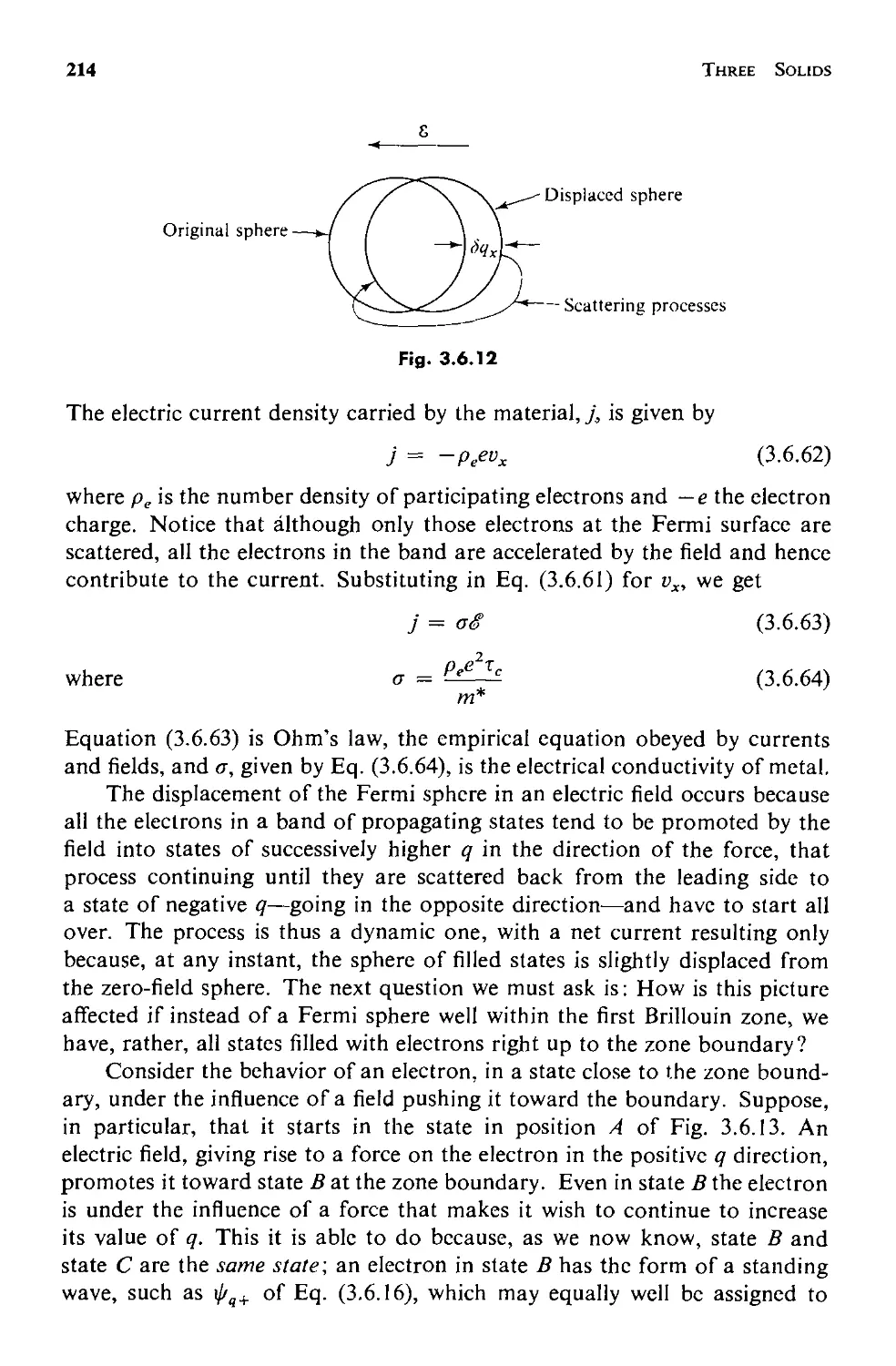


Текст
STATES
OF
MATTER
DAVID L. GOODSTEIN
Professor of physics and Applied Physics
California Institute of Technology
DOVER PUBLICATIONS, INC.
Mineola, New York
Copyright
Copyright «;) 1975, 1985 by David L. Goodstein
All rights reserved under Pan American and International Copyright
Conventions.
Published in Canada by General Publishing Company, Ltd., 895 Don Mills
Road, 400-2 Park Centre, Toronto, Ontario M3C I W3.
Published in the United Kingdom by David & Charles, Brunei House, Forde
Close, Newton Abbot, Devon TQI2 4PU.
Bibliographical Note
This Dover edition, first published in 1985 and republished in 2002, is an
unabridged and corrected republication of the work first published by Prentice-
Hall, Inc., Englewood Cliffs, New Jersey, in 1975.
Library of Congress Cataloging-in-Publication Data
Goodstein. David L., 1939 .
States of matter.
Previously published: Englewood Cliffs, N.J. : Prentice-Hall, 1975.
Includes bibliographies and index.
ISBN 0-486-49506-X
I. Matter-Properties. I. Title.
QCI73.3.G66 1985
530.4
85-680 I
Manufactured in the United States of America
Dover Publications, Inc., 31 East 2nd Street, Mineola, NY 11501
N el mezzo del cammin di nostra vita. . . .
TO JUDY
CONTENTS
PREFACE xi
1 THERMODYNAMICS AND STATISTICAL MECHANICS
1.1 Introduction: Thermodynamics and Statistical Mechanics
of the Perfect Gas 1
1.2 Thermodynamics 10
a. The Laws of Thermodynamics 10
b. Thermodynamic Quantities 13
c. Magnetic Variables in Thermodynamics 19
d. Variational Principles in Thermodynamics 23
e. Examples of the Use of Variational Principles 25
f. Thermodynamic Derivatives 29
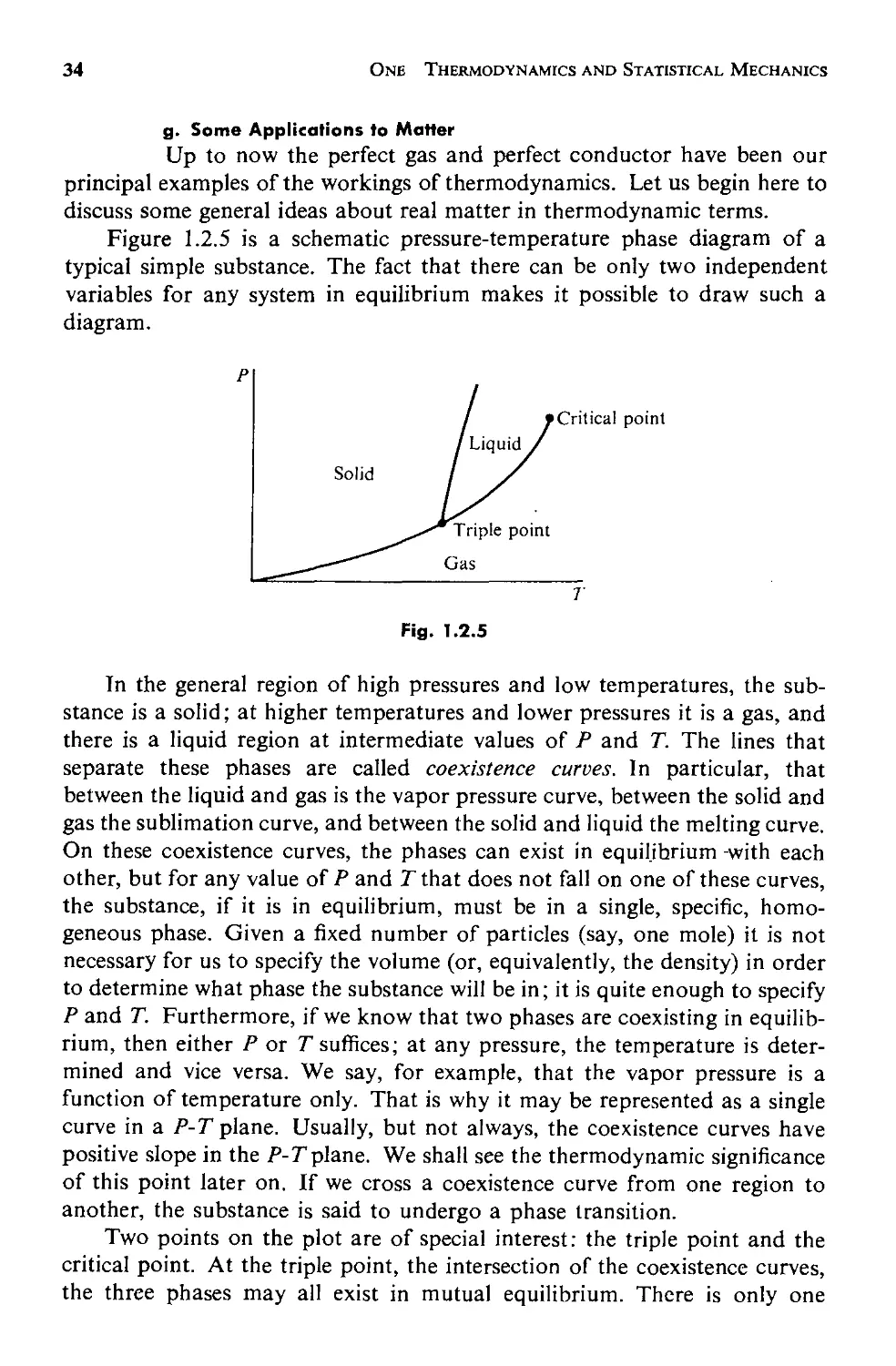
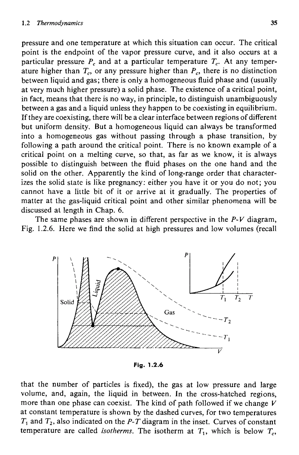
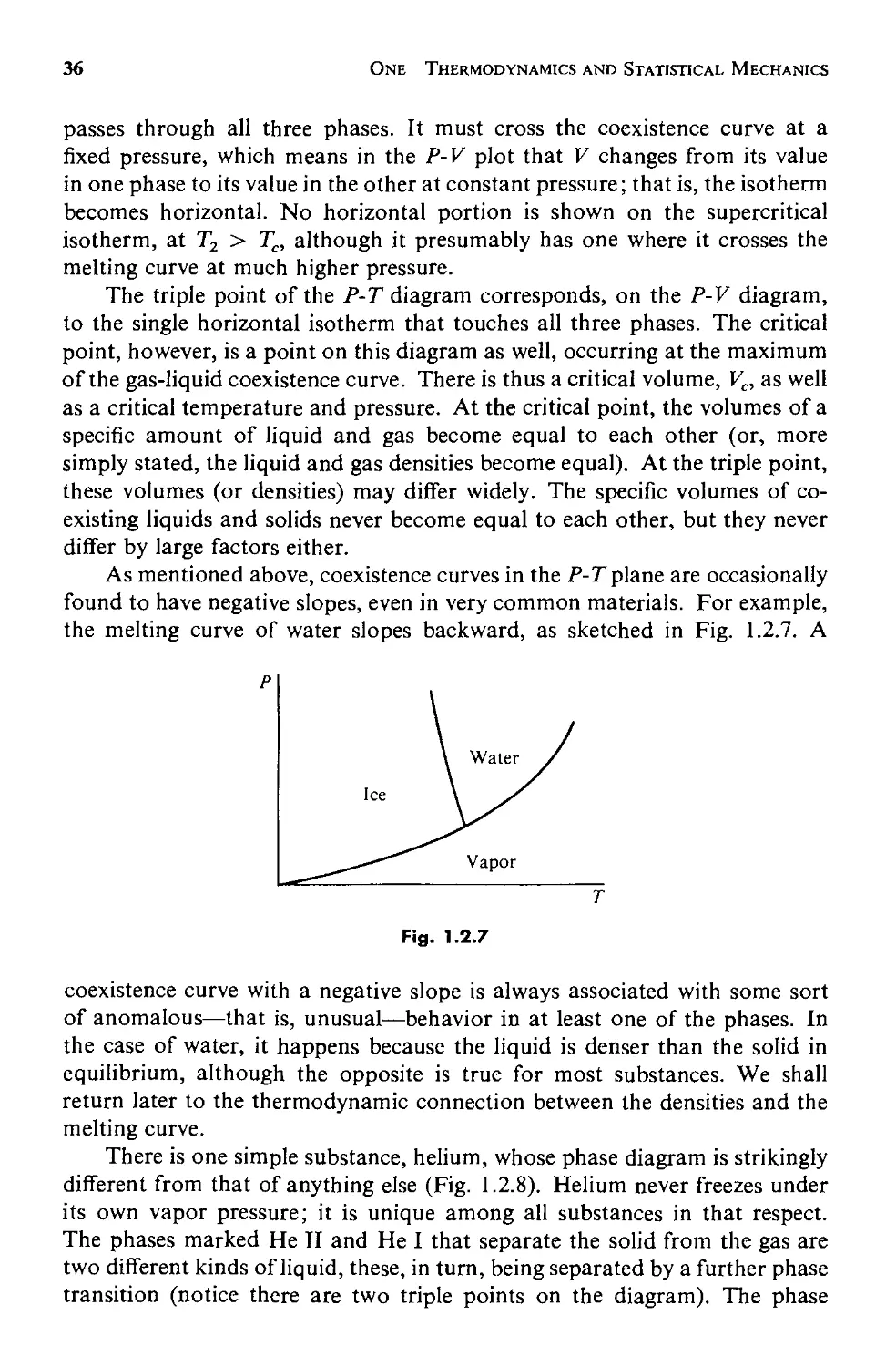
g. Some Applications to Matter 34
1.3 Statistical Mechanics 41
a. Reformulating the Problem 43
b. Some Comments 49
c. Some Properties of Z and :l' 53
d. Distinguishable States: Application to the Perfect Gas 55
e. Doing Sums over States as Integrals 61
f. Fluctuations 71
vii
viii CONTENTS
1.4 Remarks on the Foundations of Statistical Mechanics 83
a. Quantum and Thermodynamic Uncertainties 83
b. Status of the Equal Probabilities Postulate 87
c. Ensembles 89
Appendix A. Thermodynamic Mnemonic 90
2 PERFECT GASES 98
2.1
2.2
2.3
2.4
2.5
2.6
Introduction 98
The Ideal Gas 99
Bose-Einstein and Fermi-Dirac Statistics 105
Slightly Degenerate Perfect Gases 110
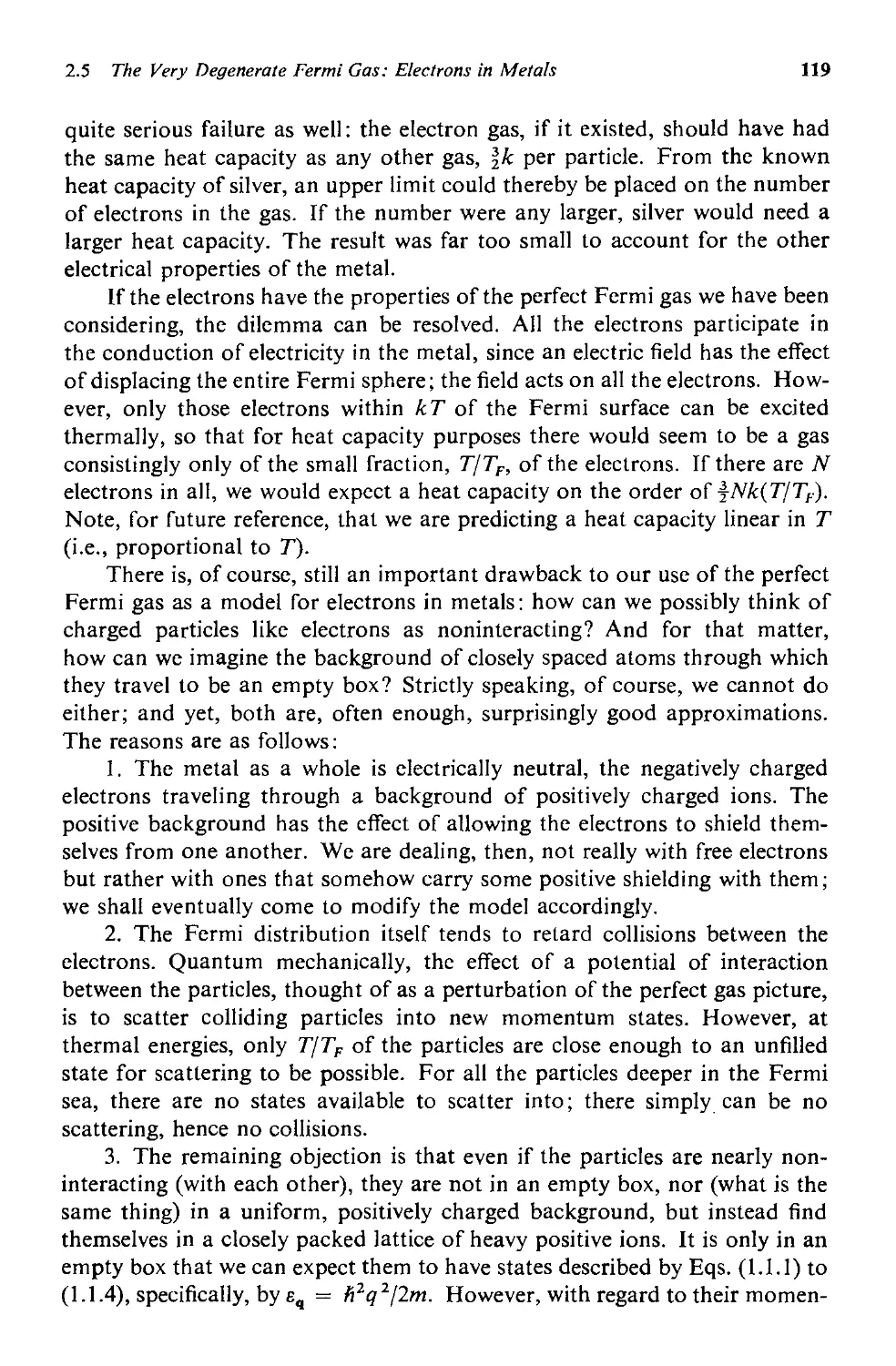
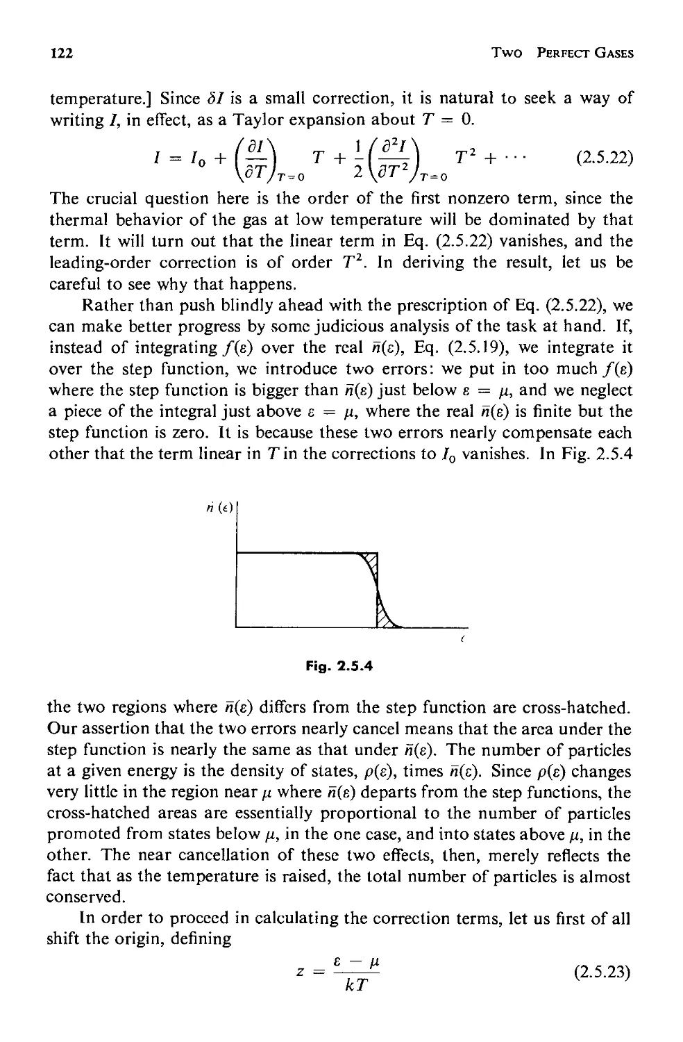
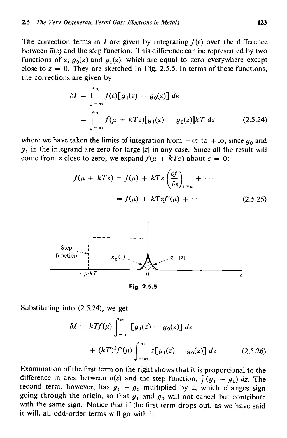
The Very Degenerate Fermi Gas: Electrons in Metals
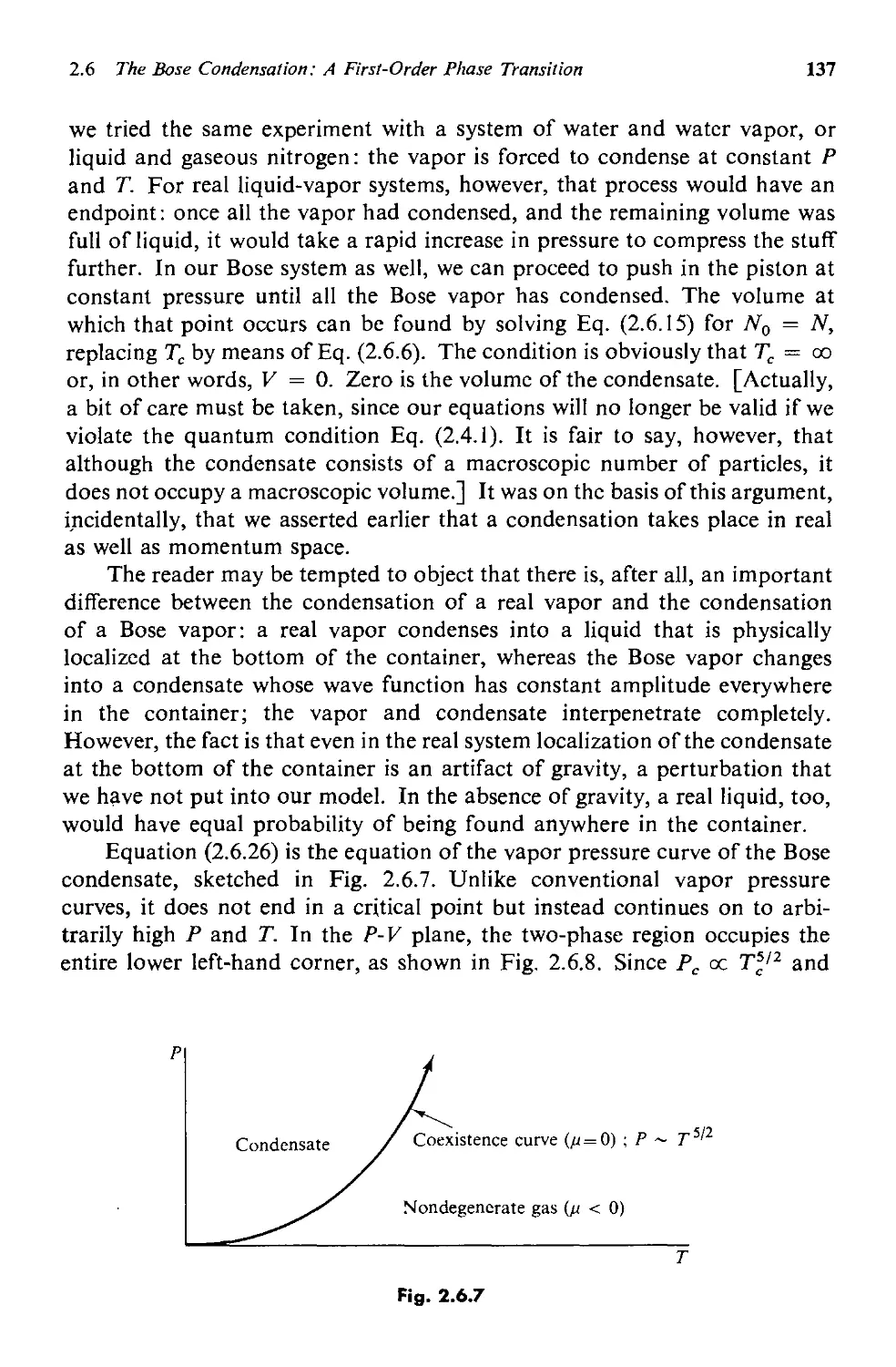
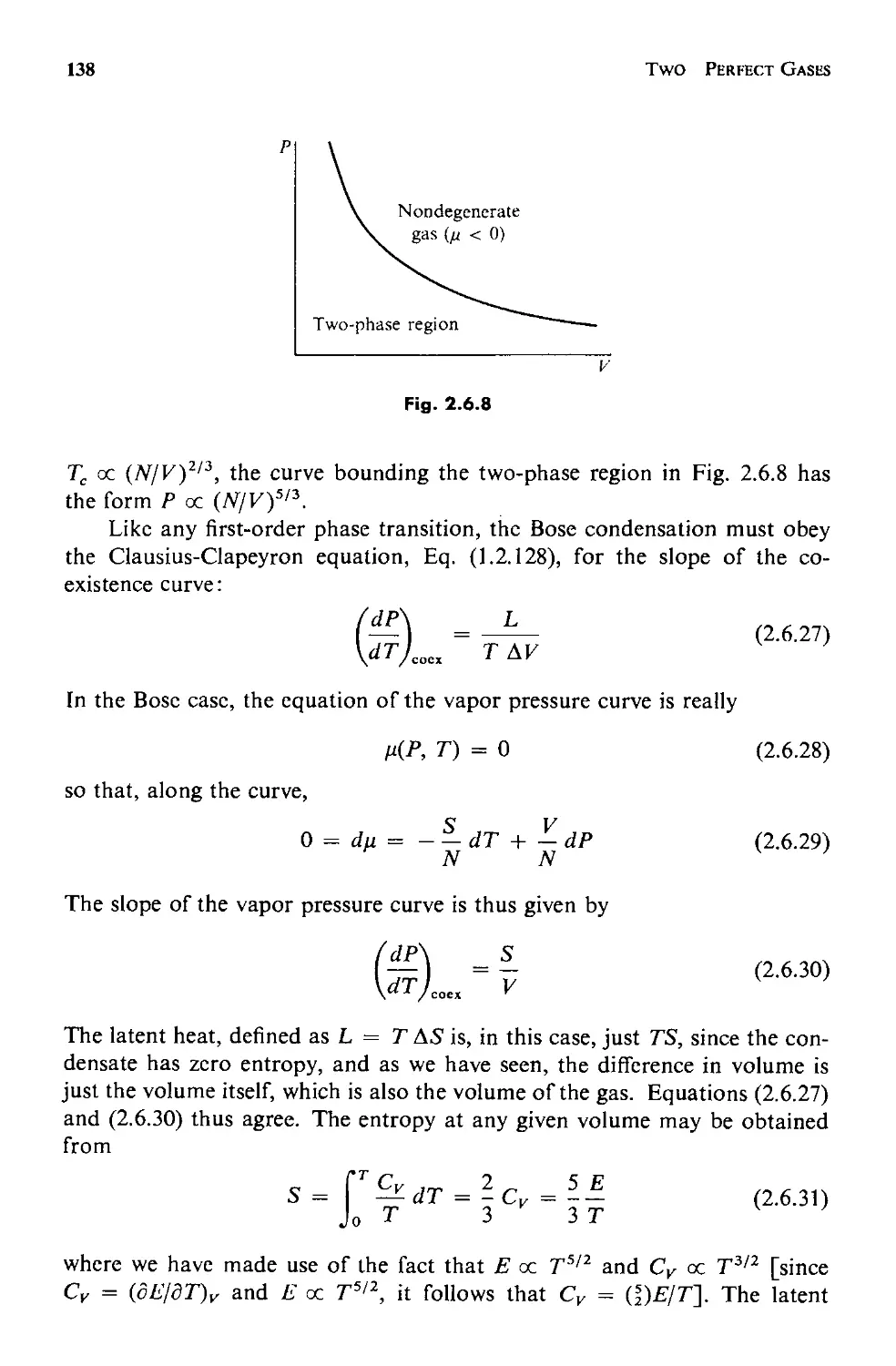
The Bose Condensation: A First Order Phase Transition
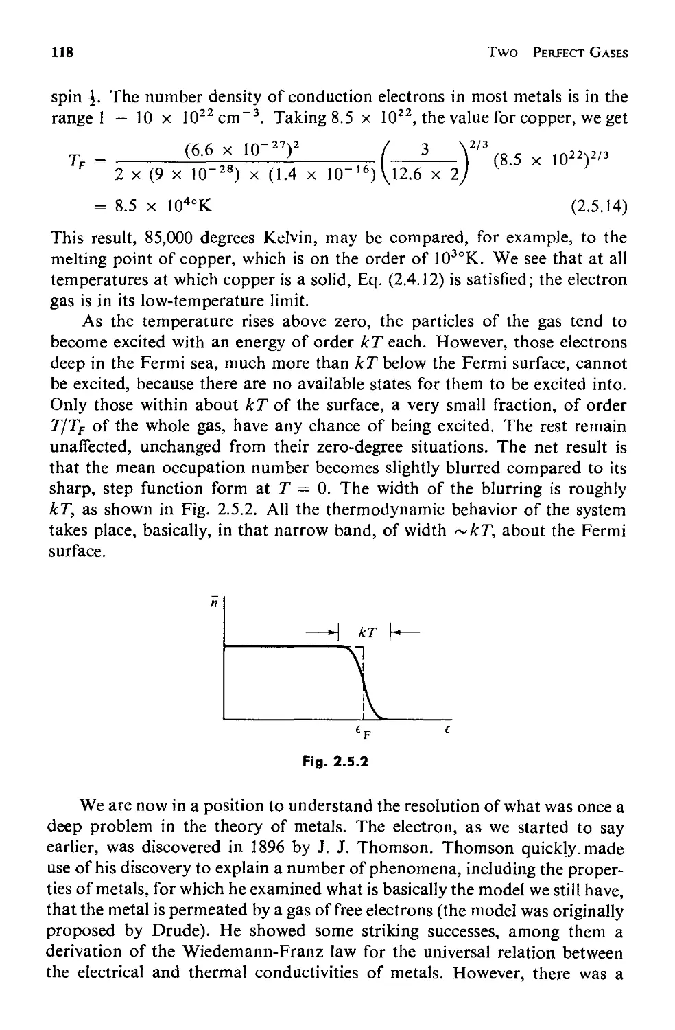
114
127
3 SOLIDS 142
3.1 Introduction 142
3.2 The Heat Capacity Dilemma 144
a. The Einstein Model 147
b. Long Wavelength Compressional Modes 152
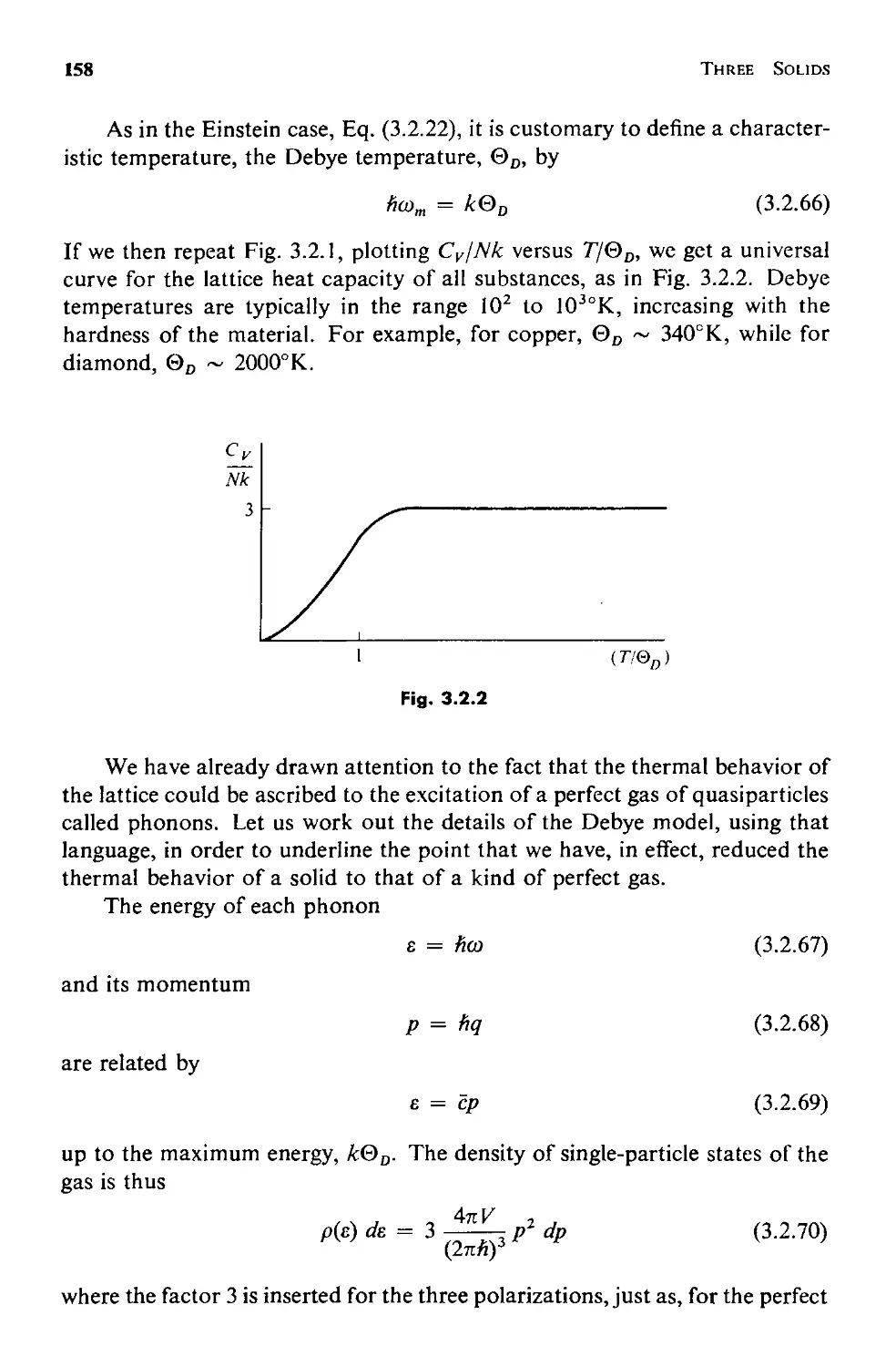
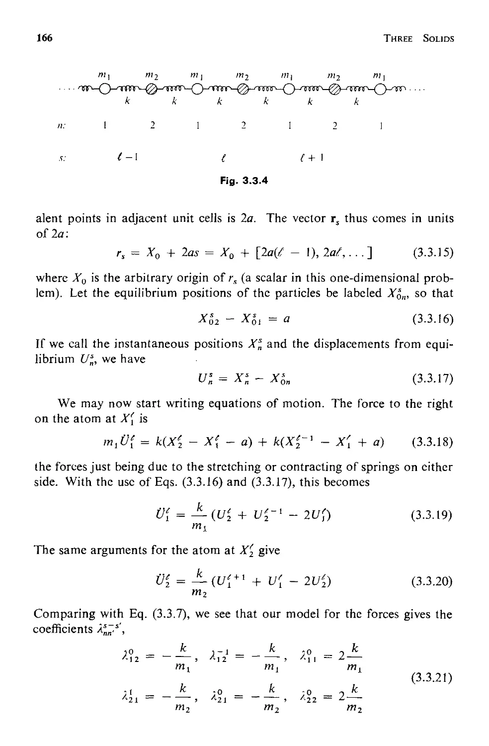
c. The Debye Model 154
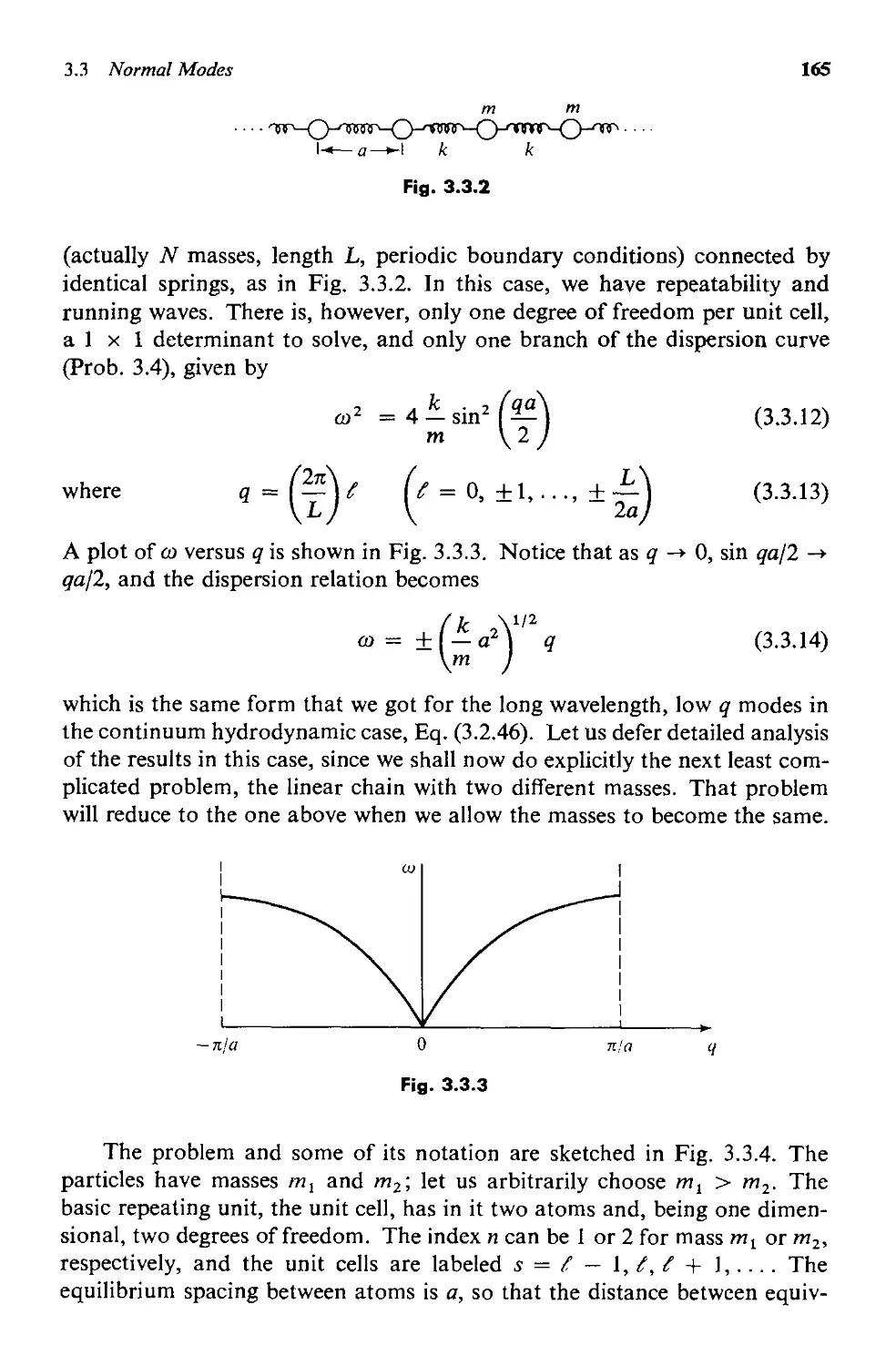
3.3 Normal Modes 160
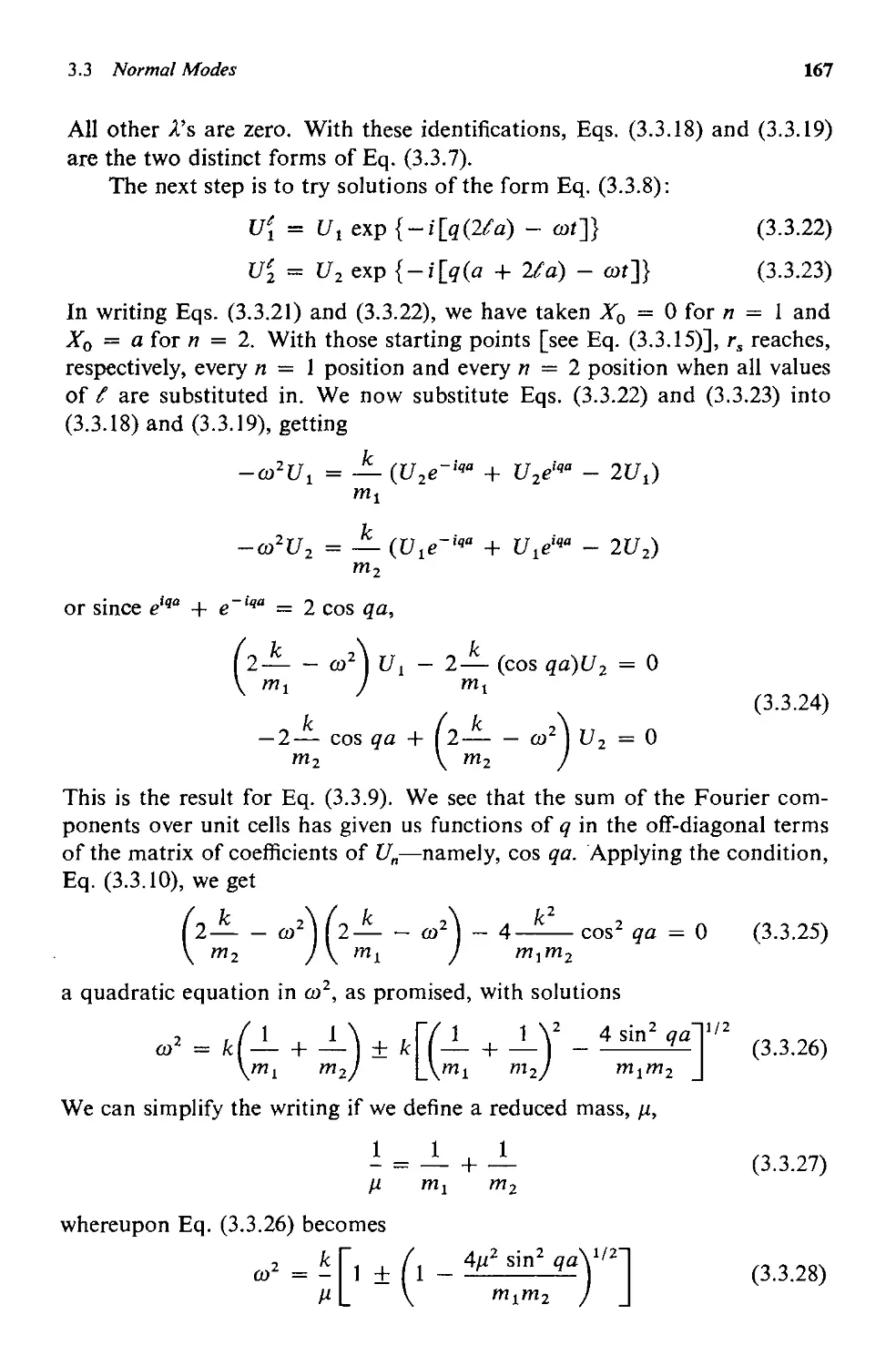
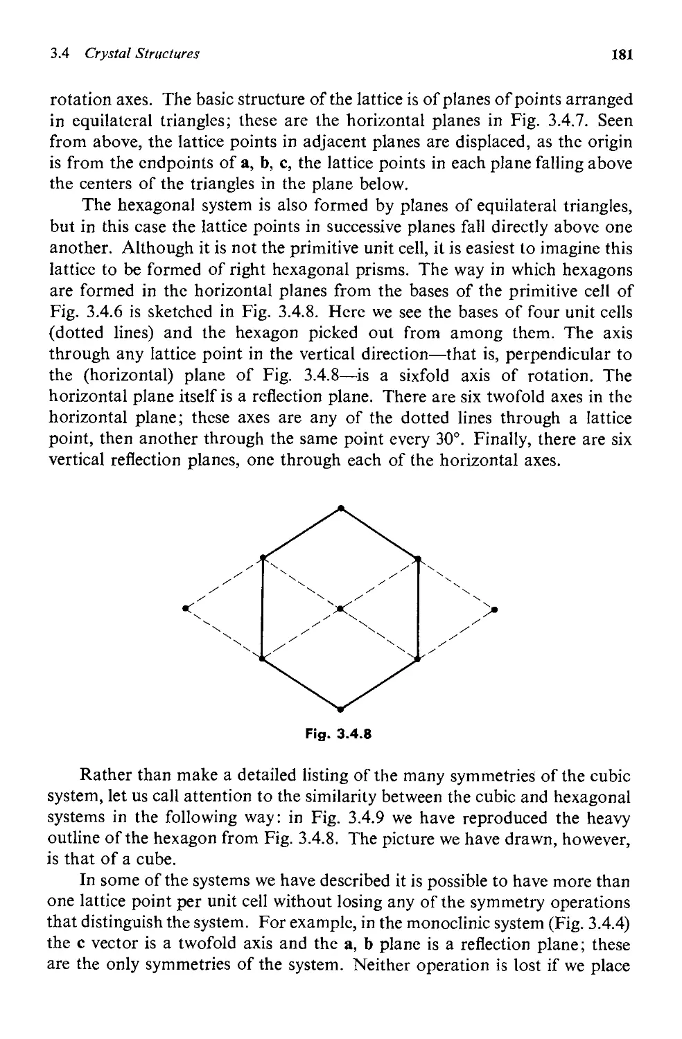
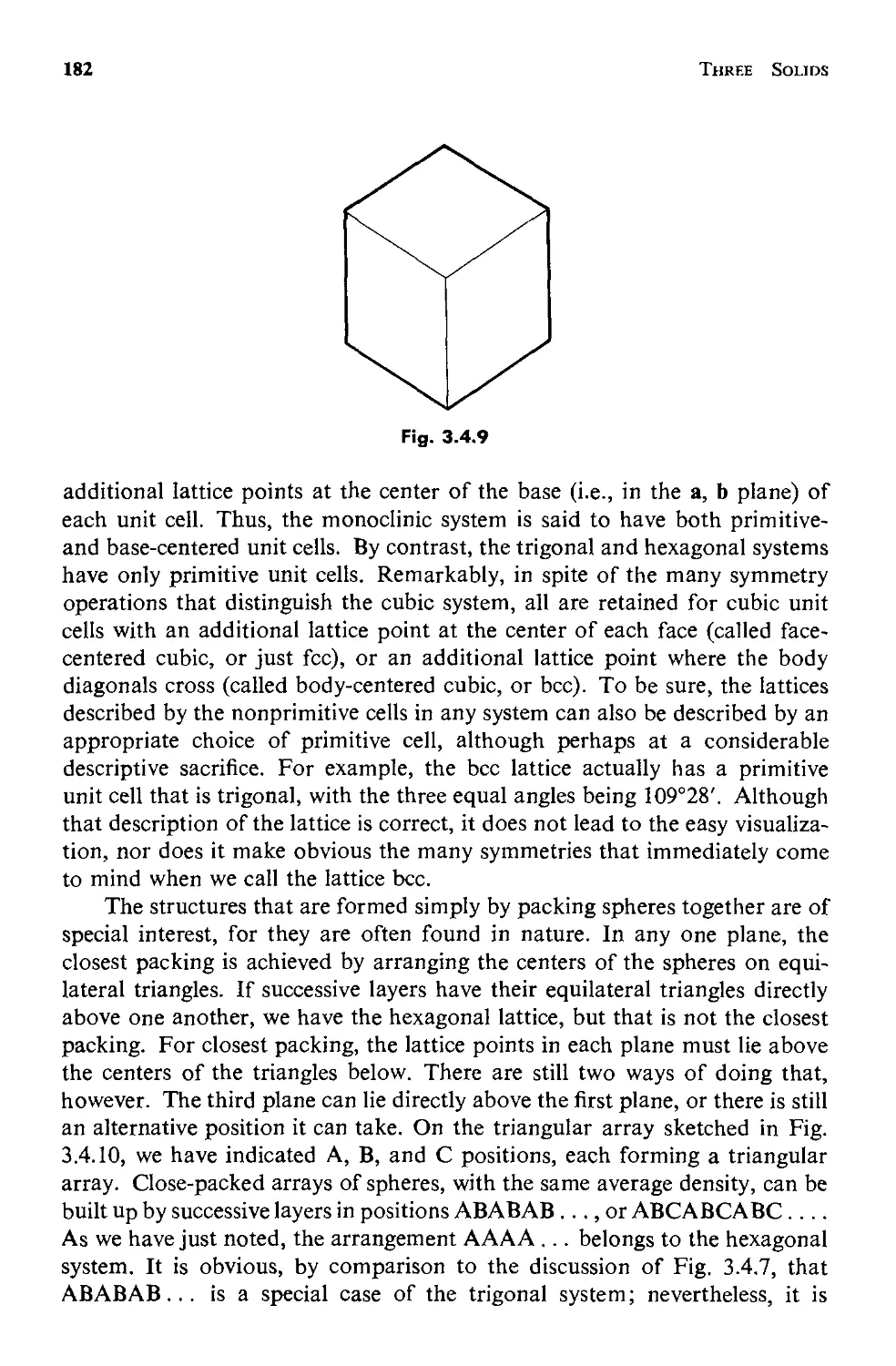
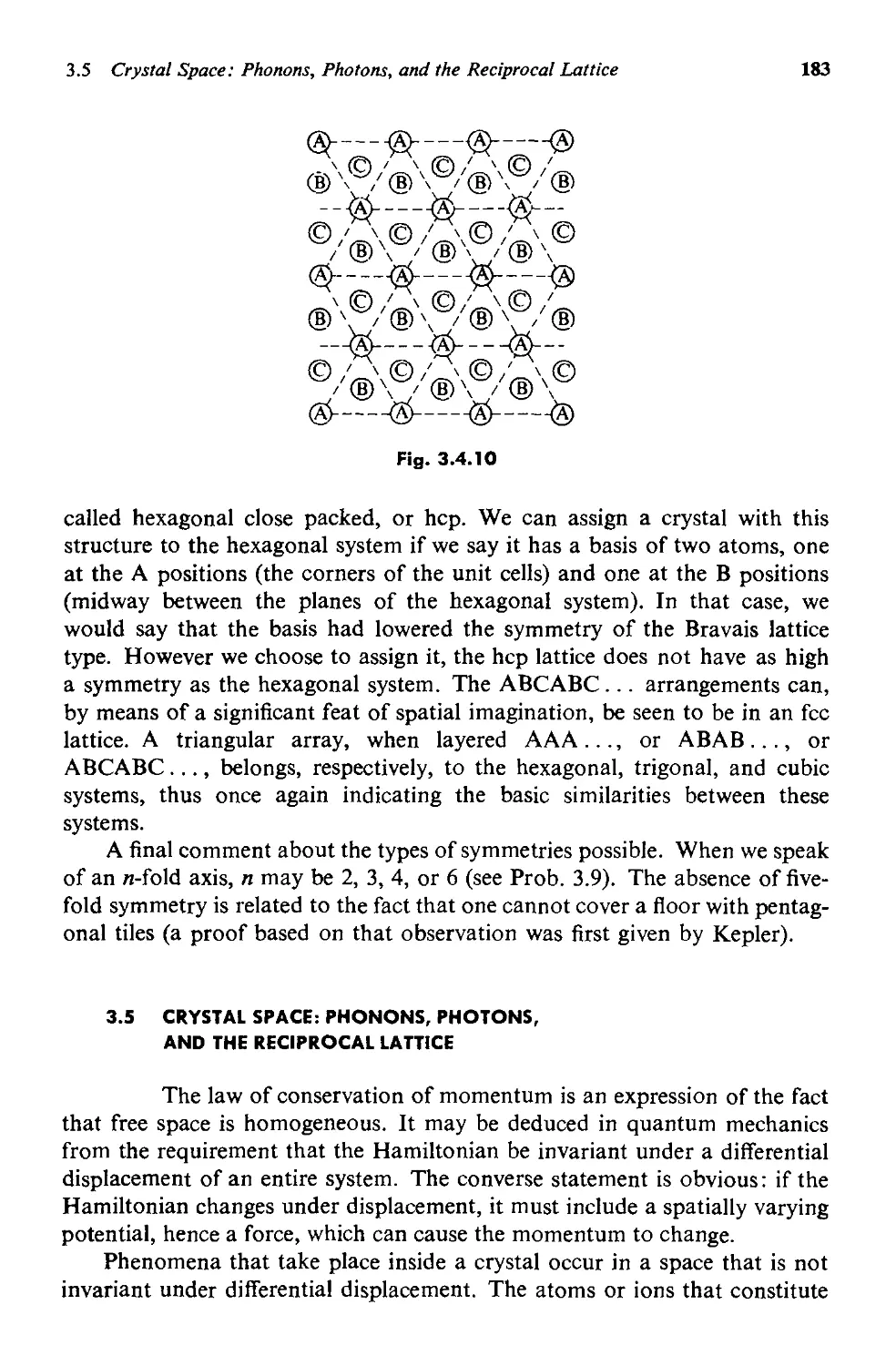
3.4 Crystal Structures 175
3.5 Crystal Space:
Phonons, Photons, and the Reciprocal Lattice 183
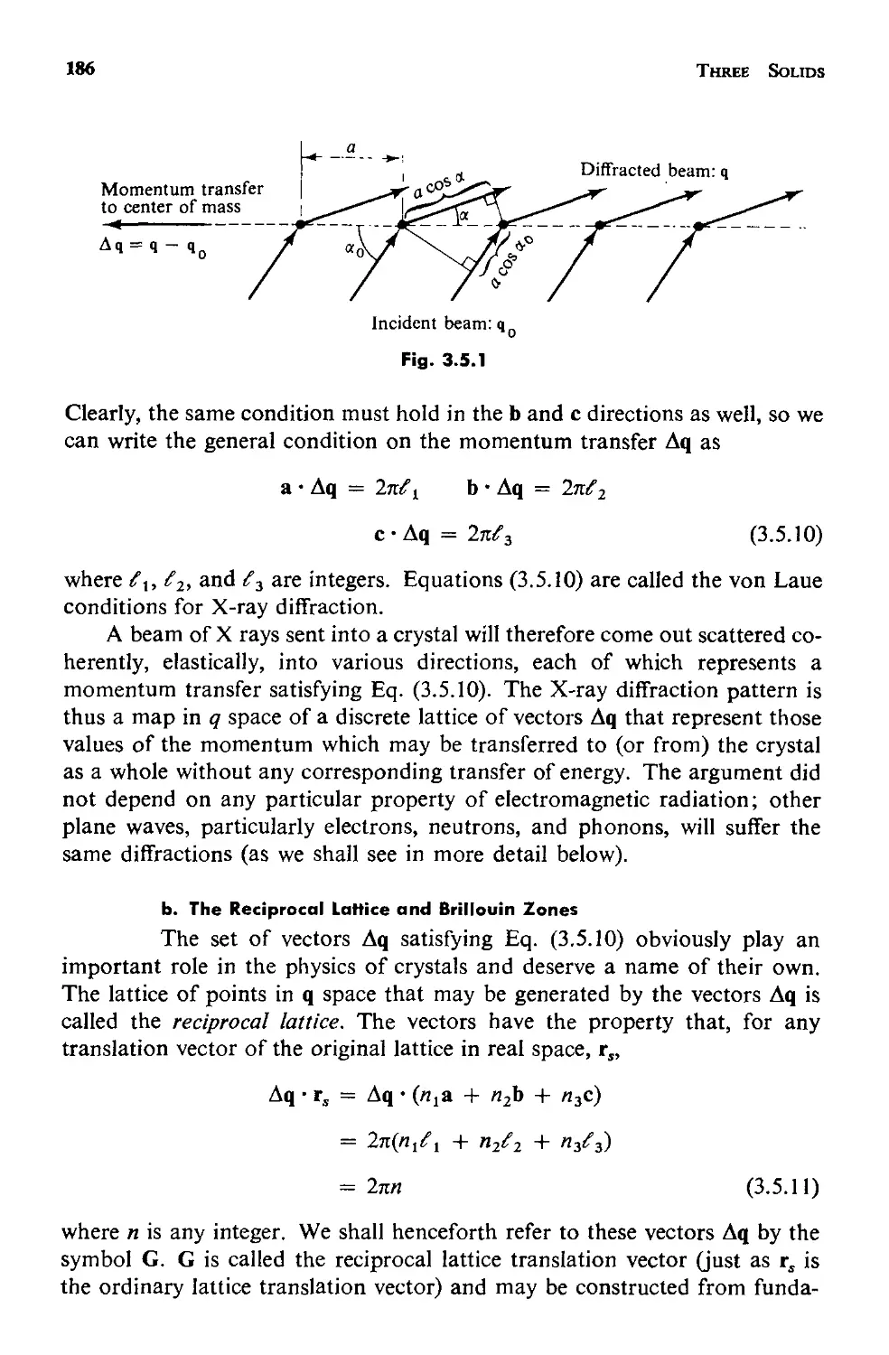
a. Diffraction of X rays 185
b. The Reciprocal Lattice and Brillouin Zones 186
c. Umklapp Processes 191
d. Some Orders of Magnitude 194
3.6 Electrons in Crystals 195
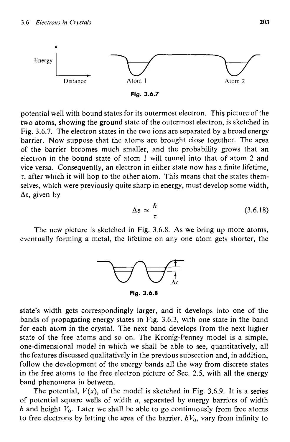
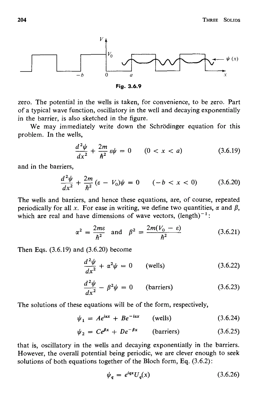
a. A Semiqualitative Discussion 195
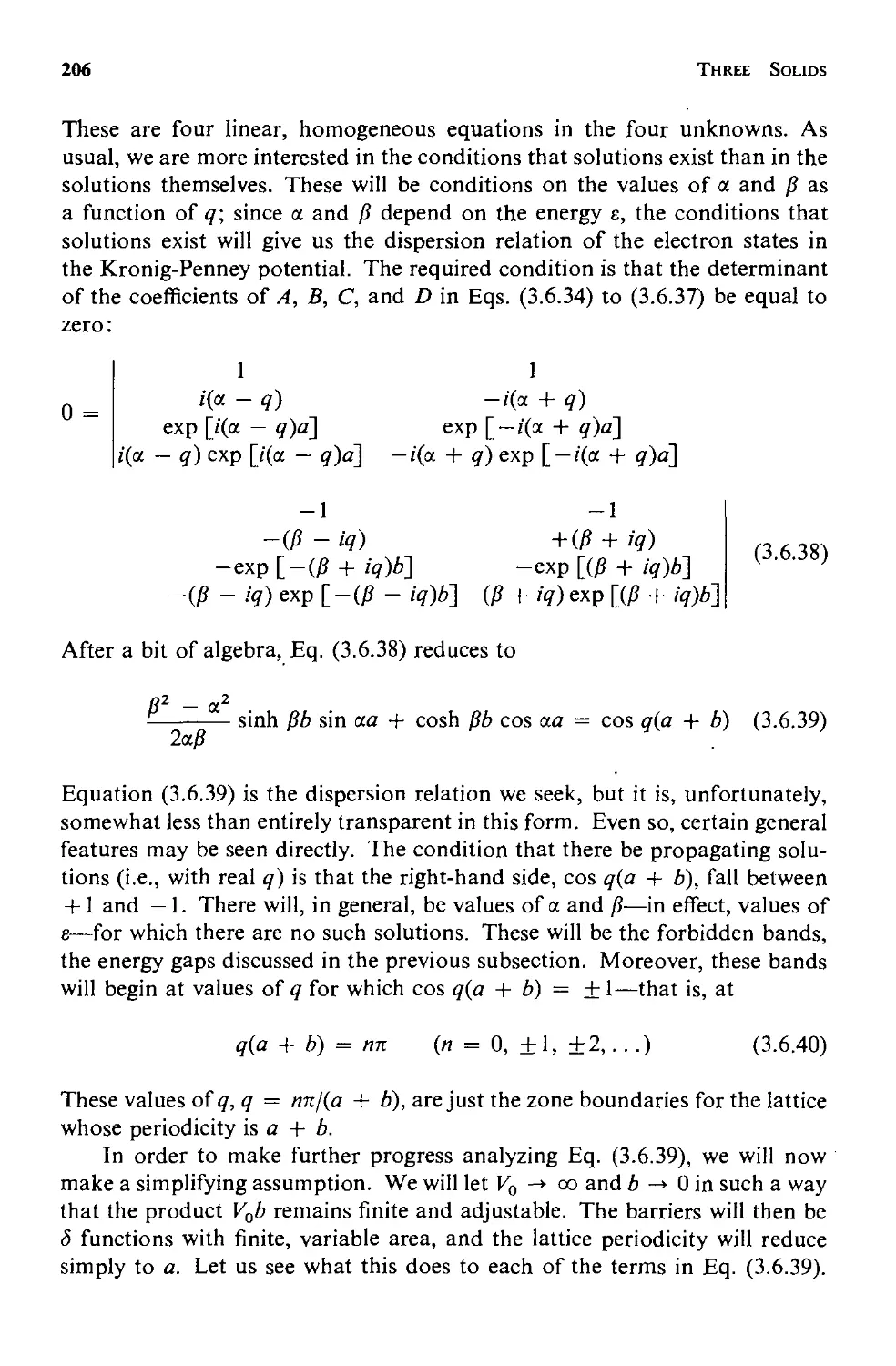
b. The Kronig-Penney Model 202
c. The Fermi Surface: Metal or Nonmetal? 212
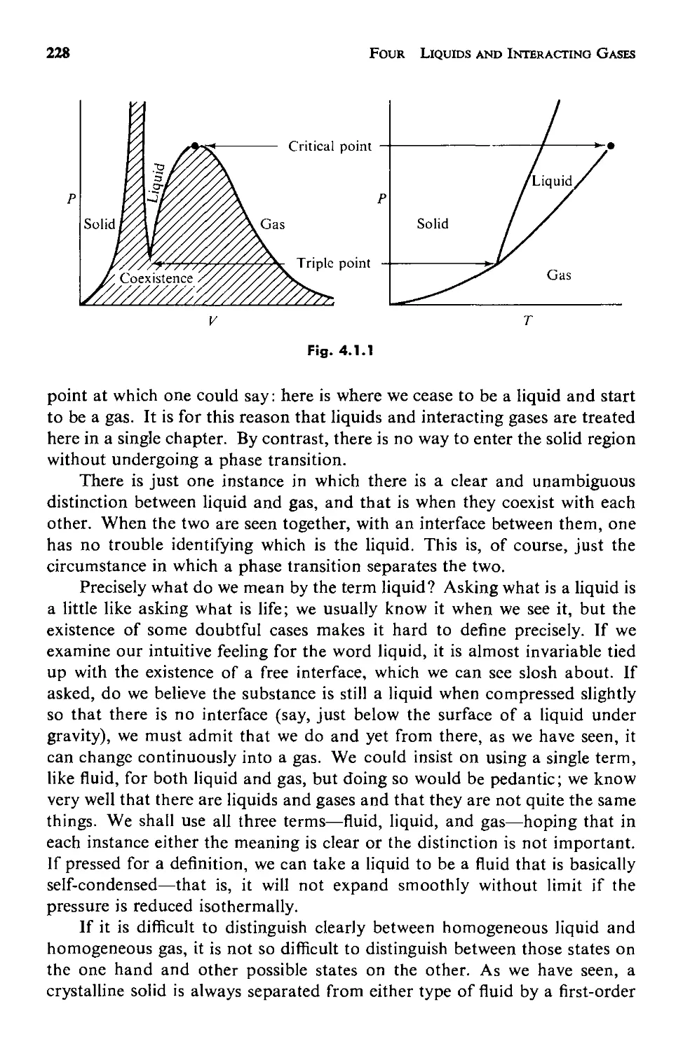
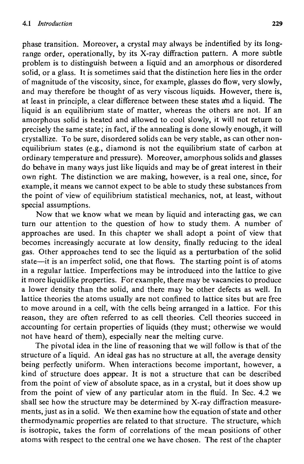
4 LIQUIDS AND INTERACTING GASES 227
4.1 Introduction 227
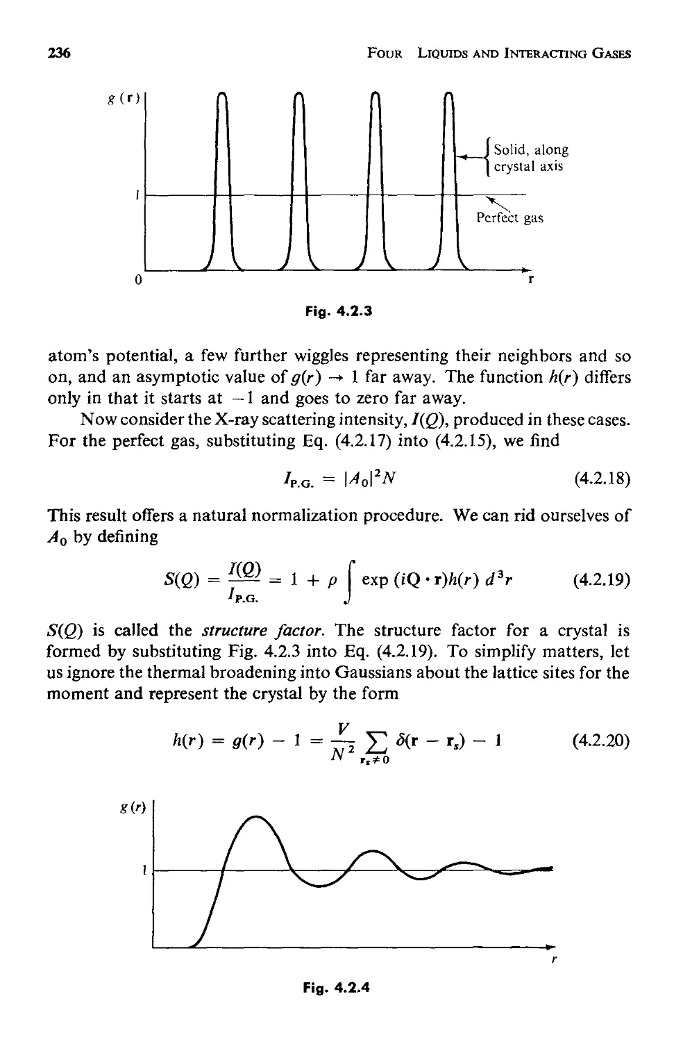
4.2 The Structure of a Fluid 231
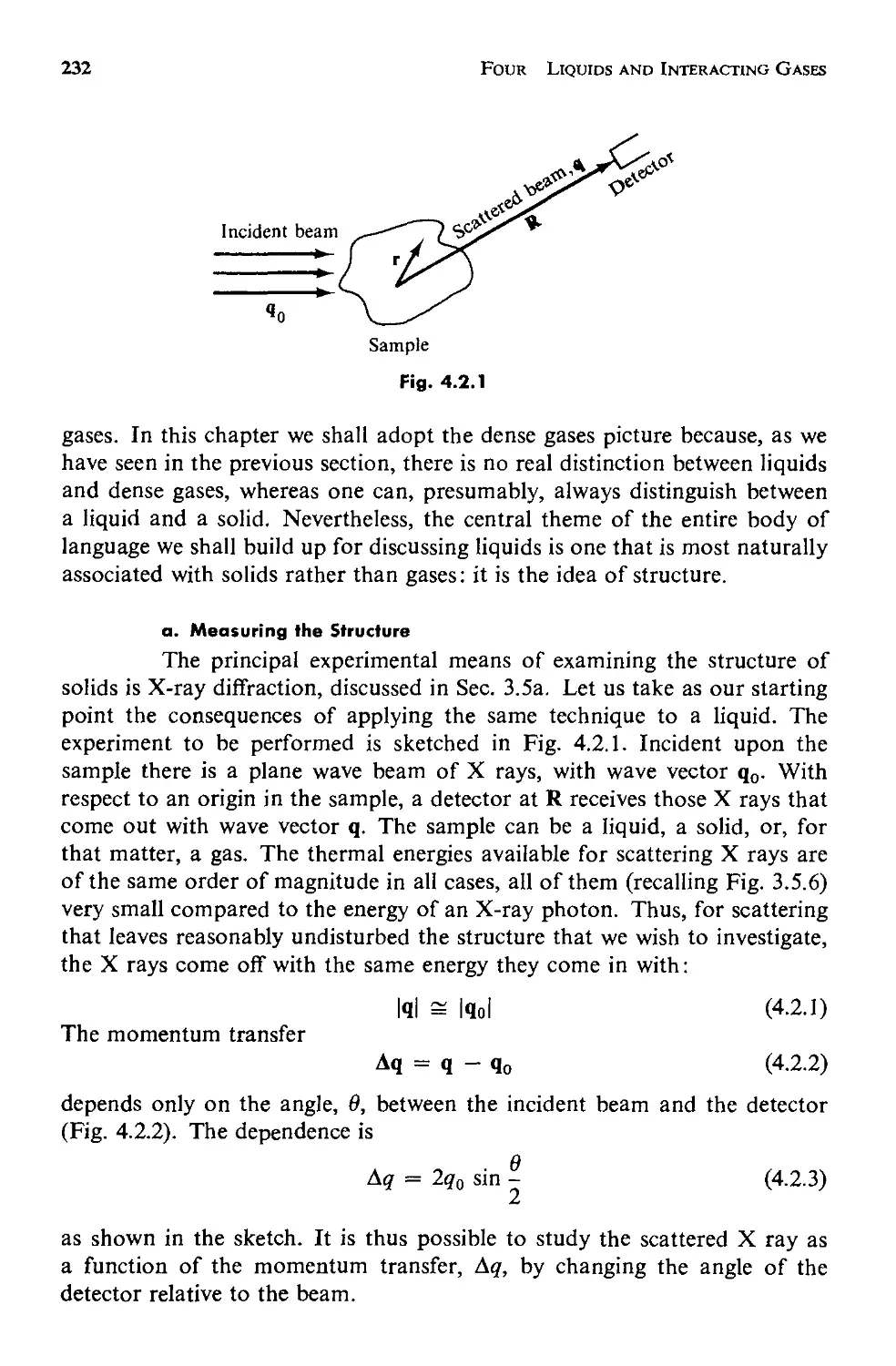
a. Measuring the Structure 232
Contents
ix
b. The Statistical Mechanics of Structure 237
c. Applicability of This Approach 246
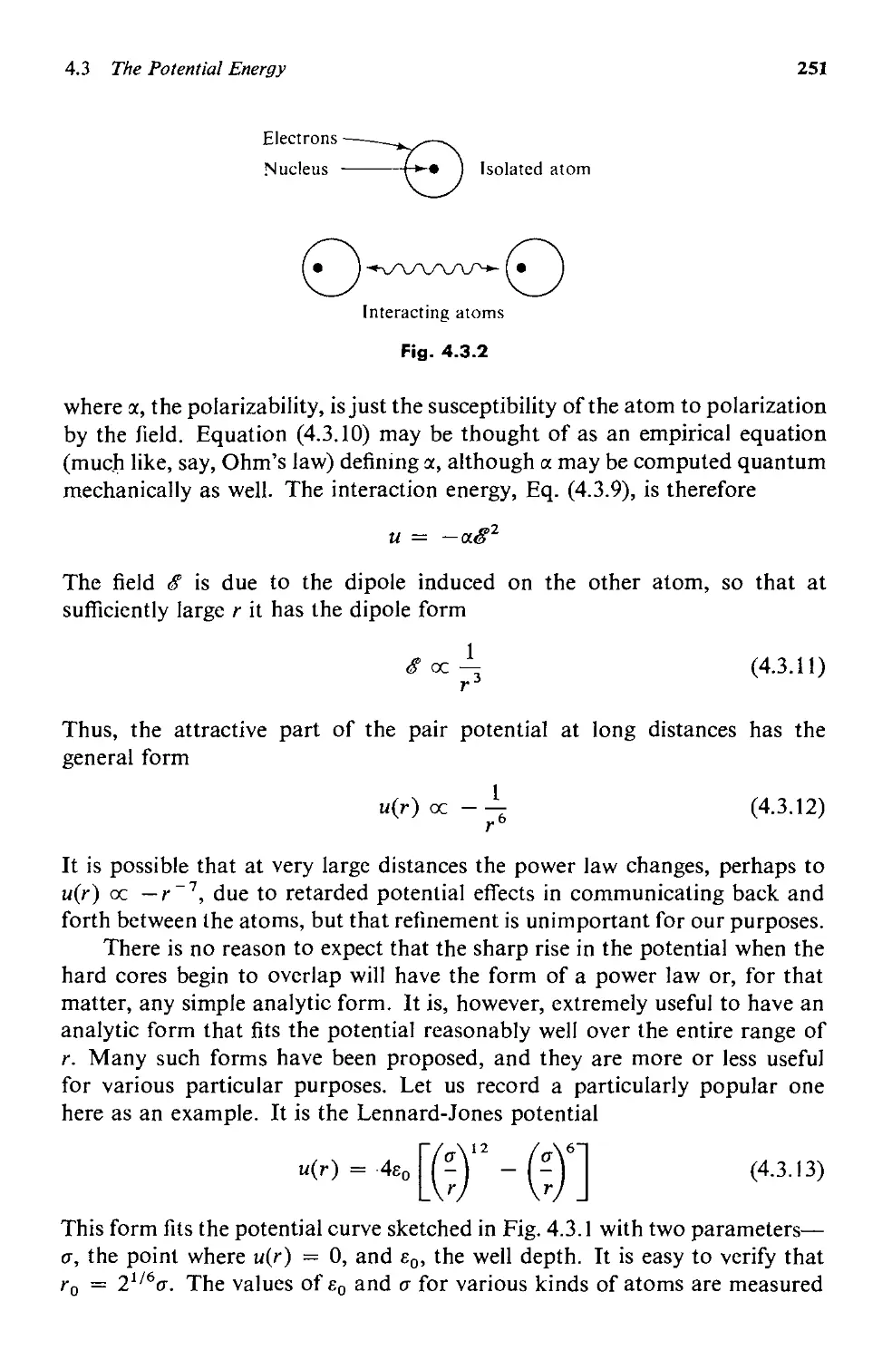
4.3 The Potential Energy 248
a. The Pair Potential 250
b. The Approximation of Pairwise Additivity 252
4.4 Interacting Gases 260
a. Cluster Expansions and the Dilute Gas 260
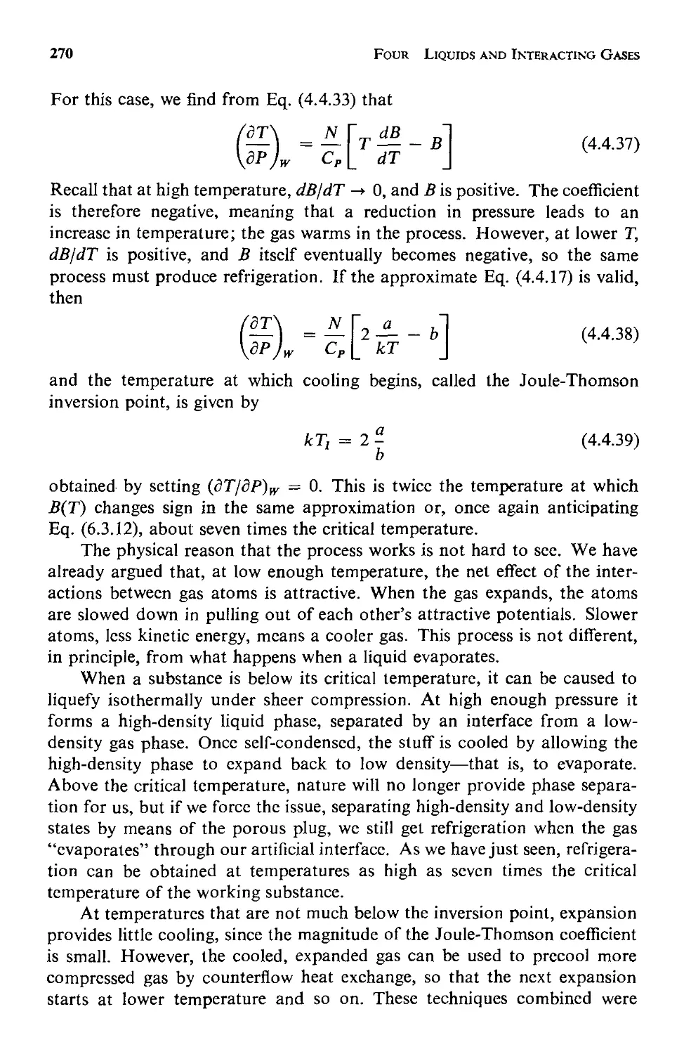
b. Behavior and Structure of a Dilute Gas 263
c. The Liquefaction of Gases
and the Joule-Thomson Process 266
d. Higher Densities 271
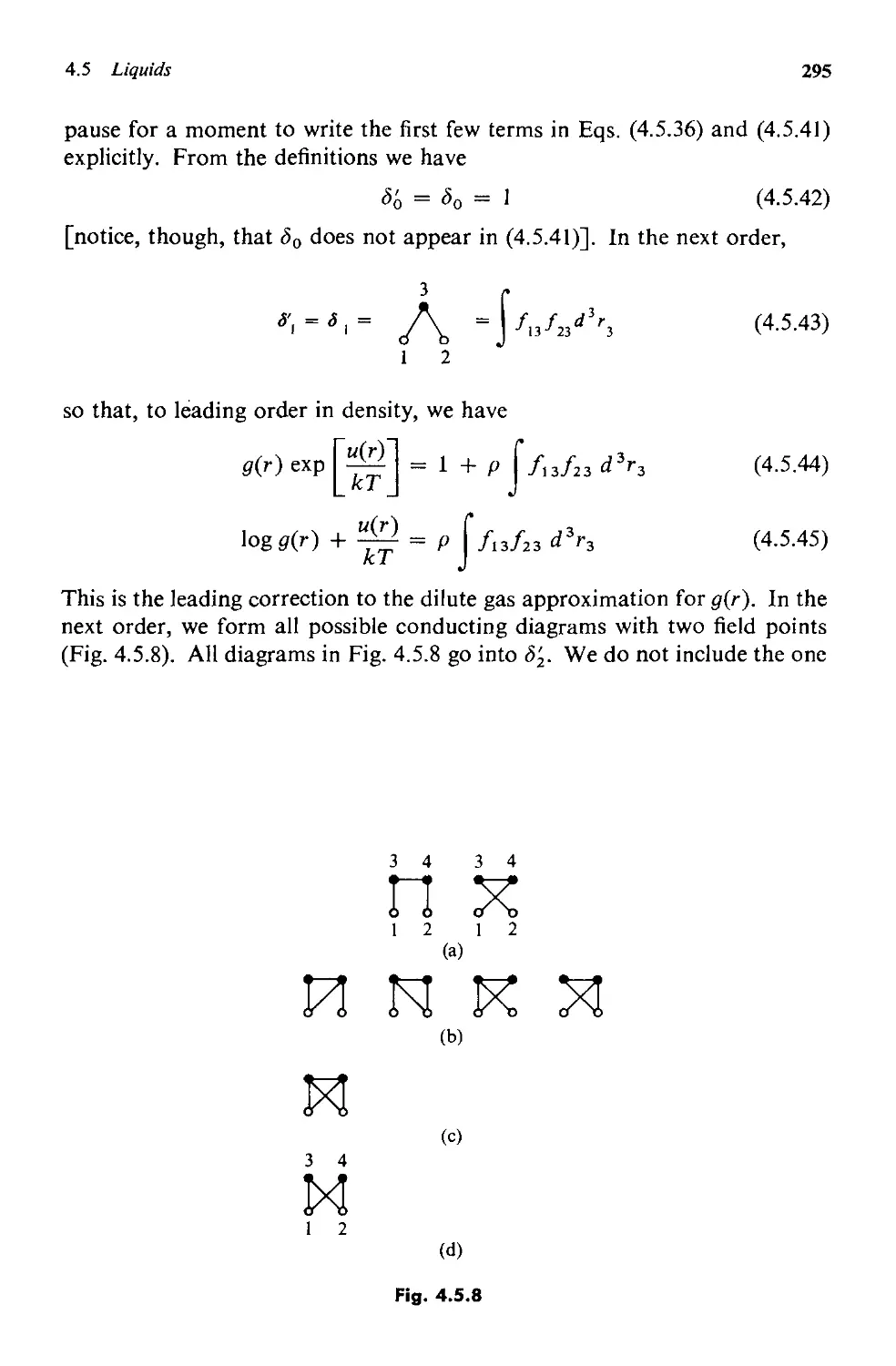
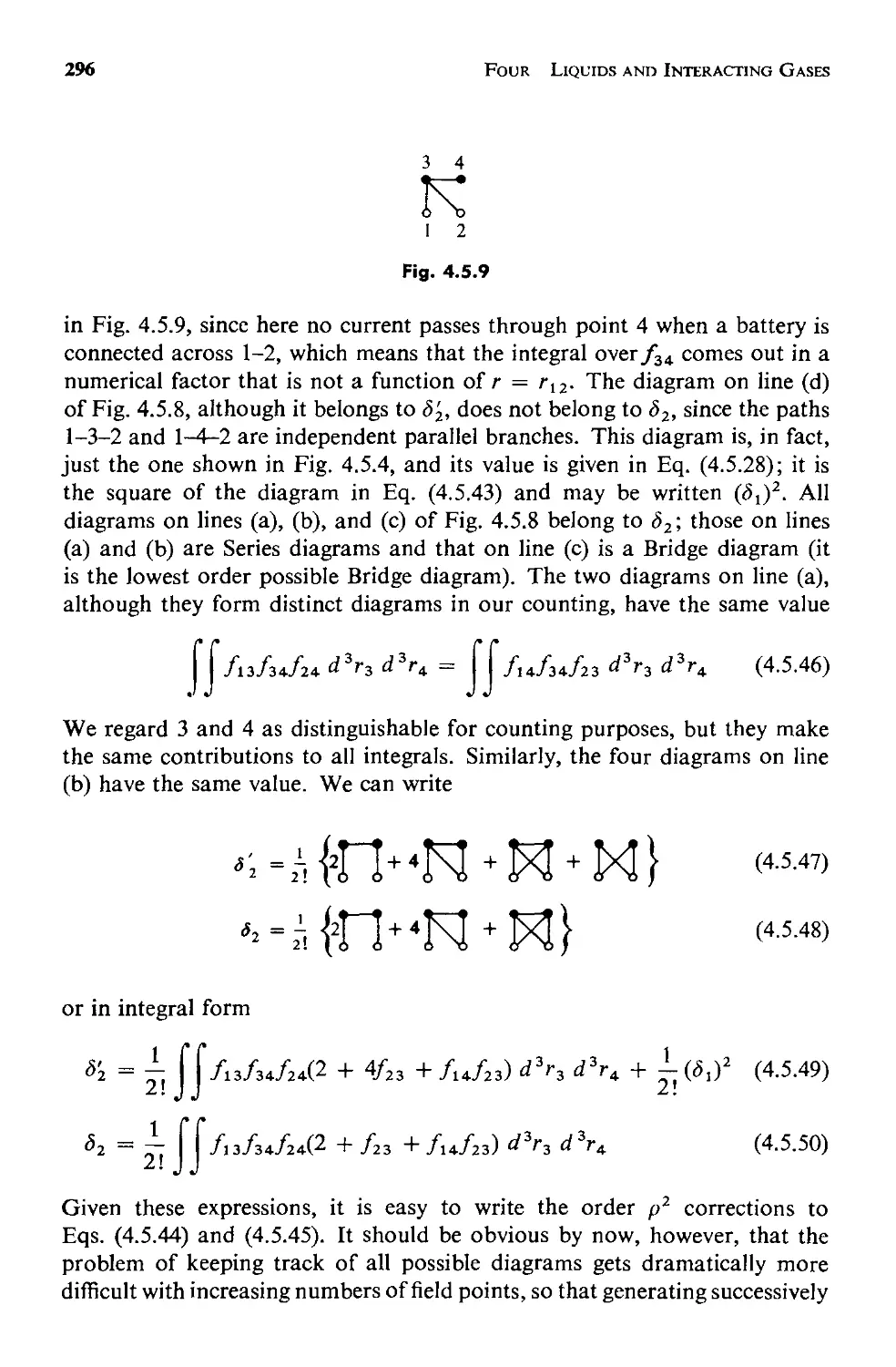
4.5 Liquids 283
a. The Yvon-Born-Green Equation 284
b. The Hypernetted Chain and Percus-Yevick Equations 288
c. Comments and Comparisons 302
5 SOME SPECIAL STATES 320
5.1 Introduction 320
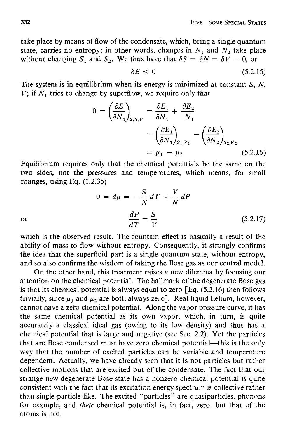
5.2 Superfluidity 321
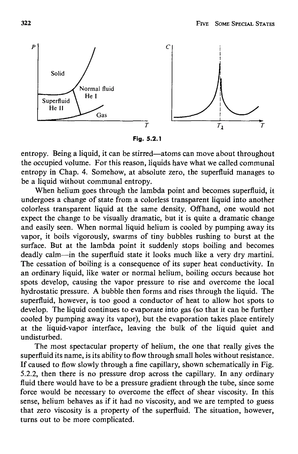
a. Properties of Liquid Helium 321
b. The Bose Gas as a Model for Superfluidity 327
c. Two-Fluid Hydrodynamics 335
d. Phonons and Rotons 342
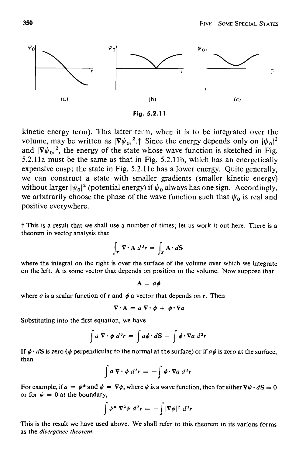
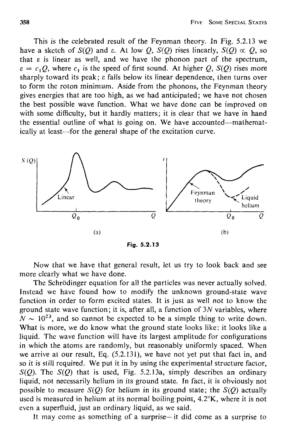
e. The Feynman Theory 348
f. A Few Loose Ends 360
5.3 Superconductivity 371
a. Introduction 371
b. Some Thermodynamic Arguments 375
c. Electron Pairs 386
d. The BCS Ground State 392
e. The Superconducting State 404
5.4 Magnetism 411
a. Introduction 411
b. Magnetic Moments 412
c. Paramagnetism 419
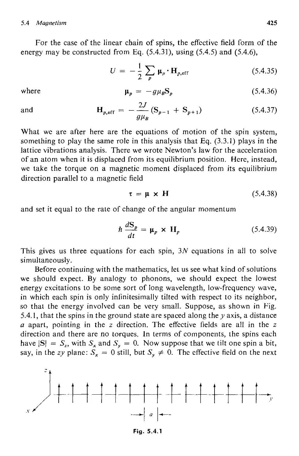
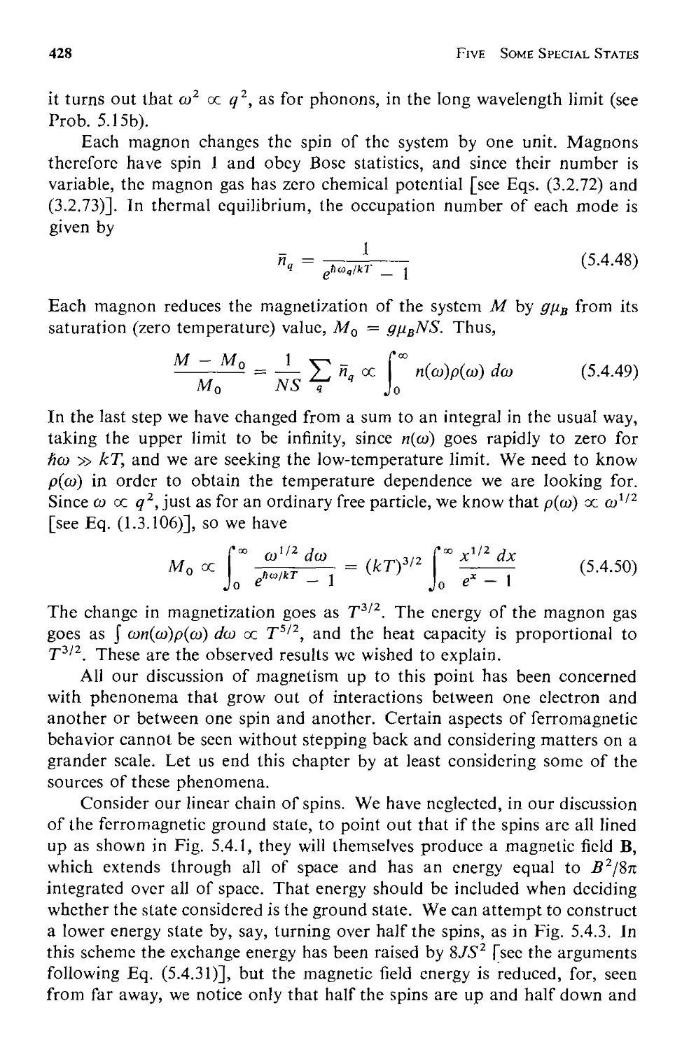
d. Ferromagnetism 421
6 CRITICAL PHENOMENA AND PHASE TRANSITIONS 436
6.1 Introduction 436
6.2 Weiss Molecular Field Theory 438
X CONTENTS
6.3 The van der Waals Equation of State 443
6.4 Analogies Between Phase Transitions 453
6.5 The Generalized Theory 457
a. Equilibrium Behavior 459
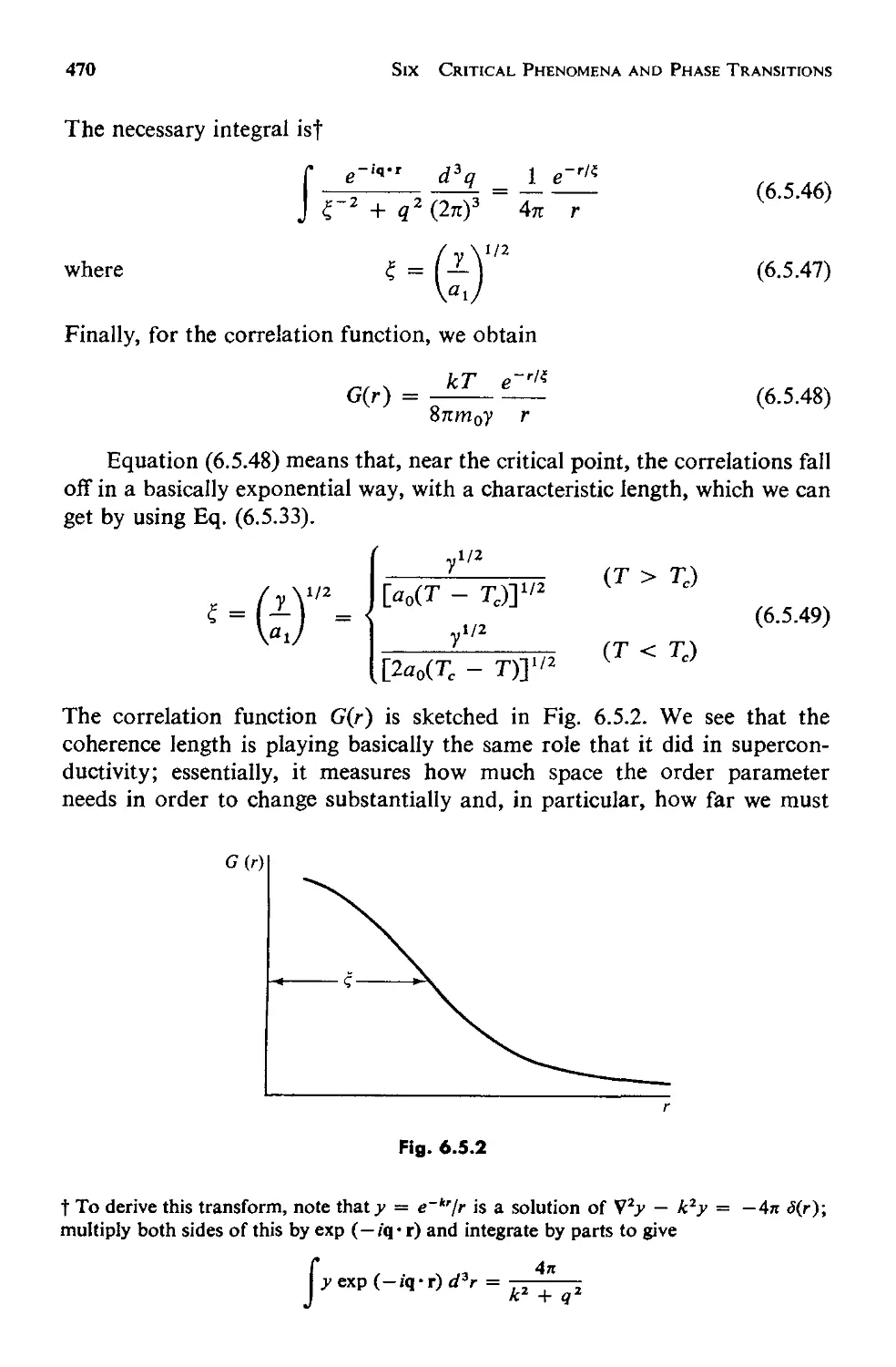
b. Fluctuations 463
6.6 Critical Point Exponents 473
6.7 Scaling Laws: Physics Discovers Dimensional Analysis 478
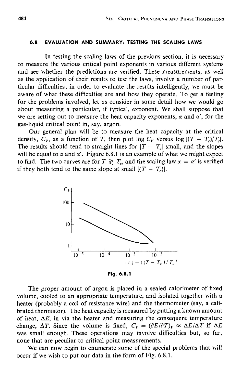
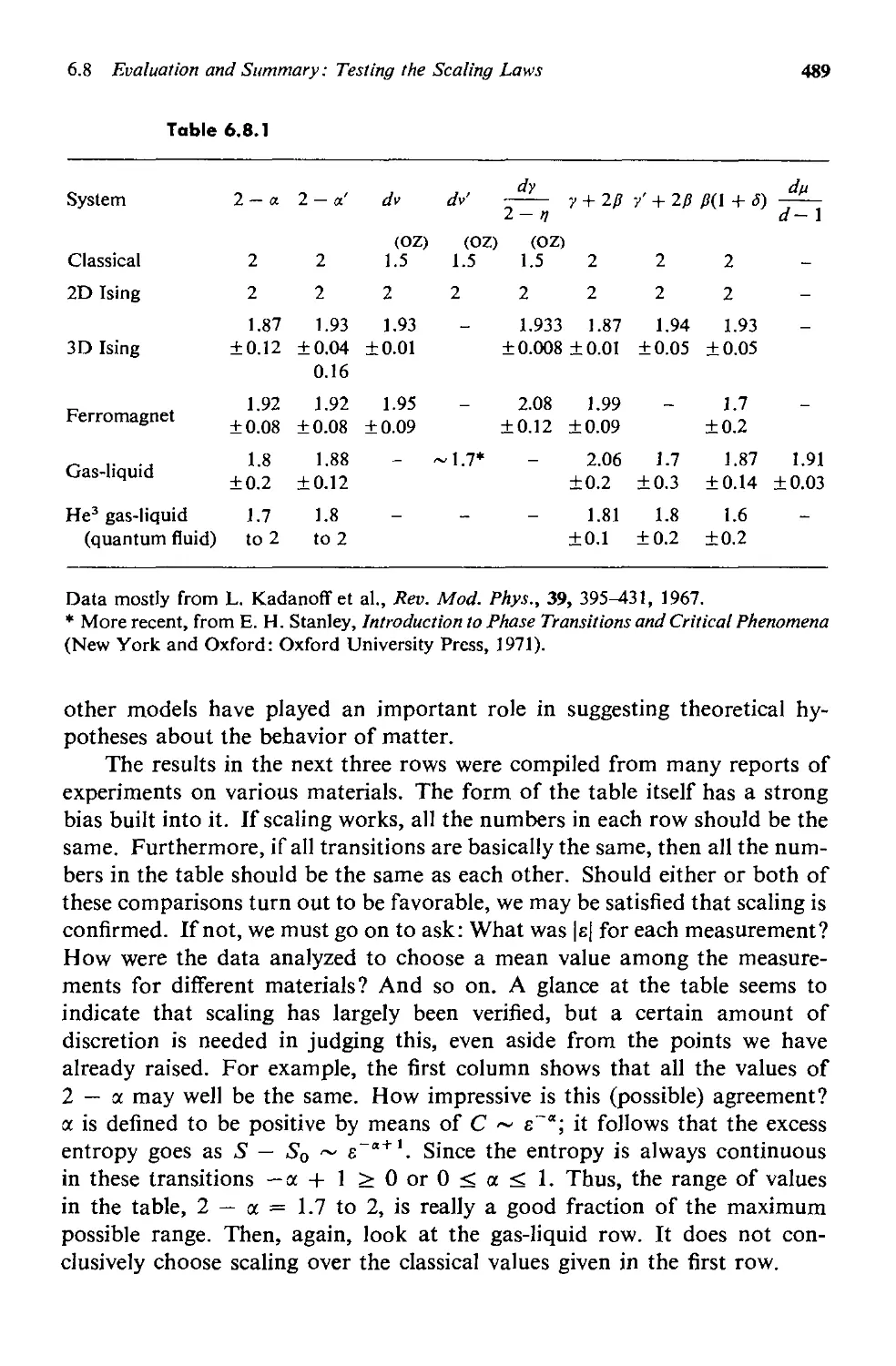
6.8 Evaluation and Summary: Testing the Scaling Laws 484
INDEX 494
PREFACE
This book is based on lectures prepared for a year-long course of the
same title, designed as a central part of a new curriculum in applied
physics. It was offered for the first time in the academic year 1971-1972
and has been repeated annuaJly since.
There is a good deal of doubt about precisely what applied physics is,
but a reasonably clear picture has emerged of how an applied physics
student ought to be educated, at least here at Caltech. There should be a
rigorous education in basic physics and related sciences, but one centered
around the macroscopic world, from the atom up rather than from the
nucleus down: that is, physics, with emphasis on those areas where the
fruits of research are likely to be applicable elsewhere. The course from
which this book arose was designed to be consistent with this concept.
The course level was designed for first-year graduate students in
applied physics, but in practice it has turned out to have a much wider
appeal. The classroom is shared by undergraduates (seniors and an
occasional junior) in physics and applied physics, plus graduate students
in applied physics, chemistry, geology, engineering, and applied math-
ematics. AJI are assumed to have a reasonable undergraduate background
in mathematics, a course including electricity and magnetism, and at
least a little quantum mechanics.
The basic outline of the book is simple. After a chapter designed to
start everyone off at the same level in thermodynamics and statistical
mechanics, we have the basic states-gases, solids, and liquids-a few
xi
xii
PREFACE
special cases, and, finaJly, phase transitions. What we seek in each case
is a feeling for the essential nature of the stuff, and how one goes about
studying it. In general, the book should help give the student an idea of
the language and ideas that are reasonably current in fields other than the
one in which he or she wiJl specialize. In short, this is an unusual beast: an
advanced survey course.
All the problems that appear at the ends of the chapters were used as
either homework or examination problems during the first three years in
which the course was taught. Some are exercises in applying the material
covered in the text, but many are designed to uncover or iJluminate
various points that arise, and are actually an integral part of the course.
Such exercises are usuaJly referred to at appropriate places in the text.
There is an annotated bibliography at the end of each chapter. The
bibliographies are by no means meant to be comprehensive surveys even
of the textbooks, much less of the research literature of each field. In-
stead they are meant to guide the student a bit deeper if he wishes to go
on, and they also serve to list aJl the material consulted in preparing the
lectures and this book. There are no footnotes to references in the text.
The history of science is used in a number of places in this book,
usuaJly to put certain ideas in perspective in one way or another. How-
ever, it serves another purpose, too: the study of physics is essentially a
humanistic enterprise. Much of its fascination lies in the fact that these
mighty feats of the inteJlect were performed by human beings, just like
you and me. I see no reason why we should ever try to forget that, even
in an advanced physics course. Physics, I think, should never be taught
from a historical point of view-the result can only be confusion or bad
history-but neither should we ignore our history. Let me hasten to
acknowledge the source of the history found in these pages: Dr. Judith
Goodstein, the fruits of whose doctoral thesis and other research have
insinuated themselves into many places in the text.
Parts of the manuscript in various stages of preparation have been
read and criticized by some of my coJleagues and students, to whom I am
deeply grateful. Among these I would like especially to thank Jeffrey
Greif, Professors T. C. McGill, C. N. Pings and H. E. Stanley, David
Palmer, John Dick, Run-Han Wang, and finaJly Deepak Dhar, a student
who contributed the steps from Eq. (4.5.20) to Eq. (4.5.24) in response to
a homework assignment. I am indebted also to Professor Donald
Langenberg, who helped to teach the course the first time it was offered.
The manuscript was typed with great skiJl and patience, principaJly by
Mae Ramirez and Ann Freeman. Needless to say, aJl errors are the
responsibility of the author alone.
Pasadena, California
April 5, 1974
DA VID L. GOODSTEIN
ONE
THERMODYNAMICS AND
STATISTICAL MECHANICS
1.1 INTRODUCTION: THERMODYNAMICS AND STATISTICAL
MECHANICS OF THE PERFECT GAS
Ludwig Boltzmann, who spent much of his life studying statistical
mechanics, died in 1906, by his own hand. Paul Ehrenfest, carrying on the
work, died similarly in 1933. Now it is our turn to study statistical mechanics.
Perhaps it will be wise to approach the subject cautiously. We will begin
by considering the simplest meaningful example, the perfect gas, in order
to get the central concepts sorted out. In Chap. 2 we will return to complete
the solution of that problem, and the results wiIl provide the foundation of
much of the rest of the book.
The quantum mechanical solution for the energy levels of a particle in a
box (with periodic boundary conditions) is
fz2 q 2
e =-
q 2m
(1.1.1)
where m is the mass of the particle, h = 27tfz is Planck's constant, and q
(which we shall calI the wave vector) has three components, x, y, and z,
given by
qx = ( ) t x ' etc.
(1.1.2)
where
t x = 0, :t 1, :t2, etc.
(1.1.3)
1
2
ONE THERMODYNAMICS AND STATISTICAL MECHANICS
and
q2 = q; + q; + q;
( 1.1.4)
L is the dimension of the box, whose volume is L 3 . The state of the particle
is specified if we give three integers, the quantum numbers (", tv' and t z .
Notice that the energy of a particle is fixed if we give the set of three integers
(or even just the sum oftheir squares) without saying which is (", for example,
whereas t x ' t y , and t z are each required to specify the state, so that there are a
number of states for each energy of the single particle.
The perfect gas is a large number of particles in the same box, each of
them independently obeying Eqs. (1.1.1) to (1.1.4). The particles occupy no
volume, have no internal motions, such as vibration or rotation, and, for the
time being, no spin. What makes the gas perfect is that the states and energies
of each particle are unaffected by the presence of the other particles, so that
there are no potential energies in Eq. (I. I.l). In other words, the particles are
noninteracting. However, the perfect gas, as we shall use it, really requires
us to make an additional, contradictory assumption: we shall assume that the
particles can exchange energy with one another, even though they do not
interact. We can, if we wish, imagine that the walls somehow help to mediate
this exchange, but the mechanism actually does not matter much as long
as the questions we ask concern the possible states of the many-particle
system, not how the system contrives to get from one state to another.
From the point of view of quantum mechanics, there are no mysteries
left in the system under consideration; the problem of the possible states of
the system is completely solved (although some details are left to add on
later). Yet we are not prepared to answer the kind of questions that one
wishes to ask about a gas, such as: If it is held at a certain temperature, what
will its pressure be? The relationship between these quantities is called the
equation of state. To answer such a question-in fact, to understand the
relation between temperature and pressure on the one hand and our quantum
mechanical solution on the other-we must bring to bear the whole apparatus
of statistical mechanics and thermodynamics.
This we shall do and, in the course of so doing, try to develop some
understanding of entropy, irreversibility, and equilibrium. Let us outline the
general ideas briefly in this section, then return for a more detailed treatment.
Suppose that we take our box and put into it a particular number of
perfect gas particles, say 10 23 of them. We can also specify the total energy
of all the particles or at least imagine that the box is physically isolated, so
that there is some definite energy; and if the energy is caused to change, we
can keep track of the changes that occur. Now, there are many ways for the
particles to divide up the available energy among themselves-that is, many
possible choices of t x ' t y , and t z for each particle such that the total energy
comes out right. We have already seen that even a single particle generally
has a number of possible states of the same energy; with 10 23 particles, the
1.1 Introduction: Thermodynamics and Statistical Mechanics of the Perfect Gas 3
number of possible quantum states of the set of particles that add up to the
same energy can become astronomical. How does the system decide which of
these states to choose?
The answer depends, in general, on details that we have not yet specified:
What is the past history-that is, how was the energy injected into the box?
And how does the system change from one state to another-that is, what
is the naturc of the interactions? Without knowing these details, there is no
way, even in principle, to answer the question.
At this point we make two suppositions that form the basis of statistical
mechanics.
I. If we wait long enough, the initial conditions become irrelevant. This
means that whatever the mechanism for changing state, however the particles
are able to redistribute energy and momentum among themselves, all memory
of how the system started out must eventually get washed away by the multi-
plicity of possible events. When a system reaches this condition, it is said
to be in equilibrium.
2. For a system in equilibrium, all possible quantum states are equally
likely. This second statement sounds like the absence of an assumption-
we do not assume that any particular kind of state is in any way preferred.
It means, however, that a state in which all the particles have roughly the
same energy has exactly the same probability as one in which most of the
particles are nearly dead, and one particle goes buzzing madly about with
most of the energy of the whole system. Would we not be better off assuming
some more reasonable kind of behavior?
The fact is that our assumptions do lead to sensible behavior. The
reason is that although the individual states are equally likely, the number
of states with energy more or less fairly shared out among the particles is
enormous compared to the number in which a single particle takes nearly all
the energy. The probability of finding approximately a given situation in the
box is proportional to the number of states that approximate that situation.
The two assumptions we have made should seem sensible; in fact, we
have apparently assumed as little as we possibly can. Yet they will allow us
to bridge the gap between the quantum mechanical solutions that give the
physically possible microscopic states of the system and the thermodynamic
questions we wish to ask about it. We shall have to learn some new language,
and especially learn how to distinguish and count quantum states of many-
particle systems, but no further fundamental assumptions will be necessary.
Let us defer for the moment the difficult problem of how to count
possible states and pretend instead that we have already done so. We have N
particles in a box of volume V = L 3 , with total energy E, and find that there
are r possible states of the system. The entropy of the system, S, is then
defined by
S = k log r
(1.1.5)
4
ONE THERMODYNAMICS AND STATISTICAL MECHANICS
where k is Boltzmann's constant
k = 1.38 X 10⁻¹⁶ erg per degree Kelvin
Thus, if we know r, we know S, and r is known in principle if we know N,
V, and E, and know in addition that the system is in equilibrium. It folIows
that, in equilibrium, S may be thought of as a definite function of E, N, and V,
S = S(E, N, V)
Furthermore, since S is just a way of expressing the number of choices the
system has, it should be evident that S will always increase if we increase E,
keeping N and V constant; given more energy, the system will always have
more ways to divide it. Being thus monotonic, the function can be inverted
E = E(S, N, V)
or if changes occur,
dE = ( OE ) dS + ( OE ) dV + ( OE ) dN
oS N,V oV S,N oN s,v
The coefficients of dS, dV, and dN in Eq. (1.1.6) play special roles in thermo-
dynamics. They are, respectively, the temperature
(1.1.6)
T _ ( OE )
oS N,V
(1.1.7)
the negative of the pressure
p _ ( OE )
OV S,N
( 1.1.8)
and the chemical potential
= (: ) S,V
(1.1.9)
These are merely formal definitions. What we have now to argue is that, for
example, the quantity Tin Eq. (I. 1.7) behaves the way a temperature ought
to behave.
How do we expect a temperature to behave? There are two require-
ments. One is merely a question of units, and we have already taken care of
that by giving the constant k a numerical value; T will come out in degrees
Kelvin. The other, more fundamental point is its role in determining whether
two systems are in equilibrium with each other. In order to predict whether
anything will happen if we put two systems in contact (barring deformation,
chemical reactions, etc.), we need only know their temperatures. If their
temperatures are equal, contact is superfluous; nothing wi]) happen. If we
1.1 Introduction: Thermodynamics and Statistical Mechanics of the Perfect Gas 5
separate them again, we will find that each has the same energy it started
with.
Let us see if T defined in Eq. (1.1.7) performs in this way. We start
with two systems of perfect gas, each with some E, N, V, each internally in
equilibrium, so that it has an 8 and a T; use subscripts 1 and 2 for the two
boxes. We establish thermal contact between the two in such a way that the
N's and V's remain fixed, but energy is free to flow between the boxes. The
question we ask is: When contact is broken, will we find that each box has
the same energy it started with?
During the time that the two systems are in contact, the combined system
fluctuates about among all the states that are allowed by the physical circum-
stances. We might imagine that at the instant in which contact is broken,
the combined system is in some particular quantum state that involves some
definite enefgy in box I and the fest in box 2; when we investigate later, these
are the energies we will find. The job, then, is to predict the quantum state
of the combined system at the instant contact is broken, but that, of course,
is impossible. Our fundamental postulate is simply that all states are equally
likely at any instant, so that we have no basis at all for predicting the state.
The precise quantum state is obviously more than we need to know in
any case-it is the distribution of energy between the two boxes that we are
interested in. That factor is also impossible to predict exactly, but we can
make progress if we become a bit less particular and ask instead: About how
much energy is each box likely to have? Obviously, the larger the number
of states of the combined system that leave approximately a certain energy
in each box, the more likely it is that we will catch the boxes with those
energies.
When the boxes are separate, either before or after contact, the total
number of available choices of the combined system is
r, = r 1 r 2
(1.1.10)
It follows from Eq. (1.1.5) that the total entropy of the system is
8, = 8 1 + 8 2
(1.1.11)
Now suppose that, while contact exists, energy flows from box 1 to box 2.
This flow has the effect of decreasing r 1 and increasing r 2' By our argument,
we are likely to find that it has occurred if the net result is to have increased
the total number of available states r Ir 2' or, equivalently, the sum 8 1 + 8 2 ,
Obviously, the condition that no net energy flow be the most likely circum-
stance is just that the energy had already been distributed in such a way that
r 1 r 2 , or 8 1 + 8 2 , was a maximum. In this case, we are more likely to
find the energy in each box approximately unchanged than to find that energy
flowed in either direction.
6
ONE THERMODYNAMICS AND STATISTICAL MECHANICS
The differences between conditions in the boxes before contact is estab-
lished and after it is broken are given by
oE]
oE 2
T] oS]
T 2 OS2
(1. 1.12)
(I. 1.13)
from Eqs. (1.1.6) to (1.1.9), with the N's and V's fixed, and
o(E I + E 2 ) = 0
(1. 1.14)
since energy is conserved overall. Thus,
TI oS] + T 2 OS2 = 0
(1.1.15)
If S] + S2 was already a maximum, then, for whatever small changes do
take place, the total will be stationary,
OSI + OS2 = 0
(1.1.16)
so that Eq. (1.1.15) reduces to
T, = T 2
(1.1. I 7)
which is the desired result.
It is easy to show by analogous arguments that if the individual volumes
are free to change, the pressures must be equal in equilibrium, and that if the
boxes can be exchange particles, the chemical potentials must be equal. We
shall, however, defer formal proof of these statements to Secs. l.2f and 1.2g,
respectively.
We are now in a position to sketch a possible procedure for answering
the prototype question suggested earlicr; At a givcn temperature, what will
the pressure be? Given the quantities E, N, V for a box of perfcct gas, we
count the possible states to compute S. Knowing E(S, V, N), we can then
find
T(5, V, N) = G )V'N
- P(5, V, N) = G )S.N
and finally arrive at P(T, V, N) by eliminating S between Eqs. (1.1.18) and
(I. 1.19). That is not the procedure we shall actually follow-thcre will be
more convenient ways of doing the problem-but the very argument that
that procedure could, in principle, be followed itself plays an important role.
It is really the logical underpinning of everything we shall do in this chapter.
For example. Eqs. (1.1.6) to (1.1.9) may be written togcther:
(1.1.18)
(1.1.19)
dE = T dS - P dV + J1 dN
( 1.1.20)
1.1 Introduction: Thermodynamics and Statistical Mechanics of the Perfect Gas 7
Our arguments have told us that not only is this equation valid, and the
meanings of the quantities in it, but also that it is integrable; that is, there
exists a function E(S, V, N) for a system in equilibrium. All of equilibrium
thermodynamics is an elaboration of the consequences of those statements.
In the course of this discussion we have ignored a number of funda-
mental questions. For example, lct us return to the argumcnts that led to
Eq. (1.1.7). As we can sec from thc argument, even if the temperatures were
equal, contact was not at all superfluous. It had an important effect: we
lost track of the exact amount of energy in each box. This realization raises
two important problems for us. The first is the question: How badly have
we lost track of the energy? In other words, how much uncertainty has
been introduced? The second is that whatever previous operations put the
original amounts of energy into the two boxes, they must have bcen subject
to the same kinds of uncertainties: wc never actually knew cxactly how much
energy was in the boxes to begin with. How does that affect our earlicr
arguments? Stated differently: Can we reapply our arguments to the box
now that we have lost track of its exact energy?
The answer to the first question is basically that the unccrtaintics intro-
duced into the energies are negligibly, even absurdly, small. This is a quan-
titative effect, which arises from the largc numbers of particles found in
macroscopic systems, and is generally true only if the system is macroscopic.
We cannot yet prove this fact, since we have not yet learncd how to count
states, but we shall return to this point later and compute how big thc un-
certainties (in the energy and other thermodynamic quantities as well)
actually are when we discuss thermodynamic fluctuations in Scc. 1.3f. It
turns out, however, that in our example, if the tcmperatures in the two boxes
were equal to start with, the number of possible statcs with cncrgies very
close to the original distribution is not only larger than any other possibility,
it is also vastly greater than all other possibilities combined. Consequently,
the probability of catching the combined system in any othcr kind of state
is very nearly zero. It is due to this remarkablc fact that statistical mechanics
works.
The simplc answer to the second question is that we did not need to know
the exact amount of energy in the box, only that it could be isolatcd and its
energy fixed, so that, in principle, it has a definite numbcr of available statcs.
Actually, there is a deeper reason why wc cannot speak of an exact energy
and an exact number of available states. At the outset we assumed that our
system was free, in some way, to fluctuate among quantum states of the same
energy. The existence of these fluctuations, or transitions, means that thc
individual states have finite lifetimes, and it follows that the energy of each
state has a quantum mechanical uncertainty, bE ;?: /i/"f, where T is the lifetime.
T may typically be estimated, say, by the time between molecular collisions,
or whatever process leads to changcs of quantum state. We cannot imagine
8
ONE THERMODYNAMICS AND STATISTICAL MECHANICS
our box of gas to have had an energy any more definite than bE. bE is
generaUy small compared to macroscopic energies due to the smallness of n.
The fact remains, however, that we must always expect to find a quantum
uncertainty in the number of states available to an isolated system.
Having said all this, the point is not as important as it seems; there is
actually less than meets the eye. It is true that there are both quantum
and thermodynamic uncertainties in the energy of any system, and it is also
true that the number of states available to the system is not as exact a concept
as it first appeared to be. However, that number of states, for a macro-
scopic system, turns out to be such a large number that we can make very
substantial mistakes in counting without introducing very much error into
its logarithm, which is aU we are interested in. For example, suppose that
we had r 10 100 . Then even a mistake of a factor of ten in counting r
introduces an error of only 1% in log r, the entropy, which is what we are
after, since S = k log (10 100 or 10101) = (100 or 101) log 10. In real sys-
tems r is more typically of order ION, where N is the number of particles,
so even an error of a factor of N in r -that is, if we make a mistake and
get an answer 10 23 times too big (nobody is perfect)-the result is something
like 10 23 x 10 1023 = 10(10 23 +23) and the error in the logarithm is im-
measurably small.
The concept that an isolated system has a definite energy and a corres-
. ponding definite number of states is thus still a useful and tenable one, but
we must understand "definite" to mean something a bit less than "exact."
Unfortunately, the indeterminacy we are speaking of makes it even more
difficult to formulate a way to count the number of states available to an
isolated system. However, there is an alternative description that we shall
find very useful, and it is closely connected to manipulations of the kind we
have been discussing. Instead of imagining a system isolated with fixed
energy, we can think of our sample as being held at a constant temperature-
for example, by repeatedly connecting it to a second box that is so much
larger that its temperature is unaffected by our little sample. In this case, the
energy of our sample is not fixed but instead fluctuates about in some narrow
range. In order to handle this situation, instead of knowing the number of
states at any fixed energy, it wilJ be more convenient to know the number of
states per unit range of energies-what we shall call the density of states. Then
all we need to know is the density of states as a function of energy, a quantity
that is not subject to quantum indeterminacy. This realization suggests the
procedure we shall actuaUy adopt. We shall imagine a large, isolated system,
of which our sample is a small part (or subsystem). The system will have some
energy, and we can make use of the fact that it has, as a result, some number
of states, but we will never calculate what that number is. The sample, on
the other hand, has a fixed temperature rather than a fixed energy when it is
1.1 Introduction: Thermodynamics and Statistical Mechanics of the Perfect Gas 9
in equilibrium, and we will wind up describing its properties in terms of its
density of states. This does not mean that the sample cannot be thought
of as having definite energies in definite states-we certainly shall assume
that it does-but rather that we shall evade the problem of ever having to
count how many states an isolated system can have.
A few more words about formalities may be in order. We have assumed,
without stating it, that T and S are nonzero; our arguments would fall
through otherwise. Arguments of the type we have used always assume that
the system actually have some disposable energy, and hence more than one
possible choice of state. This minor but necessary point will later be en-
shrined within the Third Law of Thermodynamics.
Furthermore, we have manipulated the concept of equilibrium in a way
that needs to be pointed out and underlined. As we first introduced it,
equilibrium was a condition that was necessary before we could even begin
to discuss such ideas as entropy and temperature; there was no way, for
example, that the temperature could even be defined until the system had
been allowed to forget its previous history. Later on, however, we found
ourselves asking a different kind of question: What is the requirement on the
temperature that a system be in equilibrium? This question necessarily
implies that the temperature be meaningful and defined when the system is
not in equilibrium. We accomplished this step by considering a restricted
kind of disequilibrium. We imagined the system (our combined system) to
be composed of subsystems (the individual boxes) that were themselves
internally in equilibrium. For each subsystem, then, the temperature,
entropy, and so on are well defined, and the specific question we ask is:
What are the conditions that the subsystems be in equilibrium with each other?
When we speak of a system not in equilibrium, we shall usually mean it in
this sense; we think of it as composed of various subsystems, each internally
in equilibrium but not necessarily in equilibrium with each other. For sys-
tems so defined, it follows by a natural extension of Eqs. (I. 1.10) and (1.1.11)
that the entropy of the system, whether in equilibrium or not, is the sum of
the entropies of its subsystems, and by an extension of the succeeding
arguments that a general condition that the system be in equilibrium is that
the temperature be uniform everywhere.
We have also seen that a system or subsystem in equilibrium is not in
any definite state in the quantum mechanical sense. Instead, it is free to be
in any of a very large number of states, and the requirement of equilibrium
is really only that it be equally free to be in any of those states. The system
thus fluctuates about among its various states. It is important to remember
that these fluctuations are not fluctuations out of equilibrium but rather
that the equilibrium is the averaged consequence of these fluctuations.
We now wish to carry out our program, which means that we must learn
10
ONE THERMODYNAMICS AND STATISTICAL MECHANICS
how to count the number of states it is possible for a system to have or,
more precisely, how to avoid having to count that numbcr. This is a formid-
able task, and we shall need some powerful tools. Accordingly, we shall
devote the next section to discussing the quantities that appear in thermo-
dynamics, and the methods of manipulating such quantities.
1.2 THERMODYNAMICS
a. The Laws of Thermodynamics
Thermodynamics is basically a formal system ofIogic deriving from
a set of four axioms, known as the Laws of Thermodynamics, all four of which
we arrived at, or at least flirted with, in our preliminary discussion of the
previous section. We shall not be concerned here with formalities, but let us,
without rigor and just for the record, indicate the sense of the four laws.
Being a logical system, the four laws are callcd, naturally, the Zeroth, First,
Second, and Third. From the point of view of thermodynamics, these laws
are not to be arrived at, as we have done, but rather are assumptions to be
justified (and are amply justified) by their empirical success.
The Zeroth Law says that the concept of temperature makes sense. A
single number, a scalar, assigned to each subsystem, suffices to predict
whether the subsystems will be found to be in thermal equilibrium should
they be brought into contact. Equivalently, we can say that if bodies A and
B are each separately found to be in thermal equilibrium with body C (body
C, if it is small, may be called a thermometer), then they will be in equilibrium
with each other.
The First Law is the thermodynamic statement of the principle of con-
servation of energy. It is usually stated in such a way as to distinguish
between two kinds of energy-heat and work-the changes of energy in a
system being given by
dE = dQ + dR
(1.2.1)
where Q is heat and R is work.
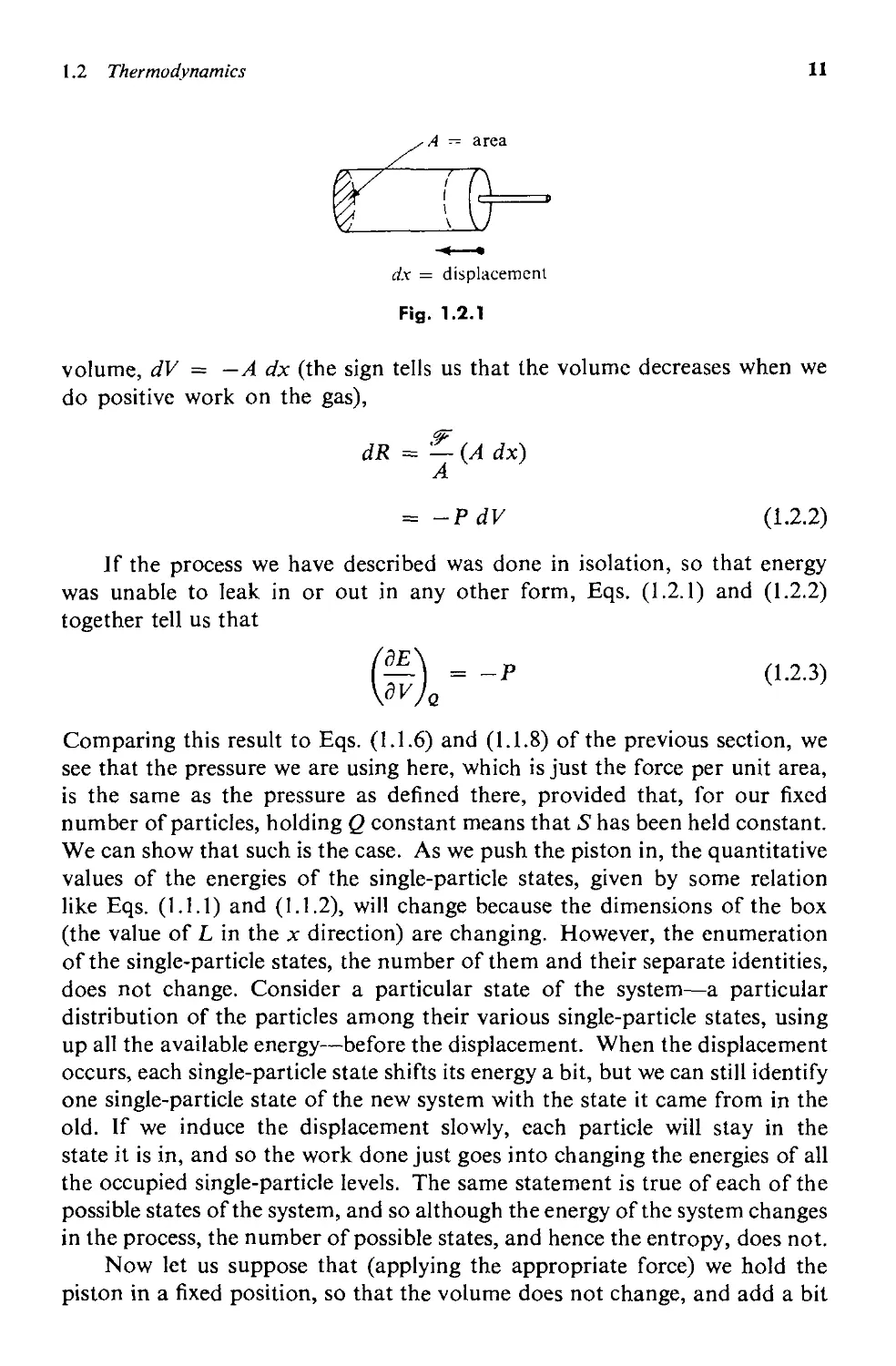
We can easily relate Eq. (1.2.1) to Eq. (1.1.6). Suppose that our box of
perfect gas wcrc actually a cylinder with a movable piston of cross-sectional
area A as in Fig. 1.2.1. It requires work to push the piston. If we apply a
force ff and displace the piston an amount dx, we are doing an amount of
mechanical work on the gas inside given by
dR = .'F dx
This can just as well be writtcn in tcrms of the pressurc, P = ffjA, and
1.2 Thermodynamics
11
/A = ar ea
:: (1=
--
dx = displacement
Fig. 1.2.1
volume, dV = -A dx (the sign tells us that the volumc decreases when we
do positive work on the gas),
.'¥'
dR = -(A dx)
A
= -P dV
( 1.2.2)
If the process we have described was done in isolation, so that energy
was unable to leak in or out in any other form, Eqs. (1.2.1) and (1.2.2)
together teU us that
G ) Q
-p
(1.2.3)
Comparing this result to Eqs. (1.1.6) and (1.1.8) of the previous section, we
see that the pressure we are using here, which is just the force per unit area,
is the same as the pressure as defincd there, provided that, for our fixcd
number of particles, holding Q constant means that S has been held constant.
We can show that such is the case. As we push the piston in, the quantitative
values of the energies of the single-particle states, given by some relation
like Eqs. (1.1.1) and (1.1.2), will change because the dimensions of the box
(the value of L in the x direction) are changing. However, the enumeration
of the single-particle states, the number of them and their separate identities,
does not change. Consider a particular state of the system-a particular
distribution of the particles among their various single-particle states, using
up aU the available energy--before the displacement. When the displacement
occurs, each single-particle state shifts its energy a bit, but we can still identify
one single-particle state of the new system with the state it came from in the
old. If we induce the displacement slowly, each particle will stay in the
state it is in, and so the work done just goes into changing the energies of aU
the occupied single-particle levels. The same statement is true of each of the
possible states of the system, and so although the energy ofthc system changes
in the process, the number of possible states, and hence the entropy, does not.
Now let us suppose that (applying the appropriate force) we hold the
piston in a fixed position, so that the volume does not change, and add a bit
12
ONE THERMODYNAMICS AND STATISTICAL MECHANICS
of energy to the gas by other means (we can imagine causing it to absorb
some light from an external source). No work (of the fJ' dx type) has been
done, and, furthermore, the single-particle states are not affected. But the
amount of energy available to be divided among the particles has increased,
the number of ways of dividing it has increased as well, and thus the entropy
has increased. From Eqs. (1.2.1) of this section with dR = 0, and (1.1.6)
and (1.1.7) of the previous section, we see that
dE)R = dQ = dE)N.V = T dS
(1.2.4)
for changes that take place in equilibrium, so that (1.1.6) is applicable.
Thus, for a fixed number of particles, we can write the first law for equilibrium
changes in the form
dE= TdS-PdV
(1.2.5)
Although changes in heat are always equal to T dS, there are kinds of
work other than P dV: magnetic work, electric work, and so on. However,
it will be convenient for us to develop the consequences of thermodynamics
for this kind of work-that is, for mechanical work alone-and return to
generalize our results later in this chapter.
According to the celebrated Second Law of thermodynamics, the entropy
of a system out of equilibrium will tend to increase. This statement means
that when a system is not in equilibrium, its number of choices is restricted-
some states not forbidden by the design of the system are nevertheless un-
available due to its past history. As time goes on, more and more of these
states gradually become available, and once a state becomes available to the
random fluctuations of a system, it never again gets cut off; it always remains
a part of the system's repertory. Systems thus tend to evolve in certain
directions, never returning to earlier conditions. This tendency of events to
progress in an irreversible way was pointed out by an eleventh-century
Persian mathematician, Omar Khayyam (translated by Edward Fitzgerald):
The Moving Finger writes; and, having writ,
Moves on: nor all thy Piety nor Wit
Shall lure it back to cancel half a line,
Nor all thy Tears Wash out a Word of it.
There have been many other statements of the Second Law, all of them less
elegant.
If disequilibrium means that the entropy tends to increase, equilibrium
must correspond to a maximum in the entropy-the point at which it no
longer can increase. We saw this in the example we considered in the previous
section. If the two boxes, initially separate, had been out of equilibrium,
one of them (the hotter one) would have started with more than its fair share
of the energy of the combined system. Owing to this accident of history, the
1.2 Thermodynamics
13
number of states available to the combined system would have been smaller
than if the cooler box had a fairer portion of the total energy to share out
among its particles. The imbalance is redressed irreversibly when contact
is made. In principle, a fluctuation could occur in which the initially cooler
box had even less energy than it started with, but such a fluctuation is so
utterly unlikely that there is no need to incorporate the possibility of it into
our description of how things work in the real world. Quite the opposite,
in fact: we have dramatic success in describing the real world if we assume
that such fluctuations are impossible. That is just what the entropy principle
does.
The Third and final Law states that at the absolute zero of temperature,
the entropy of any body is zero. In this form it is often called Nernst's
theorem. An alternative formulation is that a body cannot be brought to
absolute zero temperature by any series of operations. In this form the law
basically means that all bodies have the same entropy at zero degrees. Ac-
cording to the earlier statement, if a body had no disposable energy, so that
its temperature were zero, it would have only one possible state: r = 1 and
thus S = k log r = O. This amounts to asserting that the quantum ground
state of any system is non degenerate. Although there are no unambiguous
counterexamples to this assertion in quantum mechanics, there is no formal
proof either. In any case, there may be philosophical differences, but there
are no practical differences between the two ways of stating the law. Among
other things, the Third Law informs us that thermodynamic arguments
should always be restricted to nonzero temperatures.
b. Thermodynamic Quantities
As we see in Eq. (1.2.5), the energy of a system at equilibrium with
a fixed number of particles may be developed in terms offour variables, which
come in pairs, T and S, P and V. Pairs that go together to form energy
terms are said to be thermodynamically conjugate to each other. Of the four,
two, S and V, depend directly on the size of the system and are said to be
extensive variables. The others, T and P, are quite independent of the size
(if a body of water is said to have a temperature of 300 o K, that tells us nothing
about whether it is a teaspoonful or an ocean) and these are called intensive
variables.
We argued in Sec. 1.1 that if we know the energy as a function of Sand
V, then we can deduce everything there is to know, thermodynamically
speaking, about the body in question: P = -(aEjaV)s, T = (aEjaS)v, and
T(V, S), together with P(V, S), gives us T(P, V); if we want the entropy,
T(V, S) can be inverted to give S(T, V) and so on. If, on the other hand,
we know the energy as a function, say of T and V, we generally do not have
all the necessary information. There may, for example, be no way to find the
entropy. For this reason, we shall call S and V the proper independent
14
ONE THERMODYNAMICS AND STATISTICAL MECHANICS
variables of the energy: given in terms of these variables the energy tells the
whole story.
Unfortunately, problems seldom arise in such a way as to make it easy
for us to find the functional form, E(S, V). We usuaIly have at hand those
quantities that are easy to measure, T, P, V, rather than Sand E. It wiIl,
therefore, turn out to be convenient to have at our disposal energylike func-
tions whose proper independent variables are more convenient. In fact, there
are four possible sets of two variables each, one being either S or T and the
other either P or V, and we shaIl define energy functions for each possible set.
The special advantages of each one in particular kinds of problems will show
up as we go along.
We define F, the free energy (or Helmholz free energy), by
F = E - TS (1.2.6)
Together with (1.2.5), this gives
dF= - S dT - P dV (1.2.7)
so that S= - G ) v (1.2.8)
and P= - G ) T (1.2.9)
In other words, F = F(T, V) in terms of its proper variables, and T and V
are obviously a convenient set to use. F also has the nice property that, for
any changes that take place at constant temperature,
bFh = -PbVh = bR
(1.2.10)
so that changes in the free energy are just equal to the work done on the
system. RecaIl for comparison that
bE)s = -P bV>S = bR
(1.2.11)
the work done is equal to the change in energy only if the entropy is held
constant or, as we argued in Sec. 1.2a, if the work is done slowly with the
system isolated. It is usuaIly easier to do work on a system weIl connccted
to a large temperature bath, so that Eq. (1.2.10) applies, than to do work on
a perfectly isolated system, as required by Eq. (1.2. I I).
The function F(T, V) is so useful, in fact, that we seem to have gotten
something for almost nothing by means of the simple transformation, Eq.
(1.2.6). However, we have a fairly clear conceptual picture of what is meant
by E(S, V) in terms of the counting of states, whereas the connection between
the enumeration of the states of a system and F(T, V) is much less obvious.
Our job in Sec. 1.3 will be to develop ways of computing F(T, V) from the
1.2 Thermodynamics
15
states of a system, so that we can take advantage of this very convenient
function.
The Gibbs potential (or Gibbs free energy), <1>, is defined by
<I> = F + PV = E - TS + PV
which, combined with Eq. (1.2.7) or (1.2.5), gives
d<l> = - S dT + V dP
(1.2.12)
(1.2.13)
It foIlows that
S = _ ( 0<1»
aT p
v = ( a<l»
ap T
(1.2.14)
(1.2.15)
and, consequently, <I> = <I>(T, P) in terms of its proper variables. <I> will be
the most convenient function for problems in which the size of the system is
of no importance. For example, the conditions under which two different
phases of the same material, say liquid and gas, can coexist in equilibrium
will depend not on how much of the material is present but rather on the
intensive variables P and T.
A function of the last remaining pair of variables, Sand P, may be
constructed by
W = <I> + TS = E + PV (1.2.16)
so that dW = T dS + V dP (1.2.17)
T = CW ) (1.2.18)
as p
v = CW ) (1.2.19)
ap s
W is called the enthalpy or heat function. Its principal utility arises from
the fact that, for a process that takes place at constant pressure,
dW)p = T dS)p = dQ
(1.2.20)
which is why it is called the heat function.
A fundamental physical fact underlies all these formal manipulations.
The fact is that for any system of a fixed number of particles, everything is
determined in principle if only we know any two variables that are not
conjugate to each other and also know- that -the system is in equilibrium.
In other words, such a system in equilibrium really has only two independent
variables-at a given entropy and pressure, for example, it .has no choice
16
ONE THERMODYNAMICS AND STATISTICAL MECHANICS
at all about what volume and temperature to have. So far we have expressed
this fundamental point by defining a series of new energy functions, but the
point can be made without any reference to the energy functions themselves
by considering their cross-derivatives. For example,
G;) v = a ( - G ) Jv = aa v ( - G ) JT = G )T (1.2.21)
Suppose that we have our perfect gas in a cylinder and piston, as in Fig.
1.2.], but we immerse our system in a temperature bath, so that changes take
place at constant T. If we now change the volume by means of the piston, the
entropy will change owing to the changes in the energies of aIJ the single-
particle states. Since energy is allowed to leak into or out of the temperature
bath at the same time, it would seem difficult to figure out just how much the
entropy changes. Equation (1.2.21) tells us how to find out: we need only
make the relatively simple measurement of the change in pressure when the
temperature is changed at constant volume. It is important to realize that
this result is true not only for the perfect gas but also for any system whatso-
ever; it is perfectly general. Conversely, the fact that this relation holds for
some given system tells us nothing at aIJ about the inner workings of that
system.
Three more relations analogous to (1.2.21) are easily generated by taking
cross-derivatives of the other energy functions. They are
G ) s = - ( )v
G:) p = G;) s
(: ) T = - G ) p
(1.2.22)
(1.2.23)
(1.2.24)
Together these four equations are called the Maxwell relations.
A mnemonic device for the definitions and equations we have treated
thus far is given in Appendix A of this chapter.
The machinery developed on these last few pages prepares us to deal
with systems of fixed numbers of particles, upon which work may be done
only by changing the volume-more precisely, for systems whose energy is a
function of entropy and volume only. Let us now see how to generalize this
picture.
If the nUl}1ber of particles of the system is free to vary, then, in addition
to work and heat, the energy will depend on that number as well. We have
already seen, in Eqs. (1.1.6) and (1.1.9), that in this case,
dE = T dS - P dV + J1 dN
(1.2.2 )
1.2 Thermodynamics
17
J1 is the chemical potential, which we may take to be defined by Eq. (1.2.25),
so that
J1 = G ) S'V
(1.2.26)
If we now retain all the transformations among the energy functions as we
have defined them, then
Similarly,
dF = d(E - TS) = -S dT - P dV + J1 dN
dlf> = - S dT + V dP + J1 dN
dW = T dS + V dP + J1 dN
(1.2.27)
(1.2.28)
(1.2.29)
( OF ) ( alf» ( OW )
J1 = aN T,V = aN P,T = oN P,S
In other words, the effect of adding particles is to change anyone of the energy
functions by J1 dN if the particles were added holding its own proper in-
dependent variables fixed:
Thus,
J1 bN = (bE>s,v = (bFh,v = (blf>h.p = (bWh,p
(1.2.30)
(1.2.31 )
Notice that the first member of Eq. (1.2.31) is not necessarily relevant. If
we manage to change the energy at constant S and V (so that E depends on
something besides S and V) and we retain the transformations, Eqs. (1.2.6),
(1.2.12), and (1.2.16), then the other functions will change according to
(bE>s,v = (bFh.v = (blf>h,p = (bW)s.p
(1.2.32)
We shall make use of this result later on (to have an application to think
about now, you might consider changing the masses of the particles of a
perfect gas; see Prob. 1.2).
The introduction of J1 and changes in N thus serve as an example of how
to generalize to cases where the energy can depend on something besides
S and V, but we wish to retain the transformations between E, F, If>, and W.
However, the chemical potential is a particularly important function in
thermodynamics, and its properties deserve further elaboration.
Like P and T, J1 is an intensive variable, independent of the size of
the system (this point can be seen from the result ofProb. 1.1a, where we see
that two subsystems in equilibrium must have the same J1 regardless of their
sizes), and it is conjugate to an extensive variable, N. Suppose that we think
of Eq. (1.2.25) as applying to a piece of matter, and we rewrite it to apply
to another piece that differs from the first only in that it is A times bigger. It
18
ONE THERMODYNAMICS AND STATISTICAL MECHANICS
could have been made by putting together }, of the small pieces. Then all
the extensive quantities, E, S, V, and N, will simply be), times bigger:
d(}.E) = T d(;.S) - P d(}Y) + /l d(}.N)
or
). dE + Ed), = ;.(T dS - P dV + /l dN) + (TS - PV + /IN) d)' (1.2.33)
Since I. is arbitrary, it follows that
E = TS - PV + /IN
If we differentiate this result and subtract Eq. (1.2.25), we get
S V
d/l = - - dT + - dP
N N
(1.2.34)
(1.2.35)
so that /l, like <1>, is a proper function of T and P. In fact, comparing Eq.
(1.2.34) to (1.2.12) (which, remember, is still valid), we have
<1>(P, T) = /IN
(1.2.36)
As we have seen, the general conditions for a system to be in equilibrium
will be that T, P, and /l be uniform everywhere.
Equation (1.2.31) tells us that /l is the change in each of the energy
functions when one particle is added in equilibrium. That observation might
make it seem plausible that /l would be a positive quantity, but it turns out
instead that /l is often negative. Why this is so can be seen by studying Eq.
(1.2.26). To find /l, we ask: How much energy must we add to a system if
we are to add one particle while keeping the entropy and volume constant?
Suppose that we add a particle with no epergy to the system, holding the
volume fixed, and wait for it to come to equilibrium. The system now has
the same energy it had before, but one extra particle, giving it more ways
in which to divide that energy. The entropy has thus increased. In order
to bring the entropy back to its previous value, we must extract energy.
The chemical potential-that is, the change in energy at constant S and V-
is therefore negative. This argument breaks down if it is impossible to add a
particle at zero energy, owing to interactions between the particles; the
chemical potential will be positive when the average interaction is sufficiently
repulsive, and energy is required to add a particle. It will be negative, for
example, for low-density gases and for any solid or liquid in equilibrium
with (at the same chemical potential as) its own low density vapor.
Now that we have a new set of conjugate variables, it is possible to
define new transformations to new energy functions. For example, the
quantity E - /IN would be a proper function of the variables S, V, and /l,
and W - /IN of S, P, and /l. We do not get a new function from <1> - /IN,
which is just equal to zero: P, T, and /l are not independent variables. Of
t.2 Thermodynamics
19
the possible definitions, one wilI turn out to be most useful. We define the
Landau potential, il,
il=F-/lN
(1.2.37)
so that
dil = - S dT - P dV - N d/l
(1.2.38)
that is, the proper variables ofil are T, V, and /l. Notice that it follows from
Eqs. (1.2.37) and (1.2.34) that
il = -PV
(1.2.39)
Furthermore, since we have not altered the relations between the other energy
functions in defining il, arguments just like those leading to Eq. (1.2.32) will
yield
(bilh.v,/l = (bEh.v,N = (bFh,v.N = (b<I>h,p.N = (bW>s,P.N (1.2.40)
c. Magnetic Variables in Thermodynamics
The total energy content of a magnetic field is
E =..!.. f B2 dV
m 8n
(1.2.41)
where B is the fundamental magnetic field, produced by all currents, and the
integral extends over all space. In order to introduce magnetic work into
our equilibrium thermodynamic functions, we need to know how much
work is done on a sample when magnetic fields change-that is, the magnetic
analog of (-P dV). Equation (1.2.41) fails to tell us this for two reasons.
First, it does not sort out contributions from the sample and from external
sources; B is the total field. Second, there is no way to tell from Eq. (1.2.41)
how much work was done in producing B; the work may have been much
more than Em with the excess dissipated in heat. Only if all changes took
place in equilibrium will Em be equal to the work done in creating the field.
In other words, Em is the minimum work (by sample and external sources
together) needed to produce the distribution of fields in space.
Even assuming that alI changes take place in equilibrium, we must have
a way of distinguishing work done on the sample from other contributions-
that is, work done on an external source during the same changes. To do so,
we decompose B into two contributions
B = H + 4nM
(1.2.42)
where H is the field due to currents running in external sources and M is the
response of the sample, called the magnetization.
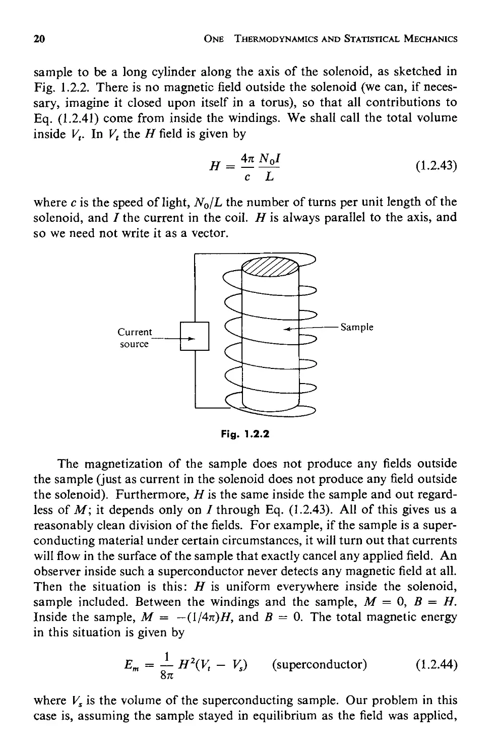
To keep things simple, let us set up a definite geometry, which we shalI
always try to return to when analyzing magnetic problems. We shalI imagine
H to be a uniform field arising from current in a long solenoid and our
20
ONE THERMODYNAMICS AND STATISTICAL MECHANICS
sample to be a long cylinder along the axis of the solenoid, as sketched in
Fig. 1.2.2. There is no magnetic field outside the solenoid (we can, if neces-
sary, imagine it closed upon itself in a torus), so that all contributions to
Eq. (1.2.41) come from inside the windings. We shall call the total volume
inside V" In V, the H field is given by
H = 4n N 0 1
c L
( 1.2.43)
where c is the speed of light, NolL the number of turns per unit length of the
solenoid, and I the current in the coil. H is always parallel to the axis, and
so we need not write it as a vector.
Current
so U fee
-Sample
Fig. 1.2.2
The magnetization of the sample does not produce any fields outside
the sample (just as current in the solenoid does not produce any field outside
the solenoid). Furthermore, H is the same inside the sample and out regard-
less of M; it depends only on I through Eq. (1.2.43). All of this gives us a
reasonably clean division of the fields. For example, if the sample is a super-
conducting material under certain circumstances, it will turn out that currents
will flow in the surface of the sample that exactly cancel any applied field. An
observer inside such a superconductor never detects any magnetic field at all.
Then the situation is this: H is uniform everywhere inside the solenoid,
sample included. Between the windings and the sample, M = 0, B = H.
Inside the sample, M = -(1/4n)H, and B = O. The total magnetic energy
in this situation is given by
E = H 2 ( V - V )
m 8n t s
(superconductor)
(1.2.44)
where V s is the volume of the superconducting sample. Our problem in this
case is, assuming the sample stayed in equilibrium as the field was applied,
1.2 Thermodynamics
21
so that Em is the work done, how much of this work was done by (or on)
the current source in Fig. 1.2.2, and how much on (or by) the sample?
In Sec. 1.2a we found how much work was done if a thermally isolated
sample changed its volume under a constant applied force. The analogy here
is to see how much work is done if a thermally isolated sample changes its
magnetic state under a constant applied H field. Suppose that with constant
current, 1, in the solenoid, there is a small uniform change, oM, in the
magnetization of the sample. The result is a change in the flux, CPo, linked
by the solenoid, inducing a voltage V o across it. Power, IV o , is extracted
from the current source or injected into it. If Ro is the work done on the
current source,
oRo = f IV o dt = 1 f V o dt
since I is constant. The voltage is given by Faraday's law of electromagnetic
induction:
(I .2.45)
V o = _ acpo
c at
(1.2.46)
Then
oRo =
- ! f acpo dt
c at
- f dcpo =
I
- - ocpo
c
(1.2.47)
The sign convention is: if flux is expelled, work is done on the source; that
is, if i5cpo is negative, oRo is positive. The flux is given by
CPo = No f B dA (1.2.48)
where the integral is taken over a cross-sectional area of the solenoid. The
change in M produces a change in B only inside the sample, so that
ocpo = NoAs(oB)s = 4:rrNoAs (jM
where As is the cross-sectional area of the sample. Then
( 1.2.49)
oRo = - 4:rrIN o A.. oM
c
(1.2.50)
Substituting 4:rrN o Jlc = HL from Eq. (1.2.43) gives
oRo = -H(LA s ) oM
(1.2.51)
But LAs is just V" the volume of the sample, so
oRo = - VsH oM
(1.2.52)
22
ONE THERMODYNAMICS AND STATISTICAL MECHANICS
Magnetization in the same direction as H extracts work from the source,
lowering Ro; M opposing If (as in the superconductor) does work on the
source, increasing Ro.
Now, since the sample is isolated thermally, the only kind of energy ever
exchanged is work, and conservation of energy then requires
oR + oRo = 0 in equilibrium
(1.2.53)
where oR is the work done on the sample. Equations (1.2.52) and (1.2.53)
then give
DR = VsHDM
(1.2.54)
If the volume V s had changed at constant M, that, too, would have changed
the linked flux, thereby doing work on the source. It is easy to see that a
more general way of writing the work is
oR = H 0 f M dV
(I :2.55)
and the First Law of Thermodynamics may be written
dE = 1'd5 + H d f M dV
(1.2.56)
For the simplest case, a uniformly magnetized sample,
dE = T d5 + H dMV
E = £(S, MV)
( 1.2. 57)
(1.2.58)
With this as a starting point, E as a unique function of S, and MV in equilib-
rium, we can define magnetic analogs of all the energy functions; we write
the following:
so
F = E - 1'5
dF= -Sd1'+HdMV
(1.2.59)
( 1.2.60)
In this way F retains its central property: for changes at constant T, F is
the work done. Its proper variables are
F = F(1', MV)
(1.2.61)
We now redefine <1>;
<I> = F - HMV
d<l> = - 5 d1' - MV dH
<I> = <1>(1', H)
(1.2.62)
(1.2.63)
(1.2.64)
1.2 Thermodynamics
23
The volume integrals may easily be replaced in transforms like Eq. (1.2.62)
and, of course, in
W = <I> + TS = E - HMV
dW = T dS - MV dH
W = W(S, H)
(1.2.65)
(1.2.66)
(1.2.67)
In all of this, H behaves the way that the pressure did before; both may usually
be thought of as uniform external "forces" to which the system must respond;
its response is to change either its volume or its magnetization. There is a
difference in sign due to a geometrical accident: the work done on a body is
proportional to -dV (you squeeze it to do work on it) but to + dMV. The
reader can easily write down the Maxwell relations and revise the mnemonic
(Appendix A) for this kind of work.
d. Variational Principles in Thermodynamics
Fundamentally there is only one variational principle in thermo-
dynamics. According to the Second Law, an isolated body in equilibrium
has the maximum entropy that physical circumstances will allow. However,
given in this form, it is often inconvenient to usc. We can find the equilib-
rium conditions for an isolated body by maximizing its entropy, but often
we are more interested in knowing the equilibrium condition of a body
immersed in a temperature bath. What do we do thcn? We can answer the
question by taking the body we are interested in, together with the temper-
ature bath and an external work source, to be a closed system. The external
source does work to change the macroscopic state of the body. If more work
is done than necessary-that is, if the body is out of equilibrium-the excess
work can be dumped into the temperature bath as heat, thus increasing its
entropy. We ensure that this step happens by requiring that the entropy
of the combined system increase as much as it can. What is left. over tells
us the equilibrium conditions on the body itself.
Let us make the argument in detail for magnetic variables, using the
formalism and geometry we have already set up (the analogous argument for
P- V variables is found in Landau and Lifshitz, Statistical Physics, pp. 57-59;
see bibliography at end of chapter). We now imagine that the region between
the solenoid and the sample is filled with some nonmagnetic material (M = 0
always), which, however, is capable of absorbing heat and is large enough to
do so at constant temperature. This is the temperature bath; we shall also
refer to it as the medium. It is always to be thought of as being in internal
equilibrium. That means that its energy E' and its entropy S' are connected by
dE' = T dS'
(1.2.68)
There are no other contributions, since no magnetic work can be done on it.
24
ONE THERMODYNAMICS AND STATISTICAL MECHANICS
We imagine the work source to be thermally isolated from the sample and
medium, so that no heat can gct in or out of it, and its changes in energy are
simply oRo. By the arguments that led to Eq. (1.2.52),
oRo + H o(MV s ) = 0
( 1.2.69)
if M is uniform in V s . Equation (1.2.69) does not imply that the sample is in
equilibrium, for it can still exchange heat with the medium. The combined
system-sample, medium, and work source-is isolated, and thus its total
energy is conserved:
o(E + E' + Ro) = 0
(1.2.70)
where E is the energy of the sample. Notice that E cannot be written as a
function of S, the entropy of the sample, and M, since it is a unique function
of those variables only in equilibrium. However, even with the sample not in
equilibrium, we can put Eqs. (1.2.68) and (1.2.69) into (1.2.70) to get
oE + T oS' - H o(MV s ) = 0
(1.2.71)
We now apply the entropy principle to the system as a whole: in whatever
changes take place,
oS + oS' 0
(1.2.72)
Substituting into (1.2.71) and rearranging, we obtain
DE:O;; ToS + H o(MV s )
(1.2.73)
If thc sample is in equilibrium, the equality holds and (1.2.73) reduces to
(1.2.57). What we have accomplished in (1.2.73) is an expression, in the form
of an inequality, for changes in the sample variables, valid even when the
sample is out of equilibrium and connected to a bath.
Suppose that changes take place at fixed T and fixed MV s . The constant
T may be taken inside the 0 sign, and c3(MV s ) = O. We have then
o( E - TS) :0;; 0
(const. T, MV s )
(1.2.74)
E - TS is the free energy. As random fluctuations occur, F will decrcase or
remain constant with time,
aF < 0
al -
(1.2.75)
When F reaches the lowest value it can possibly have, no further changes in
it can take place; under the given conditions, equilibrium has been rcached.
The equilibrium condition is
F = minimum
The constraint we have applied-that MV s be constant-really mcans, through
Eq. (1.2.69), that Ro is constant; we are considering changes in which the
1.2 Thermodynamics
25
sample does no external work. Th.e fact that we considered magnetic work
here is clearly irrelevant; we could have written oR everywherc for H oMy".
The general principle (including -P OV and other kinds of work) is as
follows: With respect to variations at constant temperature, and which do
no work, a body is in equilibrium when its free energy, F = E - TS, is a
minimum.
We can, if we wish, keep H constant and allow MV s to change. The
constant H then comes into the 0 sign, and the quantity to be minimized is
E - TS - HMV s = <I>
(T, H constant)
(1.2.76)
The analogous result for P- V work is, when T and P are held constant, to
minimize
E - TS + PV = <I>
(1.2.77)
Notice that thc transformation from F to <I> simply subtracts the work done
on the external source, (j(HMV s )' If no work is done, we minimize F; if work
is done, we subtract it off and minimize what is left; it amounts to the same
thing.
Without further ado, we can write the thermodynamic variational prin-
ciple in a very general way: for changes that take place in any body,
bE :::; T oS + H 0 f M dV - P oV + p. i5N + ...
(1.2.78)
where we have left room at the end for any other work terms that may be
involved in a given problem. In Eq. (1.2.78) the intensive variables, T, P, Ii,
and p., are those of the medium, while the extensive variables, E, V, S M dV,
and N, are those of the subsystem of interest. The appropriate variational
principle for any situation can easily be generated by applying the kind of
arguments we have just given to Eq. (1.2.78). For example, in a nonmagnctic
problem (H = M = 0), if V is fixed but N varies at constant T and /I,
n = F - p.N = minimum
e. Examples of the Use of Variational Principles
We can now apply our variational principles to a few examples to
see how they work (needless to say, thcse are not just examples; the results
we get will bc useful later on).
First, consider thc magnetic behavior of a perfect conductor. A perfect
conductor is a metal whose electrical resistance is zcro. If a magnetic field
is applied to it, currents are induced that, by Lenz's Jaw, oppose the applied
field and prevent it from penctrating. Since there is no resistance, thesc
currents pcrsist. and wc always have, inside, B = 0, or M = -(lj4n)Ii,
just as in a superconductor. However, unlike the superconductor, M =
26
ONE THERMODYNAMICS AND STATISTICAL MECHANICS
-(l/4n)H is, in this case, a dynamical result, not necessarily the tht;rmo-
dynamic equilibrium state. In order to apply thermodynamics, we' must
make an assumption very similar to the one that was needed to apply thermo-
dynamics to the perfect gas: even though there is no resistance, we assume
that the current, and hence the magnetization, of the sample fluctuates
about, seeking its most favorable level.
At a given Tand H we seek the equilibrium magnetization, which we may
as well take to be uniform over the fixed volume V s of the sample. From Eq.
(1.2.78) the quantity to be minimized is
<1> = E - TS - HMV s
(I .2.79)
or, in other words,
(::)T.1l - 0
In equilibrium, <1> does not depend on M, only on T and H. To solve the prob-
lem, we must construct the quantity <1> = E - TS - HMV s when the
body is not restricted to equilibrium and then use Eq. (1.2.80) to find the
equilibrium dependence of M on T and H. To do so, we take the energy
of the sample to be
(1.2.80)
E = Eo + Em
(1.2.81)
where Eo is whatever internal energy the sample has that is not associated
with magnetic fields:
dEo = T dS - P dV + . . .
(1.2.82)
Since it is irrelevant to our problem, we have taken the nonmagnetic part
of the sample to be in equilibrium. Putting Eqs. (1.2.81) and (1.2.82) into
(1.2.79), we find
<1> = Eo - TS + Em - HMV s
(1.2.83)
Then
There is no heat associated with Em' Eq. (1.2.41), so the sample entropy, S, is
all in Eo. From Eqs. (1.2.41) and (1.2.42),
Em = V s (H + 4nM)2
8n
= V s (:: + HM + 2nM 2 )
<1> = Eo - TS + V s (:: + 2nM 2 )
= Fo + V s (:: + 2nM 2 )
(1.2.84 )
( 1.2.85)
1.2 Thermodynamics
27
Since we are only considering magnetic work, Fa, the nonmagnetic part of the
free energy depends only on T. Therefore,
( 8<1» = 4nV.M = 0
8M H,T
M = 0
(1.2.86)
(Notice that a 2 <1>j8M 2 = 4nV. > 0, so this is really a minimum.) The result
is that, at equilibrium, there is no magnetization. B = H inside; the applied
field penetrates completely. No shielding currents flow in equilibrium.
We could have seen by means of a different kind of argument that M = 0
is necessarily the right result. We know that in a real conductor, with elec-
trical resistance, eddy currents produced by applying a magnetic field quickly
die out, dissipated by the resistance, and the field penetrates unopposed. A
dissipative effect, such as electrical resistance, turns work into heat (called
Joule heating in this case), which is just what is needed to drive a system
toward thermodynamic equilibrium, but it plays no role in the equilibrium
state. Since they differ only in the mechanism for changing states, there can
be no difference between the equilibrium of a perfect conductor and a real
conductor. For a similar reason, the equilibrium of a real gas and a perfect
gas will be the same, provided that the real gas interactions have little effect
on the possible energy levels of each particle.
As we have already said, the equilibrium magnetization of a super-
conductor is
1
M=--H
4n
(1.2.87)
which we now know to be an unfavorable state of affairs; certainly, as we
have just seen, if Eq. (1.2.87) holds in equilibrium, it is not a consequence of
the fact that superconductors have no electrical resistance. As our second
example of an application of the variational principles, let us examine this
situation. If you do not yet know what a superconductor is, relax. Part of the
beauty of thermodynamics is that you do not have to know much about what
is going on inside.
Equation (1.2.87) is the equation of state of what we shall later call a
type I superconductor. For internal reasons of its own (which we shaH
investigate much later), it chooses to go into this unfavorable magnetic
condition, in which surface currents maintain B = 0 inside. The larger the
applied H field, the more unfavorable the situation becomes until, at some
value of H, the effort is no longer worth it and the material ceases to be super-
conducting, turns normal, and lets the field in. The applied field at which this
situation occurs, He, is a definite function of temperature, He = He(T), and
is shown in Fig. 1.2.3. The process that occurs at He(T) is a phase transition.
28
ONE THERMODYNAMICS AND STATISTICAL MECHANICS
H
T
Fig. 1.2.3
At H = He(T), the superconducting phase, whose equation of state is
Eq. (1.2.87), and the normal phase, whose equation of state is M = 0, can
coexist in equilibrium.
Suppose that we think of our sample as a piece of superconducting
material (type I) held at constant T and constant H = He(T). The two
phases can coexist, but, in equilibrium, how much of each is present? Can
we apply our variational principle to find out?
Since T and H are held fixed, it is once again <1> we wish to minimize.
In particular,
8<1> = 0
8V,e
(1.2.88)
where V.e is the volume of the superconducting part of the material, and the
variations are subject to
dV.e + dV n = dV s = 0
(1.2.89)
where V n is the normal portion's volume. We can construct a generalized
<1> of the sample that depends on V,e, using the magnetic energy, Em' and then
put in the' equations of state of the two parts. Proceeding as before, we have
<1> = Fo + f dV(H + 4nM)2 - J HM dV
8n ,ample
(1.2.90)
However, we cannot assume that Fo is the same per unit volume of super-
conductor and normal conductor; after all, we know that something special
is going on inside the superconductor. Let us write the nonmagnetic parts
of the free energy densities of the phases as fo"e and fo,.. Then
<1> = fo"eV,e + fo,nVn + 8 J dV(H + 4nM)2 - J HM dV
H 2
= fO.,e V,e + fo,n V n + s; V s + 2nM 2 V,e
(1.2.91)
1.2 Thermodynamics
29
In the last step we used the fact that M = 0 in the volume V n . We now take
(o<1>joV sc )tI,T, remembering that oVnjoV sc = -J, oV.joV sc = 0, andfa,sc and
fa,n depend only on T,
a<1>
= fa,sc - fa,n + 2nM 2 = 0
av sc
(1.2.92)
Since M = -(1j4n)He, we have
H 2
fa.sc = fa,n - 8;
(1.2.93)
Curiously enough, we did not find out how big V sc is-that remains un-
determined. But we have found out that the nonmagnetic (or zero field)
part of the free energy density of a superconductor is lower than that of a
normal conductor, which is why materials like to be superconductors, and
the difference is related to He at the same temperature. We know nothing
(yet) about the nature of the difference between the superconducting and
normal states, but we do know how to measure the difference in free energy
between the two.
f. Thermodynamic Derivatives
It is convenient to give names to certain derivatives of the thermo-
dynamic quantities. The temperature, pressure, and volume are relatively
easy quantities to measure directly. The entropy is much more difficult and
cannot, in general, be measured directly. However, changes in the entropy
may be measured by putting heat in under specified conditions. In doing so,
we are said to be measuring the heat capacity. The two most commonly en-
countered heat capacities are those at constant volume and at constant
pressure, defined, respectively, by
and
C v = T ( as )
aT v
C p = T ( as )
aT p
(1.2.94)
(1.2.95)
Since many microscopic theories of matter are designed to allow us to count
states and thus arrive at the entropy, as outlined in Sec. 1.1, we often find
that the resulting prediction to be compared to experiment will be the heat
capacity. From the definitions, we may see that
C v = ( aE )
ar v
(1.2.96)
30
ONE THERMODYI'<AMICS AND STATISTICAL MECHAMCS
That is, it is the total change in energy if no work is done. It is also given by
C y =
-T ( a 2 F )
aT 2 y
(1.2.97)
and C p is given by
( 0 2 <1»
C p = -T aT 2 p
(1.2.98)
We have previously considered only the cross second derivatives of the
energy functions, which we did when deriving the Maxwell relations. Aside
from the heat capacities, there are two other direct second derivatives; let
us define the isothermal compressibility,
K T = _.!. ( av )
V ap T
and the adiabatic compressibility,
Ks = 1 ( av )
V ap s
(1.2.99)
(1.2.1 00)
The first is given by
K T = _.!. ( a 2 <1»
V ap2 T
(1.2.101)
and the second by
- [ ( a2E ) J -I
Ks - V -
av 2 s
( 1.2.102)
Of course, there are a number of other ways of constructing these quantities
from second derivatives of the energy functions.
There are definite relations between these quantities. For example, since
a body's thermodynamic variables are fixed if P and Tare fixed (for a given N),
we can write S as a function of P and T: S = S(P, T), or
so that
dS = ( as ) dP + ( as ) dT
ap T aT p
C y ( as ) ( as ) ( ap ) Cp
T = aT y = ap T aT v + T
( 1.2.103)
(1.2.104)
The quantity (as(8Ph is inaccessible to measurement, so we eliminate it by
means of the Maxwell relation, Eq. (1.2.24),
( as ) ( 8V )
ap T = - aT p
1.2 Thermodynamics
31
This gives
C p - C v = ( a V ) ( ap )
T aT p aT v
(1.2.105)
We can put the difference between C p and C v in terms of K I' by use of the
chain rule,
( av ) ( aT ) ( ap ) _ 1
aT p ap v av T
(1.2.106)
This gives us a choice of two relations; eliminating (aV jaT)p or (aPjaT)v,
we get
or
C p - C v = TVK I' [ (:; )J2
C p - C v = [ ( av ) J 2
VK I' aT p
(1.2.1 07)
(1.2.1 08)
For magnetic systems, where P and V are replaced by Hand M, we have
by obvious analogy the quantities C H , C M , and the isothermal and adiabatic
susceptibilities,
( aM )
XI' = aH I'
(1.2.109)
X = ( aM )
s aH s
(1.2.11 0)
You can easily show, by reapplying the same arguments with these variables,
that
C H - C M = TV [ ( aM ) J 2
XI' aT J/
The heat capacities, compressibilities, and susceptibilities are all deriv-
atives of the thermodynamic quantities with respect to their own conjugate
variables and are sometimes collectively called response functions. The heat
capacities and compressibilities are always positive. We can see this by
applying our extremum principle, Eq. (1.2.78). Consider, for example, a
nonmagnetic system of fixed N, and take T and V to be constant, so that the
equilibrium condition is F = minimum. We imagine that the system is all
made of the same stuff, but let it be divided into two parts by a movable
partition, as in Fig. 1.2.4. The partition is free to find its own equilibrium
position, which it does by minimizing F with respect to its position, x.
However, since dx cc dV" we may as well minimize F with respect to V lo
subject to the condition
(1.2.111)
dV, + dV 2 = dV = 0
( 1.2.112)
32
ONE THERMODYNAMICS AND STATISTICAL MECHANICS
Heat bath
at constant T
\'I ova ble partition
Fig. 1.2.4
We have
of = (F I + F 2 ) = aFI + aF 2 = aF I _ aF 2 = 0 (1.2.113)
aV I aV I aV I aV I oV I aV 2
Since these derivatives are taken at constant T and (oFjaVh = - P, we
have just found out that PI = P 2 , a result promised in Sec. 1.1. However,
we know something else: F is not only stationary under variations in VI
[used in Eq. (1.2.113)J, but it is also a minimum. Its second derivative must
be positive:
a 2 F = (PI _ P 2 ) = _ apt _ apz > 0
a a a o
In other words,
1 1
-+->0
V t KTl V 2 K T2
(1.2.114)
But V) and V 2 contain the same substance at the same pressure and temper-
ature. It follows that KT! = K T2 , so that
KI' 0
(1.2.115)
This result is perfectly general: we never did mention what was in the box.
We can show that C v 0 by a closely analogous argument. Consider an
isolated system, so that E and V (instead of T and V) are constant. Then S
will be a maximum. Divide it into two parts so that E) + E 2 = E = con-
stant. Maximize S with respect to E 1 :
= as 1 _ OS2 = _ = 0
aE I aE I iJE 2 TI T 2
(1.2.116)
Notice that we used quite precisely the same argument with slightly different
1.2 Thermodynamics
33
words in Sec. 1.1. Now get the second derivative, which must, in this case,
be negative.
a 2 s a ( 1 ) a ( 1 )
aEi = aE I T 1 Y + aE 2 T 2 Y
_ J.- aT I _ .2.. aT 2
T 1 2 aE I T 2 2 aE 2
1 1
- ----z- - ----z- :s; 0
Tj C y , T 1 C Y2
(1.2.117)
If we choose the two volumes to be equal, we see immediately that
C y 0
(1.2.118)
The case for C p can be made by an additional argument of the same type,
but it is easier to notice that since the right-hand side ofEq. (1.2.108) cannot
be negative,
C p C y
( 1.2.119)
It follows that C p is positive.
We cannot make the same kind of argument for the magnetic suscep-
tibilities, because we cannot apply to the magnetization a condition analogous
to Eq. (1.2.112). In fact, there are indeed cases of materials with both negative
and positive susceptibilities.
Finally, we should note that the two conditions we have just derived,
K T 0 and C y 0, are both eminently reasonable-in fact, really quite
obvious on intuitive physical grounds. First take K T > 0, which means
( iJP ) < 0
av T
(1.2.120)
Imagine a substance in a cylinder and piston with iJPjiJV > 0 instead. In-
creasing the volume by pulling the piston out causes the pressure to increase,
which pushes the piston out farther, causing additional increase in the pres-
sure, and so on. Such a system would be explosively unstable, a condition
incompatible with thermodynamic equilibrium. The other condition, C y > 0,
is simply that
( iJE ) > 0
aT v
(1.2.121)
It merely says, in other words, that warming a body always requires increas-
ing its energy.
34
ONE THERMODYNAMICS AND STATISTICAL MECHANICS
g. Some Applications to Ma"er
Up to now the perfect gas and perfect conductor have been our
principal examples of the workings of thermodynamics. Let us begin here to
discuss some general ideas about real matter in thermodynamic terms.
Figure 1.2.5 is a schematic pressure-temperature phase diagram of a
typical simple substance. The fact that there can be only two independent
variables for any system in equilibrium makes it possible to draw such a
diagram.
p
Critical point
7'
Fig. 1.2.5
In the general region of high pressures and low temperatures, the sub-
stance is a solid; at higher temperatures and lower pressures it is a gas, and
there is a liquid region at intermediate values of P and T. The lines that
separate these phases are called coexistence curves. In particular, that
between the liquid and gas is the vapor pressure curve, between the solid and
gas the sublimation curve, and between the solid and liquid the melting curve.
On these coexistence curves, the phases can exist in equiUbrium 'with each
other, but for any value of P and T that does not fall on one of these curves,
the substance, if it is in equilibrium, must be in a single, specific, homo-
geneous phase. Given a fixed number of particles (say, one mole) it is not
necessary for us to specify the volume (or, equivalently, the density) in order
to determine what phase the substance will be in; it is quite enough to specify
P and T. Furthermore, if we know that two phases are coexisting in equilib-
rium, then either P or T suffices; at any pressure, the temperature is deter-
mined and vice versa. We say, for example, that the vapor pressure is a
function of temperature only. That is why it may be represented as a single
curve in a P-T plane. Usually, but not always, the coexistence curves have
positive slope in the P-Tplane. We shall see the thermodynamic significance
of this point later on. If we cross a coexistence curve from one region to
another, the substance is said to undergo a phase transition.
Two points on the plot are of special interest: the triple point and the
critical point. At the triple point, the intersection of the coexistence curves,
the three phases may all exist in mutual equilibrium. There is only one
1.2 Thermodynamics
35
pressure and one temperature at which this situation can occur. The critical
point is the endpoint of the vapor pressure curve, and it also occurs at a
particular pressure Pc and at a particular temperature Tc. At any temper-
ature higher than Tc> or any pressure higher than Pc> there is no distinction
between liquid and gas; there is only a homogeneous fluid phase and (usually
at very much higher pressure) a solid phase. The existence of a critical point,
in fact, means that therc is no way, in principle, to distinguish unambiguously
between a gas and a liquid unless they happen to be coexisting in equilibrium.
If they are coexisting, there will be a clear interface between regions of different
but uniform density. But a homogeneous liquid can always be transformed
into a homogeneous gas without passing through a phase transition, by
following a path around the critical point. There is no known example of a
critical point on a melting curve, so that, as far as we know, it is always
possible to distinguish between the fluid phases on the one hand and the
solid on the other. Apparently the kind of long-range order that character-
izes the solid statc is like pregnancy: either you have it or you do not; you
cannot have a little bit of it or arrive at it gradually. The properties of
matter at thc gas-liquid critical point and other similar phenomena will be
discussed at length in Chap. 6.
The same phases are shown in different perspcctive in the P- V diagram,
Fig. 1.2.6. Hcre we find the solid at high pressures and low volumes (recall
P \
\
\
\
\
\
\
I
Solid
p
T
.
:...;'"'
'-
'-
,
,
,
,
,
,
,
"
,
"
'-
Gas
---T 2
-- - TI
v
Fig. 1.2.6
that the number of particles is fixed), the gas at low pressure and large
volume, and, again, the liquid in between. In the cross-hatched regions,
more than one phase can coexist. The kind of path followed if we change V
at constant temperature is shown by the dashed curves, for two temperatures
TI and T 2 , also indicated on the P-T diagram in the inset. Curves of constant
temperature are called isotherms. The isotherm at T 1 , which is below Tc>
36
ONE THERMODYNAMICS AND STATISTICAL MECHANICS
passes through all three phases. It must cross the coexistence curve at a
fixed pressure, which means in the P- V plot that V changes from its value
in one phase to its value in the other at constant pressure; that is, the isotherm
becomes horizontal. No horizontal portion is shown on the supercritical
isotherm, at T 2 > Tc, although it presumably has one where it crosses the
melting curve at much higher pressure.
The triple point of the P-T diagram corresponds, on the P-V diagram,
to the single horizontal isotherm that touches all three phases. The critical
point, however, is a point on this diagram as well, occurring at the maximum
of the gas-liquid coexistence curve. There is thus a critical volume, V c , as well
as a critical temperature and pressure. At the critical point, the volumes of a
specific amount of liquid and gas become equal to each other (or, more
simply stated, the liquid and gas densities become equal). At the triple point,
these volumes (or densities) may differ widely. The specific volumes of co-
existing liquids and solids never become equal to each other, but they never
differ by large factors either.
As mentioned above, coexistence curves in the P- T plane are occasionally
found to have negative slopes, even in very common materials. For example,
the melting curve of water slopes backward, as sketched in Fig. 1.2.7. A
p
T
Fig. 1.2.7
coexistence curve with a negative slope is always associated with some sort
of anomalous-that is, unusual-behavior in at least one of the phases. In
the case of water, it happens becausc the liquid is denser than the solid in
equilibrium, although the opposite is true for most substances. We shall
return later to the thermodynamic connection between the densities and the
melting curve.
There is one simple substance, helium, whose phase diagram is strikingly
different from that of anything else (Fig. 1.2.8). Helium never freezes under
its own vapor pressure; it is unique among all substances in that respect.
The phases marked He II and He I that separate the solid from the gas are
two different kinds of liquid, these, in turn, being separated by a further phase
transition (notice thcre are two triple points on the diagram). The phase
1.2 Thermodynamics
37
p
Solid
T
He II
Fig. 1.2.8
diagram would be almost normal topologically if He II were a solid, but
it is not. It is a very special liquid, called the super fluid, to which we shall
return in Chap. 5. The melting curve starts out with zero slope at zero temper-
ature, turns down, and goes through a minimum before finally turning up
as shown. Liquid He I and the gas share a more or less normal critical
point. Like the liquid and gas at the critical point, the specific volumes of
liquid He I and II are equal to each other at the phase transition separating
them.
Some progress in understanding these diagrams can be made by using
the thermodynamic machinery we have developed. Suppose that we have a
sealed container in which two phases, say liquid and gas, of the same material
are coexisting, as in Fig. 1.2.9. Gravity has a weak influence on this problem,
;/ //,/;
%
/ Phase 2
Heat bath
at constant T
Fig. 1.2.9
which we shall neglect except insofar as it makes the denser of the two phases
sink to the bottom of the container. We can think of this as a system at fixed
T, divided into two subsystems, phase 1 and phase 2, which share the same
total volume and can exchange particles. We have already worked out the
conditions for equilibrium for this situation: for example, it differs from the
situation in Fig. 1.2.4 only in that the movable partition is the interface
between the two phases, so we know immediately that the temperatures and
38
O E THERMODYJ-;AMICS AND STATISTICAL MECHANICS
pressures of the two phases must be equal. There is an additional condition,
since particles can be exchanged; we obtained it in Prob. I. I a but let us do
it now by our variational principle. For the t o-p'hase system, Eq. (1.2.78)
tells us that
bF = 0
will be the equilibrium condition. The total number of particles, Nt + N 2 ,
is fixed, but N! (or N 2 ) can vary:
o = aF = (F! + F 2 ) = aFt - aF 2 = Jl, - Jl2 (1.2.122)
aN, aN, aN! aN 2
The third condition is, as anticipated in Sec. I. I, that the chemical potentials
be eq ual.
It is clear from Eq. (J .2.35) or (1.2.36) that Jl = Jl(P, T) quite generally.
We may rewrite Eq. (1.2.122) as
Jl,(P, T) = Jl2(P, T)
(1.2. I 23)
This is a relationship between the temperatures and pressures at which co-
existence can occur: one equation in two unknowns, which may be solved,
say, for the pressure as a function of temperature, Po(T). Equation (1.2.123)
is, in othcr words, the equation of one of the curves in Fig. 1.2.5. If we seek
the conditions for three phases in simultaneous equilibrium, the pressures and
temperatures must, as usual, be the same in all phases, and
JlI (P, T) = Jl2(P, T) = Jl3(P, T)
(1.2.124)
two equations in two unknowns that may be solved for P 3 , T 3 , the unique
pressure and temperature of the triple point.
Chapters 2, 3, and 4 will concern themselves, respectively, with the gas,
solid, and liquid phases of matter. A suitable program for us would be to
work out from microscopic theory the general relation I"(P, T) for each of
the phases in its own chapter and then at the end set them equal pair by pair
and produce Fig. 1.2.5. Unfortunately, we cannot at present (nor perhaps
ever) succeed in such a program. We shall, actually, succeed quite well in
finding J.1(P, T) for the gas, Jess well, under restricted conditions, for the
solid, and poorly indeed for the liquid.
However, the fact that we are not clever enough to write down explicit
relations of the form Eq. (1.2. 123) does not diminish the importance of the
fact that they exist in principle. Because they do, we can learn something
useful about the behavior of matter. Suppose that we change the temperature
of the system in Fig. 1.2.9 by a small amount, dT, and let it come into
equilibrium. The pressure of each phase must change by the same amount,
dP, and each chemical potential will change from its previous (unknown)
value to a new (unknown) value. Since 1", and J.12 must be equal to each
1.2 Thermodynamics
39
othcr both before and after the change, they must both suffer the same
change:
djJl = djJ2
(1.2. I 25)
or, using Eq. (1.2.35),
-SI dT + VI dP = -Sz dT + V z dP
(1.2.126)
where we have written S = S/N and V = V/N; we can call these quanti tics
the molar entropy and molar volume. We solve for the slope of the coexistence
curve,
dPo = S2 - SI
dT V2 - VI
(1.2. I 27)
Equation (1.2.] 27) is known as the Clausius-Clapeyron equation: the slope
of the coexistence curve is given by the ratio of the change in molar entropy
to the change in molar volume as we go from one phase to the other. The
quantity L = T(sz - SI) = T /::"s has the form of a hcat and is called the
latent heat of the transition. The Clausius-Clapeyron equation is some-
times written
dPo
dT
L
T(v z - VI)
( 1.2.128)
Now that we know that the change in s and the change in V are important
quantities, let us return to Fig. 1.2.5 again and imagine what we might
generally expect to happen as we move across the diagram from lower right
(rarified gas) toward the upper left, through the liquid phasc and on into the
compressed solid. Crudely speaking, we are lowering T and so should gener-
ally be moving into regions of lower s, and we are raising P and so should be
causing the density to increase; thus v, like s, should be decreasing. To
repeat: as we cross from gas to liquid to solid, we should, generally speaking,
expect to be crossing into phases of successively lower entropy and lower
volume. Since the changc in entropy and the change in volume will usually
have the same sign, we see from Eq. (1.2.127) that (dPo/dT) should generally
be positive, which accounts for our earlier remark that such is the case.
The exceptions, when the slope of the coexistence curve is not positive,
mean that either s or V is not changing in the expected direction. The most
familiar example is the melting curve of ice (solid H 2 0), which has a negative
slope as we have already seen in Fig. 1.2.8. It occurs because, along the
melting curve, ice is slightly less dense than water (recall that ice cubes float-
just barely-in water). Among the consequences is the fact that it is possi ble
to ice-skate or ski; ice may be melted at constant temperature by compres-
sion, so that skis or ice-skate blades are self-lubricating. If the melting curve
departed from the triple point with positive slope, it would be no more
possible to skate on ice than on glass.
40
ONE THERMODYNAMICS AND STATISflCAL MECHANICS
Another interesting example has already been mentioned. There is a
minimum in the melting curve of helium (Fig. 1.2.8); starting at zero temper-
ature, the slope is zero, negative, zero, then positive again. In this case, it
is the entropy, rather than the density, that behaves anomalously. The zero
slope at zero degrees means that the two phases have the same entropy,
as they must if the Third Law is to be obeyed. The liquid, therefore, is able
to become just as ordered as the solid, a unique circumstance that will bear
further study later. Below the temperature of the minimum, in fact, the
liquid actually has lower entropy than the solid at the same temperature and
pressure, giving rise to the negative slope. At the minimum in the melting
curve, which occurs at about 0.7°K, both phases have the same specific
entropy, and at higher T the solid is the more ordered phase.
In Sec. 1.2e we investigated the conditions for equilibrium between the
normal and superconducting states of a metal. Although the techniques
used seem different from the ones we have applied to the gas-liquid-solid
phase equilibria, the argument could have been carried out in a way that is
strictly analogous to the way we have done it here (see Prob. 1.4). Equation
(1.2.93) relating the super and normal free energy densities plays much the
same role as Eq. (1.2.23) for the chemical potentials, and we may use it to
derive something analogous to the Clausius-Clapeyron equation. We have,
according to Eq. (1.2.93).
H 2
fO.se = fo,. - 8
wherefo,se,fo,., and He are all functions of T only. It follows that
dfo.se = dfo,. _ He dHe
dT dT 411: dT
(1.2.129)
But by definition, for either of the fo's,
dfo 1 ( OF )
dT = V aT H=O
so that Eq. (1.2.129) may be written
(1.2.130)
_ He dHe
Sn - Sse =
411: dT
(1.2.131)
where s. = S./V. and sse = Sse/Vsc- The latent heat of the transitions is
L = T(s. - sse)
(1.2.132)
so the superconducting equivalent of the Clausius-Clapeyron equation is
L = _ THe dHe
411: dT
(1.2.133)
1.3 Statistical Mechanics
41
A transition that has a latent heat is said to be a first-order phase transi-
tion. We may see from Fig. 1.2.3 that dHe/dT is always negative, so L is
always positive. However, it is also found that dHe/dT is always finite, even
in the limit as He -+ 0, so that in that limit, L -+ 0 as well. The transition
is not first order if it occurs in zero field. To find out what happens in that
case, we take the next derivative of Eq. (1.2.131):
( as n ) _ ( aS se ) = _ [ ( dH e ) 2 + H d 2 He ]
aT H=O aT H=O 4n dT e dT2 H=O
= - 4 1 n ( i Y (1.2.134)
Although the entropies are equal, their slopes are not; there is a discontinuity
in the zero-field specific heat;
C H = T ( )
aT H
( 1.2.135)
where C H = CH/Vand
C llse - C Hn = [ iJ: c (1.2.136)
where Te is the transition temperature in zero field. Equation (1.2.136) has
been well verified experimentally. Figure 1.2.10 is a sketch of the heat
capacity of a typical superconductor in zero field, showing the discontinuity
at the transition.
('
H
- c exponential in T
T
Fig. 1.2.10
1.3 STATISTICAL MECHANICS
The job of statistical mechanics is basically to count-or, more
realistically, to find ways to avoid counting-the number of equally probable
ways in which a system may divide up its energy. In principle, one might
imagine writing down all the quantum solutions to the problem, then count-
ing how many there are. For the perfect gas, for example, the procedure
would be to choose a set of single-particle states, each with a definite energy,
each to be occupied by some number of particles. A list would be drawn up
42
ONE THERMODYNAMICS AJ>;D STATISTICAL MECHANICS
of all the ways in which that could be done, using up all the particles and a
fixed total energy. It is the number of such solutions that we are seeking.
If the number of particles, and the energy, are macroscopic quantities, then
the number we seek is so incredibly large that the job we have outlined is
utterly unthinkable. The real job, then, is not literally to count but rather
to interpret numbers. We shall have to find ways of breaking the problem
down into factors that are, in some sense, countable.
The business of interpreting the meaning of numbers is a tricky one.
Even the experts are sometimes fooled. It nevertheless goes on constantly, all
around us, in all phases oflife. An interesting example is the game of baseball.
There is little action in a baseball game. Those who criticit:e basebaIl
on that account, however, do not understand the real nature of the enter-
prise. Most of the time is spent with all the men on the field going through
a carefully prescribed ritual, with absolute, deeply satisfying predictability.
On the other hand, every event occurring that is not perfectly predictable,
every ball, every strike, every hit, every out, is recorded with meticulous and
loving care for the benefit and enlightenment of posterity. The men who
follow baseball professionally become true experts at interpreting the great
mass of statistical data that emerges, masters at drawing the last atom of
meaning out of each fluctuation.
Toward the end of the 197 I season, the San Francisco Giants were play-
ing the Los Angeles Dodgers in a game televised in Los Angeles. In the first
inning, Willie Mays, approaching the end of his ilJustrious carrer, hit a
home run. Home runs in the first inning, one expects intuitively, are some-
what unusual events. The pitcher is fresh and strong, the batter's reflexes
and muscular responses perhaps not yet entirely warmed up, there may be
some mutual feeling out to be done between hitter and pitcher, and, besides,
these explosive heroics are somehow more fitting late in the game. In any
case, Willie hit a home run and that triggered a typical baseball statistician's
response. The datum was produced that, of the 646 home runs Mays had hit,
122 of them had been hit in the first inning: 19 percent! In that most unlikely
one-ninth of the innings, he had hit nearly one-fifth of his many home runs.
That item, for some reason, captured the fancy of the local basebaIl re-
porting community. It was discussed repeatedly during the remainder of the
telecast and received much subsequent publicity in the newspapers. It meant,
in the words of the Giants' publicity director, that". " Willie was always
surprising pitchers in the first inning by going for the long ball before they
were really warmed up." One sees the power of analysis of statistics to draw
out hidden truths about the actions of men.
The datum, undoubtedly, was correct, but the interpretation was quite
wrong. Throughout Mays' career, he had almost always batted third in the
Giants' lineup (occasionally, he batted fourth). That meant that he almost
always batted in the first inning. He averaged about four at bats per game,
1.3 Statistical Mechanics
43
meaning that approximately one-quarter of his at bats came in the first
inning, an inning, you will recall, in which he could only manage to hit one-
fifth of his home runs.
We do not wish to enter here into the reasons for Mays' special diffi-
culties in trying to keep up a respectable production of first-inning home
runs. More interesting is the universal misinterpretation of the meaning of
the datum, by men who spend their professional lives interpreting just that
kind of information. Of the millions of people in Los Angeles and San
Francisco who must have heard or read the item, not one came to the aid
of the befuddled sportswriters to point out their failure. It was simple, really.
In the language we shall find ourselves using later in this section, they had
the levels right but got the density of states all wrong.
Let us, now, return to physics. We shall begin our study of the statis-
tical problem by reformulating it in a way that has two important advantages.
First, it will allow us to deal with systems held at a given temperature rather
than isolated with a given energy. Thus, starting from an enumeration of
the quantum solutions, we shall have ways of writing the free energy in terms
of its proper variables. Second, by turning our attention away from the
isolated system, we shall eventually be able to avoid the difficulties of quantum
uncertainties in the exact energies and numbers of states of systems, brought
up in Sec. 1.1. The results of this reform ulation of the problem constitute
the essence of equilibrium statistical mechanics.
a. Reformulating the Problem
We began this chapter by imagining a body, such as a box of perfect
gas, whose physical description involved specifying its volume V and number
of particles N. Then, for each total energy E, there would be some number of
possible quantum states the body could be in, r. In equilibrium, all these
states would be equally likely, and the system would have entropy 5 = k log r.
Thus, in equilibrium, 5 = 5(£, V, N) or, inverting this, E = £(5, V, N).
Knowing £ as a function of these variables, all other thermodynamic quan-
tities of interest could be deduced. All that was left to do in order to make the
connection between thermodynamics and quantum mechanics was to learn
how to count the number of possible states at a given total energy.
We have already made a great deal of progress using this formulation; all
of our thermodynamic arguments basically followed from just knowing that
it was possible, in principle, to do the counting, without actually doing it.
The counting of the possible states is the job of statistical mechanics.
Given a body to study with a certain V and N, we will generally want
to know its thermodynamic properties not as a function of E but rather as a
function of T, the temperature. What we want, in other words, instead of
£(5, V, N) is F(T, V, N) or n(T, V, p). Of course, if we have £(5, V, N),
we can compute the other quantities, but it will make our work easier if
44
ONE THERMODYNAMICS AND STATISTICAL MECHANICS
wc have a formulation in which F or n is given directly in terms of the
quantum mechanical solutions for the body in question. We shall now work
out such a formulation.
For this purpose, in order to establish a temperature and, if necessary,
a chemical potential, we must imagine, as we have before, that the body or
object of interest to us is embedded in a very large medium, whose T and J.I.
will not be appreciably affected by what the object we are interested in is
doing. We thus imagine the system as a whole, which is isolated, to consist
of a subsystem-the object of our interest-and the medium, which is every-
thing left over.
The system as a whole is subject to the formulation we started with. It
has somc volume Yo, number of particles No, and, being isolated, a total
energy Eo. In equilibrium, it has r 0 possible states, all equaIly likely, and an
entropy So = k log r o. All the variables with subscript zero are properties
of the system as a whole, and all are to be thought of strictly as constants,
independent of whatever happens in the subsystem. If the subsystem is not
in cquilibrium with the medium, the entropy of the combined system wiIl be
less than So; we wiIl caIl it St, so that St So. Similarly, the number of
possible states wiIl be r t r o.
The medium is to be thought of as being always internally in equilibrium.
It has variables N', V', and E', giving r' choices and entropy S'. These
quantities are connected by equilibrium equations; that is,
dE' = TdS' - PdV' + J.I. dN'
(1.3.1 )
but we should keep in mind that E', S', V', and N' all depend on the state
of the subsystem, since the total Eo, Yo, and No are fixed and, of course, S'
depends on E', V', and N'. In other words, if the subsystem is in a state in
which it has much more than its fair share of the energy, the medium, having
less energy than it ought to, has fewer choices of what to do with it and,
consequently, less entropy than it would otherwise have.
For the subsystem (which we have set out to study), we shaIl use un-
adorned variables, E, N, V, r, and S. We can take our subsystem to have a
fixed volume within the medium (the subsystem cannot be defined unless we
fix something). Energy and particles can enter and leave the subsystem as it
fluctuates among its possible states. However, we must put in the restriction
that the subsystem is smaIl so that T and J.I. (of the medium) remain fixed
during these fluctuations. We will use the approximation that, for each
possible quantum state of the subsystem, ex,
Ea « Eo
N a « No
(1.3.2)
Here ex is the index of a single quantum state, in which the subsystem has
1.3 Statistical Mechanics
45
N a particles and energy Ea. Formally, states of the system violating Eq.
(1.3.2) should be allowed, but, for a small subsystem, there are so few of
them that little error is introduced by ignoring them. Since we are making
these restrictions, even though S', E', and N' depend on Ea and N a , they will
change very little, and we are safe in assuming that their derivatives,
aE'jaS' = T and aE'jaN' = J.I., are constant.
Under any specified set of conditions, in which the subsystem has 1
choices and the medium 1', the total system will have
It = If"
and
St = S + s'
(1.3.3)
(1.3.4)
In equilibrium, It = 10' St = So, and the probability of the system as a
whole being in any particular quantum state is
1
W =-
eq 10
(1.3.5)
Every possible state has this same probability. Suppose, however, that in-
stead of imagining the system to be in equilibrium, we specify that the
subsystem is in one particular quantum state, ex. Then the number of choices
of the medium depends on Ea and N a ; let us call 1 the number of choices
of the medium when the subsystem is in the state ex. Since we have specified
the quantum state of the subsystem, it has only one possibility, so that, for
the system as a whole,
Ita = 1 . 1
(1.3.6)
In other words, of the r 0 possible states of the system as a whole, there
are rta = r that find the subsystem in the particular state ex. Since, in
equilibrium, all r 0 states are equally likely, the random probability of the
subsystem finding itself in state ex is just the number of ways that can happen,
r , divided by the number of ways that anything can happen, r 0:
r'
w=-...!
a ro
(1.3.7)
where W a is the probability of finding the subsystem in state ex under equilib-
rium fluctuations. Notice that, unlike w eq of Eq. (1.3.5), W a is most certainly
not the same for all ex. For example, as mentioned above, the more energy
Ea the subsystem has in state ex, the less energy is left for the medium, the
fewer choices 1 it has, and so the less likely is the state ex.
The quantity W a is of central importance in statistical mechanics. For
example, if some quantity f (f might be the energy of the subsystem, say,
46
ONE THERMODYNAMICS AND STATISTICAL MECHANICS
or the number of particles) has some definite value in each state ex, fa, then
the thermodynamic, or average, value of fwilJ be
1 = L w.fa
.
(1.3.8)
subject to the condition that
L w. = 1
(1.3.9)
Equation (1.3.8) simply says that the average value offis obtained by weigh-
ing its value in each state by the probability of the state, whereas Eq. (1.3.9)
requires that the subsystem always be in some state.
If the subsystem is in the state ex, the medium has entropy S;,
S = k log r
where the notation S simply means
(1.3.10)
S; = S'(£o - E., No - N.) (1.3.11)
This follows from Eq. (1.3. I), which tells us that, for a subsystem of constant
volume, S' = S'(E', N'). Since So = k log r 0, we can use Eq. (1.3.10) to
write
r'
So - S = -klog-3. = -klogw. (1.3.12)
ro
where we have used Eq. (1.3.7) in the last step. The quantity So - S is not
the entropy of the subsystem, for we know the subsystem to be in the state ex,
so that it has no choices-its entropy is zero. However, if we average S; over
all states of the subsystem, we do get the equilibrium entropy of the medium,
and the subsystem equilibrium entropy S,
S = So - S = So - S = - k log w.
= L w.( -k log w.)
.
(1.3.13)
Here we have used Eq. (1.3.8) in the last step, regarding the quantity So - S;
to be a property of each state of the subsystem.
From Eq. (1.3.12), before an average is taken, we have
( So - S; ) A ( S; )
w. = exp - k = exp k
where A is a constant, independent of ex but determined by the normalization
condition, Eq. (1.3.9). Using Eq. (1.3. I I), we can write S; as
(1.3.14)
S = S'(E o - E., No - N.)
, ( as' ) ( as' )
= S (Eo, No) - ---; E. - ----; N.
aE V'.N' aN V',E'
(1.3.15)
1.3 Statistical Mechanics
47
We have made use of the approximations, Eq. (1.3.2), in writing Eq. (1.3.15).
Evaluating as'jaE' and as'jaN' from Eq. (1.3. I), we get
E /IN
S' = constant - --5!. + !::.....3.
· T T
where constant = S'(Eo, No) is the entropy that the medium would have if
it had all the energy and particles, and does not depend on ex. Substituting
Eq. (1.3.16) into Eq. (1.3.14) gives
w. = B exp ( _ E. :N. ) (1.3.17)
(1.3.16)
where B is another constant, again subject to the normalization condition,
Eq. (1.3.9):
B= 1
:L. exp [ -(E. - jlN.)jkT]
Equations (1.3. I 7) and (1.3. I 8) allow us to find thermodynamic average
quantities of the subsystem if we have enumerated the quantum states ex,
with E. and N. for each one. For example, the average number of particles
IS
(1.3.18)
N = :L. N. exp [ -(E. - jlN.)jkT]
:L. exp [ -(E. - jlN.)jkT]
(1.3.19)
and the average energy is
E = :L. E. exp [ -(E. - jlN.)jkT]
:L. exp [ -(E. - jlN.)jkT]
However, Eq. (1.3. I 9) formally gives us N(T, V, jl) (where V is implicit in the
enumeration of the Eo's) and Eq. (1.3.20) gives E(T, V, jl). These are not the
proper variables; the proper variables of E are S, V, and N. We can do better
if we make use of Eqs. (1.3.13) and (1.3.17).
S = - k L w. log w.
.
(1.3.20)
or
= '-k log B L w. + ..!.. L w.E. - !:.. L w.N.
. T . T .
-klogB + E - jlN
T
kT log B = E - TS - jlN = F - jlN = n
(1.3.21)
( 1.3.22)
Substituting Eq. (1.3.18) into Eq. (1.3.22), we have
n = -kT log L exp ( _ E. - jlN. )
. kT
(1.3.23)
48
ONE THERMODYNAMICS AND STATISTICAL MECHANICS
Equation (1.3.23) gives us n(T, V, J.I.) for the subsystem, which is just what
we need. If the quantum mechanical solutions, (E., N.), are known, we can
find all the thermodynamic functions.
In the formulation we have just worked out, V, T, and J.I. are held fixed,
while E, N, and S are to be found by averaging over the possible states of the
subsystem in equilibrium [the pressure P is fixed, since, in the medium,
P = P(T, J.I.)]. If we wish instead to deal with a body in which N as well as
T and V are fixed, it is not necessary to start over again. Instead, we simply
specify that
N. = N
for all ex
(1.3.24)
Then Eq. (1.3.23) becomes
n = -kT log exp ( ) exp ( - : )
= -J.l.N - kT log L exp ( _ E. )
. kT
(1.3.25)
or since F = n + J.l.N,
F = -kT log L exp ( _ E. )
. kT
(1.3.26)
Equation (1.3.26) gives us F(T, V) for bodies of a given N. Instead of Eqs.
(1.3.17), (1.3.18), and (1.3.20) we have, respectively,
w. = C exp ( - : )
c = 1
:L. exp (-E./kT)
(1.3.27)
(1.3.28)
E = :L. E. exp (-E./kT)
:L. exp (-E./kT)
(1.3.29)
Depending on whether the number of particles is taken as variable or not,
Eqs. (1.3.17) and (1.3.18) or Eqs. (1.3.27) and (1.3.28) are known as the Gibbs
distribution.
Let us define the quantities
and
Z = L exp ( _ E. )
. kT
If = L exp ( _ E. - J.l.N. )
. kT
(1.3.30)
(1.3.31 )
1.3 Statistical Mechanics
49
Z is called the partition function, and 2 is sometimes called the grand partition
function. In terms of the quantities we have used up to now,
F=-kTlogZ (1.3.32)
and n = - kT log 2 (1.3.33)
or Z _ -F/kT _ 1 (1.3.34)
- e --
C
and 2 = e-D./kT = !.. (1.3.35)
B
We shall make extensive use of the properties of Z and 2.
The arguments we have just given form the core of statistical mechanics.
The basic approach is simple and worth keeping in mind. In equilibrium, all
states of the system are equally likely. However, the states of the subsystem
are not equally likely-the more energy (and particles) the subsystem has,
the fewer are left for the medium, and hence the less likely the state is. This
is the crucial part of the argument; we found the probability of a given
quantum state of thc subsystem as a function of temperature not by watching
what the subsystem was doing but by watching what the medium was doing.
We got the message from the medium.
b. Some Comments
In order to simplify the discussion we wish to make here, let us
consider only bodies of fixed N; the entire derivation of the previous sub-
section is easily reduced to this case.
The results we obtained all depend on finding w., the probability of
finding the subsystcm in the state a. In the state a, the subsystem has energy
E., but a is not, in general, the only state of the subsystem with energy E.;
there will usually be many states with the same energy. In othcr words, the
subsystem, which can be a macroscopic body, will usually have a high degree
of quantum degeneracy-that is, many states at the same cnergy. In fact,
finding the number of states with the same energy in a macroscopic body
was just the counting problem we started out with. Nevertheless, it must be
stressed that w. is the probability that the body is in one single state; it is
not the probability that the body have energy E. but rather the probability
that it be in a particular one of the states that have energy E..
Yet wc found the value of w. by studying the number of choices left to
the medium r and S , and these quantities depend only on E., not on a
itself. How can the medium tell us the probability for a single state when it
does not know what state the body is in? Perhaps we can help clarify this
issue by starting out again but this time seeking w(E.), which we define to be
the probability that the subsystem have energy E. rather than the probability
50
ONE THERMODYNAMICS AND STATISTICAL MECHANICS
that it be in any particular state with this energy. Let us suppose that there
are PE. states of the subsystem that have energy Ea. By our fundamental
postulate, all these states are equally likely when the subsystem has energy
Ea; that is, the probability of any of the others is the same as the probability
of ex, or W a . It follows that
w(E a ) = PE.W a
(1.3.36)
Now, when the subsystem has energy Ea, the medium is left with r . choices,
but as we have already argued,
r' = r'
E« a
(1.3.37)
That is, the entropy of the medium is the same whether we specify that the
subsystem is in state ex or merely that it have energy Ea. On the other hand,
if we specify only the energy of the subsystem, the subsystem itself now has
PE. choices, so for the combined system,
r,E. = PE.r
(1.3.38)
Thus, the probability that the subsystem have energy Ea under equilibrium
fluctuations is
r r'
w(Ea) = = PE. a
ro ro
Comparison of Eqs. (1.3.36) and (1.3.39) confirms that
(1.3.39)
r'
W=
a ro
is actually the probability that the subsystem be in one particular state.
The rest of the derivation of the last subsection now goes through as
before. However, we can use PE. to help give us some insight into how the
averaging over states is actually being done. For example, according to
Eq. (1.3.27), w a is an exponentially decreasing function of Ea; at any finite
temperature, the probability of any state falls monotonically as the energy of
the state goes up. Yet we know perfectly well that the most likely energy of a
body is not its lowest possible energy-,if it were, we would constantly be
finding macroscopic bodies in their ground states. Although the probability
of any particular state, ex, declines with energy, the number of states with a
particular energy, PE., rises rapidly with energy, so that the probability of the
body having a given energy
weE ) = :!.. PE ex p ( - ) (1.3.40 )
a Z. kT
will usually have a very sharp maximum value at Ea = E, the average energy;
just how sharp that maximum is we shall compute a bit later.
1.3 Statistical Mechanics
51
In forming the partition function, Eq. (1.3.30), we sum over all states
of the body. At each energy J:., , there will be PE" equal terms, e-E"/kT. Thus,
instead of summing over states ct., we could sum over energies E.,
z = exp ( - :;) = PE" exp ( - :; )
Most of the contribution to the partition function will thus come from that
same very small range of energies where w(J:., ) is peaked.
For a macroscopic body at finite temperature, the energy levels that are
important in forming w(E.) and Z will be so closely spaced that very little
error is introduced by thinking of E. as a continuous variable. We will use
the notation g for this purpose (reserving E for the equilibrium average
value of the energy). Then the proper language to use (in accordance with the
remarks at the end of Sec. 1.1) is as follows.
The probability of the body having energy between 8 and 8 + d8 is
w(@") d8, normalized by
(1.3.41)
t" w(8) d8 = 1
The number of states in the same range is p(8) d8, where p(8) is called the
density of states. w(8) is given in terms of p(8) by
w(8) = !. p(g)e- G / kT
Z
and Z = IX) p(8)e- G / kT d8
The average value of a quantity f(8) is
J = f oo f(o")w(8) d8 = f oo f(8)p(8)e-G/kT d8
o Z 0
A comment in passing: by means of the approximations, Eq. (1.3.2), the
various sums and integrals are limited to values of 8 or E. that are small
compared to Eo. However, little error is introduced by taking them up to
infinite values of the energy because the exponential, e- G / kT , will always cut
them off; in fact, as we have seen, most of the contributions will come from
a very narrow range about a finite value of the energy.
With the energy written as a continuous variable, the free energy becomes
(1.3.42)
( 1.3.43)
(1.3.44)
( 1.3.45)
F = - kT log foro p(8)e- G / kT d8
and so the entire problem of statistical mechanics has been reduced to finding
the function p(8). (Notice that 8 itself is now just a dummy variable of
( 1.3.46)
52
ONE THERMODYNAMICS AND STATISTICAL MECHANICS
integration.) That might seem to be a significant advance, but actually it is
not. In fact, it is identical to the problem as formulated in Sec. 1.1. We
could then do our thermodynamics if we could count the number of states
ofa body at any given energy. p(lff) is simply the number of states of the body
as a function of energy-we are left with almost the same counting problem
that we had in the beginning.
Before finishing these comments, we would like to pull one more tidbit
out of the arguments of the last subsection. Since, as we have stressed, all
the states of the subsystem that play an important role are concentrated in
a narrow range of the parameter Iff or E«, it should be possible to take ad-
vantage of that fact and develop a formulation that concentrates on these
states. This we shall now do.
Under any given set of circumstances, the entropy of the system as a
whole is given by
S, = k log r, (1.3.47)
According to Eq. (1.3.38), if the subsystem has energy E«, the system entropy
will be
S,(E.) = k log PEX;
(1.3.48)
so that
r'
So - S,(E«) = -k log PEa « = -k log w(E«)
rO
(1.3.49)
In other words,
w(E«) = A exp [ S' «) J
(1.3.50)
where A = e- So / k is the same constant used in Eq. (1.3.14). We may thus
write the probability of the subsystem having E« in terms of the entropy of the
total system when we specify that the subsystem has E«. Equation (1.3.50) is
true not only for the energy but also for any quantity whose value in the sub-
system affects the medium. Thus, if some quantity x is a property of the
subsystem, and we can write
S ' - S ' as' ( - )
- ---x-x
x x ox
(1.3.51)
where x is the average value of x, then the arguments we have given for E«
follow for x as well, and we can write
w(x) = A exp [ S' X)J (1.3.52)
S,(x) will have a sharp
Now, according to the arguments we have given,
maximum at x = x:
( as, ) = 0
ox x=x
( 02 S , ) 0
ox 2 x=x <
( 1.3.53)
1.3 Statistical Mechanics
53
We can therefore expand S, about X,
( ( OS, ) ( _ ) I ( 0 2 s, ) ( _ ) 2
S,(x) = S, x) + - x - x + - ---'2 x - x
ox x=x 2 ox X=x
= S,(x) - tf3(x - X)2 (1.3.54)
where we have used (1.3.53) in the last step; the coefficient f3 is positive.
Substituting Eq. (1.3.54) into (1.3.52), we have
w(x) = D exp [ - f3(x 2 X)]
(1.3.55)
subject to
f [2;k
w(x) dx = 1 = D '<) P
( 1.3.56)
which fixes the constant D. This is a Gaussian form, with most of the con-
tribution to w(x) coming from x X as expected. We shaH return to it later
because it will be useful in calculating the mean probabilities of fluctuations
of various quantities from their equilibrium values. This formulation,
basically Eqs. (1.3.55) and (1.3.56), was the first publication, in 1904, of a
25-year-old patent clerk named Albert Einstein.
c. Some Properties of Z and 2
The quantities Z and 2, once they have been formed from the
microscopic states, contain within them all the thermodynamic information
about the systems to which they refer. From Eqs. (1.3.32) and (1.3.33),
F(T, V, N) and 0(1', V, /l) may be written directly in terms of Z(T, V, N)
and 2(1', V, /l), respectively. Given these, it is easy to write formulas for
any of the other thermodynamic quantities. For example, to form the energy
E from Z, we write
or
E = F + 1'8
of kT OZ
8 = - - = k log Z + --
aT Z aT
kT 2 az
E = - kT log Z + kT log Z + - -
Z 01'
(1.3.57)
E = kT 2 ( OZ )
Z 01' V.N
Equation (1.3.58) gives us E(T, V, N), which are not the proper variables, but
Eq. (1.3.57) gives us 8(1', V, N), so, in principle, l' may be eliminated between
(1.3.58)
54
ONE THERMODYNAMICS AND STATISTICAL MECHANICS
these two equations to give E(8, V, N). As another example, we can find
N from .!I!(T, V, /l):
N = _ an = kT ( a.!l! )
all .!I! all T,V
where N is the average number of particles; recaIl that N is variable in the n
formulation.
Equations (1.3.58) and (1.3.59) do not give us new results in terms of the
microscopic states; they merely confirm the self-consistency of our formulas.
Taking the temperature derivative of Z from Eq. (1.3.30), we obtain
( 1.3.59)
az 1" E ( E. )
aT = kT 2 "7' . exp - kT
which may be substituted into Eq. (1.3.58) to give
(1.3.60)
E = E. exp ( - :; )
(1.3.61 )
This last equation is identical to Eq. (1.3.29). Similarly, taking the /l derivative
of Eq. (1.3.31) gives
a.!l! = "N ex ( _ E. - /IN. )
a kT L.J . P kT
/l .
(1.3.62)
which, upon substitution into Eq. (1.3.59), gives
N 1" N ( E. - /IN. )
= .!I! L.J . exp - kT
.
(1.3.63)
and this teIls us, reasonably enough, that N is the average value of N.. In
other cases, we may get less obvious results. For example,
p = _ aF = kT az = _ " dE. exp ( _ E. )
av z av z "7' dV kT
(1.3.64)
so that the pressure turns out to be the average value of the quantity dE./dV
(you should have found this out for the perfect gas in Prob. 1.1 b). In per-
forming these manipulations, we have made use of the fact that the E. and
N« never depend on quantities like T and /l. They are, instead, definite, non-
statistical properties of individual quantum states.
The partition function Z is called that because of an interesting and uSl:ful
property it has: it partitions under certain circumstances. If the energies E«
are made up of independent contributions, say,
E« = Hi + G j
(1.3.65)
1.3 Statistical Mechanics
55
so that IX is a notation for two sets of quantum numbers, i and j, needed to
specify the state, then Eq. (1.3.30) becomes
" ( H + G. )
Z = L.J exp - ' J
i,j kT
exp ( - :i) exp ( - )
exp ( - ) exp ( - f)
= ZHZG
(1.3.66)
The partition function has become a product of separate partition functions
for the Hand G contributions to the energy. Hand G could be, for example,
kinetic and rotational energies of the body as a whole, or they could be the
energies of two independent parts of which the body is composed. This
property of the partition function is rather analogous to the behavior of the
wave function in quantum mechanics. If the Hamiltonian has independent
contributions in quantum mechanics, the wave function is a product of
corresponding independent factors. The partition function partitions into
independent factors if the energy, which is the expectation value of the
Hamiltonian, can be written as a sum of independent parts.
d. Distinguishable States: Application to the Perfect Gas
In order to apply our equations to the perfect gas, we must some-
how organize the problem by deciding how we are going to sort out and
describe all the possible individual quantum states of the many-particle
system. There are two principal techniques, each of which has certain draw-
backs. We can concentrate either on the particles themselves, giving the
quantum numbers of each particle to describe a state, or we can concentrate
on the single-particle states (i.e., the possible sets of quantum numbers),
giving the number of particles, or populations, of each single-particle state
to describe the state of the many-particle system.
In the first method we are basically considering the particles to be in-
dependent subsystems of the gas, with the state of the gas given by the state
of each of its subsystems. Unfortunately, this procedure leads us to count
each possible state of the gas far too many times, for we wind up counting
separately states that differ only in that some individual particles have
exchanged quantum numbers with each other. Since the particles are
identical, there is, from the point of view of the many-particle system, no
distinction between these states, and they should not be counted separately.
The second method, in which we say only how many particles have each
set of quantum numbers, is not subject to that difficulty. The difference is
56
0]'0;[ THERMODYNAMICS AND STATISTICAL MECHANICS
that in the first method we decide which particles are in each single-particle
state, thus distinguishing between the particles, whereas in the second method
we decide only how many are in each state, not distinguishing between them.
The second method leads unambiguously to a correct enumeration of the
possible quantum states of the many-particle system. The drawback to this
procedure is that it cannot be generalized for application to any problem
other than the perfect gas. The procedure depends on having single-particle
states that are quite independent of what all the particles are doing. In any
interacting system the possible states of each particle depend on the state
of all the other particles (in particular, where they are spatially located) and
thus this kind of enumeration is not possible.
The first method, which is more easily generalized, can be patched up
and made to work under certain circumstances. Suppose that the system has
enough energy per particle so that the number of single-particle states in the
range of energies that will make a contribution to the statistical properties is
very much larger than the number of particles available to occupy them. We
shall investigate the quantitative criteria for this condition in the gas shortly,
but it will generally be the case when the temperature is reasonably high and
the density reasonably low. Under these conditions, each single-particle
state will usually be unoccupied, and its probability of being occupied by
more than one particle at a time is negligibly small. If there are N particles
in the gas, they occupy N different single-particle states. In constructing a
many-body state from the particles, we have N choices of which single-
particle state to put the first particle in, N - I choices of where to put the
second particle, and so on; there are N! ways of constructing that kind of
many-particle state from the N particles. Thus, if we consider all possible
states of N particles individually, we wind up, under these conditions, count-
ing each distinct many-body state N! times. Knowing how many times we
have overcounted the many-particle states, we can easily correct the error.
This argument does not depend on each single-particle state being indepen-
dent of what the other particles are doing. It works equally well for inter-
acting systems. So long as we can ignore the possibility of two or more
particles doing exactly the same thing, N! is still the difference between how
many particles and which particles are doing each thing.
To summarize, then, the situation is this: for the perfect gas at high
temperature and low density, or for most interacting systems of atoms (or
molecules), we can count up all the possible states of the individual particles
separately and then divide by N! to enumerate the many-body states correctly.
We cannot do the same for the perfect gas when the temperature is low or the
density high. However, the perfect gas, under any circumstance, can be
handled by simply specifying the populations of all single-particle states as a
means of describing each distinct many-body state. Broadly speaking, the
N! approach is applicable to matter when it behaves classically, and some
1.3 Statistical Mechanics
57
other method is necessary when quantum effects become important. This
problem of the indistinguishability of identical particles does not arise in the
case of solids, where the particles may not be distinguished but the lattice
sites to which they are attached may be. The most important example in
nature of a system that cannot be handled by either the N! or the populations-
of-states method is liquid helium, which is a quantum fluid. We shall deal
with that problem separately in Chap. 5.
Let us consider the perfect gas in the approximation in which either of
the two methods ought to work. In order to have clear names for our
separate models and approximations, we shall call this special case of the
perfect gas, when the probability of multiple occupation of any single-
particle state is negligible, the ideal gas. We shall later study cases where the
gas is perfect but nonideal.
If we think of one particle of the ideal gas as a subsystem, we have for
the single-particle partition function
Z, = ex p ( - )
where Bq is given by Eqs. (1.1.1) to (1.1.4) and L q denotes a sum over all
possible values of the set of three quantum numbers, t x , t y , and t.. Making
use of Eq. (1.3.66), the many-body partition function will have in it N factors
identical to Z10 but in forming it this way, we will have counted each distinct
state with no multiple occupation N! times. Other distinct states (i.e., the
ground state of the whole system) are counted fewer times, but we expect
them to make little contribution to the thermodynamic properties under the
conditions we wish to investigate [the many-body density of states, PE., in
Eq. (1.3.41) will be so small for these states that we ignore them]. We
therefore approximate the many-body partition function by
(1.3.67)
Z = ...!.... (Z,t
N!
(1.3.68)
so that
F = -NkTlog Z, + kTlog N!
(1.3.69)
The term containing N! will contribute (as it should) to the entropy, S =
-8F/8T, but not to the equation of state,
peT, V) = _ ( 8F ) = NkT 8Z,
8V T Z, 8V
Using Eqs. (1.3.67) and (1.1.1) to (1.1.4), we get
8Z, = _ 1..- L exp ( - ) = 2/3 L B exp ( - )
8V kT q 8V kT VkT q q kT
(1.3.70)
(1.3.71)
58
ONE THERMODYNAMICS AND STATISTICAL MECHANICS
where we have used L = V 1 / 3 in Eq. (1.1.2). Putting Eq. (1.3.71) into
(1.3.70) gives
2N_ 2E
P=--e=--
3V 3V
e = L e q exp ( - )
2 1 q kT
Equation (1.3.72), PV = fE, could be shown earlier from much simpler (and
more general) considerations (see Prob. 1.1 b). In order to obtain the equation
of state, P = P(T, V), we must perform the sums in Eq. (1.3.73) to get
e(T, V). In the notation of continuous variables, Eq. (1.3.73) becomes
(1.3.72)
where
(1.3.73)
e = J ep(e)e-£/kT de
J p(e)e-£/kT de
(1.3.74)
where e is the continuous version of the single-particle energy and p(e) is the
single-particle density of states. We must still perform a sum or integral over
states, but the problem has been greatly simplified, for now we need only
do it for single-particle rather than many-particle states.
In the alternative method we focus our attention on the single-particle
states, rather than on the particles themselves, by choosing a single-particle
state as a subsystem. The number of particles in the state nq must be thought
of as a variable, and the energy of the subsystem is nqe q , where e q is the energy
of a single particle in that state and is independent of nq. Using the variable-
number formalism, we write for the Q of the state q,
( ne -nil )
Qq = - kT log L exp - q q q
slales k T
(1.3.75)
The LSlales is a sum over the states of the subsystem, which is itself a single-
particle state. The only thing that can change is nq itself, so nq is the sum-
mation index:
Qq = -kT log f.= exp [ - nq(e ; Il) ]
(1.3.76)
where nq = 0, 1,2, . . .. This choice of subsystem is no more peculiar than
was the choice of one particle as a subsystem earlier. In assigning thermo-
dynamic average properties to one of these essentially microscopic entities,
we can imagine, for example, that we are averaging over a very long time.
Once we compute Qq by means of Eq. (1.3.76), we can find Q for the system
as a whole from
Q = LQq
q
(1.3.77)
1.3 Statistical Mechanics
59
where L q has the same meaning it has in Eq. (1.3.73); it is a sum over single-
particle states. This formulation avoids the problem of multiple counting of
the same many-particle state. Furthermore, we have not yet made the ideal
gas approximation; Eqs. (1.3.76) and (1.3.77) are generally applicable to the
perfect gas.
Let us now make the ideal gas approximation. For each q, the prob-
ability that nq = 0 is nearly one; the probability that nq = 1 is nearly zero,
that nq = 2 is much smaller still, and so on. The general expression for the
probability of the subsystem being in a particular state comes from Eq.
(1.3. I 7), together with Eq. (1.3.22):
W« = exp [ 0 - ( T- /IN<<) ] (1.3.78)
For the probability of nq in a single-particle state q, this expression reduces to
W = ex p [ Oq - nq(Bq - /l) ]
nq kT
In particular,
Then
W o = exp( ) 1
WI = exp ( ;) exp ( _ B\-; /l )
exp ( _ B\-; /l) « 1
W 2 = exp [ - 2(B ; /l) ] = (wY « WI
(1.3.79)
(1.3.80)
(1.3.81)
(1.3.82)
and so on. From here on we shall retain only leading-order terms in the small
quantity WI = exp [ -(Bq - /l)/kT].
Before going on, let us see under what conditions our approximation is
satisfied. It is clear from Eqs. (1.3.81) and (1.3.82) that the larger Bq is,
the smaller WI' W2, and so on will be, so the approximation will be satisfied
for all the subsystems if it is satisfied for the one with the smallest value
of Bq-namely, the single-particle ground state, Bq = O. For this state, the
condition WI « 1 is just
e,,/kT « I
(1.3.83)
or, in other words, /l/kT must be large and negative. An alternative statement
of the ideal gas approximation, then, is that it is a perfect gas with a large,
negative chemical potential. Recall that we argued earlier that the chemical
potential of a perfect gas is usually negative.
60
ONE THERMODYNAMICS AND STATISTICAL MECHANICS
The average value of nq is obtained, using Eq. (1.3.63), by
n = Lnq nq exp [ -nq(Bq - /1)/kT] = exp ( _ Bq - /1 ) (1.3.84)
q Ln q exp [ -nq(Bq - /1)/kT] kT
where we have kept leading-order terms top and bottom. Doing the same in
Eq. (1.3.76) we have
Qq = -kT log [1 + exp ( - B\; /1) ]
-kT log (1 + n q )
- kT n q
since log (1 + x) = x when x « 1. For the gas as a whole,
(1.3.85)
Q = - PV = - kT L nq
q
(1.3.86)
Q = -kTN
(1.3.87)
where we have used Eqs. (1.2.39) and (1.3.77), and
N = L nq
q
(1.3.88)
which is basicaIly a normalization condition. We have thus discovered that
PV = NkT
which is the equation of state of the ideal gas.
In discussing the N! formulation, starting with Eq. (1.3.70) we attempted
to find the equation of state but failed to do so, lacking as yet the means for
doing the sum over single-particle states, Eq. (1.3.73). Here we set out to find
Q(T, V, /1) and once again failed to do so for the same reason, but we did
stumble across the equation of state without reaIly seeking it. To get
Q(T, V, /1), we must perform the sum over states in Eq. (1.3.88), which will
give us N = N(T, V, /1), to be substituted into Eq. (1.3.87).
Notice how little we have actuaIly had to assume in order to arrive at
PV = NkT. The particles must be noninteracting (so that the Bq'S are in-
dependent of how the particles are distributed) and all the nq's must be small.
We never assumed, for example, that the energies of the particles are related
to their momenta by B = p2/2m. Even particles obeying quite different
dynamics would follow the ideal gas equation of state, provided only that the
temperature is high and the density low (conditions that ensure the validity
of both assumptions we have made).
In the latter half of the nineteenth century it was weIl established that
matter was composed of atoms, and attention turned to the question of the
composition of atoms. A suggestion arose that seems peculiar to us today;
1.3 Statistical Mechanics
61
it was proposed that atoms were vortex rings in the aether. (The aether,
of course, was the medium that transmitted electromagnetic waves, such as
light.)
Vortex rings are very strange beasts. We shall have occasion to return
to them in Chap. 5, since they playa role in the physics of superfluid helium.
The oddity about them is that instead of having their energies and momenta
related by the usual s oc p2, they have s oc pl/2 (we are speaking loosely;
see Chap. 5). That means their velocities are given by
as
v =-
op
oc p-1/2
1
oc-
e
In other words, the more energy a vortex ring has, the slower it goes. How
could such intelligent men-Maxwell, Kelvin, and many others were among
the believers-how could they have supposed that matter was made up of
vortex rings? One of the most convincing elements of that belief was the
known fact that a rarified gas of vortex rings would obey PV = NkT.
The proof given then (in an essay by J. J. Thomson, written in 1879) was
by means of difficult dynamical arguments. We have, in effect, proved the
same thing, since, in deriving our result, we did not assume that atoms are
not vortex rings. But we have also shown the result to be, in effect, trivial.
Any rarified gas will behave that way, no matter how queer the dynamics
of its particles.
e. Doing Sums over States as Integrals
Whatever formulation we use, our problem eventually reduces itself
to a sum over all possible quantum states, either of the sample (giving .fi? or
Z directly) or of some astutely chosen subsystem. It is usually possible to do
the sum as an integral, provided that we know the appropriate density of
states. In fact, as pointed out in Sec. 1.3b, finding the density of states was
just the problem we started out with, arising directly from our assumption
that all states are equally likely in equilibrium. In classical statistics the
assumption of equal probability of all quantum states makes no sense, but
the equivalent statement is that, expressed as a function of momenta and
coordinates rather than energies, the density of states is simply a constant.
Using our quantum statistics, that constant is easily evaluated, and our
counting problem-at least for the perfect gas-is then solved. Let us there-
fore take this opportunity to discuss some of the ideas that lay at the basis
of classical statistics and compare them with their quantum counterparts.
62
ONE THERMODYNAMICS AND STATISTICAL MECHANICS
In classical mechanics the microscopic state of a system of many par-
ticles is given by describing the system-that is, the nature and interactions
of the particles, constraints such as boundaries or external force fields-and
by giving all the positions and momenta of the particles at some instant of
time. Given the necessary description, the energy of the system, ,{f 0' a
continuous variable, is some function of all the positions r i and momenta PI'
,{fo = ,{fO({PI}, {rJ)
(1.3.89)
where we use the notation {PI} to mean the set of all values of P i' If there are
No particles in three dimensions, the index i runs from I to 3N o , three values
of each of P and r being needed for each particle. In general, we shall say
that
i = 1, 2, . . . , fo
where fo (equal to 3N o for No particles in three dimensions) is called the
number of degrees of freedom of the system. In quantum mechanics fo
corresponds to the number of quantum numbers that must be specified in
order to determine a particular quantum state (it is also 3N o for No particles
in three dimensions). Clearly, in the classical case, there are many possible
sets of the {Pi} and {rJ that will give the same ,{fo, corresponding to the
many equally likely-states in quantum mechanics. The problem, classically,
is that there is no way, even in principle, of counting the number of ener-
getically degenerate sets of {pJ and {rJ, since neither the PI nor the ri is a
discrete variable; the degree of degeneracy cannot be expressed as a number.
We need an artificial construction in order to quantify the degeneracy.
Imagine a 6N o -dimensional space, one dimension for each of the r{ and
one for each of the PI needed to specify a state of the system. In such a space
the instantaneous state of the N-particle system is represented by a single
point (with 6N o coordinates needed to specify where it is). This generalized
space is known as phase space. A point in phase space, representing the
instantaneous state of a system, follows a trajectory with time whose future
course is completely determined-in classical mechanics-by its position at
any instant. The detailed path followed by the point is governed by the
laws of classical mechanics applied to each of the No particles, but there is a
broader restriction on where ,the point can go that is of interest to us. The
conservation of energy, expressed by Eq. (1.3.89), gives one equation con-
necting the 6N o variables, restricting its possible paths to a surface of6N o - 1
dimensions. The classical statement analogous to our equal probability of
allowed quantum states is that the phase point of the system is equally
likely to be found anywhere on that surface.
Given that assumption, it is clear that the entropy of the system must be
given by the logarithm of something proportional to the area of that surface,
1.3 Statistical Mechanics
63
but to quantify it, we will need to divide that continuous surface into a num-
ber of distinct states. This step can be done by considering anyone of the ';,
say 'k, and its conjugate momentum, Pk. We arbitrarily divide the entire
length of r k and Pk into equal segments of length I:1rk and I:1Pk and call the
product T.
T = I:1rk I:1Pk
(1.3.90)
All the coordinate-momentum pairs are to be divided into segments with the
same product. By doing so, we have divided phase space into cells of equal
volume. If we tell in which segment of each of the 'i and Pi a phase point is
to be found, then we have localized the state of the system to a cell in phase
space whose volume is T fo . Let us choose T small enough so that only one
state fits in each cell. Doing so is inconsistent with classical concepts, so if
we expect classical mechanics to work (we do not, of course), we should
anticipate letting T shrink to zero at the end of our argument. Now we have
a way of counting the number of possible states of the system. The number,
what we called r 0 in Sec. 1.3a, is given by the number of cells through which
the surface, Eq. (1.3.89), passes.
ro = o f '" f' d{Pi} d{r i }
T Jfo
(1.3.91)
where the prime on the integral means that we restrict the range of integration
to values of r i and Pi that lie within the same cells as values that satisfy
Eq. (1.3.89). By introducing some uncertainty into the locality of each phase
point, we have inevitably introduced some uncertainty into the energy, So, of
the system, and Eq. (1.3.91) gives ro proportional to the volume of a thin
shell, rather than the area of a surface in phase space. Presumably, these are
formal difficulties that will vanish when we let T ..... O. (Actually, they will
not vanish, of course, but it will turn out to make no difference. We will
return to discuss why more fully at the end of this chapter.)
We can now repeat the formal manipulations of Sec. 1.3a. Among the
results will be
and
So = k log f'" fo d{Pi} d{ri} - k log T fo
S = k log f ... s;: d{pJ d{rJ - k log Tf'
(1.3.92a)
(1.3.92b)
where f' is the number of degrees of freedom of the medium and the double
prime on the integral restricts its range to the variables of the medium (i.e.,
to volume V') and to energy
8' = 8 0 - S«
(1.3.93)
64
ONE THERMODYNAMICS AND STATISTICAL MECHANICS
where S« is the energy of the subsystem when we restrict it to a single cell
of its phase space. We can imagine the subsystem to have a fixed V and N.
Then the average entropy of the subsystem will be
S = So - S
= k log f ." Lo d{pJ d{rJ
- k log T(fo- f')
k log f ... s;: d{PI} d{r l }
(1.3.94)
Thus the entropy of any subsystem, regardless of composition, has in it an
additive term of the form
-k log T f = -fk log T
(1.3.95)
wheref = fo - f' is the number of degrees of freedom of the subsystem. If
we let T shrink to zero, all entropies become infinite, an intolerable situation.
On the other hand, the same quantity, T, appears in the entropy of every
system or sample (gas, liquid, solid, argon, water), implying that it is actually
a universal constant. Thus, we are in a position to guess that classical physics
was missing a universal constant-namely, the fundamental volume element
of phase space, whose dimensions, according to Eq. (1.3.90), are those of
action (momentum times distance or energy times time). It is not hard to
guess that T will be related to Planck's constant.
We can now perform the sum over states of any system that is not too
close to its ground state as an integral over volume in phase space, provided
that our division of phase space into cells of one state each is consistent with
quantum mechanics. The transformation is given by
L: -> f p(S) dS = If f '" f d{PI} d{r l }
states 't' f
(1.3.96)
where the integrals on both sides of the equality are restricted to the same
range of phase space. Restricted integrals are difficult to do, but we have
already developed the formalism that generally relieves us of having to do
them. Using equations like (1.3.30) or (1.3.31), we shall almost always end
up finding what we want to know by integrating over all of phase space,
which is a much easier task. This step also gets us around the dilemma of
the uncertainty we have had to introduce into the energy. What we usually
need to know is p(S), the number of states per unit range of energy, a well-
defined quantity, rather than the number of states at a fixed energy, which is
not well defined.
We must still evaluate T. Since it is a universal constant, we can obtain
it by finding the correct quantum mechanical equivalent of Eq. (1.3.96) for
1.3 Statistical Mechanics
65
the simplest possible case. We shall do so for one perfect gas particle in one
dimension. The energy of the particle is
n 2 q2
I> =-
q 2m
where
21t
q =-t
L
(t = 0, :tl, :t2,...)
L is the length of the line to which it is restricted, but in every state it has
equal probability of being anywhere on the line (the wave functions are of the
form tjJ e-1qX, so that ItjJ[2 does not depend on its coordinate x). Its number
of states is simply counted by the index t; that is, the number of states
between t and t + I:1t is simply I:1t (we should formally imagine t to be very
large, since we wish to take the classical limit). Thus the number of states
between p and p + I:1p is
L L
M = - I:1q = -l:1p
21t 21tn
The same number is now to be computed classically from Eq. (1.3.96). For
this case,f = 1, and we restrict our integral over phase space to x anywhere
in L, and pin I:1p:
(1.3.97)
1 i f L I:1p
- dp dr = -
or L Ap or
Comparing Eq. (1.3.97) to (1.3.98), the universal constant or is given by
(1.3.98)
or = 21tn = h
(1.3.99)
or is just equal to Planck's constant, or, alternatively, we have found a new
interpretation of Planck's constant: it is the volume of the fundamental
cell in phase space.
When we perform a sum over states by doing an integral over phase
space instead, we are basically performing a classical operation on our
quantum system. Before doing so, however, we have decided that we will not
specify the state of the system anymore closely than to assign it to a cell of
finite volume in phase space. This means that we are leaving some uncertainty
in each component of each coordinate and momentum of the system. Ac-
cording to Eqs. (1.3.90) and (1.3.99), that uncertainty is
I:1Pk I:1rk = 21tn
(1.3.100)
which is just the lower limit allowed by the uncertainty principle. The
formulation is thus consistent with quantum mechanics; states are packed
into phase space to the maximum density allowed. As a matter of fact, we
can now see that the uncertainty we have had to introduce into the energy in
66
ONE THERMODYNAMICS AND STATISTICAL MECHANICS
writing Eq. (1.3.91) is simply the same quantum uncertainty discussed in
Sec. 1.1.
Let us now make some use of our new prescription for doing sums over
states. In Sec. 1.3d we saw that the ideal gas problem could, in one way
or another [i.e., Eq. (1.3.73) or (1.3.88)], be reduced to a sum over a special
set of states, the states of a single particle in a box. We shall do so as a
first example.
For a single particle, the number of states in a region d 3 p d 3 , of its
phase space (the notation here is d 3 p = dpx dpy dp.) is
d 3 p d 3 ,
(2nli)3
(1.3.101)
For the perfect gas, nothing depends on " so the coordinate integration can
be extracted as V, the volume. Furthermore, the problem is isotropic, so that
d 3 p = 4np 2 dp (1.3.102)
Thus, the number of states between p and p + dp is
4n V 2 d
(2nli)3 p p
(1.3.103)
The range of momentum dp corresponds to the range of energies de =
[de(p)jdp] dp; therefore, the number of states per unit range of energy,
which we have called p(e), is given by
p(e) de = 4nV p2 dp de
(2nli)3 de
(1.3.104)
Substituting in the relation between e and p,
p2
e=-
2m
(1.3.1 05)
we get
( ) d 4n../2 Vm 3/2 1 / 2 d
pe e= 3 e e
(2nli)
(1.3.106)
As an example of the use of this formula, let us calculate the average energy,
i, of a single particle in a box at fixed temperature, according to Eq. (1.3.74).
" = S ep(e)e-<lkT de = S e 3/2 e-<lkT de
T (1.3.107)
S p(e)e-<Ik de S e I/2 e-<lkT de
Here we change variables to x = ejkT.
e = kT SO' x 3/2 e- x dx
SO' x I/2 e- x dx
(1.3.108)
1.3 Statistical Mechanics
67
The integrals are f' functions
f'(n + 1) = f'" x"e- X dx
which are generalized factorials, having the property that
(1.3.109)
f'(n + 1)
=n
f'(n)
(1.3.110)
The result is
e = tkT
which, substituted into Eq. (1.3.72), gives
PV = NkT
(1.3.111)
a result we had already obtained by other arguments.
Making use of Eqs. (1.3.76) and (1.3.77), we can solve not only the ideal
gas problem but, more generalIy, the problem of any perfect gas by reducing
the computation to a sum over the states of a single particle, which we have,
in turn, reduced to an integral over the density of states. The only requirement
of the perfect gas is that the particles be noninteracting, so that the single-
particle states be independent of their occupation numbers. It is not neces-
sary that the energy and momentum be connected by e = p2j2m. For
example, we can imagine a system of extremely relativistic particles, with
e » moc 2
(1.3.112)
where mo is the rest mass. Then Eq. (1.3.105) is replaced by
e = cp
(1.3.113)
where c is the speed of light. Substitution of this into Eq. (1.3.104) yields a
density of states:
4nV 2
p(e) de = e de
(2nnc)
(1.3.114)
In particular, a gas of photons (e.g., the radiation in a cavity) could be
described in this way.
There are other possibilities as well. In a number of instances, it is
possible to take a system of interacting particles and describe its quantum
states as being various numbers of (perhaps imaginary) particles of a new
kind, which, however, each have some energy, some momentum, and which
to a good approximation can be said not to interact with each other. Such
"particles," which are actually collective states of a system, are calIed quasi-
particles. One example, in fact, is to describe the excited states of an electro-
magnetic field as consisting of photons. Once we have made such a descrip-
tion, and have found the appropriate relation between e and p for the
68
ONE THERMODYNAMICS AND STATISTICAL MECHANICS
quasi-particles, we can, by means of Eq. (1.3.104), easily calculate the thermo-
dynamic properties of the original system. In other words, many problems
in studying the states of matter can be reduced to the properties of a perfect
gas of quasi particles. Examples of quasiparticle gases that we shall study
include phonons in crystalline solids, electrons in metals, phonons and rotons
in superfluid helium, electron pairs in superconductors, and spin waves in
ferromagnetic materials.
Unfortunately, not all the thermal behavior of interacting matter can
be reduced to one kind or another of noninteracting quasiparticles. In
particular, no way has been found to describe classical liquids, and inter-
acting fluids in general, in that way, which is one reason why fluids are the
least well-understood state of matter. We, nevertheless, can formulate the
general problem of the statistical mechanics of interacting fluids and shall
do so now to finish out this section.
It is adequate to describe the fluids we will study in classical terms.
To start with, no two particles can ever have the same positions and momenta,
so we can compute the distinguishable volume of phase space by taking the
total volume of all the single-particle phase spaces and dividing by N!:
(0") d0" = l... d {pJ d {r/}
P N! (2nn)f
(1.3.115)
where 0", as usual, is a system, or many-body, energy, and i runs from 1 to
f = 3N. The partition function is then given by
z = f p(0")e-8/kT d0" = \N f '" f e-8/kT d { Pi } d { ri } (1.3.116)
(2nn) N!
where
3N P
0"({Pi}' {riD = L: -...!- + U(hD
i=12m
(1.3.117)
Here U({rJ) is the potential energy of the system, which depends, in general,
on the coordinates of all the particles. The first term on the right is, of course,
just the kinetic energy. Since the kinetic energy depends only on the momenta,
and the potential energy only on the coordinates, the multiple integral in Eq.
(1.3.116) breaks into a product of integrals over momenta and integrals over
coordinates:
z = (2nn; 3N N! f '" f exp ( - L: 2: T ) exp ( - kf) d{Pi} d{r i }
= \N f '" f exp ( - L: ---.1L ) d{Pi} f '" f exp ( - ) d{ri}
(2nn) N! 2mkT kT
(1.3.118)
1.3 Statistical Mechanics
69
The momentum integrals similarly consist of N identical factors of the form
where
f e- c / kT d 3 p
p2 1
e = 2m = 2m (p + p; + p;)
We have already solved this problem. In fact, the entire factor
N! (;nli)3N f'" f exp ( - L 2: T) d{Pi}
1 [ f ( 2 ) I N
= ex - L d 3
N! (2nli)3N p 2m P
= [II e-c/kT d 3 p d 3 r J N
y N N! (2nli)3
_ ZIG
- yN
(1.3.119)
(1.3.120)
(1.3.121)
where ZIG is the partition function of an ideal gas. Let us define the quantity
Q = r.. I exp [ - U J) J d{rJ
(1.3.122)
which is called the configurational integral. We can then write the partition
function as
Z = ZIG Q
yN
(1.3.123)
Notice that the fluid reduces to the ideal gas if U({rJ) = O.
We have never actually evaluated ZIG but that is easily done. In Eq.
(1.3.121) we have
, I exp (- 2::T ) d 3 p = 4n f e- c / kT p2 dp
= 4nJ2: (mkT)3/2 f e- X x 1 / 2 dx
= 4nJ2: r G) (mkT)3/2
(1.3.124)
70
ONE THERMODYNAMICS AND STATISTICAL MECHANICS
With this result and the fact that r(3/2) = .j;/2, Eq. (1.3.121) may be
written
where
1 ( V ) N
ZIG = N! A3
2nn
A-
- .j2nmkT
(1.3.125)
(1.3.126)
is a characteristic length, called the thermal de Broglie wavelength of the
particles. The partition function for the fluid may be written
Z - ZIG Q - Q
-? - N! A 3N
(1.3.127)
Then the free energy may be written
F = } G + NkTlog V - kTlog Q
(1.3.128)
and the problem of fluids has been reduced to evaluating Q.
It will be useful for us to have in hand also the grand partition function
for a fluid. In this case, when we sum over states, one of the set of quantum
numbcrs over which wc must sum is the number of particles.
.fL? = L: exp ( - Ea - fJ.Na ) = L: exp ( fJ.Na ) L: exp ( - Ea ) (1.3.129)
a kT N a kT a' kT
where we arc using ':I.' to denote the remainder of the quantum numbers in ex.
Thc first mcmber of Eq. (1.3.129) is Eq. (1.3.31). For each value of N a , the
quantity we must consider is
zN a exp ( - : ) = : f exp ( - k ) d {pJ3N a d {rJ3N a (1.3.130)
where we have defined
z = eJ'/kT
(1.3.131)
a quantity called the fugacity, and the scts {pJ and {rJ in Eq. (1.3.130) range
over i from I to 3N.. The result is
ZNaQN a
N a ! A 3N a
where QN a is the configurational integral for N. particles. Substituting back
into Eq. (1.3.129), we obtain
- L: ZNQN 1 2
.z; ( .3.13 )
- N N! A 3N
1.3 Statistical Mechanics
71
where we have dropped the subscript IX from what is now a dummy variable,
N. We will make use of these formulas in Chap. 4 when we study the liquid
sta te.
f. Fluctuations
The usefulness of the apparatus we have developed so far is based
on the assertion, as yet undemonstrated, that quantities such as the temper-
ature of an isolated system or the energy of a body in a temperaturc bath,
although purely statistical results of random processes, will turn out to be
quite accurately predictable. In this section we shall investigate the uncertain-
ties in that kind of prediction.
In order to get some feeling for the situation we are considering, let us
start by returning to the example of the classical ideal gas, which we imaginc
to be immersed in a medium at temperature T. Rather than make use of thc
formulas we have worked out in terms of single-particle states, let us consider
the N-particle gas as a whole. The energy of the gas is given by
1 3N 2
,ff = - L Pi (1.3.133)
2m i=1
This is an example of Eq. (1.3.89) for the surface in phase space to which a
system of fixed energy is restricted. It is, in this case, the surface of a
3N-dimensional sphere in momentum space, of radius P*, given by
p*2 = 2m,ff = L pt
i
(1.3. 134)
(Any difficulty in visualizing the surface of a 3N-dimensional sphere is simply
a failure of imagination. The surfacc of a onc-dimensional sphere is two
points on a straight line; of a two-dimensional sphere, a circle; a thrce-
dimensional sphere is a sphere through which any two-dimensional cross
section is a circle or two-dimensional sphere; a four-dimcnsional sphere is a
figure through which any thrce-dimensional cross section is a thrce-dimen-
sional sphere; and so on.)
For the gas in a temperature bath, the probability of having energy ,ff is
[see Eq. (1.3.43)]
w(,ff) = ..! p(,ff)e- G / kT
Z
(1.3. I 35)
Here p(,ff) is the many-body density of states, proportional to the volume of a
shell in phase space at energy ,ff, .
p(,ff) M ex:. bV*(8)
where V * is the volume of the sphere of Eq. (1.3. I 34)
V* ex:. p*3N
(1.3.136)
(1.3.137)
72
ONE THERMODYNAMICS AND STATISTICAL MECHANICS
The distinguishable volume in phase space is really VNV*/N!, where V is the
volume o;the gas in real space, since V* is constructed out of the momentum
spaces of N indistinguishable particles, but we shall not have to worry about
that here. Using Eqs. (1.3.134) and (1.3.137) in (1.3.135), we get
av*
p(tff) M ex:. - M
atff
ex:. p*3N-I ap* btff
atff
ex:. (tffl/2)3N-Itff-l/2 btff
ex:. tff(3N/2)-1 btff
(1.3.138)
This result gives us the energy dependence of the density of states (there is a
VN/N! and other factors in the equation). Notice that for N = 1, Eq.
(1.3.138) reduces correctly to
pee) ex:. e l / 2
(1.3.139)
as in Eq. (1.3.106).
After we lump together I/Z and the constants in p(tff), Eq. (1.3.135)
becomes
w(tff) = C N tff(3N/2)-l e -G/kT
(1.3.1 40)
subject to
so that
= f w(tff) dtff = C N f tff(3N/2)-l e -G/kT dtff
J.... = (kT)3N/2 roo X(3N/2)- Ie- x dx
C N Jo
= r e:) (kT)3N/2
1 ( tff ) (3N/2)-1 1
w(tff) = r(3N/2) kT kT e- G / kT
(1.3.141)
or
(1.3.142)
(1.3.143)
For a single particle, this reduces to
w(e) = 1 e I / 2 e-./ kT
nt)(kT)3/2
The probability that the gas will have a given energy is the product of
two factors. One is the probability for the gas to be in some particular micro-
scopic state, proportional to e- G / kT , an exponentially declining function of tff.
The other is the number of microscopic states at energy tff, proportional to
tff(3N/2)-1, a function that starts at zero (the formula is classical; quantum
(1.3.144)
1.3 Statistical Mechanics
73
mechanically there is one state at energy zero) and rises with tff. The product
of the two factors starts at zero (or one) at zero energy and rises at first but
must eventually fall, since e- G / kT -+ 0 faster than any power of tff rises, for
sufficiently large tff. There is thus a maximum in w(tff), which represents the
most likely energy of the gas. The problem we are investigating is, how sharp
is this maximum? In other words, what is the relative probability of finding
the gas with an energy significantly different from its most probable energy?
One point should be obvious enough: if the maximum of w(tff) is ex-
tremely sharp, the most probable energy will also be the average energy,
since we will almost never observe any other value. These quantities are
easily calculated from Eq. (1.3.143). The most probable energy, tff "', is the
solution of
o = aw(tff) ex. .i. [tff(3N/2)-l e -G/k1J
atff atff
or tff '" = e: - 1) kT
The average energy is given by
;g = f tffw(tff) dtff
= C N f tff3N/2e-G/kT dtff
= C N (kT)(3N/2)+ I f x 3N / 2 e- x dx
= C N (kT)(3N/2)+Ir<-iN + 1)
= 3N kT
2
Comparing Eqs. (1.3.146) and (1.3.147), we see that tff '" and i are equal
only if N is large-that is, for a macroscopic system. For a single particle,
e = -ikT
(a result we had earlier), and
e", = !kT
(1.3.145)
(1.3.146)
./
(1.3.147)
(1.3.148)
(1.3.149)
which immediately tells us that the distribution w(e) is not very sharply
peaked. The reason is that the maximum occurs at e - kT when e- t / kT is
not changing very fast. The product e l / 2 e- t / kT is sketched in Fig. 1.3.1. For
many particles, the maximum occurs at tff - NkT, where e- G / kT is falling
very rapidly, and, moreover, p(tff) - tff(3N/2)-1 is rising very rapidly. The
74
ONE THERMODYNAMICS AND STATISTICAL MECHANICS
w (c)
,(kT
Fig. 1.3.1
result is nearly a delta function, sketched in Fig. 1.3.2. Thus, for one particle,
we expect the thermodynamic uncertainty in the energy to be of the same
order as the energy itself, whereas for many particles we expect it to be very
much less. We shall now work out just what the uncertainty is.
We will need a way to characterize or measure the width of a distribution
like w(@b)-that is, the extent to which thermodynamic quantities fluctuate
in equilibrium. However, we are venturing into potentially confusing terri-
tory when we speak of the probability that a system, in equilibrium, will have
other than the equilibrium values of its thermodynamic variables, so perhaps
it will be useful to remind ourselves of precisely the operations we are going
to describe. The discussion that follows is generally applicable, not restricted
to the ideal gas.
We imagine, as always, that our sample is a part of a much larger system
that is itself isolated, with fixed total energy. The overall system, which is
in equilibrium, fluctuates about among its allowed states. At some instant
in time, we isolate the sample from the medium, so that it has, for example,
whatever energy it had at that instant. If either the volume or the number of
particles, say, was free to fluctuate as weJl, we imagine that to be fixed also
at its instantaneous value. We now measure the various properties of the
sample: temperature, pressure, volume, whatever we are interested in. The
result will depend on the particular, say, energy and volume at the instant it
') I
1
i, (m
Fig. 1.3.2
1.3 Statistical Mechanics
75
was isolated, which mayor may not be cqual to the most probable values,
but the body itself, once isolated, is to be thought of as being internally in
equilibrium. Thus, T, P, and S, although not necessarily equal to their most
probablc values, will be complctely determined by the energy and volume
at the instant of isolation. Wc repeat this procedure many times and plot
for any quantity-E, T, P, and so on--the number of times we get a given
result versus the quantity. The result should look like Fig. 1.3.2, giving the
probability of any given fluctuation. We must rcmember, howcver, that
although all the quantities (E, P, V, T, S) fluctuate, they do not fluctuate
indcpendently of each other but are instead connected by the equilibrium
properties of the body.
Now let us start, for simplicity, by considering a body of fixed N, con-
tained within rigid walls, so that only the energy fluctuates when immersed
in the mcdium. Suppose that at the instant of isolation it is in some state
with energy rff. The fluctuation in energy is then
/:1£ = rff - E
( 1.3.150)
where E is the average energy as usual;
E = ;g = f rffw(rff) drff
(1.3.151)
It follows, then, that
/:1£ = 0
(1.3.152)
The fluctuations in any quantity always average to zero. However, if we
square the fluctuations before averaging, up fluctuations and down fluctua-
tions will both contribute with the same sign, and the result will be nonzero:
(/:11::)2 = (8' - £y = (rff2 - 2@"E + £ 2 ) = @"2 - 2 E + 1:: 2
or, putting in Eq. (1.3.151),
( 1.3'.153)
(/:1£)2 = _ £2
The quantity rff2 is, of course, given by
i 2 = f rff 2 w(rff) drff
.
(1.3.154)
(1.3.155)
The mean square fluctuation, (/:1£)2, or its square root, thc root mean square,
or RMS, fluctuation is a convenient measure of the width of the distribution.
Equations analogous to Eqs. (1.3.50) to (1.3.155) can, obviously, be writtcn
not only for the cnergy but also for any fluctuating quantity.
Given p(rff), and hence w(rff), for any system, wc can calculate (/:1E)2 .
However, there is a gencral way of relating (/:1£)2 to equilibrium propertics
76
ONE THERMODYNAMICS AND STATISTICAL MECHANICS
of the body without knowing p(Iff). The fluctuations are included in the
partition function, which was constructed by imagining precisely the same
processes that we have discussed here. Written in terms of continuous
variables,
and
z = f p(Iff)e-G!kT dlff
F= -kTlogZ
(1.3.156)
(1.3. I 57)
Then
a 2 F a 2
aT 2 - aT 2 (-kT log Z)
= [ (S Iff p(Iff)e-G!kT dlff)2 _ f Iff2 (Iff ) e-C!kT dlff J
kT 3 Z2 Z P
Thus,
E 2 _ j2
kT 3
(LiE)2 = _ E 2 = -kT 3 a 2 F = kT 2 C V
aT 2
(1.3.158)
(1.3.159)
Equation (1.3.159) gives the mean square fluctuations in the energy of any
system in terms of its own heat capacity, provided only that the fluctuations
occur at constant volume. To get some feeling for how big these fluctuations
actually are, we turn, not unexpectedly, to the ideal gas. From Eq. (1.3.147),
E = i = NkT
(1.3.160)
and since E does not depend on V for fixed N in this case,
aE 3
C v = - = - Nk
aT 2
(1.3.161)
Thus, the relative size of the fluctuations is
.J(LiE)2 _ _ .JkT2 Nk .J'N --.!....
E NkT = .J N .J'N
(1.3.162)
The relative energy fluctuations are of order 1;.JN, a result that will turn out
to be typical of extensive quantities. We see that for a single particle, N = I,
the fluctuations are of the same order as the energy itself, as asserted above,
but if N 10 22 , then the fluctuations introduce an uncertainty of order 1
part in 10 11 , an imprecision that is not usually considered intolerable.
We can study density fluctuations in an analogous way, by using the
1.3 Statistical Mechanics
77
formulation in which N is free to vary. Retaining, this time, discrete variables
(in order to demonstrate our versatility), we have
( 0 2 ° ) a2 [ ( E - J./.N )]
= - kT log L exp _ ' a
OJ./. T.Y aJ./. a kT
l/kT L. N; exp [ -(Ea - J./.Na)/kT]
La exp [ -(Ea - J./.N.)/kT]
+ l/kT{La N. exp [ -(Ea - J./.N.)/kT]}l
{L. exp [ -(Ea - J./.N.)/kT]Y
- J... ( N 2 - N 2 ) ( 13163 )
kT a . .
or (!'J.N)2 = N; _ N 2 = -kT ( 02 ) (1.3.164)
OJ./. T.V
Here we have allowed the energy and number of particles in a fixed volume
to fluctuate simultaneously, holding the temperature and chemical potential
of the medium fixed. To put the result in a more convenient form, we recall
that
( 00 ) = -N = -N.
OJ./. T,V
so that (!'J.N)2 = kT ( aN )
OJ./. T,V
Using Eq. (1.2.35), we find that
(: )1',V = (: )T'V = e:) T,V
where in the last step we have taken the constant V inside the derivative
and defined the density
(1.3.165)
(1.3. I 66)
(1.3.167)
N
p=-
V
(1.3.168)
Now, according to Eq. (1.2.99), for a system of constant N,
K T =
1 ( 0 V )
V oP T
_ a(V/N)
V oP
0(1/ p)
-p-
ap
= G;) T
(1.3.169)
78
ONE THERMODYNAMICS AND STATISTICAL MECHANICS
so
(: )T.v
1
--
NpK T
(1.3.170)
(i1N)2 = NkTpK T
(1.3.171 )
where K T is the isothermal comprcssibility. Since we arc really considering
density fluctuations, it is obvious that
(i1N)2 = (i1V)2 = kTp K T = kT K T
N 2 V 2 N V
(1.3.172)
Once again we can try this out on the ideal gas. In this case,
PV = NkT
K T = _.!. ( NkT ) = NkT = ],
V ap p p2 V p
J(!:N)2 JkTjPV
N N =J'N
(1.3.173)
(1.3.174)
and
(1.3.175)
Once again the RMS fluctuations are one part in IN.
This rcsult (as well as the one for the energy) depends on the compress-
ibility (or heat capacity) of the ideal gas. However, compressibilities (and
heat capacities) do not differ by large factors between the ideal gas and most
other substances, and so the relative RMS fluctuations of these quantities
are always of order of N- 1 / 2 . There is, as we shall see latcr, one important
type of exception to this rule: at certain phase transitions, C v and/or K T
diverge and the fluctuations become very large, ultimately dominating the
behavior of the systems in question. The study of that situation is the subject
of Chap. 6.
Equations (1.3.159) and (1.3. 172) refer, respectively, to energy fluctuations
at constant density and to density fluctuations whcn the energy is allowed to
fluctuate as well. We cannot, for example, assume that the energy fluctua-
tions in the latter case are given by Eq. (1.3. I 59), since the density fluctuations
will themselves contribute to the energy fluctuations. However, as long as the
density is kept fixed, the fluctuations of all other quantities are determined
by those of the energy, as we have said, through thc equilibrium properties
ofthe body. For cxample, the temperaturc fluctuations are given by
( aT ) 1
i1 T = - i1E = - i1E
aE V,N C v
Squaring and averaging give
(i1T)2 = (i1E)2 = kT 2
C v C v
a result valid, for the moment, only when the density is held constant.
(1.3.176)
(1.3.177)
1.3 Statistical Mechanics
79
In order to calculate the mean square fluctuations of the various thermo-
dynamic quantities in a general way, it is convenient to write probability
functions like Eq. (1.3.140) in the Gaussian form, Eqs. (1.3.55) and (1.3.56).
Suppose that we take x = 0, so x is itself the departure from equilibrium
of a quantity; for example, x = I:1T if we are interested in temperature
fluctuations. Then the mean square fluctuations. are
X1 = J f3 f oo X2 exp (-tf3x 2 ) dx
2rr - 00
I
f3
(1.3.178)
To put the probability function w(x) in the proper form, we start with
Eq. (1.3.52) in the form
where
w(x) oc exp ( 1:1:)
I:1S, = S,(x) - S,(O)
(J .3.179)
(1.3. I 80)
defines what we mean by 1:1 of any quantity and S, is the combined entropy
of the sample plus medium after we have isolated the sample to make our
measurement. Then
S, = S + S'
(1.3.181)
and since the medi m is always taken to be internally in equilibrium,
I:1S' = I:1E' + P 1:1 V' = -I:1E - P I:1V
T T
(1.3.182)
In the last step we have used the fact that V + V' and E + E' are constants.
Substituting Eqs. (1.3.182), (1.3.181), and (1.3.180) into (1.3.179), we have
( I:1E - T I:1S + P 1:1 V )
w oc exp - (1.3.183)
kT
In leading order, the argument of the exponential is zero, corresponding to
thefact that w is a maximum at equilibrium [the first member of Eq. (1.3.53)].
We are interested in the curvature about that maximum, which will give the
width of the Gaussian curve. In other words, we want to take the exponent
of second order. Expanding E about its most probable value, we get
I:1E = aE I:1S + aE 1:1 V + a 2 E (I:1S)2 + a 2 E I:1S I:1V + ! a 2 E (I:1V)2
as av 2 as 2 as av 2 av 2
(1.3.184)
80
ONE THERMODYNAMICS AND STATISTICAL MECHANICS
In cutting the series off at second order, we are assuming, in effect, that the
sample is large, and the fluctuations will therefore be small. The coefficients
are to be evaluated at their most probable values, so that aE/aS = T,
aE/aV = -P, and Eq. (1.3.184) reduces to
E - T s + P V = ! [ a 2 E ( S)2 + 2 a 2 E s V + a 2 E ( V)2 J
2 as 2 as av av 2
The term in brackets may be written
s ( a 2 E s + a 2 E v ) + V ( s + a 2 E v )
as 2 as av as av av 2
= s G ) + v G ) = s T - v P
Substituting this result into Eq. (1.3.183), we have
( T s - P V )
w ex:. exp -
2kT
(1.3.185)
Let us imagine that after we isolate the sample, we measure its temper-
ature and its volume in order to determine the fluctuations in those quantities.
All other properties of the body are definite functions of the temperature and
volume, so their fluctuations can be written in terms of those in T and V.
Thus, S = S(T, V),
s = ( as ) T + ( as ) V = C v T + ( ap ) V
aT v av T T aT v
where we have used the Maxwell relation, Eq. (1.2.21). Moreover,
P = ( ap ) T + ( ap ) v = ( ap ) T _ V
aT v av T aT v VK T
Multiplying, respectively, by T and V, we get
.b.T s - P V = C v ( T)2 _ ( V)2
T VK T
(1.3.186)
Notice that the cross term has dropped out. If we now substitute this result
into Eq. (1.3.185), we get
[ C ( T ) 2 ( V ) 2 ]
w( T V) ex:. exp _ v +
, 2kT 2 2kTVK T
(1.3.187)
1.3 Statistical Mechanics
81
Rather than a simple distribution function for one variable, as in Eq.
(1.3.55), we have here the combined probabilities of fluctuations in two
variables, with the form
w(x, y) oc exp (--tP I X 2 - tP2y2)
(1.3.188)
However, the absence of a cross term allows w(x, y) to split into two in-
dependent factors, each of which behaves like Eq. (1.3.55). For example,
1 = f f w(x, y) dx dy oc f exp (-tPIX 2 ) dx f exp (-tP 2y 2) dy
so that each is normalized as in Eq. (1.3.56).
w(x, y) = J PI exp ( -tPIX2) J P2 exp (-tP 2y 2) = w(x)w(y) (1.3.189)
2n 2n
Then = f X2W(X, y) dx dy = f w(y) dy = 1. (1.3.190)
PI PI
as in Eq. (1.3.178), and
2' 1
y =-
P2
If we take x = /1T and y = /1 V, we see by extracting PI and P2 from Eq.
(1.3.187) that
kT 2 -
(/1T)2 = - and (/1 V)2 = kTV K T
C y
in agreement with Eqs. (1.3.177) and (1.3.172). Moreover, we can compute
the correlated fluctuations of T and V:
(1.3.191)
(/1T /1V) oc f /1T exp [ - Cy(/1 )2 J dT f /1V exp [ - (/1V)2 ] dV
2kT 2kTK T
oc (/1T) (/1 V)
=0
(1.3.192)
Fluctuations in T and V are uncorrelated. /1T and /1 V are said to be satisti-
cally independent variables.
The statistical independence of Tand V is due to the fact that the temper-
ature of the medium is not changed by fluctuations in the volume of the
sample. Thus, when V fluctuates, say, to a larger than average value, T still
fluctuates symmetrically about the value fixed by the medium-there is no
net tendency for it to be higher or lower than average. For analogous reasons
(as we shall see below), P and S are statistically independent. However,
82
ONE THERMODYNAMICS AND STATISTICAL MECHANICS
other sets, such as T, Sand P, V, are not, since they are connected by the
internal properties of any sample.
One consequence of the statistical independence of T and V is that
Eq. (1.3.177), which we found for temperature fluctuations at constant V,
turns out to be correct [Eq. (1.3.191)] even if V is free to fluctuate as well.
Fluctuations in all other quantities may be deduced from the ones we have
already computed. For example, the energy fluctuations when both T and V
are free to fluctuate are
!:J.E = ( OE ) !:J.T + ( OE ) !:J.V = Cy!:J.T + [ T ( OS ) - P J !:J.V
oT y oV T oV T
Squaring and averaging give
(!:J.E)2 = C (!:J.T)2 ' + [T (: ) T - P J (!:J. V)2
= kT 2 C y + [T (: ) y - P J kTVK T
(1.3.193)
For the entropy,
(!:J.S)2 = (:; r (!:J. T)2 + (: r (!:J. V)2
= kCy + kTVK T ( OP ) 2 = kC p
oT y
We have used Eq. (1.2.107). The mean square pressure fluctuations are given
by
(1.3.194)
(!:J.p)2 = ( OP ) 2 kT2 + kTVK
oT y C y (K T V)2 T
= ( OP ) 2 kT2 + kT
oT y C y VK T
After some juggling this result reduces to
(1.3.195)
kT
(!:J.P) = - - Ks
V
(1.3.196)
We can also multiply together !:J.p and !:J.S, then average:
!:J.P !:J.S = ( oP ) Cy (!:J.T)2 + ( OS ) ( oP ) (!:J.V)2
oT y T oV T oV T
= ( oP ) kT _ ( OS ) kT = 0 (1.3.197)
oT y oV T
1.4 Remarks on the Foundations of Statistical Mechanics
83
as promised above. The mean square or correlated fluctuations of alI other
quantities may be found by similar arguments (see Prob. 1.14).
1.4 REMARKS ON THE FOUNDATIONS OF STATISTICAL MECHANICS
a. Quantum and Thermodynamic Uncertainties
We have developed the formalisms of this chapter, not as an end
in themselves, but in order to provide a clear conceptual basis for the studies
of the properties of matter that are to follow. In an attempt to keep things
relatively simple, we have evaded confronting certain points that are usualIy
dealt with in more traditional treatments. Let us, before closing the chapter,
look into some of these questions.
We started out, in Sec. I.], with what seemed to be a simple, unam-
biguous picture: an isolated system of N particles in volume V has a fixed
energy E and therefore some definite number, r, of ways in which it can
divide up the energy among its various particles. With all these ways being
equally probable in equilibrium, we could write E = E(S, V, N), where
S = k log r, and such concepts as temperature, T = aEjaS, fell neatly
into place. The rest of equilibrium thermodynamics folIowed essentially from
the fact that E is an exact function of two or three variables and has the
properties of such a function.
It turned out, however, that quantum mechanically, and even classically,
that simple picture of a definite number of states associated with a definite
energy could not be retained exactly. In quantum mechanics the difficulty
arises because, owing to the necessity of allowing the system to undergo
transitions among its allowed states, there is necessarily some uncertainty in
the energy of any system and, consequently, some uncertainty in the number
of alIowed states. The same problem arose in the classical discussion (Sec.
1.3e) when we tried to assign a number of states to the accessible portion of
phase space for an isolated system. It was necessary to think of the s stem as
restricted to a volume-a thin shell-rather than a surface in phase space,
thus introducing precisely the same uncertainty in energy [when we set
't' = 2nn in Eq. (1.3.99) the correspondence became exact].
Operationally, this difficulty was avoided by means of the formalism
set up in Sec. 1.3a. By dealing with a body immersed in a medium, rather
than an isolated body, we found ways of deducing its statistical properties
by doing weighted sums over all its states (or integrals over all its phase
space) rather than counting the number of accessible states at fixed energy.
To perform the needed operations, it is only necessary to know the body's
density of states--the number of states per unit range of energy-rather than
the total number of states at any fixed energy. Since the density of states is
84
OI'\E THERMODYNAMICS AND STATISTICAL MECHANICS
always well defined, the problem of uncertainty in the energy does not inter-
fere with the application of the formulas derived in Sec. 1.3a. Nevertheless,
the derivation of those formulas still rests on the idea that an isolated system
has a definite number of states-or at least a definite entropy-in equilibrium.
The time has come to look more deeply into this problem.
The resolution of the dilemma lies basically in the fact that the number
of states of a macroscopic system is so large that even very substantial uncer-
tainties in it make no appreciable difference in its logarithm, the entropy.
This point was aIluded to in Sec. 1.1, but we are now in a better position to
evaluate its implications. As pointed out there, since the entropy (divided by
k) of a typical system not too close to its ground state is of order N, the
number of particles, the number of possible states is a number whose log-
arithm is of order, say, ION. Thus, even a factor 10 23 uncertainty in the
num ber of states yields only an additive uncertainty of log (10 23 ) ::::: 55 to the
entropy, to be compared to its value N ::::: 10 23 . These numbers are just made
up, however. Let us see how big the errors really are.
We consider an isolated system of energy rff o. We now know that there
must be some uncertainty, (jrff 0' in that energy, and we wish to know how much
uncertainty is thereby introduced into the entropy. The density of states,
p(rff), is always a monotonicaIly rising function of rff, so we can be sure that
p(rff 0) is larger than the average value of p(rff) for all lower energies:
1 f &O
p( rff 0) :?: - p( rff) drff
rff 0 0
(1.4.1)
The entropy of a system in a shell (jrff 0 wide in phase space is
S = k log [p(rffo) Mo]
( 1.4.2)
[since the number of states in the shell is p(rff 0) (jrff 0], which, using Eq.
(1.4.1), can be given a lower bound:
(jrff f &O
k log [pC rff 0) (jrff 0] :?: k log ----.!1 + k log p( rff) drff
rff 0 0
( 1.4.3)
On the other hand, away from the ground state, the number of states at
energies up to and including the sheIl must be greater than the number in the
shell alone:
f &O
o p( rff) drff :?: p( rff 0) (jrff 0
(1.4.4)
which gives us an upper bound as well:
k log [J:0 p(rff) drff] :?: S :?: k log [J:0 p(rff) drff] - k log (j oo (1.4.5)
1.4 Remarks on the Foundations of Statistical Mechanics
85
Since the entropy is rigorously bounded in this way, the largest possible un-
certainty in the entropy is k log (,ff o/(j,ff 0)' We can be sure that our formula-
tion is valid if we require that this number be small compared to the entropy
itself. First, however, let us see if the form we have found for the uncertainty
in the entropy makes sense.
The form seems, at first, paradoxical. The smaller (j,ff 0 is, the less
certain the entropy. This behavior can be understood in a number of ways.
The most direct is from the point of view of phase space. The entropy
depends on the number of cells in a thin shell. If the shell gets too thin, the
number of cells becomes sensitive to whether celIs fall just inside or just out-
side the shell; there is an edge effect, in other words. A thick shell is less
susceptible to these fluctuations; the edges are less important.
We can, of course, imagine a truly isolated system with an exact energy.
Such a system would be in a stationary state, never making any transitions
at all, and the concept of entropy would therefore have no meaning for it.
That is not quite the situation we have envisaged, since in order to speak of
the various properties we were concerned with, we have had to think of
making measurements from time to time and then averaging over the results
of these measurements. For example, we have often spoke of "disconnecting"
a sample from the medium, so that the sample was isolated with the energy
of the quantum state it happened to be in at that instant. The state of the
system at a certain instant cannot be an exact-energy eigenstate-the very
process we described introduces uncertainties into the energies of the sub-
system and medium. Alternatively, we thought of an isolated system as
consisting of perfect gas particles, each of which has energy eigenstates given
by Eq. (1.1.1). The state of the system was described in terms of some way
of dividing all the energy of the system among the particles. But that could
not be an exact description; there had to be some residual interactions in
order to allow transitions between the states. The states, then, have finite
lifetimes, and the system has a corresponding uncertainty in its energy. If,
in fact, the energy of the system is too precisely determined, we must have
done so by eliminating some of the interactions (or measurements) that
allowed transitions to take place, thus isolating some of the states and
increasing the uncertainty in the number still accessible. That is the point
of Eq. (1.4.5).
Let us summarize briefly what we have said here. In order to make our
statistical arguments, we always imagine dividing our system into subunits
of some sort, either a macroscopic sample and a much larger medium or
perhaps into individual particles with definite energies in each state (it does
not matter whether the particles interact with each other or not). This
separation is always approximate; there are always residual interactions or,
what is the same thing, occasional measurements, which introduce un-
certainty in the system energy but at the same time allow the system to make
86
ONE THERMODYNAMICS AND STATISTICAL MECHANICS
transitions among its various states. In fact, our original argument, that a
given system would have some particular entropy depending on its energy,
remains valid provided that the uncertainty in the energy is not too small.
From Eq. (1.4.5) the condition that the entropy be precisely determined
IS
tff
----2... « e Slk
(jtff o
(1.4.6)
The uncertainty (jtff 0 is associated with a time, either the time between
measurements in our imaginary sample and medium system or, more realisti-
calIy for the matter we are going to be studying, the relaxation time for transi-
tion between states,
fz
,:=:::;:-
(jtff o
(1.4.7)
Together with Eq. (1.4.6), this gives
't' « !!... e Slk
tffo
This is not a severe restriction, since Sjk is usually of order 10 23 .
On the other hand, it is important that (jtff 0 not be too large. For one
thing, (jtff 0 « tff 0 is a condition for writing Eq. (1.4.4). There is, however, a
much more severe restriction. In working out the formalisms of Secs. 1.3a
and 1.3f, we imagined a subsystem in a temperature bath to be fluctuating
among "definite" energy states, which we now know to be somewhat in-
definite. It is obviously necessary for the validity of those arguments that the
states among which the sample is fluctuating themselves be at least relatively
well defined. To ensure this, we must require that the quantum uncertainty
in the energy be small compared to the thermodynamic uncertainty, which
we may take to be the RMS fluctuations in the energy:
(1.4.8)
(jtff o « J(/1£)2
(1.4.9)
or, for example, using Eq. (1.3.159), which refers to a sample of fixed volume,
(jtff o « J kCv T
or
fz fz
« 't' « - £Ilk
T .JkC v tffo
(1.4.10)
(S in the right-hand number is not the entropy at temperature T but rather
the entropy when the object in question is isolated with energy tff 0') Equation
(1.4. I 0) gives the outside limits of validity of the formulas we have worked
out in this chapter. It will turn out that the restrictions are comfortably
1.4 Remarks on the Foundations of Statistical Mechanics
87
satisfied by virtually all macroscopic systems, and even many quite micro-
scopic ones. When we apply these considerations to a small bit of real
matter, we must keep in mind that it is never actually isolated from its
medium; in other words, the r is not of our choosing but depends instead
on the properties of the stuff we are studying. However, for any macroscopic
system there is a widc range of r's satisfying the conditions (1.4. I 0).
b. Status of the Equal Probabilities Postulate
The basic assumption we have made is that all allowed states of a
system are equally likely. We may, if we wish, allow the justification of this
assumption to be the success of the predictions it leads to, which, of course,
is very great. It is possible, howevcr, to trace the assumption back to two
logically preccding steps, which help to illuminate what we have donc and
may also be of somc use in what follows. The two stcps are, first, the ergodic
hypothesis and, sccond, cither (quantum mechanically) the principle of
detailed balance or (classically) Liouvillc's theorem.
Thc ergodic hypothesis states that any system starting out in any (ener-
getically) allowed state will, if we wait long enough, evcntually reach any
other allowed state. Classically, this supposition is casily refuted by counter-
example, and a great deal of time and ingenuity was once expended to find
ways of arguing that it was very close to being true in sufficiently complicated
systems. Quantum mechanically, it is only necessary to suppose that there
exists some way, even if it is only indircct, by way of intermediate states,
for the system to make transitions from anyone statc to any other. That
alone is enough to ensure that, starting with the system in anyone if its
alIowed states, the probability of occupation of all othcr states will eventually
become finite.
The second step, both quantum mechanically and classically, is to use a
theorem that may be provcd directly from the appropriate mechanics. The
classical statement, Liouvillc's theorem, is that the density of points (rep-
resenting possible states of the system) in phase space is conserved in time.
The quantum statement is that in a closed system (what we have called an
isolated system) the probability of any transition is equal to the probability
of the reverse transition.
Classically, as we have said earlier, if a system occupies a given point
in phase space at some instant, its future trajcctory is completely deter-
mined. If wc imaginc a cloud of nearby points in phase space, then as time
progresses--each point following its own trajectory-the cloud wiII move
through the phase space, changing its shape, but, according to Liouville's
theorem, it will not change its volume. We shall not try to prove the theorem
here but only note that the proof is applicable only to the volume in a space
of coordinates and momenta, not, for example, coordinates and velocities.
The two kinds of spaces are cquivalent for particles of the kind we have been
88
ONE THERMODYNAMICS AND STATISTICAL MECHANICS
studying, but they differ if, for instance, we consider charged particles in
magnetic fields.
The quantum theorem of detailed balance tells us that if states a and b
of a system have the same energy, then if P ab is the probability per unit time
of a transition from a to b, and P ba that from b to a,
P ab = P ba
(1.4.11)
Aside from leading to our basic postulate that all states are equalIy likely, the
statement in the form of Eq. (1.4. 11) is often used together with that postulate
to analyze dynamical processes that occur in equilibrium. The rate at which
transitions take place from a to b is
Rab = waPab
(1.4.12)
where W a is the probability that the system be in state a. Since, according to
our postulate,
W a = W b
(1.4. I 3)
when the system is in equilibrium, it follows that
Rab = R ba
(1.4.14)
in equilibrium. Thus, for example, when a liquid is in equilibrium with its
own vapor, not only is the rate of evaporation equal to the rate of condensa-
tion, but those rates are also equal in detail-that is, for each direction and
velocity of gas atoms incident on the interface. Another celebrated example,
from which Einstein deduced the law of spontaneous and stimulated emission:
for an atom of matter in equilibrium with a radiation field, the probability
of the atom being in the ground state and absorbing a photon of a given
frequency must be equal to the probability that it is in the excited state and
emits the photon.
Given the ergodic hypothesis and either Liouville's theorem or detailed
balance, the equal probability of all states in equilibrium then follows. In
equilibrium, the probability of finding the system in any particular state must
be independent of time. Classically, only a uniform distribution of prob-
abilities in phase space is consistent with the picture of a cloud of phase points
of constant density continually wandering around, getting into every acces-
sible region, without accumulating monotonically somewhere. Quantum
mechanically, the rate at which the probability of being in state a changes,
IV a , is given by
IV a = L: WbP ba - W a L: P ab
b b
(1.4.15)
the first term on the right being the rate at which transitions are made from
all other states into a, the second term the rate at which transitions from a
1.4 Remarks on the Foundations of Statistical Mechanics
89
into all other states occur. The condition for equilibrium is that w a = 0;
since P ba = P ab , we have
o = L: Pab(W b - w a )
b
(1.4.16)
for all a. This is a set of linear homogeneous equations for all the (w b - w a )
with coefficients P ab . It turns out that the determinant of the matrix P ab is
not equal to zero, so that the only solutions of Eq. (1.4.16) are W a = w b for
all a and b, which is our postulate.
The interesting point here is that the P ab need not all be the same-in
fact, some of them may be zero. Suppose that at some instant the system is
in state a, with only a very small probability of getting to, say, state z,
although it easily makes transitions to states c, d, and so on. We can even
suppose that it has little chance of getting from any other state into z. At
first glance it looks as if it forever after will be less likely to be found in z
than in the other states, but we have just concluded instead that if we wait
long enough, z will have the same likelihood as any of the others. The way
this situation occurs is that although it is unlikely for it to get into z, once it
gets in, it is just as unlikely to get out. The result is that it spends as much
time in z as in any other state.
c. Ensembles
In our discussions up to this point, we have made much use of the
idea that a given system or subsystem has probabilities of doing various
things. When called upon to define that notion more closely, we have
imagined sampling the object in question at various times. Thus, the prob-
ability of finding a certain state (either macroscopic or microscopic) was
exactly the same as the fraction of its time the object spent in that state.
There is an alternative way in which we could picture these statistical pro-
cesses. Instead of thinking of a single system evolving in time, we could
think of a collection of many identical systems, distributed in some appro-
priate way in phase space. The probability of finding a given state is then the
fraction of the collection of systems in that state at any single instant rather
than the fraction of its time one system spends in that state. Such a collection
of systems is called an ensemble.
The idea of ensembles was introduced by Gibbs in order to avoid a
serious difficulty in classical statistics, the failure of the ergodic hypothesis.
There were certain states that could not be reached from other states of
what were otherwise perfectly respectable systems. We can imagine, for
example, a gas of particles bouncing elastically back and forth in paths
perpendicular to walls that are parallel to each other. The system will clearly
never get from that region of phase space to any other of the same energy.
The idea of ensembles circumvents this kind of difficulty. If we start out, for
90
ONE THERMODYNAMICS AND STATISTICAL MECHANICS
example, with an ensemble of systems uniformly distributed throughout a
shell of constant energy, Liouville's theorem tells us that the uniform distribu-
tion will persist forever, and we are then free to apply our statistical argu-
ments, based on that uniform distribution, to the ensemble.
In quantum statistics, the need for an ensemble over which to take our
statistical averages is not nearly so acute, and, in fact, an ensemble average
is entirely equivalent to a time average on a single system. The question of
which conceptual picture to have in the backs of our minds is purely one of
taste. The time-average idea was chosen for this chapter only because the
initial terminology is simpler, and it seemed possible to get more quickly
into intuitive discussions of how statistics works.
Whichever picture we choose to think of, it is useful to know the names
of the principal ensembles, as well as what they correspond to in the develop-
ment given here, in order to understand other books more easily. Very
briefly, the three most important are
1. The Microcanonical Ensemble This is the ensemble mentioned above:
a uniform distribution in a shell of constant energy. It corresponds to our
isolated system.
2. The Canonical Ensemble This corresponds basically to our sub-
system immersed in a temperature bath. Instead of a uniform distribution in
a restricted portion of phase space, phase points are distributed over all of
phase space, but with a density proportional to e-&/kT (it does not have to be
a temperature bath, and so a parameter other than T could appear in the
exponential, but this is the most common case). The phase points all execute
trajectories of constant energy, so the density is preserved in time. Given the
exponential dependence, the density falls off with increasing energy, but the
volume of phase space increases so rapidly with energy (for macroscopic
systems) that nearly all the systems in the ensemble have very close to the
average energy. The reader should have no difficulty switching this back into
the language we have used before.
3. Tire Grand Canonical l:-nsemble This is basically the same as the
canonical ensemble except that it is open instead of closed. For example,
instead of only the energy varying from one system to another in the ensemble,
the number of particles varies as well, and there is another parameter (f.1/kT)
in the distribution, which is proportional to e-&/kT+Np/kT
APPENDIX A: THERMODYNAMIC MNEMONIC
The sheer feat of mcmory involved in keeping track of all the thermo-
dynamic definitions, the proper independent variables of each of the energy func-
tions, and so on can become an impediment to the usefulness of thermodynamics.
To overcome this problem, there is a well-known mnemonic device for keeping
Appendix A: Thermodynamic Mnemonic
91
track of all these things. The device is shown in Fig. lA.1. You may find it neces-
sary to make up your own mnemonic to remember the mnemonic.
v
-E
S
w
Fig. 1.A.l
P
We see, first of all, that the four energy functions, each of which occupies
an edge of the figure, is each flanked by its proper independent variables at the
corners: F by V and T, <1> by T and P, and so on. The energy functions are written
in differential form by taking the coefficients from the opposite corners and the
differentials from the near corners. If, in going from coefficient to differential the
path goes counter to the arrow, the term has a minus sign, as in Fig. lA.2.
Fig. l.A.2
dE = TdS...
'" -PdV
P
Equations of the type T = (cE/aS)v follow from these differential forms. In
order to get the transformations between the energy functions, start with anyone
of them. It is equal to the next energy function (in either direction), plus the
product of the variable at the next corner times its conjugate across the diagonal,
still following the sign convention of the arrows (Fig. 1 A.3). The Maxwell relations
may also be generated, by going around three corners in order (Fig. lA.4). In the
second step, we go around three corners in the opposite direction, ending on the
same side (the paths overlap one side). If there is a minus sign flanking the side
where the two paths overlap, there is a minus sign in the result.
92
ONE THERMODYNAMICS AND STATISTICAL MECHANICS
or
W = <I> + TS
or starting with <I> and going in
the opposite direction,
<I> = W - ST
E = W - PV
and so on.
Fig. l.A.3
"Dee V dee Tat P .,."
( ) p
V
---------------"
T \
\
\
) ... = - ( ; t
/
, "... equals minus dee S dee P at T"
S
Fig. l.A.4
All this sounds more complicated than it is; you will find that after a few
minutes of practice generating all the relations, use of the mnemonic becomes easy
and automatic.
BIBLIOGRAPHY
The principal reference for this chapter and the next is L. D. Landau and
E. M, Lifshitz, Statistical Physics, 2nd ed. Translated by J. B. Sykes and M. J.
Problems
93
Kearsley. (Reading, Mass.: Addison-Wesley, 1969.) This is Volume 5 of the
Landau and Lifshitz course on theoretical physics. This book, like each of the
others in this series, would be a remarkable accomplishment all by itself. Altogether,
the series beggars the imagination.
The main shortcoming of the book is that it is too elegant. Each sentence
seems designed to be chipped in stone and stand as a monument for the ages.
The result is that although you can usually be pretty sure that what they have
done is correct, you often cannot be sure that you have understood what they
have done. It also suffers, inevitably, from being obsolete in places (not incorrect,
of course, just superseded)-for example, in the general area of phase transitions.
Nevertheless, the book is a landmark in the literature of statistical physics, an
endless source of ideas, insights, and techniques.
Wherever possible we have followed the notation of Landau and Lifshitz, as,
for example, in the letters for the thermodynamic energy functions. Many of our
arguments have been based on theirs, although generally given here in a simplified,
or at least elaborated, form. Particular examples are Sec. 1.2d here (variational
principles), which should be compared to Sec. 20, Chapter II of Landau and
Lifshitz, and Sec. 1.3f (fluctuations), which corresponds to Secs. 112, 113, 114, and
115, Chapter XII. The present chapter will have served a useful purpose if it only
has the effect of introducing you to that book.
There is a rich tradition of careful, detailed books by distinguished authors
in the field of thermodynamics and statistical mechanics. Probably the first in this
line is J. Willard Gibbs, Elementary Principles in Statistical Mechanics, Developed
with Especial Reference to the Rational Foundation of Thermodynamics (New York:
Scribners, 1902), a true classic but a bit dated to be of any real use to study physics
from. More to the point is R. C. Tolman, The Principles of Statistical Mechanics
(Oxford: Clarendon, 1938), which is still the ultimate authority on the most delicate
questions of quantum and classical statistics. Also in this tradition are J. Mayer
and M. Mayer, Statistical Mechanics (New York: Wiley, 1940) and, more recently,
K. Huang, Statistical Mechanics (New York: Wiley, 1963) and many others. At
a more elementary level, M. Zemansky, Heat and Thermodynamics (New York:
McGraw-Hili, 1957) has become a kind of classic in its own right, and, more
recently, there is an excellent treatment by F. Reif, Statistical Physics (New York:
McGraw-Hili, 1965).
PROBLEMS
1.1 This problem should be done on the basis of Sec. 1.1 only, without using
any of the machinery developed later in the chapter.
a. Prove that a perfect gas in equilibrium must have uniform pressure
and uniform chemical potential.
b. Show that for a perfect gas, PV = 1E.
c. A system in either mechanical or thermodynamic equilibrium should
resist changes. For example, a marble balanced on top of a sphere is not
in equilibrium, since a small push will cause its state to change dramatically,
and irreversibly, but a marble inside a spherical bowl is in equilibrium at the
bottom. We have defined what we mean by equilibrium differently, however.
Show that our definition of thermodynamic equilibrium, contained in sup-
94
ONE THERMODYNAMICS AND STATISTICAL MECHANICS
position I on page 3, implies stability against small perturbations. Can the
connection be made without using supposition 2?
1.2 a. For a perfect gas at very low density, we can assume that no two
particles have the same quantum numbers t'x, t'y, and t'z. This is the limit
in which PV = NkT. For this case, using the result of Prob. 1.1 b, find the
change in entropy and in volume if the masses of the particles are changed
at constant P and T.
b. Why could we not have defined the entropy to be r itself, instead of
k log r? We would then have had E = E(r, N, V) and an equation just
like Eq. (1.1.6) with S replaced by r. Where would we run into trouble?
1.3 Prove that in order for two objects to be in thermodynamic equilibrium with
each other, their center of mass velocities must be the same.
1.4 a. Show that for a magnetic material at constant T and H, the quantity
cP = ( )
T,H
must be uniform in equilibrium. In particular, for a superconductor at
critical field, show that the equilibrium condition is
CPn(T, H) = CPsc(T, H)
b. Use general arguments (like additivity of energy) to show that
cP = Jl.p - p
S
dcp= -V dT- MdH
<I> = cpV
Assume that p = NjV = constant and f M dV = MV.
c. Construct cP for the superconducting and normal states and show that
Eq. (I) above leads to the result we had, Eq. (1.2.93).
(I)
H
1 0 , sc = lo.n - 8n:
d. Show that for the superconducting and normal phases taken separately,
C H = C eq
where C H is the heat capacity at constant Hand C eq is the heat capacity with
H = Hc(T)-that is, along phase equilibrium at the same temperature.
e. Our arguments in Sec. t.2e left v'c undetermined. What does deter-
mine V,c?
1.5 It is found that a certain material has heat capacity
C n = aT + bT 3
in the normal phase (at all T) and
C sc = cT 3
in the superconducting phase.
Problems
95
a. Find the critical temperature in zero field.
b. Find the critical field at zero tempcrature.
1.6 a. Using the fact (proved in Prob. 1.1 b) that PV = 1£ in a perfect gas,
show that
( OT )
ap s
2T
5P
b. Show that
Ks = C v
K T C p
1.7 a. Sketch P-V diagrams, including typical isotherms, for the liquid,
solid, and gas phases of water and helium.
b. Sketch typical isochores (curvcs of constant density) crossing the
melting and the vapor pressure curves on a P- T diagram for argon. These
sketches nced not be to scale, nor have correct units; we are interested only
in topological features.
1.8 Suppose that in somc substance there is a phase transition with a coexistence
curve in the P- T plane. Along the curve, the latent heat is zero, and the two
phases coexist at the same density, but thcy have different heat capacities.
Find an expression for the slope of the coexistence curve in terms of other
measurable quantities.
1.9 We would like to show that particles of the same specics (e.g., perfect gas
particles with the same mass) must be considered indistinguishable if our
formulation of thermodynamics is to be consistent. Do so as follows.
a. Show that
( :; t = - (: )T
for a system of fixed volume.
b. For an ideal gas, show that
( as ) = _ k
aN T N
but be sure not. to use any result that depends on the particles being
indistinguishable.
c. Use the additivity property of the entropy to show that the dependence
of SIN on the density NfV must be of the form
= -k log ( ) + geT)
where geT) is a function of temperature.
d. Now assume that the particles are distinguishable; use Eq. (1.3.69)
without the N! term to show that the entropy is inconsistent with the result
of part c.
e. We could, in principle, make a gas of truly distinguishable particles-
say, 10 3 particles all using different elements, isotopes, molecules, etc. How
does the argument then break down?
96 ONE THERMODYNAMICS AND STATISTICAL MECHANICS
1.10 Suppose that Z = Z(T, V) is known explicitly, where Z is the partition
function for some system. Find expressions for <1> and W (the Gibbs potential
and enthalpy) as a function of Z, T, and V. Show how they then may be
written in terms of their proper variables.
1.11 Consider a system that consists of N distinguishable parts, each of which
has two possible states, with energies Eo and Eo + 1'>.. Find and sketch the
entropy and heat capacity in the high-temperature and low-temperature
limits. (What is a natural criterion for high and low temperature in this
problem?) Find the energy as a function of temperature.
1.12 There is a model of the thermal behavior of crystalline solids, according to
which each of the N atoms of the solid behaves like three independent
harmonic oscillators. The 3Nharmonic oscillators (which are on distinguish-
able sites) all have the same frequency, woo Their possible energy levels are
en = liwo(n + t)
(n = 0, 1, 2, . . . )
a. Show that the free energy of the solid is given by
F= 3NkTlog [I - exp(-liwo/kT)] + tNliwo
b. Find the heat capacity, C, as a function of temperature. Give the
general formula and, to leading order, the low-temperature limit and the
high-temperature limit, and sketch a plot of C versus T.
c. Find the average value of n, neT).
d. Suppose that in a fixed volume we wish to add one more atom to the
solid without changing the entropy. How much energy is required?
e. There is a contribution to the free energy missing from this picture
that will show up if you investigate the conditions for equilibrium between
this solid and its own vapor. What is missing from the model?
f. Assume (correctly) that the above deficiency does not affect the
entropy of the solid. Then if the model were an accurate one, we could use
the calculated entropy, together with the Clausius-Clapeyron equation and
measurements of the vapor pressure curve, to measure the absolute entropy
of the vapor. Explain why the result would not tell us whether the particles
in the vapor are distinguishable or not.
1.13 Compare the form of Eq. (1.3.143)
1 ( E ) (3N I 2>-1 1
weE) = r(3N/2) kT kT exp (-E/kT)
to the Gaussian distribution
1
w(x) = -= exp (_x 2 /2X2)
.J 2nx 2
where x = E - Em. This can be done by expanding log weE) up to second
order in (E - Em) and comparing the result to log w(x). Are they the same?
Why?
1.14 a. In the notation of Sec. 1.3, what is the difference between So and
S,(O)? Are they equal to each other? Why not?
Problems
97
b. Find the following quantities: (t!..P t!..V) , (t!..T t!..S) , (t!../lY , the mean
square velocity of a s ingle par ticle in an ideal gas.
c. Find (t!..W)2 , (t!..S t!..V), (t!..T t!..P) , (t!..J1. t!..S). See also Prob. 6.2.
1.15 Suppose that in a perfect gas the interactions that cause the system to change
its quantum state all take place at the walls of the container. What approx-
imate criteria are necessary for the application of equilibrium thermo-
dynamics? Try to make reasonable numerical estimates of whatever seems
important.
TWO
PERFECT GASES
2.1 INTRODUCTION
In this chapter we take the model system so often used as an
example in Chap. 1, the perfect gas, and work out its statistical and thermo-
dynamic behavior under a variety of conditions. In Sec. 2.2 we gather to-
gether and study in detail all the results in the ideal gas approximation to the
perfect gas. As we shall see, that approximation, which is formally that every
single-particle quantum state have a low probability of occupation, effectively
assumes low densities and high temperatures. Applied to real atoms or mol-
ecules, it is consistent with the perfect gas approximation, in that it is under
the same conditions that interactions between them may be ignored. The
net result is that the formulas arrived at in Sec. 2.2 for the ideal gas correctly
describe one of the states of real matter.
As the temperature is reduced and the density increased, the departures
from ideal gas behavior observed in real matter are invariably the conse-
quence of the potential energy of interaction between the constituent atoms.
However, if there existed a perfect, noninteracting gas in nature, it, too,
would eventually depart from ideal behavior, owing to purely quantum
mechanical effects. We shall reserve for Chap. 4 the question of how real
gases depart from ideality and shall pursue instead in this chapter the ap-
parently academic point of the behavior of perfect gases in the limits of low
temperature and high density. Under these limits, when the perfect gas is
dominated by quantum mechanical rules, it is said to be degenerate.
98
2.2 The Ideal Gas
99
Two types of degenerate behavior are possible, depending on whether
the wave function of a state of the many-particle system is symmetric or anti-
symmetric (i.e., whether it is unchanged or changes sign) under permutation
of the particles. The two types of systems form, in the language of Sec. lAb,
nonergodic sets. The Hamiltonian of the system does not change the sym-
metry character of the wave function, so that if a system is once symmetric,
it is forever after symmetric; there is no way to reach any antisymmetric
state. Particles that form symmetric systems are said to obey Bose-Einstein
statistics, and those that form anti symmetric systems are said to obey Fermi-
Dirac statistics. The necessary distinctions and their basic consequences are
worked out in Sec. 2.3.
In Sec. 204 we investigate the way in which the two kinds of perfect
gas begin to depart from ideality when we start to relax the ideal gas approx-
imation. It turns out that even though the particles are assumed strictly
noninteracting, purely quantum statistical effects lead them to behave as if
there were forces between them; repulsive forces in the Fermi-Dirac case,
attractive in the Bose-Einstein case.
In the last two sections, 2.5 and 2.6, we examine the two kinds of gases
in the extreme degenerate limit. The degenerate Fermi-Dirac gas, Sec. 2.5,
turns out to be a surprisingly good model for the behavior of conduction
electrons in metals, and so we pause in that section to examine some of the
reasons why electrons behave so much like perfect gas particles. In the Bose-
Einstein case, the apparent attractive forces that we saw start to develop in
Sec. 204 lead, in the degenerate limit, to a phase transition, a condensation,
which must be one of the most spectacular phenomena to occur purely on
paper. We treat the condensation as a first-order phase transition and take
that occasion to discuss some of the phenomenology of first-order phase
transitions in general. Although the Bose condensation never actuaIJy occurs
in nature, something related to it is responsible for the phenomena super-
fluidity and superconductivity, to be studied in Chap. 5.
2.2 THE IDEAL GAS
In the course of giving examples for various points made in Chap. I,
the ideal gas approximation to the perfect gas was worked out almost com-
pletely. Let us, however, briefly run through the whole thing again here.
The system is a box of many particles, each independently obeying Eqs.
(1.1.1) to (1.1.4). We choose as a subsystem aIJ those particles having a
particular set of quantum numbers, Ix, t'y, t'.-that is, aIJ the occupants of a
particular quantum state, whose wave vector is q. The number of particles in
the subsystem is caIJed nq, so that if e q is the energy of each particle in that
single-particle state, the energy of the subsystem is nqe q . e q and q are related
by Eq. (1.1.1), e q = 17 2 q2/2m.
100
Two PERFECT GASES
The Landau potential of the subsystem is Qq, related to Q of the system
by Eq. (1.3.77);
Q = L: Qq
q
(2.2.1 )
where the sum is over all the single-particle states. Applying Eq. (1.3.23) to
this situation, we obtain, for Q, Eq. (1.3.76):
Qq = -kT log exp [ - nq(c ; II) ] (2.2.2)
Thus far we have made no approximation of ideality, or classical behavior.
The difference between the classical behavior we wish to investigate here and
the quantum or degenerate behavior that will concern us in the rest of this
chapter lies in the choice of what occupation numbers, nq, are allowed to
contribute to Qq in Eq. (2.2.2). To obtain the classical case, we assume that
the average value of nq is small for all q:
nq « 1
As we saw in Sec. 1.3d, this is equivalent to Eq. (1.3.83):
e /kT « 1
(2.2.3)
(2.2.4)
which, as we shall see shortly, is valid when the density is low and the temper-
ature high. Each term in the sum in Eq. (2.2.2) has in it a factor e /kT raised
to the nq power. Since the other factor, exp (-cq/kT), is less than one for
all q, the approximation (2.2.4) allows us to drop all terms except nq = 0 and
nq = 1:
Qq = - kT log [1 + exp ( - C\; II )]
The average occupation number is given by
nq = - = exp ( - c q k-;' II) (2.2.6)
and we See that Eq. (2.2.3) is satisfied for all q if Eq. (2.2.4) is satisfied.
(2.2.5)
Substituting (2.2.6) into (2.2.5) gives
Qq = -kT log (J + n q ) = -kTn;, (2.2.7)
where we have made use of (2.2.3) to approximate the logarithm. Since
Q = -PV, and
N = L: nq
q
(2.2.8)
Eq. (2.2.J) may be applied to give
PV = NkT
(2.2.9)
2.2 The Ideal Gas
101
Equation (2.2.9) is the equation of state of the ideal gas, obtained by the same
argument earlier.
More information than that is available to us, however. The quantity
n; depends on T, V, and J1. through Eq. (2.2.6) [recall that e q depends on
V = IJ from Eqs. (1.1.1) to (1.1.4)]. Thus, Eq. (2.2.7), together with (2.2.1),
should give us !l(T, V, JI.), which would be everything there is to know.
Alternatively, Eq. (2.2.8) gives us N(T, V, JI.), which, together with (2.2.9),
can be solved for JI.(P, 1'). Let us proceed this latter way.
N = nq = f exp ( - e ;TJI.) pee) de
Recalling Eq. (1.3.106), we have
(e) = 41tJ2 Vm 3 / 2 e 1 / 2
p (21th)3
(2.2.10)
(2.2.11)
Then
N = 41tJ2 Vm 3 / 2 e'/kT f e-B/kTel/2 de
(21th)3
= el'/kT
A 3
(2.2.12)
where, as in Eq. (1.3.126),
21th
A-
- J21tmkT
(2.2.13)
and we have used
f 1/2 -x d - r ( 3 ) _ J;
x e x- ---
2 2
Now, using Eq. (2.2.9) to eliminate (NjV) from Eq. (2.2.12), and solving
for JI., we find
kT
J1. = -kTlog-
pN
(2.2.14)
kT
<I> = NJ1. = -kTN log -
PA 3
(2.2.15)
We at long last have one of the energy functions in terms of its proper
variables. The equation of state is easily retrieved:
v _ ( J<I»
JP T,N
kTN
P
(2.2.16)
102
Two PERFECT GASES
and we are now able to find the entropy,
S = - G )P.N
5 ( 53 m )
-NklogP + -NklogkT + Nk - + -Iog
2 2 2 2nn
or using Eq. (2.2.16) to eliminate P in favor of N/V,
N 3 ( 5 3 m )
S = -Nk log - + - Nk log kT + Nk - + -Iog-
V 2 2 2 2nn 2
(2.2.17)
(2.2.18)
All other thermodynamic results are easily derived from these formulas.
For example, from (2.2.17) and (2.2.18),
C p = T ( as ) = Nk (2.2.19)
aT p 2
C v = T ( as ) = Nk (2.2.20)
aT v 2
and so on. We may now consider the ideal gas problem solved.
Before going on to nonideal perfect gases, however, let us pause here to
make a few observations.
The ideal gas approximation, Eq. (2.2.4), may now be seen, by means of
Eq. (2.2. 14), to be
or
kT
-» 1
PA 3
( m ) 3/2 (kT)1/2
- -»1
2nn 2 P
(2.2.21)
(2.2.22)
The approximation is thus valid under a combination of high temperature
and low pressure. Using (2.2.9) to replace P by NkT/V in Eq. (2.2.21), the
condition may also be stated
A 3
N-«
V
(2.2.23)
We have been imagining the gas to consist of N, a large number, of
particles fluctuating about among momentum eigenstates, each particle with
an energy, on the average, of order kT. We can, if we wish, think of the same
many-particle states among which the gas is fluctuating as consisting of fairly
well-localized particles by constructing wave packets out of the available
momentum states. Since the particles have linear components of momentum
on the order of (2mkT)1/2, we can expect the wave packets we construct to
2.2 The Ideal Gas
103
have linear extent of the order of 1i/(2mkT)1/2- t hat is, approximately A.
Thus A 3 can be thought of, roughly, as the quantum mechanical size of the
particles. Equation (2.3.23) shows that the criterion for the ideal gas approx-
imation is essentially that the density be low enough to ensure that the
particles do not overlap quantum mechanicalIy. That being the case, we can
picture a rarefied gas of particles with fairly definite positions, whose un-
certainties in momentum are no worse than they would have been thermo-
dynamically if they were classical objects. Tn short, we can use a classical
description. As we shall see later, Eq. (2.2.23) may be satisfied, and a
classical description therefore valid, even when the system can no longer be
thought of as a rarefied gas on other grounds.
We argued in Sec. 1.3d that, for the classical perfect gas, we could
obtain the thermodynamic functions from Eq. (1.3.69), which, together with
Eq. (1.3. I 25), may be written
F= -NkTIog (:3 ) + kTlogN! (2.2.24)
This should be compared to the free energy constructed from Eq. (2.2. I 5)
with the help of the equation of state,
F = <I> - PV = -kTN log - NkT
NA 3
(2.2.25)
The two results are the same provided that
log N! = N log N - N
(2.2.26)
Equation (2.2.26) is called Stirling's formula, and we have arrived <Jt it in a
rather roundabout way. A more conventional derivation would begin by
noting that
so that
N!=lx2x3x"'xN
log N! = log 1 + log 2 + . . . + log N
N N
= L: log m = L: (log m) lim
1 1
The sum is then approximated by an integral,
t (log m) lim ::::: f: log m dm
= [mlogm - m]
::::: N log N - N
(2.2.27)
The approximations become exact in the limit of infinite N. We thus see that
it is in that limit that the two formulations we have used, what we have
104
Two PERFECT GASES
learned to call the canonical and grand canonical ensembles, become
exactly the same. That situation is to be expected, since in the canonical
ensemble there are exactly N particles in the system, whereas in the grand
canonical ensemble the particle number has fluctuations of order .IN, as
we saw in Sec. 1.3f. These latter fluctuations become negligible when N
approaches infinity.
In spite of the allegedly classical nature of our results, however, we
find fz appearing in Eqs. (2.2. I 7) and (2.2. I 8). We had actually anticipated
that this would occur, in Sec. l.3e. According to Eqs. (1.3.95) and (1.3.99),
we were to expect in every entropy a term of the form
-fk log (2nfz)
where f is the number of degrees of freedom; in this case, f = 3N. That is
just the term we find in Eqs. (2.2.27) and (2.2.18).
The behavior we have deduced for the ideal gas is to be expected to occur
when the low-density approximation we have made is valid. However, that
approximation has been applied to what was already only a model: a system
of noninteracting particles. That model is, in turn, an approximation to the
behavior of real matter under certain conditions. Basically, we can expect
the noninteracting model to be a good one to represent real matter when the
atoms composing it are far apart and when the kinetic energy of the atoms is
large compared to the potential energies of interaction between them. These
conditions are met in the same limit as the ideality conditions: high temper-
ature and low density. Real monatomic gases, at sufficiently high temper-
ature and low density, are accurately described by the ideal gas results we
have obtained.
The range of conditions under which real gases behave ideally cannot be
given in terms of density or temperature alone but require instead a com-
bination of the two, such as Eq. (2.2.23). For example, the vapor of liquid
helium satisfies Eq. (2.2.23) down to temperatures below IOK, and is, in
fact, an ideal gas even at those low temperatures, because the density of the
gas at the vapor pressure is extremely low.
Suppose that we take some (reasonably large) number of real atoms, N,
in a fixed volume V and start to lower the temperature. Regardless of what
N and V we start with, it is clear that at some temperature one or the other
of the approximations we have made must start to break down. Equation
(2.2.18), for example, cannot remain valid to arbitrarily low temperature
because the entropy would then diverge instead of vanishing, as required by
the Third Law of Thermodynamics. For all real matter, it turns out that the
perfect gas, or noninteracting approximation, breaks down first. We thus
invariably find departures from ideal behavior when Eq. (2.2.23) is still well
satisfied. The criterion necessary for a real gas to obey the ideal gas equations
2.3 Bose-Einstein and Fermi-Dirac Statistics
105
must depend on the interactions and, in practice, be more stringent than
Eq. (2.2.23). We shall return to it in Chap. 4, where we shall study the way
in which real gases depart from ideality.
Even if the initial density is quite low (say, much less than the critical
value for a given substance), as we further reduce the temperature, still
keeping N and V fixed, we reach a point where the gas begins to condense
into a liquid; and at lower temperature still (for all substances except helium),
the liquid freezes into a solid. These phenomena are, of course, consequences
of the interactions. The condensed (liquid or solid) phase eventually comes
to contain most of the atoms present, although it occupies only a small
fraction of the available volume. The remainder is gas at the vapor pressure.
This gas phase may be quite accurately ideal (as in the case of helium men-
tioned above and even more accurately for other substances), but the
number of atoms in the gas phase decreases rapidly as the temperature is
reduced. The entropy per gas atom actually does diverge as the temperature
approaches zero, but the number of atoms goes to zero, as does the total
entropy.
We are left with a question that at first sight seems purely academic.
Real substances depart from ideality because the interactions become im-
portant; but what of our perfect gas model where there are no interactions?
Granted that there are no perfect gases of the kind we have described in
nature; nevertheless, our model system ought to obey the laws of thermo-
dynamics. In particular, it should have a nondegenerate ground state, and
hence zero entropy at zero degrees. How, then, does our model system
behave when the condition (2.2.23) no longer holds?
The question is not purely academic. The answers to it involve a number
ofphysical phenomena on which a substantial part of our understanding of the
behavior of real matter is based. The remainder of this chapter will be
devoted to investigating how the perfect gas behaves when it is not ideal.
2.3 BOSE-EINSTEIN AND FERMI-DIRAC STATISTICS
In Sec. 1.3d we discussed ways of ensuring that we did not count
separately states of a many-particle system that differed from each other
only in the matter of which particles had particular quantum numbers. Since
the particles are indistinguishable, no new states of the system are to be
obtained by interchanging them. In this section we consider some further
consequences of the indistinguishability of particles.
It was known before the rise of quantum mechanics that in order to
describe the entropy of gases correctly, the particles had to be considered
indistinguishable for counting purposes. However, it is only in quantum
106
Two PERFECT GASES
mechanics that indistinguishability is installed as a fundamental principle.
Particles must be indistinguishable in order to obey the uncertainty principle.
If we momentarily localize a particle in order to identify it, we can have no
idea of its momentum, so that the identification must be lost in the next
moment.
As long as the low density and high temperature of a gas ensure that no
two particles are likely to have the same quantum numbers, the effects of
indistinguishability are purely statistical, as we have seen. However, at low
temperatures and higher densities, the kinds of quantum states that the system
can be allowed to be in must be restricted in order that there be no way to
distinguish between the particles.
To see how this restriction works, suppose that we have a system of two
particles that, in a certain state, has wave function t/J(l, 2), or if the particles
are interchanged, t/J(2, I). There must be no way of distinguishing between
these two possibilities; thus,
1t/J(1,2W
1t/J(2,IW
(2.3. I)
(2.3.2)
or
t/J(l,2) = :tt/J(2, I)
Interchanging the particles can, at most, change the sign of the wave function.
If it does so, the state is said to be antisymmetric; if not, it is symmetric.
Now let us suppose that the two particles occupy single-particle states a and
b with wave functions CPa and CPb when the system is in the state t/J. If the
notation CPa(1) means that particle I is in state a and so on, the possible ways
of constructing two-particle states from the single-particle states CPa and CPb
are CPa(1)CPb(2) and cpi2)CPb(l). The physically correct state will be a linear
combination of these states that obeys Eq. (2.3.2). Two are possible:
t/Js ex: CPa(l)CPb(2) + cpi 2 )CPb(l)
(2.3.3)
which is symmetric, or
t/J A ex: CPa(l)CPb(2) - CPa(2)CPb(l)
(2.3.4)
which is antisymmetric.
We see immediately, from Eq. (2.3.4), a remarkable result: if a and bare
the same state, so that CPa = CPb, then the antisymmetric version of t/J is zero.
For an antisymmetric system of two particles, there is no amplitude for both
to occupy the same state.
The procedures for forming Eqs. (2.3.3) and (2.3.4) are easily generalized
for systems of many particles. In the symmetric case, the system wave
function is the sum over all permutations of the particles of the product of the
single-particle functions. The antisymmetric case is formed in the same way,
except that each term in the sum is multiplied by a factor (-1) for each
2.3 Bose-Einstein and Fermi-Dirac Statistics
101
permutation of particles by which it diffcrs from the first term. For example,
the antisymmetric wave function for a system of three particles is
IjJA(I, 2, 3) oc cpil)cpb(2)(PcC3) - CPa(1)CPb(3)cpi2)
- CPa(2)CPb(1 )CPc(3) + CPa(2)CPb(3)cpc(1)
- CPa(3)CPb(2)cpc(1) + CPa(3)CPb(1 )cpP)
(2.3.5)
It is easy to see that if any two of thc statcs are the same (say, CPa = CPb),
then IjJ A = O. That is quite generally true. For an antisymmetric system of
particlcs, no more than onc can occupy any single-particle state. That re-
striction is known as the Pauli exclusion principle. There is no restriction on
the ways in which particles with symmetric wave functions can occupy single-
particle statcs.
Particles whosc wave functions are antisymmetric, and which therefore
obey the exclusion principle, are said to obey Fermi-Dirac statistics and are
somctimes calledfermions. Thosc with symmetric wave functions obey Bose:
Einstein statistics and may be called bosons. The rules for deciding which
type of statistics are to be obcyed by a given particle are simple: particles
with odd half-integral spin (spin 1-, t, etc.) are fcrmions. Those with zero or
integer spin are bosons. Notice that if two fermions (or, for that matter, any
even number) become bound together, the rulcs call for us to assign Bose-
Einstein statistics to the bound pair. AII particles in naturc obey either Bose-
Einstein or Fermi-Dirac statistics.
For the perfect gas, the states a, b, etc. are those described by Eqs.
(1.1.1) to (1.1.4) (with plane-wave functions). The choice of one or the other
kind of statistics affects the values that nq, the occupation number of each
single-particle state, is alIowed to have. In the classical case, we restrictcd
nq to eithcr zero or onc only bccause larger valucs would have negligible
probability, ensured by Eq. (2.2.4). We now wish to relax (2.2.4) and alIow
the choicc of statistics to govern thc sum Eq. (2.2.2). Let us consider the two
cases separately.
Fermi-Dirac statistics
Owing to the exclusion principle, the sum in Eq. (2.2.2) has in it
terms only for nq = 0, I:
Oq = - kT log [1 + exp (J.l ;T I: ) ] (2.3.6)
The mean occupation number is obtained by using Eq. (1.2.38) in the form
if _ _ aO q = exp [(J.l - I:q)/kT]
q-
OJ.! 1 + exp [(J.l - I:q)/kT]
1
exp [(I: q - J.l)/kT] + 1
(2.3.7)
108
Two PERFECT GASES
To get Q and N for the system as a whole, we sum Qq and nq over all single-
particle states:
Q = - kT log [1 + exp ( - f\-; .u) ]
N-:E 1
q exp [(8 q - .u)/kT] + 1
(2.3.8)
(2.3.9)
Bose-Einstein statistics
In this case, there are no restrictions on nq' The sum in Eq. (2.2.2)
runs from zero to infinity:
Qq = - kT log t exp [ n(.u - 8 q ) ]
n=O kT
(2.3.10)
The sum in Eq. (2.3.10) is of the form
00
:E x n
"=0
(2.3.11)
x = exp (.u ;/q)
The condition for the sum, Eq. (2.3.11), to converge is x < I. According to
Eq. (2.3.12), we must therefore have.u < 8q, and this condition must be met
for all q. Thus, for the Bose gas,
where
(2.3.12)
.u < 80
(2.3. I 3)
where 8 0 is the single-particle ground state. In our formulation, 8 0 = 0 for
the state q = O. Thus, we must require, for a perfect gas of bosons,
.u<0
With this restriction, Eq. (2.3.11) may be summed
(2.3.14)
n _ 1
L.Jx --
n=O 1 - x
(2.3.15)
so that Eq. (2.3.10) reduces to
[ 1 ]
Q = - kT log
q 1 - exp [ -(8q - .u)/kT]
= kT log [1 - exp ( - 8\-; .u) ]
(2.3.16)
2.3 Bose-Einstein and Fermi-Dirac Statistics
109
The mean occupation numbers are
_ an 1
n = _.::..::.:!l =
q Of-l exp [(8 q - f-l)/kT] - 1
(2.3.17)
and for the system as a whole
n = kT log [1 - exp ( - 8q f-l) ]
N-:E 1
q exp [(8 q - f-l)/kT] - 1
(2.3.18)
(2.3.19)
The classir:allimif
In discussing the ideal gas it was unnecessary to distinguish between
fermions and bosons. It follows that, in the proper limit, the formulas for
both types of particles should reduce to the ideal values. Let us write to-
gether Eqs. (2.3.8) and (2.3.18):
n = _ +kT log [1 I exp ( - 8\; f-l) ] (2.3.20)
where the upper sign refers to Fermi-Dirac particles and the lower to Bose-
Einstein. Using the same convention, Eqs. (2.3.9) and (2.3.19) become
N-:E 1
q exp [(8 q - f-l)/kT] :!:: 1
Equations (2.3.20) and (2.3.21) emphasize the great similarity between the
formulas governing the two types of particles. Yet, as we shall see, they
behave in profoundly different ways in the limit of low temperature and high
density. On the other hand, in the opposite, classical limit, since e-/,/kT » 1,
Eq. (2.3.21) reduces to
(2.3.21 )
N = :E exp ( _ 8q - f-l )
q kT
the same-and equal to the ideal gas result in both cases-and expanding the
logarithm by means of
(2.3.22)
log (1 I x) = IX - tx2 + .. .
we find in both cases,
n = -kT :E exp ( _ 8q - f-l )
q kT
which is, once again, the classical result.
(2.3.23)
(2.3.24)
110 Two PERFECT GASES
2.4 SLIGHTLY DEGENERATE PERFECT GASES
In the next three sections we shall study the way a perfect gas
behaves when its true quantum mechanical nature asserts itself. In doing so,
we obviously cannot uncritically make use of classical approximations that
we were able to apply earlier. In particular, we must reexamine the pro-
cedure for doing sums over states as integrals. We shall start this section with
a brief reconsideration of the validity of integrating over discrete states,
then go on to consider the leading-order corrections to the ideal gas equation
of state as the ideality approximation begins to break down.
The basic criterion for an integral to be an accurate approximation to a
sum over discrete states is that the distance between the states be small com-
pared to the smallest units of energy that are otherwise of interest. The sums
we wish to perform, basically Eqs. (2.3.20) and (2.3.21), are over single-
particle states. It should be obvious that no appreciable error will be intro-
duced by ignoring the discreteness of the states, provided that the distance
between adjacent states is much less than the root mean square fluctuations
of the energy of a single particle in equilibrium. For a single particle, the
energy fluctuations are of order kT, while the spacing between energy states
is (ft 2 /2m)(2n/L)2 [see Eqs. (1.1.1) to (1.1A)]. The criterion for doing
integrals is thus
ft2 ( 2n ) 2
kT »- -
2m L
(2A.l)
In the rest of this chapter, when we take results in the limit of low temper-
atures, we shall nevertheless always intend that Eq. (2A.l) is understood.
It is not excessively restrictive. For L 1 cm and m 10- 24 gram-
the mass of a hydrogen atom-we find T» 1O- 13o K. If we use the electron
mass instead, we must keep T» 1O- 1oo K. There is no difficulty in main-
taining temperatures above these values; practically speaking, it is impossible
to do otherwise.
Equations (2.3.20) and (2.3.21) are to be evaluated, then, by integration
over the density of states. There is, however, one minor modification to be
made. In distinguishing between Bose-Einstein and Fermi-Dirac particles,
we are now taking into account the spin of the particles (the only property we
considered in Sec. 1.1 was mass). In the absence of any fields that interact
with the spins, a particle with spin 5 has 25 + 1 orientations possible, and
these are energetically degenerate. This spin degeneracy is superimposed on
the momentum degeneracy that we have previously considered; it increases
the number of possible states at a given energy by a factor (25 + I) for each
particle and introduces an additive term, k log (25 + 1), in the entropy for
2.4 Slightly Degenerate Perfect Gases
111
each particle. All of this will be taken care of properly if we increase the
density of states we have been using by a factor (28 + 1). Defining
9 = 28 + 1
(2.4.2)
we rewrite Eq. (1.3.101) for the number of states in d 3 p d 3 r of phase space,
d 3 pd 3 r
9 (2nl1)3
(2.4.3)
and, correspondingly, rewrite Eq. (1.3.106) as
( ) d 4n../"2 gVm 3/2 1/2 d
p B B = (2nl1)3 B B
In this book we shall almost always be concerned with Bose particles of spin
zero, 9 = 1 (the value it has had up to now), or Fermi particles with spin
t and 9 = 2.
We are now prepared to investigate the leading-order departures from
classical behavior. The classical limit, as we have seen, is obtained from
Eq. (2.3.20) by retaining the first-order term in the expansion, Eq. (2.3.23).
Higher-order terms are negligible owing to the condition, Eq. (2.2.4),
(2.4.4 )
e" lkT « 1
(2.4.5)
We now wish to see what happens when eJ'lkT is still small but has grown
large enough so that the next-order term in the expansion of the logarithm
can no longer be neglected. We have then
0= +kT log [1 :t exp ( - B\; .u) ]
= -kT L exp ( - Bq - .u ) :t kT L exp [ _ 2(Bq - .u) ]
q kT 2 q kT
= 0 1 + kT exp ( 2.u ) L exp ( _ 2Bq ) (2.4.6)
c ass - 2 kT q kT
where 0class is the classical, or ideal, value of O. Notice that the original
argument that led to the form of 0c1a.s is somewhat different from the one we
have used here. In Sec. 1.3d, and later in Sec. 2.2, we arrived at the form
given in Eq. (2.2.5) by arguing that higher-order terms represented multiple
occupancy of single-particle states, a condition assumed to be unlikely. We
were performing a sum over occupation numbers, nq' inside the logarithm. In
this case, the sum over nq has already been performed, leading to the Bose and
Fermi equations of the last section, and so the new term we are considering
represents not two particles in a single state (which would be forbidden in
112
Two PERFECT GASES
the Fermi case) but rather the leading correction as Eq. (2.4.5) begins to fail.
We have now to evaluate the sum in Eq. (2.4.6):
exp ( - &) = too p(e) exp ( - : ) de
( 1 ) 3/2 f oo ( 2e )
= 2 0 p(2e) cxp - kT d(2B)
where we have made use of the fact that p(B) ex:. B 1/2 . Noting that the 2B in
the integral is a dummy variable, we can write the correction term in Eq.
(2.4.6) as
:t ( Y/2 kT e 2 /l lkT too p(B)e- clkT dB
The leading-order term is
Oclass = -kT exp (:T) exp ( - )
-kT e/l lkT 1 00 p(B) e- tlkT dB
(2.4.7)
(2.4.8)
(2.4.9)
Comparing Eqs. (2.4.8) and (2.4.9), we see that Eq. (2.4.6) may now be written
[ e/llkT ]
0=0 I--
class + (2)5 / 2
or recalling that 0 = -PV and Oclass = -NkT,
(2.4.10)
PV = NkT [ 1 =+= e/l lkT ]
(2)5/ 2
The upper sign, remember, is Fermi-Dirac statistics and the lower, Bose-
Einstein.
In order to interpret this result, we must think carefully about what we
have been doing. Our approach has basically been to calculate 0 in tcrms
of its proper variables, T, V, and f.l.. We have found that, at a given T, V,
and f.l., the quantum statistical corrections to the ideal gas equation of state
have different signs for Fermi and Bose statistics. The effect of the statistics
is evidently to act as a kind of force between the particles, changing the
relation between pressure and density at a given temperature. However, we
cannot, from Eq. (2.4.11) alone, decide in which case the force is attractive
and in which case it is repulsive, since, holding T, V, and f.l. fixed, we have
really found the correction to the quantity PIN. It must be remcmbcred
that N is variable in this formulation. What we would like to know is this:
What is the leading correction to the pressure of a gas of fixed T, V, and N?
(2.4.11)
2.4 Slightly Degenerate Perfect Ga. es
113
If the pressure is increased, the effective forces are repulsive, and if decreased,
they are attractive. We need, then, to compute the pressure as a function of
T, V, and N.
To do so, we must construct the free energy, F(T, V, N). In Sec. 1.2b we
argued that, owing to the way the transformations among the energy func-
tions were defined, a small change in the system will produce the same
change in each of the energy functions, if done with its own proper variables
h ld fixed. In particular, for the correction to the ideal gas free energy,
we have from Eq. (1.2.40)
(DFh,v,N = (DQh,v.1'
(2.4.12)
where we are using the notation
Q(T, V, Ji) = Qclass + (DQh,v,1'
F(T, V, N) = Fcla.s + (DFh,v,N
(2.4. I 3)
Then
ell/kT ell/kT
DQ = =t=Q - = +NkT-
class (2)5/2 - (2)5/2
To find the correction to F, we must eliminate Ji from Eq. (2.4.14) in favor of
T, V, and N. We can, to sufficient accuracy, replace Ji by its classical value
in terms of these quantities, using Eqs. (2.2.14) and (2.2.9):
(2.4.14)
V
Jiclass = -kTlog-
NA 3
(2.4.15)
There will, of course, be corrections to Jiclass(T, V, N), but these corrections,
substituted into Eq. (2.4.14), will produce terms of still higher order. With
the help of Eqs. (2.4.12) to (2.4.15), we find
N 2 kTA 3
F = F class :t
(2)5/2V
(2.4.16)
Now, peT, V, N) is given by
p = _ of = p + N 2 kTA 3 = NkT ( 1 + NA 3 ) ( 2417 )
o V class - (2)5/2 v 2 V - (2)5/2 V . .
Thus; the magnitude of the corrections depends on the quantum mechanical
overlap discussed in the last section. From the signs of the corrections, we
see that Fermi stati&tics, the exclusion of particles from multiple occupancy
of single-particle quantum states, has the effect of a repulsive force between
the particles, whereas Bose statistics, which is just the absence of any restric-
tion at all, has the effect of an attractive interaction.
In the next two sections we shall look into the ultimate consequences of
114
Two PERFECT GASES
these effective interactions, studying the Fermi and Bose gases in the extreme
degenerate, quantum mcchanical limit-that is, at high densities and low
temperature.
2.5 THE VERY DEGENERATE FERMI GAS: ELECTRONS IN METALS
At the outset of the nineteenth century, the ageless atomic theory
of matter received a solid empirical grounding in the Law of Simple and
Multiple Proportions of John Dalton. For the ensuing century, many
competent, if conservative, chemists refused to believe in atoms, finding the
hypothesis uncccssary and inconsistent with their philosophy of how science
ought to operate. One of the first to take a stand against Daltonian atomism
was Dalton's contemporary compatriot, Sir Humphry Davy, discoverer,
among many othcr things, of the metallic elements sodium and potassium.
Davy's position, however, did not derive from the obstinacy of conservatism
but rather from the inspiration of a visionary. That is, subscquent events
proved his objection to have been essentially correct.
Atoms wcre the ultimate, indivisible constituents of matter; that is the
very meaning of the word. Thcrc were 40 known elements at the time, and
that, in Dalton's scheme, mcant 40 distinct ultimate constituents, each with
its own independent, irreducible properties. Of these 40 elements, 26 were
metals, sharing in common high electrical and thermal conductivity, surface
luster, and other properties. This cannot, said Davy, be an accident that
happened 26 times. There must be a single underlying principle of metal-
ization.
Our respect for Davy's insight will only be tarnished if we go into details
of what he thought the principle of mctalization might be. At the end of the
century, the discovery of the electron--that is, the first splitting of Dalton's
unsplitable atoms--provided the essential clue. When atoms combine to
form a metal, cach loscs its outermost electron or two, these electrons
becoming common property of the system as a whole. It is the behavior of
this gas of elcctrons that givcs rise to the properties of metals. Remarkably,
an excellcnt modcl of the conduction electrons in a metal is the degenerate
pcrfect gas of fermions.
In this section we shall study the degenerate Fermi gas, pausing from
time to time to discuss its applicability as a model of electrons in metals.
These ideas will thcn be further refined in Chap. 3, Sec. 3.6, when we look
at electron energy bands in solids,. We begin by considering the ground
state of a pcrfect gas of fermions and later extend our treatment to finite
temperaturcs.
In the limit of zero temperature, the Fermi gas goes into the lowest
energy state allowed by the Pauli exclusion principle, which it is obliged to
2.5 The Very Degenerate Fermi Gas: Electrons in Metals
115
obey. If we imagine the particles to have spin t, as electrons do, then two
particles can occupy the single-particle ground state, with zero kinetic energy.
Subsequent particles must go into the lowest-lying available single-particle
states, which means that they must have nonzero kinetic energy. The lowest-
lying available states are successively filled, two spin t particles in each
momentum eigenstate, until all the particles of the gas have been used up.
The single-particle phase space will have all its cells filled up, from the origin
up to some momentum, called the Fermi momentum, PF, which will depend
on the volume of the box and the number of particles. From the point of
view of the single-particle states, we can picture a filled sphere in momentum
space, with radius PF' If we wish to think of many-body phase space, the
perfect gas sphere, Eq. (1.3.133),
1 3N
Iff = - :E pf
2m I
(2.5.1 )
has shrunk to a single point, since there is only one allowed set of the 3N
values of Pi'
This situation is depicted by the Fermi-Dirac formula for the mean
occupation numbers, Eq. (2.3.7),
- I
n =
q exp [(e q - J.l)(kT] + I
(2.5.2)
if we take it in the limit as T goes to zero. In that limit, for states with
e q < J.l, the exponent in Eq. (2.5.2) goes to negative infinity, so that iiq
becomes equal to one. For states with e q > J.l, the exponent is positive
infinity, so ilq is zero. i'iq is thus a step function, all states being filled up to
energy J.lo, where J.lo is the value of J.l at T = 0, as shown in Fig. 2.5.]. The
value of J.l at T = 0 is formally fixed by the equation
N = lim :E 1
T-O q exp [(e q - J.l)(kT] + I
(2.5.3)
Ilq
T=O
o
1'0
q
Fig. 2.5.1
116
Two PERFECT GASES
We simplify matters greatly if we take the energies, Bq, to be a con-
tinuous distribution, B, and integrate instead of summing. Our excuse for
integrating here is not as it usually is (see Sec. 2.4)-that the thermodynamic
fluctuations are large compared to the level spacing-but rather that there
are a macroscopic number of single-particle states filled, up to an energy so
much greater than the level spacing that the discreteness cannot be important.
We may then rewrite Eq. (2.5.3)
1 00 pCB) dB 1 !lO
N = lim (e-I')/kT = pCB) dB
T O 0 e + 1 0
(2.5.4)
where we have used the fact that iiq becomes a step function at T = O.
Instead of turning back to Eq. (2.4.4) to look up p(B), we can get the result
by recalling that N will be the number of cells in single-particle phase space
in a sphere of radi us PF:
N = g V(tnp:)
(2nh)3
(2.5.5)
Solving for PF' we have
( N ) 1/3 ( 3 ) 1/3
pp = 2nh V 4ng
(2.5.6)
Then f.l.o is given by
f.l.o = p = (2nh)2 ( N ) 2/3 ( ) 2/3
2m 2m V 4ng
(2.5.7)
Let us take note of the fact that the chemical potential is, in this case,
positive. In Sec. 1.2b we argued that f.l. ought, ordinarily, to be a negative
quantity, since, adding a particle to a system, we would usually have to
extract energy in order to keep the entropy from increasing. That argument
depended, however, on it being possible to add a particle at zero energy.
In the system we have here, no particle can be added with energy less than
f.l.o. The chemical potential is thus positive. f.l.o is sometimes known as the
Fermi energy, B F . Furthermore, it is customary to define a characteristic
temperature, the Fermi temperature, T F , by
kT p = B F = f.l.o
(2.5.8)
The filled sphere in momentum space is called the Fermi sphere (and some-
times the, Fermi sea) and its surface the Fermi surface.
The density of states, given by Eq. (2.4.4), is proportional to B1/2. One
2.5 The Very Degenerate Fermi Gas: Electrons in Metals
117
consequence is that the average energy per particle IS t the maximum
energy:
e = W Bp(B) dB
St F pCB) dB
_ St F B3/2 dB
- St F B1/2 dB
_ BW
- 1,. 0 3 / 2 = -Bf
3 F
(2.5.9)
The total energy is given by
E = 'iNB f = 3(2nll)2 ( N ) 2 / 3 ( ) 2/3 N
10m V 4ng
(2.5.10)
The entropy is, of course, zero, and the energy is equal to the free energy.
The pressure of the system is given by
p = _ ( JE )
JV N
2E
3V
(2.5.11)
This finite pressure at zero temperature is the ultimate consequence of the
repulsive effective force between fermions that we saw beginning to develop
in Sec. 2.4. We note, in passing, that the result of Eq. (2.5.11), E = -tPV,
is actually quite generally true in the perfect gas, depending only on the
relation B = p2/2m. (See Prob. l.l b.)
Let us now consider qualitatively what we expect to happen as the
temperature begins to rise above zero. At sufficiently low temperature, we
should be able to think of the system as a perturbed version of what we al-
ready have seen at zero temperature. There can be only one criterion for
how Iowa temperature is sufficiently low, since there is only one character-
istic temperature in the problem: we shall study the system in the limit
T« T f
(2.5.12)
We can start by estimating T F , from
T F = (2nll)2 ( ) 2/3 ( N ) 2/3
2mk 4ng V
(2.5.13)
Since we shall be interested in applying the model to electrons in metals, we
use values of the parameters that are appropriate to that case. For the mass,
we use the electron mass, 9 x 10- 28 gram; we takeg = 2 corresponding to
118
Two PERFECT GASES
spin 1-. The number density of conduction electrons in most metals is in the
range I - ]0 X 10 22 cm- 3 . Taking 8.5 x 10 22 , the value for copper, we get
(6.6 x 10- 27)2 ( 3 ) 2/3 I 0 22 ) 2/3
T F = 2 x (9 X 10- 28 ) x (1.4 x 10- 16 ) 12.6 x 2 (8.5 x
= 8.5 x 10 4 °K (2.5.14)
This result, 85,000 degrees Kelvin, may be compared, for example, to the
melting point of copper, which is on the order of J0 3 °K. We see that at all
temperatures at which copper is a solid, Eq. (2.4. I 2) is satisfied; the electron
gas is in its low-temperature limit.
As the temperature rises above zero, the particles of the gas tend to
become excited with an energy of order kT each. However, those electrons
deep in the Fermi sea, much more than kT below the Fermi surface, cannot
be excited, because there are no available states for them to be excited into.
Only those within about kT of the surface, a very small fraction, of order
TfT F of the whole gas, have any chance of being excited. The rest remain
unaffected, unchanged from their zero-degree situations. The net result is
that the mean occupation number becomes slightly blurred compared to its
sharp, step function form at T = O. The width of the blurring is roughly
kT, as shown in Fig. 2.5.2. All the thermodynamic behavior of the system
takes place, basically, in that narrow band, of width kT, about the Fermi
surface.
Ii
f-
£F
Fig. 2.5.2
We are now in a position to understand the resolution of what was once a
deep problem in the theory of metals. The electron, as we started to say
earlier, was discovered in 1896 by J. J. Thomson. Thomson quickly. made
use of his discovery to explain a number of phenomena, including the proper-
ties of metals, for which he examined what is basically the model we still have,
that the metal is permeated by a gas of free electrons (the model was originally
proposed by Drude). He showed some striking successes, among them a
derivation of the Wiedemann-Franz law for the universal relation between
the electrical and thermal conductivities of metals. However, there was a
2.5 The Very Degenerate Fermi Gas: Electrons in Metals
119
quite serious failure as well: the electron gas, if it existed, should have had
the same heat capacity as any other gas, k per particle. From the known
heat capacity of silver, an upper limit could thereby be placed on the number
of electrons in the gas. If the number were any larger, silver would need a
larger heat capacity. The result was far too small to account for the other
electrical properties of the metal.
If the electrons have the properties of the perfect Fermi gas we have been
considering, the dilemma can be resolved. AII the electrons participate in
the conduction of electricity in the metal, since an electric field has the effect
of displacing the entire Fermi sphere; the field acts on all the electrons. How-
ever, only those electrons within kT of the Fermi surface can be excited
thermally, so that for heat capacity purposes there would seem to be a gas
consistingly only of the small fraction, T/TF' of the electrons. If there are N
electrons in all, we would expect a heat capacity on the order of J;Nk(TjT F ).
Note, for future reference, that we are predicting a heat capacity linear in T
(i.e., proportional to T).
There is, of course, still an important drawback to our use of the perfect
Fermi gas as a model for electrons in metals: how can we possibly think of
charged particles like electrons as noninteracting? And for that matter,
how can we imagine the background of closely spaced atoms through which
they travel to be an empty box? Strictly speaking, of course, we cannot do
either; and yet, both are, often enough, surprisingly good approximations.
The reasons are as follows:
I. The metal as a whole is electrically neutral, the negatively charged
electrons traveling through a background of positively charged ions. The
positive background has the effect of allowing the electrons to shield them-
selves from one another. We are dealing, then, not really with free electrons
but rather with ones that somehow carry some positive shielding with them;
we shall eventually come to modify the model accordingly.
2. The Fermi distribution itself tends to retard collisions between the
electrons. Quantum mechanically, the effect of a potential of interaction
between the particles, thought of as a perturbation of the perfect gas picture,
is to scatter colliding particles into new momentum states. However, at
thermal energies, only TjTF of the particles are close enough to an unfilled
state for scattering to be possible. For all the particles deeper in the Fermi
sea, there are no states available to scatter into; there simply, can be no
scattering, hence no collisions.
3. The remaining objection is that even if the particles are nearly non-
interacting (with each other), they are not in an empty box, nor (what is the
same thing) in a uniform, positively charged background, but instead find
themselves in a closely packed lattice of heavy positive ions. It is only in an
empty box that we can expect them to have states described by Eqs. (1.1.1) to
(1.1.4), specifically, by Bq = /12q2j2m. However, with regard to their momen-
120
Two PERFECT GASES
tum states, we must think of the electrons as waves, with wavelength A = 2n/q.
The atomic structure of the background cannot be very important for those
states with A » a, where a is the spacing between the atoms; very long
wavelength electrons should be insensitive to structure on a much finer scale.
We can thus expect that for low-momentum states (p = nq = 2nnj}.) the
basic form, B ex q2, will be preserved. At higher momentum, as A starts to
approach a, the relation between Band p will depart more and more from the
perfect gas form . We shall work this process out in more detail in Chap. 3;
a typical exam pIc of what we shall find is sketched in Fig. 2.5.3. Even at
low q, wherc we preserve the quadratic relation between Band q, the curve
has a different coefficient from the free electron value. We can write
n 2 q2
B=-
2m*
(2.5. I 5)
where m* is what we shall call the effective mass. This can be thought of as
a result of the tendency of the electrons to shield themselves, as if carrying
along some of the positive background made the electrons heavier.
I
I
__ Free electron
I
I
I
I
I
I
....... Electron in metal
I
I
n/a q
Fig. 2.5.3
If thc Fermi energy, BF' falls at a value of q wherc Eq. (2.5.15) is valid
(as it does, basically, for many metals), then we nccd only modify our perfect
gas picture by putting *'s on all the m's. If, on the other hand, it falls closer
to q = n/a (as it does for insulators, semiconductors, and some metals),
then we should expect results qualitatively different from perfect gas behavior.
In any case, accurate knowledge of B(q) will allow us, in principle at least, to
find the density of states, p[ B(q)], and do our thermodynamics, just as if we
actually had a gas of noninteracting particles in an empty box. The entities,
or particles, of this gas are not true particles at all but collective properties of
the electron-lattice system. This method of reducing a complicated problem
2.5 The Very Degenerate Fermi Gas: Electrons in MetClls
121
to an effective e(q), and hence a density of states, is our first example of a
recurring theme in our study of matter: the construction of quasiparticles,
imaginary entities that do not interact very much with each other and may
thus be studied with our perfect gas formalism.
Let us go back now to the perfect Fermi gas and work out in detail some
of its thermal properties. The basic job is to evaluate Eqs. (2.3.8) and (2.3.9).
To start with,
n = -kT log [1 + exp (Il :T eq ) ]
-kT L'" p(e) log [I + exp (Ilk-;.e) ] de
(2.5.16)
We can either integrate (2.5. I 6) by parts or take a shortcut by noting that for
all perfect gases (so long as e oc p2), E = -tn. Thus,
2 2 f '"
n = - - E = - - ep(e)n(e) de
3 3 0
_ 4n V 9.)2 m 3 / 2 f '" e3/2 de
3 (2nli)3 0 e(c-/l)/k'r +
The job reduces itself to doing the integral in Eq. (2.5. 17) or, more generally,
integrals of the type
(2.5. I 7)
1 - f '" f(e) de
o e(c-'/l)/kT +
The factor in the integrand
- I
n(e) =
exp [(e - 1l)/kT] +
(2.5.18)
(2.5. I 9)
is sketched in Fig. 2.5.2. With T« T F , it is very nearly a step function.
Most of the integral I will therefore be given by
10 = f: f(e) de
and we need evaluate only the correction terms, M, where
(2.5.20)
1 = 10 + M
(2.5.21)
10 is the value of 1 at T = 0, and all the thermal behavior is included in
M. It is important to remember, however, that we are changing T at constant
Il, so that N may have to change. [We could, of course, imagine N constant,
but then Il would have to change and 1 0 , Eq. (2.5.20), would depend on
122
Two PERFECT GASES
temperature.] Since M is a small correction, it is natural to seek a way of
writing I, in effect, as a Taylor expansion about T = o.
( al ) J ( a2/ ) 2
1 = 10 + T + - ---z T +...
oT T=O 2 aT T=O
The crucial question here is the order of the first nonzero term, since the
thermal behavior of the gas at low temperature will be dominated by that
term. It will turn out that the linear term in Eq. (2.5.22) vanishes, and the
leading-order correction is of order T 2 . In deriving the result, let us be
careful to see why that happens.
Rather than push blindly ahead with the prescription of Eq. (2.5.22), we
can make better progress by some judicious analysis of the task at hand. If,
instead of integrating f(e) over the real nee), Eq. (2.5. 19), we integrate it
over the step function, we introduce two errors: we put in too much fee)
where the step function is bigger than n(e) just below e = /1, and we neglect
a piece of the integral just above e = /1, where the real n(e) is finite but the
step function is zero. It is because these two errors nearly compensate each
other that the term linear in T in the corrections to 10 vanishes. In Fig. 2.5.4
(2.5.22)
Ii(£)
Fig. 2.5.4
the two regions where n(e) differs from the step function are cross-hatched.
Our assertion that the two errors nearly cancel means that the area under the
step function is nearly the same as that under n(e). The number of particles
at a given energy is the density of states, p(e), times n(e). Since p(e) changes
very little in the region near /1 where nee) departs from the step functions, the
cross-hatched areas are essentially proportional to the number of particles
promoted from states below /1, in the one case, and into states above /1, in the
other. The near cancellation of these two effects, then, merely reflects the
fact that as the temperature is raised, the total number of particles is almost
conserved.
In order to proceed in calculating the correction terms, let us first of all
shift the origin, defining
e - /1
Z=-
kT
(2.5.23)
2.5 The Very Degenerate Fermi Gas: Electrons in Metals
123
The correction terms in I are given by integrating fee) over the difference
between nee) and the step function. This difference can be represented by two
functions of z, go(z) and gl(Z), which are equal to zero everywhere except
close to z = O. They are sketched in Fig. 2.5.5. In terms of these functions,
the corrections are given by
M = f:oo f(e)[gl(z) - go(z)] de
= f:oo f(p. + kTz)[gl(z) - go(z)]kT dz
(2.5.24)
where we have taken the limits of integration from - 00 to + 00, since go and
gl in the integrand are zero for large Izi in any case. Since all the result will
come from z close to zero, we expand f(1l + kTz) about z = 0:
f(1l + kTz) = f(ll) + kTz ( of ) + .. .
ve £=1'
= f(ll) + kTzf'(Il) + . . .
(2.5.25)
Step
function"
r ------ ---
,
I
- :
I gore)
: --''-----...
______ g I (z)
--'
. f1!kT
o
Fig. 2.5.5
Substituting into (2.5.24), we get
(jJ = kTf(p.) f:oo [gl(z) - go(z)] dz
+ (kT)2f'(Il) roooo z[gl(z) - go(z)] dz
Examination of the first term on the right shows that it is proportional to the
difference in area between ii(e) and the step function, S (gl - go) dz. The
second term, however, has gl - go multiplied by z, which changes sign
going through the origin, so that gl and go wiIl not cancel but contribute
with the same sign. Notice that if the first term drops out, as we have said
it will, all odd-order terms will go with it.
(2.5.26)
124
Two PERFECT GASES
The function 91(z) is just that part of ii found at z 0:
1
91(Z) = -
eX + 1
while 90(Z) is the step function minus ii for negative z. That is,
(z 0)
(2.5.27)
1
90(Z) = I --
e Z + I
(z < 0)
(2.5.28)
or
eX
90(Z) =-
eX + I
(z < 0)
(2.5.29)
e- X +
The first term on the right in Eq. (2.5.26) is then proportional to
f oo [9.(Z) - 90(Z)] dz = too 91(Z) dz - f go(z) dz
f oo dz f o dz
= 0 eX + 1 - -00 e- X +.
f o dz
...+ +oo ex+l
.. . - too eX d: 1
=0
(2.5.30)
while in the second term we get
f oo f o f oo z dz n 2
zg)(z) dz - Z90(Z) dz = 2 - = -
o -00 0 eX + 1 6
(2.5.31)
The net result for I, including the next-order term as welI, is
f 2 7 4
I = f(e) de + :::... f'(I1)(kT)2 + ....:::... f"'(I1)(kT)4 + . .. (2.5.32)
o 6 360
Equation (2.5.32) is the basic result needed to work out the thermal properties
of the perfect Fermi gas.
If we substitute Eq. (2.5.32) into (2.5.17), we find, up to order T 2 , that
Q is given by
Q = _ 4n V 9""'2 m 3 / 2 [ 5/2 + n 2 1 /2(kT)2 ]
3 (2nfr)3 5 11 4 11
(2.5.33)
2.5 The Very Degenerate Fermi Gas: Electrons in Metals
125
The number of particles is
N = _ an = 3 4nVgJ2: m 3/2 [ 312 + n 2 (kT)2 J
af-l 3 (2nli)3 f-l 8 f-l 1 /2
'\,
(2.5.34)
As noted above, the numbcr of particles has had to change in order to kcep
f-l fixcd, but the change is second order in T. The number at T = 0 is the
leading term [see Eg. (2.5.7)J,
2 4n V gJ2 m 3/2 f-l3/2
No = "3 (2nli)3
(2.5.35)
so that
[ n2 ( kT ) 2 ]
N = No 1 + '8 -;;
(2.5.36)
These are results in the grand canonical ensemble, in which we imagine a
large "bath" of particles, with constant chemical potential. Many experiments
on metals are done using a sample with a fixed number of electrons (although
that is not necessarily the casc-the sample could be part of an electric
circuit), so it is convenient to express our results for constant particle number.
In that case, f-l will change with T. To allow for that possibility, we once
again call f-lo the zero-temperature value of f-l and rewrite Eg. (2.5.36)
_ [ n2 ( kT ) 2 ] ( f-l ) 3/2
N - No 1 + - - -
8 f-l f-lo
since, from Eg. (2.5.35), No oc f-l3/2. Now, if N is constant, N = No but f-l
changes from f-lo. Solving for f-l, and setting f-l = f-lo in the correction term,
we get
(2.5.37)
f-lo [ n2 ( kT ) 2 J
f-l = [I + n2/8(kT/f-lo)2J2/3 = f-lo 1 - 12 -;;;;
(2.5.38)
where, in the last step, we have made a binomial expansion of the denom-
inator, always keeping terms to order T 2 . Notice that if we had kept f-l
instead of f-lo in the correction term, we could now expand it the same way,
and the difference from Eg. (2.5.38) would be of order T 4 .
We have found, according to Eg. (2.5.38), that for a gas of a constant
number of fcrmions, f-l decreases slightly as T is raised from zero. This
decrease in f-l was to be expected; after all, we know that in the oppositc limit,
T» T F , the system must reduce to an ideal gas, in which the chemical
potential is negative, not positive as it is here. The chemical potential is easily
identified from the occupation numbers at any temperature in the range
T« T F (sketched in Fig. 2.5.2), since, according to Eg. (2.5.2), at e q = f-l,
n = 1- f-l is thus the point on Fig. 2.5.2 where n passed through t. We see
that, to first order in T, it is constant as the temperature rises but that it
126
Two PERFECT GASES
actually slips slowly to lower values of e when studied with higher accuracy.
The entropy of the gas is calculated from Eq. (2.5.33), using
S = _ ( an ) = 4nVgvl2m 3/2 n 2 1 /2 k 2 T
- /1 (2.5.39)
aT V,!, (2nli)3 3
We have obtained S in terms of T, V, and /1, rather than S(T, V, N). How-
ever, we now know that the change in /1 with T if we hold N constant will
introduce into Eq. (2.5.39) a correction of order T 3 , which we ignore. Using
Eq. (2.5.13) to eliminate the constants in favor of T F , we find
S = n 2 Nk I. (2.5.40)
2 T F
For the heat capacity, we get the same result:
C v = T ( iJS ) = n 2 NkI.
aT v 2 T F
(2.5.41 )
We see, as promised earlier, that the hcat capacity is linear and of order
Nk(TjT F ).
At temperatures below IOK, the heat capacity of copper is dominated
by the electron contribution. It is found to be lincar, as predictcd, and, in
particular,
= 0.8 X 10- 4
NkT
Putting into Eq. (2.5.41) the copper value [see Eq. (2.5.14)J of T F = 8.5 x
1Q 4 °K, we find
(experimental)
= 0.6 X 10- 4
NkT
(predicted)
Thus, even the magnitude is pretty close, and we even know how to fix up
the small difference. Since C oc Ti l oc m [according to Eq. (2.5.13)], we
need only assign to electrons in copper an effective mass, m* = 1.3m, to
obtain complete agreement.
Things are not really as simple as we have pictured thcm here. For one
thing, metals are not isotropic; they have crystal structure, and so although
there is only one Fermi energy (or chemical potential), the Fermi momentum
depends on direction with respect to the crystal axes. As a consequence, m*
will depend on direction. Morcover, even if long wavelength electrons do not
interact with each other, and are largely undisturbed by a perfect lattice of
ions, there are things in any real metal with which they do interact: impurities,
imperfections, thermal excitations of the lattice, and so on. Furthermore,
as we did mention, the situation does change for electrons of shorter wave-
2.6 The Bose Condensation: A First-Order Phase Transition
127
length. Yet, ignoring all those complications temporarily, we have put
together a simple, elegant explanation of one of the fundamental properties
of matter: the existcncc of metals. Can we confirm the essential features of
this elementary modcl by any observation other than the linear temperature
dependence of the heat capacity? Application of the model has depended
on some hand-waving arguments of which we might reasonably be skeptical:
do electrons really fail to interact with each other and (under appropriate
circumstanccs) the lattice through which they move? And, do they actually
bchavc as if their masses were other than thc frce mass, or is m* just a
parameter for fixing up the magnitude of the heat capacity? There is, it
turns out, some direct cxpcrimental evidence on these points.
It is possible, under certain circumstances, to acceleratc electrons in
metals in circular paths by the same mcchanism that is used to accelerate
particles in cyclotrons. The electrons orbit in a plane perpendicular to an
applied magnetic field, resonantly accelerated by radio frequcncy radiation
if it is applicd at the right frequency,
eH
W c = -;-
me
(2.5.42)
where c is the specd of light and e the clectron charge. The resonance is
detected by loss of radio frequency power to the clectron system. The fre-
quency is thus an independent way of measuring the mass. Furthermore, the
strcngth of the signal depends on how far an electron can go in its resonant
orbit before being scattered-that is, on thc electron mcan free path. The
cxperiments are done in very pure metals at very low temperature to maximize
the mean free path, precisely by doing away with those complications to our
model cited above. If our modcJ is a good one, we should expect it to be
possible to rcach quite long mean free paths and to find masscs in agreement
with those deduced from heat capacity measurements.
Thcse cxpectations arc confirmed. Mean free paths as long as J08 lattice
spacings ( I cm) have been reported. The effective mass does depend on
direction with respect to the crystal lattice (we shall return to this kind of
detail in Chap. 3), but when properly averaged over dircction, the heat
capacity is found to be mcasuring the same kind of mass that enters into
Eq. (2.5.42). We may thus feel sufficiently confident of our basic model to
considcr more sophisticated embcllishments. This we shall do in Chap. 3.
2.6 THE BOSE CONDENSATION: A FIRST-ORDER PHASE TRANSITION
In spite of the superficial similarity between the equations govern-
ing Bose-Einstein and Fermi-Dirac perfect gases, Eqs. (2.3.20) and (2.3.2]),
the two kinds of particles behave in profoundly different ways in the low-
128
Two PERFECT GASES
temperature limit. The essence of Bose-Einstein behavior may be seen by
examining the Bose form of Eq. (2.3.21)
N - L: I
q exp [(e q - 11)/kT]
which we may immediately convert to the integral
1
(2.6.1)
4nVg.j'2 m 3 / 2 1 00
N-
- (2nfr)3 0 exp [(e - 11)/kT] - 1
Equation (2.6.2) relates the variables N, T, V, and 11. As we have already
seen in Sec. 2.3, Eq. (2.3.14), in this case, in contrast to the Fermi-Dirac case,
the chcmical potential is strictly limited to negative values.
Consider a containcr of fixed volume, held by an external bath at con-
stant temperature, into which we place particles, thus successively increasing
N. The remaining variable, 11, must adjust in order to keep Eq. (2.6.2)
balanced. The integral on the right will change in the same direction as
£!'/kT; that is, as N increases, 11 must increase. Since 11 is negative, adding
particles has the effect of pushing it toward zero. If, at some finite N, it gets
pushed asymptotically close to zero, it can no longer change to compensate
further additions to the number of particles. We can easily see whether that
actually occurs at finite N by solving Eq. (2.6.2) with 11 set equal to zero:
N = 4nVg..J2 m 3 / 2 (kT) 3/2 f oo X1/2 dx
(2.6.3)
(2nli)3 0 eX - 1
The definite integral has the value
e 1 / 2 de
(2.6.2)
f OO XJ/2 dx ..J;'
- = 2.31 = - x 2.612
o eX - I 2
We thus run into trouble at a critical density
(2.6.4 )
( ) c
2.612
- f\.3
(2.6.5)
or, conversely, if we imagine reducing the temperature while holding N/V
fixed, the problem arises at a critical temperature
1 ( N ) 2/3 (2nli)2
Tc = 2.31mk V (4n.j2)2/3
Equation (2.6.5) is a clear hint that the difficulty is related to the fact that
the particles can no longer be localized without overlapping quantum
mechanically.
The problem that we have run into here is apparently a serious one.
(2.6.6)
2.6 The Bose Condensation: A First-Order Phase Transition
129
Therc is no physical reason why we should not be able to continue adding
particles at fixed T and V, but the total number of particles, as counted by
Eq. (2.6.2), can no longer change. What happcns to the lost particles? Before
examining our mathematical apparatus to find them, let us consider for a
moment a more familiar situation in which an analogous phcnomenon
occurs.
Supposc that we takc some common gas, say nitrogen, N 2 , and start
feeding molecules of it into a fixcd volume held at constant temperaturc.
We choosc the temperature to bc 60 o K, just above the triplc point, and
assert in advance that throughout the experiment the nitrogen gas will be
ideal, obeying
V
N=P-
kT
(2.6.7)
We count the number of molccules that we have put in and simultaneously
measure the pressure, which, according to Eq. (2.6.7), also "counts" N. If
wc make a plot of the number we havc put in vcrsus the measured P, we
should, and do, get a straight line with constant slope V/kT. Howcver, wc
find at somc point that Eq. (2.6.7) abruptly brcaks down, and thc pressure
stops changing, as sketched in Fig. 2.6.1. We can describe the Bose gas in
exactly 'the samc terms if instead of Eq. (2.6.7), we use Eq. (2.6.2). On thc
ordinate, instead of P, we plot
f a) e1/2 de
y-
o exp [(e - fJ.)/kT] - 1
The initial slope is thcn 4n V gJ2 m 3 / 2 /(2nfr)3. At the critical value of N, y
abruptly stops changing, just as P does in Fig. 2.6. I.
In the nitrogcn experiment, the pressurc at which the curvc breaks is the
vapor pressure. At that point droplcts of liquid nitrogen begin to form in
(2.6.8)
p
(or y)
N
Fig. 2.6.1
130
Two PERFECT GASES
the container. As further molecules are added, the liquid droplets grow, but
the pressure remains the same; the extra molecules go, on the average, into
the denser liquid state. The gas phase, as we have promised, remains very
nearly ideal, but the amount in it ceases to change; in fact, as the liquid
comes to occupy an appreciable part of the volume, the amount of gas
declines. Figure 2.6. I is evidence that a first-order phase change-the
condensation ofa vapor-is being observed. We shall find that a very similar
phenomenon occurs in the Bose gas.
If Fig. 2.6.2 is taken to describe the Bose case, the break in the curve
occurs at the point where f1 reaches zero. Beyond that point, the quantity of
Eq. (2.6.8) is no longer able to keep track of all the particles. We have made
certain approximations in arriving at that integral form, and one of them has
evidently broken down. The first thing that comes to mind is the propriety
of writing the sum, Eq. (2.6. I), as an integral in the first place. The criterion
for doing that, Eq. (2.4. I), is
fz 2 ( 211: ) 2
kT »- -
2m L
where L 2 = V 2/3. To check the validity of the result we have here, we must
check that Eq. (2.6.9) is satisfied when T = Tc. Substituting in Eq. (2.6.6)
for Tc, the criterion becomes
N 2 / 3 2.31.(411:J2?/3
»
2
(2.6.9)
(2.6. I 0)
The right-hand side is a number of order one. Thus, for any macroscopic
number of particles, we are evidently justified in integrating. The difficulty
must lie elsewhere.
The resolution of the dilemma is actually quite simple. We have taken
the density of states to be
pee) oc e l / 2 (2.6.1 I)
so that the density of states at e = 0 is zero, where it should, in fact, be one.
We have ignored all particles in the ground state. For the ideal gas and for
the Fermi gas, that is of no consequence whatever; for the ideal case, the
average number of particles in any state, ground state included, is much less
than one, out of the 10 23 or so involved, whereas for the degenerate Fermi
gas, there are two particles in the zero-kinetic-energy state. For the Bose
gas, however, the mean number in the ground state is
I
n -
o - e- p / kT _ I
In the limit as f1 --> 0, the exponential can be expanded, to give
kT
(2.6.12)
no =
(2.6. I 3)
f1
2.6 The Bose Condensation: A First-Order Phase Transition
131
The number of particles in this single state becomes macroscopic as Jl 0,
or, to put it Jifferently, it is into the ground state that the missing particles
we have spoken of are disappearing. The phenomenon we are observing is a
phase transition: a condensation into the ground state, called the Bose
condensation.
The thermodynamics of the partly condensed system is easily worked out
once we know where to look for the missing particles. The integral in
Eq. (2.6.2) counts correctly the number of particles that are not in the ground
state. Let us call this number N*.
* _ f oo p(e) de _ ( T ) 3 / 2
N- -N-
o e'lkT - 1 Tc
The second step follows, since, according to Eq. (2.6.3), what we are now cal-
ling N* is proportional to T3/2. AIl the remaining particles are in the ground
state. Let us call this number No; then
(2.6.14)
* [ ( T ) 3/2 ]
No = N - N = N I - Tc
The N* excited particles have all the energy of the gas. We therefore
correctly compute the energy from
E = roo cp(e) dB
Jo e E / kT - I
= 41TVgJ2: (mkT)3/2kT (00 X 3 / 2 dx
(21Th)3 J 0 eX - I
Integrals of this form [Eq. (2.6.4) is another example] are given by
1 00 x'dx
---;-- = rcn + I)(n + I)
o e - 1
where' is the Riemann zeta function. In this case,
(00 X 3 / 2 dx = 3J x 1.341
Jo eX - I 4
We find for the energy,
E = 0.770kTN* = 0.770NkT( Y /2
The basic temperature dependence of the energy is E ex. T 5 / 2 . The heat
capacity at constant volume is
C v = G ) = 1.9Nk ( Y/2 = 1.9N*k
(2.6.15)
(2.6.16)
(2.6.17)
(2.6.18)
(2.6. I 9)
(2.6.20)
132
Two PERFECT GASES
From the point of view of the heat capacity, the behavior of the excited part
is not very different from that of an ideal gas, in which C v = 1.5Nk.
At a given density N/V and at sufficiently high T, the Bose gas is, in
fact, ideal and has C v = 1.5Nk. As the temperature decreases, (- fl/kT)
becomes smaller, and as we saw in Sec. 2.3, departures from ideal gas be-
havior start to appear. The effective attraction between bosons, which will
eventually result in the condensation, begins to assert itself, and, in addition,
the heat capacity starts to rise above its ideal value. It reaches 1.9Nk at
T = Tc; that is, the heat capacity is continuous in passing through Tc but
has a cusp at that point. Cv/Nk is plotted over the whole range of Tin
Fig. 2.6.2.
c
v
Nk
r
I
, - 1.9
3/2
Tc
T
Fig. 2.6.2
It is sometimes said of the Bose condensation that it is a third-order
phase transition and that it is a condensation in momentum space, not in real
space. We shall argue here that it is actually a first-order phase transition
and that condensation takes place in real as well as momentum space, also
taking this opportunity for some general discussion of the behavior of matter
at first-order phase transitions. Let us begin with a brief discussion of what
is meant by the order of a phase transition.
A first-order phase transition is one in which there is a latent heat.
As we saw in Sec. I .2g, two phases of matter separated by a first-order transi-
tion can coexist in equilibrium along a curve in the P-T plane, but when
they do, they differ in both specific entropy and in density (we also looked
into a generalization of these ideas to a magnetic transition). There are also
phase transitions in which there is no latent heat; that is, the entropy (and
consequently the density) is continuous in passing from one phase to another
(recall that the latent heat, L, is just T s, where s is the difference in specific
entropy between the two phases). There must, however, be discontinuities or
singularities of some sort in some thermodynamic function, or we would not
call whatever is happening a phase transition. An attempt was once made to
2.6 The Bose Condensation: A First-Order Phase Transition
133
make an orderly classification of all phase transitions according to where
discontinuities showed up. The scheme went like this:
1. In a first-order transition, the entropy is discontinuous.
2. In a second-order transition, the entropy is continuous, but its first
derivative, the heat capacity, is discontinuous.
3. In a third-order transition, the entropy and heat capacity are continuous,
but the derivative of the heat capacity, 8Cj8T, is discontinuous.
4. And so on.
Recently this classification scheme has become unfashionable. One reason
is that it does not seem to work very well except for first-order transitions;
higher-order phase transitions tend to have infinities rather than discon-
tinuities in their thermodynamic functions. Another' reason is that it tends
to misdirect attention from what is now thought to be the essential sameness
of all non-first-order transitions (this second point is the subject of Chap.
6 of this book). Nevertheless, this scheme has entered the language of
physics, and we can see from Fig. 2.6.2 that the Bose condensation, in
particular, seems to fit the requirements of what we have called a third-order
transition above.
Our basic objection to that assignment is that even for first-order
transitions the classification scheme can be meaningful only if we apply it in
going through transitions at constant pressure, not at constant volume as we
have done in Fig. 2.6.2. In order to see the point, let us imagine what would
appear to be the heat capacity of some ordinary material if we caused it to
pass through what we know to be a first-order transition-say evaporation
from a condensed into a gaseous phase-at constant volume. The path we
will follow is shown by X's in the P- V and poT planes in Fig. 2.6.3. At low
temperature the material is mostly liquid. As we raise T at constant Nand
V, evaporation occurs, causing the pressure to rise through the two-phase
region (i.e., along the vapor pressure curve) until, finally, at the pressure
shown by the dashed line, all the liquid is gone and P departs from the
vapor pressure curve, henceforth to follow the pure gas equation of state.
p
p
Vapor pressure
curve
7-
v
T
Fig. 2.6.3
134
Two PERFECT GASES
Now Ict us see how the heat capacity bchaves through all of this. At low
temperature, where thc phases coexist, we will have, approximately,
C v ( . dx
- = xC g + 1 - x)C t + L-
N dT
(2.6.21)
where C g is the specific heat of the gas, C t that of the liquid, and x is the
fraction of the matcrial in the gas state.
The first two terms represent the amount of heat required, per unit
tempcrature change, to warm up the gas and liquid, respectively. The third
term is the amount of heat that goes into causing liquid to evaporate. As the
temperature rises, x rises toward one, at which point we depart from the two-
phase region. At higher T we have
C v =
C g
N
(2.6.22)
In crossing out of the two-phase region, the second tcrm in Eq. (2.6.21) goes
continuously to zero, but the third term might vanish discontinuously,
depending on the shape of thc coexistence curve (L usually does not change
rapidly with T; the discontinuity depends on how fast x is changing as the
coexistence curve is crossed). Thus, in thc entire curve of C v versus T, the
most dramatic evidence we can hope to see of a first-order phase transition
is a discontinuity, as sketched in Fig. 2.6.4. The point here is that if we werc
to use this curve to decide the order of the transition according to our classi-
fication scheme, we would (incorrectly) decide it is second order at best,
possibly third order.
C v
T
Fig. 2.6.4
The correct way to do thc job is to pass through thc transition at constant
pressure. In that case, the path followed is shown in Fig. 2.6.5. Now the
entire two-phase region is traversed at constant temperature; the entire
latent heat must be put in with no change in temperature at all. The apparent
2.6 The Bose Condensation: A First-Order Phase Transition
135
p
p
Vapor pressure
curve
v
T
Fig. 2.6.5
heat capacity at that point is a delta-function infinity, the area under the
delta function being the latent heat. C p is sketched in Fig. 2.6.6.
It is, of course, experimentally difficult to measure C p directly. To do
so, we must imagine that the material of interest is in a cylinder with a
movable piston, maintained at constant pressure by changing the volume.
Nevertheless, Fig. 2.6.6 is the kind of information we need to make a clear
identification of a first-order phase transition. Fortunately, we can construct
C p out of the more easily measurable C v if we know, in addition, the equation
of state of the combined system. They are related by Eq. (1.2.107).
C p - C v = TVK T [ (: ) J2
(2.6.23)
In the two-phase region, a change in T at constant V slides P along the vapor
pressure curve, so that (oPjaT)v is finite. However, the compressibility, K T ,
defined by
K T = -i ( ) T
is infinite: isotherms in the P- V plane, as shown in Fig. 1.2.6, are horizontal.
V changes by a finite amount with no change in P, and T constant as well.
(2.6.24)
C p
Gas
T
Fig. 2.6.6
136
Two PERFECT GASES
Thus, according to Eq. (2.6.23), C p is infinite when the phases coexist cven
though C y is finite. Actually, the horizontal isotherm, meaning that a finite
discontinuity in V occurs at constant P and T, is itself sufficient to identify
a first-order phase transition.
All this discussion indicates that we must know the equation of state,
peT, V), of thc degenerate Bose gas if we are to judge the order of the
transition. To find it, we could begin by computing n from the Bose form
of Eq. (2.3.20) with fl = O. Then since, in general, n = F - flN, we have,
in this case, F = n, and we can find the pressure from P = -aF/aV. It
is easier, however, merely to recalI that PV = 5E as usual, so that
2 E NkT ( T ) 3 / 2
P = 3V = 0.513 V Tc (2.6.25)
where we have used Eq. (2.6. I 9) for E. Eliminating Tc via Eq. (2.6.6), we
find
P = 4nli (2.31m)3/ 2
x 0.523(kT)5 / 2
(2nh?
= 1.2 kT
A 3
The prcssure thus goes as T5/2, but (and here is the important point) it is
independent of the volume. At constant temperature, if we change the volume,
the pressure stays constant. In other words, the P- V isotherms are horizontal.
That was, remember, the unmistakable signature of a first-order phase
transition. The compressibility is infinite [since, according to Eq. (2.6.26),
(DP/avh = 0], and so it follows from Eq. (2.6.23) that C p is infinite.
Let us try, now, to make a detailed, consistent description of the degen-
erate Bose gas as a system in which a first-order phase transition is occurring.
When the system becomcs degenerate-that is, when fl = O--we picture it
as consisting of two phases in equilibrium: the condensate, which constitutes
those particles in the zero-energy state, and the excitcd part, which, for want
of a better tcrm, we can call thc Bose vapor. As in other gas-condensate
equilibria, the gas has a much higher entropy and occupies a much larger
volume per particle than does the condensate, but the Bose case is a bit
special in that the condensate has zero cntropy and occupics zero volume.
The zero volume is made possible becausc the particles themselves, having
been assumed not to have any hard cores (i.e., repulsive interactions at short
distancc), occupy no volume. We can see that the condensate occupies zero
volume by the following argument. Imagine the Bose material to be in a
cylinder with a movable piston. According to Eq. (2.6.26), if we push the
piston in, decreasing the available volume at constant temperature, the pres-
,sure will not change. What happens instead is exactly what would happen if
(2.6.26)
2.6 The Bose Condensation: A First-Order Phase Transition
137
we tried the same experiment with a system of water and watcr vapor, or
liquid and gaseous nitrogen: the vapor is forced to condense at constant P
and T. For real liquid-vapor systems, however, that process would have an
endpoint: once all the vapor had condensed, and the remaining volume was
full of liquid, it would take a rapid increase in pressure to compress the stuff
further. In our Bose system as well, we can proceed to push in the piston at
constant pressure until all the Bose vapor has condensed. The volume at
which that point occurs can bc found by solving Eq. (2.6. I 5) for No = N,
replacing Tc by means of Eq. (2.6.6). The condition is obviously that Tc = 00
or, in other words, V = O. Zero is the volumc of the condensate. [Actually,
a bit of care must be taken, since our equations will no longer be valid if we
violate the quantum condition Eq. (2.4.1). It is fair to say, however, that
although the condensate consists of a macroscopic number of particles, it
does not occupy a macroscopic volume.] It was on thc basis of this argument,
(ncidentally, that we asserted earlier that a condensation takes place in real
as well as momentum space.
The reader may be tempted to object that there is, after all, an important
difference between the condensation of a real vapor and the condensation
of a Bose vapor: a real vapor condenses into a liquid that is physically
localizcd at the bottom of the container, whereas the Bose vapor changes
into a condensate whose wave function has constant amplitude everywhere
in the container; the vapor and condensate interpenetrate completcly.
However, the fact is that even in the real system localization of the condensate
at the bottom of the container is an artifact of gravity, a perturbation that
we have not put into our model. In the absence of gravity, a real liquid, too,
would have equal probability of being found anywhere in the container.
Equation (2.6.26) is the equation of the vapor pressure curve of the Bose
condensate, sketched in Fig. 2.6.7. Unlike conventional vapor pressure
curves, it does not end in a cdtical point but instead continues on to arbi-
trarily high P and T. In the P-V plane, the two-phase region occupies the
entire lower left-hand corner, as shown in Fig. 2.6.8. Since Pc ex. T /2 and
p
Condensate
ondegenerate gas (J1 < 0)
T
Fig. 2.6.7
138
Two PERFECT GASES
p
Nondegenerate
gas (J.l < 0)
Two'phase region
v
Fig. 2.6.8
Tc ex (NjV)2/3, the curve bounding the two-phase region in Fig. 2.6.8 has
the form P ex (NjV)5/3.
Like any first-order phase transition, the Bose condensation must obey
the Clausius-Clapeyron equation, Eq. (1.2. I 28), for the slope of the co-
existence curve:
(: ) cocx
L
T V
(2.6.27)
In the Bose case, the equation of the vapor pressure curve is really
I1(P, T) = 0
(2.6.28)
so that, along the curve,
S V
o = dl1 = - - dT + - dP
N N
(2.6.29)
The slope of the vapor pressure curve is thus given by
( :;t ex
S
V
(2.6.30)
The latent heat, defined as L = T S is, in this case, just TS, since the con-
densate has zero entropy, and as we have seen, the difference in volume is
just the volume itself, which is also the volume of the gas. Equations (2.6.27)
and (2.6.30) thus agree. The entropy at any given volume may be obtained
from
S = (T C v dT = C v = E.
Jo T 3 3 T
(2.6.31 )
where we have made use of the fact that E ex T 5 / 2 and C v ex T 3 / 2 [since
C v = (8h'laT)v and E ex T 5 / 2 , it follows that C v = (DEjT]. The latent
Problems
139
heat of thc transition is thcn
L = TS = iE
(2.6.32)
Substitution into Eq. (2.6.27) gives, for the slope of the vapor pressure curve,
( dP ) 5 E
- ---
dT cocx 3 TV
(2.6.33)
This result may be checked directly by differcntiating Eq. (2.6.26) and finding
E in terms of the constants, but perhaps it is easier to recall that P =
:tE/V ex. T 5 / 2 , so that dPjdT = tEjTV as in Eq. (2.6.33).
Finally, it is amusing to note that sincc, in general. from Eq. (1.2.34),
E = TS - PV + flN
(2.6.34)
and since in this case, fl = 0, wc havc hcrc
E = TS - PV
(2.6.35)
which may be checked by recalling that PV = 3-E and, from Eq. (2.6.32),
TS = tE. If we expand the system from zero volume at constant T and P,
we absorb from thc mcdium an amount of hcat L = T.'>', but this is of the
cncrgy we wind up with. In the course of performing the expansion, wc do
work equal to PV on the medium, thus giving back 5' of thc final energy.
As wc have mentioned beforc, rcal interactions always dominatc the
behavior of matter at low temperature, so that the Bosc condensation in its
pure form is never observed in nature. Neverthclcss, the behavior of the Bose
degenerate gas underlies our understanding of a number of real phenomcna,
including superfluidity and superconductivity, to bc discussed in Chap. 5.
BIBLIOGRAPHY
The behavior of perfect gases is a traditional part of any course in
statistical mcchanics, and so the main features of this chapter will be found in
any of the statistical mcchanics books, from Tolman on, cited in the bibliography
of Chap. I. Our approach to thc formalism has particularly followed that of
Landau and Lifshitz.
PROBLEMS
2.1 Thc number of states available to two systems in contact is larger than thc
number availablc whcn the two are isolatcd from each other with the equi-
librium values of their thermodynamic parameters. Thus, for example, if two
containers of ideal gas, each with the same N, V, and T, arc brought into
140
Two PERFECT GASES
contact, the entropy of the combined system should increase. Investigate what
happens to the entropy of the combined system under all permutations of the
following:
a. The particles in the two containers are/are not identical.
b. The two gases are/are not allowed to mix when contact is made.
2.2 A two-dimensional perfect gas is formed by adsorbing atoms onto a plane
surface with binding energy -80 (atoms are free to move laterally on the
surface). This gas is in equilibrium with its own three-dimensional vapor.
Find the number adsorbed per unit area as a function of P and T (P is the
three-dimensional vapor pressure) in the classical limit. Also find the leading-
order corrections for quantum degeneracy in the adsorbed part. Under what
circumstances might the three-dimensional gas become degenerate?
2.3 The quantity (oT/oP)w (where W is the enthalpy) is called the Joule-Thomson
coefficient. If it is positive, a gas can be cooled by expansion through a porous
plug.
a. Find (oT/oP)w for a classical ideal gas.
b. Find the leading-order quantum corrections for Bose-Einstein and
Fermi-Dirac statistics.
2.4 For a very degenerate perfect Fermi gas, find the energy as a function of
T, V, and N up to fourth order in T.
2.5 N particles of spin t and mass m in a volume V are able to form bound pairs
of spin zero with binding energy - Eo per pair (Eo > 0). The particles are
otherwise noninteracting.
a. Show by means of a variational argument that, in equilibrium,
112 = 2111
where III is the chemical potential of a particle and 112 is the chemical potential
of a pair.
b. Find the number of pairs in equilibrium at T = O.
c. At what value of III do the pairs undergo a Bose condensation?
d. Under what conditions of N, V, and T do the particles become Fermi
degenerate?
e. Find the critical value of (N/V) for a Bose condensation of the pairs
when kT« Eo.
2.6 For perfect gases in two dimensions, find
a. The Fermi degeneracy temperature, T E .
b. The Bose condensation temperature.
c. The heat capacity at constant area in the low-temperature limit for
both the Fermi and Bose cases.
2.7 Below l°K, a liquid mixture of the isotopes He 3 and He 4 undergoes a spon-
taneous separation into separate phases, one rich in He3, the other in He 4 .
This is a first-order phase transition, with a phase diagram that looks like
this:
Problems
141
T
0.8
x ( concentration of He 3 )
0.1
A very good, simple model is as follows: (i) The He 4 is close to its ground
state and has very little entropy. (ii) The He 3 , in both phases, acts like
a degenerate perfect Fermi gas, with effective mass m* = 2.5m, where
m is the mass of a He 3 atom. Below about O.I°K, the two phases coexist at
constant concentration: 6% He 3 in one phase, 100% He 3 in the other.
a. Estimate the difference between the binding energies for a He 3 atom
in the two phases at zero degrees.
b. Find the latent heat per He 3 atom below 0.1 oK.
c. Describe, quantitatively where possible, the heat capacity at constant
concentration, Cx, as a function of temperature, with x = 10% He 3 .
THREE
SOLIDS
3.1 INTRODUCTION
It seems fair to say that of all the enterprises of physics, the study
of the solid state is one of the most successful, whercas thc study of the liquid
state is one of the least successful. Onc of our central purposes, in the next
two chapters, will be to undcrstand the reasons for this disparity.
To a large extent, our success in understanding solids is a consequence of
nature's kindness in organizing them for us. The subjcct mattcr of this chapter
is chosen to take maximum possible advantage of that natural organization.
By thc term solid, we shall really always mean crystalline solid, and, more-
over, infinite perfect crystallinc solid at that, thus ignoring all questions that
pertain cven to surfaces of perfect crystals, much less to impurities, imperfec-
tions, and, worst of all, amorphous solids and glasses. In doing so, wc turn
our backs on a very deep problem. Our ability to explain the various proper-
tics of solids may rcsult from their natural organization--that is, from their
pcriodicitics and symmetries-but the question is: To what cxtent do the
properties themselves depcnd on those qualitics? We shall return to this
point in thc introductory remarks of the next chapter, pointing out that
amorphous solids and even liquids have at least somc of the properties that
appear to result from crystal symmetries.
As we shall see in Chap. 4, thcre is some difficulty cven in defining un-
ambiguously what wc mcan by a liquid. Therc is no such difficulty in the
142
3.1 Introduction
143
case of a crystaIline solid. We can, in the first instance, distinguish between
a liquid and a solid by the observation that liquids slosh and solids do not.
To say the same thing in language more suitable for a sophisticated textbook
such as this, solids resist shear stress and support low-frequency transverse
sound while liquids do not. That, however, still leaves us with amorphous
solids and even glasses (which slosh but only very, very slowly). The real
distinguishing characteristic of the solids we wish to deal with in this chapter
is periodicity.
The crystaIline solid, as we shall know it, is a regular array of atoms, in a
structure that is repeated endlessly through space. The possible geometries
of the basic repeating unit, called the unit cell, will be discussed in Sec. 3.4.
We shaIl actually find it convenient to think of the crystal as being com-
posed of a finite (though very large) number of atoms, N. We can formaIly
do so, without introducing surfaces that behave differently from interiors,
by applying periodic boundary conditions at the surfaces, and this is what
we shall always do.
Sections 3.2 and 3.3 deal with various phenomena that arise out of thc
fact that, at finite temperatures, the atoms in a solid are thermally excited
into vibrations about their equilibrium positions. These sections come before
the discussion of crystal structures, partly in order to emphasize that the
results do not depend on geometric details, although some of the analysis
does depcnd on the fact of periodicity itself.
In Sec. 3.2, in particular, we shall be dealing with the thermal behavior
of massive particles. The thermal behavior of the particles in this casc differs
from that of the perfect gases of Chap. 2 in that the intcractions between the
particles will now be important and must be taken into account. When wc
come to count the possible states of such a system, in order to find its entropy,
we must, as always, do so in a way that does not distinguish between the
particles. This step cannot be done, as in Chap. 2, by counting the occupa-
tions of single-particle states, since that procedure dcpended on the particles
being noninteracting. Here, however, the organization provided by nature
comes to our rescue. The atomic positions in the periodic array, or lattice,
can, in principle, be labeled, and we can speak of the behavior of the atom
at a particular site. The fact that the same device cannot be used in the
theory ofliquids underlies much of the difficulty of that formidabJc discipline.
In Sec. 3.5 we examine some of the consequcnces of the fact that all
processes occurring in crystals take place in a kind of space that has period-
icity but that is not uniformly invariant under translation. As wc shall see,
one of the results of real space being periodic is that momentum spacc be-
comes periodic as well.
Finally, in Sec. 3.6, we shaIl consider what happens to the degencrate
electron gas, Sec. 2.5, when placed in a crystal structure. Among other
144
THREE SoLIDS
things, we shall see why some materials are metals while others are insulators
or semiconductors. The last two classes are dielectrics, but we shall resist
the temptation to call their study dielectrical materialism.
3.2 THE HEAT CAPACITY DILEMMA
When Niels Bohr introduced his new atomic model in 1913, he
decided, understandably, to begin his paper with the strongest arguments he
could produce to show that unorthodox new directions were needed in
physics. Among the failures of classical physics that he cited was its evident
inability to account for the heat capacities of solids, a problem that, qual-
itatively at least, had already been resolved by Einstein in 1907 by applying
the embryonic quantum ideas then available. The basic picture of a solid,
then as now, was a regular array of atoms, each caused to vibrate harmon-
ically about its equilibrium position by thermal excitation. The classical
expectation was that the heat capacity that resulted should be a constant,
independent of temperature. That was generally found to be the case at
ordinary temperature, but when low-temperature refrigerants (such as liquid
nitrogen and oxygen) became available toward the end of the nineteenth
century, it became clear that the heat capacities of solids became temperature
dependent at low T. A typical heat capacity for a simple, atomic, insulating
solid is sketched in Fig. 3.2.1. The decline of C v at low T was the dilemma
referred to by Bohr. We will come to understand both the dilemma and its
basic resolution if we construct a workable model of the solid and examine
its consequences for the heat capacity.
Rather than try immediately to attack the complex problem of the collec-
tive behavior of many densely packed interacting particles, we shall begin by
focusing our attention on anyone atom and imagine it to interact with the
averaged effect of all the other atoms. This is our first example of what we
C v
3Nk -----'..---
T
o
Fig. 3.2.1
3.2 The Heat Capacity Dilemma
145
shall call a mean field theory-others to come later include the van der Waals
and Weiss theories of Chap. 6--and we shalI find this one typical both in its
qualitative success and in certain kinds of quantitative failure.
Each atom is found at a particular site in the lattice. We take r to be the
displacement of an atom from its equilibrium position and u(r) to be the
potential energy of the atom, owing to its interaction with all the other atoms
in the crystal. We shall be interested in smalI, thermally excited displace-
ments, so we expand u(r) about r = 0, assuming, for simplicity, that the
potential is isotropic. Since there are no forces on the atom at r = 0, we
have at that point
ou
- = 0
or
02U
->0
or 2
(3.2.1 )
the second condition ensuring that r = 0 is a stable position. The leading
terms in the expansion are then
ex. 2
u(r) = Uo + - r
2
(3.2.2)
where ex. = (o2ufor 2 )r=0 > O. This is the potential of a three-dimensional
harmonic oscillator whose energy is given by
IJ = Uo + 2 (p + p; + p;) + (x 2 + y2 + Z2)
(3.2.3)
The term uo, which is negative, is the binding energy per atom of the crystal.
We can immediately write the classical partition function for each atom as
z = f "' f exp [ - IJ(p,r) J d3Pd3r
1 nhf kT
= exp (-uo/kT) [f ex ( - ) d J 3 [f ex ( - ex.X2 ) dX J 3
(2nh)3 p 2mkT P p 2kT
(3.2.4)
Aside from coefficients, the integrals are of identical form:
f ( ae ) 1 ( kT ) 1/2 f
exp - kT d = 2 -;; 1]-1 / 2 exp (-1]) d1]
(3.2.5)
The limits of integration for the momenta are zero to infinity. For the co-
ordinates, we are formally limited to small r, but since the exponential,
exp (-ex.r 2 f2kT), becomes negligible for large r, we take the limits to be -ex;
and + 00, and
f oo exp ( - ex.x 2 ) dx = 2 roo exp ( _ ex.x 2 ) dx
-00 2kT Jo 2kT
(3.2.6)
146
THREE SOLIDS
since the exponential is an evcn function of x. Thus, all the integrals in
Eq. (3.2.4) are of the form Eq. (3.2.5) with limits zero to infinity. The
partition function for each atom becomes
ZI = A(kT)3 exp (- : ) (3.2.7)
where all the constants [including six powers of S 17 -1/2 exp ( -17) d17] have
been gathered into A. The atoms are indistinguishable, but we can distinguish
between sites on the lattice and associate ZI with whichever atom is on some
particular site. The partition function of the N atom crystal is thus
Z = Z = A N (kT)3N exp (_ o )
The free energy is
F = -kTJog Z = Nu o - 3NkT log kT - NkT log A
the entropy
s = ( F ) = 3Nk log kT + 3Nk + Nk log A
oT v
and the heat capacity and energy
C v = T ( aS ) = 3Nk
aT v
E = F + TS = 3NkT + Nuo
and
(3.2.8)
(3.2.9)
(3.2.10)
(3.2.11)
(3.2. 12)
These are thc classical results. As one can see from the derivation, for
every term in the energy of thc system that is quadratic in one of the com-
ponents of p or r of any particle, we wind up with ikT of energy and tk of
hcat capacity. Thus, in the ideal gas, each particle had energy B = tm x
(p + p; + p ), contributing JkTto the energy of the system. In the present
case, each particle, according to Eq. (3.2.3), has six quadratic terms in its
energy, leading to a contribution of 3kT to the energy of the system. This
result is callcd the Law of Equipartition. Notice that the coefficients of the
quadratic terms make no difference: we have 1m multiplying the p2 terms
and 'lex multiplying the r 2 terms, but each dutifully contributes the same tkT
to the thermal energy. Details of the model are also unimportant: if the
crystal werc nonisotropic, so that ex had a different value for each direction,
or even if we abandoned the mcan field aspect and considered cooperative
oscillations of the atoms (we shall shortly see how to do that), the classical
rcsult would be the same.
As promised, the behavior of real matter, sketched in Fig. 3.2. I, dis-
agrecs with this result at low temperature.
3.2 The Heat Capacity Dilemma
147
a. The Einstein Model
The gross dilemma of why the heat capacity starts to decline at
low temperature is resolved as soon as we realize that the oscillations of the
crystal must be treated quantum mechanically rather than classically. Let
us revert once again to our mean field model. The quantum description
corresponding to Eq. (3.2.3) is that each atom behaves like three independent
harmonic oscillators, each of frequency w, with possible energies given by
e w = (n + t)nw + o = e ow + nnw
(3.2. 13)
where
U o nw
e ow = '3 + "2
(3.2.14)
is the ground state energy and n is any integer. The partition function for
each oscillator is
Z]w = exp ( - o;) [ex p ( - : ) J
(3.2.15)
exp (-eowjkT)
'I - exp(-nwjkT)
(3.2.16)
[We summed the same series earlier, Eq. (2.3. I 5).] In our mean field theory,
the system is just 3N identical oscillators associated with distinguishable
sites, so we need only find the thermodynamic functions of one of them:
Then
F lw = -kTlog Zlw = e ow + kTlog [I - exp ( - :i) ] (3.2.17)
SlW = -k log [I - exp ( - : ) ]
+ nw exp ( - frwj kT)
T 1 - exp (- nwjkT)
(3.2.18)
E lW = F lw + TS lw = e ow + finw
(3.2. I 9)
where
fi=
exp (- nwjkT)
1 - exp(-frwjkT)
1
exp (frwjkT) - 1
(3.2.20)
Comparison with Eq. (3.2.13) shows that Ii is the mean thermally excited
quantum number of the harmonic oscillator. Its form, not accidentally, is the
same as that of the number of thermally excited particles in each single-
particle state of a degenerate Bose gas.
148
THREE SOLIDS
In order to find the extensive properties of the system, r S, E, we multiply
the single-particle values by 3N. In particular, for the heat capacity,
C v = ( oE ) = 3N ( iJE 1w )
iJT v aT v
= 3Nk ( fzW E ) 2 exp (fzwE/kT)
kT [exp (nwE/kT) - 1]2
(3.2.21)
All 3N oscillators have the same frequency-that is a direct consequence of
using an isotropic mean field model. We have labeled the frequency WE' and
we expect it to have a different value for each material, WE being larger for
harder, more tightly bound materials. It is customary as well to define a
characteristic temperature, 0 E , the Einstein temperature, by
k0 E = fzw E
In terms of 0 E , Eq. (3.2.21) may be rewritten
(3.2.22)
C v = 3Nk ( 0 E ) 2 exp (0 E /T)
T [exp (0 E /T) - 1]2
(3.2.23)
We can see that Eq. (3.2.21) or (3.2.23) has the general form required by
Fig. 3.2.1 by looking at its limiting behavior at high and low temperatures.
At high T, which can only mean kT » fzWE,
exp ( fzW E ) ::::: 1 + nw E
kT kT
and we have
C v --+ 3Nk
(High T)
(3.2.24)
the classical result. At low temperature, kT « nw E ,
exp (:i ) » 1
in the denominator, and we get
( fzW E ) 2 ( nWE )
C v --+ 3Nk kT exp - kT'
(Low T)
(3.2.25)
Here the temperature dependence is dominated by the exponential, and C v
falls rapidly to zero as T --+ O. Thus, C v goes to zero exponentially at low T,
to 3Nk at high T, and varies smoothly in between. The net result cannot
look very different from Fig. 3.2.1.
The model we have just worked out is the one proposed by Einstein, in
1907, to show how the new quantum ideas would resolve the heat capacity
3.2 The Heat Capacity Dilemma
149
dilemma. With the advantage, now, of all quantum mechanics at our disposal,
we can easily see why it works. The fact is that any quantum mechanical
model, regardless of the details, will give C v -* 0 as T -* O. The reason is
related to the quantum nature of the Third Law of Thermodynamics, the
fact that thcre is only one ground statc for any system, which it occupies
at T = O. The numbcr of low-lying states that can bc excited thermally
decreases to zero as the temperature goes to zero. Consequently, at T = 0,
as/iJT must be finitc, and thc heat capacity, T(aSj3T), is zero.
Aside from its historic importance in showing the way toward resolving
the heat capacity dilemma, we can examine the Einstein model for its appli-
cability to real solids. Broadly speaking, as we have already seen, it predicts
a heat capacity not vcry different from what one actually observes. Howcver,
it disagrees with certain details of the behavior of real solids, and these areas
of disagreement wilJ turn out to be characteristic of the failures of mean
field theories in general. Two particular types of disagreement are worth
focusing on.
1. The predicted heat capacity itself is incorrect at low temperature. In
contrast to the exponential behavior predicted by Eq. (3.2.25), the lattice hcat
capacities of all solids at very low temperature are found to obey
C v ex T 3
(3.2.26)
Thus the Einstein heat capacity drops to zero too rapidly as T approaches
zero.
2. There are two material-dependent parameters in the model-wE' as
we have noted, and u o , the binding energy. It is important to realize that in
a self-consistent mean ficld theory, these quantities cannot depend on the
spacing between the atoms or, in other words, on the density of the material.
If they did depend on the spacing, the motion of each atom would affect its
neighbors, and thus they would not behave indcpcndently as we have as-
sumed, for example, in writing Eq. (3.2.21). However, the consequcnce of
this assumption, that the particles act independently, is that the material has
absurd elastic properties. The physical reason is obvious: it is indifferent to
its density and so does not oppose forces applied to it. Formally, the free
energy is 3N times the free energy per oscillator; from Eq. (3.2.17), together
with Eq. (3.2.14),
F = Nuo + NfzwE + 3NkT log [1 - exp ( - :i ) ] (3.2.27)
It folIows that the equilibrium pressure must be zero, since
p _ ( iJF )
av T,N
(3.2.28)
150
THREE SOLIDS
and the compressibility is infinite:
1 ( OV ) [ ( 02F ) J -I
K T = - II iJP T,N = - V oV 2 T,N
(3.2.29)
Both the zero pressure and the infinite compressibility follow from the fact
that F(T, V, N) is independent of V.
Obviously, in any realistic model of a solid, the potential energy of an
atom must depend on its distance from its neighbors, and, consequently, the
atoms must act collectively, not independently. What is not so obvious is
that as soon as we fix up point 2, the low-temperature dependence of the
heat capacity will come out right as well. We can see the connection between
them, however, if we think for a moment about what any real material is
likely to do at very low temperature.
At zero degrees (i.e., in its ground state) the system of atoms is in a
regular lattice at a spacing that minimizes its energy. The magnitude of the
heat capacity in this limit will depend on the lowest energy-excited states of
the system because when a bit of energy is put in, thereby raising the tempera-
ture, each possible type of excitation, acting like one of the Einstein oscillators
we ha ve just studied, will pick up a portion of it proportional to e -S/kT, where
rff is the energy of the excitation, and so each will contribute to the heat capac-
ity a term proportional to e- s / kT . Thus, the lower the smallest unit of rff,
the larger the heat capacity will be. We therefore wish to construct the
lowest-lying excited states of the system.
First, imagine moving one atom from its equilibrium position in some
direction. Doing so will raise the potential energy of the system because,
loosely speaking, the atom will move into the repulsive potential of a neighbor
on one side, and out of the attractive potential of a neighbor on the other.
The amount by which the potential changes is proportional to ex of Eq. (3.2.2),
and since that is the effective spring constant, it is proportional to w 2 of the
vibrations that will result from this motion. However, we can construct a
configuration of lower potential energy, and hence lower vibrational fre-
quency, if we aJlow the two neighboring atoms to move together with the
one we are considering, and their neighbors, in turn, to move together with
them, and so on. We cannot allow that process to go too far because if all
the atoms move together, we simply have a displacement of the center of
mass of the crystal as a whole, which is not the kind of excitation we want to
consider. Instead, we can imagine aJl the atoms moving nearly together, with
very little relative displacement of neighbors, but an absolute displacement
from equilibrium that graduaJly grows to a maximum as we proceed ov("r a
macroscopic distance through the crystal, then diminishes back to zero again.
The result will be a kind of motion that, having very little potential energy,
will have a very low frequency. Since the energy to excite this motion comes
3.2 The Heat Capacity Dilemma
151
in units of fzw, this type of motion will have very low energy, and it is there-
fore the low-lying excitation we seek. It is a long wavelength sound wave.
We may thus conclude that the low-temperature heat capacity of a solid
will be dominated by collective rather than independent motions of the atoms.
Just as in the Einstein model, we can think of the system as a collection of
quantum mechanical harmonic oscillators but now they will not all have the
same frequency. Instead, there will be many types of collective or cooperative
motions, each with some characteristic frequency. We will call each a collec-
tive mode, or normal mode of the system. The magnitude of the contribution
each mode makes to the free energy, and to the heat capacity, will depend,
as we have argued, on the frequency of the mode, but the form will be the
same as in the Einstein model. We have already found the thermal behavior
of any single oscillator, or mode, if only we know its frequency. If we label
each frequency w., then Eqs. (3.2. I 7), (3.2.19), and (3.2.20) may immediately
be adopted for the general case
F = Eo + kT log [1 - exp (- ;.) J (3.2.30)
E = Eo + L fi.rzw. (3.2.31)
.
and
_ 1
n =
· exp (frw./kT) - 1
(3.2.32)
There remains only the job of enumerating the possible modes of vibration
of a real solid.
The enumeration of the normal modes of an harmonically bound crystal
is the subject of Sec. 3.3. However, we can understand the essential nature
of the heat capacities if we can answer immediately two questions: What is
the distribution of the lowest-lying modes (for they will govern the low-
temperature behavior) and what is the total number of modes (that will be
needed for normalization)? Take the second question first. There will
obviously be some maximum frequency of vibration of the crystal, corre-
sponding to the motion with the highest potential energy (it is a mode in
which neighbors move in opposite directions). Let us call this maximum
frequency Wm' At sufficiently high temperatures (i.e., kT » I1w m ), we expect
the law of equipartition to apply-after all, real crystals do obey equi-
partition at high temperature-and so the thermal energy of the crystal must
be 3NkT. Under these conditions, frw./kT« 1 for all IX, so we can expand the
exponential in Eq. (3.2.32), giving
_ kT
n =-
· I1w.
(3.2.33)
which simply restates the Law of Equipartition; the excitation energy of each
mode is fi.frw. = kT. Since the total excitation energy is 3NkT, there must
152
THREE SOLIDS
always be 3N modes. That was true in the Einstein model (where all 3N
modes had the same frequency, WE), and it will be true in all other models
as well.
b. Long Wavelength Compressional Modes
The frequenc es of the long wavelength sound modes will be given
by the formula
W = cq (3.2.34)
where c is the speed of sound and q = 2n/A is the magnitude of a wave vector,
q, which has discrete values fixed [as in Eq. (1.1.2)] by periodic boundary con-
ditions. Solids support both transverse and longitudinal sound waves, with
different velocities, c, and Ce. Howevcr, in order to get a feeling for how
Eq. (3.2.34) comes about in the simplest possible way, lct us temporarily
ignore the existence of transverse waves and find the lowest-lying frequencies
of a medium that has only longitudinal sound. The result will be applicable,
actually, only to liquids.
We wish to consider only long wavelcngth modes, so the underlying
atomic nature of thc medium cannot be important, and we may think of it
as a continuum. A small volume element of the medium has a pressure P,
density p, and a velocity v (we will take all motion to be along the x direction).
The forcc per unit volume on the volume element is in the direction opposite
to the gradicnt of the pressure, so the Ncwton's law may be written
op av
-+p-=o
ax at
A second equation arises from the conservation of mass
op + (pv) = 0
at ax
The waves wc are interested in arc very small disturbances from the average
values of P, p, and v, so we write
(3.2.35)
(3.2.36)
P = Po + P'
p = Po + p'
(3.2.37)
v = v'
where Po and Po are constants and the primed quantItIes are the small
disturbances. We now linearize Eqs. (3.2.35) and (3.2.36) by discarding any
term in which more than one primed quantity is found:
a P' ov'
- + Po - = 0
ax at
op' ov'
- + Po - = 0
at ax
(3.2.38)
3.2 The Heat Capacity Dilemma
153
At this point we have three unknowns, P', p', and v', and only two equations.
To remedy the situation, we take the density to be a function only of the
pressure, p = p(P). Then
p = p(P 0) + op P'
oP
(3.2.39)
or
p' = op P' = 2- P'
oP c 2
(3.2.40)
where we have defined
2 _ oP _ 1
c ----
op Kp
(3.2.41 )
In the full equation of state, the density should depend both on pressure and
on temperature [as in Eq. (2.2.9) for the ideal gas]. Ignoring the temper-
ature dependence of p is equivalent to ignoring the difference between C p
and C y , or Kr and Ks, a good approximation for condensed media where the
compressibilities are small. The K appearing in Eq. (3.2.41) is thus either
K T or Ks. Substituting Eq. (3.2.40) into (3.2.38), we get
2 a p' ov'
c - + Po - = 0
AX at
op' ov'
- + Po - = 0
at ax
(3.2.42)
If we now take a/ax of the first of these equations, and a/at of the second,
and subtract, we have
0 2 p' 1 0 2 p'
- - -- = 0
8x 2 c 2 at 2
(3.2.43)
which is the equation for density waves traveling at velocity c. However, the
information we want is to be found from Eqs. (3.2.42) by putting in trial
solutions
p' = a exp [i(wt - qx)]
v' = b exp [i(wt - qx)]
(3.2.44)
The results are
iqc 2 a - iwPob = 0
(3.2.45)
-iwa + iqPob = 0
These are two linear, homogeneous equations in two unknowns, a and b.
154
THREE SoLIDS
The condition that they have nontrivial solutions (i.e., other solutions than
a = b = 0) is that the determinant of the coefficients of a and b vanish:
0= I iq 2 -. ievp ° I
-lev tqpo
_q 2 c 2 po + ev 2 po
or ev= Icq (3.2.46)
where the two solutions are for wave vectors in the positive and negative x
directions. Equation (3.2.46) is the desired result. The method that we have
used to get it parallels closely the techniques we shall use in the next section
to enumerate the normal modes of a crystal. Here we have enumerated the
low-frequency, long wavelength modes only. ev actually has a series of
discrete values given by the discrete values of q. These values, in turn, are
specified by requiring that the disturbances be periodic. For example, if in
Eq. (3.2.44) we are to have
p'(x = 0) = p'(x = L) (3.2.47)
where L is the size of the medium, then
2n
q =-t
L
(3.2.48)
where t is any (not too large) integer. Although we have not yet proved it,
we shall assume that an equation of the form (3.2.46) holds for transverse
sound waves as well, when they exist.
c. The Debye Model
With the knowledge that the lowest energy excitations of the solid
are sound waves described by Eq. (3.2.46), we should, and shall, be able to
demonstrate that these sound waves are responsible for the T 3 dependence
of the low-temperature heat capacity. Our picture is that the solid consists
of 3N quantum mechanical harmonic oscillators, which, however, are asso-
ciated not with individual atoms but rather are collective properties of the
crystal as a whole. Each oscillator makes a contribution of the same form
to the thermal behavior of the system, as does each oscillator in the Einstein
model, and therefore all we need to know is the list, or enumeration of the
frequencies, in order to be able to perform the operations indicated in
Eqs. (3.2.30) to (3.2.32).
As mentioned above, the long wavelength modes of a solid have three
polarizations, two transverse and one longitudinal, each with an equation
of the form Eq. (3.2.46) but distinguished by the fact that they have different
sound speeds, c, since the various oscillations have different restoring forces.
Let us call the speed for one polarization c i , and consider them one at a time.
3.2 The Heat Capacity Dilemma
155
Since there will be a very large number of modes, of order N, in each
polarization, we shall want to do the sums indicated in Eqs. (3.2.30) to
(3.2.32) as integrals. We therefore wish to put the enumeration in the form
of a number of modes per unit range of frequencies-that is, a density of
modes. That stcp is casily done. Rewriting Eq. (3.2.48) for the three-dimen-
sional case, we have
q = ( ) /
(3.2.49)
where
I = 11 X + I zy + 13Z
(3.2.50)
and we are imagining a crystal of dimension L on each side, so that 0 = V.
Sincc the integers II' 1 2 , t 3 simply count modes, the number of modes
between t and t + dt is just dr, which is a three-dimensional differential,
d! = d 3 t. Thus, the number between q and q + dq is
d 3 t = d 3 q
(2n)3
(3.2.51)
or for an isotropic solid,
4nV q z dq
(2n)3
These equations have, of course, a familiar ring about them. Since each
polarization has frequencies given by
(3.2.52)
w = cjq
(3.2.53)
the density of modes for each polarization (i.e., the number of modes between
wand w + dw) is given by
plw) dw = 4nV q2(W) dq(w) = 4nV w 2 dw
(2n)3 (2nc j )3
(3.2.54)
The density of modes here plays precisely the same role as the density of
single-particlc states in the perfect gas problcm of Chap. 2. Both are basically
just the number of complete waves of a given wavelength that can be fitted
into a box of a givcn size, and so they are identical in q space. Equation
(3.2.54) differs from Eq. (1.3.106) only in the relation betwecn e and p or,
equivalently, wand q. Just as thc single-particle states of the perfect gas
werc each to be filled with some average number of particles, depending on
the tempcrature, we shall now populate the modes of the harmonic crystal
with an average dcgree of excitation, an average number of units of energy
frw, given by Eq. (3.2.32). The units of excitation are thus closely analogous
to particles in a perfect gas. We think of them, in fact, as quasiparticles and
call them phonons. This follows the convention of giving quantized entities
156
THREE SOLIDS
names ending in -ons: photons, electrons, protons, and so on. Even human
populations have quantized units called persons.
The total density of modes is given by summing Eq. (3.2.54) over the
three polarizations. If we assume that the crystal is isotropic, the two trans-
verse modes will, by symmetry, have the same speed, c" and we can call the
longitudinal speed Ct. The density of modes for low frequency will then be
given by
4n V ( 1 2 )
pew) dw = ----:3 '3 + '3 w 2 dw
(2n) Ct C,
We can save some writing by defining an average speed, c, by
(3.2.55)
312
-=-+-
c 3 d c;
(3.2.56)
and then
I 2n V 2
p( w) = (2nc)3 w
Equation (3.2.57) is valid only for low-frequency, long wavelength modes.
However, we expect that only these modes will be excited at very low temper-
ature, and so we should now be able to find, say, the energy and heat capacity
of a solid in that limit. If the temperature is low enough so that Eq. (3.2.57)
is valid up to frequencies such that
(3.2.57)
frw » k T
(3.2.58)
then the higher-frequency modes, for which Eq. (3.2.57) is not valid, will have
ii, given by Eq. (3.2.32), vanishingly small, and the thermal energy will be
given by
Elb = LX) ii(w)p(w)liw dw
12nVIi roo w 3 dw
= (2nc)3 Jo exp (nwjkT) - 1
= 12nV (kT)4 roo x 3 dx
(2nlic)3 J 0 eX - 1
The definite integral in the last step of Eq. (3.2.59) is simply a number
f oo X3 dx = n 4
(3.2.60)
o eX - 1 15
and so the energy has the dependence
(3.2.59)
E'b cc T 4
(3.2.61)
,3.2 The /feat Capacity Dilemma
157
and the heat capacity, as required, is
( 8E )
C y = -;;- cc T 3
oT y
We note, in passing, that thc discussion of phonons in a solid at low temper-
ature is, up to this point, formally identical to the behavior of photons in a
cavity (i.e., blackbody radiation) except that photons do not have a lon-
gitudinal polarization. The photon formulas may thus be produced by
replacing
(3.2.62)
3 2
--->-
;:3 c3
(3.2.63)
where c, in the photon case, is the speed of light.
We have not yet taken into account thc higher-frequency modes, which
cannot be expectcd to obey Eq. (3.2.46). However, it is not difficult to see
that these modes will not have much effect on the heat capacity. The high-
temperature heat capacity, as we saw in the arguments in the vicinity of Eq.
(3.2.33), depends only on the total number of modes in the crystal, not on
their distribution. The low-temperature heat capacity, as we have just argued,
depends only on the low-frequency modcs, whose distribution wc already
know. Any smooth form that connects the high- and low-temperature
behavior simply cannot be very diffcrent from the form sketched in Fig. 3.2. I.
It follows, then, that an adequate form for the heat capacity will result if we
simply extend Eq. (3.2.57) beyond its range of validity, up to a cutoff fre-
quency chosen to give the right number of modes. That is, we assume that
p(w) cc w 2 up to some maximum frequency w m such that
3N = f'm p(w) dw
(3.2.64)
This construction, really an interpolation formula betwcen the high- and low-
temperature heat capacities, is called the Debye model. The maximum fre-
quency Wm' like the Einstcin frequency WE ofEq. (3.2.21), is a property of the
material, depending on the elastic properties by way of the average sound
speed; substituting Eq. (3.2.57) into (3.2.64), we get
_ ( 3N ) 1/3
W = 2nc -
m 4nV
We could have cut off the density of states in other ways-for example, by
choosing a different cutoff for each polarization, to ensure that the shortest
wavelength allowed is twice the lattice spacing. Doing so, as we shall see
later, also gives the right number of modes, but, for our purposes, which
require only a simple interpolation formula, it is an unnecessary complication.
(3.2.65)
158
THREE SOLIDS
As in the Einstein case, Eq. (3.2.22), it is customary to define a character-
istic temperature, the Oebye temperature, 0 D , by
nW m = k0 D
(3.2.66)
If we then repeat Fig. 3.2.1, plotting CvlNk versus TI0 D , we get a universal
curve for the lattice heat capacity of all substances, as in Fig. 3.2.2. Oebye
temperatures are typically in the range 10 2 to 10 3 °K, increasing with the
hardness of the material. For example, for copper, 0 D 340 c K, while for
diamond, 0 D 2000 o K.
C v
Nk
3
(T/G D )
Fig. 3.2.2
We have already drawn attention to the fact that the thermal behavior of
the lattice could be ascribed to the excitation of a perfect gas of quasi particles
called phonons. Let us work out the details of the Debye model, using that
language, in order to underline the point that we have, in effect, reduced the
thermal behavior of a solid to that of a kind of perfect gas.
The energy of each phonon
e = frw
(3.2.67)
and its momentum
p = nq
(3.2.68)
are related by
e = cp
(3.2.69)
up to the maximum energy, k0 D . The density of single-particle states of the
gas is th us
( ) d 3 4n V 2 d
pee = (2nfr)3 p 'P
(3.2.70)
where the factor 3 is inserted for the three polarizations, just as, for the perfect
3.2 The Heat Capacity Dilemma
159
gas in Chap. 2, we inserted a factor 9 for spin orientations. With Eq. (3.2.69),
this becomes
12nV 2
p(e) = (2nnc)3 e (3.2.71)
[which differs by the constant factor 11- 3 from the density of modes, p(w)].
There is no limit to the number of phonons occupying each state (mode), so
phonons obey Bose statistics. The total number of phonons at any T and V
is not fixed but instead adjusts itself to minimize the free energy. If n ph is
the total number of phonons, then
( :JT'V - 0
But (oFjonphh.v is just J1 p h, the chemical potential of the phonon gas. Thus,
(3.2.72)
J1 p h = 0
(3.2.73)
The phonons therefore behave like the uncondensed part of a degenerate
Bose gas. It follows that the average number ofphonons in any state (mode)
IS
ii=
1
exp (ejkT) - 1
1
exp (l1wjkT) - 1
(3.2.74)
The first form of Eq. (3.2.74) is the Bose distribution with zero chemical
potential [see Eq. (2.3.17)]. The second is identical to Eq. (3.2.32).
We may now use perfect gas formulas to compute, say, the energy and
heat capacity of the solid, but it is convenient first to write the density of
states in terms of the cutoff energy instead of the speed of sound as in Eq.
(3.2.71). To produce the Debye model, in fact, all we need to remember is
that there are 3N states with p(e) cc e 2 . Then, writing p(e) = Ae 2 , we have
3N = A f: eD e 2 de
and we may solve for A; p(e) becomes
(3.2.75)
( ) 9N 2
P e = (k0 D )3 e
(3.2.76)
Then the thermal energy is
r k9D
E'b = J 0 ep(e)ii(e) de
( T ) 3 f, 6DIT X3 dx
=9NkT - -
0 D 0 e-!.... 1
(3.2.77)
160
THREE SOLIDS
The integral in Eq. (3.2.77) depends on I' through its upper limit and cannot
be done analytically in general (it can be done numerically). At low T, in
particular, for T « 0 D , the upper limit may be replaced by infinity, and with
the help of Eq. (3.2.60), we get
3 ( 1' ) 3
Elh = - n 4 Nk1' -
5 0 D
C V = 12 n 4 Nk ( I.- ) 3 = 234Nk ( I.- ) 3
5 0 D 0 D
(low T)
(3.2.78)
and
(3.2.79)
The Debye temperature of a substance may thus be determined from measure-
ments of its low-temperature heat capacity. At high temperature, 0 D IT« I,
we may expand eX - 1 x in the denominator of the integral in Eq. (3.2.77),
and the energy becomes
Eth = 3NkT
We have, you will recall, ensured this result by choosing the number of modes
to be 3N.
3.3 NORMAL MODES
We saw in the last section that the 3N harmonic oscillators that a
mean field approach would lead us to expect somehow turn into 3N collective
modes, with 3N distinct frequencies, which are properties of the crystal as a
whole. In this section we shall see how that situation occurs, examining the
physical principles that underlie the way the modes evolve out of the forces
between the atoms.
We shall wind up by actually solving for all the modes only in certain
simple cases, chosen to illustrate the important principles. However, let us
begin by trying to set up the general problem of the modes of a real crystal.
Even here we must make an approximation at the outset: we shall assume
that the forces binding each atom to its equilibrium position are harmonic-
that is, that the restoring force acting on the atom is proportional to its
displacement. This approximation, basically the same one we made in cut-
ting off the series in Eq. (3.2.2), is a good one, but not exact, for the small-
amplitude, thermally excited oscillations we wish to study. It has the impor-
tant mathematical consequence of giving a set of exact (or eigen) frequencies
for the crystal vibrations. Since it is a good approximation, the effects of
anharmonic forces, which are present in real crystals, can be treated later as
perturbations to the results that emerge now.
In contrast to the mean field approach of Eq. (3.2.2), we must consider
not only the displacement of an atom from its equilibrium position in
3.3 Normal Modes
161
absolute space but also the instantaneous displacements of all the other
atoms that excrt forces on it. Let us temporarily call the possible independent
displacements of individual atoms that can take place in a crystal Vi' where
i is an index running from 1 to 3N. In other words, three of the V j belong
to the threc independent displacements of each atom. Each displacement,
V j , that occurs anywhere in the crystal may, in principle, exert a forcc on any
of the 3N possible motions that can occur; the only restriction is that, being
harmonic, the force-and hencc the acceleration, OJ-will be proportional
to V j . We can represent this by writing
3N
lj. = -" A..U.
,. L...J f.J J
j=l
(3.3.1)
The coefficients }'ij depend on the nature of the forces acting (or the model we
use to represcnt the forccs) in the crystal. For example, if the forces between
atoms are short rangcd, all the Aij will be zero except those representing
displacements i and j on nearly atoms. Each }'ij also has the mass of the
particle with displacement i in its denominator. There is an equation of the
form Eq.'(3.3. I) for each value of i, 3N of them in all.
We now try to solve these 3N differential equations (bear in mind that
N 1023) by putting in oscillatory trial solutions,
Vi = V w exp (iwt) (3.3.2)
Substituting Eq. (3.3.2) into (3.3.1), we get 3N equations of the form
L (}'ij - w 2 bi)U jO = 0 (3.3.3)
j
We now have 3N linear, homogeneous cquations for the 3N unknown V;'s,
which is, of course, just enough. Just as in Eq. (3.2.45), where we had two
linear homogeneous equations in two unknowns, the condition that there be
nontrivial solutions is that the determinant of the cocfficients of VjO's vanish:
Det I(Aij - w 2 bi)1 = 0
(3.3.4)
This is a 3N x 3N determinant whose off-diagonal terms are Aij and whose
diagonal terms arc (}'ii - ( 2 ). Even if we assume short-range forces, so that
many of the Aij are zero, we stilI havc a 3N x 3N determinant to multiply
out. With N 10 23 , thc job of multiplying it out may prove tedious and
require a great deal of paper, but the result will inevitably be an equation of
order 3N in w 2 . Thcre wilI thus be 3N distinct solutions for w 2 in terms of the
Ajj, and these solutions are the normal modes of the crystal.
We shall, of course, find means to simplify the problem, and not ever
have to confront a 3 x lO23-order determinant. However, we have already
made an important point: it is no accident that the crystal has just exactly 3N
modes. We argued in Sec. 3.2 that 3N was the required number to give the
162
THREE SOLIDS
known heat capacity at high temperature, and here we have seen how,that
3N comes about.
The enormous simplification, which changes the problem from being
absurd to being merely very difficult, arises from the fact that we are dealing
with a crystal, whose physical properties are periodic in space. Take, by way
of illustration, the simplest possible three-dimensional example, an infinite
crystal of a single kind of atom arranged on a regular lattice. For, say, the
x displacement of a particular atom, we have an equation like Eq. (33.1).
But for the x displacement of every other atom, we have exactly the same
equation; all the x displacements act under the same forces and must therefore
behave in the same \yay. They must execute all the same oscillations although
not necessarily at the same time. What we do, then, is write down three
equations for the three types of displacement, instead of 3N for the individual
displacements. Then instead of 3N trial solutions like Eq. (3.3.2), we use
three trial solutions, one for each type of displacement, differing from one
lattice point to another only in the phase (or time) at which the motion occurs.
In other words, we try running waves,
U x = U xo exp [i(wt - q . fs)]
(3.3.5)
where fs is a discrete vector whose possible values take us from one atom to
any other on the lattice. This is really the same as Eq. (3.3.2) except that
N values of U w are replaced by
U xo exp (-iq . fs)
(3.3.6)
where fs takes on N values to reach all lattice points. We still have the same
number of solutions, but we have arranged them in a more convenient way.
We now have three equations, three types of solution, a 3 x 3 determinant
to solve. There will thus be three solutions for w 2 , but now each is a function
of the variable q; for each value of q, each of the solutions gives a mode. We
have already seen, in the last section, that at least for small q, we expect three
equations of the form Eq. (3.2.46), w = eq. These are for the two transverse
and one longitudinal polarizations.
Rather than work the whole thing out for one kind of atom only in the
crystal, let us set it up in a way that can handle more complex situations.
The sine qua non of the crystalline solid is repeatability. There is some
smallest building block, which can be imagined to be a parallelepiped called
the unit cell, and the solid is constructed by repeating that cell in space in
all dircctions. The unit cell can have in it only one atom, as in the example
just above, or it can be extremely complex, involving many different kinds of
atoms. Either way, all the different types of displacemcnt that can be found
in the crystal are found in each unit cell. We need only writc as many equa-
tions for the displacements as there arc independent degrees of freedom
within one cell. Suppose that there are r atoms in the unit cell. We label
3.3 Normal Modes
163
the independent displacements U , where n is now an index that runs from
1 to 3r and s locates the unit cell; from some fixed origin on the corner of a
unit cell, the vector fs goes to the same corner of the sth unit cell. We can
now rewrite Eq. (3.3.1) as
() s _ 's-s' u s'
n - - L.J Ann' n'
n's'
(3.3.7)
This is really the same as Eq. (3.3.1) except that we have reorganized things.
Instead of counting i over degrees of freedom from I to 3N, we count n' over
those in one cell, from I to 3r, and s' over unit cells, from I to N a where
N a is the number of unit cells in the crystal. The number of terms in each
equation like Eq. (3.3.7) is 3rN a = 3N just as in Eq. (3.3.1). The notation
s - s' in the superscript of the coefficients A ;;;s' is meant to indicate that the
coefficients can only depend on how far apart cells sand s' are, not on their
absolute positions in space, We now try running wave solutions.
U = Un exp [ - i(q . fs - wt)]
(3.3.8)
The crucial point, once again, is that Un does not depend on s; it is the same
for the nth degree of freedom in every unit cell. At any instant, the amplitude
of the wave in any other cell, say, So, differs from that in the sth cell only
by the phase factor exp [ -iq . (fs - fso)]. Substituting Eq. (3.3.8) into
(3.3.7) and multiplying through by exp (i . q . fs), we get
-w 2 U n = - L: }, ;;;"'Un' exp [iq' (fs - fs')]
n's'
- L: }':n,Un' exp (iq' fa)
n'a
(3.3.9)
where, in the last step, we have made the obvious change of notation,
fs - fs' = fa and s - s' = (J', since nothing can depend on the absolute
values of sand s'. (We are, in fact, considering an infinite crystal, or a
finite one with periodic boundary conditions, in all these discussions. Other-
wise the position relative to the surface could be important, not only the
distance between cells.) Equation (3.3.9) is like (3.3.3). The condition that it
have solutions is
Oet I }':n' exp (iq . fa) - w 2 bnn.1 = 0
In contrast to Eq. (3.3.4), however, this is a 3r x 3r determinant rather than
3N x 3N.
We have, then, solutions for 3r values of w 2 in terms of the quantities
La A: n . exp (iq . fa)' These latter terms are just Fourier sums with coefficients
that depend on the forces and masses of the atoms. fa is the dummy variable
in these sums, so each sum is just some function of q. The net result is 3r func-
(3.3. I 0)
164
THREE SOLIDS
tional solutions w = w(q). As we have already seen, if r = I (one atom per
unit cell), these three solutions reduce for low q to the two transverse and one
longitudinal sound polarizations. We shall see shortly, by example, what
happens when there is more than one atom per cell.
The functional dependence of w on q is called the dispersion relation. For
sound in crystals, the dispersion relation has 3r branches. On each branch
there is a normal mode of definite frequency for each value ofq; since we know
(by our earlier arguments) that there will be 3N normal modes in all, there
must be just N a allowed values of q (recall rN a = N). Those values are deter-
mined by the boundary conditions on the waves, as we shall see shortly by
example.
Let us consider some specific examples of systems that have normal modes
-that is, vibrational modes that are collective properties of the system. For
simplicity, we shall consider only one-dimensional cases, since nearly all
the principles involved are illustrated by them, and, of course, they are much
more tractable than three-dimensional cases. Furthermore, we shall restrict
ourselves to nearest-neighbor forces. As a matter of fact, since the forces are
harmonic and act only between neighbors, we may as well replace the atomic
forces altogether by imaginary springs of spring constant k.
The simplest problem of this kind is the linear triatomic molecule--that
is, three masses connected by two springs in one dimension (Fig. 3.3.1).
In m m
k k
Fig. 3.3.1
Since there are three degrees of freedom, there are three solutions:
w 2 = 0,
k
3k
(3.3.11)
m m
(see or, better, do Prob. 3.3). There is no dependence on q-no running
waves-since this problem has no repeatable features. Each atom has dif-
ferent forces acting on it. The only way to approach the problem is by
Eq. (3.3.1). The zero-frequency solution corresponds to the same displace-
ment in all three atoms, which has no restoring force. There is always one
zero-frequency mode for each macroscopic degree of freedom of the system as
a whole, reserved for telling us where, in space, the system can be found. For
a three-dimensional crystal, there are actually only 3N - 6 nonzero fre-
quencies, six coordinates being needed to fix the position and orientation of
the crystal. However, since N 10 23 , the six modes are not badly missed.
The next easiest problem to do is an infinite chain of identical masses
3.3 Normal Modes
165
m
m
1---. a-I k k
Fig. 3.3.2
(actually N masses, length L, periodic boundary conditions) connected by
identical springs, as in Fig. 3.3.2. In this case, we have repeatability and
running waves. There is, however, only one degree of freedom per unit cell,
a 1 x 1 determinant to solve, and only one branch of the dispersion curve
(Prob. 3.4), given by
(J)2 k. 2 (Qa) (3.3.12)
= 4;;sm '2
where Q = ( ) t (t = 0, + 1, .. ., + ) (3.3.13)
- - 2a
A plot of (J) versus q is shown in Fig. 3.3.3. Notice that as q --> 0, sin qal2 -->
qal2, and the dispersion relation becomes
( k ) I/Z
(J) = :t ;; a Z q
(3.3.14)
which is the same form that we got for the long wavelength, low q modes in
the continuum hydrodynamic case, Eq. (3.2.46). Let us defer detailed analysis
of the results in this case, since we shall now do explicitly the next least com-
plicated problem, the linear chain with two different masses. That problem
will reduce to the one above when we allow the masses to become the same.
w
-"fa
o
n/a
'I
Fig. 3.3.3
The problem and some of its notation are sketched in Fig. 3.3.4. The
particles have masses In! and m z ; let us arbitrarily choose m! > m 2 . The
basic repeating unit, the unit cell, has in it two atoms and, being one dimen-
sional, two degrees of freedom. The index n can be 1 or 2 for mass m! or m 2 ,
respectively, and the unit cells are labeled s = t - 1, t, t + I,.... The
equilibrium spacing between atoms is a, so that the distance between equiv-
166
THREE SOLIDS
nil nl2 111J 1n2 1111 /112 nil
k k k k k k
2
n:
s:
t -I
t
t+1
Fig. 3.3.4
alent points in adjacent unit cells is 2a. The vector fs thus comes in units
of2a:
rs = Xo + 2as = Xu + [2a(! - I), 2at, . . .]
(3.3.15)
where Xu is the arbitrary origin of r" (a scalar in this one-dimensional prob-
lem). Let the equilibrium positions of the particles be labeled X OII ' so that
X 02 - X 01 = a
(3.3.16)
If we call the instantaneous positions X and the displacements from equi-
librium U , we have
u = X - Xon
(3.3. I 7)
We may now start writing equations of motion. The force to the right
on the atom at xi is
/n10[ = k(X - X; - a) + k(X -1 - X + a)
(3.3.18)
the forces just being due to the stretching or contracting of springs on cither
side. With the usc of Eqs. (3.3.16) and (3.3.17), this becomes
0; = (U + ui- 1 - 2Ui)
m!
(3.3. 19)
The same arguments for the atom at xi give
O = (Uf+l + u - 2Ui)
m2
(3.3.20)
Comparing with Eq. (3.3.7), we see that our model for the forces gives the
coefficients A. ;;;s',
J.?2 k ).;l k "0 k
I'll =2-
m l m l m l
k k (3.3.21)
'I '0 '0 2
1'21 1. 21 1'22
m2 m 2 m 2
3.3 Normal Modes
167
All other Xs are zero. With these identifications, Eqs. (3.3.18) and (3.3.19)
are the two distinct forms of Eq. (3.3.7).
The next step is to try solutions of the form Eq. (3.3.8):
ui = U I exp {-i[q(2ta) - wtJ}
U = U 2 exp {-i[q(a + 2ta) - wtJ}
(3.3.22)
(3.3.23)
In writing Eqs. (3.3.21) and (3.3.22), we have taken Xo = 0 for n = I and
Xo = a for n = 2. With those starting points [see Eq. (3.3.15)J, rs reaches,
respectively, every n = I position and every n = 2 position when all values
of t are substituted in. We now substitute Eqs. (3.3.22) and (3.3.23) into
(3.3.18) and (3.3.19), getting
-W 2 U I = .!5.... (U 2 e- iqa + U 2 e iqa - 2U I )
ml
-W 2 U 2 = .!5.... (U 1 e- iqa + U 1 e iqa - 2U 2 )
m 2
or since e iqa + e- iqa = 2 cos qa,
(2 ;1 - ( 2 ) U I - 2 ;1 (cos qa)U2 = 0
(3.3.24)
-2 cos qa + ( 2.!5.... - ( 2 ) U2 = 0
m2 m2
This is the result for Eq. (3.3.9). We see that the sum of the Fourier com-
ponents over unit cells has given us functions of q in the off-diagonal terms
of the matrix of coefficients of Un-namely, cos qo. Applying the condition,
Eq. (3.3.10), we get
(2 k 2 ) ( k 2 ) k 2 2
- - w 2 - - w - 4 - cos qa = 0
m 2 m 1 m 1 m 2
a quadratic equation in w 2 , as promised, with solutions
2 ( 1 1 ) [( 1 1 ) 2 _ 4 sin 2 qa ] I/2
w =k -+- j:k -+-
m l m 2 ml n1 2 m 1 m 2
We can simplify the writing if we define a reduced mass, J.l,
1 1 1
-=-+-
J.l m 1 m 2
whereupon Eq. (3.3.26) becomes
2 k [ ( 4J.l2 sin 2 qa ) I/2 ]
w=-Ij:l-
J.l m 1 m2
(3.3.25)
(3.3.26)
(3.3.27)
(3.3.28)
168
THREE SOLIDS
There are, as expected, two solutions for w as a function of q-that is,
two branches of the dispersion relation corresponding to the two degrees
of freedom in each unit cell. Notice that no new solutions appear for values
of Iqal > n/2; we get all the frequencies if we limit Iq I to run from 0 to
nj2a. For a wave with q = In/2a, we have from Eq. (3.3.22) or (3.3.23) the
ratio of displacements in adjacent unit cells:
U t
----rh = exp (I in) = -1 (3.3.29)
Un
Atoms in adjacent cells are exactly out of phase; that is the shortest wave-
length that can be constructed. Thus all possible wavelengths are accounted
for by writing
q = [O, II, I2,..., I ( )J
where we are imagining N atoms and N n = N/2 unit cells in a chain of length
Lt. (L/2a) is just N n , the number of unit cells, so on each branch we have
one value of q for each unit cell; between both branches there will be one
solution, w, for each degree of freedom. The number of normal modes, as
always, is equal to the number of degrees of freedom.
We wish now to sketch the general form of Eq. (3.3.28). We can get a
pretty good idea of how it goes by evaluating its ]imiting behavior, as qa -> 0
and as qa -> n/2 (negative values of q, which correspond to waves running
in the opposite direction, will give exactly the same results as positive values).
When qa -> 0, sin 2 qa -> (qa)2 -> 0, and
(3.3.30)
(1 4tl2 sin 2 qa ) I/2 2tl2q2a2
- ->1-
m 1 m 2 m 1 m2
(3.3.31)
We get
lim w 2 = 0, 2
qa O tl
(3.3.32)
We thus get one solution at zero frequency, which locates the chain in space,
and 2N" - I = N - I nonzero solutions, including one finite frequency
solution at q = O-that is, with infinite wavelength. We shall see later what
is physically vibrating at that frequency. For small but finite q, the two
solutions are, respectively,
( 2ktl ) )/2
w= I - aq
m)m2
(3.3.33)
t More precisely, L is the length over which we apply periodic boundary conditions on
each kind of wave. It is therefore the distance between atom 1 in the first cell and atom 1
in the last. The length of the chain is really L + 2a, and N. = (L + 20)/20. Then q = 211:/ L
[0, :t I, . . ., :t 1- (N. - 1)]. There are exactly N. discrete values of q on each branch.
3.3 Normal Modes
169
which is of the form of Eq. (3.2.46)-that is, an acoustic wave-and
( k ) l/Z [ 2J.lZ(Qa)Z ]
w=::I: 2- 1-
J.l m1m Z
These solutions are called, respectively, the acoustic and optical branches.
Notice that the optical branch, Eq. (3.3.34), comes into q = 0 at zero slope.
Tha tis,
(3.3.34)
lim ow = 0
q O oq
(optical branch)
(3.3.35)
We may now begin to construct the dispersion relation as it appears at low q
(see Fig. 3.3.5).
w
ftE -
!1
Slope
/2i:P- I
.j al
1n1m Z :
- 1</2a
o
1</2a
q
Fig. 3.3.5
Close to qa = n/2, we define
n
qa = - - (ja
2
(3.3.36)
Then, for (ja « 1, we have, expanding about qa = n/2,
. . ( n )
SIn qa = SIn '2 - (ja
. ( n ) «(ja)z. ( n )
= SIn '2 - 2 SIn '2
= 1 _ «(ja)Z
2
sin z qa = [1 - «(j )Z J
so that Eq. (3.3.28) becomes
W Z = {I ::I: [1
1 - ((ja)Z
(3.3.37)
4J.lZ 4J.lz Z ] l/Z }
- - + -((ja)
mlmZ mlm Z
(3.3.38)
170
THREE SoLIDS
but
At (ja = 0, we get the two solutions
w 2 = [1 j: (1 - :; J j/2J
_ 4tl 2 = (mj m2)2
m j m2 (mj + m2)2
2 2k 2k
w =-,-
mj m2
(3.3.39)
so that
(3.3.40)
Moreover, we may see from Eq. (3.3.38) that as (ja -+ 0, then owj(}(j -+ 0 as
well. With all these clues, the complete picture may be sketched (Fig. 3.3.6).
w
J 2k-
j1
jJ£
I nl2
I J 2k-
I-
I In,
I
I
1[/20
q
-1[/20
Fig. 3.3.6
All the modes of the linear crystal are shown in Fig. 3.3.6. They fall on
two curves, the acoustic and optical branches, but are restricted to a range
of q space just big enough to accommodate one mode for every degree of
freedom; there are just N solutions in Fig. 3.3.6, half of them, or N", on
each branch. The region of q space in which all the solutions are found is
our first example of a Brillouin zone, a concept we shall generalize later. The
dispersion relation comes in to the boundaries of the zone with zero slope,
a behavior we shall later see to be characteristic of all kinds of waves in
crystals, including electrons. Some of the significance of this behavior may
be seen if we recall that the group velocity of a wave is
ow 06
V =-=-
9 oq op
(3.3.41 )
Thus, at the zone boundary the solutions are not running waves at all but
standing waves, with zero group velocity. Morever, there are two standing
waves with the same q-and therefore the same wavelength-but different
3.3 Normal Modes
171
frequencies at the zone boundary. There are no modes in the crystal with
frequencies (or, what is the same thing, phonon energies) between these two
values.
Let us investigate what kinds of physical oscillations are associated with
the various modes seen in Fig. 3.3.6. After writing Eqs. (3.3.24) for the
amplitudes of the two kinds of atoms, we have since directed our attention to
the conditions that those equations have solutions, rather than the solutions
themselves. We shaJl now consider what the solutions are like at various w
and q where we have found that solutions are to be expected. The first of
Eqs. (3.3.24) may be rewritten
U I =
U z
2(k/ml) cos qa
(2k/m l ) - W Z
(3.3.42)
Recall that, in each mode, the heavier atoms are moving with amplitude pro-
portional to U I and the lighter to U z ; UI/U Z is the ratio of the amplitudes in
each mode. Looking first at the long wavelength modes, qa --> 0, and, in the
acoustic branch, W Z --> 0, so that Ut/U z --> 1. Thus, in the acoustic branch,
at low q, both kinds of atom move together with the same amplitude. These
modes are just the long wavelength sound waves we are already familiar with.
They are basicaJly macroscopic in nature, quite insensitive to such fine details
as the fact that the medium is made up of two kinds of atoms. In the optical
branch, W Z --> 2k/p, so
U I
- -->
U z
2k/ml
2k/ml - 2k/p
1
1 - [(m( + mz)/mz]
m z
m l
(3.3.43)
Thus, in these modes, the two kinds of atoms oscillate in opposite directions
but with stationary center of mass. The mode found at zero wave vector
(i.e., infinite wavelength) but finite frequency has all the atoms of one kind
moving together, but in the opposite direction to all the atoms of the other
kind. It involves the largest potential energy, has the largest restoring
force, and the highest frequency and energy of any mode in the crystal.
Near the zone boundary, we once again define b by means of Eg. (3.3.36)
and find
cos qa --> ba
(3.3.44)
!!..! --> (2k/fI} I) c'5a
U z (2k/m l ) - W Z
For the acoustic branch, taking the ( -) solution of Eq. (3.3.38) and recalling
that the limit will be W Z -. 2k/m 1 , we see that the dispersion relation will have
the form
so that
(3.3.45)
z 2k z
w = - - iXo(ba)
ml
(3.3.46)
172
THREE SOLIDS
where a o depends on the masses. Substituting into Eq. (3.3.45) and letting
fla -> 0, we find for the acoustic branch
VI -> 00 (3.3.47)
V 2
at the zone boundary. In the optical branch, w 2 -> 2k/m2' Substituting that
into Eg. (3.3.45) and letting fla -> 0, we find
VI -> 0- (3.3.48)
V 2
Using all these results, the ratio of the heavy-to-light amplitudes, Vd V 2 , is
sketched as a function of q in Fig. 3.3.7.
VI
v 2
"f2u
q
m2
m)
Optical
Fig. 3.3.7
Since all our solutions are for small amplitude, the only way we can
have VdV 2 -> 00 is if V 2 -> O. Thus, the mode found in the acoustic branch
at the zone boundary has all of the m 2 (Le., light atoms) standing still while
the heavy atoms oscillate in a standing wave with the shortest possible wave-
length, ). = 21r/q = 4a, or twice the length of a unit cell. At the same q in
the optical branch, VI = 0, only the light atoms oscillate while the heavy
ones stand still.
Guided by Fig. 3.3.7, we can now describe the oscillations corresponding
to all parts of the dispersion relation, Fig. 3.3.6. Starting in the acoustic
branch at low q, all the atoms, heavy and light, move together in long wave-
length, ordinary sound waves. At higher q, shorter wavelength, on the
acoustic branch, more and more of the motion is carried by the heavy atoms,
until, at the zone boundary, the light atoms stand still and a standing wave of
wavelength 4a appears in the heavy atoms. At the same wavelength, still on
the zone boundary, there is a higher-frequency standing wave, in which only
3.3 Normal Modes
173
the light atoms oscillate, and that mode is the endpoint of the optical branch.
Moving to smaller q along the optical branch, motion of the heavy atoms
comes increasingly into play, but now, in contrast to the acoustic branch,
neighboring atoms, light and heavy, tend to move in opposite directions.
Finally, at q = 0, there is a standing wave of infinite wavelength, all heavy
atoms moving together in one direction while all light atoms go in the other.
As we have already seen, the dispersion relation gives the possible modes
or states into which phonons may be excited, each with energy frw in the
crystal. The density of modes, p(w), or, what is the same thing, the density
of states for phonons, has in it an important feature that we shall also find
in the single-particle electron states in crystals: there is a band of frequencies,
between the acoustic and optical branches, within which no propagating
modes exist-in other words, a band of forbidden energies for phonons.
There will thus be a gap in the density of states. Moreover, the states on each
side of the forbidden band are standing waves at the zone boundary, with
zero group velocity v g . Now, the density of states is always given by
p( w) dw ex:. dq( w )
(3.3.49)
and therefore
pew) ex:. dq = ..!.
dw v g
It follows that the density of states, which is zero inside the gap, is infinite
at its edges. The density of states near the gap is sketched in Fig. 3.3.8.
(3.3.50)
p(w)
y
Ilk
-J m
I
2k
nl 2
(()
Fig. 3.3.8
The total number of states in the crystal (the area under the curve) is just the
same as if the two masses were the same, there were no forbidden band, and
p(w) followed the dotted line in Fig. 3.3.8. The states that would have been
in the gap get pushed out to the edges, thereby causing infinities there. The
areas under the solid and dotted curves are the same.
It is interesting to look at this problem in the limit m 1 -+ m 2 . In that
174
THREE SOLIDS
case, it should reduce to the problem of the linear chain with one kind of
mass (Prob. 3.4), whose solutions are given in Eq. (3.3.12) and Fig. 3.3.3.
Of the differences between those results and the ones we have here, it is
obvious that one will vanish: the gap in frequencies between ..) 2kjm t and
..) 2kjm l goes away when m l --+ ml' It looks at first as if we are left with an
unwanted optical branch in this limit, but the reason is that when m l = nil'
the basic periodicity of the lattice changes from 2a to a, so that the Brillouin
zone extends not to 'Trj2a but all the way to 'Trja. The optical branch must
thus be folded out into the region between 'Trj2a and 'Trja. Further details of
the comparison are left to Prob. 3.5.
If we consider a chain with, say, three different masses instead of two,
the dispersion relation will, as we have seen, have three branches. The
question arises as to whether the third branch will be acoustic or optical in
character- that is, whether it will come into q = 0 with zero or finite fre-
quency. The answer can be seen by recalling the solution to the triatomic
linear molecule, Eq. (3.3.11). In that case, the atoms differed not in mass but
in the forces acting on them. Nevertheless, the triatomic molecule is qual-
itatively similar to one unit cell of the chain with three masses. There are no
running wave solutions, but instead we may expect the three solutions to
correspond to the three q = 0 modes of the long triatomic chain. Thus, at
q = 0, we expect two finite-frequency (optical) and one zero-frequency mode.
In fact, no matter how complicated the unit cell, we expect one zero-frequency
mode, reserved for the position of the center of mass, and N - I finite-
frequency modes for anyone-dimensional chain. It follows that there will
be one acoustic branch, and all the rest will be optical.
Although we have only solved a one-dimensional problem, all the
features of our results are to be found in real three-dimensional crystals. For
example, in order to represent the phonon spectrum of a crystal, we can still
make a sketch like Fig. 3.3.3 (for a monatomic crystal) or Fig. 3.3.6 (for a
diatomic crystal), but we must now understand that q plotted on the abscissa
is along some particular direction in the crystal and that details of the curve
(slopes, intercepts) will differ in different directions. These features will
introduce new complexity into, for example, the density of states, in which all
directions are lumped together and we only count the number of states at a
given frequency. There will also be transverse branches in addition to the
longitudinal ones we have studied here, but their behavior, insofar as w(q) is
concerned, is not different from what we have seen here, and they will make
similar contributions to the density of states.
Details of the kind of complications that arise when the zone boundary
is encountered at different energies in different directions are far more
important for electrons in crystals than for phonons, and so we shall defer
discussion of them to the section on electrons in this chapter. However,
broadly speaking, we may expect pew), even for a monatomic crystal, to have
3.4 Crystal Structures
175
a number of peaks in it corresponding to zone boundaries in various direc-
tions, as in Fig. 3.3.9. Here we have sketched the real density of states of a
hypothetical crystal, and superimposed on it, the dotted line, is the density
of states of the Debye model. The Debye pew) shares two features with the
real one: p(w) ex:. w 2 for low w, and the total area under pew) is 3N. These
features, as we have seen, are quite enough to give a good account of the
heat capacity of the crystal. The Einstein model could be plotted on Fig.
3.3.9 as well. Its density of states would have the form of a delta function
at frequency WE' The area under the delta function would still be 3N.
p(w)
w
Fig. 3.3.9
3.4 CRYSTAL STRUCTURES
In order to understand the central common features of the solid
state, it is sufficient to know that a crystal is a periodic structure in space, with
a basic repeating unit called the unit cell. On the other hand, the rich variety
of phenomena that present themselves in solids, the differences between dif-
ferent solids, depend on the geometrical structure of the unit cell, and the
nature and arrangement of the atoms within it. In this section we shall out-
line briefly the principles by which complex crystal structures are organized
into categories with common geometrical properties.
The first step of the job of organizing things we have already done by
mentally separating the crystal into unit cells, each with some arrangement of
atoms within it. The usual nomenclature is to speak of a lattice, and a basis.
The lattice is an imaginary array of points in space, while the basis is the atom
or group of atoms that must be placed at each lattice point to form the
crystal. The unit cell is the repeating structural unit of the lattice. For
example, the salt cesium chloride, CsCI, has a simple cubic lattice-that is,
the unit cell is a cube, the lattice being the points at the corners of the cubes.
The basis is a cesium chloride molecule, with, say, the cesium at the corner
and the chlorine at the body center inside the cube. An alternative way to
176
THREE SOLIDS
describe the same arrangement is to speak of two interpenetrating cubic
lattices, one with cesium atoms at all the corners, the other with chlorine
atoms at the corners. That way does not, however, follow the convention
we are setting up.
Given any lattice of points in space, there is always more than one way
to choose a unit cell. For example, if we have a simple cubic lattice, we could
choose two adjacent cubes to be the unit cell; this unit cell, like the simple
cube itself, is a repeating unit which fills all of space. There is clearly a
distinction to be made between any old unit cell and the sma!lest possible
unit cell for a given lattice. The smallest possible choice is called the primitive
unit cell. One should not be mislead, however, into thinking that there is
some primitive unit cell for each lattice and that all other unit cells are some-
how incorrect. As we shall see below, sometimes there are real advantages in
using, for descriptive purposes, a choice other than the primitive unit cell of
certain lattices. Moreover, even the choice of primitive unit cell is not unique
in any lattice.
Suppose that we have a lattice for which we have chosen a convenient
unit cell to deal with. Although it is not the only way to make the choice,
we will imagine that the unit cell has lattice points at its corners. In that case,
it will be some sort of parallelepiped. Choose one corner ofthe parallelepiped,
and let the three edges joining at that corner be vectors, a, b, c, as shown in
Fig. 3.4.1. Notice that a, b, and c are not necessarily orthogonal. We now
construct the lattice translation vector
fs = n1a + n 2 b + n 3 c
(3.4.1 )
where the n lo n 2 , and n3 may be any positive or negative integer. Some vector
with length and direction given by Eq. (3.4.1) will get us from the lattice point
at the corner of any unit cell to the lattice point at the corner of any other.
For that matter, it will take us from any position within the cell, say, the
position of a certain atom in the basis, to the same position in every other
cell. We have already used this property of fs in constructing Eqs. (3.3.8),
(3.3.9), and (3.3.10).
a 0
o
---:o..
c " /"
,,/ "
" --- iJ
a " /
/" /
b / ,,/
----t:f
o
o
o
o
Fig. 3.4.1
3.4 Crystal Structures
177
We now make the following distinction: if the vectors r., starting from
one lattice point, enable us to reach every other lattice point, the cell that we
have chosen is primitive. It is easy to see that if the unit cell we have chosen to
define a, b, and c is primitive, the entire lattice may be generated by putting
points at the ends of all vectors produced by all possible choices of positive
and negative integers for n lo n2, and n3' There is one lattice point for every
choice (n j , n 2 , n 3 ). Since we also generate another unit cell every time we
change n j , n 2 , or n 3 by one unit and place a, b, and c at that point, it also
follows that there is one primitive unit cell for each lattice point. That is
really the essence of the primitive unit cell: there is just one lattice point for
each of them. The volume of the unit cell, primitive or otherwise, is given
by the geometric formula
Vo=a'bxc
(3.4.2)
If the cell is primitive, this volume is also equal to the volume of the entire
lattice divided by the number of lattice points.
It is possible to construct a primitive unit cell in such a way that the
lattice point is at its center rather than its corner. This construction is done by
drawing lines to all other lattice points, forming the plane that is the per-
pendicular bisector of each of those lines, and taking as the unit cell the
smallest volume enclosed by these planes. The cell so constructed is called
the Wigner-Seitz unit cell. It will not generally have the same shape as the
ordinary primitive cell, but, having one lattice point per cell, it must have
the same volume. An example in a two-dimensional lattice is shown in
Fig. 3.4.2.
All the possible lattice configurations that can fill all of space are
categorized into types according to their symmetry properties. One sym-
metry property is common to all lattices: every lattice point is a center of
symmetry. This statement means that, starting from one point, if another
point is found a certain distance in one direction, another point must be
found the same distance in the opposite direction. This property is obvious
from Eq. (3.4.1): for the point at (n j , n2, n 3 ) there is another at
.
.
.
.
a
.
Wigner-Seitz
unit cell
Ordinary primitive
unit cell
Fig. 3.4.2
178
THREE SoLIDS
( -n 1 , -n2, -n 3 ). The symmetries that distinguish between different lattice
types are of two kinds: rotation about an axis and reflection through a plane.
If there is some axis through a crystal, and a rotation of the entire lattice
through an angle of 21r/n about that axis will simply reproduce the original
lattice, the lattice is said to have an n-fold axis, and that is one of its symmetry
properties (let us defer examples until we get to the classification scheme
itself). Similarly, if the lattice can reproduce itself by reflecting through some
plane, it is said to have a symmetry plane, and that again is one of its symmetry
properties.
Classifying the possible lattices according to these symmetry properties
has a number of advantages. For example, as we shall see in Sec. 3.5a, a
crystal acts as a three-dimensional diffraction grating for X rays. Thus, if
a monochromatic beam of X rays is sent into a crystal, it will emerge dif-
fracted in various directions, to be recorded on a photographic plate, as
sketched in Fig. 3.4.3. Now, suppose that the incident beam happened to be
Diffm"'" """m,
Crystal
Incident
beam
Fig. 3.4.3
sent in along an n-fold symmetry axis. Rotation of the crystal through 21r/n
about that axis would bring it back into itself. It follows that, whatever
physical processes cause the beam to be diffracted, rotation of the photo-
graphic plate through 21r/n must bring the pattern on it back into itself. The
symmetries of the crystal show up in the symmetries of the diffraction pattern,
which, of course, will help the crystallographer to classify the crystal from the
patterns he finds. There are other advantages in that the symmetries of the
crystal may be used to simplify the tensors that represent the directional
response of the crystal-for example, to various stresses, to electric fields,
or to magnetic fields. It should be kept in mind that the crystal may have less
symmetry than its lattice type, since the basis may not be properly reproduced
under some of the symmetry operations of the lattice.
We shall list the various systems, also called Bravais lattices, into which
the possible lattices are categorized and give a brief description of each.
Afterwards we shall give some examples of the symmetry operations that
distinguish the various categories and discuss some special cases.
The Me/inie Bravais lattice is the most general type, with no symmetries
other than the necessary fact that each atom is a center of symmetry. The unit
'cell is a parallelepiped with unequal edges, lal #- jbl #- lei, and unequal
angles between (a, b), (b, e), and (e, a).
3.4 Crystal Structures
179
The monoclinic system differs from the triclinic in that the angle between
e and the plane a, b is 90°. Unit cells of the triclinic and monoclinic systems
are sketched in Fig. 3.4.4.
c
Triclinic
Monoclinic
a'*boFc
All angles unequal
a4 b oF c
but anglc ( a. c) = ( b. c) = 90
Fig. 3.4.4
In the orthorhombic system all the angles are 90°, but the edges are still
unequal. Its unit cell is thus a rectangular parallelepiped.
The tetragonal system has all right angles and two equal sides: lal =
Ibl =I lei. The cell is a rectangular parallelepiped with a square base. The
orthorhombic and tetragonal cells are sketched in Fig. 3.4.5.
Orthorhombic
All angles 90 °
,ai4'lb:t,cl
All angles 90 °
a I = b tc
Fig. 3.4.5
In the trigonal system all the edges and angles are equal, but the angles
are not 90°. The trigonal unit cell is a cube that has been stretched or com-
pressed along a body diagonal. This system is also known as rhombohedral.
It will be noticed that the sequence triclinic. monoclinic, orthorhombic, and
tetragonal was in an obviously increasing order of symmetry approaching
the cube. The trigonal (rhombohedral) system departs from that sequence.
We now start increasing symmetry again but along a different path.
In the hexagonal system lal = Ibl and the angle (a, b) is 120°. e is
180
THREE SOLIDS
b
Hexagonal
Angle (a, b) is 120
ia =Ib#e
Trigonal (rhombohedral)
A ngles and edges eq ual
Fig. 3.4.6
perpendicular to the plane a, b. The trigonal and hexagonal cells are sketched
in Fig. 3.4.6.
The final system is, of course, cubic, with lal = Ibl = Icl and all right
angles.
Figure 3.4.6 is actually somewhat misleading in that it obscurcs the basic
symmetries of the hexagonal system and also fails to reveal the close similarity
between the trigonal and hexagonal systems, and even betwcen both of those
and the cubic. We can get some insight into thcse symmetries and similarities
by considering the symmetry operations that distinguish these systems. First
consider the trigonal system, imagining the a, b, and c vectors arranged as
shown in Fig. 3.4.7. The endpoints ofthc vectors form an equilateral triangle
in the horizontal plane indicated by the cross-hatched circle. The vertical
dotted line, perpendicular to the plane, is a threefold rotation axis. In the
horizontal plane passing through the origin, there are thrce twofold axes,
two of which are shown by dotted lines. They are the projections of a, b,
and c in that plane. Furthermore, thcre are three vcrtical reflection planes,
passing through the vertical dotted line, midway between the horizontal
i
I
b la
I c
I
I "
I "-
I
Fig. 3.4.7
3.4 Crystal Structures
181
rotation axes. The basic structure of the lattice is of planes of points arranged
in equilateral triangles; these are the horizontal planes in Fig. 3.4.7. Seen
from above, the lattice points in adjacent planes are displaced, as the origin
is from the endpoints of a, b, c, the lattice points in each plane falling above
the centers of the triangles in the plane below.
The hexagonal system is also formed by planes of equilateral triangles,
but in this case the lattice points in successive planes fall directly above one
another. Although it is not the primitive unit cell, it is easiest to imagine this
lattice to be formed of right hexagonal prisms. The way in which hexagons
are formed in the horizontal planes from the bases of the primitive cell of
Fig. 3.4.6 is sketched in Fig. 3.4.8. Here we see the bases of four unit cells
(dotted lines) and the hexagon picked out from among them. The axis
through any lattice point in the vertical direction-that is, perpendicular to
the (horizontal) plane of Fig. 3.4.8-is a sixfold axis of rotation. The
horizontal plane itself is a reflection plane. There are six twofold axes in the
horizontal plane; these axes are any of the dotted lines through a lattice
point, then another through the same point every 30°. Finally, there are six
vertical reflection planes, one through each of the horizontal axes.
/'
/'
/'
/'
/'
.:
"
"-
"-
"-
,
,
,
,
,
"-
')-
/'
/'
/'
/'
/'
Fig. 3.4.8
Rather than make a detailed listing of the many symmetries of the cubic
system, let us call attention to the similarity between the cubic and hexagonal
systems in the following way: in Fig. 3.4.9 we have reproduced the heavy
outline of the hexagon from Fig. 3.4.8. The picture we have drawn, however,
is that of a cube.
In some of the systems we have described it is possible to have more than
one lattice point per unit cell without losing any of the symmetry operations
that distinguish the system. For example, in the monoclinic system (Fig. 3.4.4)
the C vector is a twofold axis and the a, b plane is a reflection plane; these
are the only symmetries of the system. Neither operation is lost if we place
182
THREE SOLIDS
Fig. 3.4.9
additional lattice points at the center of the base (i.e., in the a, b plane) of
each unit cell. Thus, the monoclinic system is said to have both primitive-
and base-centered unit cells. By contrast, the trigonal and hexagonal systems
have only primitive unit cells. Remarkably, in spite of the many symmetry
operations that distinguish the cubic system, all are retained for cubic unit
cells with an additional lattice point at the center of each face (called face-
centered cubic, or just fcc), or an additional lattice point where the body
diagonals cross (called body-centered cubic, or bcc). To be sure, the lattices
described by the nonprimitive cells in any system can also be described by an
appropriate choice of primitive cell, although perhaps at a considerable
descriptive sacrifice. For example, the bcc lattice actually has a primitive
unit cell that is trigonal, with the three equal angles being 109°28'. Although
that description of the lattice is correct, it does not lead to the easy visualiza-
tion, nor does it make obvious the many symmetries that immediately come
to mind when we call the lattice bcc.
The structures that are formed simply by packing spheres together are of
special interest, for they are often found in nature. In anyone plane, the
closest packing is achieved by arranging the centers of the spheres on equi-
lateral triangles. If successive layers have their equilateral triangles directly
above one another, we have the hexagonal lattice, but that is not the closest
packing. For closest packing, the lattice points in each plane must lie above
the centers of the triangles below. There are still two ways of doing that,
however. The third plane can lie directly above the first plane, or there is still
an alternative position it can take. On the triangular array sketched in Fig.
3.4.10, we have indicated A, B, and C positions, each forming a triangular
array. Close-packed arrays of spheres, with the same average density, can be
built up by successive layers in positions ABABAB. . . , or ABCABCABC. . . .
As we have just noted, the arrangement AAAA . .. belongs to the hexagonal
system. It is obvious, by comparison to the discussion of Fig. 3.4.7, that
ABABAB . .. is a special case of the trigonal system; nevertheless, it is
3.5 Crystal Space: Phonons, Photons, and the Reciprocal Lattice
183
--- -0{----0{----
,f?\1 'to I ,to I
@\\,:::)/@\"'=:J/@\"'=:J/@
__*_n*___ __
(91 '(9/ ,@/ ,(9
/@\ 1 @\ I@\
0't-__*-n*_--
,i('\I,(9I\@1
@ , "'=:J/ @ \ / @ \ / @
__*_n __*__
to 1 ,f?\ I ,to I ,to
"'=:J1 @ ,"'=:J1 @ ,"'=:J/ @ ,"'=:J
IB,/B,/ ,
--- --- ---
Fig. 3.4.10
called hexagonal close packed, or hcp. We can assign a crystal with this
structure to the hexagonal system if we say it has a basis of two atoms, one
at the A positions (the corners of the unit ceIls) and one at the B positions
(midway between the planes of the hexagonal system). In that case, we
would say that the basis had lowered the symmetry of the Bravais lattice
type. However we choose to assign it, the hcp lattice does not have as high
a symmetry as the hexagonal system. The ABCABC. .. arrangements can,
by means of a significant feat of spatial imagination, be seen to be in an fcc
lattice. A triangular array, when layered AAA..., or ABAB..., or
ABCABC. . ., belongs, respectively, to the hexagonal, trigonal, and cubic
systems, thus once again indicating the basic similarities between these
systems.
A final comment about the types of symmetries possible. When we speak
of an n-fold axis, n may be 2, 3, 4, or 6 (see Prob. 3.9). The absence of five-
fold symmetry is related to the fact that one cannot cover a floor with pentag-
onal tiles (a proof based on that observation was first given by Kepler).
3.5 CRYSTAL SPACE: PHONONS, PHOTONS,
AND THE RECIPROCAL LATTICE
The law of conservation of momentum is an expression of the fact
that free space is homogeneous. It may be deduced in quantum mechanics
from the requirement that the Hamiltonian be invariant under a differential
displacement of an entire system. The converse statement is obvious: if the
Hamiltonian changes under displacement, it must include a spatiaIly varying
potential, hence a force, which can cause the momentum to change.
Phenomena that take place inside a crystal occur in a space that is not
invariant under differential displacement. The atoms or ions that constitute
184
THREE SO!.!DS
the crystal have potcntials and cxert forces that can change the momentum of
entities found insidc, entities such as electrons, neutrons, photons, cven
phonons, which, as we have seen, are composed of disturbances of the crystal
itself. Nevertheless, there is, in the space inside a crystal, a restricted kind of
translational invariance. Although the Hamiltonian changes on infinitesmal
translation (with respect to the fixcd lattice), it is restored by translation
through any lattice vector, fs' The operation of translation through any fs,
starting from any point in a crystal (not necessarily a lattice point), brings
us to another placc that is physically the same as our starting point. We
might expect that this special property will lead t9, some restricted form of
momentum conservation, which, indced, turns out to bc the-case.
Necdless to say, any compromise of the absolutc conservation of momen-
tum is fiction, because of the fact that we specify that the latticc be fixed in
spacc but ignore thc forces required to kcep it therc when momentum is
transferred to it. This is not so much an omission as an approximation. The
centcr of mass of the crystal as a whole acts as a reservior for any momentum,
lost or gained, in our problems. If a microscopic entity, such as an X-ray
photon, gives a momentum, p, of microscopic magnitud to the center of
mass of a crystal, the crystal is set in motion with a velocity
v=R..
M
(3.5.1)
whcre M is the mass of thc entire crystal-that is, a macroscopic quantity
which, for most purposes, may formally be imagined to be infinite. It is the
negligible velocity v that we arc basically ignoring. More to the point, in any
process in which momcntum is to be lost or gained, energy must nevertheless
be conserved. This statement means that we are ignoring the amount by
which the energy of thc system (excluding the center of mass of the crystal)
must actually change:
2
!J.E = -lMv 2 = L
2M
(3.5.2)
The approximation we will use-that the constituents or our system can gain
or lose momentum under ccrtain circumstances whilc still conserving energy
-will bc valid as long as the energies in the problem are large compared to
!J.E of Eq. (3.5.2). !J.E is the recoil energy of the crystal.
Although we can think of momentum as being not strictly conscrved in
the crystal, there are, as we have mentioned, restrictions on its changes that
arise from the periodicity of the crystal-that is, the fact that the Hamiltonian
is invariant under certain kinds of translation operations. In more physical
terms, the restrictions occur because thc process by which momentum is
gained or lost must happen uniformly in every unit cell of the crystal. If
therc is more local momentum transfer in some regions of the crystal than
3.5 Crystal Space: Phonons, Photons, and the Reciprocal Lattice
185
in others, relative displacement of the atoms occurs, so that a phonon will
develop, carrying away with it not only momentum but encrgy (large com-
pared to 11£) as well. Only if every unit cell receives the same velocity v
[of Eq. (3.5. I)] can we imagine that the crystal has been left undisturbed
and the momentum transfcrrcd to the center of mass.
a. Diffraction of X rays
The values of momentum transfer to which we are thus restricted
are most easily found from an argument commonly given to find the con-
ditions for elastic diffraction of X rays, a phenomenon in which the X rays
change their directions without changing their frequencies (hence energies).
In other words, X-ray diffraction is an cxample of precisely the type of
phenomenon we have been discussing. Imagine a line of atoms of the same
kind along the a axis of some crystal, spaced a distance a = lal apart [a is
one of the fundamental constituent vectors ofr., as in Eq. (3.4. I)]. An X-ray
beam with a definite wave vector qo (that is, a plane wave) impinges on the
line from an angle 0: 0 , gives the same push to each atom, and this beam comcs
off with wave vector q in direction 0:, as shown in Fig. 3.5.1. The condition
that the beam come off in the same direction from each scattering center is
a( cos a - cos a o ) = {}.
(3.5.3)
In morc wavelike language, this is the condition that the scattered waves
interfere constructively in the q direction. Thus, }. is the wavelength of the
X rays and t is an integer. Since the rccoil energy goes into the center of
mass of the crystal, we are assuming that M is sufficicntly large that
2nnc
nw = - » 11£
A
(3.5.4)
Therefore, the wavelength is unchanged in the process, and
2n
Iql = Iqol
A
(3.5.5)
Then if we write
q = Iql and qo
we may rewrite Eq. (3.5.3)
Iqol o
(3.5.6)
But
a . ( - o) = fA
- o = q - qo = l:.. I1q
Iql 2n
Substituting Eq. (3.5.8) into (3.5.7), we get
a . I1q = 2nt
(3.5.7)
(3.5.8)
(3.5.9)
186
THREE SoLIDS
r- __l!... -: (j. Diffracted beam: q
O:;t U fe rl r__ i --_,-I -- /1 -' --- j --- ----- n
d q = q - q IX ",0
o 0 '"
<9
()o
Incident beam: q 0
Fig. 3.5.1
Clearly, the same condition must hold in the band c directions as well, so we
can write the general condition on the momentum transfer Aq as
a . Aq = 2nt 1
b . Aq = 2nt 2
c . Aq = 2nt 3
(3.5.10)
where tto t 2 , and t 3 are integers. Equations (3.5.10) are called the von Laue
conditions for X-ray diffraction.
A beam of X rays sent into a crystal wilI therefore come out scattered co-
herently, elastically, into various directions, each of which represents a
momentum transfer satisfying Eq. (3.5.10). The X-ray diffraction pattern is
thus a map in q space of a discrete lattice of vectors Aq that represent those
values of the momentum which may be transferred to (or from) the crystal
as a whole without any corresponding transfer of energy. The argument did
not depend on any particular property of electromagnetic radiation; other
plane waves, particularly electrons, neutrons, and phonons, will suffer the
same diffractions (as we shall see in more detail below).
b. The Reciprocal Laffice and Brillouin Zones
The set of vectors Aq satisfying Eq. (3.5.10) obviously play an
important role in the physics of crystals and deserve a name of their own.
The lattice of points in q space that may be generated by the vectors Aq is
called the reciprocal lattice. The vectors have the property that, for any
translation vector of the original lattice in real space, fso
Aq' fs = Aq' (n 1 a + n 2 b + n3c)
= 2n(n,t, + n2t2 + n3(3)
= 2nn
(3.5.11 )
where n is any integer. We shall henceforth refer to these vectors Aq by the
symbol G. G is called the reciprocal lattice translation vector Uust as fs is
the ordinary lattice translation vector) and may be constructed from funda-
3.5 Crystal Space: Phonons, Photons, and the Reciprocal Lattice
187
mental vectors A, B, and C, the edges of the unit ceU in q space of the
reciprocal lattice, by
G = mlA + m 2 B + m 3 C
(3.5.12)
where m l , m 2 , and m3 are positive or negative integers. A, B, and C depend
on the real space lattice and its fundamental vectors a, b, c and, like the latter,
are not necessarily orthogonal. It is easy to verify that A, B, and C may be
constructed from a, b, and c by means of the formulas
A = 2n b x c
V o
R - 2n c x a
V o
C = 2n a x b
V o
where V o is the volume of the real unit cell, Eq. (3.4.2),
Vo=a"bxc
(3.5.13)
(3.5.14)
The von Laue conditions for diffraction of X rays and other waves may then
be described by
G = q;
G . rs = 2nn
(3.5.15)
Let us see how lattice vibrations, or phonons, may be represented in the
reciprocal lattice. The spatial variations in the amplitude of vibrations in any
particular mode at a given instant are given by Eq. (3.3.8),
U (q) = Un exp (- iq' rs)
(3.5. I 6)
where we have chosen the instant t = O. The quantity Un refers to a particular
degree of freedom of the atom at a definite position in the unit cell, but it is
the same in every unit cell. The quantity U is not, however, the same in every
unit cell, changing by the phase factor exp (-iq " rs) from cell to ceIJ (i.e., for
different values ofrs)' We identify q with the momentum of the phonon p, by
p = liq. Now suppose that we try to construct a mode in the same set of
degrees of freedom (the nth in each unit cell) that differs from this one by a
reciprocal lattice vector-that is, with wave vector q + G. The displacements
in this new mode are given by
U (q + G) = Un exp [-i(q + G)' rs]
Un exp (- iq . rs) exp (- iG. rs)
Un exp (-iq. rs) exp (-i2nn)
U (q)
(3.5.17)
188
THREE SOLIDS
In other words, we have only succeeded in reproducing the original mode.
Although the amplitude of a phonon changes from cell to cell in real space,
the phonon spectrum is perfectly periodic in q space, with the periodicity
of the reciprocal lattice. It makes no difference in which cell of reciprocal
(or q) space we wish to represent it. To be sure, all the phonon modes may be
represented in anyone cell in reciprocal space, as noted in Sec. 3.3, just as
the complete physical arrangement of the atoms in a crystal may be repre-
sented in anyone cell in reai space. Nevertheless, we can, if we wish, represent
the phonon spectrum (i.e., the dispersion curve) as periodic. The periodic
version of Fig. 3.3.6 (in one dimension) is sketched in Fig. 3.5.2. It must
be remembered that, in this case, the lattice spacing is 2a. The reciprocal
lattice vector, given by the one-dimensional version of Eq. (3.5. 15), comes in
units of n/a rather than the usual 2n/a. The periodic representation is pro-
duced by redrawing each piece of the curve at intervals of n/a. Thus, for
example, the region marked I, which appears also in Fig. 3.3.6, shows up in
Fig. 3.5.2 in region II, III, as well as -II, and so on.
-II
,..--;-..
w
II
III
-3n/2a -n/a -n'2"
n/2a
;rIa
3n/2a
2n/a
q
Fig. 3.5.2
It is important to realize that the situation we have just described does
not mean that all phonons are free to change their wave vectors by amounts
equal to G, but rather that the same phonon mode may be represented again
a distance G away in reciprocal space. Only under restricted conditions can a
phonon change its wave vector by G-that is, be reflected by the lattice, give
momentum to the center of mass, and go off in a different direction, but with
the same energy. The restrictions are the same as those that apply to photons.
We are speaking here of a transition in which, say, a photon changes from
wave vector q to q', where
but Iql
q + G = q'
Iq'l to conserve energy; that is,
q2 = q,2
(3.5. I 8)
(3.5.19)
3.5 Crystal Space: Phonons, Photons, and the Reciprocal Lattice
189
This ensures that q and q' have the same magnitude. Squaring both sides of
Eq. (3.5.18), we get the condition
2q . G + G 2 = 0
(3.5.20)
Only photons or phonons with values of q satisfying this relation may be
coherently reflected by the crystal.
It is easy to find, by construction, the places in reciprocal space where
vectors q satisfying Eq. (3.5.20) are located. Take any reciprocal lattice
vcctor G, and construct thc plane that is its perpendicular bisector, as shown
in Fig. 3.5.3. It is obvious from the sketch that any vector q from the origin
to the plane obeys the equation
G
Iql cos 0 = -
2
(3.5.21)
which is just a way of writing Eq. (3.5.20). The smallest set of vectors
satisfying this condition are those that fall on the bisectors nearcst the origin.
The construction we are dcscribing is exactly that of the Wigner-Seitz unit cell,
sketched in Fig. 3.4.2. The planes on which the q vectors fall are the bound-
aries of the Wigncr-Seitz cell. The volumc of the cell so constructed, as
pointed out in Sec. 3.4, must be the same as that of the original unit cell in
reciprocal spacc:
A' B x C = (271:)3
Va
Equation (3.5.22) gives the result of integrating dq = d 3 q from the origin
to the boundaries of the cell. In other words,
(3.5.22)
r f d3q d 3 r
Jv cell (271:)3
V
=-=N
Va a
I
I
I
I
i
- I .
o Iq CDS 0 I G/2 G
1
1
1
1
:- Bisecting plane
I
Fig. 3.5.3
190
THREE SOLIDS
Thus the amount of phase space encompassed by the volume of the cell in q
space, together with the volume of the crystal in real space, is just enough to
accommodate one state for each unit cell or, in the language of Sec. 3.3, one
mode on each of the 3r branches of the dispersion relation, for each unit cell.
In other words, all the phonon modes are to be found in the cell; it is just
what we earlier called the first Brillouin zone. To repeat: the Wigner-Seitz
cell about the origin in reciprocal space is the first Brillouin zone.
As we noted in Fig. 3.3.6, the phonon modes become standing waves as
they approach the zone boundary. Although we have proved the point only
for photons, it is just at the zone boundary where phonons (and other waves)
satisfy the condition, Eq. (3.5.20), that elastic reflection by the crystal is
possible. We may thus imagine that phonons, trying to propogate with wave
vector at the zone boundary, are reflected back and forth, setting up the
standing waves found here. This picture will be useful later in understanding
the very similar behavior of electrons at the zone boundary. It also helps us
to see that standing waves will be found (for electrons as well as phonons)
not only on the boundaries of the first zone but everywhere on the planes in
reciprocal space that satisfy Eq. (3.5.20) as well. These planes, the bisectors of
all reciprocal lattice vectors, are everywhere zone boundaries, bounding
higher-order Brillouin zones as we move away from the origin. Each zone-
the second Brillouin zone, the third, and so on-has the same volume and
may be folded back into the first zone by means of displacements of reciprocal
lattice vectors. For a monatomic chain in one dimension with lattice spacing
a, reciprocal lattice vectors equal to 2nnja, the first three zones are shown in
Fig. 3.5.4. The vectors at the bottom of the figure show how to displace each
3rd
1 2nd
I
I zone
I
I
1-27[/(/
I
I
I
I-+-
1
1
I JT:;{f
I
1
I s[ : zone
1
1
10
1
: 2nd
--+-i zone
1
I
Ilrla
I
, 3rd i
I 70ne ,
1 I
I 1
1 2,,/a 1
I ! ),,/a q
I
I mne
I
I
1-37</(/
1
o
o
o
o
Fig. 3.5.4
segment of the higher zones in order to fold it into the first. The length of
each vector is a reciprocal lattice vector. For a square lattice in two dimen-
sions, which has a square reciprocal lattice, the first three zones are shown in
Fig. 3.5.5. The dotted lines in the figure on the left show the reciprocal lattice
vectors that were bisected to get the boundaries shown. The figure on the
right shows how pieces of the third zone are folded back to fill the first zone.
3.5 Crystal Space: Phonons, Photons, and the Reciprocal Lattice
191
Fig. 3.5.5
As we shall see, in Sec. 3.6, constructions of this type are important in
determining certain properties of metals.
c. Umklapp Processes
The ability of a phonon gas to change its momentum in units of liG
under appropriate circumstances has an interesting effect on the thermal
conductivity of insulating materials. Ignoring the factor Ii, the total momen-
tum of a phonon gas is given by
J = L: nqq (3.5.23)
q
where nq is the number of phonons in the mode with wave vector q. If the
material is in thermal equilibrium, then nq = ii, where n is given by Eq.
(3.2.74) with w = w(q); the result, then, is that J = 0, since there are equal
numbers ofphonons going in each direction in each mode. However, suppose
that we make one end of the material hotter than the other, so that there is a
net flux of energy, carried by the phonons, toward the cooler end. The
question, now, is this: If we isolate the material from the heat source, how
does the phonon gas come back to equilibrium? The gas must lose its net
momentum, J.
Up to this point we have not considered any mechanism for inter-
actions that can change the states of phonons or, what is the same thing,
create and destroy phonons. In this sense, the situation is quite the same
as that of the perfect gas of Sec. 1.1; we describe the energies of the single-
particle states (the frequencies of the phonon modes), ignoring interactions.
However, by applying statistical mechanics to find equilibrium distributions
of particles (phonons) among states (modes), we necessarily imply that the
interactions exist. In the case of the phonons, the interactions take place by
way of the higher-order terms in the forces between the atoms, neglected, for
example, in writing Eq. (3.3.7). These higher-order, or anharmonic, terms
have the effect of degrading slightly our precise solutions for distinct fre-
192
THREE SOLIDS
quencies at which vibrations in the crystal may take place. To the extent that
the anharmonicity is small, it leaves our phonon picture a reasonably good
one, but we must now associate with each phonon a small spread in frequen-
cies, bw. The spread means that the phonon has a finite lifetime T related
to bw by the uncertainty principle,
Ii 1
T=-=-
Ii bw bw
(3.5.24)
This lifetime can be thought of as the mean time between collisions that
change the states of phonons. Clearly, the mean free path, or mean distance
traveled by a phonon, is given by <0 = efT, where c is the speed of sound
or the group velocity of the mode.
We may thus imagine collisions between phonons in which two phonons
with ql and q2 give rise to two others with q3 and q4 such that
q l + q2 = q3 + q4
(3.5.25)
It should be obvious, however, that ,this kind of momentum-conserving
collision, which we have only just seen to be possible in the first place, still
cannot do the job of bringing a crystal to equilibrium. Remember, we have a
phonon gas with net momentum J which must be extracted. The net momen-
tum of the gas, Eq. (3.5.23), is not changed by an event of the type in Eq.
(3.5.25).
All the same arguments could be made for the perfect gas of Sec. I. I.
A net momentum flux in the gas could not be relaxed, even by interactions
among the particles, unless there were some mechanism for transmitting
momentum to the center of mass of the box containing the gas. The box
containing the phonon gas is the crystal itself, and the necessary mechanism
arises from the ability of the phonon system to exchange momentum with the
center of mass in units of G.
The most important interactions leading to changes in J are of the type
qt + q2 = q3 + G
with the auxiliary condition of conservation of energy,
(3.5.26)
WI + W 2 = W 3
(3.5.27)
Collisions of this type are called umklapp processes, in contrast to those of
Eq. (3.5.25), which are called normal processes.
The best empirical supporting evidence for umklapp processes comes
from the thermal conductivity, K, of crystals pure enough so that phonons
collide mainly with other phonons. For the phonon gas, as for any gas, the
thermal conductivity is proportional to the mean free path
K IX <0
(3.5.28)
3.5 Crystal Space: Phonons, Photons, and the Reciprocal Lattice
193
where we expect <t) to be the mcan free path between umklapp processes,
since only they can relax J Icading to thermal resistance. In order for Eq.
(3.5.27) to hold with q3 in the first Brillouin zone, ql + q2 must add up to a
magnitude outside of the first zone (so that G can bring the result back in).
This means that Iqd and Iq21 must be roughly of order of halfway out to the
zone boundary or morc. The frequency corresponding to q at the zone
boundary is always comparable to the highest in the crystal and may bc
estimated by the Debye frequency. Phonons capable of suffcring umklapp
collisions thus have roughly half that energy or about (k0 D /2). At high
temperature (1'» 0 D ), all modes are excited, the number of phonons in
each mode being
n=
1
exp (fzw/kT) - 1
k1'
-IX1'
liw
(3.5.29)
Since <t> is inversely proportional to the number of phonons capable of
scattering,
<t> IX ii-I IX 1'-1
(high 1')
(3.5.30)
At low 1', the number of phonons with cnergy around k0 D /2 is
_ 1 ( 0D )
n = exp (0 D /2T) _ 1 exp - 21'
and so <t> IX exp ( ; )
We thus expect
(3.5.3 I)
(3.5.32)
K IX 1'-1
(high T)
K IX exp ( ;)
That is just the kind of behavior observed.
Let us summarize briefly what we have seen in this section. Space inside
a crystal has periodicity but is not uniformly invariant. Consequently,
momentum is conditionally rather than absolutely conserved for entities that
interact with thc crystal. Those events that conserve energy but not momen-
tum are restricted to values of momentum transfer that may be given directly
to the centcr of mass of the crystal, thercby conserving overall momcntum.
The particular valucs of momentum that can be exchanged in this way are
just fz times the translation vcctors of the reciprocal lattice. Processes in
which this occurs, involving phonons, and, for that matter, clectrons as wcll,
are called umklapp processes. When the same thing happens to photons,
they are said to be diffracted. Among the phenomena that may be secn to be
governed by these processes, aside from thc thermal conductivity of phonons
(3.5.33)
(low T)
194
THREE SoLIDS
and the diffraction of X rays, is the shape of the dispersion relation of the
phonons, with standing waves, 8OJj8q = 0, at the boundaries of the Bril-
louin zones. As we shall see in the next section, very much the same thing
happens to the energy-momentum relation for electrons in metals, standing
waves and gaps in the energy, like those in Fig. 3.3.6, occurring at the zone
boundaries.
d. Some Orders of Magnitude
Let us end this section with a brief comparison of the orders of
magnitude of the energies and momenta of the types of particles whose
interactions in the crystal we are considering. Since it is only orders of
magnitude that we are interested in, it will be adequate for our purposes to
compare the simplest possible models: free electrons, as in Sec. 2.5, Debye
phonons, Sec. 3.2, and photons in free space. In real crystals, these quasi-
particles will wind up having energies differing from (usually lower than) our
estimates by factors of between one and two or so. The frequency versus q,
or energy versus momentum, of phonons, electrons, and photons is sketched
on a single, highly distorted plot in Fig. 3.5.6. For the phonons, q runs up
to the zone boundary, q nja lA-I. The slope of the curve, c, is the
(averaged) speed of sound, c 10 2 - 10 3 mjsec. The maximum energy,
in temperature units, is 0 D 10 2 - 10 3 °K. For the electrons, the interest-
ing physics occurs at the Fermi surface, where the characteristic energy is
T F 10 4 - 10 5 °K. As we shall see in the next section, the Fermi surface
falls, in momentum space, at a value of q of the same order as the zone
boundary. Thus, comparing phonons and electrons, they characteristically
have roughly the same order of momenta, but the electrons have far more
energy. Consequently, in a collision between an electron and a phonon,
w
or
(
Photons
w = cq
T F - 10 4 - 10 50 K
_,--e D - 10 2 - 10 30 K
q or p
Zone boundary
Fig. 3.5.6
3.6 Electrons in Crystals
195
the electron can suffer a serious change in direction (a change in momentum
of order of the momentum itself), but its energy can hardly be affected at all
(recall, from Sec. 2.5, that only electrons close to the Fermi surface can have
collisions). The photons, like the phonons, have a dispersion relation of the
form co = cq, but here c is the speed oflight, c = 3 X 10 8 mjsec, in contrast
to the much smaller value, the speed of sound, for the phonons. At roughly
optical frequencies, the photons have virtually zero wave vector
(q = 2n/). 10- 3 A-I) or momentum. A glance at Fig. 3.3.6 shows that
if the phonon spectrum has an optical branch, that branch will cross the photon
curve. At that point, phonons and photons at the same co and q exist, so it
is possible, for example, for a photon to be absorbed, thereby creating a
single phonon while conserving energy and momentum. Strong absorption
oflight results at the crossover frequency, resulting in the name of the optical
branch. Finally, where the photon curve crosses the zone boundary, those
photons have very high energy compared to either electrons or phonons in
the crystal, but they can satisfy Eq. (3.5.20) and so may be diffracted. These
are the X-ray photons.
3.6 ELECTRONS IN CRYSTALS
As we discussed in Sec. 2.4, a metal may be thought of as a lattice
occupied by positive ions, interpenetrated by and bound together by a gas
of perfect degenerate fermions, perfect, that is, in the sense that they barely
interact with each other. They do, however, interact with the lattice, and so
the single-particle states are not quite those of a perfect gas of particles in
an otherwise empty box. In this section we wish to investigate those electron-
lattice interactions. We shall do so by first discussing qualitatively what we
expect the single-electron states to be like, then making a detailed analysis
of a particular model, the Kronig-Penney model, which has many of the
important features of the states in real metals. The behavior of an electron
in an ionic lattice is yet another example of an entity interacting in periodic
crystal space, and the results bear strong similarities to those for phonons and
photons found in the last section. Nevertheless, the consequences of this
behavior in the case of electrons are so far-reaching that electrons deserve a
special section of their own.
a. A Semiqualitative Discussion
The principal features of the electron states are simply those sum-
marized for phonons and photons at the end of the last section. The momen-
tum of an electron in a particular state is not a unique, conserved quantity,
but instead a state with momentum q (ignoring the factor 11) may just as well
be represented with momentum q + G, where G is any reciprocal lattice
196
THREE SOLIDS
vector. Moreover, electrons with q at a zone boundary are subjcct to
umklapping, and, consequently, there are no propagating modcs at the zone
boundary. Instead, standing waves are formed on the zone boundary, and the
electrons are left with gaps, rcminiscent of Fig. 3.3.8, in their density of statcs.
Our first job is to obtain some idea of how thesc phenomena occur.
The wave functions for an electron in an empty box the size of the crystal
are of the plane wave type
ifi q = A exp (iq . r)
(3.6.1 )
where A is a normalization constant we need not worry about, and the index
q, which appears in the phase, we identify with the momentum. Now suppose
that we begin to "turn on" a very weak potential with the periodicity of a
crystal lattice. We can imagine the wave function of each single-particle
state modifying itself, taking best possible advantage of the potential in
ordcr to lower its energy. It tries not to change too rapidly, since doing so
would increase the kinctic energy of the state, which gocs as v 2 ifi, but it
does wish to concentrate as much of its amplitude as possiblc near thc attrac-
tive parts of the potential. For a weak periodic potential, it seems reasonable
to guess that the result will be to modulate the amplitude of Eq. (3.6.1) in a
periodic way
ifiq = exp (iq . r)Uq(r)
(3.6.2)
where Uq(r) is some function having the periodicity of the lattice
Uq(r) = Uq(r + rs)
(3.6.3)
where rs is any lattice translation vector. The constant A of Eq. (3.6. I) has
been absorbed into Uir). The remarkablc fact is that the solutions of thc
Schrodinger equation remain of the form Eq. (3.6.2), not only for weak
potentials but also no matter how strong the potential becomes, as long as it
is periodic. This result is known in physics as Bloch's theorem and in math-
cmatics as Floquet's theorem. We shall not formally provc the BlochjFloquet
theorcm, although we shall come rather close to doing so. The proof of the
theorem is similar to the analysis of the Kronig-Penney model given below,
and we shall see there, for a particular choicc of periodic potential in one
dimension, that the form Eq. (3.6.2) rcmains valid regardlcss of the strength
of the potential.
The electron wave functions must satisfy the Schrodinger equation
11 2
- - v 2 ifi(r) + V(r)ifi(r) = eifi(r)
2m
(3.6.4)
where, in thc crystal, the potential is periodic
V(r) = V(r + rs)
(3.6.5)
3.6 Electrons in Crystals
197
Only in the special case, V = constant, can we expect the solutions to be of
the form Eq. (3.6.l)-that is, momentum eigenstates, associated with a
single wave vector q. When the periodic part of the potential becomes non-
zero, we expect to obtain new wavc functions, which, however, may be
constructed out of linear combinations of the old ones:
ifJ(r) = L C q exp (iq. r)
q
(3.6.6)
The potential, in other words, serves to mix together the q eigenstates, and
we should not expect a definite phase factor, exp (iq' r), to emerge, particu-
larly when the potential is strong so that many of the C q in Eq. (3.6.6) may
be expected to be nonzero. This is the reason why the Bloch theorem is so
remarkable. It tells us that we always wind up with states that can be identi-
fied with a definite q-that is, a definite momentum. The states thus always
retain their correspondence with those of a particle in an empty box, which
is one of the main reasons why the arguments of Sec. 2.5 are successful in
accounting for metal properties. For the low q states, the modulations on a
scale much shorter than the wavelength will changc all the energies in a
smooth way, the dispersion relation still retaining the form e oc q2. We can,
therefore, still apply the arguments of Sec. 2.5, only, as noted there, replacing
the mass by an effective mass, m*.
The momentum q identified with each state of the form Eq. (3.6.2), al-
though definite, is, however, not unique. We can rewrite the state in Eq.
(3.6.2)
ifJ q = exp [i(q + G)' r][exp (-iG. r)Uq(r)]
= exp (iQ . r)UQ(r)
(3.6.7)
wherc we now have the wave vector Q = q + G in the phase factor, G
being a reciprocal lattice vector, and
UQ(r) = exp (-iG . r)Uq(r) (3.6.8)
The function UQ(r) has the same periodicity property of Uq(r), Eq. (3.6.3), as
we can see by direct substitution:
UQ(r + r.) = exp [ -iG' (r + rs)]Uq(r + rs)
= exp (-G. r)Uq(r) = UQ(r)
(3.6.9)
where we have made use of Eq. (3.6.3), plus Eq. (3.4. I 6), G . rs = 2nn, so that
exp (-iG . rs) = I. We could not have changed the energy of the state
merely by rewriting the wave function in Eq. (3.6.7), but it is once again of the
Bloch form, and associated with a new momentum, Q; in fact, there are a
number of new momenta, since Q can differ from q by any reciprocal lattice
vector.
198
THREE SOLIDS
We thus see that the elcctron states havc thc samc property as the phonon
modes discusscd prcviously: thcy arc periodic in reciprocal space, or, alter-
nativcly, all statcs of all cncrgics may bc rcprcscntcd in thc first Brillouin
zone. Lct us defcr sketching the states according to these schemes, however,
until we sce a little more about what the states are like at higher q.
It should be possible to construct states of the Bloch form out of the
pure plane wave statcs by an appropriate choice of the C q in Eq. (3.6.6), and
indecd it is. We have already seen the basic trick-it is just that cxp (iG . r)
is always periodic in rs-nand so any function expanded in those factors will
be periodic. So we choose as nonzero only C q and all the C Q , where Q
q + G. Thc sum is then over the G's.
i/1q(r) = L C q + G exp [i(q + G). r]
G
= exp (iq . r) L C q + G cxp (iG . r)
G
(3.6. I 0)
It is easy to see that
Vir) = L C q + G cxp (iG . r)
G
(3.6.11)
has the form Eq. (3.6.3). Thus, just as wc said when we wrote Eq. (3.6.6), the
crystal potential has the cffcct of mixing other plane wave statcs into each
electron state, but we now see that it mixes in only states that differ from the
free state by reciprocal lattice vectors.
We can use all this discussion, together with our experience with the
phonons and photons, to make an informed guess as to the form of the dis-
persion relation near the zone boundary. Like the othcr waves, single
electrons at the zone boundary may suffer umklapp processes, being reflected
back and forth. So we can expect, just as in the phonon case, that there will
be no propagating states at the zone boundary but only standing waves
instead, with 08/0q = o. If the dispersion relation, e(q), is to have 8 IX q2
for low q, and oe/oq = 0 at the zone boundary, it cannot be very different
from that sketched in Fig. 3.6. I. In sketching this figure we have assumed
that the potential acting on the electrons is small in magnitudc, so that it is
negligible at high energies, and the energy will once again take on the frce
electron form, e IX q2. Thus, the departure from free electron behavior is
principally at the zone boundaries.
Figurc 3.6. I has fcaturcs closely similar to Fig. 3.3.6; we can make it
look even more similar, and we shall later, by folding the second zone back
into the first. Like the phonon modes of Fig. 3.3.6, the electron states form
two standing wavcs, of the same q, at the zone boundary, with an energy gap
between them. Just as wc did for thc phonons in Sec. 3.3, we can sce what the
standing waves are and why they differ in energy.
Consider, again, thc electron states in a weak potential. In order to
3.6 Electrons in Crystals
199
e
I
I
L/
I /
;/
/ I
/
Zone
boundary
Zone
boundary
q
Fig. 3.6.1
simplify the arguments, take the case of one dimension and imagine that the
potential is produced by a small net positive charge at x = 0, :ta, :t2a,. . .
etc. The reciprocal lattice vectors are G n = 2nn/a, and we can index the C's
with n:
tjlq(x) = e iqx L: CneZnlnx/a
n
(3.6.12)
Far from the zone boundary, for a sufficiently weak potential, the unperturbed
wave function is a sufficiently good solution (e.g., for computing the energy
to first order in the strength of the potential), arid so ifJix) can be formed by
letting all the C n be zero except Co. Near the zone boundary, however, that
will not be adequate, and we can use our experience with phonons to see why.
The zone boundary is simply the point where we can satisfy the one-dimen-
sional form of Eq. (3.5.20)
q = -!-G- 1
(3.6.13)
where G -1 is the reciprocal lattice vector with n = -I-that is, G -1 =
-2n/a. An electron trying to propagate through the crystal with q given by
Eq. (3.6.13) merely satisfies the condition for reflection into the state given
by Eq. (3.5.18),
q' = q + G- 1 =
11:
(3.6.14)
a
whereupon it just satisfies the condition for reflection back into q, and so on.
Thus, as we consider states approaching the zone boundary at Gd2, even
in a weak potential, we must start to mix into the wave function some
amplitude for states G- 1 away; in Eq. (3.6.12) Co diminishes slightly, and
C- 1 starts to grow. Then at the zone boundary itself, where the electrons
are freely reflected back and forth, the magnitudes of the coefficients Co and
200
THREE SOLIDS
C- 1 will be equal: C- 1 = ::!::C o . Letting the magnitude be just Co, the two
states that are constructed this way are
t/tq+
CoeiqX(I + e-Z"ix/a)
(3.6.15)
I/Iq' Coeiqx(I - e-Z"ix/a)
Since q = nja, these equations reduce to
I/Iq+ = C o (e i1tX / a + e- i1tX / a ) = 2C o cos (na X )
I/Iq- = C o (e i1tX / a - e- i1tX / a ) = 2iC o sin (n:)
It is easy to see that exactly the same two states will be produced at q' = -nja.
The wave functions in Eq. (3.6. I 6) are not exact solutions of the Schrodinger
equation, but, for weak potentials, they should be good cnough to compute
the energy to leading order, just as the plane waves arc far from the zone
boundary.
The two states given by Eq. (3.6. I 6) are, as expectcd, standing waves, of
wavelength 2a. The difference in energy between the two states arises from
the difference in potential energy of interaction with the lattice. In any state
the charge density of the electron is given by _ell/ll z , where -e is the clectron
charge. Plane wave states, Eq. (3.6.1), have charge densities that are uniform
in space, but the states in Eq. (3.6.16) have chargc dcnsities given by
(3.6.16)
Il/Iq+I Z IX cos 2 nx
a
(3.6.17)
Il/Iq_I Z IX sin 2 nx
a
The charge densities of the two statcs are sketched in Fig. 3.6.2. In the solid
curve, representing !I/Iq-t I Z , the negativc charge density is concentratcd on the
positive ions, whereas the dotted curve, Il/I q -l2, has the negative chargc
between the ions. Consequently, the state 1/1 q+ has ]ower potential energy
than I/Iq_. These two states are the ones that appcar at both zone boundaries
in Fig. 3.6.1, the energy gap being thc difference in energy between thcm.
if; q _ 2
-3a
-..?a
-a
o
a
2a
3a
x
Fig_ 3.6.2
3.6 Electrons in Crystals
\
\
\
\
,
,,'
201
)
/
/
/
,/
Forbidden
Propagating
Forbidden
q
Fig. 3.6.3
The same story may be told at all zone boundaries in the reciprocal lattice.
In order to get an idea of what the dispersion relation for electrons looks
like in one dimension, or along any particular direction in two or three
dimensions, we can simply sketch the free electron parabola, and flatten it
out as we approach each zone boundary, as in Fig. 3.6.3. This figure is
called the extended zone scheme. The whole picture can be shifted into the
first zone by the operation shown in Fig. 3.6.4. The arrow shows a typical
operation transfering one segment. This is called the reduced zone scheme.
Finally, the whole thing can be represented periodically in reciprocal lattice
space, and as in Fig. 3.6.5, which is called the periodic zone scheme.
The choice of which to use depends on the problem that one wishes to
solve. For example, as we saw earlier, a photon with frequency far below the
X ray has very little momentum, even if its energy is comparable to the scales
../
'--
",'
q
Fig. 3.6.4
202
THREE SOLIDS
Fig. 3.6.5
of these figures. Thus, if Fig. 3.6.3 told the whole story, a single electron
could not absorb a photon, for there are no available states for it at higher
energy but roughtly the same momentum. However, using the scheme of
Fig. 3.6.4, we see that it is possible to absorb the photon, making transitions
of the kind shown by the arrow in Fig. 3.6.6. The transition requires that the
lower state be occupied (i.e., fan below the Fermi level) and that the upper
state be unoccupied (i.e., fall above the Fermi level). These transitions may be
detected by studying the absorption of electromagnetic radiation of solids.
The question of where the Fermi level fans is of considerable interest,
since it determines the difference between metals and nonmetals in many
cases. However, we shan defer that discussion until after we have examined
the Kronig-Penney model.
q
Fig. 3.6.6
b. The Kronig-Penney Model
In the discussion up to this point we have seen how we may under-
stand the existence of energy bands of propagating states for electrons,
separated by energy gaps. The arguments have, however, been largely
qualitative and have also been based on a single point of view: we imagine a
preexisting crystal order, into which we place our electrons and on which we
impose a potential. There is another way of looking at it. Imagine two
neutral atoms, far apart. Each may be thought of as an ion, which forms a
3.6 Electrons in Crystals
203
,,,c,, L
Distance
Atom I
Atom 2
Fig. 3.6.7
potential well with bound states for its outermost electron. This picture of the
two atoms, showing the ground state of the outermost electron, is sketched in
Fig. 3.6.7. The electron states in the two ions are separated by a broad energy
barrier. Now suppose that the atoms are brought dose together. The area
of the barrier becomes much smaller, and the probability grows that an
electron in the bound state of atom I will tunnel into that of atom 2 and
vice versa. Consequently, an electron in either state now has a finite lifetime,
T, after which it will hop to the other atom. This means that the states them-
selves, which were previously quite sharp in energy, must develop some width,
B, given by
Ii
B <::::-
T
(3.6.18)
The new picture is sketched in Fig. 3.6.8. As we bring up more atoms,
eventually forming a metal, the lifetime on anyone atom gets shorter, the
Fig. 3.6.8
state's width gets correspondingly larger, and it develops into one of the
bands of propagating energy states in Fig. 3.6.3, with one state in the band
for each atom in the crystal. The next band develops from the next higher
state of the free atoms and so on. The Kronig-Penney model is a simple,
one-dimensional model in which we shall be able to see, quantitatively, all
the features discussed qualitatively in the previous subsection and, in addition,
folIow the development of the energy bands alI the way from discrete states
in the free atoms to the free electron picture of Sec. 2.5, with alI the energy
band phenomena in between.
The potential, Vex), of the model is sketched in Fig. 3.6.9. It is a series
of potential square wells of width a, separated by energy barriers of width
b and height Vo. Later we shall be able to go continuously from free atoms
to free electrons by letting the area of the barrier, b Vo, vary from infinity to
204
THREE SOLIDS
J
T o .(')
o a x
-b
Fig. 3.6.9
zero. The potential in the wells is taken, for convenience, to be zero. Part
of a typical wave function, oscillatory in the well and decaying exponentially
in the barrier, is also sketched in the figure.
We may immediately write down the Schrodinger equation for this
problem. In the wells,
d 2 t/J 2m
- + - Bt/J = 0
dx 2 fz2
(0 < x < a)
(3.6.19)
and in the barriers,
d 2 t/J 2m
- + - (13 - Vo)t/J = 0
dx 2 fz2
( - b < x < 0)
(3.6.20)
The wells and barriers, and hence these equations, are, of course, repeated
periodically for all x. For ease in writing, we define two quantities, ct. and /3,
which are real and have dimensions of wave vectors, (length) -1 :
ct.2 = 2mB and /32 = 2m(V o - B)
fz2 fz2
(3.6.21)
Then Eqs. (3.6.19) and (3.6.20) become
d 2 t/J
- + ct. 2 t/J = 0
dx 2
(wells)
(3.6.22)
d 2 t/J _ /32t/J = 0
dX2
The solutions of these equations will be of the form, respectively,
(barriers)
(3.6.23)
t/J1 = Ae i = + Be- iax
(wells)
(3.6.24)
(3.6.25)
t/J2 = CeP x + De- Px
(barriers)
that is, oscillatory in the wells and decaying exponentially in the barriers.
However, the overall potential being periodic, we are clever enough to seek
solutions of both equations together of the Bloch form, Eq. (3.6.2):
t/Jq = eiqXUq(x)
(3.6.26)
3.6 Electrons in Crystals
205
We shall see that solutions of this form are applicable regardless of the area
of the barriers, thus, in effect, proving the BlochJFloquet theorem for this
special case. Substituting Eq. (3.6.26) into (3.6.22) and (3.6.23), we find
differential equations for the function Uix):
d 2 U . dU
----'I + 21q::.=.!1. + (a 2 - q2)U q = 0 (wells) (3.6.27)
dx 2 dx
d 2 U q + 2iq dU q _ ({32 + q2)Uq = 0 (barriers) (3.6.28)
dx 2 dx
We now form trial solutions for U q , U I in the wells and U 2 in the barriers,
which reduce exactly to Eqs. (3.6.24) and (3.6.25) written in the form of
Eq. (3.6.26):
U I = A exp [i(a - q)x] + B exp [ -i(a + q)x]
U 2 = C exp [({3 - iq)x] + D exp [ -({3 + iq)x]
(wells)
(3.6.29)
(barriers)
It is easy to see that multiplying U I and U 2 by e iqx recovers ifJI and ifJ2'
The trial solutions have four unknowns, A, B, C, and D, for the deter-
mination of which we need four boundary conditions. Two conditions are
that ifJ and difJJdx be continuous in passing from well to barrier,-that is, at
x = O. The other two arise from requiring that Uq(x) have the periodicity
property, Eq. (3.6.3), where rs = n(a + b) in this case. We apply the con-
dition both to Uix) and to its derivative, dUqJdx. In particular, we have
UI(O) = U 2 (0) (ifJ continuous) (3.6.30)
Cd I )O = ( d 2 )O ( continuous) (3.6.31)
U I(a) = U i-b) (U q periodic) (3.6.32)
( dd l) a = (dd 2 }'b ( periodic) (3.6.33)
Applying these conditions respectively to the solutions, Eqs. (3.6.29), we find
A+B-C-D=O
(3.6.34)
(3.6.35)
i(a - q)A - i(a + q)B - ({3 - iq)C + ({3 + iq)D = 0
exp [i(a - q)a]A + exp [-i(a + q)a]B - exp [ -({3 - iq)b]C
- exp [({3 + iq)b]D = 0 (3.6.36)
i(a - q) exp [i(a - q)a]A - i(a + q) exp [ -i(a + q)a]B
- ({3 - iq) exp [-({3 - iq)b]C + ({3 + iq) exp [({3 + iq)b]D = 0
(3.6.37)
206
THREE SOLIDS
These are four linear, homogeneous equations in the four unknowns. As
usual, we are more interested in the conditions that solutions exist than in the
solutions themselves. These will be conditions on the values of a and {3 as
a function of q; since a and {3 depend on the energy e, the conditions that
solutions exist will give us the dispersion relation of the electron states in
the Kronig-Penney potential. The required condition is that the determinant
of the coefficients of A, B, C, and D in Eqs. (3.6.34) to (3.6.37) be equal to
zero:
0=
1
i(a - q)
exp [i(a - q)a]
i(a - q) exp [i(a - q)a]
1
-i(':1. + q)
exp [-i(':1. + q)a]
-i(a + q) exp [ -i(a + q)a]
-1
-({3 - iq)
-exp [ -({3 + iq)h]
-({3 - iq) exp [ -({3 - iq)b]
-1
+({3 + iq)
-exp [({3 + iq)h]
({3 + iq) exp [({3 + iq)h]
(3.6.38)
After a bit of algebra" Eq. (3.6.38) reduces to
{32 - a 2
sinh {3h sin aa + cosh {3b cos aa = cos q(a + h) (3.6.39)
2a{3 ,
Equation (3.6.39) is the dispersion relation we seek, but it is, unfortunately,
somewhat less than entirely transparent in this form. Even so, certain general
features may be seen directly. The condition that there be propagating solu-
tions (i.e., with real q) is that the right-hand side, cos q(a + h), fall between
+ 1 and - I. There will, in general, be values of a and {3-in effect, values of
e-for which there are no such solutions. These will be the forbidden bands,
the energy gaps discussed in the previous subsection. Moreover, these bands
will begin at values of q for which cos q(a + b) = :t I-that is, at
q(a + b) = mr
(n = 0, :tl, :t2,...)
(3.6.40)
These values of q, q = nn/(a + h), are just the zone boundaries for the lattice
whose periodicity is a + h.
In order to make further progress analyzing Eq. (3.6.39), we will now
make a simplifying assumption. We will let V o -+ ro and h -+ 0 in such a way
that the product Vob remains finite and adjustable. The barriers will then be
8 functions with finite, variable area, and the lattice periodicity will reduce
simply to a. Let us see what this does to each of the terms in Eq. (3.6.39).
3.6 Electrons in Crystals
207
Using the definitions of 13 and a, Eqs. (3.6.21), we find
13 2 _ a 2
2afJ
2m V o - 26 m V o
=- ...-..-
2fJ 2 afJ fJ 2 afJ
(3.6.41)
eP b _ e- Pb (fJb)3
sinh fJb = = fJb + - + . .. -> fJb
2 3!
eP b + e- Pb (fJb)2
cosh fJb = = 1 + - + . . . -> 1
2 2!
(3.6.42)
(3.6.43)
Putting (3.6.41) and (3.6.42) together gives
13 2 - a 2 . m V o m
smh fJb -> - fJb = - Vob
2afJ !i 2 afJ !i 2 a
(3.6.44)
which is the combination we seek. We can now define a dimensionless param-
eter, P, proportional to the area of the barrier:
ma
p = - Vob
fJ2
(3.6.45)
Then
13 2 _ a 2 P
sinh fJb -> -
2afJ aa
Substituting Eqs. (3.6.43) and (3.6.46) into (3.6.39), we find for the dis-
persion relation
(3.6.46)
sm aa
P - + cos aa = cos qa
aa
(3.6.47)
This is an equation for a as a function of q with P as a parameter. Recalling
from Eq. (3.6.21) that a is proportional to 6 1 / 2 , we can see more clearly that
this is basically the relation, 6 = 6(q), that we seek.
Let us consider what happens to Eq. (3.6.47) in some special limits.
First, take the case P = O. This choice eliminates the barriers altogether,
and Eq. (3.6.47) reduces to
cos aa = cos qa
or
aa = qa + 21tn
(3.6.48)
Using Eq. (3.6.21), this becomes
!i 2 [ q + (21tnja)Y
6 =
2m
(3.6.49)
208
THREE SOLIDS
For n = 0, we have the familiar free electron result. The term 2nn/a is a
residue of the fact that we have solved the problem in a periodic crystal space:
we can add any reciprocal lattice vector to q.
Next let us seek zero-energy solutions: e oc a 2 = O. Then
cos aa -+ 1
SIn aa -+ 1
aa
and Eq. (3.6.47) reduces to
P + I = cos qa
(3.6.50)
A solution of this equation can exist only if P = O-that is, in the free
electron case. In all other cases, the lowest-lying electron state has zero-
point energy.
Finally, consider the opposite limiting case, P -+ 00. This choice will
correspond to the limit of free atoms, in which our model of the free atom is
an infinite square well with bound states for electrons. For this case, Eq.
(3.6.47) can have solutions only for the zeros of (sin aa)/aa. As we have just
pointed out, (sin aa)/rxa -+ I for a -+ 0, but it will be zero for all the other
zeros of sin aa. Thus, the solutions come at
aa = nn
[n = :!: 1, ::!:2,... (not zero)]
(3.6.5 I)
Substitution into Eq. (3.6.21) gives for the allowed energies
n2(nfr) 2
c=-
n 2ma 2
(3.6.52)
These values are simply the discrete energy levels for electrons in our model
of the free atom.
For finite values of P, between the limits we have looked at, there will
be allowed values of a whenever the left-hand side of Eq. (3.6.47) falls
between + I and -I. If we make a plot of the left-hand side versus aa,
allowed solutions occur wherever the curve falls in the region between + I
and - I, as shown in Fig. 3.6.10. The allowed bands of aa are indicated
at the bottom of the figure. The curve starts, with aa = 0, at I + P and
undergoes oscillations with period 2n in aa. In each period, cos aa varies
between + I and - I, as does sin aa, but (sin aa)/aa gets smaller as aa in-
creases. So the oscillations gradually decrease in amplitude until at very
large aa they remain between + I and -1 for all aa. Consequently, as
aa increases, the widths of the allowed bands increase and those of the for-
bidden bands diminish. The widths of the first few allowed bands depend
on P, getting smaller as P increases. We can depict the widths of the bands,
3.6 Electrons ill Crystals
209
I+P
::1 1 '"
.
o
:1(1
'"
"
'"
8 +1
+
'"
I
I
I
-, j1 !----
J: ! r
Fig. 3.6.10
over the entire range of P, from zcro to infinity by plotting thcm against P
from 0 to 1, then against 1/ P from 1 back to 0, as in Fig. 3.6. 11. Hcre the
regions of allowed, propagating states have been cross-hatched, and the
principal quantum number, n, in Eq. (3.6.52) of the free atom state from
which each band develops is marked on the right-hand axis.
The magnitude of the parameter P, as we have defined it, depends on a
combination of two features of the problem: how far apart the atoms are
(i.e., b) and how tightly the electrons are bound to the atoms (i.e., Vo). If we
imagine the atoms always to be bound together in a crystal, then P is simply
a measure of how tightly the electrons are bound. According to Fig. 3.6. I I,
then, bands of propagating states for electrons exist for all finite binding
energies. If it is the existence of these bands that leads to metaJlic behavior
in solids, why then, the question ariscs, are not all solids metals? Part of the
answer, as we shall see in the next section, depends on just where in these
bands the Fermi level falls. That is, however, not the whole story.
At the outset of this subsection we said that we expected this picture
Free electrons
Free atoms
2
o
P
liP
o
Fig. 3.6.11
210
THREE SoLIDS
to develop energy bands whose widths would be related to the time 't' that an
electron would spend bound to any single atom,
Ii
't -
8
(3.6.53)
where 8, the width of the band, as we can now see, depends on both P
and the principal quantum number n. Obviously it is nonsense for us to speak
of electrons more or less freely propagating through the crystal if 't' is very
long. Thus, we cannot expect metallic behavior if the atoms of the material
have their outermost electrons fall into shells that are very tightly bound.
A reasonable criterion for metallic behavior is that 't' be very short compared
to the natural time scale for thermal behavior of the material, say, the
inverse of the Oebye frequency, wi) 1, which is the period of the lattice
vibrations discussed in Secs. 3.2 and 3.3. Accordingly, we require for metallic
behavior
't' « wi) 1
(3.6.54)
Typical values of wi) 1 are in the range 10- 12 to 10- 14 sec. Thus, one way
that a solid can be an insulator is if Eq. (3.6.54) is not satisfied-that is,
if its outermost electrons are very tightly bound.
It is obvious even from the crude model that we have used here that the
width of the band will depend not only on the structure of the free atom but
also on the effects of bringing the atoms together into a condensed material,
and even then on the density of the material. Thus, for example, solid
hydrogen is known to be an insulator, but it is thought that it might become
a metal under ultrahigh pressures ( millions of atmospheres), say, at the
core of the planet Jupiter. Such changes, from insulating to metallic behavior,
may, however, involve more subtle effects not evident in our model. The
potential exerted by each positive ion on any single electron is modified by
the existence of the other free electrons if the material is a metal, since the
free electrons tend to arrange their charge densities in a way that shields the
ions. Although we alluded to this behavior in constructing Eq. (3.6.2),
the feedback effect that can result from it has been left out entirely from our
model. As the material becomes, say, less dense, so that P in our model
grows, the binding of electrons to single atoms increases. Consequently, the
shielding effect that the electrons had contributed to other atoms is reduced,
thereby causing the binding to grow still more. At some point the process
may run away, causing an abrupt transition from metallic to insulating
behavior. This phenomenon (whose existence has not been unambiguously
demonstrated in real materials) is known as a Mott transition.
Let us return now to our model in order to bring out a few final important
features of the behavior of electrons in metals. Each band of allowed states
3.6 Electrons in Crystals
211
can, as we have seen, be represented as having values of q that fall in a single
Brillouin zone-that is, between - Tr/a and Tr/a. So far we have treated q as a
continuous variable, but it is really composed of discrete states that may be
fixed by imposing on the wave function, Eq. (3.6.26), in addition to the con-
ditions, Eqs. (3.6.30) to (3.6.33), the further condition that it be periodic
at the endpoints of the macroscopic crystal-that is, at x = i:.Na/2,where
N is the number of atoms in the crystal. With this condition, applied exactly
as discussed in connection with Eq. (3.3.30), we find that q takes on precisely
N values in the Brillouin zone, just as it did for phonons. Therefore, we
have one single electron translational or kinetic energy state in each zone
for each atom in the material. This statement is correct not only in the one-
dimensional case we have studied here but in two and three dimensions as
well. It must be remembered, however, that the Pauli exclusion principle
permits each of these states to accommodate two electrons, one for each orien-
tation of spin . It thus requires two electrons per atom to fill up any single
zone. This point is central to determining the difference between metals and
semiconductors, and we shall return to it in the next subsection.
Let us make one final point to illustrate the correspondence between
the results of the Kronig-Penney model in this subsection and the qualitative
arguments of the previous subsection. We were led to believe in Sec. 3.2a
that the states to be found at the zone boundaries would be standing wave
states, and we saw that the energy gaps could be understood in terms of these
states. We can test whether these standing waves arise in our model by com-
puting the quantity Je/Jq or, more easily, Ja/Jq, which will be zero for a
standing wave. To do so, we need to take derivatives (at constant P and a)
of Eq. (3.6.47):
cos qa = P Sill aa + cos aa
aa
giving
. [ cos aa SIn aa J
-(slllqa)adq = P - - - ada
aa (aa?
(3.6.55)
or
da
dq
sin qa
sin aa{l + [P/(aa)2]} - p[(cos aa)/aa]
(3.6.56)
Clearly, at the zone boundaries where sin qa = 0, we get standing waves.
Thus, if we examine the Kronig-Penney model for small P-that is, weak
binding where the qualitative arguments of Sec. 3.6a were valid-we see that
the results approach Eq. (3.6.49), modified by the standing waves at the zone
boundary found for P > O. The pictures we would draw to represent these
results are just the same that we deduced earlier, Figs. 3.6.3 to 3.6.5. We may
consider the qualitative arguments of the previous subsection to have been
validated by this quantitative model.
212
THREE' SOLIDS
c. The Fermi Surface: Metal or Nonmetal?
Whether a material is a metal or not really comes down to the
question of how its electrons respond to an applied electric field. If all the
electrons are tightly held, say, by individual atoms or by covalently bonded
molecules, an electric field will have only minor effects, and the material will
be an insulator. If, on the other hand, large numbers of electrons are free
to move in response to a field, the material will have a shiny surface because
it reflects light, will freely conduct electricity and heat, and will, in short, be
a metal. The oscillatory electric field of incident light will excite correspond-
ing oscillations in the electrons, which, in turn, give rise to outgoing or
reflected light; electric charge and thermal energy are both easily transported
by free electrons in a metal. As we have seen, free electrons may exist if the
material develops sufficiently broad bands of propagating states out of the
outer electron shells of the constituent material. That is, however, not a
sufficient condition for metallic behavior. It is also necessary that the Fermi
level, in reciprocal space, not coincide with zone boundaries. The reason
may be seen from a brief discussion of how conduction works in a Fermi
degenerate gas of electrons.
To begin the discussion, let us suppose that the Fermi level falls suf-
ficiently far within the first zone so that the dispersion relation is little
altered from the free electron case, or, at any rate, so that we can write it as
p2
B=-
2m*
(3.6.57)
as discussed in Sec. 2.5. The electrons fill a Fermi sphere of states in q space.
Electrons in each of the states have kinetic energies and velocities, but in the
absence of an applied field equal numbers move in all directions and there
are no net currents. Now suppose that an electric field 8 is applied in, say,
the negative x direction. Each of the electrons is initially accelerated by an
amount
x
elf
m*
(3.6.58)
where x is the coordinate of any electron. Since x = nqxjm*, this corresponds
to a rate of change of the x component of each wave vector
. m* .. elf
qx = h x = - r;
(3.6.59)
Since all the q's change at this same rate, we see that a uniform acceleration
of all the electrons in real space is described by a motion in the same direction
but with constant velocity, qx, of the entire Fermi sphere in q space.
This acceleration of the electrons does not continue unimpeded, however.
3.6 Electrons in Crystals
213
Phonons and various impurities and imperfections in the material will scatter
the electrons, thus breaking up the uniform acceleration. But although these
scattering processcs occur everywhere in real space, it is casy to see from our
prior considerations that they can occur only at the surface of thc Fermi
sphere in q space. For definiteness, let us consider the scattering of electrons
by phonons (the dominant mechanism in rcasonably pure metals at room
temperature) and recall the relative magnitudes of energy and momentum
sketched in Fig. 3.5.6. The Fermi level falls at a q of ordcr of the zone bound-
ary (we have supposed here that it is less than that), comparable to typical
phonon q's, but an energy (in temperature units) of order 10 4 to ]Q 5 °K, much
greater than the phonon value, 0 D 10 2 to 10 3 °K. An electron more than
0 D in energy below the Fcrmi surface thus cannot be scattcred at all by a
phonon, because therc is simply not enough energy available to promote it
into an unoccupied state. The electrons near the Fermi surface may be
scattered, but not to very different energies compared to the Fermi energy.
However, cnough q is available to change the momentum of the electron sub-
stantially compared to its own initial valuc. In the kind of collisions we
expect, then, only electrons in states near the Fermi surfacc are affected, and
they will suffer scrious changes in momentum with hardly any change in
energy; that is just what happcns when a particle is reflected, changing its
direction at essentially constant speed.
The whole proccss can be described in q space as follows: an applied
electric field initially sets the entire Fermi sphere into uniform translational
motion. However, the leading edge of the sphere soon starts to get prefer-
entially eaten away by collisions with phonons that scatter those electrons
into states still on the surface, but toward the trailing cdge. Eventually a
steady state is reached (in constant field) in which electrons are constantly
being scattered from the front to the rear surface of the sphere, being promoted
by the field through the sphere until they reach the leading surface, then get-
ting scattered again. The net effect is a constant displacement, bq:x;, of the
entire sphere. The displacement is typically very small compared to qf', the
radius ofthc sphere; however, an exaggerated version is sketched in Fig. 3.6.12.
If each electron, on the average, has its q changed by a fixed amount,
bq:x;, then, in real space, the entire electron gas has taken on a net drift
velocity, V:x;:
fz
V:x; = * bq:x;
m
(3.6.60)
This velocity is given just by the acceleration, Eq. (3.6.58), times the mean
time between collisions for an electron at the Fermi surface, ore:
elf
v.. = - * 1:e
m
(3.6.61)
214
THREE SOLIDS
/;
-.--
Original sphere
Fig. 3.6.12
The electric current density carried by the material, j, is given by
j = -peev x
(3.6.62)
where Pe is the number density of participating electrons and -e the electron
charge. Notice that although only those electrons at the Fermi surface are
scattered, all the electrons in the band are accelerated by the field and hence
contribute to the current. Substituting in Eq. (3.6.61) for v x , we get
j = at'
(3.6.63)
where
p e e 2 ,c
a=-
m*
(3.6.64)
Equation (3.6.63) is Ohm's law, the empirical equation obeyed by currents
and fields, and a, given by Eq. (3.6.64), is the electrical conductivity of metal.
The displacement of the Fermi sphcre in an electric field occurs because
all the electrons in a band of propagating states tend to be promoted by the
field into states of successively higher q in the direction of the force, that
process continuing until they are scattered back from the leading side to
a state of negative q-going in the opposite direction-and have to start all
over. The process is thus a dynamic one, with a net current resulting only
because, at any instant, the sphere of filled states is slightly displaced from
the zero-field sphere. The next question we must ask is: How is this picture
affected if instead of a Fermi sphere well within the first Brillouin zone, we
have, rather, all states filled with electrons right up to the zone boundary?
Consider the behavior of an electron, in a state close to the zone bound-
ary, under the influence of a field pushing it toward the boundary. Suppose,
in particular, that it starts in the state in position A of Fig. 3.6.13. An
electric field, giving rise to a force on the electron in the positivc q direction,
promotes it toward state B at the zone boundary. Even in state B the electron
is under the influence of a force that makes it wish to continue to increase
its value of q. This it is able to do bccause, as we now know, state Band
state C are the same state; an electron in state B has thc form of a standing
wave, such as 1/Iq+ of Eq. (3.6.16), which may equally well bc assigncd to
3.6 Electrons in Crystals
215
c
I
I
I
I
I B
Zone
boundary
Zone
boundary
tj
Fig. 3.6.13
state C. The continued application of the force now drives the electron from
state C toward state D. The acceleration the electron is undergoing continues
to be in the same direction, toward larger, more positive values of q, but its
velocity is now in the opposite direction. Another description of the same
process is to say that an electron, driven to the zone boundary, is umklapped
back to the opposite boundary, whereupon it proceeds to travcrse the entire
dispersion curve and gets umklapped again. Each electron is accelerated up
to the zone boundary, elastically scattered to the same velocity in the opposite
direction, decelerated to rest, reaccelerated, and so on. All of this is rather
reminiscent of what we have just said about Ohm's law conduction, but it
differs from that case in two important ways. For one thing, the scattering
in the present case is elastic. In the Ohm's law case, energy from the electric
field (small amounts by electron standards but appreciable for the phonons)
is constantly fed into the phonon gas, thereby heating the material. No
energy is extracted from the source of the electric field by the present kind of
elastic umklapp scattering. Second, and here is the crucial point, no electric
current is produced by the process we are presently describing. In the
Ohm's law case, the displacement of the Fermi sphere means that each
electron spends a bit more of its time traveling in the forward direction than
in the reverse, leading to a net current. In the present case, with all states
filled, there can be no displacement of the Fermi sea; each electron spends
equal time moving in each direction. We therefore reach the following
important conclusion.
Any completely filled band of electron states makes no contribution to
the electric currents carried by a material. Conversely (since no empty band
can make a contribution either), in order to be a metal, a material must have
one or more partially filled bands.
There are thus two distinct conditions that a material must meet in order
to be a metal. First, it must have electrons sufficiently loosely bound to go
into sensibly wide bands of allowed, propagating states; and, second, it must
manage to populate a band or two without filling them. We come down,
216
THREE SOLIDS
then, to the question of what decides thc populations of the states when
bands exist.
As we have already seen, each allowcd band-that is, each Brillouin
zone-has in it, for each atom in the crystal, one translational state, with
capacity for two electrons (spin up and spin down). The question therefore
becomes: How many looscly held electrons per atom are there in the material?
If the number is odd, say, one conduction electron per atom, the zone will be
only half filled-that is, the states that are occupied will fill half the volume
of the zone in q space-and the material will be a good conductor, with the
basically sphcrical Fermi surface we used earlicr in discussing ohmic conduc-
tion. That is the case, for example, in mctals like copper, silver, and gold.
If, on the other hand, an even number of electrons per atom goes into bands,
it is possible that the uppermost occupied band will be completely filled. A
material in which that is true is called a semiconductor.
It is possible, however, for a material with an even number of electrons
per atom to contribute to its bands, such as bismuth, indium, and lead, to be
a metal. The way in which this situation can come about is not evidcnt from
the one-dimensional pictures we have considered so far, for it is basically a
geomctric effect, depending on the fact that a material can have different
properties along different crystal directions. The available electrons in a
matcrial will fill up the lowest energy states presented to them, without
regard to which band, or zone, they fall in. If it happens, say, that the lowest-
lying states in the second Brillouin zone have lower energies than the upper-
most states in the first zone, those states in the second zonc will be populated
before the first zone is filled. If the material in question has two electrons per
atom, it will wind up with some unoccupied states in the first zone and some
occupied states in the sccond. It thus has two partially fillcd bands, both
contributing to metallic behavior. Materials of that kind are, nevertheless,
not as metallic, say, as copper, silver, and gold-they have lower electrical
conductivities, a, for example-and are sometimes called semimetals. In
order to understand these points more clearly, we shall have to consider in
greater detail the geometry of the Brillouin zones, as well as the Fermi
surfaces within them.
The principles we wish to illustrate can be seen adequately in two dimen-
sions or, what is exactly the same thing, in any single plane through a three-
dimensional crystal. Since the states to be filled in q space are choscn strictly
for their low energies, thc Fermi surface, regardless of its shape, will always
be a contour (or surface) of constant energy in q space. We should therefore
begin by obtaining some idea of what such contours of constant energy
typically look like.
Consider, for simplicity, a material with a square (or cubic) lattice, so that
it has a square (or cubic) reciprocal lattice. The first Brillouin zone, together
with the dispersion relation along the qx direction, is skctched in Fig. 3.6.14.
3.6 Electrons in Crystals
217
qy
Zone q x
boundary
qx
First Brillouin zone
(a)
(b)
Fig. 3.6.14
In the first zone we have sketched three contours of constant energy, equal
energies apart, at 6 1 , 6 2 , and 6 3 , At low energies the contours are circular, as
they would be in free space. But as the zone boundary is approached, the
dispersion relation bends over toward the horizontal, and, consequently, the
contours get farther apart. The net result of the fact that the dispersion rela-
tion always comes into the zone boundary horizontally is that the contours
of constant energy always come in perpendicular to the zone boundary if
they meet it at all.
The Fermi level will fall on one of these contours. To see its general
shape, we can begin by sketching what it would look like, compared to the
first zone, if there were no interactions between the electrons and the ions.
This is done, for the case of one electron per atom, in the left-hand member of
Fig. 3.6.15. Half the states in the zone are filled up, so the circle on the left
has half the area of the square zone. The electron ion interactions will cause
the parts of the circle near the boundary to reach out toward it, with suitable
modifications elsewhere to conserve area, thereby resulting in the Fermi
contour shown on the right. Details of the shape depend, of course, on the
qy
qy
qx
qx
Fig. 3.6.15
218
THREE SOLIDS
strength of the interactions, but there will be a tendency to develop necks out
toward the boundary. In all cases, the Fermi level falls on the contour (or
surface) of constant energy whose area (volume) in q space is precisely
enough to accommodate all the available electrons.
Now let uS suppose that there are, say, two electrons per atom (the
average number of electrons need not be an integer in, for example, alloys,
but it commonly is an integer in simple atomic materials). With two electrons
per atom to accommodate, the circle representing the noninteracting case has
the same area as the square first zone, and so parts of it fall outside the first
zone, into the second, as sketched in Fig. 3.6.16. The second zone, as con-
structed in Fig. 3.5.5, is also shown. Now the details of the contour, dic-
tated by the interactions, become crucial. If the interactions are weak, so
that the gaps in the dispersion relation are small, Fig. 3.6. I 6 will be altered
only slightly, and both the first and second zones will be partly filled, leading
to metallic behavior. On the other hand, if the gaps are large, the corners
of the first zone will fill before any states become occupied in the second
zone, resulting in a semiconductor.
qy
qx
Fig. 3.6.16
In Fig. 3.6. 17 we have dispersion relations drawn along the !1. direction
to the right of the origin and the fJ direction to the left. The !1. and fJ direc-
tions through the zone are indicated at the bottom of the figure. The left-
hand dispersion relation shows a small gap, the right hand a large gap. The
lowest-lying state in the second zone falls at the zone boundary in the !1.
direction, whereas the highest state in the first zonc is at the corner, where
the boundary is encountered in the fJ direction. If these energies overlap,
as in the left-hand picture, the result is a metal; if they do not overlap, as
in the right-hand picture, the result is a semiconductor. The Fermi level,
up to which all states are filled, is shown by the dashed line in each case.
3.6 Electrons in Crystals
219
1)'-1 (
_--L/--n- ' ------
I
qfJ
o
q. CJfJ
o
CJ.
'S-H
Fig. 3.6.17
In the semiconducting case, the Fermi level (which is, to be precise, the
energy at which the mean occupation numbcr for each spin orientation is
equal to one half) falls within the energy gap separating states in the two
zones. The contour followed by the Fermi level in q space is just the square
boundaries of- the first zone.
For the case of band overlap and metallic behavior, the Fermi level may
bc constructeG following the rules for constant energy contours outlincd
above, as sketchcd in Fig. 3.6.18, where the occupied states are cross-hatched.
The diagram shows the Fermi surface in what corresponds to the extended
zone scheme, Fig. 3.6.3. We can oftcn get a better idea of the phenomena
to be observed by considering instead the periodic zone scheme, Fig. 3.6.5.
This we can now construct by repeating the first zone in Fig. 3.6.18 through
q space, as done in Fig. 3.6.19, and by using the technique of Fig. 3.5.5,
folding the second zone into the first and repeating the second zone, as in
Fig. 3.6.18
220
THREE SOLIDS
First zone.
periodic scheme
'./.
/
/'
;..-
/'
/'
Fig. 3.6.19
Fig. 3.6.20. Evidently the second zone is characterized by isolated groups of
filled states and the first zone by isolated groups of empty states.
Just as the second zone, in our example here, may be thought of as a
basically empty zone (or band) with a few electrons in it, the first zone may be
thought of as a filled band with a few holes in it. Since, as we have seen, a
completely filled band makes no contribution to the electrical properties of
the material, everything that goes on can be described in terms of the be-
havior of the holes, which can be thought of as another kind of quasiparticle.
The behavior of holes in electric and magnetic fields (really just the result
of the behavior of all the electrons in the filled states) will be consistently
described if we assign to holes the following dynamical characteristics:
compared to the properties of an electron occupying the same cell in q space,
the hole has the opposite charge, mass of the opposite sign, and q of the
opposite sign, while the magnitudes of the charge, mass, and q are the same
as those of the electron. The mass we speak of here is the effective mass, first
encountered in Sec. 2.5 and further discussed below. We shall leave the
working out of these dynamical assignments to Prob. 3.13.
Second zone.
periodic scheme
@ 1-
Fig. 3.6.20
An electron (or for that matter, a hole) responds to applied forces in a
way that depends on which state it is in. Imagine, for example, an electron
in a state near a zone boundary, as shown in Fig. 3.6.21. Suppose that there
is an electric field in the -qx direction, so that the force acting on the electron
3.6 Electrons in Crystals
221
Electron
!Zonc
I boundary
I
I
qx
Fig. 3.6.21
tends to push it in the +qx direction. The acceleration produced (in real
space) results from a displacement to higher qx, just as in Eq. (3.6.59):
etff . m*x
- r; = qx = h
In each state, however, the group velocity of the particle is
. 1 ae
x =--
Ii aqx
(3.6.65)
It is obvious from Fig. 3.6.21 that as qx increases in this case, X, proportional
to the slope of the dispersion curve, will decrease. Thus, the force is actually
serving to decelerate the electron: in other words, the effective mass is negative.
The negative effective mass near the zone boundary is an effect we have al-
ready described in other words; as the boundary is approached, the electron is
approaching a standing wave state with zero velocity. Elsewhere on the
dispersion curve, the effective mass will also differ from the free electron
mass, although usually not so dramatically. The acceleration produced by a
force need not even be collinear with the force; the effective mass is, in
general, a tensor. The reason for all this peculiar behavior is, of course, that
the electron is responding not only to the externally applied force but to
forces from the positive ions as well. For the simple one-dimensional case,
we can see how m* depends on the curvature of the dispersion relation by
rewriting Eqs. (3.6.59) and (3.6.65).
ax/at 1 a 2 e
Ii aqx/at - li 2 aq;
m*
(3.6.66)
Thus, at low q, where s oc q;, in Fig. 3.6.21, m* is a constant, usually not
too different from the free electron mass. Higher on the curve, m* becomes
infinite, where there is a point of inflection in s(qx), and, finally, it becomes
negative at the zone boundary. A hole, remember, has an effective mass of
the opposite sign in each of these states. The electron effective mass that
222
THREE SOLIDS
enters into the heat capacity, Eq. (2.5. I 5), is the average value at the Fermi
surface.
Finally, there is a point that should be mentioned if only for its enormous
technological importance. A material that forms a natural semiconductor,
with bands that are all either full or empty (e.g., silicon, germanium), can
nevertheless be made to have some mobile electrons and holes available for
conducting electricity. In fact, there are always a few at finite temperature
due to thermal excitation of electrons across the energy gap. A semiconductor
with only thermally produced electrons and holes has the same number of
each and is said to be an instrinsic semiconductor. Its electrical conductivity,
proportional to the number of charge carriers (electrons plus holes), is a very
strong, exponential function of temperature. More important technologically,
however, the material can be made to have permanent charge carriers by
putting into it impurities whose chemistry (i.e., whose numbers of outermost
electrons) is such that they either contribute or soak up electrons in the bands,
producing, respectively, mobile electrons or holes, or, again respectively,
negative and positive carriers. The Fermi level, in the middle of the gap in the
intrinsic semiconductor, is pushed up or down by the impurities. When
pieces of n-type material (i.e., with net negative carriers) and p-type material
(net positive carriers) are put together, their Fermi levels must be the same
(the Fermi level is the chemical potential for electrons) so that their band
structures are pushed up or down relative to one another. A small electric
potential, in the right direction, can allow electrons from a filled band to
pour into an empty one, but the reverse potential produces no current.
Upon this principle, in its various manifestations, is based the transistor,
and thus a growing part of the world's economy.
BIBLIOGRAPHY
The subject matter of this chapter, like that of Chaps. I and 2, falls
squarely within the traditional physics curriculum and may therefore be studied
in textbooks; for the remaining chapters, we will have to rely increasingly on
monographs and even research articles.
One of the most widely used introductory texts in solid-state physics is
C. Kittel's Introduction to Solid State Physics, 3rd ed. (New York: Wiley, 1967.)
It is encyclopedic, covering many subjects rather superficially. Generally it is a
good starting point for finding out about some particular phenomenon in solids.
Another rather good book at roughly the same level is A. J. Dekker, Solid State
Physics (Englewood Cliffs, N.J.: Prentice-Hall, 1957). The field is not distinguished
by imaginative book titles.
Many statistical mechanics books discuss at least some of the subjects in this
chapter. For example, much of what has been said here may be found in one place
or another in Landau and Lifshitz, Statistical Physics (see bibliography, Chap. I).
Among many solid state books at a more advanced level, two particularly
well-known examples are J. M. Ziman, Principles of the Theory of Solids (London:
Problems
223
Cambridge Press, 1972) and C. Kittel, Quantum Theory of Solids (New York:
Wiley, 1963). A very good recent contribution is W. A. Harrison, Solid State Theory
(New York: McGraw-Hill, 1970).
Finally, therc is a lovely classic to which we must pay homage: Theory of the
Properties of Metals and Alloys, by N. F. Mott and H. Jones (Oxford: Clarcndon
Press, 1936; New York: Dover, 1958). There are very few physics books written
as long ago as 1936 that can still be read with profit, but this one certainly can be.
PROBLEMS
3.1 Find the high- and low-temperature limits of the heat capacity of a Debye
solid in two dimensions.
3.2 There is an empirical formula relating the Debye temperature and the melting
temperature, Tm' of solids:
0 D = C ( /3 ) 1/2
where M is the atomic mass (in amu), v is the volume per atom (in A 3), and
C is a constant, roughly the same for all solids.
a. Estimate the magnitude of C from whatever information you have in
your head about the propertics of some particular solid. If you lack some
necessary datum, make an order of magnitude guess. The formula was first
proposed by Lindemann in 1910. According to the textbooks, it has no
theoretical explanation. In parts band c, you will provide an explanation.
b. Recalling that the energy of an oscillator is twice its potential energy,
calculate the mean square displacement (x 2 ) of an atom in a Debye solid.
(Hint: For the kth mode, you can show that the energy per atom is Ek =
Mwi (xf), where Wk is the frequency and (xf) is the contribution to the
mean square displacement of the kth mode. Since the modes are indepen-
dent, (x 2 ) = Lk (x ). Recall that melting occurs at high temperature.)
c. Assuming a crystal melts when the root mean square displacement is
some reasonable fraction (say, O. I) of the interatomic spacing, estimate C in
the Lindemann formula.
d. By the same kind of arguments, find the melting temperature of a
Debye solid in two dimensions.
3.3 Consider the linear triatomic molecule in one dimension (three identical
masses connected by two identical springs). Show that the normal modes
have frequencies 0, (kfm)I/2, and (3kfm)I/2, where k is the spring constant
and m the atomic mass. Identify the modes (what's vibrating?).
3.4 Find and skctch the complete dispersion relation for an infinite linear chain
of identical masses and springs in one dimension.
( k ) 1/2 ( qa )
Answer: W = :t 2;;; sin '2
where q is the wave vector and a the equilibrium interatomic spacing.
224 THREE SOLIDS
3.5 For the diatomic linear chain done in the text, show that both branches have
zero-group velocity at the zone boundary, q = :t n/2a. What happens to the
group velocity at this point when m 1 -> m2?
3.6 It is claimed on page 164 of the text that a real crystal in three dimensions
will have 3N - 6 nonzero frequency modes. We know that the solution of
the normal mode problem should give exactly 3N modes in all, so six of them
should be w 2 = O. Of these six, three come from the q = 0 limit for the
three acoustic branches. There must be three others. Discuss how proper
counting of modes will leave three others at zero frequency.
3.7 Consider a linear chain of lattice spacing a, with N - 1 atoms of mass M
and force constant C, which has at some lattice site inside an impurity atom
of mass M' and the same force constant, C.
a. Write down the two distinct equations of motion for the two kinds of
atom in the crystal (it is convenient to place the impurity atoms at the
origin). There is one vibrational mode for each atom in the crystal. A mode
is a wave with a particular frequency and wave vector. Since there is one
special atom, we can expect to find one special mode, called the impurity
mode. To find it, we must construct trial solutions to the equations of
motion. Answers to the following questions should help in guessing at a trial
solution.
b. Will the mode be a running wave or a standing wave? (Ask yourself:
what is the physical basis of running waves in crystals?)
c. Should the solution have any particular spatial symmetry built into it?
d. How big should the amplitude of the mode be very far from the site
of the impurity?
You should now be prepared to construct a trial solution. For example,
if you're looking for a running wave, then the displacement at the sth
position will be proportional to exp (iska), whereas the oscillating spatial
part of a standing wave may be represented by an amplitude proportional
to (-I)' (if the impurity is at the origin, s counts the number of sites from
the origin).
e. Write the trial solution dictated by your answers to parts b, c, and d.
f. Assuming M' < M, what is the frequency of the impurity mode?
g. How does it compare to the frequencies of the pure crystal?
h. What is the ratio of the amplitude of the impurity mode at the impurity
to the amplitude s sites away?
i. What becomes of the mode as M' -> M?
j. What is the mode like if M' > M?
3.8 It has recently been reported that, for a certain material, the following
empirical relationship is obeyed:
(: L
( 08. )
OP T
where V is the volume, P the pressure, T the temperature, 8. the energy of
an elementary excitation (such as a phonon) in mode q, and n. the number of
excitations in the mode. The equation has the appearance of a thermo-
dynamic law, and the question has arisen of whether the result is, in fact, a
Problems
225
necessary consequence of thermodynamics. We wish to show that it is not.
The idea is to show that it is not correct for the particular instance of a
perfectly harmonic solid (which we shall call a phs). For orientation, show
that the following is true for a phs:
a. It will not expand if heated at constant pressure.
b. The quantity
A = ..!:::. ( oeD )
e D ov T
is called the Grlineisen constant; here e D is the Debye temperature, taken
from the low-temperature heat capacity. For the phs, A = O.
c. K T = Ks, where K T and Ks are, respectively, the isothermal and
adiabatic compressibilities. It may be helpful to you to remember that the
linear chain problems done earlier are just phs's in one dimension.
d. Now to prove our point. Show first that, for the phs,
( OV ) = 0
on. p
It is adequate to show this for any q; it might be convenient to choose the
long wavelength longitudinal phonons.
e. For the same mode,
( ; L # 0
f. Why does this argument, for a particular mode of the phs, show that
the equation is not a thermodynamic result for some other substance? Of
what importance is this for the scientist trying to understand the significance
of his observation?
g. Now that you have done that, show that (osjoPh for a harmonic
solid is in fact equal to zero if by s we mean the energy of a particular mode
rather than the energy at a particular wave vector. Showing this for the
one-dimensional chain will be enough to illustrate the principle.
3.9 For an n-fold rotation axis, show that the only allowed values of n are 2, 3,
4, and 6.
3.10 Show that the maximum portion of the available volume that may be filled
by hard spheres arranged on various lattices is: simple cubic, 0.52; body-
centered cubic, 0.68; face-centered cubic, 0.74.
3.11 a. In the Kronig-Penny model, show that the energy at the top of each
allowed band is independent of the barrier parameter P.
b. Discuss how the width of the band depends on P for various different
bands (identified by principal quantum number n).
3.12 Consider a two-dimensional crystal whose reciprocal lattice is hexagonal:
A = B, ({I = 120°.
a. What is the lattice in real space?
b. Draw the first three Brillouin zones, using the extended zone scheme.
Assuming that there are two conduction electrons per unit cell,
226
THREE SOLIDS
c. Sketch the Fcrmi surface in the first three zones, using the periodic
zone scheme and weak interactions.
d. How large a band gap (compared to Fermi energy) would one need
to dcpopulate the third zone? The second zone? Would the crystal conduct
in these cases?
A
o
o
o
3.13 The force :F on a particle of charge Q in electric field II and magnetic field
His
:F=Q(ll+ VXH)
wherc v is the particle velocity. In a particular state in a metal, an electron
would have charge Q = -e, effective mass m*, wave vector q. Suppose that
a band is completely filled except for that state. Show that the behavior of
all the electrons in the band under the influence of elcctric and magnetic
fields is just what it would be if the entire band were empty except for a
single charge carrier of charge Q = +e, mass (- m*), and wave vector -q.
3.14 You are given a piece of solid of unknown composition. Your laboratory
is equipped for the following kinds of measurements:
Optical observation (you can look at the thing)
Specific heat
Thermal conductivity
Electrical conductivity
Thermal expansion
Each can be done in any desired temperature range. Discuss what you
could learn about the material from these observations and how you would
analyze the data to look for each feature.
FOUR
LIQUIDS AND
INTERACTING GASES
4.1 INTRODUCTION
At thc outset of Chap. J we posed the question: Given a box con-
taining a large number of noninteracting particles, what would its pressure
be at a given tempcrature? In other words, we wantcd a description of the
bchavior of the system as a macroscopic body. By the cnd of Chap. 2 we had
solved that problem in very considerable detail. In this chapter we pose thc
samc question again, except that the particles do interact as real atoms do.
No dependablc general solution will be found, not cven for the simplest of
realistic cases.
Certain portions of thc answcr are, of course, well known. At high den-
sities and low tcmperatures, the equilibrium state is the crystalline solid,
studicd in Chap. 3. In the opposite limit of low density and high temperature,
the interactions become unimportant, and thc ideal gas is an adequate
description. Now we turn to the intcrmediate case, liquids and interacting
gases, where we can make use neither of crystalline order nor of independent
particle behavior to simplify our ana]ysis. Thc problem becomes very sticky.
Let us review the phasc diagram of a simple substance in order to see
morc clearly what it is we are trying to dcscribe. We show here in Fig. 4.1. I
the P- V and P- T planes, repeating the diagrams that werc discussed in
Sec. 1.2g. As pointcd out then, it is possible, by manipulating T and V, to
go from any point in the liquid region to any point in the gas region without
ever undergoing a phase transition--that is, without ever passing through a
227
228
FOUR LIQUIDS AND INTERACTING GASES
Critical point
p
v
T
Fig. 4.1.1
point at which one could say: here is where we cease to be a liquid and start
to be a gas. It is for this reason that liquids and interacting gases are treated
here in a single chapter. By contrast, there is no way to enter the solid region
without undergoing a phase transition.
There is just one instance in which there is a clear and unambiguous
distinction between liquid and gas, and that is when they coexist with each
other. When the two are seen together, with an interface between them, one
has no trouble identifying which is the liquid. This is, of course, just the
circumstance in which a phase transition separates the two.
Precisely what do we mean by the term liquid? Asking what is a liquid is
a little like asking what is life; we usually know it when we see it, but the
existence of some doubtful cases makes it hard to define precisely. If we
examine our intuitive feeling for the word liquid, it is almost invariable tied
up with the existence of a free interface, which we can see slosh about. If
asked, do we believe the substance is still a liquid when compressed slightly
so that there is no interface (say, just below the surface of a liquid under
gravity), we must admit that we do and yet from there, as we have seen, it
can change continuously into a gas. We could insist on using a single term,
like fluid, for both liquid and gas, but doing so would be pedantic; we know
very well that there are liquids and gases and that they are not quite the same
things. We shall use all three terms-fluid, liquid, and gas-hoping that in
each instance either the meaning is clear or the distinction is not important.
If pressed for a definition, we can take a liquid to be a fluid that is basically
self-condensed-that is, it will not expand smoothly without limit if the
pressure is reduced isothermally.
If it is difficult to distinguish clearly between homogeneous liquid and
homogeneous gas, it is not so difficult to distinguish between those states on
the one hand and other possible states on the other. As we have seen, a
crystalline solid is always separated from either type of fluid by a first-order
4.1 Introduction
229
phase transition. Moreover, a crystal may always be indentified by its long-
range order, operationally, by its X-ray diffraction pattern. A more subtle
problem is to distinguish between a liquid and an amorphous or disordered
solid, or a glass. It is sometimes said that the distinction here lies in the order
of magnitude of the viscosity, since, for example, glasses do flow, very slowly,
and may therefore be thought of as very viscous liquids. However, there is,
at least in principle, a clear difference between these states and a liquid. The
liquid is an equilibrium state of matter, whereas the others are not. If an
amorphous solid is heated and allowed to cool slowly, it will not return to
precisely the same state; in fact, if the annealing is done slowly enough, it will
crystallize. To be sure, disordered solids can be very stable, as can other non-
cquilibrium states (e.g., diamond is not the equilibrium state of carbon at
ordinary temperature and pressure). Moreover, amorphous solids and glasses
do behave in many ways just like liquids and may be of great interest in their
own right. The distinction we are making, however, is a real one, since, for
example, it means we cannot expect to be able to study these substances from
the point of view of equilibrium statistical mechanics, not, at least, without
special assumptions.
Now that we know what we mean by liquid and interacting gas, we can
turn our attention to the question of how to study them. A number of
approaches are used. In this chapter we shall adopt a point of view that
becomes increasingly accurate at low density, finally reducing to the ideal
gas. Other approaches tend to sec the liquid as a perturbation of the solid
state-it is an imperfect solid, one that flows. The starting point is of atoms
in a regular lattice. Imperfections may be introduced into the lattice to give
it more liquidlike properties. For example, there may be vacancies to produce
a lower density than the solid, and there may be other defects as well. In
lattice theories the atoms usually are not confined to lattice sites but are frce
to move around in a cell, with the cells being arranged in a lattice. For this
reason, they are often referred to as cell theories. Cell theories succeed in
accounting for certain properties of liquids (they must; otherwise we would
not have heard of them), especially near the melting curve.
The pivotal idea in the line of reasoning that We will follow is that of the
structure of a liquid. An ideal gas has no structure at all, the average density
being perfectly uniform. When interactions become important, however, a
kind of structure does appear. It is not a structure that can be described
from the point of view of absolute space, as in a crystal, but it does show up
from the point of view of any particular atom in the fluid. In Sec. 4.2 We
shall see how the structure may be determined by X-ray diffraction measure-
ments, just as in a solid. We then examine how the equation of state and other
thermodynamic properties are related to that structure. The structure, which
is isotropic, takes the form of correlations of the mean positions of other
atoms with respect to the central one we have chosen. The rest of the chapter
230
FOUR LIQUIDS AND INTERACflNG GASES
examines attempts to deduce the structure from the law of interactions
between the atoms.
There seems at first to be a basic disparity between this line of argument
and the one we followed to deduce the thermal behavior of solids in Chap. 3.
For solids, we took the structure to be essentially a given fact, and the thermo-
dynamic behavior arose not from the structure itself but from departures
from the structure, which we resolved into normal modes. Why, then, the
question arises, does the thermal behavior of liquids depend on the structure,
whereas the thermal behavior of solids does not? In other words, if we can
obtain the heat capacity and equation of state of a liquid from its microscopic
structure, as we do in Eqs. (4.2.58), (4.3.24), and (4.3.36) below, why can we
not do the same for a solid?
The answer is that we can do the same for a solid (and the reader is asked
to try it in Prob. 4.2). The structure that enters this analysis is not the mere
geometric arrangement of a lattice; rather, it includes the average effect of
the thermal motions of the atoms. However, although the formalism we shaIl
develop here for liquids is perfectly applicable to solids, we shall see that it is
certainly cumbersome and unenlightening compared to the elegant techniques
of Chap. 3.
The essential difference between the two approaches is that the formalism
of this chapter is worked out in terms of the spatial correlations between the
positions of atoms, averaged over time, whereas in treating solids we con-
sidered correlations not only in space but in time as well. The trial solution
to the equations of motion, Eq. (3.3.8), was a guess at just what those space-
time correlations were, and it turned out to be right. The elegant formalism
we used, in which the solid could finaIly be replaced by a perfect gas of
phonons, could be applied because the fluctuations of the atoms themselves
were correlated in spacc and time in an extremely simple way.
It must surely be true that the motions of atoms in a liquid are correlated
in time as weIl as in space. We certainly know that fluids transmit ordinary
sound; thus, the low-frequency, long wavelength correlations are just like
those in solids, at least for longitudinal modes. At short distances and short
times, the motion of any atom must force others to get out of the way, thereby
introducing another type of correlation. A great deal of effort in the theory
of liquids is devoted to studying these dynamic effects, plus the correlations
they produce. There is actuaIly one spectacular example of a liquid whose
thermal fluctuations can be resolved into good normal modes, just like a
solid. That liquid is superfluid helium, and we shalI study it separately in
Chap. 5. For other, more ordinary liquids, there is some indication that the
correlations may be basically similar to those in helium, but they are not as
distinct and so cannot be treated as long-lived quasiparticles suitable for
analysis as a perfect gas. In any case, the study of the dynamical behavior
of liquids has so far been more successful in illuminating their transport and
4.2 The Structure of a Fluid
231
other nonequilibrium properties than in describing their thermodynamic
behavior.
The basic approach that we shall take throughout this chapter will be
toward making what progress we can in understanding the equilibrium
properties of the simplest imaginable liquids, say, argon or xenon. In thus
narrowing the scope of our inquiries, we will necessarily be unable to investi-
gate a number of questions of great interest and importance. For example,
in Chap. 3 we saw that certain materials are metallic for reasons that depcnded
essentially on the geometric structure of the lattice; for instance, lead, which
has four valence electrons, is a metal due to band overlap (Sec. 3.6c). Do we
expect, then, that when lead melts and the geometric reasons for its metal-
ization are gone, lead will be an insulator? Quite the contrary; anyonc who
has any experience soldering knows that liquid lead is a metal.
No, it is evidently not the band overlap that goes away when Icad melts
but rather the band itself. The simplest way to understand the point is to
recall that the energy gap was attributed to the existence of standing wave
states for the electrons whose periodicity matched that of the lattice: no
periodic lattice, no gap. By extension of this line of reasoning, then, we
reach a different conclusion: those materials that are nonmetallic in the solid
state because of the band gap should become metals when they melt. That
is, all semiconductors should be metals in the liquid state. Looking into the
matter, we find that germanium, which is a semiconductor whcn solid,
becomes a metal when it melts. Let us not, however, be too hasty in con-
gratulating ourselves on this triumph of pure reason. The fact is that there
do exist liquid semiconductors, and, what is just as relevant to this argument,
amorphous semiconductors as well. Moreover, the metalization of gcr-
manium when it melts seems more a result of its short-range structure than
its loss of long-range order: in crystalline germanium and in amorphous
germanium, which is also a semiconductor, each atom has four nearest
neighbors, whereas in liquid germanium each atom has eight.
In any case, the existence of liquid and amorphous materials with gaps in
their electron spectra is simply not well understood. Their existence suggests
that it is not the gap itself but our mathematical solution to the problem
of the possible electron states that depends on periodicity. Whether that is
true remains to be resolved.
Let us return, if reluctantly, to the question of simple liquids like argon
and xenon.
4.2 THE STRUCTURE OF A FLUID
We have followed the hallowed custom of pointing out that all
theories of the liquid state treat liquids either as imperfect solids or as dense
232
FOUR LIQUIDS AND INTERACTING GASES
Incident beam
.
.
.
qo
Sample
Fig. 4.2.1
gases. In this chapter we shall adopt the dense gases picture because, as we
have seen in the previous section, there is no real distinction between liquids
and dense gases, whereas one can, presumably, always distinguish between
a liquid and a solid. Nevertheless, the central theme of the entire body of
language we shall build up for discussing liquids is one that is most naturally
associated with solids rather than gases: it is the idea of structure.
a. Measuring the Structure
The principal experimental means of examining the structure of
solids is X-ray diffraction, discussed in Sec. 3.5a. Let us take as our starting
point the consequences of applying the same technique to a liquid. The
experiment to be performed is sketched in Fig. 4.2.1. Incident upon the
sample there is a plane wave beam of X rays, with wave vector qo. With
respect to an origin in the sample, a detector at R receives those X rays that
come out with wave vector q. The sample can be a liquid, a solid, or, for
that matter, a gas. The thermal energies available for scattering X rays are
of the same order of magnitude in all cases, all of them (recalling Fig. 3.5.6)
very small compared to the energy of an X-ray photon. Thus, for scattering
that leaves reasonably undisturbed the structure that we wish to investigate,
the X rays come off with the same energy they come in with:
Iql Iqol
(4.2.1)
The momentum transfer
Aq = q - qo
(4.2.2)
depends only on the angle, 8, between the incident beam and the detector
(Fig. 4.2.2). The dependence is
Aq = 2Qo sin (4.2.3)
2
as shown in the sketch. It is thus possible to study the scattered X ray as
a function of the momentum transfer, Aq, by changing the angle of the
detector relative to the beam.
4.2 The Structure of a Fluid
233
J..--
y{,\
£:5
qo
Fig. 4.2.2
The incident plane wave, whose amplitude at r j is proportional to
exp (iqo . r j ), is scattered by the atom at that position into an outgoing
spherical wave centered at r j . Thus, the amplitude of the scattered beam at
the detector is proportional to
c o ) exp (iqlR - r)
exp lqo 0 r j
IR - rjl
(4.2.4)
But since R » r j ,
IR - r) = R - R . r j
The second term on the right is unimportant in the denominator of the
amplitude, but in the phase
qlR - r) = qR - q 0 r j
since q is in the same direction as the unit vector R. Hence the amplitude
at the detector is proportional to
ex p ( i q R ) . ex p ( i q R ) .
R exp[-l(q-qo)or j ]= R exp(-l qorj)
If we consider X rays scattered at the same (prior) instant everywhere in
the sample, the total amplitude reaching the detector is proportional to
exp CiqR) .
R r: exp C -l q 0 r) (4.2.5)
J
In addition to Eg. (4.2.5), the amplitude at the detector depends on the effi-
ciency of the electron clouds at each atom in scattering the X rays. We can
write the total amplitude at the detector, A, as a product of a factor that is
the same for each atom, Ao, and one that depends on the atomic positions,
the r j:
A = Ao .L: exp (- i q 0 r)
j
(4.2.6)
This separation is convenient, for the whole idea is to try to deduce from
the experiment information about the structure of the sample-that is, all of
the r j'
234
FOUR LIQUIDS AND INTERACTING GASES
The instantaneous intcnsity at the detector is just IAI2. However, in
all experiments the data are collected, and therefore averaged, over a time
that is long compared to thc timc scalc of thermodynamic fluctuations in the
sample (say, 10- 12 to 10- 14 sec, as wc have discussed earlier), so that the
experimental results will be given by
1 = <IAI2) = I A ol2 (I exp (-i q' r)/)
where the angular brackets, < ), have precisely the meaning of the bar over
the f in Eq. (1.3.45); it is the thermodynamic average value. The sum in
Eq. (4.2.7) is to be multiplied by its complex conjugate, giving
(4.2.7)
1 = I A ol2 / r: exp [ - ; q . (r j - r;)J )
\ 't}
which may be rewritten
1 = IAol2 (f d 3 r f;: exp (; q' r) b(r + r j - r))
whcre we are Ictting the b function pick out just those terms that belong in
Eq. (4.2.8). The exponential factor can now be taken out of the sum, and,
moreover, only the b function itself will change in the fluctuations between
states that are to be averaged ovcr. Thus,
(4.2.8)
(4.2.9)
1 = I A ol2 f d 3 r exp (; q' r) (f;: b(r + r; - r))
We see, then, that the intensity, I( q), is actually the Fourier transform of
the quantity <L,.j b(r + r j - r).
Let us separatc out from the double sum those terms for which i = j:
(4.2.10)
/ r: b(r + r; - r) ) = / 4: b(r + ri - r j » ) + N b(r) (4.2.11)
\ loJ \h-J
since there arc N such terms, each a b function at r = O. The first term on the
right is a quantity that will be of central importance to us throughout the
rest of this chapter. We define, provisionally, the radial distribution function,
g(r), by
pg(r) = J.. / L b(r + r i - r) ) (4.2.12)
N \;*j
where p = N/V is the density. Substituting Eqs. (4.2.1l) and (4.2.12) into
(4.2.10), we find for thc scattered intensity
1(Q) = I A ol2N [1 + p f exp (iQ' r)g(r) d 3 rJ
(4.2.13)
4.2 The Structure of a Fluid
23S
where we have replaced !1q by Q. In thc particular case of Q = O,--that is,
in the forward direction-there is no way to distinguish bctween scattered and
un scattered X rays, and onc always finds a strong peak due to the transmitted
(i.e., unscattcrcd) part of the beam. Wc therefore cannot expect J(Q) to
represent the data at Q = 0, and it makcs no differcncc if we changc our
formula at that point. It is conventional to subtract off from the exprcssion
in Eq. (4.2.13) a b function at Q = 0,
p b(Q) = p f exp (iQ . r) d 3 r (4.2.14)
With this change,
I(Q) = IAol2N {I + p f exp (iQ. r)[g(r) - 1] d 3 r} (4.2.15)
The b function has had the effect of shifting the zero of g(r). The function
h(r), defincd by
h(r) = g(r) - I
(4.2.16)
is called the total correlation function.
Let us consider for a moment the function g(r) as it is defined in Eq.
(4.2.12). Wc arc told to pcrform thc following operation: we considcr the
vector r which has both a length, r, and a direction in spacc. In each con-
figuration of the atoms of the sample, we record a b function whenever any
two atoms anywhere in the sample arc scparated by r. This step is donc for
cach possiblc configuration, and a weighted average of the rcsults is taken
in the usual thermodynamic way. The result is made dimcnsionless by
dividing by N p, giving thc valuc of gat r. If the sample is a crystal, the result
will actually depend on both magnitude and dircction, and we should write
g(r). For a liquid or a gas, howevcr, thc result will be isotropic, so that it is
enough to write g(r). In any case, the qucstion we are basically asking is:
If we know that there is an atom at thc origin, is it more or Icss likely than
average that there will be an atom at r? For example, if wc compute g(r)
for a solid, taking r in the dircction of one of the edges of the unit cell, we
find a narrow Gaussian distribution about each latticc site (See Fig. 4.2.3.).
The oppositc casc is the perfect gas, whcrc an atom at the origin has no effect
at all on thc uniform distribution of thc other atoms, so that quite simply
g(r) = I
(perfect gas)
(4.2.17)
(we shall prove this result morc formally later on). Liquids are neither as
structured as solids nor as structureless as perfect gascs. A typical g(r) for a
liquid is sketched in Fig. 4.2.4. The main fcatures are a region at small r
where g(r) = 0 owing to repulsion of othcr atoms by the onc at the origin,
a bump representing a shell of neighbors in the attractive part of the central
236
FOUR LIQUIDS AND INTERAcnNG GASES
g (r)
--{ olid,
crystal
'.
Perfect g'
J J '" J
along
axis
as
o
Fig. 4.2.3
atom's potential, a few further wiggles representing their neighbors and so
on, and an asymptotic value of g(r) -? 1 far away. The function h(r) differs
only in that it starts at -I and goes to zero far away.
N ow consider the X-ray scattering intensity, I(Q), produced in these cases.
For the perfect gas, substituting Eq. (4.2.17) into (4.2.15), we find
I p . G . = I A ol2N
(4.2.18)
This result offers a natural normalization procedure. We can rid ourselves of
Ao by defining
S(Q) = :: = 1 + p f exp (iQ' r)h(r) d 3 r
(4.2.19)
S(Q) is called the structure factor. The structure factor for a crystal is
formed by substituting Fig. 4.2.3 into Eq. (4.2.19). To simplify matters, let
us ignore the thermal broadening into Gaussians about the lattice sites for the
moment and represent the crystal by the form
V
h(r) = g(r) - 1 = 2 .L: o(r - rs) - 1
N r."O
(4.2.20)
g(r}
Fig. 4.2.4
4.2 The Structure of a Fluid
237
where the rs are the lattice translation vectors, given by Eq. (3.4.1). This is
a double sum, as in Eq. (4.2.12), because we take every rs starting from every
atomic position. Then substituting into Eq. (4.2.19), we have
S(Q) = 1 + L! f exp (iQ' r) b(r - rs) d 3 r - p 15(Q)
r. N
= 1 + ! L exp (iQ . rs) (4.2.21)
N r.
where the term - p b(Q), arbitrarily added earlier, has now arbitrarily been
dropped. Substituting Eq. (3.4.1) into (4.2.21), we have for the scattered
intensity
1
S(Q) = I + N .L: exp [iQ . (m1a + m 2 b + m3 c )] (4.2.22)
ml,m2.Pn)
The sums over the integers m lo m2, m 3 cause the exponentials to average to
zero except for those values of Q such that
Q"a = 2nt,
Q . b = 2nt 2
Q' C = 2nt 3
(4.2.23)
at which points we get b function peaks in the intensity. t" t 2, and t 3 can
be any integer. Equations (4.2.23) with Q = q are just the von Laue
conditions, Eq. (3.5.10). If we replace our model Eq. (4.2.20) by more
realistic Gaussian forms instead of the 15 functions, the Fourier transforms
of the Gaussian will again be Gaussians, with peaks at those values of Q
satisfying Eq. (4.2.23)---that is, wherever Q is a reciprocal lattice vector (see
Prob.4.1).
Thus, X-ray scattering from a solid, in this description, turns out to be
just the same as what we expected in Chap. 3, but we have now generalized
our point of view to be able to discuss liquids as well. The structure factor
of a liquid is typically like the one sketched in Fig. 4.2.5. A measurement of
S(Q) for a liquid can be Fourier transformed numerically to give h(r) or
g(r) by means of Eq. (4.2.19). Our next task is to see how the result is
related to other properties.
b. The Statistical Mechanics of Structure
The basic results needed to study the statistical mechanics of an
interacting system of particles were worked out at the end of Sec. 1.3e. The
essential point was that the kinetic energies of the particles could be dealt
238
FOUR LIQUIDS AND INTERAcnNG GASES
S(Q)
Q
Fig. 4.2.5
with separately, leaving only the configurations to work out. Thc partition
function for N particles could be written [Eg. (1.3.123)]
ZIG
ZN = - QN
V N
wherc ZIG is the partition function of an N-particle ideal gas [Eq. (1.3.125)]
(4.2.24)
V N
ZIG = N! A3N
(4.2.25)
A is the thermal wavelength [Eg. (1.3.126)]
A = 2ITn
.J 2ITmkT
and QN is thc configurational integral [Eg. (1.3.122)]
QN = r.. f exp ( - U ;}) d{N}
The notation wc arc using here is that {N} stands for the coordinates of thc
N particles, r" r z ,..., r N , and d{N} stands for d3rl d 3 rz ... d 3 rN' The
dimensions of QN are those of V N . The grand partition function is [Eg.
(1.3.132)]
(4.2.26)
(4.2.27)
.P _ ZNQN
- -7t N ! A 3N
(4.2.28)
whcre [Eg. (1.3.131)]
z = e</kT
(4.2.29)
Thc thcrmodynamic averaging indicated by thc < > in Eg. (4.2.12) may
be performed either in the fixcd N or variable N formulations (i.e., the
canonical or grand canonical ensembles). The results, however, will not be
prcciscly thc samc in thc two cases, and wc shall distinguish betwcen thcm
4.2 The Structure of a Fluid
239
by defining g(r) and her) according to Eqs. (4.2. I 2) and (4.2. I 6), and specify-
ing that the variable N formulation is to be used. In the fixed N formulation,
we define an analogous quantity, gN(r), by
gN(r) = V ,ILb(r+ri-r) )
N(N - I) \'*j N
The difference between the two cases arises because of the fluctuations in the
value of N in the variable N formulation. For example, consider
(4.2.30)
I gN(r) d 3 r = V I I L b(r + r, - r j » ) d3r
N(N - 1) \i*j N
= V I I L b(r + r i - r j ) d 3 r ) (4.2.31)
N(N - 1) \ i*j N
In each configuration to be averaged over, there will be precisely N(N - 1) b
functions in the double sum, each pair of atoms being counted twice in sum-
ming independently over i and j. Thus,
I hN(r) d 3 r == I [gN(r) - 1] d 3 r = 0
(4.2.32)
is an exact result. On the other hand, the same argument cannot be applied to
find f h(r) d 3 r, since the number of pairs will vary, as well as the configura-
tions in the states of the subsystem that are to be averaged over when J1 rather
than N is held fixed. As we shall see below, f h(r) d 3 r will depend on the
compressibility, for that factor governs the fluctuations in the number of
particles. It must be remembered, however, that g(r) and gN(r) are measurable
quantities and cannot depend on whether N or J1 is held fixed, unless the sub-
system is so small that the fluctuations do indeed become important. The
two quantities, g(r) and gN(r), must be the same in the formal limit of very
large systems:
lim gN(r) = g(r)
N oo
V oo
p:;:: constant
(4.2.33)
Let us formally write gN(r) in terms of our statistical distributions of
Chap. 1. The averaging indicated by < > in Eg. (4.2.30) is to be performed
according to Eq. (1.3.8) in conjunction with (1.3.27) and (1.3.28). Once these
equations have been transformed by means of the operations indicated in
Sec. 1.3e for interacting particles, we find that
( b(r+ri-r))
= J... I ... I L b(r + r i - r) exp ( - U {N} ) d {N} (4.2.34)
QN i*j kT
240
FOUR LIQUIDS AND INTERACTING GASES
The quantity to be averaged depends only on the configurations and is
averaged only over them, the kinetic energy parts canceling top and bottom.
Consider the first term in the double sum on the right-hand side of Eq.
(4.2.34). It may be taken out as a separate integral,
N f .., f 15(r + r 1 - r2) exp ( - U ;}) d 3 r 1 d 3 r l d3r3'" d 3 r N
(4.2.35)
Our instructions here are to hold one vector, r = r 2 - r 1 , fixed and integrate
over the remaining N - 1 coordinates. The function U{N} in the integrand
depends only on the distances between the atoms, not on their absolute
positions in space, so that one volume integration can always be performed
in integrals of this type (including QN itself) by choosing an, origin and
integrating it over space. In other words, U{N} depends on r 2 - r 1 ,
r 3 - r lo . . . , r N - r 1 , but not on r 1 itself. Then
QN = f'" f ex p ( - U ;} )d{N}
= f'" f exp ( - U ;} ) d 3 rl d 3 (lr l - r 1 1)'" d 3 (lrN - rll)
V f .. . f exp (- U ;}) d 3 (lr 2 - rd) ... d\lrN - rd)
V f ... f exp (- U ;}) d{N - I} (4.2.36)
where the last step introduces the notation we shall use instead of the more
cumbersome notation of the second and third steps. In the term isolated in
Eq. (4.2.35), we similarly take out the integration over r 1 , r 2 is held fixed,
and we get
f ... f exp ( - U ;}) d{N - 2}
This is the first term in Eq. (4.2.34). All subsequent terms are exactly the
same except for the irrelevant choice of which is the ith atom and which the
jth. In each term there are N identical choices for the ith atom and N - 1
remaining choices for thejth atom, so there will be N(N - 1) terms in the
sum. The result for Eq. (4.2.34) is therefore
(4.2.37)
/ L- 15(r + r; - r j » )
\i>'j
= N( : 1) V f ... f exp ( - U ;}) d{N - 2} (4.2.38)
4.2 The Structure of a Fluid
241
or substituting into Eq. (4.2.30),
gN(r) = : f ... f ex p ( - U ;}) d{N - 2}
(4.2.39)
The radial distribution function is thus basically the statistical weight given
to those configurations in which atoms I and 2 are separated by r = r 2 - r J,
and it is a function of r (or of r for a crystal). Proper account is taken of the
fact that 1 and 2 can be any two atoms. Earlier we said, in effect, that it is
proportional to the probability of finding any two atoms separated by r.
Yet another way of writing it (valid for r i= 0) is
1
pg(r) = - <p(O)p(r»
p
(4.2.40)
Equation (4.2.39) is easily generalized to give expressions for the statistical
weight of particular configurations of 3, 4, or n particles. Let us call these
n-particle distribution functions, g ){n}:
g ){n} = g )(rI2' r13'" ., rln)
where
r l2 = r 2 - r l
(4.2.41)
(4.2.42)
and so on. Each correlation function thus depends on n - 1 vectors.
Generalizing Eq. (4.2.30) gives
<n) yn-I(N - n)! \ '" « ) «
gN = L..., u r l2 + rj - r j U r l3
N! i*j*k
*.. .
+ " - 'J .. ),
(4.2.43)
where N!j(N - n)! = N(N - 1)'" (N - n + I) is the number of terms
in the multiple sum in each configuration, so that, by analogy to Eq. (4.2.32),
f [g ) - 1] d{n - I} = 0
(4.2.44)
The notation used in the right-hand side of Eq. (4.2.43) is rather unwieldy;
let us define n-particle correlation functions
W .) = .!. \ L b(rl2 + r i - r) b(r l3 + r i - rk) . . . )
Y i*Nk
*... N
N! <.)
Y'(N _ n)! gN
(4.2.45)
242
FOUR LIQUIDS AND INTERACllNG GASES
Performing the operations indicated by < )N just as in Eqs. (4.2.35) to
(4.2.40), we find
w n) = N! f "' f ex p ( - U{N} ) d{N - n + I} (4.2.46)
(N - n)! QN kT
Let us write down for later reference the rather obvious general relation
win-I) = I f Win) d 3 r
N N-n+l N n
(4.2.47)
We see that there is a hierarchy of equations relating each correlation func-
tion to the next higher-order one. This hierarchy is generally quite useless,
for nothing much is known about the form of any of the W's beyond W 2).
However, one of the theories to be discussed in Sec. 4.5 cuts off the hierarchy
by making an approximation for W 3) in terms of W ). We shall then have
occasion to make use of
WP) = f W 3) d 3 r 3
N - 1
(4.2.48)
or
(2) ( ) 1 f (3) ( ) d 3
gN = gN r = II gN r 12 , r 13 r 3
(4.2.49)
The correlation functions and distribution functions can be written in the
variable N formulation (the grand canonical ensemble) by performing the
necessary averages over the configurations of subsystems of all N for fixed
V and fl. In the formal limit N --+ ex), V --+ ex) with p constant, the results
will be the same as those of the fixed N formulation, as in Eq. (4.2.33).
However, the difference between the two for a finite system depends on the
fluctuations in the number of particles, and we can take advantage of this
difference to obtain a result that wilI be of much use in what follows, an exact
equation of state in terms of g(r). In order to perform the average indicated
in Eq. (4.2.12), we write
\&; b(r + r j - r))
= J.- L ;N 3N f "' f L b(r + r j - r)ex p ( - U{N} ) d{N}
!l' N N. A i*j kT
= J.- " zNN(N - I)V f '" f ex ( - U{N} ) deN - 2 }
!l' N! A 3N P kT ..
(4.2.50)
4.2 The Structure of a Fluid
243
where we have followed the steps leading from Eq. (4.2.34) to (4.2.39). We
therefore have for g(r), Eq. (4.2.12),
(r) = " zNN(N - 1) f "' f ex ( - U{N} ) d{N - 2} (4.2.51)
9 p2.ff N! A 3N P kT
The n-particle distribution functions and correlation functions may be written
in this formulation, but care must be taken because the combinatorial factors,
such as N!j(N - II)! in Eq. (4.2A5), now change with the numbers of particles
in the subsystem. We can keep things straight if we can define the correlation
functions by
wen) = ..!.. ( L b(r + r i - r) b(r + r i - r k ) . . )
V i*jH
.... .
I ZN N!
- .ff ,f;, N! A 3N (N - n)!
x J-"fexP(- U ;}) d{N-n+l}
(4.2.52)
in analogy to the first member of Eq. (4.2A5), then write the distribution
function as
gIn) = wIn)
pn
The w(n)'s each have dimension pn, and the g(n),s are dimensionless. In any
case, the equation of state we seek is obtained by integrating g(r) over r:
(4.2.53)
f ( r ) d3r= " ZNN(N-J) f "' f ex ( _ U{N} ) d { N_I }
9 pl.ff N!A 3N P kT
- ,, [ ZNQN N(N - I) J
- p1V.ff N! A 3N
where, in the last step, we have used Eq. (4.2.36). Thus, f g(r) d 3 r is just
proportional to the quantity
(4.2.54)
" N(N - 1) ZNQN = <N(N - I»
.ff N ! A 3N
= <N 1 - N)
= <N 2 ) _ N 2 + N 1 - N
= (IJ.N)l + N 1 - N (4.2.55)
244
FOUR LIQUIDS AND INTERACTING GASES
where we have switched, in the last step, to the notation for average value
that we used in Chap. 1, particularly
(IJ.N)2 = jp - N 2
(4.2.56)
which is an application of Eq. (1.3. I 54). We could write N for N here, but
we always understand quantities like E, T, and, in the variable N formalism,
N, to be properly averaged without writing bars above them. From Eqs.
(4.2.54) and (4.2.55), we have
P f g(r)d3r = (""ifiiY + N 2 - N = (IJ.N)2 + N _ I (4.2.57)
pV N
or using Eq. (1.3. I 71) and absorbing N = p f d 3 r into the integral,
p f [g(r) - I] d 3 r + I = pkTK T
(4.2.58)
where K T is the isothermal compressibility. This is the equation of state we
have been seeking. We shall refer to it as the fluctuation equation of state.
In order to get some feeling for the relative magnitudes of the various
terms in Eq. (4.2.58), let us look at some examples. For an ideal gas, h(r) =
g(r) - I = 0, and pkTK T = 1. Thus, any nonzero contribution of the
integral in Eq. (4.2.58) can be thought of as a correction to the ideal gas
compressibility. On the other hand, consider the model expressed by Eq.
(4.2.20), which is really the classical picture of a solid at T = O. We have
in that case
p f g(r) d 3 r = L f b(r - rs) d 3 r
N rs;tO
= N - 1
(4.2.59)
where the ( -1) comes from explicitly excluding the atom at the origin-that
is, at the lattice site rs = O. Substituting into Eq. (4.2.58)
we get
p f [g(r) - I] d 3 r = -I
pkTK T = 0
(4.2.60)
(4.2.61)
In this model there are no fluctuations, not even quantum fluctuations. How-
ever, it is important to realize that the entire difference between this result
and the ideal gas result occurs because of the missing atom at the origin.
In a self-condensed medium, such as a solid or a liquid near the triple point,
4.2 The Structure of a Fluid
245
the compressibility is usually much less than that of an ideal gas (i.e., such a
medium is nearly incompressible),
o ::S; pkTK T « 1
(4.2.62)
where the left-hand inequality is given by the rigorous condition, Eq. (1.2. I 15).
It follows that
p f [g(r) - IJ d 3 r -I
This result comes about from a g(r) that looks qualitatively like the one
sketched in Fig. 4.2.4. By analogy to the argument leading to Eq. (4.2.60),
we can see that most of the magnitude of this integral arises from the region
close to r = 0 where g(r) = O-that is, from the repulsion of other atoms by
the core of the atom at the origin. It makes eminently good sense that this
should be so; after all, the essential incompressibility of condensed media
does, in fact, arise from the reluctance of atoms to penetrate each other's
cores. However, it leaves us with the realization that the smaIl difference
between Eq. (4.2.32) and Eq. (4.2.58) is the result of a near canceIlation in the
integral over the wiggles in g(r) farther from the origin. If our program in
the study of liquids involves measuring or computing g(r) as a function of
temperature and density, and then trying to compare the results to the
measured equation of state by means of Eq. (4.2.58), we see that our attempt
wiIl be doomed to failure unless the job can be done with great precision.
That program is followed, as we shall see, and the needed precision is lacking.
We cannot, then, expect to be able to measure g(r) for, say, a liquid near
the triple point by means of the X-ray scattering experiments of the previous
subsection [obtaining it from a Fourier transform of S(Q)] and use the result
to predict the equation of state via Eq. (4.2.58). However, that equation does
enter into the scattering results in a more direct manner. Taking Eq. (4.2. I 9)
in the limit as Q -+ 0, we see that
(4.2.63)
S(O) = I + p f her) d 3 r = pkTK T
Thus, Eq. (4.2.58) does serve to tell us that pkTK r will be the limiting value
of S(Q) for small Q in Fig. 4.2.5.
There is a case in which the connection between g(r) and K T by means of
Eq. (4.2.58) does become important. At the critical point of a gas-liquid phase
transition, as we shall see in Chap. 6, a P- V isotherm has an inflection point
where (iJPliJVh=O, so that
K1' = I ( OV ) ex) (critical point) (4.2.65)
V iJp T
(4.2.64)
246
FOUR LIQUIDS AND I TERACTING GASES
At the critical point, then, the left-hand side of Eq. (4.2.58), instead of nearly
canceling to zero, actually diverges:
f [g(r) - I] d 3 r = f h(r) d 3 r
= 411: f h(r)r 2 dr
--> ex)
(4.2.66)
The total correlation function, h(r), in a fluid, even one at the critical point,
always falls to zero for large r. However, we see from Eq. (4.2.66) that unless
it falls off faster than r -3, the integral will diverge (for an infinite volume
system). That is just what happens; we shall return to study this point at
length in Chap. 6.
c. Applicability of This Approach
We have at this point begun to develop a language in which we can
discuss the properties of a liquid, such as its equation of state, in terms of its
structure, embodied in g(r). The language is, of course, mathematical and,
up to now, rigorous, at least for classical systems. We should not, however,
be mislead into thinking that it necessarily follows that the language is useful.
To paraphrase Galileo, Illibro della natura e scritto nella lingua matematica.
(Galileo had a disconcerting habit of making his celebrated statements in
Italian.) The book of nature is written in the language of mathematics.
"Sf', we might answer, "ma deve essere letto nella lingua jisica." Yes, but
it must be read in the language of physics. Given that our purpose is to gain
insight into how liquids behave and why, the formalism we have been follow-
ing, albeit rigorous and even formidable, has some quite serious drawbacks.
For one thing, the principal result we have obtained so far-the fluctua-
tion equation of state-is, as we argued, not realIy a very powerful or useful
tool for studying condensed matter. We shall, in the next section, develop a
more useful equation of state based on g(r), but doing so will require making
an approximation on the potential energy that may not be a good one at
liquid densities. There is, moreover, a problem that may be even more
fundamental and that seems worth pointing out. The body of knowledge
that we are pursuing in this chapter revolves around the radial distribution
function. We shall, on the one hand, try to find ways to relate it to the inter-
atomic potential (in Sec. 4.5) and, on the other hand (as we have already
begun to do), to the macroscopic properties of liquids. In other words, g(r)
is the pivotal entity in a program designed to deduce the properties of liquids
from the interactions between atoms. This is an ambitious and certainly an
4.2 The Structure of a l-1uid
247
important program, but it must be kcpt in mind that cvcn were it to succecd
entirely, we have given up all hope of obtaining certain kinds of fundamental
information merely by focusing our attention on g(r).
Ordinarily, in applying statistical mcchanics to a problem, our immediate
goal is to find either Z or 2', as we did for perfect gases and solids. From
either of these functions, a complete thermodynamic description of thc
system follows. Even then, to be sure, we lack any understanding of dy-
namical behavior-that is, of noncquilibrium properties such as conductivi-
ties-but at least we have a thorough description of the equilibrium behavior
of the system. However, and this is the point, evcn if we know g(r) exactly
for all densities and temperatures in the liquid range, we would still be left
with an incomplete description of the system. We could obtain the equation
of state; we could relate it to the statistical properties of the system through
Eq. (4.2.51), although, of course, we cannot deduce 2' from g(r). We might
even, with the help of approximations (as in the next section), relate g(r) to
the heat capacity and thus to changes in entropy, when the density and
tempcrature are changcd, but normally there is no way to get the absolute
entropy of the system from g(r). Knowing g(r) is rather similar to knowing
the energy, E, as a function of T and V; it is useful but incomplete informa-
tion. This situation is distressing because thc absolute entropy-that is, the
disorder of the system-is very close to the crux of the problem of liquids.
The configurational entropy of an ideal gas is complete-any atom can be
anywhere in the gas. That of a solid is minimal-there is an atom executing
small oscillations about each lattice site. But a liquid has a kind of hindered
communal entropy, and g(r) has only partial knowledge of it. We cannot,
from g(r) alone, tcll when a liquid will freczc or evaporatc, or whether two
liquids will mix spontaneously. In other words, we cannot tell whether a
liquid is stable with respect to some other state. To give anothcr cxample,
the g(r) of an amorphous solid, always a thermodynamically unstable statc,
is quite the same as that of an equilibrium liquid. Given only g(r), there is no
way to tell the diffcrencc.
Neverthelcss, our program is, as we have said, a worthwhile one, and we
shall forge ahead with it. Before examining the potential energy of the
interacting system in the next section, let us pause a moment to examine one
further question: What is the range of validity of our use of classical
statistics?
Two basic errors are introduced by our use of classical mechanics and
statistics to study liquids. One is that we may be incorrect in computing the
possible energy states of the many-body system, which we do by adding the
classical kinetic and potential energies of the particles. The other is the effect
of quantum statistics in dictating the configurations that are allowed. It is
not difficult to guess that the basic condition for these errors to be small is,
as for perfect gases, that the particles have sufficient thermal momentum so
248
FOUR LIQUIDS AND INTERACTING GASES
that we can think of them as localized and therefore interacting classically.
The condition is th us just Eq. (2.2.23):
A 3
N-«
V
(4.2.67)
This is a more difficult condition to satisfy for liquids than for gases, however,
since we must now be prepared to deal with much higher values of NjV. Let
us consider the problem numerically. We may be confident of our approx-
imation if
A « 2 x 10- 8 cm (4.2.68)
since 2 x 10- 8 cm is roughly the size of an atom. Substituting numerical
values into Eq. (4.2.26), we find
A '" 2 X 10- 7 ( 2 9)
,_ / 4. .6
(MAT)! 2
where M A is the atomic mass number. For argon, then, M A 40, and the
criterion is
T » 2.5 a K
(argon)
(4.2.70)
Since the triple point for argon is 80 a K, we seem quite safe in treating
liquid argon classically. On the other hand, for helium, M A = 4, so we
require
T » 25 a K
(helium)
(4.2.71 )
This condition is never satisfied for liquid helium, whose critical temperature
is 5.2 a K. Below 2. 17 a K, helium becomes a purely quantum fluid, which we
shall study separately in Chap. 5. However, except for helium and certain
intermediate cases (neon, hydrogen), our classical approach is valid for most
liquids.
4.3 THE POTENTIAL ENERGY
The energy of any system of interacting particles can be written,
using Eqs. (1.3.58) and (4.2.24), as
E = kT 2 aZ N = NkT + kT 2 aQN
ZN aT 2 QN aT
(4.3.1)
. . where the first term, equal to the energy of the ideal gas, is also the kinetic
energy of a system with interactions. We are working here in the fixed N
4.3 The Potential Energy
249
formalism. The mean potential energy UN is obtained from Eq. (4.3.1),
together with Eq. (4.2.27),
UN = N f"'f U{N}exP(- U ;} )d{N}
(4.3.2)
This result is sufficiently obvious that we might just have started with it.
Another energy function, a kind of potential in the system, will be of
considerable interest to us. We define
<PN(r) = -kTloggN(r)
The physical significance of <PN(r) may be seen by computing
_ o<PN(r) = E- ogN(r)
Of! gN(r) Of!
_ J-" S (aU {N}jOf!) exp (- U {N}jkT) d{N - 2}
S'''Sexp(-U{N}jkT)d{N - 2}
( 4.3.3)
(4.3.4)
where the notation OjOf! means the gradient with respect to the coordinates
of particle I and where we have used Eq. (4.2.39). The quantity on the right
may be interpreted as the force on particle 1 if we hold particle 2 fixed and
average over the configurations of all the other particles. <PN(r) is the
potential for that force and is called the potential of meanforce. It is generally
a considerably more complicated object than the mere potential of inter-
action between 1 and 2, since it involves the effects of particles I and 2 on
the configurations of the other particles. A large part of the remainder of
this chapter will be devoted to examining the differences between <PN(r) and
the direct interaction, or pair potential, operating between 1 and 2. The
analogous quantity in the variable N formulation,
<p(r) = -kT log g(r)
(4.3.5)
also has the property of being a potential of mean force:
o<p(r)
Of!
_ LN [zNj(N - 2)1 A 3N ]f'" S (aU {N}jOf t ) exp (- U {N}jkT) d{N - 2}
- LN[zNj(N - 2)!A 3N ]f'''Sexp(-U{N}jkT)d{N - 2}
(4.3.6)
holding
We shall also wish to use potentials of mean force on particle
n - 1 other particles fixed:
<P<;> = - kT log g<;>
<p(n> = _ kT log g(n)
(4.3.7)
(4.3.8)
and
250
FOUR LiQ'CIDS AND I!,;TERACTING GASES
These formal definitions avail us little, of course, without some physical
model that allows us to calculate U {N}. Let us start to seek one by con-
sidering the interaction between two atoms that are otherwise isolated.
a. The Pair Potential
The potential energy of interaction, u(r), between two simple,
spherically symmetric atoms, say for example, argon atoms, is sketched in
Fig. 4.3. I. Briefly, the interaction is repulsive at small r because of the
unwillingness of the electron clouds to overlap, and it is attractive at long
distances due to the effects of mutually induced dipole moments. The
potential passes through zero at r = 0', where 0' is roughly twice what we
shall call the hard-core radius (strong repulsion begins when the two nuclei
are separated by 0'). There is a minimum in the potential at r = ro, of depth
Go, where the short-range repulsive and long-range attractive parts just
balance. We shall call eo the well depth.
1/(/')
Fig. 4.3.1
The potential u(r) is basically a coulomb effect, resulting from the
distribution of charges within the atom. For a spherically symmetric,
neutral atom, the electric potential outside the charge distribution is zero, but
when two spherically symmetric atoms interact, they find that they can lower
their combined potential energies by shifting their charge distributions a bit,
as sketched in Fig. 4.3.2. Quantum mechanically, each atom perturbs the
other, mixing asymmetric excited states into the ground-state wave function.
The situation is adequately described classically, however. Each atom
induces a dipole mOment in the other, and the force between them is the
force between electric dipoles. The energy, u, of an electric dipole of moment
p in an electric field $ is given by
u = -p.$
(4.3.9)
The dipole moment induced in an atom by the field {j' is
p = ruff
(4.3.10)
4.3 The Potential Energy
251
Electrons ==B
Nucleus . Isolated atom
8 8
Interacting atoms
Fig. 4.3.2
where x, the polarizability, is just the susceptibility of the atom to polarization
by the field. Equation (4.3.10) may be thought of as an empirical equation
(muc.h like, say, Ohm's law) defining x, although ex may be computed quantum
mechanically as well. The interaction energy, Eq. (4.3.9), is therefore
u = -ex8 2
The field 8 is due to the dipole induced on the other atom, so that at
sufficiently large r it has the dipole form
1
8 oc-
r 3
(4.3.1 I)
Thus, the attractive part of the pair potential at long distances has the
general form
u(r) oc
r 6
(4.3.12)
It is possible that at very large distances the power law changes, perhaps to
u(r) oc - r -7, due to retarded potential effects in communicating back and
forth between the atoms, but that refinement is unimportant for our purposes.
There is no reason to expect that the sharp rise in the potential when the
hard cores begin to overlap will have the form of a power law or, for that
matter, any simple analytic form. It is, however, extremely useful to have an
analytic form that fits the potential reasonably well over the entire range of
r. Many such forms have been proposed, and they are more or less useful
for various particular purposes. Let us record a particularly popular one
here as an example. It is the Lennard-Jones potential
u(r) = 4eo [( Y2 - ( rJ
(4.3.13)
This form fits the potential curve sketched in Fig. 4.3. I with two parameters-
(J, the point where u(r) = 0, and eo, the well depth. It is easy to verify that
ro = 21/6(J. The values of eo and (J for various kinds of atoms are measured
252
FOUR LIQUIDS AND INTERACTING GASES
by a variety of techniques, including atomic scattering experiments as well
as some that will be discussed in Sec. 4.4 below. Since the form Eq. (4.3.13)
is not exact, the values of (J and eo that result from analysis of data will
depend somewhat on the type of measurement used, plus the portion of the
potential to which it is most sensitive. For our purposes, however, when an
explicit form for u(r) is needed, Eq. (4.3.13) will serve.
b. The Approximation of Pairwise Additivity
We now come to an approximation that lies at the heart of much
of what we shall do throughout the rest of this chapter. We shall assume that
the potential energy of the system, in any configuration, is composed of the
sum of the potentials of all the atoms interacting two by two with the pair
potential we have jl' t discussed. In other words, if u(rij) is the pair potential
that would act between the ith and jth atoms if they were isolated and
separated by a distance r jj , we assume that the many-body potential of the
system as a whole is given by
U{N} = L: u(rij) (4.3.14)
i<j
or
1
V {N} = - L: u(rij)
2 i*j
(4.3.15)
In the second of these equations we sum separately over i and j, a procedure
that counts each pair twice, then divide by two. In either case, there are
N(N - I )/2 pairs to be accounted for.
Let us pause for a moment and consider the nature of the approximation
that we are making. The problem can be seen in a system of just three
particles, for which we have assumed that
U{3} = u(r 12 ) + u(r 13 ) + u(r23)
(4.3.16)
Let us suppose that we have atoms I and 2 separated by r 12 , with atom 3
far away. The potential of the system is u(r 12 ). We now bring up particle 3.
Just as particles 1 and 2 have induced each other to have dipole moments,
as sketched in Fig. 4.3.2, particle 3 now causes the charge distribution in
particles I and 2 to shift again in order best to take advantage of its own
fields. This rearrangement causes a change in the forces acting between I and
2 alone. It is this last change that we ignore. In writing Eq. (4.3. I 6) we take
the potential between I and 2, u(r 12 ), to be the same as if 3 were not present.
In the more general case, Eqs. (4.3.14) or (4.3.15), we take the direct potential
between I and 2 to be the same as if none of the other atoms was present.
The creative part of theoretical physics lies mainly in making inspired
approximations, for it is at this point that we decide which parts of the
problem at hand are important and which parts may be neglected. The rest
4.3 The Potential Energy
253
of the work is largely mechanical. The approximations we make, however,
must be justified, and basically there are three ways of doing so. The first
is to make an estimate of the magnitude of the errors introduced and to argue
that they are negligible, at least under some specified range of circumstances.
Equation (4.2.67), specifying the range of validity of the classical formulation
to the problem of liquids, is such an argument. There seems no way to make
a similar argument in the present case of the approximation of pairwise
additivity of potentials. A second possibility is to make the approximation,
work out its consequences, and show that they agree with experimental
reality. This alternative is probably the intent of most people who use
pairwise additivity, but it has not been possible to carry out this program,
for reasons that will become clear as we go along. The third possibility is
to give up the expectation of quantitative accuracy and make an approxima-
tion with the hope that it will be mathematically tractable and contain the
essential qualitative physical features of the problem, thereby lending insight
into whatever is important in the problem. In this last case, the approxima-
tion is usually called a model, thus relieving its inventor of the burden of
producing quantitatively accurate predictions. It is possible that pairwise
additivity actually falls into this class, although most of the practitioners in
the field do not seem to regard it that way explicitly. In any case, we cannot
justify the approximation at this point but instead shalI make use of it and
continue on, watching, as we do, the interplay between attempts at justifica-
tions of the second and third kinds. Perhaps it should be mentioned that we
made implicit use of this approximation, without much agonizing evaluation,
in Chap. 3-for example, Eq. (3.3.18). It was clear there that we were
constructing a model.
With the help of Eq. (4.3.15), the potential energy of the system, Eq.
(4.3.2), may be written
DN = ...!... f "' f ! L: u(r;) exp ( - U{N} ) d{N}
QN 2 i*j kT
This is really a sum of N(N - 1) integrals, each over a single pair potential,
u(rij). Since all the coordinates are to be integrated in each integral, the
integrals each give the same numerical result, and we may write
(4.3.17)
DN = N(N - I) f '" f u(r12) exp ( - V {N} ) d{N}
2QN kT
N(N - I) f '" f u(rlZ) exp ( - V {N} ) d{N - 2} d 3 r, d 3 r z
2QN kT
(4.3.18)
254
FOUR LIQL:IDS AND INTERACTII'\G GASES
The vector r 12 is to be held fixed in the integration over {N - 2}, and so
u(r I2 ) is a constant for those operations:
UN = N( Q I) V f [f'" f exp ( - U1;} ) d{N - 2}J U(I'J2) d 3 rJ2
N(N - I) f gN(r)u(r) d 3 r
2V
(4.3.19)
where we have extracted one volume integral as usual and used Eq. (4.2.39).
The mean potential energy per particle, a quantity that should not depend
on the size of the system, may be found in the variable N formulation by
using this formula in the limit N, V -> 00 at constant p:
U = Q = !p f u(r)g(r) d 3 r
N 2
(4.3.20)
Equations (4.3.19) and (4.3.20) are examples of the considerable simplification
of the general problem introduced by the pairwise additivity approximation.
As we have already seen, the radial distribution function, g(r), approaches
I for large r in a liquid or gas (the argument we shall make here may be
extended trivially to solids as well). Let us suppose that the long-range part
ofu(r) falls off as r- m :
u(r) oc r- m
(large r)
(4.3.21)
Then the contribution to u from large r will be
- 4np f -m 2 d
1I - r r r
2
(4.3.22)
In the formal thermodynamic limit N, V -> 00, the upper limit of the integral
is 00. The condition that u be finite is then
m>3
(4.3.23)
As we saw earlier [Eq. (4.3.12)], we actually expect m = 6 or more for
mutually induced dipole forces (and, it turns out, other common forces
between neutral atoms and molecules as well), so that the condition is well
satisfied for forces of the type that we have been considering.
Real atoms do, however, interact gravitationally as well as electrically.
The gravitational forces between atoms are normally much smaller (very,
very much smaller) than those we have been discussing, but they do come
to dominate at very large distances. Moreover, they are really pairwise
additive (as far as one knows), and so our formalism should apply to them.
For gravity, however, Eq. (4.3.23) is violated, since m = I. As matter of any
kind grows toward infinite size at constant density (the formal thermo-
dynamic limit), the potential energy per particle becomes infinite; the free
4.3 The Potential Energy
255
energy grows and the uniform density in whatever state it is in ultimately
becomes unstable merely because of its size. The result is called gravitational
collapse, a phenomenon that causes g(r) to go to zero instead of I at large r.
The nature of matter after gravitational collapse (black holes, not to be
confused with the holes of Sec. 3.6) is still somewhat speculative and will not
be treated here. We do, however, note in passing that it is, if not important,
at least amusing to remember that whenever the formal thermodynamic limit
is taken, gravity must be carefully neglected.
The energy of a system cannot be measured directly, but its heat capacity
can. We have
( 'E ) 3 I f ' ( r )
C = = - Nk + - Np u(r) d 3 r
v aT v 2 2 aT
(4.3.24)
where we have used Eq. (4.3.1), together with (4.3.20), for the potential
energy. Equation (4.3.24) may be regarded as a verifiable prediction of the
approximation of pairwise additivity, since C v , N, p, u(r), and g(r) as a
function of T may all be measured independently in principle. There are
formidable difficulties, however, in measuring all these quantities, particularly
g(r) as a function of T, with sufficient precision to make a useful test.
Equations (4.3.20) and (4.3.24) are applicable to solids (at high tem-
perature) if we remember that the radial distribution function will not be
isotropic in a crystal. Some insight into the point of view we are applying
(or trying to apply) to fluids may be gained by looking at solids in the same
way. The heat capacity of a solid when these equations are valid is given by
Eq. (3.2.1 I) as
C v = 3Nk
(4.3.25)
Just half of this value is given by the first term on the right in Eq. (4.3.24),
in accordance with the now familiar Law of Equipartition. That term is the
consequence of the kinetic energy of the atoms. The second term, which,
as we have just seen, is the temperature derivative of the potential energy,
has the same value, 1Nk, in a solid. That result followed inexorably in
Chap. 3 from the model that the atoms execute harmonic motion, whether
collectively as in the Debye model or independently as in the Einstein model.
We are now trying, however, to look at things in a quite different way. In
Chap. 3 we imagined each atom to be bound harmonically to its equilibrium
site under the combined influence of all other atoms. Equation (4.2.24), on
the other hand, relates the heat capacity to the direct potential acting between
a single pair of atoms, u(r). It is important to understand that u(r) in a solid
is not a periodic potential harmonic about equilibrium positions; rather it
is just that same pair potential sketched in Fig. 4.3.1. The thermal behavior
of the system is all contained in g(r), which is sketched in Fig. 4.2.3. The
256
FOUR LIQUIDS AND INTERACTING GASES
product of g(r) and u(r) integrated over aJl space must contribute 1NkT to
the energy above the ground state.
It is easy to see that most of the contribution comes from the first peak
in each direction in g(r), since u(r) is very smaJl farther away. It is the
temperature dependence of the width of the first peak that governs the heat
capacity (the area under the peaks simply counts the number of nearest
neighbors and is thus independent of T). The broadening of the first peak
with T is sketched in Fig. 4.3.3. We shaJl leave the quantitative details,
g (r)
('g If)
cT
II (r)
Fig. 4.3.3
showing that aJl this leads to Eq. (4.3.25) in a solid, to the problems. The
arguments are generaJly similar in a liquid. The product u(r) og(r)joT is
predominantly positive, with positive contributions at r < (J and r roo
The point to remember is that if the large-scale collective properties of the
liquid are to be reflected in the energy and heat capacity, they must somehow
show up in the very short-range structure, where u(r) is finite. Otherwise
they will not show up in Eqs. (4.3.20) and (4.3.24).
An additional equation connects the structure to macroscopic properties.
4.3 The Potential Energy
257
It is an equation of state, which, unlike Eq. (4.2.58), depends on the pairwise
additivity approximation. The equation of state in the fixed N formulation is
p = - (: ) T
= kT a log ZN
av
= pkT + kTV N ( QN ) (4.3.26)
QN av V N
where we have used Eqs. (1.2.9), (1.3.32), (4.2.24), and the ideal gas equation
of state. The configurational integral, QN' Eq. (4.2.27), depends on the
volume both through the limits of integration over {N} and through the
coordinate dependences of U{N}. In order to perform the derivative in
(4.3.26), we can temporarily extract the volume dependence of the limits of
integration by rewriting all the ri's in terms of dimensionless r;'s:
ri = V I / 3 rt
(4.3.27)
so that QN = Iv... f exp ( - U ;} ) d{N}
= v N I ... I exp ( - U ;} ) d{N'} (4.3.28)
The point here is that the integrand depends only on the distances between
particles, and each of these distances will scale with V 1/3 when V is changed
to take the derivative. We thus have
QN = (I... (I exp ( _ U{N} ) d{N'}
av V N Jo Jo av kT
= _ J...:. (1 ... (1 exp ( _ U {N} ) au {N} d{N'} (4.3.29)
kT Jo Jo kT av
At this point we put in the pairwise additive approximation, Eq. (4.3.15).
Then
au {N} = ! L: au(rij)
av 2 i*j av
1 "" du ( r.. ) ar..
=-L.J::.:::..:::...1::..:....!.l..
2 i*j drij aV
Now use Eq. (4.3.27) once more:
(4.3.30)
_ I rD _ rij
av - 3' V 2 / 3 - 3V
(4.3.31)
258
FOUR LIQUIDS AND II<TERACTING GASES
which again merely states that each rij scales with V 1/3. Equations (4.3.30)
and (4.3.31) go into (4.3.29) to give
a QN _ _ (I... (I rij du(r i ) exp ( _ V {N} ) d{N'}
avv N - 6VkT Jo Jo drij kT
- ] N+l (... I L:rij dU(rij) exp ( _ U{N} ) d{N}
6kTV Jv i*j drij kT
(4.3.32)
where we have reverted back to integrals over volume in the last step. The
summation may be taken outside the multiple integral, and we then have
N(N - I) integrals, all numerically the same, for it cannot matter which are
the ith andjth atoms. Thus,
a QN _ _ N(N - I) I ... I r du(rl2) ex ( _ U{N} ) d{N}
av V N - 6kTV N + 1 12 dr l2 p kT
- N(N - I) II r du(rl2)
6kTv N + 1 12 dr(2
x [I... I exp (- U ;} ) d{N - 2}J d 3 r( d 3 r 2 (4.3.33)
We have separated out of the multiple integral the factor in the integrand
that depends only on f l and f 2 . As usual, only f 2 - f l matters, so one
volume integral comes out as V, and we use Eq. (4.2.39) to replace the factor
in brackets, giving
QN = _ N(N - I) QN I r du(r) (r) d 3 r
av v N 6kTV N v 2 dr gN
(4.3.34)
Substitute this result into Eq. (4.3.26) to give
P - kT N(N - 1) I du(r) ( ) d 3
- P - r - gN r r
6 V 2 dr
Finally, we take the formal thermodynamic limit, replacing N(N -
p2 and gN(r) by g(r), with the result
P = pkT [ 1 - -.-L I r du(r) g(r) d 3 r J
6kT dr
(4.3.35)
1)/V 2 by
(4.3.36)
Equation (4.3.36) is the new equation of state.
Once again let us try to get some feeling for the usefulness of this equation
by looking at some special cases. Obviously the form is best suited to
considering perturbations from ideal gas behavior, since that is the first term
4.3 The Potential Energy
259
on the right. The ideal gas itself is retrieved by setting u(r) = 0, g(r) = I.
In the next approximation, with a realistic u(r), there should be some suitable
g(r) for low-density gascs that will give the leading correction to the ideal
gas due to interactions. That leading correction will be examined in Sec. 4.4,
the interacting gas. On the other hand, considcr the situation in a liquid
near the triplc point. In this case, the interactions have had the effect of
making the matter self-condense, causing the pressure to be very much lower
than it would be for an ideal gas at the same density. We might therefore
expect that thc two tcrms in the brackets in Eq. (4.3.36) will be very nearly
equal and opposite. It is easy to see, in fact, that such is exactly the case.
Near the triple point, on the vapor pressure curve, the liquid finds itself in
equilibrium with a gas at the same pressure and temperature but a much
lower density, Pg. The vapor usually obeys the ideal gas equation quite
accurately, so we may write
P = piT
Eliminating P betwcen Eqs. (4.3.36) and (4.3.37), we have
1 - L f r du(r) g(r) d 3 r = !!.R
6kT dr P
But Pg/p is normally very small near the triple point (in argon, Pg/p
2 X 10- 3 at the triple point), so that the two terms on the Icft in Eq. (4.3.38)
do indeed nearly cancel. The result is that even fairly accurate forms of u(r)
and g(r) may be expccted to give poor results for P in this region. Recall
that this is also exactly the region where the fluctuation equation of state,
Eq. (4.2.58), becomes difficult to use for much the same reason [see Eqs.
(4.2.62) and (4.2.63)].
In a sense, it is just ncar thc triplc point that we would most like to
understand liquids, for it is herc that liquid solid and gas coexist and can
most clearly be observed as distinct states of mattcr. The unsuitability of the
equations of state, Eqs. (4.2.58) and (4.3.36), in that region might lead us to
concludc that the wholc enterprise of discussing liquids in terms of structure
has the cxasperating featurc of bcing least uscful prccisely when it is most
interesting. On the other hand, we can take the point of vicw that Eqs.
(4.2.63) and (4.3.38) give us two good approximations for integrals over g(r)
that should help us to find accurate values of that function just where it is
most intercsting. The two approximate cquations, valid near the triple
point, are, respectivcly [from (4.2.63) and (4.3.38)],
(4.3.37)
(4.3.38)
and
P f [g(r) - 1] d 3 r -I
L f r du(r) g(r) d 3 r I
6kT dr
(4.3.39)
(4.3.40)
260
FOUR LIQUIDS AND INTERACTING GASES
These two equations are limiting forms for the structure of a liquid when it
is strongly self-condensed (pressure and compressibility both near zero).
Under all other circumstances, the theory of liquids is simply a theory of
dense gases.
4.4 INTERACTING GASES
In Chap. 2 we discussed departures from ideal gas behavior due
purely to quantum statistics in a noninteracting gas. In real gases, however,
the interactions always become important before quantum effects do. In
this section we shall see how departures from ideality due to interactions may
be taken into account.
Real gases behave ideally in the limit of low density. It is natural,
therefore, to represent the equation of state as a power series in the density,
with the ideal equation of state as the leading term:
P = pkT[l + pB(T) + p2C(T) + . . . ]
(4.4.1)
Equation (4.4.1) is called the virial equation of state. In principle, it is exact,
but the rate at which it converges depends, of course, on the density and it
is most useful at low densities. B(T), C(T), and so on are called the second
virial coefficient, third virial coefficient, etc. and depend, as we shall see, on
two-particle collisions, three-particle collisions, and so forth. Our first job
will be to consider the leading-order correction to the ideal gas, B(T).
a. Cluster Expansions and the Dilute Gas
The equation of state of what we shall call the dilute gas is
P = pkT[1 + pB(T)]
(4.4.2)
with the obvious condition for applicability,
pB(T) « 1
(4.4.3)
This is a low-density approximation, generalIy more restrictive than the
condition, Eq. (4.2.67),
pA 3 « I
(4.4.4)
Equation (4.4.4) is the condition for ignoring quantum effects. At some
density we must take into account binary collisions, or interactions between
pairs of atoms, but the density is still low enough so that the probability of
three or more atoms colliding simultaneously is negligible. Under these
circumstances pairwise additivity of interatomic potentials is not a further
4.4 Interacting Gases 261
approximation but rather a consequence of the low density. If we substitute
Eq. (4.3.14) into (4.2.27), we have
QN = f "' f exP [ -L J d{N}
i<j kT
= f "' f :n: e xp [ _ u(rij) ] d{N} (4.4.5)
1<) kT
At this point we use an elementary trick that lies at the basis of much of the
remaining mathematics of this chapter. We define the quantity
[ u(rj .) ]
it. = exp - - I
) kT
Here fij has the important property of being equal to zero unless rij is
sufficiently small so that u(rij) is not negligible compared to kT. In other
words, it j is zero unless atoms i and j are close together. Using Eq. (4.4.6),
Eq. (4.4.5) may be written
QN= f "' f :n:(1 +it)d{N}
1<)
The integrand is a product of N(N - ])/2 factors of the form (I + it). Let
us multiply the product out and collect the resulting terms as follows: the
first term is I, picking out the] from each of the (I + fij)' Next we pick
out one factor fij and l's from all the others, then products of the form
itJjk' and so on. We get
II (l + it) =
i<j
(4.4.6)
(4.4.7)
I
+ fJ2 + f13 + f23 + f14 + ...
+ f12f23 + f13f34 + f12f24 + . . .
+ etc. (4.4.8)
Here the second linc on the right consists of terms that are nonzero when
the pair in the subscripts is close together. There are N(N - ])/2 terms on
that line. Terms in the third line are nonzero when the three particles
referred to are simultaneously close together-the number of such terms is
N(N - I)(N - 2)/3 I-and so on. In the dilute gas only the first and second
lines survive, so we may write
QN = r.. f [1 + itj] d{N}
V N + V N - 2 ?: ff it j d3rj d 3 r j
1<)
V N [ I + N(N - 1) ff d3r ]
2V 12 12
The manipulations in Eq. (4.4.9) should be entirely familiar by now.
(4.4.9)
262
FOUR LIQUIDS AND INTERACTING GASES
Products of the fu's are called clusters, and intcgrals ovcr them are
called cluster integrals. The arrangcment of terms in Eq. (4.4.7) in clusters
obviously facilitates picking out contributions from various numbers of
atoms coming simultaneously togethcr, and that stcp, as we shall sce, leads
naturally to expansions in powcrs of the density. At the moment we are
interestcd in the tcrm of ordcr pZ in thc cquation of statc, Eq. (4.4.2), and
that term arises from two particle clusters, reprcsentcd in Eq. (4.4.9).
We havc made a rather subtlc assumption, however, that bears commcnt
before we proceed. In arriving at Eq. (4.4.9) we have not only ignored triplet
and higher-order collisions but wc have also thrown away clusters of the
form
flzf34 + f12f35 + . ..
(4.4.10)
Thcse are terms represcnting independent binary collisions bctwecn two sets
of pairs in a singlc configuration but at different places in the system. Wc
arc able to do so by a strictly formal trick. We assume that the total quantity
of gas is small, so that collisions arc restricted not only to pairs but also to
onc pair at a time. The argument willlcad to a free encrgy dcnsity that docs
not depend on the quantity N, and we then argue that, by the additivity
propcrty of the cnergy functions discusscd in Chap. I, the rcsult applics to
systems of any size, not only to small quantities. The same trick is used in
each order of approximation-that is, for higher densitics as well.
Whcn wc use Eqs. (4.4.9) and (4.4.6), the partition function ZN, Eq.
(4.2.24), becomes
ZN = ZIG{I + N( v- 1 1 f[cx p ( - ii) - IJd 3 r} (4.4.11)
The integrand in Eq. (4.4.1 I) is nonzero only for small r, so thc intcgral,
although formally taken over thc volume of the system, does not, in fact,
depend on the volumc. ZN is thus the ideal gas value plus a correction tcrm
multiplied by NZjV. f'or the correction to be small, not only NjV but N as
well must bc small, as we have just pointed out. The frcc energy is given by
F = - kT log Z,v
= FIG - kT log {I + N( ; 1) f[exp(- ii ) - IJd 3 r}
= FIG - kTN<; - I) f [ex p ( - Z;:;!) - IJ d 3 r (4.4.12)
In the last step we have taken the leading-ordcr expansion of thc logarithm,
assuming thc corrcction term to bc small. Although N is small, it is much
bigger than 1; we replacc N - I by N and have for thc frec energy density
!... = FIG _ pkT f [ exp ( - u(r» ) - I J d3r
N N 2 kT
( 4.4.13)
4.4 Interacting Gases
263
The free energy density, as promised, does not depend on N. We can
construct a system of any size by putting together many systems smalI enough
to satisfy the assumptions that we have madc-this is just the additivity
property mentioned above-so we now assume that Eq. (4.4.13) is applicable
to any size system, even to the thermodynamic limit. For the pressure we
find
aF kT 2 f [ ( u(r ) ) J 3
P = - av = pkT - 2' p exp - kT - 1 d r (4.4.14)
Comparing to Eg. (4.4.2), we see that the second yirial coefficient is given by
or
B(T) = - f[exp( _ u i) - IJd 3 r
B(T) = - f fl2 d3r12
(4.4.15)
(4.4.16)
b. Behavior and Structure of a Dilute Gas
The net effect of the pair interaction leading to B(T) can be either
attractive (decreasing the pressure relative to the ideal gas value) or repulsive
(increasing the pressure), depending on the temperature. We can get some
feeling for what goes into B(T) by considering the situation when kT » Co,
where Co is the well depth in Fig. 4.3. I [this argument does not depend on
the particular equation, (4.3.13), for the potential but does depend on the
form shown in the figure]. Since colk is usually of the order of the critical
temperature at which liquid-gas phase separation begins to occur, these
arguments will be applicable well above that temperature.
For separation r < u (we continue to refer to Fig. 4.3.1), u(r) rapidly
becomes large and positive, so that we can approximatc
fl2=-1 r<u
When r > u, u(r) < 0, and its largest magnitude is Co, which is small
compared to kT. Thus,
/12 = [ex p ( - :(;: ) - I J
_ u(r)
kT
(r > u)
We therefore find for B(T),
I f a I f 00
B(T) = - d 3 r + - u(r) d 3 r
2 0 2kT 0
= b-
kT
b = 7rU 3
3
1 f oo '
a=-- u(r)d 3 r
2 a
where
and
(4.4.17)
(4.4.18)
(4.4.19)
264
FOUR LIQUIDS AND INTERACTING GASES
a and b are both positive, since u(r) is negative for r bigger than u. Recalling
that u is twice the hard-core radius of the atom, we see that b is four times
the atomic hard-core volume. We shall encounter the same a and b in
Chap. 6, when we study the van der Waals equation of state, Eq. (6.3.1).
From Eq. (4.4.19) we see that B(T) approaches a positive constant at
high temperature. The thermal kinetic energies of the atoms are then so
large that the weak attractive well in the potential has little effect, and the
dominant interaction is hard-core repulsion. At lower T, however, the
attractions between molecules exert their influence and the pressure is
reduced, ultimately falling below the ideal gas value when B(T) becomes
negative. Anticipating Eq. (6.3.12), B(T) given by Eq. (4.4.17) wiIl change
sign at a temperature about three or four times higher than the critical
temperature. A rather important consequence of the interactions at high T
will be discussed in the next subsection, 4.4c.
If we compare the dilute gas equation, (4.4.2), to the pressure equation
of the last section, Eq. (4.3.36), we see that in the dilute gas g(r) has a definite
form needed to satisfy
f [ exp ( - u(r) ) - 1 J d3r = f r du(r) g(r) d 3 r (4.4.20)
kT 3kT dr
In order to obey Eq. (4.4.2), g(r) must have a form depending only on the
temperature, not the density, since we know that B(T) is independent of
density. The exact form can be found by integrating the left-hand side
by parts:
f[ex p ( - ii) - 1Jd 3 r = 4n f[ex p ( _ u i) -IJr 2 dr
= 4nr 3 [ex p ( - u i) - 1 J[
-4n f r d {r2 [ex p ( - U i) - 1 J}
The term to be evaluated at zero and infinity is zero at both limits. At the
upper limit we can expand the exponential, and the term becomes
-4nr 3 u(r)
which is zero, since u(r) always goes to zero faster than r - 3, as mentioned
in the last section. At the lower limit the term is just
4nr3
4.4 Interacting Gases
265
because when r ...... 0, e-u(r)f kT ...... 0 as well. We are left with
f[ex p ( - i) - IJd 3 r
-4n f r 3 d [ex p ( - i) J
-4n f [ex p ( - u i) - IJ 2r 2 dr
-4n f r 3 d [ex p ( - u i) J - 2 f [ex p ( - U i) - 1 J d 3 r
where we have absorbed 4nr 2 dr back into d 3 r in the last term. The integral
in that term is now the one we are trying to find. Bringing it over to the left,
we have
f[ ( u(r» ) J 3 4n f 3 [ ( u(r» )J
exp - kT - 1 d r = - "3 r d exp - kT
= - 4n f r3 [ _...!.... du(r) exp ( - u(r» ) J dr
3 kT dr kT
= f r du(r) exp ( - u(r» ) d3r
3kT dr kT
Comparing to Eq. (4.4.19), we see that
( u(r» )
g(r) = exp - kT
(4.4.21)
Equation (4.4.21) gives the radial distribution function of a dilute gas.
H is easy to see that with u(r) given by Fig. 4.3.1, g(r) will have the form
shown in Fig. 4.4.1. The qualitative form is obvious. The particle at the
e lo / kT
g (r)
Fig. 4.4.1
266
FOUR LIQUIDS AND INTERACTING GASES
origin excludes others out to () by hard-core repulsion and causes some
accumulation in its attractive well.
We might have guessed at the equation for g(r) by realizing that, under
the dilute gas approximation, the potential of mean force, cp(r) in Eq.
(4.3.5) would simply be the pair potential u(r). This fact follows because
there are only binary interactions in the dilute gas, the other atoms having
no effect on the forces between any two. Thus,
cp(r) = u(r)
(4.4.22)
and Eq. (4.4.21) then follows from (4.3.5).
In any case, Eq. (4.4.21) is the leading-order correction to the ideal gas
value, g(r) = I. Comparing Fig. 4.4.1 to Fig. 4.2.4, we see that the essential
features of g(r) in a liquid out to the first big bump are already present when
binary collisions alone are considered. The wiggles farther out will, of
course, require more complicated interactions. In Sec. 4.5 we will seek
closed-form expressions for the corrections to Eq. (4.4.21) to all orders in the
density, by trying to sum the appropriate cluster expansion. We will write
log g(r) + u(r) = W(r)
kT
(4.4.23)
In the ideal gas W(r) = u(r)jkT = 0 and g(r) = 1. For the dilute gas
W(r) = 0 and we have Eq. (4.4.21). The problem will be to find W(r) for
all densities.
c. The Liquefaction of Gases and the Joule-Thomson Process
One day in 1823 a certain Dr. Paris was watching a young chemist
named Michael Faraday perform an experiment that involved generating
chlorine from a heated solution inside a sealed glass tube. Paris noticed, and
pointed out, that an oily substance seemed to be accumulating in the tube.
Faraday filed open the tube to investigate, whereupon it promptly exploded.
Nothing daunted, he was able to send Paris a note the next day saying that
the oily substance was liquid chlorine. .
When Faraday published an announcement of the liquefaction of
chlorine, he must have received criticism for falsely claiming to be the first
to liquefy a gas, because a little later there appeared an article by Faraday
analyzing all previously reported experiments he could find in the literature
in which liquefaction might have occurred, whether or not the original
authors were aware of the possibility. It is now generally agreed that the
first man knowingly to liquefy a substance that is a gas under common
conditions of temperature and pressure was van Marum, a Dutch chemist
who partially liquefied ammonia while trying to test Boyle's law, late in the
eighteenth century. Faraday, however, grasped the wider significance of what
4.4 Interacting Gases
267
had happcncd in his tube and immediately undcrtook furthcr experiments,
designcd to liqucfy other gases, by generating thcm at high pressure in scaled
tubes.
It was perilous work. "I mct with anothcr explosion on Saturday
cvening," he wrote to a friend in that same year of ] 823, "which again has
laid up my eyes. It was from onc of my tubes, and was so powerful as to
drive the pieces of glass like pistol-shot through a window. However, I am
getting better and expect to see as well as ever in a few days."i" In the
cxpcrimcnts of ]823, which, happily, Faraday and his cyes both survived, he
estabJished the principle that under proper conditions of tempcrature and
prcssurc, the same matter could cxist in all phases--solid, liquid, and gas.
At about the samc time that Faraday was liquefying chlorine, Cagniard
de la Tour was busy vaporizing ether. He found that at about 160°C and 37
atmospheres pressurc, Jiquid cther turned to gas at thc same density, the
interface betwcen thc two states vanishing. This phenomcnon, first called the
critical point in 1869 by Thomas Andrews, was referred to somcwhat
cumbersomely by Faraday as the Cagniard dc la Tour state. Nevertheless,
he saw the significancc of that, too. It meant that some of the gases he
wanted to liquefy, particularly nitrogcn and hydrogen, which he suspected
might be metals, could not be jiquefied at any pressure, no mattcr how high,
at ordinary temperaturcs. He would need a combination of low tempcrature
and high pressure in order to succeed.
The necessary low-temperature bath was provided by Thilorier, who in
1835 dcvised an apparatus for producing large quantities of liquid carbon
dioxide (which liquefies at room temperature at about 30 atm). When the
liquid was ejectcd into air, it produced a snow at -78°C, which temperature
could be reduced further by mixing with ether, and further stilI (to about
- 110°C, or about 160 0 K) by pumping away its vapor. In 1844 Faraday
constructed an apparatus in which he could compress various gases to about
40 atm and cool thcm with "Thi]orier's bcautiful bath." Hc reported the
results in 1845. He had succeeded in liquefying all the known permancnt
gascs cxcept, he sadly notcd, those he really wantcd. Three compounds-
carbon monoxide, nitric oxidc, and methane-and three elements-oxygen,
nitrogcn, and hydrogen-had failed to succumb to his techniques.
We shall pick up the thread of our story again in Sec. 6.3. Nitrogen and
oxygen eventually fell to a cascade process using a series of rcfrigerants of
succcssively lower temperature, each uscd to liquefy the next. Howcver,
there were no intcrvening liquids bctween nitrogen (which freezes at about
55°K) and hydrogen (whose critical point is about 33°K). The liqucfaction
of hydrogen, and even the last stage of cooling of nitrogen and oxygen, was
t Letter to T. Huxtable, March 25, 1823. L. Pearce Williams, The Selected Correspondence
of Michael Faraday (London: Cambridge University Press, 1971), Vol. 1, p. 141.
268
FOUR LIQUIDS AND INTERACTING GASES
actually accomplished by what at first sight appears to be a quite different
technique.
Starting in 1845 and culminating in 1862, Joule, and later Joule and
Thomson (the same Thomson who later became Lord Kelvin), carried out a
series of experiments that showed that under certain circumstances the expan-
sion of a gas into a chamber held at constant pressure would produce cooling.
Seen properly, the physical reason turns out to be the same one that causes
a liquid to cool when it evaporates, but Joule and Thomson were thinking
along quite different lines; they were testing the interchangeability of work
and heat. In any case, it is the cooling effect of the Joule-Thomson expansion
that provided (and still provides) the last step in the liquefaction of cryogenic
fluids. Let us analyze the Joule-Thomson process.
PI
P, CE-
Porous plug
Fig. 4.4.2
For purposes of formal analysis, we can imagine a gas expanding
through a porous plug from a chamber at pressure PI into a chamber held
at lower pressure, P 2 , as sketched in Fig. 4.4.2. As the gas flows from left
to right, the pistons must move, changing the volumes to keep the pressures
constant. The role of the plug is merely to support the pressure difference.
Suppose that at the beginning of the experiment all the gas is in chamber I,
with volume VI at pressure Ph and at the end it is all in chamber 2, with
volume V 2 at pressure P 2 . The piston on the left does work, - S P dV =
P I VI on the gas, but the gas does work P 2 V 2 on the piston on the right. If
the whole system is isolated so that no heat leaks in or out, the net change
in energy in the process is
£2 - £1 = PI VI - P 2 V 2
(4.4.24)
where £2 and £1 are, respectively, the energies of the gas when it is all in
chamber 2 and all in chamber 1. We thus have
or
£2 + P 2 V 2 = £1 + PI VI
W 2 = WI
(4.4.25)
(4.4.26)
where W is the enthalpy; the process is isenthalpic.
We wish to know whether the temperature of the gas changes in this
process-that is, under an isenthalpic change in pressure. The quantity of
4.4 Interacting Gases
269
interest, therefore, is (aTjap)w, called the Joule-Thomson coefficient. From
Eq. (1.2.17),
dW = T dS + V dP
G;) w = - f ( : ) w
Writing the entropy as a function of P and T, we have
(4.4.27)
so that
(4.4.28)
dS = ( as ) dP + ( as ) dT
ap T aT p
(4.4.29)
or
G )w = G ) T G; )w + G )p
(4.4.30)
Substitute Eq. (4.4.30) into (4.4.28) and solve for (oPjaT)w, giving
G;) w
CpjV
1 + (TjV)(aSjoPh
(4.4.31)
where we have used C p = T(aSjaT)p. We now use the Maxwell relation,
Eq. (1.2.24),
( as ) ( a V )
- ap T = aT p
in Eq. (4.4.31) and invert the result to get
(4.4.32)
G;) w = p [T G ) p
This is what we were looking for.
Suppose that the gas is ideal. Then
T ( OV ) = T ( NkT ) = NkT = V
aT p aT P P
V]
(4.4.33)
(4.4.34)
which means that (aTjap)w = 0; there is no change of temperature in the
process. Any change that does occur must be a consequence of the inter-
actions that cause the gas to depart from ideality. For the dilute gas of the
previous subsection, the equation of state, Eq. (4.4.2), may be written
NkT
V = - [I + pB(T)]
p
(4.4.35)
In the correction term, pB(T), we substitute the ideal gas equation, p = PjkT
Then
V = NkT + NB
p
(4.4.36)
270
FOUR LIQUIDS AND II'TERACnl'G GASES
For this case, we find from Eq. (4.4.33) that
G;) w = p [T :: - BJ
Recall that at high temperature, dBjdT --> 0, and B is positive. The coefficient
is therefore negative, meaning that a reduction in pressure leads to an
increasc in temperature; the gas warms in the process. However, at lower T,
dBjdT is positive, and B itscJf eventually becomes negative, so the same
process must produce refrigeration. If the approximate Eq. (4.4.17) is valid,
then
(4.4.37)
G;)w - [2:T bJ
and the temperature at which cooling begins, called the Joule-Thomson
inversion point, is givcn by
(4.4.38)
a
kT[ = 2-
b
(4.4.39)
obtained by setting (aTjap)w = O. This is twicc the temperature at which
B(T) changes sign in the same approximation or, once again anticipating
Eq. (6.3.12), about seven times the critical temperature.
The physical reason that the process works is not hard to scc. We have
already argued that, at low enough temperature, the net effect of the inter-
actions betwecn gas atoms is attractive. When the gas expands, the atoms
are slowed down in pulling out of each other's attractive potentials. Slower
atoms, Icss kinetic energy, mcans a cooler gas. This process is not different,
in principle, from what happens when a liquid evaporates.
When a substance is below its critical temperaturc, it can be caused to
liquefy isothermally under sheer compression. At high enough pressure it
forms a high-density liquid phase, separated by an interface from a low-
density gas phase. Oncc self-condenscd, the stuff is cooled by allowing the
high-density phase to cxpand back to low density-that is, to evaporate.
Above the critical tcmperature, nature will no longer provide phase separa-
tion for us, but if we forcc thc issue, separating high-density and low-density
states by means of the porous plug, wc still get refrigeration whcn the gas
"cvaporates" through our artificial interfacc. As we have just seen, refrigera-
tion can be obtained at temperatures as high as scvcn times the critical
tcmperature of the working substance.
At temperaturcs that are not much below the inversion point, expansion
provides little cooling, since the magnitude of the Joule-Thomson coefficient
is small. However, the cooled, expanded gas can be used to prccool more
comprcssed gas by counterflow heat exchange, so that the ncxt expansion
starts at lower temperature and so on. These techniques combincd were
4.4 Interacting Gases
271
eventually used in the conquest of hydrogen, and, later still, helium, the
history of which we shall return to in Sec. 6.3.
d. Higher Densities
For densities at which the dilute gas approximation, Eq. (4.4.3), is
no longer valid, we must consider higher-order terms in the virial equation
of state, Eq. (4.4.1). These terms will depend, as we mentioned earlier, on
collisions of successively larger numbers of particles or, in the language of
Eq. (4.4.8), on successively higher-order clusters. In this section we shall
derive a general formuJa for the virial coefficients in all orders in terms of
cluster integrals. There are a number of ways to do this job. We shall do
it here by means of an argument chosen because it introduces both the
language and the methods we use in the next section in deriving a rather
similar formula for an expansion involving g(r) in powers of the density.
In the course of our arguments we shall want to make use of a quantity
that relates QN, the configurational integral, to QN- I' the val ue it would have
at the same V and T, but with one fewer particle in the system. Let us define
the dimensionless ratio
VQN 1
1'=-
QN
sometimes called the concentration activity coefficient. For fixed N, I' depends
on N and we may write it YN, but in the Jimit N --> 00, I' becomes independent
of N. We shall also find it convenient to use
(4.4.40)
= PI'
(4.4.41)
which has the dimensions of reciprocal volume.
To see how these variables are related to the more familiar thermo-
dynamic variables, consider Eq. (1.2.30) for the chemical potential, par-
ticularly,
( OF )
fl = oN T,V
N is not really a continuous variable, since it must always be an integer, but
for macroscopic systems Eq. (4.4.42) is quite the same as
(4.4.42)
fl = F(T, V, N) - F(1; V, N - I)
(4.4.43)
or in terms of the partition functions, LN and ZN-I'
fl = - kT log .. ZN
ZN_I
= kT log NA 3 QN-I
QN
(4.4.44)
272
FOUR LIQUIDS AND INTERACTING GASES
where we have used Eqs. (4.2.24) and (4.2.25). Substituting in Eqs. (4.4.40)
and (4.4.41), we have
J1. = kT log pA 3 y
= eJ'lkT
A 3
y and .;, like J1., may be thought of as functions of p and T.
Using Eq. (1.2.35) for J1.,
(4.4.45)
and
(4.4.46)
s V
dJ1. = - - dT + - dP
N N
(4.4.47)
we have that
( 0 J1. ) I ( 0 P )
op T = P op T
(4.4.48)
If J1. is known as a function of p at fixed T, Eq. (4.4.48) may be integrated
to give an equation of state:
f p 0
P = p' ..J!:.. dp'
o op'
(4.4.49)
where p' is a dummy variable and we have used the fact that p..... 0 if
p ..... O. Remembering that T is fixed in the integration, we substitute Eq.
(4.4.45) into this result to get
P = pkT + kT (p p' 0 log y dp' (4.4.50)
. Jo op'
In the arguments to follow, we shall find an expansion of log y in powers
of the density
'"
log y = - L fJmpm
m=l
(4.4.51)
This result will then reduce to the virial expansion by way of Eq. (4.4.50).
As we shall see, the arguments to be used here, basically ways of re-
arranging and collecting all the terms in Eq. (4.4.8), become rather involved.
It could be worse, however. We will consistently make use of an assumption
that greatly simplifies the mathematics. We assume that series such as Eq.
(4.4.1) or (4.4.51) converge after a finite number of terms, even if N ..... 00.
This is really a limit on the density, although somewhat iII-defined. Oper-
ationally, it has the advantage of allowing us to ignore clusters in which the
number of particles approaches N itself. That wiII prove helpful. It will not
be necessary to specify how many terms we may use in power series such as
(4.4.1) and (4.4.51), only that the number be finite.
Let us get down to work. We need a way of categorizing the terms that
4.4 Interacting Gases
273
appear in Eq. (4.4.7), integrals over the terms in (4.4.8), in order to keep
track of them while we manipulate and rearrange them. Imagine the follow-
ing scheme: on each sheet of a stack of paper, we draw N dots, one for each
atom in the system. We now use these sheets to form diagrams, by drawing
lines that connect pairs of dots to each other. These Jines represent the fij,
where i andj are the atoms connected by the lines. Each sheet represents one
term in the expression for QN formed from Eqs. (4.4.7) and (4.4.8):
QN = f '" f [ I + ?;k + . fijh.t + .. . J d{N} (4.4.52)
J.<) I<J,k<t
i,j*-k,t
For example, on one sheet all the dots wiJI be unconnected except for the
cluster shown in Fig. 4.4.3.
-LI:
1 2
Fig. 4.4.3
That sheet is a diagram representing the integral
f '" f f12f24f2d34 d{N} = V N - 4 f ... f f12f24f2d34 d{4}
All unconnected points integrate out as factors V. If a sheet has separate
unconnected clusters, they appear as products of integrals; thus (Fig. 4.4.4)
-...
1 2
3r 5
4
Fig. 4.4.4
with all other points unconnected is the term
V N - 5 f '" f f12f34f35 d{5} = V N - 3 f f12 d 3 r!2 f f f34f35 d 3 r34 d 3 r 35
Notice that one volume integral, for the origin, comes out of each separate
cluster once we change the variables of integration-for example, to f 12 =
f 2 - f 1 and so on. In order to represent all the terms in QN, we must draw
all possible N point diagrams, representing 3N-dimensional integrals, then
274
FOUR LIQUIDS AND INTERACTII'G GASES
add them up. Sincc cach pair in each diagram can be either connected or not
connected, and there are N(N - 1)/2 pairs, we shall need 2"1("1-1)/2 sheets of
papcr, each large enough for N dots (this job becomes impossible, to be sure,
if we let N -> 00, but it should gcneraJly be adequatc, say, to take N 10 23 ).
We will continue our instructions, assuming that the reader has prepared thc
necessary diagrams and has them at hand.
In view of thc worldwide paper shortage we can reduce the number of
shccts necessary if, on each sheet, we choose a certain particle to be numbcr
I but do not yet number the other points. Thcn, for example, the diagram
reprcscnted in Fig. 4.4.3 with all other points unconnected actuaJly represents
(N - I) !/(N - 4)! diagrams, since that is thc number of ways of choosing
the thrcc other points in the figure out of the remaining N - I particlcs.
Let us proceed along this line and try to organize all the terms that appear
in Q",.
Pick a particular particle, to which wc assign the number I, and a
diagram in which I joins exactly t other particles in a cluster of t + I
particles. This diagram contributcs to QN the term
f f t+ 1 f f N-t- I
. .. d {t + 1} II hj . .. d {N - t - 1} II lij
(4.4.53)
where the first product is ovcr all of thefij's in the cluster containing 1, and
the second is over all the remaining fij's in the N-particle diagram. Now
gather togethcr aJl diagrams (i.e., all sheets of paper) having the same cluster
of t + I, regardless of what the other particles are doing, and add them up.
Every tcrm has the same first factor, and in the total this factor multiplies a
sum over all possible diagrams involving the N - t - I remaining points.
That sum is just Q",-t-I, the configurational integral for the remaining
atoms if they occupicd the same volumc without the t + 1 particles in the
original cluster. Thus, the set of diagrams we have so far chosen contribute
to QN the term
f f t+1
... d{t + l} II k QN-t-I
(4.4.54)
The same contribution will be made regardless of which t particles join 1 in
the clustcr, and there are
(N - I)!
t! (N - 1 - t)!
ways of choosing the t particles out of N - 1. It should be remembered
throughout these arguments that the N particles are to be regarded as
distinguishable, each tagged with a number. When QN is used to form, say,
ZN' we will divide by N! to make them indistinguishable again. We now wish
to gather together all clusters of t + I particles, each arising (N - I)!I
(4.4.55)
4.4 Interacting Gases
275
{! (N - 1 - t)! times. For example, all clusters of particle I plus two
others are as shown in Fig. 4.4.5,
.J
I
fa)
/!
I
(b)
L
]
(c)
L1
I
(d)
Fig. 4.4.5
each occurring (N - J)(N - 2) times. Diagrams (a) and (b) here differ only
in the order of the two other particles, so that we do not wish to count under
(a) the sketch in Fig. 4.4.6
3 2
.J and .J
2 3
Fig. 4.4.6
and then under (b), the one in Fig. 4.4.7,
3 2
/1 and /1
2
Fig. 4.4.7
since, for example, the first and last of these four represent the same integral,
an integral that should appear only once in QN' It is to take care of this
multiple counting that the {! appears in the denominator of Eq. (4.4.55). Tn
order to have a symbol for all the clusters of { + I particles, we define
1 (t) f f t + I
b t + I = L" . . . d {{ + 1} IT k
({ + I)!
where L(t)" simply means sum over all clusters of ( particles plus particle I.
For example, L(2)" would mean sum over the four diagrams shown in Fig.
4.4.5. We now have, from all the { + I particle clusters, the combined
contribution
(4.4.56)
(N-l)! ( P +l)b Q
< t+1 N-t-l
(N - 1 - f)!
(4.4.57)
276
FOUR LIQUIDS AND INTERACTING GASES
Finally, all the 2 N (N-l)/2 diagrams are included if we just sum this expression
over t:
(N - 1)!
QN = L (t + l)b t + 1 QN-C-1
t (N - 1 - t)!
(4.4.58)
We have now succeeded in regrouping the terms in Eq. (4.4.52) and
collecting them back together again. A noteworthy achievement perhaps,
but the result, Eq. (4.4.58), is a little cumbersome. Things can be improved,
however, by writing for a system of fixed N [see Eq. (4.4.4I)J
c;N = !!.YN = N QN-I
V QN
(4.4.59)
where we have used Eq. (4.4.40). It follows that
c;N-n = (N - n) QN-n-I
QN-n
(4.4.60)
We can thus form the product
fr c;N-n = (N - 1) QN-2 (N - 2) QN-3 ... (N - t) QN-t-I
n= 1 QN-I QN-2 QN-C
(N - I)! QN-C-I
(N - t - I)! QN-I
(4.4.61)
But recall that c;N becomes independent of N in a large system, so we can
write
t
II c;N-n = c;t
n=1
(4.4.62)
Dividing both sides of Eq. (4.4.58) by QN-I and using (4.4.40), (4.4.61), and
(4.4.62), we have
V 00
- = L (t + l)bt+l c
Y c=o
(4.4.63)
Multiplying both sides by , we find
p = 1. t (t + l)bt+lc;c+I = 1. fjbje
Vc=o Vj=1
This result is actually an expansion for the density in powers of , which is
really almost the opposite of what we want, an expansion for Y in powers
of p.
In order to obtain the series we want, it will be necessary to start all over
(4.4.64)
4.4 Interacting Gases
277
again, regrouping the terms in QN in a slightly different way (the exercise we
just went through will provc necessary, however). Before we start, it will be
useful to understand one additional property of certain types of clusters.
Consider the cluster shown in Fig. 4.4.8,
2 5
M
I 3 4
Fig. 4.4.8
which represents the factor
f". f f12f2dld34f4sf35 d{5}
We can hold f3 fixed until the end, carrying out the other integrations by
integrating over f 13 , f 33 , and so on. The tcrm becomcs
f '" f fl2j 3f13f34f45h5 d3r13 d 3 r23 d 3 r 3 4 d 3 r35 d 3 r3
= V f f f12f23f13 d3r13 d 3 r23 f ff34f45f35 d 3 r34 d 3 r 35
It separates into independent factors. The general form here is of two clusters
connected to each othcr at a single point. It is incidcntally true that in the
example given here thc two factors are numerically equal, so that the term
may be written
V (f f f12f2dl3 d{2}Y
However, the more general point we are trying to illustrate is that whcnever
two (or more) clusters arc joined at a single point, the rcsulting integral
factors. Lct us call the common point (point 3 in our example) a node. An
alternative description of a node is that if every possible path from one point
in a cluster to some other point must pass through the same intermediate
point, the intermediate point is a node. Still anothcr way of saying it is that
if a cluster can be cut into separatc clusters by snipping it at a single point,
that point is a node. Whenever a node occurs, the subclusters joined at that
point factor into independent integrals.
278
FOUR LIQUIDS AND INTERACTING GASES
Let us introduce a new symbol for our diagrams. The symbol (Fig.
4.4.9)
<=>
Fig. 4.4.9
will represent any cluster with no nodes in it. Thus, two nodeless subclusters
joined at a node become the symbol shown in Fig. 4.4. I O.
Fig. 4.4.10
More generally, we can have the one given in Fig. 4.4.11
Fig. 4.4.11
and so on. A nodeless cluster or subcluster is said to be irreducible, since it
cannot be reduced to simpler factors.
In the arguments leading to Eq. (4.4.63), we chose one central, core
cluster, added up all the diagrams with that same core, and, finally, summed
over possible core diagrams. The core cluster that we used there, which we
called bt+ 10 were of the most general kind, t + I connected particles, but
with an undetermined number of nodes. We will now proceed by similar
arguments except that, to start with, we shall choose as our core a subcluster
that has no nodes, except possibly at particle I. Such diagrams are still
4.4 Interacting Gases
279
partially reducible, and at the very end we shaH go through one final step
of reduction, eliminating the nodes at particle I.
To begin, then, we choose some subcluster of particle 1 and k other
particles connected to it, in which none of the other k particles is a node.
We now build this subcluster up into the more general kind of cluster we
dealt with before, by the following procedure. At particle 2, we attach any
cluster of t 2 further particles, making 2 a node unless t 2 happens to be zero.
We continue on, attaching a cluster of t 3 points at particle 3 and so on, up
to particle k. The new appended subclusters may have internal nodes-they
do not need to be irreducible. When we finish, we wind up with a connected
cluster of L + 1 points, where
k+ 1
L = k + L t n
n:= 2
(4.4.65)
All possible L + 1 point clusters can be built up this way.
If we now consider together all possible diagrams containing L + I
particle clusters constructed in this way, we find that between them they
contribute to QN a term with the following factors:
QN-L-l
(a)
which arises from all possible combinations of the N - L - 1 particles not
connected to our L + I clusters;
(N - 1)!
L! (N - L - I)!
which is the number of ways of choosing L-ordered particles out of N - I
particles; and
(b)
L!
(c)
which is the number of ways of permuting the L particles in the clusters. The
scheme is to pick any L particles, then choose k out of these particles to form
the core cluster, and, finally, t 2 , t 3 , etc. out of the remainder. k and all
values of t n are fixed numbers so far, but we will consider all allowed diagrams
of k points, dividing by k! for the core cluster factor, and similarly for the
appendages. For the core clusters we have
! f'j... f d{k + I} IIlij == vp
where L(k)I means the sum over all clusters of k + I that have no nodes
except at 1; and
(d)
k+ 1 1 (t n ) f f
L, L" ". d{t n + I} IIhj
n 2 Vt n .
280
FOUR LIQUIDS AND INTERACTING GASES
where :L(t n )" once again [as in Eq. (4.4.56)J means sum ovcr all connected
clusters of t n + I particles. The last term is the product of factors due to
all of the appended subclusters, each with the appropriate combinatorial
factor for intcrnal ordering of the particles. These subclusters are of the
same class as the ones defincd in Eq. (4.4.56), and, in fact, we can rewrite
this last term as
I k+ I
k II (tn + I)b tn + I (e)
V 0=2
The factor V -k comes out because there was a term V-I in each of the k
factors in the term originally written. That factor V -1 had been inserted
there to change from an integral ovcr {to}, the to particles in the appended
subcluster, to {to + I}, in order to obtain the form used in Eq. (4.4.56) to
define b(+ I'
The combined factors (a), (b), and (c) give us
Q (N - 1)! Q J'L ( 44 66)
N-L-'(N_L_l)'= N-IS ..
where we have used Eqs. (4.4.61) and (4.4.62). Thus the factors (a) to (e)
together give us
p' k+ 1
VQN_J L II (to + l)b(n+ 1 (4.4.67)
V 0=2
We now redistribute the L factors , kecping k of them, ,k, outside the
product and the remaining L - k inside the product by assigning tn to each
term; we get
p' k+ 1
VQN_I,k II (to + l)b(n+I (n
V 0 2
(4.4.68)
In order to get QN' we must now add up all contributions from c1ustcrs of
all possible L (up to now we have considcrcd all possible diagrams with the
samc L). To do so, wc sum separately ovcr k, as well as ovcr all the to inside
thc product, which sums over L by way of Eq. (4.4.65). Thc rcsult is
( , ) k , k+! ..t
QN = VQN-I V Pk II (to + I)b tn + 1<:; n
(4.4.69)
Strictly spcaking, the sums ovcr thc to are not independent of each other, but
our approximation of limited density allows us to get away with pretcnding
that thcy are. Each of thc sums is of the form of Eq. (4.4.63), and hence of
(4.4.64), which gives the density in powers of ,. Since we expect expansions
in powers of thc density to convcrgc in a finite number of terms when
N --> 00, we can invcrt that assumption and assumc that cxpansions for the
density will also converge. For this reason, thc sums will be indcpcndcnt, and
4.4 Interacting Gases
281
we can take the upper limit of each to be infinity, and do the same in the
sum over k, ignoring the restriction implied by L + I ::; N. If we do so,
then
k+ 1 <XJ
II L: (to + l)b tn + 1 en
n==2 1-'"==0
= [ ({ + l)b{+l J
= ( y
(4.4.70)
where we have used Eq. (4.4.63). Finally, substituting
(4.4.69), and using Eqs. (4.4.40) and (4.4.41), we have
1 k fJ '
-=L..JP k
Y k=O
We still have one additional stage of reduction to accomplish before we
emerge from this combinatorial nightmare and 'arrive at the vi rial equation
of state. The diagrams fJi. are factorable because particle 1 may still be a
node. The general class of such clusters may be represented by a diagram
that looks rather like a flower with particle 1 at the center (Fig. 4.4.12). The
petals of the flower each represent any diagram that is fully irreducible-that
is, in which all points are connected and there are no nodes. In analogy to
b{ and 13;, let us define a symbol for these irreducible clusters:
Eq. (4.4.70) into
(4.4.71)
1 (m) f f
13m = m! L: . . . d {m} II /;j
(4.4.72)
Fig. 4.4.12
282
FOUR LIQUIDS AND INTERACTING GASES
where 2:(m) means sum over irreducible clusters of particle 1 plus m points.
Consider a diagram, of the type Fig. 4.4.12, which happens to have
exactly p petals and a total of k + 1 points,
P
k = L: mIl
n=l
(4.4.73)
where mil is the number of points in the nth petal. If each petal can be any
aIlowed diagram with mIl points, it wiIl contribute to some term in Eq.
(4.4.71) a factor
13 mnp m n
The p petals together give the factor
(4.4.74)
P
II 13 mnp m n
n=l
(4.4.75)
If we now take together all diagrams with exactly p petals, but any total
number of points, each factor in the product Eq. (4.4.75) becomes the same
when we add them up, giving
( 13 mnp m. y
(4.4.76)
but we have counted this term p! times too many, since the particles are
ordered in the Pi, but now we are counting separately all possible orderings
of the petals. Thus, the contribution to Eq. (4.4.71) from all clusters with p
petals is
( L: 13mpm ) P
p. m
We now include all the terms in Eq. (4.4.71) by summing over p, including
p = 0, to take into account the term k = O----that is, the term in which
particle I is isolated. We have then
(4.4.77)
y
00 I ( ) p
p! 13 mp m
(4.4.78)
Now, recalling that
00 x P
L:-=e x
P O p!
(4.4.79)
we find at last
00
-log}' = L: 13 mp m
m=l
(4.4.80)
which is just Eq. (4.4.51).
4.5 Liquids
283
The last few steps to obtain the virial equation of state should now be
performed with stately ceremony. We use Eq. (4.4.80) to evaluate the last
term in Eq. (4.4.50);
f, p iJ 10 <X> f, p
p' dp' = - L m13m p'm dp'
o iJp m ! 0
<X> m
= - L - 13 mp m+!
m ! m + 1
(4.4.81)
which result we duly substitute into Eq. (4.4.50) to get
P = pkT ( 1 - t 13mpm ) (4.4.82)
m= 1 m + 1
When we compare Eq. (4.4.82) to Eq. (4.4.1), we find that we now have an
explicit expression for each of the vi rial coefficients, B(T), C(T), etc., in
terms of integrals over all irreducible clusters of the corresponding number
of particles, the 13m' defined in Eq. (4.4.72). You can see how this prescription
works out in Prob. 4.6.
4.5 LIQUIDS
The last section was devoted to treating systems of interacting
particles in a way that works best at low densities but becomes increasingly
difficult to apply as the density increases. In this section we look into some
ways that are used to study fluids, in which the approximations are not
specifically low-density ones and hence the predictions are not necessarily
restricted to that limit. It is perhaps too much to call the results a theory of
liquids, but they are, at least, attempts to study dense gases, and we know
that there is no difference, in principle, between a dense gas and a liquid.
Our approach will be to try to find closed-form expressions for g(r) that
fix up the dilute gas approximation, sketched in Fig. 4.4. I, making it look
more like Fig. 4.2.4. Basically we want to include higher-order correlations
between the particles in order to put more wiggles in g(r) after the first big
bump (of course, the first bump will be affected quantitatively as well). The
three equations we shall arrive at are all of the form
g(r) + u(r) = W(r)
kT
(4.5.1 )
already anticipated in Eq. (4.4.23). The closed-form expressions for W(r)
will all involve g(r) itself in rather complicated ways, but at least they do
include contributions from all orders in the density. The first of these, the
Yvon-Born-Green equation, Sec. 4.5a, has the virtue that the approximation
284
FOUR LIQUIDS AND INTERACI1NG GASES
used to arrive at it is one whose physical significance is clear. It turns out
to be the least accurate of the three, however, in predicting the properties of
reasonably dense fluids. In Sec. 4.5b we will find the Hypernetted Chain
equation and the Percus-Yevick equation, by summing certain classes of
cluster integrals. The approximations are to throwaway those clusters that
cannot be summed. In all three cases, the results give a way of predicting
g(r) given u(r) and vice versa.
a. The Yvon-Born-Green Equation
In Sec. 4.3 we saw that the mean force between particles 1 and 2
was given by Eq. (4.3.4),
VfPN(r I 2)
vr l
S .. . S (VU {N}jvr l ) exp (- U {N}jkT) d {N - 2}
S'''Sexp(-U{N}jkT)d{N - 2}
(4.5.2)
where the potential for this force, fPN, had been defined by
fPN(r) = -kT log gN(r)
(4.5.3)
The force here results not only from the direct interaction between the two
particles, u(rI2)' but also from the influence that particles 1 and 2 have on
the configurations of all the other particles, thermally averaged. This latter,
indirect interaction between I and 2 is what puts the wiggles in g(r); when
they are absent, fPN(r) is just u(r), and we are back to the dilute gas
approximation.
Assuming pairwise additivity, we can write U{N} as
U{N} = u(r12) + u(r13) + . . . + u(rIN) + (terms not involving r l )
(4.5.4)
so that
VU{N} = aU(r12) + [ (N _ 2) terms of the form au(r l ) ] (4.5.5)
vr l vr l vr l
When this result is substituted into Eq. (4.5.2), the numerator on the right-
hand side becomes
vu(r 12 ) f "' f ex p ( - U{N} ) d{N - 2}
l kT
+ (N - 2) f d 3 r 3 aUi;:3) f'" f exp ( - U ;}) d{N - 3}
(4.5.6)
4.5 Liquids
285
In the first of these terms, ou(r12)jor 1 has come out of the integration over
particJes 3 to N; the remaining (N - 2) terms are identical, and ou(r13)jor 1
can then be taken out of the integration over particles 4 to N (by "integration
over particles" we mean, of course, integration over the coordinates of the
particles). Inside of the integral over particle 3, we now find isolated the
quantity
f "'f ex p ( - U ;} )d{N - 3}
(4.5.7)
which is related to the three-particle correlation function; from Eq. (4.2.46),
W 3) = N(N - (N - 2) f'" f exp ( - U ;} ) d{N - 3} (4.5.8)
Using the same formula for two particles, we have
WP) = N( : 1) f'" f exp ( - U ;} ) d{N - 2}
(4.5.9)
The integral in this expression is just the denominator in Eq. (4.5.2). Thus,
when we divide Eq. (4.5.6) by the denominator, we find
Oq>N(r12) _ ou(r 12 ) f d3r3[ou(r13)jordWk3)(rt2, r 23 )
- - + (2) (4.5.10)
or 1 ort W N (r12)
Here we have a closed form for q>N(r 12), based only on the pairwise addivity
approximation. It is not really an advance, however, over, say, Eq. (4.2.49),
connecting 9N(r) to 9 3). We know nothing about the three-particle correla-
tion functions. To get any further, we must find some reasonable approxima-
tion for functions like W 3).
In order to have a physical basis for an approximation, it is useful to
define a three-particle potential of mean force
q> ) == - kT log g )
(4.5.11)
In analogy to Eq. (4.5.2), it has the property that
_ ()q> 3) =
or 1
f"'f(oU{N}jort)exp(-U{N}jkT)d{N - 3}
f (4.5.12)
f'" exp(-U(N}jkT)d{N - 3}
286
FOUR LIQUIDS AND INTERACTING GASES
is the mean force on one particle if we hold two others fixed. We now make
what we might caJ1 the approximation of pairwise additivity of mean
potentials
fPt,i) = fPN(r 12 ) + fPN(r 2 J + fPN(r 13 )
(4.5.13)
This is actually called the superposition approximation, and it was first
suggested by Kirkwood.
Let us pause for a moment to try to get some feeling for what this
approximation means. Consider, first, just two particles in the interacting
Fig. 4.5.1
medium. To a first approximation, there is a bump in the average density
around each of the two particles, as in Fig. 4.4. I, which we represent in Fig.
4.5.1 by a smeared-out ring, actually a shell, of elevated density around each
of the two. As the two particles are brought together, the forces between
them, aside from the direct interaction u(r 12 ), arise because, for example, the
shell around 1 causes the sheJ1 around 2 to become distorted, thereby exerting
an additional force on 2. At some distances the additional force will be
repulsive, at others, attractive. Consequently, there wiJ1 be further, more
diffuse rings in the density sketch, if we average over all second particles and
start again. These bumps are the wiggles we are trying to introduce into
g(r). What we are seeing is why, even if the direct interactions are pairwise
additive, they lead to complicated correlations among the positions of many
particles.
Now suppose that we bring up a third particle with, in the first approx-
imation, its own ring of mean density, like those in Fig. 4.5.1. The ring
4.5 Liquids
287
around particle 3 interacts with the one around particle 1, leading again to
more complicated structure, and does the same with particle 2, just as we
argued above. However, bringing up particle 3 has an additional conse-
q uence: by changing the density distributions around particles 1 and 2, it
changes the forces acting between them. It is this final consequence that we
have ignored in writing Eq. (4.5.13).
If we compare the preceding argument to the discussion of the pairwise
addivity approximation itself, in Sec. 4.3b, we see that the two approximations
are analogous but quite distinct; one certainly does not imply the other. The
approximation that we have made here concerning the mutual effects of
thermally averaged distributions of the density of other atoms is the same
as the one we made earlier for the mutual effects of quantum mechanically
averaged charge distributions within the atoms. However, the pairwise
potentials of the earlier approximation do lead to correlations that are now
neglected in the superposition approximation.
We can now use Eqs. (4.5.3) and (4.5.11) to write the superposition
approximation in terms of distribution functions
gY) = gN(rn)gN(r23)gN(r I 3)
(4.5.14)
and Eq. (4.2.45) to write it in terms of correlation functions
U7 N (3) 1 U7(2) ( ) U7(2) ( ) "7(2) ( )
rr, = 3 rrN r l 2 rrN r 13 rrN r23
p
(4.5.15)
[we have taken N(N - 1)(N - 2)/V 3 = p3]. Substituting Eq. (4.5.15) into
(4.5.10) and then using (4.2.45) again, we get
vqJN(rl2) vu(rn) f vu(rI3) ( ) ( ) d 3
= - + P - gN r 13 gN r23 r 3
vr 1 Vrl vrl
(4.5.16)
Replacing qJN by -kT log gN and taking the thermodynamic limit, we have
V [I U(rI2) ] p f vu(rI3) 3
- og g(rn) + - = - - - g(rl3)g(r23) d r 3 (4.5.17)
vrl kT kT vr l
Equation (4.5.17) is our essential result, the Yvon-Born-Green equation.
Let us, however, go through the few extra steps necessary to put it in the
form of (4.5.1). Start by defining the function
288
FOUR LIQUIDS AND INTERACfING GASES
E(x) = I x du(t) g(t) dt
co dt
(4.5.18)
Then
8E(rI3) = aU(r I3 ) g(r I 3)
arl ar l
(4.5.19)
Substitute Eq. (4.5.19) into (4.5.17), obtaining
a [I ( ) U(r12) ] - P f aE(rI3) ( ) d 3
- og g r 12 + - - - - - g r23 r3
ar l kT kT Or!
(4.5.20)
Now integrate with respect to r!, giving
I ) u(r 12) P f ( ) ( ) 3
og g(r l2 + - = - - E rI3 g r23 d r3 + C
kT kT
(4.5.21)
where C is the constant of integration. We evaluate C where r 12 ..... 00,
keeping r13 fixed. The left-hand side is zero [g(r12) ..... 1 and u(r 12 ) ..... 0] and
g(r 23 ) ..... 1, so we have
o = _.!!... f E(s) d 3 s + C
kT
(4.5.22)
Substituting this result back into Eq. (4.5.21), we can write
log g(r 12 ) + U(r12) = _.!!... f E(rd[g(r23) - 1] d 3 r 3 (4.5.23)
kT kT
Equation (4.5.23), with E defined by Eq. (4.5.18), is the result we seek, the
Yvon-Born-Green equation. An alternative way of writing it, using the same
change of variables as in Eq. (4.5.70) below, is
logg(r) + u(r) = _.!!... f E(,r - yl)h(y)d 3 y
kT kT
(4.5.24)
b. The HyperneHed Chain and Percus-Yevick Equations
In this subsection we shall produce-derive would be too strong a
word-we shall produce two widely used expressions, the Hypernetted
Chain equation and the Percus-Yevick equation. The general method of
attack is to use the topological properties of cluster diagrams to derive a
power series in the density for W(r) of Eq. (4.5.1), with cluster integrals as
the coefficients. We then see how a certain subset of the cluster integrals,
involving parts of the coefficients of all orders in the density, may be summed
exactly, again by topological arguments. We then simply discard the
diagrams that cannot be summed and arrive at the two equations in question.
4.5 Liquids
289
Our starting point is Eq. (4.2.39):
gN(r) = : f'" f exp ( - U;;} ) d{N - 2}
Writing U{N} by pairs, according to Eq. (4.5.4), we find that the factor
e- u (r 12 )/kT is a constant in all the integrations, and it may be taken to the
other side of the equation (recall that r 12 = r, the argument of 9N)' Using
the/ij's introduced in Eq. (4.4.6), we write
(4.5.25)
gN(r)exp [ u(r) ] = V 2 f "' f II'(1 +J;)d{N - 2} (4.5.26)
kT QN i<j
where the symbol II' means that the product excludes the term that we have
just factored out, (1 + fl2)'
The integrals appearing in Eq. (4.5.26) are to be represented once again
by all possible N point diagrams, as in Sec. 4.4d. These new diagrams,
however, differ from the old in that each has two points, 1 and 2, over which
no integrations are to be performed. They also lack a direct line connecting
I and 2, since/ 12 has been taken out. Let us call points that are not integrated
over fixed points and represent them by open circles. All other points are
field points, still represented by dots. A simple cluster is illustrated in Fig.
4.5.2, which represents the integral
f f13f23 d 3 r 3 (4.5.27)
3
A
2
Fig. 4.5.2
As before, we wish to classify all possible clusters according to whether
they factor and how they factor into independent integrals-that is, according
to their reducibility. Here the rules are a bit different from those in Sec.
4.4d. For example, in Fig. 4.5.2, particle 3 is a node. In the earlier diagrams,
where 2 would be a field point, the integral would be factorable, but here we
see that Eq. (4.5.27) is not. Quite generally, a node on a path between 1 and
2 does not cause the cluster to be reducible. On the other hand, if we start
with any cluster including both 1 and 2 and attach a further subcluster at
any single point (including 1 or 2), that subcluster does represent an integral
that factors out, just as it did in Sec. 4.4d.
Let us adopt the following strategem for describing clusters. We imagine
the lines representing the fi/s to be electrical conductors, and we connect a
290
FOUR LIQUIDS AND INTERACTING GASES
battery between I and 2, so that a dc current flows through the paths
connecting them. Then any point that does not carry current, either because
it is entirely disconnected from 1 and 2 or because it belongs to a subcluster
appended at a single point, will not appear in the reduced factor that includes
I and 2. See Fig. 4.5.3. Here current flows only through the path 1-3-2, and
the subclusters attached to 3 and 2 represent independent factors. We shall
omit the battery in future diagrams.
1
Fig. 4.5.3
Each of the N-point diagrams, then, breaks up into many factors, one
of which represents the points that carry current. The important charac-
teristic of the current-carrying cluster is that the integral it represents is a
function of the distance between 1 and 2, r 12 . None of the other factors
depends on r 12 ; in fact, they are functions of T only. For example, the
current-carrying part of Fig. 4.5.3 represents Eq. (4.5.27), which depends on
r 12 , whereas the subcluster attached to particle 2 represents the factor
f f 124/45125 d 3 r 4 d 3 r5
This depends only on r 2 , which is arbitrary, since we are free to choose any
origin.
Let us restrict out attention to clusters containing only current-carrying
points. We can easily generalize later to all connected clusters by appending
subclusters at each point, as we did in Sec. 4.4d. Even these current-carrying
clusters are not completely irreducible. Consider, for example, the sketch of
Fig. 4.5.4, which is equal to
f f f13/14f23f24 d 3 r3 d 3 r4 = f 113f23 d 3 r 3 f 114/24 d 3 r 4
= (f 113f23 d3r3J (4.5.28)
Here the integral has factored because there are two (or more) independent
paths between I and 2; that is, 1 and 2 are connected in parallel. We shall
call such diagrams Parallel diagrams. A diagram belongs to this class if it
contains points that are not connected except by paths that pass through
4.5 Liquids
291
3
10 2
4
Fig. 4.5.4
either 1 or 2. Each branch of the parallel circuit between I and 2 can be
arbitrarily complicated, so long as every point carries current. Parallel
diagrams break up into factors, each of which is a function of r!2'
Conducting diagrams without parallel branches are completely irreduc-
ible. They may, nevertheless, be divided into two classes-those that have
nodes and those that do not. A diagram with nodes can be thought of as a
number of circuit elemcnts connected in series, and we shall call them
Series diagrams. All the current flowing from 1 to 2 passes through each
node. Finally, irreducible diagrams without nodes are called Bridge diagrams.
For example, Fig. 4.5.5 is a Bridge diagram, whereas Fig. 4.5.6 is a Series
3 4
XX!
I 2
Fig. 4.5.5
3 4
VI
I 2
Fig. 4.5.6
<{J---o
1 3 2
Fig. 4.5.7
diagram, particle 4 being a node. The Scries diagrams are of the form shown
in Fig. 4.5.7, where 3 is the first node. The portion CC)t does not
include any Series diagrams, but .---0 may have further nodes.
Notice that the portion cc:::. is not restricted only to Bridge
292
FOUR LIQUIDS AND INTERACTING GASES
diagrams; it could have parallel branches connecting 1 and 3, so long as
there are no parallel branches connecting 1 and 2. It could also simply be
fI3' Each branch of a Parallel diagram is made up of Series and Bridge
diagrams.
Just as in Sec. 4.4<1, we have extracted from all the possible N-point
diagrams various types of ccntral clusters with various degrees of reducibility.
Most general are the connectcd diagrams, points connected by any path to
1 or 2 or both (although I and 2 may not be connected to each other). A more
restricted, less reducible class arc our fully conducting diagrams, in which
1 and 2 are connected by one or more parallel branches of Series and Bridge
diagrams, all points carrying current. Then there are the irreducible diagrams,
in which 1 and 2 are connected only by Series or Bridge diagrams. By
arguments very similar to those used in Sec. 4.4<1, it will be possible to write
a power series for gN(r)eu(r)/kT with conducting diagrams as coefficients, then
rearrange that series into an exponential form, so that the series for
log gN(r) + u(r)fkT has the irreducible Series and Bridge diagrams for
coefficients. In analogy to the f3k and f3 of the earlier section, let us define
D = ! 'f" -J d{k} II' hj
where 'L\ki' means sum over all conducting diagrams of 1 and 2 plus k field
points, and
(4.5.29)
Dk = ! f ... f d{k} II' hj
where 'LW means sum over all irreducible, Series plus Bridge, diagrams of
1, 2, and k field points. To completc the definitions, we should specify that
Do = Do = I.
Let us now try to organize the diagrams in Eq. (4.5.26), much as we did
earlier ones in Eq. (4.4.52). Start with any diagram in which I and 2 are
connected in a fully conducting cluster of 2 + k points (we can formally
include k = 0, even though it does not conduct, to take account of those
diagrams in which I and 2 are not connected to each other). Now attach any
cluster of t I points at particle 1, c 2 at particle 2, c 3 at particle 3, and so on,
so that the complete central cluster has L + 2 points, where
(4.5.30)
k+2 k+2
L + 2 = L (c n + I) = k + 2 + L c n
n= 1 n=-= 1
(4.5.31 )
Add together all diagrams in which 1 and 2 belong to an L + 2 point
cluster constructed in this way. These diagrams together contribute to
gN(r)eu(r)/kT a term with the following factors:
V 2 QN_L_2
QN
(a)
4.5 Liquids
293
where y 2 /QN is the factor outside the integral in Eq. (4.5.26) and QN-L-2
arises from all possible N - L - 2 point diagrams unconnected to the
central cluster;
(N - 2)!
L! (N - L - 2)!
(b)
for the number of ways of choosing L-ordered particles out of N - 2;
L!
(c)
for the permutations of the L field points;
c5
for the fully conducting k + 2 point clusters we started with; and
(d)
1 k+2
Vk+2 g (t n + l)b tn + 1
for the appended diagrams. This is the same term as factor (e) leading to
Eq. (4.4.66), except that there were k appendages in that case and there are
k + 2 in this case. The appended diagrams, and the symbol b t + 1 repre-
senting them, are the same in the two cases. Taking factors (a), (b), and (c)
together, we have
(e)
y2QN_L_2 (N - 2)!
QN (N - L - 2)!
y2 QN-l QN-2 QN-L-2 (N - 2)!
QN QN-l QN-2 (N - L - 2)!
v 2 (iYe-
= y2 L
(4.5.32)
where we have used Eq. (4.4.40) twice and Eqs. (4.4.61) and (4.4.62). Thus,
terms (a) to (e) together give the factor
k k+ 2
1'2 yk+2 c5 g (t n + I)btn+l tn
(4.5.33)
We now sum this result over all L from I to infinity by summing over all k,
and all t n separately, assuming as usual that the series converges in a finite
number of terms when N -+ 00. Inside the product we have k + 2 factors
00 t V
L (t + I)bt+l =-
t=O l'
(4.5.34)
according to Eq. (4.4.63). Substituting (y/y)k+2 into Eq. (4.5.33) in place of
294
FOUR LIQUIDS AND INTERACTING GASES
the product, and summing over k, we have now included all the possible
diagrams and may write
gN(r) exp [ u(r) ] = i: D pk (4.5.35)
kT k O
or in the thermodynamic limit
g(r) exp [ u(r ) ] = i: D pk (4.5.36)
kT k O
Again, as in Sec. 4.4d, we can perform one further stage of reduction.
This time, instead of factors consisting of the petals of a flower, we have
somewhat less poetic factors corresponding to the branches of a parallel
circuit. Take a conducting diagram with p branches and K field points,
p
K = L m n
n=l
(4.5.37)
where m n is the number of field points in the nth branch (each branch, of
course, is either a Series or a Bridge diagram). All such diagrams contribute
to Eq. (4.5.36) a term consisting of p factors, each involving the irreducible
diagrams of Eq. (4.5.30),
p
II Dmnpmn
n= 1
(4.5.38)
To get all the terms in Eq. (4.5.36), we must sum over all values of the m n
inside the product, giving p identical factors equal to
00
L Dmpm
rn=l
(4.5.39)
However, in summing over all possible diagrams in each branch indepen-
dently, we have counted each diagram p! times too many. Divide by p! and,
finally, sum over p [including p = 0 for the case k = 0 in Eq. (4.5.36)J to
give
g(r) exp [ u(r) ] = i: [ f Dmpm ] P
kT p=o p. m=1
= exp [tl Dmpm]
( 4.5.40)
or
log g(r) + u(r)
kT
00
L Dmpm
m=l
(4.5.41)
This is the result we need.
Now that we have the power expansions we were looking for, let us
4.5 Liquids
295
pause for a moment to write the first few terms in Eqs. (4.5.36) and (4.5.41)
explicitly. From the definitions we have
Db = Do = I (4.5.42)
[notice, though, that Do does not appear in (4.5.41)]. In the next order,
15', = 15 I = A = J f13 f 23 d3r 3
2
(4.5.43)
so that, to leading order in density, we have
[ u(r) ] f 3
g(r) exp kT = 1 + p fld23 d r 3
u(r) f 3
log g(r) + - = P f13f23 d r3
kT
(4.5.44)
(4.5.45)
This is the leading correction to the dilute gas approximation for g(r). In the
next order, we form all possible conducting diagrams with two field points
(Fig. 4.5.8). All diagrams in Fig. 4.5.8 go into D . We do not include the one
3 4 3 4
nl<:
1 2 1 2
(a)
V1 R:
(b)
(c)
3 4
M
2
(d)
Fig. 4.5.8
296
FOUR LIQUIDS AND INTERACTING GASES
3 4
K
I 2
Fig. 4.5.9
in Fig. 4.5.9, since here no current passes through point 4 when a battery is
connected across 1-2, which means that the integral over f34 comes out in a
numerical factor that is not a function of r = r 12 . The diagram on line (d)
of Fig. 4.5.8, although it belongs to D 2 , does not belong to D 2 , since the paths
1-3-2 and 1-4-2 are independent parallel branches. This diagram is, in fact,
just the one shown in Fig. 4.5.4, and its value is given in Eq. (4.5.28); it is
the square of the diagram in Eq. (4.5.43) and may be written (DI)2. All
diagrams on lines (a), (b), and (c) of Fig. 4.5.8 belong to D 2 ; those on lines
(a) and (b) are Series diagrams and that on line (c) is a Bridge diagram (it
is the lowest order possible Bridge diagram). The two diagrams on line (a),
although they form distinct diagrams in our counting, have the same value
J f f13f34f24 d 3 r3 d 3 r 4 = f f f'4f34f23 d 3 r3 d 3 r 4
(4.5.46)
We regard 3 and 4 as distinguishable for counting purposes, but they make
the same contributions to all integrals. Similarly, the four diagrams on line
(b) have the same value. We can write
J; = {2n+4 + M + M}
J 2 = {2n+ 4 K1 + }
(4.5.47)
(4.5.48)
or in integral form
D 2 = .!. ff f13f34f2i2 + 4/23 + f,4f23) d 3 r 3 d 3 r 4 + (D 1 )2 (4.5.49)
2! 2!
D 2 = f f fl3f34f24(2 + f23 + f,4f23) d 3 r3 d 3 r4 (4.5.50)
Given these expressions, it is easy to write the order p2 corrections to
Eqs. (4.5.44) and (4.5.45). It should be obvious by now, however, that the
problem of keeping track of all possible diagrams gets dramatically more
difficult with increasing numbers offield points, so that generating successively
4.5 Liquids
297
higher-order terms in these series will not be the most fruitful course for us to
follow.
On the other hand, we can, and shall, once again reclassify and regroup
the diagrams in the series, a familiar activity by now. In the terms appearing
in Eq. (4.5.41), points 1 and 2 are connected by Series and Bridge diagrams
only. Let us define
5 = L(s) bkpk
k
(4.5.51)
and
B = L(B) bkpk
k
(4.5.52)
where L(s) and L(B) mean, respectively, include only Series diagrams in the
sum and include only Bridge diagrams in the sum. With these definitions we
can write
logg(r) + u(r) = 5 + B
kT
(4.5.53)
The sum in Eq. (4.5.36) involves not only Sand B but also the single term 1,
and diagrams with parallel branches each of the S or B types-that is,
products of Series and Bridge diagrams. The easiest way to write Eq.
(4.5.36) in terms of 5 and B is to exponentiate Eq. (4.5.53) and expand
g(r)exp [u i J = e S + B
1
= 1 + 5 + B + - (5 + B)2 + . . .
2!
(4.5.54)
With the definitions (4.5.51) and (4.5.52), this is exactly the same as the first
member of Eq. (4.5.40). Let us formally define
1 1
PI = - (5 + B)2 + - (5 + B)3 + ..
2! 3!
(4.5.55)
P I is then a power series in p, one power of p for each field point, in which
all the coefficients are Parallel diagrams. Notice that 5 and B themselves are
not included in PI-all diagrams in PI have at least two branches. Recall
that the b included conducting diagrams with only one branch, so the power
series in b , Eq. (4.5.36), is not simply PI' but instead, putting Eq. (4.5.55)
into (4.5.54),
g(r) exp [ u(r) ] = 1 + 5 + B + PI
kT
(4.5.56)
298
FOUR LIQuIDS AND INTERACTING GASES
Up to this point our diagrams have not included the direct line between
1 and 2,fI2' since we had factored out the term
1 + fl2 = exp [ - U i J
(4.5.57)
Let us now put this in our pictures, rewriting Eq. (4.5.56),
g(r) = (I + fI2)(1 + 8 + B + PI)
= 1 + fdl + 8 + B + PI) + 8 + B + PI
(4.5.58)
When any diagram in 8 or B is multiplied by 112, it becomes a sort of Parallel
diagram. For example,
1'2<5,=
1 2
has two parallel branches connecting 1 and 2. We can define the power
series over these generalized parallel diagrams,-the Augmented Parallel dia-
grams, P,
(4.5.59)
P = i12(8 + B + PI) + PI
(4.5.60)
Then we can write
or
g(r) = 1 + f12 + 8 + B + P
h(r) = g(r) - 1 = f12 + 8 + B + P
(4.5.61)
(4.5.62)
The terms 8, B, P, and PI are, of course, power series in p, one power of p
for each field point in the coefficient diagram. Since it is easy to keep track
of the powers of p by the number of field points, we shalI say, somewhat
loosely, that 8 is the sum of all Series diagrams, B the sum of all Bridge
diagrams, and so on, leaving the powers of density (and the combinatorial
factors) to be tacitly understood. In this sense, h(r) can be seen from Eq.
(4.5.62) to be given by the sum of all possible fully conducting diagrams
connecting 1 and 2. It thus justifies its name, the total correlation function.
It turns out to be convenient to define an additional correlation function,
c(r), by
c(r) = f12 + B + P = h(r) - 8
(4.5.63)
c(r) differs from her) in that Series diagrams are not included in its composi-
tion (although it does includefl28, which is hidden in P). c(r) is called the
direct correlation function. It includes all contributions to the correlations
between 1 and 2 except those that are mediated by single other particles, the
nodes of the 8 diagrams; we can think of the nodes as the indirect correla-
tions. The direct correlation function comes into its own in Chap. 6 when
we study critical phenomena, since at the gas-liquid critical point, when the
4.5 Liquids
299
other correlation functions tend to blow up, e(r) remains demurc1y weIl
behaved. In this chapter, however, it serves principaIly as a mathematical
convenience.
The basic reason why we have gone through all the manipulations in
this subsection is bccause it turns out to bc possiblc to sum the serics S
exactly. The machinery that we have developed so far will be useful in taking
advantage of this trick. The argument is rather similar to ones that wc have
already used; we set out to rcgroup and add up the diagrams in S by means
of their topological properties. Consider a typical diagram in S. We can
represent it by Fig. 4.5.7, which we rcpeat herc in Fig. 4.5.10. The balloon
<{J---o
I 3 2
Fig. 4.5.10
connecting I and 3 may consist of any subdiagram of the B or P class, or
it could simply be f13' The portion .--oQ includes subdiagrams
from all classes.
Let us choose from all the diagrams belonging to S all those that have
some particular diagram oft points besides 3 and 2in the part ...0()
When we add all these diagrams up, there will be a common factor for that
part, which will be a function of r23, and t + 1 powers of p for the t field
points plus point 3. Let us call the common factor
pt+ laAr 23 )
(4.5.64)
This factor will multiply a sum over all diagrams between I and 3, excluding
the Series diagrams-that is
f13 + P(r13) + B(r I 3) = e(rI3)
(4.5.65)
where wc have emphasized that since the P and B diagrams connect points I
and 3, they are functions of r13, and we have used the first membcr of Eq.
(4.5.63). All the diagrams in the class we are considcring are then given by
integrating over particle 3 the product of Eqs. (4.5.64) and (4.5.65),
p f pt at (r 2 3)e(r I 3) d 3 r 3
(4.5.66)
To get all the Series diagrams, we must sum over all possible at:
s = p f [ p t a l r23 )] e(rl3) d 3 r3
(4.5.67)
300
FOUR LIQUIDS AND INTERACTING GASES
But the IXt can be any fully conducting diagram connecting 2 and 3, with any
number, t, of field points, so that if we sum over all possible rx" we get
L P'rxlh3) = f23 + P(r23)
a,
+ B(r23) + S(r 23 )
= h(r23)
(4.5.68)
We thus have for S
S = p f h(r23)c(r13) d 3 r 3 (4.5.69)
This is the result that we are seeking. Let us rewrite it after making the
changes of variables
-y = r 23
r = r 12 = r I3 - r 23
= r 13 + y
and since 2 is held fixed in the integration,
d 3 r 3 = d 3 y
S = p f h(y)c(lr - yl) d 3 y
(4.5.70)
(4.5.71)
Then
(4.5.72)
or using Eq. (4.5.63),
h(r) = c(r) + p f h(y)c(lr - yl) d 3 y
Equation (4.5.73) is called the Ornstein-Zernike equation, and it could have
been used to define c(r). We see that the total correlation function is a sum
of the direct correlation function and a convolution of the total and direct
correlation functions. Alternatively, we could say that the Series diagrams,
S, is given by a convolution of c and h, integrated over a typical intermediate
particle, whatever that means. In any case, if either her) or c(r) is known,
the other may be obtained (numerically, if necessary) by means of Eq.
(4.5.73). It turns out that the Fourier transforms of these quantities (which
arise directly in scattering experiments; see Sec. 4.2) are easier to handle; we
shall return to that point in the next section.
We are now ready to generate the two equations that give this subsection
its title. From Eq. (4.5.53) we see that we would have a closed form for
log g(r) + u(r)jkT if we could ignore the Bridge diagrams. No sooner said
than done. Taking
(4.5.73)
B=O
(4.5.74)
4.5 Liquids
we have
log g(r) + u(r) = h(r) - c(r)
kT
Using Eq. (4.5.75), together with (4.5.73), and
h(r) = g(r) - 1
301
(4.5.75)
(4.5.76)
gives g(r) from u(r) alone, or vice versa. Equations (4.5.75) is called the
Hypernetted Chain equation.
On the other hand, we can write
g(r) - c(r) = g(r) - [h(r) - SJ
= g(r) - h(r) + S
=1+S
But we also know, from Eq. (4.5.56), that
g(r) = ex p [ _ u:i ](l + S + B + PI)
whereupon, using Eq. (4.5.57),
g(r) = (1 + Id(1 + S + B + PI)
= (1 + Id(1 + S) + (1 + Ilz)(B + PI)
Putting together Eqs. (4.5.77) and (4.5.79) gives
g(r) = (1 + Ilz)[g(r) - c(r)J + (1 + l,z)(B + PI)
(4.5.77)
(4.5.78)
(4.5.79)
(4.5.80)
Once again we would have a closed form if we could ignore the last term
on the right in Eq. (4.5.80) this time. Our wish is our command; setting
(1 + Id(B + PI) = 0
(4.5.81)
bringing (1 + Ilz) back to the left as eu(r)/kT in the remaining terms of Eq.
(4.5.80), and taking logs, we have
log g(r) + u(r) = log [g(r) - c(r)J
kT
If we again use Eqs. (4.5.73) and (4.5.76), we have yet another way to find
g(r) given u(r) and vice versa. Equation (4.5.82) is called the Percus-Yevick
equation. Both the Hypernetted Chain and Percus-Yevick equations are
closed forms involving at least some contributions from all orders in the
density. The approximations used to arrive at them, however, are of some-
what uncertain significance. We shall analyze this situation a bit further in
the next subsection.
(4.5.82)
302
FOUR LIQuIDs AND INTERACTING GASES
C. Comments and Comparisons
According to our basic precepts of statistical mechanics, the
equilibrium properties of a liquid at any temperature and density should be
entirely determined by the energies of interaction between the constituent
particles in various configurations. This chapter has been devoted to examin-
ing some of the ways in which people have tried to make that connection
between microscopic properties and macroscopic behavior. Let us now look
into some of the ways in which the results can be evaluated.
Let us suppose that we could start with a precise, quantum mechanical,
first-principles calculation of the interatomic pair potential, u(r), say, for
argon. We could then calculate g(r) from each of the equations just obtained:
the Yvon-Born-Green, Hypernetted Chain, and Percus-Yevick-Eqs.
(4.5.24), (4.5.75), and (4.5.82). (From now on we shall call them, respectively,
the YBG, HNC, and PY equations.) The results could be compared to
scattering experiments on liquid argon by means of Eq. (4.2.19). Moreover,
g(r), either experimental or theoretical, can be used to predict the equation
of state of the liquid either by the fluctuation equation, Eq. (4.2.58), or by
the pressure equation, Eq. (4.3.36), as well as to predict the heat capacity by
Eq. (4.3.24). Thcse, in turn, can be compared to experimental mcasure-
ments. We thus have a network of cross-checks that can be used at various
steps to ensure that we are always on the right track.
Unfortunately, all this manipulation does not work out too well. Not
only can we not be sure that we are right, we cannot even be sure that we
are wrong or, in any case, find out at what point wc go wrong and by how
much. We have already seen some of the causes of this dilemma in Secs. 4.2
and 4.3: the equations of state and the heat capacity are excessively sensitive
to fine details of g(r), whereas the overall shape of g(r) is always pretty much
the same. The result is that, on the one hand, wc cannot expect accurate
theoretical predictions of the equation of state and. heat capacity, while on
the other we cannot expect to rule out any theory on the basis of striking
disagreement between predicted and measured g(r). We must bear in mind
that there are serious limitations to the experimental precision with which thc
quantities we need may be measured; moreover, there are even errors in
calculating g(r) from the theories, which are evaluated by trial solutions and
iterated numerical integration. What is worse, however, is that we do not
start with an exact form foru(r); even that must be approximated in some way.
Take a specific example of how wc might proceed. Suppose that we
wanted to compare thc rcsults of the integral equations to the properties of
some real liquids, say, argon and xenon. For a starting point in solving the
integral equations, YBG, HNC, and PY, we must have an analytic form for
u(r). For this purpose, we choose the Lennard-Jones potential, Eq. (4.3.13),
u(r) = -4e o [( )12 - ( YJ
(4.5.83)
4.5 Liquids
303
with the parameters Eo and G fitted for argon and xenon.
Ar: = 119.8°K
k
NG 3 = 23.75 cm 3 jmole
(4.5.84)
Xe: = 225.3°K
k
NG 3 = 40.62 cm 3 jmole
Once we obtain g(r) in each case, we can compute the equation of state from
Eq. (4.3.36)
= 1 - L f r du(r) g(r) d 3 r
pkT 6kT dr
(4.5.85)
and compare the results to measurements of the equations of state of real
liquid argon and xenon. It turns out, however, that we can simplify matters
for ourselves, working things out for both argon and xenon at the same time,
by rewriting the last term in Eq. (4.5.85) in terms of dimensionless parameters.
We define the dimensionless quantities
p* = pG 3
r*
r
G
* u
u =-
Eo
kT*
kT
(4.5.86)
EO
With these definitions it is easy to see that Eq. (4.5.84) becomes
P - 1 P * f * du*(r*) ( * ) d 3 *
-- -- r -gr r
pkT kT* dr*
(4.5.87)
with the integral equations written entirely in terms of dimensionless
quantities as well, for example,
u*(r*)
log g(r*) + - = log [g(r*) - c(r*)J
kT*
(4.5.88)
for PY, and so on. Now we need not worry about whether we are dealing
with argon or xenon; PjpkT depends only on p* and T*. This is an example
of the Law of Corresponding States, to which we shall return in Chap. 6. It
is a consequence of the fact that, in the scheme we have set up, all the
properties of the liquid depend on u(r), which, in turn, has two parameters-
a length G and an energy Eo. When we scale the temperature to Eojk and the
density to (}-3, all liquids become the same.
304
FOUR LIQUIDS AND INTERAcnNO GASES
0,3
0,6
p'
Fig- 4.5.11
In Fig. 4.5.11, we show a sketch of PjpkT versus p* for argon and xenon
at T* = 104. According to the Law of Corresponding States, the result
should be one single curve for both substances. Clearly, the substances
themselves do not obey the Law of Corresponding States for this value of
T*. There are two possible reasons: either the Lennard-Jones form for the
pair potential is inadequate or the assumption of pairwise additivity is at
fault. Either way, the integral equations used with the Lennard-Jones
potential (or any other two-parameter form) cannot agree with both curves
in Fig. 4.5.11; each integral equation will predict only one curve.
We cannot even conclude that the situation is hopeless, however. Real
materials do come closer to obeying this law at higher temperatures-for
example, at T* = 2.74-as we shall see shortly. For orientation, the gas-
liquid critical point in argon occurs at T* = 1.26, p* = 0.32.
Evidently direct comparison with experiment is too rigorous a test
for the integral equation theories and pair potentials. There is an interesting
and prolific class of work in this field that is neither true theory nor true
experiment but something in between: the computer experiment. In these
experiments a liquid is created in the imagination of a computer and its
properties are computed. Two general techniques are used, one based on
statistical mechanics and the other on particle dynamics. Typically, some
number of particles (usually of the order of 10 2 to 103) are placed in a fixed
volume with fixed total energy or temperature, and their law of interaction
is specified (for example, a Lennard-Jones potential). Then in the statistical
mechanics approach, configurations are generated by moving one particle at
a time randomly and either accepting or rejecting the move according to a
criterion designed to make all configurations appear with frequency pro-
portional to e-U{N}/kT after an infinite number of moves. This is called the
Monte Carlo method, the name and the technique both invented by von
4.5 Liquids
305
Neumann. The other method is to start all the particles out with some set
of initial positions and velocities, then let them bounce around obeying their
equations of motion. The second technique is called molecular dynamics (in
the case of argon or xenon, of course, atomic dynamics).
Computer experiments, like real experiments, are subject to experimental
error. Because of the small number of particles in the molecular dynamics
case, for example, any single "measurement" of a thermodynamic quantity
is subject to substantial fluctuations (for 10 3 particles, .JNjN ::::: 0.03; see
Sec. l.3f), so many measurements must be made in order to get accurate
results. An elaborate program, let us say, to find the pressure at a number
of temperatures and densities, or with different parameters in the interatomic
potential, can be prohibitively expensive in computer time. Moreover, there
may even be true many-body effects which are absent entirely in systems of
10 2 or 10 3 particles; remember, for example, that there is a real difference
between g(r) and gN(r), which goes away only in the limit N -> 00. Such
difficulties may be temporary, however, becoming less important as bigger
and faster computers become available.
The first question that arises in connection with computer experiments
is: Why bother trying to work out analytic theories at all if we can get
everything we want to know from the computer? The second question is:
Why bother doing computer experiments if we can measure whatever we
want to know directly in the laboratory? The answer in both cases is that
what we want is not merely accurate quantitative descriptions of nature but
rather insight into what factors are physically important. The computer
experiments serve as a useful intermediate step to help us sort things out.
The importance of the computer experiments is that it is we rather than
nature who choose the laws to be obeyed. BasicaIly YBG, HNC, and PY are
competing theories of how liquids would behave if they were made up of
particles that interacted pairwise. In the computer we can create a world in
which interactions reaIly are pairwise, with a potential that really is, say,
Lennard-Jones, and thereby have the means to sort out the effects of pairwise
additivity and the later approximations. The danger is that the theories
become theories of computer experiments, the experiments test the theories,
and a closed intellectual system is formed with nature left out entirely. One
notices a tendency in this direction in the literature on liquids.
Nevertheless, the computer experiments playa useful role, of which the
pairwise additivity problem is only one aspect. For example, in the molecular
dynamics-type calculations, not only equilibrium properties but also transport
properties, such as diffusion, may be studied.
A thorough evaluation of YBG, HNC, and PYas theories of the
equilibrium liquid state would require comparing the results of these theories,
for various forms of u(r), at all temperatures and densities to computer
results using the same potentials and to experimental measurements, both of
306
FOUR LIQUIDS AND INTERAcnNG GASES
scattering and thermodynamic quantities, for various substances. The intent
of the study would be to isolate the errors introduced by specific approxima-
tions and estimate their magnitudes. We would then be in a position to
decide where it seems worth trying to make improvements and whether all
the essential physical features seem to be in hand. We do not have the
results of such a grandiose scheme available to analyze, but many of the
elements of the scheme have been worked out, and we can piece together
part of the general picture by looking at them.
The first step is to find out what the integral equations actually predict.
We will look at results using the Lennard-Jones potential only, since the
other forms that have been tried do not seem to change things very much.
The form of the predictions of the YBG equation is sketched in Fig. 4.5.12.
We have plotted isotherms (constant T*) in the P-V plane (reduced
pressure, P* = PG 3 jf.o; reduced volume, V* = VjNG 3 = Ijp*). In the
cross-hatched region the equation is singular; there are no solutions.
P'
V'
Fig. 4.5.12
When the equation goes singular, it is usually taken to mean that a phase
transition occurs, and there is no longer a homogeneous fluid phase. At high
p* and low V * the transition is presumably freezing, whereas at low p* and
high V * it is condensation from the gas. The two transitions seem to merge
smoothly, without the kink we see in real systems, as in Fig. 4.1.1. For
T* 1.5 there are no forbidden zones, while for T* ;S 1.4 there are no
solutions at all except at very low density. Between T* of about 1.4 and 1.5,
however, there are isotherms that enter the forbidden zone and then emerge
again, indicating the existence of two distinct fluid phases at different
densities. An example is the isotherm T* = 1.42 sketched in Fig. 4.5.12.
Those portions of isotherms in the upper left-hand corner of the diagram,
which emerge from the forbidden zone, can be taken to represent a true
condensed liquid phase. Unbroken isotherms are above the gas-liquid
4.5 Liquids
307
critical point, whereas those that enter the forbidden zone and come back out
are subcritical. The critical point itself, in the YBG-Lennard-Jones system,
is around T* 1.5.
The PY and HNC equations also have critical behavior and therefore
show what may be taken to be true liquid regions. However, in all three
cases, there is a serious difficulty with the liquid region that is sufficiently
demonstrated by the T* = 1.42 isotherm in the YBG plot: the pressure of
the liquid is much too high. The points at which the isotherm enters and
leaves the forbidden zone cannot represent phase equilibrium between
liquid and vapor because the pressures are not equal. When a liquid con-
denses, the attractive forces that come into play should bring the pressure so
far below what it would be in a gas at the same density that coexistence
between high- and low-density phases at the same P and T is possible. The
integral equations tend to give pressures that rise monotonically with
increasing density, so that true condensation never occurs (in Chap. 6 we
shall study an equation of state, the van der Waals equation, which does
predict condensation).
Of the three equations, only YBG predicts the freezing transition along
the left-hand axis in the P*- V * plane.
From the observations we have just made it is clear that the integral
equations will not produce good equations of state for the real liquid region.
This expectation is confirmed by comparing what they predict to computer
results, as in Table 4.5.1. We see that HNC and PY give pressures close to
the ideal gas value (in which, of course, there are neither attractive nor
repulsive forces), showing very little tendency to self-condense. In other
words, the approximate form, Eq. (4.3.40), is never produced by the integral
equations. The problem here cannot be the fault of the Lennard-Jones
form, nor of the pairwise additivity approximation, since Monte Carlo
calculations, using both of them, give much lower pressure, in agreement
with real liquids. The fault lies in the correlations that have been neglected
in arriving at the integral equations.
Well above the critical temperature, real substances, and computer
simulations as well, show pressures that rise monotonically with density at
Table 4.5.1
System
P/pkT
Ideal gas
HNC
py
Monte Carlo
1.00
0.8
0.7
0.0 :t 0.05
{ T* = 1.0
p* = 0.66
Lennard-Jones potential
308
FOUR LIQUIDS AND INTERACI1NG GASES
least up to the freezing curve. Here the inability of the integral equations to
show self-condensation is less important, and we might hope they would do
better. The predictions of the integral equations at T* = 2.74 are shown in
Fig. 4.5.13. Here we have shown not only the results computed from the
pressure equation, Eq. (4.5.87), the one that we have been using up to now,
but also the isothermal compressibility, Ky, from the fluctuation equation,
Eq. (4.2.58). The two equations do not give equivalent results, being based
on different assumptions (the fluctuation equation does not depend on
pairwise additivity). Thus, the PY results fall between the other two in the
left-hand graph, but PY gives the highest reciprocal compressibility on the
right. It has seemed useless to point out up to now that the three theories
agree with each other and nature as well at low densities-they are, after all,
theories of departure from dilute gas behavior-but the agreement may be
seen in these plots. Notice also the tendency of the YBG compressibility to
level off as its freezing transition is approached.
15
1 PY
Kr '14
13
7 - HNC 12
6 11
5 PY 10
P' 4 9
2 7
6
5
1" 4
3
2
0
p'
Fig. 4.5.13
4.5 Liquids
309
If we were to plot the Monte Carlo results for T* = 2.74 in Fig. 4.5. I 3,
the Monte Carlo curve in both graphs would fall essentially on top of the
PY curves. It is this fact, the great accuracy of the Percus- Yevick equation
up to quite high dcnsity in the high-temperature region, that gives impetus
to the further study of the integral equations. It is also the reason that PY
is now the most widely used of the three forms. It gives us a starting point,
something right in the theories, from which we can hope to begin drawing
conclusions.
One way to exploit the accuracy of the PY equation is to turn around
somewhat the procedurc that we have been discussing here. The PY cquation
presumably gives the g(r) that real fluids at these temperatures would have
if they interacted pairwise with a particular potential, u(r). The game, then,
is to take scattering data for real liquids and use them to work backward
with the PY equation, deducing u(r). The results can thcn bc compared to
independent measurements of u(r) (from, say, molecular beam experiments)
and the discrepancy credited to the failure of the pairwise additivity approx-
imation. Operationally this is a bit casier than it sounds. The scattering
cxpcriments actually give us the quantity, Eq. (4.2.19),
S(Q) = 1 + pii(Q)
(4.5.89)
where we have written h(Q) for the Fourier transform of her)
h(Q) = f cxp (iQ. r)h(r) d 3 r
(4.5.90)
according to the PY equation, Eq. (4.5.82),
u(r) = kT log [ g(r) - c(r) J
g(r)
= kT log [ h(r) - c(r) + I J
h(r) + 1
(4.5.91)
her) is found from the rcverse transform of h(Q), and so comes easily out of
thc data, but we need c(r) as well. That variable can be obtained from the
Ornstein-Zernike equation, Eq. (4.5.73),
her) = c(r) + p f h(y)c(lr- yl)d 3 y
(4.5.92)
Multiply both sides by e iQ . r , and integrate over d 3 r:
h(Q) = c(Q) + p f f h(y)c(lr - yl) exp (iQ. r) d 3 y d 3 r (4.5.93)
310
FOUR LIQUIDS AND INTERACTII'G GASES
where c(Q) is defined as in Eq. (4.5.90). Changing variables to ; = r - y
and inverting the order of integration give
h(Q) = c(Q) + p f f h(y)c(O exp [iQ. (; + y)] d3 d 3 y
= c(Q) + p f h(y) exp (iQ. y) d 3 y f c(O exp (iQ.;) d3
= c(Q) + pc(Q)ii(Q) (4.5.94)
This convenient property of the Fourier transform of a convoluted integral
allows us to get c(Q) directly from the data, since
1 - pc(Q) = 1 + h(Q)
(4.5.95)
Notice, incidentally, that by evaluating Eq. (4.5.95) at Q = 0 and noticing
that, from Eq. (4.5.90),
h(O) = f h(r) d 3 r (4.5.96)
and c(O) = f c(r)d 3 r (4.5.97)
we find a direct connection between integrals over h(r) and c(r):
1 + P f h(r)dr = 1
1 - P c(r)dr
(4.5.98)
The fluctuation equation, Eq. (4.2.58), may thus be written in two ways:
1 + p f h(r) d 3 r = pkTK T
1 - P f C(r)d 3 r =
pkTK T
(4.5.99)
(4.5.100)
These equations show that at the critical point, where K T -> 00, the integral
over h(r) blows up; that is, h(r) becomes long ranged but c(r) remains well
behaved, a fact we shall make use of in Chap. 6. On the other hand, when a
condensed fluid becomes incompressible, K T -> 0, h(r) is well behaved but
c(r) behaves strangely.
In any case, the procedure we have outlined, finding u(r) from scattering
data by way of the PY equation, makes possible a quantitative estimate of
the extent of the failure of the pairwise additivity approximation. It must be
4.5 Liquids
311
remembered, however, that the results will be valid only over range of T*
and p* where Percus-Yevick gives an accurate account of the behavior of
pairwise interacting fluids.
There is another tack we can take, a less quantitative one, in which we
assemble the information we have and try to deduce from it what the
important physical principles are in governing the behavior of fluids. For
example, the Monte Carlo calculations give results sufficiently close to the
behavior of real liquids and gases to allow us to conclude that the errors due
to the approximations of pairwise additivity and Lennard-Jones potential are
not important in principle. To be sure, there are quantitative difficulties, but
the essential qualitative features, including self-condensation, are present in
pairwise, Lennard-Jones systems. We can thus take a new look at the
approximations that went into the integral equations, in light of their
successes and failures, in order to get some idea of what is important for
various purposes.
Consider first the YBG equation. In a way this one is the easiest to deal
with because the superposition approximation on which it is based has direct
physical significance. Any failure of YBG (compared, e.g., to Monte Carlo)
is due to the importance of the failure of mean forces to add pairwise.
Under all circumstances of T* and p*, YBG gives the worst quantitative
results of the three equations. The averaged effect of a third particle on mean
force between two others is thus always quantitatively important. Moreover,
these forces are obviously significant as well in producing self-condensation.
On the other hand, it is argued that the superposition approximation ought
to be accurate not only at low density (where it becomes exact) but at very
high density as well, because when the atoms are tightly squeezed together,
only pairwise repulsions between them can really be important. Perhaps it
is this feature that leads to an apparent freezing transition in the YBG
system.
The HNC equation differs from Monte Carlo only in the absence of the
Bridge diagrams. Since Monte Carlo gives condensation at zero pressure,
and HNC does not (see Table 4.5.1), we are led to the remarkable conclusion
that self-condensation is essentially produced by the Bridge diagrams (more
accurately, by the correlated configurations of many particles represented by
the Bridge diagrams). That fact ought to be important somehow.
PY differs from HNC in that even more diagrams are discarded. Yet PY
is nearly always more accurate than HNC. It follows that whatever the full
effects of the Bridge diagrams, part of their job must be to cancel at least
partially the contributions of the other diagrams that are left out of PY. To
get some idea of what this may mean, let us look explicitly at some diagrams
in the first few orders of density.
The easiest way to make the comparison is to write out c(r) explicitly
up to order p2. The total correlation function, h(r), differs from c(r) only in
312
FOUR LIQUIDS AND INTERACTING GASES
that it includes the pure Series diagrams, and it does so in both theories: from
Eq. (4.5.63) and (4.5.60),
c(r) = h(r) - S
=fI2+B+P
=fI2 + B +fI2(S + B + PI) + PI
(4.5.101)
The exact expression for c(r) up to p2 is thus
c(r) = + p L +fz r t1 + 451 + + M + + M ]
IIZ
IlzS
flzS
flzS II2B 112 PI
XHNC
B
PI
XHNC
(4.5.102)
Under each term we have indicated the set of diagrams from which it comes.
In the HNC approximation
B=O
(4.5.103)
(4.5.104)
or
c(r)HNC = fl2 + fI2(S + PI) + PI
we have
c(r)HNC= 0--0 + p cL + z fU + 4!SJ + M + M ]
f lz
I JZS
f.,zS
f 12 S f.,zsz
S2
Xpy Xpy
(4.5.105)
Equation (4.5.105) is formed from Eq. (4.5.102) by dropping the diagrams
with XHNC below them in (4.5.102).
A certain care must be taken in deciding which diagrams to omit. The
approximation, Eq. (4.5.103), does not mean that each individual Bridge
diagram is equal to zero but rather that the sum over Bridge diagrams, Eq.
(4.5.52), totals zero. It does follow that the Bridge diagrams must sum to
zero in each order of p. c(r)HNC is really derived from Eq. (4.5.54), with
B = 0 and e-u(r)(kT = I + flz,
g(r )HNC = (1 + f12)e s
= (1 + flz) ( I + S + J... S2 + .. . )
2!
(4.5.106)
4.5 Liquids
313
h(r)HNC = g(r)HNC - 1
= f12 ( 1 + S + 1:.. SZ + .. . ) + S + + SZ +
2! 2!
(4.5.107)
+ S + 1:.. SZ + . . . ) + 1:.. SZ + 1:.. S3 + . . .
2! 2! 3!
(4.5.108)
In Eq. (4.5.105) each term is labeled according to the term in (Eq. 4.5.108)
from which it arose.
In the PY approximation, Eq. (4.5.81),
(1 + fiz)(B + Pi) = 0 (4.5.109)
c(r)HNC = f12 (1
we have, according to Eq. (4.5.79),
g(r )py = (1 + fdCI + S)
h(r)py = fiz + S + Sf12
c(r)py = fdl + S)
or
(4.5.110)
(4.5.111)
(4.5.112)
In terms of diagrams, then,
c(r) py = + p + i Z [2!J + 4 IS! ]
(4.5.113)
f'2
filS
flZS
f 12 S
to order pZ. This equation excludes those diagrams in Eq. (4.5.105) that are
marked X P Y.
The theories are the same to leading order in density, and both theories
include contributions from all orders of density-that is, from clusters of all
numbers of particles. However, in each theory certain terms are dropped in
each order (after the first). Consider a moment what this means.
In the HNC approximation we ignore, in second order, the diagrams
below.
and
f12B B
In higher orders we drop allfizB and pure B diagrams, as well as all Parallel
diagrams that have Bridge diagrams among their parallel branches. Thus, in
second order, we retain, for example,
M = S f'2 f 13 f '4 f 23 f 24 d 3 '3 d 3 '4
(4.5.114)
314
FOUR LIQUIDS AND II"TERACTII"G GASES
while dropping
t8I = f 2 113 114/23/24 134 d 3 '3 d 3'4
(4.5.115)
The first gets a nonzero contribution from configurations in which atoms 3
and 4 are reasonably close to 1 and 2; for the second to be nonzero, 3 and
4 must also be close to each other. For a four-particle cluster this seems
rather a poor approximation, because when 3 and 4 are close to both 1 and
2, they will necessarily be close to each other, so that the second integral
above cannot be very much smaller than the first. However, in higher order,
the approximation is more promising. Consider, for example, the particles
with a physical configuration like that sketched in Fig. 4.5.14. This con-
figuration and various distortions of it will contribute to Series terms in
eighth order. Bridge terms, however, are nonzero in a much smaller region
of configuration space, something like Fig. 4.5.15.
o
o
o
o
o
o
CD
o
o
Q)
Fig. 4.5.14
Both HNC and PY take account of configurations like that in Fig.
4.5.14 but ignore those like Fig. 4.5.15. HNC includes but PY does not
include configurations like Fig. 4.5. 16-that is, products of Series diagrams
with themselves. Excluding these as well as all Bridge diagrams somehow
improves the accuracy of the result at high temperature.
The objective of all this is to see how we can go about devising a theory
that will do a decent job of producing self-condensed liquid behavior. We
have two insights to work with.
00
00
o 0
o 0
CD 0
Fig. 4.5.15
4.5 Liquids
315
000
CD
o
0)0
o
o
o
Fig. 4.5.16
1. The Bridge diagrams are of central importance in the self-condensed
region.
2. Bridge diagrams cannot be \t:IY important in large clusters.
This suggests that all we need do is restore the low-order Bridge diagrams
to HNC. Up to what order? If the cluster is small enough so that whenever
f34f45 . . '!jk
is nonzero, 3 and k cannot be very far apart, so thatf3k will not be negligible,
the Bridge diagrams ought to be included. We can estimate how far apart
is far enough. In the true liquid range, typicalIy,
1
kT
k = exp [ - Uf ) J - 1
_ u(rij)
kT
so that
_ 4 ( !!.. ) 6
rij
(4.5.116)
where we have assumed rij large enough to make u(r;)fkT« 1. Thus, for
rij = 30' we have
hi
4
(3)6
4
729
-0.006
(4.5.1 17)
At rij = 20', the same sophisticated analysis gives
fij - 0.06
(4.5.118)
316
FOUR LIQUIDS AND INTERAcnNG GASES
It would seem that we might stop worrying about Bridge diagrams beyond
about 20' separations-that is, beyond about second-neighbor spacing (very
crudely). Each atom has roughly 12 first and second nearest neighbors in a
liquid, so we are lead to propose the following scheme: let us modify HNC
by adding on all contributions from Bridge diagrams up to about tenth order
in density (12 particle clusters).
Here we run into difficulty. The number of possible cluster diagrams of
12 particles is 2(12)(11);2 = 2 66 , a rather substantial number. To be sure, by
no means all of them will be irreducible, and not all the irreducible ones are
Bridge diagrams; nevertheless, the task of enumerating and computing all
the proposed corrections, in each order, for every value of r promises to be
a formidable one. Once it is done, we must still solve an integral equation
to get g(r) and find the thermodynamic predictions.
And if we were to carry out this program, and even if we were to discover
that a condensed liquid resulted, what would we have gained? Perhaps an
accurate equation of state, but that can easily be obtained by fitting experi-
mental data, say, to a polynomial. Besides, if we used Lennard-Jones, the
result would obey the Law of Corresponding States, which real liquids do
not. The program might be worthwhile only if it gave some promise of
revealing why Bridge diagrams are so important in condensed liquids.
The world is made of nucleons and electrons, which combine to form
atoms, which combine in various ways to form successively more complex
structures, including even you and me. All of this we understand very well,
and yet there is no way to deduce, from elementary principles, the existence
of you and me. The problem that we are dealing with in this section is one
of the most elementary steps in that chain of deduction: how simple, identical
atoms get together to form liquids. What we have seen is that the combina-
torial problem-the correlations in the behavior of many, or even not so
many, simple atoms-quickly eludes the grasp of our intuition. The essential
job of the theory of liquids is to refine and enrich our intuition, until the
central features of the liquid state seem as clear to us as, say, the vibrations
of a harmonic crystal or the way in which cells synthesize DNA. The fact
is that if one inquires closely enough, even our elegant and eminently
successful theories of solids have their quantitative shortcomings. Their
success lies in that we believe that we have a firm grasp of the basic principles
of the problem. It is that kind of grasp that we lack in the liquid problem.
All the formalism we have gone through is no substitute for the intuition we
need. The hope, rather, is that it may lead us to that intuition.
BIBLIOGRAPHY
Discussion of much of the material found in this chapter may be found
in a reasonably simple but seriously flawed monograph, P. A. Egelstaff, An
Introduction to the Liquid State (New York: Academic Press, 1967). The treatment
Bibliography
317
here, we arc told, ". . . has bccn chosen for its physical content rather than math-
ematical rigour." That is a trying job, and it is not always done well in this book.
There is, for example, the "derivation" presented for thc Feynman theory of liquid
helium, p. 219, arrived at by combining mutually exclusivc approximations (we will
discuss the Feynman theory in Chap. 5). One further examplc: the author argues
that we can tell that liquids are less ordered than solids by noticing that they
have larger entropy fluctuations (p. 9). He uses Eq. (1.3.194),
( S) 2 = kC p
pointing out that, for example, in argon near the triple point, the liquid has
Cp/N = 5.06k and the solid Cp/N = 3.89k. Following his logic, we conclude
that the ideal gas, C p/ N = 2.5k, is more ordered than either. There are other
lapses of this sort. Also, following his dictum above, many derivations lack
sufficient detail to be followed without outside help. Nevertheless, it does seem
to bc the only monograph written at a reasonably comprehensible level, and it
presents a fair outline of the kind of work done in the field.
S. A. Rice and P. Gray, The Statistical Mechanics oj Simple Liquids (New
York: Interscience, 1965), is a formidable, authoritative tome, about which nothing
is as simple as the title seems to imply. The authors say, of the notion that there is
no acceptable theory of the liquid state, "It is thc purpose of this book to show that
this view is obsolescent." They then proceed, in mind-shattering detail, to come
very closc to proving the opposite.
It is particularly amusing to compare Rice and Gray to Landau and Lifshitz
(see bibliography, Chap. 1) on the delicate issue of the pairwise additivity approx-
imation. Early on, Rice and Gray (p. 15) assume pairwise additivity, ". . .as we
do throughout the rest of the book. . . ." Landau and Lifshitz, on the other hand,
comment on the interaction energy of three atoms, .<. . . (which in general is not
equal to the sum [of pair potentials]).. 00" So much for pairwise additivity. They
agree to dismiss thc matter in a parenthetical comment, drawing, however, opposite
conclusions.
The idea of cluster expansions was first introduced by Joseph Maycr in the
late 1930s, and a discussion of thcir use may be found in the book on statistical
mechanics by Mayer and Mayer (bibliography, Chap. I). Some useful discussion
of scattering in fluids, for the detcrmination of both structure and dynamic proper-
ties, appears in the monograph on critical phenomena by Stanley (bibliography,
Chap. 6). The derivations we have used leading to Eqs. (4.4.82) and (4.5.41) were
adapted from an article, E. E. Salpeter, "On Mayer's Theory of Cluster Expansions,"
Annals oj Physics, 5, 183(1958). The analysis and discussion of Sec. 4.5c are based
in some measure on numerical solutions of the integral equations found in two
articles: D. Levcsque, "Etude des equations dc Percus et Yevick, d'hyperchaine
et de Born et Green dans Ie cas des Fluides classiques," Physica, 32, 1985(1966),
in easy French, and G. J. Throop and R. J. Bearman, "The Pair Correlation
Function and Thermodynamic Properties for the Lennard-Jones 6-12 Potential and
the Percus- Yevick Equation," Physics, 32, 1298(1966), in obscure English.
Finally, the remark by Galileo mentioned on page 246 comes from Il Saggiatore
(Roma: Mascardi, MDCXXIII) p. 25. What he really wrote was: "La Filosfia e
scritta in questo grandissimo libro, che continuamente ci sta aperto innanzi a gli
occhi (io dico l'universo) ma non si pliO intendere se prima non s'impara a intendere
la lingua, e conoscer i caratteri, ne quaili e scritto. Egli e scritto in lingua
matematica. . . ." "(Natural) philosophy is written in this enormous book, which
is continuously open before our eyes (1 mean the universe) but it cannot be under-
stood without first learning to understand the language, and recognize the charac-
ters in which it is written. It is written in mathematical language. .. ."
318
FOUR LIQUIDS AND INTERACTING GASES
PROBLEMS
4.1 3. Using a model of g(r) that realistically represents a solid at finite
temperature, find the temperature dependence of the scattered X-ray
intensity. Make a sketch of S(Q). You will need to know the mean square
displacements of atoms about their equilibrium positions, a quantity you
investigated in Prob. 3.2.
b. What happens if the crystal is two dimensional instead of three
dimensional?
4.2 3. Using a simple model of a solid to give g(r), show that at high
temperature
3 P J
2 kT = 2 g(r)u(r) d 3 r
b. For the same model, investigate the relations
p = kT [I - 6:T J r g(r) d 3 r]
kT ( :; L,T = P J [g(r) - I] d 3 r + I
What would these quantities be, using conventional solid formalism?
c. What does your model give for the heat capacity of the solid at low
temperature?
4.3 3. Working entirely in the variable N formalism, show that
P = pkT [ 1 - ..!!.... J r du g(r) dJr ]
6kT dr
b. Compare the compressibility computed from the preceding equation
to the compressibility in the fluctuation equation of state. Look for rigorous
conditions that, for example, might be applied to test the assumption of pair-
wise additivity.
4.4 Using the thermodynamic condition that the compressibility can never be
negative, find a rigorous condition on f [g(r) - gN(r)] d 3 r [where gN(r)
comes from the fixed N formalism]. Is the result testable? Does it depend
on pairwise additivity? Under what conditions would you expect g(r) to differ
appreciably from gN(r)?
4.5 3. Find the expression for the entropy in the dilute gas approximation.
b. Compare the dilute gas departure from ideality to the leading-order
quantum corrections to the perfect gas (se Sec. 2.4). What is the criterion
for ignoring the quantum correction relative to the dilute gas correction?
Might there be any other quantum corrections to worry about?
c. Suppose that you wished to make use of experimental measurements
of the equation of state of a gas in the dilute gas region to measure the
parameters eo and a in the Lennard-Jones potential. Discuss how you would
design the experiment and how you would analyze the data.
Problems
319
4.6 Write out explicitly the third and fourth virial coefficients in terms of u(r),
showing which three- and four-particle diagrams you use and which on'es
you do not use. What has happened to the problem of more than one collision
at a time? For example, in our derivation of the coefficients of terms in the
virial expansion, what did we do with configurations in which there were
simultaneous two-particle collisions?
As mentioned in the preface, the problems in this book have all been consumer
tested in the form of examination and homework problems in the course upon
which the book is based. The section on liquids presents a special problem in
that it is difficult to dream up nontrivial problems that can be done without computer
techniques and whose solutions would not be publishable. Consequently, in this
part of the course, the device of a term paper was always used. The following is an
example:
Aph 105b
Term Paper
Due Friday, March 15, 1974
Topic: The Equilibrium Statistical Mechanics of Liquids: What one would
like to know, and how to find out
Discuss the problem critically, evaluating the success or lack of it of the
enterprise, and give at least one example of what you think ought to be done.
Be specific: if you suggest an experiment, for example, be sure to estimate the
precision and range of variables necessary and how that compares to what is
ordinarily possible. The experiment must be designed to help answer whatever
you think the most important question is. In reading your paper I will look for
three things:
1. Your understanding of what we did in class
2. Your scientific judgment-that is, your ability to see what is important and
where the difficulties lie
3. Your ability to plan, in detail, what to do next
You may use any source you can lay your hands on, but be sure to list all sources
you use, published or otherwise, aside from the class notes and textbook.
FIVE
SOME SPECIAL STATES
5.1 INTRODUCTION
In the last three chapters we have surveyed the grand, pervasive
states of matter: solids, liquids, and gases. In this chapter we look at some
particular special states: superfiuidity, supercond uctivity, and magnetism.
We could equally well have chosen other states to study: plasmas (sometimes
called the Fourth State of Matter), liquid crystals, two-dimensional matter
in the form of adsorbed films. The choices that we have made servc to
illustrate and reinforce certain general principles, but they do not do so
uniquely.
There are certain general, sweeping tendencies in the properties of
matter. At high temperatures and low densities, things tend to be random
and disorganized, dominated by the behavior of single partic1es acting
alone. This is the gas limit. At low temperature arid higher density, matter
goes into highly ordered states; moreover, the excitations out of the ordered
state are collective, organized responses, which we can treat as quasiparticles.
Phonons in solids are an obvious example. In between these Jimits we have
behavior that is correlated and disorganized at the same time and hence much
more difficult to understand than at either limit: the liquid state.
Within the liquid and solid states, there are, so to speak, internal
subsystems that exhibit the same general tendencies. Superfiuid helium is a
perfectly ordered liquid whose excitations consist of phonons as well as other
types that are possible only in a fluid. The high-temperature disordered state
320
5.2 Superfiuidily
321
is the ordinary liquid. Superconductivity is a subtle, collectively ordered
state of the electron gas in metals, the (relatively) disordered state being the
degenerate Fermi gas. Ferromagnetism is an ordered state of magnetic
moments, and paramagnetism is the corresponding disordered, single-
particle state. In aU three instances, the intermediate situation is a critical
phase transition-that is, a phase transition without latent heat. Critical
phase transitions are the subject of Chap. 6.
In our discussions in this chapter and the next, we shall make much use
of the machinery and language that we have already developed: coUective
modes and quasi particles, correlation functions and variational principles. It
would be unfair to cite this usage as a proof of the underlying unity of
nature, however. For one thing, these topics were chosen for study partly
because they do make use of the ideas that we have already developed. For
another, the recurrence of these themes reflects, to some extent, the paucity
of genuinely new ideas in physics. We tend to think by analogy and therefore
to impose analogies on our descriptions of nature. Nevertheless, much of our
success in applying these analogies can be traced back to a handful of very
deep principles in nature, particularly the ideas underlying the Second and
Third Laws of Thermodynamics. AU permissible states of a system are
cqually likely. Any system has only one possible ground state and must thus
become perfectly ordcred as absolute zero is approached. AU our descriptions
of equilibrium states of matter are, in effect, particular applications of these
ideas. Elcctromagnetism and quantum mechanics govern the behavior of
particles and dictate the individual possibilities when many particles get
together. But it is the two ideas above that form the organizing principles
of matter.
5.2 SUPERFLUIDITY
a. Properties of Liquid Helium
There is a triple point on the helium vapor pressure curve just
about where we would expect to find solidification in any reasonable material.
But helium, instcad of freezing, undergoes a phasc transition known as thc
lambda point bccause a plot of the heat capacity, which has a logarithmic
infinity at that point, looks a bit like the Greek letter lambda. In spite of the
infinite heat capacity, there is no latcnt heat-the transition is of the critical
varicty discussed in Chap. 6. Figure 5.2.1 is a sketch of thc helium phase
diagram and the heat capacity.
In some ways, the most remarkable of all the properties of liquid hclium
is the simple fact that it remains a liquid all the way down to absolutc zero.
The problem hcre is thc Third Law of Thermodynamics, which tells us that
the entropy must be zero; we must somehow account for a liquid without
322
FIVE SOME SPECIAL STATES
Solid
c
p
T
L
Superfluid
He II
T).
T
Fig. 5.2.1
entropy. Being a liquid, it can be stirred-atoms can move about throughout
the occupied volume. For this reason, liquids have what we called communal
entropy in Chap. 4. Somehow, at absolute zero, the superfluid manages to
be a liquid without communal entropy.
When helium goes through the 1ambda point and becomes superfluid, it
undergoes a change of state from a colorless transparent liquid into another
colorless transparent liquid at the same density. Offhand, one would not
expect the change to be visually dramatic, but it is quite a dramatic change
and easily seen. When normal liquid helium is cooled by pumping away its
vapor, it boils vigorously, swarms of tiny bubbles rushing to burst at the
surface. But at the lambda point it suddenly stops boiling and becomes
deadly calm-in the superfluid state it looks much like a very dry martini.
The cessation of boiling is a consequence of its super heat conductivity. In
an ordinary liquid, like water or normal helium, boiling occurs because hot
spots develop, causing the vapor pressure to rise and overcome the local
hydrostatic pressure. A bubble then forms and rises through the liquid. The
superfluid, however, is too good a conductor of heat to allow hot spots to
develop. The liquid continues to evaporate into gas (so that it can be further
cooled by pumping away its vapor), but the evaporation takes place entirely
at the liquid-vapor interface, leaving the bulk of the liquid quiet and
undisturbed.
The most spectacular property of helium, the one that really gives the
superfluid its name, is its ability to flow through small holes without resistance.
If caused to flow slowly through a fine capillary, shown schematically in Fig.
5.2.2, then there is no pressure drop across the capillary. In any ordinary
fluid there would have to be a pressure gradient through the tube, since some
force would be necessary to overcome the effect of shear viscosity. In this
sense, helium behaves as if it had no viscosity, and we are tempted to guess
that zero viscosity is a property of the superfluid. The situation, however,
turns out to be more complicated.
5.2 Superjluidity
323
Manometers show
the same pressure
Superflow __
Piston __
Fig. 5.2.2
Imagine a fluid flowing in the positive x direction with velocity v'" past a
wall in the x-y plane. Atoms adjacent to the wall collide with it, lose momen-
tum, and are brought to rest. The next layer of atoms collides with the first
layer and is slowed down, and so on; there is a velocity gradient in the fluid,
with the wall effectively exerting a drag force per unit area, F D , given by
F D = 1'/ av", (5.2.1)
az
where 1'/ is the coefficient of shear viscosity of the fluid. The situation is shown
in Fig. 5.2.3. For an ordinary fluid flowing through the capillary shown in
Fig. 5.2.2, a driving force would be necessary to overcome the drag force,
and we would observe a lower pressure in the right-hand manometer than
in the left. The pressure difference-or lack of one in the case of helium-
is a measure of the viscosity of the liquid, which is basically the tendency of
a fluid to come gradually to rest locally with respect to any surface it tries
to flow past. According to this kind of measurement, the superfluid is
evidently entirely inviscid.
There is, however, another way of measuring viscosity, and it gives a
different result. It should not, in principle, matter whether we move the
fluid past the wall or the wall past the fluid. If we hold the fluid far away
at rest and try to move an object through it, the same viscous forces should
exert a drag force on the object. Specifically, suppose that we pluck a violin
) V x II Velocity far from wall
V x (:)
Velocity L
__ gradient
/'//#///////////////
x
Wall
Fig. 5.2.3
324
FIVE SOME SPECIAL STATES
string in a viscous fluid. The vibrations die away more rapidly than they
would if the string were in a vacuum, and the difference in relaxation time
is a measure of the viscosity. If we measure the viscosity of the superfluid
in this way, we get a finite result, small, to be sure, but unquestionably
inconsistent with the result of the previous experiment.
The only way to understand this peculiar behavior is to imagine that
helium is composed of two different fluids that completely interpenetrate each
other. One is normal, in the sense that it has an ordinary viscosity, and we
shall call its density Pn and its velocity Un' The other fluid is super-it has
no viscosity-and we assign to it a density Ps and a velocity US' Now our
picture of the capillary experiment is that the viscous forces bring the normal
fluid entirely to rest, so that no forces are exerted, according to Eq. (5.2.1),
whereas the superfluid part flows freely, giving the observed result. The
vibrations of the violin string, on the other hand, are damped out by viscosity
in the normal fluid, since the normal part cannot be simultaneously at rest
with respect to the vibrating string and the walls of the container.
With this two-fluid model as a context, we can discuss some further
properties of helium. The density at any point, p, is the sum of the two
partial densities (in this discussion, P is the mass per unit volume)
P = Ps + Pn
(5.2.2)
It is approximately independent of temperature. The partial densities do
depend on temperature, however, with the normal fraction Pnl P going from
1 at the lambda point to zero at zero temperature. The overall mass flow,
pU, where U is the center of mass velocity, can be described as the sum of
two separate currents
j = pu = Psu s + Pnun
(5.2.3)
[we shall see later that Eq. (5.2.3) follows from a precise definition of Pnl
The normal part then obeys (more or less) normal hydrodynamics, but the
super part has the important restriction,
v x Us = 0
( 5.2.4)
It is easy to see that Eq. (5.2.4) precludes the viscous flow situation depicted
in Fig. 5.2.2, since, according to Eq. (5.2.4),
OU sx = GU sz
OZ ax
but there is no z component to the velocity, so u sx can have no gradient in
the z direction. Flow that obeys Eq. (5.2.4) is said to be irrotational.
Before continuing, we should mention that there is a catch in all of this.
Superflow of the kind that we have been describing occurs only at low
velocities. Just how low depends in a compJicated (and not perfectly under-
5.2 Superjiuidity
325
stood) way on the particular experiment, but if a certain critical velocity is
exceeded in each experiment, resistance to flow sets in quite sharply. We
shall return to this point at the end of our discussion of helium.
There is a certain confusion of nomenclature that we must learn to
contend with here. Liquid helium above the lambda transition is call normal,
and below, super; on the other hand, the superfluid itself has now been
divided into super and normal parts. Although it does not help much, the
normal liquid above the transition temperature Tl is sometimes called He I
and the state below T l , He II. There are thus He I, He II, 3He, 4He, and
6He, this last being an unstable isotope with a radioactive decay half-life of
less than I second.
Another interesting property of He II has come to be known as the
fountain effect. This effect is the ability of the superfluid to balance a pressure
difference with a temperature difference, provided that the normal fluid is
unable to move.
Imagine two beakers connected by a capillary packed with fine powder.
Normal fluid cannot move through the powder-packed capillary, but super-
fluid can, so it serves as a superleak connecting the two containers (Fig.
5.2.4). Now suppose that we heat the left-hand side a bit. Superfluid is
drawn through the superJeak toward the heater, and the left-hand level rises
as in Fig. 5.2.4. If the two sides are reasonably well isolated thermally, we
can turn off the heater and a sort of equilibrium will establish itself, in which
the left side is at a higher temperature than the right, and there is also a
higher pressure at the left-hand end of the superleak, applied by the extra
hydrostatic head, pg z = P, 9 being the acceleration of gravity. It is
found, for small differences, that p and the excess temperature Tare
connected by
p S
---
T V
(5.2.5)
where SIV is the entropy per unit volume of the fluid. Notice that although
the superfluid in bulk is a superconductor of heat, it becomes a nonconductor
when the normal fluid is unable to move.
One final property, of great importance in understanding the nature of
the superfluid, is its ability to sustain a persistent circular current at a definite
Heater
t . -
.1.
T+ .1.T - ..- --,
t -
- T-
p+ !J.p p
Fig. 5.2.4
326
FIVE SO E SPECIAL STATES
vclocity. To demonstrate, a doughnut-shaped containcr is packed with
powder and fillcd with liquid helium. The apparatus is set into rotation
about its ccntral axis, as in Fig. 5.2.5, with the tempcraturc above T)., so that
the entire fluid is normal and goes into solid-body rotation. Still rotating, the
tempcrature is reduced below T)., so that we now have rotating superfluid.
At this point the container is brought to rest. If the superfluid is still rotating,
angular momentum is stored insidc, and thus it is a kind of gyroscope. If
the axis is tilted, it precesscs about its original direction with a rate propor-
tional to the amount of stored angular momentum. It is found that at low
velocities, if the temperature is well below T)., thc stored current will persist
for an indefinite amount of timc.
Fig. 5.2.5
So far wc have only a very scnsitive tcst of a property that we already
asserted---if the normal fluid is clampcd (by thc fine powder), the superfluid
flows without rcsistance and thus has no reason not to pcrsist. Howevcr,
there is a deeper point to this behavior. The storcd angular momentum is
t oc Ps<u s >, where <us> is the averagc superfluid vclocity inside. If the
temperature is raised (but not too close to TJ, Ps decreases and t is observcd
to decrcase. If we now lower the temperature again, t increases again,
reversibly: we have applied a rcversible torquc to the fluid, thereby changing
its angular momentum, simply by changing the temperature. Thc tempera-
ture depcndence of t is the samc as that of Ps and is, in fact, an excellent
way of measuring how Ps dcpends on T. It is the velocity rather than the
angular momentum or currcnt that has gone into a fixed, persistcnt state, an
observation that cannot be explaincd mcrely by zcro viscosity.
Let us summarizc the properties that wc have cnumeratcd for the
superfluid:
1. There is a phase transition of the critical typc into the superfluid state.
2. Helium is able to remain fluid down to absolute zero.
3. The superfluid is a superconductor of heat.
4. Thcre is a two-fluid behavior, with the super part capable of inviscid flow.
5.2 Superfiuidity
327
5. Pressure differences can be balanced by temperature differences when the
normal fluid part is clamped.
6. The superfluid can go into persistent current states of fixed velocity.
There is another peculiar aspect of superfluid behavior that one often
hears about. He II drains itself out of any container it is held in by flowing
through a film it forms on the walls. We have not listed this point separately
because it is a consequence of property 4 above, together with another
property that is not directly related to superfluidity: helium is the universal
wetting agent. The helium-helium force is the weakest atomic force in
nature, and it follows that the helium-anything else force is stronger; a
helium atom would rather be next to anything other than another helium
atom. Presented with the wall of a beaker, liquid helium quickly forms a
film whose thickness is limited only because at some point the advantage of
being reasonably near the wall is overcome by gravity. In this film, typically
a few hundred angstroms thick, the normal fluid is clamped viscously to the
wall, but the superfluid flows freely. Consequently, the films acts as a siphon,
the helium in any beaker flowing out to seek the lowest gravitational level
available. We could list as another property whatever the phenomena are
that cause breakdown of superflow at some critical velocity, mentioned
earlier. We shall return to it at the end of this section. Overall, however, the
six properties listed above are the central ones that we must explain in order
to understand superfluidity.
b. The Bose Gas as a Model for Superfluidity
Superfluidity in 4He has long been regarded as being related to the
Bose condensation of a perfect gas, examined in Sec. 2.6. In order to orient
ourselves and understand better just what an adequate theory of liquid
helium would require, let us take seriously the degenerate Bose gas as a
model of the superfluid. We shall consider, in turn, each of the six superfluid
properties listed earlier and see to what extent they are related to Bose gas
behavior.
1. The phase transition
The Bose gas also undergoes a phase transition, and it is often
pointed out that if its density were that of liquid helium (0.14 gramjcm 3 ), the
transition temperature would not be very different from the lambda temper-
ature, thereby helping to confirm the similarity between the two phenomena.
The argument is specious, however, and the agreement mostly accidental.
The Bose transition temperature increases with increasing density, whereas
the lambda temperature has the opposite behavior. There is some critical
density for Bose condensation to occur at any temperature, whereas the
lambda transition runs only from the melting curve at 1.76°K to the vapor
328
FIVE SOME SPECIAL STATES
pressure curve at 2. 17°K. The Bose condensation is a first-order phase
transition, the lambda line a critical transition. Altogether, there is actually
little similarity between the two.
To some extent the differences can be understood qualitatively as
resulting from the fact that the Bose gas is taken as composed of point
particles, while helium consists of atoms with finite volume. Thus, higher
density in the Bose gas increases the statistical degeneracy by increasing the
probability of multiple occupation of single-particle states, but in the real
liquid higher density impedes the passage of atoms by each other, effectively
decreasing the ability of the wave functions to overlap and decreasing the
degeneracy. The greater the degeneracy, the higher the transition temper-
ature. Furthermore, helium atoms cannot fall into a zero-volume condensate
as the Bose particles do, which perhaps explains why the transition is not
first order. Nevertheless, the Bose condensation does little to help us
understand the lambda transition, and the transition remains the least well
understood aspect of superfluidity. We shall discuss the problem further,
together with other critical phase transitions, in Chap. 6.
2. Fluid at zero temperature
The Bose condensate, which occupies zero volume, does not seem
a very helpful model for resolving the dilemma of how a fluid can have zero
entropy, but, in fact, it is just the indistinguishability of the helium atoms
that is needed to explain what happens. If we think of the atoms as being
identical, then stirring them around without changing the density replaces
atoms with other indistinguishable ones and thus gives us back the same
state of the system. If other states are to be possible, so that there is some
entropy, energy is required as well, and we are no longer at zero temperature.
This picture forms the basis of the Feynman theory, to which we shall return
later. The excited states of the system are longitudinal density fluctuations, or
phonons, as in a solid, and another kind, called rotons, which can occur only
in a liquid.
We have not explained why helium does not freeze, only why it does not
have to. Like any other substance, it would freeze at finite T if by doing so
it could reduce its free energy
F = E - TS
Except at T = 0, freezing will generally reduce S (by changing the kinds of
excited states available), thereby increasing F. A substance will only freeze,
then, if it can reduce its energy by doing so enough to compensate for the
increase in the term - TS. This turns out to be difficult for helium to do,
partly because of the weak attractive potential between helium atoms and
partly because of the large zero-point energy that an atom as light as helium
has when it is localized. Helium can be solidified, but only under applied
pressure (see Fig. 5.2.1).
5.2 Superfiuidity
329
3. Superconductivity 01 heat
On this point we do get some guidance from the Bose gas. Below
the condensation point the pressure of the Bose gas depends only on the
temperature [see Eq. (2.6.26)]. A temperature gradient would cause a
pressure gradient in the gas-an unbalanced force that would have to even
itself out. Gases do not support pressure gradients; instead they relax
themselves at the speed of sound. Thus, the Bose gas is, in fact, a super-
conductor of heat. As we shall see, something very much like this happens
in liquid helium. The superconductivity of heat is a quite direct consequence
of the two-fluid behavior of He II.
4. Two-fluid behavior
The two-fluid behavior of helium has an obvious counterpart in
the Bose gas: for the super and normal fluids, we have the condensate and
the excited particles. As in helium, the total density may remain constant,
but the density of each component depends on temperature, going from all
condensate at T = 0 to all excited at the transition temperature. The Bose
gas differs from helium, however, in that the condensate does not have
superfluid properties; it will not flow past a body without resistance. Of
course, those particles in the condensate, being in a single quantum state,
cannot be slowed down near a wall. But energy and momentum can be
exchanged with a wall if particles are excited out of the condensate, and loss
of energy and momentum will show up as resistance to flow. In order to be
a superfluid, there must be some mechanism that prevents excitation out of
the condensate when it flows past a wall. If no excitation can take place, then
the flow will be inviscid.
Consider a process in which a body of mass M, momentum P, and
energy E = P2/2M creates an excitation of momentum and energy p and e.
The cncrgy of the body afterward is
E' = E - e
(5.2.6)
and the momentum
P' = P - P
(5.2.7)
Squarc both sides of Eq. (5.2.7) and divide by 2M:
p,2 p2
p. P p2
--+-
M 2M
(5.2.8)
2M 2M
According to Eq. (5.2.6), the left-hand side of (5.2.8) is -e, so we may write
pPcos () p2
e= --
M 2M
(5.2.9)
330
FIVE SOME SPECIAL STATES
.<Z
p
p
Fig. 5.2.6
where 0 is the angle between P and p (see Fig. 5.2.6). Since the velocity of
the object is simply
p
v =-
M
we have
v cos 0 = + L
p 2M
(5.2.10)
Now let us take M -> 00 (the object could be, for example, the waIls of a
capillary through which the helium is flowing). Then since cos e ::;; 1, we
have the condition
v e/p
(5.2.11)
An excitation of energy e and momentum p cannot be created in flow past
an object unless Eq. (5.2. I I) is satisfied. If e/p has some minimum value, then
at velocities lower than that value, the condensate is a superfluid. We thus
appear to have accounted, in one stroke, both for the phenomenon of
superfluidity and for its breakdown at some critical flow velocity. The
observation that superflow can exist when Eq. (5.2. I I) is not satisfied is known
as the Principle of Superjiuidity.
If our model of liquid helium is the perfect Bose gas, however, then the
spectrum of the excited states is
p2
e =-
2m
(5.2.12)
where m is the mass of a helium atom, and we therefore have resistance to
flow at velocity
v> =L
- p 2m
Excited states are available at any velocity down to zero, since p can have
any value. The perfect Bose gas is not a superfluid.
We already know, of course, that the perfect Bose gas must be modified
in some way before it can serve as an adequate model for superfluid helium.
Clearly, we shaIl, among other things, have to abandon Eq. (5.2.12) as the
5.2 Superfiuidity
331
energy spectrum of the excited states. Let us do so provisionalJy at this
point. Unlike the perfect gas, the real atoms have both attractive and
repulsive interactions with each other. Just as in the case of crystaIJine solids
(see Chap. 3), the lowest energy state (the condensate) will consist of a
uniform-density medium, with each atom as nearly as possible in a position
of minimum potential energy in the force fields of its neighbors. Excitation
of individual atoms,-,the picture that gives a spectrum of the type of Eq.
(5.2.12)-will be very expensive energeticaIJy. If x is the mean distance
between the left- and right-hand neighbors of an atom, the lowest quantum-
excited state of the type of Eq. (5.2.12) will have momentum of the order
P li/ x instead of the ideal gas value, P IiIL, where L is the size of the
box. In other words, the atoms are in boxes made by their neighbors, and
so sing]e-particle excited states have high energies. The lowest excited energy
states of the system wilJ be colJective, and from our discussion of crystals we
know what they wilJ be. The lowest states wilJ be long wavelength phonons,
with spectrum
C = CtP
(5.2. I 3)
where C( is the speed of sound. According to Eq. (5.2.1 I), these cannot be
excited at flow velocities less than C I' so that, for this part of the spectrum
at least, we can understand superflow. Let us now continue to examine the
applicability of the Bose model, keeping this modification in mind.
5. The fountain effect
Consider two sealed containers of fixed volume, connected by a
superleak, with N total particles, as in Fig. 5.2.7. The two sides (referred to
by subscripts I and 2) are thermaIJy iso1ated, but particles can flow from one
side to the other by means of superflow,n-that is, in the form of condensate.
The general condition for equilibrium of the system is to be deduced from
Eq. (1.2.78) in the form
bE ::<:;; T bS - P bV + J1 bN (5.2.14)
where E = EI + E2' S = Sl + S2' N = N I + N 2 , and V = VI + V 2 .
N and V are fixed, although N I and N 2 may change. Such changes, however,
I 2
\
Supcrleak
Fig. 5.2.7
332
FIVE SOME SPECIAL STATES
take place by means of flow of the condensate, which, being a single quantum
state, carries no entropy; in other words, changes in N I and N 2 take place
without changing SI and S2' We thus have that bS = bN = bV = 0, or
b£ 0
(5.2.15)
The system is in equilibrium when its energy is minimized at constant S, N,
V; if N I tries to change by superflow, we require only that
o ( a£ ) a£ I a£2
= aNI S,N,V = aNI + N I
( a£l ) ( a£2 )
= aNI s,y, - aN 2 S2,V 2
= /11 - /12 (5.2.16)
Equilibrium requires only that the chemical potentials be the same on the
two sides, not the pressures and temperatures, which means, for small
changes, using Eq. (1.2.35)
S V
o = d/1 = - - dT + - dP
N N
dP S
or - - - (5.2.17)
dT V
which is the observed result. The fountain effect is basically a result of the
ability of mass to flow without entropy. Consequently, it strongly confirms
the idea that the superfluid part is a single quantum state, without entropy,
and so also confirms the wisdom of taking the Bose gas as our central model.
On the other hand, this treatment raises a new dilemma by focusing our
attention on the chemical potential. The hallmark of the degenerate Bose gas
is that its chemical potential is always equal to zero [Eq. (5.2.16) then follows
trivially, since /11 and /12 are both always zero]. Real liquid helium, however,
cannot have a zero chemical potential. Along the vapor pressure curve, it has
the same chemical potential as its own vapor, which, in turn, is quite
accurately a classical ideal gas (owing to its low density) and thus has a
chemical potential that is large and negative (see Sec. 2.2). Yet the particles
that are Bose condensed must have zero chemical potential-this is the only
way that the number of excited particles can be variable and temperature
dependent. Actually, we have already seen that it is not particles but rather
collective motions that are excited out of the condensate. The fact that our
strange new degenerate Bose state has a nonzero chemical potential is quite
consistent with the fact that its excitation energy spectrum is collective rather
than single-particle-like. The excited "particles" are quasiparticles, phonons
for example, and their chemical potential is, in fact, zero, but that of the
atoms is not.
5.2 Super fluidity
333
6. Persisten' c:u"en's
Think of a Bose condensate, which consists of many particles, all
in the same quantum state. The wave function of a single particle in the
state may, in general, be complex, so we write it as
if;(r) = a(r) exp [iy(r)]
(5.2. I 8)
where a is the amplitude and y the phase. For the simplest case of a gas of
particles in a box with periodic boundary conditions, a is constant, and
y = q. r for a state with momentum nq. The ground state is the state with
q = O. We wish to generalize now, in order to be able to write the wave
function for a ground state that is not necessarily at rest (external conditions,
such as rotating walls, may force it to be in motion). Equation (5.2. I 8) is the
most general wave function that we can write for one particle. The quantum
mechanical current of particles in this state is
j = '!(if;pif;* + complex conjugate)
(5.2.19)
where the momentum operator is
p = - in v
Substituting this and Eq. (5.2.18) into (5.2.19), we find
j = - fza 2 Vy(r)
(5.2.20)
(5.2.21)
But the contribution of each particle to the current is
j = ma 2 u s
(5.2.22)
where u.(r) is the velocity field of the particles in this singJe quantum state.
We have then
fz
Us = - - Vy
m
(5.2.23)
Since Us is the gradient of a scalar, we have immediately that
Vxus=O
(5.2.4)
so that the restriction on superflow, Eq. (5.2.4), drops out immediately as a
bonus; it is a consequence of the single quantum state. The quantum
mechanical phase, which is the same for all the particles, operates as a
velocity potentia! for the superflow. Now think of a current flowing in a
circular path, perhaps around some object in the fluid. We have around
the path
f Us . dl = -.; f Vy . dl
(5.2.24)
334
FIVE SOME SPECIAL STATES
The integral on the right-hand side is the change in phase in going around a
complete circuit and returning to the same point. The wave function, If;, Eq.
(5.2.18), must be single valued-it can have only one value at each point-
but the phase, y, at a given point can change by any integral multiple of 2n
without changing If; :
or
f Vy . dl = 2nn
f Us . dl = n ko
(n = 0, :t 1, :t 2, .. . )
(5.2.25)
(5.2.26)
k h 10 - 3
0=-::::; cgs
m
(for m = 4He mass)
(5.2.27)
The quantity t u . dt in hydrodynamics is called the circulation; we have
learned that, in a picture of superfluidity based on the Bose condensate,
circulation is quantized in units of him.
If we imagine helium flowing around through a narrow tube closed on
itself into a circle, the problem of the persistent current is easily resolved.
The system is in some circulation quantum state, trapped at a fixed velocity.
In order to change at all, the velocity must change by the same finite amount
everywhere; stated differently, the phase y must change by 2n at some point
along the path. There are ways that this can happen, as we shall discuss
later, but it is difficult, and it becomes increasingly unlikely at low velocities
and low temperatures. Thus, the flow tends to persist at a fixed velocity.
Let us try briefly to summarize what we have learned up to now. The
Bose degenerate gas-suitably modified to take account of the finite volume
and interaction of real helium atoms-seems a promising model for the
superfluid. We can expect it to form a zero-entropy fluid at zero temperature.
There will be some phase transition where a finite amount of condensate
starts to accumulate, although the details of the transition are not easy to
obtain from the model. Super heat conductivity, superflow, the fountain
effect, and persistent currents all find their analogs in Bose degenerate
behavior. The modifications that we make mean that we must alter our
language somewhat from what was suitable for discussing a perfect gas. We
cannot think of a condensate of particles in the same single-particle ground
state, and of excited single particles. Instead there is a ground state of the
system as a whole, plus collective excitations out of that ground state. The
excitations-quasiparticles called phonons and rotons-may, however, be
thought of as a gas, quite closely analogous to the gas of single excited
particles in the perfect Bose case. With that picture in mind, we can now
turn to a phenomenological description of real liquid helium.
5.2 Super fluidity
335
c. Two-Fluid Hydrodynamics
We shall not work out the two-fluid hydrodynamics of superfluidity
in detail, anymore than we did the one-fluid hydrodynamics of ordinary
liquids in Chap. 4. However, we shall discuss the problem a little, with two
objectives: first, to try to capture some of the spirit in which it is done, so
that our understanding at this level can be compared to the way in which
superfluidity is described in more microscopic terms; and, second, we shall
advance far enough to work out the two modcs of sound propogation in
helium that are associated with the existence of two independent velocity
fields.
The hydrodynamics of the two-fluid model was worked out principally
by L. D. Landau. To start with, said Landau, hydrodynamics is a pretty
tough problem even when there is only one possible velocity at cach point.
With two velocities at each point, the problcm looks close to impossible. Let
us start by transforming ourselvcs into a frame of refercnce at rest with
respect to the superfluid part, so that only the normal fluid moves, and there
is only one velocity
W = Un - Us
(5.2.28)
An observer in this frame sees the quasiparticle gas drift by with velocity w.
If he measured the momentum per unit volume in the gas, jo, he would find
it proportional to w, with some constant of proportionality
jo = PnW
Equation (5.2.29) defines Pn' We can now define Ps by
(5.2.29)
Ps = P - Pn
(5.2.30)
Notice that Pn is defined in a fundamental way, while Ps is merely what is
left over. This situation corresponds to the fact that it is much easier to tell
what is excited in liquid helium than what is condensed.
In order to find the momentum density in the laboratory frame, j, we
resort to a Galilean transformation. Since the super frame movcs at velocity
Us with respect to the laboratory, the entire fluid (density p) must be trans-
formed with this velocity:
j = jo + pUs
= piu n - us) + (Pn + Ps)u s
= PnUn + PsU s
(5.2.31)
which is the same as Eq. (5.2.3).
In the laboratory frame, we must have conservation of mass
ap + V . j = 0
at
(5.2.32)
336
FIVE SoME SPECIAL STATES
of momentum
a"
.1+v.7t=o
at
(5.2.33)
and of energy
ae
-+v'q=o
at
(5.2.34)
q and the tensor 7t, like j, depend on both Un and Us and arc undetermined
at this point. e is the energy per unit volume of the fluid, 7t is the momentum
flux tensor, and q is the energy flux density. There is also an equation which
expresses the fact that only the normal fluid carries entropy
a
- (ps) + V" (psu n ) = 0
at
(5.2.35)
where s is the entropy per unit mass of the fluid.
In the superfluid frame, we write an identity for the energy density eo
de o = J1 dp + T d(ps) + W. djo
(5.2.36)
Here we have used the fact that there is only one velocity, and it must be
connected to the energy by
aeo
-=W
ajo
The equality sign in Eq. (5.2.36) means that we are assuming that flow takes
place reversibly, with wand jo as thermodynamic variables of state. aeo/at
is given in terms of ap/at, a(ps)/at, and ajo/at by the time derivative of Eq.
(5.2.36). Furthermore, the quantities e, 7t, and q are related to the COrre-
sponding quantities in the superfluid frame by Galilean transformations. For
example, suppose that some element of fluid-without reference to whethcr
it is normal or super-has a velocity v in the laboratory frame. Then its
energy is, per unit volume,
(5.2.37)
e = e j + -!pv 2
where ej is its internal energy. Its velocity in the superfluid frame is
Vo = v - U"
so we have
e = e j + -!p(vo + uy
= (ej + -!pv6) + -!pu + (pvo)' Us
= eo + tpu; + jo" Us
(5.2.38)
5.2 Superjiuidity
337
where we have identified eo = ej + -pv6 and jo = pVo. Equation (5.2.38) is
the necessary transformation for energy density. Notice that the separation
into normal and super parts is a model, whereas the argument leading to
Eq. (5.2.38) is quite general.
A further equation is needed, for the superfluid acceleration. Since Us is
irrotational (Eq. 5.2.4), both Us and its time derivative are given by the
gradients of some scalar quantity
du s V 0
-+ q>=
dt
(5.2.39)
where q>, like q and n, remains to be determined. The time derivative in Eq.
(5.2.39) is the co-moving derivative, including both changes of Us in time and
steady-state changes of Us with position:
d d Us = a us + V(,}u;) - Us X (V x us)
t ot
Since the last term in Eq. (5.2.40) is always zero, we may rewrite (5.2.39) as
(5.2.40)
s + V(q> + !u;) = 0
(5.2.41 )
There are now enough conditions to specify q>, n, and q and determine a
complete set of equations, although to do so is hard work, which we shall
not attempt. For the record, the results are
q>=J1
(the chemical potential)
(5.2.42)
(5.2.43)
(5.2.44)
(5.2.45)
1r ik = Pnuniunk + Psusiusk + P (jik
where
q = (J1 + tu;)j + Tspu n + Pnun(un. w)
eo = Tsp + J1P + Pn w2 - P
Equation (5.2.45) defines P, the pressure. In ordinary fluid mechanics, the
pressure is the force per unit area in a frame at rest with respect to the fluid,
but that definition does not work here, where there are two velocities in the
fluid. Notice that J1 is here taken to be the chemical potential per unit mass
and so has the dimensions of a velocity squared. If we put Eq. (5.2.42) into
(5.2.41) and consider the steady state, aU,,j8t = 0, with the superfluid at
rest, Us = 0, we have
VJ1 = 0
The condition that the superfluid be at rest, in steady state, is that the
chemical potential be uniform (not necessarily the temperature and pressure
individually). What we have here is thp. fountain effect, Eq. (5.2.] 6). Although
Eqs. (5.2.42) to (5.2.45) are difficult to derive, they are rather easier to verify
(see Prob. 5.1).
338
FIVE SOME SPECIAL STATES
We wish to find the modes of propagation of sound in this system. To
do so, wc begin by linearizing the equations, taking the velocities to be
fluctuations about zero, as we did when studying ordinary sound in Sec.
3.2b. The equations we need are
ap + V . j = 0 (5.2.46)
at
a"
..1 + VP = 0
at
a(ps) + s V . u = 0
at p n
au s + V J1 = 0
at
(5.2.47)
(5.2.48)
(5.2.49)
Equation (5.2.46) is the same as (5.2.32). Equation (5.2.47) comes from
substituting (5.2.43) into (5.2.33) and dropping second-order terms in the
velocities. Equation (5.2.48) is (5.2.35) linearized, and Eq. (5.2.49) is (5.2.39)
linearized with (5.2.42) substituted in.
Equations (5.2.46) to (5.2.49), which are all the results of the two-fluid
hydrodynamics we shall actually make use of, are relatively simple, and we
can undcrstand directly what they mean. The first two would be true under
similar circumstances (small fluctuations about equilibrium) for any fluid; in
fact, we used thcm in Sec. 3.2, Eqs. (3.2.35) and (3.2.36). Equation (5.2.48)
merely tells us that the entropy density depends only on the flow of the normal
fluid. Finally, Eq. (5.2.49) says that J1 drives the superfluid in much the way
that P drives the fluid as a whole [Eq. (5.2.47)]. As noted above, Eq. (5.2.49)
is actually a dynamic generalization of the fountain effect.
If we now take the time derivative of Eq. (5.2.46) and the divergence of
(5.2.47) and subtract to eliminate j, we get
Z
- C Z VZp = 0
at Z 1
which is the equation for ordinary sound, with
Z ap
C 1 =-
ap
[See Eq. (3.2.41).] Rather than specify whether the derivative in Eq. (5.2.51)
is to be taken at constant Tor .1', let us make an assumption that will greatly
simplify our work. We shall assume, just as we did in Eq. (3.2.41), that P
depends only on p, not on s or T, and, conversely, that s depends only on T,
not on P or p. This is equivalent to assuming that C p = Cv-the kind of
approximation that one commonly makes for a condcnsed medium (we are,
(5.2.50)
(5.2.51)
5.2 Superfiuidity
339
after all, dealing with a liquid). The approximation is good except very close
to the lambda transition.
The approximation that we have made anticipates our result: we have
found P-p waves (at constant sand T), ordinary sound, and we shall now
find s- T waves (at constant P and p). We seek an equation of the form
azs z V z
- - Cz S = 0
at Z
(5.2.52)
where C z will be the velocity of the new kind of wave.
In Eq. (5.2.49) we have VJl, which we write as
1
VJl = -s VT + - VP
p
[This form can be deduced by writing Eq. (5.2.45) in differential form and
subtracting Eq. (5.2.36); it is really just the familiar (1.2.35).] Substituting
Eq. (5.2.47) into (5.2.53) gives
(5.2.53)
1 aj
VJl = -sVT ---
p at
(5.2.54)
and substituting
aj au s OU n
-=p-+p-
at s at n at
and (5.2.54) into (5.2.49), we get
or
au s _ 0 au s _ 12 aU n _ s VT = 0
at p at p at
12 (u - u ) - s VT = 0
p at s n
which we may write as
f2 ow + VT = 0
ps at
In order to put this result in a form that looks like (5.2.52), we take the
divergence of Eq. (5.2.55) and substitute in
(5.2.55)
VZT = aT VZs = !.. VZs
as C
where C is the specific heat, giving us
a Tsp
- V . w + - VZs = 0
at CPn
(5.2.56)
340
FIVE SOME SPECIAL STATES
We must now show that (a/at) v' w is proportional to a 2 sjat 2 . Equation
(5.2.48) may be written
ap as
s - + P - + ps v . U. = 0 (5.2.57)
at at
as
sps V . w + P at = 0
The time derivative of (5.2.59) is the result we seek:
a P a 2 s
-V.w = ---
at sps at 2
Equation (5.2.60) combines with (5.2.56), finally, to give
a 2 s _ TP s S2 V 2 s = 0
at 2 CPn
The new mode thus propagates with a velocity whose square is
2 T P s s2
C 2 =-
CPn
A sketch of C2 versus temperature is given in Fig. 5.2.8. Over a wide tem-
perature range, C 2 ::::0 20 mjsec, compared to C I ::::0 240 mjsec for ordinary
sound.
but from (5.2.46)
ap
s - = -s V . j = -s(Ps V' US + P. V . un)
at
Substituting this into (5.2.57) gives
as
(ps - SPn) V . Un + p at - Sps V . Us = 0
or since ps - SPn = sp",
C z
I
I
I
I
I
I
------ 20 mjsec
I 1';.
1°
2°
T
Fig, 5.2.8
(5.2.58)
(5.2.59)
(5.2.60)
(5.2.61)
(5.2.62)
5.2 SlIperffllidily
341
The new mode is called second sound. By default, ordinary sound in
helium is referred to asjirst sound. This technique of nomenclature has been
extended in both directions. There is something called zeroth sound in
liquid 3He that occurs when the degenerate Fermi behavior of 3He (see Sec.
2.5) makes collisions so rare that first sound can no Jonger be propagated
-that is, at very low temperature and very high frequency (for electrons in
metals, zeroth sound corresponds to plasma waves). In superfluid 4He there
is also third sound, a kind of sloshing superfluid wave in the adsorbed film,
and fourth sound, which is left as a problem for the reader (Prob. 5.2).
First sound is a density (and pressure) wave. The entire fluid oscillates
back and forth, super together with normal. The two velocities have the
same oscillations
u. = Us (first sound) (5.2.63)
Second sound, on the other hand, is an entropy (and temperature) wave at
constant density. Since only the normal fluid carries entropy, the normal
fluid must be oscillating back and forth, but there is no mass transport, so
j = P.U. + P.U s = 0 (second sound) (5.2.64)
Thus, second sound is a kind of counterflow wave. As discussed above, if
we wish to think of helium as a degenerate Bose system, the normal fluid
must be identified with collective excitations out of the ground state. First
sound (i.e., phonons) is one such excitation. Conceptually, the most useful
way of thinking about second sound is that it is a sound wave in the gas of
excitations.
The two-fluid model is very successful in describing the hydrodynamic
behavior of liquid helium. We, however, are really interested only in how it
relates to the general description of the properties of helium discussed
earlier; let us see where the two-fluid model leaves us.
The two-fluid behavior is, of course, an assumption of the model; we can
learn about its effects but not its causes. The thermodynamic behavior, such
as the temperature dependence of the entropy, of P. and P., and so on, is
not treated here and must await the next section, which deals with the
statistical mechanics of the system. On the other hand, we are now ready to
explain the property of super heat conductivity. Heat, in liquid helium II,
is not conducted diffusively as in most other media but coherently, in the
form of second sound. A heat pulse thus travels at a speed of about 20 mjsec.
We said earlier that the pressure in a Bose gas depends only on the temper-
ature, so that heat travels at the speed of sound; that is just what is happening
here, but the pressure is called the fountain pressure and the sound is second
sound. In the Bose gas, a temperature fluctuation is a fluctuation in the
number density of excited particles; here it is a fluctuation in p.-that is, in
the density of excitations or quasiparticles.
Let us now consider the statistical mechanics of those quasi particles.
342
FIVE SOME SPECIAL STATES
d. Phonons and Rotons
The picture of He II that has emerged so far from our discussions
is one of a condensate, the superfluid part, the excitations from which are
not single excited particles but some kind of collective excitations of the
system. In order to work out the thermodynamic properties of the system
by applying statistical mechanics, we need, as usual, to know the dispersion
relation, c(p), of the modes that may be excited. This relation, like the two-
fluid model, was first worked out by Landau, who guessed the form of e(p),
guided by the behavior of the heat capacity. Feynman, as we shall see below,
arrived at the same form from quantum mechanical arguments, and the
curve has also been traced out by means of neutron scattering (just as the
phonon spectrum of a solid may be deduced from inelastic scattering of
neutrons). The curve is sketched in Fig. 5.2.9.
o
I'D
p
Fig. 5.2.9
As we have already guessed on general grounds, the linear part of the
curve, which represents the lowest energy excitations, is simply a phonon
spectrum
e = CIP
(phonon part)
(5.2.65)
Excitations around the minimum of the curve are called rotons. Since we
shall need an analytic expression for them, we merely expand e(p) around the
minimum (where B = and p = Po)
e = + (p - PO)2
2110
The parameters are /k 8.5°K, 110 0.2m, where In is the mass of a
helium atom and poln 2A - 1. Although 110 has the dimensions of a mass,
it is merely a parameter and should not be thought of as the mass of a roton
nor of anything else.
Excitations can exist at any point on the curve, but only those portions
of the curve near the origin [Eq. (5.2.65)J and near the minimum [Eg.
(5.2.66)J will contribute substantially to the thermal behavior of the liquid.
At very low temperature, of course, only the low-energy, long wavelength
phonons are excited. At higher temperature (approaching I°K) the rotons
(5.2.66)
5,2 Superffuidity
343
become important because although a lot of energy (at least ) is needed to
excite a roton, the density of states, proportional to dpldr., becomes infinite
at the minimum. There is an infinite density of states at the maximum in the
curve as well, but the energy there is twice as high as at the minimum, and
so those states are unimportant (unlikely to be excited) relative to the rotons.
Whatever these excitations are physically, they are certainly strange kinds
of beasts, to judge from their properties. Around the minimum, they have
momentum Po but group velocity (dzldp) equal to zero. To the left of the
minimum, they go in the wrong direction (they have momentum and velocity
in opposite directions). That part of the curve, between the maximum and
the minimum, is called the region of anomalous dispersion. To the left of the
maximum, the curve looks just like a branch of the phonon spectrum of a
crystalline solid (see Chap. 3, Fig. 3.3.3). For a solid, the maximum would
occur at the Brillouin zone boundary, and no new states would be found at
higher values of q. Here, however, we are dealing with a liquid, in which
there is no periodic structure capable of forming Brillouin zones. The part
of the curve to the right of the maximum represents some new kind of
motion, which is specifically characteristic of the fluid nature of the system.
The name roton for the excitations around the minimum implies some kind
of rotational state, and it may well be so, but no clear model of rotons has
ever been agreed upon.
According to Eq. (5.2.1 I), superflow should be possible only up to a
velocity given by the smallest value of r.lp on this curve. zip is the slope of a
line from the origin to any point on the curve; its minimum value occurs at
the roton minimum, where
z
- = - 60 mlsec
p Po
Experimentally, one finds that superflow breaks down at much lower
velocities, a point we shall return to later.
Phonons and rotons may be treated just as we have treated other quasi-
particles. Having found their properties, we shall be able easily to deduce the
behavior of a perfect gas of them and thus account for the thermodynamic
behavior of He II, at least at reasonably low temperatures. Just as we did
for phonons in solids and for electrons in metals, we have once again reduced
our problem to that of the perfect gas, one that we know how to solve.
In fact, we have already solved the phonon part, which differs from Sec.
3.2 mainly in that there are only longitudinal modes, not transverse ones. At
very low temperatures (T ;S 0.6°K), only the phonons are excited, and we
know immediately that the heat capacity wiII be given by
C oc T 3
with a Debye temperature that may be deduced from C 1 , the speed of sound.
Measurements confirm this, with 0 D 30 0 K for the liquid under its own
344
FIVE SOME SPECIAL STATES
vapor pressure. At higher temperature the rotons become important, and
their contribution must be calculated separately.
Consider a gas of perfect rotons in states whose energies are given by
Eq. (5.2.66). The roton energies are more than about 8.SOK, whereas we
wish to apply the theory we are working out only below about 2°K. Conse-
quently, the probability of occupation of any single roton state is small; we
can treat rotons as classical particles! The roton free energy is given by
F, = -kT log Z,
(5.2.67)
where the roton partition function, Z" is
1 [f ( 10 ) d3p d 3 r J N'
Z, = N,! exp - kT (21t1i)3
This is just Eq. (1.3.116) with a different form for the energies of the perfect
gas particles. N, is the number of rotons, whose equilibrium value is yet to
be determined (unlike an ordinary classical gas, the number of rotons does
not need to be conserved). Using Eq. (2.2.26) for N,!, we can write the free
energy for arbitrary N,
(5.2.68)
F, = -N,kT log [ eV3 f exp ( - ) d3p J
(21t1i) N, kT
(5.2.69)
The equilibrium value of N, is found by minimizing F, with respect to N,:
o = ( F, ) = kT { I - log [ eV3 f exp ( - ) d3p J} (5.2.70)
oN, l' (21t1i) N, kT
(oF,joN,h is the chemical potential of the roton gas, which (like that of
phonons) is equal to zero. Equation (5.2.70) requires that the argument of
the logarithm be equal to e, so that
N, = (2 )3 f exp ( - klOT) d 3 p
(5.2.71)
The same result substituted into Eq. (5.2.69) gives, for the equilibrium free
energy,
F, = -N,kT
(5.2.72)
We must now compute N, as a function of T and V. Substituting Eq. (5.2.66)
into (5.2.71), we have
N, = exp ( _ ) (00 exp ( _ (p - PO)2 ) 41tp2 dp
(21t1i)3 kT J 0 2!1o kT
41tp exp (-t-.jkT) f oo ( (p - po)2 ) d
= 3 exp - P
(21t1i) _ 00 2!1o kT
(5.2.73)
5.2 Superjiuidity
345
To make tbe last step, we note that the exponential in the integrand goes
rapidly to zero except when p Po, so the p2 inside can be taken out as p ,
and the limits of integration can be taken from - cc to + cc. We now change
variables ,to x = (p - Po)2f2I1 o kT, bringing a factor (l1 o kT)1/2 outside, and
evaluate the remaining definite integral to give
N = 2(l1okT)1/2p V ex ( _ )
, (2n)3/2/j3 p kT
(5.2.74)
Since the free energy is F, = -N.J<.T [Eq. (5.2.72)], we see that its basic
dependences are
FlT, V) cc VT 3 / 2 exp ( - k/'"T)
F, and all its derivatives wiII be dominated by the exponential temperature
dependence, e-4/kT. In particular, the roton contribution to the entropy will
be
(5.2.75)
s = - aF, = N k ( + )
, aT '2 kT
and to the heat capacity
C = T as, = N k [ + + ( ) 2 J
' aT '4 kT kT
(5.2.76)
(5.2.77)
These quantities have the same basic exponential dependence as does N,. C"
added to the phonon contribution, can be compared directly to the measured
heat capacity of helium (see Prob. 5.3).
We now have the number of rotons and could easily calculate the
number of phonons-but how are these related to the two-fluid model of the
previous subsection? What we need there is P., the normal fluid mass per
unit volume. Are we to assign a mass to each roton and phonon? That is a
procedure not to be contemplated. We return instead to the fundamental
definition of P., Eq. (5.2.29). In the superfluid frame, we watch the excitation
gas drift by with mean velocity w. Then P. is the ratio of the observed
momentum density, jo, to w. Suppose that the superfluid is actually flowing
slowly through a capillary with velocity us, so that the excitations are at rest
in the laboratory and w = -Us' Now, the energy that must be extracted
from the wall of the capillary in order to create an excitation of a given
momentum is no longer given by the curve in Fig. 5.2.9. That curve gives
the energy of an excitation from the superfluid-that is, relative to the super-
fluid-measured in the superfluid frame. To find the energy relative to the
wall, we must use the Galilean transformation, Eq. (5.2.38), with w = -u.:
e = eo + !-pw 2 - jo . W
(5.2.78)
346
FIVE SOME SPECIAL STATES
where subscript 0, as usual, refers to the superfluid frame. The energy to be
extracted from the wall in order to create an excitation (at constant p and
w) is therefore
be = be o - bjo' w
(5.2.79)
Equation (5.2.79) means that when there is superflow, less energy is required
to create an excitation with momentum in the direction of w than, say, in
the opposite direction. It follows that there wilI be more of these excitations,
which is the reason a net momentum density will be observed in the super-
fluid frame. The energy in the laboratory frame governs the number of
excitations in each state, since the excitation gas must always be in thermal
equilibrium with the wall. Of course, w is in the opposite direction from US'
so from the point of view of the laboratory, one sees a net polarization of
the excitations, with momenta pointing upstream.
Equation (5.2.79) gives the changes in energy per unit volume. If one
excitation arises in a unit volume, it wilI have energy E* = be in the laboratory
frame, c = beo in the superfluid frame, and momentum p = bjo relative to
the superfluid. The number of quasipartic1es in each state is given by
1
n(c*) = n(e - p'w) =
exp [(10 - p' w)fkT] - 1
(5.2.80)
Notice that n(e*) diverges unless w satisfies the criterion for the maximum
velocity of superflow, Eq. (5.2. I I); a divergence in n(c*) would mean a phase
transition into the normal state. This observation is an alternative derivation
of the Principle of Superfluidity.
We may now calculate Pn' The momentum per unit volume in the
superfluid frame is
jo = f pn(e - p'w)d 3 p
(2nli)
(5.2.81)
Taking p' w « c, we expand n,
an
n(c - P . w) = n(e) - p' w -:;-
010
When this result is substituted back into Eq. (5.2.8 I), the leading-order term
integrates to zero by symmetry
f pn(e) d 3 p = 0
and we are left with
(2nli)3jo = - f p(p . w) an d 3 p
010
(5.2.82)
5.2 Superfiuidity
347
w
Fig. 5.2.10
If we take w along the e = 0 axis in polar coordinates, so p . w = pw cos e,
then by symmetry with respect to q> (see Fig. 5.2.10), we can replace p(p' w)
by W (p2 cos 2 0), or
(2nn)3jo = -w f p2 cos 2 e on 2 np 2 sin 0 de dp
oe
-w 4n f p4 an dp (5.2.83)
3 oe
RecalJing the definition of PO' we have
- 4n f 4 an d ( 5 2 84 )
Pn - - 3(2nn)3 p oe p . .
Let us finish the calculation explicitly for the phonon contribution (the
reader will do the roton part in the course of solving Prob. 5.3). For the
phonons, from Eq. (5.2.65), de = c( dp, or
(Pn)Ph = - 3(2::)3 Cj f p4 dn (5.2.85)
Integrate by parts:
f p4 dn = p4 n[g' - 4 f np3 dp = -4 too np3 dp (5.2.86)
(where we have used the fact that n goes rapidly to zero when p --> 00). We
have
( ) - 16n f n 3 d
Pn ph - 3(2nn)3 cj p p
= 4 3 2 f (Cj p)n(e)4 np 2 dp
3(2nn) C j
4 1 f
=-'- en(e)d 3 p
3ci (2nn)3
_ 4Eph
- 3C l 2
(5.2.87)
348
FIVE SOME SPECIAL STATES
where Eph is the energy density of the phonons. Since we know (from
Chap. 3) that Eph ex: T\ we bave at low T, where only the phonons are
excited,
Pn ex: T 4
(5.2.88)
Calculation of other aspects of the thermal behavior proceeds by means that
are by now very familiar to us.
e. The Feynman Theory
Aside from tying up a few loose ends-critical velocities and the
like-our principal remaining problem in understanding the essential nature
of superfluid helium is to account for the shape of the excitation curve, Fig.
5.2.9. The theory of that curve, worked out by Feynman, is the matter now
before us.
The essential question is why the helium liquid system has no available
excited states below the curve in question; this absence of low-lying states,
as we have seen [in Eq. (5.2.11)], is the key to the Principle of Superfluidity.
The job, then, is to construct the lowest-lying excited states of the system.
Before we can do so, we must have some idea of the nature of the ground
state out of which the excitations are to be formed.
The ground-state wave function will depend on the positions of the N
helium atoms in the system; let us call it l/Io{N}, where the notation {N} is
the same one used in Chap. 4--it represents the position vectors of the N
atoms, r t , r2, . . . , r n . The probability of any particular configuration is
proportional to 11/101 2 and depends on {N}, with the normalization
f .., f 11/101 2 d{N} = N
(5.2.89)
(lfN)11/I1 2 gives the quantum mechanical probability of a particular con-
figuration in exactly the same sense that
exp (- U {N}jkT)
QN
gave the thermal probability of a configuration of the N particles of a
classical liquid in Chap. 4. Thus, for example, the quantity
f ... f 11/101 2 d{N - 2}
is a two-particle correlation function. To simplify the writing, let us define
PN = 11/101 2
(5.2.90)
5.2 Sliperfillidity
349
Then
f ... f PN d{N}
N
(5.2.91)
f ... f PN d {N - 1} = = P
f'" f PNd{N - 2} = ;2 9 (r)
(5.2.92)
(5.2.93)
where g(r) is the radial distribution function. Its meaning is the same as in
Eq. (4.2.12) except that the average is quantum mcchanical rather than
thermal. Note how Eq. (5.2.93) compares to Eq. (4.2.39).
The structure of the liquid, described by g(r), will be much like that
shown in Fig. 4.2.4; just as in the classical case, g(r) can be measured by
means of X-ray scattering. The probabilities of configurations of liquid
helium in the ground state are not substantially different from those of any
other liquid; the most probable configurations have the atoms evenly
distributed in space.
To compute 1/10' however, we must start with the Schrodinger equation
J'l'1/I 0 = Eo 1/1 0
(5.2.94)
wherc Eo is the energy of the ground state, and the Hamiltonian is
h 2 N 2
J'l' = - - 1: V j + 1: u(rij)
2mj=1 i<j
(5.2.95)
Here u(rij) is the same pairwise potential used in Chap. 4 (we wiIJ not worry
here about inaccuracies due to assuming pairwise additivity). Obviously we
are not going to solve Eq. (5.2.94) for 10 23 or so particles, but we can make
some general arguments about the form of the solution.
We have already described the general form of 11/101 2 . 1/10 itself has a
particularly useful property: it has no nodes; that is, it has the same sign for
all configurations. This is a consequence, in part, of the Bose statistics
obeyed by the helium atoms. If they obeyed Fermi-Dirac statistics, 1/10 would
have to be antisymmetric; it would change sign whenever two particles were
interchanged. For the symmetric wave function 1/Io{N}, we can see why there
are no nodes by assuming that there is a node, than showing that a lower
energy state exists, thereby proving that the state with a node is not the
ground state. Suppose that holding N - 1 particles fixed and moving the
other causes 1/10 to pass through zero, as in Fig. 5.2.11a. The energy of
the state depends on 11/11 2 (the potential energy term) and on 1/1 V 2 1/10 (the
350
FIVE SOME SPECIAL STATES
O l _
r
o
O
(a)
(b)
(c)
Fig. 5.2.11
kinetic energy term). This latter term, when it is to be integrated over the
volume, may be written as IVl/lol 2 .t Since the energy depends only on 11/101 2
and IVl/Io/2, the energy of the state whose wave function is sketched in Fig.
5.2.11a must be the same as that in Fig. 5.2.1 I b, which has an energetically
expensive cusp; the state in Fig. 5.2.11 c has a lower energy. Quite generally,
we can construct a state with smaller gradients (smaller kinetic energy)
without larger 11/10/ 2 (potential energy) if 1/10 always has one sign. Accordingly,
we arbitrarily choose the phase of the wave function such that 1/10 is real and
positive everywhere.
t This is a result that we shall use a number of times; let us work it out here. There is a
theorem in vector analysis that
fy V'A d 3 r = fs A.dS
where the integral on the right is over the surface of the volume over which we integrate
on the left. A is some vector that depends on position in the volume. Now suppose that
A = aifJ
where a is a scalar function of rand ifJ a vector that depends on r. Then
V'A = a V. ifJ + ifJ'Va
Substituting into the first equation, we have
fav.ifJd 3 r= faifJ'dS- fifJoVad 3 r
If ifJ' dS is zero (ifJ perpendicular to the normal at the surface) or if aifJ is zero at the surface,
then
fav.ifJd 3 r= -f ifJoVad 3 r
For example, if a = ift. and ifJ = Vift, where ift is a wave function, then for either V ift. dS = 0
or for ift = 0 at the boundary,
f ift. V 2 ift d 3 r = - f [Vift[2 d 3 r
This is the result we have used above. We shall refer to this theorem in its various forms
as the divergence theorem.
5.2 Superfluidity
351
So much for the ground state. We now get to our real business, which
is to construct the lowest-lying excited states. We will cal1 the excited state
wave function 1/1 I' It must be orthogonal to the ground state
f'" f 1/11I/1o d {N} = 0
(5.2.96)
Since 1/10 is always positive, this integral can be zero only if 1/1 1 changes sign;
it must be positive for (roughly) half of al1 configurations and negative for
the other half (this must be true of both the real and imaginary parts of 1/1 1 ;
for simplicity, we can discuss the real part, and the imaginary will do the
same). Imagine that there is some particular configuration, {N A }, in which
1/11 has its largest positive value, and some other configuration, {N B }, in
which it has its largest negative value. The change in configuration, in going
from {N A } to {N B }, must involve the largest possible displacements of atoms
if 1/1 1 is to be a low-lying state. The reason is that if i/J 1 goes from positive
to negative when, say, atom j moves a short distance, then V jl/1 1 is large and
the energy is large. Let us therefore construct {N B } out of {N A } by taking
atom j out of a position (say) on the left-hand side of the liquid and moving
it a macroscopic distance to the right-hand side. Now the state that we have
created this way has a rather high potential energy because there is a hole
on the left and an extra atom jammed in on the right; we can obviously
lower the energy by moving a few other atoms around a bit to smooth out
the local densities. After this adjustment, let us look at the state that we have
described. There are two possibilities:
1. After smoothing out locally, we find that {N B } has an extra atom on
the right-hand side relative to {N A }. This small-amplitude, large-wavelength
change in density makes the real part of 1/1 1 go from its maximum positive
to its maximum negative value. We have just described a state with a long
wavelength phonon. We already know that phonons exist, but they do not
interfere with superfluidity.
2. After smoothing out, we find that the density is again uniform (i.e.,
we are looking now for other states, ones that cannot be constructed out of
phonons and that must, therefore, have uniform density) and {N B } differs
from {N A } principally in the fact that atom j has moved a macroscopic
distance. But, of course, the atoms are indistinguishable-there is no way of
telling which atom is atomj. It follows that whatever configuration {N B } we
end up with, it can be constructed out of {N A } without moving any atom a
long distance; any configuration of uniform density can be made out of any
other without ever moving any atom more than about half an interatomic
distance. 1/11 therefore goes from maximum positive to maximum negative
with only very small displacements of the atoms; it has large gradients and
hence large energy. Here, then, is the crux of the matter; because of the
352
FIVE SOME SPECIAL STATES
indistinguishability of the atoms, there can be no very low lying states asidc
from the phonons. Thus, the Principle of Superfluidity.
To make a more quantitative approach, we must guess about the nature
of the lowest-lying non phonon states that do exist and try to construct their
wave functions. Feynman suggested a number of possibilities:
1. Perhaps the lowest-lying state is a ring of atoms that turn together in
the liquid. If so, the lowest energy state of this type wilI involvc the smallest
ring that can rotate freely-say, a ring of six atoms. The change from {N A }
to {N B } will then consist of rotating the ring through 30° as sketched in Fig.
5 2.12. Everything else is the same. This is the largest possible change;
0 0 0
0 0
0 0
0 0 0 0
0
{NAI {NB
(a) (b)
Fig. 5.2.12
rotating 60° brings {N A } back into itself. We can construct 1/11 for this state
as follows: define a function of position in the liquid f(r) that is equal to
+! at each of the atomic positions in Fig. 5.2.l2a and -i at each position
in Fig. 5.2.12b. It is equal to zero far away and varies smoothly between
these values. We then writc
1/11 = [ !(r i )] 1/10{N}
(5.2.97)
By summing over all atoms, we have made 1/11 properly symmetric; it does
not matter which atoms are at these sites, only whether there are atoms
there. Multiplying by the ground-state wave function, 1/10' puts into 1/1 1 all
the corrclations built into 1/10: the amplitude goes to zero when atoms get too
close together, and so on. Furthermore, it is easy to sce that 1/11 wilI be
orthogonal to 1/10' since the sum will make equal positive and negative
contributions when integrated over configurations. Different choices of f(r)
will give bigger rings and other variations, but Eq. (5.2.97) will be the
general form.
2. We might imagine a state in which one single atom goes into an
excited state in the box formed by its neighbors. Then 1/11 changes from
maximum positive to maximum negative as the atom moves across the little
box it is trapped in. If wc define f(r) to go from + 1 to - 1 as r changes
5.2 Super fluidity
353
within the space normally occupied by an atom, then the state in which the
ith atom is excited has the form
f(rJl/1o{N}
But, of course, the wave function must be symmetric, we must sum over all
i, and we are back to the form Eq. (5.2.97), except thatf(r) has been redefined.
3. If the ith atom were alone in the volume containing the liquid, it
would have excited state wave functions of the form
exp (iq . rJ
(5.2.98)
These are just the states of a free particle in a box (a particle of a perfect
gas as in Chap. 2). A possible excited state of the liquid is for a single atom
to move through the liquid almost as if it were free. The other atoms would
have to move out of the way, of course-that is, there would be backflow-
but let us ignore that refinement. Instead we multiply by 1/10 once again to
put in the correlations among all the other particles and sum over i as usual.
The result still has the form Eq. (5.2.97) butf(rj) now is given by Eq. (5.2.98).
All the excited states we can think of (actually, of course, all the excited
states Feynman could think of) have the general form Eq. (5.2.97) (as we
shall see later, even the phonons have this form). This suggests a procedure.
Suppose that we assume that the excited state wave function is given by Eq.
(5.2.97) with f(r) undetermined (we do not, after all, know which of the
states we have described has the lowest energy). We can then compute the
energy of the state and minimize it with respect to f(r). The result will give
too high an energy unless the form we have guessed, Eq. (5.2.97), is exactly
right, since nature knows how to choose the wave function that really does
minimize the energy. Nevertheless, minimizing the energy with the approx-
imate form that has been assumed should give us a fair picture of what is
going on, provided that the form is shrewdly chosen.
Let us define
FJ = L: f(ri)
i
(5.2.99)
Then we may write the Shrodinger equation for the excited state (subtracting
off the ground state energy, Eo)
(.n" - Eo)1/11 = .n"F,l/1o - EoF,l/1o
tz2
= - - L: V]FJl/1o + L: u(rij)F j l/1o - EoF,l/1o (5.2.100)
2m j i<j
where we have used Eq. (5.2.95). Now
V5 F JI/10 = V j ' (1/10 VjFJ + FJ V j l/1o)
= 2 V j l/1o' VjFJ + 1/10 V F, + FJ V l/1o (5.2.101)
354
FIVE SOME SPECIAL STATES
so we can write
(JIl' - Eo)l/1! =
tz2
- - L: (1/10 V]F I + 2 V j l/1o' VjF I )
2m j
+ [ - L V]l/1o + L u(r;)l/1o - E o l/1o ] F!
2m j i<j
(5.2.102)
and we notice that the last term is just
JIl'(l/1o - Eol/1o)FI = 0
(5.2.103)
Moreover,
V j ' (11/101 2 VjF I ) = 11/101 2 V]F I + 21/10 V j l/1o' VjFI
= 1/10(1/10 V}F I + 2 V j l/1o' VjF I ) (5.2.104)
Substituting Eqs. (5.2.103) and (5.2.104) into (5.2.102), we find
tz2
(JIl' - Eo)1/11 = -- LVj'PNVjFI (5.2.105)
2ml/10 j
where PN = 1/1 , as we wrote in Eq. (5.2.90). The energy of the excited state
(above the ground state), the quantity we wish to minimize, is
,go = I ... I l/1i(JIl' - Eo)1/11 d{N}
= I ... I FNo(JIl' - Eo)1/11 d{N}
= - I .,. I Fi LVj'PNVjF! d{N}
2m j
where we have made use of Eq. (5.2. I 05).
Equation (5.2.106) is a sum of integrals, one for each particle, each
integral of the form
(5.2.106)
I... I FiVj'(PNVjFI)d3rjd{N - I}
(5.2.107)
We can transform the integral over r l , using the footnote on page 350. Let
a = Fi and cP = PN V!F!. We find
I Fi VI . (PN VP 1 ) d 3 r! = t FtPN VIP! . dS - I PN VIFI . vlFi d 3 r!
(5.2.108)
We can take the boundary conditions on 1/11 at the surface to be 1/11 = O.
Then the surface integral in Eq. (5.2. 108) politely drops out, since the same
5.2 Superjlllidity
355
condition applies to 1/10' hence PN is equal to zero at the surface. Thus, Eq.
(5.2.106) becomcs
@" =!C r: f ... f (VjFi)'(VjFI)PNd{N}
2m j
Using Eq. (5.2.99), wc see that
VjFI = VJ(rj)
since V j opcrates only on r j , not on the coordinates of the other particles.
@" in Eq. (5.2.109) now consists of N identical integrals, each of them cqual to
2 f ... f Vd*(rt)' Vd(rl)PN d{N}
= : f Vd*'Vd d3rl f ." f PN d{N - I}
When we use Eq. (5.2.92), 8 becomes
Nh z f
@" = - P V f* . V f d 3r
2m
(5.2.1 09)
(5.2.110)
(5.2.111)
This is thc quantity that wc must minimize with respect to the function
f(r). Howcver, in doing so, we must be sure that the normalization stays
fixed, since it simply counts the number of particles [see Eq. (5.2.89)].
Dcfine
1= f'" f 1/1 1jJ1 d{N}
= f ... f FiFtPN d{N}
= f ... f f*(r)f(ri)PN d {N}
I,}
(5.2.112)
This double sum has in it N terms with i = j, all of which are the same:
f ... f If(rtW d3rlPN d{N - 1} = P f If(rW d 3 r (5.2.113)
and N(N - J) terms with i =I j, each of which is equal to
f f*(rt)f(r z ) [f ... f PN d{N - 2}J d 3 r l d 3 r z
= ;z f f*(r t )f(r z )g(rJ2) d3rl d 3 rz (5.2.114)
356
FIVE SOME SPECIAL STATES
where we have used Eq. (5.2.93). Altogether, then,
I = N p f /f(rW d 3r + N p2 f f*(rl)f(r 2 )g(r12) d 3rl d 3 r2
= Np f [8(rd + pg(r 12 )]f*(r 1 )f(r 2 ) d3rl d 3 r2 (5.2.115)
We will have used again latcr for the quantity in brackets, which we define
to be
Then
G(r) = pg(r) + 8(r)
I = Np f f*(r 1 )f(r2)G(rd d3rl d 3 r2
(5.2.116)
(5.2.117)
We must now minimize the quantity (tff - eI), where e is a Lagrange
multiplier:
M-eM=O
(5.2.118)
Being generally complex,f(r) has two independent parts for each r. We can
vary f*, holding f fixed, and look for the functional form that satisfies Eq.
(5.2.117). For M we have [Eq. (5.2.111)]
M = Nh2P f 8(Vf*)'Vf d3r (5.2.119)
2m
Using the divergence theorem (page 350), we replace (8 Vf*)' Vf by
-8 f* V 2 f:
M = - Nh 2 p f 8f* V 2 f d 3 r
2m
(5.2.120)
In Eq. (5.2.117), replace r 1 by rand r 2 by r + r 1 2' Then
M = N p f 8f*(r)f(r + r 12 )G(r 12 ) d3r12 d 3 r
Substituting Eqs. (5.2.120) and (5.2.121) into (5.2.118), we have
o = f d 3 r 8f*(r) [ p V 2 fer) + eNp f f(r + r 12 )G(r 12 ) d 3 r 12 ]
(5.2.122)
(5.2.121)
This can be correct for arbitrary 8f* only if
h 2 f
- V 2 fer) + e f(r + r')G(r') d 3 r' = 0
2m
(5.2.123)
5.2 Super fluidity
357
The function we seek,f(r), is the solution of this integrodifferential equation.
Fortunately, Feynman knew the solution, which is
fer) = c Q exp (iQ . r)
(5.2.124)
Substituted into Eq. (5.2.97), this will give us a different wave function, hence
a different energy for each Q, which is just what we want-a dispersion
relation. When we put this solution into Eq. (5.2.123), we get
h 2 Q2 _ B f eiQ.r'G(r') d 3 r' = 0 (5.2.125)
2m
where we have divided through by exp (iQ' r). The integral in the second
term is a familiar quantity. Using Eq. (5.2.] 16), we have
f eiQ.r'G(r') d 3 r' = 1 + f eiQ.r'g(r') d 3 r' (5.2.126)
Aside from an irrelevant [) function at Q = 0, this is just the form of the
scattering function, Eq. (4.2.13). Following the arguments given there to Eq.
(4.2. I 9), we find that the structure factor is
S(Q) = f eiQ.r'G(r') d 3 r'
so that Eq. (5.2.125) becomes
(5.2.127)
h 2 Q2
B=-
2mS(Q)
This B is our Lagrange multiplier. It will turn out to be the energy of the
quasi particles, and Eq. (5.2.128) will be the required dispersion relation, but
we must identify it formally. Putting Eq. (5.2.]24) into (5.2.1 I I) first, we
have
IS' Nh 2 C2 fQ 2 d 3 tz2Q2 2
= - P Q r = -NpVC Q (5.2.129)
2m 2m
and then into Eq. (5.2.117)
I = NpCJ f e-iQ.r'eiQ.r2G(r12) d3rl d 3 r2
= Np C 6 V f eiQ.rG(r) d 3 r
= Np VCJS(Q) (5.2.130)
(5.2.128)
Recall that ,ff is the excitation energy and 1 the normalization. The quasi-
particle energy is therefore just ,ffjl:
IS' h 2 Q2
I = 2mS(Q) = BQ (5.2.131)
358
FIVE SOME SPECIAL STATES
This is the celebrated rcsuJt of the Feynman theory. In Fig. 5.2.13 we
have a skctch of S(Q) and c. At low Q, S(Q) rises lincarly, S(Q) ex Q, so
that e is linear as well, and we have thc phonon part of the spectrum,
e = C 1 Q, where C 1 is thc speed of first sound. At higher Q, S(Q) rises more
sharply toward its pcak; C falls below its linear dependence, then turns over
to form thc roton minimum. Aside from the phonons, thc Feynman theory
gives encrgies that are too high, as we had anticipated; we have not chosen
the best possible wave function. What wc have done can be improved on
with somc difficulty, but it hard]y matters; it is cJear that we have in hand
thc essential outline of what is going on. We have accounted-mathemat-
ically at least ,-for the general shape of the excitation curve.
S(Q}
,
\
\
\ /
\ '"
'< Liquid
helium
Q
Qo
Q
(a)
(b)
Fig. 5.2.13
Now that we have that gencral result, let us try to look back and see
more clearJy what we have done.
The Schrodinger equation for all the particJes was never actually solved.
Instead we have found how to modify the unknown ground-state wave
function in order to form excited states. It is just as well not to know the
ground state wa vc function; it is, after all, a function of 3N variables, where
N 10 23 , and so cannot be expected to be a simplc thing to write down.
What is more, we do know what the ground state looks likc: it looks like a
liquid. Thc wavc function will have its largest amplitudc for configurations
in which the atoms are randomly, but reasonably uniformly spaced. Whcn
we arrive at our result, Eq. (5.2.131), we have not yet put that fact in, and
so it is still required. We put it in by using the experimental structure factor,
.S'(Q). The S(Q) that is used, Fig. 5.2. I 3a, simply describes an ordinary
liquid, not necessarily helium in its ground statc. In fact, it is obviously not
possible to measure S(Q) for helium in its ground state; the S(Q) actually
used is measured in helium at its normal boiling point, 4.2°K, where it is not
even a superfluid, just an ordinary liquid, as we said.
It may come as something of a surprise-, it did come as a surprise to
5.2 Superjlllidily
359
Feynman-that the rcsult we obtained includes the phonons as wcll as thc
roton minimum we set out to get. Let us see how the wave function wc have
arrived at describes phonons. Although 1/10{N} has its largcst amplitudes for
configurations of reasonably uniform density, it also has finite amplitude
for configurations in which there are density variations from placc to place.
These variations represent the zero-point oscillations of the phonon modes.
The wave function for a state with one phonon in it is
I/1ph = L CQeiQ.rlljlo{N}
j
(5.2.132)
with small Q-that is, with I/Q much larger than the average distance
between atoms. The real part of I/1ph is
L C Q cos (Q'r)l/1o{N}
j
(5.2.133)
Consider first a configuration, {N}, in which the density is uniform. 1/10{N}
is just a number, thc amplitude for that configuration in the ground state.
This number is multiplied by a sum over the cosine terms, one for each
atom. With uniform density there are the same number of positive and
negative cosine terms of each magnitude, and so they sum to zcro. I/1ph has
zero amplitude for uniform density (thc argumcnt obviously works equally
well for the sine terms in the imaginary part). Now take a configuration in
which there is a sinusoidal variation in dcnsity with wavelength equal to
2n/Q (along the direction Q). 1/10{N} has a smallcr, although finite, ampli-
tude, but now we pick up more atoms in (say) the positive half-cycle of
cos (Q' r) than in the ncgativc, and I/1ph has nonzero amplitudc. I/1ph just
projects out of 1/10{N} those configurations with phonons ofwavc vector Q.
It is easy to verify that I/1ph, in fact, all the excited state wavc functions with
Q '# 0, are orthogonal to 1/10 (Prob. 5.4a).
The wave functions I/1ph or, more generally, 1/1 1
1/11 = L CQeiQ.rll/1o{N}
j
(5.2.134)
describe excited states of the system that are Q cigcnstates, with encrgy GQ'
Eq. (5.2.131), representing a single excitation. Being a Q eigenstatc, the
excitation must be thought of as spread out uniformly through the system.
A state with two excitations is
1/12 = ( CQ/Q,or 1 )( CQ2eiQ2.rk) 1/10
(5.2.135)
and has cnergy 8 Q , + 8 Q2 (Prob. 5.4b). In this way, we may build up thc
various states of the system or form localized excitations out of wa ve packcts
of excitations with different Q's. Each excitation may be considercd an
360
FIVE SOME SPECIAL STATES
independent (noninteracting) quasiparticle as long as adding one to the
system simply adds the energy we would deduce for that Q from Eq. (5.2.13 I).
This is just the criterion for treating the quasiparticles as a perfect gas (see
Sec. 1.1), and so we may apply the statistical mechanics of perfect gases to
them. That is, in fact, exactly what we have done in the preceding subscction,
Sec. 5.2d.
In a sense, we have completed our task. Wc have gone from the
propcrties of superfluid helium to Landau's picturc of the excitation spectrum
needcd to explain them and, finally, to Feynman's deduction of that excitation
spectrum from the microscopic properties of helium atoms. There are,
nevertheless, a few loose ends. We turn to them in the next subsection.
f. A Few Loose Ends
In Eq. (5.2.26) we reached the conclusion that circulation would be
quantized in units of him in the condensate of a perfect Bose gas. Liquid
helium is not a perfect gas, but now that we know its secrets, we can see how
the argument works for the real stuff. We want now to modify the ground-
state wave function, l/1o{N}, to represent not an excited state but rather a
flowing ground state, in order to see what kinds of flow are possible.
It is easy to set the entire system into uniform motion. The wave function
i/J = eXP(i q . r j ) l/1o{N}
(5.2.136)
represents the ground state with center of mass velocity
hq
y =-
m
(5.2.137)
In this case, we have obtained the total current from
j = My
= t [1/1 ( .r) 1/1* + complex conjugate]
(5.2.138)
where M is the mass of the entire system
M= Nm
(5.2.139)
Equation (5.2.138) is the many-body form of (5.2.19). Uniform motion of
the center of mass is not exactly what we are interested in. We would like
the velocity to change slowly, from place to place in the system, so that we
can have macroscopic flow of some sort while still retaining the microscopic
ground state. In a small region, then, where y is constant, the wave function
must be essentially the one in Eq. (5.2.136). On the othcr hand, if the velocity
5.2 Super/luidity
361
is not to be uniform, q must change, gradually as we move about the system.
We could try the wave function Eq. (5.2.136) with q = q(R), R being simply
a position in the fluid, or we can take this function inside the sum over atoms
and write
I/1Clow = exp [i y(r)] l/1o{N}
Now y(r) behaves just like the phase that we gave to each independent
particle in the Bose gas condensate, Eq. (5.2.18), and we immediately
reproduce the results, Eqs. (5.2.4) and (5.2.23) to (5.2.27). Real liquid
helium, too, has quantized circulation.
The restriction on the flow, Eq. (5.2.4),
(5.2.140)
v x Us = 0
poses a dilemma. Suppose that we have a perfect, inviscid fluid in a bucket,
and we set the bucket into rotation. If the fluid is inviscid, there is no
mechanism to get it into rotation, but, nevertheless, in the thermodynamic
equilibrium state of the system the fluid and bucket rotate all at the same
angular velocity, say, w, in solid-body rotation (Prob. 5.5a). The velocity
field of solid-body rotation, u, obeys
IV x ul = 2w (5.2.141)
(Prob. 5.5b). Thus, superfluid helium cannot go into solid-body rotation
because of its internal properties, although solid-body rotation is the
equilibrium state of a perfect fluid.
The situation here bears a remarkably close analogy to a problem in
superconductivity, which we discussed in Sec. 1.2e and to which we shall
return in Sec. 5.3. Although a perfect conductor, by Lenz's law, will prevent
an applied magnetic field from penetrating it, in the equilibrium state the
field penetrates uniformly. A superconductor, however, for reasons of its
own (Sec. 5.3), keeps the fields out even though it is costly of the appropriate
free energy to do so (this is called the Meissner effect). Does a superfluid
perform the analogous deed and keep the rotation field out?
The question can be answered experimentally by observing helium in a
rotating bucket. The free surface of a fluid in rotation takes on the parabolic
shape (Prob. 5.5c)
1 w 2 r 2
Z=--
2 9
where 9 is the acceleration of gravity; see Fig. 5.2.14. In liquid helium, we
would expect the normal fluid part (the excitations) to rotate in any case, so
we would predict
(5.2.142)
_ 1 Pn w 2 r 2
Z - ---
2 P 9
(5.2.143)
362
FIVE SOME SPECIAL STATES
w
Free surface
=-----+- r
Fig. 5.2.14
if we expect the superfluid to remain stationary (the superfluid Meissner
effect). Since Pn depends on T, the height of the meniscus should be temper-
ature dependent. It turns out experimentally, however, that it is Eq. (5.2.142)
that is obeyed-the entire fluid appears to go into solid-body rotation.
Since solid-body rotation is forbidden by Eq. (5.2.4), we have a problem.
The solution to the problem---worked out independently by Onsager and
by Feynman--..,is that the helium forms an array of vortex lines that imitate
solid-body rotation. A familiar example of a vortex line is the whirlpool that
forms over the drain when a bathtub empties. The flow is in circular paths
about the line, as sketched in Fig. 5.2. I 5. If we integrate the velocity along
one of the paths of constant velocity, we have, according to Eq. (5.2.26),
nko = f us' dl = 2nru s (5.2.144)
where r is the radius of the circle along which we have integrated. The
velocity field of a vortex line is thus cyJindrical, with the velocity varying with
the distance from the line according to
nko
Us =-
2nr
(5.2.145)
- Contours of constant velocity
Fig. 5.2.15
5.2 Super/luidity
363
As r gets smaller, Us gets bigger until, finally, centrifugal forces causc a hole
to appear; classically, at least, the centrifugal forces are then balanced by the
surface tension of the fluid. The holc is the vortex core. For quantized
vortices in liquid helium, the core radius is of order IA; thc core is basically
a single line of missing atoms. Evcrywhere in the fluid, V x Us = 0, but in
thc core, where thcrc is no fluid, there is vorticity (V x u is calIcd the
vorticity). This point can be seen by using the theorem
L V xu. dS = f U' dl
(5.2.146)
wherc the left-hand integral is over any surface terminating on the line of the
right-hand integral. The vorticity in a fluid is the circulation pcr unit arca;
circulation in helium is quantized, in units of ko = /rIm, and occurs in the
form of quantized vortex lines. Fig. 5.2.16 indicates how an array of vortex
lines can imitate solid-body rotation. Thc fluid is in counterclockwise
rotation. The small circles arc cross sections through vortex cores. The
vortex cores are arrayed in concentric circles (the dotted lines). Between thc
two circles of cores, their velocity fields partially cancel. On the outside (to
thc right), they add togcther, so the fluid on thc right has a larger velocity
(in the counterclockwise direction) than that between the dotted circles. The
vortex lines arrange themselves in order to do their best to cause the large-
scale fiow to resemble solid-body rotation, since that is the most favorable
state (we shall see in Sec. 5.3 that something quite similar sometimes occurs
in the analogous problem in superconductivity).
- --(0",
'0,
,
--@, '\
'o, , \
I ' I II
; I , "
JJ i /j
/ ( )
--.-@' /
/
/
--f:2J/
Fig. 5.2.16
364
FIVE SOME SPECIAL STATES
The basic equations that describe the superfluid velocity field are
and
v x Us = 0
V . Us = 0
(5.2.4)
(5.2.147)
The second equation comes from Eq. (5.2.46) for steady-state (ap/at = 0)
flow at constant temperature and density. These equations are the same as
Maxwell's equations for the behavior of the magnetic field in free space. The
velocity field of a vortex line, Eq. (5.2.145), is mathematica]Jy the same as
the magnetic field of a line current, with the circulation playing the role of
the electric current. The force on a vortex core in a moving superfluid
(Prob. 5.6b)
F = - pk x Us
(5.2.148)
called the Magnus force in hydrodynamics, is formally analogous to the
Lorentz force on a current-carrying wire in a magnetic field. In Eq. (5.2.148)
k is a vector along the vortex core, with direction defined with respect to the
sense of circulation by the right-hand rule and magnitude equal to the
circulation, nko. Just as the energy density in a magnetic field is proportional
to the square of the magnetic field, B 2 , so the energy density in the superfluid
field is proportional to the square of the velocity field; it is !Psu;. For a
vortex line along the axis of a cylinder of radius R, the energy is
1ft = f tpsu; d 3 r
= Ips ( nk o ) 2 . 2n f R dr
2 2n aD r
_ ln2k R
- - log - (5.2.149)
4n Go
where we have used Eq. (5.2.145) for US' Go is the radius of the core, and I
is the length of the line. We see immediately that since the circulation per
line is proportional to n and the energy is proportional to n 2 , it is always
preferable for vorticity to be single quantized. Henceforth we always take
n = 1. Moreover, just as an electric current cannot end in free space, it
follows from Eq. (5.2.147) that a vortex line must end on a wall, or a surface,
or on itself, forming a vortex ring.
In Maxwell's day it was necessary to explain that electric currents and
the magnetic fields they produce behave much like vortex lines and their
velocity fields, since magnetic fields were a relatively new idea, but all
physicists were acquainted with hydrodynamics. Times have changed. Now
we can make use of our familiarity with magneto statics to help visualize the
behavior of vortex lines and velocity fields.
5.2 Super/luidity
365
There are two rather fundamental problems in supcrfluidity for whose
solution quantized vorticity is commonly invoked. These are the critical
velocity and the relaxation of metastable states of superflow. Let us finish
this section with a discussion of those problems.
Equation (5.2.11) is a statement of the Principle of Superfluidity: there
is some velocity below which a superfluid cannot interact with a foreign
object. Below that velocity, it flows past the object without any resistance.
Applying the criterion, the energies and momenta of phonons and rotons
lead us to expect that this critical velocity wiIl be roughly 60 mjsec, but in
all experiments resistance-free superflow is actually found to break down at
very much lower velocities, typically of the order of millimeters per second
or, at most, centimeters per second. It would certainly help if some other
excitation were available, with a ratio of energy to momentum more of this
order of magnitude.
An object that seems to serve this purpose is a rather perverse beast
called a quantized vortex ring. It is constructed by bending a vortex line
around and having it end on itself. The result is a velocity dipole field, just
as an electric current loop produces a magnetic dipole field. Calculation of
the energy of a vortex ring is a rather formidable problem, but the answer
turns out to be
!:, = P 5R, ( - )
where R, is the radiu:> of the ring, and
I R,
= og-
Go
(5.2.1 50)
(5.2.151)
is a very slow function of R,. We shall treat it more or less as a constant.
The energy of the ring is not very different from what one might expect for
a vortex line of length I = 2nR [see Eq. (5.2.149)]. A vortex ring has no
actual momentum (ignoring small-density variations near the vortex core),
but the role of momentum is played by the impulse, J. In order to create a
vortex ring, or to change its size, a force must be applied for a finite amount
of time. J is defined as the integral of the force over the time, S :F dt, and
it behaves just like a momentum, for purposes of conservation arguments
like those leading to Eq. (5.2.11). The impulse of a circular vortex ring is
J = pskonR;
(5.2.152)
If we guess, then, that the critical velocity to be observed experimentally,
us,c' will be given by Eq. (5.2.11) for the creation of a vortex ring, we get
u = rff, = ( n _ 2 )
S,c J 4nR, '/ 4
(5.2.153)
366
I'IVE SOME SPECIAL STATES
Thc smallcst value of this velocity occurs for the largest radius, R" say, for
a ring whosc diameter is on the order of the size of the apparatus (for example,
the width of the channel in Fig. 5.2.2). If we put 2Rr ::::: d, the channel width
in various experiments, into Eq. (5.2.153), we actually obtain roughly the
observed results.
As a complete explanation for the observed critical velocitics, this
argument is much too crude. For example, Eq. (5.2.150) gives the cnergy of
a vortex ring in an infinite fluid. The cnergy of a vortex ring in a channel
comparable to its own size would be quite different (much smallcr). Never-
thcless, we apparently have transformed a fundamental dilcmma into a
messy problem in hydrodynamics, and perhaps that is a stcp forward. At
least it seems likcly that most obscrved critical velocities arc somehow
associated with quantized vortex rings.
Ignoring the question of the precise critical velocity that one expects to
find, as well as the (entire]y unsolved) problem of how vorticity nucleates
when able to do so, we still have an additional problem to consider: Exactly
how does the production of vortex rings lead to the observcd breakdown in
superflow? The clearest example is the expcriment sketched in Fig. 5.2.2. At
the critical velocity, a difference in pressure is observed between the two
manometcrs. Wc wish now to relate that prcssurc difference to thc rate at
which vortex rings arc created in the channel.
Let us look at the channel again in Fig. 5.2.17. We have flow in the
channel, at constant velocity, u" transporting helium from region ] to
region 2, at pressurcs PI and P2' We imagine that the walls are exccllent
conductors of heat, and so the whole apparatus is kept at uniform tempera-
ture. It is easy to scc that, according to the two-fluid model, we must have
PI = P 2' If there were a difference between PI and P 2, thcn the prcssure
gradient in the channel would be related to the chemical potential gradient by
vp = P VI1 (5.2.154)
[sec Eq. (5.2.53)]. With Us uniform in space, we have from Eqs. (5.2.4]) and
(5.2.42)
8u
......3. + VI1 = 0
at
(5.2.]55)
Re on I C Path a -, ·
I ---- Path b .
------.... Region 2
---------'" P 2
Fig. 5.2.17
5.2 SlIper/lllidity
367
It follows that in steady state, when iJu./ot = 0, there could be no V J.I., and
so PI = Pz. Any effect leading to dissipation in this situation must be
found outside the two-fluid model. That effect, of course, is the production
of quantized vorticity at a critical velocity given roughly by Eq. (5.2.153). At
that velocity, a pressure difference develops across the channel. Quantized
vorticity was not included in the two-fluid model, so we must modify Eq.
(5.2. I 55) when it is present. To see how, we consider the situation at a more
microscopic level.
In Eq. (5.2.140) we have the wave function of the flowing helium. The
superfluid velocity is related to the phase 1'(r) by Eq. (5.2.23)
h
Us = - - Vy
m
(5.2.23)
I n regions I and 2 of Fig. 5.2.17, Us is very small compared to its value in
the channel, so we can take the phases in those regions, 1'1 and 1'z. to be
uniform in space. The difference between 1't and 1'z can be obtained by
integrating Vy:
1'z - YI = r z Vy.dl
= - f z us' dl (5.2.156)
hI'
The result of this integral, however, may depend on the path we take. In Fig.
5.2. I 7 we have sketched two paths from I to 2, path a and path b. The
difference between the integrals along the two paths is
r V1' . dl - r Vy . dl = ,( Vy . dl
Jpatha Jpathb J
111
= - - u. dl
h s
(5.2.157)
,\ccording to Eq. (5.2.25) or (5.2.26), this difference is not necessarily equal
to zero. Should a quantized vortex core happen to be between the two paths,
we would find a difference of 211: in Ii V1" dl, depending on which path we
choose. In other words, when a vortex core crosses a path connecting I and
2, the phase difference measured along that path jumps by 2iC. To take a
simple picture, suppose that a vortex ring is created on the wall, encircling
the channel (the vortex core is a ring in the plane perpendicular to the axis
of the channel). Imagine that, staying always in the plane perpendicular to
the axis, it pulls away from the wall, diminishes in size, and finally annihilates
itself on the axis. At a certain moment, suppose that path a is outside the
ring but path b passes through it. There is then a difference of 2iC in n V1' . dl
368
FIVE SOME SPECIAL STATES
between path a and path b, since we then have Us' dl = him. The core has
passed through path a, changing I'z - 1'1 by 2rc when measured along that
path. At a later moment, both paths are outside the ring, there is no net
vorticity inside, Us' dl = 0, and the two paths agree on I'z - 1'1' The core
has now passed through path b, causing its measurement of 1'2 - 1'1 to jump
by 2rc.
Now suppose that the process we have just described takes place at a
steady average rate. Let (\/t)(dn/dt) be the number of rings per second
created in a length t of wall and annihilated at the axis (or anywhere inside,
for that matter). Then all paths between 1 and 2 will agree that 1'2 - 1'1 is
changing at the average rate
1 a 2rc dn
- - (l'z - 1'1) = - -
t at t dt
(5.2.158)
If this process is occurring uniformly along the length of the channel, then
and
_ VI' = I'z - 1'1
t
I'z - 1'1 = _ VI' = !!! oU s
at t at h at
(5.2. I 59)
where we have used Eq. (5.2.23). If the superfluid is constrained by external
forces to keep Us constant, we can replace aus/at in Eq. (5.2.159) by VJ.I.; this
is the modification that we were looking for in Eq. (5.2.155). Then, using
Eq. (5.2.154), we see that the force needed to overcome the production of
vorticity is
1 h a
-VP=---VI'
p mat
or integrating across the channel,
(5.2.160)
= 2rchp dn
Pz - PI
m dt
(5.2.161)
It is easy to see that the geometric details are not too important; the pressure
difference depends only on the total rate of production of vorticity inside.
Before finishing our discussion of liquid helium, let us consider one final
issue: when Us is smaller than the critical velocity whose effects we have been
discussing, can superflow really occur without any resistance whatever? In
Sec. 1.2e we investigated the equilibrium state of a perfect conductor in an
applied magnetic field. When the field is turned on, eddy currents are
induced and the field is thereby prevented from penetrating into the sample.
In equilibrium, there would be no eddy currents and the field would penetrate
completely. The difficulty is that a perfect conductor, having no resistance
5.2 Super/luidily
369
whatever, has no way of reaching equilibrium. This difficulty is somewhat
academic, there being no perfect conductors (superconductors, remember,
are quite another matter), but we now have cxactly the same dilemma in the
not-so-academic case of superfluid helium.
Superflow in helium is not an equilibrium statc, evcn if wc make sure
that UN = 0 so that therc is no ordinary dissipation to worry about. If there
is superflow in some part of an isolated large system, the system could always
raise its entropy if it could change thc kinetic energy of the superflow into
heat. We must ask, then, is there any way for this process to occur?
Opcrationally, we can ask the question in two equivalent ways. We can
either look for a very small pressurc difference between the two manometers
in the experiment skctched in Fig. 5.2.2, or we can ask whether the persistent
superfluid current observed in the expcriment sketched in Fig. 5.2.5 rcally
persists undiminished forever. Let us continue to examine the channel
experiment, leaving persistent currents to the reader to work out (Prob. 5.6e).
In our discussion of the critical velocity we assumed that quantized
vorticity could somehow be produced mechanically, as a result of flow past
the wall, since we had already assured ourselves that energy and momentum
could be conserved were production to occur. Wc are now interested in
conditions under which the production of a vortex ring would not conserve
energy and momentum, at least not in the production proccss itself-that is,
just when Us < us,c' However, now something more subtle can happen.
If there is no prcssure gradient across the channel, the helium flowing
in the channel is in a metastable state. It would like to come to rest, dumping
its kinetic energy into thc walls as heat. If a vortex ring were somchow to
arise, the phase across the channel would flip by 2i1:, producing a momentary
deceleration of the superflow, and the whole system would end up in a
thermodynamically morc favorable state. The energy needed to do so is
available in the form of heat, not, as we have seen, in the flow itsclf. It is,
of course, very unlikely that the available heat will spontaneously organize
itself into a vortex ring, but since the excitation of a vortex ring is, after all,
a possible state of the system, it must occur from timc to timc in the course
of ordinary thermodynamic fluctuations. Thus, there is a m ans by which
superflow might decay, or, in thc case of the channel, require a small pressure
difference to maintain the current.
The heat energy available for creating the ring resides in the normal
fluid and the wall, not the superfluid part, so we imaginc the presence of a
ring to be a possible state of the normal fluid and wall part of the system.
We look for rings that are created at rest with respect to the normal fluid,
hence moving at a velocity v, = - Us with respect to the supcrfluid. The
radius of the ring dcpends on its velocity, v" since the Magnus force, Eq.
(5.2.148), on each part of the core produced by thc velocity field arising from
the rest of the ring must be balanced by motion of the ring through the fluid;
370
FIVE SOME SPECIAL STATES
the smaller the ring, the faster it moves. Ignoring details of the core itself,
we can estimate the group velocity of a vortex ring by using Eqs. (5.2.150)
and (5.2.152):
() r
V r =
oJ
k o '1
4nR r
Roughly speaking, V r I/Rr. Since rff r R" we have the odd result
that the energy of a vortex ring goes inversely as its velocity! If we feed
energy into a ring, somehow pushing on it, it slows down (but it grows
bigger). In any case, the energy of a ring is given approximately by
(5.2.162)
cff r B 1!3
V r
(5.2.163)
where we have gathered a number of constants into B. Using Eq. (5.2.38),
the energy in the normal fluid-wall frame needed to create a ring is
" B'ps
(jcff = r + .Jfu s = -
Us
(5.2.164)
where we have used Eq. (5.2.162) to eliminate Rr from Eq. (5.2.152) and have
set Ivrl = US' B' gathers a new set of constants.
Now, the probability of a ring arising under random fluctuations is
proportional to
exp (-M/kT)
The constant of proportionality is the rate at which the helium tries to make
rings out of heat. We do not know what that number is, but we might
estimate it to be something like the interatomic spacing divided by the speed
of sound-that is, some natural number associated with thermal fluctuations.
In any case, if fo is that attempt frequency per unit volume of helium, the
rate at which rings occur will be given by
dn = JoV exp ( _ B'Ps ) (5.2.165)
dt kTu s
where V is the volume of fluid in the channel. Substituting this result into
Eq. (5.2. I 61), we have for the pressure difference across the channel
Pz - PI = 2nhNJo exp ( - B'Ps ) (5.2.166)
kTu s
where N = pV/m is the number of helium atoms in the channel.
It is useless to try to make a numerical estimate of the expected pressure
5.3 Slipercondlicticity
371
difference. We have no idea of what fa is, and we really do not know B'
either, since the formulas used to derive Eq. (5.2. I 64) are (as we have noted
earlier) valid only in an open bath, not in a narrow channel. The form of
the result is interesting, however; Pz - PI as a function of Us has the form
y = e- Ijx
(5.2.167)
As x goes to zero, y goes to zero faster than any power of x, which means
that no matter how sensitive an apparatus we build to measure Pz - P"
there will always be some value of Us below which Pz - PI will appear to
be zero. If we work very hard and make our apparatus ten times more
sensitive, we will find that Pz - PI goes to zero at a lower value of US' but
only slightly, say, a few percent lower, and so on. There will always appear
to be true superflow. We can check Eq. (5.2.165) with sufficiently sensitive
apparatus, however, by testing the dependence of Pz - Pion Us and on
temperature. We should have
B'
log (Pz - PI) = - + constant
kTu.
This dependence has been confirmed experimentally in cases where the
velocity is lower than the ordinary critical velocity discussed earlier.
5.3 SUPERCONDUCTIVITY
a. Introduction
When Kammerlingh-Onnes succeeded in liquefying helium in 1908
(see Sec. 6.3 for more details), his laboratory at Leiden had as its own domain
a whole new world to explore. Among the earliest experiments he did was a
study of the electrical conductivity of metals. Mercury was particularly
suitable for this purpose, since it could easily be purified by distillation. In
1911, using a sample of mercury, he discovered superconductivity.
The electrical resistivity of a pure metal is a smooth function of temper-
ature, falling toward zero at zero temperature. Onnes discovered that the
resistivity dropped abruptly to zero at a finite temperature; a voltmeter
across the sample read zero while an ammeter in series with it still showed
current flowing. The discovery was, of course, entirely unexpected.
Or was it? It is difficult at this distance in time to place ourselves in
Onnes's mind as he chose what experiments to try in the newly available
range of low temperatures, but it seems unlikely that he saw, as the culmina-
tion of his career, the adding of a few more points to a well-known curve.
It is more probable that he expected something to happen. His working
model of electrical conduction in metals would have been the classical
picture presented by Drude and J. J. Thomson-a fluid of electrons flowing
372
FIVE SOME SPECIAL STATES
through a lattice of positive ions. When fluids are cooled, they tend to
crystalize. A reasonable conjecture is that he expected the electron fluid to
freeze and the metal therefore to become an insulator. The phase transition
that he was looking for would show up by the resistivity abruptly becoming
infinite. Instead it dropped to zero.
Onnes's reasoning, nevertheless, would have been sound and, in a
fundamental sense, correct. The electron fluid does undergo a phase change,
a kind of condensation, into an ordered state. It was only the details of the
new state that Onnes could not have anticipated. Those details were not
fully understood until Bardeen, Cooper, and Schrieffer (BCS) explained
them in 1957.
The superconducting state has two central, unique characteristics. The
first is the absence of electrical resistance, as Onnes discovered in 1911. The
second, called the Meissner effect, is the fact that magnetic fields are expelled
from the interior of a superconducting sample. We have already examined
the relationship between these two properties in some detail in Sec. 1.2e. As
we saw then, the Meissner effect does not follow as a result of the absence
of electrical resistance. However, confusion over this point may help to
explain the fact that the Meissner effect was not discovered for over two
decades after the discovery of superconductivity.
Let us consider briefly how, in principle at least, the two properties-
zero resistance and the Meissner effect-may each be established experi-
mentally. Onnes's experiment is sketched schematically in Fig. 5.3.la. The
resistance of the sample is VII, where V is the reading of the voltmeter and
I the ammeter. There is no question that for a fixed I, V drops abruptly at a
certain temperature, but the problem arises: Is V really zero, or is it some
finite value below the sensitivity of our voltmeter? A better way to detect
very small resistances is indicated in Fig. 5.3.1 b. A circulating current is
induced around a superconducting doughnut. The current loop produces a
magnetic field, B, as shown, by which the presence and strength of the
Voltmeter
(a)
(b)
Fig. 5.3.1
5.3 Superconductivity
373
current may be detected. If there is any electrical resistance in the doughnut,
the current will die out exponentially in time according to the law
f = foe- tlr
(5.3. I)
where fo is the current at time t = 0 and T, the relaxation time, is given by
L
T=-
R
(5.3.2)
where L is the inductance of the loop and R the resistance. In this way, we
can measure an arbitrarily small resistance merely by waiting long enough.
In the purest of ordinary, normal metals at low tcmperature, such a current
would die out in a small fraction of a second. In a superconducting material,
a current of this kind has been observed, without measurable loss, over a
period of years. Only a lower limit can be placed on the resistance of a
superconductor. The number itself is of little interest, since it is probably
related to something like the life expectancy of a graduate student rather than
any intrinsic property of a superconductor.
The alert reader will have realized by now that the two experiments
sketched in Fig. 5.3.1 are precisely analogous to the experiments on liquid
helium sketched in Figs. 5.2.2 and 5.2.5. Other readers should draw out the
details of the analogy (what plays the role of V in helium?, etc.).
In order to illustrate the existence of the Meissner effect, we must show
that a superconducting sample will expel a stationary magnetic field. As we
saw in Sec. 1.2e, a superconducting material will prevent a field from
penetrating as the field is turned on, but that could be a consequence of its
lack of resistivity; eddy currents induced by the changing field persist, but
the final state is not necessarily one of thermodynamic equilibrium. The
proper test is to place a picce of normal material, above its superconducting
transition temperature, in a constant magnetic field. The field then penetrates
the material thoroughly, as it would any ordinary, nonmagnetic material.
The tempcrature is now reduced so that the sample becomes superconducting.
The induction of eddy currents depends on the rate of change of the magnetic
field, oBjat, but the field does not change during the cooling process.
Nevertheless, it is found that the field is expelled when the superconducting
transition occurs. At the end, the sample is magnetized, the supercurrents
running in the surface producing a field that just cancels the applied one. The
equilibrium magnetic equation of state is Eq. (1.2.87)
1
M = --H
4n
where M is the magnetization and H the applicd field. This is the Meissner
effect.
As we know from our discussion in Sec. 2.5, electrons in metals do not
(5.3.3)
374
FIVE SOME SPECIAL STATES
form a c1assical fluid. The electron gas is highly degenerate in the Fermi-
Dirac sense, and if no phase change occurs, it will go into a well-defined
ground state, with zero entropy at zero temperature. Thus, from the point
of view of the Third Law of Thermodynamics, there is no requirement that
the electrons go into a more ordered state at low temperature. In fact, some
metals evidently do not become superconducting. For examplc, there is no
evidence at present that copper, or silver, or gold ever becomes a super-
conductor. Nevcrtheless, the superconducting state is a common one, found
in the majority of pure elementary metals as well as in thousands of com-
pounds and alloys. In addition to the two fundamental properties discussed
above, the very fact that the state is so common is one of the factors that
needs to be understood from a microscopic point of view.
One consequence of the widespread existence of superconductivity is
that many of the details of behavior vary widely, depending on which
material the state is studied in. At sufficiently low applied magnetic fields,
all superconductors behave as we have described them. At very high applied
fields, superconductivity is always destroyed; the state thus exists in a region
of the H- T plane, as sketched in Fig. 1.2.3. Quantitative details of the
curve vary from one material to another. Tn the transition temperature in
zero-applied field, varies from a fraction of IOK up to tens of degrees; H co '
the critical field at zero temperature from hundreds of gauss up to hundreds
of thousands of gauss. Moreover, there are qualitative differences as well.
Some materia]s always behave just as we have described, as long as they are
superconducting. These are called type I superconductors. Others, called
type II superconductors, change their nature somewhat if the applied field
gets big enough, allowing some penetration of the applied field without
becoming entirely normal. The reasons for these differences in the super-
conducting state in various materials will become apparent as we develop a
deeper understanding of superconductivity.
The phenomena of superconductivity c10sely resemble those of super-
fluidity, in helium, studied in Sec. 5.2. As we saw, superfluidity is, in a deep
sense, a consequence of the Bose nature of the helium atoms. Electrons, of
course, are not bosons, but they form bosons in the superconducting state.
A bound pair of electrons obeys Bose statistics. This point can easily be seen
by forming an asymmetric wave function for a set of electrons as in Eq.
(2.3.5) and then permuting the electrons by pairs only. Since the sign of the
wave function changes twice (i.e., not at all) under permutations of pairs, the
wave function for a system of pairs is symmetric; that is, the pairs obey
Bose statistics.
Our explanation of superconductivity will ultimately involve bound
electron pairs in a Bose-condensed state. Each pair has the same wave
function
t/J p = ae iY
(5.3.4)
5.3 Superconductivily
375
where the amplitude a and the phase')' may depend on position. We have
already seen this form, of course, in, for example, Eq. (5.2.18). The reason
that pairs form in this state, and the subtle way in which they do, is the
subject of the microscopic theory of superconductivity. A system of Bose-
condensed electron pairs does not suffice to explain the phenomena of
superconductivity any more than the Bose-condensed perfect gas explains
supertluidity. However, the basic properties of zero resistance and the
Meissner effect do follow rather more easily from this picture than the
properties of helium do from the Bose gas. For one thing, the electron pairs,
unlike helium atoms, are, in fact, nearly a perfect gas. For another, the
excitation spectrum, on which the Principle of Superfluidity is based, is a
direct conseq uence of the pairing process and thus is already described once
we have understood how pairing happens in the first place. Consequently,
in the case of superconductivity (unlike superfluidity), most of the work
involved in understanding the state will turn out to consist of understanding
why the particles form bosons at all.
In Sec. 5.3b we will review and extend our discussion of superconduc-
tivity from the point of view of thermodynamics, in order to broaden our
grasp of the basic phenomena involved. Sections 5.3c and 5.3d are devoted
to the microscopic theory-that is, to the nature of the state in which
electrons form pairs. Finally, in Sec. 5.3c we shall see how the paired
electrons give rise to the macroscopic phenomena that we have been dis-
cussing.
b. Some Thermodynamic Arguments
In Sec. 1.2e the superconductor-perfect conductor problem was
used as an example on which to exercise the techniques of thermodynamic
variational principles. Let us start now by reviewing what we learned there
about superconductivity.
A perfect conductor (a metal without any electrical resistance) would not
expel a magnetic field in thermodynamic equilibrium. To do so requires work
that may be turned into heat if the field is allowed to penetrate. A super-
conductor, however, does expel the field in equilibrium. The superconductor
must gain some other energetic advantage by being superconducting that is
great enough to overcome the disadvantage of having to expel the applied
field.
According to our general variational principle, Eq. (1.2.78), a super-
conductor at a given T and H tries to minimize its Gibbs potential
<I> = E - TS - f H. M d 3 r
(5.3.5)
In a perfect conductor or, for that matter, in a normal conductor, the field
376
FIVE SOME SPECIAL STATES
penetrates, there is no magnetization of the sample (M = 0), and the Gibbs
potential is given by
<1>" = E" - TS"
(5.3.6)
In a superconductor, the equation of state describing the Meissner effect is
Eq. (5.3.3). Substituting (5.3.3) into (5.3.5), we find for the Gibbs potential
of the superconductor
TS + f H2d3r
se 4n
1 2
TS se + - H V
4n
where V is the volume of the sample (recall that we are always considering a
long, cylindrical sample parallel to the applied field, so there are no demagne-
tizing effects). In each case, the energy E is given by Eq. (1.2.81)
I f 2 d 3
E = Eo + - B r
8n
I 2
= Eo + - B V (5.3.8)
8n
<1>se = Ese -
= Ese -
(5.3.7)
with B = H for the perfect or normal case and B = 0 for the super case.
Eo is the energy in zero field. We thus have, respectively,
i'h 1 2
"'" = Eo." - TS" + 8n B V
1 2 v
=F o ,,+-H
. 8n
i'h 1 2
"'se = Eo . se - TS o se + - H V
. 4n
(5.3.9)
and
= Fa se + H 2 V
. 4n
(5.3.10)
where Fa.. and Fo.se are, respectively, the free energies of the normal and
superconductors in zero field. Application of a field raises <1>se more than <1>..
The difference is the extra work the superconductor must do in order to
remain superconducting. It would not bother to do it were it not that Fo.se
is lower than Fa.. by more than the extra work required. At the critical
field, He(T), all advantage is lost and the superconductor goes normal. This
is the field at which <1>" = <1>SC' Writing <fJ = <1>1 V and f = FI V, we have
<fJ"(T, He> = <fJse(T, He) (5.3.1 I)
H 2
fa," - fO.se = 8; (5.3.12)
5.3 Superconductivity
377
which is just Eq. (1.2.93). For reasons of its own, to be investigated later,
it is inimical to the superconducting state to have a magnetic field in its
interior. To expel a field, it is willing to do work up to H;/8n per unit
volume. It follows that H;/8n per unit volume is the amount by which a
metal is able to lower its free energy by the microscopic process of conden-
sation into the superconducting state.
As we saw in Sec. 1.2g, a number of additional conclusions follow
readily from Eq. (5.3.12). The super-normal phase transition in nonzero
field is first order, with latent heat given by Eq. (1.2.133)
L = T ( s - s ) = - THe dHe ( 53 13 )
n So 4n dT . .
At Te' He is equal to zero, and L goes to zero as well. However, there is a
discontinuity in the heat capacity, c, which, like L, is related to the temper-
ature dependence of He [Eq. (1.2.136)]:
c - c = - I... [ dH e J 2 ( 5.3.14 )
n s 4n dT
The general forms of He(T) and the heat capacity in zero field (Figs. 1.2.3
and 1.2.10) are repeated here in Fig. 5.3.2.
The order of magnitude of the difference in free energy density between
a superconductor and a normal conductor at zero temperature is of some
interest. In order to have an idea of what to expect, consider the energy
involved in the condensation of a liquid or solid relative to the gas. The
condensed medium is held together by the forces between the atoms, whose
characteristic energy is the well depth of the interatomic potential (i.e., eo in
Fig. 4.3.1). Condensation first begins to occur at the gas-liquid critical
temperature, Te. As we might reasonably expect, this is just when kT is of
order eo. By analogy, we can compare the superconducting critical temper-
ature, again Te, to the superconducting condensation energy per electron. At
T = 0, all the electrons should be condensed, yielding an energy H;0/8n per
unit volume relative to the uncondensed, normal state. For a crude estimate,
take approximate values for tin, Te 4°K, Heo 300 gauss, and suppose
H
c
He o
Tc
T
Te
Super conducting
Fig. 5.3.2
378
FiVE SOME SPECIAL STATES
that there are 10 22 electrons per unit volume. Then the condensation energy
per electron is (9 x 10 4 )j(8n x 10 22 ) :::; 4 X 10- 19 erg, while kTc:::;
(1.4 x 10- 16 ) x 4:::; 6 X 10- 16 erg. The condensation energy is too
smalI to account for Tc in this way by some three orders of magnitude. This
point alerts us to the fact that the condensation of electrons into super-
conducting pairs is a rather more subtle process than the condensation of
atoms into a liquid.
A superconductor, as we have repeatedly seen, finds it necessary to run
currents in its surface that cancel any applied magnetic field. Up to now we
have taken the magnetic field B to be equal to the applied field H outside
the sample and to be equal to zero inside. The change at the surface, however,
is not discontinuous; there is some distribution of currents and a correspond-
ing distribution of fields, B going from H outside to zero deep inside. Let
us now investigate that distribution.
We are still dealing with a sample at constant T and 1-1, and so the Gibbs
potential, Eq. (5.3.5), is still to be minimized. However, where we previously
neglected contributions from the surface of the superconductor, we must now
take them into account, since that is what we are studying. In the surface
region, the energy density has two terms that are lacking in the interior: one
is the kinetic energy density of the electrons participating in the shielding
currents; the other is the energy density in the field, B 2 j8rr, since the surface
region is just where B has not yet reached zero. The energy, then, is
E = E + f ( n m*v 2 + B2 ) dJr
o 2 s 8rr
(5.3.15)
where ns is the density of superconducting charge carriers (they will turn out
to be electron pairs), m* is their effective mass, and v is their velocity. Eo,
as before, is the energy in zero applied field. The field B is related to the
supercurrent density, J.. by Maxwell's equation
. c V B
Js = 4n x
(5.3.16)
where c is the speed of light, and
js = -l1 s e*v
(5.3. I 7)
Here - e* is the effective charge of the carriers (i.e., e* = 2e, where - e is
the electron charge). Using Eqs. (5.3.16) and (5.3.17), we can write the
kinetic energy of the electrons as
I * "
- 11 m u-
2 s
. ?
1.- IV X BI2
8rr
(5.3.18)
5.3 Superconductivity
379
where }. is a length, characteristic of the superconductor, given by
2 c 2 m*
it =--
e*2 4nns
(5.3.19)
For reasons that will soon become obvious, }. is called the penetration depth.
With the help of Eqs. (5.3.15) and (5.3.18), we can write the Gibbs potential,
Eq. (5.3.5), as
<I> = Eo - TS + f G IV X BI2 + ) d 3 r - H. f M d 3 r (5.3.20)
We wish to find the distribution of fields, B(r). However, if we now
proceed to minimize <I> with respect to B(r), we will find the solution B = H
everywhere; this is just the perfect conductor problem of Sec. 1.2e, reinforced
by putting in the kinetic energy associated with any shielding currents (see
Prob. 5.8a). <1>, as we have written it in Eq. (5.3.20), has no way of knowing
that we are dealing with a superconductor, in which Eo - TS = Fo will
jump to a higher valuc if we let the field in. In order to insert this fact, we
minimize <I> subject to the condition that
f M d 3 r = constant
under variations in B(r). In other words, we only consider variations, oB(r),
that leave an arbitrary magnetization in the sample. Variations in B(r) will
cause local variations in M(r), but wc will conserve the integrated total
magnetization and look for the best distribution under those circumstances.
The condition Eq. (5.3.21) is imposed by means ofa Lagrange multiplier.
Rather than minimize <1>, we minimize instead the quantity <I> + 6' S M d 3 r:
(5.3.21)
o = 0 (<I> + &. f M d 3 r)
= f ( .: V x B. V x c5B + :n
. c5B) d 3 r - (H - &). f oM cf 3 r
(5.3.22)
Wc now use the vector identity
V . (A x C) = C. (V x A) - A. (V x C)
with A = V x Band C = oB to writc
(V x B)' V x c5B = - V. [(V x B) x oB] + (V x V x B). oB
(5.3.23)
380
FIVE SOME SPECIAL STATES
When the first term on the right in Eq. (5.3.23) goes into the volume integral
in Eq. (5.3.22), we get
f V.[(V x B) x oB] d 3 r = f.urracc (V x B) x oB.dS
The last integral is over the surface. However, at the surface, B = H or
oB = 0, so we may drop this term. Equation (5.3.22) now becomes
o = f oB .[}.2V x V x B + B] d 3 r - (H - &) . f oB d 3 r (5.3.24)
4n 4n
where we have used B = H + 4nM and H = constant, so that oM = oB(4n.
To satisfy this equation for arbitrary oB, we must have
B - H + 11 = _,1,2V X V x B
To choose the correct value of 11, we note that deep inside the superconductor,
we wish B to be constant (V x V x B = 0) and equal to zero; thus,
11 = H. Then
B = _,1,2V X V x B
(5.3.25)
Equation (5.3.25) is caUed the London equation (London arrived at it by
different arguments).
Equation (5.3.25) is easily solved for a semi-infinite slab of super-
conductor with an applied field parallel to its surface (Prob. 5.8b). The
solution is sketched in Fig. 5.3.3. Outside the superconductor, B = H.
Inside,
B = He- x / l
and the shielding currents obey
(5.3.26)
j = joe- x / l
(5.3.27)
B
---------H
o
Superconductor
x
Fig. 5.3.3
5.3 Superconductivity
381
where jo is the current density at the surface. If H is applied in the y direction,
j will run in the z direction (right-handed system). I. is thus the characteristic
distance over which the field penetrates into the superconductor. In more
complicated geometries the essential features of the solution will be the
same, with the currents and fields falling off exponentially as we move in
from the surface.
We can see now, in retrospect, just how this distribution of currents and
fields occurred. In order for the field B to go from H outside to zero inside,
there must be a current sheet at the interface. Because the superconductor
does not like to Jet the field penetrate, it wishes the current sheet to be as
narrow as possible so that the field is nearly discontinuous. On the other
hand, since ns has been taken to be constant, and js = - nse*v, the narrower
the current sheet, the higher v must be in order to produce enough total
current to cancel the field. The kinetic energy of the electrons is proportional
to v 2 , so the narrower the current sheet, the higher this kinetic energy is. The
kinetic energy favors a spreading out of the current sheet. It is in the
competition between these two effects that Eq. (5.3.25) is forged.
In all this argument there has been a hidden assumption. Although the
fields and currents change with a characteristic distance, I" we have assumed
that the superconducting state itself is quite constant on the scale of I.. In
particular, n" the density of superconducting charge carriers, was taken to
be independent of r. In effect, the amplitude of the wave function of the
superconducting pairs, Eq. (5.3.4), must not have changed in the distance L
Let us consider for a moment what that means.
Take a situation in which we can be sure that the amplitude must change
with position. Suppose that a slab of superconductor is in intimate contact
with a slab of normal conductor (say, a slab of tin and a slab of copper).
Electrons flow freely across the interface, but deep inside the tin they are
superconducting and inside the copper they are not. The ampJitude of the
superconducting state must somehow go from a finite value in the tin to
zero in the copper. The amplitude cannot change too rapidly because to do
so would be energetically expensive (the energy of the state has in it the term
V 2 1jJ p)' As a result, we can be rather sure that the amplitude a will look
something like the sketch in Fig. 5.3.4. The ampJitude will change with some
characteristic distance, which we call , the coherence length.
In deriving the London equation, Eq. (5.3.25), we have assumed, in
effect, that A » , so that starting at any interface, the material becomes
fully superconducting much more quickly than the fields start to fall off.
Superconductors in which this condition is satisfied are called type II super-
conductors, and only for these is Eq. (5.3.25) valid. In the opposite limit,
» A, we have type I superconductors. A brief summary of the general
characteristics of the two kinds of material follows.
382
FIVE SOME SPECIAL STATES
a
Copper
Tin
x
Fig. 5.3.4
Type I: (»), Generally soft, pure, poorly conducting metals, such
as lead, indium, tin. Low critical fields (less than 10 3 gauss) and low
critical temperatures (less than 10aK).
Type II: ).» ( Generally harder materials. Some pure elements
(niobium) but more often alloys, compounds, and so on. High critical fields
and temperatures.
The two lengths themselves are usually in the range of hundreds to
thousands of angstroms. The relative magnitudes of the two characteristic
lengths, ( and )., clearly have a great deal to do with the detailed properties
of materials in the superconducting state. Since these lengths come into play
at the surface of the superconductor, the different kinds of behavior are
evidently due to some kind of surface effect. In order to understand the
differences, we must study something that has a rather unlikely sound to it:
the surface tension of a superconductor.
The part of the Gibbs potential that we have most recently been dis-
cussing is strictly associated with the surface and has a magnitude propor-
tional to the surface area of the superconductor. If the surface area is free
to change, this contribution to <1> must be positive, since if it is negative, <1>
can be decreased merely by increasing the surface area, and the situation we
are describing is therefore unstable. The surface area of the metal sample
will not change-the energies we are dealing with are much too small for that
to happen-but the interfacial area between a normal and a superconducting
part of the same sample can increase. Even if no normal phase is present,
the Gibbs potential per unit area of a hypothetical super-normal interface
must be positive, or the sample could lower its Gibbs potential by creating
bits of normal region at the surface. The Gibbs potential per unit interfacial
area is the surface tension, and, as in any other kind of matter, the surface
tension of a superconductor must be positive.
To compute the surface tension, we return to Eq. (5.3.20), writing it in
the form
<1> = f[ fo + ).2 IV x BI2 + 8 2 - H'M J d 3 r
8n 8n
(5.3.28)
5,3 SlipercolldliclivilY 383
wherefo is the free energy density in zero field. We can eliminate M in favor
of Band H, using Eq. (1.2.42),
M = (B - H) (5.3.29)
4n
We also wish to gather together volume terms and surface terms in Eq.
(5.3.28). B is nonzero only near the surface, so all the terms in the integral
containing B will go into the surface part. Using Eq. (5.3.29), we find
<1> = f fa d 3 r + f H2 d 3 r + ..!.. f (;t2IV X BJ2 + B 2 - 2HB) d 3 r
4n 8n
(5.3.30)
Since H is everywhere constant, the second term on the right isjust (lj4n)H 2 V,
where V is the volume of the sample. The last term is a pure surface term,
having zero contribution from the interior of the superconductor. The first
term, however, still has both surface and volume contributions, since fa will
generally differ near the surface from what it is inside. Without a microscopic
description to work with, we cannot say exactly how fa will depend on the
distance from the surface, but we can make a rough estimate from what little
we already know about the microscopic behavior. Wherever the material is
fully superconducting (i.e., far from the surface), its free energy density is
H 2
fO.se = fo,n - 8 (5.3.31)
[Eq. (5.3.12)]. Near a super-normal interface, however, we argued that the
material is not fully superconducting (see Fig. 5.3.4). The free energy density
goes gradually from fO.n to fo,se, with a characteristic relaxation distance .
Not knowing the precise law governing the change, let us approximate the
situation by saying that everywhere along the interface there is a strip of
width in which fa = fO.n instead of fo.se and that fa = fo,se everywhere
inside the strip. If the surface area is S, there is a small volume, S , in which
the superconductivity is "damaged" by the presence of the interface, and the
free energy is raised by (H;j8n)S . With this approximation,
f fa d 3 r = f fo,se d 3 r + :! s
f' V + H; !'s
= JO,se 8n <,
(5.3.32)
We thus have for Eq. (5.3.30)
( H2 ) H2
<1> = fo,se + 4n V + 8 S
+ f (;t2IV X BJ2 + B 2 - 2HB) d 3 r
8n
(5.3.33)
384
FIVE SOME SPECIAL STATES
For simplicity, let us evaluate the remaining integral, using the solution for
the semi-infinite slab, Eq. (5.3.26). Since B is constant in the yz plane (i.e.,
the surface), we have
f d 3 r = f dx f dy dz = s f dx
so that, substituting in Eq. (5.3.26), <1> becomes
<1> = ( 1' 0 + H2 ) V
)I.sc 4n
+ S [ H; + f (H2e-2x/). + H 2 e- 2x /). - 2H 2 e" x/).) dX ] (5.3.34)
8n 8n
The term in brackets multiplying S is the surface tension we seek. Let us call
it (J. Integrating over x, we find for the surface tension
(J = (1I; - H 2 }.)
8n
(5.3.35)
This equation cannot be taken too literally, since the first term is only
approximate; nevertheless, it telIs us what we want to know. for very small
H, the interface of the superconducting state is always stable, since (J is
positive. However, (J becomes equal to zero, and the interface becomes
unstable approximately when
H 2 = H 2 f
c A.
(5.3.36)
Now, if » ;., the interface is stable for all fields up to He, whereupon the
entire superconducting state is destroyed. That is the behavior of a type I
superconductor.
On the other hand, if ). » , then at some field considerably below He,
the sample finds that it is desirable to create more super-normal interface,
although the interior still finds it advantageous to be superconducting. It can
effectively increase the super-normal interfacial area without substantially
decreasing the superconducting volume by forming very small normal inclu-
sions. Figure 5.3.5 indicates how the interface (cross-hatched) may be in-
creased by forming an inclusion, even if no super-normal interface existed at
the start. The plane of the sketch is perpendicular to the applied field. Each
inclusion brings with it a small area of magnetic field--that is, a bit of flux.
The smaller the inclusion, the more S is increased and the less V is decreased,
so the efficiency of this process in reducing <1> is limited only by how small the
smallest possible inclusion is.
The smallest inclusion of flux in a superconductor is determined in the
same way as the smallest inclusion of vorticity in the superfluid. Flux is
5.3 Superconductivity
385
Vacuum Super
Super
,,
Vacuum Normal
Super
Vacuum
Normal
(a)
(b)
(c)
Fig. 5.3.5
quantized, into units called fluxoids or, by analogy to helium, vortices or
vortex lines. The argument that leads to the quantization condition is the
same one used in helium. Let us defer the details until Sec. 5.3e.
A material with ). » (i.e., a type II superconductor) thus does not have
a complete Meissner effect up to the critical field, He At a lower field,
called He" the magnetic field begins to penetrate in the form of quantized
fluxoids. At He, the bulk interior is ready to go normal, but the material can
still remain superconducting if it has many vortices; it takes advantage of the
negative surface tension by creating a lot of surface, and <1> remains lower
than in the pure normal state. At some higher field, H c2 , the bulk becomes
normal, but even here there is a sheath of superconductivity on the surface
to take advantage of the negative surface tension. Finally, at an even higher
field, He" the material becomes completely normaL The phase diagram of a
type II superconductor is sketched in Fig. 5.3.6. Equation (5.3.26) gives a
crude estimate of He" the field at which the vortex state begins. We sha 11
be able to do better, however, when we study the vortices themselves in
Sec. 5.3e.
H
Te T
Fig. 5.3.6
386
FIVE SOME SPECIAL STATES
c. Electron Pairs
The essential behavior of electrons in metals is that of the perfect
Fermi gas, as we saw in Sec. 2.5. In that treatment, all interactions betwecn
electrons are neglected, a procedure that we justified then by arguing that
they ought to be very weak. In this section we shall sec that the ground state
of the electrons cannot be the Fermi degenerate ground state if there is even
a very weak net attractive interaction between them. The electrons instead
form pairs, caIled Cooper pairs, which are the basic entities of the super-
conducting state. There are two important points to be understood from
these arguments. The first is how the interaction between electrons comes to
be attractive, and the second is how a very weak attraction between e1ectrons
can lead to the formation of pairs.
The direct interaction betwecn electrons is, of course, the coulomb
electrostatic force, which is repulsive. That force is largely screened by the
positively charged medium in which each electron finds itself, but how does
an attractive force between them arise? A great deal of complicated physics
and chemistry is involved in the behavior of electrons in metals (see Sec. 3.6
for an indication). The theory of superconductivity succecds because all of
it is ignored except for the essential features that lead to the superconducting
state. Let us undertake our explanation in that spirit.
Imagine two people on an o1d, sagging, nonlinear mattress. They tend
to roIl toward the middle, even if they don't like each other. That is, there
is an attractive interaction. The cause of this interaction (remember, we are
ignoring all features that are not pertinent to superconductivity) is that the
people create distortions in the mattress, and 'the distortions are attracted to
each other and try to merge. The attractive interaction between electrons
occurs in somewhat the same way. The negatively charged electrons cause
distortions of the lattice of positive ions, and the real attraction occurs
between these distortions.
Pursuing the idea further, the electrons in the metal do not stand stiIl
but rather zip through the lattice at something like the Fermi velocity. The
ions are attracted to the electrons but, owing to their large mass, move very
slowly compared to the much lighter electrons. By the time the ions respond
the electron is long gone, but it has, in effect, left behind a trail of positive
charge, which is the lattice distortion we mentioned above. Another electron,
traversing the same path, would find that its way had been prepared with the
positive charge that it finds so attractive. We can imagine, if we wish, that
the first electron created a phonon, which the second happily absorbs. This
is the nature of the interaction betwccn the two electrons. Notice that the
interaction is strongest if thc two electrons traverse cxactly the same path-
that is, if they have, say, equal and opposite momenta.
Descriptions of thc kind just givcn cannot be taken too Jiterally. For
cxample, an clectron cannot both follow a certain path (meaning it is
5.3 Superconductivity
387
localized in the crystal) and have a definite momentum (equal and opposite
to its partner) without violating the uncertainty principle. However, with a
bit of judicious compromise bctween localization in real and momentum
space, the general picturc stands and gives us some idea of where the attrac-
tion bctween electrons comes from. We shaH try to do the quantum
mechanics more corrcctly below.
The difficulty that arises now is that the interaction just described is, at
best, a rather subtle one and very weak. Weak attractive interactions between
particles do not, in general, lead to the formation of bound pairs. For
example, an attraction between helium atoms leads to the condensation of
many helium atoms into a liquid under appropriate conditions. However,
helium atoms ncver form bound pairs, not even in the saturated vapor of
liquid helium (this point is discussed further in Sec. 6.3). Why, then, do
electrons form pairs undcr thc very weak and subtle interaction we have been
discussing?
To understand what happens, wc shall perform a calculation that was
first done by Cooper. We consider a perfect Fermi gas in its ground state,
isolate two electrons from this gas, and examine the effect on them of an
interaction of the type discussed. We will find that their state is changcd
regardless of how weak the interaction, and so the many-electron ground
state wc assumed to start with is unstable when therc is any net attractive
interaction.
In the absence of the interaction, the two electrons we isolate for
cxamination are in momentum cigenstates in the Fermi sea. We choose
electrons at the Fermi surface with momenta q and -q (the magnitude of
each is thc Fermi value qF)' With this choice, their center of mass is at rest,
so that if they do form a Bose-like bound pair, it will be in the zero-
momentum condensate of thc Bose system. Morcover, as we argued above,
we expect the interaction to be strongest for a pair with equal and opposite
momenta. The spatial wave function of the pair, IjJ = 1jJ(lr 2 - rID, where r z
and r I are the positions of the two electrons, obcys the Schrodinger equation
_h z z V z
- (V 1 + 2)t/1 + V(lrz - rll)ljJ = (8 + 28 F )t/1
2m
(5.3.37)
where V is the potential acting between them and 8t' = /1ZqJ./2m is the energy
of each elcctron in the ground state when V = O. 8, then, is the energy of
the pair relative to the noninteracting state. If 8 < 0, the pair is bound and
the ordinary Fermi-degenerate ground state is unstable.
The wave function of thc pair must be antisymmetric. The spatial part
is symmctric, so in addition to specifying that the pair have opposite momenta,
wc must also specify that they have opposite spins, say, choosing the electrons
qiand -ql( +q, spin up; -q, spin down).
We have not yet put into our picture the effect of all the other electrons
388
FIVE SOME SPECIAL STATES
present. Their effect is to keep the two we are interested in from occupying
any states below the Fermi surface. In order to specify that condition, we
must rewrite the Schr6dinger equation, Eq. (5.3.37), in q space, where we
know what the situation is. To do so, we first write the pair wave function
as a Jinear combination of momentum eigenstates
ljJ(r) = L gqe iq - r
q
(5.3.38)
where we have constructed each exponential from the two members of a pair
in opposite momentum states
eiq-rzei(-q)-rl = eiq.(rz-rd = e iq . r
(5.3.39)
If V were equal to zero, then in Eq. (5.3.38) only one of the coefficients gq
would be nonzero, and the electrons would be in the momentum eigenstates
of the perfect Fermi gas. The effect of V is to scatter the pair, with some
probability, into other states, say, from q, -q into q', -q'. This process
mixes some amplitude for the state (q', -q') into the wave function. In other
words, the effect of V is that more than one of the coefficients gq will be non-
zero. On the other hand, no scattering can take place into states below the
Fermi surface, for they are all fully occupied. We can ensure that condition
by specifying
gq = 0 (for all q < qF) (5.3.40)
It was for this purpose that we have switched into q space.
Substitute Eq. (5.3.38) into (5.3.37) to obtain
2 h z L gq(2 q Z)e iq . r + VCr) L gqeiq"r = (e + 2eF) L gqe iq . r (5.3.41)
m q q q
To get rid of the residual r dependence in this equation, divide by the volume,
L 3 , multiply by exp (-iq" r), and integrate over volume, giving
h 2 q2
- gq + L gq'V qq , = (e + 2e F )gq (5.3.42)
m q
where
v . = J.. f V(r)ei(q-q').r d 3 r
qq L 3
(5.3.43)
and we have used
I f i(q-q').r d 3 - <
- e r - () ,
L 3 qq
V qq " Eq. (5.3.43), is basically the matrix element for scattering the pair from
pair state q (by which we mean qj, -q!) to pair state q'. Equation (5.3.42)
is called the Bethe-Goldstone equation.
We have now set up the machinery we need to investigate the fate of the
(5.3.44)
5.3 Superconductivity
389
pair that started out in state q, under the interaction V qq " provided that we
can specify that interaction. We know the general nature of the interaction
we want to insert from our arguments above. Somehow we need to place
two people on a mattress in this calculation. The energy available for the
interaction is the energy involved in Jattice distortions or, in other words, the
energy in the phonon spectrum of the solid. The largest interaction energy
via the lattice is the energy of the highest-frequency phonon in the spectrum,
roughly nw D , where W D is the Debye frequency. The potential V cannot
scatter a pair from the state q to the state q' if these states are separated by
more than nW D in energy, because not enough energy is available in the
lattice distortions to do so (we can imagine more compJicated processes
involving two or more phonons, but they are obviously higher order, less
likely, and Jess important).
We expect, then, that V qq , will be nonzero only for states within nW D of
the Fermi surface. Recalling that BE » nWD (see Fig. 3.5.6), we see that the
states from which and into which electrons are scattered by the potential
V(r) are all of nearJy the same energy; states q and q' really differ only in
the directions of the q vectors. In order to progress in the calculation, let us
simply assume that the potential is isotropic---independent of direction. Then
V qq , is just a constant in a narrow shell above the Fermi surface:
V qq . = - V
h 2 q2
< BE + hW D
2m
if
and
hq'2
- < BE + hW D
2m
otherwise
V qq . = 0
(5.3.45)
where V > 0 so that V qq , - V is an attractive potential. Using this
simpJification, Eq. (5.3.42) becomes
h 2 q2
- m gq - V L gq' = (B + 2f. E )gq (5.3.46)
q'
where the sum extends only over states in the interacting shell. Rearranging
terms,
( h2q 2 )
- - f. - 2e f gq = V L gq' = -D
m q'
The middle term does not depend on q (q' is a dummy variable in the
summation), so we have written it equal to a constant, -D, independent of
q. Equation (5.3.49) is really two equations
D = - V L gq'
q'
(5.3.47)
(5.3.48)
390
FiVE SOME SPECIAL STATES
D
g =
q e + 2eE - (h 2 q2jm)
Substituting gq from Eq. (5.3.49) into (5.3.48) gives
and
(5.3.49)
D
D = -v e + 2eE _ (h2q2jm )
(5.3.50)
where we have changed the dummy variable from q' to q. Defining the
variable ,
h 2 q2
= - - eE
2m
(5.3.51)
we can rewrite Eq. (5.3.50) (after canceling D from both sides) as
1 = v L:
q 2 - 8
is just thc cncrgy of a single electron relative to the Fcrmi energy. The sum
is to be carried out for valucs of bctwecn zero and nw D . Changing the sum
to an integral in the usual way, we have
(5.3.52)
1 = V r AWD pm d
J 0 2 - z
p(O is the usual single particle density of statcs [sec, for cxample, Eq.
(1.3.106)] cxcept that is the energy above the Fermi Icvcl, so that from
Eq. (1.3.106)
(5.3.53)
1 ( 0 ) = 4nJ"20m 3 / 2 zIJ2
f (2nh)3 f
In the narrow band betwecn e E and BE + nWD, p( ) hardly changcs at all; we
can take p(O "" p(O) and writc Eq. (5.3.53)
f AWD d
1 = V p(O) -
o 2 - e
I f 2hWO-cdX
= - V p(O) -
2 ,.c x
= V p(O) log (8 - :hW D ) (5.3.55)
(5.3.54)
Solving for e, we obtain
z =
2hwD
_ e 2 / p (O)V
(5.3.56)
5.3 Superconductivity
391
For weak potentials (i.e., small V), the exponential In the denominator
dominates, and we find for e
e = -2hw D e- 2 / p (O)V
(5.3.57)
This is the result that we have been seeking. The energy of the pair is
lower than it was in the pure Fermi ground state by this amount. The pair
is not bound in the ordinary sense, since its overall energy, 2eF + e, is still
quite positive, but it is quasi-bound, with energy lower than 2£F'
Let us stop to see how this peculiar bound tate has occurred. The
reason we obtained a negative e (in the limit of smaIJ V) is because we have
taken a constant density of states, p(O). This point can be seen by examining
Eq. (5.3.53). As V -+ 0, the integral must be very large to solve the equation.
Suppose that the Fermi sea of other electrons were missing, and we were
considering the interaction of two isolated particles through the weak
potential, V. Without the other electrons, they would be able to populate
states down to the origin in momentum space, and so the density of states
would be p(O <:X 1/2. In this case, the integral is always small unless there
is a zero in the denominator-that is, unless c is positive. Thus, a weak
potential does not lead to the formation of bound states between pairs of
particles, as we said earlier. Instead some minimum strength is needed in the
potential to form a bound state. Equation (5.3.57) gives us a bound state no
matter how weak the potential, V, is.
In two dimensions, perfect gas particles would have a constant density
of states rather than one that goes to zero at zero energy (see Prob. 2.6), and
so a bound state of the kind we have seen here could occur. It is, in fact, a
two-dimensional problem that we have solved, with the particles restricted
to interact on (or near) the two-dimensional surface of the Fermi sea. The
physical reason that a bound state can occur in our problem is that the
importance of a weak interaction is greatly enhanced when the density of
states is large. A large density of states means that many states are available
that may easily be mixed into the wave function of the pair [see Eq. (5.3.38)J,
even by a weak potential. The result is that the wave function can be
modified enough to result in a lower energy for the ground state.
The general form of Eq. (5.3.57) is the same as that of Eq. (5.2. I 67)
describing the decay of superflow in helium. As V gc;es to zero, - e goes to.
zero faster than any power of V. In other words, there is no way to write e
as a power series, say, a Taylor expansion, in powers of V. That is one
reason that the problem of superconductivity took so long to solve; the
superconducting state cannot be constructed from the normal state by
perturbation theory (even though the potential involved is small) because
perturbation theory always leads to a power series, which is not the form
characteristic of superconductivity.
The calculation we have just done does not describe the superconducting
392
FIVE SO E SPECIAL STATES
ground state. It only tells us that the normal ground state is unstable if there
is even a weak attractive potential between the electrons. If there is an
attractive potential acting between anyone pair, it wilJ act between all such
pairs, changing their states as well as that of the pair we have isolated. But
then the Fermi sea is no longer present in its unaltered form, and so the final
state of the pair, which depended on the presence of the unperturbed Fermi
sea, cannot be the one we have found. To find out what the superconducting
ground state is really like, we must discover some way of treating all the
electrons together, putting in the same interaction we have used here. We
shall do so now.
d. The BCS Ground State
We know that the familiar Fermi ground state is unstable under
an attractive interaction acting between pairs of electrons of opposite
momentum and spin, qi and -q!, but we do not know the form of the new
ground state. That problem was first solved by BCS. We will work it out in
a somewhat modified, simplified form.
Our general approach will be to use the same techniques developed
earlier for examining the equilibrium states of thermodynamic systems in
order to see how the perfect gas is changed by precisely the interaction we
studied in the last section. Just as in Chap. 2, we will study the Landau
potential
n = E - TS - JlN
(5.3.58)
The idea is to put the Cooper interaction into the Fermi gas problem and
find the distribution of particles among the single-particle states that
minimizes n. According to the criterion, Eq. (1.2.78), n is the quantity to
be minimized for a system at fixed T, V, and Jl. We are to imagine our system
to be in a particle bath, as we did in Chap. 2, so that N may change but II
remains fixed. The constant temperature in the problem is T = O.
Just as in the Cooper calculation, we will not consider single electrons
at all, only pairs of opposite q and spin. Instead of Eq. (5.3.38), in which
ljJ(r) is constructed out of a linear combination of pair states in momentum
space, we must now deal with the antisymmetrized wave function of the N
electron system, all together at one time. Consequently, we shaH need some
useful notation.
For this purpose, we use the Dirac notation, but for pairs of electrons
only, not for single electrons. Thus, the notation
10> or I I >
will mean, respectively, that a pair state is either unoccupied or occupied. To
reiterate: a state is avai]able for occupation by a single electron in the perfect
5.3 Superconductivity
393
Fermi gas that has momentum liq, energy 1i 2 q2f2m, and spin up, and another
state with momentum -q, energy 1i 2 q2f2m, and spin down. The notation
10) means that both states are empty, while the notation 11) means that
both are occupied. If necessary, we will use subscripts, 10 ),1' to indicate that
it is the pair (qi, -q!) rather than 10 )q" the pair (q'i, -q'!), we arc
describing.
The wave function-in this notation it is more accurate to call it the
wave vector-the wave vector of the N electron system is
lift) = II (aqIO) + b q /l»
q
(5.3.59)
where a q and b q are just numbers, giving the amplitudes for the pair state q
to be empty or full. In the non interacting ground state, b q = 1 and a q = 0
for all states up to the Fermi level (i.e., they are all occupied), and for all
states above the Fermi level, b q = 0 and a q = I. The manipulations of the
pair state vectors are simple. For state q,
< 010) =
<III) =
< 011) = 0
(5.3.60)
AIl such products commute when they refer to different states:
(aqIO)q + bqll )q)(aq.IO) + bq.1 I » = (aq.IO )q' + b q ./l )q.)(aqIO)q + bqll )q)
The probability that a state is occupied or unoccupied is the square of the
amplitude, b or a . It follows that we must always have
a; + b; = 1
(5.3.61)
Furthermore, since b is the probability of finding a pair in state q, it follows
that
N = 2 L b;
q
(5.3.62)
As an example of how computations may be done with this notation, Jet
us see how the overall state is normalized. We wish to compute
<iftlift) = II «Ola q + < Ilb q ) II (aq,IO) + b q .ll»)
q
For each pair state, we have in the left-hand product a term of the form
« Ola + < lib) and in the right-hand product one of the form (aIO) + bl I ».
As we have just seen, all these terms may be written in any order. Let us
394
FIVE SOME SPECIAL STATES
bring together at the center of the double product the two terms for any
state, say the kth. We have
<ifi/ifi) = "'«Ola k + <llbk)(akI O ) + b k ll»'"
...(a <O/O) + b (111) + akbk<OII) + a k b k (110»'"
. .. (a + b )'"
"'(1)'"
where we have used Eq. (5.3.60). In the same way, every other pair of terms
from the left and from the right collapses together to give a facto.- I. The
result is
<ifilifi) = I
We must now write a Hamiltonian that will give us the many-body
equivalent of Eq. (5.3.41) in this notation. For the kinetic energy part, we
define an operator, J'l' Oq, which has the properties
h2q 2
J'l'oqll)q = - 11)q
m
(5.3.63)
J'l'OqIO)q = 0
and J'l' Oq does not act on any state other than q. The operator for the kinetic
energy of the system is then
J'l' 0 = L: J'l' Oq
q
(5.3.64)
To compute the kinetic energy of the system, we write
< ifilJ'l' olifi) = 1] «Ola q + <Jlb q ) (: ;>)f Oq) -!J (aq"IO) + b q ,,!I»
(5.3.65)
We now use the rules, Eqs. (5.3.60), (5.3.61), and (5.3.63), to eliminate most
of the terms. It is easy to see that we are left with
h2 2
< ifil,)f olifi) = L: b; ---L
q m
(5.3.66)
for the kinetic energy of the system.
In writing an operator for the potential energy, we allow ourselves to be
guided by the Cooper calculation of the last section once again. The
interaction we are interested in is one that scatters pairs from one state, q,
to another, q'. Let us define an operator, J/ qq ., which does just that. It always
acts on two pair states at a time, and it has the property
J/qq,IO)q,ll)q = Vqq,11 )q,IO)q
(5.3.67)
5.3 Slipercondllcti"ity
395
Here it has found state q occupied and q' empty and has scattered the pair
from q into q', with strength V qq , (just a number). However, if it does not
find both q occupied and q' empty, it gives zero:
Vqq,IO) 10) = 0
Vqq,1 I ) I]) = 0 (5.3.68)
V qq ,1l ) q.IO) q = 0
The Hamiltonian for the potential energy of the system (owing to this
interaction only, of course) is
.ff I = L V qq' (5.3.69)
q,q'
It is not hard to see that the operator we have introduced here performs
exactly the same function as the potential in the Cooper argument. Starting
as a potential, VCr), between two electrons, it wound up scattering between
pair states q and q' in q space because we constructed fer) out of these pair
states. Matters are more complicated now because we cannot simply exclude
scattering into all states up to the Fermi level; we do not yet know which
states are occupied. We thus define an operator that has a result only if the
initial state is occupied and the final state is not. Equation (5.3.43) gave the
matrix element for that event in the simpler case. Now we have the machinery
to handle the more general case. The potential energy Hamiltonian, Eq.
(5.3.69), is the interaction we want between all pairs of pair states (notice that
the double sum does not count each pair twice, since the interaction only
goes one way--from q to q', not the reverse).
We now must compute the potential energy:
<flJf'llf) = II «Ola q + < Ilb q ) (f; Vq,q,,) -!J (aq,,,IO) + bq,,,ll»
(5.3.70)
We have a sum of terms in the middle, with a product on each side. Consider
one term in the sum, with its two products
.. . « Ola q + < I Ib q )« Ola q , + < I Ibq')Vqq.(aq,IO) + bq.1 I »)
x (aqIO) + bq/l»'" (5.3.71)
All other terms in the two products, of the form
"'«Ola k + <llbk)"'(akI O ) + bkll»'"
commute with everything but their opposite numbers as we have seen,
coming together to give the factor one. When we use the rules, Eqs. (5.3.67)
and (5.3.68), the term shown in Eq. (5.3.71) has in it factors
Vqq,aq.[O) q,aqIO) q = 0
396
FIVE SOME SPECIAL STATES
and so on, but also
q,aq,IO>q,bqJl >q = Vqq.aq,bqll >q,/O>q
(5.3.72)
This still gives zero when combined with the terms on the left in (5.3.71)
except for
q< Ola q q'< Ilbq, Vqq,aq,1 I > q,bqlO > q = Vqq,aqbq,aq,bq
(5.3.73)
We get just this contribution from every term in the double sum in Eq.
(5.3.70). The potential energy of the system is therefore
< iftlJf' ,lift> = L: Vqq,aqaq,bqbq'
qq'
(5.3.74)
Equations (5.3.66) and (5.3.74) together give us for the energy of the system
_ 2 h 2 q2
E - L: b q - + L: Vqq,aq,aqbq.bq (5.3.75)
q m q,q'
Let us pause now for a moment to see where we are going. Although
we are using exclusively particular pairs of single-particle states together,
these states themselves are still the solutions of the problem of a single
particle in an empty box-that is, they are the correct states only for a perfect
gas. We are now considering an interacting gas. In quantum mechanics the
exact state of the interacting gas can be formed from a linear combination
of the noninteracting states, since such states constitute a complete set, and
that is what we are seeking to do. In the noninteracting case, each state
available for occupation by a single particle is either occupied or it is not,
in the ground state of the gas as a whole. For the interacting case, linear
combinations are formed in which each single-particle state has some
amplitude, between zero and one, whose square is the probability that the
state is occupied. Our b q is the amplitude for a pair of single-particle states
taken together. We have guessed, on the basis of the Cooper argument, that
the ground state will not involve different amplitudes for the states qj and
- qt. Our job now is to find the correct values of all the bq's. In the ground
state of the noninteracting Fermi system, all the bq's are equal to one below
the Fermi level and zero above. The weak interaction we are putting in will
favor a more subtle distribution. In the noninteracting case, the kinetic
energy of the system is minimized subject to the constraints on the system
(the Pauli exclusion principle). Any other distribution of bq's will increase
the kinetic energy. However, it may also decrease the potential energy by
enhancing the importance of the attractive interaction between the members
of the pairs. It is the most favorable set of bq's that we seek.
Thus, in order to find the ground state of our system, we should minimize
the energy E with respect to the bq's. However, when the bq's change, the
number of electrons may change with them through Eq. (5.3.62). We must
5.3 Superconductivity
397
place an appropriate constraint on the system or we will simply find that the
lowest energy corresponds to N = O. We can minimize the quantity
E - AN
where ), is a Lagrange multiplier, which will later turn out to be the chemical
potential, p. Instead let us use our general variational principle. Our system
is in a particle bath at fixed p, and T = O. The quantity to minimize is n,
which at zero temperature is just
n = E - J.1N
(5.3.76)
A rather deep point here should be mentioned. The b;'s that emerge
from this calculation will be the purely quantum mechanical probabilities
that the pair states be occupied. At nonzero temperature, however, we can
use exactly the same procedure, except that we minimize
n = E - TS - pN
where the entropy also depends on the bq's. The b;'s that emerge then will
be combined quantum mechanical and thermodynamic probabilities.
Formally, we should construct all the possible quantum mechanical excited
states, write the appropriate partition function, and so on, but all that is done
at once by minimizing n at finite T. This is a nice illustration of the deep
similarity between probabilities and averages and fluctuations in quantum
mechanics and statistical mechanics. We will not actually study the finite-
temperature behavior of superconductors in the way suggested because,
alas, we would get the wrong answer. It is not because the procedure is
incorrect, but because our guess that single electron states qj and -ql must
have the same amplitude is only correct in the ground state. It is the price
we pay for simplifying the BCS theory. We shall return to this point later.
In any case, back to the ground state. Using Eqs. (5.3.62) and (5.3.75),
we find
( h 2q2 ) 2
n = L: - - 2p b q + L Vqq,aq.aqbq.bq
q m q,q'
[2 qb + Vqq.aq.aqbq.bq]
where we have defined
(5.3.77)
h2q 2
q = 2m - p
(5.3.78)
q is the energy of one electron in the pair relative to the Fermi level [see
Eq. (5.3.51)]. The aq's and bq's are not independent but are related by
398
FIVE SOME SPECIAL STATES
(5.3.61). In order to have only one parameter to deal with, we define the
angle Oq by
b q = cos 8q
a q = sin Oq
(5.3.79)
so that
n = L: [ 2 q COS2 Oq + ! V qq , sin 28q sin 28 q . ]
q 4 q
Here we have used the trigonometric identity
2 cos 8 sin 0 = sin 20
(5.3.80)
(5.3.8 I)
We now minimize n with respect to anyone of the e q , say, Ok:
an 1
o = - = -4 k COS Ok sin 8k + - cos 20 k L V kq , sin 28 q ,
aO k 2 q'
+ ! cos 20 k L: V qk sin 20 q
2 q
-2 k sin 28k + cos 28k L V qk sin 20 q
q
(5.3.82)
tan 20 k = L V qk sin 28q
2Sk q
(Notice that in these ]ast two equations q has become a dummy variable.)
We now define the quantity k'
k = _! L: V qk sin 20 q (5.3.84)
2 q
(5.3.83)
or
so that
_ k
tan 28k =
k
(5.3.85)
Since tan 28k is negative, either sin 2e k or cos 20 k must be negative [we will
have V qk negative, in Eq. (5.3.84), to represent an attractive interaction]. If
we choose the cosine to be negative, then
sin 20 k = , -
.j + L\
cos 20 k = - k
.j +
(5.3.86)
To see why this is the correct choice of signs, we use Eq. (5.3.79) together
with
cas 20 = cos 2 0 - sin 2 ()
5,3 Superconductivity
399
and we see that
b - a
k
J + A
(5.3.87)
For states very far above the Fermi level, the weak interaction we are putting
into the electron problem should make no difference, and so we expect in the
limit as k --> 00, b --> 0 and a --> I; that is, we expect very high energy
states to be empty. A glance at Eq. (5.3.87) shows that our choice of signs
in Eqs. (5.3.86) has just this effect.
At this point we substitute Eqs. (5.3.85) and (5.3.86) into (5.3.83) and get
Ak = - V qk J t; A
( 5.3.88)
We are close to being on familiar ground. The right-hand side of this
equation depends on k only through the interaction, V qk . We now make the
same approximations for the interaction as in the Cooper argument of Sec.
5.3c, and for the same reasons. The interaction can connect pair states that
differ in energy by no more than frwt), and it is angle independent. Thus,
=0
if I ql :S; frWD and I kl:s; frw D
otherwise (5.3.89)
V qk = - V
When we imposed the analogous condition in Eq. (5.3.45), we restricted the
interactions to a shell of states above the Fermi level. Now there will be
some amplitude for states to be available below the Fermi level as well, so
the shelI of interactions goes both above and below the Fermi level. Using
Eq. (5.3.89) in (5.3.88), we find
Ak = V J A; A (5.3.90)
The term on the right no longer depends on k, so Ak does not depend on k,
nor does Aq depend on q. We write
or
Ao = ! V " - -
2 J + A6
- I V L ]
2 q J + A6
= ! V f -i-n"'D p( ) d _
2 -nWf) J e + A6
(5.3.91 )
(5.3.92)
In the Cooper argument, the analogous events occurred in Eqs. (5.3.46) to
400
FIVE SOME SPECIAL STATES
(5.3.53). We once again put in the fact that p( ) p(O) in the narrow shell
of states within TWJ D of the Fermi level and find
1 = p(O)V f hWD d
2 -hWD Je + 1\6
= p(O)V sinh- I ( h:: D )
(5.3.93)
Solving for 1\0 gives
A _ nWD
LlO -
sinh [ljp(O)V]
2hw D e- 1 / p (0)V
(5.3.94)
for small V. The quantity o is often referred to as the binding energy per
electron in the formation of electron pairs. The situation is actually a bit
more subtle. Let us examine the nature of the ground state we have
discovered.
Using Eqs. (5.3.6]) and (5.3.87), together with our result that o does
not depend on q, we find that
2b; = 1 _ q (5.3.95)
J ; + 6
The b;'s arc the probabilities that the original single-particle states are
occupied. Obviously, for q « 0, b; = 1 and for q » 0, b; = O. Between
these limits, over a region whose width is of order o, b; changes smoothly
from 1 to 0, as sketched in Fig. 5.3.7. The distribution shown is reminiscent
of that in Fig. 2.5.2 for the thermal probability of the occupation of these
same states for normal electrons at finite temperature. The b;'s, however, are
quantum probabilities in the ground state, at T = O. In retrospect, it is not
hard to see why this form has occurred. The influence of the interaction,
- V, depends intimately on the number of unoccupied states nearby into
which a pair might be scattered. We saw in the Cooper argument that a weak
h 2
q
f1
112q2
2m
Fig. 5.3.7
5.3 Superconductivity
401
potential caused pairs to be bound simply because many states were available.
The effect of the interaction is to cause some states that are unoccupied in
the normal ground state (those above the Fermi level) to have some amplitude
for being occupied and to leave states below the Fermi level with some
amplitude for being unoccupied. This result, in turn, enhances the effect of
- V on other pairs, since there are now more electrons within Iiw D of states
with at least some amplitude for being unoccupied and therefore available
for scattering into. The more the distribution spreads out, the more pairs
there are available to take advantage of the attractive interaction. On the
other hand, the kinetic energy of the system is increased by any change from
the normal ground state. The more the distribution spreads out to lower its
energy by taking advantage of - V operating between pairs of electrons, the
more it raises its kinetic energy. The calculation we have done has found the
optimum compromise, the delicate balance.
If ,10 were the binding energy per electron in the pairing process, we
would expect the energy of the superconducting ground state to be lower
than the normal ground state by N ,10' Instead the difference in energy is
(Prob. 5.9a)
_ P(0),16
Es - EN =
2
To compare this to N ,10' use Eq. (5.3.54) for p(O) and (2.5.7) for 6£. Ignoring
factors of order I
(5.3.96)
N
p(O) -
6£
(5.3.97)
so that
Es - EN - N ,10 ( : ) (5.3.98)
From Eq. (5.3.94) we know that,1o « IiWD, and we recall from Chap. 3 that
Iiw D « 6£; therefore, it is clear that the energy difference between super and
normal ground states is quite small compared to N ,10' In fact, typically,
,1o/k lOoK, whereas 6£/k 10 4o K.
The difference EN - Es per unit volume is simply what we have called
the condensation energy at zero temperature. It is equal to H;/8n [see Eq.
(5.3.12), for example]. We argued in Sec. 5.2b that this quantity is much
smaller than kTc per electron, and we now see that it is much smallcr than
,10 kTc. In a simple-minded picturc, we might suppose that electrons form
bound pairs with binding energy ,10 per clectron. The critical temperature
above which no pairs form ought to be of ordcr ,1o/k, and that is correct.
The binding energy of the system at zcro temperature ought to be N ,10'
however, and this expectation is in error by a factor ,10/6£ or about 10- 3 .
We could fix up our picture by saying that only a small fraction, ,10/6£, of
402
FIVE SOME SPECIAL STATES
the electrons are close enough to the Fermi surface to participate in the
binding process, but doing so would lead us to expect that only 11 0 /c F of the
electrons are superconducting (i.e., carry supercurrent). In fact, as we shall
see later, all the conduction electrons participate in superconductivity. The
simple-minded picture will not work.
What does happen, as we already know, is nothing so gross as a direct
binding of one electron to another. Instead there is a subtle and delicate
balance in which each pair state is occupied with an amplitude that causes
the pair state to be used most effectively in the binding of all other pairs, and
in which the energy decrease in the whole binding process is nearly counter-
balanced by the increase in kinetic energy that results from it. That is why
L"s - EN is so small. 110 is a collective property of the entire system, not to be
associated with individual pairs. Moreover, it is true, as we can see in Fig.
5.3.7, that only a small fraction 110/kTF of the electrons are affected at all by
the pairing process. To understand why all electrons are superconducting,
even though only a few have been affected by the condensation, it helps if
we change our point of view a little. The fact is that in the normal state all
the electrons except those near the Fermi surface are, in some sense, already
superconducting. Recall our discussion of normal electrical conduction in
Sec. 3.6: electrons are freely accelerated from state to state through the
Fermi sphere, to be scattered only at the surface. All electrons participate
in conduction, but only those at the Fermi surface participate in resistance.
Then, in the superconducting state, even those few get tied up collectively
together and can no longer be excited with infinitesimal energy.
In order to understand the role of the quantity 11 0 , it is necessary to
investigate the excited states of the system. The wave function that we have
used, Eq. (5.3.59), like the Feynman wave function in superfluidity, represents
the ground state accurately, but it is not the best possible choice for the
excited states and so will not give the lowest-lying excited states. Nevertheless,
like the Feynman wave function, it is good enough to give us the general idea
of what is happening. The ground state is represented by Eq. (5.3.59) with
the particular set of aq's and bq's we have computed. Any other choice of
amplitudes will result in a higher energy and may thus represent an excited
state, provided that it is normalized and is orthogonal to the ground state.
For example, suppose that we select some particular pair state, (kj, -kl),
which has, in the ground state, amplitudes a k and b k , and suppose that we
construct an excited state in which all other amplitudes are unchanged, but
a k and b k are replaced, respectively, by A and B. The excited state, lifJcx),
will be normalized if
A 2 + B 2 = I
and orthogonal to the ground state if
(5.3.99)
<ifJexlifJ)=0
(5.3.100)
5.3 Supercondu('tivity
403
In this product, all the other pairs of states except for k commute toward
the middle to find their opposite numbers giving contributions, as we saw
earlier, of the form of factors
... «Ola q + < Ilbq)(aqIO) + bqll»)'"
.. . (a + b )'"
"'(1)'"
(5.3.101 )
The net result is
<ifJexlifJ) = «OIA + < I/B)(akIO) + bk/I»)
= Aa k + Bb k
=0
(5.3.102)
These conditions are enough to determine A and B, plus the energy of the
new state, which is higher than the ground state energy by (Prob. 5.9b)
B = 2J + ,16
(5.3.103)
In other words, the excited state is at least 2 ,10 above the ground state in
energy.
Equation (5.3.59), which we have used for the state of the supercon-
ducting system, suffers from the deficiency that the amplitudes for both
members of the pair state, qj and - ql, must be the same. In the more
accurate state used by BCS, the amplitudcs for thc single members of the pair
can changc separately. The ground state that results is exactly the one we
have worked out, but a lower-lying excited state may be formed by changing
the amplitudes of only one member of a pair of states instead of both
together. The resulting cnergy is just half that given in Eq. (5.3.103), so that
the minimum excitation energy of the superconducting system is actually
just ,10' For this reason, ,10 is, quite properly, known as the energy gap.
The excitation of a state of the system ,10 above the ground state is often
referred to loosely as the "breaking of a pair." It is, howevcr, really a
collective excited state of the system, in which the amplitude for occupation
of one mcmber of a pair is altered and the energy ,10 occurs because of the
effect of that alteration on the binding of all the other pairs. More highly
excited states can, of course, be formcd by altering more amplitudes. At
finite tcmperature the system behaves as any other would; it fluctuates about
among those of its possible excited states with approximately the right cnergy
and number of electrons, T and J1 being fixed.
In highly excited states, when many of the amplitudes have been altered
from their ground state values, the mutual benefits to all pairs of the carefully
chosen ground state distribution seriously deteriorates, and it takes less
energy than ,10 to change the next set of amplitudes. At temperatures above
zero the system fluctuates between states of this type, with energy gap less
404
FIVE SOME SPECIAL STATES
than o. In cffect, the energy gap becomes a function of T, (T), diminishing
as T increases. The smaller (T) is, the easier it is to excite the system, thus
further decrcasing (T), and so on. At some point the proccss runs away,
(T) is drivcn to zero, and superconductivity is destroycd. That tcmperature
is Tc, the superconducting transition tempcrature.
Treatment of the system at finite tcmperature requires the more accurate
BCS representation of the superconducting state, which we do not wish to
go into here. As we have already outlined, the proccdure does not differ in
principle from what we have already done. n, including the TS tcrm, is
minimized with rcspect to the probabilities, now both thermal and quantum
mechanical, of occupation of the single-particle statcs. In the end Eq.
(5.3.93) is replaced by
1 = p(O)V f nwD d [1 - 2f(0')J
2 -nwDJe + 2
(5.3.104)
where
1
1(0') = &/kT 1
e +
(5.3.105)
and
0' = J e + 2
(5.3.106)
As we have said, depends on T, and the transition to the normal state
occurs where (T) = O. Substituting = 0 into Eqs. (5.3.104) to (5.3.106),
we find
kTc = 1. 14hw D e- l/p(O)V
= 1.14 o
2
(5.3.107)
We shall discuss this phase transition from a different point of view in
Chap. 6.
We have seen in Secs. 5.3c and 5.3d that a weak attraction between pairs
of electrons, acting through their effects on the lattice, Icads to a serious
alteration of the state of the electron system in a metal. What wc have not
seen is why this altered state behaves like a superconductor; that is, why it
has thc peculiar properties wc described in Secs. 5.3a and 5.3b. Combining
the macroscopic and microscopic descriptions of superconductivity is the
purpose of the next section.
e. The Superconducting State
We now know that if the net, rcsidual interaction between electrons
is even weakly attractive, the ground statc of the electron system is sig-
nificantly altered from the noninteracting, perfect Fermi gas ground state.
Our final job is to see why electrons in this new state behave thc way super-
conductors are observed to behave. We must explain why current can flow
5,3 Superconductivity
405
without rcsistance and why supcrconductors have thc Mcissncr cffcct. We
will also see why magnetic flux, or vorticity, is quantizcd in supcrconductors
and, as a rcsult, just how the Meissner effect breaks down in type II super-
conductors.
In the new ground state electrons act together in pairs. Each pair has
zcro momcntum and obeys Bose statistics. In short, thc pairs form a Bosc
condensate. We have already discusscd the properties of a Bosc condensate
extensively in Sec. 5.2b. It is not difficult to cxtend our arguments to a Bose
condcnsate of electron pairs.
Thc qucstion of whcthcr thc condcnsatc is a superfluid depends, as wc
saw, not on the properties of the condensatc but rather on those of the
excitations. The condcnsatc could flow without rcsistance if the energies and
momenta of the possible excitations obeyed the Landau criterion, expressed
in Eq. (5.2. I I). If the smaIJest possible value of (sjp) for the excitation is not
zero, thcn the condcnsatc flows without resistance up to vclocity (sjp). From
the superconducting ground statc, thc lowest-lying excitation has cnergy ,10'
which is associated with the appearancc of an unpaired electron of net
momentum nqr, the Fermi momentum. Thus, the critical vclocity for the
electron pairs is
,10
v =-
c nqr
(5.3. I 08)
and thc critical currcnt dcnsity is
. *
Jc = -nse v c
_ nse* ,10
nqr
(5.3.109)
In the case of superfluidity in liquid hclium, the Landau criterion gavc a
critical velocity of two to thrcc orders of magnitude too high; as wc saw,
othcr proccsses caused breakdown in thc superflow long before the velocity
for direct creation of rotons could be reached. For supcrconductors, the
situation is simplcr. Equation (5.3.109) gives a rather good cstimate of the
actual critical current density observed if for ns we use half thc total number
of conduction electrons in thc matcrial. Since the obscrvcd critical current
is given by the largest possible choice of both ns and vc, it folJows that alJ
the electrons must be participating in the conduction of supcrcurrent, not
just those that are very close to the Fermi surface. This fact emphasizcs a
point that we made earlicr: it would bc a mistake to think that only a smaJl
fraction of thc clcctrons participate in superconductivity.
The essential property of the Bose condcnsate itself is that aJl thc
particlcs-in this case, all the pairs-have the same wavc function, Eq.
(5.2.18),
tjJ(r) = a(r) cxp [i')'(r)]
(5.3.110)
406
FIVE SOME SPECIAL STATES
No assumptions have been madc here about what thc single-particle wave
function is; l/J(r) is just the most gencral complex number wc can write.
However, there is an important rcstriction on this form if it is to rcpresent
the ground state of thc system we arc trying to describc. Wc wish to think
of our pairs as noninteracting particles. Thc rcsidual interaction between
clectrons was used up in forming the pairs, and so now the pairs themselves
form a pcrfcct gas. That picture makes sensc only as long as thc strong,
direct coulomb interactions bctween one electron and anothcr and betwccn
each clcctron and the lattice rcmain carefully balanced, as wc have assumcd
them to bc. The electron pairs arc, of course, still charged, and if cach pair
has the wavc function, Eq. (5.3.110), then the chargc density in the clcctron
gas is
- e*n s lal 2
[wherc thc normalization of Eq. (5.3.110) is (I/V) S lal 2 d 3 r = I]. The
averagc charge density of thc ions has the same magnitude and oppositc
sign. The crucial point here, however, is that the charges be ncutralized, not
on the avcragc but in detail. The positivc ion charge may be thought of as
uniform (since we are interested in variations on the scalc of the charactcristic
lengths of superconductivity, or )., both much larger than the distance
between ions), and it follows that lal 2 must bc uniform as wcll. If a(r) werc
to changc from its constant value at somc point, all the clcctrons would
change thcir chargc dcnsity at that point, thercby Icading to a vcry large nct
chargc locally, with very high energy. Thc rcsult is that a(r) is "stiff"; large
forccs arc at work to keep it from varying spatially.
Thc argumcnt we have just given is valid in the intcrior of a super-
conductor, far from any surfaces, and it is also valid at a free surfacc of a
superconductor. In these circumstances, it means that the amplitude of the
ground-state wave function is a constant, indepcndcnt of position. It is not
valid, however, at an interfacc bctween a superconductor and a normal
conductor. As we move through the transition region bctween thc two
metals, the pairing interaction breaks down (it is prescnt in the super-
conductor but not in the normal mctal). The total electron charge dcnsity
remains equal to the magnitude of thc ion charge density (ignoring contact
potentials), but near thc Fcrmi surface the fraction of the electrons in con-
densed pairs changcs from I in the superconductor to zero in thc normal
conductor. That is the situation dcpicted in Fig. 5.3.4, where thc amplitude
of the wave function is seen to fall to zero in a distancc (.
Now that we understand the naturc of the microscopic statcs of the
normal and super-matcrials, thc characteristic distance is easy to estimate
with the hclp of thc uncertainty principlc. On the normal side of the
boundary, thc clectrons are in momcntum cigenstates and thus cannot be
localizcd at all. On the super side, howcver, pairs arc formed-by mixing
5,3 Superconductivity
407
together contributions from a range of momenta of the single-particle states.
There is an indeterminacy in the momentum associated with an electron,
fr (jq, and hence a characteristic length , given by
fr (jq fr
(5.3.111)
The single-particle eigenstates mixed into the pair are those for which b
makes its transition from 1 to zero in Fig. 5.3.7, covering an energy range o:
( h 2q2 )
t\o (j 2m
2qF (jq
m
hU F (jq (5.3.112)
where Up is the Fermi velocity. From Eqs. (5.3.111) and (5.3.112),
.. hup 5 3 113)
." ( . .
o
This is the "size" of a pair and also the characteristic distance over which
the wave function changes when it is forced to.
Let us consider now the same semi-infinite slab of superconductor
sketched in Fig. 5.3.3. We wish to know the response of the superconducting
electron pairs when a magnetic field is applied parallel to the surface in, say,
the y direction. Will they exhibit the Meissner effect?
To begin with, we suppose that there are no fields and no currents. The
phase of the wave function, Eq. (5.3. 110), y(r), is a constant, which we can
take equal to zero. The amplitude, a(r), is either constant (if there is a
vacuum or an insulator to the left of the interface) or a [unction of x only
(if there is a normal metal there). Thus, t/1 = a(x) is the solution of the
equation
where
[ h2 A2 ]
- 2 * + W(x) a(x) = Boa(x)
p = -ifrV
(5.3.114)
(5.3.115)
eo is the ground state energy of the pair and W(x) is a potential that merely
describes conditions at the interface. We now wish to turn on a weak
magnetic field. We know that a strong field will destroy the supercon-
ductivity, so we consider the response to a weak field, retaining contributions
of leading order only in the field strength. When the field is turned on,
the Hamiltonian, Eq. (5.3. 114), is altered because the momentum operator,
Eq. (5.3.115), becomes
e*
p = -ihV + - A
c
(5.3.116)
408
FIVE SOME SPECIAL STATES
where A is thc magnetic vector potential, dcfined by
B=VxA
(5.3.117)
This is not enough to specify A uniquely; a gauge must be chosen. The
convenient choice for this problem is the London gauge
V'A = 0
(5.3. I I 8)
(scc Prob. 5. I 0 for thc gauge invariancc of the quantum mcchanical equations
undcr this choice). Then if B is to be in the y direction, B = B(x)y, A is a
vector in thc z direction, A = A(x)z, and
B(x) = 8A(x)
ox
(5.3.119)
When Eq. (5.3.116) is substituted into (5.3.114), the new terms gencrated
by thc prcsence of A are
ilie* ( e* ) 2
{V'[Aa(x)] + AoVa(x)} + IAI 2 a(x)
(5.3.120)
The last term hcre is second order in thc ficld strength, so wc drop it. Inside
thc brackets, we have
2A oVa(x) + aV °A
(5.3.121)
The second of these terms is zero by Eq. (5.3. I 18), and the first is zero
because A is in thc z direction, perpendicular to Va(x). The net rcsult is that,
to leading order, application of a magnctic field does not change thc
Schr6dinger cquation and hence docs not alter thc ground-state wave
function.
We may thus calculatc thc currents that flow by using thc ground-statc
wave function. The electric current density is obtained by multiplying Eq.
(5.2.19), for thc particle current, by -l1 s e*/m* and using Eq. (5.3.116) for thc
momentum operator. For later refercncc, let us use thc more gencral wavc
function, Eq. (5.3. 110), including a possible y(r),
n e* [ e* ]
js = -. -nlal 2 Vy(r) + - lal 2 A
m* c
(5.3. I 22)
Lct us restrict our attention now to type 11 superconductors, since it is
for that case that we know thc precise form of the Meissner effcct, Eq.
(5.3.25). We expect, then, that if Eq. (5.3.1 22) represents the Meissncr effect,
we will find currcnts and fields varying ovcr a distance}. » . The amplitude
5.3 Superconductivity
409
a(x) is either constant or rises to its constant value over a distance' from
the boundary; in either case, wc can take it to be constant over the distances
required by currents and ficlds to change. We thus replace lal 2 by 1 and find
. n *2 eB
VXJ =--'--VxA=--
s m*e 4n..F
(5.3.123)
where we have uscd Eqs. (5.3.19) and (5.3. I 17), as well as V x Vy(r) = O.
If we now use Eq. (5.3. I 6), we get
VxVxB=
B
}.2
(5.3.124)
which is just the same as Eq. (5.3.25), the London equation for the Meissner
cffect. We have discovercd that the Meissner effect is the property of a
charged Bose condcnsate.
In Scc. 5.2b we invcstigated the behavior of an uncharged Bosc conden-
sate and found that the current was proportional to the gradicnt of a scalar,
Eq. (5.2.21), and hence was irrotational. In the charged case, instcad, the
curl of the current is proportional to the magnetic field [Eq. (5.3. I 23)] and
that is just the Meissner cffect. The charged case also has an jrrotational part
in thc current, provided that y(r) has a gradient, as we see in Eq. (5.3.122).
In the uncharged Bose system, the curl-free current Icd to the quantization
of circulation, Eq. (5.2.26). In superconductivity, it gives rise to thc quanti-
zation of magnetic flux.
Consider the inclusion of magnetic flux shown as a normal region in
Fig. 5.3.5c. The current js is nonzero only in the cross-hatchcd rcgions,
falling off exponcntially as wc move into the pure superconductor. In this
region thcn, we can sctjs = 0 in Eq. (5.3.122), giving
e*
Vy =-A
he
(5.3.125)
Wc can integratc this cxprcssion around any closed path that stays far from
the cross-hatched regions:
f * ,.
Vy.dl = A'dl
he J
= e* f B . dS
he
e*
= - tpm
ne
(5.3.126)
410
FiVE SOME SPECIAL STATES
where ({Jm is the magnetic flux cnclosed by our path of intcgration. The first
mcmber of Eq. (5.3.126) is the change in the phase of the wave function
around a closed loop
Vy . dl = 2nn
(5.3.127)
where n must be an intcger if the wavc function is to be single valued [see
Eq. (5.2.25)]. Equation (5.3.126), together with (5.3.127), shows that the
flux comes in quantized units
({Jm = n({JmO
(5.3.128)
whcre thc quantum of magnetic flux is
(2nh )c
({JmO =
(5.3.129)
Earlier, in Sec. 5.3b, we made a rough estimate of H c1 , the field at which
the complete Mcissner effcct breaks down in a type II superconductor [see
Eq. (5.3.36)]. Now that we know more about the details of how the brcak-
down occurs, we can do a better job. The equilibrium state at fixed T and
applied H is, as always, that with the lowest Gibbs potential. We must
compare the Gibbs potential <l> of a state with complete Meissner effect to
that with a distribution of flux quanta inside. Basically, we need to know
whether the contribution to <l> of a fluxoid (alias flux quantum, vortex linc)
is positive or negative.
The fluxoid is essentially a cylinder of normal material, radius , with
ficld Hc inside, and an cxponcntially decrcasing ficld penetrating into the
superconductor [notice that the magnetic fields and shielding currents of a
fluxoid fall off much faster than the superfluid velocity field of a vortex line
in helium, Eq. (5.2.145)]. The energy per unit length of a fluxoid is
1 I X.
<% = _ [B 2 (r) + ).2(V x B)2] d 3 r + core
8n
where the core contribution, due to the cylinder of normal matcrial, is
ne(H /8n). It is small and we shall ignore it. The result for <% (scc Prob.
5.1 I) is
(5.3.130)
<% = ( 7 O Y log G)
(5.3.131)
Unlikc a vortcx linc in hclium, the energy per unit Jength does not depend
on thc size of the sample, but it is proportional to n 2 as in hclium. Thus,
fluxoids in supcrconductivity, like vortex lines in helium, are always singly
quantizcd.
5.4 Magnetism
411
In the vortex state (Fig. 5.3.6), where some distribution of fluxoids has
penetrated the sample, the B field inside is no longer zero but has instead an
average value
B = nq>{{>mO
(5.3. I 32)
where nq> is the number of fluxoids per unit area in the plane perpendicular
to the applied field. The Gibbs potential density of this array at zero
temperature is
<I> = n tff _ HB = B ( _ H )
q> 4n {{>mO 4n
(5.3.133)
For sufficiently small H, this is positive and fluxoids are excluded. HCI is the
field at which <I> changes sign
H = 4ntff = 10 ( )
Cl 4 '2 g v
{{>mO nA <;;
This equation replaces the crude estimate we made earlier, Eq. (5.3.36).
(5.3. I 34)
5.4 MAGNETISM
a. Introduction
When an external magnetic field H is applied to a piece of material,
it usually responds in some way, so that the total field B inside the material
does not remain equal to H. The difference is the magnetization of the
sample M with the three fields related by Eq. (1.2.42)
B = H + 4nM (5.4.1)
The response of the material can be described by its susceptibility, Eq.
(1.2.109),
X(T, II) = C ) T
or by the magnetization itself, Eq. (1.2.63),
M 1 ( iJ<I» (5.4.3)
= V aH T
Either X = X(T, H) or M = M(T, H) may be regarded as the magnetic
equation of state of the material, to be predicted by a suitable understanding
of its nature. We have already studied the thermodynamics of magnetism at
some length in Chap.!.
The magnetic susceptibility is a response function analogous to the
compressibility, say, of a fluid. Unlike the compressibility, however, there
are no stability conditions on its sign [see Eq. (1.2.120)]. The response of
(5.4.2)
412
FIVE SOME SPECIAL STATES
the material may be either to opposc thc applied field or to intcnsify it. If
the field is opposed, M is in the opposite direction to H, X is negative,
and the material is said to be diamagnetic. If thc field is intensified, M lines
up with H, X is positive, and the material is said to be paramagnetic.
We have alrcady dcalt cxtcnsively with a special case of magnetic
bchavior, thc Mcissner effect in superconductivity, according to which a
superconductor in low field is a perfect diamagnct with equation of statc,
Eq. (5.3.3). This case is unique because the response is purely macroscopic;
largc-scalc currents flow in thc surface of the material to shield out the
applicd field. In most other cases, the magnetic response of the material
occurs basically at the atomic level.
At the microscopic level each molecule is either permanently magnetized
or it is not, for reaSOns that we shall look into shortly. If the molcculc has
no permanent magnetization, or magnctic moment, its response to an applied
field tends to be diamagnetic; we can think crudely of shielding currents
being set up in its electron orbits. The same tendency occurs if the molecule
has a magnetic moment, but thc overall response is then always strongly
dominated by the attempt of its magnetic moment to line up with the field.
Wc shall study here only the latter kind of material, regarding the formcr,
diamagnetic kind as essentially nonmagnetic. Our basic picture will be of a
crystal in which we can think of each unit cell as having a net magnetic
moment. As we shall see below, the magnetic moment is always associated
with a net angular momentum in the clcctron system, often just with an
unpaired electron spin. Thc set of magnctic moments in the matcrial is often
referred to briefly as the spin system.
Likc othcr statistical systems, spin systems tend to be ordered at low
temperature and disordered at high tempcraturc. After seeing why atoms
have magnetic moments in Sec. 5Ab, we will investigatc the high-tcmpcrature
thermal behavior of spin systems in Sec. 5Ac and the low-tcmpcrature
thcrmal behavior in Sec. 5Ad. A more unified overall picturc, including the
phase transition bctwcen ordered and disordered states, is reserved for thc
next chapter, in Sec. 6.2.
b. Magnetic Moments
The magnctic properties of matter are a kind of afterthought of
naturc. A molccule, or an atom, or an ion in matter has a magnetic moment
JI. if any nct angular momentum exists in its electron system. The state of thc
electron system, plus its consequent angular momentum, is a result of all
the various interactions between all the particles, elcctrons, and nuclei in the
material. Of all these interactions, the direct influcncc of thc atomic magnetic
field itself is among the weakest, and so the magnetic propertics arc, in a
way, what is left over, being little influenced by magnetism itsclf. Evcn the
intcraction between separate magnetic moments On diffcrent ions in a
5.4 Magl1efiml
413
materia] is gcnerally much stronger than the direct magnetic forces operating
bctween them. Our principal interest in magnetic materials will be to study
the macroscopic phenomena of paramagnetism (Sec. 5.4c), ferromagnetism
(Sec. S.4d), and the phase transition between thosc states (Sec. 6.2). However,
it will be useful to have some idca of the kind of microscopic rules underlying
the presencc of magnetic behavior in matcrials, and that topic is what we turn
to here. fons in insulating salts will servc as our chief example.
The magnetic moment of a frec ion is given by
11 = -J.iB(L + 2S)
(5.4.4)
where L is thc net orbital and S the net spin angular momentum in
the clectron system, both in units of n. The coefficient, called the Bohr mag-
neton, is
J.iB = = 0.927 X 10- 20 erg/gauss
2mc
The magnetic moments of nuclei are much smaller beca use nUclci havc much
greater masses than clectrons, and the mass m appears in thc denominator
of the coefficient. The magnetic moment is usually written in terms of the
total angular momcntum J,
where
/l = -gJ.iB. J
J=L+S
(5.4.5)
(5.4.6)
The factor g varies betwcen 1 and 2 to fix up the difference betwcen the
magnetic contributions of spin and orbital angular momentum, and it is
givcn by
g = I + J(J ..:!::.Jl + S(S + 1) - L(L + I)
2J(J + 1)
(5.4.7)
We will try to get some general idea of what detcrmincs L, S, and J for a
free ion and then see what happens when the ion is placed in a material.
The strongcst force acting On the electrons is usually the electrostatic
coulomb force due to the nucleus. If wc first consider that interaction alonc,
wc find possibJe statcs for the electron that are simply the familiar solutions
of the Bohr hydrogen atom. The energy of the statc depends only on the
principal quantum number n and is proportional to - l/n 2 . For any
particular /1, single clectron states are availablc with orbital angular
momentum { equal to any integer from zero up to n - I, all of them
energetically degeneratc. Moreover, the state with a particular nand { stiIl
has 2f + I possible projections of thc orbital angular momentum-that is,
an additional quantum number m t , which can have integer values from +{
to -to Finally, thcre are two possible spin states, say, up and down, for cach
state with quantum numbers n, (, and mI'
414
FIVE SO E SPECIAL STATr.s
The other forces acting on the electrons, besides the electrostatic force
from the nucleus, change the nature of the possible electron states. However,
the changes are small enough so that the quaJitative enumeration of states
remains the same: we can still ]abel all the possible states by the same set
of quantum numbers, n, t, /1'1(" and up or down. What changes is the energy
of a state with a given set of quantum numbers. For example, the energies
are no longer simply proportional to - l/n2, and, moreover, for a given /1,
not all allowed values of t will have the same energy. It is these differences
that govern the choice of quantum numbers of all the electrons in an ion and
thereby determine the magnetic moment of the ion. Usually (not always) the
magnetic moment of an ion is entirely determined by the set of quantum
numbers that constitutes the ground state of its electron system.
In a subject replete with exquisite detail, we shall mereJy try to obtain
some of the main outlines. Let us construct an ion from scratch, successively
adding electrons to a nucleus that we imagine always to havc abundant
positive charge to balance all the electrons we use. The first electron goes
into the 11 = I state, with spin, say, up. Only t = 0 is allowed. The state
is designated] Sl, the first number being n, the letter representing ( according
to the scheme
spdfgh
. . . etc.
{=012345
and the superscript saying that there is one electron in this state. For the
second and all subsequent electrons, all states have their energies altered from
the original energies by the interaction between electrons. In addition, the
Pauli exclusion principle must be obeyed: no two electrons can have identical
quantum numbers. We shall see how these conditions operate to influence
the magnetic state of the ion.
The second electron can go into the n = I, [ = 0 state with spin down.
That is the lowest energy state for two electrons; the configuration is 1.1'2, and
no further electrons can have 11 = I. The third electron will have n = 2, but
now it can have { equal either to zero or one. These states are degenerate
in the absence of the Is electrons, but in their presence the ( = 0 state is
preferred, because this state has more charge density near the nucleus; in the
t = I state more of the charge density is far away and is thus shielded from
the nucleus by the inner electrons. We therefore get 1.1'22.1'1 for three electrons,
1.1'22.1'2 for four electrons, and Is22s2pl for five electrons. The 2p electron can
choose to have /1'It = I (i.e., orbital angular momentum parallel to its spin),
or /1'It = 0, or /1'It = - I. The magnetic moment of the ion depends On this
choice, but the electrostatic interaction with the nucleus and the other
electrons now gives no basis for making it. It is, in fact, decided by a quite
weak force, which is all that is left: the magnetic interaction between the
electron's own orbital and spin magnetic moments, the spin-orbit interaction.
5.4 Magnetism
415
This interaction favors opposite oricntations, so the ion has L = 1, S =1,
and IJI = IL - 81 = 1. We also have
g
1 + .K ) + 1m - 1(2) = so 1111 = JiB} I
2. !(f) 3 ' 3 = '3 JiB
Let us consider one additional case in order to illustrate one more
important and rather subtle way in which interactions decide the configura-
tion that results in a magnetic moment. With six electrons we get the
configuration 2szpz (we need not keep writing the closed Isz shell, since it is
now always understood). If the first p electron has spin up, thc second can
have spin down and the same me, or it can have spin up and a different me.
There is a diffcrence in spin-orbit interaction betwecn these possibilities, but
it is small and the choice is dominated by far stronger considerations. If the
two electrons have the same me with opposite spins, their spatial wave
functions are the same, and so their charge dcnsity distributions overlap
completely. This is an unhappy choice, since both elcctrons are negatively
chargcd. States with different me have the same energy as far as thc electron-
nuclear potential is concerned, so the electron-electron interaction is the
deciding factor, and thc electrons choose to have different values of me.
Thc two-electron system still has two choices to make. The spins are now
free to be parallel or antiparallel, and the sum of the m/s (which gives L)
can be I + (- I) = 0 or 1 + 0 = 1. Let us just look at how it decides thc
question of the spins.
Even though the two electrons are in different orbital states, their
combined wave function must still be antisymmetric under exchange of
particles. If the spins are antiparallel, the spin part of the wave function
changes sign under exchange of particles, and so the spatial part must not
change sign. The spatial part has the symmetric form, Eq. (2.3.3), for two
electrons. If the spins are parallel, the spatial part must be antisymmetric,
like Eq. (2.3.4). Ignoring normalization factors, the possible spatial wave
functions are of the form
1/1 oc <P.(1)<pb(2) :t <P.(2)<Pb(1)
(5.4.8)
where the plus sign goes with H and the minus sign goes with ii. The
differencc in energy between these two possibilities will again be decided by
the coulomb interaction between the two electrons. The potential for this
interaction, which is repulsive and therefore positive, is
v=
e Z
If l - f z !
(5.4.9)
416
FIVE SOME SPECIAL STATES
where f l and f 2 are the positions of the two electrons. The energies of the
two configurations have a term proportional to
f if; * V if; d 3 r 1 d 3 r 2 = K :t J
K = 2 f VI<PaI 2 1<PbI 2 d 3 r l d 3 r 2
J = 2 f <p:(1)<Pb(1)<p:(2)<Pa(2) d3rl d 3 r 2
Both K and J arc positive. The minus sign in Eq. (5.4.10) belongs to the
configuration ii, which has the lower energy and is therefore favored.
What we have seen here is that the requirement that any system of
electrons have an antisymmetric wave function has the effect of a kind of
interaction between the spins. It is a quasiforce, which tends to align or
disalign the spins, but it always operates by way of the other, real forces in
the system. For example, starting with just a Isl electron, the next one can
go into 1.1'2 with spin antiparallel to the first or into 2.1'1 with spin parallel.
The Is2 configuration is much favored because of the electron-nuclear
coulomb force, and so the quasiforce results in the configuration i . On the
other hand, the example we just worked out for the fifth and sixth electrons
resulted in ii. Regardless of which way it tends to line up the spins, this
kind of quasiforce is known as the exchange interaction.
Suppose that we have some ion, and we wish to know the magnetic
moment it will contribute when placed in a material. We must first know
how the electrons are arranged among the possible values of nand t quantum
numbers and then, if there is an unfilled shell, what the values of me and spin
orientation are. The successive choices of nand t as we add electrons to a
nucleus are governed by the mechanisms just discussed, and when applied to
complete neutral atoms, they give rise to the Periodic Table of the Elements.
We shall take those choices as given. We are interested not in neutral atoms
so much as in ions in the valence state in which they are commonly found
in matter. Two series in the periodic table are of particular interest because
of their magnetic behavior in matter: the rare earth series, and the iron
group.
In the rare earth series (we are interested in elements 58, cerium, to 70,
ytterbium) the 3 + ions have filled 5S 2 p 6 shells, but further in, the 4f shell
is not filled. Since t = 3 in this shell, there are 2t + I = 7 values of me,
each with two spin orientations, room for 14 electrons in all. If the shell is
empty or full, the magnetic moment is zero, so we have 13 configurations to
deal with. In the iron group ions, the outermost 3d shell, with room for 10
electrons, is the one that is not filled. The ions in this group can have valence
(5.4. I 0)
where
(5.4.11)
and
(5.4.12)
5.4 Magnetism
417
+ 2, + 3, or + 4, so the moment for a given clement depends on the material
it is in. The elements titanium (22) to copper (29) are in this group.
The problem is how to work out the magnetic moment once the number
of electrons in the unfilled shell is given. For example, dysprosium, element
66, in the form Dy3+ has the configuration 4f9. What me and spin values
do those nine electrons take? The issue is to be decided by considering the
contributions of the exchange and spin-orbit interactions in all possible
configurations, a distastefully difficult task. Fortunately, a set of three simple
rules, calIed Hund's rules, always gives the correct lowest-energy configura-
tion. The rules are as follows:
1. ISI is as big as possible.
2. ILl is as big as possible once rule I has been satisfied.
3. IJ I = IL - 81 if the shell is less than half-filled; IJ I = I L + 81 if the
shell is more than half-filled. If the shell is exactly half-filled, no rule 3
is needed, since rule I, together with the Pauli principle, then gives
L = O.
For the example of DyH, seven electrons with spin up, only two spin
down give the largest possible S, 5/2. The sum of the m/s of the seven up
electrons is zero, so the biggest L we can get comes from the other two with
me = 3 and m( = 2, or L = 5. The shell is more than half-filled, so
J = 5 + 5/2 = 15/2. The spectroscopic notation for this arrangement is
6H 15 / 2
The H means L = 5, just as h meant t = 5 for a single electron above. In
the upper left, 6 = 2S + 1; and at lower right, 15/2 = J. Given J, L, and
S, it is easy to work out the magnetic moment of the free ion using Eqs.
(5.4.5) and (5.4.7).
The next step is to ask what happens when these ions are placed in a
material. In a sense, we ought to start all over again because the material
is not a collection of independent ions but actually more like a giant
molecule. All the phenomena we have been discussing occur all over again,
but now the system consists of many, many nuclei and many more electrons.
Fortunately, however, a collection of independent ions is a reasonable
approximation. In a single ion we saw that the basic states, enumerated by
quantum numbers nand t, due to the simple electron-nucleus interaction
were perturbed, but not obliterated, by the more complicated considerations
that arose when many electrons were present. In the same way, the basic
ionic configurations we have just worked out may be perturbed, but they
will not be obliterated by the new interactions that come into play when
ions are placed in an environment created by other nearby objects. The
reason is that the interactions within a single ion-the ones we have been
418
FIV ; SO E SPECIAL STATES
. discussing-are usuaJly stronger than the interactions between electrons on
different ions.
In the rare earth series, the magneticaJly active electrons are in an inner
sheJl, protected from the environment by the outer 5S 2 p6 electrons. The
result is that the environment has little effect on the magnetic moment, which
turns out just as it would in the free ion. In the iron group, on the other
hand, it is the outermost electrons that contribute to the magnetic moment,
and to these the environment can have an importance comparable to that of
their own rather remote nucleus. It turns out that the seven spatial orbits of
the 3d shell are generally distorted by the electric fields of other ions, so that
they no longer aJl have the same energy for a single electron. The sevenfold
degeneracy associated with t = 3 is lifted. There are still seven levels, and
the first of Hund's rules still operates; the degeneracy is not lifted by enough
to overcome the advantage of maximizing the total spin. However, no
longer is any orbital angular momentum associated with the new states. The
result is that the magnetic moments come out as if there were only spin, with
L = 0 and J = S. This process is caIJed quenching the orbital angular
momentum.
As we shaJl see in Sec. 5.4c, it is possible under appropriate circumstances
to measure the quantity
/12 = g2/1 J(J + I)
(5.4.13)
This information makes it possible to compare the actual magnetic moments
to the ones that result from the arguments given above.
The next question in the natural order of things is, evidently, what is the
effect of the interaction between the magnetic moments on separate ions in
the same material? The exchange interaction wilJ operate in One way or
another, but wilJ the result be to line the moments up paraIJel to each other,
or anti parallel ? This question turns out to be unanswerable in general; both
types of behavior are actually observed in nature. But, in any case, we shaJl
postpone not answering it until Sec. S.4d. At this point another consideration
arises.
As long as the interactions we are considering involve large energies, we
can work things out simply by ranking them in quantitative order of
importance and choosing the most favorable, or lowest energy, state as each
new, less important effect is taken into consideration. The state of the system
is just the quantum mechanical ground state, and the procedure we have been
folJowing is designed to give us a good approximation of that state. What
we have been doing, in fact, is to describe in words the scheme known as
perturbation theory in quantum mechanics. At some point along the way,
however, the interaction energies we are considering must become so smalJ
that we can nO longer assume that the system will be found in its ground
state. That situation happens, of course, when the excited states we have
5.4 Magnetism
419
bcen discarding are of ordcr kT abovc the ground state. It is a vcry con-
vcnient fact that, for reasonable tempcratures, we usually arrive at this point
just when we finish considering the internal configuration of a singlc ion and
start to dcal with interactions bctwcen ions. Conscqucntly, the internal state
of thc ion is a quantum mechanical problem, but the state of a many-ion
system requires statistical mcchanics as well. In the next two sections we deal
with this latter problcm, first in Sec. 5.4c, the case whcre the interaction
between magnetic moments is negligiblc compared to kT, and thcn in Scc.
5.4d, thc low-temperature problem, where the intcraction again dominates
the situation.
c. Paramagnetism
The magnetic moments in a material intcract with each other with
some characteristic energy, to which wc shall return in Sec. 5.4d. If kT is
largc compared to thc maximum value of this interaction encrgy, thc momcnts
may be taken to be indepcndent or noninteracting. The systcm is then thc
magnetic analog of the perfect gas. Thc encrgy of a single moment /l in an
applicd ficld is
c = - /l . H = - Jill cos 0
(5.4.14)
whcre 0 is thc angle bctwecn /l and H. In thc absencc of a field, thc spins
(as we wiIl loosely caIl them) arc randomly orientcd, so that there is no nct
magnctization; but when a field is applied, thc magnetization of a unit
volume of sample containing N spins is
M = JiN < cos 0 >
(5.4.15)
M points along the direction H. The averagc ought to bc taken over the
2J + I orientations all owed quantum mcchanicaIly, but at high temperaturc
it should suffice to work out thc behavior classicaIly. The averagc value of
cos 0 may bc computcd, using the classical form of Eqs. (1.3.8) and (1.3.9):
S e- E / kT cos 0 [d 3 r d 3 q/(2n)3J
< cos 0 > = , .
S e- E / kl [d 3 r d 3 q/(2n)3J
_ S e JIll cos O/kT cos 0 do
-- S e JIII cos O/kT do
(5.4. I 6)
AIl the integrations, top and bottom, cancel cxccpt for the angular part of
thc integral over position;
do = sin 0 dO d<p = 2n sin 0 dB (5.4.17)
If we writc x = JiH/kT and s = cos B we gct
< O > _ S les"sds _ d ( 1 I I
cos - S 1 sx d - - d og
-Ie s x -1
e SX dS)
(5.4. I 8)
420
FIVE SOME SPECIAL STATES
but
I 1 eX - e- X
e SX ds =
-1 X
so
< cos 0> = !:.. [log (eX - e- X ) - log x]
dx
eX + e- x
eX - e- X x
1
= ctnhx - - (5.4.19)
x
We may thus write
M = N L ( )
where L(x), called the Langevin function after the man who first did this
calculation, is defined by
(5.4.20)
I
L(x) = ctnh x - -
x
(5.4.21)
In the high-temperature limit, x -+ O. We can expand
1 x x 3
ctnh = - + - - - + . . .
x 3 45
(5.4.22)
which diverges, but
L(x) -+ ::
3
(5.4.23)
which does not. The magnetization becomes
N 2H
M=-
3kT
(5.4.24)
and the susceptibility is
( OM )
X T = -
all T
= N 2
3kT
(5.4.25)
The susceptibility is thus proportional to liT. This result is ca]]ed the Curie
law. (It is probably irrelevant to note that Madame Curie was named
correspondent in a celebrated divorce action taken against Paul Langevin.)
If the average over orientations is performed quantum mechanically, the
result is (Prob. 5.13)
M = Ng BJBJ (J ; )
(5.4.26)
5.4 Magnetism
421
where Bix), the Brillouin function, is
2J + 1 ( 2J + 1 ) I ( x )
Bix) = -ctnh --x - -ctnh -
2J 2J 2J 2J
(5.4.27)
In the high-temperature limit, the resulting susceptibility is
2
XI = Ng 2 J(J + J)_I!l!....
3kT
(5.4.28)
If we use Eq. (5.4. I 3) for the quantum mechanical square of the magnetic
moment, this reduces exactly to the classical result, Eq. (5.4.25).
At temperatures with kT comparable to the interaction energy between
spins, the magnetic system goes into an ordered state, as we shall see shortly.
For temperatures high compared to the transition temperature, the Curie
law is obeyed, and from measurements of the susceptibility it is possible to
extract the values of /(2, which we discussed in relation to the free ion values
in Sec. 5.4b.
d. Ferromagnetism
In Sec. 5.4b we saw that there is a simple set of rules, Bund's
rules, from which to deduce the magnetic ground state of an isolated ion.
The outcome may be modified when the ion is placed in a crystal, but we
can still think of a definite 10caJized magnetic moment residing on a particuJar
ion at a certain position in each unit cell. The result is a system or lattice
of magnetic moments, which itself has some ground state determined by
interactions of the same type already discussed. However, there is no simple
set of rules for predicting the magnetic ground state of the many-body
crystal system.
The principal influence on the choice of magnetic ground state is the
exchange force discussed in Sec. 5.4b. It is by its nature a very short-range
interaction, operating only if there is overlap between the spatial wave
functions of the electrons involved. The range can be extended somewhat if
the interaction operates indirectly, by way of electrons that do not contributc
a magnetic moment of their own. In that case, the interaction is called
superexchange. Just as exchange can lead to parallel or antiparallcl alignment
in the ground state of an ion, it can lead to parallel or antiparallel, or more
complicated, ordered arrangements in the ground state of a crystal.
If, in the ground state, the magnetic moments all Jine up in the same
direction, the material is said to be ferromagnetic. If ncighboring moments
face in opposite directions, the state is called anti ferromagnetic. In a ferro-
magnetic material, the ground state has a macroscopic magnetization given
by
Mo = NJ!
(5.4.29)
422
FIVE SOME SPECIAL STATES
which follows directly from Eq. (5.4. I 5). This is a spontaneous magnetiza-
tion, which occurs in the absence of any externally applied field. An
antiferromagnctic matcrial can be thought of as consisting of two inter-
pcnetrating sublattices magnetizcd in oppositc directions. There is then no
net spontaneous macroscopic magnetization. If therc are two kinds of
magnctic ion in the material with moments of diffcrent magnitude, thcse ions
form sublattices that, in turn, may magnctize parallel or anti parallel to each
othcr. Thc formcr possibility is callcd ferrimagnetism, thc latter (which has a
small net spontancous magnetization) is called antiferrimagnctism.
In the rare earth and iron group salts, thc exchange or supercxchange
mechanism usually (but not always) opcrates to producc an antiferromagnctic
ground state. An example of how it works may be taken from mangancse
fluoridc, MnFz. Thc fluorinc ions, F-, do not themsclves contribute any
magnetic momcnt. Suppose that a fluorinc ion has a pair of outermost p
elcctrons (zcro nct Land S) that extend out toward an Mn2+ ion on eithcr
sidc. The mangancse ion (3d 5 configuration, 6 S5/Z meaning spin 5/2 and no
orbital contribution) tcnds by exchange to align its moment antiparaJlel to
the nearby electron from thc fluorine ion. That electron, in turn, is anti-
parallel to the other fluorinc clectron, which is anti parallel to the other Mn
moment. The nct result is that the Mn ions wind up antiparallel. This
process would be rcferrcd to as antiferromagnetic coupling by means of
superexchange. In real life the situation is more complicatcd, however. Thc
Mn 2 ;' ions form a bcc latticc with the corner ions magnetized one way and
thc body ccnter ions thc othcr. The P- ions do not simply fall on the line
between them, but thc net rcsult is still the same.
The elcmentary mctals iron, nickel, and cobalt havc ferromagnetic
ground states. Thc ferromagnctic intcraction prcsumably takes place by way
of cxchangc with the conduction elcctrons in the mctal: thc ions each try to
bc anti parallel to thc samc conduction electrons and thercfore wind up
parallcl to each othcr. It is, howcver, one of thc deep cmbarrassments of
solid-statc physics that no workablc theory of this intcraction exists.
Attempts to calculate the effectivc interaction betwcen thc magnetic moments
in, say, iron, tcnd not evcn to give the right sign, much less the right
magnitudc. We are thus in the odd position of bcing able to explain the
propcrties of a variety of exotic materials but unable to cxplain why a child's
magnet attracts a scrap of iron.
Evcn if wc cannot or do not wish to dcscribc the interaction mechanism
in detail, we know that the interaction cxists, know its gcneral form, and can
go on now to study thc statistical propcrties of magnetic systems at Jow
tempcraturcs. Given thc ground state of thc magnetic systcm, we wish to
know what will happcn to such thermodynamic propcrties as the magnct-
ization and thc heat capacity at finitc tempcrature. In ordcr to examinc the
problem, we, as usual, strip it to its cssence. The cnergy of interaction
5.4 Magnetiml
423
between the magnetic moments in a lattice can always be represented by the
form
u = - '" <X..II,' II .
L.J I)r, ,.. J
i<j
(5.4.30)
where <Xij is a coefficient that gives the strength of the interaction between
the ith and jth moments IIi and Ilj. If <Xij is positive, the interaction is ferro-
magnetic; if negative, antiferromagnetic. As in the instance of the vibrational
states of a crystal lattice, the essential physics of the problem can be under-
stood from the simplest imaginable example. We will consider a linear chain
of moments, each with spin S and no orbital contribution, and with ferro-
magnetic nearest-neighbor-only interactions. Equation (5.4.30) can then be
rewritten
u = -2J L Sp'SP+l
p
(5.4.31)
where J is a positive constant called the exchange integral, Sp is the pth spin
in the chain, and p runs from I to N, N being the number of spins in the
chain (take N » I and assume periodic boundary conditions). Moreover,
we can take ISI = ,} so that each spin can be imagined as having two possible
orientations, up or down.
In the ground state, all the spins point in the same direction, let us say,
in the +z direction. The interaction energy is then -2NJS 2 . The problem
now is the same one we have faced a number of times : to construct the lowest-
lying excited states. In this case, the answer seems obvious: since each spin
can only be either up or down, and they are all up in the ground state, the
first excited state must have one spin down. In the state with one spin down,
say, the kth spin, only two terms in Eq. (5.4.3 I) differ from their values in
the ground state: the (k - I)st term and the kth, each of which now
contributes + 2JS 2 to the energy. The state has energy - 2(N - 2)JS 2 +
4JS 2 , or an energy 8JS 2 above the ground state. The excitation spectrum of
this system thus has an energy gap. From our experience with thermal
systems with energy gaps, we can easily guess that the heat capacity of the
spin system should be exponential in temperature, C exp (-, EjkT), where
E is the energy gap. The departure of the magnetization from its zero-degree
value will have this same form. In Chap. 6, in fact, we will work out exactly
this model (in a three-dimensional material), and the magnetization result is
given in Eq. (6.2.10).
The model that we have just discussed is somewhat analogous to the
Einstein model of the vibrations of a solid, the essentially independent
behavior of the spins giving rise to exponential behavior in the thermo-
dynamic functions (see Sec. 3.2a). Like the Einstein mode] again, these
predictions disagree with observation; both the heat capacity and the change
in magnetization tend to go as T 3 / 2 in real materials. To fix up the Einstein
424
FIVE SOME SPECIAL STATES
model, we constructed collective rather than single-particle excitations-that
is, phonons-with an energy spectrum that could go continuously to zero.
Can we do the same here?
At first sight the answer seems to be no, since each spin must be either
up or down, and therefore there is no way for the angle between neighboring
spins to be anything but zero or 180 0 . That, however, is a misinterpretation
of the quantization condition on the spins. The total projection of the spin
angular momentum of any quantum mechanical system must change only in
integral multiples of h. If our system is a single spin, S = i-, then it can
change only from up to down, !1S = I. In the measurement we wish to
make (of the heat capacity or magnetization), it is not any single spin but
rather the entire lattice that constitutes our system. Unless we are doing
something that measures the spin projection at a single site, we cannot be
sure it is cither up or down; in fact, we cannot say anything about it. The
excited states of the system may thus be more subtle than the ones we have
already considered.
We will proceed in the following way: we will treat the spins classically,
allowing them to point in any direction, and see what configurations are to
be expected in such a system. We will then quantize the results by accepting
only solutions with integral total spin projection. If that procedure seems
strange, it may help to recall that we did precisely the same thing for the
vibrations of a crystal lattice: we first did a classical normal mode analysis
and then quantized thc resulting collection of harmonic oscillators (see Sec.
3.3). We will now do a normal mode analysis of the spin system.
If the ith magnetic moment in a lattice found itself in an applied magnetic
field H, its energy would be
U j =-llj"H
( 5.4.32)
In the absence of an applied field, the ith moment nevertheless senses an
interaction of a similar form trying to align it in some particular direction.
From Eq. (5.4.30) the energy of the ith moment may be written
U j = - 11 " L iXijllj
j
(5.4.33)
We can formally define an effective magnetic field at the ith position
H. ff = '" IX..II.
',C L.J LJr'J
(5.4.34)
Hi,eff is not a real magnetic field; for example, it cannot be related to electric
currents by means of Maxwell's equations. However, insofar as forces acting
on Ili are concerned, it behaves like a magnetic field, and we shall use it only
in that way. It is the same effective field that will emerge in Eq. (6.2.1) when
we study the ferromagnetic phase transition.
5.4 Magnetism
425
For the case of the linear chain of spins, the effcctivc field form of the
energy may be constructcd from Eq. (5.4.3]), using (5.4.5) and (5.4.6),
U = - lip. Hp,cff
(5.4.35)
where
lip = - gfl8 S p
2J
Hp,cff = - - (Sp-I + Sp+ 1)
gfl8
(5.4.36)
and
(5.4.37)
What wc are after here are the equations of motion of the spin system,
something to play the same role in this analysis that Eq. (3.3.1) plays in the
lattice vibrations analysis. There we wrote Newton's law for the accelcration
of an atom whcn it is displaced from its equilibrium position. Hcrc, instcad,
we take the torque on a magnetic momcnt displaced from its equilibrium
direction parallel to a magnetic field
t=lIxH
(5.4.38)
and set it equal to the rate of changc of thc angular momentum
h =11 x li p
dt ...p
(5.4.39)
This gives us three equations for each spin, 3N cquations in all to solve
si multaneously.
Before continuing with the mathematics, let us see what kind of solutions
we should expect. By analogy to phonons, we should expect the lowest
energy cxcitations to be some sort of long wavelength, low-frcquency wave,
in which each spin is only infinitesimally tilted with respect to its neighbor,
so that the cnergy involved can be very small. Suppose, as shown in Fig.
5.4. I, that the spins in thc ground state are spaced along the y axis, a distance
a apart, pointing in the z direction. The effcctive fields are all in the z
direction and there are no torques. In terms of components, the spins each
have ISI = S" with Sx and Sy = O. Now suppose that we tilt one spin a bit,
say, in the zy planc: Sx = 0 still, but Sy cop O. Thc cffective ficld on the next
,) +H --1-1-1++ -1- H- H- Hi
, '-_I a 1--
Fig. 5.4.1
426
FIVE SOME SPECIAL STATES
spin in the chain is no longer in the pure z direction, but rather it is tilted a
bit in the zy plane: by Eq. (5.4.38), the torque it applies is perpendicular to
that plane-that is, along the x direction-so the next spin starts to move
in that direction and so on. The point is that the wave takes place in the x
and y components of the spins. The average values of Sx and Sy at each
position remain equal to zero, but oscillations about zero take place. The
average value of Sz is approximately ISI, relative to which any small changes
in Sz may be ignored. With this point in mind, we write Eq. (5.4.39) in
component form, making use of (5.4.36) and (5.4.37), and writing S pz =
S = constant to get
dS px = 2J S[2S py - S(p-l)Y - S(p+ I)Y]
dt h
dS 1!1. = - 2J S [ 2S - S S ]
dt h px (p-l)x- (p+I)x
(5.4.40)
dS p = = 0
dt
The rest of the game is familiar to us. We seek solutions of the form
Spx = uei(pqa-wt)
Spy = vei(pqa-wr)
(5.4.41 )
which give, on substitution into Eq. (5.4.40),
4JS
-;wu = - (1 - cos qa)v
h
-iwv =
4JS
- - (1 - cos qa)u
h
(5.4.42)
The determinant of the coefficients of 1I and v must be zero; that gives us
the dispersion relation
nw = 4JS(1 - cos qa)
(5.4.43)
or, in the long wavelength limit we are interested In, qa -> 0, we have
cos qa -> I - (qa)2/2, so that
2J S 2 2
w=-aq
h
(5.4.44)
If we compare all these results to the phonon analysis, Sec. 3.3, we see that
these equations of motion bear a certain similarity to the case of the vibrations
of a linear chain (see Prob. 3.4). The principal difference is that we have a
first time derivative in the spin case instead of the second derivative we dealt
5.4 Magnetism
427
with in Chap. 3. Thus, instead of w 2 oc q 2 as for phonons, only one power
of w is brought down in Eq. (5.4.42) and we wind up with w oc q2 in the
long wavelength limit.
It is easy to see from Eq. (5.4.42) that the x and y amplitudes are related
by u = iv. The spin component in the xy plane thus executes circles with
radius u = v, as sketched in Fig. 5.4.2a. In Fig. 5.4.2b we see the wave as
it develops from one spin to the next, viewed in the xy plane.
(a)
(h)
Fig. 5.4.2
The resulting z component of each spin (which really is time independent)
is just
"2"" ''2 ( U2 )
s_ = Js - u = S I -
- 25"'
( 5.4.45)
the lr.st step being the small amplitude limit, 1I 2 « S2. The total z componcnt
of the spin of the N-particle system is NS=. Our quantization condition is
that N.)'= must be an integer, and we are now prepared to apply it (it will
be a constraint on the possible values of u). Since NS is the ground state
value of NS z it is sufficient to require that NS - NS= be an integer. Applying
the condition to each mode, wave number q, we get
2 25
u = --11
q N q
(5.4.46)
where I1q may be any integer. Given this set of allowcd amplitudes, it turns
out (Prob. 5.15a) that the magnetic energy in a wave is related to the frcquency
w q and amplitude, represcnted by I1 q , by the familiar equation
f.q = nWi1q
(5.4.47)
We thus have a new addition to our growing quasifamily of quasi-
particles. These are called spin waves or, more in kecping with the tradition
of family names, magnol1s. The form we have worked out here is applicable
only to the simplest case of ferromagnetism ; in antiferromagnets, for example,
428
FIVE SOME SPECIAL STATES
it turns out that w 2 oc q 2, as for phonons, in the long wavelength limit (see
Prob.5.15b).
Each magnon changes the spin of the system by one unit. Magnons
therefore have spin 1 and obey Bose statistics, and since their number is
variable, the magnon gas has zero chemical potential [see Eqs. (3.2.72) and
(3.2.73)]. In thermal equilibrium, the occupation number of each mode is
given by
_ 1
n =---
q e',roqlkT _ I
(5.4.48)
Each magnon reduces the magnetization of the system M by gflB from its
saturation (zero temperature) value, Mo = gflBNS. Thus,
M - M I f oo
o = _ L nq oc n(w)p(w) dw
Mo NS q 0
(5.4.49)
In the last step we have changed from a sum to an integral in the usual way,
taking the upper Jimit to be infinity, since new) goes rapidly to zero for
nw » kT, and we are seeking the low-temperature limit. We need to know
pew) in order to obtain the temperature dependence we are looking for.
Since w oc q2, just as for an ordinary free particle, we know that pew) oc W I/2
[see Eq. (1.3.106)J, so we have
f OO wl/2 dw f oo x1/2 dx
M oc = ( kT ) 3/2 -
o flrolkT I x I
o e - 0 e -
The change in magnetization goes as T 3 / 2 . The energy of the magnon gas
goes as S wn(w)p(w) dw oc T 5 / 2 , and the heat capacity is proportional to
T3/2. These are the observed results we wished to explain.
All our discussion of magnetism up to this point has been concerned
with phenonema that grow out of interactions between one electron and
another or between one spin and another. Certain aspects of ferromagnetic
behavior cannot be seen without stepping back and considering matters on a
grander scale. Let us end this chapter by at least considering some of the
sources of these phenomena.
Consider our linear chain of spins. We have neglected, in our discussion
of the ferromagnetic ground state, to point out that if the spins are alllined
up as shown in Fig. 5.4. I, they will themselves produce a magnetic field B,
which extends through all of space and has an energy equal to B 2/8n
integrated over all of space. That energy should be included when deciding
whether the state considered is the ground state. We can attempt to construct
a lower energy state by, say, turning over haJf the spins, as in Fig. 5.4.3. In
this scheme the exchange energy has been raised by 8JS 2 r see the arguments
following Eq. (5.4.31)J, but the magnetic field energy is reduced, for, seen
from far away, we notice only that half the spins are up and half down and
(5.4.50)
5.4 Magnetism 429
:t
x/+ H +t+++--tH 1+1+,
Fig. 5.4.3
so the fields nearly cancel. Thus, this configuration may well have a lower
encrgy than what we prcviously callcd the ground state.
Wc can improve on this state by going gradua1Iy from the up regions to
the down rcgions, somewhat as in thc construction of spin waves; doing so
will reduce the cxchange encrgy compared to the state shown, where the
change occurs abruptly. In fact, why have up regions and down regions?
Perhaps the best arrangement is a kind of helix, thc spin direction gradua1Iy
shifting around in the xz plane as we move in the y direction. In fact, hclical
ground states are observed in nature (c.g., in Mn0 2 ), but they are duc to
more complicated exchange intcractions rather than to field energies. In any
case, clcarly we are still lacking some of the factors needed to determine thc
truc ground statc.
Crudely speaking, the principal points are as follows: It is true that a
macroscopic sample uniformly magnctized in one dircction is an encrgetica1Iy
unfavorable statc, becausc of magnctic field energy. On thc othcr hand, in
crystalline materials, therc arc axes along which thc magnctization prcfers to
lie. This situation is a rcsult of spin-orbit coupling and the fact that the
spatial chargc distributions associated with orbital states arc pushed around
by thc anisotropic electric fields found in crystals. It is thus encrgetically
costly for a spin to be in any direction other than, say, the + or - z direction.
This is called the anisotropy energy. Thc third important point is that in
changing from an up region to a down region, less exchange energy is addcd
if thc changc is made slowly.
The nct result is that macroscopic samples of ferromagnctic material
tcnd to brcak up into domains of uniform magnetization, in different dircc-
tions, separated by walls or transition regions of finite thickness. Thc sizc of
thc domains is largc comparcd to atomic dimensions (a typical domain size
is of ordcr 0.1 mm), thercby justifying our previous discussion in which wc
ignored domains at thc microscopic levcl, but they servc to cancel the largc-
scale magnctic fields. The size of the domain is a compromise (i.e., the result
of minimizing the free encrgy) between the influence of thc exchangc and
anisotropy energies, which tend to produce uniform magnctization, and thc
field energy, which desires the opposite. The thickncss of the domain wa1Is
typically a few hundrcd angstroms, in which the spins go gradua1Iy from up
to down-is governed by competition between the exchangc and anisotropy
430
FIVE SOME SPECIAL STAH.S
energies. The walls have positive free energy per unit intcrfacc area between
domains. That frce cncrgy is thc surface tension of thc domain system, and
it hclps to ensure its stability. You can investigate the possibilities yoursclf
in Prob. 5.16.
BIBLIOGRAPHY
Probably the best rcvicw ever written about liquid helium is K. R.
Atkins's Liquid Helium (Cambridge, England: Cambridge University Press, 1959).
It is brief, rcadablc, and although considerably out of date by now, would still
scrve as a useful introduction to many aspects of the subject. Unfortunately, it
has long been out of print, and it is almost impossible to get one's hands on a copy.
Your library might have one, however. More recently, two vast compendia have
come out: J. Wilks, The Properties of Liquid and Solid Helium (Oxford, England:
Clarendon Press, 1967) and W. E. Keller, Helium-3 and Helium-4 (New York:
Plenum, 1969). Both are useful reference works if you have a problem in helium
but are not very light bedtime reading. There is also an abridged version of Wilks'
book, An Introduction to Liquid Helium (Oxford, England: Clarendon Press, 1970).
A useful (and inexpensive) book is R. J. Donnelly's Experimental Superfluidity
(Chicago: University of Chicago Press, 1967), based on notes from lectures given
at the university. It includes a complete derivation of the two-fluid hydrodynamics,
a job we delicately skipped over.
The backbone of our understanding of superfluidity comes from Landau as
well as Feynman, and their own writings are a fine place to learn about the subject.
L. D. Landau and E. M. Lifshitz, in Fluid Mechanics (Reading, Mass.: Addison-
Wesley, 1959), pp. 507 522, discuss two-fluid hydrodynamics. The statistical
mechanics of phonons and rotons is covered in Landau and Lifshitz, Statistical
Physics (see bibliography Chap. I), pp. 187-196. For Feynman's theory from the
pen of the master himself, there is a well-known article in Progress in Low Temper-
ature Physics, Vol. 1. Edited by C. J. Gorter (Amsterdam: North-Holland, 1964).
However, more interesting sources are the original papers, where you can follow
his reasoning in more detail, see him sometimes make mistakes (correcting them
later), and generally see the ideas emerge. The references are R. P. Feynman,
Phys. Rev., 91, 1301-]308(1953), and Phys. Rev., 94, 262-277(1954). He also
discusses the theory in his book of lecture notes, Statistical Mechanics (Reading,
Mass.: W. A. Benjamin, 1972). There is also a discussion of the Feynman theory
in K. Huang, Statistical Mechanics (New York: Wiley, 1967).
Three books that are classics of the helium literature should be mentioned.
W. H. Keesom, Helium (Amsterdam: Elsevier, 1942) is an early compendium of all
sorts of information about helium the element, including belium the liquid.
F. London, Superftuids, Vol. 2 (New York: Wiley, ]954) (Volume I of London's
Superfluids is about superconductivity) and I. M. Khalatnikov, An Introduction to
the Theory of Super fluidity (New York: W. A. Benjamin, 1965) are monographs.
There is a chapter on superfluidity in the book An Introduction to the Liquid
State, by Egelstaff, discussed in the bibliography of Chap. 4. As pointed out there,
it is not entirely dependable.
There are probably more people doing research on superconductivity today
than there were scientists of any kind a century ago. At least a normal proportion
of them have suffered the urge to write, and so monographs abound. One of the
Problems
431
most elegant is P. G. De Gennes' Superconductivity of Metals and Alloys (New York:
W. A. Benjamin, 1966). The book must be read with care. It is glib, even slippery
in places (note, e.g., his derivation of the London equation, pp. 3 and 4). Never-
theless, a number of the arguments used here have been adapted from De Gennes
(including the derivation of the London equation). A more painstaking treatment
appears in Theory of Superconductivity by J. M. Blatt (New York: Academic Press,
1964). At very different levels, chapters on superconductjvity are found in two of
the books mentioned in the bibliography of Chap. 3: Introduction to Solid State
Physics by Kittel and Solid State Theory by Harrison.
Chapters on magnetism may be found in virtually all books on solid-state
physics, including Kittel's Introduction and Harrison's Theory. A detailed mono-
graph on the subject is R. M. White's Quantum Theory of Magnetism (New York:
McGraw-Hili, 1970). Discussions of the ground state configurations of atoms and
ions are found in books on quantum mechanics and spectroscopy, but a partic-
ularly good source for an elementary but illuminating discussion is The FeYllman
Lectures Oil Physics (Reading, Mass.: Addison-Wesley, 1966), especially Vol. 3,
Chap. 19.
PROBLEMS
Superfluic/ify
5.1 a. In ordinary fluid mechanics, the energy flux density (per unit mass) is
given by
q = pv G v 2 + e j ; P )
and the momentum flux density tensor by
nik = PViVk + P J ik
(subscripts i and k each refer to components x, y, and z). Show that the
transformations of these quantities betwecn superfiuid and laboratory frames
are
q = ul!pu; + jo . Us + eo) + 1 u ;jo + (TCOCk)' Us + qo
where the components of (TCOik) . Us are TCOCkUsk and
TCik = pUsCUsk + usdOk + uskjOi + nOlk
b. Verify that Eqs. (5.2.42) to (5.2.45) satisfy identically Eq. (5.2.36),
together with (5.2.32) to (5.2.35), and (5.2.41).
c. Show that Eq. (5.2.36), together with (5.2.45), gives
p df.1 = dP .., ps dT - PnW' dw
5.2 Consider a narrow channel in which the normal fluid is held at rest. Consider
only one-dimensional flow, and assume, as we did in the text, that
C
dS = T dT and dP = d dp
Momentum density is not conserved in this system, since forces can be trans-
mitted to the walls. Using the other equations of the two-fluid model in
432
FIVE SOME SPECIAL STATES
linearized (small-amplitude) form, find the speed of the combined entropy
and density waves in this system. The result is called fourth sound.
5.3 a. Compute the roton contribution to the normal fluid density.
b. Suppose that you have just measured the heat capacity and normal
fluid fraction of liquid helium in your laboratory and would like to use your
data to test Landau's model of rotons and phonons. Your results are as
shown in the table and p = 0.15 gramjcm 3 . You learn that Landau's
T C v P.
(OK) (jfgramtK) P
0.80 0.022 0.00082
0.85 0.034 0.0015
0.90 0.051 0.0027
0.95 0.074 0,0044
1.00 0.10 0.0069
1.05 0.14 0.010
1.10 0.19 0.015
1.15 0.25 0.020
1.20 0.32 0.028
-----..
paarmeters have been evaluated independently (by inelastic neutron scatter-
ing) to give /';.jk O 8.6°K, Pajfz = 1.9A-l, and 110 = 0.16 of the helium
atomic mass, and the speed of sound is 237 mjsec. How would you use
all this information to evaluate the theory?
c. Show that
lim C 2 = Cr,
1,.0 -J 3
5.4 a. Show that the excited-state wave functions in Feynman's theory are
orthogonal to each other and orthogonal to the ground state.
b. Show that if two excitations are present, the energy is the sum of the
two independent excitation energies.
c. According to the Feynman theory,
fz2Q2
J cQ = c 1 Q = 2mS(Q)
so that
fz2Q
lim S(Q) = -
Q-'O 2mcl
whereas according to Eq. (4.2.64),
lim S(Q) pkTK T
Q O
Is there any contradiction between these assertions?
d, Show that a Feynman excitation of wave vector Q moving at velocity
u relative to the ground state has energy (eQ - fzQ' u).
Problems
433
5.5 a. Show that the equilibrium state of a fluid in a rotating bucket is
solid-body rotation.
b. Show that for a fluid in solid-body rotation at angular velocity w, the
fluid velocity field, u(R), obeys
IV x ul = 2w
c. Prove Eq. (5.2.142) for the free surface of a fluid in solid-body
rotation.
5.6 a. Estimate the core diameter of a singly quantized vortex line, using the
classical balance between centrifugal force and surface tension (the surface
tension of liquid helium is 0.37 ergjcm 2 ).
b. Show that the force on a vortex core of circulation k moving through
a fluid at velocity v is
F = - pk x v
(the Magnus force).
c. Show that a vortex line cannot end in the midst of an incompressible
fluid.
d. Consider a quantized vortex line parallel to a plane wall. Find the
force between the line and the wall as a function of distance from the wall.
Find the equilibrium position if the superfluid is flowing with velocity Us
parallel to th.e wall and perpendicular to the vortex line. Finally, consider a
circular tube big enough so that the wall can locally be considered plane.
It is proposed that at some critical value of Us> vortex lines can be created
at the wall and pulled out into the fluid. Discuss the merits of this proposed
mechanism for critical flow velocities.
e. Consider a persistent superfluid current. According to the model of
thermally activated vortex rings, how does the superfluid velocity depcnd on
time, on temperature, and on the size of the channels through which it
flows?
5.7 We have argued in this section that it is possible for a fluid to have zero
entropy because moving indistinguishable atoms around does not create new
states. Atoms other than helium are also indistinguishable from each other,
however, and so the same kind of arguments may be applied to other liquids
as well. This raises the question: What really is the origin of what we have
called communal entropy in a liquid? If we consider liquid and solid phases
of the same substance at the same density and temperature, why does the liquid
normally have higher entropy?
Superconductivity
5.8 a. Show that if we follow the arguments, Eqs. (5.3.22) to (5.3,25), but
without any restrictions on M(r), the result is B = H everywhere.
b. Using Eq. (5.3.25), the London equation, together with Maxwell's
equations, find the distributions of fields and currents when a uniform field
H is applied parallel to a semi-infinite slab of superconductor [the solutions
are Eqs. (5.3.26) and (5.3.27) J.
c. Even in a type I superconductor, the complete Meissner effect breaks
down at H < He if the sample is not a long cylinder as we have imagined it.
The resulting situation is called the intermediate state. Find the value of
434
FIVL SOME SPECIAL STATES
H/Hc for which the Mcissner effect breaks down in a spherical sample (H is
now the constant applied field far away from thc sample).
5.9 a. Show that the difference in energy between the BCS ground state and
the Fermi degenerate gas is
E _ E = - p(O) .<'15
s n 2
b. If each member of any pair of single-electron states, qj, -ql, always
has the samc amplitudc for being occupied as the other membcr, show that
the minimum excitation encrgy above the BCS ground state is 2 .<'10'
5.10 If we choose the uge
V'A = 0
for the magnetic vector potential, then any A can bc replaced by
A' = A + VX
where X is any scalar function of position.
Then
B = V x A'
So A' is a perfectly good vector potential. Find a way of writing the phasc
of the ground-state wave function, t, so that both the Schrodinger equation
and Eq. (5.3.122) for the current are left unchanged by the transformation
from A to A'.
5.11 Find the energy per unit length of a superconducting fluxoid.
Magnetism
5.12 We wish to calculate thc paramagnetic susceptibility of the Fermi degeneratc
perfect gas of electrons. It comes about this way: each electron has a mag-
nctic moment iI anti parallel to its spin. In an applied magnetic field H
all the ii's are either aligned parallcl or anti parallel to H. Thosc that arc
parallel havc their energy lowered by Iii' HI; those anti parallel have their
energy raiscd by Iii' H!. We can think of two gases, parallcl and antiparallcl,
connected by the equilibrium condition that their chemical potentials bc
equal. We want the susceptibility in thc zcro field limit, so it is safe to
assume that Ill' HI « kT F . Give the answer in terms of TF' the number of
electrons per unit volume, N, and /lB, the Bohr magncton.
5.13 Derive the quantum mechanical expressions, Eqs. (5.4.26) to (5.4.28), for the
magnetization and susceptibility of a system of magnetic moments each with
total angular momentum J.
5.14 a. Suppose that we measure the paramagnetic susceptibility X T of a
series of rare earth salts around room temperature. How can we test the
data to see if thc tcmperature is high enough for Eq. (5.4.28) to be a correct
prediction?
b. In thcse measurements, it should be possible to predict the quantity
3k TX T
N/l
Prob/ems
435
if we know the electronic configurations of the rare earth ions. The 13
ions have configuration 4f x 5s 2 p6, where x runs from I to 13. The measured
values of the preceding quantity are, respectively, 5.8, 12.3, 12.3, (unknown),
2.25, 11.6, 64, 90, 112, 108, 90, 53, and 20.2. Two ions are in serious dis-
agreement with the predictions of Hund's rules because, as it turns out, the
excited states of the ion are not at energies large compared to kT at room
temperature. Find out which two ions disagree.
5.15 a. Show that for ferromagnetic spin waves of the type discussed in the
text, £. = n,//(o. when q --+ O.
b. Show that for the analogous spin waves in an antiferromagnetic
material, w 2 oc q2. What is the form of the heat capacity and of the
magnetization?
5.16 Try to formulate the problem of the overall ground state of a ferromagnetic
body. You will need to guess reasonable forms for the exchange, anisotropy,
and magnetic field energies, minimize the free energies, and wind up with
domains and walls whose sizes depend on the parameters of your model.
The idea is to get a feeling for the nature of the problem, so you are free to
choose the simplest geometry that still includes all the important physical
effects.
SIX
CRITICAL PHENOMENA
AND PHASE TRANSITIONS
6.1 INTRODUCTION
Thc ways in which mattcr manages to change from one statc to
another may bc groupcd into two classcs: those that involve a latent hcat and
those that do not. Thc former arc first-order phase transitions. Thc lattcr,
which we might call critical phasc transitions, havc bccn the subjcct of intcnsc
study in recent years and will be the principal subjcct of this chaptcr.
The reason for the intense intcrest in thcsc critical phcnomena is, as
usual, not that thcy are any more important, say, than first-order transitions
but rathcr bccausc a good idca has comc along and madc progrcss possiblc.
Thc idca, which gives rise to the scaling laws described in Sec. 6.7, is basically
a way of applying dimensional analysis to the problem.
Dimensional analysis is a technique by means of which it is possible to
learn a great deal about very complicated situations if you can put your finger
on the essential features of the problem. An example is the weJl-known story
of how G. I. Taylor was able to deduce the yield of the first nuclear explosion
from a serics of photographs of thc expanding firebaJl in Life magazine. He
realized that he was seeing a strong shock cxpanding into an undisturbed
medium. Thc pictures gave him the radius as a function of time, r(t). All
that could be important in determining r(t) was the initial energy releasc, E,
and the density ofthc undisturbcd mcdium, p. Thc radius, with thc dimcnsion
of'length, depended on E, p, and t, and hc constructcd a distancc out of thcsc
436
6.1 Introduction
437
quantitics. E and p had to come in as Ejp to canccl the mass. Ejp has the
dimensions (lcngth)5 j(time)2, so the only possible combination was
1'(1) oc G IJ / 5
A log-log plot of r versus t (mcasured from the pictures) gave a slope of ,
which checked the thcory, and Ejp could be obtained from extrapolation to
thc valuc of log r when log I = O. Since p, the density of undisturbed air,
was known, E was determined to within a factor of order one. For the
practitioncr of thc art of dimensional analysis, the nation's deepcst secret
had been publishcd in Life magazine.
We shall apply a very similar kind of analysis to the problcm of critical
phase transitions. Wc shall not be interestcd in the cocfficients, for examplc,
E/p in Eq. (6.1.1), which can nevcr bc precisely dctermined by this kind of
argument (there can always be, say, a factor of 2n lurking somcwhere), but
rather we shall concentrate on the exponents. A relation like Eq. (6.1.1)
will be written in the form
(6.1.1)
r t 2/5
There should be no ambiguity in the value of the exponent. We shall be able
to answer questions such as: If the heat capacity of liquid hclium near T;.
has the dependence
C (T;. - T)-"
and the superfluid density vanishes according to
ps (T;. - TY;
then how is a' related to (?
The energy release of the first nuclear device was not obvious to every
reader of Life magazine, not even to those who were aware of the technique
of dimensional analysis. The key to success is to identify the essential features
of the problem, which can be hard to do until you have been shown how.
You can convince yourself of that point by trying now to deduce the rclation
between a' and ( mentioned above. If you havc read Chap. 5, you know a
good deal about superfluidity; no further properties peculiar to liquid helium
will be introduced before we produce the promised result in Sec. 6.7. In order
to develop some feeling for which properties are the essential ones governing
behavior very close to the phase transition, we shall spend most of this
chapter studying the nature of these transitions.
The common feature of all the transitions in question is the absence of a
latent heat. This property may not seem like much to have in common,
especially since the transitions appear to differ from each other in a number
438
SIX CRITICAL PHENOME A AND PHASE TRASSITIONS
of central features. For example, the gas-liquid critical point is the cndpoint
of a first-order phasc transition curvc (in the P-T plane; see Fig. 1.2.5),
wherc thc latent heat goes to zcro. At higher T and P, therc is no distinction
betwccn the two phases. Thc superconducting-normal critical point is also thc
endpoint of a first-order phase transition curve (in the H- T plane; see Fig.
1.2.3), but one can never pass from the super to thc normal conductor without
suffering a phase transition. The phasc transition between the ferromagnetic
and paramagnetic statcs occurs at an isolatcd point (a certain temperature,
in zcro applied field, II), whereas the supcrfluid transition is actually a line
(in the P-T plane; sec Fig. 1.2.8) bounded at both ends by first-ordcr phase
transitions. Y ct these four diversc transitions arc thc oncs wc shall study as
examples, and wc shall see that it is (almost) possiblc to study them together,
as aspects of the samc basic phenomenon.
Wc start with two venerable theories: the Wciss molccular field thcory
of the ferromagnctic transition and thc van der Waals theory of the liquid-gas
transition. It will turn out that although the thcories seem to be of different
typcs, concerning utterly different kinds of interactions and bchavior, the
results will bc very similar. This will lead us to a discussion of how to draw
analogics between the diffcrcnt phase transitions and thcn to a gcneralizcd
thcory that describes all four transitions together in the samc way and with
the samc rcsults, as the Weiss and van der Waals treatments do for their own
special cases. Thcse theories do not work-they give incorrect predictions-
but it is from reasons for their failure that we arc able to extract those crucial
fcaturcs that lead to thc scaling laws. We will thcn makc our dimensional
argumcnts and, at the vcry cnd, try to evaluate whcther they arc, in fact,
correct and where they leavc us.
6.2 WEISS MOLECULAR FIELD THEORY
The kind of magnctic systems we discussed in Sec. 5.4 undergo a
phase transition at some temperaturc Tc below which the system has a
spontaneous magnetization. In trying to account for this transition, we bcgin
by imagining that each magnetic moment finds itsclf not only in thc externally
applicd magnetic field H but also in an internal field due to the effect of the
other moments in the system. Whcn the moments are randomly oriented,
their effects on any onc moment cancel, but if there is a nct magnetization
M, we assume that each momcnt senses an effective field H eff proportional
to M:
H eff = AM
(6.2.1)
Next we inscrt this field into the formula we developed for the high-
temperature, non interacting limit. This procedure is analogous to the one
6.2 Weiss Molecular Field 7Jzeory
439
we folIowed in Chap. 4, where we studicd liquids by trying to inscrt intcrac-
tions into a formalism best suited to the study of gascs: Wc shall do much
the same in the ncxt section, when we study thc Jiquid-gas phase transition.
The individual moment finds itsclf in a field, H + H eff , and reacts with
a net alignmcnt that produces a magnetization M, according to Eq. (5.4.24):
M e
H + H eff T
(6.2.2)
whcrc C = Np 2 j3k. Putting in Eq. (6.2.1) and X y
susceptibility of the collectivc system, we have
MjH, which IS thc
=, ,-
T 1 + ),X I'
(6.2.3)
or
e
XI' =
T - }.C
e
T - Tc
(6.2.4)
At temperature 1;.. = ).e, the susceptibility becomcs infinite. Bclow Tc, with
no applied ficld, thcre is an instability in the system: as long as the spins are
randomly oriented, each spin fecls no cffectivc field and there is no magnctiza-
tion. However, fluctuations will always produce local magnctization, which
aligns our spin, thercby further increasing the magnctization and so on. The
only stable state is one with a permancnt spontaneous magnetization. Tc is
call cd the Curie temperaturc for a ferromagnctic transition.
If H eff is actually a magnetic fieJd, it must bc due to the dipolc fields of
the other moments. Sincc thesc fall off as r' 3, only near neighbors will
contributc, so H eff PBja 3 10 3 gauss, if a 2 x 10- 8 cm. We might
thcn expcct 7;. PBHefrik 10- 1 oK. Instead, thesc transitions arc com-
monly observed at Tc 10 3 "K, so there is a serious discrepancy. The
magnetic ficld of the dipolcs simply cannot causc ordering at 1000 o K.
This problem brings to mind the casc of superconductivity, whcre wc
found a quite similar discrcpancy betwcen thc transition tempcraturc and
thc apparent interaction encrgy involved in thc transition. Once again the
problem is that we have misinterpreted the interaction cnergy. Thc source
of H eff must be not the magnetic field of the dipolcs but rather the cxchange
and superexchangc mechanisms discussed in Sec. 5.4. As wc said then, this
is not actually a magnetic ficld but, for this purpose, behavcs just as if it wcre
one. In fact, Tc can be used to estimate thc magnitude of the cxchange
cocfficient J, for any particular system (see Prob. 6.1).
By simply putting the cffectivc field into thc Curic law, we have produced
a good first picture of the phase transition, but it docs not give us the magnetic
equation of state-that is, the magnetization as a function of T. We can get
440
SIX CRITICAL PHENOMEr-;A AND PHASE TRANSITIONS
that by using Eq. (5.4.26) before the high-temperature approximation is
made
M = NgPsJB J ( ;)
where J is, in this case, an angular momentum. Without any applied field,
we take H = H eff = AM and, for simplicity, just take spin 1-:
h ( PBJ.M )
M = Nps tan J:T
or defining reduced variables,
m
M
Nps
kT
t =
Np A
(6.2.5)
(6.2.6)
we have
m = tanh (9)
(6.2.7)
This transcendental equation for m(t) is solved graphica1Jy in Fig. 6.2. I by
plotting the left and right sides against m with t as a parameter. Solutions
occur when the curves cross.
There is always a solution at m = 0, but for t < 1 a second solution
appears at finite m(t). For these cases, the m = 0 solution is physicaHy
unstable, as described above, and we have a spontaneous magnetization.
The stable solutions have the form shown in Fig. 6.2.2. Figure 6.2.2 is
the equivalent of a zero-field equation of state for the magnetic system.
The critical value t c = I gives a transition temperature
T = N p A
c k
(6.2.8)
( li2
t = I
t 2
111
Fig. 6.2.1
6.2 Weiss Molecular Field Theory
441
m
Fig. 6.2.2
which is to be compared to the Curie temperature from Eq. (6.2.4), plus
( 5.4.28),
T = AC = Ng 2 S(S + 1) A
c 3k
For spin 1, g2S(S + 1)/3 = I, so that these two results are the same. In
fact, Eq. (6.2.9) gives the correct result for Tc for any spin.
In discussing thc shortcomings of this model, we should not lose sight
of the fact that it is rcmarkably successful. It is mathematically simplc,
physically transparent, and gives us a rather complete description of bchavior
that agrees with observation: Curie law at high temperature, a phase transi-
tion, and a spontaneous magnetization that varies continuously from zero to
saturation as the temperaturc goes down. While intcresting physics can be
learned from its failures, it is cssentially a matter of detail, to be understood
as fine-scale improvements in what is a gcnerally successful picture of the
behavior of these magnetic systems.
One problem arises when we consider the way in which the magnetization
approaches saturation at low temperature. Whcn m/t 00, tanh (m/t)
1 - 2e- 2m / t , so that Eq. (6.2.7) gives us
(6.2.9)
Mo - M ( -2ANfl )
= exp
Mo kT
(6.2.10)
where we have taken M = Mo = NflB in the exponcnt.
This is the cxponential dependence on T promised in Sec. 5.4c, and it
contrasts with the observed T 3 / 2 behavior. We already know both the cause
and the remedy for this problem. Just as in the Einstein model of crystals,
we have considered the interaction of one particle (or spin) with the average
effect of all the othcrs. This assumption ignores the fact that the behavior
of our one particlc affects its neighbors and changes their avcrage behavior;
in short, we have ignored correlations in the statistical fluctuations of the
particles (spins). In order to get the correct low-temperature thermal be-
havior, we constructcd corrclated fluctuations-that is, phonons in Sec. 3.2
and spin waves in Sec. 5.4. These correlated motions are important at low
442
SIX CRITICAL PHENOME A AND PHASE TRANSITlO S
temperature because they require less energy than uncorrelated single-particle
fluctuations, and therefore they are more easily excited.
What concerns us in this chapter is the detailed behavior near the phase
transition. Here, too, the theory fails and essentially for the same reason.
Correlated fluctuations, which have been ignored, become important. In
testing the theory at the transition, one's first inclination is to look at the
quantitative prediction of Tc but this involves what is essentially an adjustable
parameter, }., and thus is of little help. We do better by looking at the tem-
perature dependence ofX T above To as in Fig. 6.2.3. According to the theory,
a plot of IjX T versus T should be a straight line with intercept at Tc. This
prediction works rather well at high temperature, so that the high-tem-
perature data "predict" To but real systems tend to curve away from the
straight line as the transition is approached, with the susceptibility actually
becoming infinite at a lower temperature than expected.
In trying to understand why this situation occurs, it is useful to notice
that the mean square thermodynamic fluctuations in the magnetization are
given by
( M)2 = kTX T
V
(6.2. I I)
(Prob. 6.2). As the susceptibility blows up near the transition, the fluctuations
in the magnetization become very large. There is no latent heat in this phase
transition; the free energy is continuous in passing through the transition
(we wiJI formalize these ideas later); consequently, very close to the transition,
it costs very little in free energy for the magnetization to flop around. As a
result, the average magnetization acting on a single spin in Eq. (6.2. I) becomes
meaningless, and the system is governed by its collective rather than its single-
particle properties; that is, the fluctuations become more important than the
average values. Unfortunately, we cannot deal with the problem here, as
we did before, by constructing spin waves, since we can no longer call on
the small-amplitude approximations that made Jife easy in Sec. 5.4.
Let us summarize what we have done in this section. We worked out the
I
X
T
Fig. 6.2.3
6.3 11,e vall der Waals Equation of State
443
behavior of a system of magnetic moments or spins by averaging over the
states or fluctuations of a single spin under the average influence of all the
others. Doing so produced a description that is quantitatively correct at
high temperature (the Curie law) and has the qualitatively correct features
of a phase transition into an ordered low-temperature state. At the phase
transition, the susceptibility becomes infinite; and at lower temperatures,
the random or disordered state is still a solution of the equation of state, but
it is physically unstable.
When compared to real systems, we find that the transition temperature
predicted on the basis of our model from high-temperature data turns out to
be a bit too high. In addition, the temperature dependence of the suscepti-
bility as the transition is approached and the low-temperature equation of state
do not agree with real systems. These difficulties can be traced to the influence
of collective or correlated fluctuations, which we ignored in our model.
In the next section we shall work out the van der Waals theory of liquid-
gas systems. As we shall see, it will turn out that the preceding summary
will serve, almost word for word, to describe that situation as well, and in
subsequent sections we will adopt a point of view from which the two models
will be regarded as aspects of the same theory.
6.3 THE VAN DER WAALS EQUATION OF STATE
The van der Waals theory, like the Weiss theory of the previous
section, gives a complete qualitative description of the system it applies to--
in this case, the gas-liquid system. The equation is
[p + a ( )] (V - Nb) = NkT
(6.3.1)
where a and b are positive constants, fixed for each particular gas.
Many derivations, pseudoderivations, and plausibility arguments have
been given for this equation. We shall work it out in a way that illustrates
the points we wish to stress in comparing it to other theories.
In analogy to the last section, we start from the high-temperature limit,
taking the gas to be basically ideal, and look for departures from ideality due
to the average influence of all the other atoms on one single test atom. We
consider a box of gas and the mean potential on the ith atom at position R,
W/R) = L u(rij)
j+i
= f u(r) d 3 r
N
-- W.
V 0
(6.3.2)
444
SIX CRITICAL PHEI'O ENA AI'D PHASE TRANSITIO!'o;S
In the second step we have found our average by assuming that the other
atoms have a smoothed-out, continuous, fluidlike distribution in space. We
temporarily neglect the repulsive part of u(r i ), so W o > O. The last step
assumes that the test atom is far from the boundaries of the fluid.
Like the H field in the magnetic case, the pressure may have a local
internal, effective value that differs from the external or applied value
appearing in Eq. (6.3.1). There can, of course, be no unbalanced forces, but
there can be changes in the local gas density and pressure due to spatial
variations in potential, including Wi' In particular, if our test atom ap-
proaches the wall of the box, two things happen:
I. Our atom starts to sense the attractive potential of the atoms (of some
other species) of which the wall is constructed. The result is to cause the
local density to rise above the average value far away and the internal pressure
to rise as well.
2. On the other hand, it finds that on its wall side there are fewer of its
own kind of atoms, and Wi decreases below the value given in Eq. (6.3.2).
In many instances, the first effect is much larger than the second (in
such cases, the fluid is said to wet the wall), but it plays no role at all in
determining the applied pressure, which is the quantity of interest to us.
The reason is that, although the wall exerts a force on the fluid, the fluid
exerts an equal and opposite force on the wall, so there is no net effect on the
applied pressure (which is really the force per unit area needed to keep the
wall in place). On the other hand, the reduction in Wi near the wall is a
measure of the tendency of the fluid to pull itself together, to self-condense,
and this tendency does reduce the applied pressure. We thus ignore effect (I)
and compute the applied pressure from effect (2) alone.
Evaluated at the wall, the integral in the second of Eqs. (6.3.2) extends
only in the direction away from the wall, so that Wi is reduced by half from
its value in the middle of the fluid:
N
Wi (wall) = - - W o
2V
(6.3.3)
This effect serves to reduce the local density
( N ) _ N [ - [Wi(wall) - W;(middle)J ]
- - - exp
V wall V kT
= !!.. e-NWo/2YkT
V
6.3 The van der Waals Equation of State
445
We are looking for departures from the ideal gas limit, so we take the applied
pressure to be that of an ideal gas with density (N / V)wall:
P = kT ( !i )
V wall
= kT!i e-NWo/2VkT
V
kT !!.. ( I _ NW o )
V 2VkT
= kT!i _ ! W o ( !!.. ) 2
V 2 V
(6.3.4)
We define
W o 1 f d 3
a = 2 = - 2: u(r) r
(6.3.5)
In this way, we see that at low densities the attractions between atoms of our
fluid produce a departure from ideality of the form
P = N;T _ a ( y
(6.3.6)
We have yet to put in the effects of the repulsive, hard-core part of u(rij),
but let us stop to notice that Eq. (6.3.6) is reminiscent of the second-order
virial equation
PV = NkT (1 + B)
where we wrote, in Eq. (4.4. I 7),
B=b-.!!-
kT
(6.3.7)
Comparing Eq. (6.3.5) to (4.4.17), we see a is basically the same quantity
defined there, and b is due to the hard core, whose effect we now wish
to include. Furthermore, the same correction term that appears in Eq.
(6.3.6) may be found in (6.3.7). Let us proceed from Eq. (6.3.7). Rewrite it as
V = NkT + NB = NkT + N ( b _ ...9._ )
P P kT
where, as usual, we have substituted the ideal gas formula into the correction
term. Continuing to do so, we have
aPN N 2
P(V - Nb) = NkT - - = NkT - a-
kT V
446
SIX CRITICAL PHENO ENA AND PHASE TRANSITIONS
If Nb « V, we may write
P(V Nb) + a :2 ;:::; P(V _ Nb) + a ( )2 (V - Nb)
or, finally,
[p + a ( YJ (V - Nb) = NkT
(6.3.1)
Considerable sleight of hand is evident here, and what is more, we shall
be most interested in the behavior of this equation just where the low-density
approximation made in its derivation makes no sense. For example, at the
critical point, we shall see that V = 3Nb, contrary to the assumption Nb « V.
Obviously the value of the van der Waals equation rests principally on its
empirical behavior rather than its theoretical foundation.
In Fig. 6.3. I we have a sketch of a number of isotherms (P versus V at
constant T and N) according to Eq. (6.3.]), one of them labeled Tc. The
curves above Tc are monotonic, but those below develop a blip, which
includes a region of positive slope, (ePic Vh > O. As discussed in Sec. 1.2f,
such behavior is forbidden. It is unstable and therefore nonphysical. The
system must find some other way to get from the right side of the diagram
to the left, instead of following the curve. It does so by means of a dis-
continuity in specific volume or in density; in short, there is a first-order
phase transition.
This is the gas-liquid phase transition, condensation, or evaporation.
As we ride from right to left along one of the T < Tc curves- in the gas
phase, but increasing the density and pressure-we eventually reach the
vapor pressure of the gas. At that point the gas condenses at constant
pressure; as we continue to decrease the volume, the system departs from the
van der Waals curve and moves horizontally across to its new state,-that is,
v
Fig. 6.3.1
6.3 The wn der Waals Equation of State
447
p
T < '[
V
Fig. 6.3.2
at constant pressure cqual to the vapor prcssure as shown in Fig. 6.3.2. The
systcm docs not actually reach the instability itself but starts to condensc
instcad at a lower prcssure. The curvc has no spccial feature to identify this
pressure, but wc can figure out where it is. We wish to identify the prcssurc
at which the gas and liquid are in equilibrium, and we know that the condition
for equilibrium is, in addition to cquality of P and T, cquality of the chcmical
potcntial fl in the two phases. At each point on thc van dcr Waals curve
(even thc nonphysical part), the system has somc chcmical potcntial, so if we
integratc along the curve from gas to liquid,
i l i l V
fll - flg = dfl = - dP = 0
9 9 N
This mcans that the two shaded areas in Fig. 6.3.2 must bc equal. This
method of identifying the vapor prcssure on any isotherm is callcd the Maxwcll
cqual area construction. Once the vapor pressure is idcntified for each
isotherm, a two-phase region on the P- V plot and a vapor pressure curvc on
a P-T plot can be drawn, and thc result looks just like the gas-liquid portions
of Figs. 1.2.5 and 1.2.6 of Sec. 1.2g.
Before going on to discuss thc critical point itself, which is our objcctivc,
let us make some comments about the behavior at lower temperature. In
this rcgion the transition is not of the critical type but is first ordcr instead.
It is clear from Eq. (6.3.1) that, for V/N large enough, the correction
tcrms become unimportant and the van der Waals equation rcduces to the
ideal gas equation. At low temperatures the coexistcnce rcgion spreads
out, so that thc gas may condense at largc VjN, where it is very nearly ideal.
This behavior does, in fact, occur; vapors in equilibrium with a condenscd
state well below Tc are often quite accurately ideal. Thus, it is not uncommon
to have in equilibrium, at the samc temperature and pressure, two states of
the same matter-one self-condensed and the other virtually noninteracting.
This pcculiar situation reflects the fact that in spite of the attractivc forces
448
SIX CRITICAL PHE]OO;O ENA AND PHASE TRANSITIOI'S
between them, atoms have little tendency to form small clusters: pairs,
triplets, and so on. It is either all or nothing, condensed matter or ideal gas.
We mcntioned this point previously, in connection with the elcctron-pairing
interaction in superconductivity, where it was pointed out that particles with
weakly attractivc interactions do not normally form bound pairs.
Also connccted to this point is the existence of supercooled vapors-
homogeneous phases that ought to condense but do not. Thc T < Tc
isotherms of Figs. 6.3.1 and 6.3.2 actually have two different kinds of in-
stability: the part with positive slope, which is, so to spcak, dynamically,
eXplosively unstable and also that part inside the coexistence rcgion but with
ncgative slope. Figure 6.3.3 shows the various parts, with this one labeled
mctastable. Thc metastable part of the curve lacks stability in the thermo-
dynamic sense; at the given tempcrature and volume therc cxists a state of
lower free cncrgy. As in the case of the perfect conductor shielding out an
applied magnetic field, Sec. 1.2e, the existencc of a thcrmodynamically
preferable state docs not ensure that there is a way to reach it. The main
obstaclc to condensation should bc apparent from the last paragraph: two- or
three-particle collisions do not lead to condensation; many particles must
accidentally get together in order to discover that they are better off that way.
p
Stable
v
Fig. 6.3.3
In ordinary circumstances dust particles and othcr impurities that serve
as nucleation centers are present, bringing together enough atoms to discover
the advantages of the liquid state, so that condensation quickly ensues
when the coexistence region is reached. Ionizcd atoms of the purc system
also scrve as nucleation centers, and the cloud chamber for the detection of
cosmic rays and other high-energy particles is based on this principle. (All
of this is also true if we enter the coexistence region from the other side,
forming a superheated liquid. Thus, the principle of the bubble chamber.)
However, in a carefully controllcd experiment it is possible to push a
system along the metastable portion of the curve. An intercsting question is:
Can the true unstable part ever be reached? The answer is probably no; one
cannot gct very far into the mctastable curve. In a pure, metastable systcm,
6.3 The van der Waals Equation of State
449
nucleation is a matter of time. If wc wait long enough, random motions will
lead to the formation of a cluster big enough to initiate condensation. As wc
move in along the mctastable curvc, the free energy advantage of condensa-
tion increases, the necessary clustcr size decreases, and the waiting time de-
creases as well. Eventually it becomes too short, shorter than thermal
equilibrium requires, for exampJe, or shorter than the expcrimental time for
changing external conditions, and the system can be pushed no further.
Let us now return to the critical point as it appears in the van der Waals
equation. By examining the isotherms in Fig. 6.3.1, we can see that the
isotherm at Tc is thc one that is ncither monotonic nor possessed of thc blip
mentioncd; rathcr, it simply has a point of inflection. We thus have, at the
critical point,
CP ) = 0 (6.3.8)
8V T
and ( 8 2 P) (6.3.9)
8V 2 '[ = 0
Thcse two conditions togcther with the equation itsclf, (6.3.1), give us three
equations for the three unknowns, Tc, Pc, and V c , thc critical tcmperature,
pressure, and volume, in terms of the parametcrs a and b.
Fortunately, thcre is an algebraically simpler way of obtaining these
results. We start by rcwriting the equation as a cubic in V. Taking Nk = R
and N = No, Avagadro's number, so that wc are dealing with I mole,
we gct
V 3 _ (Noh + ) V 2 + a; J V _ a Nt = 0
On each isotherm, at any P, therc should be three solutions for V. Looking
again at Fig. 6.3. I, we sec that, for P close to what turns out to be thc vapor
pressurc, the three solutions arc real below Tc, merge together as we approach
Teo and two of the three bccome imaginary (for any pressurc) above 7 . Thc
critical point is just the point whcre all three solutions are the same:
(6.3.10)
(V - V c )3 = V 3 - 3 V c V 2 + 3 V/ V - V/ = 0
(6.3. I J)
We now equate the coefficicnts of each power of V in Eqs. (6.3.10) and (6.3. I I)
and find
V c = 3N o b,
P =
c 27b 2 '
RT = 8aN o
c 27b
(6.3.12)
It seems strange at first that numbers such as 8 and 27 show up in thc coef-
ficients of what is supposcd to bc a fundamental Jaw, but these numbers are
typicaIJy associatcd with a cubic equation: 2 3 and 3 3 . In any casc, ifthc values
450
SIX CRITICAL PHE!'o;OMENA AND PHASE TRANSITlO!'o;S
of a and b are known or measured (they depend on which particular sub-
stance we are studying), then we can predict the critical values of the variables
through (6.3.12), as well as the coexistence curve and so on.
Later on we shall discuss in some detail the ways in which the van der
Waals theory faiJs, but first let us discuss its successes; it was a very important
theoretical advance. As we have aJready seen, when taken together with
Maxwell's contribution of the equal area construction, it provides a complete
qualitative description of the liquid-gas system. Quantitive]y, as we shall see,
it has its shortcomings, but even then it is good enough to have played an
important role in the first liquefaction of hydrogen and helium, the latter
process being finally accomplished by Kammerlingh-Onnes at Leiden in 1908.
The theory first appeared in 1873 (it was van der Waals' doctoral thesis).
Four years later, in 1877, fine sprays of liquefied nitrogen and oxygen were
first produced, almost simultaneously, in Geneva and Paris, by Pictet and
Cailetet, respectively. By 1883 Olzweski in Poland had been able to collect
a few cubic centimeters of liquefied nitrogen and oxygen, enough to use as
a refrigerant to study other substances, thus opening a vast new field of
investigation. Of the permanent gases only hydrogen remained, and a race
developed between Sir James Dewar, at the Royal Institution in London,
and Onnes. As always, intense personal and nationalistic pride were involved
in this competition. Dewar could claim as predecessor an earlier occupant
of the Royal Institution professorship, Michael Faraday, who had started
the enterprise of liquefaction of gases and production of low temperatures
when he accidentally liquefied chlorine in 1823 (see Sec. 4.4c) and immediately
grasped the possibilities presented by his discovery. Onnes, on the other
hand, pointed out that it had been van Marum, a Dutchman, who had first
knowingly, if accidentally, liquefied a gas in the course of testing Boyle's
law with ammonia, still during the eighteenth century.
In any case, by the 1890s it was clear that Dewar was going to win,
partly because of his invention of the double-walled vacuum flask that
bears his name. Then in 1895 the rules suddenly changed when the British
chemist, Ramsay, announced the discovery of terrestrial helium (it had been
known from its spectral lines in the sun, from which it derives its name).
Onnes dropped his stubborn refusal to use the Dewar flask and took out after
helium. Liquid hydrogen was produced by Dewar in ] 896.
The attempt to liquefy hydrogen and helium presented qualitatively new
kinds of problems, quite aside from the more extreme requirements of
thermal insulation and the like. Oxygen, for example, could be liquefied by
a sort of cascade process: carbon dioxide jiquefies under pressure at ordinary
temperatures (7 , 304"K); upon release of the pressure, it cools to a
temperature where the next gas in the cascade may be liquefied under com-
pression, and so on, until the vicinity of the oxygen critical temperature
(J 55°K) is reached. Even so, it was important to know the critical param-
eters in advance, in order to decide which gases to use in the cascade, as
6.3 The van der Waals Equation of State
451
well as which pressures. In 1880 Amagat published P-V isotherms of a
number of gases, including nitrogen, oxygen, ethylene, and hydrogen; and
by 1882 Sarran had analyzed these data by means of the van der Waals
equation, in order to find a and b for these gases and thus predict where
Jiquefaction wouJd occur. Olzweski, making use of these results, introduced
ethyJcne into the cascade below carbon dioxide and proceeded to produce
useful quantities of cryogenic liquids. He was able to reach about 125°K
with the ethelyne. Expecting the critical parameters of oxygen to be about
160 c K at 50 atm, he applied between 20 and 30 atm, then induced a sudden
expansion, producing liquid oxygen at the boiling point.
However, there was a huge gap between the temperatures now accessible
(70 to 80 0 K) and the expected critical point of the next gas, hydrogen (33° at 13
atm, which turned out to be quite accurate), and no intervening fluids to use in a
cascade. The liquefaction would have to be done by a torturous process of
Joule-Thomson expansion, heat exchange with newly compressed gas, reex-
pansion, and so on. Moreover, phrases such as "temperatures now accessible"
cover a good deal of grief; Onnes set out to master OIzweski's cascade process
for producing liquid nitrogen in 1884, and it took him ten years to do so.
Onnes had to measure his own P- V isotherms for the new gas, helium, at
the temperature of liquid hydrogen, which he did once sufficient quantities
of helium gas and of liquid hydrogen were accessibJe (in the sense discussed
above). What he discovered was that a gap similar to that between nitrogen
and hydrogen existed between hydrogen and helium (Tc 5°K).
On July 10, 1908, at 5:45 A.M., Onncs and his students began liquefying
the 20 liters of hydrogen they expected to need. It was not until 6: 35 in the
evening that the temperature in the circulating helium system first fell below
that ofthe hydrogen. Soon afterward the last storage bottle ofJiquid hydrogen
was attached to the system. It was noted that the expansion now produced
warming instead of cooling, so they tried lowering the circulating helium
pressure from 100 to 75 atm. At this point the thermometers in the reservoir
intended for liquid helium became stable below 5°K, but there was no liquid
to be seen, and the hydrogen was nearly gone.
It turned out, however, that there was no liquid to be seen only because
the interface had managed to hide itself behind the thermometers. "The
surface of the liquid," wrote Onnes, "was soon made clearly visible by the
reftection of light from below, and that unmistakeably because it was clcarly
pierced by the two wires of the thermoeJcment. This was at 7: 30 P.M. After
the surface had once becn seen, it was no more lost sight of. It stood out
sharply defined like the edge of a knife against the glass wall."t Liquid
helium was accessibJc.
t H. Kammerlingh-Onnes. 'The Liquefaction of Helium" in Communications from the
Physical Laboratory at the University of Leiden (Leiden. 19(8) No. 108, p, 18.
452
SIX CRITICAL PHENOME A AND PHASE TRA:-JSITIOI'S
All this labor required considerable faith in the belief that gas-liquid
systems were all basically the same, even if no one had ever seen the liquid
phase. This faith arose out of the repeated success of the van der Waals
theory, which is essentially a universal equation of state, independent of the
details of any particular substance once it has been properly scaled. If we
define dimensionless quantities,
T
t =-
T'
c
p
p = p'
c
v
v =-
V c
(6.3.13)
then Eq. (6.3.1) may be written
(p + ) (3v - 1) = St
(6.3.14)
In other words, when scaled to their own critical values, alI fluids have the
same equation of state. Even when the critical temperature, say, of hydrogen
had never been obtained in a terrestrial laboratory, one could observe
departures from ideal gas behavior that looked just like the departures
observed in more condensable gases at suitably higher temperatures. As a
result, not only was it possible to believe that hydrogen could be liquefied,
but it was even possible to predict the necessary temperature and pressure.
This basic similarity of all gas-liquid systems is known as the Law of Cor-
responding States.
Just as we did for the Weiss theory, we would like to make some com-
parison between the predictions of the van der Waals equation and the
behavior of real systems for details in the immediate vicinity of the critical
point. To begin, we notice that since the critical values of the three thermo-
dynamic variables are given in terms of the parameters a and b in Eqs.
(6.3.]2), there must also be an equation relating them to each other if we
eliminate a and b. The desired equation is
PYc = (a/27b 2 )(3N o b) = = 0.375
To SN o a/27b 8
It allows us to test the magnitude of the critical values, in contrast to
the Weiss law, where To depended on the parameter i..
If we form this combination for various substances, we find that it varies
between about 0.23 (for water) to about 0.3 I (for He 4 ). In general, the
lighter, ]ess-condensable gases have values closer to the van der Waals
value, thus helping to explain its predictive utility in liquefying such gases.
In any case, there is an unmistakable discrepancy between the van der Waals
equation and real systems. We have already noted, in Sec. 4.5, that the
Law of Corresponding States is not perfectly obeyed by real fluids.
If we now wish to continue, guided by our discussion in the last section,
6.4 Analogies Between Phase Transitions
453
we should note that the compressibility, K I' = -(I/V)(8V/DP)y, becomes
infinite at the critical point and that, according to Eq. (1.3.172), fluctuations
in the density diverge as well. The result is that our picture of a single atom
interacting with a smoothed-out average of all the other atoms becomes
untenable, a fact that will help to account for the failure of the van der Waals
equation in the critical region. Obviously K T plays the same role here that
XI' plays in the magnetic system, and the density is behaving like the mag-
netization. We could then investigate the temperature dependence with
which Kr blows up in the van der Waals theory and find that it, like XI'
in the Weiss theory, departs from the behavior of real systems.
We shall do so, but let us defer the details until later. At this point it is
more interesting to pursue the analogy between the fluid and magnetic
systems, so that we may compare the two theories to each other, as well as
compare the systems to nature. The result of doing so will be to develop
a generalized point of view, from which we shall be able to discuss many
different kinds of phase transitions in the same language, at the same time.
6.4 ANALOGIES BETWEEN PHASE TRANSITIONS
At first the task of drawing analogies between magnetic and fluid
phase transitions seems perplexing. We have already implied that the mag-
netization in the former case is somehow to be compared to the density in the
latter, but the two quantities behave in very different ways. The spontaneous
magnetization is simply zero above To whereas it has a single magnitude that
depends only on temperature below Tc- The density, on the other hand, is
always finite, but, below 1 it breaks into two values that differ in magnitude.
How are we to describe them in a way that makes them sound the same?
We shall not be able to draw an exact analogy, and the differences will some-
times occur in annoying ways. However, we can do it well enough to be very
useful.
Imagine, on the one hand, a magnetic sample, with no applied field
(H = 0). For simplicity, let us suppose that there is one easy axis of mag-
netization--that is, some preferred axis along which the spontaneous
magnetization forms (recall the anisotropy energy of Sec. 5.4). Then we can
refer to the magnetization M as being either up or down, meaning in one
direction or the other along the easy axis. For comparison, we consider a
fluid system in a sealed container of constant volume, which we take equal to
the critical value V o so that we could just as well say that the average density
is equal to Pc, the critical density.
Above Tc, both systems are homogeneous, with M = 0 and P = Pc
everywhere. Let us compare, therefore, the behavior of the variables M
and (p - Pc), both of which are zero above Tc. Below Tc, the magnetic
454
SIX CRITICAL PHE OMENA A D PIIASE TRAI'SITIONS
system develops a local, nonzero magnetization at each point; but as we
discussed in Sec. 5.4, in equilibrium, it forms domains of opposing magnetiza-
tion in order not to produce any large-scale magnetic fields, and so the
average magnetization is still zero. The fluid system forms loeal regions of
positive and negative (p - Pc), but since V and N are fixed, the average
value of (p - PC> is still zero.
Let us refer jointly to these quantities, M and (p - Pc)' as the order
parameter. Anything proportional to them, such as m of Eq. (6.2.5) or
(1 - v) of Eq. (6.3.13), will do equally well [(1 -- v) = (p - pC>/ p :::::::
(p - Pc)/ Pc near the critical point]. Then we can describe both transitions
in the same words as follows: Above Tc, the order parameter is zero. Below
To> the order parameter is locally nonzero and has more than one equilibrium
value, up and down for the magnetic case, positive and negative for the fluid
case. Since both are equilibrium values, the free energy density cannot
depend on the sign or direction of the order parameter. Notice that with this
description it is easy for us to assign order parameters to the superfluid and
superconducting states as well. In both cases, we can choose Iji, the con-
densate wave function. For each state, the amplitude depends only on
temperature, but the phase is continuously variable; in other words, it can
point in any direction. In all cases, the amplitude of the order parameter
goes continuously to zero as Tc is approached from below.
To continue with the analogy, we must consider the influence of H in
the magnetic system and of P in the fluid. 11 and P are each thermody-
namically conjugate to the order parameter and have the property of breaking
up the symmetry between the multiple equilibrium values below Tc. That is,
an increase in P at fixed T below Tc will drive (p - Pc) to its liquid value,
whereas a decrease will drive it to its gas value. An H field pointed up or
down will cause the sample to have a net magnetization in the same direction.
When a quantity has these properties, we shall call it the conjugate field.
At this point we can see why the analogies between different phase
transitions are necessarily imperfect. For instance, the magnetic and fluid
examples we described are not quite the same in terms of generalized
quantities. In the magnetic case, we described the behavior of the order
parameter (M) as the temperature changed at fixed conjugate field (If = 0).
In the fluid case, we observed instead the behavior of the order parameter
(p - PC> as we changed T with the average value of the order parameter
fixed (V = V c ), and P left free to change. This discrepancy is less serious
than it might be, since, as we have argued, in the magnetic case H = 0
implies that the average value of M is zero, so there may not be any important
difference between the two systems. However, if we think of extending the
analogy to the superfluid and superconducting cases, we run into trouble,
for in these states (and certain other critical transitions as well), there is
apparently no physical quantity that behaves like a conjugate field.
6.4 Analogies Between Phase Transitions
455
p
H
Coexistence
curve
Coexistence curve
Up I
Down
l
T
7 T
Fig. 6.4.1
Even if we restrict our attention to the magnetic and fluid cases, there
are other differences. Speaking in terms of the generalized quantities, the
different equilibrium values of the order parameter can coexist for any
temperature below Tc at only one particular value of the conjugate field.
In the magnetic case, this value is just H = 0; but for fluid systems, the
appropriate value of P depends on temperature; it is just the vapor pressure,
Po(T). Of course, we could fix this up, say, by defining the fluid conjugate
field to be P - Po(T) below T" and P - Pc above. However, doing so
would only cause difficulties elsewhere; for example, at a given temperature,
below 1 , with zero conjugate field, the mean density would be indeterminate.
Instead we shall make do with this imperfection in our analogy. It becomes
significant in comparing the roles of certain thermodynamic derivatives.
For example, CII at H = 0 for the magnetic system is the heat capacity
along the coexistence curve below To and it is not at all comparable to C p
at P = Pc in the fluid system. Some feeling for the behavior of the analog
quantities may be obtained by studying Figs. 6.4. I to 6.4.3.
Now that we know how to compare magnets and fluids, it is interesting
to compare the two theories we have worked out: the Weiss theory and the
van der Waals theory. What we are interested in is the detailed behavior
P
M
Pc T 0
(domains) 1
Fig. 6.4.2
456
p
/T> To
T
/]c<]
;51 /....
/ \
/ \/
/1 .. \
/ I wo-phasc \
/ ' \
/ regIOn .
SIX CRITICAL PIIENOMEI'A A D PHASE TRAI'SITIONS
H
p
M
T < To
Fig. 6.4.3
of analogous quantities near the critical point. For example, in the Weiss
theory, we saw that
XI' OC (1' - TC)-I
(6.4. I)
The susceptibility is the second derivative of the Gibbs potential with respect
to the conjugate field at fixed 1':
XI = e ) T = - + (: ; )T (6.4.2)
The analogous fluid quantity is
_ ( 02 ) = _ ( aV ) Kr (6.4.3)
V Op2 T V DP T
The isothermal susceptibility and compressibility are analogs.
In order to find the compressibility in the van der Waals equation, start
from the reduced form, Eq. (6.3.14), so1ve for p, and expand in powers of
the new variables,
1'-1'
e=t-I=
1
(6.4.4)
v-v
O=v-I=
V c
Notice that be10w Tn e will serve as the order parameter.
6.7)
(6.4.5)
We obtain (Prob.
Since dO oc dV, we need
3 0 3
P = I + 4c - 6eO - -
2
( 6.4.6)
( UP )
DO £
_ 61; _ 0 2
2
(6.4.7)
6.5 The Generalized Theory 457
We evaluated X r at H = 0; the proper (imperfect) analog is 0 = 0:
Kr oc - ( ; \.vc oc - (: ).,o=o OC 6- 1 (6.4.8)
Since Eq. (6.4.1) may be written X J , oc en I, X r and Kr have the same
dependence.
In the magnetic case, the reduced magnetization [Eq. (6.2.5)J can point
in different directions below Tc, but it always has the same magnitude in
both directions. Let us look at the magnitude of the two values of the order
parameter for the van der Waals equation below Tc: using the Maxwell
construction, we have
lZ v dp oc lZ ° dp = 0
Substituting in p(O) at constant B from Eq. (6.4.6), we find
- (Oi - ot) - 36(Oi - oi) = 0
8
(6.4.9)
(6.4.10)
Since this is an identity for small 6, the physically acceptable solution is
8 1 = -Oz
(6.4.1 I)
In other words, Jike the magnetic case, the two values of the order parameter
have the same magnitude but different signs.
We can also find out how rapidly the order parameter vanishes when we
approach Tc from below. From the van der Waals equation, with 8 1 =
-8z and PI = Pz at any e, Eq. (6.4.6) gives O = 8i = -46, or
o oc (_6)1/2 (6.4.12)
The Weiss theory yields the same result (Prob. 6.10).
These basic similarities between the two theories suggest that we might
be able to adopt a more general point of view, speaking of order parameters
and conjugate fields, without specific reference to a particular system with a
particular type of interaction between the constituents, and still obtain the
same results. That is precisely what we shall do in the next section.
6.5 THE GENERALIZED THEORY
In this section we shall try to treat in a general way systems with
an order parameter that goes continuously to zero at some critical tem-
perature. We will develop a theory intended to be vaJid near Tc, which will
turn out to include the Weiss and van der Waals theories in this region as
special cases. This theory is principally due to Landau, although special cases
458
SIX CRITICAL PHEI'o<OMENA AND PHASE TRANSITIONS
of it havc othcr names attached to them. The result will necessarily have the
samc shortcomings as the earlicr theories, traccable primarily to thc absencc
of correlated fluctuations. We will thcn try to include these fluctuations
within thc framework of the theory, and wc will discuss the range of validity
of the results.
Since wc are going to try to work in general terms, let us define a gen-
eralized order parameter mer), which may vary from place to place in the
system, and a generalized conjugate field h. The basic procedure is to expand
f(m, T), the free energy density, in powers of mer) with coefficients that depend
on T. However, as we have sccn, analogies between phase transitions arc a
bit dangerous, and, besides, it should bc evident from earlier discussions that
the free cnergy is not always the proper quantity to minimize. We shall there-
fore mention frequcntly how various details apply to particular systcms, and
we start by indicating, in Table 6.5.1, how we apply the theory in the four
relevant systems described in this book. In each case, we are going to make a
functional variation of the total frec cnergy of the system, F, with respect to
thc internal variable, mer). For the magnetic and superconducting cases, <1>,
thc Gibbs potential, is thc correct quantity to minimize at constant H, but
since H = 0, F = <I> (scc Sec. 1.2e for further discussion of this point with
regard to superconductivity). Thc arguments of Sec. I.2d show how to go
from the third column to the fourth in the table.
Table 6.5.1
System
Order parameter,
m(r)
Held constant
Minimize
Fluid
Magnetic
Superconducting
Superfluid
p(r) - Pc
M(r)
1/1(r)
1/1(r)
T, V
T,H= 0
T, H = 0
T, V
F(T, V)
<I>(T, H)
<J>(T, H)
F(T, V)
The free energy of the system, in all cases, is givcn by
F = f f(m, T) d 3 r
whcre we are to understand that m = m(r). The trick now is to identify
all the lowest-order terms in the expansion of f(m, T) in powers of mer)
and (T - Tc). We takc account of the fact that the free energy density can
depend not only on m itself but also on its derivatives. For example, in the
fluid system bclow Tc, if we go from a liquid region to a gas region, we must
pass through a region of changing density. This region is the interface, and
(6.5.1)
6.5 The Generali:ed Theory
459
it must have a surface tension, which is an increase in the free energy density
above the value it would have in either of the homogeneous phases. Thus,
a gradient in m, in this case---and, in fact, quite generally-will increase f
The leading-order terms in powers of m and its derivatives for f(m, T) in
Eq. (6.5.1) are
f(m, T) = fo(T) + a(T)m 2 + -tf3(T)m 4 + y(T)IVmI2 (6.5.2)
Here fo(T) is the free energy density when mer) = O. The odd-order terms,
m, m 3 , etc. arc left out because, as we argued in the previous section, the
free energy density cannot depend on the sign (or direction) of the order
parameter. Also, in the case of the fluid system, we can argue that since
Iv (p - Pc) d 3 r = 0, any odd-order term infwould drop out of Eq. (6.5.1)
in any case. f cannot depend on Vm by isotropy. It could depend on V 2 m,
but any such term is integrated over the volume when put into Eq. (6.5.1),
whereupon, by means of the divergence theorem, just as we have used it in
Secs. 5.2 and 5.3, it becomes a surface term, plus a term in iVml 2 , which is
included in the last term of Eq. (6.5.2). For a sufficiently large system, any
surface contribution to F may be neglected, so we drop the surface term.
This leaves us with Eq. (6.5.2).
a. Equilibrium Behavior
Now let us consider a homogeneous system, mer) = constant.
Then there are no gradients, and if m is complex (superconductivity and
superfluidity), we can choose the phase to make it real. When we minimize F
iJF = V (2am + 2f3m 3 ) = 0
um
The solutions are
m 2 = ( - ' 0 )
(6.5.3)
We want m to have a real, nonzero solution below Tc but not above Tc.
This requirement will help us choose the leading-order terms in the expan-
sions ofa(T) and f3(T):
aCT) = a o + ao(T - Tc) + . . .
f3(T) = b o + f30(T - Tc) + . . .
(6.5.4)
(6.5.5)
and, incidentally,
y(T) = Yo + go(T - Tc) + . . .
(6.5.6)
Now, from our conditions on Eq. (6.5.3), we want -alf3 to be positive
and finite below Tc, go to zero at Tc, and become negative above Tc. To
accomplish this, we must have a o = 0, a o # 0, and b o # O. We retain only
460
SIX CRITICAL PHE"OME A AND PHASE TRAJoo;SITlONS
the leading-order term in each series (since such terms are always multiplied
by powers of the small quantity m), and we get
b
f = fo(T) + Go(T - TJm 2 + -2. m 4 (6.5.7)
. 2
(for a homogeneous system, it does not matter whether we speak off or F).
In Fig. 6.5.1 we plotfversus In from Eq. (6.5.7). For T > 7 ,fhas a
minimum at m = 0; but for T < Tc, there is a minimum at a finite value of
In and a maximum at m = O. These properties are shared with both the
Weiss and van der Waals theories, for which the order parameter had stable
solutions that were zero above 7 and nonzero below, with an unstable
solution at zero below Tc
f
f
.0
m
Fig. 6.5.1
Equation (6.5.3) gives liS, for the nonzero solution below 7 ,
m2 = _ ao(T - Tc)
b o
m will thus generally have two values of the same magnitude but opposite
sign, and the magnitude has the temperature dependence
m oc (_e)1/2 (6.5.9)
(6.5.8)
Once again these results are identical to those of the van der Waals and
Weiss theories.
Although we have not formally proved it, from now on we shall take it as
established that in the critical region this theory is a generalization of the
Weiss and van der Waals theories, giving the same results. It has become
conventional to refer to these theories together as the classical theories, not
classical as distinct from quantum mechanical, but simply because classical
is what we usually call the theory that came just before the one we believe now.
This nomenclature helps to lend a certain legitimacy to the current theory,
the scaling laws discussed later in Sec. 6.7.
6.5 The Generalized Theory
461
The van der Waals and Weiss theories produced equations of state,
essentially m(7 11), which made it easy to find the susceptibility, or the
response of the order parameter to the conjugate field. The approach here
gives us f( T) instead, and that fact makes it easy to find the heat capacity.
To do so, we substitute (6.5.8) into (6.5.7), obtaining
f = fo(T)
a6(T - TY
2b o
(6.5.10)
Then the specific entropy is
s = - ( : ) = so(T) + a 6 (T b : Tc )
(6.5.11)
Above Tc, the order parameter is zero, and the system has entropy so(T).
Below 1 , the second term arises; it is negative, meaning that the order
parameter reduces the entropy as it should. But it starts from zero at Tc
so that the entropy is continuous; there is no latent heat. The specific heat
is given by
( as ) a6
C = T aT = Co + b o T
(6.5.12)
The specific heat thus has a finite discontinuity, c = (a6;b o rTc at Tc.
Notice that the relevant heat capacity is C v for the fluid and superfluid
systems, but ClI with H = 0 in the other two.
Of the four cases we are considering, the fluid, superfluid, and magnetic
cases are all found, in practice, to have infinite heat capacities at the critical
point. Consequently, this last result is apparently another instance of the
failure of the classical theories. However, as we have already seen, there is a
finite jump in the heat capacity at the superconducting transition, so it is
possible that the classical theory is more nearly applicable for this one. Let
us pause for a moment and consider some details of this application.
For superconductivity, the classical theory is called the Ginsburg-
Landau theory, and it does, in fact, work exceedingly well. Although it was
proposed long before there was any microscopic understanding of super-
conductivity, and in a fundamental sense has been superseded by the BCS
theory, it is, in fact, still the principal working theory of superconductivity.
The reason is that it is much simpler and easier to use than BCS, and it
correctly predicts how superconductors will behave under a wide variety of
circumstances. Its utility derives largely from applications to superconductors
in strange geometries, including surfaces, carrying supercurrents, in magnetic
fields, and so on. However, we shall be content to see how it works in regard
to the phase transition, for a large, homogeneous sample, in zero field.
462
SIX CRITICAL PHENOME:-<A AND PHASE TRA)oo;SITIONS
Ginsburg and Landau startcd as wc have, writing
f = fo + :x11jl12 + /1jI/4 + y/VIjI/2
2
(6.5.13)
where we have reverted to the more suggestive notation, 1jI, for the order
parameter. IX and f3 are chosen just as wc have done it. y, as we have argucd,
does not go through zcro or change sign, since it is always energetically
expensive to change the order parameter, so the constant term in Eq. (6.5.6)
is to be chosen. In fact, Ginsburg and Landau madc the inspired gucss
h 2
)' = 2m* (6.5.14)
whcrc m* was originally taken to bc thc electron mass, but we now takc it
to be the mass of an clcctron pair. It is then required that
of 0 If 3
- = - (r) d r = 0
aljl* oljl*
and the divergence theorem is again applied, to obtain thc form
h 2
- - V 2 1j1 + 1311j1121j1 = -:xljl
2m*
(6.5.15)
which, of course, looks beguilingly like the Schrodinger cquation, with the
order parameter playing thc role of a wave function. Not quite, howcver.
This is actually a nonlincar, second-order differential cquation; the term
playing the role of the potential, 1311j112, depends on 1jI, the solution.
Since :x and 13 are the samc as they were in the morc general treatment,
thc heat capacity discontinuity is still given by Eq. (6.5.12). In addition,
thc density of superconducting pairs, 11., is just thc square of the order
paramcter, which has the temperaturc dependence given in Eq. (6.5.8),
ns oc 11jI1 2 = Go (Tc - T)
b o
This dependcnce near Tc agrees both with the BCS theory and with the
behavior of real superconductors. With appropriatc normalization, a
measurcmcnt of ns(T) and one of !'J.CH will suffice to give a o and boo
There is one more quantity to consider, one that will become incrcasingly
important to us. We can rcwritc Eq. (6.5.15) as
(6.5.16)
[ - V 2 + 11jI1 2 + I J IjI = 0
2m*:x IX
Obviously - fz2 /2mIX has the dimcnsions of a length squared, and this length
6.5 The Generalized Theory
463
is a measurc of how quickly IjI can change in space. This quantity is just what
we callcd , the coherence Icngth, in Scc. 5.3, for example, Eq. (5.3.1 13):
( , ) 1/2 h ( h 2 ) 1/2
= 1: = = - - ex:. (Tc - T)"1/2
Ct. ii 2m*a
(6.5. I 7)
This relation tells us, also correctly, that ii, the energy gap, has the same
temperature dependence as 1jI,
ii ex:. (T c - T)1/2
(6.5.18)
Notice that in the more general theory the cohcrcnce lcngth is simply
_ ( 1' ) 1/2
- -
a
(6.5. I 9)
The meaning of in the other systems will become more evident a littlc later.
All this discussion makes remarkably good sense for superconductivity,
but as we havc already indicated, it does not do so well for any of the other
systems, not even for superconductivity's sistcr state, superfluidity. Our
problem is perplexing; we want to know not only why this thcory does not
work, but also why it sometimes docs.
b. Fluctuations
We have mentioncd a number of times that the difficultics in the
classical theories lic in their neglect of the effects of correlated fluctuations
very close to the critical point. We shall now look into this problem, working
out a way to incorporate fluctuations. The rcsults will not be adequate to
give agreement with expcriment where thcre was previous disagreement,
but thcy will help us to judge the validity of the classical theories, to sce why
those idcas work bctter for superconductors than other states, and to under-
stand, at least qualitatively, the phcnomenon of critical opaJcscencc. Critical
opalcscence is the strong scattering on light obscrved in fluids close to the
critical point.
In order to gain somc insight into the situation, we shall now make a
peculiar kind of argument. We shall arguc that if the Landau generalized
theory is correct for each reasonably small part of the system, it cannot be
corrcct for the system as a wholc. Reasonably small is a vague phrase, but
herc it can have only one possiblc meaning, since there is only one length in
the problem, the cohcrence Icngth, = (yfa)1/2. Just as in the superconduct-
ing case, and by the same argument, is thc characteristic distance rcquired
by the order parameter to change its valuc. Thercfore, if we choose parts of
the system that arc smaller than , the order parameter will always have a
fairly definite value in cach part. This is what wc mean by reasonably small.
Lct us consider a particular reasonably small subsystem. Given the
464
SIX CRITICAL PIIENOMEI'A AND PHASE TRANSITIONS
temperature (and conjugate field), the free energy, both of the system and of
the subsystem, will be a minimum if the order parameter of the subsystem
(remember, it has a fairly definite value) is
m = [ ao(T o- T) J/2
m = 0
(T < TC>
(6.5.20)
(T > TC>
( 6.5.21)
However, m is a thermodynamic variable and actually takes on various
values, each with some definite probability; that is, it fluctuates. m is the
most probable value, to be sure, but it can have other values, m =I m, with
probability
w(m - m) ex:. e-[f(m)-!(m)]/k7'
(6.5.22)
We shall formalize this result in Eq. (6.5.28) below.
The local free energy density, f, depends on m, as shown in Fig. 6.5. I;
in all cases,
f(m) ;::: f(m)
(6.5.23)
Remember, now, these are not fluctuations out of equilibrium but rather
the equilibrium state is an average over these fluctuations, weighted by the
probability distribution, Eq. (6.5.22). Thus, the subsystem, since it always
fluctuates into states with free energy at least as big as f(m), must have an
average free energy density Jarger thanf(m). But the free energy of the whole
system, according to the Landau theory, is basically a sum of all the f(m)'s
of the subsystems, so it follows that the Landau theory must always under-
estimate the real free energy, with the discrepancy being due to fluctuations
in the order parameter.
The real question is: How important is all this? After all, the effect is
mitigated somewhat by the ylVml 2 term in Eq. (6.5.2), which increases the
free energy cost and therefore decreases the probability of nearby subsystems
having different order parameters; in a sense, this term tries to lock the sub-
systems together and prevent independent fluctuations. in fact, the fluctua-
tions are not very important unless we get very close to Tc.
Consider the free energy density, Eq. (6.5.2), very close to Tc. Since m
is either zero (above Tc) or very small (below), and aCT) is close to zero,
the cost of a fluctuation in m gets to be very small, and, according to Eq.
(6.5.22), the probability of the fluctuation becomes correspondingly large.
There is, of course, the expense of changing m to worry about, the ylVml 2
term, but after our experience with spin waves and phonons in earlier chap-
ters, we know exactly how to handle that: we construct slowly changing,
long wavelength, highly correlated fluctuations. These fluctuations become
increasingly probable (in quasiparticle language, increasingly easy to excite)
as Tc is approached, and they always have the effect of raising the free energy
6.5 The Generalized Theory
465
above the landau value. We thus conclude that if the landau theory is
correct on a scale smaller than (, it cannot give the correct dependences for
the free energy of the system as a whole.
Nevertheless, this problem cannot always be very important; the theory
does, after aIJ, work for superconductivity. Furthermore, if the problem in
the other cases is the one we have outlined, we should be able to fix things up
by investigating the fluctuations. let us try to do so.
The fluctuations are most easily discussed in terms of the correlation
functions, with which we became familiar in Chap. 4. Of particular interest
to us now is G(r), which is related, in the fluid case, to the other functions
we used then by
pG(r) = p 3(r) + pZh(r)
- f S( ) -iq-' d 3 q
-p qe --
(2n )3
= < p(O)p(r» _ p2
(6.5.24)
[To within an additive constant, p, this is the same quantity defined in
Eq. (5.2. I 16).] We shall return shortly and work out the behavior of the
correlated fluctuations near the critical point, making use of the language
we developed in Chap. 4 to deal with liquids. However, Jet us first deduce
the structure factor from the landau formalism we are using here. The
order parameter m(r) replaced p(r) - p, and for the sake of our general
arguments, Jet us replace pG(r) by moG(r), where mo is an appropriate low-
temperature order parameter-that is, the saturation magnetization, the
critical density, Pc' and so on. We have, then,
nloG(r) = <m(r)m(O» - ri"1 2 = <[m(r) - m][m(O) - m]>
(6.5.25)
Multiply both sides of (6.5.25) by Ve iQ ' r and integrate over d 3 r. The Fourier
transform of the left-hand side of this equation is moS(q), where S(q) is the
same structure factor we used before. For the right-hand side we may write
f < [m(r J ) - m][m(r 2 ) - m] > eiq.(r,-r,J d 3 r J d 3 r 2
= <I f [m(r) - mJeiq- r d 3 r /2>_
< 1m 1 2 > = moS(q)
q V
V 2 < Im q l 2 >
or
( 6.5.26)
The arguments used here should be familiar from Chap. 4. The only tricky
point is that, since we are concerned here only with fluctuations in the am-
plitude of m, we have taken m to be real; that is, m; = m_q' nlq is defined in
Eq. (6.5.26). We now calculate <lmY> from the landau theory.
466
SIX CRITICAL PHEt;OME A AND PHASE TRANSITIONS
To do so, we shall expect that the probability of having a given value
of mq is given by
w(m ) oc exp ( _ Imql2 )
q 2 < Imql2 >
which is a form of Eq. (1.3.55) of Chap. 1. This Gaussian distribution is to
be deduced from the fluctuations in the free energy
(6.5.27)
w[m(r)] oc exp {_ (F[m(r)r; F(rn» }
(6.5.28)
Equation (6.5.28) differs from (6.5.22) in that since we now know that the
fluctuations will be correlated over long distances, we are no longer dividing
the system into subsystems; F is the total free energy. Equation (6.5.28) may
be derived as follows.
For each type of system it may be seen that its fluctuations are statistic-
ally independent of fluctuations in 1'. Suppose that the sample is to be at-
tached to a medium that acts purely as a temperature bath. When mer)
fluctuates, the medium, as always, remains in equilibrium. Thus, for the
medium,
ijE' = 1'ij5'
while for our sample
ijE = 1'ij5 + ijF[ m(r)]
since Tis constant and E = F + 1'5 quite generally defines the free energy.
For the combined medium and sample,
ij5, = ij5 + ij5' =
ijF
T
where we have used ijE, = ij(E + E') = O. When this equation for ij5, is
substituted into Eq. (1.3.52), we arrive at Eq. (6.5.28).
In writing the Gaussian distribution, Eq. (6.5.27), we have already
assumed that the fluctuations will be small (see the arguments of Sec. 1.3b),
so we may as well rewrite Eq. (6.5.2) as
f(m, T) = fern, 1') + [ao(1' - Tc) + 3b o m2](m - m)2 + ylVml 2
= f(m, T) + at (m - rn)2 + ylVml 2 (6.5.29)
where we have expandedf(m) - f(m) in powers of (m - rn). The coefficient
at will have different values above and below Tc, depending on whether
m 2 is zero or ao(Tc - 1')jho. We now take
m - rn = L mqe- iq . r
q
(6.5.30)
6.5 The Generalized Theory
467
Substitute (6.5.30) into (6.5.29) and integrate over volume, to get
00
F(m) - F(m) = V L (at + yq2)/m q I 2
q=O
(6.5.31)
Comparing this result with Eqs. (6.5.28) and (6.5.27), we have
2 kT
< Imql > = 2V( " 2 ) -
a 1 + yq
It is possible now to reinvert this relation and get the behavior of G(r),
but before we do so, it is worthwhile to consider the meaning of this result
in the language we developed to study liquids in Chap. 4. We shall also
rederive Eq. (6.5.32), using different arguments.
The quantity <lmqI2> is basically the structure factor, according to
Eq. (6.5.26). Recalling that we have defined a 1 by
(6.5.32)
a l = ao(T - Tc) + 3b o m2 ex:. (1' - Tc)
we see that at the critical point
(6.5.33)
1
S(q) ex:. '2
q
a result valid for small q, so that S(O) --> co. Let us consider what this means
for the fluid system.
In Sec. 1.3f, where we discussed thermodynamic fluctuations, we found
for the fluctuations of the volume of a fixed number of particles, Eq. (1.3. I 72)
(6.5.34)
( V)2 = kT ( _ <JV ) = kT K T
V 2 V V oP V
(6.5.35)
or if the volume is fixed and the number fluctuates,
(tJ.N)2 = kT <Jp = kT pK T
N 2 N <JP N
( 6.5.36)
the same result. Thus, at the critical point, where K T --> co, these fluctuations
diverge. As we pointed out in Sec. 6.2, the same is true of fluctuations in
the magnetization ncar the ferromagnetic critical point. Notice that in the
derivation of Eq. (1.3. 172) we did not assume that the fluctuations were small.
The same argument that gave Eq. (1.3. I 72) as an exact result also led in
Chap. 4 to Eq. (4.2.58), which may be written
kT ( op ) = p f her) d 3 r + 1
OP J
(6.5.37)
Here the integral on the right-hand side, although formally taken over an
infinite volume, usually gives a finite result because h(r), the total correlation
468
SIX CRITICAL PIII'SO ENA A?'o:D PHASE TRA:O<SITIOSS
function, quickly falls to zcro with incrcasing r. Clearly, at thc critical point,
her) becomes long ranged, which is just anothcr way of saying that the
fluctuations become highly correlated. Thc conncction with what we havc
been doing becomes clearcr when we note that
or
S(q) = 1 + p f h(r)e iq . r d 3 r
5(0) = 1 + p f her) d 3 r = kT G; )
( 6.5.38)
(6.5.39)
which is mcrely Eq. (4.2.64). The divergence of S(O), thc long-range correla-
tion of the fluctuations in density, and the divergence of the generalized
susceptibility (in this case, K T ) arc all thc same phenomenon.
It is worth remembering that S(q), besides being mathematically relatcd
to the dcnsity fluctuations, is also proportional to the intensity of scattered
light (Sec. 4.2a). Light is strongly scattered near the critical point; esscntially,
when the rangc of the corrclated density fluctuations bccomes of ordcr of the
wavelength of the light, the medium turns opaque. This phcnomenon is
known as critical opalescence. The results being discusscd herc wcrc actually
obtained long beforc thc Landau theory originated. The theory was worked
out by Ornstein and Zcrnike, around 1917, in order to explain critical
opalescence in the framcwork ofthc understanding of the liquid gas transition
that had been obtaincd from the van der Waals theory. During thc course
of this work, they first introduccd the idea of the direct correlation function
c(r), which we encountered in Chap. 4 in discussing the liquid statc. It may
help to understand thc connection between the dcnsc fluids discussed there
and the critical fluids discussed here if we rcdcrive Eq. (6.5.32) from the
liquid-state formalism of the earlier chaptcr.
We dcfined c(r) to be the sum of all nonscrics diagrams of the cluster
integrals and then found it was related to h(r) by
h(r) = c(r) + p f c(lr - r'l)h(r') dr'
with Fourier transforms rclatcd by
(6.5.40)
l1(q)
c(q) =
] + pii(q)
(6.5.41)
[Equations (6.5.40) and (6.5.41) arise from (4.5.73) and (4.5.94).J Ornstein
and Zernikc originally defined c(r) by means of Eq. (6.5.40), and we can now
see why thcy did so. Closc to To we know that l1(q) -+ co as q -+ O. But
from Eq. (6.5.41) this simply means that c(O) -+ lip at J . Thus, at thc
critical point, when everything else is blowing up at low wave numbers, c(q)
6.5 The Generalized Theory
469
is placidly finite; we have at least one correlation function that minds its own
business. It was for this property that c(r) was first introduced.
Since c(q) remains weB behaved at Tc, we can try to expand it in a Taylor
series about q = 0:
c(q) = c(O) + l1q2 + O(q4)
(6.5.42)
We cut off the series because we are interested only in the long-range, low q
behavior. The odd-order terms drop out for the same reason that terms like
Vm were omitted from the Landau theory, because the system is isotropic.
For example, the coefficient of the linear term is
but
c(q) = [ f c(r)eiq.r d 3 r J
8q 8q q=O
= i f (r cos O)c(r) d 3 r
ex:. i f l J1. d J1. = 0
-I
where J1. = cos O. The even-order terms stay because, in the next order for
example, the J1. integral is S I J1.2 dfl =I O. Now we have Eq. (6.5.38),
S(q) = I + ph(q) (6.5.43)
ph(q) 1 1
1 + ph(q) 1 + ph(q) S(q)
S(q) = 1
1 - p[c(O) + l1q 2]
1 - pc( q) = 1
so that
(6.5.44)
At Tc, C(O) = lip, and so S(q) ex:. l1q2 just as before; Eq. (6.5.44) is basically
the same as Eq. (6.5.32) except that, in this case, our arguments have not
given us the temperature dependence of the coefficients, C(O) and 11.
We now revert back to the Landau notation. From Eqs. (6.5.26) and
(6.5.32),
S(q) = kT 1
2mo a l + yq2
We can now see how the correlation function, G(r), behaves by taking an
inverse Fourier transform
(6.5.45)
G(r) = f S(q)e-Iq.r d 3 q
(2,,)3
kT f e-iq.r d 3 q
= 2moY (ady) + q2 (2,,)3
470
SIX CRITICAL PHENOMENA AND PHASE TRANSITIONS
The necessary integral ist
f e-iq', d 3 q
C 2 + q2 (2n)3
1 e-r/
(6.5.46)
4n r
where
_ ( y ) 1/2
- -
a l
(6.5.47)
Finally, for the correlation function, we obtain
kT e-r/
G(r) =--
8nmoy r
(6.5.48)
Equation (6.5.48) means that, near the critical point, the correlations fall
off in a basically exponential way, with a characteristic length, which we can
get by using Eq. (6.5.33).
{ yl/2
= ( 1.. ) 1/2 = [ao(T - TJ]1/2
al yl/2
[ 2a o(Tc - T)]1/2
(T > Tc)
(6.5.49)
(T < Tc)
The correlation function G(r) is sketched in Fig. 6.5.2. We see that the
coherence length is playing basicaIly the same role that it did in supercon-
ductivity; essentially, it measures how much space the order parameter
needs in order to change substantiaIly and, in particular, how far we must
G (r)
Fig. 6.5.2
t To derive this transform, note that y = e-"fr is a solution of V 2 y - k 2 y = -4/t o(r);
multiply both sides of this byexp (- iq' r) and integrate by parts to give
f yeXP(-iq.r)d3r =
k' + q2
6.5 The Generalized Theory
471
go before a fluctuation dies out. We also see that at the critical point (
becomes infinite. The fluctuations are very strongly correlated, and
1
G(r) ex -
r
at Tc
(6.5.50)
Naturally her) has this same dependence, and so the compressibility, follow-
ing Eq. (6.5.37), depends on the volume of the system and becomes infinite
in the thermodynamic limit. We shaH refer to the ideas we have worked out
here as the Ornstein-Zernike theory.
Let us summarize briefly what we have done. If a sample had a homo-
geneous order parameter, the Landau theory would give us its most probable
value, m. The theory can also be used to calculate the probability that the
order parameter changes from place to place, provided that it does not change
too rapidly. We have now computed the spectrum of the fluctuations that
occur in this slow way and found that they are correlated over a range that
grows to infinity as the critical point is approached. Thus, a fluid will have
increasingly large patches of high and low density; a magnetic-system, patches
of up and down spin.
We have yet to test the assumption that the order parameter does not
change too rapidly. The function G(r) tells us by how much the fluctuations
of the order parameter differ, on the average, a distance r apart. Since we
have assumed, in effect, that it does not change much over a distance (, what
we want is that G(O be small compared to m itself. More precisely,
moG«() = ([m(O - m][m(O) - m]) « m 2
(6.5.5 I)
If this condition were not true, for example, we could not cut off the expansion
ofthe free energy density, Eq. (6.5.2), at the IVml 2 derivative, nor, equivalently,
could we cut off the expansion of c(r) in Eq. (6.5.42) at the q2 term. Large
values of q would be necessary to tell us about behavior at shorter distances,
and it is not clear that an expansion in powers of q (or derivatives of m) would
be helpful at all. Substituting Eqs. (6.5.8) for m 2 and (6.5.48) for G(() into
(6.5.51), we find
kT e- I ao(Tc - T)
--«
8n}' ( b o
Taking T = Tc on the left-hand side, and using ( = [y/2a o (T c - T)r /2 ,
we can rearrange terms to get
(6.5.52)
.J2b kT I /2 ( T - T ) 1/2
o c « «1
8nealPy3/2 Tc
(6.5.53)
The second inequality comes from our initial assumption-we started out by
expanding the free energy about the critical point.
472
SIX CRITICAL PHENOMENA AND PHASE TRANSITIONS
What Eq. (6.5.52) or (6.5.53) gives us, then, is at best a window, a range
of temperatures not too close to Tc, but not too far away either, in which the
classical theories are applicable (the shrewd reader will notice that we have
quietly started including Ornstein-Zernike in the classical theories, an un-
mistakable clue that it will be superseded before the chapter concludes). In
order to decide whether, for each type of transition, an applicable range of
temperatures exists, it will be necessary each time to find ways to evaluate
the constants a o , b o , and y.
Evaluation of these quantities may take some ingenuity. What we need,
basically, are the heat capacity discontinuity, Eq. (6.5.12), the temperature
dependence of the order parameter, Eq. (6.5.8), and the coherence length,
Eq. (6.5.49). But the theory is generally not obeyed very close to Tc, so we
must find sensible ways to estimate these quantities a little away from Tc.
What would the heat capacity discontinuity be if the heat capacity were finite?
Actually, finite discontinuities are found even though the heat capacity itself
becomes infinite. For liquid helium near the lambda transition, for example,
it is found approximately that
C = { A log (T - Tc) + B (T > Tc)
A' log (Tc - T) + B' (T < Tc)
with A A'. Then we can take !1.C = B' - B. The coherence length may
be estimated in a number of ways. There are scattering data: measurements
of S(q). According to Eq. (6.5.45), a plot of IjS(q) versus q2 (called an
Ornstein-Zernike-Debye plot) will give a 1 and y from its slope and intercept.
Lacking that, there are various indirect estimates, such as the width of a
magnetic domain wall or the core radius of a quantized vortex line in
superfluidity.
We shall leave to the reader the pleasure of finding appropriate kinds of
data and making the estimates for the various systems. One point, however,
can be cleared up immediately-the reason the theory works so well for
superconductivity. The lower limit of applicability of the theory goes as
y-3/2. Using Eq. (6.5.49) at T = 0, we have, for the zero-temperature
coherence length, o = yl/2j(2a o TY I 2. Roughly, then, the lower limit of
Eq. (6.5.53) goes as o 3. Of all the systems we have studied, o is by far
the largest in superconductivity; here it is nearly macroscopic-thousands
of angstroms in some cases. By contrast, it is about 1 angstrom (the core
radius of a vortex line) in liquid helium. In superconductivity, then, the
range of applicability is very wide, the lower limit being closer to Tc than
we will probably ever reach experimentally. In superfl.uidity, there may
be no range of applicability at all. Magnetic systems tend to be inter-
mediate, with the theories working, both according to Eq. (6.5.53) and in real
life, over a few decades of (Tc - T)jT. This argument explains why the
classical theory seems to work for superconductivity, but not for the other
cases.
6.6 Critical Point Exponents
473
6.6 CRITICAL POINT EXPONENTS
We have now developed some very general ways of thinking about
critical phase transitions and of describing them. As we ha ve seen, the various
systems are not quite identical to each other, and yet, from an appropriate
point of view, we can, in fact, work on them together. The purpose of this
section is to focus attention on questions sufficiently general so that the
answers will allow us to compare the various phase transitions to each other
and to the theories, without undue disturbance from the details of differences
between them. We made a start in the last two sections, but there we were
primarily interested in making the classical theories seem universal. Our
job now is to include real phenomena in our discussion.
The universal property of critical phase transitions, theoretical or
otherwise, is that various quantities become either zero or infinite. The
question we shall find ourselves asking for the rest of this chapter is, essen-
tially, how fast does this process occur? Actually, we have already begun
asking this question. For example, in Sec. 6.4 we found that in both the
Weiss and van der Waals theories, the order parameter
m oc (Tc - T)I/2
(6.6.1)
while the generalized susceptibility
X oc (T- TJ-1
(6.6.2)
However, as we saw in Sec. 6.2, real magnetic systems cease to obey Eq.
(6.6.2) near Tc (see Fig. 6.2.3), and what we really want now is a quantitative
way to express that kind of disagreement.
As we did in Sec. 6.4, let us define
T-T
e=-.E
Tc
(6.6.3)
Now we can write
X e- Y
(6.6.4)
which, informally, defines y and the notation . We shall do this more
formally a bit later. Equation (6.6.4) is to be read "The susceptibility goes
as e to the minus y." y is an example of a critical point exponent-that is,
an indication of how fast something becomes singular (either zero or infinite).
We can now say: for the classical theory, y = 1, but, experimentally, one
typically finds y between about 1.1 and 1.4. The situation is thus expressed
in a way that is independent of annoying details.
One of the quantities that diverges at the critical point is the number of
critical point exponents it is possible to define. Miraculously, however, the
notation for the principal ones is reasonably standard-the exponent we have
474
SIX CRITICAL PHENOMENA AND PHASE TRANSITIONS
defined to be y is always given that name-and there are even rules about
which ones are worth defining. For example, if we hold T = Tc (e = 0, the
critical isotherm) and reduce the conjugate field, h, then the order parameter
goes to zero. We define (j by
m hl/
(6.6.5)
Now, the susceptibility diverges as h --+ 0, so we could define, say e,' by
X h- e
But then we notice that
X = am (hl/ )
ah ah
1
(j
hl/ -l
(6.6.6)
so that
e = 1
The definition of e would thus be redundant and is not done. The critical
point exponents; by design, should never be related directly by thermody-
namics; they should be independent.
On the other hand, we can sometimes use thermodynamic arguments
to put limits on the behavior of certain exponents. For example, we know
that the susceptibility is to be infinite at e = h = 0, which means that the
exponent of h in Eq. (6.6.6) must be negative, so that (l/(j) - 1 O. In
other words,
(j 2 I
(6.6.7)
This constraint is not too restrictive «(j is usually found to be between 3 and
5), but it is an example of a thermodynamic inequality for critical point
exponents. There are others, as we shall mention below.
Other conventions regarding the exponents exist. They are defined to
be positive, which is why we write e- Y in Eq. (6.6.4), so that y 2 O. Also, if
a given quantity becomes singular when approaching from both sides of Tc.
then two exponents are defined, with the one below Tc being primed:
X e- Y
(T > Tc)
(T < Tc)
(6.6.8)
X (-e)-Y'
Of course, certain exponents are meaningful only on one side of Tc. For the
order parameter, we define
m (-e)P
(6.6.9)
and there is no corresponding definition to be made above Tc. It would be
considered bad form to speak of {3'. even though it is a below- Tc exponent.
Before proceeding, we need a formal definition of exactly what we mean
by a critical point exponent. If we write
fee) e!.
(6.6.10)
6.6 Critical Point Exponents
475
we mean
, == ll ' m log f(e) (6 6 11
A .. )
'-0 log (I:)
Thus, }. is the critical point exponent even if f(e) is really given by
f(e) = eA(l + Ae Y + . . .)
(y 0)
(6.6.12)
More to the point, it is obvious from Fig. 6.2.3 of Sec. 6.2 that X ex: e- 1
over some range of e for real systems, but since only the limit e -+ 0 is
involved in Eq. (6.6.11), we cannot conclude that y = 1. Also, the formal
definition helps us in certain special cases. For example, suppose thatf(e)
log e, as in the heat capacity of liquid helium, mentioned above. Then sub-
stitution into (6.6.11) gives A = O. A zero exponent can mean a finite
discontinuity, or a cusplike singularity, or a logarithmic infinity.
We are now prepared to define some of the standard exponents. The ones
we shall be most interested in appear in Table 6.6.1.
Certain of these exponents require special comment. Notice that (X and
(x' are not defined in analogous ways for the fluid and magnetic cases. For
the magnetic transition we take Cll-that is, we keep the conjugate field
Table 6.6.1
Exponenl Fluid Magnetic Classical Comment
value
IX' C V (-e)-S' C II (_e)-s' 0 Below Tc
IX C v '" £-0: C n ,..., £-IZ 0 Above Tc
p PL - P. (- e)" M (-e)P !- Below Tc only
y' K T (-e)'-Y' X T (-e)-Y' Below Tc
i' K T ,..., £-'1 X T ,..., £-y Above Tc
0 P - Pc Ip - Pel' H IMI' sgn M 3 Critical isotherm
x sgn (p - Pc)
v' c; (-e)-Y' {same !- BelOW} (classical values
from
c; e- Y Same 1 Above Ornstein-Zernike)
1f G(r) Irl-<d-H.) Same 0 d = dimensionality
Special cases
Jl u (-e)" Surface tension
, Ps (_e)' Superfluid density
476
SIX CRITICAL PHENOMENA AND PHASE TRANSITIONS
fixed-whereas in the fluid case, we consider C y . This difference is an obvious
consequence of the real difference between the two kinds of transition dis-
cussed in Sec. 6.4, and it should be kept in mind. Notice also that v and v'
cannot be deduced from thermodynamic quantities, such as the free energy
or the equation of state, since they depend directly on the fluctuations.
Finally, '1 is of a different nature from the others and requires separate
explanation.
According to the Ornstein-Zernike theory, we found that, at Tc, G(r)
r - I. This computation was done, naturally, in three dimensions. Had we
taken the integral over only two dimensions in Eq. (6.5.46), we would have
found G(r) log r at the critical point, a physically absurd result, for it
would mean that the correlations grow rather than fall off with distance.
Here is another instance of the special importance of fluctuations in two
dimensions, related to the fact that there is no Bose condensation, and
there can be no crystals in two dimensions see Prob. 6.3). The nonphysical
result suggests that in two dimensions, and perhaps in three as well, some-
thing other than Ornstein-Zernike is needed to describe the fluctuations.
The two-dimensional Ornstein-Zernike result can be written G r -0,
in three dimensions G r-l, and, quite generally, G r-(d-2). We insert
'1 as indicated in the table in order to generalize the result properly.
We are now in a position to ask, from the point of view of the critical
point exponents: Is the Ornstein-Zernike theory simply an extension of the
other classical theories, allowing us to obtain v, v', and '1, for example, or
does it actually give us different results for the other exponents? Using
Eqs. (6.5.24), (6.5.39), and (6.5.48), and keeping only the singular parts, we
find for the fluid case
K T op f G(r) d 3 r
oP
f -r/
r 2 dr
e f e- x x dx
e
But since
10- 1 / 2
we have
K T 10- 1
or y = 1, the same result as the other classical theories. However, it is
possible for the Ornstein-Zernike theory to give rise to critical exponents
different from those of the classical theories without fluctuations. (See
Prob. 6.13.)
6.6 Critical Point Exponents
477
As we pointed out above, there are no direct thermodynamic relations
between the critical point exponents, but there are relations in the form of
inequalities, which are generally consequences of fundamental thermody-
namic inequalities. To get the idea, you are asked in Prob. 6.14 to prove that
(1.' + 2{3 + y' 2
(6.6.13)
This is a consequence of the thermodynamic relation, Eq. (1.2.111),
CII - C M = T [(oMjoT)H]2
X T
(6.6.14)
which, together with
gives
C M 0
C > T[(oMjoT)H]2
H - X T
Equation (6.6.13), which follows from (6.6.16), is called the Rushbrooke ine-
quality. Notice that the comparable fluid relation
(6.6.15)
(6.6.16)
C p !.. [(oVjoT)p]Z
V K T
does not lead to the same inequality, although, of course, the inequality may
still be obeyed.
Needless to say, we would not have gone to all this trouble to define
critical point exponents if we were going to conclude that the classical theory
was right after all or that it could be adequately fixed up by means of the
Ornstein-Zernike theory. The fact is that, for each kind of phase transition,
there is a critical region close to the critical point where the classical theories
fail: specifically, the critical point exponents are found to differ from their
classical values. We can expect the critical region to be found where the
inequalities of Eqs. (6.5.52) and (6.5.53) of the last section fail. There are,
of course, very grave experimental difficulties associated with measuring
the critical point exponents, especially since one can never be sure that, say,
e is small enough to satisfy Eq. (6.6.1 I). We shall return to a discussion of
how experiments are to be evaluated in Sec. 6.8. Nevertheless, overwhelming
evidence that real systems depart from the classical predictions exists. For
example, as we have noted before, the classical theories tend to give y = I,
whereas y is commonly found, in magnetic systems, to be about 1.3. We have
also already mentioned discrepancies between classical predictions and
observations for various systems in the heat capacity. For v, t is predicted,
whereas 0.7 is commonly found. For {3, t is again the prediction, but 0.3
is closer to the typical experimental result, and so on. In the next section
we shall work out arguments that although they do not lead us to understand
why the exponents are what they are, at least give us reason to believe that
they may be related to each other.
(6.6.17)
478 SIX CRITICAL PHENOMENA AND PHASE TRANSITIONS
6.7 SCALING LAWS: PHYSICS DISCOVERS DIMENSIONAL ANALYSIS
The failure of the cJassical theories in the immediate vicinity of the
critical point still leaves us with the task of trying to organize and charac-
terize the behavior of matter at these phase transitions. To review again what
we know, these are all transitions at which the energy functions and entropy
are continuous and at which one of the phases has an order parameter whose
amplitude goes continuously to zero. It is also characteristic that, below TC'
the order parameter has more than one equilibrium value: up or down
magnetization, gas or liquid density, continuously variable phase in super-
conductivity.
The way in which the classical theories fail may be helpful in guiding
us to a new approach. We tried expanding the free energy density in powers
of the order parameter and temperature around the critical point. There is
only one way to do so, and the result is the Landau theory. The trouble with
this procedure is that it ignores local fluctuations in the order parameter,
and these fluctuations become increasingly likely near the critical point,
since they cost very little in free energy. When we tried to incJude fluctuations,
we had to assume that they did not change too rapidly, and the result,
basically the Ornstein-Zernike theory, was still not satisfactory. All of this
suggests (possibly out of desperation) that if we are to reach the core of the
matter, we should ignore the mean value of the order parameter altogether
and concentrate entirely on the fluctuations.
As the transition is approached, the range over which random fluctua-
tions are correlated grows longer and longer, finally becoming infinite at the
transition itself. Instead of trying to expand the free energy density in powers
of the order parameter whose average value goes to zero, perhaps we can make
progress by expanding in inverse powers of the average range of the cor-
relations, the quantity we have called . This quantity has the clear advantage
of not varying from place to place in the system, and, of course, it focuses
attention on the fluctuations, which we now know to be most important.
Before we start writing equations, let us try to state a clear hypothesis.
We choose the simplest one possible under the circumstances:
Nothing matters except
What we mean by this statement is that in the immediate vicinity of the
phase transition, the system itself knows only what is, not how it was arrived
at. "I have," it says to itself, "a correlation length of 1.2 cm," and that is all
it knows about its state so long as it is homogeneous. In Fig. 6.7. I we have a
generalized phase diagram. The abscissa to the left of the origin is the co-
existence curve; phases 1 and 2 could be, for example, magnetization up and
down or density liquidlike and gaslike. h could be the magnetic field, or
(P - Pc). The origin is the critical point, [; the temperature parameter. We
6.7 Scaling Laws: Physics Discovers Dimensional Analysis
479
11
Phase t
Phase 2
Fig. 6.7.1
have drawn a hypothetical contour of points with = 1.2 cm. The idea is
that the system has no way of knowing where on that contour it is. It follows
immediately that it cannot tell whether e is positive or negative; all critical
point exponents defined separately above and below Tc must be the same:
ex = ex', y = y', v = v'. The hypothesis makes no sense unless these relations
are correct.
Now let us try to expand an appropriate energy function. We choose the
Gibbs potentia], <1>, since its independent variables, e and h, are the most
easily manipulated (it will turn out not to make any difference which energy
function we choose). In order to have a dimensionless expansion parameter,
we choose a subsystem with linear dimension L and expand in powers of
(L/ ) :
( L ) n ( L ) Zn
<1> - <1>0 = a + /31 + . . .
Only the leading-order term will be of interest, since we want the limit when
-> 00. The <1>0 we have subtracted off is the uninteresting, nonsingular
part.
What, then, is n, the power of the leading-order term? If we choose
n = 3, then in leading order, the Gibbs potential density
cp
<1> - <1>0
volume
<1> - <1>0
L 3
will be independent of L, as it should be. We thus make this choice, or, more
generally, n = d, where d is the dimensionality of the system, and writet
J'-d
cp-",
t For the benefit of the experts, this hypothesis is equivalent to what is known as "strong
scaling." We could have made it weaker by not specifying the power of .
480
SIX CRITICAL PHENOMENA AND PHASE TRANSITIONS
Now we must know how fast blows up as the critical point is approached
from various directions-that is, the shape and scale of the contour in Fig.
6.7.1. Our hypothesis tells us nothing about them, so we assume that if we
approach at h = 0,
lel- x
(h = 0)
or at e = 0,
Ihl- Y
(e = 0)
These are merely definitions of x and y. They will remain the fundamcntal
unknowns of scaling theory. We are now prepared to derive the scaling laws,
which will give us all the critical point exponents in terms of x and y, or
of each other, but always with two unknowns.
Comparing to our earlier definitions, we see that
{ V'
x=
v
(T < Tc)
(T > )
or, in other words,
V = v'
which is already an experimentally verifiable prediction.
To get cc and cc', we note that
C iJzcp -z
- cpe
oe z
J'-d -'Z
" e
(Iel-X)-de-Z jel dx - Z
Since C e- a and C (_e)-a', we have
- cc = - cc' = dx - 2
or
dv = dv' = 2 - cc = 2 - cc'
(three equations in four unknowns, V, v', cc, cc'; y has not yet entered).
Now let us get [3, defined by m (-e)ll, where m is the order parameter.
We have
ocp h -I J'-d h - I
m oh cp "
This gives us m as we vary h, with e = 0, whereas what we want is m as we
vary e with h = O. But the point is that the system does not know what we are
manipulating. We really change by changing h- Y , but that is exactly the
same as changing it by varying e -x; the quantities h C l/y lel x / y are
all the same:
m Cd(-e)-x/y (Iej-X)-d(_e)-x/y (_e)dx-x/y
6.7 Scaling Laws: Physics Discovers Dimensional Analysis
481
or
j1 = X(d - )
We also have b, defined by
h m
and m '" acp cph- I -dh-I '" (h-Y)-dh-'I hdY-1
ah
or m hl/ h dY - 1
1
- = dy -
b
And, furthermore, y' defined by
X T (-e)-Y'
a 2 cp h - 2
f'V _ f'V qJ
ah 2
hdy - 2
[( -eyIYJ d Y-2
(_e)dx-2IY
y' = dv' _ 2x = Y
Y
(the last without further ado).
Eliminating y and x from all equations, the results to this point may be
summarized as
2 - IX = 2 - IX' = dv = dv' = ')' + 2j1 = y' + 2j1 = j1(b + 1)
What we are doing here is a kind of dimensional analysis except that only
the dimensions of those quantities that go to zero or infinity come into play.
Thus, the heat capacity, C = T(aS/aT), normally has the same units as
entropy, but, for these purposes, the T out in front of as/aT does not count,
since it remains finite, and C 86 -I. The singular part of any energy
density function goes away like -d, and is the only length in the problem.
Everything may then be reduced to powers of, say, : e -II"', h '" -I/Y,
S '" el- '" ( -I)lx, and so on. These rules, carefully applied, give us all
the results of the scaling hypothesis.
Let us illustrate the point by deriving three more scaling laws, now using
purely dimensional arguments.
We defined the exponent 1'/ by
G(r) '" r-(d-2-t )
It follows that
G( ) -(d-2+ )
482
SIX CRITICAL PHENOMENA AND PHASE TRAJoo;SITIONS
but G( ) will go to zero like an order parameter squared [see Eq. (6.5.25)]
and m (- 6)P :
or
C(d-2+ q ) (-6/ P [(C Ilx)]2 P
d _ 2 + 1'/ = 2/3 = 2/3
x v'
This is the scaling Jaw for '1; to put it into the string of equations, we write
d'
-L = dv' = ... etc.
2 - 1'/
One of the most striking visual features of the gas-liquid critical point
is that the interface between the phases vanishes. This fact means that one
of the quantities which vanishes at the critical point must be (J, the surface
tension, or free energy per unit interface area. As discussed earlier, there
must be a positive (J associated with any interface. Accordingly, we define
a new critical point exponent, J.I.:
(J (-6Y'
But (J has the dimensions of an energy per unit area, or an energy density times
length
(J <p CHI [(_e)-xr(d-l)
J.I. = v'(d - I)
which enters into the chain of equations as
dJ.l. d '
- = v = ... etc.
d - 1
Finally, we treat an interesting special case, the superfluid fraction in
liquid He 4 . From our discussion of superfluidity (Sec. 5.2), it is easy to
see why one is tempted to identify (Ps) I 12 as the amplitude of the order
parameter and write Ps (_e)2P. In this way, /3 could be deduced from
measurements (e.g., the speed of second sound). However, except for purposes
of comparing the exponents of superfluidity to those of other phase transitions
(a point we shall return to in the next section), to do so would be an academic
exercise. The reason is that there is no h field in superfluidity; that is, there is
no variable, thermodynamically conjugate to the order parameter, which
can be used to break up the symmetry of its multiple equilibrium values.
Consequently, the exponents y, y', and b are meaningless, and it follows that
there is no way of testing any scaling law involving /3.
Nevertheless, an appropriate (if ad hoc) scaling argument can be made.
We start by defining a new exponent
Ps (- 6)'
6.7 Scaling Laws: Physics Discovers Dimensional Analysis
483
Now we recall from our discussion of superfluidity that Ps is really defined
only in superflow; P. is the momentum density per unit velocity in the super-
fluid frame, and Ps is defined to be the part left over. We therefore imagine
some very slow motion and take the singular part of lp to be
<p -d -!Psu,;
Now, u., the superfluid velocity, is given by the gradient of the phase of
the order parameter, so we write
u 2 IVI/1,2
s ,1/1,2
This quantity has the dimensions of an inverse length squared, and there is
only one length in the problem
u; C 2
We have
or
-d (-6)'C2
,
d=-+2
v'
Since d = 3, , = v'. For the lambda transition in liquid helium, the heat
capacity is logarithmically infinite; that is, rx' = O. Using dv' = 2 - rx' = 2,
we have v' = , or' = i. Measurements of Ps along the vapor pressure curve
have given Ps = 0.667 :t 0.006.
These, then, are the static scaling laws. For each argument we have
introduced one new exponent and produced one new equation, always leav-
ing two unknowns. Many other exponents can be (and therefore have been)
defined for special purposes and may usually be related to those we have by
the same sort of arguments.
These laws are not fundamental and, in fact, may not be correct. Whether
correct or not, they serve an important purpose: they give focus and direction
to research on critical phase transitions, for they raise well-defined questions
that can be dealt with experimentally. In particular, the following questions
arise:
1. Do the scaling laws work? Are the equations we have given verified
experimentally?
2. If the laws are (more or less) correct, are all phase transitions (more or
less) the same? That is, do they have the same values of x and y? Are
there definite characteristics (e.g., continuously variable or discretely
variable order parameters) that distinguish different classes of phase
transitions?
The answers to these questions are not necessarily simple. In the next
section we shall try to evaluate and discuss this situation.
484 SIX CRITICAL PHENOMENA AND PHASE TRANSITIONS
6.8 EVALUATION AND SUMMARY: TESTING THE SCALING LAWS
In testing the scaJing Jaws of the previous section, it is necessary
to measure the various critical point exponents in various different systems
and see whether the predictions are verified. These measurements, as well
as the application of their results to test the laws, involve a number of par-
ticular difficulties; in order to evaluate the results intelligently, we must be
aware of what these difficulties are and how they operate. To get a feeling
for the problems involved, let us consider in some detail how we would go
about measuring a particular, if typical, exponent. We shall suppose that
we are setting out to measure the heat capacity exponents, C( and IX', for the
gas-liquid critical point in, say, argon.
Our general plan will be to measure the heat capacity at the critical
density, C y , as a function of T, then plot log C y versus Jog I(T - Te)jTel.
The results should tend to straight lines for IT - Tel small, and the slopes
will be equal to IX and c('. Figure 6.8.1 is an example of what we might expect
to find. The two curves are for T Z Te, and the scaling law IX = c(' is verified
if they both tend to the same slope at small[(T - Te)l.
Cy
100
10
10- 5
10 4
10 3 10 2
, ( I = i (T - Tc) / Tc I
Fig. 6.8.1
The proper amount of argon is placed in a sealed calorimeter of fixed
volume, cooled to an appropriate temperature, and isolated together with a
heater (probably a coil of resistance wire) and the thermometer (say, a cali-
brated thermistor). The heat capacity is mcasured by putting a known amount
of heat, !!E, in via the heater and measuring the consequent temperature
change, !!T. Since the volume is fixed, C y = (fJEjoT)y !!Ej!!T if !!E
was small enough. These operations may involve difficulties but, so far,
none that are peculiar to critical point measurements.
We can now begin to enumerate some of the special problems that will
occur if we wish to put our data in the form of Fig. 6.8.1.
6.8 Evaluation and Summary: Testing the Scaling Laws
485
1. For an ordinary heat capacity measurement, a sufficient criterion
that !!E was small enough is that !!T« T. We actually measure
1 f 1'+<l.T
- C y dT
!!T T
that is, an average of C y over the range !!T. If !!T« T, C y generally will
not change very much in !!T, and once we have (approximately) Cy(T),
corrections can be made for small changes of C y in!!T. However, in order
to make the plot in Fig. 6.8.1, the region we average over must obviously
be small compared to IT - Tel; we have the much more restrictive condition
I!!TI « 161 « 1
Te
In practice, the sensitivity of our thermometer will be limited, say, by electronic
noise in the readout circuit, so that the minimum error in T will be some bT,
with the resulting condition-in order to know !!T accurately-that !!T »
bT. The net consequence is that we are restricted to values of e given by
I !!T I bT
lei » - » -
T T
(6.8.1)
Remember that we are setting out to test a prediction valid in the Jimit
16\ -> O.
2. We must somehow find out just what the critical temperature Te is.
It is always much easier to measure a temperature difference, !!T, than to
calibrate for an absolute temperature. For argon, Tc ;:::: 10 2 OK. Suppose
that we can measure !!Tof 10- 3 OK with an error 10% (i.e., bT;:::: 10- 4 OK).
By the criterion (6.8. I), we should then be able to measure down to values of
lei;:::: 10- 4 (since I!!TI/T;:::: 10- 5 and IbTI/T;:::: 10- 6 ). However, to do so,
we must know Tc to much better than one part in 10 4 . It is not enough that
it be measured and tabulated somewhere with that accuracy; we must know
the resistance of our thermistor at T = Tc with that precision.
The numbers that we have used are hypothetical. Our purpose will
always be to measure to values of 161 smaller than whatever data are already
available, and an absolute calibration of our thermometer to the necessary
precision will usually be a major research effort itself, even if a sufficiently
accurate value for Tc exists. In general, we will instead try to measure Tc
ourselves in the course of our own experiment. We can try to pick it out by
using the heat capacity data themselves, thus introducing, in effect, an ad-
ditional adjustable parameter for use in trying to make the results look like
Fig. 6.8. I. Or if we are going to be more rigorously impartial about testing
the laws, we might devise some independent means of finding Tc (measuring
some other property that diverges). Suppose that we do the latter. Now,
486
SIX CRITICAL PHEJoo;OMENA AND PHASE TRANSITIONS
given our value of Tc, we analyze our data, making the plot indicated in
Fig. 6.8. I. There are two possible results. One is that things work out just
as they should, and our report verifying the scaling law is off for pubJication
in the next mail. The other is that things work out badly; no straight lines,
or the two Jines are not quite parallel. In this case, we reexamine our tech-
niques carefully, particularly our measurement of Tc, looking for errors; a
small change in Tc will considerably alter the limiting behavior in Fig. 6.8. I.
We may even redo the experiment, but in any case we search for some (honest)
way of making matters come out right. In general, if they come out right to
begin with, we will not search nearly so hard to find some way to make them
come out wrong (it will be all too easy to find). Regardless of whether the
scaling laws are correct or not, there is a strong bias in favor of verifying
them, if that is what we wish to do. Finally, if we could not make things
come out right in spite of all our efforts, it is always possible that our value
of lEI, no matter what it was, was too large for the laws to be applicable;
there is no criterion except to take the limit as lEI -> O. There is thus a built-in
tendency to prove them right, and, strictly speaking, it is impossible to prove
them wrong.
A number of other special problems are presented by critical point
measurements.
3. Owing to the effect of gravity, the pressure will not be uniform in the
calorimeter. Instead, in equilibrium, we will have
iJP
- = pg
iJy
where y is the height in the cell and g the acceleration of gravity. Thus, the
critical pressure and density will occur at only one horizontal plane, and, to
make matters worse, the density variations due to this effect will tend to be
large, since flp = (eJp/iJPh flP and (op/iJph -> 00 at the critical point. We
can make corrections for this effect if we have an accurate equation of state
to use very close to the critical point, and such an equation of state can be
generated from the scaling laws themselves. So we are put in the position
of having to assume that the laws are correct in order to test them. To be
sure, this effect can be minimized by making the sample as small as possible.
On the other hand, however,-
4. Even if the scaling laws are strictly correct, we expect them to apply
strictly only for an infinite sample. We certainly do not expect the predictions
to hold when , the correlation length, becomes of order of the size of the
sample. Once again we can correct for this problem if necessary but only by
using the scaling laws themselves.
5. There are other kinds of experimental difficulties as well. For example,
the thermal relaxation time tends to infinity at the critical point. Conse-
quently, as we approach the critical point, we must wait longer and longer
(6.8.2)
6.8 Evaluation and Summary: Testing the Scaling Laws
487
for thermal equilibrium in our heat capacity measurements. Errors are
then introduced into the results, for there is always some loss (or gain) of
heat, bE, due to imperfect isolation of the calorimeter.
The experiments, then, are extremely difficult and have built into them
all sorts of factors that make the impartial tests not nearly so impartial as
we might like to believe. Of course, none of these difficulties would make any
difference if the predictions were far off; that fact would quickly be dis-
covered. But even here there is no consolation; they cannot be far off.
Many data were already available when they werc first formulated; to some
extent, they were proposed because they agreed with what was already known.
Thus, they cannot be absurdly wrong; if they are to bc found wrong, the
disagreement must be rathcr subtle. It is in light of aJl this that we must try
to make our evaluation of whether the predictions are verified.
Although the specific problems we have discussed are peculiar to the
field of critical phenomena, the general tendency is not; thcrc is a bias in
scientific investigation in favor of vcrifying the scientist's prcjudices. Yet the
success of the scientific enterprisc is largely due to the fact that even thc most
attractive ideas are eventually discarded if they turn out to be wrong. There
must be countermechanisms at work to protect us from going too far astray,
and it is worth pausing a moment to see what they are.
First, it should be remembercd that scientists are gencrally intelligcnt,
invariably honest, and usually aware of the pitfalls outlined. They arc
honest because they believe that dishonesty in sciencc is always un-
covered. This belief derives from every scientist's most deeply held articlc
of faith: that what he is studying is an objective reality, that an experiment
can be repeated by someone else and its results reproduccd. With nature
itself acting as the great impartial arbiter, it obviously docs not pay to cheat.
This honesty, dignified as the "scientific ethic" in order to imply that the
scientist's pcrsonal integrity somchow has something to do with it, extcnds
into the area of analysis and evaluation of data and would seem to givc us some
protection from being mislead. Howcver, one can see that this protection
is not entirely adequate by considering what would happcn if it really worked
-that is, if the scientist, as a matter of integrity, approached his work in a
genuinely disinterested, impartial way. The result would be to rcmovc the
driving force from science. Scientists arc willing to do prodigious, wholly
irrational amounts of work in order to prove that they are right or to be able
(politely) to point out that somcone else is wrong. It is the convinccd ad-
vocate that keeps the enterprise going. Fcw peopJe are driven by a passion
for the impartial collecting of data. Thus, the mechanisms that tend to bias
the results of mcasurements, evcn whcn recognized and openly confronted,
still tend to operate.
On the other hand, their operation does not necessarily always lead us
astray. When a theory (like scaling) is first proposed, the exciting thing to
488
SIX CRITICAL PHENOMENA AND PHASE TRAI'SITIONS
do is to show that it is right. If immediately shown to be wrong, then it
was not really such a good idea; it will soon be forgotten, and the experiment
(no matter how clever) that showed it to be wrong will be forgotten with
it. If it is verified instead, one has helped to produce an important advance,
a new insight into nature. And so, unless the idea is a bad one, there is a
tendency at first to confirm it. As evidence in its favor accumulates, the
idea becomes better established (scaling theory, for instance, transforms
into scaling law), and at this point, if its correctness is not yet proved beyond
doubt, its importance certainly is. The idea becomes a part of the received
wisdom. Now an important inversion occurs. It becomes more exciting
to show that it is wrong. Further verification would just be adding points to
a well-known curve, but now falsification amounts to combating a crusty
prejudice that stands in the way of new insights. All those factors that at
first tended to ensure verification of the idea now operate in reverse, allowing
one to doubt the original interpretation, allowing scope for an attack on the
entrenched idea. At this point, with clever, resourceful, passionate advocates
operating on both sides of the issue, one has reason to hope that some
approximation to reality will emerge. The issue will eventually be settled by
the sheer weight of accumulated evidence, all of it scrutinized critically from
both sides.
By now the reader will be aware that he is not going to be told in any
simple way whether the scaling laws are correct or not. Instead what we can
say is that they have become a part of the received wisdom. Their importance
is established beyond question. In order to get some feeling for what the
experiments give, we can consider some results that have been gathered
together in Table 6.8.1. These results primarily come from an attempt made
in 1967 to survey and evaluate the status of scaling theory, and they give a
rather good idea of the situation as it appeared then.
The top row gives the results of classical theory, with v, v', and 1'/ cal-
culated from the Ornstein-Zernike theory [those results marked by (OZ)].
The second and third rows, the two- and three-dimensional Ising models,
introduce an active field of theoretical study that we have not discussed, the
use of calculable models to test scaling. The Ising model is a grid of points in
space, each of which has two possible states: spin up and spin down if we are
thinking of it as a model of ferromagnetism; occupied and unoccupied if it is a
model of the liquid-gas transition. The energy of a point in each state
depends on the states of each of its neighbors: The model exhibits a phase
transition of the critical type. A partition function can be formed for it,
and its properties (e.g., critical point exponents) calculated, exactly in two
dimensions, and numerically in three dimensions. The questions of whether
and why it obeys scaling can thus be explored without many of the bother-
some problems associated with experiments on real systems. These and
6.8 Evaluation and Summary: Testing the Scaling Laws 489
Table 6.8.1
System 2-a 2 - a' dv dv' dy y + 2p y' + 2P PO + 0) d/l
2-1/ d-I
(Oz) (OZ) (OZ)
Classical 2 2 1.5 1.5 1.5 2 2 2
2D Ising 2 2 2 2 2 2 2 2
1.87 1.93 1.93 1.933 1.87 1.94 1.93
3D Ising :to.12 :to.04 :to.01 :t 0.008 :t 0.01 :to.05 :to.05
0.16
Ferromagnet 1.92 1.92 1.95 2.08 1.99 1.7
:to.08 :to.08 :to.09 :t 0.12 :to.09 :to.2
Gas-liquid 1.8 1.88 - 1.7* 2.06 1.7 1.87 1.91
:to.2 :to.12 :to.2 :to.3 :to.14 :to.03
He' gas-liquid 1.7 1.8 1.81 1.8 1.6
(quantum fluid) to 2 to 2 :to.1 :to.2 :to.2
Data mostly from L. Kadanoffet aI., Rev. Mod. Phys., 39, 395-431,1967.
* More recent, from E. H. Stanley, Introduction to Phase Transitions and Critical Phenomena
(New York and Oxford: Oxford University Press, 1971).
other models have played an important role in suggesting theoretical hy-
potheses about the behavior of matter.
The results in the next three rows were compiled from many reports of
experiments on various materials. The form of the table itself has a strong
bias built into it. If scaling works, all the numbers in each row should be the
same. Furthermore, if all transitions are basically the same, then all the num-
bers in the table should be the same as each other. Should either or both of
these comparisons turn out to be favorable, we may be satisfied that scaling is
confirmed. Ifnot, we must go on to ask: What was lEI for each measurement?
How were the data analyzed to choose a mean value among the measure-
ments for different materials? And so on. A glance at the table seems to
indicate that scaling has largely been verified, but a certain amount of
discretion is needed in judging this, even aside from the points we have
already raised. For example, the first column shows that all the values of
2 - IX may well be the same. How impressive is this (possible) agreement?
IX is defined to be positive by means of C E-«; it follows that the excess
entropy goes as S - So E- d I. Since the entropy is always continuous
in these transitions -IX + 1 2::: 0 or 0 :=;; IX :=;; 1. Thus, the range of values
in the table, 2 - IX = 1.7 to 2, is really a good fraction of the maximum
possible range. Then, again, look at the gas-liquid row. It does not con-
clusively choose scaling over the classical values given in the first row.
490
SIX CRITICAL PHENOMENA AND PHASE TRANSITIONS
Neverthelcss, the influence and significance of the scaling laws are
established beyond doubt. They do work, at least approximately, possibly
cxactly. They have focused attention on the critical point exponents as the
quantities of intercst in critical phase transitions and have correlated an
enormous amount of experimental information by means of a fcw simple
rules. Finally, and of no little importance, simply because it is an attractive
and testable idea, it has stimulated a good deal of increasingly careful and
precisc measurement.
In the early 1800s, Prout, misinterpreting the results of Dalton's measure-
ments, suggested that all atomic weights might be intcgral multiples of that of
hydrogcn. This simple, testable idea, with its obviously revolutionary
implication of subatomic structure, stimulated a century of increasingly
sophisticated mcasurement of atomic weights by chemists, culminating in
the rcsolution of the paradox when Aston discovered isotopes with a kind of
mass spectrometer. Earlier, however, Prout's hypothesis simply could not be
put to rest. There was at least one glaring exception-chlorine with mass
35.5-and a good number of cases where an integral multiple was just outside
of experimcntal error. Yet it was so nearly right that there had to be some-
thing in it. The analogy to the present situation of scaling is inescapable.
There may be one or more clear exceptions and perhaps some near misses
in scaling as well; and cvcn a thorough confirmation of scaling would not
amount to a profound understanding of these phase transitions. It may
even turn out that the scaling laws have served only to misdirect our attention
from the really essential features of these phenomena. Even in that case,
it seems likely that the large body of experimental work they stimulated will
serve to ensure the historical importance of the scaling Jaws. Workers in the
field of scaling laws can take heart in that Prout was not entirely forgotten;
Rutherford named the proton after him.
Out of all the work that has been done to test scaling ideas in the past few
years, it is possible to detect a consensus forming on certain points. One is
that there are indeed differences between classes of phase transitions. For
example, those whose order parameter can have two distinct values (as in the
liquid-gas critical point) differ from those with a continuously variable phase
(as in superfluidity). Moreover, some of the scaling laws seem better estab-
lished than others (those involving the dimcnsionality, d, are somewhat
suspect). Finally, an interesting idea has emerged, based on the observation
that the classical theories would be correct if the world had more than four
dimensions (see Prob. 6.12). It appears that it might be possible to estimate
the absolute values of the critical exponents by starting from their correct
values in a 4+-dimensional world and seeing how they are changed by lower-
ing the dimensionality. As these ideas make thcir presence felt, new ques-
tions arise and new problems are debated. And that we can identify as
progress.
Problems
491
BIBLIOGRAPHY
Many of the results of the classical theories are worked out in Landau
and Lifshitz, Statistical Physics (see bibliography in Chap. 1), scattered in various
places throughout the book. The van der Waals cquation is in Paragraph 74, its
critical exponents in Paragraph 83, the Ornstein-Zernike theory in Paragraph 119,
and a version of thc generalized theory is applied in Paragraphs 137 and 138.
In the last ten ycars, experimental and theorctical work inspired by scaling ideas
has spawned an immensc research literature but little of the more pcrmancnt
interpretive kind of writing. The only book so far devoted to the subject seems to
be H. E. Stanley's Introduction to Phase Transitions and Critical Phenomena (New
York and Oxford: Oxford Univcrsity Prcss, 1971). The book is generally lively
and readable but perhaps excessively theorctical in orientation; there is remarkably
little consideration of whether thc scaling laws are supported by cxperiment.
Cooperative Phenomena Near Phase Transitions (Cambridge, Mass.: MIT Press,
1973), edited by Stanley, has recently appeared as a kind of sequel. It contains a
bibliography of the field, a section of reprints of experimental articles, including,
very appropriately, Thomas Andrews' celebrated Bakerian Lecture of 1869
(Andrews, successor to Faraday at the Royal Institution, London, coined the term
critical point), and, finally, a compilation of abstracts of theoretical articles that
reminds one strikingly of an old Sears & Roebuck catalog.
The data in Table 6.8.1 were mainly taken from a fine review article by
L. Kadanoff et aI., Rev. Mod. Phys., 39, 395-431 (1967). The article includes a
discussion of classical theory as well as scaling theory. Also uscd in the preparation
of this chapter was a set of lecture notes obtained from the University of Minnesota,
Lectures on the Theory of Phase Transitions, by N. G. van Kampcn (1968).
After writing this chapter, your author undertook, as a sort of homework
assignment, to try an expcriment in thc field of critical phenomena. It was done
in collaboration with Professor F. Scaramuzzi and Dr. A. Savoia of the C.N.E.N.
Laboratory, Frascati, Italy. Frascati is justly famous for its fine white wine.
Nevertheless, the results have appeared in Physical Review (May 1974). All the
pitfalls discussed in Sec. 6.8 presented themselves as expected, and your faithful
author had no more success in cscaping them than anyone else has.
PROBLEMS
6.1 Using the Weiss theory, find the exchange coefficicnt, J, of a material whose
Curie tempcrature is known to be Tc [J is defined in Eq. (5.4.31)].
Answer:
J = 3kTc
2zS(S + I)
where z is the coordination number and S the spin.
6.2 Show that the mean square fluctuations in magnetization are given by
(I1M) 2 = kTX T
V
492 SIX CRITICAL PHENOMENA AND PHASE TRANSITIONS
6.3 Show that the following things cannot exist in two dimensions:
a. Bose condensation
b. Crystalline solid
c. Ferromagnet
The first two were done in problems earlier in the book. You may get a
clue from them about how to do the third.
6.4 Show that the preceding arguments for crystals and magnets do not work
if you use a mean field theory (you can have two-dimensional solids and
ferromagnets in mean field theory).
6.5 We fixed up the Landau theory of phase transitions by putting in fluctuations.
Could we have done the same for our theory of the Bose condensation?
Explain.
6.6 Many substances, when adsorbed on a clean surface, act like two-dimensional
gases or liquids and even have a two-dimensional critical point. Using
van der Waals theory and Lennard-Jones potentials, estimate the ratio of
the two-dimensional critical temperature of a substance to the three-
dimensional critical temperature.
7;,2 = 0.45
TC3
6.7 Expand the reduced van der Waals equation about the critical point to
obtain Eq. (6.4.6),
Answer:
p = I + 4e - 6eO - i0 3
Why do we retain the term in 03?
6.8 Using van der Waals theory, show that if gas and liquid with reduced volume
VI and V2 are in equilibrium, then
6 ( J.. _ ) + 241 ( log 3vI - 1 + _ ) = 0
VI V2 9 3V2 - 1 3V2 - 1 3v I - I
How would you use this result to find the vapor pressure of the liquid?
6.9 Show that the generalized susceptibility above Tc has the same critical point
exponent in the Weiss, van der Waals, and Landau theories.
6.10 Show that in Weiss theory, near the Curie point,
m _ (_e)1/2
6.11 Find the necessary experimental data to evaluate the range of applicability
of classical theory to the fluid, magnetic, superfluid, and superconducting
cases, by means of Eq. (6.5.53).
6.12 Using the criterion expressed by Eq. (6.5.52), show that the classical theor)"
would be valid at the critical point if the world had more than four dimensions.
6.13 Find ce, the heat capacity exponent above Tc, for a fluid that obeys the
Ornstein-Zernike theory and has pairwise additive potentials whose attractive
long-range part - r -no What is the condition that C v remain finite?
Problems
493
6.14 Show that in the magnetic case
IX' + Zp + )" Z
Explain why this relation cannot be proved in the fluid case.
6.15 Show that according to the scaling hypothesis, if the singular part of the
Gibbs potential density qJ .;-d, then the singular part of the free energy
density, f, has the same dependence.
6.16 Define what is meant by the critical point exponents IX, IX', p, )', y', 0, v,
v', 'I. and p. in terms of measurable quantities for the following phase transi-
tions:
a. Gas-liquid transition in xenon.
b. Ferromagnetic transition in nickel.
c. Superconducting transition in tin.
d. Superfluid transition in He 4 .
6.17 Consider the following experiment: at temperatures close to the gas-liquid
critical temperature of xenon, the index of refraction of light, n, is measured
as a function of height in a long vertical tube. Assuming that the density
p may be deduced from n:
n 2 - 1
p ex: il2+2
which critical point exponents may be measured in this experiment, and which
scaling laws may be tested?
6.18 Suppose that some quantity X is measured in the range 10- 5 < e < 10- 2
and fitted to the law
X e- a
However, Tc 100 0 K but can be determined in the experiment only within
a range ZmoK wide. Discuss how much uncertainty is introduced into the
exponent a.
INDEX
Acoustic branch, 169-174
Acoustic waves (see Sound waves)
Amagat, 451
Amorphous solid, 229, 247
Andrews, Thomas, 267, 491
Anharmonicity in crystals, 192
Anisotropy energy, 429, 435, 453
Antiferromagnetic state, 421-422, 427-428
Antisymmetric wave function, 106-107,
415-416
Argon:
equation of state, 304
pair potential, 303
Aston, 490
Atkins, K. R., 430
Bardeen, Cooper and Schrieffer(BCS), 372,
392-404,461-462
Basis, 175
Bethe-Goldstone equation. 388
Blackbody radiation, 157
Blatt, J. M" 431
Bloch's theorem, 196,204-207
Bohr, Niels, 144
Bohr atom, 413
Bohr magneton. 413
494
Boltzmann, Ludwig, I
Boltzmann statistics (see Gas, ideal; Clas-
sical fluids; Classical statistics)
Boltzmann's constant, 4
Bose condensation, 99, 127-139 (see also
Superfluidity, Bose gas model; Super-
conductivity, Bose condensate of
electron pairs)
Bose-Einstein statistics, 99, 105-107, 108-
109
Bosons, 107 (see also Bose-Einstein sta-
tistics)
Bravais lattices, 178-180
Brillouin function, 421
Brillouin zone, 170, 190,211,214-221
Bubble chamber, 448
Cailetet, 450
Cell theories of liquids, 229
Circulation, quantized (see Superfluidity,
quantized circulation; Vortex lines;
V ortex rings)
Classical fluids:
statistical mechanics of, 68-70, 237-248
validity of classical approximation, 247-
248
Index
Classical statistics. 61-65, 87-90 (see also
Classical fluids; Gas, ideal)
Clausius-Clapeyron equation, 39
applied to Bose condensation, 138
Cloud chamber, 448
Cluster integrals, 262. 271-283, 288-30 I
diagrams:
Augmented Parallel. 298
Bridge, 291-292, 311-316
irreducible, 278, 291-292
nodes of, 277
Parallel, 290-292
Series, 291-292, 312-313
sum of all Series, 298-300
Coexistence curve (see Phase diagram)
Coherence (or Correlation) length, 381-
385, 406-407, 463, 470-472, 478,
486
Collective modes (see Normal modes)
Compressibility, 30
critical behavior, 245, 453, .456
equation of state (>'ee Fluctuation equation
of state)
Concentration activity coefficient, 27 I
Condensation (.ree Gas-liquid phase tran-
sition)
Conductivity:
electrical,214
thermal, of insulators, 191-194
Configurational integral, 69, 238
Conjugate field, 454, 474, 478, 480-481
Cooper pairs, 386-392 (see also Super-
conductivity)
Correlated fluctuations, 230, 441-443, 463-
472
Correlation function (see also Direct cor-
relation function; Radial distribution
function; Total correlation function):
n-particle, 241-243
Ornstein-Zernike theory, 469-472, 476
Correlation length (see Coherence length)
Corresponding states, law of, 303-304, 316,
452
Critical opalescence, 463, 468
Critical point, 34, 35, 267, 310. 438, 449-
453
Critical point exponents, 473-477 (see also
Scaling laws)
experimental values, 483, 489
inequalities, 477
measurement of, 484-487
Crystal structures, 175-183
495
Curie, Madame, 420
Curie law, 420-421. 439-441
Curie temperature, 439-442
Cyclotron resonance. 127
Dalton, John, 115, 490
Davy, Sir Humphrey, 115
de Broglie wavelength, 70, 102-103,238,
248
Debye model of solid, 154-160
Debye temperature, 158, 195
Degenerate gases, 98-99 (see also Bose
condensation; Fermi degenerate
ground state)
slightly, 110-114
de Gennes, P. G., 431
Degrees of freedom, 62, 160-162, 164, 224
Dekker, A. J., 222
de la Tour, Caignard,-267
Density of states, 8, 51, 64
many body, 71-72
photon, 67
single particle, 66
vibrational modes in a solid, 174-175
Detailed balance, principle of, 87-89
Dewar, Sir James, 450
Dewar flask. 450
Diagrams (see Cluster integrals)
Diamagnetism (see Magnetic susceptibility,
diamagnetic)
Dimensional analysis, 436-437, 478, 481-
483
Dirac notation, 392-396
Direct correlation function, 298-299, 311-
314,468-469
Discrete states, criterion for integrating
over, 110
Dispersion relation, 164
of phonons and rotons, 342-343
of various quasiparticles, 195
Distinguishability (see Indistinguishable
particles)
Divergence theorem, 350
Domains, magnetic (see Magnetic domains)
Donnelly, R. J., 430
Drude, 371
Easy axis, 453 (see also Anisotropy energy)
Effective magnetic field, 424-425, 438-439
Effective mass, 120, 126-127,220-221
496
Egelstaff, P. A., 316-317, 430
Ehrenfest, Paul, I
Einstein. Albert, 53, 144, 148
Einstein model of solid, 147-152,423-424
Einstein temperature, 148
Electron-phonon scattering, 213
Electrons in metals, 195-222 (see also
Superconductivity)
dispersion relation (energy versus mo-
mentum), 120, 198,201
energy gaps (and bands), 198-211
perfect Fermi gas model, 114-127
wave function, 196-202
Energy, potential, of a fluid, 248-260
Ensembles, 89-90
canonical, 90
grand canonical, 90
microcanonical, 90
Enthalpy, 15
Entropy. communal, 247, 322, 433
Equal probabilities postulate, 3, 61, 87-89
Equilibrium, condition for, 3, 93 (see also
Variational principles)
Equipartition, law of, 146, 151
Ergodic hypothesis, 87-88
Exchange energy, 428-429
Exchange integral (or coefficient), 423, 439,
491
Exchange interaction (or force), 416, 418,
421-423,439
Extended zone scheme, 201, 219
Extremum principles (see Variational prin-
ciples)
Faraday, Michael, 21, 266-267, 450, 491
Fermi degenerate ground state, 115-118
instability of, 387, 392
Fermi-Dirac statistics, 99, 105-108, 114-
127 (see also Electrons in metals;
Superconductivity)
Fermi energy, 115
Fermi level in metals and semiconductors,
217-222
Fermi momentum, 115
Fermi sphere, 115,212-215,402
Fermi surface, 115, 212-222
Fermi temperature, 115, 195,212-222
Fermions, 107 (see also Fermi-Dirac sta-
tistics)
Ferrimagnetism, 422
I!'<DEX
Ferromagnetism, 421-430
Feynman, R. P., 342, 348-360, 362, 402,
430, 431
Field points, 289 (see Cluster integrals)
First law of thermodynamics, 10
for magnetic work, 22
Fitzgerald, Edward (see Khayyam, Omar)
Fixed points, 289 (see Cluster integrals)
Floquet's theorem (see Bloch's theorem)
Fluctuation equation of state, 244-245, 310,
317
Fluctuations, 9, 71-83 (see also Correlated
fluctuations)
quantum mechanical (see Uncertainty.
quantum mechanical)
Fluid (see also Classical fluids; Liquids):
critical point exponents, 475
order parameter, 458 (see also Order
parameter)
Free energy, 14
for magnetic work, 22
minimization of, 24
statistical formula, 48, 51
Fugacity. 70
Galilean transformation, 335-337, 345-346
Galileo, 246, 317
Gamma functions, 67
Gas:
dense (see Virial equation of state)
dilute, 260-266
radial distribution function, 264-266
structure, 263-266
ideal. 99-105
criterion, 59, 100. 102, 104-105
definition, 57
entropy, 102
equation of state, 60, 100-102
heat capacity, 102
quantum corrections, 111-114
interacting, 260-283
Gas-liquid phase transition, 446-449 (see
also Critical point)
Gaussian distribution, 53, 79-82, 96, 466
Gibbs, J. Willard, 89, 93
Gibbs distnbution, 48
Gibbs free energy (see Gibbs potential)
Gibbs potential, 15
for magnetic work, 22
minimization of, 25
Ginsburg-Landau theory, 461-463
Index
Glass, 229
Gorter, C. J., 430
Grand partition function, 49, 53-55 (see
also Partition function)
GrUneisen constant, 225
Harmonic approximation, 160, 224-225
Harmonic oscillator, 96, 147
Harrison, W. A., 223, 431
Helium, phase diagram, 37, 40 (see also
Superfluidity)
Helmholz free energy (see Free energy)
Holes, 220-222
Holes, black, 255
Huang, K., 93, 430
Hund's rules, 417, 421, 435
Hypernetted chain equation, 284, 289-30 I,
302-316
Impurity mode,
Indeterminacy (see Uncertainty)
Indistinguishable particles, 55-57, 95, 96,
105-107, 274, 328, 351-352
Iron group elements, 416-418, 422
Ising model, 488-489
Joule-Thomson process, 140,268-270,451
Kadanoff, L., 489, 491
Kammerlingh-Onnes, 371-372, 450-451
Keesom, W. H., 430
Keller. W. E., 430
Khalatnikov, I. M., 430
Khayyam, Omar, 12
Kirkwood, 285
Kittel, c., 222, 223, 431
Kronig-penney model, 202-211
Lambda point (see Superfluid phase trans-
ition)
Landau, L. D., 335, 342, 360, 430, 432
497
Landau, L. D. and Lifshitz, E. M., 23,
92-93, 139, 222, 317, 430, 491
Landau criterion (see Superconductivity,
critical current density; Superfluid-
ity, principle of)
Landau potential, 19
minimization of. 25
statistical formula, 47
Landau theory of phase transitions, 457-472
Langevin, Paul, 420
Langevin function, 420
Lattice, 175 (see also Crystal structures)
Lattice translation vector, 176
Lennard-Jones potential, 251
Levesque, D., 317
Life magazine, 436-437
Lindemann melting formula, 223
Linear chain (see Normal modes)
Liouville's theorem, 87-88
Liquefaction, 266-268, 450-451
Liquid, definition, 227-228
Liquid metals, 231
Liquid semiconductor, 23 I
Liquids, 282-316
London, F., 430
London equation, 380, 409, 431, 433
London gauge, 408, 434
Magnetic:
critical point exponents, 475
domains, 429-430, 472
field:
energy, 19, 428-429
relation of B, H, and M, 19,411
moments. 412-419
order parameter, 458 (see also Order
parameter)
susceptibility, 31, 411
critical behavior, 442, 456
diamagnetic, 412
of electrons (see Pauli paramagnetism)
paramagnetic. 411, 420, 434-435
variables in thermodynamics, 19-23
Magnetism, 411-430
Magnetization, 19,411
critical behavior, 457
ferromagnetic, 421
mean square fluctuations, 442, 491
paramagnetic, 419-420
498
Magnetization (cont.)
of perfect conductor, 25-27
spontaneous. 440-443
of superconductor, 20, 27, 376-381 (see
a/so Meissner effect)
Magnons (or Spin waves), 427-428, 435,
441
Magnus force, 364, 369
Martini, very dry, 322
Maxwell, James c., 61, 364
Maxwell equal area construction. 447,457
Maxwell relations, 16
Mayer, Joseph and Mayer, M., 93. 317
Mays, Willie, 43
Mean field theory, 145. 149, 492 (see a/so
Einstein model of solid; Weiss mo-
lecular field theory; van der Waals
theory)
Meissner effect, 361-362, 372-373, 375,
405, 407-409, 433-434
Metalization, principle of, 114 (see a/so
Electrons in metals)
Metals (see Electrons in metals)
Molecular dynamics, 304
Momentum. conservation of in a crystal,
183-194
Monte Carlo method, 304-309, 311
Mott, N. !-", and Jones, B.. 223
Mott transition, 210
Nernst's theorem (see Third law of thermo-
dynamics)
Node, 277 (see a/so Cluster integrals)
Nonequilibrium, meaning of thermodynamic
quantities, 9
Normal modes, 151, 160-175
of linear chain, 164-175
of linear triatomic molecule, 164
Olzweski, 450, 451
Onsager, 362
Optical branch, 169- 174
Order parameter, 454, 457
critical point exponent, 473-475
Landau theory, 457-472
Ornstein-Zernike-Debye plot, 472
Ornstein-Zernike equation, 300, 309-310
Ornstein-Zernike theory, 468-472, 476,
477, 478, 488
INDEX
Pair potential, 250-252
Pairwise additivity, 252-260, 287, 304-
311,317
equation of state, 258
heat capacity, 255
of mean potentials (see Superposition
approximation)
Paramagnetism, 419-421
Paris. Dr., 266
Partition function, 49, 53-55
of ideal gas, 69-70
of interacting fluid, 68-70, 238, 247 (see
a/so Configurational integral)
Pauli exclusion principle, 107, 114 (see
a/so Antisymmetric wave function;
Fermi-Dirac statistics)
Pauli paramagnetism, 434
Percus- Y evick equation, 284, 289-30 I.
302-316
Perfect conductor (see Magnetization of
perfect conductor)
Periodic Table of the Elements, 416
Periodic zone scheme, 201, 219
Persons, 156
Phase diagram, 34-41, 95
generalized, 478-479 (see a/so 455-456)
helium, 36-37, 40
solid-liquid-gas, 35-36, 227-228
superconductor, 28, 40
water. 36. 39
Phase separation of He 3 -He' mixture,
140-141
Phase space, 62, 83-90
volume of fundamental cell, 63-65
Phase transitions, 436-490
analogies between, 453-457 (see a/so
Landau theory of phase transitions;
Critical point exponents; Scaling
laws)
Landau theory, 457-472
order of, 132-136
Phonons, 155-160, 183-195,331,342-348,
358-359,441
Photons, 157, 194-195,202
Pictet, 450
Potential of mean force, 249
for three particles, 285
Prout, 490
Quantized circulation (or vorticity) (see
Superfluidity, quantized circulation;
Index
Vortex lines; Vortex rings)
Quantized flux (see under Superconductiv-
ity: fluxoids. quantized magnetic
flux, vortcx state)
Quantum statistics (,\'ee Bose-Einstcin sta-
tistics; Fcrmi-Dirac statistics)
Quasiparticles. 67, 194-195,332 (see a/so
Electrons in metals; Holes; Mag-
nons; Persons; Phonons; Photons;
Rotons)
Qucnching of orbital angular momcntum,
418
Radial distribution function, 234-236, 239-
248, 349
theories of (.fee Gas, dilutc; Hypernetted
chain equation; Percus- Y evick equa-
tion; Yvon-Born-Green equation)
Ramsay, 450
Rare earth serics, 416-418, 422, 434-435
Reciprocal lattice, 186-191
Reduccd zone scheme. 201
Reif, F., 93
Rclatation time, limits on, for applicability
of thcrmodynamics, 87
Rice, S. A. and Gray, P., 317
Roton 328. 342-348, 358
Rushbrookc inequality, 477
Rutherford. 490
Salpeter, E. E" 3 17
Sarran, 451
Savoia, A., 491
Scaling laws, 478-490
Scaramuzzi, F., 491
Sears and Roebuck, 491
Second law of thermodynamics, 12
Second sound, 341
Semiconductors. 216-222
amorphous and liquid, 231
intrinsic, 222
Semimetals. 216
Sound waves, 151, 152-154
Spcctroscopic notation. 417
Spin degeneracy, 110
Spin-orbit interaction, 414-415
Spin waves (.1'1'1' Magnons)
Stanlcy. E. H.. 317. 489. 491
499
Statistically independcnt variables, 81-82
Stirling's formula, 103
Structure factor, 236, 245, 357-358, 465-
469
Structure of fluids, 229, 231-248
measurement of, 232-237
statistical mechanics of, 237-246
Superconductivity, 371-411
binding energy of electron pairs. 391,
400-402
Bose condensate of electron pairs, 405-
410
coherence length,381-385,406-407,463
critical current density, 405
critical (or transition) temperature, 377-
378, 404, 438
energy gap, 403
fluxoids, 385, 410, 434
order paramctcr, 458 (see a/so Order
parameter)
penetration dcpth, 379-385
quantized magnetic flux, 409-411
surface tension. 382-384
thermodynamics of. 27-29, 40-41, 375-
385
type 1 and type II, 381-382
vortex state, 385. 411
Supercooled vapors, 448-449
Superexchange. 421, 422
Superfluid, rotating, 361-362
Superfluid film, 327
Superfluid flow, 322-325, 329-331, 360-
362, 433
Superfluid fraction (or density):
critical point exponent, 437, 475
scaling argument, 482-483
Superfluid persistcnt currents, 325-326,
333-334. 369, 433
Superfluid phase transition (or Lambda
transition), 321-322, 327-328,
437-438,458,461,472
Superfluidity, 37, 40, 321-371
Bose gas model, 327-334
critical velocity. 324-325, 365-366, 433
dissipation due to fluctuations, 369-371
Feynman theory, 348-360,432
fountain effect, 325, 331-332
fourth sound, 341, 432
order parameter, 458 (see a/so Order
parameter)
principle of. 330. 346. 348. 352. 365
quantized circulation. 334, 360-363
500
Superfluidity «('ont.)
quantized vorticity (see IInder Super-
fluidity: quantizcd circulation, vortex
lines, vortex rings)
second sound, 341
super heat conductivity, 322, 25, 329
third sound, 341
two fluid modcl, 324, 329-331,335-341,
345, 366-367
vortex lines, 362-364, 433, 472
vortex rings, 365, 367-370
Surface tension, 459
critical point exponent, 475, 482
of magnctic domains, 430
of superconductor, 382-384
Superposition approximation, 285-287, 311
Susceptibility. critical point exponent, 473-
476 (see also Magnetic susceptibility)
Symmetric wave function, 106-107, 349-
350,415-416
Symmetrics of crystals (see Crystal struc-
tures)
Taylor, G. 1.,436
Thilorier, 267
Third law of thermodynamics, 13, 149
Thomson, J. J., 61,118,371
Thomson, William (Lord Kelvin), 61, 268
Throop, G. J. and Bearman, R. J., 317
Tolman, R. c., 93
Total corrclation function, 235, 298
Transistor, 222
Triple point, 34-36, 38
Umklapp processes, 191-194
Uncertainty:
quantum mechanical, 7, 61-66, 83-87,
106
statistical, 7 (see also Fluctuations)
Unit cell, 143, 162-163, 175-183
primitive, 176-182
Wigner-Seitz, 176
van der Waals thcory, 438, 443-453. 456-
457, 492
INDEX
van Kampen, N. G., 491
van Marum, 266, 450
Variational principles in thermodynamics,
23-29
applied to:
compressibility, 31
heat capacity, 32
perfect conductor, 26
phase equilibrium, 38-41
phase transitions, 458-462
supcrconductors, 28, 375-3 4, 392-
401,410
superfluid, 328, 332, 344, 353-358
Virial equation of state, 260, 271-283, 445
Viscosity, 323-324
van Laue conditions, 186, 237
von Neumann, 305
Vortex lines (see under Superconductivity:
fluxoids, quantized' magnetic flux,
vortex state; ullder Superfluidity:
quantizcd circulation, vortex lines,
vortex rings; Vortcx rings)
Vortcx rings, 61, 365
Weiss molecular field theory, 438-443, 492
White, R. M., 431
Wilks, J" 430
Xenon:
equation of state, 304
pair potential, 303
X-ray diffraction:
fluids, 232-237
solids, 178, 185-186,232-237
Yvon-Born-Green cquation, 283, 284-288,
302-316
Zcroth law of thcrmodynamics, 10
Zeroth sound, 341
Ziman, J. M., 222
Zymansky, M., 93